OpenGL® Programming Guide: The Official Guide To Learning OpenGL®, Version 4.3 Open GL+Programming+Guide
User Manual:
Open the PDF directly: View PDF ![]() .
.
Page Count: 984 [warning: Documents this large are best viewed by clicking the View PDF Link!]
- Contents
- Figures
- Tables
- Examples
- About This Guide
- 1. Introduction to OpenGL
- 2. Shader Fundamentals
- 3. Drawing with OpenGL
- 4. Color, Pixels, and Framebuffers
- 5. Viewing Transformations, Clipping, and Feedback
- 6. Textures
- 7. Light and Shadow
- 8. Procedural Texturing
- 9. Tessellation Shaders
- 10. Geometry Shaders
- 11. Memory
- 12. Compute Shaders
- A. Basics of GLUT: The OpenGL Utility Toolkit
- B. OpenGL ES and WebGL
- C. Built-in GLSL Variables and Functions
- Built-in Variables
- Built-in Constants
- Built-in Functions
- Angle and Trigonometry Functions
- Exponential Functions
- Common Functions
- Floating-Point Pack and Unpack Functions
- Geometric Functions
- Matrix Functions
- Vector Relational Functions
- Integer Functions
- Texture Functions
- Atomic-Counter Functions
- Atomic Memory Functions
- Image Functions
- Fragment Processing Functions
- Noise Functions
- Geometry Shader Functions
- Shader Invocation Control Functions
- Shader Memory Control Functions
- D. State Variables
- The Query Commands
- OpenGL State Variables
- Current Values and Associated Data
- Vertex Array Object State
- Vertex Array Data
- Buffer Object State
- Transformation State
- Coloring State
- Rasterization State
- Multisampling
- Textures
- Textures
- Textures
- Textures
- Texture Environment
- Pixel Operations
- Framebuffer Controls
- Framebuffer State
- Framebuffer State
- Frambuffer State
- Renderbuffer State
- Renderbuffer State
- Pixel State
- Shader Object State
- Shader Program Pipeline Object State
- Shader Program Object State
- Program Interface State
- Program Object Resource State
- Vertex and Geometry Shader State
- Query Object State
- Image State
- Transform Feedback State
- Atomic Counter State
- Shader Storage Buffer State
- Sync Object State
- Hints
- Compute Dispatch State
- Implementation-Dependent Values
- Tessellation Shader Implementation-Dependent Limits
- Geometry Shader Implementation-Dependent Limits
- Fragment Shader Implementation-Dependent Limits
- Implementation-Dependent Compute Shader Limits
- Implementation-Dependent Shader Limits
- Implementation-Dependent Debug Output State
- Implementation-Dependent Values
- Internal Format-Dependent Values
- Implementation-Dependent Transform Feedback Limits
- Framebuffer-Dependent Values
- Miscellaneous
- E. Homogeneous Coordinates and Transformation Matrices
- F. OpenGL and Window Systems
- G. Floating-Point Formats for Textures, Framebuffers, and Renderbuffers
- H. Debugging and Profiling OpenGL
- I. Buffer Object Layouts
- Glossary
- Index


ptg9898810
Praise for
OpenGL
R
Programming Guide,
Eighth Edition
‘‘Wow! This book is basically one-stop shopping for OpenGL information.
It is the kind of book that I will be reaching for a lot. Thanks to Dave,
Graham, John, and Bill for an amazing effort.’’
---Mike Bailey, professor, Oregon State University
‘‘The most recent Red Book parallels the grand tradition of OpenGL;
continuous evolution towards ever-greater power and efficiency. The
eighth edition contains up-to-the minute information about the latest
standard and new features, along with a solid grounding in modern
OpenGL techniques that will work anywhere. The Red Book continues to
be an essential reference for all new employees at my simulation
company. What else can be said about this essential guide? I laughed,
I cried, it was much better than Cats---I’ll read it again and again.’’
---Bob Kuehne, president, Blue Newt Software
‘‘OpenGL has undergone enormous changes since its inception twenty
years ago. This new edition is your practical guide to using the OpenGL
of today. Modern OpenGL is centered on the use of shaders, and this
edition of the Programming Guide jumps right in, with shaders covered
in depth in Chapter 2. It continues in later chapters with even more
specifics on everything from texturing to compute shaders. No matter
how well you know it or how long you’ve been doing it, if you are going
to write an OpenGL program, you want to have a copy of the OpenGL R
Programming Guide handy.’’
---Marc Olano, associate professor, UMBC
‘‘If you are looking for the definitive guide to programming with the very
latest version of OpenGL, look no further. The authors of this book have
been deeply involved in the creation of OpenGL 4.3, and everything you
need to know about the cutting edge of this industry-leading API is laid
out here in a clear, logical, and insightful manner.’’
---Neil Trevett, president, Khronos Group


ptg9898810
OpenGLR
Programming Guide
Eighth Edition
The Official Guide to
Learning OpenGLR, Version 4.3
Dave Shreiner
Graham Sellers
John Kessenich
Bill Licea-Kane
The Khronos OpenGL ARB Working Group
Upper Saddle River, NJ •Boston •Indianapolis •San Francisco
New York •Toronto •Montreal •London •Munich •Paris •Madrid
Capetown •Sydney •Tokyo •Singapore •Mexico City

ptg9898810
Many of the designations used by manufacturers and sellers to distinguish their products are
claimed as trademarks. Where those designations appear in this book, and the publisher was
aware of a trademark claim, the designations have been printed with initial capital letters or
in all capitals.
The authors and publisher have taken care in the preparation of this book, but make no
expressed or implied warranty of any kind and assume no responsibility for errors or
omissions. No liability is assumed for incidental or consequential damages in connection
with or arising out of the use of the information or programs contained herein.
The publisher offers excellent discounts on this book when ordered in quantity for bulk
purchases or special sales, which may include electronic versions and/or custom covers and
content particular to your business, training goals, marketing focus, and branding interests.
For more information, please contact:
U.S. Corporate and Government Sales
(800) 382-3419
corpsales@pearsontechgroup.com
For sales outside the United States, please contact:
International Sales
international@pearsoned.com
Visit us on the Web: informit.com/aw
Library of Congress Cataloging-in-Publication Data
OpenGL programming guide : the official guide to learning OpenGL, version 4.3 /
Dave Shreiner, Graham Sellers, John Kessenich, Bill Licea-Kane ; the Khronos OpenGL
ARB Working Group.---Eighth edition.
pages cm
Includes index.
ISBN 978-0-321-77303-6 (pbk. : alk. paper)
1. Computer graphics. 2. OpenGL. I. Shreiner, Dave. II. Sellers, Graham.
III. Kessenich, John M. IV. Licea-Kane, Bill. V. Khronos OpenGL ARB Working Group.
T385.O635 2013
006.6’63---dc23 2012043324
Copyright C
2013 Pearson Education, Inc.
All rights reserved. Printed in the United States of America. This publication is protected by
copyright, and permission must be obtained from the publisher prior to any prohibited
reproduction, storage in a retrieval system, or transmission in any form or by any means,
electronic, mechanical, photocopying, recording, or likewise. To obtain permission to use
material from this work, please submit a written request to Pearson Education, Inc.,
Permissions Department, One Lake Street, Upper Saddle River, New Jersey 07458, or you may
fax your request to (201) 236-3290.
ISBN-13: 978-0-321-77303-6
ISBN-10: 0-321-77303-9
Text printed in the United States on recycled paper at Edwards Brothers Malloy in Ann Arbor,
Michigan.
First printing, March 2013


ptg9898810
Contents
Figures .....................................................................................................xxiii
Tables.......................................................................................................xxix
Examples ............................................................................................... xxxiii
About This Guide ...................................................................................... xli
What This Guide Contains ........................................................................ xli
What’s New in This Edition .................................................................... xliii
What You Should Know Before Reading This Guide .............................. xliii
How to Obtain the Sample Code ............................................................ xliv
Errata. ........................................................................................................ xlv
Style Conventions. .................................................................................... xlv
1. Introduction to OpenGL...............................................................................1
What Is OpenGL? .........................................................................................2
Your First Look at an OpenGL Program........................................................3
OpenGL Syntax ............................................................................................8
OpenGL’s Rendering Pipeline. ................................................................... 10
Preparing to Send Data to OpenGL. ...................................................... 11
Sending Data to OpenGL ....................................................................... 11
Vertex Shading ...................................................................................... 12
Tessellation Shading .............................................................................. 12
Geometry Shading. ................................................................................ 12
Primitive Assembly ................................................................................ 12
Clipping ................................................................................................. 13
Rasterization .......................................................................................... 13
Fragment Shading ................................................................................. 13
ix

ptg9898810
Per-Fragment Operations ....................................................................... 13
Our First Program: A Detailed Discussion. ................................................ 14
Entering main() ..................................................................................... 14
OpenGL Initialization ........................................................................... 16
Our First OpenGL Rendering ................................................................. 28
2. Shader Fundamentals ............................................................................... 33
Shaders and OpenGL. ................................................................................ 34
OpenGL’s Programmable Pipeline. ............................................................ 35
An Overview of the OpenGL Shading Language ....................................... 37
Creating Shaders with GLSL ...................................................................... 37
Storage Qualifiers ....................................................................................... 45
Statements .................................................................................................. 49
Computational Invariance ......................................................................... 54
Shader Preprocessor ................................................................................... 56
Compiler Control. ...................................................................................... 58
Global Shader-Compilation Option .......................................................... 59
Interface Blocks .......................................................................................... 60
Uniform Blocks . ......................................................................................... 61
Specifying Uniform Blocks in Shaders ....................................................... 61
Accessing Uniform Blocks from Your Application..................................... 63
Buffer Blocks .............................................................................................. 69
In/Out Blocks ............................................................................................. 70
Compiling Shaders. .................................................................................... 70
Our LoadShaders() Function ............................................................. 76
Shader Subroutines .................................................................................... 76
GLSL Subroutine Setup............................................................................... 77
Selecting Shader Subroutines ..................................................................... 78
Separate Shader Objects ............................................................................. 81
3. Drawing with OpenGL ............................................................................... 85
OpenGL Graphics Primitives...................................................................... 86
Points ......................................................................................................... 87
Lines, Strips, and Loops ............................................................................. 88
Triangles, Strips, and Fans .......................................................................... 89
Data in OpenGL Buffers ............................................................................. 92
Creating and Allocating Buffers ............................................................ 92
Getting Data into and out of Buffers . .................................................... 95
xContents

ptg9898810
Accessing the Content of Buffers............................................................. 100
Discarding Buffer Data ............................................................................ 107
Vertex Specification ................................................................................ 108
VertexAttribPointer in Depth ................................................................. 108
Static Vertex-Attribute Specification. ....................................................... 112
OpenGL Drawing Commands ................................................................. 115
Restarting Primitives ............................................................................ 124
Instanced Rendering ............................................................................... 128
Instanced Vertex Attributes ................................................................. 129
Using the Instance Counter in Shaders. .............................................. 136
Instancing Redux ................................................................................ 139
4. Color, Pixels, and Framebuffers ..............................................................141
Basic Color Theory................................................................................... 142
Buffers and Their Uses ............................................................................. 144
Clearing Buffers ....................................................................................... 146
Masking Buffers ....................................................................................... 147
Color and OpenGL ................................................................................. 148
Color Representation and OpenGL. ........................................................ 149
Vertex Colors............................................................................................ 150
Rasterization ............................................................................................ 153
Multisampling. ......................................................................................... 153
Sample Shading ................................................................................... 155
Testing and Operating on Fragments ...................................................... 156
Scissor Test ............................................................................................... 157
Multisample Fragment Operations ......................................................... 158
Stencil Test. .............................................................................................. 159
Stencil Examples ...................................................................................... 161
Depth Test ............................................................................................... 163
Blending . .................................................................................................. 166
Blending Factors ...................................................................................... 167
Controlling Blending Factors................................................................... 167
The Blending Equation. ........................................................................... 170
Dithering .................................................................................................. 171
Logical Operations .................................................................................. 171
Occlusion Query ...................................................................................... 173
Conditional Rendering. ........................................................................... 176
Per-Primitive Antialiasing. ....................................................................... 178
Contents xi

ptg9898810
Antialiasing Lines. ................................................................................... 179
Antialiasing Polygons. ............................................................................. 180
Framebuffer Objects ................................................................................ 180
Renderbuffers .......................................................................................... 183
Creating Renderbuffer Storage ................................................................ 185
Framebuffer Attachments ....................................................................... 187
Framebuffer Completeness. ..................................................................... 190
Invalidating Framebuffers ....................................................................... 192
Writing to Multiple Renderbuffers Simultaneously................................. 193
Selecting Color Buffers for Writing and Reading .................................... 195
Dual-Source Blending............................................................................... 198
Reading and Copying Pixel Data ............................................................ 200
Copying Pixel Rectangles ........................................................................ 203
5. Viewing Transformations, Clipping, and Feedback.................................205
Viewing ................................................................................................... 206
Viewing Model ........................................................................................ 207
Camera Model ......................................................................................... 207
Orthographic Viewing Model ................................................................. 212
User Transformations .............................................................................. 212
Matrix Multiply Refresher ....................................................................... 214
Homogeneous Coordinates ..................................................................... 215
Linear Transformations and Matrices ..................................................... 219
Transforming Normals ............................................................................ 231
OpenGL Matrices .................................................................................... 232
OpenGL Transformations ........................................................................ 236
Advanced: User Clipping . ................................................................... 238
Transform Feedback ................................................................................ 239
Transform Feedback Objects ................................................................ 239
Transform Feedback Buffers. ................................................................ 241
Configuring Transform Feedback Varyings. ........................................ 244
Starting and Stopping Transform Feedback ........................................ 250
Transform Feedback Example---Particle System .................................. 252
6. Textures.....................................................................................................259
Texture Mapping ..................................................................................... 261
Basic Texture Types ................................................................................. 262
Creating and Initializing Textures ........................................................... 263
xii Contents

ptg9898810
Texture Formats ................................................................................... 270
Proxy Textures. ......................................................................................... 276
Specifying Texture Data .......................................................................... 277
Explicitly Setting Texture Data. ............................................................... 277
Using Pixel Unpack Buffers ..................................................................... 280
Copying Data from the Framebuffer ....................................................... 281
Loading Images from Files ...................................................................... 282
Retrieving Texture Data ........................................................................... 287
Texture Data Layout ................................................................................ 288
Sampler Objects. ...................................................................................... 292
Sampler Parameters ............................................................................. 294
Using Textures ......................................................................................... 295
Texture Coordinates. ................................................................................ 298
Arranging Texture Data ........................................................................... 302
Using Multiple Textures. .......................................................................... 303
Complex Texture Types............................................................................ 306
3D Textures .............................................................................................. 307
Array Textures ......................................................................................... 309
Cube-Map Textures. ................................................................................. 309
Shadow Samplers .................................................................................... 317
Depth-Stencil Textures ............................................................................ 318
Buffer Textures. ........................................................................................ 319
Texture Views. .......................................................................................... 321
Compressed Textures. .............................................................................. 326
Filtering ................................................................................................... 329
Linear Filtering ........................................................................................ 330
Using and Generating Mipmaps. ............................................................. 333
Calculating the Mipmap Level ................................................................ 338
Mipmap Level-of-Detail Control ............................................................. 339
Advanced Texture Lookup Functions. ..................................................... 340
Explicit Level of Detail ............................................................................ 340
Explicit Gradient Specification ............................................................... 340
Texture Fetch with Offsets ...................................................................... 341
Projective Texturing. ................................................................................ 342
Texture Queries in Shaders ...................................................................... 343
Gathering Texels ...................................................................................... 345
Combining Special Functions ................................................................. 345
Point Sprites ............................................................................................ 346
Contents xiii

ptg9898810
Textured Point Sprites ............................................................................. 347
Controlling the Appearance of Points .................................................... 350
Rendering to Texture Maps ...................................................................... 351
Discarding Rendered Data. .................................................................. 354
Chapter Summary. ................................................................................... 356
Texture Redux. ..................................................................................... 356
Texture Best Practices .......................................................................... 357
7. Light and Shadow ....................................................................................359
Lighting Introduction. ............................................................................. 360
Classic Lighting Model ............................................................................ 361
Fragment Shaders for Different Light Styles. ........................................... 362
Moving Calculations to the Vertex Shader ............................................. 373
Multiple Lights and Materials ................................................................. 376
Lighting Coordinate Systems................................................................... 383
Limitations of the Classic Lighting Model. ............................................. 383
Advanced Lighting Models ...................................................................... 384
Hemisphere Lighting ............................................................................... 384
Image-Based Lighting. ............................................................................. 389
Lighting with Spherical Harmonics ........................................................ 395
Shadow Mapping. .................................................................................... 400
Creating a Shadow Map. ...................................................................... 401
8. Procedural Texturing ...............................................................................411
Procedural Texturing ............................................................................... 412
Regular Patterns ....................................................................................... 414
Toy Ball .................................................................................................... 422
Lattice ...................................................................................................... 431
Procedural Shading Summary ................................................................. 432
Bump Mapping ....................................................................................... 433
Application Setup. ................................................................................... 436
Vertex Shader .......................................................................................... 438
Fragment Shader ...................................................................................... 439
Normal Maps............................................................................................ 441
Antialiasing Procedural Textures . ............................................................ 442
Sources of Aliasing. .............................................................................. 442
Avoiding Aliasing ................................................................................ 444
xiv Contents

ptg9898810
Increasing Resolution. ............................................................................. 445
Antialiasing High Frequencies ................................................................ 447
Frequency Clamping. ............................................................................... 457
Procedural Antialiasing Summary. .......................................................... 459
Noise ........................................................................................................ 460
Definition of Noise .................................................................................. 461
Noise Textures ......................................................................................... 468
Trade-offs.................................................................................................. 471
A Simple Noise Shader ............................................................................ 472
Turbulence ............................................................................................... 475
Marble. ..................................................................................................... 477
Granite. .................................................................................................... 478
Wood ........................................................................................................ 478
Noise Summary. ....................................................................................... 483
Further Information ................................................................................ 483
9. Tessellation Shaders................................................................................485
Tessellation Shaders. ................................................................................ 486
Tessellation Patches. ................................................................................ 487
Tessellation Control Shaders ................................................................... 488
Generating Output-Patch Vertices .......................................................... 489
Tessellation Control Shader Variables. .................................................... 490
Controlling Tessellation .......................................................................... 491
Tessellation Evaluation Shaders .............................................................. 496
Specifying the Primitive Generation Domain ........................................ 497
Specifying the Face Winding for Generated Primitives .......................... 497
Specifying the Spacing of Tessellation Coordinates. ............................... 498
Additional Tessellation Evaluation Shader layout Options .................. 498
Specifying a Vertex’s Position ................................................................. 498
Tessellation Evaluation Shader Variables . ................................................ 499
A Tessellation Example: The Teapot ....................................................... 500
Processing Patch Input Vertices. .............................................................. 501
Evaluating Tessellation Coordinates for the Teapot. ............................... 501
Additional Tessellation Techniques ........................................................ 504
View-Dependent Tessellation. ............................................................. 504
Shared Tessellated Edges and Cracking ............................................... 506
Displacement Mapping ....................................................................... 507
Contents xv

ptg9898810
10. Geometry Shaders....................................................................................509
Creating a Geometry Shader ................................................................... 510
Geometry Shader Inputs and Outputs .................................................... 514
Geometry Shader Inputs . ......................................................................... 514
Special Geometry Shader Primitives. ....................................................... 517
Geometry Shader Outputs ...................................................................... 523
Producing Primitives ............................................................................... 525
Culling Geometry ................................................................................... 525
Geometry Amplification . ......................................................................... 527
Advanced Transform Feedback ................................................................ 532
Multiple Output Streams ......................................................................... 533
Primitive Queries .................................................................................... 537
Using Transform Feedback Results .......................................................... 539
Geometry Shader Instancing. .................................................................. 549
Multiple Viewports and Layered Rendering ........................................... 550
Viewport Index ........................................................................................ 550
Layered Rendering. .................................................................................. 556
Chapter Summary. ................................................................................... 559
Geometry Shader Redux ...................................................................... 560
Geometry Shader Best Practices .......................................................... 561
11. Memory .....................................................................................................563
Using Textures for Generic Data Storage ................................................ 564
Binding Textures to Image Units ............................................................. 569
Reading from and Writing to Images ..................................................... 572
Shader Storage Buffer Objects. ................................................................. 576
Writing Structured Data. ...................................................................... 577
Atomic Operations and Synchronization ............................................... 578
Atomic Operations on Images ................................................................ 578
Atomic Operations on Buffers. ................................................................ 587
Sync Objects. ............................................................................................ 589
Image Qualifiers and Barriers................................................................... 593
High Performance Atomic Counters ....................................................... 605
Example. .................................................................................................. 609
Order-Independent Transparency. ...................................................... 609
xvi Contents

ptg9898810
12. Compute Shaders.....................................................................................623
Overview. ................................................................................................. 624
Workgroups and Dispatch ....................................................................... 625
Knowing Where You Are .................................................................... 630
Communication and Synchronization.................................................... 632
Communication ...................................................................................... 633
Synchronization ...................................................................................... 634
Examples. ................................................................................................. 636
Physical Simulation ................................................................................. 636
Image Processing...................................................................................... 642
Chapter Summary. ................................................................................... 647
Compute Shader Redux ....................................................................... 647
Compute Shader Best Practices ........................................................... 648
A. Basics of GLUT: The OpenGL Utility Toolkit...........................................651
Initializing and Creating a Window ....................................................... 652
Accessing Functions ................................................................................ 654
Handling Window and Input Events ...................................................... 655
Managing a Background Process ............................................................. 658
Running the Program .............................................................................. 658
B. OpenGL ES and WebGL ..........................................................................659
OpenGL ES ............................................................................................... 660
WebGL ..................................................................................................... 662
Setting up WebGL within an HTML5 page ......................................... 662
Initializing Shaders in WebGL ............................................................ 664
Initializing Vertex Data in WebGL ...................................................... 667
Using Texture Maps in WebGL. ........................................................... 668
C. Built-in GLSL Variables and Functions ...................................................673
Built-in Variables ..................................................................................... 674
Built-in Variable Declarations ................................................................. 674
Built-in Variable Descriptions ................................................................. 676
Built-in Constants. ................................................................................... 684
Built-in Functions .................................................................................... 686
Angle and Trigonometry Functions .................................................... 688
Exponential Functions ........................................................................ 690
Common Functions. ............................................................................ 692
Floating-Point Pack and Unpack Functions ........................................ 698
Contents xvii

ptg9898810
Geometric Functions .......................................................................... 700
Matrix Functions. ................................................................................ 702
Vector Relational Functions ................................................................ 703
Integer Functions ................................................................................ 705
Texture Functions. ............................................................................... 708
Atomic-Counter Functions. ................................................................. 722
Atomic Memory Functions ................................................................. 723
Image Functions ................................................................................. 725
Fragment Processing Functions . .......................................................... 729
Noise Functions ................................................................................... 731
Geometry Shader Functions ................................................................ 732
Shader Invocation Control Functions ................................................ 734
Shader Memory Control Functions. .................................................... 734
D. State Variables ..........................................................................................737
The Query Commands. ............................................................................ 738
OpenGL State Variables............................................................................ 745
Current Values and Associated Data.................................................... 746
Vertex Array Object State .................................................................... 747
Vertex Array Data ................................................................................ 749
Buffer Object State. .............................................................................. 750
Transformation State............................................................................ 751
Coloring State. ..................................................................................... 752
Rasterization State ............................................................................... 753
Multisampling ..................................................................................... 755
Textures. ............................................................................................... 756
Textures. ............................................................................................... 759
Textures. ............................................................................................... 762
Textures. ............................................................................................... 764
Texture Environment .......................................................................... 766
Pixel Operations................................................................................... 767
Framebuffer Controls .......................................................................... 770
Framebuffer State ................................................................................ 771
Framebuffer State ................................................................................ 772
Frambuffer State................................................................................... 773
Renderbuffer State ............................................................................... 775
Renderbuffer State ............................................................................... 776
Pixel State ............................................................................................ 778
xviii Contents

ptg9898810
Shader Object State. ............................................................................. 781
Shader Program Pipeline Object State ................................................ 782
Shader Program Object State .............................................................. 783
Program Interface State ....................................................................... 793
Program Object Resource State. ........................................................... 794
Vertex and Geometry Shader State ..................................................... 797
Query Object State .............................................................................. 797
Image State .......................................................................................... 798
Transform Feedback State ................................................................... 799
Atomic Counter State. ......................................................................... 800
Shader Storage Buffer State. ................................................................. 801
Sync Object State ................................................................................ 802
Hints..................................................................................................... 803
Compute Dispatch State ...................................................................... 803
Implementation-Dependent Values .................................................... 804
Tessellation Shader Implementation-Dependent Limits..................... 810
Geometry Shader Implementation-Dependent Limits ....................... 813
Fragment Shader Implementation-Dependent Limits. ....................... 815
Implementation-Dependent Compute Shader Limits. ....................... 816
Implementation-Dependent Shader Limits ........................................ 818
Implementation-Dependent Debug Output State .............................. 823
Implementation-Dependent Values .................................................... 824
Internal Format-Dependent Values ..................................................... 826
Implementation-Dependent Transform Feedback Limits .................. 826
Framebuffer-Dependent Values ........................................................... 827
Miscellaneous ...................................................................................... 827
E. Homogeneous Coordinates and Transformation Matrices .....................829
Homogeneous Coordinates...................................................................... 830
Transforming Vertices ............................................................................. 830
Transforming Normals ............................................................................ 831
Transformation Matrices ......................................................................... 831
Translation. .......................................................................................... 832
Scaling ................................................................................................. 832
Rotation ............................................................................................... 832
Perspective Projection ......................................................................... 834
Orthographic Projection ...................................................................... 834
Contents xix

ptg9898810
F. OpenGL and Window Systems ................................................................835
Accessing New OpenGL Functions .......................................................... 836
GLEW: The OpenGL Extension Wrangler .......................................... 837
GLX: OpenGL Extension for the X Window System .............................. 838
Initialization ............................................................................................ 839
Controlling Rendering ............................................................................ 840
GLX Prototypes ....................................................................................... 842
WGL: OpenGL Extensions for Microsoft Windows ............................... 845
Initialization ....................................................................................... 846
Controlling Rendering ........................................................................ 846
WGL Prototypes. .................................................................................. 848
OpenGL in Mac OS X: The Core OpenGL (CGL) API and the NSOpenGL
Classes ............................................................................................. 850
Mac OS X’s Core OpenGL Library ........................................................... 851
Initialization ............................................................................................ 851
Controlling Rendering ............................................................................ 852
CGL Prototypes. ....................................................................................... 852
The NSOpenGL Classes ............................................................................ 854
Initialization ....................................................................................... 854
G. Floating-Point Formats for Textures, Framebuffers, and
Renderbuffers...........................................................................................857
Reduced-Precision Floating-Point Values ................................................ 858
16-bit Floating-Point Values. ................................................................... 858
10- and 11-bit Unsigned Floating-Point Values. ..................................... 860
H. Debugging and Profiling OpenGL ...........................................................865
Creating a Debug Context ....................................................................... 866
Debug Output .......................................................................................... 868
Debug Messages ....................................................................................... 869
Filtering Messages ................................................................................... 872
Application-Generated Messages ............................................................. 874
Debug Groups .......................................................................................... 875
Naming Objects ................................................................................... 877
Profiling. .................................................................................................. 879
Profiling Tools ..................................................................................... 879
In-Application Profiling. ...................................................................... 881
xx Contents

ptg9898810
I. Buffer Object Layouts ..............................................................................885
Using Standard Layout Qualifiers. ........................................................... 886
The std140 Layout Rules . ....................................................................... 886
The std430 Layout Rules . ....................................................................... 887
Glossary ...................................................................................................889
Index .........................................................................................................919
Contents xxi


ptg9898810
Figures
Figure 1.1 Image from our first OpenGL program: triangles.cpp ..........5
Figure 1.2 The OpenGL pipeline .......................................................... 10
Figure 2.1 Shader-compilation command sequence ............................ 71
Figure 3.1 Vertex layout for a triangle strip ......................................... 89
Figure 3.2 Vertex layout for a triangle fan ........................................... 90
Figure 3.3 Packing of elements in a BGRA-packed vertex
attribute .112
Figure 3.4 Packing of elements in a RGBA-packed vertex
attribute .112
Figure 3.5 Simple example of drawing commands. ........................... 124
Figure 3.6 Using primitive restart to break a triangle strip. ............... 125
Figure 3.7 Two triangle strips forming a cube ................................... 127
Figure 3.8 Result of rendering with instanced vertex attributes. ...... 134
Figure 3.9 Result of instanced rendering using gl_InstanceID ..... 139
Figure 4.1 Region occupied by a pixel ............................................... 144
Figure 4.2 Polygons and their depth slopes ...................................... 165
Figure 4.3 Aliased and antialiased lines ............................................ 178
Figure 4.4 Close-up of RGB color elements in an LCD panel ........... 199
Figure 5.1 Steps in configuring and positioning the viewing
frustum . 207
Figure 5.2 Coordinate systems required by OpenGL ........................ 209
Figure 5.3 User coordinate systems unseen by OpenGL. .................. 210
Figure 5.4 A view frustum .................................................................. 211
Figure 5.5 Pipeline subset for user/shader part of transforming
coordinates. ....................................................................... 212
Figure 5.6 One-dimensional homogeneous space. ............................ 217
xxiii

ptg9898810
Figure 5.7 Translating by skewing ..................................................... 218
Figure 5.8 Translating an object 2.5 in the xdirection. ..................... 220
Figure 5.9 Scaling an object to three times its size ............................ 221
Figure 5.10 Scaling an object in place ................................................. 223
Figure 5.11 Rotation. ............................................................................ 225
Figure 5.12 Rotating in place .............................................................. 225
Figure 5.13 Frustum projection ........................................................... 228
Figure 5.14 Orthographic projection .................................................. 230
Figure 5.15 zprecision ......................................................................... 237
Figure 5.16 Transform feedback varyings packed in a single buffer.... 246
Figure 5.17 Transform feedback varyings packed in separate
buffers .246
Figure 5.18 Transform feedback varyings packed into multiple
buffers ............................................................................... 250
Figure 5.19 Schematic of the particle system simulator ...................... 253
Figure 5.20 Result of the particle system simulator. ............................ 258
Figure 6.1 Byte-swap effect on byte, short, and integer data ............ 289
Figure 6.2 Subimage .......................................................................... 290
Figure 6.3 *IMAGE_HEIGHT pixel storage mode .............................. 291
Figure 6.4 *SKIP_IMAGES pixel storage mode ................................... 292
Figure 6.5 Output of the simple textured quad example. ................. 299
Figure 6.6 Effect of different texture wrapping modes ...................... 301
Figure 6.7 Two textures used in the multitexture example ............... 306
Figure 6.8 Output of the simple multitexture example..................... 306
Figure 6.9 Output of the volume texture example ............................ 308
Figure 6.10 A sky box .......................................................................... 312
Figure 6.11 A golden environment mapped torus .............................. 315
Figure 6.12 A visible seam in a cube map ........................................... 316
Figure 6.13 The effect of seamless cube-map filtering ........................ 317
Figure 6.14 Effect of texture minification and magnification ............ 330
Figure 6.15 Resampling of a signal in one dimension ........................ 330
Figure 6.16 Bilinear resampling ........................................................... 331
Figure 6.17 A pre-filtered mipmap pyramid ........................................ 334
Figure 6.18 Effects of minification mipmap filters. ............................. 335
Figure 6.19 Illustration of mipmaps using unrelated colors ............... 336
Figure 6.20 Result of the simple textured point sprite example ......... 348
xxiv Figures

ptg9898810
Figure 6.21 Analytically calculated point sprites ................................. 349
Figure 6.22 Smooth edges of circular point sprites ............................. 349
Figure 7.1 Elements of the classic lighting model ............................. 361
Figure 7.2 A sphere illuminated using the hemisphere lighting
model ................................................................................ 386
Figure 7.3 Analytic hemisphere lighting function ............................ 387
Figure 7.4 Lighting model comparison.............................................. 388
Figure 7.5 Light probe image. ............................................................ 391
Figure 7.6 Lat-long map .................................................................... 391
Figure 7.7 Cube map. ......................................................................... 392
Figure 7.8 Effects of diffuse and specular environment maps .......... 394
Figure 7.9 Spherical harmonics lighting ........................................... 400
Figure 7.10 Depth rendering ................................................................ 405
Figure 7.11 Final rendering of shadow map ........................................ 409
Figure 8.1 Procedurally striped torus. ................................................ 415
Figure 8.2 Stripes close-up. ................................................................. 419
Figure 8.3 Brick patterns. ................................................................... 420
Figure 8.4 Visualizing the results of the half-space distance
calculations ....................................................................... 427
Figure 8.5 Intermediate results from the toy ball shader .................. 428
Figure 8.6 Intermediate results from ‘‘in’’ or ‘‘out’’ computation ..... 429
Figure 8.7 The lattice shader applied to the cow model ................... 432
Figure 8.8 Inconsistently defined tangents leading to large lighting
errors . ................................................................................ 437
Figure 8.9 Simple box and torus with procedural bump mapping ... 441
Figure 8.10 Normal mapping .............................................................. 442
Figure 8.11 Aliasing artifacts caused by point sampling ..................... 444
Figure 8.12 Supersampling .................................................................. 446
Figure 8.13 Using the stexture coordinate to create stripes on
a sphere ............................................................................. 448
Figure 8.14 Antialiasing the stripe pattern .......................................... 449
Figure 8.15 Visualizing the gradient .................................................... 451
Figure 8.16 Effect of adaptive analytical antialiasing on striped
teapots. .............................................................................. 452
Figure 8.17 Periodic step function. ...................................................... 454
Figure 8.18 Periodic step function (pulse train) and its integral ......... 454
Figures
xxv

ptg9898810
Figure 8.19 Brick shader with and without antialiasing. ..................... 456
Figure 8.20 Checkerboard pattern ....................................................... 458
Figure 8.21 A discrete 1D noise function ............................................ 462
Figure 8.22 A continuous 1D noise function ....................................... 463
Figure 8.23 Varying the frequency and the amplitude of the noise
function. 464
Figure 8.24 Summing noise functions. ................................................ 465
Figure 8.25 Basic 2D noise, at frequencies 4, 8, 16, and 32 ................ 467
Figure 8.26 Summed noise, at 1, 2, 3, and 4 octaves ........................... 467
Figure 8.27 Teapots rendered with noise shaders ............................... 475
Figure 8.28 Absolute value noise or ‘‘turbulence’’. .............................. 476
Figure 8.29 A bust of Beethoven rendered with the wood shader. ..... 482
Figure 9.1 Quad tessellation .............................................................. 492
Figure 9.2 Isoline tessellation ............................................................ 494
Figure 9.3 Triangle tessellation .......................................................... 495
Figure 9.4 Even and odd tessellation. ................................................ 496
Figure 9.5 The tessellated patches of the teapot ............................... 502
Figure 9.6 Tessellation cracking ........................................................ 507
Figure 10.1 Lines adjacency sequence ................................................. 518
Figure 10.2 Line-strip adjacency sequence .......................................... 519
Figure 10.3 Triangles adjacency sequence ........................................... 520
Figure 10.4 Triangle-strip adjacency layout . ........................................ 521
Figure 10.5 Triangle-strip adjacency sequence .................................... 522
Figure 10.6 Texture used to represent hairs in the fur rendering
example .530
Figure 10.7 The output of the fur rendering example ........................ 531
Figure 10.8 Schematic of geometry shader sorting example ............... 546
Figure 10.9 Final output of geometry shader sorting example ........... 548
Figure 10.10 Output of the viewport-array example . ............................ 555
Figure 11.1 Output of the simple load-store shader ............................ 575
Figure 11.2 Timeline exhibited by the naïve overdraw counter
shader. ............................................................................... 579
Figure 11.3 Output of the naïve overdraw counter shader ................. 580
Figure 11.4 Output of the atomic overdraw counter shader ............... 582
Figure 11.5 Cache hierarchy of a fictitious GPU ................................. 597
xxvi Figures

ptg9898810
Figure 11.6 Data structures used for order-independent
transparency ...................................................................... 610
Figure 11.7 Inserting an item into the per-pixel linked lists ............... 616
Figure 11.8 Result of order-independent transparency incorrect
order on left; correct order on right. ....................................................... 621
Figure 12.1 Schematic of a compute workload ................................... 626
Figure 12.2 Relationship of global and local invocation ID. ............... 632
Figure 12.3 Output of the physical simulation program as simple
points ................................................................................ 640
Figure 12.4 Output of the physical simulation program ..................... 642
Figure 12.5 Image processing .............................................................. 646
Figure 12.6 Image processing artifacts. ................................................ 647
Figure B.1 Our WebGL demo ............................................................. 671
Figure H.1 AMD’s GPUPerfStudio2 profiling Unigine Heaven 3.0 .... 880
Figure H.2 Screenshot of Unigine Heaven 3.0 ................................... 880
Figures xxvii


ptg9898810
Tables
Table 1.1 Command Suffixes and Argument Data Types .................. 10
Table 1.2 Example of Determining Parameters for
glVertexAttribPointer() ..................................................... 26
Table 1.3 Clearing Buffers . .................................................................. 28
Table 2.1 Basic Data Types in GLSL .................................................... 38
Table 2.2 Implicit Conversions in GLSL ............................................ 39
Table 2.3 GLSL Vector and Matrix Types ........................................... 40
Table 2.4 Vector Component Accessors .............................................. 43
Table 2.5 GLSL Type Modifiers ........................................................... 46
Table 2.6 GLSL Operators and Their Precedence ............................... 50
Table 2.7 GLSL Flow-Control Statements. .......................................... 52
Table 2.8 GLSL Function Parameter Access Modifiers. ....................... 54
Table 2.9 GLSL Preprocessor Directives .............................................. 57
Table 2.10 GLSL Preprocessor Predefined Macros................................. 58
Table 2.11 GLSL Extension Directive Modifiers ................................... 60
Table 2.12 Layout Qualifiers for Uniform ............................................ 62
Table 3.1 OpenGL Primitive Mode Tokens ......................................... 90
Table 3.2 Buffer Binding Targets ........................................................ 93
Table 3.3 Buffer Usage Tokens ............................................................ 96
Table 3.4 Access Modes for glMapBuffer() ..................................... 101
Table 3.5 Flags for Use with glMapBufferRange()........................... 104
Table 3.6 Values of Type for glVertexAttribPointer() ...................... 109
Table 4.1 Converting Data Values to Normalized Floating-Point
Values . ............................................................................... 150
Table 4.2 Query Values for the Stencil Test ..................................... 161
Table 4.3 Source and Destination Blending Factors ........................ 169
xxix

ptg9898810
Table 4.4 Blending Equation Mathematical Operations. ................. 171
Table 4.5 Sixteen Logical Operations ............................................... 172
Table 4.6 Values for Use with glHint() ............................................ 179
Table 4.7 Framebuffer Attachments ................................................. 187
Table 4.8 Errors Returned by glCheckFramebufferStatus() ........... 191
Table 4.9 glReadPixels() Data Formats ........................................... 201
Table 4.10 Data Types for glReadPixels() .......................................... 202
Table 5.1 Drawing Modes Allowed During Transform Feedback . .... 251
Table 6.1 Texture Targets and Corresponding Sampler Types. ......... 263
Table 6.2 Sized Internal Formats ...................................................... 271
Table 6.3 External Texture Formats. ................................................. 274
Table 6.4 Example Component Layouts for Packed Pixel
Formats. ............................................................................. 276
Table 6.5 Texture Targets and Corresponding Proxy Targets ........... 276
Table 6.6 Target Compatibility for Texture Views ............................ 322
Table 6.7 Internal Format Compatibility for Texture Views ............ 323
Table 7.1 Spherical Harmonic Coefficients for Light Probe
Images ............................................................................... 397
Table 9.1 Tessellation Control Shader Input Variables ..................... 490
Table 9.2 Evaluation Shader Primitive Types ................................... 497
Table 9.3 Options for Controlling Tessellation Level Effects ........... 498
Table 9.4 Tessellation Control Shader Input Variables ..................... 500
Table 10.1 Geometry Shader Primitive Types and Accepted Drawing
Modes. ............................................................................... 513
Table 10.2 Geometry Shader Primitives and the Vertex Count for
Each ................................................................................... 515
Table 10.3 Provoking Vertex Selection by Primitive Mode ................ 524
Table 10.4 Ordering of Cube-Map Face Indices. ................................. 559
Table 11.1 Generic Image Types in GLSL. .......................................... 565
Table 11.2 Image Format Qualifiers.................................................... 566
Table B.1 Type Strings for WebGL Shaders ...................................... 664
Table B.2 WebGL Typed Arrays ........................................................ 667
Table C.1 Cube-Map Face Targets ..................................................... 679
Table C.2 Notation for Argument or Return Type ............................ 687
Table D.1 Current Values and Associated Data ................................. 746
Table D.2 State Variables for Vertex Array Objects. ........................... 747
xxx Tables

ptg9898810
Table D.3 State Variables for Vertex Array Data (Not Stored in a
Vertex Array Object) .......................................................... 749
Table D.4 State Variables for Buffer Objects ..................................... 750
Table D.5 Transformation State Variables ......................................... 751
Table D.6 State Variables for Controlling Coloring........................... 752
Table D.7 State Variables for Controlling Rasterization ................... 753
Table D.8 State Variables for Multisampling .................................... 755
Table D.9 State Variables for Texture Units ...................................... 756
Table D.10 State Variables for Texture Objects ................................... 759
Table D.11 State Variables for Texture Images .................................... 762
Table D.12 State Variables Per Texture Sampler Object ...................... 764
Table D.13 State Variables for Texture Environment and Generation 766
Table D.14 State Variables for Pixel Operations .................................. 767
Table D.15 State Variables Controlling Framebuffer Access
and Values . ........................................................................ 770
Table D.16 State Variables for Framebuffers per Target ...................... 771
Table D.17 State Variables for Framebuffer Objects ............................ 772
Table D.18 State Variables for Framebuffer Attachments . .................. 773
Table D.19 Renderbuffer State. ............................................................ 775
Table D.20 State Variables per Renderbuffer Object ........................... 776
Table D.21 State Variables Controlling Pixel Transfers . ...................... 778
Table D.22 State Variables for Shader Objects .................................... 781
Table D.23 State Variables for Program Pipeline Object State ............ 782
Table D.24 State Variables for Shader Program Objects ...................... 783
Table D.25 State Variables for Program Interfaces .............................. 793
Table D.26 State Variables for Program Object Resources .................. 794
Table D.27 State Variables for Vertex and Geometry Shader State ..... 797
Table D.28 State Variables for Query Objects ..................................... 797
Table D.29 State Variables per Image Unit. ......................................... 798
Table D.30 State Variables for Transform Feedback ............................ 799
Table D.31 State Variables for Atomic Counters ................................. 800
Table D.32 State Variables for Shader Storage Buffers ........................ 801
Table D.33 State Variables for Sync Objects ........................................ 802
Table D.34 Hints ................................................................................. 803
Table D.35 State Variables for Compute Shader Dispatch. ................. 803
Tables xxxi

ptg9898810
Table D.36 State Variables Based on Implementation-Dependent
Values . ............................................................................... 804
Table D.37 State Variables for Implementation-Dependent
Tessellation Shader Values ................................................ 810
Table D.38 State Variables for Implementation-Dependent Geometry
Shader Values . ................................................................... 813
Table D.39 State Variables for Implementation-Dependent Fragment
Shader Values . ................................................................... 815
Table D.40 State Variables for Implementation-Dependent Compute
Shader Limits .................................................................... 816
Table D.41 State Variables for Implementation-Dependent Shader
Limits ................................................................................ 818
Table D.42 State Variables for Debug Output State ............................ 823
Table D.43 Implementation-Dependent Values.................................. 824
Table D.44 Internal Format-Dependent Values .................................. 826
Table D.45 Implementation-Dependent Transform Feedback
Limits ................................................................................ 826
Table D.46 Framebuffer-Dependent Values ........................................ 827
Table D.47 Miscellaneous State Values ............................................... 827
Table G.1 Reduced-Precision Floating-Point Formats ....................... 858
Table I.1 std140 Layout Rules . ....................................................... 886
Table I.2 std430 Layout Rules . ....................................................... 887
xxxii Tables

ptg9898810
Examples
Example 1.1 triangles.cpp: Our First OpenGL Program .......................5
Example 1.2 Vertex Shader for triangles.cpp: triangles.vert............... 23
Example 1.3 Fragment Shader for triangles.cpp: triangles.frag. ......... 25
Example 2.1 A Simple Vertex Shader ................................................. 36
Example 2.2 Obtaining a Uniform Variable’s Index and Assigning
Values ............................................................................. 48
Example 2.3 Declaring a Uniform Block ............................................ 61
Example 2.4 Initializing Uniform Variables in a Named Uniform
Block. .............................................................................. 65
Example 2.5 Static Shader Control Flow ............................................ 77
Example 2.6 Declaring a Set of Subroutines ...................................... 78
Example 3.1 Initializing a Buffer Object with glBufferSubData() .... 98
Example 3.2 Initializing a Buffer Object with glMapBuffer() ......... 103
Example 3.3 Declaration of the DrawArraysIndirectCommand
Structure ....................................................................... 118
Example 3.4 Declaration of the DrawElementsIndirectCommand
Structure ....................................................................... 119
Example 3.5 Setting up for the Drawing Command Example ......... 122
Example 3.6 Drawing Commands Example .................................... 123
Example 3.7 Intializing Data for a Cube Made of Two Triangle
Strips. ............................................................................ 125
Example 3.8 Drawing a Cube Made of Two Triangle Strips Using
Primitive Restart. .......................................................... 127
Example 3.9 Vertex Shader Attributes for the Instancing
Example ....................................................................... 130
Example 3.10 Example Setup for Instanced Vertex Attributes .......... 130
Example 3.11 Instanced Attributes Example Vertex Shader............... 132
xxxiii

ptg9898810
Example 3.12 Instancing Example Drawing Code . ............................ 132
Example 3.13 gl_VertexID Example Vertex Shader . ....................... 136
Example 3.14 Example Setup for Instanced Vertex Attributes .......... 138
Example 4.1 Specifying Vertex Color and Position Data:
gouraud.cpp ................................................................. 150
Example 4.2 A Simple Vertex Shader for Gouraud Shading ............ 152
Example 4.3 A Simple Fragment Shader for Gouraud Shading ....... 152
Example 4.4 A Multisample-Aware Fragment Shader ...................... 155
Example 4.5 Using the Stencil Test: stencil.c . .................................. 161
Example 4.6 Rendering Geometry with Occlusion Query:
occquery.c . ................................................................... 174
Example 4.7 Retrieving the Results of an Occlusion Query ............ 175
Example 4.8 Rendering Using Conditional Rendering ................... 177
Example 4.9 Setting Up Blending for Antialiasing Lines:
antilines.cpp. ................................................................ 180
Example 4.10 Creating a 256 ×256 RGBA Color Renderbuffer ......... 187
Example 4.11 Attaching a Renderbuffer for Rendering. ..................... 188
Example 4.12 Specifying layout Qualifiers for MRT Rendering ..... 194
Example 4.13 Layout Qualifiers Specifying the Index of Fragment
Shader Outputs ............................................................ 198
Example 5.1 Multiplying Multiple Matrices in a Vertex Shader. ..... 233
Example 5.2 Simple Use of gl_ClipDistance .............................. 238
Example 5.3 Example Initialization of a Transform Feedback
Buffer ............................................................................ 243
Example 5.4 Example Specification of Transform Feedback
Varyings ....................................................................... 245
Example 5.5 Leaving Gaps in a Transform Feedback Buffer ............ 247
Example 5.6 Assigning Transform Feedback Outputs to Different
Buffers. ......................................................................... 248
Example 5.7 Assigning Transform Feedback Outputs to Different
Buffers. ......................................................................... 249
Example 5.8 Vertex Shader Used in Geometry Pass of Particle
System Simulator.......................................................... 254
Example 5.9 Configuring the Geometry Pass of the Particle System
Simulator ...................................................................... 254
Example 5.10 Vertex Shader Used in Simulation Pass of Particle
System Simulator.......................................................... 255
xxxiv Examples

ptg9898810
Example 5.11 Configuring the Simulation Pass of the Particle
System Simulator.......................................................... 257
Example 5.12 Main Rendering Loop of the Particle System
Simulator ...................................................................... 257
Example 6.1 Direct Specification of Image Data in C ...................... 278
Example 6.2 Loading Static Data into Texture Objects ................... 279
Example 6.3 Loading Data into a Texture Using a Buffer Object .... 280
Example 6.4 Definition of the vglImageData Structure .................. 283
Example 6.5 Simple Image Loading Example .................................. 284
Example 6.6 Loading a Texture Using loadImage ............................ 285
Example 6.7 Simple Texture Lookup Example
(Fragment Shader) ....................................................... 297
Example 6.8 Simple Texture Lookup Example (Vertex Shader). ...... 297
Example 6.9 Simple Texturing Example .......................................... 298
Example 6.10 Setting the Border Color of a Sampler ........................ 301
Example 6.11 Texture Swizzle Example .............................................. 302
Example 6.12 Simple Multitexture Example (Vertex Shader) . ........... 304
Example 6.13 Simple Multitexture Example (Fragment Shader). ...... 305
Example 6.14 Simple Multitexture Example ..................................... 305
Example 6.15 Simple Volume Texture Vertex Shader ........................ 307
Example 6.16 Simple Volume Texture Fragment Shader . .................. 308
Example 6.17 Initializing a Cube-Map Texture .................................. 310
Example 6.18 Initializing a Cube-Map Array Texture . ....................... 311
Example 6.19 Simple Skybox Example---Vertex Shader. ..................... 313
Example 6.20 Simple Skybox Example---Fragment Shader ................ 313
Example 6.21 Cube-Map Environment Mapping Example---Vertex
Shader .......................................................................... 314
Example 6.22 Cube-Map Environment Mapping Example---Fragment
Shader .......................................................................... 314
Example 6.23 Creating and Initializing a Buffer Texture .................. 320
Example 6.24 Texel Lookups from a Buffer Texture ........................... 321
Example 6.25 Creating a Texture View with a New Format............... 324
Example 6.26 Creating a Texture View with a New Target ................ 325
Example 6.27 Simple Point Sprite Vertex Shader. .............................. 347
Example 6.28 Simple Point Sprite Fragment Shader ......................... 347
Example 6.29 Analytic Shape Fragment Shader ................................. 348
Examples xxxv

ptg9898810
Example 6.30 Attaching a Texture Level as a Framebuffer
Attachment: fbotexture.cpp ........................................ 353
Example 7.1 Setting Final Color Values with No Lighting............... 363
Example 7.2 Ambient Lighting ........................................................ 364
Example 7.3 Directional Light Source Lighting ............................... 366
Example 7.4 Point-Light Source Lighting. ........................................ 369
Example 7.5 Spotlight Lighting ....................................................... 371
Example 7.6 Point-light Source Lighting in the Vertex Shader ....... 374
Example 7.7 Structure for Holding Light Properties ........................ 376
Example 7.8 Multiple Mixed Light Sources ..................................... 377
Example 7.9 Structure to Hold Material Properties ......................... 380
Example 7.10 Code Snippets for Using an Array of Material
Properties...................................................................... 380
Example 7.11 Front and Back Material Properties ............................. 382
Example 7.12 Vertex Shader for Hemisphere Lighting ...................... 388
Example 7.13 Shaders for Image-based Lighting ............................... 394
Example 7.14 Shaders for Spherical Harmonics Lighting. ................. 398
Example 7.15 Creating a Framebuffer Object with a Depth
Attachment .................................................................. 401
Example 7.16 Setting up the Matrices for Shadow Map
Generation. .................................................................. 402
Example 7.17 Simple Shader for Shadow Map Generation. ............... 403
Example 7.18 Rendering the Scene From the Light’s Point
of View ......................................................................... 404
Example 7.19 Matrix Calculations for Shadow Map Rendering ....... 406
Example 7.20 Vertex Shader for Rendering from Shadow Maps ....... 406
Example 7.21 Fragment Shader for Rendering from Shadow Maps... 407
Example 8.1 Vertex Shader for Drawing Stripes .............................. 416
Example 8.2 Fragment Shader for Drawing Stripes ......................... 417
Example 8.3 Vertex Shader for Drawing Bricks ............................... 420
Example 8.4 Fragment Shader for Drawing Bricks ........................... 421
Example 8.5 Values for Uniform Variables Used by the Toy Ball
Shader .......................................................................... 423
Example 8.6 Vertex Shader for Drawing a Toy Ball ......................... 424
Example 8.7 Fragment Shader for Drawing a Toy Ball ..................... 429
Example 8.8 Fragment Shader for Procedurally Discarding Part of
an Object ...................................................................... 431
xxxvi Examples

ptg9898810
Example 8.9 Vertex Shader for Doing Procedural Bump
Mapping ....................................................................... 438
Example 8.10 Fragment Shader for Procedural Bump Mapping ....... 440
Example 8.11 Fragment Shader for Adaptive Analytic
Antialiasing .................................................................. 451
Example 8.12 Source Code for an Antialiased Brick Fragment
Shader .......................................................................... 456
Example 8.13 Source Code for an Antialiased Checkerboard
Fragment Shader .......................................................... 458
Example 8.14 C function to Generate a 3D Noise Texture ................ 469
Example 8.15 A Function for Activating the 3D Noise Texture ......... 471
Example 8.16 Cloud Vertex Shader .................................................... 473
Example 8.17 Fragment Shader for Cloudy Sky Effect. ...................... 474
Example 8.18 Sun Surface Fragment Shader. ..................................... 477
Example 8.19 Fragment Shader for Marble ........................................ 477
Example 8.20 Granite Fragment Shader ............................................ 478
Example 8.21 Fragment Shader for Wood. ......................................... 480
Example 9.1 Specifying Tessellation Patches ................................... 488
Example 9.2 Passing Through Tessellation Control Shader Patch
Vertices. ........................................................................ 490
Example 9.3 Tessellation Levels for Quad Domain Tessellation
Illustrated in Figure 9.1 ............................................... 492
Example 9.4 Tesslation Levels for an Isoline Domain Tessellation
Shown in Figure 9.2 ..................................................... 493
Example 9.5 Tesslation Levels for a Triangular Domain
Tessellation Shown in Figure 9.3 ................................. 494
Example 9.6 A Sample Tessellation Evaluation Shader ................... 499
Example 9.7 gl_in Parameters for Tessellation Evaluation
Shaders. ........................................................................ 499
Example 9.8 Tessellation Control Shader for Teapot Example......... 501
Example 9.9 The Main Routine of the Teapot Tessellation
Evaluation Shader. ....................................................... 502
Example 9.10 Definition of B(i,u)for the Teapot Tessellation
Evaluation Shader. ....................................................... 503
Example 9.11 Computing Tessellation Levels Based on
View-Dependent Parameters........................................ 504
Example 9.12 Specifying Tessellation Level Factors Using Perimeter
Edge Centers ................................................................ 506
Examples xxxvii

ptg9898810
Example 9.13 Displacement Mapping in main Routine of the Teapot
Tessellation Evaluation Shader .................................... 508
Example 10.1 A Simple Pass-Through Geometry Shader .................. 511
Example 10.2 Geometry Shader Layout Qualifiers ............................ 512
Example 10.3 Implicit Declaration of gl_in[] ................................. 514
Example 10.4 Implicit Declaration of Geometry Shader Outputs ..... 523
Example 10.5 A Geometry Shader that Drops Everything. ................ 526
Example 10.6 Geometry Shader Passing Only Odd-Numbered
Primitives...................................................................... 526
Example 10.7 Fur Rendering Geometry Shader. ................................. 528
Example 10.8 Fur Rendering Fragment Shader .................................. 529
Example 10.9 Global Layout Qualifiers Used to Specify a Stream
Map .............................................................................. 533
Example 10.10 Example 10.9 Rewritten to Use Interface Blocks ......... 534
Example 10.11 Incorrect Emission of Vertices into Multiple
Streams. ........................................................................ 535
Example 10.12 Corrected Emission of Vertices into Multiple
Streams. ........................................................................ 536
Example 10.13 Assigning Transform Feedback Outputs to Buffers ..... 537
Example 10.14 Simple Vertex Shader for Geometry Sorting. ............... 541
Example 10.15 Geometry Shader for Geometry Sorting ...................... 542
Example 10.16 Configuring Transform Feedback for Geometry
Sorting ......................................................................... 543
Example 10.17 Pass-Through Vertex Shader used for Geometry Shader
Sorting ......................................................................... 544
Example 10.18 OpenGL Setup Code for Geometry Shader Sorting. .... 545
Example 10.19 Rendering Loop for Geometry Shader Sorting. ........... 547
Example 10.20 Geometry Amplification Using Nested Instancing ..... 550
Example 10.21 Directing Geometry to Different Viewports with
a Geometry Shader ...................................................... 552
Example 10.22 Creation of Matrices for Viewport Array Example. ..... 553
Example 10.23 Specifying Four Viewports. .......................................... 554
Example 10.24 Example Code to Create an FBO with an Array
Texture Attachment ..................................................... 556
Example 10.25 Geometry Shader for Rendering into an Array
Texture ......................................................................... 557
Example 11.1 Examples of Image Format Layout Qualifiers ............. 568
xxxviii Examples

ptg9898810
Example 11.2 Creating, Allocating, and Binding a Texture to an
Image Unit ................................................................... 571
Example 11.3 Creating and Binding a Buffer Texture to an Image
Unit .............................................................................. 572
Example 11.4 Simple Shader Demonstrating Loading and Storing
into Images .................................................................. 574
Example 11.5 Simple Declaration of a Buffer Block ........................... 576
Example 11.6 Creating a Buffer and Using it for Shader Storage ...... 577
Example 11.7 Declaration of Structured Data. ................................... 577
Example 11.8 Naïvely Counting Overdraw in a Scene ...................... 578
Example 11.9 Counting Overdraw with Atomic Operations ............ 581
Example 11.10 Possible Definitions for IMAGE_PARAMS...................... 583
Example 11.11 Equivalent Code for imageAtomicAdd....................... 584
Example 11.12 Equivalent Code for imageAtomicExchange and
imageAtomicComp ...................................................... 585
Example 11.13 Simple Per-Pixel Mutex Using
imageAtomicCompSwap .............................................. 585
Example 11.14 Example Use of a Sync Object. .................................... 592
Example 11.15 Basic Spin-Loop Waiting on Memory ......................... 594
Example 11.16 Result of Loop-Hoisting on Spin-Loop. ....................... 594
Example 11.17 Examples of Using the volatile Keyword ................ 595
Example 11.18 Examples of Using the coherent Keyword ................ 598
Example 11.19 Example of Using the memoryBarrier() Function... 599
Example 11.20 Using the early_fragment_tests Layout
Qualifier ....................................................................... 604
Example 11.21 Counting Red and Green Fragments Using General
Atomics ........................................................................ 605
Example 11.22 Counting Red and Green Fragments Using Atomic
Counters. ...................................................................... 606
Example 11.23 Initializing an Atomic Counter Buffer ........................ 608
Example 11.24 Initializing for Order-Independent Transparency ...... 611
Example 11.25 Per-Frame Reset for Order-Independent
Transparency ................................................................ 613
Example 11.26 Appending Fragments to Linked List for
Later Sorting. ................................................................ 614
Example 11.27 Main Body of Final Order-Independent Sorting
Fragment Shader .......................................................... 617
Examples xxxix

ptg9898810
Example 11.28 Traversing Linked-Lists in a Fragment Shader ............ 618
Example 11.29 Sorting Fragments into Depth Order for OIT ............. 619
Example 11.30 Blending Sorted Fragments for OIT ............................. 619
Example 12.1 Simple Local Workgroup Declaration ......................... 626
Example 12.2 Creating, Compiling, and Linking a Compute
Shader .......................................................................... 627
Example 12.3 Dispatching Compute Workloads ............................... 629
Example 12.4 Declaration of Compute Shader Built-in Variables ..... 630
Example 12.5 Operating on Data . ...................................................... 631
Example 12.6 Example of Shared Variable Declarations ................... 633
Example 12.7 Particle Simulation Compute Shader........................... 637
Example 12.8 Initializing Buffers for Particle Simulation. ................. 638
Example 12.9 Particle Simulation Fragment Shader........................... 640
Example 12.10 Particle Simulation Rendering Loop ............................ 641
Example 12.11 Central Difference Edge Detection Compute
Shader .......................................................................... 643
Example 12.12 Dispatching the Image Processing Compute Shader... 644
Example B.1 An Example of Creating an OpenGL ES Version 2.0
Rendering Context ...................................................... 661
Example B.2 Creating an HTML5 Canvas Element ......................... 662
Example B.3 Creating an HTML5 Canvas Element that Supports
WebGL ......................................................................... 663
Example B.4 Our WebGL Applications Main HTML Page. ............... 664
Example B.5 Our WebGL Shader Loader: InitShaders.js. ................. 666
Example B.6 Loading WebGL Shaders Using InitShaders() ............ 667
Example B.7 Initializing Vertex Buffers in WebGL ........................... 668
Example B.8 Our demo.js WebGL Application ................................. 669
Example H.1 Creating a Debug Context Using WGL ....................... 866
Example H.2 Creating a Debug Context Using GLX........................ 867
Example H.3 Prototype for the Debug Message Callback
Function ....................................................................... 868
Example H.4 Creating Debug Message Filters ................................... 873
Example H.5 Sending Application-Generated Debug Messages. ...... 875
Example H.6 Using an Elapsed Time Query ..................................... 882
xl Examples

ptg9898810
About This Guide
The OpenGL graphics system is a software interface to graphics hardware.
(The GL stands for Graphics Library.) It allows you to create interactive
programs that produce color images of moving three-dimensional objects.
With OpenGL, you can control computer-graphics technology to produce
realistic pictures, or ones that depart from reality in imaginative ways. This
guide explains how to program with the OpenGL graphics system to
deliver the visual effect you want.
What This Guide Contains
This guide contains the following chapters:
•Chapter 1,‘‘Introduction to OpenGL’’, provides a glimpse into what
OpenGL can do. It also presents a simple OpenGL program and
explains the essential programming details you need to know for the
subsequent chapters.
•Chapter 2,‘‘Shader Fundamentals’’, discusses the major feature of
OpenGL, programmable shaders, demonstrating how to initialize and
use them within an application.
•Chapter 3,‘‘Drawing with OpenGL’’, describes the various methods for
rendering geometry using OpenGL, as well as some optimization
techniques for making rendering more efficient.
•Chapter 4,‘‘Color, Pixels, and Framebuffers’’, explains OpenGL’s
processing of color, including how pixels are processed, buffers are
managed, and rendering techniques focused on pixel processing.
•Chapter 5,‘‘Viewing Transformations, Clipping, and Feedback’’, details
the operations for presenting a three-dimensional scene on a
two-dimensional computer screen, including the mathematics and
shader operations for the various types of geometric projection.
•Chapter 6,‘‘Textures’’, discusses combining geometric models and
imagery for creating realistic, high-detailed three-dimensional models.
•Chapter 7,‘‘Light and Shadow’’, describes simulating illumination
effects for computer graphics, focusing on implementing those
techniques in programmable shaders.
xli

ptg9898810
•Chapter 8,‘‘Procedural Texturing’’, details the generation of textures
and other surface effects using programmable shaders for increased
realism and other rendering effects.
•Chapter 9,‘‘Tessellation Shaders’’, explains OpenGL’s shader facility for
managing and tessellating geometric surfaces.
•Chapter 10,‘‘Geometry Shaders’’, describe an additional technique for
modifying geometric primitives within the OpenGL rendering pipeline
using shaders.
•Chapter 11,‘‘Memory’’, demonstrates techniques using OpenGL’s
framebuffer and buffer memories for advanced rendering techniques
and nongraphical uses.
•Chapter 12,‘‘Compute Shaders’’, introduces the newest shader stage
which integrates general computation into the OpenGL rendering
pipeline.
Additionally, a number of appendices are available for reference.
•Appendix A,‘‘Basics of GLUT: The OpenGL Utility Toolkit’’, discusses
the library that handles window system operations. GLUT is portable
and it makes code examples shorter and more comprehensible.
•Appendix B,‘‘OpenGL ES and WebGL’’, details the other APIs in the
OpenGL family, including OpenGL ES for embedded and mobile
systems, and WebGL for interactive 3D applications within Web
browsers.
•Appendix C,‘‘Built-in GLSL Variables and Functions’’, provides a
detailed reference to OpenGL Shading Language.
•Appendix D,‘‘State Variables’’, lists the state variables that OpenGL
maintains and describes how to obtain their values.
•Appendix E,‘‘Homogeneous Coordinates and Transformation
Matrices’’, explains some of the mathematics behind matrix
transformations.
•Appendix F,‘‘OpenGL and Window Systems’’, describes the various
window--system-specific libraries that provide the binding routines
used for allowing OpenGL to render with their native windows.
•Appendix G,‘‘Floating-Point Formats for Textures, Framebuffers, and
Renderbuffers’’, provides an overview of the floating-point formats
used within OpenGL.
•Appendix H,‘‘Debugging and Profiling OpenGL’’, discusses the latest
debug features available within OpenGL.
xlii About This Guide

ptg9898810
•Appendix I,‘‘Buffer Object Layouts’’, provides a reference for use with
uniform buffers using the standard memory layouts defined in
OpenGL.
What’s New in This Edition
Virtually everything! For those familiar with previous versions of the
OpenGL Programming Guide, this edition is a complete rewrite focusing on
the latest methods and techniques for OpenGL application development.
It combines the function-centric approach of the classic Red Book, with
the shading techniques found in the OpenGL Shading Language (commonly
called the ‘‘Orange Book’’).
In this edition, the author team was expanded to include major
contributors to OpenGL’s evolution, as well as the OpenGL Shading
Language specification editor. As such, this edition covers the very latest
version of OpenGL, Version 4.3, including compute shaders. It also
describes every stage of the programmable rendering pipeline. We
sincerely hope you find it useful and educational.
What You Should Know Before Reading This Guide
This guide assumes only that you know how to program in the C language
(we do use a little bit of C++, but nothing you won’t be able to figure out
easily) and that you have some background in mathematics (geometry,
trigonometry, linear algebra, calculus, and differential geometry). Even if
you have little or no experience with computer graphics technology, you
should be able to follow most of the discussions in this book. Of course,
computer graphics is an ever-expanding subject, so you may want to
enrich your learning experience with supplemental reading:
•Computer Graphics: Principles and Practice, Third Edition, by John F.
Hughes et al. (Addison-Wesley, forthcoming 2013)---This book is an
encyclopedic treatment of the subject of computer graphics. It includes
a wealth of information but is probably best read after you have some
experience with the subject.
•3D Computer Graphics by Andrew S. Glassner (The Lyons Press,
1994)---This book is a nontechnical, gentle introduction to computer
graphics. It focuses on the visual effects that can be achieved, rather
than on the techniques needed to achieve them.
Another great place for all sorts of general information is the OpenGL Web
site. This Web site contains software, sample programs, documentation,
About This Guide xliii

ptg9898810
FAQs, discussion boards, and news. It is always a good place to start any
search for answers to your OpenGL questions:
http://www.opengl.org/
Additionally, full documentation of all the procedures and shading
language syntax that compose the latest OpenGL version are documented
and available at the official OpenGL Web site. These Web pages replace the
OpenGL Reference Manual that was published by the OpenGL Architecture
Review Board and Addison-Wesley.
OpenGL is really a hardware-independent specification of a programming
interface, and you use a particular implementation of it on a particular
kind of hardware. This guide explains how to program with any OpenGL
implementation. However, since implementations may vary slightly---in
performance and in providing additional, optional features, for example---
you might want to investigate whether supplementary documentation is
available for the particular implementation you’re using. In addition, the
provider of your particular implementation might have OpenGL-related
utilities, toolkits, programming and debugging support, widgets, sample
programs, and demos available at its Web site.
How to Obtain the Sample Code
This guide contains many sample programs to illustrate the use of
particular OpenGL programming techniques. As the audience for this
guide has a wide range of experience, from novice to seasoned veteran,
with both computer graphics and OpenGL, the examples published in
these pages usually present the simplest approach to a particular rendering
situation, demonstrated using the OpenGL Version 4.3 interface. This is
done mainly to make the presentation straightforward and accessible to
those readers just starting with OpenGL. For those of you with extensive
experience looking for implementations using the latest features of the
API, we first thank you for your patience with those following in your
footsteps, and ask that you please visit our Web site:
http://www.opengl-redbook.com/
There, you will find the source code for all examples in this text,
implementations using the latest features, and additional discussion
describing the modifications required in moving from one version of
OpenGL to another.
All of the programs contained within this book use the OpenGL Utility
Toolkit (GLUT), originally authored by Mark Kilgard. For this edition, we
xliv About This Guide

ptg9898810
use the open-source version of the GLUT interface from the folks
developing the freeglut project. They have enhanced Mark’s original work
(which is thoroughly documented in his book, OpenGL Programming for the
X Window System, Addison-Wesley, 1997). You can find their open-source
project page at the following address:
http://freeglut.sourceforge.net/
You can obtain code and binaries of their implementation at this site.
The section ‘‘OpenGL-Related Libraries’’ in Chapter 1 and Appendix A give
more information about using GLUT. Additional resources to help
accelerate your learning and programming of OpenGL and GLUT can be
found at the OpenGL Web site’s resource pages:
http://www.opengl.org/resources/
Many implementations of OpenGL might also include the code samples
as part of the system. This source code is probably the best source for your
implementation, because it might have been optimized for your system.
Read your machine-specific OpenGL documentation to see where those
code samples can be found.
Errata
Unfortunately, it is likely this book will have errors. Additionally, OpenGL
is updated during the publication of this guide: errors are corrected and
clarifications are made to the specification, and new specifications are
released. We keep a list of bugs and updates at our Web site,
http://www.opengl-redbook.com/, where we also offer facilities for
reporting any new bugs you might find. If you find an error, please accept
our apologies, and our thanks in advance for reporting it. We’ll get it
corrected as soon as possible.
Style Conventions
These style conventions are used in this guide:
•Bold---Command and routine names and matrices
•Italics---Variables, arguments, parameter names, spatial dimensions,
matrix components, and first occurrences of key terms.
•Regular---Enumerated types and defined constants
Code examples are set off from the text in a monospace font, and
command summaries are shaded with gray boxes.
About This Guide xlv

ptg9898810
In a command summary, we sometimes use braces to identify options
among data types. In the following example, glCommand() has four
possible suffixes: s, i, f, and d, which stand for the data types GLshort,
GLint, GLfloat, and GLdouble. In the function prototype for
glCommand(),TYPE is a wildcard that represents the data type indicated
by the suffix.
void glCommand{sifd}(TYPE x1, TYPE y1, TYPE x2, TYPE y2);
We use this form when the number of permutations of the function
becomes unruly.
xlvi About This Guide

ptg9898810
Chapter 1
Introduction to OpenGL
Chapter Objectives
After reading this chapter, you’ll be able to do the following:
•Describe the purpose of OpenGL, what it can and cannot do in
creating computer-generated images.
•Identify the common structure of an OpenGL application.
•Enumerate the shading stages that compose the OpenGL rendering
pipeline.
1

ptg9898810
This chapter introduces OpenGL. It has the following major sections:
•‘‘What Is OpenGL?’’ explains what OpenGL is, what it does and doesn’t
do, and how it works.
•‘‘Your First Look at an OpenGL Program’’ provides a first look at what
an OpenGL program looks like.
•‘‘OpenGL Syntax’’ describes the format of the command names that
OpenGL uses.
’•‘‘OpenGLs Rendering Pipeline’’ discusses the processing pipeline that
OpenGL uses in creating images.
•‘‘Our First Program: A Detailed Discussion’’ dissects the first program
presented and provides more detail on the activities of each section of
the program.
What Is OpenGL?
OpenGL is an application programming interface---‘‘API’’ for short---which is
merely a software library for accessing features in graphics hardware.
Version 4.3 of the OpenGL library (which this text covers) contains over
500 distinct commands that you use to specify the objects, images, and
operations needed to produce interactive three-dimensional computer-
graphics applications.
OpenGL is designed as a streamlined, hardware-independent interface
that can be implemented on many different types of graphics hardware
systems, or entirely in software (if no graphics hardware is present in the
system) independent of a computer’s operating or windowing system. As
such, OpenGL doesn’t include functions for performing windowing tasks
or processing user input; instead, your application will need to use the
facilities provided by the windowing system where the application will
execute. Similarly, OpenGL doesn’t provide any functionality for describ-
ing models of three-dimensional objects, or operations for reading image
files (like JPEG files, for example). Instead, you must construct your three-
dimensional objects from a small set of geometric primitives---points, lines,
triangles, and patches.
Since OpenGL has been around a while---it was first developed at Silicon
Graphics Computer Systems with Version 1.0 released in July of 1994---
there are both many versions of OpenGL, as well as many software libraries
2Chapter 1: Introduction to OpenGL

ptg9898810
built on OpenGL for simplifying application development, whether you’re
writing a video game, creating a visualization for scientific or medical
purposes, or just showing images. However, the more modern version of
OpenGL differs from the original in significant ways. In this book, we
describe how to use the most recent versions of OpenGL to create those
applications.
The following list briefly describes the major operations that an OpenGL
application would perform to render an image. (See ’‘‘OpenGLs Rendering
Pipeline’’ for detailed information on these operations.)
•Specify the data for constructing shapes from OpenGL’s geometric
primitives.
•Execute various shaders to perform calculations on the input primitives
to determine their position, color, and other rendering attributes.
•Convert the mathematical description of the input primitives into
their fragments associated with locations on the screen. This process is
called rasterization.
•Finally, execute a fragment shader for each of the fragments generated
by rasterization, which will determine the fragment’s final color and
position.
•Possibly perform additional per-fragment operations such as deter-
mining if the object that the fragment was generated from is visible, or
blending the fragment’s color with the current color in that screen
location.
OpenGL is implemented as a client-server system, with the application you
write being considered the client, and the OpenGL implementation pro-
vided by the manufacturer of your computer graphics hardware being the
server. In some implementations of OpenGL (such as those associated
with the X Window System), the client and server will execute on different
machines that are connected by a network. In such cases, the client will
issue the OpenGL commands, which will be converted into a window-
system specific protocol that is transmitted to the server via their shared
network, where they are executed to produce the final image.
Your First Look at an OpenGL Program
Because you can do so many things with OpenGL, an OpenGL program
can potentially be large and complicated. However, the basic structure of
Your First Look at an OpenGL Program 3

ptg9898810
all OpenGL applications is usually similar to the following:
•Initialize the state associated with how objects should be rendered.
•Specify those objects to be rendered.
Before you look at some code, let’s introduce some commonly used
graphics terms. Rendering, which we’ve already used without defining
previously, is the process by which a computer creates an image from
models. OpenGL is just one example of a rendering system; there are
many others. OpenGL is a rasterization-based system, but there are other
methods for generating images as well, such as ray tracing, whose tech-
niques are outside the scope of this book. However, even a system that uses
ray tracing may employ OpenGL to display an image, or compute
information to be used in creating an image.
Our models, or objects---we’ll use the terms interchangeably---are
constructed from geometric primitives---points, lines, and triangles---
that are specified by their vertices.
Another concept that is essential to using OpenGL is shaders, which are
special functions that the graphics hardware executes. The best way to
think of shaders is as little programs that are specifically compiled for your
graphics processing unit---commonly called a graphics processing unit (GPU).
OpenGL includes all the compiler tools internally to take the source code
of your shader and create the code that the GPU needs to execute. In
OpenGL, there are four shader stages that you can use. The most common
are vertex shaders, which process vertex data, and fragment shaders, which
operate on the fragments generated by the rasterizer. Both vertex and
fragment shaders are required in every OpenGL program.
The final generated image consists of pixels drawn on the screen; a pixel is
the smallest visible element on your display. The pixels in your system are
stored in a framebuffer, which is a chunk of memory that the graphics
hardware manages, and feeds to your display device.
Figure 1.1 shows the output of a simple OpenGL program, which renders
two blue triangles into a window. The source code for the entire example is
provided in Example 1.1.
4Chapter 1: Introduction to OpenGL
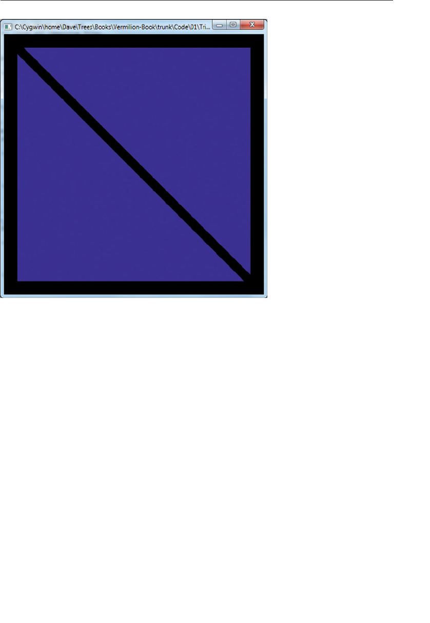
ptg9898810
Figure 1.1 Image from our first OpenGL program: triangles.cpp
Example 1.1 triangles.cpp: Our First OpenGL Program
///////////////////////////////////////////////////////////////////////
//
// triangles.cpp
//
///////////////////////////////////////////////////////////////////////
#include <iostream>
using namespace std;
#include "vgl.h"
#include "LoadShaders.h"
enum VAO_IDs { Triangles, NumVAOs };
enum Buffer_IDs { ArrayBuffer, NumBuffers };
enum Attrib_IDs { vPosition = 0 };
GLuint VAOs[NumVAOs];
GLuint Buffers[NumBuffers];
const GLuint NumVertices = 6;
Your First Look at an OpenGL Program 5

ptg9898810
//---------------------------------------------------------------------
//
// init
//
void
init(void)
{
glGenVertexArrays(NumVAOs, VAOs);
glBindVertexArray(VAOs[Triangles]);
GLfloat vertices[NumVertices][2] = {
{ -0.90, -0.90 }, // Triangle 1
{ 0.85, -0.90 },
{ -0.90, 0.85 },
{ 0.90, -0.85 }, // Triangle 2
{ 0.90, 0.90 },
{ -0.85, 0.90 }
};
glGenBuffers(NumBuffers, Buffers);
glBindBuffer(GL_ARRAY_BUFFER, Buffers[ArrayBuffer]);
glBufferData(GL_ARRAY_BUFFER, sizeof(vertices),
vertices, GL_STATIC_DRAW);
ShaderInfo shaders[] = {
{ GL_VERTEX_SHADER, "triangles.vert" },
{ GL_FRAGMENT_SHADER, "triangles.frag" },
{ GL_NONE, NULL }
};
GLuint program = LoadShaders(shaders);
glUseProgram(program);
glVertexAttribPointer(vPosition, 2, GL_FLOAT,
GL_FALSE, 0, BUFFER_OFFSET(0));
glEnableVertexAttribArray(vPosition);
}
//---------------------------------------------------------------------
//
// display
//
void
display(void)
{
glClear(GL_COLOR_BUFFER_BIT);
glBindVertexArray(VAOs[Triangles]);
glDrawArrays(GL_TRIANGLES, 0, NumVertices);
glFlush();
}
6Chapter 1: Introduction to OpenGL

ptg9898810
//---------------------------------------------------------------------
//
// main
//
int
main(int argc, char** argv)
{
glutInit(&argc, argv);
glutInitDisplayMode(GLUT_RGBA);
glutInitWindowSize(512, 512);
glutInitContextVersion(4, 3);
glutInitContextProfile(GLUT_CORE_PROFILE);
glutCreateWindow(argv[0]);
if (glewInit()) {
cerr << "Unable to initialize GLEW ... exiting" << endl;
exit(EXIT_FAILURE);
}
init();
glutDisplayFunc(display);
glutMainLoop();
}
While that may be more code than you were expecting, you’ll find that
this program will be the basis of just about every OpenGL application you
write. We use some additional software libraries that aren’t officially part of
OpenGL to simplify things like creating a window, or receiving mouse or
keyboard input---those things that OpenGL doesn’t include. We’ve also
created some helper functions and small C++ classes to simplify our exam-
ples. While OpenGL is a ‘‘C’’-language library, all of our examples are in
C++, but very simple C++. In fact, most of the C++ we use is to implement
the mathematical constructs vectors and matrices.
In a nutshell, here’s what Example 1.1 does. We’ll explain all of these
concepts in complete detail later, so don’t worry.
•In the preamble of the program, we include the appropriate header files
and declare global variables1and other useful programming constructs.
•The init() routine is used to set up data for use later in the program.
This may be vertex information for later use when rendering
1. Yes; in general we eschew global variables in large applications, but for the purposes of
demonstration, we use them here.
Your First Look at an OpenGL Program 7

ptg9898810
primitives, or image data for use in a technique called texture mapping,
which we describe in Chapter 6.
In this version of init(), we first specify the position information for
the two triangles that we render. After that, we specify shaders we’re
going to use in our program. In this case, we only use the required
vertex and fragment shaders. The LoadShaders() routine is one that
we’ve written to simplify the process of preparing shaders for a GPU.
In Chapter 2we’ll discuss everything it does.
The final part of init() is doing what we like to call shader plumbing,
where you associate the data in your application with variables in
shader programs. This is also described in detail in Chapter 2.
•The display() routine is what really does the rendering. That is, it calls
the OpenGL functions that request something be rendered. Almost all
display() routines will do the same three steps as in our simple
example here.
1. Clear the window by calling glClear().
2. Issue the OpenGL calls required to render your object.
3. Request that the image is presented to the screen.
•Finally, main() does the heavy lifting of creating a window, calling
init(), and finally entering into the event loop. Here you also see func-
tions that begin with ‘‘gl’’ but look different than the other functions
in the application. Those, which we’ll describe momentarily, are from
the libraries we use to make it simple to write OpenGL programs across
the different operating and window systems: GLUT, and GLEW.
Before we dive in to describe the routines in detail, let us explain OpenGL
labels functions, constants, and other useful programming constructs.
OpenGL Syntax
As you likely picked up on, all the functions in the OpenGL library begin
with the letters ‘‘gl’’, immediately followed by one or more capitalized
words to name the function (glBindVertexArray(), for example). All
functions in OpenGL are like that. In the program you also saw the func-
tions that began with ‘‘glut’’, which are from the OpenGL Utility Toolkit
(GLUT), a library written by Mark J. Kilgard. It’s a popular cross-platform
8Chapter 1: Introduction to OpenGL

ptg9898810
toolkit for opening windows and managing input, among other
operations. We use a version of GLUT named Freeglut, originally written by
Pawel W. Olszta with contributions from Andreas Umbach and Steve Baker
(who currently maintains the library), which is a modern variant of the
original library. Similarly, you see a single function, glewInit(), which
comes from the OpenGL Extension Wrangler written by Milan Ikits and
Marcelo Magallon. We describe both of those libraries in more detail in
Appendix A.
Similar to OpenGL’s function-naming convention, constants like
GL_COLOR_BUFFER_BIT, which you saw in display(), are defined for the
OpenGL library. All constant tokens begin with GL_, and use underscores
to separate words. Their definitions are merely #defines found in the
OpenGL header files: glcorearb.h and glext.h.
To aid in moving OpenGL applications between operating systems,
OpenGL also defines various types of data for its functions, such as
GLfloat, which is the floating-point value type we used to declare
vertices in Example 1.1. OpenGL defines typedefs for all of the data
types accepted by its functions, which are listed in Table 1.1. Additionally,
since OpenGL is a ‘‘C’’-language library, it doesn’t have function over-
loading to deal with the different types of data; it uses a function-naming
convention to organize the multitude of functions that result from that
situation. For example, we’ll encounter a function named glUniform*() in
Chapter 2,‘‘Shader Fundamentals’’, which comes in numerous forms, such
as glUniform2f() and glUniform3fv(). The suffixes at the end of the
‘‘core’’ part of the function name provide information about the
arguments passed to the function. For example, the ‘‘2’’ in glUniform2f()
represents that two data values will be passed into the function (there are
other parameters as well, but they are the same across all 24 versions of the
glUniform*() * function---In this book, we’ll use glUniform*() * to
represent the collection of all glUniform*() functions). Also note the ‘‘f’’
following the ‘‘2’’. This indicates that those two parameters are of type
GLfloat. Finally, some versions of the functions’ names end with a ‘‘v’’,
which is short for vector, meaning that the two floating-point values (in
the case of glUniform2fv()) are passed as a one-dimensional array of
GLfloats, instead of two separate parameters.
To decode all of those combinations, the letters used as suffixes are des-
cribed in Table 1.1, along with their types.
OpenGL Syntax 9
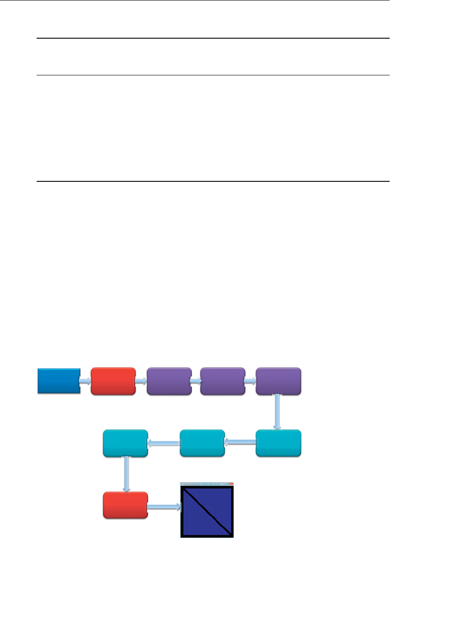
ptg9898810
Table 1.1 Command Suffixes and Argument Data Types
Suffix Data Type Typical
Corresponding
C-Language Type
OpenGL Type Definition
b 8-bit integer signed char GLbyte
s 16-bit integer signed short GLshort
i 32-bit integer int GLint, GLsizei
f 32-bit floating-point float GLfloat, GLclampf
d 64-bit floating-point double GLdouble, GLclampd
ub 8-bit unsigned integer unsigned char GLubyte
us 16-bit unsigned integer unsigned short GLushort
ui 32-bit unsigned integer unsigned int GLuint, GLenum, GLbitfield
Note: Implementations of OpenGL have leeway in selecting which ‘‘C’’
data types to use to represent OpenGL data types. If you resolutely
use the OpenGL-defined data types throughout your application,
you will avoid mismatched types when porting your code between
different implementations.
OpenGL’s Rendering Pipeline
OpenGL implements what’s commonly called a rendering pipeline, which is
a sequence of processing stages for converting the data your application
provides to OpenGL into a final rendered image. Figure 1.2 shows the
OpenGL pipeline associated with Version 4.3. The OpenGL pipeline has
evolved considerably since its introduction.
Vertex
Data
Geometry
Shader
Tessellation
Evaluation
Shader
Tessellation
Control
Shader
Vertex
Shader
Fragment
Shader
Primitive
Setup
Clipping
Rasterization
Figure 1.2 The OpenGL pipeline
10 Chapter 1: Introduction to OpenGL

ptg9898810
OpenGL begins with the geometric data you provide (vertices and geo-
metric primitives) and first processes it through a sequence of shader
stages: vertex shading, tessellation shading (which itself uses two shaders),
and finally geometry shading, before it’s passed to the rasterizer. The
rasterizer will generate fragments for any primitive that’s inside of the
clipping region, and execute a fragment shader for each of the generated
fragments.
As you can see, shaders play an essential role in creating OpenGL applica-
tions. You have complete control of which shader stages are used, and
what each of them do. Not all stages are required; in fact, only vertex
shaders and fragment shaders must be included. Tessellation and geometry
shaders are optional.
Now, we’ll dive in a little deeper into each stage to provide you a bit more
background. We understand that this may be somewhat overwhelming at
this point, but please bear with us. It will turn out that understanding just
a few concepts will get you very far along with OpenGL.
Preparing to Send Data to OpenGL
OpenGL requires that all data be stored in buffer objects, which are just
chunks of memory managed by the OpenGL server. Populating these
buffers with data can occur in numerous ways, but one of the most
common is using the glBufferData() command like in Example 1.1. There
is some additional setup required with buffers, which we’ll cover in
Chapter 3.
Sending Data to OpenGL
After we’ve initialized our buffers, we can request geometric primitives
be rendered by calling one of OpenGL’s drawing commands, such as
glDrawArrays(), as we did in Example 1.1.
Drawing in OpenGL usually means transferring vertex data to the OpenGL
server. Think of a vertex as a bundle of data values that are processed
together. While the data in the bundle can be anything you’d like it to be
(i.e., you define all the data that makes up a vertex), it almost always
includes positional data. Any other data will be values you’ll need to
determine the pixel’s final color.
Drawing commands are covered in detail in Chapter 3,‘‘Drawing with
OpenGL’’.
OpenGL’s Rendering Pipeline 11

ptg9898810
Vertex Shading
For each vertex that is issued by a drawing command, a vertex shader will
be called to process the data associated with that vertex. Depending on
whether any other pre-rasterization shaders are active, vertex shaders may
be very simple, perhaps just copying data to pass it through this shading
stage---what we’ll call a pass-through shader---to a very complex shader that’s
performing many computations to potentially compute the vertex’s screen
position (usually using transformation matrices, described in Chapter 5),
determining the vertex’s color using lighting computations described in
Chapter 7, or any multitude of other techniques.
Typically, an application of any complexity will have multiple vertex
shaders, but only one can be active at any one time.
Tessellation Shading
After the vertex shader has processed each vertex’s associated data, the
tessellation shader stage will continue processing those data, if it’s been
activated. As we’ll see in Chapter 9, tessellation uses patchs to describe an
object’s shape, and allows relatively simple collections of patch geometry
to be tessellated to increase the number of geometric primitives providing
better-looking models. The tessellation shading stage can potentially use
two shaders to manipulate the patch data and generate the final shape.
Geometry Shading
The next shader stage---geometry shading---allows additional processing
of individual geometric primitives, including creating new ones, before
rasterization. This shading stage is also optional, but very powerful as
we’ll see in Chapter 10.
Primitive Assembly
The previous shading stages all operate on vertices, with the information
about how those vertices are organized into geometric primitives being
carried along internal to OpenGL. The primitive assembly stage organizes
the vertices into their associated geometric primitives in preparation for
clipping and rasterization.
12 Chapter 1: Introduction to OpenGL

ptg9898810
Clipping
Occasionally, vertices will be outside of the viewport---the region of the
window where you’re permitted to draw---and cause the primitive associa-
ted with that vertex to be modified so none of its pixels are outside of the
viewport. This operation is called clipping and is handled automatically by
OpenGL.
Rasterization
Immediately after clipping, the updated primitives are sent to the rasterizer
for fragment generation. Consider a fragment a ‘‘candidate pixel’’, in that
pixels have a home in the framebuffer, while a fragment still can be rejec-
ted and never update its associated pixel location. Processing of fragments
occurs in the next two stages, fragment shading and per-fragment
operations.
Fragment Shading
The final stage where you have programmable control over the color of a
screen location is during fragment shading. In this shader stage, you use a
shader to determine the fragment’s final color (although the next stage,
per-fragment operations can modify the color one last time), and poten-
tially its depth value. Fragment shaders are very powerful as they often
employ texture mapping to augment the colors provided by the vertex
processing stages. A fragment shader may also terminate processing a
fragment if it determines the fragment shouldn’t be drawn; this process is
called fragment discard.
A helpful way of thinking about the difference between shaders that deal
with vertices and fragment shaders is: vertex shading (including tessella-
tion and geometry shading) determine where on the screen a primitive is,
while fragment shading uses that information to determine what color
that fragment will be.
Per-Fragment Operations
Additional fragment processing, outside of what you can currently do in a
fragment shader is the final processing of individual fragments. During
this stage a fragment’s visibility is determined using depth testing (also
commonly known as z-buffering) and stencil testing.
OpenGL’s Rendering Pipeline 13

ptg9898810
If a fragment successfully makes it through all of the enabled tests, it may
be written directly to the framebuffer, updating the color (and possibly
depth value) of its pixel, or if blending is enabled, the fragment’s color will
be combined with the pixel’s current color to generate a new color that is
written into the framebuffer.
As you saw in Figure 1.2, there’s also a path for pixel data. Generally, pixel
data comes from an image file, although it may also be created by rending
using OpenGL. Pixel data is usually stored in texture map for use with
texture mapping, which allows any texture stage to look up data values
from one or more texture maps. Texture mapping is covered in depth in
Chapter 6.
With that brief introduction to the OpenGL pipeline, we’ll dissect
Example 1.1 and map the operations back to the rendering pipeline.
Our First Program: A Detailed Discussion
Entering main()
Starting at the beginning, of how our program would execute, we first look
at what’s going on in main(). The first six lines use the OpenGL Utility
Toolkit to configure and open window for us. While the details of each of
these routines is covered in Appendix A, we’ll discuss the flow of the
commands here.
int
main(int argc, char** argv)
{
glutInit(&argc, argv);
glutInitDisplayMode(GLUT_RGBA);
glutInitWindowSize(512, 512);
glutInitContextVersion(4, 3);
glutInitContextProfile(GLUT_CORE_PROFILE);
glutCreateWindow(argv[0]);
if (glewInit()) {
cerr << "Unable to initialize GLEW ... exiting" << endl;
exit(EXIT_FAILURE);
}
init();
glutDisplayFunc(display);
glutMainLoop();
}
14 Chapter 1: Introduction to OpenGL

ptg9898810
The first function, glutInit(), initializes the GLUT library. It processes the
command-line arguments provided to the program, and removes any that
control how GLUT might operate (such as specifying the size of a window).
glutInit() needs to be the first GLUT function that your application calls,
as it sets up data structures required by subsequent GLUT routines.
glutInitDisplayMode() configures the type of window we want to use
with our application. In this case, we only request that the window use the
RGBA color space (which we discuss more in Chapter 4). There are other
options that we’ll add to configure windows with more OpenGL features,
such as depth buffers, or to enable animation.
glutInitWindowSize() specifies the size of the window, as you might
expect. While we don’t do it here, you can also query the size of the display
device to dynamically size the window relative to your computer screen.
The next two calls: glutInitContextVersion() and
glutInitContextProfile() specify the type of OpenGL context---OpenGL’s
internal data structure for keeping track of state settings and
operations---we want to use. Here, we request an OpenGL Version 4.3 core
profile for our context. Our profile selection controls whether we’re using
only the latest features in OpenGL or the features that are compatible with
OpenGL versions all the way back to OpenGL Version 1.0.
The last call in this group is glutCreateWindow(), which does just what it
says. If it’s possible to create a window matching the display mode you
requested with glutInitDisplayMode(), one will be created (by interfacing
with your computer’s windowing system). Only after GLUT has created a
window for you (which includes creating an OpenGL context) can you use
OpenGL functions.
Continuing on, the call to glewInit() initializes another help library we
use: GLEW---the OpenGL Extension Wrangler. GLEW simplifies dealing
with accessing functions and other interesting programming phenomena
introduced by the various operating systems with OpenGL. Without
GLEW, a considerable amount of additional work is required to get an
application going.
At this point, we’re truly set up to do interesting things with OpenGL. The
init() routine, which we’ll discuss momentarily, initializes all of our
relevant OpenGL data so we can use for rendering later.
The next routine, glutDisplayFunc(), sets up the display callback, which is
the routine GLUT will call when it thinks the contents of the window need
to be updated. Here, we provide the GLUT library a pointer to a function:
display(), which we’ll also discuss soon. GLUT uses a number of callback
Our First Program: A Detailed Discussion 15

ptg9898810
functions for processing things like user input, window resizing, and many
other operations. GLUT is fully described in Appendix A,‘‘Basics of GLUT:
The OpenGL Utility Toolkit’’.
The final function in main() is glutMainLoop(), which is an infinite loop
that works with the window and operating systems to process user input
and other operations like that. It’s glutMainLoop() that determines that a
window needs to be repainted, for example, and will call the function
registered with glutDisplayFunc(). An important safety tip is that since
glutMainLoop() is an infinite loop, any commands placed after it aren’t
executed.
OpenGL Initialization
The next routine that we need to discuss is init() from Example 1.1. Once
again, here’s the code to refresh your memory.
void
init(void)
{glGenVertexArrays(NumVAOs, VAOs);
glBindVertexArray(VAOs[Triangles]);
GLfloat vertices[NumVertices][2] = {
{ -0.90, -0.90 }, // Triangle 1
{ 0.85, -0.90 },
{ -0.90, 0.85 },
{ 0.90, -0.85 }, // Triangle 2
{ 0.90, 0.90 },
{ -0.85, 0.90 }
};
glGenBuffers(NumBuffers, Buffers);
glBindBuffer(GL_ARRAY_BUFFER, Buffers[ArrayBuffer]);
glBufferData(GL_ARRAY_BUFFER, sizeof(vertices),
vertices, GL_STATIC_DRAW);
ShaderInfo shaders[] = {
{ GL_VERTEX_SHADER, "triangles.vert" },
{ GL_FRAGMENT_SHADER, "triangles.frag" },
{ GL_NONE, NULL }
};
GLuint program = LoadShaders(shaders);
glUseProgram(program);
glVertexAttribPointer(vPosition, 2, GL_FLOAT,
GL_FALSE, 0, BUFFER_OFFSET(0));
glEnableVertexAttribArray(vPosition);
}
16 Chapter 1: Introduction to OpenGL

ptg9898810
Initializing Our Vertex-Array Objects
There’s a lot going on in the functions and data of init(). Starting
at the top, we begin by allocating a vertex-array object by calling
glGenVertexArrays(). This causes OpenGL to allocate some number
of vertex array object names for our use; in our case, NumVAOs, which we
specified in the global variable section of the code. glGenVertexArrays()
returns that number of names to us in the array provided, VAOs in this case.
Here’s a complete description of glGenVertexArrays():
void glGenVertexArrays(GLsizei n, GLuint *arrays);
Returns ncurrently unused names for use as vertex-array objects in the
array arrays. The names returned are marked as used for the purposes
of allocating additional buffer objects, and initialized with values
representing the default state of the collection of uninitialized vertex
arrays.
We’ll see numerous OpenGL commands of the form glGen*, for allocating
names to the various types of OpenGL objects. A name is a little like a
pointer-type variable in C, in that until you allocate some memory and
have the name reference it, the name isn’t much help. In OpenGL, the
same holds true, and our allocation scheme is called binding an object, and
is done by a collection of functions in OpenGL that have the form
glBind*. For our example, we create and bind a vertex-array object using
glBindVertexArray().
void glBindVertexArray(GLuint array);
glBindVertexArray() does three things. When using the value array that
is other than zero and was returned from glGenVertexArrays(), a new
vertex-array object is created and assigned that name. When binding to a
previously created vertex-array object, that vertex array object becomes
active, which additionally affects the vertex array state stored in the
object. When binding to an array value of zero, OpenGL stops using
application-allocated vertex-array objects and returns to the default state
for vertex arrays.
A GL_INVALID_OPERATION error is generated if array is not a value
previously returned from glGenVertexArrays(), or if it is a value that has
been released by glDeleteVertexArrays().
Our First Program: A Detailed Discussion 17

ptg9898810
In our example, after we generate a vertex-array object name, we bind it
with our call to glBindVertexArray(). Object binding like this is a very
common operation in OpenGL, but it may be immediately intuitive how
or why it works. When you bind an object for the first time (e.g., the first
time glBind*() is called for a particular object name), OpenGL will inter-
nally allocate the memory it needs and make that object current, which
means that any operations relevant to the bound object, like the vertex-
array object we’re working with, will affect its state from that point on in
the program’s execution. After the first call to any glBind*() function, the
newly created object will be initialized to its default state and will usually
require some additional initialization to make it useful.
Think of binding an object like setting a track switch in a railroad yard.
Once a track switch has been set, all trains go down that set of tracks.
When the switch is set to another track, all trains will then travel that new
track. It is the same for OpenGL objects. Generally speaking, you will bind
an object in two situations: initially when you create and initialize the data
it will hold; and then every time you want to use it, and it’s not currently
bound. We’ll see this situation when we discuss the display() routine,
where glBindVertexArray() is called the second time in the program.
Since our example is as minimal as possible, we don’t do some operations
that you might in larger programs. For example, once you’re completed with
a vertex-array object, you can delete it by calling glDeleteVertexArrays().
void glDeleteVertexArrays(GLsizei n, GLuint *arrays);
Deletes the nvertex-arrays objects specified in arrays, enabling the names
for reuse as vertex arrays later. If a bound vertex array is deleted, the
bindings for that vertex array become zero (as if you had called
glBindBuffer() with a value of zero) and the default vertex array becomes
the current one. Unused names in arrays are released, but no changes to
the current vertex array state are made.
Finally, for completeness, you can also determine if a name is already been
reserved as a vertex-array object by calling glIsVertexArray().
GLboolean glIsVertexArray(GLuint array);
Returns GL_TRUE if array is the name of a vertex-array object that was
previously generated with glGenVertexArrays(), but has not been
subsequently deleted. Returns GL_FALSE if array is zero or a nonzero
value that is not the name of a vertex-array object.
18 Chapter 1: Introduction to OpenGL

ptg9898810
You’ll find many similar routines of the form glDelete* and glIs* for all the
different types of object in OpenGL.
Allocating Vertex-Buffer Objects
A vertex-array object holds various data related to a collection of vertices.
Those data are stored in buffer objects and managed by the currently
bound vertex-array object. While there is only a single type of vertex-array
object, there are many types of objects, but not all of them specifically deal
with vertex data. As mentioned previously, a buffer object is memory that
the OpenGL server allocates and owns, and almost all data passed into
OpenGL is done by storing the data in a buffer object.
The sequence of initializing a vertex-buffer object is similar in flow to that
of creating a vertex-array object, with an added step to actually populate
the buffer with data.
To begin, you need to create some names for your vertex-buffer objects. As
you might expect, you’ll call a function of the form glGen*; in this case,
glGenBuffers(). In our example, we allocate NumVBOs (short for ‘‘Vertex-
Buffer Objects’’) into our array buffers. Here is the full description of
glGenBuffers().
void glGenBuffers(GLsizei n, GLuint *buffers);
Returns ncurrently unused names for buffer objects in the array buffers.
The names returned in buffers do not have to be a contiguous set of
integers.
The names returned are marked as used for the purposes of allocating
additional buffer objects, but only acquire a valid state once they have
been bound.
Zero is a reserved buffer object name and is never returned as a buffer
object by glGenBuffers().
Once you have allocated names for your buffers, you bring them into
existence by calling glBindBuffer(). Since there are many different types of
buffer objects in OpenGL, when we bind a buffer, we need to specify
which type we’d like it to be. In our example, since we’re storing vertex
data into the buffer, we use GL_ARRAY_BUFFER. There are currently eight
types of buffer objects, which get used for various features in OpenGL. We
will discuss each type’s operation in the relevant sections later in the book.
Here is the full detail for glBindBuffer().
Our First Program: A Detailed Discussion 19

ptg9898810
void glBindBuffer(GLenum target, GLuint buffer);
Specifies the current active buffer object. target must be set to one of
GL_ARRAY_BUFFER, GL_ELEMENT_ARRAY_BUFFER,
GL_PIXEL_PACK_BUFFER, GL_PIXEL_UNPACK_BUFFER,
GL_COPY_READ_BUFFER, GL_COPY_WRITE_BUFFER,
GL_TRANSFORM_FEEDBACK_BUFFER, or GL_UNIFORM_BUFFER. buffer
specifies the buffer object to be bound to.
glBindBuffer() does three things: 1. When using buffer of an unsigned
integer other than zero for the first time, a new buffer object is created
and assigned that name. 2. When binding to a previously created buffer
object, that buffer object becomes the active buffer object. 3. When
binding to a buffer value of zero, OpenGL stops using buffer objects for
that target.
As with other objects, you can delete buffer objects with glDeleteBuffers().
void glDeleteBuffers(GLsizei n, const GLuint *buffers);
Deletes nbuffer objects, named by elements in the array buffers. The
freed buffer objects may now be reused (for example, by glGenBuffers()).
If a buffer object is deleted while bound, all bindings to that object are
reset to the default buffer object, as if glBindBuffer() had been called
with zero as the specified buffer object. Attempts to delete nonexistent
buffer objects or the buffer object named zero are ignored without
generating an error.
You can query if an integer value is a buffer-object name with glIsBuffer().
GLboolean glIsBuffer(GLuint buffer);
Returns GL_TRUE if buffer is the name of a buffer object that has been
bound, but has not been subsequently deleted. Returns GL_FALSE if
buffer is zero or if buffer is a nonzero value that is not the name of a buffer
object.
20 Chapter 1: Introduction to OpenGL

ptg9898810
Loading Data into a Buffer Object
After initializing our vertex-buffer object, we need to transfer the vertex
data from our objects into the buffer object. This is done by the
glBufferData() routine, which does dual duty: allocating storage for
holding the vertex data and copying the data from arrays in the
application to the OpenGL server’s memory.
As glBufferData() will be used many times in many different scenarios, it’s
worth discussing it in more detail here, although we will revisit its use
many times in this book. To begin, here’s the full description of
glBufferData().
void glBufferData(GLenum target,GLsizeiptr size,
const GLvoid *data, GLenum usage);
Allocates size storage units (usually bytes) of OpenGL server memory for
storing data or indices. Any previous data associated with the currently
bound object will be deleted.
target may be either GL_ARRAY_BUFFER for vertex attribute data;
GL_ELEMENT_ARRAY_BUFFER for index data;
GL_PIXEL_UNPACK_BUFFER for pixel data being passed into OpenGL;
GL_PIXEL_PACK_BUFFER for pixel data being retrieved from
OpenGLGL_COPY_READ_BUFFER and GL_COPY_WRITE_BUFFER for
data copied between buffers; GL_TEXTURE_BUFFER for texture data
stored as a texture buffer; GL_TRANSFORM_FEEDBACK_BUFFER for
results from executing a transform feedback shader; or
GL_UNIFORM_BUFFER for uniform variable values.
size is the amount of storage required for storing the respective data. This
value is generally number of elements in the data multiplied by their
respective storage size.
data is either a pointer to a client memory that is used to initialize the
buffer object or NULL. If a valid pointer is passed, size units of storage are
copied from the client to the server. If NULL is passed, size units of
storage are reserved for use but are left uninitialized.
usage provides a hint as to how the data will be read and written after
allocation. Valid values are GL_STREAM_DRAW, GL_STREAM_READ,
GL_STREAM_COPY, GL_STATIC_DRAW, GL_STATIC_READ,
GL_STATIC_COPY, GL_DYNAMIC_DRAW, GL_DYNAMIC_READ,
GL_DYNAMIC_COPY.
Our First Program: A Detailed Discussion 21

ptg9898810
glBufferData() will generate a GL_OUT_OF_MEMORY error if the
requested size exceeds what the server is able to allocate. It will generate a
GL_INVALID_VALUE error if usage is not one of the permitted values.
We know that was a lot to see at one time, but you will use this function so
much that it’s good to make it easy to find at the beginning of the book.
For our example, our call to glBufferData() is very straightforward. Our
vertex data is stored in the array vertices. While we’ve statically allo-
cated it in our example, you might read these values from a file containing
a model, or generate the values algorithmically. Since our data is vertex-
attribute data, we’ll make this buffer a GL_ARRAY_BUFFER by specifying
that value as the first parameter. We also need to specify the size of
memory to be allocated (in bytes), so we merely compute
sizeof(vertices) which does all the heavy lifting. Finally, we need to
specify how the data will be used by OpenGL. Since this data will be used
for drawing geometry, and won’t change for the life of the program, we
choose GL_STATIC_DRAW for glBufferData()’s usage parameter.
There are a lot of options for usage, which we describe in detail in
Chapter 3.
If you look at the values in the vertices array, you’ll note they are all in
the range [−1, 1]in both xand y. In reality, OpenGL only knows how to
draw geometric primitives into coordinate space. In fact, that range of
coordinates are known as normalized-device coordinates (commonly called
NDCs). While that may sound like a limitation, it’s really none at all.
Chapter 5will discuss all the mathematics required to take the most
complex objects in a three-dimensional space, and map them into
normalized-device coordinates. We used NDCs here to simplify the
example, but in reality, you will almost always use more complex
coordinate spaces.
At this point, we’ve successfully created a vertex-array object and popu-
lated its buffer objects. Next, we need to set up the shaders that our appli-
cation will use.
Initializing Our Vertex and Fragment Shaders
Every OpenGL program that wants to use OpenGL Version 3.1 or greater
must provide at least two shaders: a vertex shader and a fragment shader.
In our example, we do that by using our helper function LoadShaders(),
which takes an array of ShaderInfo structures (all of the details for this
structure are included in the LoadShaders.h header file).
22 Chapter 1: Introduction to OpenGL

ptg9898810
For an OpenGL programmer (at this point), a shader is a small function
written in the OpenGL Shading Language (OpenGL Shading Language
(GLSL)), a special language very similar to C++ for constructing OpenGL
shaders. GLSL is used for all shaders in OpenGL, although not every
feature in GLSL is usable in every OpenGL shader stage. You provide your
GLSL shader to OpenGL as a string of characters. To simplify our examples,
and to make it easier for you to experiment with shaders, we store our
shader strings in files, and use LoadShaders() to take care of reading the
files and creating our OpenGL shader programs. The gory details of
working with OpenGL shaders are discussed in detail in Chapter 2.
To gain an appreciation of shaders, we need to show you some without
going into full detail of every nuance. There’s the entire rest of the book
for all of the GLSL details, so right now, we’ll suffice with showing our
vertex shader in Example 1.2.
Example 1.2 Vertex Shader for triangles.cpp: triangles.vert
#version 430 core
layout(location = 0) in vec4 vPosition;
void
main()
{gl_Position = vPosition;
}
Yes; that’s all there is. In fact, this is an example of a pass-through shader
we eluded to earlier. It only copies input data to output data. That said,
there is a lot to discuss here.
The first line: ‘‘#version 430 core’’ specifies which version of the OpenGL
Shading Language we want to use. The ‘‘430’’ here indicates that we want
to use the version of GLSL associated with OpenGL Version 4.3. The
naming scheme of GLSL versions based on OpenGL versions works back to
Version 3.3. In versions of OpenGL before that, the version numbers
incremented differently (the details are in Chapter 2). The ‘‘core’’ relates to
wanting to use OpenGL’s core profile, which corresponds with our request
to GLUT when we called glutInitContextProfile(). Every shader should
have a ‘‘#version’’ line at its start, otherwise version ‘‘110’’ is assumed,
which is incompatible with OpenGL’s core profile versions. We’re going to
stick to shaders declaring version 330 or above, depending on what
features the shaders use; you get a bit more portability by not using the
most recent version number, unless you need the most recent features.
Next, we allocate a shader variable. Shader variables are a shader’s
connection to the outside world. That is, a shader doesn’t know where its
Our First Program: A Detailed Discussion 23

ptg9898810
data comes from; it merely sees its input variables populated with data
every time it executes. It’s our responsibility to connect the shader plumb-
ing (this is our term, but you’ll see why it makes sense) so that data in your
application can flow into and between the various OpenGL shader stages.
In our simple example, we have one input variable named vPosition,
which you can determine by the ‘‘in’’ on its declaration line. In fact, there’s
a lot going on in this one line.
layout(location = 0) in vec4 vPosition;
It’s easier to parse the line from right to left.
•vPosition is, of course, the name of the variable. We’ll use the
convention of prefixing a vertex attribute with the letter ‘‘v’’. So, in this
case, this variable will hold a vertex’s positional information.
•Next, you see vec4, which is vPositions type. In this case, it’s a GLSL
4-component vector of floating-point values. There are many data
types in GLSL, that we’ll discuss in Chapter 2.
You may have noticed that when we specified the data for each vertex
in Example 1.1 we only specified two coordinates, but in our vertex
shader, we use a vec4. Where do the other two coordinates come
from? OpenGL will automatically fill in any missing coordinates with
default values. The default value for a vec4 is (0,0,0,1), so if we only
specify the x- and y-coordinates, the other values (zand w), are
assigned 0 and 1 respectively.
•Preceding the type is the in we mentioned before, which specifies
which direction data flows into the shader. If you’re wondering if there
might be an out; yes, you’re right. We don’t show that here, but will
soon.
•Finally, the layout(location = 0) part is called a layout qualifier,
and provides meta-data for our variable declaration. There are many
options that can be set with a layout qualifier, some of which are
shader-stage specific.
In this case, we just set vPosition attribute location to zero. We’ll use
that information in conjunction with the last two routines in init().
Finally, the core of the shader is defined in its main() routine. Every shader
in OpenGL, regardless of which shader stage its used for, will have a
main() routine. For this shader, all it does is copy the input vertex position
to the special vertex-shader output gl_Position. You’ll soon see there are
several shader variables provided by OpenGL that you’ll use, and they all
begin with the gl_ prefix.
24 Chapter 1: Introduction to OpenGL

ptg9898810
Similarly, we need a fragment shader to accompany our vertex shader.
Here’s the one for our example, shown in Example 1.3.
Example 1.3 Fragment Shader for triangles.cpp: triangles.frag
#version 430 core
out vec4 fColor;
void
main()
{fColor = vec4(0.0, 0.0, 1.0, 1.0);
}
Hopefully, much of this looks very familiar, even if it’s an entirely different
type of shader. We have the version string, a variable declaration, and our
main() routine. There are a few differences, but as you’ll find, almost all
shaders will have this structure.
The highlights of our fragment shader are as follows:
•The variable declaration for fColor. If you guessed that there was an
out qualifier, you were right! In this case, the shader will output values
through fColor, which is the fragment’s color (hence the choice of ‘‘f’’
as a prefix).
•Assigning the fragment’s color. In this case, each fragment is assigned
this vector of four values. In OpenGL, colors are represented in what’s
called the RGB color space,with each color component (‘‘R’’ for red, ‘‘G’’
for green, and ‘‘B’’ for blue) ranging from [0, 1]. The observant reader is
probably asking ‘‘Um, but there are four numbers there’’. Indeed,
OpenGL really uses an RGBA color space, with the fourth color not
really being a color at all. It’s for a value called alpha, which is really a
measure of translucency. We’ll discuss it in detail in Chapter 4, but for
now, we’ll set it to 1.0, which indicates the color is fully opaque.
Fragment shaders are immensely powerful, and there will be many
techniques that we can do with them.
We’re almost done with our initialization routine. The final two routines in
init() deal specifically with associating variables in a vertex shader with
data that we’ve stored in a buffer object. This is exactly what we mean by
shader plumbing, in that you need to connect conduits between the
application and a shader, and as we’ll see, between various shader stages.
To associate data going into our vertex shader, which is the entrance all
vertex data take to get processed by OpenGL, we need to connect our
Our First Program: A Detailed Discussion 25

ptg9898810
shader ‘‘in’’ variables to a vertex-attribute array, and we do that with the
glVertexAttribPointer() routine.
void glVertexAttribPointer(GLuint index, GLint size,
GLenum type, GLboolean normalized,
GLsizei stride, const GLvoid *pointer);
Specifies where the data values for index (shader attribute location) can be
accessed. pointer is the offset from the start of the buffer object (assuming
zero-based addressing) in basic-machine units (i.e., bytes) for the first set
of values in the array. size represents the number of components to be
updated per vertex, and can be either 1, 2, 3, 4, or GL_BGRA. type
specifies the data type (GL_BYTE, GL_UNSIGNED_BYTE, GL_SHORT,
GL_UNSIGNED_SHORT, GL_INT, GL_UNSIGNED_INT, GL_FIXED,
GL_HALF_FLOAT, GL_FLOAT, or GL_DOUBLE) of each element in the
array. normalized indicates that the vertex data should be normalized
before being stored (in the same manner as glVertexAttribFourN*()).
stride is the byte offset between consecutive elements in the array. If stride
is zero, the data is assumed to be tightly packed.
While that may seem like a lot of things to figure out, it’s because
glVertexAttribPointer() is a very flexible command. As long as your data
is regularly organized in memory (i.e., it’s in a contiguous array, and not
in some other node-based container like a linked list), you can use
glVertexAttribPointer() to tell OpenGL how to retrieve data from that
memory. In our case, vertices has all the information we need. Table 1.2
works through glVertexAttribPointer()’s parameters.
Table 1.2 Example of Determining Parameters for
glVertexAttribPointer()
Parameter Value Explanation
Name
index 0 This is the location value for the respective
vertex shader input variable---vPosition
in our case. This value can be specified by
the shader directly using the layout
qualifier, or determined after compilation
of the shader.
size 2 This is the number of values for each
vertex in our array. vertices was
allocated to have NumVertices
elements, each with two values.
type GL_FLOAT The enumerated value for the GLfloat type.
26 Chapter 1: Introduction to OpenGL

ptg9898810
Parameter Value Explanation
Name
normalized GL_FALSE We set this to GL_FALSE for two reasons:
First, and most importantly, because
positional coordinates values can basically
take on any value, so we don’t want them
constrained to the range [−1, 1]; and
second, the values are not integer types
(e.g., GLint, or GLshort).
stride 0 As our data are ‘‘tightly packed’’, which
implies that one set of data values is
immediately contiguous in memory to the
next, we can use the value zero.
pointer BUFFER_OFFSET(0) We set this to zero because our data starts
at the first byte (address zero) of our buffer
object.
Hopefully that explanation of how we arrived at the parameters will help
you determine the necessary values for your own data structures. We will
have plenty more examples of using glVertexAttribPointer().
One additional technique we use is using our BUFFER_OFFSET macro in
glVertexAttribPointer() to specify the offset. There’s nothing special about
our macro; here’s its definition.
#define BUFFER_OFFSET(offset) ((void *)(offset))
While there a long history of OpenGL lore on why one might do this,2we
use this macro to make the point that we’re specifying an offset into a
buffer object, rather than a pointer to a block of memory as
glVertexAttribPointer()’s prototype would suggest.
At this point, we have one task left to do in init(), which is to enable our
vertex-attribute array. We do this by calling glEnableVertexAttribArray()
and passing the index of the attribute array pointer we initialized by
calling glVertexAttribPointer(). The full details for
glEnableVertexAttribArray() are provided below.
2. In previous versions of OpenGL (prior to Version 3.1) vertex-attribute data was permitted to
be stored in application memory, as compared to GPU buffer objects, so pointers made sense
in that respect.
Our First Program: A Detailed Discussion 27

ptg9898810
void glEnableVertexAttribArray(GLuint index);
void glDisableVertexAttribArray(GLuint index);
Specifies that the vertex array associated with variable index be
enabled or disabled. index must be a value between zero and
GL_MAX_VERTEX_ATTRIBS −1.
Now, all that’s left is to draw something.
Our First OpenGL Rendering
With all that setup and data initialization, rendering (for the moment) will
be very simple. While our display() routine is only four lines long, its
sequence of operations is virtually the same in all OpenGL applications.
Here it is once again.
void
display(void)
{glClear(GL_COLOR_BUFFER_BIT);
glBindVertexArray(VAOs[Triangles]);
glDrawArrays(GL_TRIANGLES, 0, NumVertices);
glFlush();
}
First, we begin rendering by clearing our framebuffer. This is done by
calling glClear().
void glClear(GLbitfield mask);
Clears the specified buffers to their current clearing values. The mask
argument is a bitwise logical OR combination of the values listed in
Table 1.3.
Table 1.3 Clearing Buffers
Buffer Name
Color Buffer GL_COLOR_BUFFER_BIT
Depth Buffer GL_DEPTH_BUFFER_BIT
Stencil Buffer GL_STENCIL_BUFFER_BIT
28 Chapter 1: Introduction to OpenGL

ptg9898810
We discuss depth and stencil buffering, as well as an expanded discussion
of color in Chapter 4,‘‘Color, Pixels, and Framebuffers’’.
You may be asking yourself how we set the color that glClear() should use.
In this first program, we used OpenGL’s default clearing color, which is
black. To change the clear color, call glClearColor().
void glClearColor(GLclampf red, GLclampf green, GLclampf blue,
GLclampf alpha);
Sets the current clear color for use in clearing color buffers in RGBA mode.
(See Chapter 4for more information on RGBA mode.) The red, green,
blue, and alpha values are clamped if necessary to the range [0, 1]. The
default clear color is (0,0,0,0), which is the RGBA representation of black.
The clear color is an example of OpenGL state, which are values that
OpenGL retains in its context. OpenGL has a large collection of state
variables (which is fully described in Appendix D), all of which is initialized
to default values when a context is created. Since OpenGL retains any state
changes you update, you can reduce the number of times you set values.
Using the clear color as an example, let’s say you always want to
clear the background of the viewport to white. You would call
glClearColor(1, 1, 1, 1). But where should you make this function
call? Of course, you could set the value right before you call glClear() in
display(), but all but the first call would be redundant---OpenGL would be
changing the clear color from white to white each time you rendered. A
more efficient solution would be to set the clear color in init(). In fact, this
is the technique we use to minimize redundant state changes; any values
that will be constant over the execution of a program are set in init(). Of
course, there’s no harm in making redundant calls; it may just make your
application execute slower.
Try This
Add a call to glClearColor() into triangles.cpp.
Drawing with OpenGL
Our next two calls select the collection of vertices we want to draw and
request that they be rendered. We first call glBindVertexArray() to select
the vertex array that we want to use as vertex data. As mentioned before,
you would do this to switch between different collections of vertex data.
Our First Program: A Detailed Discussion 29

ptg9898810
Next, we call glDrawArrays(), which actually sends vertex data to the
OpenGL pipeline.
void glDrawArrays(GLenum mode, GLint first, GLsizei count);
Constructs a sequence of geometric primitives using the elements from
the currently bound vertex array starting at first and ending at
first +count −1. mode specifies what kinds of primitives are constructed
and is one of GL_POINTS, GL_LINES, GL_LINE_STRIP, GL_LINE_LOOP,
GL_TRIANGLES, GL_TRIANGLE_STRIP, GL_TRIANGLE_FAN, and
GL_PATCHES.
In our example, we request that individual triangles are rendered by
setting the rendering mode to GL_TRIANGLES, starting at offset zero with
respect to the buffer offset we set with glVertexAttribPointer(), and
continuing for NumVertices (in our case, 6) vertices. We describe all of
the rendering shapes in detail in Chapter 3.
Try This
Modify triangles.cpp to render a different type of geometric
primitive, like GL_POINTS or GL_LINES. Any of the above listed
primitives can be used, but some of the results may not be
what you expect, and for GL_PATCHES, you won’t see anything
as it requires use of tessellation shaders, which we discuss in
Chapter 9.
Finally, the last call in display() is glFlush(), which requests that any
pending OpenGL calls are flushed to the OpenGL server and processed.
Very soon, we’ll replace glFlush() with a command that aids in smooth
animation, but that requires a bit more setup than we do in our first
example.
void glFlush(void);
Forces previously issued OpenGL commands to begin execution, thus
guaranteeing that they complete in finite time.
Advanced
At some point in your OpenGL programming career, you’ll be asked (or ask
yourself), ‘‘How much time did that take?’’, where ‘‘that’’ may be the time
30 Chapter 1: Introduction to OpenGL

ptg9898810
to render an object, draw a full scene, or any other operations that
OpenGL might do. In order to do that accurately, you need to know when
OpenGL is completed with whatever operations you want to measure.
While the aforementioned command, glFlush(), may sound like the right
answer, it’s not. In particular, glFlush() merely requests all pending
commands be sent to the OpenGL server, and then it returns immediately---
it doesn’t wait until everything pending is completed, which is really
what you want. To do that, you need to use the glFinish() function, which
waits until all OpenGL operations in flight are done, and then returns.
void glFinish(void);
Forces the completion of all pending OpenGL commands and waits for
their completion.
Note: Only use glFinish() while you’re developing your application---
remove calls to it once you’ve completed development. While it’s
useful for determining the performance of a set of OpenGL
commands, it generally harms the overall performance of your
program.
Enabling and Disabling Operations in OpenGL
One important feature that we didn’t need to use in our first program, but
will use throughout this book, is enabling and disabling modes of opera-
tion in OpenGL. Most operational features are turned on and off by the
glEnable() and glDisable() commands.
void glEnable(GLenum capability);
void glDisable(GLenum capability);
glEnable() turns on a capability and glDisable() turns it off. There are
numerous enumerated values that can be passed as parameters to
glEnable() or glDisable(). Examples include GL_DEPTH_TEST for
turning on and off depth testing; GL_BLEND to control blending and
GL_RASTERIZER_DISCARD for advanced rendering control while doing
transform feedback.
You may often find, particularly if you have to write libraries that use
OpenGL that will be used by other programmers, that you need to
Our First Program: A Detailed Discussion 31

ptg9898810
determine a feature’s state before changing for your own needs.
glIsEnabled() will return if a particular capability is currently enabled.
GLboolean glIsEnabled(GLenum capability);
Returns GL_TRUE or GL_FALSE, depending on whether or not the
queried capability is currently activated.
32 Chapter 1: Introduction to OpenGL
ptg9898810
Chapter 2
Shader Fundamentals
Chapter Objectives
After reading this chapter, you’ll be able to do the following:
•Identify the various types of shaders that OpenGL uses to create images.
•Construct and compile shaders using the OpenGL Shading Language.
•Pass data into shaders using a variety of mechanisms available in
OpenGL.
•Employ advanced GLSL shading capabilities to make shaders more
reusable.
33

ptg9898810
This chapter introduces how to use programmable shaders with OpenGL.
Along the way, we describe the OpenGL Shading Language (commonly
called GLSL), and detail how shaders will influence your OpenGL
applications.
This chapter contains the following major sections:
•‘‘Shaders and OpenGL’’ discusses programmable graphics shaders in
the context of OpenGL applications.
•’‘‘OpenGLs Programmable Pipeline’’ details each stage of the OpenGL
programmable pipeline.
•‘‘An Overview of the OpenGL Shading Language’’ introduces the
OpenGL Shading Language.
•‘‘Interface Blocks’’ shows how to organize shader variables shared with
the application or between stages.
•‘‘Compiling Shaders’’ describes the process of converting GLSL shaders
into programmable shader programs usable in your OpenGL
application.
•‘‘Shader Subroutines’’ discusses a method to increase the usability of
shaders by allowing them to select execution routines without
recompiling shaders.
•‘‘Separate Shader Objects’’ details how to composite elements from
multiple shaders into a single, configurable graphics pipeline.
Shaders and OpenGL
The modern OpenGL rendering pipeline relies very heavily on using shaders
to process the data you pass to it. About the only rendering you can do
with OpenGL without shaders is clearing a window, which should give you
a feel for how important they are when using OpenGL. Versions of OpenGL
before (and including) Version 3.0, or those using a compatibility-profile
context, include a fixed-function pipeline that processes geometric and pixel
data for you, without shaders. Starting with Version 3.1, the fixed-function
pipeline was removed from the core profile, and shaders became mandatory.
Shaders, whether for OpenGL or any other graphics API, are usually
written in a specialized programming language. For OpenGL, we use GLSL,
the OpenGL Shading Language, which has been around since OpenGL
Version 2.0 (and before as extensions). It has evolved along with OpenGL,
usually being updated with each new version of OpenGL. While GLSL is a
34 Chapter 2: Shader Fundamentals

ptg9898810
programming language specially designed for graphics, you’ll find it’s very
similar to the ‘‘C’’ language, with a little C++ mixed in.
In this chapter, we’ll describe how to write shaders, gradually introducing
GLSL along the way, discuss compiling and integrating shaders into your
application, and how data in your application passes between the various
shaders.
OpenGL’s Programmable Pipeline
While Chapter 1provided a brief introduction to OpenGL’s rendering
pipeline, here we’ll describe in greater detail the various stages and what
operations they carry out. Version 4.3’s graphical pipeline contains four
processing stages, plus a compute stage, each of which you control by
providing a shader.
1. The Vertex shading stage receives the vertex data that you specified in
your vertex-buffer objects, processing each vertex separately. This
stage is mandatory for all OpenGL programs and must have a shader
bound to it. We describe vertex shading operation in Chapter 3,
‘‘Drawing with OpenGL’’.
2. The Tessellation shading stage is an optional stage that generates addi-
tional geometry within the OpenGL pipeline, as compared to having
the application specify each geometric primitive explicitly. This stage,
if activated, receives the output of the vertex shading stage, and does
further processing of the received vertices. We describe the tessellation
shading stage in Chapter 9,‘‘Tessellation Shaders’’.
3. The Geometry shading stage is another optional stage that can modify
entire geometric primitives within the OpenGL pipeline. This stage
operates on individual geometric primitives allowing each to be
modified. In this stage, you might generate more geometry from the
input primitive, change the type of geometric primitive (e.g., con-
verting triangles to lines), or discarding the geometry altogether. If
activated, geometry shading receives its input either after vertex
shading has completed processing the vertices of a geometric primi-
tive, or from the primitives generated from the tessellation shading
stage, if it’s been enabled. The geometry shading stage is described in
Chapter 10,‘‘Geometry Shaders’’.
4. Finally, the last part of the OpenGL shading pipeline is the Fragment
shading stage. This stage processes the individual fragments (or samples,
if sample-shading mode is enabled) generated by OpenGL’s rasterizer,
and also must have a shader bound to it. In this stage, a fragment’s
color and depth values are computed, and then sent for further
OpenGL’s Programmable Pipeline 35

ptg9898810
processing in the fragment-testing and blending parts of the pipeline.
Fragment shading operation is discussed in many sections of the text.
5. The Compute shading stage is not part of the graphical pipeline as the
stages above, but rather stands on its own as the only stage in a
program. A compute shader processes generic work items, driven by an
application-chosen range, rather than by graphical inputs like vertices
and fragments. Compute shaders can process buffers created and
consumed by other shader programs in your application. This includes
framebuffer post-processing effects, or really anything you want.
Compute shaders are described in Chapter 12,‘‘Compute Shaders’’.
An important concept to understand in general is how data flows
between the shading stages. Shaders, like you saw in Chapter 1, are like
a function call---data are passed in, processed, and passed back out. In ‘‘C’’,
for example, this can either be done using global variables, or arguments
to the function. GLSL is a little different. Each shader looks a complete
‘‘C’’ program, in that its entry point is a function named main(). Unlike
‘‘C’’, GLSL’s main() doesn’t take any arguments, but rather all data going
into and out of a shader stage are passed using special global variables
in the shader (please don’t confuse them with global variables in your
application---shader variables are entirely separate than the variables you’ve
declared in your application code). For example, take a look at Example 2.1.
Example 2.1 A Simple Vertex Shader
#version 330 core
in vec4 vPosition;
in vec4 vColor;
out vec4 color;
uniform mat4 ModelViewProjectionMatrix;
void
main()
{color = vColor;
gl_Position = ModelViewProjectionMatrix *vPosition;
}
Even though that’s a very short shader, there’re a lot of things to take note
of. Regardless of which shading stage you’re programming for, shaders will
generally have the same structure as this one. This includes starting with a
declaration of the version using #version.
First, notice the global variables. Those are the inputs and outputs
OpenGL uses to pass data through the shader. Aside from each variable
36 Chapter 2: Shader Fundamentals

ptg9898810
having a type (e.g., vec4, which we’ll get into more momentarily), data is
copied into the shader from OpenGL through the in variables, and
likewise, copied out of the shader through the out variables. The values in
those variables are updated every time OpenGL executes the shader (e.g., if
OpenGL is processing vertices, then new values are passed through those
variables for each vertex; when processing fragments, then for each
fragment). The other category of variable that’s available to receive data
from an OpenGL application are uniform variables. Uniform values don’t
change per vertex or fragment, but rather have the same value across
geometric primitives, until the application updates them.
An Overview of the OpenGL Shading Language
This section provides an overview of the shading language used within
OpenGL. GLSL shares many traits with C++ and Java, and is used for
authoring shaders for all the stages supported in OpenGL, although certain
features are only available for particular types of shaders. We will first
describe GLSL’s requirements, types, and other language constructs that
are shared between the various shader stages, and then discuss the features
unique to each type of shader.
Creating Shaders with GLSL
The Starting Point
A shader program, just like a ‘‘C’’ program, starts execution in main().
Every GLSL shader program begins life as follows:
#version 330 core
void
main()
{// Your code goes here
}
The // construct is a comment and terminates at the end of the current line,
just like in ‘‘C’’. Additionally, ‘‘C’’-type, multiline comments---the /*and */
type---are also supported. However, unlike ANSI ‘‘C’’, main() does not return
an integer value; it is declared void. Also, as with ‘‘C’’ and its derivative
languages, statements are terminated with a semicolon. While this is a
perfectly legal GLSL program that compiles and even runs, its functionality
leaves something to be desired. To add a little more excitement to our
shaders, we’ll continue by describing variables and their operation.
An Overview of the OpenGL Shading Language 37

ptg9898810
Declaring Variables
GLSL is a typed language; every variable must be declared and have an
associated type. Variable names conform to the same rules as those for
‘‘C’’: you can use letters, numbers, and the underscore character (_) to
compose variable names. However, neither a digit nor an underscore can
be the first character in a variable name. Similarly, variable names cannot
contain consecutive underscores---those names are reserved in GLSL.
Table 2.1 shows the basic types available in GLSL.
Table 2.1 Basic Data Types in GLSL
Type Description
float IEEE 32-bit floating-point value
double IEEE 64-bit floating-point value
int signed two’s-complement 32-bit integer value
uint unsigned 32-bit integer value
bool Boolean value
These types (and later, aggregate types composed of these) are all
transparent. That is, their internal form is exposed and the shader code
gets to assume what they look like internally.
An additional set of types, the opaque types, do not have their internal
form exposed. These include sampler types, image types, and atomic
counter types. They declare variables used as opaque handles for accessing
texture maps, images, and atomic counters as described in Chapter 4,
‘‘Color, Pixels, and Framebuffers’’.
The various types of samplers and their uses are discussed in Chapter 6,
‘‘Textures’’.
Variable Scoping
While all variables must be declared, they may be declared any time before
their use (just as in C++, where they must be the first statements in a block
of code). The scoping rules of GLSL, which closely parallel those of C++ are
as follows:
•Variables declared outside of any function definition have global scope
and are visible to all subsequent functions within the shader program.
•Variables declared within a set of curly braces (e.g., function definition,
block following a loop or ‘‘if’’ statement, and so on) exist within the
scope of those braces only.
38 Chapter 2: Shader Fundamentals

ptg9898810
•Loop iteration variables, such as i in the loop
for (int i = 0; i < 10; ++i) {
// loop body
}
are only scoped for the body of the loop.
Variable Initialization
Variables may also be initialized when declared. For example:
int i, numParticles = 1500;
float force, g = −9.8;
bool falling = true;
double pi = 3.1415926535897932384626LF;
Integer literal constants may be expressed as octal, decimal, or hexadecimal
values. An optional minus sign before a numeric value negates the
constant, and a trailing ‘‘u’’ or ‘‘U’’ denotes an unsigned integer value.
Floating-point literals must include a decimal point, unless described in
scientific format, e.g., 3E-7. (However, there are many situations where an
integer literal will be implicitly converted to a floating-point value.)
Additionally, they may optionally include an ‘‘f’’ or ‘‘F’’ suffix as in ‘‘C’’ on
afloat literal. You must include a suffix of ‘‘lF’’ or ‘‘LF’’ to make a literal
have the precision of a double.
Boolean values are either true or false, and can be initialized to either
of those values or as the result of an operation that resolves to a Boolean
expression.
Constructors
As mentioned, GLSL is more type safe than C++; having fewer implicit
conversion between values. For example,
int f = false;
will result in a compilation error due to assigning a Boolean value to an
integer variable. Types will be implicitly converted as shown in Table 2.2.
Table 2.2 Implicit Conversions in GLSL
Type Needed Can Be Implicitly Converted From
uint int
float int,uint
double int,uint,float
An Overview of the OpenGL Shading Language 39

ptg9898810
The above type conversions work for scalars, vectors, and matrices of these
types. Conversions will never change whether something is a vector or a
matrix, or how many components they have. Conversions also don’t
apply to arrays or structures.
Any other conversion of values requires explicit conversion using a
conversion constructor. A constructor, as in other languages like C++, is a
function with the same name as a type, which returns a value of that type.
For example,
float f = 10.0;
int ten = int(f);
uses an int conversion constructor to do the conversion. Likewise, the
other types also have conversion constructors: float,double,uint,
bool, and vectors and matrices of these types. Each accepts multiple other
types to explicitly convert from. These functions also illustrate another
feature of GLSL: function overloading, whereby each function takes various
input types, but all use the same base function name. We will discuss more
on functions in a bit.
Aggregate Types
GLSL’s basic types can be combined to better match core OpenGL’s data
values and to ease computational operations.
First, GLSL supports vectors of two, three, or four components for each of
the basic types of bool,int,uint,float, and double. Also, matrices of
float and double are available. Table 2.3 lists the valid vector and
matrix types.
Table 2.3 GLSL Vector and Matrix Types
Base Type 2D vec 3D vec 4D vec Matrix Types
float vec2 vec3 vec4
mat2 mat3 mat4
mat2x2 mat2x3 mat2x4
mat3x2 mat3x3 mat3x4
mat4x2 mat4x3 mat4x4
double dvec2 dvec3 dvec4
dmat2 dmat3 dmat4
dmat2x2 dmat2x3 dmat2x4
dmat3x2 dmat3x3 dmat3x4
dmat4x2 dmat4x3 dmat4x4
int ivec2 ivec3 ivec4 ---
uint uvec2 uvec3 uvec4 ---
bool bvec2 bvec3 bvec4 ---
40 Chapter 2: Shader Fundamentals

ptg9898810
Matrix types that list both dimensions, such as mat4x3, use the first value
to specify the number of columns, the second the number of rows.
Variables declared with these types can be initialized similar to their scalar
counterparts:
vec3 velocity = vec3(0.0, 2.0, 3.0);
and converting between types is equally accessible:
ivec3 steps = ivec3(velocity);
Vector constructors can also be used to truncate or lengthen a vector. If a
longer vector is passed into the constructor of a smaller vector, the vector
is truncated to the appropriate length.
vec4 color;
vec3 RGB = vec3(color); // now RGB only has three elements
Likewise, vectors are lengthened in somewhat the same manner. Scalar
values can be promoted to vectors, as in
vec3 white = vec3(1.0); // white = (1.0, 1.0, 1.0)
vec4 translucent = vec4(white, 0.5);
Matrices are constructed in the same manner and can be initialized to
either a diagonal matrix or a fully populated matrix. In the case of
diagonal matrices, a single value is passed into the constructor, and the
diagonal elements of the matrix are set to that value, with all others being
set to zero, as in
m=mat3(4.0) = ⎛
⎝
4.0 0.0 0.0
0.0 4.0 0.0
0.0 0.0 4.0⎞
⎠
Matrices can also be created by specifying the value of every element in the
matrix in the constructor. Values can be specified by combinations of
scalars and vectors, as long as enough values are provided, and each
column is specified in the same manner. Additionally, matrices are
specified in column-major order, meaning the values are used to populate
columns before rows (which is the opposite of how ‘‘C’’ initializes
two-dimensional arrays).
For example, we could initialize a 3 ×3 matrix in any of the following
ways:
mat3 M = mat3(1.0, 2.0, 3.0,
4.0, 5.0, 6.0,
7.0, 8.0, 9.0);
An Overview of the OpenGL Shading Language 41

ptg9898810
vec3 column1 = vec3(1.0, 2.0, 3.0);
vec3 column2 = vec3(4.0, 5.0, 6.0);
vec3 column3 = vec3(7.0, 8.0, 9.0);
mat3 M = mat3(column1, column2, column3);
or even
vec2 column1 = vec2(1.0, 2.0);
vec2 column2 = vec2(4.0, 5.0);
vec2 column3 = vec2(7.0, 8.0);
mat3 M = mat3(column1, 3.0,
column2, 6.0,
column3, 9.0);
all yielding the same matrix
⎛
⎝
1.0 4.0 7.0
2.0 5.0 8.0
3.0 6.0 9.0⎞
⎠
Accessing Elements in Vectors and Matrices
The individual elements of vectors and matrices can be accessed and
assigned. Vectors support two types of element access: a
named-component method and an array-like method. Matrices use a
two-dimensional, array-like method.
Components of a vector can be accessed by name, as in
float red = color.r;
float v_y = velocity.y;
or by using a zero-based index scheme. The following yield identical
results to the above:
float red = color[0];
float v_y = velocity[1];
In fact, as shown in Table 2.4, there are three sets of component names, all
of which do the same thing. The multiple sets are useful for clarifying the
operations that you’re doing.
42 Chapter 2: Shader Fundamentals

ptg9898810
Table 2.4 Vector Component Accessors
Component Accessors Description
(x,y,z,w)components associated with positions
(r,g,b,a)components associated with colors
(s,t,p,q)components associated with texture coordinates
A common use for component-wise access to vectors is for swizzling
components, as you might do with colors, perhaps for color space
conversion. For example, you could do the following to specify a
luminance value based on the red component of an input color:
vec3 luminance = color.rrr;
Likewise, if you needed to move components around in a vector, you
might do:
color = color.abgr; // reverse the components of a color
The only restriction is that only one set of components can be used with a
variable in one statement. That is, you can’t do:
vec4 color = otherColor.rgz; // Error: "z" is from a different group
Also, a compile-time error will be raised if you attempt to access an
element that’s outside the range of the type. For example,
vec2 pos;
float zPos = pos.z; // Error: no "z" component in 2D vectors
Matrix elements can be accessed using the array notation. Either a single
scalar value or an array of elements can be accessed from a matrix:
mat4 m = mat4(2.0);
vec4 zVec = m[2]; // get column 2 of the matrix
float yScale = m[1][1]; // or m[1].y works as well
Structures
You can also logically group collections of different types into a structure.
Structures are convenient for passing groups of associated data into
functions. When a structure is defined, it automatically creates a new type,
and implicitly defines a constructor function that takes the types of the
elements of the structure as parameters.
An Overview of the OpenGL Shading Language 43

ptg9898810
struct Particle {
float lifetime;
vec3 position;
vec3 velocity;
};
Particle p = Particle(10.0, pos, vel); // pos, vel are vec3s
Likewise, to reference elements of a structure, use the familiar ‘‘dot’’
notation as you would in ‘‘C’’.
Arrays
GLSL also supports arrays of any type, including structures. As with ‘‘C’’,
arrays are indexed using brackets ([ ]). The range of elements in an array of
size nis 0 ...n−1. Unlike ‘‘C’’, however, neither negative array indices nor
positive indices out of range are permitted. As of GLSL 4.3, arrays can be
made out of arrays, providing a way to handle multidimensional data.
However, GLSL 4.2 and earlier versions do not allow arrays of arrays to be
created (that is, you cannot create a multidimensional array).
Arrays can be declared sized or unsized. You might use an unsized array as
a forward declaration of an array variable and later redeclare it to the
appropriate size. Array declarations use the bracket notation, as in:
float coeff[3]; // an array of 3 floats
float[3] coeff; // same thing
int indices[]; // unsized. Redeclare later with a size
Arrays are first-class types in GLSL, meaning they have constructors and
can be used as function parameters and return types. To statically initialize
an array of values, you would use a constructor in the following manner:
float coeff[3] = float[3](2.38, 3.14, 42.0);
The dimension value on the constructor is optional.
Additionally, similar to Java, GLSL arrays have an implicit method for
reporting their number of elements: the length() method. If you would
like to operate on all the values in an array, here is an example using the
length() method:
for (int i = 0; i < coeff.length(); ++i) {
coeff[i] *= 2.0;
}
The length() method also works on vectors and matrices. A vector’s length
is the number of components it contains, while a matrix’s length is the
number of columns it contains. This is exactly what you need when using
44 Chapter 2: Shader Fundamentals

ptg9898810
array syntax for indexing vectors and matrices (m[2] is the third column
of a matrix m).
mat3x4 m;
int c = m.length(); // number of columns in m: 3
int r = m[0].length(); // number of components in column vector 0: 4
When the length is known at compile time, the length() method will
return a compile-time constant that can be used where compile-time
constants are required. For example:
mat4 m;
float diagonal[m.length()]; // array of size matching the matrix size
float x[gl_in.length()]; // array of size matching the number of
// geometry shader input vertices
For all vectors and matrices, and most arrays, length() is known at compile
time. However for some arrays, length() is not known until link time. This
happens when relying on the linker to deduce the size from multiple
shaders in the same stage. For shader storage buffer objects (declared with
buffer, as described shortly), length() might not be known until render
time. If you want a compile-time constant returned from length(), just
make sure you establish the array size in your shader before using the
length() method.
Multidimensional arrays are really arrays made from arrays and have a
syntax similar to ‘‘C’’:
float coeff[3][5]; // an array of size 3 of arrays of size 5
coeff[2][1] *= 2.0; // inner-dimension index is 1, outer is 2
coeff.length(); // this returns the constant 3
coeff[2]; // a one-dimensional array of size 5
coeff[2].length(); // this returns the constant 5
Multidimensional arrays can be formed in this way for virtually any type
and resource. When shared with the application, the inner-most
(right-most) dimension changes the fastest in the memory layout.
Storage Qualifiers
Types can also have modifiers that affect their behavior. There are four
modifiers defined in GLSL, as shown in Table 2.5, with their behaviors at
global scope.
An Overview of the OpenGL Shading Language 45

ptg9898810
Table 2.5 GLSL Type Modifiers
Type Modifier Description
const Labels a variable as a read-only. It will also be a compile-time
constant if its initializer is a compile-time constant.
in Specifies that the variable is an input to the shader stage.
out Specifies that the variable is an output from a shader stage.
uniform Specifies that the value is passed to the shader from the
application and is constant across a given primitive.
buffer Specifies read-write memory shared with the application. This
memory is also referred to as a shader storage buffer.
shared Specifies that the variables are shared within a local work group.
This is only used in compute shaders.
const Storage Qualifier
Just as with ‘‘C’’, const type modifier indicates that the variable is
read-only. For example, the statement
const float Pi = 3.141529;
sets the variable Pi to an approximation of π. With the addition of the
const modifier, it becomes an error to write to a variable after its
declaration, so they must be initialized when declared.
in Storage Qualifier
The in modifier is used to qualify inputs into a shader stage. Those inputs
may be vertex attributes (for vertex shaders), or output variables from the
preceding shader stage.
Fragment shaders can further qualify their input values using some
additional keywords that we discuss in Chapter 4,‘‘Color, Pixels, and
Framebuffers’’.
out Storage Qualifier
The out modifier is used to qualify outputs from a shader stage---for
example, the transformed homogeneous coordinates from a vertex shader,
or the final fragment color from a fragment shader.
uniform Storage Qualifier
The uniform modifier specifies that a variable’s value will be specified by
the application before the shader’s execution and does not change across
the primitive being processed. Uniform variables are shared between all the
46 Chapter 2: Shader Fundamentals

ptg9898810
shader stages enabled in a program and must be declared as global variables.
Any type of variable, including structures and arrays, can be specified as
uniform. A shader cannot write to a uniform variable and change its value.
For example, you might want to use a color for shading a primitive. You
might declare a uniform variable to pass that information into your
shaders. In the shaders, you would make the declaration:
uniform vec4 BaseColor;
Within your shaders, you can reference BaseColor by name, but to set its
value in your application, you need to do a little extra work. The GLSL
compiler creates a table of all uniform variables when it links your shader
program. To set BaseColor’s value from your application, you need to
obtain the index of BaseColor in the table, which is done using the
glGetUniformLocation() routine.
GLint glGetUniformLocation(GLuint program,
const char* name);
Returns the index of the uniform variable name associated with the
shader program.name is a null-terminated character string with no spaces.
A value of minus one (−1)is returned if name does not correspond to a
uniform variable in the active shader program, or if a reserved shader
variable name (those starting with gl_ prefix) is specified.
name can be a single variable name, an element of an array (by including
the appropriate index in brackets with the name), or a field of a structure
(by specifying name, then ‘‘.’’ followed by the field name, as you would in
the shader program). For arrays of uniform variables, the index of the
first element of the array may be queried either by specifying only the
array name (for example, ‘‘arrayName’’), or by specifying the index to the
first element of the array (as in ‘‘arrayName[0]’’).
The returned value will not change unless the shader program is relinked
(see glLinkProgram()).
Once you have the associated index for the uniform variable, you can set
the value of the uniform variable using the glUniform*() or
glUniformMatrix*() routines.
Example 2.2 demonstrates obtaining a uniform variable’s index and
assigning values.
An Overview of the OpenGL Shading Language 47

ptg9898810
Example 2.2 Obtaining a Uniform Variable’s Index and Assigning
Values
GLint timeLoc; /*Uniform index for variable "time" in shader */
GLfloat timeValue; /*Application time */
timeLoc = glGetUniformLocation(program, "time");
glUniform1f(timeLoc, timeValue);
void glUniform{1234}{fdi ui}(GLint location, TYPE value);
void glUniform{1234}{fdi ui}v(GLint location, GLsizei count,
const TYPE * values);
void glUniformMatrix{234}{fd}v(GLint location, GLsizei count,
GLboolean transpose,
const GLfloat * values);
void glUniformMatrix{2x3,2x4,3x2,3x4,4x2,4x3}{fd}v(
GLint location, GLsizei count,
GLboolean transpose,
const GLfloat * values);
Sets the value for the uniform variable associated with the index location.
The vector form loads count sets of values (from one to four values,
depending upon which glUniform*() call is used) into the uniform
variable’s starting location. If location is the start of an array, count
sequential elements of the array are loaded.
The GLfloat forms can be used to load the single-precision types of float, a
vector of floats, an array of floats, or an array of vectors of floats. Similarly
the GLdouble forms can be used for loading double-precision scalars,
vectors, and arrays. The GLfloat forms can also load Boolean types.
The GLint forms can be used to update a single signed integer, a signed
integer vector, an array of signed integers, or an array of signed integer
vectors. Additionally, individual and arrays of texture samplers and
Boolean scalars, vectors, and arrays can also be loaded. Similarly the
GLuint forms can be used for loading unsigned scalars, vectors, and
arrays.
For glUniformMatrix{234}*(), count sets of 2 ×2, 3 ×3, or 4 ×4
matrices are loaded from values.
For glUniformMatrix{2x3,2x4,3x2,3x4,4x2,4x3}*(),count sets of
like-dimensioned matrices are loaded from values. If transpose is
GL_TRUE, values are specified in row-major order (like arrays in ‘‘C’’); or if
GL_FALSE is specified, values are taken to be in column-major order.
48 Chapter 2: Shader Fundamentals

ptg9898810
buffer Storage Qualifier
The recommended way to share a large buffer with the application is
through use of a buffer variable. These are much like uniform variables,
except that they can be modified by the shader. Typically, you’d use
buffer variables in a buffer block, and blocks in general are described
later in this chapter.
The buffer modifier specifies that the subsequent block is a memory
buffer shared between the shader and the application. This buffer is both
readable and writeable by the shader. The size of the buffer can be
established after shader compilation and program linking.
shared Storage Qualifier
The shared modifier is only used in compute shaders to establish
memory shared within a local work group. This is discussed in more detail
in Chapter 12,‘‘Compute Shaders’’.
Statements
The real work in a shader is done by computing values and making
decisions. In the same manner as C++, GLSL has a rich set of operators for
constructing arithmetic operations for computing values and a standard
set of logical constructs for controlling shader execution.
Arithmetic Operations
No text describing a language is complete without the mandatory table of
operator precedence (see Table 2.6). The operators are ordered in
decreasing precedence. In general, the types being operated on must be
the same, and for vector and matrices, the operands must be of the same
dimension. In the table, integer types include int and uint and
vectors of them, floating-point types include float and double types
and vectors and matrices of them, arithmetic types include all integer
and floating-point types, and any additionally includes structures
and arrays.
Overloaded Operators
Most operators in GLSL are overloaded, meaning that they operate on a
varied set of types. Specifically, arithmetic operations (including pre- and
post-increment and -decrement) for vectors and matrices are well defined
in GLSL. For example, to multiply a vector and a matrix (recalling that the
An Overview of the OpenGL Shading Language 49

ptg9898810
Table 2.6 GLSL Operators and Their Precedence
Precedence Operators Accepted types Description
1 ( ) --- Grouping of operations
2 [ ] arrays, matrices,
vectors
Array subscripting
f( ) functions Function calls and constructors
. (period) structures Structure field or method access
++ -- arithmetic Post-increment and -decrement
3 ++ -- arithmetic Pre-increment and -decrement
+ - arithmetic Unary explicit positive or
negation
~integer Unary bit-wise not
! bool Unary logical not
4 * / % arithmetic Multiplicative operations
5 + - arithmetic Additive operations
6<< >> integer Bit-wise operations
7< > <= >= arithmetic Relational operations
8 == != any Equality operations
9 & integer Bit-wise and
10 ^integer Bit-wise exclusive or
11 |integer Bit-wise inclusive or
12 && bool Logical and operation
13 ^^ bool Logical exclusive-or operation
14 || bool Logical or operation
15 a ? b : c bool ? any : any Ternary selection operation
(inline ‘‘if’’ operation; if (a) then
(b) else (c))
16 = any Assignment
+= -= arithmetic Arithmetic assignment
*= /= arithmetic
%= <<= >>= integer
&= ^= |= integer
17 , (comma) any Sequence of operations
order of operands is important; matrix multiplication is noncommutative,
for all you math heads), use the following operation:
vec3 v;
mat3 m;
vec3 result = v *m;
50 Chapter 2: Shader Fundamentals

ptg9898810
The normal restrictions apply, that the dimensionality of the matrix and
the vector must match. Additionally, scalar multiplication with a vector or
matrix will produce the expected result. One notable exception is that the
multiplication of two vectors will result in component-wise multiplication
of components; however, multiplying two matrices will result in normal
matrix multiplication.
vec2 a, b, c;
mat2 m, u, v;
c = a *b; // c = (a.x*b.x, a.y*b.y)
m = u *v; // m = (u00*v00+u01*v10 u00*v01+u01*v11
// u01*v00+u11*v10 u10*v01+u11*v11)
Additional common vector operations (e.g., dot and cross products) are
supported by function calls, as well as various per-component operations
on vectors and matrices.
Flow Control
GLSL’s logical control structures are the popular if-else and switch
statements. As with the ‘‘C’’ language the else clause is optional, and
multiple statements require a block.
if (truth) {
// true clause
}
else {
// false clause
}
Similar to the situation in C, switch statements are available (starting with
GLSL 1.30) in their familiar form:
switch (int_value) {
case n:
// statements
break;
case m:
// statements
break;
default:
// statements
break;
}
GLSL switch statements also support ‘‘fall-through’’ cases; a case statement
that does not end with a break statement. Each case does require some
statement to execute before the end of the switch (before the closing brace).
Also, unlike C++, no statements are allowed before the first case. If no
case matches the switch, and a default label is present, then it is executed.
An Overview of the OpenGL Shading Language 51

ptg9898810
Looping Constructs
GLSL supports the familiar ‘‘C’’ form of for, while, and do ... while loops.
The for loop permits the declaration of the loop iteration variable in the
initialization clause of the for loop. The scope of iteration variables
declared in this manner is only for the lifetime of the loop.
for (int i = 0; i < 10; ++i) {
...
}
while (n < 10) {
...
}
do {...
}while (n < 10);
Flow-Control Statements
Additional control statements beyond conditionals and loops are available
in GLSL. Table 2.7 describes available flow-control statements.
The discard statement is available only in fragment programs. The
execution of the fragment shader may be terminated at the execution of
the discard statement, but this is implementation dependent.
Table 2.7 GLSL Flow-Control Statements
Statement Description
break Terminates execution of the block of a loop, and continues
execution after the scope of that block.
continue Terminates the current iteration of the enclosing block of a loop,
resuming execution with the next iteration of the loop.
return [result] Returns from the current subroutine, optionally providing a value
to be returned from the function (assuming return value matches
the return type of the enclosing function).
discard Discards the current fragment and ceases shader execution.
Discard statements are only valid in fragment shader programs.
Functions
Functions permit you to replace occurrences of common code with a
function call. This, of course, allows for smaller code, and less chances for
errors. GLSL defines a number of built-in functions, which are listed in
52 Chapter 2: Shader Fundamentals

ptg9898810
Appendix Cas well as support for user-defined functions. User-defined
functions can be defined in a single shader object, and reused in multiple
shader programs.
Declarations
Function declaration syntax is very similar to ‘‘C’’, with the exception of
the access modifiers on variables:
returnType functionName([accessModifier] type1 variable1,
[accessModifier] type2 varaible2,
...)
{// function body
return returnValue; // unless returnType is void
}
Function names can be any combination of letters, numbers, and the
underscore character, with the exception that it can neither begin with a
digit nor with gl_ nor contain consecutive underscores.
Return types can be any built-in GLSL type or user-defined structure or
array type. Arrays as return values must explicitly specify their size. If a
function doesn’t return a value, its return type is void.
Parameters to functions can also be of any type, including arrays (which
must specify their size).
Functions must be either declared with a prototype or defined with a body,
before they are called. Just as in C++, the compiler must have seen the
function’s declaration before its use or an error will be raised. If a function
is used in a shader object other than the one where it’s defined, a
prototype must be declared. A prototype is merely the function’s signature
without its accompanying body. Here’s a simple example:
float HornerEvalPolynomial(float coeff[10], float x);
Parameter Qualifiers
While functions in GLSL are able to modify and return values after their
execution, there’s no concept of a pointer or reference, as in ‘‘C’’ or C++.
Rather, parameters of functions have associated parameter qualifiers
indicating if the value should be copied into, or out of, a function after
execution. Table 2.8 describes the available parameter qualifiers in GLSL.
An Overview of the OpenGL Shading Language 53

ptg9898810
Table 2.8 GLSL Function Parameter Access Modifiers
Access Modifier Description
in Value copied into a function (default if not specified)
const in Read-only value copied into a function
out Value copied out of a function (undefined upon entrance into
the function)
inout Value copied into and out of a function
The in keyword is optional. If a variable does not include an access
modifier, then an in modifier is implicitly added to the parameter’s
declaration. However, if the variable’s value needs to be copied out of a
function, it must either be tagged with an out (for copy out-only
variables) or an inout (for a variable both copied in and copied out)
modifier. Writing to a variable not tagged with one of these modifiers will
generate a compile-time error.
Additionally, to verify at compile time that a function doesn’t modify an
input-only variable, adding a ‘‘const in’’ modifier will cause the compiler
to check that the variable is not written to in the function. If you don’t do
this and do write to an input-only variable, it only modifies the local copy
in the function.
Computational Invariance
GLSL does not guarantee that two identical computations in different
shaders will result in exactly the same value. The situation is no different
than for computational applications executing on the CPU, where the
choice of optimizations may result in tiny differences in results. These tiny
errors may be an issue for multipass algorithms that expect positions to be
computed exactly the same for each shader pass. GLSL has two methods
for enforcing this type of invariance between shaders, using the
invariant or precise keywords.
Both of these methods will cause computations done by the graphics
device to create reproducibility (invariance) in results of the same
expression. However, they do not help reproduce the same results between
the host and the graphics device. Compile-time constant expressions are
computed on the compiler’s host and there is no guarantee that the host
computes in exactly the same way as the graphics device. For example:
uniform float ten; // application sets this to 10.0
const float f = sin(10.0); // computed on compiler host
float g = sin(ten); // computed on graphics device
54 Chapter 2: Shader Fundamentals

ptg9898810
void main()
{
if (f == g) // f and g might be not equal
;
}
In this example, it would not matter if invariant or precise was used
on any of the variables involved, as they only effect two computations
done on the graphics device.
The invariant Qualifier
The invariant qualifier may be applied to any shader output variable. It
will guarantee that if two shader invocations each set the output variable
with the same expression and the same values for the variables in that
expression, then both will compute the same value.
The output variable declared as invariant may be a built-in variable or a
user-defined one. For example:
invariant gl_Position;
invariant centroid out vec3 Color;
As you may recall, output variables are used to pass data from one stage to
the next. The invariant keyword may be applied at any time before use
of the variable in the shader and may be used to modify built-in variables.
This is done by declaring the variable only with invariant, as was shown
above for gl_Position.
For debugging, it may be useful to impose invariance on all varying
variables in shader. This can be accomplished by using the vertex shader
preprocessor pragma.
#pragma STDGL invariant(all)
Global invariance in this manner is useful for debugging; however, it may
likely have an impact on the shader’s performance. Guaranteeing
invariance usually disables optimizations that may have been performed
by the GLSL compiler.
The precise Qualifier
The precise qualifier may be applied to any computed variable or
function return value. Despite its name, its purpose is not to increase
precision, but rather to increase reproducibility of a computation. It is
mostly used in tessellation shaders to avoid forming cracks in your
geometry. Tessellation shading in general is described in Chapter 9,
‘‘Tessellation Shaders’’, and there is additional discussion in that chapter
about a use case for precise qualification.
An Overview of the OpenGL Shading Language 55

ptg9898810
Generally, you use precise instead of invariant when you need to get
the same result from an expression, even if values feeding the expression
are permuted in a way that should not mathematically affect the result.
For example, the following expression should get the same result if the
values for aand bare exchanged. It should also get the same result if the
values for cand dand exchanged, or if both aand care exchanged and b
and dare exchanged, etc.
Location = a *b+c*d;
The precise qualifier may be applied to a built-in variable, user variable,
or a function return value.
precise gl_Position;
precise out vec3 Location;
precise vec3 subdivide(vec3 P1, vec3 P2) { ... }
The precise keyword may be applied at any time before use of the
variable in the shader and may be used to modify previously declared
variables.
One practical impact in a compiler of using precise is an expression like
the one above cannot be evaluated using two different methods of
multiplication for the two multiply operations. For example, a multiply
instruction for the first multiply and a fused multiply-and-add instruction
for the second multiply. This is because these two instructions will get
slightly different results for the same values. Since that was disallowed by
precise, the compiler is prevented from doing this. Because use of fused
multipy-and-add instructions is important to performance, it would be
unfortunate to completely disallow them. So, there is a built-in function in
GLSL, fma(), that you can use to explicitly say this is okay.
precise out float result;
...
float f = c *d;
float result = fma(a, b, f);
Of course, you only do that if you weren’t going to have the values of a
and cpermuted, as you would be defeating the purpose of using precise.
Shader Preprocessor
The first step in compilation of a GLSL shader is parsing by the
preprocessor. Similar to the ‘‘C’’ preprocessor, there are a number of
directives for creating conditional compilation blocks and defining values.
However, unlike the ‘‘C’’ preprocessor, there is no file inclusion (#include).
56 Chapter 2: Shader Fundamentals

ptg9898810
Preprocessor Directives
Table 2.9 lists the preprocessor directives accepted by the GLSL
preprocessor and their functions.
Table 2.9 GLSL Preprocessor Directives
Preprocessor Directive Description
#define Control the definition of constants and
#undef macros similar to the ‘‘C’’ preprocessor
#if Conditional code management similar
#ifdef to the ‘‘C’’ preprocessor, including the defined
operator.
#ifndef
#else Conditional expressions evaluate integer
#elif expressions and defined values
#endif (as specified by #define) only.
#error text Cause the compiler to insert text (up to the first
newline character) into the shader information log
#pragma options Control compiler specific options
#extension options Specify compiler operation with respect to specified
GLSL extensions
#version number Mandate a specific version of GLSL version support
#line options Control diagnostic line numbering
Macro Definition
The GLSL preprocessor allows macro definition in much the same manner
as the ‘‘C’’ preprocessor, with the exception of the string substitution and
concatenation facilities. Macros might define a single value, as in
#define NUM_ELEMENTS 10
or with parameters like
#define LPos(n) gl_LightSource[(n)].position
Additionally, there are several predefined macros for aiding in diagnostic
messages (that you might issue with the #error directive, for example), as
shown in Table 2.10.
An Overview of the OpenGL Shading Language 57

ptg9898810
Table 2.10 GLSL Preprocessor Predefined Macros
__LINE__ Line number defined by one more than the number of newline
characters processed and modified by the #line directive
__FILE__ Source string number currently being processed
__VERSION__ Integer representation of the OpenGL Shading Language version
Likewise, macros (excluding those defined by GLSL) may be undefined by
using the #undef directive. For example
#undef LPos
Preprocessor Conditionals
Identical to the processing by the ‘‘C’’ preprocessor, the GLSL preprocessor
provides conditional code inclusion based on macro definition and integer
constant evaluation.
Macro definition may be determined in two ways: Either using the #ifdef
directive
#ifdef NUM_ELEMENTS
...
#endif
or using the defined operator with the #if or #elif directives
#if defined(NUM_ELEMENTS) && NUM_ELEMENTS > 3
...
#elif NUM_ELEMENTS < 7
...
#endif
Compiler Control
The #pragma directive provides the compiler additional information
regarding how you would like your shaders compiled.
Optimization Compiler Option
The optimize option instructs the compiler to enable or disable optimiza-
tion of the shader from the point where the directive resides forward in the
shader source. You can enable or disable optimization by issuing either
#pragma optimize(on)
or
#pragma optimize(off)
58 Chapter 2: Shader Fundamentals

ptg9898810
respectively. These options may only be issued outside of a function
definition. By default, optimization is enabled for all shaders.
Debug Compiler Option
The debug option enables or disables additional diagnostic output of the
shader. You can enable or disable debugging by issuing either
#pragma debug(on)
or
#pragma debug(off)
respectively. Similar to the optimize option, these options may only be
issued outside of a function definition, and by default, debugging is
disabled for all shaders.
Global Shader-Compilation Option
One final #pragma directive that is available is STDGL. This option is
currently used to enable invariance in the output of varying values.
Extension Processing in Shaders
GLSL, like OpenGL itself, may be enhanced by extensions. As vendors may
include extensions specific to their OpenGL implementation, it’s useful to
have some control over shader compilation in light of possible extensions
that a shader may use.
The GLSL preprocessor uses the #extension directive to provide instruc-
tions to the shader compiler regarding how extension availability should
be handled during compilation. For any, or all, extensions, you can specify
how you would like the compiler to proceed with compilation.
#extension extension_name : <directive>
where extension_name uses the same extension name returned by calling
glGetString(GL_EXTENSIONS)or
#extension all : <directive>
to affect the behavior of all extensions.
An Overview of the OpenGL Shading Language 59

ptg9898810
The options available are shown in Table 2.11
Table 2.11 GLSL Extension Directive Modifiers
Directive Description
require Flag an error if the extension is not supported, or if the
all-extension specification is used.
enable Give a warning if the particular extensions specified are not
supported, or flag an error if the all-extension specification is used.
warn Give a warning if the particular extensions specified are not
supported, or give a warning if any extension use is detected
during compilation.
disable Disable support for the particular extensions listed (that is, have
the compiler act as if the extension is not supported even if it is)
or all extensions if all is present, issuing warnings and errors as if
the extension were not present.
Interface Blocks
Shader variables shared with the application or between stages can be, and
sometimes must be, organized into blocks of variables. Uniform variables
can be organized into uniform blocks, input and output variables into in
and out blocks, and shader storage buffers into buffer blocks.
These all have a similar form. First, we’ll use uniform to demonstrate.
uniform b { // "uniform" or "in" or "out" or "buffer"
vec4 v1; // list of variables
bool v2; // ...
}; // access members as "v1" and "v2"
Or:
uniform b { // "uniform" or "in" or "out" or "buffer"
vec4 v1; // list of variables
bool v2; // ...
} name; // access members as "name.v1" and "name.v2"
Specific interface block details are provided in the sections below.
Generally, the block name at the beginning (babove) is used for interface
matching or external identification, while the name at the end (name
above) is used in the rest of the shader for accessing the members.
60 Chapter 2: Shader Fundamentals

ptg9898810
Uniform Blocks
As your shader programs become more complex, it’s likely that the number
of uniform variables they use will increase. Often the same uniform value
is used within several shader programs. As uniform locations are generated
when a shader is linked (i.e., when glLinkProgram() is called), the indices
may change, even though (to you) the values of the uniform variables are
identical. Uniform buffer objects provide a method to optimize both
accessing uniform variables and enabling sharing of uniform values across
shader programs.
As you might imagine, that given uniform variables can exist both in your
application and in a shader, you’ll need to both modify your shaders and
use OpenGL routines to set up uniform buffer objects.
Specifying Uniform Blocks in Shaders
To access a collection of uniform variables using routines such as
glMapBuffer() (see Chapter 3,‘‘Drawing with OpenGL’’ for more details),
you need to slightly modify their declaration in your shader. Instead of
declaring each uniform variable individually, you group them, just as you
would do in a structure, in a uniform block. A uniform block is specified
using the uniform keyword. You then enclose all the variables you want in
that block within a pair of braces, as demonstrated in Example 2.3.
Example 2.3 Declaring a Uniform Block
uniform Matrices {
mat4 ModelView;
mat4 Projection;
mat4 Color;
};
Recall types are divided into two categories: opaque and transparent;
where the opaque types include samplers, images, and atomic counters.
Only the transparent types are permitted to be within a uniform block.
Additionally, uniform blocks must be declared at global scope.
Uniform Block Layout Control
A variety of qualifiers are available to specify how to lay out the variables
within a uniform block. These qualifiers can be used for each individual
uniform block or to specify how all subsequent uniform blocks are
Interface Blocks 61

ptg9898810
arranged (after specifying a layout declaration). The possible qualifiers are
detailed in Table 2.12.
Table 2.12 Layout Qualifiers for Uniform
Layout
Qualifier
Description
shared Specify that the uniform block is shared among multiple
programs. (This is the default layout and is not to be confused
with the shared storage qualifier.)
packed Lay out the uniform block to minimize its memory use;
however, this generally disables sharing across programs.
std140 Use a standard layout for uniform blocks or shader storage
buffer blocks, described in Appendix I,‘‘Buffer Object
Layouts’’.
std430 Use a standard layout for buffer blocks, described in
Appendix I,‘‘Buffer Object Layouts’’.
row_major Cause matrices in the uniform block to be stored in a
row-major element ordering.
column_major Specify matrices should be stored in a column-major element
ordering. (This is the default ordering.)
For example, to specify that a single uniform block is shared and has
row-major matrix storage, you would declare it in the following manner:
layout (shared, row_major) uniform { ... };
The multiple qualifying options must be separated by commas within the
parentheses. To affect the layout of all subsequent uniform blocks, use the
following construct:
layout (packed, column_major) uniform;
With this specification, all uniform blocks declared after that line will use
that layout until the global layout is changed, or unless they include a
layout override specific to their declaration.
Accessing Uniform Variables Declared in a Uniform Block
While uniform blocks are named, the uniform variables declared within
them are not qualified by that name. That is, a uniform block doesn’t
scope a uniform variable’s name, so declaring two variables of the same
name within two uniform blocks of different names will cause an error.
Using the block name is not necessary when accessing a uniform variable,
however.
62 Chapter 2: Shader Fundamentals

ptg9898810
Accessing Uniform Blocks from Your Application
Because uniform variables form a bridge to share data between shaders and
your application, you need to find the offsets of the various uniform
variables inside the named uniform blocks in your shaders. Once you
know the location of those variables, you can initialize them with data,
just as you would any type of buffer object (using calls such as
glBufferData(), for example).
To start, let’s assume that you already know the names of the uniform
blocks used inside the shaders in your application. The first step in
initializing the uniform variables in your uniform block is to obtain the
index of the block for a given program. Calling
glGetUniformBlockIndex() returns an essential piece of information
required to complete the mapping of uniform variables into your
application’s address space.
GLuint glGetUniformBlockIndex(GLuint program,
const char * uniformBlockName);
Returns the index of the named uniform block specified by
uniformBlockName associated with program. If uniformBlockName is not a
valid uniform block of program, GL_INVALID_INDEX is returned.
To initialize a buffer object to be associated with your uniform block, you’ll
need to bind a buffer object to a GL_UNIFORM_BUFFER target using the
glBindBuffer() routine as shown in the example below (Chapter 3,
‘‘Drawing with OpenGL’’ will add more details).
Once we have a buffer object initialized, we need to determine how large
to make it to accommodate the variables in the named uniform block from
our shader. To do so, we use the routine glGetActiveUniformBlockiv(),
requesting the GL_UNIFORM_BLOCK_DATA_SIZE, which returns the size
of the block as generated by the compiler (the compiler may decide to
eliminate uniform variables that aren’t used in the shader, depending on
which uniform block layout you’ve selected).
glGetActiveUniformBlockiv() can be used to obtain other parameters
associated with a named uniform block.
After obtaining the index of the uniform block, we need to associate a
buffer object with that block. The most common method for doing so is to
call either glBindBufferRange() or, if all the buffer storage is used for the
uniform block, glBindBufferBase().
Interface Blocks 63

ptg9898810
void glBindBufferRange(GLenum target, GLuint index,
GLuint buffer, GLintptr offset,
GLsizeiptr size);
void glBindBufferBase(GLenum target, GLuint index,
GLuint buffer);
Associates the buffer object buffer with the named uniform block
associated with index.target can either be GL_UNIFORM_BUFFER (for
uniform blocks) or GL_TRANSFORM_FEEDBACK_BUFFER (for use with
transform feedback; Chapter 5). index is the index associated with a
uniform block. offset and size specify the starting index and range of the
buffer that is to be mapped to the uniform buffer.
Calling glBindBufferBase() is identical to calling glBindBufferRange()
with offset equal to zero and size equal to the size of the buffer object.
These calls can generate various OpenGL errors: A GL_INVALID_VALUE
is generated if size is less than zero; if offset +size is greater than the size
of the buffer; if either offset or size is not a multiple of 4; or if index is less
than zero, or greater than or equal to the value returned when querying
GL_MAX_UNIFORM_BUFFER_BINDINGS.
Once the association between a named uniform block and a buffer object
is made, you can initialize or change values in that block by using any of
the commands that affect a buffer’s values.
You may also want to specify the binding for a particular named uniform
block to a buffer object, as compared to the process of allowing the linker
to assign a block binding and then querying the value of that assignment
after the fact. You might follow this approach if you have numerous
shader programs that will share a uniform block. It avoids having the
block be assigned a different index for each program. To explicitly control
a uniform block’s binding, call glUniformBlockBinding() before calling
glLinkProgram().
GLint glUniformBlockBinding(GLuint program,
GLuint uniformBlockIndex,
GLuint uniformBlockBinding);
Explicitly assigns uniformBlockIndex to uniformBlockBinding for
program.
64 Chapter 2: Shader Fundamentals

ptg9898810
The layout of uniform variables in a named uniform block is controlled
by the layout qualifier specified when the block was compiled and linked.
If you used the default layout specification, you will need to determine the
offset and date-store size of each variable in the uniform block. To do so, you
will use the pair of calls: glGetUniformIndices(), to retrieve the index of
a particular named uniform variable, and glGetActiveUniformsiv(), to get
the offset and size for that particular index, as demonstrated in Example 2.4.
void glGetUniformIndices(GLuint program,
GLsizei uniformCount,
const char ** uniformNames,
GLuint * uniformIndices);
Returns the indices associated with the uniformCount uniform variables
specified by name in the array uniformNames in the array uniformIndices
for program. Each name in uniformNames is assumed to be NULL
terminated, and both uniformNames and uniformIndices have
uniformCount elements in each array. If a name listed in uniformNames is
not the name of an active uniform variables, the value
GL_INVALID_INDEX is returned in the corresponding element in
uniformIndices.
Example 2.4 Initializing Uniform Variables in a Named Uniform Block
/*Vertex and fragment shaders that share a block of uniforms
** named "Uniforms" */
const char*vShader = {
"#version 330 core\n"
"uniform Uniforms {"
" vec3 translation;"
" float scale;"
" vec4 rotation;"
" bool enabled;"
"};"
"in vec2 vPos;"
"in vec3 vColor;"
"out vec4 fColor;"
"void main()"
"{"
" vec3 pos = vec3(vPos, 0.0);"
" float angle = radians(rotation[0]);"
" vec3 axis = normalize(rotation.yzw);"
" mat3 I = mat3(1.0);"
" mat3 S = mat3( 0, -axis.z, axis.y, "
" axis.z, 0, -axis.x, "
" -axis.y, axis.x, 0);"
" mat3 uuT = outerProduct(axis, axis);"
Interface Blocks 65

ptg9898810
" mat3 rot = uuT + cos(angle)*(I - uuT)
+ sin(angle)*S;"
" pos *= scale;"
" pos *= rot;"
" pos += translation;"
" fColor = vec4(scale, scale, scale, 1);"
" gl_Position = vec4(pos, 1);"
"}"
};
const char*fShader = {
"#version 330 core\n"
"uniform Uniforms {"
" vec3 translation;"
" float scale;"
" vec4 rotation;"
" bool enabled;"
"};"
"in vec4 fColor;"
"out vec4 color;"
"void main()"
"{"
" color = fColor;"
"}"
};
/*Helper function to convert GLSL types to storage sizes */
size_t
TypeSize(GLenum type)
{
size_t size;
#define CASE(Enum, Count, Type) \
case Enum: size = Count *sizeof(Type); break
switch (type) {
CASE(GL_FLOAT, 1, GLfloat);
CASE(GL_FLOAT_VEC2, 2, GLfloat);
CASE(GL_FLOAT_VEC3, 3, GLfloat);
CASE(GL_FLOAT_VEC4, 4, GLfloat);
CASE(GL_INT, 1, GLint);
CASE(GL_INT_VEC2, 2, GLint);
CASE(GL_INT_VEC3, 3, GLint);
CASE(GL_INT_VEC4, 4, GLint);
CASE(GL_UNSIGNED_INT, 1, GLuint);
CASE(GL_UNSIGNED_INT_VEC2, 2, GLuint);
CASE(GL_UNSIGNED_INT_VEC3, 3, GLuint);
CASE(GL_UNSIGNED_INT_VEC4, 4, GLuint);
CASE(GL_BOOL, 1, GLboolean);
CASE(GL_BOOL_VEC2, 2, GLboolean);
CASE(GL_BOOL_VEC3, 3, GLboolean);
CASE(GL_BOOL_VEC4, 4, GLboolean);
CASE(GL_FLOAT_MAT2, 4, GLfloat);
66 Chapter 2: Shader Fundamentals

ptg9898810
CASE(GL_FLOAT_MAT2x3, 6, GLfloat);
CASE(GL_FLOAT_MAT2x4, 8, GLfloat);
CASE(GL_FLOAT_MAT3, 9, GLfloat);
CASE(GL_FLOAT_MAT3x2, 6, GLfloat);
CASE(GL_FLOAT_MAT3x4, 12, GLfloat);
CASE(GL_FLOAT_MAT4, 16, GLfloat);
CASE(GL_FLOAT_MAT4x2, 8, GLfloat);
CASE(GL_FLOAT_MAT4x3, 12, GLfloat);
#undef CASE
default:
fprintf(stderr, "Unknown type: 0x%x\n", type);
exit(EXIT_FAILURE);
break;
}
return size;
}
void
init()
{
GLuint program;
glClearColor(1, 0, 0, 1);
ShaderInfo shaders[] = {
{ GL_VERTEX_SHADER, vShader },
{ GL_FRAGMENT_SHADER, fShader },
{ GL_NONE, NULL }
};
program = LoadShaders(shaders);
glUseProgram(program);
/*Initialize uniform values in uniform block "Uniforms" */
GLuint uboIndex;
GLint uboSize;
GLuint ubo;
GLvoid *buffer;
/*Find the uniform buffer index for "Uniforms", and
** determine the block’s sizes */
uboIndex = glGetUniformBlockIndex(program, "Uniforms");
glGetActiveUniformBlockiv(program, uboIndex,
GL_UNIFORM_BLOCK_DATA_SIZE, &uboSize);
buffer = malloc(uboSize);
if (buffer == NULL) {
fprintf(stderr, "Unable to allocate buffer\n");
exit(EXIT_FAILURE);
}
Interface Blocks 67

ptg9898810
else {
enum { Translation, Scale, Rotation, Enabled, NumUniforms };
/*Values to be stored in the buffer object */
GLfloat scale = 0.5;
GLfloat translation[] = { 0.1, 0.1, 0.0 };
GLfloat rotation[] = { 90, 0.0, 0.0, 1.0 };
GLboolean enabled = GL_TRUE;
/*Since we know the names of the uniforms
** in our block, make an array of those values */
const char*names[NumUniforms] = {
"translation",
"scale",
"rotation",
"enabled"
};
/*Query the necessary attributes to determine
** where in the buffer we should write
** the values */
GLuint indices[NumUniforms];
GLint size[NumUniforms];
GLint offset[NumUniforms];
GLint type[NumUniforms];
glGetUniformIndices(program, NumUniforms, names, indices);
glGetActiveUniformsiv(program, NumUniforms, indices,
GL_UNIFORM_OFFSET, offset);
glGetActiveUniformsiv(program, NumUniforms, indices,
GL_UNIFORM_SIZE, size);
glGetActiveUniformsiv(program, NumUniforms, indices,
GL_UNIFORM_TYPE, type);
/*Copy the uniform values into the buffer */
memcpy(buffer + offset[Scale], &scale,
size[Scale] *TypeSize(type[Scale]));
memcpy(buffer + offset[Translation], &translation,
size[Translation] *TypeSize(type[Translation]));
memcpy(buffer + offset[Rotation], &rotation,
size[Rotation] *TypeSize(type[Rotation]));
memcpy(buffer + offset[Enabled], &enabled,
size[Enabled] *TypeSize(type[Enabled]));
/*Create the uniform buffer object, initialize
** its storage, and associated it with the shader
** program */
glGenBuffers(1, &ubo);
glBindBuffer(GL_UNIFORM_BUFFER, ubo);
glBufferData(GL_UNIFORM_BUFFER, uboSize,
buffer, GL_STATIC_RAW);
68 Chapter 2: Shader Fundamentals

ptg9898810
glBindBufferBase(GL_UNIFORM_BUFFER, uboIndex, ubo);
}
...
}
Buffer Blocks
GLSL buffer blocks, or from the application’s perspective shader storage
buffer objects, operate quite similarly to uniform blocks. Two critical
differences give these blocks great power, however. First, the shader can
write to them, modifying their content as seen from other shader
invocations or the application. Second, their size can be established just
before rendering, rather than at compile or link time. For example:
buffer BufferObject { // create a read-writeable buffer
int mode; // preamble members
vec4 points[]; // last member can be unsized array
};
If the array above is not provided a size in the shader, then its size can
be established by the application before rendering, after compiling and
linking. The shader can use the length() method to find the render-
time size.
The shader may now both read and write the members of the buffer block.
Writes modifying the shader storage buffer object will be visible to other
shader invocations. This can be particularly valuable in a compute shader,
especially when manipulating nongraphical memory rather than
an image.
Memory qualifiers (e.g., coherent) and atomic operations apply to buffer
blocks and are discussed in depth in Chapter 11,‘‘Memory’’.
You set up a shader storage buffer object similarly to how a uniform buffer
was set up, except that glBindBuffer() and glBufferData() take the target
GL_SHADER_STORAGE_BUFFER. A more complete example is given in
Chapter 11,‘‘Memory’’, in section ‘‘Shader Storage Buffer Objects’’ on
Page 576.
If you don’t need to write to a buffer, use a uniform block, as your device
might not have as many resources available for buffer blocks as it does for
uniform blocks.
Interface Blocks 69

ptg9898810
In/Out Blocks
Shader variables output from one stage and input into the next stage can
also be organized into interface blocks. These logical groupings can make it
easier to visually verify interface matches between stages, as well as to
make linking separate programs easier.
For example, a vertex shader might output:
out Lighting {
vec3 normal;
vec2 bumpCoord;
};
This would match a fragment shader input:
in Lighting {
vec3 normal;
vec2 bumpCoord;
};
A vertex shader might output material and lighting information, each
grouped into its own block. The interfaces built into the OpenGL Shading
Language are also organized into blocks, like gl_PerVertex, which
contains the built-in variable gl_Position, among others. A complete list
of these is available in Appendix C,‘‘Built-in GLSL Variables and
Functions’’.
Compiling Shaders
Writing shaders for use with OpenGL programs is similar to using a
compiler-based language like ‘‘C’’. You have a compiler analyze your
program, check it for errors, and then translate it into object code. Next,
you combine a collection of object files together in a linking phase to
generate an executable program. Using GLSL shaders in your program is a
similar process, except that the compiler and linker are part of the
OpenGL API.
Figure 2.1 illustrates the steps to create GLSL shader objects and link them
to create an executable shader program.
70 Chapter 2: Shader Fundamentals
ptg9898810
Executable
Shader
Program
Shader
Object Shader
Object
Shader
Program
Shader
Source
aracterCh
Strings
glShader Source
glCompileShader
glCreateShader
glAttachShader
glCreateProgram
ramglLinkProg
glUseProgram
•
•
•
Figure 2.1 Shader-compilation command sequence
For each shader program you want to use in your application, you’ll need
to do the following sequence of steps:
For each shader object:
1. Create a shader object.
2. Compile your shader source into the object.
3. Verify that your shader compiled successfully.
Compiling Shaders 71

ptg9898810
Then, to link multiple shader objects into a shader program, you’ll
1. Create a shader program.
2. Attach the appropriate shader objects to the shader program.
3. Link the shader program.
4. Verify that the shader link phase completed successfully.
5. Use the shader for vertex or fragment processing.
Why create multiple shader objects? Just as you might reuse a function in
different programs, the same idea applies to GLSL programs. Common
routines that you create might be usable in multiple shaders. Instead of
having to compile several large shaders with lots of common code, you’ll
merely link the appropriate shader objects into a shader program.
To create a shader object, call glCreateShader().
GLuint glCreateShader(GLenum type);
Allocates a shader object. type must be one of GL_VERTEX_SHADER,
GL_FRAGMENT_SHADER, GL_TESS_CONTROL_SHADER,
GL_TESS_EVALUATION_SHADER, or GL_GEOMETRY_SHADER. The
return value is either a nonzero integer or zero if an error occurred.
Once you have created a shader object, you need to associate the source
code of the shader with that object created by glCreateShader(). This is
done by calling glShaderSource().
void glShaderSource(GLuint shader, GLsizei count,
const GLchar **string, const GLint *length);
Associates the source of a shader with a shader object shader.string is an
array of count GLchar strings that compose the shader’s source. The
character strings in string may be optionally null-terminated. length can
be one of three values. If length is NULL, then it’s assumed that each
string provided in string is null-terminated. Otherwise, length has count
elements, each of which specifies the length of the corresponding entry
in string. If the value of an element in the array length is a positive
integer, the value represents the number of characters in the
corresponding string element. If the value is negative for particular
elements, then that entry in string is assumed to be null-terminated.
72 Chapter 2: Shader Fundamentals

ptg9898810
To compile a shader object’s source, use glCompileShader().
void glCompileShader(GLuint shader);
Compiles the source code for shader. The results of the compilation can
be queried by calling glGetShaderiv() with an argument of
GL_COMPILE_STATUS.
Similar to when you compile a ‘‘C’’ program, you need to determine if the
compilation finished successfully. A call to glGetShaderiv(), with an
argument of GL_COMPILE_STATUS, will return the status of the
compilation phase. If GL_TRUE is returned, the compilation succeeded,
and the object can be linked into a shader program. If the compilation
failed, you can determine what the error was by retrieving the compilation
log. glGetShaderInfoLog() will return an implementation-specific set of
messages describing the compilation errors. The current size of the error
log can be queried by calling glGetShaderiv() with an argument of
GL_INFO_LOG_LENGTH.
void glGetShaderInfoLog(GLuint shader, GLsizei bufSize,
GLsizei *length, char *infoLog);
Returns the log associated with the last compilation of shader. The log is
returned as a null-terminated character string of length characters in the
buffer infoLog. The maximum return size of the log is specified in bufSize.
If length is NULL, infoLog’s length is not returned.
Once you have created and compiled all of the necessary shader objects,
you will need to link them to create an executable shader program. This
process is similar in nature to creating shader objects. First, you’ll need to
create a shader program to which you can attach the shader objects. Using
glCreateProgram(), a shader program will be returned for further
processing.
GLuint glCreateProgram(void);
Creates an empty shader program. The return value is either a nonzero
integer, or zero if an error occurred.
Once you have your shader program, you’ll need to populate it with the
necessary shader objects to create the executable program. This is
Compiling Shaders 73

ptg9898810
accomplished by attaching a shader object to the program by calling
glAttachShader().
void glAttachShader(GLuint program, GLuint shader);
Associates the shader object, shader, with the shader program, program. A
shader object can be attached to a shader program at any time, although
its functionality will only be available after a successful link of the shader
program. A shader object can be attached to multiple shader programs
simultaneously.
For parity, if you need to remove a shader object from a program to modify
the shader’s operation, detach the shader object by calling
glDetachShader() with the appropriate shader object identifier.
void glDetachShader(GLuint program, GLuint shader);
Removes the association of a shader object, shader, from the shader
program, program. If shader is detached from program and had been
previously marked for deletion (by calling glDeleteShader()), it is deleted
at that time.
After all the necessary shader objects have been attached to the shader
program, you will need to link the objects for an executable program. This
is accomplished by calling glLinkProgram().
void glLinkProgram(GLuint program);
Processes all shader objects attached to program to generate a completed
shader program. The result of the linking operation can be queried by
calling glGetProgramiv() with GL_LINK_STATUS. GL_TRUE is returned
for a successful link; GL_FALSE is returned otherwise.
As with shader objects, there’s a chance that the linking phase may fail due
to errors in the attached shader objects. You can query the result of the
link operation’s success by calling glGetProgramiv() with an argument of
GL_LINK_STATUS. If GL_TRUE was returned, the link was successful, and
you’re able to specify the shader program for use in processing vertices or
fragments. If the link failed, represented by GL_FALSE being returned,
74 Chapter 2: Shader Fundamentals

ptg9898810
then you can determine the cause of the failure by retrieving the program
link information log by calling glGetProgramInfoLog().
void glGetProgramInfoLog(GLuint program, GLsizei bufSize,
GLsizei *length, char *infoLog);
Returns the log associated with the last compilation of program. The log
is returned as a null-terminated character string of length characters in
the buffer infoLog. The maximum return size of the log is specified in
bufSize. If length is NULL, infoLog’s length is not returned.
After a successful program link, you can engage the vertex or fragment
program by calling glUseProgram() with the program’s object handle.
void glUseProgram(GLuint program);
Use the linked shader program program. If program is zero, any shaders
currently in use are unbound. OpenGL’s operation is undefined if no
shader is bound, but no error is generated.
While a program is in use, it can have new shader objects attached to it,
or detach previously attached objects. It may also be relinked. If the link
phase is successful, the newly linked shader program replaces the
previously active program. If the link fails, the currently bound shader
program remains active and is not replaced until either a new program is
specified with glUseProgram() or the program is successfully relinked.
When you’re done using a shader object, you can delete it using
glDeleteShader(), even if it’s attached to an active program. Just like
linking a ‘‘C’’ program, once you have an executable, you don’t need the
object files until you compile again.
void glDeleteShader(GLuint shader);
Deletes shader. If shader is currently linked to one or more active shader
programs, the object is tagged for deletion and deleted once the shader
program is no longer being used by any shader program.
Similarly, if you’re done using a shader program, you can delete it by
calling glDeleteProgram().
Compiling Shaders 75

ptg9898810
void glDeleteProgram(GLuint program);
Deletes program immediately if not currently in use in any context, or
schedules program for deletion when the program is no longer in use by
any contexts.
Finally, for completeness, you can also determine if a name is already been
reserved as a shader object by calling glIsShader(), or a shader program by
calling glIsProgram():
GLboolean glIsShader(GLuint shader);
Returns GL_TRUE if shader is the name of a shader object that was
previously generated with glCreateShader(), but has not been
subsequently deleted. Returns GL_FALSE if shader is zero or a nonzero
value that is not the name of a shader object.
GLboolean glIsProgram(GLuint program);
Returns GL_TRUE if program is the name of a program object that was
previously generated with glCreateProgram(), but has not been
subsequently deleted. Returns GL_FALSE if program is zero or a nonzero
value that is not the name of a program object.
Our LoadShaders() Function
In order to simplify using shaders in your applications, we created
LoadShaders() to help in loading and creating shader programs. We used
it in our first program in Chapter 1to load a simple set of shaders.
Shader Subroutines
Advanced
While GLSL allows you to define functions in shaders, the call flow of
those functions was always static. To dynamically select between multiple
76 Chapter 2: Shader Fundamentals

ptg9898810
functions, you either created two distinct shaders, or used an if-statement
to make a run-time selection, like demonstrated in Example 2.5.
Example 2.5 Static Shader Control Flow
#version 330 core
void func_1() { ... }
void func_2() { ... }
uniform int func;
void
main()
{
if (func == 1)
func_1();
else
func_2();
}
Shader subroutines are conceptually similar to function pointers in C for
implementing dynamic subroutine selection. In your shader, you specify a
subroutine type and use that type when declaring the set of subroutines
eligible for dynamic use. Then, you choose which subroutine from the set
to execute in the shader by setting a subroutine uniform variable.
GLSL Subroutine Setup
When you want to use subroutine selection inside of a shader, there are
three steps required to set up the pool of subroutines:
1. Define the subroutine type using the subroutine keyword
subroutine returnType subroutineType(type param, ...);
where returnType is any valid type that a function can return, and
subroutineType is any valid name. As with function prototypes, only
the parameter types are required; the parameter names are optional.
(Hint: Think of this like a typedef in C, with subroutineType as the
newly defined type.)
2. Using the subroutineType you just defined, define the set of subroutines
that you would like to dynamically select from using the subroutine
keyword. The prototype for a subroutine function looks like:
subroutine (subroutineType) returnType functionName(...);
Shader Subroutines 77

ptg9898810
3. Finally, specify the subroutine uniform variable that will hold the
‘‘function pointer’’ for the subroutine you’ve selected in your
application:
subroutine uniform subroutineType variableName;
Demonstrating those steps together, consider the following example where
we would like to dynamically select between ambient and diffuse lighting:
Example 2.6 Declaring a Set of Subroutines
subroutine vec4 LightFunc(vec3); // Step 1
subroutine (LightFunc) vec4 ambient(vec3 n) // Step 2
{
return Materials.ambient;
}
subroutine (LightFunc) vec4 diffuse(vec3 n) // Step 2 (again)
{
return Materials.diffuse *
max(dot(normalize(n), LightVec.xyz), 0.0);
}
subroutine uniform LightFunc materialShader; // Step 3
A subroutine is not restricted to being a single type of subroutine (e.g.,
LightFunc in Example 2.6). If you have defined multiple types of
subroutines, you can associate any number of the types with a subroutine
by adding the type to the list when defining the subroutine, as
demonstrated,
subroutine void Type_1();
subroutine void Type_2();
subroutine void Type_3();
subroutine (Type_1, Type_2) Func_1();
subroutine (Type_1, Type_3) Func_2();
subroutine uniform Type_1 func_1;
subroutine uniform Type_2 func_2;
subroutine uniform Type_3 func_3;
For the above example, func_1 could use either Func_1 or Func_2
because of Type_1 appearing in each of their subroutine lines. However,
func_2, for example, would be limited to only using Func_1, and
similarly, func_3 could only use Func_2.
Selecting Shader Subroutines
Once you have all your subroutine types and functions defined in your
shaders, you only need to query a few values from the linked shader
program, and then use those values to select the appropriate function.
78 Chapter 2: Shader Fundamentals

ptg9898810
In step 3 described on page 78, a subroutine uniform value was declared,
and we will need its location in order to set its value. As compared to other
shader uniforms, subroutine uniforms use
glGetSubroutineUniformLocation() to retrieve their locations.
GLint glGetSubroutineUniformLocation(GLuint program,
GLenum shadertype,
const char* name);
Returns the location of the subroutine uniform named name in program
for the shading stage specified by shadertype.name is a null-terminated
character string, and shadertype must be one of GL_VERTEX_SHADER,
GL_TESS_CONTROL_SHADER, GL_TESS_EVALUATION_SHADER,
GL_GEOMETRY_SHADER, or GL_FRAGMENT_SHADER.
If name is not an active subroutine uniform, minus one (−1)is returned.
If program is not a successfully linked shader program, a
GL_INVALID_OPERATION error will be generated.
Once we have the subroutine uniform to assign values to, we need to
determine the indices of the subroutines inside of the shader. For that, we
can call glGetSubroutineIndex().
GLuint glGetSubroutineIndex(GLuint program,
GLenum shadertype,
const char* name);
Returns the index of the shader function associated with name from
program for the shading stage specified by shadertype.name is a
null-terminated character string, and shadertype must be one of
GL_VERTEX_SHADER, GL_TESS_CONTROL_SHADER,
GL_TESS_EVALUATION_SHADER, GL_GEOMETRY_SHADER, or
GL_FRAGMENT_SHADER.
If name is not an active subroutine for the shader for shadertype,
GL_INVALID_INDEX is returned.
Shader Subroutines 79

ptg9898810
Once you have both the available subroutine indices, and subroutine
uniform location, use glUniformSubroutinesuiv() to specify which
subroutine should be executed in the shader. All active subroutine
uniforms for a shader stage must be initialized.
GLuint glUniformSubroutinesuiv(GLenum shadertype,
GLsizei count,
const GLuint * indices);
Sets count shader subroutine uniforms using the values in indices, for the
shader stage shadertype.shadertype must be one of GL_VERTEX_SHADER,
GL_TESS_CONTROL_SHADER, GL_TESS_EVALUATION_SHADER,
GL_GEOMETRY_SHADER, or GL_FRAGMENT_SHADER. The ith
subroutine uniform will be assigned the value indices[i].
If count is not equal to the value of
GL_ACTIVE_SUBROUTINE_UNIFORM_LOCATIONS for the shader stage
shadertype for the currently bound program, a GL_INVALID_VALUE error
is generated. All values in indices must be less than
GL_ACTIVE_SUBROUTINES, or a GL_INVALID_VALUE error is generated.
Assembling those steps, the following code snippet demonstrates the
process for the vertex shader described in Example 2.6.
GLint materialShaderLoc;
GLuint ambientIndex;
GLuint diffuseIndex;
glUseProgram(program);
materialShaderLoc = glGetSubroutineUniformLocation(
program, GL_VERTEX_SHADER, "materialShader");
if (materialShaderLoc < 0) {
// Error: materialShader is not an active subroutine
// uniform in the shader.
}
ambientIndex = glGetSubroutineIndex(program,
GL_VERTEX_SHADER,
"ambient");
diffuseIndex = glGetSubroutineIndex(program,
GL_VERTEX_SHADER,
"diffuse");
80 Chapter 2: Shader Fundamentals

ptg9898810
if (ambientIndex == GL_INVALID_INDEX ||
diffuseIndex == GL_INVALID_INDEX) {
// Error: the specified subroutines are not active in
// the currently bound program for the GL_VERTEX_SHADER
// stage.
}
else {
GLsizei n;
glGetIntegerv(GL_MAX_SUBROUTINE_UNIFORM_LOCATIONS, &n);
GLuint *indices = new GLuint[n];
indices[materialShaderLoc] = ambientIndex;
glUniformSubroutinesuiv(GL_VERTEX_SHADER, n, indices);
delete [] indices;
}
Note: Calling glUseProgram() will reset all of the subroutine uniform
values to an implementation-dependent ordering.
Separate Shader Objects
Advanced
Previous to OpenGL Version 4.1 (and not considering extensions) only a
single shader program could be bound at any one time in an application’s
execution. This was inconvenient if your application used multiple
fragment shaders for a collection of geometry that was all transformed
using the same vertex shader. This caused you to need to have multiple
programs around that duplicated the same vertex shader, wasting resources
and duplicating code.
Separate shader objects allows shader stages (e.g., vertex shading) from
various programs to be combined into a program pipeline.
The first step is to create a shader program that’s usable in a shader
pipeline. This is done by calling glProgramParameteri() with the
parameter GL_PROGRAM_SEPARABLE before linking the shader program.
This marks the shader program as eligible to be used in a program pipeline.
To simplify this process, a new command glCreateShaderProgramv() was
added that encapsulates the shader-compilation process, including
marking the program as sharable (as discussed above) and linking it to
produce the final object.
Separate Shader Objects 81

ptg9898810
Once your collection of shader programs are combined, you need to use
the new shader pipeline constructs to combine shader stages from multiple
programs into a usable program pipeline. As with most objects in OpenGL,
there is a gen-bind-delete sequence of calls to make. A shader pipeline is
created by calling glGenProgramPipelines(), which will create an unused
program pipeline identifier that you pass into glBindProgramPipeline(),
making that program available for editing (e.g., adding or replacing shader
stages), and use. Similar to other generated objects, program pipelines are
deleted with glDeleteProgramPipelines().
Once you’ve bound a program pipeline, you can attach program objects
that have been marked as separable to the pipeline by calling
glUseProgramStages(), which takes a bitfield describing which stages from
the provided program should be employed when this pipeline is used to
process geometry and shade fragments. The older glUseProgram() when
called with a program will replace the current program pipeline binding.
The interfaces between shader stages---the in and out variables---must
match in order for the pipeline to work. As compared to using a
nonseparate shader object, where those interfaces can be verified during
program linkage, shader pipelines with separate program objects need to
be checked at draw-call issue. If the interfaces don’t match correctly, all
varying values (out variables) are undefined.
The built-in gl_PerVertex block must be redeclared in shaders to
explicitly indicate what subset of the fixed pipeline interface will be used.
This will be necessary when using multiple programs to complete your
pipeline.
For example:
out gl_PerVertex {
vec4 gl_Position; // makes gl_Position is part of interface
float gl_PointSize; // makes gl_PointSize is part of interface
}; // no more members of gl_PerVertex are used
This establishes the output interface the shader will use with the following
pipeline stage. It must be a subset of the built-in members of
gl_PerVertex. If a built-in block interface is formed across shaders in
different programs, the shaders must all redeclare the built-in block in the
same way.
Since separable shader objects can each have their individual set of
program uniforms, two methods are provided for assigning uniform
82 Chapter 2: Shader Fundamentals

ptg9898810
variable values. First, you can select an active shader program with
glActiveShaderProgram(), which causes calls to glUniform*() and
glUniformMatrix*() to assign values to that particular shader program’s
uniform variables. Alternatively, and more preferred, is to call
glProgramUniform*() and glProgramUniformMatrix*(), which take an
explicit program object in addition to the other parameters used to
identify the program’s uniform variable.
void glProgramUniform{1234}{fdi ui}(GLuint program,
GLint location,
TYPE value);
void glProgramUniform{1234}{fdi ui}v(GLuint program,
GLint location,
GLsizei count,
const TYPE * values);
void glProgramUniformMatrix{234}{fd}v(GLuint program,
GLint location,
GLsizei count,
GLboolean transpose,
const GLfloat * values);
void glProgramUniformMatrix{2x3,2x4,3x2,3x4,4x2,4x3}{fd}v(
GLuint program, GLint location,
GLsizei count,
GLboolean transpose,
const GLfloat * values);
glProgramUniform*() and glProgramUniformMatrix*() routines
operate exactly as glUniform*() and glUniformMatrix*(), except that
program specifies the shader program to update the uniform variable for.
The advantage of these routines is that program need not be the currently
bound program (i.e., the last specified shader program to
glUseProgram()).
Separate Shader Objects 83


ptg9898810
Chapter 3
Drawing with OpenGL
Chapter Objectives
After reading this chapter, you will be able to:
•Identify all of the rendering primitives available in OpenGL.
•Initialize and populate data buffers for use in rendering geometry.
•Optimize rendering using advanced techniques like instanced rendering.
85

ptg9898810
The primary use of OpenGL is to render graphics into a framebuffer. To
accomplish this, complex objects are broken up into primitives---points, lines,
and triangles that when drawn at high enough density give the appearance
of 2D and 3D objects. OpenGL includes many functions for rendering such
primitives. These functions allow you to describe the layout of primitives
in memory, how many primitives to render, and what form they take, and
even to render many copies of the same set of primitives with one function
call. These are arguably the most important functions in OpenGL,
as without them, you wouldn’t be able to do much but clear the screen.
This chapter contains the following major sections:
•‘‘OpenGL Graphics Primitives’’ describes the available graphics
primitives in OpenGL that you can use in your renderings.
•‘‘Data in OpenGL Buffers’’ explains the mechanics of working with
data in OpenGL.
•‘‘Vertex Specification’’ outlines how to use vertex data for rendering,
and processing it using vertex shaders.
•‘‘OpenGL Drawing Commands’’ introduces the set of functions that
cause OpenGL to draw.
•‘‘Instanced Rendering’’ describes how to render multiple objects using
the same vertex data efficiently.
OpenGL Graphics Primitives
OpenGL includes support for many primitive types. Eventually they all get
rendered as one of three types---points, lines, or triangles. Line and triangle
types can be combined together to form strips, loops (for lines), and fans
(for triangles). Points, lines, and triangles are the native primitive types
supported by most graphics hardware.1Other primitive types are
supported by OpenGL, including patches, which are used as inputs to the
tessellator and the adjacency primitives that are designed to be used as
inputs to the geometry shader. Tessellation (and tessellation shaders) are
introduced in Chapter 9, and geometry shaders are introduced in
Chapter 10. The patch and adjacency primitive types will be covered in
detail in each of those chapters. In this section, we cover only the point,
line, and triangle primitive types.
1. In terms of hardware support, this means that the graphics processor likely includes direct
hardware support for rasterizing these types of primitives. Other primitive types such as patches
and adjacency primitives are never directly rasterized.
86 Chapter 3: Drawing with OpenGL

ptg9898810
Points
Points are represented by a single vertex. The vertex represents a point in
four-dimensional homogeneous coordinates. As such, a point really has no
area, and so in OpenGL it is really an analogue for a square region of the
display (or draw buffer). When rendering points, OpenGL determines
which pixels are covered by the point using a set of rules called
rasterization rules. The rules for rasterizing a point in OpenGL are quite
straightforward---a sample is considered covered by a point if it falls within
a square centered on the point’s location in window coordinates. The side
length of the square is equal to the point’s size, which is fixed state (set
with glPointSize()), or the value written to the gl_PointSize built-in
variable in the vertex, tessellation, or geometry shader. The value written
to gl_PointSize in the shader is used only if GL_PROGRAM_POINT_SIZE
is enabled, otherwise it is ignored and the fixed state value set with
glPointSize() is used.
void glPointSize(GLfloat size);
Sets the fixed size, in pixels, that will be used for points when
GL_PROGRAM_POINT_SIZE is not enabled.
The default point size is 1.0. Thus, when points are rendered, each vertex
essentially becomes a single pixel on the screen (unless it’s clipped, of
course). If the point size is increased (either with glPointSize(), or by
writing a value larger than 1.0 to gl_PointSize), then each point vertex
may end up lighting more than one pixel. For example, if the point size is
1.2 pixels and the point’s vertex lies exactly at a pixel center, then only
that pixel will be lit. However, if the point’s vertex lies exactly midway
between two horizontally or vertically adjacent pixel centers, then both of
those pixels will be lit (i.e., two pixels will be lit). If the point’s vertex lies at
the exact midpoint between four adjacent pixels, then all four pixels will
be lit---for a total of four pixels being lit for one point!
Point Sprites
When you render points with OpenGL, the fragment shader is run for
every fragment in the point. Each point is essentially a square area of the
screen and each pixel can be shaded a different color. You can calculate
that color analytically in the fragment shader or use a texture to shade the
point. To assist in this, OpenGL fragment shaders include a special built-in
variable called gl_PointCoord which contains the coordinate within the
point where the current fragment is located. gl_PointCoord is available
OpenGL Graphics Primitives 87

ptg9898810
only in the fragment shader (it doesn’t make much sense to include it in
other shaders) and has a defined value only when rendering points. By
simply using gl_PointCoord as a source for texture coordinates, bitmaps
and textures can be used instead of a simple square block. Combined with
alpha blending or with discarding fragments (using the discard
keyword), it’s even possible to create point sprites with odd shapes.
We’ll revisit point sprites with an example shortly. If you want to skip
ahead, the example is shown in ‘‘Point Sprites’’ on Page 346.
Lines, Strips, and Loops
In OpenGL, the term line refers to a line segment, not the mathematician’s
version that extends to infinity in both directions. Individual lines are
therefore represented by pairs of vertices, one for each endpoint of the
line. Lines can also be joined together to represent a connected series
of line segments, and optionally closed. The closed sequence is known as a
line loop, whereas the open sequence (one that is not closed) is known
as a line strip. As with points, lines technically have no area, and so special
rasterization rules are used to determine which pixels should be lit when a
line segment is rasterized. The rule for line rasterization is known as the
diamond exit rule. It is covered in some detail in the OpenGL specification.
However, we attempt to paraphrase it here. When rasterizing a line
running from point A to point B, a pixel should be lit if the line passes
through the imaginary edge of a diamond shape drawn inside the pixel’s
square area on the screen---unless that diamond contains point B (i.e., the
end of the line is inside the diamond). That way, if another, second line is
drawn from point B to point C, the pixel in which B resides is lit only once.
The diamond exit rule suffices for thin lines, but OpenGL allows you to
specify wider sizes for lines using the glLineWidth() function (the
equivalent for glPointSize() for lines).
void glLineWidth(GLfloat width);
Sets the fixed width of lines. The default value is 1.0. width is the new
value of line width and must be greater than 0.0, otherwise an error is
generated.
There is no equivalent to gl_PointSize for lines---lines are rendered at
one fixed width until state is changed in OpenGL. When the line width is
greater than 1, the line is simply replicated width times either horizontally
or vertically. If the line is y-major (i.e., it extends further vertically than
88 Chapter 3: Drawing with OpenGL
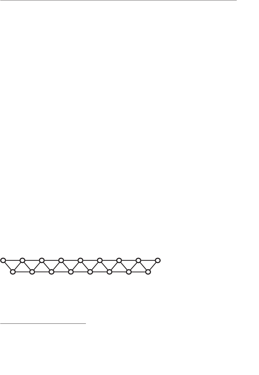
ptg9898810
horizontally), it is replicated horizontally. If it is x-major then it is
replicated vertically.
The OpenGL specification is somewhat liberal on how ends of lines are
represented and how wide lines are rasterized when antialiasing is turned
off. When antialiasing is turned on, lines are treated as rectangles aligned
along the line, with width equal to the current line width.
Triangles, Strips, and Fans
Triangles are made up of collections of three vertices. When separate
triangles are rendered, each triangle is independent of all others. A triangle
is rendered by projecting each of the three vertices into screen space and
forming three edges running between the edges. A sample is considered
covered if it lies on the positive side of all of the half spaces formed by the
lines between the vertices. If two triangles share an edge (and therefore a
pair of vertices), no single sample can be considered inside both triangles.
This is important because, although some variation in rasterization
algorithm is allowed by the OpenGL specification, the rules governing
pixels that lie along a shared edge are quite strict:
•No pixel on a shared edge between two triangles that together would
cover the pixel should be left unlit.
•No pixel on a shared edge between two triangles should be lit by more
than one of them.
This means that OpenGL will reliably rasterize meshes with shared edges
without gaps between the triangles, and without overdraw.2This is
important when rasterizing triangle strips or fans. When a triangle strip is
rendered, the first three vertices form the first triangle, then each
subsequent vertex forms another triangle along with the last two vertices
of the previous triangle. This is illustrated in Figure 3.1.
0 2 4 6 8 10 12 14 16
1357 9 11 13 15
Figure 3.1 Vertex layout for a triangle strip
When rendering a triangle fan, the first vertex forms a shared point that is
included in each subsequent triangle. Triangles are then formed using that
2. Overdraw is where the same pixel is lit more than once, and can cause artifacts when
blending is enabled, for example.
OpenGL Graphics Primitives 89
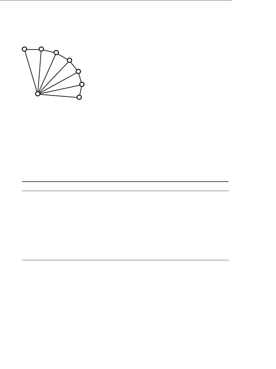
ptg9898810
shared point and the next two vertices. An arbitrarily complex convex
polygon can be rendered as a triangle fan. Figure 3.2 shows the vertex
layout of a triangle fan.
0
1 2
4
5
7
6
3
Figure 3.2 Vertex layout for a triangle fan
These primitive types are used by the drawing functions that will be
introduced in the next section. They are represented by OpenGL tokens
that are passed as arguments to functions used for rendering. Table 3.1
shows the mapping of primitive types to the OpenGL tokens used to
represent them.
Table 3.1 OpenGL Primitive Mode Tokens
Primitive Type OpenGL Token
Points GL_POINTS
Lines GL_LINES
Line Strips GL_LINE_STRIP
Line Loops GL_LINE_LOOP
Independent Triangles GL_TRIANGLES
Triangle Strips GL_TRIANGLE_STRIP
Triangle Fans GL_TRIANGLE_FAN
Rendering Polygons As Points, Outlines, or Solids
Apolygon has two sides---front and back---and might be rendered differently
depending on which side is facing the viewer. This allows you to have
cutaway views of solid objects in which there is an obvious distinction
between the parts that are inside and those that are outside. By default,
both front and back faces are drawn in the same way. To change this, or to
draw only outlines or vertices, use glPolygonMode().
90 Chapter 3: Drawing with OpenGL

ptg9898810
void glPolygonMode(GLenum face, GLenum mode);
Controls the drawing mode for a polygon’s front and back faces. The
parameter face must be GL_FRONT_AND_BACK; while mode can be
GL_POINT, GL_LINE, GL_FILL to indicate whether the polygon should
be drawn as points, outlined, or filled. By default, both the front and
back faces are drawn filled.
Reversing and Culling Polygon Faces
By convention, polygons whose vertices appear in counterclockwise order
on the screen are called front facing.You can construct the surface of any
‘‘reasonable’’ solid---a mathematician would call such a surface an
orientable manifold (spheres, donuts, and teapots are orientable; Klein
bottles and Möbius strips aren’t)---from polygons of consistent orientation.
In other words, you can use all clockwise polygons or all counterclockwise
polygons.
Suppose you’ve consistently described a model of an orientable surface but
happen to have the clockwise orientation on the outside. You can swap
what OpenGL considers the back face by using the function glFrontFace(),
supplying the desired orientation for front-facing polygons.
void glFrontFace(GLenum mode);
Controls how front-facing polygons are determined. By default, mode is
GL_CCW, which corresponds to a counterclockwise orientation of the
ordered vertices of a projected polygon in window coordinates. If mode is
GL_CW, faces with a clockwise orientation are considered front-facing.
Note: The orientation (clockwise or counterclockwise) of the vertices is
also known as its winding.
In a completely enclosed surface constructed from opaque polygons with a
consistent orientation, none of the back-facing polygons are ever visible---
they’re always obscured by the front-facing polygons. If you are outside
this surface, you might enable culling to discard polygons that OpenGL
determines are back-facing. Similarly, if you are inside the object, only
back-facing polygons are visible. To instruct OpenGL to discard front- or
back-facing polygons, use the command glCullFace() and enable culling
with glEnable().
OpenGL Graphics Primitives 91

ptg9898810
void glCullFace(GLenum mode);
Indicates which polygons should be discarded (culled) before they’re
converted to screen coordinates. The mode is either GL_FRONT,
GL_BACK, or GL_FRONT_AND_BACK to indicate front-facing,
back-facing, or all polygons. To take effect, culling must be enabled using
glEnable() with GL_CULL_FACE; it can be disabled with glDisable() and
the same argument.
Advanced
In more technical terms, deciding whether a face of a polygon is front- or
back-facing depends on the sign of the polygon’s area computed in
window coordinates. One way to compute this area is
a=1
2
n−1
i=0
xiyi⊕1−xi⊕1yi
where xiand yiare the xand ywindow coordinates of the ith vertex of the
n-vertex polygon and where i⊕1 is shorthand for (i+1)mod n, where
mod is the modulus operator.
Assuming that GL_CCW has been specified, if a>0, the polygon
corresponding to that vertex is considered to be front-facing; otherwise, it’s
back-facing. If GL_CW is specified and if a<0, then the corresponding
polygon is front-facing; otherwise, it’s back-facing.
Data in OpenGL Buffers
Almost everything you will ever do with OpenGL will involve buffers full
of data. Buffers in OpenGL are represented as buffer objects. You’ve already
had a brief introduction to buffer objects in Chapter 1. However, in this
section we’ll dig a little deeper into the specifics of how buffer objects are
used; ways to create, manage, and destroy them; and the best practices
associated with buffer objects.
Creating and Allocating Buffers
As with many things in OpenGL, buffer objects are named using GLuint
values. Values are reserved using the glGenBuffers() command. This
function has already been described in Chapter 1, but we include the
prototype here again for handy reference.
92 Chapter 3: Drawing with OpenGL

ptg9898810
void glGenBuffers(GLsizei n, GLuint *buffers);
Returns ncurrently unused names for buffer objects in the array buffers.
After calling glGenBuffers(), you will have an array of buffer object names
in buffers, but at this time, they’re just placeholders. They’re not actually
buffer objects---yet. The buffer objects themselves are not actually created
until the name is first bound to one of the buffer binding points on the
context. This is important because OpenGL may make decisions about the
best way to allocate memory for the buffer object based on where it is
bound. The buffer binding points (called targets) are described in Table 3.2.
Table 3.2 Buffer Binding Targets
Target Uses
GL_ARRAY_BUFFER This is the binding point that is used
to set vertex array data pointers using
glVertexAttribPointer(). This is the
target that you will likely use most
often.
GL_COPY_READ_BUFFER and
GL_COPY_WRITE_BUFFER
Together, these targets form a pair of
binding points that can be used to
copy data between buffers without
disturbing OpenGL state, or implying
usage of any particular kind to
OpenGL.
GL_DRAW_INDIRECT_BUFFER A buffer target used to store the
parameters for drawing commands
when using indirect drawing, which
will be explained in detail in the next
section.
GL_ELEMENT_ARRAY_BUFFER Buffers bound to this target can
contain vertex indices which are used
by indexed draw commands such as
glDrawElements().
GL_PIXEL_PACK_BUFFER The pixel pack buffer is used as the
destination for OpenGL commands
that read data from image objects
such as textures or the framebuffer.
Examples of such commands include
glGetTexImage() and glReadPixels().
Data in OpenGL Buffers 93

ptg9898810
Table 3.2 (continued) Buffer Binding Targets
Target Uses
GL_PIXEL_UNPACK_BUFFER The pixel unpack buffer is the opposite
of the pixel pack buffer---it is used as
the source of data for commands like
glTexImage2D().
GL_TEXTURE_BUFFER Texture buffers are buffers that are
bound to texture objects so that their
data can be directly read inside
shaders. The GL_TEXTURE_BUFFER
binding point provides a target for
manipulating these buffers, although
they must still be attached to textures
to make them accessible to shaders.
GL_TRANSFORM_FEEDBACK_ BUFFER Transform feedback is a facility in
OpenGL whereby transformed
vertices can be captured as they exit
the vertex processing part of the
pipeline (after the vertex or geometry
shader, if present) and some of their
attributes written into buffer objects.
This target provides a binding point
for buffers that are used to record
those attributes. Transform feedback
will be covered in some detail in
‘‘Transform Feedback’’ on Page 239.
GL_UNIFORM_BUFFER This target provides a binding point
where buffers that will be used as
uniform buffer objects may be bound.
Uniform buffers are covered in
Subsection 2,‘‘Uniform Blocks’’.
A buffer object actually is created by binding one of the names reserved
by a call to glGenBuffers() to one of the targets in Table 3.2 using
glBindBuffer(). As with glGenBuffers(),glBindBuffer() was introduced in
Chapter 1, but we include its prototype here again for completeness.
void glBindBuffer(GLenum target, GLuint buffer);
Binds the buffer object named buffer to the buffer-binding point as
specified by target.target must be one of the OpenGL buffer-binding
targets, and buffer must be a name reserved by a call to glGenBuffers().
If this the first time the name buffer has been bound, a buffer object is
created with that name.
94 Chapter 3: Drawing with OpenGL

ptg9898810
Right, so we now have a buffer object bound to one of the targets listed in
Table 3.2, now what? The default state of a newly created buffer object is a
buffer with no data in it. Before it can be used productively, we must put
some data into it.
Getting Data into and out of Buffers
There are many ways to get data into and out of buffers in OpenGL. These
range from explicitly providing the data, to replacing parts of the data in a
buffer object with new data, to generating the data with OpenGL and
recording it into the buffer object. The simplest way to get data into a
buffer object is to load data into the buffer at time of allocation. This is
accomplished through the use of the glBufferData() function. Here’s the
prototype of glBufferData() again.
void glBufferData(GLenum target, GLsizeiptr size,
const GLvoid *data, GLenum usage);
Allocates size bytes of storage for the buffer object bound to target. If data
is non-NULL, that space is initialized with the contents of memory
addressed by data.usage is provided to allow the application to supply
OpenGL with a hint as to the intended usage for the data in the buffer.
It’s important to note that glBufferData() actually allocates (or reallocates)
storage for the buffer object. That is, if the size of the new data is greater
than the current storage space allocated for the buffer object, the buffer
object will be resized to make room. Likewise, if the new data is smaller
than what has been allocated for the buffer, the buffer object will shrink to
match the new size. The fact that it is possible to specify the initial data to be
placed into the buffer object is merely a convenience and is not necessarily
the best way to do it (or even the most convenient, for that matter).
The target of the initial binding is not the only information OpenGL uses
to decide how to best allocate the buffer object’s data store. The other
important parameter to glBufferData() is the usage parameter. usage
must be one of the standard usage tokens such as GL_STATIC_DRAW or
GL_DYNAMIC_COPY. Notice how the token name is made of two
parts---the first being one of STATIC, DYNAMIC, or STREAM and the
second being one of DRAW, READ, or COPY.
The meanings of these ‘‘subtokens’’ are shown in Table 3.3.
Data in OpenGL Buffers 95

ptg9898810
Table 3.3 Buffer Usage Tokens
Token Fragment Meaning
_STATIC_ The data store contents will be modified once and used
many times.
_DYNAMIC_ The data store contents will be modified repeatedly and used
many times.
_STREAM_ The data store contents will be modified once and used at
most a few times.
_DRAW The data store contents are modified by the application and
used as the source for OpenGL drawing and image
specification commands.
_READ The data store contents are modified by reading data from
OpenGL and used to return that data when queried by the
application.
_COPY The data store contents are modified by reading data from
OpenGL and used as the source for OpenGL drawing and
image specification commands.
Accurate specification of the usage parameter is important to achieve
optimal performance. This parameter conveys useful information to
OpenGL about how you plan to use the buffer. Consider the first part of
the accepted tokens first. When the token starts with _STATIC_, this
indicates that the data will change very rarely, if at all---it is essentially
static. This should be used for data that will be specified once and never
modified again. When usage includes _STATIC_, OpenGL may decide to
shuffle the data around internally in order to make it fit in memory better,
or be a more optimal data format. This may be an expensive operation, but
since the data is static, it needs to be performed only once and so the
payoff may be great.
Including _DYNAMIC_ in usage indicates that you’re going to change the
data from time to time but will probably use it many times between
modifications. You might use this, for example, in a modeling program
where the data is essentially static---until the user edits it. In this case,
it’ll probably be used for many frames, then be modified, and then
used for many more frames, and so on. This is in contrast to the
GL_STREAM_ subtoken. This indicates that you’re planning on regularly
modifying the data in the buffer and using it only a few times (maybe only
once) between each modification. In this case, OpenGL might not even
copy your data to fast graphics memory if it can access it in place. This
should be used for applications such as physical simulations running on
the CPU where a new set of data is presented in each frame.
96 Chapter 3: Drawing with OpenGL

ptg9898810
Now turn your attention to the second part of the usage tokens. This part
of the token indicates who is responsible for updating and using the data.
When the token includes _DRAW, this infers that the buffer will be used as
a source of data during regular OpenGL drawing operations. It will be read
a lot, compared to data whose usage token includes _READ, which is likely
to be written often. Including _READ indicates that the application will
read back from the buffer (see ‘‘Accessing the Content of Buffers’’), which
in turn infers that the data is likely to be written to often by OpenGL.
usage parameters including _DRAW should be used for buffers containing
vertex data, for example, whereas parameters including _READ should be
used for pixel buffer objects and other buffers that will be used to retrieve
information from OpenGL. Finally, including _COPY in usage indicates
that the application will use OpenGL to generate data to be placed in the
buffer, which will then be used as a source for subsequent drawing
operations. An example of an appropriate use of _COPY is transform
feedback buffers---buffers that will be written by OpenGL and then be used
as vertex buffers in later drawing commands.
Initializing Part of a Buffer
Suppose you have an array containing some vertex data, another
containing some color information, and yet another containing texture
coordinates or some other data. You’d like to pack the data back to back
into one big buffer object so that OpenGL can use it. The arrays may or
may not be contiguous in memory, so you can’t use glBufferData() to
upload all of it in one go. Further, if you use glBufferData() to upload, say,
the vertex data first, then the buffer will be sized to exactly match the
vertex data and there won’t be room for the color or texture coordinate
information. That’s where glBufferSubData() comes in.
void glBufferSubData(GLenum target, GLintptr offset,
GLsizeiptr size, const GLvoid *data);
Replaces a subset of a buffer object’s data store with new data. The section
of the buffer object bound to target starting at offset bytes is updated with
the size bytes of data addressed by data. An error is thrown if offset and
size together specify a range that is beyond the bounds of the buffer
object’s data store.
By using a combination of glBufferData() and glBufferSubData(), we can
allocate and initialize a buffer object and upload data into several separate
sections of it. An example is shown in Example 3.1.
Data in OpenGL Buffers 97

ptg9898810
Example 3.1 Initializing a Buffer Object with glBufferSubData()
// Vertex positions
static const GLfloat positions[] =
{
-1.0f, -1.0f, 0.0f, 1.0f,
1.0f, -1.0f, 0.0f, 1.0f,
1.0f, 1.0f, 0.0f, 1.0f,
-1.0f, 1.0f, 0.0f, 1.0f
};
// Vertex colors
static const GLfloat colors[] =
{
1.0f, 0.0f, 0.0f,
0.0f, 1.0f, 0.0f,
0.0f, 0.0f, 1.0f,
1.0f, 1.0f, 1.0f,
};
// The buffer object
GLuint buffer;
// Reserve a name for the buffer object.
glGenBuffers(1, &buffer);
// Bind it to the GL_ARRAY_BUFFER target.
glBindBuffer(GL_ARRAY_BUFFER, buffer);
// Allocate space for it (sizeof(positions) + sizeof(colors)).
glBufferData(GL_ARRAY_BUFFER, // target
sizeof(positions) + sizeof(colors), // total size
NULL, // no data
GL_STATIC_DRAW); // usage
// Put "positions" at offset zero in the buffer.
glBufferSubData(GL_ARRAY_BUFFER, // target
0, // offset
sizeof(positions), // size
positions); // data
// Put "colors" at an offset in the buffer equal to the filled size of
// the buffer so far - i.e., sizeof(positions).
glBufferSubData(GL_ARRAY_BUFFER, // target
sizeof(positions), // offset
sizeof(colors), // size
colors); // data
// Now "positions" is at offset 0 and "colors" is directly after it
// in the same buffer.
If you simply wish to clear a buffer object’s data store to a known value,
you can use the glClearBufferData() or glClearBufferSubData()
functions. Their prototypes are as follows:
98 Chapter 3: Drawing with OpenGL

ptg9898810
void glClearBufferData(GLenum target, GLenum internalformat,
GLenum format, GLenum type,
const void * data);
void glClearBufferSubData(GLenum target,
GLenum internalformat,
GLintptr offset, GLintptr size,
GLenum format, GLenum type,
const void * data);
Clear all or part of a buffer object’s data store. The data store of the buffer
bound to target is filled with the data stored in data.format and type
specify the format and type of the data pointed to by data, respectively.
The data is first converted into the format specified by internalformat, and
then that data is used to fill the specified range of the buffer’s data store.
In the case of glClearBufferData(), the entire store is filled with the
specified data. For glClearBufferSubData(), the range is specified by
offset and size, which give the starting offset and size, in bytes of the
range, respectively.
Using glClearBufferData() or glClearBufferSubData() allows you to
initialize the data store of a buffer object without necessarily reserving and
clearing a region of system memory to do it.
Data can also be copied between buffer objects using the
glCopyBufferSubData() function. Rather than assembling chunks of data
in one large buffer object using glBufferSubData(), it is possible to upload
the data into separate buffers using glBufferData() and then copy from
those buffers into the larger buffer using glCopyBufferSubData().
Depending on the OpenGL implementation, it may be able to overlap
these copies because each time you call glBufferData() on a buffer object,
it invalidates whatever contents may have been there before. Therefore,
OpenGL can sometimes just allocate a whole new data store for your data,
even though a copy operation from the previous store has not completed
yet. It will then release the old storage at a later opportunity.
The prototype of glCopyBufferSubData() is as follows:
void glCopyBufferSubData(GLenum readtarget,
GLenum writetarget,
GLintptr readoffset,
GLintprr writeoffset, GLsizeiptr size);
Data in OpenGL Buffers 99

ptg9898810
Copies part of the data store of the buffer object bound to readtarget into
the data store of the buffer object bound to writetarget. The size bytes of
data at readoffset within readtarget are copied into writetarget at writeoffset.
If readoffset or writeoffset together with size would cause either OpenGL to
access any area outside the bound buffer objects, a GL_INVALID_VALUE
error is generated.
Whilst glCopyBufferSubData() can be used to copy data between buffers
bound to any two targets, the targets GL_COPY_READ_BUFFER and
GL_COPY_WRITE_BUFFER are provided specifically for this purpose.
Neither target is used for anything else by OpenGL, and so you can safely
bind buffers to them for the purposes of copying or staging data without
disturbing OpenGL state or needing to keep track of what was bound to
the target before your copy.
Reading the Contents of a Buffer
Data can be read back from a buffer object in a couple of different ways.
The first is to use the glGetBufferSubData() function. This function reads
data from the buffer object bound to one of the targets and places it into a
chunk of memory owned by your applications. The prototype of
glGetBufferSubData() is as follows:
void glGetBufferSubData(GLenum target, GLintptr offset,
GLsizeiptr size, GLvoid * data);
Returns some or all of the data from the buffer object currently bound
to target. Data starting at byte-offset offset and extending for size bytes is
copied from the data store to the memory pointed to by data. An error is
thrown if the buffer object is currently mapped, or if offset and size together
define a range beyond the bounds of the buffer object’s data store.
glGetBufferSubData() is useful when you have generated data using
OpenGL and wish to retrieve it. Examples include using transform
feedback to process vertices using a GPU, or reading framebuffer or texture
data into a Pixel Buffer Object. Both of these topics will be covered later. Of
course, it’s also possible to use glGetBufferSubData() to simply read back
data that you previously put into the buffer object.
Accessing the Content of Buffers
The issue with all of the functions covered in this section so far
(glBufferData(),glBufferSubData(),glCopyBufferSubData(), and
100 Chapter 3: Drawing with OpenGL

ptg9898810
glGetBufferSubData()) is that they all cause OpenGL to make a copy of
your data. glBufferData() and glBufferSubData() both copy data from
your application’s memory into memory owned by OpenGL. Obviously,
glCopyBufferSubData() causes a copy of previously buffered data to be
made. glGetBufferSubData() copies data from memory owned by OpenGL
into memory provided by your application. Depending on the hardware
configuration, it’s very possible that the memory owned by OpenGL would
be accessible to your application if only you had a pointer to it. Well, you
can get that pointer using glMapBuffer().
void * glMapBuffer(GLenum target, GLenum access);
Maps to the client’s address space the entire data store of the buffer object
currently bound to target. The data can then be directly read or written
relative to the returned pointer, depending on the specified access policy.
If OpenGL is unable to map the buffer object’s data store, glMapBuffer()
generates an error and returns NULL. This may occur for system-specific
reasons, such as low virtual memory availability.
When you call glMapBuffer(), the function returns a pointer to memory
that represents the data store of the buffer object attached to target. Note
that this memory represents only this buffer---it is not necessarily the
memory that the graphics processor will use. The access parameter specifies
how the application intends to use the memory once it is mapped. It must
be one of the tokens shown in Table 3.4.
Table 3.4 Access Modes for glMapBuffer()
Token Meaning
GL_READ_ONLY The application will only read from the memory
mapped by OpenGL.
GL_WRITE_ONLY The application will only write to the memory
mapped by OpenGL.
GL_READ_WRITE The application may read from or write to the
memory mapped by OpenGL.
If glMapBuffer() fails to map the buffer object’s data store, it returns
NULL. The access parameter forms a contract between you and OpenGL
that specifies how you will access the memory. If you violate that contract,
Data in OpenGL Buffers 101

ptg9898810
bad things will happen, which may include ignoring writes to the buffer,
corrupting your data or even crashing your program.3
Note: When you map a buffer whose data store is in memory that will
not be accessible to your application, OpenGL may need to move
the data around so that when you use the pointer it gives you, you
get what you expect. Likewise, when you’re done with the data
and have modified it, OpenGL may need to move it back to a place
where the graphics processor can see it. This can be expensive
in terms of performance, so great care should be taken when
doing this.
When the buffer is mapped with the GL_READ_ONLY or GL_READ_WRITE
access mode, the data that was in the buffer object becomes visible to your
application. You can read it back, write it to a file, and even modify it in
place (so long as you used GL_READ_WRITE as the access mode). If access is
GL_READ_WRITE or GL_WRITE_ONLY, you can write data into memory
using the pointer OpenGL gave you. Once you are done using the data or
writing data into the buffer object, you must unmap it using
glUnmapBuffer(), whose prototype is as follows:
GLboolean glUnmapBuffer(GLenum target);
Releases the mapping created by glMapBuffer().glUnmapBuffer()
returns GL_TRUE unless the data store contents have become corrupt
during the time the data store was mapped. This can occur for
system-specific reasons that affect the availability of graphics memory,
such as screen mode changes. In such situations, GL_FALSE is returned
and the data store contents are undefined. An application must detect
this rare condition and reinitialize the data store.
When you unmap the buffer, any data you wrote into the memory given
to you by OpenGL becomes visible in the buffer object. This means that
you can place data into buffer objects by allocating space for them using
glBufferData() and passing NULL as the data parameter, mapping them,
writing data into them directly, and then unmapping them again.
Example 3.2 contains an example of loading the contents of a file into a
buffer object.
3. The unfortunate thing is that so many applications do violate this contract that most OpenGL
implementations will assume you don’t know what you’re doing and will treat all calls to
glMapBuffer() as if you specified GL_READ_WRITE as the access parameter, just so these other
applications will work.
102 Chapter 3: Drawing with OpenGL

ptg9898810
Example 3.2 Initializing a Buffer Object with glMapBuffer()
GLuint buffer;
FILE *f;
size_t filesize;
// Open a file and find its size
f = fopen("data.dat", "rb");
fseek(f, 0, SEEK_END);
filesize = ftell(f);
fseek(f, 0, SEEK_SET);
// Create a buffer by generating a name and binding it to a buffer
// binding point - GL_COPY_WRITE_BUFFER here (because the binding means
// nothing in this example).
glGenBuffers(1, &buffer);
glBindBuffer(GL_COPY_WRITE_BUFFER, buffer);
// Allocate the data store for the buffer by passing NULL for the
// data parameter.
glBufferData(GL_COPY_WRITE_BUFFER, (GLsizei)filesize, NULL,
GL_STATIC_DRAW);
// Map the buffer...
void *data = glMapBuffer(GL_COPY_WRITE_BUFFER, GL_WRITE_ONLY);
// Read the file into the buffer.
fread(data, 1, filesize, f);
// Okay, done, unmap the buffer and close the file.
glUnmapBuffer(GL_COPY_WRITE_BUFFER);
fclose(f);
In Example 3.2, the entire contents of a file are read into a buffer object in
a single operation. The buffer object is created and allocated to the same
size as the file. Once the buffer is mapped, the file can be read directly into
the buffer object’s data store. No copies are made by the application, and,
if the data store is visible to both the application and the graphics
processor, no copies will be made by OpenGL.
There may be significant performance advantages to initializing buffer
objects in this manner. The logic is this; when you call glBufferData()
or glBufferSubData(), once those functions return, you are free to do
whatever you want with the memory you gave them---free it, use it for
something else---it doesn’t matter. This means that those functions must be
done with that memory by the time they return, and so they need to make
a copy of your data. However, when you call glMapBuffer(), the pointer
you get points at memory owned by OpenGL. When you call
glUnmapBuffer(), OpenGL still owns that memory---it’s the application
that has to be done with it. This means that if the data needs to be moved
Data in OpenGL Buffers 103

ptg9898810
or copied, OpenGL can start that process when you call glUnmapBuffer()
and return immediately, content in the knowledge that it can finish the
operation at its leisure without your application interfering in any way.
Thus the copy that OpenGL needs to perform can overlap whatever your
application does next (making more buffers, reading more files, and so
on). If it doesn’t need to make a copy, then great! The unmap operation
essentially becomes free in that case.
Asynchronous and Explicit Mapping
To address many of the issues involved with mapping buffers using
glMapBuffer() (such as applications incorrectly specifying the access
parameter or always using GL_READ_WRITE), glMapBufferRange() uses
flags to specify access more precisely. The prototype for
glMapBufferRange() is as follows:
void * glMapBufferRange(GLenum target, GLintptr offset,
GLsizeiptr length, GLbitfield access);
Maps all or part of a buffer object’s data store into the application’s
address space. target specifies the target to which the buffer object is
currently bound. offset and length together indicate the range of the data
(in bytes) that is to be mapped. access is a bitfield containing flags that
describe the mapping.
For glMapBufferRange(),access is a bitfield that must contain one or both
of the GL_MAP_READ_BIT and the GL_MAP_WRITE_BIT indicating
whether the application plans to read from the mapped data store, write to
it, or do both. In addition, access may contain one or more of the flags
shown in Table 3.5.
Table 3.5 Flags for Use with glMapBufferRange()
Flag Meaning
GL_MAP_INVALIDATE_RANGE_BIT If specified, any data in the specified
range of the buffer may be discarded and
considered invalid. Any data within the
specified range that is not subsequently
written by the application becomes
undefined. This flag may not be used
with GL_MAP_READ_BIT.
104 Chapter 3: Drawing with OpenGL

ptg9898810
Table 3.5 (continued) Flags for Use with glMapBufferRange()
Flag Meaning
GL_MAP_INVALIDATE_BUFFER_BIT If specified, the entire contents of the
buffer may be discarded and considered
invalid, regardless of the specified range.
Any data lying outside the mapped range
of the buffer object becomes undefined,
as does any data within the range but not
subsequently written by the application.
This flag may not be used with
GL_MAP_READ_BIT.
GL_MAP_FLUSH_EXPLICIT_BIT The application will take responsibility to
signal to OpenGL which parts of the
mapped range contain valid data by
calling glFlushMappedBufferRange()
prior to calling glUnmapBuffer(). Use
this flag if a larger range of the buffer will
be mapped and not all of it will be
written by the application. This bit must
be used in conjunction with
GL_MAP_WRITE_BIT. If
GL_MAP_FLUSH_EXPLICIT_BIT is not
specified, glUnmapBuffer() will
automatically flush the entirety of the
mapped range.
GL_MAP_UNSYNCHRONIZED_BIT If this bit is not specified, OpenGL will
wait until all pending operations that
may access the buffer have completed
before returning the mapped range. If
this flag is set, OpenGL will not attempt
to synchronize operations on the buffer.
As you can see from the flags listed in Table 3.5, the command provides a
significant level of control over how OpenGL uses the data in the buffer
and how it synchronizes operations that may access that data.
When you specify that you want to invalidate the data in the buffer object
by specifying either the GL_MAP_INVALIDATE_RANGE_BIT or
GL_MAP_INVALIDATE_BUFFER_BIT, this indicates to OpenGL that it is
free to dispose of any previously stored data in the buffer object. Either of
the flags can be set only if you also specify that you’re going to write to the
buffer by also setting the GL_MAP_WRITE_BIT flag. If you specify
GL_MAP_INVALIDATE_RANGE_BIT, it indicates that you will update the
entire range (or at least all the parts of it that you care about). If you set the
GL_MAP_INVALIDATE_BUFFER_BIT, it means that you don’t care what
Data in OpenGL Buffers 105

ptg9898810
ends up in the parts of the buffer that you didn’t map. Either way, setting
the flags indicates that you’re planning to update the rest of the buffer
with subsequent maps.4When OpenGL is allowed to throw away the rest
of the buffer’s data, it doesn’t have to make any effort to merge your
modified data back into the rest of the original buffer. It’s probably a good
idea to use GL_MAP_INVALIDATE_BUFFER_BIT for the first section of the
buffer that you map, and then GL_MAP_INVALIDATE_RANGE_BIT for the
rest of the buffer.
The GL_MAP_UNSYNCHRONIZED_BIT flag is used to disengage OpenGL’s
automatic synchronization between data transfer and use. Without this
bit, OpenGL will finish up any in-flight commands that might be using
the buffer object. This can stall the OpenGL pipeline, causing a bubble and
a loss of performance. If you can guarantee that all pending commands
will be complete before you actually modify the contents of the buffer (but
not necessarily before you call glMapBufferRange()) through a method
such as calling glFinish() or using a sync object (which are described in
‘‘Atomic Operations and Synchronization’’ on Page 578 in Chapter 11),
then OpenGL doesn’t need to do this synchronization for you.
Finally, the GL_MAP_FLUSH_EXPLICIT_BIT flag indicates that the
application will take on the responsibility of letting OpenGL know which
parts of the buffer it has modified before calling glUnmapBuffer(). It does
this through a call to glFlushMappedBufferRange(), whose prototype is as
follows:
void glFlushMappedBufferRange(GLenum target, GLintptr offset,
GLsizeiptr length);
Indicates to OpenGL that the range specified by offset and length in the
mapped buffer bound to target has been modified and should be
incorporated back into the buffer object’s data store.
It is possible to call glFlushMappedBufferRange() multiple times on
separate or even overlapping ranges of a mapped buffer object. The range
of the buffer object specified by offset and length must lie within the range
of buffer object that has been mapped, and that range must have been
mapped by a call to glMapBufferRange() with access including the
GL_MAP_FLUSH_EXPLICIT_BIT flag set. When this call is made, OpenGL
assumes that you’re done modifying the specified range of the mapped
buffer object, and can begin any operations it needs to perform in order to
4. Don’t specify the GL_MAP_INVALIDATE_BUFFER_BIT for every section, otherwise only the
last section you mapped will have valid data in it!
106 Chapter 3: Drawing with OpenGL

ptg9898810
make that data usable such as copying it to graphics processor visible
memory, or flushing, or invalidating data caches. It can do these things
even though some or all of the buffer is still mapped. This is a useful way
to parallelize OpenGL with other operations that your application might
perform. For example, if you need to load a very large piece of data from
a file into a buffer, map a range of the buffer large enough to hold the
whole file, then read chunks of the file, and after each chunk call
glFlushMappedBufferRange(). OpenGL will then operate in parallel to
your application, reading more data from the file for the next chunk.
By combining these flags in various ways, it is possible to optimize data
transfer between the application and OpenGL or to use advanced
techniques such as multithreading or asynchronous file operations.
Discarding Buffer Data
Advanced
When you are done with the data in a buffer, it can be advantageous
to tell OpenGL that you don’t plan to use it any more. For example,
consider the case where you write data into a buffer using transform
feedback, and then draw using that data. If that drawing command is the
last one that is going to access the data, then you can tell OpenGL that
it is free to discard the data and use the memory for something else. This
allows an OpenGL implementation to make optimizations such as tightly
packing memory allocations or avoiding expensive copies in systems with
more than one GPU.
To discard some or all of the data in a buffer object, you can call
glInvalidateBufferData() or glInvalidateBufferSubData(), respectively.
The prototypes of these functions are as follows:
void glInvalidateBufferData(GLuint buffer);
void glInvalidateBufferSubData(GLuint buffer, GLintptr offset,
GLsizeiptr length);
Tell OpenGL that the application is done with the contents of the buffer
object in the specified range and that it is free to discard the data if it
believes it is advantageous to do so. glInvalidateBufferSubData()
discards the data in the region of the buffer object whose name is
buffer starting at offset bytes and continuing for length bytes.
glInvalidateBufferData() discards the entire contents of the buffer’s
data store.
Data in OpenGL Buffers 107

ptg9898810
Note that semantically, calling glBufferData() with a NULL pointer does a
very similar thing to calling glInvalidateBufferData(). Both methods will
tell the OpenGL implementation that it is safe to discard the data in the
buffer. However, glBufferData() logically recreates the underlying memory
allocation, whereas glInvalidateBufferData() does not. Depending
on the OpenGL implementation, it may be more optimal to call
glInvalidateBufferData(). Further, glInvalidateBufferSubData() is really
the only way to discard a region of a buffer object’s data store.
Vertex Specification
Now that you have data in buffers, and you know how to write a basic
vertex shader, it’s time to hook the data up to the shader. You’ve
already read about vertex array objects, which contain information about
where data is located and how it is laid out, and functions like
glVertexAttribPointer(). It’s time to take a deeper dive into vertex
specifications, other variants of glVertexAttribPointer(), and how to
specify data for vertex attributes that aren’t floating point or aren’t enabled.
VertexAttribPointer in Depth
The glVertexAttribPointer() command was briefly introduced in
Chapter 1. The prototype is as follows:
void glVertexAttribPointer(GLuint index, GLint size,
GLenum type, GLboolean normalized,
GLsizei stride, const GLvoid *pointer);
Specifies where the data values for the vertex attribute with location index
can be accessed. pointer is the offset in basic-machine units (i.e.,
bytes)from the start of the buffer object currently bound to the
GL_ARRAY_BUFFER target for the first set of values in the array. size
represents the number of components to be updated per vertex. type
specifies the data type of each element in the array. normalized indicates
that the vertex data should be normalized before being presented to the
vertex shader. stride is the byte offset between consecutive elements in
the array. If stride is zero, the data is assumed to be tightly packed.
The state set by glVertexAttribPointer() is stored in the currently bound
vertex array object (VAO). size is the number of elements in the attribute’s
vector (1, 2, 3, or 4), or the special token GL_BGRA, which should be
108 Chapter 3: Drawing with OpenGL

ptg9898810
specified when packed vertex data is used. The type parameter is a token
that specifies the type of the data that is contained in the buffer object.
Table 3.6 describes the token names that may be specified for type and the
OpenGL data type that they correspond to:
Table 3.6 Values of Type for glVertexAttribPointer()
Token Value OpenGL Type
GL_BYTE GLbyte (signed 8-bit bytes)
GL_UNSIGNED_BYTE GLubyte (unsigned 8-bit bytes)
GL_SHORT GLshort (signed 16-bit words)
GL_UNSIGNED_SHORT GLushort (unsigned 16-bit words)
GL_INT GLint (signed 32-bit integers)
GL_UNSIGNED_INT GLuint (unsigned 32-bit integers)
GL_FIXED GLfixed (16.16 signed fixed point)
GL_FLOAT GLfloat (32-bit IEEE single-precision
floating point)
GL_HALF_FLOAT GLhalf (16-bit S1E5M10
half-precision floating point)
GL_DOUBLE GLdouble (64-bit IEEE
double-precision floating point)
GL_INT_2_10_10_10_REV GLuint (packed data)
GL_UNSIGNED_INT_2_10_10_10_REV GLuint (packed data)
Note that while integer types such as GL_SHORT or
GL_UNSIGNED_INT can be passed to the type argument, this tells OpenGL
only what data type is stored in memory in the buffer object. OpenGL will
convert this data to floating point in order to load it into floating-point
vertex attributes. The way this conversion is performed is controlled by the
normalize parameter. When normalize is GL_FALSE, integer data is simply
typecast into floating-point format before being passed to the vertex
shader. This means that if you place the integer value 4 into a buffer and
use the GL_INT token for the type when normalize is GL_FALSE, the value
4.0 will be placed into the shader. When normalize is GL_TRUE, the data
is normalized before being passed to the vertex shader. To do this, OpenGL
divides each element by a fixed constant that depends on the incoming
data type. When the data type is signed, the following formula is used:
f=c
2b−1
Vertex Specification 109

ptg9898810
Whereas, if the data type is unsigned, the following formula is used:
f=2c+1
2b−1
In both cases, fis the resulting floating-point value, cis the incoming
integer component, and bis the number of bits in the data type (i.e., 8 for
GL_UNSIGNED_BYTE, 16 for GL_SHORT, and so on). Note that unsigned
data types are also scaled and biased before being divided by the
type-dependent constant. To return to our example of putting 4 into an
integer vertex attribute, we get:
f=4
232 −1
which works out to about 0.000000009313---a pretty small number!
Integer Vertex Attributes
If you are familiar with the way floating-point numbers work, you’ll
also realize that precision is lost as numbers become very large, and so
the full range of integer values cannot be passed into a vertex shader using
floating-point attributes. For this reason, we have integer vertex attributes.
These are represented in vertex shaders by the int,ivec2,ivec3,orivec4
types or their unsigned counterparts---uint,uvec2 ,uvec3, and uvec4.
A second vertex-attribute function is needed in order to pass raw integers
into these vertex attributes---one that doesn’t automatically convert
everything to floating point. This is glVertexAttribIPointer()---the I stands
for integer.
void glVertexAttribIPointer(GLuint index, GLint size,
GLenum type, GLsizei stride,
const GLvoid *pointer);
Behaves similarly to glVertexAttribPointer(), but for vertex attributes
declared as integers in the vertex shader. type must be one of the integer
data type tokens GL_BYTE, GL_UNSIGNED_BYTE, GL_SHORT,
GL_UNSIGNED_SHORT, GL_INT, or GL_UNSIGNED_INT.
Notice that the parameters to glVertexAttribIPointer() are identical to the
parameters to glVertexAttribPointer(), except for the omission of the
110 Chapter 3: Drawing with OpenGL

ptg9898810
normalize parameter. normalize is missing because it’s not relevant to
integer vertex attributes. Only the integer data type tokens, GL_BYTE,
GL_UNSIGNED_BYTE, GL_SHORT, GL_UNSIGNED_SHORT, GL_INT, and
GL_UNSIGNED_INT may be used for the type parameter.
Double-Precision Vertex Attributes
The third variant of glVertexAttribPointer() is glVertexAttribLPointer()---
here the L stands for ‘‘long’’. This version of the function is specifically for
loading attribute data into 64-bit double-precision floating-point vertex
attributes.
void glVertexAttribLPointer(GLuint index, GLint size,
GLenum type, GLsizei stride,
const GLvoid *pointer);
Behaves similarly to glVertexAttribPointer(), but for vertex attributes
declared as 64-bit double-precision floating-point types in the vertex
shader. type must be GL_DOUBLE.
Again, notice the lack of the normalize parameter. In
glVertexAttribPointer(),normalize was used only for integer data types
that aren’t legal here, and so the parameter is not needed. If GL_DOUBLE
is used with glVertexAttribPointer(), the data is automatically
down-converted to 32-bit single-precision floating-point representation
before being passed to the vertex shader---even if the target vertex attribute
was declared using one of the double-precision types double,dvec2,
dvec3, or dvec4, or one of the double-precision matrix types such as
dmat4. However, with glVertexAttribLPointer(), the full precision of the
input data is kept and passed to the vertex shader.
Packed Data Formats for Vertex Attributes
Going back to the glVertexAttribPointer() command, you will notice that
the allowed values for the size parameter are 1, 2, 3, 4, and the special token
GL_BGRA. Also, the type parameter may take one of the special values
GL_INT_2_10_10_10_REV or GL_UNSIGNED_INT_2_10_10_10_REV, both
of which correspond to the GLuint data type. These special tokens are used
to represent packed data that can be consumed by OpenGL. The
GL_INT_2_10_10_10_REV and GL_UNSIGNED_INT_2_10_10_10_REV
tokens represent four-component data represented as ten bits for each of
the first three components and two for the last, packed in reverse order
into a single 32-bit quantity (a GLuint). GL_BGRA could just have easily
Vertex Specification 111
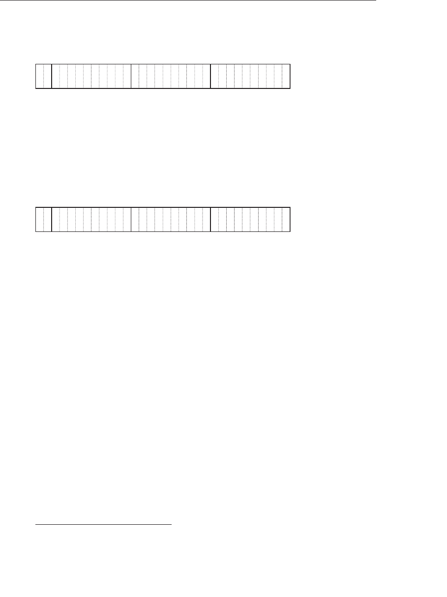
ptg9898810
been called GL_ZYXW.5Looking at the data layout within the 32-bit word,
you would see the bits divided up as shown in Figure 3.3.
W X Y Z
31 30 29 28 27 26 25 24 23 22 21 20 19 18 17 16 15 14 13 12 11 10 9 8 7 6 5 4 3 2 1 0
Figure 3.3 Packing of elements in a BGRA-packed vertex attribute
In Figure 3.3, the elements of the vertex are packed into a single 32-bit
integer in the order w,x,y,z---which when reversed is z,y,x,w, or b,g,r,a
when using color conventions. In Figure 3.4, the coordinates are packed
in the order w,z,y,x, which reversed and written in color conventions is
r,g,b,a.
W Z Y X
31 30 29 28 27 26 25 24 23 22 21 20 19 18 17 16 15 14 13 12 11 10 9 8 7 6 5 4 3 2 1 0
Figure 3.4 Packing of elements in a RGBA-packed vertex attribute
Vertex data may be specified only in the first of these two formats by using
the GL_INT_2_10_10_10_REV or GL_UNSIGNED_INT_2_10_10_10_REV
tokens. When one of these tokens is used as the type parameter to
glVertexAttribPointer(), each vertex consumes one 32-bit word in the
vertex array. The word is unpacked into its components and then
optionally normalized (depending on the value of the normalize parameter
before being loaded into the appropriate vertex attribute. This data
arrangement is particularly well suited to normals or other types of
attributes that can benefit from the additional precision afforded by the
10-bit components but perhaps don’t require the full precision offered by
half-float data (which would take 16-bits per component). This allows the
conservation of memory space and bandwidth, which helps improve
performance.
Static Vertex-Attribute Specification
Remember from Chapter 1where you were introduced to
glEnableVertexAttribArray() and glDisableVertexAttribArray().
5. Not a valid OpenGL token; just to be clear.
112 Chapter 3: Drawing with OpenGL

ptg9898810
These functions are used to tell OpenGL which vertex attributes are backed
by vertex buffers. Before OpenGL will read any data from your vertex
buffers, you must enable the corresponding vertex attribute arrays with
glEnableVertexAttribArray().You may wonder what happens if you don’t
enable the attribute array for one of your vertex attributes. In that case, the
static vertex attribute is used. The static vertex attribute for each vertex is the
default value that will be used for the attribute when there is no enabled
attribute array for it. For example, imagine you had a vertex shader that
would read the vertex color from one of the vertex attributes. Now suppose
that all of the vertices in a particular mesh or part of that mesh had the
same color. It would be a waste of memory and potentially of performance
to fill a buffer full of that constant value for all the vertices in the mesh.
Instead, you can just disable the vertex attribute array and use the static
vertex attribute to specify color for all of the vertices.
The static vertex attribute for each attribute may be specified using one of
glVertexAttrib*() functions. When the vertex attribute is declared as a
floating-point quantity in the vertex shader (i.e., it is of type float,vec2,
vec3,vec4, or one of the floating-point matrix types such as mat4 ), the
following glVertexAttrib*() commands can be used to set its value.
void glVertexAttrib{1234}{fds}(GLuint index, TYPE values);
void glVertexAttrib{1234}{fds}v(GLuint index,
const TYPE *values);
void glVertexAttrib4{bsifd ub us ui}v(GLuint index,
const TYPE *values);
Specifies the static value for the vertex attribute with index index. For the
non-vversions, up to four values are specified in the x,y,z, and w
parameters. For the vversions, up to four components are sourced from
the array whose address is specified in vand used in place of the x,y,z,
and wcomponents in that order.
All of these functions implicitly convert the supplied parameters
to floating-point before passing them to the vertex shader (unless they’re
already floating-point). This conversion is a simple typecast. That is,
the values are converted exactly as specified as if they had been specified
in a buffer and associated with a vertex attribute by calling
glVertexAttribPointer() with the normalize parameter set to GL_FALSE. For
the integer variants of the functions, versions exist that normalize the
Vertex Specification 113

ptg9898810
parameters to the range [0, 1]or [−1, 1]depending on whether the
parameters are signed or unsigned. These are:
void glVertexAttrib4Nub(GLuint index, GLubyte x, GLubyte y,
GLubyte z, GLubyte w);
void glVertexAttrib4N{bsi ub us ui}v(GLuint index,
const TYPE *v);
Specifies a single or multiple vertex-attribute values for attribute index,
normalizing the parameters to the range [0, 1]during the conversion
process for the unsigned variants and to the range [−1, 1]for the signed
variants.
Even with these commands, the parameters are still converted to
floating-point before being passed to the vertex shader. Thus, they are
suitable only for setting the static values of attributes declared with one of
the single-precision floating-point data types. If you have vertex attributes
that are declared as integers or double-precision floating-point variables,
you should use one of the following functions:
void glVertexAttribI{1234}{i ui}(GLuint index, TYPE values);
void glVertexAttribI{123}{i ui}v(GLuint index,
const TYPE *values);
void glVertexAttribI4{bsi ub us ui}v(GLuint index,
const TYPE *values);
Specifies a single or multiple static integer vertex-attribute values for
integer vertex attribute index.
Furthermore, if you have vertex attributes that are declared as one of the
double-precision floating-point types, you should use one of the Lvariants
of glVertexAttrib*(), which are:
void glVertexAttribL{1234}(GLuint index, TYPE values);
void glVertexAttribL{1234}v(GLuint index, const TYPE *values);
Specifies a single or multiple static vertex-attribute values for
double-precision vertex attribute index.
Both the glVertexAttribI*() and glVertexAttribL*() variants of
glVertexAttrib*() pass their parameters through to the underlying vertex
attribute just as the Iversions of glVertexAttribIPointer() do.
114 Chapter 3: Drawing with OpenGL

ptg9898810
If you use one of the glVertexAttrib*() functions with less components
than there are in the underlying vertex attribute (e.g., you use
glVertexAttrib*() 2f to set the value of a vertex attribute declared
as a vec4), default values are filled in for the missing components. For w,
1.0 is used as the default value, and for yand z, 0.0 is used.6If you use a
function that takes more components than are present in the vertex
attribute in the shader, the additional components are simply discarded.
Note: The static vertex attribute values are stored in the current VAO, not
the program object. That means that if the current vertex shader
has, for example, a vec3 input and you use glVertexAttrib*() 4fv
to specify a four-component vector for that attribute, the fourth
component will be ignored but still stored. If you change the vertex
shader to one that has a vec4 input at that attribute location, the
fourth component specified earlier will appear in that attribute’s
wcomponent.
OpenGL Drawing Commands
Most OpenGL drawing commands start with the word Draw.7The drawing
commands are roughly broken into two subsets---indexed and nonindexed
draws. Indexed draws use an array of indices stored in a buffer object
bound to the GL_ELEMENT_ARRAY_BUFFER binding that is used to
indirectly index into the enabled vertex arrays. On the other hand,
nonindexed draws do not use the GL_ELEMENT_ARRAY_BUFFER at all,
and simply read the vertex data sequentially. The most basic, nonindexed
drawing command in OpenGL is glDrawArrays().
void glDrawArrays(GLenum mode, GLint first, GLsizei count);
Constructs a sequence of geometric primitives using array elements
starting at first and ending at first +count −1 of each enabled array. mode
specifies what kinds of primitives are constructed and is one of the
primitive mode tokens such as GL_TRIANGLES, GL_LINE_LOOP,
GL_LINES, and GL_POINTS.
Similarly, the most basic indexed drawing command is glDrawElements().
6. The lack of a default for xis intentional---you can’t specify values for y,z, or wwithout also
specifying a value for x.
7. In fact, the only two commands in OpenGL that start with Draw but don’t draw anything
are glDrawBuffer() and glDrawBuffers().
OpenGL Drawing Commands 115

ptg9898810
void glDrawElements(GLenum mode, GLsizei count,
GLenum type, const GLvoid *indices);
Defines a sequence of geometric primitives using count number of
elements, whose indices are stored in the buffer bound to the
GL_ELEMENT_ARRAY_BUFFER buffer binding point (the element array
buffer). indices represents an offset, in bytes, into the element array buffer
where the indices begin. type must be one of GL_UNSIGNED_BYTE,
GL_UNSIGNED_SHORT, or GL_UNSIGNED_INT, indicating the data type
of the indices the element array buffer. mode specifies what kind of
primitives are constructed and is one of the primitive mode tokens, such
as GL_TRIANGLES, GL_LINE_LOOP, GL_LINES, and GL_POINTS.
Each of these functions causes vertices to be read from the enabled
vertex-attribute arrays and used to construct primitives of the type
specified by mode. Vertex-attribute arrays are enabled using
glEnableVertexAttribArray() as described in Chapter 1.glDrawArrays()
just uses the vertices in the buffer objects associated with the enabled
vertex attributes in the order they appear. glDrawElements() uses the
indices in the element array buffer to index into the vertex attribute arrays.
Each of the more complex OpenGL drawing functions essentially builds
functionality on top of these two functions. For example,
glDrawElementsBaseVertex() allows the indices in the element array
buffer to be offset by a fixed amount.
void glDrawElementsBaseVertex(GLenum mode, GLsizei count,
GLenum type,
const GLvoid *indices,
GLint basevertex);
Behaves identically to glDrawElements() except that the ith element
transferred by the corresponding draw command will be taken from
element indices[i] +basevertex of each enabled vertex attribute array.
glDrawElementsBaseVertex() allows the indices in the element array
buffer to be interpreted relative to some base index. For example,
multiple versions of a model (say, frames of an animation) can be stored in
a single set of vertex buffers at different offsets within the buffer.
glDrawElementsBaseVertex() can then be used to draw any frame of that
animation by simply specifying the first index that corresponds to that
frame. The same set of indices can be used to reference every frame.
116 Chapter 3: Drawing with OpenGL

ptg9898810
Another command that behaves similarly to glDrawElements() is
glDrawRangeElements().
void glDrawRangeElements(GLenum mode, GLuint start,
GLuint end, GLsizei count,
GLenum type,
const GLvoid *indices);
This is a restricted form of glDrawElements() in that it forms a contract
between the application (i.e., you) and OpenGL that guarantees that any
index contained in the section of the element array buffer referenced by
indices and count will fall within the range specified by start and end.
Various combinations of functionality are available through even more
advanced commands---for example, glDrawRangeElementsBaseVertex()
combines the features of glDrawElementsBaseVertex() with the
contractual arrangement of glDrawRangeElements().
void glDrawRangeElementsBaseVertex(GLenum mode,
GLuint start, GLuint end,
GLsizei count,
GLenum type,
const GLvoid *indices,
GLint basevertex);
Forms a contractual agreement between the application similar to that of
glDrawRangeElements(), while allowing the base vertex to be specified in
basevertex. In this case, the contract states that the values stored in the ele-
ment array buffer will fall between start and end before basevertex is added.
Instanced versions of both of these functions are also available. Instancing
will be covered in ‘‘Instanced Rendering’’ on Page 128. The instancing com-
mands include glDrawArraysInstanced(),glDrawElementsInstanced(),
and even glDrawElementsInstancedBaseVertex(). Finally, there are two
commands that take their parameters not from your program directly, but
from a buffer object. These are the draw-indirect functions, and to use them,
a buffer object must be bound to the GL_DRAW_INDIRECT_BUFFER
binding. The first is the indirect version of glDrawArrays(),
glDrawArraysIndirect().
OpenGL Drawing Commands 117

ptg9898810
void glDrawArraysIndirect(GLenum mode,
const GLvoid *indirect);
Behaves exactly as glDrawArraysInstanced(), except that the parameters
for the drawing command are taken from a structure stored in the buffer
bound to the GL_DRAW_INDIRECT_BUFFER binding point (the draw
indirect buffer). indirect represents an offset into the draw indirect buffer.
mode is one of the primitive types that is accepted by glDrawArrays().
In glDrawArraysIndirect(), the parameters for the actual draw command
are taken from a structure stored at offset indirect into the draw indirect
buffer. The structure’s declaration in ‘‘C’’ is presented in Example 3.3:
Example 3.3 Declaration of the DrawArraysIndirectCommand
Structure
typedef struct DrawArraysIndirectCommand_t
{GLuint count;
GLuint primCount;
GLuint first;
GLuint baseInstance;
} DrawArraysIndirectCommand;
The fields of the DrawArraysIndirectCommand structure are interpreted
as if they were parameters to a call to glDrawArraysInstanced().first and
count are passed directly to the internal function. The primCount field is
the instance count, and the baseInstance field becomes the baseInstance
offset to any instanced vertex attributes (don’t worry, the instanced
rendering commands will be described shortly).
The indirect version of glDrawElements() is glDrawElementsIndirect()
and its prototype is as follows:
void glDrawElementsIndirect(GLenum mode, GLenum type,
const GLvoid * indirect);
Behaves exactly as glDrawElements(), except that the parameters for the
drawing command are taken from a structure stored in the buffer bound
to the GL_DRAW_INDIRECT_BUFFER binding point. indirect represents
an offset into the draw indirect buffer. mode is one of the primitive types
that is accepted by glDrawElements(), and type specifies the type of the
indices stored in the element array buffer at the time the draw command
is called.
118 Chapter 3: Drawing with OpenGL

ptg9898810
As with glDrawArraysIndirect(), the parameters for the draw command in
glDrawElementsIndirect() come from a structure stored at offset indirect
stored in the element array buffer. The structure’s declaration in ‘‘C’’ is
presented in Example 3.4:
Example 3.4 Declaration of the DrawElementsIndirectCommand
Structure
typedef struct DrawElementsIndirectCommand_t
{GLuint count;
GLuint primCount;
GLuint firstIndex;
GLuint baseVertex;
GLuint baseInstance;
} DrawElementsIndirectCommand;
As with the DrawArraysIndirectCommand structure, the fields of the
DrawElementsIndirectCommand structure are also interpreted as calls to
the glDrawElementsInstancedBaseVertex() command. count and
baseVertex are passed directly to the internal function. As in
glDrawArraysIndirect(),primCount is the instance count. firstVertex is
used, along with the size of the indices implied by the type parameter to
calculate the value of indices that would have been passed to
glDrawElementsInstancedBaseVertex(). Again, baseInstance becomes the
instance offset to any instanced vertex attributes used by the resulting
drawing commands.
Now, we come to the drawing commands that do not start with Draw.
These are the multivariants of the drawing commands,
glMultiDrawArrays(),glMultiDrawElements(), and
glMultiDrawElementsBaseVertex(). Each one takes an array of first
parameters, and an array of count parameters acts as if the nonmultiversion
of the function had been called once for each element of the array. For
example, look at the prototype for glMultiDrawArrays().
void glMultiDrawArrays(GLenum mode, const GLint * first,
const GLint * count, GLsizei primcount);
Draws multiple sets of geometric primitives with a single OpenGL
function call. first and count are arrays of primcount parameters that
would be valid for a call to glDrawArrays().
OpenGL Drawing Commands 119

ptg9898810
Calling glMultiDrawArrays() is equivalent to the following OpenGL code
sequence:
void glMultiDrawArrays(GLenum mode,
const GLint *first,
const GLint *count,
GLsizei primcount)
{GLsizei i;
for (i = 0; i < primcount; i++)
{glDrawArrays(mode, first[i], count[i]);
}
}
Similarly, the multiversion of glDrawElements() is
glMultiDrawElements(), and its prototype is as follows:
void glMultiDrawElements(GLenum mode, const GLint * count,
GLenum type,
const GLvoid * const * indices,
GLsizei primcount);
Draws multiple sets of geometric primitives with a single OpenGL
function call. first and indices are arrays of primcount parameters that
would be valid for a call to glDrawElements().
Calling glMultiDrawElements() is equivalent to the following OpenGL
code sequence:
void glMultiDrawElements(GLenum mode,
const GLsizei *count,
GLenum type,
const GLvoid *const *indices,
GLsizei primcount);
{GLsizei i;
for (i = 0; i < primcount; i++)
{glDrawElements(mode, count[i], type, indices[i]);
}
}
120 Chapter 3: Drawing with OpenGL

ptg9898810
An extension of glMultiDrawElements() to include a baseVertex parameter
is glMultiDrawElementsBaseVertex(). Its prototype is as follows:
void glMultiDrawElementsBaseVertex(GLenum mode,
const GLint * count,
GLenum type,
const GLvoid * const * indices,
GLsizei primcount,
const GLint * baseVertex);
Draws multiple sets of geometric primitives with a single OpenGL
function call. first,indices, and baseVertex are arrays of primcount
parameters that would be valid for a call to
glDrawElementsBaseVertex().
As with the previously described OpenGL multidrawing commands,
glMultiDrawElementsBaseVertex() is equivalent to another code
sequence that ends up calling the nonmultiversion of the function.
void glMultiDrawElementsBaseVertex(GLenum mode,
const GLsizei *count,
GLenum type,
const GLvoid *const *indices,
GLsizei primcount,
const \GLint *baseVertex);
{
GLsizei i;
for (i = 0; i < primcount; i++)
{
glDrawElements(mode, count[i], type,
indices[i], baseVertex[i]);
}
}
Finally, if you have a large number of draws to perform and the parameters
are already in a buffer object suitable for use by glDrawArraysIndirect()
or glDrawElementsIndirect(), it is possible to use the multi versions
of these two functions, glMultiDrawArraysIndirect() and
glMultiDrawElementsIndirect().
OpenGL Drawing Commands 121

ptg9898810
void glMultiDrawArraysIndirect(GLenum mode,
const void * indirect,
GLsizei drawcount,
GLsizei stride);
Draws multiple sets of primitives, the parameters for which are stored in
a buffer object. drawcount independent draw commands are dispatched as
a result of a call to glMultiDrawArraysIndirect(), and parameters
are sourced from these commands as they would be for
glDrawArraysIndirect(). Each DrawArraysIndirectCommand structure
is separated by stride bytes. If stride is zero, then the data structures are
assumed to form a tightly packed array.
void glMultiDrawElementsIndirect(GLenum mode,
GLenum type,
const void * indirect,
GLsizei drawcount,
GLsizei stride);
Draws multiple sets of primitives, the parameters for which are stored
in a buffer object. drawcount independent draw commands are
dispatched as a result of a call to glMultiDrawElementsIndirect(), and
parameters are sourced from these commands as they would be for
glDrawElementsIndirect(). Each DrawElementsIndirectCommand
structure is separated by stride bytes. If stride is zero, then the data
structures are assumed to form a tightly packed array.
OpenGL Drawing Exercises
This is a relatively simple example of using a few of the OpenGL drawing
commands covered so far in this chapter. Example 3.5 shows how the data
is loaded into the buffers required to use the draw commands in the
example. Example 3.6 shows how the drawing commands are called.
Example 3.5 Setting up for the Drawing Command Example
// A four vertices
static const GLfloat vertex_positions[] =
{
-1.0f, -1.0f, 0.0f, 1.0f,
1.0f, -1.0f, 0.0f, 1.0f,
-1.0f, 1.0f, 0.0f, 1.0f,
-1.0f, -1.0f, 0.0f, 1.0f,
};
122 Chapter 3: Drawing with OpenGL

ptg9898810
// Color for each vertex
static const GLfloat vertex_colors[] =
{
1.0f, 1.0f, 1.0f, 1.0f,
1.0f, 1.0f, 0.0f, 1.0f,
1.0f, 0.0f, 1.0f, 1.0f,
0.0f, 1.0f, 1.0f, 1.0f
};
// Three indices (we’re going to draw one triangle at a time
static const GLushort vertex_indices[] =
{
0, 1, 2
};
// Set up the element array buffer
glGenBuffers(1, ebo);
glBindBuffer(GL_ELEMENT_ARRAY_BUFFER, ebo[0]);
glBufferData(GL_ELEMENT_ARRAY_BUFFER,
sizeof(vertex_indices), vertex_indices, GL_STATIC_DRAW);
// Set up the vertex attributes
glGenVertexArrays(1, vao);
glBindVertexArray(vao[0]);
glGenBuffers(1, vbo);
glBindBuffer(GL_ARRAY_BUFFER, vbo[0]);
glBufferData(GL_ARRAY_BUFFER,
sizeof(vertex_positions) + sizeof(vertex_colors),
NULL, GL_STATIC_DRAW);
glBufferSubData(GL_ARRAY_BUFFER, 0,
sizeof(vertex_positions), vertex_positions);
glBufferSubData(GL_ARRAY_BUFFER,
sizeof(vertex_positions), sizeof(vertex_colors),
vertex_colors);
Example 3.6 Drawing Commands Example
// DrawArrays
model_matrix = vmath::translation(-3.0f, 0.0f, -5.0f);
glUniformMatrix4fv(render_model_matrix_loc, 4, GL_FALSE, model_matrix);
glDrawArrays(GL_TRIANGLES, 0, 3);
// DrawElements
model_matrix = vmath::translation(-1.0f, 0.0f, -5.0f);
glUniformMatrix4fv(render_model_matrix_loc, 4, GL_FALSE, model_matrix);
glDrawElements(GL_TRIANGLES, 3, GL_UNSIGNED_SHORT, NULL);
// DrawElementsBaseVertex
model_matrix = vmath::translation(1.0f, 0.0f, -5.0f);
glUniformMatrix4fv(render_model_matrix_loc, 4, GL_FALSE, model_matrix);
glDrawElementsBaseVertex(GL_TRIANGLES, 3, GL_UNSIGNED_SHORT, NULL, 1);
OpenGL Drawing Commands 123
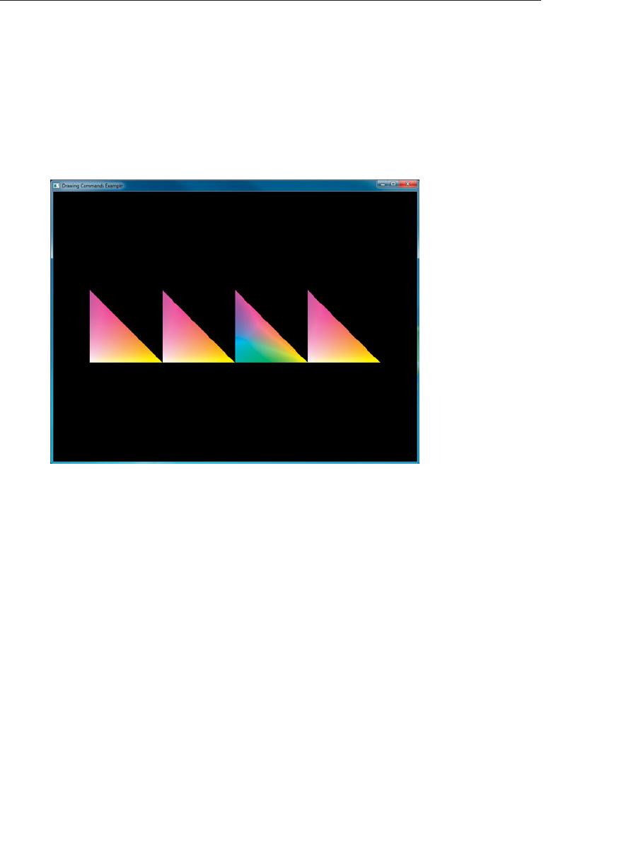
ptg9898810
// DrawArraysInstanced
model_matrix = vmath::translation(3.0f, 0.0f, -5.0f);
glUniformMatrix4fv(render_model_matrix_loc, 4, GL_FALSE, model_matrix);
glDrawArraysInstanced(GL_TRIANGLES, 0, 3, 1);
The result of the program in Examples 3.5 and 3.6 is shown in Figure 3.5.
It’s not terribly exciting, but you can see four similar triangles, each
rendered using a different drawing command.
Figure 3.5 Simple example of drawing commands
Restarting Primitives
As you start working with larger sets of vertex data, you are likely to
find that you need to make numerous calls to the OpenGL drawing
routines, usually rendering the same type of primitive (such as
GL_TRIANGLE_STRIP) that you used in the previous drawing call. Of
course, you can use the glMultiDraw*() routines, but they require the
overhead of maintaining the arrays for the starting index and length of
each primitive.
OpenGL has the ability to restart primitives within the same drawing
command by specifying a special value, the primitive restart index, which is
specially processed by OpenGL. When the primitive restart index is
encountered in a draw call, a new rendering primitive of the same type is
124 Chapter 3: Drawing with OpenGL
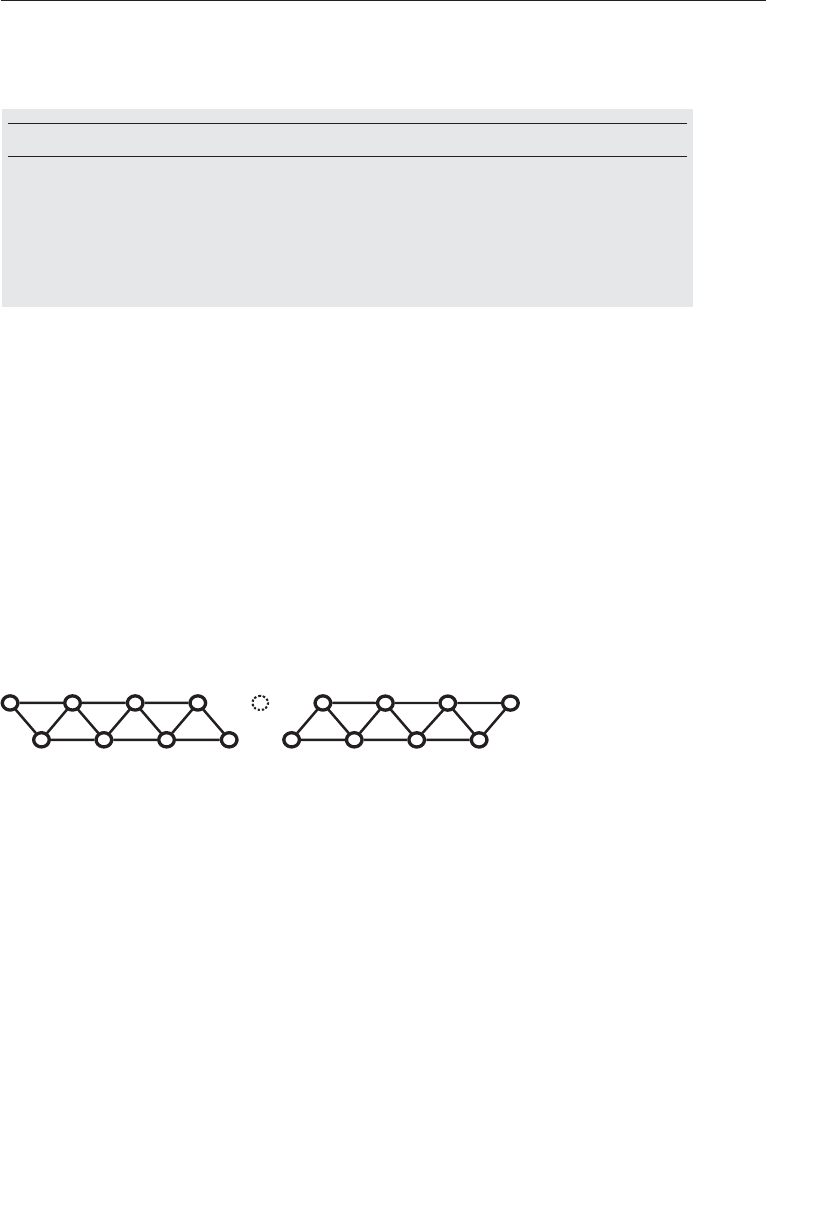
ptg9898810
started with the vertex following the index. The primitive restart index is
specified by the glPrimitiveRestartIndex() function.
void glPrimitiveRestartIndex(GLuint index);
Specifies the vertex array element index used to indicate that a new
primitive should be started during rendering. When processing of
vertex-array element indices encounters a value that matches index, no
vertex data is processed, the current graphics primitive is terminated, and
a new one of the identical type is started from the next vertex.
As vertices are rendered with one of the glDrawElements() derived
function calls, it can watch for the index specified by
glPrimitiveRestartIndex() to appear in the element array buffer. However,
it watches only for this index to appear if primitive restating is enabled.
Primitive restarting is controlled by calling glEnable() or glDisable() with
the GL_PRIMITIVE_RESTART parameter.
To illustrate, consider the layout of vertices in Figure 3.6, which shows
how a triangle strip would be broken in two by using primitive restarting.
In this figure, the primitive restart index has been set to 8. As the triangles
are rendered, OpenGL watches for the index 8 to be read from the element
array buffer, and when it sees it go by, rather than creating a vertex, it ends
the current triangle strip. The next vertex (vertex 9) becomes the first vertex
of a new triangle strip, and so in this case two triangle strips are created.
0 2 4 6 8 10 12 14 16
1 3 5 7 9 11 13 15
Figure 3.6 Using primitive restart to break a triangle strip
The following example demonstrates a simple use of primitive restart---it
draws a cube as a pair of triangle strips separated by a primitive restart
index. Examples 3.7 and 3.8 demonstrate how the data for the cube is
specified and then drawn.
Example 3.7 Intializing Data for a Cube Made of Two Triangle Strips
// 8 corners of a cube, side length 2, centered on the origin
static const GLfloat cube_positions[] =
{
-1.0f, -1.0f, -1.0f, 1.0f,
-1.0f, -1.0f, 1.0f, 1.0f,
-1.0f, 1.0f, -1.0f, 1.0f,
OpenGL Drawing Commands 125

ptg9898810
-1.0f, 1.0f, 1.0f, 1.0f,
1.0f, -1.0f, -1.0f, 1.0f,
1.0f, -1.0f, 1.0f, 1.0f,
1.0f, 1.0f, -1.0f, 1.0f,
1.0f, 1.0f, 1.0f, 1.0f
};
// Color for each vertex
static const GLfloat cube_colors[] =
{
1.0f, 1.0f, 1.0f, 1.0f,
1.0f, 1.0f, 0.0f, 1.0f,
1.0f, 0.0f, 1.0f, 1.0f,
1.0f, 0.0f, 0.0f, 1.0f,
0.0f, 1.0f, 1.0f, 1.0f,
0.0f, 1.0f, 0.0f, 1.0f,
0.0f, 0.0f, 1.0f, 1.0f,
0.5f, 0.5f, 0.5f, 1.0f
};
// Indices for the triangle strips
static const GLushort cube_indices[] =
{
0, 1, 2, 3, 6, 7, 4, 5, // First strip
0xFFFF, // <<- - This is the restart index
2, 6, 0, 4, 1, 5, 3, 7 // Second strip
};
// Set up the element array buffer
glGenBuffers(1, ebo);
glBindBuffer(GL_ELEMENT_ARRAY_BUFFER, ebo[0]);
glBufferData(GL_ELEMENT_ARRAY_BUFFER,
sizeof(cube_indices),
cube_indices, GL_STATIC_DRAW);
// Set up the vertex attributes
glGenVertexArrays(1, vao);
glBindVertexArray(vao[0]);
glGenBuffers(1, vbo);
glBindBuffer(GL_ARRAY_BUFFER, vbo[0]);
glBufferData(GL_ARRAY_BUFFER,
sizeof(cube_positions) + sizeof(cube_colors),
NULL, GL_STATIC_DRAW);
glBufferSubData(GL_ARRAY_BUFFER, 0,
sizeof(cube_positions), cube_positions);
glBufferSubData(GL_ARRAY_BUFFER, sizeof(cube_positions),
sizeof(cube_colors), cube_colors);
glVertexAttribPointer(0, 4, GL_FLOAT,
GL_FALSE, 0, NULL);
glVertexAttribPointer(1, 4, GL_FLOAT,
GL_FALSE, 0,
126 Chapter 3: Drawing with OpenGL
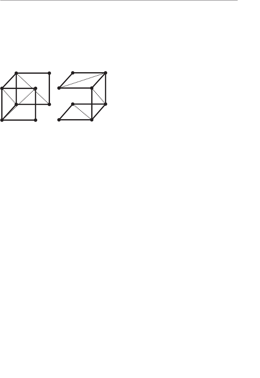
ptg9898810
(const GLvoid *)sizeof(cube_positions));
glEnableVertexAttribArray(0);
glEnableVertexAttribArray(1);
Figure 3.7 shows how the vertex data given in Example 3.7 represents the
cube as two independent triangle strips.
0 1
32
4
5
76
0 1
32
45
67
STRIP 1 STRIP 2
Figure 3.7 Two triangle strips forming a cube
Example 3.8 Drawing a Cube Made of Two Triangle Strips Using
Primitive Restart
// Set up for a glDrawElements call
glBindVertexArray(vao[0]);
glBindBuffer(GL_ELEMENT_ARRAY_BUFFER, ebo[0]);
#if USE_PRIMITIVE_RESTART
// When primitive restart is on, we can call one draw command
glEnable(GL_PRIMITIVE_RESTART);
glPrimitiveRestartIndex(0xFFFF);
glDrawElements(GL_TRIANGLE_STRIP, 17, GL_UNSIGNED_SHORT, NULL);
#else
// Without primitive restart, we need to call two draw commands
glDrawElements(GL_TRIANGLE_STRIP, 8, GL_UNSIGNED_SHORT, NULL);
glDrawElements(GL_TRIANGLE_STRIP, 8, GL_UNSIGNED_SHORT,
(const GLvoid *)(9 *sizeof(GLushort)));
#endif
Note: OpenGL will restart primitives whenever it comes across the
current restart index in the element array buffer. Therefore, it’s a
good idea to set the restart index to a value that will not be used in
your code. The default restart index is zero, which is very likely to
appear in your element array buffer. A good value to choose is
2n−1, where nis the number of bits in your indices (i.e., 16 for
GL_UNSIGNED_SHORT indices and 32 for GL_UNSIGNED_INT
indices). This is very unlikely to be used as a real index. Sticking
with such a standard also means that you don’t need to figure out
the index for every model in your program.
OpenGL Drawing Commands 127

ptg9898810
Instanced Rendering
Instancing, or instanced rendering, is a way of executing the same drawing
commands many times in a row, with each producing a slightly different
result. This can be a very efficient method of rendering a large amount of
geometry with very few API calls. Several variants of already-familiar
drawing functions exist to instruct OpenGL to execute the command
multiple times. Further, various mechanisms are available in OpenGL to
allow the shader to use the instance of the draw as an input, and to be
given new values for vertex attributes per-instance rather than per-vertex.
The simplest instanced rendering call is:
void glDrawArraysInstanced(GLenum mode, GLint first,
GLsizei count, GLsizei primCount);
Draws primCount instances of the geometric primitives specified by mode,
first, and count as if specified by individual calls to glDrawArrays(). The
built-in variable gl_InstanceID is incremented for each instance, and
new values are presented to the vertex shader for each instanced vertex
attribute.
This is the instanced version of glDrawArrays(); note similarity of the two
functions. The parameters of glDrawArraysInstanced() are identical to
those of glDrawArrays(), with the addition of the primCount argument.
This parameter specifies the count of the number of instances that are to be
rendered. When this function is executed, OpenGL will essentially execute
primCount copies of glDrawArrays(), with the mode,first, and count
parameters passed through. There are *Instanced versions of several of the
OpenGL drawing commands, including glDrawElementsInstanced() (for
glDrawElements()) and glDrawElementsInstancedBaseVertex() (for
glDrawElementsBaseVertex()). The glDrawElementsInstanced()
function is defined as:
void glDrawElementsInstanced(GLenum mode, GLsizei count,
GLenum type,
const void* indices,
GLsizei primCount);
Draws primCount instances of the geometric primitives specified by mode,
count and indices as if specified by individual calls to glDrawElements().
As with glDrawArraysInstanced(), the built-in variable gl_InstanceID
is incremented for each instance, and new values are presented to the
vertex shader for each instanced vertex attribute.
128 Chapter 3: Drawing with OpenGL

ptg9898810
Again, note that the parameters to glDrawElementsInstanced() are
identical to glDrawElements(), with the addition of primCount. Each time
one of the instanced functions is called, OpenGL essentially runs the
whole command as many times as is specified by the primCount parameter.
This on its own is not terribly useful. However, there are two mechanisms
provided by OpenGL that allow vertex attributes to be specified as instanced
and to provide the vertex shader with the index of the current instance.
void glDrawElementsInstancedBaseVertex(GLenum mode,
GLsizei count,
GLenum type,
const void* indices,
GLsizei instanceCount,
GLuint baseVertex);
Draws instanceCount instances of the geometric primitives specified by
mode,count,indices, and baseVertex as if specified by individual calls to
glDrawElementsBaseVertex(). As with glDrawArraysInstanced(), the
built-in variable gl_InstanceID is incremented for each instance, and
new values are presented to the vertex shader for each instanced vertex
attribute.
Instanced Vertex Attributes
Instanced vertex attributes behave similarly to regular vertex attributes.
They are declared and used in exactly the same way inside the vertex
shader. On the application side, they are also configured in the same way as
regular vertex attributes. That is, they are backed by buffer objects, can be
queried with glGetAttribLocation(), set up using glVertexAttribPointer(),
and enabled and disabled using glEnableVertexAttribArray()
and glDisableVertexAttribArray(). The important new
function that allows a vertex attribute to become instanced is as follows:
void glVertexAttribDivisor(GLuint index, GLuint divisor);
Specifies the rate at which new values of the instanced the vertex
attribute at index are presented to the vertex shader during instanced
rendering. A divisor value of 0 turns off instancing for the specified
attribute, whereas any other value of divisor indicates that a new value
should be presented to the vertex shader each divisor instances.
Instanced Rendering 129

ptg9898810
The glVertexAttribDivisor() function controls the rate at which the vertex
attribute is updated. index is the index of the vertex attribute whose divisor
is to be set, and is the same as you would pass into glVertexAttribPointer()
or glEnableVertexAttribArray(). By default, a new value of each enabled
attribute is delivered to each vertex. Setting divisor to zero resets the attribute
to this behavior and makes it a regular, noninstanced attribute. A nonzero
value of divisor makes the attribute instanced and causes a new value to
be fetched from the attribute array once every divisor instances rather than
for every vertex. The index within the enabled vertex attribute array from
which the attribute is taken is then instance
divisor , where instance is the current
instance number and divisor is the value of divisor for the current attribute.
For each of the instanced vertex attributes, the same value is delivered to the
vertex shader for all vertices in the instance. If divisor is two, the value of the
attribute is updated every second instance; if it is three then the attribute
is updated every third instance, and so on. Consider the vertex attributes
declared in Example 3.9, some of which will be configured as instanced.
Example 3.9 Vertex Shader Attributes for the Instancing Example
#version 410 core
// "position" and "normal" are regular vertex attributes
layout (location = 0) in vec4 position;
layout (location = 1) in vec3 normal;
// Color is a per-instance attribute
layout (location = 2) in vec4 color;
// model_matrix will be used as a per-instance transformation
// matrix. Note that a mat4 consumes 4 consecutive locations, so
// this will actually sit in locations, 3, 4, 5, and 6.
layout (location = 3) in mat4 model_matrix;
Note that in Example 3.9, there is nothing special about the declaration of
the instanced vertex attributes color and model_matrix. Now consider
the code shown in Example 3.10, which configures a subset of vertex
attributes declared in Example 3.9 as instanced.
Example 3.10 Example Setup for Instanced Vertex Attributes
// Get the locations of the vertex attributes in "prog", which is
// the (linked) program object that we’re going to be rendering
// with. Note that this isn’t really necessary because we specified
// locations for all the attributes in our vertex shader. This code
// could be made more concise by assuming the vertex attributes are
// where we asked the compiler to put them.
int position_loc = glGetAttribLocation(prog, "position");
int normal_loc = glGetAttribLocation(prog, "normal");
int color_loc = glGetAttribLocation(prog, "color");
130 Chapter 3: Drawing with OpenGL

ptg9898810
int matrix_loc = glGetAttribLocation(prog, "model_matrix");
// Configure the regular vertex attribute arrays -
// position and normal.
glBindBuffer(GL_ARRAY_BUFFER, position_buffer);
glVertexAttribPointer(position_loc, 4, GL_FLOAT, GL_FALSE, 0, NULL);
glEnableVertexAttribArray(position_loc);
glBindBuffer(GL_ARRAY_BUFFER, normal_buffer);
glVertexAttribPointer(normal_loc, 3, GL_FLOAT, GL_FALSE, 0, NULL);
glEnableVertexAttribArray(normal_loc);
// Now we set up the color array. We want each instance of our
// geometry to assume a different color, so we’ll just pack colors
// into a buffer object and make an instanced vertex attribute out
// of it.
glBindBuffer(GL_ARRAY_BUFFER, color_buffer);
glVertexAttribPointer(color_loc, 4, GL_FLOAT, GL_FALSE, 0, NULL);
glEnableVertexAttribArray(color_loc);
// This is the important bit... set the divisor for the color array
// to 1 to get OpenGL to give us a new value of "color" per-instance
// rather than per-vertex.
glVertexAttribDivisor(color_loc, 1);
// Likewise, we can do the same with the model matrix. Note that a
// matrix input to the vertex shader consumes N consecutive input
// locations, where N is the number of columns in the matrix. So...
// we have four vertex attributes to set up.
glBindBuffer(GL_ARRAY_BUFFER, model_matrix_buffer);
// Loop over each column of the matrix...
for (int i = 0; i < 4; i++)
{
// Set up the vertex attribute
glVertexAttribPointer(matrix_loc + i, // Location
4, GL_FLOAT, GL_FALSE, // vec4
sizeof(mat4), // Stride
(void *)(sizeof(vec4) *i)); // Start offset
// Enable it
glEnableVertexAttribArray(matrix_loc + i);
// Make it instanced
glVertexAttribDivisor(matrix_loc + i, 1);
}
In Example 3.10,position and normal are regular, noninstanced vertex
attributes. However, color is configured as an instanced vertex attribute
with a divisor of one. This means that each instance will have a new value
for the color attribute (which will be constant across all vertices in the
instance). Further, the model_matrix attribute will also be made
instanced to provide a new model transformation matrix for each instance.
Amat4 attribute is consuming a consecutive location. Therefore, we loop
over each column in the matrix and configure it separately. The remainder
of the vertex shader is shown in Example 3.11.
Instanced Rendering 131

ptg9898810
Example 3.11 Instanced Attributes Example Vertex Shader
// The view matrix and the projection matrix are constant
// across a draw
uniform mat4 view_matrix;
uniform mat4 projection_matrix;
// The output of the vertex shader (matched to the
// fragment shader)
out VERTEX
{
vec3 normal;
vec4 color;
} vertex;
// Ok, go!
void main(void)
{
// Construct a model-view matrix from the uniform view matrix
// and the per-instance model matrix.
mat4 model_view_matrix = view_matrix *model_matrix;
// Transform position by the model-view matrix, then by the
// projection matrix.
gl_Position = projection_matrix *(model_view_matrix *
position);
// Transform the normal by the upper-left-3x3-submatrix of the
// model-view matrix
vertex.normal = mat3(model_view_matrix) *normal;
// Pass the per-instance color through to the fragment shader.
vertex.color = color;
}
The code to set the model matrices for the instances and then draw the
instanced geometry using these shaders is shown in Example 3.12. Each
instance has its own model matrix, whereas the view matrix (consisting of
a rotation around the yaxis followed by a translation in z) is common to
all instances. The model matrices are written directly into the buffer by
mapping it using glMapBuffer(). Each model matrix translates the object
away from the origin and then rotates the translated model around the
origin. The view and projection matrices are simply placed in uniform
variables. Then, a single call to glDrawArraysInstanced() is used to draw
all instances of the model.
Example 3.12 Instancing Example Drawing Code
// Map the buffer
mat4 *matrices = (mat4 *)glMapBuffer(GL_ARRAY_BUFFER,
GL_WRITE_ONLY);
// Set model matrices for each instance
132 Chapter 3: Drawing with OpenGL

ptg9898810
for (n = 0; n < INSTANCE_COUNT; n++)
{
float a = 50.0f *float(n) / 4.0f;
float b = 50.0f *float(n) / 5.0f;
float c = 50.0f *float(n) / 6.0f;
matrices[n] = rotation(a + t *360.0f, 1.0f, 0.0f, 0.0f) *
rotation(b + t *360.0f, 0.0f, 1.0f, 0.0f) *
rotation(c + t *360.0f, 0.0f, 0.0f, 1.0f) *
translation(10.0f + a, 40.0f + b, 50.0f + c);
}
// Done. Unmap the buffer.
glUnmapBuffer(GL_ARRAY_BUFFER);
// Activate instancing program
glUseProgram(render_prog);
// Set up the view and projection matrices
mat4 view_matrix(translation(0.0f, 0.0f, -1500.0f) *
rotation(t *360.0f *2.0f, 0.0f, 1.0f, 0.0f));
mat4 projection_matrix(frustum(-1.0f, 1.0f,
-aspect, aspect, 1.0f, 5000.0f));
glUniformMatrix4fv(view_matrix_loc, 1,
GL_FALSE, view_matrix);
glUniformMatrix4fv(projection_matrix_loc, 1,
GL_FALSE, projection_matrix);
// Render INSTANCE_COUNT objects
glDrawArraysInstanced(GL_TRIANGLES, 0, object_size, INSTANCE_COUNT);
The result of the program is shown in Figure 3.8. In this example,
the constant INSTANCE_COUNT (which is referenced in the code of
Examples 3.10 and 3.12) is 100. One hundred copies of the model are
drawn, each with a different position and a different color. These
models could very easily be trees in a forest, space ships in a fleet, or
buildings in a city.
Instanced Rendering 133
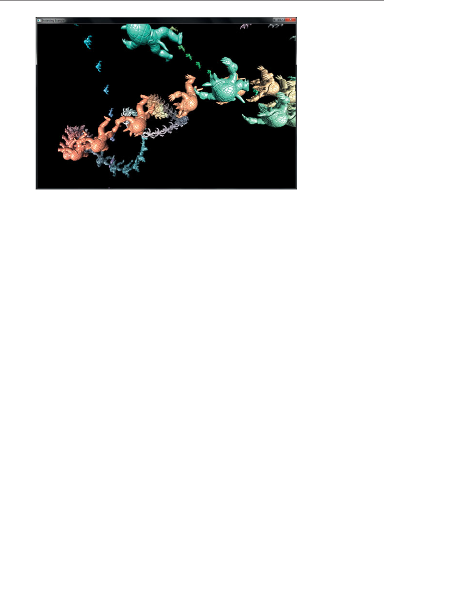
ptg9898810
Figure 3.8 Result of rendering with instanced vertex attributes
There are some inefficiencies in the example shown in Examples 3.9
through 3.12. Work that will produce the same result across all of the
vertices in an instance will still be performed per-vertex. Sometimes there
are ways to get around this. For example, the computation of
model_view_matrix will evaluate to the same matrix for all vertices
within a single instance. Here, we could avoid this work by using a second
instanced mat4 attribute to carry the per-instance model-view matrix. In
other cases, it may not be possible to avoid this work, but it may be
possible to move it into a geometry shader so that work is performed once
per-primitive rather than once per-vertex, or perhaps use geometry shader
instancing instead. Both of these techniques will be explained in
Chapter 10.
Note: Remember that calling an instanced drawing command is mostly
equivalent to calling its noninstanced counterpart many times
before executing any other OpenGL commands. Therefore,
converting a sequence of OpenGL functions called inside a loop to
a sequence of instanced draw calls will not produce identical
results.
Another example of a way to use instanced vertex attributes is to pack a set
of textures into a 2D array texture and then pass the array slice to be used
for each instance in an instanced vertex attribute. The vertex shader can
then pass the instance’s slice into the fragment shader, which can then
render each instance of the geometry with a different texture.
134 Chapter 3: Drawing with OpenGL

ptg9898810
It is possible to internally add an offset to the indices used to fetch
instanced vertex attributes from vertex buffers. Similar to the baseVertex
parameter that is available through glDrawElementsBaseVertex(), the
instance offset is exposed through an additional baseInstance parameter in
some versions of the instanced drawing functions. The functions that take
abaseInstance parameter are glDrawArraysInstancedBaseInstance(),
glDrawElementsInstancedBaseInstance(), and
glDrawElementsInstancedBaseVertexBaseInstance(). Their prototypes
are as follows:
void glDrawArraysInstancedBaseInstance(GLenum mode,
GLint first,
GLsizei count,
GLsizei instanceCount,
GLuint baseInstance);
Draws primCount instances of the geometric primitives specified by mode,
first, and count as if specified by individual calls to glDrawArrays(). The
built-in variable gl_InstanceID is incremented for each instance, and
new values are presented to the vertex shader for each instanced vertex
attribute. Furthermore, the implied index used to fetch any instanced
vertex attributes is offset by the value of baseInstance by OpenGL.
void glDrawElementsInstancedBaseInstance(GLenum mode,
GLsizei count,
GLenum type,
const GLvoid * indices,
GLsizei instanceCount,
GLuint baseInstance);
Draws primCount instances of the geometric primitives specified by mode,
count, and indices as if specified by individual calls to glDrawElements().
As with glDrawArraysInstanced(), the built-in variable gl_InstanceID
is incremented for each instance, and new values are presented to the
vertex shader for each instanced vertex attribute. Furthermore, the
implied index used to fetch any instanced vertex attributes is offset by
the value of baseInstance by OpenGL.
Instanced Rendering 135

ptg9898810
void glDrawElementsInstancedBaseVertexBaseInstance(GLenum mode,
GLsizei count,
GLenum type,
const GLvoid * indices,
GLsizei instanceCount,
GLuint baseVertex,
GLuint baseInstance);
Draws instanceCount instances of the geometric primitives specified by
mode,count,indices, and baseVertex as if specified by individual calls to
glDrawElementsBaseVertex(). As with glDrawArraysInstanced(), the built-in
variable gl_InstanceID is incremented for each instance, and new values are
presented to the vertex shader for each instanced vertex attribute. Furthermore,
the implied index used to fetch any instanced vertex attributes is offset by the
value of baseInstance by OpenGL.
Using the Instance Counter in Shaders
In addition to instanced vertex attributes, the index of the current instance
is available to the vertex shader in the built-in variable gl_InstanceID.
This variable is implicitly declared as an integer. It starts counting from
zero and counts up one each time an instance is rendered.
gl_InstanceID is always present in the vertex shader, even when the
current drawing command is not one of the instanced ones. In those cases,
it will just be zero. The value in gl_InstanceID may be used to index
into uniform arrays, perform texture lookups, as the input to an analytic
function, or for any other purpose.
In the following example, the functionality of Examples 3.9 through 3.12
is replicated by using gl_InstanceID to index into texture buffer objects
(TBOs) rather than through the use of instanced vertex attributes. Here,
the vertex attributes of Example 3.9 are replaced with TBO lookups, and so
are removed from the vertex attribute setup code. Instead, a first TBO
containing color of each instance, and a second TBO containing the model
matrices are created. The vertex attribute declaration and setup code are
the same as in Examples 3.9 and 3.10 (with the omission of the color and
model_matrix attributes, of course). As the instance’s color and model
matrix is now explicitly fetched in the vertex shader, more code is added to
the body of the vertex shader, which is shown in Example 3.13.
Example 3.13 gl_VertexID Example Vertex Shader
// The view matrix and the projection matrix are constant across a draw
uniform mat4 view_matrix;
uniform mat4 projection_matrix;
136 Chapter 3: Drawing with OpenGL

ptg9898810
// These are the TBOs that hold per-instance colors and per-instance
// model matrices
uniform samplerBuffer color_tbo;
uniform samplerBuffer model_matrix_tbo;
// The output of the vertex shader (matched to the fragment shader)
out VERTEX
{
vec3 normal;
vec4 color;
} vertex;
// Ok, go!
void main(void)
{
// Use gl_InstanceID to obtain the instance color from the color TBO
vec4 color = texelFetch(color_tbo, gl_InstanceID);
// Generating the model matrix is more complex because you can’t
// store mat4 data in a TBO. Instead, we need to store each
// matrix as four vec4 variables and assemble the matrix in the
// shader. First, fetch the four columns of the matrix
// (remember, matrices are stored in memory in column-major
// order).
vec4 col1 = texelFetch(model_matrix_tbo, gl_InstanceID *4);
vec4 col2 = texelFetch(model_matrix_tbo, gl_InstanceID *4 + 1);
vec4 col3 = texelFetch(model_matrix_tbo, gl_InstanceID *4 + 2);
vec4 col4 = texelFetch(model_matrix_tbo, gl_InstanceID *4 + 3);
// Now assemble the four columns into a matrix.
mat4 model_matrix = mat4(col1, col2, col3, col4);
// Construct a model-view matrix from the uniform view matrix
// and the per-instance model matrix.
mat4 model_view_matrix = view_matrix *model_matrix;
// Transform position by the model-view matrix, then by the
// projection matrix.
gl_Position = projection_matrix *(model_view_matrix *
position);
// Transform the normal by the upper-left-3x3-submatrix of the
// model-view matrix
vertex.normal = mat3(model_view_matrix) *normal;
// Pass the per-instance color through to the fragment shader.
vertex.color = color;
}
To drive the shader of Example 3.13, we need to create and initialize TBOs
to back the color_tbo and model_matrix_tbo samplers rather than
initializing the instanced vertex attributes. However, aside from the
differences in setup code, the program is essentially unchanged.
Instanced Rendering 137

ptg9898810
Example 3.14 contains the code to set up the TBOs for use with the shader
of Example 3.13.
Example 3.14 Example Setup for Instanced Vertex Attributes
// Get the locations of the vertex attributes in "prog", which is
// the (linked) program object that we’re going to be rendering
// with. Note that this isn’t really necessary because we specified
// locations for all the attributes in our vertex shader. This code
// could be made more concise by assuming the vertex attributes are
// where we asked the compiler to put them.
int position_loc = glGetAttribLocation(prog, "position");
int normal_loc = glGetAttribLocation(prog, "normal");
// Configure the regular vertex attribute arrays - position and normal.
glBindBuffer(GL_ARRAY_BUFFER, position_buffer);
glVertexAttribPointer(position_loc, 4, GL_FLOAT, GL_FALSE, 0, NULL);
glEnableVertexAttribArray(position_loc);
glBindBuffer(GL_ARRAY_BUFFER, normal_buffer);
glVertexAttribPointer(normal_loc, 3, GL_FLOAT, GL_FALSE, 0, NULL);
glEnableVertexAttribArray(normal_loc);
// Now set up the TBOs for the instance colors and model matrices...
// First, create the TBO to store colors, bind a buffer to it and
// initialize its format. The buffer has previously been created
// and sized to store one vec4 per-instance.
glGenTextures(1, &color_tbo);
glBindTexture(GL_TEXTURE_BUFFER, color_tbo);
glTexBuffer(GL_TEXTURE_BUFFER, GL_RGBA32F, color_buffer);
// Now do the same thing with a TBO for the model matrices. The
// buffer object (model_matrix_buffer) has been created and sized
// to store one mat4 per-instance.
glGenTextures(1, &model_matrix_tbo);
glActiveTexture(GL_TEXTURE1);
glBindTexture(GL_TEXTURE_BUFFER, model_matrix_tbo);
glTexBuffer(GL_TEXTURE_BUFFER, GL_RGBA32F, model_matrix_buffer);
Note that the code in Example 3.14 is actually shorter and simpler than
that in Example 3.10. This is because we have shifted the responsibility for
fetching per-instance data from built-in OpenGL functionality to the
shader writer. This can be seen in the increased complexity of
Example 3.13 relative to Example 3.11. With this responsibility comes
additional power and flexibility. For example, if the number of instances is
small, it may be preferable to use a uniform array rather than a TBO for
data storage, which may increase performance. Regardless, there are very
few other changes that need to be made to the original example to move
to using explicit fetches driven by gl_InstanceID. In fact, the rendering
138 Chapter 3: Drawing with OpenGL
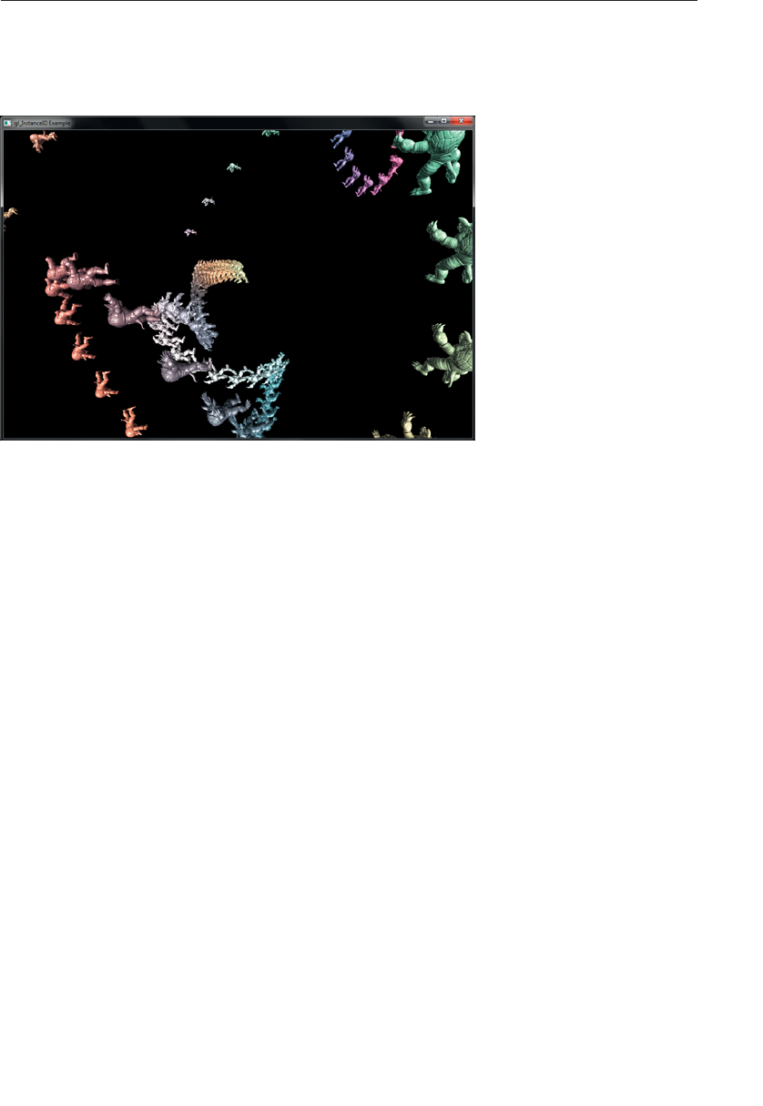
ptg9898810
code of Example 3.12 is used intact to produce an identical result to the
original program. The proof is in the screenshot (Figure 3.9).
Figure 3.9 Result of instanced rendering using gl_InstanceID
Instancing Redux
To use a instancing in your program
•Create some vertex shader inputs that you intend to be instanced.
•Set the vertex attribute divisors with glVertexAttribDivisor().
•Use the gl_InstanceID built-in variable in the vertex shader.
•Use the instanced versions of the rendering functions such as
glDrawArraysInstanced()glDrawElementsInstanced(), or
glDrawElementsInstancedBaseVertex().
Instanced Rendering 139


ptg9898810
Chapter 4
Color, Pixels, and
Framebuffers
Chapter Objectives
After reading this chapter, you’ll be able to do the following:
•Understand how OpenGL processes and represents the colors in your
generated images.
•Identify the types of buffers available in OpenGL, and be able to clear
and control writing to them.
•List the various tests and operations on fragments that occur after
fragment shading.
•Use alpha blending to render translucent objects realistically.
•Use multisampling and antialiasing to remove aliasing artifacts.
•Employ occlusion queries and conditional rendering to optimize
rendering.
•Create and use framebuffer objects for advanced techniques, and to
minimizing copying of data between buffers.
•Retrieve rendered images, and copy pixels from one place to another,
or one framebuffer to another.
141

ptg9898810
The goal of computer graphics, generally speaking, is to determine the
colors that make up an image. For OpenGL, that image is usually shown in
a window on a computer screen, which itself is made up of a rectangular
array of pixels, each of which can display its own color. This chapter
further develops how you can use shaders in OpenGL to generate the
colors of the pixels in the framebuffer. We discuss how colors set in an
application directly contribute to a fragment’s color, the processing that
occurs after the completion of the fragment shader, and other techniques
used for improving the generated image. This chapter contains the
following major sections:
•‘‘Basic Color Theory’’, which briefly describes the physics of light, and
how colors are represented in OpenGL.
•‘‘Buffers and Their Uses’’ presents different kinds of buffers, how to
clear them, when to use them, and how OpenGL operates on them.
•‘‘Color and OpenGL’’ explains how OpenGL processes color in its
pipeline.
•‘‘Multisampling’’ introduces one of OpenGL’s antialiasing techniques,
and describes how it modfies rasterization.
•‘‘Testing and Operating on Fragments’’ describes the tests and
additional operations that can be applied to individual fragments after
the fragment shader has completed, including alpha blending.
•‘‘Per-Primitive Antialiasing’’ presents how blending can be used to
smooth the appearance of individual primitives.
•‘‘Framebuffer Objects’’ explains how to create and render to your own
framebuffers.
•‘‘Writing to Multiple Renderbuffers Simultaneously’’ describes
rendering to multiple buffers simultaneously.
•‘‘Reading and Copying Pixel Data’’ explains how OpenGL represents
pixel data and the operations you can use to process is.
•‘‘Copying Pixel Rectangles’’ discusses how to copy a block of pixels
from one section of the framebuffer to another in OpenGL.
Basic Color Theory
In the physical world, light is composed of photons---in simplest terms,
tiny particles traveling along a straight path1each with their own ‘‘color’’,
1. Ignoring gravitational effects, of course.
142 Chapter 4: Color, Pixels, and Framebuffers

ptg9898810
which in terms of physical quantities, is represented by their wavelength
(or frequency).2Photons that we can see have wavelengths in the visible
spectrum, which ranges from about 390 nanometers (the color violet) to
720 nanometers (the color red). The colors in between form the dominant
colors of the rainbow: violet, indigo, blue, green, yellow, orange, and red.
Your eye is capable of seeing many more colors than the seven that
compose the colors of the rainbow. In fact, what we really see is a mixture
of photons of different wavelengths that combine to form a unique color.
For example, ideal white light is composed of a equal quantities of photons
at all visible wavelengths. By comparison, laser light is monochromatic,
with all the photons having an identical frequency.
So what does this have to do with computer graphics and OpenGL, you
may ask? Modern display devices have a much more restricted range of
colors they can display---only a small portion of the entire visible
spectrum. In fact, the set of colors a device can display is often represented
as its gamut. Most display devices you’ll work with while using OpenGL
create their colors using a combination of three primary colors---red, green,
and blue---which form the spectrum of colors that the device can display.
We’ll call that the RGB color space, and use a set of three values for each
color. In OpenGL, we’ll often pack those three components with a fourth
component alpha (which we discuss later in ‘‘Blending’’), which we’ll
predictably call the RGBA color space. In addition to RGB, OpenGL also
supports the sRGB color space. We’ll encounter more about sRGB when we
discuss framebuffer objects and texture maps.
Note: There are many color spaces, like HSV (Hue-Saturation-Value), or
CMYK (Cyan-Magenta-Yellow-Black) . If your data is in a color
space different than RGB, you’ll need to convert it from that space
into RGB (or sRGB) to process it with OpenGL.
Unlike light in the physical world, where frequencies and intensities range
continuously, computer framebuffers can only represent a comparatively
small number of discrete values (although usually numbering in the
millions of colors). This quantization of intensities limits the number of
colors we can display. Normally, each component’s intensity is stored
using a certain number of bits (usually called its bit depth), and the sum of
each component’s bit depth (excluding alpha) determines the color
buffer’s depth, which also determines the total number of display colors.
2. A photon’s frequency and wavelength are related by the equation c=νλ, where cis the
speed of light (3 ×10⁸meters/second), νis the photon’s frequency, and λits wavelength. And
for those who want to debate the wave-particle duality of light, we’re always open to that
discussion over a beer.
Basic Color Theory 143
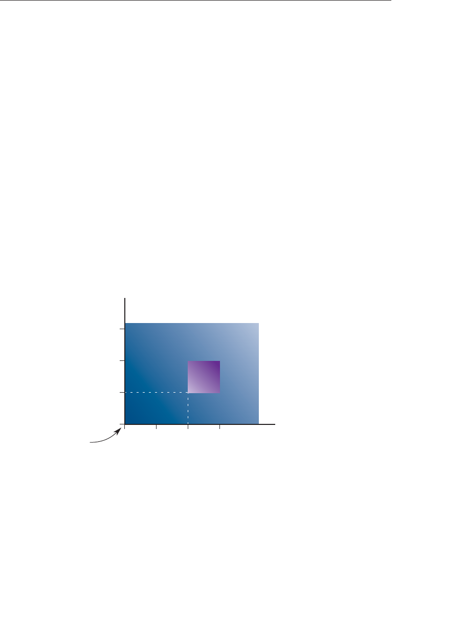
ptg9898810
For example, a common format for the color buffer is eight bits for each
red, green, and blue. This yields a 24-bit deep color buffer, which is capable
of displaying 224 unique colors. ‘‘Data in OpenGL Buffers’’ in Chapter 3
expanded on the types of buffers that OpenGL makes available and
describes how to control interactions with those buffers.
Buffers and Their Uses
An important goal of almost every graphics program is to draw pictures on
the screen (or into an off-screen buffer). The framebuffer (which is most
often the screen) is composed of a rectangular array of pixels, each capable
of displaying a tiny square of color at that point in the image. After the
rasterization stage, which is where the fragment shader was executed, the
data are not pixels yet---just fragments. Each fragment has coordinate data
that corresponds to a pixel, as well as color and depth values.
As shown in Figure 4.1, the lower-left pixel in an OpenGL window is pixel
(0, 0), corresponding to the window coordinates of the lower-left corner of
the 1 ×1 region occupied by this pixel. In general, pixel (x,y)fills the
region bounded by xon the left, x+1 on the right, yon the bottom, and
y+1 on the top.
3.0
2.0
1.0
0.0
0.0 1.0 2.0 3.0
Pixel
(2, 1)
Lower left corner
of the window
x window coordinate
y window
coordinate
Figure 4.1 Region occupied by a pixel
As an example of a buffer, let’s look more closely at the color buffer, which
holds the color information that’s to be displayed on the screen. Let’s
say that the screen is 1920 pixels wide and 1080 pixels high and that it’s
a full 24-bit color screen---in other words, that there are 224 (or 16,777,216)
different colors that can be displayed. Since 24 bits translate to 3 bytes
(8 bits per byte), the color buffer in this example has to store at least 3 bytes
144 Chapter 4: Color, Pixels, and Framebuffers

ptg9898810
of data for each of the 2,073,600 (1920 ×1080) pixels on the screen. A
particular hardware system might have more or fewer pixels on the physical
screen, as well as more or less color data per pixel. Any particular color
buffer, however, has the same amount of data for each pixel on the screen.
The color buffer is only one of several buffers that hold information about
a pixel. In fact, a pixel may have many color buffers associated with it,
which are called renderbuffers, which we’ll discuss more in ‘‘Framebuffer
Objects’’ on Page 180. The framebuffer on a system comprises all of these
buffers, and you can use multiple framebuffers within your application.
With the exception of the primary color buffer, you don’t view these other
buffers directly; instead, you use them to perform such tasks as
hidden-surface removal, stenciling, dynamic texture generation, and other
operations.
Within an OpenGL system the following types of buffers are available:
•Color buffers, of which there might be one or several active
•Depth buffer
•Stencil buffer
All of those buffers collectively form the framebuffer, although it’s up to
you to decide which of those buffers you need to use. When your
application starts, you’re using the default framebuffer, which is the one
related to the windows of your application. The default framebuffer will
always contain a double-buffered, color buffer. You can create additional
framebuffer objects for doing off-screen rendering.
Your particular OpenGL implementation determines which buffers are
available and how many bits per pixel each buffer holds. Additionally, you
can have multiple visuals, or window types, that also may have different
buffers available. As we describe each of the types of buffers, we’ll also cover
ways you can query their capabilities, in terms of data storage and precision.
We now briefly describe the type of data that each buffer type stores, and
then move to discussing operations that you do with each type of buffer.
Color Buffers
The color buffers are the ones to which you usually draw. They contain the
RGB or sRGB color data, and may also contain alpha values for each pixel
in the framebuffer. There may be multiple color buffers in a framebuffer.
The ‘‘main’’ color buffer of the default framebuffer is special because it’s
the one associated with your window on the screen and where you will
draw to have your image shown on the screen (assuming you want to
display an image there)---all other color buffers are off screen.
Buffers and Their Uses 145

ptg9898810
The pixels in a color buffer may store a single color per pixel, or may
logically divide the pixel into subpixels, which enables an antialiasing
technique called multisampling.We discuss multisampling in detail in
‘‘Multisampling’’ on Page 153.
You’ve already used double buffering for animation. Double buffering is
done by making the main color buffer have two parts: a front buffer that’s
displayed in your window; and a back buffer, which is where you render
the new image. When you swap the buffers (by calling glutSwapBuffers(),
for example), the front and back buffers are exchanged. Only the main
color buffer of the default framebuffer is double buffered.
Additionally, an OpenGL implementation might support stereoscopic
viewing, in which case the color buffer (even if it’s double buffered) will
have left and right color buffers for the respective stereo images.
Depth Buffer
The depth buffer stores a depth value for each pixel, and is used for
determining the visibility of objects in a three-dimensional scene. Depth is
measured in terms of distance to the eye, so pixels with larger depth-buffer
values are overwritten by pixels with smaller values. This is just a useful
convention, however, and the depth buffer’s behavior can be modified as
described in ‘‘Depth Test’’ on Page 163. The depth buffer is sometimes
called the z-buffer (the zcomes from the fact that x- and y-values measure
horizontal and vertical displacement on the screen, and the z-value
measures distance perpendicular to the screen).
Stencil Buffer
Finally, the stencil buffer is used to restrict drawing to certain portions of the
screen. Think of it like a cardboard stencil that can be used with a can of
spray paint to make fairly precise painted images. For example, a classic use
is to simulate the view of a rear-view mirror in a car. You render the shape
of the mirror to the stencil buffer, and then draw the entire scene. The
stencil buffer prevents anything that wouldn’t be visible in the mirror from
being drawn. We discuss the stencil buffer in ‘‘Stencil Buffer’’ on Page 146.
Clearing Buffers
Probably the most common graphics activity after rendering is clearing
buffers. You will probably do it once per frame (at least), and as such,
OpenGL tries to optimize that operation by clearing all of the active
buffers at the same time. As you’ve seen in our examples, we set the value
146 Chapter 4: Color, Pixels, and Framebuffers

ptg9898810
that each type of buffer should be initialized to in init() (if we don’t use
the default values), and then clear all the buffers we need.
The following commands set the clearing values for each buffer:
void glClearColor(GLclampf red, GLclampf green,
GLclampf blue, GLclampf alpha);
void glClearDepth(GLclampd depth);
void glClearDepthf(GLclampf depth);
void glClearStencil(GLint s);
Specifies the current clearing values for the active color buffers, the depth
buffer, and the stencil buffer. The GLclampf and GLclampd types
(clamped GLfloat and clamped GLdouble) are clamped to be between 0.0
and 1.0. The default depth-clearing value is 1.0; all the other default
clearing values are 0. The values set with the clear commands remain in
effect until they’re changed by another call to the same command.
After you’ve selected your clearing values and you’re ready to clear the
buffers, use glClear().
void glClear(GLbitfield mask);
Clears the specified buffers. The value of mask is the bitwise logical OR of
some combination of GL_COLOR_BUFFER_BIT, GL_DEPTH_BUFFER_BIT,
and GL_STENCIL_BUFFER_BIT to identify which buffers are to be cleared.
GL_COLOR_BUFFER_BIT clears the RGBA color buffer, and all the color
buffers that are enabled for writing (see ‘‘Selecting Color Buffers for
Writing and Reading’’ on Page 195). The pixel ownership test, scissor test,
and dithering, if enabled, are applied to the clearing operation, as are
masking operations as specified by glColorMask(). The depth and stencil
tests, however, do not affect the operation of glClear().
Masking Buffers
Before OpenGL writes data into the enabled color, depth, or stencil buffers,
a masking operation is applied to the data, as specified with one of the
following commands:
Buffers and Their Uses 147

ptg9898810
void glColorMask(GLboolean red, GLboolean green,
GLboolean blue, GLboolean alpha);
void glColorMaski(GLuint buffer, GLboolean red,
GLboolean green, GLboolean blue,
GLboolean alpha);
void glDepthMask(GLboolean flag);
void glStencilMask(GLboolean mask);
void glStencilMaskSeparate(GLenum face, GLuint mask);
Sets the masks used to control writing into the indicated buffers.
If flag is GL_TRUE for glDepthMask(), the depth buffer is enabled for
writing; otherwise, it’s disabled. The mask for glStencilMask() is used for
stencil data with a one in a bit in the mask indicating that writing to bit
in a pixel’s stencil value is enabled; a zero indicated that writing is
disabled.
The default values of all the GLboolean masks are GL_TRUE, and the
default values for the GLuint masks are all ones.
glStencilMaskSeparate() provides different stencil mask values for front-
and back-facing polygons.
glColorMaski() allows setting of the color mask for an individual buffer
specified by buffer when rendering to multiple color buffers.
Note: The mask specified by glStencilMask() controls which stencil
bitplanes are written. This mask isn’t related to the mask that’s
specified as the third parameter of glStencilFunc(), which specifies
which bitplanes are considered by the stencil function.
Color and OpenGL
How do we use color in OpenGL? As you’ve seen, it’s the job of the
fragment shader to assign a fragment’s color. There are many ways this can
be done.
•The fragment shader can generate the fragment’s color without using
any ‘‘external’’ data (i.e., data passed into the fragment shader). A very
limited example of this was done in our shaders from Chapter 1where
we assigned a constant color to each fragment.
•Additional color data could be provided with each input vertex,
potentially modified by another shading stage (e.g., vertex shading),
148 Chapter 4: Color, Pixels, and Framebuffers

ptg9898810
and passed to the fragment shader, which uses that data to determine a
color. We’ll demonstrate that in ‘‘Vertex Colors’’ on Page 150 in this
chapter.
•Supplemental data---but not specifically colors---could be provided to
the fragment shader and used in a computation that generates a color
(we’ll use this technique in Chapter 7,‘‘Light and Shadow’’).
•External data, like a digital image, can be referenced in a fragment
shader, which can look up colors (or other data values as well). Such
data are stored in a texture map, yielding a technique called texture
mapping, which we describe in Chapter 6,‘‘Textures’’.
Color Representation and OpenGL
Before we analyze those techniques in depth, let’s discuss how OpenGL
internally works with colors. We know that the framebuffer requires red,
green, and blue values to specify a color for a pixel, so hopefully it’s clear
that we’ll need to provide enough information to the fragment shader to
generate those values.
In the most common cases, OpenGL internally represents a color
component as a floating-point value and maintains its precision until that
value is stored in the framebuffer. Put another way, unless you specify
otherwise, a fragment shader will receive its inputs as floating-point
values, which it assigns to its fragment’s color, and those values are
expected to be in the range [0.0, 1.0]---what we’ll called a normalized value.3
That color, as it’s written into the framebuffer, will be mapped into the
range of values the framebuffer can support. For instance, if the
framebuffer once again has eight bits for each of red, green, and blue, the
possible range for any color component is [0, 255].
Your application can provide data into OpenGL in almost any basic ‘‘C’’
data type (e.g., int, or float). You have the choice of requesting OpenGL
automatically convert nonfloating-point values into normalized
floating-point values. You do this with the glVertexAttribPointer() or
glVertexAttribN*() routines, where OpenGL will convert the values from
the input data type into the suitable normalized-value range (depending
on whether the input data type was signed or unsigned). Table 4.1
describes how those data values are converted.
3. Signed normalized values are clamped to the range [−1.0, 1.0].
Color and OpenGL 149

ptg9898810
Table 4.1 Converting Data Values to Normalized Floating-Point Values
OpenGL OpenGL Minimum Min Value Maximum Max Value
Type Enum Value Maps to Value Maps to
GLbyte GL_BYTE −128 −1.0 127 1.0
GLshort GL_SHORT −32,768 −1.0 32,767 1.0
GLint GL_INT −2,147,483,648 −1.0 2,147,483,647 1.0
GLubyte GL_UNSIGNED_BYTE 00.0 255 1.0
GLushort GL_UNSIGNED_SHORT 0 0.0 65,535 1.0
GLint GL_UNSIGNED_INT 0 0.0 4,294,967,295 1.0
GLfixed GL_FIXED −32,767 −1.0 32,767 1.0
Vertex Colors
Let’s take a closer look at specifying color data with a vertex. Recall from
Chapter 1that vertices can have multiple data values associated with
them, and colors can be among them. As with any other vertex data, the
color data must be stored in a vertex-buffer object. In Example 4.1, we
interleave the vertices’ color and position data, and use an integer-valued
type to illustrate having OpenGL normalize our values.
Example 4.1 Specifying Vertex Color and Position Data: gouraud.cpp
///////////////////////////////////////////////////////////////////////
//
// Gouraud.cpp
//
///////////////////////////////////////////////////////////////////////
#include <iostream>
using namespace std;
#include "vgl.h"
#include "LoadShaders.h"
enum VAO_IDs { Triangles, NumVAOs };
enum Buffer_IDs { ArrayBuffer, NumBuffers };
enum Attrib_IDs { vPosition = 0, vColor = 1 };
GLuint VAOs[NumVAOs];
GLuint Buffers[NumBuffers];
const GLuint NumVertices = 6;
//---------------------------------------------------------------------
//
150 Chapter 4: Color, Pixels, and Framebuffers

ptg9898810
// init
//
void
init(void)
{
glGenVertexArrays(NumVAOs, VAOs);
glBindVertexArray(VAOs[Triangles]);
struct VertexData {
GLubyte color[4];
GLfloat position[4];
};
VertexData vertices[NumVertices] = {
{{ 255, 0, 0, 255 }, { -0.90, -0.90 }}, // Triangle 1
{{ 0, 255, 0, 255 }, { 0.85, -0.90 }},
{{ 0, 0, 255, 255 }, { -0.90, 0.85 }},
{{ 10, 10, 10, 255 }, { 0.90, -0.85 }}, // Triangle 2
{{ 100, 100, 100, 255 }, { 0.90, 0.90 }},
{{ 255, 255, 255, 255 }, { -0.85, 0.90 }}
};
glGenBuffers(NumBuffers, Buffers);
glBindBuffer(GL_ARRAY_BUFFER, Buffers[ArrayBuffer]);
glBufferData(GL_ARRAY_BUFFER, sizeof(vertices),
vertices, GL_STATIC_DRAW);
ShaderInfo shaders[] = {
{ GL_VERTEX_SHADER, "gouraud.vert" },
{ GL_FRAGMENT_SHADER, "gouraud.frag" },
{ GL_NONE, NULL }
};
GLuint program = LoadShaders(shaders);
glUseProgram(program);
glVertexAttribPointer(vColor, 4, GL_UNSIGNED_BYTE,
GL_TRUE, sizeof(VertexData),
BUFFER_OFFSET(0));
glVertexAttribPointer(vPosition, 2, GL_FLOAT,
GL_FALSE, sizeof(VertexData),
BUFFER_OFFSET(sizeof(vertices[0].color)));
glEnableVertexAttribArray(vColor);
glEnableVertexAttribArray(vPosition);
}
Example 4.1 is only a slight modification of our example from Chapter 1,
triangles.cpp. First, we created a simple structure VertexData that
encapsulates all of the data for a single vertex: an RGBA color for the
vertex, and its spatial position. Like before, we packed all the data into an
Color and OpenGL 151

ptg9898810
array that we’ll load into our vertex buffer object. As there are now two
vertex attributes for our vertex data, we needed to add a second vertex
attribute pointer to address the new vertex colors so we can work with that
data in our shaders. For the vertex colors, we also ask OpenGL to
normalize our colors by setting the fourth parameter to GL_TRUE.
To use our vertex colors, we need to modify our shaders to take the new
data into account. First, let’s look at the vertex shader:
Example 4.2 A Simple Vertex Shader for Gouraud Shading
#version 330 core
layout(location = 0) in vec4 vPosition;
layout(location = 1) in vec4 vColor;
out vec4 color;
void
main()
{color = vColor;
gl_Position = vPosition;
}
Modifying our vertex shader in Example 4.2 to use the new vertex colors is
straightforward. We added new input and output variables: vColor, and
color to complete the plumbing for getting our vertex colors into and out
of our vertex shader. In this case, we’ll simply pass through our color data
for use in the fragment shader.
Example 4.3 A Simple Fragment Shader for Gouraud Shading
#version 330 core
in vec4 color;
out vec4 fColor;
void
main()
{fColor = color;
}
The fragment shader in Example 4.3, looks pretty simple as well; just
assigning the shader’s input color to the fragment’s output color. However,
what’s different is that the colors passed into the fragment shader don’t
come directly from the immediately preceding shader stage (i.e., the vertex
shader), but from the rasterizer.
152 Chapter 4: Color, Pixels, and Framebuffers

ptg9898810
Rasterization
Within the OpenGL pipeline, between the vertex shading stages (vertex,
tessellation, and geometry shading) and fragment shading, is the rasterizer.
Its job is to determine which screen locations are covered by a particular
piece of geometry (point, line, or triangle). Knowing those locations, along
with the input vertex data, the rasterizer linearly interpolates the data
values for each varying variable in the fragment shader and sends those
values as inputs into your fragment shader. This process of linear
interpolation when applied to color values has a special name in computer
graphics: Gouraud shading.4Colors are not the only values that are
interpolated across a geometric primitive. We’ll see in Chapter 7,‘‘Light
and Shadow’’ that a quantity called the surface normal can also be
interpolated, as are texture coordinates used with texture mapping
(described in Chapter 6,‘‘Textures’’).
Note: How an OpenGL implementation rasterizes and interpolates
values is platform-dependent; you should not expect that different
platforms will interpolate values identically.
While rasterization starts a fragment’s life, and the computations done in
the fragment shader are essential in computing the fragment’s final color,
it’s by no means all the processing that can be applied to a fragment. In the
next sections, we’ll describe the tests and operations that are applied to
each fragment in its travels to becoming a pixel in the framebuffer.
Multisampling
Multisampling is a technique for smoothing the edges of geometric
primitives---commonly known as antialiasing. There are many ways to do
antialiasing, and OpenGL supports different methods for supporting
antialiasing. Other methods require some techniques we haven’t discussed
yet, so we’ll defer that conversation until ‘‘Per-Primitive Antialiasing’’ on
Page 178.
Multisampling works by sampling each geometric primitive multiple times
per pixel. Instead of keeping a single color (and depth and stencil values, if
present) for each pixel, multisampling uses multiple samples, which are
like mini-pixels, to store color, depth, and stencil values at each sample
location. When it comes time to present the final image, all of the samples
4. When all of the color values for a primitive’s vertices are the same, each fragment will receive
the same color value. This is called flat shading.
Multisampling 153

ptg9898810
for the pixel are resolved to determine the final pixel’s color. Aside from a
little initialization work, and turning on the feature, multisampling
requires very little modification to an application.
Your application begins by requesting a multisampled buffer (which is
done when creating your window). You can determine if the request was
successful (as not all implementations support multisampling) by querying
GL_SAMPLE_BUFFERS using glGetIntegerv(). If the value is one, then
multisampled rasterization can be used; if not, then single-sample
rasterization just like normal will be used. To engage multisampling during
rendering, call glEnable() with GL_MULTISAMPLE. Since multisampling
takes additional time in rendering each primitive, you may not always
want to multisample all of your scene’s geometry.
Next, it’s useful to know how many samples per pixel will be used when
multisampling, which you can determine by calling glGetIntegerv() with
GL_SAMPLES. This value is useful if you wish to know the sample
locations within a pixel, which you can find using the
glGetMultisamplefv() function.
void glGetMultisamplefv(GLenum pname, GLuint index,
GLfloat *val);
With pname set to GL_SAMPLE_POSITION, glGetMultisamplefv() will
return the location of sample index as a pair of floating-point values in
val. The locations will be in the range [0, 1], representing the sample’s
offset from the pixel’s lower-left corner.
A GL_INVALID_VALUE error is generated if index is greater than or equal
to the number of samples supported (as returned by a call to
glGetIntegerv() when passed GL_SAMPLES).
From within a fragment, you can get the same information by reading the
value of gl_SamplePosition. Additionally, you can determine which
sample your fragment shader is processing by using the gl_SampleID
variable.
With multisampling only enabled, the fragment shader will be executed as
normal, and the resulting color will be distributed to all samples for the
pixels. That is, the color value will be the same, but each sample will
receive individual depth and stencil values from the rasterizer. However, if
your fragment shader uses either of the previously mentioned
gl_Sample*variables, or modifies any of its shader input variables with
the sample keyword, the fragment shader will be executed multiple times
for that pixel, once for each active sample location.
154 Chapter 4: Color, Pixels, and Framebuffers

ptg9898810
Example 4.4 A Multisample-Aware Fragment Shader
#version 430 core
sample in vec4 color;
out vec4 fColor;
void main()
{fColor = color;
}
The simple addition of the sample keyword in Example 4.4 causes each
instance of the sample shader (which is the terminology used when a
fragment shader is executed per sample) to receive slightly different values
based on the sample’s location. Using these, particularly when sampling a
texture map, will provide better results.
Sample Shading
If you can’t modify a fragment shader to use the sample keyword (e.g.,
you’re creating a library that accepts shaders created by another
programmer), you can have OpenGL do sample shading by passing
GL_SAMPLE_SHADING to glEnable(). This will cause unmodified
fragment shader in variables to be interpolated to sample locations
automatically.
In order to control the number of samples that receive unique
sample-based interpolated values to be evaluated in a fragment shader, you
can specify the minimum-sample-shading ratio with
glMinSampleShading().
void glMinSampleShading(GLfloat value);
Specifies the fraction of samples per pixels that should be individually
shaded. value specifies the ratio of samples to be shaded over total
samples, and is clamped to the range [0, 1], with 1.0 representing each
sample receives a unique set of sample data.
You might ask why specify a fraction, as compared to an absolute number
of samples? Various OpenGL implementations may have differing
numbers of samples per pixel. Using a fraction-based approach reduces the
need to test multiple sample configurations.
Multisampling 155

ptg9898810
Additionally, multisampling using sample shading can add a lot more
work in computing the color of a pixel. If your system has four samples per
pixels, you’ve quadrupled the work per pixel in rasterizing primitives,
which can potentially hinder your application’s performance.
glMinSampleShading() controls how many samples per pixel receive
individually shaded values (i.e., each executing its own version of the
bound fragment shader at the sample location). Reducing the
minimum-sample-shading ratio can help improve performance in
applications bound by the speed at which it can shade fragments.
We’ll visit multisampling again in ‘‘Testing and Operating on Fragments’’
on Page 156, because a fragment’s alpha value can be modified by the
results of shading at sample locations.
Testing and Operating on Fragments
When you draw geometry on the screen, OpenGL starts processing it by
executing the currently bound vertex shader; then the tessellation, and
geometry shaders, if they’re bound; and then assembles the final geometry
into primitives that get sent to the rasterizer, which figures out which
pixels in the window are affected. After OpenGL determines that an
individual fragment should be generated, its fragment shader is executed,
and then several processing stages, which control how and whether the
fragment is drawn as a pixel into the framebuffer, remain. For example, if
the fragment is outside a rectangular region or if it’s farther from the
viewpoint than the pixel that’s already in the framebuffer, its processing is
stopped, and it’s not drawn. In another stage, the fragment’s color is
blended with the color of the pixel already in the framebuffer.
This section describes both the complete set of tests that a fragment must
pass before it goes into the framebuffer and the possible final operations
that can be performed on the fragment as it’s written. Most of these tests
and operations are enabled and disabled using glEnable() and glDisable(),
respectively. The tests and operations occur in the following order---if a
fragment is eliminated in an enabled earlier test, none of the later enabled
tests or operations are executed:
1. Scissor test
2. Multisample fragment operations
3. Stencil test
4. Depth test
156 Chapter 4: Color, Pixels, and Framebuffers

ptg9898810
5. Blending
6. Dithering
7. Logical operations
All of these tests and operations are described in detail in the following
subsections.
Note: As we’ll see in ‘‘Framebuffer Objects’’ on Page 180, we can render
into multiple buffers at the same time. For many of the fragment
tests and operations, they can be controlled on a per-buffer basis,
as well as for all of the buffers collectively. In many cases, we
describe both the OpenGL function that will set the operation for
all buffers, as well as the routine for affecting a single buffer. In
most cases, the single buffer version of a function will have an ’i’
appended to the function’s name.
Scissor Test
The first additional test you can enable to control fragment visibility is the
scissor test. The scissor box is a rectangular portion of your window and
restricts all drawing to its region. You specify the scissor box using the
glScissor() command, and enable the test by specifying GL_SCISSOR_TEST
with glEnable(). If a fragment lies inside the rectangle, it passes the scissor
test.
void glScissor(GLint x, GLint y, GLsizei width, GLsizei height);
Sets the location and size of the scissor rectangle (also known as the
scissor box). The parameters define the lower left corner (x,y)and the
width and height of the rectangle. Pixels that lie inside the rectangle pass
the scissor test. Scissoring is enabled and disabled by passing
GL_SCISSOR_TEST to glEnable() and glDisable(). By default, the
rectangle matches the size of the window and scissoring is disabled.
All rendering---including clearing the window---is restricted to the scissor
box if the test is enabled (as compared to the viewport, which doesn’t limit
screen clears). To determine whether scissoring is enabled and to obtain
the values that define the scissor rectangle, you can use GL_SCISSOR_TEST
with glIsEnabled() and GL_SCISSOR_BOX with glGetIntegerv().
Testing and Operating on Fragments 157

ptg9898810
Multisample Fragment Operations
By default, multisampling calculates fragment coverage values that are
independent of alpha. However, if you glEnable() one of the following
special modes, then a fragment’s alpha value is taken into consideration
when calculating the coverage, assuming that multisampling itself is
enabled and that there is a multisample buffer associated with the
framebuffer. The special modes are as follows:
•GL_SAMPLE_ALPHA_TO_COVERAGE uses the alpha value of the
fragment in an implementation-dependent manner to compute the
final coverage value.
•GL_SAMPLE_ALPHA_TO_ONE sets the fragment’s alpha value the
maximum alpha value, and then uses that value in the coverage
calculation.
•GL_SAMPLE_COVERAGE uses the value set with the
glSampleCoverage() routine, which is combined (ANDed) with the
calculated coverage value. Additionally, the generated sample mask can
be inverted by setting the invert flag with the glSampleCoverage()
routine.
void glSampleCoverage(GLfloat value, GLboolean invert);
Sets parameters to be used to interpret alpha values while computing
multisampling coverage. value is a temporary coverage value that is used
if GL_SAMPLE_COVERAGE or GL_SAMPLE_ALPHA_TO_COVERAGE has
been enabled. invert is a Boolean that indicates whether the temporary
coverage value ought to be bitwise inverted before it is used (ANDed)
with the fragment coverage.
•GL_SAMPLE_MASK specifies an exact bit-representation for the
coverage mask (as compared to it being generated by the OpenGL
implementation). This mask is once again ANDed with the sample
coverage for the fragment. The sample mask is specified using the
glSampleMaski() function.
158 Chapter 4: Color, Pixels, and Framebuffers

ptg9898810
void glSampleMaski(GLuint index, GLbitfield mask);
Sets one 32-bit word of the sample mask, mask. The word to set is
specified by index and the new value of that word is specified by mask. As
samples are written to the framebuffer, only those whose corresponding
bits in the current sample mask will be updated and the rest will be
discarded.
The sample mask can also be specified in a fragment shader by writing to
the gl_SampleMask variable. Details of using gl_SampleMask are covered
in ‘‘Built-in GLSL Variables and Functions’’.
Stencil Test
The stencil test takes place only if there is a stencil buffer, which you need
to request when your window is created. (If there is no stencil buffer, the
stencil test always passes.) Stenciling applies a test that compares a
reference value with the value stored at a pixel in the stencil buffer.
Depending on the result of the test, the value in the stencil buffer can be
modified. You can choose the particular comparison function used, the
reference value, and the modification performed with the glStencilFunc()
and glStencilOp() commands.
void glStencilFunc(GLenum func, GLint ref , GLuint mask);
void glStencilFuncSeparate(GLenum face, GLenum func,
GLint ref , GLuint mask);
Sets the comparison function (func), the reference value (ref ), and a mask
(mask) for use with the stencil test. The reference value is compared with
the value in the stencil buffer using the comparison function, but the
comparison applies only to those bits for which the corresponding bits of
the mask are 1. The function can be GL_NEVER, GL_ALWAYS, GL_LESS,
GL_LEQUAL, GL_EQUAL, GL_GEQUAL, GL_GREATER, or
GL_NOTEQUAL.
If it’s GL_LESS, for example, then the fragment passes if ref is less than the
value in the stencil buffer. If the stencil buffer contains sbitplanes, the
low-order sbits of mask are bitwise ANDed with the value in the stencil
buffer and with the reference value before the comparison is performed.
Testing and Operating on Fragments 159

ptg9898810
The masked values are all interpreted as nonnegative values. The stencil
test is enabled and disabled by passing GL_STENCIL_TEST to glEnable()
and glDisable(). By default, func is GL_ALWAYS, ref is zero, mask is all
ones, and stenciling is disabled.
glStencilFuncSeparate() allows separate stencil function parameters to
be specified for front- and back-facing polygons (as set with
glCullFace()).
void glStencilOp(GLenum fail, GLenum zfail, GLenum zpass);
void glStencilOpSeparate(GLenum face, GLenum fail,
GLenum zfail, GLenum zpass);
Specifies how the data in the stencil buffer is modified when a fragment
passes or fails the stencil test. The three functions fail,zfail, and zpass can
be GL_KEEP, GL_ZERO, GL_REPLACE, GL_INCR, GL_INCR_WRAP,
GL_DECR, GL_DECR_WRAP, or GL_INVERT. They correspond to keeping
the current value, replacing it with zero, replacing it with the reference
value, incrementing it with saturation, incrementing it without
saturation, decrementing it with saturation, decrementing it without
saturation, and bitwise-inverting it. The result of the increment and
decrement functions is clamped to lie between zero and the maximum
unsigned integer value (2s−1 if the stencil buffer holds sbits).
The fail function is applied if the fragment fails the stencil test; if it
passes, then zfail is applied if the depth test fails and zpass is applied if
the depth test passes, or if no depth test is performed. By default, all three
stencil operations are GL_KEEP.
glStencilOpSeparate() allows separate stencil tests to be specified for
front- and back-facing polygons (as set with glCullFace()).
‘‘With saturation’’ means that the stencil value will clamp to extreme
values. If you try to decrement zero with saturation, the stencil value
remains zero. ‘‘Without saturation’’ means that going outside the indicated
range wraps around. If you try to decrement zero without saturation, the
stencil value becomes the maximum unsigned integer value (quite large!).
Stencil Queries
You can obtain the values for all six stencil-related parameters by using the
query function glGetIntegerv() and one of the values shown in Table 4.2.
160 Chapter 4: Color, Pixels, and Framebuffers

ptg9898810
You can also determine whether the stencil test is enabled by passing
GL_STENCIL_TEST to glIsEnabled().
Table 4.2 Query Values for the Stencil Test
Query Value Meaning
GL_STENCIL_FUNC stencil function
GL_STENCIL_REF stencil reference value
GL_STENCIL_VALUE_MASK stencil mask
GL_STENCIL_FAIL stencil fail action
GL_STENCIL_PASS_DEPTH_FAIL stencil pass and depth buffer fail action
GL_STENCIL_PASS_DEPTH_PASS stencil pass and depth buffer pass action
Stencil Examples
Probably the most typical use of the stencil test is to mask out an
irregularly shaped region of the screen to prevent drawing from occurring
within it. To do this, fill the stencil mask with zeros, and then draw the
desired shape in the stencil buffer with ones. You can’t draw geometry
directly into the stencil buffer, but you can achieve the same result by
drawing into the color buffer and choosing a suitable value for the zpass
function (such as GL_REPLACE). Whenever drawing occurs, a value is also
written into the stencil buffer (in this case, the reference value). To prevent
the stencil-buffer drawing from affecting the contents of the color buffer,
set the color mask to zero (or GL_FALSE). You might also want to disable
writing into the depth buffer. After you’ve defined the stencil area, set the
reference value to one, and set the comparison function such that the
fragment passes if the reference value is equal to the stencil-plane value.
During drawing, don’t modify the contents of the stencil planes.
Example 4.5 Using the Stencil Test: stencil.c
void
init(void)
{...// Set up our vertex arrays and such
// Set the stencil’s clear value
glClearStencil(0x0);
glEnable(GL_DEPTH_TEST);
glEnable(GL_STENCIL_TEST);
}
Testing and Operating on Fragments 161

ptg9898810
// Draw a sphere in a diamond-shaped section in the
// middle of a window with 2 tori.
void
display(void)
{
glClear(GL_COLOR_BUFFER_BIT | GL_DEPTH_BUFFER_BIT);
// draw sphere where the stencil is 1
glStencilFunc(GL_EQUAL, 0x1, 0x1);
glStencilOp(GL_KEEP, GL_KEEP, GL_KEEP);
drawSphere();
// draw the tori where the stencil is not 1
glStencilFunc(GL_NOTEQUAL, 0x1, 0x1);
drawTori();
}
// Whenever the window is reshaped, redefine the
// coordinate system and redraw the stencil area.
void
reshape(int width, int height)
{glViewport(0, 0, width, height);
// create a diamond shaped stencil area
glClear(GL_STENCIL_BUFFER_BIT);
glStencilFunc(GL_ALWAYS, 0x1, 0x1);
glStencilOp(GL_REPLACE, GL_REPLACE, GL_REPLACE);
drawMask();
}
Example 4.5 demonstrates how to use the stencil test in this way. Two tori
are drawn, with a diamond-shaped cutout in the center of the scene. Within
the diamond-shaped stencil mask, a sphere is drawn. In this example,
drawing into the stencil buffer takes place only when the window is
redrawn, so the color buffer is cleared after the stencil mask has been created.
The following examples illustrate other uses of the stencil test.
1. Capping---Suppose you’re drawing a closed convex object (or several of
them, as long as they don’t intersect or enclose each other) made up of
several polygons, and you have a clipping plane that may or may not
slice off a piece of it. Suppose that if the plane does intersect the
object, you want to cap the object with some constant-colored surface,
rather than see the inside of it. To do this, clear the stencil buffer to
zeros, and begin drawing with stenciling enabled and the stencil
comparison function set always to accept fragments. Invert the value
in the stencil planes each time a fragment is accepted.
162 Chapter 4: Color, Pixels, and Framebuffers

ptg9898810
After all the objects are drawn, regions of the screen where no capping
is required have zeros in the stencil planes, and regions requiring
capping are nonzero. Reset the stencil function so that it draws only
where the stencil value is nonzero, and draw a large polygon of the
capping color across the entire screen.
2. Stippling---Suppose you want to draw an image with a stipple pattern.
You can do this by writing the stipple pattern into the stencil buffer
and then drawing conditionally on the contents of the stencil buffer.
After the original stipple pattern is drawn, the stencil buffer isn’t
altered while drawing the image, so the object is stippled by the
pattern in the stencil planes.
Depth Test
For each pixel on the screen, the depth buffer keeps track of the distance
between the viewpoint and the object occupying that pixel. Then, if the
specified depth test passes, the incoming depth value replaces the value
already in the depth buffer.
The depth buffer is generally used for hidden-surface elimination. If a new
candidate color for that pixel appears, it’s drawn only if the corresponding
object is closer than the previous object. In this way, after the entire scene
has been rendered, only objects that aren’t obscured by other items
remain. Initially, the clearing value for the depth buffer is a value that’s as
far from the viewpoint as possible, so the depth of any object is nearer
than that value. If this is how you want to use the depth buffer, you simply
have to enable it by passing GL_DEPTH_TEST to glEnable() and remember
to clear the depth buffer before you redraw each frame. (See ‘‘Clearing
Buffers’’ on Page 146.) You can also choose a different comparison function
for the depth test with glDepthFunc().
void glDepthFunc(GLenum func);
Sets the comparison fun for the depth test. The value for func must be
GL_NEVER, GL_ALWAYS, GL_LESS, GL_LEQUAL, GL_EQUAL,
GL_GEQUAL, GL_GREATER, or GL_NOTEQUAL. An incoming fragment
passes the depth test if its z-value has the specified relation to the value
already stored in the depth buffer. The default is GL_LESS, which means
that an incoming fragment passes the test if its z-value is less than that
already stored in the depth buffer. In this case, the z-value represents the
distance from the object to the viewpoint, and smaller values mean that
the corresponding objects are closer to the viewpoint.
Testing and Operating on Fragments 163

ptg9898810
More context is provided in ‘‘OpenGL Transformations’’ in Chapter 5for
setting a depth range.
Polygon Offset
If you want to highlight the edges of a solid object, you might draw the
object with polygon mode set to GL_FILL, and then draw it again, but in a
different color and with the polygon mode set to GL_LINE. However,
because lines and filled polygons are not rasterized in exactly the same
way, the depth values generated for the line and polygon edge are usually
not the same, even between the same two vertices. The highlighting lines
may fade in and out of the coincident polygons, which is sometimes called
‘‘stitching’’ and is visually unpleasant.
This undesirable effect can be eliminated by using polygon offset, which
adds an appropriate offset to force coincident z-values apart, separating a
polygon edge from its highlighting line. (The stencil buffer, can also be
used to eliminate stitching. However, polygon offset is almost always faster
than stenciling.) Polygon offset is also useful for applying decals to surfaces
by rendering images with hidden-line removal. In addition to lines and filled
polygons, this technique can also be used with points.
There are three different ways to turn on polygon offset, one for each type
of polygon rasterization mode: GL_FILL, GL_LINE, and GL_POINT. You
enable the polygon offset by passing the appropriate parameter to
glEnable()---either GL_POLYGON_OFFSET_FILL,
GL_POLYGON_OFFSET_LINE, or GL_POLYGON_OFFSET_POINT. You must
also call glPolygonMode() to set the current polygon rasterization method.
void glPolygonOffset(GLfloat factor, GLfloat units);
When enabled, the depth value of each fragment is modified by adding a
calculated offset value before the depth test is performed. The offset value
is calculated by
offset =m·factor +r·units
where mis the maximum depth slope of the polygon (computed during
rasterization), and ris the smallest value guaranteed to produce a
resolvable difference in depth values and is an implementation-specific
constant. Both factor and units may be negative.
164 Chapter 4: Color, Pixels, and Framebuffers
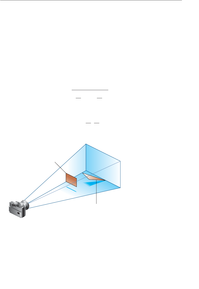
ptg9898810
To achieve a nice rendering of the highlighted solid object without visual
artifacts, you can add either a positive offset to the solid object (push it
away from you) or a negative offset to the wireframe (pull it toward you).
The big question is: How much offset is enough? Unfortunately, the offset
required depends on various factors, including the depth slope of each
polygon and the width of the lines in the wireframe.
OpenGL calculates the depth slope, as illustrated in Figure 4.2, which is
the z(depth) value divided by the change in either the x- or y-coordinates
as you traverse the polygon. The depth values are clamped to the range
[0, 1], and the x- and y-coordinates are in window coordinates. To estimate
the maximum depth slope of a polygon (min the offset equation above),
use the formula
m=∂z
∂x2
+∂z
∂y2
or an implementation may use the approximation
m= max ∂z
∂x,∂z
∂y
Polygon with depth slope = 0
Polygon with depth slope > 0
Figure 4.2 Polygons and their depth slopes
For polygons that are parallel to the near and far clipping planes, the depth
slope is zero. Those polygons can use a small constant offset, which you
can specify by setting factor =0.0 and units =1.0 in your call to
glPolygonOffset().
Testing and Operating on Fragments 165

ptg9898810
For polygons that are at a great angle to the clipping planes, the depth
slope can be significantly greater than zero, and a larger offset may be
needed. A small, nonzero value for factor, such as 0.75 or 1.0, is probably
enough to generate distinct depth values and eliminate the unpleasant
visual artifacts.
In some situations, the simplest values for factor and units (1.0 and 1.0)
aren’t the answer. For instance, if the widths of the lines that are
highlighting the edges are greater than 1, then increasing the value of
factor may be necessary. Also, since depth values while using a perspective
projection are unevenly transformed into window coordinates, less offset
is needed for polygons that are closer to the near clipping plane, and more
offset is needed for polygons that are farther away. You may need to
experiment with the values you pass to glPolygonOffset() to get the result
you’re looking for.
Blending
Once an incoming fragment has passed all of the enabled fragment tests, it
can be combined with the current contents of the color buffer in one of
several ways. The simplest way, which is also the default, is to overwrite
the existing values, which admittedly isn’t much of a combination.
Alternatively, you might want to combine the color present in the
framebuffer with the incoming fragment color---a process called blending.
Most often, blending is associated with the fragment’s alpha value (or
commonly just alpha), but that’s not a strict requirement. We’ve
mentioned alpha several times but haven’t given it a proper description.
Alpha is the fourth color component, and all colors in OpenGL have an
alpha value (even if you don’t explicitly set one). However, you don’t see
alpha, but rather you see alpha’s effect: it’s a measure of translucency, and
is what’s used when you want to simulate translucent objects, like colored
glass for example.
However, unless you enable blending by calling glEnable() with
GL_BLEND, or employ advanced techniques like order-independent
transparency (discussed in ‘‘Order-Independent Transparency’’ in
Chapter 11), alpha is pretty much ignored by the OpenGL pipeline. You
see, just like the real world, where color of a translucent object is a
combination of that object’s color with the colors of all the objects you see
behind it. For OpenGL to do something useful with alpha, the pipeline
needs more information than the current primitive’s color (which is the
color output from the fragment shader); it needs to know what color is
already present for that pixel in the framebuffer.
166 Chapter 4: Color, Pixels, and Framebuffers

ptg9898810
Blending Factors
In basic blending mode, the incoming fragment’s color is linearly
combined with the current pixel’s color. As with any linear combination,
coefficients control the contributions of each term. For blending in
OpenGL, those coefficients are called the source- and destination-blending
factors. The source-blending factor is associated with the color output from
the fragment shader, and similarly, the destination-blending factor is
associated with the color in the framebuffer.
If we let (Sr,Sg,Sb,Sa)represent the source-blending factors, and likewise let
(Dr,Dg,Db,Da)represent the destination factors, and use (Rs,Gs,Bs,As),
and (Rd,Gd,Bd,Ad)represent the colors of the source fragment and
destination pixel respectively, the blending equation yields a final color of
(SrRs+DrRd,SgGs+DgGd,SbBs+DbBd,SaAs+DaAd)
The default blending operation is addition, but we’ll see in ‘‘The Blending
Equation’’ on Page 170 that we can also control the blending operator.
Controlling Blending Factors
You have two different ways to choose the source and destination blending
factors. You may call glBlendFunc() and choose two blending factors: the
first factor for the source RGBA and the second for the destination RGBA.
Or, you may use glBlendFuncSeparate() and choose four blending factors,
which allows you to use one blending operation for RGB and a different
one for its corresponding alpha.
Note: We also list the functions glBlendFunci() and
glBlendFuncSeparatei(), which are used when you’re drawing to
multiple buffers simultaneously. This is an advanced topic that we
describe in ‘‘Framebuffer Objects’’ on Page 180, but since the
functions are virtually identical actions to glBlendFunc() and
glBlendFuncSeparate(), we include them here.
void glBlendFunc(GLenum srcfactor, GLenum destfactor);
void glBlendFunci(GLuint buffer, GLenum srcfactor,
GLenum destfactor);
Controls how color values in the fragment being processed (the source)
are combined with those already stored in the framebuffer (the
destination). The possible values for these arguments are explained in
Testing and Operating on Fragments 167

ptg9898810
Table 4.3. The argument srcfactor indicates how to compute a source
blending factor; destfactor indicates how to compute a destination
blending factor.
glBlendFunc() specifies the blending factors for all drawable buffers,
while glBlendFunci() specifies the blending factors only for buffer buffer.
The blending factors are clamped to either the range [0, 1]or [−1, 1]for
unsigned-normalized or signed-normalized framebuffer formats
respectively. If the framebuffer format is floating point, then no clamping
of factors occurs.
void glBlendFuncSeparate(GLenum srcRGB, GLenum destRGB,
GLenum srcAlpha,
GLenum destAlpha);
void glBlendFuncSeparatei(GLuint buffer, GLenum srcRGB,
GLenum destRGB, GLenum srcAlpha,
GLenum destAlpha);
Similar to glBlendFunc(),glBlendFuncSeparate() also controls how
source color values (fragment) are combined with destination values (in
the framebuffer). glBlendFuncSeparate() also accepts the same
arguments (shown in Table 4.3) as glBlendFunc(). The argument srcRGB
indicates the source-blending factor for color values; destRGB is the
destination-blending factor for color values. The argument srcAlpha
indicates the source-blending factor for alpha values; destAlpha is the
destination-blending factor for alpha values.
glBlendFuncSeparatei() specifies the blending factors for all drawable
buffers, while glBlendFuncSeparatei() specifies the blending factors only
for buffer buffer.
Note: In Table 4.3, the values with the subscript s1are for dual-source
blending factors, which are described in ‘‘Dual-Source Blending’’
on Page 198.
If you use one of the GL_CONSTANT blending functions, you need to use
glBlendColor() to specify the constant color.
168 Chapter 4: Color, Pixels, and Framebuffers

ptg9898810
Table 4.3 Source and Destination Blending Factors
Constant RGB Blend Factor Alpha Blend
Factor
GL_ZERO (0, 0, 0)0
GL_ONE (1, 1, 1)1
GL_SRC_COLOR (Rs,Gs,Bs)As
GL_ONE_MINUS_SRC_COLOR (1, 1, 1)−(Rs,Gs,Bs)1−As
GL_DST_COLOR (Rd,Gd,Bd)Ad
GL_ONE_MINUS_DST_COLOR (1, 1, 1)−(Rd,Gd,Bd)1−Ad
GL_SRC_ALPHA (As,As,As)As
GL_ONE_MINUS_SRC_ALPHA (1, 1, 1)−(As,As,As)1−As
GL_DST_ALPHA (Ad,Ad,Ad)Ad
GL_ONE_MINUS_DST_ALPHA (1, 1, 1)−(Ad,Ad,Ad)1−Ad
GL_CONSTANT_COLOR (Rc,Gc,Bc)Ac
GL_ONE_MINUS_CONSTANT_COLOR (1, 1, 1)−(Rc,Gc,Bc)1−Ac
GL_CONSTANT_ALPHA (Ac,Ac,Ac)Ac
GL_ONE_MINUS_CONSTANT_ALPHA (1, 1, 1)−(Ac,Ac,Ac)1−Ac
GL_SRC_ALPHA_SATURATE (f,f,f),f=min(As,1−Ad)1
GL_SRC1_COLOR (Rs1,Gs1,Bs1)As1
GL_ONE_MINUS_SRC1_COLOR (1, 1, 1)−(Rs1,Gs1,Bs1)1−As1
GL_SRC1_ALPHA (As1,As1,As1)As1
GL_ONE_MINUS_SRC1_ALPHA (1, 1, 1)−(As1,As1,As1)1−As1
void glBlendColor(GLclampf red, GLclampf green, GLclampf blue,
GLclampf alpha);
Sets the current red,blue,green, and alpha values for use as the constant
color (Rc,Gc,Bc,Ac)in blending operations.
Similarly, use glDisable() with GL_BLEND to disable blending. Note that
using the constants GL_ONE (as the source factor) and GL_ZERO (for the
destination factor) gives the same results as when blending is disabled;
these values are the default.
Testing and Operating on Fragments 169

ptg9898810
Advanced
OpenGL has the ability to render into multiple buffers simultaneously (see
‘‘Writing to Multiple Renderbuffers Simultaneously’’ on Page 193 for
details). All buffers can have blending enabled and disabled
simultaneously (using glEnable() and glDisable()). Blending settings can
be managed on a per-buffer basis using glEnablei() and glDisablei().
The Blending Equation
With standard blending, colors in the framebuffer are combined (using
addition) with incoming fragment colors to produce the new framebuffer
color. Either glBlendEquation() or glBlendEquationSeparate() may be
used to select other mathematical operations to compute the difference,
minimum, or maximum between color fragments and framebuffer pixels.
void glBlendEquation(GLenum mode);
void glBlendEquationi(GLuint buffer, GLenum mode);
Specifies how framebuffer and source colors are blended together. The
allowable values for mode are GL_FUNC_ADD (the default),
GL_FUNC_SUBTRACT, GL_FUNC_REVERSE_SUBTRACT, GL_MIN, and
GL_MAX. The possible modes are described in Table 4.4.
glBlendEquation() specifies the blending mode for all buffers, while
glBlendEquationi() sets the mode for the buffer specified by the buffer
argument, which is the integer index of the buffer.
void glBlendEquationSeparate(GLenum modeRGB,
GLenum modeAlpha);
void glBlendEquationSeparatei(GLuint buffer,
GLenum modeRGB,
GLenum modeAlpha);
Specifies how framebuffer and source colors are blended together, but
allows for different blending modes for the rgb and alpha color
components. The allowable values for modeRGB and modeAlpha are
identical for the modes accepted by glBlendEquation().
Again, glBlendEquationSeparate() sets the blending modes for all
buffers, while glBlendEquationSeparatei() sets the modes for the buffer
whose index is specified in buffer.
170 Chapter 4: Color, Pixels, and Framebuffers

ptg9898810
In Table 4.4,Csand Cdrepresent the source and destination colors. The S
and Dparameters in the table represent the source- and
destination-blending factors as specified with glBlendFunc() or
glBlendFuncSeparate().
Table 4.4 Blending Equation Mathematical Operations
Blending Mode Parameter Mathematical Operation
GL_FUNC_ADD CsS+CdD
GL_FUNC_SUBTRACT CsS−CdD
GL_FUNC_REVERSE_SUBTRACT CdD−CsS
GL_MIN min(CsS,CdD)
GL_MAX max(CsS,CdD)
Dithering
On systems with a small number of color bitplanes, you can improve the
color resolution at the expense of spatial resolution by dithering the color
in the image. Dithering is like half-toning in newspapers. Although The
New York Times has only two colors---black and white---it can show
photographs by representing the shades of gray with combinations of
black and white dots. Comparing a newspaper image of a photo (having
no shades of gray) with the original photo (with grayscale) makes the loss
of spatial resolution obvious. Similarly, systems with a small number of
color bitplanes may dither values of red, green, and blue on neighboring
pixels for the appearance of a wider range of colors.
The dithering operation that takes place is hardware-dependent; all
OpenGL allows you to do is to turn it on and off. In fact, on some
machines, enabling dithering might do nothing at all, which makes sense
if the machine already has high color resolution. To enable and disable
dithering, pass GL_DITHER to glEnable() and glDisable(). Dithering is
enabled by default.
Logical Operations
The final operation on a fragment is the logical operation, such as an OR,
XOR, or INVERT, which is applied to the incoming fragment values
(source) and/or those currently in the color buffer (destination). Such
fragment operations are especially useful on bit-blt-type machines, on
which the primary graphics operation is copying a rectangle of data from
Testing and Operating on Fragments 171

ptg9898810
one place in the window to another, from the window to processor
memory, or from memory to the window. Typically, the copy doesn’t write
the data directly into memory but instead allows you to perform an
arbitrary logical operation on the incoming data and the data already
present; then it replaces the existing data with the results of the operation.
Since this process can be implemented fairly cheaply in hardware, many
such machines are available. As an examplese of using a logical operation,
XOR can be used to draw on an image in a revertible way; simply XOR the
same drawing again, and the original image is restored.
You enable and disable logical operations by passing
GL_COLOR_LOGIC_OP to glEnable() and glDisable().You also must
choose among the 16 logical operations with glLogicOp(), or you’ll just
get the effect of the default value, GL_COPY.
void glLogicOp(GLenum opcode);
Selects the logical operation to be performed, given an incoming (source)
fragment and the pixel currently stored in the color buffer (destination).
Table 4.5 shows the possible values for opcode and their meaning (s
represents source and d destination). The default value is GL_COPY.
Table 4.5 Sixteen Logical Operations
Parameter Operation Parameter Operation
GL_CLEAR 0 GL_AND s∧d
GL_COPY sGL_OR s∨d
GL_NOOP dGL_NAND ¬(s∧d)
GL_SET 1 GL_NOR ¬(s∨d)
GL_COPY_INVERTED ¬sGL_XOR s XOR d
GL_INVERT ¬dGL_EQUIV ¬(s XOR d)
GL_AND_REVERSE s∧¬dGL_AND_INVERTED ¬s∧d
GL_OR_REVERSE s∨¬dGL_OR_INVERTED ¬s∨d
172 Chapter 4: Color, Pixels, and Framebuffers

ptg9898810
For floating-point buffers, or those in sRGB format, logical operations are
ignored.
Occlusion Query
Advanced
The depth buffer determines visibility on a per-pixel basis. For
performance reasons, it would be nice to be able to determine if a geometric
object is visible before sending all of its (perhaps complex) geometry for
rendering. Occlusion querys enable you to determine if a representative set
of geometry will be visible after depth testing.
This is particularly useful for complex geometric objects with many
polygons. Instead of rendering all of the geometry for a complex object,
you might render its bounding box or another simplified representation
that require less rendering resources. If OpenGL returns that no fragments
or samples would have been modified by rendering that piece of geometry,
you know that none of your complex object will be visible for that frame,
and you can skip rendering that object for the frame.
The following steps are required to utilize occlusion queries:
1. Generate a query id for each occlusion query that you need.
2. Specify the start of an occlusion query by calling glBeginQuery().
3. Render the geometry for the occlusion test.
4. Specify that you’ve completed the occlusion query by calling
glEndQuery().
5. Retrieve the number of, or if any, samples passed the depth tests.
In order to make the occlusion query process as efficient as possible, you’ll
want to disable all rendering modes that will increase the rendering time
but won’t change the visibility of a pixel.
Generating Query Objects
In order to use queries, you’ll first need to request identifiers for your query
tests. glGenQueries() will generate the requested number of unused query
ids for your subsequent use.
Testing and Operating on Fragments 173

ptg9898810
void glGenQueries(GLsizei n, GLuint *ids);
Returns ncurrently unused names for occlusion query objects in the
array ids The names returned in ids do not have to be a contiguous set of
integers.
The names returned are marked as used for the purposes of allocating
additional query objects, but only acquire valid state once they have
been specified in a call to glBeginQuery().
Zero is a reserved occlusion query object name and is never returned as a
valid value by glGenQueries().
You can also determine if an identifier is currently being used as an
occlusion query by calling glIsQuery().
GLboolean glIsQuery(GLuint id);
Returns GL_TRUE if id is the name of an occlusion query object. Returns
GL_FALSE if id is zero or if id is a nonzero value that is not the name of a
buffer object.
Initiating an Occlusion Query Test
To specify geometry that’s to be used in an occlusion query, merely bracket
the rendering operations between calls to glBeginQuery() and
glEndQuery(), as demonstrated in Example 4.6
Example 4.6 Rendering Geometry with Occlusion Query: occquery.c
glBeginQuery(GL_SAMPLES_PASSED, Query);
glDrawArrays(GL_TRIANGLES, 0, 3);
glEndQuery(GL_SAMPLES_PASSED);
All OpenGL operations are available while an occlusion query is active,
with the exception of glGenQueries() and glDeleteQueries(), which will
raise a GL_INVALID_OPERATION error.
void glBeginQuery(GLenum target, GLuint id);
Specifies the start of an occlusion query operation. target must be
GL_SAMPLES_PASSED, GL_ANY_SAMPLES_PASSED, or
GL_ANY_SAMPLES_PASSED_CONSERVATIVE. id is an unsigned integer
identifier for this occlusion query operation.
174 Chapter 4: Color, Pixels, and Framebuffers

ptg9898810
void glEndQuery(GLenum target);
Ends an occlusion query. target must be GL_SAMPLES_PASSED, or
GL_ANY_SAMPLES_PASSED.
Determining the Results of an Occlusion Query
Once you’ve completed rendering the geometry for the occlusion query,
you need to retrieve the results. This is done with a call to
glGetQueryObjectiv() or glGetQueryObjectuiv(), as shown in
Example 4.7, which will return the number of fragments, or samples, if
you’re using multisampling.
void glGetQueryObjectiv(GLenum id, GLenum pname,
GLint *params);
void glGetQueryObjectuiv(GLenum id, GLenum pname,
GLuint *params);
Queries the state of an occlusion query object. id is the name of a query
object. If pname is GL_QUERY_RESULT, then params will contain the
number of fragments or samples (if multisampling is enabled) that passed
the depth test, with a value of zero representing the object being entirely
occluded.
There may be a delay in completing the occlusion query operation. If
pname is GL_QUERY_RESULT_AVAILABLE, params will contain GL_TRUE
if the results for query id are available, or GL_FALSE otherwise.
Example 4.7 Retrieving the Results of an Occlusion Query
count = 1000; /*counter to avoid a possible infinite loop */
while (!queryReady && count-) {
glGetQueryObjectiv(Query, GL_QUERY_RESULT_AVAILABLE, &queryReady);
}
if (queryReady) {
glGetQueryObjectiv(Query, GL_QUERY_RESULT, &samples);
cerr << "Samples rendered: " << samples << endl;
}
else {
cerr << " Result not ready ... rendering anyways" << endl;
samples = 1; /*make sure we render */
}
Testing and Operating on Fragments 175

ptg9898810
if (samples > 0) {
glDrawArrays(GL_TRIANGLE_FAN}, 0, NumVertices);
}
Cleaning Up Occlusion Query Objects
After you’ve completed your occlusion query tests, you can release the
resources related to those queries by calling glDeleteQueries().
void glDeleteQueries(GLsizei n, const GLuint *ids);
Deletes nocclusion query objects, named by elements in the array ids.
The freed query objects may now be reused (for example, by
glGenQueries()).
Conditional Rendering
Advanced
One of the issues with occlusion queries is that they require OpenGL to
pause processing geometry and fragments, count the number of affected
samples in the depth buffer, and return the value to your application.
Stopping modern graphics hardware in this manner usually
catastrophically affects performance in performance-sensitive applications.
To eliminate the need to pause OpenGL’s operation, conditional rendering
allows the graphics server (hardware) to decide if an occlusion query
yielded any fragments, and to render the intervening commands.
Conditional rendering is enabled by surrounding the rendering operations
you would have conditionally executed using the results of glGetQuery*().
void glBeginConditionalRender(GLuint id, GLenum mode);
void glEndConditionalRender(void);
Delineates a sequence of OpenGL rendering commands that may be
discarded based on the results of the occlusion query object id.mode
specifies how the OpenGL implementation uses the results of the
occlusion query, and must be one of: GL_QUERY_WAIT,
GL_QUERY_NO_WAIT, GL_QUERY_BY_REGION_WAIT, or
GL_QUERY_BY_REGION_NO_WAIT.
A GL_INVALID_VALUE is set if id is not an existing occlusion query. A
GL_INVALID_OPERATION is generated if glBeginConditionalRender()
is called while a conditional-rendering sequence is in operation;
176 Chapter 4: Color, Pixels, and Framebuffers

ptg9898810
if glEndConditionalRender() is called when no conditional render is
underway; if id is the name of an occlusion query object with a target
different than GL_SAMPLES_PASSED; or if id is the name of an occlusion
query in progress.
The code shown in Example 4.8 completely replaces the sequence of code
in Example 4.7. Not only is it the code more compact, it is far more
efficient as it completely removes the results query to the OpenGL server,
which is a major performance inhibitor.
Example 4.8 Rendering Using Conditional Rendering
glBeginConditionalRender(Query, GL_QUERY_WAIT);
glDrawArrays(GL_TRIANGLE_FAN, 0, NumVertices);
glEndConditionalRender();
You may have noticed that there is a mode parameter to
glBeginConditionalRender(), which may be one of GL_QUERY_WAIT,
GL_QUERY_NO_WAIT, GL_QUERY_BY_REGION_WAIT, or
GL_QUERY_BY_REGION_NO_WAIT. These modes control whether the
GPU will wait for the results of a query to be ready before continuing to
render, and whether it will consider global results or results only
pertaining to the region of the screen that contributed to the original
occlusion query result.
•If mode is GL_QUERY_WAIT then the GPU will wait for the result of the
occlusion query to be ready before determining whether it will
continue with rendering.
•If mode is GL_QUERY_NO_WAIT then the GPU may not wait for the
result of the occlusion query to be ready before continuing to render. If
the result is not ready, then it may choose to render the part of the
scene contained in the conditional rendering section anyway.
•If mode is GL_QUERY_BY_REGION_WAIT then the GPU will wait for
anything that contributes to the region covered by the controled
rendering to be completed. It may still wait for the complete occlusion
query result to be ready.
•If mode is GL_QUERY_BY_REGION_NO_WAIT, then the GPU will
discard any rendering in regions of the framebuffer that contributed no
samples to the occlusion query, but may choose to render into other
regions if the result was not available in time.
By using these modes wisely, you can improve performance of the system.
For example, waiting for the results of an occlusion query may actually
Testing and Operating on Fragments 177
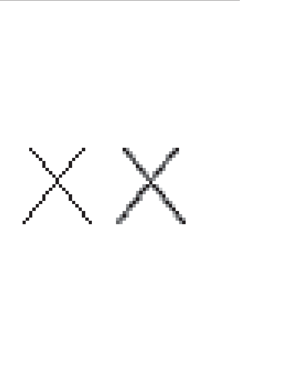
ptg9898810
take more time than just rendering the conditional part of the scene. In
particular, if it is expected that most results will mean that some rendering
should take place, then on aggregate, it may be faster to always use one of
the NO_WAIT modes even if it means more rendering will take place
overall.
Per-Primitive Antialiasing
You might have noticed in some of your OpenGL images that lines,
especially nearly horizontal and nearly vertical ones, appear jagged. These
jaggies appear because the ideal line is approximated by a series of pixels
that must lie on the pixel grid. The jaggedness is called aliasing, and this
section describes one antialiasing technique for reducing it. Figure 4.3
shows two intersecting lines, both aliased and antialiased. The pictures
have been magnified to show the effect.
Figure 4.3 Aliased and antialiased lines
Figure 4.3 shows how a diagonal line 1 pixel wide covers more of some
pixel squares than others. In fact, when performing antialiasing, OpenGL
calculates a coverage value for each fragment based on the fraction of the
pixel square on the screen that it would cover. OpenGL multiplies the
fragment’s alpha value by its coverage. You can then use the resulting
alpha value to blend the fragment with the corresponding pixel already in
the framebuffer.
The details of calculating coverage values are complex, and difficult to
specify in general. In fact, computations may vary slightly depending on
your particular implementation of OpenGL. You can use the glHint()
command to exercise some control over the trade-off between image
quality and speed, but not all implementations will take the hint.
178 Chapter 4: Color, Pixels, and Framebuffers

ptg9898810
void glHint(GLenum target, GLenum hint);
Controls certain aspects of OpenGL behavior. The target parameter
indicates which behavior is to be controlled; its possible values are shown
in Table 4.6. The hint parameter can be GL_FASTEST to indicate that the
most efficient option should be chosen, GL_NICEST to indicate the
highest-quality option, or GL_DONT_CARE to indicate no preference.
The interpretation of hints is implementation-dependent; an OpenGL
implementation can ignore them entirely.
Table 4.6 Values for Use with glHint()
Parameter Specifies
GL_LINE_SMOOTH_HINT Line antialiasing quality
GL_POLYGON_SMOOTH_HINT Polygon edge antialiasing quality
GL_TEXTURE_COMPRESSION_HINT Quality and performance of
texture-image compression (See
Chapter 6,‘‘Textures’’ for more
detail)
GL_FRAGMENT_SHADER_DERIVATIVE_HINT Derivative accuracy for fragment
processing built-in functions
dFdx,dFdy, and fwidth (See
Appendix Cfor more details)
We’ve discussed multisampling before as a technique for antialiasing;
however, it’s not usually the best solution for lines. Another way to
antialias lines, and polygons if the multisample results are quite what you
want, is to turn on antialiasing with glEnable(), and passing in
GL_LINE_SMOOTH or GL_POLYGON_SMOOTH, as appropriate. You
might also want to provide a quality hint with glHint(). We’ll describe the
steps for each type of primitive that can be antialiased in the next sections.
Antialiasing Lines
First, you need to enable blending. The blending factors you most likely
want to use are GL_SRC_ALPHA (source) and
GL_ONE_MINUS_SRC_ALPHA (destination). Alternatively, you can use
GL_ONE for the destination factor to make lines a little brighter where
they intersect. Now you’re ready to draw whatever points or lines you want
antialiased. The antialiased effect is most noticeable if you use a fairly high
alpha value. Remember that since you’re performing blending, you might
need to consider the rendering order. However, in most cases, the ordering
can be ignored without significant adverse effects.
Per-Primitive Antialiasing 179

ptg9898810
Example 4.9 shows the initialization for line antialiasing.
Example 4.9 Setting Up Blending for Antialiasing Lines: antilines.cpp
glEnable (GL_LINE_SMOOTH);
glEnable (GL_BLEND);
glBlendFunc (GL_SRC_ALPHA, GL_ONE_MINUS_SRC_ALPHA);
glHint (GL_LINE_SMOOTH_HINT, GL_DONT_CARE);
Antialiasing Polygons
Antialiasing the edges of filled polygons is similar to antialiasing lines.
When different polygons have overlapping edges, you need to blend the
color values appropriately.
To antialias polygons, you use the alpha value to represent coverage values
of polygon edges. You need to enable polygon antialiasing by passing
GL_POLYGON_SMOOTH to glEnable(). This causes pixels on the edges of
the polygon to be assigned fractional alpha values based on their coverage,
as though they were lines being antialiased. Also, if you desire, you can
supply a value for GL_POLYGON_SMOOTH_HINT.
In order to have edges blend appropriately, set the blending factors to
GL_SRC_ALPHA_SATURATE (source) and GL_ONE (destination). With this
specialized blending function, the final color is the sum of the destination
color and the scaled source color; the scale factor is the smaller of either
the incoming source alpha value or one minus the destination alpha value.
This means that for a pixel with a large alpha value, successive incoming
pixels have little effect on the final color because one minus the
destination alpha is almost zero. With this method, a pixel on the edge of
a polygon might be blended eventually with the colors from another
polygon that’s drawn later. Finally, you need to sort all the polygons in
your scene so that they’re ordered from front to back before drawing them.
Note: Antialiasing can be adversely affected when using the depth buffer,
in that pixels may be discarded when they should have been
blended. To ensure proper blending and antialiasing, you’ll need to
disable the depth buffer.
Framebuffer Objects
Advanced
Up to this point, all of our discussion regarding buffers has focused on the
buffers provided by the windowing system, as you requested when you
180 Chapter 4: Color, Pixels, and Framebuffers

ptg9898810
called glutCreateWindow() (and configured by your call to
glutInitDisplayMode()). Although you can quite successfully use any
technique with just those buffers, quite often various operations require
moving data between buffers superfluously. This is where framebuffer
objects enter the picture. Using framebuffer objects, you can create our
own framebuffers and use their attached renderbuffers to minimize data
copies and optimize performance.
Framebuffer objects are quite useful for performing off-screen-rendering,
updating texture maps, and engaging in buffer ping-ponging (a data-transfer
techniques used in GPGPU).
The framebuffer that is provided by the windowing system is the only
framebuffer that is available to the display system of your graphics
server---that is, it is the only one you can see on your screen. It also places
restrictions on the use of the buffers that were created when your window
opened. By comparison, the framebuffers that your application creates
cannot be displayed on your monitor; they support only off-screen rendering.
Another difference between window-system-provided framebuffers and
framebuffers you create is that those managed by the window system
allocate their buffers---color, depth, and stencil---when your window is
created. When you create an application-managed framebuffer object, you
need to create additional renderbuffers that you associate with the
framebuffer objects you created. The buffers with the window-system-
provided buffers can never be associated with an application-created
framebuffer object, and vice versa.
To allocate an application-generated framebuffer object name, you need to
call glGenFramebuffers(), which will allocate an unused identifier for the
framebuffer object.
void glGenFramebuffers(GLsizei n, GLuint *ids);
Allocate nunused framebuffer object names, and return those names in
ids.
A GL_INVALID_VALUE error will be generated if nis negative.
Allocating a framebuffer object name doesn’t actually create the
framebuffer object or allocate any storage for it. Those tasks are handled
through a call to glBindFramebuffer().glBindFramebuffer() operates in a
similar manner to many of the other glBind*() routines you’ve seen in
OpenGL. The first time it is called for a particular framebuffer, it causes
Framebuffer Objects 181

ptg9898810
storage for the object to be allocated and initialized. Any subsequent calls
will bind the provided framebuffer object name as the active one.
void glBindFramebuffer(GLenum target, GLuint framebuffer);
Specifies a framebuffer for either reading or writing. When target is
GL_DRAW_FRAMEBUFFER, framebuffer specifies the destination
framebuffer for rendering. Similarly, when target is set to
GL_READ_FRAMEBUFFER, framebuffer specifies the source of read
operations. Passing GL_FRAMEBUFFER for target sets both the read and
write framebuffer bindings to framebuffer.
framebuffer must either be zero, which binds target to the default
window-system-provided framebuffer, or a framebuffer object generated
by a call to glGenFramebuffers().
A GL_INVALID_OPERATION error is generated if framebuffer is neither
zero nor a valid framebuffer object previously generated by calling
glGenFramebuffers() but not deleted by calling glDeleteFramebuffers().
As with all of the other objects you have encountered in OpenGL, you can
release an application-allocated framebuffer by calling
glDeleteFramebuffers(). That function will mark the framebuffer object’s
name as unallocated and release any resources associated with the
framebuffer object.
void glDeleteFramebuffers(GLsizei n, const GLuint *ids);
Deallocates the nframebuffer objects associated with the names provided
in ids. If a framebuffer object is currently bound (i.e., its name was passed
to the most recent call to glBindFramebuffer()) and is deleted, the
framebuffer target is immediately bound to id zero (the window-system
provided framebuffer), and the framebuffer object is released.
A GL_INVALID_VALUE error is generated by glDeleteFramebuffers() if n
is negative. Passing unused names or zero does not generate any errors;
they are simply ignored.
For completeness, you can determine whether a particular unsigned integer
is an application-allocated framebuffer object by calling glIsFramebuffer():
182 Chapter 4: Color, Pixels, and Framebuffers

ptg9898810
GLboolean glIsFramebuffer(GLuint framebuffer);
Returns GL_TRUE if framebuffer is the name of a framebuffer returned
from glGenFramebuffers(). Returns GL_FALSE if framebuffer is zero (the
window-system default framebuffer) or a value that’s either unallocated
or been deleted by a call to glDeleteFramebuffers().
void glFramebufferParameteri(GLenum target, GLenum pname,
GLint param);
Sets parameters of a framebuffer object, when the framebuffer object has
no attachments, otherwise the values for these parameters are specified
by the framebuffer attachments.
target must be DRAW_FRAMEBUFFER, READ_FRAMEBUFFER, or
FRAMEBUFFER. FRAMEBUFFER is equivalent to DRAW_FRAMEBUFFER.
pname specifies the parameter of the framebuffer object bound to target
to set, and must be one of GL_FRAMEBUFFER_DEFAULT_WIDTH,
GL_FRAMEBUFFER_DEFAULT_HEIGHT,
GL_FRAMEBUFFER_DEFAULT_LAYERS,
GL_FRAMEBUFFER_DEFAULT_SAMPLES, or
GL_FRAMEBUFFER_DEFAULT_FIXED_SAMPLE_LOCATIONS.
Once a framebuffer object is created, you still can’t do much with it,
generally speaking. You need to provide a place for drawing to go and
reading to come from; those places are called framebuffer attachments. We’ll
discuss those in more detail after we examine renderbuffers, which are one
type of buffer you can attach to a framebuffer object.
Renderbuffers
Renderbuffers are effectively memory managed by OpenGL that contains
formatted image data. The data that a renderbuffer holds takes meaning
once it is attached to a framebuffer object, assuming that the format of the
image buffer matches what OpenGL is expecting to render into (e.g., you
can’t render colors into the depth buffer).
As with many other buffers in OpenGL, the process of allocating and
deleting buffers is similar to what you’ve seen before. To create a new
renderbuffer, you would call glGenRenderbuffers().
Framebuffer Objects 183

ptg9898810
void glGenRenderbuffers(GLsizei n, GLuint *ids);
Allocate nunused renderbuffer object names, and return those names in
ids. Names are unused until bound with a call to glBindRenderbuffer().
Likewise, a call to glDeleteRenderbuffers() will release the storage
associated with a renderbuffer.
void glDeleteRenderbuffers(GLsizei n, const GLuint *ids);
Deallocates the nrenderbuffer objects associated with the names
provided in ids. If one of the renderbuffers is currently bound and passed
to glDeleteRenderbuffers(), a binding of zero replaces the binding at the
current framebuffer attachment point, in addition to the renderbuffer
being released.
No errors are generated by glDeleteRenderbuffers(). Unused names or
zero are simply ignored.
Likewise, you can determine whether a name represents a valid
renderbuffer by calling glIsRenderbuffer().
void glIsRenderbuffer(GLuint renderbuffer);
Returns GL_TRUE if renderbuffer is the name of a renderbuffer returned
from glGenRenderbuffers(). Returns GL_FALSE if framebuffer is zero (the
window-system default framebuffer) or a value that’s either unallocated
or deleted by a call to glDeleteRenderbuffers().
Similar to the process of binding a framebuffer object so that you can
modify its state, you call glBindRenderbuffer() to affect a renderbuffer’s
creation and to modify the state associated with it, which includes the
format of the image data that it contains.
void glBindRenderbuffer(GLenum target, GLuint renderbuffer);
Creates a renderbuffer and associates it with the name renderbuffer.target
must be GL_RENDERBUFFER. renderbuffer must either be zero, which
removes any renderbuffer binding, or a name that was generated by a call
to glGenRenderbuffers(); otherwise, a GL_INVALID_OPERATION error
will be generated.
184 Chapter 4: Color, Pixels, and Framebuffers

ptg9898810
Creating Renderbuffer Storage
When you first call glBindRenderbuffer() with an unused renderbuffer
name, the OpenGL server creates a renderbuffer with all its state
information set to the default values. In this configuration, no storage has
been allocated to store image data. Before you can attach a renderbuffer to
a framebuffer and render into it, you need to allocate storage and specify
its image format. This is done by calling either glRenderbufferStorage() or
glRenderbufferStorageMultisample().
void glRenderbufferStorage(GLenum target,
GLenum internalformat,
GLsizei width, GLsizei height);
void glRenderbufferStorageMultisample(GLenum target,
GLsizei samples,
GLenum internalformat,
GLsizei width,
GLsizei height);
Allocates storage for image data for the bound renderbuffer. target must
be GL_RENDERBUFFER. For a color-renderable buffer, internalformat must
be one of:
GL_RED GL_R8 GL_R16
GL_RG GL_RG8 GL_RG16
GL_RGB GL_R3_G3_B2 GL_RGB4
GL_RGB5 GL_RGB8 GL_RGB10
GL_RGB12 GL_RGB16 GL_RGBA
GL_RGBA2 GL_RGBA4 GL_RGB5_A1
GL_RGBA8 GL_RGB10_A2 GL_RGBA12
GL_RGBA16 GL_SRGB GL_SRGB8
GL_SRGB_ALPHA GL_SRGB8_ALPHA8 GL_R16F
Framebuffer Objects 185

ptg9898810
GL_R32F GL_RG16F GL_RG32F
GL_RGB16F GL_RGB32F GL_RGBA16F
GL_RGBA32F GL_R11F_G11F_B10F GL_RGB9_E5
GL_R8I GL_R8UI GL_R16I
GL_R16UI GL_R32I GL_R32UI
GL_RG8I GL_RG8UI GL_RG16I
GL_RG16UI GL_RG32I GL_RG32UI
GL_RGB8I GL_RGB8UI GL_RGB16I
GL_RGB16UI GL_RGB32I GL_RGB32UI
GL_RGBA8I GL_RGBA8UI GL_RGBA16I
GL_RGBA16UI GL_RGBA32I GL_R8_SNORM
GL_R16_SNORM GL_RG8_SNORM GL_RG16_SNORM
GL_RGB8_SNORM GL_RGB16_SNORM GL_RGBA8_SNORM
GL_RGBA16_SNORM
To use a renderbuffer as a depth buffer, it must be depth-renderable,
which is specified by setting internalformat to either
GL_DEPTH_COMPONENT, GL_DEPTH_COMPONENT16,
GL_DEPTH_COMPONENT32, GL_DEPTH_COMPONENT32, or
GL_DEPTH_COMPONENT32F.
For use exclusively as a stencil buffer, internalformat should be specified
as either GL_STENCIL_INDEX, GL_STENCIL_INDEX1,
GL_STENCIL_INDEX4, GL_STENCIL_INDEX8, or
GL_STENCIL_INDEX16.
For packed depth-stencil storage, internalformat must be
GL_DEPTH_STENCIL, which allows the renderbuffer to be attached as
the depth buffer, stencil buffer, or at the combined depth-stencil
attachment point.
width and height specify the size of the renderbuffer in pixels, and
samples specifies the number of multisample samples per pixel. Setting
samples to zero in a call to glRenderbufferStorageMultisample() is
identical to calling glRenderbufferStorage().
A GL_INVALID_VALUE is generated if width or height is greater than the
value returned when querying GL_MAX_RENDERBUFFER_SIZE, or if
samples is greater than the value returned when querying
GL_MAX_SAMPLES. A GL_INVALID_OPERATION is generated if
internalformat is a signed- or unsigned-integer format (e.g., a format
containing a ‘‘I’’, or ‘‘UI’’ in its token), and samples is not zero, and the
implementation doesn’t support multisampled integer buffers. Finally, if
the renderbuffer size and format combined exceed the available memory
able to be allocated, then a GL_OUT_OF_MEMORY error is generated.
186 Chapter 4: Color, Pixels, and Framebuffers

ptg9898810
Example 4.10 Creating a 256 ×256 RGBA Color Renderbuffer
glGenRenderbuffers(1, &color);
glBindRenderbuffer(GL_RENDERBUFFER, color);
glRenderbufferStorage(GL_RENDERBUFFER, GL_RGBA, 256, 256);
Once you have created storage for your renderbuffer as shown in
Example 4.10, you need to attach it to a framebuffer object before you can
render into it.
Framebuffer Attachments
When you render, you can send the results of that rendering to a number
of places:
•The color buffer to create an image, or even multiple color buffers if
you’re using multiple render targets (see ‘‘Writing to Multiple
Renderbuffers Simultaneously’’ on Page 193).
•The depth buffer to store occlusion information.
•The stencil buffer for storing per-pixel masks to control rendering. Each
of those buffers represents a framebuffer attachment, to which you can
attach suitable image buffers that you later render into, or read from.
The possible framebuffer attachment points are listed in Table 4.7.
Table 4.7 Framebuffer Attachments
Attachment Name Description
GL_COLOR_ATTACHMENTiThe ith color buffer. ican range from
zero (the default color buffer) to
GL_MAX_COLOR_ATTACHMENTS - 1
GL_DEPTH_ATTACHMENT The depth buffer
GL_STENCIL_ATTACHMENT The stencil buffer
GL_DEPTH_STENCIL_ATTACHMENT A special attachment for packed
depth-stencil buffers (which require the
renderbuffer to have been allocated as a
GL_DEPTH_STENCIL pixel format)
Currently, there are two types of rendering surfaces you can associate with
one of those attachments: renderbuffers and a level of a texture image.
We’ll first discuss attaching a renderbuffer to a framebuffer object, which is
done by calling glFramebufferRenderbuffer().
Framebuffer Objects 187

ptg9898810
void glFramebufferRenderbuffer(GLenum target,
GLenum attachment,
GLenum renderbuffertarget,
GLuint renderbuffer);
Attaches renderbuffer to attachment of the currently bound framebuffer
object. target must either be GL_READ_FRAMEBUFFER,
GL_DRAW_FRAMEBUFFER, or GL_FRAMEBUFFER (which is equivalent to
GL_DRAW_FRAMEBUFFER).
attachment is one of GL_COLOR_ATTACHMENTi,
GL_DEPTH_ATTACHMENT, GL_STENCIL_ATTACHMENT, or
GL_DEPTH_STENCIL_ATTACHMENT.
renderbuffertarget must be GL_RENDERBUFFER, and renderbuffer must
either be zero, which removes any renderbuffer attachment at
attachment, or a renderbuffer name returned from glGenRenderbuffers(),
or a GL_INVALID_OPERATION error is generated.
In Example 4.11, we create and attach two renderbuffers: one for color,
and the other for depth. We then proceed to render, and finally copy the
results back to the window-system-provided framebuffer to display the
results. You might use this technique to generate frames for a movie
rendering off-screen, where you don’t have to worry about the visible
framebuffer being corrupted by overlapping windows or someone resizing
the window and interrupting rendering.
One important point to remember is that you might need to reset the
viewport for each framebuffer before rendering, particularly if the size of
your application-defined framebuffers differs from the window-system
provided framebuffer.
Example 4.11 Attaching a Renderbuffer for Rendering
enum { Color, Depth, NumRenderbuffers };
GLuint framebuffer, renderbuffer[NumRenderbuffers]
void
init()
{
glGenRenderbuffers(NumRenderbuffers, renderbuffer);
glBindRenderbuffer(GL_RENDERBUFFER, renderbuffer[Color]);
glRenderbufferStorage(GL_RENDERBUFFER, GL_RGBA, 256, 256);
glBindRenderbuffer(GL_RENDERBUFFER, renderbuffer[Depth]);
188 Chapter 4: Color, Pixels, and Framebuffers

ptg9898810
glRenderbufferStorage(GL_RENDERBUFFER, GL_DEPTH_COMPONENT24, 256, 256);
glGenFramebuffers(1, &framebuffer);
glBindFramebuffer(GL_DRAW_FRAMEBUFFER, framebuffer);
glFramebufferRenderbuffer(GL_DRAW_FRAMEBUFFER, GL_COLOR_ATTACHMENT0,
GL_RENDERBUFFER, renderbuffer[Color]);
glFramebufferRenderbuffer(GL_DRAW_FRAMEBUFFER, GL_DEPTH_ATTACHMENT,
GL_RENDERBUFFER, renderbuffer[Depth]);
glEnable(GL_DEPTH_TEST);
}
void
display()
{
// Prepare to render into the renderbuffer
glBindFramebuffer(GL_DRAW_FRAMEBUFFER, framebuffer);
glViewport(0, 0, 256, 256);
// Render into renderbuffer
glClearColor(1.0, 0.0, 0.0, 1.0);
glClear(GL_COLOR_BUFFER_BIT | GL_DEPTH_BUFFER_BIT);
...
// Set up to read from the renderbuffer and draw to
// window-system framebuffer
glBindFramebuffer(GL_READ_FRAMEBUFFER, framebuffer);
glBindFramebuffer(GL_DRAW_FRAMEBUFFER, 0);
glViewport(0, 0, windowWidth, windowHeight);
glClearColor(0.0, 0.0, 1.0, 1.0);
glClear(GL_COLOR_BUFFER_BIT | GL_DEPTH_BUFFER_BIT);
/*Do the copy */
glBlitFramebuffer(0, 0, 255, 255, 0, 0, 255, 255,
GL_COLOR_BUFFER_BIT, GL_NEAREST);
glutSwapBuffers();
}
Framebuffer Objects 189

ptg9898810
Framebuffer Completeness
Given the myriad of combinations between texture and buffer formats,
and between framebuffer attachments, various situations can arise that
prevent the completion of rendering when you are using
application-defined framebuffer objects. After modifying the attachments
to a framebuffer object, it’s best to check the framebuffer’s status by calling
glCheckFramebufferStatus().
GLenum glCheckFramebufferStatus(GLenum target);
Returns one of the framebuffer completeness status enums listed in
Table 4.8.target must be one of GL_READ_FRAMEBUFFER,
GL_DRAW_FRAMEBUFFER, or GL_FRAMEBUFFER (which is equivalent to
GL_DRAW_FRAMEBUFFER).
If glCheckFramebufferStatus() generates an error, zero is returned.
The errors representing the various violations of framebuffer
configurations are listed in Table 4.8.
Of the listed errors, GL_FRAMEBUFFER_UNSUPPORTED is very
implementation dependent, and may be the most complicated to debug.
Advanced
glClear(GL_COLOR_BUFFER_BIT)will clear all of the bound color buffers
(we have see in ‘‘Framebuffer Objects’’ on Page 180 how to configure
multiple color buffers). You can use the glClearBuffer*() commands to
clear individual buffers.
If you’re using multiple draw buffers---particularly those that have
floating-point or nonnormalized integer pixel formats---you can clear each
individually bound buffer using glClearBuffer*() functions. Unlike
functions such as glClearColor() and glClearDepth(), which set a clear
value within OpenGL that’s used when glClear() is called, glClearBuffer*()
uses the values passed to it to immediately clear the bound drawing
buffers. Additionally, to reduce the number of function calls associated
with using multiple draw buffers, you can call glClearBufferfi() to
simultaneously clear the depth and stencil buffers (which is effectively
equivalent to calling glClearBuffer*() twice---once for the depth buffer and
once for the stencil buffer).
190 Chapter 4: Color, Pixels, and Framebuffers

ptg9898810
Table 4.8 Errors Returned by glCheckFramebufferStatus()
Framebuffer Completeness Status Enum Description
GL_FRAMEBUFFER_COMPLETE The framebuffer and its
attachments match the
rendering or reading state
required.
GL_FRAMEBUFFER_UNDEFINED The bound framebuffer is
specified to be the default
framebuffer (i.e.,
glBindFramebuffer()
with zero specified as the
framebuffer), and the
default framebuffer
doesn’t exist.
GL_FRAMEBUFFER_INCOMPLETE_ATTACHMENT A necessary attachment
to the bound framebuffer
is uninitialized
GL_FRAMEBUFFER_INCOMPLETE_MISSING_ATTACHMENT There are no images (e.g.,
texture layers or
renderbuffers) attached
to the framebuffer.
GL_FRAMEBUFFER_INCOMPLETE_DRAW_BUFFER Every drawing buffer
(e.g., GL_DRAW_BUFFERi
as specified by
glDrawBuffers()) has an
attachment.
GL_FRAMEBUFFER_INCOMPLETE_READ_BUFFER An attachment exists for
the buffer specified for
the buffer specified by
glReadBuffer().
GL_FRAMEBUFFER_UNSUPPORTED The combination of
images attached to the
framebuffer object is
incompatible with the
requirements of the
OpenGL
implementation.
GL_FRAMEBUFFER_INCOMPLETE_MULTISAMPLE The number of samples
for all images across the
framebuffer’s
attachments do not
match.
Framebuffer Objects 191

ptg9898810
void glClearBuffer{fi ui}v(GLenum buffer, GLint drawbuffer,
const TYPE *value);
void glClearBufferfi(GLenum buffer,GLint drawbuffer,
GLfloat depth,GLint stencil);
Clears the buffer indexed by drawbuffer associated with buffer to value.
buffer must be one of GL_COLOR, GL_DEPTH, or GL_STENCIL.
If buffer is GL_COLOR, drawbuffer specifies an index to a particular draw
buffer, and value is a four-element array containing the clear color. If the
buffer indexed by drawbuffer has multiple draw buffers (as specified by a
call the glDrawBuffers()), all draw buffers are cleared to value.
If buffer is GL_DEPTH or GL_STENCIL, drawbuffer must be zero, and value
is a single-element array containing an appropriate clear value (subject to
clamping and type conversion for depth values, and masking and type
conversion for stencil values). Use only glClearBufferfv() for clearing the
depth buffer, and glClearBufferiv() for clearing the stencil buffer.
glClearBufferfi() can be used to clear both the depth and stencil buffers
simultaneously. buffer in this case must be GL_DEPTH_STENCIL.
GL_INVALID_ENUM is generated by glClearbuffer{if ui}v if buffer is not
one of the accepted values listed above. GL_INVALID_ENUM is generated
by glClearBufferfi() if buffer is not GL_DEPTH_STENCIL.
GL_INVALID_VALUE is generated if buffer is GL_COLOR, and drawbuffer
is less than zero, or greater than or equal to GL_MAX_DRAW_BUFFERS;
or if buffer is GL_DEPTH, GL_STENCIL, or GL_DEPTH_STENCIL and
drawbuffer is not zero.
Invalidating Framebuffers
Implementations of OpenGL (including OpenGL ES on mobile or
embedded devices, most often) may work in limited memory
environments. Framebuffers have the potential of taking up considerable
memory resources (particularly for multiple, multisampled color
attachments and textures). OpenGL provides a mechanism to state that a
region or all of a framebuffer is no longer needed and can be released. This
operation is done with either glInvalidateSubFramebuffer() or
glInvalidateFramebuffer().
192 Chapter 4: Color, Pixels, and Framebuffers

ptg9898810
void glInvalidateFramebuffer(GLenum target,
GLsizei numAttachments,
const GLenum *attachments);
void glInvalidateSubFramebuffer(GLenum target,
GLsizei numAttachmens,
const GLenum *attachments,
GLint x, GLint y,
GLsizei width, GLsizei height);
Specifies that a portion, or the entirety, of the bound framebuffer object
are not necessary to preserve. For either function, target must be either
GL_DRAW_FRAMEBUFFER, GL_READ_FRAMEBUFFER, or
GL_FRAMEBUFFER specifying both the draw and read targets at the same
time. attachments provides a list of attachment tokens:
GL_COLOR_ATTACHMENTi, GL_DEPTH_ATTACHMENT, or
GL_STENCIL_ATTACHMENT; and numAttachments specifies how many
entries are in the attachments list.
For glInvalidateSubFramebuffer(), the region specified by lower-left
corner (x,y)with width width, and height height (measured from (x,y)), is
marked as invalid for all attachments in attachments.
Various errors are returned from the calls: A GL_INVALID_ENUM is
generated if any tokens are not from those listed above; A
GL_INVALID_OPERATION is generated if an index of an attachment
(e.g., ifrom GL_COLOR_ATTACHMENTi) is greater than or equal to the
maximum number of color attachments; A GL_INVALID_VALUE is
generated if any of numAttachments,width,orheight are negative.
Writing to Multiple Renderbuffers Simultaneously
Advanced
One feature of using framebuffer objects with multiple renderbuffer (or
textures, as described in Chapter 6,‘‘Textures’’) is the ability to write to
multiple buffers from a fragment shader simultaneously, often called MRT
(for multiple-render target) rendering. This is mostly a performance
optimization, saving processing the same list of vertices multiple times and
rasterizing the same primitives multiple times.
Writing to Multiple Renderbuffers Simultaneously 193

ptg9898810
While this technique is used often in GPGPU, it can also be used when
generating geometry and other information (like textures or normal map)
which is written to different buffers during the same rendering pass.
Enabling this technique requires setting up a framebuffer object with
multiple color (and potentially depth and stencil) attachments, and
modification of the fragment shader. Having just discussed setting up
multiple attachments, we’ll focus on the fragment shader here.
As we’ve discussed, fragment shaders output values through their out
variables. In order to specify the correspondence between out variables
and framebuffer attachments, we simply need to use the layout qualifier
to direct values to the right places. For instance, Example 4.12
demonstrates associating two variables with color attachment locations
zero and one.
Example 4.12 Specifying layout Qualifiers for MRT Rendering
layout (location = 0) out vec4 color;
layout (location = 1) out vec4 normal;
If the attachments of the currently bound framebuffer don’t match those
of the currently bound fragment shader, misdirected data (i.e., fragment
shader data written to an attachment with nothing attached) accumulates
in dark corners of the universe, but is otherwise ignored.
Additionally, if you’re using dual-source blending (see ‘‘Dual-Source
Blending’’ on Page 198), with MRT rendering, you merely specify both the
location and index options to the layout directive.
Using the layout qualifier within a shader is the preferred way to associate
fragment shader outputs with framebuffer attachments, but if they are
not specified, then OpenGL will do the assignments during shader linking.
You can direct the linker to make the appropriate associations by using
the glBindFragDataLocation(), or glBindFragDataLocationIndexed()
if you need to also specify the fragment index. Fragment shader
bindings specified in the shader source will be used if specified,
regardless of whether a location was specified using one of these functions.
194 Chapter 4: Color, Pixels, and Framebuffers

ptg9898810
void glBindFragDataLocation(GLuint program,
GLuint colorNumber,
const GLchar *name);
void glBindFragDataLocationIndexed(GLuint program,
GLuint colorNumber,
GLuint index,
const GLchar *name);
Uses the value in color for fragment shader variable name to specify the
output location associated with shader program. For the indexed case,
index specifies the output index as well as the location.
A GL_INVALID_VALUE is generated if program is not a shader program, or
if either index is greater than one, or if colorNumber is greater than or
equal to the maximum number of color attachments.
After a program is linked, you can retrieve a fragment shader variable’s
output location, and source index, if applicable, by calling either
glGetFragDataLocation(), or glGetFragDataIndex().
GLint glGetFragDataLocation(GLuint program,
const GLchar *name);
GLint glGetFragDataIndex(GLuint program,
const GLchar *name);
Returns either the location or index of a fragment shader variable name
associated with the linked shader program program.
A−1 is returned if: name is not the name of applicable variable for
program; if program successfully linked, but doesn’t have an associated
fragment shader; or if program has not yet been, or failed, linking. In the
last case, a GL_INVALID_OPERATION error is also generated.
Selecting Color Buffers for Writing and Reading
The results of a drawing or reading operation can go into or come from
any of the color buffers:
•front, back, front-left, back-left, front-right, or back-right for the
default framebuffer, or
•front, or any renderbuffer attachment for a user-defined framebuffer
object.
Writing to Multiple Renderbuffers Simultaneously 195

ptg9898810
You can choose an individual buffer to be the drawing or reading target.
For drawing, you can also set the target to draw into more than one buffer
at the same time. You use glDrawBuffer(),orglDrawBuffers() to select the
buffers to be written and glReadBuffer() to select the buffer as the source
for glReadPixels(),glCopyTexImage*(), and glCopyTexSubImage*().
void glDrawBuffer(GLenum mode);
void glDrawBuffers(GLsizei n, const GLenum *buffers);
Selects the color buffers enabled for writing or clearing and disables
buffers enabled by previous calls to glDrawBuffer() or glDrawBuffers().
More than one buffer may be enabled at one time. The value of mode can
be one of the following:
GL_FRONT GL_FRONT_LEFT GL_NONE
GL_BACK GL_FRONT_RIGHT GL_FRONT_AND_BACK
GL_LEFT GL_BACK_LEFT GL_COLOR_ATTACHMENTi
GL_RIGHT GL_BACK_RIGHT
If mode, or the entries in buffers is not one of the above, a
GL_INVALID_ENUM error is generated. Additionally, if a framebuffer
object is bound that is not the default framebuffer, then only GL_NONE
and GL_COLOR_ATTACHMENTiare accepted, otherwise a
GL_INVALID_ENUM error is generated.
Arguments that omit LEFT or RIGHT refer to both the left and right stereo
buffers; similarly, arguments that omit FRONT or BACK refer to both.
By default, mode is GL_BACK for double-buffered contexts.
The glDrawBuffers() routine specifies multiple color buffers capable of
receiving color values. buffers is an array of buffer enumerates. Only
GL_NONE, GL_FRONT_LEFT, GL_FRONT_RIGHT, GL_BACK_LEFT, and
GL_BACK_RIGHT are accepted.
When you are using double-buffering, you usually want to draw only in the
back buffer (and swap the buffers when you’re finished drawing). In some
situations, you might want to treat a double-buffered window as though
it were single-buffered by calling glDrawBuffer(GL_FRONT_AND_BACK)
to enable you to draw to both front and back buffers at the same time.
For selecting the read buffer, use glReadBuffer().
196 Chapter 4: Color, Pixels, and Framebuffers

ptg9898810
void glReadBuffer(GLenum mode);
Selects the color buffer enabled as the source for reading pixels for
subsequent calls to glReadPixels(),glCopyTexImage*(),
glCopyTexSubImage*(), and disables buffers enabled by previous calls to
glReadBuffer(). The value of mode can be one of the following:
GL_FRONT GL_FRONT_LEFT GL_NONE
GL_BACK GL_FRONT_RIGHT GL_FRONT_AND_BACK
GL_LEFT GL_BACK_LEFT GL_COLOR_ATTACHMENTi
GL_RIGHT GL_BACK_RIGHT
If mode is not one of the above tokens, a GL_INVALID_ENUM is
generated.
As we’ve seen, when a framebuffer object has multiple attachments, you
can control various aspects of what happens with the renderbuffer at an
attachment, like controlling the scissors box, or blending. You use the
commands glEnablei() and glDisablei() to control capabilities on a
per-attachment granularity.
void glEnablei(GLenum capability, GLuint index);
void glDisablei(GLenum capability, GLuint index);
Enables or disables capability for buffer index.
A GL_INVALID_VALUE is generated if index is greater than or equal to
GL_MAX_DRAW_BUFFERS.
GLboolean glIsEnabledi(GLenum capability, GLuint index);
Specifies whether target is enabled for buffer index.
A GL_INVALID_VALUE is generated if index is outside of the range
supported for target.
Writing to Multiple Renderbuffers Simultaneously 197

ptg9898810
Dual-Source Blending
Advanced
Two of the blend factors already described in this chapters are the second
source blending factors and are special in that they are driven by a second
output in the fragment shader. These factors, GL_SRC1_COLOR and
GL_SRC1_ALPHA, are produced in the fragment shader by writing to an
output whose index is 1 (rather than the default 0). To create such an
output we use the index layout qualifier when declaring it in the fragment
shader. Example 4.13 shows an example of such a declaration.
Example 4.13 Layout Qualifiers Specifying the Index of Fragment
Shader Outputs
layout (location = 0, index = 0) out vec4 first_output;
layout (location = 0, index = 1) out vec4 second_output;
When calling glBlendFunc(),glBlendFunci(),glBlendFuncSeparate(), or
glBlendFuncSeparatei(), the GL_SRC_COLOR, GL_SRC_ALPHA,
GL_ONE_MINUS_SRC_COLOR, or GL_ONE_MINUS_SRC_ALPHA factors
will cause the blending equation’s input to be taken from first_input.
However, passing GL_SRC1_COLOR, GL_SRC1_ALPHA
GL_ONE_MINUS_SRC1_COLOR, or GL_ONE_MINUS_SRC1_ALPHA to
these functions will cause the input to be taken from second_output.
This allows some interesting blending equations to be built up by using
combinations of the first and second sources in each of the source and
destination blend factors.
For example, setting the source factor to GL_SRC1_COLOR and the
destination factor to GL_ONE_MINUS_SRC1_COLOR using one of the
blending functions essentially allows a per-channel alpha to be created in
the fragment shader. This type of functionality is especially useful when
implementing subpixel accurate antialiasing techniques in the fragment
shader. By taking the location of the red, green, and blue color elements in
the pixels on the screen into account, coverage for each element can be
generated in the fragment shader and be used to selectively light each color
by a function of its coverage. Figure 4.4 shows a close-up picture of the red,
green and blue picture elements in a liquid crystal computer monitor. The
subpixels are clearly visible, although when viewed at normal distance, the
display appears white. By lighting each of the red, green, and blue
elements separately, very high-quality antialiasing can be implemented.
198 Chapter 4: Color, Pixels, and Framebuffers
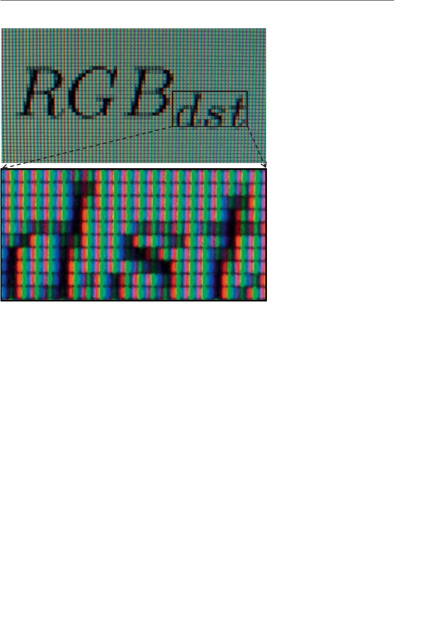
ptg9898810
Figure 4.4 Close-up of RGB color elements in an LCD panel
Another possible use is to set the source and destination factors in the
blending equation to GL_ONE and GL_SRC1_COLOR. In this
configuration, the first color output is added to the framebuffer’s content,
while the second color output is used to attenuate the framebuffer’s
content. The equation becomes:
RGBdst =RGBsrc0+RGBsrc1∗RGBdst
This is a classic multiply-add operation and can be used for many
purposes. For example, if you want to render a translucent object with a
colored specular highlight, write the color of the object to
second_output and the highlight color to first_output.
Writing to Multiple Renderbuffers Simultaneously 199

ptg9898810
Dual-Source Blending and Multiple Fragment Shader Outputs
Because the second output from the fragment shader that
is required to implement dual source blending may take from the resources
available to produce outputs for multiple framebuffer attachments (draw
buffers), there are special counting rules for dual-source blending. When
dual-source blending is enabled---that is, when any of the factors specified
to one of the glBlendFunc() functions is one of the tokens that includes
SRC1, the total number of outputs available in the fragment shader may be
reduced. To determine how many outputs may be used (and consequently,
how many framebuffer attachments may be active), query for the value
of GL_MAX_DUAL_SOURCE_DRAW_BUFFERS. Note that the OpenGL
specification only requires that GL_MAX_DUAL_SOURCE_DRAW_BUFFERS
be at least one. If GL_MAX_DUAL_SOURCE_DRAW_BUFFERS
is exactly one, this means that dual source blending and
multiple draw buffers are mutually exclusive and cannot be used together.
Reading and Copying Pixel Data
Once your rendering is complete, you may want to retrieve the rendered
image for posterity. In that case, you can use the glReadPixels() function
to read pixels from the read framebuffer and return the pixels to your
application. You can return the pixels into memory allocated by the
application, or into a pixel pack buffer, if one’s currently bound.
void glReadPixels(GLint x, GLint y, GLsizei width, GLsizei height,
GLenum format, GLenum type, void *pixels);
Reads pixel data from the read framebuffer rectangle whose lower-left
corner is at (x,y)in window coordinates and whose dimensions are width
and height, and then stores the data in the array pointed to by pixels.
format indicates the kind of pixel data elements that are read (color,
depth, or stencil value as listed in Table 4.9), and type indicates the data
type of each element (see Table 4.10.)
glReadPixels() can generate a few OpenGL errors. A
GL_INVALID_OPERATION error will be generated if format is set to
GL_DEPTH and there is no depth buffer; or if format is GL_STENCIL and
there is no stencil buffer; or if format is set to GL_DEPTH_STENCIL and
there are not both a depth and a stencil buffer associated with the
framebuffer, or if type is neither GL_UNSIGNED_INT_24_8 nor
GL_FLOAT_32_UNSIGNED_INT_24_8_REV, then GL_INVALID_ENUM is
set.
200 Chapter 4: Color, Pixels, and Framebuffers

ptg9898810
Table 4.9 glReadPixels() Data Formats
Format Value Pixel Format
GL_RED or
GL_RED_INTEGER a single red color component
GL_GREEN or
GL_GREEN_INTEGER a single green color component
GL_BLUE or
GL_BLUE_INTEGER a single blue color component
GL_ALPHA or
GL_ALPHA_INTEGER a single alpha color component
GL_RG or
GL_RG_INTEGER a red color component, followed by a
green component
GL_RGB or
GL_RGB_INTEGER a red color component, followed by green
and blue components
GL_RGBA or
GL_RGBA_INTEGER a red color component, followed by green,
blue, and alpha components
GL_BGR or
GL_BGR_INTEGER a blue color component, followed by
green and red components
GL_BGRA or
GL_BGRA_INTEGER a blue color component, followed by
green, red, and alpha components
GL_STENCIL_INDEX a single stencil index
GL_DEPTH_COMPONENT a single depth component
GL_DEPTH_STENCIL combined depth and stencil components
You may need to specify which buffer you want to retrieve pixel values
from. For example, in a double-buffered window, you could read the pixels
from the front buffer or the back buffer. You can use the glReadBuffer()
routine to specify which buffer to retrieve the pixels from.
Reading and Copying Pixel Data 201

ptg9898810
Table 4.10 Data Types for glReadPixels()
Type Value Data Type Packed
GL_UNSIGNED_BYTE GLubyte No
GL_BYTE GLbyte No
GL_UNSIGNED_SHORT GLushort No
GL_SHORT GLshort No
GL_UNSIGNED_INT GLuint No
GL_INT GLint No
GL_HALF_FLOAT GLhalf
GL_FLOAT GLfloat No
GL_UNSIGNED_BYTE_3_3_2 GLubyte Yes
GL_UNSIGNED_BYTE_2_3_3_REV GLubyte Yes
GL_UNSIGNED_SHORT_5_6_5 GLushort Yes
GL_UNSIGNED_SHORT_5_6_5_REV GLushort Yes
GL_UNSIGNED_SHORT_4_4_4_4 GLushort Yes
GL_UNSIGNED_SHORT_4_4_4_4_REV GLushort Yes
GL_UNSIGNED_SHORT_5_5_5_1 GLushort Yes
GL_UNSIGNED_SHORT_1_5_5_5_REV GLushort Yes
GL_UNSIGNED_INT_8_8_8_8 GLuint Yes
GL_UNSIGNED_INT_8_8_8_8_REV GLuint Yes
GL_UNSIGNED_INT_10_10_10_2 GLuint Yes
GL_UNSIGNED_INT_2_10_10_10_REV GLuint Yes
GL_UNSIGNED_INT_24_8 GLuint Yes
GL_UNSIGNED_INT_10F_11F_11F_REV GLuint Yes
GL_UNSIGNED_INT_5_9_9_9_REV GLuint Yes
GL_FLOAT_32_UNSIGNED_INT_24_8_REV GLfloat Yes
Clamping Returned Values
Various types of buffers within OpenGL---most notably floating-point
buffers---can store values with ranges outside of the normal [0, 1]range of
colors in OpenGL. When you read those values back using glReadPixels(),
202 Chapter 4: Color, Pixels, and Framebuffers

ptg9898810
you can control whether the values should be clamped to the normalized
range or left at their full range using glClampColor().
void glClampColor(GLenum target, GLenum clamp);
Controls the clamping of color values for floating- and fixed-point
buffers, when target is GL_CLAMP_READ_COLOR. If clamp is set to
GL_TRUE, color values read from buffers are clamped to the range [0, 1];
conversely, if clamp is GL_FALSE, no clamping is engaged. If your
application uses a combination of fixed- and floating-point buffers, set
clamp to GL_FIXED_ONLY to clamp only the fixed-point values;
floating-point values are returned with their full range.
Copying Pixel Rectangles
To copy pixels between regions of a buffer, or even different framebuffers,
use glBlitFramebuffer(). It uses greater pixel filtering during the copy
operation, much in the same manner as texture mapping (in fact, the same
filtering operations, GL_NEAREST and GL_LINEAR are used during the
copy). Additionally, this routine is aware of multisampled buffers and
supports copying between different framebuffers (as controlled by
framebuffer objects).
void glBlitFramebuffer(GLint srcX0, GLint srcY0, GLint srcX1,
GLint srcY1, GLint dstX0, GLint dstY0,
GLint dstX1, GLint dstY1,
GLbitfield buffers, GLenum filter);
Copies a rectangle of pixel values from one region of the read framebuffer
to another region of the draw framebuffer, potentially resizing, reversing,
converting, and filtering the pixels in the process. srcX0,srcY0,srcX1,
srcY1 represent the source region where pixels are sourced from, and
written to the rectangular region specified by dstX0,dstY0,dstX1, and
dstY1.buffers is the bitwise-or of GL_COLOR_BUFFER_BIT,
GL_DEPTH_BUFFER_BIT, and GL_STENCIL_BUFFER_BIT, which
represent the buffers in which the copy should occur. Finally, filter
specifies the method of interpolation done if the two rectangular regions
are of different sizes, and must be one of GL_NEAREST or GL_LINEAR; no
filtering is applied if the regions are of the same size.
If there are multiple-color draw buffers, each buffer receives a copy of the
source region.
Copying Pixel Rectangles 203

ptg9898810
If srcX1 <srcX0, or dstX1 <dstX0, the image is reversed in the horizontal
direction. Likewise, if srcY1 <srcY0 or dstY1 <dstY0, the image is reversed
in the vertical direction. However, If both the source and destination
sizes are negative in the same direction, no reversal is done.
If the source and destination buffers are of different formats, conversion
of the pixel values is done in most situations. However, if the read color
buffer is a floating-point format, and any of the write color buffers are
not, or vice versa; and if the read-color buffer is a signed (unsigned)
integer format and not all of the draw buffers are signed (unsigned)
integer values, the call will generate a GL_INVALID_OPERATION, and no
pixels will be copied.
Multisampled buffers also have an effect on the copying of pixels. If the
source buffer is multisampled, and the destination is not, the samples are
resolved to a single pixel value for the destination buffer. Conversely, if
the source buffer is not multisampled, and the destination is, the source
pixel’s data is replicated for each sample. Finally, if both buffers are
multisampled and the number of samples for each buffer is the same, the
samples are copied without modification. However, if the buffers have a
different number of samples, no pixels are copied, and a
GL_INVALID_OPERATION error is generated.
A GL_INVALID_VALUE error is generated if buffers have other bits set
than those permitted, or if filter is other than GL_LINEAR or
GL_NEAREST.
204 Chapter 4: Color, Pixels, and Framebuffers

ptg9898810
Chapter 5
Viewing Transformations,
Clipping, and Feedback
Chapter Objectives
After reading this chapter, you’ll be able to do the following:
•View a three-dimensional geometric model by transforming it to have
any size, orientation, and perspective.
•Understand a variety of useful coordinate systems, which ones are
required by OpenGL, and how to transform from one to the next.
•Transform surface normals.
•Clip your geometric model against arbitrary planes.
•Capture the geometric result of these transforms, before displaying
them.
205

ptg9898810
Previous chapters hinted at how to manipulate your geometry to fit into
the viewing area on the screen, but we’ll give a complete treatment in this
chapter. This includes feedback, the ability to send it back to the
application, as well as clipping, the intersection of your geometry with
planes either by OpenGL or by you.
Typically, you’ll have many objects with independently specified
geometric coordinates. These need to be transformed (moved, scaled, and
oriented) into the scene. Then, the scene itself needs to be viewed from a
particular location, direction, scaling, and orientation.
This chapter contains the following major sections:
•‘‘Viewing’’ provides an overview of how computer graphics simulates
the three-dimensional world on a two-dimensional display.
•‘‘User Transformations’’ characterize the various types of
transformations that you can employ in shaders to manipulate vertex
data.
•‘‘OpenGL Transformations’’ are the transformations OpenGL
implements.
•‘‘Transform Feedback’’ describes processing and storing vertex data
using vertex-transforming shaders to optimize rendering performance.
Viewing
If we display a typical geometric model’s coordinates directly onto the
display device, we probably won’t see much. The range of coordinates in
the model (e.g., −100 to +100 meters) will not match the range of
coordinates consumed by the display device (e.g., 0 to 1919 pixels) and it
is cumbersome to restrict ourselves to coordinates that would match. In
addition, we want to view the model from different locations, directions,
and perspectives. How do we compensate for this?
Fundamentally, the display is a flat, fixed, two-dimensional rectangle while
our model contains extended three-dimensional geometry. This chapter
will show how to project our model’s three-dimensional coordinates onto
the fixed two-dimensional screen coordinates.
The key tools for projecting three dimensions down to two are a viewing
model, use of homogeneous coordinates, application of linear transformations
by matrix multiplication, and setting up a viewportmapping. These tools
are each discussed in detail below.
206 Chapter 5: Viewing Transformations, Clipping, and Feedback
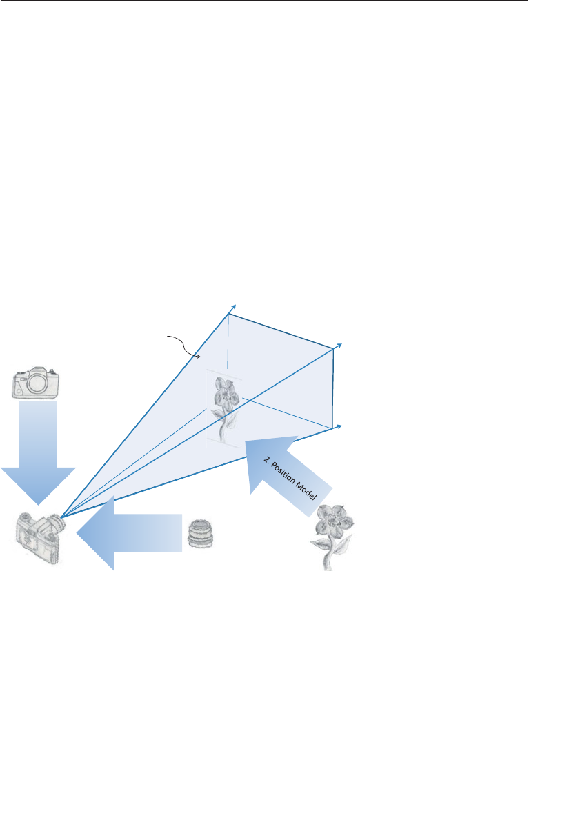
ptg9898810
Viewing Model
For the time being, it is important to keep thinking in terms of
three-dimensional coordinates while making many of the decisions that
determine what is drawn on the screen. It is too early to start thinking
about which pixels need to be drawn. Instead, try to visualize
three-dimensional space. It is later, after the viewing transformations are
completed, after the subjects of this chapter, that pixels will enter the
discussion.
Camera Model
The common transformation process for producing the desired view is
analogous to taking a photograph with a camera. As shown in Figure 5.1
the steps with a camera (or a computer) might be the following:
Rectangular
cone of view
1.
Posion
Camera
3. Select Lens
Figure 5.1 Steps in configuring and positioning the viewing frustum
1. Move your camera to the location you want to shoot from and point
the camera the desired direction (viewing transformation).
2. Move the subject to be photographed into the desired location in the
scene (modeling transformation).
3. Choose a camera lens or adjust the zoom (projection transformation).
4. Take the picture (apply the transformations).
Viewing 207

ptg9898810
5. Stretch or shrink the resulting image to the desired picture size
(viewport transformation). For 3D graphics, this also includes
stretching or shrinking the depth (depth-range scaling). This is not to
be confused with Step 3, which selected how much of the scene to
capture, not how much to stretch the result.
Notice that Steps 1 and 2 can be considered doing the same thing, but in
opposite directions. You can leave the camera where you found it and
bring the subject in front of it, or leave the subject where it is and move
the camera toward the subject. Moving the camera to the left is the same
as moving the subject to the right. Twisting the camera clockwise is the
same as twisting the subject counterclockwise. It is really up to you which
movements you perform as part of Step 1, with the remainder belonging to
Step 2. Because of this, these two steps are normally lumped together as
the model-view transform. It will, though, always consist of some
sequence of movements (translations), rotations, and scalings. The
defining characteristic of this combination is in making a single, unified
space for all the objects assembled into one scene to view, or eye space.
In OpenGL, you are responsible for doing Steps 1 through 3 above in your
shaders. That is, you’ll be required to hand OpenGL coordinates with the
model-view and projective transformations already done. You are also
responsible for telling OpenGL how to do the viewport transformation for
Step 5, but the fixed rendering pipeline will do that transformation for
you, as described in ‘‘OpenGL Transformations’’ on Page 236.
Figure 5.2 summarizes the coordinate systems required by OpenGL for the
full process. So far, we have discussed the second box (user transforms) but
are showing the rest to set the context for the whole viewing stack,
finishing with how you specify your viewport and depth range to OpenGL.
The final coordinates handed to OpenGL for clipping and rasterization are
normalized homogeneous coordinates. That is, the coordinates to be drawn
will be in the range [−1.0, 1.0]until OpenGL scales them to fit the
viewport.
208 Chapter 5: Viewing Transformations, Clipping, and Feedback
ptg9898810
Object units; could be
meters, inches, etc.
(x,y,z) object/model
coordinates
Append wof 1.0
Same units(x, y, z, 1.0) homogeneous
model coordinates
User/shader transforms: scale, rotate, translate, project
Units normalized such that divide by w
leaves visible points between -1.0 to +1.0
(x,y,z,w) homogeneous
clip coordinates
OpenGL divide by w
Range of -1.0 to +1.0 for xand y
and 0.0 to 1.0 for z
(x,y, z) normalized
device coordinates
OpenGL clipping and viewport/depth-range transform
(x,y) units are in pixels (with fracons)
zis in range of 0.0 to 1.0, or depth range
(x,y) are window coordinates
zis depth coordinate
Your starng
coordinates
You need these
in order to
translate and
project
OpenGL
required input
Scaled by OpenGL to
your viewport and
depth range
Rasterizaon
Figure 5.2 Coordinate systems required by OpenGL
(The coordinate systems are the boxes on the left. The central boxes
transform from one coordinate system to the next. Units are described to
the right.)
It will be useful to name additional coordinate systems lying within the
view, model, and projection transforms. These are no longer part of the
OpenGL model, but still highly useful and conventional when using
shaders to assemble a scene or calculate lighting. Figure 5.3 shows an
expansion of the user transforms box from Figure 5.2. In particular, most
lighting calculations done in shaders will be done in eye space. Examples
making full use of eye space are provided in Chapter 7,‘‘Light and
Shadow’’.
Viewing 209
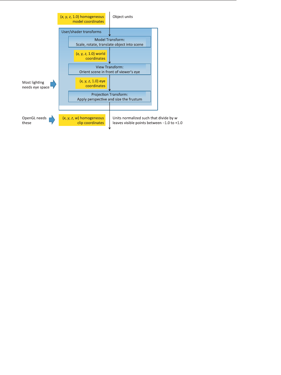
ptg9898810
Figure 5.3 User coordinate systems unseen by OpenGL
(These coordinate systems, while not used by OpenGL, are still vital for
lighting and other shader operations.)
Viewing Frustum
Step 3 in our camera analogy chose a lens, or zoom amount. This selects
how narrow or wide of a rectangular cone through the scene the camera
will capture. Only geometry falling within this cone will be in the final
picture. At the same time, Step 3 will also produce the information needed
(in the homogeneous fourth coordinate, w) to later create the
foreshortening effect of perspective.
210 Chapter 5: Viewing Transformations, Clipping, and Feedback
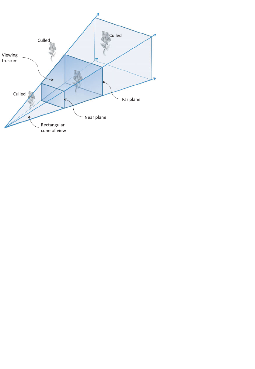
ptg9898810
Figure 5.4 A view frustum
OpenGL will additionally exclude geometry that is too close or too far
away; that is, those in front of a near plane or those behind a far plane.
There is no counterpart to this in the camera analogy (other than cleaning
foreign objects from inside your lens), but is helpful in a variety of ways.
Most importantly, objects approaching the cone’s apex appear infinitely
large, which causes problems, especially if they should reach the apex. At
the other end of this spectrum, objects too far away to be drawn in the
scene are best excluded for performance reasons and some depth precision
reasons as well, if depth must span too large a distance.
Thus, we have two additional planes intersecting the four planes of the
rectangular viewing cone. As shown in Figure 5.4, these six planes define a
frustum-shaped viewing volume.
Frustum Clipping
Any primitive falling outside the four planes forming the rectangular
viewing cone will not get drawn (culled), as it would fall outside our
rectangular display. Further, anything in front of the near plane or behind
the far plane will also be culled. What about a primitive that spans both
sides of one of these planes? OpenGL will clip such primitives. That is, it
will compute the intersection of their geometry with the plane and form
new geometry for just the shape that falls within the frustum.
Viewing 211
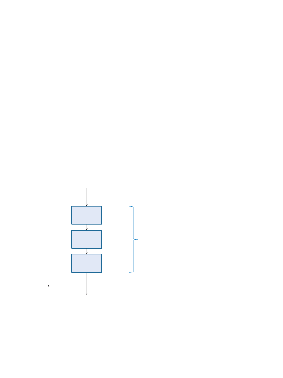
ptg9898810
Because OpenGL has to perform this clipping to draw correctly, the
application must tell OpenGL where this frustum is. This is part of Step 3
of the camera analogy, where the shader must apply the transformations,
but OpenGL must know about it for clipping. There are ways shaders can
clip against additional user planes, discussed later, but the six frustum
planes are an intrinsic part of OpenGL.
Orthographic Viewing Model
Sometimes, a perspective view is not desired, and an orthographic view is
used instead. This type of projection is used by applications for
architectural blueprints and computer-aided design, where it’s crucial to
maintain the actual sizes of objects and the angles between them as they’re
projected. This could be done simply by ignoring one of the x,y, or z
coordinates, letting the other two coordinates give two-dimensional
locations. You would do that, of course, after orienting the objects and the
scene with model-view transformations, as with the camera model. But, in
the end, you will still need to locate and scale the resulting model for
display in normalized device coordinates. The transformation for this is
the last one given in the next section.
User Transformations
Inial model
coordinates
Stages that transform
coordinates to OpenGL
required form
Coordinates OpenGL
can map to a window
(clip coordinates)
Transform
feedback
.
.
.
Rasterizer
Vertex
Shading Stage
Tessellaon
Shading
Stages
Geometry
Shading Stage
Figure 5.5 Pipeline subset for user/shader part of transforming
coordinates
212 Chapter 5: Viewing Transformations, Clipping, and Feedback

ptg9898810
The stages of the rendering pipeline that transform three-dimensional
coordinates for OpenGL viewing are shown in Figure 5.5. Essentially,
they are the programmable stages appearing before rasterization. Because
these stages are programmable, you have a lot of flexibility in the initial
form of your coordinates and in how you transform them. However, you
are constrained to end with the form the subsequent fixed
(nonprogrammable) stages need. That is, we’ll need to make homogeneous
coordinates that are ready for perspective division (also referred to as clip
coordinates). What that means and how to do it are the subjects of the
following sections.
Each of the viewing model steps above was called out as a transformation.
They are all linear transformations that can be accomplished through
matrix multiplication on homogeneous coordinates. The upcoming matrix
multiplication and homogenous coordinate sections give refreshers on
these topics. Understanding them is the key to truly understanding how
OpenGL transformations work.
In a shader, transforming a vertex by a matrix looks like this:
#version 330 core
uniform mat4 Transform; // stays the same for many vertices
// (primitive granularity)
in vec4 Vertex; // per-vertex data sent each time this
// shader is run
void main()
{
gl_Position = Transform *Vertex;
}
Linear transformations are composable; so just because our camera analogy
needed four transformation steps does not mean we have to transform our
data four times. Rather, all those transformations can be composed into a
single transformation. If we want to transform our model first by
transformation matrix Afollowed by transformation matrix B, we will see
we can do so with transformation matrix C, where
C=BA
(Because we are showing examples of matrix multiplication with the
vertex on the right and the matrix on the left, composing transforms show
up in reverse order: Bis applied to the result of applying Ato a vertex. The
details behind this are explained in the upcoming refresher.)
So, the good news is we can collapse any number of linear transformations
into a single matrix multiply, allowing the freedom to think in terms of
whatever steps are most convenient.
User Transformations 213

ptg9898810
Matrix Multiply Refresher
For our use, matrices and matrix multiplication are nothing more than a
convenient mechanism for expressing linear transformations, which in
turn are a useful way to do the coordinate manipulations needed for
displaying models. The vital matrix mechanism is explained here, while
interesting uses for it will come up in numerous places in subsequent
discussions.
First, a definition. A 4 ×4 matrix takes a four-component vector to another
four-component vector through multiplication by the following rule:
⎡
⎢⎢⎢
⎣
a b c d
e f g h
i j k l
m n o p
⎤
⎥⎥⎥
⎦⎛
⎜⎜⎜
⎝
x
y
z
w
⎞
⎟⎟⎟
⎠→⎛
⎜⎜⎜
⎝
ax +by +cz +dw
ex +fy +gz +hw
ix +jy +kz +lw
mx +ny +oz +pw
⎞
⎟⎟⎟
⎠
Now, some observations.
•Each component of the new vector is a linear function of all the
components of the old vector, hence the need for 16 values in the
matrix.
•The multiplication always takes the vector (0, 0, 0, 0)to (0, 0, 0, 0). This
is characteristic of linear transformations and shows that if this was a
3×3 matrix times a three-component vector, why translation
(moving) can’t be done with a matrix multiply. We’ll see how
translating a three-component vector becomes possible with a
4×4 matrix and homogeneous coordinates.
In our viewing models, we will want to take a vector through multiple
transformations, here expressed as matrix multiplications by matrices A
and then B:
v=Av (5.1)
v =Bv=B(Av) = (BA)v(5.2)
and we’ll want to do this efficiently by finding a matrix Csuch that
v =Cv
where
C=BA
214 Chapter 5: Viewing Transformations, Clipping, and Feedback

ptg9898810
Being able to compose the Btransform and the Atransform into a single
transform Cis a benefit we get by sticking to linear transformations. The
following definition of matrix multiplication makes all of this work out.
⎡
⎢⎢⎢
⎣
b11 b12 b13 b14
b21 b22 b23 b24
b31 b32 b33 b34
b41 b42 b43 b44
⎤
⎥⎥⎥
⎦⎡
⎢⎢⎢
⎣
a11 a12 a13 a14
a21 a22 a23 a24
a31 a32 a33 a34
a41 a42 a43 a44
⎤
⎥⎥⎥
⎦→⎡
⎢⎢⎢
⎣
c11 c12 c13 c14
c21 c22 c23 c24
c31 c32 c33 c34
c41 c42 c43 c44
⎤
⎥⎥⎥
⎦
where
cij =bi1a1j+bi2a2j+bi3a3j+bi4a4j
that is c11 =b11a11 +b12a21 +b13a31 +b14a41
c12 =b11a12 +b12a22 +b13a32 +b14a42
c13 =b11a13 +b12a23 +b13a33 +b14a43
c14 =b11a14 +b12a24 +b13a34 +b14a44
c21 =b21a11 +b12a21 +b13a31 +b14a41
c22 =b21a12 +b22a22 +b23a32 +b24a42
.
.
....
c44 =b41a14 +b42a24 +b43a34 +b44a44
Matrix multiplication is noncommutative: generally speaking, when
multiplying matrices and Aand B
AB =BA
and, generally, when multiplying matrix Aand vector v
Av =vA
so care is needed to multiply in the correct order. Matrix multiplication is,
fortunately, associative:
C(BA) = (CB)A=CBA
That’s useful, as accumulated matrix multiplies on a vector can be
re-associated.
C(B(Av)) = (CBA)v
This is a key result we will take advantage of to improve performance.
Homogeneous Coordinates
The geometry we want to transform is innately three-dimensional.
However, we will gain two key advantages by moving from
User Transformations 215

ptg9898810
three-component Cartesian coordinates to four-component homogeneous
coordinates. These are 1) the ability to apply perspective and 2) the ability
to translate (move) the model using only a linear transform. That is, we
will be able to get all the rotations, translations, scaling, and projective
transformations we need by doing matrix multiplication if we first move
to a four-coordinate system. More accurately, the projective
transformation is a key step in creating perspective, and it is the step we
must perform in our shaders. (The final step is performed by the system
when it eliminates this new fourth coordinate.)
If you want to understand this and homogeneous coordinates more
deeply, read the next section. If you just want to go on some faith and grab
4×4 matrices that will get the job done, you can skip to the next section.
Advanced: What Are Homogeneous Coordinates?
Three-dimensional data can be scaled and rotated with linear
transformations of three-component vectors by multiplying by 3 ×3
matrices.
Unfortunately, translating (moving/sliding over) three-dimensional
Cartesian coordinates cannot be done by multiplying with a 3 ×3 matrix. It
requires an extra vector addition to move the point (0, 0, 0)somewhere
else. This is a called an affine transformation, which is not a linear
transformation. (Recall that any linear transformation maps (0, 0, 0)to
(0, 0, 0).) Including that addition means the loss of the benefits of linear
transformations, like the ability to compose multiple transformations into
a single transformation. So, we want to find a way to translate with a linear
transformation. Fortunately, by embedding our data in a four-coordinate
space, affine transformations turn back into a simple linear transform
(meaning you can move your model laterally using only multiplication by
a 4 ×4 matrix).
For example, to move data by 0.3 in the ydirection, assuming a fourth
vector coordinate of 1.0:
⎡
⎢⎢⎢
⎣
1.0 0.00.0 0.0
0.01.00.0 0.3
0.00.01.0 0.0
0.00.00.0 1.0
⎤
⎥⎥⎥
⎦⎛
⎜⎜⎜
⎝
x
y
z
1.0
⎞
⎟⎟⎟
⎠→⎛
⎜⎜⎜
⎝
x
y+0.3
z
1.0
⎞
⎟⎟⎟
⎠
At the same time, we acquire the extra component needed to do
perspective.
216 Chapter 5: Viewing Transformations, Clipping, and Feedback
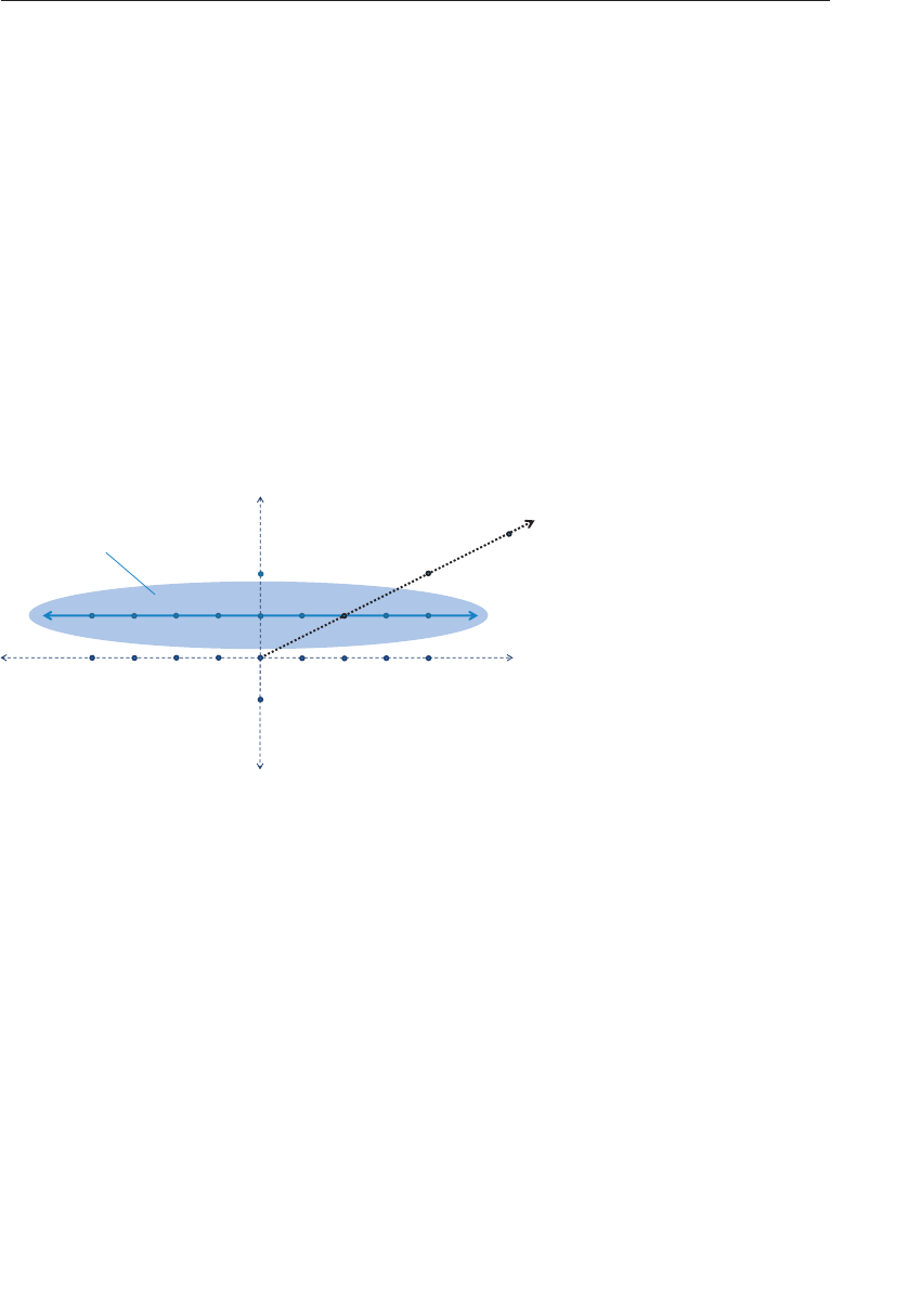
ptg9898810
A homogeneous coordinate has one extra component and does not change
the point it represents when all its components are scaled by the same
amount.
For example, all these coordinates represent the same point:
(2.0, 3.0, 5.0, 1.0)
(4.0, 6.0, 10.0, 2.0)
(0.2, 0.3, 0.5, 0.1)
In this way, homogeneous coordinates act as directions instead of
locations; scaling a direction leaves it pointing in the same direction. This
is shown in Figure 5.6. Standing at (0, 0), the homogeneous points (1, 2),
(2, 4), and others along that line appear in the same place. When projected
onto the 1D space, they all become the point 2.
1234 x
y
0
1
2
1234
-4 -3 -2 -1
-4 -3 -2 -1
2-D Space
Many two-component homogeneous
Coordinates for the number 2
-1
(2, 1)
(4, 2)
0
Embedded
1-D Space
(6, 3)
Figure 5.6 One-dimensional homogeneous space
(Shows how to embed the 1D space into two dimensions, at the location
y=1, to get homogeneous coordinates.)
Skewing is a linear transformation. Skewing Figure 5.6 can translate the
embedded 1D space, as show in Figure 5.7, while preserving the location of
(0, 0)in the 2D space (all linear transforms keep (0, 0)fixed).
User Transformations 217
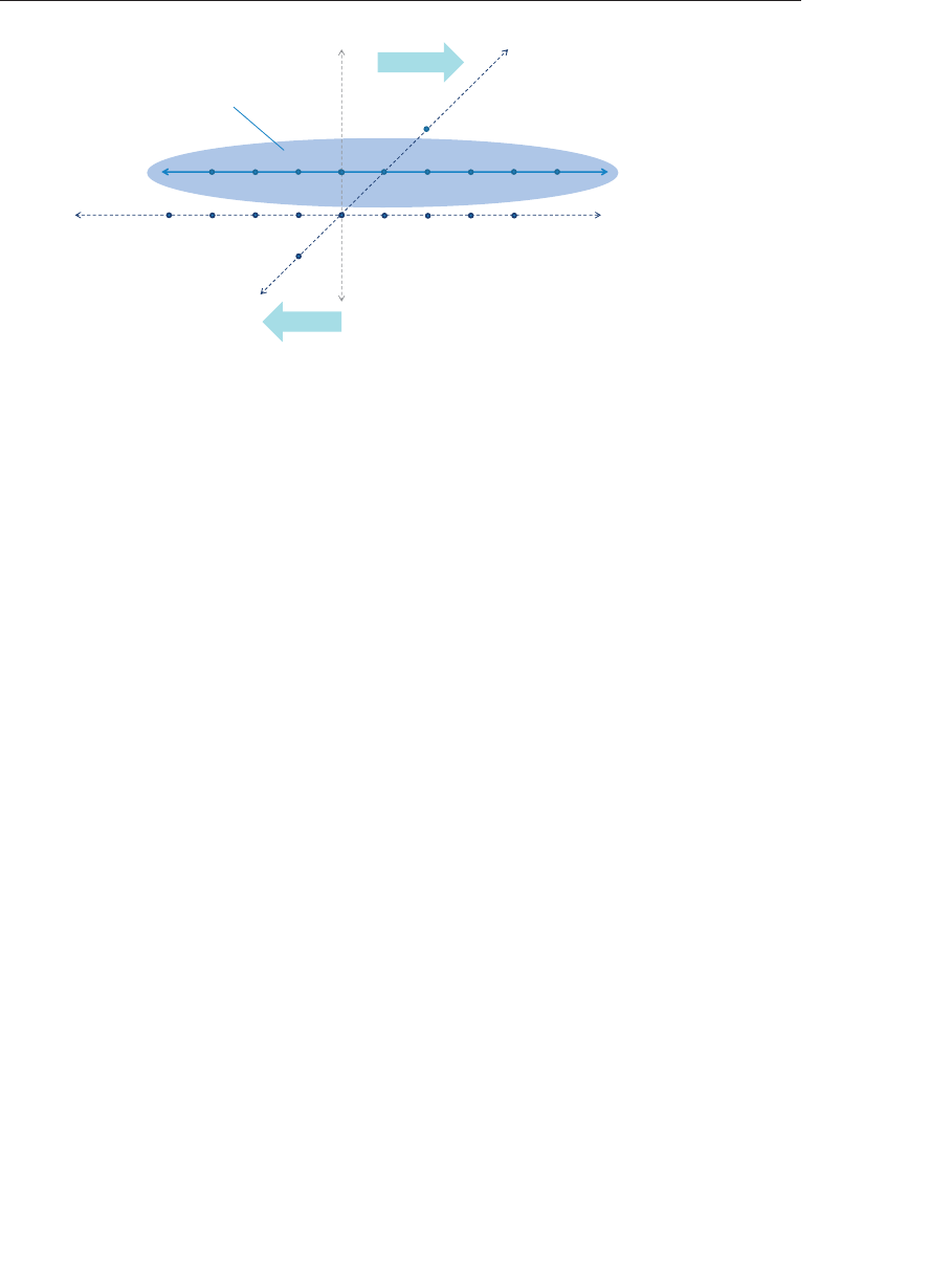
ptg9898810
1234 x
-4 -3 -2 -1
-1
y
0
y
1
2
2-D skewing (linear transform) allows 1-D
translaon (non-linear) transform
Skew
Skew
01234
-4 -3 -2 -1
Embedded
1-D Space
Figure 5.7 Translating by skewing
The desire is to translate points in the 1D space with a linear transform.
This is impossible within the 1D space, as the point 0 needs to
move---something 1D linear transformations cannot do. However, the 2D
skewing transformation is linear and accomplishes the goal of translating
the 1D space.
If the last component of an homogeneous coordinate is 0, it implies a
‘‘point at infinity’’. The 1D space has only two such points at infinity, one
in the positive direction and one in the negative direction. However, the
3D space, embedded in a four-coordinate homogeneous space, has a point
at infinity for any direction you can point. These points can model the
perspective point where two parallel lines (e.g., sides of a building or
railroad tracks) would appear to meet. The perspective effects we care
about, though, will become visible without needing to specifically think
about this.
We will move to homogeneous coordinates by adding a fourth w
component of 1.0.
(2.0, 3.0, 5.0)→(2.0, 3.0, 5.0, 1.0)
and later go back to Cartesian coordinates by dividing all components by
the fourth component and dropping the fourth component.
(4.0, 6.0, 10.0, 2.0)divide by w
−−−−−−−→ (2.0, 3.0, 5.0, 1.0)drop w
−−−−→ (2.0, 3.0, 5.0)
Perspective transforms modify wcomponents to values other than 1.0.
Making wlarger can make coordinates appear further away. When it’s time
to display geometry, OpenGL will transform homogeneous coordinates
218 Chapter 5: Viewing Transformations, Clipping, and Feedback

ptg9898810
back to the three-dimensional Cartesian coordinates by dividing their first
three components by the last component. This will make the objects
farther away (now having a larger w) have smaller Cartesian coordinates,
hence getting drawn on a smaller scale. A wof 0.0 implies (x,y)
coordinates at infinity (the object got so close to the viewpoint that its
perspective view got infinitely large). This can lead to undefined results.
There is nothing fundamentally wrong with a negative w; the following
coordinates represent the same point.
(2.0, 3.0, 5.0, 1.0)
(−2.0, −3.0, −5.0, −1.0)
But negative wcan stir up trouble in some parts of the graphics pipeline,
especially if it ever gets interpolated toward a positive w, as that can make
it land on or very near 0.0. The simplest way to avoid problems is to keep
your wcomponents positive.
Linear Transformations and Matrices
We start our task of mapping into device coordinates by adding a fourth
component to our three-dimensional Cartesian coordinates, with a value
of 1.0, to make homogeneous coordinates. These coordinates are then
ready to be multiplied by one or more 4 ×4 matrices that rotate, scale,
translate, and apply perspective. Examples of how to use each of these
transforms are given below. The summary is that each of these
transformations can be made through multiplication by a 4 ×4 matrix,
and a series of such transformations can be composed into a single 4 ×4
matrix, once, that can then be used on multiple vertices.
Translation
Translating an object takes advantage of the fourth component we just
added to our model coordinates and of the fourth column of a 4 ×4
transformation matrix. We want a matrix Tto multiply all our object’s
vertices vby to get translated vertices v.
v=Tv
Each component can be translated by a different amount by putting those
amounts in the fourth column of T. For example, to translate by 2.5 in the
positive xdirection, and not at all in the yor zdirections:
T=⎡
⎢⎢⎢
⎣
1.0 0.0 0.02.5
0.0 1.0 0.00.0
0.0 0.0 1.00.0
0.0 0.00.01.0
⎤
⎥⎥⎥
⎦
User Transformations 219
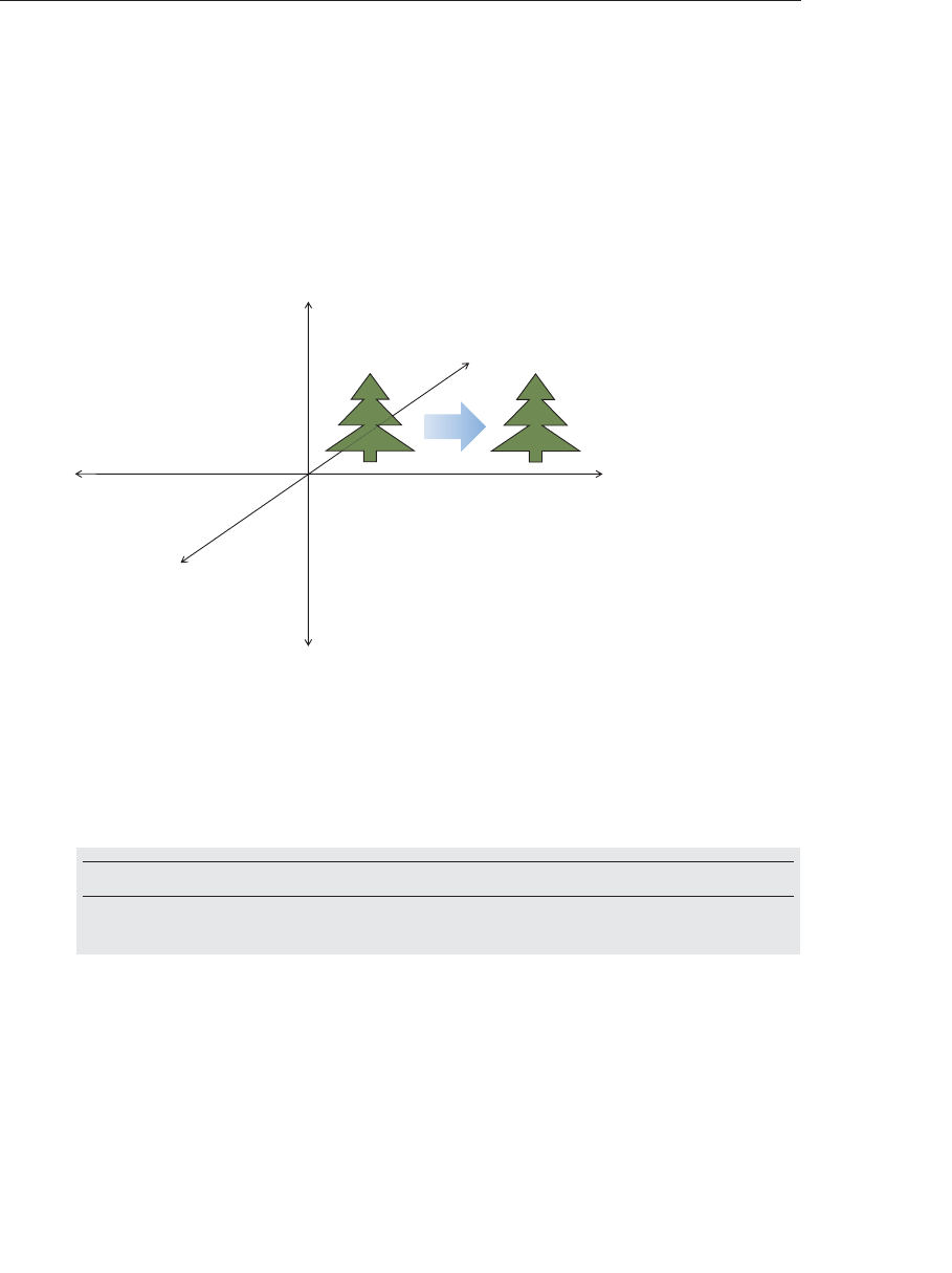
ptg9898810
and multiplying by a vector v= (x,y,z,1)gives
⎛
⎜⎜⎜
⎝
x+2.5
y
z
1.0
⎞
⎟⎟⎟
⎠
=⎡
⎢⎢⎢
⎣
1.0 0.0 0.0 2.5
0.0 1.0 0.0 0.0
0.0 0.0 1.00.0
0.0 0.0 0.01.0
⎤
⎥⎥⎥
⎦⎛
⎜⎜⎜
⎝
x
y
z
1.0
⎞
⎟⎟⎟
⎠
This is demonstrated in Figure 5.8.
z
0
x
y
+ 2.5
21 3 4
Figure 5.8 Translating an object 2.5 in the xdirection
Of course, you’ll want such matrix operations encapsulated. There are
numerous utilities available for this and one is included in the
accompanying vmath.h. We already used it in Chapter 3,‘‘Drawing with
OpenGL’’. To create a translation matrix using this utility, call:
vmath::mat4 vmath::translate(float x, float y, float z);
Returns a transformation matrix for translating an amount (x,y,z).
The following listing shows a use of this.
// Application (C++) code
#include "vmath.h"
.
.
.
// Make a transformation matrix that translates coordinates by (1, 2, 3)
220 Chapter 5: Viewing Transformations, Clipping, and Feedback
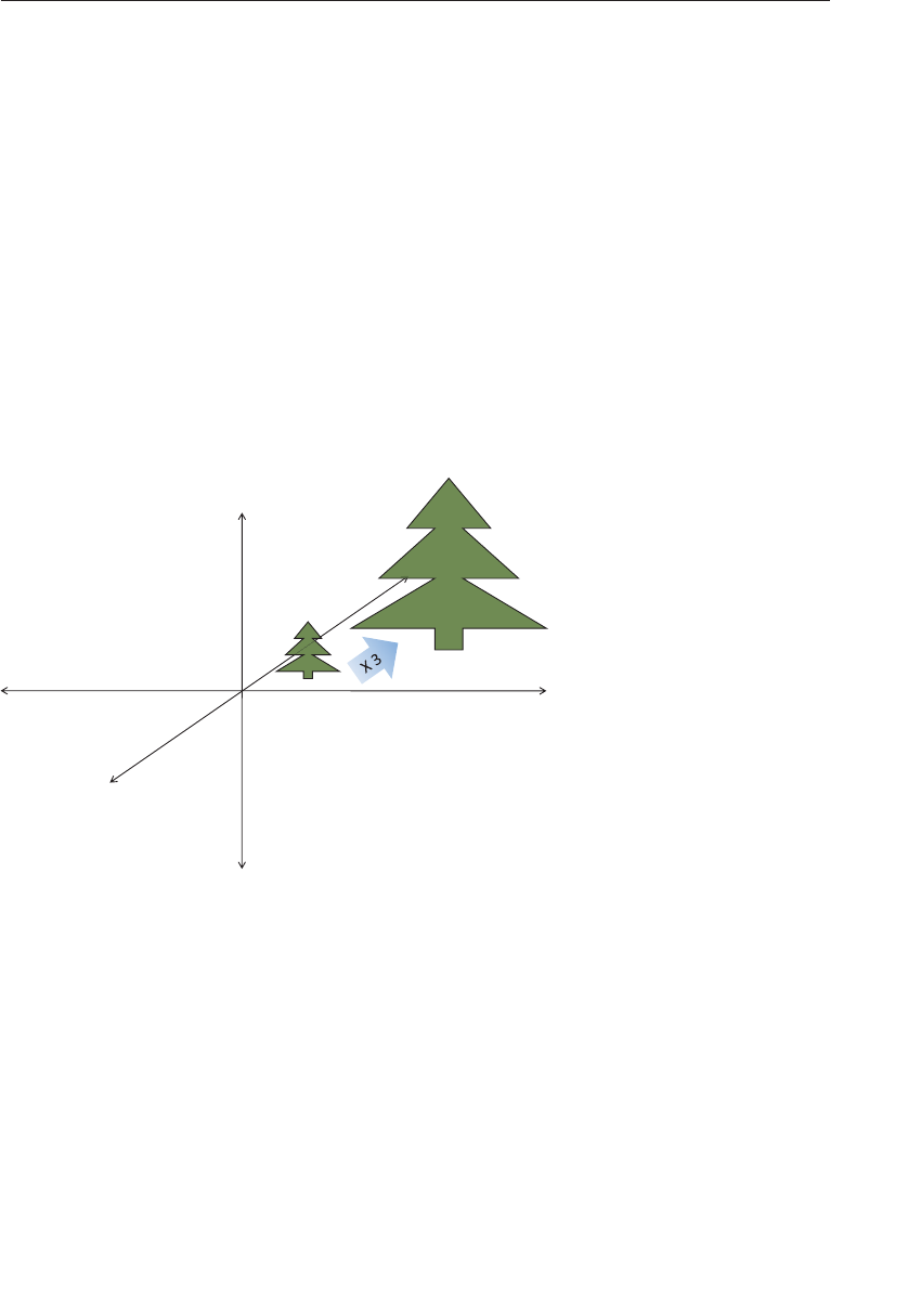
ptg9898810
vmath::mat4 translationMatrix = vmath::translate(1.0, 2.0, 3,0);
// Set this matrix into the current program.
glUniformMatrix4fv(matrix_loc, 1, GL_FALSE, translationMatrix);
.
.
.
After going through the next type of transformation, we’ll show a code
example for combining transformations with this utility.
Scaling
Grow or shrink an object, as in Figure 5.9, by putting the desired scaling
factor on the first three diagonal components of the matrix. Making a
scaling matrix S, which applied to all vertices vin an object, would change
its size.
z
0
x
y
21 3 4
Figure 5.9 Scaling an object to three times its size
(Note that if the object is off center, this also moves its center three times
further from (0, 0, 0).)
User Transformations 221

ptg9898810
The following example makes geometry 3 times larger.
S=⎡
⎢⎢⎢
⎣
3.0 0.00.0 0.0
0.0 3.00.0 0.0
0.0 0.03.0 0.0
0.0 0.00.0 1.0
⎤
⎥⎥⎥
⎦
⎛
⎜⎜⎜
⎝
3x
3y
3z
1
⎞
⎟⎟⎟
⎠
=⎡
⎢⎢⎢
⎣
3.00.0 0.0 0.0
0.03.0 0.0 0.0
0.0 0.0 3.0 0.0
0.0 0.0 0.01.0
⎤
⎥⎥⎥
⎦⎛
⎜⎜⎜
⎝
x
y
z
1.0
⎞
⎟⎟⎟
⎠
Note that nonisomorphic scaling is easily done, as the scaling is per
component, but it would be rare to do so when setting up your view and
model transforms. (If you want to stretch results vertically or horizontally,
do that at the end with the viewport transformation. Doing it too early
would make shapes change when they rotate.) Note that when scaling, we
didn’t scale the wcomponent, as that would result in no net change to the
point represented by the homogeneous coordinate (since in the end, all
components are divided by w).
If the object being scaled is not centered at (0, 0, 0), the simple matrix
above will also move it further or closer to (0, 0, 0)by the scaling amount.
Usually, it is easier to understand what happens when scaling if you first
center the object around (0, 0, 0). Then scaling leaves it in the same place
while changing its size. If you want to change the size of an off-center
object without moving it, first translate its center to (0, 0, 0), then scale it,
and finally translate it back. This is shown in Figure 5.10.
222 Chapter 5: Viewing Transformations, Clipping, and Feedback
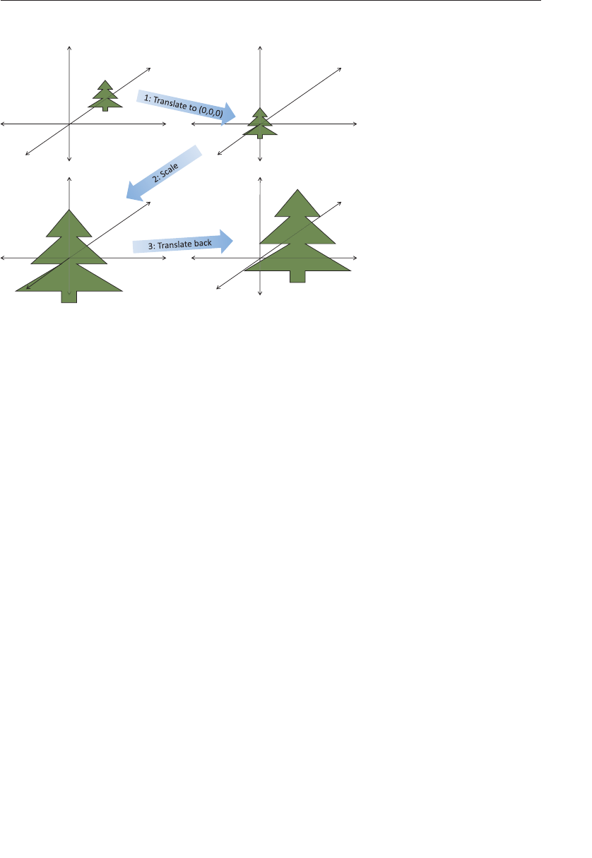
ptg9898810
z
0x
y
21
z
0x
y
21
z
0
x
21
z
0
x
21
Figure 5.10 Scaling an object in place
(Scale in place by moving to (0, 0, 0), scaling, and then moving it back.)
This would use three matrices, T,S, and T−1, for translate to (0, 0, 0), scale,
and translate back, respectively. When each vertex vof the object is
multiplied by each of these matrices in turn, the final effect is that the
object would change size in place, yielding a new set of vertices v:
v=T−1(S(Tv))
or
v= (T−1ST)v
which allows for pre-multiplication of the three matrices into a single
matrix.
M=T−1ST
v=Mv
Mnow does the complete job of scaling an off-center object.
To create a scaling transformation with the included utility, you can use
User Transformations 223

ptg9898810
vmath::mat4 vmath::scale(float s);
Returns a transformation matrix for scaling an amount s.
The resulting matrix can be directly multiplied by another such
transformation matrix to compose them into a single matrix that performs
both transformations.
// Application (C++) code
#include "vmath.h"
.
.
.
// Compose translation and scaling transforms
vmath::mat4 translateMatrix = vmath::translate(1.0, 2.0, 3,0);
vmath::mat4 scaleMatrix = vmath::scale(5.0);
vmath::mat4 scaleTranslateMatrix = scaleMatrix *translateMatrix;
.
.
.
Any sequence of transformations can be combined into a single matrix
this way.
Rotation
Rotating an object follows a similar scheme. We want a matrix Rthat when
applied to all vertices vin an object will rotate it. The following example,
shown in Figure 5.11 rotates 50 degrees counterclockwise around the z
axis. Figure 5.12 shows how to rotate an object without moving its center,
instead of also revolving it around the zaxis.
224 Chapter 5: Viewing Transformations, Clipping, and Feedback
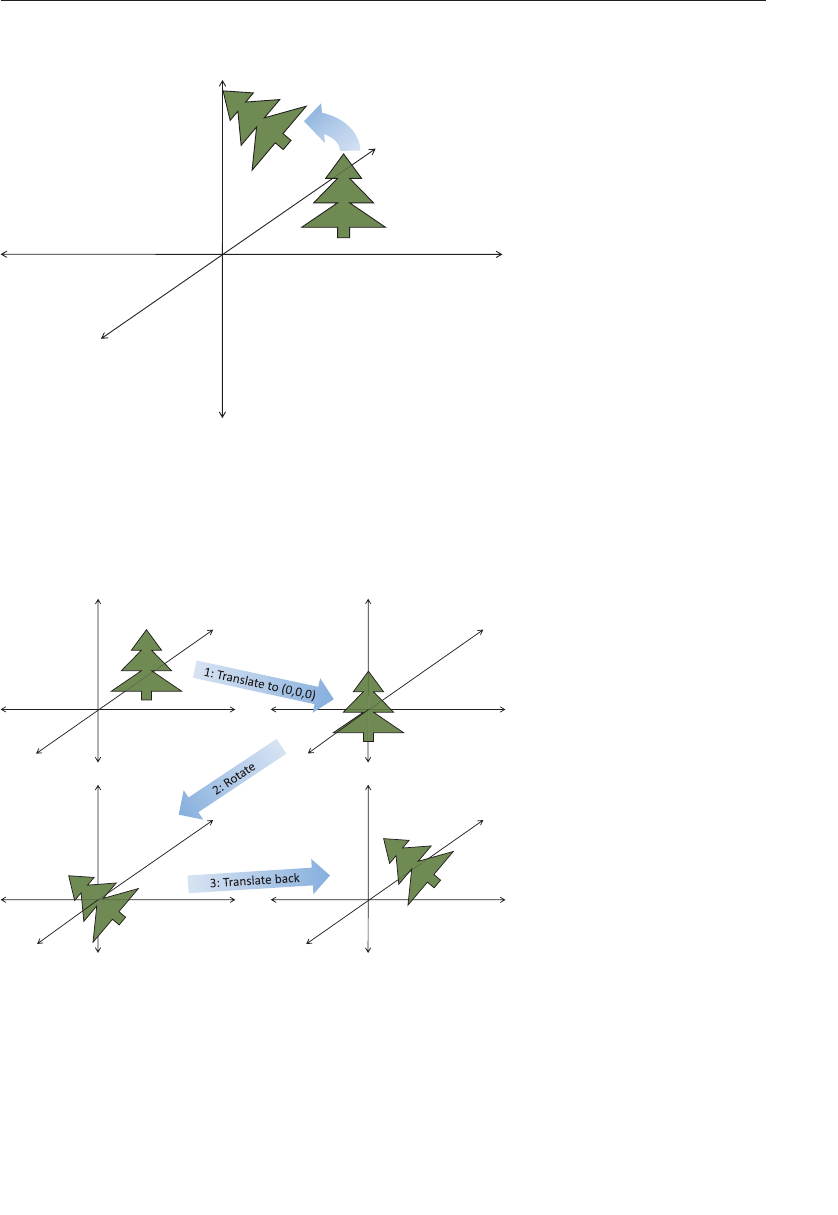
ptg9898810
z
0
x
y
21 3 4
50
degrees
Figure 5.11 Rotation
(Rotating an object 50 degrees in the xy plane, around the zaxis. Note if the
object is off center, it also revolves the object around the point (0, 0, 0).)
z
0x
y
21
z
0x
y
21
z
0
x
21
z
0x
21
Figure 5.12 Rotating in place
(Rotating an object in place by moving it to (0, 0, 0), rotating, and then
moving it back.)
User Transformations 225

ptg9898810
R=⎡
⎢⎢⎢
⎣
cos 50 −sin 50 0.0 0.0
sin 50 cos 50 0.0 0.0
0.0 0.0 1.0 0.0
0.0 0.0 0.0 1.0
⎤
⎥⎥⎥
⎦
⎛
⎜⎜⎜
⎝
cos 50 ·x−sin 50 ·y
sin 50 ·x+cos 50 ·y
z
1.0
⎞
⎟⎟⎟
⎠
=⎡
⎢⎢⎢
⎣
cos 50 −sin 50 0.0 0.0
sin 50 cos 50 0.0 0.0
0.0 0.0 1.0 0.0
0.0 0.0 0.0 1.0
⎤
⎥⎥⎥
⎦⎛
⎜⎜⎜
⎝
x
y
z
1.0
⎞
⎟⎟⎟
⎠
When rotating around the zaxis above, the vertices in the object keep
their zvalues the same, rotating in the xy plane. To rotate instead around
the xaxis by an amount θ:
Rx=⎡
⎢⎢⎢
⎢⎢⎢
⎣
1.0 0.0 0.0 0.0
0.0cos θ−sin θ0.0
0.0sin θcos θ0.0
0.0 0.0 1.0 0.0
0.0 0.0 0.0 1.0
⎤
⎥⎥⎥
⎥⎥⎥
⎦
and around the yaxis:
Ry=⎡
⎢⎢⎢
⎣
cos θ0.0−sin θ0.0
0.0 1.0 0.0 0.0
sin θ0.0cos θ0.0
0.0 0.0 0.0 1.0
⎤
⎥⎥⎥
⎦
In all cases, the rotation is in the direction of the first axis toward the
second axis. That is, from the row with the cos −sin pattern to the row
with the sin cos pattern, for the positive axes corresponding to these rows.
If the object being rotated is not centered at (0, 0, 0), the matrices above
will also rotate the whole object around (0, 0, 0), changing its location.
Again, as with scaling, it’ll be easier to first center the object around
(0, 0, 0). So, again, translate it to (0, 0, 0), transform it, and then translate it
back. This could use three matrices, T,R, and T−1, to translate to (0, 0, 0),
rotate, and translate back.
v=T−1(R(Tv))
or
v= (T−1RT)v
which again allows for the pre-multiplication into a single matrix.
226 Chapter 5: Viewing Transformations, Clipping, and Feedback

ptg9898810
To create a rotation transformation with the included utility, you can use
vmath::mat4 vmath::rotate(float x, float y, float z);
Returns a transformation matrix for rotating xdegrees around the xaxis,
ydegrees around the yaxis, and zdegrees around the zaxis. It then
multiplies that matrix (on the left) by the current matrix (on the right).
Perspective Projection
This one is a bit tougher. We now assume viewing and modeling
transformations are completed, with larger zvalues meaning objects are
further away.
We will consider the following two cases:
1. Symmetric, centered frustum, where the z-axis is centered in the cone.
2. Asymmetric frustum, like seeing what’s through a window when you
looking near it, but not toward its middle.
For all, the viewpoint is now at (0, 0, 0), looking generally toward the
positive zdirection.
First, however, let’s consider an over-simplified (hypothetical) perspective
projection.
⎡
⎢⎢⎢
⎣
1.0 0.00.0 0.0
0.0 1.00.0 0.0
0.0 0.01.0 0.0
0.0 0.01.0 0.0
⎤
⎥⎥⎥
⎦⎛
⎜⎜⎜
⎝
x
y
z
1.0
⎞
⎟⎟⎟
⎠→⎛
⎜⎜⎜
⎝
x
y
z
z
⎞
⎟⎟⎟
⎠
Note the last matrix row replaces the w(fourth) coordinate with the z
coordinate. This will make objects with a larger z(further away) appear
smaller when the division by woccurs, creating a perspective effect.
However, this particular method has some shortcomings. For one, all z
values will end up at 1.0, losing information about depth. We also didn’t
have much control over the cone we are projecting and the rectangle we
are projecting onto. Finally, we didn’t scale the result to the [−1.0, 1.0]
range expected by the viewport transform. The remaining examples take
all this into account.
So, we consider now a fuller example for OpenGL, using a symmetric
centered frustum. We refer back to our view frustum, shown again with the
size of the near plane labeled in Figure 5.13.
User Transformations 227
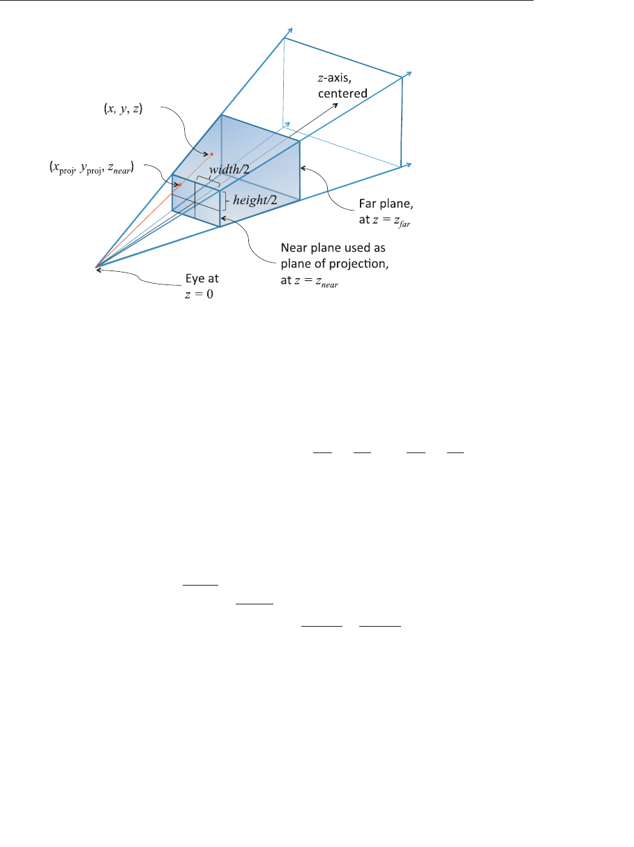
ptg9898810
Figure 5.13 Frustum projection
(Frustum with the near plane and half its width and height labeled.)
We want to project points in the frustum onto the near plane, directed
along straight lines going toward (0, 0, 0). Any straight line emanating
from (0, 0, 0)keeps the ratio if zto xthe same for all its points, and
similarly for the ratio of zto y. Thus, the (xproj,yproj)value of the projection
on the near plane will keep the ratios of znear
z=xproj
xand znear
z=yproj
y.We know
there is an upcoming division by depth to eliminate homogeneous
coordinates, so solving for xproj while still in the homogeneous space
simply gives xproj =x·znear. Similarly, yproj =y·znear . If we then include a
divide by the size of the near plane to scale the near plane to the range of
[−1.0, 1.0], we end up with the requisite first two diagonal elements shown
in the projection transformation matrix.
⎡
⎢⎢⎢
⎢⎣
znear
width/20.0 0.0 0.0
0.0znear
height/20.0 0.0
0.0 0.0−zfar +znear
zfar −znear
2zfar znear
zfar −znear
0.0 0.0−1.0 0.0
⎤
⎥⎥⎥
⎥⎦
(This could also be computed from the angle of the viewing cone, if so
desired.)
Finally, we consider the second perspective projection case: the
asymmetric frustum. This is the fully general frustum, when the near plane
might not be centered on the zaxis. The zaxis could even be completely
228 Chapter 5: Viewing Transformations, Clipping, and Feedback

ptg9898810
outside it, as mentioned earlier when looking at an interior wall next to a
window. Your direction of view is the positive zaxis, which is not going
through the window. You see the window off to the side, with an
asymmetric perspective view of what’s outside the window. In this case,
points on the near plane are already in the correct location, but those
further away need to be adjusted for the fact that the projection in the
near plane is off center. You can see this adjustment in the third column of
the matrix, which moves the points an amount based on how off-center
the near-plane projection is, scaled by how far away the points are
(because this column multiplies by z).
⎡
⎢⎢⎢
⎢⎢⎢
⎣
znear
width/20.0left+right
width/20.0
0.0znear
height/2
top+bottom
height/20.0
0.0 0.0−zfar +znear
zfar −znear
2zfar znear
zfar −znear
0.0 0.0−1.0 0.0
⎤
⎥⎥⎥
⎥⎥⎥
⎦
All the above steps, rotate, scale, translate, project, and possibly others,
will make matrices that can be multiplied together into a single matrix.
Now with one multiplication by this new matrix, we can simultaneously
scale, translate, rotate, and apply the perspective projection.
To create a perspective projection transformation with the included utility,
there are a couple of choices. You can have full control, as above, using a
frustum call or you can more casually and intuitively create one with the
lookat call.
vmath::mat4 vmath::frustum(float left, float right, float bottom,
float top, float near, float far);
Returns a perspective projection matrix based on the described frustum.
The rectangle of the near plane is defined by the left,right,bottom, and
top. The distances of the near and far planes are defined by near and far.
vmath::mat4 vmath::lookAt(vmath::vec3 eye, vmath::vec3 center,
vmath::vec3 up);
Returns a perspective projection matrix based on looking toward center
from eye with up defining what direction is up.
User Transformations 229
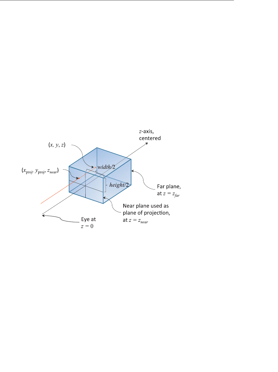
ptg9898810
The resulting vectors, still having four coordinates, are the homogeneous
coordinates expected by the OpenGL pipeline.
The final step in projecting the perspective view onto the screen is to
divide the (x,y,z)coordinates in vby the wcoordinate in v, for every
vertex. However, this is done internally by OpenGL; it is not something
you do in your shaders.
Orthographic Projection
With an orthographic projection, the viewing volume is a rectangular
parallelpiped, or, more informally, a box (see Figure 5.14). Unlike
perspective projection, the size of the viewing volume doesn’t change from
one end to the other, so distance from the camera doesn’t affect how large
an object appears.
Figure 5.14 Orthographic projection
(Starts with straightforward projection of the parallelpiped onto the front
plane. x,y, and zwill need to be scaled to fit into [−1, 1],[−1, 1], and [0, 1],
respectively. This will be done by dividing by the sizes of the width, height,
and depth in the model.)
This is done after all the translation, scaling, and rotation is done to look
in the positive zdirection to see the model to view. With no perspective,
we will keep the was it is (1.0), accomplished by making the bottom row
of the transformation matrix (0, 0, 0, 1).We will still scale zto lie within
[0, 1]so z-buffering can hide obscured objects, but neither znor wwill
have any effect on the screen location. That leaves scaling xfrom the
width of the model to [−1, 1]and similarly for y. For a symmetric volume
230 Chapter 5: Viewing Transformations, Clipping, and Feedback

ptg9898810
(positive zgoing down the middle of the parallelpiped) this can be done
with the following matrix:
⎡
⎢⎢⎢
⎢⎣
1
width/20.0 0.00.0
0.01
height/20.0 0.0
0.0 0.0−1
(zfar −znear )/2−zfar +znear
zfar −znear
0.0 0.0 0.0 1.0
⎤
⎥⎥⎥
⎥⎦
For the case of the positive znot going down the middle of the view (but
still looking parallel to the zaxis to see the model), the matrix is just
slightly more complex. We use the diagonal to scale and the fourth
column to center.
⎡
⎢⎢⎢
⎢⎢⎢
⎢⎣
1
(right−left)/20.0 0.0−right+left
right−left
0.01
(top−bottom)/20.0−top+bottom
top−bottom
0.0 0.0−1
(zfar −znear )/2−zfar +znear
zfar −znear
0.0 0.0 0.0 1.0
⎤
⎥⎥⎥
⎥⎥⎥
⎥⎦
To create an orthographic projection transformation with the included
utility, you can use the following:
vmath::mat4 vmath::ortho(vmath::vec3 eye, vmath::vec3 center,
vmath::vec3 up);
Returns an orthographic projection transformation based on looking
toward center from eye with up defining which direction is up.
Transforming Normals
In addition to transforming vertices, we will have need to transform
surface normals, that is, vectors that point in the direction perpendicular to
a surface at some point. In perhaps one of the most confusing twists of
terminology, normals are often required to be normalized, that is, of length
1.0. However, the ‘‘normal’’ meaning perpendicular and the ‘‘normal’’ in
normalize are completely unrelated, and we will come upon needs for
normalized normals when computing lighting.
Typically, when computing lighting, a vertex will have a normal associated
with it, so the lighting calculation knows what direction the surface
reflects light. Shaders doing these calculations appear in Chapter 7,‘‘Light
and Shadow’’. Here, though, we will discuss the fundamantals of
transforming them by taking them through rotations, scaling, and so on,
along with the vertices in a model.
User Transformations 231

ptg9898810
Normal vectors are typically only three-component vectors; not using
homogeneous coordinates. For one thing, translating a surface does not
change its normal, so normals don’t care about translation, removing one
of the reasons we used homogeneous coordinates. Since normals are
mostly used for lighting, which we complete in a pre-perspective space, we
remove the other reason we use homogeneous coordinates (projection).
Perhaps counterintuitively, normal vectors aren’t transformed in the same
way as vertices or position vectors are. Imagine a surface at an angle that
gets stretched by a transformation. Stretching makes the angle of the
surface shallower, which changes the perpendicular direction in the
opposite way than applying the same stretching to the normal would. This
would happen, for example, if you stretch a sphere to make an ellipse. We
need to come up with a different transformation matrix to transform
normals than the one we used for vertices.
So, how do we transform normals? To start, let Mbe the 3 ×3 matrix that
has all the rotations and scaling needed to transform your object from
model coordinates to eye coordinates, before transforming for perspective.
This would be the upper 3 ×3 block in your 4 ×4 transformation matrix,
before compounding translation or projection transformations into it.
Then, to transform normals, use the following equation.
n=M−1Tn
That is, take the transpose of the inverse of Mand use that to transform
your normals. If all you did was rotation and isometric (nonshape
changing) scaling, you could transform directions with just M. They’d be
scaled by a different amount, but will no doubt have a normalize call in
their future that will even that out.
OpenGL Matrices
While shaders know how to multiply matrices, the API in the OpenGL core
profile does not manipulate matrices beyond setting them, possibly trans-
posed, into uniform and per-vertex data to be used by your shaders. It is up to
you to build up the matrices you want to use in your shader, which you can
do with the included helper routines as described in the previous section.
You will want to be multiplying matrices in your application, before
sending them to your shaders, for a performance benefit. For example, let’s
say you need matrices to do the following transformations:
232 Chapter 5: Viewing Transformations, Clipping, and Feedback

ptg9898810
1. Move the camera to the right view: Translate and rotate.
2. Move the model into view: Translate, rotate, and scale.
3. Apply perspective projection.
That’s a total of six matrices. You can use a vertex shader to do all this
math, as in Example 5.1.
Example 5.1 Multiplying Multiple Matrices in a Vertex Shader
#version 330 core
uniform mat4 ViewT, ViewR, ModelT, ModelR, ModelS, Project;
in vec4 Vertex;
void main()
{gl_Position = Project
*ModelS *ModelR *ModelT
*ViewR *ViewT
*Vertex;
}
However, that’s a lot of arithmetic to do for each vertex. Fortunately, the
intermediate results for many vertices will be the same each time. To the
extent consecutive transforms (matrices) are staying the same for a large
number of vertices, you’ll want to instead pre-compute their composition
(product) in your application and send the single resulting matrix to your
shader.
// Application (C++) code
#include "vmath.h"
.
.
.
vmath::mat4 ViewT = vmath::rotate(...)
vmath::mat4 ViewR = vmath::translate(...);
vmath::mat4 View = ViewR *ViewT;
vmath::mat4 ModelS = vmath::scale(...);
vmath::mat4 ModelR = vmath::rotate(...);
vmath::mat4 ModelT = vmath::translate(...);
vmath::mat4 Model = ModelS *ModelR *ModelT;
vmath::mat4 Project = vmath::frustum(...);
vmath::mat4 ModelViewProject = Project *Model *View;
An intermediate situation might be to have a single-view transformation
and a single-perspective projection, but multiple-model transformations.
You might do this if you reuse the same model to make many instances of
an object in the same view.
User Transformations 233

ptg9898810
#version 330 core
uniform mat4 View, Model, Project;
in vec4 Vertex;
void main()
{gl_Position = View *Model *Project *Vertex;
}
In this situation, the application would change the model matrix more
frequently than the others. This will be economical if enough vertices are
drawn per change of the matrix Model. If only a few vertices are drawn per
instance, it will be faster to send the model matrix as a vertex attribute.
#version 330 core
uniform mat4 View, Project;
in vec4 Vertex;
in mat4 Model; // a transform sent per vertex
void main()
{gl_Position = View *Model *Project *Vertex;
}
(Another alternative for creating multiple instances is to construct the
model transformation within the vertex shader based on the built-in
variable gl_InstanceID. This was described in detail in Chapter 3,
‘‘Drawing with OpenGL’’.)
Of course, when you can draw a large number of vertices all with the same
cumulative transformation, you’ll want to do only one multiply in your
shader.
#version 330 core
uniform mat4 ModelViewProject;
in vec4 Vertex;
void main()
{gl_Position = ModelViewProject *Vertex;
}
Matrix Rows and Columns in OpenGL
The notation used in this book corresponds to the broadly used traditional
matrix notation. We stay true to this notation, regardless of how data is set
into a matrix. A column will always mean a vertical slice of a matrix when
written in this traditional notation.
234 Chapter 5: Viewing Transformations, Clipping, and Feedback

ptg9898810
Beyond notation, matrices have semantics for setting and accessing parts
of a matrix, and these semantics are always column oriented. In a shader,
using array syntax on a matrix yields a vector with values coming from a
column of the matrix
mat3x4 m; // 3 columns, 4 rows
vec4 v = m[1]; // v is initialized to the second column of m
Note: Neither the notation we use nor these column-oriented semantics
are to be confused with column-major order and row-major order,
which refer strictly to memory layout of the data behind a matrix.
The memory layout has nothing to do with our notation in this
book and nothing to do with the language semantics of GLSL: You
will probably not know whether internally a matrix is stored in
column-major or row-major order.
Caring about column-major or row-major memory order will only come
up when you are, in fact, laying out the memory backing a GLSL matrix
yourself. This is done when setting matrices in a uniform block. As was
shown in Chapter 2,‘‘Shader Fundamentals’’, when discussing uniform
blocks, you use layout qualifiers row_major and column_major to control
how GLSL will load the matrix from this memory.
Since OpenGL is not creating or interpreting your matrices, you can treat
them as you wish. If you want to transform a vertex by matrix
multiplication with the matrix on the right
#version 330 core
uniform mat4 M;
in vec4 Vertex;
void main()
{
gl_Position = Vertex *M; // nontraditional order of multiplication
}
then, as expected, gl_Position.x will be formed by the dot product of
Vertex and the first column of matrix M, and so on for gl_Position y,z,
and wcomponents transformed by the second, third, and fourth columns.
However, we’ll stick to the tradition of keeping the matrix on the left and
the vertices on the right.
Note: GLSL vectors automatically adapt to being either row vectors or
column vectors, depending on whether they are on the left side or
right side of a matrix multiply, respectively. In this way, they are
different than a one-column or one-row matrix.
User Transformations 235

ptg9898810
OpenGL Transformations
To tell OpenGL where you want the near and far planes, use the
glDepthRange() commands.
void glDepthRange(GLclampd near, GLclampd far);
void glDepthRangef(GLclampf near, GLclampf far);
Sets the near plane to be near on the zaxis and the far plane to far on the
zaxis. This defines an encoding for z-coordinates that’s performed during
the viewport transformation. The near and far values represent
adjustments to the minimum and maximum values that can be stored in
the depth buffer. By default, they’re 0.0 and 1.0, respectively, which work
for most applications. These parameters are clamped to lie within [0, 1].
Viewport
To tell OpenGL where to display the rectangular viewing cone, use:
void glViewport(GLint x, GLint y, GLint width, GLint height);
Defines a pixel rectangle in the window into which the final image is
mapped. The xand yparameters specify the lower-left corner of the
viewport, and width and height are the size of the viewport rectangle, in
pixels. By default, the initial viewport values are (0, 0, winWidth,
winHeight), where winWidth and winHeight specify the size of the
window.
The underlying windowing system of your platform, not OpenGL, is
responsible for opening a window on the screen. However, by default, the
viewport is set to the entire pixel rectangle of the window that’s opened.
You use glViewport() to choose a smaller drawing region; for example, you
can subdivide the window to create a split-screen effect for multiple views
in the same window.
Multiple Viewports
You will sometimes want to render a scene through multiple viewports.
OpenGL has commands to support doing this, and the geometry shading
236 Chapter 5: Viewing Transformations, Clipping, and Feedback
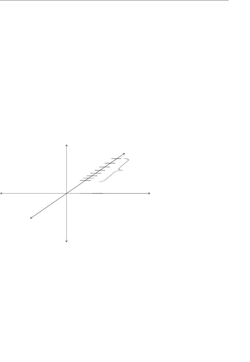
ptg9898810
stage can select which viewport subsequent rendering will target. More
details and an example are given in ‘‘Multiple Viewports and Layered
Rendering’’ on Page 550.
Advanced: zPrecision
One bizarre effect of these transformations is z fighting. The hardware’s
floating-point numbers used to do the computation have limited precision.
Hence, depth coordinates that are mathematically distinct end up having
the same (or even reversed) actual floating-point zvalues. This in turn
causes incorrectly hidden objects in the depth buffer. The effect varies per
pixel and can cause disturbing flickering intersections of nearby objects.
Precision of zis made even worse with perspective division, which is
applied to the depth coordinate along with all the other coordinates: As the
transformed depth coordinate moves farther away from the near clipping
plane, its location becomes increasingly less precise, as shown in Figure 5.15.
z
0x
y
21 3 4
Pre-divide z
values that will
be disnct
post divide
Figure 5.15 zprecision
(An exaggerated showing of adjacent, distinctly representable depths,
assuming an upcoming perspective division.)
Even without perspective division, there is a finite granularity to
floating-point numbers, but the divide makes it worse and nonlinear,
resulting in more severe problems at greater depths. The bottom line is it is
possible to ask for too much of too small a range of zvalues. To avoid this,
take care to keep the far plane as close to the near plane as possible, and
don’t compress the zvalues into a narrower range than necessary.
OpenGL Transformations 237

ptg9898810
Advanced: User Clipping
OpenGL automatically clips geometry against the near and far planes as
well as the viewport. User clipping refers to adding additional clip planes at
arbitrary orientations, intersecting your geometry, such that the display
sees the geometry on one side of the plane, but not on the other side. You
might use one, for example, to show a cut away of a complex object.
OpenGL user clipping is a joint effort between OpenGL and a special
built-in vertex shader array, gl_ClipDistance, which you are responsible
for setting. This variable lets you control where vertices are in relation to a
plane. Normal interpolation then assigns distances to the fragments
between the vertices. Example 5.2 shows a straight-forward use of this
built-in variable.
Example 5.2 Simple Use of gl_ClipDistance
#version 330 core
uniform vec4 Plane; // A, B, C, and D for Ax + By + Cz + D = 0
in vec4 Vertex; // w == 1.0
float gl_ClipDistance[1]; // declare use of 1 clip plane.
void main()
{
// evaluate plane equation
gl_ClipDistance[0] = dot(Vertex, Plane);
}
The convention is that a distance of 0 means the vertex is on the plane, a
positive distance means the vertex is inside (the keep it side) of the clip
plane, and a negative distance means the point is outside (the cull it side)
of the clip plane. The clip distances will be linearly interpolated across the
primitive, and OpenGL will cull fragments whose interpolated distance is
less than 0.
Each element of the gl_ClipDistance array is set up to represent one
plane. There are a limited number of clip planes, likely around eight or
more. The built-in, gl_ClipDistance[] is declared with no size. You
either need to redeclare it with a specific size or only access it with
compile-time constants.
All shaders in all stages that declare or use gl_ClipDistance[] should
make the array the same size. (The constant gl_MaxClipDistances lets
your shader know the maximum array size on the current OpenGL
implementation.) This size needs to include all the clip planes that are
enabled via the OpenGL API; if the size does not include all enabled planes,
238 Chapter 5: Viewing Transformations, Clipping, and Feedback

ptg9898810
results are undefined. To enable OpenGL clipping of the clip plane written
to in Example 5.2, enable the following enumerant in your application:
glEnable(GL_CLIP_PLANE0);
There are also other enumerates like GL_CLIP_PLANE1, GL_CLIP_PLANE2.
These enumerants are organized sequentially, so that GL_CLIP_PLANEiis
equal to GL_CLIP_PLANE0 + i. This allows programmatic selection of
which and how many user clip planes to use. Your shaders should write to
all the enabled planes, or you’ll end up with odd system clipping behavior.
The built-in gl_ClipDistance is also available in a fragment shader,
allowing nonclipped fragments to read their interpolated distances from
each clip plane.
Transform Feedback
Transform feedback can be considered a stage of the OpenGL pipeline that
sits after all of the vertex-processing stages and directly before primitive
assembly and rasterization.1Transform feedback captures vertices as they
are assembled into primitives (points, lines, or triangles) and allows some
or all of their attributes to be recorded into buffer objects. In fact, the
minimal OpenGL pipeline that produces useful work is a vertex shader
with transform feedback enabled---no fragment shader is necessary. Each
time a vertex passes through primitive assembly, those attributes that have
been marked for capture are recorded into one or more buffer objects.
Those buffer objects can then be read back by the application, or their
contents used in subsequent rendering passes by OpenGL.
Transform Feedback Objects
The state required to represent transform feedback is encapsulated into a
transform feedback object. This state includes the buffer objects that will be
used for recording the captured vertex data, counters indicating how full
each buffer object is, and state indicating whether transform feedback is
currently active. A transform feedback object is created by reserving a
transform feedback object name and then binding it to the transform
feedback object binding point on the current context. To reserve transform
feedback object names, call:
1. To be more exact, transform feedback is tightly integrated into the primitive assembly process
as whole primitives are captured into buffer objects. This is seen as buffers run out of space
and partial primitives are discarded. For this to occur, some knowledge of the current primitive
type is required in the transform feedback stage.
Transform Feedback 239
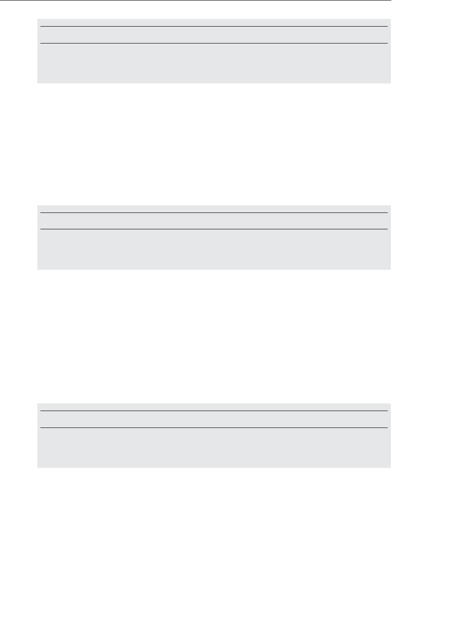
ptg9898810
void glGenTransformFeedbacks(GLsizei n, GLuint * ids);
Reserves nnames for transform feedback objects and places the reserved
names in the array ids.
The parameter nspecifies how many transform feedback object names are
to be reserved, and ids specifies the address of an array where the reserved
names will be placed. If you want only one name, you can set nto one and
pass the address of a GLuint variable in ids. Once you have reserved a
name for a transform feedback object, the object doesn’t actually exist
until the first time it is bound, at which point it is created. To bind a
transform feedback object to the context, call:
void glBindTransformFeedback(GLenum target, GLuint id);
Binds a transform feedback object specified by id to the target target,
which must be GL_TRANSFORM_FEEDBACK.
This binds the transform feedback object named id to the binding on the
context indicated by target, which in this case must be
GL_TRANSFORM_FEEDBACK. If this is the first time this name has been
bound, a new transform feedback object is created and initialized with the
default state, otherwise, the existing state of that object again becomes
current. To determine whether a particular value is the name of a
transform feedback object, you can call glIsTransformFeedback(), whose
prototype is as follows:
GLboolean glIsTransformFeedback(GLenum id);
Returns GL_TRUE if id is the name of an existing transform feedback
object and GL_FALSE otherwise.
Once a transform feedback object is bound, all commands affecting
transform feedback state affect that transform feedback object. It’s not
necessary to have a transform feedback object bound in order to use
transform feedback functionality as there is a default transform feedback
object. The default transform feedback object assumes the id zero and so
passing zero as the id parameter to glBindTransformFeedback() returns
240 Chapter 5: Viewing Transformations, Clipping, and Feedback

ptg9898810
the context to use the default transform feedback object (unbinding any
previously bound transform feedback object in the process). However, as
more complex uses of transform feedback are introduced, it becomes
convenient to encapsulate the state of transform feedback into transform
feedback objects. Therefore, it’s good practice to create and bind a
transform feedback object even if you intend to use only one.
Once a transform feedback object is no longer needed, it should be deleted
by calling:
void glDeleteTransformFeedbacks(GLsizei n, const GLuint ids);
Deletes ntransform feedback objects whose names are stored in the array
ids. Elements of ids that are not names of transform feedback objects are
silently ignored, as is the name zero.
This function deletes the ntransform feedback objects whose names are
stored in the array whose address is passed in ids. Deletion of the object is
deferred until it is no longer in use. That is, if the transform feedback
object is active when glDeleteTransformFeedbacks() is called, it is not
deleted until transform feedback is ended.
Transform Feedback Buffers
Transform feedback objects are primarily responsible for managing the
state representing capture of vertices into buffer objects. This state includes
which buffers are bound to the transform feedback buffer binding points.
Multiple buffers can be bound simultaneously for transform feedback and
subsections of buffer objects can also be bound. It is even possible to bind
different subsections of the same buffer object to different transform
feedback buffer binding points simultaneously. To bind an entire buffer
object to one of the transform feedback buffer binding points, call:
void glBindBufferBase(GLenum target, GLuint index,
GLuint buffer);
Binds the buffer object with name buffer to the indexed binding point on
target target at index index, and to the generic buffer binding point
specified by target.
Transform Feedback 241

ptg9898810
The target parameter should be set to
GL_TRANSFORM_FEEDBACK_BUFFER and index should be set to the index
of the transform feedback buffer binding point in the currently bound
transform feedback object. The name of the buffer to bind is passed in
buffer. The total number of binding points is an implementation-dependent
constant that can be discovered by querying the value of
GL_MAX_TRANSFORM_FEEDBACK_BUFFERS, and index must be less than
this value. All OpenGL implementations must support at least 64 transform
feedback buffer binding points. It’s also possible to bind a range of a buffer
object to one of the transform feedback buffer binding points by calling:
void glBindBufferRange(GLenum target, GLuint index,
GLuint buffer, GLintptr offset,
GLsizeiptr size);
Binds a range of a buffer object to the indexed buffer binding point on
target target specified by index.offset and size, both in bytes, indicate the
range of the buffer object to bind. glBindBufferRange() also binds the
buffer buffer to the generic buffer binding point specified by target.
Again, target should be GL_TRANSFORM_FEEDBACK_BUFFER, index
should be between zero and one less than the value of
GL_MAX_TRANSFORM_FEEDBACK_BUFFERS, and buffer contains the
name of the buffer object to bind. The offset and size parameters define
which section of the buffer object to bind. This functionality can be used
to bind different ranges of the same buffer object to different transform
feedback buffer binding points. Care should be taken that the ranges do
not overlap. Attempting to perform transform feedback into multiple,
overlapping sections of the same buffer object will result in undefined
behavior, possibly including data corruption or worse.
In addition to binding buffers (or sections of buffers) to the indexed
binding points, glBindBufferBase() and glBindBufferRange() also bind
the buffer object to the generic buffer binding point indicated by target.
This is useful because it allows other commands that operate on buffer
objects such as glBufferData(),glBufferSubData(), and
glGetBufferSubData() to operate on the buffer object most recently bound
to one of the indexed buffer binding points. Note though, that neither
glBindBufferBase() nor glBindBufferRange() create buffer objects (unlike
glBindBuffer()), and so you can’t use a glBindBufferBase(),
glBufferData() sequence to create and allocate space for a transform
feedback buffer. In order to allocate a transform feedback buffer, code such
as in that shown in Example 5.3 should be used.
242 Chapter 5: Viewing Transformations, Clipping, and Feedback

ptg9898810
Example 5.3 Example Initialization of a Transform Feedback Buffer
// Generate the name of a buffer object
GLuint buffer;
glGenBuffers(1, &buffer);
// Bind it to the TRANSFORM_FEEDBACK binding to create it
glBindBuffer(GL_TRANSFORM_FEEDBACK_BUFFER, buffer);
// Call glBufferData to allocate 1MB of space
glBufferData(GL_TRANSFORM_FEEDBACK_BUFFER, // target
1024 *1024, // 1 MB
NULL, // no initial data
GL_DYNAMIC_COPY); // usage
// Now we can bind it to indexed buffer binding points.
glBindBufferRange(GL_TRANSFORM_FEEDBACK_BUFFER, // target
0, // index 0
buffer, // buffer name
0, // start of range
512 *1024); // first half of buffer
glBindBufferRange(GL_TRANSFORM_FEEDBACK_BUFFER, // target
1, // index 1
buffer, // same buffer
512 *1024, // start half way
512 *1024); // second half
Notice how in Example 5.3, the newly reserved buffer object name is first
bound to the GL_TRANSFORM_FEEDBACK_BUFFER target, and then
glBufferData() is called to allocate space. The data parameter to
glBufferData() is set to NULL to indicate that we wish to simply allocate
space but do not wish to provide initial data for the buffer. In this case, the
buffer’s contents will initially be undefined. Also, GL_DYNAMIC_COPY is
used as the usage parameter. This provides a hint to the OpenGL
implementation of the intended use for the buffer object. The DYNAMIC
part of the token implies that the data in the buffer will be changed often,
and the COPY part of the token indicates that we will be using OpenGL
(normally a GPU) to produce data to be written into the buffer. This,
together with the fact that the buffer is bound to the
GL_TRANSFORM_FEEDBACK_BUFFER binding point should give the
implementation enough information to intelligently allocate memory for
the buffer object in an optimal manner for it to be used for transform
feedback.
Once the buffer has been bound to the generic
GL_TRANSFORM_FEEDBACK_BUFFER target and space has been allocated
for it, sections of it are then bound to the indexed transform feedback
buffer binding points by calling glBindBufferRange() twice---once to bind
Transform Feedback 243

ptg9898810
the first half of the buffer to the first binding point, and again to bind the
second half of the buffer to the second binding point. This demonstrates
why the buffer needs to be created and allocated first before using it with
glBindBufferRange().glBindBufferRange() takes an offset,size
parameters describing a range of the buffer object that must lie within the
buffer object. This cannot be determined if the object does not yet exist.
Configuring Transform Feedback Varyings
While the buffer bindings used for transform feedback are associated with
a transform feedback object, the configuration of which outputs of the
vertex (or geometry) shader are to be recorded into those buffers is stored
in the active program object. To specify which varyings will be recorded
during transform feedback, call:
void glTransformFeedbackVaryings(GLuint program,
GLsizei count,
const GLchar ** varyings,
GLenum bufferMode);
Sets the varyings to be recorded by transform feedback for the program
specified by program.count specifies the number of strings contained in
the array varyings, which contains the names of the varyings to be
captured. buferMode is the mode in which the varyings will be
captured---either separate mode (specified by GL_SEPARATE_ATTRIBS) or
interleaved mode (specified by GL_INTERLEAVED_ATTRIBS).
In this function, program specifies the program object that will be used for
transform feedback. varyings contains an array of strings that represent the
names of varying variables that are outputs of the fragment (or geometry)
shader that are to be captured by transform feedback. count is the number
of strings in varyings.bufferMode is a token indicating how the captured
varyings should be allocated to transform feedback buffers. If bufferMode is
set to GL_INTERLEAVED_ATTRIBS, all of the varyings will be recorded one
after another into the buffer object bound to the first transform feedback
buffer binding point on the current transform feedback object. If
bufferMode is GL_SEPARATE_ATTRIBS, each varying will be captured into
its own buffer object.
244 Chapter 5: Viewing Transformations, Clipping, and Feedback

ptg9898810
An example of the use of glTransformFeedbackVaryings() is shown in
Example 5.4 below.
Example 5.4 Example Specification of Transform Feedback Varyings
// Create an array containing the names of varyings to record
static const char *const vars[] =
{
"foo", "bar", "baz"
};
// Call glTransformFeedbackVaryings
glTransformFeedbackVaryings(prog,
sizeof(vars) / sizeof(vars[0]),
varyings,
GL_INTERLEAVED_ATTRIBS);
// Now the program object is set up to record varyings squashed
// together in the same buffer object. Alternatively, we could call...
glTransformFeedbackVaryings(prog,
sizeof(vars) / sizeof(vars[0]),
varyings,
GL_SEPARATE_ATTRIBS);
// This sets up the varyings to be recorded into separate buffers.
// Now (this is important), link the program object...
// ... even if it’s already been linked before.
glLinkProgram(prog);
Notice in Example 5.4 that there is a call to glLinkProgram() directly after
the call to glTransformFeedbackVaryings(). This is because the selection
of varyings specified in the call to glTransformFeedbackVaryings() does
not take effect until the next time the program object is linked. If the program
has previously been linked and is then used without being re-linked, no
errors will occur, but nothing will be captured during transform feedback.2
After the code in Example 5.4 has been executed, whenever prog is in use
while transform feedback is active, the values written to foo,bar, and baz
will be recorded into the transform feedback buffers bound to the current
transform feedback object. In the case where the bufferMode parameter is
set to GL_INTERLEAVED_ATTRIBS, the values of foo,bar, and baz will be
tightly packed into the buffer bound to the first transform feedback buffer
binding point as shown in Figure 5.16.
2. Calling glTransformFeedbackVaryings() after a program object has already been linked and
then not linking it again is a common error made even by experienced OpenGL programmers.
Transform Feedback 245
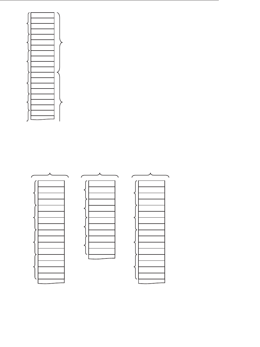
ptg9898810
foo[0].x
foo[0].y
foo[0].z
foo[0].w
bar[0].x
bar[0].y
bar[0].z
baz[0].x
baz[0].y
baz[0].z
baz[0].w
foo[1].x
foo[1].y
foo[1].z
foo[1].w
VERTEX 1
bar[1].x
bar[1].y
bar[1].z
baz[1].x
VERTEX 2
vec4
vec4
vec4
vec3
vec3
Figure 5.16 Transform feedback varyings packed in a single buffer
However, if bufferMode is GL_SEPARATE_ATTRIBS then each of foo,bar,
and baz will be packed tightly into its own buffer object as shown in
Figure 5.17.
foo[0].x
foo[0].y
foo[0].z
foo[0].w
VERTEX 1
foo[1].x
foo[1].y
foo[1].z
foo[1].w
VERTEX 2
foo[2].x
foo[2].y
foo[2].z
foo[2].w
VERTEX 3
foo[3].x
foo[3].y
foo[3].z
foo[3].w
VERTEX 4
BUFFER 0
bar[0].x
bar[0].y
bar[0].z
VERTEX 1
bar[1].x
bar[1].y
bar[1].z
VERTEX 2
bar[2].x
bar[2].y
bar[2].z
VERTEX 3
bar[3].x
bar[3].y
bar[3].z
VERTEX 4
BUFFER 1
baz[0].x
baz[0].y
baz[0].z
baz[0].w
VERTEX 1
baz[1].x
baz[1].y
baz[1].z
baz[1].w
VERTEX 2
baz[2].x
baz[2].y
baz[2].z
baz[2].w
VERTEX 3
baz[3].x
baz[3].y
baz[3].z
baz[3].w
VERTEX 4
BUFFER 2
Figure 5.17 Transform feedback varyings packed in separate buffers
246 Chapter 5: Viewing Transformations, Clipping, and Feedback

ptg9898810
In both cases, the attributes will be tightly packed together. The amount of
space in the buffer object that each varying consumes is determined by its
type in the vertex shader. That is, if foo is declared as a vec3 in the vertex
shader, it will consume exactly three floats in the buffer object. In the case
where bufferMode is GL_INTERLEAVED_ATTRIBS, the value of bar will be
written immediately after the value of foo. In the case where bufferMode is
GL_SEPARATE_ATTRIBS, the values of foo will be tightly packed into one
buffer with no gaps between them (as will the values of bar and baz).
This seems rather rigid. There are cases where you may wish to align the
data written into the transform feedback buffer differently from default
(leaving unwritten gaps in the buffer). There may also be cases where you
would want to record more than one variable into one buffer, but record
other variables into another. For example, you may wish to record foo and
bar into one buffer while recording baz into another. In order to increase
the flexibility of transform feedback varying setup and allow this kind of
usage, there are some special variable names reserved by OpenGL that
signal to the transform feedback subsystem that you wish to leave gaps in
the output buffer, or to move between buffers. These are
gl_SkipComponents1,gl_SkipComponents2,gl_SkipComponents3,
gl_SkipComponents4, and gl_NextBuffer. When any of the
gl_SkipComponents variants is encountered, OpenGL will leave a gap for
the number of components specified (1, 2, 3, or 4) in the transform
feedback buffer. These variable names can only be used when bufferMode is
GL_INTERLEAVED_ATTRIBS. An example of using this is shown in
Example 5.5.
Example 5.5 Leaving Gaps in a Transform Feedback Buffer
// Declare the transform feedback varying names
static const char *const vars[] =
{"foo",
"gl_SkipComponents2",
"bar",
"gl_SkipComponents3",
"baz"
};
// Set the varyings
glTransformFeedbackVaryings(prog,
sizeof(vars) / sizeof(vars[0]),
varyings,
GL_INTERLEAVED_ATTRIBS);
// Remember to link the program object
glLinkProgram(prog);
Transform Feedback 247

ptg9898810
When the other special variable name, gl_NextBuffer name is
encountered, OpenGL will start allocating varyings into the buffer bound
to the next transform feedback buffer. This allows multiple varyings to be
recorded into a single buffer object. Additionally, if gl_NextBuffer is
encountered when bufferMode is GL_SEPARATE_ATTRIBS, or if two or more
instances of gl_NextBuffer are encountered in a row in
GL_INTERLEAVED_ATTRIBS, it allows a whole binding point to be skipped
and nothing recorded into the buffer bound there. An example of
gl_NextBuffer is shown in Example 5.6.
Example 5.6 Assigning Transform Feedback Outputs to Different
Buffers
// Declare the transform feedback varying names
static const char *const vars[] =
{"foo", "bar" // Variables to record into buffer 0
"gl_NextBuffer", // Move to binding point 1
"baz" // Variable to record into buffer 1
};
// Set the varyings
glTransformFeedbackVaryings(prog,
sizeof(vars) /
sizeof(vars[0]), varyings,
GL_INTERLEAVED_ATTRIBS);
// Remember to link the program object
glLinkProgram(prog);
The special variables names gl_SkipComponentsN and gl_NextBuffer
can be combined to allow very flexible vertex layouts to be created. If it is
necessary to skip over more than four components, multiple instances of
gl_SkipComponents may be used back to back. Care should be taken
with aggressive use of gl_SkipComponents, though, because skipped
components still contribute toward the count of the count of the number
of components captured during transform feedback, even though no data
is actually written. This may cause a reduction in performance, or even a
failure to link a program. If there is a lot of unchanged, static data in a
buffer, it may be preferable to separate the data into static and dynamic
parts and leave the static data in its own buffer object(s), allowing the
dynamic data to be more tightly packed.
248 Chapter 5: Viewing Transformations, Clipping, and Feedback

ptg9898810
Finally, Example 5.7 shows an (albeit rather contrived) example of the
combined use of gl_SkipComponents and gl_NextBuffer, and
Figure 5.18 shows how the data ends up laid out in the transform feedback
buffers.
Example 5.7 Assigning Transform Feedback Outputs to Different
Buffers
// Declare the transform feedback varying names
static const char *const vars[] =
{
// Record foo, a gap of 1 float, bar, and then two floats
"foo", "gl_SkipComponents1", "bar", "gl_SkipComponents2"
// Move to binding point 1
"gl_NextBuffer",
// Leave a gap of 4 floats, then record baz, then leave
// another gap of 2 floats
"gl_SkipComponents4" "baz", "gl_SkipComponents2"
// Move to binding point 2
"gl_NextBuffer",
// Move directly to binding point 3 without directing anything
// to binding point 2
"gl_NextBuffer",
// Record iron and copper with a 3 component gap between them
"iron", "gl_SkipComponents3", "copper"
};
// Set the varyings
glTransformFeedbackVaryings(prog,
sizeof(vars) / sizeof(vars[0]),
varyings,
GL_INTERLEAVED_ATTRIBS);
// Remember to link the program object
glLinkProgram(prog);
As you can see in Example 5.7,gl_SkipComponents can come between
varyings, or at the start or end of the list of varyings to record into a single
buffer. Putting a gl_SkipComponents variant-first in the list of varyings
to capture will result in OpenGL leaving a gap at the front of the buffer
before it records data (and then a gap between each sequence of varyings).
Also, multiple gl_NextBuffer variables can come back to back, causing a
buffer binding point to be entirely passed over and nothing recorded into
that buffer. The resulting output layout is shown in Figure 5.18.
Transform Feedback 249
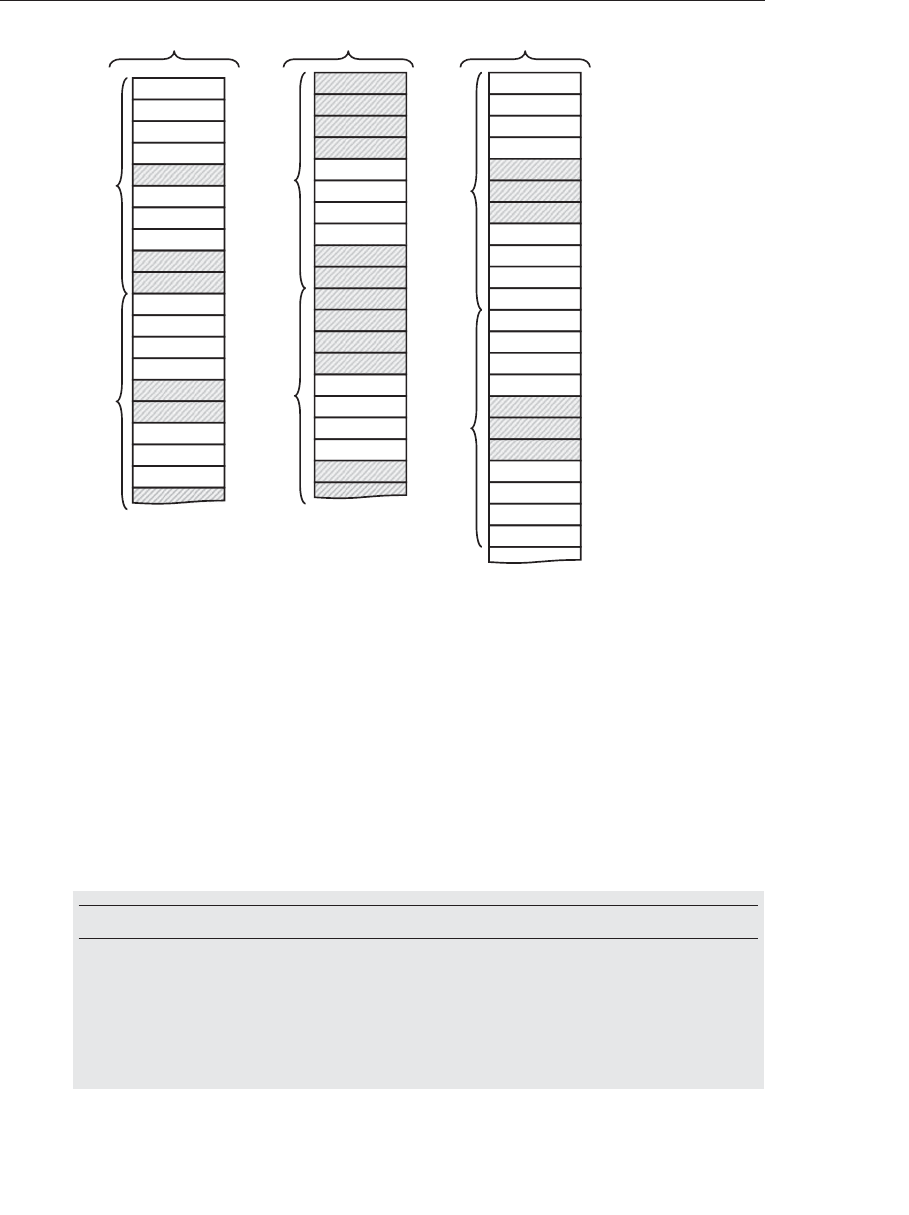
ptg9898810
foo[0].x
foo[0].y
foo[0].z
foo[0].w
VERTEX 1
foo[1].x
foo[1].y
foo[1].z
foo[1].w
BUFFER 0
bar[0].x
bar[0].y
bar[0].z
BUFFER 1
baz[0].x
baz[0].y
baz[0].z
baz[0].w
BUFFER 3
baz[1].x
baz[1].y
baz[1].z
baz[1].w
VERTEX 2
VERTEX 1
VERTEX 2
iron[1].x
iron[1].y
iron[1].z
iron[1].w
copper[1].x
copper[1].y
copper[1].z
copper[1].w
VERTEX 2
iron[0].x
iron[0].y
iron[0].z
iron[0].w
copper[0].x
copper[0].y
copper[0].z
copper[0].w
VERTEX 1
bar[1].x
bar[1].y
bar[1].z
Figure 5.18 Transform feedback varyings packed into multiple buffers
Starting and Stopping Transform Feedback
Transform feedback can be started and stopped, and even paused. As might
be expected starting transform feedback when it is not paused causes it to
start recording into the bound transform feedback buffers from the begin-
ning. However, starting transform feedback when it is already paused causes
it to continue recording from wherever it left off. This is useful to allow mul-
tiple components of a scene to be recorded into transform feedback buffers
with other components rendered in between that are not to be recorded.
To start transform feedback, call glBeginTransformFeedback().
void glBeginTransformFeedback(GLenum primitiveMode);
Sets the primitive type expected to be recorded by transform feedback.
primitiveMode must be GL_POINTS, GL_LINES, or GL_TRIANGLES. The
primitive mode specified in subsequent drawing commands must match
primitiveMode, or (if present) the output of the geometry shader must
match primitiveMode.
250 Chapter 5: Viewing Transformations, Clipping, and Feedback

ptg9898810
The glBeginTransformFeedback() function starts transform feedback on
the currently bound transform feedback object. The primitiveMode
parameter must be GL_POINTS, GL_LINES, or GL_TRIANGLES, and must
match the primitive type expected to arrive at primitive assembly. Note that it
does not need to match the primitive mode used in subsequent draw
commands if tessellation or a geometry shader is active because those
stages might change the primitive type mid-pipeline. That will be covered
in Chapters 9and 10. For the moment, just set the primitiveMode to match
the primitive type you plan to draw with. Table 5.1 shows the allowed
combinations of primitiveMode and draw command modes.
Table 5.1 Drawing Modes Allowed During Transform Feedback
Transform Feedback primitiveMode Allowed Drawing types
GL_POINTS GL_POINTS
GL_LINES GL_LINES
GL_LINE_STRIP
GL_LINE_LOOP
GL_LINES_ADJACENCY
GL_LINE_STRIP_ADJACENCY
GL_TRIANGLES GL_TRIANGLES
GL_TRIANGLE_STRIP
GL_TRIANGLE_FAN
GL_TRIANGLES_ADJACENCY
GL_TRIANGLE_STRIP_ADJACENCY
Once transform feedback is started, it is considered to be active. It may be
paused by calling glPauseTransformFeedback(). When transform
feedback is paused, it is still considered active, but will not record any data
into the transform feedback buffers. There are also several restrictions
about changing state related to transform feedback while transform
feedback is active but paused.
•The currently bound transform feedback object may not be changed.
•It is not possible to bind different buffers to the
GL_TRANSFORM_FEEDBACK_BUFFER binding points.
•The current program object cannot be changed.3
3. Actually, it is possible to change the current program object, but an error will be generated by
glResumeTransformFeedback() if the program object that was current when glBeginTrans-
formFeedback() was called is no longer current. So, be sure to put the original program object
back before calling glResumeTransformFeedback().
Transform Feedback 251

ptg9898810
void glPauseTransformFeedback(void );
Pauses the recording of varyings in transform feedback mode. Transform
feedback may be resumed by calling glResumeTransformFeedback().
glPauseTransformFeedback() will generate an error if transform feedback
is not active, or if it is already paused. To restart transform feedback while
it is paused, glResumeTransformFeedback() must be used (not
glBeginTransformFeedback()). Likewise, glResumeTransformFeedback()
will generate an error if it is called when transform feedback is not active
or if it is active but not paused.
void glResumeTransformFeedback(void);
Resumes transform feedback that has previously been paused by a call to
glPauseTransformFeedback().
When you’ve completed rendering all of the primitives for transform
feedback, you change back to normal rendering mode by calling
glEndTransformFeedback().
void glEndTransformFeedback(void);
Completes the recording of varyings in transform feedback mode.
Transform Feedback Example---Particle System
This section contains the description of a moderately complex use of
transform feedback. The application uses transform feedback in two ways
to implement a particle system. On a first pass, transform feedback is used
to capture geometry as it passes through the OpenGL pipeline. The
captured geometry is then used in a second pass along with another
instance of transform feedback in order to implement a particle system that
uses the vertex shader to perform collision detection between particles and
the rendered geometry. A schematic of the system is shown in Figure 5.19.
252 Chapter 5: Viewing Transformations, Clipping, and Feedback
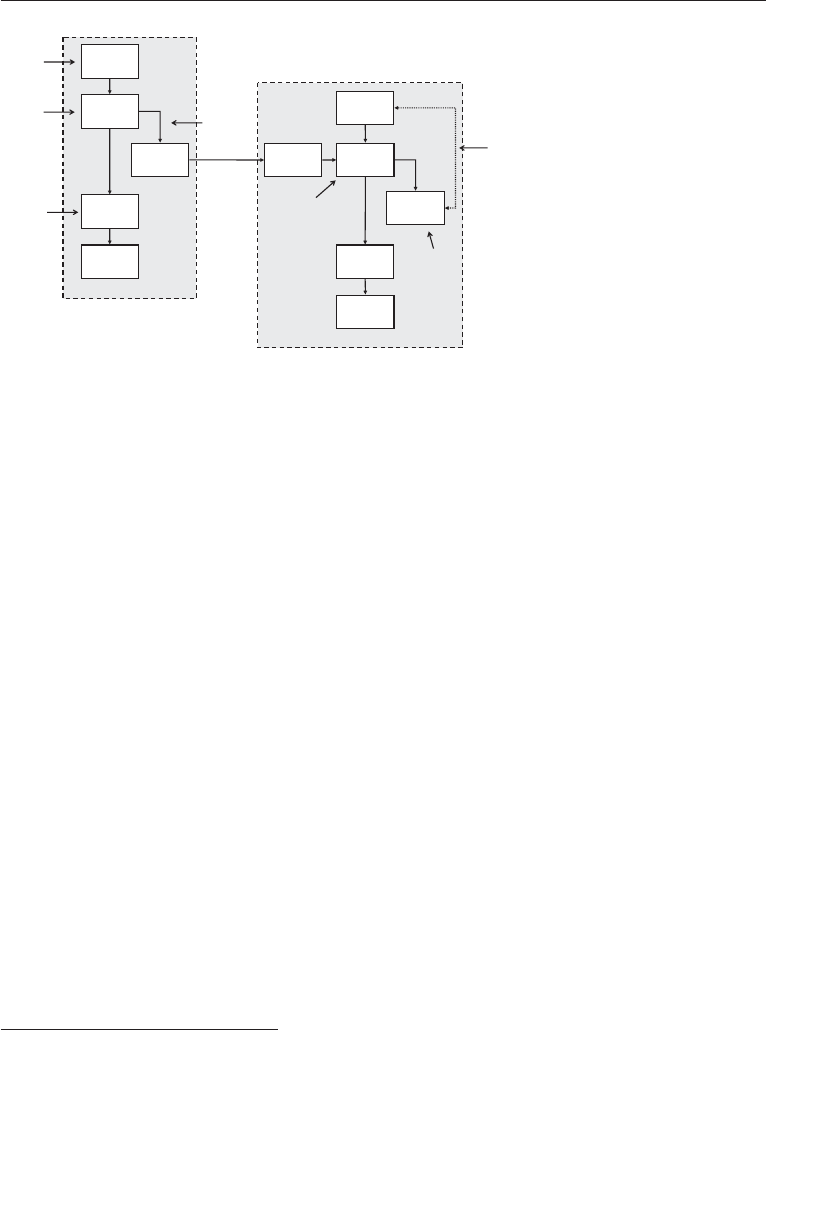
ptg9898810
Input
Geometry
World
Space
Geometry
Vertex
Shader
Rasterize
Triangles
Fragment
Shader
Particle
Position +
velocity
Collision
Detector
Particle
Position +
velocity
Rasterize
Points
Fragment
Shader
Geometry pass
Particle pass
Object
Space
Vertices
Generates
View and world
Space vertices Capture with
Transform
Feedback
View space
Geometry rendered
As normal
Double buffer
Position and
Velocity data
Texture
Buffer
Object
Collision
Detection
Implemented in a
vertex shader
Updated
Positions
Recorded with
Transform
Feedback
Figure 5.19 Schematic of the particle system simulator
In this application, the particle system is simulated in world space. In a
first pass, a vertex shader is used to transform object space geometry into
both world space (for later use in the particle system simulation), and into
eye space for rendering. The world space results are captured into a buffer
using transform feedback, while the eye space geometry is passed through
to the rasterizer. The buffer containing the captured world space geometry
is attached to a texture buffer object (TBO) so that it can be randomly
accessed in the vertex shader that is used to implement collision detection
in the second, simulation pass. Using this mechanism, any object that
would normally be rendered can be captured, so long as the vertex (or
geometry) shader produces world space vertices in addition to eye space
vertices. This allows the particle system to interact with multiple objects,
potentially with each rendered using a different set of shaders---perhaps
even with tessellation enabled or other procedurally generated geometry.4
The second pass is where the particle system simulation occurs. Particle
position and velocity vectors are stored in a pair of buffers. Two buffers are
used so that data can be double-buffered as it’s not possible to update
vertex data in place. Each vertex in the buffer represents a single particle in
the system. Each instance of the vertex shader performs collision detection
between the particle (using its velocity to compute where it will move to
during the time-step) and all of the geometry captured during the first
pass. It calculates new position and velocity vectors, which are captured
using transform feedback, and written into a buffer object ready for the
next step in the simulation.
4. Care should be taken here---tessellation can generate a very large amount of geometry, all of
which the simulated particles must be tested against, which could severely affect performance
and increase storage requirements for the intermediate geometry.
Transform Feedback 253

ptg9898810
Example 5.8 contains the source of the vertex shader used to transform the
incoming geometry into both world and eye space, and Example 5.9 shows
how transform feedback is configured to capture the resulting world space
geometry.
Example 5.8 Vertex Shader Used in Geometry Pass of Particle
System Simulator
#version 420 core
uniform mat4 model_matrix;
uniform mat4 projection_matrix;
layout (location = 0) in vec4 position;
layout (location = 1) in vec3 normal;
out vec4 world_space_position;
out vec3 vs_fs_normal;
void main(void)
{
vec4 pos = (model_matrix *(position *vec4(1.0, 1.0, 1.0, 1.0)));
world_space_position = pos;
vs_fs_normal = normalize((model_matrix *vec4(normal, 0.0)).xyz);
gl_Position = projection_matrix *pos;
};
Example 5.9 Configuring the Geometry Pass of the Particle System
Simulator
static const char *varyings2[] =
{"world_space_position"
};
glTransformFeedbackVaryings(render_prog, 1, varyings2,
GL_INTERLEAVED_ATTRIBS);
glLinkProgram(render_prog);
During the first geometry pass, the code in Exaples 5.8 and 5.9 will cause
the world space geometry to be captured into a buffer object. Each triangle
in the buffer is represented by three vertices5that are read (three at a time)
during the second pass into the vertex shader and used to perform line
segment against triangle intersection test. A TBO is used to access the data
in the intermediate buffer so that the three vertices can be read in a simple
5. Only triangles are used here. It’s not possible to perform a meaningful physical collision
detection between a line segment and another line segment or a point. Also, individual trian-
gles are required for this to work. If strips or fans are present in the input geometry, it may
be necessary to include a geometry shader in order to convert the connected triangles into
independent triangles.
254 Chapter 5: Viewing Transformations, Clipping, and Feedback

ptg9898810
for loop. The line segment is formed by taking the particle’s current
position and using its velocity to calculate where it will be at the end of the
time step. This is performed for every captured triangle. If a collision is
found, the point’s new position is reflected about the plane of the triangle
to make it ‘‘bounce’’ off the geometry.
Example 5.10 contains the code of the vertex shader used to perform
collision detection in the simulation pass.
Example 5.10 Vertex Shader Used in Simulation Pass of Particle
System Simulator
#version 420 core
uniform mat4 model_matrix;
uniform mat4 projection_matrix;
uniform int triangle_count;
layout (location = 0) in vec4 position;
layout (location = 1) in vec3 velocity;
out vec4 position_out;
out vec3 velocity_out;
uniform samplerBuffer geometry_tbo;
uniform float time_step = 0.02;
bool intersect(vec3 origin, vec3 direction, vec3 v0, vec3 v1, vec3 v2,
out vec3 point)
{
vec3 u, v, n;
vec3 w0, w;
float r, a, b;
u = (v1 −v0);
v = (v2 −v0);
n = cross(u, v);
w0 = origin −v0;
a = −dot(n, w0);
b = dot(n, direction);
r = a / b;
if (r < 0.0 || r > 1.0)
return false;
point = origin + r *direction;
float uu, uv, vv, wu, wv, D;
uu = dot(u, u);
uv = dot(u, v);
vv = dot(v, v);
w = point −v0;
Transform Feedback 255

ptg9898810
wu = dot(w, u);
wv = dot(w, v);
D = uv *uv −uu *vv;
float s, t;
s = (uv *wv −vv *wu) / D;
if (s < 0.0 || s > 1.0)
return false;
t = (uv *wu −uu *wv) / D;
if (t < 0.0 || (s + t) > 1.0)
return false;
return true;
}
vec3 reflect_vector(vec3 v, vec3 n)
{
return v−2.0 *dot(v, n) *n;
}
void main(void)
{
vec3 acceleration = vec3(0.0, −0.3, 0.0);
vec3 new_velocity = velocity + acceleration *time_step;
vec4 new_position = position + vec4(new_velocity *time_step, 0.0);
vec3 v0, v1, v2;
vec3 point;
int i;
for (i = 0; i < triangle_count; i++)
{
v0 = texelFetch(geometry_tbo, i *3).xyz;
v1 = texelFetch(geometry_tbo, i *3 + 1).xyz;
v2 = texelFetch(geometry_tbo, i *3 + 2).xyz;
if (intersect(position.xyz, position.xyz −new_position.xyz,
v0, v1, v2, point))
{
vec3 n = normalize(cross(v1 −v0, v2 −v0));
new_position = vec4(point
+ reflect_vector(new_position.xyz −
point, n), 1.0);
new_velocity = 0.8 *reflect_vector(new_velocity, n);
}
}
if (new_position.y < −40.0)
{
new_position = vec4(−new_position.x *0.3, position.y + 80.0,
0.0, 1.0);
new_velocity *=vec3(0.2, 0.1, −0.3);
}
velocity_out = new_velocity *0.9999;
position_out = new_position;
gl_Position = projection_matrix *(model_matrix *position);
};
256 Chapter 5: Viewing Transformations, Clipping, and Feedback

ptg9898810
The code to set up transform feedback to capture the updated particle
position and velocity vectors is shown in Example 5.11.
Example 5.11 Configuring the Simulation Pass of the Particle
System Simulator
static const char *varyings[] =
{"position_out", "velocity_out"
};
glTransformFeedbackVaryings(update_prog, 2, varyings,
GL_INTERLEAVED_ATTRIBS);
glLinkProgram(update_prog);
The inner rendering loop of the application is quite simple. First, the
program object used for rendering the geometry is bound, as is a transform
feedback object representing the state required to capture the world space
geometry. Then, all of the solid objects in the scene are rendered, causing
the intermediate buffer to be filled with world space geometry. Next, the
program object used for updating particle positions is made current, as is
the transform feedback object used for capturing position and velocity
data for the particle system. Finally, the particles are rendered. The code for
this inner loop is shown in Example 5.12.
Example 5.12 Main Rendering Loop of the Particle System Simulator
glUseProgram(render_prog);
glUniformMatrix4fv(render_model_matrix_loc, 1, GL_FALSE, model_matrix);
glUniformMatrix4fv(render_projection_matrix_loc, 1, GL_FALSE,
projection_matrix);
glBindVertexArray(render_vao);
glBindBufferBase(GL_TRANSFORM_FEEDBACK_BUFFER, 0, geometry_vbo);
glBeginTransformFeedback(GL_TRIANGLES);
object.Render();
glEndTransformFeedback();
glUseProgram(update_prog);
glUniformMatrix4fv(model_matrix_loc, 1, GL_FALSE, model_matrix);
glUniformMatrix4fv(projection_matrix_loc, 1, GL_FALSE,
projection_matrix);
glUniform1i(triangle_count_loc, object.GetVertexCount() / 3);
if ((frame_count & 1) != 0)
{
glBindVertexArray(vao[1]);
glBindBufferBase(GL_TRANSFORM_FEEDBACK_BUFFER, 0, vbo[0]);
}
Transform Feedback 257
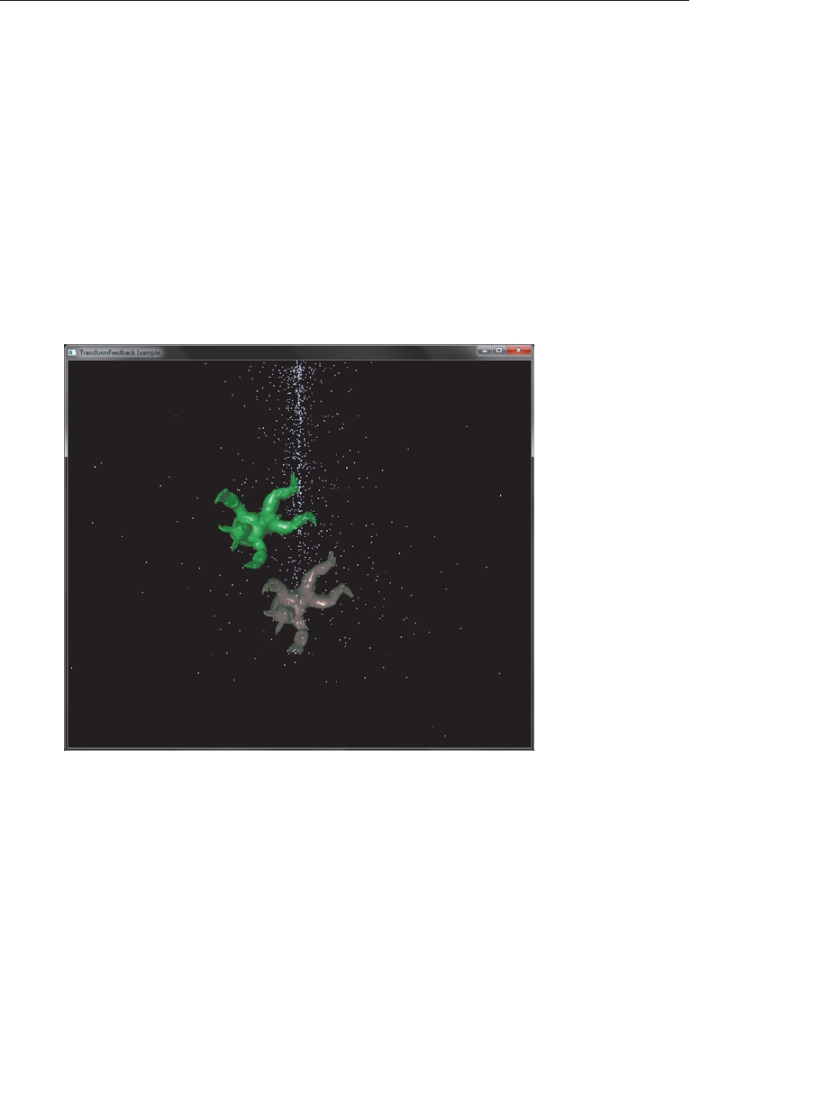
ptg9898810
else
{
glBindVertexArray(vao[0]);
glBindBufferBase(GL_TRANSFORM_FEEDBACK_BUFFER, 0, vbo[1]);
}
glBeginTransformFeedback(GL_POINTS);
glDrawArrays(GL_POINTS, 0, min(point_count, (frame_count >> 3)));
glEndTransformFeedback();
glBindVertexArray(0);
frame_count++;
The result of the program is shown in Figure 5.20.
Figure 5.20 Result of the particle system simulator
258 Chapter 5: Viewing Transformations, Clipping, and Feedback

ptg9898810
Chapter 6
Textures
Chapter Objectives
After reading this chapter, you’ll be able to do the following:
•Understand what texture mapping can add to your scene.
•Supply texture images in compressed and uncompressed formats.
•Control how a texture image is filtered as it is applied to a fragment.
•Create and manage texture images in texture objects.
•Supply texture coordinates describing what part of the texture image
should be mapped onto objects in your scene.
•Perform complex texture operations using multiple textures in a single
shader.
•Specify textures to be used for processing point sprites.
259

ptg9898810
The goal of computer graphics, generally speaking, is to determine the
colors that make up each part of an image. While it is possible to calculate
the color of a pixel using an advanced shading algorithm, often the com-
plexity of such a shader is so great that it is not practical to implement
such approaches. Instead, we rely on textures---large chunks of image data
that can be used to paint the surfaces of objects to make them appear more
realistic. This chapter discusses various approaches and techniques to
apply textures using shaders in your application.
This chapter has the following major sections:
•‘‘Texture Mapping’’ provides an overview the the process of texture
mapping.
•‘‘Basic Texture Types’’ provides an outline of the types of texture that
are available in OpenGL.
•‘‘Creating and Initializing Textures’’ explains how to create and set up a
texture for use in your application.
•‘‘Proxy Textures’’ introduces the proxy texture targets, which provide a
mechanism to probe the capabilities of the OpenGL implementation.
•‘‘Specifying Texture Data’’ provides a description of the formatting of
texture data in OpenGL and how you get that data into your texture
objects.
•‘‘Sampler Objects’’ shows how sampler objects can be used to control the
way that OpenGL reads data from textures into your shaders.
•‘‘Using Textures’’ delves into the ways that you can make best use of
textures in your shaders.
•‘‘Complex Texture Types’’ describes some of the more advanced texture
types that are available in OpenGL, including array textures, cube
maps, depth, and buffer textures.
•‘‘Texture Views’’ describes how to share one texture’s data with one or
more other textures, and to interpret it in different ways.
•‘‘Compressed Textures’’ explores methods to use compressed texture data
in your application in order to save memory and bandwidth, which are
both important performance considerations.
•‘‘Filtering’’ outlines the various ways in which multiple texels may be
combined in order to reduce artifacts and to improve the quality of
your rendered images.
•‘‘Advanced Texture Lookup Functions’’ takes acloser look at some of
the more advanced functions available in GLSL that can be used to
read data from textures with more control.
260 Chapter 6: Textures

ptg9898810
•‘‘Point Sprites’’ describes a feature of OpenGL that provides texture
coordinates automatically for geometry rendered as points, allowing
your application to very quickly render small bitmaps to the display.
•‘‘Rendering to Texture Maps’’ explains how to render directly into a
texture map by using framebuffer objects.
Texture Mapping
In the physical world, colors within your field of view can change rapidly.
Odds are you’re reading this book inside of a building.1Look at the walls,
ceiling, floors, and objects in the room. Unless you’ve furnished your
home entirely at Ikea, it’s likely some surface in the room will have detail
where the colors change rapidly across a small area. Capturing color
changes with that amount of detail is both toilsome and data-intensive
(effectively, you need to specify a triangle for each region of linear color
change). It would be much simpler to be able to use a picture and ‘‘glue’’ it
onto the surface like wallpaper. Enter texture mapping. This technique
allows you to look up values, like colors, from a shader in a special type of
table. While texture mapping is available in all of OpenGL’s shading
stages, we’ll first discuss it in the context of processing fragments, because
that’s where it’s used most often.
Often a texture map (or just ‘‘texture’’ for short) is an image captured by a
camera or painted by an artist, but there’s no requirement that be the
case---it’s possible that the image is procedurally generated (see Chapter 8,
‘‘Procedural Texturing’’) or even rendered by OpenGL targeting a texture
instead of the display device. Textures of this nature would be two-
dimensional, but OpenGL supports many other types of textures as well:
one-, and three-dimensional textures, cube-map textures, and buffer
textures. Array textures are also supported, which are treated as a set of
slices of similar dimension and format, wrapped up in a single texture
object. All of these will be discussed in detail below.
Textures are composed of texels, which will often contain color values.
However, there’s a lot of utility in merely considering a texture as a table of
values that you can query in a shader and use for any purpose you desire.
In order to use texture mapping in your application, you will need to do
the following steps:
•Create a texture object and load texel data into it.
•Include texture coordinates with your vertices.
1. We applaud you if that’s not true, except if you’re currently operating a moving vehicle.
Texture Mapping 261

ptg9898810
•Associate a texture sampler with each texture map you intend to use
in your shader.
•Retrieve the texel values through the texture sampler from your
shader.
We’ll discuss each of those steps in the following sections.
Basic Texture Types
OpenGL supports many types of texture object of varying dimensiona-
lities and layout. Each texture object represents a set of images that make
up the complete texture. Each image is a 1D, 2D, or 3D array of texels
and many images may be ‘‘stacked’’ one on top of another to form what
is known as a mipmap pyramid. More information about mipmaps, how
they affect texturing, and how to create them is covered in ‘‘Using and
Generating Mipmaps’’ on Page 333. Furthermore, textures may contain
arrays of 1D or 2D slices---such textures are known as array textures, and
each element of the array is known as a slice. A cube map is a special case of
an array texture that has a multiple of six slices. A single cube-map texture
has exactly six faces, whereas a cube-map array represents an array of
cube-map textures, always having an integer multiple of six faces. Textures
may be used to represent multisampled surfaces by using the multisampled
texture types for 2D and 2D-array textures. Multisampling is a term that
refers to an implementation of antialiasing where each texel (or pixel) is
assigned multiple independent colors and those colors may be merged
together later in the rendering process to produce the final output color.
A multisampled texture has several samples (typically between two and
eight) for each texel.
Textures are bound to the OpenGL context via texture units, which
are represented as binding points named GL_TEXTURE0 through
GL_TEXTUREiwhere iis one less than the number of texture units
supported by the implementation. Many textures may be bound to the
same context concurrently as the context supports many texture units.
Once a texture has been bound to a context, it may be accessed in shaders
using sampler variables, which were declared with dimensionality that
matches the texture. Table 6.1 gives a list of the available texture
dimensionalities (known as texture targets) and the corresponding
sampler type that must be used in shaders to access the texels in the
texture.
262 Chapter 6: Textures

ptg9898810
Table 6.1 Texture Targets and Corresponding Sampler Types
Target (GL_TEXTURE* Sampler Type Dimensionality
1D sampler1D 1D
1D_ARRAY sampler1DArray 1D array
2D sampler2D 2D
2D_ARRAY sampler2DArray 2D array
2D_MULTISAMPLE sampler2DMS 2D multisample
2D_MULTISAMPLE_ARRAY sampler2DMSArray 2D multisample array
3D sampler3D 3D
CUBE samplerCube cube-map texture
ARRAY samplerCubeArray cube-map array
RECTANGLE samplerRect 2D rectangle
BUFFER samplerBuffer 1D buffer
In Table 6.1, a number of special texture targets are listed. First, the
rectangle texture target (GL_TEXTURE_RECTANGLE) is a special case of 2D
texture that represents a simple rectangle of texels---it cannot have
mipmaps and it cannot be used to represent a texture array. Also, some of
the texture wrapping modes are not supported for rectangle textures.
Second, the buffer texture (GL_TEXTURE_BUFFER), which represents
arbitrary 1D arrays of texels. Like rectangle textures, they do not have
mipmaps and cannot be aggregated into arrays. Furthermore, the storage
(i.e., memory) for buffer textures is actually represented using a buffer
object. Because of this, the upper bound on the size of a buffer texture is
much larger than a normal one-dimensional texture. Buffer textures make
it possible to access things like vertex data from any shader stage without
needing to copy it into a texture image. In the first few sections of this
chapter, we will cover basic texturing using single 2D textures, which will
be sufficient to describe how to create, initialize, and access textures in
shaders. Later in the chapter, beginning in ‘‘Complex Texture Types’’ on
Page 306, we will discuss more advanced texture types such as volume
textures, buffer textures, and texture arrays. First, we will continue our
introduction to texturing using 2D textures, and then return to each of the
special types in detail once the basics have been covered.
Creating and Initializing Textures
The first step in using textures in OpenGL is to reserve names for texture
objects and bind them to the context’s texture units. To create a texture, as
with many other objects in OpenGL, names are reserved and then bound
Creating and Initializing Textures 263

ptg9898810
to their appropriate target. To reserve names for texture objects, call
glGenTextures(), specifying the number of names to reserve and the
address of an array into which to deposit the names.
void glGenTextures(GLsizei n, GLuint *textures);
Returns ncurrently unused names for texture objects in the array textures.
The names returned in textures will not necessarily be a contiguous set of
integers.
The names in textures are marked as used, but they acquire texture state
and dimensionality (1D, 2D, or 3D, for example) only when they are first
bound.
Zero is a reserved texture name and is never returned
by glGenTextures().
After texture object names have first been reserved, they don’t yet
represent textures and so they don’t have any dimensionality or type. A
texture object is created with the reserved name the first time it is bound
to a texture target using glBindTexture(). The target used for this initial
binding determines what type of texture is created. From then on, the
texture may only be bound to that target2until it is destroyed.
void glBindTexture(GLenum target, GLuint texture);
glBindTexture() does three things. First, when using an unsigned integer
value of texture other than zero for the first time, a new texture object is
created and assigned that name. Next, when binding a previously created
texture object, that texture object becomes active. Finally, when binding
atexture value of zero, OpenGL removes any binding previously
associated with the specified target of the active texture unit, leaving no
texture bound there.
When a texture object is initially bound (i.e., created), it assumes the
dimensionality of target, which must be one of GL_TEXTURE_1D,
GL_TEXTURE_2D, GL_TEXTURE_3D, GL_TEXTURE_1D_ARRAY,
GL_TEXTURE_2D_ARRAY, GL_TEXTURE_RECTANGLE,
GL_TEXTURE_BUFFER, GL_TEXTURE_CUBE_MAP,
GL_TEXTURE_CUBE_MAP_ARRAY, GL_TEXTURE_2D_MULTISAMPLE,
GL_TEXTURE_2D_MULTISAMPLE_ARRAY
2. Or targets that are compatible with that type of texture.
264 Chapter 6: Textures

ptg9898810
Immediately on its initial binding, the state of the texture object is reset
to the default state for the specified target. In this initial state, texture and
sampler properties such as coordinate wrapping modes, and minification
and magnification filters are set to their default values, which may be
found in the state tables contained in the OpenGL specification.
An GL_INVALID_OPERATION error is generated if texture is not zero, or
the name previously generated by glGenTextures(). If texture is the name
of an existing texture object (i.e., it has previously been bound to any
target), then an GL_INVALID_OPERATION error is generated if the
dimensionality of texture does not match the dimensionality of target.
As already described, the OpenGL context supports multiple texture
units. Calling glBindTexture() binds a texture object to the active
texture unit with the dimensionality specified by target. The active texture
unit is inferred from a selector which may be changed by calling the
glActiveTexture() function. A single texture may be bound to multiple
texture units simultaneously. This causes the same texture data to be read
through different samplers representing the texture units to which the
texture is bound.
void glActiveTexture(GLenum texture);
Selects the texture unit that is currently modified by texturing functions.
texture is a symbolic constant of the form GL_TEXTUREi, where iis in the
range from 0 to k−1, where kis the maximum number of texture units.
The value of GL_TEXTUREiis equal to the value of GL_TEXTURE0+i.
The maximum number of texture units supported by OpenGL
can be determined by retrieving the value of the GL_MAX_COMBINED_
TEXTURE_IMAGE_UNITS constant, which is guaranteed to be at least 80 as
of OpenGL 4.0. Once a texture has been bound to a texture unit for the
first time, it is initialized with default state3and becomes a texture object.
Until this point, the reserved name is really just a placeholder and is not
yet a texture object. To determine whether a reserved name refers to a
texture object, you may call glIsTexture().
3. The default state of texture objects may be found in the state tables in the OpenGL
specification.
Creating and Initializing Textures 265

ptg9898810
GLboolean glIsTexture(GLuint texture);
Returns GL_TRUE if texture is the name of a texture that has been bound
and has not been subsequently deleted, and returns GL_FALSE if texture is
zero or is a nonzero value that is not the name of an existing texture.
Once a texture object has reached the end of its useful life, it should be
deleted. The function for deleting textures is glDeleteTextures(), and it
works similarly to glGenTextures() in that it takes a number of texture
objects to delete and the address of an array containing the names of those
textures. Any reference to the underlying storage associated with the
textures is removed, and that storage will eventually be released by
OpenGL when it is no longer needed.
void glDeleteTextures(GLsizei n, const GLuint *textures);
Deletes ntexture objects, named by the elements of the array textures.
The freed texture names may now be reused (e.g., by glGenTextures()).
If a texture that is currently bound is deleted, the binding reverts to the
default texture, as if glBindTexture() were called with zero for the value
of texture. Attempts to delete nonexistent texture names or the texture
name of zero are ignored without generating an error.
Once a texture object has been deleted using glDeleteTextures(), its name
becomes unused again and may be returned from a subsequent call to
glGenTextures().
Once we have created some texture objects, we must specify storage and
ultimately data for them. Each dimensionality of texture object has an
associated storage function that defines the bounds of the texture. These
are glTexStorage1D(),glTexStorage2D(), and glTexStorage3D(), which
define the storage for 1D, 2D, and 3D textures, respectively. For array
textures, the next higher dimension is used to specify the size of the array.
For example, glTexStorage2D() is used to initialize storage for 1D-array
textures, and glTexStorage3D() is used to initialize storage for 2D-array
textures and cube-map array textures. Array textures will be covered in
more detail in ‘‘Array Textures’’ on Page 309.
266 Chapter 6: Textures

ptg9898810
void glTexStorage1D(GLenum target, GLsizei levels,
GLenum internalFormat, GLsizei width);
void glTexStorage2D(GLenum target, GLsizei levels,
GLenum internalFormat, GLsizei width,
GLsizei height);
void glTexStorage3D(GLenum target, GLsizei levels,
GLenum internalFormat, GLsizei width,
GLsizei height, GLsizei depth);
Specify immutable texture storage for the texture object currently bound
to target.glTexStorage1D() may be used to specify storage for 1D
textures, and for this function, target must be GL_TEXTURE_1D.
glTexStorage2D() is used to specify storage for 1D array textures when
target is GL_TEXTURE_1D_ARRAY, and for 2D textures when target is
GL_TEXTURE_2D. For 1D array textures, width specifies the extent of the
texture and height specifies the number of slices in the array. For 2D
textures, width and height specify the dimensions of the texture.
glTexStorage3D() is used to specify storage for 2D array textures when
target is GL_TEXTURE_2D_ARRAY and for 3D textures when target is
GL_TEXTURE_3D. For 2D array textures, width and height specify the
dimensions of each slice, and depth specifies the number of slices in the
array. For 3D textures, width,height, and depth specify the dimensions of
the texel array.
The glTexStorage1D() through glTexStorage3D() are used to create
immutable storage for textures. The attributes of the storage for the texture
include the amount of memory required to store all of the texels in all of
the mipmap levels for the texture in the chosen internal format at the
specified resolution. Once allocated with one of these functions, the
storage may not be redefined. This is generally considered best practice in
OpenGL as once defined, the OpenGL implementation can make
assumptions that the dimensions and format of the texture object will not
change over its lifetime and thus can stop tracking certain aspects of the
texture object. Note that it’s only the attributes of the storage that cannot
change once a texture has been designated as immutable---the contents of
the texture may be changed using functions such as glTexSubImage2D()
as explained in ‘‘Specifying Texture Data’’ on Page 277.
The functions glTexStorage1D(),glTexStorage2D(), and
glTexStorage3D() only allow the creation of storage for single-sampled
textures. If a multisampled texture is being used, you may call
glTexStorage2DMultisample() or glTexStorage3DMultisample() to
create storage for the textures.
Creating and Initializing Textures 267

ptg9898810
void glTexStorage2DMultisample(GLenum target,
GLsizei samples,
GLenum internalFormat,
GLsizei width, GLsizei height,
GLboolean fixedsamplelocations);
void glTexStorage3DMultisample(GLenum target,
GLsizei samples,
GLenum internalFormat,
GLsizei width, GLsizei height,
GLsizei depth,
GLboolean fixedsamplelocations);
Specify immutable texture storage for the multisample texture object
currently bound to target. For glTexStorage2DMultisample(),target must
be GL_TEXTURE_2D_MULTISAMPLE, and it is used to specify storage 2D
multisample textures. width and height specify the dimensions of the
texture. glTexStorage3D() is used to specify storage for 2D multisample
array textures. target must be GL_TEXTURE_2D_MULTISAMPLE_ARRAY.
For 2D multisample array textures, width and height specify the
dimensions of each slice, and depth specifies the number of slices in the
array. In both functions, samples specifies the number of samples
represented by the texture. If fixedsamplelocations is GL_TRUE then
OpenGL will use the same sub-texel position for the same sample in each
texel of the texture. If fixedsamplelocations is GL_FALSE, then OpenGL
may choose a spatially varying location for a given sample in each texel.
Although it is best practice to declare texture storage as immutable, it may
be desirable to allow texture objects to be redefined (to be resized, or have
their format changed, for example). If immutable storage is not desired,
one of the mutable texture allocation functions may be used. The mutable
texture image specification commands include, glTexImage1D(),
glTexImage2D(), and glTexImage3D(), or their multisample variants,
glTexImage2DMultisample() and glTexImage3DMultisample().
void glTexImage1D(GLenum target, GLint level,
GLint internalFormat, GLsizei width,
GLint border, GLenum format, GLenum type,
const void *data);
void glTexImage2D(GLenum target, GLint level,
GLint internalFormat, GLsizei width,
GLsizei height, GLint border, GLenum format,
GLenum type, const void *data);
268 Chapter 6: Textures

ptg9898810
void glTexImage3D(GLenum target,GLint level,
GLint internalFormat, GLsizei width,
GLsizei height,GLsizei depth, GLint border,
GLenum format, GLenum type,
const void *data);
The functions glTexImage1D(),glTexImage2D(), and glTexImage3D()
are used to specify mutable storage and to optionally provide initial
image data for a single mipmap level of a 1D, 2D, or 3D texture, respec-
tively. In addition, glTexImage2D() and glTexImage3D() may be used to
specify storage and image data for a single mipmap level of a
1D- or 2D-array texture.
The parameters width,height, and depth (if present) specify the width,
height, and depth of the resulting texel array in texels. For array texture
specification, height specifies the number of slices in a 1D array texture
and depth specifies the number of slices in a 2D array texture.
internalFormat specifies the format with which OpenGL should store the
texels in the texture. data specifies the location of the initial texel data in
memory. If a buffer is bound to the GL_PIXEL_UNPACK_BUFFER binding
point, texel data is read from that buffer object, and data is interpreted as
an offset into that buffer object from which to read the data. If no buffer
is bound to GL_PIXEL_UNPACK_BUFFER then data is interpreted as a
direct pointer to the data in application memory, unless it is NULL, in
which case the initial contents of the texture are undefined. The format
of the initial texel data is given by the combination of format and type.
OpenGL will convert the specified data from this format into the internal
format specified by internalFormat.
void glTexImage3DMultisample(GLenum target,
GLenum samples,
GLint internalFormat,
GLsizei width, GLsizei height,
GLsizei depth,
GLboolean fixedsamplelocations);
void glTexImage2DMultisample(GLenum target,
GLenum samples,
GLint internalFormat,
GLsizei width, GLsizei height,
GLboolean fixedsamplelocations);
Creating and Initializing Textures 269

ptg9898810
The glTexImage2DMultisample() and glTexImage3DMultisample()
functions specify storage for 2D and 2D-array multisample textures,
respectively. For glTexImage2DMultisample(),target must be
GL_TEXTURE_2D_MULTISAMPLE, and for glTexImage3DMultisample(),
target must be GL_TEXTURE_2D_MULTISAMPLE_ARRAY. Unlike
nonmultisampled textures, no initial data may be specified for
multisample textures, and multisample textures may not have mipmaps.
width and height specify the width and height of the texture. For 2D-array
textures specified by glTexImage3DMultisample(),depth specifies the
number of slices in the array.
If fixedsamplelocations is GL_TRUE then the locations of the samples
within each texel are always the same for a given sample count and are
invariant with respect to position in the texel array. If fixedsamplelocations
is GL_FALSE then OpenGL may use a different set of locations for the
samples in each texel based on its position within the array or on some
other criteria.
Because initial data cannot be specified for multisample textures, and
functions such as glTexSubImage2D() cannot be used to update the
contents of multisample textures, the only way to place data into a
multisample texture is to attach it to a framebuffer object and render into
it. Rendering into textures using framebuffer objects is discussed in more
detail in Chapter 4,‘‘Color, Pixels, and Framebuffers’’.
Texture Formats
The functions glTexStorage1D(),glTexStorage2D(),glTexStorage3D(),
glTexImage1D(),glTexImage2D(), and glTexImage3D() and their
corresponding multisample variants all take an internalformat parameter,
which determines the format that OpenGL will use to store the internal
texture data. They also take a format and type parameter indicating the
format and type of the data supplied by the application.
Internal Formats
The internal format of a texture is the format that OpenGL will use to
internally store the texture data you give it. Your data will be converted (if
necessary) into this format at image specification time. There are a large
number of internal formats that OpenGL can store image data in, and each
270 Chapter 6: Textures

ptg9898810
comes with a size, performance, and quality tradeoff. It is up to you, the
application writer, to determine the appropriate format for your needs.
Table 6.2 lists all of the internal formats supported by OpenGL, along with
their bit sizes for each component.
Table 6.2 Sized Internal Formats
Sized Base R G B A Shared
Internal Format Internal Format Bits Bits Bits Bits Bits
GL_R8 GL_RED 8
GL_R8_SNORM GL_RED s8
GL_R16 GL_RED 16
GL_R16_SNORM GL_RED s16
GL_RG8 GL_RG 8 8
GL_RG8_SNORM GL_RG s8 s8
GL_RG16 GL_RG 16 16
GL_RG16_SNORM GL_RG s16 s16
GL_R3_G3_B2 GL_RGB 3 3 2
GL_RGB4 GL_RGB 4 4 4
GL_RGB5 GL_RGB 5 5 5
GL_RGB565 GL_RGB 5 6 5
GL_RGB8 GL_RGB 8 8 8
GL_RGB8_SNORM GL_RGB s8 s8 s8
GL_RGB10 GL_RGB 10 10 10
GL_RGB12 GL_RGB 12 12 12
GL_RGB16 GL_RGB 16 16 16
GL_RGB16_SNORM GL_RGB s16 s16 s16
GL_RGBA2 GL_RGBA 2 2 2 2
GL_RGBA4 GL_RGBA 4 4 4 4
GL_RGB5_A1 GL_RGBA 5 5 5 1
GL_RGBA8 GL_RGBA 8 8 8 8
GL_RGBA8_SNORM GL_RGBA s8 s8 s8 s8
GL_RGB10_A2 GL_RGBA 10 10 10 2
GL_RGB10_A2UI GL_RGBA ui10 ui10 ui10 ui2
GL_RGBA12 GL_RGBA 12 12 12 12
GL_RGBA16 GL_RGBA 16 16 16 16
GL_RGBA16_SNORM GL_RGBA s16 s16 s16 s16
GL_SRGB8 GL_RGB 8 8 8
GL_SRGB8_ALPHA8 GL_RGBA 8 8 8 8
Creating and Initializing Textures 271

ptg9898810
Table 6.2 (continued) Sized Internal Formats
Sized Base R G B A Shared
Internal Format Internal Format Bits Bits Bits Bits Bits
GL_R16F GL_RED f16
GL_RG16F GL_RG f16 f16
GL_RGB16F GL_RGB f16 f16 f16
GL_RGBA16F GL_RGBA f16 f16 f16 f16
GL_R32F GL_RED f32
GL_RG32F GL_RG f32 f32
GL_RGB32F GL_RGB f32 f32 f32
GL_RGBA32F GL_RGBA f32 f32 f32 f32
GL_R11F_G11F_B10F GL_RGB f11 f11 f10
GL_RGB9_E5 GL_RGB 9 9 9 5
GL_R8I GL_RED i8
GL_R8UI GL_RED ui8
GL_R16I GL_RED i16
GL_R16UI GL_RED ui16
GL_R32I GL_RED i32
GL_R32UI GL_RED ui32
GL_RG8I GL_RG i8 i8
GL_RG8UI GL_RG ui8 ui8
GL_RG16I GL_RG i16 i16
GL_RG16UI GL_RG ui16 ui16
GL_RG32I GL_RG i32 i32
GL_RG32UI GL_RG ui32 ui32
GL_RGB8I GL_RGB i8 i8 i8
GL_RGB8UI GL_RGB ui8 ui8 ui8
GL_RGB16I GL_RGB i16 i16 i16
GL_RGB16UI GL_RGB ui16 ui16 ui16
GL_RGB32I GL_RGB i32 i32 i32
GL_RGB32UI GL_RGB ui32 ui32 ui32
GL_RGBA8I GL_RGBA i8 i8 i8 i8
GL_RGBA8UI GL_RGBA ui8 ui8 ui8 ui8
GL_RGBA16I GL_RGBA i16 i16 i16 i16
GL_RGBA16UI GL_RGBA ui16 ui16 ui16 ui16
GL_RGBA32I GL_RGBA i32 i32 i32 i32
GL_RGBA32UI GL_RGBA ui32 ui32 ui32 ui32
272 Chapter 6: Textures

ptg9898810
For each format listed in Table 6.2 the full format is made up of an
identifier representing the base format, one or more size indicators, and an
optional type. The base format essentially determines which components
of the texture are present. Formats starting with GL_R have only the red
component present, GL_RG formats have both red and green, GL_RGB
formats contain red, green, and blue, and finally, GL_RGBA contain red,
green, blue, and alpha.
The subsequent size indicator determines the number of bits that are used
to store the texture data. In many cases, only a single size parameter is
included. In such cases, all components present receive the same number
of bits. By default, OpenGL stores textures in unsigned normalized format.
When data is stored in unsigned normalized format, the values of the
texels are stored in memory as an integer which when read into a shader is
converted to floating point and divided by the maximum representable
value for the corresponding size of integer. This results in data in the range
0.0 to 1.0 (i.e., normalized data) being presented to the shader. If the
_SNORM modifier is present (as in GL_RGBA8_SNORM, for example) then
the data is signed normalized. In this case, the data in memory is treated as a
signed integer, and before it is returned to the shader, it is converted to
floating point and divided by the maximum representable signed integer
value, resulting in floating-point values in the range −1.0 to 1.0 being
returned to the shader.
Type specifiers may be present in the internal format name. These type
specifiers are I, UI, and F, indicating signed integer, unsigned integer, and
floating-point data, respectively. The signed and unsigned integer internal
formats are designed to be used with signed or unsigned integer sampler
types in your shader (isampler2D or usampler2D, for example). The
floating point internal formats are true floating-point formats in that the
data is stored in memory in a floating-point representation and returned to
the shader with the full precision supported by the OpenGL implemen-
tation. In such cases, the texels can represent floating-point values outside
the range −1.0 to 1.0.
In some cases, a different size specifier is used for some or each of the
channels. In these cases, OpenGL will use a different number of bits for
each of the channels. For example, GL_RGB10_A2 textures are stored using
a 32-bit quantity per texel with 10 bits allocated to each of the red, green,
and blue channels, but only 2 bits allocated to the alpha channel. This
format of texture is useful for representing higher dynamic range textures
with only a few levels of opacity (or with the alpha channel used to store
something other than traditional opacity). The GL_R11F_G11F_B10F uses
11 bits for each of red and green, and 10 bits for blue, but stores each
Creating and Initializing Textures 273

ptg9898810
channel in a special reduced-precision floating point format. The 11-bit
components have no sign bit, a 5-bit exponent and a 6-bit mantissa.
The format GL_RGB9_E5 is special in that it is a shared exponent format.
Each component is stored as an independent 9-bit mantissa but shares a
single 5-bit exponent between all of the components. This allows textures
to be stored with a fairly high dynamic range but to only consume 16 bits
per texel.
The GL_SRGB8 and GL_SRGB8_ALPHA8 formats are RGB textures in the
sRGB color space, the former without alpha and the latter including an
alpha channel. The alpha channel in GL_SRGB8_ALPHA8 is represented
separately because it is not part of the sRGB color space and is not subject
to the (de)gamma calculations affecting the other components.
External Formats
The external format is the format that you use to supply data through the
OpenGL API and is represented by the format and type parameters to
functions such as glTexSubImage2D(). The format is made up of a part
indicating which channels are present and an optional INTEGER format
specifier. Additionally, there are a handful of packed integer formats that are
used to represent prepacked texture data. Ideally, there would be no
conversion required to take your texture data and place it into the texture
with the requested internal format.
The possible values for the format parameter are given in Table 6.3, which
lists the external format identifier, the components present, their order,
and whether the data is comprised of integer values.
Table 6.3 External Texture Formats
Format Components Present
GL_RED Red
GL_GREEN Green
GL_BLUE Blue
GL_RG Red, Green
GL_RGB Red, Green, Blue
GL_RGBA Red, Green, Blue, Alpha
GL_BGR Blue, Green, Red
GL_BGRA Blue, Green, Red, Alpha
GL_RED_INTEGER Red (Integer)
GL_GREEN_INTEGER Green (Integer)
274 Chapter 6: Textures

ptg9898810
Table 6.3 (continued) External Texture Formats
Format Components Present
GL_BLUE_INTEGER Blue (Integer)
GL_RG_INTEGER Red, Green (Integer)
GL_RGB_INTEGER Red, Green, Blue (Integer)
GL_RGBA_INTEGER Red, Green, Blue, Alpha (Integer)
GL_BGR_INTEGER Blue, Green, Red (Integer)
GL_BGRA_INTEGER Blue, Green, Red, Alpha (Integer)
Again, notice that the format specifiers listed in Table 6.3 indicate which
components are present (red, green, blue, and alpha), their order, and an
optional _INTEGER suffix. If this suffix is present, then the values passed
to OpenGL are treated as unnormalized integer data and used verbatim. If
the internal format of the texture is a floating-point format, then the data
is converted to floating point directly---that is, an integer value of 100
becomes 100.0 in floating point, regardless of the incoming data type. If
you wish to receive integers in your shader, then you should use an integer
sampler type, an integer internal format (e.g., GL_RGBA32UI), and an
integer external format and type (e.g., GL_RGBA_INTEGER and
GL_UNSIGNED_INT).
The format parameter is used in conjunction with a type parameter to
describe the texture data in memory. type is normally one of GL_BYTE,
GL_UNSIGNED_BYTE, GL_SHORT, GL_UNSIGNED_SHORT, GL_INT,
GL_UNSIGNED_INT, GL_HALF_FLOAT, or GL_FLOAT to indicate signed or
unsigned bytes, signed or unsigned shorts, signed or unsigned integers, or
half-precision, or full-precision floating-point quantities. GL_DOUBLE
may also be used to indicate double-precision quantities. These tokens
correspond to the GLbyte, GLubyte, GLshort, GLushort, GLint, GLuint,
GLhalf, GLfloat, and GLdouble types, respectively.
In addition to the tokens representing the native types, several special
tokens are used to specify packed or mixed-type formats. These are used
when data is packed into larger native types with the boundaries between
components not necessarily lining up nicely on native byte, short, or
integer boundaries. These type names are generally made up of a standard
type specifier (such as GL_UNSIGNED_INT) followed by a suffix indicating
how the data is laid out in memory. Table 6.4 shows a few examples of
how components may be packed into native data types using packed
format tokens.
Creating and Initializing Textures 275
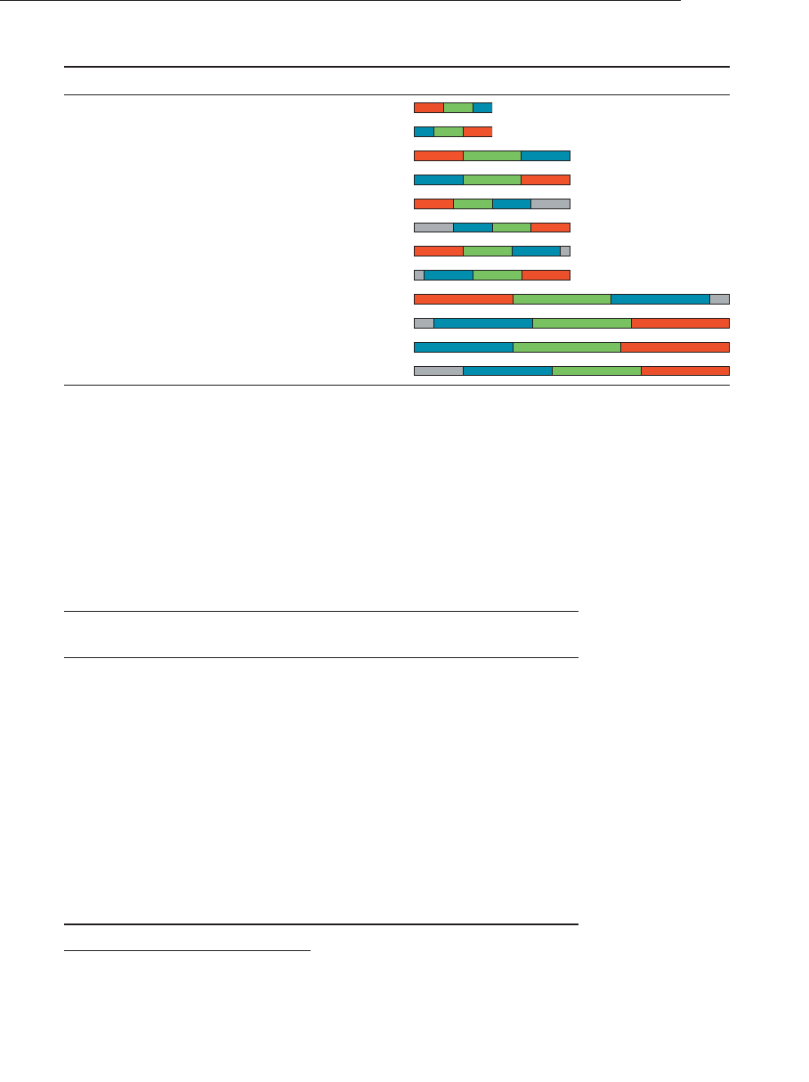
ptg9898810
Table 6.4 Example Component Layouts for Packed Pixel Formats
Format Token Component Layout
GL_UNSIGNED_BYTE_3_3_2 RED GREEN BLUE
GL_UNSIGNED_BYTE_2_3_2_REV BLUE REDGREEN
GL_UNSIGNED_SHORT_5_6_5 RED GREEN BLUE
GL_UNSIGNED_SHORT_5_6_5_REV REDGREENBLUE
GL_UNSIGNED_SHORT_4_4_4_4 BLUERED GREEN ALPHA
GL_UNSIGNED_SHORT_4_4_4_4_REV BLUE REDGREENALPHA
GL_UNSIGNED_SHORT_5_5_5_1 BLUERED GREEN A
GL_UNSIGNED_SHORT_1_5_5_5_REV BLUE REDGREENA
GL_UNSIGNED_INT_10_10_10_2 BLUERED GREEN A
GL_UNSIGNED_INT_2_10_10_10_REV BLUE REDGREENA
GL_UNSIGNED_INT_10F_11F_11F_REV BLUE REDGREEN
GL_UNSIGNED_INT_5_9_9_9_REV REDGREENBLUEALPHA
Proxy Textures
In addition to the texture targets listed in Table 6.1, OpenGL supports
what are known as proxy texture targets. Each standard texture target4has
a corresponding proxy texture target. Table 6.5 lists the standard texture
targets and their corresponding proxy texture targets.
Table 6.5 Texture Targets and Corresponding Proxy Targets
Texture Proxy Texture Target
Target (GL_TEXTURE*) (GL_PROXY_TEXTURE*)
1D 1D
1D_ARRAY 1D_ARRAY
2D 2D
2D_ARRAY 2D_ARRAY
2D_MULTISAMPLE 2D_MULTISAMPLE
2D_MULTISAMPLE_ARRAY 2D_MULTISAMPLE_ARRAY
3D 3D
CUBE CUBE
CUBE_ARRAY CUBE_ARRAY
RECTANGLE RECTANGLE
BUFFER n/a
4. All targets except for GL_TEXTURE_BUFFER have a corresponding proxy texture target.
276 Chapter 6: Textures

ptg9898810
Proxy texture targets may be used to test the capabilities of the OpenGL
implementation when certain limits are used in combination with
each other. For example, consider an OpenGL implementation that reports
a maximum texture size of 16384 texels (which is the minimum
requirement for OpenGL 4). If one were to create a texture of 16384 ×
16384 texels with an internal format of GL_RGBA8 (which requires four
bytes of storage per texel), then the total storage requirement for such a
texture would be at least a gigabyte---more if mipmaps or other internal
storage is required. Therefore, such a request would fail on an OpenGL
implementation with less than a gigabyte of available storage for textures.
By requesting such a texture allocation on a proxy texture target, the
implementation can tell you whether the request might5succeed on a
normal target, or whether it is destined to fail. If an allocation of a texture
on a proxy texture target fails, the texture on the virtual proxy target will
have a width and height of zero. Querying the dimensions of the proxy
target will tell you whether the call was successful and whether such a
request on a real target might succeed.
Specifying Texture Data
In this section, we describe the method in which image data is loaded into
texture objects. Two methods are covered---first, we show how to load
images directly into the texture object either from data stored in arrays
in your program or from buffer objects. This illustrates the storage and
data formats used for texture objects. Next, we show how to use the
vglLoadImage() function that is supplied as part of the sample code
for this book and how it allows you to load images from files.
Explicitly Setting Texture Data
In order to describe the process in which texture data is specified to
OpenGL, it’s possibly easiest to be able to see the image data directly in
your program. Texture data is laid out6as you might expect it to be---left to
right, top to bottom. In Example 6.1, texture data is stored in a constant
array declared in C.
5. Just because an allocation appears to succeed on a proxy texture target, it does not mean
that it will definitely succeed on a real target. It may fail for a variety of other reasons such as
the total amount of other textures allocated, or memory fragmentation, for example. However,
if it fails on a proxy texture target, it will certainly fail on a real texture target.
6. There are several parameters supported by OpenGL that allow you to change the layout of
image data in memory. These are discussed later in this chapter, but the defaults are sufficient
for this example.
Specifying Texture Data 277

ptg9898810
Example 6.1 Direct Specification of Image Data in C
// The following is an 8x8 checkerboard pattern using
// GL_RED, GL_UNSIGNED_BYTE data.
static const GLubyte tex_checkerboard_data[] =
{0xFF, 0x00, 0xFF, 0x00, 0xFF, 0x00, 0xFF, 0x00,
0x00, 0xFF, 0x00, 0xFF, 0x00, 0xFF, 0x00, 0xFF,
0xFF, 0x00, 0xFF, 0x00, 0xFF, 0x00, 0xFF, 0x00,
0x00, 0xFF, 0x00, 0xFF, 0x00, 0xFF, 0x00, 0xFF,
0xFF, 0x00, 0xFF, 0x00, 0xFF, 0x00, 0xFF, 0x00,
0x00, 0xFF, 0x00, 0xFF, 0x00, 0xFF, 0x00, 0xFF,
0xFF, 0x00, 0xFF, 0x00, 0xFF, 0x00, 0xFF, 0x00,
0x00, 0xFF, 0x00, 0xFF, 0x00, 0xFF, 0x00, 0xFF
};
// The following data represents a 2x2 texture with red,
// green, blue, and yellow texels represented as GL_RGBA,
// GL_FLOAT data.
static const GLfloat tex_color_data[] =
{// Red texel Green texel
1.0f, 0.0f, 0.0f, 1.0f, 0.0f, 1.0f, 0.0f, 1.0f,
// Blue texel Yellow texel
0.0f, 0.0f, 1.0f, 1.0f, 1.0f, 1.0f, 0.0f, 1.0f
};
Of course, specifying texture data by hand directly in your code is not the
most efficient way of creating textures. For simple cases such as solid colors
or basic checkerboard patterns, it will suffice though. You can load the data
into a texture object using one of the glTexSubImage1D(),
glTexSubImage2D(), or glTexSubImage3D() functions listed below.
void glTexSubImage1D(GLenum target, GLint level, GLint xoffset,
GLsizei width, GLenum format,
GLenum type, const void *data);
void glTexSubImage2D(GLenum target, GLint level, GLint xoffset,
GLint yoffset, GLsizei width,
GLsizei height, GLenum format,
GLenum type, const void *data);
void glTexSubImage3D(GLenum target, GLint level, GLint xoffset,
GLint yoffset, GLint zoffset,
GLsizei width, GLsizei height,
GLsizei depth, GLenum format,
GLenum type, const void *data);
278 Chapter 6: Textures

ptg9898810
Replace a region of a texture with new data specified in data. The level,
format, and type parameters have the same meaning as in
glTexImage1D() through glTexImage3D().level is the mipmap level
number. format and type describe the format and data type of the texture
image data pointed to by data.
data contains the texture data for the subimage. width,height, and depth
(if present) are the dimensions of the region that is to replace all or part
of the current texture image. xoffset,yoffset, and zoffset (if present) specify
the texel offset in the x,y, and zdimensions, respectively. target
represents the texture target to which the texture object to be modified is
bound. If target represents a 1D array texture, then yoffset and height
specify the first layer and number of layers to be updated, respectively,
otherwise they are treated as texel coordinates. If target is a 2D array
texture, cube map, or cube-map array texture, zoffset and depth represent
the first layer and number of layers to be updated, otherwise they are
treated as texel coordinates.
The specified region may not include any texels outside the range of the
originally defined texture array.
The data shown in Example 6.1 shows two simple textures directly coded
into constant arrays. The first, tex_checkerboard_data, specifies a
simple 8 ×8 region of texels of alternating full intensity (0xFF) and zero
intensity (0x00) represented as single unsigned bytes. The second array in
Example 6.1 shows color data, this time represented as floating-point data
with four channels---the channels representing the amount of red, green,
blue, and alpha7in each texel. Example 6.2 shows how to load this data
into texture objects using glTexSubImage2D().
Example 6.2 Loading Static Data into Texture Objects
// First, the black-and-white checkerboard texture...
// Bind the texture (possibly creating it)
glBindTexture(GL_TEXTURE_2D, tex_checkerboard);
// Allocate storage for the texture data
glTexStorage2D(GL_TEXTURE_2D, 4, GL_R8, 8, 8);
// Specify the data for the texture
glTexSubImage2D(GL_TEXTURE_2D, // target
0, // First mipmap level
0, 0, // x and y offset
8, 8, // width and height
GL_RED, GL_UNSIGNED_BYTE, // format and type
tex_checkerboard_data); // data
7. Alpha is normally used to represent opacity, but in this case we have set the alpha channel
to its maximum value to represent fully opaque texels.
Specifying Texture Data 279

ptg9898810
// Next, the color, floating-point data.
// Bind the next texture
glBindTexture(GL_TEXTURE_2D, tex_color);
// Allocate storage
glTexStorage2D(GL_TEXTURE_2D, 2, GL_RGBA32F, 2, 2);
// Specify the data
glTexSubImage2D(GL_TEXTURE_2D, // target
0, // First mipmap level
0, 0, // x and y offset
2, 2, // width and height
GL_RGBA, GL_FLOAT, // format and type
tex_color_data); // data
Notice how, in Example 6.2, we specify an internal format for the texture
that somewhat matches our supplied texture data. For the array of
unsigned bytes, we used the internal format GL_R8, which indicates a
single channel, 8-bit format. For the color data, we used GL_RGBA32F,
which is a four-channel, 32-bit floating-point format. There is no
requirement that we use an internal format that matches the data we’ll
supply. There are well-defined rules as to how OpenGL converts the data
you supply into each internal format and these are explained in detail in
the OpenGL specification.
Using Pixel Unpack Buffers
The data parameter to glTexSubImage2D() may be interpreted in one of
two ways. The first is as a natural pointer to data stored in the application’s
memory. This is the use case shown in Example 6.2.data is interpreted this
way if no buffer object is bound to the GL_PIXEL_UNPACK_BUFFER target.
The second interpretation of data, which is used when there is a buffer
bound to the GL_PIXEL_UNPACK_BUFFER target, is as an offset into that
buffer object. This allows the application to stage data into a buffer object
and transfer it from there into a texture object at a later time.
Example 6.3 Loading Data into a Texture Using a Buffer Object
// First, bind a buffer to the GL_PIXEL_UNPACK_BUFFER binding
glBindBuffer(GL_PIXEL_UNPACK_BUFFER, buf);
// Place our source data into the buffer
glBufferData(GL_PIXEL_UNPACK_BUFFER,
sizeof(tex_checkerboard_data),
tex_checkerboard_data,
GL_STATIC_DRAW);
// Bind the texture (possibly creating it)
glBindTexture(GL_TEXTURE_2D, tex_checkerboard);
// Allocate storage for the texture data
glTexStorage2D(GL_TEXTURE_2D, 4, GL_R8, 8, 8);
// Specify the data for the texture
280 Chapter 6: Textures

ptg9898810
glTexSubImage2D(GL_TEXTURE_2D, // target
0, // First mipmap level
0, 0, // x and y offset
8, 8, // width and height
GL_RED, // Format
GL_UNSIGNED_BYTE, // Type
NULL); // data(an offset into buffer)
In Example 6.3, we first place our source data (tex_checkerboard_data)
into a buffer object bound to the GL_PIXEL_UNPACK_BUFFER binding
point, and then call glTexSubImage2D() as we did before. However, this
time data is interpreted as an offset into the buffer object rather than a raw
pointer because we left the buffer bound. This causes OpenGL to take the
data from the buffer object, but not necessarily immediately. The primary
advantage of using a buffer object to stage texture data is that the transfer
from the buffer object into the texture need not occur immediately, so
long as it occurs by the time the data is required by a shader. This allows
the transfer to occur in parallel with the application running. If instead
the data is located in application memory, then the semantics of
glTexSubImage2D() require that a copy of the data is made before the
function returns, preventing a parallel transfer. The advantage of this
method is that the application is free to modify the data it passed to the
function as soon as the function returns.
Copying Data from the Framebuffer
It is possible to read part of the framebuffer into a texture object, and then
use it in subsequent rendering. To do this, use either the
glCopyTexImage1D() or glCopyTexImage2D() functions whose
prototypes are as follows:
void glCopyTexImage1D(GLenum target, GLint level,
GLint internalFormat, GLint x, GLint y,
GLsizei width, GLint border);
void glCopyTexImage2D(GLenum target, GLint level,
GLint internalFormat, GLint x, GLint y,
GLsizei width, GLsizei height,
GLint border);
Copy pixels from the current read framebuffer into the texture currently
bound to target of the active texture unit. xand yspecify the horizontal
and vertical offset of the source region to copy from the framebuffer.
width and height (if present) specify the width and height of the region,
respectively. internalFormat specifies the format with which the resulting
texels should be stored. border is reserved and must be zero.
Specifying Texture Data 281

ptg9898810
When glCopyTexImage1D() or glCopyTexImage2D() is called, it is
essentially equivalent to calling glReadPixels(), and then immediately
calling either glTexImage1D() or glTexImage2D() to re-upload the image
data into the texture.
void glCopyTexSubImage1D(GLenum target, GLint level,
GLint xoffset, GLint x, GLint y,
GLsizei width);
void glCopyTexSubImage2D(GLenum target, GLint level,
GLint xoffset, GLint yoffset,
GLint x, GLint y, GLsizei width,
GLsizei height);
void glCopyTexSubImage3D(GLenum target, GLint level,
GLint xoffset, GLint yoffset,
GLint zoffset, GLint x, GLint y,
GLsizei width, GLsizei height);
Use image data from the framebuffer to replace all or part of a contiguous
subregion of the current, existing texture image in the texture object
bound to target of the active texture unit. xand yspecify the xand y
offset of the region in the framebuffer to copy. width and height (if
present) specify the width and height of the region to copy, respectively.
xoffset,yoffset, and zoffset (if present) specify the origin of the destination
region in the target texture. If target is a 1D array texture, then yoffset is
the layer of the texture into which the 1D region of texels will be written,
otherwise it is the ycoordinate of the origin of the destination region. If
target is a 2D array, cube map, or cube-map array texture, then zoffset is
the index of the layer of the texture containing the destination region,
otherwise it is the zcoordinate of the destination region in a 3D texture.
Although it is possible to read from the framebuffer into a texture, this
involves making a copy of the image data, and may also involve format
conversions or other work being conducted by the graphics hardware. In
general, it is more efficient to draw directly into the texture wherever
possible. This is covered in detail in Chapter 4,‘‘Color, Pixels, and
Framebuffers’’.
Loading Images from Files
The simple example of directly storing image data in arrays in your ‘‘C’’
code (or from buffer objects) isn’t very practical if you have large images
stored on disk. In most applications, you’ll store your texture data in a
282 Chapter 6: Textures

ptg9898810
formatted image file---a JPEG, PNG, GIF, or other type for image format---
OpenGL works either with raw pixels or with textures compressed with
specific algorithms. As such, your application will need to decode the
image file into memory that OpenGL can read to initialize its internal
texture store. To simplify that process for our examples, we wrote a
function, vglLoadImage(), which will read an image file,8and return the
texels in memory, along with other information you’ll need to help
OpenGL to decode the its pixel data:
•Width (measured in pixels)
•Height (measured in pixels)
•OpenGL’s pixel format (e.g., GL_RGB for RGB pixels)
•A recommended internal format to use for the texture
•The number of mipmap levels present in the texture
•Data type for each component in a pixel
•Image data
All of that data is stored in structure of type vglImageData, which is
defined in LoadImage.h. The definition of vglImageData is shown in
Example 6.4 below.
Example 6.4 Definition of the vglImageData Structure
// Enough mips for 16K x 16K, which is the minimum required for
// OpenGL 4.x and higher
#define MAX_TEXTURE_MIPS 14
// Each texture image data structure contains an array of
// MAX_TEXTURE_MIPS of these mipmap structures. The structure
// represents the mipmap data for all slices at that level.
struct vglImageMipData
{
GLsizei width; // Width of this mipmap level
GLsizei height; // Height of this mipmap level
GLsizei depth; // Depth pof mipmap level
GLsizeiptr mipStride; // Distance between mip levels
in memory
GLvoid*data; // Pointer to data
};
// This is the main image data structure. It contains all
// the parameters needed to place texture data into a texture
// object using OpenGL.
8. Currently, DDS files are supported by vglLoadImage().
Specifying Texture Data 283

ptg9898810
struct vglImageData
{
GLenum target; // Texture target (2D, cube map, etc.)
GLenum internalFormat; // Recommended internal format
GLenum format; // Format in memory
GLenum type; // Type in memory (GL_RGB, etc.)
GLenum swizzle[4]; // Swizzle for RGBA
GLsizei mipLevels; // Number of present mipmap levels
GLsizei slices; // Number of slices (for arrays)
GLsizeiptr sliceStride; // Distance between slices of an
array texture
GLsizeiptr totalDataSize; // Total data allocated for texture
vglImageMipData mip[MAX_TEXTURE_MIPS]; // Actual mipmap data
};
In order to create, initialize, manipulate, and destroy images in memory,
we have defined two functions---vglLoadImage() and vglUnloadImage().
Each takes a pointer to a vglImageData structure. vglLoadImage() fills it in
and vglUnloadImage() releases any resources that were allocated by a
previous call to vglLoadImage(). The prototypes of vglLoadImage() and
vglUnloadImage() are as follows:
void vglLoadImage(const char* filename, vglImageData* image);
void vglUnloadImage(vglImageData* image);
vglLoadImage() loads an image from a file on disk. filename specifies the
name of the file to load. image is the address of a vglImageData structure
that will be filled with the parameters of the image on success. On failure,
image will be cleared. vglUnloadImage() should be used to release any
resources consumed by a previous, successful call to vglLoadImage().
To load an image file, simply use code such as that shown in Example 6.5
in your application.
Example 6.5 Simple Image Loading Example
vglImageData image;
vglLoadImage(filename, &image);
// Use image data here
vglUnloadImage(&image);
The result of calling vglLoadImage() is that the texture data from the
specified image file is loaded into memory, and information about that
image data is stored in the vglImageData structure given to the function.
Once the image data has been loaded from the file, you may use it to
establish the texels for your texture object. To do this, pass the data pointer
284 Chapter 6: Textures

ptg9898810
and texture dimensions to the appropriate texture image function. If the
texture is allocated as an immutable object (using glTexStorage2D(), for
example), then the image data is specified using a texture subimage
command such as glTexSubImage2D(). The vglImageData structure
contains all of the parameters required to initialize the image.
Example 6.6 shows a simple but complete example of using the
vglLoadImage() function to load an image from disk, the
glTexStorage2D() function to allocate storage in texture object, and
glTexSubImage2D() to load the image data into the texture object.
Example 6.6 Loading a Texture Using loadImage
GLuint LoadTexture(const char*filename,
GLuint texture,
GLboolean generateMips)
{vglImageData image;
int level;
vglLoadImage(filename, &image);
if (texture == 0)
{glGenTextures(1, &texture);
}
glBindTexture(image.target, texture);
switch (image.target)
{
case GL_TEXTURE_2D:
glTexStorage2D(image.target,
image.mipLevels,
image.internalFormat,
image.mip[0].width,
image.mip[0].height);
// Handle other texture targets here.
default:
break;
}
// Assume this is a 2D texture.
for (level = 0; level < image.mipLevels; ++level)
{glTexSubImage2D(GL_TEXTURE_2D,
level,
0, 0,
image.mip[level].width,
image.mip[level].height,
image.format, image.type,
image.mip[level].data);
}
Specifying Texture Data 285

ptg9898810
// Unload the image here as glTexSubImage2D has consumed
// the data and we don’t need it any more.
vglUnloadImage(&image);
return texture;
}
As you can see, this code could become quite complex depending on how
generic your texture-loading function might be and how many types of
texture you might want to load. To make things easier for you, we have
included the function vglLoadTexture(), which internally uses
vglLoadImage() to load an image file, and then place its contents into a
texture object for you. The listing shows a simplified version of the
vglLoadTexture() function, which will take an image file and load it into a
texture object for you. It will handle any dimensional image, array
textures, cube maps, compressed textures, and anything else that’s
supported by the vglLoadImage() function. The complete implementation
of vglLoadTexture() is included in this book’s accompanying source code.
GLuint vglLoadTexture(const char* filename, GLuint texture,
vglImageData* image);
Loads a texture from disk and places it into an OpenGL texture object.
filename is the name of the file to load. texture is the name of a texture
object into which to load the data. If texture is zero, then
vglLoadTexture() will create a new texture object into which to place the
data. image is the address of a vglImageData structure that may be used
to return the parameters of the loaded image. If image is not NULL, then it
will be used to return information about the image, and the image data
will not be freed. The application should use vglUnloadImage() to
release any resources associated with the image. If image is NULL then
internal data structures will be used to load the image, and the resulting
image data will be freed automatically. Upon success, vglLoadTexture()
returns the texture object into which the texture image was loaded. If
texture is not zero, then the return value will be equal to texture, otherwise
it is a newly created texture object. Upon failure, vglLoadTexture()
returns zero.
Note: It’s not possible to directly specify the image data for a
multisampled texture. The only way to place data into a
multisampled texture is to attach it to a framebuffer object and
render into it. Framebuffers and multisampling is explained in
some detail in Chapter 4,‘‘Color, Pixels, and Framebuffers’’.
286 Chapter 6: Textures

ptg9898810
Retrieving Texture Data
Once you have a texture containing data, it is possible to read that data
either back into your application’s memory or back into a buffer object.
The function for reading image data from a texture is glGetTexImage(),
whose prototype is as follows:
void glGetTexImage(GLenum target, GLint lod, GLenum format,
GLenum type, GLvoid* image);
Retrieves a texture image from the texture bound to target.target must be
one of GL_TEXTURE_1D, GL_TEXTURE_2D, GL_TEXTURE_3D,
GL_TEXTURE_1D_ARRAY, GL_TEXTURE_2D_ARRAY,
GL_TEXTURE_CUBE_MAP_ARRAY, or GL_TEXTURE_RECTANGLE.
Additionally, the targets GL_TEXTURE_CUBE_MAP_POSITIVE_X,
GL_TEXTURE_CUBE_MAP_NEGATIVE_X,
GL_TEXTURE_CUBE_MAP_POSITIVE_Y,
GL_TEXTURE_CUBE_MAP_NEGATIVE_Y,
GL_TEXTURE_CUBE_MAP_POSITIVE_Z, and
GL_TEXTURE_CUBE_MAP_NEGATIVE_Z may be used to indicate the
corresponding face of a single cube-map texture. lod is the level-of-detail
number. format and type are the pixel format and type of the desired data.
image is interpreted either as an address in client memory where the
image data will be placed or, if a buffer is bound to the
GL_PIXEL_PACK_BUFFER target as an offset into that buffer at which the
image data will be placed.
Great care should be exercised when using this function. The number of
bytes written into image is determined by the dimensions of the texture
currently bound to target, and by format and type. Potentially, a great deal
of data could be returned and no bound checks are performed by OpenGL
on the memory area you supply. Therefore, incorrect usage of this function
could lead to buffer overruns and bad things happening.
Furthermore, reading pixel data back from textures is generally not a
high-performance operation. Doing so should be a sparingly invoked
operation and should certainly not be in a performance critical path of
your application. If you must read data back from textures, we strongly
recommend that you bind a buffer to the GL_PIXEL_PACK_BUFFER buffer
target, read the texels into that, and subsequently map the buffer in order
to transfer the pixel data into your application.
Specifying Texture Data 287

ptg9898810
Texture Data Layout
So far, our descriptions of the texture image specification commands have
not addressed the physical layout of image data in memory. In many cases,
image data is laid out left-to-right, top-to-bottom9in memory with texels
closely following each other. However, this is not always the case, and so
OpenGL provides several controls that allow you to describe how the data
is laid out in your application.
These parameters are set using the glPixelStorei() and glPixelStoref()
commands, whose prototypes are as follows:
void glPixelStorei(GLenum pname, GLint param);
void glPixelStoref(GLenum pname, GLfloat param);
Set the pixel storage parameter pname to the value specified by param.
pname must be one of the pixel unpacking parameter names
(GL_UNPACK_ROW_LENGTH, GL_UNPACK_SWAP_BYTES,
GL_UNPACK_SKIP_PIXELS, GL_UNPACK_SKIP_ROWS,
GL_UNPACK_SKIP_IMAGES, GL_UNPACK_ALIGNMENT,
GL_UNPACK_IMAGE_HEIGHT, or GL_UNPACK_LSB_FIRST) or one of the
pixel packing parameter names (GL_PACK_ROW_LENGTH,
GL_PACK_SWAP_BYTES, GL_PACK_SKIP_PIXELS, GL_PACK_SKIP_ROWS,
GL_PACK_SKIP_IMAGES, GL_PACK_ALIGNMENT,
GL_PACK_IMAGE_HEIGHT, or GL_PACK_LSB_FIRST).
The unpack parameters set by glPixelStorei() and glPixelStoref() (those
beginning with GL_UNPACK_) specify how OpenGL will read data from
client memory or the buffer bound to the GL_PIXEL_UNPACK_BUFFER
binding in functions such as glTexSubImage2D(). The packing parameters
specify how OpenGL will write texture data into memory during functions
such as glGetTexImage().
Since the corresponding parameters for packing and unpacking have the
same meanings, they’re discussed together in the rest of this section and
referred to without the GL_PACK_ or GL_UNPACK_ prefix. For example,
*SWAP_BYTES refers to GL_PACK_SWAP_BYTES and
GL_UNPACK_SWAP_BYTES. If the *SWAP_BYTES parameter is GL_FALSE
(the default), the ordering of the bytes in memory is whatever is native for
the OpenGL client; otherwise, the bytes are reversed. The byte reversal
9. It’s important to understand that textures don’t really have a top and a bottom, but rather they
have an origin and a direction of increasing of texture coordinates. What appears to be rendered
at the top of a frame in window coordinates depends entirely on the texture coordinates used.
288 Chapter 6: Textures
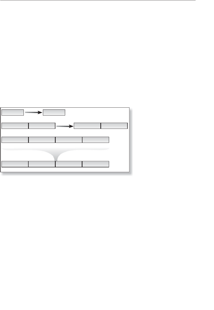
ptg9898810
applies to any size element, but has a meaningful effect only for multibyte
elements.
The effect of byte swapping may differ among OpenGL implementations. If
on an implementation, GLubyte has 8 bits, GLushort has 16 bits, and GLuint
has 32 bits, then Figure 6.1 illustrates how bytes are swapped for different
data types. Note that byte swapping has no effect on single-byte data.
Note: As long as your OpenGL application doesn’t share images with
other machines, you can ignore the issue of byte ordering. If your
application must render an OpenGL image that was created on a
different machine, and the two machines have different byte
orders, byte ordering can be swapped using *SWAP_BYTES.
However, *SWAP_BYTES does not allow you to reorder elements
(e.g., to swap red and green).
Byte
7 6 5 4 3 2 1 0
Byte
7 6 5 4 3 2 1 0
Short (Byte 0)
15 14 13 12 11 10 9 8
Short (Byte 1)
7 6 5 4 3 2 1 0
Short (Byte 0)
15 14 13 12 11 10 9 8
Short (Byte 1)
7 6 5 4 3 2 1 0
Integer (Byte 1)
23 22 21 20 19 18 17 16
Integer (Byte 0)
31 30 29 28 27 26 25 24
Integer (Byte 3)
7 6 5 4 3 2 1 0
Integer (Byte 2)
15 14 13 12 11 10 9 8
Integer (Byte 1)
23 22 21 20 19 18 17 16
Integer (Byte 0)
31 30 29 28 27 26 25 24
Integer (Byte 3)
7 6 5 4 3 2 1 0
Integer (Byte 2)
15 14 13 12 11 10 9 8
Figure 6.1 Byte-swap effect on byte, short, and integer data
The *LSB_FIRST parameter applies only when drawing or reading 1-bit
images or bitmaps for which a single bit of data is saved or restored for
each pixel. If *LSB_FIRST is GL_FALSE (the default), the bits are taken from
the bytes starting with the most significant bit; otherwise, they’re taken in
the opposite order. For example, if *LSB_FIRST is GL_FALSE, and the byte
in question is 0x31, the bits, in order, are {0, 0, 1, 1, 0, 0, 0, 1}. If
*LSB_FIRST is GL_TRUE, the order is {1, 0, 0, 0, 1, 1, 0, 0}.
Sometimes you want to draw or read only a subrectangle of the entire
rectangle of image data stored in memory. If the rectangle in memory is
larger than the subrectangle that’s being drawn or read, you need to
specify the actual length (measured in pixels) of the larger rectangle with
*ROW_LENGTH. If *ROW_LENGTH is zero (which it is by default), the row
length is understood to be the same as the width that’s implied by the
Specifying Texture Data 289
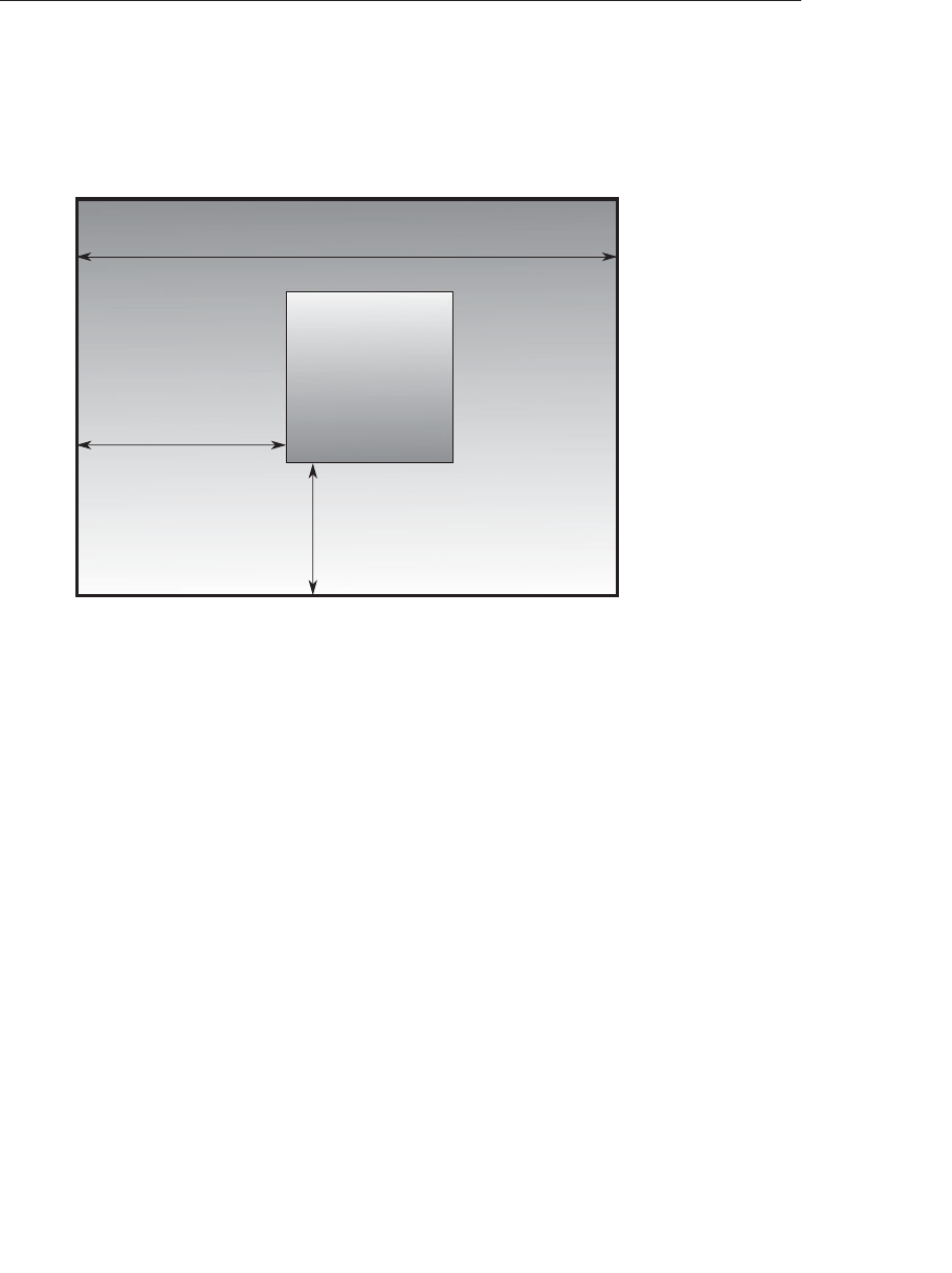
ptg9898810
parameters to glTexSubImage2D(), for example. You also need to specify
the number of rows and pixels to skip before starting to copy the data for
the subrectangle. These numbers are set using the parameters *SKIP_ROWS
and *SKIP_PIXELS, as shown in Figure 6.2. By default, both parameters are
0, so you start at the lower left corner.
*_ROW_LENGTH
*_SKIP_PIXELS
*_SKIP_ROWS
Subimage
Image
Figure 6.2 Subimage
(A subimage identified by *SKIP_ROWS, *SKIP_PIXELS, and *ROW_LENGTH
parameters.)
Often, a particular machine’s hardware is optimized for a particular byte
alignment when moving pixel data to and from memory. For example, in a
machine with 32-bit words, hardware can often retrieve data much faster if
it’s initially aligned on a 32-bit boundary, which typically has an address
that is a multiple of 4. Likewise, 64-bit architectures might work better
when the data is aligned to 8-byte boundaries. On some machines,
however, byte alignment makes no difference.
As an example, suppose your machine works better with pixel data aligned
to a 4-byte boundary. Images are most efficiently saved by forcing the data
for each row of the image to begin on a 4-byte boundary. If the image is
5 pixels wide and each pixel consists of 1 byte each of red, green, and blue
information, a row requires 5 ×3=15 bytes of data. Maximum display
efficiency can be achieved if the first row, and each successive row, begins
on a 4-byte boundary, so there is 1 byte of waste in the memory storage for
each row. If your data is stored in this way, set the *ALIGNMENT parameter
appropriately (to 4, in this case).
290 Chapter 6: Textures
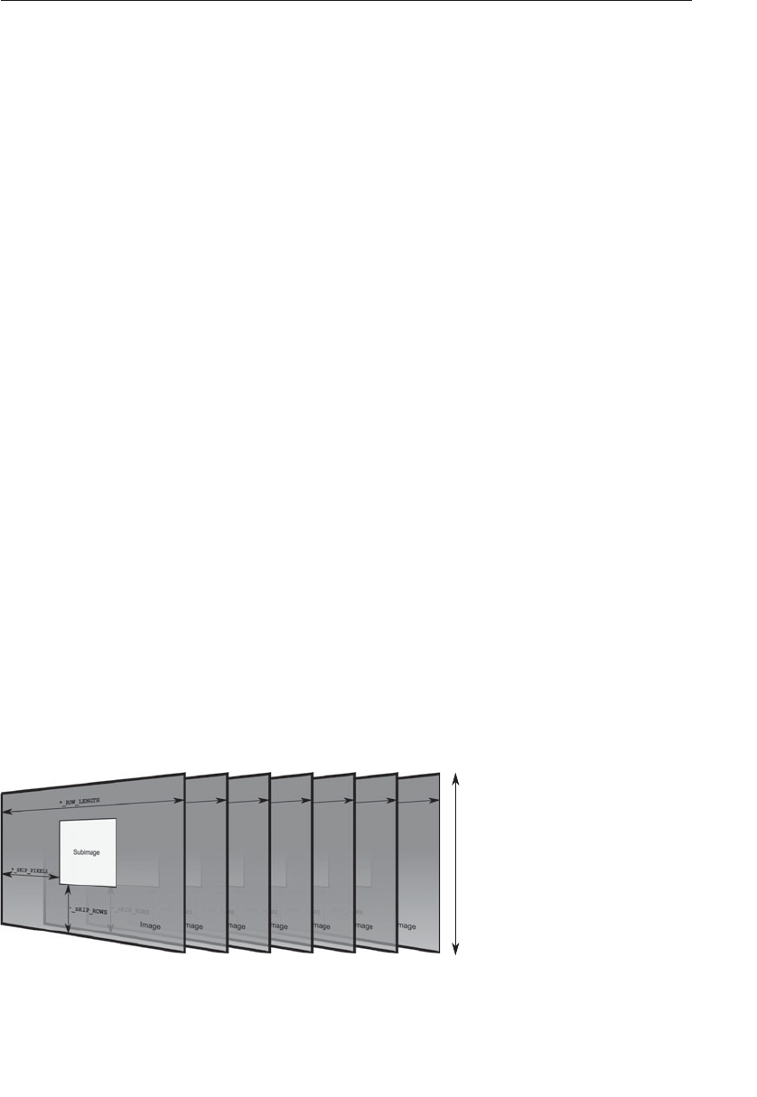
ptg9898810
If *ALIGNMENT is set to 1, the next available byte is used. If it’s 2, a byte is
skipped if necessary at the end of each row so that the first byte of the next
row has an address that’s a multiple of 2. In the case of bitmaps (or 1-bit
images), where a single bit is saved for each pixel, the same byte alignment
works, although you have to count individual bits. For example, if you’re
saving a single bit per pixel, if the row length is 75, and if the alignment
is 4, then each row requires 75/8, or 93/8 bytes. Since 12 is the smallest
multiple of 4 that is bigger than 93/8, 12 bytes of memory are used for
each row. If the alignment is 1, then 10 bytes are used for each row, as 9
3/8 is rounded up to the next byte.
Note: The default value for *ALIGNMENT is 4. A common programming
mistake is to assume that image data is tightly packed and byte
aligned (which assumes that *ALIGNMENT is set to 1).
The parameters *IMAGE_HEIGHT and *SKIP_IMAGES affect only the
defining and querying of three-dimensional textures and two-dimensional
texture arrays. These pixel-storage parameters allow the routines
glTexImage3D(),glTexSubImage3D(), and glGetTexImage() to delimit
and access any desired subvolume or subset of slices of an array texture.
If the three-dimensional texture in memory is larger than the subvolume
that is defined, you need to specify the height of a single subimage with
the *IMAGE_HEIGHT parameter. Also, if the subvolume does not start with
the very first layer, the *SKIP_IMAGES parameter needs to be set.
*IMAGE_HEIGHT is a pixel-storage parameter that defines the height
(number of rows) of a single layer of a three-dimensional texture image, as
shown in Figure 6.3. If the *IMAGE_HEIGHT value is zero (a negative
number is invalid), then the number of rows in each two-dimensional
rectangle is the value of height, which is the parameter passed to
glTexImage3D() or glTexSubImage3D(). (This is commonplace because
*IMAGE_HEIGHT is zero, by default.) Otherwise, the height of a single
layer is the *IMAGE_HEIGHT value.
*_IMAGE_HEIGHT
Figure 6.3 *IMAGE_HEIGHT pixel storage mode
Specifying Texture Data 291
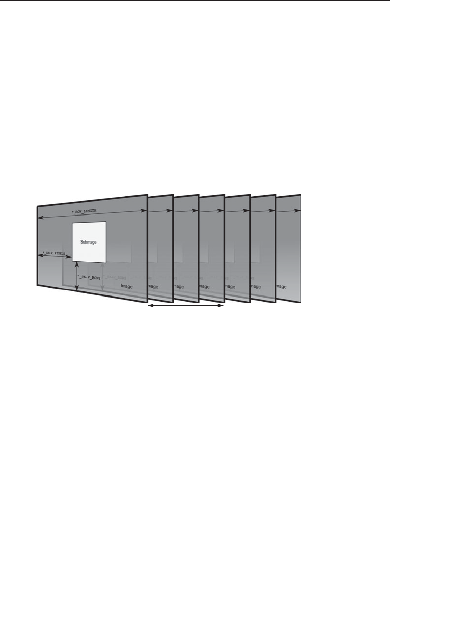
ptg9898810
*SKIP_IMAGES defines how many layers to bypass before accessing the first
data of the subvolume. If the *SKIP_IMAGES value is a positive integer (call
the value n), then the pointer in the texture image data is advanced that
many layers (n* the size of one layer of texels). The resulting subvolume
starts at layer nand is several layers deep---how many layers deep is
determined by the depth parameter passed to glTexImage3D() or
glTexSubImage3D(). If the *SKIP_IMAGES value is zero (the default), then
accessing the texel data begins with the very first layer described in the
texel array.
Figure 6.4 shows how the *SKIP_IMAGES parameter can bypass several
layers to get to where the subvolume is actually located. In this example,
*SKIP_IMAGES is 4 and the subvolume begins at layer 4.
*_SKIP_IMAGES
Figure 6.4 *SKIP_IMAGES pixel storage mode
Sampler Objects
Textures may be read by a shader by associating a sampler variable with a
texture unit and using GLSL’s built-in functions to fetch texels from the
texture’s image. The way in which the texels are fetched depends on a
number of parameters that are contained in another object called a
sampler object. Sampler objects are bound to sampler units much as
texture objects are bound to texture units. For convenience, a texture
object may be considered to contain a built-in sampler object of its own
that will be used by default to read from it, if no sampler object is bound to
the corresponding sampler unit.
To create a sampler object, as with most other object types in OpenGL, we
reserve a name for the new object and bind it to a binding point---in this
case, one of the GL_SAMPLER binding points. The prototype of
glGenSamplers() is as follows:
292 Chapter 6: Textures

ptg9898810
void glGenSamplers(GLsizei count, GLuint *samplers);
Returns count currently unused names for sampler objects in the array
samplers. The names returned in samplers will not necessarily be a
contiguous set of integers.
The names in samplers are marked as used, but they acquire sampler state
only when they are first bound.
The value zero is reserved and is never returned by glGenSamplers().
glGenSamplers() will return a set of unused sampler object names. Once
the names have been generated, they are reserved for use as sampler
objects and may be bound to the sampler binding points using the
glBindSampler() function, whose prototype is shown below.
void glBindSampler(GLuint unit, GLuint sampler);
Binds the sampler object named sampler to the sampler unit whose index
is given in unit.Ifsampler is zero, any sampler object currently bound to
sampler unit unit is unbound and no object is bound in its place.
Until a name has been bound to a sampler unit, it is not yet considered a
sampler object. To determine if a given value is the name of an existing
sampler object, you can call glIsSampler(), whose prototype is as follows:
GLboolean glIsSampler(GLenum id);
Returns GL_TRUE if id is the name of an existing sampler object and
GL_FALSE otherwise.
Notice that there are a couple of subtle differences10 between the
glBindSampler() function and the glBindTexture() function. First, there
is no target parameter for samplers. This is because the target is implied by
10. These differences may seem to introduce inconsistency into the OpenGL API. That is a fair
observation. However, it is a byproduct of the way that OpenGL evolves. The API takes small,
incremental steps, each striking a balance among introduction of new functionality, enable-
ment of innovation, and maintenance of backwards compatibility. It has been recognized that
modern OpenGL implementations can support a huge number of textures and samplers, and
reserving tokens from GL_SAMPLER0 through GL_SAMPLER79 is simply not practical,
and is not forward-looking. Thus, the decision to sacrifice some consistency in order to achieve
some forward compatibility was made.
Sampler Objects 293

ptg9898810
the function. As sampler objects have no inherent dimensionality, there is
no reason to distinguish among multiple sampler object types. Secondly,
the unit parameter is present here, and there is no selector for sampler
objects---that is, there is no glActiveSampler() function. Furthermore, in
contrast to the parameter to glActiveTexture(), which is a token between
GL_TEXTURE0 and GL_TEXTUREi, where iis an arbitrarily large
implementation-defined maximum, unit is a zero-based unsigned integer,
allowing any number of sampler units to be supported by an OpenGL
implementation without reserving a large number of OpenGL tokens.
Sampler Parameters
Each sampler object represents a number of parameter that controls the
way texels will ultimately be read from a texture object. The parameters of
the sampler object are set using the glSamplerParameteri() and
glSamplerParameterf() functions (for integer and floating-point
parameters), and glSamplerParameteriv() and glSamplerParameterfv()
functions (for vectors of integer and floating-point parameters). Their
prototypes are given below.
void glSamplerParameter{fi}(GLuint sampler, GLenum pname,
Type param );
void glSamplerParameter{fi}v(GLuint sampler, GLenum pname,
const Type* param );
void glSamplerParameterI{i ui}v(GLuint sampler,
GLenum pname,
const Type* param );
Set the parameter given by pname on the sampler object whose name is
passed in sampler to the value or values given in param. For
glSamplerParameteri(),param is a single integer value, and for
glSamplerParameterf(),param is a single floating-point value. For
glSamplerParameteriv(),param is the address of an array of integer
values, and for glSamplerParameterfv(),param is the address of an array
of floating-point values.
The glSamplerParameteri() and similar functions set the parameters of a
sampler object directly. The sampler argument of the functions is the name
of the sampler object that is being modified. However, as noted, there is a
default sampler object contained in each texture object that will be used to
read from the texture when no sampler object is bound to the
corresponding sampler unit. To modify the parameters of this object,
similar glTexParameter functions are provided.
294 Chapter 6: Textures

ptg9898810
void glTexParameter{fi}(GLenum target, GLenum pname,
Type param );
void glTexParameter{fi}v(GLenum target, GLenum pname,
const Type *param );
void glTexParameterI{i ui}v(GLenum target, GLenum pname,
const Type *param );
Set the parameter pname on the texture object currently bound to target
of the active texture unit to the value or values given by param. For
glTexParameteri(),param is a single integer, and for glTexParameterf(),
param is a single floating-point value. For glTexParameteriv() and
glTexParameterIiv(),param is the address of an array of integer values.
For glTexParameterfv(),param is the address of an array of
floating-point values. Finally, for glTexParameterIuiv(),param is the
address of an array of unsigned integer values. If pname represents one of
the parameters of a sampler object, then the textures internal default
sampler object is accessed.
For both the glSamplerParameter and glTexParameter functions,
there are a multitude of values that may be used for the pname parameters.
Each controls a different aspect of sampling, and for the glTexParameter
functions, there are some values for pname that are not related to sampling
at all. Rather than introduce each and every legal value for pname here, we
introduce each in the following subsections as the topics to which they
pertain are covered.
Once you are done using a sampler object, as with any other type of object in
OpenGL, it is good practice to clean up after yourself and delete any unused
objects. To delete sampler objects, use the glDeleteSamplers() function.
void glDeleteSamplers(GLsizei count, const GLuint *samplers );
Deletes count samplers whose names are stored in the array samplers.
After deletion, the names in samplers are no longer used, and may again
be returned from a subsequent call to glGenSamplers().
Using Textures
Once you have created and initialized a texture object and have placed
image data into it, you may read from it using shaders in your application.
As already noted, textures in shaders are represented as sampler variables
of dimensioned sampler types. Each sampler variable is a combination of a
set of image data represented by the texture object and a set of sampling
Using Textures 295

ptg9898810
parameters that are represented by a sampler object (or the texture’s own,
internal sampler object). A texture is bound to a texture unit and a sampler
object is bound to the corresponding sampler unit, and together they are
used to read data from the texture’s images. This process is called sampling,
and is performed using the texture built-in function in GLSL or one of its
many variants.
The usual way to read data from a texture in GLSL is to use one of the
built-in functions. GLSL supports function overloading, which is a term that
should be familiar to C++ programmers, among others. Function over-
loading is the process where a single function name can represent several
different functions with different parameter types. At compile time, the
compiler can determine which version of the function should be called
based on the types of the parameter used to call it. The basic overloaded
variants of the texture lookup functions are given below. (All texture
functions are listed in Appendix C,‘‘Built-in GLSL Variables and
Functions’’.)
gvec4 texture(gsampler1D tex, float P[, float bias]);
gvec4 texture(gsampler2D tex, vec2 P[, float bias]);
gvec4 texture(gsampler3D tex, vec3 P[, float bias]);
gvec4 texture(gsamplerCube tex, vec3 P[, float bias]);
gvec4 texture(gsampler1DArray tex, vec2 P[, float bias]);
gvec4 texture(gsampler2DArray tex, vec3 P[, float bias]);
gvec4 texture(gsampler2DRect tex, vec2 P);
gvec4 texture(gsamplerCubeArray tex, vec4 P[, float bias]);
Sample a texel from the sampler given by tex at the texture coordinates
given by P. If mipmapping is enabled and if bias is present, it is used to
offset the level-of-detail calculation that determines the mipmap from
which to sample. The return value is a vector containing the sampled
texture data.
Note: A note on terminology: In many of the GLSL function prototypes,
you will see the term gvec4 (or other dimensional vectors). This is
aplaceholder type that means a vector of any type. It could stand
for vec4,ivec4, or uvec4. Likewise, gsampler2D, for example, is
a placeholder that may stand for sampler2D,isampler2D, or
usampler2D. Also, if you see a parameter surrounded in square
brackets (i.e., [and ]), that means that the parameter is optional
and may be omitted if desired.
The texture functions in GLSL each take a sampler variable and a set of
texture coordinates. The return value from the functions is the result of
sampling from the texture represented by the sampler.
296 Chapter 6: Textures

ptg9898810
The sampler argument passed into the texture function can be an element
of a sampler array, or a parameter in a function. In all cases the argument
must be dynamically uniform. That is, the argument must be the result of an
expression involving uniforms, constants, or variables otherwise known to
have the same value for all the instances of the shader (such as loop
counters).
An example of using a texture function to read texels from a texture is
given in Example 6.7.
Example 6.7 Simple Texture Lookup Example (Fragment Shader)
#version 330 core
uniform sampler2D tex;
in vec2 vs_tex_coord;
layout (location = 0) out vec4 color;
void main(void)
{color = texture(tex, vs_tex_coord);
}
In Example 6.7, a fragment shader that reads from a texture is given.
Textures may be used from any shader stage, but the effects of texturing are
easiest to demonstrate in a fragment shader. At the top of the shader, a 2D
uniform sampler, tex, is declared. The single input to the fragment shader
is the texture coordinate (vs_tex_coord), which is declared as a vec2 and
the output from the fragment shader is a single color output color.
The corresponding vertex shader is shown in Example 6.8.
Example 6.8 Simple Texture Lookup Example (Vertex Shader)
#version 330 core
layout (location = 0) in vec4 in_position;
layout (location = 1) in vec2 in_tex_coord;
out vec2 vs_tex_coord;
void main(void)
{gl_Position = in_position;
vs_tex_coord = in_tex_coord;
}
Using Textures 297

ptg9898810
In Example 6.8, the two inputs are the vertex position and the input
texture coordinate, which is passed directly to the shader’s outputs. In this
case, these are the built-in gl_Position output and the vs_tex_coord
user-defined output that will be passed to the similarly named input in the
fragment shader given in Example 6.7.
Texture Coordinates
Texture coordinates are the coordinates within the texture at which to
sample the image. These are often supplied per vertex, and then inter-
polated over the area of the resulting geometry to provide a per-fragment
coordinate. This coordinate is used in the fragment shader to read from the
texture and retrieve a color from the texture for the resulting fragment.
The texture coordinates in the example of Examples 6.7 and 6.8 is supplied
by the application, passed to the vertex shader in in_tex_coord,
interpolated by OpenGL, and then passed to the fragment shader in
vs_tex_coord before being used to read from the texture.
The application side code to set up a simple set of texture coordinates is
shown in Example 6.9.
Example 6.9 Simple Texturing Example
// prog is the name of a linked program containing our
// example vertex and fragment shaders
glUseProgram(prog);
// tex is the name of a texture object that has been
// initialized with some texture data
glBindTexture(GL_TEXTURE_2D, tex);
// Simple quad with texture coordinates
static const GLfloat quad_data[] =
{// Vertex positions
−1.0f, −1.0f, 0.0f, 1.0f,
1.0f, −1.0f, 0.0f, 1.0f,
1.0f, 1.0f, 0.0f, 1.0f,
−1.0f, 1.0f, 0.0f, 1.0f,
// Texture coordinates
0.0f, 0.0f,
1.0f, 0.0f,
1.0f, 0.0f,
0.0f, 0.0f
};
// Create and initialize a buffer object
GLuint buf;
298 Chapter 6: Textures
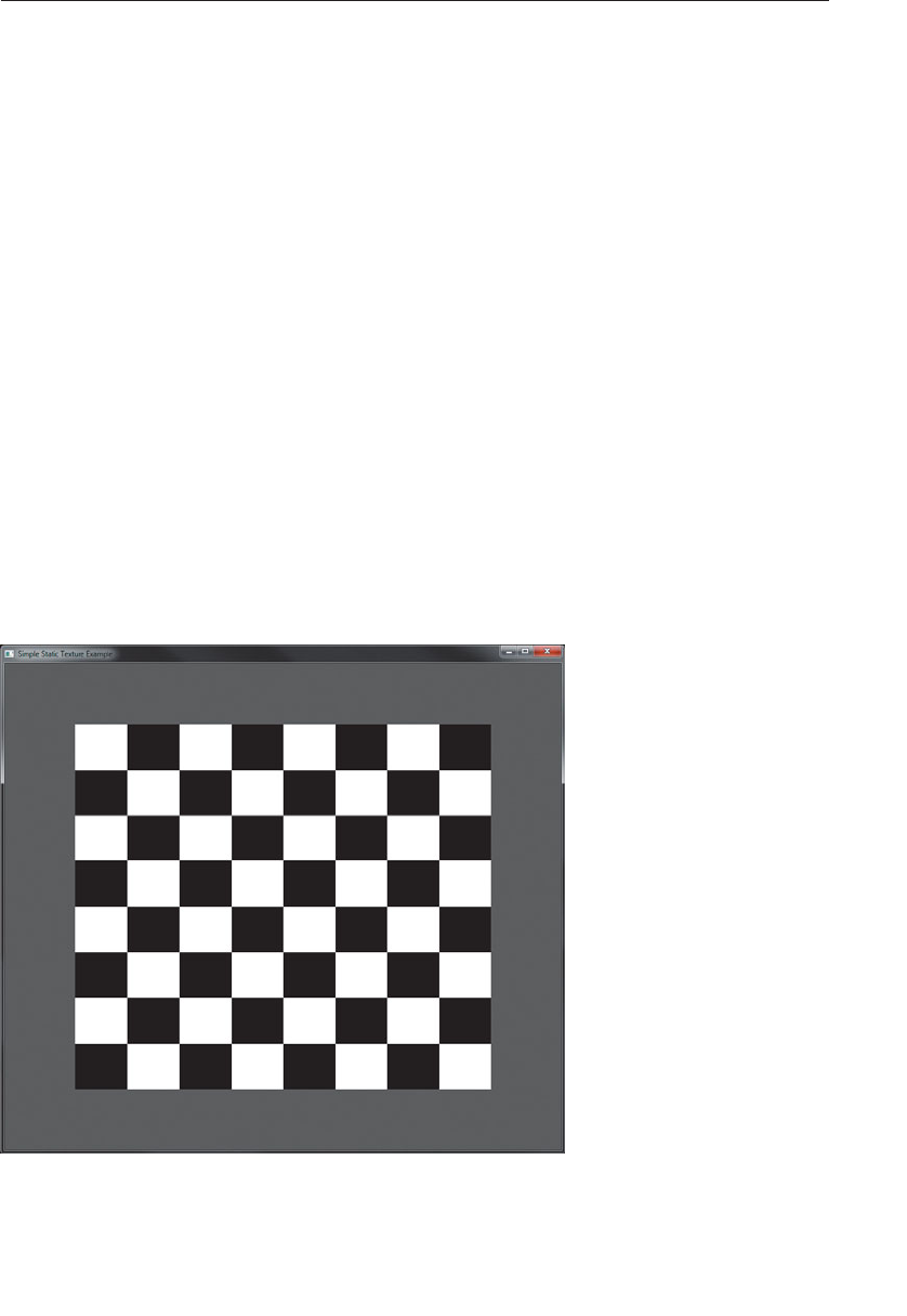
ptg9898810
glGenBuffers(1, &buf);
glBindBuffer(GL_ARRAY_BUFFER, buf);
glBufferData(GL_ARRAY_BUFFER, quad_data,
sizeof(quad_data), GL_STATIC_DRAW);
// Setup vertex attributes
GLuint vao;
glGenVertexArrays(1, &vao);
glBindVertexArray(vao);
glVertexAttribPointer(0, 4, GL_FLOAT, GL_FALSE, 0, (GLvoid*)0);
glEnableVertexAttribArray(0);
glVertexAttribPointer(1, 2, GL_FLOAT, GL_FALSE, 0,
(GLvoid*)(16 *sizeof(float)));
glEnableVertexAttribArray(1);
// Ready. Draw.
glDrawArrays(GL_TRIANGLE_FAN, 0, 4);
In Example 6.9, the geometry for a simple quadrilateral is placed into a
buffer object along with texture coordinates for each of its four vertices.
The position data is sent to vertex attribute 0 and the texture coordinates
are sent to vertex attribute 1. In the example, prog is the name of a
program object that has previously had the shaders of Examples 6.7 and
6.8 compiled and linked into it, and tex is a texture object with texture
data already loaded into it. The result of rendering with this program is
shown in Figure 6.5.
Figure 6.5 Output of the simple textured quad example
Using Textures 299

ptg9898810
Each of the texture lookup functions in GLSL takes a set of coordinates
from which to sample the texel. A texture is considered to occupy a
domain spanning from 0.0 to 1.0 along each axis (remember, you may use
one-, two-, or even three-dimensional textures). It is the responsibility of
the application to generate or supply texture coordinates for these
functions to use, as we have done in Example 6.9. Normally, these would
be passed into your vertex shader in the form of a vertex input and then
interpolated across the face of each polygon by OpenGL before being sent
to the fragment shader. In Example 6.9 the texture coordinates used range
from 0.0 to 1.0, so all of the resulting interpolated coordinates lie within
this range. If texture coordinates passed to a texture lookup function end
up outside the range 0.0 to 1.0, they must be modified to bring them back
into this range. There are several ways in which OpenGL will do this for
you, controlled by the GL_TEXTURE_WRAP_S, GL_TEXTURE_WRAP_T,
and GL_TEXTURE_WRAP_R sampler parameters.
The GL_TEXTURE_WRAP_S, GL_TEXTURE_WRAP_T, and
GL_TEXTURE_WRAP_R parameters control the way that texture
coordinates outside the range 0.0 to 1.0 are handled by OpenGL for the S,
T, and R11 axes of the texture’s domain respectively. The clamping mode in
each dimension may be set to one of GL_CLAMP_TO_EDGE,
GL_CLAMP_TO_BORDER, GL_REPEAT, or GL_MIRRORED_REPEAT. The
clamping modes work as follows:
•If the mode is GL_CLAMP_TO_EDGE, whenever a texture coordinate is
outside the range 0.0 to 1.0, texels on the very edge of the texture are
used to form the value returned to the shader.
•When the mode is GL_CLAMP_TO_BORDER, an attempt to read
outside the texture will result in the constant border color for the
texture being used to form the final value.
•When the clamping mode is set to GL_REPEAT, the texture is simply
wrapped and considered to repeat infinitely. In essence, only the
fractional part of the texture coordinate is used to lookup texels, and
the integer part is discarded.
•The clamping mode GL_MIRRORED_REPEAT is a special mode that
allows a texture to be repeated in a mirrored fashion. Texture
coordinates whose integer part is even have only their fractional part
considered. Texture coordinates whose integer part is odd (i.e., 1.3, 3.8,
etc.) have their fractional part subtracted from 1.0 in order to form the
11. Texture coordinates are traditionally referred to as s,t,r, and q, to distinguish them from
spatial coordinates (x,y,z, and w) and color coordinates (r,g,b, and a). One caveat is that in
GLSL, ris already used for red, so the four components of a texture coordinate are referred to
as s,t,p, and q.
300 Chapter 6: Textures
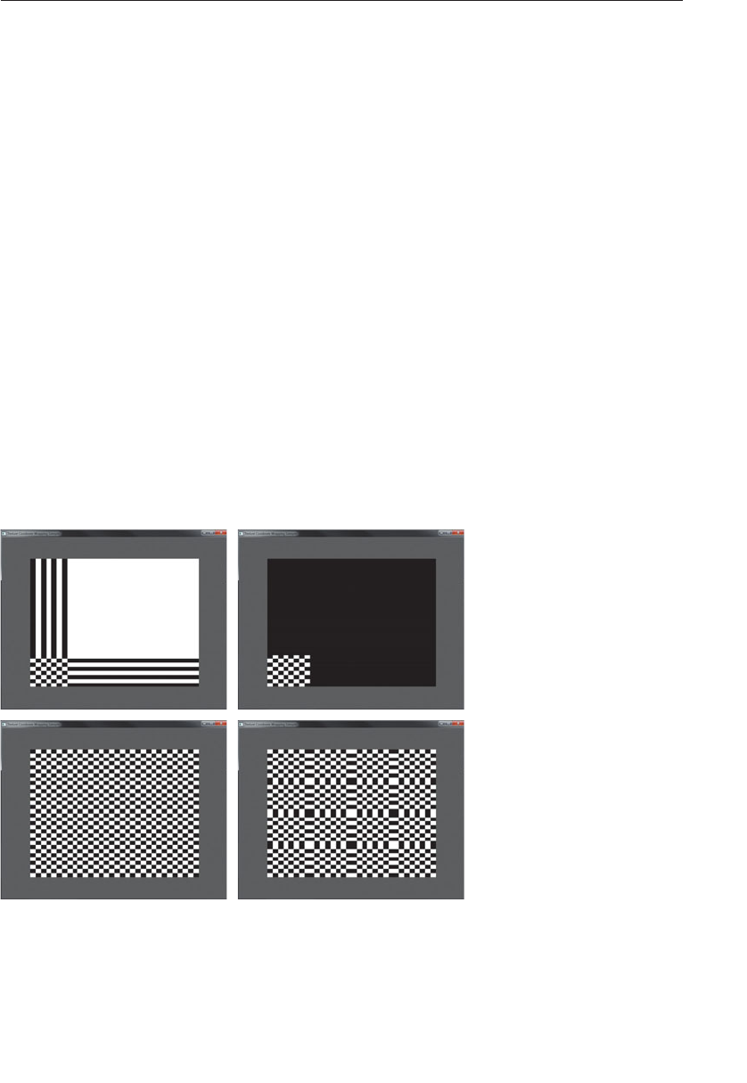
ptg9898810
final coordinate. This mode can help to eliminate tiling artifacts from
repeating textures.
Figure 6.6 shows each of the texture modes used to handle texture
coordinates ranging from 0.0 to 4.0. All of these modes, except for
GL_CLAMP_TO_BORDER eventually take texels from somewhere in the
texture’s data store. In the case of GL_CLAMP_TO_BORDER, the returned
texels come from the texture’s virtual border, which is a constant color. By
default, this color is transparent black (i.e., 0.0 in each component of the
texture). However, you may change this color by setting the value of the
GL_TEXTURE_BORDER_COLOR sampler parameter. The snippet of
Example 6.10 shows how to set the texture border color to red.
Example 6.10 Setting the Border Color of a Sampler
GLuint sampler; // This variable holds the name of our sampler.
GLuint texture; // This variable holds the name of a texture.
const GLfloat red[] = { 1.0f, 0.0f, 0.0f, 1.0f }; // Opaque red.
// Set the GL_TEXTURE_BORDER_COLOR for the sampler object
glSamplerParameterfv(sampler, GL_TEXTURE_BORDER_COLOR, red);
// Or alternatively, set the border color for a texture object.
// This will be used when a texture is bound to a texture unit
// without a corresponding sampler object.
glBindTexture(GL_TEXTURE_2D, texture);
glTexParameterfv(GL_TEXTURE_2D, GL_TEXTURE_BORDER_COLOR, red);
Figure 6.6 Effect of different texture wrapping modes
(GL_CLAMP_TO_EDGE (top left), GL_CLAMP_TO_BORDER (top right),
GL_REPEAT (bottom left), and GL_MIRRORED_REPEAT (bottom right).)
Using Textures 301

ptg9898810
Arranging Texture Data
Suppose you have an external source of texture data---say an image editing
program or another component of your application, perhaps written in
another language or using another API over which you have no control. It
is possible that the texture data is stored using a component order other
than red, green, blue, alpha (RGBA). For example, ABGR is fairly common
(i.e., RGBA bytes stored in little-endian order), as is ARGB and even RGBx
(RGB data packed into a 32-bit word with one byte left unused). OpenGL is
quite capable of consuming this data and making it appear as nicely
formatted RGBA data to your shader. To do this, we use texture swizzle,
which is a mechanism that allows you to rearrange the component order
of texture data on-the-fly as it is read by the graphics hardware.
Texture swizzle is a set of texture parameters---one for each channel of the
texture---that can be set using the glTexParameteri() function by passing
one of the texture swizzle parameter names and the desired source for the
data. The swizzle texture parameters are GL_TEXTURE_SWIZZLE_R,
GL_TEXTURE_SWIZZLE_G, GL_TEXTURE_SWIZZLE_B, and
GL_TEXTURE_SWIZZLE_A, which specify the outgoing texture channels in
the order red, green, blue, and alpha, respectively. Furthermore, the token
name GL_TEXTURE_SWIZZLE_RGBA is provided to allow all four channels
to be configured using a single call to glTexParameteriv(). Each one
specifies what the source of data should be for the corresponding channel
of the texture and may be set to one of the source selectors GL_RED,
GL_GREEN, GL_BLUE, GL_ALPHA, GL_ONE, or GL_ZERO. These indicate
the values of the red, green, blue, or alpha channels of the incoming
texture, or the constant values one and zero, respectively.
By default, the swizzle settings are configured to pass the data directly
through unmodified. That is, GL_TEXTURE_SWIZZLE_R, GL_TEXTURE_
SWIZZLE_G, GL_TEXTURE_SWIZZLE_B, and GL_TEXTURE_SWIZZLE_A
are set to GL_RED, GL_GREEN, GL_BLUE, and GL_ALPHA, respectively.
Example 6.11 shows how to configure a texture to read from ABGR and
RGBx data. In the case of RGBx, we specify that the constant value 1.0 be
returned for the missing alpha channel.
Example 6.11 Texture Swizzle Example
// The name of a texture whose data is in ABGR format.
GLuint abgr_texture;
// The name of a texture whose data is in RGBx format.
GLyint rgbx_texture;
302 Chapter 6: Textures

ptg9898810
// An array of tokens to set ABGR swizzle in one function call.
static const GLenum abgr_swizzle[] =
{GL_ALPHA, GL_RED, GL_GREEN, GL_BLUE
};
// Bind the ABGR texture
glBindTexture(GL_TEXTURE_2D, abgr_texture);
// Set all four swizzle parameters in one call to glTexParameteriv
glTexParameteriv(GL_TEXTURE_2D,
GL_TEXTURE_SWIZZLE_RGBA,
abgr_swizzle);
// Now bind the RGBx texture
glBindTexture(GL_TEXTURE_2D, rgbx_texture);
// We’re only setting the GL_TEXTURE_SWIZZLE_A parameter here
// because the R, G, and B swizzles can be left as their default values.
glTexParameteri(GL_TEXTURE_2D,
GL_TEXTURE_SWIZZLE_A,
GL_ONE);
Using Multiple Textures
Now that you have seen a simple application of texture to rendering, you
may have noticed some omissions from the sample above. For example, in
Example 6.9, we did not set a value for the sampler in the fragment shader.
This is because we are only using a single texture. In fact, OpenGL can
support many textures simultaneously---a minimum of 16 textures per
shader stage are supported, which when multiplied by the number of
shader stages supported by OpenGL comes out to 80 textures! In fact,
OpenGL has 80 texture units, referred to by tokens named GL_TEXTURE0
through GL_TEXTURE79. Whenever one of the texture functions, such as
glBindTexture() is called, it operates on the texture bound to the active
texture unit, which is implied by what is known as a selector. By default,
the active texture selector is 0. However, it may be changed (and will
need to be if you want to use more than one texture). The function to
change the active texture selector is glActiveTexture(), which was
introduced above.
In order to use multiple textures in your shader, you will need to declare
multiple uniform sampler variables. Each will refer to a different12 texture
unit. From the application side, uniform samplers appear much like
uniform integers. They are enumerated using the normal
12. Technically, they don’t need to be associated with different texture units. If two or more
samplers refer to the same texture unit, then they will both end up sampling from the same
texture.
Using Textures 303

ptg9898810
glGetActiveUniform() function and may have their values modified using
the glUniform1i() function. The integer value assigned to a uniform
sampler is the index of the texture unit to which it refers.
The steps to use multiple textures in a single shader (or program) are
therefore as follows: first, we need to select the first texture unit using
glActiveTexture() and bind a texture to one of its targets using
glBindTexture().We repeat this process for each texture unit. Then, we set
the values of the uniform sampler variables to the indices of the texture
units that we wish to use by calling the glUniform1i() function.
To illustrate this, we will modify our example from the previous section to
use two textures. We will first change the vertex shader of Example 6.8 to
produce two sets of texture coordinates. The updated vertex shader is
shown in Example 6.12.
Example 6.12 Simple Multitexture Example (Vertex Shader)
#version 330 core
layout (location = 0) in vec2 in_position;
layout (location = 1) in vec2 in_tex_coord;
out vec2 tex_coord0;
out vec2 tex_coord1;
uniform float time;
void main(void)
{
const mat2 m = mat2(vec2(cos(time), sin(time)),
vec2(−sin(time), cos(time)));
tex_coord0 = in_tex_coord *m;
tex_coord1 = in_tex_coord *transpose(m);
gl_Position = vec4(in_position, 0.5, 1.0);
}
The new vertex shader performs simple animation by using a time
uniform variable to construct a rotation matrix, and uses that to rotate the
incoming texture coordinates in opposite directions. Next, we modify the
original fragment shader from Example 6.7 to include two uniform
sampler variables, read a texel from each, and sum them together. This
new shader is shown in Example 6.13.
304 Chapter 6: Textures

ptg9898810
Example 6.13 Simple Multitexture Example (Fragment Shader)
#version 330 core
in vec2 tex_coord0;
in vec2 tex_coord1;
layout (location = 0) out vec4 color;
uniform sampler2D tex1;
uniform sampler2D tex2;
void main(void)
{color = texture(tex1, tex_coord0) + texture(tex2, tex_coord1);
}
In Example 6.13 we are using a different texture coordinate to sample from
the two textures. However, it is perfectly reasonable to use the same set of
texture coordinates for both textures. In order to make this shader do
something useful, we need to set values for the two uniform samplers,
tex1 and tex2 and bind textures to the corresponding texture units. We
do this using the glUniform1i(),glActiveTexture(), and glBindTexture()
functions as shown in Example 6.14.
Example 6.14 Simple Multitexture Example
// prog is the name of a linked program containing our example
// vertex and fragment shaders
glUseProgram(prog);
// For the first texture, we will use texture unit 0...
// Get the uniform location
GLint tex1_uniform_loc = glGetUniformLocation(prog, "tex1");
// Set it to 0
glUniform1i(tex1_uniform_loc, 0);
// Select texture unit 0
glActiveTexture(GL_TEXTURE0);
// Bind a texture to it
glBindTexture(GL_TEXTURE_2D, tex1);
// Repeat the above process for texture unit 1
GLint tex2_uniform_loc = glGetUniformLocation(prog, "tex2");
glUniform1i(tex2_uniform_loc, 1);
glActiveTexture(GL_TEXTURE1);
glBindTexture(GL_TEXTURE_2D, tex2);
Using Textures 305
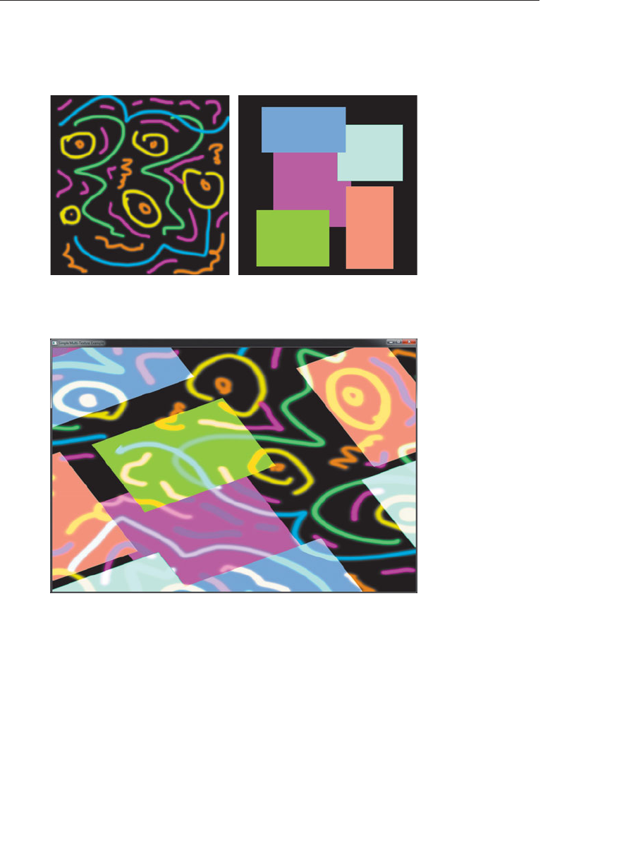
ptg9898810
The two source textures used in this example are shown in Figure 6.7 and
the result of rendering with our updated fragment shader with two
textures bound is shown in Figure 6.8.
Figure 6.7 Two textures used in the multitexture example
Figure 6.8 Output of the simple multitexture example
Complex Texture Types
Textures are often considered only as one- or two-dimensional images that
may be read from. However, there are several types of textures, including
3D textures, texture arrays, and cube maps, shadows, depth-stencil, and
buffer textures. This section describes the types of texture and outlines
their potential use cases.
306 Chapter 6: Textures

ptg9898810
3D Textures
A 3D texture can be thought of as a volume of texels arranged in a
3D grid. To create a 3D texture, generate a texture object name and bind
it initially to the GL_TEXTURE_3D target. Once bound, you may use
glTexStorage3D() or glTexImage3D() to create the storage for the
texture object. The 3D texture has not only a width and a height but
also a depth. The maximum width and height of a 3D texture is the same
as that of a 2D texture and may be found by retrieving the value of
GL_MAX_TEXTURE_SIZE. The maximum depth of a 3D texture supported
by your OpenGL implementation is found by retrieving the value of
GL_MAX_3D_TEXTURE_SIZE, and this may be different than the
maximum width and height of the texture.
3D textures are read in shaders using three-dimensional texture
coordinates. Otherwise, they work very similarly to other textures types.
A typical use case for a 3D texture is for volume rendering in fields such as
medical imaging or fluid simulation. In this type of application, the
content of the texture is usually a density map where each voxel13
represents the density of a medium at that point.
A simple way to render a volume is to render planes cutting through the
volume as a textured quadrilateral with a 3D texture coordinate at each
vertex. The vertex shader in Example 6.15 shows how a set of two-
dimensional texture coordinates are transformed into three-dimensional
space using a transformation matrix. These coordinates are then
interpolated by OpenGL and used in the fragment shader of Example 6.16.
Example 6.15 Simple Volume Texture Vertex Shader
#version 330 core
// Position and 2D texture coordinate from application
layout (location = 0) in vec2 in_position;
layout (location = 1) in vec2 in_tex_coord;
// Output 3D texture coordinate after transformation
out vec3 tex_coord;
// Matrix to transform the texture coordinates into 3D space
uniform mat4 tc_rotate;
void main(void)
{
13. A voxel is a term that refers to an element of a volume, just as pixel refers to an element of
a picture and texel refers to an element of a texture.
Complex Texture Types 307

ptg9898810
// Multiply the texture coordinate by the transformation
// matrix to place it into 3D space
tex_coord = (vec4(in_tex_coord, 0.0, 1.0) *tc_rotate).stp;
// Pass position through unchanged.
gl_Position = vec4(in_position, 0.5, 1.0);
}
Example 6.16 Simple Volume Texture Fragment Shader
#version 330 core
// Incoming texture coordinate from vertex shader
in vec3 tex_coord;
// Final color
layout (location = 0) out vec4 color;
// Volume texture
uniform sampler3D tex;
void main(void)
{// Simply read from the texture at the 3D texture coordinate
// and replicate the single channel across R, G, B, and A
color = texture(tex, tex_coord).rrrr;
}
The result of rendering with the vertex and fragment shaders of Examples
6.15 and 6.16 is shown in Figure 6.9. In this example, the volume texture
contains a density field of a cloud. The example animates the cloud by
moving a cutting plane through the volume and sampling the 3D texture
at each point on the plane.
Figure 6.9 Output of the volume texture example
308 Chapter 6: Textures

ptg9898810
Array Textures
For certain applications, you may have a number of one- or two-
dimensional textures that you might like to access simultaneously within
the confines of a single draw call. For instance, suppose you’re authoring a
game that features multiple characters of basically the same geometry, but
each of which has its own costume. Or you might want to use multiple
layers of texture for the character (diffuse color, a normal map, a specular
intensity map, and a number of other attributes).
When using many textures like this, you would need to bind all of the
required textures before the draw command. The calls to glBindTexture()
for each draw call could have performance implications for the application
if the texture objects needed to be updated by OpenGL.
Texture arrays allow you to combine a collection of one- or two-
dimensional textures, all of the same size and format, into a texture of the
next higher dimension (e.g., an array of two-dimensional textures becomes
something like a three-dimensional texture). If you were to try to use a
three-dimensional texture to store a collection of two-dimensional
textures, you would encounter a few inconveniences: The indexing texture
coordinate---rin this case---is normalized to the range [0,1]. To access the
third texture in a stack of seven, you would need to pass 0.35714 (or
thereabouts) to access what you would probably like to access as ‘‘2’’.
Texture arrays permit this type of texture selection. Additionally, texture
arrays allow suitable mipmap filtering within the texture accessed by the
index. In comparison, a three-dimensional texture would filter between
the texture ‘‘slices’’, likely in a way that doesn’t return the results you were
hoping for.
gvec4 texture(gsampler2D tex, vec2 P[, float bias]);
gvec4 texture(gsampler2DArray tex, vec3 P[, float bias]);
Compare the prototypes of the texture function for 2D textures and for
2D array textures. The second function takes a sampler2DArray sampler
type and its texture coordinate, P, has an additional dimension. This third
component of Pis the array index, or slice.
Cube-Map Textures
Cube-map textures are a special type of texture, useful for environment
mapping, that takes a set of images and treats them as the faces of a cube.
The six faces of the cube are represented by six subtextures that must be
Complex Texture Types 309

ptg9898810
square and of the same size. When you sample from a cube map, the
texture coordinate used is three dimensional and is treated as a direction
from the origin. This direction essentially points at the location on the
surface of the cube from where to read the texture. Imagine you were
standing in the middle of a square room with a laser pointer. You could
point the laser in any direction and hit part of the wall, floor, or ceiling of
the room. The spot where the pointer shines is the point from which you
would sample the texture map. Cube maps are ideal for representing
surrounding environments, lighting, and reflection effects, and can also be
used to wrap complex objects with textures.
Allocating storage for cube-map textures is achieved by binding a new
texture name to the GL_TEXTURE_CUBE_MAP texture target and calling
glTexStorage2D() on the GL_TEXTURE_CUBE_MAP target. This single call
will allocate the storage for all six faces of the cube map. However, once
allocated, the cube map is represented by a set of six special targets, which
can be thought of as subtargets of the GL_TEXTURE_CUBE_MAP target.
These are GL_TEXTURE_CUBE_MAP_POSITIVE_X,
GL_TEXTURE_CUBE_MAP_NEGATIVE_X,
GL_TEXTURE_CUBE_MAP_POSITIVE_Y,
GL_TEXTURE_CUBE_MAP_NEGATIVE_Y,
GL_TEXTURE_CUBE_MAP_POSITIVE_Z, and
GL_TEXTURE_CUBE_MAP_NEGATIVE_Z14. Each face has its own complete
set of mipmaps. These special targets may be passed to the
glTexSubImage2D() command in order to specify image data for the cube
map’s faces. Example 6.17 gives an example of how to create and initialize
a cube-map texture.
Example 6.17 Initializing a Cube-Map Texture
GLuint tex; // Texture to be created
extern const GLvoid*texture_data[6]; // Data for the faces
// Generate, bind, and initialize a texture object using
// the GL_TEXTURE_CUBE_MAP target.
glGenTextures(1, &tex);
glBindTexture(GL_TEXTURE_CUBE_MAP, tex);
glTexStorage2D(GL_TEXTURE_CUBE_MAP, 10, GL_RGBA8, 1024, 1024);
14. Note that the tokens GL_TEXTURE_CUBE_MAP_POSITIVE_X, GL_TEXTURE_CUBE_MAP_
NEGATIVE_X, GL_TEXTURE_CUBE_MAP_POSITIVE_Y, GL_TEXTURE_CUBE_MAP_
NEGATIVE_Y, GL_TEXTURE_CUBE_MAP_POSITIVE_Z, and GL_TEXTURE_CUBE_MAP_
NEGATIVE_Z have contiguous numeric values defined in that order. Thus, it’s possible to index
into the faces of the cube map by simply adding a face index to GL_TEXTURE_CUBE_MAP_
POSITIVE_X so long as the index is consistent with the defined ordering.
310 Chapter 6: Textures

ptg9898810
// Now that storage is allocated for the texture object,
// we can place the texture data into its texel array.
for (int face = 0; face < 6; face++)
{GLenum target = GL_TEXTURE_CUBE_MAP_POSITIVE_X + face;
glTexSubImage2D(target, // Face
0, // Level
0, 0, // X, Y offset
1024, 1024, // Size of face
GL_RGBA, // Format
GL_UNSIGNED_BYTE, // Type
texture_data[face]); // Data
}
// Now, optionally, we could specify the data for the
// lower mipmap levels of each of the faces.
Cube-map textures may also be aggregated into arrays. The
GL_TEXTURE_CUBE_MAP_ARRAY texture target may be used to create
and modify cube-map array textures. Each cube in the cube-map array
consumes six contiguous slices of the underlying array texture. Thus, an
array with five cube-map textures in it will have a total of 30 slices. The
example shown in Example 6.17 is modified below in Example 6.18 to
create a cube-map array of five cubes in a single texture.
Example 6.18 Initializing a Cube-Map Array Texture
GLuint tex; // Texture to be created
extern const GLvoid*texture_data[6][5]; // Data for the faces
// Generate, bind, and initialize a texture object using the
// GL_TEXTURE_CUBE_MAP_ARRAY target.
glGenTextures(1, &tex);
glBindTexture(GL_TEXTURE_CUBE_MAP_ARRAY, tex);
glTexStorage3D(GL_TEXTURE_CUBE_MAP_ARRAY, 10,
GL_RGBA8, 1024, 1024, 5);
// Now that storage is allocated for the texture object, we can
// place the texture data into its texel array.
for (int cube_index = 0; cube_index < 5; cube_index++)
{
for (int face = 0; face < 6; face++)
{
GLenum target = GL_TEXTURE_CUBE_MAP_POSITIVE_X + face;
glTexSubImage3D(target, // Face
0, // Level
0, 0, // Offset
cube_index, // Cube index
1024, 1024, // Width, Height
1, // Face count
Complex Texture Types 311
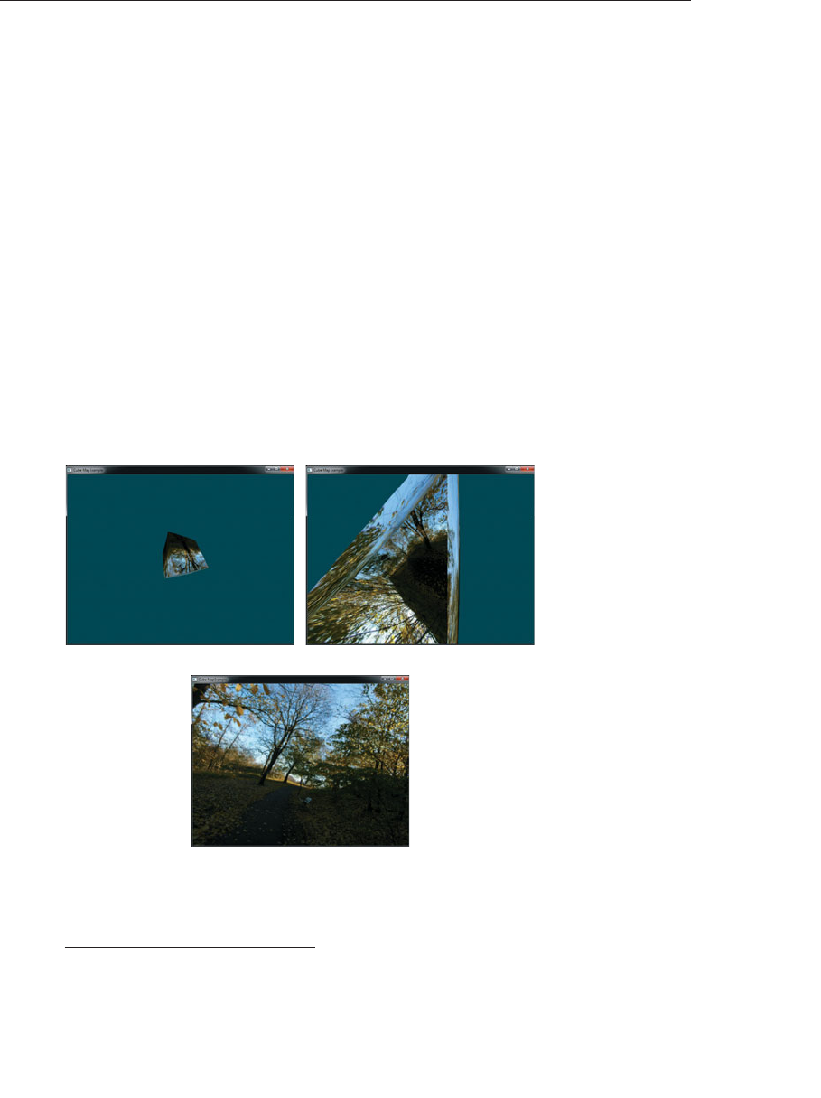
ptg9898810
GL_RGBA, // Format
GL_UNSIGNED_BYTE, // Type
texture_data[face][cube_index]); // Data
}
}
Cube-Map Example---Sky Boxes
A common use for cube-map texture is as sky boxs. A sky box is an
application of texturing where the entire scene is effectively wrapped in a
large cube with the viewer placed in the center. As the scene is rendered
anything not covered by objects within the scene is displayed as the inside
of the cube. With an appropriate texture, it appears as if the viewer is
located in the environment represented by the cube map.
Figure 6.10 (a) shows a cube map15 viewed from the outside, illustrating
that a sky box really is just a cube with a texture applied to it. In
Figure 6.10 (b), we have zoomed in until the sky box cuts the near plane
and we can now see inside it. Finally, in Figure 6.10 (c), we have placed the
viewer at the very center of the cube, making it appear as if we are in the
environment represented by the cube map.
(a) (b)
(c)
Figure 6.10 A sky box
(Shown as seen from the outside, from close up, and from the center.)
15. The cube-map images shown in this example were taken, with permission, from
http://humus.name.
312 Chapter 6: Textures

ptg9898810
To render the images shown in Figure 6.10, we simply render a unit cube
centered at the origin and use the object space position as a texture
coordinate from which to sample the cube map. The vertex shader for this
example is shown in Example 6.19 and the corresponding fragment shader
is shown in Example 6.20.
Example 6.19 Simple Skybox Example---Vertex Shader
#version 330 core
layout (location = 0) in vec3 in_position;
out vec3 tex_coord;
uniform mat4 tc_rotate;
void main(void)
{tex_coord = in_position;
gl_Position = tc_rotate *vec4(in_position, 1.0);
}
Example 6.20 Simple Skybox Example---Fragment Shader
#version 330 core
in vec3 tex_coord;
layout (location = 0) out vec4 color;
uniform samplerCube tex;
void main(void)
{color = texture(tex, tex_coord);
}
Using Cube Maps for Environment Mapping
Now that we have created an environment into which we can place the
components of our scene, we can make the objects appear to be part of the
environment. This is known as environment mapping, and is another
common use for cube-map textures. Here, the cube map is employed as an
environment map and is used to texture objects in the scene. To implement
environment mapping, we must calculate the texture coordinate from
which to sample the cube map by reflecting the incoming view vector
around the surface normal at the point to be textured.
The vertex shader shown in Example 6.21 transforms the object space
position into view space by multiplying it by a concatenated
model-view-projection matrix. It also rotates the surface normal into view
space by multiplying it by a concatenated model-view matrix.
Complex Texture Types 313

ptg9898810
Example 6.21 Cube-Map Environment Mapping Example---Vertex
Shader
#version 330 core
// Incoming position and normal
layout (location = 0) in vec4 in_position;
layout (location = 1) in vec3 in_normal;
// Outgoing surface normal and view-space position
out vec3 vs_fs_normal;
out vec3 vs_fs_position;
// Model-view-projection and model-view matrices
uniform mat4 mat_mvp;
uniform mat4 mat_mv;
void main(void)
{// Clip-space position
gl_Position = mat_mvp *in_position;
// View-space normal and position
vs_fs_normal = mat3(mat_mv) *in_normal;
vs_fs_position = (mat_mv *in_position).xyz;
}
Once the view-space normal and position of the surface point have been
passed into the fragment shader, we can use the GLSL reflect function to
reflect the fragment’s view-space position around the surface normal at
each point. This effectively bounces the view vector off the surface and into
the cube map. We use this reflected vector as a texture coordinate to
sample from the cube map, using the resulting texel to color the surface.
The result of this is that the environment appears to be reflected in the
object’s surface. The fragment shader performing these operations is
shown in Example 6.22.
Example 6.22 Cube-Map Environment Mapping Example---Fragment
Shader
#version 330 core
// Incoming surface normal and view-space position
in vec3 vs_fs_normal;
in vec3 vs_fs_position;
// Final fragment color
layout (location = 0) out vec4 color;
// The cube-map texture
uniform samplerCube tex;
void main(void)
{// Calculate the texture coordinate by reflecting the
314 Chapter 6: Textures
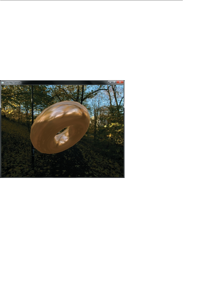
ptg9898810
// view-space position around the surface normal.
vec3 tc = reflect(-vs_fs_position, normalize(vs_fs_normal));
// Sample the texture and color the resulting fragment
// a golden color.
color = vec4(0.3, 0.2, 0.1, 1.0) +
vec4(0.97, 0.83, 0.79, 0.0) *
texture(tex, tc);
}
The fragment shader also slightly modifies the sampled texture value
retrieved from the cube map in order to make it appear to be slightly
golden in color. The result of rendering with the vertex and fragment
shaders of Examples 6.21 and 6.22 is shown in Figure 6.11 below.
Figure 6.11 A golden environment mapped torus
Seamless Cube-Map Sampling
A cube map is a collection of six independent faces, possibly aggregated
into arrays of cubes with an integer multiple of six faces in total. When
OpenGL samples from a cube map, as a first step, it uses the dominant
component of the three-dimensional texture coordinate to determine
which of the six faces of the cube to sample from. Once this face has been
determined, it is effectively treated as a two-dimensional texture and used
to look up texel values. By default, at the edges of the texture, normal
texture coordinate wrapping modes are used. At first thought, this would
seem logical, and as the generated two-dimensional texture coordinates
always lie within a face, we don’t expect to see any issues with this.
Complex Texture Types 315
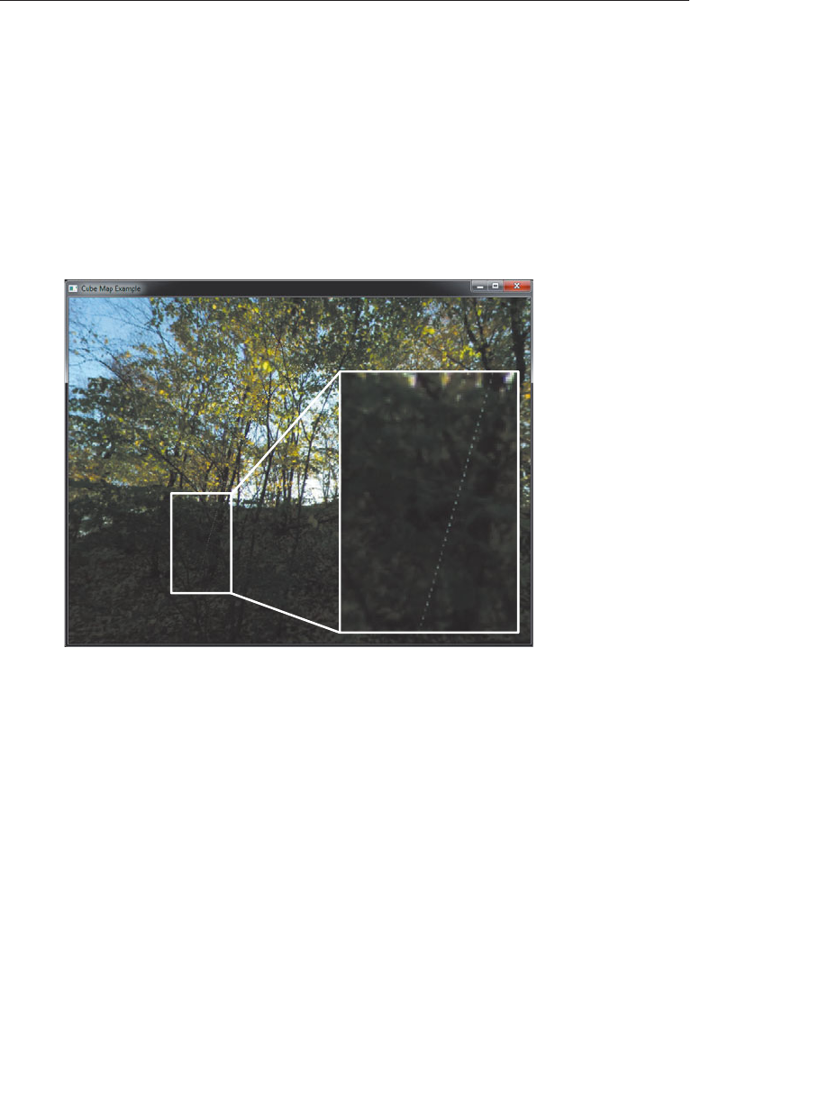
ptg9898810
However, if the texture filtering mode is linear, toward the edges of the
cube’s faces, the adjoining faces’ texels are not considered when calculating
the final filtered texel values. This can cause a noticeable seam to appear in
the filtered texture. Even worse, if the texture coordinate wrapping mode is
left at one of the repeating modes, then texels from the opposite side of
the face may be used, causing quite incorrect results.
Figure 6.12 shows the result of sampling from a cube-map texture across
the join between two faces. Inset is a close-up view of the seam that is
visible between the adjacent faces of the cube map.
Figure 6.12 A visible seam in a cube map
To avoid the visible seams between adjacent faces of a cube map, we can
enable seamless cube-map filtering. To do this, call glEnable() with cap set
to GL_TEXTURE_CUBE_MAP_SEAMLESS. When seamless cube-map
filtering is enabled, OpenGL will use texels from adjacent cube-map faces
to retrieve texels for use in filtering. This will eliminate artifacts, especially
when there is an abrupt change in color from one face to another, or when
the cube map is a particularly low resolution. Figure 6.13 shows the result
of enabling seamless cube-map filtering. Notice that the bright line of
pixels has been eliminated.
316 Chapter 6: Textures
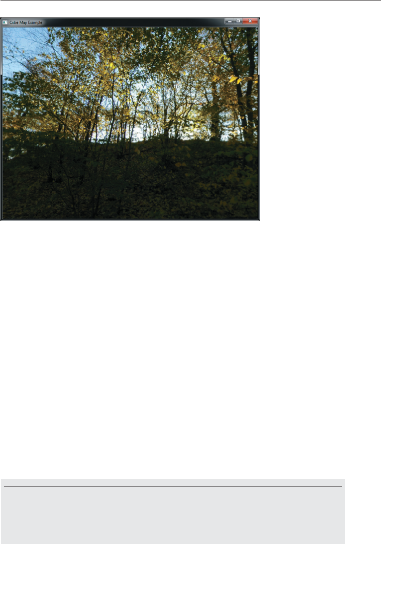
ptg9898810
Figure 6.13 The effect of seamless cube-map filtering
Shadow Samplers
A special type of sampler is provided in GLSL called a shadow sampler.
A shadow sampler takes an additional component in the texture
coordinate that is used as a reference against which to compare the fetched
texel values. When using a shadow sampler, the value returned from the
texture function is a floating-point value between 0.0 and 1.0, indicating
the fraction of fetched texel values that passed the comparison operator.
For texture accesses that sample only a single texel value (using the
GL_NEAREST filtering mode, no mipmaps, and one sample per texel), the
returned value will be either 0.0 or 1.0, depending on whether the texel
passes the comparison or not. If more than one texel would normally be
used to construct the value returned to the shader (such as when the filter
mode is linear, or if a multisample texture is used), then the value may be
anything between 0.0 and 1.0, depending on how many of those texels
pass the comparison operator. The shadow texturing functions are as
follows:
float texture(gsampler1DShadow tex, vec3 P[, float bias]);
float texture(gsampler2DShadow tex, vec3 P[, float bias]);
float texture(gsamplerCubeShadow tex, vec4 P[, float bias]);
float texture(gsampler1DArrayShadow tex, vec3 P[, float bias]);
Complex Texture Types 317

ptg9898810
float texture(gsampler2DArrayShadow tex, vec4 P[, float bias]);
float texture(gsampler2DRectShadow tex, vec3 P);
float texture(gsamplerCubeArrayShadow tex, vecP P, float
compare);
Sample the shadow texture bound to the texture unit referenced by tex at
the texture coordinates specified by P. The return value is a floating-point
quantity representing the fraction of samples that passed the shadow
comparison operator with the fetched texel data.
To enable the comparison function for a sampler, call
glSamplerParameteri() (or glTexParameteri() if you are not using a
sampler object) with pname set to GL_TEXTURE_COMPARE_MODE and
param set to GL_COMPARE_REF_TO_TEXTURE, and to disable it, set param
to GL_NONE. When the texture comparison mode is set to
GL_COMPARE_REF_TO_TEXTURE, the comparison is carried out with the
mode specified by the sampler. This is set by calling
glSamplerParameteri() with pname set to GL_TEXTURE_COMPARE_FUNC
and param set to one of the comparison functions, GL_LEQUAL,
GL_GEQUAL, GL_LESS, GL_GREATER, GL_EQUAL, GL_NOTEQUAL,
GL_ALWAYS, or GL_NEVER. These comparison functions have the same
meanings as they do for depth testing.
A comprehensive example of using a shadow sampler is shown in ‘‘Shadow
Mapping’’ on Page 400 of Chapter 7,‘‘Light and Shadow’’.
Depth-Stencil Textures
Instead of an image, a texture can hold depth and stencil values, one of
each per texel, using the texture format GL_DEPTH_STENCIL. This is the
typical way a framebuffer will store the rendered zcomponent for depth
and the stencil value, as discussed in detail in Chapter 4,‘‘Color, Pixels,
and Framebuffers’’. When texturing from a depth-stencil texture, by
default a shader will read the depth. However, as of version 4.3, a shader
can also read the stencil value. To do so, the application must set
GL_DEPTH_STENCIL_TEXTURE_MODE to GL_STENCIL_COMPONENTS
and the shader must use an integer sampler type.
318 Chapter 6: Textures

ptg9898810
Buffer Textures
Buffer textures are a special class of texture that allow a buffer object to be
accessed from a shader as if it were a large, one-dimensional texture.
Buffer textures have certain restrictions and differences from normal
one-dimensional textures but otherwise appear similar to them in your
code. You create them as normal texture objects, bind them to texture
units, control their parameters16 with glTexParameteri(). However, the
storage for the texture’s data is actually owned and controlled by a buffer
object (hence the name buffer texture). Also, buffer textures have no
internal sampler and sampler objects have no effect on buffer textures. The
main differences between buffer textures and one-dimensional textures are
as follows:
•One-dimensional textures have sizes limited to the value of GL_MAX_
TEXTURE_SIZE, but buffer textures are limited to the value of
GL_MAX_TEXTURE_BUFFER_SIZE, which is often two gigabytes or
more.
•One-dimensional textures support filtering, mipmaps, texture
coordinate wrapping and other sampler parameters, buffer textures
do not.
•Texture coordinates for one-dimensional textures are normalized
floating-point values, but buffer textures use unnormalized integer
texture coordinates.
Whether you decide to use a buffer texture or a one-dimensional texture
for a particular application will depend on your needs. In order to create a
buffer texture, you need to generate a name for your new texture using
glGenTextures(), bind it to the GL_TEXTURE_BUFFER texture target, and
then associate a buffer object with the texture using the glTexBuffer()
function.
void glTexBuffer(GLenum target, GLenum internalFormat,
GLuint buffer);
Attaches the storage for the buffer object named buffer to the buffer
texture bound to the target target of the active texture unit. target must be
GL_TEXTURE_BUFFER. The data store of buffer is then interpreted as an
array of elements whose type is determined by internalFormat, which
must be a sized internal format. If buffer is zero, than any existing
association between the active buffer texture and its data store is broken.
16. Not all texture parameters are relevant for buffer textures, and as no sampler is used with
buffer textures, sampler parameters are essentially ignored.
Complex Texture Types 319

ptg9898810
The code shown in Example 6.23 shows an example of creating a buffer,
initializing its data store, and then associating it with a buffer texture.
Example 6.23 Creating and Initializing a Buffer Texture
// Buffer to be used as the data store
GLuint buf;
// Texture to be used as a buffer texture
GLuint tex;
// Data is located somewhere else in this program
extern const GLvoid*data;
// Generate, bind, and initialize a buffer object
// using the GL_TEXTURE_BUFFER binding. Assume we’re
// going to use one megabyte of data here.
glGenBuffers(1, &buf);
glBindBuffer(GL_TEXTURE_BUFFER, buf);
glBufferData(GL_TEXTURE_BUFFER, 1024 *1024,
data, GL_STATIC_DRAW);
// Now create the buffer texture and associate it
// with the buffer object.
glGenTextures(1, &tex);
glBindTexture(GL_TEXTURE_BUFFER, tex);
glTexBuffer(GL_TEXTURE_BUFFER, GL_R32F, buf);
To attach only a range of a buffer object to a buffer texture, you may use
the glTexBufferRange() function, whose prototype is as follows:
void glTexBufferRange(GLenum target, GLenum internalFormat,
GLuint buffer, GLintptr offset,
GLsizeiptr size);
Attaches a section of the storage for the buffer object named buffer
starting at offset and reaching for size bytes to the buffer texture bound to
the target target of the active texture unit. target must be
GL_TEXTURE_BUFFER. The data store of buffer is then interpreted as an
array of elements whose type is determined by internalFormat, which
must be a sized internal format. If buffer is zero, than any existing
association between the active buffer texture and its data store is broken.
offset must be an integer multiple of the implementation-defined
constant GL_TEXTURE_BUFFER_OFFSET_ALIGNMENT.
To access a buffer texture in a shader, you must create a uniform
samplerBuffer (or one of its signed- or unsigned-integer variants,
isamplerBuffer or usamplerBuffer), and use it with the texelFetch
320 Chapter 6: Textures

ptg9898810
function17 to read individual samples from it. The texelFetch function
for buffer textures is defined as follows:
vec4 texelFetch(samplerBuffer s, int coord);
ivec4 texelFetch(isamplerBuffer s, int coord);
uvec4 texelFetch(usamplerBuffer s, int coord);
Perform a lookup of a single texel from texture coordinate coord in the
texture bound to s.
An example of the declaration of a buffer sampler and fetching from it
using texelFetch is shown in Example 6.24.
Example 6.24 Texel Lookups from a Buffer Texture
#version 330 core
uniform samplerBuffer buf
in int buf_tex_coord;
layout (location = 0) out vec4 color;
void main(void)
{color = texelFetch(buf, tex_coord);
}
Texture Views
So far, we have considered textures to be large buffers of data that have a
specified format and consume a fixed amount of storage space. The
amount of space depends on the format and on other parameters such as
the texture’s dimensions and whether it has mipmaps or not. However,
conceptually, the format and to some extent the dimensions can be
separated from the size of the underlying storage requirements of a
texture. For example, many texture internal formats will consume the
same number of bits per texel, and in some cases it is possible to interpret
17. The texelFetch function may be used with regular textures as well as buffer textures.
When it is used to sample from a nonbuffer texture, the texture’s sampler parameters are
ignored, and the texture coordinate is still interpreted as a nonnormalized integer value as it
is with buffer textures. We introduce this function here solely because its most common use is
with buffer textures.
Texture Views 321

ptg9898810
textures with various different dimensionalities---perhaps taking a single
slice of an array texture and treating it as a single 2D texture, say.
OpenGL allows you to share a single data store between multiple textures,
each with its own format and dimensions. First, a texture is created and its
data store initialized with one of the immutable data storage functions
(such as glTexStorage2D()). Next, we create a texture view of the ‘‘parent’’
texture. In effect, this increments a reference count to the underlying
storage allocated for the first texture, giving each view a reference to it. To
create a texture view, call glTextureView(), whose prototype is as follows:
void glTextureView(GLuint texture, GLenum target,
GLuint origTexture, GLenum internalFormat,
GLuint minLevel, GLuint numLevels,
GLuint minLayer, GLuint numLayers);
Creates a new view of the texture named by origTexture, which must be
the name of an existing texture whose data store has been initialized and
is immutable. texture is attached to the data store of origTexture and
becomes an immutable texture with a target specified by target. The
internal format of texture is specified by internalFormat, which must be
compatible with the internal format of origTexture.minLevel and numLevels
specify the first mipmap level and number of mipmap levels to use for the
new texture, respectively. Likewise, minLayer and numLayers specify the
first layer and number of layers of an array texture to attach to texture.
When creating views of existing textures, the target for the new texture
must be compatible with the target of the original texture. The compatible
targets are given in Table 6.6.
Table 6.6 Target Compatibility for Texture Views
Original Target (GL_TEXTURE*) Compatible Targets (GL_TEXTURE*)
1D 1D, 1D_ARRAY
2D 2D, 2D_ARRAY
3D 3D
CUBE_MAP CUBE_MAP, 2D,
2D_ARRAY,
CUBE_MAP_ARRAY
RECTANGLE RECTANGLE
BUFFER none
322 Chapter 6: Textures

ptg9898810
Table 6.6 (continued) Target Compatibility for Texture Views
Original Target (GL_TEXTURE*) Compatible Targets (GL_TEXTURE*)
1D_ARRAY 1D, 1D_ARRAY
2D_ARRAY 2D, 2D_ARRAY
CUBE_MAP_ARRAY CUBE_MAP, 2D,
2D_ARRAY,
CUBE_MAP_ARRAY
2D_MULTISAMPLE 2D_MULTISAMPLE,
2D_MULTISAMPLE_ARRAY
2D_MULTISAMPLE_ARRAY 2D_MULTISAMPLE,
2D_MULTISAMPLE_ARRAY
In addition to target compatibility, the internal format of the new view
must be of the same format class (i.e., bits-per-texel) of the original parent
texture. Table 6.7 lists the texture format classes and their compatible
specific internal formats.
Table 6.7 Internal Format Compatibility for Texture Views
Original Target Compatible Targets
128-bit GL_RGBA32F, GL_RGBA32UI, GL_RGBA32I
96-bit GL_RGB32F, GL_RGB32UI, GL_RGB32I
64-bit GL_RGBA16F, GL_RG32F, GL_RGBA16UI, GL_RG32UI,
GL_RGBA16I, GL_RG32I, GL_RGBA16, GL_RGBA16_SNORM
48-bit GL_RGB16, GL_RGB16_SNORM, GL_RGB16F,
GL_RGB16UI, GL_RGB16I
32-bit GL_RG16F, GL_R11F_G11F_B10F, GL_R32F,
GL_RGB10_A2UI, GL_RGBA8UI, GL_RG16UI,
GL_R32UI, GL_RGBA8I, GL_RG16I, GL_R32I,
GL_RGB10_A2, GL_RGBA8, GL_RG16,
GL_RGBA8_SNORM, GL_RG16_SNORM,
GL_SRGB8_ALPHA8, GL_RGB9_E5
24-bit GL_RGB8, GL_RGB8_SNORM, GL_SRGB8,
GL_RGB8UI, GL_RGB8I
16-bit GL_R16F, GL_RG8UI, GL_R16UI, GL_RG8I,
GL_R16I, GL_RG8, GL_R16, GL_RG8_SNORM,
GL_R16_SNORM
8-bit GL_R8UI, GL_R8I, GL_R8, GL_R8_SNORM
Texture Views 323

ptg9898810
Table 6.7 (continued) Internal Format Compatibility for Texture Views
Original Target Compatible Targets
GL_RGTC1_RED GL_COMPRESSED_RED_RGTC1,
GL_COMPRESSED_SIGNED_RED_RGTC1
GL_RGTC2_RG GL_COMPRESSED_RG_RGTC2,
GL_COMPRESSED_SIGNED_RG_RGTC2
GL_BPTC_UNORM GL_COMPRESSED_RGBA_BPTC_UNORM,
GL_COMPRESSED_SRGB_ALPHA_BPTC_UNORM
GL_BPTC_FLOAT GL_COMPRESSED_RGB_BPTC_SIGNED_FLOAT,
GL_COMPRESSED_RGB_BPTC_UNSIGNED_FLOAT
Given the format and target compatibility matrices above, it is possible to
reinterpret data in a texture in multiple ways simultaneously. For example,
it is possible to create two views of an RGB8 texture, one as unsigned
normalized (returning floating-point data to the shader) and another as an
unsigned integer texture (which will return the underlying integer data to
the shader). Example 6.25 shows an example of how to achieve this.
Example 6.25 Creating a Texture View with a New Format
// Create two texture names - one will be our parent,
// one will be the view
GLuint tex[2];
glGenTextures(2, &tex);
// Bind the first texture and initialize its data store
// Here, the store will be 1024 x 1024 2D texture with
// mipmaps and the format will be GL_RGB8 - 8-bits per
// component RGB, unsigned normalized
glBindTexture(GL_TEXTURE_2D, tex[0]);
glTexStorage2D(GL_TEXTURE_2D, 10, GL_RGB8, 1024, 1024);
// Now,.create a view of the texture, this time using
// GL_RGB8UI so as to receive the raw data from the texture
glTextureView(tex[1], // New texture view
GL_TEXTURE_2D, // Target for the new view
tex[0], // Original texture
GL_RGB8UI, // New format
0, 10, // All mipmaps
0, 1); // Only one layer
As a second example, consider a case where you have a large 2D array
texture and wish to take a single slice of the array and use it as an
independent 2D texture. To do this, we can create a view of the target
324 Chapter 6: Textures

ptg9898810
GL_TEXTURE_2D even though the original texture is
GL_TEXTURE_2D_ARRAY. Example 6.26 shows an example of this.
Example 6.26 Creating a Texture View with a New Target
// Create two texture names - one will be our parent,
// one will be the view
GLuint tex[2];
glGenTextures(2, &tex);
// Bind the first texture and initialize its data store
// We are going to create a 2D array texture with a layer
// size of 256x256 texels and 100 layers.
glBindTexture(GL_TEXTURE_2D_ARRAY, tex[0]);
glTexStorage3D(GL_TEXTURE_2D_ARRAY, 8, GL_RGAB32F, 256, 256, 100);
// Now,.create a GL_TEXTURE_2D view of the texture,
// extracting a single slice from the middle of the array
glTextureView(tex[1], // New texture view
GL_TEXTURE_2D, // Target for the new view
tex[0], // Original texture
GL_RGBA32F, // Same format as original texture
0, 8, // All mipmaps
50, 1); // Only one layer
Once a view of a texture has been created, it can be used in any place that
you can use a texture, including image loads and stores or framebuffer
attachments. It is also possible to create views of views (and views of those
views, etc.), with each view holding a reference to the original data store. It
is even legal to delete the original parent texture. So long as at least one
view of the data exists, it will not be deleted.
Other use cases for texture views include aliasing data of various formats---
for example, bit casting floating-point and integer data to enable atomic
operations and OpenGL’s logic-op to be performed on floating-point data,
which would normally not be allowed. Aliasing a single data store as both
sRGB and linear data allows a single shader to simultaneously access the
same data with and without sRGB conversion applied. A single-array
texture may effectively have different format data stored in its slices by
creating multiple array views of the texture and rendering different
outputs to different slices of the texture. With some lateral thinking
applied, texture views become a very powerful way to access and manage
texture data.
Texture Views 325

ptg9898810
Compressed Textures
Compression is a mechanism by which the amount of data required to
store or transmit information is reduced. Because texture data can
consume a very large amount of memory (and consequently, memory
bandwidth), OpenGL supports storing textures in compressed forms in
order to reduce their size. Compression algorithms fall into two general
categories---lossless and lossy.Lossless compression algorithms will not
discard any information and an exact copy of the original is retrievable
after decompression. However, lossy compression sacrifices some of the
original information during the process in order to make the remaining
information more suited to the compression algorithm and reduce its size.
This will reduce quality some but normally provides much greater
reduction in memory cost. Obviously for some content, such as computer
executables, text documents, and the like, it is imperative that no
information is lost. You may be familiar with lossless compression in the
form of zip-type algorithms used to compress file archives.
For other content, though, some loss in quality is acceptable. For example,
common audio and video compression algorithms such as MPEG are lossy.
They throw out some information in order to improve the compression
ratio. A trade-off is made between the acceptable loss in quality and
reduced file sizes. Without lossy compression, MP3 players and streaming
video would be almost impractical.
For the most part, the loss in fidelity is not perceptible to most audiences18---
think, when was the last time you noticed that the music you were listening
to was compressed? Most texture compression schemes in use today are
based on lossy algorithms designed to be easy to decompress, even at the
expense of additional complexity in the compression side of the algorithm.
There are two ways to get compressed texture data into OpenGL. The
first is to ask OpenGL to compress it for you. In this case, you supply
uncompressed data but specify a compressed internal format. The OpenGL
implementation will take the uncompressed, raw texture data, and attempt
to compress it. Because this is a real-time process, the compressor in the
OpenGL implementation will often implement a rather naive algorithm in
order to compress the data quickly resulting in a poor quality compressed
texture. The other way to bring compressed texture data into OpenGL is
to compress it offline (i.e., before your program runs) and pass the
18. Lossless compressors such as FLAC are popular for archival of digital music. These algorithms
normally reach compression ratios of the order of 30% to 50% of the original file size. However,
for day-to-day use, lossy algorithms such as MP3 and AC3 can reach compression ratios of 10%
or less and provide satisfactory experience to most users.
326 Chapter 6: Textures

ptg9898810
compressed data to OpenGL directly. This way, you can spend as much
time as is necessary to achieve the desired quality level in the resulting
texture without sacrificing run-time performance.
Under either mechanism, the first step is to choose a compressed internal
format. There are a myriad of texture-compression algorithms and formats,
and different hardware and implementations of OpenGL will support
different sets of formats---many of which are documented in extensions. To
determine which formats your OpenGL implementation supports, you can
examine the implementation’s list of extensions.
Although the set of formats supported by a particular implementation of
OpenGL may well contain several proprietary and possibly undocumented
compression formats, two format families are guaranteed to be supported
by OpenGL. These are RGTC (Red-Green Texture Compression) and BPTC
(Block Partitioned Texture Compression). Both formats are block-based
and store texels in units of 4 ×4 texel blocks. This means that they store
the image in blocks of 4 ×4 texels, each independently compressed. Such
blocks can be easily decompressed by hardware as they are brought from
main memory into the graphics processor’s texture caches.
If you have chosen to ask the OpenGL implementation to compress your
texture for you, all you need to do is choose the appropriate compressed
internal format and specify the texel data as normal. OpenGL will take
that data and compress it as its read. However, if you have texel data that
has been processed offline and is already in its compressed form, you need
to call one of the compressed texture image specification functions. To
establish immutable storage for the texture using a compressed format, you
may use the glTexStorage1D(),glTexStorage2D() or glTexStorage3D()
functions described earlier. You may also create a mutable store for the
texture using glCompressedTexImage1D(),glCompressedTexImage2D(),
glCompressedTexImage3D(), whose prototypes are shown below.
void glCompressedTexImage1D(GLenum target, GLint level,
GLenum internalFormat,
GLsizei width, GLint border,
GLsizei imageSize,
const void *data);
void glCompressedTexImage2D(GLenum target, GLint level,
GLenum internalFormat,
GLsizei width, GLsizei height,
GLint border, GLsizei imageSize,
const void *data);
Compressed Textures 327

ptg9898810
void glCompressedTexImage3D(GLenum target, GLint level,
GLenum internalFormat,
GLsizei width, GLsizei height,
GLsizei depth, GLint border,
GLsizei imageSize,
const void *data);
Establish storage for textures using a compressed internal format. Any
existing data store for level level of the texture bound to target of the
active texture unit is released and a new store is established in its place.
internalFormat specifies the format of the texture data, which must be a
supported compressed internal texture format. width specifies the width
of the new store, in texels. For 2D and 3D textures, height, if present
specifies the height of the texture and for 1D array textures, it specifies
the number of slices in the array. depth, if present, specifies the depth of a
3D texture and the number of slices in a 2D array texture. data specifies
the address in memory of the compressed image data to be used in the
texture, and imageSize is the size of that data in memory. border is
reserved and must be zero.
When you specify compressed data, the absolute size of the data is
determined by the compression format. Therefore, all of the compressed
image data functions take a parameter that specifies this size, in bytes. It is
your application’s responsibility to make sure that this size is correct and
that the data you give to OpenGL is of a valid form for the compression
format that you have chosen. Once storage for a texture object has been
established, it is also possible to update parts of that texture using the
following functions.
void glCompressedTexSubImage1D(GLenum target, GLint level,
GLint xoffset, GLsizei width,
GLenum format,
GLsizei imageSize,
const void *data);
void glCompressedTexSubImage2D(GLenum target, GLint level,
GLint xoffset, GLint yoffset,
GLsizei width,
GLsizei height,
GLenum format,
GLsizei imageSize,
const void *data);
328 Chapter 6: Textures

ptg9898810
void glCompressedTexSubImage3D(GLenum target, GLint level,
GLint xoffset, GLint yoffset,
GLint zoffset, GLsizei width,
GLsizei height, GLsizei depth,
GLenum format,
GLsizei imageSize,
const void *data);
Update the compressed texture data in level of the texture bound to target
of the active texture unit. xoffset and width specify the offset in the x-axis
and the width of the texture data, in texels. For 2D and 3D textures,
yoffset and height specify offset in the y-axis and the height of the texture
data, respectively. For 1D array textures, yoffset and height specify the
starting slice and number of slices to update. For 3D textures, zoffset and
depth specify the offset in the z-axis and depth of the texture data. For 2D
array textures, they specify the starting slice and number of slices to
update. format specifies the format of the compressed image data and
must match the internal format of the texture. imageSize and data specify
the size and location of the data to be used to update the texture.
Filtering
Texture maps may be linear, square, or rectangular, or even 3D, but after
being mapped to a polygon or surface and transformed into screen
coordinates, the individual texels of a texture rarely correspond directly to
individual pixels of the final screen image. Depending on the transfor-
mations used and the texture mapping applied, a single pixel on the
screen can correspond to anything from a tiny portion of a single texel
(magnification) to a large collection of texels (minification), as shown in
Figure 6.14. In either case, it’s unclear exactly which texel values should be
used and how they should be averaged or interpolated. Consequently,
OpenGL allows you to specify any of several filtering options to determine
these calculations. The options provide different trade-offs between speed
and image quality. Also, you can specify the filtering methods to be used
for magnification and minification independently.
In some cases, it isn’t obvious whether magnification or minification is
called for. If the texture map needs to be stretched (or shrunk) in both the
xand ydirections, then magnification (or minification) is needed. If
Filtering 329
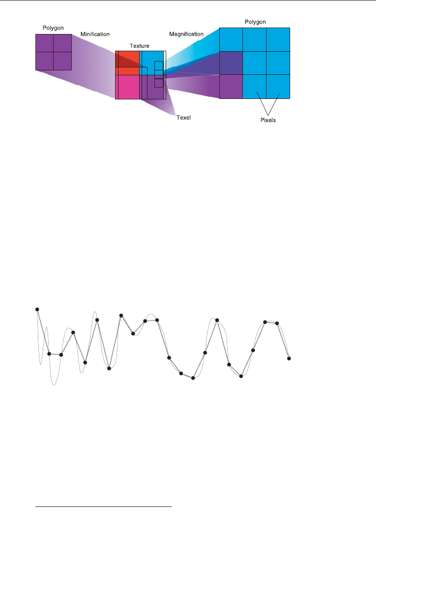
ptg9898810
Figure 6.14 Effect of texture minification and magnification
the texture map needs to be stretched in one direction and shrunk in the
other, OpenGL makes a choice between magnification and minification19
that in most cases gives the best result possible. It’s best to try to avoid
these situations by using texture coordinates that map without such
distortion.
Linear Filtering
Linear filtering is a technique in which a coordinate is used to select adjacent
samples from a discretely sampled signal and replace that signal with a linear
approximation of the original. Consider the signal shown in Figure 6.15.
Figure 6.15 Resampling of a signal in one dimension
In Figure 6.15, the signal represented by the solid line has been discretely
sampled at the points shown by the large dots. The original signal cannot be
reconstructed by placing a straight line between each of the dots. In some
areas of the signal, the linear reconstruction matches the original signal
reasonably well. However, in other areas, the reconstruction is not faithful
to the original and sharp peaks that were present before resampling are lost.
19. When a texture is enlarged by different amounts in the horizontal and vertical axes, this
is referred to as anisotropic filtering. This is exposed by some OpenGL implementations in the
form of an extension. However, this is not part of core OpenGL.
330 Chapter 6: Textures
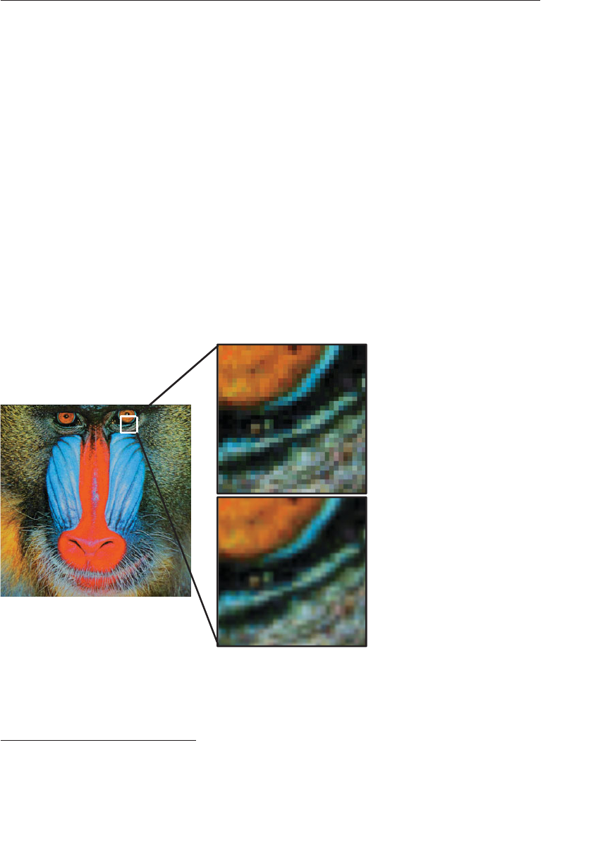
ptg9898810
For image data, the same technique can be applied. So long as the
sampling rate (resolution) of the texture is high enough relative to the
sharp peaks in the image data (details), a linear reconstruction of the image
will appear to have reasonably high quality. The translation from a signal
as shown in Figure 6.15 into a texture is easy to conceive when a 1D
texture is considered. Simply place the samples into a 1D texture and
reconstruct the original 1D image from those samples as needed.
To do this, OpenGL takes the texture coordinate that you pass it as a
floating-point number and finds the two samples that lie closest to it. It
uses the distance to each of those two points to create weights for each of
the samples and then uses those weights to create a weighted average of
them. Because linear resampling is separable20, OpenGL can apply this
technique first in one dimension, and then again in a second dimension in
order to reconstruct 2D images and even a third time for 3D textures.
Figure 6.16 illustrates the process as applied to a 2D image.
GL_LINEAR
GL_NEAREST
Figure 6.16 Bilinear resampling
20. A separable operation is one that can be deconstructed into two or more, usually similar
passes over the data. In this case, we can apply one pass per dimension of the image data.
Filtering 331

ptg9898810
Not only can linear filtering be used to smoothly transition from one
sample to the adjacent ones in 1D, 2D, and 3D textures, it can also be used
to blend texels sampled from adjacent mipmap levels in a texture. This
works in a very similar manner to that described above. OpenGL calculates
the mipmap level from which it needs to select samples and the result of
this calculation will often be a floating-point value with a fractional
component. This is used just as a fractional texture coordinate is used to
filter spatially adjacent texels. The two closest mipmaps are used to
construct a pair of samples and the fractional part of the level-of-detail
calculation is used to weight the two samples into an average.
All of these filtering options are controlled by the texture filter modes in
OpenGL’s sampler objects. As explained in ‘‘Sampler Objects’’ on Page 292,
the sampler object represents a collection of parameters that control how
texels are read from textures. Two of those parameters,
GL_TEXTURE_MAG_FILTER and GL_TEXTURE_MIN_FILTER, control how
OpenGL filters textures. The first is used when the texture is
magnified---that is, when the level-of-detail required is of a higher
resolution than the highest resolution mipmip level (by default, level 0)
and represents cases where the mipmip calculation produces a level less
than or equal to zero. Because, under magnification, only one mipmap
level is used, only two choices are available for
GL_TEXTURE_MAG_FILTER. These are GL_NEAREST and GL_LINEAR. The
first disables filtering and returns the nearest texel to the sample location.
The second enables linear filtering.
Texture minification is where mipmapping takes effect, and this is
explained in some detail in the following sections.
Advanced
From a signaling-theory perspective, a texture needs to sample the original
signal at at least twice the frequency of the highest frequency data present.
The original should be low-pass filtered to some frequency, then sampled
at greater than twice that frequency. This gives enough samples to exactly
reconstruct the original image. However, linear filtering fails to do this
reconstruction and can lead to aliasing. Also, if the original filtering and
2X sampling are not done, aliasing and other artifacts can occur. This is
discussed in more detail in Chapter 8,‘‘Procedural Texturing’’, and
mipmapping as one technique for dealing with it is described below. You
can also do custom filtering using texture gathers to improve over the
artifacts of linear filtering. Gathering texels is discussed later in this
chapter.
332 Chapter 6: Textures

ptg9898810
Using and Generating Mipmaps
Textured objects can be viewed, like any other objects in a scene, at
different distances from the viewpoint. In a dynamic scene, as a textured
object moves farther from the viewpoint, the ratio of pixels to texels in the
texture becomes very low and the texture ends up being sampled at a very
low rate. This has the effect of producing artifacts in the rendered image
due to undersampling of the texture data. For example, to render a brick
wall, you may use a large texture image (say 1024 ×1024 texels) when the
wall is close to the viewer. But if the wall is moved farther away from the
viewer until it appears on the screen as a single pixel, then the sampled
texture may appear to change abruptly at certain transition points.
To reduce this effect, we can pre-filter the texture map and store the
pre-filtered images as successively lower and lower-resolution versions of
the full resolution image. These are called mipmaps, and are shown in
Figure 6.17. The term mipmap was coined by Lance Williams, when he
introduced the idea in his paper ‘‘Pyramidal Parametrics’’ (SIGGRAPH 1983
Proceedings). Mip stands for the Latin multum in parvo, meaning ‘‘many
things in a small place.’’ Mipmapping uses some clever methods to pack
image data into memory.
When using mipmapping, OpenGL automatically determines which
resolution level of the texture map to use based on the size (in pixels) of
the object being mapped. With this approach, the level of detail in the
texture map is appropriate for the image that’s drawn on the screen; as the
image of the object gets smaller, the size of the texture map decreases.
Mipmapping requires some extra computation and texture storage area.
However, when it’s not used, textures that are mapped onto smaller objects
might shimmer and flash as the objects move.
This description of OpenGL mipmapping avoids detailed discussion of the
scale factor (known as λ) between texel size and polygon size. This
description also assumes default values for parameters related to
mipmapping. To see an explanation of λand the effects of mipmapping
parameters, see ‘‘Calculating the Mipmap Level’’ on Page 338. Additional
details on controlling λfrom your application can be found in ‘‘Mipmap
Level-of-Detail Control’’ on Page 339.
Filtering 333
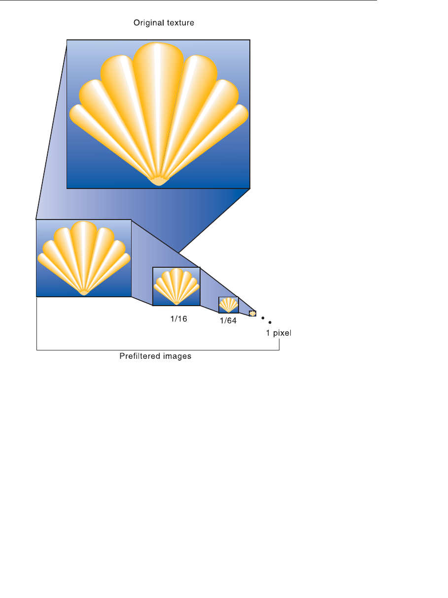
ptg9898810
Figure 6.17 A pre-filtered mipmap pyramid
The parameter GL_TEXTURE_MIN_FILTER controls how texels are
constructed when the mipmap level is greater than zero. There are a total
of six settings available for this parameter. The first two are the same as for
magnification---GL_NEAREST and GL_LINEAR. Choosing one of these two
modes disables mipmapping and causes OpenGL to only use the base level
(level 0) of the texture. The other four modes enable mipmapping and
control how the mipmaps are used. The four values are
GL_NEAREST_MIPMAP_NEAREST, GL_NEAREST_MIPMAP_LINEAR,
GL_LINEAR_MIPMAP_NEAREST, and GL_LINEAR_MIPMAP_LINEAR.
Notice how each mode is made up of two parts and the token names are
structured as GL_{A}_MIPMAP_{B}. Here, {A} and {B} may both be either
334 Chapter 6: Textures
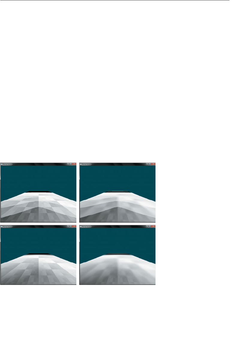
ptg9898810
NEAREST or LINEAR. The first part, {A}, controls how the texels from each
of the mipmap levels is constructed and works the same way as the
GL_TEXTURE_MAG_FILTER setting. The second, {B}, controls how these
samples are blended between the mipmap levels. When it’s NEAREST, only
the closest mipmap level is used. When it’s LINEAR, the two closest
mipmaps are linearly interpolated.
To illustrate the effect of the GL_TEXTURE_MIN_FILTER parameter on a
mipmapped texture, Figure 6.18 shows how each affects a simple checker
type pattern at different resolutions in a mipmap pyramid. Notice how
with the intra-mipmap filter specified as NEAREST (as in GL_NEAREST_
MIPMAP_NEAREST and GL_NEAREST_MIPMAP_LINEAR), the
checkerboard pattern becomes quite evident, whereas when it is LINEAR
(as in GL_LINEAR_MIPMAP_NEAREST and GL_LINEAR_MIPMAP_LINEAR),
it is less well defined and the texture appears blurred. Likewise, when the
inter-mipmap filter mode is NEAREST (as in GL_NEAREST_MIPMAP_
NEAREST and GL_LINEAR_MIPMAP_NEAREST), the boundary between the
mipmap levels is visible. However, when the inter-mipmap filter is LINEAR
(as in GL_NEAREST_MIPMAP_LINEAR and GL_LINEAR_MIPMAP_LINEAR),
that boundary is hidden by filtering.
Figure 6.18 Effects of minification mipmap filters
(GL_NEAREST_MIPMAP_NEAREST (top left), GL_LINEAR_MIPMAP_
NEAREST (top right), GL_NEAREST_MIPMAP_LINEAR (bottom left), and
GL_LINEAR_MIPMAP_LINEAR (bottom right).)
Filtering 335
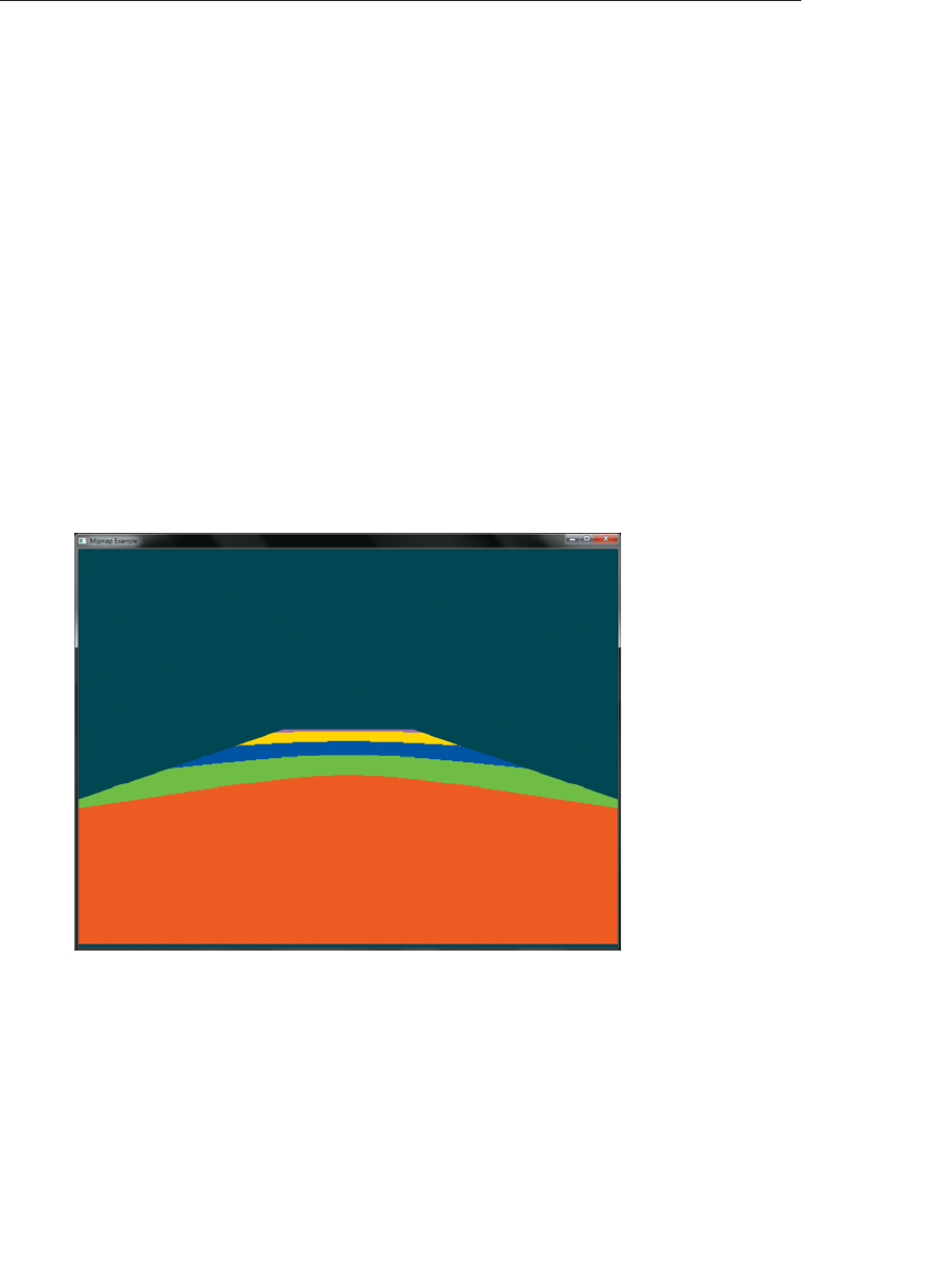
ptg9898810
To use mipmapping, you must provide all sizes of your texture in powers
of 2 between the largest size and a 1 ×1 map. If you don’t intend to use
mipmapping to go all the way to a 1 ×1 texture, you can set the value of
GL_TEXTURE_MAX_LEVEL to the maximum level you have supplied, and
OpenGL will not consider any further levels in its evaluation of texture
completeness. If the highest resolution level of the texture is not square,
one dimension will reach one texel in size before the other. In this case,
continue making new levels with that dimension sized to one texel until
the level becomes 1 ×1 texel in size. For example, if your highest
resolution map is 64 ×16, you must also provide maps of size 32 ×8,
16 ×4, 8 ×2, 4 ×1, 2 ×1, and 1 ×1. The smaller maps are typically filtered,
and down-sampled versions of the largest map in which each texel in a
smaller texture is a weighted average of the corresponding 4 texels in the
higher-resolution texture. (Since OpenGL doesn’t require any particular
method for calculating the lower-resolution maps, the differently sized
textures could be totally unrelated. In practice, unrelated textures would
make the transitions between mipmaps extremely noticeable, as in
Figure 6.19.)
Figure 6.19 Illustration of mipmaps using unrelated colors
The image in Figure 6.19 was generated by creating a 64 ×64 texture and
filling each of its 7 mipmap levels with a different color. The highest
resolution level was filled with red, then green, blue, yellow, and so on
336 Chapter 6: Textures

ptg9898810
down the mipmap pyramid. This texture was applied to a large plane
extending into the distance. The further the plane gets from the viewer,
the narrower it becomes in screen space and the more compressed the
texture becomes. OpenGL chooses successively higher mipmap levels
(lower resolution levels) from the texture. To further illustrate the effect,
the example sets the mipmap filtering mode to nearest and applies a bias
to the calculated mipmap level.
To specify these textures, allocate the texture using glTexStorage2D() and
then call glTexSubImage2D() once for each resolution of the texture map,
with different values for the level, width, height, and image parameters.
Starting with zero, level identifies which texture in the series is specified;
with the previous example, the highest-resolution texture of size 64 ×64
would be declared with level =0, the 32 ×32 texture with level =1, and so
on. In addition, for the mipmapped textures to take effect, you need to
choose one of the mipmapped minification filters as described earlier.
OpenGL provides a function to automatically generate all of the mipmaps
for a texture under application control. This function is called
glGenerateMipmap(), and it is up to the OpenGL implementation to
provide a mechanism to downsample the high resolution images to
produce the lower resolution mipmaps. This will often be implemented
internally by using a shader or perhaps the texture-filtering hardware. The
technique used will generally be designed for performance over quality
and will vary from implementation to implementation. If you want
high-quality, well-defined results, it is best to generate and supply the
mipmap images yourself. However, if you need to quickly generate a
mipmap chain and are satisfied with whatever results you get, you can rely
on glGenerateMipmap() for this purpose.
void glGenerateMipmap(GLenum target);
Generates a complete set of mipmaps for the texture image associated
with target, which must be one of GL_TEXTURE_1D, GL_TEXTURE_2D,
GL_TEXTURE_3D, GL_TEXTURE_1D_ARRAY, GL_TEXTURE_2D_ARRAY,
or GL_TEXTURE_CUBE_MAP. The mipmap levels constructed are
controlled by the GL_TEXTURE_BASE_LEVEL and
GL_TEXTURE_MAX_LEVEL. If those values are left to their defaults, an
entire mipmap stack down to a single-texel texture map is created. The
filtering method used in creating each successive level is implementation
dependent. A GL_INVALID_OPERATION error will be generated if target
is GL_TEXTURE_CUBE_MAP, and not all cube-map faces are initialized
and consistent.
Filtering 337

ptg9898810
Calculating the Mipmap Level
The computation of which mipmap level of a texture to use for a particular
pixel depends on the scale factor between the texture image and the size of
the polygon to be textured (in pixels). Let’s call this scale factor ρ, and also
define a second value, λ, where λ= log2ρ+lodbias. (Since texture images
can be multidimensional, it is important to clarify that ρis the maximum
scale factor of all dimensions.)
lodbias is the level-of-detail bias for the sampler, a constant value set by
calling glSamplerParameteri() with the pname parameter set to
GL_TEXTURE_LOD_BIAS and is used to adjust λ. By default, lodbias =0.0,
which has no effect. It’s best to start with this default value and adjust in
small amounts, if needed. If λ≤0.0, then the texel is smaller than the
pixel, and so a magnification filter is used. If λ>0.0, then a minification
filter is used. If the minification filter selected uses mipmapping, then λ
indicates the mipmap level. (The minification-to-magnification switchover
point is usually at λ=0.0, but not always. The choice of mipmapping filter
may shift the switchover point.)
For example, if the texture image is 64 ×64 texels and the polygon size is
32 ×32 pixels, then ρ=2.0 (not 4.0), and therefore λ=1.0. If the texture
image is 64 ×32 texels and the polygon size is 8 ×16 pixels, then ρ=8.0
(xscales by 8.0, yby 2.0; use the maximum value), and therefore λ=3.0.
The equations for the calculation of λand ρare as follows:
λbase (x,y) = log2[ρ(x,y)] (6.1)
λ(x,y) = λbase +clamp biastexobj +biasshader(6.2)
The calculation of mipmap level can be further controlled by a number of
sampler parameters. In particular, the GL_TEXTURE_LOD_BIAS parameter
may be used to bias λ. Once λhas been calculated, it may be clamped into
a user-specified range, which is given by the parameters
GL_TEXTURE_MIN_LOD and GL_TEXTURE_MAX_LOD, which are
specified by passing those token values to glSamplerParameterf() (or to
glTexParameterf() if sampler objects are not in use). The default values for
GL_TEXTURE_MIN_LOD and GL_TEXTURE_MAX_LOD are −1000.0 and
1000.0, respectively, allowing them to effectively pass through any value.
The values of GL_TEXTURE_MIN_LOD and GL_TEXTURE_MAX_LOD are
represented by lodmin and lodmax in the following equation.
λ=⎧
⎪⎪⎪
⎨
⎪⎪⎪
⎩
lodmax,λ>lodmax
λ,lodmin ≤λ≤lodmax
lodmin,λ<lodmin
undefined,lodmin >lodmax
(6.3)
338 Chapter 6: Textures

ptg9898810
The default parameters for GL_TEXTURE_MAG_
FILTER and GL_TEXTURE_MIN_FILTER are GL_LINEAR
and GL_LINEAR_MIPMAP_LINEAR, respectively. Notice
that the default minification filter enables mipmapping. This is
important because in order to use mipmapping, the texture must
have a complete set of mipmap levels and they must have a con-
sistent set of resolutions as described in ‘‘Using and Generating
Mipmaps’’ on Page 333; otherwise, the texture is considered in-
complete and will not return useful data to the shader. Textures
allocated using the glTexStorage2D() function are always com-
plete, so you don’t need to worry about that; but these textures
will still contain no data when they are newly created. This is a
common source of errors for new OpenGL programmers---they
forget to either change the filtering mode or fill in the mipmaps
for newly created textures resulting in their texturing code not
working.
Mipmap Level-of-Detail Control
In addition to the parameters controlling lodmin,lodmax, and λbase during
the calculation of λ, further control over the selected level of the mipmap
pyramid is provided through the GL_TEXTURE_BASE_LEVEL and
GL_TEXTURE_MAX_LEVEL parameters, which may be set using
glSamplerParameteri(). GL_TEXTURE_BASE_LEVEL specifies the lowest
mipmap level (i.e., highest resolution) that will be sampled, regardless of
the value of λ, whereas GL_TEXTURE_MAX_LEVEL specifies the highest
mipmap level (i.e., lowest resolution) that will be sampled. This can be
used to constrain sampling to a subset of the mipmap pyramid.
One potential use for GL_TEXTURE_BASE_LEVEL is texture streaming.
When using texture streaming, storage for the complete texture object is
allocated using a function such as glTexStorage2D() but the initial data is
not loaded. As the application runs and new objects come into view, their
texture data is loaded from lowest to highest resolution mipmap. To ensure
that something meaningful is displayed to the user even when the
complete texture has not yet been loaded, the value of GL_TEXTURE_
BASE_LEVEL can be set to the highest resolution mipmap level that has
been loaded so far. That way, as more and more texture data is loaded,
objects on the screen achieve higher and higher fidelity.
Filtering 339

ptg9898810
Advanced Texture Lookup Functions
In addition to simple texturing functions such as texture and
texelFetch, several more variants of the texture fetch functions are
supported by the shading language. These are covered in this subsection.
Explicit Level of Detail
Normally, when using mipmaps, OpenGL will calculate the level of detail
and the resulting mipmap levels from which to sample for you (see
‘‘Calculating the Mipmap Level’’ on Page 338 for more details on how
OpenGL calculates mipmap levels). However, it is possible to override this
calculation and specify the level of detail explicitly as an argument to the
texture fetch function. The textureLod function takes this lod parameter
in place of the bias parameter that would normally be optionally supplied
to the texture function. Like other texture functions supported by GLSL,
textureLod has many overloaded prototypes for the various types and
dimensionalities of the supported sampler types. Some key prototypes of
textureLod are as follows: (A full list is in Appendix C,‘‘Built-in GLSL
Variables and Functions’’.)
gvec4 textureLod(gsampler1D tex, float P, float lod);
gvec4 textureLod(gsampler2D tex, vec2 P, float lod);
gvec4 textureLod(gsampler3D tex, vec3 P, float lod);
gvec4 textureLod(gsamplerCube tex, vec3 P, float lod);
gvec4 textureLod(gsampler1DArray tex, vec2 P, float lod);
gvec4 textureLod(gsampler2DArray tex, vec3 P, float lod);
gvec4 textureLod(gsampler2DRect tex, vec2 P, float lod);
gvec4 textureLod(gsamplerCubeArray tex, vec4 P, float lod);
Sample a texel from the sampler given by tex at the texture coordinates
given by Pwith explicit level of detail given by lod.
Notice that because they don’t support mipmaps, samplerBuffer and
samplerRect are missing from the supported sampler types for
textureLod.
Explicit Gradient Specification
It is also possible to override the level-of-detail calculation for mipmapping
at an earlier part of the process rather than explicitly giving the level-
of-detail parameter directly. When the gradient texture functions are used,
340 Chapter 6: Textures

ptg9898810
the partial derivative of the texture coordinates is given as a parameter.
Some key prototypes are listed below. (A full list is in Appendix C,‘‘Built-in
GLSL Variables and Functions’’.)
gvec4 textureGrad(gsampler1D tex, float P,float dPdx, float dPdy);
gvec4 textureGrad(gsampler2D tex, vec2 P,vec2 dPdx, vec2 dPdy);
gvec4 textureGrad(gsampler3D tex, vec3 P,vec3 dPdx, vec3 dPdy);
gvec4 textureGrad(gsamplerCube tex, vec3 P,vec3 dPdx,
vec3 dPdy);
gvec4 textureGrad(gsampler1DArray tex, vec2 P,float dPdx,
float dPdy);
gvec4 textureGrad(gsampler2DArray tex, vec3 P,vec2 dPdx,
vec2 dPdy);
gvec4 textureGrad(gsamplerCubeArray tex, vec4 P,vec3 dPdx,
vec3 dPdy);
Sample a texel from the sampler given by tex at the texture coordinates
given by Pusing the partial derivatives for Pin xand yas specified by
dPdx and dPdy, respectively.
In the textureGrad functions, the variable ρas described in ‘‘Calculating
the Mipmap Level’’ on Page 338 is essentially passed in using dPdx and
dPdy. This can be useful when an analytic function for the derivative of a
texture coordinate may be known, or when a function that is not the
derivative of the texture coordinate is required.
Texture Fetch with Offsets
Some applications require a number of texels around a region of interest,
or may need to offset the texture coordinates slightly during sampling.
GLSL includes functions for doing this that will likely be more efficient
than physically offsetting the texture coordinates in the shader. This
functionality is exposed through an overloaded set of texture lookup
functions called textureOffset with some example prototypes as
follows: (A full list is in Appendix C,‘‘Built-in GLSL Variables and
Functions’’.)
gvec4 textureOffset(gsampler1D tex, float P, int offset,
[float bias]);
gvec4 textureOffset(gsampler2D tex, vec2 P, ivec2 offset,
[float bias]);
gvec4 textureOffset(gsampler3D tex, vec3 P, ivec3 offset,
[float bias]);
Advanced Texture Lookup Functions 341

ptg9898810
gvec4 textureOffset(gsampler1DArray tex, vec2 P, int offset,
[float bias]);
gvec4 textureOffset(gsampler2DArray tex, vec3 P, ivec2 offset,
[float bias]);
gvec4 textureOffset(gsampler2DRect tex, vec2 P, ivec2 offset,
[float bias]);
Sample a texel from the sampler given by tex at the texture coordinates
given by P. After the floating-point texture coordinate Phas been
suitably scaled and converted to absolute texel coordinates, offset is
added to the texel coordinates before the fetch is performed.
Notice that for the textureOffset function, the offset parameter is an
integer value. In fact, this must be a constant expression and must be with
a limited range. This range is given by the built-in GLSL constants
gl_MinProgramTexelOffset and gl_MaxProgramTexelOffset.
Projective Texturing
Projective texturing is employed when a perspective transformation matrix
has been used to transform texture coordinates. The input to the transform
is a set of homogeneous coordinates and the resulting output of this
transform is a vector whose last component is unlikely to be 1. The
textureProj function can be used to divide through by this final
component, projecting the resulting texture coordinate into the
coordinate space of the texture. This is useful for techniques such as
projecting decals onto flat surfaces (e.g., the halo projected by a flashlight)
or in shadow mapping21. Some example prototypes are given below. (A full
list is in Appendix C,‘‘Built-in GLSL Variables and Functions’’.)
gvec4 textureProj(gsampler1D tex, vec2 P[, float bias);
gvec4 textureProj(gsampler1D tex, vec4 P[, float bias);
gvec4 textureProj(gsampler2D tex, vec3 P[, float bias);
gvec4 textureProj(gsampler2D tex, vec4 P[, float bias);
gvec4 txtureProj(gsampler3D tex, vec4 P[, float bias);
21. An in-depth example of shadow mapping is given in ‘‘Shadow Mapping’’ on Page 400.
342 Chapter 6: Textures

ptg9898810
gvec4 textureProj(gsamplerRect tex, vec3 P);
gvec4 textureProj(gsamplerRect tex, vec4 P);
Perform a texture lookup with projection by dividing the texture
coordinate specified in Pby the last component of Pand using the
resulting values to perform a texture lookup as would be executed by the
normal texture.
Texture Queries in Shaders
The following two built-in GLSL functions don’t actually read from the
texture, but return information about the texture or about how it will be
processed. The first function, textureQueryLod retrieves mipmap
information calculated by the fixed-function texture lookup hardware.
vec2 textureQueryLod(gsampler1D tex, float P);
vec2 textureQueryLod(gsampler2D tex, vec2 P);
vec2 textureQueryLod(gsampler3D tex, vec3 P);
vec2 textureQueryLod(gsamplerCube tex, vec3 P);
vec2 textureQueryLod(gsampler1DArray tex, float P);
vec2 textureQueryLod(gsampler2DArray tex, vec2 P);
vec2 textureQueryLod(gsamplerCubeArray tex, vec3 P);
vec2 textureQueryLod(sampler1DShadow tex, float P);
vec2 textureQueryLod(sampler2DShadow tex, vec2 P);
vec2 textureQueryLod(samplerCubeShadow tex, vec3 P);
vec2 textureQueryLod(sampler1DArrayShadow tex, float P);
vec2 textureQueryLod(sampler2DArrayShadow tex, vec2 P);
vec2 textureQueryLod(samplerCubeArrayShadow tex, vec3 P);
Return the mipmap array(s) that would be accessed in the xcomponent
of the return value and the computed level of detail relative to the base
level of the texture in the ycomponent.
For each of these textureQueryLod() functions, there is a corresponding
query, textureQueryLevels(), that returns the number of mipmap
levels present.
Advanced Texture Lookup Functions 343

ptg9898810
int textureQueryLevels(gsampler1D tex);
int textureQueryLevels(gsampler2D tex);
int textureQueryLevels(gsampler3D tex);
int textureQueryLevels(gsamplerCube tex);
int textureQueryLevels(gsampler1DArray tex);
int textureQueryLevels(gsampler2DArray tex);
int textureQueryLevels(gsamplerCubeArray tex);
int textureQueryLevels(sampler1DShadow tex);
int textureQueryLevels(sampler2DShadow tex);
int textureQueryLevels(samplerCubeShadow tex);
int textureQueryLevels(sampler1DArrayShadow tex);
int textureQueryLevels(sampler2DArrayShadow tex);
int textureQueryLevels(samplerCubeArrayShadow tex);
Return the number of mipmap levels the provided sampler contains.
Sometimes, it may be necessary to know the dimensions of a texture from
which you are about to sample. For example, you may need to scale an
integer texture coordinate representing an absolute texel location into a
floating-point range suitable for sampling from the texture, or to iterate
over all the samples in a texture. The textureSize function will return
the dimensions of the texture at a specified level of detail. Its prototype is
as follows: (A full list is in Appendix C,‘‘Built-in GLSL Variables and
Functions’’.)
int textureSize(gsampler1D tex, int lod);
ivec2 textureSize(gsampler2D tex, int lod);
ivec3 textureSize(gsampler3D tex, int lod);
ivec2 textureSize(gsamplerCube tex, int lod);
ivec2 textureSize(gsamplerRect tex, int lod);
ivec3 textureSize(gsamplerCubeRect tex);
ivec2 textureSize(gsampler1DArray tex, int lod);
ivec3 textureSize(gsampler2DArray tex, int lod);
int textureSize(gsamplerBuffer tex);
Return the dimensions of the level-of-detail lod (if present) of the texture
bound to sampler tex. The components of the return value are filled in
order with the width, height, and depth of the texture. For array forms,
the last component of the return value is the number of slices in the
array.
344 Chapter 6: Textures

ptg9898810
Gathering Texels
The textureGather function is a special function that allows your shader
to read the four samples that would have been used to create a bilinearly
filtered texel from a 2D texture (or cube map, rectangle texture, or array of
these types). Typically used with single-channel textures, the optional
comp component of the function allows you to select a channel other than
the xor rcomponent of the underlying data. This function can provide
significant performance advantages when you need to sample many times
from a single channel of a texture because, depending on the desired
access pattern, it is possible to use this function to cut the number of
texture lookups by three quarters.
gvec4 textureGather(gsampler2D tex, vec2 P[, int comp]);
gvec4 textureGather(gsampler2DArray tex, vec3 P[, int comp]);
gvec4 textureGather(gsamplerCube tex, vec3 P[, int comp]);
gvec4 textureGather(gsamplerCubeArray tex, vec4 P[, int comp]);
gvec4 textureGather(gsamplerRect tex, vec2 P[, int comp]);
Gather the four texels from the underlying rectangle, two-dimensional
(array), or cube-map (array) texture bound to the sampler tex that would
normally have been used to create a bilinearly filtered texel value and
return a selected component of the four texels in the four components of
the return value. If specified, comp specifies the component to fetch with
0, 1, 2, and 3 representing the x,y,z, and wcomponents, respectively. If
comp is not specified, then the xcomponent is returned.
Combining Special Functions
In addition to all of the special texturing functions, several more variants
of these functions exist that combine features from multiple variants. For
example, if you want to do projective texturing with an explicit
level-of-detail or gradients (each is described in ‘‘Explicit Gradient
Specification’’ on Page 340), then you can use the combined functions
textureProjLod or textureProjGrad, respectively. The combined
functions using a 2D sampler are shown below. Variants of almost all of
these functions exist for other dimensionalities and types of sampler, and a
full list is in Appendix C,‘‘Built-in GLSL Variables and Functions’’.
Advanced Texture Lookup Functions 345

ptg9898810
gvec4 textureProjLod(gsampler2D tex, vec2 P, float lod);
gvec4 textureProjGrad(gsampler2D tex, vec3 P, vec2 dPdx,
vec2 dPdy);
gvec4 textureProjOffset(gsampler2D tex, vec3 P, ivec2 offset[,
float bias);
gvec4 textureGradOffset(gsampler2D tex, vec2 P, vec2 dPdx,
vec2 dPdy, ivec2 offset);
gvec4 textureProjLodOffset(gsampler2D tex, vec3 P, float lod,
ivec2 offset);
gvec4 textureProjGradOffset(gsampler2D tex, vec3 P, vec2 dPdx,
vec2 dPdy, ivec2 offset);
Advanced texture lookup functions may be combined to perform more
than one special function in a single call. textureProjLod performs
projective texturing from the texture bound to the unit represented bytex
as would be performed by textureProj, but with explicit level of detail
specified in lod, as accepted by textureLod. Similarly,
textureProjGrad executes a projective texture lookup as performed by
textureProj, but with explicit gradients passed in dPdx and dPdy as
would be accepted by textureGrad.textureProjOffset performs a
projective texture lookup with texel offsets applied to the post projected
texture coordinates. textureProjLodOffset and
textureProjGradOffset further combine two special functions---the
first performs a projective texture fetch with explicit level of detail and
texel offsets (as accepted by textureOffset) and the second performs a
projective texture lookup with explicit gradients and texel offsets.
Point Sprites
Point sprites are essentially OpenGL points rendered using a fragment
shader that takes the fragment’s coordinates within the point into account
when running. The coordinate within the point is available in the
two-dimensional vector gl_PointCoord. This variable can be used in any
number of ways. Two common uses are to use it as a texture coordinate
(this is the classic origin of the term point sprite), or to use it to
analytically compute color or coverage. The following are a few examples
of how to use the gl_PointCoord vector to produce interesting effects in
the fragment shader.
346 Chapter 6: Textures

ptg9898810
Textured Point Sprites
By using gl_PointCoord to lookup texels in a texture in the fragment
shader, simple point sprites can be generated. Each point sprite simply
shows the texture as a square. Example 6.27 is the vertex shader used in
the example. Notice that we’re writing to gl_PointSize in the vertex
shader. This is to control the size of the point sprites---they’re scaled
relative to their distance from the near plane. Here we’ve used a simple
linear mapping, but more complex logarithmic mappings can be used.
Example 6.27 Simple Point Sprite Vertex Shader
uniform mat4 model_matrix;
uniform mat4 projection_matrix;
layout (location = 0) in vec4 position;
void main(void)
{vec4 pos = projection_matrix *(model_matrix *position);
gl_PointSize = (1.0 - pos.z / pos.w) *64.0;
gl_Position = pos;
}
Example 6.28 shows the fragment shader used in this example. Not
including the declaration of the texture and the output vector, it’s a single
line of real code! We simply look up into the texture using
gl_PointCoord as a texture coordinate.
Example 6.28 Simple Point Sprite Fragment Shader
uniform sampler2D sprite_texture;
out vec4 color;
void main(void)
{color = texture(sprite_texture, gl_PointCoord);
}
When we render 400 points randomly placed in a two-unit cube centered
on the origin, we get the result shown in Figure 6.20.
Point Sprites 347
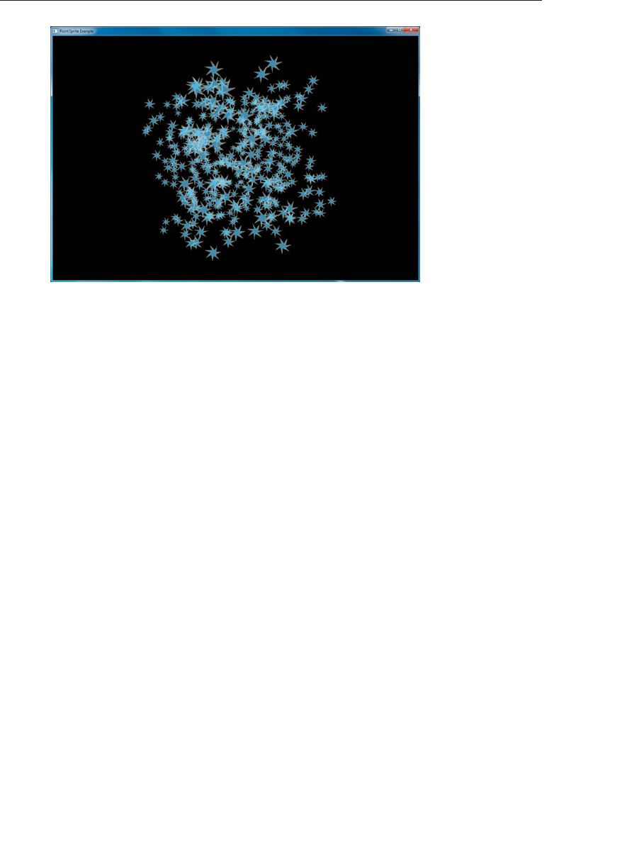
ptg9898810
Figure 6.20 Result of the simple textured point sprite example
Analytic Color and Shape
You are not limited to sourcing your point sprite data from a texture.
Textures have a limited resolution, but gl_PointCoord can be quite
precise. The shader shown in Example 6.29 demonstrates how you can
analytically determine coverage in the fragment shader. This shader
centers gl_PointCoord around the origin and then calculates the squared
distance of the fragment from the center of the point sprite. If it’s greater
than 0.25 (the square root of half the width of the sprite---or the radius of
a circle that just fits inside it) then the fragment is rejected using the
discard keyword. Otherwise, we interpolate between two colors to
produce the final output. This produces a perfect circle. Note that the
same vertex shown in Example 6.27 is used for this example as well.
Example 6.29 Analytic Shape Fragment Shader
out vec4 color;
void main(void)
{
const vec4 color1 = vec4(0.6, 0.0, 0.0, 1.0);
const vec4 color2 = vec4(0.9, 0.7, 1.0, 0.0);
vec2 temp = gl_PointCoord - vec2(0.5);
float f = dot(temp, temp);
if (f > 0.25)
discard;
color = mix(color1, color2, smoothstep(0.1, 0.25, f));
}
348 Chapter 6: Textures
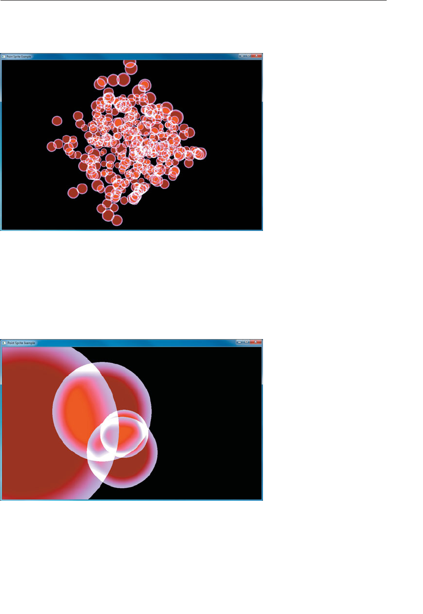
ptg9898810
Figure 6.21 shows the output of this example.
Figure 6.21 Analytically calculated point sprites
By increasing the size of the point sprite and reducing the number of
points in the scene, it is possible to see the extremely smooth edges of the
discs formed by the fragment shader as shown in Figure 6.22.
Figure 6.22 Smooth edges of circular point sprites
Point Sprites 349

ptg9898810
Controlling the Appearance of Points
Various controls exist to allow the appearance of points to be tuned by
your application. These parameters are set using glPointParameterf() or
glPointParameteri().
void glPointParameter{if}(GLenum pname, TYPE param);
void glPointParameter{if}v(GLenum pname, const TYPE *param);
Set the point parameter specified by pname to the value(s) specified by
param.pname must be GL_POINT_SPRITE_COORD_ORIGIN or
GL_POINT_FADE_THRESHOLD_SIZE. If pname is
GL_POINT_SPRITE_COORD_ORIGIN, param must be one of
GL_LOWER_LEFT or GL_UPPER_LEFT (or the address of a variable
containing one of these values). If pname is
GL_POINT_FADE_THRESHOLD_SIZE, param must be a floating point
quantity greater than or equal to zero (or the address of a variable
containing such a value).
The two parameters that you can change with glPointParameteri() or
glPointParameterf() are the origin for gl_PointCoord (using
GL_POINT_SPRITE_COORD_ORIGIN) the point fade threshold (using
GL_POINT_FADE_THRESHOLD_SIZE). The point sprite coordinate origin
controls whether gl_PointCoord.y increases from top down or bottom
up in the fragment shader as points are rasterized. By default, the value of
GL_POINT_SPRITE_COORD_ORIGIN is GL_UPPER_LEFT, meaning that it
increases from top down. Note that this goes in the opposite direction to
window coordinates, which have their origin in the lower right. By
specifying GL_LOWER_LEFT for GL_POINT_SPRITE_COORD_ORIGIN you
can make gl_PointCoord.y increase in the same direction as
gl_FragCoord.y, which represents the fragment’s window coordinate.
The other parameter that can be changed, GL_POINT_FADE_THRESHOLD
controls how points (and point sprites) are antialiased. When the size of a
point falls below this threshold, OpenGL has the option to stop
performing true antialiasing and instead fade the point into the
background using blending. The default value of this parameter is 1.0,
which means that if a point whose size is less than 1.0 is rasterized, rather
than only lighting a single sample within each fragment, it may light all
the fragments in that sample but end up having its alpha component
350 Chapter 6: Textures

ptg9898810
attenuated by the point fade factor, which is computed as follows:
fade =⎧
⎨
⎩
1 if (derived_size ≥threshold)
derived_size
threshold 2
otherwise
Rendering to Texture Maps
In addition to using framebuffer objects (as described in ‘‘Framebuffer
Objects’’ on Page 180 in Chapter 4) for offscreen rendering, you can also
use FBOs to update texture maps. You might do this to indicate changes in
the texture for a surface (such as damage to a wall in a game) or to update
values in a lookup table, if you’re doing GPGPU-like computations. In
these cases, you bind a level of a texture map as a framebuffer attachment.
After rendering, the texture map can be detached from the framebuffer
object, and used for subsequent rendering.
Note: Nothing prevents you from reading from a texture that is
simultaneously bound as a framebuffer attachment for writing. In
this scenario, called a framebuffer rendering loop, the results are
undefined for both operations. That is, the values returned from
sampling the bound texture map, as well as the values written into
the texture level while bound, are undefined, and likely incorrect.
void glFramebufferTexture(GLenum target, GLenum attachment,
GLuint texture, GLint level);
void glFramebufferTexture1D(GLenum target,
GLenum attachment,
GLenum texturetarget,
GLuint texture, GLint level);
void glFramebufferTexture2D(GLenum target,
GLenum attachment,
GLenum texturetarget,
GLuint texture, GLint level);
void glFramebufferTexture3D(GLenum target,
GLenum attachment,
GLenum texturetarget,
GLuint texture, GLint level,
GLint layer);
Rendering to Texture Maps 351

ptg9898810
The glFramebufferTexture* family of routines attaches levels of a texture
map as a framebuffer attachment. glFramebufferTexture() attaches level
of texture object texture (assuming texture is not zero) to attachment.
glFramebufferTexture1D(),glFramebufferTexture2D(), and
glFramebufferTexture3D() each attach a specified texture image of a
texture object as a rendering attachment to a framebuffer object. target
must be either GL_READ_FRAMEBUFFER, GL_DRAW_FRAMEBUFFER, or
GL_FRAMEBUFFER (which is equivalent to GL_DRAW_FRAMEBUFFER).
attachment must be one of the framebuffer attachment points:
GL_COLOR_ATTACHMENTi, GL_DEPTH_ATTACHMENT,
GL_STENCIL_ATTACHMENT, or GL_DEPTH_STENCIL_ATTACHMENT
(in which case, the internal format of the texture must be
GL_DEPTH_STENCIL). For glFramebufferTexture1D(),texturetarget must
be GL_TEXTURE_1D, if texture is not zero. For
glFramebufferTexture2D(),texturetarget must be GL_TEXTURE_2D,
GL_TEXTURE_RECTANGLE, GL_TEXTURE_CUBE_MAP_POSITIVE_X,
GL_TEXTURE_CUBE_MAP_POSITIVE_Y,
GL_TEXTURE_CUBE_MAP_POSITIVE_Z,
GL_TEXTURE_CUBE_MAP_NEGATIVE_X,
GL_TEXTURE_CUBE_MAP_NEGATIVE_Y,
GL_TEXTURE_CUBE_MAP_NEGATIVE_Z,
and for glFramebufferTexture3D() texturetarget must be
GL_TEXTURE_3D.
If texture is zero, indicating that any texture bound to attachment is
released, no subsequent bind to attachment is made. In this case,
texturetarget,level, and layer are ignored.
If texture is not zero, it must be the name of an existing texture object
(created with glGenTextures()), with texturetarget matching the texture
type (e.g., GL_TEXTURE_1D, etc.) associated with the texture object, or if
texture is a cube map, then texturetarget must be one of the cube-map face
targets, otherwise, a GL_INVALID_OPERATION error is generated.
level represents the mipmap level of the associated texture image to be
attached as a render target, and for three-dimensional textures or
two-dimensional texture arrays, layer represents the layer of the texture
to be used. If texturetarget is GL_TEXTURE_RECTANGLE, or
GL_TEXTURE_2D_MULTISAMPLE, then level must be zero.
352 Chapter 6: Textures

ptg9898810
Example 6.30 Attaching a Texture Level as a Framebuffer
Attachment: fbotexture.cpp
GLsizei TexWidth, TexHeight;
GLuint framebuffer, texture;
void init() {
GLuint renderbuffer;
// Create an empty texture
glGenTextures(1, &texture);
glBindTexture(GL_TEXTURE_2D, texture);
glTexImage2D(GL_TEXTURE_2D, 0, GL_RGBA8, TexWidth,
TexHeight, 0, GL_RGBA, GL_UNSIGNED_BYTE, NULL);
// Create a depth buffer for our framebuffer
glGenRenderbuffers(1, &renderbuffer);
glBindRenderbuffer(GL_RENDERBUFFER, renderbuffer);
glRenderbufferStorage(GL_RENDERBUFFER, GL_DEPTH_COMPONENT24,
TexWidth, TexHeight);
// Attach the texture and depth buffer to the framebuffer
glGenFramebuffers(1, &framebuffer);
glBindFramebuffer(GL_DRAW_FRAMEBUFFER, framebuffer);
glFramebufferTexture2D(GL_DRAW_FRAMEBUFFER,
GL_COLOR_ATTACHMENT0, GL_TEXTURE_2D, texture, 0);
glFramebufferRenderbuffer(GL_DRAW_FRAMEBUFFER,
GL_DEPTH_ATTACHMENT, GL_RENDERBUFFER, renderbuffer);
glEnable(GL_DEPTH_TEST);
}
void
display()
{// Render into the renderbuffer
glBindFramebuffer(GL_DRAW_FRAMEBUFFER, framebuffer);
glViewport(0, 0, TexWidth, TexHeight);
glClearColor(1.0, 0.0, 1.0, 1.0);
glClear(GL_COLOR_BUFFER_BIT | GL_DEPTH_BUFFER_BIT);
...
//Generate mipmaps of our texture
glGenerateMipmap(GL_TEXTURE_2D);
// Bind to the window-system framebuffer, unbinding from
// the texture, which we can use to texture other objects
glBindFramebuffer(GL_FRAMEBUFFER, 0);
glViewport(0, 0, windowWidth, windowHeight);
glClearColor(0.0, 0.0, 1.0, 1.0);
glClear(GL_COLOR_BUFFER_BIT | GL_DEPTH_BUFFER_BIT);
// Render using the texture
glEnable(GL_TEXTURE_2D);
...
glutSwapBuffers();
}
Rendering to Texture Maps 353

ptg9898810
For three-dimensional, or one- and two-dimensional texture arrays, you
can also attach a single layer of the texture as a framebuffer attachment.
void glFramebufferTextureLayer(GLenum target,
GLenum attachment,
GLuint texture, GLint level,
GLint layer);
Attaches a layer of a three-dimensional texture, or a one- or two-
dimensional array texture as a framebuffer attachment, in a similar
manner to glFramebufferTexture3D().
target must be one of GL_READ_FRAMEBUFFER,
GL_DRAW_FRAMEBUFFER, or GL_FRAMEBUFFER (which is equivalent to
GL_DRAW_FRAMEBUFFER). attachment must be one of
GL_COLOR_ATTACHMENTi, GL_DEPTH_ATTACHMENT,
GL_STENCIL_ATTACHMENT, or GL_DEPTH_STENCIL_ATTACHMENT.
texture must be either zero, indicating that the current binding for the
attachment should be released, or a texture object name (as returned
from glGenTextures()). level indicates the mipmap level of the texture
object, and layer represents which layer of the texture (or array element)
should be bound as an attachment.
Discarding Rendered Data
Advanced
As a rule of thumb, you should always clear the framebuffer before you
begin rendering a frame. Modern GPUs implement compression and other
techniques to improve performance, memory bandwidth requirements,
and so on. When you clear a framebuffer, the OpenGL implementation
knows that it can discard any rendered data in the framebuffer and return
it to a clean, compressed state if possible. However, what happens if you’re
sure that you’re about to render over the whole framebuffer? It seems that
clearing it would be a waste as you are about to draw all over the cleared
area. If you are certain that you are going to completely replace the
contents of the framebuffer with new rendering, you can discard it with a
call to glInvalidateFramebuffer() or glInvalidateSubFramebuffer(). Their
prototypes are as follows:
354 Chapter 6: Textures

ptg9898810
void glInvalidateFramebuffer(GLenum target,
GLsizei numAttachments,
const GLenum * attachments);
void glInvalidateSubFramebuffer(GLenum target,
GLsizei numAttachments,
const GLenum * attachments,
GLint x, GLint y, GLint width,
GLint height);
Instruct OpenGL that it may discard the contents of the specified
framebuffer attachments within the region delimited by x,y,width, and
height.glInvalidateFramebuffer() discards the entire contents of the
specified attachments. The number of attachments is given by
numAttachments and attachments is the address of an array of that many
tokens. For the nondefault framebuffer, the tokens stored in the
attachments arary must be selected from GL_DEPTH_ATTACHMENT,
GL_STENCIL_ATTACHMENT, GL_DEPTH_STENCIL_ATTACHMENT, and
GL_COLOR_ATTACHMENTiwhere iis the index of a color attachment.
Discarding the content of a framebuffer can be far more efficient than
clearing it, depending on the OpenGL implementation. Furthermore, this
can eliminate some expensive data copies in systems with more than one
GPU. If, rather than discarding the content of the attachments of a
framebuffer object you wish to discard the content of a texture directly,
you can call glInvalidateTexImage() or glInvalidateTexSubImage(). The
prototypes for glInvalidateTexImage() and glInvalidateTexSubImage()
are as follows:
void glInvalidateTexImage(GLuint texture, GLint level);
void glInvalidateTexSubImage(GLuint texture, GLint level,
GLint xoffset, GLint yoffset,
GLint zoffset, GLint width,
GLint height, GLint depth);
Instruct OpenGL that it may discard the contents of the specified level of
the texture whose name is given in texture.glInvalidateTexImage()
discards the entire image level of the texture object, whereas
glInvalidateTexSubImage() discards only the region encompassed by
the width by height by depth region whose origin is given by xoffset,
yoffset, and zoffset.
Rendering to Texture Maps 355

ptg9898810
Chapter Summary
In this chapter, we have given an overview of texturing in OpenGL.
Applications of textures in computer graphics are wide ranging and
surprisingly complex. The best that can be done in a single chapter of a
book is to scratch the surface and hopefully convey to the reader the depth
and usefulness of textures. Entire books could be written on advanced uses
of textures. More information about textures can be found in subsequent
chapters---including examples of how to draw into textures, use buffer
textures, and store nonimage data in textures.
Texture Redux
To use a texture in your program:
•Create a texture by
-- Reserving a name for a texture using glGenTextures().
-- How about: Binding its name to the appropriate binding point
using glBindTexture().
-- Specifying the dimensions and format of the texture using
glTexStorage2D() or the appropriate function for the specified
texture target.
-- Placing data into the texture using glTexSubImage2D(), or the
appropriate function for the specified texture target.
•Access the texture in your shader by
-- Declaring a uniform sampler in your shader to represent the
texture.
-- Associating the sampler with the desired texture unit using
glUniform1i().
-- Binding the texture object and optionally a sampler object to the
correct texture unit.
-- Reading from the texture in the shader using texture or one of
other the built-in texture functions.
To use a buffer object as a texture:
•Create a buffer texture by
-- Generating a texture name using glGenTextures().
-- Binding that name to the GL_TEXTURE_BUFFER texture target.
•Create and initialize a buffer texture by
-- Generating a buffer name using glGenBuffers().
356 Chapter 6: Textures

ptg9898810
-- Binding the buffer to a target, preferably the
GL_TEXTURE_BUFFER target.
-- Defining the storage for the buffer object using glBufferData().
•Attach the buffer object’s data store to the texture by
-- Binding the texture to the GL_TEXTURE_BUFFER target and,
-- Calling glTexBuffer() with the name of the initialized buffer
object.
Texture Best Practices
Here are some tips to ensure that you allow OpenGL to use your textures
most efficiently, ensuring the best possible performance for your
application. Some common pitfalls are enumerated here with some advice
on how to avoid them.
Immutable Texture Storage
Use immutable texture storage for textures wherever possible. Immutable
storage for textures is created using the glTexStorage2D() function or the
appropriate one for your chosen texture target. Mutable storage is created
by calling glTexImage2D(). When a texture is marked as immutable, the
OpenGL implementation can make certain assumptions about the validity
of a texture object. For example, the texture will always be complete.
Mipmaps
Create and initialize the mipmap chain for textures unless you have a good
reason not to. Allowing the graphics hardware to use a lower resolution
mipmap when it needs to will not only improve the image quality of your
program’s rendering, but it will also make more efficient use of the caches
in the graphics processor. The texture cache is a small piece of memory
that is used to store recently accessed texture data. The smaller the textures
your application uses, the more of them will fit into the cache, and the
faster your application will run.
Integer Format Textures
Don’t forget to use an integer sampler (isampler2D,usampler3D, etc.)
in your shader when your texture data is an unnormalized integer and you
intend to use the integer values it contains directly in the shader. A
common mistake is to create a floating-point sampler and use an integer
internal format for the sampler, such as GL_RED_INTEGER. In this case,
you may get undesired or even undefined results.
Chapter Summary 357


ptg9898810
Chapter 7
Light and Shadow
Chapter Objectives
After reading this chapter, you’ll be able to do the following:
•Code a spectrum of fragment shaders to light surfaces with ambient,
diffuse, and specular lighting from multiple light sources.
•Migrate lighting code between fragment and vertex shaders, based on
quality and performance trade-offs.
•Use a single shader to apply a collection of lights to a variety of
materials.
•Select from a variety of alternative lighting models.
•Have the objects in your scene cast shadows onto other objects.
359

ptg9898810
In the real world, we see things because they reflect light from a light
source or because they are light sources themselves. In computer graphics,
just as in real life, we won’t be able to see an object unless it is illuminated
by or emits light. We will explore how the OpenGL Shading Language can
help us implement such models so that they can execute at interactive
rates on programmable graphics hardware.
This chapter contains the following major sections:
•‘‘Classic Lighting Model’’ shows lighting fundamentals, first based on
doing light computations in a fragment shader, then in both the vertex
and fragment shaders. This section also shows how to handle multiple
lights and materials in a single shader.
•‘‘Advanced Lighting Models’’ introduces a sampling of advanced
methods for lighting a scene including hemisphere lighting,
image-based lighting, and spherical harmonics. These can be layered
on top of the classic lighting model to create hybrid models.
•‘‘Shadow Mapping’’ shows a key technique for adding shadows to a
scene.
Lighting Introduction
The programmability of OpenGL shaders allows virtually limitless
possibilities for lighting a scene. Old-school fixed-functionality lighting
models were comparatively constraining, lacking in some realism and in
performance-quality trade-offs. Programmable shaders can provide far
superior results, especially in the area of realism. Nevertheless, it is still
important to start with an understanding of the classic lighting model that
was embodied by old fixed functionality, though we will be more flexible
on which shader stages do which part. This lighting model still provides
the fundamentals on which most rasterization lighting techniques are
based, and is a springboard for grasping the more advanced techniques.
In that light, we will first show a number of simple shaders that each
perform some aspect of the classic lighting model, with the goal being that
you may pick and choose the techniques you want in your scene, combine
them, and incorporate them into your shaders. Viewing transformations
and other aspects of rendering are absent from these shaders so that we
may focus just on lighting.
In the later examples in this chapter, we explore a variety of more complex
shaders that provide more flexible results. But even with these more
flexible shaders, we are limited only by our imaginations. Keep exploring
new lighting methods on your own.
360 Chapter 7: Light and Shadow
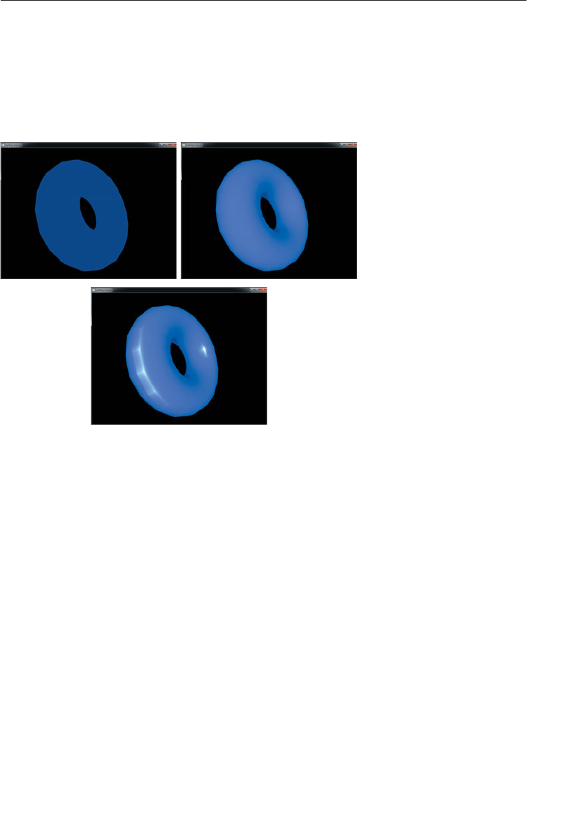
ptg9898810
Classic Lighting Model
The classic lighting model adds up a set of independently computed
lighting components to get a total lighting effect for a particular spot on a
material surface. These components are ambient,diffuse, and specular. Each
is described below, and Figure 7.1 shows them visually.
Figure 7.1 Elements of the classic lighting model
(Ambient (top left) plus diffuse (top right) plus specular (bottom) light
adding to an overall realistic effect.)
Ambient light is light not coming from any specific direction. The classic
lighting model considers it a constant throughout the scene, forming a
decent first approximation to the scattered light present in a scene.
Computing it does not involve any analysis of the direction of light
sources or the direction of the eye observing the scene. It could either be
accumulated as a base contribution per light source or be pre-computed as
a single global effect.
Diffuse light is light scattered by the surface equally in all directions for a
particular light source. Diffuse light is responsible for being able to see a
surface lit by a light even if the surface is not oriented to reflect the light
source directly toward your eye. It doesn’t matter which direction the eye
is, but it does matter which direction the light is. It is brighter when the
surface is more directly facing the light source, simply because that
orientation collects more light than an oblique orientation. Diffuse light
Classic Lighting Model 361

ptg9898810
computation depends on the direction of the surface normal and the
direction of the light source, but not the direction of the eye. It also
depends on the color of the surface.
Specular highlighting is light reflected directly by the surface. This
highlighting refers to how much the surface material acts like a mirror. A
highly polished metal ball reflects a very sharp bright specular highlight,
while a duller polish reflects a larger, dimmer specular highlight, and a
cloth ball would reflect virtually none at all. The strength of this
angle-specific effect is referred to as shininess. Computing specular
highlights requires knowing how close the surface’s orientation is to the
needed direct reflection between the light source and the eye, hence it
requires knowing the surface normal, the direction of the light source, and
the direction of the eye. Specular highlights might or might not
incorporate the color of the surface. As a first approximation, it is more
realistic to not involve any surface color, making it purely reflective. The
underlying color will be present anyway from the diffuse term, giving it
the proper tinge.
Fragment Shaders for Different Light Styles
We’ll next discuss how fragment shaders compute the ambient, diffuse,
and speculative amounts for several types of light, including directional
lighting, point lighting, and spotlight lighting. These will be complete with
a vertex and fragment shader pair built up as we go from simplest to more
complex. The later shaders may seem long, but if you start with the
simplest and follow the incremental additions, it will be easy to
understand.
Note: The comments in each example highlight the change or difference
from the previous step, making it easy to look and identify the
new concepts.
No Lighting
We’ll start with the simplest lighting---no lighting! By this, we don’t mean
everything will be black, but rather that we’ll just draw objects with color
unmodulated by any lighting effects. This is inexpensive, occasionally
useful, and is the base we’ll build on. Unless your object is a perfect mirror,
you’ll need this color as the basis for upcoming lighting calculations; all
lighting calculations will somehow modulate this base color. It is a simple
matter to set a per-vertex color in the vertex shader that will be interpolated
and displayed by the fragment shader, as shown in Example 7.1.
362 Chapter 7: Light and Shadow

ptg9898810
Example 7.1 Setting Final Color Values with No Lighting
----------------------- Vertex Shader -------------------------
// Vertex shader with no lighting
#version 330 core
uniform mat4 MVPMatrix; // model-view-projection transform
in vec4 VertexColor; // sent from the application, includes alpha
in vec4 VertexPosition; // pre-transformed position
out vec4 Color; // sent to the rasterizer for interpolation
void main()
{Color = VertexColor;
gl_Position = MVPMatrix *VertexPosition;
}
---------------------- Fragment Shader ------------------------
// Fragment shader with no lighting
#version 330 core
in vec4 Color; // interpolated between vertices
out vec4 FragColor; // color result for this fragment
void main()
{FragColor = Color;
}
In the cases of texture mapping or procedural texturing, the base color will
come from sending texture coordinates instead of a color, using those
coordinates to manifest the color in the fragment shader. Or, if you set up
material properties, the color will come from an indexed material lookup.
Either way, we start with an unlit base color.
Ambient Light
The ambient light doesn’t change across primitives, so we will pass it in
from the application as a uniform variable.
It’s a good time to mention that light itself has color, not just intensity.
The color of the light interacts with the color of the surface being lit. This
interaction of the surface color by the light color is modeled well by
multiplication. Using 0.0 to represent black and 1.0 to represent full
Classic Lighting Model 363

ptg9898810
intensity enables multiplication to model expected interaction. This is
demonstrated for ambient light in Example 7.2.
It is okay for light colors to go above 1.0 though, especially as we start
adding up multiple sources of light. We will start now using the min()
function to saturate the light at white. This is important if the output color
is the final value for display in a framebuffer. However, if it is an interme-
diate result, skip the saturation step now, and save it for application to a
final color when that time comes.
Example 7.2 Ambient Lighting
--------------------------- Vertex Shader -----------------------------
// Vertex shader for ambient light
#version 330 core
uniform mat4 MVPMatrix;
in vec4 VertexColor;
in vec4 VertexPosition;
out vec4 Color;
void main()
{
Color = VertexColor;
gl_Position = MVPMatrix *VertexPosition;
}
-------------------------- Fragment Shader ----------------------------
// Fragment shader for global ambient lighting
#version 330 core
uniform vec4 Ambient; // sets lighting level, same across many vertices
in vec4 Color;
out vec4 FragColor;
void main()
{
vec4 scatteredLight = Ambient; // this is the only light
// modulate surface color with light, but saturate at white
FragColor = min(Color *scatteredLight, vec4(1.0));
}
You probably have an alpha (fourth component) value in your color that
you care about, and don’t want it modified by lighting. So, unless you’re after
specific transparency effects, make sure your ambient color has as an alpha
364 Chapter 7: Light and Shadow

ptg9898810
of 1.0, or just include only the r,g, and bcomponents in the computation.
For example, the two lines of code in the fragment shader could read
vec3 scatteredLight = vec3(Ambient); // this is the only light
vec3 rgb = min(Color.rgb *scatteredLight, vec3(1.0));
FragColor = vec4(rgb, Color.a);
which passes the Color alpha component straight through to the output
FragColor alpha component, modifying only the r,g, and bcomponents.
We will generally do this in the subsequent examples.
A keen observer might notice that scatteredLight could have been
multiplied by Color in the vertex shader instead of the fragment shader.
For this case, the interpolated result would be the same. Since the vertex
shader usually processes fewer vertices than the number of fragments
processed by the fragment shader, it would probably run faster too.
However, for many lighting techniques, the interpolated results will not be
the same. Higher quality will be obtained by computing per fragment
rather than per vertex. It is up to you to make this performance vs. quality
trade-off, probably by experimenting with what is best for a particular
situation. We will first show the computation in the fragment shader, and
then discuss optimizations (approximations) that involve moving
computations up into the vertex shader, or even to the application. Feel
free to put them whereever is best for your situation.
Directional Light
If a light is far, far away, it can be approximated as having the same direction
from every point on our surface. We refer to such a light as directional.
Similarly, if a viewer is far, far away, the viewer (eye) can also be approxi-
mated as having the same direction from every point on our surface. These
assumptions simplify the math, so the code to implement a directional light
is simple and runs faster than the code for other types of lights. This type of
light source is useful for mimicking the effects of a light source like the sun.
We’ll start with the ambient light computation from the previous example,
and add on the effects for diffuse scattering and specular highlighting. We
compute these effects for each fragment of the surface we are lighting.
Again, just like with ambient light, the directional light will have its own
color and we will modulate the surface color with this light color for the
diffuse scattering. The specular contribution will be computed separately
to allow the specular highlights to be the color of the light source, not
modulated by the color of the surface.
The scattered and reflected amounts we need to compute vary with the
cosine of the angles involved. Two vectors in the same direction form an
angle of 0◦with a cosine of 1.0. This indicates a completely direct
Classic Lighting Model 365

ptg9898810
reflection. As the angle widens, the cosine moves toward 0.0, indicating
less reflected light. Fortunately, if our vectors are normalized (having a
length of 1.0), these cosines are computed with a simple dot product, as
shown in Example 7.3. The surface normal will be interpolated between
vertices, though it could also come from a texture map or an analytic
computation. The far away light-source assumption lets us pass in the light
direction as the uniform variable LightDirection. For a far-away light
and eye, the specular highlights all peak for the same surface-normal
direction. We compute this direction once in the application and pass it in
through the uniform variable HalfVector. Then, cosines of this direction
with the actual surface normal are used to start specular highlighting.
Shininess for specular highlighting is measured with an exponent
used to sharpen the angular fall off from a direct reflection. Squaring
a number less than 1.0 but near to 1.0 makes it closer to 0.0. Higher
exponents sharpen the effect even more. That is, leaving only angles
near 0◦, whose cosine is near 1.0, with a final specular value near 1.0.
The other angles decay quickly to a specular value of 0.0. Hence, we see
the desired effect of a shiny spot on the surface. Overall, higher exponents
dim the amount of computed reflection, so in practice you’ll probably
want to use either a brighter light color or an extra multiplication factor to
compensate. We pass such defining specular values as uniform variables,
because they are surface properties that are constant across the surface.
The only way either a diffuse reflection component or a specular reflection
component can be present is if the angle between the light source direction
and the surface normal is in the range [−90.0◦,90.0◦]: a normal at 90◦means
the surface itself is edge on to the light. Tip it a bit further, and no light will
hit it. As soon as the angle grows beyond 90◦, the cosine goes below 0. We
determine the angle by examining the variable diffuse. This is set to the
greater of 0.0 and the cosine of the angle between the light source direction
and the surface normal. If this value ends up being 0.0, the value that deter-
mines the amount of specular reflection is set to 0.0 as well. Recall we assume
that the direction vectors and surface normal vector are normalized, so the
dot product between them yields the cosine of the angle between them.
Example 7.3 Directional Light Source Lighting
--------------------------- Vertex Shader -----------------------------
// Vertex shader for a directional light computed in the fragment shader
#version 330 core
uniform mat4 MVPMatrix;
uniform mat3 NormalMatrix; // to transform normals, pre-perspective
366 Chapter 7: Light and Shadow

ptg9898810
in vec4 VertexColor;
in vec3 VertexNormal; // we now need a surface normal
in vec4 VertexPosition;
out vec4 Color;
out vec3 Normal; // interpolate the normalized surface normal
void main()
{
Color = VertexColor;
// transform the normal, without perspective, and normalize it
Normal = normalize(NormalMatrix *VertexNormal);
gl_Position = MVPMatrix *VertexPosition;
}
-------------------------- Fragment Shader ----------------------------
// Fragment shader computing lighting for a directional light
#version 330 core
uniform vec3 Ambient;
uniform vec3 LightColor;
uniform vec3 LightDirection; // direction toward the light
uniform vec3 HalfVector; // surface orientation for shiniest spots
uniform float Shininess; // exponent for sharping highlights
uniform float Strength; // extra factor to adjust shininess
in vec4 Color;
in vec3 Normal; // surface normal, interpolated between vertices
out vec4 FragColor;
void main()
{
// compute cosine of the directions, using dot products,
// to see how much light would be reflected
float diffuse = max(0.0, dot(Normal, LightDirection));
float specular = max(0.0, dot(Normal, HalfVector));
// surfaces facing away from the light (negative dot products)
// won’t be lit by the directional light
if (diffuse == 0.0)
specular = 0.0;
else
specular = pow(specular, Shininess); // sharpen the highlight
vec3 scatteredLight = Ambient + LightColor *diffuse;
vec3 reflectedLight = LightColor *specular *Strength;
Classic Lighting Model 367

ptg9898810
// don’t modulate the underlying color with reflected light,
// only with scattered light
vec3 rgb = min(Color.rgb *scatteredLight + reflectedLight, vec3(1.0));
FragColor = vec4(rgb, Color.a);
}
A couple more notes about this example. First, in this example, we used a
scalar Strength to allow independent adjustment of the brightness of the
specular reflection relative to the scattered light. This could potentially be
a separate light color, allowing per-channel (red, green, or blue) control, as
will be done with material-properties a bit later in Example 7.9. Second,
near the end of Example 7.3, it is easy for these lighting effects to add up
to color components greater than 1.0. Again, usually, you’ll want to keep
the brightest final color to 1.0, so we use the min() function. Also note
that we already took care to not get negative values, as in this example we
caught that case when we found the surface facing away from the light,
unable to reflect any of it. However, if negative values do come into play,
you’ll want to use the clamp() function to keep the color components in
the range [0.0, 1.0]. Finally, some interesting starting values would be a
Shininess of around 20 for a pretty tight specular reflection, with a
Strength of around 10 to make it bright enough to stand out, and with
Ambient colors around 0.2 and LightColor colors near 1.0. That should
make something interesting and visible for a material with color near 1.0
as well, and then you can fine tune the effect you want from there.
Point Lights
Point lights mimic lights that are near the scene or within the scene, such
as lamps or ceiling lights or street lights. There are two main differences
between point lights and directional lights. First, with a point-light source,
the direction of the light is different for each point on the surface, so
cannot be represented by a uniform direction. Second, light received at
the surface is expected to decrease as the surface gets farther and farther
from the light.
This fading of reflected light based on increasing distance is called
attenuation. Reality and physics will state that light attenuates as the square
of the distance. However, this attenuation normally fades too fast, unless
you are adding on light from all the scattering of surrounding objects and
otherwise completely modeling everything physically happening with
light. In the classic model, the ambient light helps fill in the gap from not
doing a full modeling, and attenuating linearly fills it in some more. So, we
will show an attenuation model that includes coefficients for constant,
linear, and quadratic functions of the distance.
368 Chapter 7: Light and Shadow

ptg9898810
The additional calculations needed for a point light over a directional light
show up in the first few lines of the fragment shader in Example 7.4. The
first step is to compute the light direction vector from the surface to the
light position. We then compute light distance by using the length()
function. Next, we normalize the light direction vector so we can use it in
a dot product to compute a proper cosine. We then compute the
attenuation factor and the direction of maximum highlights. The
remaining code is the same as for our directional-light shader except that
the diffuse and specular terms are multiplied by the attenuation factor.
Example 7.4 Point-Light Source Lighting
--------------------------- Vertex Shader -----------------------------
// Vertex shader for a point-light (local) source, with computation
// done in the fragment shader.
#version 330 core
uniform mat4 MVPMatrix;
uniform mat4 MVMatrix; // now need the transform, minus perspective
uniform mat3 NormalMatrix;
in vec4 VertexColor;
in vec3 VertexNormal;
in vec4 VertexPosition;
out vec4 Color;
out vec3 Normal;
out vec4 Position; // adding position, so we know where we are
void main()
{
Color = VertexColor;
Normal = normalize(NormalMatrix *VertexNormal);
Position = MVMatrix *VertexPosition; // pre-perspective space
gl_Position = MVPMatrix *VertexPosition; // includes perspective
}
-------------------------- Fragment Shader ----------------------------
// Fragment shader computing a point-light (local) source lighting.
#version 330 core
uniform vec3 Ambient;
uniform vec3 LightColor;
uniform vec3 LightPosition; // location of the light, eye space
uniform float Shininess;
uniform float Strength;
uniform vec3 EyeDirection;
uniform float ConstantAttenuation; // attenuation coefficients
Classic Lighting Model 369

ptg9898810
uniform float LinearAttenuation;
uniform float QuadraticAttenuation;
in vec4 Color;
in vec3 Normal;
in vec4 Position;
out vec4 FragColor;
void main()
{
// find the direction and distance of the light,
// which changes fragment to fragment for a local light
vec3 lightDirection = LightPosition - vec3(Position);
float lightDistance = length(lightDirection);
// normalize the light direction vector, so
// that a dot products give cosines
lightDirection = lightDirection / lightDistance;
// model how much light is available for this fragment
float attenuation = 1.0 /
(ConstantAttenuation +
LinearAttenuation *lightDistance +
QuadraticAttenuation *lightDistance *lightDistance);
// the direction of maximum highlight also changes per fragment
vec3 halfVector = normalize(lightDirection + EyeDirection);
float diffuse = max(0.0, dot(Normal, lightDirection));
float specular = max(0.0, dot(Normal, halfVector));
if (diffuse == 0.0)
specular = 0.0;
else
specular = pow(specular, Shininess) *Strength;
vec3 scatteredLight = Ambient + LightColor *diffuse *attenuation;
vec3 reflectedLight = LightColor *specular *attenuation;
vec3 rgb = min(Color.rgb *scatteredLight + reflectedLight,
vec3(1.0));
FragColor = vec4(rgb, Color.a);
}
Depending on what specific effects you are after, you can leave out one or
two of the constant, linear, or quadratic terms. Or, you can attenuate the
Ambient term. Attenuating ambient light will depend on whether you
have a global ambient color, or per-light ambient colors, or both. It would
be the per-light ambient colors for point lights that you’d want to
attenuate. You could also put the constant attenuation in your Ambient
and leave it out of the attenuation expression.
370 Chapter 7: Light and Shadow

ptg9898810
Spotlights
In stage and cinema, spotlights project a strong beam of light that
illuminates a well-defined area. The illuminated area can be further shaped
through the use of flaps or shutters on the sides of the light. OpenGL
includes light attributes that simulate a simple type of spotlight. Whereas
point lights are modeled as sending light equally in all directions, OpenGL
models spotlights as restricted to producing a cone of light in a particular
direction.
The direction to the spotlight is not the same as the focus direction of the
cone from the spotlight, unless you are looking from the middle of the
‘‘spot’’ (Well, technically, they’d be opposite directions; nothing a minus
sign can’t clear up). Once again our friend the cosine, computed as a dot
product, will tell us to what extent these two directions are in alignment.
This is precisely what we need to know to deduce if we are inside or
outside the cone of illumination. A real spotlight has an angle whose
cosine is very near 1.0, so you might want to start with cosines around
0.99 to see an actual spot.
Just as with specular highlighting, we can sharpen (or not) the light falling
within the cone by raising the cosine of the angle to higher powers. This
allows control over how much the light fades as it gets near the edge of the
cutoff.
The vertex shader and the first and last parts of our spotlight fragment
shader (see Example 7.5) look the same as our point-light shader (shown
earlier in Example 7.4). The differences occur in the middle of the shader.
We take the dot product of the spotlight’s focus direction with the light
direction, and compare it to a pre-computed cosine cutoff value
SpotCosCutoff to determine whether the position on the surface is inside
or outside the spotlight. If it is outside, the spotlight attenuation is set to 0;
otherwise, this value is raised to a power specified by SpotExponent. The
resulting spotlight attenuation factor is multiplied by the previously
computed attenuation factor to give the overall attenuation factor. The
remaining lines of code are the same as they were for point lights.
Example 7.5 Spotlight Lighting
--------------------------- Vertex Shader -----------------------------
// Vertex shader for spotlight computed in the fragment shader
#version 330 core
uniform mat4 MVPMatrix;
uniform mat4 MVMatrix;
uniform mat3 NormalMatrix;
Classic Lighting Model 371

ptg9898810
in vec4 VertexColor;
in vec3 VertexNormal;
in vec4 VertexPosition;
out vec4 Color;
out vec3 Normal;
out vec4 Position;
void main()
{
Color = VertexColor;
Normal = normalize(NormalMatrix *VertexNormal);
Position = MVMatrix *VertexPosition;
gl_Position = MVPMatrix *VertexPosition;
}
-------------------------- Fragment Shader ----------------------------
// Fragment shader computing a spotlight’s effect
#version 330 core
uniform vec3 Ambient;
uniform vec3 LightColor;
uniform vec3 LightPosition;
uniform float Shininess;
uniform float Strength;
uniform vec3 EyeDirection;
uniform float ConstantAttenuation;
uniform float LinearAttenuation;
uniform float QuadraticAttenuation;
uniform vec3 ConeDirection; // adding spotlight attributes
uniform float SpotCosCutoff; // how wide the spot is, as a cosine
uniform float SpotExponent; // control light fall-off in the spot
in vec4 Color;
in vec3 Normal;
in vec4 Position;
out vec4 FragColor;
void main()
{
vec3 lightDirection = LightPosition - vec3(Position);
float lightDistance = length(lightDirection);
lightDirection = lightDirection / lightDistance;
float attenuation = 1.0 /
(ConstantAttenuation +
LinearAttenuation *lightDistance +
QuadraticAttenuation *lightDistance *lightDistance);
372 Chapter 7: Light and Shadow

ptg9898810
// how close are we to being in the spot?
float spotCos = dot(lightDirection, -ConeDirection);
// attenuate more, based on spot-relative position
if (spotCos < SpotCosCutoff)
attenuation = 0.0;
else
attenuation *= pow(spotCos, SpotExponent);
vec3 halfVector = normalize(lightDirection + EyeDirection);
float diffuse = max(0.0, dot(Normal, lightDirection));
float specular = max(0.0, dot(Normal, halfVector));
if (diffuse == 0.0)
specular = 0.0;
else
specular = pow(specular, Shininess) *Strength;
vec3 scatteredLight = Ambient + LightColor *diffuse *attenuation;
vec3 reflectedLight = LightColor *specular *attenuation;
vec3 rgb = min(Color.rgb *scatteredLight + reflectedLight,
vec3(1.0));
FragColor = vec4(rgb, Color.a);
}
Moving Calculations to the Vertex Shader
We’ve been doing all these calculations per fragment. For example,
Position is interpolated and then the lightDistance is computed per
fragment. This gives pretty high-quality lighting, at the cost of doing an
expensive square-root computation (hidden in the length() built-in
function) per fragment. Sometimes, we can swap these steps: perform the
light distance calculation per vertex in the vertex shader and interpolate
the result. That is, rather than interpolating all the terms in the calculation
and calculating per fragment, calculate per vertex and interpolate the
result. The fragment shader then gets the result as an input and directly
uses it.
Interpolating vectors between two normalized vectors (vectors of length
1.0) does not typically yield normalized vectors. (It’s easy to imagine two
vectors pointing notably different directions; the vector that’s the average
of them comes out quite a bit shorter.) However, when the two vectors are
nearly the same, the interpolated vectors between them all have length
quite close to 1.0. Close enough, in fact, to finish doing decent lighting
calculations in the fragment shader. So, there is a balance between having
vertices far enough apart that you can improve performance by computing
Classic Lighting Model 373

ptg9898810
in the vertex shader, but not too far apart that the lighting vectors (surface
normal, light direction, etc.) point in notably different directions.
Example 7.6 goes back to the point-light code (from Example 7.4) and
moves some lighting calculations to the vertex shader.
Example 7.6 Point-light Source Lighting in the Vertex Shader
--------------------------- Vertex Shader -----------------------------
// Vertex shader pulling point-light calculations up from the
// fragment shader.
#version 330 core
uniform mat4 MVPMatrix;
uniform mat3 NormalMatrix;
uniform vec3 LightPosition; // consume in the vertex shader now
uniform vec3 EyeDirection;
uniform float ConstantAttenuation;
uniform float LinearAttenuation;
uniform float QuadraticAttenuation;
in vec4 VertexColor;
in vec3 VertexNormal;
in vec4 VertexPosition;
out vec4 Color;
out vec3 Normal;
// out vec4 Position; // no longer need to interpolate this
out vec3 LightDirection; // send the results instead
out vec3 HalfVector;
out float Attenuation;
void main()
{
Color = VertexColor;
Normal = normalize(NormalMatrix *VertexNormal);
// Compute these in the vertex shader instead of the fragment shader
LightDirection = LightPosition - vec3(VertexPosition);
float lightDistance = length(LightDirection);
LightDirection = LightDirection / lightDistance;
Attenuation = 1.0 /
(ConstantAttenuation +
LinearAttenuation *lightDistance +
QuadraticAttenuation *lightDistance *lightDistance);
HalfVector = normalize(LightDirection + EyeDirection);
374 Chapter 7: Light and Shadow

ptg9898810
gl_Position = MVPMatrix *VertexPosition;
}
-------------------------- Fragment Shader ----------------------------
// Fragment shader with point-light calculations done in vertex shader
#version 330 core
uniform vec3 Ambient;
uniform vec3 LightColor;
// uniform vec3 LightPosition; // no longer need this
uniform float Shininess;
uniform float Strength;
in vec4 Color;
in vec3 Normal;
// in vec4 Position; // no longer need this
in vec3 LightDirection; // get these from vertex shader instead
in vec3 HalfVector;
in float Attenuation;
out vec4 FragColor;
void main()
{
// LightDirection, HalfVector, and Attenuation are interpolated
// now, from vertex shader calculations
float diffuse = max(0.0, dot(Normal, LightDirection));
float specular = max(0.0, dot(Normal, HalfVector));
if (diffuse == 0.0)
specular = 0.0;
else
specular = pow(specular, Shininess) *Strength;
vec3 scatteredLight = Ambient + LightColor *diffuse *Attenuation;
vec3 reflectedLight = LightColor *specular *Attenuation;
vec3 rgb = min(Color.rgb *scatteredLight + reflectedLight,
vec3(1.0));
FragColor = vec4(rgb, Color.a);
}
There are no rules about where to do each calculation. Pick one, or
experiment to find what is best for your surfaces.
In the extreme, the color can be completely computed in the vertex
shader, just at the vertex, and then interpolated. The fragment shader then
has little to no lighting computation left to do. This is the essence of
Gouraud shading. While cheap from a computational perspective, it leaves
Classic Lighting Model 375

ptg9898810
lighting artifacts that betray a surface’s tessellation to the viewer. This is
especially obvious for coarse tessellations and specular highlights.
When surface normals are interpolated and then consumed in the
fragment shader, we get variants of Phong shading. This is not to be
confused with the Phong reflection model, which is essentially what this
entire section on classic lighting has been describing.
Multiple Lights and Materials
Typically, a scene has many light sources and many surface materials.
Normally, you shade one material at a time, but many lights will light that
material. We’ll show a shading model where each invocation of the shader
selects a material and then applies all of, or a subset of, the lights to light it.
Multiple Lights
Normally, we need to light with multiple lights, while we’ve been writing
example shaders for just one. A scene might have a street light, a
flashlight, and the moon, for example, with each surface fragment getting
a share of light from all three. You’d likely model these three lights as a
point light, a spotlight, and a directional light, respectively, and have a
single shader invocation perform all three.
Group a light’s characteristics into structure, as shown in Example 7.7, and
then create an array of them for the shader to process.
Example 7.7 Structure for Holding Light Properties
// Structure for holding light properties
struct LightProperties {
bool isEnabled; // true to apply this light in this invocation
bool isLocal; // true for a point light or a spotlight,
// false for a positional light
bool isSpot; // true if the light is a spotlight
vec3 ambient; // light’s contribution to ambient light
vec3 color; // color of light
vec3 position; // location of light, if is Local is true,
// otherwise the direction toward the light
vec3 halfVector; // direction of highlights for directional light
vec3 coneDirection; // spotlight attributes
float spotCosCutoff;
float spotExponent;
float constantAttenuation; // local light attenuation coefficients
float linearAttenuation;
float quadraticAttenuation;
// other properties you may desire
};
376 Chapter 7: Light and Shadow

ptg9898810
In this example, we are using a couple of Booleans, isLocal and isSpot
to select what kind of light is represented. If you end up with lots of
different light types to choose from, this would be better done as an int
going through a switch statement.
This structure also includes an ambient color contribution. Earlier, we used
a global Ambient assumed to represent all ambient light, but we can also
have each light making its own contribution. For directional lights, it
doesn’t make any difference, but for local lights it helps to have their
ambient contribution attenuated. You could also add separate diffuse and
specular colors to get richer effects.
The first member, isEnabled, can be used to selectively turn lights on and
off. If a light were truly off while rendering a whole scene, it would be
faster to not include it in the set of lights to begin with. However,
sometimes we want one surface lit with a different subset of lights than
another, and so might be enabling and disabling a light at a faster rate.
Depending on how frequently you enable/disable, it might be better as a
separate array, or even as a per-vertex input.
All the pieces are put together in Example 7.8.We now need all the lighting
forms together in a single shader, so we can loop over different kinds of
lights and do the right calculations for each one. It is based on the shaders
that did all lighting in the fragment shader, but again, performance/quality
trade-offs can be made by moving some of it into the vertex shader.
Example 7.8 Multiple Mixed Light Sources
--------------------------- Vertex Shader -----------------------------
// Vertex shader for multiple lights stays the same with all lighting
// done in the fragment shader.
#version 330 core
uniform mat4 MVPMatrix;
uniform mat4 MVMatrix;
uniform mat3 NormalMatrix;
in vec4 VertexColor;
in vec3 VertexNormal;
in vec4 VertexPosition;
out vec4 Color;
out vec3 Normal;
out vec4 Position;
void main()
{
Color = VertexColor;
Normal = normalize(NormalMatrix *VertexNormal);
Classic Lighting Model 377

ptg9898810
Position = MVMatrix *VertexPosition;
gl_Position = MVPMatrix *VertexPosition;
}
-------------------------- Fragment Shader ----------------------------
// Fragment shader for multiple lights.
#version 330 core
struct LightProperties {
bool isEnabled;
bool isLocal;
bool isSpot;
vec3 ambient;
vec3 color;
vec3 position;
vec3 halfVector;
vec3 coneDirection;
float spotCosCutoff;
float spotExponent;
float constantAttenuation;
float linearAttenuation;
float quadraticAttenuation;
};
// the set of lights to apply, per invocation of this shader
const int MaxLights = 10;
uniform LightProperties Lights[MaxLights];
uniform float Shininess;
uniform float Strength;
uniform vec3 EyeDirection;
in vec4 Color;
in vec3 Normal;
in vec4 Position;
out vec4 FragColor;
void main()
{
vec3 scatteredLight = vec3(0.0); // or, to a global ambient light
vec3 reflectedLight = vec3(0.0);
// loop over all the lights
for (int light = 0; light < MaxLights; ++light) {
if (! Lights[light].isEnabled)
continue;
vec3 halfVector;
vec3 lightDirection = Lights[light].position;
float attenuation = 1.0;
// for local lights, compute per-fragment direction,
// halfVector, and attenuation
378 Chapter 7: Light and Shadow

ptg9898810
if (Lights[light].isLocal) {
lightDirection = lightDirection - vec3(Position);
float lightDistance = length(lightDirection);
lightDirection = lightDirection / lightDistance;
attenuation = 1.0 /
(Lights[light].constantAttenuation
+ Lights[light].linearAttenuation *lightDistance
+ Lights[light].quadraticAttenuation *lightDistance
*lightDistance);
if (Lights[light].isSpot) {
float spotCos = dot(lightDirection,
-Lights[light].coneDirection);
if (spotCos < Lights[light].spotCosCutoff)
attenuation = 0.0;
else
attenuation *= pow(spotCos,
Lights[light].spotExponent);
}
halfVector = normalize(lightDirection + EyeDirection);
}else {
halfVector = Lights[light].halfVector;
}
float diffuse = max(0.0, dot(Normal, lightDirection));
float specular = max(0.0, dot(Normal, halfVector));
if (diffuse == 0.0)
specular = 0.0;
else
specular = pow(specular, Shininess) *Strength;
// Accumulate all the lights’ effects
scatteredLight += Lights[light].ambient *attenuation +
Lights[light].color *diffuse *attenuation;
reflectedLight += Lights[light].color *specular *attenuation;
}
vec3 rgb = min(Color.rgb *scatteredLight + reflectedLight,
vec3(1.0));
FragColor = vec4(rgb, Color.a);
}
Material Properties
One material property we came across above was shininess. We use
shininess to control how sharply defined specular highlights are. Different
materials have differently sized specular highlights, and seeing this is key
to your viewer recognizing a material once rendered on the screen. We can
also have material-specific modulation of the color of ambient, diffuse,
and specular lighting. This is an easy new addition to our computations:
Classic Lighting Model 379

ptg9898810
Some metals and clothes display cool-looking properties as having
different underlying colors for scattered light and reflected light. It’s your
choice how many of these independent colors you mix together for the
effect you want to create. For example, in the method below, setting the
material’s specular value to (1.0, 1.0, 1.0, 1.0)would make the model
degenerate to the model used in the examples above.
Materials can also have their own real or apparent light source. For
example, something glowing will emit its own light. This light could easily
include colors not present in the any of the light sources; so light won’t be
visible unless it is added on the light calculation we’ve done so far.
It is natural to use a structure to store a material’s properties, as shown in
Example 7.9.
Example 7.9 Structure to Hold Material Properties
struct MaterialProperties {
vec3 emission; // light produced by the material
vec3 ambient; // what part of ambient light is reflected
vec3 diffuse; // what part of diffuse light is scattered
vec3 specular; // what part of specular light is scattered
float shininess; // exponent for sharpening specular reflection
// other properties you may desire
};
These material properties (and others you may wish to add) are not specific
to surface location; so they can be passed into the shader as a uniform
structure.
Scenes have multiple materials with different properties. If your
application switches between materials frequently, consider using the
same fragment shader to shade several different materials without having
to change shaders or update uniforms. To do this, make an array of
MaterialProperties, each element holding the description of a
different material. Pass the material index into a vertex shader input,
which it will pass on to the fragment shader. Then the fragment shader
will index into the material array and render properly for that material. For
example, see Example 7.10. We’ve modified snippets of the multilight
shader to make a multilight--selected-material shader.
Example 7.10 Code Snippets for Using an Array of Material Properties
-------------------------- Fragment Shader ----------------------------
// Snippets of fragment shader selecting what material to shade
// with multiple lights.
#version 330 core
380 Chapter 7: Light and Shadow

ptg9898810
struct MaterialProperties {
vec3 emission;
vec3 ambient;
vec3 diffuse;
vec3 specular;
float shininess;
};
// a set of materials to select between, per shader invocation
const int NumMaterials = 14;
uniform MaterialProperties Material[NumMaterials];
flat in int MatIndex; // input material index from vertex shader
.
.
.
void main()
{
.
.
.
// Accumulate all the lights’ effects
scatteredLight +=
Lights[light].ambient *Material[MatIndex].ambient *
attenuation +
Lights[light].color *Material[MatIndex].diffuse *
diffuse *attenuation;
reflectedLight +=
Lights[light].color *Material[MatIndex].specular *
specular *attenuation;
}
vec3 rgb = min(Material[MatIndex].emission
+ Color.rgb *scatteredLight + reflectedLight,
vec3(1.0));
FragColor = vec4(rgb, Color.a);
}
Two-Sided Lighting
You might want to render a surface differently if the eye is looking at the
‘‘back’’ of the surface than if looking at the front of the surface. OpenGL
Shading Language has a built-in Boolean variable gl_FrontFacing
allowing you to do so. The gl_FrontFacing variable is set for each
fragment to true if the fragment is part of a front-facing primitive; the
gl_FrontFacing variable is set to false otherwise. It is only available in
fragment shaders.
If the backs have properties quite different than the fronts, just make two
sets of MaterialProperties, as in Example 7.11. There are lots of ways
Classic Lighting Model 381

ptg9898810
to do this. Here we chose to double the array and use even indexes for the
front and odd indexes for the back. This is likely faster than having two
separate arrays. If the properties are extensive and mostly the same, it
might be more efficient to just expand MaterialProperties with the
one or two differing properties.
Example 7.11 Front and Back Material Properties
struct MaterialProperties {
vec3 emission;
vec3 ambient;
vec3 diffuse;
vec3 specular;
float shininess;
};
// a set of materials to select between, per shader invocation
// use even indexes for front-facing surfaces and odd indexes
// for back facing
const int NumMaterials = 14;
uniform MaterialProperties Material[2 *NumMaterials];
flat in int MatIndex; // input material index from vertex shader
.
.
.
void main()
{
int mat;
if (gl_FrontFacing)
mat = MatIndex;
else
mat = MatIndex + 1;
.
.
.
// Accumulate all the lights’ effects
scatteredLight +=
Lights[light].ambient *Material[mat].ambient *
attenuation +
Lights[light].color *Material[mat].diffuse *
diffuse *attenuation;
reflectedLight +=
Lights[light].color *Material[mat].specular *
specular *attenuation;
}
vec3 rgb = min(Material[mat].emission
+ Color.rgb *scatteredLight + reflectedLight,
vec3(1.0));
FragColor = vec4(rgb, Color.a);
}
382 Chapter 7: Light and Shadow

ptg9898810
Lighting Coordinate Systems
To make any sense, all the normal, direction, and position coordinates
used in a lighting calculation must come from the same coordinate system.
If light-position coordinates come after model-view transforms but before
perspective projection, so should the surface coordinates that will be
compared against them. In this typical case, both are in eye space. That is,
the eye is at (0, 0, 0)looking in the negative zdirection. This is a regular
3D-coordinate system, not the 4-component homogeneous space needed
for perspective. (See the first block diagrams in Chapter 5,‘‘Viewing
Transformations, Clipping, and Feedback’’ to see where in the stack of
transformations eye space resides.) This is why, in the examples above, we
sent Position separately with its own transform and the types involved
are vec3 and mat3 rather than vec4 and mat4. Generally, we used eye
space for all the directions and locations feeding light equations, while
alongside, homogeneous coordinates were fed to the rasterizer.
OpenGL lighting calculations require knowing the eye direction in order
to compute specular reflection terms. For eye space, the view direction is
parallel to and in the direction of the −zaxis. In the examples above, we
could have replaced the EyeDirection with the vector (0, 0, 1), knowing
our coordinates were in eye space. But for clarity and potential flexibility,
we used a variable. This could be generalized a bit to allow a local viewer,
much like we had local lights, rather than only directional lights. With a
local viewer, specular highlights on multiple objects will tend toward the
eye location rather than all being in the same parallel direction.
Limitations of the Classic Lighting Model
The classic lighting model works pretty well at what it tries to do:
modeling the surface reflection properties, modeling each light, combin-
ing them together to modulate an underlying color, and getting a pretty
realistic approximation of what color is scattered and reflected. Yet, there
are some important things missing.
Shadows are a big item. We lit each surface as if it was the only surface
present, with no other objects blocking the path of the lights to the
surface. We will provide techniques for shadowing later in this chapter.
Another big missing item is accurate ambient lighting. If you look around
a room, you won’t see a constant level of ambient lighting. Corners, for
example, are darker than other areas. As another example, consider a
bright red ball resting near other objects. You’ll probably see that the
ambient light around the other objects has a reddish tint, created by the
Classic Lighting Model 383

ptg9898810
red ball. These nearby objects then reflect a redder ambient light than
objects further from the ball. We look at some techniques for addressing
this in ‘‘Advanced Lighting Models’’ on Page 384. Other techniques for
adding in this realism, loosely referred to as global illumination, are outside
the scope of this book.
A glowing object or very bright object might also have both a halo around
it as well as lens flare.We used an emission value earlier to model a glowing
object, but that effect is limited to the actual geometric extent of the
object, whereas haloing and lens flare extend beyond the object. In real
life, these effects are apparent not only when taking videos or photo-
graphs; the lens and fluid in our eye also make them occur. Multiple
techniques have been developed for rendering this effect.
A textured surface usually is not perfectly smooth. The bumps on the
surface must individually be affected by lighting, or the surface ends up
looking artificially flat. Bump mapping techniques for doing this are
described in Chapter 8,‘‘Procedural Texturing’’.
Advanced Lighting Models
The classic lighting model lacks some realism. To generate more realistic
images, we need to have more realistic models for illumination, shadows,
and reflection than those we’ve discussed so far. In this section, we explore
how OpenGL Shading Language can help us implement some of these
models. Much has been written on the topic of lighting in computer
graphics. We examine only a few methods now. Ideally, you’ll be inspired
to try implementing some others on your own.
Hemisphere Lighting
Earlier we looked carefully at the classic lighting model. However, this
model has a number of flaws, and these flaws become more apparent as we
strive for more realistic rendering effects. One problem is that objects in a
scene do not typically receive all their illumination from a small number
of specific light sources. Interreflections between objects often have
noticeable and important contributions to objects in the scene. The
384 Chapter 7: Light and Shadow

ptg9898810
traditional computer graphics illumination model attempts to account for
this phenomena through an ambient light term. However, this ambient
light term is usually applied equally across an object or an entire scene.
The result is a flat and unrealistic look for areas of the scene that are not
affected by direct illumination.
Another problem with the traditional illumination model is that light
sources in real scenes are not point lights or even spotlights---they are area
lights. Consider the indirect light coming in from the window and
illuminating the floor and the long fluorescent light bulbs behind a
rectangular translucent panel. For an even more common case, consider
the illumination outdoors on a cloudy day. In this case, the entire visible
hemisphere is acting like an area light source. In several presentations and
tutorials, Chas Boyd, Dan Baker, and Philip Taylor of Microsoft described
this situation as hemisphere lighting. Let’s look at how we might create an
OpenGL shader to simulate this type of lighting environment.
The idea behind hemisphere lighting is that we model the illumination as
two hemispheres. The upper hemisphere represents the sky and the lower
hemisphere represents the ground. A location on an object with a surface
normal that points straight up gets all of its illumination from the upper
hemisphere, and a location with a surface normal pointing straight down
gets all of its illumination from the lower hemisphere (see Figure 7.2). By
picking appropriate colors for the two hemispheres, we can make the
sphere look as though locations with normals pointing up are illuminated
and those with surface normals pointing down are in shadow.
To compute the illumination at any point on the surface, we compute the
linear interpolation for the illumination received at that point:
Color =a·SkyColor +(1−a)·GroundColor
where
a=1.0−(0.5·sin(θ)) for θ≤90◦,
a=0.5·sin(θ)for θ>90◦,
with θbeing the angle between the surface normal and the north pole
direction.
Advanced Lighting Models 385
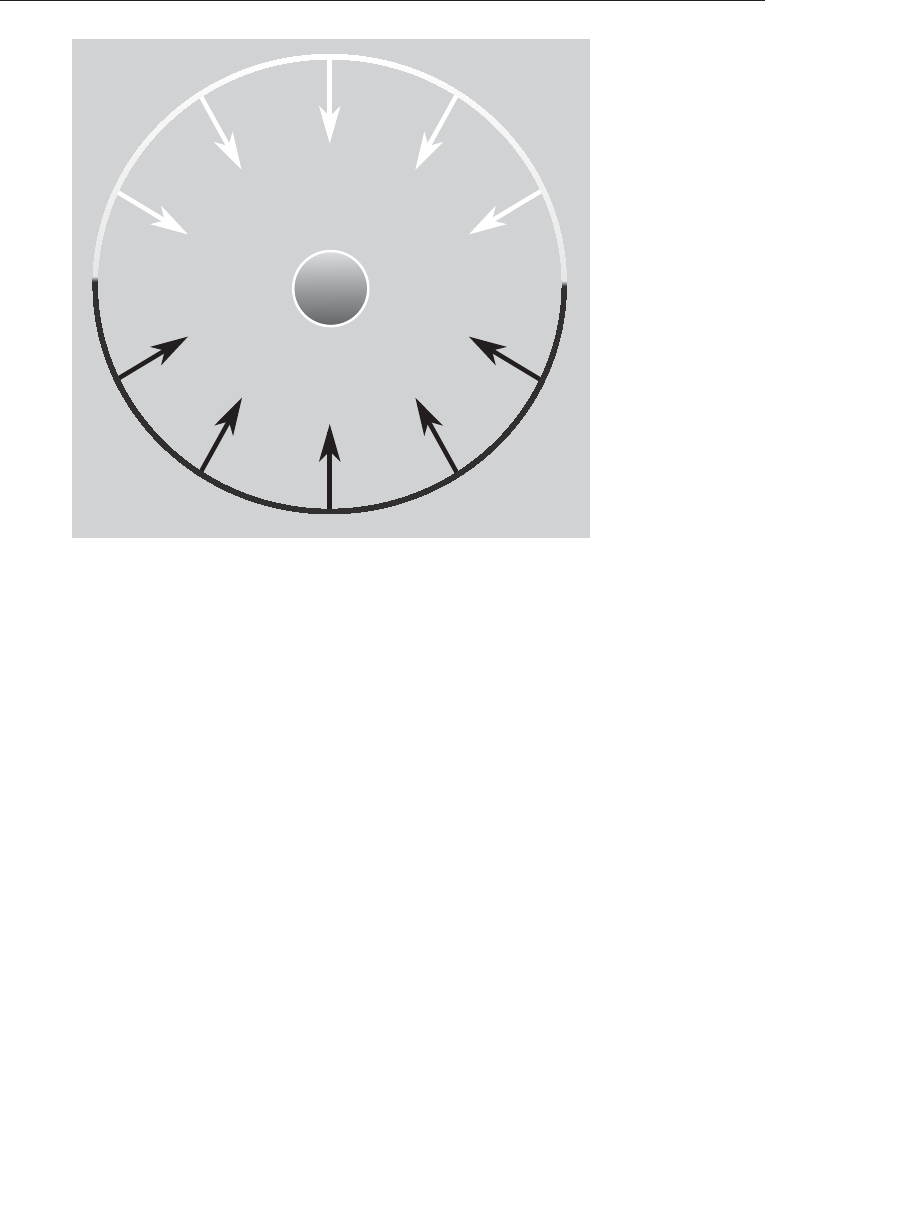
ptg9898810
X
X
Figure 7.2 A sphere illuminated using the hemisphere lighting model
In Figure 7.2, a point on the top of the sphere (the black ‘‘x’’) receives
illumination only from the upper hemisphere (i.e., the sky color). A point
on the bottom of the sphere (the white ‘‘x’’) receives illumination only
from the lower hemisphere (i.e., the ground color). A point right on the
equator would receive half of its illumination from the upper hemisphere
and half from the lower hemisphere (e.g., 50% sky color and 50% ground
color).
But we can actually calculate ain another way that is simpler but roughly
equivalent:
a=0.5+(0.5·cos(θ))
This approach eliminates the need for a conditional. Furthermore, we can
easily compute the cosine of the angle between two unit vectors by taking
the dot product of the two vectors. This is an example of what Jim Blinn
likes to call ‘‘the ancient Chinese art of Chi Ting.’’ In computer graphics, if
it looks good enough, it is good enough. It doesn’t really matter whether
your calculations are physically correct or a bit of a cheat. The difference
between the two functions is shown in Figure 7.3. The shape of the two
386 Chapter 7: Light and Shadow
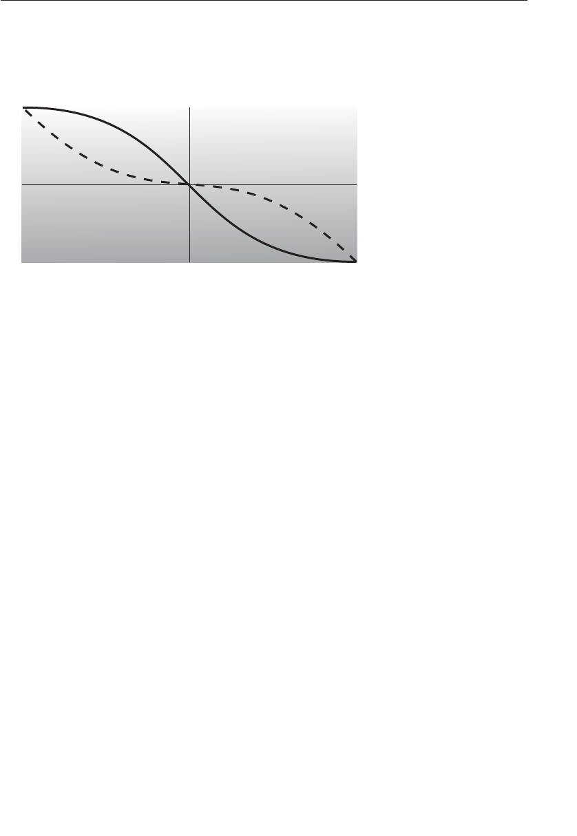
ptg9898810
curves is similar. One is the mirror of the other, but the area under the
curves is the same. This general equivalency is good enough for the effect
we’re after, and the shader is simpler and will execute faster as well.
A
ctual Solution
Chi Ting Solution
o° 90° 180°
0
1
Figure 7.3 Analytic hemisphere lighting function
(Compares the actual analytic function for hemisphere lighting to a similar
but higher-performance function.)
For the hemisphere shader, we need to pass in uniform variables for the
sky color and the ground color. We can also consider the ‘‘north pole’’ to
be our light position. If we pass this in as a uniform variable, we can light
the model from different directions.
Example 7.12 shows a vertex shader that implements hemisphere lighting.
As you can see, the shader is quite simple. The main purpose of the shader
is to compute the diffuse color value and leave it in the user-defined out
variable Color, as with the chapter’s earlier examples. Results for this
shader are shown in Figure 7.4. Compare the hemisphere lighting (D) with
a single directional light source (A and B). Not only is the hemisphere
shader simpler and more efficient, it produces a much more realistic
lighting effect too! This lighting model can be used for tasks like model
preview, where it is important to examine all the details of a model. It can
also be used in conjunction with the traditional computer graphics
illumination model. Point, directional, or spotlights can be added on top
of the hemisphere lighting model to provide more illumination to impor-
tant parts of the scene. And, as always, if you want to move some or all
these computations to the fragment shader, you may do so.
Advanced Lighting Models 387
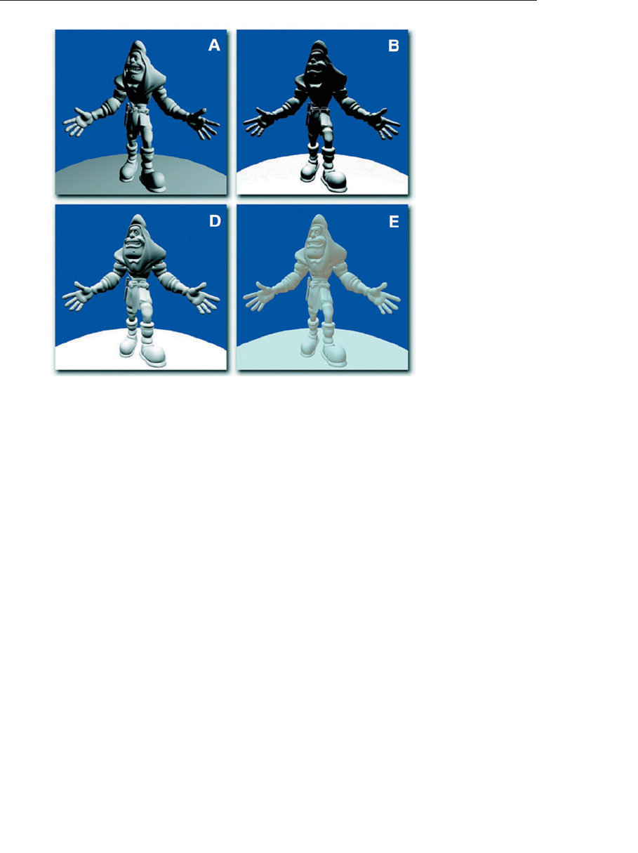
ptg9898810
Figure 7.4 Lighting model comparison
(A comparison of some of the lighting models discussed in this chapter.
The model uses a base color of white, RGB = (1.0, 1.0, 1.0), to emphasize
areas of light and shadow. (A) uses a directional light above and to the
right of the model. (B) uses a directional light directly above the model.
These two images illustrate the difficulties with the traditional lighting
model. Detail is lost in areas of shadow. (D) illustrates hemisphere lighting.
(E) illustrates spherical harmonic lighting using the Old Town Square
coefficients. (3Dlabs, Inc.))
Example 7.12 Vertex Shader for Hemisphere Lighting
#version 330 core
uniform vec3 LightPosition;
uniform vec3 SkyColor;
uniform vec3 GroundColor;
uniform mat4 MVMatrix;
uniform mat4 MVPMatrix;
uniform mat3 NormalMatrix;
in vec4 VertexPosition;
in vec3 VertexNormal;
388 Chapter 7: Light and Shadow

ptg9898810
out vec3 Color;
void main()
{
vec3 position = vec3(MVMatrix *VertexPosition);
vec3 tnorm = normalize(NormalMatrix *VertexNormal);
vec3 lightVec = normalize(LightPosition - position);
float costheta = dot(tnorm, lightVec);
float a = costheta *0.5 + 0.5;
Color = mix(GroundColor, SkyColor, a);
gl_Position = MVPMatrix *VertexPosition;
}
One of the issues with this model is that it doesn’t account for self-
occlusion. Regions that should really be in shadow because of the
geometry of the model will appear too bright. We will remedy this later.
Image-Based Lighting
If we’re trying to achieve realistic lighting in a computer graphics scene,
why not just use an environment map for the lighting? This approach to
illumination is called image-based lighting; it has been popularized in recent
years by researcher Paul Debevec at the University of Southern California.
Churches and auditoriums may have dozens of light sources on the ceiling.
Rooms with many windows also have complex lighting environments. It is
often easier and much more efficient to sample the lighting in such
environments and store the results in one or more environment maps
than it is to simulate numerous individual light sources.
The steps involved in image-based lighting are as follows:
1. Use a light probe (e.g., a reflective sphere) to capture (e.g., photograph)
the illumination that occurs in a real-world scene. The captured
omnidirectional, high-dynamic range image is called a light probe
image.
2. Use the light probe image to create a representation of the
environment (e.g., an environment map).
3. Place the synthetic objects to be rendered inside the environment.
4. Render the synthetic objects by using the representation of the
environment created in Step 2.
On his Web site (www.debevec.org), Debevec offers a number of useful
things to developers. For one, he has made available a number of images
that can be used as high-quality environment maps to provide realistic
Advanced Lighting Models 389

ptg9898810
lighting in a scene. These images are high dynamic range (HDR) images
that represent each color component with a 32-bit floating-point value.
Such images can represent a much greater range of intensity values than
can 8-bit-per-component images. For another, he makes available a tool
called HDRShop that manipulates and transforms these environment
maps. Through links to his various publications and tutorials, he also
provides step-by-step instructions on creating your own environment
maps and using them to add realistic lighting effects to computer graphics
scenes.
Following Debevec’s guidance, we purchased a 2-inch chrome steel ball
from McMaster-Carr Supply Company (www.mcmaster.com). We used this
ball to capture a light probe image from the center of the square outside
our office building in downtown Fort Collins, Colorado, shown in
Figure 7.5.We then used HDRShop to create a lat-long environment map,
shown in Figure 7.6, and a cube map, shown in Figure 7.7. The cube map
and lat-long map can be used to perform environment mapping. That
shader simulated a surface with an underlying base color and diffuse
reflection characteristics that was covered by a transparent mirror-like
layer that reflected the environment flawlessly.
390 Chapter 7: Light and Shadow

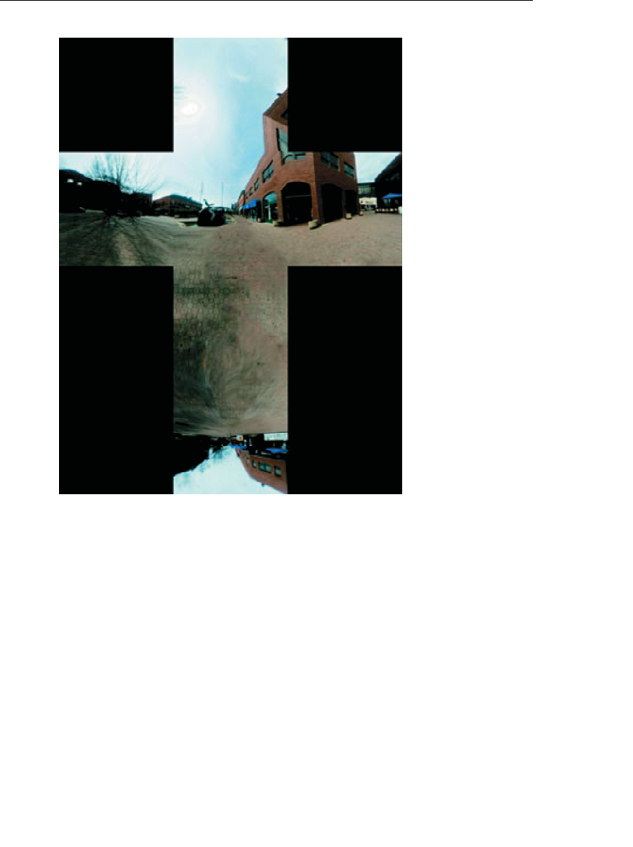
ptg9898810
Figure 7.7 Cube map
(A cube-map version of the Old Town Square light probe image. (3Dlabs,
Inc.))
We can simulate other types of objects if we modify the environment maps
before they are used. A point on the surface that reflects light in a diffuse
fashion reflects light from all the light sources that are in the hemisphere
in the direction of the surface normal at that point. We can’t really afford
to access the environment map a large number of times in our shader.
What we can do instead is similar to what we discussed for hemisphere
lighting. Starting from our light probe image, we can construct an
environment map for diffuse lighting. Each texel in this environment map
will contain the weighted average (i.e., the convolution) of other texels in
the visible hemisphere as defined by the surface normal that would be
used to access that texel in the environment.
392 Chapter 7: Light and Shadow

ptg9898810
Again, HDRShop has exactly what we need. We can use HDRShop to create
a lat-long image from our original light probe image. We can then use a
command built into HDRShop that performs the necessary convolution.
This operation can be time consuming, because at each texel in the image,
the contributions from half of the other texels in the image must be
considered. Luckily, we don’t need a very large image for this purpose. The
effect is essentially the same as creating a very blurry image of the original
light probe image. Since there is no high-frequency content in the
computed image, a cube map with faces that are 64 ×64 or 128 ×128
works just fine.
A single texture access into this diffuse environment map provides us
with the value needed for our diffuse reflection calculation. What about
the specular contribution? A surface that is very shiny will reflect the
illumination from a light source just like a mirror. A single point on the
surface reflects a single point in the environment. For surfaces that are
rougher, the highlight defocuses and spreads out. In this case, a single
point on the surface reflects several points in the environment, though not
the whole visible hemisphere like a diffuse surface. HDRShop lets us blur
an environment map by providing a Phong exponent---a degree of
shininess. A value of 1.0 convolves the environment map to simulate
diffuse reflection, and a value of 50 or more convolves the environment
map to simulate a somewhat shiny surface.
The shaders that implement these concepts end up being quite simple and
quite fast. In the vertex shader, all that is needed is to compute the
reflection direction at each vertex. This value and the surface normal are
sent to the fragment shader as out variables. They are interpolated across
each polygon, and the interpolated values are used in the fragment shader
to access the two environment maps in order to obtain the diffuse and the
specular components. The values obtained from the environment maps are
combined with the object’s base color to arrive at the final color for the
fragment. The shaders are shown in Example 7.13. Examples of images
created with this technique are shown in Figure 7.8.
Advanced Lighting Models 393
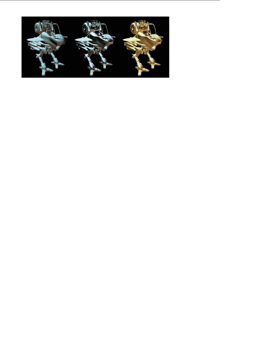
ptg9898810
Figure 7.8 Effects of diffuse and specular environment maps
(A variety of effects using the Old Town Square diffuse and specular en-
vironment maps shown in Figure 7.6. Left: BaseColor set to (1.0, 1.0, 1.0),
SpecularPercent is 0, and DiffusePercent is 1.0. Middle: BaseColor is set to
(0, 0, 0), SpecularPercent is set to 1.0, and DiffusePercent is set to 0. Right:
BaseColor is set to (0.35, 0.29, 0.09), SpecularPercent is set to 0.75, and Dif-
fusePercent is set to 0.5. (3Dlabs, Inc.))
Example 7.13 Shaders for Image-based Lighting
--------------------- Vertex Shader ---------------------
// Vertex shader for image-based lighting
#version 330 core
uniform mat4 MVMatrix;
uniform mat4 MVPMatrix;
uniform mat3 NormalMatrix;
in vec4 VertexPosition;
in vec3 VertexNormal;
out vec3 ReflectDir;
out vec3 Normal;
void main()
{
Normal = normalize(NormalMatrix *VertexNormal);
vec4 pos = MVMatrix *VertexPosition;
vec3 eyeDir = pos.xyz;
ReflectDir = reflect(eyeDir, Normal);
gl_Position = MVPMatrix *VertexPosition;
}
-------------------- Fragment Shader --------------------
// Fragment shader for image-based lighting
#version 330 core
394 Chapter 7: Light and Shadow

ptg9898810
uniform vec3 BaseColor;
uniform float SpecularPercent;
uniform float DiffusePercent;
uniform samplerCube SpecularEnvMap;
uniform samplerCube DiffuseEnvMap;
in vec3 ReflectDir;
in vec3 Normal;
out vec4 FragColor;
void main()
{
// Look up environment map values in cube maps
vec3 diffuseColor =
vec3(texture(DiffuseEnvMap, normalize(Normal)));
vec3 specularColor =
vec3(texture(SpecularEnvMap, normalize(ReflectDir)));
// Add lighting to base color and mix
vec3color=mix(BaseColor,diffuseColor*BaseColor,DiffusePercent);
color = mix(color, specularColor + color, SpecularPercent);
FragColor = vec4(color, 1.0);
}
The environment maps that are used can reproduce the light from the
whole scene. Of course, objects with different specular reflection properties
require different specular environment maps. And producing these
environment maps requires some manual effort and lengthy pre-
processing. But the resulting quality and performance make image-based
lighting a great choice in many situations.
Lighting with Spherical Harmonics
In 2001, Ravi Ramamoorthi and Pat Hanrahan presented a method that
uses spherical harmonics for computing the diffuse lighting term. This
method reproduces accurate diffuse reflection, based on the content of a
light probe image, without accessing the light probe image at runtime. The
light probe image is pre-processed to produce coefficients that are used in a
mathematical representation of the image at runtime. The mathematics
behind this approach is beyond the scope of this book. Instead, we lay
the necessary groundwork for this shader by describing the underlying
mathematics in an intuitive fashion. The result is remarkably simple,
accurate, and realistic, and it can easily be codified in an OpenGL shader.
This technique has already been used successfully to provide real-time
Advanced Lighting Models 395

ptg9898810
illumination for games and has applications in computer vision and other
areas as well.
Spherical harmonics provides a frequency space representation of an image
over a sphere. It is analogous to the Fourier transform on the line or circle.
This representation of the image is continuous and rotationally invariant.
Using this representation for a light probe image, Ramamoorthi and
Hanrahan showed that you could accurately reproduce the diffuse
reflection from a surface with just nine spherical harmonic basis functions.
These nine spherical harmonics are obtained with constant, linear, and
quadratic polynomials of the normalized surface normal.
Intuitively, we can see that it is plausible to accurately simulate the diffuse
reflection with a small number of basis functions in frequency space since
diffuse reflection varies slowly across a surface. With just nine terms used,
the average error over all surface orientations is less than 3 percent for any
physical input lighting distribution. With Debevec’s light probe images,
the average error was shown to be less than 1 percent, and the maximum
error for any pixel was less than 5 percent.
Each spherical harmonic basis function has a coefficient that depends on
the light probe image being used. The coefficients are different for each
color channel, so you can think of each coefficient as an RGB value. A
pre-processing step is required to compute the nine RGB coefficients for
the light probe image to be used. Ramamoorthi makes the code for this
pre-processing step available for free on his Web site. We used this program
to compute the coefficients for all the light probe images in Debevec’s light
probe gallery as well as the Old Town Square light probe image and
summarized the results in Table 7.1.
396 Chapter 7: Light and Shadow

ptg9898810
Table 7.1 Spherical Harmonic Coefficients for Light Probe Images
Coefficient
Old Town square
Grace cathedral
Eucalyptus grove
St. Peter’s basilica
Uffizi gallery
L00 .87 .88 .86 .79 .44 .54 .38 .43 .45 .36 .26 .23 .32 .31 .35
L1m1.18 .25 .31 .39 .35 .60 .29 .36 .41 .18 .14 .13 .37 .37 .43
L10 .03 .04 .04 −.34 −.18 −.27 .04 .03 .01 −.02 −.01 .00 .00 .00 .00
L11 −.00 −.03 −.05 −.29 −.06 .01 −.10 −.10 −.09 .03 .02 .00 −.01 −.01 −.01
L2m1.00 .00 .01 −.26 −.22 −.47 .01 −.01 −.05 −.05 −.03 −.01 −.01 −.01 −.01
L2m2−.12 −.12 −.12 −.11 −.05 −.12 −.06 −.06 −.04 .02 .01 .00 −.02 −.02 −.03
L20 −.03 −.02 −.02 −.16 −.09 −.15 −.09 −.13 −.15 −.09 −.08 −.07 −.28 −.28 −.32
L21 −.08 −.09 −.09 .56 .21 .14 −.06 −.05 −.04 .01 .00 .00 .00 .00 .00
L22 −.16 −.19 −.22 .21 −.05 −.30 .02 .00 −.05 −.08 −.03 .00 −.24 −.24 −.28
Coefficient
Galileo’s tomb
Vine street kitchen
Breezeway
Campus sunset
Funston Beach sunset
L00 1.04 .76 .71 .64 .67 .73 .32 .36 .38 .79 .94 .98 .68 .69 .70
L1m1.44 .34 .34 .28 .32 .33 .37 .41 .45 .44 .56 .70 .32 .37 .44
L10 −.22 −.18 −.17 .42 .60 .77 −.01 −.01 −.01 −.10 −.18 −.27 −.17 −.17 −.17
L11 .71 .54 .56 −.05 −.04 −.02 −.10 −.12 −.12 .45 .38 .20 −.45 −.42 −.34
L2m1−.12 −.09 −.08 .25 .39 .53 −.01 −.02 .02 −.14 −.22 −.31 −.08 −.09 −.10
L2m2.64 .50 .52 −.10 −.08 −.05 −.13 −.15 −.17 .18 .14 .05 −.17 −.17 −.15
L20 −.37 −.28 −.29 .38 .54 .71 −.07 −.08 −.09 −.39 −.40 −.36 −.03 −.02 −.01
L21 −.17 −.13 −.13 .06 .01 −.02 .02 .03 .03 .09 .07 .04 .16 .14 .10
L22 .55 .42 .42 −.03 −.02 −.03 −.29 −.32 −.36 .67 .67 .52 .37 .31 .20
The formula for diffuse reflection using spherical harmonics is
diffuse =c1L22(x2−y2)+c3L20z2+c4L00 −c5L20 +(7.1)
2c1(L2m2xy +L21xz +L2m1yz)+2c2(L11x+L1m1y+L10z)
The constants c1--c5result from the derivation of this formula and are
shown in the vertex shader code in Example 7.14. The Lcoefficients are
the nine basis function coefficients computed for a specific light probe
Advanced Lighting Models 397

ptg9898810
image in the pre-processing phase. The x,y, and zvalues are the
coordinates of the normalized surface normal at the point that is to be
shaded. Unlike low dynamic range images (e.g., 8 bits per color
component) that have an implicit minimum value of 0 and an implicit
maximum value of 255, HDR images represented with a floating-point
value for each color component don’t contain well-defined minimum and
maximum values. The minimum and maximum values for two HDR
images may be quite different from each other, unless the same calibration
or creation process was used to create both images. It is even possible to
have an HDR image that contains negative values. For this reason, the
vertex shader contains an overall scaling factor to make the final effect
look right.
The vertex shader that encodes the formula for the nine spherical
harmonic basis functions is actually quite simple. When the compiler gets
hold of it, it becomes simpler still. An optimizing compiler typically
reduces all the operations involving constants. The resulting code is quite
efficient because it contains a relatively small number of addition and
multiplication operations that involve the components of the surface
normal.
Example 7.14 Shaders for Spherical Harmonics Lighting
--------------------- Vertex Shader ---------------------
// Vertex shader for computing spherical harmonics
#version 330 core
uniform mat4 MVMatrix;
uniform mat4 MVPMatrix;
uniform mat3 NormalMatrix;
uniform float ScaleFactor;
const float C1 = 0.429043;
const float C2 = 0.511664;
const float C3 = 0.743125;
const float C4 = 0.886227;
const float C5 = 0.247708;
// Constants for Old Town Square lighting
const vec3 L00 = vec3( 0.871297, 0.875222, 0.864470);
const vec3 L1m1 = vec3( 0.175058, 0.245335, 0.312891);
const vec3 L10 = vec3( 0.034675, 0.036107, 0.037362);
const vec3 L11 = vec3(-0.004629, -0.029448, -0.048028);
const vec3 L2m2 = vec3(-0.120535, -0.121160, -0.117507);
const vec3 L2m1 = vec3( 0.003242, 0.003624, 0.007511);
const vec3 L20 = vec3(-0.028667, -0.024926, -0.020998);
const vec3 L21 = vec3(-0.077539, -0.086325, -0.091591);
const vec3 L22 = vec3(-0.161784, -0.191783, -0.219152);
398 Chapter 7: Light and Shadow

ptg9898810
in vec4 VertexPosition;
in vec3 VertexNormal;
out vec3 DiffuseColor;
void main()
{
vec3 tnorm = normalize(NormalMatrix *VertexNormal);
DiffuseColor = C1 *L22 *(tnorm.x *tnorm.x - tnorm.y *tnorm.y) +
C3 *L20 *tnorm.z *tnorm.z +
C4 *L00 -
C5 *L20 +
2.0 *C1 *L2m2 *tnorm.x *tnorm.y +
2.0 *C1 *L21 *tnorm.x *tnorm.z +
2.0 *C1 *L2m1 *tnorm.y *tnorm.z +
2.0 *C2 *L11 *tnorm.x +
2.0 *C2 *L1m1 *tnorm.y +
2.0 *C2 *L10 *tnorm.z;
DiffuseColor *= ScaleFactor;
gl_Position = MVPMatrix *VertexPosition;
}
-------------------- Fragment Shader --------------------
// Fragment shader for lighting with spherical harmonics
#version 330 core
in vec3 DiffuseColor;
out vec4 FragColor;
void main()
{
FragColor = vec4(DiffuseColor, 1.0);
}
Our fragment shader, shown in Example 7.14, has very little work to do.
Because the diffuse reflection typically changes slowly, for scenes without
large polygons we can reasonably compute it in the vertex shader and
interpolate it during rasterization. As with hemispherical lighting, we can
add procedurally defined point, directional, or spotlights on top of the
spherical harmonics lighting to provide more illumination to important
parts of the scene. Results of the spherical harmonics shader are shown in
Figure 7.9.We could make the diffuse lighting from the spherical
harmonics computation more subtle by blending it with the object’s base
color.
Advanced Lighting Models 399
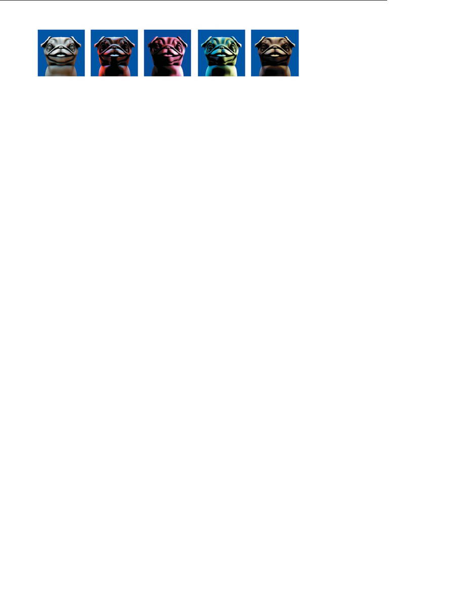
ptg9898810
Figure 7.9 Spherical harmonics lighting
(Lighting using the coefficients from Table 7.1. From the left: Old Town
Square, Grace Cathedral, Galileo’s Tomb, Campus Sunset, and St. Peter’s
Basilica. (3Dlabs, Inc.))
The trade-offs in using image-based lighting versus procedurally defined
lights are similar to the trade-offs between using stored textures versus
procedural textures. Image-based lighting techniques can capture and
re-create complex lighting environments relatively easily. It would be
exceedingly difficult to simulate such an environment with a large number
of procedural light sources. On the other hand, procedurally defined light
sources do not use up texture memory and can easily be modified and
animated.
Shadow Mapping
Recent advances in computer graphics have produced a plethora of
techniques for rendering realistic lighting and shadows. OpenGL can be
used to implement almost any of them. In this section, we will cover one
technique known as shadow mapping, which uses a depth texture to
determine whether a point is lit or not.
Shadow mapping is a multipass technique that uses depth textures to
provide a solution to rendering shadows. A key pass is to view the scene
from the shadow-casting light source rather than from the final viewpoint.
By moving the viewpoint to the position of the light source, you will
notice that everything seen from that location is lit---there are no shadows
from the perspective of the light. By rendering the scene’s depth from the
point of view of the light into a depth buffer, we can obtain a map of the
shadowed and unshadowed points in the scene---a shadow map. Those
points visible to the light will be rendered, and those points hidden from
the light (those in shadow) will be culled away by the depth test. The
resulting depth buffer then contains the distance from the light to the
closest point to the light for each pixel. It contains nothing for anything in
shadow.
400 Chapter 7: Light and Shadow

ptg9898810
The condensed two-pass description is as follows:
•Render the scene from the point of view of the light source. It doesn’t
matter what the scene looks like; you only want the depth values.
Create a shadow map by attaching a depth texture to a framebuffer
object and rendering depth directly into it.
•Render the scene from the point of view of the viewer. Project the
surface coordinates into the light’s reference frame and compare their
depths to the depth recorded into the light’s depth texture. Fragments
that are further from the light than the recorded depth value were not
visible to the light, and hence in shadow.
The following sections provide a more detailed discussion, along with
sample code illustrating each of the steps.
Creating a Shadow Map
The first step is to create a texture map of depth values as seen from the
light’s point of view. You create this by rendering the scene with the
viewpoint located at the light’s position. Before we can render depth into a
depth texture, we need to create the depth texture and attach it to a
framebuffer object. Example 7.15 shows how to do this. This code is
included in the initialization sequence for the application.
Example 7.15 Creating a Framebuffer Object with a Depth Attachment
// Create a depth texture
glGenTextures(1, &depth_texture);
glBindTexture(GL_TEXTURE_2D, depth_texture);
// Allocate storage for the texture data
glTexImage2D(GL_TEXTURE_2D, 0, GL_DEPTH_COMPONENT32,
DEPTH_TEXTURE_SIZE, DEPTH_TEXTURE_SIZE,
0, GL_DEPTH_COMPONENT, GL_FLOAT, NULL);
// Set the default filtering modes
glTexParameteri(GL_TEXTURE_2D, GL_TEXTURE_MIN_FILTER, GL_LINEAR);
glTexParameteri(GL_TEXTURE_2D, GL_TEXTURE_MAG_FILTER, GL_LINEAR);
// Set up depth comparison mode
glTexParameteri(GL_TEXTURE_2D, GL_TEXTURE_COMPARE_MODE,
GL_COMPARE_REF_TO_TEXTURE);
glTexParameteri(GL_TEXTURE_2D, GL_TEXTURE_COMPARE_FUNC, GL_LEQUAL);
// Set up wrapping modes
glTexParameteri(GL_TEXTURE_2D, GL_TEXTURE_WRAP_S, GL_CLAMP_TO_EDGE);
glTexParameteri(GL_TEXTURE_2D, GL_TEXTURE_WRAP_T, GL_CLAMP_TO_EDGE);
glBindTexture(GL_TEXTURE_2D, 0);
// Create FBO to render depth into
glGenFramebuffers(1, &depth_fbo);
glBindFramebuffer(GL_FRAMEBUFFER, depth_fbo);
Shadow Mapping 401

ptg9898810
// Attach the depth texture to it
glFramebufferTexture(GL_FRAMEBUFFER, GL_DEPTH_STENCIL_ATTACHMENT,
depth_texture, 0);
// Disable color rendering as there are no color attachments
glDrawBuffer(GL_NONE);
In Example 7.15, the depth texture is created and allocated using the
GL_DEPTH_COMPONENT32 internal format. This creates a texture that is
capable of being used as the depth buffer for rendering and as a texture
that can be used later for reading from. Notice also how we set the texture
comparison mode. This allows us to leverage shadow textures---a feature of
OpenGL that allows the comparison between a reference value and a value
stored in the texture to be performed by the texture hardware rather than
explicitly in the shader. In the example, DEPTH_TEXTURE_SIZE has
previously been defined to be the desired size for the shadow map. This
should generally be at least as big as the default framebuffer (your OpenGL
window); otherwise, aliasing and sampling artifacts could be present in the
resulting images. However, making the depth texture unnecessarily large
will waste lots of memory and bandwidth and adversely affect the
performance of your program.
The next step is to render the scene from the point of view of the light. To
do this, we create a view-transformation matrix for the light source using
the provided lookat function. We also need to set the light’s projection
matrix. As world and eye coordinates for the light’s viewpoint, we can
multiply these matrices together to provide a single view-projection
matrix. In this simple example we can also bake the scene’s model matrix
into the same matrix (providing a model-view-projection matrix to the
light shader). The code to perform these steps is shown in Example 7.16.
Example 7.16 Setting up the Matrices for Shadow Map Generation
// Time varying light position
vec3 light_position = vec3(
sinf(t *6.0f *3.141592f) *300.0f,
200.0f,
cosf(t *4.0f *3.141592f) *100.0f + 250.0f);
// Matrices for rendering the scene
mat4 scene_model_matrix = rotate(t *720.0f, Y);
// Matrices used when rendering from the light’s position
mat4 light_view_matrix = lookat(light_position, vec3(0.0f), Y);
mat4 light_projection_matrix(frustum(-1.0f, 1.0f, -1.0f, 1.0f,
1.0f, FRUSTUM_DEPTH));
// Now we render from the light’s position into the depth buffer.
// Select the appropriate program
glUseProgram(render_light_prog);
402 Chapter 7: Light and Shadow

ptg9898810
glUniformMatrix4fv(render_light_uniforms.MVPMatrix,
1, GL_FALSE,
light_projection_matrix *
light_view_matrix *
scene_model_matrix);
In Example 7.16, we set the light’s position using a function of time (t)
and point it towards the origin. This will cause the shadows to move
around. FRUSTUM_DEPTH is set to the maximum depth over which the
light will influence and represents the far plan of the light’s frustum. The
near plane is set to 1.0f, but ideally the ratio of far plane to near plane
distance should be as small as possible (i.e., the near plane should be as far
as possible from the light and the far plane should be as close as possible to
the light) to maximize the precision of the depth buffer.
The shaders used to generate the depth buffer from the light’s position are
trivial. The vertex shader simply transforms the incoming position by the
provided model-view-projection matrix. The fragment shader writes a
constant into a dummy output and is only present because OpenGL
requires it.1The vertex and fragment shaders used to render depth from
the light’s point of view are shown in Example 7.17.
Example 7.17 Simple Shader for Shadow Map Generation
--------------------- Vertex Shader ---------------------
// Vertex shader for shadow map generation
#version 330 core
uniform mat4 MVPMatrix;
layout (location = 0) in vec4 position;
void main(void)
{gl_Position = MVPMatrix *position;
}
------------------- Fragment Shader ---------------------
// Fragment shader for shadow map generation
#version 330 core
layout (location = 0) out vec4 color;
void main(void)
{color = vec4(1.0);
}
1. The results of rasterization are undefined in OpenGL if no fragment shader is present. It
is legal to have no fragment shader when rasterization is turned off, but here we do want to
rasterize so that we can generate depth values for the scene.
Shadow Mapping 403

ptg9898810
At this point we are ready to render the scene into the depth texture we
created earlier. We need to bind the framebuffer object with the depth
texture attachment and set the viewport to the depth texture size. Then we
clear the depth buffer (which is actually our depth texture now) and draw
the scene. Example 7.18 contains the code to do this.
Example 7.18 Rendering the Scene From the Light’s Point of View
// Bind the "depth only" FBO and set the viewport to the size
// of the depth texture
glBindFramebuffer(GL_FRAMEBUFFER, depth_fbo);
glViewport(0, 0, DEPTH_TEXTURE_SIZE, DEPTH_TEXTURE_SIZE);
// Clear
glClearDepth(1.0f);
glClear(GL_DEPTH_BUFFER_BIT);
// Enable polygon offset to resolve depth-fighting isuses
glEnable(GL_POLYGON_OFFSET_FILL);
glPolygonOffset(2.0f, 4.0f);
// Draw from the light’s point of view
DrawScene(true);
glDisable(GL_POLYGON_OFFSET_FILL);
Notice that we’re using polygon offset here. This pushes the generated depth
values away from the viewer (the light, in this case) by a small amount. In
this application, we want the depth test to be conservative, insofar as
when there is doubt about whether a point is in shadow or not, we want to
light it. If we did not do this, we would end up with depth fighting in the
rendered image due to precision issues with the floating-point depth
buffer. Figure 7.10 shows the resulting depth map of our scene as seen
from the light’s position.
404 Chapter 7: Light and Shadow
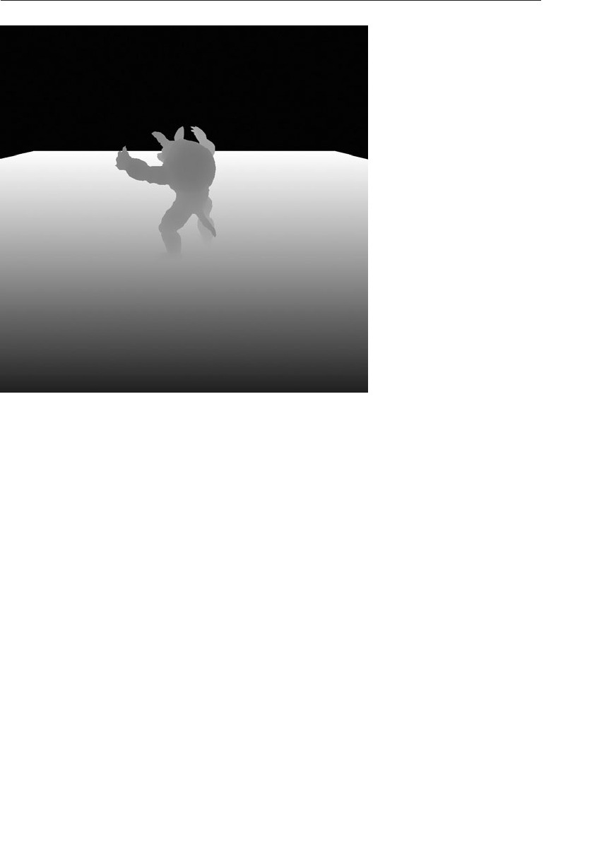
ptg9898810
Figure 7.10 Depth rendering
(Depths are rendered from the light’s position. Within rendered objects,
closer points have smaller depths and show up darker.)
Using a Shadow Map
Now that we have the depth for the scene rendered from the light’s point
of view we can render the scene with our regular shaders and use the
resulting depth texture to produce shadows as part of our lighting
calculations. This is where the meat of the algorithm is. First, we need to
set up the matrices for rendering the scene from the viewer’s position. The
matrices we’ll need are the model matrix,view matrix (which transforms
vertices for classic lighting), and the projection matrix (which transforms
coordinates to projective space for rasterization). Also, we’ll need a shadow
matrix. This matrix transforms world coordinates into the light’s projective
space and simultaneously applies a scale and bias to the resulting depth
values. The transformation to the light’s eye space is performed by
transforming the world space vertex coordinates through the light’s view
matrix followed by the light’s projection matrix (which we calculated
earlier). The scale and bias matrix maps depth values in projection space
(which lie between −1.0 and +1.0) into the range 0.0 to 1.0.
Shadow Mapping 405

ptg9898810
The code to set all these matrices up is given in Example 7.19.
Example 7.19 Matrix Calculations for Shadow Map Rendering
mat4 scene_model_matrix = rotate(t *720.0f, Y);
mat4 scene_view_matrix = translate(0.0f, 0.0f, -300.0f);
mat4 scene_projection_matrix = frustum(-1.0f, 1.0f, -aspect, aspect,
1.0f, FRUSTUM_DEPTH);
mat4 scale_bias_matrix = mat4(vec4(0.5f, 0.0f, 0.0f, 0.0f),
vec4(0.0f, 0.5f, 0.0f, 0.0f),
vec4(0.0f, 0.0f, 0.5f, 0.0f),
vec4(0.5f, 0.5f, 0.5f, 1.0f));
mat4 shadow_matrix = scale_bias_matrix *
light_projection_matrix *
light_view_matrix;
The vertex shader used for the final render transforms the incoming vertex
coordinates through all of these matrices and provides world coordinates,
eye coordinates, and shadow coordinates to the fragment shader, which will
perform the actual lighting calculations. This vertex shader is given in
Example 7.20.
Example 7.20 Vertex Shader for Rendering from Shadow Maps
#version 330 core
uniform mat4 model_matrix;
uniform mat4 view_matrix;
uniform mat4 projection_matrix;
uniform mat4 shadow_matrix;
layout (location = 0) in vec4 position;
layout (location = 1) in vec3 normal;
out VS_FS_INTERFACE
{
vec4 shadow_coord;
vec3 world_coord;
vec3 eye_coord;
vec3 normal;
} vertex;
void main(void)
{
vec4 world_pos = model_matrix *position;
vec4 eye_pos = view_matrix *world_pos;
vec4 clip_pos = projection_matrix *eye_pos;
vertex.world_coord = world_pos.xyz;
vertex.eye_coord = eye_pos.xyz;
vertex.shadow_coord = shadow_matrix *world_pos;
406 Chapter 7: Light and Shadow

ptg9898810
vertex.normal = mat3(view_matrix *model_matrix) *normal;
gl_Position = clip_pos;
}
Finally, the fragment shader performs lighting calculations for the scene. If
the point is considered to be illuminated by the light, the light’s
contribution is included in the final lighting calculation, otherwise only
ambient light is applied. The shader given in Example 7.21 performs these
calculations.
Example 7.21 Fragment Shader for Rendering from Shadow Maps
#version 330 core
uniform sampler2DShadow depth_texture;
uniform vec3 light_position;
uniform vec3 material_ambient;
uniform vec3 material_diffuse;
uniform vec3 material_specular;
uniform float material_specular_power;
layout (location = 0) out vec4 color;
in VS_FS_INTERFACE
{
vec4 shadow_coord;
vec3 world_coord;
vec3 eye_coord;
vec3 normal;
} fragment;
void main(void)
{
vec3 N = fragment.normal;
vec3 L = normalize(light_position - fragment.world_coord);
vec3 R = reflect(-L, N);
vec3 E = normalize(fragment.eye_coord);
float NdotL = dot(N, L);
float EdotR = dot(-E, R);
float diffuse = max(NdotL, 0.0);
float specular = max(pow(EdotR, material_specular_power),0.0);
float f = textureProj(depth_texture, fragment.shadow_coord);
color = vec4(material_ambient +
f*(material_diffuse *diffuse +
material_specular *specular), 1.0);
}
Shadow Mapping 407

ptg9898810
Don’t worry about the complexity of the lighting calculations in this
shader. The important part of the algorithm is the use of the
sampler2DShadow sampler type and the textureProj function. The
sampler2DShadow sampler is a special type of 2D texture that, when
sampled, will return either 1.0 if the sampled texture satisfies the
comparison test for the texture, and 0.0 if it does not. The texture
comparison mode for the depth texture was set earlier in Example 7.15 by
calling glTexParameteri() with the GL_TEXTURE_COMPARE_MODE
parameter name and GL_COMPARE_REF_TO_TEXTURE parameter value.
When the depth comparison mode for the texture is configured like this,
the texel values will be compared against the reference value that is
supplied in the third component of fragment.shadow_coord---which is
the zcomponent of the scaled and biased projective-space coordinate of
the fragment as viewed from the light. The depth comparison function is
set to GL_LEQUAL, which causes the test to pass if the reference value is
less than or equal to the value in the texture. When multiple texels are
sampled (e.g., when the texture mode is linear), the result of reading from
the texture is the average of all the 0.0s and 1.0s for the samples making up
the final texel. That is, near the edge of a shadow, the returned value might
be 0.25, or 0.5, and so on, rather than just 0.0 or 1.0. We scale the lighting
calculations by this result to take light visibility into account during
shading.
The textureProj function is a projective texturing function. It divides the
incoming texture coordinate (in this case fragment.shadow_coord by its
own last component (fragment.shadow_coord.w) to transform it into
normalized device coordinates, which is exactly what the perspective
transformation performed by OpenGL before rasterization does.
The result of rendering our scene with this shader is shown in Figure 7.11.
408 Chapter 7: Light and Shadow


ptg9898810
Chapter 8
Procedural Texturing
Chapter Objectives
After reading this chapter, you’ll be able to do the following:
•Texture a surface without using texture look-ups; instead texture a
surface using a shader that computes the texture procedurally.
•Antialias a procedurally generated texture.
•Light a surface using a bump map.
•Use noise to modulate shapes and textures to get quite realistic surfaces
and shapes.
•Generate your own noise texture map for storing multiple octaves of
portable noise.
411

ptg9898810
Generally, this chapter will cover using computation in shaders to supply
quality versions of what might normally come from large texture maps,
complex geometry, or expensive multisampling. However, accessing
textures won’t be forbidden. We’ll still occasionally use them as side tables
to drive the calculations performed in the shaders.
This chapter contains the following major sections:
•‘‘Procedural Texturing’’ shows several techniques for using computation
to create patterns, rather than accessing images stored in memory.
•‘‘Bump Mapping’’ presents a key method to give the appearance of a
bumpy surface without having to construct geometry to represent it.
•‘‘Antialiasing Procedural Textures’’ explains how to compute amount of
color for each pixel such that aliasing does not occur, especially for
edges and patterns created procedurally.
•‘‘Noise’’ will explain what noise is and how to use it to improve realism.
Procedural Texturing
The fact that we have a full-featured, high-level programming language to
express the processing at each fragment means that we can algorithmically
compute a pattern on an object’s surface. We can use this freedom to create
a wide variety of rendering effects that wouldn’t be possible otherwise. We
can also algorithmically compute the content of a volume from which a
surface is cut away, as in a wood object made from a tree. This can lead to a
result superior to texture mapping the surface.
In previous chapters, we discussed shaders that achieve their primary effect
by reading values from texture memory. This chapter focuses on shaders
that do interesting things primarily by means of an algorithm defined by
the shader. The results from such a shader are synthesized according to the
algorithm rather than being based primarily on precomputed values such
as a digitized painting or photograph. This type of shader is sometimes
called a procedural texture shader, and the process of applying such a shader
is called procedural texturing or procedural shading. Often the texture
coordinate or the object coordinate position at each point on the object is
the only piece of information needed to shade the object with a shader
that is entirely procedural.
In principle, procedural texture shaders can accomplish many of the same
tasks as shaders that access stored textures. In practice, there are times
when it is more convenient or feasible to use a procedural texture shader
and times when it is more convenient or feasible to use a stored texture
412 Chapter 8: Procedural Texturing

ptg9898810
shader. When deciding whether to write a procedural texture shader or one
that uses stored textures, keep in mind some of the main advantages of
procedural texture shaders.
•Textures generated procedurally have very low memory requirements
compared with stored textures. The only primary representation of the
texture is in the algorithm defined by the code in the procedural
texture shader. This representation is extremely compact compared
with the size of stored 2D textures. Typically, it is a couple of orders of
magnitude smaller (e.g., a few kilobytes for the code in a procedural
shader versus a few hundred kilobytes or more for a high-quality 2D
texture). This means procedural texture shaders require far less memory
on the graphics accelerator. Procedural texture shaders have an even
greater advantage when the desire is to have a 3D (solid) texture
applied to an object (a few kilobytes versus tens of megabytes or more
for a stored 3D texture).
•Textures generated by procedural texture shaders have no fixed area or
resolution. They can be applied to objects of any scale with precise
results because they are defined algorithmically rather than with
sampled data, as in the case of stored textures. There are no decisions
to be made about how to map a 2D image onto a 3D surface patch that
is larger or smaller than the texture, and there are no seams or
unwanted replication. As your viewpoint gets closer and closer to a
surface rendered with a procedural texture shader, you won’t see
reduced detail or sampling artifacts like you might with a shader that
uses a stored texture.
•Procedural texture shaders can be written to parameterize key aspects
of the algorithm. These parameters can easily be changed, allowing a
single shader to produce an interesting variety of effects. Very little can
be done to alter the shape of the pattern in a stored texture after it has
been created.
•When a volume is computed by a procedural texture, rather than a
surface, surface cutaways of that volume can be far more realistic than
any method of pasting a 2D texture onto the surface. And while a 3D
texture could be used, getting high resolution with a 3D texture can
take a prohibitive amount of memory.
Some of the disadvantages of using procedural shaders rather than stored
textures are as follows:
•Procedural texture shaders require the algorithm to be encoded in a
program. Not everyone has the technical skills needed to write such a
program, whereas it is fairly straightforward to create a 2D or 3D
texture with limited technical skills.
Procedural Texturing 413

ptg9898810
•Performing the algorithm embodied by a procedural texture shader at
each location on an object can take longer than accessing a stored
texture.
•Procedural texture shaders can have serious aliasing artifacts that can
be difficult to overcome. Today’s graphics hardware has built-in
capabilities for antialiasing stored textures (e.g., filtering methods and
mipmaps).
•Because of differences in arithmetic precision and differences in
implementations of built-in functions such as noise, procedural texture
shaders could produce somewhat different results on different
platforms.
The ultimate choice of whether to use a procedural shader or a stored
texture shader should be made pragmatically. Things that would be
artwork in the real world (paintings, billboards, anything with writing,
etc.) are good candidates for rendering with stored textures. Objects that
are extremely important to the final ‘‘look’’ of the image (character faces,
costumes, important props) can also be rendered with stored textures
because this presents the easiest route for an artist to be involved. Things
that are relatively unimportant to the final image and yet cover a lot of
area are good candidates for rendering with a procedural shader (walls,
floors, ground).
Often, a hybrid approach is the right answer. A golf ball might be rendered
with a base color, a hand-painted texture map that contains scuff marks, a
texture map containing a logo, and a procedurally generated dimple
pattern. Stored textures can also control or constrain procedural effects. If
our golf ball needs grass stains on certain parts of its surface and it is
important to achieve and reproduce just the right look, an artist could
paint a grayscale map that would direct the shader to locations where grass
smudges should be applied on the surface (for instance, black portions of
the grayscale map), and where they should not be applied (white portions
of the grayscale map). The shader can read this control texture and use it to
blend between a grass-smudged representation of the surface and a pristine
surface.
All that said, let’s turn our attention to a few examples of shaders that are
entirely procedural.
Regular Patterns
For our first example, we construct a shader that renders stripes on an
object. A variety of man-made objects can be rendered with such a shader:
children’s toys, wallpaper, wrapping paper, flags, fabrics, and so on.
414 Chapter 8: Procedural Texturing
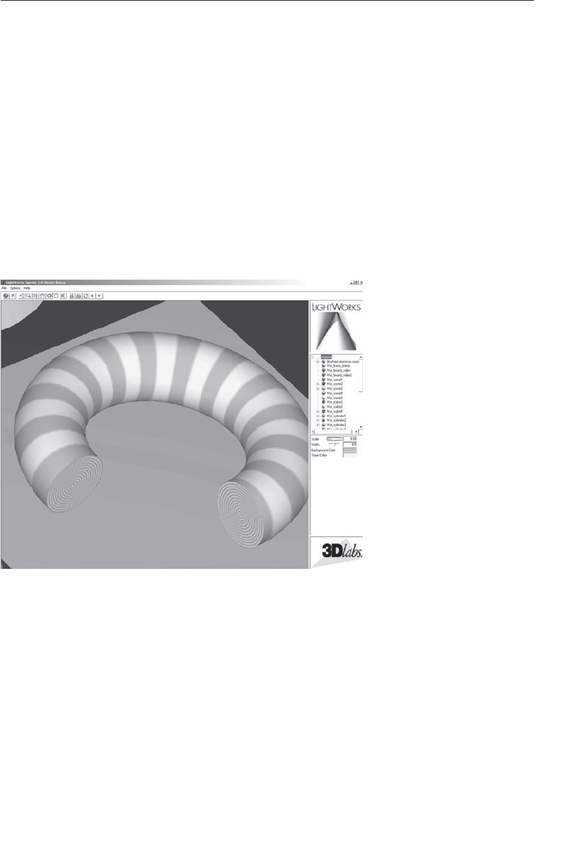
ptg9898810
The object in Figure 8.1 is a partial torus rendered with a stripe shader.
The stripe shader and the application in which it is shown were both
developed in 2002 by LightWork Design, a company that develops soft-
ware to provide photorealistic views of objects created with commercial
CAD/CAM packages. The application developed by LightWork Design
contains a graphical user interface that allows the user to interactively
modify the shader’s parameters. The various shaders that are available
are accessible on the upper-right portion of the user interface, and the
modifiable parameters for the current shader are accessible in the
lower-right portion of the user interface. In this case, you can see that
the parameters for the stripe shader include the stripe color (blue), the
background color (orange), the stripe scale (how many stripes there will
be), and the stripe width (the ratio of stripe to background; in this case, it
is 0.5 to make blue and orange stripes of equal width).
Figure 8.1 Procedurally striped torus
(Close-up of a partial torus rendered with the stripe shader described in
‘‘Regular Patterns’’ (courtesy of LightWork Design).)
For our stripe shader to work properly, the application needs to send down
only the geometry (vertex values) and the texture coordinate at each
vertex. The key to drawing the stripe color or the background color is the t
texture coordinate at each fragment (the stexture coordinate is not used at
all). The application must also supply values that the vertex shader uses to
perform a lighting computation. And the aforementioned stripe color,
Procedural Texturing 415

ptg9898810
background color, scale, and stripe width must be passed to the fragment
shader so that our procedural stripe computation can be performed at each
fragment.
Stripes Vertex Shader
The vertex shader for our stripe effect is shown in Example 8.1.
Example 8.1 Vertex Shader for Drawing Stripes
#version 330 core
uniform vec3 LightPosition;
uniform vec3 LightColor;
uniform vec3 EyePosition;
uniform vec3 Specular;
uniform vec3 Ambient;
uniform float Kd;
uniform mat4 MVMatrix;
uniform mat4 MVPMatrix;
uniform mat3 NormalMatrix;
in vec4 MCVertex;
in vec3 MCNormal;
in vec2 TexCoord0;
out vec3 DiffuseColor;
out vec3 SpecularColor;
out float TexCoord;
void main()
{
vec3 ecPosition = vec3(MVMatrix *MCVertex);
vec3 tnorm = normalize(NormalMatrix *MCNormal);
vec3 lightVec = normalize(LightPosition - ecPosition);
vec3 viewVec = normalize(EyePosition - ecPosition);
vec3 hvec = normalize(viewVec + lightVec);
float spec = clamp(dot(hvec, tnorm), 0.0, 1.0);
spec = pow(spec, 16.0);
DiffuseColor = LightColor *vec3(Kd *dot(lightVec, tnorm));
DiffuseColor = clamp(Ambient + DiffuseColor, 0.0, 1.0);
SpecularColor = clamp((LightColor *Specular *spec), 0.0, 1.0);
TexCoord = TexCoord0.t;
gl_Position = MVPMatrix *MCVertex;
}
There are some nice features to this particular shader. Nothing in it really
makes it specific to drawing stripes. It provides a good example of how we
might do the lighting calculation in a general way that would be compa-
tible with a variety of fragment shaders.
416 Chapter 8: Procedural Texturing

ptg9898810
As we mentioned, the values for doing the lighting computation
(LightPosition,LightColor,EyePosition,Specular,Ambient, and
Kd) are all passed in by the application as uniform variables. The purpose
of this shader is to compute DiffuseColor and SpecularColor, two
out variables that will be interpolated across each primitive and made
available to the fragment shader at each fragment location. These values
are computed in the typical way. A small optimization is that Ambient is
added to the value computed for the diffuse reflection so that we send one
less value to the fragment shader as an out variable. The incoming texture
coordinate is passed down to the fragment shader as the out variable
TexCoord, and the vertex position is transformed in the usual way.
Stripes Fragment Shader
The fragment shader contains the algorithm for drawing procedural
stripes. It is shown in Example 8.2.
Example 8.2 Fragment Shader for Drawing Stripes
#version 330 core
uniform vec3 StripeColor;
uniform vec3 BackColor;
uniform float Width;
uniform float Fuzz;
uniform float Scale;
in vec3 DiffuseColor;
in vec3 SpecularColor;
in float TexCoord;
out vec4 FragColor;
void main()
{
float scaledT = fract(TexCoord *Scale);
float frac1 = clamp(scaledT / Fuzz, 0.0, 1.0);
float frac2 = clamp((scaledT - Width) / Fuzz, 0.0, 1.0);
frac1 = frac1 *(1.0 - frac2);
frac1 = frac1 *frac1 *(3.0 - (2.0 *frac1));
vec3 finalColor = mix(BackColor, StripeColor, frac1);
finalColor = finalColor *DiffuseColor + SpecularColor;
FragColor = vec4(finalColor, 1.0);
}
The application provides one other uniform variable, called Fuzz. This
value controls the smooth transitions (i.e., antialiasing) between stripe
color and background color. With a Scale value of 10.0, a reasonable
Procedural Texturing 417

ptg9898810
value for Fuzz is 0.1. It can be adjusted as the object changes size to
prevent excessive blurriness at high magnification levels or aliasing at low
magnification levels. It shouldn’t really be set to a value higher than 0.5
(maximum blurriness of stripe edges).
The first step in this shader is to multiply the incoming ttexture
coordinate by the stripe scale factor and take the fractional part. This
computation gives the position of the fragment within the stripe pattern.
The larger the value of Scale, the more stripes we have as a result of this
calculation. The resulting value for the local variable scaledT is in the
range from [0, 1].
We’d like to have nicely antialiased transitions between the stripe colors.
One way to do this would be to use smoothstep() in the transition from
StripeColor to BackColor and use it again in the transition from
BackColor to StripeColor. But this shader uses the fact that these
transitions are symmetric to combine the two transitions into one.
So, to get our desired transition, we use scaledT to compute two other
values, frac1 and frac2. These two values tell us where we are in relation
to the two transitions between BackColor and StripeColor. For frac1,
if scaledT/Fuzz is greater than 1, that indicates that this point is not in
the transition zone, so we clamp the value to 1. If scaledT is less than
Fuzz,scaledT/Fuzz specifies the fragment’s relative distance into the
transition zone for one side of the stripe. We compute a similar value for
the other edge of the stripe by subtracting Width from scaledT, dividing
by Fuzz, clamping the result, and storing it in frac2.
These values represent the amount of fuzz (blurriness) to be applied. At
one edge of the stripe, frac2 is 0 and frac1 is the relative distance into
the transition zone. At the other edge of the stripe, frac1 is 1 and frac2
is the relative distance into the transition zone. Our next line of code
(frac1 = frac1 *(1.0 - frac2)) produces a value that can be used
to do a proper linear blend between BackColor and StripeColor. But
we’d actually like to perform a transition that is smoother than a linear
blend. The next line of code performs a Hermite interpolation in the same
way as the smoothstep() function. The final value for frac1 performs the
blend between BackColor and StripeColor.
The result of this effort is a smoothly ‘‘fuzzed’’ boundary in the transition
region between the stripe colors. Without this fuzzing effect, we would
have aliasing; abrupt transitions between the stripe colors that would flash
and pop as the object is moved on the screen. The fuzzing of the transition
region eliminates those artifacts. A close-up view of the fuzzed boundary is
shown in Figure 8.2. (More information about antialiasing procedural
shaders can be found in ‘‘Antialiasing Procedural Textures’’ on Page 442.)
418 Chapter 8: Procedural Texturing
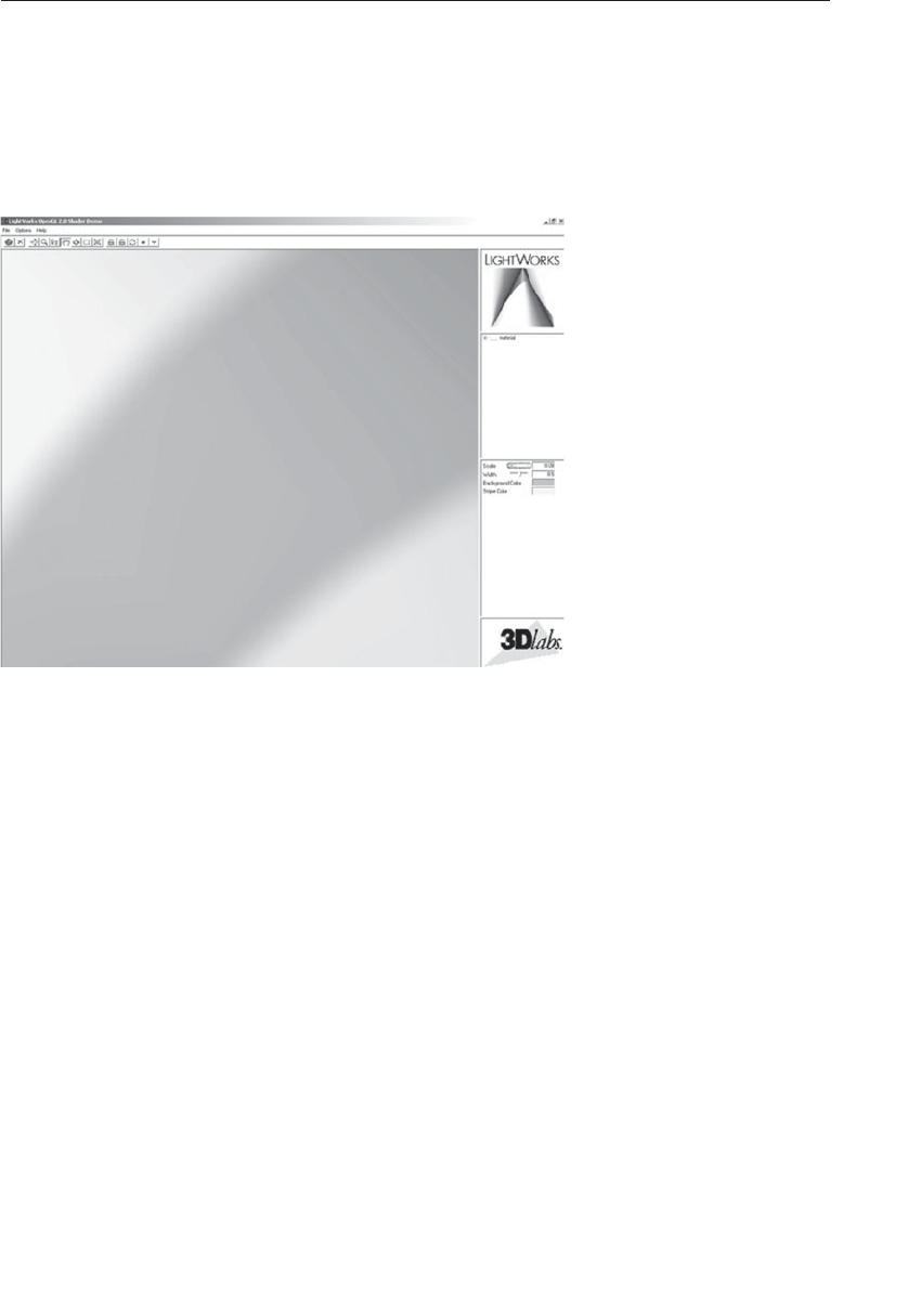
ptg9898810
Now all that remains to be done is to apply the diffuse and specular
lighting effects computed by the vertex shader and supply an alpha value
of 1.0 to produce our final fragment color. By modifying the five basic
parameters of our fragment shader, we can create a fairly interesting
number of variations of our stripe pattern, using the same shader.
Figure 8.2 Stripes close-up
(Extreme close-up view of one of the stripes that shows the effect of the
‘‘fuzz’’ calculation from the stripe shader (courtesy of LightWork Design).)
Brick
As a second example of a regular pattern, we will look at a shader that
draws brick with a slightly different method of lighting than the stripes
example. Again, the vertex shader here is somewhat generic and could be
used with multiple different fragment shaders. To see the effect they will
produce, see Figure 8.3.
Our brick example will also clearly display aliasing, which we will come
back and visit in the upcoming antialiasing section. There is a close-up of
this aliasing in the left picture in Figure 8.19.
Procedural Texturing 419
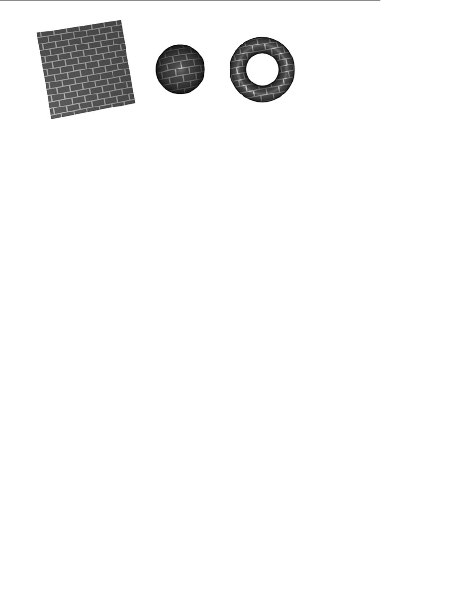
ptg9898810
Figure 8.3 Brick patterns
(A flat polygon, a sphere, and a torus rendered with the brick shaders.)
Bricks Vertex Shader
Let’s dive right in with the vertex shader, shown in Example 8.3. It has
little to do with drawing brick, but does compute how the brick will be lit.
If you wish, read through it, and if you’ve internalized the beginning of
Chapter 7as well as the first example given above, it should all start to
make sense. The brick pattern will come from the fragment shader, and
we’ll explain that next.
Example 8.3 Vertex Shader for Drawing Bricks
#version 330 core
in vec4 MCvertex;
in vec3 MCnormal;
uniform mat4 MVMatrix;
uniform mat4 MVPMatrix;
uniform mat3 NormalMatrix;
uniform vec3 LightPosition;
const float SpecularContribution = 0.3;
const float DiffuseContribution = 1.0 - SpecularContribution;
out float LightIntensity;
out vec2 MCposition;
void main()
{
vec3 ecPosition = vec3(MVMatrix *MCvertex);
vec3 tnorm = normalize(NormalMatrix *MCnormal);
vec3 lightVec = normalize(LightPosition - ecPosition);
vec3 reflectVec = reflect(-lightVec, tnorm);
vec3 viewVec = normalize(-ecPosition);
float diffuse = max(dot(lightVec, tnorm), 0.0);
420 Chapter 8: Procedural Texturing

ptg9898810
float spec = 0.0;
if (diffuse > 0.0)
{spec = max(dot(reflectVec, viewVec), 0.0);
spec = pow(spec, 16.0);
}
LightIntensity = DiffuseContribution *diffuse +
SpecularContribution *spec;
MCposition = MCvertex.xy;
gl_Position = MVPMatrix *MCvertex;
}
Bricks Fragment Shader
The fragment shader contains the core algorithm to make the brick
pattern. It is provided in Example 8.4, and we will point out the key
computations that make it work.
Example 8.4 Fragment Shader for Drawing Bricks
#version 330 core
uniform vec3 BrickColor, MortarColor;
uniform vec2 BrickSize;
uniform vec2 BrickPct;
in vec2 MCposition;
in float LightIntensity;
out vec4 FragColor;
void main()
{
vec3 color;
vec2 position, useBrick;
position = MCposition / BrickSize;
if (fract(position.y *0.5) > 0.5)
position.x += 0.5;
position = fract(position);
useBrick = step(position, BrickPct);
color = mix(MortarColor, BrickColor, useBrick.x *useBrick.y);
color *= LightIntensity;
FragColor = vec4(color, 1.0);
}
Procedural Texturing 421

ptg9898810
The colors to make the brick and mortar are selected by the application
and sent in as BrickColor and MortarColor. The size of the brick
pattern uses two independent components for width and height and is
also sent by the application, in BrickSize. Finally, the application selects
what percentage of the pattern will be brick, in BrickPct, with the
remaining being mortar.
The sizes are in the same units as the position coming from the vertex
shader, MCposition, which in turn was passed into the vertex shader from
the application. The input MCposition is effectively our texture
coordinate.
The key to knowing where we are in the brick pattern is looking at
the fractional part of dividing MCposition by the brick size: Each time the
pattern completes, we are at a whole number of repetitions of the brick,
hence the fractional part goes to 0. As we move through one iteration of
the brick, the fractional part approaches 1.0. These computations are done
with vec2 math, so we get both dimensions answered at the same time.
Because alternating rows of brick are offset, we conditionally add 0.5 to the
xdimension for alternating counts of the repeat pattern in the ydimension.
This is cryptically done as fract(position.y *0.5) > 0.5,
for which you might have other ways of expressing.
Once we know where we are in the brick pattern, we could use a bunch of
if tests to select the right color, or we could use math. In this example, we
chose math. The range of position is [0.0, 1.0), and we need BrickPct to
be in the same range. The step() function says the first argument is an
edge, the left of which should return 0.0 and the right of which should
1.0. So, for a particular dimension,step(position, BrickPct) will
return 1.0 if we are in the brick and 0.0 if in the mortar. We want to draw
mortar if either dimension says to draw mortar. Well, with these 0.0 and 1.0
results, multiplying them answers that question without using any
if tests. Finally, the mix() function is used to pick one of the colors.
No actual mixing occurs, because the ratio of mixing is either going
to be 0.0 or 1.0; it simply selects the first or second argument. Additional
reasons for using step and mix in this way will become clear when we
antialias.
Toy Ball
Programmability is the key to procedurally defining all sorts of texture
patterns. This next shader takes things a bit further by shading a sphere
with a procedurally defined star pattern and a procedurally defined stripe.
This shader was inspired by the ball in one of Pixar’s early short
422 Chapter 8: Procedural Texturing

ptg9898810
animations, Luxo Jr. This shader is quite specialized. It shades any surface
as long as it’s a sphere. The reason is that the fragment shader exploits the
following property of the sphere: The surface normal for any point on the
surface points in the same direction as the vector from the center of the
sphere to that point on the surface. This property is used to analytically
compute the surface normal used in the shading calculations within the
fragment shader. (This is actually a reasonable approximation for convex
hulls that aren’t too far from being spherical.)
The key to this shader is that the star pattern is defined by the coefficients
for five half-spaces that define the star shape. These coefficients were
chosen to make the star pattern an appropriate size for the ball. Points on
the sphere are classified as ‘‘in’’ or ‘‘out’’, relative to each half space.
Locations in the very center of the star pattern are ‘‘in’’ with respect to all
five half-spaces. Locations in the points of the star are ‘‘in’’ with respect to
four of the five half-spaces. All other locations are ‘‘in’’ with respect to
three or fewer half-spaces. Fragments that are in the stripe pattern are
simpler to compute. After we have classified each location on the surface
as ‘‘star’’, ‘‘stripe’’, or ‘‘other’’, we can color each fragment appropriately.
The color computations are applied in an order that ensures a reasonable
result even if the ball is viewed from far away. A surface normal is
calculated analytically (i.e., exactly) within the fragment shader. A lighting
computation that includes a specular highlight calculation is also applied
at every fragment.
Application Setup
The application needs only to provide vertex positions for this shader to
work properly. Both colors and normals are computed algorithmically in
the fragment shader. The only catch is that for this shader to work
properly, the vertices must define a sphere. The sphere can be of arbitrary
size because the fragment shader performs all the necessary computations,
based on the known geometry of a sphere.
A number of parameters to this shader are specified with uniform
variables. The values that produce the images shown in the remainder of
this section are summarized in Example 8.5.
Example 8.5 Values for Uniform Variables Used by the Toy Ball Shader
HalfSpace[0] 1.0, 0.0, 0.0, 0.2
HalfSpace[1] 0.309016994, 0.951056516, 0.0, 0.2
HalfSpace[2] -0.809016994, 0.587785252, 0.0, 0.2
HalfSpace[3] -0.809016994, -0.587785252, 0.0, 0.2
HalfSpace[4] 0.309016994, -0.951056516, 0.0, 0.2
StripeWidth 0.3
Procedural Texturing 423

ptg9898810
InOrOutInit -3.0
FWidth 0.005
StarColor 0.6, 0.0, 0.0, 1.0
StripeColor 0.0, 0.3, 0.6, 1.0
BaseColor 0.6, 0.5, 0.0, 1.0
BallCenter 0.0, 0.0, 0.0, 1.0
LightDir 0.57735, 0.57735, 0.57735, 0.0
HVector 0.32506, 0.32506, 0.88808, 0.0
SpecularColor 1.0, 1.0, 1.0, 1.0
SpecularExponent 200.0
Ka 0.3
Kd 0.7
Ks 0.4
Vertex Shader
The fragment shader is the workhorse for this shader duo, so the vertex
shader needs only to compute the ball’s center position in eye coordinates,
the eye-coordinate position of the vertex, and the clip space position at
each vertex. The application could provide the ball’s center position in eye
coordinates, but our vertex shader doesn’t have much to do, and doing it
this way means the application doesn’t have to keep track of the
model-view matrix. This value could easily be computed in the fragment
shader, but the fragment shader will likely have a little better performance
if we leave the computation in the vertex shader and pass the result as a
flat interpolated out variable (see Example 8.6).
Example 8.6 Vertex Shader for Drawing a Toy Ball
#version 330 core
uniform vec4 MCBallCenter;
uniform mat4 MVMatrix;
uniform mat4 MVPMatrix;
uniform mat3 NormalMatrix;
in vec4 MCVertex;
out vec3 OCPosition;
out vec4 ECPosition;
flat out vec4 ECBallCenter;
void main (void)
{OCPosition = MCVertex.xyz;
ECPosition = MVMatrix *MCVertex;
ECBallCenter = MVMatrix *MCBallCenter;
gl_Position = MVPMatrix *MCVertex;
}
424 Chapter 8: Procedural Texturing

ptg9898810
Fragment Shader
The toy ball fragment shader is a little bit longer than some of the previous
examples, so we build it up a few lines of code at a time and illustrate
some intermediate results. The definitions for the local variables that are
used in the toy ball fragment shader are as follows:
vec3 normal; // Analytically computed normal
vec4 pShade; // Point in shader space
vec4 surfColor; // Computed color of the surface
float intensity; // Computed light intensity
vec4 distance; // Computed distance values
float inorout; // Counter for classifying star pattern
The first thing we do is turn the surface location that we’re shading into a
point on a sphere with a radius of 1.0. We can do this with the normalize
function:
pShade.xyz = normalize(OCPosition.xyz);
pShade.w = 1.0;
We don’t want to include the wcoordinate in the computation, so we use
the component selector .xyz to select the first three components of
OCposition. This normalized vector is stored in the first three
components of pShade. With this computation, pShade represents a point
on the sphere with radius 1, so all three components of pShade are in the
range [−1, 1]. The wcoordinate isn’t really pertinent to our computations
at this point, but to make subsequent calculations work properly, we
initialize it to a value of 1.0.
We are always going to be shading spheres with this fragment shader, so
we analytically calculate the surface normal of the sphere:
normal = normalize(ECPosition.xyz-ECBallCenter.xyz);
Next, we perform our half-space computations. We initialize a counter
inorout to a value of −3.0. We increment the counter each time the
surface location is ‘‘in’’ with respect to a half-space. Because five half-spaces
are defined, the final counter value will be in the range [−3, 2]. Values of 1
or 2 signify that the fragment is within the star pattern. Values of 0 or less
signify that the fragment is outside the star pattern.
inorout = InOrOutInit; // initialize inorout to -3
We have defined the half-spaces as an array of five vec4 values, done our
‘‘in’’ or ‘‘out’’ computations, and stored the results in an array of five float
Procedural Texturing 425

ptg9898810
values. But we can take a little better advantage of the parallel nature of
the underlying graphics hardware if we do things a bit differently. You’ll
see how in a minute. First, we compute the distance between pShade and
the first four half-spaces by using the built-in dot-product function:
distance[0] = dot(p, HalfSpace[0]);
distance[1] = dot(p, HalfSpace[1]);
distance[2] = dot(p, HalfSpace[2]);
distance[3] = dot(p, HalfSpace[3]);
The results of these half-space distance calculations are visualized in
(A)--(D) of Figure 8.4. Surface locations that are ‘‘in’’ with respect to the
half-space are shaded in gray, and points that are ‘‘out’’ are shaded in black.
You may have been wondering why our counter was defined as a float
instead of an int . We’re going to use the counter value as the basis for a
smoothly antialiased transition between the color of the star pattern and
the color of the rest of the ball’s surface. To this end, we use the
smoothstep() function to set the distance to 0 if the computed distance is
less than -FWidth, to 1 if the computed distance is greater than FWidth,
and to a smoothly interpolated value between 0 and 1 if the computed
distance is between those two values. By defining distance as a vec4 , we
can perform the smooth-step computation on four values in parallel. The
built-in function smoothstep() implies a divide operation, and because
FWidth is a float, only one divide operation is necessary. This makes it all
very efficient.
distance = smoothstep(-FWidth, FWidth, distance);
Now we can quickly add the values in distance by performing a dot
product between distance and a vec4 containing 1.0 for all components:
inorout += dot(distance, vec4(1.0));
Because we initialized inorout to −3, we add the result of the dot product
to the previous value of inorout. This variable now contains a value in
the range [−3, 1]and we have one more half-space distance to compute.
We compute the distance to the fifth half-space, and we do the
computation to determine whether we’re ‘‘in’’ or ‘‘out’’ of the stripe around
the ball. We call the smoothstep() function to do the same operation on
these two values as was performed on the previous four half-space
distances. We update the inorout counter by adding the result from the
distance computation with the final half-space. The distance computation
with respect to the fifth half-space is illustrated in (E) of Figure 8.4.
426 Chapter 8: Procedural Texturing
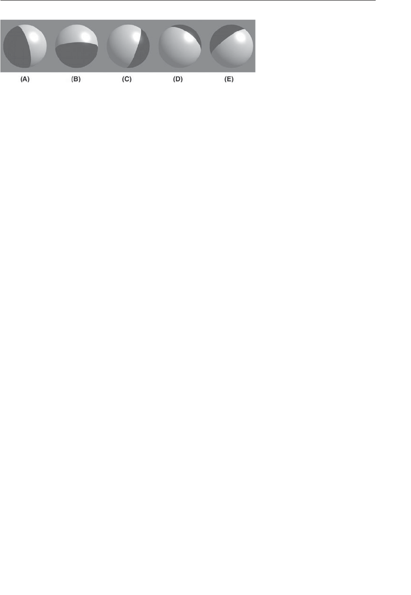
ptg9898810
Figure 8.4 Visualizing the results of the half-space distance calculations
(courtesy of AMD)
distance.x = dot(pShade, HalfSpace[4]);
distance.y = StripeWidth - abs(pShade.z);
distance.xy = smoothstep(-FWidth, FWidth, distance.xy);
inorout += distance.x;
(In this case, we’re performing a smooth-step operation only on the xand
ycomponents.)
The value for inorout is now in the range [−3, 2]. This intermediate result
is illustrated in Figure 8.5 (A). By clamping the value of inorout to the
range [0, 1], we obtain the result shown in Figure 8.5 (B).
inorout = clamp(inorout, 0.0, 1.0);
At this point, we can compute the surface color for the fragment. We use
the computed value of inorout to perform a linear blend between yellow
and red to define the star pattern. If we were to stop here, the result would
look like ball (A) in Figure 8.6. If we take the results of this calculation and
do a linear blend with the color of the stripe, we get the result shown for
ball (B) Figure 8.6. Because we used smoothstep(), the values of inorout
and distance.y provide a nicely antialiased edge at the border between
colors.
surfColor = mix(BaseColor, StarColor, inorout);
surfColor = mix(surfColor, StripeColor, distance.y);
The result at this stage is flat and unrealistic. Performing a lighting
calculation will fix this. The first step is to analytically compute the
normal for this fragment, which we can do because we know the
eye-coordinate position of the center of the ball (it’s provided in the in
variable ECballCenter) and we know the eye-coordinate position of the
fragment (it’s passed in the in variable ECposition).
// Calculate analytic normal of a sphere
normal = normalize(ECPosition.xyz - ECBallCenter.xyz);
Procedural Texturing 427
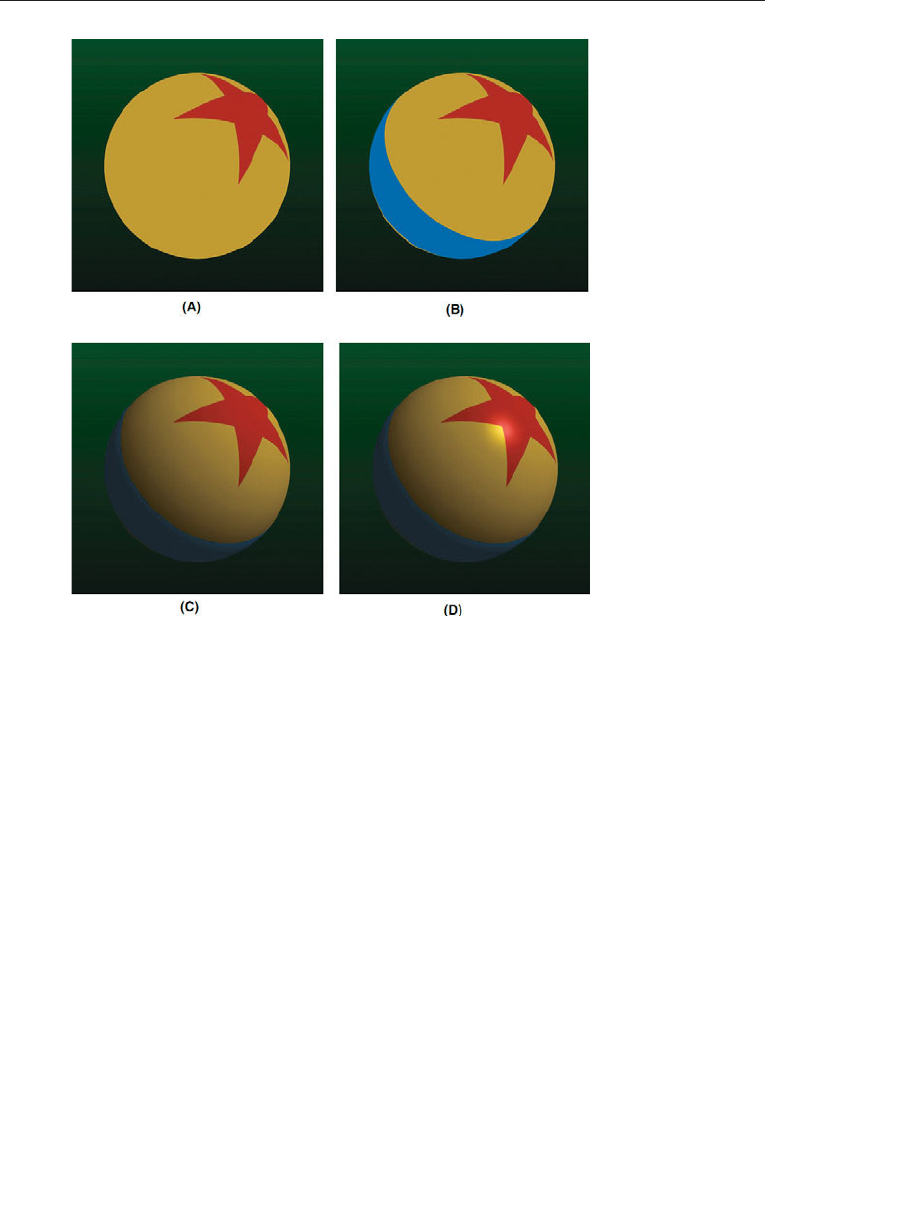
ptg9898810
Figure 8.5 Intermediate results from the toy ball shader
(In (A), the procedurally defined star pattern is displayed. In (B), the stripe is
added. In (C), diffuse lighting is applied. In (D), the analytically defined nor-
mal is used to apply a specular highlight. (Courtesy of ATI Research, Inc.))
The diffuse part of the lighting equation is computed with these three lines
of code:
// Per-fragment diffuse lighting
intensity = Ka; // ambient
intensity += Kd *clamp(dot(LightDir.xyz, normal), 0.0, 1.0);
surfColor *= intensity;
The result of diffuse-only lighting is shown as ball C in Figure 8.5. The
final step is to add a specular contribution with these three lines of code:
// Per-fragment specular lighting
intensity = clamp(dot(HVector.xyz, normal), 0.0, 1.0);
intensity = Ks *pow(intensity, SpecularExponent);
surfColor.rgb += SpecularColor.rgb *intensity;
428 Chapter 8: Procedural Texturing
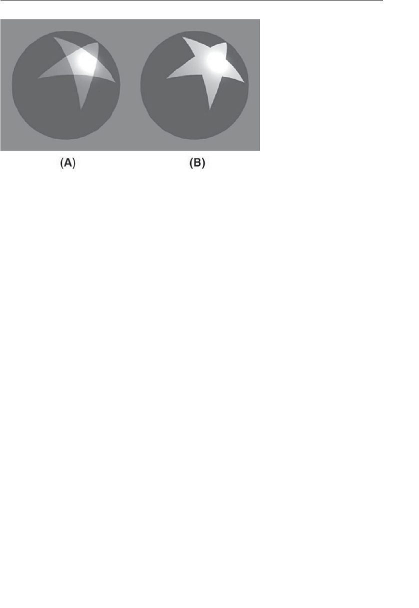
ptg9898810
Figure 8.6 Intermediate results from ‘‘in’’ or ‘‘out’’ computation
(Surface points that are ‘‘in’’ with respect to all five half-planes are shown in
white, and points that are ‘‘in’’ with respect to four half-planes are shown
in gray (A). The value of inorout is clamped to the range [0, 1]to produce
the result shown in (B). (Courtesy of AMD.))
Notice in ball D in Figure 8.5 that the specular highlight is perfect! Because
the surface normal at each fragment is computed exactly, there is no
misshapen specular highlight caused by tessellation facets like we’re used
to seeing. The resulting value is written to FragColor and sent on for final
processing before ultimately being written into the framebuffer.
FragColor = surfColor;
Voila! Your very own toy ball, created completely out of thin air! The
complete listing of the toy ball fragment shader is shown in Example 8.7.
Example 8.7 Fragment Shader for Drawing a Toy Ball
#version 330 core
uniform vec4 HalfSpace[5]; // half-spaces used to define star pattern
uniform float StripeWidth;
uniform float InOrOutInit; // -3.0
uniform float FWidth; // = 0.005
uniform vec4 StarColor;
uniform vec4 StripeColor;
uniform vec4 BaseColor;
uniform vec4 LightDir; // light direction, should be normalized
uniform vec4 HVector; // reflection vector for infinite light
Procedural Texturing 429

ptg9898810
uniform vec4 SpecularColor;
uniform float SpecularExponent;
uniform float Ka;
uniform float Kd;
uniform float Ks;
in vec4 ECPosition; // surface position in eye coordinates
in vec3 OCPosition; // surface position in object coordinates
flat in vec4 ECBallCenter; // ball center in eye coordinates
out vec4 FragColor;
void main()
{
vec3 normal; // Analytically computed normal
vec4 pShade; // Point in shader space
vec4 surfColor; // Computed color of the surface
float intensity; // Computed light intensity
vec4 distance; // Computed distance values
float inorout; // Counter for classifying star pattern
pShade.xyz = normalize(OCPosition.xyz);
pShade.w = 1.0;
inorout = InOrOutInit; // initialize inorout to -3.0
distance[0] = dot(pShade, HalfSpace[0]);
distance[1] = dot(pShade, HalfSpace[1]);
distance[2] = dot(pShade, HalfSpace[2]);
distance[3] = dot(pShade, HalfSpace[3]);
//float FWidth = fwidth(pShade);
distance = smoothstep(-FWidth, FWidth, distance);
inorout += dot(distance, vec4(1.0));
distance.x = dot(pShade, HalfSpace[4]);
distance.y = StripeWidth - abs(pShade.z);
distance.xy = smoothstep(-FWidth, FWidth, distance.xy);
inorout += distance.x;
inorout = clamp(inorout, 0.0, 1.0);
surfColor = mix(BaseColor, StarColor, inorout);
surfColor = mix(surfColor, StripeColor, distance.y);
// Calculate analytic normal of a sphere
normal = normalize(ECPosition.xyz-ECBallCenter.xyz);
// Per-fragment diffuse lighting
intensity = Ka; // ambient
intensity += Kd *clamp(dot(LightDir.xyz, normal), 0.0, 1.0);
430 Chapter 8: Procedural Texturing

ptg9898810
surfColor *= intensity;
// Per-fragment specular lighting
intensity = clamp(dot(HVector.xyz, normal), 0.0, 1.0);
intensity = Ks *pow(intensity, SpecularExponent);
surfColor.rgb += SpecularColor.rgb *intensity;
FragColor = surfColor;
}
Lattice
Here’s a little bit of a gimmick. In this example, we show how not to draw
the object procedurally.
In this example, we look at how the discard command can be used in a
fragment shader to achieve some interesting effects. The discard command
causes fragments to be discarded rather than used to update the
framebuffer. We use this to draw geometry with ‘‘holes’’. The vertex shader
is the exact same vertex shader used for stripes (‘‘Regular Patterns’’). The
fragment shader is shown in Example 8.8.
Example 8.8 Fragment Shader for Procedurally Discarding Part of an
Object
in vec3 DiffuseColor;
in vec3 SpecularColor;
in vec2 TexCoord
out vec3 FragColor;
uniform vec2 Scale;
uniform vec2 Threshold;
uniform vec3 SurfaceColor;
void main()
{
float ss = fract(TexCoord.s *Scale.s);
float tt = fract(TexCoord.t *Scale.t);
if ((ss > Threshold.s) && (tt > Threshold.t))
discard;
vec3 finalColor = SurfaceColor *DiffuseColor + SpecularColor;
FragColor = vec4(finalColor, 1.0);
}
The part of the object to be discarded is determined by the values of the s
and ttexture coordinates. A scale factor is applied to adjust the frequency
Procedural Texturing 431
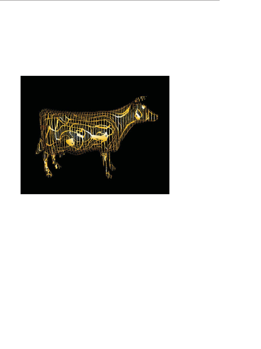
ptg9898810
of the lattice. The fractional part of this scaled texture-coordinate value is
computed to provide a number in the range [0, 1]. These values are
compared with the threshold values that have been provided. If both
values exceed the threshold, the fragment is discarded. Otherwise, we do
a simple lighting calculation and render the fragment.
In Figure 8.7, the threshold values were both set to 0.13. This means that
more than three-quarters of the fragments were being discarded!
Figure 8.7 The lattice shader applied to the cow model
(3Dlabs, Inc.)
Procedural Shading Summary
A master magician can make it look like something is created out of
thin air. With procedural textures, you, as a shader writer, can express
algorithms that turn flat gray surfaces into colorful, patterned, bumpy, or
reflective ones. The trick is to come up with an algorithm that expresses
the texture you envision. By coding this algorithm into a shader, you too
can create something out of thin air.
In this section, we only scratched the surface of what’s possible. We created
a stripe shader, but grids and checkerboards and polka dots are no more
difficult. We created a toy ball with a star, but we could have created a
beach ball with snowflakes. Shaders can be written to procedurally include
432 Chapter 8: Procedural Texturing

ptg9898810
or exclude geometry or to add bumps or grooves. Additional procedural
texturing effects are illustrated in this rest of this chapter. In particular,
‘‘Noise’’ shows how an irregular function (noise) can achieve a wide range
of procedural texturing effects.
Procedural textures are mathematically precise, are easy to parameterize,
and don’t require large amounts of texture memory, bandwidth, or
filtering. The end goal of a fragment shader is to produce a color value
(and possibly a depth value) that will be written into the framebuffer.
Because the OpenGL Shading Language is a procedural programming
language, the only limit to this computation is your imagination.
Bump Mapping
We have already seen procedural shader examples that modified color
(brick and stripes) and opacity (lattice). Another class of interesting effects
can be applied to a surface with a technique called bump mapping. Bump
mapping involves modulating the surface normal before lighting is
applied. We can perform the modulation algorithmically to apply a regular
pattern, we can add noise to the components of a normal, or we can look
up a perturbation value in a texture map. Bump mapping has proved to be
an effective way of increasing the apparent realism of an object without
increasing the geometric complexity. It can be used to simulate surface
detail or surface irregularities.
The technique does not truly alter the shape of the surface being shaded; it
merely ‘‘tricks’’ the lighting calculations. Therefore, the ‘‘bumping’’ does
not show up on the silhouette edges of an object. Imagine modeling a
planet as a sphere and shading it with a bump map so that it appears to
have mountains that are quite large relative to the diameter of the planet.
Because nothing has been done to change the underlying geometry, which
is perfectly round, the silhouette of the sphere always appears perfectly
round, even if the mountains (bumps) should stick out of the silhouette
edge. In real life, you would expect the mountains on the silhouette edges
to prevent the silhouette from looking perfectly round. Also, bump-to-
bump interactions of lighting and occlusion aren’t necessarily correct. For
these reasons, it is a good idea to use bump mapping to apply only ‘‘small’’
effects to a surface (at least relative to the size of the surface) or to surfaces
that won’t be viewed near edge on. Wrinkles on an orange, embossed
logos, and pitted bricks are all good examples of things that can be
successfully bump mapped.
Bump mapping adds apparent geometric complexity during fragment
processing, so once again the key to the process is our fragment shader.
This implies that the lighting operation must be performed by our
Bump Mapping 433

ptg9898810
fragment shader instead of by the vertex shader where it is often handled.
Again, this points out one of the advantages of the programmability that is
available through the OpenGL Shading Language. We are free to perform
whatever operations are necessary, in either the vertex shader or the
fragment shader. We don’t need to be bound to the fixed functionality
ideas of where things like lighting are performed.
The key to bump mapping is that we need a valid surface normal at each
fragment location, and we also need a light source vector and a viewing
direction vector. If we have access to all these values in the fragment
shader, we can procedurally perturb the normal prior to the light source
calculation to produce the appearance of ‘‘bumps’’. In this case, we really
are attempting to produce bumps or small spherical nodules on the surface
being rendered.
The light source computation is typically performed with dot products. For
the result to have meaning, all the components of the light source
calculation must be defined in the same coordinate space. So if we used
the vertex shader to perform lighting, we would typically define light
source positions or directions in eye coordinates and would transform
incoming normals and vertex values into this space to do the calculation.
However, the eye-coordinate system isn’t necessarily the best choice for
doing lighting in the fragment shader. We could normalize the direction to
the light and the surface normal after transforming them to eye space and
then pass them to the fragment shader as out variables. However, the light
direction vector would need to be renormalized after interpolation to get
accurate results. Moreover, whatever method we use to compute the
perturbation normal, it would need to be transformed into eye space and
added to the surface normal; that vector would also need to be normalized.
Without renormalization, the lighting artifacts would be quite noticeable.
Performing these operations at every fragment might be reasonably costly
in terms of performance. There is a better way.
Let us look at another coordinate space called the surface-local coordinate
space. This coordinate system adapts over a rendered object’s surface,
assuming that each point is at (0, 0, 0)and that the unperturbed surface
normal at each point is (0, 0, 1). This is a highly convenient coordinate
system in which to do our bump mapping calculations. But to do our
lighting computation, we need to make sure that our light direction,
viewing direction, and the computed perturbed normal are all defined in
the same coordinate system. If our perturbed normal is defined in
surface-local coordinates, that means we need to transform our light
direction and viewing direction into surface-local space as well. How is
that accomplished?
434 Chapter 8: Procedural Texturing

ptg9898810
What we need is a transformation matrix that transforms each incoming
vertex into surface-local coordinates (i.e., incoming vertex (x,y,z)is
transformed to (0, 0, 0)). We need to construct this transformation
matrix at each vertex. Then, at each vertex, we use the surface-local
transformation matrix to transform both the light direction and the
viewing direction. In this way, the surface local coordinates of the light
direction and the viewing direction are computed at each vertex and
interpolated across the primitive. At each fragment, we can use these values
to perform our lighting calculation with the perturbed normal that we
calculate.
But we still haven’t answered the real question. How do we create the
transformation matrix that transforms from object coordinates to
surface-local coordinates? An infinite number of transforms will transform
a particular vertex to (0, 0, 0).To transform incoming vertex values, we
need a way that gives consistent results as we interpolate between them.
The solution is to require the application to send down one more attribute
value for each vertex, a surface tangent vector. Furthermore, we require the
application to send us tangents that are consistently defined across the
surface of the object. By definition, this tangent vector is in the plane of
the surface being rendered and perpendicular to the incoming surface
normal. If defined consistently across the object, it serves to orient
consistently the coordinate system that we derive. If we perform a
cross-product between the tangent vector and the surface normal, we get a
third vector that is perpendicular to the other two. This third vector is
called the binormal, and it’s something that we can compute in our vertex
shader. Together, these three vectors form an orthonormal basis of a new
coordinate system, which is what we need to define the transformation
from object coordinates into surface-local coordinates. Because this
particular surface-local coordinate system is defined with a tangent vector
as one of the basis vectors, this coordinate system is sometimes referred
to as tangent spaces.
The transformation from object space to surface-local space is as follows:
⎡
⎣
Sx
Sy
Sz⎤
⎦=⎡
⎣
TxTyTz
BxByBz
NxNyNz⎤
⎦⎡
⎣
Ox
Oy
Oz⎤
⎦
We transform the object space vector (Ox,Oy,Oz)into surface-local space
by multiplying it by a matrix that contains the tangent vector (Tx,Ty,Tz)
in the first row, the binormal vector (Bx,By,Bz)in the second row, and the
surface normal (Nx,Ny,Nz)in the third row. We can use this process to
transform both the light direction vector and the viewing direction vector
into surface-local coordinates. The transformed vectors are interpolated
Bump Mapping 435

ptg9898810
across the primitive, and the interpolated vectors are used in the frag-
ment shader to compute the reflection with the procedurally perturbed
normal.
Application Setup
For our procedural bump map shader to work properly, the application
must send a vertex position, a surface normal, and a tangent vector in the
plane of the surface being rendered. The application passes the tangent
vector as a generic vertex attribute and binds the index of the generic
attribute to be used to the vertex shader variable tangent by calling
glBindAttribLocation(). The application is also responsible for providing
values for the uniform variables LightPosition,SurfaceColor,
BumpDensity,BumpSize, and SpecularFactor.
You must be careful to orient the tangent vectors consistently between
vertices; otherwise, the transformation into surface-local coordinates will
be inconsistent, and the lighting computation will yield unpredictable
results. To be consistent, vertices near each other need to have tangent
vectors that point in nearly the same direction. (Flat surfaces would have
the same tangent direction everywhere.) Consistent tangents can be
computed algorithmically for mathematically defined surfaces. Consistent
tangents for polygonal objects can be computed with neighboring vertices
and by application of a consistent orientation with respect to the object’s
texture coordinate system.
The problem with inconsistently defined normals is illustrated in
Figure 8.8. This diagram shows two triangles, one with consistently
defined tangents and one with inconsistently defined tangents. The gray
arrowheads indicate the tangent and binormal vectors (the surface normal
is pointing straight out of the page). The white arrowheads indicate the
direction toward the light source (in this case, a directional light source is
illustrated).
When we transform vertex 1 to surface-local coordinates, we get the same
initial result in both cases. When we transform vertex 2, we get a large
difference because the tangent vectors are very different between the two
vertices. If tangents were defined consistently, this situation would not
occur unless the surface had a high degree of curvature across this
polygon. And if that were the case, we would really want to tessellate
the geometry further to prevent this from happening.
The result is that in case 1, our light direction vector is smoothly
interpolated from the first vertex to the second, and all the interpolated
436 Chapter 8: Procedural Texturing
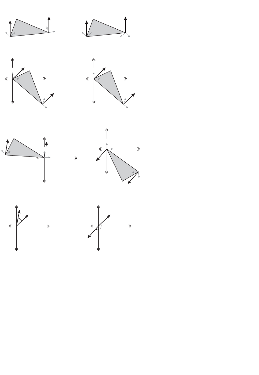
ptg9898810
Case 1: Consistent tangents Case 2: Inconsistent tangents
Case 1: Surface-local space for vertex 1 Case 2: Surface-local space for vertex 1
Case 1: Surface-local space for vertex 2 Case 2: Surface-local space for vertex 2
Case 1: Small interpolation between light vectors Case 2: Large interpolation between light vectors
2x
y
2y
x
L1
L2
2x
y
2y
x
L1
L2
L1
B1
B2
T2
T1
L2L1
B1
B2
T2
T1
L2
2x
y
2y
x
L1
T1
B2
T2
L2
B1
2x
y
2y
x
L1
T1
B2
T2
L2
B1
2x
y
2y
x
L1
T1B2
L2
B
1
T2
2x
y
2y
x
L1
T1
L2
B1
B2
T2
Figure 8.8 Inconsistently defined tangents leading to large lighting
errors
vectors are roughly the same length. If we normalize this light vector at
each vertex, the interpolated vectors are very close to unit length as well.
But in case 2, the interpolation causes vectors of wildly different lengths to
be generated, some of them near zero. This causes severe artifacts in the
lighting calculation.
Bump Mapping 437

ptg9898810
Remember OpenGL does not need to send down a binormal vertex
attribute, only a normal vector and a tangent vector. So, we don’t compute
the binormal in the application; rather we have the vertex shader compute
it automatically. (Simple computation is typically faster than memory
access or transfer.)
Vertex Shader
The vertex shader for our procedural bump-map shader is shown in
Example 8.9. This shader is responsible for computing the surface-local
direction to the light and the surface-local direction to the eye. To do this,
it accepts the incoming vertex position, surface normal, and tangent
vector; computes the binormal; and transforms the eye space light
direction and viewing direction, using the created surface-local
transformation matrix. The texture coordinates are also passed on to the
fragment shader because they are used to determine the position of our
procedural bumps.
Example 8.9 Vertex Shader for Doing Procedural Bump Mapping
#version 330 core
uniform vec3 LightPosition;
uniform mat4 MVMatrix;
uniform mat4 MVPMatrix;
uniform mat3 NormalMatrix;
in vec4 MCVertex;
in vec3 MCNormal;
in vec3 MCTangent;
in vec2 TexCoord0;
out vec3 LightDir;
out vec3 EyeDir;
out vec2 TexCoord;
void main()
{EyeDir = vec3(MVMatrix *MCVertex);
TexCoord = TexCoord0.st;
vec3 n = normalize(NormalMatrix *MCNormal);
vec3 t = normalize(NormalMatrix *MCTangent);
vec3 b = cross(n, t);
vec3 v;
v.x = dot(LightPosition, t);
v.y = dot(LightPosition, b);
v.z = dot(LightPosition, n);
LightDir = normalize(v);
v.x = dot(EyeDir, t);
438 Chapter 8: Procedural Texturing

ptg9898810
v.y = dot(EyeDir, b);
v.z = dot(EyeDir, n);
EyeDir = normalize(v);
gl_Position = MVPMatrix *MCVertex;
}
Fragment Shader
The fragment shader for doing procedural bump mapping is shown in
Example 8.10. A couple of the characteristics of the bump pattern are
parameterized by being declared as uniform variables, namely,
BumpDensity (how many bumps per unit area) and BumpSize (how wide
each bump will be). Two of the general characteristics of the overall surface
are also defined as uniform variables: SurfaceColor (base color of the
surface) and SpecularFactor (specular reflectance property).
The bumps that we compute are round. Because the texture coordinate
is used to determine the positioning of the bumps, the first thing
we do is multiply the incoming texture coordinate by the density value.
This controls whether we see more or fewer bumps on the surface. Using
the resulting grid, we compute a bump located in the center of each grid
square. The components of the perturbation vector p are computed as the
distance from the center of the bump in the xdirection and the distance
from the center of the bump in the ydirection. (We only perturb the
normal in the xand ydirections; the zvalue for our perturbation normal is
always 1.0.) We compute a ‘‘pseudodistance’’ dby squaring the components
of pand summing them. (The real distance could be computed at the cost
of doing another square root, but it’s not really necessary if we consider
BumpSize to be a relative value rather than an absolute value.)
To perform a proper reflection calculation later on, we really need to
normalize the perturbation normal. This normal must be a unit vector so
that we can perform dot products and get accurate cosine values for use in
the lighting computation. We generally normalize a vector by multiplying
each component of the normal by:
1.0
x2+y2+z2
Because of our computation for d, we’ve already computed part of what we
need (i.e., x2+y2). Furthermore, because we’re not perturbing zat all, we
know that z2will always be 1.0. To minimize the computation, we just
finish computing our normalization factor at this point in the shader by
computing:
1.0
√d+1.0
Bump Mapping 439

ptg9898810
Next, we compare dto BumpSize to see if we’re in a bump or not. If
we’re not, we set our perturbation vector to 0 and our normalization
factor to 1.0. The lighting computation happens in the next few lines.
We compute our normalized perturbation vector by multiplying through
with the normalization factor f. The diffuse and specular reflection
values are computed in the usual way, except that the interpolated
surface-local coordinate light and view direction vectors are used. We get
decent results without normalizing these two vectors as long as we
don’t have large differences in their interpolated values between vertices.
Example 8.10 Fragment Shader for Procedural Bump Mapping
#version 330 core
uniform vec4 SurfaceColor; // = (0.7, 0.6, 0.18, 1.0)
uniform float BumpDensity; // = 16.0
uniform float BumpSize; // = 0.15
uniform float SpecularFactor; // = 0.5
in vec3 LightDir;
in vec3 EyeDir;
in vec2 TexCoord;
out vec4 FragColor;
void main()
{
vec3 litColor;
vec2 c = BumpDensity *TexCoord.st;
vec2 p = fract(c) - vec2(0.5);
float d, f;
d = dot(p,p);
f = inversesqrt(d + 1.0);
if (d >= BumpSize) {
p = vec2(0.0);
f = 1.0;
}
vec3 normDelta = vec3(p.x, p.y, 1.0) *f;
litColor = SurfaceColor.rgb *max(dot(normDelta, LightDir), 0.0);
vec3 reflectDir = reflect(LightDir, normDelta);
float spec = max(dot(EyeDir, reflectDir), 0.0);
spec = pow(spec, 6.0);
spec *= SpecularFactor;
litColor = min(litColor + spec, vec3(1.0));
FragColor = vec4(litColor, SurfaceColor.a);
}
440 Chapter 8: Procedural Texturing
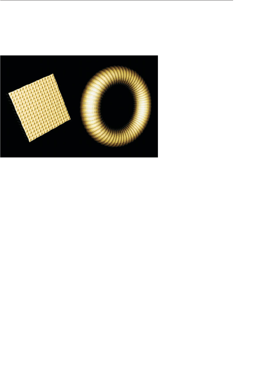
ptg9898810
The results from the procedural bump map shader are shown applied
to two objects, a simple box and a torus, in Figure 8.9. The texture
coordinates are used as the basis for positioning the bumps, and because
the texture coordinates go from 0.0 to 1.0 four times around the diameter
of the torus, the bumps look much closer together on that object.
Figure 8.9 Simple box and torus with procedural bump mapping
(3Dlabs, inc.)
Normal Maps
It is easy to modify our shader so that it obtains the normal perturbation
values from a texture rather than generating them procedurally. A texture
that contains normal perturbation values for the purpose of bump
mapping is called a bump map or a normal map.
An example of a normal map and the results applied to our simple box
object are shown in Figure 8.10. Individual components for the normals
can be in the range [−1, 1].To be encoded into an RGB texture with 8 bits
per component, they must be mapped into the range [0, 1]. The normal
map appears chalk blue because the default perturbation vector of (0, 0, 1)
is encoded in the normal map as (0.5, 0.5, 1.0). The normal map could be
stored in a floating-point texture. Today’s graphics hardware supports
textures both with 16-bit floating-point values per color component and
32-bit floating-point values per color component. If you use a floating-
point texture format for storing normals, your image quality tends to
increase (for instance, reducing banding effects in specular highlights).
Of course, textures that are 16 bits per component require twice as much
Bump Mapping 441
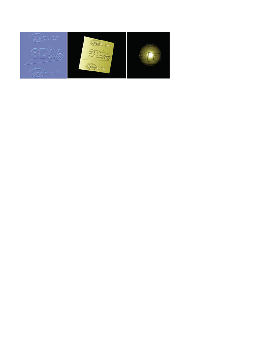
ptg9898810
texture memory as 8-bit per component textures, and performance might
be reduced.
Figure 8.10 Normal mapping
(A normal map (left) and the rendered result on a simple box and a sphere.
(3Dlabs, Inc.))
The vertex program is identical to the one described in ‘‘Bump Mapping’’.
The fragment shader is almost the same, except that instead of computing
the perturbed normal procedurally, the fragment shader obtains it from a
normal map stored in texture memory.
Antialiasing Procedural Textures
Jaggies, popping, sparkling, stair steps, strobing, and marching ants.
They’re all names used to describe the anathema of computer graphics---
aliasing. Anyone who has used a computer has seen it. For still images, it’s
not always that noticeable or objectionable. But as soon as you put an
object in motion, the movement of the jagged edges catches your eye and
distracts you. From the early days of computer graphics, the fight to
eliminate these nasty artifacts has been called antialiasing.
This section introduces the main reasons aliasing occurs, techniques to
avoid it, and the facilities within the OpenGL Shading Language to help
with antialiasing. Armed with this knowledge, you should be well on your
way to fighting the jaggies in your own shaders.
Sources of Aliasing
Aliasing can be generally explained by sampling theory, while specific
forms of aliasing can be explained more concretely by specific situations.
We will tie together both approaches, and this will become clearer as the
forms are discussed. Most generally, from a sampling theory perspective, a
graphics image is made from point samples of the scene. If patterns in the
442 Chapter 8: Procedural Texturing

ptg9898810
scene vary at a high spatial frequency with respect to the samples, the
samples can’t accurately reproduce the scene; they are hit and miss on
interesting features. A periodic pattern needs to be sampled at at least twice
the frequency of the pattern itself; otherwise the image will break down
when it has a pattern changing faster than every two samples, causing
moiré patterns in a static image and sparkling in a moving image. The edge
of an object is an interesting case, as it forms a step function as it is crossed.
This is effectively a square wave, which includes super-high frequencies
(it’s an infinite sum of ever increasing frequencies). So, it is impossible to
correctly sample an edge with point samples without undersampling. This
is discussed further as we go and should become more clear.
The human eye is extremely good at noticing edges. This is how we
comprehend shape and form and how we recognize letters and words. Our
eye is naturally good at it, and we spend our whole lives practicing it, so
naturally it is something we do very, very well.
A computer display is limited in its capability to present an image. The
display is made up of a finite number of discrete elements (pixels). At a
given time, each pixel can produce only one color. This makes it
impossible for a computer display to accurately represent detail that is
smaller than one pixel in screen space, such as an edge, especially when
each pixel is only representing a point sample for the pixel’s center.
When you combine these two things, the human eye’s ability to discern
edges and the computer graphics display’s limitations in replicating them,
you have a problem, and this problem is known as aliasing. In a nutshell,
aliasing occurs when we try to reproduce a signal with an insufficient
sampling frequency (less than two times the highest frequency present in
the image). With a computer graphics display, we’ll always have a fixed
number of samples (pixels) with which to reconstruct our image, and this
will always be insufficient to provide adequate sampling for edges, so we
will always have aliasing, unless we use the pixels to represent something
other than point samples. In the end, we can eliminate aliasing by
reducing the spatial frequency in the image to half the spatial frequency of
the pixels, exchanging aliasing for some other problem that is less
objectionable, like loss of detail, blurriness, or noise, and sometimes also
lowering the render-time performance.
The problem is illustrated in Figure 8.11. In this diagram, we show the
results of trying to draw a gray object. The intended shape is shown in
Figure 8.11 (A). The computer graphics display limits us to a discrete
sampling grid. If we choose only one location within each grid square
(usually the center) and determine the color to be used by sampling the
desired image at that point, we see some apparent artifacts. This is called
Antialiasing Procedural Textures 443
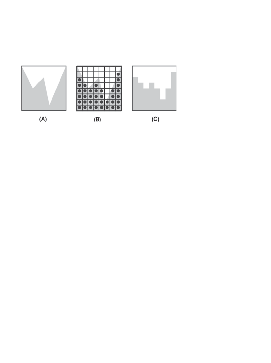
ptg9898810
point sampling and is illustrated in Figure 8.11 (B). The result is ugly
aliasing artifacts for edges that don’t line up naturally with the sampling
grid (see Figure 8.11 (C)). It actually depends on your display device
technology whether pixels are more like overlapping circles (CRT), or
collections of smaller red, green, and blue sub pixels (LCD), but the
artifacts are obvious in all cases.
Figure 8.11 Aliasing artifacts caused by point sampling
(The gray region represents the shape of the object to be rendered (A). The
computer graphics display presents us with a limited sampling grid (B). The
result of choosing to draw or not draw gray at each pixel results in jaggies,
or aliasing artifacts (C).)
Aliasing takes on other forms as well. If you are developing a sequence of
images for an animation and you don’t properly time-sample objects that
are in motion, you might notice temporal aliasings. This is caused by
objects that are moving too rapidly for the time sampling frequency being
used. Objects may appear to stutter as they move or blink on and off. The
classic example of temporal aliasing comes from the movies: A vehicle (car,
truck, or covered wagon) in motion is going forward, but the spokes of its
wheels appear to be rotating backwards. This effect is caused when the
time sampling rate (movie frames per second) is too low relative to the
motion of the wheel spokes. In reality, the wheel may be rotating two- and
three-quarter revolutions per frame, but on film it looks like it’s rotating
one-quarter revolution backward each frame.
To render images that look truly realistic rather than computer generated,
we need to develop techniques for overcoming the inherent limitations of
the graphics display, both spatially and temporally.
Avoiding Aliasing
One way to achieve good results without aliasing is to avoid situations in
which aliasing occurs.
444 Chapter 8: Procedural Texturing

ptg9898810
For instance, if you know that a particular object will always be a certain
size in the final rendered image, you can design a shader that looks good
while rendering that object at that size. This is the assumption behind
some of the shaders presented previously in this book. The smoothstep(),
mix(), and clamp() functions are handy functions to use to avoid sharp
transitions and to make a procedural texture look good at a particular scale.
Aliasing is often a problem when you are rendering an object at different
sizes. Mipmap textures address this very issue, and you can do something
similar with shaders. If you know that a particular object must appear at
different sizes in the final rendering, you can design a shader for each
different size. Each of these shaders would provide an appropriate level of
detail and avoid aliasing for an object of that size. For this to work, the
application must determine the approximate size of the final rendered
object before it is drawn and then install the appropriate shader. In
addition, if a continuous zoom (in or out) is applied to a single object,
some ‘‘popping’’ will occur when the level of detail changes.
You can avoid aliasing in some situations by using a texture instead of
computing something procedurally. This lets you take advantage of the
filtering support that is built into the texture mapping. However, linear
filtering between adjacent texels is only a solution to aliasing when the
resolution of the texels is similar to the resolution of the pixels. Otherwise,
you can still end up undersampling a texture and still get aliasing. Proper
use of mipmaps will help keep you in antialiasing territory. Of course,
there are other issues with using stored textures as opposed to doing things
procedurally, as discussed earlier in this chapter.
Increasing Resolution
The effects of aliasing can be reduced through a brute force method called
supersampling that performs sampling at several locations within a pixel
and averages the result of those samples. This is exactly the approach
supported in today’s graphics hardware with the multisample buffer. This
method of antialiasing replaces a single-point sampling operation with a
several-point sampling operation, so it doesn’t actually eliminate aliasing,
but it can reduce aliasing to the point that it is no longer objectionable.
You may be able to ignore the issue of aliasing if your shaders will always
be used in conjunction with a multisample buffer.
But this approach does use up hardware resources (graphics board memory
for storing the multisample buffer), and even with hardware acceleration,
it still may be slower than performing the antialiasing as part of the
procedural texture-generation algorithm. And because this approach
Antialiasing Procedural Textures 445
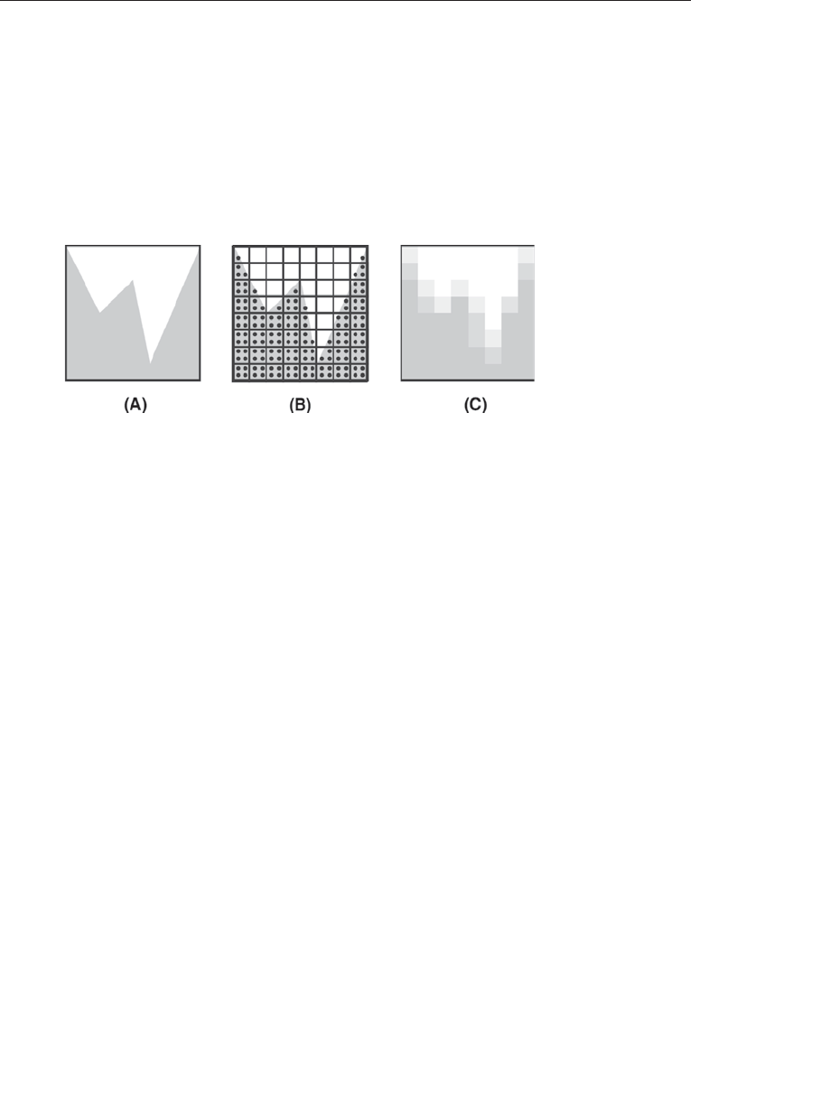
ptg9898810
doesn’t eliminate aliasing, your result is still apt to exhibit signs of aliasing,
albeit at a higher frequency (less visibly) than before.
Supersampling is illustrated in Figure 8.12. Each of the pixels is rendered
by sampling at four locations rather than at one. The average of the four
samples is used as the value for the pixel. This averaging provides a better
result, but it is not sufficient to eliminate aliasing because high-frequency
components can still be misrepresented.
Figure 8.12 Supersampling
(Supersampling with four samples per pixel yields a better result, but aliasing
artifacts are still present. The shape of the object to be rendered is shown
in (A). Sampling occurs at four locations within each pixel as shown in
(B). The results are averaged to produce the final pixel value as shown in
(C). Some samples that are almost half covered were sampled with just one
supersample point instead of two, and one pixel contains image data that
was missed entirely, even with supersampling.)
Supersampling can also be implemented within a fragment shader. The
code that is used to produce the fragment color can be constructed as a
function, and this function can be called several times from within the
main function of the fragment shader to sample the function at several
discrete locations. The returned values can be averaged to create the final
value for the fragment. Results are improved if the sample positions are
varied stochastically rather than spaced on a regular grid. Supersampling
within a fragment shader has the obvious downside of requiring N times as
much processing per fragment, where N is the number of samples
computed at each fragment.
There will be times when aliasing is unavoidable and supersampling is
infeasible. If you want to perform procedural texturing and you want a
single shader that is useful at a variety of scales, there’s little choice but to
take steps to counteract aliasing in your shaders.
446 Chapter 8: Procedural Texturing

ptg9898810
Antialiasing High Frequencies
Aliasing does not occur until we attempt to represent a continuous image
with discrete samples. This conversion occurs during rasterization. There
are only two choices: either don’t have high-frequency detail in the image
to render, or somehow deal with undersampling of high-frequency detail.
Since the former is almost never desirable due to viewing with a variety of
scales, we focus on the latter. Therefore, our attempts to mitigate its effects
will always occur in the fragment shader. They will still include both tools
of removing high-frequencies or sampling at higher rates, but both are
done after rasterization, where we can compare the frequencies of detail
present in the image with the frequency of the pixels. The OpenGL
Shading Language has several functions for this purpose that are available
only to fragment shaders. To help explain the motivation for some of
the language facilities for filter estimation, we develop a worst-case
scenario---alternating black and white stripes drawn on a sphere.
Developing a fragment shader that performs antialiasing enables us to
further illustrate the aliasing problem and the methods for reducing
aliasing artifacts. Bert Freudenberg developed the first version of the
GLSL shaders discussed in this section.
Generating Stripes
The antialiasing fragment shader determines whether each fragment is to
be drawn as white or black to create lines on the surface of an object. The
first step is to determine the method to be used for drawing lines. We use a
single parameter as the basis for our stripe pattern. For illustration, let’s
assume that the parameter is the scoordinate of the object’s texture
coordinate. We have the vertex shader pass this value to us as a
floating-point out variable named V, eventually giving us a method for
creating vertical stripes on a sphere. Figure 8.13 (A) shows the result of
using the stexture coordinate directly as the intensity (grayscale) value on
the surface of the sphere. The viewing position is slightly above the sphere,
so we are looking down at the ‘‘north pole’’. The stexture coordinate starts
off at 0 (black) and increases to 1 (white) as it goes around the sphere. The
edge where black meets white can be seen at the pole, and it runs down
the back side of the sphere. The front side of the sphere looks mostly gray
but increases from left to right.
We create a sawtooth wave by multiplying the stexture coordinate by 16
and taking the fractional part (see Figure 8.13 (B)). This causes the intensity
value to start at 0, rise quickly to 1, and then drop back down to 0. This
sequence is repeated 16 times. The GLSL shader code to implement this is
float sawtooth = fract(V *16.0);
Antialiasing Procedural Textures 447
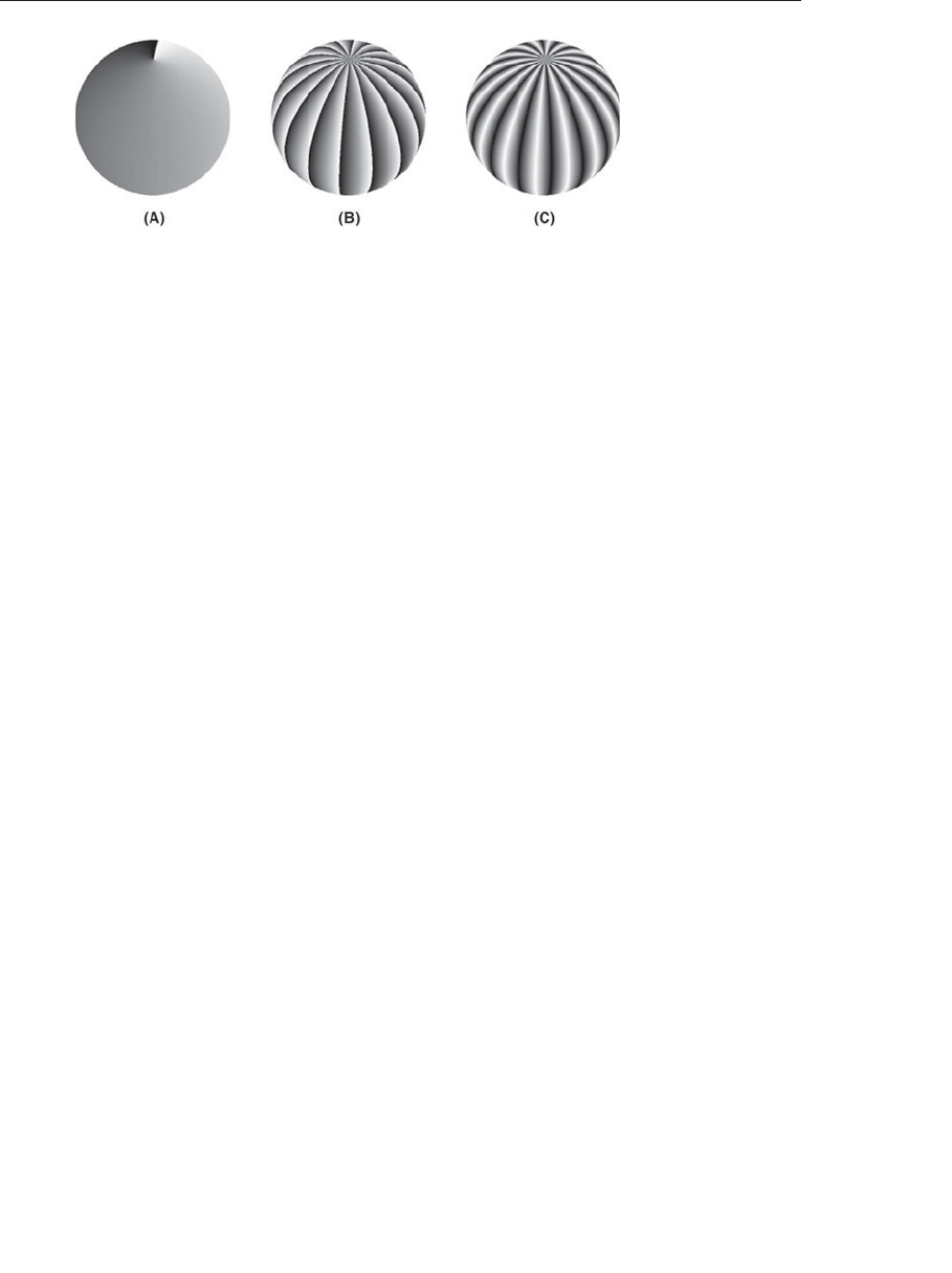
ptg9898810
Figure 8.13 Using the stexture coordinate to create stripes on a sphere
(In (A), the stexture coordinate is used directly as the intensity (gray) value.
In (B), a modulus function creates a sawtooth function. In (C), the abso-
lute value function turns the sawtooth function into a triangle function.
(Courtesy of Bert Freudenberg, University of Magdeburg, 2002.))
This isn’t quite the stripe pattern we’re after. To get closer, we employ the
absolute value function (see Figure 8.13 (C)). By multiplying the value of
sawtooth by 2 and subtracting 1, we get a function that varies in the range
[−1, 1]. Taking the absolute value of this function results in a function that
goes from 1 down to 0 and then back to 1 (i.e., a triangle wave). The line of
code to do this is
float triangle = abs(2.0 *sawtooth - 1.0);
A stripe pattern is starting to appear, but it’s either too blurry or our glasses
need adjustment. We make the stripes pure black and white by using the
step() function. When we compare our triangle variable to 0.5, this
function returns 0 whenever triangle is less than or equal to 0.5, and 1
whenever triangle is greater than 0.5. This could be written as
float square = step(0.5, triangle);
This effectively produces a square wave, and the result is illustrated in
Figure 8.14 (A). We can modify the relative size of the alternating stripes by
adjusting the threshold value provided in the step function.
Analytic Pre-filtering
In Figure 8.14 (A), we see that the stripes are now distinct, but aliasing has
reared its ugly head. The step function returns values that are either 0 or 1,
with nothing in between, so the jagged edges in the transitions between
white and black are easy to spot. They will not go away if we increase the
resolution of the image; they’ll just be smaller. The problem is caused by
the fact that the step function introduced an immediate transition from
448 Chapter 8: Procedural Texturing
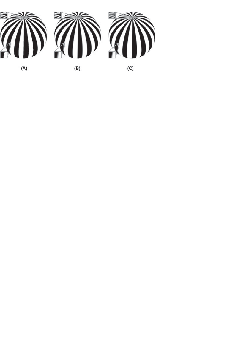
ptg9898810
Figure 8.14 Antialiasing the stripe pattern
(We can see that the square wave produced by the step function produces
aliasing artifacts (A). The smoothstep() function with a fixed-width filter
produces too much blurring near the equator but not enough at the pole
(B). An adaptive approach provides reasonable antialiasing in both regions
(C). (Courtesy of Bert Freudenberg, University of Magdeburg, 2002.))
white to black or an edge, which includes frequencies marching up toward
infinity. There is no way to sample this transition at a high enough
frequency to eliminate the aliasing artifacts. To get good results, we need
to take steps within our shader to remove such high frequencies.
A variety of antialiasing techniques rely on eliminating overly high
frequencies before sampling. This is called low-pass filtering because low
frequencies are passed through unmodified, whereas high frequencies are
eliminated. The visual effect of low-pass filtering is that the resulting
image is blurred.
To eliminate the high frequencies from the stripe pattern, we use the
smoothstep() function. We know that this function produces a smooth
transition between white and black. It requires that we specify two edges,
and a smooth transition occurs between those two edges. Figure 8.14 (B)
illustrates the result from the following line of code:
float square = smoothstep(0.4, 0.6, triangle);
Adaptive Analytic Pre-filtering
Analytic pre-filtering produces acceptable results in some regions of the
sphere but not in others. The size of the smoothing filter (0.2) is defined in
parameter space. But the parameter does not vary at a constant rate in
screen space. In this case, the stexture coordinate varies quite rapidly in
screen space near the poles and less rapidly at the equator. Our fixed-width
filter produces blurring across several pixels at the equator and very little
effect at the poles. What we need is a way to determine the size of the
Antialiasing Procedural Textures 449
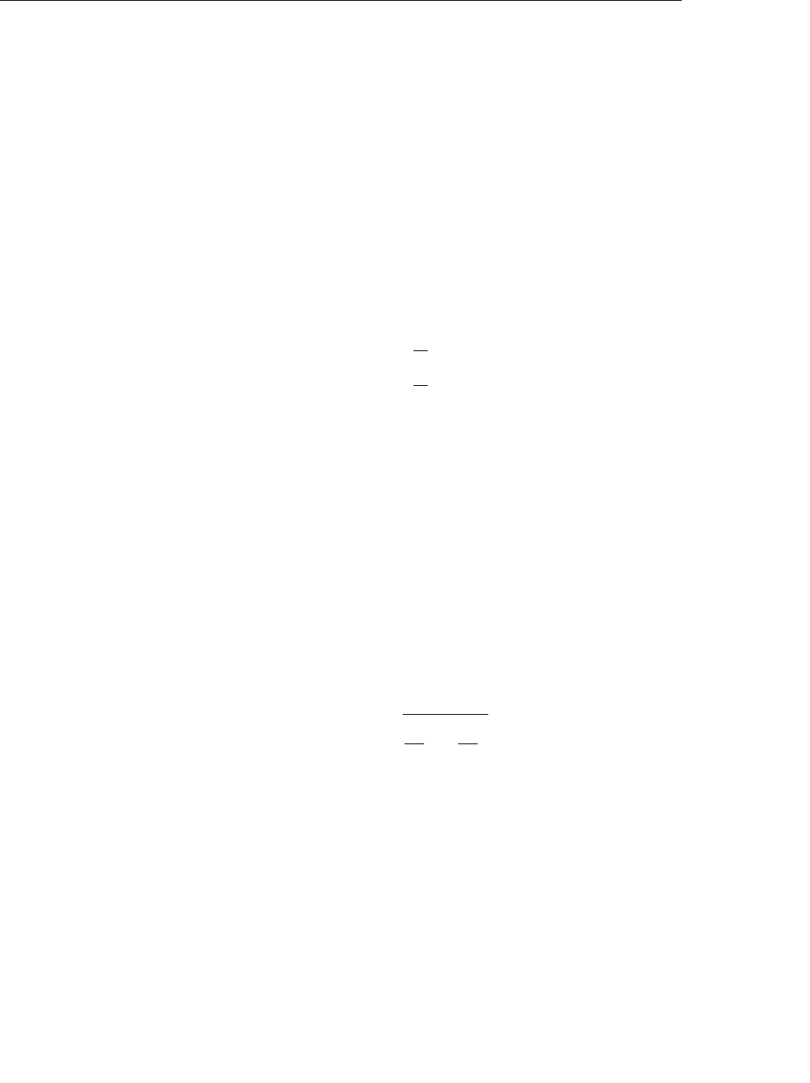
ptg9898810
smoothing filter adaptively so that transition can be appropriate at all
scales in screen space. This requires a measurement of how rapidly the
function we’re interested in is changing at a particular position in screen
space.
Fortunately, GLSL provides a built-in function that can give us the rate of
change (derivative) of any parameter in screen space. The function dFdx()
gives the rate of change in screen coordinates in the xdirection, and
dFdy() gives the rate of change in the ydirection. Because these functions
deal with screen space, they are available only in a fragment shader. These
two functions can provide the information needed to compute a gradient
vector for the position of interest.
Given a function f(x,y), the gradient of fat the position (x,y)is defined as
the vector
G[f(x,y)] =⎡
⎣
∂f
∂x
∂f
∂y⎤
⎦
In English, the gradient vector comprises the partial derivative of function
fwith respect to x(i.e., the measure of how rapidly fis changing in the x
direction) and the partial derivative of the function fwith respect to
y(i.e., the measure of how rapidly fis changing in the ydirection). The
important properties of the gradient vector are that it points in the
direction of the maximum rate of increase of the function f(x,y)(the
gradient direction) and that the magnitude of this vector equals the
maximum rate of increase of f(x,y)in the gradient direction. (These
properties are useful for image processing too, as we see later.) The built-in
functions dFdx() and dFdy() give us exactly what we need to define the
gradient vector for functions used in fragment shaders.
The magnitude of the gradient vector for the function f(x,y)is commonly
called the gradient of the function f(x,y). It is defined as
G[f(x,y)]= +∂f
∂x
2
+∂f
∂y
2
In practice, it is not always necessary to perform the (possibly costly)
square root operation. The gradient can be approximated with absolute
values:
G[f(x,y)]∼
=f(x,y)−f(x+1, y)+f(x,y)−f(x,y+1)
This is exactly what is returned by the built-in function fwidth(). The sum
of the absolute values is an upper bound on the width of the sampling
filter needed to eliminate aliasing. If it is too large, the resulting image
looks somewhat blurrier than it should, but this is usually acceptable.
450 Chapter 8: Procedural Texturing
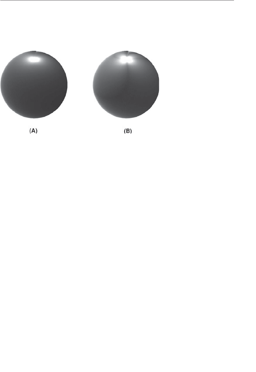
ptg9898810
The two methods of computing the gradient are compared in Figure 8.15.
As you can see, there is little visible difference. Because the value of the
gradient was quite small for the function being evaluated on this object,
the values were scaled so that they would be visible.
Figure 8.15 Visualizing the gradient
(In (A), the magnitude of the gradient vector is used as the intensity (gray)
value. In (B), the gradient is approximated with absolute values. (Actual
gradient values are scaled for visualization.) (Courtesy of Bert Freudenberg,
University of Magdeburg, 2002.))
To compute the actual gradient for the in variable Vwithin a fragment
shader, we use
float width = length(vec2(dFdx(V), dFdy(V)));
To approximate it, we use the potentially higher-performance calculation.
float width = fwidth(V);
We then use the filter width within our call to smoothstep() as follows:
float edge = dp *Frequency *2.0;
float square = smoothstep(0.5 - edge, 0.5 + edge, triangle);
If we put this all together in a fragment shader, we get Example 8.11.
Example 8.11 Fragment Shader for Adaptive Analytic Antialiasing
#version 330 core
uniform float Frequency; // Stripe frequency = 6
uniform vec3 Color0;
uniform vec3 Color1;
Antialiasing Procedural Textures 451
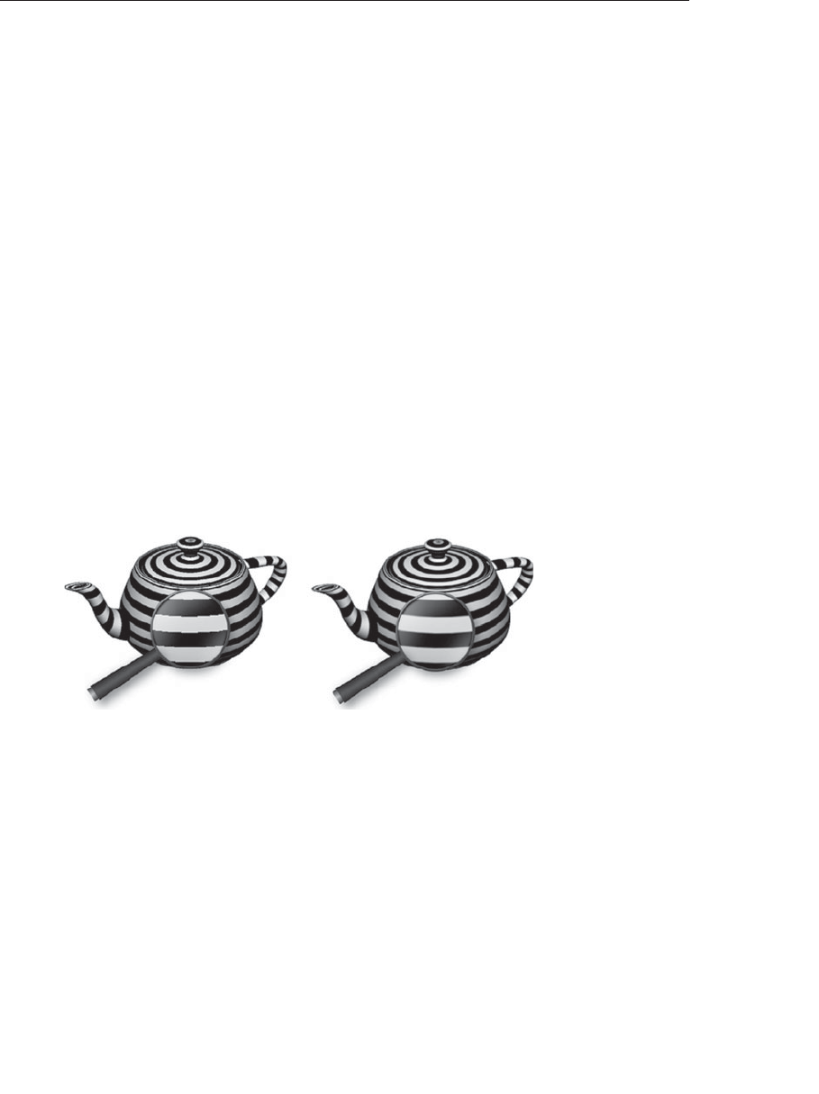
ptg9898810
in float V; // generic varying
in float LightIntensity;
out vec4 FragColor;
void main()
{
float sawtooth = fract(V *Frequency);
float triangle = abs(2.0 *sawtooth - 1.0);
float dp = length(vec2(dFdx(V), dFdy(V)));
float edge = dp *Frequency *2.0;
float square = smoothstep(0.5 - edge, 0.5 + edge, triangle);
vec3 color = mix(Color0, Color1, square);
FragColor = vec4(color, 1.0);
FragColor.rgb *= LightIntensity;
}
If we scale the frequency of our texture, we must also increase the filter
width accordingly. After the value of the function is computed, it is
replicated across the red, green, and blue components of a vec3 and used
as the color of the fragment. The results of this adaptive antialiasing
approach are shown in Figure 8.14 (C). The results are much more
consistent across the surface of the sphere. A simple lighting computation
is added, and the resulting shader is applied to the teapot in Figure 8.16.
Figure 8.16 Effect of adaptive analytical antialiasing on striped teapots
(On the left, the teapot is drawn with no antialiasing. On the right, the
adaptive antialiasing shader is used. A small portion of the striped surface is
magnified 200 percent to make it easier to see the difference.)
This approach to antialiasing works well until the filter width gets larger
than the frequency. This is the situation that occurs at the north pole of
the sphere. The stripes very close to the pole are much thinner than one
pixel, so no step function will produce the correct gray value here. In such
regions, you need to switch to integration or frequency clamping, both of
which are discussed in subsequent sections.
452 Chapter 8: Procedural Texturing

ptg9898810
Analytic Integration
The weighted average of a function over a specified interval is called a
convolution. The values that do the weighting are called the convolution
kernel or the convolution filter. In some cases, we can reduce or eliminate
aliasing by determining the convolution of a function ahead of time and
then sampling the convolved function rather than the original function.
The convolution can be performed over a fixed interval in a computation
that is equivalent to convolving the input function with a box filter. A box
filter is far from ideal, but it is simple and easy to compute and often good
enough.
This method corresponds to the notion of antialiasing by area sampling. It
is different from point sampling or super sampling in that we attempt to
calculate the area of the object being rendered relative to the sampling
region. Referring to Figure 8.12, if we used an area sampling technique, we
would get more accurate values for each of the pixels, and we wouldn’t
miss that pixel that just had a sliver of coverage.
In Advanced RenderMan: Creating CGI for Motion Pictures, Apodaca and Gritz
(1999) explain how to perform analytic antialiasing of a periodic step
function, sometimes called a pulse train. Darwyn Peachey described how to
apply this method to his procedural brick RenderMan shader in Texturing
and Modeling: A Procedural Approach, and Dave Baldwin published a GLSL
version of this shader in the original paper on the OpenGL Shading
Language. We use this technique to analytically antialias the procedural
brick shader we introduced at the beginning of this chapter in the
subsection ‘‘Regular Patterns’’ on Page 414.
This example uses the step function to produce the periodic brick pattern.
The function that creates the brick pattern in the horizontal direction is
illustrated in Figure 8.17. From 0 to BrickPct.x (the brick-width fraction),
the function is 1.0. At the value of BrickPct.x, there is an edge with infinite
slope as the function drops to 0. At the value 1, the function jumps back
up to 1.0, and the process is repeated for the next brick.
The key to antialiasing this function is to compute its integral, or
accumulated, value. We have to consider the possibility that, in areas of
high complexity, the filter width that is computed by fwidth() will cover
several of these pulses. By sampling the integral rather than the function
itself, we get a properly weighted average and avoid the high frequencies
caused by point sampling that would produce aliasing artifacts.
So what is the integral of this function? It is illustrated in Figure 8.18. From
0 to BrickPct.x, the function value is 1, so the integral increases with a
slope of 1. From BrickPct.x to 1.0, the function has a value of 0, so the
Antialiasing Procedural Textures 453
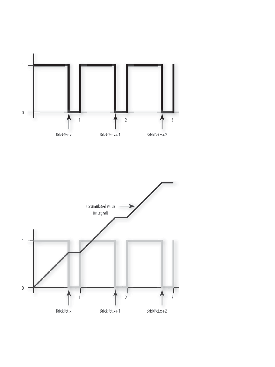
ptg9898810
integral stays constant in this region. At 1, the function jumps back to 1.0,
so the integral increases until the function reaches BrickPct.x + 1. At this
point, the integral changes to a slope of 0 again, and this pattern of ramps
and plateaus continues.
Figure 8.17 Periodic step function
(The periodic step function, or pulse train, that defines the horizontal com-
ponent of the procedural brick texture.)
Figure 8.18 Periodic step function (pulse train) and its integral
454 Chapter 8: Procedural Texturing

ptg9898810
We perform antialiasing by determining the value of the integral over the
area of the filter, and we do that by evaluating the integral at the edges of
the filter and subtracting the two values. The integral for this function
consists of two parts: the sum of the area for all the pulses that have been
fully completed before the edge we are considering and the area of the
partially completed pulse for the edge we are considering.
For our procedural brick shader, we use the variable position.x as the
basis for generating the pulse function in the horizontal direction. So, the
number of fully completed pulses is just floor(position.x). Because
the height of each pulse is 1.0, the area of each fully completed pulse is
just BrickPct.x. Multiplying floor(position.x) by BrickPct.x
gives the area for all the fully completed pulses. The edge that we’re
considering may be in the part of the function that is equal to 0, or it may
be in the part of the function that is equal to 1. We can find out by
computing fract(position.x) - (1.0 - BrickPct.x). If the result
of this subtraction is less than 0, we were in the part of the function that
returns 0, so nothing more needs to be done. But if the value is greater
than 0, we are partway into a region of the function that is equal to 1.
Because the height of the pulse is 1, the area of this partial pulse is
fract(position.x) - (1.0 - BrickPct.x). Therefore, the second
part of our integral is the expression
max(fract(position.x) - (1.0 - BrickPct.x), 0.0).
We use this integral for both the horizontal and vertical components of
our procedural brick pattern. Because the application knows the brick
width and height fractions (BrickPct.x and BrickPct.y), it can easily
compute 1.0 - BrickPct.x and 1.0 - BrickPct.y and provide them
to our fragment shader as well. This keeps us from unnecessarily
computing these values several times for every fragment that is rendered.
We call these values the mortar percentage. Because we evaluate this
expression twice with different arguments, we define it as a macro or a
function for convenience.
#define Integral(x, p, notp) ((floor(x)*(p))+max(fract(x)-(notp), 0.0))
The parameter pindicates the value that is part of the pulse (i.e., when the
function is 1.0), and notp indicates the value that is not part of the pulse
(i.e., when the function is 0). Using this macro, we can write the code to
compute the value of the integral over the width of the filter as follows:
vec2 fw, useBrick;
fw = fwidth(position);
useBrick = (Integral(position + fw, BrickPct, MortarPct) -
Integral(position, BrickPct, MortarPct)) / fw;
Antialiasing Procedural Textures 455
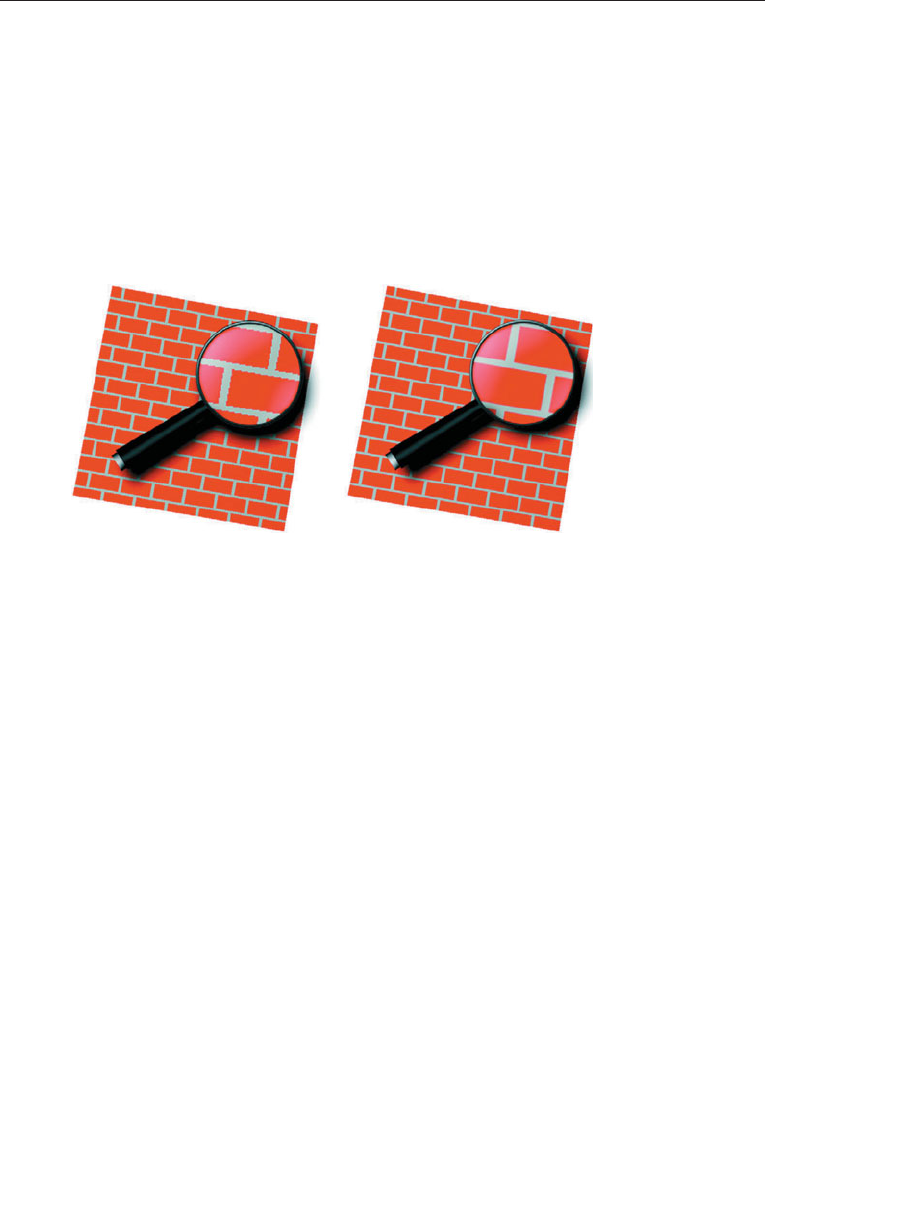
ptg9898810
The result is divided by the area of the filter (a box filter is assumed in this
case) to obtain the average value for the function in the selected interval.
Antialiased Brick Fragment Shader
Now we can put all this to work to build better bricks. We replace the
simple point sampling technique with analytic integration. The resulting
shader is shown in Example 8.12. The difference between the aliased and
antialiased brick shaders is shown in Figure 8.19.
Figure 8.19 Brick shader with and without antialiasing
(On the left, the results of the brick shader without antialiasing. On the
right, results of antialiasing by analytic integration. (3Dlabs, Inc.))
Example 8.12 Source Code for an Antialiased Brick Fragment Shader
#version 330 core
uniform vec3 BrickColor, MortarColor;
uniform vec2 BrickSize;
uniform vec2 BrickPct;
uniform vec2 MortarPct;
in vec2 MCPosition;
in float LightIntensity;
out vec4 FragColor;
#define Integral(x, p, notp) ((floor(x)*(p)) + max(fract(x)-(notp), 0.0))
void main()
{
vec2 position, fw, useBrick;
vec3 color;
// Determine position within the brick pattern
456 Chapter 8: Procedural Texturing

ptg9898810
position = MCPosition / BrickSize;
// Adjust every other row by an offset of half a brick
if (fract(position.y *0.5) > 0.5)
position.x += 0.5;
// Calculate filter size
fw = fwidth(position);
// Perform filtering by integrating the 2D pulse made by the
// brick pattern over the filter width and height
useBrick = (Integral(position + fw, BrickPct, MortarPct) -
Integral(position, BrickPct, MortarPct)) / fw;
// Determine final color
color = mix(MortarColor, BrickColor, useBrick.x *useBrick.y);
color *= LightIntensity;
FragColor = vec4(color, 1.0);
}
Frequency Clamping
Certain functions do not have an analytic solution, or they are just too
difficult to solve. If this is the case, you might try a technique called
frequency clampings. In this technique, the average value of the function
replaces the actual value of the function when the filter width is too large.
This is convenient for functions such as sine and noise, whose average is
known.
Antialiased Checkerboard Fragment Shader
The checkerboard pattern is the standard measure of the quality of an
antialiasing technique (see Figure 8.20). Larry Gritz wrote a checkerboard
RenderMan shader that performs antialiasing by frequency sampling,
and Dave Baldwin translated this shader to GLSL. Example 8.13 shows
a fragment shader that produces a procedurally generated, antialiased
checkerboard pattern. The vertex shader transforms the vertex position
and passes along the texture coordinate, nothing more. The application
provides values for the two colors of the checkerboard pattern, the average
of these two colors (the application can compute this and provide it through
a uniform variable, rather than having the fragment shader compute
it for every fragment), and the frequency of the checkerboard pattern.
The fragment shader computes the appropriate size of the filter and uses it
to perform smooth interpolation between adjoining checkerboard squares.
If the filter is too wide (i.e., the in variable is changing too quickly for
proper filtering), the average color is substituted. Even though this
fragment shader uses a conditional statement, care is taken to avoid
aliasing. In the transition zone between the if clause and the else clause,
Antialiasing Procedural Textures 457
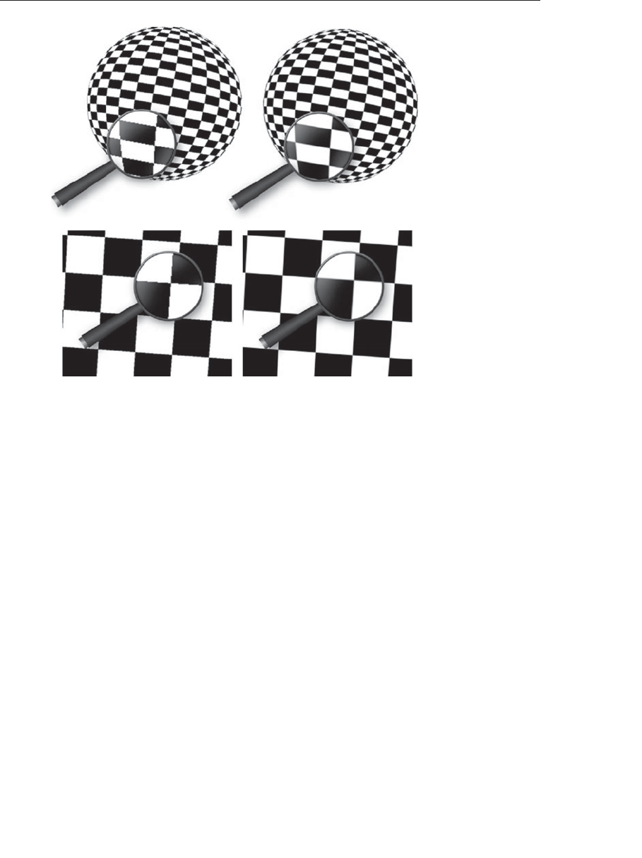
ptg9898810
Figure 8.20 Checkerboard pattern
(Rendered with the antialiased checkerboard shader. On the left, the filter
width is set to 0, so aliasing occurs. On the right, the filter width is computed
using the fwidth() function.)
a smooth interpolation is performed between the computed color and the
average color.
Example 8.13 Source Code for an Antialiased Checkerboard
Fragment Shader
#version 330 core
uniform vec3 Color0;
uniform vec3 Color1;
uniform vec3 AvgColor;
uniform float Frequency;
in vec2 TexCoord;
out vec4 FragColor;
void main()
{
vec3 color;
458 Chapter 8: Procedural Texturing

ptg9898810
// Determine the width of the projection of one pixel into
// s-t space
vec2 fw = fwidth(TexCoord);
// Determine the amount of fuzziness
vec2 fuzz = fw *Frequency *2.0;
float fuzzMax = max(fuzz.s, fuzz.t);
// Determine the position in the checkerboard pattern
vec2 checkPos = fract(TexCoord *Frequency);
if (fuzzMax < 0.5)
{// If the filter width is small enough,
// compute the pattern color
vec2 p = smoothstep(vec2(0.5), fuzz + vec2(0.5), checkPos) +
(1.0 - smoothstep(vec2(0.0), fuzz, checkPos));
color = mix(Color0, Color1,
p.x *p.y + (1.0 - p.x) *(1.0 - p.y));
// Fade in the average color when we get close to the limit
color=mix(color,AvgColor,smoothstep(0.125,0.5,fuzzMax));
}
else
{// Otherwise, use only the average color
color = AvgColor;
}
FragColor = vec4(color, 1.0);
}
Procedural Antialiasing Summary
With increased freedom comes increased responsibility. The OpenGL
Shading Language permits the computation of procedural textures without
restriction. It is quite easy to write a shader that exhibits unsightly aliasing
artifacts (using a conditional or a step function is all it takes), and it can be
difficult to eliminate these artifacts. After describing the aliasing problem
in general terms, this chapter explored several options for antialiasing
procedural textures. Facilities in the language, such as the built-in
functions for smooth interpolation (smoothstep()), for determining
derivatives in screen space (dFdx(),dFdy()), and for estimating filter width
(fwidth()) can assist in the fight against jaggies, moiré patterns, and
sparkling points. These functions were fundamental components of
shaders that were presented to perform antialiasing by prefiltering,
adaptive prefiltering, integration, and frequency clamping.
Antialiasing Procedural Textures 459

ptg9898810
Noise
In computer graphics, it’s easy to make things look good. By definition,
geometry is drawn and rendered precisely. However, when realism is a goal,
perfection isn’t always such a good thing. Real-world objects have dents
and dings and scuffs. They show wear and tear. Computer graphics artists
have to work hard to make a perfectly defined bowling pin look like it has
been used and abused for 20 years in a bowling alley or to make a spaceship
that seems a little worse for wear after many years of galactic travel.
This was the problem that Ken Perlin was trying to solve when he worked
for a company called Magi in the early 1980s. Magi was working with
Disney on the original feature film Tron that was the most ambitious
film in its use of computer graphics until that time. Perlin recognized
the ‘‘imperfection’’ of the perfectly rendered objects in that film, and he
resolved to do something about it, with techniques still highly useful today.
In a seminal paper published in 1985, Perlin described a renderer that he
had written that used a technique he called noise. His definition of noise was
a little different from the common definition of noise. Normally, when we
refer to noise, we’re referring to something like a random changing pattern
of pixels on an old television with no signal (also called snow) or a grainy
image taken with a digital camera in low light, induced by thermal noise.
However, an always changing randomness like this isn’t that useful for
computer graphics. For computer graphics, we need a function that is
repeatable so that an object can be drawn from different view angles. We
also need the ability to draw the object the same way, frame after frame, in
an animation. Normal random-number functions do not depend on any
input location, so an object rendered with such a function would look
different each time it was drawn.
The visual artifacts caused by this type of rendering would look horrible as
the object was moved around the screen. What is needed is a function that
produces the same output value for a given input location every time and
yet gives the appearance of randomness. That is, for a typical surface, we
want random variation across space, but not across time, unless that is also
desired. This function also needs to be continuous at all levels of detail, fast
to compute, and have some other important properties discussed shortly.
Perlin was the first to come up with a usable function, Perlin noise, for that
purpose. Since then, a variety of similar noise functions have been defined
and used in combinations to produce interesting rendering effects such as
•Rendering natural phenomena (clouds, fire, smoke, wind effects, etc.)
•Rendering natural materials (marble, granite, wood, mountains, etc.)
460 Chapter 8: Procedural Texturing

ptg9898810
•Rendering man-made materials (stucco, asphalt, cement, etc.)
•Adding imperfections to perfect models (rust, dirt, smudges, dents, etc.)
•Adding imperfections to perfect patterns (wiggles, bumps, color
variations, etc.)
•Adding imperfections to time periods (time between blinks, amount of
change between successive frames, etc.)
•Adding imperfections to motion (wobbles, jitters, bumps, etc.)
Actually, the list is endless. Today, most rendering libraries include support
for Perlin noise or something nearly equivalent. It is a staple of realistic
rendering, and it’s been heavily used in the generation of computer
graphics images for the movie industry. For his groundbreaking work in
this area, Perlin was presented with an Academy Award for technical
achievement in 1997.
Because noise is such an important technique, it is included as a built-in
function in the OpenGL Shading Language. However, not all GLSL
platforms implement it, or implement it in exactly the same way. So if you
need maximum portability, you’ll want to use methods you have complete
control over, giving complete portability. We’ll focus on such a portable
method in this section.
Once you have a source of noise, there are several ways to make use of it
within a fragment shader. After laying the groundwork for a portable
noise, we take a look at several shader examples that employ noise to
achieve a variety of interesting effects.
Definition of Noise
The purpose of this section is to provide a definition and enough of an
intuitive feel that you can grasp the noise-based OpenGL shaders presented
in this section and then use GLSL to create additional noise-based effects.
As Ken Perlin describes it, you can think of noise as ‘‘seasoning’’ for graphics.
It often helps to add a little noise. A perfect model looks a little less perfect
and, therefore, a little more realistic if some subtle noise effects are applied.
The ideal noise function has the following important qualities that make it
the valuable tool we need for creating a variety of interesting effects,
needed for successful use in modeling, rendering, or animation:
•It does not show any obvious regular or repeated patterns.
•It is a continuous function, and its derivative is also continuous. That
is, there are no sudden steps or sharp bends, only smooth variation,
Noise 461
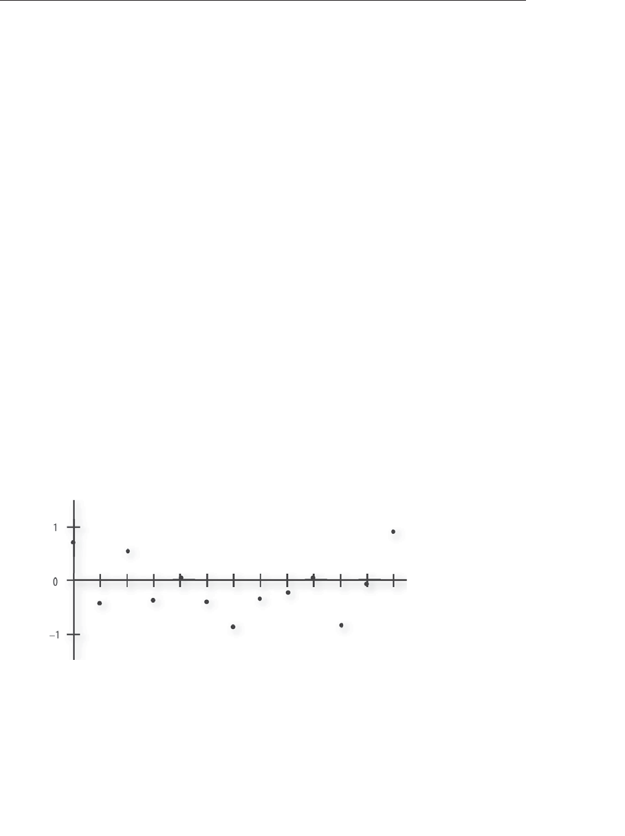
ptg9898810
and zooming in to smaller and smaller scales still shows only smooth
variation.
•It is a function that is repeatable across time (i.e., it generates the same
value each time it is presented with the same input).
•It has a well-defined range of output values (usually the range is [−1, 1]
or [0, 1]).
•It is a function whose small-scale form is roughly independent of
large-scale position (there is an underlying frequency to variation, or
statistical character, that is the same everywhere).
•It is a function that is isotropic (its statistical character is the same in
all directions).
•It can be defined for 1, 2, 3, 4, or even more dimensions.
•It is fast to compute for any given input.
In practice, all this adds up to a noise function that quickly and smoothly
perturbs, or adds an apparent element of ‘‘randomness’’, to an initial
regular periodic pattern, for example, taking a normal square grid and
moving each intersection a bit in a some psuedo-random direction. A
variety of functions can do this, but each makes various trade-offs in
quality and performance, so they meet the preceding criteria with varying
degrees of success.
We can construct a simple noise function (called value noise by Peachey) by
first assigning a pseudorandom number in the range [−1, 1]to each integer
value along the xaxis, as shown in Figure 8.21, and then smoothly
Figure 8.21 A discrete 1D noise function
462 Chapter 8: Procedural Texturing
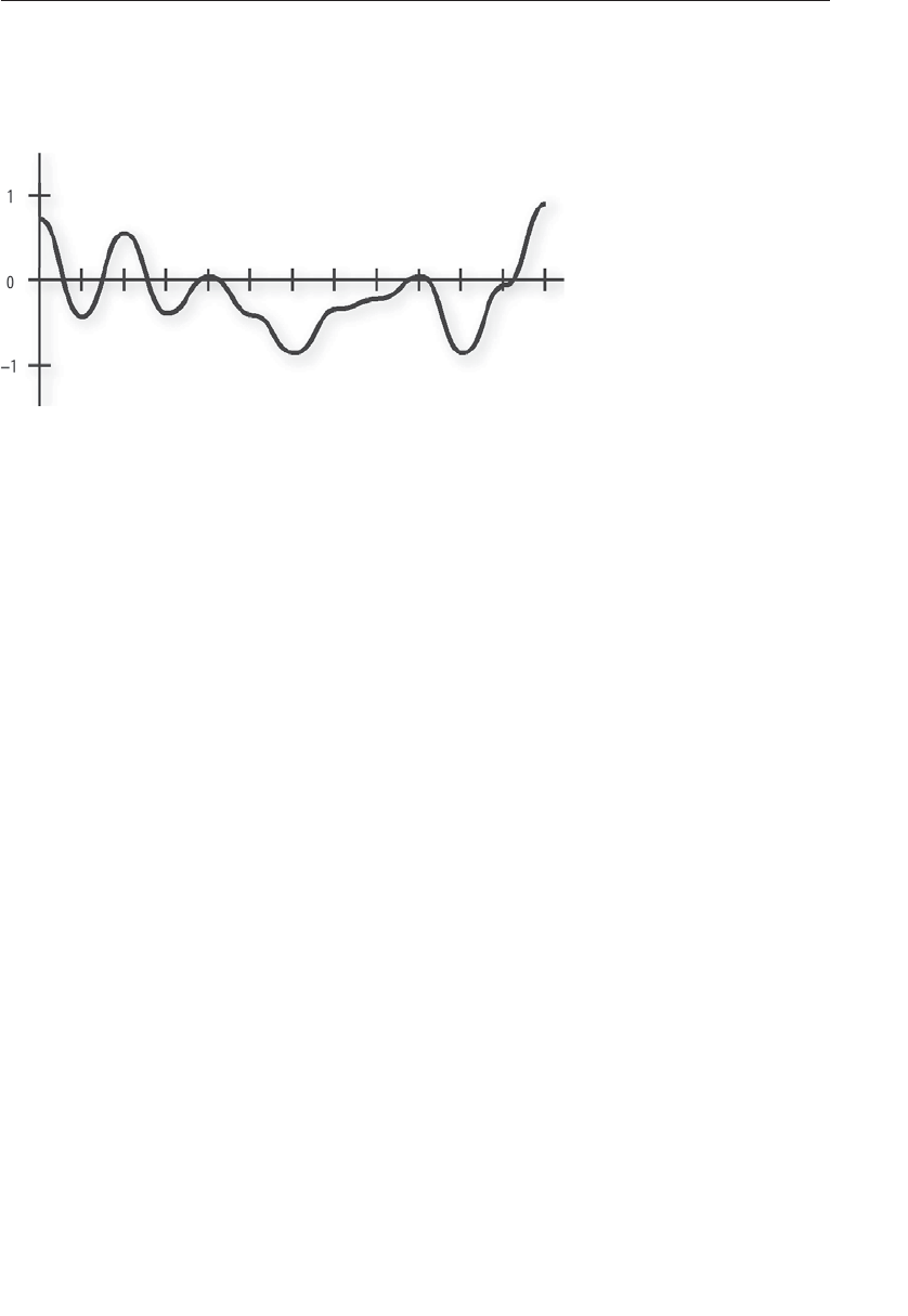
ptg9898810
interpolating between these points, as shown in Figure 8.22. The function
is repeatable in that, for a given input value, it always returns the same
output value.
Figure 8.22 A continuous 1D noise function
A key choice to be made in this type of noise function is the method used
to interpolate between successive points. Linear interpolation is not good
enough because it is not continuous, making the resulting noise pattern
show obvious artifacts. A cubic interpolation method is usually used to
produce smooth-looking results.
By varying the frequency and the amplitude, you can get a variety of noise
functions (see Figure 8.23).
As you can see, the ‘‘features’’ in these functions get smaller and closer
together as the frequency increases and the amplitude decreases.
When two frequencies are related by a ratio of 2:1, it’s called an octave.
Figure 8.23 illustrates five octaves of the 1D noise function. These images
of noise don’t look all that useful, but by themselves they can provide
some interesting characteristics to shaders. If we add the functions at
different frequencies (see Figure 8.24), we start to see something that looks
even more interesting.
The result is a function that contains features of various sizes. The larger
bumps from the lower-frequency functions provide the overall shape,
whereas the smaller bumps from the higher-frequency functions provide
detail and interest at a smaller scale. The function that results from
summing the noise of consecutive octaves, each at half the amplitude of
the previous octave, was called 1/fnoise by Perlin, but the terms fractional
Brownian motion or fBm are used more commonly today.
If you sum octaves of noise in a procedural shader, at some point you will
begin to add frequencies that cause aliasing artifacts. When the frequency
Noise 463
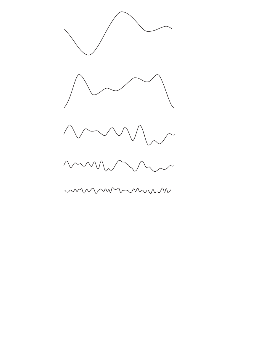
ptg9898810
frequency 5 4
amplitude 5 1.0
frequency 5 8
amplitude 5 0.5
frequency 5 16
amplitude 5 0.25
frequency 5 32
amplitude 5 0.125
frequency 5 64
amplitude 5 0.0625
Figure 8.23 Varying the frequency and the amplitude of the noise
function
of noise is greater than twice the frequency of sampling (e.g., pixel
spacing), you really do start getting random sample values that will cause
the flickering forms of aliasing. Hence, algorithms for antialiasing noise
functions typically stop adding detail (higher-frequency noise) before this
occurs. This is another useful feature of the noise function---it can be faded
to the average sample value at the point at which aliasing artifacts would
begin to occur.
The noise function defined by Perlin (Perlin noise) is sometimes called
gradient noise. It is defined as a function whose value is 0 at each integer
input value, and its shape is created by defining a pseudorandom gradient
vector for the function at each of these points. The characteristics of this
noise function make it a somewhat better choice, in general, for the effects
we’re after. It is used for the implementation of the noise function in
464 Chapter 8: Procedural Texturing
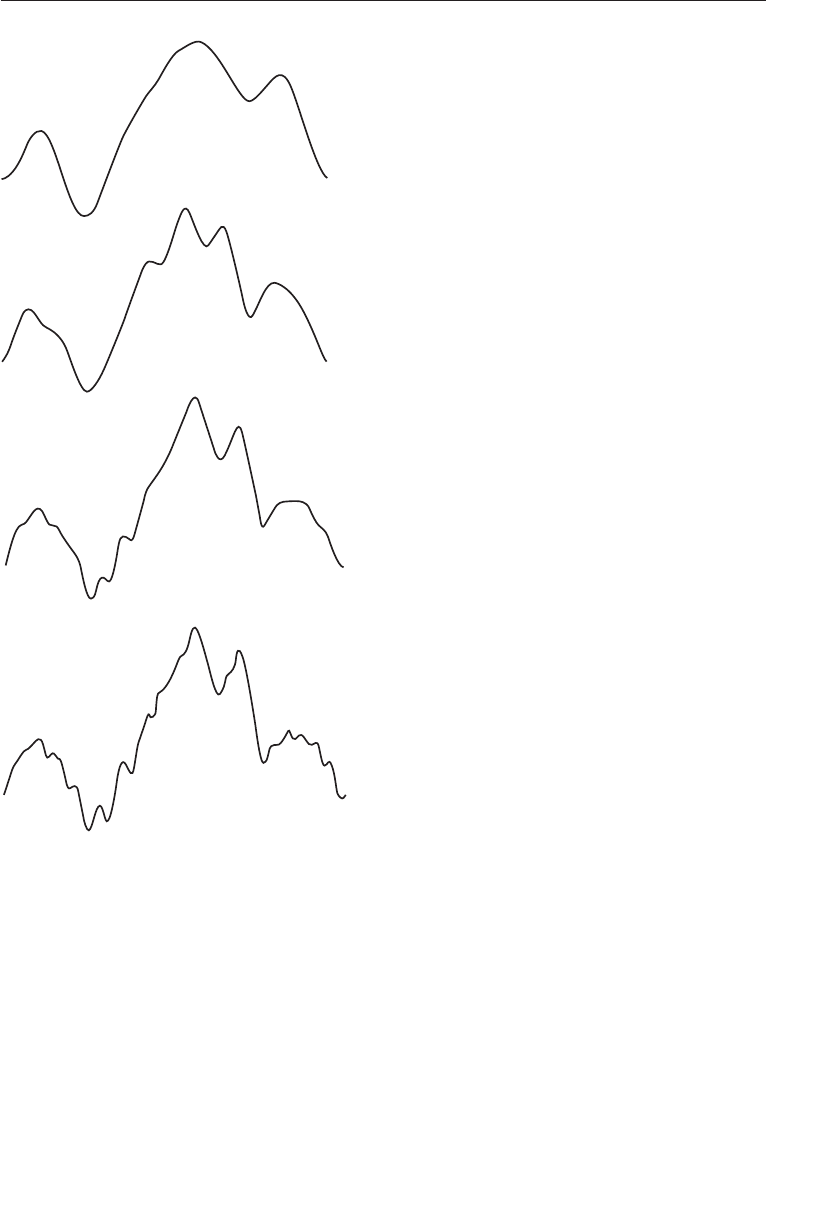
ptg9898810
sum of 2 octaves
sum of 3 octaves
sum of 4 octaves
sum of 5 octaves
Figure 8.24 Summing noise functions
(Shows the result of summing noise functions of different amplitude and
frequency.)
RenderMan, and it is also intended to be used for implementations of the
noise function built into GLSL.
Lots of other noise functions have been defined, and there are many ways
to vary the basic ideas. The examples of Perlin noise shown previously
have a frequency multiplier of 2, but it can be useful to use a frequency
Noise 465

ptg9898810
multiplier, such as 2.21, that is not an integer value. This frequency
multiplier is called the lacunarity of the function. The word comes from the
Latin word lacuna, which means gap. Using a value larger than 2 allows us
to build up more ‘‘variety’’ more quickly (e.g., by summing fewer octaves
to achieve the same apparent visual complexity). Similarly, it is not
necessary to divide the amplitude of each successive octave by 2.
Summed noise functions are the basis for the terrain and features found
in the planet-building software package MojoWorld from Pandromeda.
In Texturing and Modeling: A Procedural Approach, Ken Musgrave defines a
fractal as ‘‘a geometrically complex object, the complexity of which arises
through the repetition of a given form over a range of scales’’. The
relationship between the change in frequency and the change in
amplitude determines the fractal dimension of the resulting function. If we
use a noise function as the basis for generating a terrain model, we can
take steps to make it behave differently at different locations. For instance,
natural terrain has plains, rolling hills, foothills, and mountains.
Varying the fractal dimension based on location can create a similar
appearance---such a function is called a multifractal.
You can achieve interesting effects by using different noise functions for
different situations or by combining noise functions of different types. It’s
not that easy to visualize in advance the results of calculations that depend
on noise values, so varied experience will be a key ally as you try to achieve
the effect you’re after.
2D Noise
Armed with a basic idea of what the noise function looks like in one
dimension, we can take a look at two-dimensional noise. Figure 8.25
contains images of 2D Perlin noise at various frequencies mapped into the
range [0, 1]and displayed as a grayscale image. Each successive image is
twice the frequency of the previous one. In each image, the contrast has
been enhanced to make the peaks brighter and the valleys darker. In actual
use, each subsequent image has an average that is half the previous one
and an amplitude that is half the previous one. If we were to print images
of the actual values, the images would be much grayer, and it would be
harder to see what 2D noise really looks like.
As in the 1D case, adding the different frequency functions provides more
interesting results (Figure 8.26).
466 Chapter 8: Procedural Texturing
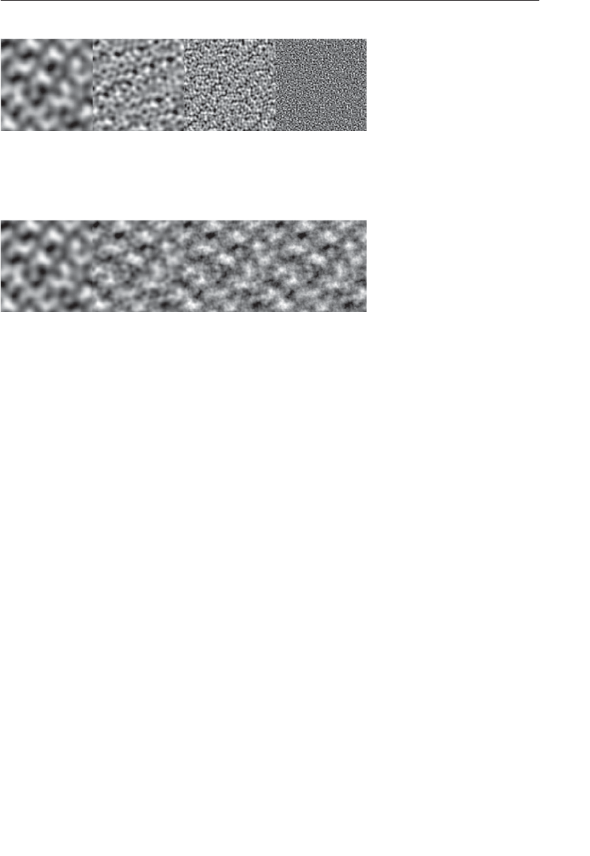
ptg9898810
Figure 8.25 Basic 2D noise, at frequencies 4, 8, 16, and 32
(contrast enhanced)
Figure 8.26 Summed noise, at 1, 2, 3, and 4 octaves
(contrast enhanced)
The first image in Figure 8.26 is exactly the same as the first image in
Figure 8.25. The second image in Figure 8.26 is the sum of the first image
in Figure 8.26 plus half of the second image in Figure 8.25 shifted so that
its average intensity value is 0. This causes intensity to be increased in
some areas and decreased in others. The third image in Figure 8.26
adds the third octave of noise to the first two, and the fourth image in
Figure 8.26 adds the fourth octave. The fourth picture is starting to
look a little bit like clouds in the sky.
Higher Dimensions of Noise
3D and 4D noise functions are obvious extensions of the 1D and 2D
functions. It’s a little hard to generate pictures of 3D noise, but the images
in Figure 8.25 can be thought of as 2D slices out of a 3D noise function.
Neighboring slices have continuity between them.
Often, a higher dimension of noise is used to control the time aspect of the
next lower-dimension noise function. For instance, 1D noise can add some
wiggle to otherwise straight lines in a drawing. If you have a 2D noise
function, one dimension can control the wiggle, and the second
dimension can animate the effect (i.e., make the wiggles move in
successive frames). Similarly, a 2D noise function can create a 2D cloud
pattern, whereas a 3D noise function can generate the 2D cloud pattern
Noise 467

ptg9898810
and animate it in a realistic way. With a 4D noise function, you can create
a 3D object like a planet, and use the fourth dimension to watch it evolve
in ‘‘fits and starts’’.
Using Noise in the OpenGL Shading Language
You include noise in a shader in the following three ways:
1. Use GLSL built-in noise functions.
2. Write your own noise function in GLSL.
3. Use a texture map to store a previously computed noise function.
With today’s graphics systems, options 2 and 3 give the best portability,
and option 3 typically gives the best performance. Here, we will focus on
techniques based on option 3. Option 3 is not done to the exclusion of
options 1 and 2, as the ‘‘previously computed noise function’’ comes from
them. The difference is really whether the function is computed on the fly
for arbitrary inputs (options 1 and 2), or precomputed and stored away for
a predetermined set of inputs (option 3), typically as a texture map.
Noise Textures
The programmability offered by GLSL lets us use values stored in texture
memory in new and unique ways. We can precompute a noise function
and save it in a 1D, 2D, or 3D texture map. We can then access this texture
map (or texture maps) from within a shader. Because textures can contain
up to four components, we can use a single texture map to store four
octaves of noise or four completely separate noise functions.
Example 8.14 shows a ‘‘C’’ function that generates a 3D noise texture. This
function creates an RGBA texture with the first octave of noise stored in
the red texture component, the second octave stored in the green texture
component, the third octave stored in the blue component, and the fourth
octave stored in the alpha component. Each octave has twice the
frequency and half the amplitude as the previous one.
This function assumes the existence of a noise3 function that can generate
3D noise values in the range [−1, 1]. If you want, you can start with Perlin’s
C implementation. John Kessenich made some changes to that code
(adding a setNoiseFrequency function) to produce noise values that wrap
smoothly from one edge of the array to the other. This means we can use
the texture with the wrapping mode set to GL_REPEAT, and we won’t see
any discontinuities in the function when it wraps. The revised version of
the code is in the GLSLdemo program from 3Dlabs.
468 Chapter 8: Procedural Texturing

ptg9898810
Example 8.14 C function to Generate a 3D Noise Texture
int noise3DTexSize = 128;
GLuint noise3DTexName = 0;
GLubyte *noise3DTexPtr;
void make3DNoiseTexture(void)
{
int f, i, j, k, inc;
int startFrequency = 4;
int numOctaves = 4;
double ni[3];
double inci, incj, inck;
int frequency = startFrequency;
GLubyte *ptr;
double amp = 0.5;
if ((noise3DTexPtr = (GLubyte *) malloc(noise3DTexSize *
noise3DTexSize *
noise3DTexSize *4))
== NULL)
{
fprintf(stderr,
"ERROR: Could not allocate 3D noise texture\n");
exit(1);
}
for (f = 0, inc = 0; f < numOctaves;
++f, frequency *= 2, ++inc, amp *= 0.5)
{
setNoiseFrequency(frequency);
ptr = noise3DTexPtr;
ni[0] = ni[1] = ni[2] = 0;
inci = 1.0 / (noise3DTexSize / frequency);
for (i = 0; i < noise3DTexSize; ++i, ni[0] += inci)
{
incj = 1.0 / (noise3DTexSize / frequency);
for (j = 0; j < noise3DTexSize; ++j, ni[1] += incj)
{
inck = 1.0 / (noise3DTexSize / frequency);
for (k = 0; k < noise3DTexSize;
++k, ni[2] += inck, ptr += 4)
{
*(ptr+inc) = (GLubyte)(((noise3(ni)+1.0) *amp)
*128.0);
}
}
}
}
}
Noise 469

ptg9898810
This function computes noise values for four octaves of noise and stores
them in a 3D RGBA texture of size 128 ×128 ×128. This code also assumes
that each component of the texture is stored as an 8-bit integer value. The
first octave has a frequency of 4 and an amplitude of 0.5. In the innermost
part of the loop, we call the noise3 function to generate a noise value
based on the current value of ni. The noise3 function returns a value in
the range [−1, 1], so by adding 1, we end up with a noise value in the range
[0, 2]. Multiplying by our amplitude value of 0.5 gives a value in the range
[0, 1]. Finally, we multiply by 128 to give us an integer value in the range
[0, 128]that can be stored in the red component of a texture. (When
accessed from within a shader, the value is a floating-point value in the
range [0, 0.5].)
The amplitude value is cut in half and the frequency is doubled in each
pass through the loop. The result is that integer values in the range [0, 64]
are stored in the green component of the noise texture, integer values in
the range [0, 32]are stored in the blue component of the noise texture, and
integer values in the range [0, 16]are stored in the alpha component of the
texture. We generated the images in Figure 8.25 by looking at each of these
channels independently after scaling the values by a constant value that
allowed them to span the maximum intensity range (i.e., integer values in
the range [0, 255]or floating-point values in the range [0, 1]).
After the values for the noise texture are computed, the texture can be
provided to the graphics hardware with the code in Example 8.15. First, we
pick a texture unit and bind to it the 3D texture we’ve created. We set up
its wrapping parameters so that the texture wraps in all three dimensions.
This way, we always get a valid result for our noise function no matter
what input values are used. We still have to be somewhat careful to avoid
using the texture in a way that makes obvious repeating patterns. The next
two lines set the texture-filtering modes to linear because the default is
mipmap linear and we’re not using mipmap textures here. We are
controlling the scaling factors from within our noise shaders, so a single
texture is sufficient.
Though we won’t go into it more deeply here, using a mipmapped texture
will improve quality when using a broad range of level of detail. When
zoomed in, to avoid seeing blockiness in the noise, you’ll need a base texel
frequency two times greater than the highest-frequency noise. When
zoomed out, you’ll need a properly filtered mipmap to avoid seeing aliasing
when the pixel frequency approaches or surpasses the noise frequency.
When all the parameters are set up, we can download the noise texture to
the hardware by using the glTexImage3D function.
470 Chapter 8: Procedural Texturing

ptg9898810
Example 8.15 A Function for Activating the 3D Noise Texture
void init3DNoiseTexture()
{
glGenTextures(1, & noise3DTexName);
glActiveTexture(GL_TEXTURE6);
glBindTexture(GL_TEXTURE_3D, noise3DTexName);
glTexParameterf(GL_TEXTURE_3D, GL_TEXTURE_WRAP_S, GL_REPEAT);
glTexParameterf(GL_TEXTURE_3D, GL_TEXTURE_WRAP_T, GL_REPEAT);
glTexParameterf(GL_TEXTURE_3D, GL_TEXTURE_WRAP_R, GL_REPEAT);
glTexParameterf(GL_TEXTURE_3D, GL_TEXTURE_MAG_FILTER, GL_LINEAR);
glTexParameterf(GL_TEXTURE_3D, GL_TEXTURE_MIN_FILTER, GL_LINEAR);
glTexImage3D(GL_TEXTURE_3D, 0, GL_RGBA, noise3DTexSize,
noise3DTexSize, noise3DTexSize, 0, GL_RGBA,
GL_UNSIGNED_BYTE, noise3DTexPtr);
}
This is an excellent approach if the period of repeatability can be avoided
in the final rendering. One way to avoid it is to make sure that no texture
value is accessed more than once when the target object is rendered. For
instance, if a 128 ×128 ×128 texture is being used and the position on the
object is used as the input to the noise function, the repeatability won’t be
visible if the entire object fits within the texture.
Trade-offs
As previously mentioned, three methods can be used to generate noise
values in a shader. How do you know which is the best choice for your
application? A lot depends on the underlying implementation, but
generally speaking, if we assume a hardware computation of noise that
does not use texturing, the points favoring usage of GLSL built-in noise
function are the following:
•It doesn’t consume any texture memory (a 128 ×128 ×128 texture
map stored as RGBA with 8 bits per component uses 8MB of texture
memory).
•It doesn’t use a texture unit.
•It is a continuous function rather than a discrete one, so it does not
look ‘‘pixelated’’ no matter what the scaling is.
•The repeatability of the function should be undetectable, especially for
2D and 3D noise (but it depends on the hardware implementation).
•Shaders written with the built-in noise function don’t depend on the
application to set up appropriate textures.
Noise 471

ptg9898810
The advantages of using a texture map to implement the noise function
are as follows:
•Because the noise function is computed by the application, the appli-
cation has total control of this function and can ensure matching
behavior on every hardware platform.
•You can store four noise values (i.e., one each for the R, G, B, and A
values of the texture) at each texture location. This lets you
precompute four octaves of noise, for instance, and retrieve all four
values with a single texture access.
•Accessing a texture map may be faster than calling the built-in noise
function.
User-defined functions can implement noise functions that provide
a different appearance from that of the built-in noise functions. A
user-defined function can also provide matching behavior on every
platform, whereas the built-in noise functions cannot (at least not until all
graphics hardware developers support the noise function in exactly the
same way). But hardware developers will optimize the built-in noise
function, perhaps accelerating it with special hardware, so it is apt to be
faster than user-defined noise functions.
In the long run, using the built-in noise function or user-defined noise
functions will be the way to go for most applications. This will result
in noise that doesn’t show a repetitive pattern, has greater numerical
precision, and doesn’t use up any texture resources. Applications that want
full control over the noise function and can live within the constraints of a
fixed-size noise function can be successful using textures for their noise.
With current generation hardware, noise textures may also provide better
performance and require fewer instructions in the shader.
A Simple Noise Shader
Now we put all these ideas into some shaders that do some interesting
rendering for us. The first shader we look at uses noise in a simple way to
produce a cloud effect.
Application Setup
Very little needs to be passed to the noise shaders discussed in this section,
or in ‘‘Turbulence’’ and ‘‘Granite’’. The vertex position must be passed
in as always, and the surface normal is needed for performing lighting
computations. Colors and scale factors are parameterized as uniform
variables for the various shaders.
472 Chapter 8: Procedural Texturing

ptg9898810
Vertex Shader
The code shown in Example 8.16 is the vertex shader that we use for the
four noise fragment shaders that follow. It is fairly simple because it really
only needs to accomplish three things.
•As in all vertex shaders, our vertex shader transforms the incoming
vertex value and stores it in the built-in special variable gl_Position.
•Using the incoming normal and the uniform variable LightPos, the
vertex shader computes the light intensity from a single white light
source and applies a scale factor of 1.5 to increase the amount of
illumination.
•The vertex shader scales the incoming vertex value and stores it in the
out variable MCposition. This value is available to us in our fragment
shader as the modeling coordinate position of the object at every
fragment. It is an ideal value to use as the input for our 3D texture
lookup.
No matter how the object is drawn, fragments always produce the same
position values (or very close to them); therefore, the noise value obtained
for each point on the surface is also the same (or very close to it). The
application can set a uniform variable called Scale to optimally scale the
object in relationship to the size of the noise texture.
Example 8.16 Cloud Vertex Shader
#version 330 core
uniform mat4 MVMatrix;
uniform mat4 MVPMatrix;
uniform mat3 NormalMatrix;
uniform vec3 LightPos;
uniform float Scale;
in vec4 MCvertex;
in vec3 MCnormal;
out float LightIntensity;
out vec3 MCposition;
void main()
{
vec3 ECposition = vec3(MVMatrix *MCVertex);
MCposition = vec3(MCVertex) *Scale;
vec3 tnorm = normalize(vec3(NormalMatrix *MCNormal));
LightIntensity = dot(normalize(LightPos - ECposition), tnorm);
LightIntensity *= 1.5;
gl_Position = MVPMatrix *MCVertex;
}
Noise 473

ptg9898810
Fragment Shader
After we’ve computed a noise texture and used OpenGL calls to download
it to the graphics card, we can use a fairly simple fragment shader together
with the vertex shader described in the previous section to make an
interesting ‘‘cloudy sky’’ effect (see Example 8.17). This shader results in
something that looks like the sky on a mostly cloudy day. You can
experiment with the color values to get a result that is visually pleasing.
This fragment shader receives as input the two in variables---
LightIntensity and MCposition---that were computed by the vertex
shader shown in the previous section. These values were computed at each
vertex by the vertex shader and then interpolated across the primitive by
the rasterization hardware. Here, in our fragment shader, we have access to
the interpolated value of each of these variables at every fragment.
The first line of code in the shader performs a 3D texture lookup on our 3D
noise texture to produce a four-component result. We compute the value
of intensity by summing the four components of our noise texture. This
value is then scaled by 1.5 and used to perform a linear blend between two
colors: white and sky blue. The four channels in our noise texture have
mean values of 0.25, 0.125, 0.0625, and 0.03125. An additional 0.03125
term is added to account for the average values of all the octaves at higher
frequencies. You can think of this as fading to the average values of all the
higher frequency octaves that aren’t being included in the calculation, as
described earlier in ‘‘Definition of Noise’’. Scaling the sum by 1.5 stretches
the resulting value to use up more of the range from [0, 1].
The computed color is then scaled by LightIntensity value to simulate
a diffuse surface lit by a single light source. The result is assigned to the out
variable FragColor with an alpha value of 1.0 to produce the color value
that is used by the remainder of the OpenGL pipeline. An object rendered
with this shader is shown in Figure 8.27. Notice that the texture on the
teapot looks a lot like the final image in Figure 8.26.
Example 8.17 Fragment Shader for Cloudy Sky Effect
#version 330 core
uniform sampler3D Noise;
uniform vec3 SkyColor; // (0.0, 0.0, 0.8)
uniform vec3 CloudColor; // (0.8, 0.8, 0.8)
in float LightIntensity;
in vec3 MCposition;
out vec4 FragColor;
474 Chapter 8: Procedural Texturing
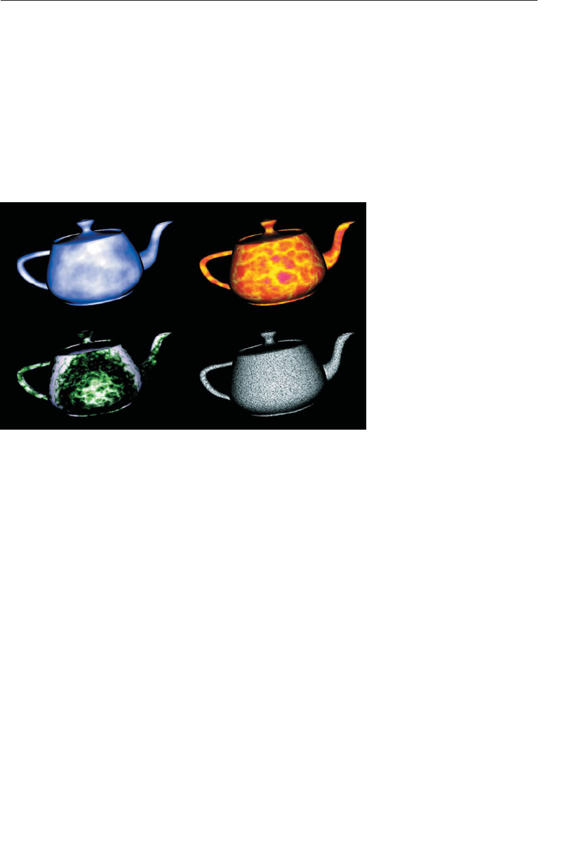
ptg9898810
void main()
{
vec4 noisevec = texture(Noise, MCposition);
float intensity = (noisevec[0] + noisevec[1] +
noisevec[2] + noisevec[3] + 0.03125) *1.5;
vec3 color = mix(SkyColor, CloudColor, intensity) *
LightIntensity;
FragColor = vec4(color, 1.0);
}
Figure 8.27 Teapots rendered with noise shaders
(Clockwise from upper left: a cloud shader that sums four octaves of
noise and uses a blue-to-white color gradient to code the result; a sun
surface shader that uses the absolute value function to introduce discon-
tinuities (turbulence); a granite shader that uses a single high-frequency
noise value to modulate between white and black; a marble shader that uses
noise to modulate a sine function to produce alternating ‘‘veins’’ of color.
(3Dlabs, Inc.))
Turbulence
We can obtain some additional interesting effects by taking the absolute
value of the noise function. This technique introduces a discontinuity of
the derivative because the function folds on itself when it reaches 0. When
this folding is done to noise functions at several frequencies and the results
are summed, the result is cusps or creases in the texture at various scales.
Perlin started referring to this type of noise as turbulence because it is
reminiscent of turbulent flow. It shows up in a variety of places in nature,
Noise 475
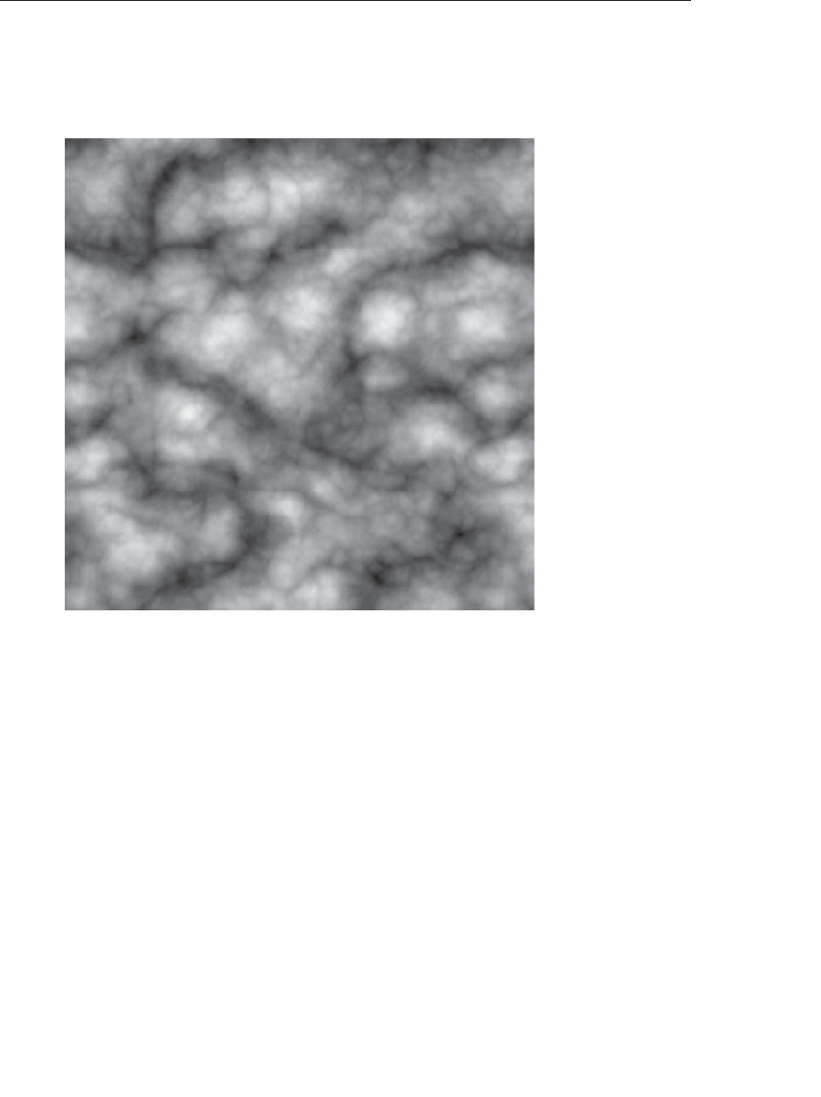
ptg9898810
so this type of noise can be used to simulate various things like flames or
lava. The two-dimensional appearance of this type of noise is shown in
Figure 8.28.
Figure 8.28 Absolute value noise or ‘‘turbulence’’
Sun Surface Shader
We can achieve an effect that looks like a pit of hot molten lava or the
surface of the sun by using the same vertex shader as the cloud shader and
a slightly different fragment shader. The main difference is that we scale
each noise value and shift it over so that it is centered at 0; then we take its
absolute value. After summing the values, we scale the result again to
occupy nearly the full range of [0, 1].We clamp this value and use it to mix
between yellow and red to get the result shown in Figure 8.27 (see
Example 8.18). This technique can be extended to change the results over
time, using another dimension of noise for time, resulting in animation of
the effect.
476 Chapter 8: Procedural Texturing

ptg9898810
Example 8.18 Sun Surface Fragment Shader
#version 330 core
in float LightIntensity;
in vec3 MCposition;
uniform sampler3D Noise;
uniform vec3 Color1; // (0.8, 0.7, 0.0)
uniform vec3 Color2; // (0.6, 0.1, 0.0)
uniform float NoiseScale; // 1.2
out vec4 FragColor;
void main()
{
vec4 noisevec = texture(Noise, MCposition *NoiseScale);
float intensity = abs(noisevec[0] - 0.25) +
abs(noisevec[1] - 0.125) +
abs(noisevec[2] - 0.0625) +
abs(noisevec[3] - 0.03125);
intensity = clamp(intensity *6.0, 0.0, 1.0);
vec3 color = mix(Color1, Color2, intensity) *LightIntensity;
FragColor = vec4(color, 1.0);
}
Marble
Yet another variation on the noise function is to use it as part of a perio-
dic function such as sine. By adding noise to the input value for the sine
function, we get a ‘‘noisy’’ oscillating function. We use this to create
a look similar to the alternating color veins of some types of marble.
Example 8.19 shows the fragment shader to do it. Again, we use the same
vertex shader. Results of this shader are also shown in Figure 8.27.
Example 8.19 Fragment Shader for Marble
#version 330 core
uniform sampler3D Noise;
uniform vec3 MarbleColor;
uniform vec3 VeinColor;
in float LightIntensity;
in vec3 MCposition;
out vec4 FragColor;
Noise 477

ptg9898810
void main()
{
vec4 noisevec = texture(Noise, MCposition);
float intensity = abs(noisevec[0] - 0.25) +
abs(noisevec[1] - 0.125) +
abs(noisevec[2] - 0.0625) +
abs(noisevec[3] - 0.03125);
float sineval = sin(MCposition.y *6.0 + intensity *12.0)
*0.5 + 0.5;
vec3 color = mix(VeinColor, MarbleColor, sineval)
*LightIntensity;
FragColor = vec4(color, 1.0);
}
Granite
With noise, it’s also easy just to try to make stuff up. In this example, we
want to simulate a grayish rocky material with small black specks. To
generate a relatively high-frequency noise texture, we use only the fourth
component (the highest frequency one). We scale it by an arbitrary amount
to provide an appropriate intensity level and then use this value for each
of the red, green, and blue components. The shader in Example 8.20
generates an appearance similar to granite, as shown in Figure 8.27.
Example 8.20 Granite Fragment Shader
#version 330 core
uniform sampler3D Noise;
uniform float NoiseScale;
in float LightIntensity;
in vec3 MCposition;
out vec4 FragColor;
void main()
{
vec4 noisevec = texture(Noise, NoiseScale *MCposition);
float intensity = min(1.0, noisevec[3] *18.0);
vec3 color = vec3(intensity *LightIntensity);
FragColor = vec4(color, 1.0);
}
Wood
We can do a fair approximation of wood with this approach as well. In
Advanced Renderman, Anthony A. Apodaca and Larry Gritz describe a
478 Chapter 8: Procedural Texturing

ptg9898810
model for simulating the appearance of wood. We can adapt their
approach to create wood shaders in GLSL. Following are the basic ideas
behind the wood fragment shader shown in Example 8.21:
•Wood is composed of light and dark areas alternating in concentric
cylinders surrounding a central axis.
•Noise is added to warp the cylinders to create a more natural-looking
pattern.
•The center of the ‘‘tree’’ is taken to be the yaxis.
•Throughout the wood, a high-frequency grain pattern gives the
appearance of wood that has been sawed, exposing the open grain
nature of the wood.
The wood shader uses the same vertex shader as the other noise-based
shaders discussed in this section.
Application Setup
The wood shaders don’t require too much from the application. The
application is expected to pass in a vertex position and a normal, per
vertex, using the usual OpenGL entry points. In addition, the vertex
shader takes a light position and a scale factor that are passed in as
uniform variables. The fragment shader takes a number of uniform
variables that parameterize the appearance of the wood.
The uniform variables needed for the wood shaders are initialized as
follows:
LightPos 0.0, 0.0, 4.0
Scale 2.0
LightWood 0.6, 0.3, 0.1
DarkWood 0.4, 0.2, 0.07
RingFreq 4.0
LightGrains 1.0
DarkGrains 0.0
GrainThreshold 0.5
NoiseScale 0.5, 0.1, 0.1
Noisiness 3.0
GrainScale 27.0
Fragment Shader
Example 8.21 shows the fragment shader for procedurally generated wood.
Noise 479

ptg9898810
Example 8.21 Fragment Shader for Wood
#version 330 core
uniform sampler3D Noise;
uniform vec3 LightWood;
uniform vec3 DarkWood;
uniform float RingFreq;
uniform float LightGrains;
uniform float DarkGrains;
uniform float GrainThreshold;
uniform vec3 NoiseScale;
uniform float Noisiness;
uniform float GrainScale;
in float LightIntensity;
in vec3 MCposition;
out vec4 FragColor;
void main()
{
vec3 noisevec = vec3(texture(Noise, MCposition *NoiseScale) *
Noisiness);
vec3 location = MCposition + noisevec;
float dist = sqrt(location.x *location.x + location.z *location.z);
dist *= RingFreq;
float r = fract(dist + noisevec[0] + noisevec[1] + noisevec[2])
*2.0;
if (r > 1.0)
r = 2.0 - r;
vec3 color = mix(LightWood, DarkWood, r);
r = fract((MCposition.x + MCposition.z) *GrainScale + 0.5);
noisevec[2] *= r;
if (r < GrainThreshold)
color += LightWood *LightGrains *noisevec[2];
else
color -= LightWood *DarkGrains *noisevec[2];
color *= LightIntensity;
FragColor = vec4(color, 1.0);
}
As you can see, we’ve parameterized quite a bit of this shader through the
use of uniform variables to make it easy to manipulate through the
application’s user interface. As in many procedural shaders, the object
position is the basis for computing the procedural texture. In this case, the
object position is multiplied by NoiseScale (a vec3 that allows us to
scale the noise independently in the x,y, and zdirections), and the
computed value is used as the index into our 3D noise texture. The noise
values obtained from the texture are scaled by the value Noisiness,
which allows us to increase or decrease the contribution of the noise.
480 Chapter 8: Procedural Texturing

ptg9898810
Our tree is assumed to be a series of concentric rings of alternating light
wood and dark wood. To give some interest to our grain pattern, we add
the noise vector to our object position. This has the effect of adding our
low-frequency (first octave) noise to the xcoordinate of the position and
the third-octave noise to the zcoordinate (the ycoordinate won’t be used).
The result is rings that are still relatively circular but have some variation
in width and distance from the center of the tree.
To compute where we are in relation to the center of the tree, we square
the xand zcomponents and take the square root of the result. This gives
us the distance from the center of the tree. The distance is multiplied
by RingFreq, a scale factor that gives the wood pattern more rings or
fewer rings.
Following this, we attempt to create a function that goes from 0 up to 1.0
and then back down to 0. We add three octaves of noise to the distance
value to give more interest to the wood grain pattern. We could compute
different noise values here, but the ones we’ve already obtained will do
just fine. Taking the fractional part of the resulting value gives us a
function in the range [0.0, 1.0). Multiplying this value by 2.0 gives us a
function in the range [0.0, 2.0). And finally, by subtracting 1.0 from values
that are greater than 1.0, we get our desired function that varies from 0 to
1.0 and back to 0.
We use this ‘‘triangle’’ function to compute the basic color for the
fragment, using the built-in mix() function. The mix() function linearly
blends LightWood and DarkWood according to our computed value r.
At this point, we would have a pretty nice result for our wood function,
but we attempt to make it a little better by adding a subtle effect to
simulate the look of open-grain wood that has been sawed. (You may not
be able to see this effect on the object shown in Figure 8.29.)
Our desire is to produce streaks that are roughly parallel to the yaxis. So
we add the xand zcoordinates, multiply by the GrainScale factor
(another uniform variable that we can adjust to change the frequency of
this effect), add 0.5, and take the fractional part of the result. Again, this
gives us a function that varies from [0.0, 1.0), but for the default values for
GrainScale (27.0) and RingFreq (4.0), this function for rgoes from 0 to
1.0 much more often than our previous function for r.
We could just make our ‘‘grains’’ go linearly from light to dark, but we try
something a little more subtle. We multiply the value of rby our third
octave noise value to produce a value that increases nonlinearly. Finally,
we compare our value of rto the GrainThreshold value (the default is
0.5). If the value of ris less than GrainThreshold, we modify our current
Noise 481
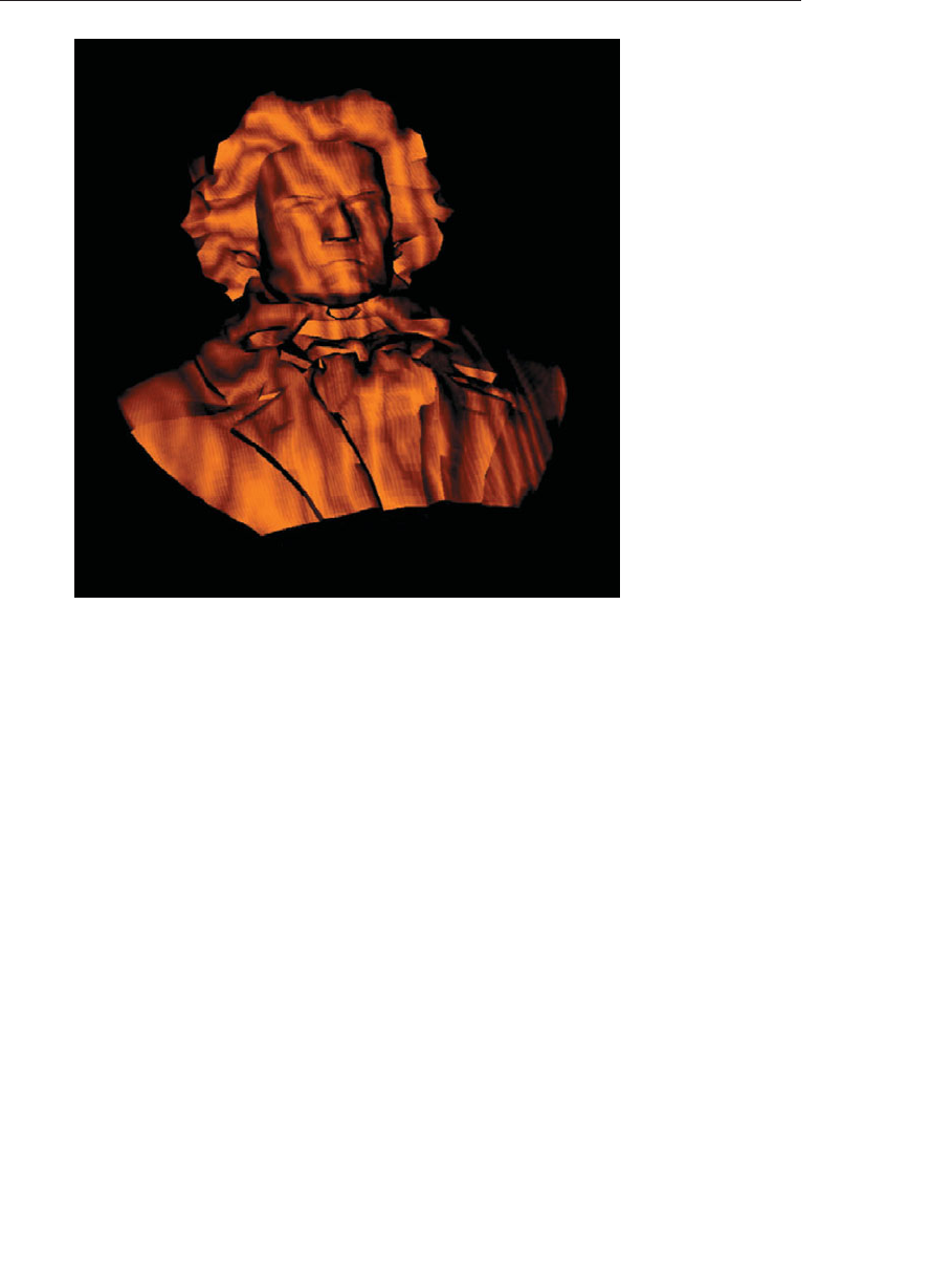
ptg9898810
Figure 8.29 A bust of Beethoven rendered with the wood shader
(3Dlabs, Inc.)
color by adding to it a value we computed by multiplying the LightWood
color, the LightGrains color, and our modified noise value. Conversely, if
the value of ris greater than GrainThreshold, we modify our current
color by subtracting from it a value we computed by multiplying the
DarkWood color, the DarkGrains color, and our modified noise value. (By
default, the value of LightGrains is 1.0 and the value of DarkGrains is 0,
so we don’t actually see any change if ris greater than GrainThreshold.)
You can play around with this effect and see if it really does help the
appearance. It seemed to me that it added to the effect of the wood texture
for the default settings I’ve chosen, but there probably is a way to achieve a
better effect more simply.
With our final color computed, all that remains is to multiply the color by
the interpolated diffuse lighting factor and add an alpha value of 1.0 to
produce our final fragment value. The results of our shader are applied to a
bust of Beethoven in Figure 8.29.
482 Chapter 8: Procedural Texturing

ptg9898810
Noise Summary
This section introduced noise, an incredibly useful function for adding
irregularity to procedural shaders. After a brief description of the
mathematical definition of this function, we used it as the basis for shaders
that simulated clouds, turbulent flow, marble, granite, and wood. There is
a noise function available as a built-in function in some implementations
of GLSL. Portable noise functions can be created with user-defined shader
functions or textures. However it is implemented, noise can increase the
apparent realism of an image or an animation by adding imperfections,
complexity, and an element of apparent randomness.
Further Information
The book Texturing and Modeling: A Procedural Approach, Third Edition, by
David S. Ebert et al. (2002) is entirely devoted to creating images
procedurally. This book contains a wealth of information and inspires a
ton of ideas for the creation and use of procedural models and textures. It
contains several significant discussions of noise, including a description by
Perlin of his original noise function. Darwyn Peachey also provides a
taxonomy of noise functions called Making Noises. The application of
different noise functions and combinations of noise functions are
discussed by Ken Musgrave in his section on building procedural planets.
The shaders written in the RenderMan Shading Language are often
procedural in nature, and The RenderMan Companion by Steve Upstill (1990)
and Advanced RenderMan: Creating CGI for Motion Pictures by Anthony A.
Apodaca and Larry Gritz (1999) contain some notable examples.
Bump mapping was invented by Jim Blinn and described in his 1978
SIGGRAPH paper, Simulation of Wrinkled Surfaces. A very good overview of
bump mapping techniques can be found in a paper titled A Practical and
Robust Bump-mapping Technique for Today’s GPUs by Mark Kilgard (2000).
A Photoshop plug-in for creating a normal map from an image is available
at NVIDIA’s developer Web site http://developer.nvidia.com/.
Most signal-processing and image-processing books contain a discussion of
the concepts of sampling, reconstruction, and aliasing. Books by Glassner,
Wolberg, and Gonzalez and Woods can be consulted for additional
information on these topics. Technical memos by Alvy Ray Smith address
the issues of aliasing in computer graphics directly.
The book Advanced RenderMan: Creating CGI for Motion Pictures by Anthony
A. Apodaca and Larry Gritz (1999) contains a chapter that describes
Further Information 483

ptg9898810
shader antialiasing in terms of the RenderMan shading language, and
much of the discussion is germane to the OpenGL Shading Language as
well. Darwyn Peachey has a similar discussion in Texturing & Modeling: A
Procedural Approach, Third Edition, by David Ebert et al. (2002).
Bert Freudenberg developed a GLSL shader to do adaptive antialiasing and
presented this work at the SIGGRAPH 2002 in San Antonio, Texas. This
subject is also covered in his Ph.D. thesis, ‘‘Real-Time Stroke-based
Halftoning’’.
Ken Perlin has a tutorial and history of the noise function as well as a
reference implementation in the Java programming language at his Web
site. A lot of other interesting things are available on Ken’s home page at
NYU (http://mrl.nyu.edu/˜perlin). His paper, An Image Synthesizer, appeared
in the 1985 SIGGRAPH proceedings, and his improvements to the original
algorithm were published in the paper ‘‘Improving Noise’’ as part of
SIGGRAPH 2002. He also described a clever method for combining two
small 3D textures to get a large 3D Perlin-like noise function in the article
Implementing Improved Perlin Noise in the book GPU Gems.
484 Chapter 8: Procedural Texturing

ptg9898810
Chapter 9
Tessellation Shaders
Chapter Objectives
After reading this chapter, you’ll be able to do the following:
•Understand the differences between tessellation shaders and vertex
shaders.
•Identify the phases of processing that occur when using tessellation
shaders.
•Recognize the various tessellation domains and know which one best
matches the type of geometry you need to generate.
•Initialize data and draw using the patch geometric primitive.
485

ptg9898810
This chapter introduces OpenGL’s tessellation shader stages. It has the
following major sections:
•‘‘Tessellation Shaders’’ provides an overview of how tessellation shaders
work in OpenGL.
•‘‘Tessellation Patches’’ introduces tessellation’s rendering primitive, the
patch.
•‘‘Tessellation Control Shaders’’ explains the operation and purpose of
the first tessellation shading.
•‘‘Tessellation Evaluation Shaders’’ describes the second tessellation
stage and how it operates.
•‘‘A Tessellation Example: The Teapot’’ shows an example of rendering a
teapot using tessellation shaders and Bézier patches.
•‘‘Additional Tessellation Techniques’’ discusses some additional
techniques that are enabled by tessellation shading.
Tessellation Shaders
Up to this point, only vertex shaders have been available for us to
manipulate geometric primitives. While there are numerous graphics
techniques you can do using vertex shaders, they do have their
limitations. One limitation is that they can’t create additional geometry
during their execution. They really only update the data associated with
the current vertex they are processing, and they can’t even access the data
of other vertices in the primitives.
To address those issues, the OpenGL pipeline contains several other shader
stages that address those limitations. In this chapter, we introduce
tessellation shaders which, for example, can generate a mesh of triangles,
using a new geometric primitive type called a patch.
Tessellation shading adds two shading stages to the OpenGL pipeline to
generate a mesh of geometric primitives. As compared to having to specify
all of the lines or triangles to form your model as you do with vertex
shading---with tessellation, you begin by specifying a patch, which is just
an ordered list of vertices. When a patch is rendered, the tessellation control
shaders executes first, operating on your patch vertices, and specifying how
much geometry should be generated from your patch. Tessellation control
shaders are optional, and we’ll see what’s required if you don’t use one.
After the tessellation control shader completes, the second shader, the
tessellation evaluation shaders, positions the vertices of the generated mesh
486 Chapter 9: Tessellation Shaders

ptg9898810
using tessellation coordinatess and sends them to the rasterizer, or for more
processing by a geometry shader (which we describe in Chapter 10,
‘‘Geometry Shaders’’).
As we describe OpenGL’s process of tessellation, we’ll start at the beginning
with describing patches in ‘‘Tessellation Patches’’ on Page 487, then move
to describe the tessellation control shader’s operation detail in
‘‘Tessellation Control Shaders’’ on Page 488. OpenGL passes the output of
the tessellation control shader to the primitive generator, which generates
the mesh of geometric primitives and tessellation coordinates that the
tessellation evaluation shader stage uses. Finally, the tessellation
evaluation shader positions each of the vertices in the final mesh, a process
described in ‘‘Tessellation Evaluation Shaders’’ on Page 496.
We conclude the chapter with a few examples, including a demonstration
of displacement mapping, which combines texture-mapping for vertices
(which is discussed in Chapter 6,‘‘Textures’’) with tessellation shaders.
Tessellation Patches
The tessellation process doesn’t operate on OpenGL’s classic geometric
primitives: points, lines, and triangles, but uses a new primitive (added in
OpenGL Version 4.0) called a patch. Patches are processed by all of active
shading stages in the pipeline. By comparison, other primitive types are
only processed by vertex, fragment, and geometry shaders, and bypass the
tessellation stage. In fact, if any tessellation shaders are active, passing any
other type of geometry will generate a GL_INVALID_OPERATION error.
Conversely, you’ll get a GL_INVALID_OPERATION error if you try to
render a patch without any tessellation shaders (specifically, a tessellation
evaluation shader; we’ll see that tessellation control shaders are optional)
bound.
Patches are nothing more than a list of vertices that you pass into OpenGL,
which preserves their order during processing. When rendering with
tessellation and patches, you use OpenGL rendering commands, like
glDrawArrays(), and specify the total number of vertices to be read from
the bound vertex-buffer objects and processed for that draw call. When
you’re rendering with the other OpenGL primitives, OpenGL implicitly
knows how many vertices to use based on the primitive type you specified
in your draw call, like using three vertices to make a triangle. However,
when you use a patch, OpenGL needs to be told how many vertices from
your vertex array to use to make one patch, which you specify using
glPatchParameteri(). Patches processed by the same draw call will all be
the same size.
Tessellation Patches 487

ptg9898810
void glPatchParameteri(GLenum pname, GLint value);
Specifies the number of vertices in a patch using value.pname must be set
to GL_PATCH_VERTICES.
A GL_INVALID_ENUM error is generated if value is less than zero, or
greater than GL_MAX_PATCH_VERTICES.
The default number of vertices for a patch is three. If the number of
vertices for a patch is less that value, the patch is ignored, and no
geometry will be generated.
To specify a patch, use the input type GL_PATCHES into any OpenGL
drawing command. Example 9.1 demonstrates issuing two patches, each
with four vertices
Example 9.1 Specifying Tessellation Patches
GLfloat vertices [][2] = {
{-0.75, -0.25}, {-0.25, -0.25}, {-0.25, 0.25}, {-0.75, 0.25},
{ 0.25, -0.25}, { 0.75, -0.25}, { 0.75, 0.25}, { 0.25, 0.25}
};
glBindVertexArray(VAO);
glBindBuffer(GL_ARRAY_BUFFER, VBO);
glBufferData(GL_ARRAY_BUFFER, sizeof(vertices), vertices,
GL_STATIC_DRAW);
glVertexAttribPointer(vPos, 2, GL_FLOAT, GL_FALSE, 0, BUFFER_OFFSET(0));
glPatchParameteri(GL_PATCH_VERTICES, 4);
glDrawArrays(GL_PATCHES, 0, 8);
The vertices of each patch are first processed by the currently bound vertex
shader, and then used to initialize the array gl_in, which is implicitly
declared in the tessellation control shader. The number of elements in
gl_in is the same as the patch size specified by glPatchParameteri(). Inside
of a tessellation control shader, the variable gl_PatchVerticesIn provides
the number of elements in gl_in (as does querying gl_in.length()).
Tessellation Control Shaders
Once your application issues a patch, the tessellation control shader will
be called (if one is bound) and is responsible for completing the following
actions:
•Generate the tessellation output patch vertices that are passed to the
tessellation evaluation shader, as well as update any per-vertex, or
per-patch attribute values as necessary.
488 Chapter 9: Tessellation Shaders

ptg9898810
•Specify the tessellation level factors that control the operation of the
primitive generator. These are special tessellation control shader
variables called gl_TessLevelInner and gl_TessLevelOuter, and
are implicitly declared in your tessellation control shader.
We’ll discuss each of these actions in turn.
Generating Output-Patch Vertices
Tessellation control shaders use the vertices specified by the application,
which we’ll call input-patch vertexs, to generate a new set of vertices, the
output-patch vertices, which are stored in the gl_out array of the tessella-
tion control shader. At this point, you might be asking what’s going on; why
not just pass in the original set of vertices from the application, and skip all
this work? Tessellation control shaders can modify the values passed from
the application, but can also create or remove vertices from the input-patch
vertices when producing the output-patch vertices. You might use this func-
tionality when working with sprites, or when minimizing the amount of
data sent from the application to OpenGL, which may increase performance.
You already know how to set the number of input-patch vertices using
glPatchParameteri().You specify the number of output-patch vertices
using a layout construct in your tessellation control shader, as
demonstrated below, which sets the number of output-patch vertices to 16.
layout (vertices = 16) out;
The value set by the vertices parameter in the layout directive does
two things: it sets the size of the output-patch vertices, gl_out; and
specifies how many times the tessellation control shader will execute: once
for each output-patch vertex.
In order to determine which output vertex is being processed, the
tessellation control shader can use the gl_InvocationID variable. Its
value is most often used as an index into the gl_out array. While a
tessellation control shader is executing, it has access to all patch vertex
data---both input and output. This can lead to issues where a shader
invocation might need data values from a shader invocation that hasn’t
happened yet. tessellation control shaders can use the GLSL barrier()
function, which causes all of the control shaders for an input patch to
execute and wait until all of them have reached that point, thus
guaranteeing that all of the data values you might set will be computed.
A common idiom of tessellation control shaders is just passing the
input-patch vertices out of the shader. Example 9.2 demonstrates this for
an output patch with four vertices.
Tessellation Control Shaders 489

ptg9898810
Example 9.2 Passing Through Tessellation Control Shader Patch Vertices
#version 420 core
layout (vertices = 4) out;
void
main()
{gl_out[gl_InvocationID].gl_Position
= gl_in[gl_InvocationID].gl_Position;
// and then set tessellation levels
}
Tessellation Control Shader Variables
The gl_in array is actually an array of structures, with each element
defined as:
in gl_PerVertex {
vec4 gl_Position;
float gl_PointSize;
float gl_ClipDistance[]
} gl_in[gl_PatchVerticesIn];
and for each value that you need downstream (e.g., in the tessellation
evaluation shader), you’ll need to assign values similar to what we did with
the gl_Position field.
The gl_out array has the same fields, but is a different size specified by
gl_PatchVerticesOut, which as we saw, was set in the tessellation
control shader’s out layout qualifier. Additionally, the following scalar
values, described in Table 9.1 are provided for determining which
primitive and output vertex invocation is being shaded:
Table 9.1 Tessellation Control Shader Input Variables
Variable Declaration Description
gl_InvocationID Invocation index for the output vertex of the
current tessellation control shader
gl_PrimitiveID Primitive index for current input patch
gl_PatchVerticesIn Number of vertices in the input patch, which is the
dimension of gl_in
gl_PatchVerticesOut Number of vertices in the output patch, which is the
dimension of gl_out
490 Chapter 9: Tessellation Shaders

ptg9898810
If you have additional per-vertex attribute values, either for input or
output, these need to be declared as either in or out arrays in your
tessellation control shader. The size of an input array needs to be sized to
the input-patch size, or can be declared unsized, and OpenGL will
appropriately allocate space for all its values. Similarly, per-vertex output
attributes, which you will be able to access in the tessellation evaluation
shader need to be sized to the number of vertices in the output patch, or
can be declared unsized as well.
Controlling Tessellation
The other function of a tessellation control shader is to specify how much
to tessellate the output patch. While we haven’t discussed tessellation
evaluation shaders in detail yet, they control the type of output patch for
rendering, and consequently, the domain where tessellation occurs.
OpenGL supports three tessellation domains: a quadrilateral, a triangle,
and a collection of isolines.
The amount of tessellation is controlled by specifying two sets of values:
the inner- and outer-tessellation levels. The outer-tessellation levels
control how the perimeter of the domain is subdivided, and is stored in an
implicitly declared four-element array named gl_TessLevelOuter.
Similarly, the inner-tessellation levels specify how the interior of the
domain is subdivided and stored in a two-element array named
gl_TessLevelInner. All tessellation level factors are floating-point
values, and we’ll see the effect that fractional values have on tessellations
in a bit. One final point is that while the dimensions of the implicitly
declared tessellation level factors arrays are fixed, the number of
values used from those arrays depends on the type of tessellation
domain.
Understanding how the inner- and outer-tessellation levels operate is key
to getting tessellation to do what you want. Each of the tessellation level
factors specifies how many ‘‘segments’’ to subdivide a region, as well as
how many tessellation coordinates and geometric primitives to generate.
How that subdivision is done varies by domain type. We’ll discuss each
type of domain in turn, as they operate differently.
Quad Tessellation
Using the quadrilaterial domain may be the most intuitive, so we’ll begin
with it. It’s useful when your input patches are rectangular in shape, as you
might have when using two-dimensional spline surfaces, like Bézier
surfaces. The quad domain subdivides the unit square using all of the
Tessellation Control Shaders 491
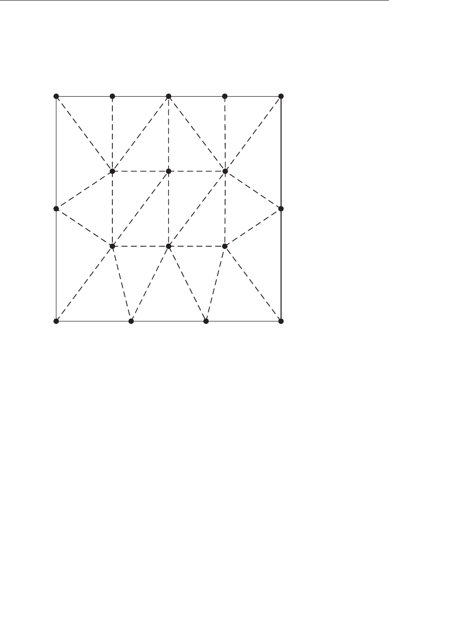
ptg9898810
inner- and outer-tessellation levels. For instance, if we were to set the
tessellation level factors to the following values, OpenGL would tessellate
the quad domain as illustrated in Figure 9.1.
gl_TessLevelOuter[0]
gl_TessLevelOuter[1]
gl_TessLevelOuter[2]
gl_TessLevelOuter[3]
(0,0) (1,0)
(1,1)(0,1)
gl_TessLevelInner[1]
gl_TessLevelInner[0]
Figure 9.1 Quad tessellation
(A tessellation of a quad domain using the tessellation levels from Exam-
ple 9.3.)
Example 9.3 Tessellation Levels for Quad Domain Tessellation
Illustrated in Figure 9.1
gl_TessLevelOuter[0] = 2.0;
gl_TessLevelOuter[1] = 3.0;
gl_TessLevelOuter[2] = 2.0;
gl_TessLevelOuter[3] = 5.0;
gl_TessLevelInner[0] = 3.0;
gl_TessLevelInner[1] = 4.0;
492 Chapter 9: Tessellation Shaders

ptg9898810
Notice that the outer-tessellation levels values correspond to the
number of segments for each edge around the perimeter, while the
inner-tessellation levels specify how many ‘‘regions’’ are in the horizontal
and vertical directions in the interior of the domain. Also shown in
Figure 9.1 is a possible triangularization of the domain,1shown using
the dashed lines. Likewise, the solid circles represent the tessellation
coordinates, each of which will be provided as input into the tessellation
evaluation shader. In the case of the quad domain, the Tessellation
coordinates will have two coordinates, (u,v), which will both be in the
range [0, 1], and each Tessellation coordinate will be passed into an
invocation of an tessellation evaluation shader.
Isoline Tessellation
Similar to the quad domain, the isoline domain also generates (u,v)pairs
as tessellation coordinates for the tessellation evaluation shader. Isolines,
however, use only two of the outer-tessellation levels to determine the
amount of subdivsion (and none of the inner-tessellation levels). This is
illustrated in Figure 9.2 for the tessellation level factors shown in
Example 9.4.
Example 9.4 Tesslation Levels for an Isoline Domain Tessellation
Shown in Figure 9.2
gl_TessLevelOuter[0] = 6;
gl_TessLevelOuter[1] = 8;
You’ll notice that there’s a dashed line along the v=1 edge. That’s because
isolines don’t include a tessellated isoline along that edge, and if you place
two isoline patches together (i.e., two patches share an edge), there isn’t
overlap of the edges.
Triangle Tessellation
Finally, let’s discuss tessellation using a triangle domain. As compared to
either the quad or isolines domains, coordinates related to the three
vertices of a triangle aren’t very conveniently represented by a (u,v)pair.
Instead, triangular domains use barycentric coordinates to specify their
Tessellation coordinates. Barycentric coordinates are represented by a
triplet of numbers (a,b,c), each of which lies in the range [0, 1], and which
1. Triangularization of the domain is implementation-dependent.
Tessellation Control Shaders 493
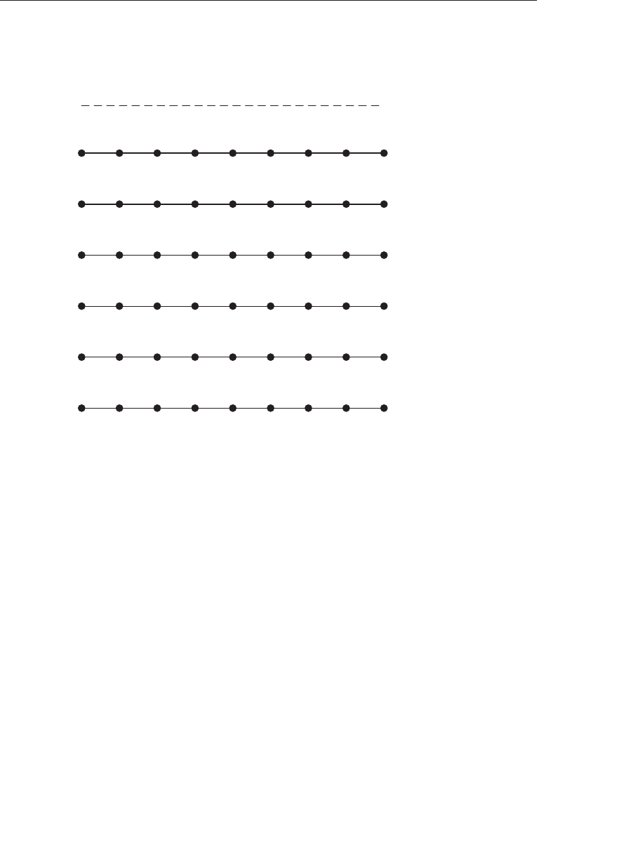
ptg9898810
have the property that a+b+c=1. Think of a,b, or cas weights for each
individual triangle vertex.
gl_TessLevelOuter[0]
gl_TessLevelOuter[1]
(0,0) (1,0)
(1,1)(0,1)
Figure 9.2 Isoline tessellation
(A tessellation of an isolines domain using the tessellations levels from Ex-
ample 9.4.)
As with any of the other domains, the generated tessellation coordinates
are a function of the tessellation level factors, and in particular, the first
three outer-tessellation levels, and only inner-tessellation level zero. The
tessellation of a triangular domain with tessellation level factors set as in
Example 9.5 is shown in Figure 9.3.
Example 9.5 Tesslation Levels for a Triangular Domain
Tessellation Shown in Figure 9.3
gl_TessLevelOuter[0] = 6;
gl_TessLevelOuter[1] = 5;
gl_TessLevelOuter[2] = 8;
gl_TessLevelInner[0] = 5;
494 Chapter 9: Tessellation Shaders
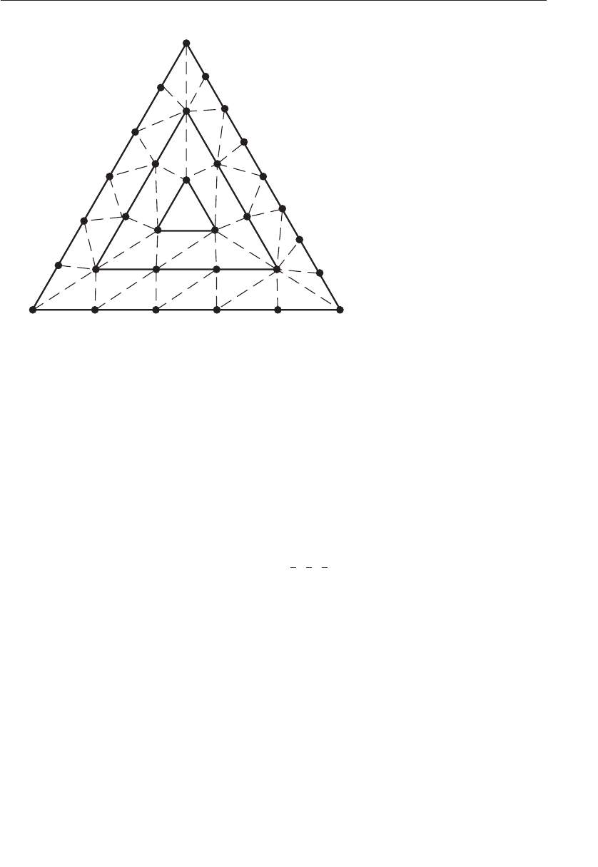
ptg9898810
gl_TessLevelOuter[0]
gl_TessLevelOuter[1]
gl_TessLevelOuter[2]
(1,0,0)
(0,1,0)
(0,0,1)
gl_TessLevelInner[0]
Figure 9.3 Triangle tessellation
(A tessellation of a triangular domain using the tessellation levels from
Example 9.5.)
As with the other domains, the outer-tessellation levels control the
subdivision of the perimeter of the triangle and the inner-tessellation level
controls how the interior is partitioned. As compared to the rectangular
domains, where the interior is partitioned in a set of rectangles forming a
grid, the interior of the triangular domain is partitioned into a set of
concentric triangles that form the regions. Specifically, let trepresent the
inner-tessellation level. If tis an even value, then the center of the
triangular domain (barycentric coordinate (1
2,1
2,1
2)is located, and then
(t/2)−1 concentric triangles are generated between the center point and
the perimeter. Conversely, if tis an odd value, then (t/2)−1 concentric
triangles are out to the perimeter, however, the center point (in barycentric
coordinates) will not be a tessellation coordinate. These two scenarios are
shown in Figure 9.4.
Bypassing the Tessellation Control Shader
As we mentioned, often your tessellation control shader will just be a
pass-through shader, copying data from input to output. In such a case,
you can actually bypass using a tessellation control shader and set the
Tessellation Control Shaders 495

ptg9898810
Odd inner tessellation levels
create a small triangle in the
center of the triangular
tessellation domain
Even inner tessellation levels
create a single tessellation
coordinate in the center of the
triangular tessellation domain
Figure 9.4 Even and odd tessellation
(Examples of how even and odd inner tessellation levels affect triangular
tessellation.)
tessellation level factors using the OpenGL API, as compared to using a
shader. The glPatchParameterfv() function can be used to set the inner-
and outer-tessellation levels.
void glPatchParameterfv(GLenum pname, const GLfloat *values);
Sets the inner- and outer-tessellation levels for when no tessellation
control shader is bound. pname must be either
GL_PATCH_DEFAULT_OUTER_LEVEL, or
GL_PATCH_DEFAULT_INNER_LEVEL.
When pname is GL_PATCH_DEFAULT_OUTER_LEVEL, values must be an
array of four floating-point values that specify the four outer-tessellation
levels.
Similarly, when pname is GL_PATCH_DEFAULT_INNER_LEVEL, values
must be an array of two floating-point values that specify the two
inner-tessellation levels.
Tessellation Evaluation Shaders
The final phase in OpenGL’s tessellation pipeline is the tessellation
evaluation shader execution. The bound tessellation evaluation shader is
executed one for each tessellation coordinate that the primitive generator
496 Chapter 9: Tessellation Shaders

ptg9898810
emits, and is responsible for determining the position of the vertex derived
from the tessellation coordinate. As we’ll see, tessellation evaluation
shaders look similar to vertex shaders in transforming vertices into screen
positions (unless the tessellation evaluation shader’s data is going to be
further processed by a geometry shader).
The first step in configuring a tessellation evaluation shader is to configure
the primitive generator, which is done using a layout directive, similar to
what we did in the tessellation control shader. Its parameters specify the
tessellation domain and subsequently, the type of primitives generated;
face orientation for solid primitives (used for face culling); and how the
tessellation levels should be applied during primitive generation.
Specifying the Primitive Generation Domain
We’ll now describe the parameters that you will use to set up the
tessellation evaluation shader’s out layout directive. First, we’ll talk
about specifying the tessellation domain. As you’ve seen, There are three
types of domains used for generating tessellation coordinates, which are
described in Table 9.2.
Table 9.2 Evaluation Shader Primitive Types
Primitive Type Description Domain Coordinates
quads A rectangular domain over
the unit square
a(u,v)pair with u,vvalues ranging
from 0 to 1.
triangles A triangular shaped
domain using barycentric
coordinates
(a,b,c)with a,b, and cvalues
ranging from 0 to 1 and where
a+b+c=1
isolines A collection of lines across
the unit square
a(u,v)pair with uvalues ranging
from 0 to 1 and vvalues ranging
from 0 to almost 1
Specifying the Face Winding for Generated Primitives
As with any filled primitive in OpenGL, the order the vertices are issued
determines the facedness of the primitive. Since we don’t issue the vertices
directly in this case, but rather have the primitive generator do it on our
behalf, we need to tell it the face winding of our primitives. In the layout
directive, specify cw for clockwise vertex winding or ccw for counterclock-
wise vertex winding.
Tessellation Evaluation Shaders 497

ptg9898810
Specifying the Spacing of Tessellation Coordinates
Additionally, we can control how fractional values for the
outer-tessellation levels are used in determining the tessellation coordinate
generation for the perimeter edges. (Inner-tessellation levels are affected by
these options.) Table 9.3 describes the three spacing options available,
where max represents an OpenGL implementation’s maximum accepted
value for a tessellation level.
Table 9.3 Options for Controlling Tessellation Level Effects
Option Description
equal_spacing Tessellation level is clamped to [1, max], and
is then rounded up to the next largest integer
value
fractional_even_spacing The value is clamped to [2, max], and then
rounded up to the next largest even integer
value n. The edge is then divided into n−2
equal length parts, and two other parts, one
at either end, which may be shorter than the
other lengths.
fractional_odd_spacing The value is clamped to [1, max −1], and then
rounded up to the next largest odd integer
value n. The edge is then divided into n−2
equal length parts, and two other parts, one
at either end, which may be shorter than the
other lengths.
Additional Tessellation Evaluation Shader layout Options
Finally, should you want to output points, as compared to isolines or filled
regions, you can supply the point_mode option, which will render a single
point for each vertex processed by the tessellation evaluation shader.
The order of options within the layout directive is not important. As an
example, the following layout directive will request primitives generated
on a triangular domain using equal spacing, counterclockwise-oriented
triangles, but only rendering points, as compared to connected primitives.
layout (triangles, equal_spacing, ccw, points) out;
Specifying a Vertex’s Position
The vertices output from the tessellation control shader (i.e., the
gl_Position values in gl_out array) are made available in the evaluation
498 Chapter 9: Tessellation Shaders

ptg9898810
shader in the gl_in variable, which when combined with tessellation
coordinates, can be used to generate the output vertex’s position.
Tessellation coordinates are provided to the shader in the variable
gl_TessCoord. In Example 9.6, we use a combination of equal-spaced
quads to render a simple patch. In this case, the tessellation coordinates
are used to color the surface, and illustrates how to compute the vertex’s
position.
Example 9.6 A Sample Tessellation Evaluation Shader
#version 420 core
layout (quads, equal_spacing, ccw) in;
out vec4 color;
void main()
{
float u = gl_TessCoord.x;
float omu = 1 - u; // one minus "u"
float v = gl_TessCoord.y;
float omv = 1 - v; // one minus "v"
color = gl_TessCoord;
gl_Position =
omu *omv *gl_in[0].gl_Position +
u*omv *gl_in[1].gl_Position +
u*v*gl_in[2].gl_Position +
omu *v*gl_in[3].gl_Position;
}
Tessellation Evaluation Shader Variables
Similar to tessellation control shaders, tessellation evaluation shaders have
agl_in array that is actually an array of structures, with each element
defined as shown in Example 9.7.
Example 9.7 gl_in Parameters for Tessellation Evaluation Shaders
in gl_PerVertex {
vec4 gl_Position;
float gl_PointSize;
float gl_ClipDistance[]
} gl_in[gl_PatchVerticesIn];
Tessellation Evaluation Shaders 499

ptg9898810
Additionally, the following scalar values, described in Table 9.4, are
provided for determining which primitive and for computing the position
of the output vertex.
Table 9.4 Tessellation Control Shader Input Variables
Variable Declaration Description
gl_PrimitiveID Primitive index for current input patch
gl_PatchVerticesIn Number of vertices in the input patch, which is
the dimension of gl_in
gl_TessLevelOuter[4] Outer-tessellation level values
gl_TessLevelInner[2] Inner-tessellation level values
gl_TessCoord Coordinates in patch domain space of the vertex
being shaded in the evaluation shader
The output vertex’s data is stored in an interface block defined as follows:
out gl_PerVertex {
vec4 gl_Position;
float gl_PointSize;
float gl_ClipDistance[]
};
A Tessellation Example: The Teapot
All of that theory could use a concrete demonstration. In this section, we’ll
render the famous Utah teapot using Bézier patches. A Bézier patch, named
after French engineer Pierre Bézier, defines a parametric surface evaluated
over the unit square using control points arranged in a grid. For our
example, we’ll use 16 control points arranged in a 4 ×4 grid. As such, we
make the following observations to help us set up our tessellation:
•Bézier patches are defined over the unit square, which indicates we
should use the quads domain type that we’ll specify in our layout
directive in the tessellation evaluation shader.
•Each patch has 16 control points, so our GL_PATCH_VERTICES should
be set to 16 using glPatchParameteri().
•The 16 control points also define the number of input-patch vertices,
which tells us our maximum index into the gl_in array in our
tessellation control shader.
•Finally, since the tessellation control shader doesn’t add or remove any
vertices to the patch, the number of output-patch vertices will also be
16, which specifies the value we’ll use in our layout directive in the
tessellation control shader.
500 Chapter 9: Tessellation Shaders

ptg9898810
Processing Patch Input Vertices
Given the information from our patches, we can easily construct the
tessellation control shader for our application, which is shown in
Example 9.8.
Example 9.8 Tessellation Control Shader for Teapot Example
#version 420 core
layout (vertices = 16) out;
void main()
{gl_TessLevelInner[0] = 4;
gl_TessLevelInner[1] = 4;
gl_TessLevelOuter[0] = 4;
gl_TessLevelOuter[1] = 4;
gl_TessLevelOuter[2] = 4;
gl_TessLevelOuter[3] = 4;
gl_out[gl_InvocationID].gl_Position
= gl_in[gl_InvocationID].gl_Position;
}
Using the tessellation level factors from Example 9.8, Figure 9.5 shows
the patches of the teapot (shrunk slightly to expose each individual
patch).
This is a very simple example of a tessellation control shader. In fact, it’s
a great example of a pass-through shader, where mostly the inputs are
copied to the output. The shader also sets the inner- and outer-tessellation
levels to constant values, which could also be done in the application
using a call to glPatchParameterfv(). However, we include the example
here for completeness.
Evaluating Tessellation Coordinates for the Teapot
Bézier patches use a bit of mathematics to determine the final vertex
position from the input control points. The equation mapping a
tessellation coordinate to a vertex position for our 4 ×4 patch is:
p(u,v) =
3
i=0
3
j=0
B(i,u)B(j,v)vij
A Tessellation Example: The Teapot 501
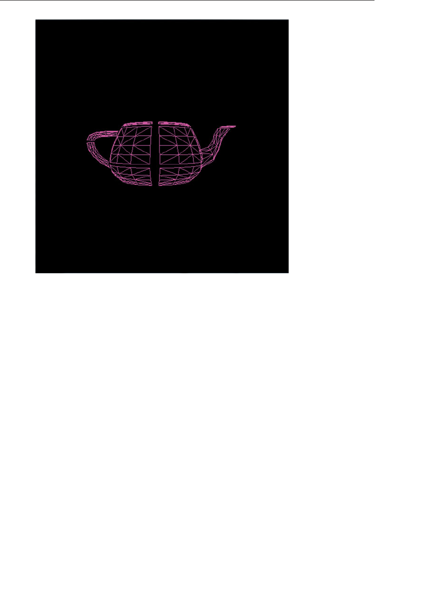
ptg9898810
Figure 9.5 The tessellated patches of the teapot
with pbeing the final vertex position, vij the input control point at index
(i,j)in our input patch (both of which are vec4s in GLSL), and Bwhich
are two scaling functions.
While it might not seem like it, we can map easily the formula to a
tessellation evaluation shader, as show in Example 9.9. In the following
shader, the Bfunction will be a GLSL function we’ll define in a moment.
We also specify our quads domain, spacing options, and polygon face
orientation in the layout directive.
Example 9.9 The Main Routine of the Teapot Tessellation
Evaluation Shader
#version 420 core
layout (quads, equal_spacing, ccw) out;
uniform mat4 MV; // Model-view matrix
uniform mat4 P; // Projection matrix
void main()
502 Chapter 9: Tessellation Shaders

ptg9898810
{
vec4 p = vec4(0.0);
float u = gl_TessCoord.x;
float v = gl_TessCoord.y;
for (int j = 0; j < 4; ++j) {
for (int i = 0; i < 4; ++i) {
p += B(i, u) *B(j, v) *gl_in[4*j+i].gl_Position;
}
}
gl_Position = P *MV *p;
}
Our Bfunction is one of the Bernstein polynomials, which is an entire family
of mathematical functions. Each one returns a scalar value. We’re using a
small, select set of functions, which we index using the first parameter,
and evaluate the function’s value at one component of our tessellation
coordinate. Here’s the mathematical definition of our functions
B(i,u) = 3
iui(1−u)3−i
where the 3
iis a particular instance of a mathematical construct called a
binomial coefficient.2We’ll spare you the gory details and just say we’re
lucky that it evaluates to either 1 or 3 in our cases, and which we’ll hard
code into a lookup table, bc in the function’s definition, and that we’ll
index using i. As such, we can rewrite B(i,u)as
B(i,u)=bciui(1−u)3−i
This also translates easily into GLSL, shown in Example 9.10.
Example 9.10 Definition of B(i,u)for the Teapot Tessellation
Evaluation Shader
float
B(int i, float u)
{// Binomial coefficient lookup table
const vec4 bc = vec4(1, 3, 3, 1);
return bc[i] *pow(u, i) *pow(1.0 - u, 3 - i);
}
2. Binomial coefficients in generally defined using the formula n
k=n!
k!(n−k)!, where n!is the
factorial of n, which is just the product of the values nto 1: n! = (n)(n−1)(n−2)...(2)(1).
A Tessellation Example: The Teapot 503

ptg9898810
While that conversation involved more mathematics than most of the
other techniques we’ve described in the book, it is representative of what
you will encounter when working with tessellated surfaces. While
discussion of the mathematics of surfaces is outside of this text, copious
resources are available that describe the required techniques.
Additional Tessellation Techniques
In this final section, we briefly describe a few additional techniques you
can employ while using tessellation shaders.
View-Dependent Tessellation
Most of the examples in this chapter have set the tessellation level factors
to constant values (either in the shader or through uniform variables). One
key feature of tessellation is being able to compute tessellation levels
dynamically in the tessellation control shader, and in particular, basing
the amount of tessellation on view-dependent parameters.
For example, you might implement a level-of-detail scheme based on the
distance of the patch from the eye’s location in the scene. In Example 9.11,
we use the average of all the input-patch vertices to specify a single
representative point for the patch, and derive all the tessellation level
factors from the distance of that point to the eye point.
Example 9.11 Computing Tessellation Levels Based on
View-Dependent Parameters
uniform vec3 EyePosition;
void main()
{
vec4 center = vec4(0.0);
for (int i = 0; i < gl_in.length(); ++i) {
center += gl_in[i].gl_Position;
}
center /= gl_in.length();
float d = distance(center, vec4(EyePosition, 1.0));
const float lodScale = 2.5; // distance scaling variable
float tessLOD = mix(0.0, gl_MaxTessGenLevel, d *lodScale);
504 Chapter 9: Tessellation Shaders

ptg9898810
for (int i = 0; i < 4; ++i) {
gl_TessLevelOuter[i] = tessLOD;
}
tessLOD = clamp(0.5 *tessLOD, 0.0, gl_MaxTessGenLevel);
gl_TessLevelInner[0] = tessLOD;
gl_TessLevelInner[1] = tessLOD;
gl_out[gl_InvocationID].gl_Position
= gl_in[gl_InvocationID].gl_Position;
}
Example 9.11 is a very rudimentary method for computing a patch’s level
of detail. In particular, each perimeter edge is tessellated the same amount,
regardless of its distance from the eye. This doesn’t take full advantage of
tessellation possibilities based on view information, which is usually
employed as a geometry optimization technique (i.e., reducing the object’s
geometric complexity the farther from the eye that object is, assuming a
perspective projection is used). Another failing of this approach is that if
you have multiple patches that share edges, it’s likely that the shared edges
may be assigned different levels of tessellation depending on the objects’
orientation with respect to the eye’s position, and that might lead to
cracking along the shared edges. Cracking is an important issue with
tessellation, and we address another concern in ‘‘Shared Tessellated Edges
and Cracking’’ on Page 506.
To address guaranteeing that shared edges are tessellated the same, we
need to find a method that returns the same tessellation factor for those
edges. However, as compared to Example 9.11, which doesn’t need to
know anything about the logical ordering of input-patch vertices, any
algorithm that needs to know which vertices are incident on a perimeter
edge is data-dependent. This is because a patch is a logical ordering---only
the application knows how it ordered the input-patch vertices. For
Example 9.12, we introduce the following array of structures that contain
our edge information for our tessellation control shader.
struct EdgeCenters {
vec4 edgeCenter[4];
};
The application would need to populate this array using the world-space
positions of the centers of each edge. In that example, we’ll assume we’re
working with the quads domain, which is why there are four points in
each EdgeCenters structure; the number of points would need to be
modified for the other domains. The number of EdgeCenters structures
in the array is the number of patches that will be issued in the draw call
Additional Tessellation Techniques 505

ptg9898810
process. We would modify the tessellation control shader to implement
the following:
Example 9.12 Specifying Tessellation Level Factors Using Perimeter
Edge Centers
struct EdgeCenters { vec4 edgeCenter[4]; };
uniform vec3 EyePosition;
uniform EdgeCenters patch[];
void main()
{
for (int i = 0; i < 4; ++i) {
float d = distance(patch[gl_PrimitiveID].edgeCenter[i],
vec4(EyePosition, 1.0));
const float lodScale = 2.5; // distance scaling variable
float tessLOD = mix(0.0, gl_MaxTessGenLevel, d *lodScale);
gl_TessLevelOuter[i] = tessLOD;
}
tessLOD = clamp(0.5 *tessLOD, 0.0, gl_MaxTessGenLevel);
gl_TessLevelInner[0] = tessLOD;
gl_TessLevelInner[1] = tessLOD;
gl_out[gl_InvocationID].gl_Position
= gl_in[gl_InvocationID].gl_Position;
}
Shared Tessellated Edges and Cracking
Often a geometric model that uses tessellation will have patches with
shared edges. Tessellation in OpenGL guarantees that the geometry
generated for the primitives within a patch won’t have any cracks between
them, but it can’t make the same claim for patches that share edges. That’s
something the application needs to address, and clearly the starting point
is that shared edges need to be tessellated the same amounts. However,
there’s a secondary issue that can creep in---precision in mathematical
computations done by a computer.
For all but trivial tessellation applications, the points along a perimeter
edge will be positioned using multiple tessellation control shader
output-patch vertices, which are combined with the tessellation
coordinates in the tessellation evaluation shader. In order to truly prevent
cracking along edges between similarly tessellated adjacent patches, the
506 Chapter 9: Tessellation Shaders
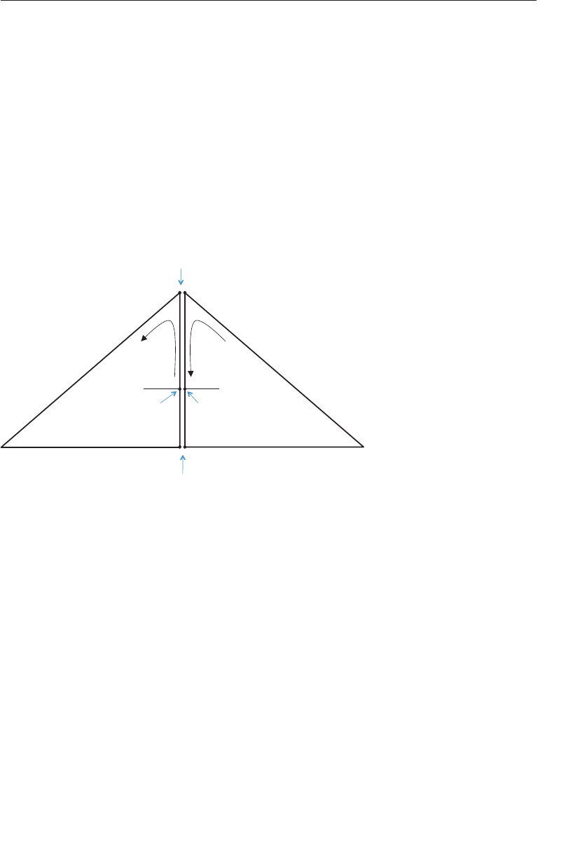
ptg9898810
order of accumulation of mathematical operations in the tessellation
evaluation shader must also match. Depending upon how the tessellation
evaluation shader generates the mesh’s vertices final positions, you may
need to reorder the processing of vertices in the tessellation evaluation
shader. A common approach to this problem is to recognize the
output-patch vertices that contribute to a vertex incident to a perimeter
edge, and sort those vertices in a predictable manner, say, in terms of
increasing magnitude along the edge.
Another technique to avoid cracking is applying the precise qualifier to
shader computations where points might be in reversed order between two
shader invocations. This is illustrated in Figure 9.6.
Subdivided
point
Subdivided
point
End points (same
locaon/value)
End points (same
locaon/value)
Direcon of
Edge walking
Direcon of
Edge walking
Figure 9.6 Tessellation cracking
(When walking the interior edge in opposite directions, the computed sub-
division points need to result in the same value, or the edge may crack.)
As explained in ‘‘The precise Qualifier’’ on Page 55 in Chapter 2, this
computation can result in different values if the expression is the same and
the input values are the same but some of them are swapped due to the
opposite direction of edge walking. Qualifying the results of such
computations as precise will prevent this.
Displacement Mapping
A final technique we’ll discuss in terms of tessellation is displacement
mapping, which is merely a form of vertex texture mapping, like we
Additional Tessellation Techniques 507

ptg9898810
described in Chapter 6,‘‘Textures’’. In fact, there’s really not much to say,
other than you would likely use the tessellation coordinate provided to the
tessellation evaluation shader in some manner to sample a texture map
containing displacement information.
Adding displacement mapping to the teapot from Example 9.9, would
requite adding two lines into the tessellation evaluation shader, as shown
in Example 9.13.
Example 9.13 Displacement Mapping in main Routine of the Teapot
Tessellation Evaluation Shader
#version 420 core
layout (quads, equal_spacing, ccw) out;
uniform mat4 MV; // Model-view matrix
uniform mat4 P; // Projection matrix
uniform sampler2D DisplacementMap;
void main()
{
vec4 p = vec4(0.0);
float u = gl_TessCoord.x;
float v = gl_TessCoord.y;
for (int j = 0; j < 4; ++j) {
for (int i = 0; i < 4; ++i) {
p += B(i, u) *B(j, v) *gl_in[4*j+i].gl_Position;
}
}
p += texture(DisplacementMap, gl_TessCoord.xy);
gl_Position = P *MV *p;
}
508 Chapter 9: Tessellation Shaders

ptg9898810
Chapter 10
Geometry Shaders
Chapter Objectives
After reading this chapter, you’ll be able to do the following:
•Create and use geometry shaders to further process geometry within
the OpenGL pipeline.
•Create additional geometric primitives using a geometry shader.
•Use geometry shaders in combination with transform feedback to
generate multiple streams of geometric data.
•Render to multiple viewports in a single rendering pass.
509

ptg9898810
In this chapter, we introduce an entirely new shader stage---the geometry
shader. The geometry shader sits logically right before primitive assembly
and fragment shading. It receives as its input complete primitives as a
collection of vertices, and these inputs are represented as arrays. Typically,
the inputs are provided by the vertex shader. However, when tessellation is
active, the input to the geometry shader is provided by the tessellation
evaluation shader. Because each invocation of the geometry shader
processes an entire primitive, it is possible to implement techniques that
require access to all of the vertices of that primitive.
In addition to this enhanced, multivertex access, the geometry shader can
output a variable amount of data. Outputting nothing amounts to culling
geometry and outputting more vertices than were in the original primitive
results in geometry amplification. The geometry shader is also capable of
producing a different primitive type at its output than it accepts on its
input, allowing it to change the type of geometry as it passes through the
pipeline. There are four special primitive types provided for use as inputs
to geometry shaders. Finally, geometry shaders can be used with transform
feedback to split an input stream of vertex data into several substreams.
These are very powerful features that enable a large array of techniques
and algorithms to be implemented on the GPU.
It has the following major sections:
•‘‘Creating a Geometry Shader’’ describes the fundamental mechanics of
using geometry shaders.
•‘‘Geometry Shader Inputs and Outputs’’ defines the input and output
data structures used with geometry shaders.
•‘‘Producing Primitives’’ illustrates how primitives can be generated
within a geometry shader.
•‘‘Advanced Transform Feedback’’ extends the transform feedback
mechanism (described in ‘‘Transform Feedback’’ on Page 239) to
support more advanced techniques.
•‘‘Geometry Shader Instancing’’ describes optimization techniques
available when using geometry shaders for geometric instancing.
•‘‘Multiple Viewports and Layered Rendering’’ explains rendering to
multiple viewports in a single rendering pass.
Creating a Geometry Shader
Geometry shaders are created in exactly the same manner as any other
type of shader---by using the glCreateShader() function. To create a
510 Chapter 10: Geometry Shaders

ptg9898810
geometry shader, pass GL_GEOMETRY_SHADER as the shader type parame-
ter to glCreateShader(). The shader source is passed as normal using the
glShaderSource() function and then the shader is compiled using
glCompileShader(). Multiple geometry shaders may be attached to a
single program object and when that program is linked, the attached
geometry shaders will be linked into an executable that can run on the
GPU. When a program object containing a geometry shader is active the
geometry shader will run on each primitive produced by OpenGL. These
primitives may be points, lines, triangles or one of the special adjacency
primitives, which will be discussed shortly.
The geometry shader is an optional stage in OpenGL---your program object
does not need to contain one. It sits right before rasterization and
fragment shading. The output of the geometry shader can be captured
using transform feedback, and it is often used in this mode to process
vertices for use in subsequent rendering, or even nongraphics tasks. If no
fragment shader is present, rasterization can even be turned off by calling
glEnable() with the parameter GL_RASTERIZER_DISCARD. This makes
transform feedback the end of the pipeline and it can be used in this mode
when only the captured vertex data is of interest and the rendering of
primitives is not required.
One of the unique aspects of the geometry shader is that it is capable of
changing the type and number of primitives that are passing through the
OpenGL pipeline. The methods and applications of doing these things will
be explained shortly. However, before a geometry shader may be linked,
the input primitive type, output primitive type, and the maximum number
of vertices that it might produce must be specified. These parameters are
given in the form of layout qualifiers in the geometry shader source code.
Example 10.1 shows a very basic example of a geometry shader that simply
passes primitives through unmodified (a pass-through geometry shader).
Example 10.1 A Simple Pass-Through Geometry Shader
// This is a very simple pass-through geometry shader
#version 330 core
// Specify the input and output primitive types, along
// with the maximum number of vertices that this shader
// might produce. Here, the input type is triangles and
// the output type is triangle strips.
layout (triangles) in;
layout (triangle_strip, max_vertices = 3) out;
// Geometry shaders have a main function just
// like any other type of shader
Creating a Geometry Shader 511

ptg9898810
void main()
{
int n;
// Loop over the input vertices
for (n = 0; n < gl_in.length(); n++)
{// Copy the input position to the output
gl_Position = gl_in[0].gl_Position;
// Emit the vertex
EmitVertex();
}
// End the primitive. This is not strictly necessary
// and is only here for illustrative purposes.
EndPrimitive();
}
This shader simply copies its input into its output. You don’t need to worry
about how this works right now, but you might notice several features of
this example that are unique to geometry shaders. First, at the top of the
shader is a pair of layout qualifiers containing the declaration of the input
and output primitive types and the maximum number of vertices that may
be produced. These are shown in Example 10.2.
Example 10.2 Geometry Shader Layout Qualifiers
layout (triangles) in;
layout (triangle_strip, max_vertices = 3)out;
The first line specifies that the input primitive type is triangles. This means
that the geometry shader will be run once for each triangle rendered.
Drawing commands used by the program must use a primitive mode that
is compatible with the primitive type expected by the geometry shader (if
present). If a drawing command specifies strips or fans
(GL_TRIANGLE_STRIP or GL_TRIANGLE_FAN, in the case of triangles), the
geometry shader will run once for each triangle in the strip or fan. The
second line of the declaration specifies that the output of the geometry
shader is triangle strips and that the maximum number of vertices that will
be produced is three. The accepted primitive types accepted as inputs to
the geometry shader and the corresponding primitive types that are
allowed to be used in drawing commands are listed in Table 10.1.
Notice that even though we are only producing a single triangle in this
example, we still specify that the output primitive type is triangle strips.
Geometry shaders are designed to produce only points, line strips, or
triangle strips, but not individual lines or triangles, nor loops or fans. This
is because strips are a superset of individual primitive types---think of an
independent triangle or line as a strip of only one primitive. By
512 Chapter 10: Geometry Shaders

ptg9898810
Table 10.1 Geometry Shader Primitive Types and Accepted Drawing
Modes
Geometry Shader Primitive Type Accepted Drawing Command Modes
points GL_POINTS, GL_PATCHES1
lines GL_LINES, GL_LINE_STRIP,
GL_LINE_LOOP, GL_PATCHES1
triangles GL_TRIANGLES, GL_TRIANGLE_STRIP
GL_TRIANGLE_FAN, GL_PATCHES1
lines_adjacency2GL_LINES_ADJACENCY,
GL_LINE_STRIP_ADJACENCY
triangles_adjacency2GL_TRIANGLES_ADJACENCY,
GL_TRIANGLE_STRIP_ADJACENCY
terminating the strip after only a single triangle, independent triangles
may be drawn.
The special GLSL function EmitVertex() produces a new vertex at the
output of the geometry shader. Each time it is called, a vertex is appended
to the end of the current strip if the output primitive type is line_strip
or triangle_strip. If the output primitive type is points, then each call
to EmitVertex() produces a new, independent point. A second special
geometry shader function, EndPrimitive(), breaks the current strip
and signals OpenGL that a new strip should be started the next time
EmitVertex() is called. As discussed, single primitives such as lines or
triangles are not directly supported, although they may be generated by
calling EndPrimitive() after every two or three vertices in the case of
lines or triangles, respectively. By calling EndPrimitive() after every two
vertices are emitted when producing line strips or after every three vertices
are emitted when producing triangle strips, it is possible to generate
independent lines or triangles. As there is no such thing as a point
strip, each point is treated as an individual primitive and so calling
EndPrimitive() when the output primitive mode is points has no
effect (although it is still legal).
When the geometry shader exits, the current primitive is ended implicitly
and so it is not strictly necessary to call EndPrimitive() explicitly at the
end of the geometry shader. When EndPrimitive() is called (or at the
1. GL_PATCHES are accepted by drawing commands when a geometry shader is present so
long as the selected tessellation mode will cause the patches to be converted to something
compatible with the geometry shader input.
2. The adjacency primitive types lines_adjacency and triangles_adjacency are special
types introduced for geometry shaders and will be discussed shortly.
Creating a Geometry Shader 513

ptg9898810
end of the shader), any incomplete primitives will simply be discarded.
That is, if the shader produces a triangle strip with only two vertices or if it
produces a line strip with only one vertex, the extra vertices making up the
partial strip will be thrown away.
Geometry Shader Inputs and Outputs
The inputs and outputs of the geometry shader are specified using layout
qualifiers and the in and out keywords in GLSL. In addition to user-
defined inputs and outputs, there are several built-in inputs and outputs
that are specific to geometry shaders. These are described in some detail in
the following subsections. The in and out keywords are also used in
conjunction with layout qualifiers to specify how the geometry shader fits
into the pipeline, how it behaves, and how it interacts with adjacent
shader stages.
Geometry Shader Inputs
The input to the geometry shader is fed by the output of the vertex shader,
or if tessellation is active, the output of the tessellation evaluation shader.3
As the geometry shader runs once per input primitive, outputs from the
previous stage (vertex shader or tessellation evaluation shader) become
arrays in the geometry shader. This includes all user-defined inputs and the
special built-in input variable, gl_in, which is array containing the
built-in outputs that are available in the previous stage. The gl_in input is
implicitly declared as an interface block. The definition of gl_in is shown
in Example 10.3.
Example 10.3 Implicit Declaration of gl_in[]
in gl_PerVertex {
vec4 gl_Position;
float gl_PointSize;
float gl_ClipDistance[];
} gl_in[];
As noted, gl_in is implicitly declared as an array. The length of the array
is determined by the input primitive type. Whatever is written to
gl_Position,gl_PointSize, or gl_ClipDistance in the vertex shader
(or tessellation evaluation shader) becomes visible to the geometry shader
in the appropriate member of each member of the gl_in array. Like any
3. Tessellation shaders are covered in detail in Chapter 9.
514 Chapter 10: Geometry Shaders

ptg9898810
array, the number of elements in the gl_in array can be found using the
.length() method. Returning to our example geometry shader, we see a
loop:
// Loop over the input vertices
for (n = 0; n < gl_in.length(); n++)
{...
}
The loop runs over the elements of the gl_in array, whose length is
dependent on the input primitive type declared at the top of the shader. In
this particular shader, the input primitive type is triangles, meaning that
each invocation of the geometry shader processes a single triangle, and so
the gl_in.length() function will return three. This is very convenient as
it allows us to change the input primitive type of the geometry shader
without changing any source code except the input primitive type layout
qualifier. For example, if we change the input primitive type to lines, the
geometry shader will now run once per line, and gl_in.length() will
return two. The rest of the code in the shader need not change.
The size of the input arrays is determined by the type of primitives that the
geometry shader accepts. The accepted primitive types are points,lines,
triangles,lines_adjacency, and triangles_adjacency. The
number of vertices in each primitive of these types is shown in Table 10.2
below.
Table 10.2 Geometry Shader Primitives and the Vertex Count for Each
Primitive Type Input Array Size
points 1
lines 2
triangles 3
lines_adjacency 4
triangles_adjacency 6
The first three represent points, lines, and triangles, respectively. Points are
represented by single vertices, and so although the inputs to the geometry
shader are still arrays, the length of those arrays is one. Lines and triangles
are generated both by independent triangles (GL_TRIANGLES and
GL_LINES primitive types) and from the individual members of strips and
fans (GL_TRIANGLE_STRIP, for example). Even if the drawing command
specified GL_TRIANGLE_STRIP, GL_TRIANGLE_FAN, GL_LINE_STRIP, or
GL_LINE_LOOP, the geometry shader still receives individual primitives as
appropriate.
Geometry Shader Inputs and Outputs 515

ptg9898810
The last two input primitive types represent adjacency primitives, which
are special primitives that are accepted by the geometry shader. They have
special meaning and interpretation when no geometry shader is present
(which will be described shortly), but for most cases where a geometry
shader is present can be considered to be simple collections of four or six
vertices and it is up to the geometry shader to convert them into some
other primitive type. You cannot specify an adjacency primitive type as the
output mode of the geometry shader.
Just as the built-in variable gl_in is an array with a length determined by
the input primitive type, so are user-defined inputs. Consider the
following vertex shader output declarations:
out vec4 position;
out vec3 normal;
out vec4 color;
out vec2 tex_coord;
In the geometry shader, these must be declared as arrays as follows:
in vec4 position[];
in vec3 normal[];
in vec4 color[];
in vec2 tex_coord[];
Note that the size of the arrays does not have to be given explicitly. If the
array declarations are left unsized, then the size is implied by the input
primitive type declared earlier in the shader. If the size is given explicitly
then it is cross-checked at compile time against the input primitive type,
giving an additional layer of error checking. If an input array is declared
with an explicit size and that size does not match what is expected given
the input primitive type, the GLSL compiler will generate an error.
GLSL versions earlier than 4.3 did not contain support for two-dimensional
arrays. So, what happened to vertex shader outputs that are declared as
arrays? To pass an array from a vertex shader to a geometry shader, we took
advantage of an interface block. Using an interface block helps group all the
data for a single vertex, rather than managing collections of arrays, so you
may want to use interface blocks regardless of arrays or version numbers.
The interface block can contain arrays, but it is the interface block itself
that becomes an array when passed into a geometry shader. This technique
is already used in the definition of the gl_in[] built-in variable---the
gl_ClipDistance[] array is a member of the block.
Consider the example above. Let’s assume that we wish to pass more than
one texture coordinate from the vertex shader to the fragment shader. We
will do that by making tex_coord an array. We can re-declare the
variables listed in the example in an interface block and see how that
affects their declaration in the geometry shader.
516 Chapter 10: Geometry Shaders

ptg9898810
First, in the vertex shader:
out VS_GS_INTERFACE
{
out vec4 position;
out vec3 normal;
out vec4 color;
out vec2 tex_coord[4];
} vs_out;
Now, in the geometry shader:
in VS_GS_INTERFACE
{
out vec4 position;
out vec3 normal;
out vec4 color;
out vec2 tex_coord[4];
} gs_in[];
Now we have declared the output of the vertex shader as vs_out
using an interface block, which is matched to gs_in[] in the geometry
shader. Remember that interface block matching is performed by block
name (VS_GS_INTERFACE in this example) rather than instance name.
This allows the variables representing the block instance to have
a different name in each shader stage. gs_in[] is an array, and
the four texture coordinates are available in the geometry shader as
gs_in[n].tex_coord[m]. Anything that can be passed from a vertex
shader to a fragment shader can be passed in this manner, including
arrays, structures, matrices, and other compound types.
In addition to the built-in members of gl_in[] and to user-defined
inputs, there are a few other special inputs to the geometry shader.
These are gl_PrimitiveIDIn and gl_InvocationID. The first,
gl_PrimitiveIDIn, is the equivalent of gl_PrimitiveID that
is available to the fragment shader. The In suffix distinguishes it from
gl_PrimitiveID, which is actually an output in the geometry shader and
must be assigned by the geometry shader if it is to be made available in the
subsequent fragment shader. The second input, gl_InvocationID, is used
during geometry shader instancing, which will be explained shortly. Both
gl_PrimitiveIDIn and gl_InvocationID are intrinsically declared as
integers.
Special Geometry Shader Primitives
Special attention should be paid to the adjacency primitive types available
to geometry shaders (lines_adjacency and triangles_adjacency).
Geometry Shader Inputs and Outputs 517
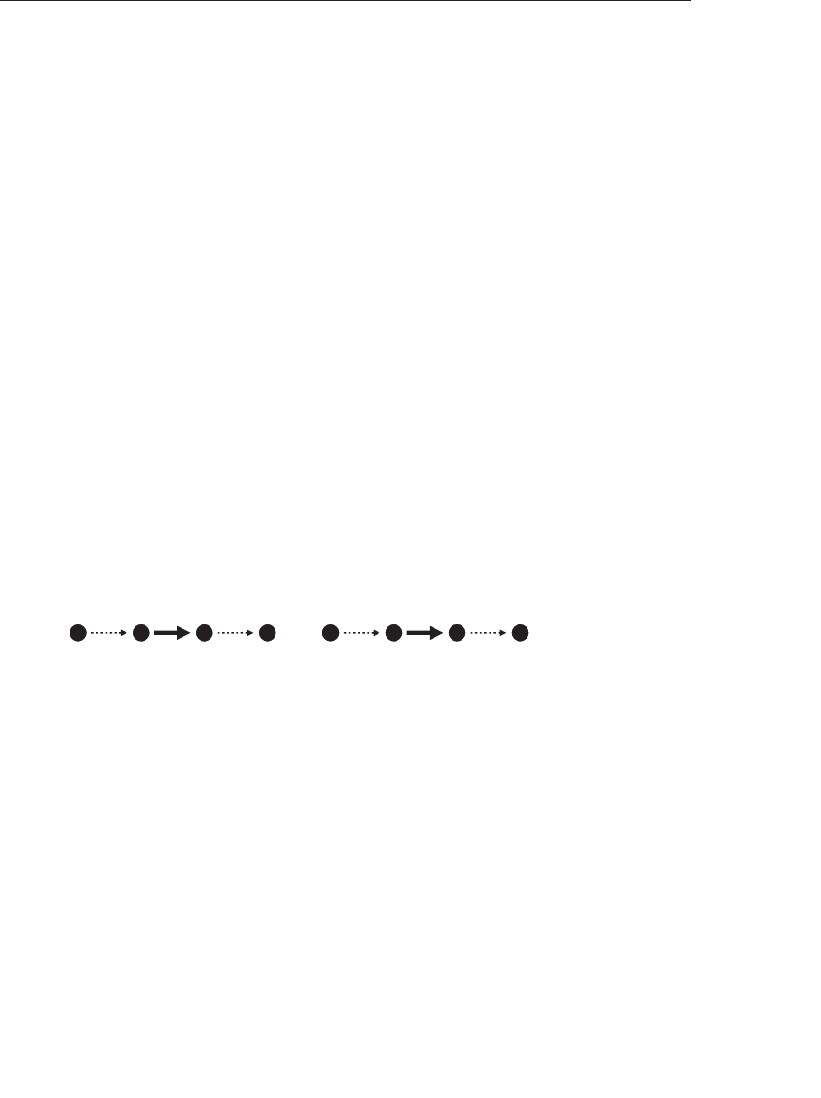
ptg9898810
These primitives have four and six vertices, respectively, and allow
adjacency information---information about adjacent primitives or
edges---to be passed into the geometry shader. Lines with adjacency
information are generated by using the GL_LINES_ADJACENCY or
GL_LINE_STRIP_ADJACENCY primitive mode in a draw command such as
glDrawArrays(). Likewise, triangles with adjacency information are
produced by using the GL_TRIANGLES_ADJACENCY or
GL_TRIANGLE_STRIP_ADJACENCY primitive types. These primitive types
can be used without a geometry shader present and will be interpreted as
lines or triangles with additional vertices being discarded.
Lines with Adjacency
At the input of the geometry shader, each lines_adjacency primitive is
represented as a four-vertex primitive (i.e., the geometry shader inputs
such as gl_in and user-defined inputs are four element arrays). In the
OpenGL API, there are two adjacency primitives representing
lines---GL_LINES_ADJACENCY or GL_LINE_STRIP_ADJACENCY. The first
represents individual line primitives and each primitive sent to the
geometry shader is formed from an independent collection of four vertices.
Four vertices are consumed from the input arrays each time a primitive is
assembled. The vertex layout is shown in Figure 10.1, where the first
primitive passed to the geometry shader is made up from vertices A, B, C,
and D. The second primitive is made up of vertices E, F, G, and H. This
sequence continues, four vertices at a time for the length of the draw.
ABCDE F G H
1 2
Figure 10.1 Lines adjacency sequence
(Vertex sequence for GL_LINES_ADJACENCY primitives.)
The second of these line primitive types (GL_LINE_STRIP_ADJACENCY)
represents a line strip in much the same way as the regular GL_LINE_STRIP
primitive does. Each primitive to the geometry shader is still made up of
four vertices. The first primitive in a draw is constructed from the first four
vertices in the enabled arrays,4and then a new four-vertex primitive is
constructed from each successive vertex together with the preceding three
4. When using vertex indices with a draw command like glDrawElements(), primitives are not
actually constructed from the first vertices in the arrays, rather they are constructed from the
vertices referred to by the first few indices in the element array. For simplicity of explanation
though, we will refer to these as the first few vertices, even though there may be an indirection
involved.
518 Chapter 10: Geometry Shaders
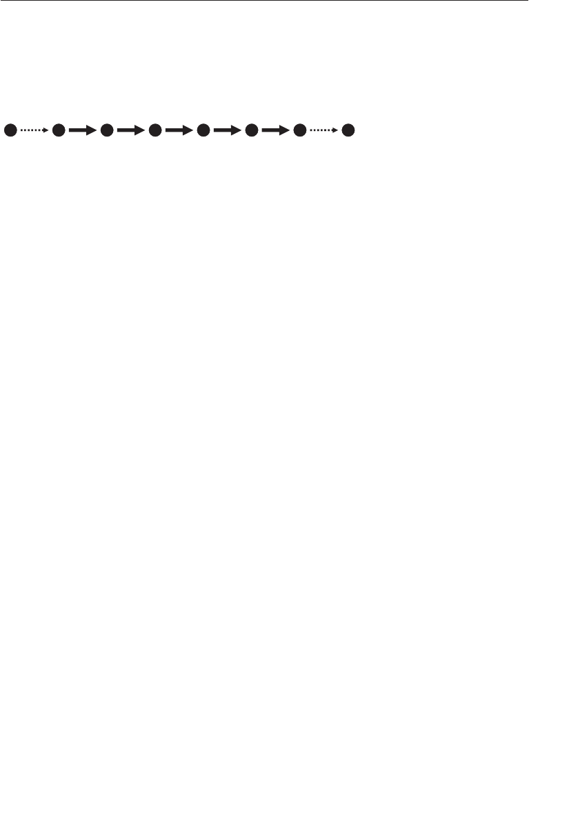
ptg9898810
vertices. Figure 10.2 below demonstrates this. In Figure 10.2, the first
primitive passed to the geometry shader is made up from vertices A, B, C,
and D, the second from B, C, D, and E, the third from C, D, E, and F
and so on.
A B C D EF G H
12345
Figure 10.2 Line-strip adjacency sequence
(Vertex sequence for GL_LINE_STRIP_ADJACENCY primitives.)
The lines_adjacency primitive type is a good way to pass an arbitrary
four-vertex primitive to the geometry shader (which does not actually
have to represent a line). This is particularly true when the GL_LINES_
ADJACENCY primitive mode is used as it does not infer any connectivity
semantics. Note that the geometry shader cannot emit alines_adjacency
primitive. It must convert the primitive to another type. For example, if
the vertices really do represent lines, then the geometry output primitive
type can be set to lines and the shader can simply emit lines. However, it is
possible to represent any arbitrary quadrilateral with four vertices, and in
such a case the geometry shader can be used to convert it into a pair of
triangles.
You may be wondering why we call them line primitives if any arbitrary
four-vertex primitive can be passed to the geometry shader using the lines
with adjacency primitive types. After all, the geometry shader can’t
actually produce lines with adjacency primitive and must convert them to
another primitive type to be rendered. The answer is in how the primitives
are interpreted by OpenGL when there is no geometry shader present. For
each four-vertex primitive (whether it originated from the GL_LINES_
ADJACENCY or GL_LINE_STRIP_ADJACENCY primitive mode), the
additional vertices representing adjacency information are considered to
be the first and last vertices in the primitive and those representing the
line itself are the second and third vertices (the middle two vertices).
When no geometry shader is present, the adjacency vertices are discarded
and a line is formed from the two central vertices in the four-vertex
primitive. In this manner, the vertex information is still interpreted as
lines, although much of it may ultimately be discarded.
In Figures 10.1 and 10.2, the solid arrows represent the lines that will be
generated by OpenGL when no geometry shader is present, and the dotted
arrows represent the virtual lines that will be discarded.
Geometry Shader Inputs and Outputs 519

ptg9898810
Triangles with Adjacency
Like the lines with adjacency primitive types, the triangles_adjacency input
primitive type is designed to allow triangles with adjacency information to
be passed into a geometry shader. Each triangles_adjacency primitive is
constructed from six vertices and so gl_in and the other geometry shader
inputs become six-element arrays. There are also two primitive modes that
may be used with OpenGL drawing commands, GL_TRIANGLES_
ADJACENCY and GL_TRIANGLE_STRIP_ADJACENCY. Like GL_LINES_
ADJACENCY, each GL_TRIANGLES_ADJACENCY primitive is formed from
six independent vertices. Again, the geometry shader cannot emit a
triangles_adjacency primitive and so must generate another type of
primitive from the six incoming vertices.
Figure 10.3 illustrates the layout of vertices in a triangles_adjacency
primitive and how they are passed to the geometry shader. When the
primitive mode is GL_TRIANGLES_ADJACENCY, the first primitive will be
formed from vertices A through F, the second from G through L, and so
on. When no geometry shader is present, a triangle is formed from every
other vertex. As in Figure 10.1, solid arrows represent triangles that will be
rendered, and dotted arrows represent the virtual triangles that will be
discarded. In this case, a triangle is formed from vertices A, C, and E, and
another is formed from vertices G, I, and K. Vertices B, D, F, H, and J are
discarded in the absence of a geometry shader.
A
B C D
E
F
G
H I J
K
L
1 2
Figure 10.3 Triangles adjacency sequence
(Vertex sequence for GL_TRIANGLES_ADJACENCY primitives.)
Finally, we come to the GL_TRIANGLE_STRIP_ADJACENCY primitive mode.
This primitive can be hard to understand and is possibly best illustrated us-
ing a diagram. Figure 10.4 shows how vertices are assembled into triangles,
where the extra vertices come from, and as in previous figures shows which
vertices are used to form triangles when no geometry shader is present.
When the primitive mode is GL_TRIANGLE_STRIP_ADJACENCY, six vertices
520 Chapter 10: Geometry Shaders
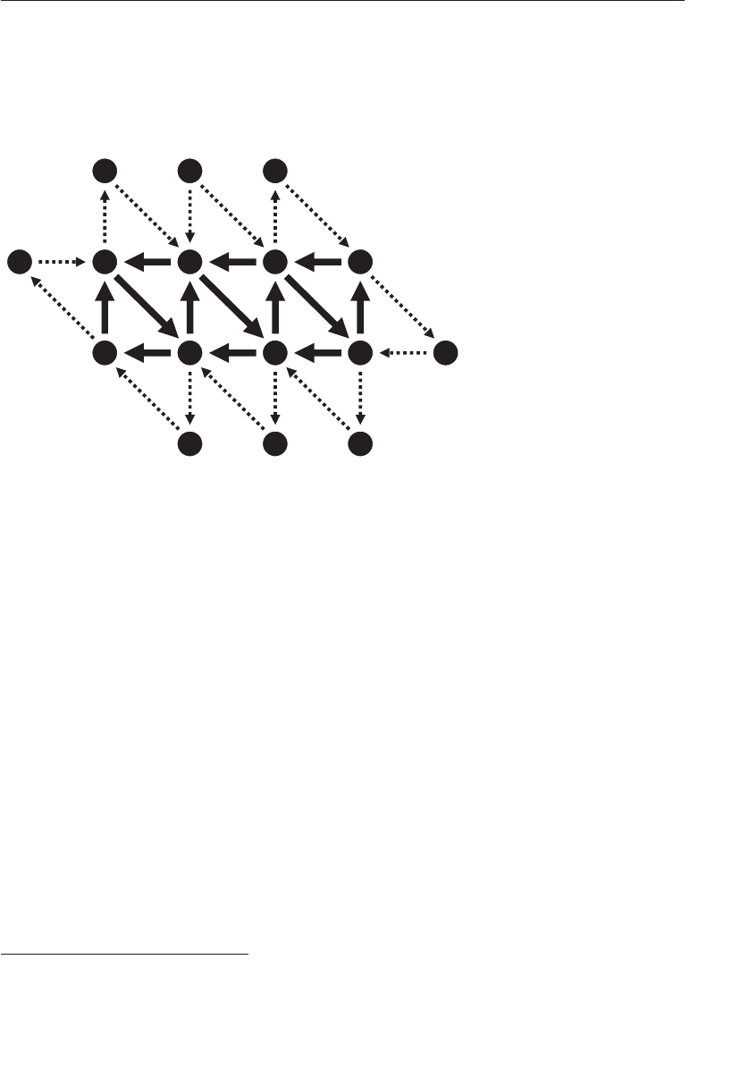
ptg9898810
are still used to construct each primitive passed to the geometry shader.
The first primitive is made from the first six vertices in the enabled arrays
and then a new primitive is constructed for each vertex, reusing the
previous five.
B
F
C
A
J
D
G
E
N
H
K
I
L
O
M P
135
246
Figure 10.4 Triangle-strip adjacency layout
(Vertex layout for GL_TRIANGLE_STRIP_ADJACENCY primitives.)
If the pattern of triangles is removed and instead arrows representing the
order of vertices are overlaid onto Figure 10.4, a pattern emerges that can
be helpful in understanding the ordering of vertices in the arrays. This is
shown in Figure 10.5.
Notice how, in Figures 10.4 and 10.5, it appears that adjacency
information about every triangle is not conveyed. Instead, additional
vertices outside the strip are passed to the geometry shader. However,
which vertices are used to fill the inputs to the geometry shader vary based
on whether the triangle is the only one in the strip, the first in a strip, an
odd- or even-numbered triangle within the strip or the last triangle in a
strip containing an even or odd number of triangles. This is described in
some detail in the OpenGL specification.5
Given the geometry shown in Figure 10.4, triangle 1 will have its inputs
made from vertices A, C, and E with vertices B, D, and G forming the
additional adjacency vertices. Triangle 2 will have its inputs filled from
vertices E, C, and G, with A, F, and I forming the adjacency vertices.
5. See Table 10.1 of the OpenGL Specification, Version 4.3.
Geometry Shader Inputs and Outputs 521
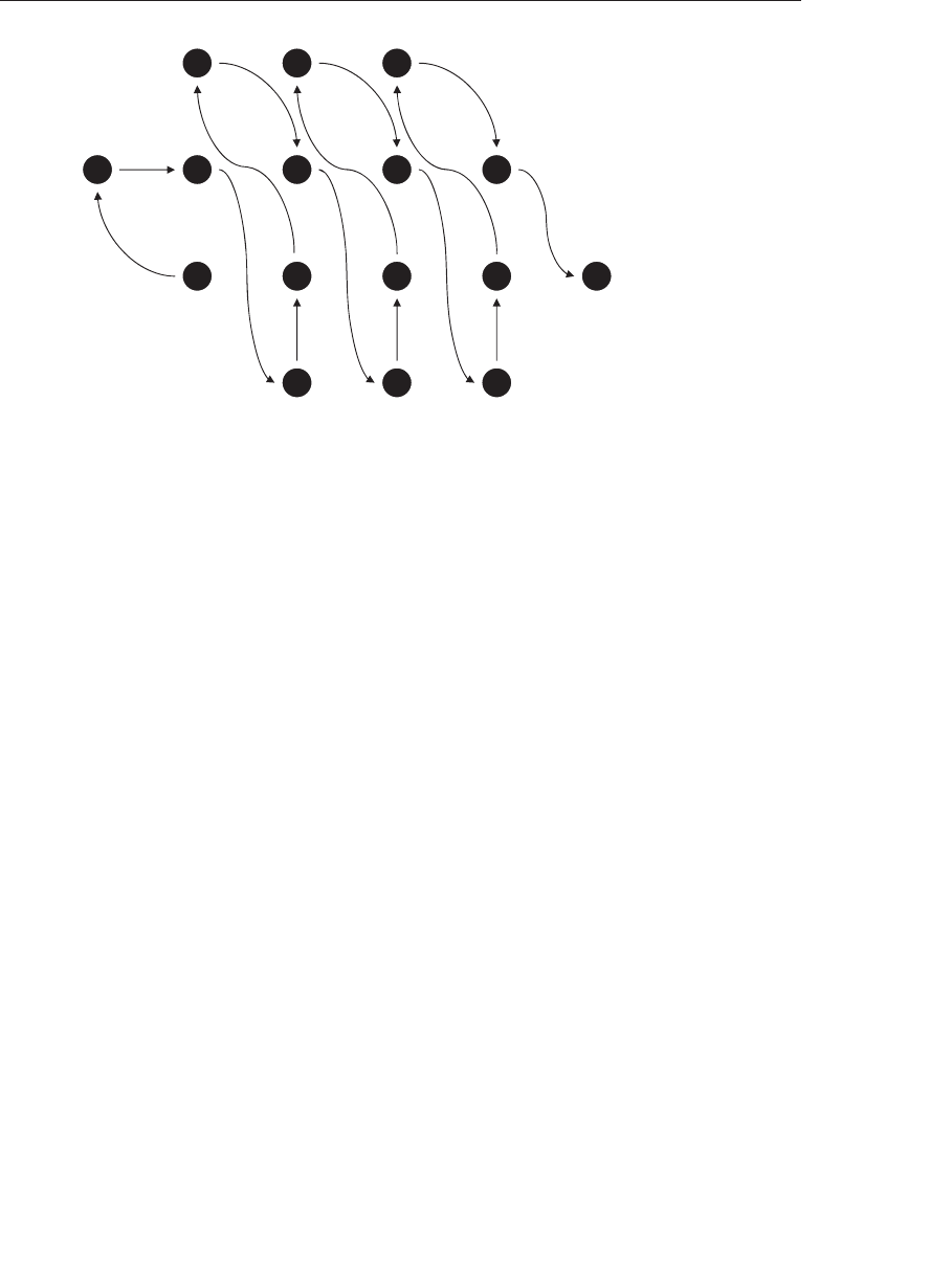
ptg9898810
B
F
C
A
J
D
G
E
N
H
K
I
L
O
M P
Figure 10.5 Triangle-strip adjacency sequence
(Vertex sequence for GL_TRIANGLE_STRIP_ADJACENCY primitives.)
Triangle 3 will be made up of vertices E, G, and I, and the adjacency
vertices will be C, K, and H. This pattern repeats until the end of the strip,
where triangle 6 is made from vertices M, K, and O, and the adjacency
vertices are I, N, and P. Remember that in the geometry shader, the first,
third, and fifth elements of gl_in represent the triangle while the second,
fourth, and sixth elements represent the adjacency vertices. Putting all this
together tells us that gl_in for triangle 1 will be constructed from vertices
A, B, C, D, E, and G (in that order), for triangle 2 it is constructed from
vertices E, A, C, F, G, and I, and in triangle 3 it is E, C, G, K, I, and H.
Finally, for triangle 6 it is constructed from vertices M, I, K, N, O, and P.
Generating Data for Adjacency Primitives
Seeing the strange patterns of vertices in Figures 10.1 through 10.4 might
make you think that you need to have specialized software or jump
though some mental contortions to generate geometry data to feed to
OpenGL when these primitive types are used. While it is possible to hijack
the adjacency primitive types (especially GL_LINES_ADJACENCY and
GL_TRIANGLES_ADJACECNCY) to pass arbitrary groups of four or six
vertices into the pipeline, these primitive types are often used with vertex
indices stored in a buffer bound to the GL_ELEMENT_ARRAY_BUFFER
binding and a drawing command such as glDrawElements().
The additional vertices in the adjacency primitives are intended to allow
the geometry shader to obtain knowledge of the primitives adjacent to the
522 Chapter 10: Geometry Shaders

ptg9898810
one that it’s processing in the mesh. For triangles, the extra vertex is often
the third vertex of a triangle sharing an edge (and therefore two vertices)
with the current primitive. This vertex likely already exists in the mesh. If
indexed vertices are used, then no additional vertex data is required to
represent this---only additional indices in the element buffer. In many
cases, these extra indices can be generated by a preprocessing tool. Of
course it is also possible to store information about an edge in the
adjacency vertex, and it’s also possible that the adjacency vertex is used
only for that purpose and is not referenced as a real vertex at all.
Geometry Shader Outputs
The output of the geometry shader is fed into the primitive setup engine,
rasterizer, and eventually into the fragment shader. In general, the output
of the geometry shader is equivalent to the output of the vertex shader if
no geometry shader is present. As many of the same outputs exist in the
geometry shader as exist in the vertex shader. The same gl_PerVertex
interface block specification is used for per-vertex outputs in the geometry
shader. The definition of this block is given in Example 10.4.
Example 10.4 Implicit Declaration of Geometry Shader Outputs
out gl_PerVertex
{
vec4 gl_Position;
float gl_PointSize;
float gl_ClipDistance[];
};
Note that although the same gl_PerVertex interface block is used to
declare the geometry shader outputs, in this instance it has no name, and
so the outputs are essentially in global scope. Of course, user-defined
outputs may be declared as well, and these will be passed to the fragment
shader along with the built-in interface block members. Because each
geometry shader invocation can produce multiple output vertices, each
vertex must be explicitly produced by calling the EmitVertex() function.
When EmitVertex() is called, the current values of all outputs of the
geometry shader are recorded and used to form a new vertex. After
EmitVertex() is called, the values of all geometry shader outputs become
undefined and thus it is necessary to write all outputs in the geometry
shader before producing a vertex, even if the values of some of those
outputs are the same from vertex to vertex. The only exception to this
general rule for outputs that are marked with the flat keyword. In this
case, only the value generated for the provoking vertex is used in subsequent
stages and so, although the value of the outputs is still undefined for the
Geometry Shader Inputs and Outputs 523

ptg9898810
other vertices, that doesn’t really matter as those undefined values will
never be used.
To specify which vertex is to be used as the provoking vertex, you can
call glProvokingVertex() with the desired mode. The default is GL_LAST_
VERTEX_CONVENTION, which means that flat shaded interpolants will
be taken from the last vertex in each primivite. However, you can specify
that they can take their values from the first vertex by passing
GL_FIRST_VERTEX_CONVENTION to glProvokingVertex(). The
prototype for glProvokingVertex() is as follows:
void glProvokingVertex(GLenum provokeMode);
Sets the provoking vertex mode to provokeMode, which may be one of
GL_LAST_VERTEX_CONVENTION, or
GL_FIRST_VERTEX_CONVENTION to specify that flat interpolants be
taken from the last vertex or the first vertex, respectively.
Which vertex is considered the provoking vertex depends not only on the
provoking vertex convention set with glProvokingVertex(), but also on
the primitive type. Table 10.3 shows which vertices are considered the
provoking vertex for each primitive mode.
Table 10.3 Provoking Vertex Selection by Primitive Mode
Primitive Mode First Vertex Index Last Vertex Index
GL_POINTS i i
GL_LINES 2i−1 2i
GL_LINE_LOOP i i +1 if i<nand
1 if i=n
GL_LINE_STRIP i i +1
GL_TRIANGLES 3i−2 3i
GL_TRIANGLE_STRIP i i +2
GL_TRIANGLE_FAN i+1i+2
GL_LINES_ADJACENCY 4i−2 4i−1
GL_LINE_STRIP_ADJACENCY i+1i+2
GL_TRIANGLES_ADJACENCY 6i−5 6i−1
GL_TRIANGLE_STRIP_ADJACENCY 2i−1 2i+3
In addition to the built-in and user-defined per-vertex outputs from the
geometry shader, there are three further special built-in variables that are
passed to the subsequent stage. These are gl_PrimitiveID,gl_Layer,
and gl_ViewportIndex. The first of these should be familiar to you
524 Chapter 10: Geometry Shaders

ptg9898810
already---it is available in the fragment shader to identify the primitive to
which the fragment belongs. Because the geometry shader may produce a
variable amount of output primitives (or none at all), it is not possible for
the system to generate gl_PrimitiveID automatically. Instead, the value
that would have been generated if no geometry shader were present is
passed as an input to the geometry shader in the built-in input
gl_PrimitiveIDIn and it is the responsibility of the geometry shader to
produce a value for the fragment shader to use if required. In a simple
geometry shader that produces at most one output primitive per input
primitive, the value in gl_PrimitiveIDIn can be written directly to
gl_PrimitiveID and the expected behavior will occur. In a more
complex geometry shader that might produce more than one primitive per
invocation (this is known as amplification), a more in-depth scheme might
be devised. For example, the shader could multiply the incoming
gl_PrimitiveIDIn by the maximum number of primitives expected to
be produced by the shader invocation and then apply an offset to that
value for each generated primitive.
The other two variables, gl_Layer and gl_ViewportIndex, are used in
layered rendering and with viewport arrays, respectively. Both of these topics
will be covered shortly.
Producing Primitives
Primitives are produced in the geometry shader with the two special
built-in functions, EmitVertex() and EndPrimitive(). As already
discussed, a single geometry shader invocation must call EmitVertex()
and possibly EndPrimitive() to produce output primitives. If the
geometry shader does not call these functions, no output geometry is
produced, and the inputs to the shader are essentially discarded. This is
culling. On the other hand, if the geometry shader calls EmitVertex()
many times, it can produce more output than it receives at its input,
amplifying the geometry.
Another unique feature of geometry shaders is that they can have a
different primitive type for their output than they do for their input. This
can be used for techniques like wireframe rendering, billboards and even
interesting instancing effects.
Culling Geometry
The simplest possible geometry shader is a culling geometry shader. The
shader does absolutely nothing. We already gave an example of a simple
geometry shader earlier in this chapter. The pass-through geometry shader
Producing Primitives 525

ptg9898810
is possibly the simplest geometry that actually does anything. However,
Example 10.5 contains a perfectly legal geometry shader.
Example 10.5 A Geometry Shader that Drops Everything
#version 330 core
layout (triangles) in;
layout (triangle_strip, max_vertices = 3) out;
void main()
{/*Do nothing */
}
However, this isn’t particularly useful---it doesn’t produce any output
primitives and using it in a program will result in absolutely nothing being
rendered. Now, consider that the geometry shader can conditionally discard
geometry. It’s possible to discard primitives in the geometry shader based
on some predefined condition in order to implement selective culling.
Take a look at the shader in Example 10.6 below.
Example 10.6 Geometry Shader Passing Only Odd-Numbered
Primitives
#version 330 core
layout (triangles) in;
layout (triangle_strip, max_vertices = 3) out;
void main()
{
int n;
// Check the LSB of the primitive ID.
// If it’s set, emit a primitive.
if (gl_PrimitiveIDIn & 1)
{
for (n = 0; n < gl_in.length(); ++n)
{gl_Position = gl_in[n].gl_Position;
EmitVertex();
}
EndPrimitive();
}
}
The shader in Example 10.6 is similar to the pass-through shader shown
earlier, except that it only runs when gl_PrimitiveIDIn is odd, allowing
odd-numbered input primitives to pass and discarding, or culling the
even-numbered ones.
526 Chapter 10: Geometry Shaders

ptg9898810
Geometry Amplification
As you have read, it is possible for a geometry shader to output a different
amount of primitives in than it accepts as input. So far we have looked at a
simple pass-through geometry shader and at a shader that selectively culls
geometry. Now we will look at a shader that produces more primitives on
its output than it accepts on its input. This is known as amplification.
Amplification can be used to implement fur shells or moderate
tessellation, for example (although tessellation is best left to fixed-function
tessellation hardware). Also, in combination with layered rendering or
viewport indices, the geometry shader can produce several versions of the
same geometry as slices of an array texture or different regions of the
framebuffer.
Amplification in a geometry shader cannot be unlimited. Most OpenGL
implementations have a moderate upper bound on the number of vertices
that a single geometry shader invocation can produce. The maximum
number of output vertices supported by the implementation is given in
the built-in shader variable gl_MaxGeometryOutputVertices. It can also
be found by the application by calling glGetIntegerv() to read the value of
the GL_MAX_GEOMETRY_OUTPUT_VERTICES constant. The minimum
required value of this constant is 256, so you can be sure that all
implementations support at least this many output vertices in the
geometry shader stage. However, the geometry shader is not really
intended for large amplification, and performance may drop off
dramatically when a very large number of primitives are generated in a
single geometry shader invocation. So, even though your implementation
might support a larger number of output vertices, measurements should be
taken to ensure that producing a large amount of geometry isn’t going to
be detrimental to performance.
Fur Rendering Using a Geometry Shader
The following is a worked example of using amplification in a geometry
shader to produce a fur-rendering effect. This is an implementation of the
fur shell method---there are several methods for rendering fur and hair, but
this method neatly demonstrates how moderate amplification in a
geometry shader can be used to implement the effect. The basic principle
is that hair or fur on a surface is modeled as a volume that is rendered
using slices, and the geometry shader is used to generate those slices. The
more slices that are rendered, the more detailed and continuous the hair
effect will be. This number can be varied to hit a particular performance or
quality target. The input to the geometry shader is the triangles forming
the underlying mesh and the effect parameters are the number of layers
Producing Primitives 527

ptg9898810
(shells) and the depth of the fur. The geometry shader produces the fur
shells by displacing the incoming vertices along their normals and
essentially producing multiple copies of the incoming geometry. As the
shells are rendered, the fragment shader uses a fur texture to selectively
blend and ultimately discard pixels that are not part of a hair. The
geometry shader is shown in Example 10.7.
Example 10.7 Fur Rendering Geometry Shader
// Fur rendering geometry shader
#version 330 core
// Triangles in, triangles out, large max_vertices as we’re amplifying
layout (triangles) in;
layout (triangle_strip, max_vertices = 120) out;
uniform mat4 model_matrix;
uniform mat4 projection_matrix;
// The number of layers in the fur volume and the depth of the volume
uniform int fur_layers = 30;
uniform float fur_depth = 5.0;
// Input from the vertex shader
in VS_GS_VERTEX
{
vec3 normal;
vec2 tex_coord;
} vertex_in[];
// Output to the fragment shader
out GS_FS_VERTEX
{
vec3 normal;
vec2 tex_coord;
flat float fur_strength;
} vertex_out;
void main()
{
int i, layer;
// The displacement between each layer
float disp_delta = 1.0 / float(fur_layers);
float d = 0.0;
// For each layer...
for (layer = 0; layer < fur_layers; layer++)
{
// For each incoming vertex (should be three of them)
for (i = 0; i < gl_in.length(); i++) {
// Get the vertex normal
528 Chapter 10: Geometry Shaders

ptg9898810
vec3 n = vertex_in[i].normal;
// Copy it to the output for use in the fragment shader
vertex_out.normal = n;
// Copy the texture coordinate too - we’ll need that to
// fetch from the fur texture
vertex_out.tex_coord = vertex_in[i].tex_coord;
// Fur "strength" reduces linearly along the length of
// the hairs
vertex_out.fur_strength = 1.0 - d;
// This is the core - displace each vertex along its normal
// to generate shells
position = gl_in[i].gl_Position +
vec4(n *d*fur_depth, 0.0);
// Transform into place and emit a vertex
gl_Position = projection_matrix *(model_matrix *position);
EmitVertex();
}
// Move outwards by our calculated delta
d += disp_delta;
// End the "strip" ready for the next layer
EndPrimitive();
}
}
The geometry shader in Example 10.7 begins by specifying that it takes
triangles as input and will produce a triangle strip as output with a
maximum of 120 vertices. This is quite a large number, but we will not use
them all unless the number of fur layers is increased significantly. A
maximum of 120 vertices output from the geometry shader will allow for
40 fur layers. The shader will displace vertices along their normal vectors
(which are assumed to point outwards) and amplify the incoming
geometry to produce the shells that will be used to render the fur. The
displacement for each shell is calculated into disp_delta. Then for each
layer (the number of layers is in the fur_layers uniform) the vertex
position is displaced by scaling the normal and adding it to the original
position. A displaced version of the triangle is thus generated by
performing the operation on each vertex. A call to EndPrimitive()
causes the geometry shader to create unconnected triangles as its output.
Next, we pass into the fragment shader, which is given in Example 10.8
below.
Example 10.8 Fur Rendering Fragment Shader
// Fur rendering fragment shader
#version 330 core
// One output
layout (location = 0) out vec4 color;
Producing Primitives 529
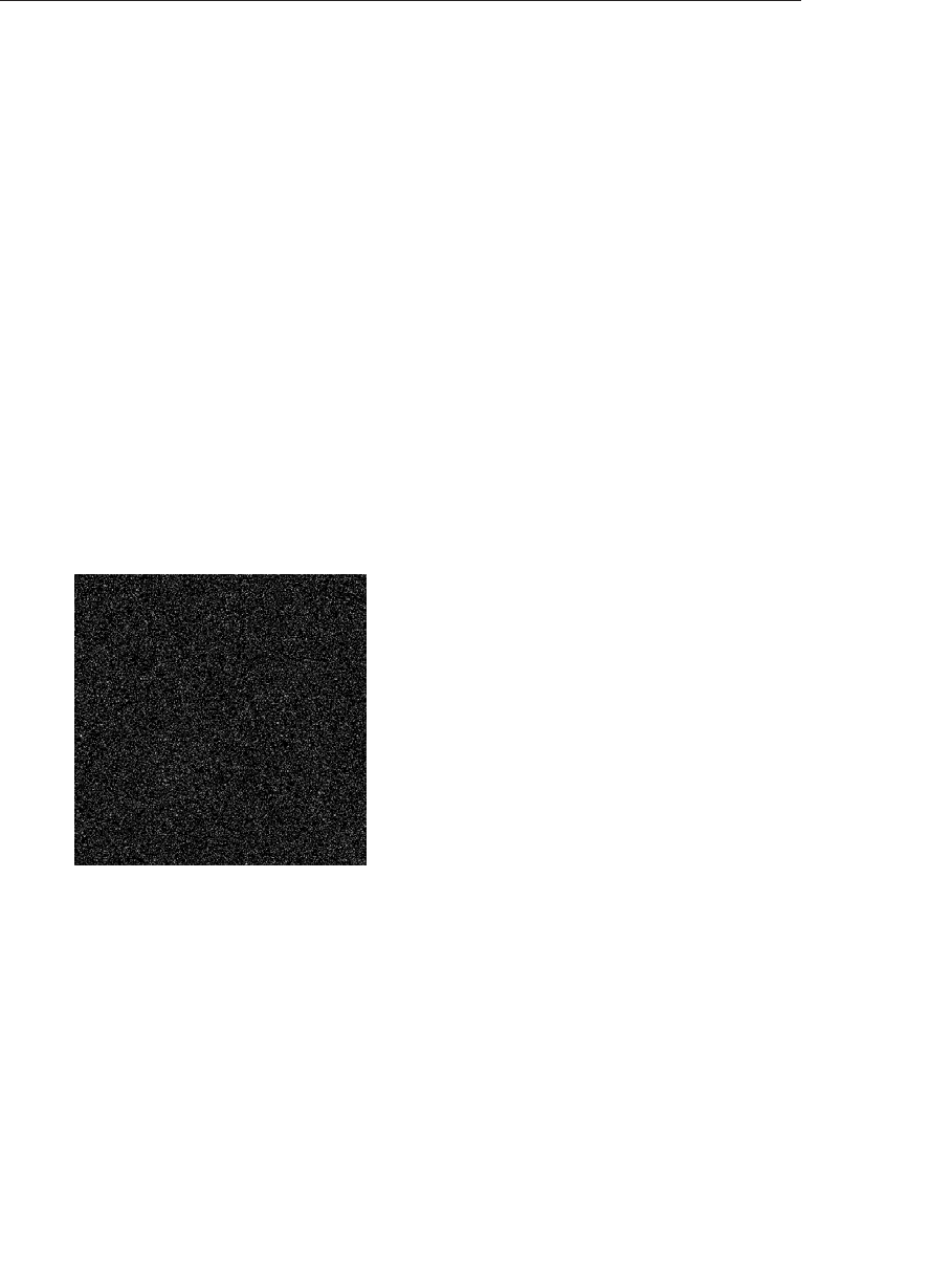
ptg9898810
// The fur texture
uniform sampler2D fur_texture;
// Color of the fur. Silvery gray by default...
uniform vec4 fur_color = vec4(0.8, 0.8, 0.9, 1.0);
// Input from the geometry shader
in GS_FS_VERTEX
{
vec3 normal;
vec2 tex_coord;
flat float fur_strength;
} fragment_in;
void main()
{// Fetch from the fur texture. We’ll only use the alpha channel
// here, but we could easily have a color fur texture.
vec4 rgba = texture(fur_texture, fragment_in.tex_coord);
float t = rgba.a;
// Multiply by fur strength calculated in the GS for the
// current shell t *= fragment_in.fur_strength;
// Scale fur color alpha by fur strength.
color = fur_color *vec4(1.0, 1.0, 1.0, t);
}
Figure 10.6 Texture used to represent hairs in the fur rendering
example
The fur fragment shader uses a texture to represent the layout of hairs in
the fur. The texture used in the fur example is shown in Figure 10.6. The
brightness of each texel maps to the length of the hair at that point. Zero
essentially means no hair, and white represents hairs whose length is equal
to the full depth of the fur volume.
The texture in Figure 10.6 is generated using a simple random placement
of hairs. A more sophisticated algorithm could be developed to allow hair
530 Chapter 10: Geometry Shaders
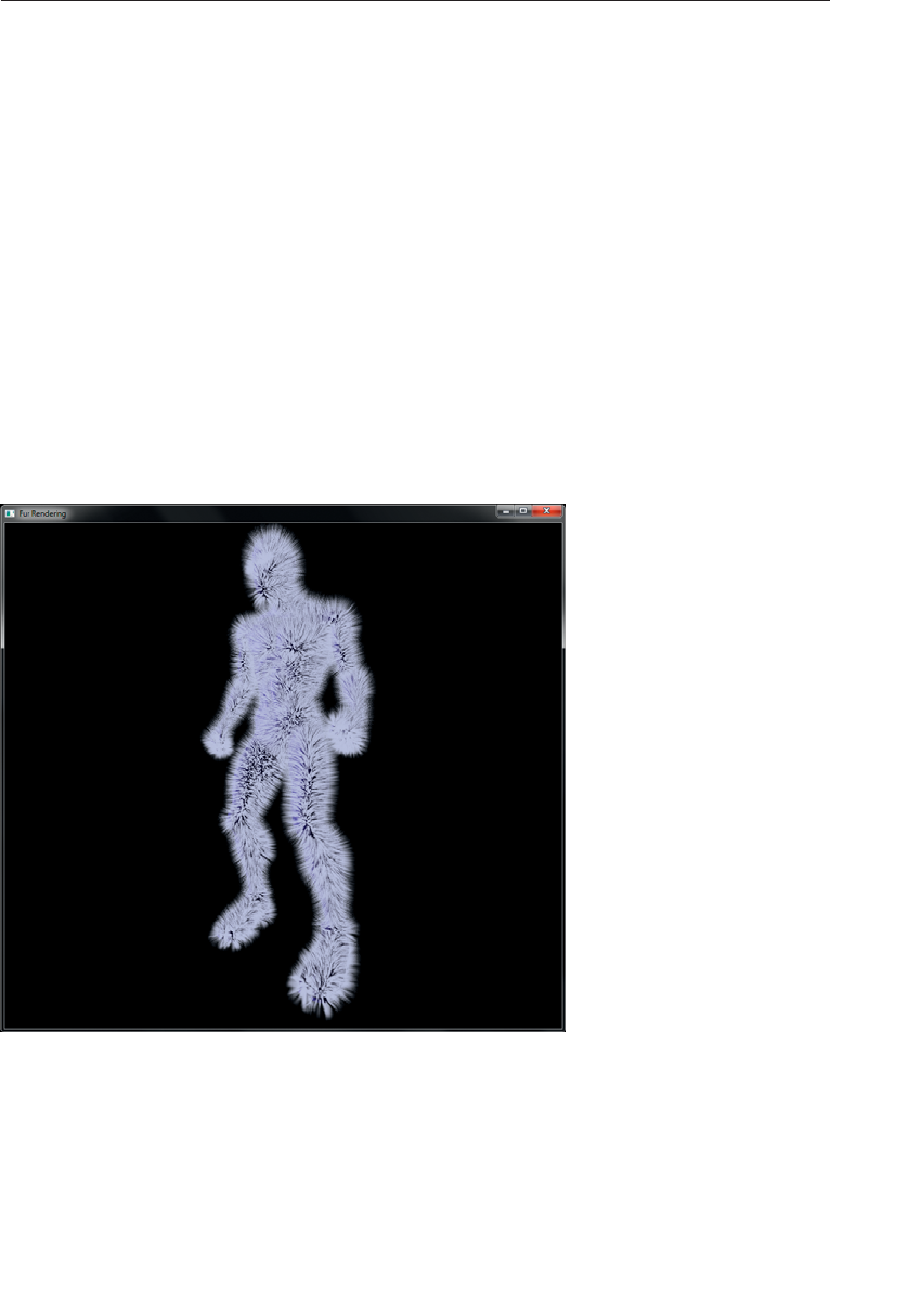
ptg9898810
density and distribution to be controlled programmatically. The current
depth of the shell being rendered is passed from the geometry shader into
the fragment shader. The fragment shader uses this, along with the
contents of the fur texture to determine how far along the hair the
fragment being rendered is. This information is used to calculate the
fragment’s color and opacity, which are used to generate the fragment
shader output.
A first pass of the underlying geometry is rendered without the fur shaders
active. This represents the skin of the object and prevents holes or gaps
appearing when the hair is sparse. Next, the fur rendering shader is
activated and another pass of the original geometry is rendered. Depth
testing is used to quickly reject fur fragments that are behind the solid
geometry. However, while the fur is being rendered, depth writes are
turned off. This causes the very fine tips of the hairs to not occlude thicker
hairs that may be behind them. Figure 10.7 shows the result of the
algorithm.
Figure 10.7 The output of the fur rendering example
As you can see from Figure 10.7, the fur rendered with this method is
reasonably convincing. There are ways to improve on the algorithm
though. For example, when polygons are seen edge-on, it is possible to see
Producing Primitives 531

ptg9898810
the individual slices that make up the shells. This means that we need a lot
of shells (and thus a lot of amplification in the geometry shader) to
produce a visually compelling result and hide this artifact. This can be
detrimental to performance. When fur shells are used, we will generally
also generate fur fins.
Fins are additional primitives emitted perpendicular to the edges of the
mesh that are determined to be silhouettes (edges that make the outline of
the shape). The fins are generated in the geometry shader, possibly at the
same time as generating the shells. We only generate fins for edges that are
silhouettes, and to make that decision we need to examine the two
triangles that share the edge. If the triangle on one side of the edge faces
towards the viewer and the triangle on the other side of the edge faces
away from the viewer then the edge is considered to be a silhouette. To
obtain information about the face normal of the adjacent face, we use the
adjacency primitive type. With access to the additional vertex forming
a triangle sharing an edge with our own, we can calculate the face
normal of both our own triangle and the adjacent one with a couple
of cross-products.
Another way to improve appearance is to use a true volume texture to
represent the hair. In this example, we used a simple two-dimensional
texture containing the length of a hair at each texel to represent fur. This is
a fairly crude approximation, and better results can be obtained by using a
real three-dimensional texture to store the density of the hair at all points
within the volume of the fur. This obviously requires a lot more storage
space but can improve visual quality and increase the level of control over
the effect.
Advanced Transform Feedback
We have already covered the concept of transform feedback and seen how
it works when only a vertex shader is present. In summary, the output of
the vertex shader is captured and recorded into one or more buffer objects.
Those buffer objects can subsequently be used for rendering (e.g., as vertex
buffers) or read back by the CPU using functions like glMapBuffer() or
glGetBufferSubData().We have also seen how to disable rasterization
such that only the vertex shader is active. However, the vertex shader is a
relatively simple one-in, one-out shader stage and cannot create or destroy
vertices. Also, it only has a single set of outputs.
You have just read about the ability of a geometry shader to produce a
variable amount of output vertices. When a geometry shader is present,
transform feedback captures the output of the geometry shader. In
addition to the stream of vertices that is usually sent to primitive assembly
532 Chapter 10: Geometry Shaders

ptg9898810
and rasterization, the geometry shader is capable of producing other,
ancillary streams of vertex information that can be captured using
transform feedback. By combining the geometry shader’s ability to
produce a variable amount of vertices at its output and its ability to send
those input vertices to any one of several output streams, some
sophisticated sorting, bucketing, and processing algorithms can be
implemented using the geometry shader and transform feedback.
In this subsection, we will introduce the concept of multiple vertex
streams as outputs from the geometry shader. We also introduce methods
to determine how many vertices were produced by the geometry shader,
both when using a single output stream and when using multiple output
streams. Finally, we discuss methods to use data generated by a geometry
shader and stored into a transform feedback buffer in subsequent draw
commands without requiring a round-trip to the CPU.
Multiple Output Streams
Multiple streams of vertices can be declared as outputs in the geometry
shader. Output streams are declared using the stream layout qualifier. This
layout qualifier may be applied globally, to an interface block, or to a
single output declaration. Each stream is numbered, starting from zero and
an implementation defined maximum number of streams can be declared.
That maximum can be found by calling glGetIntegerv() with the
parameter GL_MAX_VERTEX_STREAMS, and all OpenGL implementations
are required to support at least four geometry shader output streams.
When the stream number is given at global scope, all subsequently
declared geometry shader outputs become members of that stream until
another output stream layout qualifier is specified. The default output
stream for all outputs is zero. That is, unless otherwise specified, all
outputs belong to stream zero. The global stream layout qualifiers shown
in Example 10.9 demonstrate how to assign geometry shader outputs to
different streams.
Example 10.9 Global Layout Qualifiers Used to Specify a Stream Map
// Redundant as the default stream is 0
layout (stream=0) out;
// foo and bar become members of stream 0
out vec4 foo;
out vec4 bar;
// Switch the output stream to stream 1
layout (stream=1) out;
// proton and electron are members of stream 1
out vec4 proton;
Advanced Transform Feedback 533

ptg9898810
flat out float electron;
// Output stream declarations have no effect on input
// declarations elephant is just a regular input
in vec2 elephant;
// It’s possible to go back to a previously
// defined stream
layout (stream=0) out;
// baz joins it’s cousins foo and bar in stream 0
out vec4 baz;
// And then jump right to stream 3, skipping stream 2
// altogether
layout (stream=3) out;
// iron and copper are members of stream 3
flat out int iron;
out vec2 copper;
The declarations in Example 10.9 set up three output streams from a
geometry shader, numbered zero, one, and three. Stream zero contains
foo,bar, and baz, stream one contains proton and electron and
stream three contains iron and copper. Note that stream two is not used
at all and there are no outputs in it. An equivalent stream mapping can be
constructed using output interface blocks and is shown in Example 10.10.
Example 10.10 Example 10.9 Rewritten to Use Interface Blocks
// Again, redundant as the default output stream is 0
layout (stream=0) out stream0
{
vec4 foo;
vec4 bar;
vec4 baz;
};
// All of stream 1 output
layout (stream=1) out stream1
{
vec4 proton;
flat float electron;
};
// Skip stream 2, go directly to stream 3
layout (stream=3) out stream3
{
flat int iron;
vec2 copper;
};
As can be seen in Example 10.10, grouping members of a single stream in
an interface block can make the declarations appear more organized and so
534 Chapter 10: Geometry Shaders

ptg9898810
easier to read. Now that we have defined which outputs belong to which
streams, we need to direct output vertices to one or more of those streams.
As with a regular, single-stream geometry shader, vertices are emitted
and primitives are ended programmatically using special built-in GLSL
functions. When multiple output streams are active, the function to emit
vertices on a specific stream is EmitStreamVertex(int stream)
and the function to end a primitive on a specific stream is
EndStreamPrimitive(int stream). Calling EmitVertex is equivalent
to calling EmitStreamVertex with stream set to zero. Likewise, calling
EndPrimitive is equivalent to calling EndStreamPrimitive with
stream set to zero.
When EmitStreamVertex is called, the current values for any variables
associated with the specified stream are recorded and used to form a new
vertex on that stream. Just as when EmitVertex is called, the values of all
output variables become undefined, so too do they become undefined
when EmitStreamVertex is called. In fact, the current values of all
output variables on all streams become undefined. This is an important
consideration as code that assumes that the values of output variables
remain consistent across a call to EmitStreamVertex (or EmitVertex)
may work on some OpenGL implementations and not others, and most
shader compilers will not warn about this---especially on implementations
where it will work!
To illustrate, consider the example shown in Example 10.11.
Example 10.11 Incorrect Emission of Vertices into Multiple Streams
// Set up outputs for stream 0
foo = vec4(1.0, 2.0, 3.0, 4.0);
bar = vec4(5.0);
baz = vec4(4.0, 3.0, 2.0, 1.0);
// Set up outputs for stream 1
proton = atom;
electron = 2.0;
// Set up outputs for stream 3
iron = 4;
copper = shiny;
// Now emit all the vertices
EmitStreamVertex(0);
EmitStreamVertex(1);
EmitStreamVertex(3);
This example will produce undefined results because it assumes that the
values of the output variables associated with streams 1 and 3 remain valid
Advanced Transform Feedback 535

ptg9898810
across the calls to EmitStreamVerex. This is incorrect, and on some
OpenGL implementations, the values of proton,electron,iron and
copper will become undefined after the first call to EmitStreamVerex.
Such a shader should be written as shown in Example 10.12.
Example 10.12 Corrected Emission of Vertices into Multiple Streams
// Set up and emit outputs for stream 0
foo = vec4(1.0, 2.0, 3.0, 4.0);
bar = vec4(5.0);
baz = vec4(4.0, 3.0, 2.0, 1.0);
EmitStreamVertex(0);
// Set up and emit outputs for stream 1
proton = atom;
electron = 2.0;
EmitStreamVertex(1);
// Note, there’s nothing in stream 2
// Set up and emit outputs for stream 3
iron = 4;
copper = shiny;
EmitStreamVertex(3);
Now that we have a shader that outputs vertices on multiple output
streams, we need to inform OpenGL how those streams are mapped into
transform feedback buffers. This mapping is specified with the
glTransformFeedbackVaryings() function just as when only a single
output stream is present. Under normal circumstances, all output variables
are to be captured by transform feedback recorded into a single buffer (by
specifying GL_INTERLEAVED_ATTRIBS as the bufferMode parameter to
glTransformFeedbackVaryings()) or into a separate buffer for each
variable (by specifying GL_SEPARATE_ATTRIBS). When multiple streams
are active, it is required that variables associated with a single stream are
not written into the same buffer binding point as those associated with
any other stream.6It may be desirable, however, to have some or all of the
varyings associated with a single stream written, interleaved, into a single
buffer. To provide this functionality, the reserved variable name
gl_NextBuffer is used to signal that the following output variables are to
be recorded into the buffer object bound to the next transform feedback
binding point. Recall from Chapter 3that gl_NextBuffer is not a real
variable---it cannot be used in the shader; it is provided solely as a marker
to delimit groups of variables that will be written into the same buffer. For
6. Although it is not possible to direct output variables from different streams into the same
transform feedback buffer binding point, it is possible to bind the same buffer object (or better,
different sections of the same buffer) to different transform feedback buffer binding points.
This allows variables from different streams to be written into the same buffer.
536 Chapter 10: Geometry Shaders

ptg9898810
Examples 10.9 and 10.10, we will record the variables for the first stream
(foo,bar, and baz) into the buffer object bound to the first transform
feedback buffer binding point, the variables for the second stream (proton
and electron) into the buffer bound to the second binding point, and
finally the variables associated with stream 3 (iron and copper) into the
buffer bound to the third buffer binding point. Example 10.13 shows how
to express this layout.
Example 10.13 Assigning Transform Feedback Outputs to Buffers
static const char *const vars[] =
{"foo", "bar", "baz", // Variables from stream 0
"gl_NextBuffer", // Move to binding point 1
"proton", "electron", // Variables from stream 1
"gl_NextBuffer", // Move to binding point 2
// Note, there are no variables
// in stream 2
"iron", "copper" // Variables from stream 3
};
glTransformFeedbackVaryings(prog,
sizeof(vars) / sizeof(vars[0]),
varyings,
GL_INTERLEAVED_ATTRIBS);
glLinkProgram(prog);
Notice the call to glLinkProgram() after the call to
glTransformFeedbackVaryings() in Example 10.13. As previously
mentioned, the mapping specified by glTransformFeedbackVaryings()
does not take effect until the next time the program object is linked.
Therefore, it is necessary to call glLinkProgram() after
glTransformFeedbackVaryings() before the program object is used.
If rasterization is enabled and there is a fragment shader present, the
output variables belonging to stream 0 (foo,bar, and baz) will be used to
form primitives for rasterization and will be passed into the fragment
shader. Output variables belonging to other streams (proton,electron,
iron, and copper) will not be visible in the fragment shader and if
transform feedback is not active, they will be discarded. Also note that
when multiple output streams are used in a geometry shader, they must all
have points as the primitive type. This means that if rasterization is used in
conjunction with multiple geometry shader output streams, an application
is limited to rendering points with that shader.
Primitive Queries
Transform feedback was introduced in ‘‘Transform Feedback’’ on Page 239
as a method to record the output of a vertex shader into a buffer that could
Advanced Transform Feedback 537

ptg9898810
be used in subsequent rendering. Because the vertex shader is a simple,
one-in, one-out pipeline stage, it is known up front how many vertices the
vertex shader will generate. Assuming that the transform feedback buffer is
large enough to hold all of the output data, the number of vertices stored
in the transform feedback buffer is simply the number of vertices processed
by the vertex shader. Such a simple relationship is not present for the
geometry shader. Because the geometry shader can emit a variable number
of vertices per invocation, the number of vertices recorded into transform
feedback buffers when a geometry shader is present may not be easy to
infer. In addition to this, should the space available in the transform
feedback buffers be exhausted, the geometry shader will produce more
vertices than are actually recorded. Those vertices will still be used to
generate primitives for rasterization (if they are emitted on stream 0), but
they will not be written into the transform feedback buffers.
To provide this information to the application, two types of queries are
available to count both the number of primitives the geometry shader
generates, and the number of primitives actually written into the
transform feedback buffers. These are the GL_PRIMITIVES_GENERATED
and GL_TRANSFORM_FEEDBACK_PRIMITIVES_WRITTEN queries. The
GL_PRIMITIVES_GENERATED query counts the number of vertices output
by the geometry shader, even if space in the transform feedback buffers
was exhausted and the vertices were not recorded. The GL_TRANSFORM_
FEEDBACK_PRIMITIVES_WRITTEN query counts the number of vertices
actually written into a transform feedback buffer. Note that the GL_
PRIMITIVES_GENERATED query is valid at any time, even when transform
feedback is not active (hence the lack of TRANSFORM_FEEDBACK in the
name of the query), whereas GL_TRANSFORM_FEEDBACK_PRIMITIVES_
WRITTEN only counts when transform feedback is active.7
Because a geometry shader can output to multiple transform feedback
streams, primitive queries are indexed. That is, there are multiple binding
points for each type of query---one for each supported output stream. To
begin and end a primitive query for a particular primitive stream, call:
void glBeginQueryIndexed(GLenum target, GLuint index,
GLuint id);
Begins a query using the query object id on the indexed query target
point specified by target and index.
7. This makes sense. In a way, a GL_TRANSFORM_FEEDBACK_PRIMITIVES_WRITTEN query
does continue to count when transform feedback is not active, but as no primitives are written,
it will not increment, and so the result is the same.
538 Chapter 10: Geometry Shaders

ptg9898810
and
void glEndQueryIndexed(GLenum target, GLuint index);
Ends the active query on the indexed query target point specified by
target and index.
Here, target is set to either GL_PRIMITIVES_GENERATED or
GL_TRANSFORM_FEEDBACK_PRIMITIVES_WRITTEN, index is the index of
the primitive query binding point on which to execute the query, and id is
the name of a query object that was previously created using the
glGenQueries() function. Once the primitive query has been ended, the
availability of the result can be checked by calling glGetQueryObjectuiv()
with the pname parameter set to GL_QUERY_RESULT_AVAILABLE and
the actual value of the query can be retrieved by calling
glGetQueryObjectuiv() with pname set to GL_QUERY_RESULT. Don’t
forget that if the result of the query object is retrieved by calling
glGetQueryObjectuiv() with name set to GL_QUERY_RESULT and the
result was not available yet, the GPU will likely stall, significantly reducing
performance.
It is possible to run both a GL_PRIMITIVES_GENERATED and a
GL_TRANSFORM_FEEDBACK_PRIMITIVES_WRITTEN query
simultaneously on the same stream. If the result of the GL_PRIMITIVES_
GENERATED query is greater than the result of the GL_TRANSFORM_
FEEDBACK_PRIMITIVES_WRITTEN query, it may indicate that the
transform feedback buffer was not large enough to record all of the results.
Using Transform Feedback Results
Now that the number of vertices recorded into a transform feedback buffer
is known, it is possible to pass that vertex count into a function like
glDrawArrays() to use it as the source of vertex data in subsequent
rendering. However, to retrieve this count requires the CPU to read
information generated by the GPU, which is generally detrimental to
performance. In this case, the CPU will wait for the GPU to finish
rendering anything that might contribute to the primitive count, and then
the GPU will wait for the CPU to send a new rendering command using
that count. Ideally, the count would never make the round trip from the
GPU to the CPU and back again. To achieve this, the OpenGL commands
Advanced Transform Feedback 539

ptg9898810
glDrawTransformFeedback() and glDrawTransformFeedbackStream()
are supplied. The prototypes of these functions are as follows:
void glDrawTransformFeedback(GLenum mode, GLuint id);
void glDrawTransformFeedbackStream(GLenum mode,
GLuint id,
GLuint stream);
Draw primitives as if glDrawArrays() had been called with mode set as
specified, first set to zero and count set to the number of primitives
captured by transform feedback stream stream on the transform feedback
object id. Calling glDrawTransformFeedback() is equivalent to calling
glDrawTransformFeedbackStream() with stream set to zero.
When glDrawTransformFeedbackStream() is called, it is equivalent to
calling glDrawArrays() with the same mode parameter, with first set to
zero, and with the count parameter taken from a virtual
GL_TRANSFORM_FEEDBACK_PRIMITIVES_WRITTEN query running on
stream stream of the transform feedback object id. Note that there is no
need to execute a real
GL_TRANSFORM_FEEDBACK_PRIMITIVES_WRITTEN query and the
primitive count is never actually transferred from the GPU to the CPU.
Also, there is no requirement that the buffers used to record the results of
the transform feedback operation need to be bound for use in the new
draw. The vertex count used in such a draw is whatever was recorded the
last time glEndTransformFeedback() was called while the transform
feedback object id was bound. It is possible for transform feedback to still
be active for id---the previously recorded vertex count will be used.
By using the glDrawTransformFeedbackStream() function, it is possible
to circulate the result of rendering through the pipeline. By repeatedly
calling glDrawTransformFeedbackStream(), vertices will be transformed
by the OpenGL vertex and geometry shaders. Combined with double
buffering of vertex data,8it is possible to implement recursive algorithms
that change the number of vertices in flight on each iteration of the loop.
Drawing transform feedback may be combined with instancing to allow
you to draw many instances of the data produced by transform feedback.
To support this, the functions glDrawTransformFeedbackInstanced() and
8. Double buffering is required because undefined results will be produced if the same buffer
objects are bound both for transform feedback and as the source of data.
540 Chapter 10: Geometry Shaders

ptg9898810
glDrawTransformFeedbackStreamInstanced() are provided. Their
prototypes are as follows:
void glDrawTransformFeedbackInstanced(GLenum mode,
GLuint id,
GLsizei instancecount);
void glDrawTransformFeedbackStreamInstanced(GLenum mode,
GLuint id,
GLuint stream,
GLsizei instancecount);
Draw primitives as if glDrawArraysInstanced() had been called with first
set to zero, count set to the number of primitives captured by transform
feedback stream stream on the transform feedback object id and with
mode and instancecount passed as specified. Calling
glDrawTransformFeedbackInstanced() is equivalent to calling
glDrawTransformFeedbackStreamInstanced() with stream set to zero.
Combining Multiple Streams and DrawTransformFeedback
As a worked example of the techniques just described, we’ll go over an
application that demonstrates how to use a geometry shader to sort
incoming geometry, and then render subsets of it in subsequent passes. In
this example, we’ll use the geometry shader to sort ‘‘left-facing’’ and
‘‘right-facing’’ polygons---that is, polygons whose face normal points to the
left or right. The left-facing polygons will be sent to stream zero, while the
right-facing polygons will be sent to stream one. Both streams will be
recorded into transform feedback buffers. The contents of those buffers
will then be drawn using glDrawTransformFeedbackStream() while a
different program object is active. This causes left-facing primitives to be
rendered with a completely different state from right-facing primitives,
even though they are physically part of the same mesh.
First, we will use a vertex shader to transform incoming vertices into view
space. This shader is shown in Example 10.14 below.
Example 10.14 Simple Vertex Shader for Geometry Sorting
#version 330 core
uniform mat4 model_matrix;
layout (location = 0) in vec4 position;
layout (location = 1) in vec3 normal;
out vec3 vs_normal;
Advanced Transform Feedback 541

ptg9898810
void main()
{vs_normal = (model_matrix *vec4(normal, 0.0)).xyz;
gl_Position = model_matrix *position;
}
Vertices enter the geometry shader shown in Example 10.15 in view space.
This shader takes the incoming stream of primitives, calculates a per-face
normal, and then uses the sign of the X component of the normal to
determine whether the triangle is left-facing or right-facing. The face
normal for the triangle is calculated by taking the cross product of two of
its edges. Left-facing triangles are emitted to stream zero and right-facing
triangles are emitted to stream one, where outputs belonging to each
stream will be recorded into separate transform feedback buffers.
Example 10.15 Geometry Shader for Geometry Sorting
#version 330 core
// Triangles input, points output (although we’ll write
// three points for each incoming triangle.
layout (triangles) in;
layout (points, max_vertices =3)out;
uniform mat4 projection_matrix;
in vec3 vs_normal[];
// Stream 0 - left-facing polygons
layout (stream = 0) out vec4 lf_position;
layout (stream = 0) out vec3 lf_normal;
// Stream 1 - right-facing polygons
layout (stream = 1) out vec4 rf_position;
layout (stream = 1) out vec3 rf_normal;
void main()
{
// Take the three vertices and find the (unnormalized face normal)
vec4 A = gl_in[0].gl_Position;
vec4 B = gl_in[1].gl_Position;
vec4 C = gl_in[2].gl_Position;
vec3 AB = (B - A).xyz;
vec3 AC = (C - A).xyz;
vec3 face_normal = cross(AB, AC);
int i;
// If the normal’s X coordinate is negative, it faces to the left of
// the viewer and is "left-facing", so stuff it in stream 0
if (face_normal.x < 0.0)
{
// For each input vertex ...
542 Chapter 10: Geometry Shaders

ptg9898810
for (i = 0; i < gl_in.length(); i++)
{
// Transform to clip space
lf_position = projection_matrix *
(gl_in[i].gl_Position -
vec4(30.0, 0.0, 0.0, 0.0));
// Copy the incoming normal to the output stream
lf_normal = vs_normal[i];
// Emit the vertex
EmitStreamVertex(0);
}
// Calling EndStreamPrimitive is not strictly necessary as
// these are points
EndStreamPrimitive(0);
}
// Otherwise, it’s "right-facing" and we should write it to stream 1.
else
{
// Exactly as above but writing to rf_position and rf_normal
// for stream 1.
for (i = 0; i < gl_in.length(); i++)
{
rf_position = projection_matrix *
(gl_in[i].gl_Position -
vec4(30.0, 0.0, 0.0, 0.0));
rf_normal = vs_normal[i];
EmitStreamVertex(1);
}
EndStreamPrimitive(1);
}
}
When rendering the sorting pass, we will not be rasterizing any polygons,
and so our first pass program has no fragment shader. To disable
rasterization we will call glEnable(GL_RASTERIZER_DISCARD). If an
attempt is made to render with a program object that does not contain a
fragment shader and rasterization is not disabled, an error will be
generated. Before linking the sorting program, we need to specify where
the transform feedback varyings will be written to. To do this, we use the
code shown in Example 10.16 below.
Example 10.16 Configuring Transform Feedback for Geometry Sorting
static const char *varyings[] =
{// These two varyings belong to stream 0
"rf_position", "rf_normal",
// Move to the next binding point (can’t write
// varyings from different streams to the same buffer
// binding point.)
"gl_NextBuffer",
// These two varyings belong to stream 1
Advanced Transform Feedback 543

ptg9898810
"lf_position", "lf_normal"
};
glTransformFeedbackVaryings(sort_prog,
5,
varyings,
GL_INTERLEAVED_ATTRIBS);
Notice that the output of the geometry shader for stream zero and stream
one are identical. The same data is written to the selected stream regardless
of whether the polygon is left- or right-facing. In the first pass, all of the
vertex data recorded into the transform feedback buffers have already been
transformed into clip space and so we can reuse that work on the second
and third passes that will be used to render it. All we need to supply is a
pass-through vertex shader (shown in Example 10.17 below) to read the
pre-transformed vertices and feed the fragment shader. There is no
geometry shader in the second pass.
Example 10.17 Pass-Through Vertex Shader used for Geometry Shader
Sorting
#version 330 core
layout (location = 0) in vec4 position;
layout (location = 1) in vec3 normal;
out vec3 vs_normal;
void main()
{vs_normal = normal;
gl_Position = position;
}
We’ll use the same fragment shader in the second and third passes, but in a
more complex application of this technique, a different shader could be
used for each pass.
Now, to drive this system we need several objects to manage data and logic
at the OpenGL API level. First, we need two program objects for the
programs that will be used in the three passes (one containing the vertex
and geometry shaders for sorting the left-facing and right-facing
primitives, and one containing the pass-through vertex and fragment
shaders for the two rendering passes). We need buffer objects for storing
the input geometry shader and the intermediate data produced by the
geometry shader. We need a pair of vertex array objects (VAOs) to represent
the vertex inputs to the two rendering passes. Finally, we need a transform
544 Chapter 10: Geometry Shaders

ptg9898810
feedback object to manage transform feedback data and primitive counts.
The code to set all this up is given in Example 10.18 below.
Example 10.18 OpenGL Setup Code for Geometry Shader Sorting
// Create a pair of vertex array objects and buffer objects
// to store the intermediate data.
glGenVertexArrays(2, vao);
glGenBuffers(2, vbo);
// Create a transform feedback object upon which transform
// feedback operations (including the following buffer
// bindings) will operate, and then bind it.
glGenTransformFeedbacks(1, &xfb);
glBindTransformFeedback(GL_TRANSFORM_FEEDBACK, xfb);
// For each of the two streams ...
for (i = 0; i < 2; i++)
{// Bind the buffer object to create it.
glBindBuffer(GL_TRANSFORM_FEEDBACK_BUFFER, vbo[i]);
// Call glBufferData to allocate space. 2ˆ20 floats
// should be enough for this example. Note GL_DYNAMIC_COPY.
// This means that the data will change often (DYNAMIC)
// and will be both written by and used by the GPU (COPY).
glBufferData(GL_TRANSFORM_FEEDBACK_BUFFER,
1024 *1024 *sizeof(GLfloat),
NULL, GL_DYNAMIC_COPY);
// Now bind it to the transform feedback buffer binding
// point corresponding to the stream.
glBindBufferBase(GL_TRANSFORM_FEEDBACK_BUFFER, i, vbo[i]);
// Now set up the VAOs. First, bind to create.
glBindVertexArray(vao[i]);
// Now bind the VBO to the ARRAY_BUFFER binding.
glBindBuffer(GL_ARRAY_BUFFER, vbo[i]);
// Set up the vertex attributes for position and normal ...
glVertexAttribPointer(0, 4, GL_FLOAT, GL_FALSE,
sizeof(vec4) + sizeof(vec3),
NULL);
glVertexAttribPointer(1, 3, GL_FLOAT, GL_FALSE,
sizeof(vec4) + sizeof(vec3),
(GLvoid *)(sizeof(vec4)));
// ... and remember to enable them!
glEnableVertexAttribArray(0);
glEnableVertexAttribArray(1);
}
Once we have created and set up all of our data management objects, we
need to write our rendering loop. The general flow is shown in Figure 10.8
below. The first pass is responsible for sorting the geometry into front- and
Advanced Transform Feedback 545
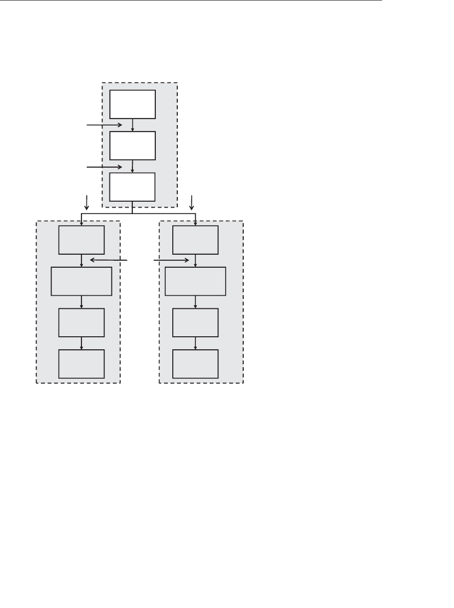
ptg9898810
back-facing polygons and performs no rasterization. The second and third
passes are essentially identical in this example, although a completely
different shading algorithm could be used in each. These passes actually
render the sorted geometry as if it were supplied by the application.
INPUT
GEOMETRY
SORTING
GEOMETRY
SHADER
REAL
VERTEX
SHADER
OBJECT
SPACE
VERTICES
VIEW
SPACE
VERTICES
PASS-THROUGH
VERTEX
SHADER
RASTERIZE
FRAGMENT
SHADER
STREAM 0STREAM 1
PASS-THROUGH
VERTEX
SHADER
RASTERIZE
FRAGMENT
SHADER
CLIP
SPACE
VERTICES
RIGHT-
FACING
GEOMETRY
LEFT-
FACING
GEOMETRY
FIRST PASS
SECOND PASS
THIRD PASS
Figure 10.8 Schematic of geometry shader sorting example
For the first pass, we bind the VAO representing the original input
geometry and the program object containing the sorting geometry shader.
We bind the transform feedback object and the intermediate buffer
to the transform feedback buffer binding, start transform feedback, and
draw the original geometry. The geometry shader sorts the incoming
triangles into left- and right-facing groups and sends them to the
appropriate stream. After the first pass, we turn off transform feedback.
For the second pass, bind the VAO representing the intermediate data
written to stream zero, bind the second pass program object, and use
glDrawTransformFeedbackStream() to draw the intermediate left-facing
geometry using the primitives-written count from stream zero on the first
546 Chapter 10: Geometry Shaders

ptg9898810
pass. Likewise, in the third pass we draw the right-facing geometry by
using glDrawTransformFeedbackStream() with stream one.
Example 10.19 Rendering Loop for Geometry Shader Sorting
// First pass - start with the "sorting" program object.
glUseProgram(sort_prog);
// Set up projection and model-view matrices
mat4 p(frustum(-1.0f, 1.0f, aspect, -aspect, 1.0f, 5000.0f));
mat4 m;
m = mat4(translation(0.0f,
0.0f,
100.0f *sinf(6.28318531f *t) - 230.0f) *
rotation(360.0f *t, X) *
rotation(360.0f *t*2.0f, Y) *
rotation(360.0f *t*5.0f, Z) *
translation(0.0f, -80.0f, 0.0f));
glUniformMatrix4fv(model_matrix_pos, 1, GL_FALSE, m[0]);
glUniformMatrix4fv(projection_matrix_pos, 1, GL_FALSE, p);
// Turn off rasterization
glEnable(GL_RASTERIZER_DISCARD);
// Bind the transform feedback object and start
// recording (note GL_POINTS used here...)
glBindTransformFeedback(GL_TRANSFORM_FEEDBACK, xfb);
glBeginTransformFeedback(GL_POINTS);
// Render the object
object.Render();
// Stop recording and unbind the transform feedback object
glEndTransformFeedback();
glBindTransformFeedback(GL_TRANSFORM_FEEDBACK, 0);
// Turn rasterization back on
glDisable(GL_RASTERIZER_DISCARD);
static const vec4 colors[2] =
{
vec4(0.8f, 0.8f, 0.9f, 0.5f),
vec4(0.3f, 1.0f, 0.3f, 0.8f)
};
// Use the rendering program
glUseProgram(render_prog);
// Second pass - left facing polygons. Regular rendering
glUniform4fv(0, 1, colors[0]);
Advanced Transform Feedback 547
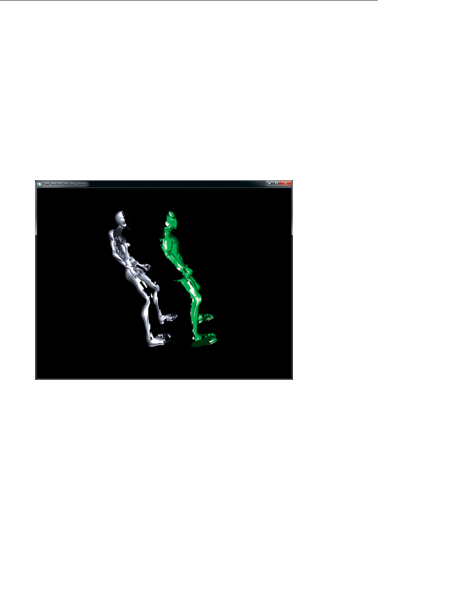
ptg9898810
glBindVertexArray(vao[0]);
glDrawTransformFeedbackStream(GL_TRIANGLES, xfb, 0);
// Now draw stream 1, which contains right facing polygons.
glUniform4fv(0, 1, colors[1]);
glBindVertexArray(vao[1]);
glDrawTransformFeedbackStream(GL_TRIANGLES, xfb, 1);
The output of the program shown in Example 10.19 is shown in
Figure 10.9. While this is not the most exciting program ever written,
it does demonstrate the techniques involved in configuring and
using transform feedback with multiple streams and the
glDrawTransformFeedback() function.
Figure 10.9 Final output of geometry shader sorting example
An interesting note is that although we are drawing triangles when
rendering the original model, the transform feedback mode is GL_POINTS.
This is because the sorting geometry shader converts the incoming
triangles into points. OpenGL requires that when multiple output streams
are in use in a geometry shader, the output primitive type is points
(although the input can be anything). If this restriction were not present,
this application would run in two passes rather than three. Even though
we recorded points into the transform feedback buffers, we can still draw
the second and third passes using GL_TRIANGLES. Once the vertices have
been recorded into the transform feedback buffers, they are simply
interpreted as raw data and can be used for any purpose.
548 Chapter 10: Geometry Shaders

ptg9898810
Geometry Shader Instancing
One type of instancing has already been covered in Chapter 3. In this first
type of instancing, functions like glDrawArraysInstanced() or
glDrawElementsInstanced() are used to simply run the whole OpenGL
pipeline on a set of input data multiple times. This results in the vertex
shader running several times on all of the input vertices, with the same
vertex data being fetched from memory for each instance of the draw.
Also, if tessellation is active, primitives will be tessellated multiple times,
resulting in a potentially huge processing load for the GPU. To differentiate
between members of each instance in the shader, the built-in GLSL variable
gl_InstanceID is provided. Another type of instancing, known as
geometry shader instancing, is available that only runs the geometry shader
and subsequent stages (rasterization and fragment shading) multiple times,
rather than the whole pipeline. Geometry shader instancing requires that a
geometry shader is present, and so cannot be used without a geometry
shader in the currently active program. Both methods of instancing may
be used simultaneously. That is, glDrawArraysInstanced() may be called
while a geometry shader is present that uses geometry shader instancing.
Geometry shader instancing is enabled in the shader by specifying the
invocations layout qualifier as part of the input definition as follows:
layout (triangles, invocations = 4) in;
This example specifies that the geometry shader will be invoked four times
for each input primitive (in this case, triangles). The special built-in GLSL
input variable gl_InvocationID will contain the invocation number
while the geometry shader is running (starting at zero). In effect, all
geometry shaders are instanced, although the default invocation count is
one. gl_InvocationID is always available as a geometry shader input,
but when instancing is not active, its value will be zero. When using
instancing in the geometry shader, it is advisable to move as much work as
possible from the geometry shader to the vertex shader. By doing so, any
such work is performed only once and then shared across all geometry
shader invocations. If that work were to be performed in the geometry
shader, it would run once per instance.
The maximum invocation count for geometry shader supported by the
OpenGL implementation can be found by calling glGetIntegerv() with
pname set to GL_MAX_GEOMETRY_SHADER_INVOCATIONS. All OpenGL
implementations must support at least 32 invocations for instanced
geometry shaders, but the count may be higher. Each invocation of the
geometry shader may still output the maximum number of vertices
allowed by the OpenGL implementation. In this way, an instanced
Geometry Shader Instancing 549

ptg9898810
geometry shader may reach a much higher amplification level as with a
noninstanced geometry shader, any amplification performed must be
limited to the maximum number of output vertices supported by the
implementation. By combining API level instancing with geometry shader
instancing and amplification in the geometry shader, it is possible to
essentially nest three levels of geometry in a single draw. Pseudo-code for
this is shown in Example 10.20 below.
Example 10.20 Geometry Amplification Using Nested Instancing
for each API instance // glDrawArraysInstanced
{
for each geometry shader invocation // layout (invocations=N)
{
for each primitive produced by the geometry shader
{render primitive
}
}
}
Multiple Viewports and Layered Rendering
This section of the chapter covers two output variables available in the
geometry shader that can redirect rendering into different regions of
the framebuffer, or to layers of array textures. These variables are
gl_ViewportIndex and gl_Layer, respectively. Their values are
also available as inputs to fragment shaders.9
Viewport Index
The first of these two variables, gl_ViewportIndex is used to specify
which set of viewport parameters will be used to perform the viewport
transformation by OpenGL. These parameters are passed to OpenGL by
calling glViewportIndexedf() or glViewportIndexedfv() to specify how
window xand ycoordinates are generated from clip coordinates. Addition-
ally, glDepthRangeIndexed() can be used to specify how the window z
coordinate is generated. The prototypes of these functions are as follows:
9. As of GLSL version 4.3, gl_Layer and gl_Viewport are available as inputs to the fragment
shader. In earlier versions of OpenGL (and GLSL), if you need the values of these variables in
the fragment shader, you would need to pass them explicitly as a user-defined variable.
550 Chapter 10: Geometry Shaders

ptg9898810
void glViewportIndexedf(GLuint index, GLfloat x, GLfloat y,
GLfloat w, GLfloat h);
void glViewportIndexedfv(GLuint index, const GLfloat * v);
void glDepthRangeIndexed(GLuint index, GLclampd n,
GLclampd f);
Sets the bounds of a specific viewport. glViewportIndexedf() sets the
bounds of the viewport determined by index to the rectangle whose
upper left is at (x,y) and whose width and height ar wand h, respectively.
glViewportIndexedfv() performs the same action, but with x,y,w, and h
taken from the first through fourth elements of the array v.
glDepthRangeIndexed() sets the depth extent of the viewport indexed
by index.nand frepresent the near and far planes, respectively.
The viewport origins, widths, and heights are stored in an array by
OpenGL and when a geometry shader is active that writes to
gl_ViewportIndex, that value is used to index into the array of viewport
parameters. If the geometry shader does not write to gl_ViewportIndex,
or if no geometry shader is present, the first viewport is used.
If you need to set the extent of a number of viewports (and their depth
ranges), you can also use the glViewportArrayv() and
glDepthRangeArrayv() functions. These functions take a count of the
number of viewports whose bounds to update, the index of the first
viewport to update, and an array of parameters that will be used to
update the viewports’ bounds. Their prototypes are as follows:
void glViewportArrayv(GLuint first, GLsizei count,
const GLfloat * v);
void glDepthRangeArrayv(GLuint first, GLsizei count,
const GLdouble * v);
Set the bounds of number of viewports with a single command. For
both functions, first contains the index of the first viewport to
update and count contains the number of viewports to update. For
glViewportArrayv(),vcontains the address of an array if 4 ×count
floating point values---one set of four for each viewport, which represent
the x,y,w, and hparameters to a call to glViewportIndexedf(), in that
order. For glDepthRangeArrayv(),vcontains the address of an array of
2×count double-precision floating point values---one set of two for each
viewport, which represent the nand fparameters to a call to
glDepthRangeIndexed().
Multiple Viewports and Layered Rendering 551

ptg9898810
An example use case is to specify multiple viewports within a single
framebuffer (e.g., a top, side, and front view in a 3D modeling application)
and use the geometry shader to render the same input vertex data into
each of the viewports. This can be performed using any of the techniques
discussed previously. For example, the geometry shader could perform a
simple loop and amplify the geometry---outputting more primitives than it
receives as input. Alternatively, the geometry shader could be made to
perform instancing with an invocation count of three, and redirect the
geometry to the appropriate viewport during each invocation. In either
case, it’s advisable to perform per-vertex operations in the vertex shader
and simply direct rendering to the appropriate viewport in the geometry
shader. The geometry shader will also need to perform any operations that
are unique for each viewport. In this example, a different projection
matrix will be needed for each viewport.
Example 10.21 below contains a simple but a complete example of a
geometry shader that uses instancing and multiple invocations to direct
rendering to an array of four viewports.
Example 10.21 Directing Geometry to Different Viewports with
a Geometry Shader
#version 330 core
// Triangles in, four invocations (instances)
layout (triangles,invocations = 4) in;
// Triangles (strips) out, 3 vertices each
layout (triangle_strip,max_vertices = 3) out;
// Four model matrices and a common projection matrix
uniform mat4 model_matrix[4];
uniform mat4 projection_matrix;
// Normal input from the vertex shader
in vec3 vs_normal[];
// Color and normal output to the fragment shader
out vec4 gs_color;
out vec3 gs_normal;
// Colors that will be used for the four instances
const vec4 colors[4] = vec4[4]
(
vec4(1.0, 0.7, 0.3, 1.0),
vec4(1.0, 0.2, 0.3, 1.0),
vec4(0.1, 0.6, 1.0, 1.0),
vec4(0.3, 0.7, 0.5, 1.0)
);
void main()
552 Chapter 10: Geometry Shaders

ptg9898810
{
for (int i = 0; i < gl_in.length(); i++)
{// Set the viewport index for every vertex.
gl_ViewportIndex = gl_InvocationID;
// Color comes from the "colors" array, also
// indexed by gl_InvocationID.
gs_color = colors[gl_InvocationID];
// Normal is transformed using the model matrix.
// Note that this assumes that there is no
// shearing in the model matrix.
gs_normal = (model_matrix[gl_InvocationID] *
vec4(vs_normal[i], 0.0)).xyz;
// Finally, transform the vertex into position
// and emit it.
gl_Position = projection_matrix *
(model_matrix[gl_InvocationID] *
gl_in[i].gl_Position);
EmitVertex();
}
}
In this shader, the viewport index is simply initialized using the invocation
number (gl_InvocationID). Note that this is set for every vertex in the
output primitive, even though it is the same for each. An array of four
model matrices is used to apply a different transformation to each of
several copies of the incoming geometry. The geometry shader invocation
number is also used to index into the array of transformation matrices.
Finally, an array of colors is used to color each instance of the geometry
differently and this is also indexed using the invocation number.
Before drawing each frame, the array of model matrices is updated using
the code shown in Example 10.22 below. A different translation and
rotation is used for each of the four matrices.
Example 10.22 Creation of Matrices for Viewport Array Example
static const vec3 X(1.0f, 0.0f, 0.0f);
static const vec3 Y(0.0f, 1.0f, 0.0f);
static const vec3 Z(0.0f, 0.0f, 1.0f);
mat4 m[4];
for (int i = 0; i < 4; i++)
{m[i] = mat4(
translation(
0.0f,
0.0f,
100.0f *sin(6.28318531f *t + i) - 230.0f) *
Multiple Viewports and Layered Rendering 553

ptg9898810
rotation(360.0f *t*float(i + 1), X) *
rotation(360.0f *t*float(i + 2), Y) *
rotation(360.0f *t*float(5 - i), Z) *
translation(0.0f, -80.0f, 0.0f));
}
glUniformMatrix4fv(model_matrix_pos, 4, GL_FALSE, m[0]);
Notice in Example 10.22 how glUniformMatrix4fv() is used to set the
complete array of four matrix uniforms with a single function call. In the
window resize handler for the program, the four viewports are set using
the code shown in Example 10.23.
Example 10.23 Specifying Four Viewports
void ViewportArrayApplication::Reshape(int width, int height)
{
const float wot = float(width) *0.5f;
const float hot = float(height) *0.5f;
glViewportIndexedf(0, 0.0f, 0.0f, wot, hot);
glViewportIndexedf(1, wot, 0.0f, wot, hot);
glViewportIndexedf(2, 0.0f, hot, wot, hot);
glViewportIndexedf(3, wot, hot, wot, hot);
}
In Example 10.23,wot and hot represent the width and height on two,
respectively. This code divides the window into four quadrants with a
viewport for each. The glViewportIndexedf() function is used to set the
viewports individually. Figure 10.10 shows the output of the program.
In addition to the multiple viewports supported by OpenGL, multiple
scissor rectangles are also supported. Individual scissor rectangles may be
specified using the glScissorIndexed() and glScissorIndexedv() functions,
whose prototypes are as follows:
void glScissorIndexed(GLuint index, GLint left, GLint bottom,
GLsizei width, GLsizei height);
void glScissorIndexedv(GLuint index, const GLint * v);
Set the bounds of a specific scissor rectangle. glScissorIndexed() sets the
bounds of the scissor rectangle determined by index to the rectangle
whose lower left is at (left,bottom) and whose width and height are width
and height, respectively. glScissorIndexedv() performs the same action,
but with left,bottom,width, and height taken from the first through
fourth elements of the array v.
554 Chapter 10: Geometry Shaders
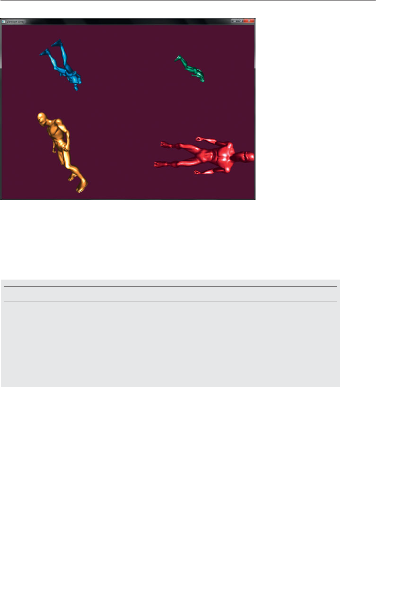
ptg9898810
Figure 10.10 Output of the viewport-array example
As with glDepthRangeArrayv() and glViewportArrayv(), there is an array
form of glScissorIndexed(), which sets multiple scissor rectangles
simultaneously. Its prototype is as follows:
void glScissorArrayv(GLuint first, GLsizei count, const GLint * v);
Sets the bounds of multiple scissor rectangles with a single command.
first contains the index of the first scissor rectangle to update, count
contains the number of scissor rectangles to update, and vcontains the
address of an array of 4 ×count integers---four integers for each scissor
rectangle, which are equivalent to the left,bottom,width, and height
parameters to glScissorIndexed(), in that order.
The same index written to gl_ViewportIndex is used to specify which
scissor rectangle should be used for the pixel ownership test. Both
viewport and scissor rectangles are specified in screen coordinates. Thus,
you may wish to offset each scissor rectangle by the origin of the viewport
whose index it shares. Although the same index is used to determine both
the scissor rectangle and the viewport to use, they may be effectively
decoupled by specifying the same viewport for multiple indices, but a
different scissor rectangle for each, or vice-versa. The maximum number of
viewports (and scissor rectangles) that an implementation supports can be
found by calling glGetIntegerv() with pname set to GL_MAX_VIEWPORTS.
The minimum requirement for this value is 16, and so you can be sure that
your implementation supports at least that many. Having large arrays of
Multiple Viewports and Layered Rendering 555

ptg9898810
viewports and scissor rectangles allows for some combinatorial use. For
example, you could specify four viewports and four scissor rectangles,
producing 16 possible combinations of viewport and scissor rectangles,
which can be indexed in the geometry shader independently.
Layered Rendering
When rendering into a framebuffer object, it is possible to use a 2D array
texture as a color attachment and render into the slices of the array using a
geometry shader. To create a 2D array texture and attach it to a framebuffer
object, use code such as that shown in Example 10.24.
Example 10.24 Example Code to Create an FBO with an Array
Texture Attachment
// Declare variables
GLuint tex; // This will be the 2D array texture
GLuint fbo; // The framebuffer object
// Create and allocate a 1024x1024x32 2D array texture
glGenTextures(1, &tex);
glBindTexture(GL_TEXTURE_2D_ARRAY, tex);
glTexImage3D(GL_TEXTURE_2D_ARRAY,
0,
GL_RGBA,
1024,
1024,
32,
0,
GL_RGBA,
GL_UNSIGNED_BYTE,
NULL);
// Now create a framebuffer object and attach the
// 2D array texture to one of its color attachments
glGenFramebuffers(1 &fbo);
glBindFramebuffer(GL_FRAMEBUFFER, fbo);
glFramebufferTexture(GL_FRAMEBUFFER,
GL_COLOR_ATTACHMENT0,
tex,
0);
// Now, make the framebuffer’s color attachment(s) the
// current draw buffer.
static const GLenum draw_buffers[] =
{GL_COLOR_ATTACHMENT0
};
glDrawBuffers(1, draw_buffers);
556 Chapter 10: Geometry Shaders

ptg9898810
A different array texture can be attached to each of the framebuffer’s color
attachments (GL_COLOR_ATTACHMENTi, where iis the index of the color
attachment). It is also possible to create a 2D array texture with a format of
GL_DEPTH_COMPONENT, GL_DEPTH_STENCIL, or GL_STENCIL_INDEX
and attach it to GL_DEPTH_ATTACHMENT, GL_STENCIL_ATTACHMENT,
or GL_DEPTH_STENCIL_ATTACHMENT. This will allow the array texture
to be used as a layered depth or stencil buffer. Note that this type of 2D
array texture must be used for this purpose because there is no such thing
as an array renderbuffer in OpenGL.
Now we have a layered framebuffer that we can render into. A restriction
exists that when using layered attachments to a framebuffer, all the
attachments of that framebuffer must be layered. Also, all attachments of a
layered framebuffer must be of the same type (one- or two-dimensional
array textures, cube maps, etc.). Thus, it is not possible, for example, to
bind a six-slice 2D array texture and the six faces of a cube-map texture to
the same framebuffer object at the same time. Attempting to render into
such a framebuffer object will result in glCheckFramebufferStatus()
returning GL_FRAMEBUFFER_INCOMPLETE_LAYER_TARGETS.
It is also possible to render into the slices of a 3D texture by attaching each
of the slices individually as layers of the framebuffer using the
glFramebufferTextureLayer() function.
Now that an array texture is attached to the color attachment point
of the current framebuffer object, the geometry shader can be used to
direct rendering into the slices of the array. To do this, the geometry shader
can write into the GLSL built-in variable gl_Layer.gl_Layer is used
to specify the zero-based index of the layer into which rendering will be
directed. An example of such a geometry shader is shown in Example 10.25.
Note: Be careful when writing to gl_Layer that the value written is
a valid index into the current layered framebuffer object. Writing
outside this range will produce undefined results, which may include
discarding the geometry, rendering it into the first or last slice,
corrupting other slices, or even corrupting other areas of memory.
Example 10.25 Geometry Shader for Rendering into an Array Texture
#version 330 core
layout (triangles) in;
layout (triangle_strip,max_vertices=128) out;
in VS_GS_VERTEX
{
vec4 color;
Multiple Viewports and Layered Rendering 557

ptg9898810
vec3 normal;
} vertex_in[];
out GS_FS_VERTEX
{
vec4 color;
vec3 normal;
} vertex_out;
uniform mat4 projection_matrix;
uniform int output_slices;
void main()
{
int i, j;
mat4 slice_matrix;
float alpha = 0.0;
float delta = float(output_slices - 1) *0.5 / 3.1415927;
for (j = 0; j < output_slices; ++j)
{
float s = sin(alpha);
float c = cos(alpha);
slice_matrix = mat4(vec4(c, 0.0, -s, 0.0),
vec4(0.0, 1.0, 0.0, 0.0),
vec4(s, 0.0, c, 0.0),
vec4(0.0, 0.0, 0.0, 1.0));
slice_matrix = slice_matrix *projection_matrix;
for (i = 0; i < gl_in.length(); ++i)
{
gl_Layer = j;
gl_Position = slice_matrix *gl_in[i].gl_Position;
vertex_out.color = vertex_in[i].color;
vertex_out.normal = vertex_in[i].normal;
EmitVertex();
}
EndPrimitive();
}
}
Example 10.25 amplifies the incoming geometry and renders a complete
copy of it into each layer of the layered color attachment of the current
framebuffer. Each copy is a rotated version of the incoming geometry such
that after a single pass of rendering, the output array texture contains a
view of the geometry as seen from several different angles. This can be
used, for example to update impostors.10
10. Impostors are views of real geometry rendered into textures and then used in place of that
geometry when many instances are needed, rather than rendering the entire mesh. An example
use is a forest of trees. Trees are rendered as seen from an array of angles into a texture and the
appropriate view of the tree selected when the forest is rendered.
558 Chapter 10: Geometry Shaders

ptg9898810
In this particular example, a simple loop is used to amplify the incoming
geometry. This is sufficient when the number of layers in the framebuffer
attachment is relatively small---less than one third of the maximum
number of output vertices allowed by the implementation in a geometry
shader. When a larger number of array slices must be rendered, instanced
rendering or even geometry shader instancing can be employed and
gl_InstanceID (or gl_InvocationID) used to derive the output layer. In
the second case, attention should be paid to the maximum geometry shader
invocations allowed, as 32 is the minimum requirement. The maximum
number of layers in an array texture can be determined by calling
glGetIntegerv() with a pname of GL_MAX_ARRAY_TEXTURE_LAYERS,
and the minimum required value of this parameter is 2048.
Another application of layered rendering using a geometry shader is to
update the faces of a cube-map texture that might be used as an
environment map in another pass. When a cube-map texture is attached as
a color attachment to a framebuffer object, it appears as a six-layer array
texture. The faces of the cube map appear as the slices of the array in the
order shown in Table 10.4 below.
Table 10.4 Ordering of Cube-Map Face Indices
Layer Number Cube-Map Face
0 GL_TEXTURE_CUBE_MAP_POSITIVE_X
1 GL_TEXTURE_CUBE_MAP_NEGATIVE_X
2 GL_TEXTURE_CUBE_MAP_POSITIVE_Y
3 GL_TEXTURE_CUBE_MAP_NEGATIVE_Y
4 GL_TEXTURE_CUBE_MAP_POSITIVE_Z
5 GL_TEXTURE_CUBE_MAP_NEGATIVE_Z
To render an environment map into a cube map using a geometry shader,
set up six projection matrices representing the view frustums for each of
the faces. Next, use an instanced geometry shader with an invocation
count of six to emit the same incoming geometry into each of the faces.
Use gl_InvocationID to the output gl_Layer and to index into the
array of projection matrices. In a single pass, the cube-map environment
map will be updated.
Chapter Summary
In this chapter, we have covered geometry shaders---a shader stage that
runs per-primitive, has access to all vertices in the primitive, and can create
and destroy geometry as it passes through the OpenGL pipeline. It can
Chapter Summary 559

ptg9898810
even change the types of primitives. The geometry shader can be used for
user-controlled culling, geometric transformations, and even sorting
algorithms. It provides access to features such as multiple viewports and
rendering into texture arrays, three-dimensional textures, and cube maps.
The geometry shader can be instanced, which when combined with its
other features is an extremely powerful tool. The geometry shader is
perhaps the most versatile and flexible shader stage. Geometry shaders
even have their own special primitive modes---GL_LINES_ADJACENCY,
GL_LINE_STRIP_ADJACENCY, GL_TRIANGLES_ADJACENCY, and
GL_TRIANGLE_STRIP_ADJACENCY.
Effective use of geometry shaders, in conjunction with features such as
layered framebuffers, transform feedback, primitive queries, and instancing
allows some very advanced and interesting algorithms to be implemented.
Geometry Shader Redux
To use a geometry shader in your program:
•Create a geometry shader with
glCreateShader(GL_GEOMETRY_SHADER).
•Set the shader source with glShaderSource and compile it with
glCompileShader.
•Attach it to a program object with glAttachShader, and link the
program with glLinkProgram.
Inside your geometry shader do the following:
•Specify input and output primitive types with the
layout (<primitive_type>) in;or
layout (<primitive_type>) out;layout qualifiers.
•Specify the maximum number of vertices the shader might produce
with the layout (max_vertices = <vertex_count>) in;layout
qualifier.
•Declare all inputs to the geometry shader as arrays (using the in
keyword). You can use the .length() method on the input arrays
(including gl_in[]) to retrieve the size of the primitive being
processed.
•If using multiple output streams with transform feedback, declare
outputs using the layout(stream = <stream>) out;layout
qualifier. Use interface blocks to group outputs for a single stream
together, keeping your code neat and tidy.
560 Chapter 10: Geometry Shaders

ptg9898810
To produce geometry do the following:
•Use EmitVertex() or EmitStreamVertex(<stream>) to produce
vertices and EndPrimitive() or EndStreamPrimitive(<stream>)
to break apart long output strips (remember, geometry shaders can
only produce points, line strips or triangle strips).
The special inputs and outputs available to geometry shaders are as follows:
•gl_in[]---an input array containing all the per-vertex built-in data
(gl_Position,gl_PointSize and gl_ClipDistance[].
•gl_InvocationID---an input containing invocation index for an
instanced geometry shader. For noninstanced geometry shaders, this is
still available; it will just be zero, always.
•gl_PrimitiveIDIn---an input containing the index of the incoming
primitive. So named because in a geometry shader, gl_PrimitiveID is
an output.
•gl_PrimitiveID---an output that is to be written with the primitive
index as seen by the subsequent fragment shader.
•gl_Layer---an output that contains the index of the layer within a
layered framebuffer to render the primitive to. This is also an input to
the fragment shader.
•gl_ViewportIndex---an output that contains the index of the
viewport to use for the viewport transformation before rasterization.
This is also an input to the fragment shader.
Geometry Shader Best Practices
The following are some tips for using geometry shaders wisely. This will
help you obtain the best possible performance from a program using
geometry shaders. These aren’t hard-and-fast rules, but if followed should
allow you to use geometry shaders effectively in your programs.
Do Work in the Right Place
If you have work that is to be done per-vertex, do it in the vertex shader
(or tessellation evaluation shader, if present). When rendering triangle
strips or fans, each triangle is presented individually to the geometry
shader. Performing per-vertex work in the geometry shader will result in it
being done multiple times per vertex. Likewise, if you have work that is to
be done per-face (such as calculating the values for attributes with flat
interpolation qualifiers), perform it in the geometry shader rather than in
Chapter Summary 561

ptg9898810
the vertex shader. If independent triangles are rendered, calculating the
values of flat interpolated attributes in the vertex shader will result in that
computation being performed for vertices that are not the provoking vertex
for the primitive. Moving that work to the geometry shader allows it to be
performed only once and then the value (which should be stored in local
variables) propagated to all of the output variables.
Only Use a Geometry Shader When You Need One
Geometry shaders are not free. Even a pass-through geometry shader will
have some impact on the performance of your program. Consider whether
you really need a geometry shader. Do you need per-primitive calculations
that can’t be performed in the vertex shader? Do you need access to all the
vertices of the primitive, or to adjacency information? If your algorithm
can be implemented with reasonable efficiency using only the vertex
shader (or tessellation shaders, if you’re using tessellation), then that may
be worth considering.
Allocate Carefully
When specifying the max_vertices input layout qualifier, only make
it as large as is needed by the algorithm you intend to implement. The
max_vertices qualifier essentially acts as an allocation. Depending on
the OpenGL implementation you’re using, performance may be degraded
if you allocate too many output vertices---even if you don’t use them all.
It’s very easy to simply specify the maximum allowed, but care should be
taken to only allocate as many as is necessary.
Don’t Amplify Too Aggressively
For the same reasons that you shouldn’t allocate too many output vertices
with the max_vertices layout qualifier, care should be taken with
producing a very large amount of vertices in the geometry shader. While
it is possible to implement algorithms like tessellation in the geometry
shader, some OpenGL implementations may run at a reduced performance
level if this is attempted. This is why OpenGL includes tessellation! The
geometry shader is best suited to algorithms that need access to
whole-primitive information, and perform culling or small amounts
of primitive amplification.
562 Chapter 10: Geometry Shaders


ptg9898810
Everything in the OpenGL pipeline thus far has essentially been free from
side effects. That is, the pipeline is constructed from a sequence of stages,
either programmable (such as the vertex and fragment shaders) or fixed
function (such as the tessellation engine) with well-defined inputs and out-
puts (such as vertex attributes or color outputs to a framebuffer). Although
it has been possible to read from arbitrary memory locations using textures
or texture buffer objects (TBOs), in general, writing has been allowed only
to fixed and predictable locations. For example, vertices captured during
transform feedback operations are written in well-defined sequences to
transform feedback buffers, and pixels produced in the fragment shader are
written into the framebuffer in a regular pattern defined by rasterization.
In this chapter we introduce mechanisms by which shaders may both read
from and write to user-specified locations. This allows shaders to construct
data structures in memory and, by carefully updating the same memory
locations, effect a level of communication between each other. To this end,
we also introduce special functions both in the shading language and in
the OpenGL API that provide control over the order of access and of the
operations performed during those memory accesses.
This chapter has the following major sections:
•‘‘Using Textures for Generic Data Storage’’ shows how to read and write
memory held in a texture object, through GLSL built-in functions.
•‘‘Shader Storage Buffer Objects’’ shows how to read and write ageneric
memory buffer, directly through user-declared variables.
•‘‘Atomic Operations and Synchronization’’ explains multiple-writer
synchronization problems with images, and how to solve them.
•‘‘Example’’ discusses an interesting use of many of the features outlined
in the chapter in order to demonstrate the power and flexibility that
generalized memory access provides to the experienced OpenGL
programmer.
Using Textures for Generic Data Storage
It is possible to use the memory representing a buffer object or a single
level of a texture object for general purpose read and write access in
shaders. To support this, the OpenGL Shading Language provides several
image types to represent raw image data.
Images are declared in shaders as uniforms in a similar manner to
samplers. Just like samplers, they are assigned locations by the shader
compiler that can be passed to glUniform1i() to specify the image unit
564 Chapter 11: Memory

ptg9898810
which they represent. The OpenGL Shading Language image types are
shown in Table 11.1.
Table 11.1 Generic Image Types in GLSL
Image Type Meaning
image1D Floating-Point 1D
image2D Floating-Point 2D
image3D Floating-Point 3D
imageCube Floating-Point Cube Map
image2DRect Floating-Point Rectangle
image1DArray Floating-Point 1D Array
image2DArray Floating-Point 2D Array
imageBuffer Floating-Point Buffer
image2DMS Multisample 2D Floating Point
image2DMSArray Floating-Point 2D Multisample Array
imageCubeArray Floating-Point Cube-Map Array
iimage1D Signed Integer 1D
iimage2D Signed Integer 2D
iimage3D Signed Integer 3D
iimageCube Signed Integer Cube Map
iimage2DRect Signed Integer Rectangle
iimage1DArray Signed Integer 1D Array
iimage2DArray Signed Integer 2D Array
iimageBuffer Signed Integer Buffer
iimage2DMS Multisample 2D Signed Integer
iimage2DMSArray Signed Integer 2D Multisample Array
iimageCubeArray Signed Integer Cube-Map Array
uimage1D Unsigned Integer 1D
uimage2D Unsigned Integer 2D
uimage3D Unsigned Integer 3D
uimageCube Unsigned Integer Cube Map
uimage2DRect Unsigned Integer Rectangle
uimage1DArray Unsigned Integer 1D Array
Using Textures for Generic Data Storage 565

ptg9898810
Table 11.1 (continued) Generic Image Types in GLSL
Image Type Meaning
uimage2DArray Unsigned Integer 2D Array
uimageBuffer Unsigned Integer Buffer
uimage2DMS Multisample 2D Unsigned Integer
uimage2DMSArray Unsigned Integer 2D Multisample Array
uimageCubeArray Unsigned Integer Cube-Map Array
Notice that most of GLSL sampler types have an analog as an image type.
The primary differences between a sampler type (such as sampler2D) and
an image type (such as image2D) are first, that the image type represents a
single layer of the texture, not a complete mipmap chain and second, that
image types do not support sampler operations such as filtering. Note that
these unsupported sampling operations include depth comparison, which
is why the shadow sampler types such as sampler2DShadow do not have
an equivalent image type.
The three basic classes of image types, image*,iimage*, and uimage*are
used to declare images containing floating point, signed integer, or
unsigned integer data, respectively.
In addition to the general data type (floating point, signed, or unsigned
integer) associated with the image variable, a format layout qualifier may
also be given to further specify the underlying image format of the data in
memory. Any image from which data will be read must be declared with a
format layout qualifier, but in general it is a good idea to explicitly state
the format of the data in the image at declaration time. The format layout
qualifiers and their corresponding OpenGL internal format types are
shown in Table 11.2.
Table 11.2 Image Format Qualifiers
Image Type OpenGL Internal Format
rgba32f GL_RGBA32F
rgba16f GL_RGBA16F
rg32f GL_RG32F
rg16f GL_RG16F
r11f_g11f_b10f GL_R11F_G11F_B10F
r32f GL_R32F
r16f GL_R16F
566 Chapter 11: Memory

ptg9898810
Table 11.2 (continued) Image Format Qualifiers
Image Type OpenGL Internal Format
rgba16 GL_RGBA16UI
rgb10_a2 GL_RGB10_A2UI
rgba8 GL_RGBA8UI
rg16 GL_RG16UI
rg8 GL_RG8UI
r16 GL_R16UI
r8 GL_R8UI
rgba16_snorm GL_RGBA16_SNORM
rgba8_snorm GL_RGBA8_SNORM
rg16_snorm GL_RG16_SNORM
rg8_snorm GL_RG8_SNORM
r16_snorm GL_R16_SNORM
r8_snorm GL_R8_SNORM
rgba32i GL_RGBA32I
rgba16i GL_RGBA16I
rgba8i GL_RGBA8I
rg32i GL_RG32I
rg16i GL_RG16I
rg8i GL_RG8I
r32i GL_R32I
r16i GL_R16I
r8i GL_R8I
rgba32ui GL_RGBA32UI
rgba16ui GL_RGBA16UI
rgba8ui GL_RGBA8UI
rg32ui GL_RG32UI
rg16ui GL_RG16UI
rg8ui GL_RG8UI
r32ui GL_R32UI
r16ui GL_R16UI
r8ui GL_R8UI
Using Textures for Generic Data Storage 567

ptg9898810
The image format qualifier is provided as part of the image variable
declaration and must be used when declaring an image variable that will
be used to read from an image. It is optional if the image will only ever be
written to (see the explanation of writeonly below for more details). The
image format qualifier used in the declaration of such variables (if present)
must batch the basic data type of the image. That is, floating-point format
specifiers such as r32f or rgba16_unorm must be used with floating-point
image variables such as image2D, while nonfloating-point qualifiers (such
as rg8ui) may not. Likewise, signed integer format qualifiers such as
rgba32i must be used to declare signed integer image variables
(iimage2D) and unsigned format qualifiers (rgba32ui) must be used to
declare unsigned integer image variables (uimage2D).
Examples of using the format layout qualifiers to declare image uniforms
are shown in Example 11.1.
Example 11.1 Examples of Image Format Layout Qualifiers
// 2D image whose data format is 4-component floating point
layout (rgba32f) uniform image2D image1;
// 2D image whose data format is 2-component integer
layout (rg32i) uniform iimage2D image2;
// 1D image whose data format is single-component unsigned integer
layout (r32ui) uniform uimage1D image3;
// 3D image whose data format is single-component integer, and is
// initialized to refer to image unit 4
layout (binding=4, r32) uniform iimage3D image4;
The format type used in the declaration of the image variable does not
need to exactly match the underlying format of the data in the image (as
given by the texture’s internal format), but should be compatible as defined
by the OpenGL specification. In general, if the amount of data storage
required per texel is the same between two formats, then they are
considered to be compatible. For example, a texture whose internal format
is GL_RGBA32F has four, 32-bit (floating point) components, for a total of
128 bits per texel. Levels of this texture may be accessed in a shader
through image variables whose format is rgba32f,rgba32ui, or rgba32i
as all of these formats represent a single texel using 128 bits. Furthermore,
a texture whose internal format is GL_RG16F is represented as 32 bits per
texel. This type of texture may be accessed using image variables declared
as r32f,rgba8ui,rgb10_a2ui, or any other format that represents a
texel using 32 bits. When texture and image variable formats do not match
exactly but are otherwise compatible, the raw data in the image is
568 Chapter 11: Memory

ptg9898810
reinterpreted as the type specified in the shader. For example, reading from
a texture with the GL_R32F internal format using an image variable
declared as r32ui will return an unsigned integer whose bit-pattern
represents the floating-point data stored in the texture.
The maximum number of image uniforms that may be used in a single
shader stage may be determined by querying the value of
GL_MAX_VERTEX_IMAGE_UNIFORMS for vertex shaders,
GL_MAX_TESS_CONTROL_IMAGE_UNIFORMS, and
GL_MAX_TESS_EVALUATION_IMAGE_UNIFORMS for tessellation
control and evaluation shaders, respectively,
GL_MAX_GEOMETRY_IMAGE_UNIFORMS for geometry shaders
and finally, GL_MAX_FRAGMENT_IMAGE_UNIFORMS for fragment
shaders. Additionally, the maximum number of image uniforms
that may be used across all active shaders is given by
GL_MAX_COMBINED_IMAGE_UNIFORMS. In addition to these
limits, some implementations may have restrictions upon the
number of image uniforms available to a fragment shader when that
shader also writes to the framebuffer using traditional output variables.
To determine whether this is the case, retrieve the value of
GL_MAX_COMBINED_IMAGE_UNITS_AND_FRAGMENT_OUTPUTS.
A final note is that although the OpenGL API supports image uniforms
in every shader stage, it only mandates that implementations
provide support in the fragment shader and that only
GL_MAX_FRAGMENT_IMAGE_UNIFORMS be nonzero.
Binding Textures to Image Units
Just as sampler variables represent texture units in the OpenGL API, so do
image variables represent a binding to an image unit in the OpenGL API.
Image uniforms declared in a shader have a location that may be retrieved
by calling glGetUniformLocation(). This is passed in a call to
glUniform1i() to set the index of the image unit to which the image
uniform refers. This binding may also be specified directly1in the shader
using a binding layout qualifier as shown in the declaration of image4 in
Example 11.1. By default, an image uniform has the binding 0, and so if
only one image is used in a shader, there is no need to explicitly set its
1. The option of specifying the image unit in the shader using the binding layout qualifier
is generally preferred. This is because some OpenGL implementations may provide a multi-
threaded shader compiler. If properties of a linked program, such as the locations of uniforms,
are queried too soon after the program is linked, the implementation may need to stall to allow
compilation and linking to complete before it can return. By specifying the bindings explicitly,
the uniform location query and the potential stall may be avoided.
Using Textures for Generic Data Storage 569

ptg9898810
binding to 0. The number of image units supported by the OpenGL
implementation may be determined by retrieving the value of
GL_MAX_IMAGE_UNITS. A single layer of a texture object must be bound
to an image unit before it can be accessed in a shader. To do this, call
glBindImageTexture() whose prototype is as follows:
void glBindImageTexture(GLuint unit, Gluint texture, GLint level,
GLboolean layered, GLint layer,
GLenum access, GLenum format);
Binds level level of texture texture to image unit unit.unit is the zero-based
unit index of the image unit to which to bind the texture level. If texture is
zero, any texture currently bound to the specified image unit is unbound.
If texture refers to an array texture type, such as a 1D- or 2D-array texture
type, it is possible to either bind the entire array or only a single layer of
the array to the image unit. If layered is GL_TRUE then the entire array is
bound and layer is ignored whereas if layered is GL_FALSE then only layer
layer of the texture is bound. When a single layer of an array texture is
bound, it is treated as if it were a single-layer, nonarray texture.
access may be GL_READ_ONLY, GL_WRITE_ONLY, or GL_READ_WRITE
and describes how the image will be accessed by the shader. format
specifies the format that the elements of the image will be treated as
when performing formatted stores and should be one of the OpenGL
enumerants listed in Table 11.2.
Texture objects that will be used for generic memory access are created and
allocated as usual by calling glGenTextures() and one of the texture
allocation functions such as glTexImage2D() or glTexStorage3D(). Once
created and allocated, they are bound to an image unit using
glBindImageTexture() for either read, write, or both read and write access,
as specified by the access parameter to glBindImageTexture(). Violating
this declaration (for example by writing to an image bound using
GL_READ_ONLY for access) will cause undesired behavior, possibly
crashing the application.
An example of creating, allocating, and binding a texture for read and
write access in shaders is given in Example 11.2.
570 Chapter 11: Memory

ptg9898810
Example 11.2 Creating, Allocating, and Binding a Texture to an Image
Unit
GLuint tex;
// Generate a new name for our texture
glGenTextures(1, &tex);
// Bind it to the regular 2D texture target to create it
glBindTexture(GL_TEXTURE_2D, tex);
// Allocate immutable storage for the texture
glTexStorage2D(GL_TEXTURE_2D, 1, GL_RGBA32F, 512, 512);
// Unbind it from the 2D texture target
glBindTexture(GL_TEXTURE_2D, 0);
// Now bind it for read-write to one of the image units
glBindImageTexture(0, tex, 0, GL_FALSE, 0, GL_READ_WRITE, GL_RGBA32F);
glBindImageTexture() works similarly to glBindTexture(). There are,
however, a few subtle differences. Firstly, the index of the image unit to
which to bind the texture is specified directly in the unit parameter rather
than being inferred through the current active texture unit. This makes
calls to glActiveTexture() unnecessary when binding texture levels to
image units. Secondly, the format in which formatted stores (writes from
the shader) will be performed is specified during the API call. This format
should match the format of the image uniform in the shaders that will
access the texture. However, it need not match the format of the actual
texture. For textures allocated by calling one of the glTexImage() or
glTexStorage() functions, any format that matches in size may be specified
for format. For example, formats GL_R32F, GL_RGBA8, and
GL_R11F_G11F_B10F are all considered to consist of 32 bits per texel and
therefore to match in size. A complete table of all of the sizes of the texture
formats is given in the OpenGL specification.
To use a buffer object as the backing store for an imageBuffer image in a
shader, it must still be represented as a texture by creating a buffer texture,
attaching the buffer object to the texture object and then binding the
buffer texture to the image unit as shown in Example 11.3. The format of
the data in the buffer object is specified when it is attached to the texture
object. The same buffer may be attached to multiple texture objects
simultaneously with different formats, allowing some level of format
aliasing to be implemented.
Using Textures for Generic Data Storage 571

ptg9898810
Example 11.3 Creating and Binding a Buffer Texture to an Image Unit
GLuint tex, buf;
// Generate a name for the buffer object, bind it to the
// GL_TEXTURE_BINDING, and allocate 4K for the buffer
glGenBuffers(1, &buf);
glBindBuffer(GL_TEXTURE_BUFFER, buf);
glBufferData(GL_TEXTURE_BUFFER, 4096, NULL, GL_DYNAMIC_COPY);
// Generate a new name for our texture
glGenTextures(1, &tex);
// Bind it to the buffer texture target to create it
glBindTexture(GL_TEXTURE_BUFFER, tex);
// Attach the buffer object to the texture and specify format as
// single channel floating point
glTexBuffer(GL_TEXTURE_BUFFER, GL_R32F, buf);
// Now bind it for read-write to one of the image units
glBindImageTexture(0, tex, 0, GL_FALSE, 0, GL_READ_WRITE, GL_RGBA32F);
Reading from and Writing to Images
Once an image has been declared in the shader and a level and layer of a tex-
ture have been bound to the corresponding image unit, the shader may ac-
cess the data in the texture directly for both read and write. Reading and writ-
ing are done only through built-in functions that load or store their argu-
ments to or from an image. To load texels from an image, call imageLoad().
There are many overloaded variants of imageLoad(). They are as follows:
gvec4 imageLoad(readonly gimage1D image, int P);
gvec4 imageLoad(readonly gimage2D image, ivec2 P);
gvec4 imageLoad(readonly gimage3D image, ivec3 P);
gvec4 imageLoad(readonly gimage2DRect image, ivec2 P);
gvec4 imageLoad(readonly gimageCube image, ivec3 P);
gvec4 imageLoad(readonly gimageBuffer image, int P);
gvec4 imageLoad(readonly gimage1DArray image, ivec2 P);
gvec4 imageLoad(readonly gimage2DArray image, ivec3 P);
gvec4 imageLoad(readonly gimageCubeArray image, ivec3 P);
gvec4 imageLoad(readonly gimage2DMS image, ivec2 P,
int sample);
gvec4 imageLoad(readonly gimage2DMSArray image, ivec3 P,
int sample);
Load the texel at coordinate Pfrom the image unit image. For loads from
multisample images, the sample number is given in sample.
572 Chapter 11: Memory

ptg9898810
The imageLoad() functions operate similarly to texelFetch(), which is
used to directly read texels from textures without any filtering applied. In
order to store into images, the imageStore() function may be used.
imageStore() is defined as follows:
gvec4 imageStore(writeonly gimage1D image, int P, gvec4 data);
gvec4 imageStore(writeonly gimage2D image, ivec2 P, gvec4
data);
gvec4 imageStore(writeonly gimage3D image, ivec3 P, gvec4
data);
gvec4 imageStore(writeonly gimage2DRect image, ivec2 P, gvec4
data);
gvec4 imageStore(writeonly gimageCube image, ivec3 P, gvec4
data);
gvec4 imageStore(writeonly gimageBuffer image, int P, gvec4
data);
gvec4 imageStore(writeonly gimage1DArray image, ivec2 P, gvec4
data);
gvec4 imageStore(writeonly gimage2DArray image, ivec3 P, gvec4
data);
gvec4 imageStore(writeonly gimageCubeArray image, ivec3 P,
gvec4 data);
gvec4 imageStore(writeonly gimage2DMS image, ivec2 P,
int sample, gvec4 data);
gvec4 imageStore(writeonly gimage2DMSArray image, ivec3 P,
int sample, gvec4 data);
Store data into the texel at coordinate Pin the image specified by image.
For multisample stores,the sample number is given by sample.
If you need to know the size of an image in the shader, you can query with
the imageSize() functions listed below.
int imageSize(gimage1D image);
int imageSize(gimageBuffer image);
ivec2 imageSize(gimage2D image);
ivec2 imageSize(gimageCube image);
ivec2 imageSize(gimageRect image);
ivec2 imageSize(gimage1DArray image);
ivec2 imageSize(gimage2DMS image);
ivec3 imageSize(gimageCubeArray image);
Using Textures for Generic Data Storage 573

ptg9898810
ivec3 imageSize(gimage3D image);
ivec3 imageSize(gimage2DArray image);
ivec3 imageSize(gimage2DMSArray image);
Return the dimensions of the image. For arrayed images, the last
component of the return value will hold the size of the array. Cube
images return only the dimensions of one face and the number of cubes
in the cube-map array, if arrayed.
Example 11.4 shows a simple but complete example of a fragment shader
that performs both image loads and stores from and to multiple images. It
also performs multiple stores per invocation.
Example 11.4 Simple Shader Demonstrating Loading and Storing into
Images
#version 420 core
// Buffer containing a palette of colors to mark primitives by ID
layout (binding = 0, rgba32f)uniform imageBuffer colors;
// The buffer that we will write to
layout (binding = 1, rgba32f)uniform image2D output_buffer;
out vec4 color;
void main(void)
{
// Load a color from the palette based on primitive ID % 256
vec4 col = imageLoad(colors, gl_PrimitiveID & 255);
// Store the resulting fragment at two locations. First at the
// fragments window space coordinate shifted left...
imageStore(output_buffer,
ivec2(gl_FragCoord.xy) - ivec2(200, 0), col);
// ... then at the location shifted right
imageStore(output_buffer,
ivec2(gl_FragCoord.xy) +ivec2(200, 0), col);
}
The shader in Example 11.4 loads a color from a buffer texture indexed by
a function of gl_PrimitiveID and then writes it twice into a single image
indexed by functions of the current two-dimensional fragment coordinate.
Notice that the shader has no other per-fragment outputs. The result of
running this shader on some simple geometry is shown in Figure 11.1
574 Chapter 11: Memory
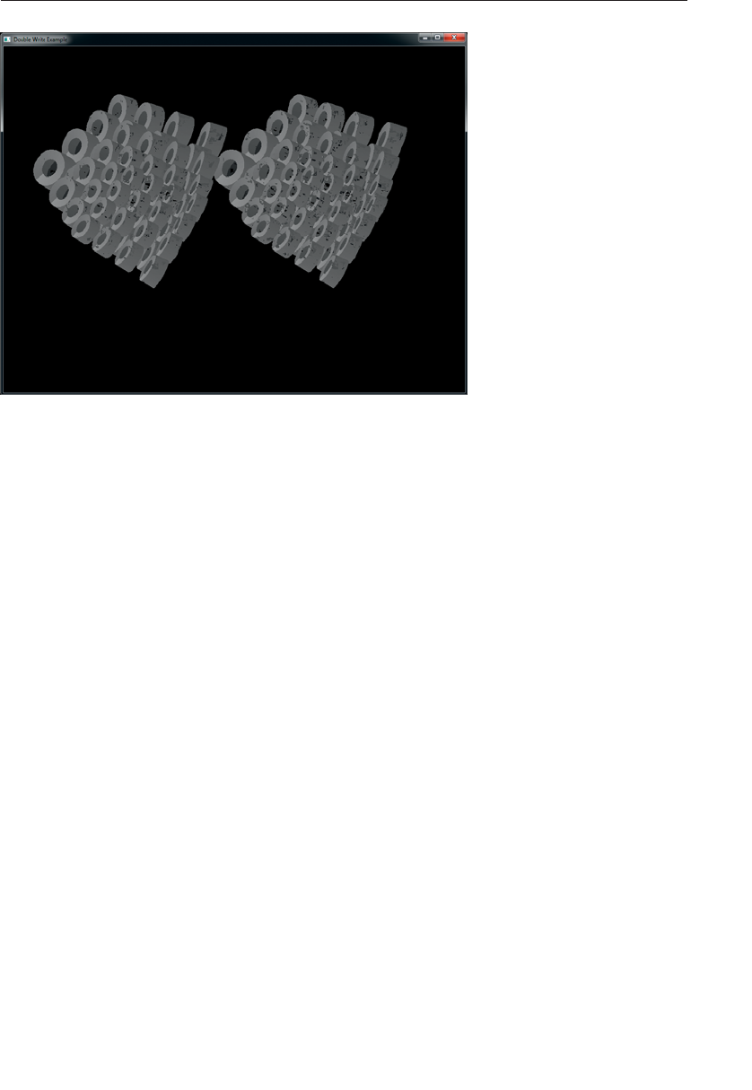
ptg9898810
Figure 11.1 Output of the simple load-store shader
As can be seen in Figure 11.1, two copies of the output geometry have
been rendered---one in the left half of the image and the other in the right
half of the image. The data in the resulting texture was explicitly placed
with the shader of Example 11.4. While this may seem like a minor
accomplishment, it actually illustrates the power of image store operations.
It demonstrates that a fragment shader is able to write to arbitrary locations
in a surface. In traditional rasterization into a framebuffer, the location at
which the fragment is written is determined by fixed function processing
before the shader executes. However, with image stores, this location is
determined by the shader. Another thing to consider is that the number of
stores to images is not limited, whereas the number of attachments allowed
on a single framebuffer object is, and only one fragment is written to each
attachment. This means that a much larger amount of data may be written
by a fragment shader using image stores than would be possible using a
framebuffer and its attachments. In fact, an arbitrary amount of data may
be written to memory by a single shader invocation using image stores.
Figure 11.1 also demonstrates another facet of stores from shaders. That
is, they are unordered and can be subject to race conditions. The program
that generated the image disabled both depth testing and back-face
culling, meaning that each pixel has at least two primitives rendering into
it. The speckled corruption that can be seen in the image is the result of the
nondeterministic order with which the primitives are rendered by OpenGL.
We will cover race conditions and how to avoid them later in this chapter.
Using Textures for Generic Data Storage 575

ptg9898810
Shader Storage Buffer Objects
Reading data from and writing data to memory using image variables
works well for simple cases where large arrays of homogeneous data are
needed, or where the data is naturally image-based (such as the output of
OpenGL rendering or where the shader is writing into an OpenGL texture).
However, in some cases, large blocks of structured data may be required.
For these use cases, we can use a buffer variable to store the data. Buffer
variables are declared in shaders by placing them in an interface block
which in turn is declared using the buffer keyword. A simple example is
given in Example 11.5.
Example 11.5 Simple Declaration of a Buffer Block
#version 430 core
// create a readable-writeable buffer
layout (std430, binding = 0) buffer BufferObject {
int mode; // preamble members
vec4 points[]; // last member can be unsized array
};
In addition to declaring the interface block BufferObject as a buffer
block, Example 11.5 also includes two further layout qualifiers attached to
the block. The first, std430, indicates that the memory layout of the block
should follow the std430 standard, which is important if you want to read
the data produced by the shader in your application, or possibly generate
data in the application and then consume it from the shader. The std430
layout is documented in Appendix I,‘‘Buffer Object Layouts’’ and is similar
to the std140 layout used for uniform blocks, but a bit more economical
with its use of memory.
The second qualifier, binding =0, specifies that the block should be
associated with the GL_SHADER_STORAGE_BUFFER binding at index zero.
Declaring an interface block using the buffer keyword indicates that the
block should be stored in memory and backed by a buffer object. This is
similar to how a uniform block is backed by buffer object bound to one of
the GL_UNIFORM_BUFFER indexed binding points. The big difference
between a uniform buffer and a shader storage buffer is that the shader
storage buffer can both be read and written from the shader. Any writes to
the storage buffer via a buffer block will eventually be seen by other shader
invocations and can be read back by the application.
An example of how to initialize a buffer object and bind it to one of the
indexed GL_SHADER_STORAGE_BUFFER bindings is shown in
Example 11.6.
576 Chapter 11: Memory

ptg9898810
Example 11.6 Creating a Buffer and Using it for Shader Storage
GLuint buf;
// Generate the buffer, bind it to create it and declare storage
glGenBuffers(1, &buf);
glBindBuffer(GL_SHADER_STORAGE_BUFFER, buf);
glBufferData(GL_SHADER_STORAGE_BUFFER, 8192, NULL, GL_DYNAMIC_COPY);
// Now bind the buffer to the zeroth GL_SHADER_STORAGE_BUFFER
// binding point
glBindBufferBase(GL_SHADER_STORAGE_BUFFER, 0, buf);
Writing Structured Data
In the beginning of the section, we mentioned reading and writing
structured data. If all you had was an array of vec4, you probably could
get by with using image buffers. However, if you really have a collection of
structured objects, where each is a heterogeneous collection of types, image
buffers would become quite cumbersome. With shader storage buffers,
however, you get full use of GLSL structure definitions and arrays to define
the layout of your buffer. See the example in Example 11.7 to get the idea.
Example 11.7 Declaration of Structured Data
#version 430 core
// structure of a single data item
struct ItemType {
int count;
vec4 data[3];
// ... other fields
};
// declare a buffer block using ItemType
layout (std430, binding = 0) buffer BufferObject {
// ... other data here
ItemType items[]; // render-time sized array of
// items typed above
};
As you see existing examples of using images to play the role of accessing
memory, it will be easy to imagine smoother sailing through the more direct
representation enabled by using buffer blocks (shader storage buffer objects).
Shader Storage Buffer Objects 577

ptg9898810
Atomic Operations and Synchronization
Now that you have seen how shaders may read and write arbitrary
locations in textures (through built-in functions) and buffers (through
direct memory access), it is important to understand how these accesses
can be controlled such that simultaneous operations to the same memory
location do not destroy each other’s effects. In this section, you will be
introduced to a number of atomic operations that may be performed safely
by many shader invocations simultaneously on the same memory
location. Also, we will cover functionality that allows your application to
provide ordering information to OpenGL. This to ensure that reads
observe the results of any previous writes and that writes occur in desired
order, leaving the correct value in memory.
Atomic Operations on Images
The number of applications for simply being able to store randomly into
images and buffers is limited. However, GLSL provides many more built-in
functions for manipulating images. These include atomic functions that
perform simple mathematical operations directly on the image in an atomic
fashion. Atomic operations (or atomics) are important in these applications
because multiple shader instances could attempt to write to the same mem-
ory location. OpenGL does not guarantee the order of operations for shader
invocations produced by the same draw command or even between invoca-
tions produced by separate drawing commands. It is this undefined ordering
that allows OpenGL to be implemented on massively parallel architectures
and provide extremely high performance. However, this also means that the
fragment shader might be run on multiple fragments generated from a single
primitive or even fragments making up multiple primitives simultaneously.
In some cases, different fragment shader invocations could literally access
the same memory location at the same instant in time, could run out of or-
der with respect to one another, or could even pass each other in execution
order. As an example, consider the naïve shader shown in Example 11.8.
Example 11.8 Naïvely Counting Overdraw in a Scene
#version 420 core
// This is an image that will be used to count overdraw in the scene.
layout (r32ui)uniform uimage2D overdraw_count;
void main(void)
{
// Read the current overdraw counter
578 Chapter 11: Memory
ptg9898810
uint count = imageLoad(overdraw_count, ivec2(gl_FragCoord.xy));
// Add one
count = count + 1;
// Write it back to the image
imageStore(output_buffer, ivec2(gl_FragCoord.xy), count);
}
The shader in Example 11.8 attempts to count overdraw in a scene. It does
so by storing the current overdraw count for each pixel in an image.
Whenever a fragment is shaded, the current overdraw count is loaded into
a variable, incremented, and then written back into the image. This works
well when there is no overlap in the processing of fragments that make up
the final pixel. However, when image complexity grows and multiple
fragments are rendered into the final pixel, strange results will be
produced. This is because the read-modify-write cycle performed explicitly
by the shader can be interrupted by another instance of the same shader.
Take a look at the timeline shown in Figure 11.2.
t0 = mem[loc]
t0 = t0 + 1
mem[loc] = t0
t1 = mem[loc]
t1 = t1 + 1
mem[loc] = t1
t2 = mem[loc]
t2 = t2 + 1
mem[loc] = t2
t3 = mem[loc]
t3 = t3 + 1
mem[loc] = t3
TIME
0
1
2
3
4
5
6
7
8
9
FRAGMENT 0 FRAGMENT 1 FRAGMENT 2 FRAGMENT 3
MEMORY
CONTENT
0
0
1
1
1
2
2
2
3
3
Figure 11.2 Timeline exhibited by the naïve overdraw counter shader
Figure 11.2 shows a simplified timeline of four fragment shader
invocations running in parallel. Each shader is running the code in
Example 11.8 and reads a value from memory, increments it, and then
writes it back to memory over three consecutive time steps. Now, consider
what happens if all four invocations of the shader end up accessing the
same location in memory. At time 0, the first invocation reads the memory
Atomic Operations and Synchronization 579
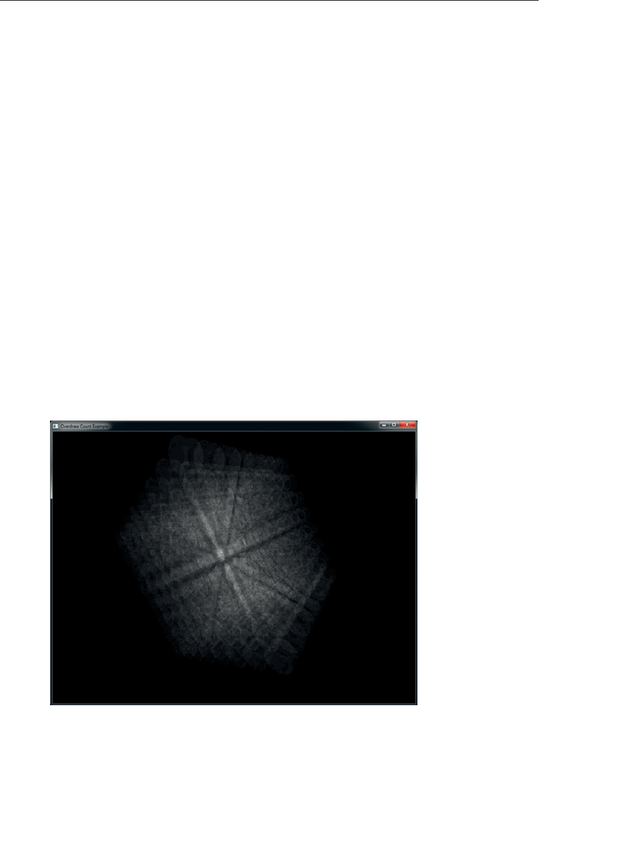
ptg9898810
location, at time 1, it increments it, and at time 2, it writes the value back
to memory. The value in memory (shown in the right-most column) is
now 1 as expected. Starting at time 3, the second invocation of the shader
(fragment 1) executes the same sequence of operations---load, increment,
and write, over three time steps. The value in memory at the end of time
Step 5 is now 2, again as expected.
Now consider what happens during the third and fourth invocations of the
shader. In time Step 6, the third invocation reads the value from memory
(which is currently 2) into a local variable and at time Step 7, it increments
the variable ready to write it back to memory. However, also during time
Step 7, the fourth invocation of the shader reads the same location in
memory (which still contains the value 2) into its own local variable. It
increments that value in time Step 8 while the third invocation writes its
local variable back to memory. Memory now contains the value 3. Finally,
the fourth invocation of the shader writes its own copy of the value into
memory in time Step 9. However, because it read the original value in time
Step 7---after the third invocation had read from memory but before it had
written the updated value back---the data written is stale. The value of the
local variable in the fourth shader invocation is three (the stale value plus
one), not four as might be expected. The desired value in memory is 4,
not 3, and the result is the blocky corruption as seen in Figure 11.3.
Figure 11.3 Output of the naïve overdraw counter shader
580 Chapter 11: Memory

ptg9898810
The reason for the corruption seen in this example is that the increment
operations performed by the shader are not atomic with respect to each
other. That is, they do not operate as a single, indivisible operation but
rather as a sequence of independent operations that may be interrupted or
may overlap with the processing performed by other shader invocations
accessing the same resources. Although the simple explanation above only
describes the hypothetical behavior of four invocations, when considering
that modern GPUs typically have hundreds or even thousands of
concurrently executing invocations, it becomes easy to see how this type
of issue can be more likely to encounter than one would imagine.
To avoid this, OpenGL provides a set of atomic functions that operate
directly on memory. They have two properties that make them suitable for
accessing and modifying shared memory locations. Firstly, they apparently
operate in a single time step2without interruption by other shader
invocations and secondly, the graphics hardware provides mechanisms to
ensure that even if multiple concurrent invocations perform an atomic
operation on the same memory location at the same instant, they will
appear to be serialized such that they take turns executing and produce the
expected result. Note that there is still no guarantee of order---just a
guarantee that all invocations execute their operation without stepping on
each other’s results.
The shader in Example 11.8 may be rewritten using an atomic function as
shown in Example 11.9. In Example 11.9, the imageAtomicAdd function
is used to directly add one to the value stored in memory. This is executed
by OpenGL as a single, indivisible operation and therefore isn’t susceptible
to the issues illustrated in Figure 11.2.
Example 11.9 Counting Overdraw with Atomic Operations
#version 420 core
// This is an image that will be used to count overdraw in
// the scene.
layout (r32ui)uniform uimage2D overdraw_count;
void main(void)
{
// Atomically add one to the contents of memory
imageAtomicAdd(overdraw_count, ivec2(gl_FragCoord.xy), 1);
}
2. This may not actually be true---they could take several tens of clock cycles, but the graphics
hardware will make them appear as if they are single, indivisible operations.
Atomic Operations and Synchronization 581
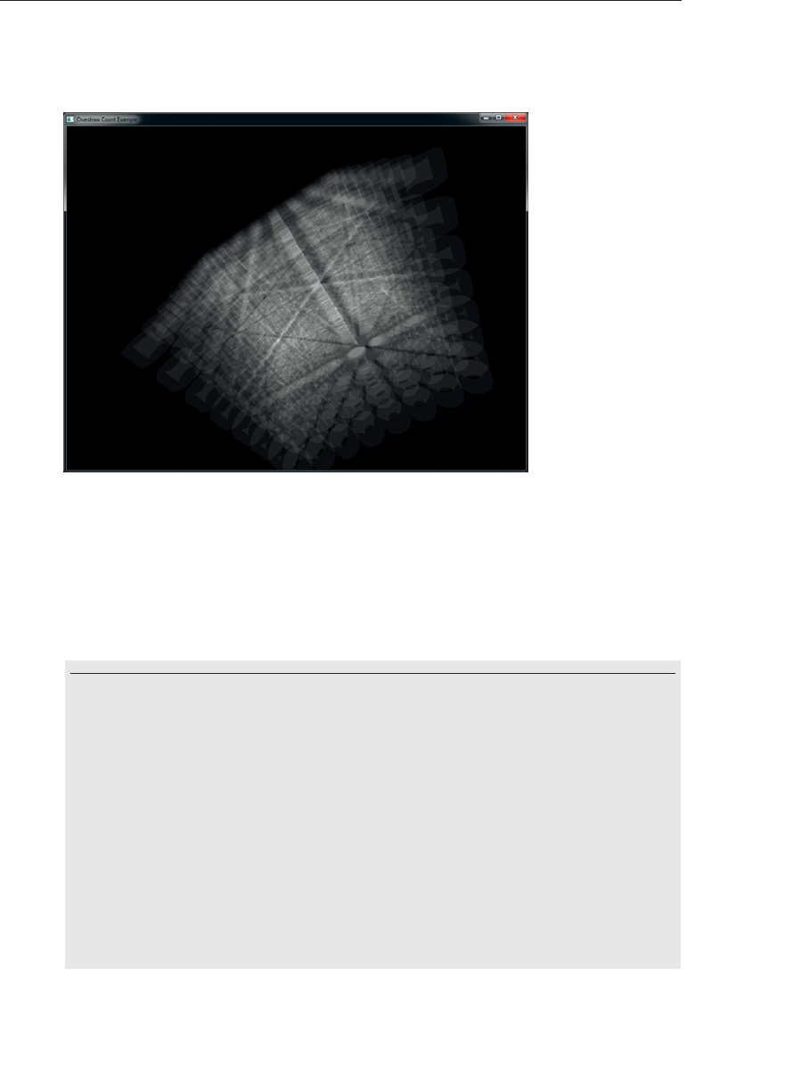
ptg9898810
The result of executing the shader shown in Example 11.9 is shown in
Figure 11.4. As you can see, the output is much cleaner.
Figure 11.4 Output of the atomic overdraw counter shader
imageAtomicAdd is one of many atomic built-in functions in GLSL. These
functions include addition and subtraction, logical operations, and
comparison and exchange operations. The complete list of GLSL atomics is
shown below.
uint imageAtomicAdd(IMAGE_PARAMS mem, uint data);
int imageAtomicAdd(IMAGE_PARAMS mem, int data);
uint imageAtomicMin(IMAGE_PARAMS mem, uint data);
int imageAtomicMin(IMAGE_PARAMS mem, int data);
uint imageAtomicMax(IMAGE_PARAMS mem, uint data);
int imageAtomicMax(IMAGE_PARAMS mem, int data);
uint imageAtomicAnd(IMAGE_PARAMS mem, uint data);
int imageAtomicAnd(IMAGE_PARAMS mem, int data);
uint imageAtomicOr(IMAGE_PARAMS mem, uint data);
int imageAtomicOr(IMAGE_PARAMS mem, int data);
uint imageAtomicXor(IMAGE_PARAMS mem, uint data);
int imageAtomicXor(IMAGE_PARAMS mem, int data);
uint imageAtomicExchange(IMAGE_PARAMS mem, uint data);
582 Chapter 11: Memory

ptg9898810
int imageAtomicExchange(IMAGE_PARAMS mem, int data);
uint imageAtomicCompSwap(IMAGE_PARAMS mem,
uint compare uint data);
int imageAtomicCompSwap(IMAGE_PARAMS mem, int compare,
int data);
imageAtomicAdd,imageAtomicMin, and imageAtomicMax perform an
atomic addition, minimum, and maximum operation between data and
the contents of the specified image at the specified coordinates,
respectively. imageAtomicAnd,imageAtomicOr, and imageAtomicXor
perform an atomic logical AND, OR, and XOR operation between data
and the contents of the specified image at the specified coordinates,
respectively. Each function returns the value originally in memory before
the operation was performed.
imageAtomicExchange writes the value of data into the specified image
at the specified coordinates and returns the value originally in memory
before the write was performed.
imageAtomicCompSwap compares the value of compare with the value in
the specified image at the specified coordinates and if they are equal, it
writes the value of data into that memory location. The compare and
write operations are performed atomically. The value originally in
memory before the write occurred is returned.
In the declarations of the atomic image functions, IMAGE_PARAMS may be
replaced with any of the definitions given in Example 11.10. The effect of
this is that there are several overloaded versions of each of the atomic
functions.
Example 11.10 Possible Definitions for IMAGE_PARAMS
#define IMAGE_PARAMS gimage1D image, int P // or
#define IMAGE_PARAMS gimage2D image, ivec2 P // or
#define IMAGE_PARAMS gimage3D image, ivec3 P // or
#define IMAGE_PARAMS gimage2DRect image, ivec2 P // or
#define IMAGE_PARAMS gimageCube image, ivec3 P // or
#define IMAGE_PARAMS gimageBuffer image, int P // or
#define IMAGE_PARAMS gimage1DArray image, ivec2 P // or
#define IMAGE_PARAMS gimage2DArray image, ivec3 P // or
#define IMAGE_PARAMS gimageCubeArray image, ivec3 P // or
#define IMAGE_PARAMS gimage2DMS image, ivec2 P, int sample // or
#define IMAGE_PARAMS gimage2DMSArray image, ivec3 P, int sample
Atomic functions can operate only on single signed or unsigned integers---
that is, neither floating-point images nor images of vectors of any type are
Atomic Operations and Synchronization 583

ptg9898810
supported in atomic operations. Each atomic function returns the value
that was previously in memory at the specified location. If this value is not
required by the shader, it may be safely ignored. Shader compilers may
then perform data-flow analysis and eliminate unnecessary memory reads
if it is advantageous to do so. As an example, the equivalent code for
imageAtomicAdd is given in Example 11.11. Although Example 11.11
shows imageAtomicAdd implemented as several lines of code, it is
important to remember that this is for illustration only and that the
built-in imageAtomicAdd function operates as a single, indivisible
operation.
Example 11.11 Equivalent Code for imageAtomicAdd
// THIS FUNCTION OPERATES ATOMICALLY
uint imageAtomicAdd(uimage2D image, ivec2 P, uint data)
{// Read the value that’s currently in memory
uint val = imageLoad(image, P).x;
// Write the new value to memory
imageStore(image, P, uvec4(val + data));
// Return the *old*value.
return val;
}
As has been shown in Example 11.9, this atomic behavior may be used to
effectively serialize access to a memory location. Similar functionality for
other operations such as logical operations is achieved through the
use of imageAtomicAnd,imageAtomicXor, and so on. For example, two
shader invocations may simultaneously set different bits in a single
memory location using the imageAtomicOr function. The two atomic
functions that do not perform arithmetic or logical operations on
memory are imageAtomicExchange and imageAtomicCompSwap.
imageAtomicExchange is similar to a regular store, except that it returns
the value that was previously in memory. In effect, it exchanges the value
in memory with the value passed to the function, returning the old value
to the shader. imageAtomicCompSwap is a generic compare-and-swap
operation that conditionally stores the specified data in memory. The
equivalent code for these functions is shown in Example 11.12.
584 Chapter 11: Memory

ptg9898810
Example 11.12 Equivalent Code for imageAtomicExchange and
imageAtomicComp
// THIS FUNCTION OPERATES ATOMICALLY
uint imageAtomicExchange(uimage2D image, ivec2 P, uint data)
{
uint val = imageLoad(image, P);
imageStore(image, P, data);
return val;
}
// THIS FUNCTION OPERATES ATOMICALLY
uint imageAtomicCompSwap(uimage2D image, ivec2 P,
uint compare, uint data)
{
uint val = imageLoad(image, P);
if (compare == val)
{
imageStore(image, P, data);
}
return val;
}
Again, it is important to remember that the code given in Example 11.12
is for illustrative purposes only and that the imageAtomicExchange
and imageAtomicCompSwap functions are truly implemented using
hardware support as opposed to a sequence of lower-level operations.
One of the primary use cases for imageAtomicExchange is in the
implementation of linked lists or other complex data structures. In a
linked list, the head and tail pointers may be swapped with references to
new items inserted into the list atomically to effectively achieve parallel
list insertion. Likewise, imageAtomicCompSwap may be used to
implement locks (also known as mutexes) to prevent simultaneous access
to a shared resource (such as another image). An example of taking a lock
using an atomic compare-and-swap operation (as implemented by
imageAtomicCompSwap) is shown in Example 11.13.
Example 11.13 Simple Per-Pixel Mutex Using imageAtomicCompSwap
#version 420 core
layout (r32ui)uniform uimage2D lock_image;
layout (rgba8f) uniform image2D protected_image;
Atomic Operations and Synchronization 585

ptg9898810
void takeLock(ivec2 pos)
{
int lock_available;
do {
// Take the lock - the value in lock_image is 0 if the lock
// is not already taken. If so, then it is overwritten with
// 1 otherwise it is left alone. The function returns the value
// that was originally in memory - 0 if the lock was not taken,
// 1 if it was. We terminate the loop when we see that the lock
// was not already taken and thus we now hold it because we’ve
// written a one to memory.
lock_available = imageAtomicCompSwap(lock_image, pos, 0, 1);
}while (lock_available == 0);
}
void releaseLock(ivec2 pos)
{
imageStore(lock_image, pos, 0);
}
void operateOnFragment()
{
// Perform a sequence of operations on the current fragment
// that need to be indivisible. Here, we simply perform
// multiplication by a constant as there is no atomic version
// of this (imageAtomicMult, for example). More complex functions
// could easily be implemented.
vec4 old_fragment;
old_fragment = imageLoad(protected_image,
ivec2(gl_FragCoord.xy));
imageStore(protected_image,
ivec2(gl_FragCoord.xy),
old_fragment *13.37);
}
void main(void)
{
// Take a per-pixel lock
takeLock(ivec2(gl_FragCoord.xy));
// Now we own the lock and can safely operate on a shared resource
operateOnPixel();
// Be sure to release the lock...
releaseLock(ivec2(gl_FragCoord.xy));
}
586 Chapter 11: Memory

ptg9898810
The code shown in Example 11.13 implements a simple per-pixel mutex
using the imageAtomicCompSwap function. To do this, it compares
the value already in memory to zero (the third parameter to
imageAtomicCompSwap). If they are equal (i.e., if the current value in
memory is zero), it writes the new value (one, here) into memory.
imageAtomicCompSwap then returns the value that was originally in
memory. That is, if the lock was not previously taken, the value in memory
will be zero (which is what is returned), but this will be replaced with one,
reserving the lock. If the lock was previously taken by another shader
invocation, the value in memory will already be one, and this is what will
be returned. Therefore, we know that we received the lock
when imageAtomicCompSwap returns zero. This loop therefore executes
until imageAtomicCompSwap returns zero, indicating that the lock was
available. When it does, this shader invocation will have the lock. The first
invocation (after serialization by the hardware) that receives a zero from
imageAtomicComSwap will hold the lock until it places a zero back into
memory (which is what releaseLock does). All other invocations will
spin in the loop in takeLock. They will be released from this loop one at a
time until all invocations have taken the lock, performed their operations,
and then released it again.
The functionality implemented in operateOnFragment can be anything.
It does not have to use atomics because the whole function is running
while the lock is taken by the current shader invocation. For example,
programmable blending3operations could be implemented here by using
imageLoad and imageStore to read and write a texture. Also, operations
for which there is no built-in atomic function can be implemented---for
example, multiplication, arithmetic shift, or transcendental functions can
be performed on images.
Atomic Operations on Buffers
In addition to the atomic operations that may be performed on images,
atomic operations may also be performed on buffer variables. Buffer
variables are variables inside interface blocks that have been declared with
the buffer keyword. As with images, several built-in functions to perform
atomic operations are defined. The atomic operations that may be
performed on buffer variables are the same set that may be performed on
image variables.
3. Note that there is still no ordering guarantee, so only blending operations that are
order-independent can be implemented here. A more complete example that includes order-
independent blending is given at the end of this chapter.
Atomic Operations and Synchronization 587

ptg9898810
uint atomicAdd(inout uint mem, uint data);
int atomicAdd(inout int mem, int data);
uint atomicMin(inout uint mem, uint data);
int atomicMin(inout int mem, int data);
uint atomicMax(inout uint mem, uint data);
int atomicMax(inout int mem, int data);
uint atomicAnd(inout uint mem, uint data);
int atomicAnd(inout int mem, int data);
uint atomicOr(inout uint mem, uint data);
int atomicOr(inout int mem, int data);
uint atomicXor(inout uint mem, uint data);
int atomicXor(inout int mem, int data);
uint atomicExchange(inout uint mem, uint data);
int atomicExchange(inout int mem, int data);
uint atomicCompSwap(inout uint mem, uint compare uint data);
int atomicCompSwap(inout int mem, int compare, int data);
atomicAdd,atomicMin, and atomicMax perform an atomic addition,
minimum, and maximum operation between data and mem, respectively.
atomicAnd,atomicOr, and atomicXor perform an atomic logical AND,
OR, and XOR operation between data and mem, respectively. Each
function returns the value originally in memory before the operation was
performed.
atomicExchange writes the value of data into the memory location
referenced by mem and returns the value originally in memory before the
write was performed.
atomicCompSwap compares the value of compare with the value in the
memory location referenced by mem and if they are equal, it writes the
value of data into that memory location. The compare and write
operations are performed atomically. The value originally in memory
before the write occurred is returned.
Each of the atomic functions listed above takes an inout parameter that
serves as a reference to a memory location. The value passed to any of
these atomic functions in the mem parameter must4be a member of a
block declared with the buffer keyword. Like the image atomic functions,
each of these functions returns the value originally in memory before it
was updated. This effectively allows you to swap the content of memory
for a new value, possibly conditionally as in the case of atomicCompSwap.
4. Actually, these atomic functions may also be used on variables declared as shared. This will
be discussed further in ‘‘Compute Shaders’’.
588 Chapter 11: Memory

ptg9898810
Sync Objects
OpenGL operates in a client-server model, where a server operates
asynchronously to the client. Originally, this allowed the user’s terminal to
render high-performance graphics and for the application to run on a
server in a remote location. This was an extension of the X protocol, which
was always designed with remote rendering and network operations in
mind. In modern graphics workstations, we have a similar arrangement,
with a slightly different interpretation. Here, the client is the CPU and the
application runs on it, sending commands to the server, which is a
high-performance GPU. However, the bandwidth between the two is still
relatively low compared to the throughput and performance of either one.
Therefore, for maximum performance, the GPU runs asynchronously to
the CPU and can often be several OpenGL commands behind the
application.
In some circumstances, it is necessary, however, to ensure that the client
and the server---the CPU and the GPU execute in a synchronized manner.
To achieve this, we can use a sync object, which can also be known as a
fence. A fence is essentially a marker in the stream of commands that can
be sent along with drawing and state change commands to the GPU. The
fence starts life in an unsignaled state and becomes signaled when the GPU
has executed it. At any given time, the application can look at the state of
the fence to see if the GPU has reached it yet, and it can wait for the GPU
to have executed the fence before moving on. To inject a fence into the
OpenGL command stream, call glFenceSync():
GLsync glFenceSync(GLenum condition, GLbitfield flags);
Creates a new fence sync object by inserting a fence into the OpenGL
command stream and returning a handle to the newly created fence. The
fence begins in an unsignaled state and becomes signaled when the
conditions specified by condition becomes true. The only legal value for
condition is GL_SYNC_GPU_COMMANDS_COMPLETE. flags is currently
unused and must be set to zero.
When you call glFenceSync(), a new fence sync object is created, and the
corresponding fence is inserted into the OpenGL command stream. The
sync starts of unsignaled and will eventually become signaled when the GPU
processes it. Because (although asynchronous) OpenGL has a well-defined
order of execution, when a fence becomes signaled, you know that any
commands that precede it in the command stream have finished executing,
although nothing is known about commands that follow. To check
if a fence has been executed by the GPU yet, you can call glGetSynciv():
Atomic Operations and Synchronization 589

ptg9898810
void glGetSynciv(GLsync sync, GLenum pname, GLsizei bufSize,
GLsizei *length, GLint *values);
Retrieves the properties of a sync object. sync specifies a handle to the
sync object from which to read the property specified by pname.bufSize is
the size in bytes of the buffer whose address is given in values.length is
the address of an integer variable that will receive the number of bytes
written into values.
To check to see if a fence object has become signaled yet, call
glGetSynciv() with pname set to GL_SYNC_STATUS. Assuming no error is
generated, and the buffer is big enough, either GL_SIGNALED or
GL_UNSIGNALED will be written into the buffer pointed to by values
depending on whether the fence had been reached by the GPU or not. You
can use this to poll a sync object to wait for it to become signaled, but this
can be quite inefficient, with control passing backwards between your
application and the OpenGL implementation, and with all the error
checking and other validation that the OpenGL drivers might do on your
system occurring for each transition. If you wish to wait for a sync object
to become signaled, you should call glClientWaitSync():
GLenum glClientWaitSync(GLsync sync, GLbitfields flags,
GLuint64 timeout);
Causes the client to wait for the sync object sync to become signaled.
glClientWaitSync() will wait at most timeout nanoseconds for the object
to become signaled before generating a timeout. The flags parameter may
be used to control flushing behavior of the command. Specifying
GL_SYNC_FLUSH_COMMANDS_BIT is equivalent to calling glFlush()
before executing the wait.
The glClientWaitSync() function is used to wait in the client for a fence to
be reached by the server. It will wait for up to timeout nanoseconds for the
sync object given by sync to become signaled before giving up. If flags
contains GL_SYNC_FLUSH_COMMANDS_BIT then glClientWaitSync()
will implicitly send any pending commands to the server before beginning
to wait. It’s generally a good idea to always set this bit as without it, the
OpenGL driver might buffer up commands and never send them to the
server, ensuring that your call to glClientWaitSync() will generate a
timeout. glClientWaitSync() will generate one of four return values:
590 Chapter 11: Memory

ptg9898810
•GL_ALREADY_SIGNALED is returned if sync was already signaled when
the call to glClientWaitSync() was made.
•GL_TIMEOUT_EXPIRED is returned if sync did not enter the signaled
state before nanoseconds nanoseconds passed.
•GL_CONDITION_SATISFIED is returned if sync was not signaled when
the call to glClientWaitSync() was made, but became signaled before
nanoseconds nanoseconds elapsed.
•GL_WAIT_FAILED is returned if the call to glClientWaitSync() failed
for some reason, such as sync not being the name of a sync object. In
this case, a regular OpenGL error is also generated and should be
checked with glGetError(). Furthermore, if you are using a debug
context, then there is a good chance that its log will tell you exactly
what went wrong.
Sync objects can only go from the unsignaled state (which is the state that
they are created in) into the signaled state. Thus, they are basically a
single-use object. Once you have finished waiting for a sync object, or if
you decide you don’t need it any more, you should delete the sync object.
To delete a sync object, call glDeleteSync():
void glDeleteSync(GLsync sync);
Deletes the sync object specified by sync. If sync is already signaled at this
time, it is deleted immediately, otherwise it is marked for deletion and will
be deleted when the implementation determines that it is safe to do so.
A very common use-case for sync objects is to ensure that the GPU is done
using data in a mapped buffer before overwriting the data. This can occur
if the buffer (or a range of it) was mapped using the glMapBufferRange()
function with the GL_MAP_UNSYNCHRONIZED_BIT set. This causes
OpenGL to not wait for any pending commands that may be about to read
from the buffer to complete before handing your application a pointer to
write into. Under some circumstances, this pointer may actually address
memory that the GPU is about to use. To make sure that you don’t stomp
all over data that hasn’t been used yet, you can insert a fence right after the
last command that might read from a buffer, and then issue a call to
glClientWaitSync() right before you write into the buffer. Ideally, you’d
execute something that takes some time between the call to glFenceSync()
and the call to glClientWaitSync(). A simple example is shown in
Example 11.14.
Atomic Operations and Synchronization 591

ptg9898810
Example 11.14 Example Use of a Sync Object
// This will be our sync object.
GLsync s;
// Bind a vertex array and draw a bunch of geometry
glBindVertexArray(vao);
glDrawArrays(GL_TRIANGLES, 0, 30000);
// Now create a fence that will become signaled when the
// above drawing command has completed
s = glFenceSync();
// Map the uniform buffer that’s in use by the above draw
void *data = glMapBufferRange(GL_UNIFORM_BUFFER,
0, 256,
GL_WRITE_BIT |
GL_MAP_UNSYNCHRONIZED_BIT);
// Now go do something that will last a while...
// ... say, calculate the new values of the uniforms
do_something_time_consuming();
// Wait for the sync object to become signaled.
// 1,000,000 ns = 1 ms.
switch (glClientWaitSync(s, 0, 1000000);
// Now delete the sync object, write over the uniform
// buffer and unmap it
glDeleteSync(s);
memcpy(data, source_data, source_data_size);
glUnmapBuffer(GL_UNIFORM_BUFFER);
As with many other object types in OpenGL, it is possible to simply ask
whether the object you have is what you think it is. To find out if an object
is a valid sync object, you can call glIsSync():
GLboolean glIsSync(GLsync sync);
Returns GL_TRUE if sync is the name of an existing sync object that has
not been deleted and GL_FALSE otherwise.
Advanced
If you are sharing objects between two or more contexts, it is possible to
wait in one context for a sync object to become signaled as the result of
commands issued in another. To do this, call glFenceSync() in the source
592 Chapter 11: Memory

ptg9898810
context (the one which you want to wait on) and then call glWaitSync()
in the destination context (the one that will do the waiting). The
prototype for glWaitSync() is as follows:
void glWaitSync(GLsync sync, GLbitfield flags, GLuint64 timeout);
Causes the server to wait for the sync object indicated by sync to become
signaled. flags is not used and must be set to zero. timeout is also unused,
but must be set to the special value, GL_TIMEOUT_IGNORED. The server
will wait an implementation-dependent amount of time before
considering the sync object to have timed out and will then continue
execution of subsequent commands.
glWaitSync() presents a rather limited form of what may be achieved with
glClientWaitSync(). The major differences are the
GL_SYNC_FLUSH_COMMANDS_BIT flag is not accepted in the flags
parameter (nor is any other flag), and the timeout is implementation-
defined. You still have to ask for this implementation-defined timeout
value by passing GL_TIMEOUT_IGNORED in timeout. However, you can
find out what that implementation-dependent timeout value is by calling
glGetIntegerv() with the parameter GL_MAX_SERVER_WAIT_TIMEOUT.
An example use for glWaitSync() synchronizing two contexts is when you
are writing data into a buffer using transform feedback and want to
consume that data in another context. In this case, you would issue the
drawing commands that would ultimately update the transform feedback
buffer and then issue the fence with a call to glFenceSync(). Next, switch
to the consuming thread (either with a true context switch or by handing
control to another application thread) and then wait on the fence to
become signaled by calling glWaitSync() before issuing any drawing
commands that might consume the data.
Image Qualifiers and Barriers
The techniques outlined above work well when compilers don’t perform
overly aggressive optimizations on your shaders. However, under certain
circumstances, the compiler might change the order or frequency of image
loads or stores, and may eliminate them altogether if it believes they are
redundant. For example, consider the simple example loop in
Example 11.15.
Atomic Operations and Synchronization 593

ptg9898810
Example 11.15 Basic Spin-Loop Waiting on Memory
#version 420 core
// Image that we’ll read from in the loop
layout (r32ui}uniform uimageBuffer my_image;
void waitForImageToBeNonZero()
{
uint val;
do
{// (Re-)read from the image at a fixed location.
val = imageLoad(my_image, 0).x;
// Loop until the value is nonzero
}while (val == 0);
}
In Example 11.15, the function waitForImageToBeNonZero contains a
tight loop that repeatedly reads from the same location in the image and
only breaks out of the loop when the data returned is nonzero. The
compiler might assume that the data in the image does not change and
therefore, the imageLoad function will always return the same value. In
such a case, it may move the imageLoad out of the loop. This is a very
common optimization known as hoisting and effectively replaces
waitForImageToBeNonZero with the version shown in Example 11.16.
Example 11.16 Result of Loop-Hoisting on Spin-Loop
#version 420 core
// Image that we’ll read from in the loop
layout (r32ui}uniform uimageBuffer my_image;
void waitForImageToBeNonZero()
{
uint val;
// The shader complier has assumed that the image
// data does not change and has moved the load
// outside the loop.
val = imageLoad(my_image, 0).x;
do
{// Nothing remains in the loop. It will either
// exit after one iteration, or execute forever!
}while (val == 0);
}
594 Chapter 11: Memory

ptg9898810
As may be obvious, each call to the optimized version of
waitForImageToBeNonZero in Example 11.16 will either read a nonzero
value from the image and return immediately or enter an infinite
loop---quite possibly crashing or hanging the graphics hardware. In order
to avoid this situation, the volatile keyword must be used when
declaring the image uniform to instruct the compiler to not perform such
an optimization on any loads or stores to the image. To declare an image
uniform (or parameter to a function) as volatile, simply include the
volatile keyword in its declaration. This is similar to the volatile
keyword supported by the ‘‘C’’ and C++ languages, and examples of this
type of declaration are shown in Example 11.17.
Example 11.17 Examples of Using the volatile Keyword
#version 420 core
// Declaration of image uniform that is volatile. The
// compiler will not make any assumptions about the
// content of the image and will not perform any
// unsafe optimizations on code accessing the image.
layout (r32ui}uniform volatile uimageBuffer my_image;
// Declaration of function that does declares its
// parameter as volatile...
void functionTakingVolatileImage(volatile uimageBuffer i)
{// Read and write i here.
}
The volatile keyword may be applied to global declarations and
uniforms, function parameters, or local variables. In particular, image
variables that have not been declared as volatile may be passed to
functions as parameters that do have the volatile keyword. In such
cases, the operations performed by the called function will be treated as
volatile, whereas operations on the image elsewhere will not be volatile. In
effect, the volatile qualifier may be added to a variable based on scope.
However, the volatile keyword (or any other keyword discussed in this
section) may not be removed from a variable. That is, it is illegal to pass an
image variable declared as volatile as a parameter to a function that
does not also declare that parameter as volatile.
Another qualifier originating in the ‘‘C’’ languages that is available in GLSL
is the restrict keyword, which instructs the compiler that data
referenced by one image does not alias5the data referenced by any other.
5. That is, no two images reference the same piece of memory, so stores to one cannot possibly
affect the result of loads from the other.
Atomic Operations and Synchronization 595

ptg9898810
In such cases, writes to one image do not affect the contents of any other
image. The compiler can therefore be more aggressive about making
optimizations that might otherwise be unsafe. Note that by default, the
compiler assumes that aliasing of external buffers is possible and is less
likely to perform optimizations that may break otherwise well-formed
code. (Note GLSL assumes no aliasing of variables and parameters residing
within the shader, and fully optimizes based on that.) The restrict
keyword is used in a similar manner to the volatile keyword as
described above---that is, it may be added to global or local declarations to
effectively add the restrict qualifier to existing image variables in certain
scope. In essence, references to memory buffers through restrict
qualified image variables behave similarly to references to memory
through restricted pointers in ‘‘C’’ and C++.
There are three further qualifiers available in GLSL that do not have an
equivalent in C. These are coherent,readonly, and writeonly. First,
coherent is used to control cache behavior for images. This type of
functionality is generally not exposed by high-level languages. However, as
GLSL is designed for writing code that will execute on highly parallel and
specialized hardware, coherent is included to allow some level of
management of where data is placed.
Consider a typical graphics processing unit (GPU). It is made up of
hundreds or potentially thousands of separate processors grouped into
blocks. Different models of otherwise similar GPUs may contain different
numbers of these blocks depending on their power and performance
targets. Now, such GPUs will normally include large, multilevel caches that
may or may not be fully coherent.6If the data store for an image is placed
in a noncoherent cache, then changes made by one client of that cache
may not be noticed by another client until that cache is explicitly flushed
back to a lower level in a memory hierarchy. A schematic of this is shown
in Figure 11.5, which depicts the memory hierarchy of a fictitious GPU
with a multilevel cache hierarchy.
6. A coherent cache is a cache that allows local changes to be immediately observed by other
clients of the same memory subsystem. Caches in CPUs tend to be coherent (a write performed
by one CPU core is seen immediately by other CPU cores), whereas caches in GPUs may or
may not be coherent.
596 Chapter 11: Memory
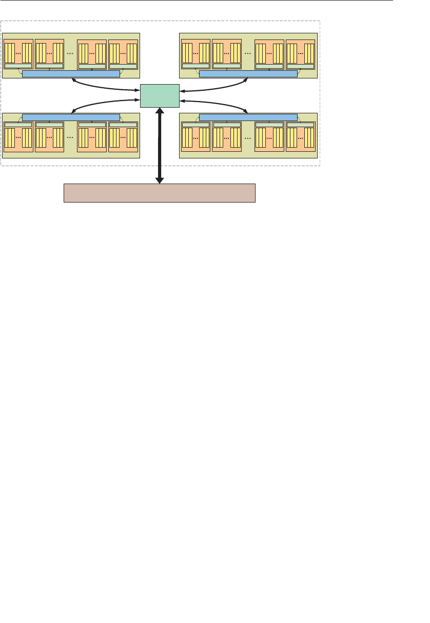
ptg9898810
GPU
MEMORY
CONTROLLER
PROCESSOR GROUP 2
SHADER PROCESSOR 0
VECTOR LANE 0
VECTOR LANE 1
VECTOR LANE 2
VECTOR LANE 13
VECTOR LANE 14
VECTOR LANE 15
L1 CACHE
L2 CACHE
SHADER PROCESSOR 1
VECTOR LANE 0
VECTOR LANE 1
VECTOR LANE 2
VECTOR LANE 13
VECTOR LANE 14
VECTOR LANE 15
L1 CACHE
SHADER PROCESSOR 14
VECTOR LANE 0
VECTOR LANE 1
VECTOR LANE 2
VECTOR LANE 13
VECTOR LANE 14
VECTOR LANE 15
L1 CACHE
SHADER PROCESSOR 15
VECTOR LANE 0
VECTOR LANE 1
VECTOR LANE 2
VECTOR LANE 13
VECTOR LANE 14
VECTOR LANE 15
L1 CACHE
MAIN MEMORY
PROCESSOR GROUP 3
SHADER PROCESSOR 0
VECTOR LANE 0
VECTOR LANE 1
VECTOR LANE 2
VECTOR LANE 13
VECTOR LANE 14
VECTOR LANE 15
L1 CACHE
L2 CACHE
SHADER PROCESSOR 1
VECTOR LANE 0
VECTOR LANE 1
VECTOR LANE 2
VECTOR LANE 13
VECTOR LANE 14
VECTOR LANE 15
L1 CACHE
SHADER PROCESSOR 14
VECTOR LANE 0
VECTOR LANE 1
VECTOR LANE 2
VECTOR LANE 13
VECTOR LANE 14
VECTOR LANE 15
L1 CACHE
SHADER PROCESSOR 15
VECTOR LANE 0
VECTOR LANE 1
VECTOR LANE 2
VECTOR LANE 13
VECTOR LANE 14
VECTOR LANE 15
L1 CACHE
PROCESSOR GROUP 0
SHADER PROCESSOR 0
VECTOR LANE 0
VECTOR LANE 1
VECTOR LANE 2
VECTOR LANE 13
VECTOR LANE 14
VECTOR LANE 15
L1 CACHE
SHADER PROCESSOR 1
VECTOR LANE 0
VECTOR LANE 1
VECTOR LANE 2
VECTOR LANE 13
VECTOR LANE 14
VECTOR LANE 15
L1 CACHE
SHADER PROCESSOR 14
VECTOR LANE 0
VECTOR LANE 1
VECTOR LANE 2
VECTOR LANE 13
VECTOR LANE 14
VECTOR LANE 15
L1 CACHE
SHADER PROCESSOR 15
VECTOR LANE 0
VECTOR LANE 1
VECTOR LANE 2
VECTOR LANE 13
VECTOR LANE 14
VECTOR LANE 15
L1 CACHE
L2 CACHE
PROCESSOR GROUP 1
SHADER PROCESSOR 0
VECTOR LANE 0
VECTOR LANE 1
VECTOR LANE 2
VECTOR LANE 13
VECTOR LANE 14
VECTOR LANE 15
L1 CACHE
SHADER PROCESSOR 1
VECTOR LANE 0
VECTOR LANE 1
VECTOR LANE 2
VECTOR LANE 13
VECTOR LANE 14
VECTOR LANE 15
L1 CACHE
SHADER PROCESSOR 14
VECTOR LANE 0
VECTOR LANE 1
VECTOR LANE 2
VECTOR LANE 13
VECTOR LANE 14
VECTOR LANE 15
L1 CACHE
SHADER PROCESSOR 15
VECTOR LANE 0
VECTOR LANE 1
VECTOR LANE 2
VECTOR LANE 13
VECTOR LANE 14
VECTOR LANE 15
L1 CACHE
L2 CACHE
Figure 11.5 Cache hierarchy of a fictitious GPU
In Figure 11.5, each shader processor is made up of a 16-wide vector
processor that concurrently processes 16 data items (these may be
fragments, vertices, patches, or primitives depending on what type of
shader is executing). Each vector processor has its own, small, level-1
cache, which is coherent among all of the shader invocations running in
that processor. That is, a write performed by one invocation on that
processor will be observed by and its data made available to any other
invocation executing on the same processor. Furthermore, there are four
shader processor groups, each with 16, 16-element-wide vector processors
and a single, shared, level-2 cache, that is, there is a level-2 cache per
shader processor group that is shared by 16, 16-wide vector processors
(256 data items). There are therefore four independent level-2 caches, each
serving 16 processors with 16-wide vectors for a total of 1024 concurrently
processing data items. Each of the level-2 caches is a client of the memory
controller.
For highest performance, the GPU will attempt to keep data in the
highest-level cache, that is, in caches labeled with the smallest number,
closest to the processor accessing the data. If data is only to be read from
memory, but not written, then data can be stored in noncoherent caches.
In such cases, our fictitious GPU will place data in the level-1 caches
within the vector processors. However, if memory writes made by one
processor must be seen by another processor, (this includes atomics that
implicitly read, modify, and write data), the data must be placed in a
coherent memory location. Here, we have two choices: the first, to bypass
Atomic Operations and Synchronization 597

ptg9898810
cache altogether, and the second, to bypass level-1 caches and place data
in level-2 caches while ensuring that any work that needs to share data is
run only in that cache’s shader processor group. Other GPUs may have
ways of keeping the level-2 caches coherent. This type of decision is
generally made by the OpenGL driver, but a requirement to do so is given
in the shader by using the coherent keyword. An example coherent
declaration is shown in Example 11.18.
Example 11.18 Examples of Using the coherent Keyword
#version 420 core
// Declaration of image uniform that is coherent. The OpenGL
// implementation will ensure that the data for the image is
// placed in caches that are coherent, or perhaps used an uncached
// location for data storage.
layout (r32ui}uniform coherent uimageBuffer my_image;
// Declaration of function that does declares its parameter
// as coherent...
uint functionTakingCoherentImage(coherent uimageBuffer i, int n)
{
// Write i here...
imageStore(my_image, n, uint(n));
// Any changes will be visible to all other shader invocations.
// Likewise, changes made by invocations are visible here.
uint m = imageStore(my_image, n - 1).x;
return m;
}
The final two image qualifier keywords, readonly and writeonly,
control access to image data. readonly behaves somewhat like const,
being a contract between the programmer and the OpenGL
implementation that the programmer will not access a readonly image
for writing. The difference between const and readonly applied to an
image variable is that const applies to the variable itself. That is, an image
variable declared as const may not be written, however, the shader may
write to the image bound to the image unit referenced by that variable. On
the other hand, readonly applies to the underlying image data. A shader
may assign new values to an image variable declared as readonly, but it
may not write to an image through that variable. An image variable may
be declared both const and readonly at the
same time.
The writeonly keyword also applies to the image data attached to the
image unit to which an image variable refers. Attempting to read from an
598 Chapter 11: Memory

ptg9898810
image variable declared as writeonly will generate an error. Note that
atomic operations implicitly perform a read operation as part of their
read-modify-write cycle and so are not allowed on readonly or
writeonly image variables.
Memory Barriers
Now that we understand how to control compiler optimizations using the
volatile and restrict keywords and control caching behavior using
the coherent keyword, we can accurately describe how image data is to be
used. However, the compiler may still reorder memory operations, or allow
different shader invocations to run out of order with respect to each other.
This is particularly true in the case of shaders from different stages of the
OpenGL pipeline. Some level of asynchrony is required in order to achieve
best performance. Because of this, GLSL includes the memoryBarrier()
function that may be used to ensure that any writes made to a particular
location in memory are observed by other shader invocations in the order
that they were made in. It causes a singe shader invocation to wait until
any outstanding memory transactions have completed.7As an example,
see Example 11.19.
Example 11.19 Example of Using the memoryBarrier() Function
#version 420 core
layout (rgba32f}uniform coherent image2D my_image;
// Declaration of function
void functionUsingBarriers(coherent uimageBuffer i)
{
uint val;
// This loop essentially waits until at least one fragment from
// an earlier primitive (that is, one with gl_PrimitiveID - 1)
// has reached the end of this function point. Note that this is
// not a robust loop as not every primitive will generate
// fragments.
do
7. Writes to memory may be posted. This means that a request is made to the memory subsystem
(caches and controller) to write data at a specific address. The memory system inserts this
request in a queue and services one or more requests at a time until the data is written to
memory. At this time, it signals the original requester that the write has completed. Because
there may be multiple caches and memory controllers in a system and each may service
multiple requests at a time, the requests may complete out of order. The memoryBarrier
function forces a shader invocation to wait until the completion signal comes back from the
memory subsystem for all pending writes before continuing execution.
Atomic Operations and Synchronization 599

ptg9898810
{
val = imageLoad(i, 0).x;
}while (val != gl_PrimitiveID);
// At this point, we can load data from another global image
vec4 frag = imageLoad(my_image, gl_FragCoord.xy);
// Operate on it...
frag *= 0.1234;
frag = pow(frag, 2.2);
// Write it back to memory
imageStore(my_image, gl_FragCoord.xy, frag);
// Now, we’re about to signal that we’re done with processing
// the pixel. We need to ensure that all stores thus far have
// been posted to memory. So, we insert a memory barrier.
memoryBarrier();
// Now we write back into the original "primitive count" memory
// to signal that we have reached this point. The stores
// resulting from processing "my_image" will have reached memory
// before this store is committed due to the barrier.
imageStore(i, 0, gl_PrimitiveID + 1);
// Now issue another barrier to ensure that the results of the
// image store are committed to memory before this shader
// invocation ends.
memoryBarrier();
}
Example 11.19 shows a very simple use case for memory barriers. It allows
some level of ordering between fragments to be ensured. At the top of
functionUsingBarriers, a simple loop is used to wait for the contents
of a memory location to reach our current primitive ID. Because we know
that no two fragments from the same primitive can land on the same
pixel,8we know that when we’re executing the code in the body of the
function, at least one fragment from the previous primitive has been
processed. We then go about modifying the contents of memory at our
fragment’s location using nonatomic operations. We signal to other shader
invocations that we are done by writing to the shared memory location
originally polled at the top of the function.
8. This is true except for patches or other complex geometry generated by the geometry shader.
In such cases, the primitive ID seen by the fragment shader is generated explicitly by the
upstream shader (tessellation evaluation or geometry shader) and it is up to the user to ensure
that no two overlapping fragments see the same primitive ID if this is required by the algorithm.
600 Chapter 11: Memory

ptg9898810
To ensure that our modified image contents are written back to memory
before other shader invocations start into the body of the function, we use
a call to memoryBarrier between updates of the color image and the
primitive counter to enforce ordering. We then insert another barrier after
the primitive counter update to ensure that other shader invocations see
our update. This doesn’t guarantee full per-pixel ordering (especially if
fragments from multiple primitives are packed into a single vector), but it
may be close enough for many purposes. Also, it should be noted that if
primitives are discarded (because they are clipped, back-facing, or have no
area), they will generate no fragments and will not update the primitive ID
counter. In such a case, this loop will deadlock waiting for primitives that
never come.
Not only can barriers be used inside shader code to ensure that memory
operations are ordered with respect to one another, some level of control
over memory transactions and caching behavior is provided by the OpenGL
API through the glMemoryBarrier() function. Its prototype is as follows:
void glMemoryBarrier(GLbitfield barriers);
Defines a barrier ordering memory transactions issued before the
command relative to those issued after the command. Memory
transactions performed by shaders are considered to be issued by the
rendering command that invoked the execution of the shader. The
bitfield parameter contains a set of bits indicating that operations are to
be synchronized with stores performed by shaders.
The glMemoryBarrier() function may be used to ensure ordering
of memory operations performed by shaders relative to those performed
by other parts of the OpenGL pipeline. Which operations are to be
synchronized is specified using the barriers parameter to glMemoryBarrier()
and is a logical combination of any of the following values.
•GL_VERTEX_ATTRIB_ARRAY_BARRIER_BIT specifies that data read
from vertex buffers after the barrier should reflect data written to those
buffers by commands issued before the barrier.
•GL_ELEMENT_ARRAY_BARRIER_BIT specifies that indices read from
the bound element array buffer should reflect data written to that
buffer by commands issued before the barrier.
•GL_UNIFORM_BARRIER_BIT specifies that uniforms sourced from
uniform buffer objects whose backing store was written before the
barrier was issued should reflect those values.
Atomic Operations and Synchronization 601

ptg9898810
•GL_TEXTURE_FETCH_BARRIER_BIT specifies that any fetch from a
texture issued after the barrier should reflect data written to the texture
by commands issued before the barrier.
•GL_SHADER_IMAGE_ACCESS_BARRIER_BIT specifies that data read
from an image variable in shaders executed by commands after the
barrier should reflect data written into those images by commands
issued before the barrier.
•GL_COMMAND_BARRIER_BIT specifies that command parameters
source from buffer objects using the glDraw*Indirect commands
should reflect data written into those buffer objects by commands
issued before the barrier.
•GL_PIXEL_BUFFER_BARRIER_BIT specifies that accesses to buffers
bound to the GL_PIXEL_UNPACK_BUFFER or
GL_PIXEL_PACK_BUFFER should be ordered with respect to accesses to
those buffers by commands issued before the barrier.
•GL_TEXTURE_UPDATE_BARRIER_BIT specifies that writes to textures
via calls like glTexImage*D(),glTexSubImage*D(), or other texture
commands, and reads from textures via glGetTexImage() issued after
the barrier will reflect data written to the texture by commands issued
before the barrier.
•GL_BUFFER_UPDATE_BARRIER_BIT specifies that reads from buffer
objects either through glCopyBufferSubData() or
glGetBufferSubData(), or via mapping, will reflect data written by
shaders before the barrier. Likewise, writes to buffers through mapping
or glBufferData() and glBufferSubData() before the barrier, will be
reflected in the data read from buffers in shaders executed after the
barrier.
•GL_FRAMEBUFFER_BARRIER_BIT specifies that reads or writes through
framebuffer attachments issued after the barrier will reflect data written
to those attachments by shaders executed before the barrier. Further,
writes to framebuffers issued after the barrier will be ordered with
respect to writes performed by shaders before the barrier.
•GL_TRANSFORM_FEEDBACK_BARRIER_BIT specifies that writes
performed through transform feedback before the barrier will be visible
to shaders issued after the barrier. Likewise, writes performed by
transform feedback after the barrier will be ordered with respect to
writes performed by shaders before the barrier.
•GL_ATOMIC_COUNTER_BARRIER_BIT specifies that any accesses to
atomic counters after the barrier will reflect writes prior to the barrier.
602 Chapter 11: Memory

ptg9898810
In addition to the flags listed above, the special value
GL_ALL_BARRIER_BITS may be used to specify that all caches be flushed or
invalidated and all pending operations be finished before proceeding. This
value is included to allow additional bits to be added to the accepted set by
future versions of OpenGL or by extensions in a forward compatible
manner. The extension documentation will provide instruction on how to
use any such added flags, but they will be implicitly included in the set
specified by GL_ALL_BARRIER_BITS.
Note that calling glMemoryBarrier() may have no effect, or may be crucial
to the correct functioning of your application. This depends on the
OpenGL implementation that its running on. Some implementations may
have specialized caches for each major functional block (vertex fetching,
framebuffers and so on) and these caches will need to be flushed or
invalidated9before data written by one block may be read by another.
Meanwhile, other implementations may have fully unified and coherent
cache systems (or no caches at all) and therefore any data written by one
block will be immediately visible to other blocks.
In addition to controlling cache behavior, glMemoryBarrier() controls
ordering. Given the lengthy OpenGL pipeline and highly parallel nature of
the operations it performs (such as fragment shading), commands issued
by your application can be executing at the same time and possibly even
out of order. For example, OpenGL may be reading vertices from vertex
buffers for one draw while the fragments from the previous draw are still
being shaded. If the fragment shader for the first draw writes to a buffer
that may be the source of vertex data for the second, the first draw must
complete before the second may begin---even if the memory subsystem is
coherent. Of course, the amount of overlap between draws will also
depend on the OpenGL implementation and will vary depending on
architecture and performance.
For these reasons, it’s generally a good idea to use glMemoryBarrier() to
delineate dependent operations on buffer and texture objects through
image operations in shaders and by other fixed functionality in OpenGL.
Implementations that are implicitly ordered and coherent can effectively
ignore barrier operations while implementations that require explicit
9. In the context of caches, flushing the cache involves writing any modified data still held in
the cache back into memory, whereas invalidating the cache means to mark the data currently
held in cache as stale. Subsequent reads from an invalidated cache will cause new data to be
fetched from the next level of the memory hierarchy. However, no data transfer is performed
during invalidation. Flushing is generally performed on writable caches while invalidation is
performed on read-only caches.
Atomic Operations and Synchronization 603

ptg9898810
synchronization will depend on the barriers in order to perform cache
control and ordering functions.
Controlling Early Fragment Test Optimizations
The OpenGL pipeline is defined to perform fragment shading followed by
depth and stencil tests before writing to the framebuffer. This is almost
always the desired behavior---certainly when a fragment shader writes to
gl_FragDepth. However, modern graphics hardware employs
optimizations like discarding fragments before shading when it can
guarantee those fragments would have failed the depth test, and therefore
saving the processing power required to execute the fragment shader. It
can also do the same with the stencil test---perform the test early in the
pipeline and discard the fragment before the shader runs. If a shader writes
to gl_FragDepth, however, the optimization becomes invalid and is
therefore not used. This is because the value written into gl_FragDepth is
the one that should be used to perform the per-fragment depth test.
In the context of a traditional OpenGL pipeline, this is the correct
behavior. Now consider a case where a fragment shader writes data into an
image and the desired result is that data is only written if the fragment
passes the depth and stencil tests. In this case, running these tests after the
fragment shader has run will cause all rasterized fragments to have an
effect on the output image, regardless of whether they will eventually pass
or fail the depth or stencil tests. This is likely not the desired behavior and
the shader author intends that the tests be run before the fragment shader
such that the shader only has effects for fragments that pass the tests.
In order to specify that per-fragment tests should be evaluated before the
fragment shader executes, GLSL provides the early_fragment_tests
layout qualifier. This can be used with an input declaration in at least one
fragment shader to turn on early depth test and early stencil test as shown
in Example 11.20.Not including the early_fragment_tests layout
qualifier in any fragment shader implies that depth and stencil test should
run after the shader as normal.
Example 11.20 Using the early_fragment_tests Layout Qualifier
#version 420 core
layout (early_fragment_tests) in;
604 Chapter 11: Memory

ptg9898810
High Performance Atomic Counters
The OpenGL Shading Language also supports a dedicated,
high-performance set of atomic counters. However, to motivate their use,
we will start with the ones already introduced; that is, the large suite of
functions that perform atomic operations on the content of images, as
described in ‘‘Atomic Operations on Images’’ on Page 578. These functions
are extremely powerful and provide a great deal of flexibility when it
comes to dealing with image data. Let’s imagine that we want to count
fragments in a shader. This can often be accomplished using an occlusion
query. However, an occlusion query blindly counts all fragments that pass
the depth and stencil tests and runs after the shader has executed. Look at
the example in Example 11.21.
Example 11.21 Counting Red and Green Fragments Using General
Atomics
#version 420 core
uniform (r32ui)uimageBuffer counter_buffer;
uniform sampler2D my_texture;
in vec2 tex_coord;
layout (location=0) out vec4 fragment_color;
void main(void)
{
vec4 texel_color = texture(my_texture, tex_coord);
if (texel_color.r > texel_color.g)
{imageAtomicAdd(counter_buffer, 0, 1);
}
else
{imageAtomicAdd(counter_buffer, 1, 1);
}
fragment_color = texel_color;
}
The shader shown in Example 11.21 samples a texture and compares the
resulting red channel to the green channel. If the red channel is greater
than the green channel (i.e., the fragment will be generally red in color), it
atomically increments the memory in the first location of the
counter_buffer image, otherwise it increments the second location.
After rendering a scene with this shader, the result is that there are two
Atomic Operations and Synchronization 605

ptg9898810
counts in the buffer---the first being the count of all fragments whose red
channel is greater than its green channel and the second being the count
of all other fragments. Obviously, the sum is the total number of fragments
that executed this shader and is what would have been generated by an
occlusion query.
This type of operation is fairly common---counting events by incrementing
a counter. In the example shown in Example 11.21, a very large amount of
memory traffic is generated by the atomic operations used to count
fragments. Every transaction accesses one of two adjacent memory
operations. Depending on the implementation of atomics provided by
OpenGL, this can have a serious impact on performance. Because simply
incrementing or decrementing counters is such a common operation used
in a large number of algorithms, GLSL includes special functionality
specifically for this purpose. Atomic counters are special objects that
represent elements used for counting. The only operations supported by
them are to increment them, decrement them, or to obtain their current
value. Example 11.22 shows the algorithm of Example 11.21 modified to
use atomic counters rather than regular image operations.
Example 11.22 Counting Red and Green Fragments Using Atomic
Counters
#version 420 core
layout (binding = 0, offset = 0) uniform atomic_uint red_texels;
layout (binding = 0, offset = 4) uniform atomic_unit green_texels;
uniform sampler2D my_texture;
in vec2 tex_coord;
layout (location=0) out vec4 fragment_color;
void main(void)
{
vec4 texel_color = texture(my_texture, tex_coord);
if (texel_color.r > texel_color.g)
{
atomicCounterIncrement(red_texels);
}
else
{
atomicCounterInrement(green_texels);
}
fragment_color = texel_color;
}
606 Chapter 11: Memory

ptg9898810
Notice the two new uniforms declared at the top of Example 11.22,
red_texels and green_texels. They are declared with the type
atomic_uint and are atomic counter uniforms. The values of atomic
counters may be reset to particular values and their contents read by the
application. To provide this functionality, atomic counters are backed by
buffer objects bound to the GL_ATOMIC_COUNTER_BUFFER bindings
that are indexed buffer bindings. The atomic counter buffer binding point
to which the buffer object will be bound and the offset within that buffer
are specified by the layout qualifiers used in Example 11.22.
The binding layout qualifier, when applied to atomic_uint uniforms is
used to specify the index of the atomic counter buffer binding point that
the counter refers to. Likewise, the offset layout qualifier is used to
specify the offset within that buffer (in bytes, or basic machine units) at
which the counter resides. This way, many counters may be placed into a
single buffer, or several buffers can be used, each containing one or more
counters.
The maximum number of counters that may be used in each shader stage is
given by the OpenGL constants GL_MAX_VERTEX_ATOMIC_COUNTERS,
GL_MAX_TESS_CONTROL_ATOMIC_COUNTERS,
GL_MAX_TESS_EVALUATION_ATOMIC_COUNTERS,
GL_MAX_GEOMETRY_ATOMIC_COUNTERS, and
GL_MAX_FRAGMENT_ATOMIC_COUNTERS for vertex, tessellation
control, tessellation evaluation, geometry, and fragment shaders,
respectively. This includes cases where many counters are packed into a
single buffer object, or when they are distributed across multiple buffer
objects. Further, the maximum combined total number of atomic counters
that may be used in all programs attached to a single program pipeline
object can be determined by reading the value of the
GL_MAX_COMBINED_ATOMIC_COUNTERS limit.
Likewise, the number of atomic counter buffer binding points supported
by each of the shading stages may be determined by retrieving the values
of GL_MAX_VERTEX_ATOMIC_COUNTER_BUFFERS,
GL_MAX_TESS_CONTROL_ATOMIC_COUNTER_BUFFERS,
GL_MAX_TESS_EVALUATION_ATOMIC_COUNTER_BUFFERS,
GL_MAX_GEOMETRY_ATOMIC_COUNTER_BUFFERS, and
GL_MAX_FRAGMENT_ATOMIC_COUNTER_BUFFERS for the vertex,
tessellation control, tessellation evaluation, geometry,
and fragment stages, respectively. Again, the
GL_MAX_COMBINED_ATOMIC_COUNTER_BUFFERS limit is
provided to indicate the maximum number of atomic counter buffers
that may be referred to from all shader stages combined. For example, if
each of the vertex, geometry, and fragment shader stages referred to one
Atomic Operations and Synchronization 607

ptg9898810
atomic counter buffer but the value reported for
GL_MAX_COMBINED_ATOMIC_COUNTER_BUFFERS is 2, the program
will fail to link.
Note: Note that while these limits are queryable, it is only required that
an OpenGL implementation support atomic counters in the
fragment shader---at least one atomic counter buffer binding and
8 atomic counters are supported in the fragment shader, and all
other stages may report zero counters and zero buffers supported.
In the application, the code in Example 11.23 is used to create and bind
buffers to the atomic counter buffer binding points. A small buffer large
enough to contain GLuint variables is created and initialized and then it is
bound to the indexed GL_ATOMIC_COUNTER_BUFFER binding at index
0. This provides backing store for the counters. Note that even though a
buffer object is used to provide storage for atomic counters, hardware
implementations may not operate directly on memory. Some
implementations may provide dedicated hardware to extremely quickly
increment and decrement counters without accessing memory at all.
Example 11.23 Initializing an Atomic Counter Buffer
// Local variables
GLuint buffer;
GLuint *counters;
// Generate a name for the buffer and create it by bind
// the name to the generic GL_ATOMIC_COUNTER_BUFFER
// binding point
glGenBuffers(1, &buffer);
glBindBuffer(GL_ATOMIC_COUNTER_BUFFER, buffer);
// Allocate enough space for two GLuints in the buffer
glBufferData(GL_ATOMIC_COUNTER_BUFFER, 2 *sizeof(GLuint),
NULL, GL_DYNAMIC_COPY);
// Now map the buffer and initialize it
counters = (GLuint*)glMapBuffer(GL_ATOMIC_COUNTER_BUFFER,
GL_MAP_WRITE_ONLY);
counters[0] = 0;
counters[1] = 0;
glUnmapBuffer(GL_ATOMIC_COUNTER_BUFFER);
// Finally, bind the now initialized buffer to the 0th indexed
// GL_ATOMIC_COUNTER_BUFFER binding point
glBindBufferBase(GL_ATOMIC_COUNTER_BUFFER, 0, buffer);
608 Chapter 11: Memory

ptg9898810
Example
The following section includes an example of the types of effect and
techniques that can implemented using the functionality described in this
chapter.
Order-Independent Transparency
Order-independent transparency is a technique where blending operations
are carried out in a manner such that rasterization order is not important.
The fixed function blending provided by OpenGL through functions such
as glBlendEquation() and glBlendFunc() are fairly restrictive. They
provide a small, fixed set of operations that may be performed, most of
which are not commutative. That is, the order of their operations
matters---blend(a, blend(b, c)) does not produce the same result as
blend(blend(a, b), c). This means that geometry must be sorted
into a fixed, known order before being rendered. This can be very
time-consuming, especially for complex geometry and in some cases,
such as where geometry may self-intersect, may be impossible. The imple-
mentation in this example is based on a technique devised by demo
engineers at AMD that uses sorted fragment lists to reorder fragments after
rasterization and then perform blending in the fragment shader. This
provides two benefits. First, the order in which the geometry is submitted
to the GPU is not important and it can be rasterized in any order. Second,
arbitrary blending functions can be implemented as all operations are
performed in the shader and so programmable blending is achievable.
Principles of Operation
The order-independent transparency technique described here uses
OpenGL to rasterize transparent polygons. However, rather than rendering
directly to the framebuffer, the fragment shader builds a set of linked lists
into a large, one-dimensional buffer image. Each element in the list is a
record of a fragment that contributes to the final pixel color and includes
the fragment’s color, alpha, and perhaps most importantly, its depth. Also
included in each record is the classic next pointer10 seen in almost any
linked-list implementation. An atomic counter is used to keep track of the
total number of fragments appended to the list so far. Each pixel on the
screen generates a separate linked list of all of the transparent fragments
that contribute to it. Although the fragments for all pixels are contained in
10. Note that when the term pointer is used here, it is not used to refer to a physical (or virtual)
address but to an offset into the fragment buffer.
Example 609
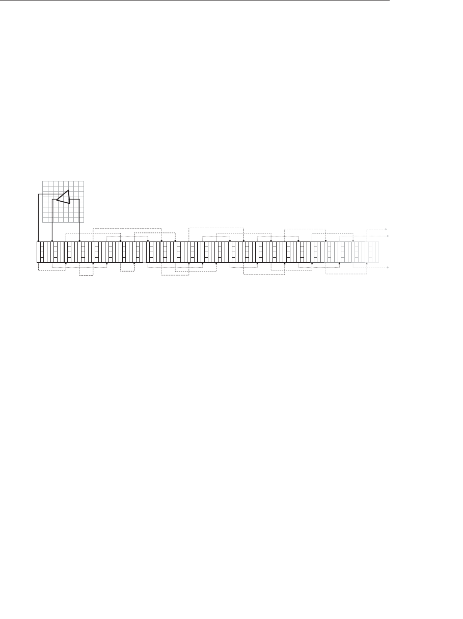
ptg9898810
the same buffer image, the resulting linked lists are interleaved and each
pixel has its own head pointer, stored in a 2D image that is the size of the
framebuffer. The head pointer is updated using atomic operations---items
are always appended at the head of the image and use of an atomic
exchange operation ensures that multiple shader invocations attempting
to append to the same list will not corrupt each other’s results.
A simplified diagram of the data structures used by this algorithm is shown
in Figure 11.6. Each element in the linked list is represented by a uvec4
vector and the fields used for different purposes. As uvec4 is a native type
in GLSL and the OpenGL API, no special handling is required to interpret
it as a structure.
-1 -1
-1 -1
-1 -1
-1 -1
-1 -1
-1 -1
-1 -1
-1 1
-1 -1
-1 -1
-1 -1
-1 -1
0-1
2-1
-1 -1
-1 -1
-1 -1
-1 -1
-1 -1
-1 -1
-1 -1
-1 -1
-1 -1
-1 -1
-1 -1
-1 -1
-1 -1
-1 -1
-1 -1
-1 -1
-1 -1
-1 -1
R
NEXT
DEPTH
UNUSED
A
BG
R
NEXT
DEPTH
UNUSED
A
BG
R
NEXT
DEPTH
UNUSED
A
BG
R
NEXT
DEPTH
UNUSED
A
BG
R
NEXT
DEPTH
UNUSED
A
BG
R
NEXT
DEPTH
UNUSED
A
BG
R
NEXT
DEPTH
UNUSED
A
BG
R
NEXT
DEPTH
UNUSED
A
BG
R
NEXT
DEPTH
UNUSED
A
BG
R
NEXT
DEPTH
UNUSED
A
BG
R
NEXT
DEPTH
UNUSED
A
BG
R
NEXT
DEPTH
UNUSED
A
BG
R
NEXT
DEPTH
UNUSED
A
BG
R
NEXT
DEPTH
UNUSED
A
BG
R
NEXT
DEPTH
UNUSED
A
BG
R
NEXT
DEPTH
UNUSED
A
BG
R
NEXT
DEPTH
UNUSED
A
BG
R
NEXT
DEPTH
UNUSED
A
BG
R
NEXT
DEPTH
UNUSED
A
BG
R
NEXT
DEPTH
UNUSED
A
BG
R
NEXT
DEPTH
UNUSED
A
BG
R
NEXT
DEPTH
UNUSED
A
BG
R
NEXT
DEPTH
UNUSED
A
BG
R
NEXT
DEPTH
UNUSED
A
BG
R
NEXT
DEPTH
UNUSED
A
BG
Figure 11.6 Data structures used for order-independent transparency
In Figure 11.6, the first field (.x) of each record is used to store the next
pointer (the index of the next item in the linked list). The second field (.y)
is used to store the color of the fragment. It is stored in a single uint
component by packing the red, green, blue, and alpha channels together
in the shader as will be shown shortly. The third component (.z) is used to
store the depth of the fragment that will later be used to sort the list. As
depth is a floating-point vlaue, but we’re using integer components here,
we’ll cast the floating-point value to an unsigned integer and store its
bit-wise representation in the vector directly. This is a completely
reversible operation and will provide the exact depth value during the
sorting stage. The final component (.w) is not used currently, but will be
used during an enhancement to the algorithm shown later.
Once the linked list data structures have been built, a second pass is
performed over the entire framebuffer. In this pass, the fragment shader
traverses the linked list corresponding to its pixel and sorts all of the
fragments in the list in order of depth. Once the fragments are in depth
order, they can be blended together from back to front using any desired
function.
610 Chapter 11: Memory

ptg9898810
To summarize, what is required for this algorithm to function are
•A buffer large enough to hold all of the fragments that might be
rasterized.
•An atomic counter to serve as an allocator for records within the
linked list.
•A 2D image the size of the framebuffer that will be used to store the
head pointer for each pixel’s linked list of fragments.
Initialization
Before any rendering can occur, we need to create the resources that our
algorithm will use and initialize them to known values. In particular, we
need to create our atomic counter that will be used to allocate items from
our buffer object to store our linked list, create a 2D image the size of the
framebuffer, and create a one-dimensional buffer object that is large
enough to store all of the transparent fragments. Note that this doesn’t
have to be large enough to store the number of pixels on the screen times
the maximum expected overdraw as most pixels will have no visible
transparent fragments or perhaps very few transparent fragments. The
code shown in Example 11.24 creates the required resources but does not
initialize them because they need to be initialized before each frame
anyway.
Example 11.24 Initializing for Order-Independent Transparency
// This is the maximum supported framebuffer width and height. We
// could support higher resolutions, but this is reasonable for
// this application
#define MAX_FRAMEBUFFER_WIDTH 2048
#define MAX_FRAMEBUFFER_HEIGHT 2048
// Local variables
GLuint *data;
size_t total_pixels = MAX_FRAMEBUFFER_WIDTH *
MAX_FRAMEBUFFER_HEIGHT;
// Create the 2D image that will be used to store the head pointers
// for the per-pixel linked lists.
GLuint head_pointer_texture;
glGenTextures(1, &head_pointer_texture);
glBindTexture(GL_TEXTURE_2D, head_pointer_texture);
glTexImage2D(GL_TEXTURE_2D, 0, // 2D texture, level 0
GL_R32UI, // 32-bit GLuint per texel
MAX_FRAMEBUFFER_WIDTH, // Width
MAX_FRAMEBUFFER_HEIGHT, // Height
Example 611

ptg9898810
0, // No border
GL_RED_INTEGER, // Single channel
GL_UNSIGNED_INT, // Unsigned int
NULL); // No data... yet
// We will need to re-initialize the head pointer each frame. The
// easiest way to do this is probably to copy from a PBO. We’ll
// create that here...
GLuint head_pointer_initializer;
glGenBuffers(1, &head_pointer_initializer);
glBindBuffer(GL_PIXEL_UNPACK_BUFFER, head_pointer_initializer);
glBufferData(GL_PIXEL_UNPACK_BUFFER,
total_pixels *
sizeof(GLuint), // 1 uint per pixel
NULL, // No data - we’ll map it
GL_STATIC_DRAW); // Never going to change
data = (GLuint)glMapBuffer(GL_PIXEL_UNPACK_BUFFER, GL_WRITE_ONLY);
// 0xFF will be our "end of list" marker.
memset(data, 0xFF, total_pixels *sizeof(GLuint));
glUnmapBuffer(GL_PIXEL_UNPACK_BUFFER);
// Next, create our atomic counter buffer to back our atomic
// counter. We only need one counter, so a small buffer will
// suffice.
GLuint atomic_counter_buffer;
glGenBuffers(1, &atomic_counter_buffer);
glBindBuffer(GL_ATOMIC_COUNTER_BUFFER, atomic_counter_buffer);
glBufferData(GL_ATOMIC_COUNTER_BUFFER, // Allocate buffer...
sizeof(GLuint), NULL, // with space for 1 GLuint
GL_DYNAMIC_COPY); // written to by GPU
// Finally, our large, one-dimensional buffer for fragment storage.
// We’re going to allocate enough storage for 2 fragments for every
// pixel on the screen. Note again that this is average overdraw and
// should be sufficient and allow a few pixels to include tens of
// fragments so long as the average remains low.
GLuint fragment_storage_buffer;
glGenBuffers(1, &fragment_storage_buffer);
glBindBuffer(GL_TEXTURE_BUFFER, fragment_storage_buffer);
glBufferData(GL_TEXTURE_BUFFER,
2*total_pixels *// Twice the maximum number of pixels
sizeof(vec4), // Times vec4
NULL, // No data
GL_DYNAMIC_COPY); // Updated often by GPU
Rendering
For each frame, we will render the transparent objects in the scene using a
fragment shader that determines the color and opacity for each fragment
and then appends that information, along with the fragment’s depth into
the linked list data structures. Before each frame’s transparent objects are
612 Chapter 11: Memory

ptg9898810
drawn, the head pointer and atomic counter buffers must be initialized to
known values; otherwise, our shader will continue to append to the
structures created in the previous frame. The code for this is given in
Example 11.25.
Example 11.25 Per-Frame Reset for Order-Independent Transparency
// First, clear the head-pointer 2D image with known values. Bind it
// to the GL_TEXTURE_2D target and then initialize it from a PBO that
// has been pre-loaded with the value 0x00
glBindBuffer(GL_PIXEL_UNPACK_BUFFER, head_pointer_initializer);
glBindTexture(GL_TEXTURE_2D, head_pointer_texture);
glTexImage2D(GL_TEXTURE_2D, 0, // 2D texture, first level
GL_R32UI, // 32-bit GLuint per texel
MAX_FRAMEBUFFER_WIDTH, // Width
MAX_FRAMEBUFFER_HEIGHT, // Height
0, // No border
GL_UNSIGNED_INT, // Unsigned int
NULL); // Consume data from PBO
// Now bind it to the image unit that will be used for
// read-write access
glBindImageTexture(0, // Image unit 0
head_pointer_texture,
GL_FALSE, 0, // Not layered
GL_READ_WRITE, // Read and write access
GL_R32UI); // 32-bit GLuint per pixel
// Now bind the atomic counter buffer ready for use and reset the
// counter to zero
glBindBufferBase(GL_ATOMIC_COUNTER_BUFFER, // Atomic counter...
0, // Binding point 0
atomic_counter_buffer);
// Note that this also binds the buffer to the generic buffer
// binding point, so we can use that to initialize the buffer.
const GLuint zero = 0;
glBufferSubData(GL_ATOMIC_COUNTER_BUFFER, 0, sizeof(zero), &zero);
Once the code in Example 11.25 has executed, the head pointer image
contains the value 0x00 in all texels and the buffer that stores our atomic
counter contains zero, which resets the atomic counter to zero. Note that it
is not necessary to clear the one-dimensional buffer that is used to store
the linked lists as these lists will be completely rebuilt during each frame.
Now we are ready to render the frame. First, we render all nontransparent
objects as there is no reason to append their fragments into the per-pixel
fragment lists. Next, we render all of the transparent objects in an arbitrary
order (this is the point of the algorithm, after all). The transparent objects
are rendered using the fragment shader shown in Example 11.26.
Example 613

ptg9898810
Example 11.26 Appending Fragments to Linked List for Later Sorting
#version 420 core
// Turn on early fragment testing
layout (early_fragment_tests) in;
// This is the atomic counter used to allocate items in the
// linked list
layout (binding = 0, offset = 0) uniform atomic_uint index_counter;
// Linked list 1D buffer
layout (binding = 0, rgba32ui)uniform imageBuffer list_buffer;
// Head pointer 2D buffer
layout (binding = 1, r32ui)uniform imageRect head_pointer_image;
void main(void)
{
// First, shade the fragment - how is not important right now.
vec4 frag_color = shadeFragment();
// Allocate an index in the linked list buffer. Remember,
// atomicCounterIncrement increments the atomic counter and
// returns the _old_ value of the counter. Thus, the first
// fragment to execute this code will receive the value 0, the
// next will receive 1, and so on.
uint new = atomicCounterIncrement(index_counter);
// Now, insert the fragment into the list. To do this, we
// atomically exchange our newly allocated index with the
// current content of the head pointer image. Remember
// imageAtomicExchange, writes our new value to memory and
// returns the _old_ value.
uint old_head = imageAtomicExchange(head_pointer_image,
ivec2(gl_FragCoord.xy),
index);
// Before this code executed, we had:
// head_pointer_image(x,y) -> old_item
// Now we have:
// head_pointer_image(x,y) -> new_item
// _and_
// old_head -> old_item
// Now assemble the fragment into the buffer.
// This will be the item...
uvec4 item;
// item.x = next pointer
item.x = old_head;
// Now we have
// head_pointer_image(x,y) -> new_item (.x) -> old_item.
614 Chapter 11: Memory

ptg9898810
// item.y = color
item.y = packUnorm4x8(frag_color);
// item.z = depth (gl_FragCoord.z)
item.z = floatBitsToUint(gl_FragCoord.z);
// item.w = unused (so far...)
item.w = 0;
// Write the data into the buffer at the right location
imageStore(list_buffer, index, item);
}
The shader shown in Example 11.26 appends fragments into the per-pixel
linked list using atomics counters, general purpose atomic operations, bit
packing, and bit casting. First, the global atomic counter is incremented in
order to allocate a record in the one-dimensional linked-list buffer. This
can be used as an allocator because the atomic increment operation
doesn’t necessarily return (n + 1), but rather a new, unique value that is
greater than (n). This is shown in Figure 11.7 (a). In Figure 11.7 (a), the
head pointer contains the index of the first item in the linked list and the
index of the newly allocated item is stored in the new variable.
Next, this value is inserted into the head pointer texture and the previous
value of head retrieved. This is performed in a single step by using an
atomic exchange operation. This is shown in Figure 11.7 (b), where the
head of the list is now pointing at the newly allocated item, and old_head
contains the previous value of the head pointer---the index of the first item
in the list. At this stage, the list is actually broken as the head pointer
indexes an item without a valid next pointer. However, this doesn’t matter
because the list is never traversed as it is built.
Finally, the old value of the head pointer is used as the new next value for
the inserted item. This means that the head pointer now refers to the item
we allocated using the atomic counter, and the next pointer for that item
points to what was previously the first item in the list. This is achieved by
simply writing the old value of the head pointer into the next field of the
new item as shown in Figure 11.7 (c). In all parts of Figure 11.7, the new
item is marked with a gray crosshatch pattern.
Example 615
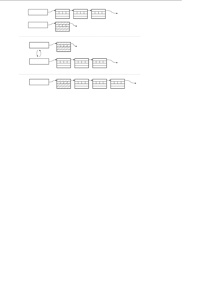
ptg9898810
HEAD X
NEW X
R
NEXT
DEPTH
UNUSED
A
B
GR
NEXT
DEPTH
UNUSED
A
BG
R
NEXT
DEPTH
UNUSED
A
BG
RRRR
NEXT
DEPTH
UNUSED
A
BG
(a)
X
OLD_HEAD
HEAD X
R
NEXT
DEPTH
UNUSED
A
B
GR
NEXT
DEPTH
UNUSED
A
B
G
R
NEXT
DEPTH
UNUSED
A
BG
RRRR
NEXT
DEPTH
UNUSED
ABG
(b)
HEAD R
NEXT
DEPTH
UNUSED
A
BG X
R
NEXT
DEPTH
UNUSED
A
BG R
NEXT
DEPTH
UNUSED
ABG
RRRR
OLD_HEAD
DEPTH
UNUSED
A
BG
(c)
Figure 11.7 Inserting an item into the per-pixel linked lists
The end result is set of unsorted lists of fragment records, each containing
a color, depth, and link to the next item in the list, with one list per pixel.
Notice that all of the data that might be shared between shader
invocations---the atomic counter and the head pointer---is only ever
modified by using atomic operations. We never actually traversed the
linked list during building as we only prepended items to the head. We are
now ready to consume this data by sorting the fragments in order of depth
and blending them together to form the final fragment color.
Finally, notice that the shader in Example 11.26 turns on early fragment
testing using the early_fragment_tests layout qualifier. This is because
we wish to ensure that fragments that are obscured by previously rendered
opaque geometry are not added to the linked lists. As the transparent
geometry is rendered with depth testing on but the shader has side effects
(writing into the linked list), OpenGL would normally perform the depth
test after it has executed by default. Using the early_fragment_tests
input layout qualifier instructs OpenGL to perform depth testing before the
shader runs and to not execute it if the fragment fails the test. This ensures
that the shader will not be executed for obscured fragments and those
fragments will not be added to the lists.
Sorting and Blending
Once the data structures have been built, the per-pixel linked lists are
essentially a compressed representation of the scene. The next step is to
616 Chapter 11: Memory

ptg9898810
walk the per-pixel lists and blend all of the fragments together in order to
build the final output colors. To do this, we render a full-screen quad using
a fragment shader that will read from the list corresponding to its output
pixel, sort all of the fragments into order, and then perform the blending
operations of our choice. Because the number of fragments per-pixel is
expected to be low, a simple sorting algorithm can be used.
In this pass, we again take our head pointer image and our linked-list
buffer and access them from the shader. However, as we are only going to
be reading from them, we can bind them as a regular 2D texture and as a
texture buffer object (TBO), respectively. This gives additional hints to the
implementation that it can access the image in a read-only manner
without worrying about coherency or caching issues. The atomic counter
used to allocate list items is not required in the blending pass as we are not
going to allocate more items on the list. The main body of the sorting and
blending shader is shown in Example 11.27.
Example 11.27 Main Body of Final Order-Independent Sorting
Fragment Shader
#version 420 core
// Head pointer 2D buffer
uniform sampler2D head_pointer_image;
// Linked list 1D buffer
uniform samplerBuffer list_buffer;
#define MAX_FRAGMENTS 15
// Small buffer to hold all of the fragments corresponding
// to this pixel
uvec4 fragments[MAX_FRAGMENTS];
layout (location = 0) out vec4 output_color;
void main(void)
{
int frag_count;
// Traverse the list and build an array of fragments
frag_count = build_local_fragment_list();
// Sort the array in depth order
sort_fragment_list(frag_count);
// Blend the sorted fragments together to compute the final
Example 617

ptg9898810
// output color
output_color = calculate_final_color(frag_count);
}
Example 11.27 makes use of three functions. First,
build_local_fragment_list traverses the linked list of fragments
corresponding to the current pixel and places all of the fragments into the
fragments[] array. The code for this function is shown in Example 11.28.
Notice that the size of the per-pixel fragment array is defined as 15 here,
even though the buffer allocated in Example 11.24 is only twice the
number of pixels in the framebuffer. This is possible because the fragment
lists only needs to be large enough to store the average number of
fragments per-pixel, but the maximum overdraw supported can be much
larger.
Example 11.28 Traversing Linked-Lists in a Fragment Shader
// Traverse the linked list, place all of the fragments into the
// fragments[] array and return the number of fragments retrieved
// from the list.
int build_local_fragment_list(void)
{
uint current;
int frag_count = 0;
// Get the initial head pointer from the header-pointer image
current = texelFetch(head_pointer_image,
ivec2(gl_FragCoord.xy), 0);
// While we haven’t reached the end of the list or exhausted
// the storage available in fragments[]...
while (current != 0xFFFFFFFF && frag_count < MAX_FRAGMENTS)
{
// Read an item from the linked list
item = texelFetch(list_buffer, current);
// item.x contains the "next" pointer - update current
current = item.x;
// Store the fragment in the array
uvec4 fragments[frag_count] = item;
// Update the fragment count
frag_count++;
}
// Done - return the fragment count
return frag_count;
}
618 Chapter 11: Memory

ptg9898810
After the local array of fragments has been built, it is sorted in order of
depth using the sort_fragment_list function shown in Example 11.29.
This function implements a simple bubble-sort algorithm. While this is a
very simple algorithm and is not well suited for sorting large amounts of
data, because the number of items is very low, the cost of the function is
still small, and the algorithm suffices.
Example 11.29 Sorting Fragments into Depth Order for OIT
// Simple bubble-sort for sorting the fragments[] array
void sort_fragment_list(int frag_count)
{
int i;
int j;
for (i = 0; i < frag_count; i++)
{
for (j = i + 1; j < frag_count; j++)
{
// The depth of each fragment is bit-encoded into the
// .z channel of the fragment array. Unpack it here.
float depth_i = uintBitsToFloat(fragments[i].z);
float depth_j = uintBitsToFloat(fragments[j].z);
// Compare depth and if the comparison fails...
if (depth_i > depth_j)
{
// Swap the fragments in the array
uvec4 temp = fragments[i];
fragments[i] = fragments[j];
fragments[j] = temp;
}
}
}
}
Once the fragments in the fragments[] array have been sorted into
depth order, we can traverse the array and blend the fragments together
using a blending operation of our choice. This is implemented in the
calculate_final_color function that is shown in Example 11.30.
Example 11.30 Blending Sorted Fragments for OIT
// Simple alpha blending function -- we could replace
// this with anything...
vec4 blend(vec4 current_color, vec4 new_color)
{
return mix(current_color, new_color, new_color.a);
}
Example 619

ptg9898810
// Function for calculating the final output color. Walks the
// fragments[] array and blends each pixel on top of each other
vec4 calculate_final_color(int frag_count)
{
// Initialize the final color output
vec4 final_color = vec4(0.0);
// For each fragment in the array...
for (i = 0; i < frag_count; i++)
{
// The color is stored packed into the .y channel of the
// fragment vector. Unpack it here.
vec4 frag_color = unpackUnorm4x8(fragments[i].y);
// Now call the blending function.
final_color = blend(final_color, frag_color);
}
// Done -- return the final color.
return final_color;
}
The blend function shown in Example 11.30 simply uses the mix function
to implement basic alpha blending. This is equivalent to using
fixed-function OpenGL blending with the blend equation set to
GL_FUNC_ADD and the blend functions set to GL_SRC_ALPHA and
GL_ONE_MINUS_SRC_ALPHA for source and destination factors,
respectively.
Results
The results of rendering with this algorithm are shown in Figure 11.8. The
image on the left is produced using fixed-function OpenGL blending. As
can be seen, the image does not look correct in all areas. This is because
geometry is rendered in order of submission rather than in order of depth.
Because the blending equations used are not commutative and are
therefore sensitive to order, they produce different results depending on
the submission order of the geometry. Contrast this to the result shown on
the right of Figure 11.8. This is rendered with the order-independent
algorithm described in this example. The result is correct in all areas.
620 Chapter 11: Memory


ptg9898810
Chapter 12
Compute Shaders
Chapter Objectives
After reading this chapter, you’ll be able to do the following:
•Create, compile, and link compute shaders.
•Launch compute shaders, which operate on buffers, images, and
counters.
•Allow compute shader invocations to communicate with each other
and to synchronize their execution.
623

ptg9898810
Compute shaders run in a completely separate stage of the GPU than the
rest of the graphics pipeline. They allow an application to make use of the
power of the GPU for general purpose work that may or may not be related
to graphics. Compute shaders have access to many of the same resources as
graphics shaders, but have more control over their application flow and
how they execute. This chapter introduces the compute shader and
describes its use.
This chapter has the following major sections:
•‘‘Overview’’ gives a brief introduction to compute shaders and outlines
their general operation.
•The organization and detailed working of compute shaders with regards
to the graphics processor is given in ‘‘Workgroups and Dispatch’’.
•Next, methods for communicating between the individual invocations
of a compute shader are presented in ‘‘Communication and
Synchronization’’, along with the synchronization mechanisms that
can be used to control the flow of data between those invocations.
•A few examples of compute shaders are shown, including both
graphics and nongraphics work are given in ‘‘Examples’’.
Overview
The graphics processor is an immensely powerful device capable of
performing trillions of calculations each second. Over the years, it has been
developed to crunch the huge amount of math operations required to
render real-time graphics. However, it is possible to use the computational
power of the processor for tasks that are not considered graphics, or that
don’t fit neatly into the relatively fixed graphical pipeline. To enable this
type of use, OpenGL includes a special shader stage called the compute
shader. The compute shader can be considered a special, single-stage
pipeline that has no fixed input or output. Instead, all automatic input is
through a handful of built-in variables. If additional input is needed, those
fixed-function inputs may be used to control access to textures and buffers.
All visible side effects are through image stores, atomics, and access to
atomic counters. While at first this seems like it would be quite limiting, it
includes general read and write of memory, and this level of flexibility and
lack of graphical idioms open up a wide range of applications for compute
shaders.
Compute shaders in OpenGL are very similar to any other shader stage.
They are created using the glCreateShader() function, compiled using
glCompileShader(), and attached to program objects using
624 Chapter 12: Compute Shaders

ptg9898810
glAttachShader(). These programs are linked as normal by using
glLinkProgram(). Compute shaders are written in GLSL and in general,
any functionality accessible to normal graphics shaders (for example,
vertex, geometry or fragment shaders) is available. Obviously, this excludes
graphics pipeline functionality such as the geometry shaders’
EmitVertex() or EndPrimitive(), or to the similarly pipeline-specific
built-in variables. On the other hand, several built-in functions and
variables are available to a compute shader that are available nowhere else
in the OpenGL pipeline.
Workgroups and Dispatch
Just as the graphics shaders fit into the pipeline at specific points and
operate on graphics-specific elements, compute shaders effectively fit into
the (single-stage) compute pipeline and operate on compute-specific
elements. In this analogy, vertex shaders execute per vertex, geometry
shaders execute per primitive and fragment shaders execute per fragment.
Performance of graphics hardware is obtained through parallelism, which
in turn is achieved through the very large number of vertices, primitives, or
fragments, respectively, passing through each stage of the pipeline. In the
context of compute shaders, this parallelism is more explicit, with work
being launched in groups known as workgroups. Workgroups have a local
neighborhood known as a local workgroup, and these are again grouped to
form a global workgroup as the result of one of the dispatch commands.
The compute shader is then executed once for each element of each local
workgroup within the global workgroup. Each element of the workgroup is
known as a work item and is processed by an invocation. The invocations of
the compute shader can communicate with each other via variables and
memory, and can perform synchronization operations to keep their work
coherent. Figure 12.1 shows a schematic of this work layout. In this
simplified example, the global workgroup consists of 16 local workgroups,
and each local workgroup consists of 16 invocations, arranged in a 4 ×4
grid. Each invocation has a local index that is a two-dimensional vector.
While Figure 12.1 visualizes the global and local workgroups as two-
dimensional entities, they are in fact in three dimensions. To issue work
that is logically one- or two-dimensional, we simply make a
three-dimensional work size where the extent in one or two of the
dimensions is of size one. The invocations of a compute shader are
essentially independent and may run in parallel on some implementations
of OpenGL. In practice, most OpenGL implementations will group subsets
of the work together and run it in lockstep, grouping yet more of these
subsets together to form the local workgroups. The size of a local
Workgroups and Dispatch 625
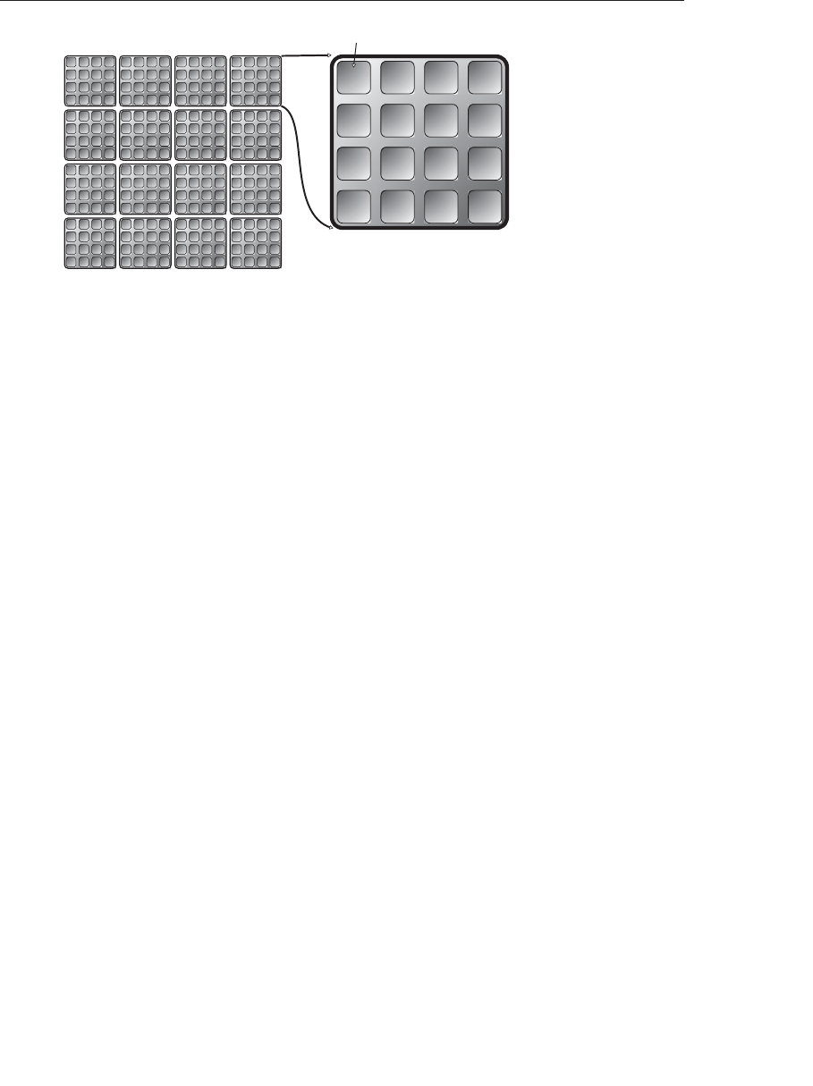
ptg9898810
INV. 0,0 INV. 0,1 INV. 0,2 INV. 0,3
INV. 1,0 INV. 1,1 INV. 1,2 INV. 1,3
INV. 2,0 INV. 2,1 INV. 2,2 INV. 2,3
INV. 3,0 INV. 3,1 INV. 3,2 INV. 3,3
{
Global Work Group
Local Work Group
Invocation
Figure 12.1 Schematic of a compute workload
workgroup is defined in the compute shader source code using an input
layout qualifier. The global workgroup size is measured as an integer
multiple of the local workgroup size. As the compute shader executes, it is
provided with its location within the local workgroup, the size of the
workgroup, and the location of its local workgroup within the global
workgroup through built-in variables. There are further variables available
that are derived from these providing the location of the invocation
within the global workgroup, among other things. The shader may use
these variables to determine which elements of the computation it should
work on and also can know its neighbors within the workgroup, which
facilitates some amount of data sharing.
The input layout qualifiers that are used in the compute shader to declare
the local workgroup size are local_size_x,local_size_y, and
local_size_z. The defaults for these are all one, and so omitting
local_size_z, for example, would create an N×Mtwo-dimensional
workgroup size. An example of declaring a shader with a local workgroup
size of 16 ×16 is shown in Example 12.1.
Example 12.1 Simple Local Workgroup Declaration
#version 430 core
// Input layout qualifier declaring a 16 x 16 (x 1) local
// workgroup size
layout (local_size_x = 16, local_size_y = 16) in;
void main(void)
{// Do nothing.
}
626 Chapter 12: Compute Shaders

ptg9898810
Although the simple shader of Example 12.1 does nothing, it is a valid
compute shader and will compile, link, and execute on an OpenGL
implementation. To create a compute shader, simply call glCreateShader()
with type set to GL_COMPUTE_SHADER, set the shader’s source code with
glShaderSource() and compile it as normal. Then, attach the shader to a
program and call glLinkProgram(). This creates the executable for the
compute shader stage that will operate on the work items. A complete
example of creating and linking a compute program1is shown in
Example 12.2.
Example 12.2 Creating, Compiling, and Linking a Compute Shader
GLuint shader, program;
static const GLchar*source[] =
{
"#version 430 core\n"
"\n"
"// Input layout qualifier declaring a 16 x 16 (x 1) local\n"
"// workgroup size\n"
"layout (local_size_x = 16, local_size_y = 16) in;\n"
"\n"
"void main(void)\n"
"{\n"
" // Do nothing.\n"
"}\n"
};
shader = glCreateShader(GL_COMPUTE_SHADER);
glShaderSource(shader, 1, source, NULL);
glCompileShader(shader);
program = glCreateProgram();
glAttachShader(program, shader);
glLinkProgram(program);
Once we have created and linked a compute shader as shown in Example
12.2, we can make the program current using glUseProgram() and then
dispatch workgroups into the compute pipeline using the function
glDispatchCompute(), whose prototype is as follows:
1. We use the term compute program to refer to a linked program object containing a compute
shader.
Workgroups and Dispatch 627

ptg9898810
void glDispatchCompute(GLuint num_groups_x,
GLuint num_groups_y,
GLuint num_groups_z);
Dispatch compute workgroups in three dimensions. num_groups_x,
num_groups_y, and num_groups_z specify the number of workgroups to
launch in the X, Y, and Z dimensions, respectively. Each parameter must
be greater than zero and less than or equal to the corresponding element
of the implementation-dependent constant vector
GL_MAX_COMPUTE_WORK_GROUP_SIZE.
When you call glDispatchCompute(), OpenGL will create a
three-dimensional array of local workgroups whose size is num_groups_x by
num_groups_y by num_groups_z groups. Remember, the size of the
workgroup in one or more of these dimensions may be one, as may be any
of the parameters to glDispatchCompute(). Thus the total number of
invocations of the compute shader will be the size of this array times the
size of the local workgroup declared in the shader code. As you can see, this
can produce an extremely large amount of work for the graphics processor
and it is relatively easy to achieve parallelism using compute shaders.
As glDrawArraysIndirect() is to glDrawArrays(), so
glDispatchComputeIndirect() is to glDispatchCompute().
glDispatchComputeIndirect() launches compute work using parameters
stored in a buffer object. The buffer object is bound to the
GL_DISPATCH_INDIRECT_BUFFER binding point and the parameters
stored in the buffer consist of three unsigned integers, tightly packed
together. Those three unsigned integers are equivalent to the parameters to
glDispatchCompute(). The prototype for glDispatchComputeIndirect()
is as follows:
void glDispatchComputeIndirect(GLintptr indirect);
Dispatch compute workgroups in three dimensions using parameters
stored in a buffer object. indirect is the offset, in basic machine units, into
the buffer’s data store at which the parameters are located. The
parameters in the buffer at this offset are three, tightly packed unsigned
integers representing the number of local workgroups to be dispatch.
These unsigned integers are equivalent to the num_groups_x,
num_groups_y, and num_groups_z parameters to glDispatchCompute().
Each parameter must be greater than zero and less than or equal to the
corresponding element of the implementation-dependent constant
vector GL_MAX_COMPUTE_WORK_GROUP_SIZE.
628 Chapter 12: Compute Shaders

ptg9898810
The data in the buffer bound to GL_DISPATCH_INDIRECT_BUFFER
binding could come from anywhere---including another compute shader.
As such, the graphics processor can be made to feed work to itself by
writing the parameters for a dispatch (or draws) into a buffer object.
Example 12.3 shows an example of dispatching compute workloads using
glDispatchComputeIndirect().
Example 12.3 Dispatching Compute Workloads
// program is a successfully linked program object containing
// a compute shader executable
GLuint program = ...;
// Activate the program object
glUseProgram(program);
// Create a buffer, bind it to the DISPATCH_INDIRECT_BUFFER
// binding point and fill it with some data.
glGenBuffers(1, &dispatch_buffer);
glBindBuffer(GL_DISPATCH_INDIRECT_BUFFER, dispatch_buffer);
static const struct
{
GLuint num_groups_x;
GLuint num_groups_y;
GLuint num_groups_z;
} dispatch_params = { 16, 16, 1 };
glBufferData(GL_DISPATCH_INDIRECT_BUFFER,
sizeof(dispatch_params),
&dispatch_params,
GL_STATIC_DRAW);
// Dispatch the compute shader using the parameters stored
// in the buffer object
glDispatchComputeIndirect(0);
Notice how in Example 12.3 we simply use glUseProgram() to set the
current program object to the compute program. Aside from having no
access to the fixed-function graphics pipeline (such as the rasterizer or
framebuffer), compute shaders and the programs that they are linked into
are completely normal, first-class shader and program objects. This means
that you can use glGetProgramiv() to query their properties (such as
active uniform or storage blocks) and can access uniforms as normal. Of
course, compute shaders also have access to almost all of the resources that
other types shaders have, including images, samplers, buffers, atomic
counters, and uniform blocks.
Compute shaders and their linked programs also have several compute-
specific properties. For example, to retrieve the local workgroup size of a
Workgroups and Dispatch 629

ptg9898810
compute shader (which would have been set using a layout qualifier in the
source of the compute shader), call glGetProgramiv() with pname set to
GL_MAX_COMPUTE_WORK_GROUP_SIZE and param set to the address of
an array of three unsigned integers. The three elements of the array will be
filled with the size of the local workgroup size in the X, Y, and Z
dimensions, in that order.
Knowing Where You Are
Once your compute shader is executing, it likely has the responsibility to
set the value of one or more elements of some output array (such as an
image or an array of atomic counters), or to read data from a specific
location in an input array. To do this, you will need to know where in the
local workgroup you are and where that workgroup is within the larger
global workgroup. For these purposes, OpenGL provides several built-in
variables to compute shaders. These built-in variables are implicitly
declared as shown in Example 12.4.
Example 12.4 Declaration of Compute Shader Built-in Variables
const uvec3 gl_WorkGroupSize;
in uvec3 gl_NumWorkGroups;
in uvec3 gl_LocalInvocationID;
in uvec3 gl_WorkGroupID;
in uvec3 gl_GlobalInvocationID;
in uint gl_LocalInvocationIndex;
The compute shader built-in variables have the following definitions:
•gl_WorkGroupSize is a constant that stores the size of the local
workgroup as declared by the local_size_x,local_size_y and
local_size_z layout qualifiers in the shader. Replicating this
information here serves two purposes; first, it allows the workgroup
size to be referred to multiple times in the shader without relying on
the preprocessor and second, it allows multidimensional workgroup
size to be treated as a vector without having to construct it explicitly.
•gl_NumWorkGroups is a vector that contains the parameters that were
passed to glDispatchCompute() (num_groups_x,num_groups_y, and
num_groups_z). This allows the shader to know the extent of the global
workgroup that it is part of. Besides being more convenient than
needing to set the values of uniforms by hand, some OpenGL
implementations may have a very efficient path for setting these
constants.
630 Chapter 12: Compute Shaders

ptg9898810
•gl_LocalInvocationID is the location of the current invocation of a
compute shader within the local workgroup. It will range from
uvec3(0) to gl_WorkGroupSize - uvec3(1).
•gl_WorkGroupID is the location of the current local workgroup within
the larger global workgroup. This variable will range from uvec3(0) to
gl_NumWorkGroups - uvec3(1).
•gl_GlobalInvocationID is derived from gl_LocalInvocationID,
gl_WorkGroupSize, and gl_WorkGroupID. Its exact value is equal to
gl_WorkGroupID *gl_WorkGroupSize + gl_LocalInvocationID
and as such, it is effectively the three-dimensional index of the current
invocation within the global workgroup.
•gl_LocalInvocationIndex is a flattened form of
gl_LocalInvocationID. It is equal to gl_LocalInvocationID.z *
gl_WorkGroupSize.x *gl_WorkGroupSize.y +
gl_LocalInvocationID.y *gl_WorkGroupSize.x +
gl_LocalInvocationID.x. It can be used to index into
one-dimensional arrays that represent two- or three-dimensional data.
Given that we now know where we are within both the local workgroup
and the global workgroup, we can use this information to operate on data.
Taking the example of Example 12.5 and adding an image variable allows
us to write into the image at a location derived from the coordinate of the
invocation within the global workgroup and update it from our compute
shader. This modified shader is shown in Example 12.5.
Example 12.5 Operating on Data
#version 430 core
layout (local_size_x = 32, local_size_y = 16) in;
// An image to store data into.
layout (rg32f) uniform image2D data;
void main(void)
{// Store the local invocation ID into the image.
imageStore(data,
ivec2(gl_GlobalInvocationID.xy),
vec4(vec2(gl_LocalInvocationID.xy) /
vec2(gl_WorkGroupSize.xy),
0.0, 0.0));
}
The shader shown in Example 12.5 simply takes the local invocation
index, normalizes it to the local workgroup size, and stores the result into
Workgroups and Dispatch 631
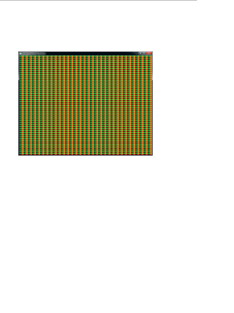
ptg9898810
the data image at the location given by the global invocation ID. The
resulting image shows the relationship between the global and local
invocation IDs and clearly shows the rectangular local workgroup size
specified in the compute shader (in this case, 32 ×16 work items). The
resulting image is shown in Figure 12.2.
Figure 12.2 Relationship of global and local invocation ID
To generate the image of Figure 12.2, after being written by the compute
shader, the texture is simply rendered to a full screen triangle fan.
Communication and Synchronization
When you call glDispatchCompute() (or glDispatchComputeIndirect()),
a potentially huge amount of work is sent to the graphics processor. The
graphics processor will run that work in parallel if it can, and the
invocations that execute the compute shader can be considered to be a
team trying to accomplish a task. Teamwork is facilitated greatly by
communication and so, while the order of execution and level of
parallelism is not defined by OpenGL, some level of cooperation between
the invocations is enabled by allowing them to communicate via shared
variables. Furthermore, it is possible to sync up all the invocations in the
local workgroup so that they reach the same part of your shader at the
same time.
632 Chapter 12: Compute Shaders

ptg9898810
Communication
The shared keyword is used to declare variables in shaders in a similar
manner to other keywords such as uniform,in, or out. Some example
declarations using the shared keyword are shown in Example 12.6.
Example 12.6 Example of Shared Variable Declarations
// A single shared unsigned integer;
shared uint foo;
// A shared array of vectors
shared vec4 bar[128];
// A shared block of data
shared struct baz_struct
{vec4 a_vector;
int an_integer;
ivec2 an_array_of_integers[27];
} baz[42];
When a variable is declared as shared, that means it will be kept in
storage that is visible to all of the compute shader invocations in the same
local workgroup. When one invocation of the compute shader writes to a
shared variable, then the data it wrote will eventually become visible to
other invocations of that shader within the same local workgroup. We say
eventually because the relative order of execution of compute shader
invocations is not defined---even within the same local workgroup.
Therefore, one shader invocation may write to a shared variable long
before another invocation reads from that variable, or even long after the
other invocation has read from that variable. To ensure that you get the
results you expect, you need to include some synchronization primitives
in your code. These are covered in detail in the next section.
The performance of accesses to shared variables is often significantly
better than accesses to images or to shader storage buffers (i.e., main
memory). As shared memory is local to a shader processor and may be
duplicated throughout the device, access to shared variables can be even
faster than hitting the cache. For this reason, it is recommended that if
your shader performs more than a few accesses to a region of memory, and
especially if multiple shader invocations will access the same memory
locations, that you first copy that memory into some shared variables in
the shader, operate on them there, and then write the results back into
main memory if required.
Communication and Synchronization 633

ptg9898810
Because it is expected that variables declared as shared will be stored
inside the graphics processor in dedicated high-performance resources,
and because those resources may be limited, it is possible to query the
combined maximum size of all shared variables that can be accessed by a
single compute program. To retrieve this limit, call glGetIntegerv() with
pname set to GL_MAX_COMPUTE_SHARED_MEMORY_SIZE.
Synchronization
If the order of execution of the invocations of a local workgroup and all of
the local workgroups that make up the global workgroup are not defined,
the operations that an invocation performs can occur out of order with
respect to other invocations. If no communication between the
invocations is required and they can all run completely independently of
each other, then this likely isn’t going to be an issue. However, if the
invocations need to communicate with each other either through images
and buffers or through shared variables, then it may be necessary to
synchronize their operations with each other.
There are two types of synchronization commands. The first is an
execution barrier, which is invoked using the barrier() function. This is
similar to the barrier() function you can use in a tessellation control
shader to synchronize the invocations that are processing the control
points. When an invocation of a compute shader reaches a call to
barrier(), it will stop executing and wait for all other invocations within
the same local workgroup to catch up. Once the invocation resumes
executing, having returned from the call to barrier(), it is safe to assume
that all other invocations have also reached their corresponding call to
barrier(), and have completed any operations that they performed before
this call. The usage of barrier() in a compute shader is somewhat more
flexible than what is allowed in a tessellation control shader. In particular,
there is no requirement that barrier() be called only from the shader’s
main() function. Calls to barrier() must, however, only be executed inside
uniform flow control. That is, if one invocation within a local workgroup
executes a barrier() function, then all invocations within that workgroup
must also execute the same call. This seems logical as one invocation of
the shader has no knowledge of the control flow of any other and must
assume that the other invocations will eventually reach the barrier---if they
do not, then deadlock can occur.
When communicating between invocations within a local workgroup, you
can write to shared variables from one invocation and then read from
them in another. However, you need to make sure that by the time you
read from a shared variable in the destination invocation that the source
634 Chapter 12: Compute Shaders

ptg9898810
invocation has completed the corresponding write to that variable. To
ensure this, you can write to the variable in the source invocation, and
then in both invocations execute the barrier() function. When the
destination invocation returns from the barrier() call, it can be sure that
the source invocation has also executed the function (and therefore
completed the write to the shared variable), and so it is safe to read from
the variable.
The second type of synchronization primitive is the memory barrier. The
heaviest, most brute-force version of the memory barrier is
memoryBarrier(). When memoryBarrier() is called, it ensures that any
writes to memory that have been performed by the shader invocation have
been committed to memory rather than lingering in caches or being
scheduled after the call to memoryBarrier(), for example. Any operations
that occur after the call to memoryBarrier() will see the results of those
memory writes if the same memory locations are read again---even in
different invocations of the same compute shader. Furthermore,
memoryBarrier() can serve as instruction to the shader compiler to not
reorder memory operations if it means that they will cross the barrier. If
memoryBarrier() seems somewhat heavy handed, that would be an astute
observation. In fact, there are several other memory barrier functions that
serve as subsets of the memoryBarrier() mega function. In fact,
memoryBarrier() is simply defined as calling each of these subfunctions
back to back in some undefined (but not really relevant) order.
The memoryBarrierAtomicCounter() function wait for any updates to
atomic counters to complete before continuing. The
memoryBarrierBuffer() and memoryBarrierImage() functions wait for
any write accesses to buffer and image variables to complete, respectively.
The memoryBarrierShared() function waits for any updates to variables
declared with the shared qualifier. These functions allow much
finer-grained control over what types of memory accesses are waited for.
For example, if you are using an atomic counter to arbitrate accesses to a
buffer variable, you might want to ensure that updates to atomic counters
are seen by other invocations of the shader without necessarily waiting for
any prior writes to the buffer to complete, as the latter may take much
longer than the former. Also, calling memoryBarrierAtomicCounter()
will allow the shader compiler to reorder accesses to buffer variables
without violating the logic implied by atomic counter operations.
Note that even after a call to memoryBarrier() or one of its subfunctions,
there is still no guarantee that all other invocations have reached this
point in the shader. To ensure this, you will need to call the execution
barrier function, barrier(), before reading from memory that would have
been written prior to the call to memoryBarrier().
Communication and Synchronization 635

ptg9898810
Use of memory barriers is not necessary to ensure the observed order of
memory transactions within a single shader invocation. Reading the value
of a variable in a particular invocation of a shader will always return the
value most recently written to that variable, even if the compiler reordered
them behind the scenes.
One final function, groupMemoryBarrier() is effectively equivalent to
memoryBarrier(), except that it applies only to other invocations within
the same local workgroup. All of the other memory barrier functions apply
globally. That is, they ensure that memory writes performed by any
invocation in the global workgroup is committed before continuing.
Examples
This section includes a number of example use cases for compute shaders.
As compute shaders are designed to execute arbitrary work with very little
fixed-function plumbing to tie them to specific functionality, they are very
flexible and very powerful. As such, the best way to see them in action is to
work through a few examples in order to see their application in real-world
scenarios.
Physical Simulation
The first example is a simple particle simulator. In this example, we use a
compute shader to update the positions of close to a million particles in
real time. Although the physical simulation is very simple, it produces
visually interesting results and demonstrates the relative ease with which
this type of algorithm can be implemented in a compute shader.
The algorithm implemented in this example is as follows. Two large buffers
are allocated, one which stores the current velocity of each particle and a
second which stores the current position. At each time step, a compute
shader executes and each invocation processes a single particle. The
current velocity and position are read from their respective buffers. A new
velocity is calculated for the particle and then this velocity is used to
update the particle’s position. The new velocity and position are then
written back into the buffers. To make the buffers accessible to the shader,
they are attached to buffer textures that are then used with image load and
store operations. An alternative to buffer textures is to use shader storage
buffers, declared with as a buffer interface block.
In this toy example, we don’t consider the interaction of the particles with
each other, which would be an O(n2) problem. Instead, we use a small
636 Chapter 12: Compute Shaders

ptg9898810
number of attractors, each with a position and a mass. The mass of each
particle is also considered to be the same. Each particle is considered to be
gravitationally attracted to the attractors. The force exerted on the particle
by each of the attractors is used to update the velocity of the particle by
integrating over time. The positions and masses of the attractors are stored
in a uniform block.
In addition to a position and velocity, the particles have a life expectancy.
The life expectancy of the particle is stored in the wcomponent
of its position vector and each time the particle’s position is updated, its
life expectancy is reduced slightly. Once its life expectancy is below a small
threshold, it is reset to one, and rather than update the particle’s position,
we reset it to be close to the origin. We also reduce the particle’s velocity by
two orders of magnitude. This causes aged particles (including those that
may have been flung to the corners of the universe) to reappear at the center,
creating a stream of fresh young particles to keep our simulation going.
The source code for the particle simulation shader is given in Example 12.7.
Example 12.7 Particle Simulation Compute Shader
#version 430 core
// Uniform block containing positions and masses of the attractors
layout (std140, binding = 0) uniform attractor_block
{
vec4 attractor[64]; // xyz = position, w = mass
};
// Process particles in blocks of 128
layout (local_size_x = 128) in;
// Buffers containing the positions and velocities of the particles
layout (rgba32f,binding = 0) uniform imageBuffer velocity_buffer;
layout (rgba32f,binding = 1) uniform imageBuffer position_buffer;
// Delta time
uniform float dt;
void main(void)
{
// Read the current position and velocity from the buffers
vec4 vel = imageLoad(velocity_buffer, int(gl_GlobalInvocationID.x));
vec4 pos = imageLoad(position_buffer, int(gl_GlobalInvocationID.x));
int i;
// Update position using current velocity *time
pos.xyz += vel.xyz *dt;
// Update "life" of particle in w component
Examples 637

ptg9898810
pos.w -= 0.0001 *dt;
// For each attractor...
for (i = 0; i < 4; i++)
{
// Calculate force and update velocity accordingly
vec3 dist = (attractor[i].xyz - pos.xyz);
vel.xyz += dt *dt *
attractor[i].w *
normalize(dist) / (dot(dist, dist) + 10.0);
}
// If the particle expires, reset it
if (pos.w <= 0.0)
{
pos.xyz = -pos.xyz *0.01;
vel.xyz *= 0.01;
pos.w += 1.0f;
}
// Store the new position and velocity back into the buffers
imageStore(position_buffer, int(gl_GlobalInvocationID.x), pos);
imageStore(velocity_buffer, int(gl_GlobalInvocationID.x), vel);
}
To kick off the simulation, we first create the two buffer objects that will
store the positions and velocities of all of the particles. The position of
each particle is set to a random location in the vicinity of the origin and its
life expectancy is set to random value between zero and one. This means
that each particle will reach the end of its first iteration and be brought
back to the origin after a random amount of time. The velocity of each
particle is also initialized to a random vector with a small magnitude. The
code to do this is shown in Example 12.8.
Example 12.8 Initializing Buffers for Particle Simulation
// Generate two buffers, bind them and initialize their data stores
glGenBuffers(2, buffers);
glBindBuffer(GL_ARRAY_BUFFER, position_buffer);
glBufferData(GL_ARRAY_BUFFER,
PARTICLE_COUNT *sizeof(vmath::vec4),
NULL,
GL_DYNAMIC_COPY);
// Map the position buffer and fill it with random vectors
vmath::vec4 *positions = (vmath::vec4 *)
glMapBufferRange(GL_ARRAY_BUFFER,
0,
PARTICLE_COUNT *sizeof(vmath::vec4),
GL_MAP_WRITE_BIT |
GL_MAP_INVALIDATE_BUFFER_BIT);
638 Chapter 12: Compute Shaders

ptg9898810
for (i = 0; i < PARTICLE_COUNT; i++)
{
positions[i] = vmath::vec4(random_vector(-10.0f, 10.0f),
random_float());
}
glUnmapBuffer(GL_ARRAY_BUFFER);
// Initialization of the velocity buffer - also filled with random vectors
glBindBuffer(GL_ARRAY_BUFFER, velocity_buffer);
glBufferData(GL_ARRAY_BUFFER,
PARTICLE_COUNT *sizeof(vmath::vec4),
NULL,
GL_DYNAMIC_COPY);
vmath::vec4 *velocities = (vmath::vec4 *)
glMapBufferRange(GL_ARRAY_BUFFER,
0,
PARTICLE_COUNT *sizeof(vmath::vec4),
GL_MAP_WRITE_BIT |
GL_MAP_INVALIDATE_BUFFER_BIT);
for (i = 0; i < PARTICLE_COUNT; i++)
{
velocities[i] = vmath::vec4(random_vector(-0.1f, 0.1f), 0.0f);
}
glUnmapBuffer(GL_ARRAY_BUFFER);
The masses of the attractors are also set to random numbers between 0.5
and 1.0. Their positions are initialized to zero, but these will be moved
during the rendering loop. Their masses are stored in a variable in the
application because, as they are fixed, they need to be restored after each
update of the uniform buffer containing the updated positions of the
attractors. Finally, the position buffer is attached to a vertex array object so
that the particles can be rendered as points.
The rendering loop is quite simple. First, we execute the compute shader
with sufficient invocations to update all of the particles. Then, we render
all of the particles as points with a single call to glDrawArrays(). The
shader vertex shader simply transforms the incoming vertex position by a
perspective transformation matrix and the fragment shader outputs solid
white. The result of rendering the particle system as simple, white points is
shown in Figure 12.3.
The initial output of the program is not terribly exciting. While it does
demonstrate that the particle simulation is working, the visual complexity
of the scene isn’t high. To add some interest to the output (this is a
graphics API after all), we add some simple shading to the points.
Examples 639
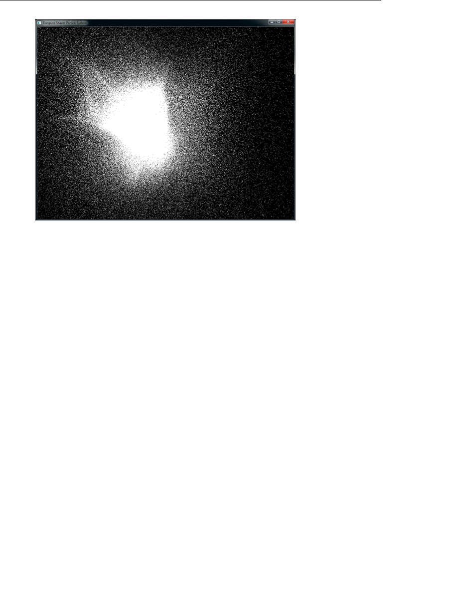
ptg9898810
Figure 12.3 Output of the physical simulation program as simple points
In the fragment shader for rendering the points, we first use the age of the
point (which is stored in its wcomponent) to fade the point from red hot
to cool blue as it gets older. Also, we turn on additive blending by enabling
GL_BLEND and setting both the source and destination factors to
GL_ONE. This causes the points to accumulate in the framebuffer and for
more densely populated areas to ‘‘glow’’ due to the number of particles in
the region. The fragment shader used to do this is shown in Listing 12.9.
Example 12.9 Particle Simulation Fragment Shader
#version 430 core
layout (location = 0) out vec4 color;
// This is derived from the age of the particle read
// by the vertex shader
in float intensity;
void main(void)
{// Blend between red-hot and cool-blue based on the
// age of the particle.
color = mix(vec4(0.0f, 0.2f, 1.0f, 1.0f),
vec4(0.2f, 0.05f, 0.0f, 1.0f),
intensity);
}
640 Chapter 12: Compute Shaders

ptg9898810
In our rendering loop, the positions and masses of the attractors are
updated before we dispatch the compute shader over the buffers
containing the positions and velocities. We then render the particles as
points having issued a memory barrier to ensure that the writes performed
by the compute shader have been completed. This loop is shown in
Example 12.10.
Example 12.10 Particle Simulation Rendering Loop
// Update the buffer containing the attractor positions and masses
vmath::vec4 *attractors =
(vmath::vec4 *)glMapBufferRange(GL_UNIFORM_BUFFER,
0,
32 *sizeof(vmath::vec4),
GL_MAP_WRITE_BIT |
GL_MAP_INVALIDATE_BUFFER_BIT);
int i;
for (i = 0; i < 32; i++)
{
attractors[i] =
vmath::vec4(sinf(time *(float)(i + 4) *7.5f *20.0f) *50.0f,
cosf(time *(float)(i + 7) *3.9f *20.0f) *50.0f,
sinf(time *(float)(i + 3) *5.3f *20.0f) *
cosf(time *(float)(i + 5) *9.1f) *100.0f,
attractor_masses[i]);
}
glUnmapBuffer(GL_UNIFORM_BUFFER);
// Activate the compute program and bind the position
// and velocity buffers
glUseProgram(compute_prog);
glBindImageTexture(0, velocity_tbo, 0,
GL_FALSE, 0,
GL_READ_WRITE, GL_RGBA32F);
glBindImageTexture(1, position_tbo, 0,
GL_FALSE, 0,
GL_READ_WRITE, GL_RGBA32F);
// Set delta time
glUniform1f(dt_location, delta_time);
// Dispatch the compute shader
glDispatchCompute(PARTICLE_GROUP_COUNT, 1, 1);
// Ensure that writes by the compute shader have completed
glMemoryBarrier(GL_SHADER_IMAGE_ACCESS_BARRIER_BIT);
// Set up our mvp matrix for viewing
vmath::mat4 mvp = vmath::perspective(45.0f, aspect_ratio,
0.1f, 1000.0f) *
Examples 641
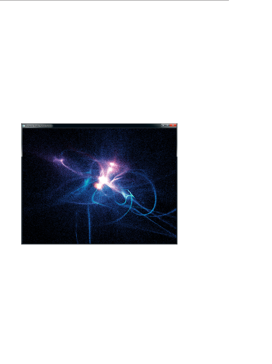
ptg9898810
vmath::translate(0.0f, 0.0f, -60.0f) *
vmath::rotate(time *1000.0f,
vmath::vec3(0.0f, 1.0f, 0.0f));
// Clear, select the rendering program and draw a full screen quad
glClear(GL_COLOR_BUFFER_BIT | GL_DEPTH_BUFFER_BIT);
glUseProgram(render_prog);
glUniformMatrix4fv(0, 1, GL_FALSE, mvp);
glBindVertexArray(render_vao);
glEnable(GL_BLEND);
glBlendFunc(GL_ONE, GL_ONE);
glDrawArrays(GL_POINTS, 0, PARTICLE_COUNT);
Finally, the result of rendering the particle system with the fragment shader
of Example 12.9 and with blending turned on is shown in Figure 12.4.
Figure 12.4 Output of the physical simulation program
Image Processing
This example of compute shaders uses them as a means to implement
image processing algorithms. In this case, we implement a simple
edge-detection algorithm by convolving an input image with an
edge-detection filter. The filter chosen is an example of a separable filter. A
separable filter is one that can be applied one dimension at a time in a
multidimensional space to produce a final result. Here, it is is applied to a
642 Chapter 12: Compute Shaders

ptg9898810
two-dimensional image by applying it first in the horizontal dimension
and then again in the vertical dimension. The actual kernel is a central
difference kernel −1 0 1.
To implement this kernel, each invocation of the compute shader produces
a single pixel in the output image. It must read from the input image and
subtract the samples to either side of the target pixel. Of course, this means
that each invocation of the shader must read from the input image twice
and that two invocations of the shader will read from the same location.
To reduce memory accesses, this implementation uses shared variables to
store a row of the input image.
Rather than reading the needed input samples directly from the input
image, each invocation reads the value of its target pixel from the input
image and stores it in an element of a shared array. After all invocations of
the shader have read from the input image, the shared array contains a
complete copy of the current scanline of the input image---each pixel of
that image having been read only once. However, now that the pixels are
stored in the shared array, all other invocations in the local workgroup can
read from that array to retrieve the pixel values they need at very high
speed.
The edge-detection compute shader is shown in Example 12.11.
Example 12.11 Central Difference Edge Detection Compute Shader
#version 430 core
// One scanline of the image... 1024 is the minimum maximum
// guaranteed by OpenGL
layout (local_size_x = 1024) in;
// Input and output images
layout (rgba32f, binding = 0) uniform image2D input_image;
layout (rgba32f, binding = 1) uniform image2D output_image;
// Shared memory for the scanline data -- must be the same size
// as (or larger than) as the local workgroup
shared vec4 scanline[1024];
void main(void)
{
// Get the current position in the image.
ivec2 pos = ivec2(gl_GlobalInvocationID.xy);
// Read an input pixel and store it in the shared array
scanline[pos.x] = imageLoad(input_image, pos);
// Ensure that all other invocations have reached this point
// and written their shared data by calling barrier()
Examples 643

ptg9898810
barrier();
// Compute our result and write it back to the image
vec4 result = scanline[min(pos.x + 1, 1023)] -
scanline[max(pos.x - 1, 0)];
imageStore(output_image, pos.yx, result);
}
The image processing shader of Example 12.11 uses a one-dimensional
local workgroup size of 1024 pixels (which is the largest workgroup size that
is guaranteed to be supported by an OpenGL implementation). This places
an upper bound on the width or height of the image of 1024 pixels. While
this is sufficient for this rather simple example, a more complex approach
would be required to implement larger filters or operate on larger images.
The global invocation ID is converted to a signed integer vector and is used
to read from the input image. The result is written into the scanline
shared variable. Then the shader calls barrier(). This is to ensure that all of
the invocations in the local workgroup have reached this point in the
shader. Next, the shader takes the difference between the pixels to the left
and the right of the target pixel. These values have been placed into the
shared array by the invocations logically to the left and right of the current
invocation. The resulting difference is placed into the output image.
Another thing to note about this shader is that when it stores the resulting
pixel, it transposes the coordinates of the output pixel, effectively writing
in a vertical line down the image. This has the effect of transposing the
image. An alternative is to read from the input image in vertical strips and
write horizontally. The idea behind this is that the same shader can be
used for both passes of the separable filter---the second pass re-transposing
the already transposed intermediate image, restoring it to its original
orientation.
The code to invoke the compute shader is shown in Example 12.12.
Example 12.12 Dispatching the Image Processing Compute Shader
// Activate the compute program...
glUseProgram(compute_prog);
// Bind the source image as input and the intermediate
// image as output
glBindImageTexture(0, input_image, 0,
GL_FALSE, 0,
GL_READ_ONLY, GL_RGBA32F);
glBindImageTexture(1, intermediate_image, 0,
GL_FALSE, 0, GL_WRITE_ONLY,
GL_RGBA32F);
// Dispatch the horizontal pass
644 Chapter 12: Compute Shaders

ptg9898810
glDispatchCompute(1, 1024, 1);
// Issue a memory barrier between the passes
glMemoryBarrier(GL_SHADER_IMAGE_ACCESS_BARRIER_BIT);
// Now bind the intermediate image as input and the final
// image for output
glBindImageTexture(0, intermediate_image, 0,
GL_FALSE, 0,
GL_READ_ONLY, GL_RGBA32F);
glBindImageTexture(1, output_image, 0,
GL_FALSE, 0,
GL_WRITE_ONLY, GL_RGBA32F);
// Dispatch the vertical pass
glDispatchCompute(1, 1024, 1);
Figure 12.5 shows the original input image2at the top and the resulting
output image at the bottom. The edges are clearly visible in the output
image.
The image-processing example shader includes a call to barrier after all
of the input image data has been read into the shared variable scanline.
This ensures that all of the invocations in the local workgroup (including
the current invocation’s neighbors) have completed the read from the
input image and have written the result into the shared variable. Without
the barrier, it is possible to suffer from a race condition where some
invocations of the shader will read from the shared variable before the
adjacent invocations have completed their writes into it. The result can be
sparkling corruption in the output image.
Figure 12.6 shows the result of applying this shader with the call to
barrier removed. A horizontal and vertical grid-like pattern of seemingly
random pixels is visible. This is due to some invocations of the shader
receiving stale or uninitialized data because they move ahead of their
neighbors within the local workgroup. The reason that the corruption
appears as a grid-like pattern is that the graphics processor used to generate
this example processes a number of invocations in lockstep and therefore
those invocations cannot get out of sync with each other. However, the
local workgroup is broken up into a number of these subgroups, and they
can get ahead of each other. Therefore, we see corrupted pixels produced by
the invocations that happen to be executed by the first and last members
of the subgroups. If the number of invocations working in lockstep were
different then the spacing of the grid pattern would change accordingly.
2. This image is a picture of the Martian surface as seen from the Curiosity rover and was
obtained from NASA’s Web site in August of 2012. NASA does not endorse this simple image
processing example---they have much better ones.
Examples 645

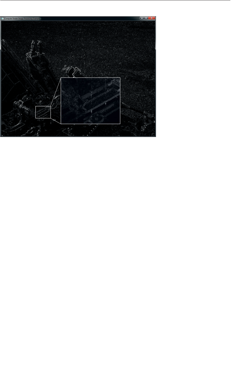
ptg9898810
Figure 12.6 Image processing artifacts
(Output of the image processing example, without barriers, showing arti-
facts.)
Chapter Summary
In this chapter, you have read an introduction to compute shaders. As they
are not tied to a specific part of the traditional graphics pipeline and have
no fixed intended use, the amount that could be written about compute
shaders is enormous. Instead, we have covered the basics and provided a
couple of examples that should demonstrate how compute shaders may be
used to perform the nongraphics parts of your graphics applications.
Compute Shader Redux
To use a compute shader in your program:
•Create a compute shader with glCreateShader() using the type
GL_COMPUTE_SHADER.
•Set the shader source with glShaderSource() and compile it with
glCompileShader().
•Attach it to a program object with glAttachShader() and link it with
glLinkProgram().
Chapter Summary 647

ptg9898810
•Make the program current with glUseProgram().
•Launch compute workloads with glDispatchCompute() or
glDispatchComputeIndirect().
In your compute shader:
•Specify the local workgroup size using the local_size_x,
local_size_y and local_size_z input layout qualifiers.
•Read and write memory using buffer or image variables, or by updating
the values of atomic counters.
The special built-in variables available to a compute shader are as follows:
•gl_WorkGroupSize is a constant containing the three-dimensional
local size as declared by the input layout qualifiers.
•gl_NumWorkGroups is a copy of the global workgroup count as passed
to the glDispatchCompute() or glDispatchCompute() function.
•gl_LocalInvocationID is the coordinate of the current shader
invocation within the local workgroup.
•gl_WorkGroupID is the coordinate of the local workgroup within the
global workgroup.
•gl_GlobalInvocationID is the coordinate of the current shader
invocation within the global workgroup.
•gl_LocalInvocationIndex is a flattened version of
gl_LocalInvocationID.
Compute Shader Best Practices
The following are a handful of tips for making effective use of compute
shaders. By following this advice, your compute shaders are more likely to
perform well and work correctly on a wide range of hardware.
Choose the Right Workgroup Size
Choose a local workgroup size that is appropriate for the workload you
need to process. Choosing a size that is too large may not allow you to fit
everything you need into shared variables. On the other hand, choosing a
size that is too small may reduce efficiency, depending on the architecture
of the graphics processor.
648 Chapter 12: Compute Shaders

ptg9898810
Use Barriers
Remember to insert control flow and memory barriers before attempting
to communicate between compute shader invocations. If you leave out
memory barriers, you open your application up to the effects of race
conditions. It may appear to work on one machine but could produce
corrupted data on others.
Use Shared Variables
Make effective use of shared variables. Try to structure your workload into
blocks---especially if it is memory intensive and multiple invocations will
read the same memory locations. Read blocks of data into shared
variables, issue a barrier, and then operate on the data in the shared
variable. Write the results back to memory at the end of the shader. Ideally,
each memory location accessed by an invocation will be read exactly once
and written exactly once.
Do Other Things While Your Compute Shader Runs
If you can, insert graphics work (or even more compute work) between
producing data with a compute shader and consuming that data in a
graphics shader. Not doing this will force the compute shader to complete
execution before the graphics shader can begin execution. By placing
unrelated work between the compute shader producer and the graphics
shader consumer, that work may be overlapped, improving overall
performance.
Chapter Summary 649


ptg9898810
Appendix A
Basics of GLUT: The
OpenGL Utility Toolkit
In this text, we used the OpenGL Utility Toolkit (GLUT) as a simple,
cross-platform application framework to simplify our examples.
The two versions of GLUT in circulation are as follows:
•Freeglut, written by Pawel W. Olszta with contributions from Andreas
Umbach and Steve Baker, is the most up-to-date version and the one
that we’ve used in this book.
•The original version was written by Mark Kilgard many years ago. This
version hasn’t been kept up to date with respect to recent changes.
However, its Version 3.7 (which is the most recent) is the foundation of
Apple Computer’s Mac OS X 10.8 (aka ‘‘Mountain Lion’’) GLUT
framework.
This appendix describes a subset of functions available in the Freeglut
version.
GLUT makes the process of creating an OpenGL application simple, since
in its most basic form, only four steps are required to get the application
going.
1. Initialize the GLUT library
2. Create a GLUT window
3. Register the display() callback
4. Enter GLUT’s main loop
651

ptg9898810
In this appendix, we explain those steps and expand on other options
that the GLUT library makes available. For complete details on Freeglut
(which is the version we recommend), please visit their Web site
http://freeglut.sourceforge.net/.
This appendix contains the following major sections:
•‘‘Initializing and Creating a Window’’
•‘‘Accessing Functions’’
•‘‘Handling Window and Input Events’’
•‘‘Managing a Background Process’’
•‘‘Running the Program’’
Initializing and Creating a Window
To use GLUT, you first need to initialize the GLUT library by calling
glutInit(). The function also parses any relevant command-line options
you pass for specifying GLUT options.
void glutInit(int argc, char **argv);
glutInit() should be called before any other GLUT routine because it
initializes the GLUT library. glutInit() will also process command-line
options, but the specific options are window system dependent. For
many windowing systems, command-line options like -iconic,
-geometry, and -display are examples of options you might set that
are processed by glutInit().
Following that, you’ll usually call glutInitDisplayMode() to configure the
characteristics of the window, like having a depth or stencil buffer, its pixel
type, or controlling multisampling. Likewise, you’ll use
glutInitContextVersion(),glutInitContextProfile(), and
glutInitContextFlags() to configure the type of OpenGL implementation
your application requires. Additionally, you might call
glutInitWindowSize() or glutInitWindowPosition() to set the geometry
of the window. To finally open your configured window, call
glutCreateWindow() to open the window.
652 Appendix A: Basics of GLUT: The OpenGL Utility Toolkit

ptg9898810
void glutInitDisplayMode(unsigned int mode);
Specifies a display mode for windows created when glutCreateWindow()
is called. You can specify that the window have an associated depth,
stencil, or be an RGB or RGBA window. The mode argument is a bitwise
OR combination of GLUT_RGB, GLUT_RGBA, GLUT_DOUBLE,
GLUT_ALPHA, GLUT_DEPTH, GLUT_STENCIL, GLUT_MULTISAMPLE, or
GLUT_STEREO. Additionally, if you’re using the compatibility profile,
you can include the following options: GLUT_INDEX (for color-index
mode), GLUT_SINGLE (for single-buffered rendering), GLUT_ACCUM (to
use the accumulation buffer), and GLUT_LUMINANCE (for luminance
[greyscale] only rendering).
The default mode is the bitwise OR of GLUT_INDEX, GLUT_SINGLE, and
GLUT_DEPTH (which relies on a compatibility mode context).
void glutInitContextVersion(int majorVersion, int minorVersion);
Specifies the major and minor versions of the OpenGL implementation
that you want a context created for. To use OpenGL Version 3.0 or
greater, you need to call this routine before calling glutCreateWindow(),
due to the different context creation semantics introduced by OpenGL
Version 3.0.
If you don’t specify a context version, a compatibility profile version of
the most recent OpenGL version will be created for you.
void glutInitContextProfile(int profile);
Specifies the context profile you want created: core or compatibility. To
specify a core profile (as we did in this manual), use
GLUT_CORE_PROFILE; for a compatibility profile, use
GLUT_COMPATIBILITY_PROFILE.
void glutInitContextFlags(int flags);
Specifies any attribute flags to be used in the creation of the OpenGL
context. The flags argument is a bitwise OR of the following values:
GLUT_DEBUG to specify a context with debug facilities enabled or
Initializing and Creating a Window 653

ptg9898810
GLUT_FORWARD_COMPATIBLE to specify a testing context for forward
application compatibility.
void glutInitWindowSize(int width, int height);
void glutInitWindowPosition(int x, int y);
Request windows created by glutCreateWindow() to have an initial size
and position. The arguments (x,y)indicate the location of a corner of the
window, relative to the entire display. The parameters width and height
indicate the window’s size (in pixels). The initial window size and
position are hints and may be overridden by other requests.
int glutCreateWindow(char *name);
Opens a window with previously set characteristics (display mode, width,
height, etc.). The string name may appear in the title bar if your window
system does that sort of thing. The window is not initially displayed until
glutMainLoop() is entered, so do not render into the window until then.
The value returned is a unique integer identifier for the window. This
identifier can be used for controlling and rendering to multiple windows
(each with an OpenGL rendering context) from the same application.
Accessing Functions
Depending on the operating system you’re using, there may be differences
in the compilation (or specifically, the program-linking phase) libraries,
and the libraries used by the application when it runs. For example, in
Microsoft Windows, your application will link with opengl32.lib but
execute using opengl32.dll (along with other libraries). In this particular
case (and also in other operating systems), the set of functions available in
the link-time library differs from those available in the run-time library. To
solve this problem, each window system that supports OpenGL has a
mechanism for obtaining function pointers at run time. GLUT abstracts
away the window--system-specific functions, and presents
glutGetProcAddress(), which will call the window-specific function to
return a function address for your use.
654 Appendix A: Basics of GLUT: The OpenGL Utility Toolkit

ptg9898810
void (*GLUTproc)() glutGetProcAddress(const char *procName);
Retrieves the function address associated with procName or returns NULL
if procName names a function that’s not supported in the OpenGL
implementation.
Note: In our examples, you may notice we don’t use
glutGetProcAddress() explicitly. Instead, we use GLEW, the
OpenGL Extension Wrangler library, which further abstracts away
all of this function pointer inconvenience and allows you to just
write OpenGL routines.
Handling Window and Input Events
After the window is created, but before you enter the main loop, you
should register callback functions using the following routines. Callback
functions are routines you write that you present to GLUT as a function
pointer, and that GLUT will call when the right circumstances occur. You
will specify certain callback functions once, and never change them
throughout the execution of your program. Others, however, you may
specify when a certain event occurs (like when a mouse button is pressed),
and disable that callback function by specifying NULL (or zero) as the new
callback function.
The most important routine is glutDisplayFunc(), which is where you will
do all of your rendering in your application. It’s required for every GLUT
program.
void glutDisplayFunc(void (*func)(void));
Specifies the function to be called whenever the contents of the window
need to be redrawn. The contents of the window will need to be drawn
when the window is initially opened, and likely when the window is
raised above other windows and previously obscured areas are exposed,
or when glutPostRedisplay() is explicitly called.
Likewise, when your window changes geometry or position, you’ll
probably need to update things like the window’s viewport and projection
Handling Window and Input Events 655

ptg9898810
transformation. The glutReshapeFunc() callback is the right place to make
those updates.
void glutReshapeFunc(void (*func)(int width, int height));
Specifies the function that’s called whenever the window is resized or
moved. The argument func is a pointer to a function that expects two
arguments, the new width and height of the window. Typically, func calls
glViewport(), so that the display is clipped to the new size and it
redefines the projection matrix so that the aspect ratio of the projected
image matches the viewport, avoiding aspect-ratio distortion. If
glutReshapeFunc() isn’t called or is deregistered by passing NULL, a
default reshape function is called, which calls glViewport(0, 0, width,
height).
Responding to user input is crucial in interactive graphics applications.
The most common forms of input are keyboard and mouse events. GLUT
makes it easy to process those events as well, using the same callback
mechanism. glutKeyboardFunc(), as the name suggests, is called when a
user presses a keyboard key.
void glutKeyboardFunc(void (*func)(unsigned char key, int x, int y));
Specifies the function, func, that’s called when a key that generates an
ASCII character is pressed. The key callback parameter is the generated
ASCII value. The xand ycallback parameters indicate the location of the
mouse (in window-relative coordinates) when the key was pressed.
If, however, you’re interested when a key is released, use
glutKeyboardUpFunc().
void glutKeyboardUpFunc(void (*func)(unsigned char key, int x, int y));
Specifies the function, func, that’s called when a key that generates an
ASCII character is released. The key callback parameter is the generated
ASCII value. The xand ycallback parameters indicate the location of the
mouse (in window-relative coordinates) when the key was pressed.
656 Appendix A: Basics of GLUT: The OpenGL Utility Toolkit

ptg9898810
Processing mouse input events is more varied. For instance, does your
application require that a mouse button be pressed to have the application
respond to events? Or are you only interested in knowing if the mouse if
moving, regardless of the button state. There are different mouse-event
processing routines for these situations.
void glutMouseFunc(void (*func)(int button, int state, int x, int y));
Specifies the function, func, that’s called when a mouse button is pressed
or released. The button callback parameter is GLUT_LEFT_BUTTON,
GLUT_MIDDLE_BUTTON, or GLUT_RIGHT_BUTTON. The state callback
parameter is either GLUT_UP or GLUT_DOWN, depending on whether
the mouse has been released or pressed. The xand ycallback parameters
indicate the location (in window-relative coordinates) of the mouse
when the event occurred.
void glutMotionFunc(void (*func)(int x, int y));
Specifies the function, func, that’s called when the mouse pointer moves
within the window while one or more mouse buttons are pressed. The x
and ycallback parameters indicate the location (in window-relative
coordinates) of the mouse when the event occurred.
Similar is glutPassiveMotionEvent(), which reports the mouse’s position
regardless of the state of the mouse’s buttons.
void glutPassiveMotionFunc(void (*func)(int x, int y));
Specifies the function, func, that’s called when the mouse pointer moves
within the window. The xand ycallback parameters indicate the location
(in window-relative coordinates) of the mouse when the event occurred.
In order to keep interactive programs responding rapidly to lots of input
events, it’s best to process all input events and then update your image by
rendering. Generally speaking, it takes much less time to process an input
event than it does to render your scene. As such, the GLUT event loop will
continue to retrieve events and call your application’s callback functions
while there are events to process. How, though, do you know when you’re
completed processing input events and it’s time to render? That’s what
glutPostRedisplay() is for. Place a call to it as the last operation any
Handling Window and Input Events 657
ptg9898810
input-processing callback. When GLUT detects that there are no more
input events, it will call the display callback (the one set with
glutDisplayFunc()).
void glutPostRedisplay(void);
Marks the current window as needing to be redrawn. At the next
opportunity, the callback function registered by glutDisplayFunc() will
be called.
Managing a Background Process
You can specify a function to be executed if no other events are
pending---for example, when the event loop would otherwise be idle---with
glutIdleFunc(). This is particularly useful for continuous animation or
other background processing.
void glutIdleFunc(void (*func)(void));
Specifies the function, func, to be executed if no other events are
pending. If NULL (zero) is passed in, execution of func is disabled.
Running the Program
After all the setup is completed, GLUT programs enter an event-processing
loop, glutMainLoop().
void glutMainLoop(void);
Enters the GLUT-processing loop, never to return. Registered callback
functions will be called when the corresponding events instigate them.
Note: For those of you familiar with previous versions of GLUT
(regardless of whether it’s the Freeglut version or the original),
various features---like menus and shapes, for example---will not
work when you ask for a core profile, as they use deprecated
features. If you need those features, the simplest approach is to ask
for a compatibility profile.
658 Appendix A: Basics of GLUT: The OpenGL Utility Toolkit

ptg9898810
Appendix B
OpenGL ES and WebGL
While the OpenGL API is great for many computer graphics applications,
under certain circumstances, it may not be the best solution, which is why
the OpenGL API has spawned two other APIs. The first is OpenGL ES,
where the ‘‘ES’’ stands for ‘‘Embedded Subsystem’’, and was crafted from
the ‘‘desktop’’ version of OpenGL for use in embedded devices like mobile
phones, Internet tablets, televisions, and other devices with color screens,
but limited system resources. The other API is WebGL, which enables
OpenGL-style rendering within most Web browsers using the JavaScript
Web programming language.
This appendix provides an overview of the OpenGL ES and WebGL,
highlighting the differences between OpenGL as described throughout the
rest of this book, and these derivative versions. It contains the following
major sections:
•‘‘OpenGL ES’’
•‘‘WebGL’’
659

ptg9898810
OpenGL ES
OpenGL ES is developed to meet the need of early embedded devices
like mobile phones and set-top boxes. The original version, OpenGL ES Ver-
sion 1.0 was derived from OpenGL Version 1.3, and was quickly expanded
to OpenGL ES Version 1.1, which is based on OpenGL Version 1.5,
and released in April of 2007. This version reached much popularity
in original mobile phones with fixed-function graphics hardware.
As mobile graphics hardware became more capable, principally by
programmable shaders, a new version of OpenGL ES was required, and
OpenGL ES Version 2.0---based on OpenGL Version 2.0---was originally
specified in January of 2008. Keeping with its minimalist mantra of
supporting only a single method for processing graphics, the API switched
to an entirely shader-based rendering pipeline using both vertex and
fragment shaders (which also broke source-code compatibility with
OpenGL ES Version 1.1). OpenGL ES Version 2.0 has become very
influential in dictating hardware requirements for many different types of
devices. With the release of OpenGL Version 4.1, all functionality for
OpenGL ES Version 2.0 was added to OpenGL, making OpenGL ES a
proper subset of OpenGL’s functionality.
At SIGGRAPH 2012, OpenGL ES Version 3.0 was announced, expanding
on the rendering capabilities of OpenGL ES (however, not adding any
additional programmable shader stages like geometry or tessellation
shading). This version did retain backwards compatibility with
OpenGL ES Version 2.0, with most of the new features focusing on
increased shader programmabilty (leveraging sampler objects, for
example), instanced rendering and transform feedback, and extended pixel
and framebuffer formats.
As OpenGL ES is a subset of OpenGL in terms of both features and
functions, everything you’ve read in this text applies in terms of
techniques it supports. In fact, perhaps the largest noticeable difference
between an OpenGL ES program and that of OpenGL core profile may be
in creating a window for rendering. In most systems (but notably not
Apple’s iOS), OpenGL ES is connected to the system’s windowing system
by a binding layer named EGL. EGL was patterned after the X Window
System’s binding layer, GLX (as described in Appendix F).
We now provide a brief example of creating an OpenGL ES Version 2.0
context (since, at the time of this writing, there are no OpenGL ES
Version 3.0 capable devices available). Example B.1 demonstrates creating
an RGB-capable rendering context with a depth buffer for use in a window.
660 Appendix B: OpenGL ES and WebGL

ptg9898810
Example B.1 An Example of Creating an OpenGL ES Version 2.0
Rendering Context
EGLBoolean initializeWindow(EGLNativeWindow nativeWindow)
{
const EGLint configAttribs[] = {
EGL_RENDER_TYPE, EGL_WINDOW_BIT,
EGL_RED_SIZE, 8,
EGL_GREEN_SIZE, 8,
EGL_BLUE_SIZE, 8,
EGL_DEPTH_SIZE, 24,
EGL_NONE
};
const EGLint contextAttribs[] = {
EGL_CONTEXT_CLIENT_VERSION, 2,
EGL_NONE
};
EGLDisplay dpy;
dpy = eglGetNativeDispay(EGL_DEFAULT_DISPLAY);
if (dpy == EGL_NO_DISPLAY) { return EGL_FALSE; }
EGLint major, minor;
if (!eglInitialize(dpy, &major, &minor)) { return EGL_FALSE;
EGLConfig config;
EGLint numConfigs;
if (!eglChooseConfig(dpy, configAttribs, &config, 1, &numConfigs)) {
return EGL_FALSE;
}
EGLSurface window;
window = eglCreateWindowSurface(dpy, config, nativeWindow, NULL);
if (window == EGL_NO_SURFACE) { return EGL_FALSE; }
EGLContext context;
context = eglCreateContext(dpy, config, EGL_NO_CONTEXT,
contextAttribs);
if (context == EGL_NO_CONTEXT) { return EGL_FALSE; }
if (!eglMakeCurrent(dpy, window, window, context)) {
return EGL_FALSE;
}
return EGL_TRUE;
}
OpenGL ES 661

ptg9898810
WebGL
WebGL takes OpenGL (or specifically, OpenGL ES Version 2.0) to the
Internet by adding high-performance, 3D rendering within HTML5’s
Canvas element. Virtually all functions from OpenGL ES Version 2.0 are
available in their exact form, except for small changes necessitated because
of its JavaScript interface.
This section provides a brief introduction to WebGL through a simple
example, which works natively in all modern Web browsers (except
Microsoft’s Internet Explorer, which requires a plug-in for support).
Our example focuses exclusively on rendering; event processing and user
interaction aren’t discussed.
Setting up WebGL within an HTML5 page
To provide a ‘‘window’’ for WebGL to use for rendering, you first create an
HTML5 Canvas element within your Web page. Example B.2 demonstrates
creating a 512 ×512-sized Canvas with a blue background. In the case that
the browser doesn’t support WebGL, a simple page stating the browser
doesn’t support Canvas elements is shown. In the example, we name the
Canvas gl-canvas by setting its id attribute. We’ll use its id later when we
initialize WebGL.
Example B.2 Creating an HTML5 Canvas Element
<html>
<style type="text/css">
canvas { background: blue; }
</style>
<body>
<canvas id="gl-canvas" width="512" height="512">
Oops ... your browser doesn’t support HTML5’s Canvas elements!
</canvas>
</body>
</html>
Note: Example B.2 uses a cascading style sheet for specifying the Canvas
element’s background color.
Assuming this worked in your browser, we can now continue to the next
step: creating a WebGL context. There are multiple ways to do this;
however, we’ll use a utility function defined in a JavaScript file hosted by
the Khronos Group from their Web site, https://www.khronos.org
/registry/webgl/sdk/demos/common/webgl-utils.js. You will likely find it
662 Appendix B: OpenGL ES and WebGL

ptg9898810
convenient to include this JavaScript file in your WebGL applications.1It
includes the package WebGLUtils and its method setupWebGL(), which
makes it easy to enable WebGL on an HTML5 Canvas. Example B.3
expands on the previous example and handles setting up a WebGL context
that works in all supported Web browsers. The return value from
setupWebGL() is a JavaScript object containing methods for all OpenGL
functions supported in WebGL.
Example B.3 Creating an HTML5 Canvas Element that Supports WebGL
<html>
<style type="text/css">
canvas { background: blue; }
</style>
<script type="text/javascript"
src="https://www.khronos.org/registry/webgl/sdk/demos/common/webgl-utils.js">
</script>
<script type="text/javascript">
var canvas;
var gl;
window.onload = init;
function init() {
canvas = document.getElementById("gl-canvas");
gl = WebGLUtils.setupWebGL(canvas);
if (!gl) { alert("WebGL isn’t available"); }
gl.viewport(0, 0, canvas.width, canvas.height);
gl.clearColor(1.0, 0.0, 0.0, 1.0);
gl.clear(gl.COLOR_BUFFER_BIT);
}
</script>
<body>
<canvas id="gl-canvas" width="512" height="512">
Oops ... your browser doesn’t support HTML5’s Canvas elements!
</canvas>
</body>
</html>
Example B.3 specifies an init() function that is executed when the page
loads (specified by the line window.onload = init). Our init() function
retrieves our gl-canvas Canvas id, passes it to setupWebGL(), which will
return a WebGL object that we can use if initialization was successful; or
1. This file can also be hosted from the Web server serving the pages composing the WebGL
application.
WebGL 663

ptg9898810
false otherwise, which we use to emit an error message. Assuming WebGL
is available, we set up some WebGL state, and clear the window---to red
now. Once WebGL takes over the Canvas, all of its contents are controlled
by WebGL.
Now that we know WebGL is supported, we’ll expand our example by initial-
izing the required shaders, setting up vertex buffers, and finally rendering.
Initializing Shaders in WebGL
OpenGL ES Version 2.0---and therefore WebGL---is a shader-based API, like
OpenGL, requiring every application to use vertex and fragment shaders
for its rendering. As such, you encounter the same requirement of loading
shaders as you saw in OpenGL.
To include vertex and fragment shaders in a WebGL application, it’s
simplest to include the shader as a script in the HTML page.2A shader
within an HTML page needs to be identified correctly. There are two
mime-types associated with WebGL shaders, as shown in Table B.1.
Table B.1 Type Strings for WebGL Shaders
<script> Tag Type Shader Type
x-shader/x-vertex Vertex
x-shader/x-fragment Fragment
For our WebGL application, Example B.4 shows our main HTML page
including the shader sources. You’ll also notice that we include two more
JavaScript files, which are as follows:
•demo.js, which includes the JavaScript implementation of our
application (including the final version of our init() routine).
•InitShaders.js, which is a helper function for loading shaders similar to
our LoadShaders() routine.
Example B.4 Our WebGL Applications Main HTML Page
<html>
<style type="text/css">
canvas { background: blue; }
</style>
2. It is possible to store the shader in a separate file from the original HTML page, but the
mechanism is very cumbersome with current Web technology. We’ve opted for the simple
approach here.
664 Appendix B: OpenGL ES and WebGL

ptg9898810
<script id="vertex-shader" type="x-shader/x-vertex">
attribute vec4 vPos;
attribute vec2 vTexCoord;
uniform float uFrame; // Frame number
varying vec2 texCoord;
void
main()
{
float angle = radians(uFrame);
float c = cos(angle);
float s = sin(angle);
mat4 m = mat4(1.0);
m[0][0] = c;
m[0][1] = s;
m[1][1] = c;
m[1][0] = -s;
texCoord = vTexCoord;
gl_Position = m *vPos;
}
</script>
<script id="fragment-shader" type="x-shader/x-fragment">
#ifdef GL_ES
precision highp float;
#endif
uniform sampler2D uTexture;
varying vec2 texCoord;
void
main()
{
gl_FragColor = texture2D(uTexture, texCoord);
}
</script>
<script type="text/javascript"
<src="http://www.khronos.org/registry/webgl/sdk/demos/common/webgl-utils.js">
</script>
<script type="text/javascript" src="InitShaders.js"></script>
<script type="text/javascript" src="demo.js"></script>
<body>
<canvas id="gl-canvas" width="512" height="512"
Oops ... your browser doesn’t support the HTML5 canvas element
</canvas>
</body>
</html>
To simplify compiling and linking our shaders in WebGL, we created a
routine similar to LoadShaders() that we’ve used in the book. Here, we call
WebGL 665

ptg9898810
it InitShaders(), since there are no files to load; shaders are defined in the
HTML source for the page. In order to organize our code better, we created
a JavaScript file named InitShaders.js to store the code.
Example B.5 Our WebGL Shader Loader: InitShaders.js
//
// InitShaders.js
//
function InitShaders(gl, vertexShaderId, fragmentShaderId)
{
var vertShdr;
var fragShdr;
var vertElem = document.getElementById(vertexShaderId);
if (!vertElem) {
alert("Unable to load vertex shader " + vertexShaderId);
return -1;
}
else {
vertShdr = gl.createShader(gl.VERTEX_SHADER);
gl.shaderSource(vertShdr, vertElem.text);
gl.compileShader(vertShdr);
if (!gl.getShaderParameter(vertShdr, gl.COMPILE_STATUS)) {
var msg = "Vertex shader failed to compile."
+ "The error log is:"
+ "<pre>" + gl.getShaderInfoLog(vertShdr) + "</pre>";
alert(msg);
return -1;
}
}
var fragElem = document.getElementById(fragmentShaderId);
if (!fragElem) {
alert("Unable to load vertex shader " + fragmentShaderId);
return -1;
}
else {
fragShdr = gl.createShader(gl.FRAGMENT_SHADER);
gl.shaderSource(fragShdr, fragElem.text);
gl.compileShader(fragShdr);
if (!gl.getShaderParameter(fragShdr, gl.COMPILE_STATUS)) {
var msg = "Fragment shader failed to compile. "
+ "The error log is:"
+ "<pre>" + gl.getShaderInfoLog(fragShdr) + "</pre>";
alert(msg);
return -1;
}
}
var program = gl.createProgram();
gl.attachShader(program, vertShdr);
666 Appendix B: OpenGL ES and WebGL

ptg9898810
gl.attachShader(program, fragShdr);
gl.linkProgram(program);
if (!gl.getProgramParameter(program, gl.LINK_STATUS)) {
var msg = "Shader program failed to link."
+ "The error log is:"
+ "<pre>" + gl.getProgramInfoLog(program) + "</pre>";
alert(msg);
return -1;
}
return program;
}
While InitShaders() is JavaScript, most of it should look recognizable. The
major difference here is that compared to LoadShaders(), which took file
names for our vertex and fragment shaders, InitShaders() takes HTML
element ids (vertex-shader and fragment-shader in our example). The routine
returns a program name that can be passed into the JavaScript equivalent
of glUseProgram().
Example B.6 Loading WebGL Shaders Using InitShaders()
var program = InitShaders(gl, "vertex-shader", "fragment-shader");
gl.useProgram(program);
Armed with a method for compiling and linking our shaders, we can move
on to initializing our graphics data, loading textures, and completing the
setup of the rest of our WebGL application.
Initializing Vertex Data in WebGL
One major addition to JavaScript that came from WebGL were typed arrays,
which extend the concept of a JavaScript array but match the type support
required for OpenGL-style rendering. Several types of typed arrays are
listed in Table B.2.
Table B.2 WebGL Typed Arrays
Array Type C Type
Int8Array signed char
Uint8Array unsigned char
Uint8ClampedArray unsigned char
Int16Array signed short
Uint16Array unsigned short
Int32Array signed int
Uint32Array unsigned int
Float32Array float
Float64Array double
WebGL 667

ptg9898810
You first allocate and populate (both of which you can do in a single
operation) a typed array to store your vertex data. After that, setting up
your VBOs is identical to what you’ve done in OpenGL. We show our
initialization in Example B.7.
Example B.7 Initializing Vertex Buffers in WebGL
var vertices = {};
vertices.data = new Float32Array(
[
-0.5, -0.5,
0.5, -0.5,
0.5, 0.5,
-0.5, 0.5
]);
vertices.bufferId = gl.createBuffer();
gl.bindBuffer(gl.ARRAY_BUFFER, vertices.bufferId);
gl.bufferData(gl.ARRAY_BUFFER, vertices.data, gl.STATIC_DRAW);
var vPos = gl.getAttribLocation(program, "vPos");
gl.vertexAttribPointer(vPos, 2, gl.FLOAT, false, 0, 0);
gl.enableVertexAttribArray(vPos);
Using Texture Maps in WebGL
Using textures in WebGL is also the same as in OpenGL, but handling the
loading and setup is much simpler, since HTML lends a helping hand. In
fact, loading a texture from a file is a one-line operation. In our demo, we
use a single texture named OpenGL-logo.png.
var image = new Image();
image.src = "OpenGL-logo.png";
Yes; that’s all there is to loading the pixels from the image into a variable.
However, HTML pages load asynchronously, so knowing when the image file
has been received and loaded needs to be handled in a callback. Fortunately,
JavaScript has a ready-made method in the Image class for handling
that situation: onload().We can specify the onload() method as follows:
image.onload = function () {
configureTexture(image);
render();
}
The onload() method defined above will be called once our image has
been completely loaded and ready for use by WebGL. We group all of our
texture-initialization code in a local function: configureTexture.
function configureTexture(image) {
texture = gl.createTexture();
668 Appendix B: OpenGL ES and WebGL

ptg9898810
gl.activeTexture(gl.TEXTURE0);
gl.bindTexture(gl.TEXTURE_2D, texture);
gl.pixelStorei(gl.UNPACK_FLIP_Y_WEBGL, true);
gl.texImage2D(gl.TEXTURE_2D, 0, gl.RGB, gl.RGB, gl.UNSIGNED_BYTE,
image);
gl.generateMipmap(gl.TEXTURE_2D);
gl.texParameteri(gl.TEXTURE_2D, gl.TEXTURE_MIN_FILTER,
gl.NEAREST_MIPMAP_LINEAR);
gl.texParameteri(gl.TEXTURE_2D, gl.TEXTURE_MAG_FILTER, gl.NEAREST);
}
The code sequence in configureTexture should look very similar to
what was presented in Chapter 6,‘‘Textures’’. The one notable addition is
the WebGL extension to glPixelStore*() for flipping image data. The
WebGL token UNPACK_FLIP_Y_WEBGL will orient the image data to
match what WebGL is expecting.
Note: As with OpenGL ES Version 2.0, WebGL only supports
power-of-two textures.
Having covered the important parts of our demo.js, we now show the file
in its entirety, and the resulting image.
Example B.8 Our demo.js WebGL Application
var canvas;
var gl;
var texture;
var uFrame; // vertex shader angle uniform variable
window.onload = init;
function CheckError(msg) {
var error = gl.getError();
if (error != 0) {
var errMsg = "OpenGL error: " + error.toString(16);
if (msg) { errMsg = msg + "\n" + errMsg; }
alert(errMsg);
}
}
function configureTexture(image) {
texture = gl.createTexture();
gl.activeTexture(gl.TEXTURE0);
gl.bindTexture(gl.TEXTURE_2D, texture);
gl.pixelStorei(gl.UNPACK_FLIP_Y_WEBGL, true);
gl.texImage2D(gl.TEXTURE_2D, 0, gl.RGB, gl.RGB, gl.UNSIGNED_BYTE,
image);
gl.generateMipmap(gl.TEXTURE_2D);
gl.texParameteri(gl.TEXTURE_2D, gl.TEXTURE_MIN_FILTER,
gl.NEAREST_MIPMAP_LINEAR);
gl.texParameteri(gl.TEXTURE_2D, gl.TEXTURE_MAG_FILTER, gl.NEAREST);
WebGL 669

ptg9898810
}
function init() {
canvas = document.getElementById("gl-canvas");
gl = WebGLUtils.setupWebGL(canvas);
if (!gl) { alert("WebGL isn’t available"); }
gl.viewport(0, 0, canvas.width, canvas.height);
gl.clearColor(1.0, 0.0, 0.0, 1.0);
//
// Load shaders and initialize attribute buffers
//
var program = InitShaders(gl, "vertex-shader", "fragment-shader");
gl.useProgram(program);
var vertices = {};
vertices.data = new Float32Array(
[
-0.5, -0.5,
0.5, -0.5,
0.5, 0.5,
-0.5, 0.5
]);
vertices.bufferId = gl.createBuffer();
gl.bindBuffer(gl.ARRAY_BUFFER, vertices.bufferId);
gl.bufferData(gl.ARRAY_BUFFER, vertices.data, gl.STATIC_DRAW);
var vPos = gl.getAttribLocation(program, "vPos");
gl.vertexAttribPointer(vPos, 2, gl.FLOAT, false, 0, 0);
gl.enableVertexAttribArray(vPos);
var texCoords = {};
texCoords.data = new Float32Array(
[
0.0, 0.0,
1.0, 0.0,
1.0, 1.0,
0.0, 1.0
]);
texCoords.bufferId = gl.createBuffer();
gl.bindBuffer(gl.ARRAY_BUFFER, texCoords.bufferId);
gl.bufferData(gl.ARRAY_BUFFER, texCoords.data, gl.STATIC_DRAW);
var vTexCoord = gl.getAttribLocation(program, "vTexCoord");
gl.vertexAttribPointer(vTexCoord, 2, gl.FLOAT, false, 0, 0);
gl.enableVertexAttribArray(vTexCoord);
//
// Initialize a texture
//
var image = new Image();
image.onload = function() {
configureTexture(image);
670 Appendix B: OpenGL ES and WebGL

ptg9898810
render();
}
image.src = "OpenGL-logo.png";
gl.activeTexture(gl.TEXTURE0);
var uTexture = gl.getUniformLocation(program, "uTexture");
gl.uniform1i(uTexture, 0);
uFrame = gl.getUniformLocation(program, "uFrame");
}
var frameNumber = 0;
function render() {
gl.uniform1f(uFrame, frameNumber++);
gl.clear(gl.COLOR_BUFFER_BIT | gl.DEPTH_BUFFER_BIT);
gl.drawArrays(gl.TRIANGLE_FAN, 0, 4);
window.requestAnimFrame(render, canvas);
}
Figure B.1 Our WebGL demo
WebGL 671


ptg9898810
Appendix C
Built-in GLSL Variables and
Functions
The OpenGL Shading Language has a small number of built-in variables, a
set of constants, and a large collection of built-in functions. This appendix
describes each of these, in the following major sections:
•‘‘Built-in Variables’’ lists the variables, first showing the declarations for
all stages, followed by the description of each.
•‘‘Built-in Constants’’ lists all the built-in constants.
•‘‘Built-in Functions’’ describes all GLSL built-in functions. You’ll need
to refer to the table at the beginning of the section to decode the types.
673

ptg9898810
Built-in Variables
Each programmable stage has a different set of built-in variables,
though there is some overlap. We’ll first show all the built-in
variable declarations in ‘‘Built-in Variable Declarations’’
and then describe each one in ‘‘Built-in Variable Descriptions’’.
Built-in Variable Declarations
Vertex Shader Built-in Variables
in int gl_VertexID;
in int gl_InstanceID;
out gl_PerVertex {
vec4 gl_Position;
float gl_PointSize;
float gl_ClipDistance[];
};
Tessellation Control Shader Built-in Variables
in gl_PerVertex {
vec4 gl_Position;
float gl_PointSize;
float gl_ClipDistance[];
} gl_in[gl_MaxPatchVertices];
in int gl_PatchVerticesIn;
in int gl_PrimitiveID;
in int gl_InvocationID;
out gl_PerVertex {
vec4 gl_Position;
float gl_PointSize;
float gl_ClipDistance[];
} gl_out[];
patch out float gl_TessLevelOuter[4];
patch out float gl_TessLevelInner[2];
Tessellation Evaluation Shader Built-in Variables
in gl_PerVertex {
vec4 gl_Position;
float gl_PointSize;
float gl_ClipDistance[];
} gl_in[gl_MaxPatchVertices];
in int gl_PatchVerticesIn;
in int gl_PrimitiveID;
674 Appendix C: Built-in GLSL Variables and Functions

ptg9898810
in vec3 gl_TessCoord;
patch in float gl_TessLevelOuter[4];
patch in float gl_TessLevelInner[2];
out gl_PerVertex {
vec4 gl_Position;
float gl_PointSize;
float gl_ClipDistance[];
};
Geometry Shader Built-in Variables
in gl_PerVertex {
vec4 gl_Position;
float gl_PointSize;
float gl_ClipDistance[];
} gl_in[];
in int gl_PrimitiveIDIn;
in int gl_InvocationID;
out gl_PerVertex {
vec4 gl_Position;
float gl_PointSize;
float gl_ClipDistance[];
};
out int gl_PrimitiveID;
out int gl_Layer;
out int gl_ViewportIndex;
Fragment Shader Built-in Variables
in vec4 gl_FragCoord;
in bool gl_FrontFacing;
in float gl_ClipDistance[];
in vec2 gl_PointCoord;
in int gl_PrimitiveID;
in int gl_SampleID;
in vec2 gl_SamplePosition;
in int gl_SampleMaskIn[];
in int gl_Layer;
in int gl_ViewportIndex;
out float gl_FragDepth;
out int gl_SampleMask[];
Compute Shader Built-in Variables
// work group dimensions
in uvec3 gl_NumWorkGroups;
const uvec3 gl_WorkGroupSize;
Built-in Variables 675

ptg9898810
// work group and invocation IDs
in uvec3 gl_WorkGroupID;
in uvec3 gl_LocalInvocationID;
// derived variables
in uvec3 gl_GlobalInvocationID;
in uint gl_LocalInvocationIndex;
All Shaders’ Built-in State Variables
struct gl_DepthRangeParameters {
float near;
float far;
float diff;
};
uniform gl_DepthRangeParameters gl_DepthRange;
uniform int gl_NumSamples;
Built-in Variable Descriptions
The descriptions of each of the declared variables above are given below in
alphabetical order.
gl_ClipDistance[]
This provides the mechanism for controlling user clipping. The element
gl_ClipDistance[i] specifies a clip distance for each plane [i]. A distance of
0 means the vertex is on the plane, a positive distance means the vertex is
inside the clip plane, and a negative distance means the point is outside
the clip plane. The output clip distances will be linearly interpolated across
the primitive, and the portion of the primitive with interpolated distances
less than 0 will be clipped.
The gl_ClipDistance[] array is predeclared as unsized and must be sized by
the shader either redeclaring it with a size or indexing it only with integral
constant expressions. This needs to size the array to include all the clip
planes that are enabled via the OpenGL API; if the size does not include all
enabled planes, results are undefined. The size can be at most
gl_MaxClipDistances. The number of varying components
(gl_MaxVaryingComponents) consumed by gl_ClipDistance[] will match
the size of the array, no matter how many planes are enabled. The shader
must also set all values in gl_ClipDistance[] that have been enabled
via the OpenGL API, or results are undefined. Values written into
gl_ClipDistance[] for planes that are not enabled have no effect.
As an output variable, gl_ClipDistance[] provides the place for the shader
to write these distances. As an input in all shaders except fragment
676 Appendix C: Built-in GLSL Variables and Functions

ptg9898810
shaders, it reads the values written in the previous shader stage. In a
fragment shader, gl_ClipDistance[] array contains linearly interpolated
values for the vertex values written by a shader to the gl_ClipDistance[]
vertex output variable. Only elements in this array that have clipping
enabled will have defined values.
gl_DepthRange
The structure gl_DepthRange contains the locations of the near clip plane
and far clip plane for viewport 0. Values are given in window coordinates.
The field diff contains the difference far -- near.
gl_FragCoord
The fixed functionality computed depth for a fragment may be obtained
by reading gl_FragCoord.z.
The gl_FragCoord fragment shader input variable holds the window
relative coordinates (x,y,z,1
w)values for the current fragment.
If multisampling, this value can be for any location within the pixel. It is
the result of the fixed functionality that interpolates primitives after vertex
processing to generate fragments. The zcomponent is the depth value that
would be used for the fragment’s depth if no shader contained any writes
to gl_FragDepth. This is useful for invariance if a shader conditionally
computes gl_FragDepth but otherwise wants the fixed functionality
fragment depth.
gl_FragDepth
Writing to gl_FragDepth in a fragment shader will establish the depth
value for the fragment being processed. If depth buffering is enabled, and
no shader writes gl_FragDepth, then the fixed function value for depth will
be used as the fragment’s depth value. If a shader in the fragment stage
contains any assignment anywhere to gl_FragDepth, and there is an
execution path through the shader that does not set gl_FragDepth, the
value of the fragment’s depth might not be undefined when the
nonassigning path is taken. So, if you write it anywhere, make sure all
paths write it.
gl_FrontFacing
Fragment shaders can read the input built-in variable gl_FrontFacing,
whose value is true if the fragment belongs to a front-facing primitive.
Built-in Variables 677

ptg9898810
One use of this is to emulate two-sided lighting by selecting one of two
colors calculated by a vertex or geometry shader.
gl_GlobalInvocationID
The compute shader input gl_GlobalInvocationID contains the global
index of the current work item. This value uniquely identifies this
invocation from all other invocations across all local and global work
groups initiated by the current glDispatchCompute call. This is computed
as follows:
gl_GlobalInvocationID =
gl_WorkGroupID *gl_WorkGroupSize + gl_LocalInvocationID;
gl_InstanceID
The vertex shader input gl_InstanceID holds the instance number of the
current primitive in an instanced draw call. If the current primitive does
not come from an instanced draw call, the value of gl_InstanceID is zero.
gl_InvocationID
Tessellation control and geometry shaders can read gl_InvocationID. In the
tessellation control shader, it identifies the number of the output patch
vertex assigned to the tessellation control shader invocation. In the
geometry shader, it identifies the invocation number assigned to the
geometry shader invocation. In both cases, gl_InvocationID is assigned
integer values in the range [0, N−1], where Nis the number of output
patch vertices or geometry shader invocations per primitive.
gl_Layer
The gl_Layer variable is both an output from geometry shaders and an
input to fragment shaders. In a geometry shader, it is used to select a
specific layer (or face and layer of a cube map) of a multilayer framebuffer
attachment. The actual layer used will come from one of the vertices in the
primitive being shaded. Which vertex the layer comes from is undefined,
so it is best to write the same layer value for all vertices of a primitive. If
any geometry shader in a program contains an assignment to gl_Layer,
layered rendering mode is enabled. Once enabled, if there is an execution
path through the shader that does not set gl_Layer, it will be undefined.
So, ensure you always set it for all paths through the shader.
The output variable gl_Layer takes on a special value when used with an
array of cube-map textures. Instead of only referring to the layer, it is used
678 Appendix C: Built-in GLSL Variables and Functions

ptg9898810
to select a cube-map face and a layer. Setting gl_Layer to the value
layer ×6+face will render to face face of the cube defined in layer layer.
The face values are listed in Table C.1.
Table C.1 Cube-Map Face Targets
Face Value Face Target
0 TEXTURE_CUBE_MAP_POSITIVE_X
1 TEXTURE_CUBE_MAP_NEGATIVE_X
2 TEXTURE_CUBE_MAP_POSITIVE_Y
3 TEXTURE_CUBE_MAP_NEGATIVE_Y
4 TEXTURE_CUBE_MAP_POSITIVE_Z
5 TEXTURE_CUBE_MAP_NEGATIVE_Z
For example, to render to the positive ycube-map face located in the 5th
layer of the cube-map array, gl_Layer should be set to 5 ×6+2.
The gl_Layer input to a fragment shader will have the same value that was
written to the gl_Layer output from the geometry shader. If no shader in
the geometry stage dynamically assigns a value to gl_Layer, the value of
gl_Layer in the fragment shaders will be undefined. If the geometry stage
contains no assignment at all to gl_Layer, the input gl_Value in the
fragment stage will be zero. Otherwise, the fragment stage will read the
same value written by the geometry stage, even if that value is out of
range. If a fragment shader contains any access to gl_Layer, it will count
against the implementation-defined limit for the maximum number of
inputs to the fragment stage.
gl_LocalInvocationID
The compute shader input gl_LocalInvocationID contains the
t-dimensional index of the local work group within the global work group
that the current invocation is executing in. The possible values for this
variable range across the local work group size are as follows:
(0,0,0)
to
(gl_WorkGroupSize.x - 1, gl_WorkGroupSize.y - 1, gl_WorkGroupSize.z - 1)
gl_LocalInvocationIndex
The compute shader input gl_LocalInvocationIndex contains the
one-dimensional representation of the gl_LocalInvocationID. This is
Built-in Variables 679

ptg9898810
useful for uniquely identifying a unique region of shared memory within
the local work group for this invocation to use. It is computed as follows:
gl_LocalInvocationIndex =
gl_LocalInvocationID.z *gl_WorkGroupSize.x *gl_WorkGroupSize.y +
gl_LocalInvocationID.y *gl_WorkGroupSize.x +
gl_LocalInvocationID.x;
gl_NumSamples
The uniform input gl_NumSamples to all stages contains the total number
of samples in the framebuffer, when using a multisample framebuffer.
When using nonmultisample framebuffer, gl_NumSamples just contains 1.
gl_NumWorkGroups
The compute shader input gl_NumWorkGroups contains the total number
of global work items in each dimension of the work group that will
execute the compute shader. Its content is equal to the values specified in
the num_groups_x, num_groups_y, and num_groups_z parameters passed
to the glDispatchCompute API entry point.
gl_PatchVerticesIn
Tessellation shaders can read gl_PatchVerticesIn. It is an integer specifying
the number of vertices in the input patch being processed by the shader.
A single tessellation control or evaluation shader can read patches of
differing sizes, so the value of gl_PatchVerticesIn may differ between
patches.
gl_PointCoord
The values in gl_PointCoord are two-dimensional coordinates indicating
where within a point primitive the current fragment is located when point
sprites are enabled. They range from 0.0 to 1.0 across the point. If the
current primitive is not a point, or if point sprites are not enabled, then
the values read from gl_PointCoord are undefined.
gl_PointSize
As an output variable, gl_PointSize is intended for a shader to write the size
of the point to be rasterized. It is measured in pixels. If gl_PointSize is not
written to, its value is undefined in subsequent stages. As an input
variable, gl_PointSize reads the value written to gl_PointSize in the
previous shader stage.
680 Appendix C: Built-in GLSL Variables and Functions

ptg9898810
gl_Position
As an output variable, gl_Position is intended for writing the
homogeneous vertex position. This value will be used by primitive
assembly, clipping, culling, and other fixed functionality operations, if
present, that operate on primitives after vertex processing has occurred.
Its value is undefined after the vertex processing stage if the vertex shader
executable does not write gl_Position, and it is undefined after geometry
processing if the geometry executable calls EmitVertex without having
written gl_Position since the last EmitVertex (or hasn’t written it at all).
As an input variable, gl_Position reads the output written in the previous
shader stage to gl_Position.
gl_PrimitiveID
Geometry shaders output gl_PrimitiveID to provide a single integer that
serves as a primitive identifier. This is then available to fragment shaders as
the fragment input gl_PrimitiveID, which will select the written primitive
ID from the provoking vertex in the primitive being shaded. If a fragment
shader using gl_PrimitiveID is active and a geometry shader is also active,
the geometry shader must write to gl_PrimitiveID or the fragment shader
input gl_PrimitiveID is undefined.
For tessellation control and evaluation shaders the input variable
gl_PrimitiveID is filled with the number of primitives processed by the
shader since the current set of rendering primitives was started. For the
fragment shader, it is filled with the value written to the gl_PrimitiveID
geometry shader output if a geometry shader is present. Otherwise, it is
assigned in the same manner as with tessellation control and evaluation
shaders.
gl_PrimitiveIDIn
The geometry shader input variable gl_PrimitiveIDIn behaves identically
to the tessellation control and evaluation shader input variable
gl_PrimitiveID, described just above.
gl_SampleID
The fragment shader input variable gl_SampleID is filled with the sample
number of the sample currently being processed. This variable is in the
range 0 to gl_NumSamples--1, where gl_NumSamples is the total number
of samples in the framebuffer, or 1 if rendering to a nonmultisample
Built-in Variables 681

ptg9898810
framebuffer. Any use of this variable in a fragment shader causes the entire
shader to be evaluated per-sample.
gl_SampleMask
The fragment output array gl_SampleMask[] sets the sample mask for the
fragment being processed. Coverage for the current fragment will become
the logical AND of the coverage mask and the output gl_SampleMask. This
array must be sized in the fragment shader either implicitly or explicitly to
be the same size described above.
If any fragment shader contains any assignment to gl_SampleMask, the
sample mask will be undefined for any array elements of any fragment
shader invocations that fail to assign a value. If no shader has any
assignment to gl_SampleMask, the sample mask has no effect on the
processing of a fragment.
Bit Bof mask gl_SampleMask[M] corresponds to sample 32 ×M+B. There
are ceil(s/32) array elements, where sis the maximum number of color
samples supported by the implementation.
gl_SampleMaskIn
The fragment shader input gl_SampleMaskIn indicates the set of samples
covered by the primitive generating the fragment during multisample
rasterization. It has a sample bit set if and only if the sample is considered
covered for this fragment shader invocation.
Bit Bof mask gl_SampleMaskIn[M] corresponds to sample 32 ×M+B.
There are ceil(s/32) array elements, where sis the maximum number of
color samples supported by the implementation.
gl_SamplePosition
The fragment shader input gl_SamplePosition contains the position of the
current sample within the multisample draw buffer. The xand y
components of gl_SamplePosition contain the sub-pixel coordinate of the
current sample and will have values in the range 0.0 to 1.0. Any use of this
variable in any fragment shader causes the entire fragment stage to be
evaluated per sample.
gl_TessCoord
The variable gl_TessCoord is available only in tessellation evaluation
shaders. It specifies a three-component (u,v,w)vector identifying the
682 Appendix C: Built-in GLSL Variables and Functions

ptg9898810
position of the vertex being processed by the shader relative to the
primitive being tessellated. Its values will obey the properties
gl_TessCoord.x == 1.0 - (1.0 - gl_TessCoord.x)
gl_TessCoord.y == 1.0 - (1.0 - gl_TessCoord.y)
gl_TessCoord.z == 1.0 - (1.0 - gl_TessCoord.z)
to aid in replicating subdivision computations.
gl_TessLevelOuter and gl_TessLevelOuter
The input variables gl_TessLevelOuter[] and gl_TessLevelInner[] are
available only in tessellation evaluation shaders. If a tessellation control
shader is active, these variables are filled with corresponding outputs
written by the tessellation control shader. Otherwise, they are assigned
with default tessellation levels.
The output variables gl_TessLevelOuter[] and gl_TessLevelInner[]
are available only in tessellation control shaders. The values written
to these variables are assigned to the corresponding outer and inner
tessellation levels of the output patch. They are used by the tessellation
primitive generator to control primitive tessellation and may be read by
tessellation evaluation shaders.
gl_ViewportID
The vertex shader input gl_VertexID holds an integer index for the vertex.
While the variable gl_VertexID is always present, its value is not always
defined.
gl_ViewportIndex
The variable gl_ViewportIndex is available as an output variable from
geometry shaders and an input variable to fragment shaders. In geometry
shaders, it provides the index of the viewport to which the next primitive
emitted from the geometry shader should be drawn. Primitives generated
by the geometry shader will undergo viewport transformation and scissor
testing using the viewport transformation and scissor rectangle selected by
the value of gl_ViewportIndex. The viewport index used will come from
one of the vertices in the primitive being shaded. However, which vertex
the viewport index comes from is implementation-dependent, so it is best
to use the same viewport index for all vertices of the primitive. If a
geometry shader does not assign a value to gl_ViewportIndex, viewport
transform and scissor rectangle zero will be used. If any geometry shader
assigns a value to gl_ViewportIndex, and there is a path through the
geometry stage that does not assign a value to gl_ViewportIndex, the value
Built-in Variables 683

ptg9898810
of gl_ViewportIndex is undefined for executions of the shader that take
that path.
As a fragment shader input, gl_ViewportIndex will have the same value
that was written to the output variable gl_ViewportIndex in the
geometry stage. If the geometry stage does not dynamically assign to
gl_ViewportIndex, the value of gl_ViewportIndex in the fragment shader
will be undefined. If the geometry stage contains no assignment to
gl_ViewportIndex, the fragment stage will read zero. Otherwise, the
fragment stage will read the same value written by the geometry stage,
even if that value is out of range. If a fragment shader contains any access
to gl_ViewportIndex, it will count against the implementation defined
limit for the maximum number of inputs to the fragment stage.
gl_WorkGroupSize
The built-in constant gl_WorkGroupSize is a compute shader constant
containing the local workgroup size of the shader. The size of the work
group in the x,y, and zdimensions is stored in the x,y, and zcomponents.
The values stored in gl_WorkGroupSize match those specified in the
required local_size_x, local_size_y, and local_size_z layout qualifiers for the
current shader. This value is a constant so that it can be used to size arrays
of memory that can be shared within the local work group.
gl_WorkGroupID
The compute shader input gl_WorkGroupID contains the
three-dimensional index of the global work group that the current
invocation is executing in. The possible values range across the parameters
passed into glDispatchCompute, i.e., from:
(0, 0, 0)
to
(gl_NumWorkGroups.x - 1, gl_NumWorkGroups.y - 1, gl_NumWorkGroups.z - 1)
Built-in Constants
The constants are relatively self-explanatory and referred to as needed by
other sections. The numbers below are the not necessarily the numbers
you will see on your rendering platform. Rather, the numbers you will see
on any particular platform will be at least as big as these.
const ivec3 gl_MaxComputeWorkGroupCount = { 65535, 65535,
65535 };
const ivec3 gl_MaxComputeWorkGroupSize = { 1024, 1024,
64 };
const int gl_MaxComputeUniformComponents = 1024;
const int gl_MaxComputeTextureImageUnits = 16;
684 Appendix C: Built-in GLSL Variables and Functions

ptg9898810
const int gl_MaxComputeImageUniforms = 8;
const int gl_MaxComputeAtomicCounters = 8;
const int gl_MaxComputeAtomicCounterBuffers = 1;
const int gl_MaxVertexAttribs = 16;
const int gl_MaxVertexUniformComponents = 1024;
const int gl_MaxVaryingComponents = 60;
const int gl_MaxVertexOutputComponents = 64;
const int gl_MaxGeometryInputComponents = 64;
const int gl_MaxGeometryOutputComponents = 128;
const int gl_MaxFragmentInputComponents = 128;
const int gl_MaxVertexTextureImageUnits = 16;
const int gl_MaxCombinedTextureImageUnits = 80;
const int gl_MaxTextureImageUnits = 16;
const int gl_MaxImageUnits = 8;
const int gl_MaxCombinedImageUnitsAndFragmentOutputs = 8;
const int gl_MaxImageSamples = 0;
const int gl_MaxVertexImageUniforms = 0;
const int gl_MaxTessControlImageUniforms = 0;
const int gl_MaxTessEvaluationImageUniforms = 0;
const int gl_MaxGeometryImageUniforms = 0;
const int gl_MaxFragmentImageUniforms = 8;
const int gl_MaxCombinedImageUniforms = 8;
const int gl_MaxFragmentUniformComponents = 1024;
const int gl_MaxDrawBuffers = 8;
const int gl_MaxClipDistances = 8;
const int gl_MaxGeometryTextureImageUnits = 16;
const int gl_MaxGeometryOutputVertices = 256;
const int gl_MaxGeometryTotalOutputComponents = 1024;
const int gl_MaxGeometryUniformComponents = 1024;
const int gl_MaxGeometryVaryingComponents = 64;
const int gl_MaxTessControlInputComponents = 128;
const int gl_MaxTessControlOutputComponents = 128;
const int gl_MaxTessControlTextureImageUnits = 16;
const int gl_MaxTessControlUniformComponents = 1024;
const int gl_MaxTessControlTotalOutputComponents = 4096;
const int gl_MaxTessEvaluationInputComponents = 128;
const int gl_MaxTessEvaluationOutputComponents = 128;
const int gl_MaxTessEvaluationTextureImageUnits = 16;
const int gl_MaxTessEvaluationUniformComponents = 1024;
const int gl_MaxTessPatchComponents = 120;
const int gl_MaxPatchVertices = 32;
const int gl_MaxTessGenLevel = 64;
const int gl_MaxViewports = 16;
const int gl_MaxVertexUniformVectors = 256;
const int gl_MaxFragmentUniformVectors = 256;
const int gl_MaxVaryingVectors = 15;
Built-in Constants 685

ptg9898810
const int gl_MaxVertexAtomicCounters = 0;
const int gl_MaxTessControlAtomicCounters = 0;
const int gl_MaxTessEvaluationAtomicCounters = 0;
const int gl_MaxGeometryAtomicCounters = 0;
const int gl_MaxFragmentAtomicCounters = 8;
const int gl_MaxCombinedAtomicCounters = 8;
const int gl_MaxAtomicCounterBindings = 1;
const int gl_MaxVertexAtomicCounterBuffers = 0;
const int gl_MaxTessControlAtomicCounterBuffers = 0;
const int gl_MaxTessEvaluationAtomicCounterBuffers = 0;
const int gl_MaxGeometryAtomicCounterBuffers = 0;
const int gl_MaxFragmentAtomicCounterBuffers = 1;
const int gl_MaxCombinedAtomicCounterBuffers = 1;
const int gl_MaxAtomicCounterBufferSize = 16384;
const int gl_MinProgramTexelOffset = -8;
const int gl_MaxProgramTexelOffset = 7;
Built-in Functions
The OpenGL Shading Language defines an assortment of built-in
convenience functions for scalar and vector operations. These are grouped
as shown below, and use the subsequently defined notation for types.
•‘‘Angle and Trigonometry Functions’’
•‘‘Exponential Functions’’
•‘‘Common Functions’’
•‘‘Floating-Point Pack and Unpack Functions’’
•‘‘Geometric Functions’’
•‘‘Matrix Functions’’
•‘‘Vector Relational Functions’’
•‘‘Integer Functions’’
•‘‘Texture Functions’’
•‘‘Atomic-Counter Functions’’
•‘‘Atomic Memory Functions’’
•‘‘Image Functions’’
•‘‘Fragment Processing Functions’’
•‘‘Noise Functions’’
•‘‘Geometry Shader Functions’’
686 Appendix C: Built-in GLSL Variables and Functions
ptg9898810
•‘‘Shader Invocation Control Functions’’
•‘‘Shader Memory Control Functions’’
Listing all the prototypes for all the GLSL built-in functions would fill this
entire book. Instead, we use some generic notations that represent
multiple types. These are listed in Table C.2, and allow a single prototype
listing below to represent multiple actual prototypes.
Table C.2 Notation for Argument or Return Type
Generic Notation Specific Types
genType float vec2 vec3 vec4
genDType double dvec2 dvec3 dvec4
genIType int ivec2 ivec3 ivec4
genUType uint uvec2 uvec3 uvec4
genBType bool bvec2 bvec3 bvec4
vec vec2 vec3 vec4
ivec ivec2 ivec3 ivec4
uvec uvec2 uvec3 uvec4
bvec bvec2 bvec3 bvec4
gvec4 vec4 ivec4 uvec4
gsampler[...] sampler[...] isampler[...] usampler[...]
gimage[...] image[...] iimage[...] uimage[...]
mat any single-precision matrix type; mat4, mat2x3, ...
dmat any double-precision matrix type; dmat4, dmat2x3, ...
For any specific use of a function, the actual types substituted for genType,
genIType, and so on, have to have the same number of components for all
arguments as well as the return type. When gsampler... is used, the
underlying type (floating point, signed integer, and unsigned integer) must
match the underlying type in the gvec4.
One final note: most built-in functions operate component-wise and are
described as if operating on a single component. That is, if the actual type
is, say, a vec3, the xcomponent will be operated on as described,
independently of the yand zcomponents. Similarly, each of yand zwill be
operated on independently of the other two components. Unless
otherwise noted, the functions operate component-wise. Dot product is a
Built-in Functions 687
ptg9898810
great counterexample, where each component of the result is affected by
all the components of the input.
Angle and Trigonometry Functions
Function parameters specified as angle are assumed to be in units of radians.
genType radians(genType degrees);
Converts degrees to radians:
π
180degrees
genType degrees(genType radians);
Converts radians to degrees:
180
πradians
genType sin(genType angle);
The standard trigonometric sine function.
genType cos(genType angle);
The standard trigonometric cosine function.
genType tan(genType angle);
The standard trigonometric tangent.
688 Appendix C: Built-in GLSL Variables and Functions
ptg9898810
genType asin(genType x);
Arc sine. Returns an angle whose sine is x. The range of values returned
by this function is −π
2to π
2, inclusive.
Results are undefined if x>1 or x<−1.
genType acos(genType x);
Arc cosine. Returns an angle whose cosine is x. The range of values
returned by this function is 0 to π, inclusive.
Results are undefined if x>1 or x<−1.
genType atan(genType y, genType x);
Arc tangent. Returns an angle whose tangent is y
x. The signs of xand y
are used to determine what quadrant the angle is in. The range of values
returned by this function is −πto π, inclusive.
Results are undefined if xand yare both 0.
genType atan(genType y_over_x);
Arc tangent. Returns an angle whose tangent is y_over_x. The range of
values returned by this function is −π
2to π
2, inclusive.
genType sinh(genType x);
Returns the hyperbolic sine function ex−e−x
2.
genType cosh(genType x);
Returns the hyperbolic cosine function ex+e−x
2.
Built-in Functions 689

ptg9898810
genType tanh(genType x);
Returns the hyperbolic tangent function sinh(x)
cosh(x).
genType asinh(genType x);
Arc hyperbolic sine; returns the inverse of sinh.
genType acosh(genType x);
Arc hyperbolic cosine; returns the nonnegative inverse of cosh.
Results are undefined if x<1.
genType atanh(genType x);
Arc hyperbolic tangent; returns the inverse of tanh.
Results are undefined if x≥1 or if x≤−1.
Exponential Functions
genType pow(genType x, genType y);
Returns xraised to the ypower, i.e., xy.
Results are undefined if x<0.
Results are undefined if x=0 and y≤0.
genType exp(genType x);
Returns the natural exponentiation of x;ex.
690 Appendix C: Built-in GLSL Variables and Functions

ptg9898810
genType log(genType x);
Returns the natural logarithm of x, i.e., returns the value ythat satisfies
the equation x=ey.
Results are undefined if x≤0.
genType exp2(genType x);
Returns 2 raised to the xpower; 2x.
genType log2(genType x);
Returns the base 2 logarithm of x, i.e., returns the value ythat satisfies
the equation x=2y.
Results are undefined if x≤0.
genType sqrt(genType x);
genDType sqrt(genDType x);
Returns √x.
Results are undefined if x<0.
genType inversesqrt(genType x);
genDType inversesqrt(genDType x);
Returns 1
√x.
Results are undefined if x≤0.
Built-in Functions 691

ptg9898810
Common Functions
genType abs(genType x);
genIType abs(genIType x);
genDType abs(genDType x);
Return xif x≥0; otherwise it returns −x.
genType sign(genType x);
genIType sign(genIType x);
genDType sign(genDType x);
Return 1.0 if x>0, 0.0 if x=0, or −1.0 if x<0.
genType floor(genType x);
genDType floor(genDType x);
Return a value equal to the nearest integer that is less than or equal to x.
genType trunc(genType x);
genDType trunc(genDType x);
Return a value equal to the nearest integer to xwhose absolute value is
not larger than the absolute value of x.
genType round(genType x);
genDType round(genDType x);
Return a value equal to the nearest integer to x. The fraction 0.5 will
round in a direction chosen by the implementation, presumably the
direction that is fastest. This includes the possibility that round(x)
returns the same value as roundEven(x) for all values of x.
692 Appendix C: Built-in GLSL Variables and Functions

ptg9898810
genType roundEven(genType x);
genDType roundEven(genDType x);
Return a value equal to the nearest integer to x. A fractional part of 0.5
will round toward the nearest even integer. (Both 3.5 and 4.5 for xwill
return 4.0.)
genType ceil(genType x);
genDType ceil(genDType x);
Return a value equal to the nearest integer that is greater than or equal to x.
genType fract(genType x);
genDType fract(genDType x);
Return x−floor(x).
genType mod(genType x, float y);
genType mod(genType x, genType y);
genDType mod(genDType x, double y);
genDType mod(genDType x, genDType y);
Modulus. Return x−y×floor(x/y).
genType modf(genType x, out genType i);
genDType modf(genDType x, out genDType i);
Return the fractional part of xand sets ito the integer part (as a whole
number floating-point value). Both the return value and the output
argument will have the same sign as x.
genType min(genType x, genType y);
genType min(genType x, float y);
Built-in Functions 693

ptg9898810
genDType min(genDType x, genDType y);
genDType min(genDType x, double y);
genIType min(genIType x, genIType y);
genIType min(genIType x, int y);
genUType min(genUType x, genUType y);
genUType min(genUType x, uint y);
Return yif y<x; otherwise it returns x.
genType max(genType x, genType y);
genType max(genType x, float y);
genDType max(genDType x, genDType y);
genDType max(genDType x, double y);
genIType max(genIType x, genIType y);
genIType max(genIType x, int y);
genUType max(genUType x, genUType y);
genUType max(genUType x, uint y);
Return yif x<y; otherwise it returns x.
genType clamp(genType x, genType minVal, genType maxVal);
genType clamp(genType x, float minVal, float maxVal);
genDType clamp(genDType x, genDType minVal,
genDType maxVal);
genDType clamp(genDType x, double minVal, double maxVal);
genIType clamp(genIType x, genIType minVal, genIType maxVal);
genIType clamp(genIType x, int minVal, int maxVal);
genUType clamp(genUType x, genUType minVal,
genUType maxVal);
genUType clamp(genUType x, uint minVal, uint maxVal);
Return min(max(x, minVal), maxVal).
Results are undefined if minVal >maxVal.
694 Appendix C: Built-in GLSL Variables and Functions

ptg9898810
genType mix(genType x, genType y, genType a);
genType mix(genType x, genType y, float a);
genDType mix(genDType x, genDType y, genDType a);
genDType mix(genDType x, genDType y, double a);
Return the linear blend of xand y, i.e., x(1−a)+ya.
genType mix(genType x, genType y, genBType a);
genDType mix(genDType x, genDType y, genBType a);
Select which vector each returned component comes from. For a
component of athat is false the corresponding component of xis
returned. For a component of athat is true , the corresponding
component of yis returned. Components of xand ythat are not selected
are allowed to be invalid floating-point values and will have no effect on
the results. Thus, this provides different functionality than, for example,
genType mix(genType x, genType y, genType(a))
where ais a Boolean vector.
genType step(genType edge, genType x);
genType step(float edge, genType x);
genDType step(genDType edge, genDType x);
genDType step(double edge, genDType x);
Return 0.0 if x<edge; otherwise it returns 1.0.
genType smoothstep(genType edge0, genType edge1, genType x);
genType smoothstep(float edge0, float edge1, genType x);
genDType smoothstep(genDType edge0, genDType edge1,
genDType x);
genDType smoothstep(double edge0, double edge1, genDType x);
Built-in Functions 695

ptg9898810
Return 0.0 if x≤edge0 and 1.0 if x≥edge1, and performs smooth Hermite
interpolation between 0 and 1 when edge0 <x<edge1. This is useful in
cases where you would want a threshold function with a smooth
transition. This is equivalent to:
genType t;
t = clamp ((x - edge0) / (edge1 - edge0), 0, 1);
return t*t*(3 - 2 *t);
(And similarly for doubles.) Results are undefined if edge0 ≥edge1.
genBType isnan(genType x);
genBType isnan(genDType x);
Return true if xholds a NaN. Returns false otherwise. Always return
false if NaNs are not implemented.
genBType isinf(genType x);
genBType isinf(genDType x);
Return true if xholds a positive infinity or negative infinity. Return
false otherwise.
genIType floatBitsToInt(genType value);
genUType floatBitsToUint(genType value);
Return a signed or unsigned integer value representing the encoding of a
float. The float value’s bit-level representation is preserved.
genType intBitsToFloat(genIType value);
genType uintBitsToFloat(genUType value);
Return a float value corresponding to a signed or unsigned integer
encoding of a float. If a NaN is passed in, it will not signal, and the
resulting value is unspecified. If an Inf is passed in, the resulting value is
the corresponding Inf.
696 Appendix C: Built-in GLSL Variables and Functions

ptg9898810
genType fma(genType a, genType b, genType c);
genDType fma(genDType a, genDType b, genDType c);
Compute and return a×b+c.
In uses where the return value is eventually consumed by a variable
declared as precise:
•fma is considered a single operation, whereas the expression a×b+c
consumed by a variable declared precise is considered two operations.
•The precision of fma can differ from the precision of the expression
a×b+c.
•fma will be computed with the same precision as any other fma
consumed by a precise variable, giving invariant results for the same
input values of a,b, and c.
Otherwise, in the absence of precise consumption, there are no special
constraints on the number of operations or difference in precision
between fma and the expression a×b+c.
genType frexp(genType x, out genIType exp);
genDType frexp(genDType x, out genIType exp);
Split xinto a floating-point significand in the range [0.5, 1.0)and an
integral exponent of two, such that:
x=significand ×2exponent
The significand is returned by the function and the exponent is returned
in the argument exp. For a floating-point value of zero, the significand
and exponent are both zero. For a floating-point value that is an infinity
or is not a number, the results are undefined.
genType ldexp(genType x, in genIType exp);
genDType ldexp(genDType x, in genIType exp);
Build a floating-point number from xand the corresponding integral
exponent of two in exp, returning:
significand ×2exponent
If this product is too large to be represented in the floating-point type,
the result is undefined.
Built-in Functions 697

ptg9898810
Floating-Point Pack and Unpack Functions
These functions do not operate component-wise, rather, as described in
each case.
uint packUnorm2x16(vec2 v);
uint packSnorm2x16(vec2 v);
uint packUnorm4x8(vec4 v);
uint packSnorm4x8(vec4 v);
First, converts each component of the normalized floating-point value v
into 8- or 16-bit integer values. Then, the results are packed into the
returned 32-bit unsigned integer. The conversion for component cof vto
fixed point is done as follows:
packUnorm2x16: round(clamp(c, 0, +1) *65535.0)
packSnorm2x16: round(clamp(c, -1, +1) *32767.0)
packUnorm4x8: round(clamp(c, 0, +1) *255.0)
packSnorm4x8: round(clamp(c, -1, +1) *127.0)
The first component of the vector will be written to the least significant
bits of the output; the last component will be written to the most
significant bits.
vec2 unpackUnorm2x16(uint p);
vec2 unpackSnorm2x16(uint p);
vec4 unpackUnorm4x8(uint p);
vec4 unpackSnorm4x8(uint p);
First, unpacks a single 32-bit unsigned integer pinto a pair of
16-bit unsigned integers, four 8-bit unsigned integers, or four 8-bit signed
integers. Then, each component is converted to a normalized floating-
point value to generate the returned two- or four-component vector.
The conversion for unpacked fixed-point value fto floating point is done
as follows:
unpackUnorm2x16: f / 65535.0
unpackSnorm2x16: clamp(f / 32767.0, -1, +1)
unpackUnorm4x8: f / 255.0
unpackSnorm4x8: clamp(f / 127.0, -1, +1)
The first component of the returned vector will be extracted from the
least significant bits of the input; the last component will be extracted
from the most significant bits.
698 Appendix C: Built-in GLSL Variables and Functions

ptg9898810
double packDouble2x32(uvec2 v);
Returns a double-precision value obtained by packing the components of
vinto a 64-bit value. If an IEEE 754 Inf or NaN is created, it will not
signal, and the resulting floating-point value is unspecified. Otherwise,
the bit-level representation of vis preserved. The first vector component
specifies the 32 least significant bits; the second component specifies the
32 most significant bits.
uvec2 unpackDouble2x32(double v);
Returns a two-component unsigned integer vector representation of v.
The bit-level representation of vis preserved. The first component of the
vector contains the 32 least significant bits of the double; the second
component consists of the 32 most significant bits.
uint packHalf2x16(vec2 v);
Returns an unsigned integer obtained by converting the components of a
two-component floating-point vector to a 16-bit floating-point
representation, and then packing these two 16-bit integers into a 32-bit
unsigned integer.
The first vector component specifies the 16 least-significant bits of the
result; the second component specifies the 16 most-significant bits.
vec2 unpackHalf2x16(uint v);
Returns a two-component floating-point vector with components
obtained by unpacking a 32-bit unsigned integer into a pair of 16-bit
values, interpreting those values as 16-bit floating-point numbers, and
converting them to 32-bit floating-point values.
The first component of the vector is obtained from the 16
least-significant bits of v; the second component is obtained from the
16 most-significant bits of v.
Built-in Functions 699

ptg9898810
Geometric Functions
These operate on vectors as vectors, not component-wise.
float length(genType x);
double length(genDType x);
Return the length of vector x, i.e.,
x[0]2+x[1]2+···
float distance(genType p0, genType p1);
double distance(genDType p0, genDType p1);
Return the distance between p0 and p1: length (p0 −p1).
float dot(genType x, genType y);
double dot(genDType x, genDType y);
Return the dot product of xand y, i.e.,
x[0]×y[0]+x[1]×y[1]+···
vec3 cross(vec3 x, vec3 y);
dvec3 cross(dvec3 x, dvec3 y);
Return the cross product of xand y, i.e.,
⎡
⎣
x[1]×y[2]−y[1]×x[2]
x[2]×y[0]−y[2]×x[0]
x[0]×y[1]−y[0]×x[1]⎤
⎦
700 Appendix C: Built-in GLSL Variables and Functions

ptg9898810
genType normalize(genType x);
genDType normalize(genDType x);
Return a vector in the same direction as xbut with a length of 1.
genType faceforward(genType N, genType I, genType Nref );
genDType faceforward(genDType N, genDType I,
genDType Nref );
if (dot(Nref, I) < 0.0)
return N;
else
return -N;
genType reflect(genType I, genType N);
genDType reflect(genDType I, genDType N);
For the incident vector Iand surface orientation N, returns the reflection
direction:
I-2*dot(N, I) *N
Nmust already be normalized in order to achieve the desired result.
genType refract(genType I, genType N, float eta);
genDType refract(genDType I, genDType N, float eta);
For the incident vector Iand surface normal N, and the ratio of indices of
refraction eta, return the refraction vector. The result is computed by
k = 1.0 - eta *eta *(1.0 - dot(N, I) *dot(N, I));
if (k < 0.0)
return genType(0.0); // or genDType(0.0)
else
return eta *I - (eta *dot(N, I) + sqrt(k)) *N;
The input arguments for the incident vector Iand the surface normal N
must already be normalized to get the desired results.
Built-in Functions 701

ptg9898810
Matrix Functions
For each of the following built-in matrix functions, there is both a
single-precision floating-point version, where all arguments and return
values are single precision, and a double-precision floating-point version,
where all arguments and return values are double precision. Only the
single-precision floating-point version is shown.
mat matrixCompMult(mat x, mat y);
Multiply matrix xby matrix ycomponent-wise, i.e.,
result[i][j] = x[i][j]×y[i][j]
for all iand j.
Note: to get linear algebraic matrix multiplication, use the multiply
operator (*).
mat2 outerProduct(vec2 c, vec2 r);
mat3 outerProduct(vec3 c, vec3 r);
mat4 outerProduct(vec4 c, vec4 r);
mat2x3 outerProduct(vec3 c, vec2 r);
mat3x2 outerProduct(vec2 c, vec3 r);
mat2x4 outerProduct(vec4 c, vec2 r);
mat4x2 outerProduct(vec2 c, vec4 r);
mat3x4 outerProduct(vec4 c, vec3 r);
mat4x3 outerProduct(vec3 c, vec4 r);
Treat the first argument cas a column vector (matrix with one column),
the second argument ras a row vector (matrix with one row), and do a
linear algebraic matrix multiply c×r, yielding a matrix whose number of
rows is the number of components in cand whose number of columns is
the number of components in r.
mat2 transpose(mat2 m);
mat3 transpose(mat3 m);
mat4 transpose(mat4 m);
702 Appendix C: Built-in GLSL Variables and Functions

ptg9898810
mat2x3 transpose(mat3x2 m);
mat3x2 transpose(mat2x3 m);
mat2x4 transpose(mat4x2 m);
mat4x2 transpose(mat2x4 m);
mat3x4 transpose(mat4x3 m);
mat4x3 transpose(mat3x4 m);
Return a matrix that is the transpose of m. The input matrix mis not
modified.
float determinant(mat2 m);
float determinant(mat3 m);
float determinant(mat4 m);
Return the determinant of m.
mat2 inverse(mat2 m);
mat3 inverse(mat3 m);
mat4 inverse(mat4 m);
Return a matrix that is the inverse of m. The input matrix mis not
modified. The values in the returned matrix are undefined if mis
singular or poorly-conditioned (nearly singular).
Vector Relational Functions
The following are for comparing vectors. (Scalars are compared with
operators.)
In all cases, the sizes of all the input and return vectors for any particular
call must match.
Built-in Functions 703

ptg9898810
bvec lessThan(vec x, vec y);
bvec lessThan(ivec x, ivec y);
bvec lessThan(uvec x, uvec y);
Return the component-wise compare of x<y.
bvec lessThanEqual(vec x, vec y);
bvec lessThanEqual(ivec x, ivec y);
bvec lessThanEqual(uvec x, uvec y);
Return the component-wise compare of x≤y.
bvec greaterThan(vec x, vec y);
bvec greaterThan(ivec x, ivec y);
bvec greaterThan(uvec x, uvec y);
Return the component-wise compare of x>y.
bvec greaterThanEqual(vec x, vec y);
bvec greaterThanEqual(ivec x, ivec y);
bvec greaterThanEqual(uvec x, uvec y);
Return the component-wise compare of x≥y.
bvec equal(vec x, vec y);
bvec equal(ivec x, ivec y);
bvec equal(uvec x, uvec y);
bvec equal(bvec x, bvec y);
Return the component-wise compare of x=y.
704 Appendix C: Built-in GLSL Variables and Functions

ptg9898810
bvec notEqual(vec x, vec y);
bvec notEqual(ivec x, ivec y);
bvec notEqual(uvec x, uvec y);
bvec notEqual(bvec x, bvec y);
Return the component-wise compare of x =y.
bool any(bvec x);
Returns true if any component of xis true.
bool all(bvec x);
Returns true only if all components of xare true.
bvec not(bvec x);
Returns the component-wise logical complement of x.
Integer Functions
For these functions, the notation [a,b]means the set of bits from
bit-number athrough bit-number b, inclusive. The lowest-order bit is bit 0.
‘‘Bit number’’ will always refer to counting up from the lowest-order bit as
bit 0.
genUType uaddCarry(genUType x, genUType y,
out genUType carry);
Adds 32-bit unsigned integer xand y, returning the sum modulo 232. The
value carry is set to 0 if the sum was less than 232, or to 1 otherwise.
Built-in Functions 705

ptg9898810
genUType usubBorrow(genUType x, genUType y,
out genUType borrow);
Subtracts the 32-bit unsigned integer yfrom x, returning the difference if
nonnegative, or 232 plus the difference otherwise. The value borrow is set
to 0 if x≥y, or to 1 otherwise.
void umulExtended(genUType x, genUType y,
out genUType msb, out genUType lsb);
void imulExtended(genIType x, genIType y, out genIType msb,
out genIType lsb);
Multiply 32-bit integers xand y, producing a 64-bit result. The 32
least-significant bits are returned in lsb. The 32 most-significant bits are
returned in msb.
genIType bitfieldExtract(genIType value, int offset, int bits);
genUType bitfieldExtract(genUType value, int offset, int bits);
Extract bits [offset,offset +bits −1]from value, returning them in the least
significant bits of the result.
For unsigned data types, the most significant bits of the result will be set
to zero. For signed data types, the most significant bits will be set to the
value of bit offset +bits −1.
If bits is zero, the result will be zero. The result will be undefined if offset
or bits is negative or if the sum of offset and bits is greater than the
number of bits used to store the operand.
genIType bitfieldInsert(genIType base, genIType insert, int offset,
int bits);
genUType bitfieldInsert(genUType base, genUType insert,
int offset, int bits);
Return the insertion of the bits least-significant bits of insert into base.
706 Appendix C: Built-in GLSL Variables and Functions

ptg9898810
The result will have bits [offset,offset +bits −1]taken from bits [0, bits −1]
of insert, and all other bits taken directly from the corresponding bits of
base. If bits is zero, the result will simply be base. The result will be
undefined if offset or bits is negative or if the sum of offset and bits is
greater than the number of bits used to store the operand.
genIType bitfieldReverse(genIType value);
genUType bitfieldReverse(genUType value);
Return the reversal of the bits of value. The bit numbered nof the result
will be taken from bit (bits −1)−nof value, where bits is the total
number of bits used to represent value.
genIType bitCount(genIType value);
genIType bitCount(genUType value);
Return the number of bits set to 1 in the binary representation of value.
genIType findLSB(genIType value);
genIType findLSB(genUType value);
Return the bit number of the least significant bit set to 1 in the binary
representation of value. If value is zero, −1 will be returned.
genIType findMSB(genIType value);
genIType findMSB(genUType value);
Return the bit number of the most significant bit in the binary
representation of value.
For positive integers, the result will be the bit number of the most
significant bit set to 1. For negative integers, the result will be the bit
number of the most significant bit set to 0. For a value of zero or negative
one, −1 will be returned.
Built-in Functions 707

ptg9898810
Texture Functions
Texture lookup functions are available in all shading stages. However, level
of detail is implicitly computed only for fragment shaders, so that OpenGL
can automatically perform mipmap filtering. Other shading stages use a
base level of detail of zero or use the texture directly if it is not
mipmapped. When texture functions require implicit derivatives, they
must be called outside of nonuniform flow control. That is, if they are
called within flow control that varies from fragment to fragment, there is
not enough information to properly compute the level of detail, giving
undefined implicit derivatives and hence undefined results from the
texture lookup.
Texture data can be stored by the GL as single-precision floating point,
unsigned normalized integer, unsigned integer, or signed integer data. This
is determined by the type of the internal format of the texture. Texture
lookups on unsigned normalized integer and floating-point data return
floating-point values in the range [0.0, 1.0].
Texture lookup functions that can return their result as floating point,
unsigned integer, or signed integer are provided, depending on the
sampler type passed to the lookup function. Care must be taken to use the
right sampler type for texture access. If an integer sampler type is used, the
result of a texture lookup is an ivec4. If an unsigned integer sampler type is
used, the result of a texture lookup is a uvec4. If a floating-point sampler
type is used, the result of a texture lookup is a vec4, where each
component is in the range [0, 1].
For shadow forms (the sampler parameter is a shadow-type), a depth
comparison lookup on the depth texture bound to sampler is done. See the
table below for which component specifies Dref . The texture bound to
sampler must be a depth texture, or results are undefined. If a nonshadow
texture call is made to a sampler that represents a depth texture with depth
comparisons turned on, then results are undefined. If a shadow texture
call is made to a sampler that represents a depth texture with depth
comparisons turned off, then results are undefined. If a shadow texture call
is made to a sampler that does not represent a depth texture, then results
are undefined.
In all functions below, the bias argument is optional for fragment-stage
shaders. The bias argument is not accepted in any other stages. For a
fragment shader, if bias is present, it is added to the implicit level of detail
prior to performing the texture access operation. No bias or lod arguments
for rectangle textures, multisample textures, or texture buffers are
supported because mipmaps are not allowed for these types of textures.
708 Appendix C: Built-in GLSL Variables and Functions

ptg9898810
For Cube forms, the direction of Pis used to select which face to do a
two-dimensional texture lookup in.
For Array forms, the array layer used will be
max(0, min(d−1, floor(layer +0.5)))
where dis the depth of the texture array and layer comes from the
component indicated in the tables below.
For depth-stencil textures, the sampler type should match the component
being accessed as set through the OpenGL API. When the depth-stencil
texture mode is set to DEPTH_COMPONENT, a floating-point sampler type
should be used. When the depth-stencil texture mode is set to
STENCIL_INDEX, an unsigned integer sampler type should be used. Doing
a texture lookup with an unsupported combination will return undefined
values.
Texture Query Functions
The textureSize functions query the dimensions of a specific texture
level for a sampler.
The textureQueryLod functions are available only in a fragment shader.
They take the components of Pand compute the level of detail
information that the texture pipe would use to access that texture through
a normal texture lookup. The level of detail is obtained after any LOD bias,
but prior to clamping to [TEXTURE_MIN_LOD, TEXTURE_MAX_LOD].
The mipmap array(s) that would be accessed are also computed. If a single
level of detail would be accessed, the level-of-detail number relative to the
base level is returned. If multiple levels of detail would be accessed, a
floating-point number between the two levels is returned, with the
fractional part equal to the fractional part of the computed and clamped
level of detail.
int textureSize(gsampler1D sampler, int lod);
ivec2 textureSize(gsampler2D sampler, int lod);
ivec3 textureSize(gsampler3D sampler, int lod);
ivec2 textureSize(gsamplerCube sampler, int lod);
int textureSize(sampler1DShadow sampler, int lod);
ivec2 textureSize(sampler2DShadow sampler, int lod);
ivec2 textureSize(samplerCubeShadow sampler, int lod);
ivec3 textureSize(gsamplerCubeArray sampler, int lod);
ivec3 textureSize(samplerCubeArrayShadow sampler, int lod);
Built-in Functions 709

ptg9898810
ivec2 textureSize(gsampler2DRect sampler);
ivec2 textureSize(sampler2DRectShadow sampler);
ivec2 textureSize(gsampler1DArray sampler, int lod);
ivec3 textureSize(gsampler2DArray sampler, int lod);
ivec2 textureSize(sampler1DArrayShadow sampler, int lod);
ivec3 textureSize(sampler2DArrayShadow sampler, int lod);
int textureSize(gsamplerBuffer sampler);
ivec2 textureSize(gsampler2DMS sampler);
ivec3 textureSize(gsampler2DMSArray sampler);
Return the dimensions of level lod (if present) for the texture bound to
sampler. The components in the return value are filled in, in order, with
the width, height, and depth of the texture. For the array forms, the last
component of the return value is the number of layers in the texture
array, or the number of cubes in the texture cube-map array.
vec2 textureQueryLod(gsampler1D sampler, float P);
vec2 textureQueryLod(gsampler2D sampler, vec2 P);
vec2 textureQueryLod(gsampler3D sampler, vec3 P);
vec2 textureQueryLod(gsamplerCube sampler, vec3 P);
vec2 textureQueryLod(gsampler1DArray sampler, float P);
vec2 textureQueryLod(gsampler2DArray sampler, vec2 P);
vec2 textureQueryLod(gsamplerCubeArray sampler, vec3 P);
vec2 textureQueryLod(sampler1DShadow sampler, float P);
vec2 textureQueryLod(sampler2DShadow sampler, vec2 P);
vec2 textureQueryLod(samplerCubeShadow sampler, vec3 P);
vec2 textureQueryLod(sampler1DArrayShadow sampler, float P);
vec2 textureQueryLod(sampler2DArrayShadow sampler, vec2 P);
vec2 textureQueryLod(samplerCubeArrayShadow sampler,
vec3 P);
Return the mipmap array(s) that would be accessed in the xcomponent
of the return value.
Return the computed level of detail relative to the base level in the y
component of the return value.
If called on an incomplete texture, the results are undefined.
710 Appendix C: Built-in GLSL Variables and Functions

ptg9898810
int textureQueryLevels(gsampler1D sampler);
int textureQueryLevels(gsampler2D sampler);
int textureQueryLevels(gsampler3D sampler);
int textureQueryLevels(gsamplerCube sampler);
int textureQueryLevels(gsampler1DArray sampler);
int textureQueryLevels(gsampler2DArray sampler);
int textureQueryLevels(gsamplerCubeArray sampler);
int textureQueryLevels(gsampler1DShadow sampler);
int textureQueryLevels(gsampler2DShadow sampler);
int textureQueryLevels(gsamplerCubeShadow sampler);
int textureQueryLevels(gsampler1DArrayShadow sampler);
int textureQueryLevels(gsampler2DArrayShadow sampler);
int textureQueryLevels(gsamplerCubeArrayShadow sampler);
Return the number of mipmap levels accessible in the texture associated
with sampler.
The value zero will be returned if no texture or an incomplete texture is
associated with sampler.
Available in all shader stages.
Texel Lookup Functions
gvec4 texture(gsampler1D sampler, float P[, float bias]);
gvec4 texture(gsampler2D sampler, vec2 P[, float bias]);
gvec4 texture(gsampler3D sampler, vec3 P[, float bias]);
gvec4 texture(gsamplerCube sampler, vec3 P[, float bias]);
float texture(sampler1DShadow sampler, vec3 P[, float bias]);
float texture(sampler2DShadow sampler, vec3 P[, float bias]);
float texture(samplerCubeShadow sampler, vec4 P[, float bias]);
gvec4 texture(gsampler1DArray sampler, vec2 P[, float bias]);
gvec4 texture(gsampler2DArray sampler, vec3 P[, float bias]);
gvec4 texture(gsamplerCubeArray sampler, vec4 P[, float bias]);
float texture(sampler1DArrayShadow sampler, vec3 P[,
float bias]);
float texture(sampler2DArrayShadow sampler, vec4 P);
gvec4 texture(gsampler2DRect sampler, vec2 P);
float texture(sampler2DRectShadow sampler, vec3 P);
float texture(gsamplerCubeArrayShadow sampler, vec4 P,
float compare);
Built-in Functions 711

ptg9898810
Use the texture coordinate Pto do a texture lookup in the texture
currently bound to sampler. For shadow forms: When compare is present,
it is used as Dref and the array layer comes from P. w . When compare is not
present, the last component of Pis used as Dref and the array layer comes
from the second to last component of P. (The second component of Pis
unused for 1D shadow lookups.)
For nonshadow forms the array layer comes from the last component of P.
gvec4 textureProj(gsampler1D sampler, vec2 P[, float bias]);
gvec4 textureProj(gsampler1D sampler, vec4 P[, float bias]);
gvec4 textureProj(gsampler2D sampler, vec3 P[, float bias]);
gvec4 textureProj(gsampler2D sampler, vec4 P[, float bias]);
gvec4 textureProj(gsampler3D sampler, vec4 P[, float bias]);
float textureProj(sampler1DShadow sampler, vec4 P[, float bias]);
float textureProj(sampler2DShadow sampler, vec4 P[, float bias]);
gvec4 textureProj(gsampler2DRect sampler, vec3 P);
gvec4 textureProj(gsampler2DRect sampler, vec4 P);
float textureProj(sampler2DRectShadow sampler, vec4 P);
Do a texture lookup with projection. The texture coordinates consumed
from P, not including the last component of P, are divided by the last
component of P. The resulting 3rd component of Pin the shadow forms
is used as Dref . After these values are computed, texture lookup proceeds
as in texture.
gvec4 textureLod(gsampler1D sampler, float P, float lod);
gvec4 textureLod(gsampler2D sampler, vec2 P, float lod);
gvec4 textureLod(gsampler3D sampler, vec3 P, float lod);
gvec4 textureLod(gsamplerCube sampler, vec3 P, float lod);
float textureLod(sampler1DShadow sampler, vec3 P, float lod);
float textureLod(sampler2DShadow sampler, vec3 P, float lod);
gvec4 textureLod(gsampler1DArray sampler, vec2 P, float lod);
gvec4 textureLod(gsampler2DArray sampler, vec3 P, float lod);
float textureLod(sampler1DArrayShadow sampler, vec3 P,
float lod);
gvec4 textureLod(gsamplerCubeArray sampler, vec4 P, float lod);
712 Appendix C: Built-in GLSL Variables and Functions

ptg9898810
Do a texture lookup as in texture but with explicit level of detail; lod
specifies λbase and sets the partial derivatives as follows:
∂u
∂x=0∂v
∂x=0∂w
∂x=0
∂u
∂y=0∂v
∂y=0∂w
∂y=0
gvec4 textureOffset(gsampler1D sampler, float P, int offset [,
float bias]);
gvec4 textureOffset(gsampler2D sampler, vec2 P, ivec2 offset [,
float bias]);
gvec4 textureOffset(gsampler3D sampler, vec3 P, ivec3 offset [,
float bias]);
gvec4 textureOffset(gsampler2DRect sampler, vec2 P,
ivec2 offset);
float textureOffset(sampler2DRectShadow sampler, vec3 P,
ivec2 offset);
float textureOffset(sampler1DShadow sampler, vec3 P, int offset [,
float bias]);
float textureOffset(sampler2DShadow sampler, vec3 P,
ivec2 offset [, float bias]);
gvec4 textureOffset(gsampler1DArray sampler, vec2 P, int offset [,
float bias]);
gvec4 textureOffset(gsampler2DArray sampler, vec3 P,
ivec2 offset [, float bias]);
float textureOffset(sampler1DArrayShadow sampler, vec3 P,
int offset [, float bias]);
float textureOffset(sampler2DArrayShadow sampler, vec4 P,
vec2 offset [, float bias]);
Do a texture lookup as in texture but with offset added to the (u,v,w)
texel coordinates before looking up each texel. The offset value must be a
constant expression. A limited range of offset values are supported; the
minimum and maximum offset values are implementation-dependent
and given by gl_MinProgramTexelOffset and gl_MaxProgramTexelOffset,
respectively.
Built-in Functions 713

ptg9898810
Note that offset does not apply to the layer coordinate for texture arrays.
Note that texel offsets are also not supported for cube maps.
gvec4 texelFetch(gsampler1D sampler, int P, int lod);
gvec4 texelFetch(gsampler2D sampler, ivec2 P, int lod);
gvec4 texelFetch(gsampler3D sampler, ivec3 P, int lod);
gvec4 texelFetch(gsampler2DRect sampler, ivec2 P);
gvec4 texelFetch(gsampler1DArray sampler, ivec2 P, int lod);
gvec4 texelFetch(gsampler2DArray sampler, ivec3 P, int lod);
gvec4 texelFetch(gsamplerBuffer sampler, int P);
gvec4 texelFetch(gsampler2DMS sampler, ivec2 P, int sample);
gvec4 texelFetch(gsampler2DMSArray sampler, ivec3 P,
int sample);
Use integer texture coordinate Pto look up a single texel from sampler.
The array layer comes from the last component of Pfor the array forms.
gvec4 texelFetchOffset(gsampler1D sampler, int P, int lod,
int offset);
gvec4 texelFetchOffset(gsampler2D sampler, ivec2 P, int lod,
ivec2 offset);
gvec4 texelFetchOffset(gsampler3D sampler, ivec3 P, int lod,
ivec3 offset);
gvec4 texelFetchOffset(gsampler2DRect sampler, ivec2 P,
ivec2 offset);
gvec4 texelFetchOffset(gsampler1DArray sampler, ivec2 P, int lod,
int offset);
gvec4 texelFetchOffset(gsampler2DArray sampler, ivec3 P, int lod,
ivec2 offset);
Fetch a single texel as in texelFetch offset by offset as described in
textureOffset.
714 Appendix C: Built-in GLSL Variables and Functions

ptg9898810
gvec4 textureProjOffset(gsampler1D sampler, vec2 P, int offset [,
float bias]);
gvec4 textureProjOffset(gsampler1D sampler, vec4 P, int offset [,
float bias]);
gvec4 textureProjOffset(gsampler2D sampler, vec3 P, ivec2 offset
[, float bias]);
gvec4 textureProjOffset(gsampler2D sampler, vec4 P, ivec2 offset
[, float bias]);
gvec4 textureProjOffset(gsampler3D sampler, vec4 P, ivec3 offset
[, float bias]);
gvec4 textureProjOffset(gsampler2DRect sampler, vec3 P,
ivec2 offset);
gvec4 textureProjOffset(gsampler2DRect sampler, vec4 P,
ivec2 offset);
float textureProjOffset(sampler2DRectShadow sampler, vec4 P,
ivec2 offset);
float textureProjOffset(sampler1DShadow sampler, vec4 P,
int offset [, float bias]);
float textureProjOffset(sampler2DShadow sampler, vec4 P,
ivec2 offset [, float bias]);
Do a projective texture lookup as described in textureProj offset by offset
as described in textureOffset.
gvec4 textureLodOffset(gsampler1D sampler, float P, float lod,
int offset);
gvec4 textureLodOffset(gsampler2D sampler, vec2 P, float lod,
ivec2 offset);
gvec4 textureLodOffset(gsampler3D sampler, vec3 P, float lod,
ivec3 offset);
float textureLodOffset(sampler1DShadow sampler, vec3 P,
float lod, int offset);
float textureLodOffset(sampler2DShadow sampler, vec3 P,
float lod, ivec2 offset);
gvec4 textureLodOffset(gsampler1DArray sampler, vec2 P,
float lod, int offset);
gvec4 textureLodOffset(gsampler2DArray sampler, vec3 P,
float lod, ivec2 offset);
float textureLodOffset(sampler1DArrayShadow sampler, vec3 P,
float lod, int offset);
Built-in Functions 715

ptg9898810
Do an offset texture lookup with explicit level of detail.
See textureLod and textureOffset.
gvec4 textureProjLod(gsampler1D sampler, vec2 P, float lod);
gvec4 textureProjLod(gsampler1D sampler, vec4 P, float lod);
gvec4 textureProjLod(gsampler2D sampler, vec3 P, float lod);
gvec4 textureProjLod(gsampler2D sampler, vec4 P, float lod);
gvec4 textureProjLod(gsampler3D sampler, vec4 P, float lod);
float textureProjLod(sampler1DShadow sampler, vec4 P,
float lod);
float textureProjLod(sampler2DShadow sampler, vec4 P,
float lod);
Do a projective texture lookup with explicit level of detail.
See textureProj and textureLod.
gvec4 textureProjLodOffset(gsampler1D sampler, vec2 P,
float lod, int offset);
gvec4 textureProjLodOffset(gsampler1D sampler, vec4 P,
float lod, int offset);
gvec4 textureProjLodOffset(gsampler2D sampler, vec3 P,
float lod, ivec2 offset);
gvec4 textureProjLodOffset(gsampler2D sampler, vec4 P,
float lod, ivec2 offset);
gvec4 textureProjLodOffset(gsampler3D sampler, vec4 P,
float lod, ivec3 offset);
float textureProjLodOffset(sampler1DShadow sampler, vec4 P,
float lod, int offset);
float textureProjLodOffset(sampler2DShadow sampler, vec4 P,
float lod, ivec2 offset);
Do an offset projective texture lookup with explicit level of detail.
See textureProj,textureLod, and textureOffset.
716 Appendix C: Built-in GLSL Variables and Functions

ptg9898810
gvec4 textureGrad(gsampler1D sampler, float P, float dPdx,
float dPdy);
gvec4 textureGrad(gsampler2D sampler, vec2 P, vec2 dPdx,
vec2 dPdy);
gvec4 textureGrad(gsampler3D sampler, vec3 P, vec3 dPdx,
vec3 dPdy);
gvec4 textureGrad(gsamplerCube sampler, vec3 P, vec3 dPdx,
vec3 dPdy);
gvec4 textureGrad(gsampler2DRect sampler, vec2 P, vec2 dPdx,
vec2 dPdy);
float textureGrad(sampler2DRectShadow sampler, vec3 P,
vec2 dPdx, vec2 dPdy);
float textureGrad(sampler1DShadow sampler, vec3 P, float dPdx,
float dPdy);
float textureGrad(sampler2DShadow sampler, vec3 P, vec2 dPdx,
vec2 dPdy);
float textureGrad(samplerCubeShadow sampler, vec4 P,
vec3 dPdx, vec3 dPdy);
gvec4 textureGrad(gsampler1DArray sampler, vec2 P, float dPdx,
float dPdy);
gvec4 textureGrad(gsampler2DArray sampler, vec3 P, vec2 dPdx,
vec2 dPdy);
float textureGrad(sampler1DArrayShadow sampler, vec3 P,
float dPdx, float dPdy);
float textureGrad(sampler2DArrayShadow sampler, vec4 P,
vec2 dPdx, vec2 dPdy);
gvec4 textureGrad(gsamplerCubeArray sampler, vec4 P,
vec3 dPdx, vec3 dPdy);
Do a texture lookup as in texture but with explicit gradients. The partial
derivatives of Pare with respect to window xand window y.
For a 1D texture, set
∂s
∂x=∂P
∂x
∂t
∂x=0∂r
∂x=0
∂s
∂y=∂P
∂y
∂t
∂y=0∂r
∂y=0
Built-in Functions 717

ptg9898810
For a multidimensional texture, set
∂s
∂x=∂P.s
∂x
∂t
∂x=∂P.t
∂x
∂r
∂x=∂P.p
∂x
∂t
∂y=∂P.t
∂y
∂s
∂y=∂P.s
∂y
∂r
∂y=∂P.p
∂y
For the cube version, the partial derivatives of Pare assumed to be in the
coordinate system used before texture coordinates are projected onto the
appropriate cube face.
gvec4 textureGradOffset(gsampler1D sampler, float P, float dPdx,
float dPdy, int offset);
gvec4 textureGradOffset(gsampler2D sampler, vec2 P, vec2 dPdx,
vec2 dPdy, ivec2 offset);
gvec4 textureGradOffset(gsampler3D sampler, vec3 P, vec3 dPdx,
vec3 dPdy, ivec3 offset);
gvec4 textureGradOffset(gsampler2DRect sampler, vec2 P,
vec2 dPdx, vec2 dPdy, ivec2 offset);
float textureGradOffset(sampler2DRectShadow sampler, vec3 P,
vec2 dPdx, vec2 dPdy, ivec2 offset);
float textureGradOffset(sampler1DShadow sampler, vec3 P,
float dPdx, float dPdy, int offset);
float textureGradOffset(sampler2DShadow sampler, vec3 P,
vec2 dPdx, vec2 dPdy, ivec2 offset);
gvec4 textureGradOffset(gsampler1DArray sampler, vec2 P,
float dPdx, float dPdy, int offset);
gvec4 textureGradOffset(gsampler2DArray sampler, vec3 P,
vec2 dPdx, vec2 dPdy, ivec2 offset);
float textureGradOffset(sampler1DArrayShadow sampler, vec3 P,
float dPdx, float dPdy, int offset);
float textureGradOffset(sampler2DArrayShadow sampler, vec4 P,
vec2 dPdx, vec2 dPdy, ivec2 offset);
Do a texture lookup with both explicit gradient and offset, as described
in textureGrad and textureOffset.
718 Appendix C: Built-in GLSL Variables and Functions

ptg9898810
gvec4 textureProjGrad(gsampler1D sampler, vec2 P, float dPdx,
float dPdy);
gvec4 textureProjGrad(gsampler1D sampler, vec4 P, float dPdx,
float dPdy);
gvec4 textureProjGrad(gsampler2D sampler, vec3 P, vec2 dPdx,
vec2 dPdy);
gvec4 textureProjGrad(gsampler2D sampler, vec4 P, vec2 dPdx,
vec2 dPdy);
gvec4 textureProjGrad(gsampler3D sampler, vec4 P, vec3 dPdx,
vec3 dPdy);
gvec4 textureProjGrad(gsampler2DRect sampler, vec3 P,
vec2 dPdx, vec2 dPdy);
gvec4 textureProjGrad(gsampler2DRect sampler, vec4 P,
vec2 dPdx, vec2 dPdy);
float textureProjGrad(sampler2DRectShadow sampler, vec4 P,
vec2 dPdx, vec2 dPdy);
float textureProjGrad(sampler1DShadow sampler, vec4 P,
float dPdx, float dPdy);
float textureProjGrad(sampler2DShadow sampler, vec4 P,
vec2 dPdx, vec2 dPdy);
Do a texture lookup both projectively, as described in textureProj, and
with explicit gradient as described in textureGrad.
The partial derivatives dPdx and dPdy are assumed to be already
projected.
gvec4 textureProjGradOffset(gsampler1D sampler, vec2 P,
float dPdx, float dPdy, int offset);
gvec4 textureProjGradOffset(gsampler1D sampler, vec4 P,
float dPdx, float dPdy, int offset);
gvec4 textureProjGradOffset(gsampler2D sampler, vec3 P,
vec2 dPdx, vec2 dPdy, ivec2 offset);
gvec4 textureProjGradOffset(gsampler2D sampler, vec4 P,
vec2 dPdx, vec2 dPdy, ivec2 offset);
gvec4 textureProjGradOffset(gsampler2DRect sampler, vec3 P,
vec2 dPdx, vec2 dPdy, ivec2 offset);
gvec4 textureProjGradOffset(gsampler2DRect sampler, vec4 P,
vec2 dPdx, vec2 dPdy, ivec2 offset);
Built-in Functions 719

ptg9898810
float textureProjGradOffset(sampler2DRectShadow sampler,
vec4 P, vec2 dPdx, vec2 dPdy,
ivec2 offset);
gvec4 textureProjGradOffset(gsampler3D sampler, vec4 P,
vec3 dPdx, vec3 dPdy, ivec3 offset);
float textureProjGradOffset(sampler1DShadow sampler, vec4 P,
float dPdx, float dPdy, int offset);
float textureProjGradOffset(sampler2DShadow sampler, vec4 P,
vec2 dPdx, vec2 dPdy, ivec2 offset);
Do a texture lookup projectively and with explicit gradient as described
in textureProjGrad, as well as with offset, as described in textureOffset.
Texture Gather Functions
The texture gather functions take components of a single floating-point
vector operand as a texture coordinate, determine a set of four texels to
sample from the base level of detail of the specified texture image, and
return one component from each texel in a four-component result vector.
When performing a texture gather operation, the minification
and magnification filters are ignored, and the rules for LINEAR filtering
are applied to the base level of the texture image to identify the four
texels i0j1,i1j1,i1j0, and i0j0. The texels are then converted to texture base
colors (Rs,Gs,Bs,As), followed by application of the texture swizzle. A four-
component vector is assembled by taking the selected component from each
of the post-swizzled texture source colors in the order (i0j1,i1j1,i1j0,i0j0).
For texture gather functions using a shadow sampler type, each of the four
texel lookups performs a depth comparison against the depth reference
value passed in refZ, and returns the result of that comparison in the
appropriate component of the result vector.
As with other texture lookup functions, the results of a texture gather are
undefined for shadow samplers if the texture referenced is not a depth
texture or has depth comparisons disabled; or for nonshadow samplers
if the texture referenced is a depth texture with depth comparisons
enabled.
720 Appendix C: Built-in GLSL Variables and Functions

ptg9898810
gvec4 textureGather(gsampler2D sampler, vec2 P[, int comp]);
gvec4 textureGather(gsampler2DArray sampler, vec3 P[,
int comp]);
gvec4 textureGather(gsamplerCube sampler, vec3 P[, int comp]);
gvec4 textureGather(gsamplerCubeArray sampler, vec4 P[,
int comp]);
gvec4 textureGather(gsampler2DRect sampler, vec2 P[,
int comp]);
vec4 textureGather(sampler2DShadow sampler, vec2 P,
float refZ);
vec4 textureGather(sampler2DArrayShadow sampler, vec3 P,
float refZ);
vec4 textureGather(samplerCubeShadow sampler, vec3 P,
float refZ);
vec4 textureGather(samplerCubeArrayShadow sampler, vec4 P,
float refZ);
vec4 textureGather(sampler2DRectShadow sampler, vec2 P,
float refZ);
Return a vec4 value from the following four components:
Sample i0j1(P,base).comp
Sample i1j1(P,base).comp
Sample i1j0(P,base).comp
Sample i0j0(P,base).comp
If specified, the value of comp must be a constant integer expression with
a value of 0, 1, 2, or 3, identifying the x,y,z, or wpost-swizzled
component of the four-component vector lookup result for each texel,
respectively. If comp is not specified, it is treated as 0, selecting the x
component of each texel to generate the result.
gvec4 textureGatherOffset(gsampler2D sampler, vec2 P,
ivec2 offset [, int comp]);
gvec4 textureGatherOffset(gsampler2DArray sampler, vec3 P,
ivec2 offset [, int comp]);
gvec4 textureGatherOffset(gsampler2DRect sampler, vec2 P,
ivec2 offset [, int comp]);
Built-in Functions 721

ptg9898810
vec4 textureGatherOffset(sampler2DShadow sampler, vec2 P,
float refZ, ivec2 offset);
vec4 textureGatherOffset(sampler2DArrayShadow sampler,
vec3 P, float refZ, ivec2 offset);
vec4 textureGatherOffset(sampler2DRectShadow sampler, vec2 P,
float refZ, ivec2 offset);
Perform a texture gather operation as in textureGather by offset as
described in textureOffset except that offset can be variable (non
constant) and the implementation-dependent minimum and maximum
offset values are given by MIN_PROGRAM_TEXTURE_GATHER_OFFSET
and MAX_PROGRAM_TEXTURE_GATHER_OFFSET, respectively.
gvec4 textureGatherOffsets(gsampler2D sampler, vec2 P,
ivec2 offsets[4] [, int comp]);
gvec4 textureGatherOffsets(gsampler2DArray sampler, vec3 P,
ivec2 offsets[4] [, int comp]);
gvec4 textureGatherOffsets(gsampler2DRect sampler, vec3 P,
ivec2 offsets[4] [, int comp]);
vec4 textureGatherOffsets(sampler2DShadow sampler, vec2 P,
float refZ, ivec2 offsets[4]);
vec4 textureGatherOffsets(sampler2DArrayShadow sampler,
vec3 P, float refZ, ivec2 offsets[4]);
vec4 textureGatherOffsets(sampler2DRectShadow sampler,
vec2 P, float refZ, ivec2 offsets[4]);
Operate identically to textureGatherOffset except that offsets is used to
determine the location of the four texels to sample. Each of the four
texels is obtained by applying the corresponding offset in offsets as a (u,v)
coordinate offset to P, identifying the four-texel LINEAR footprint, and
then selecting the texel i0j0of that footprint. The specified values in
offsets must be set with constant integral expressions.
Atomic-Counter Functions
The atomic-counter operations in this section operate atomically with
respect to each other. They are atomic for any single counter, meaning any
of these operations on a specific counter in one shader instantiation will be
indivisible by any of these operations on the same counter from another
shader instantiation. There is no guarantee that these operations are atomic
722 Appendix C: Built-in GLSL Variables and Functions

ptg9898810
with respect to other forms of access to the counter or that they are serialized
when applied to separate counters. Such cases would require additional
use of fences, barriers, or other forms of synchronization, if atomicity or
serialization is desired. The value returned by an atomic-counter function is
the value of an atomic counter, which may be returned and incremented in
an atomic operation, or decremented and returned in an atomic operation,
or simply returned. The underlying counter is a 32-bit unsigned integer.
Increments and decrements at the limit of the range will wrap to [0, 232 −1].
uint atomicCounterIncrement(atomic_uint c);
Atomically
1. increments the counter for c, and
2. returns its value prior to the increment operation.
These two steps are done atomically with respect to the atomic-counter
functions in this table.
uint atomicCounterDecrement(atomic_uint c);
Atomically
1. decrements the counter for c, and
2. returns the value resulting from the decrement operation.
These two steps are done atomically with respect to the atomic-counter
functions in this table.
uint atomicCounter(atomic_uint c);
Returns the counter value for c.
Atomic Memory Functions
Atomic memory functions perform atomic operations on an individual
signed or unsigned integer stored in buffer-object or shared-variable
storage. All of the atomic memory operations read a value from memory,
compute a new value using one of the operations described below, write
Built-in Functions 723

ptg9898810
the new value to memory, and return the original value read. The contents
of the memory being updated by the atomic operation are guaranteed not
to be modified by any other assignment or atomic memory function in
any shader invocation between the time the original value is read and the
time the new value is written. Atomic memory functions are supported
only for a limited set of variables. A shader will fail to compile if the value
passed to the mem argument of an atomic memory function does not
correspond to a buffer or shared variable. It is acceptable to pass an
element of an array or a single component of a vector to the mem
argument of an atomic memory function, as long as the underlying array
or vector is a buffer or shared variable.
uint atomicAdd(inout uint mem, uint data);
int atomicAdd(inout int mem, int data);
Compute a new value by adding the value of data to the contents mem.
uint atomicMin(inout uint mem, uint data);
int atomicMin(inout int mem, int data);
Compute a new value by taking the minimum of the value of data and
the contents of mem.
uint atomicMax(inout uint mem, uint data);
int atomicMax(inout int mem, int data);
Compute a new value by taking the maximum of the value of data and
the contents of mem.
uint atomicAnd(inout uint mem, uint data);
int atomicAnd(inout int mem, int data);
Compute a new value by performing a bit-wise and of the value of data
and the contents of mem.
724 Appendix C: Built-in GLSL Variables and Functions

ptg9898810
uint atomicOr(inout uint mem, uint data);
int atomicOr(inout int mem, int data);
Compute a new value by performing a bit-wise or of the value of data and
the contents of mem.
uint atomicXor(inout uint mem, uint data);
int atomicXor(inout int mem, int data);
Compute a new value by performing a bit-wise exclusive or of the value of
data and the contents of mem.
uint atomicExchange(inout uint mem, uint data);
int atomicExchange(inout int mem, int data);
Compute a new value by simply copying the value of data.
uint atomicCompSwap(inout uint mem, uint compare, uint data);
int atomicCompSwap(inout int mem, int compare, int data);
Compare the value of compare and the contents of mem. If the values are
equal, the new value is given by data; otherwise, it is taken from the
original contents of mem.
Image Functions
Variables using one of the image basic types may be used by the built-in
shader image memory functions defined in this section to read and write
individual texels of a texture. Each image variable references an image
unit, which has a texture image attached.
When the image functions access memory, an individual texel in the
image is identified using an (i),(i,j), or (i,j,k)coordinate corresponding to
the values of P. For image2DMS and image2DMSArray variables (and the
corresponding signed- and unsigned-int types) corresponding to
multisample textures, each texel may have multiple samples and an
individual sample is identified using the integer sample argument.
Built-in Functions 725

ptg9898810
Loads and stores support float, integer, and unsigned integer types. The
IMAGE_PARAMS in the prototypes below is a placeholder representing 33
separate functions, each for a different type of image variable. The
IMAGE_PARAMS placeholder is replaced by one of the following parameter
lists:
•gimage1D image, int P
•gimage2D image, ivec2 P
•gimage3D image, ivec3 P
•gimage2DRect image, ivec2 P
•gimageCube image, ivec3 P
•gimageBuffer image, int P
•gimage1DArray image, ivec2 P
•gimage2DArray image, ivec3 P
•gimageCubeArray image, ivec3 P
•gimage2DMS image, ivec2 P, int sample
•gimage2DMSArray image, ivec3 P, int sample
where each of the lines represents one of three different image variable
types, and image,P, and sample specify the individual texel to operate on.
The atomic functions perform atomic operations on individual texels or
samples of an image variable. Atomic memory operations read a value
from the selected texel, compute a new value using one of the operations
described below, write the new value to the selected texel, and return the
original value read. The contents of the texel being updated by the atomic
operation are guaranteed not to be modified by any other image store or
atomic function between the time the original value is read and the time
the new value is written.
Atomic memory operations are supported on only a subset of all image
variable types; image must be either
•a signed integer image variable (type starts ‘‘iimage’’) and a format
qualifier of r32i, used with a data argument of type int, or
•an unsigned image variable (type starts ‘‘uimage’’) and a format
qualifier of r32ui, used with a data argument of type uint.
726 Appendix C: Built-in GLSL Variables and Functions

ptg9898810
int imageSize(gimage1D image);
ivec2 imageSize(gimage2D image);
ivec3 imageSize(gimage3D image);
ivec2 imageSize(gimageCube image);
ivec3 imageSize(gimageCubeArray image);
ivec2 imageSize(gimageRect image);
ivec2 imageSize(gimage1DArray image);
ivec3 imageSize(gimage2DArray image);
int imageSize(gimageBuffer image);
ivec2 imageSize(gimage2DMS image);
ivec3 imageSize(gimage2DMSArray image);
Return the dimensions of the image or images bound to image. For
arrayed images, the last component of the return value will hold the size
of the array. Cube images return only the dimensions of one face, and
the number of cubes in the cube-map array, if arrayed.
gvec4 imageLoad(readonly IMAGE_PARAMS);
Loads the texel at the coordinate Pfrom the image unit image (in
IMAGE_PARAMS). For multisample loads, the sample number is given by
sample. When image,P, and sample identify a valid texel, the bits used to
represent the selected texel in memory are converted to a vec4, ivec4, or
uvec4.
void imageStore(writeonly IMAGE_PARAMS, gvec4 data);
Stores data into the texel at the coordinate Pfrom the image specified by
image. For multisample stores, the sample number is given by sample.
When image,P, and sample identify a valid texel, the bits used to
represent data are converted to the format of the image unit.
uint imageAtomicAdd(IMAGE_PARAMS, uint data);
int imageAtomicAdd(IMAGE_PARAMS, int data);
Compute a new value by adding the value of data to the contents of the
selected texel.
Built-in Functions 727

ptg9898810
uint imageAtomicMin(IMAGE_PARAMS, uint data);
int imageAtomicMin(IMAGE_PARAMS, int data);
Compute a new value by taking the minimum of the value of data and
the contents of the selected texel.
uint imageAtomicMax(IMAGE_PARAMS, uint data);
int imageAtomicMax(IMAGE_PARAMS, int data);
Compute a new value by taking the maximum of the value data and the
contents of the selected texel.
uint imageAtomicAnd(IMAGE_PARAMS, uint data);
int imageAtomicAnd(IMAGE_PARAMS, int data);
Compute a new value by performing a bit-wise and of the value of data
and the contents of the selected texel.
uint imageAtomicOr(IMAGE_PARAMS, uint data);
int imageAtomicOr(IMAGE_PARAMS, int data);
Compute a new value by performing a bit-wise or of the value of data and
the contents of the selected texel.
uint imageAtomicXor(IMAGE_PARAMS, uint data);
int imageAtomicXor(IMAGE_PARAMS, int data);
Compute a new value by performing a bit-wise exclusive or of the value of
data and the contents of the selected texel.
uint imageAtomicExchange(IMAGE_PARAMS, uint data);
int imageAtomicExchange(IMAGE_PARAMS, int data);
Compute a new value by simply copying the value of data.
728 Appendix C: Built-in GLSL Variables and Functions

ptg9898810
uint imageAtomicCompSwap(IMAGE_PARAMS, uint compare,
uint data);
int imageAtomicCompSwap(IMAGE_PARAMS, int compare,
int data);
Compare the value of compare and the contents of the selected texel. If
the values are equal, the new value is given by data; otherwise, it is taken
from the original value loaded from the texel.
Fragment Processing Functions
Fragment processing functions are available only in fragment shaders.
Derivative Functions
OpenGL implementations typically approximate derivatives by comparing
a computed expression’s value at neighboring fragments. Hence, when this
is requested within nonuniform control flow (lines of the shader that are
conditionally executed, where the condition varies from pixel to pixel),
the derivative is undefined.
genType dFdx(genType p);
Returns the derivative in the xdirection, based on the value of pat
neighboring fragments.
genType dFdy(genType p);
Returns the derivative in the ydirection, based on the value of pat
neighboring fragments.
genType fwidth(genType p);
Returns the sum of the absolute derivative in xand yfor the input
argument p.
abs (dFdx (p)) + abs (dFdy (p));
Built-in Functions 729

ptg9898810
Interpolation Functions
Built-in interpolation functions are available to compute an interpolated
value of a fragment shader input variable at a shader-specified (x,y)
location. A separate (x,y)location may be used for each invocation of the
built-in function, and those locations may differ from the default (x,y)
location used to produce the default value of the input. For all of the
interpolation functions, interpolant must be an input variable or an
element of an input variable declared as an array. Component selection
operators (e.g., .xy) may not be used when specifying interpolant. If
interpolant is declared with a flat or centroid qualifier, the qualifier
will have no effect on the interpolated value. If interpolant is declared with
the noperspective qualifier, the interpolated value will be computed
without perspective correction.
float interpolateAtCentroid(float interpolant);
vec2 interpolateAtCentroid(vec2 interpolant);
vec3 interpolateAtCentroid(vec3 interpolant);
vec4 interpolateAtCentroid(vec4 interpolant);
Return the value of the input interpolant sampled at a location inside
both the pixel and the primitive being processed. The value obtained
would be the same value assigned to the input variable if declared with
the centroid qualifier.
float interpolateAtSample(float interpolant, int sample);
vec2 interpolateAtSample(vec2 interpolant, int sample);
vec3 interpolateAtSample(vec3 interpolant, int sample);
vec4 interpolateAtSample(vec4 interpolant, int sample);
Return the value of the input interpolant variable at the location of
sample number sample. If multisample buffers are not available, the
input variable will be evaluated at the center of the pixel. If sample
sample does not exist, the position used to interpolate the input variable
is undefined.
float interpolateAtOffset(float interpolant, vec2 offset);
vec2 interpolateAtOffset(vec2 interpolant, vec2 offset);
730 Appendix C: Built-in GLSL Variables and Functions

ptg9898810
vec3 interpolateAtOffset(vec3 interpolant, vec2 offset);
vec4 interpolateAtOffset(vec4 interpolant, vec2 offset);
Return the value of the input interpolant variable sampled at an offset
from the center of the pixel specified by offset. The two floating-point
components of offset give the offset in pixels in the xand ydirections,
respectively. An offset of (0, 0)identifies the center of the pixel.
The range and granularity of offsets supported by this function are
implementation-dependent.
Noise Functions
Portability Note: Built-in noise functions are not reproducible from
platform to platform. Verify their support and appearance on all platforms
you care about.
Noise functions can be used to increase visual complexity. Values returned
by the following noise functions give the appearance of randomness but
are not random. Rather, they give the same result for the same input,
allowing reproduction of the same variance from frame to frame.
The noise functions below are defined to have the following characteristics:
•The return value(s) are always in the range [--1.0, 1.0], and cover at
least the range [--0.6, 0.6], with a Gaussian-like distribution.
•The return value(s) have an overall average of 0.0.
•They are repeatable, in that a particular input value will always
produce the same return value.
•They have a statistical invariance under translation (i.e., no matter how
the domain is translated, it has the same statistical character).
•They give different results under translation.
•The spatial frequency is narrowly concentrated, centered somewhere
between 0.5 and 1.0.
•They are C1 continuous everywhere (i.e., the first derivative is
continuous).
Built-in Functions 731

ptg9898810
float noise1(genType x);
Returns a 1D noise value based on the input value x.
vec2 noise2(genType x);
Returns a 2D noise value based on the input value x.
vec3 noise3(genType x);
Returns a 3D noise value based on the input value x.
vec4 noise4(genType x);
Returns a 4D noise value based on the input value x.
Geometry Shader Functions
These functions are available only in geometry shaders to manage the
output data streams created by this stage.
The function EmitStreamVertex specifies that a vertex is completed. A
vertex is added to the current output primitive in vertex stream stream
using the current values of all output variables associated with stream.
These include gl_PointSize, gl_ClipDistance[], gl_Layer, gl_Position,
gl_PrimitiveID, and gl_ViewportIndex. The values of all output variables
for all output streams are undefined after a call to EmitStreamVertex. If a
geometry shader invocation has emitted more vertices than permitted by
the output layout qualifier max_vertices, the results of calling
EmitStreamVertex are undefined.
The function EndStreamPrimitive specifies that the current output
primitive for vertex stream stream is completed and a new output primitive
(of the same type) will be started by any subsequent EmitStreamVertex.
This function does not emit a vertex. If the output layout is declared to be
‘‘points’’, calling EndStreamPrimitive is optional.
A geometry shader starts with an output primitive containing no vertices
for each stream. When a geometry shader terminates, the current output
732 Appendix C: Built-in GLSL Variables and Functions

ptg9898810
primitive for each stream is automatically completed. It is not necessary to
call EndStreamPrimitive if the geometry shader writes only a single
primitive.
Multiple output streams are supported only if the output primitive type is
declared to be points. A program will fail to link if it contains a geometry
shader calling EmitStreamVertex or EndStreamPrimitive if its output
primitive type is not points.
void EmitStreamVertex(int stream);
Emits the current values of output variables to the current output
primitive on stream stream. The argument to stream must be a constant
integral expression. On return from this call, the values of all output
variables are undefined.
Can be used only if multiple output streams are supported.
void EndStreamPrimitive(int stream);
Completes the current output primitive on stream stream and starts a
new one. The argument to stream must be a constant integral expression.
No vertex is emitted.
Can be used only if multiple output streams are supported.
void EmitVertex();
Emits the current values of output variables to the current output
primitive. On return from this call, the values of output variables are
undefined. When multiple output streams are supported, this is
equivalent to calling EmitStreamVertex(0).
void EndPrimitive();
Completes the current output primitive and starts a new one. No vertex
is emitted.
Built-in Functions 733

ptg9898810
When multiple output streams are supported, this is equivalent to calling
EndStreamPrimitive(0).
Shader Invocation Control Functions
The shader invocation control function is available only in tessellation con-
trol shaders and compute shaders. It is used to control the relative execution
order of multiple shader invocations used to process a patch (in the case of
tessellation control shaders) or a local work group (in the case of compute
shaders), which are otherwise executed with an undefined relative order.
void barrier();
For any given static instance of barrier, all tessellation control shader
invocations for a single input patch must enter it before any will be
allowed to continue beyond it, or all invocations for a single work group
must enter it before any will continue beyond it.
The function barrier provides a partially defined order of execution
between shader invocations. This ensures that values written by one
invocation prior to a given static instance of barrier can be safely read by
other invocations after their call to the same static instance barrier.
Because invocations may execute in undefined order between these barrier
calls, the values of a per-vertex or per-patch output variable or shared
variables for compute shaders will be undefined in some cases. The barrier
function may only be placed inside the function main of the tessellation
control shader and may not be called within any control flow. Barriers are
also disallowed after a return statement in the function main. Any such
misplaced barriers result in a compile-time error.
Shader Memory Control Functions
Shaders of all types may read and write the contents of textures and buffer
objects using image variables. While the order of reads and writes within a
single shader invocation is well defined, the relative order of reads and
writes to a single shared memory address from multiple separate shader
invocations is largely undefined. The order of memory accesses performed
by one shader invocation, as observed by other shader invocations, is also
largely undefined but can be controlled through memory control
functions.
734 Appendix C: Built-in GLSL Variables and Functions

ptg9898810
void memoryBarrier();
Controls the ordering of memory transactions issued by a single shader
invocation.
void memoryBarrierAtomicCounter();
Controls the ordering of accesses to atomic-counter variables issued by a
single shader invocation.
void memoryBarrierBuffer();
Controls the ordering of memory transactions to buffer variables issued
within a single shader invocation.
void memoryBarrierShared();
Controls the ordering of memory transactions to shared variables issued
within a single shader invocation. Only available in compute shaders.
void memoryBarrierImage();
Controls the ordering of memory transactions to images issued within a
single shader invocation.
void groupMemoryBarrier();
Controls the ordering of all memory transactions issued within a single
shader invocation, as viewed by other invocations in the same work
group. Only available in compute shaders.
The memory barrier built-in functions can be used to order reads and
writes to variables stored in memory accessible to other shader
invocations. When called, these functions will wait for the completion of
Built-in Functions 735

ptg9898810
all reads and writes previously performed by the caller that accessed
selected variable types, and then return with no other effect. The built-in
functions memoryBarrierAtomicCounter,memoryBarrierBuffer,
memoryBarrierImage, and memoryBarrierShared wait for the
completion of accesses to atomic counter, buffer, image, and shared
variables, respectively. The built-in functions memoryBarrier and
groupMemoryBarrier wait for the completion of accesses to all of the
above variable types. The functions memoryBarrierShared and
groupMemoryBarrier are available only in compute shaders; the other
functions are available in all shader types.
When these functions return, the results of any memory stores performed
using coherent variables performed prior to the call will be visible to any
future coherent access to the same memory performed by any other shader
invocation. In particular, the values written this way in one shader stage
are guaranteed to be visible to coherent memory accesses performed by
shader invocations in subsequent stages when those invocations were
triggered by the execution of the original shader invocation (e.g., fragment
shader invocations for a primitive resulting from a particular geometry
shader invocation).
Additionally, memory barrier functions order stores performed by the
calling invocation, as observed by other shader invocations. Without
memory barriers, if one shader invocation performs two stores to coherent
variables, a second shader invocation might see the values written by the
second store prior to seeing those written by the first. However, if the first
shader invocation calls a memory barrier function between the two stores,
selected other shader invocations will never see the results of the second
store before seeing those of the first. When using the function
groupMemoryBarrier, this ordering guarantee applies only to other
shader invocations in the same compute shader work group; all other
memory barrier functions provide the guarantee to all other shader
invocations. No memory barrier is required to guarantee the order of
memory stores as observed by the invocation performing the stores; an
invocation reading from a variable that it previously wrote will always see
the most recently written value unless another shader invocation also
wrote to the same memory.
736 Appendix C: Built-in GLSL Variables and Functions


ptg9898810
The Query Commands
In addition to the basic commands, such as glGetIntegerv() and
glIsEnabled(), to obtain the values of simple state variables, there are
other specialized commands to return more complex state variables. The
prototypes for these specialized commands are listed here. Some of these
routines, such as glGetError() and glGetString(), were discussed in more
detail in Chapter 1.
To find out when you need to use these commands and their
corresponding symbolic constants, use the tables in the next section,
‘‘OpenGL State Variables’’ on Page 745.
void glGetActiveAtomicCounterBufferiv(GLuint program,
GLuint bufferIndex,
GLenum pname,
GLint *params);
void glGetActiveAttrib(GLuint program, GLuint index,
GLsizei bufSize, GLsizei *length,
GLint *size, GLenum *type,
GLchar *name);
void glGetActiveSubroutineName(GLuint program,
GLenum shadertype,
GLuint index, GLsizei bufsize,
GLsizei *length,
GLchar *name);
void glGetActiveSubroutineUniformiv(GLuint program,
GLenum shadertype,
GLuint index,
GLenum pname,
GLint *values);
void glGetActiveSubroutineUniformName(GLuint program,
GLenum shadertype,
GLuint index,
GLsizei bufsize,
GLsizei *length,
GLchar *name);
void glGetActiveUniform(GLuint program, GLuint index,
GLsizei bufSize, GLsizei *length,
GLint *size, GLenum *type,
GLchar *name);
738 Appendix D: State Variables

ptg9898810
void glGetActiveUniformBlockiv(GLuint program,
GLuint uniformBlockIndex,
GLenum pname,
GLint *params);
void glGetActiveUniformBlockName(GLuint program,
GLuint uniformBlockIndex,
GLsizei bufSize,
GLsizei *length,
GLchar *uniformBlockName);
void glGetActiveUniformName(GLuint program,
GLuint uniformIndex,
GLsizei bufSize, GLsizei *length,
GLchar *uniformName);
void glGetActiveUniformsiv(GLuint program,
GLsizei uniformCount,
const GLuint *uniformIndices,
GLenum pname, GLint *params);
void glGetAttachedShaders(GLuint program, GLsizei maxCount,
GLsizei *count, GLuint *obj);
GLint glGetAttribLocation(GLuint program,
const GLchar *name);
void glGetBooleanv(GLenum pname, GLboolean *params);
void glGetBooleani_v(GLenum target, GLuint index,
GLboolean *data);
void glGetBufferParameteriv(GLenum target, GLenum pname,
GLint *params);
void glGetBufferParameteri64v(GLenum target, GLenum pname,
GLint64 *params);
void glGetBufferPointerv(GLenum target, GLenum pname,
GLvoid* *params);
void glGetBufferSubData(GLenum target, GLintptr offset,
GLsizeiptr size, GLvoid *data);
void glGetCompressedTexImage(GLenum target, GLint level,
GLvoid *img);
The Query Commands 739

ptg9898810
GLuint glGetDebugMessageLog(GLuint count, GLsizei bufsize,
GLenum *sources,
GLenum *types, GLuint *ids,
GLenum *severities,
GLsizei *lengths,
GLchar *messageLog);
void glGetDoublev(GLenum pname, GLdouble *params);
void glGetDoublei_v(GLenum target, GLuint index,
GLdouble *data);
GLenum glGetError(void);
void glGetFloatv(GLenum pname, GLfloat *params);
void glGetFloati_v(GLenum target, GLuint index, GLfloat *data);
GLint glGetFragDataIndex(GLuint program,
const GLchar *name);
GLint glGetFragDataLocation(GLuint program,
const GLchar *name);
void glGetFramebufferAttachmentParameteriv(GLenum target,
GLenum attachment,
GLenum pname,
GLint *params);
void glGetFramebufferParameteriv(GLenum target,
GLenum pname,
GLint *params);
void glGetIntegerv(GLenum pname, GLint *params);
void glGetInteger64v(GLenum pname, GLint64 *params);
void glGetIntegeri_v(GLenum target, GLuint index, GLint *data);
void glGetInteger64i_v(GLenum target, GLuint index,
GLint64 *data);
void glGetInternalformativ(GLenum target,
GLenum internalformat,
GLenum pname, GLsizei bufSize,
GLint *params);
740 Appendix D: State Variables

ptg9898810
void glGetInternalformati64v(GLenum target,
GLenum internalformat,
GLenum pname, GLsizei bufSize,
GLint64 *params);
void glGetMultisamplefv(GLenum pname, GLuint index,
GLfloat *val);
void glGetObjectLabel(GLenum identifier, GLuint name,
GLsizei bufSize, GLsizei *length,
GLchar *label);
void glGetObjectPtrLabel(const void *ptr, GLsizei bufSize,
GLsizei *length, GLchar *label);
void glGetPointerv(GLenum pname, GLvoid* *params);
void glGetProgramBinary(GLuint program, GLsizei bufSize,
GLsizei *length,
GLenum *binaryFormat,
GLvoid *binary);
void glGetProgramInfoLog(GLuint program, GLsizei bufSize,
GLsizei *length, GLchar *infoLog);
void glGetProgramiv(GLuint program, GLenum pname,
GLint *params);
void glGetProgramPipelineInfoLog(GLuint pipeline,
GLsizei bufSize,
GLsizei *length,
GLchar *infoLog);
void glGetProgramPipelineiv(GLuint pipeline, GLenum pname,
GLint *params);
void glGetProgramInterfaceiv(GLuint program,
GLenum programInterface,
GLenum pname, GLint *params);
GLuint glGetProgramResourceIndex(GLuint program,
GLenum programInterface,
const GLchar *name);
GLint glGetProgramResourceLocation(GLuint program,
GLenum programInterface,
const GLchar *name);
The Query Commands 741

ptg9898810
GLint glGetProgramResourceLocationIndex(GLuint program,
GLenum programInterface,
const GLchar *name);
void glGetProgramResourceName(GLuint program,
GLenum programInterface,
GLuint index, GLsizei bufSize,
GLsizei *length,
GLchar *name);
void glGetProgramResourceiv(GLuint program,
GLenum programInterface,
GLuint index, GLsizei propCount,
const GLenum *props,
GLsizei bufSize, GLsizei *length,
GLint *params);
void glGetProgramStageiv(GLuint program, GLenum shadertype,
GLenum pname, GLint *values);
void glGetQueryIndexediv(GLenum target, GLuint index,
GLenum pname, GLint *params);
void glGetQueryiv(GLenum target, GLenum pname,
GLint *params);
void glGetQueryObjectiv(GLuint id, GLenum pname,
GLint *params);
void glGetQueryObjecti64v(GLuint id, GLenum pname,
GLint64 *params);
void glGetQueryObjectuiv(GLuint id, GLenum pname,
GLuint *params);
void glGetQueryObjectui64v(GLuint id, GLenum pname,
GLuint64 *params);
void glGetRenderbufferParameteriv(GLenum target,
GLenum pname,
GLint *params);
void glGetSamplerParameterfv(GLuint sampler, GLenum pname,
GLfloat *params);
void glGetSamplerParameteriv(GLuint sampler, GLenum pname,
GLint *params);
742 Appendix D: State Variables

ptg9898810
void glGetSamplerParameterIiv(GLuint sampler,
GLenum pname,
GLint *params);
void glGetSamplerParameterIuiv(GLuint sampler,
GLenum pname,
GLuint *params);
void glGetShaderInfoLog(GLuint shader, GLsizei bufSize,
GLsizei *length, GLchar *infoLog);
void glGetShaderiv(GLuint shader, GLenum pname,
GLint *params);
void glGetShaderPrecisionFormat(GLenum shadertype,
GLenum precisiontype,
GLint *range,
GLint *precision);
void glGetShaderSource(GLuint shader, GLsizei bufSize,
GLsizei *length, GLchar *source);
const GLubyte * glGetString(GLenum name);
const GLubyte * glGetStringi(GLenum name, GLuint index);
GLuint glGetSubroutineIndex(GLuint program,
GLenum shadertype,
const GLchar *name);
GLint glGetSubroutineUniformLocation(GLuint program,
GLenum shadertype,
const GLchar *name);
void glGetSynciv(GLsync sync, GLenum pname, GLsizei bufSize,
GLsizei *length, GLint *values);
void glGetTexImage(GLenum target, GLint level, GLenum format,
GLenum type, GLvoid *pixels);
void glGetTexLevelParameterfv(GLenum target, GLint level,
GLenum pname,
GLfloat *params);
void glGetTexLevelParameteriv(GLenum target, GLint level,
GLenum pname, GLint *params);
The Query Commands 743

ptg9898810
void glGetTexParameterfv(GLenum target, GLenum pname,
GLfloat *params);
void glGetTexParameteriv(GLenum target, GLenum pname,
GLint *params);
void glGetTexParameterIiv(GLenum target, GLenum pname,
GLint *params);
void glGetTexParameterIuiv(GLenum target, GLenum pname,
GLuint *params);
void glGetTransformFeedbackVarying(GLuint program,
GLuint index,
GLsizei bufSize,
GLsizei *length,
GLsizei *size,
GLenum *type,
GLchar *name);
GLuint glGetUniformBlockIndex(GLuint program,
const GLchar *uniformBlockName);
void glGetUniformdv(GLuint program, GLint location,
GLdouble *params);
void glGetUniformfv(GLuint program, GLint location,
GLfloat *params);
void glGetUniformiv(GLuint program, GLint location,
GLint *params);
void glGetUniformuiv(GLuint program, GLint location,
GLuint *params);
void glGetUniformIndices(GLuint program,
GLsizei uniformCount,
const GLchar* *uniformNames,
GLuint *uniformIndices);
GLint glGetUniformLocation(GLuint program,
const GLchar *name);
void glGetUniformSubroutineuiv(GLenum shadertype,
GLint location,
GLuint *params);
744 Appendix D: State Variables

ptg9898810
void glGetVertexAttribdv(GLuint index, GLenum pname,
GLdouble *params);
void glGetVertexAttribfv(GLuint index, GLenum pname,
GLfloat *params);
void glGetVertexAttribiv(GLuint index, GLenum pname,
GLint *params);
void glGetVertexAttribIiv(GLuint index, GLenum pname,
GLint *params);
void glGetVertexAttribIuiv(GLuint index, GLenum pname,
GLuint *params);
void glGetVertexAttribLdv(GLuint index, GLenum pname,
GLdouble *params);
void glGetVertexAttribPointerv(GLuint index, GLenum pname,
GLvoid* *pointer);
OpenGL State Variables
The following pages contain tables that list the names of queryable state
variables that OpenGL maintains. Variables are grouped by their related
functionality. For each variable in a table, the token you pass to query its
value, along with a description, its initial values, and a recommended
glGet*() function are provided. Most state variables can be obtained using
glGetBooleanv(),glGetIntegerv(),glGetFloatv(), or glGetDoublev(). The
tables list the most appropriate one given the type of data to be returned.
However, state variables for which glIsEnabled() is listed as the query
command can also be obtained using any of glGetBooleanv(),
glGetIntegerv(),glGetFloatv(), or glGetDoublev(). State variables for
which any other command is listed can be obtained only by using that
command.
More detail on all the query functions and values is available online at
http://www.opengl.org/sdk/docs/.
OpenGL State Variables 745

ptg9898810
Current Values and Associated Data
Table D.1 Current Values and Associated Data
State Variable Description Initial Value Get Command
GL_PATCH_VERTICES Number of vertices in an input
patch
3glGetIntegerv()
GL_PATCH_DEFAULT_OUTER_LEVEL Default outer tessellation level
when not using a tessellation
control shader
(1.0, 1.0, 1.0, 1.0)glGetFloatv()
GL_PATCH_DEFAULT_INNER_LEVEL Default inner tessellation level
when not using a tessellation
control shader
(1.0, 1.0)glGetFloatv()
746 Appendix D: State Variables

ptg9898810
Vertex Array Object State
Table D.2 State Variables for Vertex Array Objects
State Variable Description Initial Value Get Command
GL_VERTEX_ATTRIB_ARRAY_ENABLED Vertex attribute array enable GL_FALSE glGetVertexAttribiv()
GL_VERTEX_ATTRIB_ARRAY_SIZE Vertex attribute array size 4 glGetVertexAttribiv()
GL_VERTEX_ATTRIB_ARRAY_STRIDE Vertex attribute array stride 0 glGetVertexAttribiv()
GL_VERTEX_ATTRIB_ARRAY_TYPE Vertex attribute array type GL_FLOAT glGetVertexAttribiv()
GL_VERTEX_ATTRIB_ARRAY_NORMALIZED Vertex attribute array
normalized
GL_FALSE glGetVertexAttribiv()
GL_VERTEX_ATTRIB_ARRAY_INTEGER Vertex attribute array has
unconverted integers
GL_FALSE glGetVertexAttribiv()
GL_VERTEX_ATTRIB_ARRAY_LONG Vertex attribute array has
unconverted integers
GL_FALSE glGetVertexAttribiv()
GL_VERTEX_ATTRIB_ARRAY_DIVISOR Vertex attribute array
instance divisor
0glGetVertexAttribiv()
OpenGL State Variables 747

ptg9898810
Table D.2 (continued) State Variables for Vertex Array Objects
State Variable Description Initial Value Get Command
GL_VERTEX_ATTRIB_ARRAY_POINTER Vertex attribute array pointer NULL glGetVertexAttrib
Pointerv()
GL_LABEL Debug label empty string glGetObjectLabel()
GL_ELEMENT_ARRAY_BUFFER_BINDING Element array buffer binding 0 glGetIntegerv()
GL_VERTEX_ATTRIB_ARRAY_BUFFER_BINDING Attribute array buffer
binding
0glGetVertexAttribiv()
GL_VERTEX_ATTRIB_BINDING Vertex buffer binding used
by vertex attribute i
iglGetVertexAttribiv()
GL_VERTEX_ATTRIB_RELATIVE_OFFSET Byte offset added to vertex
binding offset for this
attribute
0glGetVertexAttribiv()
GL_VERTEX_BINDING_OFFSET Byte offset of the first
element in the bound buffer
iglGetInteger64i_v()
GL_VERTEX_BINDING_STRIDE Vertex buffer binding stride 16 glGetIntegeri_v()
748 Appendix D: State Variables

ptg9898810
Vertex Array Data
Table D.3 State Variables for Vertex Array Data (Not Stored in a Vertex Array Object)
State Variable Description Initial Value Get Command
GL_ARRAY_BUFFER_BINDING Current buffer binding 0 glGetIntegerv()
GL_DRAW_INDIRECT_BUFFER_BINDING Indirect command buffer binding 0 glGetIntegerv()
GL_VERTEX_ARRAY_BINDING Current vertex array object binding 0glGetIntegerv()
GL_PRIMITIVE_RESTART Primitive restart enable GL_FALSE glIsEnabled()
GL_PRIMITIVE_RESTART_INDEX Primitive restart index 0 glGetIntegerv()
OpenGL State Variables 749

ptg9898810
Buffer Object State
Table D.4 State Variables for Buffer Objects
State Variable Description Initial Value Get Command
GL_BUFFER_SIZE Buffer data size 0 glGetBuffer
Parameteri64v()
GL_BUFFER_USAGE Buffer usage pattern GL_STATIC_DRAW glGetBuffer
Parameteriv()
GL_BUFFER_ACCESS Buffer access flag GL_READ_WRITE glGetBuffer
Parameteriv()
GL_BUFFER_ACCESS_FLAGS Extended buffer access flag 0 glGetBuffer
Parameteriv()
GL_BUFFER_MAPPED Buffer map flag GL_FALSE glGetBuffer
Parameteriv()
GL_BUFFER_MAP_POINTER Mapped buffer pointer NULL glGetBufferPointerv()
GL_BUFFER_MAP_OFFSET Start of mapped buffer range 0 glGetBuffer
Parameteri64v()
GL_BUFFER_MAP_LENGTH Size of mapped buffer range 0 glGetBuffer
Parameteri64v()
GL_LABEL Debug label empty string glGetObjectLabel()
750 Appendix D: State Variables

ptg9898810
Transformation State
Table D.5 Transformation State Variables
State Variable Description Initial Value Get Command
GL_VIEWPORT Viewport origin and extent (0, 0, width,height)
where width and
height represent the
dimensions of the
window that
OpenGL will render
into
glGetFloati_v()
GL_DEPTH_RANGE Depth range near and far 0,1 glGetDoublei_v()
GL_CLIP_DISTANCEi ith user clipping plane enabled GL_FALSE glIsEnabled()
GL_DEPTH_CLAMP Depth clamping enabled GL_FALSE glIsEnabled()
GL_TRANSFORM_FEEDBACK_BINDING Object bound for transform
feedback operations
0glGetIntegerv()
OpenGL State Variables 751

ptg9898810
Coloring State
Table D.6 State Variables for Controlling Coloring
State Variable Description Initial Value Get Command
GL_CLAMP_READ_COLOR Read color clamping GL_FIXED_ONLY glGetIntegerv()
GL_PROVOKING_VERTEX Provoking vertex convention GL_LAST_VERTEX_CONVENTION glGetIntegerv()
752 Appendix D: State Variables

ptg9898810
Rasterization State
Table D.7 State Variables for Controlling Rasterization
State Variable Description Initial Value Get Command
GL_RASTERIZER_DISCARD Discard primitives before
rasterization
GL_FALSE glIsEnabled()
GL_POINT_SIZE Point size 1.0 glGetFloatv()
GL_POINT_FADE_THRESHOLD_SIZE Threshold for alpha attenuation 1.0 glGetFloatv()
GL_POINT_SPRITE_COORD_ORIGIN Origin orientation for point sprites GL_UPPER_LEFT glGetIntegerv()
GL_LINE_WIDTH Line width 1.0 glGetFloatv()
GL_LINE_SMOOTH Line antialiasing on GL_FALSE glIsEnabled()
GL_CULL_FACE Polygon culling enabled GL_FALSE glIsEnabled()
GL_CULL_FACE_MODE Cull front-/back-facing polygons GL_BACK glGetIntegerv()
GL_FRONT_FACE Polygon frontface CW/CCW
indicator
GL_CCW glGetIntegerv()
GL_POLYGON_SMOOTH Polygon antialiasing on GL_FALSE glIsEnabled()
OpenGL State Variables 753

ptg9898810
Table D.7 (continued) State Variables for Controlling Rasterization
State Variable Description Initial Value Get Command
GL_POLYGON_MODE Polygon rasterization mode (front
and back)
GL_FILL glGetIntegerv()
GL_POLYGON_OFFSET_FACTOR Polygon offset factor 0 glGetFloatv()
GL_POLYGON_OFFSET_UNITS Polygon offset units 0 glGetFloatv()
GL_POLYGON_OFFSET_POINT Polygon offset enable for GL_POINT
mode rasterization
GL_FALSE glIsEnabled()
GL_POLYGON_OFFSET_LINE Polygon offset enable for GL_LINE
mode rasterization
GL_FALSE glIsEnabled()
GL_POLYGON_OFFSET_FILL Polygon offset enable for GL_FILL
mode rasterization
GL_FALSE glIsEnabled()
754 Appendix D: State Variables

ptg9898810
Multisampling
Table D.8 State Variables for Multisampling
State Variable Description Initial Value Get Command
GL_MULTISAMPLE Multisample rasterization GL_TRUE glIsEnabled()
GL_SAMPLE_ALPHA_TO_COVERAGE Modify coverage from alpha GL_FALSE glIsEnabled()
GL_SAMPLE_ALPHA_TO_ONE Set alpha to maximum GL_FALSE glIsEnabled()
GL_SAMPLE_COVERAGE Mask to modify coverage GL_FALSE glIsEnabled()
GL_SAMPLE_COVERAGE_VALUE Coverage mask value 1 glGetFloatv()
GL_SAMPLE_COVERAGE_INVERT Invert coverage mask value GL_FALSE glGetBooleanv()
GL_SAMPLE_SHADING Sample shading enable GL_FALSE glIsEnabled()
GL_MIN_SAMPLE_SHADING_VALUE Fraction of multisamples to use
for sample shading
0glGetFloatv()
GL_SAMPLE_MASK Sample mask enable GL_FALSE glIsEnabled()
GL_SAMPLE_MASK_VALUE Sample mask words all bits of all words set glGetIntegeri_v()
OpenGL State Variables 755

ptg9898810
Textures
Table D.9 State Variables for Texture Units
State Variable Description Initial Value Get Command
GL_TEXTURE_xD True if xD texturing is enabled;
xis 1, 2, or 3
GL_FALSE glIsEnabled()
GL_TEXTURE_CUBE_MAP True if cube-map texturing is enabled GL_FALSE glIsEnabled()
GL_TEXTURE_BINDING_xD Texture object bound to
GL_TEXTURE_xD
0glGetIntegerv()
GL_TEXTURE_BINDING_1D_ARRAY Texture object bound to
GL_TEXTURE_1D_ARRAY
0glGetIntegerv()
GL_TEXTURE_BINDING_2D_ARRAY Texture object bound to
GL_TEXTURE_2D_ARRAY
0glGetIntegerv()
GL_TEXTURE_BINDING_CUBE_MAP_ARRAY Texture object bound to
GL_TEXTURE_CUBE_MAP_ARRAY
0glGetIntegerv()
GL_TEXTURE_BINDING_RECTANGLE Texture object bound to
GL_TEXTURE_RECTANGLE
0glGetIntegerv()
GL_TEXTURE_BINDING_BUFFER Texture object bound to
GL_TEXTURE_BUFFER
0glGetIntegerv()
GL_TEXTURE_BINDING_CUBE_MAP Texture object bound to
GL_TEXTURE_CUBE_MAP
0glGetIntegerv()
756 Appendix D: State Variables

ptg9898810
Table D.9 (continued) State Variables for Texture Units
State Variable Description Initial Value Get Command
GL_TEXTURE_BINDING_2D_MULTISAMPLE Texture object bound to
GL_TEXTURE_2D_MULTISAMPLE
0glGetIntegerv()
GL_TEXTURE_BINDING_2D_MULTISAMPLE_
ARRAY
Texture object bound to
GL_TEXTURE_2D_MULTISAMPLE_
ARRAY
0glGetIntegerv()
GL_SAMPLER_BINDING Sampler object bound to active texture
unit
0glGetIntegerv()
GL_TEXTURE_xDxD texture image at level-of-detail i--- glGetTexImage()
GL_TEXTURE_1D_ARRAY 1D texture array image at row i--- glGetTexImage()
GL_TEXTURE_2D_ARRAY 2D texture array image at slice i--- glGetTexImage()
GL_TEXTURE_CUBE_MAP_ARRAY Cube-map array texture image at
level-of-detail i
--- glGetTexImage()
GL_TEXTURE_RECTANGLE Rectangular texture image at
level-of-detail zero
--- glGetTexImage()
GL_TEXTURE_CUBE_MAP_POSITIVE_X +xface cube-map texture image at
level-of-detail i
--- glGetTexImage()
OpenGL State Variables 757

ptg9898810
Table D.9 (continued) State Variables for Texture Units
State Variable Description Initial Value Get Command
GL_TEXTURE_CUBE_MAP_NEGATIVE_X −xface cube-map texture image at
level-of-detail i
--- glGetTexImage()
GL_TEXTURE_CUBE_MAP_POSITIVE_Y +yface cube-map texture image at
level-of-detail i
--- glGetTexImage()
GL_TEXTURE_CUBE_MAP_NEGATIVE_Y −yface cube-map texture image at
level-of-detail i
--- glGetTexImage()
GL_TEXTURE_CUBE_MAP_POSITIVE_Z +zface cube-map texture image at
level-of-detail i
--- glGetTexImage()
GL_TEXTURE_CUBE_MAP_NEGATIVE_Z −zface cube-map texture image at
level-of-detail i
--- glGetTexImage()
758 Appendix D: State Variables

ptg9898810
Textures
Table D.10 State Variables for Texture Objects
State Variable Description Initial Value Get Command
GL_TEXTURE_SWIZZLE_R Red component swizzle GL_RED glGetTexParameter*()
GL_TEXTURE_SWIZZLE_G Green component swizzle GL_GREEN glGetTexParameter*()
GL_TEXTURE_SWIZZLE_B Blue component swizzle GL_BLUE glGetTexParameter*()
GL_TEXTURE_SWIZZLE_A Alpha component swizzle GL_ALPHA glGetTexParameter*()
GL_TEXTURE_BORDER_COLOR Border color (0.0, 0.0, 0.0, 0.0)glGetTexParameter*()
GL_TEXTURE_MIN_FILTER Minification function GL_NEAREST_MIPMAP_
LINEAR, or GL_LINEAR for
rectangle textures
glGetTexParameter*()
GL_TEXTURE_MAG_FILTER Magnification function GL_LINEAR glGetTexParameter*()
GL_TEXTURE_WRAP_S Texcoord swrap mode GL_REPEAT, or
GL_CLAMP_TO_EDGE for
rectangle textures
glGetTexParameter*()
GL_TEXTURE_WRAP_T Texcoord twrap mode (2D, 3D,
cube-map textures only)
GL_REPEAT, or
GL_CLAMP_TO_EDGE for
rectangle textures
glGetTexParameter*()
OpenGL State Variables 759

ptg9898810
Table D.10 (continued) State Variables for Texture Objects
State Variable Description Initial Value Get Command
GL_TEXTURE_WRAP_R Texcoord rwrap mode (3D
textures only)
GL_REPEAT glGetTexParameter*()
GL_TEXTURE_MIN_LOD Minimum level of detail --1000 glGetTexParameterfv()
GL_TEXTURE_MAX_LOD Maximum level of detail 1000 glGetTexParameterfv()
GL_TEXTURE_BASE_LEVEL Base texture array 0 glGetTexParameterfv()
GL_TEXTURE_MAX_LEVEL Maximum texture array
level
1000 glGetTexParameterfv()
GL_TEXTURE_LOD_BIAS Texture level of detail bias 0.0 glGetTexParameterfv()
GL_DEPTH_STENCIL_TEXTURE_MODE Depth stencil texture mode GL_DEPTH_COMPONENT glGetTexParameteriv()
GL_TEXTURE_COMPARE_MODE Comparison mode GL_NONE glGetTexParameteriv()
GL_TEXTURE_COMPARE_FUNC Comparison function GL_LEQUAL glGetTexParameteriv()
GL_TEXTURE_IMMUTABLE_FORMAT Size and format immutable GL_FALSE glGetTexParameter*()
760 Appendix D: State Variables

ptg9898810
Table D.10 (continued) State Variables for Texture Objects
State Variable Description Initial Value Get Command
GL_IMAGE_FORMAT_COMPATIBILITY_TYPE Compatibility rules for
texture use with image
units
Implementation-
dependent selection
from either
GL_IMAGE_FORMAT_
COMPATIBILITY_BY_
SIZE or
GL_IMAGE_FORMAT_
COMPATIBILITY_BY_
CLASS
glGetTexParameteriv()
GL_TEXTURE_IMMUTABLE_LEVELS Number of texture
storage levels
0glGetTexParameter*()
GL_TEXTURE_VIEW_MIN_LEVEL View base texture level 0 glGetTexParameter*()
GL_TEXTURE_VIEW_NUM_LEVEL Number of view texture
levels
0glGetTexParameter*()
GL_TEXTURE_VIEW_MIN_LAYER View minimum array
level
0glGetTexParameter*()
GL_TEXTURE_VIEW_NUM_LEVEL Number of view array
layers
0glGetTexParameter*()
GL_LABEL Debug label empty string glGetObjectLabel()
OpenGL State Variables 761

ptg9898810
Textures
Table D.11 State Variables for Texture Images
State Variable Description Initial Value Get Command
GL_TEXTURE_WIDTH Specified width 0 glGetTexLevel
Parameter*()
GL_TEXTURE_HEIGHT Specified height (2D/3D) 0 glGetTexLevel
Parameter*()
GL_TEXTURE_DEPTH Specified depth (3D) 0 glGetTexLevel
Parameter*()
GL_TEXTURE_SAMPLES Number of samples per texel 0 glGetTexLevel
Parameter*()
GL_TEXTURE_FIXED_SAMPLE_LOCATIONS Whether the image uses a fixed
sample pattern
GL_TRUE glGetTexLevel
Parameter*()
GL_TEXTURE_INTERNAL_FORMAT Internal format GL_RGBA or GL_R8 glGetTexLevel
Parameter*()
GL_TEXTURE_x_SIZE Component resolution (xis
GL_RED, GL_GREEN, GL_BLUE,
GL_ALPHA, GL_DEPTH, or
GL_STENCIL)
0glGetTexLevel
Parameter*()
GL_TEXTURE_SHARED_SIZE Shared exponent field resolution 0 glGetTexLevel
Parameter*()
762 Appendix D: State Variables

ptg9898810
Table D.11 (continued) State Variables for Texture Images
State Variable Description Initial Value Get Command
GL_TEXTURE_x_TYPE Component type (xis
GL_RED, GL_GREEN,
GL_BLUE, GL_ALPHA, or
GL_DEPTH)
GL_NONE glGetTexLevel
Parameter*()
GL_TEXTURE_COMPRESSED True if image has a
compressed internal format
GL_FALSE glGetTexLevel
Parameter*()
GL_TEXTURE_COMPRESSED_IMAGE_SIZE Size (in GLubytes) of
compressed image
0glGetTexLevel
Parameter*()
GL_TEXTURE_BUFFER_DATA_STORE_BINDING Buffer object bound as the
data store for the active
image unit’s buffer texture
0glGetTexLevel
Parameter*()
GL_TEXTURE_BUFFER_OFFSET Offset into buffer’s data used
for the active image unit’s
buffer texture
0glGetTexLevel
Parameter*()
GL_TEXTURE_BUFFER_SIZE Sizes into buffer’s data used
for the active image unit’s
buffer texture
0glGetTexLevel
Parameter*()
OpenGL State Variables 763

ptg9898810
Textures
Table D.12 State Variables Per Texture Sampler Object
State Variable Description Initial Value Get Command
GL_TEXTURE_BORDER_COLOR Border color (0.0, 0.0, 0.0, 0.0)glGetSampler
Parameter*()
GL_TEXTURE_COMPARE_FUNC Comparison function GL_LEQUAL glGetSampler
Parameteriv()
GL_TEXTURE_COMPARE_MODE Comparison mode GL_NONE glGetSampler
Parameteriv()
GL_TEXTURE_LOD_BIAS Texture level of detail bias 0.0 glGetSampler
Parameterfv()
GL_TEXTURE_MAX_LOD Maximum level of detail 1000 glGetSampler
Parameterfv()
GL_TEXTURE_MAG_FILTER Magnification function GL_LINEAR glGetSampler
Parameter*()
GL_TEXTURE_MIN_FILTER Minification function GL_NEAREST_
MIPMAP_LINEAR, or
GL_LINEAR for
rectangle textures
glGetSampler
Parameter*()
GL_TEXTURE_MIN_LOD Minimum level of detail --1000 glGetSampler
Parameterfv()
764 Appendix D: State Variables

ptg9898810
Table D.12 (continued) State Variables Per Texture Sampler Object
State Variable Description Initial Value Get Command
GL_TEXTURE_WRAP_S Texcoord swrap mode GL_REPEAT, or
GL_CLAMP_TO_EDGE
for rectangle textures
glGetSampler
Parameter*()
GL_TEXTURE_WRAP_T Texcoord twrap mode (2D, 3D,
cube-map textures only)
GL_REPEAT, or
GL_CLAMP_TO_EDGE
for rectangle textures
glGetSampler
Parameter*()
GL_TEXTURE_WRAP_R Texcoord rwrap mode (3D
textures only)
GL_REPEAT glGetSampler
Parameter*()
GL_LABEL Debug label empty string glGetObjectLabel()
OpenGL State Variables 765


ptg9898810
Pixel Operations
Table D.14 State Variables for Pixel Operations
State Variable Description Initial Value Get Command
GL_SCISSOR_TEST Scissoring enabled GL_FALSE glIsEnabledi()
GL_SCISSOR_BOX Scissor box (0, 0, width,height)
where width and height
represent the
dimensions of the
window that OpenGL
will render into
glGetIntegeri_v()
GL_STENCIL_TEST Stenciling enabled GL_FALSE glIsEnabled()
GL_STENCIL_FUNC Front stencil function GL_ALWAYS glGetIntegerv()
GL_STENCIL_VALUE_MASK Front stencil mask 2s−1 where sis at least
the number of bits in
the deepest stencil
buffer supported by
the OpenGL
implementation
glGetIntegerv()
GL_STENCIL_REF Front stencil reference value 0 glGetIntegerv()
GL_STENCIL_FAIL Front stencil fail action GL_KEEP glGetIntegerv()
OpenGL State Variables 767

ptg9898810
Table D.14 (continued) State Variables for Pixel Operations
State Variable Description Initial Value Get Command
GL_STENCIL_PASS_DEPTH_FAIL Front stencil depth buffer fail
action
GL_KEEP glGetIntegerv()
GL_STENCIL_PASS_DEPTH_PASS Front stencil depth buffer pass
action
GL_KEEP glGetIntegerv()
GL_STENCIL_BACK_FUNC Back stencil function GL_ALWAYS glGetIntegerv()
GL_STENCIL_BACK_VALUE_MASK Back stencil mask 2s−1 where sis at least
the number of bits in
the deepest stencil
buffer supported by
the OpenGL
implementation
glGetIntegerv()
GL_STENCIL_BACK_REF Back stencil reference value 0 glGetIntegerv()
GL_STENCIL_BACK_FAIL Back stencil fail action GL_KEEP glGetIntegerv()
GL_STENCIL_BACK_PASS_DEPTH_FAIL Back stencil depth buffer fail
action
GL_KEEP glGetIntegerv()
GL_STENCIL_BACK_PASS_DEPTH_PASS Back stencil depth buffer pass
action
GL_KEEP glGetIntegerv()
GL_DEPTH_TEST Depth buffer enabled GL_FALSE glIsEnabled()
GL_DEPTH_FUNC Depth buffer test function GL_LESS glGetIntegerv()
768 Appendix D: State Variables

ptg9898810
Table D.14 (continued) State Variables for Pixel Operations
State Variable Description Initial Value Get Command
GL_BLEND Blending enabled for draw
buffer i
GL_FALSE glIsEnabledi()
GL_BLEND_SRC_RGB Blending source RGB function for
draw buffer i
GL_ONE glGetIntegeri_v()
GL_BLEND_SRC_ALPHA Blending source A function for
draw buffer i
GL_ONE glGetIntegeri_v()
GL_BLEND_DST_RGB RGB destination blending
function for draw buffer i
GL_ZERO glGetIntegeri_v()
GL_BLEND_DST_ALPHA Alpha destination blending
function for draw buffer i
GL_ZERO glGetIntegeri_v()
GL_BLEND_EQUATION_RGB RGB blending equation for draw
buffer i
GL_FUNC_ADD glGetIntegeri_v()
GL_BLEND_EQUATION_ALPHA Alpha blending equation for
draw buffer i
GL_FUNC_ADD glGetIntegeri_v()
GL_BLEND_COLOR Constant blend color (0.0, 0.0, 0.0, 0.0)glGetFloatv()
GL_FRAMEBUFFER_SRGB sRGB update and blending enable GL_FALSE glIsEnabled()
GL_DITHER Dithering enabled GL_TRUE glIsEnabled()
GL_COLOR_LOGIC_OP Color logic op enabled GL_FALSE glIsEnabled()
GL_LOGIC_OP_MODE Logic op function GL_COPY glGetIntegerv()
OpenGL State Variables 769

ptg9898810
Framebuffer Controls
Table D.15 State Variables Controlling Framebuffer Access and Values
State Variable Description Initial Value Get Command
GL_COLOR_WRITEMASK Color write enables (R,G,B,A) for
draw buffer i
(GL_TRUE,GL_TRUE,
GL_TRUE,GL_TRUE)
glGetBooleani_v()
GL_DEPTH_WRITEMASK Depth buffer enabled for writing GL_TRUE glGetBooleanv()
GL_STENCIL_WRITEMASK Front stencil buffer writemask 1s glGetIntegerv()
GL_STENCIL_BACK_WRITEMASK Back stencil buffer writemask 1s glGetIntegerv()
GL_COLOR_CLEAR_VALUE Color buffer clear value (0.0, 0.0, 0.0, 0.0)glGetFloatv()
GL_DEPTH_CLEAR_VALUE Depth buffer clear value 1 glGetFloatv()
GL_STENCIL_CLEAR_VALUE Stencil clear value 0 glGetIntegerv()
770 Appendix D: State Variables

ptg9898810
Framebuffer State
Table D.16 State Variables for Framebuffers per Target
State Variable Description Initial Value Get Command
GL_DRAW_FRAMEBUFFER_BINDING Framebuffer object bound to
GL_DRAW_FRAMEBUFFER
0glGetIntegerv()
GL_READ_FRAMEBUFFER_BINDING Framebuffer object bound to
GL_READ_FRAMEBUFFER
0glGetIntegerv()
OpenGL State Variables 771

ptg9898810
Framebuffer State
Table D.17 State Variables for Framebuffer Objects
State Variable Description Initial Value Get Command
GL_DRAW_BUFFERiDraw buffer selected for color
output i
GL_BACK if there is a back buffer,
otherwise GL_FRONT, unless there is
no default framebuffer, then GL_NONE.
GL_COLOR_ATTACHMENT0 for
framebuffer object fragment color zero,
otherwise GL_NONE
glGetIntegerv()
GL_READ_BUFFER Read source buffer GL_BACK if there is a back buffer,
otherwise GL_FRONT, unless there is
no default framebuffer, then GL_NONE
glGetIntegerv()
GL_LABEL Debug label empty string glGetObjectLabel()
772 Appendix D: State Variables

ptg9898810
Frambuffer State
Table D.18 State Variables for Framebuffer Attachments
State Variable Description Initial Value Get Command
GL_FRAMEBUFFER_ATTACHMENT_OBJECT_TYPE Type of image attached to
framebuffer attachment
point
GL_NONE glGetFramebuffer
Attachment
Parameteriv()
GL_FRAMEBUFFER_ATTACHMENT_OBJECT_NAME Name of object attached to
framebuffer attachment
point
0glGetFramebuffer
Attachment
Parameteriv()
GL_FRAMEBUFFER_ATTACHMENT_TEXTURE_LEVEL Mipmap level of texture
image attached, if object
attached is texture
0glGetFramebuffer
Attachment
Parameteriv()
GL_FRAMEBUFFER_ATTACHMENT_TEXTURE_CUBE_
MAP_FACE
Cube-map face of texture
image attached, if object
attached is cube-map texture
GL_NONE glGetFramebuffer
Attachment
Parameteriv()
GL_FRAMEBUFFER_ATTACHMENT_TEXTURE_LAYER Layer of texture image
attached, if object attached is
3D texture
0glGetFramebuffer
Attachment
Parameteriv()
OpenGL State Variables 773

ptg9898810
Table D.18 (continued) State Variables for Framebuffer Attachments
State Variable Description Initial Value Get Command
GL_FRAMEBUFFER_ATTACHMENT_LAYERED Framebuffer attachment is
layered
GL_FALSE glGetFramebuffer
Attachment
Parameteriv()
GL_FRAMEBUFFER_ATTACHMENT_COLOR_ENCODING Encoding of components in
the attached image
--- glGetFramebuffer
Attachment
Parameteriv()
GL_FRAMEBUFFER_ATTACHMENT_COMPONENT_TYPE Data type of components in
the attached image
--- glGetFramebuffer
Attachment
Parameteriv()
GL_FRAMEBUFFER_ATTACHMENT_x_SIZE Size in bits of attached
image’s xcomponent; xis
GL_RED, GL_GREEN,
GL_BLUE, GL_ALPHA,
GL_DEPTH, or GL_STENCIL
--- glGetFramebuffer
Attachment
Parameteriv()
774 Appendix D: State Variables


ptg9898810
Renderbuffer State
Table D.20 State Variables per Renderbuffer Object
State Variable Description Initial Value Get Command
GL_RENDERBUFFER_WIDTH Width of renderbuffer 0 glGetRenderbuffer
Parameteriv()
GL_RENDERBUFFER_HEIGHT Height of renderbuffer 0 glGetRenderbuffer
Parameteriv()
GL_RENDERBUFFER_INTERNAL_FORMAT Internal format of renderbuffer GL_RGBA glGetRenderbuffer
Parameteriv()
GL_RENDERBUFFER_RED_SIZE Size in bits of renderbuffer image’s red
component
0glGetRenderbuffer
Parameteriv()
GL_RENDERBUFFER_GREEN_SIZE Size in bits of renderbuffer image’s
green component
0glGetRenderbuffer
Parameteriv()
GL_RENDERBUFFER_BLUE_SIZE Size in bits of renderbuffer image’s
blue component
0glGetRenderbuffer
Parameteriv()
GL_RENDERBUFFER_ALPHA_SIZE Size in bits of renderbuffer image’s
alpha component
0glGetRenderbuffer
Parameteriv()
776 Appendix D: State Variables

ptg9898810
Table D.20 (continued) State Variables Per Renderbuffer Object
State Variable Description Initial Value Get Command
GL_RENDERBUFFER_DEPTH_SIZE Size in bits of renderbuffer
image’s depth component
0glGetRenderbuffer
Parameteriv()
GL_RENDERBUFFER_STENCIL_SIZE Size in bits of renderbuffer
image’s stencil component
0glGetRenderbuffer
Parameteriv()
GL_RENDERBUFFER_SAMPLES Number of samples 0 glGetRenderbuffer
Parameteriv()
GL_LABEL Debug label empty string glGetObjectLabel()
OpenGL State Variables 777

ptg9898810
Pixel State
Table D.21 State Variables Controlling Pixel Transfers
State Variable Description Initial Value Get Command
GL_UNPACK_SWAP_BYTES Value of GL_UNPACK_SWAP_BYTES GL_FALSE glGetBooleanv()
GL_UNPACK_LSB_FIRST Value of GL_UNPACK_LSB_FIRST GL_FALSE glGetBooleanv()
GL_UNPACK_IMAGE_HEIGHT Value of GL_UNPACK_IMAGE_HEIGHT 0glGetIntegerv()
GL_UNPACK_SKIP_IMAGES Value of GL_UNPACK_SKIP_IMAGES 0 glGetIntegerv()
GL_UNPACK_ROW_LENGTH Value of GL_UNPACK_ROW_LENGTH 0 glGetIntegerv()
GL_UNPACK_SKIP_ROWS Value of GL_UNPACK_SKIP_ROWS 0 glGetIntegerv()
GL_UNPACK_SKIP_PIXELS Value of GL_UNPACK_SKIP_PIXELS 0 glGetIntegerv()
GL_UNPACK_ALIGNMENT Value of GL_UNPACK_ALIGNMENT 4 glGetIntegerv()
GL_UNPACK_COMPRESSED_BLOCK_WIDTH Value of GL_UNPACK_COMPRESSED_
BLOCK_WIDTH
0glGetIntegerv()
778 Appendix D: State Variables

ptg9898810
Table D.21 (continued) State Variables Controlling Pixel Transfers
State Variable Description Initial Value Get Command
GL_UNPACK_COMPRESSED_BLOCK_
HEIGHT
Value of
GL_UNPACK_COMPRESSED_BLOCK_
HEIGHT
0glGetIntegerv()
GL_UNPACK_COMPRESSED_BLOCK_DEPTH Value of GL_UNPACK_COMPRESSED_
BLOCK_DEPTH
0glGetIntegerv()
GL_UNPACK_COMPRESSED_BLOCK_SIZE Value of GL_UNPACK_COMPRESSED_
BLOCK_SIZE
0glGetIntegerv()
GL_PIXEL_UNPACK_BUFFER_BINDING Pixel unpack buffer binding 0 glGetIntegerv()
GL_PACK_SWAP_BYTES Value of GL_PACK_SWAP_BYTES GL_FALSE glGetBooleanv()
GL_PACK_LSB_FIRST Value of GL_PACK_LSB_FIRST GL_FALSE glGetBooleanv()
GL_PACK_IMAGE_HEIGHT Value of GL_PACK_IMAGE_HEIGHT 0 glGetIntegerv()
GL_PACK_SKIP_IMAGES Value of GL_PACK_SKIP_IMAGES 0 glGetIntegerv()
GL_PACK_ROW_LENGTH Value of GL_PACK_ROW_LENGTH 0 glGetIntegerv()
OpenGL State Variables 779

ptg9898810
Table D.21 (continued) State Variables Controlling Pixel Transfers
State Variable Description Initial Value Get Command
GL_PACK_SKIP_ROWS Value of GL_PACK_SKIP_ROWS 0 glGetIntegerv()
GL_PACK_SKIP_PIXELS Value of GL_PACK_SKIP_PIXELS 0 glGetIntegerv()
GL_PACK_ALIGNMENT Value of GL_PACK_ALIGNMENT 4 glGetIntegerv()
GL_PACK_COMPRESSED_BLOCK_WIDTH Value of
GL_PACK_COMPRESSED_BLOCK_WIDTH
0glGetIntegerv()
GL_PACK_COMPRESSED_BLOCK_HEIGHT Value of
GL_PACK_COMPRESSED_BLOCK_HEIGHT
0glGetIntegerv()
GL_PACK_COMPRESSED_BLOCK_DEPTH Value of
GL_PACK_COMPRESSED_BLOCK_DEPTH
0glGetIntegerv()
GL_PACK_COMPRESSED_BLOCK_SIZE Value of
GL_PACK_COMPRESSED_BLOCK_SIZE
0glGetIntegerv()
GL_PIXEL_PACK_BUFFER_BINDING Pixel pack buffer binding 0 glGetIntegerv()
780 Appendix D: State Variables

ptg9898810
Shader Object State
Table D.22 State Variables for Shader Objects
State Variable Description Initial Value Get Command
GL_SHADER_TYPE Type of shader (vertex, geometry,
or fragment)
--- glGetShaderiv()
GL_DELETE_STATUS Shader flagged for deletion GL_FALSE glGetShaderiv()
GL_COMPILE_STATUS Last compile succeeded GL_FALSE glGetShaderiv()
Info log for shader objects empty string glGetShaderInfoLog()
GL_INFO_LOG_LENGTH Length of info log 0 glGetShaderiv()
Source code for a shader empty string glGetShaderSource()
GL_SHADER_SOURCE_LENGTH Length of source code 0 glGetShaderiv()
GL_LABEL Debug label empty string glGetObjectLabel()
OpenGL State Variables 781

ptg9898810
Shader Program Pipeline Object State
Table D.23 State Variables for Program Pipeline Object State
State Variable Description Initial Value Get Command
GL_ACTIVE_PROGRAM Program object updated by
Uniform* when PPO bound
0glGetProgram
Pipelineiv()
GL_VERTEX_SHADER Name of current vertex shader
program object
0glGetProgram
Pipelineiv()
GL_GEOMETRY_SHADER Name of current geometry shader
program object
0glGetProgram
Pipelineiv()
GL_FRAGMENT_SHADER Name of current fragment shader
program object
0glGetProgram
Pipelineiv()
GL_TESS_CONTROL_SHADER Name of current tessellation-
control shader program object
0glGetProgram
Pipelineiv()
GL_TESS_EVALUATION_SHADER Name of current tessellation-
evaluation shader program object
0glGetProgram
Pipelineiv()
GL_VALIDATE_STATUS Validate status of program
pipeline object
GL_FALSE glGetProgram
Pipelineiv()
Info log for program pipeline
object
empty glGetProgramPipeline
InfoLog()
GL_INFO_LOG_LENGTH Length of info log 0 glGetProgram
Pipelineiv()
GL_LABEL Debug label empty string glGetObjectLabel()
782 Appendix D: State Variables

ptg9898810
Shader Program Object State
Table D.24 State Variables for Shader Program Objects
State Variable Description Initial Value Get Command
GL_CURRENT_PROGRAM Name of current program object 0 glGetIntegerv()
GL_PROGRAM_PIPELINE_BINDING Current program pipeline object binding 0glGetIntegerv()
GL_PROGRAM_SEPARABLE Program object capable of being bound
for separate pipeline stages
GL_FALSE glGetProgramiv()
GL_DELETE_STATUS Program object deleted GL_FALSE glGetProgramiv()
GL_LINK_STATUS Last link attempt succeeded GL_FALSE glGetProgramiv()
GL_VALIDATE_STATUS Last validate attempt succeeded GL_FALSE glGetProgramiv()
GL_ATTACHED_SHADERS Number of attached shader objects 0 glGetProgramiv()
Shader objects attached empty glGetAttachedShaders()
Info log for program object empty glGetProgramInfoLog()
GL_INFO_LOG_LENGTH Length of info log 0 glGetProgramiv()
GL_PROGRAM_BINARY_LENGTH Length of program binary 0 glGetProgramiv()
OpenGL State Variables 783

ptg9898810
Table D.24 (continued) State Variables for Shader Program Objects
State Variable Description Initial Value Get Command
GL_PROGRAM_BINARY_
RETRIEVABLE_HINT
Retrievable binary hint enabled GL_FALSE glGetProgramiv()
Binary representation of program --- glGetProgramBinary()
GL_COMPUTE_WORK_GROUP_
SIZE
Local work group size of a linked
compute program
glGetProgramiv() 0, ...
GL_LABEL Debug label empty string glGetObjectLabel()
GL_ACTIVE_UNIFORMS Number of active uniforms 0 glGetProgramiv()
Location of active uniforms --- glGetUniformLocation()
Size of active uniform --- glGetActiveUniform()
Type of active uniform --- glGetActiveUniform()
Name of active uniform empty string glGetActiveUniform()
GL_ACTIVE_UNIFORM_MAX_
LENGTH
Maximum active uniform name
length
0glGetProgramiv()
Uniform value 0 glGetUniform*()
GL_ACTIVE_ATTRIBUTES Number of active attributes 0 glGetProgramiv()
Location of active generic
attribute
--- glGetAttribLocation()
Size of active attribute --- glGetActiveAttrib()
784 Appendix D: State Variables

ptg9898810
Table D.24 (continued) State Variables for Shader Program Objects
State Variable Description Initial Value Get Command
Type of active attribute --- glGetActiveAttrib()
Name of active attribute empty string glGetActiveAttrib()
GL_ACTIVE_ATTRIBUTE_MAX_
LENGTH
Maximum active attribute name
length
0glGetProgramiv()
GL_GEOMETRY_VERTICES_OUT Maximum number of output
vertices
0glGetProgramiv()
GL_GEOMETRY_INPUT_TYPE Primitive input type GL_TRIANGLES glGetProgramiv()
GL_GEOMETRY_OUTPUT_TYPE Primitive output type GL_TRIANGLE_STRIP glGetProgramiv()
GL_GEOMETRY_SHADER_
INVOCATIONS
Number of times a geometry
shader should be executed for
each input primitive
1glGetProgramiv()
GL_TRANSFORM_FEEDBACK_
BUFFER_MODE
Transform feedback mode for the
program
GL_INTERLEAVED_
ATTRIBS
glGetProgramiv()
GL_TRANSFORM_FEEDBACK_
VARYINGS
Number of outputs to stream to
buffer object(s)
0glGetProgramiv()
GL_TRANSFORM_FEEDBACK_
VARYING_MAX_LENGTH
Maximum transform feedback
output variable name length
0glGetProgramiv()
Size of each transform feedback
output variable
--- glGetTransform
FeedbackVarying()
OpenGL State Variables 785

ptg9898810
Table D.24 (continued) State Variables for Shader Program Objects
State Variable Description Initial Value Get Command
Type of each transform feedback
output variable
--- glGetTransform
FeedbackVarying()
Name of each transform feedback
output variable
--- glGetTransform
FeedbackVarying()
GL_UNIFORM_BUFFER_BINDING Uniform buffer object bound to
the context for buffer object
manipulation
0glGetIntegerv()
GL_UNIFORM_BUFFER_BINDING Uniform buffer object bound to
the specified context binding
point
0glGetIntegeri_v()
GL_UNIFORM_BUFFER_START Start of bound uniform buffer
region
0glGetInteger64i_v()
GL_UNIFORM_BUFFER_SIZE Size of bound uniform buffer
region
0glGetInteger64i_v()
GL_ACTIVE_UNIFORM_BLOCKS Number of active uniform blocks
in a program
0glGetProgramiv()
GL_ACTIVE_UNIFORM_BLOCK_
MAX_NAME_LENGTH
Length of longest active uniform
block name
0glGetProgramiv()
GL_UNIFORM_TYPE Type of active uniform --- glGetActiveUniformsiv()
GL_UNIFORM_SIZE Size of active uniform --- glGetActiveUniformsiv()
786 Appendix D: State Variables

ptg9898810
Table D.24 (continued) State Variables for Shader Program Objects
State Variable Description Initial Value Get Command
GL_UNIFORM_NAME_LENGTH Uniform name length --- glGetActiveUniformsiv()
GL_UNIFORM_BLOCK_INDEX Uniform block index --- glGetActiveUniformsiv()
GL_UNIFORM_OFFSET Uniform buffer offset --- glGetActiveUniformsiv()
GL_UNIFORM_ARRAY_STRIDE Uniform buffer array stride --- glGetActiveUniformsiv()
GL_UNIFORM_MATRIX_STRIDE Uniform buffer intra-matrix
stride
--- glGetActiveUniformsiv()
GL_UNIFORM_IS_ROW_MAJOR Whether uniform is a row-major
matrix
--- glGetActiveUniformsiv()
GL_UNIFORM_BLOCK_BINDING Uniform buffer binding points
associated with the specified
uniform block
0glGetActiveUniform
Blockiv()
GL_UNIFORM_BLOCK_DATA_SIZE Size of the storage needed to hold
this uniform block’s data
--- glGetActiveUniform
Blockiv()
GL_UNIFORM_BLOCK_ACTIVE_UNIFORMS Count of active uniforms in the
specified uniform block
--- glGetActiveUniform
Blockiv()
GL_UNIFORM_BLOCK_ACTIVE_UNIFORM_
INDICES
Array of active uniform indices of
the specified uniform block
--- glGetActiveUniform
Blockiv()
OpenGL State Variables 787

ptg9898810
Table D.24 (continued) State Variables for Shader Program Objects
State Variable Description Initial Value Get Command
GL_UNIFORM_BLOCK_
REFERENCED_BY_VERTEX_
SHADER
True if uniform block is actively
referenced by the vertex stage
GL_FALSE glGetActiveUniform
Blockiv()
GL_UNIFORM_BLOCK_
REFERENCED_BY_TESS_
CONTROL_SHADER
True if uniform block is actively
referenced by tessellation control
stage
GL_FALSE glGetActiveUniform
Blockiv()
GL_UNIFORM_BLOCK_
REFERENCED_BY_TESS_
EVALUTION_SHADER
True if uniform block is actively
referenced by tessellation
evaluation stage
GL_FALSE glGetActiveUniform
Blockiv()
GL_UNIFORM_BLOCK_
REFERENCED_BY_GEOMETRY_
SHADER
True if uniform block is actively
referenced by the geometry stage
GL_FALSE glGetActiveUniform
Blockiv()
GL_UNIFORM_BLOCK_
REFERENCED_BY_FRAGMENT_
SHADER
True if uniform block is actively
referenced by the fragment stage
GL_FALSE glGetActiveUniform
Blockiv()
GL_UNIFORM_BLOCK_
REFERENCED_BY_COMPUTE_
SHADER
True if uniform block is actively
referenced by the compute stage
GL_FALSE glGetActiveUniform
Blockiv()
GL_TESS_CONTROL_OUTPUT_
VERTICES
Output patch size for
tessellationcontrol shader
0glGetProgramiv()
788 Appendix D: State Variables

ptg9898810
Table D.24 (continued) State Variables for Shader Program Objects
State Variable Description Initial Value Get Command
GL_TESS_GEN_MODE Base primitive type for
tessellation primitive generator
GL_QUADS glGetProgramiv()
GL_TESS_GEN_SPACING Spacing of tessellation primitive
generator edge subdivision
GL_EQUAL glGetProgramiv()
GL_TESS_GEN_VERTEX_ORDER Order of vertices in primitives
generated by tessellation prim
generator
GL_CCW glGetProgramiv()
GL_TESS_GEN_POINT_MODE Tessellation primitive generator
emits primitives or points
GL_FALSE glGetProgramiv()
GL_ACTIVE_SUBROUTINE_
UNIFORM_LOCATIONS
Number of subroutine uniform
locations in the shader
0glGetProgramStageiv()
GL_ACTIVE_SUBROUTINE_
UNIFORMS
Number of subroutine uniform
variables in the shader
0glGetProgramStageiv()
GL_ACTIVE_SUBROUTINES Number of subroutine functions
in the shader
0glGetProgramStageiv()
GL_ACTIVE_SUBROUTINE_
UNIFORM_MAX_LENGTH
Maximum subroutine uniform
name length
0glGetProgramStageiv()
OpenGL State Variables 789

ptg9898810
Table D.24 (continued) State Variables for Shader Program Objects
State Variable Description Initial Value Get Command
GL_ACTIVE_SUBROUTINE_MAX_LENGTH Maximum subroutine name
length
0glGetProgramStageiv()
GL_NUM_COMPATIBLE_SUBROUTINES Number of subroutines
compatible with a subroutine
uniform
--- glGetActiveSub
routineUniformiv()
GL_COMPATIBLE_SUBROUTINES List of subroutines compatible
with a subroutine uniform
--- glGetActiveSub
routineUniformiv()
GL_UNIFORM_SIZE Number of elements in
subroutine uniform array
--- glGetActiveSub
routineUniformiv()
GL_UNIFORM_NAME_LENGTH Length of subroutine uniform
name
--- glGetActiveSub
routineUniformiv()
Subroutine uniform name string --- glGetActiveSubroutine
UniformName()
Length of subroutine name --- glGetActiveSubroutine
Name()
Subroutine name string --- glGetActiveSubroutine
Name()
GL_ACTIVE_ATOMIC_COUNTER_BUFFERS Number of active atomic-counter
buffers used by a program
0glGetProgramiv()
790 Appendix D: State Variables

ptg9898810
Table D.24 (continued) State Variables for Shader Program Objects
State Variable Description Initial Value Get Command
GL_ATOMIC_COUNTER_BUFFER_
BINDING
Binding point associated with an
active atomic-counter buffer
--- glGetActiveAtomic
CounterBufferiv()
GL_ATOMIC_COUNTER_BUFFER_
DATA_SIZE
Minimum size required by an
active atomic-counter buffer
--- glGetActiveAtomic
CounterBufferiv()
GL_ATOMIC_COUNTER_BUFFER_
ACTIVE_ATOMIC_COUNTERS
Number of active atomic
counters in an active
atomic-counter buffer
--- glGetActiveAtomic
CounterBufferiv()
GL_ATOMIC_COUNTER_BUFFER_
ACTIVE_ATOMIC_COUNTER_-
INDICES
List of active atomic counters in
an active atomic-counter buffer
--- glGetActiveAtomic
CounterBufferiv()
GL_ATOMIC_COUNTER_BUFFER_
REFERENCED_BY_VERTEX_
SHADER
Active atomic-counter buffer has
a counter used by vertex shaders
GL_FALSE glGetActiveAtomic
CounterBufferiv()
GL_ATOMIC_COUNTER_BUFFER_
REFERENCED_BY_TESS_
CONTROL_SHADER
Active atomic-counter buffer has
a counter used by tessellation
control shaders
GL_FALSE glGetActiveAtomic
CounterBufferiv()
OpenGL State Variables 791

ptg9898810
Table D.24 (continued) State Variables for Shader Program Objects
State Variable Description Initial Value Get Command
GL_ATOMIC_COUNTER_BUFFER_
REFERENCED_BY_TESS_
EVALUTION_SHADER
Active atomic-counter buffer has
a counter used by tessellation
evaluation shaders
GL_FALSE glGetActiveAtomic
CounterBufferiv()
GL_ATOMIC_COUNTER_BUFFER_
REFERENCED_BY_GEOMETRY_
SHADER
Active atomic-counter buffer has
a counter used by geometry
shaders
GL_FALSE glGetActiveAtomic
CounterBufferiv()
GL_ATOMIC_COUNTER_BUFFER_
REFERENCED_BY_FRAGMENT_
SHADER
Active atomic-counter buffer has
a counter used by fragment
shaders
GL_FALSE glGetActiveAtomic
CounterBufferiv()
GL_ATOMIC_COUNTER_BUFFER_
REFERENCED_BY_COMPUTE_
SHADER
Active atomic-counter buffer has
a counter used by compute
shaders
GL_FALSE glGetActiveAtomic
CounterBufferiv()
GL_UNIFORM_ATOMIC_
COUNTER_BUFFER_INDEX
Active atomic-counter buffer
associated with an active uniform
--- glGetActiveUniformsiv()
792 Appendix D: State Variables

ptg9898810
Program Interface State
Table D.25 State Variables for Program Interfaces
State Variable Description Initial Value Get Command
GL_ACTIVE_RESOURCES Number of active resources on a
program interface
0glGetProgram
Interfaceiv()
GL_MAX_NAME_LENGTH Maximum name length for active
resources
0glGetProgram
Interfaceiv()
GL_MAX_NUM_ACTIVE_VARIABLES Maximum number of active
variables for active resources
0glGetProgram
Interfaceiv()
GL_MAX_NUM_COMPATIBLE_SUBROUTINES Maximum number of compatible
subroutines for subroutine
uniforms
0glGetProgram
Interfaceiv()
OpenGL State Variables 793

ptg9898810
Program Object Resource State
Table D.26 State Variables for Program Object Resources
State Variable Description Initial Value Get Command
GL_NAME_LENGTH Length of active resource name --- glGetProgram
Resourceiv()
GL_TYPE Active resource type --- glGetProgram
Resourceiv()
GL_ARRAY_SIZE Active resource array size --- glGetProgram
Resourceiv()
GL_OFFSET Active resource offset in memory --- glGetProgram
Resourceiv()
GL_BLOCK_INDEX Index of interface block owning resource --- glGetProgram
Resourceiv()
GL_ARRAY_STRIDE Active resource array stride in memory --- glGetProgram
Resourceiv()
GL_MATRIX_STRIDE Active resource matrix stride in memory --- glGetProgram
Resourceiv()
GL_IS_ROW_MAJOR Active resource stored as a row major
matrix
--- glGetProgram
Resourceiv()
794 Appendix D: State Variables

ptg9898810
Table D.26 (continued) State Variables for Program Object Resources
State Variable Description Initial Value Get Command
GL_ATOMIC_COUNTER_BUFFER_
INDEX
Index of atomic-counter buffer
owning resource
--- glGetProgram
Resourceiv()
GL_BUFFER_BINDING Buffer binding assigned to active
resource
--- glGetProgram
Resourceiv()
GL_BUFFER_DATA_SIZE Minimum buffer data size
required for resource
--- glGetProgram
Resourceiv()
GL_NUM_ACTIVE_VARIABLES Number of active variables
owned by active resource
--- glGetProgram
Resourceiv()
GL_ACTIVE_VARIABLES List of active variables owned by
active resource
--- glGetProgram
Resourceiv()
GL_REFERENCED_BY_VERTEX_
SHADER
Active resource used by vertex
shader
--- glGetProgram
Resourceiv()
GL_REFERENCED_BY_TESS_
CONTROL_SHADER
Active resource used by
tessellation control shader
--- glGetProgram
Resourceiv()
GL_REFERENCED_BY_TESS_
EVALUATION_SHADER
Active resource used by
tessellation evaluation shader
--- glGetProgram
Resourceiv()
OpenGL State Variables 795

ptg9898810
Table D.26 (continued) State Variables for Program Object Resources
State Variable Description Initial Value Get Command
GL_REFERENCED_BY_GEOMETRY_SHADER Active resource used by geometry
shader
--- glGetProgram
Resourceiv()
GL_REFERENCED_BY_FRAGMENT_SHADER Active resource used by fragment
shader
--- glGetProgram
Resourceiv()
GL_REFERENCED_BY_COMPUTE_SHADER Active resource used by compute
shader
--- glGetProgram
Resourceiv()
GL_TOP_LEVEL_ARRAY_SIZE Array size of top level shared
storage block member
--- glGetProgram
Resourceiv()
GL_TOP_LEVEL_ARRAY_STRIDE Array stride of top level shared
storage block member
--- glGetProgram
Resourceiv()
GL_LOCATION Location assigned to active
resource
--- glGetProgram
Resourceiv()
GL_LOCATION_INDEX Location index assigned to active
resource
--- glGetProgram
Resourceiv()
GL_IS_PER_PATCH As active input or output a
per-patch attribute
--- glGetProgram
Resourceiv()
GL_NUM_COMPATIBLE_SUBROUTINES Number of compatible
subroutines for active subroutine
uniform
--- glGetProgram
Resourceiv()
GL_COMPATIBLE_SUBROUTINES List of compatible subroutines
for active subroutine uniform
--- glGetProgram
Resourceiv()
796 Appendix D: State Variables

ptg9898810
Vertex and Geometry Shader State
Table D.27 State Variables for Vertex and Geometry Shader State
State Variable Description Initial Value Get Command
GL_CURRENT_VERTEX_ATTRIB Current generic vertex attribute
values
0.0,0.0,0.0,1.0 glGetVertexAttribfv()
GL_PROGRAM_POINT_SIZE Point size mode GL_FALSE glIsEnabled()
Query Object State
Table D.28 State Variables for Query Objects
State Variable Description Initial Value Get Command
GL_QUERY_RESULT Query object result 0 or GL_FALSE glGetQueryObjectuiv()
GL_QUERY_RESULT_AVAILABLE Is the query object result
available?
GL_FALSE glGetQueryObjectiv()
GL_LABEL Debug label empty string glGetObjectLabel()
OpenGL State Variables 797

ptg9898810
Image State
Table D.29 State Variables per Image Unit
State Variable Description Initial Value Get Command
GL_IMAGE_BINDING_NAME Name of bound texture object 0 glGetIntegeri_v()
GL_IMAGE_BINDING_LEVEL Level of bound texture object 0 glGetIntegeri_v()
GL_IMAGE_BINDING_LAYERED Texture object bound with
multiple layers
GL_FALSE glGetBooleani_v()
GL_IMAGE_BINDING_LAYER Layer of bound texture, if not
layered
0glGetIntegeri_v()
GL_IMAGE_BINDING_ACCESS Read and/or write access for
bound texture
GL_READ_ONLY glGetIntegeri_v()
GL_IMAGE_BINDING_FORMAT Format used for accesses to
bound texture
GL_R8 glGetIntegeri_v()
798 Appendix D: State Variables

ptg9898810
Transform Feedback State
Table D.30 State Variables for Transform Feedback
State Variable Description Initial Value Get Command
GL_TRANSFORM_FEEDBACK_BUFFER_BINDING Buffer object bound to generic
bind point for transform
feedback
0glGetIntegerv()
GL_TRANSFORM_FEEDBACK_BUFFER_BINDING Buffer object bound to each
transform feedback attribute
stream
0glGetIntegeri_v()
GL_TRANSFORM_FEEDBACK_BUFFER_START Start offset of binding range for
each transform feedback attribute
stream
0glGetInteger64i_v()
GL_TRANSFORM_FEEDBACK_BUFFER_SIZE Size of binding range for each
transform feedback attribute
stream
0glGetInteger64i_v()
GL_TRANSFORM_FEEDBACK_PAUSED Is transform feedback paused on
this object?
GL_FALSE glGetBooleanv()
GL_TRANSFORM_FEEDBACK_ACTIVE Is transform feedback active on
this object?
GL_FALSE glGetBooleanv()
GL_LABEL Debug label empty
string
glGetObjectLabel()
OpenGL State Variables 799

ptg9898810
Atomic Counter State
Table D.31 State Variables for Atomic Counters
State Variable Description Initial Value Get Command
GL_ATOMIC_COUNTER_BUFFER_BINDING Current value of generic
atomic-counter buffer binding
0glGetIntegerv()
GL_ATOMIC_COUNTER_BUFFER_BINDING Buffer object bound to each
atomic counter buffer binding
point
0glGetIntegeri_v()
GL_ATOMIC_COUNTER_BUFFER_START Start offset of binding range for
each atomic counter buffer
0glGetInteger64i_v()
GL_ATOMIC_COUNTER_BUFFER_SIZE Size of binding range for each
atomic counter buffer
0glGetInteger64i_v()
800 Appendix D: State Variables

ptg9898810
Shader Storage Buffer State
Table D.32 State Variables for Shader Storage Buffers
State Variable Description Initial Value Get Command
GL_SHADER_STORAGE_BUFFER_BINDING Current value of generic shader
storage buffer binding
0glGetIntegerv()
GL_SHADER_STORAGE_BUFFER_BINDING Buffer object bound to each
shader storage buffer binding
point
0glGetIntegeri_v()
GL_SHADER_STORAGE_BUFFER_START Start offset of binding range for
each shader storage buffer
0glGetInteger64i_v()
GL_SHADER_STORAGE_BUFFER_SIZE Size of binding range for each
shader storage buffer
0glGetInteger64i_v()
OpenGL State Variables 801

ptg9898810
Sync Object State
Table D.33 State Variables for Sync Objects
State Variable Description Initial Value Get Command
GL_OBJECT_TYPE Type of sync object GL_SYNC_FENCE glGetSynciv()
GL_SYNC_STATUS Sync object status GL_UNSIGNALED glGetSynciv()
GL_SYNC_CONDITION Sync object condition GL_SYNC_GPU_COMMANDS_COMPLETE glGetSynciv()
GL_SYNC_FLAGS Sync object flags 0 glGetSynciv()
GL_LABEL Debug label empty string glGetObjectLabel()
802 Appendix D: State Variables

ptg9898810
Hints
Table D.34 Hints
State Variable Description Initial Value Get Command
GL_LINE_SMOOTH_HINT Line smooth hint GL_DONT_CARE glGetIntegerv()
GL_POLYGON_SMOOTH_HINT Polygon smooth hint GL_DONT_CARE glGetIntegerv()
GL_TEXTURE_COMPRESSION_HINT Texture compression quality hint GL_DONT_CARE glGetIntegerv()
GL_FRAGMENT_SHADER_DERIVATIVE_HINT Fragment shader derivative
accuracy hint
GL_DONT_CARE glGetIntegerv()
Compute Dispatch State
Table D.35 State Variables for Compute Shader Dispatch
State Variable Description Initial Value Get Command
GL_DISPATCH_INDIRECT_BUFFER_BINDING Indirect dispatch buffer binding 0 glGetIntegerv()
OpenGL State Variables 803

ptg9898810
Implementation-Dependent Values
Table D.36 State Variables Based on Implementation-Dependent Values
State Variable Description Initial Value Get Command
GL_MAX_CLIP_DISTANCES Maximum number of user
clipping planes
8glGetIntegerv()
GL_SUBPIXEL_BITS Number of bits of subpixel
precision in screen xwand yw
4glGetIntegerv()
GL_IMPLEMENTATION_COLOR_
READ_TYPE
Implementation preferred pixel
type
GL_UNSIGNED_BYTE glGetIntegerv()
GL_IMPLEMENTATION_COLOR_
READ_FORMAT
Implementation preferred pixel
format
GL_RGBA glGetIntegerv()
GL_MAX_3D_TEXTURE_SIZE Maximum 3D texture image
dimension
2048 glGetIntegerv()
GL_MAX_TEXTURE_SIZE Maximum 2D/1D texture image
dimension
16384 glGetIntegerv()
GL_MAX_ARRAY_TEXTURE_
LAYERS
Maximum number of layers for
texture arrays
2048 glGetIntegerv()
GL_MAX_TEXTURE_LOD_BIAS Maximum absolute texture level
of detail bias
2.0 glGetFloatv()
GL_MAX_CUBE_MAP_TEXTURE_
SIZE
Maximum cube-map texture
image dimension
16384 glGetIntegerv()
804 Appendix D: State Variables

ptg9898810
Table D.36 (continued) State Variables Based on Implementation-Dependent Values
State Variable Description Initial Value Get Command
GL_MAX_RENDERBUFFER_SIZE Maximum width and height of
renderbuffers
16384 glGetIntegerv()
GL_MAX_VIEWPORT_DIMS Maximum viewport dimensions Implementation-
dependent maximum
values
glGetFloatv()
GL_MAX_VIEWPORTS Maximum number of active
viewports
16 glGetIntegerv()
GL_VIEWPORT_SUBPIXEL_BITS Number of bits of subpixel
precision for viewport bounds
0glGetIntegerv()
GL_VIEWPORT_BOUNDS_RANGE Viewport bounds range
[min,max](at least
[−32768, 32767])
Implementation
dependent
glGetFloatv()
GL_LAYER_PROVOKING_VERTEX Vertex convention followed by
gl_Layer
Implementation
dependent
glGetIntegerv()
GL_VIEWPORT_INDEX_
PROVOKING_VERTEX
Vertex convention followed by
gl_ViewportIndex
Implementation
dependent
glGetIntegerv()
GL_POINT_SIZE_RANGE Range (low to high) of point
sprite sizes
1,1 glGetFloatv()
GL_POINT_SIZE_GRANULARITY Point sprite size granularity --- glGetFloatv()
OpenGL State Variables 805

ptg9898810
Table D.36 (continued) State Variables Based on Implementation-Dependent Values
State Variable Description Initial Value Get Command
GL_ALIASED_LINE_WIDTH_RANGE Range (low to high) of aliased
line widths
1,1 glGetFloatv()
GL_SMOOTH_LINE_WIDTH_RANGE Range (low to high) of antialiased
line widths
1,1 glGetFloatv()
GL_SMOOTH_LINE_WIDTH_GRANULARITY Antialiased line width granularity --- glGetFloatv()
GL_MAX_ELEMENTS_INDICES Recommended maximum
number of
glDrawRangeElements() indices
--- glGetIntegerv()
GL_MAX_ELEMENTS_VERTICES Recommended maximum
number of
glDrawRangeElements() vertices
--- glGetIntegerv()
GL_COMPRESSED_TEXTURE_FORMATS Enumerated compressed texture
formats
--- glGetIntegerv()
GL_MAX_VERTEX_ATTRIB_RELATIVE_OFFSET Maximum offset added to vertex
buffer binding offset
2047 glGetIntegerv()
GL_MAX_VERTEX_ATTRIB_BINDINGS Maximum number of vertex
buffers
16 glGetIntegerv()
GL_NUM_COMPRESSED_TEXTURE_FORMATS Number of compressed texture
formats
0glGetIntegerv()
806 Appendix D: State Variables

ptg9898810
Table D.36 (continued) State Variables Based on Implementation-Dependent Values
State Variable Description Initial Value Get Command
GL_MAX_TEXTURE_BUFFER_SIZE Number of addressable texels for
buffer textures
65536 glGetIntegerv()
GL_MAX_RECTANGLE_TEXTURE_SIZE Maximum width and height of
rectangular textures
16384 glGetIntegerv()
GL_PROGRAM_BINARY_FORMATS Enumerated program binary
formats
N/A glGetIntegerv()
GL_NUM_PROGRAM_BINARY_FORMATS Number of program binary
formats
0glGetIntegerv()
GL_SHADER_BINARY_FORMATS Enumerated shader binary
formats
--- glGetIntegerv()
GL_NUM_SHADER_BINARY_FORMATS Number of shader binary formats 0glGetIntegerv()
GL_SHADER_COMPILER Shader compiler supported --- glGetBooleanv()
GL_MIN_MAP_BUFFER_ALIGNMENT Minimum byte alignment of
pointers returned by
glMapBuffer()
64 glGetIntegerv()
GL_TEXTURE_BUFFER_OFFSET_ALIGNMENT Minimum required alignment for
texture buffer offsets
1glGetIntegerv()
GL_MAJOR_VERSION Major version number supported --- glGetIntegerv()
OpenGL State Variables 807

ptg9898810
Table D.36 (continued) State Variables Based on Implementation-Dependent Values
State Variable Description Initial Value Get Command
GL_MINOR_VERSION Minor version number supported --- glGetIntegerv()
GL_CONTEXT_FLAGS Context full/forward-compatible
flag
--- glGetIntegerv()
GL_EXTENSIONS Supported individual extension
names
--- glGetStringi()
GL_NUM_EXTENSIONS Number of individual extension
names
--- glGetIntegerv()
GL_SHADING_LANGUAGE_VERSION Latest shading language version
supported
--- glGetString()
GL_SHADING_LANGUAGE_VERSION Supported shading language
versions
--- glGetStringi()
GL_NUM_SHADING_LANGUAGE_VERSIONS Number of shading languages
supported
3glGetIntegerv()
GL_VENDOR Vendor string --- glGetString()
GL_VERSION OpenGL version supported --- glGetString()
GL_MAX_VERTEX_ATTRIBS Number of active vertex
attributes
16 glGetIntegerv()
GL_MAX_VERTEX_UNIFORM_COMPONENTS Number of components for
vertex shader uniform variables
1024 glGetIntegerv()
808 Appendix D: State Variables

ptg9898810
Table D.36 (continued) State Variables Based on Implementation-Dependent Values
State Variable Description Initial Value Get Command
GL_MAX_VERTEX_UNIFORM_VECTORS Number of vectors for vertex
shader uniform variables
256 glGetIntegerv()
GL_MAX_VERTEX_UNIFORM_BLOCKS Maximum number of vertex
uniform buffers per program
14 glGetIntegerv()
GL_MAX_VERTEX_OUTPUT_COMPONENTS Maximum number of
components of outputs written
by a vertex shader
64 glGetIntegerv()
GL_MAX_VERTEX_TEXTURE_IMAGE_UNITS Number of texture image units
accessible by a vertex shader
16 glGetIntegerv()
GL_MAX_VERTEX_ATOMIC_COUNTER_BUFFERS Number of atomic-counter
buffers accessed by a vertex
shader
0glGetIntegerv()
GL_MAX_VERTEX_ATOMIC_COUNTERS Number of atomic counters
accessed by a vertex shader
0glGetIntegerv()
GL_MAX_VERTEX_SHADER_STORAGE_BLOCKS Number of shader storage blocks
accessed by a vertex shader
0glGetIntegerv()
OpenGL State Variables 809

ptg9898810
Tessellation Shader Implementation-Dependent Limits
Table D.37 State Variables for Implementation-Dependent Tessellation Shader Values
State Variable Description Initial Value Get Command
GL_MAX_TESS_GEN_LEVEL Maximum level supported by
tessellation primitive generator
64 glGetIntegerv()
GL_MAX_PATCH_VERTICES Maximum patch size 32 glGetIntegerv()
GL_MAX_TESS_CONTROL_
UNIFORM_COMPONENTS
Number of words for tessellation
control shader
(tessellation-control shader)
uniforms
1024 glGetIntegerv()
GL_MAX_TESS_CONTROL_
TEXTURE_IMAGE_UNITS
Number of texture image units
for tessellation-control shader
16 glGetIntegerv()
GL_MAX_TESS_CONTROL_
OUTPUT_COMPONENTS
Number components for
tessellation-control shader
per-vertex outputs
128 glGetIntegerv()
GL_MAX_TESS_PATCH_
COMPONENTS
Number components for
tessellation-control shader
per-patch outputs
120 glGetIntegerv()
GL_MAX_TESS_CONTROL_
TOTAL_OUTPUT_COMPONENTS
Number components for
tessellation-control shader
per-patch outputs
4096 glGetIntegerv()
810 Appendix D: State Variables

ptg9898810
Table D.37 (continued) State Variables for Implementation-Dependent Tessellation Shader Values
State Variable Description Initial Value Get Command
GL_MAX_TESS_CONTROL_
INPUT_COMPONENTS
Number components for
tessellation-control shader
per-vertex inputs
128 glGetIntegerv()
GL_MAX_TESS_CONTROL_
UNIFORM_BLOCKS
Number of supported uniform
blocks for tessellation-control
shader
14 glGetIntegerv()
GL_MAX_TESS_CONTROL_
ATOMIC_COUNTER_BUFFERS
Number of atomic-counter
buffers accessed by a
tessellation-control shader
0glGetIntegerv()
GL_MAX_TESS_CONTROL_
ATOMIC_COUNTERS
Number of atomic-counters
accessed by a tessellation-control
shader
0glGetIntegerv()
GL_MAX_TESS_CONTROL_
SHADER_STORAGE_BLOCKS
Number of supported shader
storage blocks for
tessellation-control shader
0glGetIntegerv()
GL_MAX_TESS_EVALUATION_
UNIFORM_COMPONENTS
Number of words for tessellation
evaluation shader
(tessellation-evaluation shader)
uniforms
1024 glGetIntegerv()
GL_MAX_TESS_EVALUATION_
TEXTURE_IMAGE_UNITS
Number of texture image units
for tessellation-evaluation shader
16 glGetIntegerv()
OpenGL State Variables 811

ptg9898810
Table D.37 (continued) State Variables for Implementation-Dependent Tessellation Shader Values
State Variable Description Initial Value Get Command
GL_MAX_TESS_EVALUATION_
OUTPUT_COMPONENTS
Number components for
tessellation-evaluation
shaderper-vertex outputs
128 glGetIntegerv()
GL_MAX_TESS_EVALUATION_
INPUT_COMPONENTS
Number components for
tessellation-evaluation
shaderper-vertex inputs
128 glGetIntegerv()
GL_MAX_TESS_EVALUATION_
UNIFORM_BLOCKS
Number of supported uniform
blocks for tessellation-evaluation
shader
12 glGetIntegerv()
GL_MAX_TESS_EVALUATION_
ATOMIC_COUNTER_BUFFERS
Number of atomic-counter
buffers accessed by a
tessellation-evaluation shader
0glGetIntegerv()
GL_MAX_TESS_EVALUATION_
ATOMIC_COUNTERS
Number of atomic counters
accessed by a tessellation-
evaluation shader
0glGetIntegerv()
GL_MAX_TESS_EVALUATION_
SHADER_STOAGE_BLOCKS
Number of shader storage blocks
accessed by a tessellation-
evaluation shader
0glGetIntegerv()
812 Appendix D: State Variables

ptg9898810
Geometry Shader Implementation-Dependent Limits
Table D.38 State Variables for Implementation-Dependent Geometry Shader Values
State Variable Description Initial Value Get Command
GL_MAX_GEOMETRY_UNIFORM_COMPONENTS Number of components for
geometry shader uniform
variables
512 glGetIntegerv()
GL_MAX_GEOMETRY_UNIFORM_BLOCKS Maximum number of geometry
uniform buffers per program
14 glGetIntegerv()
GL_MAX_GEOMETRY_INPUT_COMPONENTS Maximum number of
components of inputs read by a
geometry shader
64 glGetIntegerv()
GL_MAX_GEOMETRY_OUTPUT_COMPONENTS Maximum number of
components of outputs written
by a geometry shader
128 glGetIntegerv()
GL_MAX_GEOMETRY_OUTPUT_VERTICES Maximum number of vertices
that any geometry shader can
can emit
256 glGetIntegerv()
OpenGL State Variables 813

ptg9898810
Table D.38 (continued) State Variables for Implementation-Dependent Geometry Shader Values
State Variable Description Initial Value Get Command
GL_MAX_GEOMETRY_TOTAL_OUTPUT_
COMPONENTS
Maximum number of total
components (all vertices) of
active outputs that a geometry
shader can emit
1024 glGetIntegerv()
GL_MAX_GEOMETRY_TEXTURE_IMAGE_UNITS Number of texture image units
accessible by a geometry shader
16 glGetIntegerv()
GL_MAX_GEOMETRY_SHADER_INVOCATIONS Maximum supported geometry
shader invocation count
32 glGetIntegerv()
GL_MAX_VERTEX_STREAMS Total number of vertex streams 4 glGetIntegerv()
GL_MAX_GEOMETRY_ATOMIC_COUNTER_
BUFFERS
Number of atomic-counter
buffers accessed by a geometry
shader
0glGetIntegerv()
GL_MAX_GEOMETRY_ATOMIC_COUNTERS Number of atomic counters
accessed by a geometry shader
0glGetIntegerv()
GL_MAX_GEOMETRY_SHADER_STOAGE_BLOCKS Number of shader storage blocks
accessed by a geometry shader
0glGetIntegerv()
814 Appendix D: State Variables

ptg9898810
Fragment Shader Implementation-Dependent Limits
Table D.39 State Variables for Implementation-Dependent Fragment Shader Values
State Variable Description Initial Value Get Command
GL_MAX_FRAGMENT_UNIFORM_COMPONENTS Number of components for
fragment shader uniform
variables
1024 glGetIntegerv()
GL_MAX_FRAGMENT_UNIFORM_VECTORS Number of vectors for fragment
shader uniform variables
256 glGetIntegerv()
GL_MAX_FRAGMENT_UNIFORM_BLOCKS Maximum number of fragment
uniform buffers per program
14 glGetIntegerv()
GL_MAX_FRAGMENT_INPUT_COMPONENTS Maximum number of
components of inputs read by a
fragment shader
128 glGetIntegerv()
GL_MAX_TEXTURE_IMAGE_UNITS Number of texture image units
accessible by a fragment shader
16 glGetIntegerv()
GL_MIN_PROGRAM_TEXTURE_GATHER_OFFSET Minimum texel offset for
textureGather
−8glGetIntegerv()
GL_MAX_PROGRAM_TEXTURE_GATHER_OFFSET Maximum texel offset for
textureGather
7glGetIntegerv()
GL_MAX_FRAGMENT_ATOMIC_COUNTER_BUFFERS Number of atomic-counter
buffers accessed by a fragment
shader
1glGetIntegerv()
GL_MAX_FRAGMENT_ATOMIC_COUNTERS Number of atomic counters
accessed by a fragment shader
8glGetIntegerv()
GL_MAX_FRAGMENT_SHADER_STOAGE_BLOCKS Number of shader storage blocks
accessed by a fragment shader
8glGetIntegerv()
OpenGL State Variables 815

ptg9898810
Implementation-Dependent Compute Shader Limits
Table D.40 State Variables for Implementation-Dependent Compute Shader Limits
State Variable Description Initial Value Get Command
GL_MAX_COMPUTE_WORK_
GROUP_COUNT
Maximum number of work
groups that may be dispatched
by a single dispatch command
(per dimension)
65535 glGetIntegeri_v()
GL_MAX_COMPUTE_WORK_
GROUP_SIZE
Maximum local size of a compute
work group (per dimension)
1024 (x,y), 64 (z)glGetIntegeri_v()
GL_MAX_COMPUTE_WORK_
GROUP_INVOCATIONS
Maximum total compute shader
invocations in a single local work
group
1024 glGetIntegerv()
GL_MAX_COMPUTE_UNIFORM_
BLOCKS
Maximum number of uniform
blocks per compute program
14 glGetIntegerv()
GL_MAX_COMPUTE_TEXTURE_
IMAGE_UNITS
Maximum number of texture
image units accessible by a
compute shader
16 glGetIntegerv()
GL_MAX_COMPUTE_ATOMIC_
COUNTER_BUFFERS
Number of atomic-counter
buffers accessed by a compute
shader
8glGetIntegerv()
816 Appendix D: State Variables

ptg9898810
Table D.40 (continued) State Variables for Implementation-Dependent Compute Shader Limits
State Variable Description Initial Value Get Command
GL_MAX_COMPUTE_ATOMIC_COUNTERS Number of atomic counters
accessed by a compute shader
8glGetIntegerv()
GL_MAX_COMPUTE_SHARED_MEMORY_SIZE Maximum total storage size of all
variables declared as shared in all
compute shaders linked into a
single program object
32768 glGetIntegerv()
GL_MAX_COMPUTE_UNIFORM_COMPONENTS Number of components for
compute shader uniform
variables
512 glGetIntegerv()
GL_MAX_COMPUTE_IMAGE_UNIFORMS Number of image variables in
compute shaders
8glGetIntegerv()
GL_MAX_COMBINED_COMPUTE_UNIFORM_
COMPONENTS
Number of words for compute
shader uniform variables in all
uniform blocks, including the
default
--- glGetIntegerv()
GL_MAX_COMPUTE_SHADER_STORAGE_BLOCKS Number of shader storage blocks
accessed by a compute shader
8glGetIntegerv()
OpenGL State Variables 817

ptg9898810
Implementation-Dependent Shader Limits
Table D.41 State Variables for Implementation-Dependent Shader Limits
State Variable Description Initial Value Get Command
GL_MIN_PROGRAM_TEXEL_OFFSET Minimum texel offset allowed in
lookup
−8glGetIntegerv()
GL_MAX_PROGRAM_TEXEL_OFFSET Maximum texel offset allowed in
lookup
7glGetIntegerv()
GL_MAX_UNIFORM_BUFFER_BINDINGS Maximum number of uniform
buffer binding points on the
context
72 glGetIntegerv()
GL_MAX_UNIFORM_BLOCK_SIZE Maximum size in basic machine
units of a uniform block
16384 glGetIntegerv()
GL_UNIFORM_BUFFER_OFFSET_ALIGNMENT Minimum required alignment for
uniform buffer sizes and offsets
1glGetIntegerv()
GL_MAX_COMBINED_UNIFORM_BLOCKS Maximum number of uniform
buffers per program
70 glGetIntegerv()
GL_MAX_VARYING_COMPONENTS Number of components for
output variables
60 glGetIntegerv()
GL_MAX_VARYING_VECTORS Number of vectors for output
variables
15 glGetIntegerv()
818 Appendix D: State Variables

ptg9898810
Table D.41 (continued) State Variables for Implementation-Dependent Shader Limits
State Variable Description Initial Value Get Command
GL_MAX_COMBINED_TEXTURE_
IMAGE_UNITS
Total number of texture units
accessible by the GL
96 glGetIntegerv()
GL_MAX_SUBROUTINES Maximum number of
subroutines per shader stage
256 glGetIntegerv()
GL_MAX_SUBROUTINE_
UNIFORM_LOCATIONS
Maximum number of subroutine
uniform locations per stage
1024 glGetIntegerv()
GL_MAX_UNIFORM_LOCATIONS Maximum number of
user-assignable uniform locations
1024 glGetIntegerv()
GL_MAX_ATOMIC_COUNTER_
BUFFER_BINDINGS
Maximum number of
atomic-counter buffer bindings
1glGetIntegerv()
GL_MAX_ATOMIC_COUNTER_
BUFFER_SIZE
Maximum size in basic machine
units of an atomic-counter buffer
32 glGetIntegerv()
GL_MAX_COMBINED_ATOMIC_
COUNTER_BUFFERS
Maximum number of
atomic-counter buffers per
program
1glGetIntegerv()
GL_MAX_COMBINED_ATOMIC_
COUNTERS
Maximum number of
atomic-counter uniforms per
program
8glGetIntegerv()
OpenGL State Variables 819

ptg9898810
Table D.41 (continued) State Variables for Implementation-Dependent Shader Limits
State Variable Description Initial Value Get Command
GL_MAX_SHADER_STORAGE_
BUFFER_BINDINGS
Maximum number of shader
storage buffer binding
8glGetIntegerv()
GL_MAX_SHADER_STORAGE_
BLOCK_SIZE
Maximum size of shader storage
buffer binding
224 glGetInteger64v()
GL_MAX_COMBINED_SHADER_
STORAGE_BLOCKS
Maximum number of shader
storage buffer accessed by a
program
8glGetIntegerv()
GL_SHADER_STORAGE_BUFFER_
OFFSET_ALIGNMENT
Minimum required alignment for
shader storage buffer binding
offsets
256 glGetIntegerv()
GL_MAX_IMAGE_UNITS Number of units for image
load/store/atom
8glGetIntegerv()
GL_MAX_COMBINED_IMAGE_
UNITS_AND_FRAGMENT_
OUTPUTS
Limit on active image units +
fragment outputs
8glGetIntegerv()
GL_MAX_IMAGE_SAMPLES Maximum allowed samples for a
texture level bound to an image
unit
0glGetIntegerv()
GL_MAX_VERTEX_IMAGE_
UNIFORMS
Number of image variables in
vertex shaders
0glGetIntegerv()
820 Appendix D: State Variables

ptg9898810
Table D.41 (continued) State Variables for Implementation-Dependent Shader Limits
State Variable Description Initial Value Get Command
GL_MAX_TESS_CONTROL_
IMAGE_UNIFORMS
Number of image variables in
tessellation control shaders
0glGetIntegerv()
GL_MAX_TESS_EVALUATION_
IMAGE_UNIFORMS
Number of image variables in
tessellation evaluation shaders
0glGetIntegerv()
GL_MAX_GEOMETRY_IMAGE_
UNIFORMS
Number of image variables in
geometry shaders
0glGetIntegerv()
GL_MAX_FRAGMENT_IMAGE_
UNIFORMS
Number of image variables in
fragment shaders
8glGetIntegerv()
GL_MAX_COMBINED_IMAGE_
UNIFORMS
Number of image variables in all
shaders
8glGetIntegerv()
GL_MAX_COMBINED_VERTEX_
UNIFORM_COMPONENTS
Number of words for vertex
shader uniform variables in all
uniform blocks (including
default)
Implementation
dependent
glGetIntegerv()
GL_MAX_COMBINED_
GEOMETRY_UNIFORM_
COMPONENTS
Number of words for geometry
shader uniform variables in all
uniform blocks (including
default)
Implementation
dependent
glGetIntegerv()
OpenGL State Variables 821

ptg9898810
Table D.41 (continued) State Variables for Implementation-Dependent Shader Limits
State Variable Description Initial Value Get Command
GL_MAX_COMBINED_TESS_
CONTROL_UNIFORM_
COMPONENTS
Number of words for
tessellation-control shader
uniform variables in all uniform
blocks (including default)
Implementation
dependent
glGetIntegerv()
GL_MAX_COMBINED_TESS_
EVALUATION_UNIFORM_
COMPONENTS
Number of words for
tessellation-evaluation
shaderuniform variables in all
uniform blocks (including
default)
Implementation
dependent
glGetIntegerv()
GL_MAX_COMBINED_
FRAGMENT_UNIFORM_
COMPONENTS
Number of words for fragment
shader uniform variables in all
uniform blocks (including
default)
Implementation
dependent
glGetIntegerv()
822 Appendix D: State Variables

ptg9898810
Implementation-Dependent Debug Output State
Table D.42 State Variables for Debug Output State
State Variable Description Initial Value Get Command
GL_MAX_DEBUG_MESSAGE_LENGTH The maximum length of a debug
message string, including its null
terminator
1glGetIntegerv()
GL_MAX_DEBUG_LOGGED_MESSAGES The maximum number of
messages stored in the debug
message log
1glGetIntegerv()
GL_MAX_DEBUG_GROUP_STACK_DEPTH Maximum debug group stack
depth
64 glGetIntegerv()
GL_MAX_LABEL_LENGTH Maximum length of a label string 256 glGetIntegerv()
OpenGL State Variables 823

ptg9898810
Implementation-Dependent Values
Table D.43 Implementation-Dependent Values
State Variable Description Initial Value Get Command
GL_MAX_SAMPLE_MASK_WORDS Maximum number of sample
mask words
1glGetIntegerv()
GL_MAX_SAMPLES Maximum number of samples
supported for all noninteger
formats
4glGetIntegerv()
GL_MAX_COLOR_TEXTURE_SAMPLES Maximum number of samples
supported for all color formats in
a multisample texture
1glGetIntegerv()
GL_MAX_DEPTH_TEXTURE_SAMPLES Maximum number of samples
supported for all depth/stencil
formats in a multisample texture
1glGetIntegerv()
GL_MAX_INTEGER_SAMPLES Maximum number of samples
supported for all integer format
multisample buffers
1glGetIntegerv()
824 Appendix D: State Variables

ptg9898810
Table D.43 (continued) Implementation-Dependent Values
State Variable Description Initial Value Get Command
GL_QUERY_COUNTER_BITS Asynchronous query counter bits Implementation
dependent
glGetQueryiv()
GL_MAX_SERVER_WAIT_
TIMEOUT
Maximum glWaitSync() timeout
interval
0glGetInteger64v()
GL_MIN_FRAGMENT_
INTERPOLATION_OFFSET
Furthest negative offset for
interpolate AtOffset
−0.5 glGetFloatv()
GL_MAX_FRAGMENT_
INTERPOLATION_OFFSET
Furthest positive offset for
interpolate AtOffset
+0.5 glGetFloatv()
GL_FRAGMENT_
INTERPOLATION_OFFSET_BITS
Subpixel bits for
interpolate AtOffset
4glGetIntegerv()
GL_MAX_DRAW_BUFFERS Maximum number of active draw
buffers
8glGetIntegerv()
GL_MAX_DUAL_SOURCE_
DRAW_BUFFERS
Maximum number of active draw
buffers when using dual-source
blending
1glGetIntegerv()
GL_MAX_COLOR_ATTACHMENTS Maximum number of FBO
attachment points for color
buffers
8glGetIntegerv()
OpenGL State Variables 825

ptg9898810
Internal Format-Dependent Values
Table D.44 Internal Format-Dependent Values
State Variable Description Initial Value Get Command
GL_SAMPLES Supported sample counts Implementation
dependent
glGetInternalformativ()
GL_NUM_SAMPLE_COUNTS Number of supported sample
counts
1glGetInternalformativ()
Implementation-Dependent Transform Feedback Limits
Table D.45 Implementation-Dependent Transform Feedback Limits
State Variable Description Initial Value Get Command
GL_MAX_TRANSFORM_
FEEDBACK_INTERLEAVED_
COMPONENTS
Maximum number of components
to write to a single buffer in
interleaved mode
64 glGetIntegerv()
GL_MAX_TRANSFORM_
FEEDBACK_SEPARATE_ATTRIBS
Maximum number of separate
attributes or outputs that can be
captured in transform feedback
4glGetIntegerv()
GL_MAX_TRANSFORM_
FEEDBACK_SEPARATE_
COMPONENTS
Maximum number of components
per attribute or output in separate
mode
4glGetIntegerv()
GL_MAX_TRANSFORM_
FEEDBACK_BUFFERS
Maximum number of buffer objects
to write with transform feedback
4glGetIntegerv()
826 Appendix D: State Variables

ptg9898810
Framebuffer-Dependent Values
Table D.46 Framebuffer-Dependent Values
State Variable Description Initial Value Get Command
GL_DOUBLEBUFFER True if front and back buffers
exist
--- glGetBooleanv()
GL_STEREO True if left and right buffers exist --- glGetBooleanv()
GL_SAMPLE_BUFFERS Number of multisample buffers 0 glGetIntegerv()
GL_SAMPLES Coverage mask size 0 glGetIntegerv()
GL_SAMPLE_POSITION Explicit sample positions --- glGetMultisamplefv()
Miscellaneous
Table D.47 Miscellaneous State Values
State Variable Description Initial Value Get Command
GL_--- Current error code GL_NO_ERROR glGetError()
GL_CURRENT_QUERY Active query object names 0 glGetQueryiv()
GL_COPY_READ_BUFFER_BINDING Buffer object bound to copy
buffer’s ‘‘read’’ bind point
0glGetIntegerv()
GL_COPY_WRITE_BUFFER_BINDING Buffer object bound to copy
buffer’s ‘‘write’’ bind point
0glGetIntegerv()
GL_TEXTURE_CUBE_MAP_SEAMLESS Seamless cube-map filtering
enable
GL_FALSE glIsEnabled()
OpenGL State Variables 827


ptg9898810
Appendix E
Homogeneous Coordinates
and Transformation
Matrices
This appendix presents a brief discussion of homogeneous coordinates,
stated in a different way than Chapter 5,‘‘Viewing Transformations,
Clipping, and Feedback’’. It also summarizes the forms of the
transformation matrices used for rotation, scaling, translation, perspective,
and orthographic projection discussed in detail in Chapter 5. For a more
detailed discussion on projection, see The Real Projective Plane, by H. S. M.
Coxeter, 3rd ed. (Springer, 1992). To see how to use the library
accompanying this book, see Chapter 5.
In the discussion that follows, the term homogeneous coordinates always
means three-dimensional homogeneous coordinates, although projective
geometries exist for all dimensions.
This appendix has the following major sections:
•‘‘Homogeneous Coordinates’’
•‘‘Transformation Matrices’’
829

ptg9898810
Homogeneous Coordinates
OpenGL commands usually deal with two- and three-dimensional vertices,
but in fact all are treated internally as three-dimensional homogeneous
vertices comprising four coordinates. Every column vector
⎛
⎜⎜⎜
⎜⎜⎜
⎜
⎝
x
y
z
w
⎞
⎟⎟⎟
⎟⎟⎟
⎟
⎠
(which we write as (x,y,z,w)T) represents a homogeneous vertex if at least
one of its elements is nonzero. If the real number ais nonzero, then
(x,y,z,w)Tand (ax,ay,az,aw)Trepresent the same homogeneous vertex.
(This is just like fractions: x/y= (ax)/(ay).) A three-dimensional Euclidean
space point (x,y,z)Tbecomes the homogeneous vertex with coordinates
(x,y,z,1.0)T, and the two-dimensional Euclidean point (x,y)Tbecomes
(x,y,0.0, 1.0)T.
As long as wis nonzero, the homogeneous vertex (x,y,z,w)Tcorresponds
to the three-dimensional point (x/w,y/w,z/w)T. If w=0.0, it corresponds
to no Euclidean point, but rather to some idealized ‘‘point at infinity.’’ To
understand this point at infinity, consider the point (1, 2, 0, 0)and note
that the sequence of points (1, 2, 0, 1),(1, 2, 0, 0.01), and
(1, 2.0, 0.0, 0.0001)corresponds to the Euclidean points (1, 2),(100, 200),
and (10, 000, 20, 000). This sequence represents points rapidly moving
toward infinity along the line 2x=y. Thus, you can think of (1, 2, 0, 0)as
the point at infinity in the direction of that line.
OpenGL might not handle homogeneous clip coordinates with w<0
correctly. To be sure that your code is portable to all OpenGL systems, use
only nonnegative w-values.
Transforming Vertices
Vertex transformations (such as rotations, translations, scaling, and
shearing) and projections (such as perspective and orthographic) can all be
represented by applying an appropriate 4 ×4 matrix to the coordinates
representing the vertex. If vrepresents a homogeneous vertex and Mis a
4×4 transformation matrix, then Mv is the image of vunder the
transformation by M. (In computer-graphics applications, the
transformations used are usually nonsingular---in other words, the matrix
Mcan be inverted. This isn’t required, but some problems arise with
singular matrices.)
830 Appendix E: Homogeneous Coordinates and Transformation Matrices

ptg9898810
After transformation, all transformed vertices are clipped so that x,y, and z
are in the range [−w,w](assuming w>0). Note that this range corresponds
in Euclidean space to [−1.0, 1.0].
Transforming Normals
Normal vectors aren’t transformed in the same way as vertices or position
vectors are. Mathematically, it’s better to think of normal vectors not as
vectors, but as planes perpendicular to those vectors. Then, the
transformation rules for normal vectors are described by the
transformation rules for perpendicular planes.
A homogeneous plane is denoted by the row vector (a,b,c,d), where at
least one of a,b,c, and dis nonzero. If qis a nonzero real number, then
(a,b,c,d)and (qa,qb,qc,qd)represent the same plane. A point (x,y,z,w)Tis
on the plane (a,b,c,d)if ax +by +cz +dw =0. (If w=1, this is the
standard description of a Euclidean plane.) In order for (a,b,c,d)to
represent a Euclidean plane, at least one of a,b, or cmust be nonzero. If
they’re all zero, then (0, 0, 0, d)represents the ‘‘plane at infinity,’’ which
contains all the ‘‘points at infinity.’’
If pis a homogeneous plane and vis a homogeneous vertex, then the
statement ‘‘vlies on plane p’’ is written mathematically as pv =0, where pv
is normal matrix multiplication. If Mis a nonsingular vertex transfor-
mation (i.e., a 4 ×4 matrix that has an inverse M−1), then pv =0 is
equivalent to pM−1Mv =0, so Mv lies in the plane pM−1. Thus, pM−1is the
image of the plane under the vertex transformation M.
If you like to think of normal vectors as vectors instead of as the planes
perpendicular to them, let vand nbe vectors such that vis perpendicular
to n. Then, nTv=0. Thus, for an arbitrary nonsingular transformation M,
nTM−1Mv =0, which means that nTM−1is the transpose of the trans-
formed normal vector. Thus, the transformed normal vector is M−1Tn. In
other words, normal vectors are transformed by the inverse transpose of
the transformation that transforms points. Whew!
Transformation Matrices
Although any nonsingular matrix Mrepresents a valid projective
transformation, a few special matrices are particularly useful. These
matrices are listed in the following subsections.
Transformation Matrices 831

ptg9898810
Translation
T=⎡
⎢⎢⎢
⎢⎢⎢
⎢⎣
100x
010y
001z
0 0 0 1
⎤
⎥⎥⎥
⎥⎥⎥
⎥⎦
and, T−1=⎡
⎢⎢⎢
⎢⎢⎢
⎢⎣
1 0 0 −x
0 1 0 −y
0 0 1 −z
0 0 0 1
⎤
⎥⎥⎥
⎥⎥⎥
⎥⎦
Scaling
S=⎡
⎢⎢⎢
⎢⎢⎢
⎢⎣
x001
0y0 1
0 0 z1
0 0 0 1
⎤
⎥⎥⎥
⎥⎥⎥
⎥⎦
and, S−1=⎡
⎢⎢⎢
⎢⎢⎢
⎢⎣
1
x0 0 1
01
y0 1
0 0 1
z1
0 0 0 1
⎤
⎥⎥⎥
⎥⎥⎥
⎥⎦
Notice that S−1is defined only if x,y, and zare all nonzero.
Rotation
Let v= (x,y,z)T, and u=v/||v|| = (x,y,z)T. Also let
S=⎡
⎢⎢⎢
⎣
0−zy
z0−x
−yx0
⎤
⎥⎥⎥
⎦
and,
M=uu
T+cosθ(I−uu
T)+sinθS
where
uu
T=⎡
⎢⎢⎢
⎣
x2xy xz
xy y2yz
xz yz z2
⎤
⎥⎥⎥
⎦
832 Appendix E: Homogeneous Coordinates and Transformation Matrices

ptg9898810
Then
R=⎡
⎢⎢⎢
⎢⎢⎢
⎢⎣
m m m 0
m m m 0
m m m 0
0 0 0 1
⎤
⎥⎥⎥
⎥⎥⎥
⎥⎦
where mrepresents the elements from M, which is the 3 ×3 matrix defined
on the preceding page. The Rmatrix is always defined. If x=y=z=0,
then Ris the identity matrix. You can obtain the inverse of R,R−1, by
substituting −θfor θ, or by transposition.
Often, you’re rotating about one of the coordinate axes; the corresponding
matrices are as follows:
Rotate(θ,1,0,0) = ⎡
⎢⎢⎢
⎢⎢⎢
⎢⎣
1 0 0 0
0cos θ−sin θ0
0sin θcos θ0
0 0 0 1
⎤
⎥⎥⎥
⎥⎥⎥
⎥⎦
Rotate(θ,0,1,0) = ⎡
⎢⎢⎢
⎢⎢⎢
⎢⎣
cos θ0sin θ0
0 1 0 0
−sin θ0cos θ0
0 0 0 1
⎤
⎥⎥⎥
⎥⎥⎥
⎥⎦
Rotate(θ,0,0,1) = ⎡
⎢⎢⎢
⎢⎢⎢
⎢⎣
cos θ−sin θ0 0
sin θcos θ0 0
0 0 1 0
0 0 0 1
⎤
⎥⎥⎥
⎥⎥⎥
⎥⎦
As before, the inverses are obtained by transposition.
Transformation Matrices 833
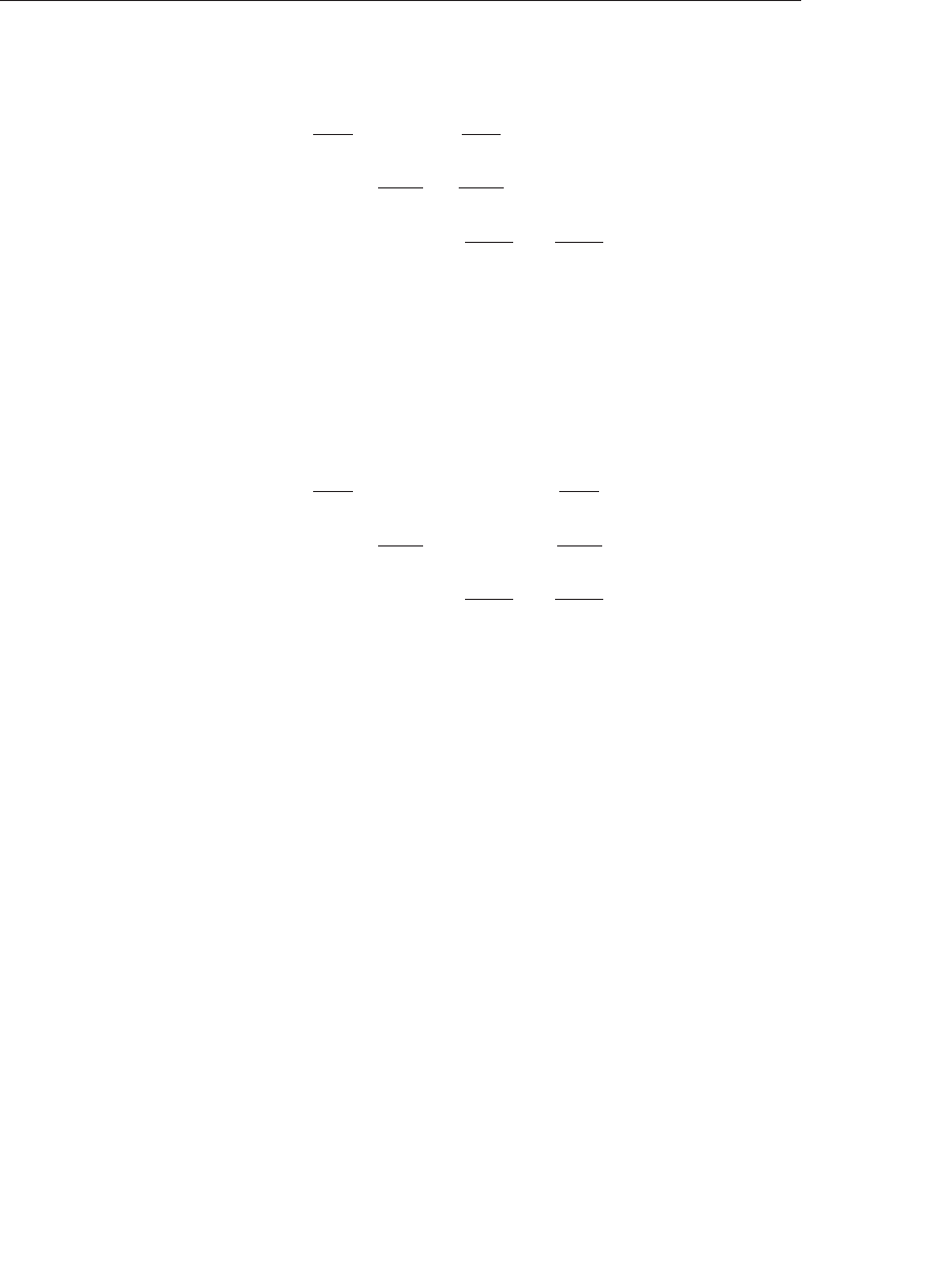
ptg9898810
Perspective Projection
P=
⎡
⎢⎢⎢
⎢⎢⎢
⎢⎢⎢
⎢⎢⎢
⎢⎢⎢
⎣
2n
r−l0r+l
r−l0
02n
t−b
t+b
t−b0
0 0 −f+n
f−n−2fn
f−n
0 0 −1 0
⎤
⎥⎥⎥
⎥⎥⎥
⎥⎥⎥
⎥⎥⎥
⎥⎥⎥
⎦
Pis defined as long as l =r,t =b, and n =f.
Orthographic Projection
P=
⎡
⎢⎢⎢
⎢⎢⎢
⎢⎢⎢
⎢⎢⎢
⎢⎢⎢
⎣
2
r−l0 0 −r+l
r−l
02
t−b0−t+b
t−b
0 0 −2
f−n−f+n
f−n
0 0 0 1
⎤
⎥⎥⎥
⎥⎥⎥
⎥⎥⎥
⎥⎥⎥
⎥⎥⎥
⎦
Pis defined as long as l =r,t =b, and n =f.
834 Appendix E: Homogeneous Coordinates and Transformation Matrices

ptg9898810
Appendix F
OpenGL and Window
Systems
OpenGL is available on many different platforms and works with many
different window systems. It is designed to complement window systems,
not duplicate their functionality. Therefore, OpenGL performs geometric
and image rendering in two and three dimensions, but it does not manage
windows or handle input events.
However, the basic definitions of most window systems don’t support a
library as sophisticated as OpenGL, with its complex and diverse pixel
formats, including depth, and stencil buffers, as well as double-buffering.
For most window systems, some routines are added to extend the window
system to support OpenGL.
This appendix introduces the extensions defined for several window and
operating systems: the X Window System that is supported on most Unix
systems, Microsoft Windows, and Apple Computer’s Mac OS X. You need
to have some knowledge of the window systems to fully understand this
appendix.
This appendix has the following major sections:
•‘‘Accessing New OpenGL Functions’’
•‘‘GLX: OpenGL Extension for the X Window System’’
•‘‘WGL: OpenGL Extensions for Microsoft Windows’’
•‘‘OpenGL in Mac OS X: The Core OpenGL (CGL) API and the
NSOpenGL Classes’’
835

ptg9898810
Accessing New OpenGL Functions
OpenGL changes all the time. The manufacturers of OpenGL graphics
hardware add new extensions and the OpenGL Architecture Review Board
approves those extensions and merges them into the core of OpenGL.
Since each manufacturer needs to be able to update its version of OpenGL,
the header files (like glcorearb.h1), and the library you use to compile (like
opengl32.lib, on Microsoft Windows, for example) may be out of sync
with the latest version. This would likely cause errors when compiling (or
more specifically, linking) your application.
To help you work around this problem, a mechanism for accessing the new
functions was added for many of the window system libraries. This
method varies among the different window systems, but the idea is the
same in all cases. You will need to retrieve function pointers for the
functions that you want to use. You need to do this only if the function is
not available explicitly from your library (you’ll know when it isn’t; you’ll
get a linker error).
Each window system that uses this mechanism has its own function for
getting an OpenGL function pointer; check the respective section in this
appendix for specifics.
Here is an example for Microsoft Windows:
#include <windows.h> /*for wglGetProcAddress() */
#include "glext.h" /*declares function pointer typedefs */
PFNGLBINDPROGRAMARBPROC glBindProgramARB;
void
init(void)
{
glBindProgramARB = (PFNGLBINDPROGRAMARB)
wglGetProcAddress("glBindProgramARB");
...
}
The function pointer type---in this case, PFNGLBINDPROGRAMARBPROC---is
defined in glext.h, as are all of the enumerants that you pass into OpenGL
functions. If the returned value is zero (effectively a NULL pointer), the
function is not available in the OpenGL implementation that your
program is using.
GLUT includes a similar routine, glutGetProcAddress(), which simply
wraps the window--system-dependent routine.
1. Newly named for Version 4.3. Preceeding version were named gl3.h, and before that, just
gl.h. For those in the know, glext.h is still the compendium of all OpenGL extensions.
836 Appendix F: OpenGL and Window Systems

ptg9898810
It’s not sufficient in all cases to merely retrieve a function pointer to
determine if functionality is present. To verify that the extension the
functionality is defined from is available, check the extension string (see
‘‘The Query Commands’’ on Page 738 in Appendix D,‘‘State Variables’’ for
details).
GLEW: The OpenGL Extension Wrangler
To simplify both verifying extension support and dealing with the
associated function pointers, we recommend using the open-source GLEW
library (http://glew.sourceforge.net/) developed by Milan Ikits and Marcelo
Magallon, which manages this process simply and elegantly.
To incorporate GLEW into your applications, follow these three simple
steps:
1. Replace the OpenGL and glext.h header files with those of GLEW:
glew.h.
2. Initialize GLEW by calling glewInit() after you’ve created your
window (or more specifically, your OpenGL context). This causes
GLEW to query and retrieve all available function pointers from your
implementation as well as to provide a convenient set of variables for
determining whether a particular version or extension is supported.
3. Verify that the OpenGL version or extension containing the
functionality you want to use is available. GLEW provides a set of
Boolean variables you can check at runtime. For example, the variable
GL_version_4_3 will be available to verify if the OpenGL version is 4.3.
Likewise, for each extension, a variable like GL_ARB_map_buffer_range
(which is the OpenGL token for the map buffer range extension) is
also defined. If the variable’s value is true, you can use the extension’s
functions.
In the case of OpenGL versions and GLEW variables, all version variables
will have a true value up to and including the current version.
Here’s a short example using our init() routine, which is executed after
calling glutCreateWindow():
#include <GLEW.h>
void
init()
{
GLuint vao;
Accessing New OpenGL Functions 837

ptg9898810
glewInit(); // Initialize the GLEW library
if (GL_version_3_0) {
// We know that OpenGL version 3.0 is supported, which is the
// minimum version of OpenGL supporting vertex array objects
glGenVertexArrays(1, &vao);
glBindVertexArray(vao);
}
// Initialize and bind all other vertex arrays
...
}
GLX: OpenGL Extension for the X Window System
In the X Window System, OpenGL rendering is made available as an
extension to X in the formal X sense. GLX is an extension to the X
protocol (and its associated API) for communicating OpenGL commands
to an extended X server. Connection and authentication are accomplished
with the normal X mechanisms.
As with other X extensions, there is a defined network protocol for
OpenGL’s rendering commands encapsulated within the X byte stream, so
client-server OpenGL rendering is supported. Since performance is critical
in three-dimensional rendering, the OpenGL extension to X allows
OpenGL to bypass the X server’s involvement in data encoding, copying,
and interpretation, and instead render directly to the graphics pipeline.
GLX Version 1.3 introduces several sweeping changes, starting with the
new GLXFBConfig data structure, which describes the GLX framebuffer
configuration (including the depth of the color buffer components, and
the types, quantities, and sizes of the depth, stencil, accumulation, and
auxiliary buffers). The GLXFBConfig structure describes these framebuffer
attributes for a GLXDrawable rendering surface. (In X, a rendering surface
is called a Drawable.)
GLX 1.3 also provides for three types of GLXDrawable surfaces:
GLXWindow, GLXPixmap, and GLXPbuffer. A GLXWindow is on-screen; a
GLXPixmap or GLXPbuffer is off-screen. Because a GLXPixmap has an
associated X pixmap, both X and GLX may render into a GLXPixmap.
GLX may be the only way to render into a GLXPbuffer. The GLXPbuffer is
intended to store pixel data in nonvisible framebuffer memory. (Off-screen
rendering isn’t guaranteed to be supported for direct renderers.)
GLX version 1.4 (the current version at the time of this writing), increased
support for framebuffer configuration by adding drawable configuration
options for number of buffers and samples for multisampled drawables.
838 Appendix F: OpenGL and Window Systems

ptg9898810
The X Visual is an important data structure for maintaining pixel format
information about an OpenGL window. A variable of data type
XVisualInfo keeps track of pixel format information, including pixel type
(RGBA or color-index), single- or double-buffering, resolution of colors,
and presence of depth, stencil, and accumulation buffers. The standard X
Visuals (for example, PseudoColor and TrueColor) do not describe the
pixel format details, so each implementation must extend the number of X
Visuals supported.
In GLX 1.3, a GLXWindow has an X Visual, associated with its
GLXFBConfig. For a GLXPixmap or a GLXPbuffer, there may or may not
be a similar associated X Visual. Prior to GLX 1.3, all surfaces (windows or
pixmaps) were associated with an X Visual. (Prior to 1.3, Pbuffers were not
part of GLX.)
The GLX routines are discussed in more detail in the OpenGL Reference
Manual. Integrating OpenGL applications with the X Window System and
the Motif widget set is discussed in great detail in OpenGL Programming
for the X Window System by Mark Kilgard (Addison-Wesley, 1996), which
includes full source code examples. If you absolutely want to learn about
the internals of GLX, you may want to read the GLX specification, which
can be found at
http://www.opengl.org/registry/doc/glx1.4.pdf
Initialization
Use glXQueryExtension() and glXQueryVersion() to determine whether
the GLX extension is defined for an X server and, if so, which version is
present. glXQueryExtensionsString() returns extension information
about the client-server connection. glXGetClientString() returns
information about the client library, including extensions and version
number. glXQueryServerString() returns similar information about the
server.
glXChooseFBConfig() returns a pointer to an array of GLXFBConfig
structures describing all GLX framebuffer configurations that meet the
client’s specified attributes. You may use glXGetFBConfigAttrib() to query
a framebuffer configuration about its support of a particular GLX attribute.
You may also call glXGetVisualFromFBConfig() to retrieve the X Visual
associated with a GLXFBConfig.
Creation of rendering areas varies slightly, depending on the type of
drawable. For a GLXWindow, first create an X Window with an X Visual
that corresponds to the GLXFBConfig. Then use that X Window when
GLX: OpenGL Extension for the X Window System 839

ptg9898810
calling glXCreateWindow(), which returns a GLXWindow. Similarly for a
GLXPixmap, first create an X Pixmap with a pixel depth that matches the
vGLXFBConfig. Then use that Pixmap when calling glXCreatePixmap() to
create a GLXPixmap. A GLXPbuffer does not require an X Window or an X
Pixmap; just call glXCreatePbuffer() with the appropriate GLXFBConfig.
Note: If you are using GLX 1.2 or earlier, you do not have a
GLXFBConfig structure. Instead, use glXChooseVisual(), which
returns a pointer to an XVisualInfo structure describing the X
Visual that meets the client’s specified attributes. You can query a
visual about its support of a particular OpenGL attribute with
glXGetConfig().To render to an off-screen pixmap, you must use
the earlier glXCreateGLXPixmap() routine.
Accessing OpenGL Functions
To access function pointers for extensions and new features in the X
Window System, use the glXGetProcAddress() function. This function is
defined in the glxext.h header file, which can be downloaded from the
OpenGL Web site.
Controlling Rendering
Several GLX routines are provided for creating and managing an OpenGL
rendering context. Routines are also provided for such tasks as handling
GLX events, synchronizing execution between the X and OpenGL streams,
swapping front and back buffers, and using an X font.
Managing an OpenGL Rendering Context
An OpenGL rendering context is created with either
glXCreateNewContext() or glXCreateContextAttribsARB(), whose use is
required in OpenGL Version 3.0 and greater. One of the arguments to these
routines allows you to request a direct rendering context that bypasses the
X server as described previously. (To perform direct rendering, the X server
connection must be local, and the OpenGL implementation needs to
support direct rendering.) Another argument also allows display-list and
texture-object indices and definitions to be shared by multiple rendering
contexts. You can determine whether a GLX context is direct with
glXIsDirect().
glXMakeContextCurrent() binds a rendering context to the current
rendering thread and also establishes two current drawable surfaces. You
840 Appendix F: OpenGL and Window Systems

ptg9898810
can draw into one of the current drawable surfaces and read pixel data
from the other drawable. In many situations, the draw and read drawables
refer to the same GLXDrawable surface. glXGetCurrentContext() returns
the current context. You can also obtain the current draw drawable with
glXGetCurrentDrawable(), the current read drawable with
glXGetCurrentReadDrawable(), and the current X Display with
glXGetCurrentDisplay().You can use glXQueryContext() to determine
the current values for context attributes.
Only one context can be current for any thread at any one time. If you
have multiple contexts, you can copy selected groups of OpenGL state
variables from one context to another with glXCopyContext(). When
you’re finished with a particular context, destroy it with
glXDestroyContext().
Note: If you are using GLX 1.2 or earlier, use glXCreateContext() to
create a rendering context and glXMakeCurrent() to make it
current. You cannot declare a drawable as a separate read drawable,
so you do not have glXGetCurrentReadDrawable().
Handling GLX Events
GLX 1.3 introduces GLX events, which are returned in the event stream of
standard X11 events. GLX event handling has been added specifically to
deal with the uncertainty of the contents of a GLXPbuffer, which may be
clobbered at any time. In GLX 1.3, you may use glXSelectEvent() to select
only one event with GLX_PBUFFER_CLOBBER_MASK. With standard X
event-handling routines, you can now determine if a portion of a
GLXPbuffer (or GLXWindow) has been damaged and then take steps, if
desired, to recover. (Also, you can call glXGetSelectedEvent() to find out if
you are already monitoring this GLX event.)
Synchronizing Execution
To prevent X requests from executing until any outstanding OpenGL
rendering is completed, call glXWaitGL(). Then, any previously issued
OpenGL commands are guaranteed to be executed before any X rendering
calls made after glXWaitGL(). Although the same result can be achieved
with glFinish(),glXWaitGL() doesn’t require a round-trip to the server
and thus is more efficient in cases where the client and server are on
separate machines.
To prevent an OpenGL command sequence from executing until any
outstanding X requests are completed, use glXWaitX(). This routine
GLX: OpenGL Extension for the X Window System 841

ptg9898810
guarantees that previously issued X rendering calls are executed before any
OpenGL calls made after glXWaitX().
Swapping Buffers
For drawables that are double-buffered, the front and back buffers can be
exchanged by calling glXSwapBuffers(). An implicit glFlush() is done as
part of this routine.
Using an X Font
A shortcut for using X fonts in OpenGL is provided with the command
glXUseXFont(). This routine builds display lists for each requested
character from the specified font and font size.
Note: glXUseXFont() uses functionality that was removed from the core
profile of OpenGL in Version 3.1. You can still use glXUseXFont()
if you use the compatibility profile.
Cleaning Up Drawables
Once rendering is completed, you can destroy the drawable surface with
the appropriate call to glXDestroyWindow(),glXDestroyPixmap(), or
glXDestroyPbuffer(). (These routines are not available prior to GLX 1.3,
although there is glXDestroyGLXPixmap(), which is similar to
glXDestroyPixmap().)
GLX Prototypes
Initialization
Determine whether the GLX extension is defined on the X server:
Bool glXQueryExtension(Display *dpy, int *errorBase,
int *eventBase);
Query version and extension information for client and server:
Bool glXQueryVersion(Display *dpy, int *major, int *minor);
const char* glXGetClientString(Display *dpy, int name);
const char* glXQueryServerString(Display *dpy, int screen,
int name);
const char* glXQueryExtensionsString(Display *dpy, int screen);
842 Appendix F: OpenGL and Window Systems

ptg9898810
Obtain available GLX framebuffer configurations:
GLXFBConfig * glXGetFBConfigs(Display *dpy, int screen,
int *nelements);
GLXFBConfig * glXChooseFBConfig(Display *dpy, int screen,
const int attribList,
int *nelements);
Query a GLX framebuffer configuration for attribute or X Visual
information:
int glXGetFBConfigAttrib(Display *dpy, GLXFBConfig config,
int attribute, int *value);
XVisualInfo * glXGetVisualFromFBConfig(Display *dpy,
GLXFBConfig config);
Create surfaces that support rendering (both on-screen and off-screen):
GLXWindow glXCreateWindow(Display *dpy,
GLXFBConfig config,
Window win,
const int *attribList);
GLXPixmap glXCreatePixmap(Display *dpy,
GLXFBConfig config,
Pixmap pixmap,
const int *attribList);
GLXPbuffer glXCreatePbuffer(Display *dpy, GLXFBConfig config,
const int *attribList);
Obtain a pointer to an OpenGL function:
__GLXextFuncPtr glXGetProcAddress(const char *funcName);
Controlling Rendering
Manage and query an OpenGL rendering context:
GLXContext glXCreateNewContext(Display *dpy,
GLXFBConfig config,
int renderType,
GLXContext shareList,
Bool direct);
GLX: OpenGL Extension for the X Window System 843

ptg9898810
GLXContext glXCreateContextAttribsARB((Display *dpy,
GLXFBConfig config,
GLXContext shareList,
Bool direct,
const int *attribs);
Bool glXMakeContextCurrent(Display *dpy,
GLXDrawable drawable,
GLXDrawable read,
GLXContext context);
void glXCopyContext(Display *dpy, GLXContext source,
GLXContext dest, unsigned long mask);
Bool glXIsDirect(Display *dpy, GLXContext context);
GLXContext glXGetCurrentContext(void);
Display* glXGetCurrentDisplay(void);
GLXDrawable glXGetCurrentDrawable(void);
GLXDrawable glXGetCurrentReadDrawable(void);
int glXQueryContext(Display *dpy, GLXContext context,
int attribute, int *value);
void glXDestroyContext(Display *dpy, GLXContext context);
Ask to receive and query GLX events:
int glXSelectEvent(Display *dpy, GLXDrawable drawable,
unsigned long eventMask);
int glXGetSelectedEvent(Display *dpy, GLXDrawable drawable,
unsigned long *eventMask);
Synchronize execution:
void glXWaitGL(void);
void glXWaitX(void);
Exchange front and back buffers:
void glXSwapBuffers(Display *dpy, GLXDrawable drawable);
Use an X font:
void glXUseXFont(Font font, int first, int count, int listBase);
844 Appendix F: OpenGL and Window Systems

ptg9898810
Clean up drawables:
void glXDestroyWindow(Display *dpy, GLXWindow win);
void glXDestroyPixmap(Display *dpy, GLXPixmap pixmap);
void glXDestroyPbuffer(Display *dpy, GLXPbuffer pbuffer);
Deprecated GLX Prototypes
The following routines have been deprecated in GLX 1.3. If you are using
GLX 1.2 or a predecessor, you may need to use several of these routines.
Obtain the desired visual:
XVisualInfo* glXChooseVisual(Display *dpy, int screen,
int *attribList);
int glXGetConfig(Display *dpy, XVisualInfo *visual, int attrib,
int *value);
Manage an OpenGL rendering context:
GLXContext glXCreateContext(Display *dpy,
XVisualInfo *visual,
GLXContext shareList,
Bool direct);
Bool glXMakeCurrent(Display *dpy, GLXDrawable drawable,
GLXContext context);
Perform off-screen rendering:
GLXPixmap glXCreateGLXPixmap(Display *dpy,
XVisualInfo *visual,
Pixmap pixmap);
void glXDestroyGLXPixmap(Display *dpy, GLXPixmap pix);
WGL: OpenGL Extensions for Microsoft Windows
OpenGL rendering is supported on systems that run any modern version
of Microsoft Windows (from Windows 95 and later). The functions and
routines of the Win32 library are necessary to initialize the pixel format
and control rendering, and for access to extensions for OpenGL. Some
routines, which are prefixed by wgl, extend Win32 so that OpenGL can be
fully supported.
WGL: OpenGL Extensions for Microsoft Windows 845

ptg9898810
For Win32/WGL, the PIXELFORMATDESCRIPTOR is the key data structure
for maintaining pixel format information about the OpenGL window.
A variable of data type PIXELFORMATDESCRIPTOR keeps track of pixel
information, including pixel type (RGBA or color-index); single- or
double-buffering; resolution of colors; and presence of depth, stencil, and
accumulation buffers.
To get more information about WGL, you may want to start with technical
articles available through the Microsoft Developer Network Web site
(http://msdn.microsoft.com/).
Initialization
Use GetVersion() or the newer GetVersionEx() to determine version
information. ChoosePixelFormat() tries to find a
PIXELFORMATDESCRIPTOR with specified attributes. If a good match for
the requested pixel format is found, then SetPixelFormat() should be
called for actual use of the pixel format. You should select a pixel format in
the device context before creating a rendering context.
If you want to find out details about a given pixel format, use
DescribePixelFormat() or, for overlays or underlays,
wglDescribeLayerPlane().
Accessing OpenGL Functions
To access function pointers for extensions and new features in Microsoft
Windows, use the wglGetProcAddress() function. This function is defined
in the wingdi.h header file, which is automatically included when you
include windows.h in your application.
Controlling Rendering
Several WGL routines are provided for creating and managing an OpenGL
rendering context, rendering to a bitmap, swapping front and back buffers,
finding a color palette, and using either bitmap or outline fonts.
Managing an OpenGL Rendering Context
wglCreateContext() and wglCreateContextAttribsARB() (the latter for
use with OpenGL Version 3.0 and greater) create an OpenGL rendering
context for drawing on the device in the selected pixel format of the device
context. (To create an OpenGL rendering context for overlay or underlay
windows, use wglCreateLayerContext() instead.) To make a rendering
846 Appendix F: OpenGL and Window Systems

ptg9898810
context current, use wglMakeCurrent();wglGetCurrentContext() returns
the current context. You can also obtain the current device context with
wglGetCurrentDC().You can copy some OpenGL state variables from one
context to another with wglCopyContext() or make two contexts share
the same display lists and texture objects with wglShareLists(). When
you’re finished with a particular context, destroy it with
wglDestroyContext().
Accessing OpenGL Extensions
Use wglGetProcAddress() to access implementation-specific OpenGL
extension procedure calls. To determine which extensions are supported
by your implementation, first call glGetIntegerv() passing
GL_NUM_EXTENSIONS to determine the number of extensions available,
and then call glGetStringi() to retrieve each extension name.
wglGetProcAddress(), when passed the exact name of the extension
returned from glGetStringi(), returns a function pointer for the extension
procedure call, or returns NULL if the extension is not supported.
OpenGL Rendering to a Bitmap
Win32 has a few routines for allocating (and deallocating) bitmaps, to
which you can render OpenGL directly. CreateDIBitmap() creates a
device-dependent bitmap (DDB) from a device-independent bitmap (DIB).
CreateDIBSection() creates a DIB that applications can write to directly.
When finished with your bitmap, you can use DeleteObject() to free it up.
Synchronizing Execution
If you want to combine GDI and OpenGL rendering, be aware that there
are no equivalents to functions such as glXWaitGL(), or glXWaitX() in
Win32. Although glXWaitGL() has no equivalent in Win32, you can
achieve the same effect by calling glFinish(), which waits until all pending
OpenGL commands are executed, or by calling GdiFlush(), which waits
until all GDI drawing has been completed.
Swapping Buffers
For windows that are double-buffered, the front and back buffers can be
exchanged by calling SwapBuffers() or wglSwapLayerBuffers(); the latter
is used for overlays and underlays.
Finding a Color Palette
To access the color palette for the standard (nonlayer) bitplanes, use the
standard GDI functions to set the palette entries. For overlay or underlay
WGL: OpenGL Extensions for Microsoft Windows 847

ptg9898810
layers, use wglRealizeLayerPalette(), which maps palette entries from a
given color-index layer plane into the physical palette or initializes the
palette of an RGBA layer plane. wglGetLayerPaletteEntries() and
wglSetLayerPaletteEntries() are used to query and set the entries in
palettes of layer planes.
Using a Bitmap or Outline Font
WGL has two routines, wglUseFontBitmaps() and wglUseFontOutlines(),
for converting system fonts for use with OpenGL. Both routines build a
display list for each requested character from the specified font and font
size.
Note: Display lists, a feature used by wglUseFontBitmaps() and
wglUseFontOutlines(), were removed from the core profile of
OpenGL since Version 3.1. As such, these routines will not work
properly if you’re using a core profile. However, they are supported
if you use the compatiblity profile.
WGL Prototypes
Initialization
Determine version information:
BOOL GetVersion(LPOSVERSIONINFO lpVersionInformation);
BOOL GetVersionEx(LPOSVERSIONINFO lpVersionInformation);
Pixel format availability, selection, and capability:
int ChoosePixelFormat(HDC hdc,
CONST PIXELFORMATDESCRIPTOR *ppfd);
BOOL SetPixelFormat(HDC hdc, int iPixelFormat,
CONST PIXELFORMATDESCRIPTOR *ppfd);
int DescribePixelFormat(HDC hdc, int iPixelFormat, UINT nBytes,
LPPIXELFORMATDESCRIPTOR ppfd);
BOOL wglDescribeLayerPlane(HDC hdc, int iPixelFormat,
int iLayerPlane,
UINT nBytes,
LPLAYERPLANEDESCRIPTOR plpd);
Obtain a pointer to an OpenGL function:
PROC wglGetProcAddress(LPCSTR funcNam);
848 Appendix F: OpenGL and Window Systems

ptg9898810
Controlling Rendering
Manage or query an OpenGL rendering context:
HGLRC wglCreateContext(HDC hdc);
HGLRC wglCreateContextAttribsARB(HDC hdc,
HGLRC hShareContext,
const int *attribList);
HGLRC wglCreateLayerContext(HDC hdc, int iLayerPlane);
BOOL wglShareLists(HGLRC hglrc1, HGLRC hglrc2);
BOOL wglDeleteContext(HGLRC hglrc);
BOOL wglCopyContext(HGLRC hglrcSource, HGLRC hlglrcDest,
UINT mask);
BOOL wglMakeCurrent(HDC hdc, HGLRC hglrc);
HGLRC wglGetCurrentContext(void);
HDC wglGetCurrentDC(void);
Access implementation-dependent extension procedure calls:
PROC wglGetProcAddress(LPCSTR lpszProc);
Access and release the bitmap of the front buffer:
HBITMAP CreateDIBitmap(HDC hdc,
CONST BITMAPINFOHEADER *lpbmih,
DWORD fdwInit,
CONST VOID *lpbInit,
CONST BITMAPINFO *lpbmi,
UINT fuUsage);
HBITMAP CreateDIBSection(HDC hdc,
CONST BITMAPINFO *pbmi,
UINT iUsage,
VOID *ppvBits,
HANDLE hSection,
DWORD dwOffset);
BOOL DeleteObject(HGDIOBJ hObject);
WGL: OpenGL Extensions for Microsoft Windows 849

ptg9898810
Exchange front and back buffers:
BOOL SwapBuffers(HDC hdc);
BOOL wglSwapLayerBuffers(HDC hdc, UINT fuPlanes);
Find a color palette for overlay or underlay layers:
int wglGetLayerPaletteEntries(HDC hdc, int iLayerPlane,
int iStart, int cEntries,
CONST COLORREF *pcr);
int wglSetLayerPaletteEntries(HDC hdc, int iLayerPlane,
int iStart,
int cEntries,
CONST COLORREF *pcr);
BOOL wglRealizeLayerPalette(HDC hdc, int iLayerPlane,
BOOL bRealize);
Use a bitmap or an outline font:
BOOL wglUseFontBitmaps(HDC hdc, DWORD first,
DWORD count, DWORD listBase);
BOOL wglUsexFontOutlines(HDC hdc, DWORD first,
DWORD count,
DWORD listBase, FLOAT deviation,
FLOAT extrusion, int format,
LPGLYPHMETRICSFLOAT lpgmf );
OpenGL in Mac OS X: The Core OpenGL (CGL) API
and the NSOpenGL Classes
In Apple Computer’s Mac OS X, OpenGL is an integral part of the
windowing system. In fact, the window manager Quartz uses OpenGL to
display windows on the screen and perform all of the window transitions
(like minimizing, etc.). On Mac OS X, there are two methods for setting up
an application to use OpenGL. They are as follows:
•Using CGL, the ‘‘Core OpenGL Library’’, which is a low-lever access API
similar to those of the X Window System and Microsoft Windows.
•Using the NSOpenGL Objective-C classes for direct support in Apple’s
Cocoa framework.
Mac OS X also supports GLUT as an application framework, but its use for
complex application development is discouraged, generally speaking.
850 Appendix F: OpenGL and Window Systems

ptg9898810
Mac OS X also makes an implementation of the X Window System
available as a client application, which supports GLX as described
previously.
We’ll begin by describing the CGL, and then discuss the NSOpenGL
classes, as they use CGL for suppporting OpenGL.
Note: There current window-system framework of Mac OS X is called
‘‘Cocoa’’, and supports the topics described in the following
sections. The previous window-system framework called ‘‘Carbon’’
also supported the CGL API (including some functions which were
deprecated), and a deprecated API named AGL, which we do not
describe.
Mac OS X’s Core OpenGL Library
On Mac OS X, an OpenGL implementation is described using a concept
called a renderer. Usually, Mac OS X manages renderers for you, but you
can control the selection if you need. Once the renderer is chosen, you
then select the buffer attributes your application requires, create a context,
and your application is ready to render using OpenGL.
For complete details of Mac OS X’s OpenGL implementations, go to the
Apple developer Web site (http://developer.apple.com), which contains
user guides and reference documents.
Initialization
Usually, renderers are selected and managed automatically for your by
Mac OS X; however, if you need or want to explicitly control the renderer
for your application, do the following: first, determine the available
renderers by calling CGLQueryRendererInfo(), which returns an opaque
data structure---CGLRendererInfoObj---that you need to use to query the
characteristics of each renderer. Properties of a renderer can be determined
by calling CGLDescribeRenderer(). Once you’ve completed all of your
system queries, you need to release the returned CGLRendererInfoObj by
calling CGLDestroyRendererInfo().
Once you’ve selected the appropriate renderer, you next specify the buffer
attributes required for your application. Specify the attributes you need,
and then verify that the configuration you need is supported by calling
CGLChoosePixelFormat(), which returns a CGLPixelFormatObj object.
As with other objects, you need to release its resource, and in this case,
you’ll call CGLDestroyPixelFormat().
Mac OS X’s Core OpenGL Library 851

ptg9898810
Controlling Rendering
Like the other binding APIs, CGL has routines for controlling OpenGL’s
interaction with the windowing system, including managing OpenGL
contexts.
Managing an OpenGL Rendering Context
After selecting a pixel format, create an OpenGL context by calling
CGLCreateContext() using the returned CGLPixelFormatObj object.
Once the context is created, you need to call CGLSetCurrentContext() to
make the context current and available for OpenGL rendering.
Accessing OpenGL Extensions
Synchronizing Execution
Swapping Buffers
CGL Prototypes
Initialization
Managing Pixel Format Objects:
CGLError CGLChoosePixelFormat(const CGLPixelFormatAttribute *attribs,
CGLPixelFormatObj *pix,
GLint *npix);
CGLError CGLDescribePixelFormat(CGLPixelFormatObj pix,
GLint pix num,
CGLPixelFormatAttribute attrib,
GLintp *value);
CGLPixelFormatObj CGLGetPixelFormat(CGLContextObj ctx);
CGLPixelFormatObj CGLRetainPixelFormat(CGLPixelFormatObj pix);
void CGLReleasePixelFormat(CGLPixelFormatObj pix);
GLuint CGLGetPixelFormatRetainCount(CGLPixelFormatObj pix);
CGLError CGLDestroyPixelFormat(CGLPixelFormatObj pix);
Controlling Rendering
Managing rendering contexts:
852 Appendix F: OpenGL and Window Systems

ptg9898810
CGLError CGLCreateContext(CGLPixelFormatObj pix,
CGLContextObj share,
CGLContextObj *ctx);
CGLContextObj CGLRetainContext(CGLContextObj ctx);
void CGLReleaseContext(CGLContextObj ctx);
GLuint CGLGetContextRetainCount(CGLContextObj ctx);
CGLError CGLDestroyContext(CGLContextObj ctx);
CGLContextObj CGLGetCurrentContext(void);
CGLError CGLSetCurrentContext(CGLContextObj ctx);
Getting and Setting Context Options:
CGLError CGLEnable(CGLContextObj ctx,
CGLContextEnable pname);
CGLError CGLDisable(CGLContextObj ctx,
CGLContextEnable pname);
CGLError CGLIsEnabled(CGLContextObj ctx,
CGLContextEnable pname,
GLint *enable);
CGLError CGLSetParameter(CGLContextObj ctx,
CGLContextParameter pname,
const GLint *params);
CGLError CGLGetParameter(CGLContextObj ctx,
CGLContextParameter pname,
GLint *params);
Locking and unlocking contexts:
CGLError CGLLockContext(CGLContextObj ctx);
CGLError CGLUnlockContext(CGLContextObj ctx);
Managing drawable objects:
CGLError CGLClearDrawable(CGLContextObj ctx);
CGLError CGLFlushDrawable(CGLContextObj ctx);
Getting error information:
const char* CGLErrorString(CGLError error);
Managing global information:
Mac OS X’s Core OpenGL Library 853

ptg9898810
CGLError CGLSetGlobalOption(CGLGlobalOption pname,
const GLint *params);
CGLError CGLGetGlobalOption(CGLGlobalOption pname,
GLint *params);
void CGLGetVersion(GLint *majorvers, GLint *minorvers);
Retrieve rendering information:
CGLError CGLDescribeRenderer(CGLRendererInfoObj rend,
GLint rend_num,
CGLRendererProperty prop,
GLint *value);
CGLError CGLDestroyRendererInfo(CGLRendererInfoObj rend);
CGLError CGLQueryRendererInfo(GLuint display_mask,
CGLRendererInfoObj *rend,
GLint *nrend);
Managing virtual screens:
CGLError CGLSetVirtualScreen(CGLContextObj ctx,
GLint screen);
CGLError CGLGetVirtualScreen(CGLContextObj ctx,
GLint *screen);
CGLError CGLUpdateContext(CGLContextObj ctx);
The NSOpenGL Classes
Initialization
Begin by adding an OpenGL view (through an instance of
NSOpenGLView()) to your application window. Using an
NSOpenGLView() takes care of managing the OpenGL context and the
associated pixel formats; otherwise, you will need to specify the pixel
format for the application’s OpenGL window by allocating an
NSOpenGLPixelFormat() class and using the returned class instance when
creating an OpenGL context with NSOpenGLContext().
It is also possible to add an NSOpenGLView() to your application using
the Interface Builder, but you will need to manually create the associated
pixel format and context objects programmatically.
854 Appendix F: OpenGL and Window Systems

ptg9898810
Once your view is created, you can proceed with OpenGL rendering.
Accessing OpenGL Functions
As compared to the GLX and WGL OpenGL implementations, Mac OS X
provides full-linkage capabilities with its OpenGL framework. That is,
there’s no need (or supported functions) for retrieving function pointers to
OpenGL extensions. All supported entry poins are exported.
The NSOpenGL Classes 855


ptg9898810
Appendix G
Floating-Point Formats for
Textures, Framebuffers,
and Renderbuffers
This appendix describes the floating-point formats used for pixel storage in
framebuffers and renderbuffers, and texel storage in textures. It has the
following major sections:
•‘‘Reduced-Precision Floating-Point Values’’
•‘‘16-bit Floating-Point Values’’
•‘‘10- and 11-bit Unsigned Floating-Point Values’’
857

ptg9898810
Reduced-Precision Floating-Point Values
In addition to the normal 32-bit single-precision floating-point values you
usually use when you declare a GLfloat in your application, OpenGL
supports reduced-precision floating-point representations for storing data
more compactly than its 32-bit representation. In many instances, your
floating-point data may not require the entire dynamic range of a 32-bit
float, and storing or processing data in a reduced-precision format may
save memory and increase data transfer rates.
OpenGL supports three reduced-precision floating-point formats: 16-bit
(signed) floating-point values, and 10- and 11-bit unsigned floating-point
values. Table G-1 describes the bit layout of each representation, and the
associated pixel formats.
Table G.1 Reduced-Precision Floating-Point Formats
Floating-
Point
Type
Associated Pixel Formats Sign Bit
Number
of Expo-
nents
Bits
Number
of
Mantissa
Bits
16-bit GL_RGB16F, GL_RGBA16F 1 5 10
11-bit GL_R11F_G11F_B10F (red
and green components)
056
10-bit GL_R11F_G11F_B10F (blue
component)
055
16-bit Floating-Point Values
For signed 16-bit floating-point values, the minimum and maximum
values that can be represented are (about) 6.103 ×10⁻⁵, and 65504.0,
respectively.
The following routine, F32toF16(), will convert a single, full-precision
32-bit floating-point value to a 16-bit reduced-precision form (stored as an
unsigned short integer).
#define F16_EXPONENT_BITS 0x1F
#define F16_EXPONENT_SHIFT 10
#define F16_EXPONENT_BIAS 15
#define F16_MANTISSA_BITS 0x3ff
#define F16_MANTISSA_SHIFT (23 - F16_EXPONENT_SHIFT)
#define F16_MAX_EXPONENT \
(F16_EXPONENT_BITS << F16_EXPONENT_SHIFT)
858 Appendix G: Floating-Point Formats for Textures, Framebuffers, and Renderbuffers

ptg9898810
GLushort
F32toF16(GLfloat val)
{
GLuint f32 = (*(GLuint *) &val);
GLushort f16 = 0;
/*Decode IEEE 754 little-endian 32-bit floating-point value */
int sign = (f32 >> 16) & 0x8000;
/*Map exponent to the range [-127,128] */
int exponent = ((f32 >> 23) & 0xff) - 127;
int mantissa = f32 & 0x007fffff;
if (exponent == 128) { /*Infinity or NaN */
f16 = sign | F16_MAX_EXPONENT;
if (mantissa) f16 |= (mantissa & F16_MANTISSA_BITS);
}
else if (exponent > 15) { /*Overflow - flush to Infinity */
f16 = sign | F16_MAX_EXPONENT;
}
else if (exponent > -15) { /*Representable value */
exponent += F16_EXPONENT_BIAS;
mantissa >>= F16_MANTISSA_SHIFT;
f16 = sign | exponent << F16_EXPONENT_SHIFT | mantissa;
}
else {
f16 = sign;
}
return f16;
}
Likewise, F16toF32() converts from the reduced-precision floating-point
form into a normal 32-bit floating-point value.
#define F32_INFINITY 0x7f800000
GLfloat
F16toF32(GLushort val)
{
union {
GLfloat f;
GLuint ui;
} f32;
int sign = (val & 0x8000) << 15;
int exponent = (val & 0x7c00) >> 10;
int mantissa = (val & 0x03ff);
f32.f = 0.0;
if (exponent == 0) {
16-bit Floating-Point Values 859

ptg9898810
if (mantissa != 0) {
const GLfloat scale = 1.0 / (1 << 24);
f32.f = scale *mantissa;
}
}
else if (exponent == 31) {
f32.ui = sign | F32_INFINITY | mantissa;
}
else {
GLfloat scale, decimal;
exponent -= 15;
if (exponent < 0) {
scale = 1.0 / (1 << -exponent);
}
else {
scale = 1 << exponent;
}
decimal = 1.0 + (float) mantissa / (1 << 10);
f32.f = scale *decimal;
}
if (sign) f32.f = -f32.f;
return f32.f;
}
10- and 11-bit Unsigned Floating-Point Values
For normalized color values in the range [0, 1], unsigned 10- and 11-bit
floating-point formats may provide a more compact format with better
dynamic range than either floating-point values, or OpenGL’s unsigned
integer pixel formats. The maximum representable values are 65204 and
64512, respectively.
Routines for converting floating-point values into 10-bit unsigned
floating-point values, and vice versa, are shown below.
#define UF11_EXPONENT_BIAS 15
#define UF11_EXPONENT_BITS 0x1F
#define UF11_EXPONENT_SHIFT 6
#define UF11_MANTISSA_BITS 0x3F
#define UF11_MANTISSA_SHIFT (23 - UF11_EXPONENT_SHIFT)
#define UF11_MAX_EXPONENT \
(UF11_EXPONENT_BITS << UF11_EXPONENT_SHIFT)
GLushort
F32toUF11(GLfloat val)
{
860 Appendix G: Floating-Point Formats for Textures, Framebuffers, and Renderbuffers

ptg9898810
GLuint f32 = (*(GLuint *) &val);
GLushort uf11 = 0;
/*Decode little-endian 32-bit floating-point value */
int sign = (f32 >> 16) & 0x8000;
/*Map exponent to the range [-127,128] */
int exponent = ((f32 >> 23) & 0xff) - 127;
int mantissa = f32 & 0x007fffff;
if (sign) return 0;
if (exponent == 128) { /*Infinity or NaN */
uf11 = UF11_MAX_EXPONENT;
if (mantissa) uf11 |= (mantissa & UF11_MANTISSA_BITS);
}
else if (exponent > 15) { /*Overflow - flush to Infinity */
uf11 = UF11_MAX_EXPONENT;
}
else if (exponent > -15) { /*Representable value */
exponent += UF11_EXPONENT_BIAS;
mantissa >>= UF11_MANTISSA_SHIFT;
uf11 = exponent << UF11_EXPONENT_SHIFT | mantissa;
}
return uf11;
}
#define F32_INFINITY 0x7f800000
GLfloat
UF11toF32(GLushort val)
{
union {
GLfloat f;
GLuint ui;
} f32;
int exponent = (val & 0x07c0) >> UF11_EXPONENT_SHIFT;
int mantissa = (val & 0x003f);
f32.f = 0.0;
if (exponent == 0) {
if (mantissa != 0) {
const GLfloat scale = 1.0 / (1 << 20);
f32.f = scale *mantissa;
}
}
else if (exponent == 31) {
f32.ui = F32_INFINITY | mantissa;
}
else {
GLfloat scale, decimal;
10- and 11-bit Unsigned Floating-Point Values 861

ptg9898810
exponent -= 15;
if (exponent < 0) {
scale = 1.0 / (1 << -exponent);
}
else {
scale = 1 << exponent;
}
decimal = 1.0 + (float) mantissa / 64;
f32.f = scale *decimal;
}
return f32.f;
}
For completeness, we present similar routines for converting 10-bit
unsigned floating-point values.
#define UF10_EXPONENT_BIAS 15
#define UF10_EXPONENT_BITS 0x1F
#define UF10_EXPONENT_SHIFT 5
#define UF10_MANTISSA_BITS 0x3F
#define UF10_MANTISSA_SHIFT (23 - UF10_EXPONENT_SHIFT)
#define UF10_MAX_EXPONENT \
(UF10_EXPONENT_BITS << UF10_EXPONENT_SHIFT)
GLushort
F32toUF10(GLfloat val)
{
GLuint f32 = (*(GLuint *) &val);
GLushort uf10 = 0;
/*Decode little-endian 32-bit floating-point value */
int sign = (f32 >> 16) & 0x8000;
/*Map exponent to the range [-127,128] */
int exponent = ((f32 >> 23) & 0xff) - 127;
int mantissa = f32 & 0x007fffff;
if (sign) return 0;
if (exponent == 128) { /*Infinity or NaN */
uf10 = UF10_MAX_EXPONENT;
if (mantissa) uf10 |= (mantissa & UF10_MANTISSA_BITS);
}
else if (exponent > 15) { /*Overflow - flush to Infinity */
uf10 = UF10_MAX_EXPONENT;
}
else if (exponent > -15) { /*Representable value */
exponent += UF10_EXPONENT_BIAS;
mantissa >>= UF10_MANTISSA_SHIFT;
uf10 = exponent << UF10_EXPONENT_SHIFT | mantissa;
}
862 Appendix G: Floating-Point Formats for Textures, Framebuffers, and Renderbuffers

ptg9898810
return uf10;
}
#define F32_INFINITY 0x7f800000
GLfloat
UF10toF32(GLushort val)
{
union {
GLfloat f;
GLuint ui;
} f32;
int exponent = (val & 0x07c0) >> UF10_EXPONENT_SHIFT;
int mantissa = (val & 0x003f);
f32.f = 0.0;
if (exponent == 0) {
if (mantissa != 0) {
const GLfloat scale = 1.0 / (1 << 20);
f32.f = scale *mantissa;
}
}
else if (exponent == 31) {
f32.ui = F32_INFINITY | mantissa;
}
else {
GLfloat scale, decimal;
exponent -= 15;
if (exponent < 0) {
scale = 1.0 / (1 << -exponent);
}
else {
scale = 1 << exponent;
}
decimal = 1.0 + (float) mantissa / 64;
f32.f = scale *decimal;
}
return f32.f;
}
10- and 11-bit Unsigned Floating-Point Values 863


ptg9898810
Appendix H
Debugging and Profiling
OpenGL
This appendix describes the facilities provided by debug contexts, which can
greatly assist you in finding errors in your programs and with getting the
best possible performance from OpenGL. This appendix contains the
following major sections:
•‘‘Creating a Debug Context’’ explains how to create OpenGL contexts
in debug mode, enabling debugging features.
•‘‘Debug Output’’ describes how OpenGL communicates debugging
information back to your application.
•‘‘Debug Groups’’ delves deeper into debug output, showing how your
application, any utility libraries, and tools you use can cooperate to
group parts of your scenes for debug purposes.
•‘‘Profiling’’ concludes the appendix with information about profiling
and optimizing your application for performance.
865

ptg9898810
Creating a Debug Context
To get the most from OpenGL’s debugging facilities, it is necessary to
create a debug context, which implies that you need control over the flags
and parameters used to create the context. Context creation is a platform-
specific task that is often handled by a wrapper layer such as GLUT.
Modern implementations of GLUT (such as FreeGLUT, which we use in
many of this book’s samples) include the function glutInitContextFlags().
This function takes a number of flags that can be used to control how
contexts subsequently created behave. One of these flags is GLUT_DEBUG,
which will enable a debug context. Many other platform abstraction layers
have similar mechanisms. If you are not using an abstraction layer, then
you will need to interface to your platform’s context-creation mechanisms
directly.
In WGL (the window system layer for Microsoft Windows), you need to
use the WGL_ARB_create_context extension and access the
wglCreateContextAttribsARB() function. This function takes as one of its
parameters an attribute list. By specifying the
WGL_CONTEXT_DEBUG_BIT_ARB as one of the context flags, a debug
context will be created. The code to create this context is given in
Example H.1.
Example H.1 Creating a Debug Context Using WGL
HGLRC CreateDebugContext(HDC hDC, HGLRC hShareContext,
int major, int minor)
{
const int attriblist[] =
{// Major version of context
WGL_CONTEXT_MAJOR_VERSION_ARB,
major,
// Minor version of context
WGL_CONTEXT_MINOR_VERSION_ARB,
minor,
// Always select a core profile
WGL_CONTEXT_PROFILE_MASK_ARB,
WGL_CONTEXT_CORE_PROFILE_BIT_ARB,
// Turn on the debug context
WGL_CONTEXT_FLAGS_ARB,
WGL_CONTEXT_DEBUG_BIT_ARB,
0
};
return wglCreateContextAttribsARB(hDC, hShareContext,
attribs);
}
866 Appendix H: Debugging and Profiling OpenGL

ptg9898810
Note that due to some nastiness in the design of WGL, it is not possible
to use any WGL extensions without first creating a context. This is
because wglGetProcAddress() will return NULL if no context is current
at the time it is called. This means that you will need to create a context
with wglCreateContext() first, make it current, get the address of the
wglCreateContextAttribsARB() function and then create a second context
using that function. If you wish, you may delete the first context. Ultimately,
though, you will always end up creating at least two contexts in any new
application that uses a core profile context or needs debugging features.
GLX has a similar mechanism, using the similarly named
glXCreateContextAttribsARB() function. Unlike WGL, there is no
requirement to create and activate a context before determining the
address of glXCreateContextAttribsARB() and so you should use this
function to create the first (and possibly only) context in your application.
Code for GLX equivalent to Example H.1 is given in Example H.2.
Example H.2 Creating a Debug Context Using GLX
GLXContext CreateDebugContext(Display*dpy,
GLXFBConfig config,
GLXContext share_context,
int major, int minor)
{
const int attriblist[] =
{// Major version of context
GLX_CONTEXT_MAJOR_VERSION_ARB,
major,
// Minor version of context
GLX_CONTEXT_MINOR_VERSION_ARB,
minor,
// Always select a core profile
GLX_CONTEXT_PROFILE_MASK_ARB,
GLX_CONTEXT_CORE_PROFILE_BIT_ARB,
// Turn on the debug context
GLX_CONTEXT_FLAGS_ARB,
GLX_CONTEXT_DEBUG_BIT_ARB,
0
};
return glXCreateContextAttribsARB(dpy, config,
share_context,
True, attriblist);
}
Creating a debug context doesn’t really do anything special---it just tells
OpenGL that you’re intending to use its debugging facilities and that it
should turn them on. Once development of your application is completed
Creating a Debug Context 867

ptg9898810
and you’re no longer debugging, you should turn the debug context off as
some of the debugging features supported by OpenGL may come at a
performance cost. Once your application is debugged and working
correctly, you don’t really need to use a debug context and it’s best to avoid
this potential performance loss in a shipping application.
Debug Output
The primary feature of a debug context is the ability to perform additional
error checking and analysis. There are two ways that a debug context can
get this information back to you. The first, which is really intended to
support remote rendering is via a log that is part of the context and must
be queried. The second, and far more efficient mechanism is through the
use of a callback function. The reason that a log exists for remote rendering
is that a remote server cannot call a callback function in the client
application. However, whenever direct rendering is in use, it is strongly
recommended to use the callback function.
A callback function is essentially a function pointer that you pass a
third-party component (such as OpenGL). That component holds on to
the pointer and calls it when it needs the attention of the host application.
The callback function has an agreed-upon prototype and calling
convention such that both sides of the call know how that call should be
handled. The prototype for the callback function is shown in Example H.3.
You hand the pointer to a function with this prototype using the
glDebugMessageCallback() function, whose prototype and a simple
implementation of which is shown below.
Example H.3 Prototype for the Debug Message Callback Function
typedef void (APIENTRY *DEBUGPROC)(GLenum source,
GLenum type,
GLuint id,
GLenum severity,
GLsizei length,
const GLchar*message,
void*userParam);
void APIENTRY DebugCallbackFunction(GLenum source,
GLenum type,
GLuint id,
GLenum severity,
GLsizei length,
const GLchar*message,
void*userParam)
{
868 Appendix H: Debugging and Profiling OpenGL

ptg9898810
printf("Debug Message: SOURCE(0x%04X),"
"TYPE(0x%04X),"
"ID(0x%08X),"
"SEVERITY(0x%04X), \"%s\"\n",
source, type, id, severity, message);
}
void glDebugMessageCallback(DEBUGPROC callback,
void* userParam);
Sets the current debug message callback function pointer to the value
specified in callback. This function will be called when the
implementation needs to notify the client of the generation of a new
debug message. When the callback function is invoked, the userParam
argument to glDebugMessageCallback() will be passed in the userParam
argument of the callback. Otherwise, userParam has no meaning to
OpenGL and may be used for any purpose.
Debug Messages
Each message generated by OpenGL is comprised of a text string and a
number of attributes. These are passed back to the application in the
parameters to the callback function. The prototype of the callback function
is shown in Example H.3 and a declaration of the function is shown below.
void callback(GLenum source, GLenum type, GLuint id,
GLenum severity, GLsizei length,
const GLchar* message, void* userParam);
This is a callback function that will be called by OpenGL when it needs to
send the application a debug message. source,type,id, and severity indicate
the source, type, id, and severity of the message, respectively. length
contains the length of the string whose address is given by message.
userParam contains the value passed to glDebugMessageCallback() in
the userParam argument and otherwise holds no meaning to OpenGL.
Each debug message has several attributes associated with it---the source,
type, and severity of the message, and a unique identifier for that message.
These attributes are passed to the callback function you’ve specified and
can also be used as the basis for message filtering, which will be covered
shortly. The source may be one of the following:
•GL_DEBUG_SOURCE_API indicates that the message originates from
direct usage of OpenGL.
Debug Output 869

ptg9898810
•GL_DEBUG_SOURCE_WINDOW_SYSTEM indicates that the message
originates from the window system (e.g., WGL, GLX, or EGL).
•GL_DEBUG_SOURCE_SHADER_COMPILER indicates that the message
is generated by the shader compiler.
•GL_DEBUG_SOURCE_THIRD_PARTY indicates that the message is
generated by a third-party source such as a utility library, middleware,
or tool.
•GL_DEBUG_SOURCE_APPLICATION indicates that the message was
generated explicitly by the application.
•GL_DEBUG_SOURCE_OTHER indicates that the message does not fit
into any of the above categories.
Messages with the source GL_DEBUG_SOURCE_THIRD_PARTY or
GL_DEBUG_SOURCE_APPLICATION should never be generated by the
OpenGL implementation, but are instead injected into the debug message
stream explicitly either by a tool or library, or by the application directly.
The mechanisms to insert messages into the debug stream will be covered
shortly.
Each debug message also has a type. This allows your application to
determine what to do with the message. The available types of message are
as follows:
•GL_DEBUG_TYPE_ERROR is generated when an error is generated.
•GL_DEBUG_TYPE_DEPRECATED_BEHAVIOR is produced by the use of
deprecated functionality in OpenGL.
•GL_DEBUG_TYPE_UNDEFINED_BEHAVIOR is generated if the
application has attempted to use functionality in a way that might
produce undefined results.
•GL_DEBUG_TYPE_PERFORMANCE indicates that the application is
using OpenGL in a way that is not optimal for performance.
•GL_DEBUG_TYPE_PORTABILITY is generated if the behavior of the
application is relying on the functionality of the OpenGL
implementation that may not be portable to other implementations or
platforms.
•GL_DEBUG_TYPE_MARKER is used for annotation of the debug stream.
•GL_DEBUG_TYPE_PUSH_GROUP is generated when the application
calls glPushDebugGroup().
•GL_DEBUG_TYPE_POP_GROUP is generated when the application calls
glPopDebugGroup().
870 Appendix H: Debugging and Profiling OpenGL

ptg9898810
•GL_DEBUG_TYPE_OTHER is used when the type of the debug message
does not fall into any of the above categories.
In addition to a source and a type, each debug message has a severity
associated with it. Again, these may be used for filtering or otherwise
directing output. For example, an application may choose to log all
message, but cause a break into a debugger in the case that a high severity
message is encountered. The available severities are as follows:
•GL_DEBUG_SEVERITY_HIGH is used to mark the most important
messages and would generally be used for OpenGL errors, shader
compiler failures, and so on.
•GL_DEBUG_SEVERITY_MEDIUM is used to mark messages that the
application really should know about, but that may not be fatal. These
might include portability issues or performance warnings.
•GL_DEBUG_SEVERITY_LOW is used when the OpenGL
implementation needs the developer about issues that they should
address, but that aren’t going to be detrimental to the functioning of
the application. These might include minor performance issues,
redundant state changes, and so on.
•GL_DEBUG_SEVERITY_NOTIFICATION is used to mark messages that
may not have a negative consequence such as a tool attaching to an
application or initialization of the context.
Finally, the unique identifier assigned to each message is implementation
dependent and may be used for any purpose.
Enabling Debug Output
It is possible to enable or disable debug output globally without affecting
filter state. In a debug context, debug output is on by default, and you
should receive fairly verbose messages from the context if your application
does anything it shouldn’t. However, in a nondebug context, while the
default is to not produce any debug output, it is possible to enable debug
messages anyway. You should be aware that a nondebug context may not
generate very useful output---in fact, it may generate nothing at all. To
enable or disable debug output, glEnable() or glDisable() with the
GL_DEBUG_OUTPUT.
In many cases, OpenGL may operate somewhat asynchronously to the
application. In some implementations, OpenGL might batch up several
function calls and execute them later. In some cases this can help the
implementation work around redundancy in the command stream, or to
batch related state changes together and validate a lot of parameters in one
Debug Output 871

ptg9898810
go. In other implementations, the OpenGL driver might run in multiple
threads that could be behind the application in processing order. The
debug output is often generated when parameters are validated, or even
cross-validated against each other, and this can happen some time after
the actual error has occurred from the application’s perspective. The net
result is that the debug callback might not be called immediately when the
application generates an error, but rather when the OpenGL
implementation validates the requested state changes.
To change this behavior, it is possible to ask OpenGL to operate
synchronously with regards to generating debug output. To do this, call
glEnable() with the GL_DEBUG_OUTPUT_SYNCHRONOUS parameter.
This is disabled by default, although some implementations may force all
debug output to be synchronous in a debug context, for example.
However, it’s generally a good idea to turn synchronous debug output on if
you want to rely on it for catching errors.
Filtering Messages
Messages are filtered before they are sent to your callback function. When
you create a debug context, by default, only medium- and high-severity
messages are sent to your callback function. You can enable and disable
various types of messages, filter messages by severity, and even turn
individual messages on and off using their identifiers. To do this, use
glDebugMessageControl().
void glDebugMessageControl(GLenum source, GLenum type,
GLenum severity, GLsizei count,
const GLuint * ids,
Glboolean enabled);
Establishes a message filter that is applied to subsequently generated
messages. If enabled is GL_TRUE, then generated messages matching the
filter formed by source,type,severity, and the list of messages whose
identifiers are stored in ids will be sent to the active debug output
callback. If enabled is GL_FALSE, then those messages will be discarded.
source must be GL_DONT_CARE or one of the defined message severities,
GL_DEBUG_SOURCE_API, GL_DEBUG_SOURCE_WINDOW_SYSTEM,
GL_DEBUG_SOURCE_SHADER_COMPILER,
GL_DEBUG_SOURCE_THIRD_PARTY,
GL_DEBUG_SOURCE_APPLICATION, or GL_DEBUG_SOURCE_OTHER.
872 Appendix H: Debugging and Profiling OpenGL

ptg9898810
type must be GL_DONT_CARE or one of the defined message types,
GL_DEBUG_TYPE_ERROR, GL_DEBUG_TYPE_DEPRECATED_BEHAVIOR,
GL_DEBUG_TYPE_UNDEFINED_BEHAVIOR,
GL_DEBUG_TYPE_PERFORMANCE, GL_DEBUG_TYPE_PORTABILITY,
GL_DEBUG_TYPE_MARKER, GL_DEBUG_TYPE_PUSH_GROUP, or
GL_DEBUG_TYPE_POP_GROUP.
severity must be GL_DONT_CARE or one of the defined message severities,
GL_DEBUG_SEVERITY_HIGH, GL_DEBUG_SEVERITY_MEDIUM,
GL_DEBUG_SEVERITY_LOW, or GL_DEBUG_SEVERITY_NOTIFICATION.
count contains a count of the number of message identifiers stored in the
array whose address is given by ids. If count is nonzero, then ids is the
address of an array of message identifiers that will be used to filter
messages.
If source is GL_DONT_CARE, then the source of the messages will not be
used when forming the filter. That is, messages from any source will be
considered to match the filter. Likewise, if either type or severity is
GL_DONT_CARE, then the type or severity of the message will not be
included in the filter, respectively, and messages of any type or severity will
be considered to match the filter. If count is nonzero, then it indicates the
number of items in the array ids, allowing messages to be filtered by their
unique identifiers. Example H.4 shows a couple of examples of how to
build filters to enable and disable certain classes of debug message.
Example H.4 Creating Debug Message Filters
// Enable all messages generated by the application
glDebugMessageControl(GL_DEBUG_SOURCE_APPLICATION, // Application messages
GL_DONT_CARE, // Don’t care about type
GL_DONT_CARE, // Don’t care about severity
0, NULL, // No unique identifiers
GL_TRUE); // Enable them
// Enable all high severity messages
glDebugMessageControl(GL_DONT_CARE, // Don’t care about origin
GL_DONT_CARE, // Don’t care about type
GL_DEBUG_SEVERITY_HIGH, // High severity messages
0, NULL, // No identifiers
GL_TRUE); // Enable
// Disable all low severity messages
glDebugMessageControl(GL_DONT_CARE, // Don’t care about origin
GL_DONT_CARE, // Don’t care about type
GL_DEBUG_SEVERITY_LOW, // Low severity messages
Debug Output 873

ptg9898810
0, NULL, // No identifiers
GL_FALSE);
// Enable a couple of messages by identifiers
static const GLuint messages[] = { 0x1234, 0x1337 };
glDebugMessageControl(GL_DONT_CARE, // Don’t care about origin
GL_DONT_CARE, // Don’t care about type
GL_DONT_CARE, // Don’t care about severity
2, messages, // 2 ids in "messages"
GL_TRUE);
Application-Generated Messages
There are two sources of message that are reserved for the application or its
helper libraries and tools. These two sources are
GL_DEBUG_SOURCE_APPLICATION, which is intended to be used by the
application for its own messages, and
GL_DEBUG_SOURCE_THIRD_PARTY, which is intended for use by
third-party libraries such as middleware or by tools such as debuggers and
profilers. Messages with these two source identifiers should never be
generated by an OpenGL implementation. Instead they may be injected
into the debug output stream by the application, library, or tool. To do
this, call glDebugMessageInsert(), whose prototype is as follows:
void glDebugMessageInsert(GLenum source, GLenum type,
GLuint id, GLenum severity,
GLint length, const GLchar * buf );
Insert a message into the context’s debug message stream. The text
message contained in buf is sent to the context’s debug message callback
function along with the source,type,id, and severity as specified. If length
is greater than or equal to zero, it is considered to be the length of the
string contained in buf . Otherwise, buf is treated as the address of a
NUL-terminated string.
When you call glDebugMessageInsert() the message contained in buf is
sent directly to the context’s callback function (which might be inside
your application or inside a debugging or profiling tool). The values you
pass in source,type,id, and severity are passed as specified to the callback
function. In general, you should use GL_DEBUG_SOURCE_APPLICATION
for messages generated by your application (or
GL_DEBUG_SOURCE_THIRD_PARTY if you are writing a tool or utility
library). Example H.5 shows an example of sending a message via the
glDebugMessageInsert() function.
874 Appendix H: Debugging and Profiling OpenGL

ptg9898810
Example H.5 Sending Application-Generated Debug Messages
// Create a debug context and make it current
MakeContextCurrent(CreateDebugContext());
// Get some information about the context
const GLchar *vendor = (const GLchar *)glGetString(GL_VENDOR);
const GLchar *renderer = (const GLchar *)glGetString(GL_RENDERER);
const GLchar *version = (const GLchar *)glGetString(GL_VERSION);
// Assemble a message
std::string message = std::string("Created debug context with ") +
std::string(vendor) + std::string(" ") +
std::string(renderer) +
std::string(". The OpenGL version is ") +
std::string(version) + std::string(".");
// Send the message to the debug output log
glDebugMessageInsert(GL_DEBUG_SOURCE_APPLICATION,
GL_DEBUG_TYPE_MARKER,
0x4752415A,
GL_DEBUG_SEVERITY_NOTIFICATION,
-1,
message.c_str());
The result of executing this code on a debug context with the example
implementation of the debug callback function given in Example H.3 is
shown below.
Debug Message: SOURCE(0x824A), TYPE(0x8268),
ID(0x4752415A), SEVERITY(0x826B), "Created
debug context with NVIDIA Corporation GeForce
GTX 560 SE/PCIe/SSE2. The OpenGL version is
4.3.0."
Debug Groups
In a large, complex application, you may have many subsystems rendering
various parts of the scene. For example, you may render the world,
dynamic and animated objects, special effects and particle systems, user
interfaces, or post processing. At any given moment, it is likely that you’ll
be concentrating your attention on just one of these elements. You may be
debugging issues or concentrating on performance. It is likely that you’ll
want to turn on very verbose debug message reporting for the sections of
code you’re working on while leaving debug messages only at their most
concise levels for code that you’ve already debugged. To do this, you will
Debug Groups 875

ptg9898810
need to turn certain categories of messages on and off and to restore the
debug log to its original state, you would need to query the current state of
the debug context to determine whether certain types of messages are
enabled or disabled.
Rather than trying to implement all of this yourself, you can rely on
OpenGL’s debug groups, which is a stack-based system of filters that allows
you to push the current debug state onto an internal stack managed by
OpenGL, modify the state, and then return to a previously saved state by
popping it of the stack. The functions to do this are glPushDebugGroup()
and glPopDebugGroup().
void glPushDebugGroup(GLenum source, GLuint id,
GLint length, const GLchar * message);
void glPopDebugGroup();
glPushDebugGroup() pushes the current state of the debug output filter
onto the debug group stack and injects message into the current debug
output message stream with the type GL_DEBUG_TYPE_PUSH_GROUP,
severity GL_DEBUG_SEVERITY_NOTIFICATION, and the source and id as
specified. If length is greater than or equal to zero, then it is considered to
be the length of the string in message, otherwise message is treated as a
NUL-terminated string.
glPopDebugGroup() removes the debug state from the top of the debug
group stack and injects a debug message into the debug message output
stream with type GL_DEBUG_TYPE_POP_GROUP and all other parameters
sourced from the corresponding group that was popped from the stack.
For both functions, source must be either
GL_DEBUG_SOURCE_APPLICATION or
GL_DEBUG_SOURCE_THIRD_PARTY.
In addition to allowing the current state of the debug output filters to be
saved and restored, pushing and popping the debug group also generates
messages to the debug output callback function. This function, often
implemented inside tools and debuggers, can track the current depth of
the debug group stack and apply formatting changes to the displayed
output such as coloring or indentation.
Each implementation has a maximum depth of the debug group stack.
This depth must be at least 64 groups, but you can find the actual
maximum by calling glGetIntegerv() with the parameter
GL_MAX_DEBUG_GROUP_STACK_DEPTH. If you attempt to push more
876 Appendix H: Debugging and Profiling OpenGL

ptg9898810
than this number of debug groups onto the stack, then
glPushDebugGroup() will generate a GL_STACK_OVERFLOW error.
Likewise, if you try to pop an item from an empty stack, then
glPopDebugGroup() will generate a GL_STACK_UNDERFLOW error.
Naming Objects
When OpenGL generates debugging messages, it will sometimes make
reference to objects such as textures, buffers, or framebuffers. In a complex
application, there may be hundreds or thousands of textures and buffers in
existence at any given time. Each of these objects has a unique identifier
that was assigned by OpenGL’s glGenTextures(),glGenBuffers(), or other
name-generation functions and those names may have no bearing on
what the application intends to use them for. It is possible to name the
objects by giving them labels. If you give an object a label, then when a
reference to it appears in a debug message, OpenGL will use the object’s
label rather than (or as well as) its number. To give an object a label, use
glObjectLabel() or glObjectPtrLabel().
void glObjectLabel(GLenum identifier, GLuint name,
GLsizei length, const GLchar * label);
void glObjectPtrLabel(void * ptr, GLsizei length,
const GLchar * label);
glObjectLabel() and glObjectPtrLabel() allow objects owned by OpenGL
to be labeled for the purpose of identification during debugging. Labeling
objects allows them to be referenced by name rather than number in
debug messages. glObjectLabel() is provided to label objects represented
by names within the namespace identifier, whereas glObjectPtrLabel() is
provided to label objects that are represented as pointers by OpenGL
(such as sync objects).
If length is greater than or equal to zero, then it is interpreted as the
length of the string pointed to by label. Otherwise, label is considered to
point to a NUL-terminated string that will be used to label the object.
When you apply a label to an object then the label is stored with the
object by OpenGL. When it is referred to in a debug message, OpenGL can
then use the label you provided rather than just using the numerical name
directly. You can also retrieve the label of the object by calling
glGetObjectLabel() or glGetObjectPtrLabel().
Debug Groups 877

ptg9898810
void glGetObjectLabel(GLenum identifier, GLuint name,
GLsizei bufsize, GLsizei * length,
GLchar * label);
void glGetObjectPtrLabel(void * ptr, GLsizei bufsize,
GLsizei * length, GLchar * label);
glGetObjectLabel() and glGetObjectPtrLabel() retrieve the labels that
have previously been assigned to objects by the glObjectLabel() or
glObjectPtrLabel() functions, respectively. For glGetObjectLabel(),name
and identifier provide the numeric name of an object and the namespace
from which it was allocated. For glGetObjectPtrLabel(),ptr is the pointer
variable that is provided by OpenGL.
For both glObjectLabel() and glGetObjectLabel(),name is the numerical
name of the object that was provided by OpenGL through a call to
glGenTextures(),glGenBuffers(), or other object name-generation
functions. Because names for different object types are allocated from
different namespaces, the identifier parameter is provided to allow you to
tell OpenGL which namespace name resides in. identifier must be one of
the following tokens:
•GL_BUFFER indicates that name is the name of a buffer object
generated by glGenBuffers().
•GL_SHADER indicates that name is the name of a shader object
generated by glCreateShader().
•GL_PROGRAM indicates that name is the name of a program object
generated by glCreateProgram().
•GL_QUERY indicates that name is the name of a query object generated
by glGenQueries().
•GL_PROGRAM_PIPELINE indicates that name is the name of a program
pipeline object generated by glGenProgramPipelines().
•GL_SAMPLER indicates that name is the name of a sampler object
generated by glGenSamplers().
The maximum length of a label that can be applied to an object is given by
the value of the implementation-dependent constant
GL_MAX_LABEL_LENGTH. One potential use of object labels, for example,
is to modify your texture-loading code such that the generated texture
objects are labeled with the filename of the texture. Then, if there’s a
problem with a particular texture, a tool might be able to cross reference
the texture object with the file that it was loaded from to verify that the
data ended up in the right place.
878 Appendix H: Debugging and Profiling OpenGL

ptg9898810
Profiling
Once your application is close to its final state, you may wish to turn your
attention to performance tuning. One of the most important aspects of
performance tuning is not the modifications you make to your code to
make it run faster, but the measurements and experiments you make to
determine what you should do to your code to achieve your desired
performance goals. This is known as performance profiling.
Performance measurement techniques generally fall into two1categories;
the first is tool-assisted profiling and the second involves actually making
changes to your code to measure its execution time.
Profiling Tools
Perhaps the most powerful way to profile your application is to use an
external profiling and debugging tool. This type of tool hooks OpenGL on a
running system and intercepts the function calls that your application
makes. The simplest tools merely take a log of the function calls, perhaps
gathering statistics or other information about them. Some of these tools
may even allow you to play back the resulting trace and replicate the
execution of your application in a standalone environment. More
advanced tools allow you to inspect data that flows between the
application and OpenGL, to time execution of various elements of the
scene and even to modify the application’s behavior as it executes by
disabling parts of the OpenGL pipeline, replacing shaders or textures with
alternatives, and so on.
One such application is AMD’s GPUPerfStudio 2, a screenshot of which is
shown in Figure H.1.2
In Figure H.1, GPUPerfStudio 2 is being used to examine the application’s
call trace generated by the Unigine Heaven 3.0 benchmark, which makes
advanced use of modern OpenGL. A screenshot of the application is
shown in Figure H.2.3The application makes use of advanced graphics
features including tessellation, instancing, and off-screen rendering, and
renders effects such as reflections and volumetric lighting effects.
GPUPerfStudio 2 is able to capture the OpenGL calls made by the
benchmark and measure their execution time. On some GPUs, it is even
1. Not including ‘‘try a bunch of stuff and see what happens’’.
2. Figure H.1 courtesy of AMD.
3. Figure H.2 is of Unigine Heaven DX11 benchmark developed by Unigine Corp.:
http://unigine.com/ . Used by permission.
Profiling 879
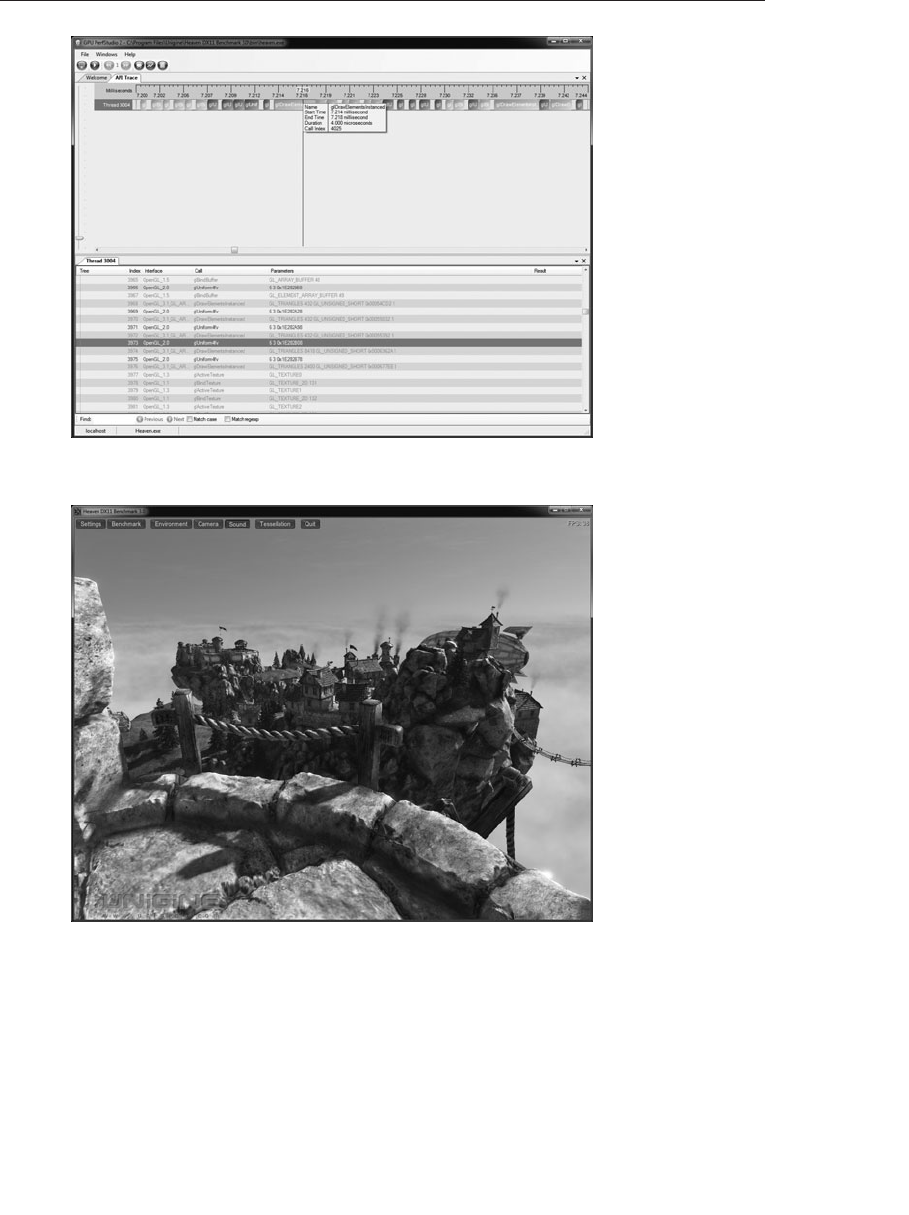
ptg9898810
Figure H.1 AMD’s GPUPerfStudio2 profiling Unigine Heaven 3.0
Figure H.2 Screenshot of Unigine Heaven 3.0
able to measure the amount of time various parts of the OpenGL pipeline
(such as the texture processor, tessellation engine, blending unit, etc.)
spend on individual commands. The tool will tell you if you are making
too many draw commands, which ones are the most expensive, and what
880 Appendix H: Debugging and Profiling OpenGL

ptg9898810
the GPU spends its time on for each one. Profiling tools such as
GPUPerfStudio 2 are an invaluable resource for performance tuning and
debugging OpenGL applications.
In-Application Profiling
It is possible for your application to measure its own performance. A naïve
approach is to simply measure the amount of time taken for a particular
piece of code to execute by reading the system time or just measuring
framerate (besides, framerate is a fairly poor measure of application
performance). However, assuming your application is efficiently written,
the goal is for the graphics processor to be the bottleneck, and therefore
you are interested in the amount of time it takes to process parts of your
scene.
You can make these measurements yourself. In fact, some tools may use
very similar mechanisms to measure GPU performance by injecting
equivalent sequences of commands into your application’s rendering
thread. OpenGL provides two types of timer queries for this purpose. The
two types of query are an elapsed time query and an instantaneous time
query. The first operates very similarly to an occlusion query as described
in ‘‘Occlusion Query’’ in Chapter 4.
Elapsed Time Queries
Elapsed time queries use the GPU’s internal counters to measure the
amount of time it spends processing OpenGL commands. As with
occlusion queries, you wrap one or more rendering commands in a timer
query and then read the results of the query back into the application,
ideally at a later time so as to not force the GPU to finish rendering that
may be in the pipeline.
To start an elapsed time query, call glBeginQuery() with the target
parameter set to GL_TIME_ELAPSED and with id set to the name of a query
object retrieved from a call to glGenQueries().To end the query, call
glEndQuery() again with the target parameter set to GL_TIME_ELAPSED.
Once the query has ended, retrieve the result by calling
glGetQueryObjectuiv() with the name of the query object in id and the
pname parameter set to GL_QUERY_RESULT. The resulting value is the
time, measured in nanoseconds to execute the commands between the calls
to glBeginQuery() and glEndQuery().You should be aware that a
nanosecond is an extremely small amount of time. One unsigned integer is
large enough to count roughly four seconds worth of nanoseconds, after
which it will roll over and start from zero again. If you expect your timer
Profiling 881

ptg9898810
queries to last a very long time (such as the duration of several tens or
hundreds of frames), you might want to use glGetQueryObjectui64v(),
which retrieves the result as a 64-bit number.4
An example of using an elapsed time query is shown in Example H.6.
Example H.6 Using an Elapsed Time Query
GLuint timer_query;
GLuint nanoseconds;
// Generate the timer query
glGenQueries(1, &timer_query);
// Set up some state... (not relevant to the timer query)
glEnable(GL_DEPTH_TEST);
glDepthFunc(GL_LEQUAL);
glEnable(GL_BLEND);
glBlendFunc(GL_SRC_ALPHA, GL_ONE_MINUS_SRC_ALPHA);
glBindVertexArray(vao);
// Begin the query
glBeginQuery(GL_TIME_ELAPSED, timer_query);
// Draw some geometry
glDrawArraysInstanced(GL_TRIANGLES, 0, 1337, 1234);
// End the query
glEndQuery(GL_TIME_ELAPSED);
// Go do something time consuming so as to not stall
// the OpenGL pipeline
do_something_that_takes_ages();
// Now retrieve the timer result
glGetQueryObjectuiv(timer_query, &nanoseconds);
Instantaneous Timer Queries
Instantaneous timer queries also use the query object mechanism to
retrieve times measured in nanoseconds from the GPU. However, as they
are essentially snapshots of the GPU clock, they don’t have a duration and
are never ‘‘current’’, and so cannot be used with glBeginQuery() or
glEndQuery(). Instead, you use the glQueryCounter() function to issue a
timestamp query.
4. 64-bits worth of nanoseconds should allow you to count until the end of the universe.
882 Appendix H: Debugging and Profiling OpenGL

ptg9898810
void glQueryCounter(GLuint id, GLenum target);
Issues a timestamp query into the OpenGL command queue using the
query object whose name is id.target must be GL_TIMESTAMP.
When glQueryCounter() is called, OpenGL inserts a command into the
GPU’s queue to record its current time into the query object as soon as it
comes across it. It may still take some time to get to the timestamp query,
and so your application should perform meaningful work before retrieving
the result of the query. Again, to get the result of the query object, call
glGetQueryObjectuiv(). Once you have instantaneous timestamps taken
at various parts of your scene, you can take deltas between them to
determine how long each part of the scene took, in GPU time and have
some idea what is making the application expensive to execute and where
you should focus your energy as you try to make it run faster.
Profiling 883


ptg9898810
Using Standard Layout Qualifiers
When you group a number of variables in a uniform buffer or shader
storage buffer, and want to read or write their values outside a shader, you
need to know the offset of each one. You can query these offsets, but for
large collections of uniforms this process requires many queries and is
cumbersome. As an alternative, the standard layout qualifiers request that
the GLSL shader compiler organize the variables according to a set of rules,
where you can predictably compute the offset of any member in the block.
In order to qualify a block to use the std140 layout, you need to add a
layout directive to its declaration, as demonstrated below:
layout (std140) uniform UniformBlock {
// declared variables
};
This std140 qualification also works for shader storage buffer objects. The
layout qualifier std430 is available only for shader storage buffer objects,
and is shown below:
layout (std430) buffer BufferBlock {
// declared variables
};
To use these, the offset of a member in the block is the accumulated total
of the alignment and sizes of the previous members in the block (those
declared before the variable in question), bumped up to the alignment of
the member. The starting offset of the first member is always zero.
The std140 Layout Rules
The set of rules shown in Table I.1 are used by the GLSL compiler to place
members in an std140-qualified uniform block. This feature is available
only with GLSL Version 1.40 or greater.
Table I.1 std140 Layout Rules
Variable Type Variable Size and Alignment
Scalar bool,int,uint,float and
double
Both the size and alignment are the size
of the scalar in basic machine types
(e.g., sizeof(GLfloat)).
Two-component vectors (e.g., ivec2) Both the size and alignment are twice
the size of the underlying scalar type.
Three-component vectors (e.g., vec3)
and
Four-component vectors (e.g., vec4)
Both the size and alignment are four
times the size of the underlying scalar
type.
886 Appendix I: Buffer Object Layouts

ptg9898810
Table I.1 (continued) std140 Layout Rules
Variable Type Variable Size and Alignment
An array of scalars or vectors The size of each element in the array
will be the size of the element type,
rounded up to a multiple of the size of a
vec4. This is also the array’s alignment.
The array’s size will be this rounded-up
element’s size times the number of
elements in the array.
A column-major matrix or an array
of column-major matrices of size C
columns and Rrows
Same layout as an array of Nvectors
each with Rcomponents, where Nis
the total number of columns present.
A row-major matrix or an array of
row-major matrices with Rrows and C
columns
Same layout as an array of Nvectors
each with Ccomponents, where Nis
the total number of rows present.
A single-structure definition, or an array
of structures
Structure alignment will be
the alignment for the biggest structure
member, according to the previous
rules, rounded up to a multiple of the
size of a vec4. Each structure will start
on this alignment, and its size will be the
space needed by its members, according
to the previous rules, rounded up to
a multiple of the structure alignment.
The std430 Layout Rules
The set of rules shown in Table I.2 are used by the GLSL compiler to place
members in an std430-qualified uniform block. This feature is available
only with GLSL Version 4.30 or greater.
Table I.2 std430 Layout Rules
Variable Type Variable Size and Alignment
Scalar bool,int,uint,float and
double
Both the size and alignment are the size
of the scalar in basic machine types
(e.g., sizeof(GLfloat)).
Two-component vectors (e.g., ivec2) Both the size and alignment are twice
the size of the underlying scalar type.
Three-component vectors (e.g., vec3)
and
Four-component vectors (e.g., vec4)
Both the size and alignment are four
times the size of the underlying scalar
type. However, this is true only when
the member is not part of an array or
nested structure.
The std430 Layout Rules 887

ptg9898810
Table I.2 (continued) std430 Layout Rules
Variable Type Variable Size and Alignment
An array of scalars or vectors The size of each element in the array
will be the same size of the element
type, where three-component vectors
are not rounded up to the size of
four-component vectors. This is also the
array’s alignment. The array’s size will
be the element’s size times the number
of elements in the array.
A column-major matrix or an array
of column-major matrices of size C
columns and Rrows
Same layout as an array of Nvectors
each with Rcomponents, where Nis
the total number of columns present.
A row-major matrix or an array of
row-major matrices with Rrows and C
columns
Same layout as an array of Nvectors
each with Ccomponents, where Nis
the total number of rows present.
A single-structure definition or an array
of structures
Structure alignment is the same as the
alignment for the biggest structure
member, where three-component
vectors are not rounded up to the size of
four-component vectors. Each structure
will start on this alignment, and its size
will be the space needed by its
members, according to the previous
rules, rounded up to a multiple of the
structure alignment.
888 Appendix I: Buffer Object Layouts

ptg9898810
Glossary
affine transformation A transformation that preserves straight lines and
the ratio of distances of points lying on lines.
aliasing Artifacts created by undersampling a scene, typically caused by
assigning one point sample per pixel, where there are edges or
patterns in the scene of higher frequency than the pixels. This results
in jagged edges (jaggies), moiré patterns, and scintillation. See
antialiasing.
alpha The fourth color component. The alpha component is never
displayed directly, and is typically used to control blending of colors.
By convention, OpenGL alpha corresponds to the notion of opacity,
rather than transparency, meaning that an alpha value of 1.0 implies
complete opacity, and an alpha value of 0.0 complete transparency.
alpha value See alpha.
ambient Ambient light is light not directly associated with a light source,
and is distributed uniformly throughout space, with light falling
upon a surface approaching from all directions. The light is reflected
from the object independent of surface location and orientation,
with equal intensity in all directions.
amplication The process of a geometry shader creating more geometry
than was passed to it.
animation Generating repeated renderings of a scene, with smoothly
changing viewpoint and object positions, quickly enough so that the
illusion of motion is achieved. OpenGL animation is almost always
done using double-buffering.
anisotropic filtering A texture-filtering technique that improves image
quality by sampling the texture using independent
texture-interpolation rates for each texture dimension.
889

ptg9898810
antialiasing Rendering techniques that reduce aliasing. These techniques
include sampling at a higher frequency, assigning pixel colors based
on the fraction of the pixel’s area covered by the primitive being
rendered, removing high-frequency components in the scene, and
integrating or averaging the area of the scene covered by a pixel, as in
area sampling. See antialiasing.
API See application programming interface.
application programming interface A library of functions and
subroutines that an application makes calls into. OpenGL is an
example of an application programming interface.
area sampling Deciding what color to color a pixel based on looking at
the entire content of the scene covered by the pixel. This is as
opposed to point sampling.
array textures Array textures are texture objects that contain multiple
layers or slices that are treated as one associated block of data.
atomic counter A counter object usable in all of OpenGL’s shader stages
that is updated atomically. See atomic operation.
atomic operation In the context of concurrent (multithreaded)
programming, an operation that is always completed without
interruption.
attenuation The property of light that describes how a light’s intensity
diminishes over distance.
back faces See faces.
barycentric coordinates A coordinate system where a point is
represented as a weighted sum of two or more reference points.
Varying a barycentric coordinate between zero and one in each
component moves it within its domain.
Bernstein polynomials A family of polynomial equations named after
Sergei Natanovich Bernstein that are used in evaluating Bézier curves.
The polynomials are defined as follows:
bn,m(x) = n
mxn(1−x)n−m
where n
mis a binomial coefficient.
billboard Usually a texture-mapped quadrilateral that is oriented to be
perpendicular to the viewer. Often billboards are used to approximate
complex geometry at a distance.
890 Glossary

ptg9898810
binding an object Attaching an object to the OpenGL context,
commonly through a function that starts with the word bind, such as
glBindTexture(),glBindBuffer(), or glBindSampler().
binomial coefficient The coefficients of the terms in the expansion of the
polynomial (1+x)n. Binomial coefficients are often described using
the notation n
k, where
n
k=n!
k!(n−k)!
where n!is the factorial of n.
binormal A vector perpendicular to both a surface tangent vector and the
surface normal vector. These three mutually orthogonal vectors can
form the basis of a local coordinate system, including a surface-local
coordinate space.
bit A short form for ‘‘binary digit’’. A state variable having only two
possible values: 0 or 1. Binary numbers are constructions of one or
more bits.
bit depth The number of bits available for a particular component,
limiting the set of values that can be stored in the component.
bitplane A rectangular array of bits mapped one-to-one with pixels. The
framebuffer can be considered a stack of bitplanes.
blending Reduction of two color components to one component, usually
as a linear interpolation between the two components.
buffer A group of bitplanes that store a single component, such as depth
or green. Sometimes the red, green, blue, and alpha buffers together
are referred to as the color buffer, rather than the color buffers.
buffer object A buffer located in the OpenGL’s server memory. Vertex
and pixel data, uniform variables, and element-array indices may be
stored in buffer objects.
buffer objects Objects representing linear allocations of memory that
may be used to store data.
buffer ping-ponging A technique---mostly used for GPGPU---where two
equally sized buffers are used accumulating results. For a particular
frame, one buffer holds current results and is read from, and the
other buffer is written to updating those results. For the next frame,
the buffers’ roles are swapped (ping-ponged).
bump map See normal map.
Glossary 891

ptg9898810
bump mapping Broadly, this is adding the appearance of bumps through
lighting effects even though the surface being rendered is flat. This is
commonly done using a normal map to light a flat surface as if it were
shaped as dictated by the normal map, giving lighting as if bumps
existed on the surface, even though there is no geometry describing
the bumps.
byte swapping The process of exchanging the ordering of bytes in a
(usually integer) variable type (i.e., int,short, etc.).
CThe programming language of Unix kernel hackers.
C++ Most common programming language for programming computer
graphics.
cascading style sheet A presentation mechanism for specifying the look
and layout of Web pages.
client The computer from which OpenGL commands are issued. The
client may be the same computer that the OpenGL server is running
on (see server), or it may be a different machine connected via a
network (assuming the OpenGL implementation supports network
rendering).
clip See clipping.
clip coordinates The coordinate system that follows transformation by
the projection matrix and precedes perspective division. View-
volume clipping is done in clip coordinates.
clipping Elimination of the portion of a geometric primitive that’s
outside the half-space defined by a clipping plane. Points are simply
rejected if outside. The portion of a line or triangle that’s outside the
half-space is eliminated, and additional vertices are generated as
necessary to complete the primitive within the clipping half-space.
Geometric primitives are always clipped against the six half-spaces
defined by the left, right, bottom, top, near, and far planes of the view
volume. Applications can optionally perform application-specific
clipping through use of clip distances, gl_ClipDistance[].
clipping region The intersection of all the half-spaces defined by the
clipping planes. See clipping.
CMYK Cyan, Magenta, Yellow, Black. A color space often used in printing.
color space A model for describing colors, often as vectors within a
three- or four-dimensional domain such as the RGB color space.
892 Glossary

ptg9898810
compatibility profile The profile of OpenGL that still supports all legacy
functionality. It is primarily intended to allow the continued
development of older applications. See also core profile.
components Individual scalar values in a color or direction vector. They
can be integer or floating-point values. Usually, for colors, a
component value of zero represents the minimum value or intensity,
and a component value of one represents the maximum value or
intensity, although other ranges are sometimes used. Because
component values are interpreted in a normalized range, they are
specified independent of actual resolution. For example, the RGB
triple (1,1,1) is white, regardless of whether the color buffers store 4,
8, or 12 bits each. Out-of-range components are typically clamped to
the normalized range, not truncated or otherwise interpreted. For
example, the RGB triple (1.4,1.5,0.9) is clamped to (1.0,1.0,0.9) before
it’s used to update the color buffer. Red, green, blue, alpha, and depth
are always treated as components, never as indices.
compressed texture A texture image which is stored in a compressed
form. Compressed textures benefit from requiring less memory, and
using texture-cache memory more efficiently.
compression Reducing the storage requirements of data by changing its
representation in memory.
compression ratio The ratio of the amount of storage required for some
compressed data relative to the size of the original, uncompressed
data.
compute shader A shader that is executed as the result of a compute
dispatch command. A single invocation of a compute shader
represents one work item and a group of invocations forms a local
workgroup. A number of local workgroups form a global workgroup.
concave A polygon that is not convex. See convex.
conditional rendering A technique of impliclitly using occlusion queries
to determine if a sequence of OpenGL rendering commands should
be executed based on their visibility (as predicated by depth testing).
constructor A function used for initializing an object. In GLSL, cons-
tructors are used to both initialze new objects (e.g., vec4 ), but also
convert between types.
context A complete set of OpenGL state variables. Note that framebuffer
contents are not part of OpenGL state, but that the configuration of
the framebuffer (and any associated renderbuffers) is.
Glossary 893

ptg9898810
control texture A texture that tells the shader where an effect should be
done, or that otherwise controls how and where an effect is done,
rather than simply being an image. This is likely to be a single-
component texture.
convex A polygon is convex if no straight line in the plane of the
polygon intersects the polygon’s edge more than twice.
convex hull The smallest convex region enclosing a specified group of
points. In two dimensions, the convex hull is found conceptually by
stretching a rubber band around the points so that all of the points
lie within the band.
convolution A mathematical function that combines two functions such
that evaluating the combined function at a point returns the area of
the overlap of the two input functions. Convolutions in graphics are
usually used in image processing operations.
convolution filter In image processing, a two-dimensional array of values
which are used in a convolution operation on the pixels of an image.
convolution kernel See convolution filter.
coordinate system In n-dimensional space, a set of nlinearly indepen-
dent basis vectors anchored to a point (called the origin). A group of
coordinates specifies a point in space (or a vector from the origin) by
indicating how far to travel along each vector to reach the point (or
tip of the vector).
core profile The modern, streamlined profile of OpenGL that should be
used for new application development. See also compatibility profile.
cracking Gaps that appear between edges of adjoining, filled geometric
primitives. Cracking can occur during tessellation when the
tessellation levels of two adjoining edges are not equal.
cube map A type of texture that has a multiple of six square faces that
may be used to provide environment maps and other effects in
OpenGL.
culling Removing objects that shouldn’t be or don’t need to be rendered.
They can be geometric primitives outside the view frustum, the
nonvisible front or back face of a polygon, a fragment outside the
viewport, etc.
current The state used to describe when an OpenGL object is active,
either for use or modification. For instance, a texture is made current
by calling glBindTexture(), after which time, it can be modified,
such as changing its minification filter.
894 Glossary

ptg9898810
debug context An OpenGL context that automatically reports errors to
simplify debugging of OpenGL applications.
decal A method of calculating color values during texture application,
where the texture colors replace the fragment colors or, if alpha
blending is enabled, the texture colors are blended with the fragment
colors, using only the alpha value.
default framebuffer The framebuffer object with name zero that’s created
for every OpenGL application. Its color buffer is the only one that
can be displayed to the physical screen.
deprecated The identification of a function entry point, or feature
exposed as a token passed into a function call, that is slated for
potential removal in future versions of an API or language. Use of the
feature is still legal, but will suffer from reduced support and
interaction with new features.
depreciation model The plan used for the identification and potential
removal of features from the OpenGL library. The depreciation model
was introduced with Version 3.0, and the first features were removed
from the API in Version 3.1.
depth Generally refers to the zwindow coordinate. See depth value.
depth buffer Memory that stores the depth value at every pixel. To
perform hidden-surface removal, the depth buffer records the depth
value of the object that lies closest to the observer at every pixel. The
depth value of every new fragment uses the recorded value for depth
comparison and must pass the comparison test before being rendered.
depth range The portion of the zdirection (range of zcoordinates) that
will be rendered for a scene. OpenGL takes a near and far parameter
to describe this range. Goes hand-in-hand with your viewport.
depth testing Comparison of a fragment’s depth coordinate against that
stored in the depth buffer. The result of this test may then be used to
control further rendering---say to discard the fragment, or to control
how the stencil buffer is updated.
depth texture A texture map composed of depth values---as compared to
colors---often used in generating shadows.
depth value The depth coordinate of a fragment, or a value stored in the
depth buffer.
destination-blending factor The coefficient associated with the color
stored in the frame buffer used for blending.
Glossary 895

ptg9898810
diffuse Diffuse lighting and reflection account for the direction of a light
source. The intensity of light striking a surface varies with the angle
between the orientation of the object and the direction of the light
source. A diffuse material scatters that light evenly in all directions.
directional light source See infinite light source.
displacement mapping Use of a texture or other data source to move the
vertices of a tessellated object along the surface normal to give the
appearance of a bumpy finish.
display The device used to show the image to the user, usually a
computer monitor, projector, or television. Also refers to the final
framebuffer into which a computer image is rendered.
display callback A function that is called by an application framework
whenever it is time to render a new frame of animation.
dithering A technique (no longer used on modern graphics displays) for
increasing the perceived range of colors in an image at the cost of
spatial resolution. Adjacent pixels are assigned differing color values;
when viewed from a distance, these colors seem to blend into a single
intermediate color. The technique is similar to the half-toning used
in black-and-white publications to achieve shades of gray.
double buffering OpenGL contexts supporting both front and back color
buffers are double-buffered. Smooth animation is accomplished by
rendering into only the back buffer (which isn’t displayed), and then
causing the front and back buffers to be swapped. See
glutSwapBuffers() in Appendix A.
dual-source blending A blending mode where the fragment shader
outputs two colors: one to be used as the source color in blending,
and the other as one of the blending factors (either soruce or
destination).
dynamically uniform In GLSL, a dynamically uniform expression is one
where each shader invocation evaluating that expression will
generate the same value as a result.
emission The color of an object that is self-illuminating or self-radiating.
The intensity of an emissive material is not attributed to any external
light source.
environment map A texture used to color surfaces to make them appear
to be more integrated into their environment.
environment mapping The application of an environment map.
896 Glossary

ptg9898810
event loop In event-based applications, the event loop is a loop in the
program that continuously checks for the arrival of new events and
decides how to handle them.
exponent Part of a floating-point number, the power of two to which the
mantissa is raised after normalization.
eye coordinates The coordinate system that follows transformation by
the model-view matrix, and precedes transformation by the
projection matrix. Lighting and application-specific clipping are
done in eye coordinates.
eye space See eye coordinates.
faces Each polygon has two faces: a front face and a back face. Only one
face is ever visible in the window at a time. Whether the front or back
face is visible is effectively determined after the polygon is projected
onto the window. After this projection, if the polygon’s edges are
directed clockwise, one of the faces is visible; if directed
counterclockwise, the other face is visible. Whether clockwise
corresponds to front or back (and counterclockwise corresponds to
back or front) is determined by the OpenGL programmer.
factorial For nonnegative integers, the factorial of n(denoted as n!) is the
product of the integer values from nto 1, inclusive.
far plane One of the six clipping planes of the viewing frustum. The far
plane, is the clipping plane farthest from the eye and perpendicular
to the line-of-sight.
feedback Modes of operation for OpenGL, where the results of rendering
operations, such as transformation of data by a vertex shader, are
returned to the application.
filtering The process of combining pixels or texels to obtain a higher or
lower resolution version of an input image or texture.
fixed-function pipeline A version of the graphics pipeline that contained
processing stages whose operation were controlled by a fixed number
of parameters that the application could configure. Programmable
pipelines, like the current OpenGL pipeline, that allowed more
flexibilty in operation have replaced the fixed-function versions.
flat shading Refers to a primitive colored with a single, constant color
across its extent, rather than smoothly interpolated colors across the
primitive. See Gouraud shading.
Glossary 897

ptg9898810
fonts Groups of graphical character representations generally used to
display strings of text. The characters may be roman letters,
mathematical symbols, Asian ideograms, Egyptian hieroglyphics, and
so on.
fractional Brownian motion A procedural-texturing technique to produce
randomized noise textures.
fragment Fragments are generated by the rasterization of primitives. Each
fragment corresponds to a single pixel and includes color, depth, and
sometimes texture-coordinate values.
fragment discard The execution of the discard; keyword in a fragment
shader is known as fragment discard. It causes the fragment to have
no effect on the framebuffer, including depth, stencil, and any
enabled color attachments.
fragment shader The shader that is executed as a result of rasterization.
One invocation of the fragment shader is executed for each fragment
that is rasterized.
fragment shading The process of executing a fragment shader.
framebuffer All the buffers of a given window or context. Sometimes
includes all the pixel memory of the graphics hardware accelerator.
framebuffer attachment A connection point in a framebuffer object that
makes an association between allocated image storage (which might
be a texture map level, a renderbuffer, pixel buffer object, or any of
the other types of object storage in OpenGL), and a rendering target,
such as a color buffer, the depth buffer, or the stencil buffer.
framebuffer object The OpenGL object that stores all of the associated
render buffers for a framebuffer.
framebuffer rendering loop The condition where a framebuffer
attachment is both simultaneously being written and read. This
situation is undesirable, and should be avoided.
Freeglut An open-source implemetation of the OpenGL Utility Toolkit
written by Pawel W. Olszta and others that is an up-to-date version of
the original GLUT library by Mark Kilgard.
frequency clamping A technique used during procedural texturing to
represent complex functions in a simpler form.
front faces See faces.
898 Glossary

ptg9898810
front facing The classification of a polygon’s vertex ordering. When the
screen-space projection of a polygon’s vertices is oriented such that
traveling around the vertices in the order they were submitted to
OpenGL results in a counterclockwise traversal (by definition,
glFrontFace() controls which faces are front facing).
frustum The view volume warped by perspective division.
function overloading The technique of modern programming lanugages
where functions with the same name accept different numbers of
parameters or data types.
gamma correction A function applied to colors stored in the framebuffer
to correct for the nonlinear response of the eye (and sometimes of
the monitor) to linear changes in color-intensity values.
gamut The subset of all possible colors that can be displayed in a certain
color space.
geometric model The object-coordinate vertices and parameters that
describe an object. Note that OpenGL doesn’t define a syntax for
geometric models, but rather a syntax and semantics for the
rendering of geometric models.
geometric object See geometric model.
geometric primitive A point, a line, or a triangle.
global illumination A rendering technique that illumates a scene using all
available light sources, including reflections. This technique is
generally not possible in rasterization-based systems.
global workgroup The complete set of work items that are dispatched by
a single call to glDispatchCompute(). The global workgroup is
comprised of an integer number of local workgroups in the x,y, and z
dimensions.
GLSL OpenGL Shading Language
GLUT the OpenGL Utility Toolkit
GLX The window system interface for OpenGL on the X Window System.
Gouraud shading Smooth interpolation of colors across a polygon or line
segment. Colors are assigned at vertices and linearly interpolated
across the primitive to produce a relatively smooth variation in color.
Also called smooth shading.
Glossary 899

ptg9898810
GPGPU The short name for General-Purpose computing on GPUs, which
is the field of techniques attempting to do general computation
(algorithms that you would normally execute on a CPU) on graphics
processors.
GPU graphics processing unit
gradient noise Another name for Perlin noise.
gradient vector A vector directed along the directional-derivative of a
function.
graphics processing The tasks involved in producing graphical images
such as vertex processing, clipping, rasterization, tessellation, and
shading.
graphics processing unit A term used to describe the subsection of a
computer system comprising one or more integrated circuits that are
at least partially dedicated for the generation of graphical images.
half space A plane divides space into two half spaces.
halo An illumination effect that simulates light shining behind an object
that produces a halo-like appearance around the object’s silhouette.
hidden-line removal A technique to determine which portions of a
wireframe object should be visible. The lines that comprise the
wireframe are considered to be edges of opaque surfaces, which may
obscure other edges that are farther away from the viewer.
hidden-surface removal A technique to determine which portions of an
opaque, shaded object should be visible, and which portions should
be obscured. A test of the depth coordinate, using the depth buffer
for storage, is a common method of hidden-surface removal.
homogeneous coordinate A set of n+1 coordinates used to represent
points in n-dimensional projective space. Points in projective space
can be thought of as points in Euclidean space together with some
points at infinity. The coordinates are homogeneous because a scaling
of each of the coordinates by the same nonzero constant doesn’t alter
the point that the coordinates refer to. Homogeneous coordinates are
useful in the calculations of projective geometry, and thus in
computer graphics, where scenes must be projected onto a window.
image A rectangular array of pixels, either in client memory or in the
framebuffer.
900 Glossary

ptg9898810
image plane Another name for the clipping plane of the viewing frustum
that is closest to the eye. The geometry of the scene is projected onto
the image plane, and displayed in the application’s window.
image-based lighting An illumination technique that uses an image of
the light falling on an object to illuminate the object, as compared to
directly computing the illumation using analytical means.
immutable The state of being unmodifiable. Applied to textures, it means
that the parameters of the texture (width,height, and storage format)
cannot be changed.
impostor A simplified model of a complex geometric object, often using
a single, texture-mapped polygon.
infinite light source A directional source of illumination. The radiating
light from an infinite light source strikes all objects as parallel rays.
input-patch vertex The input vertices that form a patch primitive. After
processing by the vertex shader, these are passed to the tessellation
control shader where they may be used as control points in the
representation of a high-order-surface.
instance id An identifier available in vertex shaders for identifying a
unique group of primitives. In GLSL, the instance id is provided in
the monotonically increasing variable gl_InstanceID.
instanced rendering Drawing multiple copies of the same set of
geometry, varying a unique identifier for each copy of the geometry.
See instance id.
interface block The grouping of shader variables between two successive
shader stages.
interleaved A method of storing vertex arrays by which heterogeneous
types of data (i.e., vertex, normals, texture coordinates, etc.) are
grouped for faster retrieval.
internal fomat The storage format used by OpenGL for storing a texture
map. A texture’s internal format is often different than the format of
the pixels passed to OpenGL.
interpolation Calculation of values (such as color or depth) for interior
pixels, given the values at the boundaries (such as at the vertices of a
polygon or a line).
invocation A single execution of a shader. In tessellation control shaders,
it represents a single control point. In geometry shaders, it represents
Glossary 901

ptg9898810
a single instance of the shader when instancing is turned on. In
compute shaders, a single invocation is created for each work item.
IRIS GL Silicon Graphics’ proprietary graphics library, developed from
1982 through 1992. OpenGL was designed with IRIS GL as a starting
point.
jaggies Artifacts of aliased rendering. The edges of primitives that are
rendered with aliasing are jagged, rather than smooth. A
near-horizontal aliased line, for example, is rendered as a set of
horizontal lines on adjacent pixel rows, rather than as a smooth,
continuous line.
lacunarity A multipler that determines how quickly the freqeuncy
increases for each successive octave for Perlin noise.
layout qualifier A declaration associated with the inputs, outputs, or
variables in a shader that describe how they are laid out in memory,
or what the logical configuration of that shader is to be.
lens flare An illumination effect that simulates the light scattered
through a lens.
level of detail The process of creating multiple copies of an object or
image with different levels of resolution. See mipmap.
light probe A device for capturing the illumination of a scene. A common
physical light probe is a reflective hemisphere.
light probe image The image collected by a light probe.
lighting The process of computing the color of a vertex based on current
lights, material properties, and lighting-model modes.
line A straight region of finite width between two vertices. (Unlike
mathematical lines, OpenGL lines have finite width and length.)
Each segment of a strip of lines is itself a line.
local light source A source of illumination that has a position instead of
a direction. The radiating light from a local light source emanates
from that position. Other names for a local light source are point
light source or positional light source. A spotlight is a special kind of
local light source.
local viewer The mode of the Phong lighting model that more accurately
simulates how specular highlights shine on objects.
902 Glossary

ptg9898810
local workgroup The local scope of a workgroup that has access to the
same set of shared local variables.
logical operation Boolean mathematical operations between the
incoming fragment’s RGBA color or color-index values and the RGBA
color or color-index values already stored at the corresponding
location in the framebuffer. Examples of logical operations include
AND, OR, XOR, NAND, and INVERT.
lossless compression Any method of compressing data where the
original data may be retrieved without any loss of information.
lossy compression Any method of compressing data where some of the
original information is discarded in order to improve the
compression ratio.
low-pass filtering Taking a scene and keeping the low-frequency
components (slower spatial variation) while discarding the
high-frequency components. This is one way to avoid undersampling,
by bringing the highest frequency present down to the level that
sampling will be done.
luminance The perceived brightness of a surface. Often refers to a
weighted average of red, green, and blue color values that indicates
the perceived brightness of the combination.
machine word A unit of processing as seen by computer systems---usually
represented by a single register in a processor. For example, 32-bit
systems generally have a 32-bit machine word and 32-bit wide
registers.
mantissa Part of a floating-point number, represents the numeric
quantity that is subsequently normalized and raised to the power of
two represented by the exponent.
material A surface property used in computing the illumination of a
surface.
matrix A two-dimensional array of values. OpenGL matrices are all 4 ×4,
though when stored in client memory they’re treated as 1 ×16
single-dimension arrays.
mipmap A reduced resolution version of a texture map, used to texture a
geometric primitive whose screen resolution differs from the
resolution of the source texture map.
models Sets of geometric primitives representing objects, often including
texture coordinate (and textures), normals, and other properties.
Glossary 903

ptg9898810
modulate A method of calculating color values during texture application
by which the texture and the fragment colors are combined.
monitor The device that displays the image in the framebuffer.
multifractal A procedural-texturing technique that varies the fractal
dimension of the noise function based on an object’s location.
multisampling The process of generating or producing multiple samples
per pixel.
multitexturing The process of applying several texture images to a single
primitive. The images are applied one after another, in a pipeline of
texturing operations.
mutable Capable of being modified, usually in reference to a texture
map. See immutable.
name In OpenGL, a name is an unsigned integer representing an
instance of an object (texture or buffer, for example).
NDCs Normalized Device Coordinates.
near plane One of the six clipping planes of the viewing frustum. The
near plane, which is also called the image plane is the clipping plane
closest to the eye and perpendicular to the line-of-sight.
network A connection between two or more computers that enables each
to transfer data to and from the others.
noise A repeatable pseudo-random deviance as a function of an input
location, used to modify surface colors and geometries to give a less
than perfect look, such as to make stains, clouds, turbulence, wood
grain, etc., that are not based on rigid, detectable patterns.
nonconvex A polygon is nonconvex if a line exists in the plane of the
polygon that intersects the polygon more than twice. See concave.
normal The short form for a surface normal, and a synonym for
perpendicular.
normal map A map saying for each location on a surface how much an
apparent surface normal should deviate from the true surface normal.
This is typically used when bump mapping. Usually, the normal is
stored as a relative vector for a surface-local coordinate space where the
vector (0,0,1) is assumed to be the base surface normal.
normal texture Anormal map stored as a texture.
904 Glossary

ptg9898810
normal vector See normal.
normalize To change the length of a vector to have some canonical form,
usually to have a length 1.0. The GLSL built-in normalize does this.
To normalize a normal vector, divide each of the components by the
square root of the sum of their squares. Then, if the normal is
thought of as a vector from the origin to the point (nx,ny,nz), this
vector has unit length.
factor =nx2+ny2+nz2
nx=nx/factor
ny=ny/factor
nz=nz/factor
normalized See normalize; after normalizing, a vector is normalized.
normalized-device coordinates The coordinate space used to represent
positions after division by the homogeneous clip coordinate before
transformation into window coordinates by the viewport transform.
normalized value A normalized value is one that lies between an
assumed range---for OpenGL, almost always meaning having a vector
length or absolute value of 1.0. See normalize.
NURBS Non-Uniform Rational B-Spline. A common way to specify
parametric curves and surfaces.
object An object-coordinate model that’s rendered as a collection of
primitives.
object coordinates Coordinate system prior to any OpenGL
transformation.
occlusion query A mechanism for determining if geometry is visible by
using the depth buffer (but not modifying its values).
octave The name given to the relationship of two functions when one
function’s frequency is twice the other function’s frequency.
off-screen rendering The process of drawing into a framebuffer that is
not directly displayed to the visible screen.
The OpenGL Shading Language The language used for authoring shader
program. Also commonly known as GLSL.
Glossary 905

ptg9898810
orthographic Nonperspective (or parallel) projection, as in some
engineering drawings, with no foreshortening.
output-patch vertex A vertex generated by the tessellation control shader.
These vertices generally form the control mesh of a patch.
overloading As in C++, creating multiple functions with the same name
but with different parameters, allowing a compiler to generate
different signatures for the functions and call the correct version
based on its use.
pack The process of converting pixel colors from a buffer into the format
requested by the application.
padding a structure The addition of members (often unused) to a
structure---normally at the end---in order to ensure that it is a specific
size, or will be aligned on a specific boundary.
pass-through shader A shader that performs no substantial work other
than to pass its inputs to its output.
patch A high order surface representation made up of a number of
control points. Patches are used as the input to a tessellation control
shader, which executes once for each control point in the patch and
may generate a set of data for the patch to be used by the
fixed-function tessellator or the subsequent tessellation evaluation
shader.
Perlin noise A form of noise invented by Ken Perlin designed to be
effective while not too computationally difficult for real-time
rendering.
perspective correction An additional calculation for texture coordinates
to fix texturing artifacts for a textured geometric rendered in a
perspective projection.
perspective division The division of x,y, and zby w, carried out in clip
coordinates.
Phong reflection model An illumination model used for simulating
lighting effects in computer-generated images.
Phong shading The coloring of pixels using the Phong reflection model
evaluated at every pixel of a geometric primitive. This is in
comparison to evaluating the Phong reflective model at the vertices,
and interpolating the computed colors across the geometric primitive.
906 Glossary

ptg9898810
ping-pong buffers A GPGPU technique of writing values to a buffer
(usually a texture map) that is immediately rebound as a texture map
to be read from to do a subsequent computation. Effectively, you can
consider the buffer written-to, and subsequently read-from as being a
collection of temporary values. Ping-ponging buffers is usually done
using framebuffer objects.
pixel Short for ‘‘picture element’’. The bits at location (x,y)of all the
bitplanes in the framebuffer constitute the single pixel (x,y). In an
image in client memory, a pixel is one group of elements. In OpenGL
window coordinates, each pixel corresponds to a 1.0×1.0 screen
area. The coordinates of the lower left corner of the pixel are (x,y),
and of the upper right corner are (x+1, y+1).
point An exact location in space, which is rendered as a finite-diameter
dot.
point fade threshold The minimum value used in point rasterization
where point-antialiasing effects are disabled.
point light source See local light source.
point sampling Finding the color of a scene at specific points of zero size.
For example, deciding what color to turn a pixel based on the color of
the scene at the pixel’s center, or based on a finite number of point
samples within the pixel, as opposed to looking at the entire area the
pixel covers (see area sampling).
polygon A near-planar surface bounded by edges specified by vertices.
Each triangle of a triangle mesh is a polygon, as is each quadrilateral
of a quadrilateral mesh.
polygon offset A technique to modify depth-buffer values of a polygon
when additional geometric primitives are drawn with identical
geometric coordinates.
positional light source See local light source.
primitive assembler A component in graphics hardware that groups
vertices into points, lines, or triangles ready for rendering. The
primitive assembler may also perform tasks such as perspective
division and the viewport transform.
primitive generator See primitive assembler.
procedural shading Using shaders to create a surface texture, primarily
algorithmically (procedurally) rather than by doing texture lookups.
While side tables or maps may be stored and looked up as textures,
Glossary 907

ptg9898810
the bulk of the resources to create the desired effect come from
computation rather from a stored image.
procedural texture shader A shader that helps perform procedural shading.
procedural texturing See procedural shading.
programmable blending The blending of colors under shader control, as
compared to OpenGL’s fixed-function blending operations.
programmable graphics pipeline The mode of operation where the
processing of vertices, fragments, and their associated data (e.g.,
texture coordinates) is under the control of shader programs specified
by the programmer.
projection matrix The 4 ×4 matrix that transforms points, lines,
polygons, and raster positions from eye coordinates to clip
coordinates.
projective texturing A texture-mapping technique that simualtes
projecting an image onto the objects in a scene.
protocol A standard for interchanging messages between computer
systems. Some implementations of OpenGL use a protocol for
communicating between the client (usually the application) and the
server (usually the machine rendering OpenGL).
proxy texture A placeholder for a texture image, which is used to
determine if there are enough resources to support a texture image of
a given size and internal format resolution.
pulse train A sequence of pulses---usually equally spaced---used in
procedural shading techniques.
quadrilateral A polygon with four edges.
race condition A situation in multithreaded-application execution in
which two or more threads compete for the same resource, such as a
counter. The results of computations during a race condition are
unpredictable.
rasterization Converts a projected point, line, or polygon, or the pixels of
a bitmap or image, to fragments, each corresponding to a pixel in the
framebuffer. Note that all primitives are rasterized, not just points,
lines, and polygons.
908 Glossary

ptg9898810
rasterizer The fixed function unit that converts a primitive (point, line,
or triangle) into a sequence of fragments ready for shading. The raste-
rizer performs rasterization.
ray tracing A family of algorithms that produce images or other outputs
by calculating the path of rays through media.
rectangle A quadrilateral whose alternate edges are parallel to each other
in object coordinates.
render-to-texture A technique where the storage for a texture map is used
as a destination for rendering (i.e., a renderbuffer). Render-to-texture
enables a more efficient method for updating texture maps than
rendering into the color buffer, and copy the results into texture
memory, saving the copy operation.
renderbuffer An allocation of memory in the OpenGL server for the
storage of pixel values. Renderbuffers are used as a destination for
rendering, as well as able to be as texture maps without requiring a
copy of the renderbuffer’s data.
renderer An OpenGL implementation in Apple Computer’s Mac OS X
operating system. Since a computer may have multiple
graphics-capable facilities (e.g., multiple graphics cards or a software
implementation), there may be multiple renderers supported on a
Mac OS X machine.
rendering The process of taking a representation of a scene in memory
and generating an image of that scene.
rendering pipeline The sequence of independent functions that together
implement rendering. This may be a set of both fixed-function and
programmable units.
resident texture A texture image that is cached in special, high-
performance texture memory. If an OpenGL implementation does
not have special, high-performance texture memory, then all texture
images are deemed resident textures.
resolved The process of combining pixel sample values (usually by a
weighted, linear combination) to the final pixel color.
RGB color space The three-dimensional color space commonly used for
computer graphic images, with one channel for each of the red,
green, and blue components. Other commonly used color spaces are
CMKY (in printing) and YUV (in video processing).
RGBA Red, Green, Blue, Alpha.
Glossary 909

ptg9898810
RGBA mode An OpenGL context is in RGBA mode if its color buffers
store red, green, blue, and alpha color components, rather than color
indices.
sample A subpixel entity used for multisampled antialiasing. A pixel can
store color (and potentially depth and stencil) data for multiple
samples. Before the final pixel is rendered on the screen, samples are
resolved into the final pixel color.
sample shader A fragment shader that’s executed per pixel sample
location, allowing much finer-grain determination of a pixel’s color.
sampler object An OpenGL object representing the state used to fetch
texture values from a texture map.
sampler variables Variables used in shaders to represent references to
texture or sampler units.
samples Independent color elements that make up a multisampled pixel
or texel. See also multisampling.
sampling See point sampling.
scissor box The rectangular region defining where the scissor test will be
applied to fragments. See scissoring.
scissoring A fragment clipping test. Fragments outside of a rectangular
scissor region are rejected.
second-source blending Blending that uses both the first and second
outputs from the fragment shader in the calculation of the final
fragment data.
selector Part of the OpenGL state that stores the unit to be used for
subsequent operations on indexed state. For example, the active
texture unit is a selector.
server The computer on which OpenGL commands are executed. This
might differ from the computer from which commands are issued.
See client.
shader Executable programs that take as input data produced by one
stage of a pipeline (such as vertices, primitives, or fragments) and
produce a different type of data ready for consumption by the
subsequent stage in the pipeline.
shader plumbing The administrative work involved in executing shaders.
This will include setting the values of uniforms, setting input and
output primitive types, defining interfaces, and so on.
910 Glossary

ptg9898810
shader program A set of instructions written in a graphics shading
language (the OpenGL Shading Language, also called GLSL) that
control the processing of graphics primitives.
shader stage A logical part of the shading pipeline that executes a
particular type of shader. A shader stage may not be a physically
separate execution unit in the OpenGL implementation; for example,
a hardware implementation may execute both vertex and geometry
shaders on the same execution engine.
shader storage buffer objects Render-time sizeable GLSL buffer objects
that can be read and written from within a shader.
shader variable A variable declared and used in a shader.
shading The process of interpolating color within the interior of a
polygon, or between the vertices of a line, during rasterization.
shadow map A texture map that contains information relating to the
locations of shadows within a scene.
shadow mapping A texture-mapping technique employing shadow maps,
to render geometric objects while simulating shadowing in the scene.
shadow sampler A sampler type that performs a comparison between the
sampled texels and a provided reference value, returning a value
between 0.0 and 1.0 to indicate whether the fetched texel satisfies the
comparison condition. Commonly used in shadow mapping
algorithms.
shadow texture See shadow map.
shared exponent A numeric representation of a multicomponent
floating-point vector where components of the vector are packed
together into a single quantity containing a mantissa per component,
but with a single exponent value shared across all components.
shininess The exponent associated with specular reflection and lighting.
Shininess controls the degree with which the specular highlight
decays.
singular matrix A matrix that has no inverse. Geometrically, such a
matrix represents a transformation that collapses points along at least
one line to a single point.
sky box A representative piece of geometry---usually a cube---that
contains encompasses all other geometry in the scene, and is usually
texture mapped to look like the sky.
Glossary 911

ptg9898810
slice An element of an array texture.
smooth shading See Gouraud shading.
source-blending factor The coefficient associated with the source color
(i.e., the color output from the fragment shader) used in blending
computations.
specular Specular lighting and reflection incorporate reflection off shiny
objects and the position of the viewer. Maximum specular reflectance
occurs when the angle between the viewer and the direction of the
reflected light is zero. A specular material scatters light with greatest
intensity in the direction of the reflection, and its brightness decays,
based upon the exponential value shininess.
spotlight A special type of local light source that has a direction (where it
points to) as well as a position. A spotlight simulates a cone of light,
which may have a fall-off in intensity, based upon distance from the
center of the cone.
sprite A screen-aligned graphics primitive. Sprites are usually represented
as either a single vertex that is expanded to cover many pixels around
the transformed vertex, or as a quadrilateral its vertices specified so
that it is perpendicular to the viewing direction (or put another way,
parallel to the image plane).
sRGB color space An RGB color space standard specified by the
International Electrotechnical Commission (IEC) that matches the
color intensity outputs of monitors and printers better than a linear
RGB space. The sRGB approximately corresponds to gamma
correcting RGB (but not alpha) values using a gamma value of 2.2.
See IEC standard 61966-2-1 for all of the gory details.
state All of the variables that make up a part of an OpenGL context. For
example, texture, blending, and vertex attribute setup are considered
state.
stencil buffer Memory (bitplanes) that is used for additional per-
fragment testing, along with the depth buffer. The stencil test may be
used for masking regions, capping solid geometry, and overlapping
translucent polygons.
stencil testing Testing the value contained in the stencil buffer against
the current stencil reference value to determine if and how the
fragment should be written to the framebuffer.
912 Glossary

ptg9898810
stereo Enhanced three-dimensional perception of a rendered image by
computing separate images for each eye. Stereo requires special
hardware, such as two synchronized monitors or special glasses, to
alternate viewed frames for each eye. Some implementations of
OpenGL support stereo by including both left and right buffers for
color data.
stipple A one- or two-dimensional binary pattern that defeats the
generation of fragments where its value is zero. Line stipples are
one-dimensional and are applied relative to the start of a line.
Polygon stipples are two-dimensional and are applied with a fixed
orientation to the window.
subpixel The logical division of a physical pixel into subregions. See
sample.
supersampling Performing full per-sample rendering for multiple
samples per pixel, and then coloring the pixel based on the average
of the colors found for each sample in the pixel.
surface normal A surface normal vector at some pointis a vector pointing
in the direction perpendicular to the surface at that point. A three-
component normal vector can define theangular orientation of a
plane, but not its position.
surface-local coordinate space A coordinate system relative to a surface,
where no matter the true orientation of the surface, the surface is
taken to be the xy plane, and the normal to the surface is (0,0,1).
surface-local coordinates Coordinates relative to a surface-local coordinate
space.
swizzle Rearranging the components of a vector---for example, a texel or
vertex into a desired order.
tangent space The space of vectors tangent to a point. In general,
tangent space is the plane perpendicular to the normal vector at a
vertex.
temporal aliasing Aliasing artifacts that vary with time.
tessellated A patch is said to be tessellated after it has been broken down
into many primitives---often quads or triangles.
tessellation control shader A shader that executes in the tessellation
control stage and accepts as input the control points of a patch and
produces inner- and outer-tessellation factors for the patch and
Glossary 913

ptg9898810
per-patch parameters for consumption by the tessellation evaluation
shader.
tessellation coordinates The generated barycentric coordinates within the
tessellation domain produced by the fixed-function tessellator and
provided to the tessellation evaluation shader.
tessellation domain The domain over which a high-order-surface is
tessellated. This includes quad, triangle, and isoline domains.
tessellation evaluation shader A shader that executes once per
tessellation output-patch vertex produced by the fixed-function
tessellator.
tessellation level factor See tessellation levels.
tessellation levels There are two tessellation levels associated with a
single patch primitive and that are generated by the tessellation
control shader. The inner tessellation factor controls by how much the
interior of a patch is tessellated. Additionally, each outer edge of the
patch has an associated outer tessellation factor that controls by how
much that edge is tessellated.
tessellation output patch vertices The output vertices produced by the
tessellation control shader.
tessellation shaders Collectively the tessellation control and tessellation
evaluation shaders.
texel A texture element. A texel is obtained from texture memory and
represents the color of the texture to be applied to a corresponding
fragment.
texture comparison mode A mode of texture mapping that evaluates a
comparison when sampling a texture map, as compared to directly
returning the sampled texel value.
texture coordinates The coordinates used to fetch data from a texture
map.
texture filter A color-smoothing operation applied when a texture map is
sampled.
texture map See textures.
texture mapping The process of applying an image (the texture) to a
primitive. Texture mapping is often used to add realism to a scene.
For example, you can apply a picture of a building facade to a
polygon representing a wall.
914 Glossary

ptg9898810
texture object A named cache that stores texture data, such as the image
array, associated mipmaps, and associated texture parameter values:
width, height, border width, internal format, resolution of
components, minification and magnification filters, wrapping
modes, border color, and texture priority.
texture sampler A variable used in a shader to sample from a texture.
texture streaming A technique where texture maps are updated at a
periodic frequency (e.g., one per frame).
texture swizzle See swizzle.
texture targets Often used in place of a texture type, the texture targets
include 1D, 2D, 3D, cube map, array forms, and so on.
texture unit When multitexturing, as part of an overall multiple pass
application of texture images, a texture unit controls one processing
step for a single texture image. A texture unit maintains the texturing
state for one texturing pass, including the texture image, filter,
environment, coordinate generation, and matrix stack. Multi-
texturing consists of a chain of texture units.
texture view A technique that interprets a single texture map’s data in
different formats.
textures One- or two-dimensional images that are used to modify the
color of fragments produced by rasterization.
transform feedback object The OpenGL object that contains post-
transform (e.g., after vertex-, tessellation-, or geometry shading) data.
transformation matrices Matrices that are used to transform vertices
from one coordinate space to another.
transformations The warping of spaces. In OpenGL, transformations are
limited to projective transformations that include anything that can
be represented by a 4 ×4 matrix. Such transformations include
rotations, translations, (nonuniform) scalings along the coordinate
axes, perspective transformations, and combinations of these.
triangle A polygon with three edges. Triangles are always convex.
turbulence A form of procedurally-generated noise that includes sharp
creases and cusps in the output image.
typed array A JavaScript construct for storing binary-typed data in a
JavaScript arrays. It’s required for use with WebGL.
Glossary 915

ptg9898810
undersampling Choosing pixel colors to display by point sampling at
intervals further apart than the detail in the scene to render. More
formally, it is sampling at less than double the frequency of the
highest frequencies present in the scene. Point sampling always
under samples edges, since edges are step functions containing
arbitrarily high frequencies. This results in aliasing.
uniform buffer object A type of buffer object that encapsulates a set of
uniform variables, making access and update of that collection of
uniform variables much faster with less function call overhead.
uniform variable A type of variable used in vertex or fragment shaders
that doesn’t change its value across a set of primitives (either a
single primitive, or the collection of primitives specified by a single
draw call).
unit square A square that has a side length of one.
unpack The process of converting pixels supplied by an application to
OpenGL’s internal format.
Utah teapot The quintessential computer-graphics object. The Utah
teapot was originally modeled by Martin Newell at the University
of Utah.
value noise A function-based noise generation technique.
vector A multidimensional number often used to represent position,
velocity, or direction.
vertex A point in three-dimensional space.
vertex array A block of vertex data (vertex coordinates, texture
coordinates, surface normals, RGBA colors, color indices, and edge
flags) may be stored in an array and then used to specify multiple
geometric primitives through the execution of a single OpenGL
command.
vertex-array object An object representing the state of a set of vertex
arrays.
vertex-attribute array An array of data that will be used to form the
inputs to the vertex shader.
vertex shader A shader that consumes as input vertices supplied by the
application and produces vertices for consumption by the subsequent
stage (tessellation control, geometry, or rasterization).
916 Glossary

ptg9898810
vertex winding The order of vertices that will be used to determine
whether a polygon is front facing or back facing.
view volume The volume in clip coordinates whose coordinates satisfy
the following three conditions:
−w<x<w
−w<y<w
−w<z<w
Geometric primitives that extend outside this volume are clipped.
viewing model The conceptual model used for transforming
three-dimensional coordinates into two-dimensional screen
coordinates.
viewpoint The origin of either the eye- or the clip-coordinate system,
depending on context. (For example, when discussing lighting, the
viewpoint is the origin of the eye-coordinate system. When
discussing projection, the viewpoint is the origin of the
clip-coordinate system.) With a typical projection matrix, the
eye-coordinate and clip-coordinate origins are at the same location.
viewport A rectangular collection of pixels on the screen through which
the rendered scene will be seen. Goes hand-in-hand with depth-range
parameters (see depth range).
voxel An element of a volume. See also texel and pixel.
winding See vertex winding.
window A subregion of the framebuffer, usually rectangular, whose pixels
all have the same buffer configuration. An OpenGL context renders
to a single window at a time.
window aligned When referring to line segments or polygon edges,
implies that these are parallel to the window boundaries. (In
OpenGL, the window is rectangular, with horizontal and vertical
edges.) When referring to a polygon pattern, implies that the pattern
is fixed relative to the window origin.
window coordinates The pixel coordinate system of a window.
wireframe A representation of an object that contains line segments only.
Typically, the line segments indicate polygon edges.
word aligned A memory address is said to be word aligned if it is an
integer multiple of the machine word size.
Glossary 917

ptg9898810
work item A single item of work within a workgroup. Also known as an
invocation.
workgroup A group of work items that collectively operate on data. See
also global workgroup and local workgroup.
X Window System A window system used by many of the machines on
which OpenGL is implemented. GLX is the name of the OpenGL
extension to the X Window System. (See Appendix F.)
z
-buffer See depth buffer.
z
-buffering See depth testing.
918 Glossary

ptg9898810
Index
abs(), 692
acos(), 689
acosh(), 690
adjacency primitives, 511,516--523
aliasing, 178,442
all(), 705
alpha, 25,143,166
alpha value, 166
ambient light, 361,363
amplification
geometry, 527
analytic integration, 452
anisotropic filtering, 330
antialiasing, 153,442--459
any(), 705
application programming
interface, 2
area sampling, 453
array textures, 262
arrays, 44
asin(), 689
asinh(), 690
atan(), 689
atanh(), 690
atomic counter, 604--608,624,629
atomic operation, 577
on image variables, 578
atomicAdd(), 588,724
atomicAnd(), 588,724
atomicCompSwap(), 588,725
atomicCounter(), 723
atomicCounterDecrement(), 723
atomicCounterIncrement(), 723
atomicExchange(), 588,725
atomicMax(), 588,724
atomicMin(), 588,724
atomicOr(), 588,725
atomicXor(), 588,725
attenuation, 368
barrier, 599
memory, 599
barrier(), 734
barycentric coordinates, 493
Bernstein polynomials, 503
Bézier patches, 500
billboard, 525
binding an object, 17
binomial coefficient, 503
binormal, 435
bit depth, 143
bitCount(), 707
bitfieldExtract(), 706
bitfieldInsert(), 706
bitfieldReverse(), 707
bitplane, 148
blending, 14,166,616
buffer
pixel unpack, 280
shader storage, 575
919

ptg9898810
buffer objects, 11
buffer ping-ponging, 181
built-in variables
compute shader, 630
geometry shader, 561
bump map, 441
bump mapping, 433--442
byte swapping, 289
cache, 596
coherency, 596
hierarchy, 596
callback
function, 868
callback(), 869
cascading style sheet, 662
ceil(), 693
CGL
CGLChoosePixelFormat(),
851
CGLCreateContext(), 852
CGLDescribeRenderer(), 851
CGLDestroyPixelFormat(), 851
CGLDestroyRendererInfo(), 851
CGLQueryRendererInfo(), 851
CGLSetCurrentContext(), 852
ChoosePixelFormat(), 846
clamp(), 694
client, 3
clip, 211
clip coordinates, 213
clipping, 13,206
frustum, 211
user, 237,238
clipping region, 11
coherent, 598
communication, 632
compatibility profile, 842
components, 42
compressed texture, 260
compression, 179
compression ratio, 326
compute shader, 36,623--649
conditional rendering, 176
constructor, 40
constructors, 39
context, 15
debug, 866
control texture, 414
controlling polygon rendering, 90
convex, 90
convolution, 453
convolution filter, 453
convolution kernel, 453
coordinate system, 205
coordinate systems, 208
core profile, 15
cos(), 688
cosh(), 689
cracking, 505
CreateDIBitmap(), 847
CreateDIBSection(), 847
cross(), 700
cube map, 262,559
culling
frustum, 211
in a geometry shader, 527
current, 18
deadlock, 601
Debug
Groups, 875
debug context, 865,866
debug message, 869
debug output, 868
default framebuffer, 145
degrees(), 688
DeleteObject(), 847
deprecated, 658
depth buffer, 146,375,400
depth coordinate, 209
depth fighting, 404
depth range, 208,236
depth testing, 13
depth texture, 400
depth value, 13
DescribePixelFormat(), 846
determinant(), 703
920 Index

ptg9898810
dFdx(), 729
dFdy(), 729
diffuse light, 361
directional light, 365
dispatch, 627
indirect, 628
displacement mapping, 487,507
display, 4
display callback, 15
display(), 8,9,15,18,28--30,
651
distance(), 700
dithering, 171
dot(), 700
double buffering, 146
dual-source blending, 168
dynamically uniform, 297
edge detection, 643
emission, 384
emissive lighting, 380
EmitStreamVertex(), 733
EmitVertex(), 733
end
of the universe, 882
EndPrimitive(), 733
EndStreamPrimitive(), 733
environment map, 313,559
environment mapping, 313
equal(), 704
event loop, 8
exp(), 690
exp2(), 691
exponent, 274
eye coordinates, 209,232,382
eye space, 208,209,382
faceforward(), 701
faces, 90
factorial, 503
far plane, 211,227,236
feedback, 206,239
feedback buffer objects, 239
fence, 589
filtering, 203
debug messages, 872
linear, 330
findLSB(), 707
findMSB(), 707
fixed-function pipeline, 34
flat shading, 153
floatBitsToInt(), 696
floatBitsToUint(), 696
floor(), 692
fma(), 697
fonts, 842
fract(), 693
fractional brownian motion, 463
fragment, 3,144
fragment discard, 13
fragment shader, 3,4,35
fragment shading, 13
fragment tests
early, 604
framebuffer, 4,145
framebuffer attachment, 183
framebuffer object, 145
framebuffer rendering loop, 351
frequency clamping, 457
frexp(), 697
front facing, 91
frustum, 210
clipping, 211
culling, 211
function overloading, 296
fwidth(), 729
gamut, 143
GdiFlush(), 847
geometric model, xli
geometric object, 173
geometric primitive, 2
geometry shader, 35,509
geometry shaders, 562
GetVersion(), 846
GetVersionEx(), 846
gl.h, 836
gl3.h, 836
Index 921

ptg9898810
glActiveSampler(), 294
glActiveShaderProgram(), 83
glActiveTexture(), 265,294,
303--305,571
glAttachShader(), 74,625,647
glBeginConditionalRender(),
176,177
glBeginQuery(), 173,174,881,882
glBeginQueryIndexed(), 538
glBeginTransformFeedback(),
250--252
glBind*(), 18,181
glBindAttribLocation(), 436
glBindBuffer(), 18--20,63,69,94,
242,891
glBindBufferBase(), 63,64,241,242
glBindBufferRange(), 63,64,
242--244
glBindFragDataLocation(), 194,195
glBindFragDataLocationIndexed(),
194,195
glBindFramebuffer(), 181,182,191
glBindImageTexture(), 570,571
glBindProgramPipeline(), 82
glBindRenderbuffer(), 184,185
glBindSampler(), 293,891
glBindTexture(), 264--266,293,
303--305,309,356,571,
891,894
glBindTransformFeedback(), 240
glBindVertexArray(), 8,17,18,29
glBlendColor(), 168,169
glBlendEquation(), 170,609
glBlendEquationi(), 170
glBlendEquationSeparate(), 170
glBlendEquationSeparatei(), 170
glBlendFunc(), 167,168,171,198,
200,609
glBlendFunci(), 167,
168,198
glBlendFuncSeparate(), 167,168,
171,198
glBlendFuncSeparatei(), 167,168,
198
glBlitFramebuffer(), 203
glBufferData(), 11,21,22,63,69,
95,97,99--103,108,242,243,
357,602
glBufferSubData(), 97--101,103,
242,602
glCheckFramebufferStatus(), 190,
191,557
glClampColor(), 203
glClear(), 8,28,29,147,190
glClearBuffer(), 192
glClearBuffer*(), 190
glClearBufferData(), 98,99
glClearBufferfi(), 190,192
glClearBufferfv(), 192
glClearBufferiv(), 192
glClearBufferSubData(), 98,99
glClearColor(), 29,147,190
glClearDepth(), 147,190
glClearDepthf(), 147
glClearStencil(), 147
glClientWaitSync(), 590,591,593
glColorMask(), 147,148
glColorMaski(), 148
glCommand{sifd}(), xlvi
glCompileShader(), 73,511,
624,647
glCompressedTexImage1D(), 327
glCompressedTexImage2D(), 327
glCompressedTexImage3D(), 327,
328
glCompressedTexSubImage1D(),
328
glCompressedTexSubImage2D(),
328
glCompressedTexSubImage3D(),
329
glCopyBufferSubData(), 99--101,
602
glCopyTexImage*(), 196,197
glCopyTexImage1D(), 281,282
glCopyTexImage2D(), 281,282
glCopyTexSubImage*(), 196,197
glCopyTexSubImage1D(), 282
922 Index

ptg9898810
glCopyTexSubImage2D(), 282
glCopyTexSubImage3D(),
282
glcorearb.h, 9,836
glCreateProgram(), 73,76,878
glCreateShader(), 72,76,510,511,
624,627,647,878
glCreateShaderProgramv(), 81
glCullFace(), 91,92,160
glDebugMessageCallback(), 868,869
glDebugMessageControl(), 872
glDebugMessageInsert(), 874
glDeleteBuffers(), 20
glDeleteFramebuffers(), 182,183
glDeleteProgram(), 75,76
glDeleteProgramPipelines(), 82
glDeleteQueries(), 174,176
glDeleteRenderbuffers(), 184
glDeleteSamplers(), 295
glDeleteShader(), 74,75
glDeleteSync(), 591
glDeleteTextures(), 266
glDeleteTransformFeedbacks(), 241
glDeleteVertexArrays(), 17,18
glDepthFunc(), 163
glDepthMask(), 148
glDepthRange(), 236
glDepthRangeArrayv(), 551,555
glDepthRangef(), 236
glDepthRangeIndexed(), 550,551
glDetachShader(), 74
glDisable(), 31,92,125,156,157,
160,169--172,871
glDisablei(), 170,197
glDisableVertexAttribArray(), 28,
112,129
glDispatchCompute(), 627,628,
630,632,648,899
glDispatchComputeIndirect(), 628,
629,632,648
glDrawArrays(), 11,30,115--119,
128,135,487,518,539,540,
628,639
glDrawArraysIndirect(), 117--119,
121,122,628
glDrawArraysInstanced(), 117,118,
128,129,132,135,136,139,
541,549
glDrawArraysInstancedBase
Instance(), 135
glDrawBuffer(), 115,196
glDrawBuffers(), 115,191,192,196
glDrawElements(), 93,115--118,
120,125,128,129,135,518,
522
glDrawElementsBaseVertex(), 116,
117,121,128,129,135,136
glDrawElementsIndirect(), 118,119,
121,122
glDrawElementsInstanced(), 117,
128,129,139,549
glDrawElementsInstancedBase
Instance(), 135
glDrawElementsInstancedBase
Vertex(), 117,119,128,129,
139
glDrawElementsInstancedBaseVertex
BaseInstance(), 135,136
glDrawRangeElements(), 117,806
glDrawRangeElementsBaseVertex(),
117
glDrawTransformFeedback(), 540,
548
glDrawTransformFeedback
Instanced(), 540,541
glDrawTransformFeedbackStream(),
540,541,546,547
glDrawTransformFeedbackStream
Instanced(), 541
glEnable(), 31,91,92,125,154--158,
160,163,164,166,170--172,
179,180,316,511,871,872
glEnablei(), 170,197
glEnableVertexAttribArray(), 27,28,
112,113,116,129,130
glEndConditionalRender(), 176,177
glEndQuery(), 173--175,881,882
glEndQueryIndexed(), 539
Index 923

ptg9898810
glEndTransformFeedback(), 252,540
GLEW
glewInit(), 9,15,837
glew.h, 837
glext.h, 9,836,837
glFenceSync(), 589,591--593
glFinish(), 31,106,841,847
glFlush(), 30,31,590,842
glFlushMappedBufferRange(),
105--107
glFramebufferParameteri(), 183
glFramebufferRenderbuffer(), 187,
188
glFramebufferTexture(), 351,352
glFramebufferTexture1D(), 351,352
glFramebufferTexture2D(), 351,352
glFramebufferTexture3D(), 351,352,
354
glFramebufferTextureLayer(), 354,
557
glFrontFace(), 91,899
glGenBuffers(), 19,20,92--94,356,
877,878
glGenerateMipmap(), 337
glGenFramebuffers(), 181--183
glGenProgramPipelines(), 82,878
glGenQueries(), 173,174,176,539,
878,881
glGenRenderbuffers(), 183,184,188
glGenSamplers(), 292,293,295,878
glGenTextures(), 264--266,319,352,
354,356,570,877,878
glGenTransformFeedbacks(), 240
glGenVertexArrays(), 17,18
glGet*(), 745
glGetActiveAtomicCounter
Bufferiv(), 738
glGetActiveAttrib(), 738,784,785
glGetActiveSubroutineName(), 738
glGetActiveSubroutineUniformiv(),
738
glGetActiveSubroutineUniform
Name(), 738
glGetActiveUniform(), 304,738,784
glGetActiveUniformBlockiv(), 63,
739
glGetActiveUniformBlockName(),
739
glGetActiveUniformName(), 739
glGetActiveUniformsiv(), 65,739,
786,787,792
glGetAttachedShaders(), 739,783
glGetAttribLocation(), 129,739,784
glGetBooleani_v(), 739,770,798
glGetBooleanv(), 739,745,755,770,
778,779,799,807,827
glGetBufferParameteri64v(), 739
glGetBufferParameteriv(), 739
glGetBufferPointerv(), 739,750
glGetBufferSubData(), 100,101,
242,532,602,739
glGetCompressedTexImage(), 739
glGetDebugMessageLog(), 739
glGetDoublei_v(), 740,751
glGetDoublev(), 740,745
glGetError(), 591,738,740,827
glGetFloati_v(), 740,751
glGetFloatv(), 740,745,746,
753--755,769,770,804--806,
825
glGetFragDataIndex(), 195,740
glGetFragDataLocation(), 195,740
glGetFramebufferAttachment
Parameteriv(), 740
glGetFramebufferParameteriv(), 740
glGetInteger64i_v(), 740,748,786,
799--801
glGetInteger64v(), 740,820,825
glGetIntegeri_v(), 740,748,755,
767,769,786,798--801,816
glGetIntegerv(), 154,157,160,527,
533,549,555,559,593,634,
738,740,745,746,748,749,
751--754,756,757,766--772,
775,778--780,783,786,
799--801,803--827,847,876
glGetInternalformati64v(), 740
glGetInternalformativ(), 740,826
924 Index

ptg9898810
glGetMultisamplefv(), 154,741,827
glGetObjectLabel(), 741,748,750,
761,765,772,777,781,782,
784,797,799,802,877,878
glGetObjectPtrLabel(), 741,877,878
glGetPointerv(), 741
glGetProgramBinary(), 741,784
glGetProgramInfoLog(), 75,741,
783
glGetProgramInterfaceiv(), 741
glGetProgramiv(), 74,629,630,741,
783--786,788--790
glGetProgramPipelineInfoLog(), 741
glGetProgramPipelineiv(), 741
glGetProgramResourceIndex(), 741
glGetProgramResourceiv(), 742
glGetProgramResourceLocation(),
741
glGetProgramResourceLocation
Index(), 742
glGetProgramResourceName(), 742
glGetProgramStageiv(), 742,789,
790
glGetQuery*(), 176
glGetQueryIndexediv(), 742
glGetQueryiv(), 742,825,827
glGetQueryObjecti64v(), 742
glGetQueryObjectiv(), 175,742,797
glGetQueryObjectui64v(), 742,882
glGetQueryObjectuiv(), 175,539,
742,797,881,883
glGetRenderbufferParameteriv(),
742
glGetSamplerParameterfv(), 742
glGetSamplerParameterIiv(), 743
glGetSamplerParameterIuiv(), 743
glGetSamplerParameteriv(), 742
glGetShaderInfoLog(), 73,743,781
glGetShaderiv(), 73,743,781
glGetShaderPrecisionFormat(), 743
glGetShaderSource(), 743,781
glGetString(), 738,743,808
glGetStringi(), 743,808,847
glGetSubroutineIndex(), 79,743
glGetSubroutineUniformLocation(),
79,743
glGetSynciv(), 589,590,743,802
glGetTexImage(), 93,287,288,291,
602,743,757,758
glGetTexLevelParameterfv(), 743
glGetTexLevelParameteriv(), 743
glGetTexParameter*(), 759--761
glGetTexParameterfv(), 744,760
glGetTexParameterIiv(), 744
glGetTexParameterIuiv(), 744
glGetTexParameteriv(), 744,760,
761
glGetTransformFeedbackVarying(),
744
glGetUniform*(), 784
glGetUniformBlockIndex(), 63,744
glGetUniformdv(), 744
glGetUniformfv(), 744
glGetUniformIndices(), 65,744
glGetUniformiv(), 744
glGetUniformLocation(), 47,569,
744,784
glGetUniformSubroutineuiv(), 744
glGetUniformuiv(), 744
glGetVertexAttribdv(), 745
glGetVertexAttribfv(), 745,797
glGetVertexAttribIiv(), 745
glGetVertexAttribIuiv(), 745
glGetVertexAttribiv(), 745
glGetVertexAttribLdv(), 745
glGetVertexAttribPointerv(), 745
glHint(), 178,179
glInvalidateBufferData(), 107,108
glInvalidateBufferSubData(), 107,
108
glInvalidateFramebuffer(), 192,193,
354,355
glInvalidateSubFramebuffer(), 192,
193,354,355
glInvalidateTexImage(), 355
glInvalidateTexSubImage(), 355
glIsBuffer(), 20
glIsEnabled(), 32,157,161,738,
Index 925

ptg9898810
745,749,751,753--756,
767--769,797,827
glIsEnabledi(), 197,767,769
glIsFramebuffer(), 182,183
glIsProgram(), 76
glIsQuery(), 174
glIsRenderbuffer(), 184
glIsSampler(), 293
glIsShader(), 76
glIsSync(), 592
glIsTexture(), 265,266
glIsTransformFeedback(), 240
glIsVertexArray(), 18
glLineWidth(), 88
glLinkProgram(), 47,61,64,74,
245,537,625,627,647
glLogicOp(), 172
glMapBuffer(), 61,101--104,132,
532,807
glMapBufferRange(), 104--106,591
glMemoryBarrier(), 601,603
glMinSampleShading(), 155,156
glMultiDrawArrays(), 119,120
glMultiDrawArraysIndirect(), 121,
122
glMultiDrawElements(), 119--121
glMultiDrawElementsBaseVertex(),
119,121
glMultiDrawElementsIndirect(),
121,122
global illumination, 384
glObjectLabel(), 877,878
glObjectPtrLabel(), 877,878
glPatchParameterfv(), 496,501
glPatchParameteri(), 487--489,500
glPauseTransformFeedback(), 251,
252
glPixelStore*(), 669
glPixelStoref(), 288
glPixelStorei(), 288
glPointParameter(), 350
glPointParameterf(), 350
glPointParameteri(), 350
glPointSize(), 87,88
glPolygonMode(), 90,91,164
glPolygonOffset(), 164--166
glPopDebugGroup(), 870,876,877
glPrimitiveRestartIndex(), 125
glProgramParameteri(), 81
glProgramUniform(), 83
glProgramUniform*(), 83
glProgramUniformMatrix(), 83
glProgramUniformMatrix*(), 83
glProvokingVertex(), 524
glPushDebugGroup(), 870,876,877
glQueryCounter(), 882,883
glReadBuffer(), 191,196,197,201
glReadPixels(), 93,196,197,
200--202,282
glRenderbufferStorage(), 185,186
glRenderbufferStorageMultisample(),
185,186
glResumeTransformFeedback(), 251,
252
glSampleCoverage(), 158
glSampleMaski(), 158,159
glSamplerParameterf(), 294,338
glSamplerParameterfv(), 294
glSamplerParameteri(), 294,318,
338,339
glSamplerParameteriv(), 294
glSamplerParameterI{i ui}v(), 294
glSamplerParameter{fi}(), 294
glSamplerParameter{fi}v(), 294
glScissor(), 157
glScissorArrayv(), 555
glScissorIndexed(), 554,555
glScissorIndexedv(), 554
glShaderSource(), 72,511,627,647
GLSL, 23,34--84
.length(), 44
#version, 23,36
arrays, 44
barrier(), 489,634,635,644
blocks, 60
bool, 40
boolean types, 38
buffer block, 49
926 Index

ptg9898810
GLSL continued
buffer blocks, 69
buffer, 46,49,60,62,636
centroid, 730
clamp(), 445
column_major, 62
const, 46,54
constructors, 39
control flow, 52
conversions, 39
defined, 57,58
dFdx(), 450,459
dFdy(), 450,459
discard, 88
dmat4, 111
do-while loop, 52
double, 39,40,49,111
dvec2, 111
dvec3, 111
dvec4, 111
extensions, 59
false, 39,695,696
flat, 424,730
float, 39,40,49,113,426
floating-point types, 38
for loop, 52
functions, 52
fwidth(), 450,453,458,459
groupMemoryBarrier(), 636
if-else statement, 51
image, 564
implicit conversions, 39
in blocks, 70
in, 37,46,54,60,155,451,491
inout, 54
int, 40,49,110,426
integer types, 38
interface block, 60
invariant, 55
isolines, 497
ivec2, 110
ivec3, 110
ivec4, 110
layout, 194,489,490,497,498,
500,502,886
length(), 44,45,69
location, 194
mat4, 113
matrix, 40,42
memoryBarrier(), 635,636
memoryBarrierAtomicCounter(),
635
memoryBarrierBuffer(), 635
memoryBarrierImage(), 635
memoryBarrierShared(), 635
mix(), 445,481
noperspective, 730
operator precedence, 49
operators, 49
out blocks, 70
out, 37,46,54,60,194,417,424,
490,491,497
packed, 62
parameter qualifiers, 53
precise qualifier, 55
precise, 507
preprocessor, 56--59
#extension, 59
#if,#else,#endif, 57
#version, 23,36
__FILE__, 58
__LINE__, 58
__VERSION__, 58
quads, 497,500,502,505
row_major, 62
sample, 154,155
shared storage, 49
shared, 46,49,62
smoothstep(), 418,426,427,445,
449,451,459
std140, 62
std430, 62
step(), 448
storage qualifiers, 45
structures, 43
subroutines, 76
switch statement, 51
Index 927

ptg9898810
GLSL continued
triangles, 497
true, 39,695,696,705
uint, 40,49,110
uniform block, 61--69
uniform, 37,46,47,49,60,62,
235,363,366,368,380
uvec2, 110
uvec3, 110
uvec4, 110
vec2, 113
vec3, 113,115,452,480
vec4, 37,113,115,425,426,502,
577,893
component names, 42
vectors, 40,42
while loop, 52
glStencilFunc(), 148,159
glStencilFuncSeparate(), 159,160
glStencilMask(), 148
glStencilMaskSeparate(), 148
glStencilOp(), 159,160
glStencilOpSeparate(), 160
glTexBuffer(), 319,357
glTexBufferRange(), 320
glTexImage*D(), 602
glTexImage1D(), 268--270,279,282
glTexImage2D(), 94,268--270,282,
357,570
glTexImage2DMultisample(),
268--270
glTexImage3D(), 268--270,279,291,
292,307
glTexImage3DMultisample(),
268--270
glTexParameterf(), 295,338
glTexParameterfv(), 295
glTexParameteri(), 295,302,318,
319,408
glTexParameterIiv(), 295
glTexParameterIuiv(), 295
glTexParameteriv(), 295,302
glTexParameterI{i ui}v(), 295
glTexParameter{fi}(), 295
glTexParameter{fi}v(), 295
glTexStorage1D(), 266,267,270,
327
glTexStorage2D(), 266,267,270,
285,310,322,327,337,339,
356,357
glTexStorage2DMultisample(), 267,
268
glTexStorage3D(), 266--268,270,
307,327,570
glTexStorage3DMultisample(), 267,
268
glTexSubImage*D(), 602
glTexSubImage1D(), 278
glTexSubImage2D(), 267,270,274,
278--281,285,288,290,310,
337,356
glTexSubImage3D(), 278,291,292
glTextureView(), 322
glTransformFeedbackVaryings(),
244,245,536,537
glUniform(), 48
glUniform*(), 9,47,48,83
glUniform1i(), 304,305,356,564,
569
glUniform2f(), 9
glUniform2fv(), 9
glUniform3fv(), 9
glUniformBlockBinding(), 64
glUniformMatrix(), 48
glUniformMatrix*(), 47,48,83
glUniformMatrix4fv(), 554
glUniformSubroutinesuiv(), 80
glUnmapBuffer(), 102--106
glUseProgram(), 75,81--83,627,
629,648,667
glUseProgramStages(), 82
GLUT, 8
glutCreateWindow(), 15,181,
652,653,654,837
glutDisplayFunc(), 15,16,655,
658
glutGetProcAddress(), 654,655,
836
928 Index

ptg9898810
GLUT continued
glutIdleFunc(), 658
glutInit(), 15,652
glutInitContextFlags(), 652,866
glutInitContextProfile(), 15,23,
652
glutInitContextVersion(), 15,652
glutInitDisplayMode(), 15,181,
652
glutInitWindowPosition(), 652
glutInitWindowSize(), 15,652
glutKeyboardFunc(), 656
glutKeyboardUpFunc(), 656
glutMainLoop(), 16,654,658
glutPassiveMotionEvent(), 657
glutPostRedisplay(), 655,657
glutReshapeFunc(), 656
glutSwapBuffers(), 146,896
glVertexAttrib(), 113
glVertexAttrib*(), 113--115
glVertexAttrib4(), 113
glVertexAttrib4N(), 114
glVertexAttrib4N*(), 26
glVertexAttrib4Nub(), 114
glVertexAttribDivisor(), 129,130,
139
glVertexAttribI(), 114
glVertexAttribI*(), 114
glVertexAttribI4(), 114
glVertexAttribIPointer(), 110,114
glVertexAttribL(), 114
glVertexAttribL*(), 114
glVertexAttribLPointer(), 111
glVertexAttribN*(), 149
glVertexAttribPointer(), 26,27,30,
93,108--113,129,130,149
glViewport(), 236,656
glViewportArrayv(), 551,555
glViewportIndexedf(), 550,551,554
glViewportIndexedfv(), 550,551
glWaitSync(), 593,825
GLX
glXChooseFBConfig(), 839
glXChooseVisual(), 840
glXCopyContext(), 841
glXCreateContext(), 841
glXCreateContextAttribsARB(),
840,867
glXCreateGLXPixmap(), 840
glXCreateNewContext(), 840
glXCreatePbuffer(), 840
glXCreatePixmap(), 840
glXCreateWindow(), 840
glXDestroyContext(), 841
glXDestroyGLXPixmap(), 842
glXDestroyPbuffer(), 842
glXDestroyPixmap(), 842
glXDestroyWindow(), 842
glXGetClientString(), 839
glXGetConfig(), 840
glXGetCurrentContext(), 841
glXGetCurrentDisplay(), 841
glXGetCurrentDrawable(), 841
glXGetCurrentReadDrawable(),
841
glXGetFBConfigAttrib(), 839
glXGetProcAddress(), 840
glXGetSelectedEvent(), 841
glXGetVisualFromFBConfig(), 839
glXIsDirect(), 840
glXMakeContextCurrent(), 840
glXMakeCurrent(), 841
glXQueryContext(), 841
glXQueryExtension(), 839
glXQueryExtensionsString(), 839
glXQueryServerString(), 839
glXQueryVersion(), 839
glXSelectEvent(), 841
glXSwapBuffers(), 842
glXUseXFont(), 842
glXWaitGL(), 841,847
glXWaitX(), 841,842,847
glxext.h, 840
gl_ClipDistance, 238
GL_CLIP_PLANE0, 239
Gouraud shading, 153
GPGPU, 181,194
GPU, 4
Index 929

ptg9898810
gradient vector, 450
gradient, 450
graphics processing unit, 4
greaterThan(), 704
greaterThanEqual(), 704
groupMemoryBarrier(), 735
half space, 89
halo, 384
hemispherical lighting, 384
hidden-line removal, 164
hidden-surface removal, 145
homogeneous clip coordinates, 209
homogeneous coordinate, 206
homogeneous coordinates, 209,
215,216
image processing, 642
image, xli
image-based lighting, 389
imageAtomicAdd(), 582,727
imageAtomicAnd(), 582,728
imageAtomicCompSwap(), 583,729
imageAtomicExchange(), 582,583,
728
imageAtomicMax(), 582,728
imageAtomicMin(), 582,728
imageAtomicOr(), 582,728
imageAtomicXor(), 582,728
imageLoad(), 572,727
imageSize(), 573,574,727
imageStore(), 573,727
immutable, 267
impostor, 558
imulExtended(), 706
init(), 7,8,15--17,24,25,27,29,
147,663,664,837
input-patch vertex, 489
instanced rendering, 85
instancing
geometry shader, 548--550
intBitsToFloat(), 696
interface block, 60,514,516
interpolateAtCentroid(), 730
interpolateAtOffset(), 730,731
interpolateAtSample(), 730
interpolation, 153
invariance, 54
inverse(), 703
inversesqrt(), 691
invocation, 55
invocation
compute shader, 625
isinf(), 696
isnan(), 696
jaggies, 178
lacunarity, 466
layered rendering, 525,550--559
layout qualifier, 24,511,566,626
ldexp(), 697
length(), 700
lens flare, 384
lessThan(), 704
lessThanEqual(), 704
level of detail, 333,340
light probe, 389
lighting, 70
ambient, 363
directional, 365
emissive, 380
hemispherical, 384
image based, 389
material properties, 379
multiple lights, 376
point lights, 368
spherical harmonics, 395
spotlight, 370
two sided, 381
linked list, 610
LoadImage.h, 283
LoadShaders(), 8,22,23,76,664,
665,667
LoadShaders.h, 22
local viewer, 383
log(), 691
log2(), 691
930 Index

ptg9898810
logical operation, 171
lossless compression, 326
lossy compression, 326
low-pass filtering, 449
luminance, 43
Mac OS X
NSOpenGLContext(), 854
NSOpenGLPixelFormat(), 854
NSOpenGLView(), 854
magnification, 329
mantissa, 274
material, 70
matrix, xlii,214
matrix
column major, 234
multiplication, 214
OpenGL, 232
row major, 234
matrixCompMult(), 702
max(), 694
memory
read only, 598
memoryBarrier(), 735
memoryBarrierAtomicCounter(),
735
memoryBarrierBuffer(), 735
memoryBarrierImage(), 735
memoryBarrierShared(), 735
min(), 693,694
minification, 329
magnification, 335
mipmap, 262
mipmaps, 332
mix(), 695
mod(), 693
model coordinates, 209
modeling transformation, 207
models, 4
modf(), 693
modulate, 362
monitor, 181
multisampling, 146,153,262
mutex, 585
nanosecond, 881
near plane, 211,227,236
network, 3
noise, 459--483
gradient noise, 464
granite, 478
marble, 477
octave, 463
turbulence, 475
value noise, 462
wood, 478
noise1(), 732
noise2(), 732
noise3(), 732
noise4(), 732
normal, 362
normal vectors
transforming, 831
normal map, 441
normal maps, 441
normalize(), 701
normalized device coordinates, 209
normalized homogeneous
coordinates, 208
normalized value, 149
normalized-device coordinates, 22
not(), 705
notEqual(), 705
object, xli
label, 877
object coordinates, 209
occlusion query, 173
octave, 463
off-screen rendering, 181
opaque types, 38
optimization
loop hoisting, 594
orthographic projection, 230
orthographic viewing model, 212
orthographic, 212
outerProduct(), 702
overloading, 40
Index 931

ptg9898810
pack, 97
packDouble2x32(), 699
packHalf2x16(), 699
packSnorm2x16(), 698
packSnorm4x8(), 698
packUnorm2x16(), 698
packUnorm4x8(), 698
pass-through shader, 12,501
patch, 12,485,486
performance profiling, 879
Perlin noise, 460
perspective correction, 730
perspective division, 213
perspective projection, 207,210,
227
Phong reflection model, 376
Phong shading, 376
pixel, 4
point fade threshold, 350
point lighting, 368
point sampling, 444
point sprites, 346
point, 4
polygon culling, 91
polygon faces, 91
polygon offset, 404
polygon, 90
pow(), 690
primitive generator, 487
procedural shading, 412
procedural texture shader, 412
procedural texturing, 412--433
brick, 419
lattice, 431
regular patterns, 414
toy ball, 422
programmable blending, 609
projective texturing, 342,408
protocol, 3
proxy texture, 260,276
quadrilateral, 299
queries
timer, 881
race condition, 645
radians(), 688
rasterization, 3
rasterization
disabling, 511
rasterizer, 152,153
ray tracing, 4
readonly, 598
reflect(), 701
refract(), 701
renderbuffer, 145,181
renderer, 851
rendering pipeline, 10
rendering, 4
resolved, 154
restrict, 595
restricted pointer, 595
RGB color space, 25,143
RGBA mode, 29
RGBA, 143
rotation, 224
round(), 692
roundEven(), 693
sample shader, 155
sample, 153
sampler, 629
object, 292
sampler variables, 262
samples, 35
scaling, 221
scissor box, 157
scissoring, 157
selector, 265
separate shader objects, 81
server, 3
SetPixelFormat(), 846
shader, 3
compiling, 627
compute, 36,623--649
fragment, 35
geometry, 35,510
subroutines, 76
tessellation, 35,510
932 Index

ptg9898810
vertex, 35
shader plumbing, 8
shader program, 8
shader stage, 4
shader storage buffer object, 69
shader storage buffer, 46
shader variable, 23
shading, xliii
shadow coordinates, 406
shadow map, 400
shadow mapping, 400
shadow sampler, 317
shadow texture, 402
shared exponent, 274
shared variables, 633
sign(), 692
sin(), 688
sinh(), 689
sky box, 312
slice, 261,262
smoothstep(), 695
sorting, 616
spaces
clip space, 209
eye space, 209
eye, 383
model space, 209
object space, 209
specular light, 362
spherical harmonic lighting, 395
spotlight, 370
sprite, 88
sqrt(), 691
sRGB color space, 143,274
state, 4,29
stencil buffer, 146
stencil testing, 13
step(), 695
stereo, 146
stipple, 163
storage qualifiers, 45
structures, 43
subpixel, 146
subroutines, 76
supersampling, 445
surface-local coordinate space, 434
surface-local coordinates, 434
SwapBuffers(), 847
sync object, 589
synchronization, 577,634
tan(), 688
tangent space, 435
tanh(), 690
temporal aliasing, 444
tessellated, 12
tessellation
control shaders, 488--491
bypassing, 495
gl_in variable, 490
gl_out variable, 490
other variables, 491
pass-through, 495
cracking along shared edges, 506
displacement mapping, 507
domains
isolines, 493
quads, 491--493
selecting, 497
triangles, 493--495
evaluation shaders, 496--510
coordinate spacing options, 498
gl_in variable, 499
gl_out variable, 500
other variables, 500
patches, 487,488
primitive winding, 497
tessellation coordinates, 498
view-dependent, 504--506
tessellation control shader, 486
tessellation coordinates, 487
tessellation domain, 485
tessellation evaluation shader, 486
tessellation level factor, 489
tessellation output patch vertices,
488
tessellation shader, 35,514
tessellation shaders, 486
Index 933

ptg9898810
texelFetch(), 321,714
texelFetchOffset(), 714
texels, 261
texture
array, 262
buffer, 319--321,572
compressed, 326--329
cube map, 559
gathering texels, 345
immutable storage, 357
proxy, 276,277
rectangle, 263
target, 263
unit, 262
view, 321--325
writing to, 574
texture comparison mode, 402
texture coordinates, 153,261
texture map, 14,149
texture mapping, 8,149
texture object, 261
texture sampler, 262
texture streaming, 339
texture swizzle, 302
texture targets, 262
texture unit, 262
texture view, 322
texture(), 296,309,317,318,711
textureGather(), 345,721
textureGatherOffset(), 721,722
textureGatherOffsets(), 722
textureGrad(), 341,717
textureGradOffset(), 346,718
textureLod(), 340,712
textureLodOffset(), 715
textureOffset(), 341,342,713
textureProj(), 342,343,712
textureProjGrad(), 346,719
textureProjGradOffset(), 346,719,
720
textureProjLod(), 346,716
textureProjLodOffset(), 346,716
textureProjOffset(), 346,715
textureQueryLevels(), 344,711
textureQueryLod(), 343,710
textures
binding to image units, 569
textureSize(), 344,709,710
timeout, 590
transform feedback, 239,532--548
objects, 239
particle system example, 252
starting and stopping, 250
varyings, 244
transform feedback object, 239
transformation matrices, 12,831
transformation matrix
projection
orthographic, 230
perspective, 227
rotation, 224
scaling, 221
translation, 219
transformations
model-view, 209
modeling, 207
normals, 231
orthographic projection, 230
perspective projection, 207,210,
227
rotation, 224
scaling, 221
translation, 219
viewing, 207
viewport, 209
translation, 219
transparency
order independent, 609
transparent types, 38
transpose(), 702,703
trunc(), 692
turbulence, 475
txtureProj(), 342
typed array, 667
uaddCarry(), 705
uintBitsToFloat(), 696
umulExtended(), 706
934 Index

ptg9898810
uniform block, 61--69,629
uniform buffer object, 61
uniform variable, 46
unit square, 491
universe
end of, 882
unpackDouble2x32(), 699
unpackHalf2x16(), 699
unpackSnorm2x16(), 698
unpackSnorm4x8(), 698
unpackUnorm2x16(), 698
unpackUnorm4x8(), 698
user clipping, 238
usubBorrow(), 706
Utah teapot, 500
vector, 7,214
vertex shader, 4,35
vertex winding, 497
vertex, 11
vertex-array object, 17
vertex-attribute array, 26
vglLoadImage(), 277,283--286
vglLoadTexture(), 286
vglUnloadImage(), 284,286
viewing frustum, 210
viewing model, 206
viewing transformation, 207
viewpoint, 156
viewport, 13
index, 555
multiple, 550--559
transform, 209
vmath::frustum(), 229
vmath::lookAt(), 229
vmath::ortho(), 231
vmath::rotate(), 227
vmath::scale(), 224
vmath::translate(), 220
volatile, 595
voxel, 307
WebGL
InitShaders(), 666,667
onload(), 668
setupWebGL(), 663
WGL
wglCopyContext(), 847
wglCreateContext(), 846,867
wglCreateContextAttribsARB(),
846,866,867
wglCreateLayerContext(), 846
wglDescribeLayerPlane(), 846
wglDestroyContext(), 847
wglGetCurrentContext(), 847
wglGetCurrentDC(), 847
wglGetLayerPaletteEntries(), 848
wglGetProcAddress(), 846,847,
867
wglMakeCurrent(), 847
wglRealizeLayerPalette(), 848
wglSetLayerPaletteEntries(), 848
wglShareLists(), 847
wglSwapLayerBuffers(), 847
wglUseFontBitmaps(), 848
wglUseFontOutlines(), 848
winding, 91
window coordinates, 209
window system, 866,867
windows.h, 846
wingdi.h, 846
wireframe, 165,525
workgroup, 625,630
world coordinates, 209
writeonly, 598
X Window System, 3
z precision, 237
z-buffer, 146
z-buffering, 13
Index 935


ptg9898810
You love our titles and you love to
share them with your colleagues and friends...why
not earn some $$ doing it!
If you have a website, blog, or even a Facebook
page, you can start earning money by putting
InformIT links on your page.
Whenever a visitor clicks on these links and makes
a purchase on informit.com, you earn commissions*
on all sales!
Every sale you bring to our site will earn you a
commission. All you have to do is post the links to
the titles you want, as many as you want, and we’ll
take care of the rest.
APPLY AND GET STARTED!
It’s quick and easy to apply.
To learn more go to:
http://www.informit.com/affiliates/
*Valid for all books, eBooks and video sales at www.informit.com
JOIN THE
InformIt
AFFILIATE TEAM!
