Open Source IP Manual

User Manual:

Open the PDF directly: View PDF .
Page Count: 10

Report of Open-Source IPs

PI: Deming Chen (UIUC)

In collaboration with Zhiru Zhang (Cornell)

February 21, 2019

1 Introduction

This document describes an open-source IP repository speciﬁcally designed for machine learning

applications, such as convolution and pooling IPs for convolutional neural network (CNN), long-

term recurrent convolutional network (LRCN), etc. Each IP is provided with: introduction,

interface description, inputs and outputs description, parameter conﬁguration, resource and

performance, as well as a github link to download the source code. The IPs include:

1. Standard convolution IPs

2. Depth-wise seperatable convolution IPs

3. Pooling IPs

4. Bounding box regression IP

5. Long-term Recurrent Convolutional Network IP

The IPs are developed in C/C++. The source code are synthesizable through Xilinx Vivado

High Level Synthesis (VivadoHLS), and Register Transfer Level (RTL) code can be generated

conveniently using VivadoHLS.

The source code for the above mentioned IPs can be found in the github:

https://github.com/DNN-Accelerators/Open-Source-IPs

In addition, we further present two full-ﬂedged FPGA accelerator designs for machine learn-

ing applications: spam ﬁltering and binarized neural networks. A brief introduction to the

accelerator designs is presented in Section 3. The source code of the designs is available at:

https://github.com/cornell-zhang/rosetta

2 IP Repository

2.1 Standard Convolution IPs

2.1.1 Introduction

Convolution computation is the most common component in a DNN model. Given its various

sizes and types of convolution computation, we developed a conﬁgurable standard convolution

IP template, which can accept run-time arguments to complete convolution layer tasks in DNN

models with ﬂexible layer conﬁgurations. This IP can be conﬁgured with hardware parameters

to accommodate diﬀerent resource and performance requirement.

2.1.2 Interface

The interfaces of input/output use memory mapped AXI4 bus protocol. The bus width is 128

bit. The Control signals use AXI-lite GPIO register interface.

2.1.3 Inputs and Outputs

•Inputs: feature map data of size (Hin, Win, Cin). The input feature map size can be

speciﬁed by the user according to the input image size or intermediate results. Hin and

Win represents the height and width of the input data, respectively, and Cin represents

the number of input channels. These arguments will also be used for corresponding input

data address computation during the IP’s execution.

•Output: feature map data of size (Hout, Wout, Cout). The output feature map size can be

speciﬁed by the user according to the input image size or intermediate results. Hout and

Wout represent the height and width of the output data, respectively, and Cout represents

the number of output channels. These arguments will also be used for corresponding

output data address computation during the IP’s execution.

•Weights: weight data of size (K, K, Cin , Cout) as well as bias data of size (Cout). The

data are supposed to be stored as ﬂattened array in the oﬀ-chip memory (DDR).

2.1.4 Parameter Conﬁguration

Conﬁgurable Run-time Parameters: The IP is capable of executing diﬀerent convolution

tasks under diﬀerent run-time arguments to achieve application ﬂexibility, including:

1. Input feature map dimension size (Hin, Win, Cin). the output feature map dimension is

determined by the IP accordingly.

2. Kernel size Kand kernel stride S. The convolution kernel size and kernel stride can be

parsed into the IPs as argument Kand argument S. These arguments will also be used

for corresponding weight data address computation during IP’s execution.

3. Weight data precision Wdata. The IP can accept 8 or 6 bits as weight precision options.

Conﬁgurable Hardware Performance Parameters: The IP can be conﬁgured into dif-

ferent block sizes and data precision options to achieve the best eﬃciency in diﬀerent platforms,

including:

1. Computation Parallel Factor Din and Dout . The computation parallel factor decides how

many multiply and add operations are performed each cycle in the computation module.

The larger Din and Dout are, the faster the computation can be conducted, and the shorter

the IP latency is, but the more resources (mainly DSPs and LUTs) are occupied. Currently,

Din and Dout can only be set as 8,16 or 32.

2. Input/Output buﬀer size IBUFFSIZE and OBUFFSIZE. These two parameters decide the

size of the input/output ping-pong buﬀers. IPs with larger buﬀer size can store more

input/output on-chip data and thus can reduce data communication overhead, but also

occupy more BRAM resource.

Table 1: Performance Result in AlexNet

layer Latency

(6 bit)

Latency

(8 bit)

Input Size

(H, W, C)

Output Size

(H, W, C)

Kernel Conﬁg

(K, S)

Conv1 0.789 ms 0.871 ms (224,224,3) (55,55,96) (11,4)

Conv2 1.060 ms 1.824 ms (55,55,96) (55,55,256) (5,1)

Conv3 0.660 ms 1.049 ms (27,27,128) (13,13,192) (3,1)

Conv4 0.699 ms 1.045 ms (13,13,192) (13,13,192) (3,1)

Conv5 0.555 ms 0.789 ms (13,13,192) (13,13,128) (3,1)

2.1.5 Resource and Performance:

In Table 1 we use Xilinx Zynq ZCU102 Evaluation Kit as the hardware platform to verify the

IP. We list the IP performance for convolution layers in AlexNet with hardware conﬁguration

of IBUFFSIZE as 8192, OBUFFSIZE as 2048, Din = 16 and Dout = 32 in Table 1.

We are also planning to implement and verify the streaming interface for this IP as our next

step, so that the inter-layer streaming can be possible under proper IP integration and IP task

assignment.

2.2 Depth-wise Separable Convolution IPs

2.2.1 Introduction

The depth-wise Conv K×KIP is used to conduct depthwise separable convolution computation,

which is ﬁrst proposed in [1] and subsequently used in Inception models [2] to reduce the com-

putation. Diﬀerent from the standard convolution computations, it does a spatial convolution

performed independently over each channel of the input, followed by a point-wise convolution,

i.e. a 1x1 convolution (to be introduced in Section 2.3), projecting the channels output by

the depthwise convolution onto a new channel space. One of its successful applications is on

the MobileNet [4], which achieves higher classiﬁcation accuracy on ImageNet with up to 60×

parameter reduction compared to the most popular models such as GoogleNet [5] and VGG [6].

Given the promising performance of depthwise convolution, we provide the depth-wise Conv

K×Kopen source IP to conduct its computation. We will introduce its inputs, outputs,

conﬁgurable parameters, implementation block diagrams and performance in detail.

2.2.2 Interface

The communication between Programmable Logic (PL) and Processing System (PS) is memory

mapped AXI4 bus protocol. The bus width is 512 bit.

2.2.3 Inputs and Outputs

Inputs and Outputs:

•Inputs: The IP takes feature map data of size (Hin, Win , Cin) as inputs.

•Outputs: The outputs are feature map data of size (Hout, Wout, Cout), where Cout =Cin .

The data should be stored as three dimension arrays in the on-chip memory (BRAM) to

achieve best computational performance.

•Weights: The IP consumes weights of size (K, K, Cin). Given the property of depth-wise

convolution, the weights does not need a Cout dimension.

2.2.4 Parameter Conﬁguration

Conﬁgurable Run-time Parameters: The IP is capable of executing diﬀerent convolution

tasks under diﬀerent run-time arguments to achieve application ﬂexibility, including:

1. Input feature map dimension (Hin, Win, Cin). The input feature map size can be speciﬁed

by the user according to the input image size or intermediate results; the output feature

map dimension is determined by the IP itself accordingly.

2. Kernel size K. The convolution kernel size can be conﬁgured by changing parameter K.

Generally the most commonly used kernel sizes are 3, 5 and 7.

3. Stride S. The stride of the convolution computation can be speciﬁed by changing param-

eter S. Usually the stride is 1 or 2. When S= 1, the output data dimension is the same

as input, where Hout =Hin,Wout =Win ; when S= 2, the output data dimension will

shrink by 2, where Hout =Hin/2, Wout =Win /2.

Conﬁgurable Hardware Performance Parameters: The IP can be conﬁgured into dif-

ferent block sizes and data precision options to achieve the best eﬃciency in diﬀerent platforms,

including:

1. Parallel degree Palong Cdimension. The parallel degree indicates how many multiplica-

tion operations can be executed within a same clock cycle. Given a ﬁxed input size, the

larger Pis, the faster the computation can be conducted, and the shorter the IP latency is,

but the more resources (mainly DSPs and LUTs) are occupied. According to the FPGA

resources, the user can specify the parallel degree. Note that the parallel degree Pshall

be a divisor of Cin.

2. Data precision of input/output feature map and weights. Users can specify the data

precision to be either ﬂoating point or ﬁxed point. For ﬁxed point, it can be speciﬁed in

the format of < I, F >, where Irepresents the number of integer bits, and Frepresents

the number of fractional bits.

2.2.5 Resource and Performance

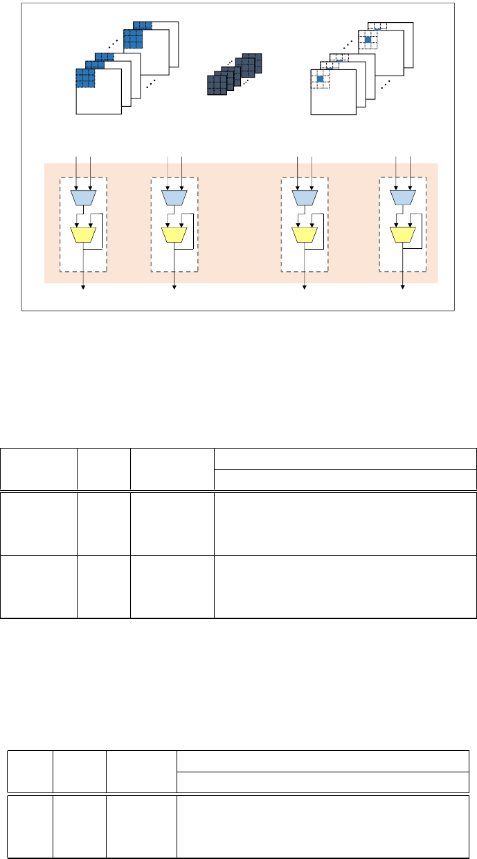
In Figure 1 we show an example diagram of a depth-wise conv 3 ×3 with stride 1 to illus-

trate our IP architecture. In this example the input data dimension is (40,20,16), the output

dimension is (40,20,16), and the parallel degree P= 16. As the ﬁgure shows, there are 16

computational units to conduct multiplication in parallel.

In Table 2 we provide some data of IP performance and resource usage under diﬀerent

conﬁgurations on the Pynq-Z1 FPGA board. In this table, the data precision for feature map

is 8 bit ﬁxed point with 2-bit integer, and the weights are 10 bit ﬁxed point with 1-bit integer.

The parallel factors are set to be 4, 8 and 16, respectively. The latency is represented as the

number of clock cycles under diﬀerent parallel conﬁguration. As shown in the table, the larger

the parallel factor is, the shorter latency is, and the more resources are occupied.

2.3 Point-wise Convolution 1×1IP

The point-wise convolution 1 ×1 IP is usually used after a depthwise separable convolution

to combine the output channels, as described in Section 2.2. Actually it can be regarded as

a special case of a standard convolution computation, which have been discussed in Section

2.1, so we omit detailed descriptions here. Similar to the depthwise conv IP, Table 3 shows its

performance and resource usage on the Pynq-Z1 board.

data_in1weight1

data_out1

…

channel 1 channel 2 channel 15

…

accumulate

channel 16

data_out2data_out15 data_out16

data_in2weight2data_in15 weight15 data_in16 weight16

di1

data in

di2

di16

weight

w16

16 input

channels

data out

do1

do2

do16

16 output

channels

Figure 1: Depth-wise 3 ×3 convolutional IP design

Table 2: Performance of Depth-Wise 3 ×3 IP on Pynq-z1 Board [3]

IP Paral. Latency Resource

Factor # of cycles LUT DSP Flip-Flop

DW-Conv 4 53206 1866 (1.4%) 16 (7.3%) 722 (0.7%)

3x3 8 38807 2177 (1.2%) 16 (7.3%) 1549 (1.5%)

16 18117 4394 (8.3%) 36 (16.4%) 2027 (2.0%)

DW-Conv 4 120075 2001 (3.8%) 16 (7.3%) 738 (0.7%)

5x5 8 64007 2668 (5.0%) 16 (7.3%) 554 (0.5%)

16 30996 4966 (9.3%) 36 (16.4%) 1045 (1.0%)

Table 3: Performance of Point-Wise 1 ×1 IP on Pynq-z1 Board [3]

IP Paral. Latency Resource

Factor # of clks LUT DSP Flip-Flop

Conv 4 50012 3318 (6.2%) 48 (21.8%) 4517 (4.6%)

1x1 8 29875 5076 (9.5%) 64 (29.1%) 4920 (4.6%)

16 14378 11871 (22.3%) 130 (59.1%) 10580 (9.9%)

Table 4: Performance of Max Pooling 2 ×2 IP on Pynq-z1 Board [3]

IP Paral. Latency Resource

Factor # of clks LUT DSP Flip-Flop

Pooling 4 2805 1037 (2.0%) 4 (1.8%) 825 (0.8%)

2x2 8 1411 895 (1.7%) 4 (1.8%) 758 (0.7%)

16 815 807 (1.5%) 4 (1.8%) 739 (0.7%)

2.4 Down-sampling (pooling) IP

Down sampling, also called pooling, is another very common component in most deep neural

networks. Pooling is used to reduce the spatial dimensions, which helps gain computation

performance, avoid over-ﬁtting and improve translation invariance. The interface protocols are

the same as above mentioned IPs.

•Input and Output: The inputs and outputs of pooling IP are similar to the depth-wise

conv IP but no weights are required. The input/out data shall also be stored in the on-chip

memory.

•Conﬁgurable Parameters: The parameters for Pooling K×KIP include:

1. Pooling size K, which indicates how much the input is down sampled by its spacial

dimension. Most common choices are K= 2 and K= 3. When K= 2, the xand y

dimensions of the input data are downsampled by a factor of 2, and when K= 3, x

and ydimensions are downsampled by a factor of 3.

2. Pooling method. We support three most commonly used pooling methods: max

pooling, average pooling and sum pooling.

3. Input feature map dimension (Hin, Win, Cin). Similar to depthwise conv IP, the

output data dimension is decided by the pooling size.

4. Parallel degree Palong Cdimension, data precision of input/output feature map.

These parameters are similar to depthwise conv IP.

•Resource and Performance: In Table 4 we provide some performance data of pooling

IP. The conﬁguration is K= 2, S= 1, and it is demonstrated using max pooling method.

2.5 Bounding Box Regression

Most IPs we provide are convolution and pooling, which are mostly used for feature extraction

in image classiﬁcation. In order to support more types of deep neural networks for diﬀerent

applications, we provide an IP for object detection task. Diﬀerent from image classiﬁcation,

object detection requires the neural network to draw a bounding box on the detected object.

It is usually done by a bounding box regression component after convolutional layers. For this

purpose, we borrow the regression algorithm from the popular YOLO [7], and implement it as

a conﬁgurable IP on FPGA.

The input of this IP is the feature map of the last convolution layer, and the output is the

coordinates of the detected bounding boxes. The conﬁgurable parameters of this IP include: 1)

the input feature map dimension; 2) the intermediate data precision during regression; and 3)

the number of anchor boxes and their aspect ratios, as described in [7]. It provides the ﬂexibility

that the user can alter this IP according to the object features to be detected.

2.6 Long-term Recurrent Convolution Network IP

2.6.1 Introduction

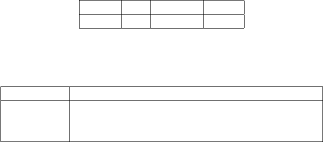
Apart from General purpose DNN component IPs, we also developed an image content recogni-

tion IP based on Long-term Recurrent Convolution Network. The IP takes image as input and

generates descriptive sentence as output. The overall network ﬂow is shown in ﬁgure 2. The

input image is ﬁrst processed by the CNN module for feature extraction. The extracted feature

vector is then fed into the RNN module for recurrent word generation. The LRCN computation

ﬂow is implemented and packed into a single IP with the structure shown in ﬁgure 3. The IP

have two memory AXI interface for input/output data transportation and one block control

interface for operation control. The input interface module is responsible for reading in input

data (including image data and neural network parameters) and stream the data into CNN com-

ponent and LSTM component in requested order. The output interface module is responsible

for writing data out back to the oﬀ chip memory.

2.6.2 Interface

The input and output interfaces between IP and DDR are memory mapped AXI4 bus protocol.

The bus width is 512 bit. The Control signals use AXI-lite GPIO register interface.

Figure 2: LRCN Network Flow

Figure 3: LRCN IP Structure

•Input and Output: The overall LRCN IP accepts image and rearranged weight data as

input and generates word index sequence as the output.

•Conﬁgurable Components: The CNN component and RNN component is composed by

conﬁgurable convolution and fully connected modules. The users may alter these modules

for diﬀerent CNN or LSTM structures.

1. Convolution module. Similar to the standard convolution IPs described in Section

2.1, its conﬁgurable parameters include: input dimensions IH ×IH ×ID, output

dimensions OH ×OH ×OD, kernel dimensions F W ×F H, data precision (8 bit,

12bit or 16 bit) and input/output parallel factor (8 or 16). The diﬀerence is, the

convolution module in the LRCN IP uses stream interface to receive weight data to

achieve best performance.

2. Fully Connected mocules. The conﬁgurable parameters include: input vector length

ID, output vector length OD, data precision (8 bit, 12bit or 16 bit) and input/output

parallel factor (8 or 16).

3. LSTM (long short-term memory) module. The LSTM module generates predicted

output, and stores the intermediate data in BRAM. In the next execution, it takes the

stored intermediate data in BRAM as a part of its inputs and generate next output.

The intermediate data are stored in streaming type to achieve lowest latency.

2.6.3 Resource and Performance:

We collect the resource and performance data of the image content recognition IP with AlexNet

as CNN component and LSTM as the RNN component. We used Xilinx Virtex-7 VC709 evalua-

tion platform with XC7VX690T FPGA for LRCN IP evaluation, and used PCIe for the host-chip

data transmission. The LRCN IP performance is shown in Table 5 and Table 6.

Table 5: Resource Consumption of LRCN

BRAM DSP Flip-Flop LUT

1508 3130 321195 316250

Table 6: LRCN performance on FPGA Virtex-7 VC709 with comparisons to CPU and GPU

implementations

Frequency Latency Speedup Power Eﬃciency

Our LRCN 100MHz 40ms 4.75X 23.6W 0.94J/pic

NVidia K80 562MHz 124ms 1.53X 133W 16.49J/pic

Intel Xeon 2.6GHz 190ms 1.00X 88W 16.72J/pic

3 Open-Source FPGA Accelerators for Machine Learning Ap-

plications

Aside from the open-source IPs for machine learning described in Section 2, in this section we

present two open-source FPGA accelerators for machine learning applications: spam ﬁltering and

binarized neural network. These two open-source designs are implemented in C++, leveraging

the Xilinx SDx design suite for high-level synthesis, logic synthesis, place & route, and bitstream

generation. The designs are currently collected in the Rosetta benchmark suite [8] developed by

Prof. Zhang’s group at Cornell. As a recent benchmark suite for software-programmable FP-

GAs, Rosetta contains fully-developed, complex applications which are representative of realistic

academic and industry accelerator designs. The benchmarks in Rosetta have been tested on a

cloud FPGA platform (AWS F1 with Xilinx VU9P FPGA) and an embedded FPGA platform

(Xilinx ZC706). Since the Xilinx toolﬂow on AWS is being continuously updated, we are also

working on porting the Rosetta designs to the latest AWS ﬂow.

3.1 Spam Filtering

The spam ﬁltering application uses stochastic gradient descent (SGD) to train a logistic regres-

sion model for spam email classiﬁcation. Diﬀerent with many FPGA accelerators that target the

inference phase of machine learning models, the spam ﬁltering accelerator tries to achieve high

performance in the training phase. In our current implementation, each email is represented by

a 1024-dimensional vector, thus the weight vector is also 1024-dimensional.

Since the compute kernels in this application are highly parallel, parallelization techniques

such as loop unrolling, loop pipelining and dataﬂow optimization are applied to improve per-

formance. Our implementation features datatype customization, where the features, weights

and intermediate results are represented using hardware-friendly ﬁxed-point types. The sigmoid

activation function is implemented using a look-up table to avoid exponent and division opera-

tions. Users can adjust the bitwidths of the feature vector and the weight vector, as well as the

parallelization factor of compute kernels. The performance and resource utilization of the spam

ﬁltering accelerator on two Xilinx FPGA platforms are summarized in Table 7.

Table 7: Performance and Resource Utilization of Spam Filtering

Device BRAM DSP Flip-Flop LUT Throughput

Xilinx ZC706 69 224 22134 12678 370k samples/s

Xilinx VU9P 90 224 17434 7207 1.6G samples/s

3.2 Binarized Neural Network

One challenge of implementing eﬃcient neural network accelerators on FPGAs is that ﬂoating

point operations are very expensive even on modern FPGA devices. As a result, quantization

techniques are often applied in modern FPGA neural network accelerators, where the features

and weights are quantized to ﬁxed-point datatypes of fewer bits. Binarized neural network

(BNN) [9] is an extreme of quantization, where both the weights and features are represented

using only one bit. For BNNs, the MAC operations in normal neural networks are replaced

by XNORs and popcount operations, which can be eﬃciently mapped to the LUT-rich FPGA

architecture.

Our binarized neural network accelerator is adopted from [10], where the accelerator targets

the inference phase of the BNN model proposed in [9] and works on CIFAR-10 images. There

are two major compute kernels in the BNN benchmark: binarized convolution for the convo-

lutional layers, and binarized dot product for the fully-connected layers. In order to achieve

high performance, our BNN implementation features intensive memory optimization, where a

specialized line buﬀer is designed to maximize data reuse within the feature maps. The design

is also parameterizable in that diﬀerent number of convolutional units can be instantiated to

achieve a trade-oﬀ between performance and resource utilization. The performance and resource

utilization of the BNN accelerator on Xilinx ZC706 are summarized in Table 8.

Table 8: Performance and Resource Utilization of BNN

BRAM DSP Flip-Flop LUT Throughput

102 4 46760 46899 200 images/s

References

[1] L. Sifre. Rigid-motion scattering for image classiﬁcation. PhD thesis, Ph. D. thesis, 2014.

[2] S. Ioﬀe and C. Szegedy. Batch normalization: Accelerating deep network training by reducing

internal covariate shift. arXiv preprint arXiv:1502.03167, 2015.

[3] https://reference.digilentinc.com/reference/programmable-logic/pynq-z1/start

[4] Howard, Andrew G., et al. ”Mobilenets: Eﬃcient convolutional neural networks for mobile

vision applications.” arXiv preprint arXiv:1704.04861 (2017).

[5] C. Szegedy, W. Liu, Y. Jia, P. Sermanet, S. Reed, D. Anguelov, D. Erhan, V. Vanhoucke,

and A. Rabinovich. Going deeper with convolutions. In Proceedings of the IEEE Conference

on Computer Vision and Pattern Recognition, pages 1–9, 2015.

[6] K. Simonyan and A. Zisserman. Very deep convolutional networks for large-scale image

recognition. arXiv preprint arXiv:1409.1556, 2014.

[7] Redmon, Joseph, et al. ”You only look once: Uniﬁed, real-time object detection.” Proceed-

ings of the IEEE conference on computer vision and pattern recognition. 2016.

[8] Zhou, Yuan, Udit Gupta, Steve Dai, Ritchie Zhao, Nitish Srivastava, Hanchen Jin, Joseph

Featherston et al. ”Rosetta: A Realistic High-Level Synthesis Benchmark Suite for Software

Programmable FPGAs.” In Proceedings of the 2018 ACM/SIGDA International Symposium

on Field-Programmable Gate Arrays, pp. 269-278. ACM, 2018.

[9] Courbariaux, Matthieu, Itay Hubara, Daniel Soudry, Ran El-Yaniv, and Yoshua Bengio.

”Binarized neural networks: Training deep neural networks with weights and activations

constrained to+ 1 or-1.” arXiv preprint arXiv:1602.02830 (2016).

[10] Zhao, Ritchie, Weinan Song, Wentao Zhang, Tianwei Xing, Jeng-Hau Lin, Mani Srivastava,

Rajesh Gupta, and Zhiru Zhang. ”Accelerating binarized convolutional neural networks with

software-programmable fpgas.” In Proceedings of the 2017 ACM/SIGDA International Sym-

posium on Field-Programmable Gate Arrays, pp. 15-24. ACM, 2017.

Open Source IP Manual

Navigation menu

Versions of this User Manual:

Views

Navigation