Optimus User Manual
User Manual:
Open the PDF directly: View PDF ![]() .
.
Page Count: 56
- Introduction
- Tutorial 1: Finding Coefficients for a Polynomial Function
- Tutorial 2: Selecting Terms for a Least Squares Representation of Data
- Tutorial 3: Vitamin C Molecular Geometry Optimisation
- Tutorial 4: Determining Rate Constants for Coupled ODEs Modelling a Biological System
- Advanced User Manual
- References
Optimus User Manual
Nicholas Andre G. Johnson and Aleksandr B. Sahakyan
21 August 2018
Contents
Introduction 2
Motivation ................................................. 2
Briefly on Monte Carlo and Temperature Simulated Annealing Procedures . . . . . . . . . . . . . . 2
Acceptance Ratio Annealing Procedure . . . . . . . . . . . . . . . . . . . . . . . . . . . . . . . . . 3
AdaptiveThermoregulation ........................................ 3
ReplicaExchangeProcedure ....................................... 4
InstallationInstructions .......................................... 5
Tutorial 1: Finding Coefficients for a Polynomial Function 6
ProblemStatement............................................. 6
DefiningOptimusInputs.......................................... 7
Acceptance Ratio Annealing Optimus Run . . . . . . . . . . . . . . . . . . . . . . . . . . . . . . . . 9
ReplicaExchangeOptimusRun...................................... 11
Summary .................................................. 14
Tutorial 2: Selecting Terms for a Least Squares Representation of Data 15
ProblemStatement............................................. 15
DefiningOptimusInputs.......................................... 16
Acceptance Ratio Annealing Optimus Run . . . . . . . . . . . . . . . . . . . . . . . . . . . . . . . . 19
ReplicaExchangeOptimusRun...................................... 22
Summary .................................................. 26
Tutorial 3: Vitamin C Molecular Geometry Optimisation 27
ProblemStatement............................................. 27
DefiningOptimusInputs.......................................... 27
DefiningaBenchmarkSolution...................................... 31
Acceptance Ratio Annealing Optimus Run . . . . . . . . . . . . . . . . . . . . . . . . . . . . . . . . 31
ReplicaExchangeOptimusRun...................................... 34
Summary .................................................. 37
Tutorial 4: Determining Rate Constants for Coupled ODEs Modelling a Biological System 38
ProblemStatement............................................. 38
DefiningOptimusInputs.......................................... 40
ExploringtheSystemDynamics ..................................... 42
Acceptance Ratio Annealing Optimus Run . . . . . . . . . . . . . . . . . . . . . . . . . . . . . . . . 44
ReplicaExchangeOptimusRun...................................... 45
Summary .................................................. 47
Advanced User Manual 49
MandatoryInputArguments ....................................... 49
OptionalInputArguments......................................... 50
Acceptance Ratio Annealing Specific Optional Inputs . . . . . . . . . . . . . . . . . . . . . . . . . . 52
Replica Exchange Specific Optional Inputs . . . . . . . . . . . . . . . . . . . . . . . . . . . . . . . . 53
OptimusOutput .............................................. 53
References 56
1

Introduction
Motivation
For a complex model, where the unknown parameters cannot be determined by conventional linear or
non-linear fitting techniques, Monte Carlo methods for optimisation, based on the random sampling of the
parameter space, is the method of choice (Cowles and Carlin 1996). In such a case, the quality of the solution
found following some optimisation protocol depends on that protocol’s ability to effectively explore the
parameter space (Gilks, Richardson, and Spiegelhalter 1996). Many existing methods perform well for certain
models, but fail in other models due in part to inefficient exploration of the parameter space. In this manual,
we present Optimus, a Universal Monte Carlo optimisation engine in R with acceptance ratio annealing,
replica exchange and adaptive thermoregulation. It can universally interface with any model definition and
efficiently optimise the model’s parameters by consistently exploring the parameter space effectively. Optimus
can execute either an acceptance ratio annealing procedure or a replica exchange procedure, depending on
the desires of the user.
This User Manual will begin with a brief overview of Monte Carlo optimisation and the common temperature
simulated annealing framework. It will then proceed with a presentation of Optimus’ acceptance ratio
annealing procedure, its adaptive thermoregulation feature, and its replica exchange procedure. After an
explantion of how to download the Optimus R package from GitHub and install it locally, 4 Tutorials will be
presented to illustrate how users should employ Optimus and to demonstrate its flexibility as an optimisation
engine. Finally, an “Advanced User Manual” section will be included in which all possible input parameters
to Optimus will be outlined and the output format will be specified.
Briefly on Monte Carlo and Temperature Simulated Annealing Procedures
Let us assume that our model is a certain function
m
() that performs operations on the inputted
K
coefficient
set and returns the observable object
O
=
m
(
K
). Our task is to optimise
K
, the set of coefficients, so that the
error metric
u
(
O
)that measures the violations of the target
Otrg
set by the model-generated
O
is minimal.
In a Monte Carlo optimisation procedure, we can define a pseudo-energy
e
(
u
)of the system as a function of
u
(), where lower values of the pseudo-energy
e
correspond to better candidate solutions
K
. In order to find a
better set of
K
, we need to alter it by a certain rule
r
() that, if repeated many times, enables the sampling of
the parameter space for K. One can then evaluate the pseudo-energies before and after the alterations:
E1=e(u(m(K)))
E2=e(u(m(r(K))))
We then accept or reject the move, meaning we accept the new set of
r
(
K
)coefficients as the new K or
revert back to the previous K, guided by the following acceptance probability, as postulated in a Metropolis
criterion (Chib and Greenberg 1995, Chen and Roux (2015)):
paccept =min(1, e
−∆E
T)
∆E=E2−E1
where T is the pseudo temperature, that should be always greater than 0. For a given ∆
E >
0energy
difference, one would have different stringency for accepting the move depending on the value of the pseudo-
temperature T. Therefore, in case the Monte Carlo simulation were to drive the
K
set to a state where any
further moves would increase the pseudo-energy great enough for the moves to be always rejected, then
one could overcome that and further sample the other values in the parameter space by increasing the
pseudo-temperature.
2
In molecular dynamics simulation, where the objective is to sample the free energy surface populated by a
molecule, one way to overcome the barriers is by using the technique known as simulated annealing, where we
anneal the temperature gradually from some higher value to a lower value during the course of the simulation
(Kirkpatrick 1984). The parts of the simulation where the pseudo-temperature is higher allows relatively
unconstrained exploration of the search space whereas those parts with a lower pseudo-temperature limit
the search to a more local area of the parameter space. Multiple cycles of this annealing procedure can be
executed to increase the overall sampling. In the same manner, we can anneal the pseudo-temperature in the
Monte Carlo procedures for model optimisation.
Acceptance Ratio Annealing Procedure
A significant limitation of pseudo-temperature simulated annealing is that a given scheme of temperature
annealing might be efficient for some models or pseudo-energy metrics, but not efficient for others (Ingber
1993). A temperature at a given point of the annealing cycle that is designed to be quite permissive in terms
of accepting the move, can actually not be permissive depending on the value and scale of the ∆
E
energy
difference, as can be seen in the equation for
paccept
. Furthermore, even within the single model optimisation
procedure, the pseudo-energy metric can shift into a value range that does not match with the selected
temperature scheme anymore, leading to similar problems (meaning poor sampling of the parameter space).
This can often be the case when the pseudo-energy of the system does not exhibit a smooth dependency on
K, loosely meaning that similar values of Kdo not necessarily produce similar pseudo-energy values.
To this end, in general cases where we do not deal with energies and temperatures that display the smoothness
emulating real physical systems (such smoothness is often found in molecular dynamics or Monte Carlo
simulations of molecules), we need to anneal a more robust metric for crossing different barriers. As such a
metric, Optimus, when in its default mode, uses the acceptance ratio.
In a given annealing cycle, Optimus constructs a linear target acceptance ratio schedule for each step based
on an initial target acceptance ratio, a final acceptance ratio and the number of iterations in each cycle for
a given optimisation run (all of which can be specified as inputs). Once the optimisation process begins,
Optimus calculates an observed acceptance ratio at the end of each STATWINDOW (a fixed number of
steps which can be specified by the user) by calculating the fraction of the accepted moves from all the past
trials in the current STATWINDOW. Thereafter, Optimus compares the observed acceptance ratio with the
target acceptance ratio based on the annealing schedule and determines whether and how to alter the system
pseudo-temperature (adaptive thermoregulation) to align the observed acceptance ratio with the target ratio
at the end of the following STATWINDOW. Thus, by employing acceptance ratio annealing and adaptive
thermoregulation, Optimus is able to methodically explore the parameter space for
K
even when no smooth
relationship exists between Kand the system pseudo-energy.
Adaptive Thermoregulation
All decisions governing system pseudo-temperature alterations are made by a Temperature Control Unit
(TCU) that interfaces directly with Optimus on the backend (note that the TCU is completely encapsulated
such that modifications can be easily made in future should they be needed). This section articulates the
exact protocol followed by the current TCU.
The initial system temperature is specified as an input argument. At the end of each STATWINDOW, if
the observed acceptance ratio is within a fixed value T.DELTA (specified as an input argument) of the
target acceptance ratio based on the annealing schedule, the TCU will make no change to the current system
pseudo-temperature. If the observed acceptance ratio is less than the ideal ratio and outside the range of
T.DELTA, the TCU will increase the system pseudo-temperature by a value T.ADJSTEP (the initial value of
T.ADJSTEP is specified as an input argument). Similarly, if the observed acceptance ratio is greater than the
ideal ratio and outside the range of T.DELTA, the TCU will reduce the temperature by a value T.ADJSTEP.
3
If the observed acceptance ratio has been below the ideal acceptance ratio for TSCLnum (an integer input
argument) subsequent STATWINDOWs, T.ADJSTEP will be increased by a factor T.SCALING (an input
argument). Similarly, T.ADJSTEP will also be increased by a factor T.SCALING if the observed acceptance
ratio is greater than the ideal acceptance ratio for TSCLnum subsequent STATWINDOWs. T.ADJSTEP is
reset to its original input value whenever a series of subsequent observed acceptance ratios being greater
than/less than ideal acceptance ratios is broken. If ever the TCU subtracts T.ADJSTEP from the current
temperature and the result is a negative value, the system pseudo-temperature is set to T.MIN (an input
argument). The final feature of the TCU is that although the initial system pseudo-temperature is specified
by the user, if multiple annealing cycles are employed, the initial pseudo-temperature for acceptance ratio
annealing cycles after the first cycle is inferred from the decisions of the TCU on previous cycles.
This collection of decision rules that comprise the TCU result in pseudo-temperature alterations that cause the
observed acceptance ratios during Optimus optimsation runs to follow the ideal acceptance ratios remarkably
well. Moreover, as will be highlighted in the Tutorials, large temeperature alterations are often required to
align the observed acceptance ratios with the ideal ratios, a task which Optimus excels at whereas other
protocols would have difficulty.
Replica Exchange Procedure
Optimus additionally supports replica exchange as an optimisation mode which can be selected in place
of acceptance ratio annealing, provided that the user has access to multiple processors (ideally at least
4, and preferably 8 or more). The inspiration for this additional mode was taken from Replica Exchnage
Molecular Dynamics (REMD) simulations. REMD simulation is a technique employed to obtain equilibrium
sampling of a molecule (for instance, a new protein whose properties one desires to characterize), usually at
low temperatures. Let
T
=
{T1, T2, ..., Tn}
be a set of n distinct temperatures for which
T1< T2< ... < Tn
.
In REMD,
n
replicas of Monte Carlo simulation for a given molecule are initialized at each
Ti∈T
. Note that
each temperature
Ti
corresponds to a slightly different energy landscape for the examined molecule. A key fact
that underlies REMD simulations is that many configurations in a given energy landscape corresponding to
Ti
are likely also found in the energy landscapes corresponding to
Ti−1
and
Ti+1
. If molecule configurations in
adjacent replicas are allowed to exchange, the simulation will be able to overcome energy barriers at the various
temperature replicas and thoroughly explore the parameter space. Moreover, for molecule configuration
xn
in
replica
Ti
and configuration
xm
in replica
Ti+1
, it has been proven that equilibirum sampling will occur if an
exchange happens with the following probability (Sugita and Okamoto 1999):
pREM D =min(1, e−∆)
∆=(Ti+1 −Ti)(E(xn)−E(xm))
where
E
(
x
)represents the energy associated with the molecule configuration
x
. Thus, REMD simulation can
be executed by repeating the following two steps for a chosen number of iterations (Sugita and Okamoto
1999):
1)
Simulate
n
replicas of Monte Carlo Optimisation at distinct temperatures simultaneously and indepen-
dently
2) Randomly select two configurations in adjacent replicas and exchange them with probability pREM D
Optimus extends this approach to apply to arbitrary optimisation problems with two primary modifications.
Firstly, due to the aforementioned robustness of utilizing acceptance ratio as a controlling metric rather than
pseudo-temperature in arbitrary systems, Optimus initializes
n
replicas with different target acceptance ratios
as opposed to different temperatures and uses the previously described TCU for adaptive thermoregulation.
Secondly, given that Optimus is only concerned with finding an Optimal solution and is not concerned with
equilibrium sampling of the parameter space (as equilibrium sampling has no meaning for non physcial
systems), after two candidate configurations are selected for exchange, they are necessarily exchanged (this
can be viewed as setting
pREM D
= 1 in the above procedure) (Ballard and Jarzynski 2009). By relaxing
the equilibrium sampling criterion, the parameter space can be more extensively explored. This approach
4

produced good results (as illustrated in the tutorials) and is a viable alternative to the acceptance ratio
annealing mode of Optimus when the user has access to good computing resources.
Installation Instructions
Installing Optimus locally for immediate use requires only an R client and a connection to the internet. After
opening an R client, execute the commands below to install Optimus. Note that the latest version of Rtools
is required for this installation to work. If it is not available locally and the installation is attempted with
RStudio, a prompt will appear to download and install Rtools. After following those instructions, restart the
RStudio session before reattempting the Optimus installation.
install.packaes("devtools")# install devtools
library(devtools) # load devtools
install_github("SahakyanLab/Optimus")# install Optimus
library(Optimus) # load Optimus
5
Tutorial 1: Finding Coefficients for a Polynomial Function
Problem Statement
In this example, we shall use Optimus to find the coefficients of the polynomial function that is known to
represent the observations ythe best. This, of course, is a simple task that can be addressed more robustly
by least-squares linear model fitting. However, starting with this example will focus our attention on the
organisation of the Optimus input, rather than the complexity of the task.
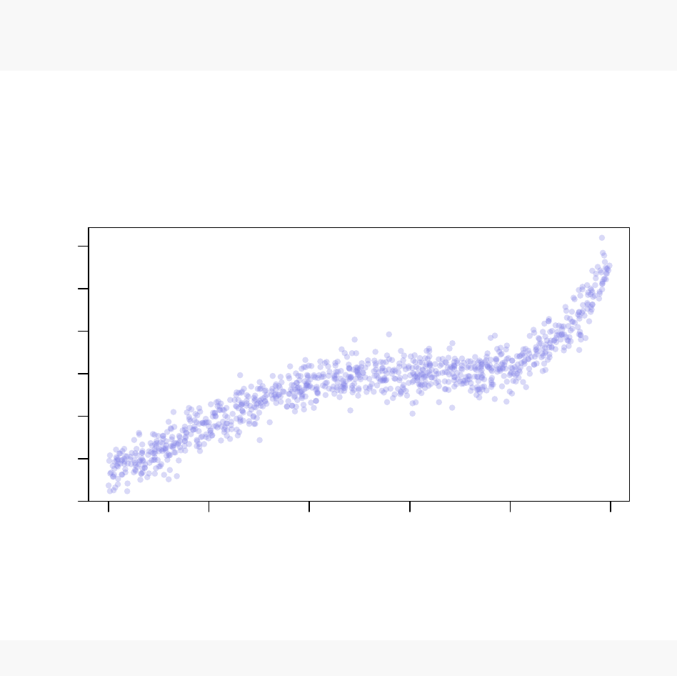
First of all, let us create some data for the example.
set.seed(845)
x <- runif(1000,min = -15,max = 10)
y <- -1*x-0.3 *x^2+0.2 *x^3+0.01 *x^4+rnorm(length(x), mean = 0,
sd=30)
The good side of this noisy data generation is that we know the original function that describes it:
y
=
−
1
.
0
x−
0
.
3
x2
+ 0
.
2
x3
+ 0
.
01
x4
. Hence, we can check how well Optimus performs at finding the correct
coefficients. The synthetic “real world” noisy data that we generated looks like this:
−15 −10 −5 0 5 10
−300 −100 0 100 300
Synthetic Example Dataset
x
y
Before we turn to Optimus, let us see how the proper linear model fitting will perform using this data.
lm.model <- lm(y ~x+I(x^2)+I(x^3)+I(x^4)+0)
lm.model
##
## Call:
## lm(formula = y ~ x + I(x^2) + I(x^3) + I(x^4) + 0)
6
##
## Coefficients:
## x I(x^2) I(x^3) I(x^4)
## -0.74056 -0.30735 0.19777 0.00991
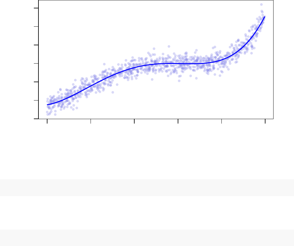
The least-squares linear model fitting for the coefficients to the known functional form is quite close to the
original equation: y=−0.741x−0.307x2+ 0.198x3+ 0.010x4.
−15 −10 −5 0 5 10
−300 −100 0 100 300
Least−Squares Linear Model Fitting
x
y
The RMSD between the observed data y and the linear model fitting outcome is:
y.pred <- predict(newdata = data.frame(x=x), object = lm.model)
sqrt(mean((y -y.pred)^2))
## [1] 28.82655
which is even slightly better in describing the noisy data, as compared to the maximum possible RMSD based
on the de-noised data:
y.realdep <- -1*x-0.3 *x^2+0.2 *x^3+0.01 *x^4
sqrt(mean((y -y.realdep)^2))
## [1] 28.85858
Defining Optimus Inputs
Now we can set up the inputs for the Optimus run. We shall use the model
k1x
+
k2x2
+
k3x3
+
k4x4
to
fit the
y
observables based on the values for
x
. The dependent functions that are needed for setting up an
Optimus run, are given as inputs in the Optimus function call.
7

First, we need to create an object
K
, which stores the initial values for the parameter(s) to be optimised.
K
can be an object of any type. From a single numeric or character value to a vector of values or a data frame
holding, say, Cartesian coordinates of a molecule to be optimised. The only requirement for
K
is that it
should be something alterable (via a rule function
r
(), see below) and something that influences the outcome
of another required model function -
m
() (see below). In this example, we have 4 coefficients to optimise
from some random initial state. We can thus make
K
be a numeric vector of size 4. Let us start from all
the components being 1.0, which, as entries in
K
, can be both named and unnamed. Though not the case
here, the entry-named data for
K
can be essential for some models that specifically use coefficient names, for
instance when a system of ODEs is used in the model function m().
K <- c(k1=1,k2=1,k3=1,k4=1)# entries are named as k1, k2, k3 and k4
Second, we should create the function
m
for the model. The function
m
should be designed to operate on the
whole set of parameter snapshot
K
and return the corresponding observable object
O
. Please note that the
size of
K
and
O
are not necessarily to match, depending on the nature of the model used. Operating on
K
is
the only hard condition on
m
(), which can optionally operate on other data as well. In our situation, the
function
m
() should operate on the provided instance of four coefficients (in the object
K
), and, additionally
on the values
x
. It should then return a vector of observations
O
(to be compared with
y
target observations)
of the same size as vector
x
. Any additional data required by the model, in our case an object with the set of
1000
x
values, must be provided to the function in an input variable DATA, a list holding the additional data
that must be accessed by
m
() and
u
() (see below). The variable DATA must be provided to Optimus in the
function call, and
m
() must take it as an input (in the case that neither
m
() nor
u
() require additional data,
the two functions should still be created such that they take a variable DATA as an input, and the variable
DATA passed to Optimus will be set to NULL).
DATA <- NULL
DATA$x <- x
DATA$y <- y
m <- function(K, DATA) {
x <- DATA$x
O <- K["k1"]*x+K["k2"]*x^2+K["k3"]*x^3+K["k4"]*x^4
return(O)
}
At this point, calling
m
(
K
=
K, DAT A
=
DAT A
)will return the predicted
O
set from the initial, non-optimal
values for K, hence rather far from the target Otrg =y.
In this example, the optimisation goal is for the
O
model outcomes to come as close as possible to the target
observations
y
, to be achieved by optimising the coefficients
K
. The object
y
holding the target values
therefore also needs to be specified and given as an input to the
Optimus
() function (as an entry in the
DATA variable), just like x required, in this example, by the function m().
Now, we need to define how the performance of a given snapshot of coefficients
K
is to be evaluated. For
Optimus, this is done by specifying a function
u
(), which should necessarily take as inputs
O
(the output of
m
()) and the variable DATA. The output should have two components,
Q
holding a single number of the
quality of the
K
coefficients, and
E
holding a (pseudo)energy for the given snapshot
K
. It is important that
the returned (pseudo)energy value is lower for better performance/version of
K
, never vice-versa. The
Q
component of the
u
() function output is only used for plotting the optimisation process, and, if desired, can
just repeat the value of the Ecomponent.
For our example, the
u
() function will assess the agreement between the snapshot of predictions
O
and the
complete set of real observables (target)
y
. Here, we can use RMSD between
O
and
y
as a measure of
K
snapshot quality (
Q
). Since bettter agreement means better RMSD, it can be directly used as a pseudo-energy
(E), without putting a negative sign or performing some other mathematical operation on Q.
8

u <- function(O, DATA) {
y <- DATA$y
Q <- sqrt(mean((O -y)^2))
E <- Q # For RMSD, <-> negative sign or other mathematical operation
# is not needed.
RESULT <- NULL
RESULT$Q <- Q
RESULT$E <- E
return(RESULT)
}
And finally, we need to define the rule, by which the
K
coefficient vector is to be altered from one step to
another. This is done by defining a rule function
r
() that must take
K
, and return an object equivalent to
K
,
but with some alteration(s). In this example, for each snapshot of
K
, we shall randomly select one of its four
coefficients, then either increment or decrement (chosen randomly) it by 0.0005, returning the altered set of
coefficients.
r <- function(K) {
K.new <- K
# Randomly selecting a coefficient to alter:
K.ind.toalter <- sample(size = 1,x=1:length(K.new))
# Creating a potentially new set of coefficients where one entry is altered
# by either +move.step or -move.step, also randomly selected:
move.step <- 5e-04
K.new[K.ind.toalter] <- K.new[K.ind.toalter] +sample(size = 1,x = c(-move.step,
move.step))
## Setting the negative coefficients to 0 (not necessary in this example,
## useful for optimising rate constants): neg.ind <- which(K.new < 0)
## if(length(neg.ind)>0){ K.new[neg.ind] <- 0 }
return(K.new)
}
All the constructed objects (
K
) and functions (
m, u, r
), as well as the data required by
m
() and
u
() (stored
in the variable DATA) should be defined in an R session and given to Optimus as inputs. The users are
free to define some dependencies as additional files (for example initial protein geometry for a Monte-Carlo
optimisation), which should be called from within the function definitions.
Acceptance Ratio Annealing Optimus Run
Having constructed
K
, DATA,
m
(),
u
() and
r
(), we are now ready to call Optimus. Let us first investigate
the Acceptance Ratio Annealing (SA) version of Optimus on 4 processors (the vast majority of personal
computers currently have 4 processors), which can be executed as follows:
Optimus(NCPU = 4,K.INITIAL = K, rDEF = r, mDEF = m, uDEF = u, OPT.TYPE = "SA",
DATA = DATA, OPTNAME = "poly_4_SA",LONG = FALSE)
Note that the field
LONG
=
F ALSE
is included in the function call so that all data from the optimsation
process is saved. Calling Optimus with
LONG
=
T RU E
will result in a memory saving optimisation process
(more details in the Advanced User Manual). Of the 4 optimisation replicas, the second and fourth processors
found the best parameter configuration (lowest RMSD):
9
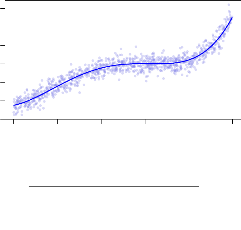
−15 −10 −5 0 5 10
−300 −100 0 100 300
Acceptance Ratio Annealing Optimus Fitting (4 Cores)
x
y
Table 1: 4 Core Acceptance Ratio Annealing Optimus Run Results
E (RMSD) K1 K2 K3 K4
Processor 1 28.857 -0.1560 -0.2850 0.1905 0.0095
Processor 2 28.841 -0.3760 -0.2825 0.1920 0.0095
Processor 3 28.864 -0.1045 -0.2820 0.1905 0.0095
Processor 4 28.841 -0.3760 -0.2825 0.1920 0.0095
The equation recovered by Processor 2 (and 4) is y=−0.3760x−0.2825x2+ 0.192x3+ 0.0095x4.
Notice that although the RMSD of this solution, 28
.
841, is greater than the RMSD of the least squares
solution, 28.82655, it is less than the RMSD of the de-noised data found above, 28.85858.
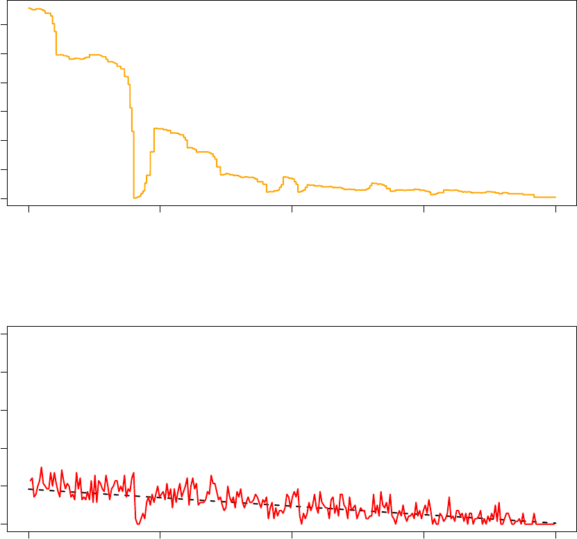
The two graphs below illustrate the evolution of the system pseudo-temperature in response to alterations
made by the Temperature Control Unit (TCU) as a function of the optimsation iteration and the observed
acceptance ratio as a function of the optimisation iteration respectively. The graphs show data from the last
20 000 iterations of the optimisation executed by Processor 2.
10
980000 985000 990000 995000 1000000
0.0e+00 1.0e−06 2.0e−06 3.0e−06
System Pseudo−Temperature (Processor 2)
Step
Temperature
980000 985000 990000 995000 1000000
0 20 40 60 80 100
Observed Acceptance Ratio (Processor 2)
Step
Acceptance ratios (%)
In the graph titled “Observed Acceptance Ratio (Processor 2),” the solid red line tracks the observed
acceptance ratios calculated by Optimus at the end of each STATWINDOW and the dashed black line tracks
the target acceptance ratio based on the annealing schedule. From the above two graphs, notice that while
the observed acceptance ratio tracks the target acceptance ratio closely, the system pseudo-temperature
changes significantly and non-monotonically. This illustrates that the adaptive thermoregulation of the TCU
allows Optimus to effectively anneal the system acceptance ratio.
Replica Exchange Optimus Run
Let us now consider the Replica Exchange version of Optimus on 12 processors. Let us reiterate that the
purpose here is to illustrate how to run an optimisation using the Replica Exchange version of Optimus; this
method is of course not the most robust method to solve this simple task and is likely overkill.
In addition to the arguments specified above, the Replica Exchange version of Optimus also requires an input
11
variable ACCRATIO which is a vector that defines the acceptance ratio to be used for each of the Replicas
initiated, 12 in this case (note that the length of ACCRATIO must always be equal to the argument NCPU).
ACCRATIO <- c(90,82,74,66,58,50,42,34,26,18,10,2)
Having defined the acceptance ratios for each level, the optimisation can be executed as follows:
Optimus(NCPU = 12,K.INITIAL = K, rDEF = r, mDEF = m, uDEF = u, ACCRATIO = ACCRATIO,
OPT.TYPE = "RE",DATA = DATA, OPTNAME = "poly_12_RE",LONG = FALSE)
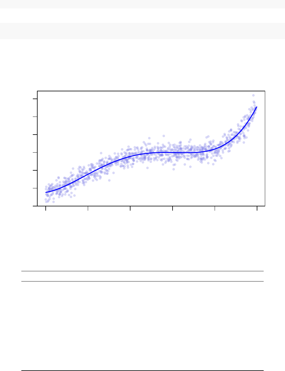
Of the 12 optimisation replicas, replica 8 finds the best parameter configuration (lowest RMSD):
−15 −10 −5 0 5 10
−300 −100 0 100 300
Replica Exchange Optimus Fitting (12 Cores)
x
y
Table 2: 12 Core Replica Exchange Optimus Run Results
Replica Acceptance Ratio E (RMSD) K1 K2 K3 K4
Processor 1 90 29.71934 -3.2760 -0.5760 0.2395 0.0135
Processor 2 82 29.51819 -3.4445 -0.3755 0.2300 0.0115
Processor 3 74 28.88707 -0.0340 -0.2375 0.1870 0.0090
Processor 4 66 30.10499 -3.8095 -0.6630 0.2435 0.0140
Processor 5 58 29.06293 -2.3575 -0.4180 0.2200 0.0115
Processor 6 50 29.70906 -3.7360 -0.3785 0.2320 0.0115
Processor 7 42 28.85095 -1.1370 -0.3515 0.2045 0.0105
Processor 8 34 28.82721 -0.8175 -0.3130 0.1990 0.0100
Processor 9 26 28.84057 -0.5760 -0.2740 0.1940 0.0095
Processor 10 18 29.48785 -2.7805 -0.5420 0.2325 0.0130
Processor 11 10 28.85095 -1.1370 -0.3515 0.2045 0.0105
Processor 12 2 29.41377 1.2255 -0.0895 0.1645 0.0070
12
The equation recovered by Processor 8 is y=−0.8175x−0.313x2+ 0.199x3+ 0.01x4.
Notice that the RMSD of this solution, 28
.
82721, is less than the RMSD of the Acceptance Ratio Annealing
solution, 28.841, and only slightly greater than the RMSD of the least squares solution, 28.82655.
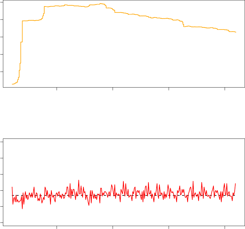
Let us now briefly examine the evolution of the system pseudo-temperature in response to alterations made by
the Temperature Control Unit (TCU) as a function of the optimsation iteration and the observed acceptance
ratio as a function of the optimisation iteration for the Replica Exchange version of Optimus. The following
two graphs represent data from the last 20 000 iterations of the optimisation replica running on Processor 8
(34% target acceptance ratio).
985000 990000 995000 1000000
3.4e−05 3.6e−05 3.8e−05
System Pseudo−Temperature (Processor 8 − 34% Acceptance Ratio)
Step
Temperature
985000 990000 995000 1000000
0 20 40 60 80 100
Observed Acceptance Ratio (Processor 8 − 34% Acceptance Ratio)
Step
Acceptance ratios (%)
Notice that in the observed acceptance ratio graph, the dashed line indicating the target acceptance ratio is
constant (as opposed to linearly changing as in acceptance ratio annealing). This is because each processor
in the replica exchnage mode has a single target acceptance ratio, as articulated in the previous section
of this manual which addressed the theoretical underpinnings of Optimus. Here again, adaptive decisions
13

made by the TCU result in non-monotonic, non uniform psuedo-temperature adjustments while the observed
acceptance ratios fluctuates relatively closely around the target ratio.
Summary
We now understand the input requirements to interface with the Acceptance Ratio Annealing and Replica
Exchange versions of Optimus. In this example, both the Acceptance Ratio Annealing and Replica Exchange
Optimus versions retrieved solutions having a lower RMSD than the de-noised data and only a slightly
greater RMSD than the optimal Least Squares solution. Replica Exchange resulted in a better solution than
Acceptance Ratio Annealing, at the cost of greater computing resources.
Table 3: Summary of Solutions
E (RMSD) K1 K2 K3 K4
De-noised Function 28.85858 -1.00000 -0.30000 0.20000 0.01000
Optimus (Acceptance Ratio Annealing) 28.84100 -0.37600 -0.28250 0.19200 0.00950
Optimus (Replica Exchange) 28.82721 -0.81750 -0.31300 0.19900 0.01000
Least Squares 28.82655 -0.74056 -0.30735 0.19777 0.00991
14
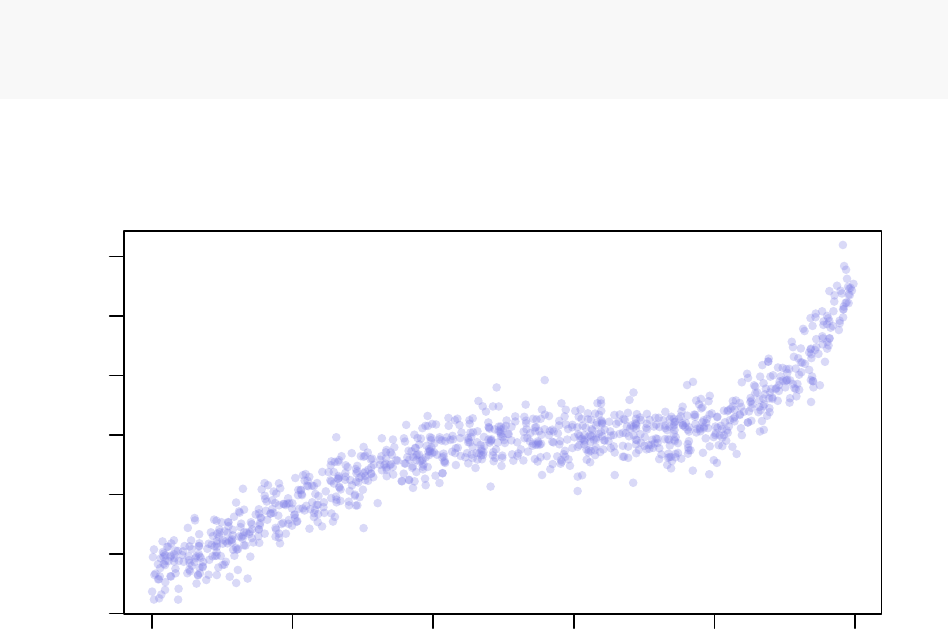
Tutorial 2: Selecting Terms for a Least Squares Representation of
Data
Problem Statement
Consider again the synthetic data that was created in Tutorial 1. Suppose that we were only provided
with the data and, unlike in Tutorial 1, had no knowledge of the best terms to be included in a functional
representation of said data. In this example, we shall use Optimus to determine which terms should be used
in a Least Squares representation of the data to achieve a representation with low RMSD while not overfitting
the data.
Let us start by generating the same data which was used in Tutorial 1:
set.seed(845)
x <- runif(1000,min = -15,max = 10)
y <- -1*x-0.3 *x^2+0.2 *x^3+0.01 *x^4+rnorm(length(x), mean = 0,
sd=30)
−15 −10 −5 0 5 10
−300 −100 0 100 300
Synthetic Example Dataset
x
y
From Tutorial 1, we know that if presented with this data and under the assumption that the most
appropriate model to describe the data is
k1x
+
k2x2
+
k3x3
+
k4x4
, the Least Squares model fitting is
y
=
−
0
.
741
x−
0
.
307
x2
+ 0
.
198
x3
+ 0
.
010
x4
. We also know that the RMSD between the observed data y and
the linear model fitting outcome is:
## [1] 28.82655
15
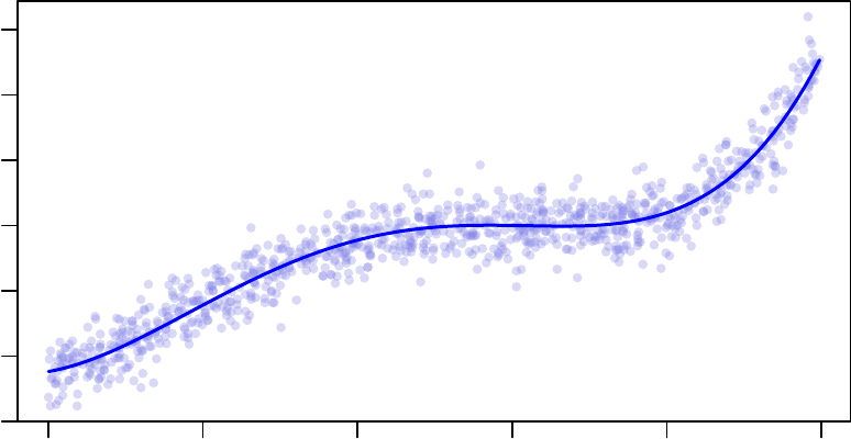
−15 −10 −5 0 5 10
−300 −100 0 100 300
Least−Squares Linear Model Fitting
x
y
Defining Optimus Inputs
Let us first define an ordered set
terms
that is a collection of candidate terms to include in the representation
of the data:
terms
=
{x, x2, x3, x4, x5, x6, x7, x8, x9, x10, ex,|x|, sin
(
x
)
, cos
(
x
)
, tan
(
x
)
, sin
(
x
)
cos
(
x
)
, sin2
(
x
)
, cos2
(
x
)
,
sin
(
x2
)
, sin
(
x3
)
, cos
(
x2
)
, cos
(
x3
)
, sin
(
x3
)
cos
(
−x
)
, cos
(
x3
)
sin
(
−x
)
, sin
(
x5
)
cos
(
−x
)
, cos
(
x5
)
sin
(
−x
)
, exsin
(
x
)
,
excos(x),|x|sin(x),|x|cos(x)}
Let termsidenote the ith term in the set terms (for example, terms14 =cos(x)). We shall use the model:
y=b+
card(terms)
X
i=1
kicitermsi
where each
ki
is a binary variable (meaning a variable taking a value of either 0 or 1) indicating whether the
ith
term is included in the representation, each
ci
is a non-zero coefficient for the
ith
term and b is a real
number (the intercept). In our case, card(terms) = 30 so explicitly, our model is:
y
=
b
+
k1c1x
+
k2c2x2
+
k3c3x3
+
k4c4x4
+
k5c5x5
+
k6c6x6
+
k7c7x7
+
k8c8x8
+
k9c9x9
+
k10c10x10
+
k11c11ex
+
k12c12|x|
+
k13c13six
(
x
) +
k14c14cos
(
x
) +
k15c15tan
(
x
) +
k16c16sin
(
x
)
cos
(
x
) +
k17c17sin2
(
x
) +
k18c18cos2
(
x
) +
k19c19sin
(
x2
) +
k20c20sin
(
x3
) +
k21c21cos
(
x2
) +
k22c22cos
(
x3
) +
k23c23sin
(
x3
)
cos
(
−x
) +
k24c24cos
(
x3
)
sin
(
−x
) +
k25c25sin
(
x5
)
cos
(
−x
) +
k26c26cos
(
x5
)
sin
(
−x
) +
k27c27exsin
(
x
) +
k28c28excos
(
x
) +
k29c29|x|sin(x) + k30c30|x|cos(x)
Formally,
K
will be a numeric vector of length
card
(
terms
)whose
ith
entry is
ki
.
K
uniquely specifies a set
activeT erms
=
{termsi∀i|ki
= 1
}
. Note that
activeT erms ⊆terms
. Each binary variable
ki
should be
16

initialized randomly as below:
K <- c(term1=rbinom(n=1,size=1,prob=0.5),
term2=rbinom(n=1,size=1,prob=0.5),
term3=rbinom(n=1,size=1,prob=0.5),
term4=rbinom(n=1,size=1,prob=0.5),
term5=rbinom(n=1,size=1,prob=0.5),
term6=rbinom(n=1,size=1,prob=0.5),
term7=rbinom(n=1,size=1,prob=0.5),
term8=rbinom(n=1,size=1,prob=0.5),
term9=rbinom(n=1,size=1,prob=0.5),
term10=rbinom(n=1,size=1,prob=0.5),
term11=rbinom(n=1,size=1,prob=0.5),
term12=rbinom(n=1,size=1,prob=0.5),
term13=rbinom(n=1,size=1,prob=0.5),
term14=rbinom(n=1,size=1,prob=0.5),
term15=rbinom(n=1,size=1,prob=0.5),
term16=rbinom(n=1,size=1,prob=0.5),
term17=rbinom(n=1,size=1,prob=0.5),
term18=rbinom(n=1,size=1,prob=0.5),
term19=rbinom(n=1,size=1,prob=0.5),
term20=rbinom(n=1,size=1,prob=0.5),
term21=rbinom(n=1,size=1,prob=0.5),
term22=rbinom(n=1,size=1,prob=0.5),
term23=rbinom(n=1,size=1,prob=0.5),
term24=rbinom(n=1,size=1,prob=0.5),
term25=rbinom(n=1,size=1,prob=0.5),
term26=rbinom(n=1,size=1,prob=0.5),
term27=rbinom(n=1,size=1,prob=0.5),
term28=rbinom(n=1,size=1,prob=0.5),
term29=rbinom(n=1,size=1,prob=0.5),
term30=rbinom(n=1,size=1,prob=0.5))
Next, we must define the model function
m
that will operate on the parameter snapshot
K
and return an
observable object
O
. For a given set
activeT erms
specified by
K
,
m
() will fit a linear model to the data using
the entries in
activeT erms
and using the built in generalized linear model (
glm
()) function in R, thereby
determining values for the variables
ci
and
b
. Accordingly,
m
() will require access to the variables
x
and
y
,
which will be provided as entries in DATA, a variable of type list, as in Tutorial 1. The object
O
will be the
corresponding output of the function
glm
(). In the case that the set
activeT erms
is the empty set (meaning
that all entries in Kare 0), m() will fit a model using the relationship y~x.
DATA <- NULL
DATA$x <- x
DATA$y <- y
m <- function(K, DATA){
y <- DATA$y
x <- DATA$x
terms <- c("+x",
"+I(x^2)",
"+I(x^3)",
"+I(x^4)",
"+I(x^5)",
"+I(x^6)",
17

"+I(x^7)",
"+I(x^8)",
"+I(x^9)",
"+I(x^10)",
"+I(exp(x))",
"+I(abs(x))",
"+I(sin(x))",
"+I(cos(x))",
"+I(tan(x))",
"+I(sin(x)*cos(x))",
"+I((sin(x))^2)",
"+I((cos(x))^2)",
"+I(sin(x^2))",
"+I(sin(x^3))",
"+I(cos(x^2))",
"+I(cos(x^3))",
"+I(sin(x^3)*cos(-x))",
"+I(cos(x^3)*sin(-x))",
"+I(sin(x^5)*cos(-x))",
"+I(cos(x^5)*sin(-x))",
"+I(exp(x)*sin(x))",
"+I(exp(x)*cos(x))",
"+I(abs(x)*sin(x))",
"+I(abs(x)*cos(x))")
ind.terms <- which(K == 1)
if(length(ind.terms)!=0){
equation <- paste(c("y~",terms[ind.terms]), collapse="")
}else {
equation <-"y~x" # In case there are no active terms, use a simple linear model.
}
O <- glm(equation, data = environment())
return(O)
}
Having defined the function
m
, we can now proceed to define the function
u
, which will define how well a
given configuration of parameters
K
is performing by operating on the observable object
O
outputted by
m
()
and on the variable DATA. Here, to quantify (and thus be able to compare) the desirability of a given model
for the data, we will employ the Aikake Information Criterion (
AIC
) from Information Theory, defined as
follows where
p
is the number of parameters in the fitted model
M
and
L
is the likelihood of the model given
the data:
AIC(M)=2p−2ln(L)
The target representation will be the fitted model
M
(whose terms are elements of
terms
) that minimizes
the
AIC
. It is important to note that the 2
p
term in the
AIC
penalizes overfitting by increasing
AIC
as
function of the number of parameters while the
−
2
ln
(
L
)term rewards models that better represent the data
by decreasing AIC as a function of the likelihood of the model.
As articulated in Tutorial 1, the output of
u
() should have a component
E
holding a pseudo-energy for the
parameter snapshot
K
and a component
Q
that can be used for plotting the optimisation process. In this
case,
E
will be equal to the value of
AIC
(implemented using the built in
AIC
() function in R) and
Q
will
18

be equal to the RMSD between the predicted values of
y
from the fitted model and the actual
y
values.
Consequently, u() will need access to the variable y. The definition of u() is below:
u <- function(O, DATA) {
y <- DATA$y
Q <- sqrt(mean((O$fitted.values -y)^2))
E <- AIC(O)/1000 # Akaike's information criterion.
result <- NULL
result$Q <- Q
result$E <- E
return(result)
}
Finally, we need to define the rule function
r
. We will adopt the following simply procedure: randomly select
an entry in Kand switch its value to the other binary value.
r <- function(K) {
K.new <- K
# Randomly selecting a term:
K.ind.toalter <- sample(size = 1,x=1:length(K.new))
# If the term is on (1), switching it off (0) or vice versa:
if (K.new[K.ind.toalter] == 1) {
K.new[K.ind.toalter] <- 0
}else {
K.new[K.ind.toalter] <- 1
}
return(K.new)
}
Having defined all the necessary inputs, we are now ready to call Optimus.
An important remark is that modelling this problem in this manner results in an objective function (
AIC
) that
is not smooth because small changes in the parameter set
K
(as defined by
r
()) can produce significantly large
changes in the objective value because an entirely different model is being used to fit the data. Despite this,
we will see that Optimus arrives at good solutions largely as a consequence of its adaptive thermoregulation.
Whereas other optimisation procedures don’t work or do poorly in such situations (non smooth objective
function), Optimus will get the job done.
Acceptance Ratio Annealing Optimus Run
In addition to the inputs defined above, Optimus can optionally take other inputs to dictate the optimisation
process (see the Advanced User Manual), all of which have built in default values and some of which will
be altered in this example due to the increased computational complexity of the model defined in this
Tutorial compared to that of Tutorial 1. The variable NUMITER represents the number of iterations of the
optimisation process (per core) and has a default value of 1 000 000. For this example, 200 000 iterations will
be used to reduce the running time of Optimus given that each iteration is more computationally demanding
than in Tutorial 1. The variable CYCLES (unique to Acceptance Ratio Annealing Optimus) denotes the
number of acceptance ratio annealing cycles. Its default value is 10, however it will be set to 2 in this example
so that each annealing cycle has 100 000 iterations just as in Tutorial 1 (the number of iterations per cycle is
calculated as NUMITER/CYCLES). Lastly, the variable DUMP.FREQ, the frequency (in iterations) with
which the best found model is outputted by the function, will be set to 100 000 (its default value is 10 000).
Let us again investigate the Simulated Annealing (SA) version of Optimus on 4 processors, which can be
executed as follows:
19
Optimus(NCPU = 4,K.INITIAL = K, rDEF = r, mDEF = m, uDEF = u, OPT.TYPE = "SA",
DATA = DATA, OPTNAME = "term_4_SA",NUMITER = 2e+05,CYCLES = 2,DUMP.FREQ = 1e+05,
LONG = FALSE)
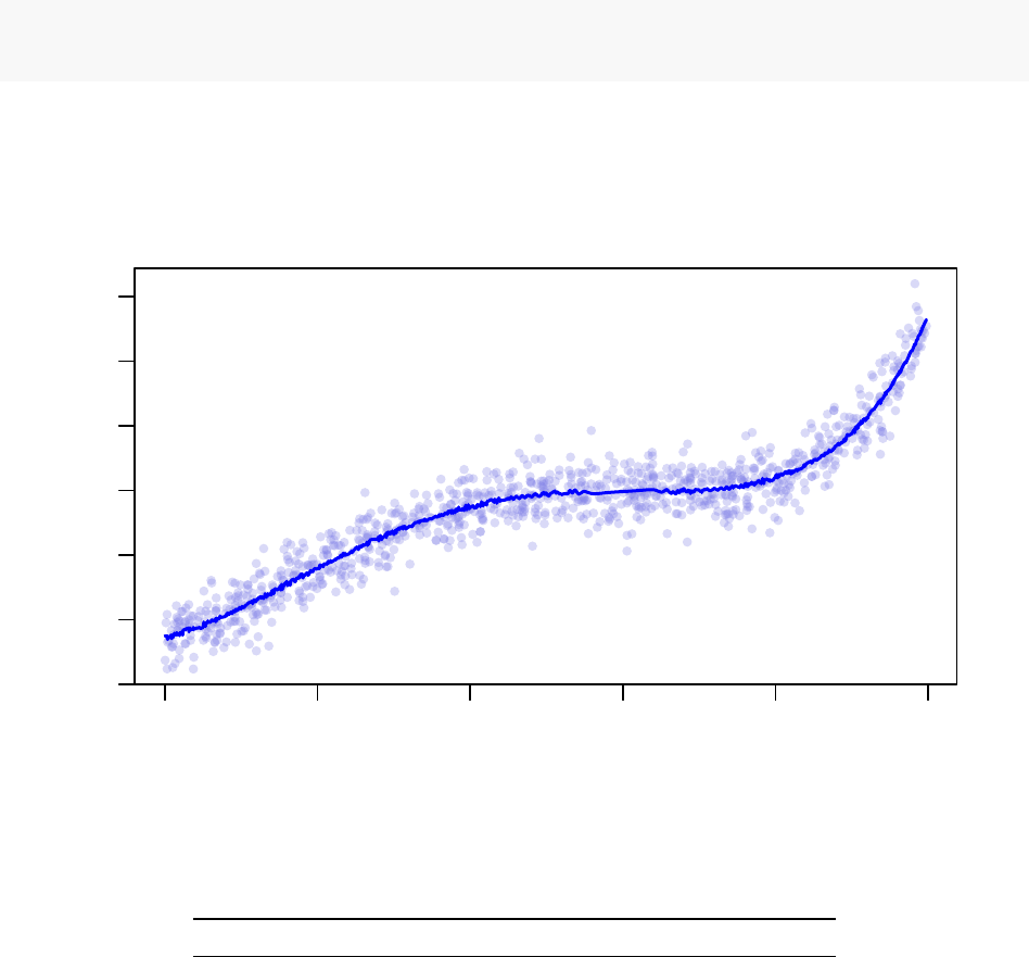
Interestingly, each of the 4 processors arrive at the same solution in this instance.
−15 −10 −5 0 5 10
−300 −100 0 100 300
Acceptance Ratio Annealing Optimus Fitting (4 Cores)
x
y
Table 4: 4 Core Acceptance Ratio Annealing Optimus Run Results
Processor 1 Processor 2 Processor 3 Processor 4
E (AIC) 9.567 9.567 9.567 9.567
Q (RMSD) 28.693 28.693 28.693 28.693
Term 1 0.000 0.000 0.000 0.000
Term 2 1.000 1.000 1.000 1.000
Term 3 1.000 1.000 1.000 1.000
Term 4 1.000 1.000 1.000 1.000
Term 5 0.000 0.000 0.000 0.000
Term 6 0.000 0.000 0.000 0.000
Term 7 0.000 0.000 0.000 0.000
Term 8 0.000 0.000 0.000 0.000
Term 9 0.000 0.000 0.000 0.000
Term 10 0.000 0.000 0.000 0.000
Term 11 1.000 1.000 1.000 1.000
Term 12 0.000 0.000 0.000 0.000
Term 13 0.000 0.000 0.000 0.000
Term 14 0.000 0.000 0.000 0.000
Term 15 0.000 0.000 0.000 0.000
20

Processor 1 Processor 2 Processor 3 Processor 4
Term 16 0.000 0.000 0.000 0.000
Term 17 0.000 0.000 0.000 0.000
Term 18 0.000 0.000 0.000 0.000
Term 19 0.000 0.000 0.000 0.000
Term 20 1.000 1.000 1.000 1.000
Term 21 0.000 0.000 0.000 0.000
Term 22 0.000 0.000 0.000 0.000
Term 23 0.000 0.000 0.000 0.000
Term 24 0.000 0.000 0.000 0.000
Term 25 0.000 0.000 0.000 0.000
Term 26 1.000 1.000 1.000 1.000
Term 27 0.000 0.000 0.000 0.000
Term 28 0.000 0.000 0.000 0.000
Term 29 0.000 0.000 0.000 0.000
Term 30 0.000 0.000 0.000 0.000
Thus, the optimal functional representation found by Optimus has the following form:
y=b+c2x2+c3x3+c4x4+c11ex+c20sin(x3) + c26cos(x5)sin(−x)
Below is the explicit representation after determing the coefficients ciand b:
##
## Call: glm(formula = equation, data = environment())
##
## Coefficients:
## (Intercept) I(x^2) I(x^3)
## -1.988699 -0.253437 0.178807
## I(x^4) I(exp(x)) I(sin(x^3))
## 0.008567 0.001569 1.878796
## I(cos(x^5) * sin(-x))
## -2.770457
##
## Degrees of Freedom: 999 Total (i.e. Null); 993 Residual
## Null Deviance: 10850000
## Residual Deviance: 823300 AIC: 9567
Notice that the solution selected by Optimus results in an RMSD of 28
.
693 which is lower than the RMSD of
the Least Squares Solution (28
.
82655) which assumes the appropriate model is
k1x
+
k2x2
+
k3x3
+
k4x4
.
Optimus selected a model which does not include all terms from the form used to generate the data. If a user
were concerned by the fact that the model Optimus selected contains more terms (6) than are used in the
representation of the de-noised data (4), the user could either increase the multiplicative factor associated with
the term
p
in the
AIC
to more strongly penalize representations involving a greater number of parameters.
Alternatively, the user could also modify the function r() to ensure that only a fixed number of terms are
ever active.
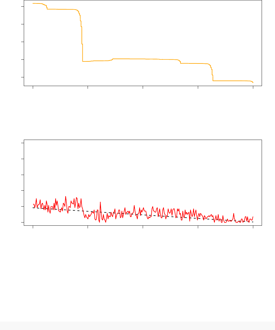
Let us now take a look at how the Temeperature Control Unit performed given this highly non-smooth
objective. The graphs below should now feel very familiar, they represent data taken from the last 20 000
iterations of the optimisation protocol executed by Processor 1.
21
180000 185000 190000 195000 200000
1e−04 2e−04 3e−04 4e−04 5e−04
System Pseudo−Temperature (Processor 1)
Step
Temperature
180000 185000 190000 195000 200000
0 20 40 60 80 100
Observed Acceptance Ratio (Processor 1)
Step
Acceptance ratios (%)
Despite optimising a completely different model with a non-smooth objective function, the TCU succeeds in
dynamically adjusting the system pseudo-temperature such that the observed acceptance ratio follows the
annealing schedule rather well.
Replica Exchange Optimus Run
Let us now consider the Replica Exchange version of Optimus on 12 processors with the variable ACCRATIO
defined as in Tutorial 1.
ACCRATIO <- c(90,82,74,66,58,50,42,34,26,18,10,2)
As in the Acceptance Ratio Annealing run above, we will again execute the optimisation procedure for 200
000 iterations. The Replica Exchange version of Optimus takes an input argument EXCHANGE.FREQ
22
(default value 1000) which specifies the total number of exchanges that will occur during the optimisation
process. Consequently, the number of optimisation iterations that occur between subsequent exchanges
between replicas can be calculated as
NUM IT ER/EXCHANGE.F REQ
, which is 200 iterations in this
case.
Here we will set the input parameter STATWINDOW to have value 50 (its default value is 70). This signifies
that the TCU will update the system pseudo-temperature once every 50 iterations on each optimisation
replica. This guarantees that 4 temperature adjustments will be made if a given replica is involved in
two subsequent exchanges (because the number of iterations between exchanges is 200, as explained in the
preceding paragraph) as opposed to merely 2 adjustments which would be the case if STATWINDOW were
left to take its default value and could result in poor agreement between the observed acceptance ratio of
the replica in question and the target acceptance ratio. The following line executes Optimus with the above
specified inputs:
Optimus(NCPU = 12,K.INITIAL = K, rDEF = r, mDEF = m, uDEF = u, ACCRATIO = ACCRATIO,
OPT.TYPE = "RE",DATA = DATA, OPTNAME = "term_12_RE",NUMITER = 2e+05,STATWINDOW = 50,
DUMP.FREQ = 1e+05,LONG = FALSE)
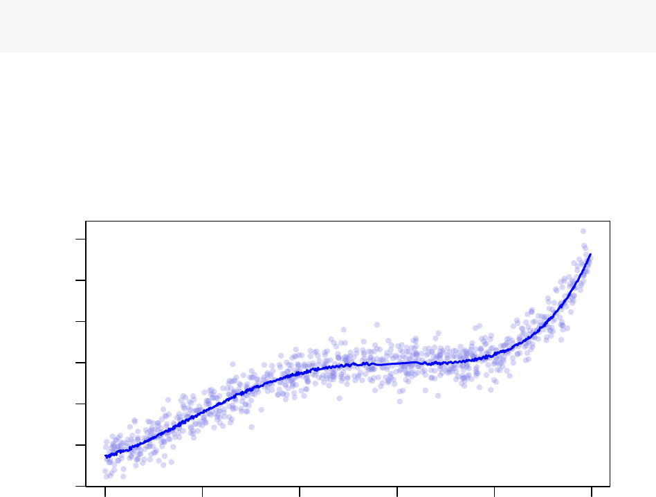
Nine of the optimisation replicas (Processors 1, 2, 3, 5, 6, 8, 9, 10 and 12) recovered the same solution that
was found by the Acceptance Ratio Annealing Optimus run. Moreover, this solution is better (lower
AIC
)
than those recovered by Processors 4, 7 and 11. Thus, in this example, the Acceptance Ratio Annealing and
Replica Exchange versions produce the same solution.
−15 −10 −5 0 5 10
−300 −100 0 100 300
Replica Exchange Optimus Fitting (12 Cores)
x
y
Please note that for convenience, only those replicas which produced a unique solution are listed in the table
below (replicas 1, 2, 3, 6, 8, 9, 10 and 12 produced the same solution as replica 5; replica 11 produced the
same solution as replica 7).
23

Table 5: 12 Core Replica Exchange Optimus Run Results
Processor 4 Processor 5 Processor 7
Replica Acceptance Ratio 66.00000 58.00000 42.00000
E (AIC) 9.56730 9.56720 9.56730
Q (RMSD) 28.66639 28.69324 28.69512
Term 1 0.00000 0.00000 0.00000
Term 2 1.00000 1.00000 1.00000
Term 3 1.00000 1.00000 1.00000
Term 4 1.00000 1.00000 1.00000
Term 5 0.00000 0.00000 0.00000
Term 6 0.00000 0.00000 0.00000
Term 7 0.00000 0.00000 0.00000
Term 8 0.00000 0.00000 0.00000
Term 9 0.00000 0.00000 0.00000
Term 10 0.00000 0.00000 0.00000
Term 11 1.00000 1.00000 0.00000
Term 12 0.00000 0.00000 0.00000
Term 13 1.00000 0.00000 1.00000
Term 14 0.00000 0.00000 0.00000
Term 15 0.00000 0.00000 0.00000
Term 16 0.00000 0.00000 0.00000
Term 17 0.00000 0.00000 0.00000
Term 18 0.00000 0.00000 0.00000
Term 19 0.00000 0.00000 0.00000
Term 20 1.00000 1.00000 0.00000
Term 21 0.00000 0.00000 0.00000
Term 22 0.00000 0.00000 0.00000
Term 23 0.00000 0.00000 0.00000
Term 24 0.00000 0.00000 0.00000
Term 25 0.00000 0.00000 0.00000
Term 26 1.00000 1.00000 1.00000
Term 27 0.00000 0.00000 0.00000
Term 28 0.00000 0.00000 1.00000
Term 29 0.00000 0.00000 0.00000
Term 30 0.00000 0.00000 0.00000
Note that the various replica outcomes illustrate the penalizing effects of the
AIC
on models using a greater
number of parameters. Consider the solutions found by the 66% acceptance ratio replica and the 58%
acceptance ratio replica (Processors 4 and 5 respectively). Let
yi
denote the solution found by Processor
i
.
Then, we have:
y4=b+c2x2+c3x3+c4x4+c11ex+k13c13six(x) + c20sin(x3) + c26cos(x5)sin(−x)
y5=b+c2x2+c3x3+c4x4+c11ex+c20sin(x3) + c26cos(x5)sin(−x)
Although the RMSD of
y4
,28
.
66639, is lower than the RMSD of
y5
,28
.
69324,
y5
has a lower value for
AIC
because it contains one less term than
y4
. Since
AIC
was specified as the objective metric, Optimus (perhaps
counterintuitively) selecyed y5as the more optimal solution to reduce overfitting.
24
180000 185000 190000 195000 200000
0.0017885 0.0017895 0.0017905
System Pseudo−Temperature (Processor 5 − 58% Acceptance Ratio)
Step
Temperature
180000 185000 190000 195000 200000
0 20 40 60 80 100
Observed Acceptance Ratio (Processor 5 − 58% Acceptance Ratio)
Step
Acceptance ratios (%)
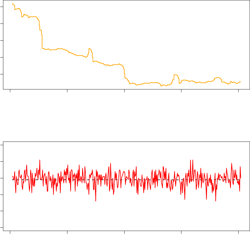
The above graphs are produced using data from the last 20 000 iterations of the 58% acceptance ratio replica
(Processor 5). It is clear that the observed acceptance ratio more strongly oscillated around the target
acceptance ratio than was the case in the Acceptance Ratio Annealing run from the previous part of this
tutorial. More generally, it should be expected that the observed acceptance ratio fluctuates more significantly
around the target acceptance ratio in Replica Exchange than in Acceptance Ratio Annealing, especially when
the objective function is non-smooth as is the case in this example. This is because an exchange between two
replicas has the same effect as restarting a Monte Carlo optimisation from a random initial configuration with
a temperature that very likely is not conducive to the target acceptance ratio for the given configuration.
As such, each time an exchange occurs, significant deviations from the target acceptance ratio may occur
and may require several STATWINDOWs for the TCU to correct. Despite this challenge, the TCU performs
satisfactorily.
25

Summary
We now understand how to employ Optimus to solve a more general problem than was addressed in Tutorial
1 and one with a non-smooth objective function. Additionally, we have a better understanding of the
performance of the Temperature Control Unit. Using the Aikake Information Criterion (
AIC
) as a metric
with which to evaluate the performance of a candidate model, taking into account the desire to represent the
data while avoiding to overfit the data, both the Acceptance Ratio Annealing and Replica Exchange versions
of Optimus recovered a better functional form to describe the data than the form which was assumed in
Tutorial 1 (based on how the data had been generated).
Table 6: Summary of Solutions
E (AIC) Q (RMSD)
Least Squares (Tutorial 1) 9.570471 28.82655
Optimus (Acceptance Ratio Annealing) 9.567200 28.69324
Optimus (Replica Exchange) 9.567200 28.69324
Least Squares(Tutorial 1):
y=c1x+c2x2+c3x3+c4x4
Optimus (Acceptance Ratio Annealing):
y=b+c2x2+c3x3+c4x4+c11ex+c20sin(x3) + c26cos(x5)sin(−x)
Optimus (Replica Exchange):
y=b+c2x2+c3x3+c4x4+c11ex+c20sin(x3) + c26cos(x5)sin(−x)
26
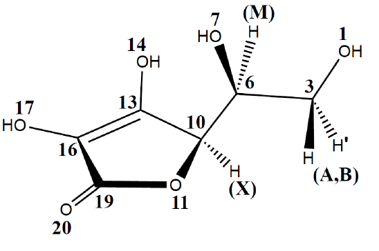
Tutorial 3: Vitamin C Molecular Geometry Optimisation
Problem Statement
The focus of this Tutorial is to depart from problem classes involving the search for functions to represent
data and demonstrate how Optimus can be flexibly applied to arbitrary problem classes provided that they
are formulated in accordance with Optimus specifications. Additionally, this Tutorial will illustrate that
Optimus can act as an optimisation kernel while calling external programs to execute a significant amount of
the necessary computation for the optimisation process.
In this Tutorial, Optimus will be used to solve a molecular geometry optimisation problem. Specifically,
Optimus will be used to determine the values of two dihedral angles in the L-ascorbic acid (Vitamin C)
molecule such that the molecule is in its ground state energy conformation. Vitamin C was selected to be the
studied molecule because it has more than one freely rotating carbon-carbon sigma bond and the potential
for intramolecular hydrogen bonding due to the presence of multiple hydroxy groups and lone pair donating
oxygen atoms. Moreover, Vitamin C is not a particularly large molecule. Due to these circumstances, Vitamin
C has a non trivial groud energy state (as opposed to a molecule like ethane for instance) but one that does
not require several days or weeks of simulation to arrive at (the optimisation procedures below took roughly
14-18 hours to terminate).
This is the molecular structure of Vitamin C:
Free rotation is possible around two sigma bonds in this structure: the bond joining carbon 3 and 6, and the
bond joining carbon 6 and 10. The ground state conformation of Vitamin C will be a conformation such that
steric clash between the constituent members bonded to the freely rotating bonds is minimized while also
allowing for close proximity between hydrogen bond donating and hydrogen bond accepting groups. In the
following sections, we formalize this optimisation problem and use Optimus to arrive at the solution.
Defining Optimus Inputs
As in the previous Tutorials, we must first rigorously define the parameters which we are optimising. Let us
begin by defining a dihedral angle as it applies to molecular geometry: a dihedral angle is the angle between
two intersecting planes, where each plane is specified by 3 atoms of which 2 are common between both planes.
Thus, a total of 4 atoms are needed to specify a dihedral angle. The conformation of Vitamin C with respect
to its two freely rotating sigma bonds can be specified via two dihedral angles. Let
ψ
be the dihedral angle
defined by the atoms numbered 1, 3, 6 and 7 and let
φ
be the dihedral angle defined by the atoms numbered
6, 7, 10 and 11. Loosely,
ψ
can be thought of as the angle between oxygen atoms 1 and 7 while
φ
can be
thought of as the angle between oxygen atoms 7 and 11. Having defined these two angles, we can now define
27
the parameter set
K
as a numeric vector of length 2 whose entries are
ψ
and
φ
. We will arbitrarily initialize
ψ
and
φ
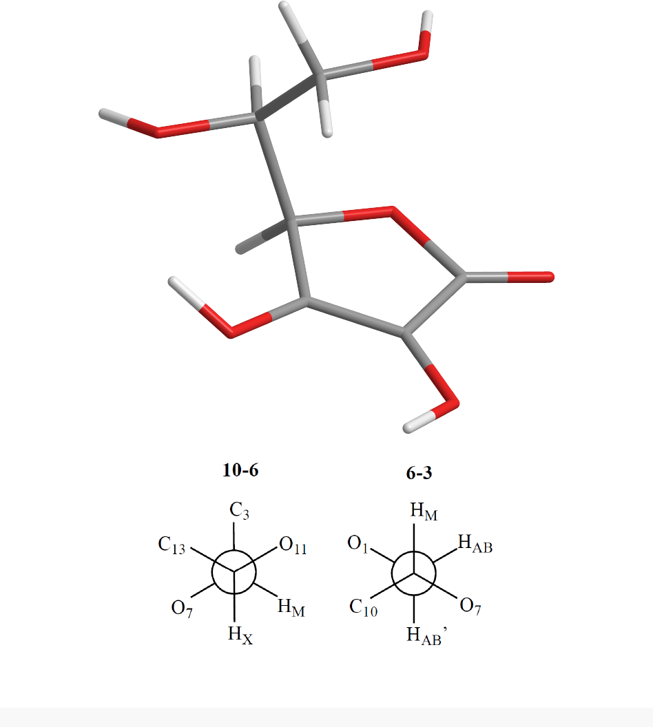
to have value 180. The corresponding Vitamin C conformation is illustrated below using a 3D
structure and Newman Projections along the two rotatable carbon-carbon bonds:
In the 3D structure, grey denoted Carbon, red denotes Oxygen and white denoted Hydrogen.
K <- c(PHI=180,PSI=180)
Now we will specify a model function
m
() which will operate on
K
. Starting from an arbitrary molecular
conformation, altering the value of
K
will likely cause certain clashes or non-optimal interactions between
atoms in the molecule that are not used in the definition of the angles ψand φ. As such, after receiving an
input set of parameters
K
,
m
() will have to alter the 3D location of constituents atoms while holding
K
fixed to arrive at the most stable geometry for the input
K
. Here, unlike in previous Tutorials, to accomplish
28

this task
m
() will call a completely external program: MOPAC (2016). MOPAC is a geometry optimiser that
uses EigenFollowing to arrive at a local minimum (note that calling MOPAC for a single instance does not
guarantee a global minimum will be found). MOPAC takes as input the specification of an initial molecular
geometry in addition to an indication of which molecules the program is able to displace (or angles it can
alter) and outputs a nearby local minimum molecular conformation with its corresponding energy in kcal/mol.
For this optimisation problem, the input to MOPAC will be structured as a Z matrix, a common form for
describing a molecular conformation which consists of using lengths, angles and dihedral angles with respect
to previously defined atoms to define new atoms in the conformation.
The function
m
() will construct a Z matrix for Vitamin C using the input dihedral angles
K
and default
values for the remaining relationships needed to define the molecule.
m
() will then call MOPAC with the
newly constrcuted Z matrix, specifiying that all relationships may be altered except the input dihedral angles
K. Finally, m() will return the energy calculated by MOPAC.
Note that to avoid non convergence issues when calling MOPAC,
m
() returns a default energy value of -100
kcal/mol if a call to MOPAC does not terminate within 10 seconds. Also, note that although
m
() requires no
additonal data on top of
K
to operate,
m
() must still be defined to take an input DATA in accordance with
Optimus specifications. Lastly, note that a local installation of MOPAC (2016) is required to execute this
optimisation procedure. Below is the definition of m():
m <- function(K, DATA = NULL){
notconvergedE = -100.00
# this should be your local path to MOPAC
mopac.cmd="/home/group/prog/mopac2016/MOPAC2016.exe"
clean = TRUE
# MOPAC semiempirical QM input file preparation, with given PHI and PSI
# dihedral angles.
geo <- c(
"RHF PM6 EF GEO-OK MMOK T=10 THREADS=1",
"Vitamin C with two controllable dihedral angles psi(7,6,3,1) and phi(11,10,6,7)",
" ",
"O 0.00000000 0 0.0000000 0 0.0000000 0 0 0 0",
"H 0.98468620 1 0.0000000 0 0.0000000 0 1 0 0",
"C 1.43651250 1 110.7230618 1 0.0000000 0 1 2 0",
"H 1.10751723 1 103.6603154 1 -167.5282722 1 3 1 2",
"H 1.10658657 1 110.2236860 1 -51.3620456 1 3 1 2",
"C 1.53950336 1 112.8074046 1 -123.2791585 1 3 4 5",
paste0("O 1.42824262 1 103.4315186 1 ",K["PSI"]," 0 6 3 1"),
"H 0.99584949 1 109.9022382 1 -165.7055126 1 7 6 3",
"H 1.11472171 1 108.4417082 1 75.1535637 1 6 7 8",
"C 1.54244170 1 109.4042184 1 -120.8240216 1 6 7 9",
paste0("O 1.46313669 1 105.7792445 1 ",K["PHI"]," 0 10 6 7"),
"H 1.11252563 1 112.8336666 1 -114.5813834 1 10 6 11",
"C 1.51686608 1 113.4849244 1 -112.8332453 1 10 12 11",
"O 1.34410484 1 125.3617342 1 179.6090511 1 13 10 11",
"H 1.03381724 1 110.9736522 1 -13.3419919 1 14 13 10",
"C 1.36084908 1 124.8906459 1 167.6242325 1 13 14 15",
"O 1.35614887 1 131.9374989 1 -0.0333000 1 16 13 14",
"H 1.00338885 1 109.4220239 1 0.3798200 1 17 16 13",
"C 1.49109250 1 118.0837177 1 -179.7749947 1 16 17 18",
"O 1.18961787 1 136.9144035 1 -0.6060924 1 19 16 17",
" "
29

)
# Submitting the MOPAC optimisation job, where all the spatial parameters
# are relaxed except the pre-set PHI and PSI angles. The job is run requesting
# maximum 10 seconds of time limitation. Most (if not all) complete within
# half a second.
random.id <- as.character(sample(size=1,x=1:10000000))
write(geo, file=paste0(random.id,".mop"))
system(paste0(mopac.cmd," ",random.id,".mop"))
if(file.exists(paste0(random.id,".arc")) ){
e.line <- grep("HEAT OF FORMATION",
readLines(paste0(random.id,".arc")),
value=TRUE)
e.line <- strsplit(e.line," ")[[1]]
O <- as.numeric(e.line[e.line!=""][5])
}else {
O <- notconvergedE
}
if(clean){
file.remove(grep(random.id, dir(), value=TRUE))
}
return(O) # heat of formation in kcal/mol
}
Next, we define the function
u
() which returns an energy
E
and a quality
Q
of the candidate solution. Since
the
m
() will already output a value for the physcial energy of the candidate Vitamin C conformation,
u
() can
simply set
E
to be the return value of
m
(). We will make
u
() set
Q
to be the negative of the return value
of
m
() such that candidate conformations with lower energies produce higher values of
Q
. Again, although
u
() does not require any additional data to accomplish this functionality, it must nevertheless be written to
optionally accept an input parameter DATA.
u <- function(O, DATA = NULL) {
result <- NULL
result$Q <- -O
result$E <- O
return(result)
}
Finally, we define the function
r
().
r
() will randomly select either
ψ
or
φ
to alter. Thereafter,
r
() randomly
increases or decreases the selected angle by 2 degrees.
r
() will also ensure that
ψ, φ ∈
[
−
180
.
0
,
180
.
0]
throughout the optimisation process.
r <- function(K) {
K.new <- K
# Setting the alteration angle to 3 degrees:
alter.by <- 2
# Randomly selecting a term:
K.ind.toalter <- sample(size = 1,x=1:length(K.new))
# Altering that term by either +alter.by or -alter.by
K.new[K.ind.toalter] <- K.new[K.ind.toalter] +sample(size = 1,x = c(alter.by,
-alter.by))
30

# Setting the dihedral angles to be always within the -180 to 180 range.
if (K.new[K.ind.toalter] >180) {
K.new[K.ind.toalter] <- K.new[K.ind.toalter] -360
}
if (K.new[K.ind.toalter] < -180) {
K.new[K.ind.toalter] <- K.new[K.ind.toalter] +360
}
return(K.new)
}
The process of determining the energy of a conformation corresponding to a given set of angles
ψ, φ
is the
most computationally intensive part of this optimisation formulation. Having defined the necessary inputs
for Optimus, it should be apparent that this calculation will entirely be handled by MOPAC. This ability to
serve as an optimisation kernel by off-loading a significant amount of computation to an external program is
one of the many strengths of Optimus.
Defining a Benchmark Solution
Before calling Optimus, we must establish a benchmark solution which will be used to evaluate the efficacy
of Optimus. In order to explore the energy landscape associated with the parameter space of
ψ
and
φ
, a
PM6 optimization was performed on 10 conformers from an MM2 optimization run (the details of PM6 and
MM2 are not important for the purposes of this tutorial) which resulted in the identification of 7 local energy
minima, shown in the table below (listed in increasing order by energy):
Table 7: 7 Vitamin C Conformational Local Minima
E (kcal/mol) PHI PSI
Conformation 1 -233.206 92.58 74.19
Conformation 2 -232.877 50.60 -172.79
Conformation 3 -231.800 -169.67 -41.23
Conformation 4 -230.822 47.43 -166.61
Conformation 5 -230.274 -172.20 -54.45
Conformation 6 -225.214 -75.69 -104.44
Conformation 7 -224.875 -73.31 155.02
We will assume that the above listed conformations represent all conformational local minima in the parameter
space of
ψ
and
φ
. Under this assumption, Conformation 1 should be considered the ground state conformation
of Vitamin C. The accuracy of the results produced by Optimus can thus be judged by comparing them
to the data listed in this table. It is important to recognize that the “resolution” of
ψ
and
φ
when being
optimized by Optimus is 2 degrees due to the manner in which
r
() was defined. As such, results produced by
Optimus that are within plus or minus 2 degrees of a reference conformation should be tolerated.
Acceptance Ratio Annealing Optimus Run
For the Acceptance Ratio Annealing run, we will set NUMITER = 100 000 because each optimsation step is
more costly due to the relatively computationally expensive calls to MOPAC. Moreover, we will set CYCLES
= 2. Although this shortens the length of an annealing cycle to 50 000 steps (whereas 100 000 steps per
cycle has been kept constant over the previous tutorials), having more than 1 annealing cycle is likely more
beneficial than insisting on a cycle lasting 100 000 steps as opposed to 50 000.
31
Optimus(NCPU = 4,K.INITIAL = K, rDEF = r, mDEF = m, uDEF = u, OPT.TYPE = "SA",
OPTNAME = "vitamin_4_SA",NUMITER = 1e+05,CYCLES = 2,DUMP.FREQ = 50000,
LONG = FALSE)
Table 8: 4 Core Acceptance Ratio Annealing Optimus Run Results
E (kcal/mol) PHI PSI
Processor 1 -232.874 50 -172
Processor 2 -232.353 -158 30
Processor 3 -232.874 50 -172
Processor 4 -232.874 50 -172
Processors 1, 3 and 4 all arrived at a conformation defined by
{φ
= 50
, ψ
=
−
172
}
, with an energy of
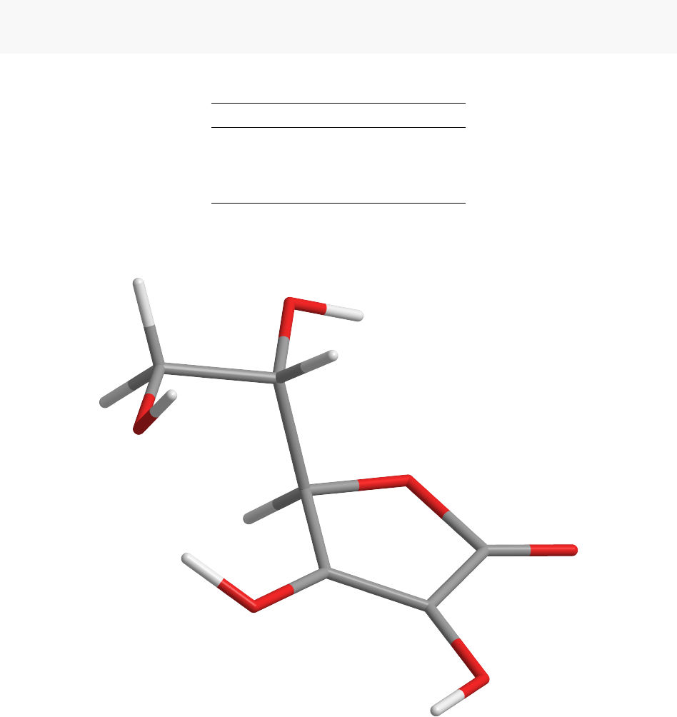
−232.874 kcal/mol. The below 3D structure and Newman Projections depict this solution:
32
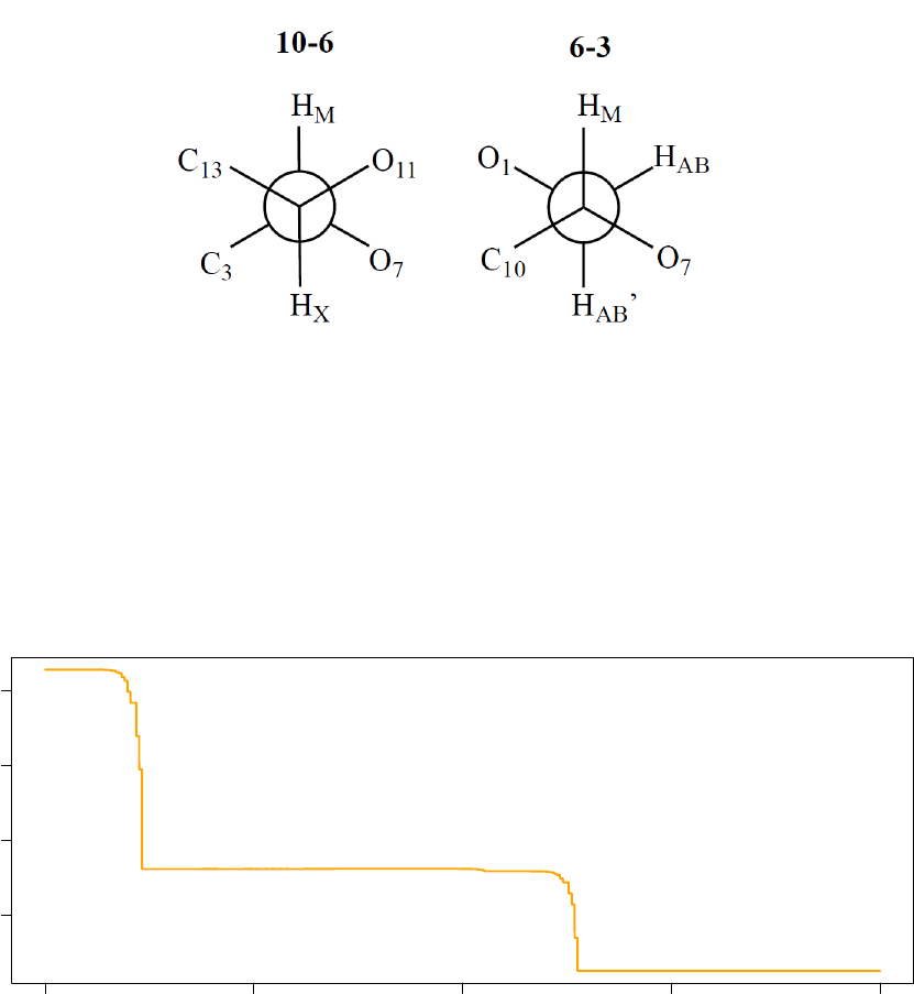
This conformation is equivalent to benchmark Conformation 2. Thus, in this example, Acceptance Ratio
Annealing was able to find the Vitamin C conformation with the second lowest energy in the parameter
space. This performance is strong, especially given that the energy difference between Conformation 1 and
Conformation 2 is only -0.329 kcal/mol.
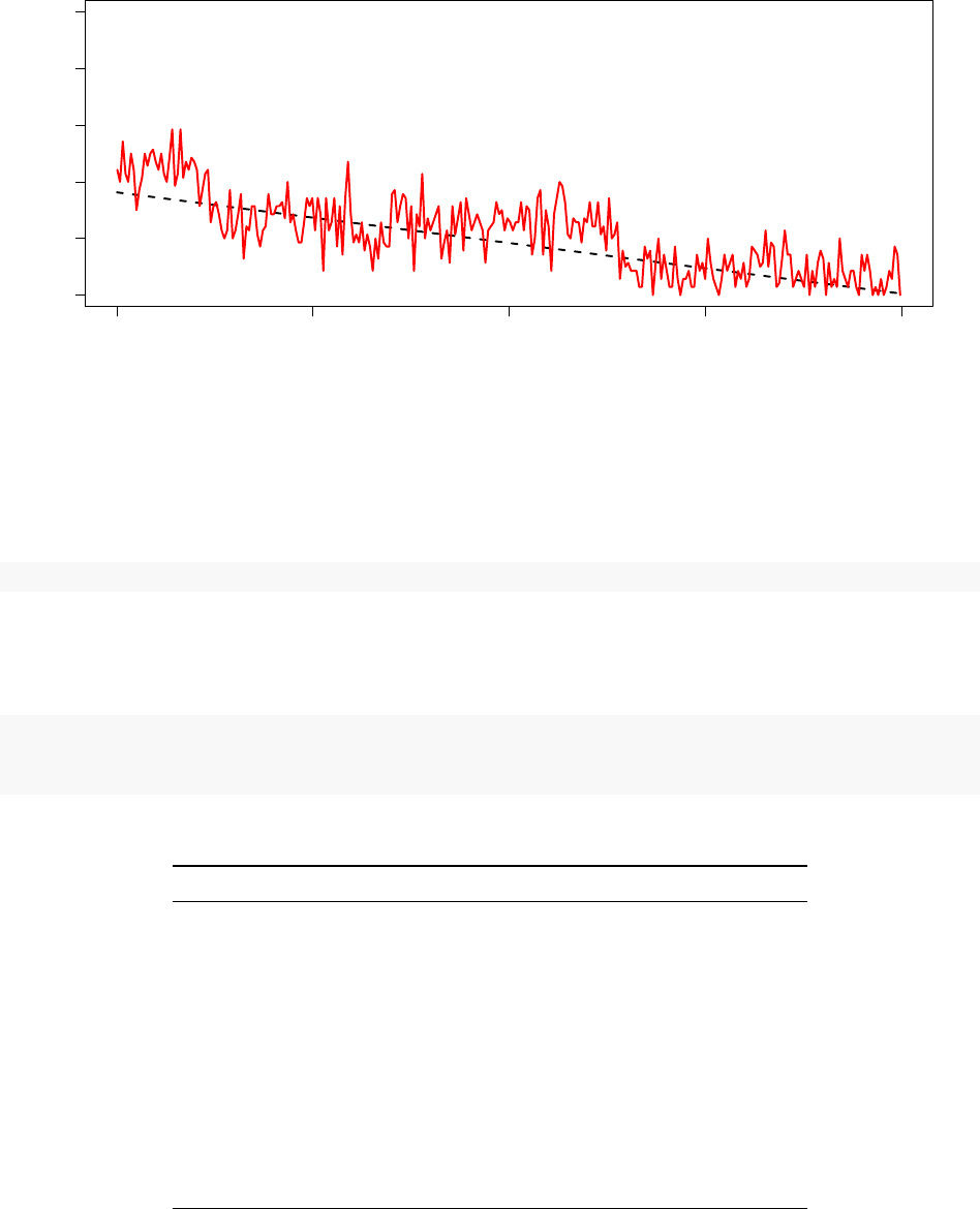
The graphs below illustrate the system psuedo-temperature and observed acceptance ratio for the last 20 000
optimisation iterations executed by Processor 3.
80000 85000 90000 95000 100000
0.004 0.006 0.008 0.010
System Pseudo−Temperature (Processor 3)
Step
Temperature
33
80000 85000 90000 95000 100000
0 20 40 60 80 100
Observed Acceptance Ratio (Processor 3)
Step
Acceptance ratios (%)
Replica Exchange Optimus Run
Let us now consider the Replica Exchange version of Optimus on 12 processors with the variable ACCRATIO
defined as in the previous Tutorials.
ACCRATIO <- c(90,82,74,66,58,50,42,34,26,18,10,2)
Just as in the Acceptance Ratio Annealing run, we will set NUMITER = 100 000. Moreover, we will set
EXCHANGE.FREQ = 500 such that the number of iterations between subsequent exchanges between replicas
is 200 as it was in Tutorial 2. For the same reasons as in Tutorial 2, we will set STATWINDOW = 50 for the
Replica Exchange run.
Optimus(NCPU = 12,K.INITIAL = K, rDEF = r, mDEF = m, uDEF = u, ACCRATIO = ACCRATIO,
OPT.TYPE = "RE",DATA = DATA, OPTNAME = "vitamin_12_RE",NUMITER = 1e+05,
EXCHANGE.FREQ = 500,STATWINDOW = 50,DUMP.FREQ = 50000,LONG = FALSE)
Table 9: 12 Core Replica Exchange Optimus Run Results
Replica Acceptance Ratio E (kcal/mol) PHI PSI
Processor 1 90 -229.2359 -164 -178
Processor 2 82 -229.2359 -164 -178
Processor 3 74 -233.1453 82 84
Processor 4 66 -233.1979 90 76
Processor 5 58 -229.2359 -164 -178
Processor 6 50 -232.8742 50 -172
Processor 7 42 -233.1947 94 74
Processor 8 34 -229.2359 -164 -178
Processor 9 26 -229.2359 -164 -178
Processor 10 18 -227.6394 180 158
Processor 11 10 -229.2359 -164 -178
Processor 12 2 -229.2359 -164 -178
34
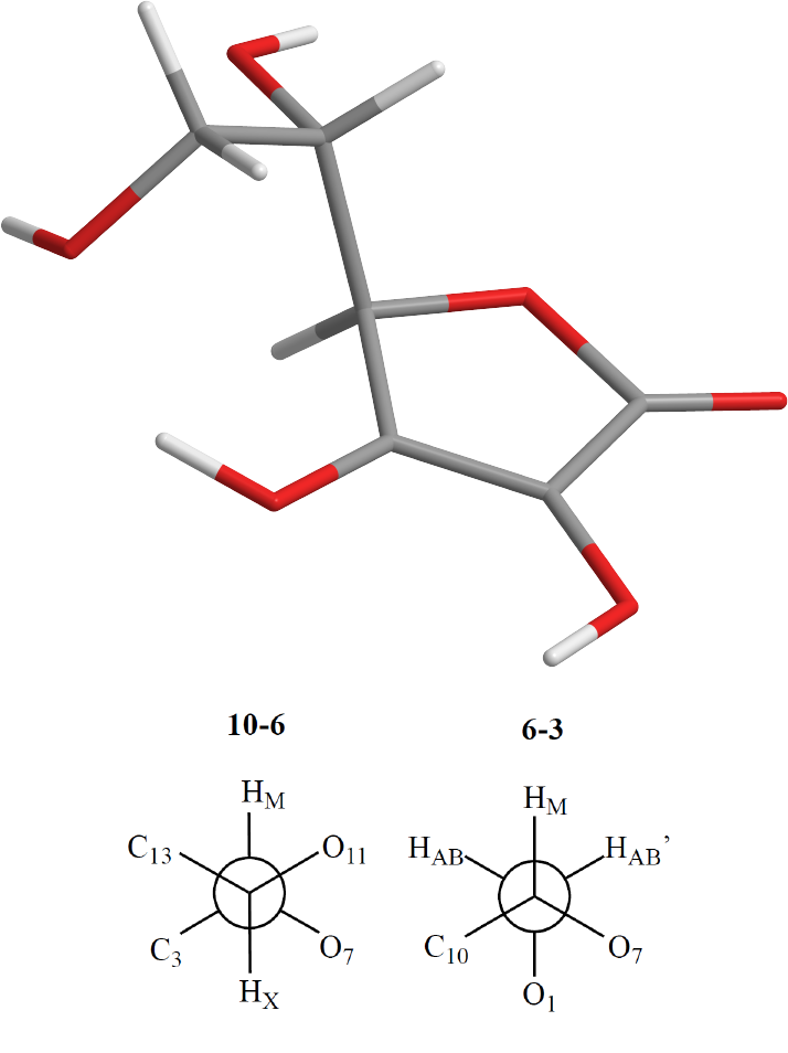
Of the 12 replicas, Processor 4 recovered the conformation with the lowest energy (
−
233
.
1979), defined by
{φ= 90, ψ = 76}. The below 3D structure and Newman Projections depict this solution:
This solution corresponds to reference Conformation 1, the global minimum energy state for Vitamin C. Thus,
for this optimisation problem, the Replica Exchange version of Optimus outperformed Acceptance Ratio
Annealing by succeeding in finding the global minimum of the energy landscape while the latter version found
only the second lowest local energy minimum.
If we compare the solution found by Processor 4 to benchmark Conformation 1, it is evident that the value
for
φ
found by Optimus lies slightly outside of the plus or minus 2 degree window that was discussed earlier.
Contrarily, Processor 7 finds a solution
{φ
= 94
, ψ
= 74
}
which does lie strictly within the resolution window.
Despite this, the solution of Processor 4 has a slightly lower energy (
−
233
.
1979) than the solution of Processor
7 (
−
233
.
1947) and so represents a better solution. Given that the local energy landscape around Conformation
1 is unknown, it is not unreasonable that within this local area, a conformation “closer” to Conformation 1
35
does not necessarily result in a lower energy. Finally, notice that Replica 6 recovered the same conformation
that was identified by Acceptance Ratio Annealing Optimus.
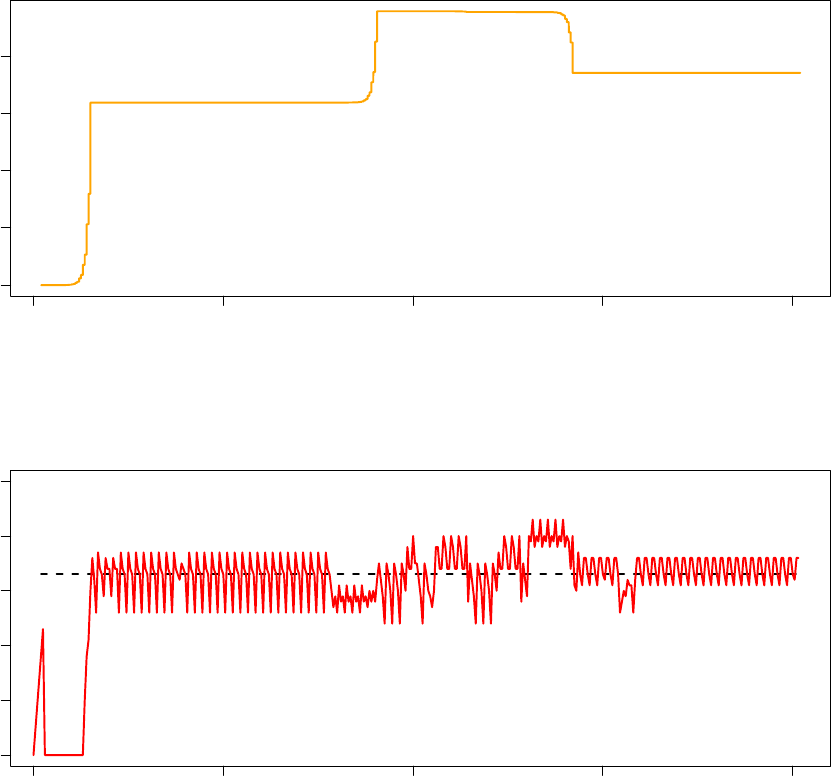
The below graphs illustrate the system psuedo-temperature and observed acceptance ratio for the first 20 000
optimisation iterations executed by Processor 4 (66% acceptance ratio replica).
0 5000 10000 15000 20000
0.000 0.005 0.010 0.015 0.020
System Pseudo−Temperature (Processor 4 − 66% Acceptance Ratio)
Step
Temperature
0 5000 10000 15000 20000
0 20 40 60 80 100
Observed Acceptance Ratio (Processor 4 − 66% Acceptance Ratio)
Step
Acceptance ratios (%)
When the optimisation process is first initialized, it is very unlikely that the input initial temperature is
conducive to the target acceptance ratio. As such, the Temperature Control Unit alters the system pseudo-
temperature considerably and rapidly to align the observed acceptance ratio with the target acceptance ratio,
as can be seen in the above two graphs. Moreover, as stated in the previous Tutorial, an exchange between
two replicas often has a similar effect of introducing a parameter configuration that is not conducive to the
current system pseudo-temperature, which catalyzes significant temperature adjustments executed by the
TCU. Accordingly, sharp increases or decreases in the system pseudo-temperature and significant changes in
the value around which the observed acceptance ratio oscillates in the graph above likely indicate steps at
which an exchange involving replica 4 occurred.
36

Summary
We are now familiar with how to structure a molecular geometry optimisation problem to be solved with
Optimus as a kernel while interfacing with an entirely external program, MOPAC, to handle a significant
amount of the necessary computation. Using 7 local minima identified by a PM6 optimization of 10 conformers
from an MM2 run as validation, we saw that the Acceptance Ratio Annealing mode of Optimus was able to
find the second lowest local minima while the Replica Exchange mode recovered the global energy minimum
(outperforming Acceptance Ratio Annealing).
Table 10: Summary of Solutions
Energy (kcal/mol) PHI PSI
Ground State Reference -233.2060 92.58 74.19
Optimus (Acceptance Ratio Annealing) -232.8740 50.00 -172.00
Optimus (Replica Exchange) -233.1979 90.00 76.00
37
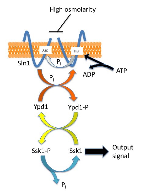
Tutorial 4: Determining Rate Constants for Coupled ODEs Mod-
elling a Biological System
Problem Statement
This Tutorial will demonstrate the use of Optimus to address a problem from yet another problem class. We
will employ Optimus to recover the rate constants for a system of coupled ordinary differential equations
(ODEs) modelling a biological pathway. Specifically, we will study a phosphorelay system from the high
osmolarity glycerol (HOG) pathway in Yeast. A phosphorelay system is a network involving multiple
proteins in which after an initial phosphorylation event using ATP (or an alternate phosphate donor), the
phosphorylation and dephosphorylation events of proteins in the network proceed without further consumption
of ATP (Klipp et al. 2009). The below diagram illustrates the phosphorelay system that will be studied in
detail (Klipp et al. 2009):
Under normal circumstances, the transmembrane protein Sln1, which is present as a dimer, autophosphorylates
at a histidine residue (consuming ATP). The phosphate group is then transferred to an aspartate residue of
Sln1. Thereafter, the phosphate is transferred to the protein Ypd1 and finally to the protein Ssk1. Ssk1 is
continuously dephosphortylated to give an output signal. The signalling pathway is inhibitted by an increase
is osmolarity outside of the cell (Klipp et al. 2009). If we let
A
represent Sln1,
B
represent Ypd1,
C
represent
Ssk1 and
XP
represent the phophorylated form of protein
X
, then the above network can be represented by
the below schematic (Klipp et al. 2009):
38

where each kirepresents the rate constant for the relevant phosphorylation/dephosphorylation reaction.
The above graphic allows us to arrive at the following equations to describe the temporal behavior of the
phosphorelay system:
d
dt[A] = −k1[A] + k2[AP ][B]
d
dt[B] = −k2[AP ][B] + k3[BP ][C]
d
dt[C] = −k3[BP ][C] + k4[CP ]
Moreover, under the generally accepted assumption that the degradation and production of proteins occurs on
a time scale that far exceeds that of phosphorylation events, we have the following conservation relationships
(Klipp et al. 2009):
[A]total = [A]+[AP ]
[B]total = [B]+[BP ]
[C]total = [C]+[CP ]
where [A]total,[B]total and [C]total are constants. Differentiating, we have:
d
dt[AP ] = −d
dt[A]
d
dt[BP ] = −d
dt[B]
d
dt[CP ] = −d
dt[C]
Given this model of the phosphorelay system, the question we desire to answer is as follows: given ini-
tial concentrations of the three proteins
{
[
A
]
i,
[
B
]
i,
[
C
]
i}
and target concentrations of the three proteins
{
[
A
]
t,
[
B
]
t,
[
C
]
t}
, what are the values
{k1, k2, k3, k4}
that result in the proteins having the target concen-
trations at steady state when the system is allowed to equilibrate from the initial concentrations? This
formulation assumes that no information is known about the rate constants and that initial and target
concentrations can be determined experimentally, which is often the case in practice (Raue et al. 2013). The
problem formulation could be altered depending on the information that is known or that can be determined
experimentally.
39

Defining Optimus Inputs
Having outlined how the behaviour of the phosphorelay system can be modelled using a system of differential
equations, we can now proceed with defining input parameters for Optimus. We will create a variable state
that will be a numeric vector holding the names and initial concentrations of all species in the network.
For this Tutorial, we will choose [
A
]
i
= [
B
]
i
= [
C
]
i
= 100 and [
AP
]
i
= [
BP
]
i
= [
CP
]
i
= 0. Note that the
units are arbitrary and that the total sum of units across this vector will remain constant throughout the
simulation of the dynamics of the phosphorelay system.
state <- c(cA=100,cB=100,cC=100,cAP=0,cBP=0,cCP=0)
Next, we will create a variable target which will be a numeric vector holding the names and target concentration
of all species in the network. We will arbitrarily choose target values of [
A
]
t
= 90,[
B
]
t
= 20,[
C
]
t
= 70,
[
AP
]
t
= 10,[
BP
]
t
= 80 and [
CP
]
t
= 30. Note that the chosen target values must be consistent with the
above defined conservation equations, meaning we must have [
X
]
i
+ [
XP
]
i
= [
X
]
t
+ [
XP
]
t,∀X∈ {A, B, C}
.
target <- c(cA=90,cB=20,cC=70,cAP=10,cBP=80,cCP=30)
In order to determine the steady state behavior of the ODE system, we will employ the function
ode
() from
the R package deSolve (this function interfaces with the Fortran library typically used to solve systems of
differential equations). This function requires as input a function that describes the dynamics of the ODE
system. We will call this function
model
(). At a high level,
model
() will simply define the equations derived
in the previous section that describe the network. It should contain equations that use the objects with
the names specified within state above, and should have equations that assign the outcomes to new objects
that have the same order and names as specified in state, but with “d” at the beginning (a more detailed
description of the requirements of model() can be found in the documentation of ode()).
model <- function(t, state, K){
with(as.list(c(state, K)), {
# rate of change
dcA <- -k1*cA+k2*cAP*cB
dcB <- -k2*cAP*cB+k3*cBP*cC
dcC <- -k3*cBP*cC+k4*cCP
dcAP <- -dcA
dcBP <- -dcB
dcCP <- -dcC
# return the rate of change
list(c(dcA, dcB, dcC, dcAP, dcBP, dcCP))
})
}
The variables
state
and
target
, and the function
model
() should be stored as entries in a list
DAT A
which
will be given to the functions m() and u() as inputs.
DATA <- NULL
DATA$state <- state
DATA$target <- target
DATA$model <- model
We will make
K
be a numeric vector holding the set of rate constants
{k1, k2, k3, k4}
. We will (arbitrarily)
initialize each rate constant to have value 1.0.
K <- c(k1=1.0,k2=1.0,k3=1.0,k4=1.0)
The function
m
() will take as input the vector
K
of rate constants and the list
DAT A
. It will return an
object
O
that contains the concentrations of the six species in the network when the system is simulated
from the initial state specified in
DAT A
using the
K
rate constants for 10 time steps. Note that it is not
40

necessarily guaranteed that the system will reach a steady state after 10 time steps; the number of time steps
was chosen such that the optimisation procedure would terminate within 1-2 hours.
m
() will call the function
ode() from the package deSolve, so we must first ensure that deSolve is installed.
install.packages("deSolve")
library(deSolve)
m <- function(K, DATA){
state <- DATA$state
model <- DATA$model
span = 10.0
times <- c(0, span)
O <- ode(y=state, times=times, func=model, parms=K)[2,2:(length(state)+1)]
return(O)
}
Recall that the function
u
() must return an energy
E
and a quality
Q
of the candidate solution. Here,
u
()
will set both
E
and
Q
to be the RMSD between the steady state concentrations of the network correponding
to the current set of rate constants K, as determined by m(), and the target concentrations.
u <- function(O, DATA){
target <- DATA$target
RESULT <- NULL
RESULT$Q <- sqrt(mean((O-target)^2)) # measure of the fit quality
RESULT$E <- RESULT$Q# the pseudoenergy derived from the above measure
return(RESULT)
}
The final mandatory input to Optimus which must be defined is the alteration fucntion
r
(). Just as in
Tutorial 1, for each snapshot of
K
, we shall randomly select one of its four coefficients, then either increment
or decrement (chosen randomly) it by 0.0002, returning the altered set of coefficients. Since we are dealing
with rate constants in this case, if ever
r
() were to make an entry in
K
negative, that entry will automatically
be set to 0.
r <- function(K){
K.new <- K
# Randomly selecting a coefficient to alter:
K.ind.toalter <- sample(size=1,x=1:length(K.new))
# Creating a potentially new set of coefficients where one entry is altered
# by either +move.step or -move.step, also randomly selected:
move.step <- 0.0002
K.new[K.ind.toalter] <- K.new[K.ind.toalter] +sample(size=1,x=c(-move.step, move.step))
## Setting the negative coefficients to 0
neg.ind <- which(K.new <0)
if(length(neg.ind)>0){ K.new[neg.ind] <- 0}
return(K.new)
}
41
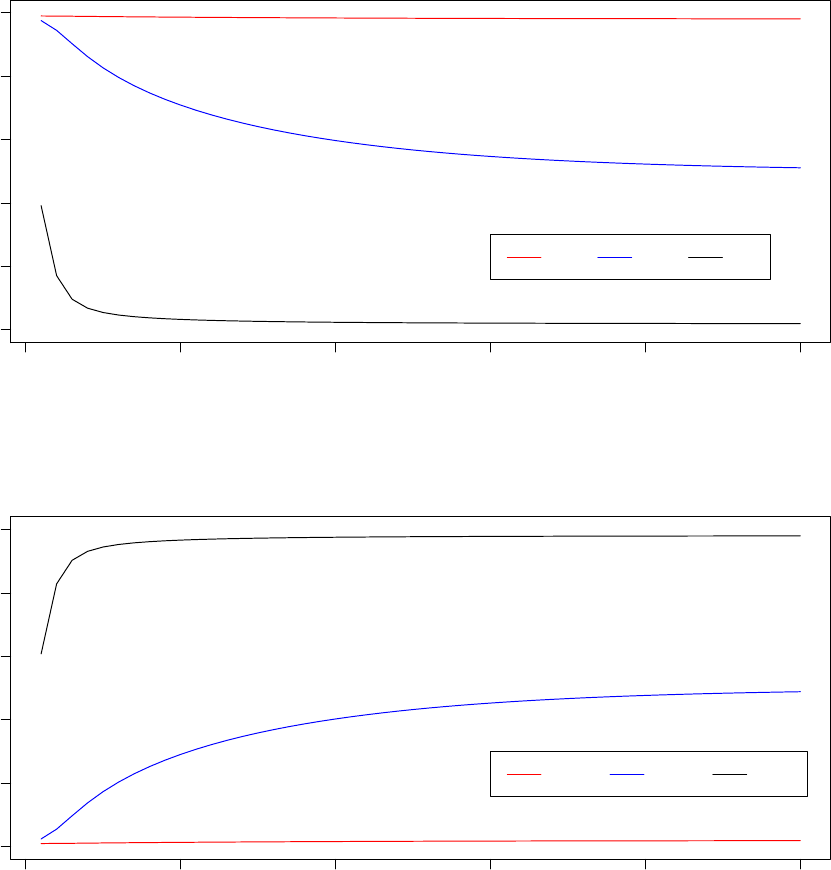
Exploring the System Dynamics
Before calling Optimus to solve this problem, let us first simulate the system of ODEs from the chosen initial
state using a few sets of arbitrary rate constants to become familiar with how the system evolves. The below
graphs illustrate the evolution of the system for 50 time steps for the rate constants
{k1
= 1
.
0
, k2
= 1
.
0
, k3
=
1.0, k4= 1.0}:
0 10 20 30 40 50
0 20 40 60 80 100
Concentration of Dephosphorylated Species as a function of Time Step
Time Step
Concentration
[A] [B] [C]
0 10 20 30 40 50
0 20 40 60 80 100
Concentration of Phosphorylated Species as a function of Time Step
Time Step
Concentration
[AP] [BP] [CP]
The table below summarizes the initial and final concentrations of the various species when the system is
simulated for 50 time steps using the rate constants {k1= 1.0, k2= 1.0, k3= 1.0, k4= 1.0}:
42
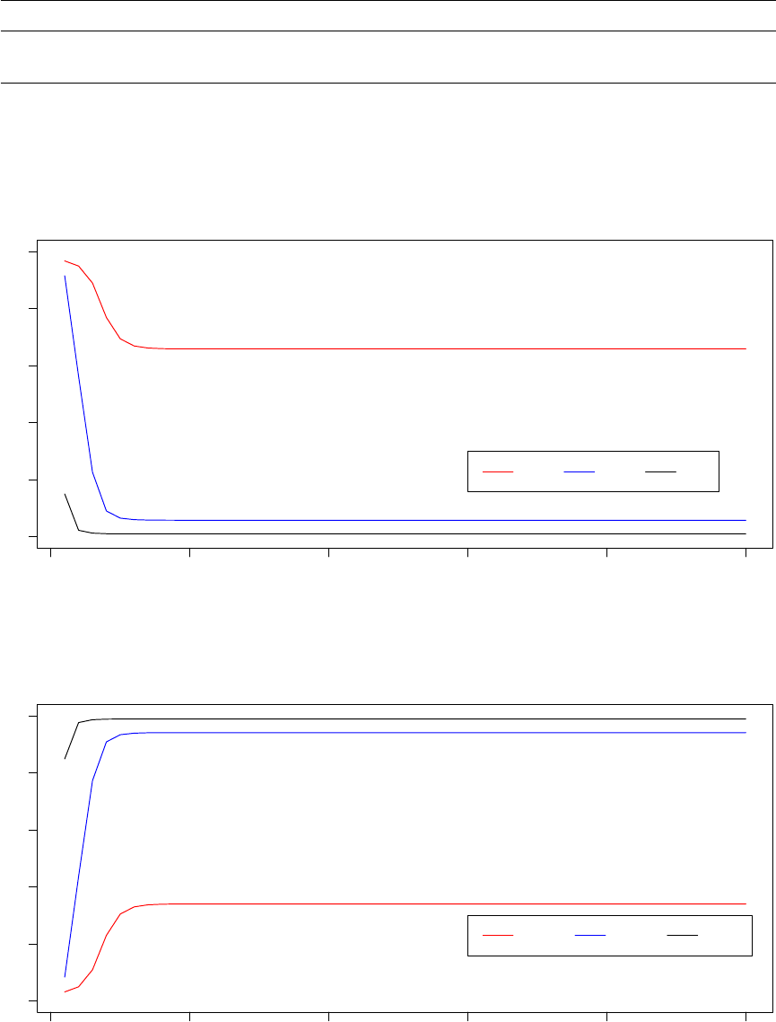
Table 11: System Summary for k1 = k2 = k3 = k4 = 1.0
[A] [B] [C] [AP] [BP] [CP]
Initial 100.00000 100.00000 100.000000 0.000000 0.00000 0.00000
Final (after 50 time steps) 98.08145 51.12118 2.004924 1.918549 48.87882 97.99508
If instead we use the set of rate constants
{k1
= 1
.
5
, k2
= 0
.
5
, k3
= 1
.
0
, k4
= 1
.
0
}
, the system evolves as
follows:
0 10 20 30 40 50
0 20 40 60 80 100
Concentration of Dephosphorylated Species as a function of Time Step
Time Step
Concentration
[A] [B] [C]
0 10 20 30 40 50
0 20 40 60 80 100
Concentration of Phosphorylated Species as a function of Time Step
Time Step
Concentration
[AP] [BP] [CP]
The table below summarizes the initial and final concentrations of the various species when the system is
43
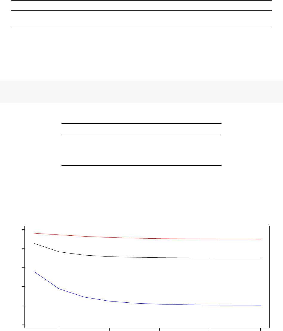
simulated for 50 time steps using the rate constants {k1= 1.5, k2= 0.5, k3= 1.0, k4= 1.0}:
Table 12: System Summary for k1 = 1.5, k2 = 0.5, k3 = k4 = 1.0
[A] [B] [C] [AP] [BP] [CP]
Initial 100.00000 100.000000 100.000000 0.00000 0.00000 0.00000
Final (after 50 time steps) 65.96628 5.814787 1.050583 34.03372 94.18521 98.94942
Acceptance Ratio Annealing Optimus Run
We will now call Acceptance Ratio Annealing Optimus to solve our problem. Similarly to Tutorial 2, we will
execute 200 000 optimisation iterations and perform 2 annealing cycles. We will set DUMP.FREQ to have a
value of 100 000.
Optimus(NCPU = 4,K.INITIAL = K, rDEF = r, mDEF = m, uDEF = u, OPT.TYPE = "SA",
OPTNAME = "DE_4_SA",DATA = DATA, NUMITER = 2e+05,CYCLES = 2,DUMP.FREQ = 1e+05,
LONG = FALSE)
Table 13: 4 Core Acceptance Ratio Annealing Optimus Run Results
E (RMSD) K1 K2 K3 K4
Processor 1 0.0012516 0.7974 0.3586 0.0128 2.3886
Processor 2 0.0017556 0.7850 0.3532 0.0126 2.3512
Processor 3 0.0013625 0.8098 0.3642 0.0130 2.4262
Processor 4 0.0012516 0.7974 0.3586 0.0128 2.3886
Of the 4 optimisation replicas, Processors 1 and 4 find the best set of rate constants,
{k1
= 0
.
7974
, k2
=
0
.
3586
, k3
= 0
.
0128
, k4
= 2
.
3886
}
. This set of rate constants results in an RMSD (after 10 iterations) of
0.0012516. Let us simulate how the system evolves according to these rate constants for 10 time steps:
2 4 6 8 10
0 20 40 60 80 100
Concentration of Dephosphorylated Species as a function of Time Step
Time Step
Concentration
44
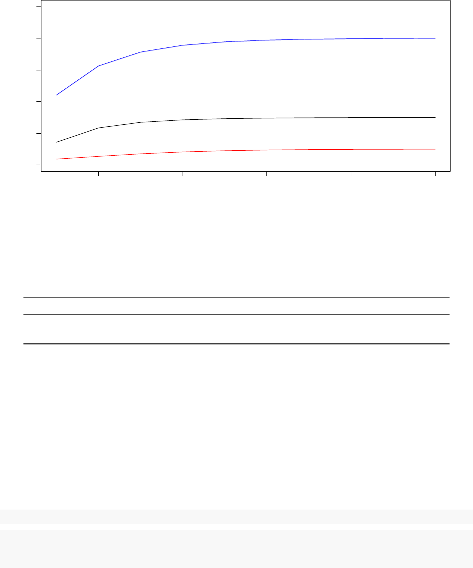
2 4 6 8 10
0 20 40 60 80 100
Concentration of Phosphorylated Species as a function of Time Step
Time Step
Concentration
The table below summarizes the initial and final concentrations of the various species when the system is
simulated for 10 time steps using the rate constants {k1= 0.7974, k2= 0.3586, k3= 0.0128, k4= 2.3886}:
Table 14: System Summary for k1 = 0.7974, k2 = 0.3586, k3 =
0.0128, k4 = 2.3886
[A] [B] [C] [AP] [BP] [CP]
Initial 100.00000 100.00000 100.00000 0.00000 0.00000 0.00000
Final (after 10 time steps) 89.99814 20.00081 69.99924 10.00186 79.99919 30.00076
As can be seen in the above table, the concentration of the species in the system after 10 time steps are very
close to the target values [
A
]
t
= 90,[
B
]
t
= 20,[
C
]
t
= 70,[
AP
]
t
= 10,[
BP
]
t
= 80 and [
CP
]
t
= 30. As alluded
to earlier, it is possible that the system has not reached a steady state after 10 time steps, however the above
graphs suggest that the concentrations after 10 steps are already extremely close to, if not equal to, steady
state values. The optimisation process could be re-executed after increasing the value of the parameter
span
in the function m() to simulate the system for a larger number of time steps.
Replica Exchange Optimus Run
Let us now examine how replica exchange Optimus using 12 cores performs on this task. We will use 200 000
optimisation iterations and set STATWINDOW to equal 50, similarly to Tutorials 2 and 3.
ACCRATIO <- c(90,82,74,66,58,50,42,34,26,18,10,2)
Optimus(NCPU = 12,K.INITIAL = K, rDEF = r, mDEF = m, uDEF = u, ACCRATIO = ACCRATIO,
OPT.TYPE = "RE",DATA = DATA, OPTNAME = "DE_12_RE",NUMITER = 2e+05,STATWINDOW = 50,
DUMP.FREQ = 1e+05,LONG = FALSE)
45
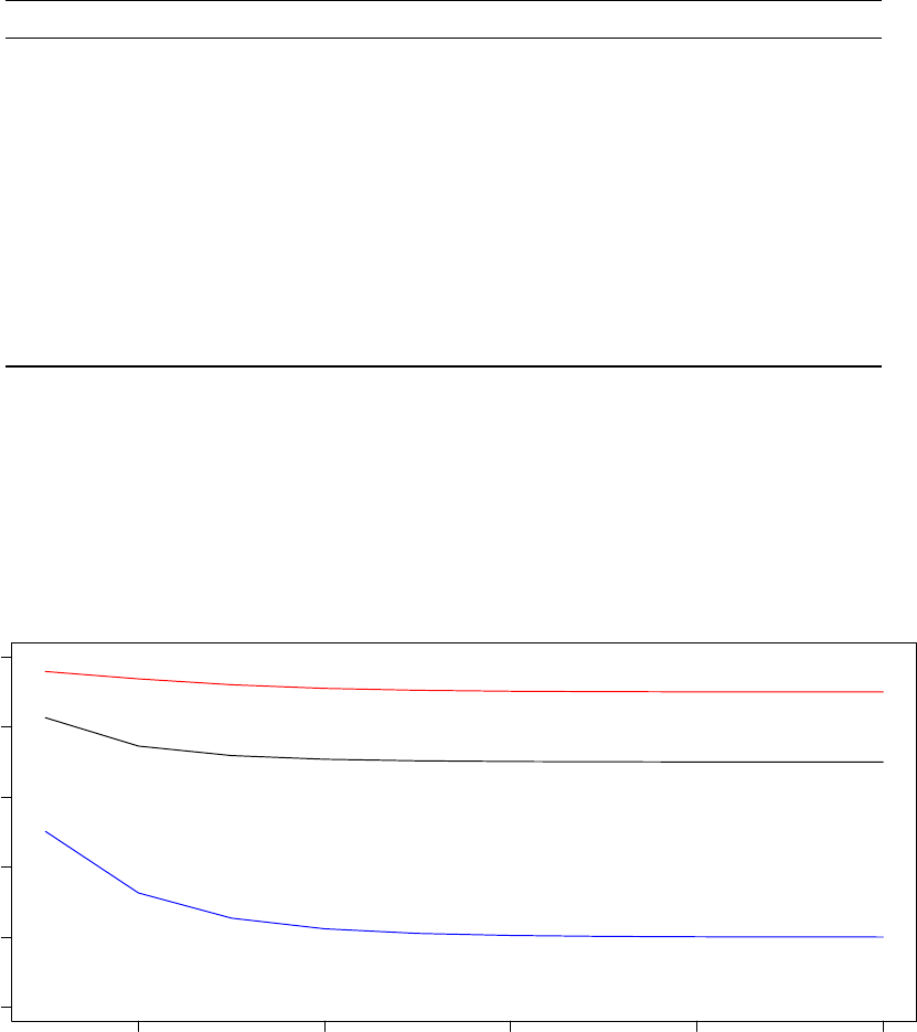
Table 15: 12 Core Replica Exchange Optimus Run Results
Replica Acceptance Ratio E (RMSD) K1 K2 K3 K4
Processor 1 90 0.0026225 0.9088 0.4090 0.0146 2.7246
Processor 2 82 0.0026343 0.8346 0.3754 0.0134 2.5012
Processor 3 74 0.0019724 0.7234 0.3252 0.0116 2.1644
Processor 4 66 0.0020945 0.9586 0.4312 0.0154 2.8748
Processor 5 58 0.0029243 0.9338 0.4200 0.0150 2.8002
Processor 6 50 0.0025811 0.8964 0.4034 0.0144 2.6872
Processor 7 42 0.0028685 0.8592 0.3866 0.0138 2.5752
Processor 8 34 0.0025121 0.8840 0.3978 0.0142 2.6500
Processor 9 26 0.0011265 0.9834 0.4424 0.0158 2.9492
Processor 10 18 0.0025811 0.8964 0.4034 0.0144 2.6872
Processor 11 10 0.0012516 0.7974 0.3586 0.0128 2.3886
Processor 12 2 0.0017556 0.7850 0.3532 0.0126 2.3512
Of the 12 optimisation replicas, Processor 9 (26% acceptance ratio) finds the best set of rate constants,
{k1
= 0
.
9834
, k2
= 0
.
4424
, k3
= 0
.
0158
, k4
= 2
.
9492
}
. This set of rate constants results in an RMSD (after 10
iterations) of 0
.
0011265, which is lower than the RMSD of the solution found by acceptance ratio annealing
Optimus (0
.
0012516). Let us simulate how the system evolves according to these rate constants for 10 time
steps:
2 4 6 8 10
0 20 40 60 80 100
Concentration of Dephosphorylated Species as a function of Time Step
Time Step
Concentration
46
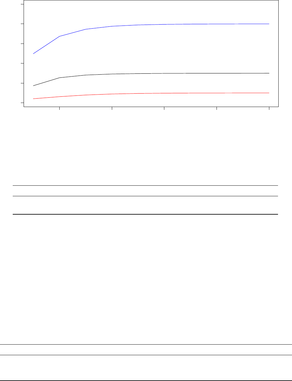
2 4 6 8 10
0 20 40 60 80 100
Concentration of Phosphorylated Species as a function of Time Step
Time Step
Concentration
The table below summarizes the initial and final concentrations of the various species when the system is
simulated for 10 time steps using the rate constants {k1= 0.9834, k2= 0.4424, k3= 0.0158, k4= 2.9492}:
Table 16: System Summary for k1 = 0.9834, k2 = 0.4424, k3 =
0.0158, k4 = 2.9492
[A] [B] [C] [AP] [BP] [CP]
Initial 100.00000 100.00000 100.00000 0.00000 0.00000 0.00000
Final (after 10 time steps) 89.99807 19.99983 70.00022 10.00193 80.00017 29.99978
Here again, we see that the species’ concentrations after 10 time steps are remarkably close to the target
values [
A
]
t
= 90,[
B
]
t
= 20,[
C
]
t
= 70,[
AP
]
t
= 10,[
BP
]
t
= 80 and [
CP
]
t
= 30 and the graphs suggests that
these concetrations have either converged or are very close to converging to steady state.
Summary
We have seen how Optimus can be empoyed to recover rate constants for a system of coupled ODEs that
describes a biological pathway. Given an initial state of the system and a target state, both Acceptance
Ratio Annealing Optimus and Replica Exchange Optimus found a set of rate constants that resulted in the
desired system behaviour upon simulation of the system. Replica Exchange Optimus retrieved a solution
that resulted in a lower RMSD after 10 time steps (0
.
0011265) than the solution found by Acceptance Ratio
Annealing Optimus (0.0012516).
Table 17: Summary of Species’ Concentrations after 10 Time Steps
[A] [B] [C] [AP] [BP] [CP]
Target 90.00000 20.00000 70.00000 10.00000 80.00000 30.00000
Optimus (Acceptance Ratio Annealing) 89.99814 20.00081 69.99924 10.00186 79.99919 30.00076
Optimus (Replica Exchange) 89.99807 19.99983 70.00022 10.00193 80.00017 29.99978
47

Table 18: Summary of Recovered Rate Constants
E (RMSD) K1 K2 K3 K4
Optimus (Acceptance Ratio Annealing) 0.0012516 0.7974 0.3586 0.0128 2.3886
Optimus (Replica Exchange) 0.0011265 0.9834 0.4424 0.0158 2.9492
48

Advanced User Manual
This section will document all possible input arguments to Optimus and will describe the output format of
Optimus. The code snippet below is the first part of the definition of Optimus which lists all input arguments.
We will refer to input arguments without default values as mandatory input arguments and those with default
values as optional input arguments (with the exception of K.INITIAL, which will be considered a mandatory
input argument).
Optimus <- function(NUMITER = 1000000,
STATWINDOW = 70,
T.INI = 0.00001,
T.ADJSTEP = 0.000000005,
TSCLnum = 2,
T.SCALING = 3,
T.MIN = 0.000000005,
T.DELTA = 2,
DUMP.FREQ = 10000,
LIVEPLOT = TRUE,
LIVEPLOT.FREQ = 100000,
PDFheight = 29,
PDFwidth = 20,
NCPU = 4,
LONG = TRUE,
SEED = 840,
OPTNAME = "",
DATA = NULL,
K.INITIAL = 0,
rDEF,
mDEF,
uDEF,
EXCHANGE.FREQ = 1000,
ACCRATIO = c(90,50,5,1),
CYCLES = 10,
ACCRATIO.IN = 90,
ACCRATIO.FIN = 0.5,
OPT.TYPE = "SA"
){...}
Mandatory Input Arguments
All mandatory input arguments have necessarily already been defined in the Tutorials. However, we will
reiterate these definitions in this section.Optimus has four mandatory inputs, mDEF, uDEF, rDEF (refered
to as m(),u() and r() respectively in the Tutorials) and K.INITIAL.
mDEF
mDEF must be of type closure. mDEF should be a function designed to operate on the whole set of parameter
snapshot
K
and return the corresponding observable object
O
. Please note, that the size of
K
and
O
are not
necessarily to match, depending on the nature of the model used. mDEF must necessarily take K and DATA
as input variables, and it must necessarily operate on
K
to produce
O
(operating on DATA in optional, see
Tutorial 3 for an illustration).
49
uDEF
uDEF must be of type closure. uDEF should be a function designed to evaluate the performance of a given
snapshot of coefficients
K
. uDEF should necessarily take as inputs
O
(the output of mDEF) and the variable
DATA. The output of uDEF should have two components,
Q
holding a single number of the quality of the
K
coefficients, and
E
holding a (pseudo)energy for the given snapshot
K
. It is important that the returned
(pseudo)energy value is lower for better performance/version of
K
, never vice-versa. The
Q
component of the
uDEF function output is only used for plotting the optimisation process, and, if desired, can just repeat the
value of the Ecomponent.
rDEF
rDEF must be of type closure. rDEF should be a function that defines a rule by which the
K
coefficient
vector is to be altered from one step to another. rDEF must accept
K
as an input and return an object
equivalent to K, but with some alteration(s).
K.INITIAL
K.INITIAL is an object of any type which stores the initial values for the parameter(s) to be optimised. The
only requirement for
K
is that it should be something alterable via rDEF and something that influences the
outcome of mDEF.
Optional Input Arguments
NUMITER
NUMITER is a variable of type double that is the number of iterations (or steps) of the optimisation process
per core. It has a default value of 1 000 000.
STATWINDOW
STATWINDOW is a variable of type double that is the number of iterations executed between subsequent
temperature adjustments executed by the Temperature Control Unit (STATWINDOW is also the number of
iterations used to calculate the observed aceptance ratio). It has a default value of 70.
T.INI
T.INI is a variable of type double that represents the initial system pseudo-temperature at the beginning of
the optimisation procedure. It has a default value of 0.00001.
T.ADJSTEP
T.ADJSTEP is a variable of type double that represents the baseline temperature change step-size for
temperature auto-adjustment. It has a default value of 0.000000005.
50
TSCLnum
TSCLnum is a variable of type double that indicates the maximum number of STATWINDOWS for which the
observed acceptance ratio can sequentially be below or above the ideal acceptance ratio before T.ADJSTEP
is scaled by T.SCALING. It has a default value of 2.
T.SCALING
T.SCALING is a variable of type double that represents the value by which T.ADJSTEP is scaled in
accordance with the condition specified by TSCLnum. It has a default value of 3.
T.MIN
T.MIN is a variable of type double and is the value that the system pseudo-temperature is automatically set
to if at any time, the Temperature Control Unit attempts to make the pseudo-temperature a negative value.
It has a default value of 0.000000005.
T.DELTA
T.DELTA is a variable of type double. If after a STATWINDOW, the observed acceptance ratio is within
T.DELTA of the ideal acceptance ratio, the Temperature Control Unit will make no change to the system
pseudo-temperature. It has a default value of 2.
DUMP.FREQ
DUMP.FREQ is a variable of type double. It is the frequency in steps of printing the best found model to
the working directory. It has a default value of 10 000.
LIVEPLOT
LIVEPLOT is a variable of type logical that indicates whether the optimisation process will be plotted in a
pdf file in the working directory. It has a default value of TRUE.
LIVEPLOT.FREQ
LIVEPLOT.FREQ is a variable of type double that indicates the frequency in steps of printing the optimisation
process in a pdf (this variable is only relevant if LIVEPLOT = TRUE). It has a default value of 100 000.
PDFheight
PDFheight is a variable of type double that indicates the height of the PDF that is produced (if LIVEPLOT
= TRUE). It has a default value of 29.
PDFwidth
PDFwidth is a variable of type double that indicates the width of the PDF that is produced (if LIVEPLOT
= TRUE). It has a default value of 20.
51
NCPU
NCPU is a variable of type double that indicates the number of Optimisation replicas to execute. If calling
the Replica Exchange Version of Optimus, NCPU must be greater than 1. NCPU has a default value of 4.
LONG
LONG is a variable of type logical. If LONG = TRUE, a memory-friendly version of Optimus will be activated
(in anticipation of a long simulation) and only data from the optimal explored parameter configuration and
the last 10 000 optimisation iterations will be stored. LONG has a default value of TRUE.
SEED
SEED is a variable of type double which sets the seed for the random number generator. It has a default
value of 840.
OPTNAME
OPTNAME is a variable of type character that can be thought of as the name of the optimisation process.
OPTNAME is used when creating the file names of the Optimus output. OPTNAME = “” is the default
value.
DATA
DATA is a variable of type list holding any additional data that must be accessed by mDEF and uDEF. The
default value for DATA is NULL.
OPT.TYPE
OPT.TYPE is a variable of type character which specifies the mode of Optimus to execute and should always
be equal to “SA” or “RE”. If equal to “SA” (for Simulated Annealing), the Acceptance Ratio Annealing
version of Optimus will be executed. If equal to “RE” (for Replica Exchange), the Replica Exchange version
of Optimus will be executed. The default value of OPT.TYPE is “SA”.
Acceptance Ratio Annealing Specific Optional Inputs
The below optional input arguments only impact the Acceptance Ratio Annealing mode of Optimus.
CYCLES
CYCLES is a variable of type double that specifies the number of annealing cycles to execute per core during
the optimisation process. It has a default value of 10.
ACCRATIO.IN
ACCRATIO.IN is a variable of type double that specifies the initial target acceptance ratio for the annealing
schedule in each annealing cycle. It has a default value of 90.
52
ACCRATIO.FIN
ACCRATIO.FIN is a variable of type double that specifies the final target acceptance ratio for the annealing
schedule in each annealing cycle. It has a default value of 0.5.
Replica Exchange Specific Optional Inputs
The below optional input arguments only impact the Replica Exchange mode of Optimus.
EXCHANGE.FREQ
EXCHANGE.FREQ is a variable of type double that specifies the number of optimisation iterations to
execute between subsequent parameter configuration exchanges between adjacent replicas. It has a default
value of 1000.
ACCRATIO
ACCRATIO is a vector of doubles that must have length equal to the value of NCPU. ACCRATIO specifies
the target acceptance ratio for each optimisation replica. It has a default value of c(90, 50, 5, 1).
Optimus Output
Optimus creates multiple output files in a user’s working directory during an optimisation run. Each core
used will generate 4 or 5 output files (depending on the value of LIVEPLOT):
1) [OPTNAME][Core number]_model_ALL
2) [OPTNAME][Core number]_model_K
3) [OPTNAME][Core number]_model_O
4) [OPTNAME][Core number]_model_QE
5) [OPTNAME][Core number]
Note that the 5th file is only produced if LIVEPLOT = TRUE. As an illustration, for the Acceptance
Ratio Annealing run from Tutorial 1, Optimus generates 20 output files with the following names:
poly_4_SA1_model_ALL, poly_4_SA1_model_K, poly_4_SA1_model_O, poly_4_SA1_model_QE,
poly_4_SA1, poly_4_SA2_model_ALL, poly_4_SA2_model_K, poly_4_SA2_model_O, poly_4_SA2_model_QE,
poly_4_SA2, poly_4_SA3_model_ALL, poly_4_SA3_model_K, poly_4_SA3_model_O, poly_4_SA3_model_QE,
poly_4_SA3,poly_4_SA4_model_ALL, poly_4_SA4_model_K, poly_4_SA4_model_O, poly_4_SA4_model_QE
and poly_4_SA4.
[OPTNAME][Core number]_model_ALL
This is the most important output file in that essentially all contents from the other output files is contained
in this file. The *_model_ALL file is an R workspace that contains a variable OUTPUT of type list. For
Acceptance Ratio Annealing, OUTPUT has 12 fields (numbered 1-12 below) while for Replica Exchange,
OUTPUT contains an additional 14 fields (numbered 13-26 below). Note that the additional fields of
OUTPUT in Replica Exchange were included to facilitate the writing of the code; they can largely be ignored
by the user.
1) K.stored
2) O.stored
3) STEP
4) PROB.VEC
53
5) T.DE.FACTO
6) IDEAL.ACC.VEC
7) ACC.VEC.DE.FACTO
8) STEP4ACC.VEC.DE.FACTO
9) ENERGY.DE.FACTO
10) Q.STRG
11) ACCEPTANCE
12) STEP.STORED
13) E.stored
14) E.old
15) Q.old
16) K
17) T
18) Step.stored
19) ENERGY.TRIAL.VEC
20) STEP.add
21) NumofAccRatSMIdeal
22) NumofAccRatGRIdeal
23) t.adjstep
24) AccR.category
25) new.T.INI
26) instanceOFswitch
K.stored holds the optimal parameter configuration found by the given processor. O.stored holds the
object
O
generated by mDEF from the optimal parameter configuration K.stored. STEP is a double
that holds the current optimisation iteration number. PROB.VEC is a vector that holds the acceptance
probability for each optimisation step. T.DE.FACTO is a vector that holds the system pseudo-temperature
during each optimisation iteration. IDEAL.ACC.VEC is a vector that holds the target acceptance ratio for
each optimisation iteration in the case of Acceptance Ratio Annealing. In the case of Replica Exchange,
IDEAL.ACC.VEC holds the same value as the input variable ACCRATIO. ACC.VEC.DE.FACTO is a vector
that holds the observed acceptance ratio at the end of each STATWINDOW. STEP4ACC.VEC.DE.FACTO
is a vector that holds the optimisation step numbers that correspond to the end of a STATWINDOW.
ENERGY.DE.FACTO is a vector that holds the actual system energy
E
at each optimisation step. Q.STRG
is a vector that holds the system quality
Q
at each optimisation step. ACCEPTANCE is a vector of binary
variables whose
ith
entry is 1 if the candidate parameter configuration was accepted on the
ith
optimisation
step and 0 otherwise. STEP.STORED is a vector storing the number of each optimisation step.
E.stored is a double that stores the energy
E
associated with the optimal parameter configuration K.stored.
E.old is a double that stores the energy
E
associated with the most recently considered parameter configuration.
Q.old is a double that stores the quality
Q
associated with the most recently considered parameter configuration.
K
hold the most recently considered parameter configuration.
T
is a double that holds the current system
temperature. Step.stored is a double that holds the optimisation step number on which the optimal parameter
configuration K.stored was discovered. ENERGY.TRIAL.VEC is a vector that holds the energy
E
of the
candidate parameter configuration at every optimisation step. STEP.add is a double that facilitates indexing
into output vectors. NumofAccRatSMIdeal is a double that represents the number of times the observed
acceptance ratio has sequentially been smaller than the target acceptance ratio. NumofAccRatGRIdeal is
a double that represents the number of times the observed acceptance ratio has been sequentially greater
than the target acceptance ratio. t.adjstep is a double holding the current value by which the system pseudo-
temperature is increased or decreased each STATWINDOW by the Temperature Control Unit. AccR.category
is a character that indicates whether the observed acceptance ratio was above or below the target acceptance
ratio during the previous STATWINDOW. new.T.INI is a double that stores an estimate for the ideal initial
system pseudo-temperature deduced by the Temperature Control Unit. Finally, instanceOFswitch is a double
that tracks the number of times the observed acceptance ratio has transitioned from being less than the
target ratio to greater than the target ratio or vice versa.
54
[OPTNAME][Core number]_model_K
The *_model_K file is an R workspace that contains a variable K.stored of the same type as K.INITIAL. It
holds the optimal parameter configuration found by the given processor.
[OPTNAME][Core number]_model_O
The *_model_O file is an R workspace that contains a variable O.stored that holds the object
O
generated
by mDEF from the optimal parameter configuration K.stored.
[OPTNAME][Core number]_model_QE
The *_model_QE file is a text file that stores the values of
E
and
Q
that are produced from the optimal
parameter cofiguration K.stored and, in the case of the Replica Exchange Version of Optimus, stores the
target acceptance ratio associated with the given replica.
[OPTNAME][Core number]
The * file is a pdf file that includes 5 plots:
1) Acceptance probability as a function of optimisation iteration.
2) System psuedo-temperature as a function of optimisation iteration.
3)
Observed (red solid line) and target (black dashed line) acceptance ratio as a function of optimisation
iteration.
4) Energy Eas a function of optimisation iteration.
5) Quality Qas a function of optimisation iteration.
55
References
Ballard, Andrew, and Christopher Jarzynski. 2009. “Replica Exchange with Nonequilibrium
Switches.” Proceedings of the National Academy of Sciences of the United States of America 106
(July). doi:10.1073/pnas.0900406106.
Chen, Yunjie, and Benoit Roux. 2015. “Generalized Metropolis Acceptance Criterion for Hybrid Non-
Equilibrium Molecular Dynamics - Monte Carlo Simulations.” The Journal of Chemical Physics 142 (January).
doi:10.1063/1.4904889.
Chib, Siddhartha, and Edward Greenberg. 1995. “Understanding the Metropolis-Hastings Algorithm.” The
American Statistician 49 (November): 327–35. doi:10.2307/2684568.
Cowles, Mary, and Bradley Carlin. 1996. “Markov Chain Monte Carlo Convergence Diagnos-
tics: A Comparative Review.” Journal of the American Statistical Association 91 (June): 883–904.
doi:10.1080/01621459.1996.10476956.
Gilks, W.R., S. Richardson, and D.J. Spiegelhalter. 1996. Markov Chain Monte Carlo in Practice.Chapman
& Hall.
Ingber, Lester. 1993. “Simulated Annealing: Practice Versus Theory.” Mathematical and Computer Modelling
18 (December): 29–57. doi:10.1016/0895-7177(93)90204-C.
Kirkpatrick, Scott. 1984. “Optimization by Simulated Annealing: Quantitative Studies.” Journal of Statistical
Physics 34: 975–86. doi:10.1007/BF01009452.
Klipp, Edda, Wolfram Liebermeister, Cristoph Wierling, Axel Kowald, Hans Lehrach, and Ralf Herwig. 2009.
Systems Biology.Wiley-VCH.
Raue, Andreas, Marcel Schilling, Julie Bachmann, Andrew Matteson, Max Schelke, Daniel Kaschek, Sabine
Hug, et al. 2013. “Lessons Learned from Quantitative Dynamical Modeling in Systems Biology.” PLOS ONE,
September. doi:10.1371/journal.pone.0074335.
Sugita, Yuji, and Yuko Okamoto. 1999. “Replica-Exchange Molecular Dynamics Method for Protein Folding.”
Chemical Physics Letters 314 (November): 141–51. doi:10.1016/S0009-2614(99)01123-9.
56