Oracle JRockit The Definitive Guide
User Manual:
Open the PDF directly: View PDF ![]() .
.
Page Count: 588 [warning: Documents this large are best viewed by clicking the View PDF Link!]
- Cover
- Copyright
- Credits
- Foreword
- About the Authors
- About the Reviewers
- Table of Contents
- Preface
- Chapter 1: Getting Started
- Chapter 2: Adaptive Code Generation
- Chapter 3: Adaptive Memory Management
- The concept of automatic memory management
- Fundamental heap management
- Garbage collection algorithms
- Speeding it up and making it scale
- Near-real-time garbage collection
- The Java memory API
- Pitfalls and false optimizations
- Controlling JRockit memory management
- Summary
- Chapter 4: Threads and Synchronization
- Chapter 5: Benchmarking and Tuning
- Reasons for benchmarking
- What to think of when creating a benchmark
- Deciding what to measure
- Industry standard benchmarks
- The dangers of benchmarking
- Tuning
- Common bottlenecks and how to avoid them
- Wait/notify and fat locks
- Summary
- Chapter 6: JRockit Mission Control
- Background
- Mission Control overview
- The Experimental Update Site
- Debugging JRockit Mission Control
- Summary
- Chapter 7: The Management Console
- Chapter 8: The Runtime Analyzer
- Chapter 9: The Flight Recorder
- Chapter 10: The Memory Leak Detector
- Chapter 11: JRCMD
- Introduction
- Overriding SIGQUIT
- Limitations of JRCMD
- JRCMD command reference
- check_flightrecording (R28)
- checkjrarecording (R27)
- command_line
- dump_flightrecording (R28)
- heap_diagnostics (R28)
- hprofdump (R28)
- kill_management_server
- list_vmflags (R28)
- lockprofile_print
- lockprofile_reset
- memleakserver
- oom_diagnostics (R27)
- print_class_summary
- print_codegen_list
- print_memusage (R27)
- print_memusage (R28)
- print_object_summary
- print_properties
- print_threads
- print_utf8pool
- print_vm_state
- run_optfile (R27)
- run_optfile (R28)
- runfinalization
- runsystemgc
- set_vmflag (R28)
- start_flightrecording (R28)
- start_management_server
- startjrarecording (R27)
- stop_flightrecording (R28)
- timestamp
- verbosity
- version
- Summary
- Chapter 12: Using the JRockit Management APIs
- Chapter 13: JRockit Virtual Edition
- Appendix A: Bibliography
- Appendix B: Glossary
- Index

Oracle JRockit
The Denitive Guide
Develop and manage robust Java applications with
Oracle's high-performance Java Virtual Machine
Marcus Hirt
Marcus Lagergren
BIRMINGHAM - MUMBAI
Oracle JRockit
The Denitive Guide
Copyright © 2010 Packt Publishing
All rights reserved. No part of this book may be reproduced, stored in a retrieval
system, or transmitted in any form or by any means, without the prior written
permission of the publisher, except in the case of brief quotations embedded in
critical articles or reviews.
Every effort has been made in the preparation of this book to ensure the accuracy
of the information presented. However, the information contained in this book is
sold without warranty, either express or implied. Neither the authors, nor Packt
Publishing, and its dealers and distributors will be held liable for any damages
caused or alleged to be caused directly or indirectly by this book.
Packt Publishing has endeavored to provide trademark information about all of the
companies and products mentioned in this book by the appropriate use of capitals.
However, Packt Publishing cannot guarantee the accuracy of this information.
First published: June 2010
Production Reference: 1260510
Published by Packt Publishing Ltd.
32 Lincoln Road
Olton
Birmingham, B27 6PA, UK.
ISBN 978-1-847198-06-8
www.packtpub.com
Cover Image by Mark Holland (MJH767@bham.ac.uk)

Credits
Authors
Marcus Hirt
Marcus Lagergren
Reviewers
Anders Åstrand
Staffan Friberg
Markus Grönlund
Daniel Källander
Bengt Rutisson
Henrik Ståhl
Acquisition Editor
James Lumsden
Development Editor
Rakesh Shejwal
Technical Editor
Sandesh Modhe
Indexer
Rekha Nair
Editorial Team Leader
Gagandeep Singh
Project Team Leader
Priya Mukherji
Project Coordinator
Ashwin Shetty
Proofreader
Andie Scothern
Graphics
Geetanjali Sawant
Production Coordinator
Melwyn D'sa
Cover Work
Melwyn D'sa
Foreword
I remember quite clearly the rst time I met the JRockit team. It was JavaOne 1999
and I was there representing WebLogic. Here were these Swedish college kids in
black T-shirts describing how they would build the world's best server VM. I was
interested in hearing their story as the 1.2 release of HotSpot had been delayed again
and we'd been running into no end of scalability problems with the Classic VM.
However I walked away from the booth thinking that, while these guys were smart,
they had no idea what they were biting off.
Fast-forward a few years. BEA buys JRockit and I become the technical liaison
between the WebLogic and JRockit teams. By now JRockit has developed into an
excellent offering—providing great scalability and performance on server-side
systems. As we begin working together I have the distinct pleasure of getting to
know the authors of this book: Marcus Lagergren and Marcus Hirt.
Lagergren is a remarkably prolic developer, who at the time was working on the
compiler. He and I spent several sessions together examining optimizations of
WebLogic code and deciphering why this method or that wasn't getting inlined or
devirtualized. In the process we, along with the rest of the WebLogic and JRockit
teams, were able to produce several SPECjAppServer world records and cement
JRockit's reputation for performance.
Hirt, on the other hand, is extremely focused on proling and diagnostics. It was
natural, therefore, that he should lead the nascent tooling effort that would become
JRockit Mission Control. This was an extension of an early observation we had, that
in order to scale the JRockit engineering team, we would have to invest in tooling to
make support and debugging easier.
Fast-forward a few more years. I'm now at Oracle when it acquires BEA. I have the
distinct pleasure of again welcoming the JRockit team into a new company as they
joined my team at Oracle. The core of the JRockit team is still the same and they now
have a place among the small group of the world's experts in virtual machines.
Lagergren is still working on internals—now on JRockit Virtual Edition—and is
as productive as ever. Under Hirt's leadership, Mission Control has evolved from
an internal developer's tool into one of the JRockit features most appreciated by
customers. With this combination of long experience and expertise in all layers of
JRockit, it is difcult for me to imagine a better combination of authors to write
this book.
Therefore, as has been the case many times before, I'm proud to be associated in some
small way with the JRockit team. I trust that you will enjoy reading this book and hope
that you will nd the topic to be as satisfying as I have found it to be over the years.
Adam Messinger
Vice President of Development, Oracle Fusion Middleware group
February 14, 2010
San Francisco, CA
About the Authors
Marcus Hirt is one of the founders of Appeal Virtual Machines, the company that
created the JRockit Java Virtual Machine. He is currently working as Architect, Team
Lead, and Engineering Manager for the JRockit Mission Control team. In his spare
time he enjoys coding on his many pet projects, composing music, and scuba diving.
Marcus has contributed JRockit related articles, whitepapers, tutorials, and webinars
to the JRockit community, and has been an appreciated speaker at Oracle Open World,
eWorld, BEAWorld, EclipseCon, Nordev, and Expert Zone Developer Summit. He
received his M.Sc. education in Computer Science at the Royal Institute of Technology
in Stockholm. Marcus Hirt lives in Stockholm with his wife and two children.
Marcus Lagergren has an M.Sc. in Computer Science from the Royal Institute of
Technology in Stockholm, Sweden. He majored in theoretical computer science and
complexity theory since it was way more manly than, for example, database systems.
He has a background in computer security but has worked with runtimes since 1999.
Marcus was one of the founding members of Appeal Virtual Machines, the company
that developed the JRockit JVM. Marcus has been Team Lead and Architect for the
JRockit code generators and has been involved in pretty much every other aspect of
the JRockit JVM internals over the years. He has presented at various conferences, such
as JavaOne, BEAWorld, and eWorld and holds several patents on runtime technology.
Since 2008, he works for Oracle on a fast virtualization platform. Marcus likes power
tools, heavy metal, and scuba diving. Marcus Lagergren lives in Stockholm with his
wife and two daughters.
Acknowledgement
We'd like to thank all the people who have been creative with us throughout the
years, especially the other Appeal guys who have been a part of our lives for quite
some time now. The authors cannot think of a ner and more competent group of
people to have shared this journey with.
Furthermore, a great thank you is in order to our families who have been extremely
patient with us during the writing of this book.

About the Reviewers
Anders Åstrand has a Master's degree in Computer Science from the Royal
Institute of Technology, Sweden. He has worked at Oracle (formerly BEA Systems)
since 2007, in the JRockit performance team.
Staffan Friberg leads the JRockit Performance Team at Oracle, with seven years
of experience in QA and Performance Engineering for the JVM.
Markus Grönlund is a Senior Software Engineer with Oracle Corporation and
has worked extensively in the Oracle JRockit Virtual Machine development and
support arena for the past three years. Markus has been supporting Oracle JRockit
VMs the largest mission critical JRockit customers, providing expertise in debugging,
conguration, and training.
Prior to joining Oracle Corporation, Markus worked for seven years as a Senior
Technical Architect for Intel Corporation, driving early adoption of next-generation
Intel Architectures.
I would like to thank the entire Oracle JRockit Virtual Machine team
in Stockholm, Sweden. It is a true privilege to be part of such an
amazing group of talented people. Thank you all!
Daniel Källander is Development Manager for JRockit and has been with the
JRockit team since 2005. Since 1996, he has been a founding member of three IT
companies. Before entering the IT industry he completed a Ph.D. in Theoretical
Physics, and later also an MBA in International Business.
Bengt Rutisson is Development Manager at Oracle focusing on JRockit garbage
collection and memory management. He joined the JRockit team in 2006 and has
been working with garbage collection and memory management since then.
Prior to working with JRockit, Bengt has been responsible for several products
in Java (for example, the Appear Context Engine) and in Component Pascal
(for example, the BlackBox Component Builder).
Henrik Ståhl is Senior Director of Product Management at Oracle, responsible for
product strategy for JRockit. In this position, he is constantly looking for new ways
to make the Java Virtual Machine more useful. He has been working with the JRockit
team since 2004, starting out as Team Lead for the JVM performance team before
moving to a product management role. Prior to Oracle, he was Co-Founder and
CTO of the Swedish IT consultancy Omegapoint, lead developer for the core part of
the Swedish BankID service and Senior Consultant at Icon Medialab. Henrik holds
an M.Sc. in Engineering Physics from the Royal Institute of Technology and lives
outside of Stockholm, Sweden with his family.
For my family, who endured me being inaccessible for nights and weekends both working on
the new major release and writing this book: Malin, Alexander, and little Natalie.
– Marcus Hirt
For my family: Klara, Alice, and Ylva. Especially for my lovely wife Klara, who ended up
having to singlehandedly juggle two children too often and who, more than once, expressed
her desire to purchase a copy of this book and burn it.
– Marcus Lagergren

Table of Contents
Preface 1
Chapter 1: Getting Started 11
Obtaining the JRockit JVM 11
Migrating to JRockit 13
Command-line options 13
System properties 13
Standardized options 14
Non-standard options 14
Changes in behavior 14
A note on JRockit versioning 15
Getting help 17
Summary 18
Chapter 2: Adaptive Code Generation 19
Platform independence 20
The Java Virtual Machine 21
Stack machine 21
Bytecode format 22
Operations and operands 23
The constant pool 24
Code generation strategies 24
Pure bytecode interpretation 24
Static compilation 26
Total JIT compilation 27
Mixed mode interpretation 28
Adaptive code generation 29
Determining "hotness" 30
Invocation counters 30
Software-based thread sampling 31
Hardware-based sampling 31

Table of Contents
[ ii ]
Optimizing a changing program 31
Inside the JIT compiler 34
Working with bytecode 34
Bytecode obfuscation 36
Bytecode "optimizers" 37
Abstract syntax trees 38
Where to optimize 41
The JRockit code pipeline 42
Why JRockit has no bytecode interpreter 43
Bootstrapping 44
Runtime code generation 44
Trampolines 45
Code generation requests 46
Optimization requests 47
On-stack replacement 47
Bookkeeping 48
A walkthrough of method generation in JRockit 49
The JRockit IR format 49
JIT compilation 51
Generating optimized code 58
Controlling code generation in JRockit 64
Command-line ags and directive les 64
Command-line ags 64
Directive les 67
Summary 70
Chapter 3: Adaptive Memory Management 71
The concept of automatic memory
management 72
Adaptive memory management 72
Advantages of automatic memory management 73
Disadvantages of automatic memory management 74
Fundamental heap management 74
Allocating and releasing objects 74
Fragmentation and compaction 75
Garbage collection algorithms 76
Reference counting 77
Tracing techniques 77
Mark and sweep 78
Stop and copy 80
Stopping the world 81
Conservative versus exact collectors 82
Livemaps 84
Generational garbage collection 87
Multi generation nurseries 88

Table of Contents
[ iii ]
Write barriers 88
Throughput versus low latency 90
Optimizing for throughput 91
Optimizing for low latency 91
Garbage collection in JRockit 92
Old collections 93
Nursery collections 93
Permanent generations 94
Compaction 95
Speeding it up and making it scale 95
Thread local allocation 96
Larger heaps 97
32-Bits and the 4-GB Barrier 97
The 64-bit world 98
Cache friendliness 100
Prefetching 101
Data placement 102
NUMA 102
Large pages 104
Adaptability 105
Near-real-time garbage collection 107
Hard and soft real-time 107
JRockit Real Time 108
Does the soft real-time approach work? 109
How does it work? 111
The Java memory API 112
Finalizers 112
References 113
Weak references 113
Soft references 114
Phantom references 114
Differences in JVM behavior 116
Pitfalls and false optimizations 116
Java is not C++ 117
Controlling JRockit memory
management 117
Basic switches 118
Outputting GC data 118
Set initial and maximum heap size 119
Controlling what to optimize for 119
Specifying a garbage collection strategy 120
Compressed references 120
Advanced switches 121
Summary 121

Table of Contents
[ iv ]
Chapter 4: Threads and Synchronization 123
Fundamental concepts 124
Hard to debug 126
Difcult to optimize 126
Latency analysis 127
Java API 129
The synchronized keyword 129
The java.lang.Thread class 129
The java.util.concurrent package 130
Semaphores 131
The volatile keyword 133
Implementing threads and
synchronization in Java 135
The Java Memory Model 135
Early problems and ambiguities 136
JSR-133 138
Implementing synchronization 139
Primitives 139
Locks 141
The Java bytecode implementation 146
Lock pairing 148
Implementing threads 150
Green threads 150
OS threads 151
Optimizing threads and synchronization 152
Lock ination and lock deation 152
Recursive locking 153
Lock fusion 154
Lazy unlocking 155
Implementation 156
Object banning 157
Class banning 157
Results 158
Pitfalls and false optimizations 159
Thread.stop, Thread.resume and Thread.suspend 159
Double checked locking 160
JRockit ags 162
Examining locks and lazy unlocking 162
Lock details from -Xverbose:locks 162
Controlling lazy unlocking with
–XX:UseLazyUnlocking 163
Using SIGQUIT or Ctrl-Break for Stack Traces 163

Table of Contents
[ v ]
Lock proling 166
Enabling lock proling with -XX:UseLockProling 166
Setting thread stack size using -Xss 168
Controlling lock heuristics 168
Summary 168
Chapter 5: Benchmarking and Tuning 171
Reasons for benchmarking 172
Performance goals 172
Performance regression testing 173
Easier problem domains to optimize 174
Commercial success 175
What to think of when creating a
benchmark 175
Measuring outside the system 177
Measuring several times 179
Micro benchmarks 179
Micro benchmarks and on-stack replacement 181
Micro benchmarks and startup time 182
Give the benchmark a chance to warm-up 183
Deciding what to measure 183
Throughput 184
Throughput with response time and latency 184
Scalability 185
Power consumption 186
Other issues 187
Industry-standard benchmarks 187
The SPEC benchmarks 188
The SPECjvm suite 188
The SPECjAppServer / SPECjEnterprise2010 suite 189
The SPECjbb suite 190
SipStone 192
The DaCapo benchmarks 192
Real world applications 193
The dangers of benchmarking 193
Tuning 194
Out of the box behavior 194
What to tune for 196
Tuning memory management 196
Tuning code generation 202
Tuning locks and threads 204
Generic tuning 205

Table of Contents
[ vi ]
Common bottlenecks and how to avoid them 206
The –XXaggressive ag 207
Too many nalizers 207
Too many reference objects 207
Object pooling 208
Bad algorithms and data structures 209
Classic textbook issues 209
Unwanted intrinsic properties 210
Misuse of System.gc 211
Too many threads 211
One contended lock is the global bottleneck 212
Unnecessary exceptions 212
Large objects 214
Native memory versus heap memory 215
Wait/notify and fat locks 216
Wrong heap size 216
Too much live data 216
Java is not a silver bullet 217
Summary 218
Chapter 6: JRockit Mission Control 219
Background 220
Sampling-based proling versus exact proling 221
A different animal to different people 223
Mission Control overview 224
Mission Control server-side components 226
Mission Control client-side components 226
Terminology 228
Running the standalone version of Mission Control 230
Running JRockit Mission Control inside Eclipse 232
Starting JRockit for remote management 235
The JRockit Discovery Protocol 236
Running in a secure environment 241
Troubleshooting connections 243
Hostname resolution issues 245
The Experimental Update Site 246
Debugging JRockit Mission Control 247
Summary 249
Chapter 7: The Management Console 251
A JMX Management Console 252
Using the console 253
General 254

Table of Contents
[ vii ]
The Overview 254
MBeans 261
MBean Browser 262
Triggers 266
Runtime 271
System 272
Memory 273
Threads 275
Advanced 276
Method Proler 277
Exception Count 280
Diagnostic Commands 281
Other 283
JConsole 283
Extending the JRockit Mission Control Console 284
Summary 292
Chapter 8: The Runtime Analyzer 293
The need for feedback 294
Recording 295
Analyzing JRA recordings 298
General 299
Overview 299
Recording 300
System 301
Memory 302
Overview 302
GCs 302
GC Statistics 306
Allocation 308
Heap Contents 309
Object Statistics 309
Code 310
Overview 310
Hot Methods 312
Optimizations 314
Thread/Locks 315
Overview 316
Threads 317
Java Locks 318
JVM Locks 320
Thread Dumps 320
Latency 321
Overview 322
Log 323
Graph 324

Table of Contents
[ viii ]
Threads 325
Traces 326
Histogram 327
Using the Operative Set 327
Troubleshooting 331
Summary 331
Chapter 9: The Flight Recorder 333
The evolved Runtime Analyzer 334
A word on events 334
The recording engine 335
Startup options 337
Starting time-limited recordings 339
Flight Recorder in JRockit Mission
Control 340
Advanced Flight Recorder Wizard concepts 345
Differences to JRA 348
The range selector 349
The Operative Set 351
The relational key 351
What's in a Latency? 354
Exception proling 357
Memory 359
Adding custom events 361
Extending the Flight Recorder client 366
Summary 377
Chapter 10: The Memory Leak Detector 379
A Java memory leak 379
Memory leaks in static languages 380
Memory leaks in garbage collected languages 380
Detecting a Java memory leak 381
Memleak technology 382
Tracking down the leak 383
A look at classloader-related information 392
Interactive memory leak hunting 394
The general purpose heap analyzer 397
Allocation traces 398
Troubleshooting Memleak 399
Summary 401

Table of Contents
[ ix ]
Chapter 11: JRCMD 403
Introduction 404
Overriding SIGQUIT 405
Special commands 407
Limitations of JRCMD 407
JRCMD command reference 408
check_ightrecording (R28) 408
checkjrarecording (R27) 409
command_line 410
dump_ightrecording (R28) 410
heap_diagnostics (R28) 411
hprofdump (R28) 415
kill_management_server 416
list_vmags (R28) 416
lockprole_print 417
lockprole_reset 418
memleakserver 418
oom_diagnostics (R27) 419
print_class_summary 419
print_codegen_list 420
print_memusage (R27) 421
print_memusage (R28) 422
print_object_summary 428
print_properties 431
print_threads 432
print_utf8pool 434
print_vm_state 434
run_optle (R27) 435
run_optle (R28) 436
runnalization 436
runsystemgc 436
set_vmag (R28) 437
start_ightrecording (R28) 437
start_management_server 438
startjrarecording (R27) 439
stop_ightrecording (R28) 440
timestamp 441
verbosity 441
version 443
Summary 443
Table of Contents
[ x ]
Chapter 12: Using the JRockit Management APIs 445
JMAPI 445
JMAPI examples 447
JMXMAPI 450
The JRockit internal performance counters 452
An example—building a remote version of JRCMD 455
Summary 460
Chapter 13: JRockit Virtual Edition 461
Introduction to virtualization 462
Full virtualization 464
Paravirtualization 464
Other virtualization keywords 465
Hypervisors 465
Hosted hypervisors 465
Native hypervisors 466
Hypervisors in the market 466
Advantages of virtualization 467
Disadvantages of virtualization 468
Virtualizing Java 468
Introducing JRockit Virtual Edition 470
The JRockit VE kernel 472
The virtual machine image concept and management frameworks 474
Benets of JRockit VE 481
Performance and better resource utilization 481
Manageability 484
Simplicity and security 484
Constraints and limitations of JRockit VE 486
A look ahead—can virtual be faster than real? 486
Quality of hot code samples 486
Adaptive heap resizing 487
Inter-thread page protection 488
Improved garbage collection 488
Concurrent compaction 491
Summary 491
Appendix A: Bibliography 493
Appendix B: Glossary 503
Index 545
Preface
This book is the result of an amazing series of events.
In high school, back in the pre-Internet era, the authors used to hang out at the same
bulletin board systems and found each other in a particularly geeky thread about
math problems. Bulletin board friendship led to friendship in real life, as well as
several collaborative software projects. Eventually, both authors went on to study
at the Royal Institute of Technology (KTH) in Stockholm.
More friends were made at KTH, and a course in database systems in our third year
brought enough people with a similar mindset together to achieve critical mass. The
decision was made to form a consulting business named Appeal Software Solutions
(the acronym A.S.S. seemed like a perfectly valid choice at the time). Several of us
started to work alongside our studies and a certain percentage of our earnings was
put away so that the business could be bootstrapped into a full-time occupation
when everyone was out of university. Our long-term goal was always to work with
product development, not consulting. However, at the time we did not know what
the products would turn out to be.
In 1997, Joakim Dahlstedt, Fredrik Stridsman and Mattias Joëlson won a trip to
one of the rst JavaOne conferences by out-coding everyone in a Sun sponsored
competition for university students. For fun, they did it again the next year with
the same result.
It all started when our three heroes noticed that between the two JavaOne
conferences in 1997 and 1998, the presentation of Sun's adaptive virtual machine
HotSpot remained virtually unchanged. HotSpot, it seemed at the time, was the
answer to the Java performance problem. Java back then was mostly an interpreted
language and several static compilers for Java were on the market, producing code
that ran faster than bytecode, but that usually violated the language semantics in
some fundamental way. As this book will stress again and again, the potential power
of an adaptive runtime approach exceeds, by far, that of any ahead-of-time solution,
but is harder to achieve.

Preface
[ 2 ]
Since there were no news about HotSpot in 1998, youthful hubris caused us to ask
ourselves "How hard can it be? Let's make a better adaptive VM, and faster!" We
had the right academic backgrounds and thought we knew in which direction to go.
Even though it denitely was more of a challenge than we expected, we would still
like to remind the reader that in 1998, Java on the server side was only just beginning
to take off, J2EE hardly existed and no one had ever heard of a JSP. The problem
domain was indeed a lot smaller in 1998.
The original plan was to have a proof of concept implementation of our own JVM
nished in a year, while running the consulting business at the same time to nance
the JVM development. The JVM was originally christened "RockIT", being both rock
'n' roll, rock solid and IT. A leading "J" was later added for trademark reasons.
Naturally, after a few false starts, we needed to bring in venture capital. Explaining
how to capitalize on an adaptive runtime (that the competitors gave away their own
free versions of) provided quite a challenge. Not just because this was 1998, and
investors had trouble understanding any venture not ultimately designed to either
(1) send text messages with advertisements to cell phones or (2) start up a web-based
mail order company.
Eventually, venture capital was secured and in early 2000, the rst prototype of
JRockit 1.0 went public. JRockit 1.0, besides being, as someone on the Internet put it
"very 1.0", made some headlines by being extremely fast at things like multi-threaded
server applications. Further venture capital was acquired using this as leverage. The
consulting business was broken out into a separate corporation and Appeal Software
Solutions was renamed Appeal Virtual Machines. Sales people were hired and we
started negotiations with Sun for a Java license.
Thus, JRockit started taking up more and more of our time. In 2001, the remaining
engineers working in the consulting business, which had also grown, were all nally
absorbed into the full-time JVM project and the consulting company was mothballed.
At this time we realized that we both knew exactly how to take JRockit to the next
level and that our burn rate was too high. Management started looking for a suitor in
the form of a larger company to marry.
In February 2002, BEA Systems acquired Appeal Virtual Machines, letting nervous
venture capitalists sleep at night, and nally securing us the resources that we
needed for a proper research and development lab. A good-sized server hall for
testing was built, requiring reinforced oors and more electricity than was available
in our building. For quite a while, there was a huge cable from a junction box on
the street outside coming in through the server room window. After some time,
we outgrew that lab as well and had to rent another site to host some of our servers.

Preface
[ 3 ]
As part of the BEA platform, JRockit matured considerably. The rst two years at
BEA, plenty of the value-adds and key differentiators between JRockit and other
Java solutions were invented, for example the framework that was later to become
JRockit Mission Control. Several press releases, world-beating benchmark scores,
and a virtualization platform quickly followed. With JRockit, BEA turned into one of
the "big three" JVM vendors on the market, along with Sun and IBM, and a customer
base of thousands of users developed. A celebration was in order when JRockit
started generating revenue, rst from the tools suite and later from the unparalleled
GC performance provided by the JRockit Real Time product.
In 2008, BEA was acquired by Oracle, which caused some initial concerns, but
JRockit and the JRockit team ended up getting a lot of attention and appreciation.
For many years now, JRockit has been running mission-critical applications all over
the world. We are proud to have been part of the making of a piece of software
with that kind of market penetration and importance. We are equally proud to have
gone from a pre-alpha designed by six guys in a cramped ofce in the Old Town of
Stockholm to a world-class product with a world-class product organization.
The contents of this book stems from more than a decade of our experience with
adaptive runtimes in general, and with JRockit in particular. Plenty of the information
in this book has, to our knowledge, never been published anywhere before.
We hope you will nd it both useful and educational!
What this book covers
Chapter 1: Getting Started. This chapter introduces the JRockit JVM and JRockit
Mission Control. Explains how to obtain the software and what the support matrix
is for different platforms. We point out things to watch out for when migrating
between JVMs from different vendors, and explain the versioning scheme for
JRockit and JRockit Mission control. We also give pointers to resources where
further information and assistance can be found.
Chapter 2: Adaptive Code Generation. Code generation in an adaptive runtime is
introduced. We explain why adaptive code generation is both harder to do in a
JVM than in a static environment as well as why it is potentially much more
powerful. The concept of "gambling" for performance is introduced. We examine
the JRockit code generation and optimization pipeline and walk through it with
an example. Adaptive and classic code optimizations are discussed. Finally, we
introduce various ags and directive les that can be used to control code
generation in JRockit.

Preface
[ 4 ]
Chapter 3: Adaptive Memory Management. Memory management in an adaptive
runtime is introduced. We explain how a garbage collector works, both by looking
at the concept of automatic memory management as well as at specic algorithms.
Object allocation in a JVM is covered in some detail, as well as the meta-info needed
for a garbage collector to do its work. The latter part of the chapter is dedicated to the
most important Java APIs for controlling memory management. We also introduce
the JRockit Real Time product, which can produce deterministic latencies in a Java
application. Finally, ags for controlling the JRockit JVM memory management
system are introduced.
Chapter 4: Threads and Synchronization. Threads and synchronization are very important
building blocks in Java and a JVM. We explain how these concepts work in the Java
language and how they are implemented in the JVM. We talk about the need for a Java
Memory Model and the intrinsic complexity it brings. Adaptive optimization based on
runtime feedback is done here as well as in all other areas of the JVM. A few important
anti-patterns such as double-checked locking are introduced, along with common
pitfalls in parallel programming. Finally we discuss how to do lock proling in JRockit
and introduce ags that control the thread system.
Chapter 5: Benchmarking and Tuning. The relevance of benchmarking and the
importance of performance goals and metrics is discussed. We explain how to create
an appropriate benchmark for a particular problem set. Some industrial benchmarks
for Java are introduced. Finally, we discuss in detail how to modify application
and JVM behavior based on benchmark feedback. Extensive examples of useful
command-line ags for the JRockit JVM are given.
Chapter 6: JRockit Mission Control. The JRockit Mission Control tools suite is
introduced. Startup and conguration details for different setups are given. We
explain how to run JRockit Mission Control in Eclipse, along with tips on how
to congure JRockit to run Eclipse itself. The different tools are introduced and
common terminology is established. Various ways to enable JRockit Mission
Control to access a remotely running JRockit, together with trouble-shooting tips,
are provided.
Chapter 7: The Management Console. This chapter is about the Management Console
component in JRockit Mission Control. We introduce the concept of diagnostic
commands and online monitoring of a JVM instance. We explain how trigger rules
can be set, so that notications can be given upon certain events. Finally, we show
how to extend the Management Console with custom components.

Preface
[ 5 ]
Chapter 8: The Runtime Analyzer. The JRockit Runtime Analyzer (JRA) is introduced.
The JRockit Runtime Analyzer is an on-demand proling framework that produces
detailed recordings about the JVM and the application it is running. The recorded
prole can later be analyzed ofine, using the JRA Mission Control plugin.
Recorded data includes proling of methods and locks, as well as garbage collection
information, optimization decisions, object statistics, and latency events. You will
learn how to detect some common problems in a JRA recording and how the latency
analyzer works.
Chapter 9: The Flight Recorder. The JRockit Flight Recorder has superseded JRA
in newer versions of the JRockit Mission Control suite. This chapter explains the
features that have been added that facilitate even more verbose runtime recordings.
Differences in functionality and GUI are covered.
Chapter 10: The Memory Leak Detector. This chapter introduces the JRockit Memory
Leak Detector, the nal tool in the JRockit Mission Control tools suite. We explain
the concept of a memory leak in a garbage collected language and discuss several
use cases for the Memory Leak Detector. Not only can it be used to nd unintentional
object retention in a Java application, but it also works as a generic heap analyzer.
Some of the internal implementation details are given, explaining why this tool
also runs with a very low overhead.
Chapter 11: JRCMD. The command-line tool JRCMD is introduced. JRCMD enables
a user to interact with all JVMs that are running on a particular machine and to
issue them diagnostic commands. The chapter has the form of a reference guide and
explains the most important available diagnostic commands. A diagnostic command
can be used to examine or modify the state of a running JRockit JVM
Chapter 12: Using the JRockit Management APIs. This chapter explains how to
programmatically access some of the functionality in the JRockit JVM. This is
the way the JRockit Mission Control suite does it. The APIs JMAPI and JMXMAPI
are introduced. While they are not fully ofcially supported, several insights can be
gained about the inner mechanisms of the JVM by understanding how they work.
We encourage you to experiment with your own setup.
Chapter 13: JRockit Virtual Edition. We explain virtualization in a modern
"cloud-based" environment. We introduce the product JRockit Virtual Edition.
Removing the OS layer from a virtualized Java setup is less problematic than
one might think. It can also help getting rid of some of the runtime overhead
that is typically associated with virtualization. We go on to explain how potentially
this can even reduce Java virtualization overhead to levels not possible even on
physical hardware.

Preface
[ 6 ]
What you need for this book
You will need a correctly installed JRockit JVM and runtime environment. To get full
benets from this book, a JRockit version of R28 or later is recommended. However,
an R27 version will also work. Also, a correctly installed Eclipse for RCP/Plug-in
Developers is useful, especially if trying out the different ways to extend JRockit
Mission Control and for working with the programs in the code bundle.
Who this book is for
This book is for anyone with a working knowledge of Java, such as developers or
administrators with experience from a few years of professional Java development
or from managing larger Java installations. The book is divided into three parts.
The rst part is focused on what a Java Virtual Machine, and to some extent any
adaptive runtime, does and how it works. It will bring up strengths and weaknesses
of runtimes in general and of JRockit more specically, attempting to explain good
Java coding practices where appropriate. Peeking inside the "black box" that is the
JVM will hopefully provide key insights into what happens when a Java system
runs. The information in the rst part of the book will help developers and architects
understand the consequences of certain design decisions and help them make better
ones. This part might also work as study material in a university-level course on
adaptive runtimes.
The second part of the book focuses on using the JRockit Mission Control to
make Java applications run more optimally. This part of the book is useful for
administrators and developers who want to tune JRockit to run their particular
applications with maximum performance. It is also useful for developers who want
to tune their Java applications for better resource utilization and performance. It
should be realized, however, that there is only so much that can be done by tuning
the JVM—sometimes there are simple or complex issues in the actual applications,
that, if resolved, will lead to massive performance increases. We teach you how the
JRockit Mission Control suite suite assists you in nding such bottlenecks and helps
you cut hardware and processing costs.
The nal part of the book deals with important JRockit-related technologies that
have recently, or will soon, be released. This chapter is for anyone interested in
how the Java landscape is transforming over the next few years and why. The
emphasis is on virtualization.
Finally, there is a bibliography and a glossary of all technical terms used in the book.
Preface
[ 7 ]
Conventions
This book will, at times, show Java source code and command lines. Java code
is formatted with a xed width font with standard Java formatting. Command-
line utilities and parameters are also be printed with a xed width font. Likewise,
references to le names, code fragments, and Java packages in sentences will use a
xed width font.
Short and important information, or anecdotes, relevant to the current section of text
is placed in information boxes.
The contents of an information box—this is important!
Technical terms and fundamental concepts are highlighted as keywords. Keywords
also often appear in the glossary for quick reference.
Throughout the book, the capitalized tags JROCKIT_HOME and JAVA_HOME should be
expanded to the full path of your JRockit JDK/JRE installation. For example, if you
have installed JRockit so that your java executable is located in:
C:\jrockits\jrockit-jdk1.5.0_17\bin\java.exe
the JROCKIT_HOME and JAVA_HOME variables should be expanded to:
C:\jrockits\jrockit-jdk1.5.0_17\
The JRockit JVM has its own version number. The latest major version of JRockit is
R28. Minor revisions of JRockit are annotated with point release numbers after the
major version number. For example R27.1 and R27.2. We will, throughout the book,
assume R27.x to mean any R27-based version of the JRockit JVM, and R28.x to mean
any R28-based version of the JRockit JVM.
This book assumes that R28 is the JRockit JVM being used, where
no other context is supplied. Information relevant only to earlier
versions of JRockit is specically tagged.
JRockit Mission Control clients use more standard revision numbers, for example
4.0. Any reference to 3.x and 4.0 in the context of tools mean the corresponding
versions of the JRockit Mission Control clients. At the time of this writing, 4.0 is the
latest version of the Mission Control client, and is, unless explicitly stated otherwise,
assumed to be the version in use in the examples in this book.

Preface
[ 8 ]
We will sometimes refer to third-party products. No deeper familiarity with them
is required to get full benets from this book. The products mentioned are:
Oracle WebLogic Server—the Oracle J2EE application server.
http://www.oracle.com/weblogicserver
Oracle Coherence—the Oracle in-memory distributed cache technology.
http://www.oracle.com/technology/products/coherence/index.html
Oracle Enterprise Manager—the Oracle application management suite.
http://www.oracle.com/us/products/enterprise-manager/index.htm
Eclipse—the Integrated Development Environment for Java (and other languages).
http://www.eclipse.org
HotSpot™—the HotSpot™ virtual machine.
http://java.sun.com/products/hotspot
See the link associated with each product for further information.
Reader feedback
Feedback from our readers is always welcome. Let us know what you think about
this book—what you liked or may have disliked. Reader feedback is important for
us to develop titles that you really get the most out of.
To send us general feedback, simply send an e-mail to feedback@packtpub.com,
and mention the book title via the subject of your message.
If there is a book that you need and would like to see us publish, please send
us a note in the SUGGEST A TITLE form on www.packtpub.com or
e-mail suggest@packtpub.com.
If there is a topic that you have expertise in and you are interested in either writing
or contributing to a book on, see our author guide on www.packtpub.com/authors.
Customer support
Now that you are the proud owner of a Packt book, we have a number of things to
help you to get the most from your purchase.

Preface
[ 9 ]
Downloading the example code for the book
Visit http://www.packtpub.com/site/default/
files/8068_Code.zip to directly download the example code.
The downloadable les contain instructions on how to use them.
Errata
Although we have taken every care to ensure the accuracy of our content, mistakes
do happen. If you nd a mistake in one of our books—maybe a mistake in the text
or the code—we would be grateful if you would report this to us. By doing so, you
can save other readers from frustration and help us improve subsequent versions
of this book. If you nd any errata, please report them by visiting http://www.
packtpub.com/support, selecting your book, clicking on the let us know link, and
entering the details of your errata. Once your errata are veried, your submission
will be accepted and the errata will be uploaded on our website, or added to any list
of existing errata, under the Errata section of that title. Any existing errata can be
viewed by selecting your title from http://www.packtpub.com/support.
Piracy
Piracy of copyright material on the Internet is an ongoing problem across all media.
At Packt, we take the protection of our copyright and licenses very seriously. If you
come across any illegal copies of our works, in any form, on the Internet, please
provide us with the location address or website name immediately so that we can
pursue a remedy.
Please contact us at copyright@packtpub.com with a link to the suspected
pirated material.
We appreciate your help in protecting our authors, and our ability to bring you
valuable content.
Questions
You can contact us at questions@packtpub.com if you are having a problem with
any aspect of the book, and we will do our best to address it.

Getting Started
While parts of this book, mainly the rst part, contain generic information on the
inner workings of all adaptive runtimes, the examples and in-depth information
still assume that the JRockit JVM is used. This chapter briey explains how to obtain
the JRockit JVM and covers porting issues that may arise while deploying your Java
application on JRockit.
In this chapter, you will learn:
• How to obtain JRockit
• The platforms supported by JRockit
• How to migrate to JRockit
• About the command-line options to JRockit
• How to interpret JRockit version numbers
• Where to get help if you run into trouble
Obtaining the JRockit JVM
To get the most out of this book, the latest version of the JRockit JVM is required. For
JRockit versions prior to R27.5, a license key was required to access some of the more
advanced features in JRockit. As part of the Oracle acquisition of BEA Systems, the
license system was removed and it is now possible to access all features in JRockit
without any license key at all. This makes it much easier to evaluate JRockit and
to use JRockit in development. To use JRockit in production, a license must still be
purchased. For Oracle customers, this is rarely an issue, as JRockit is included with
most application suites, for example, any suite that includes WebLogic Server will
also include JRockit.

Getting Started
[ 12 ]
At the time of writing, the easiest way to get a JRockit JVM is to download and
install JRockit Mission Control—the diagnostics and proling tools suite for JRockit.
The folder layout of the Mission Control distribution is nearly identical to that of any
JDK and can readily be used as a JDK. The authors would very much like to be able
to provide a self-contained JVM-only JDK for JRockit, but this is currently beyond
our control. We anticipate this will change in the near future.
Before JRockit Mission Control is downloaded, ensure that a supported platform
is used. The server part of Mission Control is supported on all platforms for which
JRockit is supported.
Following is the platform matrix for JRockit Mission Control 3.1.x:
Platform Java 1.4.2 Java 5.0 Java 6
Linux x86 XXX
Linux x86-64 N/A X X
Linux Itanium X (server only) X (server only) N/A
Solaris SPARC (64-bit) X (server only) X (server only) X (server only)
Windows x86 XXX
Windows x86-64 N/A X (server only) X (server only)
Windows Itanium X (server only) X (server only) N/A
Following is the platform matrix for JRockit Mission Control 4.0.0:
Platform Java 5.0 Java 6
Linux x86 X X
Linux x86-64 X X
Solaris SPARC (64-bit) X (server only) X (server only)
Windows x86 X X
Windows x86-64 X X
Note that the JRockit Mission Control client is not (yet) supported on Solaris, but
that 64-bit Windows support has been added in 4.0.0.
When running JRockit Mission Control on Windows, ensure that
the system's temporary directory is on a le system that supports
per-user le access rights. In other words, make sure it is not on a
FAT formatted disk. On a FAT formatted disk, essential features
such as automatic discovery of local JVMs will be disabled.
Chapter 1
[ 13 ]
The easiest way to get to the JRockit home page is to go to your favorite search
engine and type in "download JRockit". You should end up on a page on the
Oracle Technology Network from which the JVM and the Mission Control suite
can be downloaded. The installation process varies between platforms, but should
be rather self explanatory.
Migrating to JRockit
Throughout this book, we will refer to the directory where the JRockit JVM is installed
as JROCKIT_HOME. It might simplify things to make JROCKIT_HOME a system variable
pointing to that particular path. After the installation has completed, it is a good idea to
put the JROCKIT_HOME/bin directory on the path and to update the scripts for any Java
applications that should be migrated to JRockit. Setting the JAVA_HOME environment
variable to JROCKIT_HOME is also recommended. In most respects JRockit is a direct
drop in replacement for other JVMs, but some startup arguments, for example
arguments that control specic garbage collection behavior, typically differ between
JVMs from different vendors. Common arguments, however, such as arguments for
setting a maximum heap size, tend to be standardized between JVMs.
For more information about specic migration details, see the
Migrating Applications to the Oracle JRockit JDK Chapter in the
online documentation for JRockit.
Command-line options
There are three main types of command-line options to JRockit—system properties,
standardized options (-X ags), and non-standard ones (-XX ags).
System properties
Startup arguments to a JVM come in many different avors. Arguments starting
with –D are interpreted as a directive to set a system property. Such system
properties can provide conguration settings for various parts of the Java class
libraries, for example RMI. JRockit Mission Control provides debugging information
if started with –Dcom.jrockit.mc.debug=true. In JRockit versions post R28, the use
of system properties to provide parameters to the JVM has been mostly deprecated.
Instead, most options to the JVM are provided through non-standard options and the
new HotSpot style VM ags.

Getting Started
[ 14 ]
Standardized options
Conguration settings for the JVM typically start with -X for settings that are
commonly supported across vendors. For example, the option for setting the
maximum heap size, -Xmx, is the same on most JVMs, JRockit included. There
are a few exceptions here. The JRockit ag –Xverbose provides logging with
optional sub modules. The similar (but more limited) ag in HotSpot is called
just –verbose.
Non-standard options
Vendor-specic conguration options are usually prexed with -XX. These options
should be treated as potentially unsupported and subject to change without notice.
If any JVM setup depends on -XX-prexed options, those ags should be removed
or ported before an application is started on a JVM from a different vendor.
Once the JVM options have been determined, the user application can be started.
Typically, moving an existing application to JRockit leads to an increase in runtime
performance and a slight increase in memory consumption.
The JVM documentation should always be consulted to determine if non-standard
command-line options have the same semantics between different JVMs and
JVM versions.
VM ags
In JRockit versions post R28, there is also a subset of the non-standard options called
VM ags. The VM ags use the -XX:<flag>=<value> syntax. These ags can also be
read and, depending on the particular ag, written using the command-line utility
JRCMD after the JVM has been started. For more information on JRCMD,
see Chapter 11.
Changes in behavior
Sometimes there is a change of runtime behavior when moving from one JVM to
another. Usually it boils down to different JVMs interpreting the Java Language
Specication or Java Virtual Machine Specication differently, but correctly. In
several places there is some leeway in the specication that allows different vendors
to implement the functionality in a way that best suits the vendor's architecture. If an
application relies too much on a particular implementation of the specication, the
application will almost certainly fail when switching to another implementation.
For example, during the milestone testing for an older version of Eclipse, some of
the tests started failing when running on JRockit. This was due to the tests having
inter-test dependencies, and this particular set of tests were relying on the test

Chapter 1
[ 15 ]
harness running the tests in a particular order. The JRockit implementation of the
reective listing of methods (Class#getDeclaredMethods) did not return the
methods in the same order as other JVMs, which according to the specication
is ne. It was later decided by the Eclipse development team that relying on a
particular method ordering was a bug, and the tests were consequently corrected.
If an application has not been written to the specication, but rather to the behavior
of the JVM from a certain vendor, it can fail. It can even fail when running with a
more recent version of the JVM from the same vendor. When in doubt, consult the
Java Language Specication and the documentation for the JDK.
Differences in performance may also be an issue when switching JVMs for an
application. Latent bugs that weren't an issue with one JVM may well be an issue
with another, if for example, performance differences cause events to trigger earlier
or later than before. These things tend to generate support issues but are rarely the
fault of the JVM.
For example, a customer reported that JRockit crashed after only a day. Investigation
concluded that the application also crashed with a JVM from another vendor, but
it took a few more days for the application to crash. It was found that the crashing
program ran faster in JRockit, and that the problem; a memory leak, simply came to
light much more quickly.
Naturally, any JVM, JRockit included, can have bugs. In order to brand itself "Java",
a Java Virtual Machine implementation has to pass an extensive test suite—the Java
Compatibility Kit (JCK).
JRockit is continuously subjected to a battery of tests using a distributed test system.
Large test suites, of which the JCK is one component, are run to ensure that JRockit
can be released as a stable, Java compatible, and certied JVM. Large test suites
from various high prole products, such as Eclipse and WebLogic Server, as well as
specially designed stress tests, are run on all supported platforms before a release
can take place. Continuous testing against performance regressions is also done as a
fundamental part of our QA infrastructure. Even so, bugs do happen. If JRockit does
crash, it should always be reported to Oracle support engineers.
A note on JRockit versioning
The way JRockit is versioned can be a little confusing. There are at least three version
numbers of interest for each JRockit release:
1. The JRockit JVM version.
2. The JDK version.
3. The Mission Control version.
Getting Started
[ 16 ]
One way to obtain the version number of the JVM is to run java –version from the
command prompt. This would typically result in something like the following lines
being printed to the console:
java version "1.6.0_14"
Java(TM) SE Runtime Environment (build 1.6.0_14-b08)
Oracle JRockit(R) (build R28.0.0-582-123273-1.6.0_
14-20091029-2121-windows-ia32, compiled mode)
The rst version number is the JDK version being bundled with the JVM. This
number is in sync with the standard JDK versions, for the JDK shipped with
HotSpot. From the example, we can gather that Java 1.6 is supported and that it is
bundled with the JDK classes from update 14-b08. If you, for example, are looking
to see what JDK class-level security xes are included in a certain release, this would
be the version number to check.
The JRockit version is the version number starting with an 'R'. In the above example
this would be R28.0.0. Each version of the JRockit JVM is built for several different
JDKs. The R27.6.5, for instance, exists in versions for Java 1.4, 1.5 (5.0) and 1.6 (6.0).
With the R28 version of JRockit, the support for Java 1.4 was phased out.
The number following the version number is the build number, and the number
after that is the change number from the versioning system. In the example, the
build number was 582 and the change number 123273. The two numbers after the
change number are the date (in compact ISO 8601 format) and time (CET) the build
was made. After that comes the operating system and CPU architecture that the JVM
was built for.
The version number for JRockit Mission Control can be gathered by executing
jrmc -version or jrmc -version | more from the command line.
On Windows, the JRockit Mission Control launcher (jrmc)
is based on the javaw launcher to avoid opening a console
window. Console output will not show unless explicitly
redirected, for example to more.
Chapter 1
[ 17 ]
The output should look like this:
Oracle JRockit(R) Mission Control(TM) 4.0 (for JRockit R28.0.0)
java.vm.version = R28.0.0-582-123273-1.6.0
_14-20091029-2121-windows-ia32
build = R28.0.0-582
chno = 123217
jrmc.fullversion = 4.0.0
jrmc.version = 4.0
jrockit.version = R28.0.0
year = 2009
The rst line tells us what version of Mission Control this is and what version of
JRockit it was created for. The java.vm.version line tells us what JVM Mission
Control is actually running on. If Mission Control has been launched too "creatively",
for example by directly invoking its main class, there may be differences between
the JVM information in the two lines. If this is the case, some functionality in
JRockit Mission Control, such as automatic local JVM discovery, may be disabled.
Getting help
There are plenty of helpful resources on JRockit and JRockit Mission Control
available on the Oracle Technology Network, such as blogs, articles, and forums.
JRockit developers and support staff are continuously monitoring the forums, so
if an answer to a particular question cannot be found in the forums already, it is
usually answered within a few days. Some questions are asked more frequently
than others and have been made into "stickies"—forum posts that will stay at the
top of the topic listings. There is, for example, a "sticky" available on how to acquire
license les for older versions of JRockit.
The JRockit Forum can, at the time of writing, be found here:
http://forums.oracle.com/forums/forum.jspa?forumID=561
Here are the locations of some popular JRockit blogs:
http://blogs.oracle.com/jrockit/
http://blogs.oracle.com/hirt/
http://blogs.oracle.com/staffan/

Getting Started
[ 18 ]
Summary
This chapter provided a short guide for getting started with the JRockit JVM and for
migrating existing applications to the JRockit JVM. We covered installing JRockit and
provided insights into common pitfalls when migrating a Java application from one
JVM to another.
The different categories of command-line ags that JRockit supports were explained,
and we showed examples of how to nd the version numbers for the different
components of the JRockit JDK.
Finally, we provided pointers to additional help.

Adaptive Code Generation
This chapter covers code generation and code optimization in a JVM runtime
environment, both as a general concept as well as taking a closer look at the JRockit
code generation internals. We start by discussing the Java bytecode format, and how
a JIT compiler works, making a case for the power of adaptive runtimes. After that,
we drill down into the JRockit JVM. Finally, the reader learns how to control code
generation and optimization in JRockit.
You will learn the following from this chapter:
• The benets of a portable platform-independent language such as Java.
• The structure of the Java bytecode format and key details of the Java Virtual
Machine specication.
• How the JVM interprets bytecode in order to execute a Java program.
• Adaptive optimizations at runtime versus static ahead-of-time
compilation. Why the former is better but harder to do. The
"gambling on performance" metaphor.
• Why code generation in an adaptive runtime is potentially very powerful.
• How Java can be compiled to native code, and what the main problems are.
Where should optimizations be done—by the Java programmer, by the JVM,
or at the bytecode level?
• How the JRockit code pipeline works and its design rationales.
• How to control the code generator in JRockit.

Adaptive Code Generation
[ 20 ]
Platform independence
The main selling point for Java when it rst came out, and the main contributor to its
success as a mainstream language, was the write once/run everywhere concept. Java
programs compile into platform-independent, compact Java bytecode (.class les).
There is no need to recompile a Java application for different architectures, since all
Java programs run on a platform-specic Java Virtual Machine that takes care of the
nal transition to native code.
This widely enhanced portability is a good thing. An application, such as a C++
program, that compiles to a platform-dependent format, has a lot less exibility.
The C++ compiler may compile and heavily optimize the program, for example for
the x86 architecture. Then x86 will be the only architecture on which the program
can run. We can't readily move the program, optimizations and all, to SPARC. It has
to be recompiled, perhaps by a weaker compiler that doesn't optimize as well as for
x86. Also if the x86 architecture is upgraded with new instructions, the program will
not be able to take advantage of these without being recompiled. Portability can of
course be achieved by distributing source code, but that may instead be subject to
various license restrictions. In Java, the portability problem is moved to the JVM,
and thus becomes third-party responsibility for the programmer.
In the Java world, all platforms on which a JVM exists can execute Java.
Platform-independent bytecode is not a new concept per se, and has been used in
several languages in the past, for example Pascal and Smalltalk. However, Java was
the rst language where it was a major factor in its widespread adoption.
When Java was new, its applications were mainly in the form of Applets, designed
for embedded execution in a web browser. Applets are typical examples of client
side programs. However, Java is not only platform-independent, but it also has
several other nice intrinsic language properties such as built-in memory management
and protection against buffer overruns. The JVM also provides the application with
a secure sandboxed platform model. All of these things make Java ideal not only for
client applications, but also for complex server side logic.
It took a few years before the benets of Java as a server-side language were
fully acknowledged. Its inherent robustness led to rapidly shorter application
development times compared to C++, and to widespread server adoption. Shorter
development cycles matter a lot when the application being developed is fairly
complex, such as is typically the case for the server side.
Chapter 2
[ 21 ]
The Java Virtual Machine
While platform-independent bytecode provides complete portability between
different hardware platforms, a physical CPU still can't execute it. The CPU
only knows to execute its particular avor of native code.
Throughout this text, we will refer to code that is specic to a certain
hardware architecture as native code. For example, x86 assembly language or
x86 machine code is native code for the x86 platform. Machine code should
be taken to mean code in binary platform-dependent format. Assembly
language should be taken to mean machine code in human-readable form.
Thus, the JVM is required to turn the bytecodes into native code for the CPU on
which the Java application executes. This can be done in one of the following two
ways (or a combination of both):
• The Java Virtual Machine specication fully describes the JVM as a state
machine, so there is no need to actually translate bytecode to native code.
The JVM can emulate the entire execution state of the Java program,
including emulating each bytecode instruction as a function of the JVM
state. This is referred to as bytecode interpretation. The only native code
(barring JNI) that executes directly here is the JVM itself.
• The Java Virtual Machine compiles the bytecode that is to be executed to
native code for a particular platform and then calls the native code. When
bytecode programs are compiled to native code, this is typically done one
method at the time, just before the method in question is to be executed for
the rst time. This is known as Just-In-Time compilation (JIT).
Naturally, a native code version of a program executes orders of magnitude
faster than an interpreted one. The tradeoff is, as we shall see, bookkeeping
and compilation time overhead.
Stack machine
The Java Virtual Machine is a stack machine. All bytecode operations, with few
exceptions, are computed on an evaluation stack by popping operands from the
stack, executing the operation and pushing the result back to the stack. For example,
an addition is performed by pushing the two terms to the stack, executing an add
instruction that consumes the operands and produces a sum, which is placed on
the stack. The party interested in the result of the addition then pops the result.
In addition to the stack, the bytecode format species up to 65,536 registers or
local variables.
Adaptive Code Generation
[ 22 ]
An operation in bytecode is encoded by just one byte, so Java supports up to 256
opcodes, from which most available values are claimed. Each operation has
a unique byte value and a human-readable mnemonic.
The only new bytecode value that has been assigned throughout the
history of the Java Virtual Machine specication is 0xba—previously
reserved, but about to be used for the new operation invokedynamic.
This operation can be used to implement dynamic dispatch when a
dynamic language (such as Ruby) has been compiled to Java bytecode.
For more information about using Java bytecode for dynamic languages,
please refer to Java Specication Request (JSR) 292 on the Internet.
Bytecode format
Consider the following example of an add method in Java source code and then in
Java bytecode format:
public int add(int a, int b) {
return a + b;
}
public int add(int, int);
Code:
0: iload_1 // stack: a
1: iload_2 // stack: a, b
2: iadd // stack: (a+b)
3: ireturn // stack:
}
The input parameters to the add method, a and b, are passed in local variable
slots 1 and 2 (Slot 0 in an instance method is reserved for this, according to the
JVM specication, and this particular example is an instance method). The rst
two operations, with opcodes iload_1 and iload_2, push the contents of these
local variables onto the evaluation stack. The third operation, iadd, pops the two
values from the stack, adds them and pushes the resulting sum. The fourth and
nal operation, ireturn, pops the sum from the bytecode stack and terminates
the method using the sum as return value. The bytecode in the previous example
has been annotated with the contents of the evaluation stack after each operation
has been executed.
Bytecode for a class can be dumped using the javap command with
the –c command-line switch. The command javap is part of the JDK.

Chapter 2
[ 23 ]
Operations and operands
As we see, Java bytecode is a relatively compact format, the previous method
only being four bytes in length (a fraction of the source code mass). Operations
are always encoded with one byte for the opcode, followed by an optional number
of operands of variable length. Typically, a bytecode instruction complete with
operands is just one to three bytes.
Here is another small example, a method that determines if a number is even or not.
The bytecode has been annotated with the hexadecimal values corresponding to the
opcodes and operand data.
public boolean even(int number) {
return (number & 1) == 0;
}
public boolean even(int);
Code:
0: iload_1 // 0x1b number
1: iconst_1 // 0x04 number, 1
2: iand // 0x7e (number & 1)
3: ifne 10 // 0x9a 0x00 0x07
6: iconst_1 // 0x03 1
7: goto 11 // 0xa7 0x00 0x04
10: iconst_0 // 0x03 0
11: ireturn // 0xac
}
The program pushes its in-parameter, number and the constant 1 onto the evaluation
stack. The values are then popped, ANDed together, and the result is pushed on
the stack. The ifne instruction is a conditional branch that pops its operand from
the stack and branches if it is not zero. The iconst_0 operation pushes the constant
0 onto the evaluation stack. It has the opcode value 0x3 in bytecode and takes no
operands. In a similar fashion iconst_1 pushes the constant 1. The constants are
used for the boolean return value.
Compare and jump instructions, for example ifne (branch on not equal, bytecode
0x9a), generally take two bytes of operand data (enough for a 16 bit jump offset).
For example, if a conditional jump should move the instruction pointer
10,000 bytes forward in the case of a true condition, the operation would
be encoded as 0x9a 0x27 0x10 (0x2710 is 10,000 in hexadecimal. All
values in bytecode are big-endian).
Other more complex constructs such as table switches also exist in bytecode with
an entire jump table of offsets following the opcode in the bytecode.

Adaptive Code Generation
[ 24 ]
The constant pool
A program requires data as well as code. Data is used for operands. The operand
data for a bytecode program can, as we have seen, be kept in the bytecode instruction
itself. But this is only true when the data is small enough, or commonly used (such as
the constant 0).
Larger chunks of data, such as string constants or large numbers, are stored
in a constant pool at the beginning of the .class le. Indexes to the data in
the pool are used as operands instead of the actual data itself. If the string
aVeryLongFunctionName had to be separately encoded in a compiled method
each time it was operated on, bytecode would not be compact at all.
Furthermore, references to other parts of the Java program in the form of method, eld,
and class metadata are also part of the .class le and stored in the constant pool.
Code generation strategies
There are several ways of executing bytecode in a JVM, from just emulating the
bytecode in a pure bytecode interpreter to converting everything to native code
for a particular platform.
Pure bytecode interpretation
Early JVMs contained only simple bytecode interpreters as a means of executing
Java code. To simplify this a little, a bytecode interpreter is just a main function
with a large switch construct on the possible opcodes. The function is called with
a state representing the contents of the Java evaluation stack and the local variables.
Interpreting a bytecode operation uses this state as input and output. All in all,
the fundamentals of a working interpreter shouldn't amount to more than a
couple of thousand lines of code.
There are several simplicity benets to using a pure interpreter. The code generator
of an interpreting JVM just needs to be recompiled to support a new hardware
architecture. No new native compiler needs to be written. Also, a native compiler
for just one platform is probably much larger than our simple switch construct.
A pure bytecode interpreter also needs little bookkeeping. A JVM that compiles
some or all methods to native code would need to keep track of all compiled code.
If a method is changed at runtime, which Java allows, it needs to be scheduled
for regeneration as the old code is obsolete. In a pure interpreter, its new bytecodes
are simply interpreted again from the start the next time that we emulate a call to
the method.

Chapter 2
[ 25 ]
It follows that the amount of bookkeeping in a completely interpreted model is
minimal. This lends itself well to being used in an adaptive runtime such as a
JVM, where things change all the time.
Naturally, there is a signicant performance penalty to a purely interpreted language
when comparing the execution time of an interpreted method with a native code
version of the same code. Sun Microsystems' Classic Virtual Machine started out as
a pure bytecode interpreter.
Running our previous add method, with its four bytecode instructions, might easily
require the execution of ten times as many native instructions in an interpreter
written in C. Whereas, a native version of our add most likely would just be two
assembly instructions (add and return).
int evaluate(int opcode, int* stack, int* localvars) {
switch (opcode) {
...
case iload_1:
case iload_2:
int lslot = opcode - iload_1;
stack[sp++] = localvars[lslot];
break;
case iadd:
int sum = stack[--sp] + stack[--sp];
stack[sp++] = sum;
break;
case ireturn:
return stack[--sp];
...
}
}
The previous example shows simple pseudo code for a bytecode interpreter with
just enough functionality to execute our add method. Even this simple code snippet
amounts to tens of assembly instructions in the natively compiled JVM. Considering
that a natively compiled version of the add method would just be two instructions,
this illustrates the performance problem with pure bytecode interpretation.
JIT compiling the add method on x86 yields us:
add eax, edx // eax = edx+eax
ret // return eax

Adaptive Code Generation
[ 26 ]
Note that this book will sometimes show assembly code examples in
places, to illustrate points. No prior knowledge of assembly code on
any platform is needed to reap the full benets of the text. However, the
concept of low level languages should be familiar to the reader. If you
feel yourself breaking out in a cold sweat over the assembly listings that
are displayed in a few places throughout the text, don't worry too much.
They are not necessary to understand the big picture.
Static compilation
In the early days of Java, several simple "brute force" approaches to getting around the
bytecode performance problem were made. These usually involved static compilation
in some form. Usually, an entire Java program was compiled into native code before
execution. This is known as ahead-of-time compilation. Basically, ahead-of-time
compilation is what your average C++ compiler does all the time.
As a limited subset of the problem of static compilation for Java is easy to solve,
a row of products appeared in the late nineties, using methodologies like turning
bytecodes into naive C code and then passing it to a C compiler. Most of the time,
the resulting code ran signicantly faster than purely interpreted bytecode.
However, these kinds of products rarely supported the full dynamic nature of the
Java language and were unable to graciously handle things like code being replaced
at runtime without large workarounds.
The obvious disadvantage of static compilation for Java is that the benets of platform
independence immediately disappear. The JVM is removed from the equation.
Another disadvantage is that the automatic memory management of Java has
to be handled more or less explicitly, leading to limited implementations with
scalability issues.
As Java gradually moved more and more towards server side applications, where its
dynamic nature was put to even more use, static solutions became impractical. For
example, an application server generating plenty of Java Server Pages (JSPs) on the
y reduces a static compiler to a JIT compiling JVM, only slower and less adaptive.
Chapter 2
[ 27 ]
Note that static ahead-of-time solutions, while unsuitable for
implementing Java, can be useful in certain other contexts, for example
ahead-of-time analysis. Program analysis is a time consuming
business. If some of it can be done ofine, before program execution, and
communicated to the JVM, there may be performance benets to be had.
For example, .class les may be annotated with ofine proling data,
perhaps in the form of Java Annotations.
Total JIT compilation
Another way to speed up bytecode execution is to not use an interpreter at all, and JIT
compile all Java methods to native code immediately when they are rst encountered.
The compilation takes place at runtime, inside the JVM, not ahead-of-time.
Unlike completely static ahead-of-time compilation, on the y compilation ts better
into the Java model with a mobile adaptive language.
Total JIT compilation has the advantage that we do not need to maintain an
interpreter, but the disadvantage is that compile time becomes a factor in the total
runtime. While we denitely see benets in JIT compiling hot methods, we also
unnecessarily spend expensive compile time on cold methods and methods that
are run only once. Those methods might as well have been interpreted instead.
A frequently executed method is said to be hot. A method that is not
frequently executed and doesn't contribute to the overall program
performance regardless of its implementation is said to be cold.
This can be remedied by implementing different levels of compiler quality in the
JIT compiler, starting out with every method as a quick and dirty version. When
the JVM knows that a method is hot, for example if the number of invocations of
the method reaches a certain threshold value, it can be queued for recompilation
with more optimizations applied. This naturally takes longer.

Adaptive Code Generation
[ 28 ]
The main disadvantage of total JIT compilation is still low code generation speed.
In the same way that an interpreted method executes hundreds of times slower than
a native one, a native method that has to be generated from Java bytecodes takes
hundreds of times longer to get ready for execution than an interpreted method.
When using total JIT compilation, it is extremely important to spend clock cycles on
optimizing code only where it will pay off in better execution time. The mechanism
that detects hot methods has to be very advanced, indeed. Even a quick and dirty JIT
compiler is still signicantly slower at getting code ready for execution than a pure
interpreter. The interpreter never needs to translate bytecodes into anything else.
Another issue that becomes more important with total JIT compilation is the large
amounts of throwaway code that is produced. If a method is regenerated, for
example since assumptions made by the compiler are no longer valid, the old code
takes up precious memory. The same is true for a method that has been optimized.
Therefore, the JVM requires some kind of "garbage collection" for generated code
or a system with large amounts of JIT compilation would slowly run out of native
memory as code buffers grow.
JRockit is an example of a JVM that uses an advanced variant of total JIT compilation
as its code generation strategy.
Mixed mode interpretation
The rst workable solution that was proposed, that would both increase
execution speed and not compromise the dynamic nature of Java, was mixed
mode interpretation.
In a JVM using mixed mode interpretation, all methods start out as interpreted when
they are rst encountered. However, when a method is found to be hot, it is scheduled
for JIT compilation and turned into more efcient native code. This adaptive approach
is similar to that of keeping different code quality levels in the JIT, described in the
previous section.
Detecting hot methods is a fundamental functionality of every modern JVM,
regardless of code execution model, and it will be covered to a greater extent later
in this chapter. Early mixed mode interpreters typically detected the hotness of a
method by counting the number of times it was invoked. If this number was large
enough, optimizing JIT compilation would be triggered for the method.
Similar to total JIT compilation, if the process of determining if a method is hot is
good enough, the JVM spends compilation time only on the methods where it makes
the most difference. If a method is seldom executed, the JVM would waste no time
turning it into native code, but rather keep interpreting it each time that it is called.
Chapter 2
[ 29 ]
Bookkeping JIT code is a simple problem with mixed mode interpretation. If a version
of a compiled method needs to be regenerated or an assumption is invalidated, its code
is thrown out. The next time the method is called, it will once again be interpreted. If
the method is still hot, it will eventually be recompiled with the changed model of the
world incorporated.
Sun Microsystems was the rst vendor to embrace mixed mode
interpretation in the HotSpot compiler, available both in a client
version and a server side version, the latter with more advanced code
optimizations. HotSpot in turn, was based on technology acquired
from Longview Technologies LLC (which started out as Animorphic).
Adaptive code generation
Java is dynamic in nature and certain code generation strategies t less well than
others. From the earlier discussion, the following conclusions can be drawn:
• Code generation should be done at runtime, not ahead of time.
• All methods cannot be treated equally by code generator. There needs to
be a way to discern a hot method from a cold one. Otherwise unnecessary
optimization effort is spent on cold methods, or worse, not enough
optimization effort on hot methods.
• In a JIT compiler, bookkeeping needs to be in place in order to keep
up with the adaptive runtime. This is because generated native code
invalidated by changes to the running program must be thrown away
and potentially regenerated.
Achieving code execution efciency in an adaptive runtime, no matter what JIT
or interpretation strategy it uses, all boils down to the equation:
Total Execution Time = Code Generation Time + Execution Time
In other words, if we spend lots of effort carefully generating and optimizing every
method to make sure it turns into efcient native code, we contribute too much code
generation time to the total execution time. We want the JVM to execute our Java
code in every available clock cycle, not use the expensive cycles to garbage collect
or generate code.
If we spend too little time preparing methods for execution, their runtime performance
is likely to be bad and thus contribute too many "inefcient" cycles to the total
execution time.
The JVM needs to know precisely which methods are worth the extra time spent
on more elaborate code generation and optimization efforts.

Adaptive Code Generation
[ 30 ]
There are, of course, other aspects of total execution time, such as time spent in
garbage collection. This, however, is beyond the scope of this chapter and will be
covered in more detail in the chapter on memory management. Here it is sufcient
to mention that the code optimizer sometimes can help reduce garbage collection
overhead by generating efcient code, that is less memory bound. One example
would be by applying escape analysis, which is briey covered later in
this chapter.
Determining "hotness"
As we have seen, "one size ts all" code generation that interprets every method,
or JIT compiling every method with a high optimization level, is a bad idea in an
adaptive runtime. The former, because although it keeps code generation time
down, execution time goes way up. The latter, because even though execution is fast,
generating the highly optimized code takes up a signicant part of the total runtime.
We need to know if a method is hot or not in order to know if we should give it lots
of code generator attention, as we can't treat all methods the same.
Proling to determine "hotness" can, as was hinted at in the previous sections, be
implemented in several different ways. The common denominator for all ways of
proling is that a number of samples of where code spends execution time is collected.
These are used by the runtime to make optimization decisions—the more samples
available, the better informed decisions are made. Just a few isolated samples in
different methods won't really tell us much about the execution prole of a program.
Naturally, collecting samples always incurs some overhead in itself, and there is a
tradeoff between having enough samples and the overhead of collecting them.
Invocation counters
One way to sample hot methods is to use invocation counters. An invocation counter
is typically associated with each method and is incremented when the method is
called. This is done either by the bytecode interpreter or in the form of an extra add
instruction compiled into the prologue of the native code version of the method.
Especially in the JIT compiled world, where code execution speed doesn't
disappear into interpretation overhead, invocation counters may incur some
visible runtime overhead, usually in the form of cache misses in the CPU. This
is because a particular location in memory has to be frequently written to by the
add at the start of each method.

Chapter 2
[ 31 ]
Software-based thread sampling
Another, more cache friendly, way to determine hotness is by using thread
sampling. This means periodically examining where in the program Java threads are
currently executing and logging their instruction pointers. Thread sampling requires
no code instrumentation.
Stopping threads, which is normally required in order to extract their contexts is,
however, quite an expensive operation. Thus, getting a large amount of samples
without disrupting anything at all requires a complete JVM-internal thread
implementation, a custom operating system such as in Oracle JRockit Virtual Edition,
or specialized hardware support.
Hardware-based sampling
Certain hardware platforms, such as Intel IA-64, provides hardware instrumentation
mechanisms that may be used by an application. One example is the hardware IP
sample buffer. While generating code for IA-64 is a rather complex business, at least
the hardware architecture allows for collecting a large amount of samples cheaply,
thus facilitating better optimization decisions.
Another benet of hardware-based sampling is that it may provide other data, not
just instruction pointers, cheaply. For example, hardware prolers may export data
on how often a hardware branch predictor makes an incorrect assumption, or on
how often the CPU caches miss in particular locations. The runtime can use this
information to generate more optimal code. Inverting the condition of the jump
instruction that caused the branch prediction miss and prefetching data ahead
of the instruction that caused the cache miss would solve these issues. Thus, efcient
hardware-based sampling can lay an excellent groundwork for further adaptive
code optimizations in the runtime.
Optimizing a changing program
In assembly code, method calls typically end up as call instructions. Variants of
these exist in all hardware architectures. Depending on the type of call, the format
of the call instruction varies.
In object-oriented languages, virtual method dispatch is usually compiled as indirect
calls (that is the destination has to be read from memory) to addresses in a dispatch
table. This is because a virtual call can have several possible receivers depending on
the class hierarchy. A dispatch table exists for every class and contains the receivers
of its virtual calls. A static method or a virtual method that is known to have only
one implementation can instead be turned into a direct call with a xed destination.
This is typically much faster to execute.

Adaptive Code Generation
[ 32 ]
In native code, a static call would look something similar to:
call 0x2345670 (a jump to a xed location)
A virtual call would look something similar to:
mov eax, [esi] (load type info from receiver in esi)
call [eax+0x4c] (eax + 0x4c is the dispatch table entry)
As we have to dereference memory twice for the virtual call, it is slower
than just calling a xed destination address.
Consider a static environment, such as a compiled C++ program. For the code
generator, everything that can be known about the application is known at
compile time. For example, we know that any given virtual method with a single
implementation will never be overridden by another, simply because no other
virtual method exists. New code cannot enter the system, so the overrider also will
never exist. This not only removes the need for the extra bookkeeping required for
throwing out old code, but it also allows for the C++ compiler to generate static calls
to the virtual method.
Now, consider the same virtual method in a Java program. At the moment it exists
only in one version, but Java allows that it can be overridden at any time during
program execution. When the JIT compiler wants to generate a call to this method,
it would prefer that the method remained a single implementation forever. Then,
the previous C++ optimization can be used and the call can be generated as a fast
xed call instead of a slower virtual dispatch. However, if the method is not declared
final, it can be overridden at any time. It looks like we don't dare use the direct call
at all, even though it is highly unlikely that the method will ever be overridden.
There are several other situations in Java where the world looks good right now
to the compiler, and optimizations can be applied, but if the world changes in the
future, the optimizations would have to be immediately reverted. For compiled Java,
in order to match compiled C++ in speed, there must be a way to do these kinds of
optimizations anyway.
The JVM solves this by "gambling". It bases its code generation decisions on
assumptions that the world will remain unchanged forever, which is usually
the case. If it turns out not to be so, its bookkeeping system triggers callbacks if
any assumption is violated. When this happens, the code containing the original
assumption needs to be regenerated—in our example the static dispatch needs to be
replaced by a virtual one. Having to revert code generated based on an assumption
about a closed world is typically very costly, but if it happens rarely enough, the
benet of the original assumption will deliver a performance increase anyway.

Chapter 2
[ 33 ]
Some typical assumptions that the JIT compiler and JVM, in general, might bet on are:
• A virtual method probably won't be overridden. As it only exists only in one
version, it can always be called with a xed destination address like a
static method.
• A float will probably never be NaN. We can use hardware instructions
instead of an expensive call to the native oating point library that is
required for corner cases.
• The program probably won't throw an exception in a particular try
block. Schedule the catch clause as cold code and give it less attention
from the optimizer.
• The hardware instruction fsin probably has the right precision for most
trigonometry. If it doesn't, cause an exception and call the native oating
point library instead.
• A lock probably won't be too saturated and can start out as a fast spinlock.
• A lock will probably be repeatedly taken and released by the same thread,
so the unlock operation and future reacquisitions of the lock can optimistically
be treated as no-ops.
A static environment that was compiled ahead of time and runs in a closed world
can not, in general, make these kinds of assumptions. An adaptive runtime, however,
can revert its illegal decisions if the criteria they were based on are violated. In
theory, it can make any crazy assumption that might pay off, as long as it can be
reverted with small enough cost. Thus, an adaptive runtime is potentially far more
powerful than a static environment given that the "gambling" pays off.
Getting the gambling right is a very difcult problem. If we assume that relatively
rare events will occur frequently, in order to avoid regenerating code, we can
never achieve anything near the performance of a static compiler. However, if very
frequent events are assumed to be rare, we will instead have to pay the penalty in
increased code generation time for reoptimizations or invalidations. There is a ne
area of middle ground here of what kinds of assumptions can be made. There is a
signicant art to nding this middle ground, and this is where a high performance
runtime can make its impact. Given that we nd this area—and JRockit is based on
runtime information feedback in all relevant areas to make the best decisions—an
adaptive runtime has the potential to outperform a static environment every time.

Adaptive Code Generation
[ 34 ]
Inside the JIT compiler
While it is one thing to compile bytecodes to native code and have it executed within
the JVM, getting it to run as efciently as possible is a different story. This is where
40 years of research into compilers is useful, along with some insight into the Java
language. This section discusses how a JIT compiler can turn bytecode into efcient
native code.
Working with bytecode
A compiler for a programming language typically starts out with source code,
such as C++. A Java JIT compiler, in a JVM, is different in the way that it has to
start out with Java bytecode, parts of which are quite low level and assembly-like.
The JIT compiler frontend, similar to a C++ compiler frontend, can be reused on
all architectures, as it's all about tokenizing and understanding a format that is
platform-independent—bytecode.
While compiled bytecode may sound low level, it is still a well-dened format
that keeps its code (operations) and data (operands and constant pool entries)
strictly separated from each other. Parsing bytecode and turning it into a program
description for the compiler frontend actually has a lot more in common with
compiling Java or C++ source code, than trying to deconstruct a binary executable.
Thus, it is easier to think of bytecode as just a different form of source code—a
structured program description. The bytecode format adds no serious complexities
to the compiler frontend compared to source code. In some ways, bytecode helps
the compiler by being unambiguous. Types of variables, for instance, can always
be easily inferred by the kind of bytecode instruction that operates on a variable.
However, bytecode also makes things more complex for the compiler writer.
Compiling byte code to native code is, somewhat surprisingly, in some ways
harder than compiling human-readable source code.
One of the problems that has to be solved is the evaluation stack metaphor that
the Java Virtual Machine specication mandates. As we have seen, most bytecode
operations pop operands from the stack and push results. No native platforms are
stack machines, rather they rely on registers for storing intermediate values. Mapping
a language that uses local variables to native registers is straightforward, but mapping
an evaluation stack to registers is slightly more complex. Java also denes plenty of
virtual registers, local variables, but uses an evaluation stack anyway. It is the authors'
opinion that this is less than optimal. One might argue that it is strange that the
virtual stack is there at all, when we have plenty of virtual registers. Why isn't an add
operation implemented simply as "x = y+z" instead of "push y, push z, add, pop x".
Clearly the former is simpler, given that we have an ample supply of registers.
Chapter 2
[ 35 ]
It turns out that as one needs to compile bytecodes to a native code, the stack
metaphor often adds extra complexity. In order to reconstruct an expression, such
as add, the contents of the execution stack must be emulated at any given point in
the program.
Another problem, that in rare cases may be a design advantage, is the ability of Java
bytecodes to express more than Java source code. This sounds like a good thing
when it comes to portability—Java bytecode is a mobile format executable by any
JVM. Wouldn't it make sense to decouple the Java source code from the bytecode
format so that one might write Java compilers for other languages that in turn can
run on Java Virtual Machines? Of course it would, and it was probably argued
that this would further help the spread and adoption of Java early in its design
stage. However, for some reason or other, auto-generated bytecode from foreign
environments is rarely encountered. A small number of products that turn other
languages into Java bytecode exist, but they are rarely used. It seems that when the
need for automatic bytecode generation exists, the industry prefers to convert the
alien source code to Java and then compile the generated Java code. Also, when
auto generated Java code exists, it tends to conform pretty much to the structure
of compiled Java source code.
POWER OF EXPRESSION
JAVA BYTECODE
POWER OF EXPRESSION - JAVA SOURCE CODE
The problem that bytecode can express more than Java has led to the need
for bytecode verication in the JVM, a requirement dened by the Java
Virtual Machine specication. Each JVM implementation needs to check
that the bytecode of an executing program does no apparently malicious
tricks, such as jumping outside the method, overowing the evaluation
stack, or creating recursive subroutines.
Though bytecode portability and cross compiling several languages to bytecode
is potentially a good thing, it also leads to problems. This is especially because
bytecode allows unstructured control ow. Control ow with gotos to arbitrary
labels is available in bytecode, which is not possible in the Java language. Therefore,
it is possible to generate bytecodes that have no Java source code equivalent.

Adaptive Code Generation
[ 36 ]
Allowing bytecodes that have no Java equivalent can lead to some other problems.
For example, how would a Java source code debugger handle bytecode that cannot
be decompiled into Java?
Consider the following examples:
• In bytecode, it is conceivable to create a goto that jumps into the body of a
loop from before the loop header (irreducible ow graphs). This construct is
not allowed in Java source code. Irreducible ow graphs are a classic obstacle
for an optimizing compiler.
• It is possible to create a try block that is its own catch block. This is not
allowed in Java source code.
• It is possible to take a lock in one method and release it in another method.
This is not allowed in Java source code and will be discussed further in
Chapter 4.
Bytecode obfuscation
The problem of bytecode expressing more than source code is even more complex.
Through the years, various bytecode obfuscators have been sold with promises of
"protecting your Java program from prying eyes". For Java bytecode this is mostly
a futile exercise because, as we have already discussed, there is a strict separation
between code and data. Classic anti-cracking techniques are designed to make it
hard or impossible for adversaries to nd a sensitive place in a program. Typically,
this works best in something like a native binary executable, such as an .exe le,
where distinctions between code and data are less clear. The same applies to an
environment that allows self-modifying code. Java bytecode allows none of these.
So, for a human adversary with enough determination, any compiled Java program
is more vulnerable by design.
Bytecode obfuscators use different techniques to protect bytecode. Usually, it boils
down to name mangling or control ow obfuscation.
Name mangling means that the obfuscator goes over all the variable info and eld
and method names in a Java program, changing them to short and inexplicable
strings, such as a, a_, and a__ (or even more obscure Unicode strings) instead of
getPassword, setPassword, and decryptPassword. This makes it harder for an
adversary to crack your program, since no clues can be gleaned from method and
eld names. Name mangling isn't too much of a problem for the compiler writer,
as no control ow has been changed from the Java source code.

Chapter 2
[ 37 ]
It is more problematic if the bytecode obfuscator deliberately creates unstructured
control ow not allowed in Java source code. This technique is used to prevent
decompilers from reconstructing the original program. Sadly though, obfuscated
control ow usually leads to the compiler having to do extra work, restructuring
the lost control ow information that is needed for optimizations. Sometimes it isn't
possible for the JVM to do a proper job at all, and the result is lowered performance.
Thus control ow obfuscation should be avoided.
Bytecode "optimizers"
Various bytecode "optimizers" are also available in the market. They were especially
popular in the early days of Java, but they are still encountered from time to time.
Bytecode "optimizers" claim performance through restructuring bytecodes into
more "efcient" forms. For example, divisions with powers of two can be replaced
by shifts, or a loop can be inverted, potentially saving a goto instruction.
In modern JVMs, we have failed to nd proof that "optimized" bytecodes are
superior to unaltered ones straight out of javac. A modern JVM has a code
generator well capable of doing a ne job optimizing code, and even though
bytecode may look low level, it certainly isn't to the JVM. Any optimization
done already at the bytecode level is likely to be retransformed into something
else several times over on the long journey to native code.
We have never seen a case where a customer has been able to demonstrate a
performance benet from bytecode optimization. However, we have frequently
run into customer cases where the program behavior isn't the expected one and
varies between VMs because of failed bytecode optimization.
Our advice is to not use bytecode optimizers, ever!

Adaptive Code Generation
[ 38 ]
Abstract syntax trees
As we have seen, Java bytecode has its advantages and disadvantages. The authors
nd it helpful just to think of bytecode as serialized source code, and not as some
low level assembler that needs to run as fast as possible. In an interpreter, bytecode
performance matters, but not to a great extent as the interpretation process is so
slow anyway. Performance comes later in the code pipeline.
While bytecode is both compact and extremely portable, it suffers from
the strength of expression problem. It contains low-level constructs such
as gotos and conditional jumps, and even the dreaded jsr (jump to
subroutine, used for implementing finally clauses) instruction. As of
Java 1.6, however, subroutines are inlined instead by javac and most
other Java compilers.
A bytecode to native compiler can't simply assume that the given bytecode is
compiled Java source code, but needs to cover all eventualities. A compiler whose
frontend reads source code (be it Java, C++, or anything else) usually works by
rst tokenizing the source code into known constructs and building an Abstract
Syntax Tree (AST). Clean ASTs are possible only if control ow is structured and
no arbitrary goto instructions exist, which is the case for Java source code. The AST
represents code as sequences, expressions, or iterations (loop nodes). Doing an
in-order traversal of the tree reconstructs the program. The AST representation
has many advantages compared to bytecode.
For example, consider the following method that computes the sum of the elements
in an array:
public int add(int [] series) {
int sum = 0;
for (int i = 0; i < series.length; i++) {
sum += series[i];
}
return sum;
}
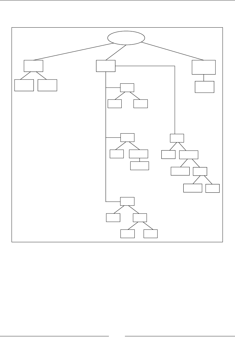
Chapter 2
[ 39 ]
When turning it to bytecode, the javac compiler most likely creates an abstract
syntax tree that looks something like this:
SEQUENCE
LOOP
=
sum sum
sum
sum
<
RETURN
+
1
=
=
=
+
init
iter
cond
body
series
series
length
aload
i
i
i
i
i
0
0
Several important prerequisites for code optimization, such as identifying loop
invariants and loop bodies require expensive analysis in a control ow graph.
Here, this comes very cheap, as loops are given implicitly by the representation.
Adaptive Code Generation
[ 40 ]
However, in order to create the bytecode, the structured for loop, probably already
represented as a loop node in the Java compiler's abstract syntax tree, needs to be
broken up into conditional and unconditional jumps.
public int add(int[]);
Code:
0: iconst_0
1: istore_2 //sum=0
2: iconst_0
3: istore_3 //i=0
4: iload_3 //loop_header:
5: aload_1
6: arraylength
7: if_icmpge 22 //if (i>=series.length) then goto 22
10: iload_2
11: aload_1
12: iload_3
13: iaload
14: iadd
15: istore_2 //sum += series[i]
16: iinc 3, 1 //i++
19: goto 4 //goto loop_header
22: iload_2
23: ireturn //return sum
Now, without structured control ow information, the bytecode compiler has to
spend expensive CPU cycles restructuring control ow information that has been
lost, sometimes irretrievably.
Perhaps, in retrospect, it would have been a better design rationale to directly use
an encoded version of the compiler's ASTs as bytecode format. Various academic
papers have shown that ASTs are possible to represent in an equally compact or
more compact way than Java bytecode, so space is not a problem. Interpreting an
AST at runtime would also only be slightly more difcult than interpreting bytecode.
The earliest versions of the JRockit JIT used a decompiling frontend.
Starting from byte code, it tried to recreate the ASTs present when
javac turned source code into bytecode. If unsuccessful, the
decompiler fell back to more naive JIT compilation. Reconstructing
ASTs, however, turned out to be a very complex problem and the
decompiler was scrapped in the early 2000s, to be replaced by a unied
frontend that created control ow graphs, able to support arbitrary
control ow directly from bytecode.

Chapter 2
[ 41 ]
Where to optimize
Programmers tend to optimize their Java programs prematurely. This is completely
understandable. How can you trust the black box, the JVM below your application,
to do something optimal with such a high-level construct as Java source code?
Of course this is partially true, but even though the JVM can't fully create an
understanding of what your program does, it can still do a lot with what it gets.
It is sometimes surprising how much faster a program runs after automatic adaptive
optimization, simply because the JVM is better at detecting patterns in a very large
runtime environment than a human. On the other hand, some things lend themselves
better to manual optimization. This book is in no way expressing the viewpoint that all
code optimizations should be left to the JVM; however, as we have explained, explicit
optimization on the bytecode level is probably a good thing to avoid.
There are plenty of opportunities for writing efcient programs in Java and
situations where an adaptive runtime can't help. For example, a JVM can never turn
a quadratic algorithm into a linear one, replacing your BubbleSort with a QuickSort.
A JVM can never invent its own object cache where you should have written one
yourself. These are the kinds of cases that matter in Java code. The JVM isn't magical.
Adaptive optimization can never substitute bad algorithms with good ones. At most,
it can make the bad ones run a little bit faster.
However, the JVM can easily deal with many constructs in standard object-oriented
code. The programmer will probably gain very little by avoiding the declaration of
an extra variable or by copying and pasting eld loads and stores all over the place
instead of calling a simple getter or setter. These are examples of micro-optimizations
that make the Java code harder to read and that don't make the JIT compiled code
execute any faster.

Adaptive Code Generation
[ 42 ]
Sometimes, Java source code level optimizations are downright
destructive. All too often people come up with hard-to-read Java
code that they claim is optimal because some micro benchmark
(where only the interpreter was active and not the optimizing JIT)
told them so. An example from the real world is a server application
where the programmer did a lot of iterations over elements in
arrays. Believing it important to avoid using a loop condition, he
surrounded the for loops with a try block and catch clause for the
ArrayIndexOutOfBoundsException, that was thrown when the
program tried to read outside the array. Not only was the source very
hard to read, but once the runtime had optimized the method, it was
also signicantly slower than a standard loop would have been. This is
because exceptions are very expensive operations and are assumed to
be just that—exceptions. The "gambling" behavior of the JVM, thinking
that exceptions are rare, became a bad t.
It is all too easy to misunderstand what you are measuring when you are looking
for a performance bottleneck. Not every problem can be stripped down into a small
self contained benchmark. Not every benchmark accurately reects the problem
that is being examined. Chapter 5 will go into extensive detail on benchmarking and
how to know what to look for in Java performance. The second part of this book will
cover the various components of the JRockit Mission Control Suite, which is an ideal
toolbox for performance analysis.
The JRockit code pipeline
Given that the frontend of the JIT compiler is nished with the bytecode, having
turned it into some other form that is easier to process, what happens next? Typically,
the code goes through several levels of transformations and optimizations, each level
becoming increasingly platform-dependent. The nal level of code is native code
for a particular platform. The native code is emitted into a code buffer and executed
whenever the function it represents is called.
Naturally, it makes sense to keep the JIT compiler portable as far as possible. So,
most optimizations are usually done when the intermediate code format is still
platform-independent. This makes it easier to port the JIT compiler to different
architectures. However, low-level, platform-specic optimizations must naturally
be implemented as well to achieve industrial strength performance.
This section describes how the JIT compiler gets from bytecode to native code and
the stages involved. We concentrate on the JRockit JIT compiler, but in general terms
the process of generating native code is similar between JVMs.

Chapter 2
[ 43 ]
Why JRockit has no bytecode interpreter
JRockit uses the code generation strategy total JIT compilation.
When the JRockit project started in 1998, the JVM architects realized early on that
pure server-side Java was a niche so far unexploited, and JRockit was originally
designed to be only a server-side JVM. Most server-side applications, it was argued,
stay running for a long time and can afford to take some time reaching a steady state.
Thus, for a server-side-only JVM, it was decided that code generation time was a
smaller problem than efcient execution. This saved us the trouble of implementing
both a JIT compiler and a bytecode interpreter as well as handling the state
transitions between them.
It was quickly noted that compiling every method contributed to additional startup
time. This was initially not considered to be a major issue. Server-side applications,
once they are up and running, stay running for a long time.
Later, as JRockit became a major mainstream JVM, known for its performance,
the need to diversify the code pipeline into client and server parts was recognized.
No interpreter was added, however. Rather the JIT was modied to differentiate even
further between cold and hot code, enabling faster "sloppy" code generation the rst
time a method was encountered. This greatly improved startup time to a satisfying
degree, but of course, getting to pure interpreter speeds with a compile-only approach
is still very hard.
Another aspect that makes life easier with an interpreter is debuggability. Bytecode
contains meta information about things like variable names and line numbers. These
are needed by the debugger. In order to support debuggability, the JRockit JIT had to
propagate this kind of information all the way from per-bytecode basis to per-native
instruction basis. Once that bookkeeping problem was solved, there was little reason
to add an interpreter. This has the added benet that, to our knowledge, JRockit is the
only virtual machine that lets the user debug optimized code.
The main problems with the compile-only strategy in JRockit are the code bloat
(solved by garbage collecting code buffers with methods no longer in use) and
compilation time for large methods (solved by having a sloppy mode for the JIT).
Adaptive Code Generation
[ 44 ]
The compile-only strategy is sometimes less scalable than it should
be. For example, sometimes, JRockit will use a lot of time generating a
relatively large method, the typical example being a JSP. Once nished,
however, the response time for accessing that JSP will be better than
that of an interpreted version.
If you run into problems with code generation time using JRockit,
these can often be worked around. More on this will be covered in the
Controlling code generation in JRockit section at the end of this chapter.
Bootstrapping
The "brain" of the JRockit JVM is the runtime system itself. It keeps track of what
goes on in the world that comprises the virtual execution environment. The
runtime system is aware of which Java classes and methods make up the "world"
and requests that the code generator compiles them at appropriate times with
appropriate levels of code quality.
To simplify things a bit, the rst thing the runtime wants to do when the JVM
is started, is to look up and jump to the main method of a Java program. This is
done through a standard JNI call from the native JVM, just like any other native
application would use JNI to call Java code.
Searching for main triggers a complex chain of actions and dependencies. A lot of
other Java methods required for bootstrapping and fundamental JVM behavior need
to be generated in order to resolve the main function. When nally main is ready and
compiled to native code, the JVM can execute its rst native-to-Java stub and pass
control from the JVM to the Java program.
To study the bootstrap behavior of JRockit, try running a simple Java
program with the command-line switch –Xverbose:codegen. It may
seem shocking that running a simple "Hello World" program involves JIT
compiling around 1,000 methods. This, however, takes very little time. On
a modern Intel Core2 machine, the total code generation time is less than
250 milliseconds.
Runtime code generation
Total JIT compilation needs to be a lazy process. If any method or class referenced from
another method would be fully generated depth rst at referral time, there would be
signicant code generation overhead. Also, just because a class is referenced from the
code doesn't mean that every method of the class has to be compiled right away or
even that any of its methods will ever be executed. Control ow through the Java

Chapter 2
[ 45 ]
program might take a different path. This problem obviously doesn't exist in a mixed
mode solution, in which everything starts out as interpreted bytecode with no need
to compile ahead of execution.
Trampolines
JRockit solves this problem by generating stub code for newly referred but not yet
generated methods. These stubs are called trampolines, and basically consist of a few
lines of native code pretending to be the nal version of the method. When the method
is rst called, and control jumps to the trampoline, all it does is execute a call that
tells JRockit that the real method needs to be generated. The code generator fulls the
request and returns the starting address of the real method, to which the trampoline
then dispatches control. To the user it looks like the Java method was called directly,
when in fact it was generated just at the rst time it was actually called.
0x1000: method A
call method B @ 0x2000
0x2000: method B (trampoline)
call JVM.Generate(B) -> start
write trap @ 0x2000
goto start @ 0x4000
0x3000: method C
call method B @ 0x2000
0x4000: The "real" method B
...
Consider the previous example. method A, whose generated code resides at
address 0x1000 is executing a call to method B, that it believes is placed at address
0x2000. This is the rst call to method B ever. Consequently, all that is at address
0x2000 is a trampoline. The rst thing the trampoline does is to issue a native call
to the JVM, telling it to generate the real method B. Execution then halts until this
code generation request has been fullled, and a starting address for method B is
returned, let's say 0x4000. The trampoline then dispatches control to method B by
jumping to that address.
Note that there may be several calls to method B in the code already, also pointing
to the trampoline address 0x2000. Consider, for example, the call in method C
that hasn't been executed yet. These calls need to be updated as well, without
method B being regenerated. JRockit solves this by writing an illegal instruction at
address 0x2000, when the trampoline has run. This way, the system will trap if the
trampoline is called more than once. The JVM has a special exception handler that
catches the trap, and patches the call to the trampoline so that it points to the real
method instead. In this case it means overwriting the call to 0x2000 in method C
with a call to 0x4000. This process is called back patching.

Adaptive Code Generation
[ 46 ]
Back patching is used for all kinds of code replacement in the virtual machine, not
just for method generation. If, for example, a hot method has been regenerated to a
more efcient version, the cold version of the code is tted with a trap at the start
and back patching takes place in a similar manner, gradually redirecting calls from
the old method to the new one.
Again, note that this is a lazy approach. We don't have time to go over the entire
compiled code base and look for potential jumps to code that has changed since
the caller was generated.
If there are no more references to an older version of a method, its native code buffer
can be scheduled for garbage collection by the run time system so as to unclutter
the memory. This is necessary in a world that uses a total JIT strategy because the
amount of code produced can be quite large.
Code generation requests
In JRockit, code generation requests are passed to the code generator from
the runtime when a method needs to be compiled. The requests can be either
synchronous or asynchronous.
Synchronous code generation requests do one of the following:
• Quickly generate a method for the JIT, with a specied level of efciency
• Generate an optimized method, with a specied level of efciency
An asynchronous request is:
• Act upon an invalidated assumption, for example, force regeneration of a
method or patch the native code of a method
Internally, JRockit keeps synchronous code generation requests in a code generation
queue and an optimization queue, depending on request type. The queues are
consumed by one or more code generation and/or optimization threads, depending
on system conguration.
The code generation queue contains generation requests for methods that are needed
for program execution to proceed. These requests, except for special cases during
bootstrapping, are essentially generated by trampolines. The call "generate me" that
each trampoline contains, inserts a request in the code generation queue, and blocks
until the method generation is complete. The return value of the call is the address in
memory where the new method starts, to which the trampoline nally jumps.

Chapter 2
[ 47 ]
Optimization requests
Optimization requests are added to the optimization queue whenever a method is
found to be hot, that is when the runtime system has realized that we are spending
enough time executing the Java code of that method so that optimization is warranted.
The optimization queue understandably runs at a lower priority than the code
generation queue as its work is not necessary for code execution, but just for code
performance. Also, an optimization request usually takes orders of magnitude
longer than a standard code generation request to execute, trading compile time
for efcient code.
On-stack replacement
Once an optimized version of a method is generated, the existing version of the
code for that method needs to be replaced. As previously described, the method
entry point of the existing cold version of the method is overwritten with a trap
instruction. Calls to the old method will be back patched to point to the new,
optimized piece of code.
If the Java program spends a very large amount of time in a method, it will be
agged as hot and queued for replacement. However, consider the case where the
method contains a loop that executes for a very long time. This method may well
be hotspotted and regenerated, but the old method still keeps executing even if the
method entry to the old method is tted with a trap. Obviously, the performance
enhancement that the optimized method contributes will enter the runtime much
later, or never if the loop is innite.
Some optimizers swap out code on the existing execution stack by replacing the code
of a method with a new version in the middle of its execution. This is referred to as
on-stack replacement and requires extensive bookkeeping. Though this is possible
in a completely JIT-compiled world, it is easier to implement where there is an
interpreter to fall back to.
JRockit doesn't do on-stack replacement, as the complexity required to do so is
deemed too great. Even though the code for a more optimal version of the method
may have been generated, JRockit will continue executing the old version of the
method if it is currently running.
Our research has shown that in the real world, this matters little for achieving
performance. The only places we have encountered performance penalties because
of not doing on-stack replacement is in badly written micro benchmarks, such as
when the main function contains all the computations in a very long loop. Moving the
bulk of the benchmark into a separate function and calling this repeatedly from main
will resolve this problem. We will thoroughly discuss the most important aspects of
benchmarking in Chapter 5.

Adaptive Code Generation
[ 48 ]
Bookkeeping
The code generator in the JVM has to perform a number of necessary bookkeeping
tasks for the runtime system.
Object information for GC
For various reasons, a garbage collector needs to keep track of which registers and
stack frame locations contain Java objects at any given point in the program. This
information is generated by the JIT compiler and is stored in a database in the runtime
system. The JIT compiler is the component responsible for creating this data because
type information is available "for free" while generating code. The compiler has to deal
with types anyway. In JRockit, the object meta info is called livemaps, and a detailed
explanation of how the code generation system works with the garbage collector is
given in Chapter 3, Adaptive Memory Management.
Source code and variable information
Another bookkeeping issue in the compiled world is the challenge of preserving
source code level information all the way down to machine language. The JVM
must always be able to trace program points back from an arbitrary native
instruction to a particular line of Java source code. We need to support proper
stack traces for debugging purposes, even stack traces containing optimized code.
This gets even more complicated as the optimizer may have transformed a method
heavily from its original form. A method may even contain parts of other methods
due to inlining. If an exception occurs anywhere in our highly optimized native
code, the stack trace must still be able to show the line number where this happened.
This is not a difcult problem to solve—bookkeeping just involves some kind of
database, as it is large and complex. JRockit successfully preserves mappings between
most native instructions and the actual line of Java source code that created them.
This, obviously, is much more work in a compiled world than in an interpreted one.
In the Java bytecode format, local variable information and line number information
are mapped to individual bytecodes, but JRockit has to make sure that the mapping
survives all the way down to native code. Each bytecode instruction eventually turns
into zero or more native code instructions that may or may not execute in sequence.
Assumptions made about the generated code
Finally, as we have already discussed, remembering what assumptions or "gambles"
have been made while generating methods is vital in Java. As soon as one of the
assumptions is violated, we need to send asynchronous code regeneration requests
for whatever methods are affected. Thus, an assumption database is another part of
the JRockit runtime that communicates with the code generator.

Chapter 2
[ 49 ]
A walkthrough of method generation in
JRockit
Let us now take a look at what happens on the road from bytecode to native code in
the JRockit JIT compiler. This section describes how a small method is transformed
to native code by the JRockit JIT. Large parts of this process are similar in other JIT
compilers (as well as in other static compilers), and some parts are not. The end
result, native code, is the same.
Let us, consider the following Java method as an example:
public static int md5_F(int x, int y, int z) {
return (x & y) | ((~x) & z);
}
This is part of the well known MD5 hash function and performs bit operations on
three pieces of input.
The JRockit IR format
The rst stage of the JRockit code pipeline turns the bytecode into an Intermediate
Representation (IR). As it is conceivable that other languages may be compiled
by the same frontend, and also for convenience, optimizers tend to work with a
common internal intermediate format.
JRockit works with an intermediate format that differs from bytecode, looking
more like classic text book compiler formats. This is the common approach that
most compilers use, but of course the format of IR that a compiler uses always
varies slightly depending on implementation and the language being compiled.
Aside from the previously mentioned portability issue, JRockit also doesn't work
with bytecode internally because of the issues with unstructured control ow and
the execution stack model, which differs from any modern hardware register model.
Because we lack the information to completely reconstruct the ASTs, a method in
JRockit is represented as a directed graph, a control ow graph, whose nodes are
basic blocks. The denition of a basic block is that if one instruction in the basic
block is executed, all other instructions in it will be executed as well. Since there are
no branches in our example, the md5_F function will turn into exactly one basic block.
Data ow
A basic block contains zero to many operations, which in turn have operands.
Operands can be other operations (forming expression trees), variables (virtual
registers or atomic operands), constants, addresses, and so on, depending on
how close to the actual hardware representation the IR is.
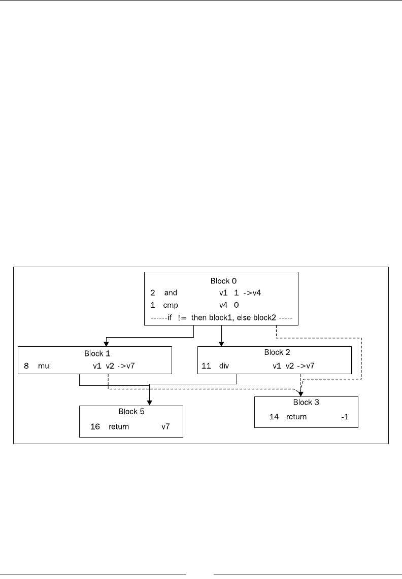
Adaptive Code Generation
[ 50 ]
Control ow
Basic blocks can have multiple entries and multiple exits. The edges in the graph
represent control ow. Any control ow construct, such as a simple fallthrough to
the next basic block, a goto, a conditional jump, a switch, or an exception,
produces one or more edges in the graph.
When control enters a method, there is a designated start basic block for the execution.
A basic block with no exits ends the method execution. Typically such a block ends
with a return or throw clause.
A word about exceptions
A small complication is the presence of exceptions, which, if consistent to this model,
should form conditional jumps from every bytecode operation that may fault to an
appropriate catch block, where one is available.
This would quickly turn into a combinatorial explosion of edges in the ow graph
(and consequently of basic blocks), severely handicapping any O(|V||E|) (nodes
x edges) graph traversal algorithm that needs to work on the code. Therefore,
exceptions are treated specially on a per-basic block basis instead.
This gure shows the basic block graph of a slightly larger example. Method entry is
at Block 0 that has three exits—two normal ones, as it contains a conditional branch,
and an exception edge. This means that Block 0 is a try block, whose catch starts
at Block 3. The same try block spans Block 1 and Block 2 as well. The method can
exit either by triggering the exception and ending up in Block 3 or by falling through
to Block 5. Both these blocks end with return instructions. Even though the only
instruction that can trigger an exception is the div in Block 2 (on division by zero),
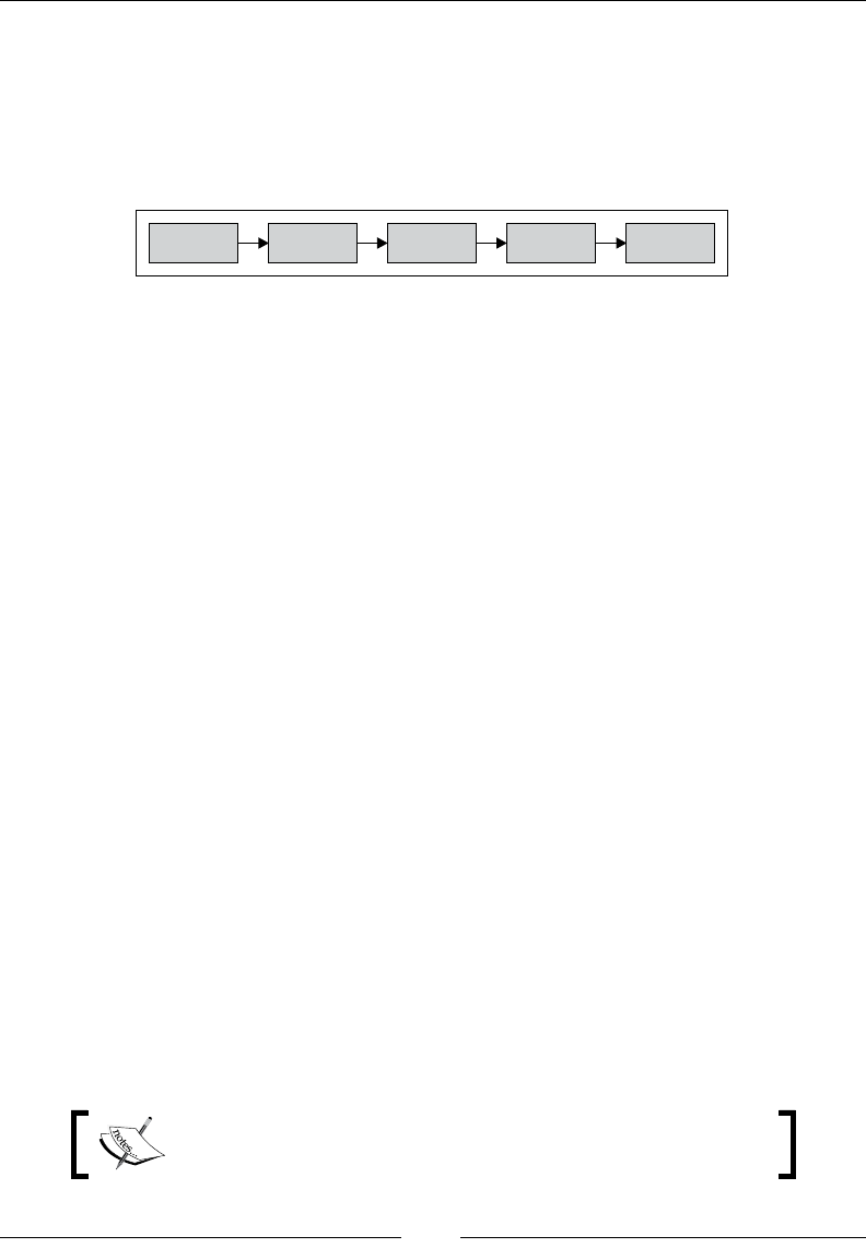
Chapter 2
[ 51 ]
the try block spans several nodes because this is what the bytecode (and possibly
the source code) looked like. Optimizers may choose to deal with this later.
JIT compilation
This following gure illustrates the different stages of the JRockit code pipeline:
BC2HIR HIR2MIR MIR2LIR RegAlloc EMIT
Generating HIR
The rst module in the code generator, BC2HIR, is the frontend against the bytecode
and its purpose is to quickly translate bytecodes into IR. HIR in this case stands for
High-level Intermediate Representation. For the md5_F method, where no control
ow in the form of conditional or unconditional jumps is present, we get just one
basic block.
The following code snippet shows the md5_F method in bytecode form:
public static int md5_F(int, int, int);
Code: Stack contents: Emitted code:
0: iload_0 v0
1: iload_1 v1
2: iand (v0&v1)
3: iload_0 (v0&v1), v0
4: iconst_m1 (v0&v1), v0, -1
5: ixor (v0&v1), (v0^-1)
6: iload_2 (v0&v1), (v0^-1), v2
7: iand (v0&v1), ((v0^-1) & v2)
8: ior ((v0&v1) | ((v0^-1) & v2))
9: ireturn return ((v0&v1) |
((v0^-1) & v2));
The JIT works by computing a control ow graph for the IR by examining where
the jumps in the bytecode are, and then lling its basic blocks with code. Code is
constructed by emulating the contents of the evaluation stack at any given location
in the program. Emulating a bytecode operation results in changes to the evaluation
stack and/or code being generated. The example has been annotated with the
contents of the emulated evaluation stack and the resulting generated code after each
bytecode has been processed
Bit negation (~) is implemented by javac as an xor with -1
(0xffffffff), as bytecode lacks a specic not operator.
Adaptive Code Generation
[ 52 ]
As we can see, by representing the contents of a variable on the evaluation stack with
a variable handle, we can reconstruct the expressions from the original source code.
For example, the iload_0 instruction, which means "push the contents of variable
0" turns into the expression "variable 0" on the emulated stack. In the example, the
emulator gradually forms a more and more complex expression on the stack, and
when it is time to pop it and return it, the expression in its entirety can be used to
form code.
This is the output, the High-level IR, or HIR:
params: v1 v2 v3
block0: [first] [id=0]
10 @9:49 (i32) return {or {and v1 v2} {and {xor v1 -1} v3}}
In JRockit IR, the annotation @ before each statement identies its
program point in the code all the way down to assembler level. The
rst number following the @ is the bytecode offset of the expression
and the last is the source code line number information. This is part
of the complex meta info framework in JRockit that maps individual
native instructions back to their Java program points.
The variable indexes were assigned by JRockit, and differ from those in the
bytecode. Notice that operations may contain other operations as their operands,
similar to the original Java code. These nested expressions are actually a useful
byproduct of turning the bytecode stack back into expressions. This way we get a
High-level Representation instead of typical "at" compiler code with temporary
variable assignments, where operations may not contain other operations. The HIR
lends itself well to some optimizations that are harder to do on another format; for
example, discovering if a sub-expression (in the form of a subtree) is present twice
in an expression. Then the sub-expression can be folded into a temporary variable,
saving it from being evaluated twice.
Emulating the bytecode stack to form HIR is not without problems though. Since
at compile time, we only know what expression is on the stack, and not its value,
we run into various problems. One example would be in situations where the stack
is used as memory. Take for example the construct result = x ? a : b. The
bytecode compiles into something like this:
/* bytecode for: "return x ? a : b" */
static int test(boolean x, int a, int b);
0: iload_0 //push x
1: ifeq 8 //if x == false then goto 8
4: iload_1 //push a

Chapter 2
[ 53 ]
5: goto 9
8: iload_2 //push b
9: ireturn //return pop
When the emulator gets to the ireturn instruction, the value popped can be either
a (local variable 1) or b (local variable 2). Since we can't express "either a or b" as a
variable, we need to replace the loads at offsets 4 and 8 with writes to one and the
same temporary variable, and place that on the stack instead.
The BC2HIR module that turns bytecodes into a control ow graph with expressions
is not computationally complex. However, it contains several other little special
cases, similar to the earlier one, which are beyond the scope of this book. Most of
them have to do with the lack of structure in byte code and with the evaluation stack
metaphor. Another example would be the need to associate monitorenter bytecodes
with their corresponding monitorexit(s), the need for which is explained in great
detail in Chapter 4.
MIR
MIR or Middle-level Intermediate Representation, is the transform domain where
most code optimizations take place. This is because most optimizations work best
with three address code or rather instructions that only contain atomic operands,
not other instructions. Transforming HIR to MIR is simply an in-order traversal
of the expression trees mentioned earlier and the creation of temporary variables.
As no hardware deals with expression trees, it is natural that code turns into
progressively simpler operations on the path through the code pipeline.
Our md5_F example would look something like the following code to the JIT
compiler, when the expression trees have been attened. Note that no operation
contains other operations anymore. Each operation writes its result to a temporary
variable, which is in turn used by later operations.
params: v1 v2 v3
block0: [first] [id=0]
2 @2:49* (i32) and v1 v2 -> v4
5 @5:49* (i32) xor v1 -1 -> v5
7 @7:49* (i32) and v5 v3 -> v5
8 @8:49* (i32) or v4 v5 -> v4
10 @9:49* (i32) return v4
If the JIT compiler is executing a code generation request from the optimizer, most
optimizations on the way down to native code are carried out on MIR. This will be
discussed later in the chapter.

Adaptive Code Generation
[ 54 ]
LIR
After MIR, it is time to turn platform dependent as we are approaching native code.
LIR, or Low-level IR, looks different depending on hardware architecture.
Consider the Intel x86, where the biggest customer base for JRockit exists. The x86
has legacy operations dating back to the early 1980s. The RISC-like format of the
previous MIR operations is inappropriate. For example, a logical and operation on
the x86 requires the same rst source and destination operand. That is why we need
to introduce a number of new temporaries in order to turn the code into something
that ts the x86 model better.
If we were compiling for SPARC, whose native format looks more like the JRockit IR,
fewer transformations would have been needed.
Following is the LIR for the md5_F method on a 32-bit x86 platform:
params: v1 v2 v3
block0: [first] [id=0]
2 @2:49* (i32) x86_and v2 v1 -> v2
11 @2:49 (i32) x86_mov v2 -> v4
5 @5:49* (i32) x86_xor v1 -1 -> v1
12 @5:49 (i32) x86_mov v1 -> v5
7 @7:49* (i32) x86_and v5 v3 -> v5
8 @8:49* (i32) x86_or v4 v5 -> v4
14 @9:49 (i32) x86_mov v4 -> eax
13 @9:49* (i32) x86_ret eax
A couple of platform-independent mov instructions have been inserted to get the
correct x86 semantics. Note that the and, xor, and or operations now have the same
rst operand as destination, the way x86 requires. Another interesting thing is that
we already see hard-coded machine registers here. The JRockit calling convention
demands that integers be returned in the register eax, so the register allocator that
is the next step of the code pipeline doesn't really have a choice for a register for the
return value.
Register allocation
There can be any number of virtual registers (variables) in the code, but the physical
platform only has a small number of them. Therefore, the JIT compiler needs to do
register allocation, transforming the virtual variable mappings into machine registers.
If at any given point in the program, we need to use more variables than there are
physical registers in the machine at the same time, the local stack frame has to be used
for temporary storage. This is called spilling, and the register allocator implements
spills by inserting move instructions that shufe registers back and forth from the
stack. Naturally spill moves incur overhead, so their placement is highly signicant
in optimized code.

Chapter 2
[ 55 ]
Register allocation is a very fast process if done sloppily, such as in the rst JIT
stage, but computationally intensive if a good job is needed, especially when
there are many variables in use (or live) at the same time. However, because of
the small number of variables, we get an optimal result with little effort in our
example method. Several of the temporary mov instructions have been coalesced
and removed.
Our md5_F method needs no spills, as x86 has seven available registers (15 on the
64-bit platforms), and we use only three.
params: ecx eax edx
block0: [first] [id=0]
2 @2:49* (i32) x86_and eax ecx -> eax
5 @5:49* (i32) x86_xor ecx -1 -> ecx
7 @7:49* (i32) x86_and ecx edx -> ecx
8 @8:49* (i32) x86_or eax ecx -> eax
13 @9:49* (void) x86_ret eax
Every instruction in our register allocated LIR has a native instruction equivalent
on the platform that we are generating code for.
Just to put spill code in to perspective, following is a slightly longer example. The
main method of the Spill program does eight eld loads to eight variables that
are then used at the same time (for multiplying them together).
public class Spill {
static int aField, bField, cField, dField;
static int eField, fField, gField, hField;
static int answer;
public static void main(String args[]) {
int a = aField;
int b = bField;
int c = cField;
int d = dField;
int e = eField;
int f = fField;
int g = gField;
int h = hField;
answer = a*b*c*d*e*f*g*h;
}
}
Adaptive Code Generation
[ 56 ]
We will examine the native code for this method on a 32-bit x86 platform. As
32-bit x86 has only seven available registers, one of the intermediate values has
to be spilled to the stack. The resulting register allocated LIR code is shown in the
following code snippet:
Assembly or LIR instructions that dereference memory typically annotate
their pointers as a value or variable within square brackets. For example,
[esp+8] dereferences the memory eight bytes above the stack pointer
(esp) on x86 architectures.
block0: [first] [id=0]
68 (i32) x86_push ebx //store callee save reg
69 (i32) x86_push ebp //store callee save reg
70 (i32) x86_sub esp 4 -> esp //alloc stack for 1 spill
43 @0:7* (i32) x86_mov [0xf56bd7f8] -> esi //*aField->esi (a)
44 @4:8* (i32) x86_mov [0xf56bd7fc] -> edx //*bField->edx (b)
67 @4:8 (i32) x86_mov edx -> [esp+0x0] //spill b to stack
45 @8:9* (i32) x86_mov [0xf56bd800] -> edi //*cField->edi (c)
46 @12:10* (i32) x86_mov [0xf56bd804] -> ecx //*dField->ecx (d)
47 @17:11* (i32) x86_mov [0xf56bd808] -> edx //*eField->edx (e)
48 @22:12* (i32) x86_mov [0xf56bd80c] -> eax //*fField->eax (f)
49 @27:13* (i32) x86_mov [0xf56bd810] -> ebx //*gField->ebx (g)
50 @32:14* (i32) x86_mov [0xf56bd814] -> ebp //*hField->ebp (h)
26 @39:16 (i32) x86_imul esi [esp+0x0] -> esi //a *= b
28 @41:16 (i32) x86_imul esi edi -> esi //a *= c
30 @44:16 (i32) x86_imul esi ecx -> esi //a *= d
32 @47:16 (i32) x86_imul esi edx -> esi //a *= e
34 @50:16 (i32) x86_imul esi eax -> esi //a *= f
36 @53:16 (i32) x86_imul esi ebx -> esi //a *= g
38 @56:16 (i32) x86_imul esi ebp -> esi //a *= h
65 @57:16* (i32) x86_mov esi -> [0xf56bd818] //*answer = a
71 @60:18* (i32) x86_add esp, 4 -> esp //free stack slot
72 @60:18 (i32) x86_pop -> ebp //restore used callee save
73 @60:18 (i32) x86_pop -> ebx //restore used callee save
66 @60:18 (void) x86_ret //return

Chapter 2
[ 57 ]
We can also note that the register allocator has added an epilogue and prologue to
the method in which stack manipulation takes place. This is because it has gured
out that one stack position will be required for the spilled variable and that it also
needs to use two callee-save registers for storage. A register being callee-save means
that a called method has to preserve the contents of the register for the caller. If the
method needs to overwrite callee-save registers, they have to be stored on the local
stack frame and restored just before the method returns. By JRockit convention on
x86, callee-save registers for Java code are ebx and ebp. Any calling convention
typically includes a few callee-save registers since if every register was potentially
destroyed over a call, the end result would be even more spill code.
Native code emission
After register allocation, every operation in the IR maps one-to-one to a native
operation in x86 machine language and we can send the IR to the code emitter. The last
thing that the JIT compiler does to the register allocated LIR is to add mov instructions
for parameter marshalling (in this case moving values from in-parameters as dened
by the calling convention to positions that the register allocator has picked). Even
though the register allocator thought it appropriate to put the rst parameter in ecx,
compilers work internally with a predened calling convention. JRockit passes the rst
parameter in eax instead, requiring a shufe mov. In the example, the JRockit calling
convention passes parameters x in eax, y in edx, and z in esi respectively.
Assembly code displayed in gures generated by code dumps from
JRockit use Intel style syntax on the x86, with the destination as the rst
operand, for example "and ebx, eax" means "ebx = ebx & eax".
Following is the resulting native code in a code buffer:
[method is md5_F(III)I [02DB2FF0 - 02DB3002]]
02DB2FF0: mov ecx,eax
02DB2FF2: mov eax,edx
02DB2FF4: and eax,ecx
02DB2FF6: xor ecx,0xffffffff
02DB2FF9: and ecx,esi
02DB2FFC: or eax,ecx
02DB2FFF: ret
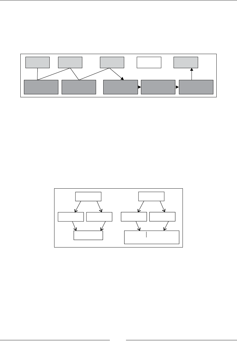
Adaptive Code Generation
[ 58 ]
Generating optimized code
Regenerating an optimized version of a method found to be hot is not too dissimilar
to normal JIT compilation. The optimizing JIT compiler basically piggybacks on the
original code pipeline, using it as a "spine" for the code generation process, but at each
stage, an optimization module is plugged into the JIT.
BC2HIR HIR2MIR MIR2LIR RegAlloc EMIT
Optimize HIR Optimize MIR Optimize LIR Graph Fusion
Based Regalloc
Optimize Native
Code
A general overview
Different optimizations are suitable for different levels of IR. For example, HIR
lends itself well to value numbering in expression trees, substituting two equivalent
subtrees of an expression with one subtree and a temporary variable assignment.
MIR readily transforms into Single Static Assignment (SSA) form, a transform
domain that makes sure that any variable has only one denition. SSA transformation
is part of virtually every commercial compiler today and makes implementing many
code optimizations much easier. Another added benet is that code optimizations in
SSA form can be potentially more powerful.
if (x > 0) if (x > 0)
1
result = 1
result =
3
result = 1
1result =0
2
result =0
result
return (r )esult result
1, 2
return result3
0
The previous ow graph shows what happens before and after transformation to
SSA form. The result variable that is returned by the program is assigned either
1 or 0 depending on the value of x and the branch destination. Since SSA form
allows only one assignment of each variable, the result variable has been split into
three different variables. At the return statement, result can either be result1
or result2. To express this "either" semantic, a special join operator, denoted
by the Greek letter phi (Φ), is used. Trivially, no hardware platform can express
this ambiguity, so the code has to be transformed back to normal form before
emission. The reverse transform basically replaces each join operator with preceding
assignments, one per ow path, to the destination of the join instruction.
Chapter 2
[ 59 ]
Many classic code optimizations such as constant propagation and copy propagation
have their own faster SSA form equivalents. This mostly has to do with the fact that
given any use of a variable, it is unambiguous where in the code that variable is
dened. There is plenty of literature on the subject and a thorough discussion on
all the benets of SSA form is beyond the scope of this book.
LIR is platform-dependent and initially not register allocated, so transformations
that form more efcient native operation sequences can be performed here.
An example would be replacing dumb copy loops with specialized Intel SSE4
instructions for faster array copies on the x86.
When generating optimized code, register allocation tends to be very
important. Any compiler textbook will tell you that optimal register
allocation basically is the same problem as graph coloring. This is
because if two variables are in use at the same time, they obviously
cannot share the same register. Variables in use at the same time can
be represented as connected nodes in a graph. The problem of register
allocation can then be reduced to assigning colors to the nodes in the
graph, so that no connected nodes have the same color. The amount of
colors available is the same as the number of registers on the platform.
Sadly enough, in computational complexity terms, graph coloring is
NP-hard. This means that no efcient (polynomial time) algorithm
exists that can solve the problem. However, graph coloring can be
approximated in quadratic time. Most compilers contain some variant
of the graph coloring algorithm for register allocation.
The JRockit optimizer contains a very advanced register allocator that is based
on a technique called graph fusion, that extends the standard graph coloring
approximation algorithm to work on subregions in the IR. Graph fusion has the
attractive property that the edges in the ow graph, processed early, generate fewer
spills than the edges processed later. Therefore, if we can pick hot subregions before
cold ones, the resulting code will be more optimal. Additional penalty comes from
the need to insert shufe code when fusing regions in order to form a complete
method. Shufe code consists of sequences of move instructions to copy the
contents of one local register allocation into another one.
Finally, just before code emission, various peephole optimizations can be applied to
the native code, replacing one to several register allocated instructions in sequence
with more optimal ones.

Adaptive Code Generation
[ 60 ]
Clearing a register is usually done by XORing the register with itself.
Replacing instructions such as mov eax, 0 with xor eax, eax,
which is potentially faster, is an example of a peephole optimization that
works on exactly one instruction. Another example would be turning a
multiplication with the power of two followed by an add instruction into
a simple lea instruction on x86, optimized to do both.
How does the optimizer work?
A complete walkthrough of the JRockit code pipeline with the algorithms and
optimizations within would be the subject for an entire book of its own. This
section merely tries to highlight some of the things that a JVM can do with code,
given adequate runtime feedback.
Generating optimized code for a method in JRockit generally takes 10 to 100 times
as long as JITing it with no demands for execution speed. Therefore, it is important
to only optimize frequently executed methods.
Grossly oversimplifying things, the bulk of the optimizer modules plugged into the
code pipeline work like this:
do {
1) get rid of calls, exposing more control flow
through aggressive inlining.
2) apply optimizations on enlarged code mass, try to shrink it.
} while ("enough time left" && "code not growing too fast");
Java is an object-oriented language and contains a lot of getters, setters, and other
small "nuisance" calls. The compiler has to presume that calls do very complex things
and have side effects unless it knows what's inside them. So, for simplication, small
methods are frequently inlined, replacing the call with the code of the called function.
JRockit tries to aggressively inline everything that seems remotely interesting on
hot execution paths, with reasonable prioritization of candidates using sample and
proling information.
In a statically compiled environment, too aggressive inlining would be total
overkill, and too large methods would cause instruction cache penalties and slow
down execution. In a runtime, however, we can hope to have good enough sample
information to make more realistic guesses about what needs to be inlined.
After bringing in whatever good inlining candidates we can nd into the method, the
JIT applies optimizations to the, now usually quite large, code mass, trying to shrink
it. For example, this is done by folding constants, eliminating expressions based on
escape analysis, and applying plenty of other simplifying transforms. Dead code

Chapter 2
[ 61 ]
that is proved never to be executed is removed. Multiple loads and stores that access
the same memory location can, under certain conditions, be eliminated, and so on.
Surprisingly enough, the size of the total code mass after inlining and then optimizing
the inlined code is often less than the original code mass of a method before anything
was inlined.
The runtime system can perform relatively large simplications, given relatively
little input. Consider the following program that implements the representation
of a circle by its radius and allows for area computation:
public class Circle {
private double radius;
public Circle(int radius) {
this.radius = radius;
}
public double getArea() {
return 3.1415 * radius * radius;
}
public static double getAreaFromRadius(int radius) {
Circle c = new Circle(radius);
return c.getArea();
}
static int areas[] = new int[0x10000];
static int radii[] = new int[0x10000];
static java.util.Random r = new java.util.Random();
static int MAX_ITERATIONS = 1000;
public static void gen() {
for (int i = 0; i < areas.length; i++) {
areas[i] = (int)getAreaFromRadius(radii[i]);
}
}
public static void main(String args[]) {
for (int i = 0; i < radii.length; i++) {
radii[i] = r.nextInt();
}
for (int i = 0; i < MAX_ITERATIONS; i++) {
gen(); //avoid on stack replacement problems
}
}
}

Adaptive Code Generation
[ 62 ]
Running the previous program with JRockit with the command-line
ag –Xverbose:opt,gc, to make JRockit dump all garbage collection
and code optimization events, produces the following output:
hastur:material marcus$ java –Xverbose:opt,gc Circle
[INFO ][memory ] [YC#1] 0.584-0.587: YC 33280KB->8962KB (65536KB),
0.003 s, sum of pauses 2.546 ms, longest pause 2.546 ms
[INFO ][memory ] [YC#2] 0.665-0.666: YC 33536KB->9026KB (65536KB),
0.001 s, sum of pauses 0.533 ms, longest pause 0.533 ms
[INFO ][memory ] [YC#3] 0.743-0.743: YC 33600KB->9026KB (65536KB),
0.001 s, sum of pauses 0.462 ms, longest pause 0.462 ms
[INFO ][memory ] [YC#4] 0.821-0.821: YC 33600KB->9026KB (65536KB),
0.001 s, sum of pauses 0.462 ms, longest pause 0.462 ms
[INFO ][memory ] [YC#5] 0.898-0.899: YC 33600KB->9026KB (65536KB),
0.001 s, sum of pauses 0.463 ms, longest pause 0.463 ms
[INFO ][memory ] [YC#6] 0.975-0.976: YC 33600KB->9026KB (65536KB),
0.001 s, sum of pauses 0.448 ms, longest pause 0.448 ms
[INFO ][memory ] [YC#7] 1.055-1.055: YC 33600KB->9026KB (65536KB),
0.001 s, sum of pauses 0.461 ms, longest pause 0.461 ms
[INFO ][memory ] [YC#8] 1.132-1.133: YC 33600KB->9026KB (65536KB),
0.001 s, sum of pauses 0.448 ms, longest pause 0.448 ms
[INFO ][memory ] [YC#9] 1.210-1.210: YC 33600KB->9026KB (65536KB),
0.001 s, sum of pauses 0.480 ms, longest pause 0.480 ms
[INFO ][opt ][00020] #1 (Opt)
jrockit/vm/Allocator.allocObjectOrArray(IIIZ)Ljava/lang/Object;
[INFO ][opt ][00020] #1 1.575-1.581 0x9e04c000-0x9e04c1ad 5
.72 ms 192KB 49274 bc/s (5.72 ms 49274 bc/s)
[INFO ][memory ] [YC#10] 1.607-1.608: YC 33600KB->9090KB
(65536KB), 0.001 s, sum of pauses 0.650 ms, longest pause 0.650 ms
[INFO ][memory ] [YC#11] 1.671-1.672: YC 33664KB->9090KB (65536KB),
0.001 s, sum of pauses 0.453 ms, longest pause 0.453 ms.
[INFO ][opt ][00020] #2 (Opt)
jrockit/vm/Allocator.allocObject(I)Ljava/lang/Object;
[INFO ][opt ][00020] #2 1.685-1.689 0x9e04c1c0-0x9e04c30d 3
.88 ms 192KB 83078 bc/s (9.60 ms 62923 bc/s)
[INFO ][memory ] [YC#12] 1.733-1.734: YC 33664KB->9090KB
(65536KB), 0.001 s, sum of pauses 0.459 ms, longest pause 0.459 ms.
[INFO ][opt ][00020] #3 (Opt) Circle.gen()V
[INFO ][opt ][00020] #3 1.741-1.743 0x9e04c320-0x9e04c3f2 2
.43 ms 128KB 44937 bc/s (12.02 ms 59295 bc/s)
[INFO ][opt ][00020] #4 (Opt) Circle.main([Ljava/lang/String;)V
[INFO ][opt ][00020] #4 1.818-1.829 0x9e04c400-0x9e04c7af 11
.04 ms 384KB 27364 bc/s (23.06 ms 44013 bc/s)
hastur:material marcus$
No more output is produced until the program is nished.
Chapter 2
[ 63 ]
The various log formats for the code generator will be discussed in more detail at the
end of this chapter. Log formats for the memory manager are covered in Chapter 3.
It can be noticed here, except for optimization being performed on the four hottest
methods in the code (where two are JRockit internal), that the garbage collections
stop after the optimizations have completed. This is because the optimizer was able
to prove that the Circle objects created in the getAreaFromRadius method aren't
escaping from the scope of the method. They are only used for an area calculation.
Once the call to c.getArea is inlined, it becomes clear that the entire lifecycle of the
Circle objects is spent in the getAreaFromRadius method. A Circle object just
contains a radius eld, a single double, and is thus easily represented just as that
double if we know it has a limited lifespan. An allocation that caused signicant
garbage collection overhead was removed by intelligent optimization.
Naturally, this is a fairly trivial example, and the optimization issue is easy for the
programmer to avoid by not instantiating a Circle every time the area method is
called in the rst place. However, if properly implemented, adaptive optimizations
scale well to large object-oriented applications.
The runtime is always better than the programmer at detecting certain
patterns. It is often surprising what optimization opportunities the
virtual machine discovers, that a human programmer hasn't seen. It
is equally surprising how rarely a "gamble", such as assuming that a
particular method never will be overridden, is invalidated. This shows
some of the true strength of the adaptive runtime.
Unoptimized Java carries plenty of overhead. The javac compiler needs to do
workarounds to implement some language features in bytecode. For example,
string concatenation with the + operator is just syntactic sugar for the creation of
StringBuilder objects and calls to their append functions. An optimizing compiler
should, however, have very few problems transforming things like this into more
optimal constructs. For example, we can use the fact that the implementation of
java.lang.StringBuilder is known, and tell the optimizer that its methods
have no harmful side effects, even though they haven't been generated yet.
Similar issues exist with boxed types. Boxed types turn into hidden objects
(for example instances of java.lang.Integer) on the bytecode level. Several
traditional compiler optimizations, such as escape analysis, can often easily strip
down a boxed type to its primitive value. This removes the hidden object allocation
that javac put in the bytecode to implement the boxed type.
Adaptive Code Generation
[ 64 ]
Controlling code generation in JRockit
JRockit is designed to work well out of the box, and it is generally discouraged to
play around too much with its command-line options. Changing the behavior of
code generation and optimization is no exception. This section exists mostly for
informational purposes and the user should be aware of possible unwanted side
effects that can arise from changing the behavior of the code generators.
This section applies mainly to the versions of JRockit from R28 and later.
For earlier versions of JRockit, please consult the JRockit documentation
for equivalent ways of doing the same thing. Note that all R28
functionality does not have equivalents in earlier versions of JRockit.
Command-line ags and directive les
In the rare case that the code generator causes problems in JRockit, or an application
behaves strangely or erroneously, or it just takes too long time to optimize a particular
method, the JRockit code generator behavior can be altered and controlled. Naturally,
if you know what you are doing, code generation can be controlled for other purposes
as well.
Command-line ags
JRockit has several command-lines ags that control code generation behavior in
a coarse grained way. For the purpose of this text, we will only mention a few.
Logging
The –Xverbose:codegen (and –Xverbose:opt) options make JRockit output two
lines of information per JIT compiled (or optimized) method to stderr.
Consider the output for a simple HelloWorld program. Every code generation event
produces two lines in the log, one when it starts and one when it nishes.
hastur:material marcus$ java –Xverbose:codegen HelloWorld
[INFO ][codegen][00004] #1 (Normal) jrockit/vm/RNI.transitToJava(I)V
[INFO ][codegen][00004] #1 0.027-0.027 0x9e5c0000-0x9e5c0023 0
.14 ms (0.00 ms)
[INFO ][codegen][00004] #2 (Normal)
jrockit/vm/RNI.transitToJavaFromDbgEvent(I)V
[INFO ][codegen][00004] #2 0.027-0.027 0x9e5c0040-0x9e5c0063 0
.03 ms (0.00 ms)
[INFO ][codegen][00004] #3 (Normal) jrockit/vm/RNI.debuggerEvent()V

Chapter 2
[ 65 ]
[INFO ][codegen][00004] #3 0.027-0.027 0x9e5c0080-0x9e5c0131 0
.40 ms 64KB 0 bc/s (0.40 ms 0 bc/s)
[INFO ][codegen][00004] #4 (Normal)
jrockit/vm/ExceptionHandler.enterExceptionHandler()
Ljava/lang/Throwable;
[INFO ][codegen][00004] #4 0.027-0.028 0x9e5c0140-0x9e5c01ff 0
.34 ms 64KB 0 bc/s (0.74 ms 0 bc/s)
[INFO ][codegen][00004] #5 (Normal)
jrockit/vm/ExceptionHandler.gotoHandler()V
[INFO ][codegen][00004] #5 0.028-0.028 0x9e5c0200-0x9e5c025c 0
.02 ms (0.74 ms)
...
[INFO ][codegen][00044] #1149 (Normal) java/lang/Shutdown.runHooks()V
[INFO ][codegen][00044] #1149 0.347-0.348 0x9e3b4040-0x9e3b4106 0
.26 ms 128KB 219584 bc/s (270.77 ms 215775 bc/s)
hastur:material marcus$
The rst log line of a code generation request (event start) contains the following
information from left to right:
• Info tag and log module identier (code generator).
• The thread ID of the thread generating the code: Depending on the system
conguration, there can be more than one code generator thread and more
than one code optimizer thread.
• The index of the generated method: The rst method to be generated starts
at index 1. As we notice, at the beginning of the output, code generation is
single threaded, and the order between the start and end of a code generation
event is maintained, forming consecutive entries. This doesn't have to be
the case if multiple code generation and optimization threads are working.
• The code generation strategy: The code generation strategy tells you how
this particular method will be generated. As it is too early to have received
runtime feedback information, all methods are generated using a normal
code generator strategy, or even a quick one that is even sloppier. The quick
strategy is applied for methods that are known to be of exceedingly little
importance for the runtime performance. This can be, for example, static
initializers that will run only once and thus make no sense to even register
allocate properly.
• The generated method: This is uniquely identied by class name, method
name, and descriptor.

Adaptive Code Generation
[ 66 ]
The second line of a code generation request (event end) contains the following
information from left to right:
• Info tag and log module identier (code generator).
• The thread ID of the thread generating the code.
• The index of the generated method.
• Start and end time for the code generation event: This is measured in
seconds from the start of the JVM.
• The address range: This is where the resulting native code is placed
in memory.
• Code generation time: The number of milliseconds it took for the code
generator to turn this particular method into machine language (starting
from bytecode).
• Maximum amount of thread local memory used: This is the maximum
amount of memory that the code generator thread needed to allocate in
order to generate the method.
• Average number of bytecodes per second: The number of bytecodes
processed per second for this method. 0 should be interpreted as
innity—the precision was not good enough
• Total code generation time: The total number of milliseconds this thread has
spent in code generation since JVM startup and average bytecodes compiled
per second for the thread so far.
Turning off optimizations
The command-line ag -XnoOpt, or –XX:DisableOptsAfter=<time> turns off all
optimization in the compiler, optionally after a specied number of seconds after
the start of the JVM. The ag -XnoOpt makes programs compile faster, but run
slower, and can be used if there is a suspected problem with the JRockit optimizer
or if compile time turns out to be a very big issue, for example in application
response time.
Changing the number of code generation threads
Depending on the machine conguration, it might make sense to change the number
of code generation and optimization threads that the JVM should use. Code generation
and code optimization is a process that can, with the exception of emitting code into
native code buffers and some aspects of class loading, be parallelized. The number
of JIT compiler threads can be changed with the –XX:JITThreads=<n> option. The
number of optimizing threads can be changed with the –XX:OptThreads=<n> option.
Note that optimizations typically are quite memory and CPU intensive, even if the
machine has plenty of cores.

Chapter 2
[ 67 ]
Directive les
A more versatile method for code generation control is provided by directive les.
Here, wild card patterns for interesting methods can be specied, for which the code
generator should customize its behavior. The amount of available customizations is
very large, and this section serves merely to introduce the concept of directive les,
not serve as a reference of any kind.
Warning! Directive les are a completely unsupported way of controlling
JRockit code generation. The directives in the les are undocumented
externally and are subject to change without notice. Oracle will not give
support to JRockit congurations that use directive les.
A directive le is passed to JRockit by the ag –XX:OptFile=<filename>. It can also
be added to or removed from the runtime state using JRCMD or through the JRockit
Java API, both of which will be covered later in this book. In order to be able to use
directive les, the command-line switch -XX:+UnlockDiagnosticVMOptions needs
to be passed on the command line as well. Diagnostic VM options are subject to
change without notice between releases and should be used at your own risk.
A directive le is a tuple of directives in a format compatible with the JavaScript
Object Notation (JSON) format. An example would be:
{
//pattern to match against class+method+signature
match: "java.dingo.Dango.*",
enable: jit
}
This is a very simple le that forbids the optimization of any method whose descriptor
matches java.dingo.Dango.*. This is because the enable directive only contains
the word jit, not the word hotspot, which would allow the matched methods to be
selected for optimization through sampling.
If, on the other hand, we want to force optimization of the matched methods on their
rst code generation, we'd use something like this:
{
match: "java.dingo.Dango.*",
//types of "reasons" for codegen we allow
enable: jit,
jit: {
preset : opt
}
}
Adaptive Code Generation
[ 68 ]
This means that we only allow the JIT strategy for the method, but when it is
compiled we should use the preset optimization strategy on it. JRockit contains a
number of preset strategies that are also directives, and opt means "immediately
generate this method with full optimization".
Applying full optimization to a method the rst time it is generated by
the system doesn't necessarily produce the same code or performance as
it would have done if that method was detected to be hot and queued for
normal optimization by the runtime. If a method is optimized too early,
the risk is that we don't know enough about the program yet to do a good
enough job. The fact is that the method might even have been queued for
optimization, since the runtime has learned new things about the running
program, but not optimized yet. Forcing the immediate optimization
of many methods is not only expensive in clock cycles, but it is also not
guaranteed to perform as well as it would by just letting things run their
natural course.
The code generation strategy can be overridden in a more ne-grained way as well,
for example, by turning off individual optimizations that are normally run, or by
forbidding the inlining of a particular method.
The following is an example of a directive le with multiple directives:
//Using more than one directive, should use an array '['.
[
//directive 1
{
match: "java.dingo.Dango.*",
enable: [ jit, hotspot ], //allow both jit and optimization
hotspot: {
fusion_regalloc : false; //forbid graph fusion for opt
},
jit_inline : false, //forbid jit inlining
},

Chapter 2
[ 69 ]
//directive 2
{
match: [ "java.lang.*", "com.sun.*" ],
enable: jit ,
jit: {
//copy the opt preset, i.e. force optimization
//for jit, but disable inlining
preset : opt,
opt_inline : false,
},
},
//directive 3
{
match: "com.oracle.*",
//force optimizer to always inline java.util methods
//force optimizer to NEVER inline com.sun.methods
inline: [ "+java.util.*", "-com.sun.*" ],
}
]
Practically, any part of compilation to native code for each kind of code
generation strategy in JRockit, down to individual optimizations, can be
controlled through a directive le. All aspects of directive les and names
of directives are generally not documented. While directive les are a
great instrument for helping you track down problems in a dialogue with
JRockit support, playing around too much with them on your own is
generally discouraged.
When using a directive le, it is a good idea to run with the –Xverbose:opt
command-line ag enabled, in order to make sure that the le is actually read
and understood by the JVM.

Adaptive Code Generation
[ 70 ]
Summary
This chapter discussed code generation in a runtime environment. The topic
was introduced as a general problem, comparing adaptive compilation to static
compilation. We also explained special situations that apply to code generation
in a Java Virtual Machine.
We have discussed some aspects of the Java bytecode format, its pros and cons,
and the challenges of making Java code run fast, using different techniques from
interpretation to total JIT compilation.
Furthermore, we have discussed the challenges of an adaptive runtime, where new
code can enter the system at any time, and how to overcome them by "educated
guesses", or "gambling". This means that JVM takes the optimistic approach when
optimizing that made assumptions rarely change. We also mentioned the equation
compilation speed versus execution speed, depending on method "hotness".
Finally, the chapter introduced the code pipeline in the JRockit Virtual Machine and
its state of the art optimizations, using a comprehensive example with snapshots of a
method generation cycle, all the way to native code. At the end of the chapter, some
ways of modifying JRockit code generation behavior through command-line ags
and directive les were explained.
The next chapter covers another fundamental aspect of adaptive runtimes; the
memory management system, and techniques for efcient garbage collection, both as
an overview, for garbage collected languages in general and specically for Java with
the JRockit JVM.

Adaptive Memory
Management
This chapter is an introduction to automatic and adaptive memory management
in the Java runtime. It provides a background on techniques for garbage collection
and looks at the history of automatic memory management. It also discusses the
advantages and disadvantages of automatic memory management compared to
static solutions.
You will learn the following from this chapter:
• The concepts of automatic and adaptive memory management and
understanding the problems and possibilities associated with these
• How a garbage collector works, including algorithms for garbage collection
and implementation details
• How a garbage collector must be implemented in order to perform well and
be scalable
• About the latency versus throughput equation
• The problems of object allocation in a runtime and algorithms for doing
efcient object allocation
• The most important Java APIs for memory management, for example, the
java.lang.ref package
• How the JRockit Real Time product and deterministic garbage collection works
• How to write Java code that plays well with the garbage collector, and
common pitfalls and false optimizations
• How to use the most fundamental command-line ags associated with the
memory subsystem

Adaptive Memory Management
[ 72 ]
The concept of automatic memory
management
Automatic memory management is dened as any garbage collection technique
that automatically gets rid of stale references, making a free operator unnecessary.
This is quite an old idea—implementations have been with us for almost as long as
the history of modern computer science, probably starting out as reference counting
methods in early Lisp machines. After that, other heap management strategies were
developed. Most are renements of tracing techniques, which involve traversing live
object graphs on the heap in order to determine what can be garbage collected.
We will use the term heap throughout this chapter to mean all
the non-thread local memory available for objects in a garbage
collected environment.
Adaptive memory management
As we have already seen in the previous chapter, basing JVM behavior on
runtime feedback is a good idea. JRockit was the rst JVM to recognize that
adaptive optimizations based on runtime feedback could be applied to all
subsystems in the runtime and not just to code generation. One of these
subsystems is memory management.
We will use the term adaptive memory management to describe a memory
management system whose behavior is based heavily on runtime feedback.
Adaptive memory management is a special case of automatic memory management.
Automatic memory management should be taken to mean just that some kind
of garbage collection technique is employed. Garbage collection means, of course,
that the user does not have to explicitly remove objects that are no longer in use.
The system will automatically detect and free those resources.
Adaptive memory management must correctly utilize runtime feedback for optimal
performance. This can mean changing GC strategies, automatic heap resizing, getting
rid of memory fragmentation at the right intervals, or mainly recognizing when it is
most appropriate to "stop the world". Stopping the world means halting the executing
Java program, which is a necessary evil for parts of a garbage collection cycle.
Chapter 3
[ 73 ]
Advantages of automatic memory
management
The rst and foremost advantage of automatic memory management is its
contribution to the speed of the software development cycle. Any support
organization knows that, with the possible exception of erroneous multi-threaded
behavior, some of the most common causes for problems in software are memory
allocation bugs, buffer overruns, and memory leaks. All of these are fairly hard to
debug. It may not be a trivial matter to spot a one-byte-off allocation that leads to
a crash much later in the program lifetime, when, for example, a totally different
object is freed.
Both memory allocation bugs and buffer overruns are impossible in Java due to the
intrinsic properties of the Java language. Memory allocation bugs can't occur because
automatic memory management exists and buffer overruns can't occur because the
runtime does not allow them. For example, whenever the program tries to write
outside an array, an ArrayIndexOutOfBoundsException is thrown.
While memory leaks are still possible in a garbage collected world, modern JVMs
provide ways of detecting them. There are also constructs in the Java language
that can help the developer work around them. In the case of JRockit, the JRockit
Mission Control suite contains a tool that can, with very low overhead, detect
memory leaks in a running application. This is possible, as the garbage collector
in the JVM already collects a lot of useful information that can be used for multiple
purposes. The Memory Leak Detector tool is covered in detail in Chapter 10
of this book. It is a prime example of a value add, stemming from automatic
memory management.
It is the authors opinion that built-in automatic memory management
and the shorter development cycles it enabled, was one of the main
factors behind today's widespread Java adoption. Complex server
applications crash less often with automatic memory management.
An additional advantage is that an adaptive memory manager may pick the
appropriate garbage collection strategy for an application based on its current
behavior, appropriately changing the number of garbage collecting threads or ne
tuning other aspects of garbage collection strategies whenever needed. This might
be compared to the adaptive behavior of the code generator, as explained in the
previous chapter. The code generator can use runtime feedback to, for example,
optimize only hot parts of methods and leave cold parts alone until they become
hot at some later stage.

Adaptive Memory Management
[ 74 ]
Disadvantages of automatic memory
management
It is often argued that automatic memory management can slow down execution
for certain applications to such an extent that it becomes impractical. This is because
automatic memory management can introduce a high degree of non-determinism to a
program that requires short response times. To avoid this, extensive workarounds may
be needed to get enough application performance.
In truth, giving up control of memory management to the runtime may result in
slowdowns, but this is rarely the case anymore, at least for well written applications.
The main bottleneck for a garbage collector tends to be the amount of live data on
the heap, not the actual heap size. Any garbage collection algorithm will break down
given too large an amount of live data. This could indeed be less of a problem in a
non-garbage collecting system, but humans are fallible and there is no guarantee
that manual memory management would fare any better with a large live data set.
Finally, there may still be memory leaks in a garbage collected environment. If the
program erroneously holds on to references that should have been garbage collected,
these will be treated as live. A common example is a broken cache implementation, for
example in the form of a java.util.HashMap that doesn't throw away all old objects
as it should. The system has no way of knowing that a forgotten object, still referenced
by a key/value pair in a HashMap that is still in use, should be reclaimed.
Fundamental heap management
Before addressing actual algorithms for garbage collection, we need to talk about
allocation and deallocation of objects. We will also need to know which specic
objects on the heap to garbage collect, and we need to briey discuss how they
get there and how they are removed.
Allocating and releasing objects
Allocation on a per-object basis normally, in the common case, never takes place
directly on the heap. Rather, it is performed in thread local buffers or similar
constructs that are promoted to the heap from time to time. However, in the
end, allocation is still about nding appropriate space on the heap for the newly
allocated objects or collections of objects.
In order to put allocated objects on the heap, the memory management system must
keep track of which sections of the heap are free (that is, those which contain no live
objects). Free heap space is usually managed by maintaining a free list—a linked list
of the free memory chunks on the heap, prioritized in some order that makes sense.
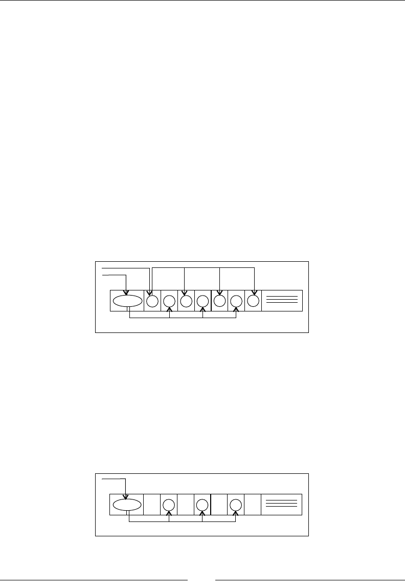
Chapter 3
[ 75 ]
A best t or rst t can then be performed on the free list in order to nd a heap
address where enough free space is available for the new object. There are many
different algorithms for this, with different advantages.
Fragmentation and compaction
It is not enough to just keep track of free space in a useful manner. Fragmentation is
also an issue for the memory manager. When dead objects are garbage collected all
over the heap, we end up with a lot of holes from where objects have been removed.
Fragmentation is a serious scalability issue for garbage collection, as we can have a
very large amount of free space on the heap that, even though it is free, is virtually
unusable. This is because there is not enough contiguous space for the allocation of
new objects—no hole is big enough. Typically, this will lead to the runtime system
triggering more and more GCs in order to attempt clean up of the mess, but still isn't
able to reclaim enough contiguous space for new objects. Untreated fragmentation is
a classic performance death spiral.
The following gure shows a heap occupied by several objects:
AE F CGDB H
0 1 2 345678
The heap section shown is completely occupied by live objects. The object A is two
heap units in size and the other objects are just one heap unit in size. The application
has two objects reachable from a program point where garbage collection takes place,
A that references the object graph ABCD and E that references the object graph
EFGH, where ABCD and EFGH are mutually independent.
If E is assigned null and thus removed from the scope of the program, E and its
children can be garbage collected. The resulting heap after garbage collection will
look like in the following gure:
ACDB
0 1 2 345678
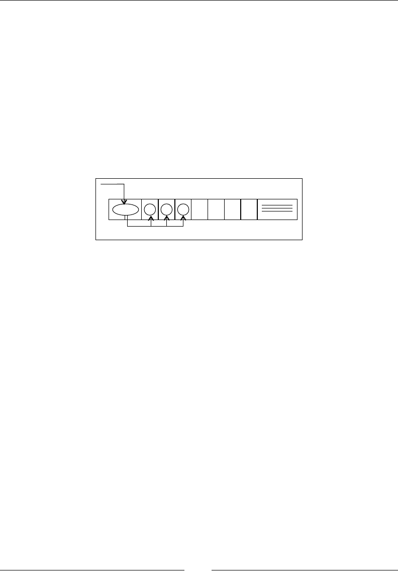
Adaptive Memory Management
[ 76 ]
There is now free space on the heap, but even though there is a total amount of four
free heap units, there is no place on the heap with more than one free unit in sequence.
If the memory manager now attempts to nd space for a new object that is, say, two
heap units in size, an OutOfMemoryError will be thrown, even though there are four
free units on the heap. This illustrates why fragmentation is problematic.
It follows that a memory management system needs some logic for moving objects
around on the heap, in order to create larger contiguous free regions. This process is
called compaction, and involves a separate GC stage where the heap is defragmented
by moving live objects so that they are next to one another on the heap.
The following gure shows the heap from our example after compaction has
taken place:
AC DB
0 1 2 345678
Now, we have four consecutive free heap units, and so we are able to allocate larger
objects than before with the same amount of free space.
Compaction is difcult to do without stopping the world, but we will discuss some
ways of making it more efcient later in this chapter (and to some extent in Chapter 5
and 13).
By looking at the object reference graph and by gambling that objects referencing
each other are likely to be accessed in sequence, the compaction algorithm may
move these objects so that they are next to one another on the heap. This is benecial
for the cache, and hopefully, the object lifetimes are similar so that larger free heap
holes are created upon reclamation.
Intrinsic properties of different garbage collection algorithms also prevent some
degree of fragmentation (generational GCs) or allow for automatic compaction
(stop and copy). These are discussed later in this chapter.
Garbage collection algorithms
All techniques for automatic memory management boil down to keeping
track of which objects are being used by the running program, in other words,
which objects are referenced by other objects that are also in use. Objects that
are no longer in use may be garbage collected. We will use the terms live and
in use interchangeably.

Chapter 3
[ 77 ]
It is hard to exactly place garbage collection techniques in different categories. With
the risk of drawing re from the academic community, we will use the term "tracing
garbage collection" for everything except reference counting. Tracing garbage
collection means building a graph of live objects at a collection event and
discarding unreachable ones. The only other kind of technique that we will
cover is reference counting.
Reference counting
Reference counting is a memory management technique where the runtime keeps
track of how many live objects point to a particular object at a given time.
When the reference count for an object decreases to zero, the object has no referrers
left, and trivially, the object is available for garbage collection. This approach was
rst used in Lisp implementations and is fairly efcient, except for the obvious aw
that cyclic constructs can never be garbage collected. If two objects refer to each other
but have no outside referrers, their reference counts are obviously non-zero but they
are still unreachable by the GC, consequently turning into a memory leak.
The main advantage of reference counting, aside from its obvious simplicity, is that
any unreferenced object may be reclaimed immediately when its reference count
drops to zero.
However, keeping the reference counts up to date can be expensive, especially in a
parallel environment where synchronization is required. There are no commercial
Java implementations today where reference counting is a main garbage collection
technique in the JVM, but it might well be used by subsystems and for simple
protocols in the application layer.
Tracing techniques
The concept of a tracing garbage collector is very simple. Start by marking all objects
currently seen by the running program as live. Then recursively mark all objects
reachable from those objects live as well.
Naturally, the variations to this theme are endless.
From now on, we will use the term root set to mean the initial input set for this kind
of search algorithm, that is the set of live objects from which the trace will start.
Typically, the root set includes all Java objects on local frames in whatever methods
the program is executing when it is halted for GC. This includes everything we can
obtain from the user stack and registers in the thread contexts of the halted program.
The root set also contains global data, such as static elds. Or even simpler—the root
set contains all objects that are available without having to trace any references.
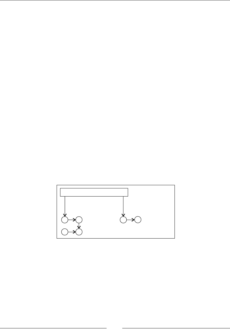
Adaptive Memory Management
[ 78 ]
We will discuss how to identify the root sets in more detail later in this chapter.
Mark and sweep
The mark and sweep algorithm is the basis of all the garbage collectors in all
commercial JVMs today. Mark and sweep can be done with or without copying
or moving objects (see the section on Generational garbage collection and the section
on Compaction for details). However, the real challenge is turning it into an efcient
and highly scalable algorithm for memory management. The following pseudocode
describes a naive mark and sweep algorithm:
Mark:
Add each object in the root set to a queue
For each object X in the queue
Mark X reachable
Add all objects referenced from X to the queue
Sweep:
For each object X on the heap
If the X not marked, garbage collect it
As can be inferred from the previous algorithm and the explanation of tracing
techniques, the computational complexity of mark and sweep is both a function of
the amount of live data on the heap (for mark) and the actual heap size (for sweep).
The following gure shows a heap before the mark phase:
A B CD
E F
root set
before mark
First, the live object graph needs to be traversed for marking. Then the entire heap
needs to be traversed to identify unmarked objects. This is not necessarily optimal
and there are several ways that have been addressed in research over the years to
make faster and more parallelizable variants.
In the following gure, the mark phase is done. All objects that are reachable from
the root set have been marked. Only E is not reachable from the root set.
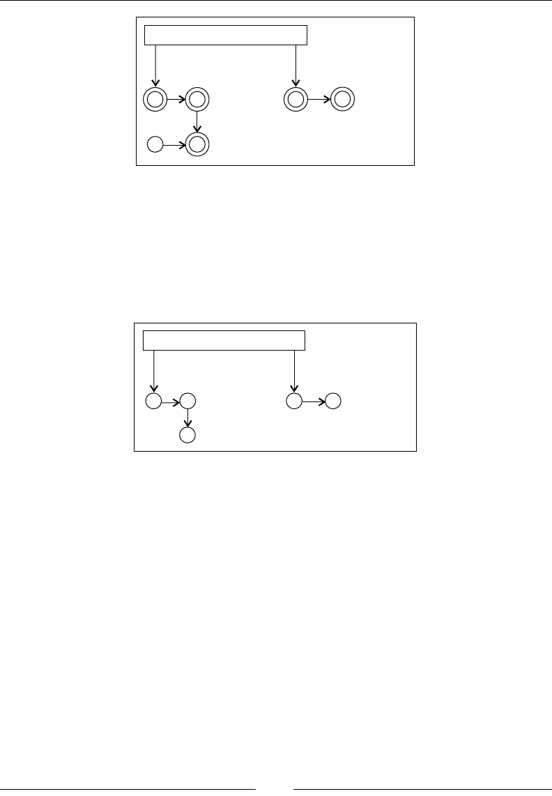
Chapter 3
[ 79 ]
A B CD
E F
root set
after mark
The simplest version of mark and sweep assumes that the object graph doesn't change
during the mark phase. This means that all code execution that may modify the object
graph through, for example, eld reassignments, must be halted when the mark takes
place. This is never good enough for modern applications with large data sets.
The following gure shows the heap after the sweep phase has taken place and
E has been garbage collected:
A B CD
F
root set
after sweep
In naive mark and sweep implementations, a mark bit is typically associated with
each reachable object. The mark bit keeps track of if the object has been marked or
not. Objects are typically allocated so that they are aligned on even addresses in
memory. Thus, the lowest bit in an object pointer is always zero. This is one example
of a good place to keep the mark bit.
A variant of mark and sweep that parallelizes better is tri-coloring mark and
sweep. Basically, instead of using just one binary mark bit per object, a color, or
ternary value is used. The color associated with each object in the object graph is
conventionally referred to as white, grey, or black. White objects are considered
dead and should be garbage collected. Black objects are guaranteed to have no
references to white objects. Initially, there are no black objects—the marking
algorithm needs to nd them. No black object is ever allowed to reference a white
object. Grey objects are live, but with the status of their children unknown. Initially,
the root set is colored grey to make the algorithm explore the entire reachable object
graph. All other objects start out as white.

Adaptive Memory Management
[ 80 ]
The tri-color algorithm is fairly simple:
Mark:
All objects are White by default.
Color all objects in the root set Grey.
While there exist Grey objects
For all Grey Objects, X
For all White objects (sucessors) Y, that X references
Color Y Grey.
If all edges from X lead to another Grey object,
Color X black.
Sweep:
Garbage collect all White objects
The main idea here is that as long as the invariant that no black nodes ever point
to white nodes is maintained, the garbage collector can continue marking even
while changes to the object graph take place. These changes may be caused by, for
example, allocations and eld assignments in the executing program. Typically, the
marking is "outsourced" so that many parts of the memory manager help maintain
the coloring while the program is running. For example, objects may be marked
immediately upon allocation.
There are several variants to parallelizing mark and sweep beyond the scope of this
chapter. This section merely serves as an example of how mark and sweep can be
improved for incremental and parallel garbage collection.
Stop and copy
Stop and copy can be seen as a special case of tracing GC, and is intelligent in its
way, but is impractical for large heap sizes in real applications.
Stop and copy garbage collection requires partitioning the heap into two regions of
equal size. Only one region is in use at a time, which is quite wasteful and ensures
that only a maximum of half the available heap memory can be utilized for live data.
In its simplest form, stop and copy garbage collection goes through all live objects
in one of the heap regions, starting at the root set, following the root set pointers to
other objects and so on. The marked live objects are moved to the other heap region.
After garbage collection, the heap regions are switched so that the other half of the
heap becomes the active region before the next collection cycle.
This approach is advantageous as fragmentation can't become an issue. Surviving
objects are laid out rst-t in the new heap section on each garbage collection. As
objects are laid out in their referencing order as the object graph is explored, stop and
copy can signicantly decrease cache overhead for the running program by keeping
objects and the objects they reference close on the heap.
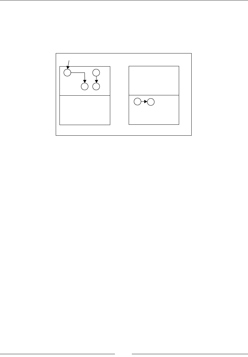
Chapter 3
[ 81 ]
The obvious disadvantage of this approach is of course that all live data must be
copied each time a garbage collection is performed, introducing a serious overhead
in GC time as a function of the amount of live data, not to mention the very serious
cache performance issues for the GC itself. More importantly, only using half of the
heap at a time is an unforgivable waste of memory.
A B
C D
root set
AC
FREE
before after
R 1 R 1
R 2 R 2
FREE
This gure illustrates a stop and copy cycle. The heap is divided into two regions. The
root set contains only the object A at the start of garbage collection. A references C and
no other objects. The mark phase of the GC cycle determines that A and C are the only
live objects, and they are moved to the new region, R2. B and D are garbage collected.
A and C were not adjacent in memory in R1, but will be automatically adjacent in R2
as objects are laid out rst-come-rst-serve from tracing the object graph.
Stopping the world
Stopping the world, that is halting all executing Java threads for garbage collection, is
the main Achilles' heel of automatic memory management. Even though an algorithm
such as mark and sweep may run mostly in parallel, it is still a complicated problem
that references may change during actual garbage collections. If the Java program is
allowed to run, executing arbitrary eld assignments and move instructions at the
same time as the garbage collector tries to clean up the heap, mutual bookkeeping
between the program and the garbage collector is needed. Ultimately this means
synchronization, and synchronization, even in a smart algorithm, means stopping
the world. Stopping the world for short periods of time is necessary for all languages
where garbage collection and heap management is involved. This is one of the main
sources of latencies and non-determinism in a runtime.

Adaptive Memory Management
[ 82 ]
Garbage collection may move objects around on the heap, for example by compaction.
If a register in a thread context of a running program contains a pointer to an object
and that object is moved to another location in memory, it is easy to realize that the
program will break if it is just allowed to continue running without the GC updating
the register contents in the thread context. This is done by synchronously modifying
the thread context of the executing thread. The same applies to any object reference
that points out an object on the heap whose address has changed as an effect of the
garbage collection.
The easy way out would be to stop the world for a long period of time and just
brute force garbage collect as much as possible with as many threads as possible.
Before resuming the threads, all registers are updated. Normally, however, this
isn't possible because low latencies are usually the main requirement for a modern
server-side application. It doesn't do to halt execution for hundreds of milliseconds
at a time. Thus, for low latency environments, which seek to minimize application
response time, the garbage collector needs to do as much work as it can while the
Java program is still running, and still handle these possible pointer reassignments.
This is the difcult part. However, there is no getting around stopping the world
completely at some point, unless the application has very special behavior. The real
challenge is keeping these pauses as short as possible.
Conservative versus exact collectors
As we have discussed earlier, the virtual machine needs to provide some information
to the memory system so that it can identify which positions on a local stack frame
contain objects. This is needed to build the root set of objects that will form the rst
nodes of the live object graph. Every thread that is executing Java code handles
objects, and if the thread is stopped, we need to know where in its context they are.
It is easy to identify objects in elds of other objects, as all object layouts are known
to the garbage collector. If all instances of object X contain a eld of type Y, the
pointer to the eld contents of Y for all X instances is always at the same offset
from the start of an X instance. An object is little more than a C struct to the JVM.
However, the GC doesn't automatically know where objects are on a stack frame.

Chapter 3
[ 83 ]
Finding the method in which a particular thread has stopped is simple. We can just use
a lookup table or search tree to nd out in which Java method an instruction pointer
belongs. Objects occur in the scope of this method, either present from the beginning
of its execution as in-parameters, or as the result of eld loads or function calls in the
method. Move instructions may also copy objects from one register to another. Given
an arbitrary point in the code of the method, the point where the execution has been
halted, there is no way to backtrack the context where the thread is stopped to the
context in which these objects were created. We have no way of knowing which code
was just executed to get us to this particular address. However, the GC must, given a
stack frame, know where objects are stored to form a correct root set.
Trivially, one might tell the compiler to only use certain registers and positions
on the local stack frame for objects and certain other registers and positions for
non-objects, such as integers. For example on x86, one might force the code
generator to place objects only in the registers esi and edi and integers only in all
other registers. One might spill objects only to stack positions whose offsets are even
multiples of the pointer size ([esp+0*4], [esp+2*4] and so on) and integers only
to stack positions that are odd multiples ([esp+1*4], [esp+3*4] and so on). This
makes it simple for the GC, as our "objects only" locations can only contain a valid
object or null. Other locations need not be processed by the GC at all, as they never
contain objects. However, limiting the number of registers for generic use by the
compiler requires the register allocator to produce more spills. This is completely
impractical for performance reasons, especially on architectures like x86, where the
amount of available general purpose registers is limited.
One way to get around this is to use a conservative garbage collector, treating
every location that looks like an object pointer as an object pointer. Trivially, values
like 17 and 4711 can be disregarded and are known to be integers, but values that
look like addresses must be examined and checked against the heap. This produces
overhead, and is necessary if we want to add automatic memory management to
some languages, such as C, which is weakly typed. Conservative garbage collectors
also have problems with unintentional object retention to varying degrees and with
moving objects in memory.
In Java, however, we can get by with an exact garbage collector that knows precisely
where object pointers are and where they are not. We only need a way to get this
information to the garbage collector. Typically, this is done by generating meta info
along with code for a Java method.

Adaptive Memory Management
[ 84 ]
Livemaps
In JRockit, a piece of meta info that consists of a collection of registers and stack
positions containing objects at a given program point is called a livemap. An
additional bit of info per object pointer tells us whether it is an internal pointer
or the actual start of an object. Internal pointers refer to some piece of information
inside an object, thus pointing to the heap, but not to an object header. Internal
pointers need to be tracked as they must be updated along with their base object
if it is moved in memory, but they cannot be treated as base objects themselves.
A typical example of the use of internal pointers is when iterating through an array. In
Java no internal pointers to objects may exist, but compiled code may well run faster if
a sequence like:
for (int i = 0; i < array.length; i++) {
sum += array[i];
}
were to be compiled to native code equivalent to:
for (int ptr = array.getData();
ptr < sizeof(int) * array.length;
ptr += sizeof(int)) {
sum += *ptr;
}
In this case, the GC has to know that ptr is an internal pointer to the array so that
it can be updated as well if array is moved to another position in memory. The
code potentially runs faster since the pointer to the array element data need not be
computed at every iteration in the loop.
So, it is clear that object pointers and internal object pointers need to be stored in
meta info, livemaps, for the garbage collector. To illustrate how this information
looks to the memory system, the following is a small example of compiled Java code
in JRockit annotated with livemap info. The code example is a simple method that
computes the sum of the elements of an array.
public static Integer sum(Integer array[]) {
Integer sum = 0;
for (int i = 0; i < array.length; i++) {
sum += array[i];
}
return sum;
}

Chapter 3
[ 85 ]
Letting JRockit generate the method on a 64-bit x86 platform produces the following
assembly code:
[SumArray.sum([Ljava/lang/Integer;)Ljava/lang/Integer;
7a8c90: push rbx
7a8c91: push rbp
7a8c92: sub rsp,8
7a8c96: mov rbx,rsi
*----- [rsib, rbxb]
7a8c99: test eax,[0x7fffe000]
*--B-- [rsib, rbxb]
7a8ca0: mov ebp,[rsi+8]
7a8ca3: test ebp,ebp
7a8ca5: jg 7a8cb1
*----- [nothing live]
7a8ca7: xor rax,rax
*----- [nothing live]
7a8caa: call Integer.valueOf(I)
*C---- [rsib]
7a8caf: jmp 0x7a8cf7
*--B-- [rsib, rbxb]
7a8cb1: mov r9d,[rsi+16]
*----- [r9b, rbxb]
7a8cb5: mov eax,[r9+8]
*----- [rbxb]
7a8cb9: call Integer.valueOf(I)
*C---- [rsib, rbxb]
7a8cbe: mov r9d,1
7a8cc4: cmp rbp,1
7a8cc7: jle 0x7a8cf7
*----- [rsib, rbxb]
7a8cc9: mov [rsp+0],rbx
7a8ccd: mov ebx,r9d
*----- [rsib, [rsp+0]b]
7a8cd0: mov r9d,[rsi+8]
*--B-- [[rsp+0]b]
7a8cd4: test eax,[0x7fffe000]
7a8cdb: mov r11,[rsp+0]
*----- [r11b, [rsp+0]b]
7a8cdf: mov ecx,[r11+4*rbx+16]
*--B-- [rcxb, [rsp+0]b]
7a8ce4: add r9d,[rcx+8]
7a8ce8: mov eax,r9d
*----- [[rsp+0]b]
7a8ceb: call Integer.valueOf(I)
*C-B-- [rsib, [rsp+0]b]
7a8cf0: add ebx,1
7a8cf3: cmp ebx,ebp
7a8cf5: jl 7a8cd0
*--B-- [rsib]
7a8cf7: pop rcx
7a8cf8: pop rbp
7a8cf9: pop rbx
7a8cfa: ret
Though it is not important to understand what the code generator has done here
in detail, the main idea is that several program points in the assembly code are
annotated with liveness information. In this case, the optimization level is not
sufciently high to generate the inner pointer pattern described earlier. Also, the
calls to Integer.valueOf have not been inlined.
The livemap information under annotated operations tells the garbage collector
which registers and stack positions contain objects at the given program point.
Notice, for example, that the calls to Integer.valueOf, by calling convention
always return a new integer object in rsi (the b after rsi means "base pointer"
as opposed to "internal pointer").
Adaptive Memory Management
[ 86 ]
The livemaps also tell us that rsi and rbx contain objects after the frame entry at the
beginning of the method. This follows from the mov rbx, rsi at address 7a8c96,
which is a register allocator artifact that shufes the in-parameter from register rsi to
register rbx.
As rbx, in the JRockit calling convention is callee save (not destroyed
over calls), the compiler chooses, for efciency reasons, to keep the object
alive in a register over the calls to Integer.valueOf. This way, the
register allocator avoids doing a spill.
So, where can the garbage collector stop the world? Intuitively, it is too expensive
to tag every single native instruction, each being a potential thread suspension point,
with liveness information. As can be seen from the previous example, this is neither
the case.
In JRockit, only certain instructions are tagged with livemaps, for example loop
headers or headers of basic blocks with multiple entries, where it isn't possible to
know which way control ow took to get there. Another example of instructions
annotated with livemaps are call instructions. This is because liveness information
must, for execution speed, be available immediately when computing a stack trace.
Recall from Chapter 2 that JRockit performs tasks like back patching calls. This
means that the JVM must be equipped with a mechanism to understand and
decompile native code. Originally, this mechanism was extended to make it
possible to also emulate all native instructions from an address, given an operating
system thread context as a starting point. If a livemap wasn't available at a certain
instruction pointer in the context of a stopped thread, JRockit simply emulated the
code, instruction by instruction, from that position until a livemap was reached.
This is called rollforwarding.
Rollforwarding was abandoned with JRockit R28. JRockit now uses
a more traditional safepoint-based approach.
The advantages to this approach were that threads could be stopped anywhere.
This was implemented using the signaling mechanisms of the underlying
operating system. No extra instructions in the generated code were required.
The disadvantages were that emulation still took time and that large emulation
frameworks needed to be in place, one for each supported hardware architecture. This
was extremely difcult to test, as the set of inputs was virtually innite, and emulation

Chapter 3
[ 87 ]
itself was very error prone. In addition, porting to a new hardware architecture became
very expensive, requiring the implementation of a new complete emulation framework
for that particular piece of silicon. Bugs in the emulators were usually subtle and
generated intermittent and hard-to-nd problems.
Throughout the years, there were also several problems with the signaling approach to
stopping threads. It turns out that certain operating systems, especially Linux, seem to
be poorly tested when it comes to applications that use a lot of signals. There were also
issues with third-party native libraries that did not respect signal conventions, causing
signal collisions. The external dependency on signals proved too error-prone to be
completely reliable.
Newer versions of JRockit use a more traditional safepoint approach instead.
Throughout the code, safepoint instructions that dereference a certain guard page
in memory are inserted. At these instruction pointers, a complete livemap is always
guaranteed to be in place. Whenever a Java thread is to be stopped, the runtime
protects the guard page from access. This makes the safepoint instruction trigger a
fault when executed. Variants of this technique are, as far as we know, employed in
all commercial JVMs today. Loop headers are a typical example of program points
where it makes sense to place safepoint instructions. We cannot allow a situation
where the program will continue executing without ever trying to dereference a
guard page. Thus, constructs like potentially innite loops cannot be left without
safepoint instructions.
The disadvantage here is that explicit code for dereferencing the guard page has to
be inserted in the generated code, contributing to some execution overhead. But the
advantages easily pay for this small inconvenience.
By now we have covered a lot of material on garbage collection, but only the basic
concepts and algorithms. We've also discussed the surprisingly difcult problem of
generating root sets for our garbage collectors. We will now attempt to cross the bridge
to the "real world" and move on to discuss how garbage collection can be optimized
and made more scalable.
Generational garbage collection
In object-oriented languages, a very important observation is that most objects are
temporary or short-lived.
For temporary objects, escape analysis at compile time might be able to stop them from
being allocated on the heap altogether, but in an imperfect world this is not always
possible. Especially in a language like Java.

Adaptive Memory Management
[ 88 ]
However, performance improvements for handling short-lived objects on the heap can
be had if the heap is split into two or more parts called generations. New objects are
allocated in the "young" generations of the heap, that typically are orders of magnitude
smaller than the "old" generation, the main part of the heap. Garbage collection is then
split into young and old collections, a young collection merely sweeping the young
spaces of the heap, removing dead objects and promoting surviving objects by moving
them to an older generation.
Collecting a smaller young space is orders of magnitude faster than collecting the
larger old space. Even though young collections need to happen far more frequently,
this is more efcient because many objects die young and never need to be promoted.
Ideally, total throughput is increased and some potential fragmentation is removed.
JRockit refers to the young generations as nurseries.
Multi generation nurseries
While generational GCs typically default to using just one nursery, sometimes it can
be a good idea to keep several small nursery partitions in the heap and gradually age
young objects, moving them from the "younger" nurseries to the "older" ones before
nally promoting them to the "old" part of heap. This stands in contrast with the
normal case that usually involves just one nursery and one old space.
Multi generation nurseries may be more useful in situations where heavy object
allocation takes place.
We assume that the most freshly allocated objects will live for a very short period of
time. If they live just a bit longer, typically if they survive a rst nursery collection, the
standard behavior of a single generation nursery collector, would cause these objects to
be promoted to the old space. There, they will contribute more to fragmentation when
they are garbage collected. So it might make sense to have several young generations
on the heap, with different age spans for young objects in different nurseries, to try to
keep the heap holes away from the old space where they do the most damage.
Of course the benets of a multi-generational nursery must be balanced against the
overhead of copying objects multiple times.
Write barriers
In generational GC, objects may reference other objects located in different generations
of the heap. For example, objects in the old space may point to objects in the young
spaces and vice versa. If we had to handle updates to all references from the old space
to the young space on GC by traversing the entire old space, no performance would
be gained from the generational approach. As the whole point of generational garbage
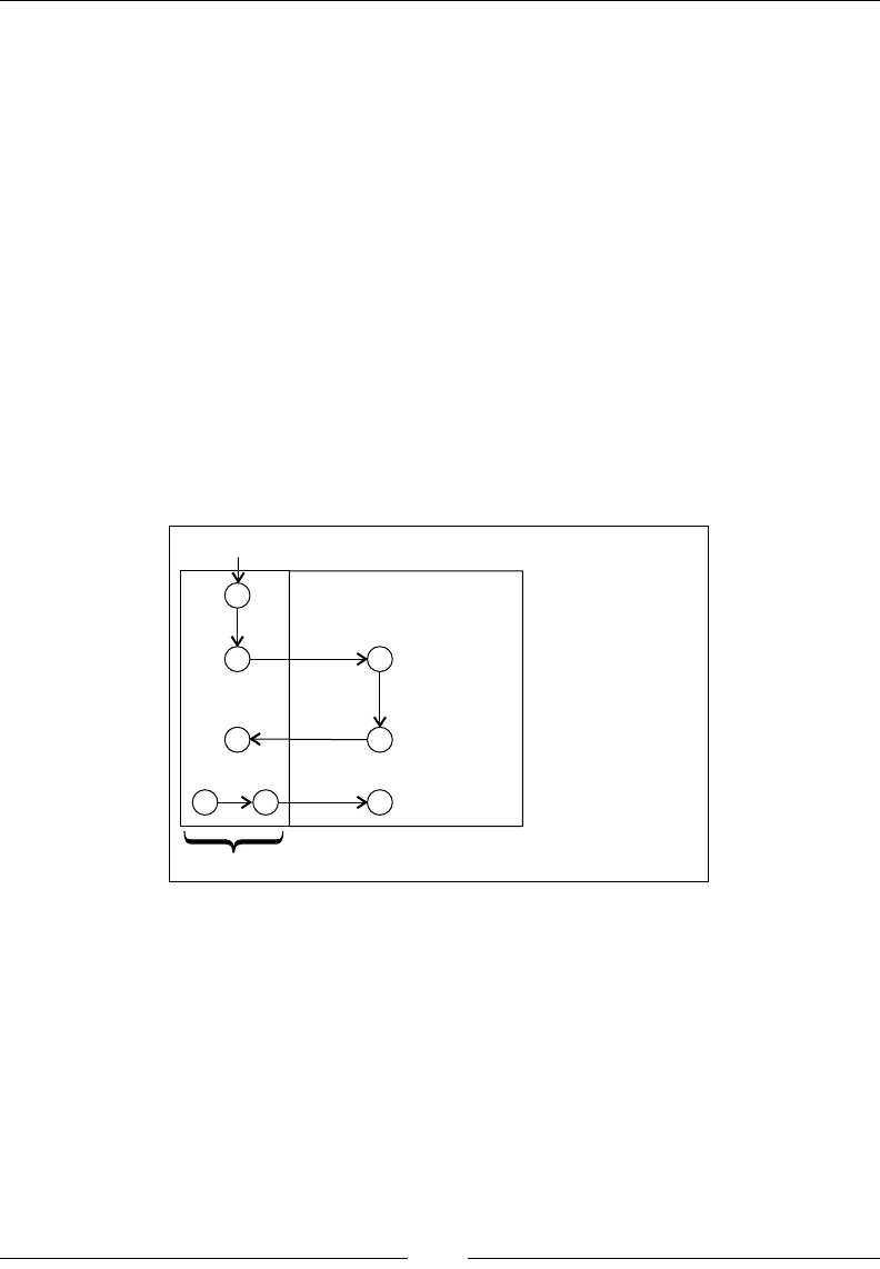
Chapter 3
[ 89 ]
collection is only to have to go over a small heap segment, further assistance from the
code generator is required.
In generational GC, most JVMs use a mechanism called write barriers to keep track
of which parts of the heap need to be traversed. Every time an object A starts to
reference another object B, by means of B being placed in one of A's elds or arrays,
write barriers are needed. Write barriers consist of a small amount of helper code
that needs to be executed after each eld or array store in the executing Java code.
The traditional approach to implementing write barriers is to divide the heap into a
number of small consecutive sections (typically about 512 bytes each) that are called
cards. The address space of the heap is thus mapped to a more coarse grained card
table. Whenever the Java program writes to a eld in an object, the card on the heap
where the object resides is "dirtied" by having the write barrier code set a dirty bit.
Now, the traversion time problem for references from the old generation to the
nursery is shortened. When doing a nursery collection, the GC only has to check
the portions of the old space represented by dirty cards.
A
B C
root set
E
F
HG I
BEFORE NURSERY GC
nursery
Consider the previous gure. The runtime is about to do a nursery collection. If the
root set contains object A only, at the start of the collection, we would easily detect
A and B as live by pointer tracing A to B. The pointer trace from B to C would be
ignored, as C is in the old space. However, for the GC to work, we must add E in the
old space to the root set, as it references an object in the nursery. With write barriers,
we don't have to go over the entire old space to nd E, but we just have to check the
areas of the old space that correspond to dirty cards. In this example, the card for E
was dirtied by the write barrier code after a previous assignment of F to a eld in E.
Thus, we can add F to the set of objects to be traced by the nursery GC.
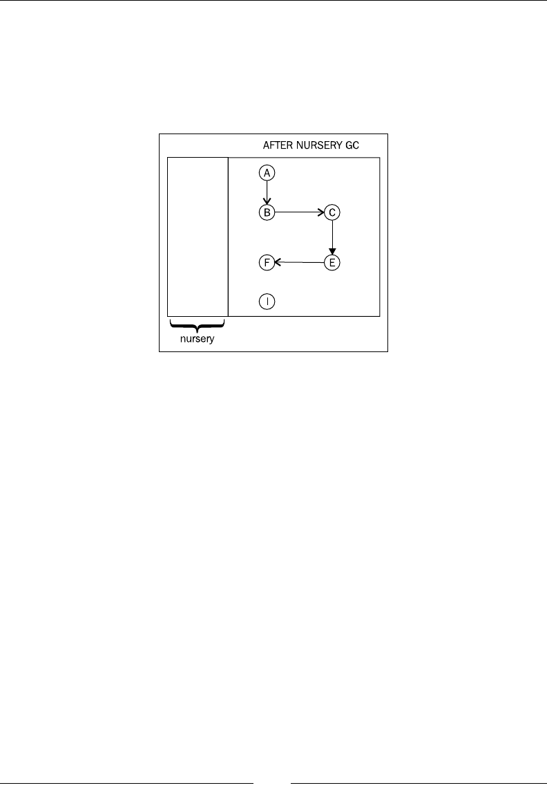
Adaptive Memory Management
[ 90 ]
A and B are root reachable and will be promoted to the old space after the nursery
collection. G and H are not, and will be garbage collected. E and F were root
reachable, and thus F will be promoted. While I is dead, it is part of the old space
and won't be handled until the next old collection. The following gure shows the
heap after the completed nursery collection and promotion. The objects in the old
space are untouched, as this was a nursery collection.
Throughput versus low latency
Recollect from Chapter 2 that the main factor that the JVM wants to minimize is the
total runtime. In code generation, the total runtime is dened by the time to compile
the code plus the time to execute the code. As we saw, we can only minimize one
factor at the cost of another.
In memory management, the equation is simpler. All time spent in GC is of course
detrimental to runtime. Minimizing the time spent in GC might seem the proper
and only solution to lower the total runtime.
However, recollect that garbage collection requires stopping the world, halting
all program execution, at some stage. Performing GC and executing Java code
concurrently requires a lot more bookkeeping and thus, the total time spent in GC
will be longer. If we only care about throughput, stopping the world isn't an issue
—just halt everything and use all CPUs to garbage collect, one part of the heap per
CPU. However, to most applications, latency is the main problem, and latency is
caused by not spending every available cycle executing Java code.
Thus, the tradeoff in memory management is between maximizing throughput and
maintaining low latencies. In an imperfect world, we can't expect to have both.

Chapter 3
[ 91 ]
Optimizing for throughput
In some cases, latencies do not matter at all in an application, for example, in ofine
jobs that do large amounts of object crunching. A batch job running overnight may
not be as vulnerable to response times as a client/server application.
If pause times up to several seconds are permissible, throughput can be maximized
to a degree that is not possible if low latency is critical.
There are many variants of high throughput GC. The simplest approach is to
stop the world and then garbage collect the heap with as many threads as possible,
at least as many as the number of cores on the platform, each handling a separate
part of the heap. Naturally, some synchronization between GC threads is still
required for references that point to other heap parts. JRockit refers to this as
parallel garbage collection.
We can still achieve levels of throughput not attainable in a low latency environment
with other, less intrusive variants of this parallel approach. One example would be
by using generations in the heap.
Optimizing for low latency
Optimizing for low latencies is basically a matter of avoiding stopping the world,
and therefore also Java execution, by any means necessary. But naturally, if the
garbage collector gets too little total CPU time and it can't keep up with the allocation
frequency, the heap will ll up and an OutOfMemoryError will be thrown by the JVM.
We need a GC that performs large parts of its work when the program is running.
JRockit refers to this kind of GC as concurrent garbage collection, using a term from
one of the rst scientic papers describing this technique, by Boehm and others. Later,
the term mostly concurrent was introduced for improved versions of this algorithm.
There is a slight degree of confusion in the terminology here. The parallel,
throughput oriented GC, described in the previous section, does not run
at the same time as the Java program executes. It is known as "parallel"
because it uses as many threads as possible in parallel to garbage collect
the heap. Garbage collection that runs at the same time as the Java program
executes, as described in this section, is known as concurrent GC.
The concurrent garbage collector is also parallel, in the traditional
meaning of the word, because it uses several worker threads. However,
the terms concurrent and parallel used in the manner of this book are not
just specic to JRockit. This is often the standard way of referring to these
respective GC techniques in academic research and other commercial
implementations.
Adaptive Memory Management
[ 92 ]
Many stages of a mark and sweep garbage collection algorithm can be made to run
concurrently with the executing Java program. Marking is the most critical of the
stages, as it usually takes up around 90 percent of the total garbage collection time.
Fortunately, marking is very parallelizable and large parts of a mark phase can also be
run concurrently with executing Java code. Sweeping and compaction, however, tend
to be more troublesome, even though it is fairly simple to compact parts of the heap
while others are swept, thus achieving better throughput.
The main idea behind mostly concurrent garbage collection is to spend as much
time running garbage collection as possible, while the Java program still executes.
Throughout the GC cycle, several shorter stop the world phases are used, where some
merely seek to synchronize the GC with the object graph, as the running Java program
continuously makes changes to it. This is trivially not an issue if no Java execution is
allowed to take place during GC. As far as we know, all commercial JVMs use variants
of the mostly concurrent approach for low latency garbage collection.
The section on Near-real-time garbage collection, later in this chapter, goes into further
details on how to achieve both performance and low latencies. And specically, how
JRockit does it.
Garbage collection in JRockit
The backbone of the GC algorithm used in JRockit is based on the tri-coloring
mark and sweep algorithm described earlier in this chapter. However, several
optimizations and improvements have been made to make it more parallel, both
to enable it to run at the same time as the Java program is executing and to use an
optimal number of threads. For nursery collections, heavily modied variants of
stop and copy are used.
Garbage collection in JRockit can work with or without generations, depending
on what we are optimizing for. Garbage collection strategies and adaptive
implementation thereof is covered later in this chapter.
The JRockit garbage collector can chose to tag any object on the
heap as pinned for a shorter or longer period of time. This makes
concurrent garbage collection algorithms more exible. It can also
enable I/O performance in that things like buffers can be kept in
the same place on the heap for an entire I/O operation. This makes
memory-intensive operations signicantly faster. Pinned objects are a
relatively simple concept in a GC, but for some reason, JRockit seems
to be one of the few commercial JVMs that implements it.

Chapter 3
[ 93 ]
Old collections
The mark and sweep algorithm that is the fundament of all JRockit garbage
collectors, parallel or concurrent, uses two colors and not three, for its objects, but
still allows for efcient parallelization in the manner described in the section on Mark
and sweep earlier in this chapter. Objects belong to one of two sets. One set is used
to mark live objects. JRockit calls this set the grey bits, even though it is actually the
semantic equivalent of a mix of grey and black objects in traditional tri-coloring.
The distinction between grey and black objects is instead handled by putting grey
objects in thread local queues for each garbage collecting thread. This approach has
two advantages. First of all it allows parallel threads to work on thread local data
instead of competing for a synchronized common set. Furthermore, it is possible
to efciently use prefetching on the contents of the queues as their elements are
accessed both in FIFO order and close in time to one another. The general advantages
of prefetching in memory management will be discussed later in this chapter.
For concurrent collectors in JRockit, an additional set called the live bits is used. It
keeps track of all live objects in the system, including the newly created ones. This
makes it possible for JRockit to quickly nd objects that have been created during a
concurrent mark phase, that is one running at the same time as the Java application.
JRockit uses a card table not only for generational GCs, but also to avoid searching
the entire live object graph when a concurrent mark phase cleans up. This is because
JRockit needs to nd any new objects that may have been created by the running
program during that mark phase. Recollect that write barriers in the running code
continuously update the card table. The card table also has one card per region in the
live object graph. As described, a card can be dirty or clean and all cards where objects
have been newly created or have had their object references modied are marked as
dirty. At the end of a concurrent mark phase, JRockit only needs to look at the dirty
cards and scan the objects in the corresponding heap regions that have their live bit set.
This guarantees that all objects, freshly allocated and old ones, are found even after a
concurrent mark phase.
Nursery collections
For nursery collections, JRockit uses a variant of stop and copy. All threads are halted,
and all objects in the nursery are copied or promoted to the old space.
The copying is done hierarchically in breadth rst manner, which increases cache
locality (objects that reference each other should be stored close to each other
in memory for maximum cache efciency). The breadth-rst copy algorithm is
parallelizable in a way that automatically contributes to good load balancing.

Adaptive Memory Management
[ 94 ]
Only live objects are copied to the old space. Instead of having to scan the entire heap
to nd out what objects in the nursery are live, the young collection uses the live bits
and the card table that were mentioned in the previous section. As we start out with
an empty nursery and because all objects that have their references updated get the
corresponding card in the card table marked as dirty by write barrier code, all live
objects in the nursery can be found by merely scanning objects that have their live
bit set in a region corresponding to a dirty card.
Nursery collections in JRockit are always parallel but never concurrent. However, for
efciency reasons, young collections may occur at any time during a concurrent old
collection. This complicates matters, especially because both the young collection and
the old collection depend heavily on the same data structures.
However, it turns out that these data structures, the bit sets and the card table, can
be shared as long as an old collection is guaranteed to see all cards that have become
dirty during a concurrent phase. This is achieved by having an extra card table that
records all dirty cards from the original card table. JRockit calls this union of all card
table changes the modied union set. The nursery collection is free to process and
clear dirty cards as long as the modied union set is kept intact for the old collection.
So the young and old collector can operate at the same time without getting in the
way of each other.
JRockit also uses a concept called keep area. The keep area is a region in the nursery
where objects are not copied to old space during a young collection. By making sure
that the youngest objects are allocated in the keep area, JRockit can ensure that newly
created objects have an extra chance to become garbage collected before they are
considered long lived, and copied to old space. This is the rough, simpler, equivalent
to a multi-generational approach.
Permanent generations
One thing that sets JRockit apart from the HotSpot VM is the lack of a permanent
generation on the heap. In HotSpot, a heap part of predened size, the permanent
generation, is used to store metadata about, for example, class objects. Once the
data is in the permanent generation, the default behavior is that it remains there
forever (this might vary between garbage collection policies). This means that if
a large amount of classloading takes place, the permanent generation will ll up
and OutOfMemoryErrors will be thrown. We have seen customer cases, where
the problem with a permanent generation gets so bad that the JVM and the Java
application have to be restarted regularly.

Chapter 3
[ 95 ]
JRockit is different in that it stores metadata off the heap in native memory
instead. Code buffers for generated methods along with metadata pointed to by
ClassLoaders that are no longer used are also constantly garbage collected. The
problem of running out of memory for metadata in JRockit is not that different from
the same problem in HotSpot, except for the fact that it is native memory instead
of heap memory. There are, however, two signicant differences. Firstly, in JRockit,
cleaning up stale metadata is always enabled by default and secondly, there is no
xed size limit for the space used to store metadata. One of the larger problems with
HotSpot is probably that intuitively, it is very hard to pick a size for the permanent
generation. Is 128 MB enough? No? What about 256 MB? It is really very difcult to
know for any given application. JRockit, being completely dynamic in its metadata
allocation, need not consider size limits. It will, out of the maximum amount of
native memory, allocate as much space as it needs for its metadata at any given time.
Compaction
In JRockit, compaction is always single-threaded and non-concurrent. However,
for parallel collectors, compaction runs at the same time as the sweep phase. As
compaction is always done with a single thread, it is important that it is fast and that
the time spent doing compaction can be controlled. JRockit limits compaction time
by only compacting a part of the heap in each garbage collection. Most of the time,
heuristics are used for choosing where on the heap to compact, and how much. The
heuristics are also used to decide between different types of compactions—internal
compaction just within one heap partition or external compaction (also referred to
as evacuation) between different areas on the heap.
In order to make it more efcient to update all references to an object when it is
moved, JRockit lets the mark phase keep track of all references that point to objects
inside a heap region that is to be compacted. This information can also be used to
determine if it is possible to do any compaction at all or if certain popular objects
should be excluded from compaction as too many other objects reference them.
Speeding it up and making it scale
This section addresses what a modern runtime can do to speed up memory
management, going from impractical and "academic" algorithms to real
world performance.

Adaptive Memory Management
[ 96 ]
Thread local allocation
One technique, used in JRockit, that signicantly speeds up object allocation is the
concept of thread local allocation. It is normally much cheaper to allocate an object
locally in a buffer in the running Java thread than going through the synchronized
process of placing it directly on the heap. A naive garbage collector doing direct heap
allocations would need a global heap lock for each allocation. This would quickly be
the site for a nightmarish amount of contention. On the other hand, if each Java thread
keeps a thread local object buffer, most object allocations may be implemented simply
as the addition of a pointer, one assembly instruction on most hardware platforms. We
refer to these thread local buffers as Thread Local Areas (TLA). The TLAs naturally
have to processed by the garbage collector as well.
For cache and performance reasons, each TLA is typically between 16 and 128
kilobytes, but this can be modied from the command line. Whenever a thread local
buffer is full, everything in it is promoted to the heap. We can think of a thread local
buffer as a small thread local nursery.
Whenever a new operator in Java is compiled and the JIT set to a sufciently high level
of optimization, the allocation code turns into a construct that can be illustrated by the
following pseudocode:
Object allocateNewObject(Class objectClass) {
Thread current = getCurrentThread();
int objectSize = alignedSize(objectClass);
if (current.nextTLAOffset + objectSize > TLA_SIZE) {
current.promoteTLAToHeap(); //slow and synchronized
current.nextTLAOffset = 0;
}
Object ptr = current.TLAStart + current.nextTLAOffset;
current.nextTLAOffset += objectSize;
return ptr;
}
The pseudocode just seen presents a somewhat simplied view of the
world, in order to illustrate the point. Objects that are larger than a
certain threshold value or that are too big to t in any available TLA are
still allocated directly on the heap. As of JRockit R28, a measurement
used to better optimize TLA usage, called the TLA waste limit, has
been introduced. This is discussed to a greater extent in Chapter 5.
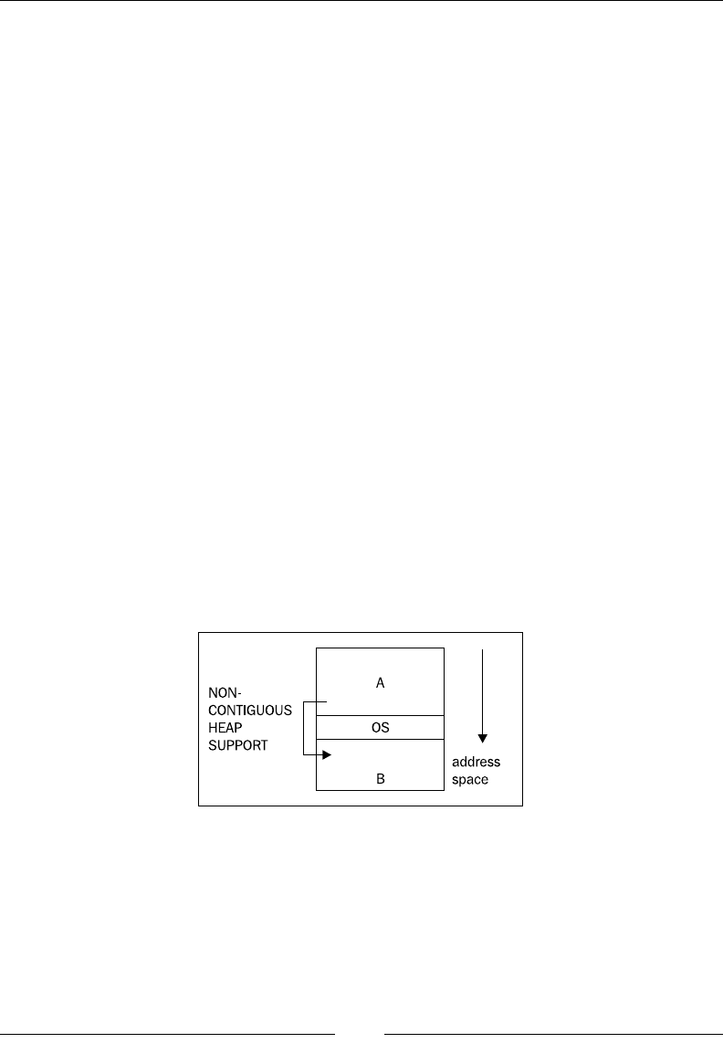
Chapter 3
[ 97 ]
In certain architectures where registers are plentiful, further performance gains can be
achieved by always keeping the nextTLAOffset, and possibly the pointer to the TLA
itself, in registers for the thread that is currently executing Java code. On x86 with its
limited register set, however, this is a luxury we can't afford.
Larger heaps
As the complexity of a well written GC is mostly a function of the size of the live
data set, and not the heap size, it is not too costly to support larger heaps for the
same amount of live data. This has the added benet of it being harder to run into
fragmentation issues and of course, implicitly, the possibility to store more live data.
32-Bits and the 4-GB Barrier
On a 32-bit system, a maximum 4 GB of memory can be addressed. This is the
theoretical maximum size of any heap, but of course there are other things that need
to be kept in memory as well, such as the operating system. Some operating systems,
for example Windows, are very picky about how they lay out kernel and libraries in
memory. On Windows, the kernel often lies almost in the middle of the address space,
making it difcult to fully utilize all available memory as one contiguous Java heap.
Most JVMs only support heaps that consist of contiguous chunks of memory, so this
can be a problem.
To our knowledge, JRockit is the only JVM that supports non-contiguous heaps and
is able to utilize the memory both above and below the operating system kernel and
any other external libraries for its heap space.

Adaptive Memory Management
[ 98 ]
In the previous gure, the OS resides roughly in the middle of the address space,
effectively limiting the maximum virtual address space for a process. The memory
areas A and B come before and after the operating system respectively. A is slightly
larger than B, so A corresponds to the largest heap that we can use without support
for non-contiguous heaps. A non-contiguous heap implementation would allow us
to use the combined memory in A and B for our heap at the price of a small bit of
extra bookkeeping overhead. This is implemented by basically pretending that the
OS area is a large pinned object in the middle of the address space.
While 32-bit architectures tend to grow less and less common with the 64-bit
revolution, there are still scenarios where they are used a lot. Currently, virtualized
environments seem to be such a place, and so it still makes sense to maximize
performance for 32-bit platforms, with the limited address space that entails.
The 64-bit world
On a 64-bit system, even when running a 32-bit JVM, the larger available virtual
address space can be tweaked so that we don't need to work around occupied
areas of the address space.
Most modern architectures are 64-bit, and the theoretical amount of data that ts
into a 64-bit address range, 16 exabytes, is staggeringly huge. Currently, it is not
affordable to populate that large an address space with physical memory.
There are both benets and disadvantages to using a 64-bit architecture for automatic
memory management, unlike with code generation, which tends to see only benets
(such as more registers, wider registers, and lager data bandwidth).
Pointers on a 64-bit machine are 8 bytes wide instead of 4 bytes. This consumes more
bandwidth and CPU cache space. Simplifying a bit, dereferencing a 32-bit pointer is
faster than dereferencing a 64-bit one, so a 64-bit 4.1 GB heap, although only slightly
larger than a 32-bit 4 GB one, may actually be a lot slower to use.
Compressed references
A fair compromise is the compressed reference optimization that JRockit was the
rst JVM to implement. If a JVM running on a 64-bit system uses less than 4 GB of
heap space, it obviously makes no sense to represent objects as 64-bit pointers. 32 bits
are enough, and consequently all object access will be a lot quicker.

Chapter 3
[ 99 ]
Native pointers outside the heap that are still part of the runtime environment must be
system wide, 64 bits, on a 64-bit system. The typical example is handles that represent
JNI references to Java objects. Transitions to and from native code through JNI may
occur in any Java program. For the sake of native code and to some extent the GC,
which needs to operate on native pointers internally, we need ways to go from the
transform domain of compressed references to that of ordinary system wide pointers.
We refer to these transforms as reference compression and reference decompression.
Following is the pseudocode for compression and decompression of a 4 GB heap
on a 64-bit platform. The virtual address of the heap base can be placed anywhere
in memory.
CompRef compress(Ref ref) {
return (uint32_t)ref; //truncate reference to 32-bits
}
Ref decompress(CompRef ref) {
return globalHeapBase | ref;
}
When compressed references are 32-bit, it sufces to use a logical or with the actual
(64-bit) heap base to decompress them into system-wide pointers. This operation has
the added benet that it can be applied an arbitrary number of times without further
changing the pointer. However, depending on the number of bits in a compressed
reference, this representation isn't always possible and strict state machines must
therefore be maintained so we know when a reference is compressed and when it isn't,
for example in stubs to and from native code or when the code refers to actual 64-bit
handles to objects.
Note that 4-GB heaps aren't the only application of compressed references. For
example, consider a 64-GB heap, where instead of using all 64 bits to represent an
object, we can use 4 + 32 bits, where four of the bits are used to point out which
of sixteen possible 4-GB heap sections an object resides in. Note that this requires
four free bits in the object, which in turn requires that allocated objects are aligned
on 16-byte boundaries. This may waste some heap space, but can still be a win
performance-wise.
CompRef compress(Ref ref) {
return (uint32_t)(ref >> log2(objectAlignment));
}
Ref decompress(CompRef ref) {
return globalHeapBase | (ref << log2(objectAlignment));
}
Adaptive Memory Management
[ 100 ]
The method can be made even simpler, if we keep the 16-byte object alignment and
make sure that the virtual address space starts at address 0 and ends at address "64
GB". Then a reference may be decompressed by just shifting it four bits left, and
compressed by shifting it four bits right, not needing to involve a global heap base.
This is how JRockit does it, thereby maintaining 32-bit wide compressed references
for the general case. JRockit, for convenience, still wants address 0 to be used for
null pointers, so the lowest 4 GB of the virtual space is not used for anything else,
effectively reducing the 64 GB of heap to 60 GB, but this is of little importance for
performance. If the difference between a 64-GB heap and a 60-GB heap matters
to you, you are in trouble anyway.
This method is generic as it works for all heap sizes larger than or equal to 4 GB.
The generic approach, however, has a new drawback. The attractive property that
decompression can be applied an innite number of times, to both uncompressed and
compressed references, disappears.
Naturally, 64 GB isn't a theoretical limit but just an example. It was mentioned
because compressed references on 64-GB heaps have proven benecial compared
to full 64-bit pointers in some benchmarks and applications. What really matters, is
how many bits can be spared and the performance benet of this approach. In some
cases, it might just be easier to use full length 64-bit pointers.
JRockit R28 supports compressed references in different congurations
that can support theoretical heap sizes up to 64 GB. Parts of the
compressed references framework is adaptive.
Some variant of compressed references is always enabled by default in
JRockit if the maximum heap size is either unspecied or set to a value
less than or equal to 64 GB. The required object alignment (and therefore
implementation) varies depending on maximum heap size. Compressed
references can be explicitly disabled from the command line.
In JRockit, what we are mostly trying to maximize with the compressed reference
approach is the available heap space and the amount of objects that t in the L1
cache. To avoid a number of problematic special cases, references on a local stack
frame in a method are never compressed. Basically, code inserted after every
eld load decompresses a reference and code inserted before every eld store re-
compresses it. The overhead from doing this is negligible.
Cache friendliness
It is also important for the garbage collector to care about other aspects of the
underlying system architecture. The most important issue to consider is cache
friendliness. Repeated cache misses can cause signicant performance degradation.
Chapter 3
[ 101 ]
CPUs contain both instruction and data caches (along with several
specialized caches for other purposes). In this section we are addressing
data cache issues. A cache consists of several cache-lines of data, which is
the smallest accessible cache unit. When data is retrieved from memory,
it is placed into the caches so that it can be quickly accessed again in the
near future. Accessing data in a cache is orders of magnitude faster than
retrieving it from memory.
A CPU cache is usually hierarchical and multi level (for example, with
three levels). The rst level of cache is the fastest, smallest, and closest
to the CPU. On modern architectures, each core tends to have its own
L1 cache, while higher level caches may or may not be shared between
cores. An L1 cache is usually on the order of kilobytes and an L2 cache
on the order of megabytes. Accessing an L2 cache is more expensive than
an L1 cache, but still much cheaper than having to go to memory, which
will be the case if the highest level cache in the hierarchy misses.
Intelligent prefetching of data into a cache before it is to be accessed
can both reduce the number of cache misses if it is the correct data, or
destroy cache performance if cache contents are replaced by irrelevant
data. An adaptive runtime seems like an ideal environment to nd out
what data is likely to be relevant.
In code generation, this can be remedied by using runtime feedback to determine
which object accesses in Java code cause cache misses and compensate by generating
code that does intelligent prefetching. In the memory system, we need to care about
things like object placement on the heap, alignment, and allocation strategies.
Prefetching
Using software prefetching to load data that is soon to be accessed, thus getting
it into the cache during cycles of other activity, can be very benecial. This
is because when the data is accessed "for real", the cache won't miss.
Explicit prefetching done by the program is known as software
prefetching. It should be noted that modern hardware architectures
also have advanced hardware prefetching built in that can do an
excellent automatic prefetching job if any memory access pattern is
regular and predictable enough.

Adaptive Memory Management
[ 102 ]
One example of when intelligent prefetching improves garbage collection speed in
JRockit stems from the fact that the thread local areas for allocation are divided into
many small chunks. When a chunk is rst to be used, the next chunk is heuristically
prefetched. This means that the following allocations will already have the next chunk
of the TLA in the cache.
Done correctly, there are signicant performance improvements in using prefetching
to improve cache hits.
The downside is of course that every time an item is loaded into the cache, other
cached data is destroyed. Prefetching too often may decrease cache functionality.
Also, a prefetch retrieves an entire cache line, which takes time, so unless the prefetch
operation can be pipelined, or hidden in parallel with other actions before its data is
to be used, it has no or even negative effects.
Data placement
If we know certain data accesses to be sequential or close in time, it makes a lot of
sense for the GC to try to place the objects involved on the same cache line—spatial
locality follows temporal locality. An example is that a java.lang.String and the
char array which it contains are almost always accessed in sequence. The more
runtime feedback the memory system has, the better guesses it can make which
data should belong together.
There are of course good static guesses as well, that usually pay off, such as trying to
best-t an object on the heap next to other objects that it may reference and an array
next to its elements.
NUMA
Modern Non-Uniform Memory Access (NUMA) architectures provide even more
challenges for a garbage collector. Typically, in a NUMA architecture, the address
space is divided between processors. This is in order to avoid the bus (and possibly
cache) latency bottleneck when several CPUs try to access the same memory. Each
CPU owns a part of the address space and memory on a CPU-specic bus. A CPU
that wants to access its own memory handles this very quickly, while the further
away that the memory is that it wants to access, the longer it takes (depending on
the conguration). The traditional approach is Uniform Memory Access (UMA),
where all CPUs uniformly access memory and where access time to a particular
memory location is independent of which CPU requests it.
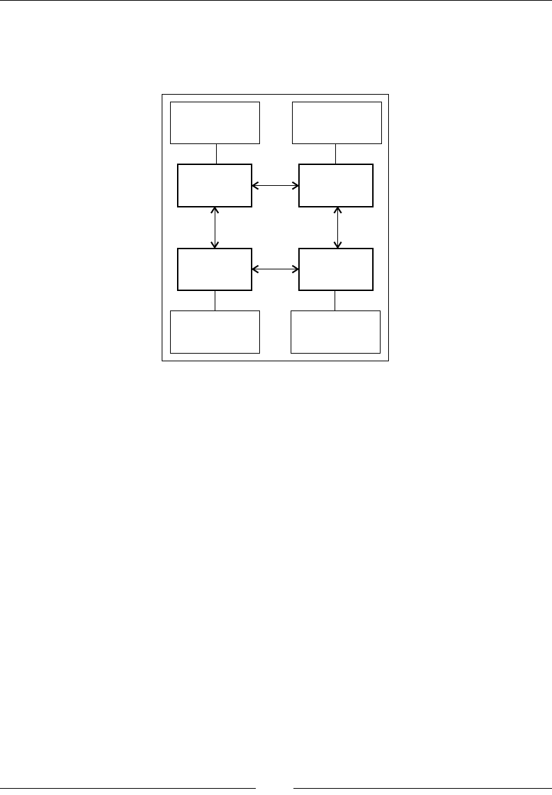
Chapter 3
[ 103 ]
Two of the modern NUMA architectures that are used in several server-side
environments are the AMD Opteron and the newer Intel Nehalem architecture.
The following gure illustrates a NUMA node conguration:
MEMORY
BANK 1
MEMORY
BANK 2
CPU
NODE 1
CPU
NODE 2
CPU
NODE 3
CPU
NODE 4
MEMORY
BANK 3
MEMORY
BANK 4
Here, any CPU, or NUMA node, has to perform at most two communication hops with
the other NUMA nodes in the system to get at arbitrary memory. The ideal (and the
fastest) memory access consists of zero hops (the node's own memory). There is not
necessarily be a one-to-one mapping between CPUs and NUMA nodes. For example,
one NUMA node may contain several CPUs who share local memory.
So, to perform well on a NUMA architecture, the garbage collector threads should
be structured in a benecial way. If a CPU is executing a mark thread in the GC
it should be the one working on the parts of the heap memory that belong to the
CPU itself. This way NUMA performance is maximized. As referenced objects may,
in worst case, appear anywhere on the heap, on NUMA the GC usually needs an
additional object moving heuristic. This is to make sure that objects referenced near
other objects in time appear near them in memory as well, evacuating them from
suboptimal NUMA nodes. If this works correctly, there are substantial performance
gains to be had. The main problem is keeping objects from being moved back and
forth, "ping ponging", between memory sections that are the responsibilities of
different NUMA nodes. Theoretically, an adaptive runtime could be very good at this.
Adaptive Memory Management
[ 104 ]
This is another example of an optimization that can work well in an adaptive runtime,
but perhaps not so much in a static environment. Command-line ags that modify
memory allocation behavior in the JVM and change NUMA node afnity for the JVM
process will be discussed in greater detail in Chapter 5.
NUMA is a challenging architecture to implement good memory
management for. However, research on JRockit shows that it is
still possible to get pretty good performance without specic
NUMA optimizations as long as prefetching and cache behavior
is intelligent enough in the JVM.
Large pages
At the base of all memory allocations lies the operating system and its page table.
An OS divides the physical memory into pages, a page typically being the smallest
possible memory allocation unit. Traditionally, a page is somewhere in the order
of 4 KB. A process in an OS only sees a virtual address space, not a physical one. In
order for a CPU to map a virtual page to the actual physical page in memory, a cache
called the Translation Lookaside Buffer (TLB) is used to speed things up. If pages
are too small, TLB misses are consequently more common.
This problem can be remedied if pages were several orders of magnitude larger;
megabytes instead of kilobytes. All modern operating systems tend to support
large pages in some form.
Obviously, in an OS where many processes allocate memory in separate address
spaces and where pages are much larger than a couple of KB, fragmentation becomes
a bigger problem because more page space is wasted. An allocation that requires
slightly more memory than the size of a page suddenly carries a lot of dead weight.
This doesn't matter to a runtime that does its own memory management in one
process and owns a large part of the memory, but even if it were a problem it could
be remedied by providing abstraction for many different page sizes on an underlying
large page.
A performance increase of at least 10 percent can usually be gained for a
memory intensive application if it runs on large pages instead of normal
ones. JRockit has support for this and can use large pages if enabled on
the underlying operating system.

Chapter 3
[ 105 ]
Typically, on most operating systems, enabling large page support is a privileged
operation that requires administrator access, which makes it slightly harder to just
"plug and play".
Adaptability
As we have discussed to a great extent in the chapter on code generation,
adaptability is the key to success in a runtime for a mobile language such as Java.
Traditionally, only code was adaptively reoptimized and was subject to hotspot
analysis. However, the JRockit designers recognized from the start that all aspects
of the runtime system should be made adaptive if possible.
So, JRockit may heuristically change garbage collection behavior at runtime, based on
feedback from the memory system and adjust parameters such as heap size, number of
generations in the heap, and even the overall strategy used to garbage collect.
Here is an example output generated by running JRockit with the
-Xverbose:gc ag:
marcusl@nyarlathotep:$ java -Xmx1024M -Xms1024M -Xverbose:gc
-cp dist/bmbm.jar com.oracle.jrpg.bmbm.minisjas.server.Server
[memory] Running with 32 bit heap and compressed references.
[memory] GC mode: Garbage collection optimized for throughput,
initial strategy: Generational Parallel Mark & Sweep.
[memory] Heap size: 1048576KB, maximal heap size: 1048576KB,
nursery size: 524288KB.
[memory] <s>-<end>: GC <before>KB-><after>KB (<heap>KB), <pause>ms.
[memory] <s/start> - start time of collection (seconds since jvm start).
[memory] <end> - end time of collection (seconds since jvm start).
[memory] <before> - memory used by objects before collection (KB).
[memory] <after> - memory used by objects after collection (KB).
[memory] <heap> - size of heap after collection (KB).
[memory] <pause> - total sum of pauses
during collection (milliseconds).
[memory] run with -Xverbose:gcpause to see
individual pauses.
[memory] [YC#1] 28.298-28.431: YC 831035KB->449198KB
(1048576KB), 132.7 ms
[memory] [OC#1] 32.142-32.182: OC 978105KB->83709KB
(1048576KB), 40.9 ms

Adaptive Memory Management
[ 106 ]
[memory] [OC#2] Changing GC strategy to Parallel Mark & Sweep
[memory] [OC#2] 39.103-39.177: OC 1044486KB->146959KB
(1048576KB), 73.0 ms
[memory] [OC#3] Changing GC strategy to Generational
Parallel Mark & Sweep
[memory] [OC#3] 45.433-45.495: OC 1048576KB->146996KB
(1048576KB), 61.8 ms
[memory] [YC#2] 50.547-50.671: YC 968200KB->644988KB
(1048576KB), 124.4 ms
[memory] [OC#4] 51.504-51.524: OC 785815KB->21012KB
(1048576KB), 20.2 ms
[memory] [YC#3] 56.230-56.338: YC 741361KB->413781KB
(1048576KB), 108.2 ms
...
[memory] [YC#8] 87.853-87.972: YC 867172KB->505900KB
(1048576KB), 119.4 ms
[memory] [OC#9] 90.206-90.234: OC 875693KB->67591KB
(1048576KB), 27.4 ms
[memory] [YC#9] 95.532-95.665: YC 954972KB->591713KB
(1048576KB), 133.2 ms
[memory] [OC#10] 96.740-96.757: OC 746168KB->29846KB
(1048576KB), 17.8 ms
[memory] [YC#10] 101.498-101.617: YC 823790KB->466860KB
(1048576KB), 118.8 ms
[memory] [OC#11] 104.832-104.866: OC 1000505KB->94669KB
(1048576KB), 34.5 ms
[memory] [OC#12] Changing GC strategy to Parallel Mark & Sweep
[memory] [OC#12] 110.680-110.742: OC 1027768KB->151658KB
(1048576KB), 61.9 ms
[memory] [OC#13] Changing GC strategy to Generational
Parallel Mark & Sweep
[memory] [OC#13] 116.236-116.296: OC 1048576KB->163430KB
(1048576KB), 59.1 ms.
[memory] [YC#11] 121.084-121.205: YC 944063KB->623389KB
(1048576KB), 120.1 ms

Chapter 3
[ 107 ]
JRockit versions from R28 tend not to change garbage collection
strategies at runtime. Default values will be picked depending on
conguration. This, along with better garbage collectors, was
found to provide a larger degree of determinism for customers.
The previous output is from the R27 line of JRockit releases. For R28,
non-standard GC strategies should be explicitly specied on the
command line. R28 defaults to a generational parallel mark and sweep
(optimized for throughput). The R28 memory management system
still adaptively modies many aspects of the garbage collection
behavior, but to a lesser extent than R27.
All garbage collections in the previous example take place using a parallel mark and
sweep algorithm, optimized for throughput. However, the JVM heuristically decides
whether nurseries should be used or not depending on feedback from the runtime
system. In the beginning, these changes are fairly frequent, but after a warm-up
period and maintained steady-state behavior, the idea is that the JVM should settle
upon an optimal algorithm. If, after a while, the steady-state behavior changes from
one kind to another, the JVM may once again change strategies to a more optimal one.
Near-real-time garbage collection
Real-time systems tend to t badly in a garbage collecting world. No matter how
well a garbage collector performs, we still have a non-deterministic runtime
overhead. Even if the latencies introduced by the GC are few and stopping the world
completely is a rare event, a certain degree of non-determinism cannot be avoided.
So what do we mean by real-time? The terminology suffers from a certain degree of
misuse. To avoid some of the confusion associated with real-time, we will divide the
concept into hard real-time and soft real-time.
Hard and soft real-time
Hard real-time should be understood as the more traditional real-time
system—perhaps a synthesizer or a pacemaker, a system where 100 percent
determinism is an absolute requirement. There are few runtimes with automatic
memory management that can work for this kind of environment, at least not
without extensive modications to the application and some kind of program
language constructs for controlling the garbage collection.

Adaptive Memory Management
[ 108 ]
A typical example is the Java real-time effort as specied in Java Specication
Request (JSR) 1, which species an API (javax.realtime) for interacting with the
runtime and for controlling the occurrence of garbage collection at certain program
points. When using Java to develop a new application, this might be a feasible way to
go ahead, but porting an existing Java production system to use a new API with new
semantics is often very challenging or downright impossible. Even if it is technically
feasible, modifying the key aspects of an existing system is very costly. Hence, the
concept soft real-time.
We use the term soft real-time to mean a runtime system where it is possible to specify
a quality of service level for latencies, and control pause times so that, even though
they are non-deterministic, no single pause will last longer than a certain amount of
time. This is the technique that is implemented in the product JRockit Real Time.
JRockit Real Time
It turns out that guaranteeing a quality of service level in the form of a maximum
pause time setting is sufcient for most complex systems that require a certain
degree of determinism. It is enough for the system to guarantee that latencies stay
below the given bound. If this works as it should, the immediate benet is of course
that more deterministic and lower latencies can be gained without modifying an
existing application.
The main selling point of JRockit Real Time is that getting deterministic latencies
requires no modications to the application—it just plugs in. The only thing that
needs to be specied from the user side is the pause time target in milliseconds.
Current JRockit releases have no problems maintaining single millisecond pause
time targets on modern CPU architectures.
No world is perfect, however, and as we have discussed in the section about
concurrent GC, the price of low latencies has to be paid for with longer total garbage
collection time. Recollect that it is more difcult to garbage collect efciently when
the application is running, and if we have to interrupt GC more often, it might be
even more problematic. In practice, this has turned out not to be a problem. It is
more important to most customers who want JRockit Real Time that the degree of
predictability and latency is deterministic, than that the total garbage collection time
goes down. Most customers feel that response times is their main problem and that
a sudden increase in pause time while large garbage collections take place is more
harmful than if the total time spent in GC increases.
The following graph illustrates response times over time for a running application.
The application in question is a benchmark for WebLogic SIP Server, a product for the
telecom industry. JRockit Real Time is not enabled. As can be seen, the deviation in
response times is large.
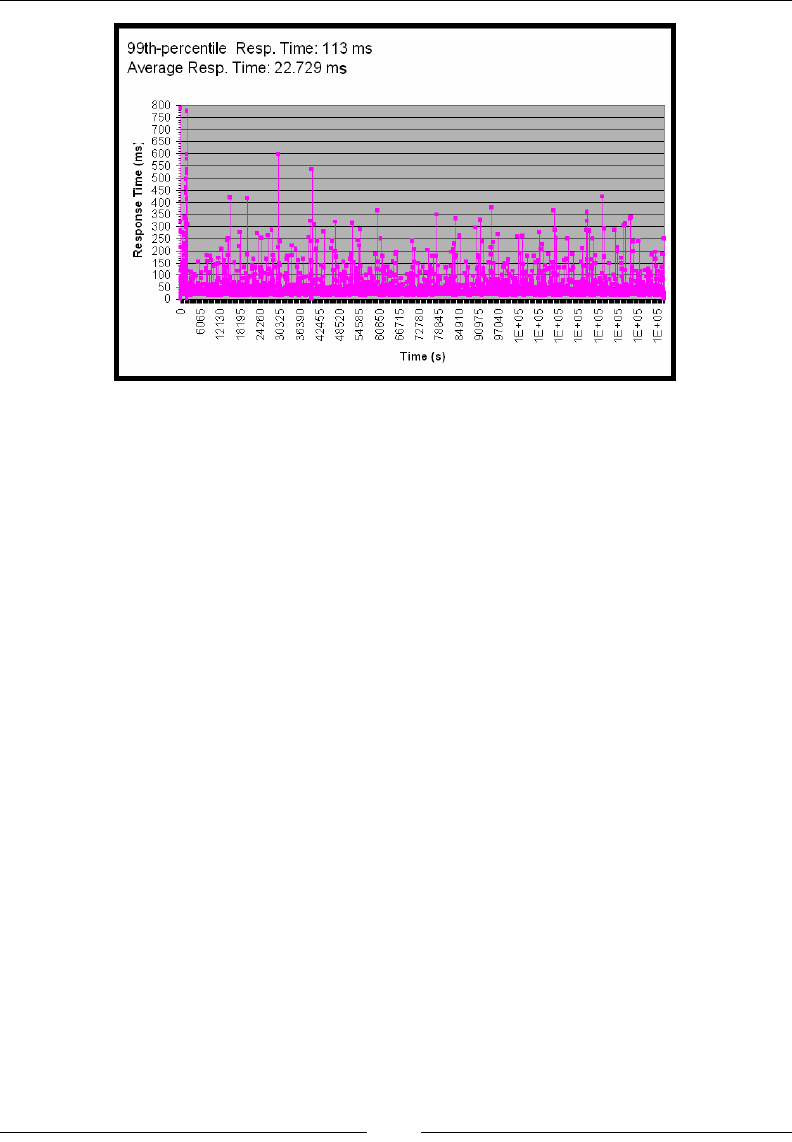
Chapter 3
[ 109 ]
Does the soft real-time approach work?
The soft real-time approach in JRockit Real Time has turned out to be a major winner.
But how can a non-deterministic system like a garbage collector provide the degree
of determinism required to never have longer than single millisecond pause times?
The complete answer is that it can't, but the boundary cases are rare enough so that it
doesn't matter.
Of course there is no silver bullet, and there are indeed scenarios when a pause
time target cannot be guaranteed. It turns out, however, that practically all standard
applications, with live data sets up to about 30 to 50 percent of the heap size, can be
successfully handled by JRockit Real Time with pause times shorter than, or equal to,
the supported service level. This ts the majority of all Java applications that customers
run. The live data set bound of 30 to 50 percent is constantly being improved by
tuning and gets better with each new JRockit Real Time release. The minimum
supported pause time is also continuously made lower.
In the event that JRockit Real Time isn't a perfect rst t for an application, several
other things can be done to tune the behavior of the garbage collector. When looking
for the cause of latencies in a Java program, there are frequently non GC-related user
issues involved. For example, it is common that a lock in the Java code is so contended
that it is actually contributing more to program latencies than the GC itself. JRockit
Mission Control contains a set of diagnostic tools that can fairly easily point out
problems like this from a runtime recording.
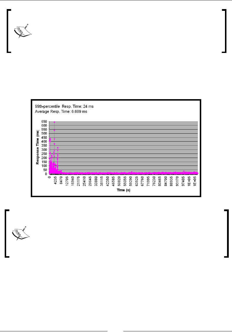
Adaptive Memory Management
[ 110 ]
We often hear success stories from the eld, such as when a trading
system started making tens of thousands of dollars more per day
because of lower latencies and consequently faster response times. The
system could complete a signicant number of more trades per day on
the same hardware. No other action than switching VMs to JRockit Real
Time was required.
The following graph shows the same benchmark run as before, with JRockit Real
Time enabled and a maximum latency service level set to 10 milliseconds using
the –XpauseTarget ag. Note that after the initial warm-up spikes, there is
virtually no unpredictability left in the latencies.
One might easily theorize that the spikes in the beginning of the run are
caused by the VM aggressively trying to reach a steady state, for example
through large amounts of code optimization. This can be true, and indeed
this kind of pattern can show up. For this particular benchmark run,
however, the initial latencies were actually caused by a bug in the Java
application, unrelated to GC or adaptive optimization. The problem was
subsequently xed.
We also note that JRockit Real Time has no trouble fullling the 10 millisecond
guarantee it was given. All of this comes at the affordable price of a slightly longer
total time spent in garbage collection.

Chapter 3
[ 111 ]
How does it work?
So how can JRockit deliver this kind of garbage collection performance? There are
three key issues at work here:
• Efcient parallelization
• Splitting garbage collection work into work packets, transactions that may be
rollbacked or aborted if they fail to complete in time
• Efcient heuristics
Efcient parallelization isn't a novel concept. There are several concurrent garbage
collectors in existing literature, and there are few conceptual changes or technological
leaps in how JRockit Real Time handles concurrency. Performance is, as always, in the
details—synchronize efciently, avoid locks if possible, make sure existing locks aren't
saturated, and schedule the worker threads in an efcient manner.
The key to low latency is still to let the Java program run as much as possible, and
keep heap usage and fragmentation at a decent level. We can think of JRockit Real
Time as a greedy strategy for keeping Java programs running. The basic strategy
is postponing stopping the world for as long as possible, hoping that whatever
problem that caused us to want to stop the world in the rst place will resolve
itself, or that the time required to stop the world will go down once it is inevitable.
Hopefully, there are fewer objects to compact or sweep when we nally pause.
All garbage collector work in JRockit Real Time is split up into work packets. If we
start to execute a work packet, for example a compaction job for part of the heap,
with the Java program halted, and it takes too long, we can throw away whatever
work it has done so far and restart the application. Sometimes the partial work
can be kept, but the entire transaction doesn't have time to complete. The time to
completion while the world is stopped is governed by the quality of service level for
latencies that the user has specied. If a very low latency bound has been specied
we might have to throw away more of a partially completed transaction in order to
keep the Java program running than with a higher one.
The mark phase is, as has already been covered, simple to modify, so that it runs
concurrently with the Java program. However, both the sweep phase and compaction
need to stop the world at times. Luckily, mark time tends to make up around 90
percent of the total garbage collection time. If the phases that need stopping the world
take too long, we just have to make sure we can terminate what they are doing and
restart the concurrent phase, hoping that the problem goes away in the meantime.
The work package abstraction makes it easier to implement this functionality.

Adaptive Memory Management
[ 112 ]
There are, of course, several heuristics involved. Slight modications to the runtime
system helps JRockit Real Time make more informed decisions. One example is a
somewhat more complex write barrier that keeps track of the number of cards dirtied
on a per-thread basis. The code takes a little bit more time to execute than that of a
traditional generational GC write barrier, but provides more adequate proling data
to the GC. If one thread is much more active at dirtying cards than others, it probably
needs special attention. JRockit also uses the sum of all executed write barriers in a
thread as a heuristic trigger.
The Java memory API
This section covers some of the unique constructs of the Java language, related to
memory management.
Dreaming of delete or free operators for Java or trying to explicitly control the
garbage collection behavior in a JVM by, for example, hanging on to objects longer
than their natural lifespans is a sure way of shooting yourself in the foot. There are,
however, some mechanisms in the Java language that make it possible to help the
GC by giving it "hints". Some of the available mechanisms are good and some are
bad. Some should be used with caution to avoid unwanted side effects.
Finalizers
In Java, since Java 1.0, every object contains a method called finalize that may be
freely overridden by any implementer. The contract is that the finalize method is
called just before the object in question is about to be garbage collected. This might
seem like a good idea, making it possible to do cleanups before the object goes away,
such as closing any open le handles that the object may hold on to.
However, since a finalize method can contain arbitrary code, there are several
potentially bad scenarios to consider as well, for example, the case that a nalizer
resurrects the object, or clones a new object from the dying one, in effect preventing
an object from being garbage collected. In addition, placing code that releases limited
resources, such as le handles, in a nalizer may cause resource starvation. This is
because there is never a predictable point in time where nalizers are guaranteed to
be run. System resources should always be released explicitly in a situation where
the programmer has control.
Furthermore, nalizers can also be called at any time in any thread, no matter
which locks the thread is holding. This is extremely bad and can lead to all kinds
of unintended deadlock situations and violations of mutual exclusion semantics.

Chapter 3
[ 113 ]
It is not just the authors' opinion, but that of the Java community in general, that
nalizers are a bad design choice and that their use should be avoided at any cost.
References
When programming Java, one might think that there is only one kind of object
reference. An object is either live or unreachable, eventually leading to it being
garbage collected and removed from the system. There are, however, several kinds
of references in Java, which may be thought of as references with varying degrees
of liveness. We refer to the normal references or standard object references, as
strong references.
The package java.lang.ref contains several classes that wrap Java objects and
thereby provide a classication for the object's reference type. The different reference
classes all extend java.lang.ref.Reference. All Reference objects in Java have
a get method that will return the actual object being referenced or null if that
particular object isn't reachable, i.e. if the object has been garbage collected.
Java also provides the class java.lang.ref.ReferenceQueue, where objects
that change reachability or scope are enqueued, for example when the object a
Reference points to gets garbage collected. A Reference object can be bound to
a java.lang.ref.ReferenceQueue at instantiation. By polling an instance of the
ReferenceQueue, a small amount of insight into what the memory management
system is doing can be gained programmatically.
There are four main types of references in Java—strong, weak, soft and
phantom references.
Weak references
A weak reference that points to an object isn't strong enough to force that object to
remain in memory. The java.lang.ref.WeakReference class is in effect a wrapper
around a strong reference, tagging it as weak.
WeakReference weak = new WeakReference(object);
In the example, to get the actual object the reference points to, use weak.get(). As
object may be garbage collected at any time, this call returns null when object is
no longer in memory.

Adaptive Memory Management
[ 114 ]
A typical application for weak references is the java.util.WeakHashMap class,
which gets rid of an entry if its key is no longer referenced. This is ideal for
caches. Using weak references in the memory leak prone HashMap cache example,
introduced in the rst section of this chapter, would prevent leaks caused by
forgotten objects left in the hash table. It would also have the added benet of not
requiring that hash table contents are cleared out in order for it to ever be garbage
collected. Weak references can provide an intrinsic protection against memory leaks.
Soft references
A soft reference is a weak reference that the garbage collector is more reluctant to
throw away. Typically, the garbage collector tries to keep them around as long as
possible, but they are the rst to go if memory is running low.
How much stronger a soft reference should be, than a weak reference, is left to
the JVM implementation. In theory, a soft reference may behave exactly like a
weak reference and not violate the Java semantics.
Phantom references
Phantom references are the preferred way of implementing nalization. They are
designed to supersede the use of nalizers that, as we have seen, are deeply awed.
Phantom references wrap ordinary objects similar to weak and soft references, but
their get method always returns null.
Phantom references are accessed through the java.lang.ref.ReferenceQueue
class mentioned earlier, by polling an instance to which the phantom references
one is interested in are bound. Polling the reference queue at regular intervals
(or doing a blocking remove) reveals if a new phantom reference is available for
garbage collection. If this is the case, as the get method of phantom references
always returns null, there is no possible way to get hold of a handle to the object
in question and resurrect it. This avoids the problems with nalizers and provides
all the benets of a similar mechanism.
Here is a code example that prints the number of nalized TestObjects in the
system using nalizers:
/**
* Prints the number of finalized objects
*/
public class Finalize {
static class TestObject {
static int nObjectsFinalized = 0;
protected void finalize() throws Throwable {
System.err.println(++nObjectsFinalized);
}

Chapter 3
[ 115 ]
}
public static void main(String[] args) {
for (;;) {
TestObject o = new TestObject();
doStuff(o);
o = null; //clear any remaining refs to "o"
System.gc(); //try to force gc
}
}
}
The equivalent approach with PhantomReferences in a ReferenceQueue might look
something like this:
/**
* Prints the number of finalized objects using PhantomReferences
*/
import java.lang.ref.*;
public class Finalize {
static class TestObject {
static int nObjectsFinalized = 0;
}
static ReferenceQueue<TestObject> q =
new ReferenceQueue<TestObject>();
public static void main(String[] args) {
Thread finalizerThread = new Thread() {
public void run() {
for (;;) {
try {
//block until PhantomReference is available
Reference ref = q.remove();
System.err.println(++TestObject.nObjectsFinalized);
} catch (InterruptedException e) {
}
}
}
};
finalizerThread.start();
for (;;) {
TestObject o = new TestObject();
PhantomReference<TestObject> pr =
new PhantomReference<TestObject>(o, q);
doStuff(o);
o = null; //clear any remaining refs to "o"
System.gc(); //try to force GC
}
}
}

Adaptive Memory Management
[ 116 ]
Differences in JVM behavior
The most important thing to remember is that all of the above language constructs
merely provide hints to the GC. The Java language, by design, gives no exact control
over the memory system. It is a bad practice to assume, for example, that just because
soft references are alive in a cache for a certain amount of time in one VM vendor's
implementation, the same will be true for another vendor's implementation too.
Another example, which recurs quite frequently among customers, is misuse of the
System.gc method. The System.gc method is only dened as a hint to the runtime
that "now will be a good time to garbage collect". In some VMs this hint is taken
almost all the time, leading to extensive GCs and the possible freeing of massive
amounts of memory. In other VMs it is ignored most of the time.
In the authors' old line of work as performance consultants, we have time and
time again seen this function abused. More than once, the simple removal of a
couple of calls to System.gc has led to immense speedups for quite a few customer
applications. This is the story behind the JRockit –XX:AllowSystemGC=false ag
that basically just tells JRockit to ignore all System.gc calls.
Pitfalls and false optimizations
As with code generation, it is fairly common to see false optimizations in Java
applications, implemented with the belief that they will assist the garbage collector.
Again, premature optimization is the root of all evil. At the Java level there is really
very little to be known about how the GC will treat the program. The general sin is
believing that the garbage collector will always behave in a certain way and try to
manipulate it.
We have already discussed the case of System.gc that is not required to do anything at
all, or might do a full-heap-GC stopping the world every time, or anything in between.
Another false optimization is different types of object pooling. Keeping a pool of
objects alive and reusing them, instead of allocating new objects, is often believed
to increase garbage collection performance. But not only does this add complexity
to the Java application, it is also easy to get wrong. Using the java.lang.ref.
Reference classes for caching or simply making sure to set object references to null
as soon as they aren't needed anymore is usually sufcient enough for any modern
garbage collector. Keeping objects alive longer than their natural lifespan can
backre. Generational GC usually takes care of temporary objects quickly, but
if they are articially kept alive and reused, they will eventually clog up the old
space instead.

Chapter 3
[ 117 ]
Java is not C++
Frequently, people express the belief that there should be a static way to control all
aspects of Java garbage collection, complete with free or delete operators as well as
the ability to turn off and on garbage collection at arbitrary intervals. Another example
is wishing for ways to get at and modify objects as native pointers directly in the JVM.
Both these strategies would be extremely dangerous if introduced in Java, and
successful usage would, in the authors' opinion, be very hard or impossible.
There are several advantages of automatic memory management, and some
disadvantages, chief of which is non-determinism. JRockit Real Time has tried
to provide good enough ways around this without the need for modifying
an application or interfacing with the GC.
We still recall with horror the "Java should have a free operator"
discussion that swamped the entire HotSpot session at JavaOne 1999.
The guy who started it raised his hand and opened up with the now
classic line "Many of my friends are C++ programmers…"
In truth, a well-written Java program that uses all the allowed tricks in the book
correctly, such as the correct java.lang.ref.Reference classes, and takes heed
of the dynamic nature of Java, should run ne on a modern JVM. If a program has
real-time needs that require further manipulation, maybe it shouldn't have been
written in Java to begin with, but rather in a static language where the programmer's
control over the memory system is more absolute.
Automatic memory management, while being a helpful tool that shortens
development cycles and reduces program complexity, isn't a golden hammer
that can be applied to all programmatic problems.
Controlling JRockit memory
management
This section covers the most fundamental command-line switches that control
garbage collection in JRockit. For more advanced manipulation of the memory
system, for example tuning compaction, please refer to Chapter 5, Benchmarking
and Tuning.

Adaptive Memory Management
[ 118 ]
Basic switches
Following are the most fundamental command-line switches for interacting with the
JRockit memory system.
Outputting GC data
Running JRockit with –Xverbose:gc will, similar to –Xverbose:codegen, output
plenty of verbose information on what the JVM memory management system is doing.
This information includes garbage collections, where they take place (nurseries or old
space), changes of GC strategy, and the time a particular garbage collection takes.
-Xverbose:gc (or -Xverbose:memory) is, except for JRockit Mission Control, the
main information provider when it comes to studying garbage collector behavior for
an application.
Here is an example of the output generated by –Xverbose:gc:
hastur:material marcus$ java –Xverbose:gc GarbageDemo
[INFO ][memory ] GC mode: Garbage collection optimized for
throughput, strategy: Generational Parallel Mark & Sweep.
[INFO ][memory ] Heap size: 65536KB, maximal heap size:
382140KB, nursery size: 32768KB.
[INFO ][memory ] [YC#1] 1.028-1.077: YC 33232KB->16133KB
(65536KB), 0.049 s, sum of pauses 48.474 ms, longest pause 48.474 ms.
[INFO ][memory ] [YC#2] 1.195-1.272: YC 41091KB->34565KB
(65536KB), 0.077 s, sum of pauses 76.850 ms, longest pause 76.850 ms.
[INFO ][memory ] [YC#3] 1.857-1.902: YC 59587KB->65536KB
(65536KB), 0.045 s, sum of pauses 45.122 ms, longest pause 45.122 ms.
[INFO ][memory ] [OC#1] 1.902-1.912: OC 65536KB->15561KB
(78644KB), 0.010 s, sum of pauses 9.078 ms, longest pause 9.078 ms.
[INFO ][memory ] [YC#4] 2.073-2.117: YC 48711KB->39530KB
(78644KB), 0.044 s, sum of pauses 44.435 ms, longest pause 44.435 ms.
Typically, the log shows things such as garbage collection strategy changes and heap
size adjustments, as well as when a garbage collection take place and for how long.
OC or YC means Old Collection or Young Collection (nursery), followed by
the sequence number of the particular collection. Sequence numbers start at 1.
After the OC and YC identier comes the time span in seconds, since the start of the
JVM, that was spent in this particular GC.

Chapter 3
[ 119 ]
Then JRockit reports how much live data the particular heap region that was
collected contained before and after the GC, the total size of the region, and the time
that particular garbage collection took. We can see that the GC chooses to gradually
grow the heap in this particular example.
Finally, the sum of pauses, that is for how long the world was stopped during the
last garbage collection, is reported along with the longest individual pause. In the
previous example, we can infer that as these values are the same, we are dealing
with complete stop-the-world-collections, i.e. parallel GC. They each consist of one
large pause.
For advanced users, as has been covered, each garbage collection consists of several
phases, and if you want more granularity on them, a ag called –Xverbose:gcpause
will provide it. It should be noted, however, that JRockit Mission Control with its
graphic illustration of garbage collection behavior probably provides more insight
into application behavior.
Set initial and maximum heap size
The –Xms and –Xmx ags are standard and variants are available in all JVMs. They
specify initial and maximum heap size to be allocated to the JVM. If no arguments
are given, the heap will grow and shrink heuristically during runtime. Consider
the following example:
java –Xms1024M –Xmx2048M <application>
The code shown in the previous example will force the initial heap size to 1 GB
and prevent it from ever growing above 2 GB. If enough heap to accommodate
the demands isn't available, an OutOfMemoryError will be thrown.
Controlling what to optimize for
Unless you really know what you are doing, the –XgcPrio ag is the preferred
way to tell JRockit what garbage collection strategies to run. Instead of xing a
GC strategy, JRockit will heuristically determine what is best for the application,
depending on what the user thinks is important and change strategies at runtime
when appropriate.
• –XgcPrio:throughput: This optimizes for throughput, not caring about
pause times
• –XgcPrio:pausetime: This optimizes for low latency
• -XgcPrio:deterministic: This activates the JRockit Real Time
functionality, striving for extremely short pauses at the cost of some
additional runtime overhead

Adaptive Memory Management
[ 120 ]
The maximum pause time target for the GC (not applicable for –XgcPrio:throughput)
can be set with the ag –XpauseTarget. Depending on the amount of live data
on the heap and system conguration, JRockit may or may not be able to keep
up. Experimenting with different pause time targets for a particular application
is encouraged.
Following is command-line example for enabling deterministic GC (JRockit Real
Time) with an upper pause time target of ve milliseconds:
java –XgcPrio:deterministic –XpauseTarget:5ms <application>
Specifying a garbage collection strategy
For even further control over GC behavior, a more ne grained garbage collection
strategy can be set from the command line using the –Xgc ag. This xes a garbage
collection strategy for the JVM and prevents it from being changed at runtime. The
strategy can be made more ne grained than with one of the three -XgcPrio choices.
Again, we use the terms concurrent and parallel to describe if we are optimizing
for low latencies or throughput. The possible options are –Xgc:singlecon (single
generational concurrent), -Xgc:gencon (generational concurrent), -Xgc:singlepar
(single generational parallel) and –Xgc:genpar (generational parallel). "Generational",
as opposed to "single generational", means that a nursery is used.
Compressed references
As already mentioned, given a maximum heap size smaller than 64 GB, JRockit will
use some form of compressed references by default. But the usage of compressed
references can also be explicitly controlled with the –XXcompressedRefs ag. The
ag takes two arguments—whether compressed references should be enabled at all
and in that case the maximum size of the heap that they should support.
The following command-line example disables compressed references, and forces
JRockit to use native size pointers for all objects:
java –XXcompressedRefs:enable=false <application>
This following command-line example enables compressed references that can
support up to 64-GB heaps:
java –XXcompressedRefs:enable=true,size=64GB <application>

Chapter 3
[ 121 ]
Advanced switches
It should be noted that playing around too much with JVM switches doesn't
necessarily lead to increased performance and might interfere with more optimal
runtime behavior.
If memory performance is believed to be an application bottleneck, it is recommended
to use the JRockit Mission Control suite for instrumentation. Chapters in the second
part of this book will explain how to do a runtime recording with JRockit and how
to analyze it. Collecting as much information as possible about an application before
starting to modify non-standard parameters is strongly recommended.
Almost any aspect of the garbage collector can be tuned from the command line
—everything from the size of the thread local buffers used for allocation to
the strategies used for heap compaction.
Some less fundamental switches that control memory management are covered in
Chapter 5. Please study the JRockit documentation for a more in-depth description
of all memory management options.
Summary
This chapter covered automatic memory management in detail, concentrating
on adaptive memory management, where feedback from the runtime system is
continuously used to optimize GC performance.
We explained the mark and sweep as well as the stop and copy strategies for garbage
collection and discussed how more advanced variants of these can work in a modern
runtime, especially JRockit. We discussed how to implement fast scalable GC on all
levels from software to hardware.
Every GC needs to stop the world at some point, for example when sweeping or
compacting. Stopping the world introduces latencies. The main lesson is that we
can optimize either for throughput or for low latencies, one at the cost of the other.
We introduced the product JRockit Real Time, that provides a degree of determinism
and pause time targets for the JVM. JRockit Real Time can massively improve
response times and decrease their deviation for most applications without the need
to modify the applications.

Adaptive Memory Management
[ 122 ]
Some of the constructs available in the Java language that can help control garbage
collection and memory management were introduced, followed by a section on false
optimizations. It is dangerous to believe that complete deterministic control can be
exerted over as non-deterministic a system as a garbage collector.
Finally, the most common command-line options used to control memory
management in JRockit were explained.
Now code generation and memory management in an adaptive runtime environment
have been introduced. In the next chapter, we will cover the nal fundamental
building block that makes up a Java runtime—threads and synchronization.

Threads and Synchronization
This chapter covers threads and synchronization in Java and in the Java Virtual
Machine. Threads are the de facto mechanism for running several parallel tasks in a
process. Locks are the de facto mechanism for constraining access to a critical section
of code to one thread at a time. These are the building blocks we need in order to
implement parallelism in software.
You will learn the following from this chapter:
• How fundamental parallel concepts such as threads and synchronization
work in Java and how the Java APIs can be used for synchronization. This
includes concepts like wait, notify, and the often misunderstood volatile
keyword. We will also briey look at the java.util.concurrent package.
• The concept of the Java Memory Model, and why it is required.
Understanding the memory model is the key to writing working
multithreaded Java programs.
• How the JVM can efciently implement threads and synchronization
and a discussion about a few different models.
• How the JVM can optimize threads and synchronization using different
types of locks, locking policies, and code optimizations, all based on
adaptive runtime feedback.
• How to avoid common pitfalls and false optimizations in parallel Java
programming—learning to stay clear of things like deprecated java.lang.
Thread methods and double checked locking.
• How to work with JRockit to modify thread and synchronization behavior
as well as an introduction on how to do lock proling.
Threads and Synchronization
[ 124 ]
Fundamental concepts
Java was, from its inception, a language designed for parallelism. It has
intrinsic mechanisms like the java.lang.Thread class as an abstraction for
threads, a synchronized keyword and wait and notify methods in every
object. This made it fairly unique at the time of its release, at least outside
academia. The most common approach for commercially proven languages so far
was to use platform-dependent OS library calls for thread management. Naturally,
Java needed a platform-independent way to do the same, and what can be better
than integrating the mechanisms for parallelism and synchronization into
the language itself?
Java is a nice language to work with, when it comes to synchronization. Not only
does it have explicit constructs that can be used for threads, locks, and semaphores
but it was also designed so that every object in a Java program can conveniently
be used as the limiting resource, or monitor object, constraining access to code in a
critical section. As of Java 1.5, the JDK also contains a package full of useful parallel
data structures, java.util.concurrent.
The term monitor is used to represent a handle to a synchronized
resource—only one thread can hold the monitor at a time, thus being
allowed exclusive access to the resource.
The advantages of this are obvious—Java synchronization involves no third-party
library calls and the semantics for locking are well-dened. It is easy to use locks
and threads when programming Java.
A disadvantage may be that it is too easy. It is simple to add synchronization
anywhere and everywhere "just to be sure", resulting in possible performance loss.
There are, of course, also questions of implementation overhead. As every object
is allowed to be a monitor, every object also needs to carry synchronization
information (for example whether the object is used in a lock right now, how that
lock is implemented, and so on). Typically, to enable quick access, this information
is stored in a lock word that exists in the header of every object. For more than the
simplest form of automatic memory management, similar performance concerns also
exist. Therefore, fundamental GC info, such as what GC state an object is in, must
also be available for quick access. Recollect, for example, the discussion about mark
bits from the section on tracing garbage collection in Chapter 3. Thus, both locking
and GC need certain kinds of information to be quickly available on a per-object
basis. Consequently, JRockit also uses a few bits in the lock word to store garbage
collection state information. However, we will still refer to this word as the "lock
word" for convenience throughout this text.
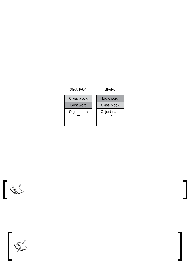
Chapter 4
[ 125 ]
Naturally, too compact a meta info representation in every object header introduces
extra execution overhead for decoding and encoding the information. A too large
representation introduces extra memory overhead in every object instead. Thus,
some care has to be taken when choosing a representation for the lock and GC bits
for the object.
Another thing that needs to go into every object header is a pointer to its type
information. JRockit calls this the class block.
The following gure shows the layout of a Java object in JRockit. All words in
the header are 32-bit wide on all platforms to save memory and provide faster
dereferencing. The class block is a 32-bit pointer to an external structure, with
type information for the object and virtual dispatch tables.
In JRockit, and as far as we know in most JVMs, a complete object header is
represented by two 32-bit words. JRockit stores type information at the 0th offset of
an object pointer and the lock word four bytes into the object. On SPARC, the layout
is reversed because there it is cheaper to execute atomic instructions that manipulate
pointers with no offset. As the class block, unlike the lock word, is not subject to any
atomic operations, it can be placed later in the header on SPARC.
We dene an atomic instruction as a native instruction that can only be
either fully executed or not executed at all. When it is fully executed, its
results are guaranteed to be visible to all potential accessors.
Atomic operations are required for reads and writes to the lock word, as they have to
be exclusive—they are the most fundamental building block of the synchronization
state machine in the JVM.
Various academic research has shown that there is relatively little to
be gained by compressing an object header further, for example into
a single 32-bit word. The extra processing overhead does not make it
worthwhile, even though it saves some more memory per object.
Threads and Synchronization
[ 126 ]
Hard to debug
True for most platforms and programming languages is that a single concurrency
problem may manifest itself in many different ways such as deadlocks, livelocks, or
plain crashes. The common denominator is usually non-determinism. This is a classic
challenge. As concurrency problems tend to depend on timing, attaching a debugger
to the running program before it breaks might not necessarily reproduce the issue.
Timing changes with the added debugger overhead.
A deadlock occurs when two threads are sleeping, both waiting for the
other to nish using a resource that each of them needs. Obviously, they
never wake up. A livelock is similar, but involves active processing
from the threads. One can liken it to the case when two people meet in a
narrow corridor and step out of each other's way, but happen to do it in
the same direction so that they end up blocking each other again.
Because of these kinds of issues, debugging parallel systems is generally difcult.
The greatest help comes from visualization aids and debuggers that can untangle
thread and lock dependencies.
JRockit, like all major JVMs, supports dumping stack traces from all threads in a
running Java application to the console, along with lock holder information. This is
enough to resolve simple deadlock problems, where it is possible to determine which
mutually dependent threads are stuck waiting for a single resource. Examples will be
given later in this chapter.
The JRockit Mission Control suite can also be used to visualize lock information in a
more convenient way.
Difcult to optimize
It is also very common that performance issues arise from using synchronization.
Every lock is a bottleneck, as it introduces a critical section that can only be accessed
by one thread at a time. The more threads trying to get at a critical section, the more
contention will arise as threads have to wait their turn. If a lock is badly placed
or covers too wide a section in the interest of easier debugging (or just because of
general laziness) performance penalties will almost certainly occur.
Chapter 4
[ 127 ]
Sadly enough, it seems to be quite a common case in commercial software that
a single lock or a just a few locks cause the majority of the latency in a program.
We have seen this more than once when debugging third-party applications. The
programmer is normally not aware of this. Luckily, if the problematic locks are few
and can be identied, the latency problem is simple to x. Again, the JRockit Mission
Control suite can be used to easily establish which locks are most contended in a
running program.
A lock is said to be contended when many threads spend
signicant time competing to acquire it
Latency analysis
The JRockit Mission Control suite comes with a unique component for latency
analysis that, given a JRockit ight recording of a Java program, visualizes latency
data for the program. Latency analysis can be the programmer's best friend when
optimizing concurrent programs with plenty of synchronization. Instead of taking
the traditional proler's approach of displaying where the program spends its
active runtime, the latency analyzer provides information on where it does not.
Any nanosecond where a thread isn't executing Java code is mapped and laid out
in a thread graph. This way, it can be determined if the idle time is spent waiting
for I/O or the network, or, which is potentially more serious, in Java locks, i.e. code
waiting to enter synchronized blocks or methods.
Latency analysis with JRockit Mission Control is covered in greater
detail in the next section of this book, where the JRockit Mission Control
suite is introduced, specically in Chapter 8, The Runtime Analyzer and
Chapter 9, The Flight Recorder.
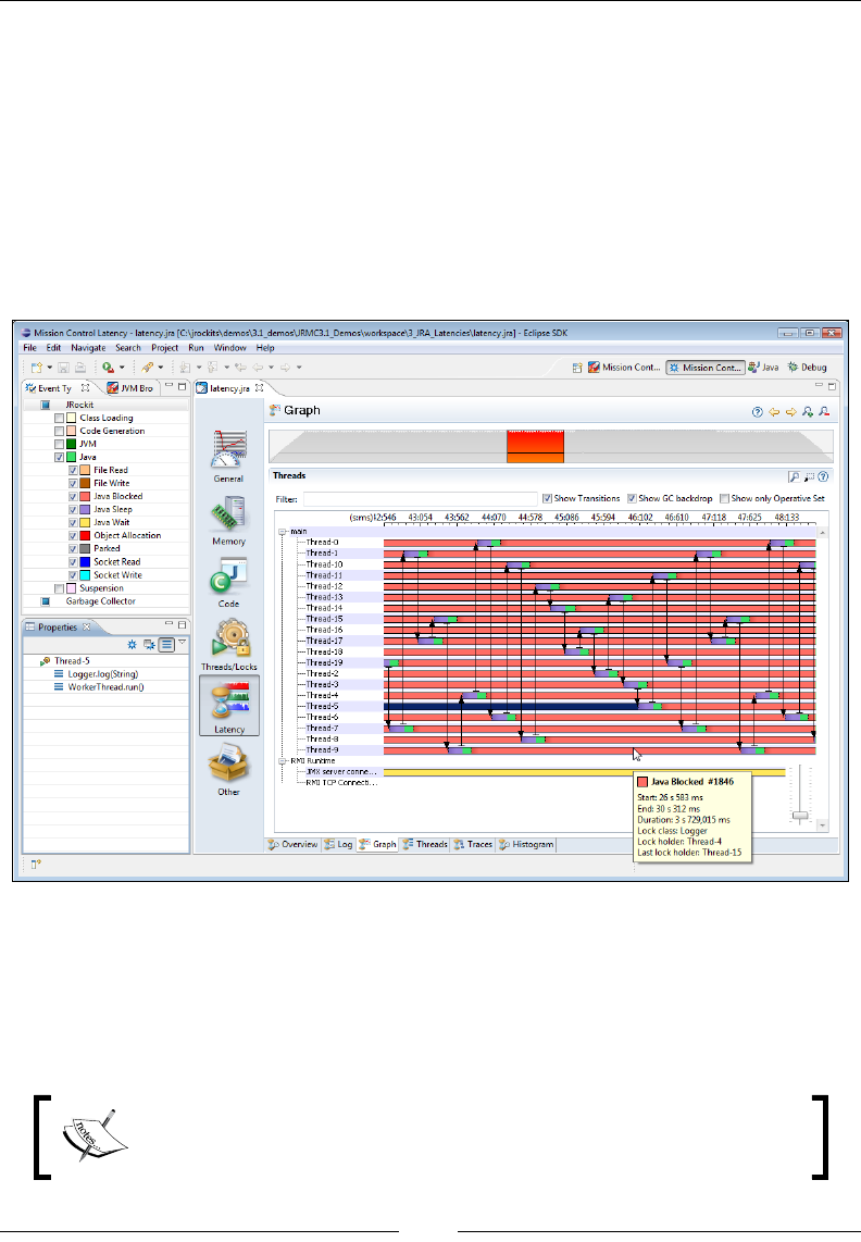
Threads and Synchronization
[ 128 ]
The following screenshot shows the latency analysis tab in the JRockit Runtime
Analyzer. The data comes from a recording of a running server application and the
recording is now about to be examined ofine. One colored bar per thread in the
program represents where the program spent its time during the recording. The
time axis goes from left to right. A different color is used for each latency generating
activity. In the following screenshot, all thread bars are mostly the same color. In this
case red, meaning "blocked in Java". This is bad, as it means almost all program time
was spent waiting for a Java lock, for example in a synchronized block. To be precise,
all colors except green mean "not executing Java". This might entail native threads
waiting for I/O or network trafc or any other source of latency.
Recollect our intuitive latency argument on memory management from Chapter 3—if
the JVM spends clock cycles garbage collecting, these cannot be used to execute Java
code. Similarly, if the clock cycles are spent waiting for le I/O or Java locks, latency
arises. This is the same kind of latency—time spent outside Java execution. It affects
response times and is the root of most performance problems.
JRockit Flight Recorder can help locate sources of latency in your Java
programs. In the example above, it turns out that virtually all latency
comes from a single badly placed Java lock in a logging module.

Chapter 4
[ 129 ]
Java API
This section covers the built-in synchronization mechanisms in Java. These are
convenient to have as intrinsic mechanisms in the language. There are, however,
potential dangers of misusing or overusing Java synchronization mechanisms.
The synchronized keyword
In Java, the keyword synchronized is used to dene a critical section. Both code
blocks inside a method and entire methods can be synchronized. The following
code example illustrates a synchronized method:
public synchronized void setGadget(Gadget g) {
this.gadget = g;
}
As the method is synchronized, only one thread at a time can write to the gadget
eld in a given object.
In a synchronized method, the monitor object is implicit. Static synchronized
methods use the class object of the method's class as monitor object, while
synchronized instance methods use this. So, the previous code would be
equivalent to:
public void setGadget(Gadget g) {
synchronized(this) {
this.gadget = g;
}
}
The java.lang.Thread class
The built-in thread abstraction in Java is represented by the class java.lang.
Thread. This class is a somewhat more generic thread representation than that of
corresponding OS implementations. It contains, among other things, fundamental
methods for starting threads and for inserting the thread payload code. This is
symmetrical with typical OS thread implementations where payload is passed as
a function pointer to the main thread function by the creator of the thread. Java
uses an object-oriented approach instead, but the semantics are the same. Any class
implementing the java.lang.Runnable interface can become a thread. The run
method inherited from the interface must be implemented and lled with payload
code. java.lang.Thread can also be subclassed directly.

Threads and Synchronization
[ 130 ]
There is also a simple priority mechanism in the java.lang.Thread class that may
or may not be efciently mapped to the underlying OS variant. The setPriority
method can be used to change the priority level of a thread, hinting to the JVM that
it's more important (real-time) or less important. Normally, for most JVMs, little is
gained by setting thread priorities explicitly from Java. The JRockit JVM may even
ignore Java thread priorities when the runtime "knows better".
Threads can be made to yield the rest of their scheduled time slice to other threads,
go to sleep or join (that is, wait for this thread to die).
Threads can be arranged in java.lang.ThreadGroups, a *NIX process like abstraction,
which can also contain other thread groups. Thread operations may be applied to all
threads in a thread group.
A thread may hold thread local object data, represented by the java.lang.
ThreadLocal class. Each thread will own a copy of any ThreadLocal it contains.
This is a very useful mechanism that has been around since Java 1.2. Even though it
is a somewhat clumsy retrot for a language without the concept of stack local object
allocation, it can be a performance life saver. Given that the programmer knows
what he is doing, explicitly declaring data thread local in Java may lead to signicant
speed ups.
The java.lang.Thread class has suffered some changes and deprecations to its API
during its lifetime. Originally, it came with methods for stopping, suspending, and
resuming threads. These turned out to be inherently unsafe. They still occur from
time to time in Java programs, and we will discuss why they are dangerous in the
section Pitfalls and false optimizations, later in this chapter.
The java.util.concurrent package
The java.util.concurrent package, introduced in JDK 1.5, contains several classes
that implement data structures useful for concurrent programming. One example is
the BlockingQueue that halts execution and waits for space to become available in
the queue before storing elements and for elements to be inserted before retrieving
them. This is the classic synchronized producer/consumer pattern.
The java.util.concurrent package helps the programmer spend less effort
on re-implementing the most fundamental building blocks of synchronization
mechanisms. Effort has also been made to ensure that the concurrent classes are
optimized for scalability and performance.
Possibly, even more useful is the child package java.util.concurrent.atomic
that contains lightweight thread safe mechanisms for modifying elds. For example,
representations of integers (java.util.concurrent.atomic.AtomicInteger) and
longs (java.util.concurrent.atomic.AtomicLong) that can be atomically
Chapter 4
[ 131 ]
incremented and decremented and have native-style atomic compares applied to
them. Using the atomic package, when applicable, can be a good way of avoiding
explicit heavyweight synchronization in the Java program.
Finally, the concurrent package includes the sub package java.util.concurrent.
locks that contains implementations of data structures with common locking
semantics. This includes reader/writer locks, another useful pattern that the
programmer no longer has to implement from scratch.
A reader/writer lock is a lock that allows unsynchronized reads from
the data it protects, but enforces exclusiveness for writes to the data.
Semaphores
A semaphore is a synchronization mechanism that can come in handy when one
thread tries to acquire a resource and fails because the resource is already being held
by another thread. In case of failure, the thread that wanted the resource may want
to go to sleep until explicitly woken up when the resource has been released. This
is what semaphores are for. Semaphores are a common locking mechanism with
abstraction and library calls present in every operating system, modern as well as
antique. They are also enabled by an integral feature of the Java language.
In Java, each object contains methods named wait, notify, and notifyAll that
may be used to implement semaphores. They are all inherited from the java.
lang.Object class. The methods are meant to be used in the context of a monitor
object, for example in a synchronized block. If there is no monitor available in the
context they are called from, an IllegalMonitorStateException will be thrown at
runtime.
Calling wait suspends the executing thread. It will be woken up as soon as a
notication is received. When notify is called, one of the threads waiting for the
synchronized resource will be arbitrarily selected and woken up by
the thread scheduler in the JVM. The executing thread will go to sleep and block.
When notifyAll is called, all threads waiting for the lock will be woken up. Only
one of them will succeed in acquiring the lock and the rest will go to sleep again.
The notifyAll method is safer than notify, as everyone will get a chance to acquire
the lock, and deadlock situations are easier to avoid. The downside to notifyAll is
that it carries a greater overhead than notify. So, if you know what you are doing,
notifyAll should probably be avoided.
The wait method also comes with an optional timeout argument, which, when
exceeded, always results in the suspended thread being woken up again.

Threads and Synchronization
[ 132 ]
To exemplify how semaphores work in Java, we can study the following code.
The code is a component that can be used in a classic producer/consumer example,
a message port, with the instance this used as an implicit monitor object in its
synchronized methods.
public class Mailbox {
private String message;
private boolean messagePending;
/**
* Places a message in the mailbox
*/
public synchronized void putMessage(String message) {
while (messagePending) { //wait for consumers to consume
try {
wait(); //blocks until notified
} catch (InterruptedException e) {
}
}
this.message = message; //store message in mailbox
messagePending = true; //raise flag on mailbox
notifyAll(); //wake up any random consumer
}
/**
* Retrieves a message from the mailbox
*/
public synchronized String getMessage() {
while (!messagePending) { //wait for producer to produce
try {
wait(); //blocks until notified
} catch (InterruptedException e) {
}
}
messagePending = false; //lower flag on mailbox
notifyAll(); //wake up any random producer
return message;
}
}

Chapter 4
[ 133 ]
Multiple producer and consumer threads can easily use a Mailbox object for
synchronized message passing between them. Any consumer wanting to retrieve a
message from an empty Mailbox by calling getMessage will block until a producer
has used putMessage to place a message in the Mailbox. Symmetrically, if the
Mailbox is already full, any producer will block in putMessage until a consumer
has emptied the Mailbox.
We have deliberately simplied things here. Semaphores can be either
binary or counting. Binary semaphores are similar to the Mailbox
example described above—there is an explicit "true or false" control over
a single resource. Counting semaphores can instead limit access to a
given number of accessors. This is exemplied by the class java.util.
concurrent.Sempahore, which is another excellent tool that can be
used for synchronization.
The volatile keyword
In a multi-threaded environment, it is not guaranteed that a write to a eld or a
memory location will be seen simultaneously by all executing threads. We will get into
some more details of this in the section on The Java Memory Model, later in this chapter.
However, if program execution relies on all threads needing to see the same value of a
eld at any given time, Java provides the volatile keyword.
Declaring a eld volatile will ensure that any writes to the eld go directly to
memory. The data cannot linger in caches and cannot be written later, which is
what may cause different threads to simultaneously see different values of the
same eld. The underlying virtual machine typically implements this by having
the JIT insert memory barrier code after stores to the eld, which naturally is bad
for program performance.
While people usually have trouble with the concept that different threads can
end up with different values for a eld load, they tend not to suffer from the
phenomenon. Usually, the memory model of the underlying machine is strong
enough or the structure of the program itself isn't too prone to causing problems
with non-volatile elds. However, bringing an optimizing JIT compiler into the
picture might wreak some additional havoc on the unsuspecting programmer.
Hopefully, the following example explains why it is important to think about
memory semantics in all kinds of Java programs, even (especially) in those
where problems do not readily manifest themselves:

Threads and Synchronization
[ 134 ]
public class MyThread extends Thread {
private volatile boolean finished;
public void run() {
while (!finished) {
//
}
}
public void signalDone() {
this.finished = true;
}
}
If finished isn't declared volatile here, the JIT compiler may theoretically choose,
as an optimization, to load its value from memory only once, before the while loop
is run, thus breaking the thread ending criterion. In that case, as finished starts out
as false, the while loop condition will be forever true and the thread will never
exit, even though signalDone is called later on. The Java Language Specication
basically allows the compiler to create its own thread local copies of non-volatile
elds if it sees t to do so.
For further insight about volatile elds, consider the following code:
public class Test {
volatile int a = 1;
volatile int b = 1;
void add() {
a++;
b++;
}
void print() {
System.out.println(a + " " + b);
}
}
Here, the volatile keyword implicitly guarantees that b never appears greater
than a to any thread, even if the add and print functions are frequently called in
a multithreaded environment. An even tougher restriction would be to declare the
add method synchronized, in which case a and b would always have the same
value when print is called (as they both start at 1). If none of the elds are declared
volatile and the method is not synchronized, it is important to remember that Java
guarantees no relationship between a and b!
Chapter 4
[ 135 ]
volatile elds should be used with caution, as their implementation
in the JIT usually involves expensive barrier instructions that may ruin
CPU caches and slow down program execution.
Naturally, synchronized mechanisms incur runtime overhead to a greater degree
than unsynchronized ones. Instead of readily using volatile and synchronized
declarations, with their potential slowdowns, the programmer should sometimes
consider other ways of propagating information if it doesn't change the semantics
of the memory model.
Implementing threads and
synchronization in Java
Once again, it's time to look inside the JVM. This section covers some of the issues
implementing threads and synchronization in a Java runtime. The aim is to provide
enough insight and technical background so that the reader will be better equipped
to handle parallel constructs and understand how to use synchronization without
too much performance loss.
The Java Memory Model
On modern CPU architectures, data caches exist, which is a necessary mechanism
for speeding up data access for loads and stores and for reducing contention on the
processor bus. As with any cache mechanism, invalidation issues are a problem,
especially on multiprocessor systems where we often get the situation that two
processors want to access the same memory at the same time.
A memory model denes the circumstances under which different CPUs will and
won't see the same data. Memory models can be strong (x86 is fairly strong), where
multiple CPUs almost automatically see the same, newly stored, data after one of
them does a write to memory. In strong memory models, multiple writes to memory
locations as good as always occur in the same order as they were placed in the
code. Memory models can also be weak (such as IA-64), where there is virtually no
guarantee (unless the CPU writing the data executes a special barrier instruction)
when eld accesses and, more generally, all Java induced memory accesses should
be visible to all.

Threads and Synchronization
[ 136 ]
Subtle differences handling read-after-write, write-after-read and write-after-
write dependencies of the same data exist on different hardware platforms. Java,
being a hardware agnostic language, needs to dene strict semantics for how these
dependencies should be interpreted for threads in the JVM. This is a complication
not present in a static language like C++ that compiles to hardware specic code
and lacks a memory model per se. Although there is a volatile keyword in C++ as
well as in Java, parts of the C++ program behavior are still impossible to decouple
from that of the hardware architecture for which it is compiled. Parts of the "de facto"
memory model in a C++ program also reside outside the language itself—in thread
libraries and in the semantics of operating system calls. On architectures with weak
memory models such as Intel IA-64, the programmer may even have to explicitly put
calls to memory barrier functions in the C++ program. Anyway, once compiled, the
behavior of the native code generated from the C++ will remain the same within the
chosen architecture.
But how can the programmer make sure that the same behavior applies to a
compiled Java program, no matter if it is running on x86, Itanium, PowerPC,
or SPARC? There are no explicit memory barriers in Java, and probably shouldn't
be either, because of its platform independence.
Early problems and ambiguities
The need for a unied memory model for Java that guarantees identical behavior
across different hardware architectures was acknowledged from the start. Java
1.0 through 1.4 implemented the memory model as specied in the original Java
Language Specication. However, the rst Java Memory Model contained several
surprising issues that were counter-intuitive and even made standard compiler
optimizations invalid.
The original memory model allowed volatile and non-volatile writes to be reordered
interchangeably. Consider the following code:
volatile int x;
int y;
volatile boolean finished;
/* Code executed by Thread 1 */
x = 17;
y = 4711;
finished = true;
/* Thread 1 goes to sleep here */
/* Code executed by Thread 2 */
if (finished) {
System.err.println(x):
System.err.println(y);
}

Chapter 4
[ 137 ]
In the old memory model, the previous code was guaranteed to print out 17, but not
necessarily 4711, once Thread 2 was woken up. This had to do with the semantics
for volatile. They were clearly dened, but not in relation to non-volatile reads or
writes. To a person used to working closer to hardware than a Java programmer, this
might not be too surprising, but often Java programmers intuitively expected that
constructs like the assignment to finished shown earlier would act as a barrier, and
commit all earlier eld stores to memory, including the non-volatile ones. The new
memory model has enforced stricter barrier behavior for volatile, also with respect
to non-volatile elds.
Recollect from our "innite loop" example in the introduction to volatile earlier in
this chapter, that the JIT compiler may optimize code by creating thread local copies
of any non-volatile eld.
Consider the following code:
int operation(Item a, Item b) {
return (a.value + b.value) * a.value;
}
The compiler might choose to optimize the previous method to the assembly
equivalent of:
int operation(Item a, Item b) {
int tmp = a.value;
return (tmp + b.value) * tmp;
}
Notice how two eld loads turned into one. Depending on CPU architecture, this
will lead to a smaller or larger performance increase if the method is hot. However, it
is almost certainly a good idea for the JIT compiler to try to eliminate loads wherever
possible, as memory access is always orders of magnitude more expensive than
register access. The equivalent optimization is performed by compilers in virtually
all statically compiled languages, and not being able to perform it in Java would lead
to severe performance loss in comparison.
Originally, through some oversights in the original Java Memory Model, this kind
of optimization wasn't guaranteed to be allowed (if it couldn't be proven that a and
b were the same object). Luckily, the new Java Memory Model allows this kind of
optimization as long as the value eld isn't declared volatile. The new memory
model allows any thread to keep local copies of non-volatile eld values, as was
also illustrated with the potentially innite loop on the eld finished earlier in
this chapter.

Threads and Synchronization
[ 138 ]
Immutability
One of the most surprising problems in the original Java Memory Model was that
objects that were declared final were sometimes not in fact final (immutable) at
all. final objects were dened to require no synchronization, intuitively through
their immutability, but there were problems. These manifested themselves to the
ordinary user in unexpected ways. A nal instance eld in a Java object is assigned
its one and only value in a constructor, but as all uninitialized elds, it also has
an implicit default value (0 or maybe null) before the constructor is run. Without
explicit synchronization, the old memory model could allow a different thread
to temporarily see this default value of the eld before the assignment in the
constructor had been committed to memory.
This issue typically led to problems with String instances. A String instance
contains a char array with its text, a start offset in the array for where the text begins
and a length. All these elds are final and immutable, just like Strings themselves
are guaranteed to be in the Java language. So, two String objects can save memory
by reusing the same immutable char array. For example, the String "cat" may
point out the same char array as the String "housecat", but with a start offset of 5
instead of 0. However, the old memory model would allow the String object for
"cat" to be visible with its uninitialized (zeroed) start offsets for a very short period
of time, before its constructor was run, basically allowing other threads to think it
was spelling out "housecat" very briey until it became "cat". This clearly violates the
immutability of a java.lang.String.
The new memory model has xed this problem, and nal elds without
synchronization are indeed immutable. Note that there can still be problems if
an object with nal elds is badly constructed, so that the this reference is allowed
to escape the constructor before it has nished executing.
JSR-133
Redesigning the memory model in Java was done through the Java community
process, in Java Specication Request (JSR) 133. It was ready as of Sun's reference
implementation of Java 1.5, which was released in 2004. The JSR document itself,
and the updated Java Language Specication, are fairly complex, full of precise and
formal language. Getting into the details of JSR-133 is beyond the scope of this book.
The reader is, however, encouraged to examine the documents, to become a better
Java programmer.
Chapter 4
[ 139 ]
There are also several great resources on the Internet about the Java
Memory Model that are easier to read. One example is the excellent JSR-
133 FAQ by Jeremy Manson and Brian Goetz. Another is Fixing the Java
memory Model by Brian Goetz. Both are referenced in the bibliography of
this book.
For this text, it sufces to say that JSR-133 cleaned up the problem with reordering
elds across volatiles, the semantics of nal elds, immutability, and other
visibility issues that plagued Java 1.0 through 1.4. Volatiles were made stricter,
and consequently, using volatile has become slightly more expensive.
JSR-133 and the new Java Memory Model was a huge step in making sure that intrinsic
synchronized semantics were simpler and more intuitive. The intuitive approach
to using volatile declarations in Java became the approach that also provided
correct synchronization. Of course, a Java programmer may still stumble upon
counterintuitive effects of memory semantics in the new memory model, especially
if doing something stupid. But the worst unpredictable issues are gone. Maintaining
proper synchronization discipline and understanding locks and volatiles will keep the
number of synchronization bugs (or races) down to a minimum.
Implementing synchronization
Now that we have covered specication and semantics, we'll see how synchronization
is actually implemented, both in Java bytecode and inside the JVM.
Primitives
On the lowest level, i.e. in every CPU architecture, are atomic instructions which
are used to implement synchronization. These may or may not have to be modied
in some way. For example on x86, a special lock prex is used to make instructions
maintain atomicity in multiprocessor environments.
Usually, standard instructions such as increments and decrements can be made
atomic on most architectures.
A compare and exchange instruction is also commonly available, for atomically
and conditionally loading and/or storing data in memory. Compare and exchange
examines the contents of a memory location and an input value, and if they are
equal, a second input value is written to the memory location. The compare and
exchange may write the old memory contents to a destination operand or set a
conditional ag if the exchange succeeded. This way, it can be used to branch on.
Compare and exchange can, as we shall see later, be used as a fundamental building
block for implementing locks.

Threads and Synchronization
[ 140 ]
Another example is memory fence instructions that ensure that reads or writes from
memory can be seen by all CPUs after execution of the fence. Fences can be used, for
example, to implement Java volatiles by having the compiler insert a fence after each
store to a volatile eld.
Atomic instructions introduce overhead, as they enforce memory ordering,
potentially destroy CPU caches, and disallow parallel execution. So, even though
they are a necessary ingredient for synchronization, the runtime should use them
with care.
A simple optimization in the JVM is to use atomic instructions as intrinsic calls for
various JDK functions. For example, certain calls to java.util.concurrent.atomic
methods can be implemented directly as a few inline assembly instructions if the
virtual machine is programmed to recognize them. Consider the following code:
import java.util.concurrent.atomic.*;
public class AtomicAdder {
AtomicInteger counter = new AtomicInteger(17);
public int add() {
return counter.incrementAndGet();
}
}
public class AtomicAdder {
int counter = 17;
public int add() {
synchronized(this) {
return ++counter;
}
}
}
Given the rst case, the virtual machine knows what is intended and uses an atomic
add instruction in the generated code instead of even contemplating generating
whatever code is inside AtomicInteger.incrementAndGet. We can do this because
java.util.concurrent.AtomicInteger is a system class that is part of the JDK. Its
semantics are well dened. In the case without atomics, it is possible, but a little bit
harder, to deduce that the synchronization contains a simple atomic add.

Chapter 4
[ 141 ]
Trivially, using synchronization to gain exclusive access to a resource is expensive, as
a program that might have been running faster in parallel doesn't anymore. But beside
from the obvious issue that the code in a critical section can be run only by one thread
at a time, the actual synchronization itself might also add overhead to execution.
On the micro-architecture level, what happens when a locking atomic instruction
executes varies widely between hardware platforms. Typically, it stalls the dispatch
of the CPU pipeline until all pending instructions have nished executing and their
memory writes have been nalized. The CPU also typically blocks other CPUs from
the particular cache line with the memory location in the instruction. They continue
to be blocked until the instruction has completed. A fence instruction on modern
x86 hardware may take a large amount of CPU cycles to complete if it interrupts
sufciently complex multi-CPU execution. From this it can be concluded that not
only are too many critical sections in a program bad for performance, but the lock
implementation of the platform also matters—especially if locks are frequently
taken and released, even for small critical sections.
Locks
While any lock may be implemented as a simple OS call to whatever appropriate
synchronization mechanism the native platform provides, including one that puts
threads to sleep and handles wait queues of monitor objects competing for the lock,
one quickly realizes that this one-size-ts-all approach is suboptimal.
What if a lock is never contended and is acquired only a small number of times?
Or what if a lock is severely contended and many threads compete for the resource
that the particular lock protects? It is once more time to bring the power of the
adaptive runtime into play. Before we discuss how the runtime can pick optimal
lock implementations for a particular situation, we need to introduce the two
fundamental types of lock implementations—thin locks and fat locks.
Thin locks are usually used for fast uncontended locks that are held for a short time
only. Fat locks are used for anything more complex. The runtime should be able to
turn one kind of lock into the other, depending on the current level of contention.
Thin locks
The simplest implementation of a thin lock is the spinlock. A spinlock spends its
time in a while loop, waiting for its monitor object to be released—that is, burning
CPU cycles. Typically, a spinlock is implemented with an atomic compare and
exchange instruction to provide the basic exclusivity, and a conditional jump
back to the compare and exchange if the test failed to acquire the lock.

Threads and Synchronization
[ 142 ]
Following is the pseudocode for a very simple spinlock implementation:
public class PseudoSpinlock {
private static final int LOCK_FREE = 0;
private static final int LOCK_TAKEN = 1;
//memory position for lock, either free or taken
static int lock;
/**
* try to atomically replace lock contents with
* LOCK_TAKEN.
*
* cmpxchg returns the old value of [lock].
* If lock already was taken, this is a no-op.
*
* As long as we fail to set the taken bit,
* we spin
*/
public void lock() {
//burn cycles, or do a yield
while (cmpxchg(LOCK_TAKEN, [lock]) == LOCK_TAKEN);
}
/**
* atomically replace lock contents with "free".
*/
public void unlock() {
int old = cmpxchg(LOCK_FREE, [lock]);
//guard against recursive locks, i.e. the same lock
//being taken twice
assert(old == LOCK_TAKEN);
}
}
Due to the simplicity and low overhead of entering a spinlock, but because of the
relatively high overhead maintaining it, spinlocks are only optimal if used in an
implementation where locks are taken for very short periods of time. Spinlocks do
not handle contention well. If the lock gets too contended, signicant runtime will
be wasted executing the loop that tries to acquire the lock. The cmpxchg itself is also
dangerous when frequently executed, in that it may ruin caches and prevent any
thread from running at maximum capacity.
Spinlocks are referred to as "thin" if they are simple to implement and take up
few resources in a contention free environment. Less intrusive varieties can be
implemented with slightly more complex logic (for example adding a yield or
CPU pause to the spin loop), but the basic idea is the same.

Chapter 4
[ 143 ]
As the implementation is nothing but a while loop with an atomic check, spinlocks
cannot be used to support every aspect of Java synchronization. One example is the
wait/notify mechanism that has to communicate with the thread system and the
scheduler in order to put threads to sleep and wake them up when so required.
Fat locks
Fat locks are normally an order of magnitude slower than thin locks to release or
acquire. They require a more complex representation than the thin lock and also have
to provide better performance in a contended environment. Fat lock implementations
may, for example, fall back to an OS level locking mechanism and thread controls.
Threads waiting for a fat lock are suspended. A lock queue for each fat lock is
typically maintained, where the threads waiting for the lock are kept. The threads
are usually woken up in FIFO order. The lock queue may be rearranged by the
runtime as the scheduler sees t or based on thread priorities. For objects used in
wait / notify constructs, the JVM may also keep a wait queue for each monitor
resource where the threads that are to be notied upon its release are queued.
A word on fairness
In scheduling, the term fairness is often used to describe a scheduling policy where
each thread gets an equally sized time quantum to execute. If a thread has used its
quantum, another thread gets an opportunity to run.
If fairness is not an issue—such as when we don't need a certain level of even thread
spread over CPUs and threads perform the same kind of work—it is, in general, faster
to allow whatever thread that gets a chance to run to keep running. Simply put, if we
are just concerned about maximizing Java execution cycles, it can be a good idea to
let a thread that just released a lock reacquire it again. This avoids expensive context
switching and doesn't ruin the caches. Surprisingly enough, unfair behavior like this
from the scheduler can, in several cases, improve runtime performance.
When it comes to thin locks, there is actually no fairness involved by design.
All locking threads race with each other when attempting to acquire a lock.
With fat locks, in principle, the same thing applies. The lock queue is ordered, but
threads will still have to race for the lock if several threads at once are awoken from
the queue.
The lock word in JRockit
Recollect the 2 x 32-bit word header of any object in JRockit. One word is the class
block that contains a pointer to type information for the object. The other word is the
lock and GC word. Of the 32 bits in the lock and GC word, JRockit uses 8 bits for GC
information and 24 bits for lock information.
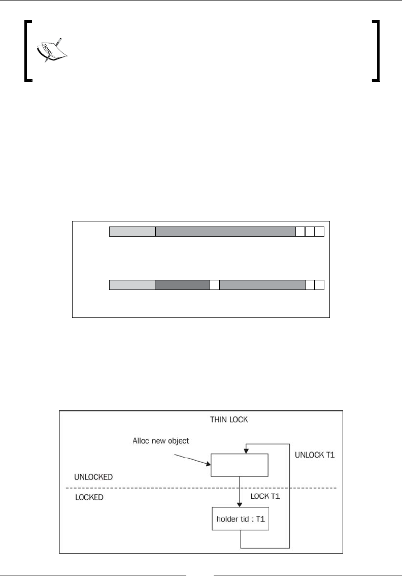
Threads and Synchronization
[ 144 ]
The lock word and object header layout described in this section
reects the current state of the implementation in JRockit R28 and
is subject to change without notice between releases. The bit-level
details are only introduced to further help explaining lock states
and their implementation.
In JRockit, every lock is assumed to be a thin lock when rst taken. The lock bits
of a thin locked object contain information about the thread that is holding the lock,
along with various extra information bits used for optimization. For example for
keeping track of the number of lock transfers between threads to determine if a
lock is mostly thread local, and thus mostly unnecessary.
A fat lock requires a JVM internal monitor to be allocated for lock and semaphore
queue management. Therefore, most of the space in the lock word for fat locks is
taken up by an index (handle) to the monitor structure.
Fat lock
Thin lock
8-bit GC
8-bit GC
21-bit Monitor index
7-bit transfers 14-bit Holder Thread ID
Forbid
mLock
n/a
1
0
n/a
The JRockit lock bits are one example of an implementation of helper data structures
for thin and fat locks, but of course both object header layout and contents vary
between different vendors' JVM implementations. The various state diagrams that
follow, go into some more detail on how thin locks and fat locks are converted to
each other in JRockit and how lock words are affected by the state transitions.
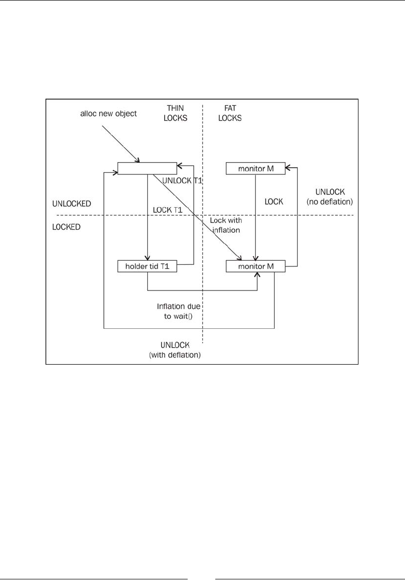
Chapter 4
[ 145 ]
The previous gure shows the relatively simple transitions between a locked and
unlocked state if only thin locks are involved. An unlocked object is locked when
thread T1 executes a successful lock on the object. The lock word in the object header
now contains the thread ID of the lock taker and the object is agged as thin locked.
As soon as T1 executes an unlock, the object reverts back to unlocked state and the
lock holder bits are zeroed out in the object header.
If we add fat locks to the picture, things get a little bit more complex. Recollect that
a thin lock can be inated into a fat lock if it is determined that it is too contended
or if a call to wait is applied to it, such as a call to wait. The object can go directly to
fat locked if thread T1 attempts to acquire it and it is known to be contended. There
is also a path from the thin locked version of the lock to the fat locked version in the
event of a wait call. As a fat lock keeps its allocated JVM internal monitor, along
with the handle to it, in the lock word, unlocking a fat lock without nding the
need to deate it will retain the monitor ID in the lock word, reusing the
monitor structure.
The section on Pitfalls and false optimizations later in this chapter will further discuss
how the runtime adaptively turns thin locks and fat locks into one another using
contention based heuristics.

Threads and Synchronization
[ 146 ]
The Java bytecode implementation
Java bytecode denes two opcodes for controlling synchronization—monitorenter
and monitorexit. They both pop a monitor object from the execution stack as their
only operand. The opcodes monitorenter and monitorexit are generated by
javac when there are synchronized regions with explicit monitor objects in the
code. Consider the following short Java method that synchronizes on an implicit
monitor object, in this case this, as it is an instance method:
public synchronized int multiply(int something) {
return something * this.somethingElse;
}
The bytecode consists of the seemingly simple sequence shown as follows:
public synchronized int multiply(int);
Code:
0: iload_1
1: aload_0
2: getfield #2; //Field somethingElse:I
5: imul
6: ireturn
Here, the runtime or JIT compiler has to check that the method is synchronized by
examining an access ag set for this particular method in the .class le. Recollect
that a synchronized method has no explicit monitor, but in instance methods this
is used and in static methods a unique object representing the class of the object is
used. So, the earlier source code is trivially equivalent to:
public int multiply(int something) {
synchronized(this) {
return something * this.somethingElse;
}
}
But, the previous code compiles to this rather more complex sequence:
public int multiply(int);
Code:
0: aload_0
1: dup
2: astore_2
3: monitorenter

Chapter 4
[ 147 ]
4: iload_1
5: aload_0
6: getfield #2; //Field somethingElse:I
9: imul
10: aload_2
11: monitorexit
12: ireturn
13: astore_3
14: aload_2
15: monitorexit
16: aload_3
17: athrow
Exception table:
from to target type
4 12 13 any
13 16 13 any
What javac has done here, except for generating monitorenter and monitorexit
instructions for this, is that it has added a generic catch-all try block for the entire
code of the synchronized block, bytecode 4 to bytecode 9 in the previous example.
Upon any unhandled exception, control will go to bytecode 13, the catch block,
which will release the lock before re-throwing whatever exception was caught.
Compiler intervention in this fashion is the standard way of solving the issue of
unlocking a locked object when an exception occurs. Also notice that if there are
exceptions in the catch block from bytecode 13 to bytecode 16, it will use itself as the
catch-all, creating a cyclic construct that isn't possible to express in Java source code.
We explained the problems with this in Chapter 2.
Naturally, we could treat this as unstructured control ow, but as the recursive catch
is a common pattern, and as we don't want it to complicate control ow analysis, it is
treated specially by the JRockit compiler. Otherwise it would be considered obfuscated
code, and a number of optimizations would be forbidden from being done.
JRockit internally translates all methods with an implicit monitor object into methods
with an explicit one, similar to what is shown in the second part of example, in order
to avoid the special case with the synchronized ag.
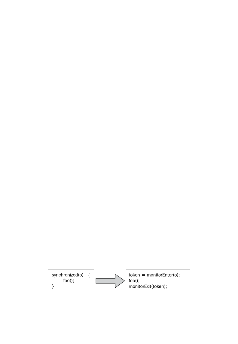
Threads and Synchronization
[ 148 ]
Lock pairing
Other than the previous bytecode issue there is a more serious one—monitorenter
and monitorexit are not paired. It is simple to generate weird bytecode where, for
example, a monitorexit is executed on an unlocked object. This would lead to an
IllegalMonitorStateException at runtime. However, bytecode where a lock is
taken in one method and then released in another is also possible (and perfectly legal
at runtime). The same applies to various many-to-many mappings of monitorenter
and monitorexit for the same lock. Neither of these constructs have Java source
code equivalents. The problem of the power of expression comes back to bite us.
For performance reasons, in a JIT compiler, it is very important to be able to identify
the matching lock for a particular unlock operation. The type of the lock determines
the unlock code that has to be executed. As we shall soon see, given even more kinds
of locks than just thin and fat ones, this becomes increasingly important. Sadly,
we cannot assume that locks are nicely paired, because of the non-symmetrical
semantics of the bytecode. Unpaired locks don't occur in ordinary bytecode and in
ordinary programs, but as it is possible, JRockit needs to be able to handle unpaired
synchronization constructs as well.
The JRockit code generator does control ow analysis upon method generation and
tries to match every monitorenter to its corresponding monitorexit instruction(s).
For structured bytecode that was compiled from Java source, this is almost always
possible (if we treat the anomalous catch produced by synchronized blocks as a
special case). The match is done when turning the stack-based metaphor into a
register-based one, piggybacking on the BC2HIR pass of the code generator, which,
as explained in Chapter 2, has to do control ow analysis anyway.
JRockit uses a mechanism called lock tokens to determine which monitorenter and
monitorexit instructions belong together. Each monitorenter is translated into an
instruction with a lock token destination. Its matching monitorexit is translated
into an instruction with that particular lock token as a source operand.
Following is a pseudocode example of the transformation of a Java synchronized
region to JRockit matched (or paired) locks:

Chapter 4
[ 149 ]
In the rare case that a monitorenter can't be mapped to a particular monitorexit,
JRockit tags these instructions with a special "unmatched" ag. While, this is still
supported by the runtime, and needs to be for full bytecode compliance, we shall
soon see that handling unmatched locks is orders of magnitude more expensive than
handling tokenized locks.
From a practical perspective, unmatched locks never occur in standard compiled
bytecode, but may show up in obfuscated code or as the result of various bytecode
prolers. Running JRockit with verbose code generator output (-Xverbose:codegen)
will display information about unmatched locks if they are detected. In JRockit
versions from R28, there is also special JRockit Flight Recorder event for unmatched
locks that can be used for performance proling. If unmatched locks show up in your
Java program, all performance bets are off. You probably need to get rid of them.
A special case, where lock pairing can never be done is in native code. Calls from
native code, accessed through JNI, to monitorenter and monitorexit equivalents
will always be treated as unmatched locks, as once the program is executing native
code, we have no control over the stack. However, JNI marshalling overhead, i.e.
executing the stub code to get from Java code to native code, is orders of magnitude
slower than taking locks anyway. So, the key to lock performance may lie elsewhere
if we enter and exit native code frequently.
So what is a lock token? JRockit implements a lock token as a reference to a monitor
object, the operand to monitorenter, with a couple of bits added at the end. As we
have seen in Chapter 3, objects are typically aligned on even addresses, in practice on 8
byte boundaries (or more for compressed references with larger heaps). So, we always
have the lowest bits of any object pointer available for storing arbitrary information.
Whenever any of the three lowest bits in an object pointer are non-zero, JRockit takes
this to mean that the object is used as a monitor, locked with a lock token. The seven
different possible non-zero bit congurations can be used to communicate different
information about the lock, for instance if it is thin, taken recursively by the same
thread, fat, or unmatched. Lock tokens can only exist in local stack frames, never on
the heap. Since JRockit doesn't use compressed references in local frames, we are
guaranteed to be able to claim the alignment bits of any object for token information.
Recollect from the previous chapter that all live registers at any given time are
explicitly determined by the compiler and stored as livemaps, metadata accessible to
the code generator. The same thing applies to lock tokens.

Threads and Synchronization
[ 150 ]
Trivially, because of the implicit lock pairing in structured Java code, one lock
cannot be released before another one, taken inside that lock. It is easy to look at an
object in a livemap and determine whether it is a lock token or not, but in order to
be able to unlock tokens in the correct order upon, for example, an exception being
thrown, nesting information is required as well. If many locks are taken when an
exception occurs, the runtime needs to know the order in which they were locked.
Consequently, the livemap system also provides the nesting order of lock tokens.
For unmatched unlocks, an expensive stack walk is required in order to discover the
matching lock operation and update the lock state in its lock token reference. The
JVM needs to look for it on all previous frames on the stack. This requires stopping
the world and is several orders of magnitude slower than with perfect lock pairing
that can be immediately handled by modifying a lock token on the local stack frame.
Luckily, unmatched locks are rare. No code that is compiled with javac is likely to
contain unmatched locks.
Implementing threads
This section briey covers some different types of thread implementations. It is fairly
brief, as unmodied OS threads are the preferred way of implementing threads in a
JVM these days.
Green threads
Green threads usually refers to implementing threads with some kind of multiplexing
algorithm, using one OS thread to represent several or all Java threads in the JVM. This
requires that the runtime handle the thread scheduling for the Java threads inside the
OS thread. The advantages to using green threads is that the overhead is a lot smaller
than for OS threads when it comes to things like context switches and starting a new
thread. Many early JVMs tended to favor some kind of green thread approach.
However, aside from the added complexity of having to implement lifecycle and
scheduling code for the green threads, there is also the intrinsic problem of Java
native code. If a green thread goes into native code that then blocks on the OS level,
the entire OS thread containing all the green threads will be suspended. This most
likely causes a deadlock issue by preventing any other Java thread contained in the
same OS thread from running. So, a mechanism for detecting this is needed. Early
versions of JRockit used green threads and solved the OS-level suspension problem
with a mechanism called renegade threads, basically branching off a native thread
from the main OS thread whenever a native operation was to be performed. If this
happened frequently, the green thread model incrementally turned into a model
where Java threads were one-to-one mapped to OS threads.

Chapter 4
[ 151 ]
N x M threads
A variety of the green thread approach is to use several OS threads that in turn
represent several green threads—sort of a hybrid solution. This is referred to as
an n x m thread model. This can somewhat alleviate the green thread problem of
blocking in native code.
In the early days of server-side Java, certain kinds of applications lent themselves
well to this model—applications where thread scalability and low thread start
overhead was everything. Several of the rst paying JRockit customers had setups
with the need for a very large number of concurrent threads and for low thread
creation overhead, the prime example being chat servers. JRockit 1.0 used the n
x m model and was able to provide massive performance increases in these very
specialized domains.
As time went by and Java applications grew more complex, the added complexity of
multiplexing virtual threads on OS threads, the common reliance on native code, and
the renement of other techniques such as more efcient synchronization, made the
n x m approach obsolete.
To our knowledge, no modern server-side JVM still uses a thread implementation
based on green threads. Because of their intrinsic simplicity and the issues
mentioned earlier, OS threads are the preferred way of representing Java threads.
OS threads
Naturally, the most obvious implementation of a java.lang.Thread is to use an
underlying operating system thread, for example a POSIX thread on *NIX, one-to-
one-mapped against each java.lang.Thread object. This has the advantage that
most of the semantics are similar and little extra work needs to be done. Thread
scheduling can also be outsourced to the operating system.
This is the most common approach and as far as we know, it is used in all modern
JVM implementations. Other approaches often aren't worth the complexity anymore,
at least not for standard server-side applications. In, for example, embedded
environments, it may still make sense to use other approaches, but then, on the
other hand, implementation space is constrained.

Threads and Synchronization
[ 152 ]
Thread pooling
If we can rely on threads being OS threads, optimization techniques with slightly
bad reputations, such as thread pooling, also make a certain amount of sense. The
creation and starting of OS threads introduces a signicantly larger overhead than
if the VM uses some kind of green thread model. Under special circumstances, in
a java.lang.Thread implementation based on OS threads, it might make sense to
reuse existing thread objects in a Java program, to try to reduce this overhead. This
is typically done by keeping nished threads in a thread pool and reusing them
for new tasks instead of allocating new threads. The authors of this book generally
frown upon trying to outsmart the JVM, but this is a case where it might sometimes
pay off. However, serious proling should be done before trying thread pooling to
determine if it is really necessary.
Also, if the underlying thread implementation is not using pure OS threads,
thread pooling may be disruptive and counterproductive. In a green thread
model, starting a thread is extremely cheap. While to our knowledge no other
JVM thread implementation than OS threads exists today, Java is still supposed
to be a platform-independent language. So, proceed with caution.
Optimizing threads and synchronization
This section discusses how threads and synchronization can be optimized in an
adaptive runtime environment.
Lock ination and lock deation
As was mentioned when the different types of locks were introduced, one of the
most important optimizations in an adaptive runtime is the ability to convert
thin locks to fat locks and vice versa, depending on load and contention. Both the
code generator and the lock implementation will attempt to solve this problem as
efciently as possible.
In an adaptive environment, the runtime has the benet of free lock proling
information (at least a small amount of free lock proling information, as, we shall see,
doing complete in-depth lock proling incurs some runtime overhead). Whenever a
lock is taken or released, information can be logged about who is trying to get the lock
and how many times it has been contended. So, if a single thread has failed to acquire
a thin lock in too many subsequent attempts, it makes good sense for the virtual
machine to convert it to a fat lock. The fat lock is better suited for handling contention,
in that waiting threads sleep instead of spin and therefore use less CPU cycles. We
refer to the practice of converting a thin lock to a fat lock as lock ination.

Chapter 4
[ 153 ]
JRockit, by default, also uses a small spinlock to implement a fat
lock while it has been recently inated and held only for a very
short time. This might seem counterintuitive, but is generally
benecial. This behavior can be turned off from the command
line (with the ag –XX:UseFatSpin=false), if deemed too
slow—for example, in an environment with highly contended
locks with long waiting periods. The spinlock that is part of
the fat lock can also be made adaptive and based on runtime
feedback. This is turned off by default, but can be enabled with
the command-line ag –XX:UseAdaptiveFatSpin=true.
In the same manner, when many subsequent unlocks of a fat lock have been done
without any other thread being queued on its lock or wait queue, it makes sense to
turn the fat lock into a thin lock again. We refer to this as lock deation.
JRockit uses heuristics to perform both ination and deation, thus adapting to the
changed behavior of a given program where, for example, locks that were contended
in the beginning of program execution stop being contended. Then these locks are
candidates for deation.
The heuristics that trigger transitions between thin and fat locks can be overridden and
modied from the command line if needed, but this is generally not recommended.
The next chapter will briey discuss how to do this.
Recursive locking
It is permissible, though unnecessary, for the same thread to lock the same object
several times, also known as recursive locking. Code that does so occurs, for
example, where inlining has taken place or in a recursive synchronized method.
Then the code generator may remove the inner locks completely, if no unsafe code
exists within the critical section, (such as volatile accesses or escaping calls between
the inner and outer locks).
This can be combined with optimizing for the recursive lock case. JRockit uses a
special lock token bit conguration to identify recursive locks. As long as a lock
has been taken at least twice by one thread without rst being released, it is tagged
as recursive. So, forced unlock operations upon exceptions can still be correctly
implemented, resetting the recursion count to the correct state, with no extra
synchronization overhead.

Threads and Synchronization
[ 154 ]
Lock fusion
The JRockit optimizing JIT compiler also uses a code optimization called lock fusion
(sometimes also referred to as lock coarsening in literature). When inlining plenty of
code, especially synchronized methods, the observation can be made that frequent
sequential locks and unlocks with the same monitor object are common.
Consider code that, after inlining, looks like:
synchronized(x) {
//Do something...
}
//Short snippet of code...
x = y;
synchronized(y) {
//Do something else...
}
Classic alias analysis by the compiler trivially gives us that x and y are the same object.
If the short piece of code between the synchronized blocks carries little execution
overhead, less than the overhead of releasing and reacquiring the lock, it is benecial
to let the code generator fuse the lock regions into one.
synchronized(x) {
//Do something...
//Short snippet of code...
x = y;
//Do something else...
}
Additional requirements are of course that there are no escaping or volatile
operations in the code between the synchronized blocks, or the Java Memory Model
semantics for equivalence would be violated. There are of course a few other code
optimization issues that have to be handled that are beyond the scope of this chapter.
An example would be that any exception handlers for the regions that are to be fused
need to be compatible.
Naturally, it might not be benecial just to fuse every block of code we see, but we
can avoid some overhead if the blocks to fuse are picked cleverly. And if enough
sampling information is available for the short snippet of code, we can make clever
adaptive guesses to whether a lock fusion would be benecial or not.

Chapter 4
[ 155 ]
To summarize, this code optimization all boils down to not releasing a lock
unnecessarily. The thread system itself can, by making its state machine a little
bit more complicated, implement a similar optimization, independent of the code
generator, known as lazy unlocking.
Lazy unlocking
So what does the previous observation really mean, if it can be showed that there
are many instances of thread local unlocks and re-locks that simply slow down
execution? Perhaps this is the case almost all the time? Perhaps the runtime should
start assuming that each individual unlock operation is actually not needed?
This gamble will succeed each time the lock is reacquired by the same thread, almost
immediately after release. It will fail as soon as another thread tries to acquire the
seemingly unlocked object, which semantics must allow it to do. Then the original
thread will need to have the lock forcefully unlocked in order to make it seem as if
"nothing has happened". We refer to this practice as lazy unlocking (also referred
to as biased locking in some literature).
Even in the case that there is no contention on a lock, the actual process of
acquiring and releasing the lock is expensive compared to doing nothing at all.
Atomic instructions incur overhead to all Java execution in their vicinity.
In Java, sometimes it is reasonable to assume that most locks are thread local.
Third-party code often uses synchronization unnecessarily for a local application,
as the authors of third-party libraries cannot be sure if the code is to run in a parallel
environment or not. They need to be safe unless it is explicitly specied that thread
safety is not supported. There are plentiful examples of this in the JDK alone, for
example the java.util.Vector class. If the programmer needs vector abstraction
for a thread local application, he might pick java.util.Vector for convenience, not
thinking about its inherent synchronization, when java.util.ArrayList virtually
performs the same job but is unsynchronized.
It seems sensible that if we assume most locks are thread local and never shared, we
would gain performance in such cases, taking a lazy unlocking approach. As always,
we have a trade off—if another thread needs to acquire a lazy unlocked object, more
overhead is introduced than in a non-lazy model, as the seemingly free object must
be located and released.
It seems reasonable to assume that, as an overall approach, always gambling that
an unlock won't be needed, isn't such a safe bet. We need to optimize for several
different runtime behaviors.

Threads and Synchronization
[ 156 ]
Implementation
The semantics of a lazy unlocking implementation are fairly simple.
For the lock operation, monitorenter:
• If the object is unlocked, the thread that locks the object will reserve the lock,
tagging the object as lazily locked.
• If the object is already tagged as lazily locked:
° If the lock is wanted by the same thread, do nothing (in
principle a recursive lock).
° If the lock is wanted by another thread, we need to stop the
thread holding the lock, detect the "real" locking state of
the object, i.e. is it locked or unlocked. This is done with an
expensive stack walk. If the object is locked, it is converted to
a thin lock, otherwise it is forcefully unlocked so that it can be
acquired by the new thread.
For the unlock operation, monitorexit:
• Do nothing for a lazily locked object and leave the object in a locked state,
that is, perform lazy unlocking.
In order to revoke a reservation for a thread that wants the lock, the thread that did
the reservation needs to be stopped. This is extremely expensive. The actual state of
the lock to be released is determined by inspecting the thread stack for lock tokens.
This is similar to the approach of handling unmatched locks described earlier. Lazy
unlocking uses a lock token of its own, whose bit conguration means "this object is
lazily locked".
If we never had to revert a lazy locked object, that is if all our locks are in fact thread
local, all would be well and we would see immense performance gains. In the real
world, however, we cannot afford to take the very steep penalty of releasing lazy
locked objects time and time again, if our guess proves to be wrong. So, we have to
keep track of the number of times a lazy lock is transferred between threads—the
number of penalties incurred. This information is stored in the lock word of the
monitor object in the so called transfer bits.
If the number of transfers between threads is too large, a particular object or its entire
type (class) and all its instances can be forbidden from further lazy locking and will
just be locked and unlocked normally using standard thin and fat lock mechanisms.
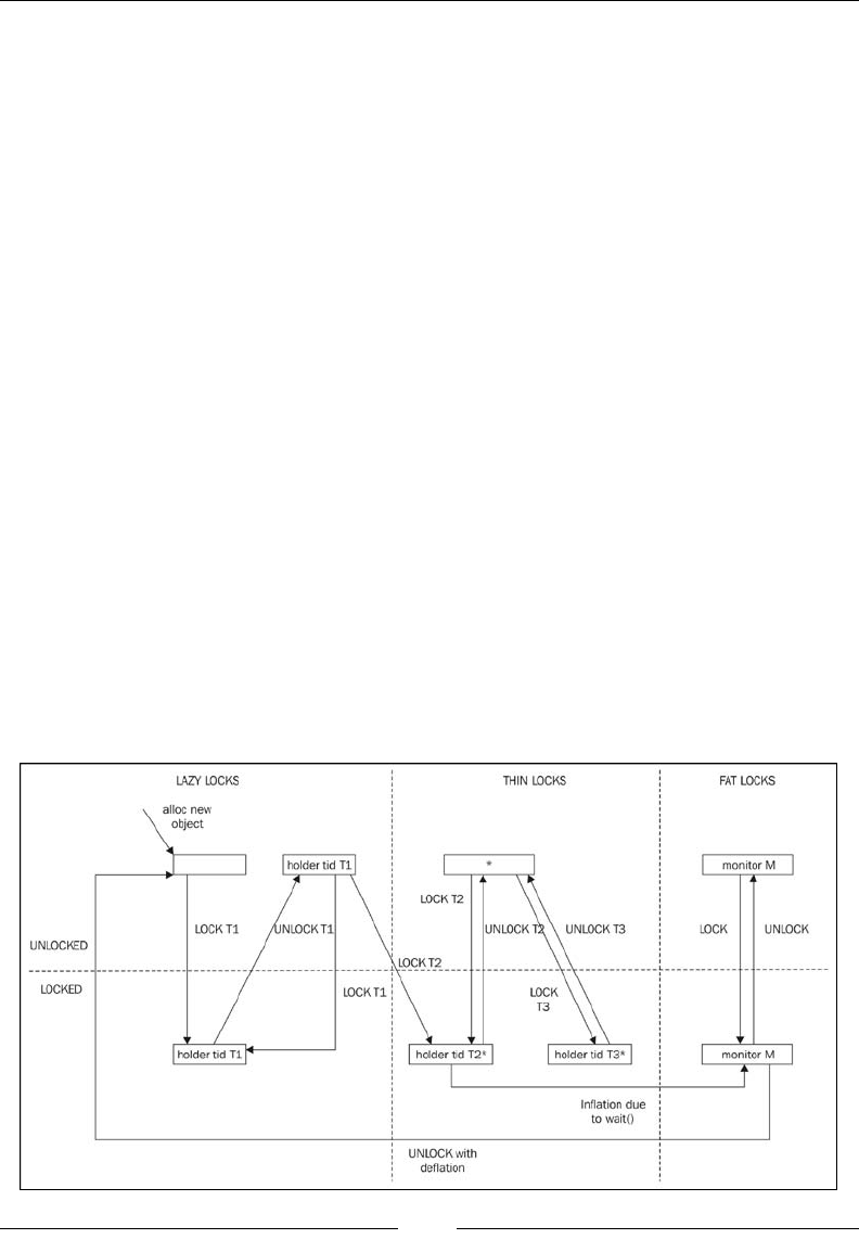
Chapter 4
[ 157 ]
Object banning
When a transfer limit is hit, the forbid bit in a JRockit object lock word is set. This bit
indicates that a specic object instance is unsuitable for lazy unlocking. If the forbid
bit is set in an object header, this particular object cannot be used for lazy unlocking
ever again.
Also, if a lock is contended, regardless of other settings, lazy unlocking is
immediately banned for its monitor object.
Further locking on a banned object will behave as ordinary thin and fat locks.
Class banning
Just banning certain instances from being used in lazy unlocking may not be enough.
Several objects of the same type often use locks similarly. Thus an entire class can
be tagged so that none of its instances can be subject to lazy unlocking. If too many
instances of a class are banned or too many transfers take place for instances of a
class, the entire class is banned.
A dynamic twist to class bans and object bans can be introduced by letting the bans
"age"—the runtime system gets a new chance to retry lazy unlocking with a certain
object if a signicant amount of time has been spent since the last ban. If we end up
with the same ban in effect again, the aging can be set to be restarted, but run more
slowly, or the ban can be made permanent.
The following gure tries to better illustrate the complexities of states involved in
lazy unlocking:

Threads and Synchronization
[ 158 ]
Now, we have three lock domains, as opposed to two (thin and fat) shown in the
state graphs earlier in this chapter. The new domain "lazy" is added, which is where
locking of hitherto unseen objects starts—we hope our "gamble" that locks are mostly
thread local pays off.
Just as before, starting at the unlocked, previously untouched object, a monitorenter
by thread T1 will transition it to lazy locked state (just as with the thin locked state
before). However, if T1 performs a monitorexit on the object, it will pretend to be
unlocked, but really remain in a locked state, with the thread ID for T1 still agging
ownership in the lock bits. Subsequent locks by T1 will then be no-ops.
If another thread, T2 now tries to lock the object, we need to respect that, take the
penalty for our erroneous guess that the lock was taken mostly by T1, ush out T1
from the thread ID bits and replace them with T2. If this happens often enough, the
object may be subject to banning from lazy unlocking and then we must transfer the
object to a normal thin locked state. Pretending that this was the case with the rst
monitorenter T2 did on our object, this moves the state diagram to the familiar
thin locked domain. Objects that are banned from lazy unlocking in the gure
are denoted by (*). If thread T3 tries to lock a banned (but unlocked) object,
we notice that we remain in the thin locked section of the picture. No lazy
unlocking is allowed.
In similar fashion as before, thin locks are inated to fat locks if they get contended
or their objects are used with wait / notify, which requires wait queues. This is true
for objects in the lazy domain as well.
Results
Most commercial JVM implementations maintain some kind of mechanism for lazy
unlocking. Somewhat cynically, this may have its origin in the popular SPECjbb2005
benchmark, which has many thread local locks and where small optimization efforts
towards hanging on to locks result in huge performance gains.
SPEC and the benchmark name SPECjbb2005 are trademarks
of the Standard Performance Evaluation Corporation.
However, there are also several real-world applications, for example, application
servers where it turns out that lazy unlocking can deliver performance. This is just
because the sheer complexity and many abstraction layers has made it hard for
developers to see if synchronization across threads needs be used at all.

Chapter 4
[ 159 ]
Some versions of JRockit, such as the x86 implementation running JDK 1.6.0, come
with lazy unlocking and banning heuristics enabled out of the box. This can be
turned off from the command line if needed. To nd out if a particular shipment of
JRockit uses lazy unlocking as a default option, please consult the section on locks in
the JRockit documentation.
Pitfalls and false optimizations
As in previous chapters, we will nish up with a discussion of obvious
caveats. This section discusses things to be aware of when working with threads
and synchronization in Java.
Thread.stop, Thread.resume and Thread.
suspend
The single most dangerous part of the Java thread API, are the methods in the java.
lang.Thread class called stop, resume, and suspend. They were included in Java
1.0, but immediately found unsafe and deprecated. This however, was a bit too late,
and, even today, they are widely used both in legacy code and new applications,
despite the deprecation warnings. We are sad to report that we've come across them
in commercial code that was developed as late as 2008.
The stop method (meant to halt the execution of a thread) is unsafe. This is because
stopping the execution of a thread that is modifying global data would possibly
leave the global data in an inconsistent, broken state. A thread that receives a stop
signal will unlock all of the locks that it was holding, thus making the data under
modication by these locks briey visible to the rest of the world, which violates
the Java sandbox model.
Stopping threads should instead be handled by wait / notify or (volatile) variables,
properly synchronized when this needs to be the case.
What about suspension? Suspending a thread is inherently deadlock prone. That is,
if a thread is holding a lock and then is suspended, no other thread can access the
resource protected by the lock until the suspended thread is resumed. If the thread
responsible for the resume call, waking up the suspended thread, tries to acquire that
lock, a deadlock will occur. Thus, Thread.resume and Thread.suspend are deemed
too dangerous to leave to the user and were deprecated as well.
Consequently, never use Thread.stop, Thread.resume or Thread.suspend in any
program and be aware of their issues when working with legacy code.

Threads and Synchronization
[ 160 ]
Double checked locking
Lack of understanding of the underlying memory model and CPU architecture, can
cause trouble in the highest levels of platform-independent Java as well. Consider
the following thread safe code that returns a singleton object, instantiated once only
upon demand:
public class GadgetHolder {
private Gadget theGadget;
public synchronized Gadget getGadget() {
if (this.theGadget == null) {
this.theGadget = new Gadget();
}
return this.theGadget;
}
}
The previous example works ne for multiple threads, as the method is synchronized,
using the GadgetHolder instance itself as the monitor. However, when the Gadget
constructor has run once, further synchronization might seem unnecessary and
expensive. Therefore, one might be tempted to optimize the method as:
public Gadget getGadget() {
if (this.theGadget == null) {
synchronized(this) {
if (this.theGadget == null) {
this.theGadget = new Gadget();
}
}
}
return this.theGadget;
}
The previous optimization might seem like a clever trick. If the object exists, which
will be the usual case, we can return it immediately without synchronization.
The singleton instantiation is still synchronized, including the original null check,
retaining thread safety.
The problem here is that we have created a common anti-pattern known as double
checked locking. Now, one thread can start initializing the Gadget eld upon
completing the inner null check in the synchronization. This thread might start
allocating and writing the object to the Gadget eld, which may well be a non-atomic
process, containing several writes to memory without guaranteed ordering. If this
Chapter 4
[ 161 ]
happens in the middle of a context switch, another thread can come in, see the partially
written object in the eld and thus fail the rst null check. Then the partially allocated
object may be returned. The same thing can happen not just with objects, but with
other eld types as well. For example, longs on a 32-bit platform often need to
be initialized by two 32-bit writes to memory. A 32-bit int, on the other hand
(just one memory write on initialization) would slip past the trap.
The problem may, though only in the new version of the Java Memory Model, be
gotten around by declaring the theGadget eld volatile, but this incurs overhead
anyway. Possibly less overhead than the original synchronization, but still overhead.
For clarity, and because underlying memory model implementations may not be
correct, double checked locking should be avoided! There are several good web
pages explaining why double checked locking should be considered an anti-pattern
in several languages, not just Java.
The danger with problems like this is that on strong memory models
they rarely break down. Intel IA-64 deployment is a typical real-world
scenario where Java applications that previously have been running
awlessly start malfunctioning. Intel IA-64 has a notoriously weak
memory model. It is all too easy to suspect a bug in the JVM instead of
in the Java program if it runs ne on x86 but breaks on IA-64.
For static singletons, initialization can be performed with initialize on demand,
providing the same semantics and avoiding double checked locking.
public class GadgetMaker {
public static Gadget theGadget = new Gadget();
}
Java guarantees that the class initialization is atomic, and as the GadgetMaker class
has no other contents, theGadget will always be atomically assigned when the class
is rst referenced. This works both in the old and the new memory model.
In conclusion, there are plenty of caveats when programming parallel Java, but most
of them can be avoided by understanding the Java Memory Model. Furthermore,
even if you don't care about the underlying hardware, not understanding the Java
Memory Model can still be a sure way of shooting yourself in the foot.

Threads and Synchronization
[ 162 ]
JRockit ags
This section covers the most important command-line ags that can be used to
control and instrument JRockit lock behavior.
While plenty of information can be gleaned from log les using some of these ags,
synchronization is a complex business and the preferred and best way to visualize
multithreaded behavior is through the JRockit Mission Control suite.
Examining locks and lazy unlocking
This section explains the most important ags for studying and manipulating
lock behavior.
Lock details from -Xverbose:locks
This ag makes JRockit report information related to synchronization in the running
program. Most of the information that the –Xverbose:locks ag produces has to
do with the lazy unlocking optimization. This is a good way to see, for example,
which types and objects are temporarily or permanently banned for lazy unlocking,
or if lazy unlocking performs as efciently as it should, without having to revert its
assumptions all the time.
Following is a sample output from –Xverbose:locks. We can see that lazy
unlocking is determined inappropriate for a couple of classes, whose instances
are competed for by different threads. These classes are banned from further
lazy unlocking.
hastur:SPECjbb2005 marcus$ java -Xverbose:locks -cp jbb.jar:check.
jar spec.jbb.JBBmain -propfile SPECjbb.props >/dev/null
[INFO ][locks ] Lazy unlocking enabled
[INFO ][locks ] No of CPUs: 8
[INFO ][locks ] Banning spec/jbb/Customer for lazy unlocking.
(forbidden 6 times, limit is 5)
[INFO ][locks ] Banning spec/jbb/Address for lazy unlocking.
(forbidden 6 times, limit is 5)
[INFO ][locks ] Banning java/lang/Object for lazy unlocking.
(forbidden 5 times, limit is 5)
[INFO ][locks ] Banning spec/jbb/TimerData for lazy unlocking.
(forbidden 6 times, limit is 5)
[INFO ][locks ] Banning spec/jbb/District for lazy unlocking.
(forbidden 6 times, limit is 5)

Chapter 4
[ 163 ]
Controlling lazy unlocking with
–XX:UseLazyUnlocking
Depending on the platform and JRockit version, lazy unlocking may or may not be
enabled out of the box. Please refer to the JRockit Documentation to nd out what
applies to a particular platform or study the output from –Xverbose:locks. Given
that adaptive reversion strategies form part of the lazy unlocking algorithm, it is
more often the case than not, that when enabled, lazy unlocking will contribute to
increased performance.
The default lazy unlocking behavior can be overridden with the ag:
-XX:UseLazyUnlocking=false or –XX:UseLazyUnlocking=true.
Finally, -Xverbose:codegen will, as mentioned earlier in the chapter, output warnings
for any method where the compiler failed to create matched locks and unlocks.
Using SIGQUIT or Ctrl-Break for Stack Traces
Issuing a SIGQUIT signal to a JRockit process, typically by executing kill –QUIT
<PID> or kill -3 <PID> in *NIX environments or by pressing Ctrl-Break in a console
window on Windows, will dump complete stack traces (where available) for all the
threads in the JVM, both native and Java threads. The locks taken by the threads
are also displayed, along with their types. This is a "poor man's way" of quickly
detecting deadlocks, by nding out if a thread is waiting for a resource held by
another suspended thread.
Following is an example thread dump including lock holders, what type of lock they
are holding and where on the execution stacks the locks were taken:
===== FULL THREAD DUMP ===============
Tue Jun 02 14:36:39 2009
BEA JRockit(R) R27.6.3-40_o-112056-1.6.0_11-20090318-2104-windows-ia32
"Main Thread" id=1 idx=0x4 tid=4220 prio=5 alive,
in native, sleeping, native_waiting
at java/lang/Thread.sleep(J)V(Native Method)
at spec/jbb/JBButil.SecondsToSleep(J)V(Unknown Source)
at spec/jbb/Company.displayResultTotals(Z)V(Unknown Source)
at spec/jbb/JBBmain.DoARun(Lspec/jbb/Company;SII)V(Unknown Source)
at spec/jbb/JBBmain.runWarehouse(IIF)Z(Unknown Source)
at spec/jbb/JBBmain.doIt()V(Unknown Source)
at spec/jbb/JBBmain.main([Ljava/lang/String;)V(Unknown Source)
at jrockit/vm/RNI.c2java(IIIII)V(Native Method)
-- end of trace

Threads and Synchronization
[ 164 ]
"(Signal Handler)" id=2 idx=0x8 tid=1236 prio=5 alive, in native, daemon
"(GC Main Thread)" id=3 idx=0xc tid=5956 prio=5 alive,
in native, native_waiting, daemon
"(GC Worker Thread 1)" id=? idx=0x10 tid=5884 prio=5 alive,
in native, daemon
"(GC Worker Thread 2)" id=? idx=0x14 tid=3440 prio=5 alive,
in native, daemon
"(GC Worker Thread 3)" id=? idx=0x18 tid=4744 prio=5 alive,
in native, daemon
"(GC Worker Thread 4)" id=? idx=0x1c tid=5304 prio=5 alive,
in native, daemon
"(GC Worker Thread 5)" id=? idx=0x20 tid=5024 prio=5 alive,
in native, daemon
"(GC Worker Thread 6)" id=? idx=0x24 tid=3632 prio=5 alive,
in native, daemon
"(GC Worker Thread 7)" id=? idx=0x28 tid=1924 prio=5 alive,
in native, daemon
"(GC Worker Thread 8)" id=? idx=0x2c tid=5144 prio=5 alive,
in native, daemon
"(Code Generation Thread 1)" id=4 idx=0x30 tid=3956 prio=5 alive,
in native, native_waiting, daemon
"(Code Optimization Thread 1)" id=5 idx=0x34 tid=4268 prio=5 alive,
in native, native_waiting, daemon
"(VM Periodic Task)" id=6 idx=0x38 tid=6068 prio=10 alive,
in native, native_blocked, daemon
"(Attach Listener)" id=7 idx=0x3c tid=6076 prio=5 alive,
in native, daemon
...
"Thread-7" id=18 idx=0x64 tid=4428 prio=5 alive
at spec/jbb/infra/Util/TransactionLogBuffer.privText
(Ljava/lang/String;IIIS)V(UnknownSource)[optimized]
at spec/jbb/infra/Util/TransactionLogBuffer.putText
(Ljava/lang/String;IIIS)V(Unknown Source)[inlined]
at spec/jbb/infra/Util/TransactionLogBuffer.putDollars
(Ljava/math/BigDecimal;III)V(Unknown Source)[optimized]
at spec/jbb/NewOrderTransaction.processTransactionLog()
V(Unknown Source)[optimized]
^-- Holding lock: spec/jbb/NewOrderTransaction@0x0D674030[biased lock]
at spec/jbb/TransactionManager.runTxn(Lspec/jbb/Transaction;JJD)
J(Unknown Source)[inlined]
at spec/jbb/TransactionManager.goManual(ILspec/jbb/TimerData;)
J(Unknown Source)[optimized]

Chapter 4
[ 165 ]
at spec/jbb/TransactionManager.go()V(Unknown Source)[optimized]
at spec/jbb/JBBmain.run()V(Unknown Source)[optimized]
at java/lang/Thread.run(Thread.java:619)[optimized]
at jrockit/vm/RNI.c2java(IIIII)V(Native Method)
-- end of trace
"Thread-8" id=19 idx=0x68 tid=5784 prio=5 alive,
in native, native_blocked
at jrockit/vm/Locks.checkLazyLocked(Ljava/lang/Object;)
I(Native Method)
at jrockit/vm/Locks.monitorEnterSecondStage(Locks.java:1225)
at spec/jbb/Stock.getQuantity()I(Unknown Source)[inlined]
at spec/jbb/Orderline.process(Lspec/jbb/Item;Lspec/jbb/Stock;)
V(Unknown Source)[optimized]
at spec/jbb/Orderline.validateAndProcess(Lspec/jbb/Warehouse;)
Z(Unknown Source)[inlined]
at spec/jbb/Order.processLines(Lspec/jbb/Warehouse;SZ)
Z(Unknown Source)[inlined]
at spec/jbb/NewOrderTransaction.process()Z(Unknown Source)[optimized]
^-- Holding lock: spec/jbb/Orderline@0x09575D00[biased lock]
^-- Holding lock: spec/jbb/Order@0x05DDB4E8[biased lock]
at spec/jbb/TransactionManager.runTxn(Lspec/jbb/Transaction;JJD)
J(Unknown Source)[inlined]
at spec/jbb/TransactionManager.goManual(ILspec/jbb/TimerData;)
J(Unknown Source)[optimized]
at spec/jbb/TransactionManager.go()V(Unknown Source)[optimized]
at spec/jbb/JBBmain.run()V(Unknown Source)[optimized]
at java/lang/Thread.run(Thread.java:619)[optimized]
at jrockit/vm/RNI.c2java(IIIII)V(Native Method)
-- end of trace
"Thread-9" id=20 idx=0x6c tid=3296 prio=5 alive,
in native, native_blocked
at jrockit/vm/Locks.checkLazyLocked(Ljava/lang/Object;)
I(Native Method)
at jrockit/vm/Locks.monitorEnterSecondStage(Locks.java:1225)
at spec/jbb/Stock.getQuantity()I(Unknown Source)[inlined]
at spec/jbb/Orderline.process(Lspec/jbb/Item;Lspec/jbb/Stock;)
V(Unknown Source)[optimized]

Threads and Synchronization
[ 166 ]
at spec/jbb/Orderline.validateAndProcess(Lspec/jbb/Warehouse;)
Z(Unknown Source)[inlined]
at spec/jbb/Order.processLines(Lspec/jbb/Warehouse;SZ)
Z(Unknown Source)[inlined]
at spec/jbb/NewOrderTransaction.process()Z(Unknown Source)[optimized]
^-- Holding lock: spec/jbb/Orderline@0x09736E10[biased lock]
^-- Holding lock: spec/jbb/Order@0x09736958[biased lock]
at spec/jbb/TransactionManager.runTxn(Lspec/jbb/Transaction;JJD)
J(Unknown Source)[inlined]
at spec/jbb/TransactionManager.goManual(ILspec/jbb/TimerData;)
J(Unknown Source)[optimized]
at spec/jbb/TransactionManager.go()V(Unknown Source)[optimized]
at spec/jbb/JBBmain.run()V(Unknown Source)[optimized]
at java/lang/Thread.run(Thread.java:619)[optimized]
===== END OF THREAD DUMP ===============
Lock proling
JRockit can produce extensive proling information about each lock in a running
program at the cost of some overhead. Typically, running with lock proling adds
about three percent or possibly more to the total runtime, depending heavily on
the application.
For more information about analyzing lock proling info, please see the chapters on
JRockit Mission Control.
Enabling lock proling with -XX:UseLockProling
For more extensive information about where a Java application spends its time, the
ag –XX:UseLockProfiling=true can be used. This will instrument all locks and
unlocks in the Java program and store information under which condition it was
taken and the number of times it has been in use. Lock proling can be augmented
with information on native locks inside the JVM, such as code buffer locks or locks
taken by the garbage collector. In order to get this information as well, use the
ag –XX:UseNativeLockProfiling=true.
JRockit Mission Control can be used to analyze any JRockit Flight Recording with
lock proling information. Any lock in the Java program (or JVM) can be studied
in detail, revealing, for example, how many times it was thin, fat, contended, lazily
reserved, recursive, and so on.
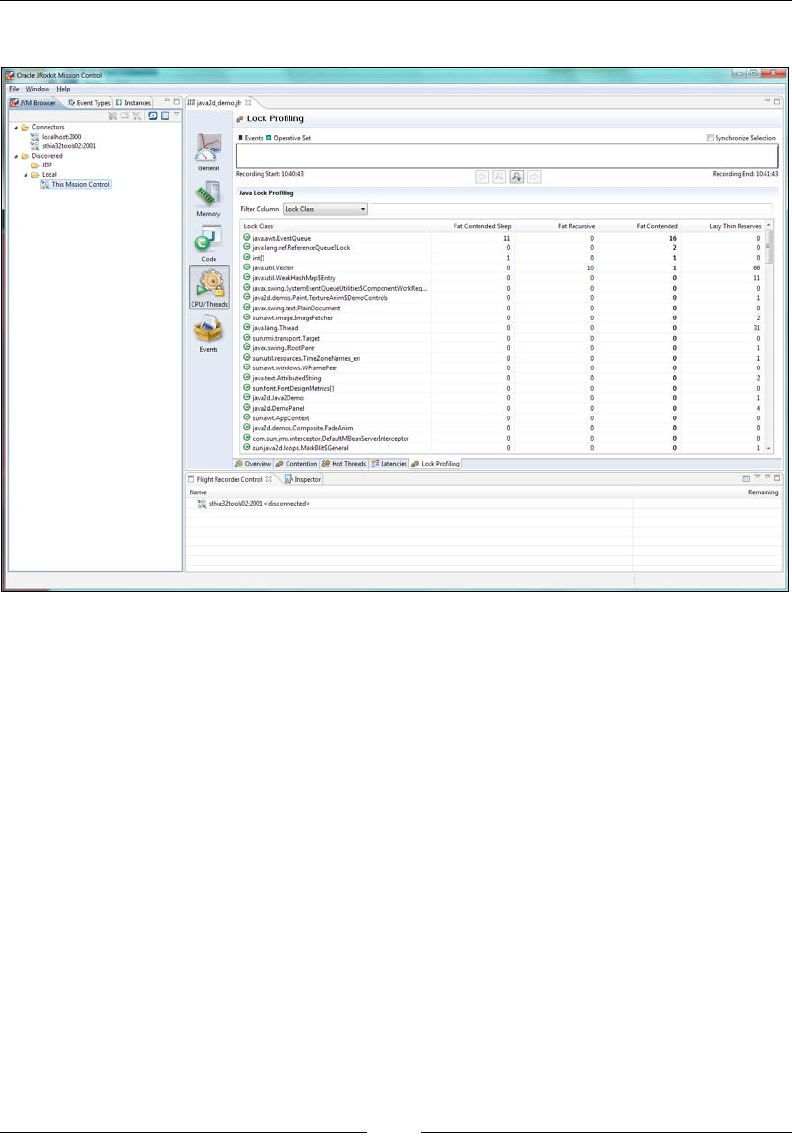
Chapter 4
[ 167 ]
Following is a screenshot of the lock proling tab in JRockit Mission Control:
For further information about generating and using lock proling information,
please consult the JRockit Documentation.
JRCMD
The lock prole can also be controlled through the JRCMD command-line
instrumentation tool that is part of the JRockit JDK. Whenever JRockit is run
with the lock proling ag enabled, JRCMD will respond to the commands
lockprofile_reset and lockprofile_print that will respectively clear all
lock performance counters and dump them to the console.
A detailed explanation on how to use JRCMD and its diagnostic commands
is given in Chapter 11, JRCMD.

Threads and Synchronization
[ 168 ]
Setting thread stack size using -Xss
The -Xss ag species how much stack each thread should be allocated. Thread
stacks are the memory areas allocated for each Java thread for their internal use.
This is where the thread stores its execution state. It normally makes little sense to
increase this size, unless there is plenty of recursion or a large amount of stack local
information. For example, –Xss:256k will set the thread stack size to 256 KB.
The default stack size varies between platforms. Please refer to the ofcial JRockit
Documentation to nd the default stack size for a particular platform.
StackOverflowError(s) in a Java program might be resolved by using larger thread
stacks, unless they are the product of innite recursion.
Controlling lock heuristics
Finally, there are several ags for controlling heuristics for the JRockit locks.
One example would be the ability to disable the spinlock part of a fat lock
(-XX:UseFatSpin=false) that is otherwise enabled by default. Another would
be –XX:UseAdaptiveFatSpin=true that enables adaptive runtime feedback to
adjust the behavior of the spinlock part of a fat lock. It is disabled by default.
There are also several default values for lazy unlocking heuristics, lock ination,
and lock deation heuristics that can be modied. This is generally not needed. To
satisfy the curious readers, some more advanced JRockit lock tweaks are described
in Chapter 5, Benchmarking and Tuning. The JRockit documentation also contains
information on all applicable command-line ags.
Summary
It is hard to code and debug in a parallel environment. Java can give us some help
here, with its built-in mechanisms for synchronization and the data structures in the
JDK. As synchronization is integrated into the Java language, using it comes naturally.
Every object in Java may be a monitor object and used for synchronization. The
downside is that if it is too easy to use synchronization, it might be used unnecessarily.
This chapter also covered the Java Memory Model that is meant to unify the parallel
behavior of multithreaded Java across all hardware architectures, as well as the
problems therein.
We covered the implementation of synchronization and threads in a virtual machine
and went over the most common ways of implementing adaptive locks, using thin
locks and fat locks. In an adaptive runtime, locks can be inated or deated, based
on runtime feedback, turning one into another depending on contention level.

Chapter 4
[ 169 ]
Some basic optimizations were explained; most notably the lazy unlocking framework
and the shortcuts the code generator can provide, by running lock fusion.
At the end of the chapter, some common caveats were reviewed, the most important
ones being the usage of the deprecated methods Thread.stop, Thread.suspend
and Thread.resume and the anti-pattern known as double checked locking. The
biggest trap of all when writing complex multithreaded Java applications is to not
understand the Java Memory Model.
Finally, common JRockit command-line ags for instrumenting and examining threads
and synchronization, as well as modifying the behavior of the JVM were introduced.
The next chapter will talk about the necessity of benchmarking an application, both
in order to guard against regressions and to provide information that can be used for
performance improvements. Benchmarking and instrumentation can only be done
well if you are equipped with a good understanding of JVM internals and of how
Java works. Hopefully, enough fundamentals for this, on code generation, memory
management, and threads and synchronization has been provided by the chapters
so far.

Benchmarking and Tuning
This chapter introduces benchmarking as a fundamental method to measure
the performance of a Java application. It also covers the JVM side of performance,
discussing how the virtual machine can be made to execute Java faster.
Benchmarking can, and should, be used to regression test an application during
development, to ensure that new code modications do not impact performance.
Time and time again during our careers, we have seen unexpected performance
regressions crop up from seemingly innocent changes. Continuous, preferably
automated, benchmarking is the best way to prevent this from happening. Each
software project should have a performance goal and benchmarking is the way
to make sure that this goal is achieved.
Once we have discussed the hows and whys of good benchmarks, we will go on to
discuss how to draw conclusions from what is measured and when there is a need
to change the application or to just recongure the JVM by tuning parameters and
setup. Tuning will be discussed in general terms, but concrete examples will be
JRockit specic.
You will learn the following from this chapter:
• The relevance of benchmarking an application for nding bottlenecks, in
order to avoid regressions and in order to make sure that performance goals
for your software are achieved.
• How to create a benchmark appropriate for a particular problem set. This
includes deciding what to measure and making sure that the benchmark
actually does that. This also includes correctly extracting core application
functionality into a smaller benchmark.
• How some of the various industry-standard benchmarks for Java work.
Benchmarking and Tuning
[ 172 ]
• How to use benchmark results to tune an application and the JVM for
increased runtime performance.
• How to recognize bottlenecks in a Java program and how to avoid them.
This includes standard pitfalls, common mistakes, and false optimizations.
Throughout this chapter, we will, among other things, discuss the
SPEC benchmarks. SPEC (www.spec.org) is a non-prot organization
that establishes, maintains, and endorses standardized benchmarks to
evaluate performance for the newest generation of computing systems.
Product and service names mentioned within this chapter are SPEC's
intellectual property and are protected by trademarks and service marks.
Reasons for benchmarking
Benchmarking is always needed in a complex environment. There are several
reasons for benchmarking, for example making sure that an application is actually
usable in the real world or to detect and avoid performance regressions when new
code is checked in. Benchmarking can also help optimize a complex application by
breaking it down into more manageable problem domains (specialized benchmarks)
that are easier to optimize. Finally, benchmarking should not be underestimated as
a tool for marketing purposes.
Performance goals
Benchmarking is relevant in software development on all levels, from OEM or
Java Virtual Machine vendors to developers of standalone Java applications. It is
too often the case in software development that while the functionality goals of
an application are well specied, no performance goals are dened at all. Without
performance goals and benchmarks in place to track the progress of those goals, the
end result may be stable but completely unusable. During our careers we have seen
this many times, including during the development of business critical systems. If a
critical performance issue is discovered too late in the development cycle, the entire
application may need to be scrapped.
Performance benchmarking needs to be a fundamental part of any
software development process—set a performance goal, create
benchmarks for it, examine the benchmarking results, tune the
application, and repeat until done.

Chapter 5
[ 173 ]
Typically, in order to avoid these kinds of embarrassments, performance must be a
fundamental requirement of a system throughout the entire software development
process, and it needs to be veried with regular benchmarking. The importance of
application performance should never be underestimated. Inadequate performance
should be treated as any other bug.
Performance regression testing
An application that is developed without a good Quality Assurance (QA)
infrastructure in place from day one is likely to be prone to bugs and instabilities.
More specically, an application without good functional unit tests that run whenever
new code is checked in, is likely to break, no matter how well the new code has been
reviewed. This is conventional wisdom in software engineering.
The rst and foremost purpose of regression testing is to maintain stability.
Whenever a new bug is discovered along with its x, it is a good practice to check-in
a regression test in the form of a reproducer, possibly based on code left over from
debugging the problem. The ideal reproducer is a program with a few lines of code
in a main function that breaks whatever was wrong with the system, but reproducers
can also be more complex. It is almost always worth it to spend time turning a more
complex reproducer into a regression test. Keeping the regression test running upon
new source code check-ins will prevent the particular problem from recurring,
potentially saving future hours of debugging an issue that has been xed at least
once already. Naturally, all functionality tests don't easily break down into simple
regression tests or self-contained reproducers. Extensive runs of large, hard-to-setup
applications are still often needed to validate stability.
The other side of regression testing is to maintain performance. For some reason this
has not been as large a part of the conventional wisdom in software engineering as
functionality testing, but it is equally important. New code might as easily introduce
performance regressions as functional problems. The former is harder to spot, as
performance degradations normally don't cause a program to actually break down and
crash. Thus, including performance tests as part of the QA infrastructure makes a lot
of sense. Discovering too late that application performance has gone down requires
plenty of detective work to gure out exactly where the regression happened. Possibly
this involves going over a large number of recent source code check-ins, recompiling
the application at different changes and rerunning the affected application until the
guilty check-in is spotted. Thus, integrating simple performance regression tests into
the source code check-in criteria to guard against regressions makes as much sense as
with unit tests or regression tests for functionality.

Benchmarking and Tuning
[ 174 ]
A good QA infrastructure should contain benchmarking for the purpose
of detecting slowdowns as well as traditional functionality tests for the
purpose of detecting bugs. A performance regression should be treated
as no less serious than any other traditional bug.
Performance regression testing is also good for detecting unexplained performance
boosts. While this might seem like a good thing, sometimes this indicates that a bug
has been introduced, for example important code may no longer be executed. In
general, all unexpected performance changes should be investigated and performance
regression tests should trigger warnings both if performance unexpectedly goes up as
well as if it goes down.
A cardinal rule when regression testing performance is to have as many points of
measurements as possible, in order to quickly detect regressions. One per source
control modication or check-in is ideal, if the infrastructure and test resources
allow for it.
Let us, for a moment, disregard large and complex tests in the QA infrastructure
and concentrate on simple programs that can serve as unit tests. While a unit test for
functionality usually takes the form of a small program that either works or doesn't,
a unit test for performance is a micro benchmark. A micro benchmark should be
fairly simple to set up, it should run only for a short time, and it can be used to
quickly determine if a performance requirement is reached. We will extensively
discuss techniques for implementing micro benchmarks as well as more complex
benchmarks later in this chapter.
Easier problem domains to optimize
Another reason for keeping a collection of relevant benchmarks around is that
performance is a difcult thing to quantify—are we talking about high throughput
or low latency? Surely we can't have both at the same time, or can we? If so, how
can we ensure that our application is good enough in both these problem domains?
While running an application with a large set of inputs and workloads is a good idea
for the general QA perspective, it might provide too complex a picture to illustrate
where the application performs well and where it requires improvements.
A lot of trouble can be avoided if a program can be broken down into sub-programs
that can be treated as individual benchmarks and if it can be made sure that all of
them perform well. Not only is it easier to understand the different aspects of the
performance of the program, it is also easier to work on improving these aspects on
a simpler problem domain that only measures one thing at a time. Furthermore,
Chapter 5
[ 175 ]
it is also simpler to verify that code optimizations actually result in performance
improvements. It should be common sense for an engineer that the fewer factors that
are affected at once, the easier it is to measure and draw conclusions from the results.
Also, if a simple and self-contained benchmark correctly reects the behavior of a
larger application, performance improvements to the benchmarks will most likely be
applicable to the larger application as well. In that case, working with the benchmark
code instead of with the complete application may signicantly speed up the
development process.
Commercial success
Finally, a large number of industry-standard benchmarks for various applications
and environments exist on the Internet. These are useful for verifying and measuring
performance in a specic problem domain, for example, XML processing, decoding
mp3s, or processing database transactions.
Industry benchmarks also provide standards with which to measure the performance
of an application against competing products. Later in this chapter, we will introduce
a few common industrial benchmarks, targeting both the JVM itself as well as Java
applications on various levels in the stack.
Marketing based on standard benchmark scores is naturally a rather
OEM centric (or JVM centric) practice. It can also be important when
developing a competing product in a market segment with many
vendors. It is not as relevant for more unique third-party software.
Being the world leader on a recognized benchmark makes for good press release
material and excellent marketing.
What to think of when creating a
benchmark
Creating a benchmark, large as well as small, for an application without knowing
much about the application behavior is a fairly futile exercise. In order to understand
which benchmarks may be relevant for performance testing an application, the
application needs to be well proled.
Benchmarking and Tuning
[ 176 ]
There are several tools available for examining Java applications that either work by
creating a special version of the application by inserting instrumentation code in the
bytecode or through online analysis of an unmodied program. The JRockit Mission
Control suite is an example of the latter. The next part of this book extensively
explains how to use the JRockit Mission Control suite for proling purposes.
Proling an application will reveal things such as in which methods most of the
run time is spent, common patterns in garbage collection, and which locks are often
contended versus those that do not matter for overall performance.
Naturally, proling or instrumenting an application does not necessarily require
advanced tools. In some cases, it can be as simple as using System.out.println to
occasionally output statistics to the console and examine them.
Once enough data about an application has been collected, suitable subsets of the
application can hopefully be isolated for benchmarking. However, before creating
a benchmark, we need to determine if it is relevant, and whether the benchmark
and the application are subject to the same kind of performance issues or not.
When normalizing a benchmark against an application, warm-up time is an important
factor to consider. If an application requires warm-up time to reach a steady state,
as most server-side applications do, the benchmark might require this as well. Can
the application be turned into a small self-contained benchmark with lower startup
time, for the sake of simplicity? Is it still a case of comparing apples with apples if the
benchmarking time is shrunk to ve minutes from an application runtime of an hour,
including warm-up, or does this kind of scaledown not work? Has the benchmark
turned into an application with a completely different kind of behavior?
An example of a complex application that needs to be broken
down into benchmark domains is an application server, which
typically is a collection of a vast number of subcomponents with
varying functions.
The ideal benchmark is a small self-contained program that emulates a relevant part
of an application. If this isn't easy to implement, maybe individual subsystems of
the application can still be broken out as "black boxes" that can be fed with limited
subsets of the input data. Then the subsystems may still form a simpler basis for
measurements than the entire application, which might be hard to set up and require
multiple input sources.

Chapter 5
[ 177 ]
Measuring outside the system
For anything but very small benchmarks and small pieces of proof of concept code,
it is usually a good idea to measure "outside the system". By that, we mean running
the benchmark with some kind of external driver. The driver is an application
independent of the actual benchmark code on which the performance evaluation
is to take place.
Working with a driver usually means that the driver injects a workload into
the benchmark, for example over the network. The entire response time,
including network trafc, for the benchmark to run its payload code and
respond is then measured.
Using a driver has the benet that response times can be accurately measured
without mixing up the measurements with the data generation or load generation.
The driver can also be moved to another machine, and can be run under lower total
load, to make sure that neither data generation nor load generation is a bottleneck in
the benchmark.
The need for externalizing certain measurements can perhaps be more
simply illustrated by a smaller example. Consider the following benchmark
that measures how fast an implementation of the MD5 message digest algorithm
runs on random data:
import java.util.Random;
import java.security.*;
public class Md5ThruPut {
static MessageDigest algorithm;
static Random r = new Random();
static int ops;
public static void main(String args[]) throws Exception {
algorithm = MessageDigest.getInstance("MD5");
algorithm.reset();
long t0 = System.currentTimeMillis();
test(100000);
long t1 = System.currentTimeMillis();
System.out.println((long)ops / (t1 - t0) + " ops/ms");
}
public static void test(int size) {
for (int i = 0; i < size; i++) {
byte b[] = new byte[1024];
r.nextBytes(b);
digest(b);
}
}

Benchmarking and Tuning
[ 178 ]
public static void digest(byte [] data) {
algorithm.update(data);
algorithm.digest();
ops++;
}
}
If our goal was to only measure the performance of the MD5 algorithm, the previous
benchmark is less than optimal, as the generation of the random input data is part
of the time of an operation being measured. So, the total runtime will not only reect
the performance of the MD5 algorithm, but it will also reect the performance
of the random number generator. This was probably not intended. A better
version of the MD5 benchmark would look like the following program:
import java.util.Random;
import java.security.*;
public class Md5ThruPutBetter {
static MessageDigest algorithm;
static Random r = new Random();
static int ops;
static byte[][] input;
public static void main(String args[]) throws Exception {
algorithm = MessageDigest.getInstance("MD5");
algorithm.reset();
generateInput(100000);
long t0 = System.currentTimeMillis();
test();
long t1 = System.currentTimeMillis();
System.out.println((long)ops / (t1 - t0) + " ops/ms");
}
public static void generateInput(int size) {
input = new byte[size];
for (int i = 0; i < size; i++) {
input[i] = new byte[1024];
r.nextBytes(input[i]);
}
}
public static void test() {
for (int i = 0; i < input.length; i++) {
digest(input[i]);
}
}

Chapter 5
[ 179 ]
public static void digest(byte [] data) {
algorithm.update(data);
algorithm.digest();
ops++;
}
}
Measuring several times
It is also of the utmost importance to collect a large amount of statistics before
drawing any conclusions from a benchmark. The simplest way to do this is to repeat
the measurements many times—do multiple benchmark runs. This way, a better
grasp of the standard deviations in benchmark results can be obtained. Relevant
benchmark scores can only be recorded if the size of deviation for the score in your
benchmarking setup is known.
If possible, multiple runs should also be spread over multiple equivalent machines.
That way, conguration errors can be discovered and removed from the data. For
example, a forgotten load generator may be running on one of the benchmarking
machines, contributing to lower scores. If all runs take place on that machine,
erroneous measurements will be recorded.
Micro benchmarks
Micro benchmarks are benchmarks that contain a very small amount of code
and only measure a small piece of functionality, for example, how quickly the
JVM multiplies instances of java.math.BigInteger or how quickly it does AES
encryption. Micro benchmarks are simple to write and often require just a single
or a few function calls that contain the algorithmic payload.
Micro benchmarks are convenient, as they are simple to write and
simple to run. They may prove invaluable in understanding a particular
bottleneck in a very large application. They form an excellent backbone
both for regression testing against performance loss and for optimizing
the execution of known problems in the code, as discussed in the rst
section of this chapter.
We strongly encourage any application developer to keep a number of
micro benchmarks around for regression testing, the same way as we
encourage creating and keeping unit tests around when xing bugs.
In both cases, this is to verify that a resolved issue doesn't ever happen
again and causes a regression.

Benchmarking and Tuning
[ 180 ]
If any large application could be reduced to a number of micro benchmarks, or at
least "mini benchmarks", life would be easier. Sadly, for modern complex applications
this is rarely the case. However, almost always, a fair (but for industrial purposes,
incomplete) amount of micro benchmarks can be created from the understanding
gained by proling an application and guring out what it does. The following code is
a function from a real world micro benchmark that is used as a performance regression
test for the JRockit JVM:
public Result testArrayClear(Loop loop, boolean validate) {
long count = 0;
OpsPerMillis t = new OpsPerMillis("testArrayClear");
t.start();
loop.start();
while (!loop.done()) {
int[] intArray = new int[ARRAYSIZE];
System.arraycopy(this.sourceIntArray, 0, intArray, 0, ARRAYSIZE);
//Introduce side effects:
//This call prevents dead code elimination
//from removing the entire allocation.
escape(intArray);
count++;
}
t.end();
return new OpsPerMillis(count, t.elapsed());
}
Java requires that objects are cleared on allocation, so that all their elds are initiated
to their default values. The code optimizer in JRockit should be able to detect that
the newly allocated array intArray is immediately and completely overwritten by
data, and so, as it is non-volatile, need not be cleared. If, for some reason, this code
optimization starts to fail, this benchmark will take longer to complete, and the QA
infrastructure will trigger a warning while examining the result database.
Micro benchmarks can (and should) also be created from scratch for problems
that are known to be performance-critical in an application. For example for an
XML parser, it makes sense to create a small benchmark that operates on a set of
auto-generated XML les of different sizes. For a math package that wants to use
java.math.BigDecimal, it makes sense to write a couple of small self-contained
applications that operate on BigDecimal instances.
Chapter 5
[ 181 ]
Creating micro benchmarks that aren't valid or that don't produce useful results
for the problem set is not just a waste of time and effort, but it is also potentially
harmful if the benchmark is believed to accurately measure all important aspects
of a problem. For example, testing an implementation of java.util.HashMap by
just creating a HashMap and lling it up with data might not be good enough. How
long does rehashing take? Extracting elements? What about collisions in HashMaps
of different sizes?
Similarly, testing a java.math.BigDecimal implementation by just performing a
large number of additions is almost certainly not good enough. What if there is a
fatal performance aw in the division algorithm?
When creating a micro benchmark, the main rule is always to
understand what you are measuring. Verify that the benchmark
is valid and that the result is useful.
While the previous two examples might seem somewhat articial, they are
still examples of the kind of thinking that can lead you astray when creating
benchmarks. A somewhat more relevant example might be the case of
benchmarking an important synchronized operation in a class library. If the lock
in the synchronized operation is contended in an application, this obviously won't
show up in a single threaded micro benchmark. It may seem trivial that reducing the
load from many to fewer threads fundamentally changes the lock behavior, but this
is one of the main reasons that benchmarks fail to represent the real workload. Make
sure that any lock in a benchmark is actually stressed by many threads, if this is the
case in the real application.
Finally, it might make sense to try to eliminate parts of the runtime that aren't relevant
to the problem from the benchmark. If you want to measure pure code performance
for some algorithm, it probably makes little sense to create large numbers of objects
and stress the garbage collector at the same time. Or at least, pick a good garbage
collection strategy that won't interfere too much with the execution of the algorithm
(large heap, no nursery, and optimized for throughput).
Micro benchmarks and on-stack replacement
Another common benchmarking mistake is to assume that any JVM will perform
on-stack replacement, i.e. that any method can be optimized and replaced in the
middle of its execution. As was also mentioned in Chapter 2 on adaptive code
generation, all VMs do not perform on-stack replacement. Thus, if the entire payload
of the benchmark exists in a loop in the main function, code replacement may never
have a chance to take place, even though all relevant methods are agged as hot and
reoptimized into more optimal versions.

Benchmarking and Tuning
[ 182 ]
The following benchmark executes some kind of complex operation in each iteration
of a loop in main. A JVM that, like JRockit, doesn't use on-stack replacement may
well select main for optimization and make the operation in the loop execute a lot
faster. However, since main never returns during the execution of the benchmark,
the new code is never run. Moving the main benchmark operation into a separate
method, and calling that method each iteration in the loop would solve the problem.
public class BadMicro {
public static void main(String args[]) {
long t0 = System.currentTimeMillis();
for (int i = 0; i < 1000000; i++) {
// complex benchmarking operation
}
long t1 = System.currentTimeMillis();
System.out.println("Time: " + (t1 - t0) + " ms");
}
}
Micro benchmarks and startup time
Recall, from the chapter on code generation, that JVM startup time is dependent on
the time it takes to load initial classes and generate bootstrap code. If the intention
is to measure only the runtime of the benchmark payload, startup time needs to be
subtracted from the overall runtime. The problem can also be solved by having the
benchmark perform enough operations so that startup time won't be a factor.
It is important to realize that if a micro benchmark does its work quickly and then
exits, the JVM startup time contributes signicantly to the overall benchmark runtime.
A micro benchmark that measures the time it takes to multiply 100 oating point
numbers will be all startup time and nothing else, but if it multiplies trillions of
oating point numbers instead, startup time won't matter.
This point is somewhat more relevant for JVMs, such as JRockit, that lack interpreters
and consequently start up slightly slower than JVMs that use bytecode interpretation
for cold or previously unseen code.
So, it is important to start timing the micro benchmark only when the main workload
function is called, and not from the start of main. Similarly, using an external library
for timing that measures the time a Java program takes from start to nish will also
implicitly factor in startup time.
There may of course be cases where startup time is a very
relevant thing to measure, even in a micro benchmark.

Chapter 5
[ 183 ]
The runtime of the benchmark in the following example will almost certainly only
be startup time, since the required time to get the VM up and running signicantly
exceeds the time required to add 1,000 random numbers.
import java.util.Random;
public class AnotherBadMicro {
static Random r = new Random();
static int sum;
public static void main(String args[]) {
long t0 = System.currentTimeMillis();
int s = 0;
for (int i = 0; i < 1000; i++) {
s += r.nextInt();
}
sum = s;
long t1 = System.currentTimeMillis();
System.out.println("Time: " + (t1 - t0) + " ms");
}
}
Give the benchmark a chance to warm-up
Different VMs use different optimization heuristics that trigger at different times.
So, it might be possible to improve the quality of measurements and decrease
deviation by doing a small amount of "dry runs" or warm-up rounds before starting
the actual measurements. The warm-up gives the VM a chance to retrieve runtime
feedback from the executing code and perform optimizations in relevant places,
before measurements start. This ensures that the measurements are done in a steady
optimized state.
Many industry standard benchmarks, such as the SPECjvm2008 suite mentioned
later in this chapter, come with warm-up rounds built into the benchmark.
Deciding what to measure
Deciding what a benchmark should measure depends on the kind of application for
which it should assist performance tuning.
Benchmarking and Tuning
[ 184 ]
Throughput
An application that is optimized for throughput has relatively simple needs. The
only thing that matters is performing as many operations as possible in a given
time interval. Used as a regression test, a throughput benchmark veries that the
application still can do x operations in y seconds on the baselined hardware. Once
this criterion is fullled, the benchmark can be used to verify that it is maintained.
Again, as we have learned from the chapter on memory management, throughput
alone is not usually a real life problem (except in, for example, batch jobs or ofine
processing). However, as can be easily understood, writing a benchmark that
measures throughput is very simple. Its functionality can usually be extracted from
a larger application without the need for elaborate software engineering tricks.
Throughput with response time and latency
Throughput benchmarks can be improved to more accurately reect real life use
cases. Typically, throughput can be measured with a xed response time demand.
The previously mentioned and easily extractable throughput benchmark can usually,
with relatively small effort, be modied to accommodate this.
If a xed response time is added as a constraint to a throughput benchmark, the
benchmark will also factor in latencies into its problem set. The benchmark can then
be used to verify that an application keeps it service level agreements, such as preset
response times, under different amounts of load.
The internal JRockit JVM benchmark suite used by JRockit QA contains
many throughput benchmarks with response time requirements. These
benchmarks are used to verify that the deterministic garbage collector
fulls its service level agreements for various kinds of workloads.
Low latency is typically more important to customers than high throughput, at
least for client/server type systems. Writing relevant benchmarks for low latency
is somewhat more challenging.
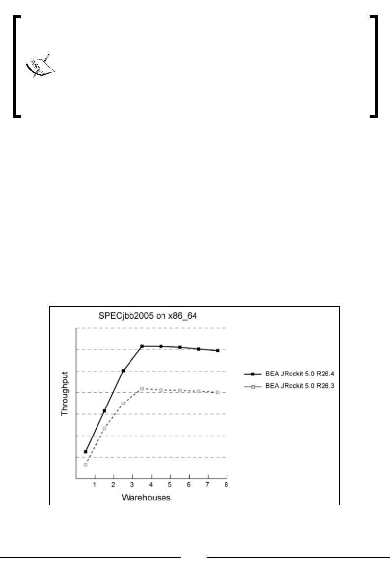
Chapter 5
[ 185 ]
Normally, simple web applications can get through with response times
on the order of a second or so. In the nancial industry, however,
applications that require pause time targets of less than 10 milliseconds,
all the way down to single digits, are becoming increasingly common.
A similar case can be made for the telecom industry that usually
requests pause times of no more than 50 milliseconds. Both the
customer and the JVM vendor need to do latency benchmarking in
order to understand how to meet these challenges. For this, relevant
benchmarks are required.
Scalability
Benchmarking for scalability is all about measuring resource utilization. Good
scalability means that service levels can be maintained while the workload is
increasing. If an application does not scale well, it isn't fully utilizing the hardware.
Consequently, throughput will suffer. In an ideal world, linearly increasing load on
the application should at most linearly degrade service levels and performance.
The following gure illustrates a nice example of near linear scalability on a
per-core basis. It shows the performance in ops per second for an older version
of the JRockit JVM running the well-known SPECjbb2005 benchmark. SPECjbb2005
is a multithreaded benchmark that gradually increases load on a transaction
processing framework.
Benchmarking and Tuning
[ 186 ]
A SPECjbb run starts out using fewer load generating worker threads than cores
in the physical machine (one thread per virtual warehouse in the benchmark).
Gradually, throughout the run, threads are added, enabling more throughput
(sort of an incremental warm-up). From the previous graph, we can see that
adding more threads (warehouses) makes the throughput score scale linearly
until the number of threads equals the number of cores, that is when saturation
is reached. Adding even more warehouses maintains the same service level until
the very end. This means that we have adequate scalability. SPECjbb will be
covered in greater detail later in this chapter.
A result like this is good. It means that the application is indeed scalable on the JVM.
Somewhat simplied, if data sets grow larger, all that is required to ensure that the
application can keep up is throwing more hardware at it. Maintaining scalability is a
complex equation that involves the algorithms in the application as well as the ability
of the JVM and OS to keep up with increased load in the form of network trafc, CPU
cycles, and number of threads executing in parallel.
While scalability is a most desirable property, as a target goal, it is
usually enough to maximize performance up to the most powerful
hardware specication (number of cores, and so on) that the application
will realistically be deployed on. Optimizing for good scalability on
some theoretical mega-machine with thousands of cores may be wasted
effort. Focusing too much on total scalability may also run the risk
of decreasing performance on smaller congurations. It is actually
quite simple to construct a naive but perfectly scalable system that has
horrible overall performance.
Power consumption
Power consumption is a somewhat neglected benchmarking area that is becoming
increasingly more important. Power consumption matters, not only in embedded
systems, but also on the server side if the server cluster is large enough. Minimizing
power consumption is becoming increasingly important due to cooling costs and
infrastructure issues. Power consumption is directly related to datacenter space
requirements. Virtualization is an increasingly popular way to get more out of
existing hardware, but it also makes sense to benchmark power consumption on
the general application level.
Optimizing an application for low power consumption may, for example, involve
minimizing used CPU cycles by utilizing locks with OS thread suspension instead
of spin locks. It may also be the other way around—doing less frequent expensive
transitions between OS and application can be the key to low power usage instead.
Chapter 5
[ 187 ]
One might also take a more proactive approach by making sure during development
that performance criteria can be fullled on lower CPU frequencies or with the
application bound only to a subset of the CPUs in a machine.
Other issues
Naturally, these are just a few of the possible areas where application performance
might need to be benchmarked. If performance for an application is important in
a completely different area, another kind of benchmark will be more appropriate.
Sometimes, just quantifying what "performance" should mean is surprisingly difcult.
Industry-standard benchmarks
The industry and the academic community continuously strive to provide generic
benchmarks that emulate many common programmatic problems for Java. This is,
of course, is of interest to JVM vendors and hardware vendors (to make sure that the
JVM itself performs well and also for marketing purposes). However, the standardized
benchmarks often provide some insights on tuning the JVM for a specic problem.
It is recommended to have a look at some of the things that the industry tries
to benchmark in order to understand how Java can be applied to different
problem domains.
Naturally, standard benchmarks for anything and everything exists. Many software
stacks are subject to performance measurement standardization, with organizations
releasing benchmarks for everything from application servers down to network
libraries. Finding and using industry-standard benchmarks is a relevant exercise
for the modern Java developer.
This section is written from a somewhat JVM centric perspective. We
are JVM developers and it has been in our interest to make sure that the
JVM performs as well as possible on many congurations. So, we have
chosen to highlight many standard benchmarks that JVM vendors tend
to use. However, a lot of the effort we have spent optimizing the JVM
has had very real impact on all kinds of Java applications. This is exactly
the point that this chapter has tried to make so far—optimizing for good
benchmarks that accurately represent real-world applications leads to
real-world application performance.
Some of the benchmarks we mention, such as SPECjAppServer also work
well as generic benchmarks for larger software stacks.

Benchmarking and Tuning
[ 188 ]
The SPEC benchmarks
The Standard Performance Evaluation Corporation (SPEC) is a non-prot
organization that strives to maintain and develop a set of benchmarks that can be used
to measure performance in several runtime environments on modern architectures.
This section will quickly introduce the most well known SPEC benchmarks that are
relevant to Java.
None of the SPEC benchmarks mentioned in this section are available for free, with
the sole exception of SPECjvm2008.
The SPECjvm suite
SPECjvm—its rst incarnation released in 1998 as SPECjvm98 (now retired)—was
designed to measure the performance of a JVM/Java Runtime Environment. The
original SPECjvm98 benchmark contained almost only single-threaded, CPU-bound
benchmarks, which indeed said something about the quality of the code optimizations
in a JVM, but little else. Object working sets were quickly, after a few years, deemed
too small for modern JVMs. SPECjvm98 contained simple problem sets such as
compression, mp3 decoding, and measuring the performance of the javac compiler.
The current version of SPECjvm, SPECjvm2008, is a modication of the original
SPECjvm98 suite, including several new benchmarks, updated (larger) workloads,
and it also factors in multi-core aspects. Furthermore, it tests out of the box settings
for the JVM such as startup time and lock performance.
Several real-life applications have recently been added to SPECjvm, such as the Java
database Derby, XML processors, and cryptography frameworks. Larger emphasis
than before has been placed on warm-up rounds and on measuring performance
from a steady state.
The venerable scientic computing benchmark SciMark has also been integrated into
SPECjvm2008. The original standalone version of SciMark suffered from the on-stack
replacement problem in that the main function contained the main work loop for
each individual benchmark, which compromised, for example, the JRockit JVM and
made it hard to compare its results with those of other virtual machines. This has
been xed in the SPECjvm2008 implementation.

Chapter 5
[ 189 ]
The SPECjAppServer / SPECjEnterprise2010 suite
SPECjAppServer is a rather complex benchmark, and a rather good one, though hard
to set up. It started its life called ECPerf and has gone through several generations—
SPECjAppServer2001, SPECjAppServer2002, and SPECjAppServer2004. The latest
version of this benchmark has changed names to SPECjEnterprise2010, but the basic
benchmark setup is the same.
The idea behind this benchmark is to exercise as much of the underlying infrastructure,
hardware, and software, as possible, while running a typical J2EE application.
The J2EE application emulates a number of car dealerships interacting with a
manufacturer. The dealers use simulated web browsers to talk to the manufacturer,
and stock and transactions are updated and kept in a database. The manufacturing
process is implemented using RMI. SPECjEnterprise2010 has further modernized the
benchmark by introducing web services and more Java EE 5.0 functionality.
The SPECjAppServer suite is not just a JVM benchmark but it can also be used to
measure performance in everything from server hardware and network switches to
a particular brand of an application server. The publication guidelines specify that
the complete stack of software and hardware needs to be provided along with the
score. SPECjAppServer / SPECjEnterprise2010 is an excellent benchmark in that any
part of a complete system setup can be measured against a reference implementation.
This makes it relevant for everyone from hardware vendors to application server
developers. The benchmark attempts to measure performance of the middle tier of the
J2EE application, rather than the database or the data generator (driver).
The benchmark is quite complicated to set up and hard to tune. However, theoretically,
once set up, it can run self-contained on a single machine, but is rather resource heavy,
and this will not produce any interesting results.
A typical setup requires a System Under Test (SUT), consisting of network
infrastructure, application servers, and a database server, all residing on different
machines. A driver, external to the test system, injects load into the setup. This is
an example of the technique for measuring outside the system that was explained
earlier in this chapter. In SPECjEnterprise2010, one of the more fundamental changes,
compared to earlier versions, is that database load has been signicantly reduced so
that other parts of the setup (the actual application on the application server) becomes
more relevant for performance.
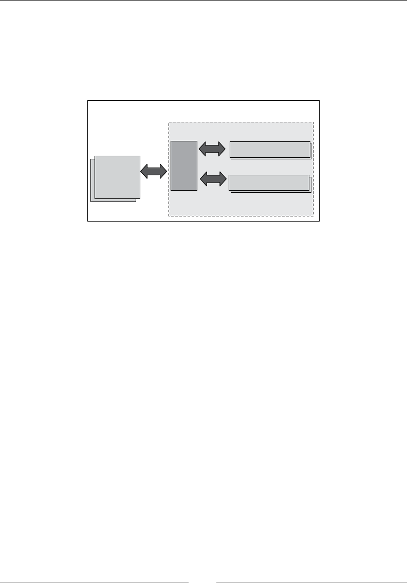
Benchmarking and Tuning
[ 190 ]
In a complete setup, the performance of everything, from which network switch to
which RAID solution the disk uses, matters. For a JVM, SPECjAppServer is quite a
good benchmark. It covers a large Java code base and the execution prole is spread
out over many long stack traces with no particular "extra hot" methods. This places
strict demands on the JIT to do correct inlining. It can no longer look for just a few
bottleneck methods and optimize them.
System Under Test
Application Servers
Database Server(s)
Switch
Drivers
/ Emulators
As of SPECjAppServer2004, in order to successfully run the benchmark, a transaction
rate (TxRate) is used for work packet injection. This is increased as long as the
benchmark can keep up with the load, and as soon as the benchmark fails, the
maximum TxRate for the benchmark system can thus be determined. This is used
to compute the score.
The realism is much better in newer generations of the benchmark. Application
servers use more up-to-date standards and workloads have been increased to t
modern architectures. Support for multiple application servers and multiple driver
machines has also been added. Measurements have also been changed to more
accurately reect performance.
The SPECjbb suite
SPECjbb is probably one of the most widespread Java benchmarks in use today.
It is interesting because it has been used frequently in academic research, and has
been a point of competition between the big three JVM providers, Oracle, IBM,
and Sun Microsystems. The big three, in cooperation with hardware vendors,
have taken turns publishing press releases announcing new world records.
SPECjbb has existed in two generations, SPECjbb2000 (retired), and lately
SPECjbb2005, that is still in use. SPECjbb, similar to SPECjAppServer, emulates
a transaction processing system in several tiers, but is run on one machine in a
self-contained application.
Chapter 5
[ 191 ]
SPECjbb has done the Java world some good in that a lot of optimizations that
JVMs perform, especially code optimizations, have been driven by this benchmark,
producing benecial spin-off effects. There are also many examples of real-life
applications that the quest for SPECjbb scores has contributed performance
to—for example, more efcient garbage collection and locks.
Here are some examples of functionality and optimizations
in the JRockit JVM that are a direct result of trying to achieve
high scores on SPECjbb. There are many more. All of these
optimizations have produced measurable performance
increases for real-world applications, outside the benchmark:
• Lazy unlocking (biased locking)
• Better heuristics for object prefetching
• Support for large pages for code and heap
• Support for non-contiguous heaps
• Improvements to array handling such as System.
arraycopy implementations, clear-on-alloc
optimizations, and assignments to arrays
• Advanced escape analysis that runs only on parts
of methods
A downside of SPECjbb is that it is, in fact, quite hardware-dependent. SPECjbb is very
much memory bound, and just switching architectures to one with a larger L2 cache
will dramatically increase performance.
Another downside to SPECjbb is that it is possible to get away with only caring
about throughput performance. The best scores can be achieved if all execution is
occasionally stopped and then, massive amounts of parallel garbage collection is
allowed to take place for as long as it takes to clean the heap.
SPECjbb2005 has also been used as the basis for the SPECpower_ssj2008 benchmark
that utilizes the same transaction code, but with an externalized driver. It is used
to quantify transactions per Watt at different levels of load, to provide a basis for
measuring power consumption.
Benchmarking and Tuning
[ 192 ]
Here's another benchmarking anecdote. Sometimes an optimization
designed for a benchmark is only that and has no real world applications.
An example from JRockit is calls to System.currentTimeMillis.
This is a Java method that goes to native and nds out what the system
time is, expressed in milliseconds since January 1, 1970. Because this
typically involves a system call or a privileged operation, very frequent
calls to System.currentTimeMillis could be a bottleneck on several
platforms.
Irritatingly enough, it turned out that calls to System.
currentTimeMillis made up several percent of the total runtime of
SPECjbb2000. On some platforms, such as Windows and Solaris, quick
workarounds to obtain system time were available, but not on Linux.
On Linux, JRockit got around the bottleneck by using its own signal-
based OS timers instead. The Linux JVM uses a dedicated thread to catch
an OS-generated signal every 10 milliseconds. Each time the signal is
caught, a local time counter is increased. This makes timer granularity a
little worse than with the system timer. However, as long as the timer is
safe (that is, it cannot go backwards) this maintains Java semantics and
SPECjbb runs much faster.
Today on JRockit versions for Linux, native-safe timers are disabled.
If you, for some weird reason, have problems with the performance of
System.currentTimeMillis in your application, they can still be
enabled with the hidden ag -XX:UseSafeTimer=true. We have
never heard of anyone who needs this.
SipStone
SipStone (www.sipstone.org) provides a suite of benchmarks that are interesting
for the telecom industry, making it possible to benchmark implementations of the
Session Initiation Protocol (SIP).
Real life scenarios for testing telecom applications are provided. One of
the benchmarks used is Proxy200, where the SIP application is provided by
the benchmark user. Typically, the benchmark user is a SIP server provider.
This benchmark is interesting as it provides a standardized proxy for testing
SIP performance.
The DaCapo benchmarks
The DaCapo (www.dacapobench.org) suite is a free benchmark suite created by
the DaCapo group, an academic consortium that does JVM and runtime research.
The idea behind the initiative is to create a benchmark with more GC-intensive
loads and more modern Java applications.
Chapter 5
[ 193 ]
The benchmark suite includes, for example, a parser generator, a bytecode optimizer,
a Java based Python interpreter, and some of the non-GUI unit tests for the Eclipse
IDE. It is fairly simple to run and makes for an interesting collection of benchmarks
that stresses some typical applications of Java.
Real world applications
Of course, one should not underestimate the usefulness of keeping a library of real
world applications around for benchmarking, if they can exercise relevant areas of
your code. For example, for developers of a Java web server, including a couple of
free Java web servers in the benchmarking matrix is probably a good idea to make
sure that competitive advantage is maintained over them.
The authors of this book, and their JVM development teams use, with kind
permission, a collection of customer applications that have caused performance
issues with JRockit over the years. This enables us to better understand performance
and make sure that no regressions appear. These applications have been turned
into benchmarks that are executed in known environments in nightly or weekly
performance runs. Smaller benchmarks are run more often.
Having "thrashatons" for a development team every now and then
is a fun and useful activity. Have the developers spend a few days
deploying their product on every kind of relevant (and not so relevant)
compatible application platform downloaded from the web. This helps
weed out bugs and performance problems. While, naturally, nding
thrashaton fodder for a JVM or a compiler is easy (the input is any
Java program), there is still plenty of source out there for testing more
specialized platforms. Also look for load generators, network tests, and
other platform-agnostic products that can stress an application until
unknown issues pop up.
Our recommendation is always to keep a large "zoo" of applications around,
for platform testing. If your platform is a J2EE application, deploy it on several
application servers. If it is a mathematical package, run it with several JVMs and
different java.lang.math implementations, and so on. Storage is cheap—so never
throw anything away. Test, benchmark, improve, and repeat!
The dangers of benchmarking
It is sometimes all too easy to focus too much on the results of a particular
benchmark and let this "tunnel vision" take over all performance work.

Benchmarking and Tuning
[ 194 ]
It is very important that a wide selection of standard industry benchmarks exists, as
they will be used by anyone from hardware vendors to undergraduate researchers, for
ultimately increasing performance for various runtimes and applications. Conclusions
drawn, given a benchmark setup, can have wide-ranging implications.
One danger is, of course, if a mainstream benchmark gets too well adopted. Classic
examples here are the SPECjvm benchmark suite and later the SPECjbb benchmark.
To put it bluntly, if a graduate student can run a benchmark from his workstation with
a simple command line, the problems it addresses will get much love and research.
If not, they won't. SPECjbb has a simple command line, SPECjAppServer doesn't.
SPECjAppServer, in itself, is an excellent benchmark that pretty much stresses any
desired portion of a Java platform stack and can be used to test everything from
application servers to network cards in a realistic environment. SPECjAppServer
requires quite a lot of hardware and has an extensive hard-to-congure setup.
Consequently, few relevant publications have been released using SPECjAppServer
in the academic world, but plenty of SPECjbb results are still published, even though
it may not be that relevant for all aspects of modern performance research.
Tuning
Once a working benchmark is in place in your test infrastructure, be it a version of an
application that can be run in a controlled environment or a subset of the algorithmic
problem that an application tries to solve, regression testing can be performed. This
ensures that no performance is lost during future code alterations.
Another purpose of the benchmark is to provide a small self-contained sandbox that
can be used to tune the runtime environment in order to provide optimal performance
for that particular application and to make sure that performance goals set for the
software project are reached.
Whereas, in some cases, it may be obvious from benchmarking that parts of
an application need to be rewritten using more efcient algorithms, sometimes
it may just be enough to provide a more optimal runtime environment by tuning
the JVM parameters.
Out of the box behavior
The previous three chapters on code generation, memory management, and threads
and synchronization have all, quite strongly, made the case for adaptive runtime
environments. All the feedback that a runtime collects can be put to powerful use
by the JVM for optimization.

Chapter 5
[ 195 ]
Indeed, in Utopia, an adaptive runtime would never need tuning at all, as the runtime
feedback alone would determine how the application should behave for any given
scenario at any given time. Sadly enough, a human always knows more about some
aspects of application runtime and lifecycles than a machine can deduce. The machine
may beat the human at things such as picking the hottest methods to optimize
rst, and at inating and deating locks depending on the current contention level.
However, if the human knows, for example, that the heap never needs to be resized,
as it is large enough for the application, or that heap compaction should never take
place because fragmentation won't ever become much of an issue, the JVM may need
to be told that from the start for optimal performance. On the other hand, the human
may think he knows more than the machine and misguidedly change the runtime
conguration for the worse. Playing around with a JVM conguration with too little
information is always dangerous and strongly discouraged.
In-depth data about application behavior can (and should) be collected by running
thorough proling analyses on the application. JRockit provides an excellent selection
of tools for non-intrusive proling of Java programs that can be used to do low cost
live recordings of an application. The recordings can then be analyzed ofine.
Before attempting to tune the performance of an application, it is important to
know where the bottlenecks are. That way no unnecessary effort is spent on adding
complex optimizations in places where it doesn't really matter. Again, this is a
lesson learned from our previous discussions on adaptive runtimes. For example,
if network overhead is the main performance bottleneck (as revealed by latency
analysis in a JRockit Flight Recorder), it might be too early to turn the ten lines
of code that comprise a very readable search algorithm into one hundred lines
of "more optimal" code. Low hanging fruit should always be handled rst, to
avoid introducing unnecessary complexity to the application.
In some cases, when the analysis is nished, no actual modication of the application
needs to be done. The analysis might reveal that the problem is such that some
runtime option can be added to handle it, helping our imperfect non-out of the box
world a bit. However, before we introduce command-line ags that can modify
anything and everything, we want to stress that good out of the box behavior is a
research area that always gets plenty of attention, both by Oracle and by other JVM
vendors. For JRockit, dramatic improvements have taken place for each new release.
It makes sense to optimize out of the box behavior to make it easier for the customer
to achieve the performance he needs and to off-load support, who instead should be
concentrating on actual bugs.
Benchmarking and Tuning
[ 196 ]
A nal word of warning—modifying JVM behavior through command-
line switches may produce unexpected results and functionality lock-ins
and should always be done with plenty of caution. A combination of
switches that work well for performance in a particular version of a JVM
may very well be harmful instead in a new version of the same JVM.
Typically, JRockit ags that start with –XX can never be relied on to be
unchanged between releases.
What to tune for
Recollect from Chapter 3 that no matter what tasks the underlying JVM performs,
tuning is universal. We can, for example, tune for throughput, low pause times,
or real-time performance, the latter being a stronger variant of low pause times.
While the general aspects of this have already been covered in previous chapters,
we will proceed to go over a selection of important JVM parameters that may be
benecial to use for reconguration. This section covers JRockit parameters only,
as the innermost workings of other JVMs are beyond the scope of this book.
However, while parameters vary between different JVMs, some of the techniques
presented below, such as modifying heap size, are relevant on all runtimes.
Before attempting to use any of the switches, the JRockit Documentation, particularly
the JRockit Diagnostics Guide, should be consulted to ensure that their full implications
are understood. Much insight can also be gained by using the JRockit Mission Control
suite to do recordings before and after a parameter change, to understand how the
overall runtime behavior was affected.
In the interest of keeping this section fairly short, extensive examples of using
the mentioned ags will not be included. Extensive examples, along with default
values for different congurations, are available in the JRockit Documentation and
the JRockit Diagnostics Guide.
Flags and options presented here are specic to the R28 versions of
the JRockit JVM. Earlier versions may have different ags for doing
the same thing, or lack the functionality altogether. Please consult the
JRockit Documentation to nd out what is supported for a particular
JRockit version.
Tuning memory management
This section covers command-line parameters specic to the memory management
system and garbage collector.

Chapter 5
[ 197 ]
Heap sizes
Recollect from Chapter 3 that the most fundamental way to tune the memory
system is to specify initial heap size using the –Xms ag and maximum heap size
using the –Xmx ag.
While tuning for real time, it is usually helpful to set both values to a xed maximum
size that the system has enough resources to allocate. Thus, unnecessary heap resizing,
a somewhat costly process, will be prevented from occurring during run time.
Example: java –Xms1024M –Xmx1024M <application> (set both the initial and
maximum heap size to 1 GB)
The GC algorithm
Furthermore, pick a GC algorithm that makes sense for the current application.
For real-time performance targets, do not forget to specify a service level agreement,
using the –XpauseTarget option.
For batch processing and throughput optimization, –XgcPrio:throughput is the
way to go.
Example: java –XgcPrio:pausetime –XpauseTarget:250ms (set up GC optimizing
for low pause times with a pause time target of maximum 250 milliseconds)
Compaction
It is inevitable that a heap gets fragmented over time. Traditionally, the "stone age"
approach to handling fragmentation for a long running program has been to restart
the server during a nightly service interval. This contributes to latencies, generates
downtime, and costs CPU cycles. However, experience has shown that by using
partial compaction, which is the default in JRockit, the problem is handled very
well. The JRockit compaction heuristics are mostly self-tuning.
One of the worst GC bottlenecks is compaction. Since compaction is not a fully
concurrent operation, if anything is known about fragmentation and object sizes
(for example from JRockit Flight Recorder data), it might be benecial to tune
compaction as well. In JRockit, this can be done through the –XXcompaction ag
and its arguments.
The compaction algorithm in JRockit divides the heap into a number of equally large
parts. Each of these is subject to separate compaction that occasionally may stop the
world. The default is to use 4,096 heap parts, but it might be benecial to increase this
number if compaction is too disruptive or decrease it if compaction fails to keep up
with fragmentation. Typically, for strategies other than throughput, GC compaction
areas are dynamically sized depending on how busy they are. Setting the number
of heap parts is done by passing the subcommand heapParts to –XXcompaction.
Benchmarking and Tuning
[ 198 ]
Compaction in JRockit is divided into internal and external compaction (the latter
also referred to as evacuation). Internal compaction never moves objects outside
a heap part, but completely compacts that heap part by moving objects to its
beginning. External compaction works on several heap parts and strives to move
objects to the start of the heap as is needed to keep overall fragmentation down.
Consequently, external compaction is less concurrent and requires stopping the
world for longer periods of time.
Compaction takes place inside a sliding window that gradually moves over
the entire heap. Currently, JRockit interleaves the use of internal and external
compaction between GCs. If one GC does internal compaction, the next does
external compaction, and so on.
The maximum percentages of the heap to compact for internal and external
compaction per GC compaction event can be set with the internalPercentage
ag for internal compaction and externalPercentage ag for external compaction.
If the object allocation strategies in the program are well known and latencies need
to be decreased, the ag –XXcompaction:enable=false will turn off all compaction
in the JRockit garbage collector. Before enabling this option, JRockit Mission
Control should be used to establish that fragmentation is not an issue. Turning off
compaction will dramatically reduce the need for memory management to halt Java
execution. However, death by fragmentation is a likely outcome for large and long
running applications that run with compaction switched off. This will manifest itself
as OutOfMemoryErrors.
If, on the other hand, latencies aren't an issue and optimizing for throughput is the
only concern, -XXcompaction:full will force full heap compaction at every GC,
keeping fragmentation at a minimum but at the cost of large pause times. Enabling
full compaction may be a dangerous experiment. Performing full compaction for
every GC can, in some cases, be so slow and cause such long pauses that throughput
is reduced to unusable levels anyway.
Full compaction is also sometimes referred to as exceptional
compaction in the JRockit Mission Control suite.
In GCs that optimize for short pausetimes, compaction can be aborted if the world
has been stopped for too long. The default in throughput GC is not to allow this, in
the interest of battling fragmentation. Abortable compactions can be forced by using
the –XXcompaction:abortable ag.

Chapter 5
[ 199 ]
There are several additional ways to tune compaction that are beyond the scope
of this chapter. Please refer to the JRockit Diagnostics Guide for in-depth guidance.
Finally, note that playing around with compaction parameters when tuning for real-
time, might result in larger performance deviations and in less deterministic pause
times. Some of the ways to tune compaction are:
Example: java –XXcompaction:enable=false <application> (turn off
all compaction)
Example: java –XXcompaction:full <application> (compact as much as
possible, optimizing for throughput)
Example: java –XXcompaction:internalPercentage=1.5,
externalPercentage=2,heapParts=512 <application> (use 512 heap parts.
Use up to two percent of the heap per external compaction and up to 1.5 percent of
the heap per internal compaction)
Example: java –XgcPrio:throughput –XXcompaction:abortable=true
(use throughput oriented GC, but soften the latency blow somewhat by allowing
abortable compaction)
Tweaking System.gc
The ag –XX:AllowSystemGC may be used to turn calls to System.gc into no-ops.
For example java –XX:AllowSystemGC=false <application> is used to turn any
System.gc call into a no-op. This can be a quick x for applications that frequently call
System.gc in ways detrimental to their performance. The default is to allow System.
gc, which may or may not do full heap garbage collections when invoked. Please see
Chapter 3, Adaptive Memory Management, and the section Common bottlenecks and how to
avoid them at the end of this chapter for more information.
For high throughput setups, on the other hand, System.gc can be made to force
the JVM to do a full heap garbage collection each time it is called. This is done
with the –XX:FullSystemGC ag. This ag should be used with caution
Example: java –XX:FullSystemGC=true <application> (force any System.gc
to perform a full heap garbage collection)
Benchmarking and Tuning
[ 200 ]
Nursery size
Recall from Chapter 3 that nurseries are the young generations of short-lived objects
on the heap. Nurseries are normally adaptively resized by the JVM. Specifying the
size of the nursery in the heap, by using the –Xns (nursery size) parameter, may be
an option if the application uses generational GC and produces large amounts of
temporary objects. In that case the size of the nursery should be increased. When
tuning for high throughput, it is most likely a good idea to skip generational GCs
altogether and run with -XgcPrio:throughput.
Example: java –Xns:10M <application> (set the nursery size to 10 MB of heap)
GC strategies
If, for some reason, the adaptive garbage collection strategy changes are too frequent
and incur an overhead, strategy changes can be disabled altogether by using the
command-line option –XXdisableGCHeuristics. Compaction and nursery size
heuristics aren't affected.
This ag works for JRockit versions prior to R28 only. As of JRockit R28,
GC heuristic changes are disabled altogether or are far less intrusive, so
this ag has been deprecated.
Thread local area size and large objects
Recollect that each thread allocates objects in a thread local area that is promoted to
the heap when full. The size of the TLA can be controlled by the ag -XXtlaSize.
The JVM may allocate larger objects directly on the heap, if they don't t into a TLA
or would lead to too much waste of space within the TLA. This is to prevent the
thread local areas from lling up too quickly and incurring extra overhead.
Large objects can be a problem for an application, and, sometimes, if something is
known about common object sizes in the running application, it helps to play around
with various TLA settings.
Example: java –XXtlaSize:min=2k,preferred=8k <application> (allocate
a preferred size of 8 KB for the TLAs, but down to 2 KB is also acceptable)
Chapter 5
[ 201 ]
In JRockit versions earlier than R28, large objects were allocated
immediately on the heap and never in a TLA. A ag called
–XXlargeObjectLimit was provided to tell JRockit the minimum
number of bytes an object should be of in order to be treated as "large".
The default was 2 KB. JRockit post R28 uses a waste limit for TLA space
instead. This constrains the amount of TLA space that can be thrown
away for each TLA when large objects are allocated and is a more exible
solution.
The R28 allocation algorithm now works like this—JRockit tries to
allocate every object regardless of its size in the current TLA. If it doesn't
t and the waste limit is less than the space left in the TLA, the object
goes directly on the heap. Otherwise, JRockit will "waste" the rest of this
TLA and try to allocate the object in a new TLA or directly on the heap,
depending on the size of the object.
Example: java –XXlargeObjectLimit:16k <application> (raise the large object
limit to 16 KB, only pre R28)
Example: java –XXtlaSize:min=16k,preferred=256k,wasteLimit=8k
<application> (TLAs should be 256 KB, but down to 16 KB is acceptable. Never
waste more than 8 KB of a TLA—rather allocate too large objects directly on the heap)
Tuning for large objects will be covered in further detail in the "Common Bottlenecks"
section of this chapter. It sufces to say that there is a natural trade-off between heap
fragmentation and the overhead of frequently allocating new TLAs—constantly
promoting objects to the heap from TLAs with lots of space left in them is wasteful
and defeats the lock-free purpose of TLA allocation.
Number of GC threads
JRockit, out of the box, tends to assume that it has the computer all to itself, and
strives to increase the number of parallel GC threads to a limit bounded by the OS
and the physical hardware. Typically, JRockit uses as many GC threads as there are
cores in the machine. If this is inappropriate for some reason, for example if other
applications need CPU time on the machine as well, the number of GC threads can
be explicitly set with the –XXgcThreads option.
Using too few GC threads introduces the risk that the garbage collector cannot
keep up with the growing set of dead objects. In extreme cases, this will lead to
OutOfMemoryErrors being thrown. However, it is more likely that in order to
save itself, the GC repeatedly needs to do emergency full heap garbage collections.
This leads to stalls and unacceptable latencies.
Example: java –XXgcThreads:4 <application> (use four GC threads)

Benchmarking and Tuning
[ 202 ]
NUMA and CPU afnity
Most modern operating systems have some notion of changing or setting processor
afnity for a process, making it possible to lock that process to one or more particular
CPUs. In NUMA environments, this might be most important, as better locality can
be achieved by binding the JVM process to a small number of NUMA nodes. The
trade-off is of course less dynamism and not being able to use some of
the memory efciently. The application behavior must be very well understood
before trying to modify the process afnity.
The ag –XX:BindToCPUs can be used to force JRockit to only use certain CPUs in
the machine.
Example: java –XX:BindToCPUs=0,2 <application> (used to set JRockit CPU
afnity to CPU 0 and 2 only)
For NUMA, a separate afnity ags exists for NUMA nodes (–XX:BindToNumaNodes)
as well as a ag that can control the NUMA memory allocation policy. This enables
the user to specify if JRockit should interleave allocated pages evenly across all
NUMA nodes or bind them in the local node where the memory allocation takes
place. A "preferred local" policy can also be selected, that is JRockit should try to use
the local node, but interleaved allocation is also ne.
Example: java –XX:NumaMemoryPolicy=strictlocal <application> (force local
NUMA allocation. Other values are preferredlocal and interleave)
Tuning code generation
This section covers parameters specic to the code generator.
Call proling
By using the ag –XX:UseCallProfiling, the JRockit code generator can be told to
add additional instrumentation to code while it is JITed, in order to collect data for
more intelligent decisions about inlining once a method is found to be a candidate
for optimization.
Normally, the execution overhead in JIT code is deemed too large to efciently
allow arbitrary instrumentation code. However, if the application will run for a
long time, most methods where runtime is spent are likely to be optimized and
won't have any instrumentation code left in them. The resulting optimized methods
will potentially run faster if the optimizer has extra call proling information to
base inlining decisions on.

Chapter 5
[ 203 ]
This ag is disabled by default, but may be enabled by default for future versions
of JRockit. It is especially benecial for an application with long call chains.
Example: java –XX:UseCallProfiling=true <application> (enable call proling
as an additional way of collecting hotness information)
Changing the number of optimization threads
Code optimization in JRockit is a fairly aggressive operation that uses plenty of CPU
time and memory. However, it might not make sense to spend too many CPU cycles
doing it. Recall from Chapter 2 that the number of code generation threads and the
number of optimization threads in the JRockit JIT compiler can be controlled.
If there are CPU cycles to spare and the application is to be deployed on a large
multi-core platform, steady state might be achieved faster by enabling a larger
number of code optimization threads.
The number of code optimization threads can be set with the –XX:OptThreads option.
The default is one optimization thread only. Benchmarking should be made to
establish if more optimization threads are more efcient. Eventually, the application
will reach a steady state anyway. The number of JIT compiler threads can be modied
in similar fashion.
Example: java –XX:JITThreads=2 <application> (use two JIT compiler threads
instead of one, which is the default)
Example: java –XX:OptThreads=2 <application> (use two optimization threads
instead of one, which is the default)
Turning off code optimizations
Sometimes, code optimization, being a fairly CPU-intensive operation, may
incur unacceptable overhead, either in the form of too long warm-up periods
or by introducing latency spikes. All code optimizations can be switched off
with the –XnoOpt ag. This will lead to a much more predictable JVM behavior.
However, severe performance penalties for the executing code should be expected.
Optimizations can also be turned off after a specic amount of time (in seconds),
by using the –XX:DisableOptsAfter switch.
Example: java –XnoOpt <application> (disable all code optimizations)
Example: java –XX:DisableOptsAfter=600 <application> (disable all code
optimization after 10 minutes of runtime)

Benchmarking and Tuning
[ 204 ]
Tuning locks and threads
When it comes to lock tuning, it is often a good idea to leave well enough alone
and not modify the default behavior. It is rare that the user can add anything by
modifying lock heuristics. It is more often the case that performance gains can come
from modifying the application. However, for the sake of completeness, this section
presents some switches that control lock behavior in JRockit.
Lazy unlocking
Recall from Chapter 4 that lazy unlocking is benecial in an environment where a
particular lock is frequently taken and released by the same thread. If we know that
the same thread will soon reacquire the lock, it makes little sense to release it for just a
short period of time.
Lazy unlocking is enabled by default in JRockit (except when running with
deterministic GC on versions earlier than Java 1.6). It can be explicitly turned
on and off with the ag –XX:UseLazyUnlocking.
Example: java –XX:UseLazyUnlocking=false <application> (explicitly turn
off lazy unlocking)
Class banning, i.e. the heuristic that stops a certain class from being used for lazy
unlocking after too many erroneous guesses, can be switched off with the ag
–XX:UseLazyUnlockingClassBan=false.
Enforcing thread priorities
The java.lang.Thread class supports different priorities for thread execution, but
they are rarely implemented by the VM by default. This is because the potential for
trouble tends to be greater than the gain. Messing around with thread scheduling
policies at the Java level might lead to unforeseen problems.
JRockit supports forcing the VM to respect thread priorities set through the
setPriority method of java.lang.Thread. The default is to ignore thread
priorities, but they can be enabled with the –XX:UseThreadPriorities ag.
Example: java –XX:UseThreadPriorities=true <application> (enable thread
priority changes)
Thresholds for ination and deation
Finally, advanced users may nd it useful to tune the heuristic thresholds for lock
deation and lock ination, i.e. the criteria with which a lock is turned from thin to
fat or vice versa.

Chapter 5
[ 205 ]
Example: java –XX:ThinLockConvertToFatThreshold=100 <application>
(no more than 100 iterations are allowed to run in the thin lock spin loop before a
lock is inated)
The JRockit spin loop isn't pure CPU wastage, as it does some kind of micropause
or yield each iteration. Naturally, specifying a limit for the number of iterations in the
spinlock loop modies timing in completely incomparable ways between
architectures and CPUs.
Example: java –XX:UseFatLockDeflation=false <application> (never deate a
fat lock. The default is true)
Example: java –XX:FatLockDeflationThreshold=10 <application> (deate a fat
lock to thin again after 10 uncontended entries)
Recall from the last chapter that a spinlock is part of the JRockit fat lock
implementation. It is used as a "second chance" when a lock is inated, but
only for a short period of time before entering the real fat lock. This behavior
can be modied as well.
Example: java –XX:UseFatSpin=false <application> (never use a spinlock as part
of a fat lock)
Example: java –XX:UseAdaptiveFatSpin=false <application> (never try to
adaptively change the spinlock part of a fat lock based on runtime feedback)
There are several other advanced ags for controlling lock heuristics. For more
information, please refer to the JRockit Diagnostics Guide. In general, be careful when
messing around with lock settings—it can produce strange and unexpected results.
Generic tuning
Finally, we present some switches and aspects that have to do with tuning and don't
t into a particular category or span several.
Compressed references
Recall from the chapter on memory management that compressed references are
enabled by default on 64-bit platforms for most heap sizes. So, they shouldn't need
to be congured manually. JRockit will, by default, enable different avors of
compressed references depending on maximum heap size for all heap sizes up to 64
GB. This can be explicitly overridden. Consult the documentation to decide whether
this is appropriate or not.
Example: java -XXcompressedRefs:enable=false <application> (never use
compressed references)
Benchmarking and Tuning
[ 206 ]
Example: java –XXcompressedRefs:enable=true,size=64GB <application>
(enable compressed references supporting heaps up to 64 GB)
Large pages
Large pages can be used for both code buffers and for the heap. This can be controlled
by using the –XX:UseLargePagesForCode and –XX:UseLargePagesForHeap options.
The default is to not use large pages for anything.
If appropriate support for large pages is enabled and available in the underlying OS,
having the JVM use large pages reduces TLB misses to a large extent. On memory
intensive applications, it is not unusual to achieve a performance gain of 10-15 percent.
We denitely recommend trying out large pages for any large long running
application to see if there is a performance gain. If the underlying operating
system doesn't support large pages, JRockit will print a warning and fall back
to normal behavior.
Example: java –XX:UseLargePagesForCode=true <application> (use large
pages for code buffers)
Example: java –XX:UseLargePagesForHeap=true <application> (use large
pages for the heap)
Common bottlenecks and how to
avoid them
As in most of our chapters so far, we will nish by reviewing a few common
mistakes and false optimizations. In the benchmarking world, this is all about
understanding the bottlenecks and the anti patterns that frequently show up in
application code and how they can be avoided.
Care should be taken that any instrumentation is not too intrusive. If,
for example, the chosen instrumentation tool inserts extra bytecode
operations all over the application code, the overall timing of the
program can change completely. This may make the resulting prole
useless for drawing any kinds of conclusions about the original program
behavior. While small bytecode instrumenters may be handy for things
like implementing counters for specic kinds of events, they rarely
produce a true execution prole. Bytecode instrumenters also make it
necessary to recompile and restart the application. The JRockit Mission
Control suite, on the other hand, can plug in at runtime and proles the
application with virtually no extra overhead.

Chapter 5
[ 207 ]
A benchmark or instrumentation result can provide great insights into why
an application contains performance bottlenecks. Over the years, the authors of
this book have examined many applications to determine why they aren't running
as fast as they should. Some ndings keep recurring, and the following section
provides information on several common areas that cause performance problems and
what practices should be avoided or used with caution when programming Java.
The –XXaggressive ag
From one time to another we discover customers using the undocumented and
experimental –XXaggressive ag for JRockit. This ag is a wrapper for other
ags that tell JRockit to perform at high speed and try to reach a stable state as
soon as possible. The cost of this is more resource use at startup. The parameters
that this option modies are subject to change from release to release. Because
of its experimental nature, the frivolous use of –XXaggressive is discouraged.
However, it can be useful to try as one of many different setups when doing
proling. Use this ag at your own risk.
Too many nalizers
Finalizers are, as we have already discussed in Chapter 3, unsafe in that they can
resurrect objects and interfere with the GC. They usually incur processing overhead
in the JVM as well.
Objects waiting for nalization have to be kept track of separately by the garbage
collector. There is also call overhead when the finalize method is invoked (not to
mention the execution time of the finalize method itself, if it does something fairly
complex). Finalizers should simply be avoided.
Too many reference objects
As with nalizers, the garbage collector has to treat soft, weak, and phantom
references specially. Although all of these can provide great aid in, for example,
simplifying a cache implementation, too many live Reference objects will make
the garbage collector run slower. A Reference object is usually a magnitude more
expensive than a normal object (strong reference) to bookkeep.

Benchmarking and Tuning
[ 208 ]
To get information on Reference object processing along with garbage collections,
JRockit can be started with the ag –Xverbose:refobj. Following is an example of
its output:
hastur:material marcus$ java –Xverbose:refobj GarbageCollectionTest
[INFO ][refobj ] [YC#1] SoftRef: Reach: 25 Act: 0 PrevAct: 0 Null: 0
[INFO ][refobj ] [YC#1] WeakRef: Reach: 103 Act: 0 PrevAct: 0 Null: 0
[INFO ][refobj ] [YC#1] Phantom: Reach: 0 Act: 0 PrevAct: 0 Null: 0
[INFO ][refobj ] [YC#1] ClearPh: Reach: 0 Act: 0 PrevAct: 0 Null: 0
[INFO ][refobj ] [YC#1] Finaliz: Reach: 12 Act: 3 PrevAct: 0 Null: 0
[INFO ][refobj ] [YC#1] WeakHnd: Reach: 217 Act: 0 PrevAct: 0 Null: 0
[INFO ][refobj ] [YC#1] SoftRef: @Mark: 25
@Preclean: 0 @FinalMark: 0
[INFO ][refobj ] [YC#1] WeakRef: @Mark: 94
@Preclean: 0 @FinalMark: 9
[INFO ][refobj ] [YC#1] Phantom: @Mark: 0
@Preclean: 0 @FinalMark: 0
[INFO ][refobj ] [YC#1] ClearPh: @Mark: 0
@Preclean: 0 @FinalMark: 0
[INFO ][refobj ] [YC#1] Finaliz: @Mark: 0
@Preclean: 0 @FinalMark: 15
[INFO ][refobj ] [YC#1] WeakHnd: @Mark: 0
@Preclean: 0 @FinalMark: 217
[INFO ][refobj ] [YC#1] SoftRef: SoftAliveOnly: 24 SoftAliveAndReach:1
[INFO ][refobj ] [YC#1] NOTE: This count only
applies to a part of the heap.
The program in the previous example seems to have only a small number of
Reference objects and the GC has no trouble keeping up. Beware of applications
where each GC needs to handle hundreds of thousands of soft references.
Object pooling
As was discussed in the chapter on memory management, object pooling,
the practice of keeping a collection of objects alive for reuse in order to reduce
allocation overhead, is usually a bad idea.
Apart from interfering with GC workloads and heuristics, pooling objects will
also cause objects to live longer, and thus eventually force their promotion to
the old generation on the heap. This introduces extra overhead and contributes
to fragmentation. Recall from Chapter 3 that large amounts of live data is a GC
bottleneck and the GC is optimized to handle many objects with short life spans.
Object pooling contributes both to more live data and to longer object life spans.
Also, allocating fresh objects instead of keeping old objects alive, will most likely
be more benecial to cache locality.

Chapter 5
[ 209 ]
No rule without exception, however. In very specic applications, allocation time
is actually a program bottleneck, especially the clearing part of allocations. As Java
guarantees that every new object is initialized with null, freshly allocated objects
have to be cleared. Performance in an environment with many large objects, for
example large arrays, may therefore occasionally benet from object pooling. JRockit
tries to remove unnecessary object clearings if it can prove that they are not needed.
In general, though, it is probably a good idea to just keep things simple.
Bad algorithms and data structures
It should be fairly obvious that a hash table is a better data structure for fast element
lookups than a linked list. It should also be clear that a QuickSort algorithm of runtime
complexity O(n log n) is better than a naively implemented BubbleSort of O(n2). We
assume that the reader is fairly procient in picking the correct algorithms and data
structures in order to minimize algorithm complexity.
Classic textbook issues
However, when working with a poorly written third-party application, bad data
structures can still be a problem. By benchmarking and by working backwards
from where the program spends its time, serious runtime improvements can
sometimes be made.
public List<Node> breadthFirstSearchSlow(Node root) {
List<Node> order = new LinkedList<Node>();
List<Node> queue = new LinkedList<Node>();
queue.add(root);
while (!queue.isEmpty()) {
Node node = queue.remove(0);
order.add(node);
for (Node succ : node.getSuccessors()) {
if (!order.contains(succ) && !queue.contains(succ)) {
queue.add(succ);
}
}
}
return order;
}

Benchmarking and Tuning
[ 210 ]
The previous code is a standard breadth rst search algorithm for (possibly cyclic)
graphs. Given a root node, the algorithm uses a queue to traverse its successors in
breadth rst order. In order to avoid duplicates and potentially innite loops, a check
to see if a node has been already processed is done before adding it to the queue.
The method contains, used for nding an element in a linked list, is implemented
in the JDK as a linear scan of the entire list. This means that in the worst case, our
search algorithm is quadratic to the number of nodes, which will be very slow for
large data sets.
public List<Node> breadthFirstSearchFast(Node root) {
List<Node> order = new LinkedList<Node>();
List<Node> queue = new LinkedList<Node>();
Set<Node> visited = new HashSet<Node>();
queue.add(root);
visited.add(root);
while (!queue.isEmpty()) {
Node node = queue.remove(0);
order.add(node);
for (Node succ : node.getSuccessors()) {
if (!visited.contains(succ)) {
queue.add(succ);
visited.add(succ);
}
}
}
return order;
}
The previous code corrects the problem by adding a HashSet type data structure to
keep track of visited nodes. Constant time lookups replace the linear traversion
when checking if a node already has been visited. The potential difference for
large data sets is enormous.
Unwanted intrinsic properties
There are however other, more subtle problems caused by picking the wrong data
structure. Consider a queue implementation in the form of a linked list. This is
seemingly a good general purpose data structure that can be used as a queue without
any modications. It provides the ability of inserting elements last in the list and
removing elements from the list head. These are both constant time operations and
no other functionality is required. So, what can go wrong? First of all, even if your
program never iterates over the entire linked list, the garbage collector still has to.

Chapter 5
[ 211 ]
If the queue contains large amounts of data, many objects are kept alive as long as
they are referenced from the linked list. As the linked list elements consist of object
references that both point out the next list element and wrap a payload of data, the
queue elements may exist anywhere on the heap. Thus, accessing objects in a linked
list may actually lead to bad cache locality and long pause times. Bad cache locality
can ensue because payloads or element wrappers aren't guaranteed to be stored next
to each other in memory. This will cause long pause times as, if the object pointers
are spread over a very large heap area, a garbage collector would repeatedly miss
the cache while doing pointer chasing during its mark phase.
So, seemingly innocent data structures with low complexities for the operations
involved can turn out to introduce intrinsic problems in systems with automatic
memory management.
Misuse of System.gc
There is no guarantee from the Java language specication that calling System.gc
will do anything at all. But if it does, it probably does more than you want or doesn't
do the same thing every time you call it. To reiterate, don't confuse the garbage
collector by trying to tell it what to do. To be safe, don't call System.gc.
Too many threads
While it is a good thing to be able to break up a problem into many computational
threads with little inter-thread communication, context switches always incur
overhead anyway. We have been over the different thread implementations, from
green threads to OS threads in Chapter 4. However, true for all thread implementation
is that some kind of context switch, during which no useful program execution can
be performed, takes place while shifting execution from one thread to another. The
number of context switches grows proportionally to the number of fairly scheduled
threads, and there may also be hidden overhead here.
A worst-case example from real life is the Intel IA-64 processor,
with its massive amount of registers, where a native thread context
is on the order of several KB. Every memory copy performed
in order to initiate a new thread context after a context switch
contributes to the overhead. This makes many threads executing in
parallel particularly expensive as their contexts are large.

Benchmarking and Tuning
[ 212 ]
One contended lock is the global bottleneck
Contended locks are bottlenecks, as their presence means that several threads want to
access the same resource or execute the same piece of code at the same time. It is not
uncommon that one lock is the main source of all contention in a program. A typical
example is an application using some third-party library for logging that acquires
a global lock each time log le information is to be written. When many, mutually
independent, threads are trying to log output at the same time, the log lock might be
the one bottleneck that brings an otherwise well written application to its knees.
Unnecessary exceptions
Handling exceptions takes time and interrupts normal program ow. Using
exceptions for the common case in a program as means of communicating results
or implementing control ow is denitely bad practice.
It is useful to try to create some kind of exception prole of the program to nd out
what exceptions are thrown and from where. Unnecessary hardware exceptions
such as null pointers and divisions by zero should be removed wherever possible.
Hardware exceptions are the most expensive type of exception, as they are triggered
by an interrupt at the native level, whereas throwing a Java exception explicitly
from code keeps most of the (though still expensive) work of handling the exception
inside the JVM.
We have seen cases with customer applications throwing tens of
thousands of unnecessary NullPointerExceptions every second,
as part of normal control ow. Once this behavior was rectied,
performance gains of an order of magnitude were achieved.
The simplest way to discover which exceptions, both caught and uncaught, are
thrown by JRockit, is to use the ag –Xverbose:exceptions. An example of its
output is shown as follows:
hastur:~ marcus$ java -Xverbose:exceptions Jvm98Wrapper _200_check
[INFO ][excepti][00004] java/io/FileNotFoundException:
/localhome/jrockits/R28.0.0_R28.0.0-454_1.6.0/jre/classes
[INFO ][excepti][00004] java/lang/ArrayIndexOutOfBoundsException: 6
[INFO ][excepti][00004] java/lang/ArithmeticException: / by zero
[INFO ][excepti][00004] java/lang/ArithmeticException: fisk
[INFO ][excepti][00004] java/lang/ArrayIndexOutOfBoundsException: 11
[INFO ][excepti][00004] java/lang/RuntimeException: fisk

Chapter 5
[ 213 ]
Each line in the log corresponds to a thrown exception. To get stack traces along with
the exceptions, use –Xverbose:exceptions=debug. The JRockit Mission Control suite
also contains frameworks for proling exceptions and for introspecting them in a more
user friendly way. The following is an example output that shows exceptions along
with their stack traces, as they are thrown by the JVM:
hastur:~ marcus$ java -Xverbose:exceptions=debug Jvm98Wrapper _200_check
[DEBUG][excepti][00004] java/lang/ArrayIndexOutOfBoundsException: 6
at spec/jbb/validity/PepTest.testArray()Ljava/lang/String;
(Unknown Source)
at spec/jbb/validity/PepTest.instanceMain()V(Unknown Source)
at spec/jbb/validity/Check.doCheck()Z(Unknown Source)
at spec/jbb/JBBmain.main([Ljava/lang/String;)V(Unknown Source)
at jrockit/vm/RNI.c2java(JJJJJ)V(Native Method)
--- End of stack trace
[DEBUG][excepti][00004] java/lang/ArithmeticException: / by zero
at jrockit/vm/Reflect.fillInStackTrace0(Ljava/lang/Throwable;)
V(Native Method)
at java/lang/Throwable.fillInStackTrace()Ljava/lang/Throwable;
(Native Method)
at java/lang/Throwable.<init>(Throwable.java:196)
at java/lang/Exception.<init>(Exception.java:41)
at java/lang/RuntimeException.<init>(RuntimeException.java:43)
at java/lang/ArithmeticException.<init>(ArithmeticException.java:36)
at jrockit/vm/RNI.c2java(JJJJJ)V(Native Method)
at jrockit/vm/ExceptionHandler.throwPendingType()V(Native Method)
at spec/jbb/validity/PepTest.testDiv()Ljava/lang/String;
(Unknown Source)
at spec/jbb/validity/PepTest.instanceMain()V(Unknown Source)
at spec/jbb/validity/Check.doCheck()Z(Unknown Source)
at spec/jbb/JBBmain.main([Ljava/lang/String;)V(Unknown Source)
at jrockit/vm/RNI.c2java(JJJJJ)V(Native Method)
--- End of stack trace
[DEBUG][excepti][00004] java/lang/ArithmeticException: fisk
at spec/jbb/validity/PepTest.testExc1()Ljava/lang/String;
(Unknown Source)
at spec/jbb/validity/PepTest.instanceMain()V(Unknown Source)
at spec/jbb/validity/Check.doCheck()Z(Unknown Source)
at spec/jbb/JBBmain.main([Ljava/lang/String;)V(Unknown Source)

Benchmarking and Tuning
[ 214 ]
at jrockit/vm/RNI.c2java(JJJJJ)V(Native Method)
--- End of stack trace
[DEBUG][excepti][00004] java/lang/ArrayIndexOutOfBoundsException: 11
at spec/jbb/validity/PepTest.testExc1()Ljava/lang/String;
(Unknown Source)
at spec/jbb/validity/PepTest.instanceMain()V(Unknown Source)
at spec/jbb/validity/Check.doCheck()Z(Unknown Source)
at spec/jbb/JBBmain.main([Ljava/lang/String;)V(Unknown Source)
at jrockit/vm/RNI.c2java(JJJJJ)V(Native Method)
--- End of stack trace
[DEBUG][excepti][00004] java/lang/RuntimeException: fisk
at spec/jbb/validity/PepTest.testExc2()Ljava/lang/String;
(Unknown Source)
at spec/jbb/validity/PepTest.instanceMain()V(Unknown Source)
at spec/jbb/validity/Check.doCheck()Z(Unknown Source)
at spec/jbb/JBBmain.main([Ljava/lang/String;)V(Unknown Source)
at jrockit/vm/RNI.c2java(JJJJJ)V(Native Method)
--- End of stack trace
Any JRockit Flight Recording contains an exception prole of the running program
that can be examined using JRockit Mission Control.
Large objects
Large objects sometimes have to be allocated directly on the heap and not in thread
local areas. The rationale is that they would mostly contribute to overhead in a small
TLA and cause frequent evacuations. In JRockit versions prior to R28, an explicit
large object size could be given and objects that were larger were never allocated in a
TLA. Post R28, the waste limit for a TLA is instead the modiable property, allowing
large objects to be allocated in a TLA if they t well enough.
Large objects on the heap are bad in that they contribute to fragmentation more
quickly. This is because they might not readily t in most spaces provided by the
free list, where smaller "normal" objects have been previously garbage collected.
Allocation time increases dramatically on a fragmented heap, and juggling many
large objects extensively contributes to fragmentation. As large objects may be
allocated directly on the heap and not in the TLA, large object allocation in JRockit also
contributes to overhead because it may require taking a global heap lock on allocation.
The worst case scenario is that an overuse of large objects leads to full heap
compaction being done too frequently, which is very disruptive and requires
stopping the world for large amounts of time.

Chapter 5
[ 215 ]
As it is hard to pick a "one size ts all" value as an explicit large object limit, for any
given application, the large object limit in JRockit (or the TLA waste limit in R28)
can be changed. This is useful if analysis shows that there are, for example, a large
number of xed size objects slightly larger than the default, or if many direct-to-heap
allocations take place as the TLAs want to be too tightly packed. In that case, it might
be benecial to increase the large object limit or TLA waste limit, depending on
JRockit version.
The bad corner cases, the large object death spirals, occur when objects frequently
are on the orders of several megabytes. The real world examples are typically
database query results or very large arrays. Avoid them at all costs. Do whatever
it takes to keep them off the heap, even implement a native layer for them, but do
not let your Java Virtual Machine juggle a large number of humongous objects.
Native memory versus heap memory
To the JVM, all memory that exists is system memory, available from the underlying
operating system. Some of this system memory is used by the JVM to allocate the
Java heap. The amount of memory used for the heap can be controlled by the –Xms
(initial heap size) and –Xmx (maximum heap size) ags.
The JVM will throw OutOfMemoryError both from inside the JVM, when there is not
enough memory available to complete some internal operation, and from Java, when
a program tries to allocate more objects than will t on the current heap.
A JVM is a native application that also consumes system memory for its own purposes,
for example, to allocate data structures used for code optimization. Internal JVM
memory management is, to a large extent, kept off the Java heap and allocated natively
in the operating system, through system calls like malloc. We refer to non-heap
system memory allocated by the JVM as native memory.
While heap memory can be reclaimed when the JVM garbage collects objects in
running program, native memory can't. If all native memory management was
handled by the JVM alone, and the JVM was economic enough in its native
memory usage, all would be well. However, there are complications.
In certain scenarios, we can run out of native memory. One example is when several
parallel threads perform code optimizations in the JVM. Code optimization typically
is one of the JVM operations that consumes the largest amounts of native memory,
though only when the optimizing JIT is running and only on a per-method basis.
There are also mechanisms that allow the Java program, and not just the JVM, to
allocate native memory, for example through JNI calls. If a JNI call executes a native
malloc to reserve a large amount of memory, this memory will be unavailable to the
JVM until it is freed.

Benchmarking and Tuning
[ 216 ]
Mechanisms for tracking native memory usage are available in
JRockit, and can be accessed through the JRockit Mission Control
suite or JRCMD. Histograms that show the native memory usage
of individual JVM modules are also available.
If the heap is too large, it may well be the case that not enough native memory is
left for JVM internal usage—bookkeeping, code optimizations, and so on. In that
case, the JVM may have no other choice than to throw an OutOfMemoryError from
native code. For JRockit, increasing the amount of available native memory is done
implicitly by lowering the maximum Java heap size using –Xmx.
Wait/notify and fat locks
Recall from the last chapter that wait and notify always inates thin locks to fat
locks in JRockit. Locks that are frequently taken and released, but are only held for a
short time might do better as thin locks. So, immediately using wait or notify on
a new object will create a new monitor and consequently a fat lock that might lead
to performance overhead.
Wrong heap size
Another common problem that causes performance issues is using the wrong heap
size for the JVM. Too small heaps trigger frequent and time consuming garbage
collections. Too large heaps lead to longer mean GC times and may cause the JVM
to run out of native memory. It makes sense to do proling runs to gure out the
memory requirements of your application and try to nd an optimal maximum heap
size. JRockit Mission Control will almost always provide good data on the memory
requirements for a particular application.
Too much live data
As we have discussed in the chapter on garbage collection, the main contributor to
runtime complexity in memory management is not the heap size per se, but rather
the amount of live data on the heap. Large amounts of live data almost certainly
create garbage collection overhead. Again, proling can help gure out if there
are any large object clusters kept in memory even though there shouldn't be.
The Memleak tool, which is part of the JRockit Mission Control suit is ideal for this
kind of analysis.

Chapter 5
[ 217 ]
Java is not a silver bullet
Finally, Java is a powerful and versatile language that contributes to short application
development time because of its friendly semantics and built-in memory management.
However, Java is not a silver bullet. The last caveat this chapter will warn of is trying
to use Java to solve a problem that in fact is totally inappropriate for Java.
• Is the application a telecom application with virtually tens of thousands of
concurrent threads that need near-real-time support?
• Does the application contain a database layer that frequently returns 20 MB
query results of binary data in the form of byte arrays?
• Is the application completely dependent on the underlying OS scheduler
for performance and determinism, with bad overhead problems if the
scheduling semantics change even slightly?
• Is the application a device driver?
• Has the development team implemented a C/Fortran/COBOL-to-Java
automatic translator, so that those 100,000 lines of legacy code can "easily"
be deployed on a modern Java runtime?
• Is the program highly concurrent or embarrassingly parallel, that is, it tries
to use a divide and conquer strategy that branches off tens of thousands of
threads that run computations for a short period of time before fusing the
partial results?
In these cases, and there are probably plenty of others, it might be considered doubtful
if using Java is the correct approach. Java is highly attractive in that the JVM provides
an abstract layer on top of the operating system and in that Java programs can be
compiled once, and run everywhere. But, stretching it a bit, so can ANSI C. Just ship
the source code and make sure it is portable. Choose your tool with care. Java is a
lovely multi-purpose hammer, but not every problem is a nail!

Benchmarking and Tuning
[ 218 ]
Summary
This chapter has covered benchmarking and tuning. We have motivated the need
for benchmarking, mostly since having a benchmark framework in place prevents
performance regressions, but also because well understood and easy-to-setup
sub-problems are simpler to work with than complex applications. We also stressed
the importance of having performance goals for commercial software development,
another area where benchmarking is of a great help. It can also be useful to maintain
a set of third-party applications as part of a benchmark suite.
We have discussed micro benchmarks to some extent and explained why they
are useful and when they are not. We also talked about the importance of knowing
what you are measuring.
Proling always needs to be done to understand where the bottlenecks are in
an application and to make sure that external benchmarks really address these
bottlenecks. Proling can be done with several levels of complexity, and with
several levels of intrusiveness. For JRockit, low cost proling is easily facilitated
by the JRockit Mission Control suite.
We went on to present some industrial standard benchmarks, most famously
the SPEC suite, and discussed where they can do some good for everyone from
hardware vendors to application developers.
Once an application is well understood, it is time to decide if tuning JVM parameters
alone can improve performance or if rewriting certain parts of the program is required.
Using JRockit as an example JVM, we covered the parameters that can be used to tune
application behavior in the memory system, in the code generator, and elsewhere.
Finally, we presented a section on common bottlenecks or anti-patterns that are
frequently seen in Java applications and taught the reader how to avoid them.
This concludes the rst part of this book. The next part of the book will go over the
versatile and powerful tools in JRockit Mission Control in great detail. Hopefully
this chapter contained enough philosophy on benchmarking and tuning to provide
an excellent primer for understanding how to apply the necessary tools to solve
your performance problems.

JRockit Mission Control
JRockit, as a Java runtime, is required to constantly monitor the running Java
application. As has been explained in previous chapters, JRockit must, among
other things, be able to nd out in which methods the Java application is spending
the most time executing code. JRockit is also responsible for keeping track of the
memory usage and memory allocation behavior of the application—it would be
fairly upsetting if JRockit forgot a few objects, or if memory was not reclaimed
when objects were no longer referenced.
The wealth of data that JRockit already collects is, of course, a very good source of
information when proling your Java program or when doing diagnostics.
In this, the second part of the book, the JRockit tools suite is presented. The
following chapters introduce four of the tools that are included in the JRockit
distribution—the JRockit Mission Control Console, the JRockit Runtime Analyzer
(which was superseded by the JRockit Flight Recorder in R28), the JRockit Memory
Leak Detector, and JRCMD.
The rst three tools are included in the JRockit Mission Control tools suite. The last
one, JRCMD, is a command-line tool that ships as part of the JRockit JDK. A common
denominator for the tools is their ability to interact with an already running JVM.
There is no need to pre-congure the JVM or the application to be able to later attach
the tools. Also, the tools add virtually no overhead, making them suitable for use in
live production environments.
In this chapter you will learn:
• How to start JRockit Mission Control, both as a standalone application and
inside the Eclipse IDE
• How to congure JRockit JVM instances so that they can be managed by
JRockit Mission Control from remote locations

JRockit Mission Control
[ 220 ]
• How to make JRockit Mission Control automatically discover remotely
running JRockit instances
• How to congure the management agent that is part of the JRockit JVM
• How to use JRockit Mission Control and the JRockit Management Agent in
a secure environment
• How to troubleshoot connections between JRockit Mission Control
and JRockit
• Various ways to get more debug information from JRockit Mission Control
• About the Experimental Update Site for JRockit Mission Control and how
to extend JRockit Mission Control with plug-ins from the Experimental
Update Site
While not necessary for the bigger picture, parts of this chapter assume various
degrees of familiarity with Eclipse IDE. For more information about Eclipse,
see the Eclipse homepage at http://www.eclipse.org.
Background
JRockit Mission Control started out as a set of internal tools used by the JRockit team
to monitor and tune the JRockit JVM in order to make it a better Java runtime. The
early analysis tools were initially not available to end customers. However, after we
used the tools to resolve a couple of high prole customer issues, the word started
to spread. We realized that customers found the tools useful when tuning and
proling their Java applications, and consequently the tools were made more
user friendly, packaged together, and released as the Java tools suite known as
JRockit Mission Control.
Today, the JRockit Mission Control tools suite is a set of tools for monitoring,
managing and proling Java applications running on JRockit. It also includes a
powerful tool for tracking down memory leaks. The JRockit Mission Control tools
can, with very little overhead, retrieve a prole that is a fair approximation of the
actual runtime behavior of an application. Most other prolers cause signicant
slowdowns which, in turn, can alter the behavior of the running application. As
mentioned in Chapter 5, Benchmarking and Tuning, if a lot of overhead is incurred
from the actual proler, it is fair to say that what is being observed is no longer a
true representation of the application behavior. It is rather the behavior of the
application, plus that of the proler itself, that is being proled.

Chapter 6
[ 221 ]
Behavior change in an application due to proling is sometimes
referred to as the observer effect—when the act of observation
alters what is being observed. The term Heisenberg effect is also
sometimes used. The Heisenberg Uncertainty Principle is related to,
and often conated with, the observer effect.
In a BEA internal study, before the Oracle acquisition, the BEA
performance team was benchmarking different prolers. They were
looking for a low overhead tool to prole a J2EE benchmark on
WebLogic Server. Several different prolers were examined, and the
overhead as a function of change in response time was calculated.
For this particular benchmark, the overhead for Mission Control was
0.5 percent. The second best tool, a leading Java proler, incurred
93.8 percent (!) overhead on that very same benchmark.
Sampling-based proling versus exact
proling
Naturally, different tools have different strengths and weaknesses. The data
captured by JRockit Mission Control aims to provide a statistically accurate
representation of what is going on in the JRockit JVM. It will not always be exact,
but it will usually provide the information required to solve important problems.
We call this sampling-based proling. Sampling-based proling lends itself well
to when a statistical approach can be used to periodically record a state. The most
common variants in JRockit Mission Control are time-based sampling and sampling
based on a subset of state changes. The JVM, being a large state machine, can cheaply
provide a large amount of samples and events. The data can be readily exposed by
the JVM to a consumer, for example Mission Control. Sampling-based proling has
the additional benet that it is much easier to estimate the proling overhead.
For example, the best way to nd out where an application is spending the most
execution time is to use the JRockit Flight Recorder tool to look at the hot methods list.
The list provides a statistically representative view of what methods JRockit spent the
most time executing, using information from the code proling thread in the JRockit
code generator. It will, however, not provide information about every single method
call or exactly how much wall clock time was spent executing the method.
JRockit Mission Control
[ 222 ]
There are some exact proling alternatives in JRockit Mission Control, as well, that
can provide such metrics. These, however, may incur a much larger overhead if
enabled. It is, for instance, possible (but please don't try this at home) to connect the
JRockit Management Console to a running application and enable exact timing and
invocation counters for each and every method in the system. Doing exact proling
always incurs extra runtime overhead. Enabling exact proling for every method
in the system will require the JVM to both generate and execute a large amount of
extra proling code. This will not only adversely affect performance, but it is also
quite difcult to determine the exact performance implications. Some of the JRockit
code is written in Java. Instrumenting all allocation and locking code would almost
certainly bring the application to its knees. If the aim is to determine what parts of
the application would benet most from improvements and optimization, the
sampling-based approach is superior.
One might think that the cost of overhead for exact proling is paid for in better
measurements. For example, given exact data, the timing values for all the methods
in the system can then be measured, and the one with the highest invocation count
multiplied by execution time would be the natural one to target for optimization
rst, wouldn't it?
It might, but in a sufciently complex system the data will be misleading and
distorted. The overhead of the methods on the critical paths in the system will
quite likely increase drastically and the overall system performance will degrade.
Furthermore, applying the exact method proler to every single method in the
system would most likely severely change the behavior of the application,
rendering the measurements inaccurate.
Using the JRockit Mission Control Management Console to retrieve exact
method timings and invocation counts is one of the rare cases where the
overhead of running the JRockit tools suite is very difcult to estimate.
The time it takes to calculate the proling data can be considered to
be constant. Invocation counting code is mainly placed at method
entries and method exits. So, the distortion caused by the proling
is proportional to how often the method is invoked and inversely
proportional to the time the method takes to execute. If the method is
frequently called, the overhead will add up. If the method already takes
a long time to execute, the overhead may be less noticeable. In multi-
threaded scenarios, the non-determinism of exact proling with the
Management Console is even greater.

Chapter 6
[ 223 ]
A different animal to different people
JRockit Mission Control is used in very different ways by different people. Outside
Oracle, it is most commonly used as a very capable proling tool.
Some people use JRockit Mission Control to track down application problems.
This is the main use case for Oracle Support. The authors also nd it enlightening
to turn JRockit Mission Control on itself during the development phase to nd both
performance issues and bugs.
There are also the ultra nerds, the authors included, who use the JRockit Mission
Control tools suite to squeeze out that extra percentage of performance from JRockit
by doing benchmarking and by tuning the JVM for a very specic application.
Here are a few typical JRockit Mission Control use cases:
• Finding hotspots: Where should we start optimizing an application? Is the
application even computationally bound or is it experiencing latency related
issues? Which method is being executed the most and would thus be the
most important to improve for better performance?
• Tracking latencies: Finding out why application throughput is worse
than expected or why response times are too long. In applications with
latency-related throughput problems, the CPU is typically not saturated.
Over-reliance on synchronization may cause thread stalls. Why are all the
worker threads blocking most of the time? Why is the system starting to
time out on requests while utilizing only 20 percent of the CPU?
• Memory proling: Useful when trying to nd out what is causing all those
garbage collections. Where is the pressure on the memory system created?
What part of the program is causing all those garbage collections? How much
time is spent doing garbage collections? What phase of a garbage collection is
making them take so long? How badly fragmented is the heap?
• Exception proling: Throwing and handling a lot of unnecessary exceptions
can be taxing on a system. How many exceptions are being thrown? Where
do they originate? Tracking down and eliminating the sources of unnecessary
exceptions often leads to signicant increases in runtime performance.
• Heap analysis: Finding out what type of data is on the heap in various
phases of a running program can provide insight on how to choose, for
example, garbage collector strategies or compaction strategies. It can also
identify and help get rid of situations where too many Reference objects
are used.

JRockit Mission Control
[ 224 ]
"George, why does your ticker quote cache contain a HashMap holding on to
96 percent of the heap? It is still growing by the way, and I expect the server
will throw an OutOfMemoryError in two hours at this rate. We need to restart
our server twice a week. Otherwise we will get an OutOfMemoryError. But
that's okay. Everyone does that..."
• Tuning the memory system: The out of the box behavior for the memory
system is usually good enough, but some extra performance can usually
be gained by tuning it a little. For some corner case applications, tuning
may even be necessary to get the required performance. In those cases,
JRockit Mission Control can quickly reveal why the garbage collector
fails to keep up.
Mission Control overview
The different tools currently available in JRockit Mission Control 4.0 are:
• The JRockit Management Console: Usually referred to as just the console,
this tool is used for monitoring the JVM and the application running in the
JVM. The Management Console supports customizable graphs, trigger rules
(so that actions can be taken on user-dened conditions), and more.
• JRockit Flight Recorder: Normally referred to as the Flight Recorder or JFR.
A low overhead, always on, recorder that creates a prole of what JRockit
has been up to lately. The recording can be dumped from the JRockit Mission
Control GUI and the contents analyzed ofine. JRockit Flight Recorder is the
main proling tool in the suite and supersedes the old
(prior to R27.x/3.x) JRockit Runtime Analyzer (JRA).
• The JRockit Memory Leak Detector: Memleak for short. A powerful, online,
heap analyzer that visualizes memory usage trends, relationships between
instances of different classes on the heap, and more. Memleak can quickly
detect quite slow memory leaks that only become problematic over time. It
accomplishes this by doing trend analysis on the live set for each type in
the system.
Mission Control consists of two major parts—a set of APIs, agents and protocols
built into the JRockit JVM and the JRockit Mission Control client. The different tools
rely on different sets of APIs, but they all initiate communication with the JRockit
JVM using JMX.
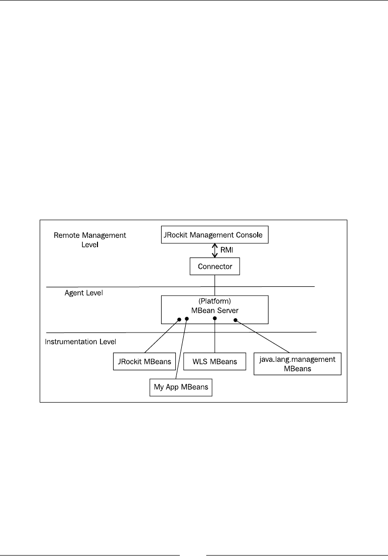
Chapter 6
[ 225 ]
A full discussion on JMX is beyond the scope of this book, but we'll briey discuss
the basic concepts. The JMX standard is a three-layered architecture. It consists of:
• The Instrumentation Level: This is where applications running in the JVM
expose resources for manageability through Managed Beans (MBeans). An
MBean is a type of Java Bean that is dened by its attributes, its operations,
and the notications it can emit.
• The Agent Level: The agent is the component managing the MBeans.
The most important agent-level component is the MBean server, which is a
container where MBeans are registered and managed.
• The Remote Management Level: This level provides protocol
adapters that enable communication with the MBean server from
outside the JVM process.
The following gure shows how the different architectural levels of JMX apply
in a typical JRockit deployment:
JRockit Mission Control
[ 226 ]
Mission Control server-side components
From a high-level Mission Control perspective, the monitored JRockit JVM
consists of:
• A set of server-side APIs:
° JMXMAPI: JRockit JVM-specic extensions to the MBeans
available in the platform MBean server. MBeans and the
platform MBean server will be discussed in the next chapter.
° JRockit internal local Java APIs: For example the JRockit
Management API (JMAPI).
° Server-side native APIs: APIs that are built into JRockit and
not implemented in Java. For example, the native API used
by Memleak.
• Agents exposing the previously mentioned APIs and miscellaneous services:
° The default JMX agent
° The Memleak server: A native server that exposes the native
Memleak API over the proprietary Memleak Protocol (MLP)
° The JRockit Discovery Protocol (JDP) server: An optional
service that broadcasts the locations of JVM instances on the
network
Mission Control client-side components
As of JRockit Mission Control 2.0, the JRMC client is based on Eclipse RCP (Rich
Client Platform) Technology. This provides a series of architectural advantages, such
as an OSGi-based component model and being able to run JRockit Mission Control
both as a standalone application and inside the Eclipse IDE.
Mission Control 2.0 was internally codenamed Energy, as
E=mc2. Yes, we're nerds!
Chapter 6
[ 227 ]
The Rich Client Platform is the base platform for the Eclipse IDE. It
contains, among other things, the Standard Widget Toolkit (SWT),
JFace, the Eclipse OSGi implementation (Equinox), and an integrated
mechanism to deliver and update RCP applications. OSGi is a
standardized dynamic module system for Java, backed by numerous
large corporations. RCP provides an excellent base platform for writing
and delivering highly modular applications with a look and feel that is
native to the host operating system.
For more information on RCP, please see http://www.eclipse.org/
home/categories/rcp.php.
For more information on OSGi, please see http://www.osgi.org/.
The client-side of JRockit Mission Control is highly modular—new tools can easily
be plugged in, and the tools themselves can be extended.
From a high-level Mission Control perspective, the Mission Control Client
consists of:
• RCP: The Eclipse Rich Client Platform
• Client-side APIs:
° RJMX: Extended JMX services, such as an MBean attribute
subscription framework, triggers, proxies for the old
proprietary, and obsolete RMP protocol (used in 1.4 versions
of JRockit)
° Memleak API: For communicating with the Memleak server
° Flight Recorder Model: For parsing JRockit Flight Recorder
recordings
° JDP Client API: For detecting JRockit instances running on
the network
• JRockit Mission Control core: Contains the core framework for the JRockit
Mission Control client and denes the core extension points
• The JVM Browser: Keeps track of the detected and/or user-dened
connections to JVMs
• The Tools: The various tools that can be launched from the JVM browser—
the Management Console, the Flight Recorder, and Memleak
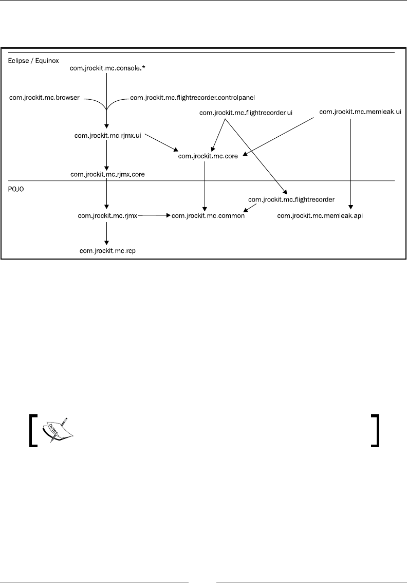
JRockit Mission Control
[ 228 ]
The following gure shows a simplied breakdown of the plug-ins in the 4.0.0
version of JRockit Mission Control:
The rest of this chapter will focus on how to get JRockit Mission Control up and
running and how to troubleshoot JRockit Mission Control. The different tools in
JRockit Mission Control will be explained in detail in the chapters that follow.
Terminology
In order to efciently communicate about the JRockit Mission Control client, a
common terminology is needed. The terms discussed here apply when running
Mission Control standalone as well as inside Eclipse.
The reader familiar with Eclipse may note that we use the same
terminology as with Eclipse and the Eclipse Workbench.
In an Eclipse RCP application, the main window is called the workbench. Inside the
workbench there are two types of windows—views and editors. The editors occupy
the center of the workbench—the editor area. The views are normally located around
the editor area.
As shown in the following screenshot, the JVM Browser is the view to the left:
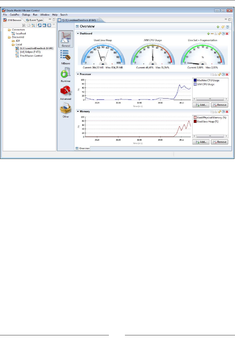
Chapter 6
[ 229 ]
Views are normally used to show a specialized presentation of the contents of the
selected editor, to manipulate the contents of an editor, or to launch new editors.
Several views can be docked on each other by dragging a view on top of another
view into the same view folder.
A certain conguration of which views to show, along with how they should be
located, is called a perspective. In the screenshot, the Mission Control perspective is
used, that shows the JVM Browser view and the Event Types view co-located in the
same view folder to the left. Should you ever lose a view or mistakenly rearrange the
views in a way you are not satised with, the perspective can easily be reset from the
workbench menu (Window | Reset Perspective).
The editor currently opened in the editor area in the screenshot above is a JRockit
Mission Control Console. It is being used to monitor a locally running application
where the main class is called LoadAndDeadlock.
In Eclipse parlance, the JRockit tools are built as editors—any tool that is started
will open up in the editor area. Several editors can be open at the same time. They
will show as multiple tabs in the editor area. Several editors can also be viewed
side-by-side by dragging an editor by the tab and docking it at any side of another
editor. Views, such as the JVM Browser, cannot be docked into the editor area.
They can, however, be docked to any side of the editor area.

JRockit Mission Control
[ 230 ]
To the left in the Management Console (in the editor area) is the tab group toolbar
that selects tabs that are currently visible in the tab container at the bottom of the
editor. A tab group toolbar is available in other JRockit Mission Control tools as
well. In JRockit Mission Control 3.1, the General tab group, which is automatically
selected when a Management Console is started, contains only a single tab—the
Overview tab.
Running the standalone version of Mission
Control
JRockit Mission Control exists both as a standalone executable and as a plug-in for
the Eclipse IDE. The version of JRockit Mission Control included in the JRockit JDK
is the standalone version.
Starting Mission Control in standalone mode is simple. Just run the
executable named jrmc (or jrmc.exe on Windows) in the bin directory
of the JRockit distribution.
Do not attempt to start JRockit Mission Control in standalone mode
through any mechanism other than running the jrmc executable.
Sometimes we run into homegrown customer setups where Mission
Control is started by running the jar les in the Mission Control
directory with some elaborate class path conguration. This is
generally a very bad idea and is strongly discouraged. The jrmc
launcher ensures, among other things, that the correct version of
JRockit is being used to launch JRockit Mission Control, and that the
class path is correctly congured.
For example:
JROCKIT_HOME/bin/jrmc
On Windows systems, JRockit Mission Control, when installed, will also be available
in the start menu.
Once JRockit Mission Control has been started, an empty workspace (JRockit Mission
Control 3.x), or a welcome screen (JRockit Mission Control 4.0) is displayed. If
everything is correctly set up, JRockit Mission Control will automatically discover
JVMs running on the local system. Even if there are no other Java applications
running, the JRockit JVM used to execute the JRockit Mission Control client will be
discovered and displayed as This Mission Control in the JVM Browser.
From the JVM Browser, the different JRockit Mission Control tools can be launched
against a selected JVM.
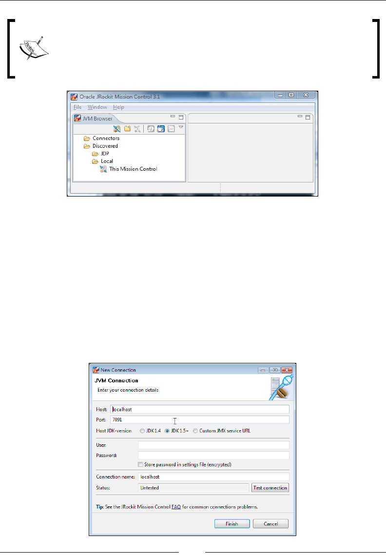
Chapter 6
[ 231 ]
Most of the tools require the JVM to be a JRockit JVM, as they are relying
on JRockit specic APIs. The Management Console is currently the only
exception among the tools, as it can be connected to any JMX compliant
JVM. Some functionality will however be unavailable if connected to
anything but a JRockit JVM.
Finding and monitoring locally running JVMs is simple and convenient—no additional
setup is required. However, having the Mission Control client running on the same
machine as the monitored JVM is usually a bad idea, especially in an enterprise
conguration. The resources required by the client will be taken from whatever
mission critical application executing on the JVM that is to be proled. Of course, in
a testing or development environment, this may be acceptable. Also, changes made
to the settings, for instance the addition of an attribute to a graph in the JRockit
Management Console, are stored on a per-connection basis. They are, however, not
stored at all for local connections.
To add a user-dened connection, simply click on the Connectors folder and click
on the Create Connection button.

JRockit Mission Control
[ 232 ]
The Connection Wizard, as shown in the previous screenshot, will open. Here, the
details of the connection can be specied. It is usually enough to enter the Host and
Port, but the following is worth noting:
• If connecting to a JDK 1.4 version of JRockit, select the JDK 1.4 radio button.
• Selecting the Custom JMX service URL radio button will allow full control
over the JMX Service URL. The JMX Service URL is a URL that species how
to connect to a JMX agent. Specifying a custom URL is useful if a protocol
other than JMX over RMI is required by the agent.
The protocol used by the default agent is JMX over RMI (JMXRMI).
Other possible protocols include JMXMP (as described in the Java SE
documentation) and IIOP. There are also proprietary protocols, such as
WebLogic Server's t3. If using a custom agent and a custom protocol, see
the agent documentation for more information.
• Passwords can be stored by checking the Store password in settings
le (encrypted) check box. If storing passwords is enabled, a master
password will be used each time the password is encrypted or decrypted.
If no master password is set, one will be asked for. The master password
can be reset by clicking on the Reset Master Password button in the
JRockit Mission Control preferences.
• The Test connection button is very useful for validating that a connection
is correctly congured before leaving the wizard.
Running JRockit Mission Control inside
Eclipse
There are some advantages to running JRockit Mission Control inside the Eclipse
IDE, there are however no fundamental differences in functionality. One advantage,
if the source code for the application being monitored is in the Eclipse workspace,
is that it is possible to jump directly to the corresponding source whenever a class,
method, or stack frame is shown in the JRockit Mission Control client.
If you are unfamiliar with Eclipse, or if you do not plan to use it for Java
development, you can safely skip this section, as it assumes some familiarity with the
Eclipse IDE.
In order to start JRockit Mission Control inside Eclipse, the JRockit Mission Control
plug-ins from the JRockit Mission Control update site must rst be installed. The
latest version of the update site will be available from the JRockit Mission Control
home page on Oracle Technology Network. At the time of writing, the JRockit
Mission Control homepage is located at http://www.oracle.com/technology/
products/jrockit/missioncontrol/index.html.
Chapter 6
[ 233 ]
As that's a handful to remember, it can also be reached at http://www.tinyurl.
com/missioncontrol.
Installation instructions can be found at the update site and will not be discussed
in detail here. To fully take advantage of all of the features in the JRockit Mission
Control plug-ins, Eclipse should be run on a JRockit JVM. Most of the functionality
is available, even if Mission Control is running in an Eclipse instance executing on
another JVM, but features such as local JVM discovery and some JRockit specic
functionality in the Management Console will not work.
There are additional benets of running Eclipse on JRockit. JRockit Real Time,
discussed in Chapter 3, Adaptive Memory Management can be used to make any
interactive application more responsive.
In the Eclipse home folder, there is a conguration le, eclipse.ini, that can be
altered to change the command-line ags of the JVM running Eclipse. Here is an
example eclipse.ini le that the authors use:
-showsplash
org.eclipse.platform
-framework
plugins\org.eclipse.osgi_3.4.3.R34x_v20081215-1030.jar
-vm
d:\jrockits\R27.6.3_R27.6.3-16_1.5.0\bin
-vmargs
-Xms512m
-Xmx512m
-XgcPrio:deterministic
-XpauseTarget:20
The previous example is for Eclipse 3.4 and JRockit R27, but it is very similar in
Eclipse 3.5 and JRockit R28. To make it work with R28, simply specify the path
to the R28 JVM after the –vm argument, and keep everything after the –vmargs.
There are differences in command-line ags between R27 and
R28, and the JRockit Documentation should be consulted for
more elaborate JVM congurations.
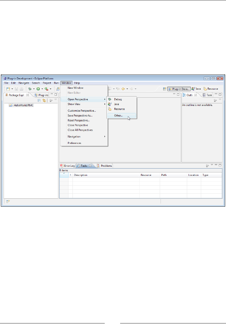
JRockit Mission Control
[ 234 ]
To start JRockit Mission Control once it is installed in Eclipse, the Mission Control
perspective must be opened. There are two Mission Control perspectives available
in 3.x—the Mission Control main perspective and the Mission Control Latency
perspective. The latter is used to study JRA recordings containing latency data. In
the 4.0 version of JRockit Mission Control, there is only one perspective optimized
to work with all the tools.
As shown in the following screenshot, the Mission Control perspectives can be found
in the Window | Open Perspective | Other... menu:
Once the Mission Control perspective has been opened, things will look pretty
much the same as when using the standalone version of JRockit Mission Control.
As mentioned, one benet of running JRockit Mission Control from within Eclipse
is the ability to open up the corresponding application source code from most
places where JRockit Mission Control shows a class or method, as shown in
the following screenshot:
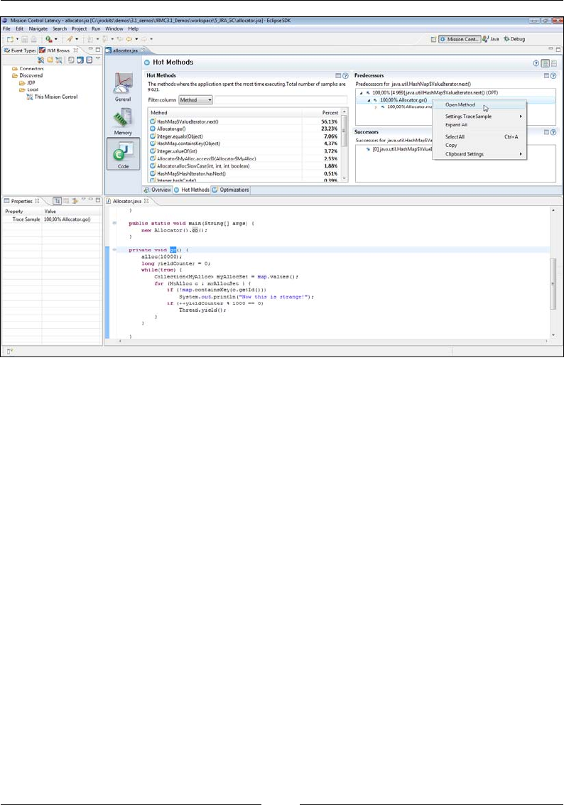
Chapter 6
[ 235 ]
Starting JRockit for remote management
To enable a JRockit JVM for remote management, the external management agent
must be started. It can either be started with the –Xmanagement command-line
switch, or JRCMD can be used. JRCMD is discussed in detail in Chapter 11.
The following example starts up a JRockit JVM with a simple test program and
enables it for remote monitoring on port 4712. Authentication and SSL support
for the connection are turned off.
JROCKIT_HOME/bin/java
–Xmanagement:ssl=false,authenticate=false,port=4712 –cp . HelloJRMC
For now, let's ignore the security ags and focus on the port. Examples of how to
set up JRockit Mission Control with security turned on will be shown in the section
Running in a Secure Environment, later in this chapter.

JRockit Mission Control
[ 236 ]
As mentioned, the default management agent uses the JMX over RMI protocol for
communication. This has been a source of some grief to people trying to establish
connections through rewalls as RMI usually requires communication over an
anonymous port. A full discussion on RMI is outside the scope of the book, but
this is how it used to work in versions prior to R28:
• -Xmanagement:port=<port> opens up a single entry, read only, RMI
registry on the specied port (default 7091)
• The RMI registry contains a single entry: jmxrmi—the stub for
communicating with the RMI server
• The port of the RMI server is anonymous with no way to override it
In R28, things have improved. The RMI registry and the RMI server ports are the
same by default, making rewall conguration much easier.
The JRockit Discovery Protocol
The JRockit JVM comes with a network auto discovery feature called JRockit
Discovery Protocol (JDP). The JDP Server works like a beacon that broadcasts the
presence of the JRockit instance to the network. This makes it easier for JRockit
Mission Control to automatically discover remote JVMs. The following example
shows how to enable auto discovery.
JROCKIT_HOME/bin/java
–Xmanagement:ssl=false,authenticate=false,port=4712,
autodiscovery=true –cp . HelloJRMC
The following table lists the various system properties that can be used to control the
JDP server in R28. Use the standard –D syntax for setting system properties on the
command line when starting up the JRockit JVM.
For example:
–Dcom.oracle.management.autodiscovery.period=2500
System property Explanation
com.oracle.management.autodiscovery.
period
Time between broadcasts
(milliseconds). Default is 5000.
com.oracle.management.autodiscovery.ttl Time to live for the broadcast
packages. Default is 1 hop.
com.oracle.management.autodiscovery.
address
The multicast address to use
for autodiscovery. Default is
232.192.1.212.
Chapter 6
[ 237 ]
System property Explanation
com.oracle.management.autodiscovery.
targetport
Override the port used to broadcast
autodiscovery information. Default
is 7095.
com.oracle.management.autodiscovery.
name
Hierarchical name. See the
following example.
To use the properties in the previous table for JRockit versions prior to
R28, the com.oracle.management.autodiscovery namespace in
the properties must be replaced by jrockit.managementserver.
discovery, as it was called earlier.
When a JDP server transmits the location of a running JRockit JVM, the JVM
Browser in the JRockit Mission Control client can use the hierarchical name in
three different ways.
• Simple name:
Example: -Djrockit.managementserver.discovery.name=MyJVM
Result: The name of the connection when it appears in the browser will
be MyJVM.
• Full path:
Example: -Djrockit.managementserver.discovery.name=/MyJVMs/MyJVM
Result: The connection will appear under a MyJVMs folder in the browser, and
the name will be MyJVM.
• Path ending with path delimiter:
Example:-Djrockit.managementserver.discovery.name=/MyJVMs/
Result: The connection will appear under MyJVMs, the name will be the result
of a reverse DNS lookup of the host reported by the JDP packet.
Advanced tip for plug-in developers
System properties starting with the string com.oracle.management.
autodiscovery.property will be automatically picked up by the JDP
server and broadcast to the client. For the R28.0.0 version, no such extra
properties are actually used by the client. The properties will, however,
be present in the IConnectionDescriptor of the Mission Control
client—a fact that can be used by authors of plug-ins for Mission Control.
JRockit Mission Control
[ 238 ]
For reference, the following table lists the various –Xmanagement arguments in
JRockit R28:
Flag Explanation Default
port = <int> The port of the RMI registry. 7091
ssl =
[true|false]
Enables secure monitoring over SSL. Note that
this only enables server-side SSL. If you also
want clients to authenticate themselves, set
com.sun.management.jmxremote.ssl.
need.client.auth=true. Also note that
SSL communication with the registry will not
be enabled by default. See registry.ssl.
true
registry.ssl =
[true|false]
Binds the RMI connector stub to an RMI
registry protected by SSL.
false
authenticate =
[true|false]
If this is set to false, JMX does not use
passwords or access les—all users are allowed
full access.
true
autodiscovery =
[true|false]
Enables autodiscovery service for the remote
JMX connector. Autodiscovery allows other
machines on the same subnet to automatically
detect a JVM with remote management
enabled. Note that the autodiscovery service
will only start if remote JMX management
is enabled.
false
local =
[true|false]
Explicitly enables or disables the local
management agent.
true
rmiserver.port
= <int>
Binds the RMI server to the specied port.
Default behavior is to bind to the same port as
the RMI registry if possible. However, if the
RMI server is using SSL and the registry is not,
an arbitrary free port will instead be selected.
Same as port
remote =
[true|false]
Explicitly enables or disables the remote
management agent.
false
config.file =
<path>
Species a le from which to load additional
management conguration properties.
JRE_HOME/lib/
management/
management.
properties
Chapter 6
[ 239 ]
There are also system properties available in JRockit R28 for controlling
specic settings. The following table lists the relevant system properties
with their default values:
Property Explanation Default
com.oracle.management.
jmxremote =
[true|false]
Enables JMX local monitoring
through a JMX connector. The
connector is published on a private
interface used by local JMX clients
through the Attach API (see the
Java Documentation for com.sun.
tools.attach). Clients can use
this connector if it is started by the
same user as the one that started the
agent. No password or access les
are checked for requests coming
through this connector. If explicitly
set to false, no local connector is
started even if jmxremote.port
is specied.
true
com.oracle.management.
jmxremote.port = <int>
Same as
-Xmanagement:port=<int>
7091
com.oracle.management.
jmxremote.rmiserver.
port = <int>
Same as
-Xmanagement:rmiserver.
port=<int>
7091
com.oracle.management.
jmxremote.ssl =
[true|false]
Same as -Xmanagement:ssl
=[true|false]
true
com.oracle.management.
jmxremote.registry.ssl
= [true|false]
Same as
-Xmanagement:registry.ssl =
[true|false]
false
com.oracle.management.
jmxremote.ssl.enabled.
protocols = <values>
A comma-delimited list of SSL/TLS
protocol versions to enable. Used in
conjunction with the SSL ags.
Default SSL/TLS
protocol version.
com.sun.management.
jmxremote.ssl.enabled.
cipher.suites =
<values>
A comma-delimited list of SSL/
TLS cipher suites to enable. Used in
conjunction with the SSL ags.
Default SSL/TLS
cipher suites.
JRockit Mission Control
[ 240 ]
Property Explanation Default
com.oracle.management.
jmxremote.ssl.
need.client.auth =
[true|false]
If this property is true and SSL is
enabled, client authentication will be
performed.
false
com.oracle.management.
jmxremote.authenticate
= [true|false]
Same as –
Xmanagement:authenticate =
[true|false]
true
com.oracle.management.
jmxremote.password.file
= <path>
Species the location of the
password le. If com.sun.
management.jmxremote.
authenticate is false, this
property and the password and
access le are ignored. Otherwise,
the password le must exist and be
in the valid format. If the password
le is empty or nonexistent, no
access is allowed.
JRE_HOME/lib/
management/
jmxremote.
password
com.oracle.management.
jmxremote.access.file =
<path>
Species the location for the access
le. If com.sun.management.
jmxremote.authenticate is
false, then this property and
the password and access le are
ignored. Otherwise, the access
le must exist and be in the valid
format. If the access le is empty or
nonexistent, no access is allowed.
JRE_HOME/lib/
management/
jmxremote.
access
com.oracle.management.
jmxremote.login.config
= <config entry>
Species the name of a Java
Authentication and Authorization
Service (JAAS) login conguration
entry to use when the JMX agent
authenticates users. When using
this property to override the default
login conguration, the named
conguration entry must be in a le
that is loaded by JAAS. In addition,
the login modules specied in
the conguration should use the
name and password callbacks
to acquire the user's credentials.
For more information, see the
API documentation for javax.
security.auth.callback.
NameCallback and javax.
security.auth.callback.
PasswordCallback
Default login
conguration
is le-based
password
authentication
Chapter 6
[ 241 ]
Property Explanation Default
com.oracle.management.
jmxremote.config.file
Same as -Xmanagement:config.
file=<file name>
JRE_HOME/lib/
management/
management.
properties
com.oracle.management.
snmp.port = <int>
Enables the built-in SNMP agent on
the specied port.
No default
com.oracle.management.
snmp.trap = <int>
Remote port to which the built-in
SNMP agent sends traps.
162
com.oracle.management.
snmp.acl = [true|false]
Enables Access Control Lists (ACL)
for the built-in SNMP agent.
true
com.oracle.management.
snmp.acl.file = <path>
Path to a valid ACL le. After the
agent has started, modifying the
ACL le has no further effect.
JRE_HOME/lib/
management/
snmp.acl
com.oracle.
management.snmp.
interface=<inetaddress>
The inetAddress of the local host.
This is used to force the built-in
SNMP agent to bind to the given
inetAddress. This is for
multi-home hosts if one wants to
listen to a specic subnet only.
No default
com.oracle.management.
autodiscovery =
[true|false]
Same as
–Xmanagement:
autodiscovery=true
false
Running in a secure environment
The best way to ensure a secure environment with JRockit Mission Control is to rst
use standard networking techniques, such as rewalls, to ensure that only a very
limited set of machines are allowed to even attempt a connection to the management
agent. Setting up routers and rewalls is beyond the scope of this book.
In versions prior to the JRockit R28, using rewalls with the
management agent was complicated, as communication with the RMI
server was done on an anonymous port. That is, after establishing a
connection with the RMI registry, there was no way of inuencing
on what port the communication with the RMI server would take
place. In R28, the same port is used for the registry and the server by
default, which makes rewall conguration much easier.
JRockit Mission Control
[ 242 ]
For secure communication, the management agent should be congured to only
allow SSL encrypted connections. The management agent can be congured to use
SSL both for the RMI registry and the RMI server. For a secure environment, both
should use SSL. By default, secure server authentication over SSL is enabled,
but client authentication is not.
Following is an example of the options used to enable SSL on the server and the
registry, as well as for enabling secure client authentication:
JROCKIT_HOME\bin\java –Xmanagement:ssl=true,registry.ssl=true,port=4711
-Dcom.oracle.management.jmxremote.ssl.need.client.auth=true MyApp
For SSL to work, certicates must be set up. In most Java environments, a keystore is
used to store the private keys, and a truststore to store the trusted certicates.
For more information on using keystores, please see the J2SE
SDK Documentation, on the Internet, especially the JSSE section
on creating keystores.
Next, authentication and roles need to be congured to ensure that only authorized
entities have access to sensitive functionality. Access rights are controlled by the
jmxremote.password and jmxremote.access les. These are normally placed in
the directory JROCKIT_HOME/jre/lib/management/. The password le contains
the passwords for the different roles, and the access le species the access rights of
each role. A role must have an entry in both les in order to work.
To facilitate easy setup, there is a jmxremote.password template le included with
the JRockit JRE. To get started with this template, copy the le JROCKIT_HOME/jre/
lib/management/jmxremote.password.template to JROCKIT_HOME/jre/lib/
management/jmxremote.password.
To be able to initiate JMXMAPI, which is necessary for all Mission
Control tools to work, the user must have the permission to create
the JRockitConsole MBean.
Following is an example of granting permission to create the JRockitConsole
MBean to the control role (see the jmxremote.access le):
controlRole readwrite \
create oracle.jrockit.management.JRockitConsole
Chapter 6
[ 243 ]
The JRockitConsole MBean will in turn initiate the rest of JMXMAPI.
In a multi-user environment, that is, in an environment where different users will
use the same Java installation, the custom is to copy the jmxremote.password
le to each user's home directory and use the com.sun.management.jmxremote.
password.file system property to specify the location of the le.
As the password le contains unencrypted passwords, Java will rely on the le
permissions of the underlying operating system to ensure that the le can only be
read by the user executing the JVM. If an error is shown about the password le not
being restricted, steps must be taken to ensure that the password le is only readable
by the user that is executing the Java process. On a *NIX system, this can be done
by executing something like chmod 600 <password file name> from a shell. On a
Windows system, the process is slightly more complicated.
There is a good guide for setting le access permissions on Windows
in the Java 1.5.0 documentation, available at http://java.sun.
com/j2se/1.5.0/docs/guide/management/security-
windows.html.
To top things off, all communication can be done over an encrypted SSH tunnel,
instead of by opening an additional port in the rewall. Access to the SSH tunnel
is commonly enabled through a port on localhost. The stub transmitted when
a connection to the JMX agent is established normally contains the address of the
computer to connect to. We want to trick the computer running the agent into
transmitting a stub containing the loopback address or localhost instead. This
can either be done by editing the hosts le, or by setting the java.rmi.server.
hostname system property on startup. Both these techniques should be used with
caution, as they may cause problems for other software running in the system
and/or on the same JVM.
Troubleshooting connections
If you are having problems connecting to locally discovered JRockit JVMs, you
should check:
• If you are running on Windows, verify that the system temporary directory
is on a le system that supports le permissions (for example NTFS). This is
required. Local connections will create artifacts that rely on le permissions
to work, and will simply fail if running on a FAT le system.
• Are you really attempting to connect to a JRockit JVM, and is the Mission
Control client (or Eclipse, if running in Eclipse) running on a JRockit JVM?
JRockit Mission Control
[ 244 ]
• If a local connection is attempted, are both your JRockit Mission Control
Client and the JRockit JVM that you are attempting to connect to, using
a JDK version of 1.5 or later?
• Is the JVM you are trying to connect to executing as your user?
To connect to a locally executing 1.4 version of the JRockit JVM, create
a connection manually in the JRockit Mission Control JVM Browser.
Then start the management agent explicitly on the JRockit JVM that
you want to monitor. This is because 1.4 versions of the JVM really do
not have a platform MBean server. JRockit 1.4 versions did, however,
implement a proprietary management protocol called RMP that is
translated to JMX on the client. Starting the agent can either be done
by using the command-line options as described earlier, or by using
the JRCMD tool, described in Chapter 11.
If you are having problems connecting to an external management agent (usually,
but not necessarily, one running on a remote machine) you should check:
• Is the connection properly congured? There is a test button in the
connection wizard that will verify the settings for you. If you are trying
to connect to a JDK 1.4 version of the JRockit JVM, you should be using
a 3.x client.
• Is the correct version of the client being used? The easiest way to be sure is to
use the version that came with the JVM. If attempting to connect to a JDK 1.4
version of the JRockit JVM, a 3.x version should be used.
• Is the 1.4/1.5 setting correct in the Connection Wizard?
• Is the rewall congured to let the trafc through on the appropriate ports?
• If SSL is being used, are the SSL settings correct on both the server and
the client?
• If authentication is enabled, is the jmxremote.access le properly set up, as
described in the Java SE documentation?
• Verify the hosts le of the machine to which you are trying to connect.
While troubleshooting connections to the remote management agent, rst make
sure that the connection works with SSL and that authentication is turned off. If that
works, make sure that all the steps in the Running in a Secure Environment section
have been followed, that the certicate is valid, that the keystore password is correct,
and that the password.properties le has been properly congured.

Chapter 6
[ 245 ]
If the Management Console tells you that a certain MBean, for instance the Proling
MBean, cannot be found, it may be due to a miscongured jmxremote.access le.
To be able to initialize JMXMAPI, the user must have authorization to create the
JRockitConsole MBean that, in turn, will initialize the rest of the JMXMAPI. See the
Running in a Secure Environment section for more information.
Hostname resolution issues
Trouble connecting Mission Control to a remote machine can sometimes stem from the
hostname resolving to the wrong address, for example to 127.0.0.1 (or localhost).
An exception looking something like this would normally be shown in such a case:
Could not open Management Console for sthx6454:7094.
java.rmi.ConnectException: Connection refused to host:
127.0.0.1; nested exception is: java.net.ConnectException:
Connection refused: connect
at sun.rmi.transport.tcp.TCPEndpoint.newSocket(TCPEndpoint.java:574)
at sun.rmi.transport.tcp.TCPChannel.createConnection
(TCPChannel.java:185)
at sun.rmi.transport.tcp.TCPChannel.newConnection(TCPChannel.java:171)
at sun.rmi.server.UnicastRef.invoke(UnicastRef.java:94)
at javax.management.remote.rmi.RMIServerImpl_Stub.newClient
(Unknown Source)
at javax.management.remote.rmi.RMIConnector.getConnection
(RMIConnector.java:2239)
at javax.management.remote.rmi.RMIConnector.connect
(RMIConnector.java:271)
at javax.management.remote.rmi.RMIConnector.connect
(RMIConnector.java:229)
at com.jrockit.console.rjmx.RJMXConnection.setupServer
(RJMXConnection.java:504)
The RMI registry exports a stub relying on a hostname to establish a connection
to the RMI server. In the previous example, we have successfully connected to the
RMI registry and retrieved a stub for connecting to the RMI server. However, the
default behavior when creating the stub is to use InetAddress.getLocalHost().
getHostAddress(), to nd out what host name to use. This will of course be a
problem if the machine is multi-homed (that is, has several network interfaces)
or if it is badly congured. In the previous example, the information provided in
the stub tells us to connect to localhost instead of sthx6454.

JRockit Mission Control
[ 246 ]
The most common problem is that the hosts le (/etc/hosts on Linux systems,
%SYSTEMROOT%\system32\drivers\etc\hosts on Windows) is not properly
congured. On a Linux system, hostname –i can be used to see what the
hostname resolves to.
A workaround is to set the java.rmi.server.hostname system property on the
server to whatever name the client should use to locate the machine. Note that this
can affect other applications running on the JVM.
Another workaround is to use SSH tunneling where the fact that the hostname
resolves to localhost can be used to an advantage. This workaround is only
possible using JRockit R28, where the RMI server port can be explicitly specied.
The Experimental Update Site
Since JRockit Mission Control 3.1, there is an Experimental Update Site from which
plug-ins for Mission Control can be installed. The plug-ins either extend JRockit
Mission Control, or facilitate building extensions for JRockit Mission Control. The
homepage for the update site for 3.1 versions of JRockit Mission Control can be
found here:
http://www.oracle.com/technology/software/products/jrockit/
missioncontrol/updates/experimental/3.1.0/eclipse/index.html
The update site for the 4.0 release can be found here:
http://www.oracle.com/technology/software/products/jrockit/
missioncontrol/updates/experimental/4.0.0/eclipse/index.html
When using the update site URLs in Eclipse, the ending index.html must
be removed.
Both the JRockit and reference J2SE distributions contain a reference JMX console
called JConsole. The 3.1.0 release of the update site included a plug-in that allowed
JConsole plug-ins to be run within JRockit Mission Control. It also contained a set
of Plug-in Development Environment (PDE) plug-ins that allows the development
of custom plug-ins for the JRockit Mission Control Console. More information on
creating plug-ins for JRockit Mission Control can be found at the end of Chapter 7
(The Management Console), in Chapter 9 (The Flight Recorder), and in Chapter 10
(The Memory Leak Detector).
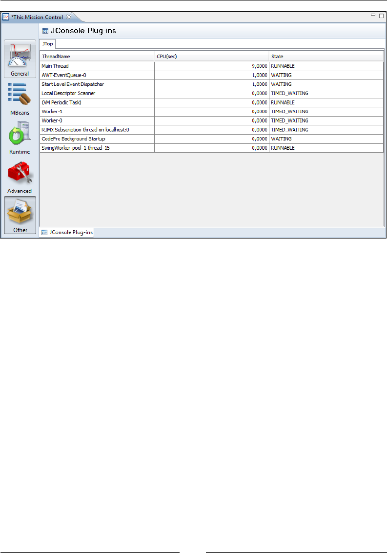
Chapter 6
[ 247 ]
After the 4.0 release of JRockit Mission Control, Oracle plants to make additional
plug-ins for Mission Control available. New experimental plug-ins will be
announced on the blog at http://blogs.oracle.com/hirt.
Debugging JRockit Mission Control
JRockit Mission Control can be started in debugging mode to provide more
information. Simply add the –debug ag when launching the jrmc executable.
Starting in debug mode will cause various subsystems to behave differently. For
example, the console charts will start showing rendering information and log levels
will be changed to display more verbose output.
To view the log messages sent to the console on Windows systems, stderr must be
redirected somewhere. This is because the jrmc launcher is derived from the javaw
launcher. Following is an example:
D:\>%JROCKIT_HOME%\bin\jrmc –consoleLog -debug 2>&1 | more
To only change the logging levels, select a Logging settings le in the Preferences.
The logging settings le is a le on standard java.util.logging format. After
changing the logging settings, JRockit Mission Control must be restarted.

JRockit Mission Control
[ 248 ]
The following example shows the debug settings used when starting with
the –debug ag:
############################################################
# JRockit Mission Control Logging Configuration File
#
# This file can be overridden by setting the path to another
# settings file in the Mission Control preferences.
############################################################
############################################################
# Global properties
############################################################
# "handlers" specifies a comma separated list of log Handler
# classes. These handlers will be installed during ApplicationPlugin
# startup.
# Note that these classes must be on the system classpath.
handlers= java.util.logging.FileHandler,
java.util.logging.ConsoleHandler
# Default global logging level.
# This specifies which kinds of events are logged across
# all loggers. For any given facility this global level
# can be overridden by a facility specific level
# Note that the ConsoleHandler also has a separate level
# setting to limit messages printed to the console.
.level= ALL
############################################################
# Handler specific properties.
# Describes specific configuration info for Handlers.
############################################################
# Default file output is in user's home directory.
java.util.logging.FileHandler.pattern = %h/mc_%u.log
java.util.logging.FileHandler.limit = 50000

Chapter 6
[ 249 ]
java.util.logging.FileHandler.count = 1
java.util.logging.FileHandler.formatter =
java.util.logging.SimpleFormatter
java.util.logging.FileHandler.level = FINE
java.util.logging.ConsoleHandler.formatter =
java.util.logging.SimpleFormatter
java.util.logging.ConsoleHandler.level = FINE
############################################################
# Facility specific properties.
# Provides extra control for each logger.
# For example setting the warning level for logging from the
# JRockit Browser, add the following line:
# com.jrockit.mc.browser.level = INFO
############################################################
sun.rmi.level = INFO
javax.management.level = INFO
Summary
This chapter explained how to get started with the JRockit Mission Control
tools suite. We briey went over the background for the product and its various
subcomponents—the Management Console, the Memory Leak Detector, and the
Flight Recorder. For completeness, we also mentioned JRCMD, the command-line
tool that is part of the JRockit JDK.
We showed how to run both the standalone version of Mission Control and
the plug-in version for the Eclipse IDE. We explained how to enable the JRockit
management agent for remote management and how to troubleshoot the
connection when Mission Control fails to connect. Additional tips and tricks
on how to debug the Mission Control client were also presented.
We outlined how to secure access to the server-side Mission Control components.
Finally, the Experimental Update Site, where additional content for Mission Control
can be found, was introduced.
The next few chapters will focus on the various tools in the JRockit Mission
Control suite.
The Management Console
The oldest tool in the JRockit Mission Control tools suite is the JRockit Management
Console. The Management Console can be used to monitor the JRockit JVM and
any application running in the JVM. It can also be used to alter the runtime state
of certain parameters in JRockit. This chapter assumes some prior familiarity with
Java Management Extensions (JMX) and the JMX terminology.
For more information on JMX go to http://java.sun.com/javase/
technologies/core/mntr-mgmt/javamanagement/
The Management Console relies on the JMX standard and provides a way to
monitor any application that exposes manageability features through JMX,
including the JRockit JVM.
In this chapter you will learn:
• How to start up the Management Console
• How to monitor and plot arbitrary MBean attributes
• How to invoke arbitrary MBean operations
• How to create trigger rules
• How to enable deadlock detection
• How to perform per-thread memory allocation and CPU proling
• About the diagnostic commands
• How to extend the Management Console
The Management Console
[ 252 ]
A JMX Management Console
The JRockit Management Console predates the JRockit Mission Control tools suite. It
even predates JMX.
The rst few versions of JRockit were made available as "Virtual
Machines for Java", not JVMs. The key difference is that only a virtual
machine certied by Sun (now Oracle) to be compliant with the Java
standard is allowed to be called a JVM. Furthermore, if the VM is not
certied, it may not use the Java trademark. At that time, in order
to be accepted as a Sun certied JVM, a key differentiator, known as
"value add" was required. In our rst attempt to become a proper Java
licensee, we had specied "superior performance" as our value add.
While technically true, it was not deemed to be a valid value add, so we
exposed some of the online manageability aspects of the JVM instead.
This is what became the JRockit Management Console.
The primary use of the Management Console is to provide detailed monitoring of one
or more JRockit instances. As each monitored JVM has its own Management Console
(editor), more than a few JVM instances are rarely monitored at a time. To monitor
large installations for longer periods of time, a distributed solution that scales well
over large amounts of JVMs should be used, such as Oracle Enterprise Manager.
The Management Console and JRockit use standard JMX technology for
communication. As of Java 5.0, some aspects of using JMX to expose manageability
features of the JVM are standardized through JSR-174.
JSR-174 enhanced the manageability of the JVM by adding the java.
lang.management classes and providing the platform MBean server.
For more information on the platform MBean server, see the Java APIs
and Documentation on SDN on the Internet and search for java.lang.
management.ManagementFactory.getPlatformMBeanServer()
Since the advent of JSR-174 and the platform MBean server, most Java applications
and frameworks are publishing their monitoring and management MBeans to the
platform MBean server, which in effect means that the Management Console can
monitor most parts of the software stack running in the JVM.
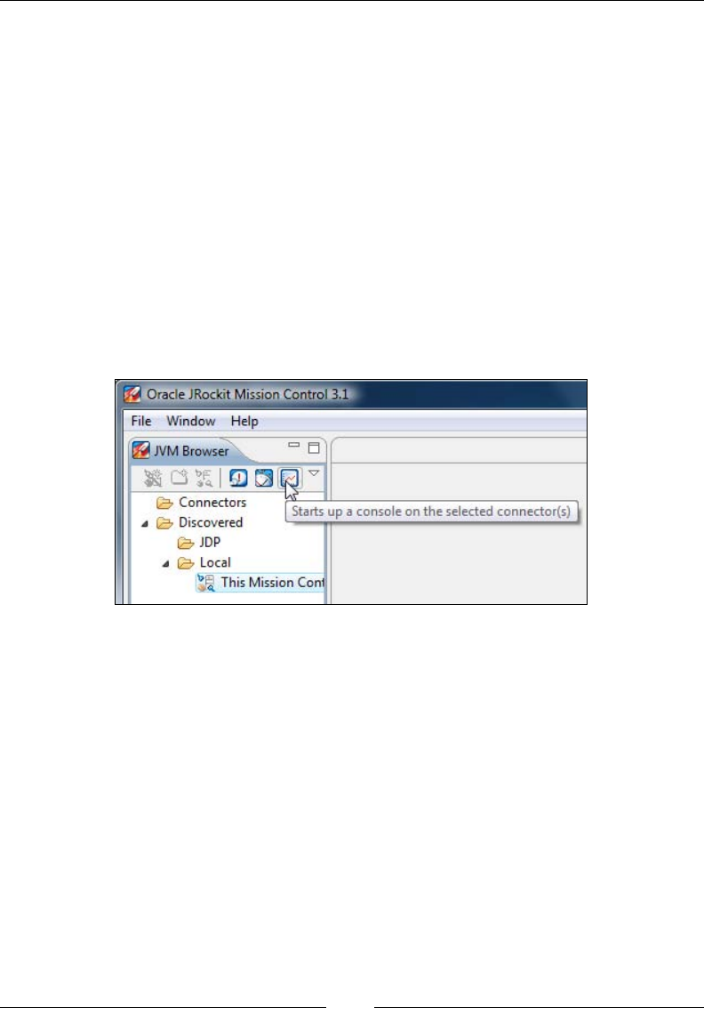
Chapter 7
[ 253 ]
As JRockit had a Management Console well before the start of JSR-174, the JRockit
Management Console can also connect to pre 1.5.0 versions of JRockit. In these
setups, everything still looks like JMX to the client, but underneath a proprietary
protocol is used.
The rest of this chapter is dedicated to discussing the JRockit Mission Control
Console and its various uses. The chapter is divided into sections corresponding
to the different tabs in the Management Console, so that it can also be used as a
reference to quickly check on details for a specic tab.
Using the console
Starting a JRockit Management Console is quite easy—simply select the JVM to
connect to from the JVM Browser and either click on the Management Console
button from the toolbar, or click on Start Console from the context menu.
There is a trick available for starting the console—connections can be dragged and
dropped into the editor area. The default action for dragging a connection to the
editor area is to open up the Console on the connection. Recollect from Chapter 6 ,
JRockit Mission Control, that connections are either remote or local—the difference
being that the local connections are automatically discovered JVMs running on the
local machine. This particular trick does not work with local connections, as they
cannot be used as sources in drag-and-drop operations.
For more information on the different types of connections and how to establish
remote connections, see the previous chapter.
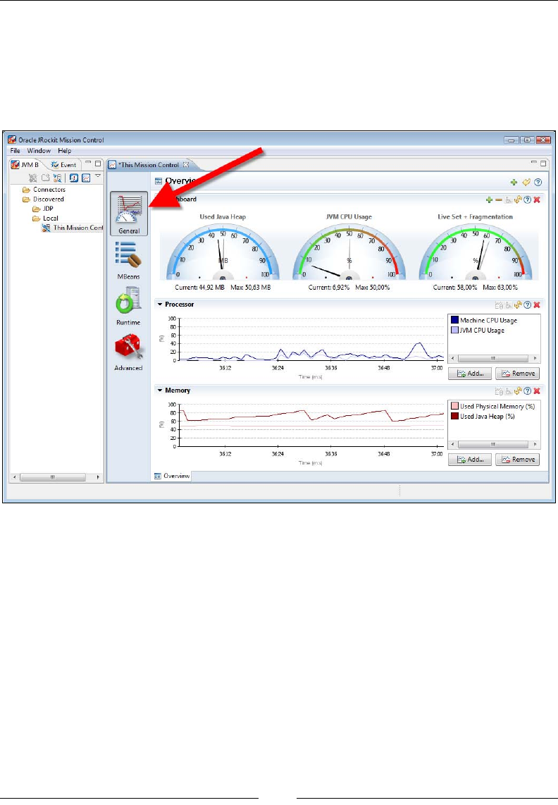
The Management Console
[ 254 ]
General
The tabs in the Management Console are grouped into different tab groups, the rst
one being the General tab-group. The different tab groups are accessible through
the vertical toolbar to the left in the Management Console editor, as shown in the
following screenshot:
The General tab group only contains one tab—the Overview. The tab folder
where the visible tab can be changed is located at the bottom of the JRockit Mission
Control editor.
The Overview
This tab shows an overview of some key characteristics of the JVM and its operating
environment. The tab is highly congurable and should you require other information
than the chosen key characteristics; it can be adapted to your needs.
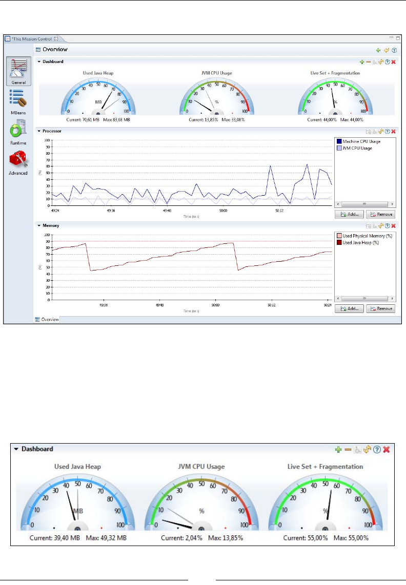
Chapter 7
[ 255 ]
The following screenshot shows the Overview tab of the JRockit Management Console:
The tabs in JRockit Mission Control are divided into section parts. At the top of
the Overview tab is a section part called Dashboard. The Dashboard contains an
array of dials. Each dial can plot the current and maximum value obtained for an
attribute that is being monitored. The lighter of the two indicators in a dial shows
the watermark, which indicates the maximum value attained since a subscription to
the attribute started. The darker indicator shows the current value. Both the current
and maximum values are also shown as numbers below the dial.
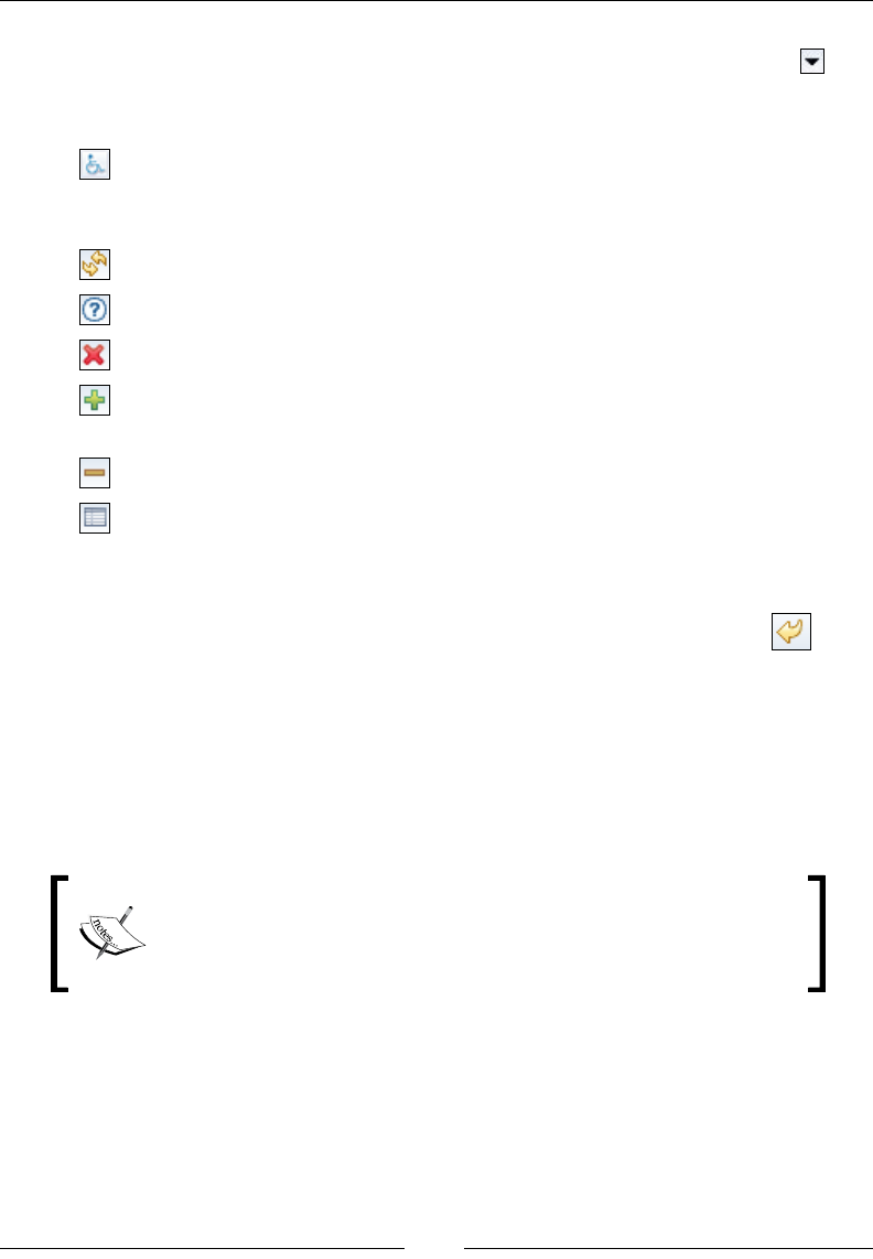
The Management Console
[ 256 ]
In the Management Console, most section parts can be folded away to allow more
space for the other sections in the same tab. Simply click on the little triangle ( )
at the top left of the section part to fold it. The section parts also contain a toolbar
with various actions. Some commonly used actions are:
• Accessibility mode toggle: Toggles the contents of the section part
between the default graphical representation and an alternative, text-based
representation.
• Updates toggle: Toggles updates for the contents of the section part.
• Help: Provides context sensitive help for the section part when clicked.
• Remove: Removes the section part altogether.
• Add: Adds a component of the kind that the section part contains. In the
case of a dial section part, a dial will be added.
• Delete: Deletes one of the enclosed components from the section part.
• Table settings: This action provides a dialog for conguring a table. Most
tables only show a selection of columns by default, and more columns can be
made visible, as needed, by using the table conguration dialog.
It is possible to revert any changes by clicking the Reset to default button ( ) in
the upper right corner of the toolbar for the tab.
The Dashboard can be recongured in various ways. It is possible to add dials,
remove dials, and change the attributes that each dial displays. The entire dial
section part can be removed altogether. As the dial has a resettable watermark that
shows the maximum value attained for an attribute, dials are useful for attributes
that may peak very intermittently, but that you still want to keep an eye on.
Changes made to automatically discovered connections are not
saved. If you suspect you will want to keep the adjustments made
in the console user interface, make sure that you use a user-dened
connection as described in the previous chapter.
The default attributes shown in the dial dashboard are the Current and Max
values for heap usage, the CPU usage of the JVM process, and the live set and
fragmentation as a percentage of the heap size. The last value is a good measure
of how full the heap is and it is only calculated and updated on every garbage
collection. If no indicator is shown for the Live Set + Fragmentation dial, it means
that no garbage collection has taken place yet.
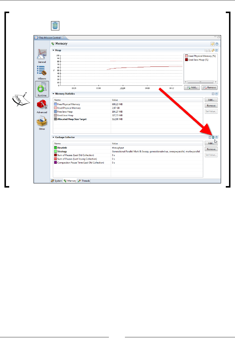
Chapter 7
[ 257 ]
One way to force a garbage collection is to press the little garbage can
icon ( ) in the Runtime | Memory tab.
A JVM process that is constantly saturating the CPU (maxing out the CPU load)
can be a good thing. For instance, for a batch application that is computationally
bound, it would normally be a best case scenario for it to complete as soon as
possible. Normally, however, some over-provisioning is needed to keep an
application responsive. If the CPU usage is very high, you may want to invest in
better hardware, or look over the data structures and algorithms employed by the
application. One very good way to proceed is to capture a JRockit Flight Recording
to nd out where all those cycles are being spent.
Having a very large percentage of the heap lled with live objects will increase the
garbage collector overhead, as GCs will have to be run more frequently. If the Live
Set + Fragmentation dial remains steady on a high level and garbage collection
performance is an issue, increasing the heap size will improve performance. If the
trend is for the Live Set + Fragmentation dial instead to steadily increase over time,
there is probably a memory leak in the application. We will give memory leaks more
attention in Chapter 10, The Memory Leak Detector.
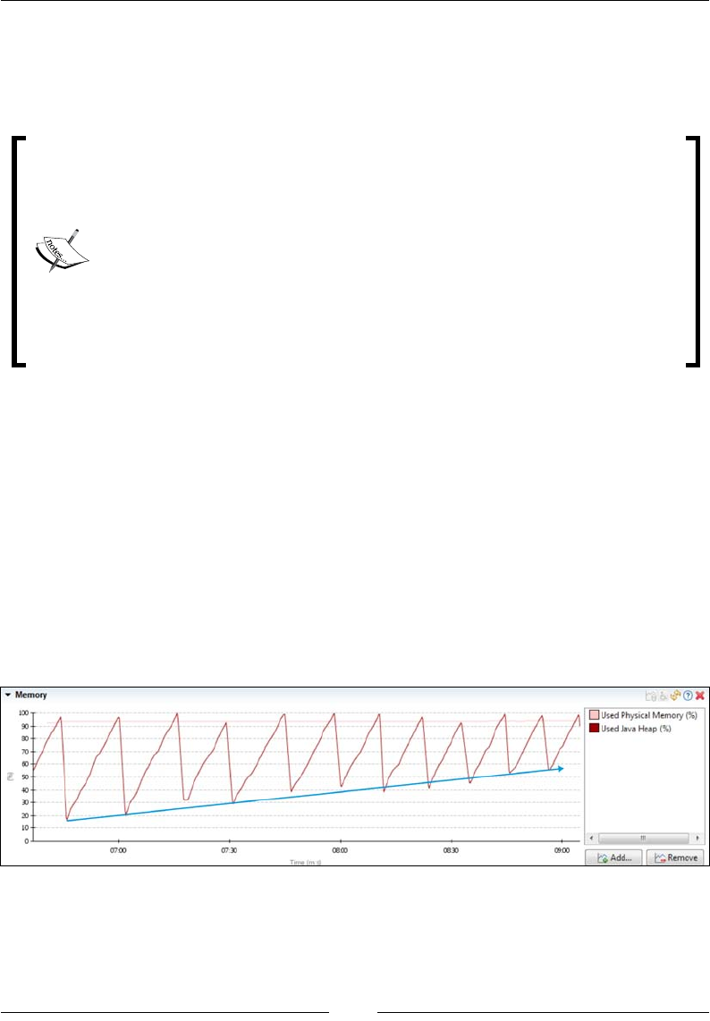
The Management Console
[ 258 ]
As any attribute available in the platform MBean server can be subscribed to. This
includes attributes from any domain, such as application server MBeans or even
your own MBeans that you have registered in the platform MBean server. An
example of such an attribute is the OpenSessionsCurrentCount in WebLogic Server.
WebLogic Server does not use the platform MBean server by default.
However, if you wish to monitor the WebLogic Server MBeans together
with the MBeans provided by the rest of the platform, it may be
convenient to make WebLogic Server add the MBeans to the platform
MBean server. Consult your WebLogic Server documentation for
information on how to do this.
The recommendation from WebLogic Server is to not use the platform
MBean server, as there are potential security implications, especially if the
applications running in the JVM cannot be trusted. If you use the platform
MBean server, make sure you understand the security implications, as all
code running in the JVM will have access to the WebLogic MBeans.
The two charts under the Dashboard show CPU usage information and memory
information, one below the other. The CPU usage is listed as a percentage of full
CPU saturation and is an average across all available cores. It is shown for both the
entire machine and the JVM process. For the memory chart, the used heap is shown
as a percentage of the total heap size and used physical memory is shown as a
percentage of the total physical memory available.
One way to track the live set and fragmentation is to check how the heap usage
changes over time in the memory chart.
Consider the following screenshot. An imaginary line is drawn through each point in
time where a garbage collection has nished and where memory has been reclaimed.
This gives us a good indication as to what is happening to the live set.
An even better way to watch live set and fragmentation is of course to simply add the
Live Set + Fragmentation attribute to the chart, as shown in the following screenshot.
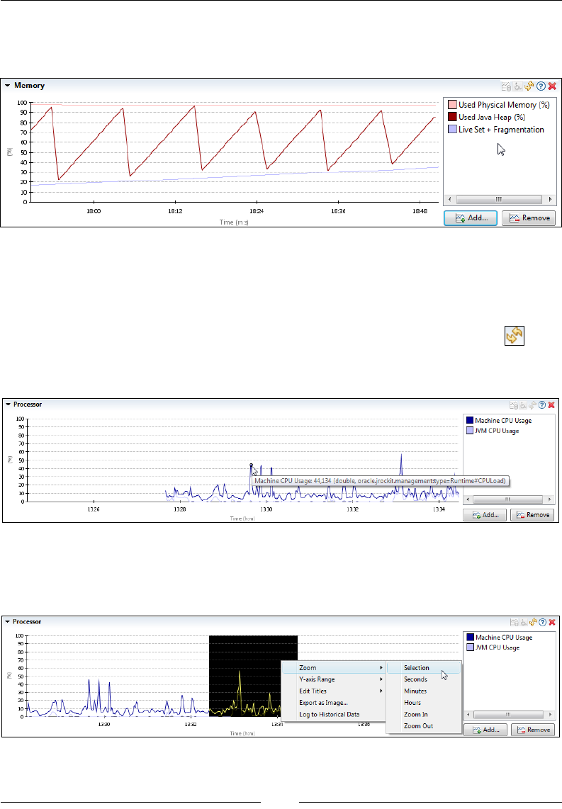
Chapter 7
[ 259 ]
As can be seen from the growing live set in the screenshot, the monitored application
probably has a memory leak. If left unchecked, the application will eventually throw
an OutOfMemoryError.
The charts can also be congured. It is possible to add or remove attributes to subscribe
to. The colors used to visualize attributes, the text labels, and various other properties
can also be changed.
Another useful, but often overlooked, feature is that additional info can be gained
when the chart is frozen. If a chart is frozen by toggling the updates button ( ),
context sensitive tooltips will be shown with detailed information when the pointer
is hovered near a point in a data series. This is shown in the following screenshot:
A chart will automatically be frozen when zooming in on a selection. To make a
selection in a chart, simply left click and drag with the mouse to select the time
period to zoom in on. To zoom in, select Zoom | Selection from the context menu.
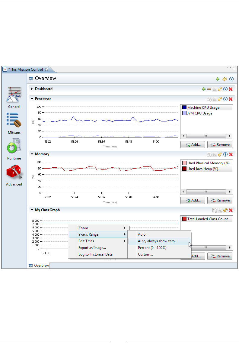
The Management Console
[ 260 ]
The default value range selected for the Y-axis of new charts and most of the default
charts in the user interface is between 0 and 100. This setting must be changed when
adding an attribute that has values outside this range. In the following screenshot,
the Total Loaded Class Count attribute has been added. It will always be outside the
0 to 100 range. To congure the Y-axis range to automatically select the correct range,
select one of the auto range alternatives, for instance Y-axis Range | Auto, always
show zero, from the context menu.
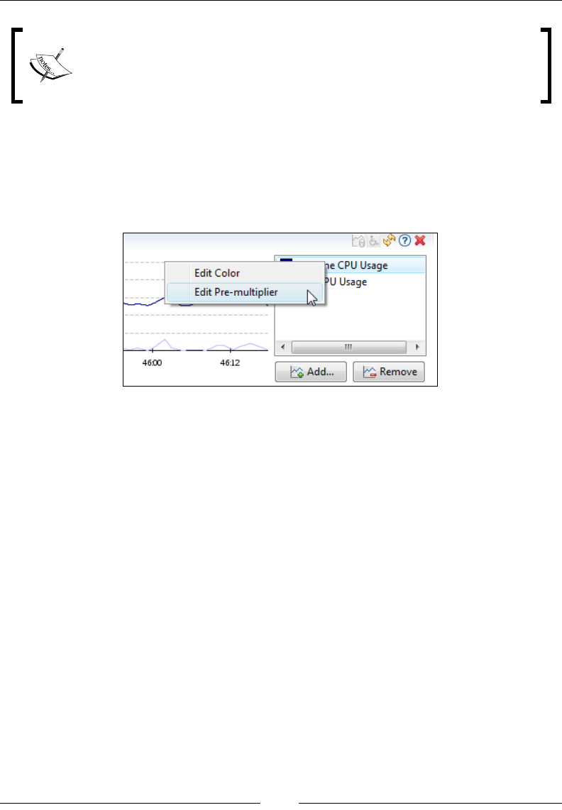
Chapter 7
[ 261 ]
None of the range choices will alter the input data in any way. The
Percent range will simply set the range to 0-100% and add a percent sign
to the Y-axis title. An attribute value of 1 will not be rendered as 100%.
An attribute that has a value range of 0 to 1 can still be rendered correctly in
the Percent (0-100%) range by adding a pre-multiplier to the attribute. Both
CPU usage attributes have a pre-multiplier setting of 100. To change the
pre-multiplier, right click on the attribute and then, click on Edit Pre-multiplier
as shown in the following screenshot:
The charts are quite useful and there are more options available for charts than
described here. A tip (certainly valid for most components in JRockit Mission
Control) is to examine the choices available in the context menus for a component.
MBeans
The MBeans tab group contains tabs with general tools for viewing, manipulating,
subscribing, and creating trigger rules for various aspects of the MBeans. It contains
two tabs—the MBean Browser that can be used for browsing the different attributes
in the MBeans registered in the platform MBean server, and the Triggers tab that can
be used to create rules that trigger when user specied conditions occur.
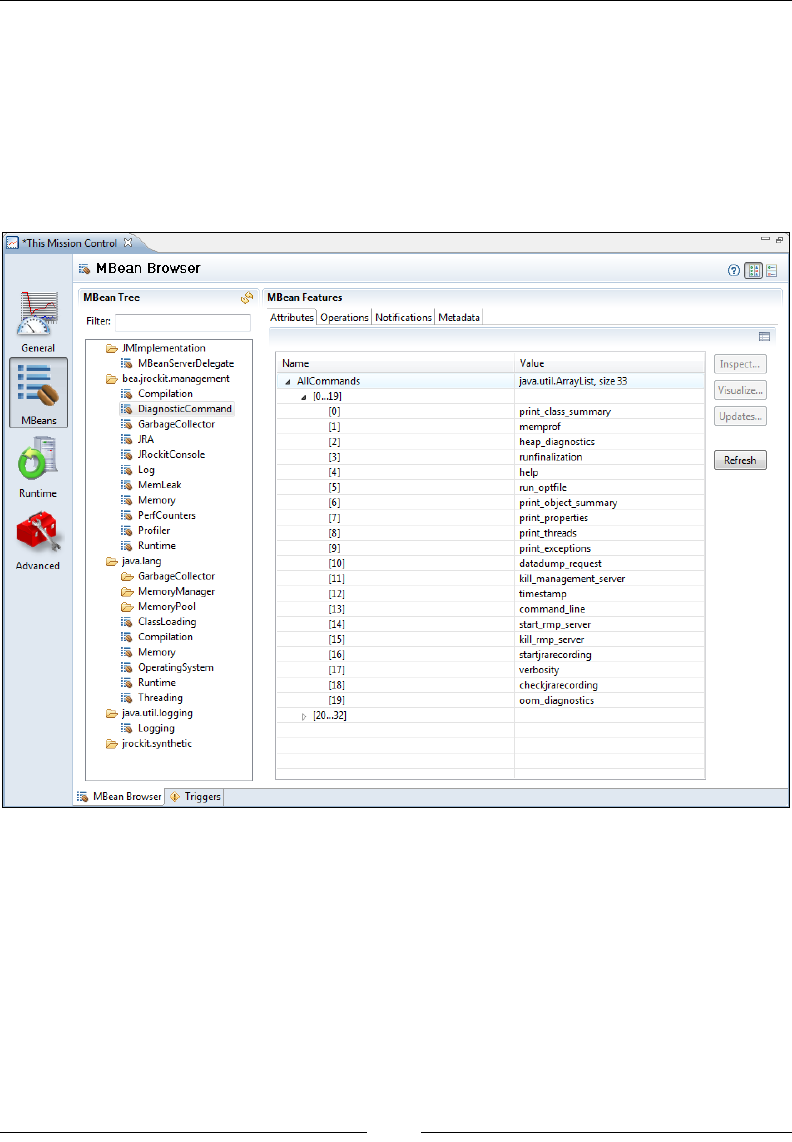
The Management Console
[ 262 ]
MBean Browser
The rst tab in the MBeans tab group is the MBean Browser. This is where all the
attributes available in the platform MBean server can be browsed. Primitive values
as well as collections, arrays, composite data, and tabular data can be viewed. To
make it easier to view large collections, the MBean Browser will automatically group
values into subgroups. How the values are grouped can be controlled by changing the
preferences.
If an attribute in the list is rendered in a bold faced font, it means it is writable.
Simple MBean attributes can be changed directly in the MBean browser table. It is,
for example, possible to go to the GarbageCollector MBean under the oracle.jrockit.
management domain and change the allocated heap size of JRockit. Simply double
click on the AllocatedHeapSizeTarget, and change the value. Don't worry if the
value of the AllocatedHeapSize does not follow suit immediately, as JRockit may
have to choose another heap size for various reasons, including memory alignment
and currently occupied memory.
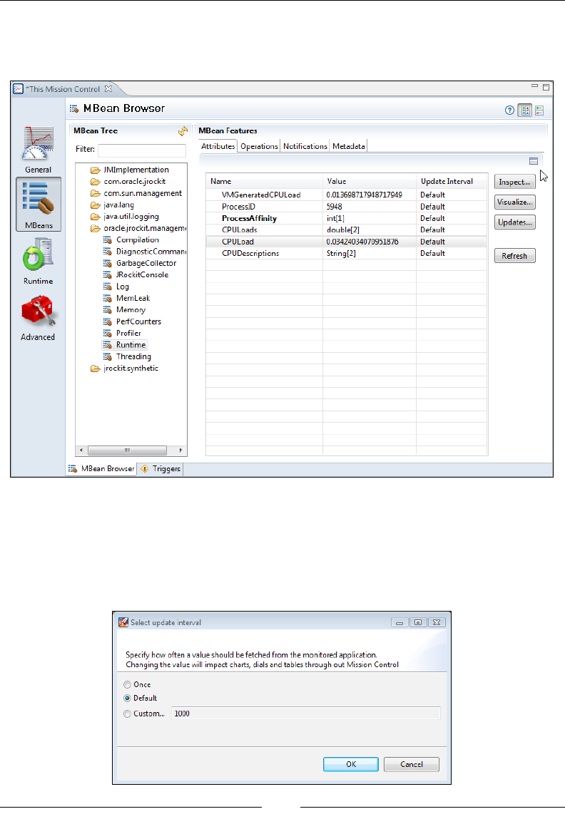
Chapter 7
[ 263 ]
The attribute table in the MBean Browser contains more information than is shown
by default. In the following screenshot, the table settings have been updated to show
the update interval for the attributes:
The default update interval is once every second (1,000 milliseconds). To change the
default update interval for an attribute, select the attribute in the table and click on
the Updates... button.
This will open the update interval dialog, where the appropriate update interval can
be selected, as shown in the following screenshot:
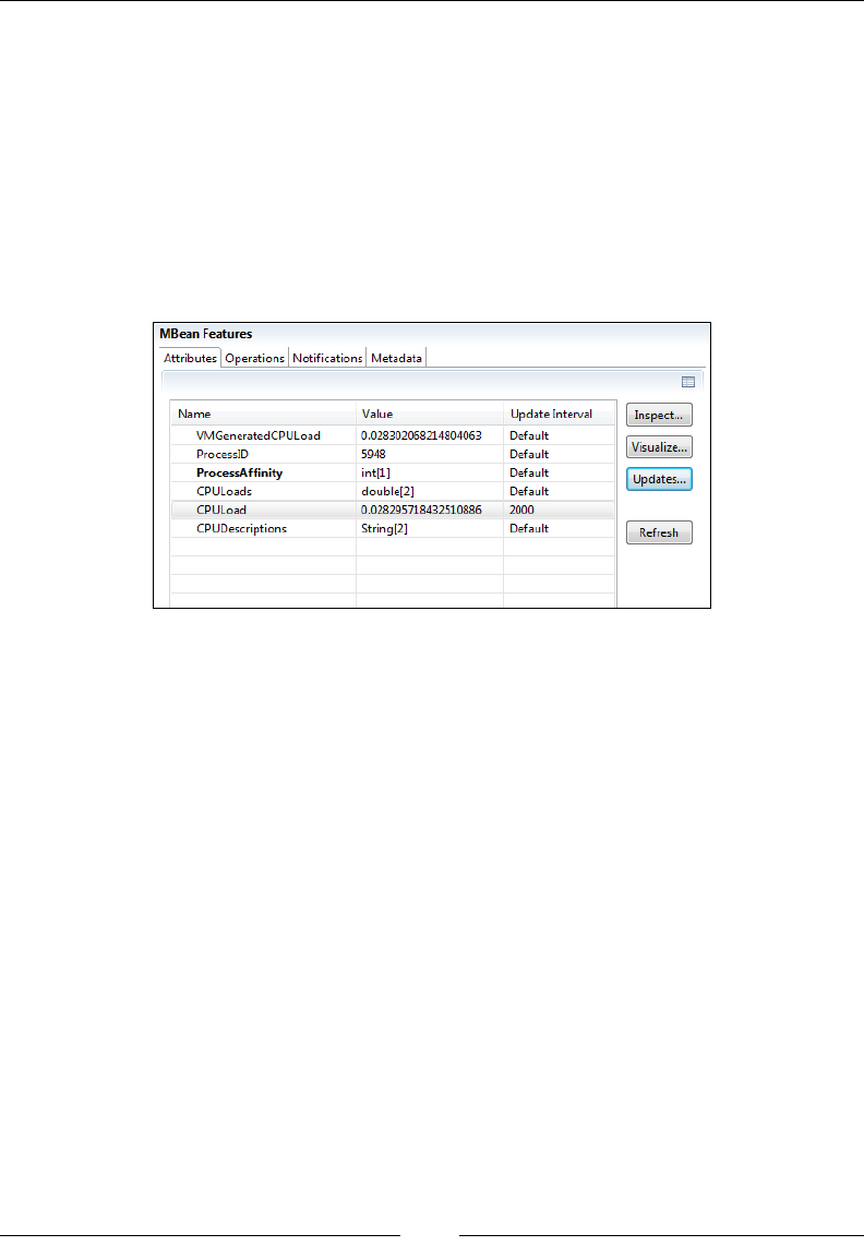
The Management Console
[ 264 ]
The update interval for an attribute can be set to:
• Once: The attribute will only be fetched once if subscribed to. This is good
for attributes that are not expected to change, such as the number of CPUs.
• Default: The default update interval setting. The default update interval is
normally set to 1,000 milliseconds, but that can be changed in the preferences.
• Custom: A custom update interval specied in milliseconds.
In the following screenshot, the update interval has been changed for the CPU
load—it will only be fetched once every two seconds:
The MBean Browser can also be used to invoke MBean operations dynamically.
This feature is very useful when prototyping a JMX API or when simply trying out
someone else's JMX API.
For example:
A diagnostic command can be invoked by browsing to the DiagnosticCommand
MBean under the oracle.jrockit.management domain. Diagnostic commands are
explained in detail later in this chapter, as well as in Chapter 11, JRCMD.
Select the Operations tab and then select the execute(String p1) operation and click
on invoke. Click on the p1 button to set the parameter and enter print_threads.
Click on OK to set the parameter and then OK again to execute the operation. You
should now see a thread stack dump. There is, of course, a much easier way to do
this. Simply use the Diagnostic Commands tab under the Advanced tab group.
One thing that sets aside the Mission Control Management Console from other
JMX consoles is that it is able to subscribe to many different kinds of values, or
even part of values. It is, for instance, possible to subscribe to sub-values of a
composite data attribute.

Chapter 7
[ 265 ]
For example:
1. Go to the java.lang | MemoryPool | Old Space MBean (The java.
lang:type=MemoryPool:name=Old Space MBean to be precise).
2. Expand the Usage attribute and select a key in the composite data, for
instance # used.
3. Right click and select Visualize....
4. Select a chart to add the attribute to, or click on Add Chart to add a
new chart.
Go back to Overview to check out your chart. Remember to change the Y-axis to
auto, as the chart defaults to a xed range between 0 and 100.
The subscription engine can also handle subscriptions based on JMX notications and
synthetic attributes. Synthetic attributes have a corresponding, client side, class that
implement the value retrieval. As the class can be implemented in whatever way the
implementer desires, it can be used to retrieve the value from any source at all, not
even necessarily JMX. The LiveSet attribute is an example of a synthetic attribute that
relies on the notication-based GC attribute and some additional calculations. There
is also a Notication tab, where you will nd the JMX notications available on the
selected MBean. Most MBeans do not have notications.
For example:
1. Go to the GarbageCollector MBean under the oracle.jrockit.management
domain.
2. Select the Notications tab.
3. Check the Subscribe check box.
4. Go to the Operations tab.
5. Invoke the gc operation.
6. Go back to the Notications tab and check the result.
Depending on which garbage collector you have selected and which version
of JRockit you are using, you may have one or several notications listed in
notications tab.
For other examples on notications available, see the Java documentation on java.
lang.management.MemoryPoolMXBean and the java.lang:Memory MBean.

The Management Console
[ 266 ]
The Notication tab is not very interesting—it is mostly meant for trying out
notication-based JMX APIs. It is much more useful to weave the notications into
the subscription service in the Management Console, so that they can participate in
the attribute visualization framework.
There is, unfortunately, currently no ofcially documented way
of adding your own synthetic or notication based attributes. To
see how it works today, search the attributes.xml le in the
com.jrockit.mc.rjmx plugin for flavour="synthetic" and
flavour="Notification" respectively. If you would like to see
ofcial support for this, please let the authors know.
Triggers
With the Management Console, rules can be built that trigger when a certain user-
dened condition occurs. Such a rule consists of three different parts:
1. A trigger condition: This species when to trigger. An example of a trigger
condition can be that CPU Load exceeds 90 percent.
2. An action: The action denes what to do when the rule triggers. An example
of an action is to send an e-mail with information about the condition that
caused the rule to trigger.
3. A set of constraints: This is a set of constraints that, in addition to the trigger
condition, must be fullled for the rule to trigger. An example of such a set
of constraints can be a day and a time, for instance "only weekdays" and
"between 9:00 AM and 6:00 PM".
In the Triggers tab, you can add, remove, activate, deactivate, and edit such rules. As
of JRockit Mission Control 3.1, these rules can be added to a set of rules that can be
exported and imported.
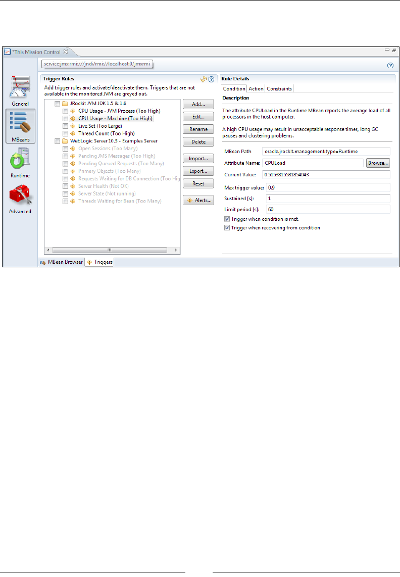
Chapter 7
[ 267 ]
As shown in the following screenshot, the rules already dened are listed in the
Trigger Rules tree to the left, and the details for a selected rule are shown to the right:
Note that simple modications to an existing rule, such as changing what action to
take, or changing the trigger value, can be done by directly editing the rule in the Rule
Details section. In the earlier example, no trigger rule is currently active. To activate a
rule, simply click on the check box next to rule name in the Trigger Rules tree.
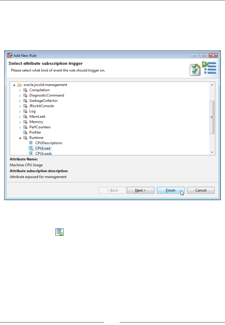
The Management Console
[ 268 ]
For example:
JRockit Mission Control comes pre-packaged with various example rules. For the
sake of clarity, let's create a duplicate rule of one of the pre-existing ones.
1. Click on Add.... This will bring up the Add New Rule Wizard.
2. Expand the oracle.jrockit.management | Runtime MBean.
3. Select the CPULoad attribute.
The little N ( ) in the icon indicates that this is a numeric attribute.
It is possible to build rules that are not based on numeric attributes;
for string attributes there is a string matching expression instead of
a numeric evaluator.
4. Click on Next and choose the Max trigger value—this is the boundary value
upon which the trigger will take action. In this case we can, for example,
choose 0.25. Triggers operate on the raw value from the subscription, so
the pre-multiplier will not be active. The CPULoad attribute gives us the
CPU load as a fraction, and so 0.25 would mean 25 percent. With the default
settings, this means that action will be taken once the CPU load passes 25
percent and once when the trigger recovers and goes below 25 percent.
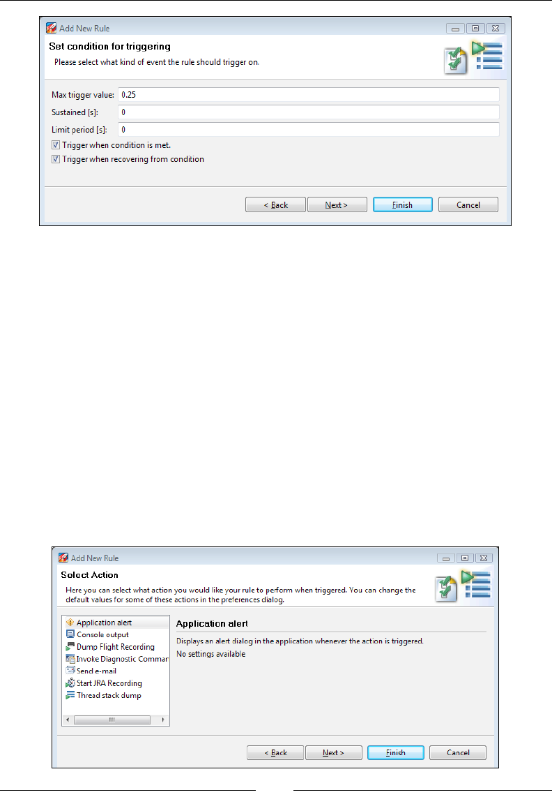
Chapter 7
[ 269 ]
5. There are other options available to us, that we won't change for
this example:
° Sustained [s]: This decides for how long the value must be
sustained above the threshold before triggering.
° Limit period [s]: The period after which to throttle the events,
that is events will not trigger more often than this. Events that
do trigger more often will simply be discarded.
° Trigger when condition is met: In our case, when the
attribute goes from less than 0.25 to greater than or equal
to 0.25.
° Trigger when recovering from condition: In our case, when
the attribute goes from greater than or equal to 0.25 to less
than 0.25.
6. Click on Next and select the Application alert action.
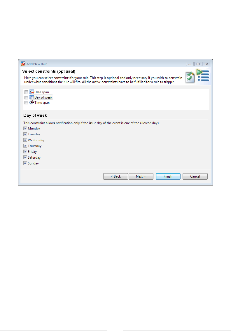
The Management Console
[ 270 ]
The Application alert action requires no settings. When a rule triggers with
the application alert action, the triggered event is logged and optionally
displayed in a log dialog window. There are a few default actions available,
but the fun part is that it is possible to write your own actions. We'll show
you how at the end of this chapter.
7. Click on Next and optionally select one or more constraints.
For this example, it really isn't necessary, but it is nice to be able to have
constraints that limit when the rule may trigger, such as only on weekdays.
You can write your own constraints too. It works pretty much the same way
as the actions.
8. Click on Next and review the group and rule names.
It is usually a good idea to put in an informative description of the rule as
well as to explain in a little more detail what the rule does and how it is
supposed to be used. You can use the standard <b>, </b>, and <br/> HTML
tags in your description for formatting.
9. Click on Finish.
10. Enable the new rule by checking the check box next to the rule name in the
Trigger Rules tree.
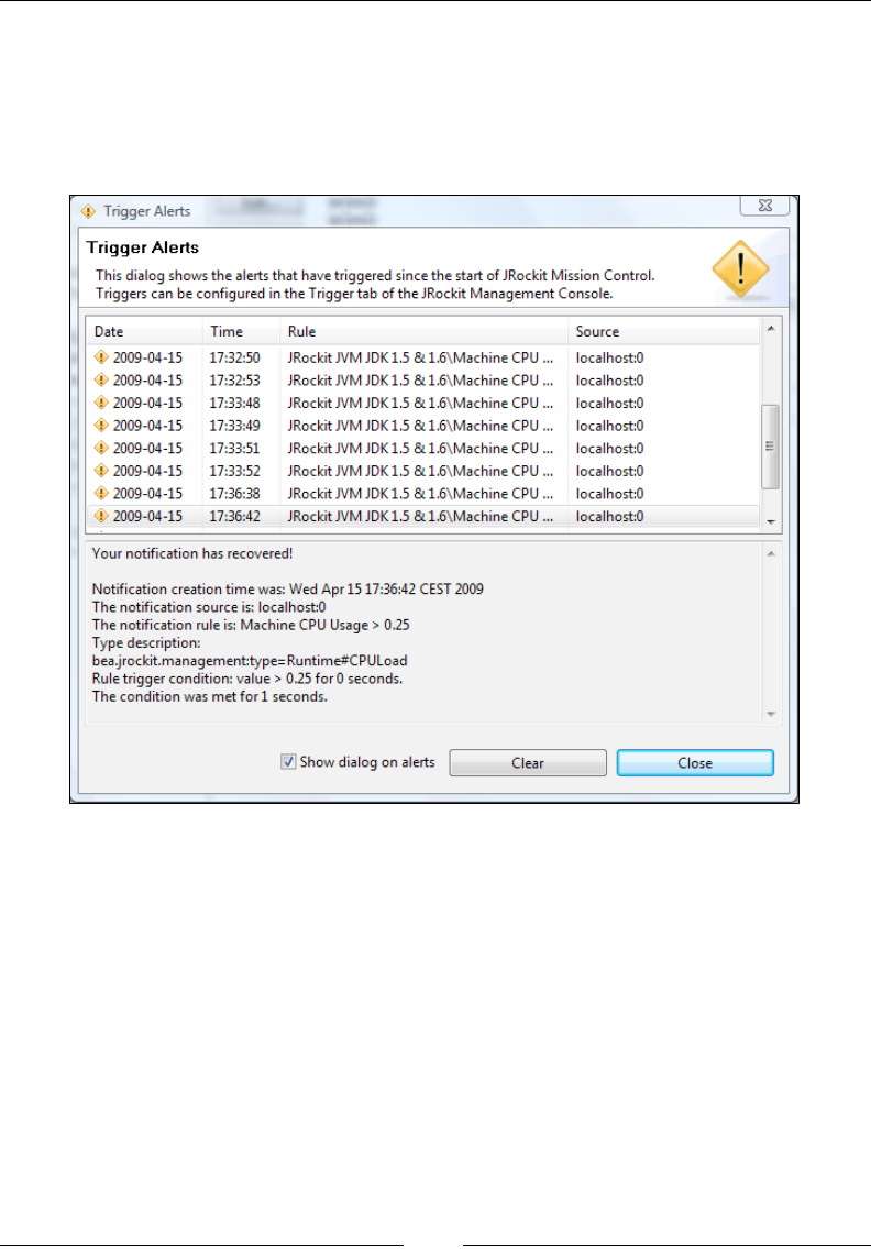
Chapter 7
[ 271 ]
11. Add some CPU load to make the rule trigger. You can usually peak the load
by forcing the UI to redraw itself a lot, for example by frantically resizing the
UI for a little while.
The Trigger Alerts dialog should pop up and show you the details of why
one of your rules triggered, as shown in the following screenshot:
It is possible to extend the Management Console with custom-made actions
and constraints. This is done by creating custom-made plug-ins that use a few
well-dened extension points. Please see the end of this chapter for details on
how to do this.
Runtime
The Runtime tab group contains a few tabs that visualize information about
the JRockit runtime. The rst tab in the Runtime tab group is the System tab.
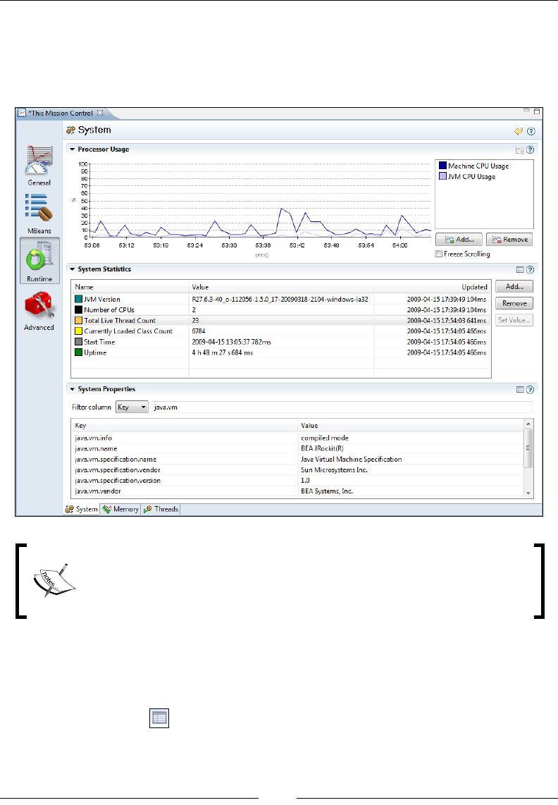
The Management Console
[ 272 ]
System
The most useful thing in this tab is the lterable System Properties table. System
properties can either be ltered by key or by property. For example, to show the
properties that start with java.vm, simply write java.vm in the lter text box.
It is possible to use regular expressions in the JRockit Mission Control
lter textboxes by prexing the lter string with "regexp:". For example,
to lter out all properties starting with "sun." and ending with "path",
the following expression can be used: regexp:sun\..*path
Some useful default properties have been added to an attribute table named System
Statistics. Most tables in JRockit Mission Control only show a few selected columns
by default. To show more columns, either select the column to show from the table
context menu (Visible Columns | <column name>), or click on the little table icon
in the section toolbar ( ) to bring up the Table Settings dialog. In the previous
screenshot, the Updated column has been added to the table, which shows when
the attribute was last updated. Note that different tables will have different
information available.
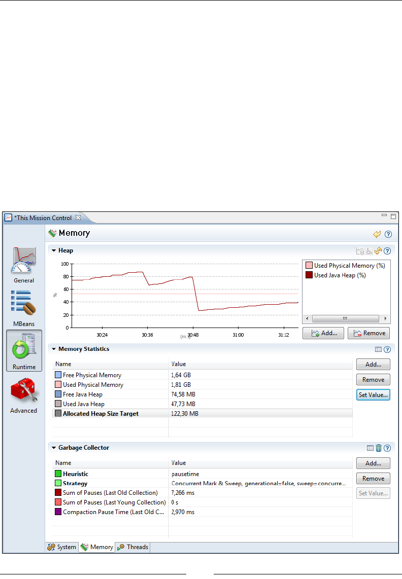
Chapter 7
[ 273 ]
As you can see from the example, different attributes may have different update
policies. Attributes that are not likely to change very often will be requested less
often than other attributes. The JVM version can be expected to not change at all.
The number of CPUs in the machine will also probably not change during a
particular run. How often an attribute is to be updated can be changed in the
MBean Browser.
Memory
This tab contains memory-related information. At the top is the familiar memory
chart from the Overview tab, followed by two attribute tables. The rst attribute
table contains memory statistics, and the second one GC-related attributes. The most
interesting part here is that there are actually a few of these that can be changed at
runtime—the allocated heap size, the garbage collector strategy, and the garbage
collector heuristic.

The Management Console
[ 274 ]
The GC heuristic is the rule set that the garbage collector currently uses to adaptively
alter the GC strategy and other GC parameters. Such a heuristic can, for instance, be
throughput that optimizes for maximum memory system throughput or pausetime,
that optimizes for lowest possible pause times.
The rules for valid heuristic changes are somewhat different for different
releases of JRockit. The rules for changing GC heuristic in R28 are quite versatile.
Heuristics can be changed freely with one exception—it is not possible to change
another heuristic to deterministic. This is because a lot of special data structures
and conguration settings are created at JVM startup when starting with the
deterministic garbage collector (JRockit Real Time).
The garbage collection strategy is dened by nursery, mark strategy and sweep
strategy. The nursery can either be present or not present. The mark and sweep
phases can either be concurrent or parallel, using the terms as dened in Chapter 3.
The strategy can also be changed freely in R28, with one exception—if JRockit
was started explicitly with the singlepar strategy (-Xgc:singlepar), the strategy
cannot be changed at all. However, if starting with any other strategy, it is possible
to change back and forth from singlepar.
An example of a complete strategy name is Concurrent Mark & Sweep,
generational=false, sweep=concurrent, mark=concurrent. The names are
unfortunately quite long and also a bit redundant. As was mentioned in Chapter
3, when explicitly setting the same strategy with the –Xgc command-line option,
the same strategy is simply named singlecon. The best way to get the input value
right when attempting to change these attributes is to rst look it up in the oracle.
jrockit.management:GarbageCollector MBean. There is one attribute for
strategies and and one for heuristics. Each contains an array of CompositeData,
and each CompositeData entry contains a name and description. Each name value
is valid input to change the corresponding Strategy or Heuristic attribute.
It is worth noting that changing strategies can implicitly change the heuristic as
well. A change to any strategy with a concurrent part will result in a change to
the heuristic pausetime. Any purely parallel strategy will result in a change to
throughput. Changing the heuristic can, in the same manner, result in an implicit
strategy change.
Also worth noting is that changing to a new heuristic or strategy will not exactly
be the same thing as starting with that heuristic or strategy because of the
following reasons:
• Changing the heuristic to pausetime will not set up some necessary
data structures for abortable compaction, if it wasn't previously enabled.
Abortable compaction will not be available to the garbage collector.
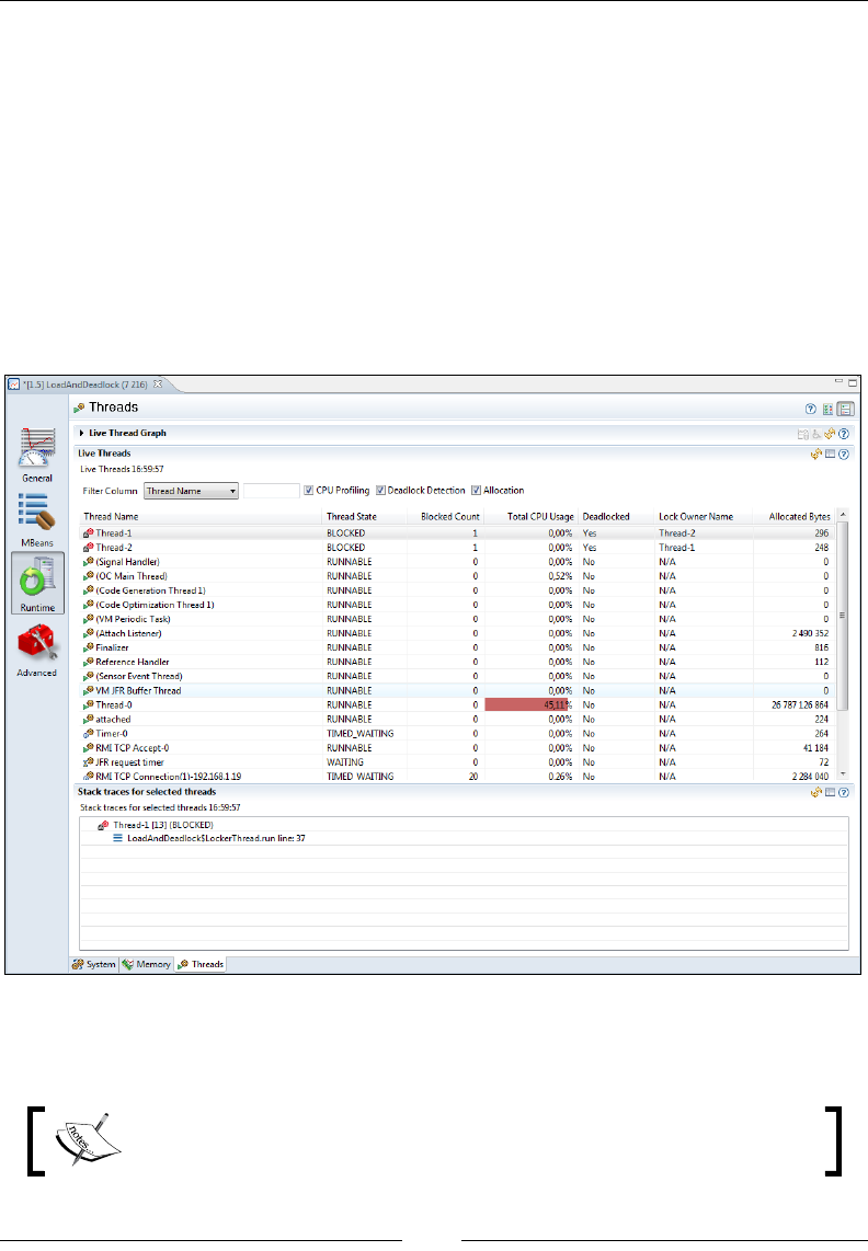
Chapter 7
[ 275 ]
• TLA sizes will be calculated based on the startup arguments. They will not be
recalculated upon strategy or heuristic change.
Threads
The Threads tab contains information about the running threads. All available
threads are listed in a table, together with information related to each thread, such
as the thread state. If a thread is selected, the stack trace for the thread will appear
in the trace tree, as shown in the following screenshot. CPU proling, deadlock
detection, and allocation proling can be enabled by checking the appropriate
checkboxes. As usual, more information can be enabled in the table by clicking on
the table properties icon in the section toolbar.
In the previous screenshot, we've added the Lock Owner Name attribute to the table,
and enabled Deadlock Detection.
Deadlock detection is a very useful feature in the JRockit Management
Console, which can make debugging parallel programs easier.
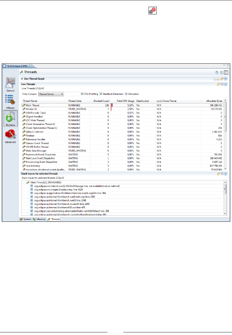
The Management Console
[ 276 ]
As can be seen, the icon used for deadlocked threads ( ) is different. We can infer
that two of the threads are in a deadlock, waiting for each other.
Another easy-to-miss feature in the Threads tab is the CPU proling check box.
When it is enabled, the total CPU usage per thread will be shown in the Total CPU
Usage column, and a normalized bar chart will be shown in the background of the
cells in that column.
Enabling allocation proling will show how much memory has been allocated in
each thread. Note that this value is the amount of memory that has been allocated
by the thread in total since it started, not how much memory the thread is currently
keeping live.
Advanced
The Advanced tab group contains tabs that can be somewhat complex to use as they
may either have performance implications, or require knowledge about the JRockit
JVM internals. After reading this book, you should be able to put most of the tabs in
the Advanced tab group to good use.
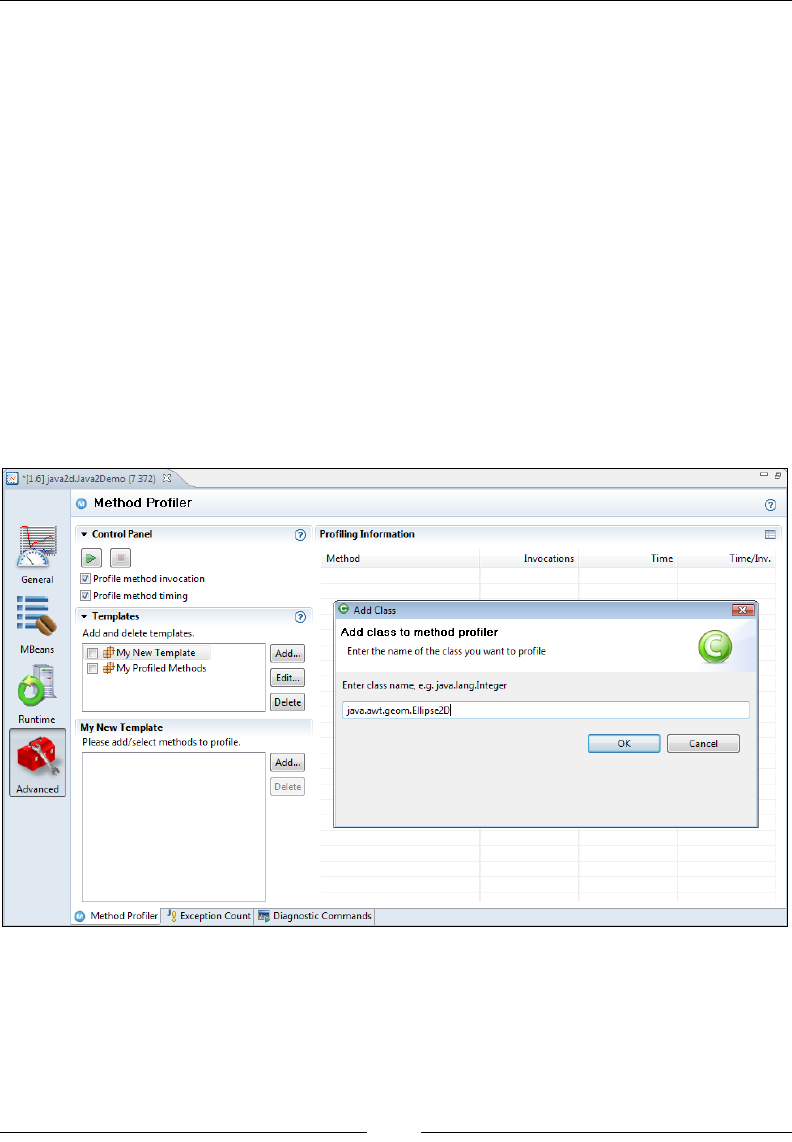
Chapter 7
[ 277 ]
Method Proler
The Method Proler in the JRockit Management Console can be used to do exact
method proling, for a selected set of methods. This is not the same thing as sample
based method proling. Exact method proling means that the proler will report
exact invocation counts for the selected methods and the total time spent executing
them. Sample-based method proling will be discussed in Chapter 8, The Runtime
Analyzer and Chapter 9, The Flight Recorder.
To add a method for proling, rst make sure that the proler is turned off. Then
select a template to which to add the method, or create a new template by clicking
on the Add… button in the Templates section. The templates are very useful, not
only for saving commonly proled methods for easy access later, but also to quickly
turn on and off proling for groups of methods in the method proler.
Next click on the Add… button in the methods section for the selected template
(My New Template in the following screenshot). In the dialog box, select the
class that declares the method you want to prole.
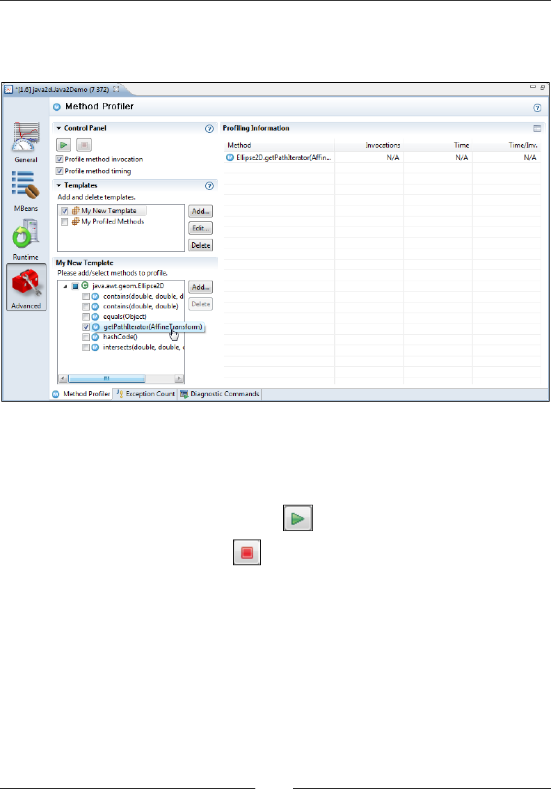
The Management Console
[ 278 ]
The Method Proler will fetch information about the class from the JVM that the
console is connected to, and display the methods available for proling in the
method tree as shown in the following screenshot:
If the template to which the method was added is active, it should now show up
in the Proling Information table to the right in the Method Proler tab. If it is
not, simply activate it by checking the check box next to the template name in the
Templates section.
To start the proler, simply press the play ( ) button.
To stop the proler, press the stop ( ) button.
The following screenshot shows a few of the methods on the critical path in one of
the Java2D demos that come with the JDK (located in the demo/jfc folder):
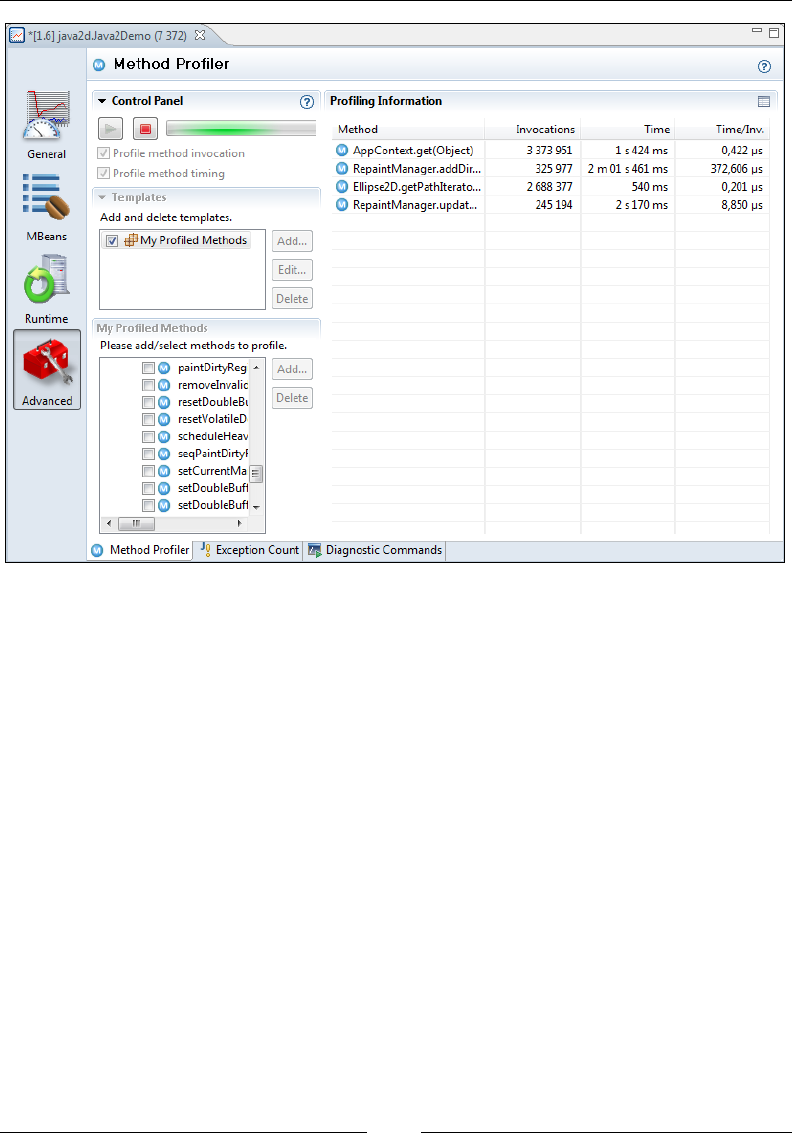
Chapter 7
[ 279 ]
There are a few caveats worth mentioning when using the Method Proler in the
Management Console. These are the top three culprits:
• The proler requires you to select the exact set of methods you want to
prole: This is somewhat of a chicken and egg problem, as it's hard to know
which methods to prole until you've done some proling. And once you've
done that proling (for example using JRockit Flight Recorder), you usually
have the answers you were looking for anyway.
• The overhead of gathering the exact proling information is hard to
estimate: This particular Method Proler is not sampling-based, like the one
in the JRockit Flight Recorder. The overhead, especially for a method that does
not take long to execute and that is being executed a lot, such as the hot
parts of a rendering engine, may be hard to predict. This is especially true
for method timing information. If all hot methods in the system are proled,
the overhead can be quite large.
• There is currently no class loader information available when selecting the
class: The proler will use the rst matching class it can nd. So, there is no
way to know which is the exact version of the class that is being proled if it
has been loaded by multiple class loaders.
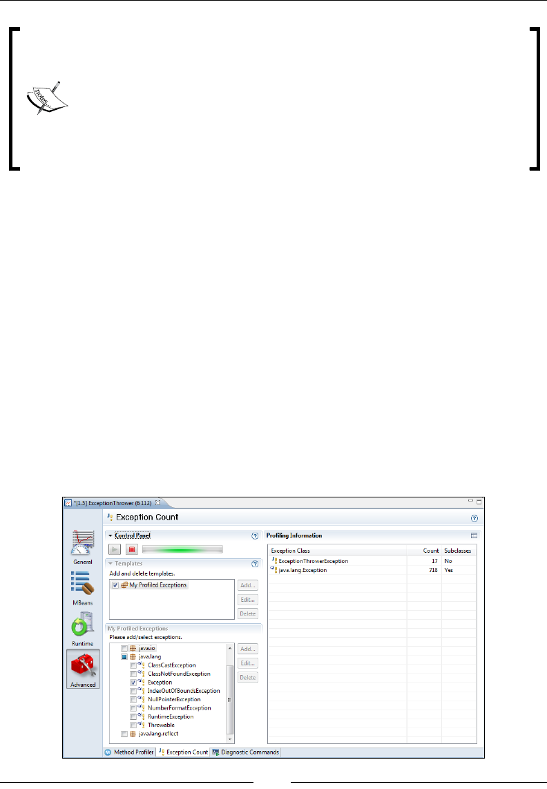
The Management Console
[ 280 ]
We have been at various customer sites and customer meetings when
developers have been certain a particular method is the main performance
bottleneck. Usually, plenty of exact measurements on that particular
method have been made, and after optimization it runs a magnitude
faster. Unfortunately, the performance of the application as such, has still
not been improved. After performing a JRockit Flight Recording, before
and after the change, it is usually concluded that the method in question
is not even among the top 50 hot spots in the application, and that, in
practice, the optimization effort was a waste of time.
When proling an application, the JRockit Flight Recorder is usually the best place
to start. If you still believe there is a need for online exact method proling after
doing a recording, you should convince yourself that the need is valid. Maybe you
have already done a recording so that you know that the method you are spending
time on tuning is worth the effort. You may be curious as to how the timing
information changes for a certain optimization (fully realizing that, if the method is
on the critical path, the difference in overhead of the measurements themselves may
actually change after the optimizations have been implemented). Or perhaps you are
simply wondering if a certain method is called at all. This is probably, in the authors'
humble opinion, one of the most valid reasons for using the method proler in the
Management Console.
Exception Count
The exception tab can be used to count the number of exceptions thrown. You can
either count all the exceptions of a specic type or count the exceptions of a specic
type including subclasses of that type.
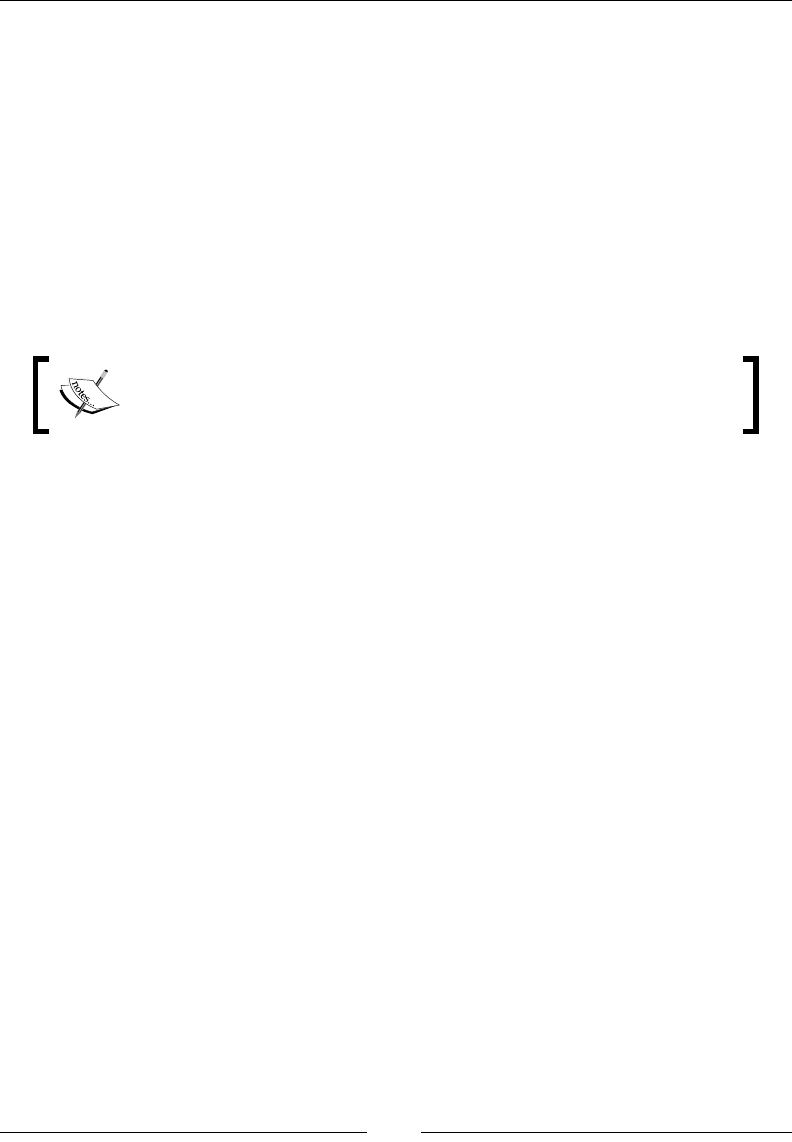
Chapter 7
[ 281 ]
The functionality is somewhat limited, as it will not show the stack traces for the
exceptions. If you not only want to know how many exceptions are thrown, but
also where they are thrown, you should instead use JRockit Flight Recorder or enable
verbose logging for exceptions. For more information on JRockit Flight Recorder, see
Chapter 9. For more information on how to do verbose logging, please see Chapter 5,
Benchmarking and Tuning or Chapter 11, JRCMD.
Diagnostic Commands
The Mission Control Console also provides a tab that facilitates access to the diagnostic
commands in JRockit. The diagnostic commands is a set of commands that can be sent
to JRockit through the JRockit Management APIs and the command-line tool JRCMD.
For more information on individual diagnostic commands and
on JRCMD, see Chapter 11. For more information about the
management APIs, see Chapter 12, Using the JRockit Management APIs.
The list in the upper left corner of the Diagnostic Commands tab shows the available
commands classied in three different groups—normal, advanced, and internal. The
ones in the "normal" class are usually the easiest to understand. They are also the ones
that can be executed without any risk of affecting the runtime in adverse ways. Of
course, no truth without exceptions, for example invoking the runsystemgc command
over and over again may incur a performance overhead. The print_object_summary
command can also be fairly expensive as it will, in effect, cause a garbage collection
(gathering info on all objects on the heap requires traversing the heap).
The diagnostic commands in the "advanced" group are more complicated; they are
either more complex, requiring a lot of low level JRockit or JVM knowledge, or have
security or performance implications. For example, the heap_diagnostic command
can be expensive to execute and there may be security implications of starting up the
external management agent with start_management_server.
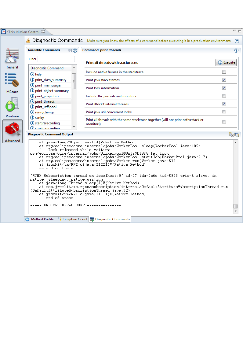
The Management Console
[ 282 ]
The lter box above the command list helps nding specic commands, and to the
right of the command list the parameters of a selected command can be congured.
Clicking on the Execute button invokes the diagnostic command in the JVM that the
Management Console is connected to. When the command completes, the result is
displayed in the Diagnostic Command Output box at the bottom of the tab. Note
that not all commands have output, but some of them simply instruct the JRockit
runtime to take some action.
The output of several commands can be appended by clicking on the Append result
button in the Diagnostic Command Output section toolbar.
Chapter 7
[ 283 ]
Other
The last tab group is the Other group. This tab group will only be visible if you
have installed custom tabs—either your own, or custom tabs from the experimental
update site. As the JConsole Meta Plug-in tab is easily installed from the
experimental update site, we will briey explain it here.
JConsole
In the JDK, a JMX management console named JConsole is included. In 6.0 versions
of the JDK, JConsole has its own plug-in interface, through which additional tabs
can be added. The JConsole plug-in for JRockit Mission Control allows such plug-ins
to run inside the JRockit Management Console, as shown in the following screenshot:
To be able to run the JConsole plug-in, JRockit Mission Control (or Eclipse, if using
the plug-in version of JRockit Mission Control), must be running on a JDK 6.0
version of JRockit. The plug-in will automatically attempt to nd the JTop plug-in
delivered with the JDK (located in the demo/management/JTop folder), and to use
that folder as the JConsole plug-in directory. Any jar le containing a JConsole
plug-in found in the JConsole plug-in directory will be added under its own tab in
the JConsole plug-ins tab.
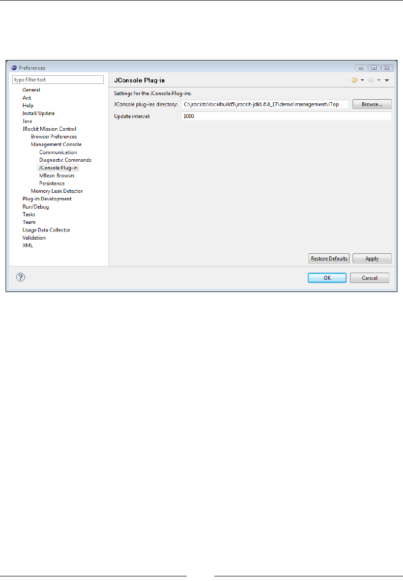
The Management Console
[ 284 ]
The JConsole plug-in directory and update interval, that is how often the
plug-ins should be refreshed, can be changed in the Console preferences
(Window | Preferences), as shown in the following screenshot:
Extending the JRockit Mission Control
Console
This section is for developers interested in extending the JRockit Mission Control
Management Console with custom tabs. It assumes some familiarity with the Eclipse
platform and terminology, such as extension point and form page.
There is an extension point available for the console that can be used to implement
custom tabs. This extension point was, for instance, used when creating the JConsole
plug-in tab available from the JRockit Mission Control experimental update site. See
the previous chapter for more information on the experimental update site.
The easiest way to get started building your own JRockit Mission Control Console
plug-in is to use the PDE wizard available from the experimental update site. First
make sure that Eclipse for RCP/Plug-in Developers (Eclipse 3.5/Ganymede or later
versions) is installed. Next install the JRockit Mission Control Plug-in into Eclipse.
Finally install the PDE Integration Plug-in from the experimental update site.
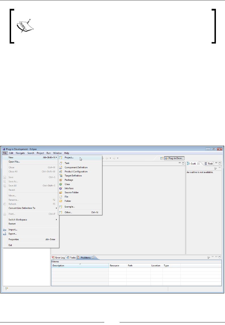
Chapter 7
[ 285 ]
PDE is short for Plug-in Development Environment, which is a set
of tools built into Eclipse to help create, develop, test, debug, build,
and deploy Eclipse plug-ins. The PDE Integration Plug-in from the
experimental update site provides specialized wizards and templates
that make it easier to write plug-ins for JRockit Mission Control.
The available console PDE wizards can be used to generate the boilerplate code
needed to contribute custom tabs to the JRockit Mission Control Console. They
also serve as examples on how custom tabs can be implemented.
There are two different wizards for creating JRockit Mission Control tabs available in
the PDE plug-in—simple and advanced. The simple wizard will generate an example
tab that shows a label with the CPU load. The advanced wizard will use various
components built into the JRockit Mission Control console to show three selected
attributes in various different ways.
This section walks you through how to create a new tab project:
1. Select File | New | Project...

The Management Console
[ 286 ]
2. In the New Project dialog box, select Plug-in Project and click on Next.
3. Name your project. It is common practice to name the plug-in project after
the main package of your plug-in, for example com.example.mc.console.
myplugin.
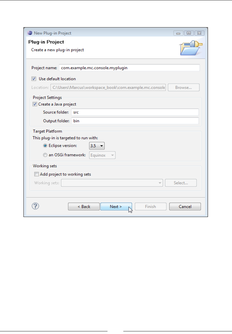
Chapter 7
[ 287 ]
4. Ensure that the correct target platform is selected (Eclipse 3.4 for JRockit
Mission Control 3.1 and Eclipse 3.5 for JRockit Mission Control 4.0).
5. Click on Next and optionally change plug-in property details. When
satised, click on Next again.
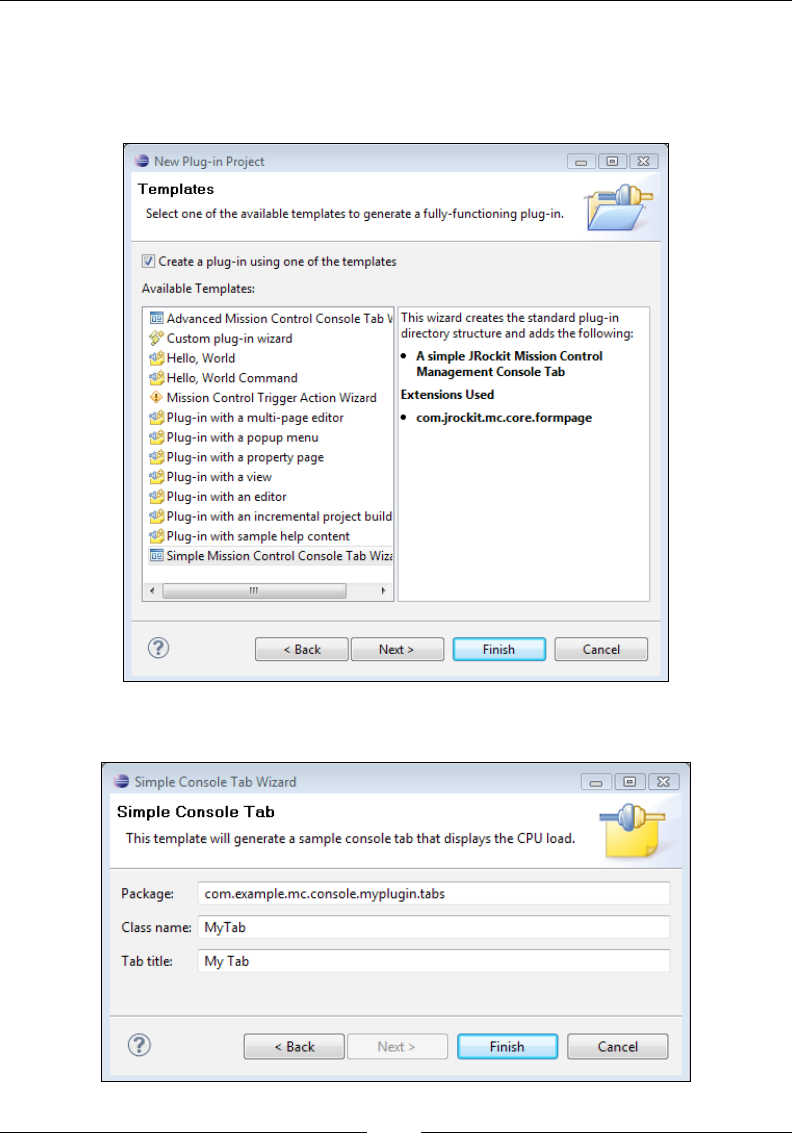
The Management Console
[ 288 ]
6. If the PDE plug-in is correctly installed, you should now be presented with
numerous templates, two of which should be the advanced and simple
console tab ones. Select either the advanced or the simple one and then click
on Next.
7. Change the details to match your plug-in and then click on Finish.
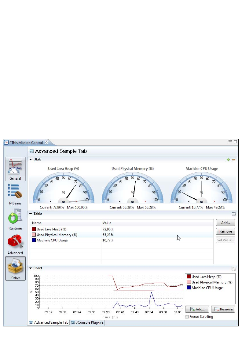
Chapter 7
[ 289 ]
The end result should be a plug-in project with all the necessary code for an
additional tab in the JRockit Mission Control Console. To try out your new tab,
simply go to Run | Run Congurations... In the Run Congurations Dialog,
right click on Eclipse Application and select New. This will create a new run
conguration for launching Eclipse. By default, it should be using the Eclipse
in which you are developing as a target platform and include all the plug-ins
in your workspace. As your Eclipse includes the JRockit Mission Control
plug-in, everything should be ne. Select the new conguration and press
the Run button in the lower right corner.
A new Eclipse should be launched with your brand new plug-in deployed. Open up
the Mission Control perspective the way you normally would and start the console.
Your tab will show up under the Other tab group.
If the advanced wizard was used, a class containing the code for creating a
tab looking much like the standard Overview tab should have been created.
It displays three different attributes in various different ways.

The Management Console
[ 290 ]
Setting up the tab is done programmatically and the code for it is rather simple.
The extension point only requires us to subclass org.eclipse.ui.forms.editor.
FormPage. So, there are really no dependencies on JRockit or JRockit Mission
Control specic classes for the extension point itself. The editor input from the form
page can be adapted to an IMBeanService, which is a communication helper service
for the console available in the com.jrockit.mc.rjmx.core package.
private IMBeanService getMBeanService() {
return (IMBeanService)
getEditorInput().getAdapter(IMBeanService.class);
}
This allows access to the JRockit Mission Control specic MBean layer residing in the
com.jrockit.mc.rjmx* plug-ins. RJMX provides, among other things, access to the
subscription engine and the proxy layer in JRockit Mission Control.
The proxy layer can be used to access JRockit specic attributes and operations
in a version neutral way with respect to the API. Use getMBeanService().
getProxyNames() for the attributes and getMBeanService().
getProxyOperations() for the operations.
For example, the location of the attribute for the CPU load is different in JRockit
versions R26.4 , R27.x, and R28.x. To get the location of the CPU load, regardless
of JRockit version, the proxy layer can be used like this:
getMBeanService().getProxyNames().
getAttributeDescriptor(IProxyNames.Key.OS_CPU_LOAD);
This will return an attribute descriptor containing the MBean ObjectName
and attribute name needed to locate the attribute. Most of RJMX makes use
of attribute descriptors that are objects encapsulating the MBean ObjectName
and the attribute name.
This is how we create an attribute descriptor directly pointing to the CPU load where
it is located in R28 versions of JRockit:
new AttributeDescriptor(
"oracle.jrockit.management:type=Runtime","CPULoad");
To invoke a garbage collection, regardless of JRockit version, the proxy layer can be
used in the following way:
getMBeanService().getProxyOperations().gc();

Chapter 7
[ 291 ]
As can be seen from the advanced template code, adding a table for a collection of
attributes is very easy.
builder.setProperty(
AttributeVisualizerBuilder.TITLE, "Chart");
builder.setProperty(
AttributeVisualizerBuilder.TITLE_AXIS_Y, "%");
builder.setProperty(
AttributeVisualizerBuilder.TITLE_AXIS_X, "Time");
addAttributesToVisualizer(builder.createChart());
The simple template is actually a little bit more complex than it seems, as it uses the
different services directly and does not rely on the standard Mission Control GUI
components. The resulting GUI is, however, much simpler. The tab generated from
the simple template provides a good example for how to use the RJMX subscription
service. The subscription service allows subscribing to the values of one or more
attributes using the same subscription mechanism as the rest of the console. Adding
a subscription to the CPU load is done by using the SubscriptionService.
getMBeanService().getAttributeSubscriptionService()
.addAttributeValueListener(getMBeanService().getProxyNames().
getAttributeDescriptor(IProxyNames.Key.OS_CPU_LOAD),
new LabelUpdater(valueLabel));
The LabelUpdater is a simple implementation of the IAttributeValueListener
interface dened in the com.jrockit.mc.rjmx.subscription package. Each time a
new value is retrieved, the valueChanged method is called with an event containing
the value. Note that there are no guarantees as to which thread is delivering the event.
In the current implementation, it will either be the subscription thread (most events)
or the JMX subsystem (notication based events). It will very likely never be the GUI
thread, which means that any updates to the GUI will need to be posted to the GUI
thread, as done by using DisplayToolkit.safeAsyncExec in the LabelUpdater
example code:
public static class LabelUpdater
implements IAttributeValueListener {
private final Label label;
public LabelUpdater(Label label) {
this.label = label;
}
public void valueChanged(final AttributeValueEvent event) {
DisplayToolkit.safeAsyncExec(label, new Runnable(){
public void run() {
Double latestValue = (Double) event.getValue();

The Management Console
[ 292 ]
label.setText("CPU Load is: "
+ (latestValue.doubleValue() * 100) + "%");
}
});
}
}
Creating an extension for a trigger action is done in the same way. Simply select the
Mission Control Trigger Action Wizard template from the plug-in project wizard
in step 6.
Summary
This chapter has demonstrated how to use the Management Console to monitor
any application running on JRockit. The information and functionality available in
the different tabs of the JRockit Management Console was described together with
examples and various use cases.
We have also shown how the Management Console can easily be extended with
custom tabs with specialized user interfaces as well as custom actions to be used
with the trigger rules.
The next chapter will explain how to use the JRockit Runtime Analyzer to prole
and diagnose both the JRockit runtime as well as the applications running in JRockit.
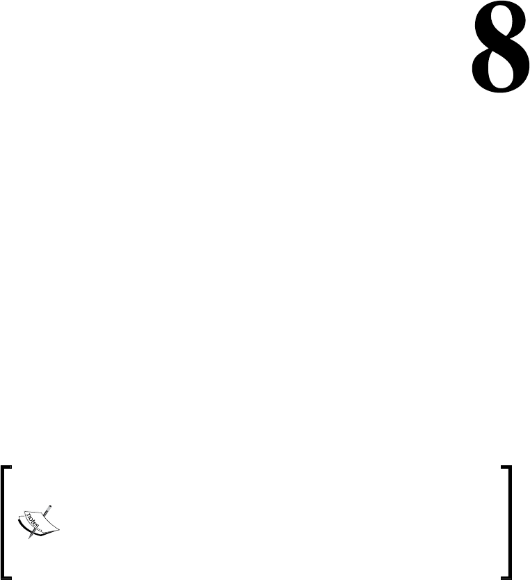
The Runtime Analyzer
The JRockit Runtime Analyzer, or JRA for short, is a JRockit-specic proling tool
that provides information about both the JRockit runtime and the application running
in JRockit. JRA was the main proling tool for JRockit R27 and earlier, but has been
superseded in later versions by the JRockit Flight Recorder. Because of its extremely
low overhead, JRA is suitable for use in production.
In this chapter you will learn:
• Different ways to create a JRA recording
• How to nd the hot spots in your application
• How to interpret memory-related information in JRA
• How to hunt down latency-related problems
• How to detect indications of a memory leak in an application
• How to use the operative set in the JRA latency analyzer component
This chapter is mainly targeted at R27.x/3.x versions of JRockit and
Mission Control. The next chapter covers performing and analyzing
runtime recordings in R28/4.0 using JRockit Flight Recorder. As
several of the components for recording analysis in Mission Control
are similar in R28, they are introduced in this chapter. Where
applicable, the next chapter covers new components and the most
important differences between R27.x/3.x and R28/4.0.

The Runtime Analyzer
[ 294 ]
The need for feedback
In order to make JRockit an industry-leading JVM, there has been a great need
for customer collaboration. As the focus for JRockit consistently has been on
performance and scalability in server-side applications, the closest collaboration
has been with customers with large server installations. An example is the nancial
industry. The birth of the JRockit Runtime Analyzer, or JRA, originally came from
the need for gathering proling information on how well JRockit performed at
customer sites.
One can easily understand that customers were rather reluctant to send us, for
example, their latest proprietary trading applications to play with in our labs. And,
of course, allowing us to poke around in a customer's mission critical application in
production was completely out of the question. Some of these applications shufe
around billions of dollars per week. We found ourselves in a situation where we
needed a tool to gather as much information as possible on how JRockit, and the
application running on JRockit, behaved together; both to nd opportunities to
improve JRockit and to nd erratic behavior in the customer application. This was a
bit of a challenge, as we needed to get high quality data. If the information was not
accurate, we would not know how to improve JRockit in the areas most needed by
customers or perhaps at all. At the same time, we needed to keep the overhead down
to a minimum. If the proling itself incurred signicant overhead, we would no longer
get a true representation of the system. Also, with anything but near-zero overhead,
the customer would not let us perform recordings on their mission critical systems
in production.
JRA was invented as a method of recording information in a way that the customer
could feel condent with, while still providing us with the data needed to improve
JRockit. The tool was eventually widely used within our support organization to
both diagnose problems and as a tuning companion for JRockit.
In the beginning, a simple XML format was used for our runtime recordings. A
human-readable format made it simple to debug, and the customer could easily
see what data was being recorded. Later, the format was upgraded to include data
from a new recording engine for latency-related data. When the latency data came
along, the data format for JRA was split into two parts, the human-readable XML
and a binary le containing the latency events. The latency data was put into JRockit
internal memory buffers during the recording, and to avoid introducing unnecessary
latencies and performance penalties that would surely be incurred by translating the
buffers to XML, it was decided that the least intrusive way was to simply dump the
buffers to disk.
To summarize, recordings come in two different avors having either the .jra
extension (recordings prior to JRockit R28/JRockit Mission Control 4.0) or the .jfr

Chapter 8
[ 295 ]
(JRockit Flight Recorder) extension (R28 or later). Prior to the R28 version of JRockit,
the recording les mainly consisted of XML without a coherent data model. As
of R28, the recording les are binaries where all data adheres to an event model,
making it much easier to analyze the data.
To open a JFR recording, a JRockit Mission Control of version 3.x must be used. To
open a Flight Recorder recording, JRockit Mission Control version 4.0 or later must
be used.
Recording
The recording engine that starts and stops recordings can be controlled in several
different ways:
• By using the JRCMD command-line tool. For more information on JRCMD,
see Chapter 11, JRCMD.
• By using the JVM command-line parameters. For more information on this,
see the -XXjra parameter in the JRockit documentation.
• From within the JRA GUI in JRockit Mission Control.
The easiest way to control recordings is to use the JRA/JFR wizard from within
the JRockit Mission Control GUI. Simply select the JVM on which to perform a JRA
recording in the JVM Browser and click on the JRA button in the JVM Browser
toolbar. You can also click on Start JRA Recording from the context menu. Usually,
one of the pre-dened templates will do just ne, but under special circumstances
it may be necessary to adjust them. The pre-dened templates in JRockit Mission
Control 3.x are:
• Full Recording: This is the standard use case. By default, it is congured to
do a ve minute recording that contains most data of interest.
• Minimal Overhead Recording: This template can be used for very
latency-sensitive applications. It will, for example, not record heap statistics,
as the gathering of heap statistics will, in effect, cause an extra garbage
collection at the beginning and at the end of the recording.
• Real Time Recording: This template is useful when hunting latency-related
problems, for instance when tuning a system that is running on JRockit
Real Time. This template provides an additional text eld for setting the
latency threshold. The latency threshold is explained later in the chapter in
the section on the latency analyzer. The threshold is by default lowered to 5
milliseconds for this type of recording, from the default 20 milliseconds, and
the default recording time is longer.
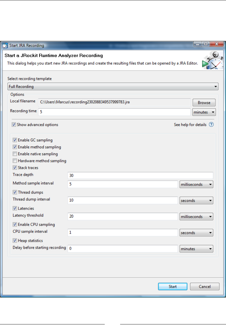
The Runtime Analyzer
[ 296 ]
• Classic Recording: This resembles a classic JRA recording from earlier
versions of Mission Control. Most notably, it will not contain any latency
data. Use this template with JRockit versions prior to R27.3 or if there is no
interest in recording latency data.

Chapter 8
[ 297 ]
All recording templates can be customized by checking the Show advanced options
check box. This is usually not needed, but let's go through the options and why you
may want to change them:
• Enable GC sampling: This option selects whether or not GC-related
information should be recorded. It can be turned off if you know that you
will not be interested in GC-related information. It is on by default, and it is a
good idea to keep it enabled.
• Enable method sampling: This option enables or disables method sampling.
Method sampling is implemented by using sample data from the JRockit
code optimizer. If proling overhead is a concern (it is usually very low, but
still), it is usually a good idea to use the Method sample interval option to
control how much method sampling information to record.
• Enable native sampling: This option determines whether or not to attempt
to sample time spent executing native code as a part of the method sampling.
This feature is disabled by default, as it is mostly used by JRockit developers
and support. Most Java developers probably do ne without it.
• Hardware method sampling: On some hardware architectures, JRockit
can make use of special hardware counters in the CPU to provide higher
resolution for the method sampling. This option only makes sense on such
architectures. Chapter 2, Adaptive Code Generation discusses hardware-based
sampling to a greater extent.
• Stack traces: Use this option to not only get sample counts but also stack traces
from method samples. If this is disabled, no call traces are available for sample
points in the methods that show up in the Hot Methods list.
• Trace depth: This setting determines how many stack frames to retrieve
for each stack trace. For JRockit Mission Control versions prior to 4.0, this
defaulted to the rather limited depth of 16. For applications running in
application containers or using large frameworks, this is usually way too
low to generate data from which any useful conclusions can be drawn. A tip,
when proling such an application, would be to bump this to 30 or more.
• Method sampling interval: This setting controls how often thread samples
should be taken. JRockit will stop a subset of the threads every Method
sample interval milliseconds in a round robin fashion. Only threads
executing when the sample is taken will be counted, not blocking threads.
Use this to nd out where the computational load in an application takes
place. See the section, Hot Methods for more information.

The Runtime Analyzer
[ 298 ]
• Thread dumps: When enabled, JRockit will record a thread stack dump at
the beginning and the end of the recording. If the Thread dump interval
setting is also specied, thread dumps will be recorded at regular intervals
for the duration of the recording.
• Thread dump interval: This setting controls how often, in seconds, to record
the thread stack dumps mentioned earlier.
• Latencies: If this setting is enabled, the JRA recording will contain latency
data. For more information on latencies, please refer to the section Latency
later in this chapter.
• Latency threshold: To limit the amount of data in the recording, it is possible
to set a threshold for the minimum latency (duration) required for an event to
actually be recorded. This is normally set to 20 milliseconds. It is usually safe
to lower this to around 1 millisecond without incurring too much proling
overhead. Less than that and there is a risk that the proling overhead will
become unacceptably high and/or that the le size of the recording becomes
unmanageably large. Latency thresholds can be set as low as nanosecond
values by changing the unit in the unit combo box.
• Enable CPU sampling: When this setting is enabled, JRockit will record the
CPU load at regular intervals.
• Heap statistics: This setting causes JRockit to do a heap analysis pass at the
beginning and at the end of the recording. As heap analysis involves forcing
extra garbage collections at these points in order to collect information, it is
disabled in the low overhead template.
• Delay before starting a recording: This option can be used to schedule the
recording to start at a later time. The delay is normally dened in minutes,
but the unit combo box can be used to specify the time in a more appropriate
unit—everything from seconds to days is supported.
Before starting the recording, a location to which the nished recording is to be
downloaded must be specied. Once the JRA recording is started, an editor will open
up showing the options with which the recording was started and a progress bar.
When the recording is completed, it is downloaded and the editor input is changed
to show the contents of the recording.
Analyzing JRA recordings
Analyzing JRA recordings may easily seem like black magic to the uninitiated, so
just like we did with the Management Console, we will go through each tab of the
JRA editor to explain the information in that particular tab, with examples on when
it is useful.
Just like in the console, there are several tabs in different tab groups.
Chapter 8
[ 299 ]
General
The tabs in the General tab group provide views of key characteristics and recording
metadata. In JRA, there are three tabs—Overview, Recording, and System.
Overview
The rst tab in the General tab group is the Overview tab. This tab contains an
overview of selected key information from the recording. The information is useful
for checking the system health at a glance.
The rst section in the tab is a dial dashboard that contains CPU usage, heap, and
pause time statistics.
What to look for depends on the system. Ideally the system should be well utilized, but
not saturated. A good rule of thumb for most setups would be to keep the Occupied
Heap (Live Set + Fragmentation) to half or less than half of the max heap. This keeps
the garbage collection ratio down.

The Runtime Analyzer
[ 300 ]
All this, of course, depends on the type of application. For an application with
very low allocation rates, the occupied heap can be allowed to be much larger. An
application that does batch calculations, concerned with throughput only, would
want the CPU to be fully saturated while garbage collection pause times may not be
a concern at all.
The Trends section shows charts for the CPU usage and occupied heap over time
so that trends can be spotted. Next to the Trends section is a pie chart showing
heap usage at the end of the recording. If more than about a third of the memory
is fragmented, some time should probably be spent tuning the JRockit garbage
collector (see Chapter 5, Benchmarking and Tuning and the JRockit Diagnostics Guide
on the Internet). It may also be the case that the allocation behavior of the application
needs to be investigated. See the Histogram section for more information.
At the bottom of the page is some general information about the recording, such
as the version information for the recorded JVM. Version information is necessary
when ling support requests.
In our example, we can see that the trend for Live Set + Fragmentation is constantly
increasing. This basically means that after each garbage collection, there is less free
memory left on the heap. It is very likely that we have a memory leak, and that, if
we continue to let this application run, we will end up with an OutOfMemoryError.
Recording
This tab contains meta information about the recording, such as its duration and the
values of all the recording parameters used. This information can, among other things,
be used to check if information is missing from a recording, or if that particular piece of
information had simply been disabled for the recording.
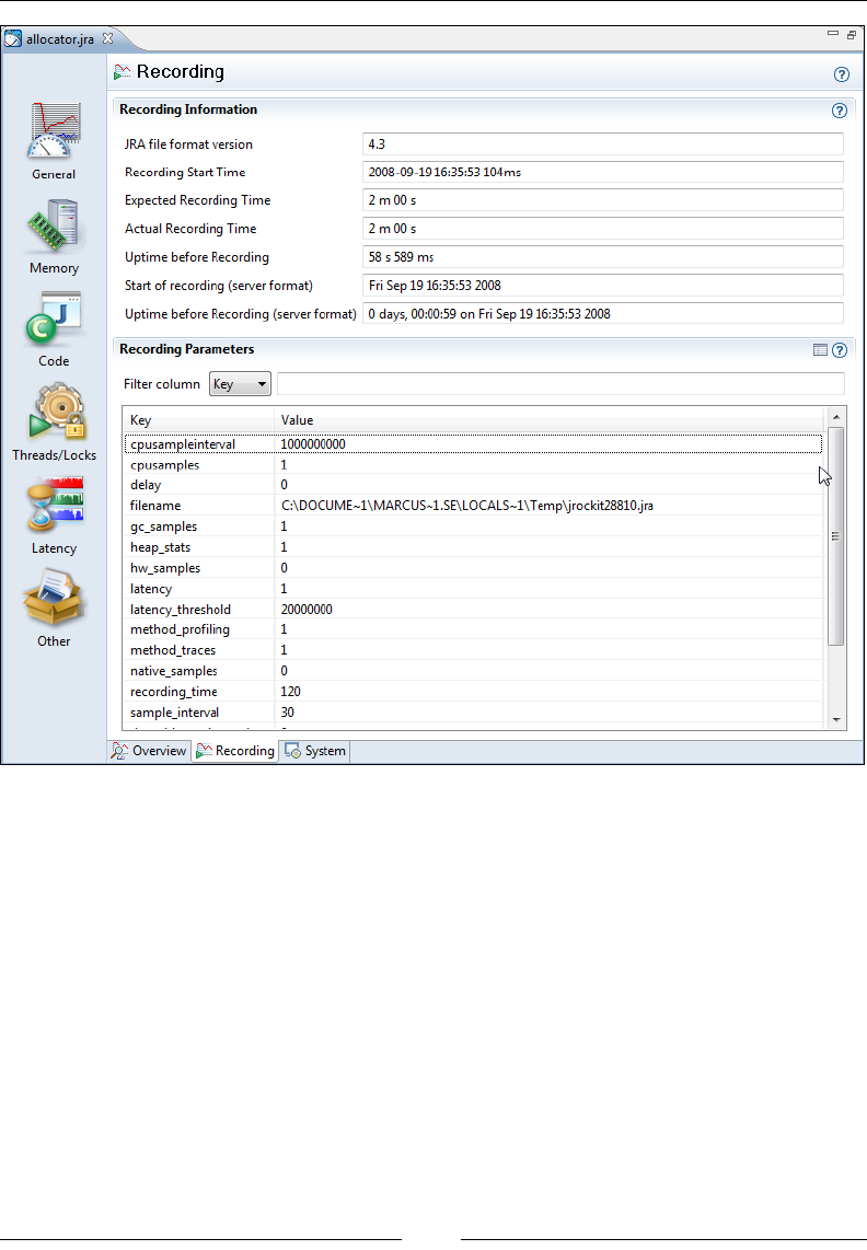
Chapter 8
[ 301 ]
System
This tab contains information about the system the JRockit JVM was running on,
such as the OS. The JVM arguments used to start the JVM can also be viewed here.

The Runtime Analyzer
[ 302 ]
Memory
The Memory tab group contains tabs that deal with memory-related information, such
as heap usage and garbage collections. In JRA there are six such tabs, Overview, GCs,
GC Statistics, Allocation, Heap Statistics, Heap Contents, and Object Statistics.
Overview
The rst tab in the Memory tab group is the Overview tab. It shows an overview of
the key memory statistics, such as the physical memory available on the hardware
on which the JVM was running. It also shows the GC pause ratio, i.e. the time spent
paused in GC in relation to the duration of the entire recording.
If the GC pause ratio is higher than 15-20%, it usually means that there is signicant
allocation pressure on the JVM.
At the bottom of the Overview tab, there is a listing of the different garbage
collection strategy changes that have occurred during recording. See Chapter 3,
Adaptive Memory Management, for more information on how these strategy changes
can occur.
GCs
Here you can nd all the information you would ever want to know about the
garbage collections that occurred during the recording, and probably more.
With the GCs tab, it is usually a good idea to sort the Garbage Collections table on
the attribute Longest Pause, unless you know exactly at what time from the start of
the JVM you want to drill down. You might know this from reading the application
log or from the information in some other tab in JRA. In the following example, the
longest pause also happens to be the rst one.
It is sometimes a good idea to leave out the rst and last garbage collections from the
analysis, depending on the recording settings. Some settings will force the rst and
last GC in the recording to be full garbage collections with exceptional compaction,
to gather extra data. This may very well break the pausetime target for deterministic
GC. This is also true for JRockit Flight Recorder
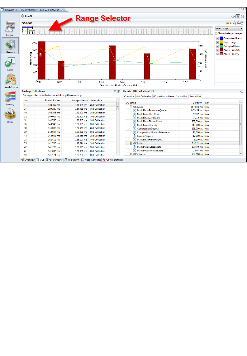
Chapter 8
[ 303 ]
At the top of the screen is the Range Selector. The Range Selector is used to
temporally select a set of events in the recording. In this case, we have zoomed in
on a few of the events at the beginning of the recording. We can see that throughout
this range, the size of the occupied heap (the lowest line, which shows up in green) is
around half the committed heap size (the at topmost line, which shows up in blue),
with some small deviations.
In an application with a very high pause-to-run ratio, the occupied heap would have
been close to the max heap. In that case, increasing the heap would probably be a good
start to increase performance. There are various ways of increasing the heap size, but
the easiest is simply setting a maximum heap size using the –Xmx ag on the command
line. In the example, however, everything concerning the heap usage seems to be ne.
In the Details section, there are various tabs with detailed information about a
selected garbage collection. A specic garbage collection can be examined more
closely, either by clicking in the GC chart or by selecting it in the table.
Information about the reason for a particular GC, reference queue sizes, and heap
usage information is included in the tabs in the Details section. Verbose heap
information about the state before and after the recording, the stack trace for the
allocation that caused the GC to happen, if available, and detailed information
about every single pause part can also be found here.
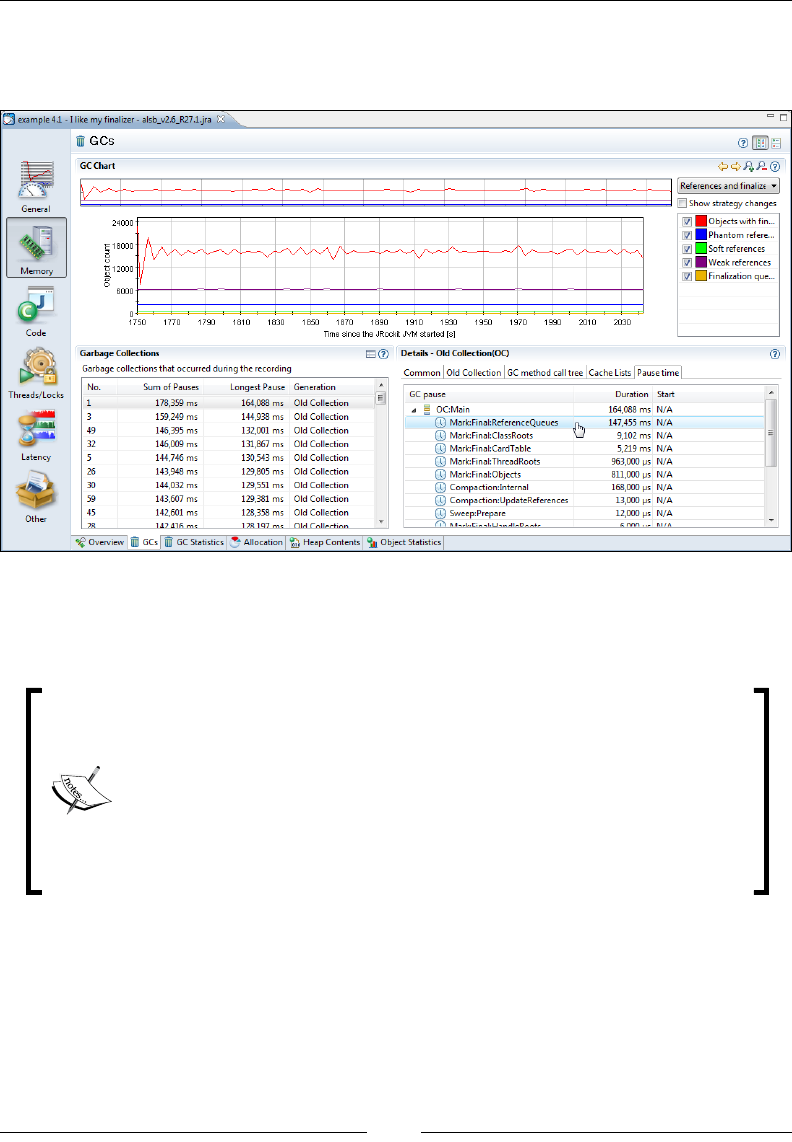
The Runtime Analyzer
[ 304 ]
In the previous screenshot, a very large portion of the GC pause is spent handling
the reference queues. Switching to the References and Finalizers chart will reveal
that the nalizer queue is the one with most objects in it.
One way to improve the memory performance for this particular application would
be to rely less heavily on nalizers. This is, as discussed in Chapter 3, always a good
idea anyway.
The recordings shown in the GCs tab examples earlier were created
with JRockit R27.1, but are quite good examples anyway, as they are
based on real-life data that was actually used to improve a product. As
can be seen from the screenshot, there is no information about the start
time of the individual pause parts. Recordings made using a more recent
version of JRockit would contain such information. We are continuously
improving the data set and adding new events to recordings. JRockit
Flight Recorder, described in the next chapter, is the latest leap in
recording detail.
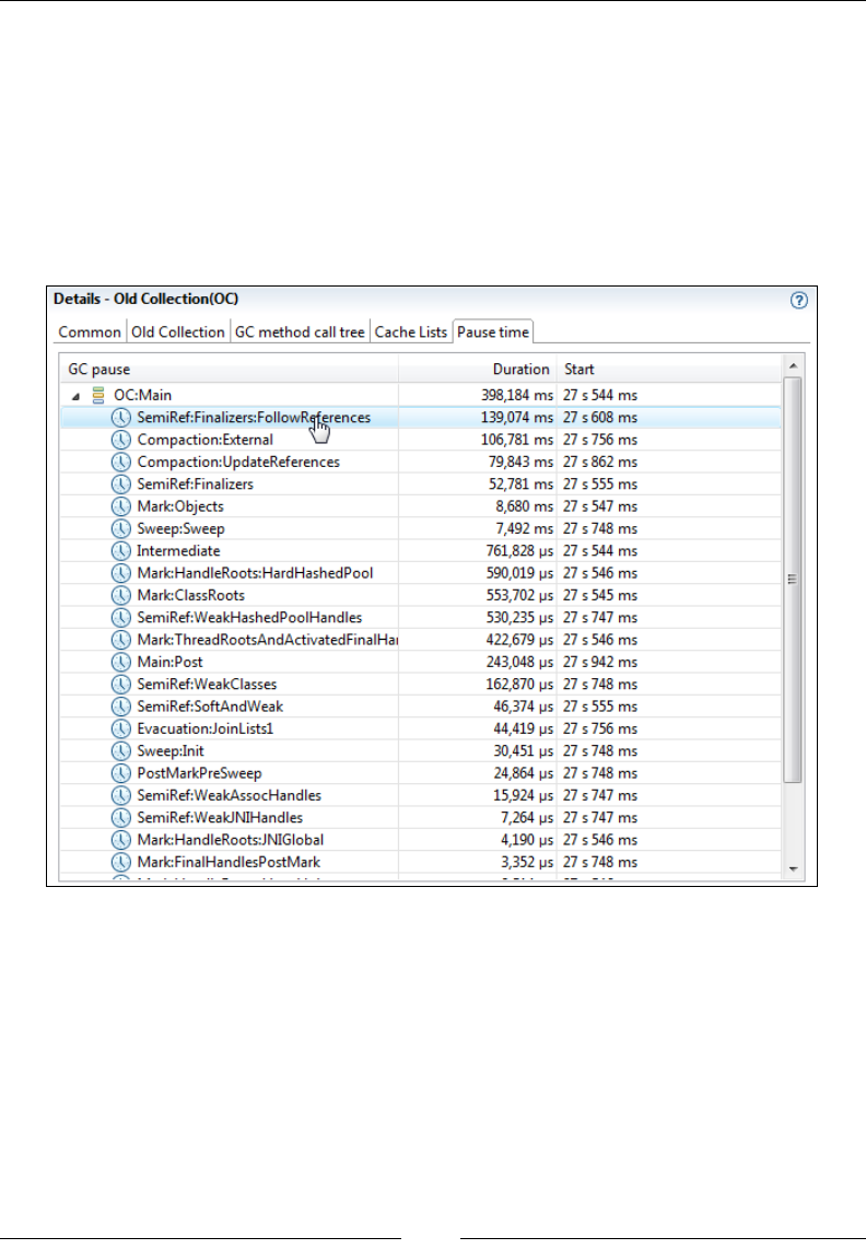
Chapter 8
[ 305 ]
Following is a more recent recording with an obvious nalizer problem. The reasons
that the pause parts differ from the previous examples is both that we are now using
a different GC strategy as well as the fact that more recent recordings contain more
detail. The nalizer problem stands out quite clearly in the next screenshot.
The data in the screenshot is from a different application, but it nicely illustrates
how a large portion of the garbage collection pause is spent following references in
the nalizers. Handling the nalizers is even taking more time than the notorious
synchronized external compaction. Finalizers are an obvious bottleneck.
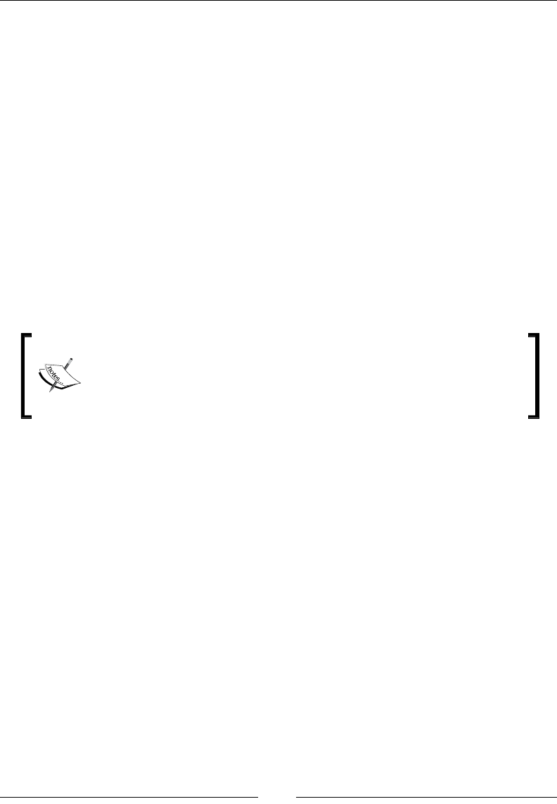
The Runtime Analyzer
[ 306 ]
To make fewer GCs happen altogether, we need to nd out what is actually causing
the GCs to occur. This means that we have to identify the points in the program
where the most object allocation takes place. One good place to start looking is the
GC Call Trees table introduced in the next section. If more specic allocation-related
information is required, go to the Object Allocation events in the Latency tab group.
For some applications, we can lower the garbage collection pause times by tuning
the JRockit memory system. For more about JRockit tuning, see Chapter 5.
GC Statistics
This tab contains some general statistics about the garbage collections that took
place during the recording. One of the most interesting parts is the GC Call Trees
table that shows an aggregated view of the stack traces for any garbage collection.
Unfortunately, it shows JRockit-specic internal code frames as well, which means
that you may have to dig down a few stack frames until the frames of interest are
found—i.e., code you can affect.
Prior to version R27.6 of JRockit, this was one of the better ways of
getting an idea of where allocation pressure originated. In more recent
versions, there is a much more powerful way of doing allocation
proling, which will be described in the Histogram section.
In the interest of conserving space, only the JRockit internal frames up to the rst
non-internal frame have been expanded in the following screenshot. The information
should be interpreted as most of the GCs are being caused as the result of calls to
Arrays.copyOf(char[], int) in the Java program.
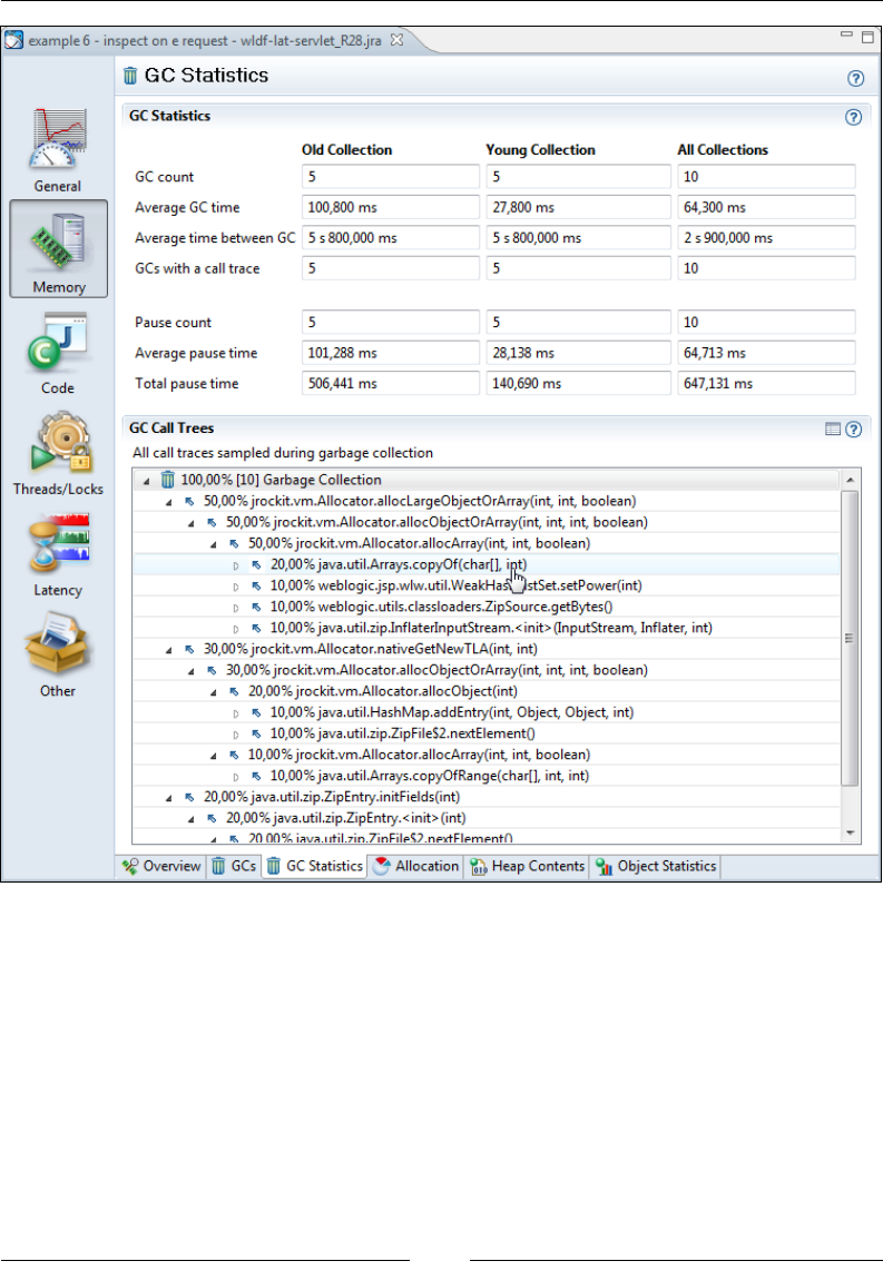
Chapter 8
[ 307 ]
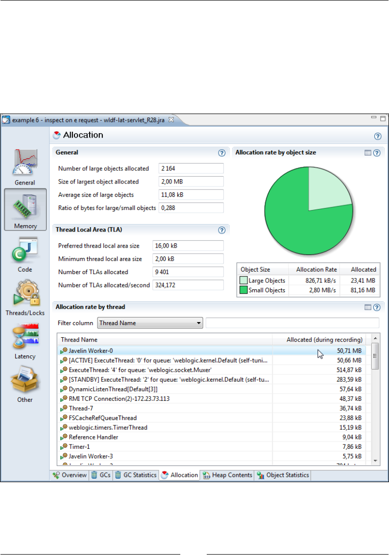
The Runtime Analyzer
[ 308 ]
Allocation
The Allocation tab contains information that can be used mainly for tuning the
JRockit memory system. Here, relative allocation rates of large and small objects are
displayed, which affects the choice of the Thread Local Area (TLA) size. TLAs are
discussed to a great extent in Chapter 3 and Chapter 5. Allocation can also be viewed
on a per-thread basis, which can help nd out where to start tuning the Java program
in order to make it stress the memory system less.
Again, a more powerful way of nding out where to start tuning the allocation
behavior of a Java program is usually to work with the Latency | Histogram tab,
described later in this chapter.
Chapter 8
[ 309 ]
Heap Contents
Information on the memory distribution of the heap can be found under the Heap
Contents tab. The snapshot for this information is taken at the end of the recording.
If you nd that your heap is heavily fragmented, there are two choices—either try to
tune JRockit to take better care of the fragmentation or try to change the allocation
behavior of your Java application. As described in Chapter 3, the JVM combats
fragmentation by doing compaction. In extreme cases, with large allocation pressure
and high performance demands, you may have to change the allocation patterns of
your application to get the performance you want.
Object Statistics
The Object Statistics tab shows a histogram of what was on the heap at the beginning
and at the end of the recording. Here you can nd out what types (classes) of objects
are using the most memory on the heap. If there is a large positive delta between the
snapshots at the beginning and at the end of the recording, it means that there either is
a memory leak or that the application was merely executing some large operation that
required a lot of memory.

The Runtime Analyzer
[ 310 ]
In the previous example, there is actually a memory leak that causes instances
of Double to be held on to forever by the program. This will eventually cause an
OutOfMemoryError.
The best way to nd out where these instances are being created is to either check
for Object Allocation events of Double (see the second example in the Histogram
section) or to turn on allocation proling in the Memory Leak Detector. The Memory
Leak Detector is covered in detail in Chapter 10, The Memory Leak Detector.
Code
The Code tab group contains information from the code generator and the
method sampler. It consists of three tabs—the Overview, Hot Methods,
and Optimizations tab.
Overview
This tab aggregates information from the code generator with sample information
from the code optimizer. This allows us to see which methods the Java program
spends the most time executing. Again, this information is available virtually
"for free", as the code generation system needs it anyway.
For CPU-bound applications, this tab is a good place to start looking for
opportunities to optimize your application code. By CPU-bound, we mean
an application for which the CPU is the limiting factor; with a faster CPU,
the application would have a higher throughput.
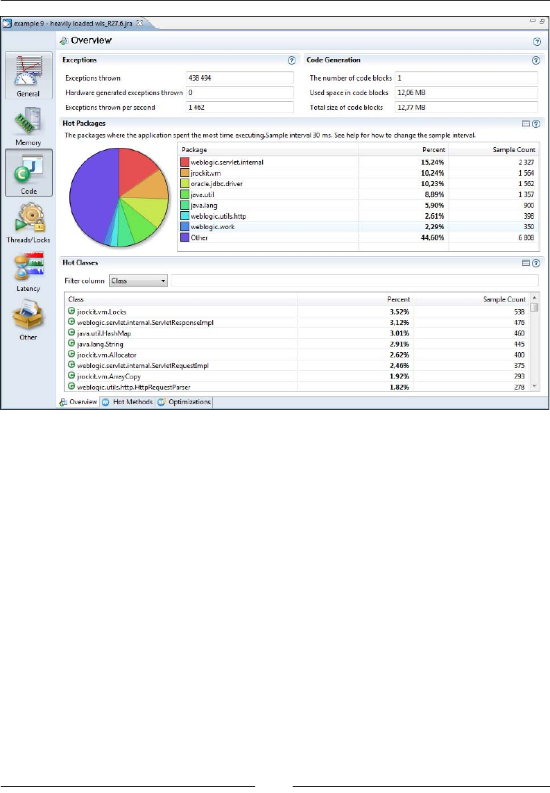
Chapter 8
[ 311 ]
In the rst section, the amount of exceptions thrown per second is shown. This
number depends both on the hardware and on the application—faster hardware
may execute an application more quickly, and consequently throw more exceptions.
However, a higher value is always worse than a lower one on identical setups.
Recall that exceptions are just that, rare corner cases. As we have explained, the
JVM typically gambles that they aren't occurring too frequently. If an application
throws hundreds of thousands exceptions per second, you should investigate why.
Someone may be using exceptions for control ow, or there may be a conguration
error. Either way, performance will suffer.

The Runtime Analyzer
[ 312 ]
In JRockit Mission Control 3.1, the recording will only provide
information about how many exceptions were thrown. The only
way to nd out where the exceptions originated is unfortunately
by changing the verbosity of the log, as described in Chapter 5 and
Chapter 11. As the next chapter will show, exception proling using
JRockit Flight Recorder is both easier and more powerful.
An overview of where the JVM spends most of the time executing Java code can be
found in the Hot Packages and Hot Classes sections. The only difference between
them is the way the sample data from the JVM code optimizer is aggregated. In Hot
Packages, hot executing code is sorted on a per-package basis and in Hot Classes on
a per-class basis. For more ne-grained information, use the Hot Methods tab.
As shown in the example screenshot, most of the time is spent executing code in the
weblogic.servlet.internal package. There is also a fair amount of exceptions
being thrown.
Hot Methods
This tab provides a detailed view of the information provided by the JVM code
optimizer. If the objective is to nd a good candidate method for optimizing the
application, this is the place to look. If a lot of the method samples are from one
particular method, and a lot of the method traces through that method share the
same origin, much can potentially be gained by either manually optimizing that
method or by reducing the amount of calls along that call chain.
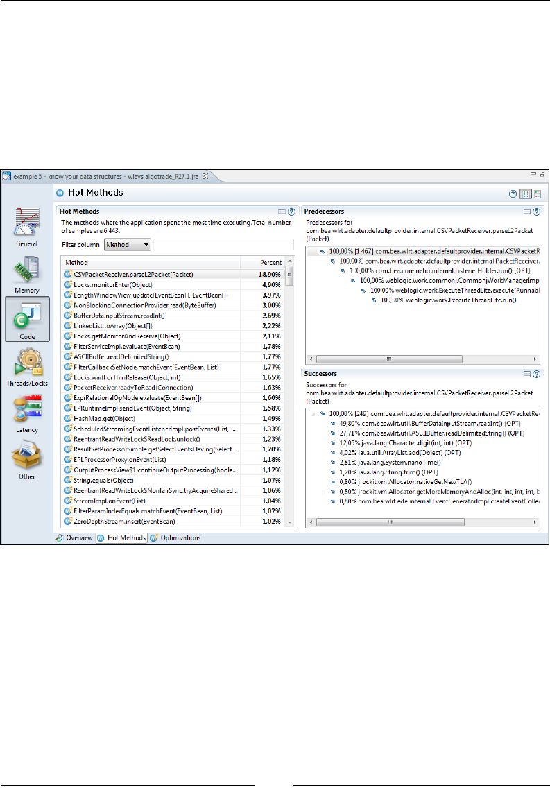
Chapter 8
[ 313 ]
In the following example, much of the time is spent in the method com.bea.wlrt.
adapter.defaultprovider.internal.CSVPacketReceiver.parseL2Packet().
It seems likely that the best way to improve the performance of this particular
application would be to optimize a method internal to the application container
(WebLogic Event Server) and not the code in the application itself, running inside the
container. This illustrates both the power of the JRockit Mission Control tools and a
dilemma that the resulting analysis may reveal—the answers provided sometimes
require solutions beyond your immediate control.
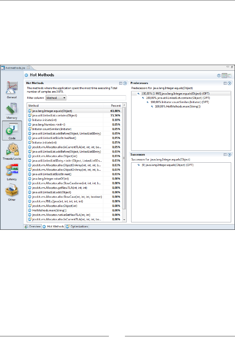
The Runtime Analyzer
[ 314 ]
Sometimes, the information provided may cause us to reconsider the way we use data
structures. In the next example, the program frequently checks if an object is in a java.
util.LinkedList. This is a rather slow operation that is proportional to the size of the
list (time complexity O(n)), as it potentially involves traversing the entire list, looking
for the element. Changing to another data structure, such as a HashSet would most
certainly speed up the check, making the time complexity constant (O(1)) on average,
given that the hash function is good enough and the set large enough.
Optimizations
This tab shows various statistics from the JIT-compiler. The information in this tab is
mostly of interest when hunting down optimization-related bugs in JRockit. It shows
how much time was spent doing optimizations as well as how much time was spent
JIT-compiling code at the beginning and at the end of the recording. For each method
optimized during the recording, native code size before and after optimization is
shown, as well as how long it took to optimize the particular method
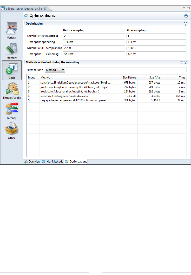
Chapter 8
[ 315 ]
Thread/Locks
The Thread/Locks tab group contains tabs that visualize thread- and lock-related
data. There are ve such tabs in JRA—the Overview, Thread, Java Locks, JVM
Locks, and Thread Dumps tab.
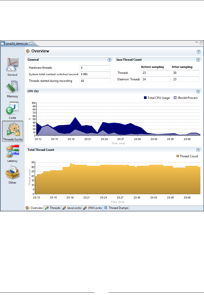
The Runtime Analyzer
[ 316 ]
Overview
The Overview tab shows fundamental thread and hardware-related information,
such as the number of hardware threads available on the system and the number
of context switches per second.

Chapter 8
[ 317 ]
A dual-core CPU has two hardware threads, and a hyperthreaded core also counts
as two hardware threads. That is, a dual-core CPU with hyperthreading will be
displayed as having four hardware threads.
A high amount of context switches per second may not be a real problem, but better
synchronization behavior may lead to better total throughput in the system.
There is a CPU graph showing both the total CPU load on the system, as well as
the CPU load generated by the JVM. A saturated CPU is usually a good thing—you
are fully utilizing the hardware on which you spent a lot of money! As previously
mentioned, in some CPU-bound applications, for example batch jobs, it is normally a
good thing for the system to be completely saturated during the run. However, for a
standard server-side application it is probably more benecial if the system is able to
handle some extra load in addition to the expected one.
The hardware provisioning problem is not simple, but normally
server-side systems should have some spare computational
power for when things get hairy. This is usually referred to as
overprovisioning, and has traditionally just involved buying faster
hardware. Virtualization has given us exciting new ways to handle
the provisioning problem. Some of these are discussed in Chapter 13,
JRockit Virtual Edition.
Threads
This tab shows a table where each row corresponds to a thread. The tab has more
to offer than rst meets the eye. By default, only the start time, the thread duration,
and the Java thread ID are shown for each thread. More columns can be made visible
by changing the table properties. This can be done either by clicking on the Table
Settings icon, or by using the context menu in the table.
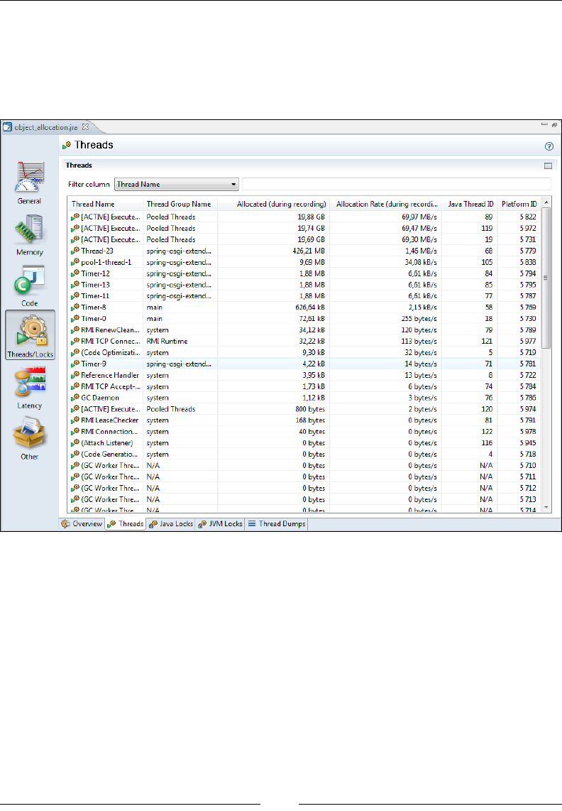
The Runtime Analyzer
[ 318 ]
As can be seen in the example screenshot, information such as the thread group
that the thread belongs to, allocation-related information, and the platform thread
ID can also be displayed. The platform thread ID is the ID assigned to the thread by
the operating system, in case we are working with native threads. This information
can be useful if you are using operating system-specic tools together with JRA.
Java Locks
This tab displays information on how Java locks have been used during the
recording. The information is aggregated per type (class) of monitor object.
For more information regarding the different kind of locks, please refer to
Chapter 4, Threads and Synchronization.
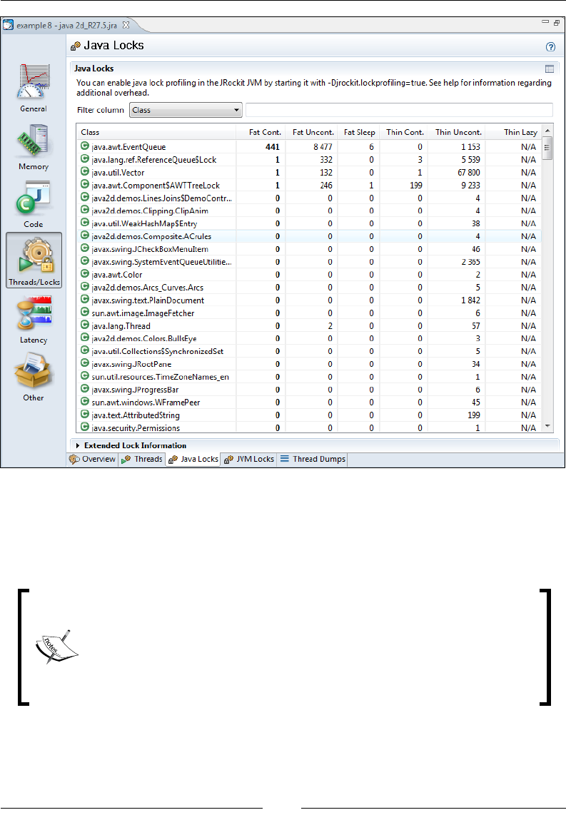
Chapter 8
[ 319 ]
This tab is normally empty. You need to start JRockit with the system property
jrockit.lockprofiling set to true, for the lock proling information to be
recorded. This is because lock proling may cause anything from a small to a
considerable overhead, especially if there is a lot of synchronization.
With recent changes to the JRockit thread and locking model, it would
be possible to dynamically enable lock proling. This is unfortunately
not the case yet, not even in JRockit Flight Recorder.
For R28, the system property jrockit.lockprofiling has been
deprecated and replaced with the ag -XX:UseLockProfiling.
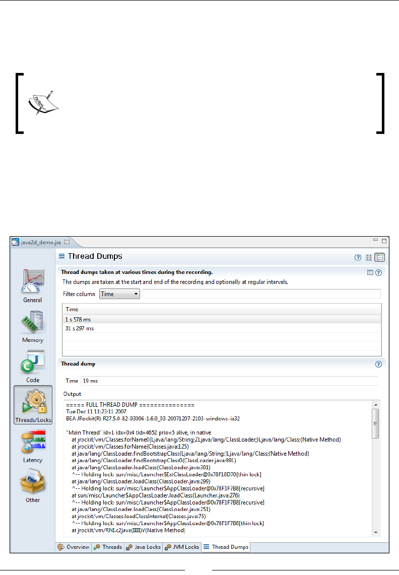
The Runtime Analyzer
[ 320 ]
JVM Locks
This tab contains information on JVM internal native locks. This is normally useful
for the JRockit JVM developers and for JRockit support.
Native locks were discussed to some extent in Chapter 4. An example
of a native lock would be the code buffer lock that the JVM acquires
in order to emit compiled methods into a native code buffer. This is
done to ensure that no other code generation threads interfere with
that particular code emission.
Thread Dumps
The JRA recordings normally contain thread dumps from the beginning and the
end of the recording. By changing the Thread dump interval parameter in the JRA
recording wizard, more thread dumps can be made available at regular intervals
throughout the recording.
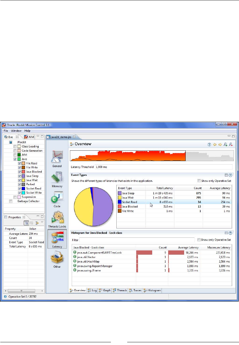
Chapter 8
[ 321 ]
Latency
The latency tools were introduced as a companion to JRockit Real Time. The
predictable garbage collection pause times offered by JRockit Real Time made
necessary a tool to help developers hunt down latencies introduced by the Java
application itself, as opposed to by the JVM. It is not enough to be able to guarantee
that the GC does not halt execution for more than a millisecond if the application
itself blocks for hundreds of milliseconds when, for example, waiting for I/O.
When working with the tabs in the Latency tab group, we strongly recommend
switching to the Latency perspective. The switch can be made from the menu
Window | Show Perspective. In the latency perspective, two new views are
available to the left—the Event Types view and the Properties view. The Event
Types view can be used to select which latency events to examine and the
Properties view shows detailed information on any selected event.
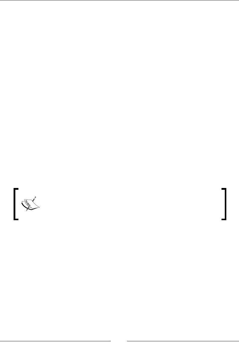
The Runtime Analyzer
[ 322 ]
Similar to in the GCs tab, at the top of all the latency tabs is the Range Selector. The
range selector allows you to temporarily select a subset of the events and only examine
this subset. Any changes either to the Event Types view or the range selector will be
instantly reected in the tab. The graph in the backdrop of the range selector, normally
colored red, is the normalized amount of events at a specic point in time. The range
selector also shows the CPU load as a black graph rendered over the event bars. It is
possible to congure what should be displayed using the range selector context menu.
The operative set is an important concept to understand when examining latencies
and subsets of latencies. It is a set of events that can be added to and removed from,
by using the different tabs in the latency tab group. Think of it as a collection of
events that can be brought from one tab to another and which can be modied using
the different views in the different tabs. Understanding and using the operative set is
very important to get the most out of the latency analysis tool.
Overview
The Overview tab provides an aggregated view of the latency events in the
recording. At the top, just under the range selector, the Latency Threshold used
during the recording can be seen. As potentially very large volumes of data can be
recorded, the Latency Threshold is normally used to limit the amount of events so
that only the ones longer than a certain threshold are actually recorded. The default
is to only record latency events that are longer than 20 milliseconds.
A latency event is any time slice longer than a preset value that
the JVM spends not executing Java code. For example, it may
instead be waiting for data on a socket or performing a phase of
garbage collection that stops the world.
The Event Types histogram and accompanying pie chart show breakdowns per
event type. This is useful to quickly get a feel for what kind of events were recorded
and their proportions. Note that the pie chart shows the number of events logged, not
the total time that the events took. A tip for nding out where certain types of events
are occurring is to use the context menu in the Event Types histogram to add the
events of a certain type to the operative set. This causes the events of that type to be
colored turquoise in the range selector.
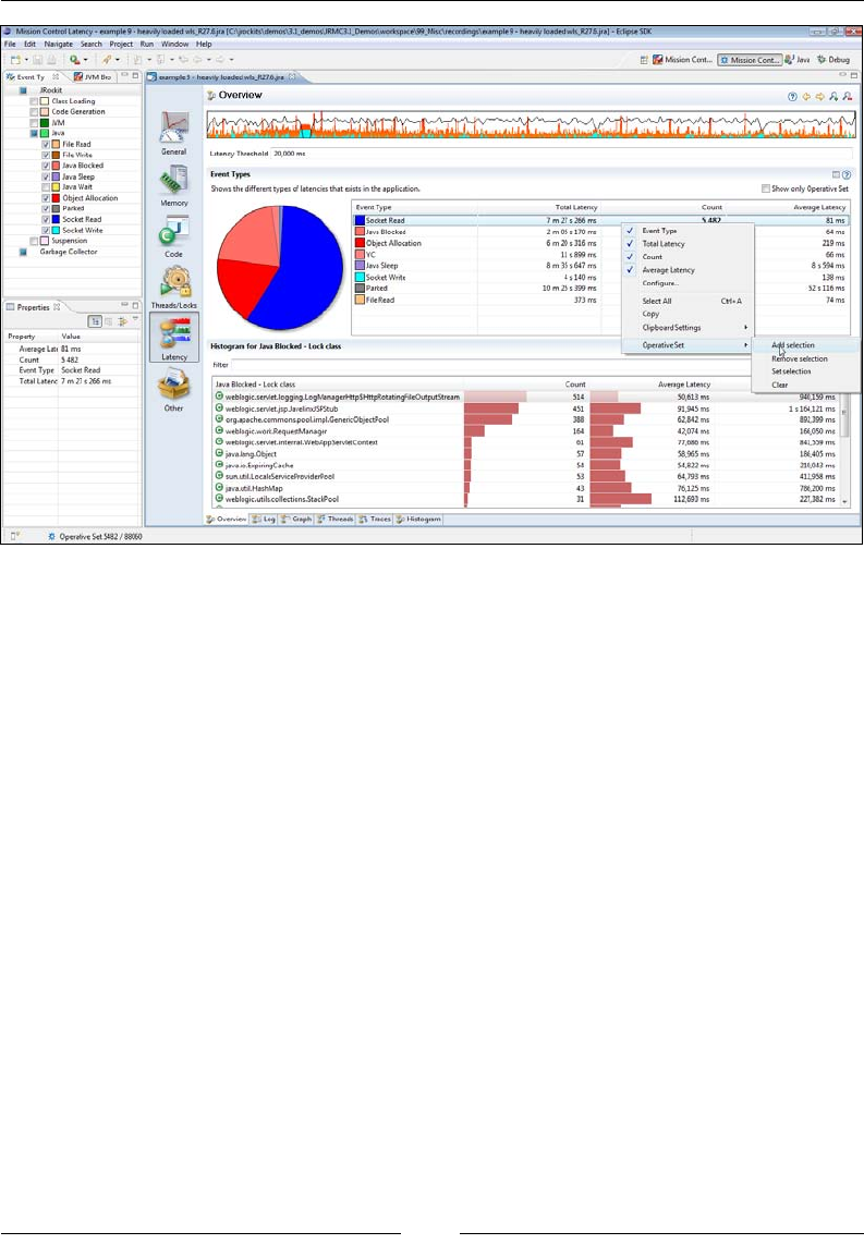
Chapter 8
[ 323 ]
Another tip is to go to the Traces view and click on Show only Operative Set, to see
the stack traces that led up to the events of that particular type.
Log
The latency Log tab shows all the available events in a table. The table can be used
for ltering events, for sorting them, and for showing the events currently in the
operative set. It is mostly used to quickly sort the events on duration to nd the
longest ones. Sometimes, the longest latencies may be due to socket accepts or
other blocking calls that would actually be expected to take a long time. In such
cases, this table can be used to quickly nd and remove such events from the
operative set, concentrating only on the problematic latencies.
The Runtime Analyzer
[ 324 ]
Graph
The latency Graph tab contains a graph where the events are displayed, aggregated
per thread. In the following example, we only show the events from the Java and
Garbage Collector event types. The normal rendering procedure for the graph is that
each event producer gets its own per-thread lane where the events for that particular
producer are displayed. For each thread, only one event can occur in a lane at any
given time. Garbage collection events are drawn in a slightly different way—they are
always shown at the top of the latency event graph, and each GC is highlighted as
a backdrop across all the other threads. This is useful for seeing if a certain latency
event was caused by a garbage collection. If part of a lane in the latency graph is
green, it means that the thread is happily executing Java code. Any other color means
that a latency event is taking place at that point in time. To nd out what the color
means, either hover the mouse over an event and read the tooltip, or check the colors
in the Event Types view.
The latency Graph can also show thread transitions. The application in the next
screenshot has an exaggerated pathological behavior, where all threads in an
application are sharing a logger through a static eld, and where the logger is
using a synchronized resource for writing log data. As can be seen, the worker
threads are all waiting on the shared resource. The worker threads that are there
to execute parts of the work in parallel, rely on the shared logger. This actually
causes the entire application to execute the work in a sequential fashion instead.
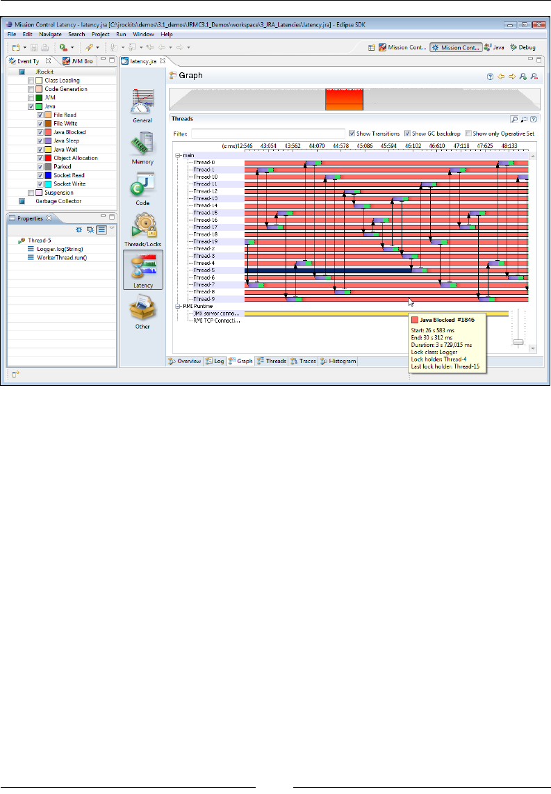
Chapter 8
[ 325 ]
If you see an event that you want to get more information on, you can either select it in
the graph and study it in the properties view, hover the mouse pointer over it and read
the tooltip that pops up, or add it to the operative set for closer examination in one of
the other views.
To summarize, the Graph view is good for providing an overview of the latency and
thread behavior of the application.
Threads
The Threads tab is basically a table containing the threads in the system, much
like the threads tab in the Management Console, as described in Chapter 7. The most
useful properties in this table tend to be the event Count and the Allocation Rate
per thread.
This view is mainly used to select a specic thread, either based on an attribute, such
as the one with the highest allocation rate, or for nding a specic thread by name.
The operative set is then used to select the events for that particular thread, so that
the events can be studied in the other views. Sets of threads can also be selected.
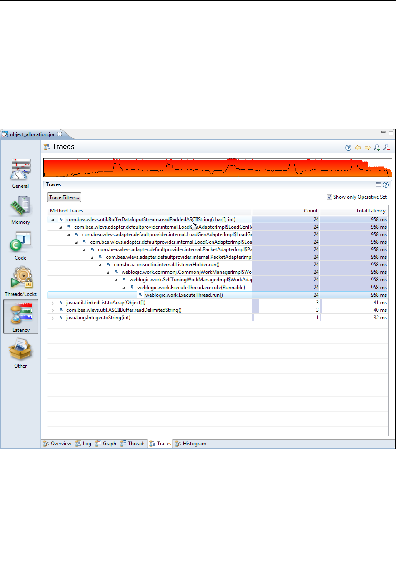
The Runtime Analyzer
[ 326 ]
Traces
This is where the stack traces for sets of events get aggregated. For instance, if the
operative set contains the set of allocation events for String arrays, this is the tab
you would go to for nding out where those object allocations take place. In the
next example, only the traces for the operative set are visible. As can be seen, the
Count and Total Latency columns have bar chart backdrops that show how much
of the max value, relative to the other children on the same level, the value in the
cell corresponds to. Everything is normalized with respect to the max value.
Normally, while analyzing a recording, you end up in this tab once you have used
the other tabs to lter out the set of events that you are interested in. This tab reveals
where in the code the events are originating from.
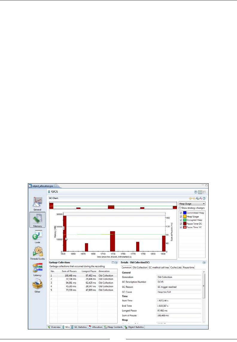
Chapter 8
[ 327 ]
Histogram
This very powerful tab is used to build histograms of the events. The histogram can
be built around any event value. A few examples of useful ones are:
• Object Allocation | Class Name: For nding out what types of allocations
are most common
• Java Blocked | Lock Class: For nding out which locks are most frequently
blocking in the application
• Java Wait | Lock Class: For nding out where the application spends the
most time in wait()
Once the interesting events have been found, they are usually added to the operative
set and brought to another tab for further investigation.
Using the Operative Set
Sadly, one of the most overlooked features in JRA is the operative set. This example
will explain how the operative set can be used to lter out a very specic set of events
to solve a specic problem. In this example, we have been given a JRA recording from
another team. The team is unhappy with the garbage collections that take place in an
application. Garbage collections seem to be performed too frequently and take too long
to complete. We start by looking at the GCs tab in the Memory section.
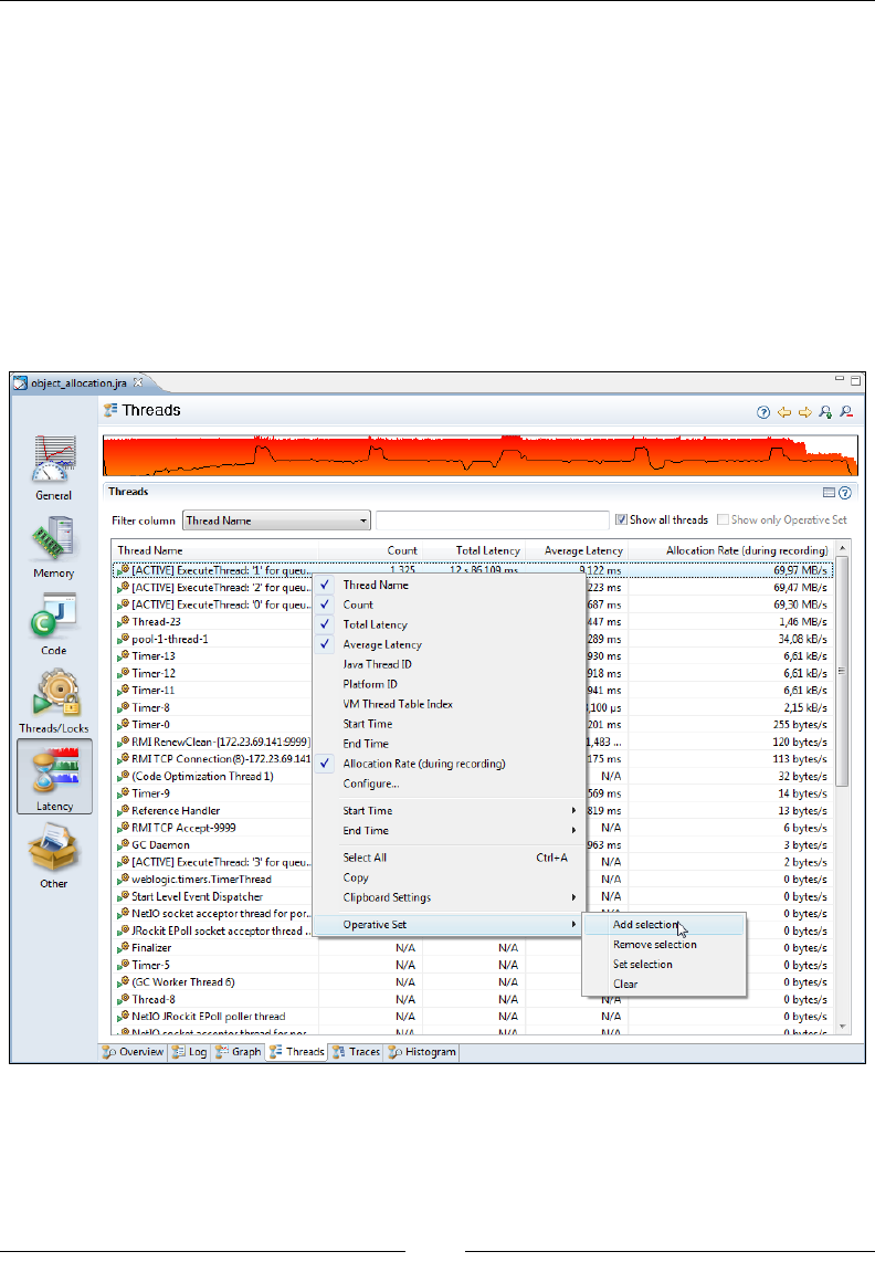
The Runtime Analyzer
[ 328 ]
The initial reaction from examining the garbage collections is that they are indeed quite
long, tens of milliseconds, but they do not happen all that often. For the duration of
the recording only ve GCs took place. We could probably ask the clients to switch
to deterministic GC. This would cause more frequent but much shorter garbage
collections. However, as we are curious, we would like to get back to them with more
than just a GC strategy recommendation. We would still like to know where most of
the pressure on the memory system is being created.
As this is an example, we'll make this slightly more complicated than necessary, just
to hint at the power of JRA. We switch to the latency data thread tab and look for the
most allocation intensive threads. Then we add these events to the Operative Set. It
seems that almost all allocation is done in the top three threads.
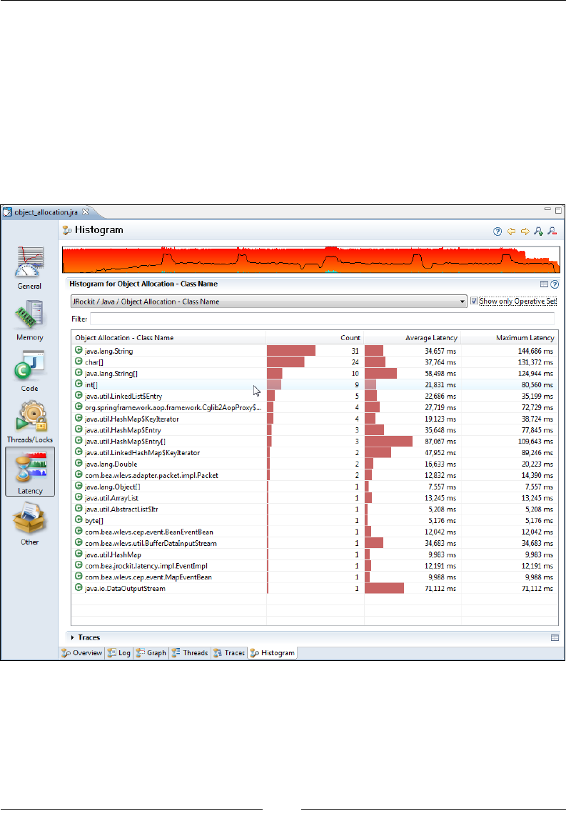
Chapter 8
[ 329 ]
We have now added all the events for the three threads to our Operative Set, but
we are only interested in studying the allocation behavior. In order to do this, we
move to the Histogram tab and build a histogram for the allocation events in our
Operative Set.
Note that object allocations are weird latency events, as we are normally not
interested in their duration, but rather the number of occurrences. We therefore sort
them on event count and see that most of the object allocation events in our three
threads are caused by instantiating Strings. As we're eager to nd out where these
events take place, we limit the operative set to the String allocation events.
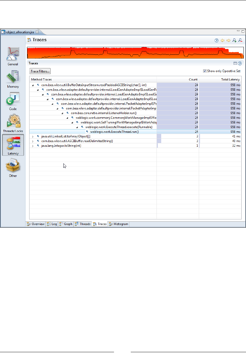
The Runtime Analyzer
[ 330 ]
We proceed to the Traces view with our trimmed Operative Set, and once again
check the Show only Operative Set button.
We quickly see that almost all the String instances in our three most allocation-
intensive threads are allocated by the same method
—readPaddedASCIIString(char [], int). If we also add char arrays,
we can see that the char arrays are mostly created as a result of allocating
the String objects in the same method. This makes sense as each String
wraps one char array.
We can now recommend the team not only to change GC strategies, but we can also
say for sure, that one way to drastically reduce the pressure on the memory system in
this particular application would be to either create less strings in the method at the
top in the Traces view, or to reduce the number of calls along the path to that method.

Chapter 8
[ 331 ]
Troubleshooting
Sometimes, there will be no data in the Code | Hot methods tab, even if the method
sampling was enabled. The most common reason is that the application did not
generate enough load to provide the method sampler with data. The method sampler
only samples threads that are actively running Java code. If the recording is short
and the threads are spending most of their time waiting and doing nothing, chances
are that no samples will be recorded at all. If you aren't proling a production
system, try to stress your application during proling, if possible in a manner that
is close to the real deployment scenario.
When using native method sampling, all samples will be stored. Normally, only
the samples for threads executing Java will be stored. Don't be surprised if you
nd almost all of the native samples to be in some native method, such as ntdll.
dll#KiFastSystemCallRet, even when the system is mostly idle.
Summary
In this chapter, we showed how to use the JRockit Runtime Analyzer to analyze
the behavior of the JRockit runtime and the application running in JRockit.
We showed various different ways to create recordings. We also discussed
the information available in JRA recordings with examples.
Several use cases were demonstrated, such as:
• How to nd methods that would make good candidates for manual
optimization, also known as hot spots
• How to interpret memory-related information, such as the live set, garbage
collection-related information, fragmentation, the object summary, and the
heap histogram
• How to hunt down latency-related problems
We also provided an example on how to use the Operative Set in the latency
analyzer to quickly narrow down the amount of data being studied and to
focus on the data of interest.
The next chapter covers JRockit Flight Recorder, which has superseded JRA as of
JRockit R28 and JRockit Mission Control 4.0. Most of what has been covered in this
chapter works in similar ways and is still applicable.

The Flight Recorder
The overhead of using JRA proved so low that we started considering the notion of
always having it enabled when the JVM is running. The project to implement such a
recording engine was internally rst known as continuous JRA. In the R28 version
of JRockit, this has nally been productized and named JRockit Flight Recorder.
As near-zero overhead data is continuously stored about JVM behavior, the
JRockit Flight Recorder allows us to go back in time and analyze the behavior of
the application and the JVM even after something has gone wrong. This is a very
powerful feature for JVM and application forensics—the recording being the "black
box" that contains information on all events leading up to a problem. Naturally, the
framework still works well as a proling and instrumentation tool, which will likely
remain the most common use case.
In this chapter, you will learn:
• How JRockit Flight Recorder works
• About the Flight Recorder event model
• How to start a continuous recording
• How to start a JRA-style recording
• How recordings interact in JRockit Flight Recorder
• How to congure the various aspects of JRockit Flight Recorder
• The main differences between JRockit Flight Recorder and the JRockit
Runtime Analyzer
• How to record custom events
• How to design custom extensions to the JRockit Flight Recorder client
• About future tools, APIs, and projects around JRockit Flight Recorder
JRockit Flight Recorder
[ 334 ]
The evolved Runtime Analyzer
Just like the JRockit Runtime Analyzer, the JRockit Flight Recorder consists of two
parts—a recording engine built into the JRockit JVM and an analysis tool built into
the JRockit Mission Control client. The recording engine produces a recording le
that can be analyzed. The le does not require an active connection; the format is self
describing, that is, all metadata that the recording needs is part of the recording and
can be saved for later or sent to a third party for further analysis.
Throughout this chapter, we will use the terms JRockit Flight
Recorder and Flight Recorder interchangeably.
With JRockit Flight Recorder, recordings are no longer in XML format. Everything
is recorded as time-stamped events in internal memory buffers and written to a
binary le, which constitutes the recording. There is also a public Java API available
for providing custom events to the JRockit recording engine, and a design mode
that allows the creation of custom designed user interfaces from within the analysis
tool itself.
Recall from Chapter 8, The Runtime Analyzer, that a JRA recording is
in XML format and the les are sufxed .jra. With Flight Recorder,
the les are sufxed .jfr and are in a binary format. Because of
the immense amount of events produced, there is a need to avoid
unnecessary overhead and consequently to store events in a more
compact way. JRA recordings are not forward-compatible and cannot
be opened with JRockit Flight Recorder.
A word on events
As mentioned, data is recorded as events. An event is simply data recorded at a
specic time.
There are four different types of events:
• Duration events: Duration events are events that last over a duration of time
or, in other words, events with a start time and an end time. The Garbage
Collection event is an example of a duration event.
• Timed events: The timed events are duration events for which a threshold
can be set. The concept of a threshold is discussed in detail later in this
chapter. The Java Wait and Java Sleep events are examples of timed events.

Chapter 9
[ 335 ]
• Instant events: Instant events have no duration, only a start time. The
Exception and the Event Settings Changed events are examples of instant
events.
• Requestable events: Requestable events can be congured to be polled
periodically by the recording engine. The event implements a callback that
a separate thread in the recording engine will call at specied intervals. An
example of a requestable event is the CPU Load Sample event.
Events are produced by event producers. An event producer denes the types of
events being produced, also known as event types, as well as the actual events. An
event type contains metadata that describes how the events of that type will look.
The metadata contains information such as what attributes (also known as elds) the
event contains, of what types the attributes are, and human-readable descriptions of
the attributes. Every recording le contains information about its event producers.
An event producer with the imaginative and thought-provoking name "JRockit JVM"
is already built into JRockit. The main advantage of the JRockit JVM producer, just
as with JRA, is that it cheaply records information that the runtime already needs
to collect as part of doing its job. Using the Java API, which will be discussed later,
anyone can contribute events to bring additional context to the lower level events
created by the JRockit JVM producer.
The recording engine
The recording engine, also known as the recording agent, is part of the JVM itself
and provides highly optimized services for the event producers. A few examples are:
• A recording facility: Of course, the main purpose of the recording engine
is to record events. It does this highly efciently by providing thread local
buffers where the events are recorded and a scheme to transfer these to a
global buffer when the thread local buffers are full. Once the global buffer is
full, it is either emitted to disk in the previously mentioned compact binary
format, or reused in a circular fashion depending on the conguration. See
the next gure.
• Stack traces: If the event producer sets the appropriate options, the stack
trace that generated the event will be recorded along with the event.
This is useful for nding where, in the source code of a Java application,
an event originated.
• Threshold: The recording engine can be congured to only include duration
events that last longer than a specied amount of time. This is used to both
limit the amount of data in the recording, and to lter out data that would be
of no interest anyway. The threshold can be congured per event type.
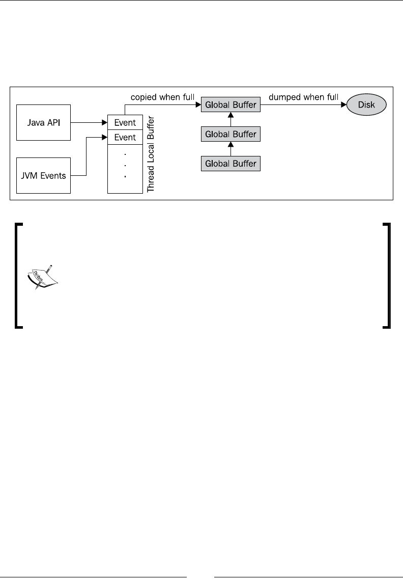
JRockit Flight Recorder
[ 336 ]
• Highly optimized time stamping of events: As was briey discussed in
Chapter 5, Benchmarking and Tuning, using System.currentTimeMillis()
for getting the system time can be a much more expensive operation than
one would think. The recording engine provides a highly optimized native
implementation for timestamping events.
As JRockit R28 is released as part of a patch release of the application
stack, it was decided that enabling the default recording was too
big a change. The recording engine is enabled in R28, but there is
no recording running from the start of the JVM. Both the recording
engine and the JRockit JVM event producer have been designed and
tested for always being enabled. As a matter of fact, all of the testing,
including the stress testing of JRockit R28, was performed with the
default recording enabled. The default recording will most likely be
enabled out of the box in future releases of JRockit.
Ongoing recordings in the JVM have an associated recording ID, which is unique,
and a recording name, which does not have to be. The recording ID is automatically
assigned to the recording when it is created, and can be used for identifying a
recording. The recording ID can, for example, be used when referring to a
recording from JRCMD.
To enable the Flight Recorder and to congure it to continuously record data with
the default settings, simply start JRockit with the following option:
-XX:FlightRecorderOptions=defaultrecording=true

Chapter 9
[ 337 ]
This will create a recording with recording ID 0 and the name JRockit default.
There can be an arbitrary amount of recordings running in JRockit Flight Recorder
at any given time. If more than one recording is active, the recorded data will contain
events from the union of the enabled event types and use the threshold found for
each type. For users new to the Flight Recorder, this can be quite confusing, as there
may actually be more events in the recording than asked for.
To congure the engine to record more detailed information, you can either change
the event settings of the default recording, or start a new recording with different
settings. To record less information, the event settings of any ongoing recording
must be changed.
Startup options
There are various ways to congure the different aspects of the recording engine,
some of which are only available from the command line when starting the JVM.
There are two main command-line parameters. As previously mentioned, the rst
one turns on (+) or off (-) the Flight Recorder altogether:
-XX:[+|-]FlightRecorder
The second is for controlling the Flight Recorder:
-XX:FlightRecorderOptions=parameter1=value1[,parameter2=value2]
The available parameters are:
Parameter Description
settings=[name|filepath] Loads additional event settings from this server-
side template. The default templates available under
JROCKIT_HOME/jre/lib/jfr can be referred to by
name. More information on server-side templates is
available after this table.
repository=[dir] The base directory where the Flight Recorder will emit
chunks of data. This can be seen as the temporary
directory of the Flight Recorder. The default is a
directory under java.io.tmpdir with a name
generated in the format yyyy_mm_dd_hh_mm_ss_
pid. For example, a repository created at the time
of writing for a process with a process ID of 4711
would have the repository base directory name
2010_04_21_16_28_59_4711.

JRockit Flight Recorder
[ 338 ]
Option Description
threadbuffersize=[size] The size to use for the thread local buffers. The default
is 5 KB.
globalbuffersize=[size] The size to use for a single global buffer. The default is
64 KB.
numglobalbuffers=[num] There may be more than one global buffer. This sets the
number of global buffers to use. The default is 8.
maxchunksize=[size] The maximum size of a single data chunk in the
repository. The default is 12 MB.
continuous=[true|false] Enable the default continuous recording, that is the
built-in continuous recording with recording ID 0.
This does not enable or disable continuous recording
as a concept. No matter what value this attribute has,
continuous recordings can still be started from JRockit
Mission Control as long as the Flight Recorder engine
itself is enabled. As mentioned, the default recording is
disabled in JRockit R28.0, but is likely to be enabled by
default in future versions of JRockit.
disk=[true|false] Emit data to disk. This is disabled by default, meaning
that circular in-memory buffers will be used instead.
The contents of the buffers can be dumped to disk,
either from Mission Control or by using JRCMD.
maxage=[nanotime] Denes the maximum age of the data kept on disk.
Data younger than this is retained. The time is specied
in nanoseconds by default. The default value is 0,
which means the age check is ignored and that all data
is retained.
maxsize=[size] The maximum size of the data to keep on disk. The
default value is 0, which means the size check is
ignored.
When using either JRCMD or the command-line options, specifying what
information will actually be recorded is done through JSON-based template les.
The JRockit distribution comes with several example templates available under
JROCKIT_HOME/jre/lib/jfr. These templates are also known as server-side
templates, as they differ from the ones used by the JRockit Mission Control client.
The templates in the JRockit distribution serve as good examples, should you want
to create your own server-side template.
Chapter 9
[ 339 ]
An in-depth discussion on the server-side templates is beyond the
scope of this book. See the example templates for further information
on server-side templates and Chapter 11, JRCMD, for information
about using JRCMD to control the recording life cycle.
Starting time-limited recordings
Just like with JRA, it is possible to use command-line options to start
time-limited recordings. In the Flight Recorder, the parameter is called –
XX:StartFlightRecording. This parameter is useful when wanting to do
several recordings and compare them. It is for instance possible to delay a
recording to give the application and the JVM time to warm up. The following
example starts a recording after two minutes. The recording will last for one minute
and will be named MyRecording. The resulting recording le ends up as C:\tmp\
myrecording.jfr. Just like with -XX:FlightRecorderOptions,
a server-side template can be referred to by name. The example uses the
profile.jfs template.
-XX:StartFlightRecording=delay=120s,duration=60s,
name=MyRecording,filename=C:\tmp\myrecording.jfr,settings=profile
See the command-line reference for JRockit R28 for more information
about the available parameters to the StartFlightRecording option.
The rest of this chapter focuses on using the JRockit Mission Control client for
controlling the Flight Recorder and for viewing recordings.
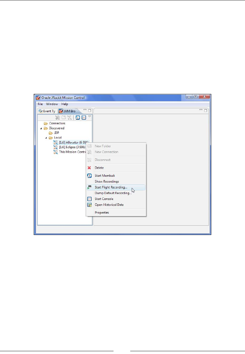
JRockit Flight Recorder
[ 340 ]
Flight Recorder in JRockit Mission
Control
The easiest way to both control the life cycle of recordings and transfer whole or
parts of recordings to JRockit Mission Control, is to do everything from inside the
JRockit Mission Control client.
Starting a JRA-style time-bound recording is quite similar to how it was done in
previous JRockit versions, using JRA—simply right click on the JVM in the JVM
Browser, and then click on Start Flight Recording....
In JRockit Mission Control 4.0, two things will happen:
1. The Start Flight Recording wizard dialog box will open.
2. The Flight Recorder Control view will open.
The Flight Recorder Control view is new for JRockit Mission Control 4.0. It shows the
recordings available for one or more connections, and can also be used for controlling
the recordings. It is quite useful for checking if any recordings are already running in
the JVM. In the following screenshot, the continuous recording is already running:
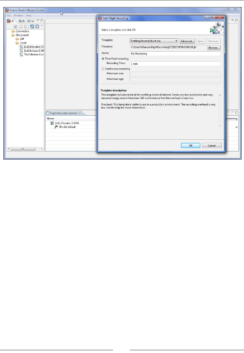
Chapter 9
[ 341 ]
Similar to JRA, this wizard contains a few built-in templates to choose from, and if
none of the provided templates records the information of interest, new templates
can be created. These templates differ from the server-side templates in that they are
fully resolved (no wildcards anywhere), and in that they support metadata for the
user interface.
The default built-in client-side templates are:
• Default Proling: A good, general-purpose proling template with low
proling overhead.
• Proling with Locks: Same as the previous one, but with lock proling
enabled. This requires the JRockit instance that is to be proled to be started
with -XX:+UseLockProfiling. This, in turn, causes some additional
overhead, even when not recording.
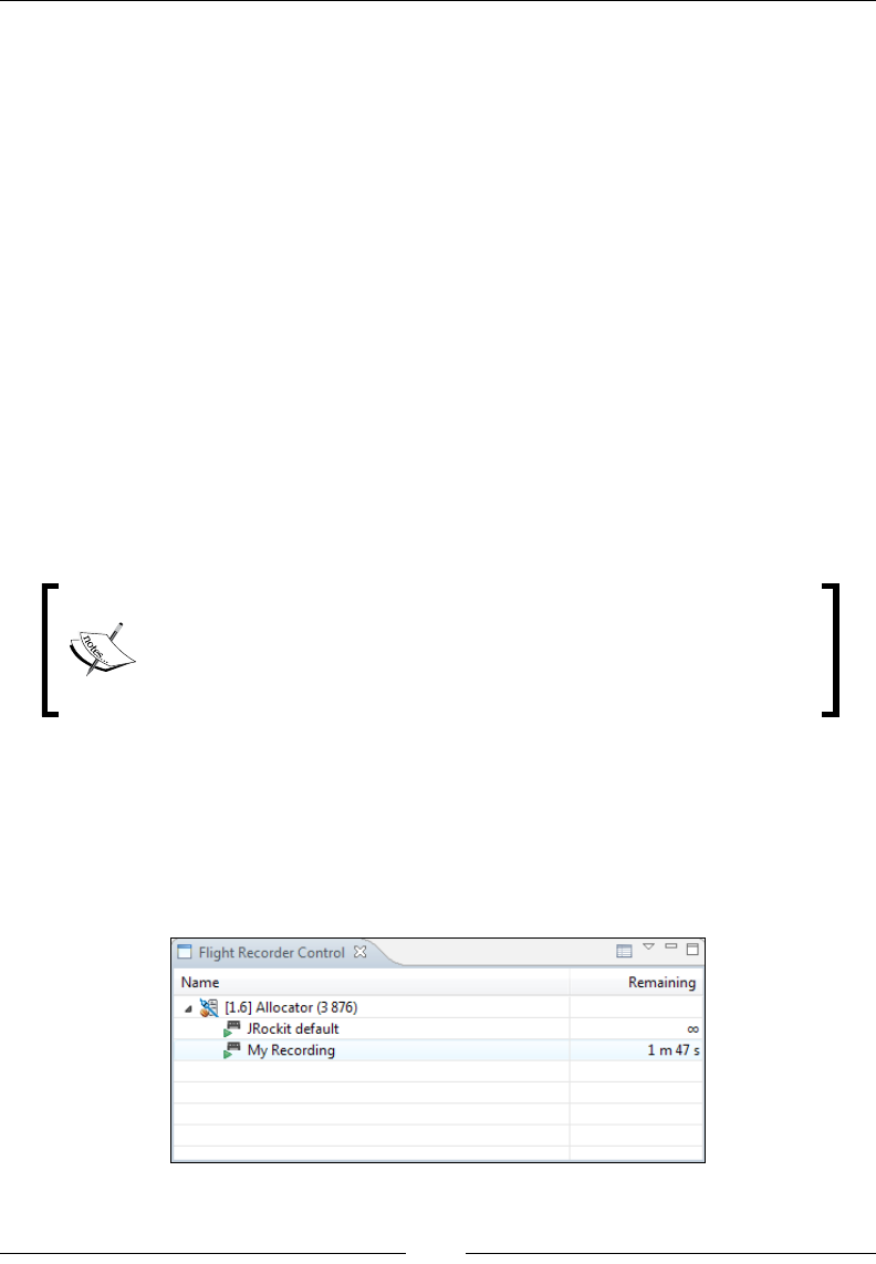
JRockit Flight Recorder
[ 342 ]
• Proling with Exceptions: Same as the Default Proling template, but with
exception proling enabled. For most applications, the overhead of this
template will not be different from that of the Default Proling template.
However, for some pathological applications, where a large number of
exceptions are thrown, the overhead can be considerable.
• Real-Time: Focuses on garbage collection related events, but leaves out some
of the most resource hungry events.
Worth noting is that both the default client-side and server-side templates omit
exception events by default, as it is difcult to estimate their performance impact
on a pathological application. To include exception proling, select the built-in
Proling with Exceptions template. Exception proling will be further discussed
later in this chapter.
Once a suitable template is selected, a destination le must be specied, and an
appropriate name chosen. Some event producers, such as the ones from the WebLogic
Diagnostics Framework, have their own recordings running. In a large system, there
can be quite a few recordings running in parallel. Naming the recording properly will
make it easier to nd it later.
Not only the JVM can record events in the Flight Recorder. There
are already event producers for the Oracle WebLogic Diagnostics
Framework (WLDF) and the Oracle Dynamic Monitoring System
(DMS). We expect more Oracle products to provide producers in
the future, such as JRockit Virtual Edition.
It is possible to perform either a time-limited recording or a continuous one. For a
time-limited recording, a duration must be chosen. In order to limit the resource
usage of continuous recordings, it is possible to limit the amount of data to store,
either by time, size, or both.
Once the recording wizard is lled out, clicking on Continue will start the recording.
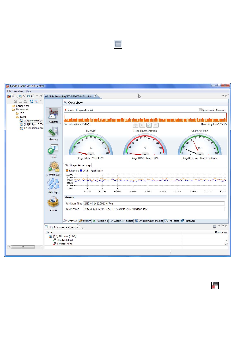
Chapter 9
[ 343 ]
The Flight Recorder Control view is updated to show the newly started recording.
For time-limited recordings, the remaining time until the recording is done is shown
and periodically updated. Continuous recordings show an innity (∞) sign instead of
the remaining time.
Note that there is a table settings action ( ) in the toolbar of the Flight Recorder
control view. The table can be congured to show more information, if needed.
For a time-limited recording, the recording will be downloaded automatically once it
is complete.
As can be seen in the previous screenshot, recordings are left on the server by default
when completed, even after they have been downloaded. In the screenshot, My
Recording has just been downloaded. It is also displayed as being nished ( ) in
the Flight Recorder Control view, with no time remaining. Such nished recordings
can be removed by right clicking on the recording in the Flight Recorder Control
view and then clicking on Close.
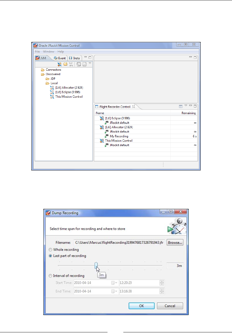
JRockit Flight Recorder
[ 344 ]
As mentioned, it is possible to see the recording activities of more than one JVM at a
time in the Flight Recorder Control view. To add a connection to monitor, simply right
click on the connection in the JVM Browser and then click on Show Recordings. The
following screenshot shows the recordings for three different JVMs at once:
To use the control view to dump data from an ongoing recording, simply right click
on it and select Dump.... This brings up the Dump Recording dialog, as shown in
the following screenshot:
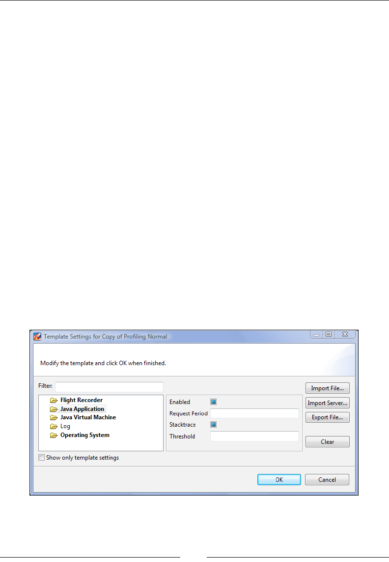
Chapter 9
[ 345 ]
There are three different ways to select what part of the recording to dump:
• Whole recording: Dumps all available data.
• Last part of recording: Dumps the last data in the recording, given a
specied period of time. Note that it is possible to get more data than was
specied, as only whole data chunks will be dumped.
• Interval of recording: Dumps recording data for a specied interval of
time. Note that the time is specied in server time. If the client is running in
Stockholm and the server in Tokyo, make sure you specify the correct time.
If there is no data within the specied time, an error message is displayed.
Again, what is actually dumped may be more than you were asking for.
The data is dumped in whole data chunks of a xed size. Each chunk of data
contains a constant pool that the events in the chunk use to resolve the data. For
instance, there is a pool containing the stack traces for the events. When an event
contains a stack trace, the event will refer to the stack trace by index in the pool. This
way, the format can be streamed and used on a per-chunk basis, each chunk being
self-contained.
Advanced Flight Recorder Wizard concepts
The Flight Recording Wizard lets you create custom templates. Clicking on the
Advanced... button next to a template name brings up a dialog box where the
template settings can be edited.
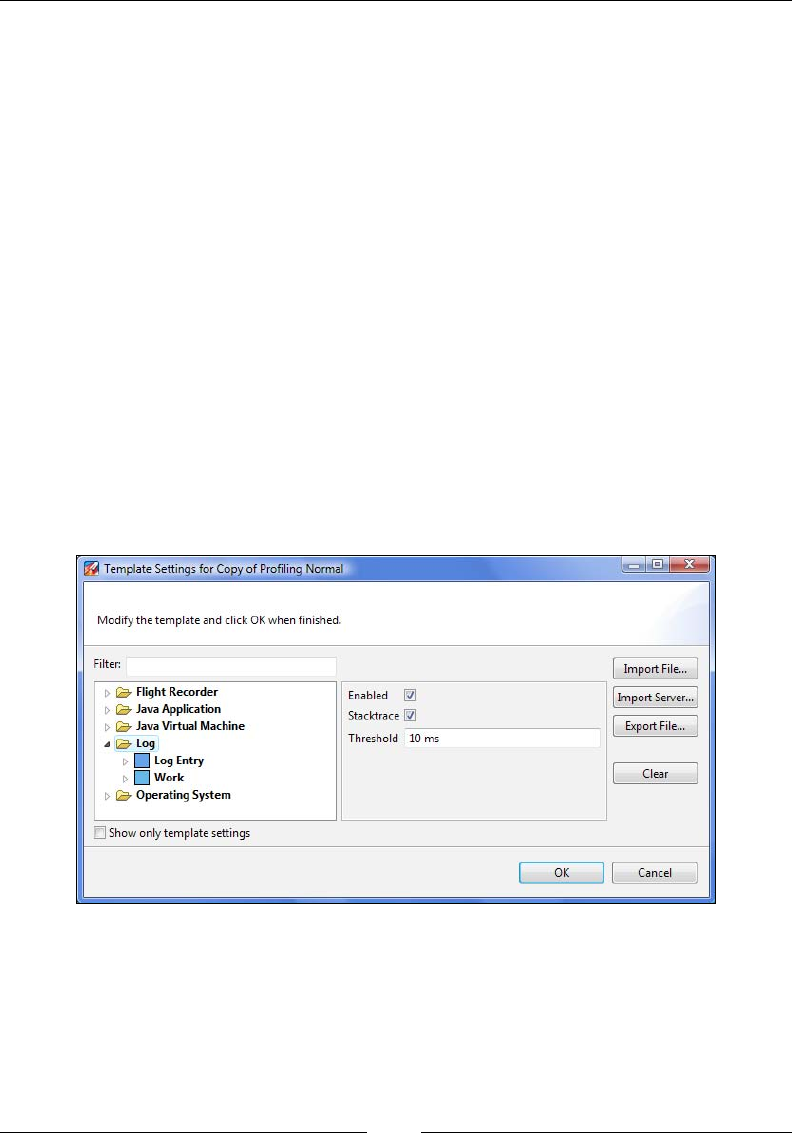
JRockit Flight Recorder
[ 346 ]
To the left in the wizard is an event type tree similar to the one in the Event Types
view. Selecting a parent node will allow the settings to be changed recursively
for all the descendants of that node. If there are different settings for the different
children, no value is shown for that of the parent node. For example, in the previous
screenshot, the settings for the events under the Java Application node vary, so no
values are shown for the Request Period and Threshold. Also, it would seem that
some events in the selection are disabled as well, as there is no check mark in the
check box for Enabled. To enable all of the Java Application events, click on the
Enabled check box.
In our example, the check box under the event type tree has been unchecked to allow
event types that are not a part of the current template to be shown. Nodes with
children that are part of a template are rendered in a bold faced font. Consequently,
we can see that no event types under Log are part of the current template.
The event types shown in the tree depend both on what application is running in the
JVM (the application may also utilize the Flight Recorder API) and on the settings in
the template. This allows the user to change settings for event types originating in
producers other than the default JRockit JVM producer. In the following example,
an event producer with event types with a path beginning with Log is available in
the running JVM.
Updating the settings for event types will make them bold, indicating that they are
now part of the template.
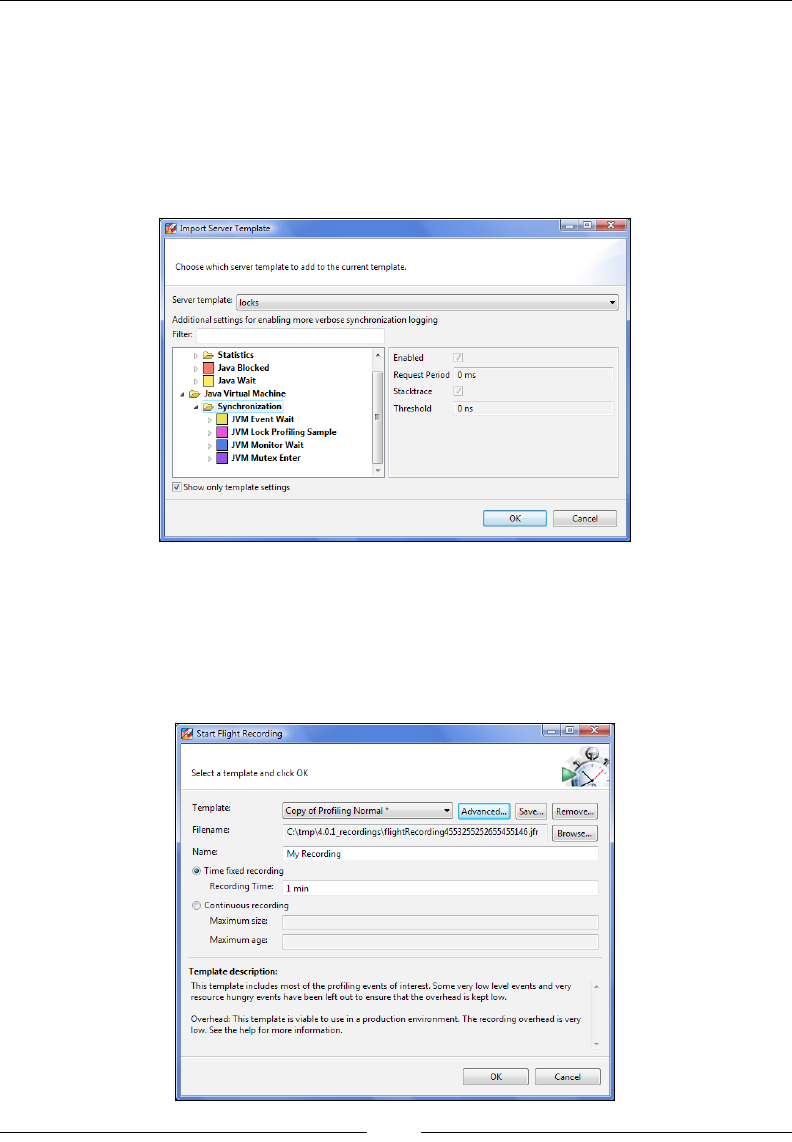
Chapter 9
[ 347 ]
It is possible to import server-side templates from the advanced wizard. A good
idea when doing so is to rst clear the template from any interfering settings. To
clear the template of all settings, click on the Clear button. The import functionality
is additive, as the server-side templates are meant to be used in an additive fashion.
This means that it is possible to, for example, start out with the settings for a default
recording and then add lock proling, by rst importing the default template, and
then importing the locks template. The next screenshot shows the import dialog:
Entering the advanced dialog creates a temporary working copy of the template.
Clicking on OK will save the settings to this temporary copy. An asterisk (*) next to
the template name indicates that the copy has not yet been stored. If the changes to
the template were done for only this particular recording, the template changes need
probably not be stored.
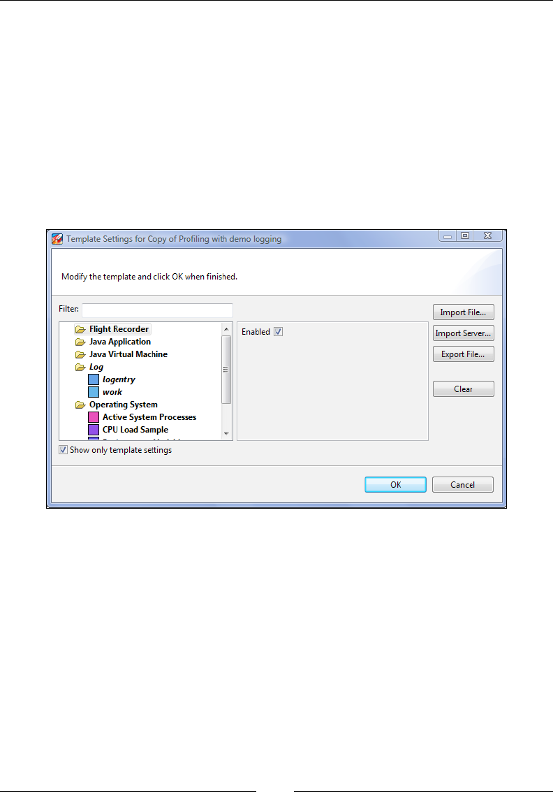
JRockit Flight Recorder
[ 348 ]
Simply clicking on OK in the Start Flight Recording dialog box allows the recording
to commence without the template rst being saved. The template will be available for
the rest of the session, but gone the next time that JRockit Mission Control is started.
To save the template and give it a name and description, click on Save….
Once the recording is saved, it can be reused, even on JVMs that do not support all
the event types for which the template has settings. For instance, when connecting
to a JVM not supporting the log event types, a template containing settings for the
log event types will render the log event types in italics, as shown in the following
screenshot. As the template can be applied anyway, it is easy to store your favorite
settings for a lot of different producers and scenarios in a small set of templates.
Differences to JRA
Due to the change to an event-based data model, some things are radically different
compared to JRA. For instance, almost every tab now has a range selector. As
everything now is an event, it almost always makes sense to be able to lter out data
for a specic period of time. Another major change is that the data in general is much
more ne-grained and there is a large number of new data sources.
We will discuss some of the more fundamental differences in detail.
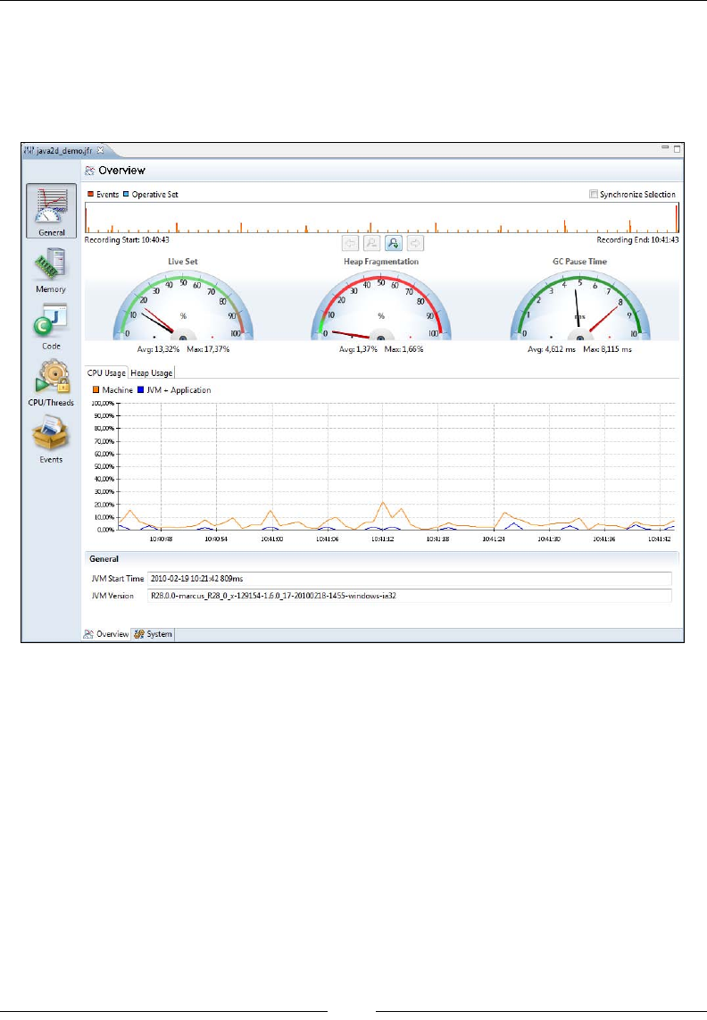
Chapter 9
[ 349 ]
The range selector
The following screenshot shows the General | Overview tab in the Flight Recorder
GUI. This can be compared with the way it looked in JRA, as introduced in Chapter 8,
The Runtime Analyzer.
As mentioned, the range selector (available at the top of the window) can now be
found in almost every tab in the Flight Recorder. The backdrop for the range selector
in a tab normally shows the amount of events active during the time of recording for
the events used in that particular tab. For example, the Overview tab uses various
heap, garbage collection, CPU usage, and general information events.
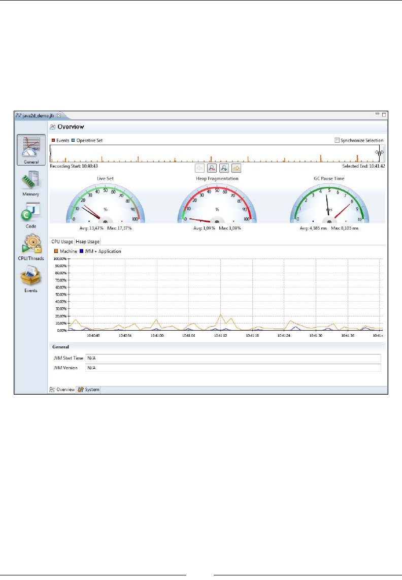
JRockit Flight Recorder
[ 350 ]
One effect of the event-based data model is that it is possible to select a range that
does not include an event where such data is available. Recall from Chapter 8 that
some of the general information is written at the end of the recording. In the Flight
Recorder, some events are written at the end of a chunk. If a range is selected that
does not include the needed event, N/A is displayed, as shown in the following
screenshot. Thus, care should be taken when modifying the range so that events
of interest are actually included for the active view.
As the range selector is used in so many places, it is now possible to synchronize
the selected range between all range selectors in all tabs. Check the Synchronize
Selection check box to make the other range selectors follow the selection made.
Just as before, in JRA, the Operative Set will be highlighted in turquoise if any of the
events are added to the Operative Set.
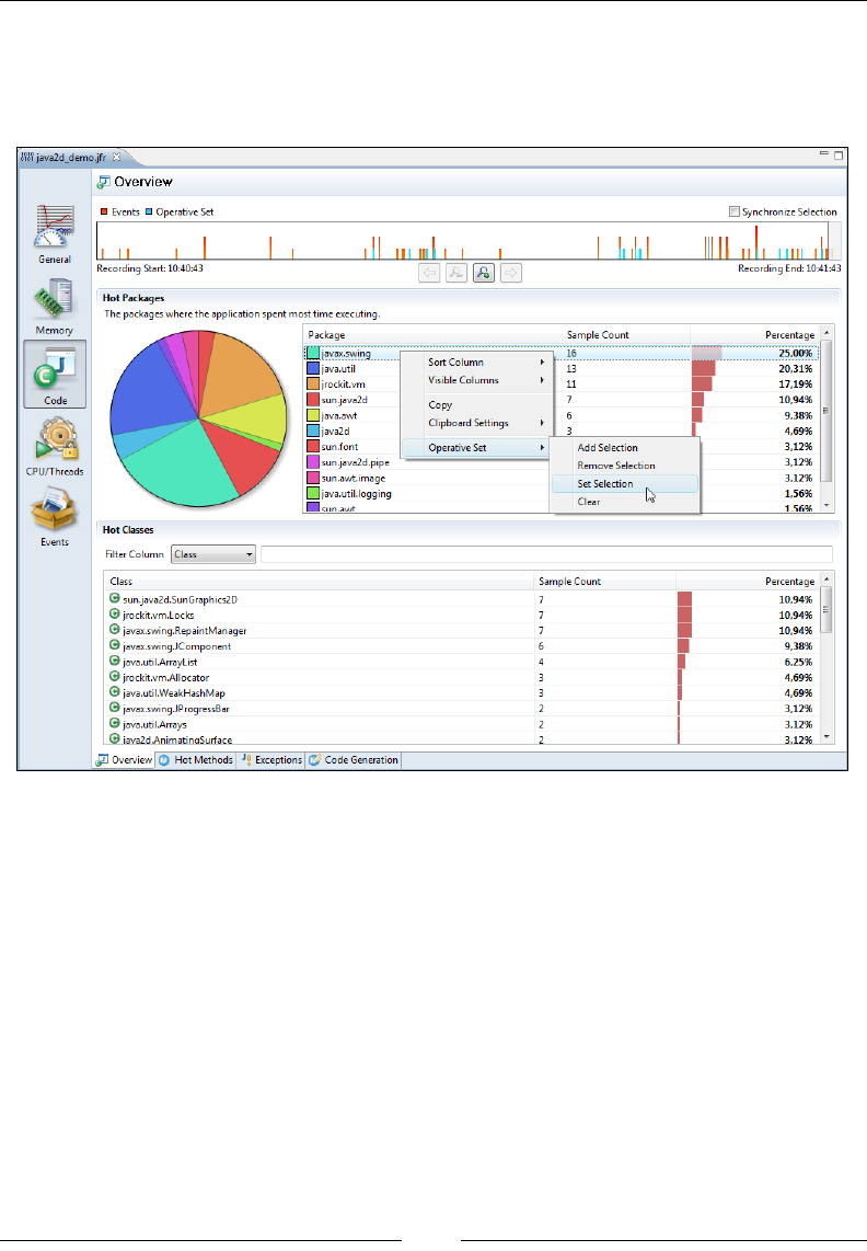
Chapter 9
[ 351 ]
The Operative Set
The Operative Set has also been improved. It is now possible to manipulate the
Operative Set from most views, even the ones mimicking the old JRA-style tabs.
In the screenshot, we are adding the code samples found in the javax.swing
package that, in this case, is the hottest package to the operative set. The
corresponding events are highlighted in the range selector.
The relational key
Event attributes can now have a relational key. The relational key is globally unique,
and is used to associate events of different types with each other. One such example
is the GCID of the GC events. The GCID is specied to have the relational key
http://www.oracle.com/jrockit/jvm/vm/gc/id. This makes it easy to nd all
events that are related to a specic garbage collection.
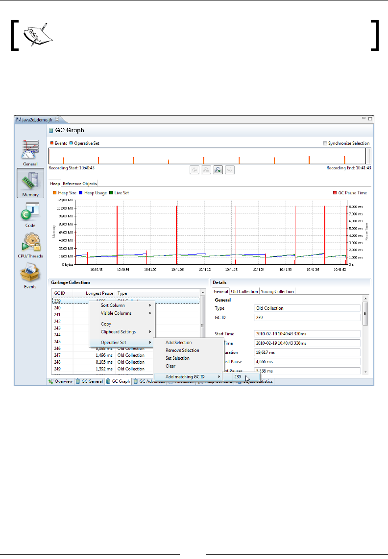
JRockit Flight Recorder
[ 352 ]
The relational key is on an URI format, much like name spaces in XML.
The user interface provides menu alternatives on the Operative Set context menu for
events having attributes with relational keys. In the next screenshot, we do this for
garbage collection number 239:
Third-party event producers use the relational key to associate events across
producers. For instance, WLDF and DMS use the Execution Context ID (ECID)
relational key to associate events across probes and producers all over WebLogic
Server. It is, for example, possible to add all the events associated with a certain
database call to the Operative Set.
These producers also provide relational keys for other attributes. The following
example screenshot uses the experimental WebLogic Tab Pack to illustrate this by
adding all the events with a matching SQL statement to the operative set.
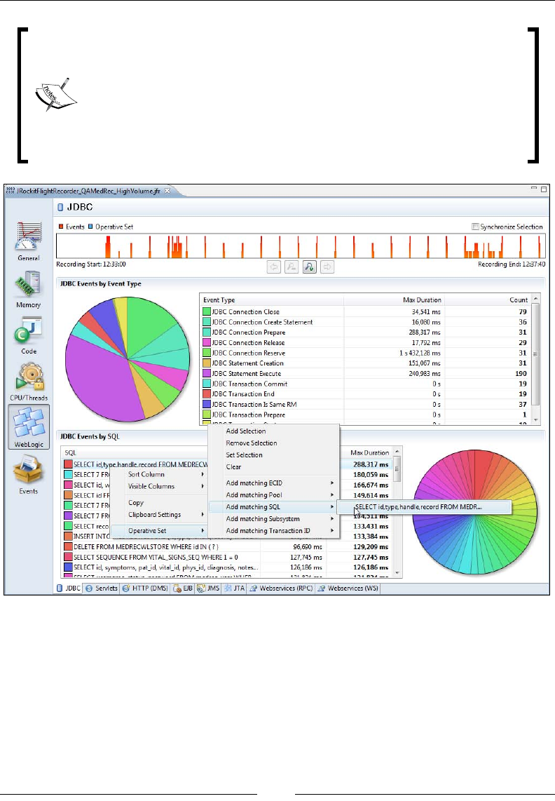
Chapter 9
[ 353 ]
The experimental plug-ins used in some of the examples in this book,
such as the WebLogic Tab Pack, are only available for JRockit Mission
Control 4.0.1 or later. Chances are that this book is published before
the release of 4.0.1, and that the plug-ins will not be available for a little
while. The good news is that the experimental plug-ins are available
for download from within the JRockit Mission Control 4.0.1 GUI. As
soon as version 4.0.1 (or later) of Mission Control is out, the authors'
advice is to upgrade immediately.
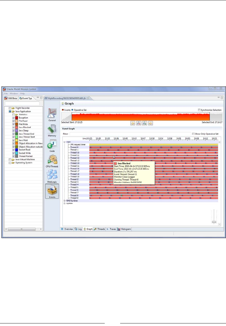
JRockit Flight Recorder
[ 354 ]
What's in a Latency?
Now that everything is an event, it is no longer wise to assume that all events are
latency-related, as was the case in JRA. By latency-related, we mean any event
directly involved in stalling the execution of a thread. There are specic tabs in the
Flight Recorder GUI that deal with latency-related events, and latency-related Java
events may still be used in a fashion similar to the old latency analyzer in JRA.
The Events tab group now contains general-purpose tabs for visualizing events,
similar to how the Latency tab group was used in JRA. The following screenshot
shows a synchronization problem:
If only the Java Application events are selected in the Event Types view, the result
will be very similar to the way things looked in the old latency analyzer in JRA.
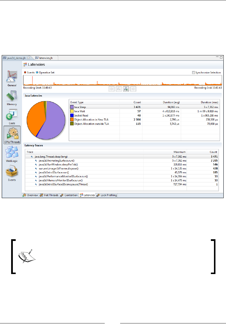
Chapter 9
[ 355 ]
The specialized tabs related to latencies can be found under the CPU | Threads tab
group. There are new tabs in the Flight Recorder that aggregate the latency-related
events in several interesting ways. The Latencies tab will, for instance, show an
aggregation per event type, and the aggregated stack traces for the selected event type.
In the next example, which is a recording from the Java 2D demo shipped with the
JDK, we can see that the threads are mostly halted by (explicit/voluntary) sleeps.
This is as would be expected, as there is probably a lot of thread sleeps going on
between each rendering pass in the rendering loops. Note that the pie chart to the left
is based on the event count, and not on the max duration, on which the table is sorted.
In Mission Control 4.0.0, the pie chart is bound to a pre-dened
column. It is possible to change which column by using the design
mode, as is explained later in this chapter. In the next minor version
of the Flight Recorder, we're exploring the option to bind the pie
chart to whichever numerical column was sorted last.
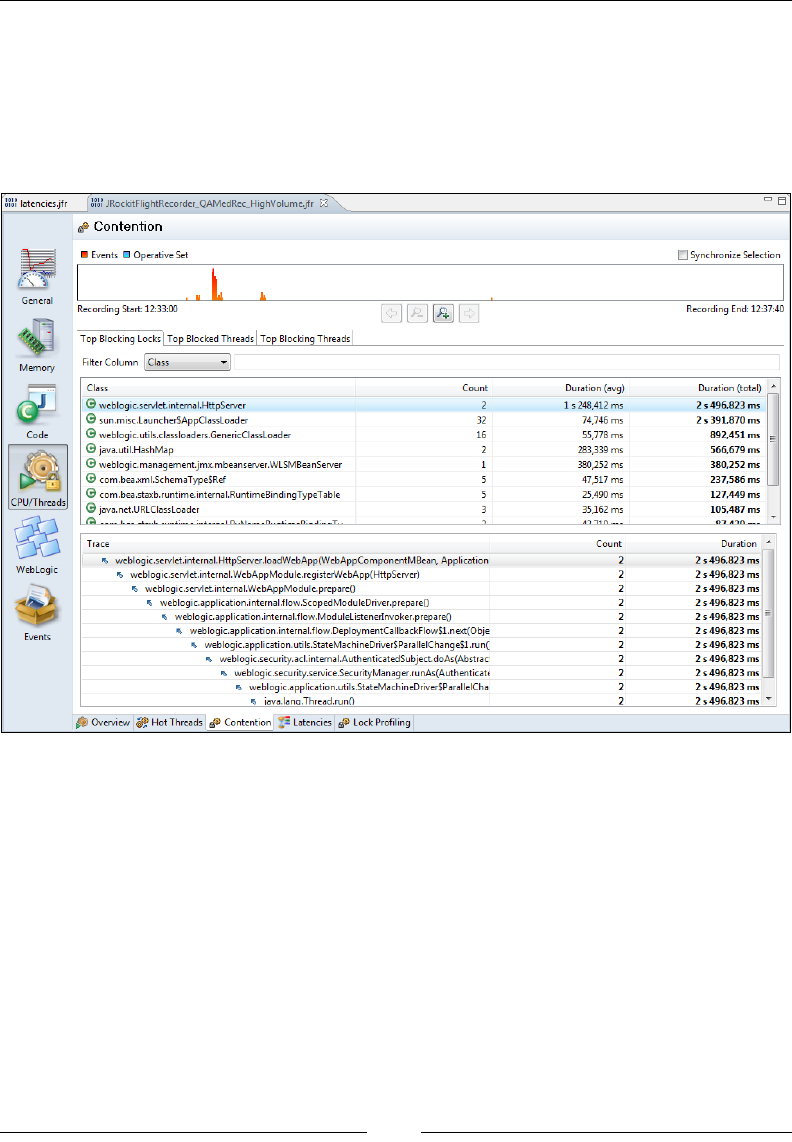
JRockit Flight Recorder
[ 356 ]
The Contention tab, introduced in JRockit Flight Recorder, is specialized for showing
the Java Blocking (threads blocked, waiting on acquiring monitors) events. In the
example recording from WebLogic Server shown in the next screenshot, we can see
that the longest total time a thread had to wait for acquiring a monitor was spent
waiting on an instance of weblogic.servlet.internal.HttpServer, trying to
execute the method loadWebApp(…).
It is also possible to see which threads were blocked the most, as well as which
threads were blocking other threads the most.
Just like in JRA, it is possible to enable very detailed lock proling, and just
like in JRA, lock proling comes with a small additional runtime overhead,
even when not recording. To enable lock proling, start JRockit with the ag
-XX:+UseLockProfiling and use the Proling with Locks template. More
information on the lock proling ags was given in Chapter 4, Threads
and Synchronization.
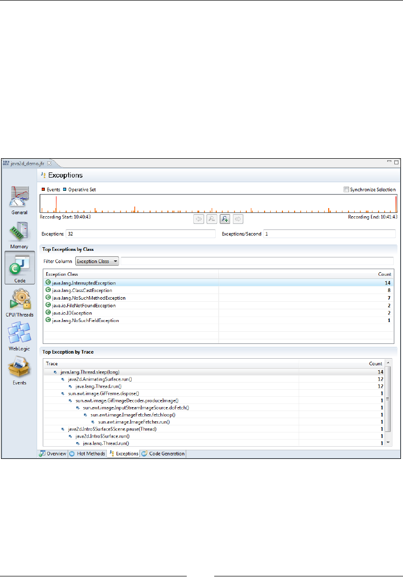
Chapter 9
[ 357 ]
Exception proling
In JRA, the only available exception proling information was the total number
of exceptions being thrown. The only way to correlate that to where in the code
the exceptions were thrown, was to change the log settings for the JVM to enable
the logging of exceptions. For example, through JRCMD or by restarting the JVM
with –Xverbose:exceptions=debug, and then checking the output. With the Flight
Recorder, there are now events containing the necessary information, and a tab that
allows for easy browsing. Remember to use the Proling with Exceptions template
when creating a recording that is to use exception proling. The tab is located under
Code | Exceptions.
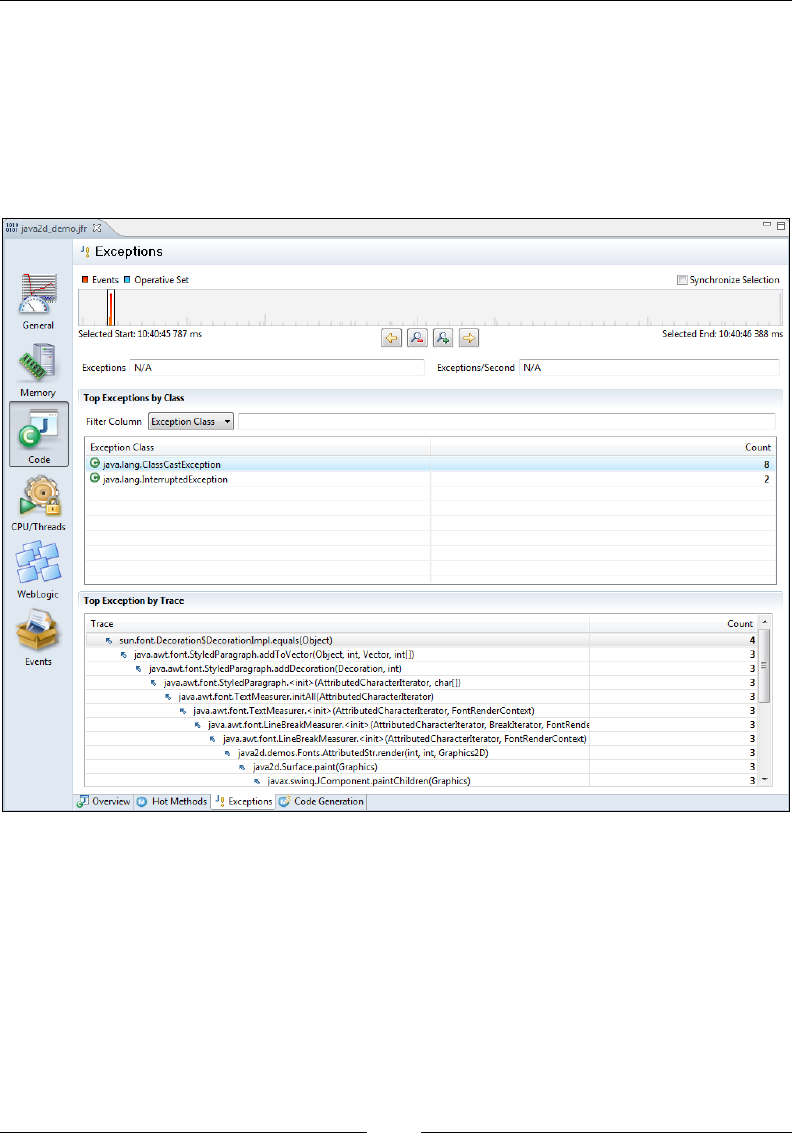
JRockit Flight Recorder
[ 358 ]
In the example recording from the Java 2D demo, we can see that most of the
exceptions are InterruptedExceptions thrown from java2d.AnimatingSurface.
run(). The range selector shows us two main bursts of exceptions, one at the
beginning of the recording and one at the end. The burst of exceptions at the
beginning of the recording is mostly due to ClassCastExceptions, and the burst at
the end is due to NoSuchMethodExceptions. This can easily be determined by using
the range selector to home in on the peaks, as shown in the following screenshot:
The Java 2D demo does not throw that many exceptions, so the exception data in
the recording merely serves as an example on how to use the user interface. If an
application throws more than several hundred exceptions per second, the cause
should be investigated.
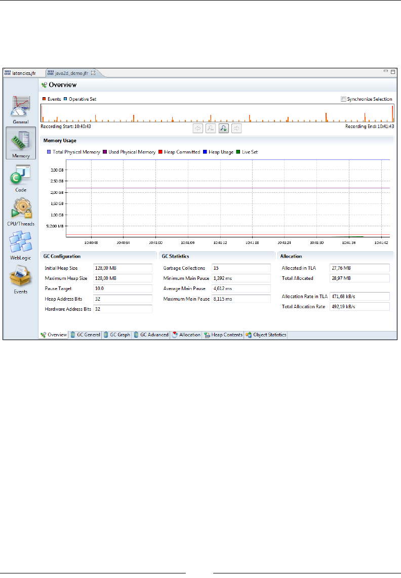
Chapter 9
[ 359 ]
Memory
Even though the memory tabs, and the information in them, are quite similar to the
old JRA layout there are a few things worth pointing out.
In the Memory | Overview tab, the Total Physical Memory and Used Physical
Memory both refer to the physical memory on the machine and not the Java process!
In the Java2D Demo recording earlier, the recording was done on a machine with 4
GB of physical memory, and at the point of recording, approximately 2.2 GB was in
use. The committed Java heap was as small as 128 MB, as can be seen from both the
graph and the GC Conguration section part. To see graphs of the Java heap usage,
use the Heap Contents tab.
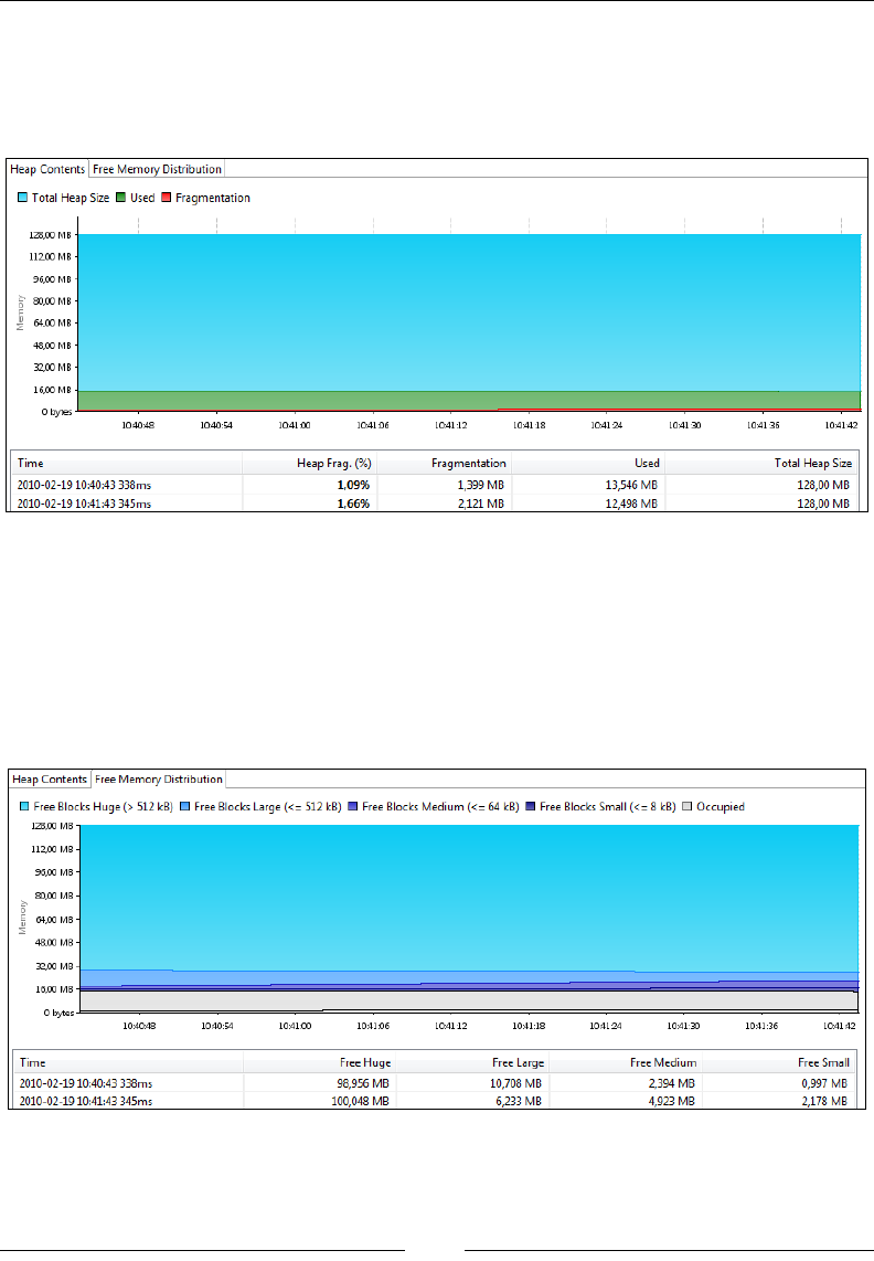
JRockit Flight Recorder
[ 360 ]
In the Heap Contents tab are two graphs, one focusing on the contents of the heap,
and one focusing on how the free space of the heap is distributed. Worth noting in
the Heap Contents tab, is that what was previously referred to as dark matter is now
called Fragmentation, which is a more descriptive name.
The used memory is simply rendered grey in the Free Memory Distribution chart,
with a line delimiting the used and fragmented parts. The charts in the example
show a very healthy heap, with lots of free memory and with fragmentation under
control. In the following screenshot, most of the free contiguous heap blocks are
huge. If the heap were instead made up of a lot of smaller free blocks, an allocation
of, for example, a large array would fail and cause the garbage collector to need to
perform costly compactions and possibly stop the world.
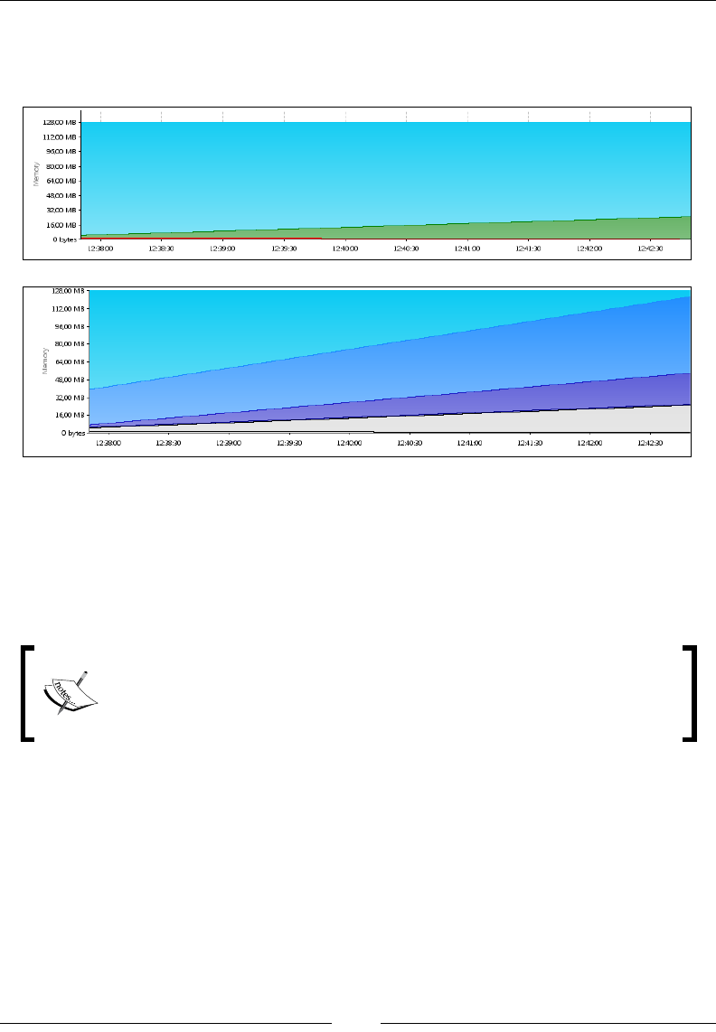
Chapter 9
[ 361 ]
In the next screenshot, a recording from the memory leaking demo application
further studied in Chapter 10 is shown. As can be seen, the live set is steadily
increasing over time and the free parts of the heap are split into smaller free blocks:
Adding custom events
There is a simple Java API that can be used to contribute custom events to ight
recordings. It is located under the package com.oracle.jrockit.jfr and is
distributed as part of the JRockit JDK. It is located in the JRockit rt.jar.
The com.oracle.jrockit.jfr API is under development, and not
currently supported outside Oracle. Some internal Oracle products, like
WebLogic Server already use it to plug into JRockit Flight Recorder.
To create a custom event using the API, rst decide what kind of event is needed.
You may recall from the start of this chapter that there are four main event types.
Depending on what kind of event is needed, a different event class will need to
be extended. There are four different ones, each corresponding to a different kind
of event:
• com.oracle.jrockit.jfr.InstantEvent
• com.oracle.jrockit.jfr.DurationEvent
• com.oracle.jrockit.jfr.TimedEvent
• com.oracle.jrockit.jfr.RequestableEvent

JRockit Flight Recorder
[ 362 ]
Events can also be created dynamically, which will be discussed later.
Our next example creates a simple event that will be logged every time a hypothetical
logging service is called. We choose to make this a timed event, as we want to know
the duration of the logging calls. We also want to be able to set a threshold so that only
the longest lasting events are logged.
Creating the event is easy. Following is the full source code:
import com.oracle.jrockit.jfr.EventDefinition;
import com.oracle.jrockit.jfr.TimedEvent;
import com.oracle.jrockit.jfr.ValueDefinition;
@EventDefinition(name = "logentry")
public class LogEvent extends TimedEvent {
@ValueDefinition(name = "message")
private String text;
public LogEvent(String text) {
this.text = text;
}
public String getText() {
return text;
}
}
To use the event from our Java application, we simply create a new event instance,
and use it like this in our logging method:
public synchronized void log(String text) {
LogEvent event = new LogEvent(text);
event.begin();
// Do logging here
event.end();
event.commit();
}
Before we can use the event, however, we need to create and register an event
producer:
private static Producer registerProducer() {
try {
Producer p;
p = new Producer("Log Producer (Demo)",

Chapter 9
[ 363 ]
"A demo event producer for the demo logger.",
"http://www.example.com/logdemo");
p.addEvent(LogEvent.class);
p.register();
return p;
} catch (Exception e) {
// Add proper exception handling.
e.printStackTrace();
}
return null;
}
The Producer reference that is returned needs to be kept alive for as long as we want
the producer to be available.
That is really all that is needed. However, the previous code is not very efcient.
Whenever one of our events is created, a lookup is implicitly made to nd the
corresponding event type. The addEvent() call when registering our event with our
producer actually returns an event token that, if provided to the event constructor,
avoids these global lookups altogether.
We would also like the recording engine to provide stack traces and thread
information for each event. Also, to be a good event producing citizen, the event
should be self documenting. Consequently, we modify the event slightly as follows:
import com.oracle.jrockit.jfr.EventDefinition;
import com.oracle.jrockit.jfr.EventToken;
import com.oracle.jrockit.jfr.TimedEvent;
import com.oracle.jrockit.jfr.ValueDefinition;
@EventDefinition(path = "log/logentry", name = "Log Entry",
description = "A log call in the custom logger.",
stacktrace = true, thread = true)
public class LogEvent extends TimedEvent {
@ValueDefinition(name = "Message", description =
"The logged message.")
private String text;
public LogEvent(EventToken eventToken, String text) {
super(eventToken);
this.text = text;
}
public String getText() {
return text;
}
}

JRockit Flight Recorder
[ 364 ]
This means we would need to save the event token when registering the producer:
static EventToken token;
static Producer producer;
static {
registerProducer();
}
static void registerProducer() {
try {
producer = new Producer("Log Producer (Demo)",
"A demo event producer for the demo logger.",
"http://www.example.com/logdemo");
token = producer.addEvent(LogEvent.class);
producer.register();
} catch (Exception e) {
// Add proper exception handling.
e.printStackTrace();
}
}
And then use the stored event token like this:
public synchronized void log(String text) {
LogEvent event = new LogEvent(token, text);
event.begin();
// Do logging here
event.end();
event.commit();
}
Also, if the event is guaranteed to only be used in a thread safe manner, the text
attribute can be made writable, and the event instance stored and reused like this.
private LogEvent event = new LogEvent(token);
public synchronized void log(String text) {
event.reset();//clear the instance for reuse
event.setText(text);
event.begin();
// Do logging here
event.end();
event.commit();
}

Chapter 9
[ 365 ]
The events are disabled by default. To start recording the events, remember to
enable them in the template used to start the recording. It is also possible to enable
the events programmatically by creating a recording with the event enabled. The
following code snippet shows how to enable all events for a producer with the
URI PRODUCER_URI (for our example, that would be http://www.example.com/
logdemo/) by creating a recording and then enabling the events for the recording:
FlightRecorderClient fr = new FlightRecorderClient();
FlightRecordingClient rec = fr.createRecordingObject("tmp");
for (CompositeData pd : fr.getProducers()) {
if (!PRODUCER_URI.equals(pd.get("uri"))) {
continue;
}
CompositeData events[] = (CompositeData[]) pd.get("events");
for (CompositeData d : events) {
int id = (Integer) d.get("id");
rec.setEventEnabled(id, true);
rec.setStackTraceEnabled(id, true);
rec.setThreshold(id, 200);
rec.setPeriod(id, 5);
System.out.println("Enabled event " + d.get("name"));
}
}
rec.close();
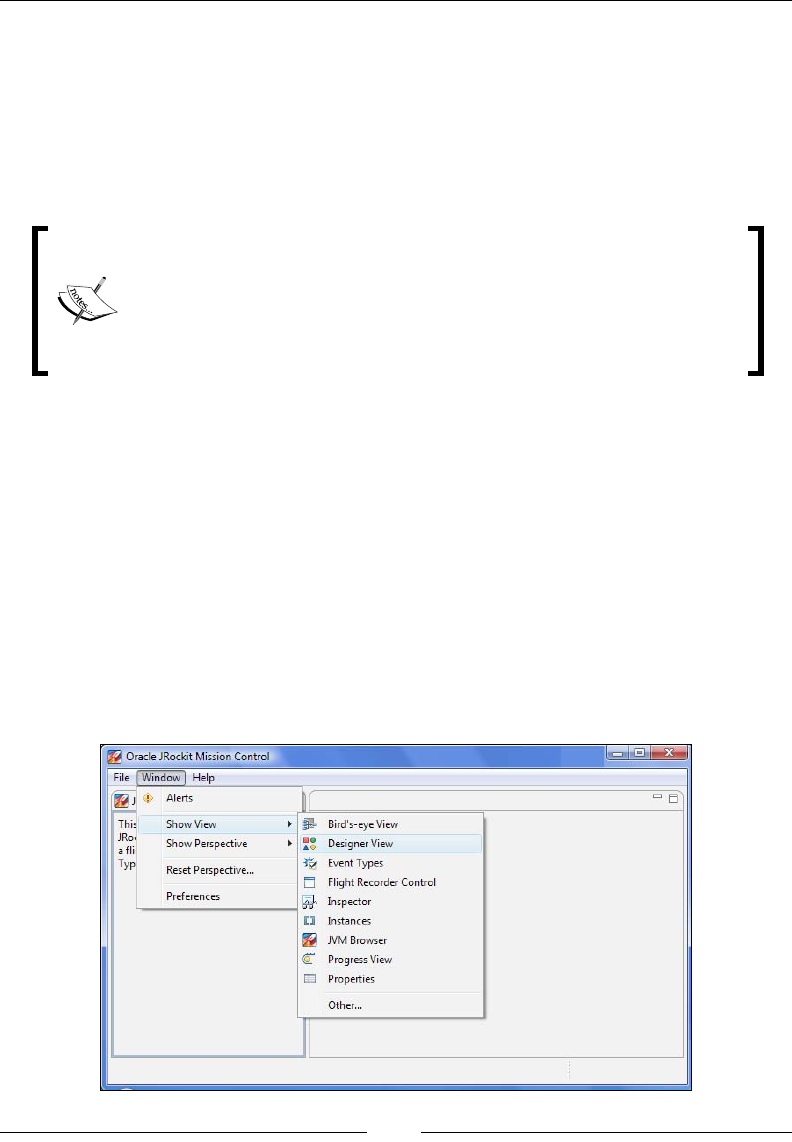
JRockit Flight Recorder
[ 366 ]
Extending the Flight Recorder client
The Flight Recorder contains a GUI builder that allows anyone to modify the Flight
Recorder user interface, as well as creating and exporting custom-designed user
interfaces. This functionality was used by the Mission Control team to radically
reduce development time and turn-around time for bugxes when developing the
Flight Recorder user interface.
The current GUI builder was designed by the JRockit Mission Control
team to be "good enough" for Oracle internal use. It is not intended
for use outside of Oracle in JRockit R28. Thus, using the GUI builder
is unsupported in R28/4.0. We mean it! You are on your own. We are
planning on supporting the GUI builder at some point, but the exact
release date for this has not been decided yet.
Even though the GUI builder is unsupported, it can be quite useful for modifying the
things you want to change the most in the user interface. It can also be used to add
custom tabs for your own event producers. The best part is that any customizations
can be exported directly from within the user interface. Such plug-ins can easily be
shared with colleagues by simply dropping the plug-in into the JROCKIT_HOME/
missioncontrol/plug-in folder of a JRockit installation.
To gain access to the GUI builder, JRockit Mission Control must be started with
the designer option, JROCKIT_HOME\bin\jrmc –designer.
This will enable the Designer View under the Window | Show View menu, as
shown in the following screenshot. The view appears in the same view folder as
the JVM Browser view and the Event Types view by default.
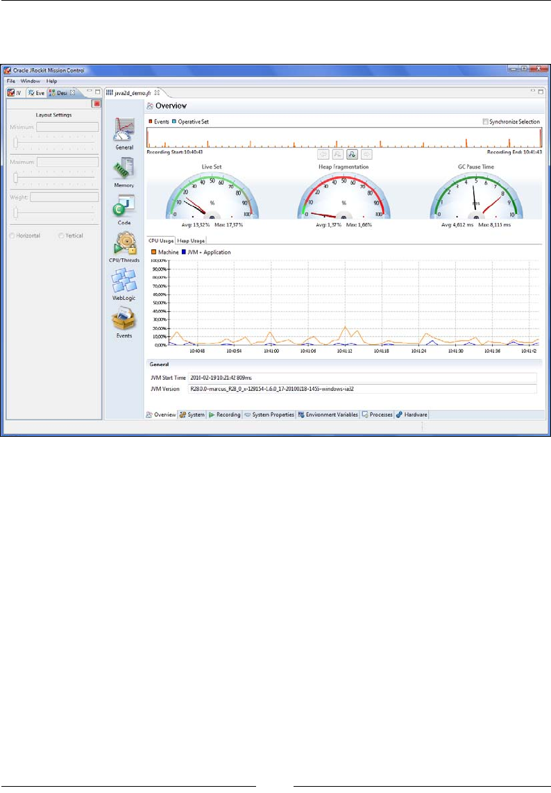
Chapter 9
[ 367 ]
Once a ight recording is opened, the Designer View enables switching back and
forth between design mode and run mode.
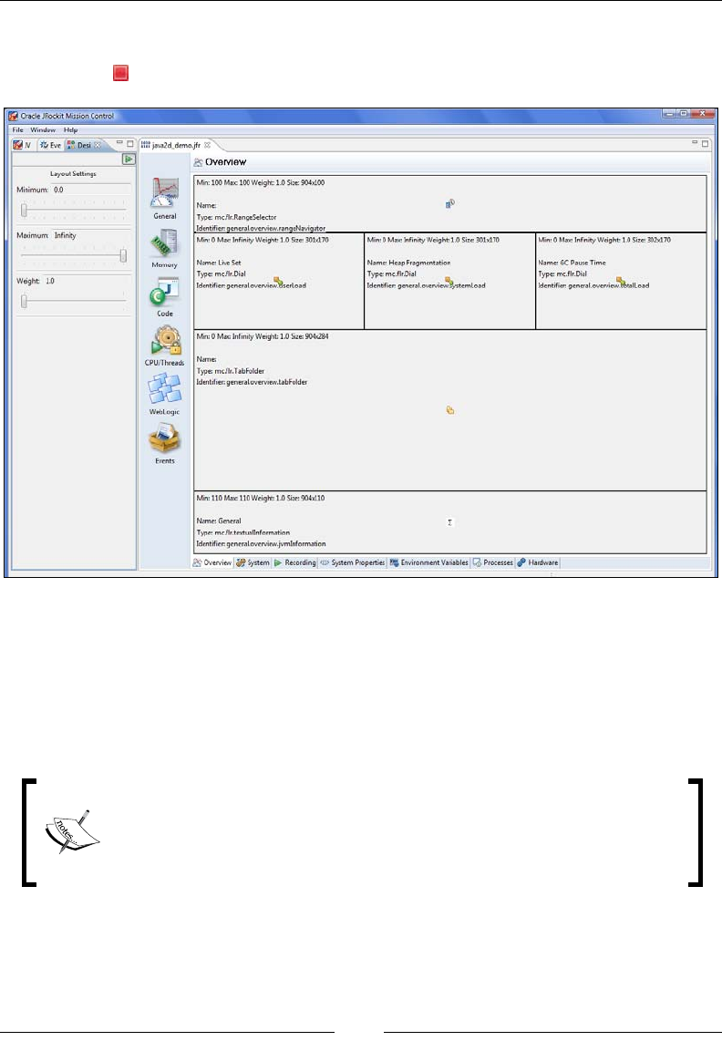
JRockit Flight Recorder
[ 368 ]
When in run mode, the only available operation is to stop the recording and enter
design mode. To stop and enter design mode, simply click on the red rectangular
stop button ( ).
When in the design mode, any part of the Flight Recorder user interface can be
modied, even the tabs that were delivered as part of the Flight Recorder. This is
quite powerful, but also means it is potentially very easy to mess up pretty much
every part of the Flight Recorder user interface. Fortunately, it is simple to reset the
user interface to factory settings. In Window | Preferences under Flight Recorder,
there is a button for resetting the user interface.
Reverting to factory settings through the GUI is only available in
JRockit Mission Control 4.0.1 or later. This can be accomplished in
4.0.0 by erasing the <user.home>/.jrmc folder. However, this will
unfortunately also erase any other custom JRockit Mission Control
settings you may have.
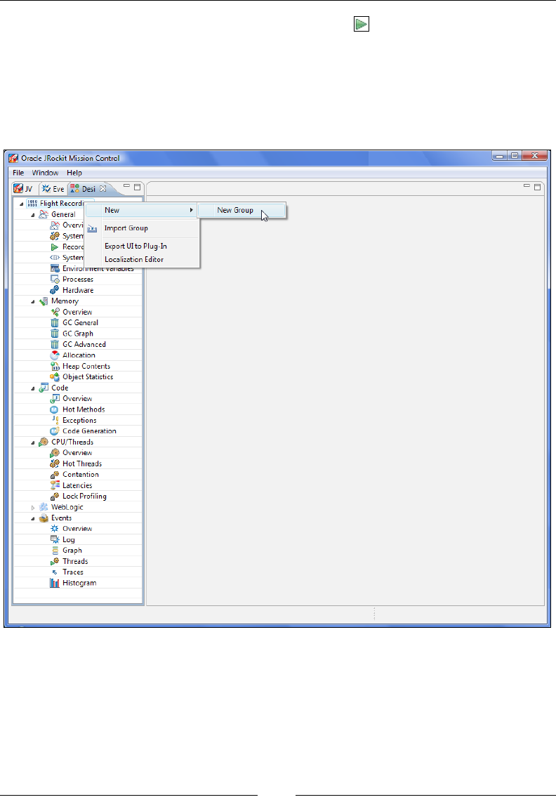
Chapter 9
[ 369 ]
Once satised with the changes, press the play button ( ) to see how the changes
play out in the recording. To add new tabs and tab groups, the recording must rst be
closed. This will change the design view to show a tree of available tabs, as illustrated
in the next screenshot.
To add a new group, right click on the root and select New | New Group from the
context menu.
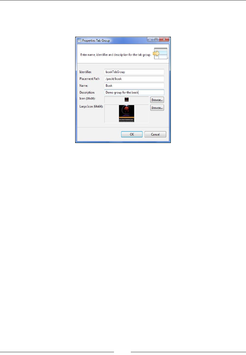
JRockit Flight Recorder
[ 370 ]
The tab group Placement Path, in the Properties Tab Group, is used to determine
where on the toolbar the tab group will appear. Two icons are needed—the smaller
one is used when there is not enough space for the larger one.
New tabs are created by right clicking on the tab group under which the tab shall be
created, and selecting New | New Tab.
To design the newly-created tab, rst load a recording containing events of the kind
you want to visualize. As an example, we will design a new tab for examining the
total amount of memory allocation in the JVM.
First navigate to the tab to design. Since it currently is empty, it will be blank and
show an Unknown Component message in the upper left corner.
Now, we take care of the layout of our tab. We want a standard range selector at the
top, and a chart under the range selector.
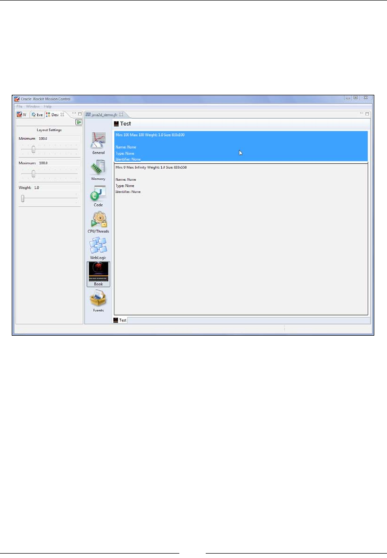
Chapter 9
[ 371 ]
To add a space for a range selector at the top, do the following:
1. Vertically split the area by right clicking in the editor and selecting Vertical
Split from the context menu.
2. Use the sliders in the Design View to set the minimum and maximum size of
the topmost area to 100 pixels. All range selectors are exactly 100 pixels high.
Next, we want to add a chart to the large remaining area below the range selector.
Right click on this area and select Assign Component | Graphics | Chart from
the context menu. This brings up the chart conguration dialog box. To add a total
allocation attribute to the chart, do the following:
1. Select the tab for the axis with which to associate the attribute. In this case,
we select the Left Y Axis.
2. Select the Data Series tab to congure the data series that is to be shown.
3. Click the Add… button to open the attribute browser dialog box. For the
4.0.0 version of JRockit Mission Control, all attributes are listed in a attened
hierarchy of event types (in human-readable form) with all attributes for a
certain event type listed as children.
4. Select the attribute to use. In this case, Allocated by All Threads/
Total Allocated.
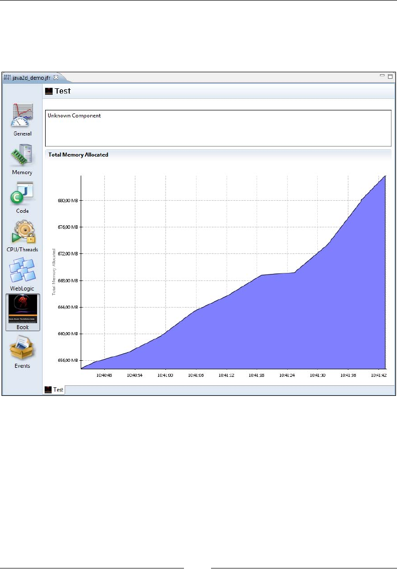
JRockit Flight Recorder
[ 372 ]
That is all that is required. The chart can be congured to look better by selecting
various options. In the following screenshot, the content type for the axis was
modied to "Memory". Fill colors for the data series were also chosen, and the
axis was given a name.
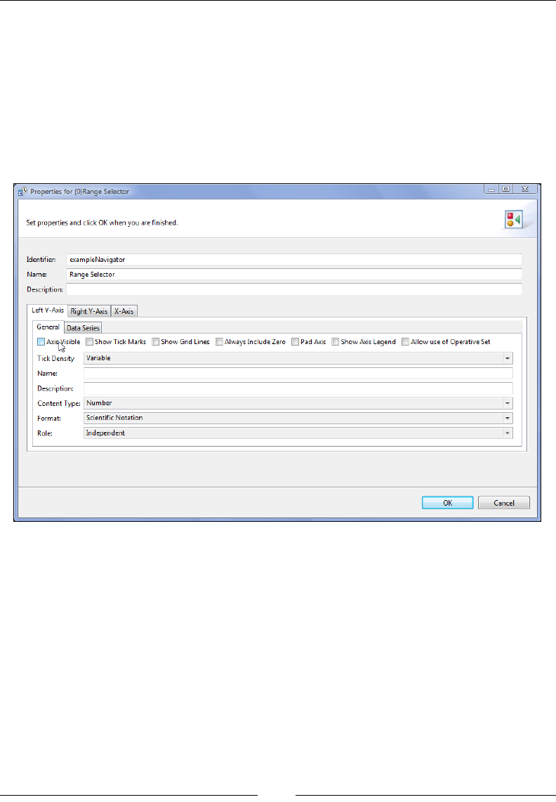
Chapter 9
[ 373 ]
Creating the range selector for the custom tab is slightly more complicated. Start by
assigning the correct component to the topmost area by selecting Assign Component
| Other | Range Selector from the context menu.
This brings up a dialog box where the properties for the range selector can be
congured. The range selector contains a chart, so conguring it is quite similar to
conguring a standard chart. If we want it to look like the other range selectors,
we must remove the tick marks and the visibility for each axis by unchecking the
corresponding check boxes.
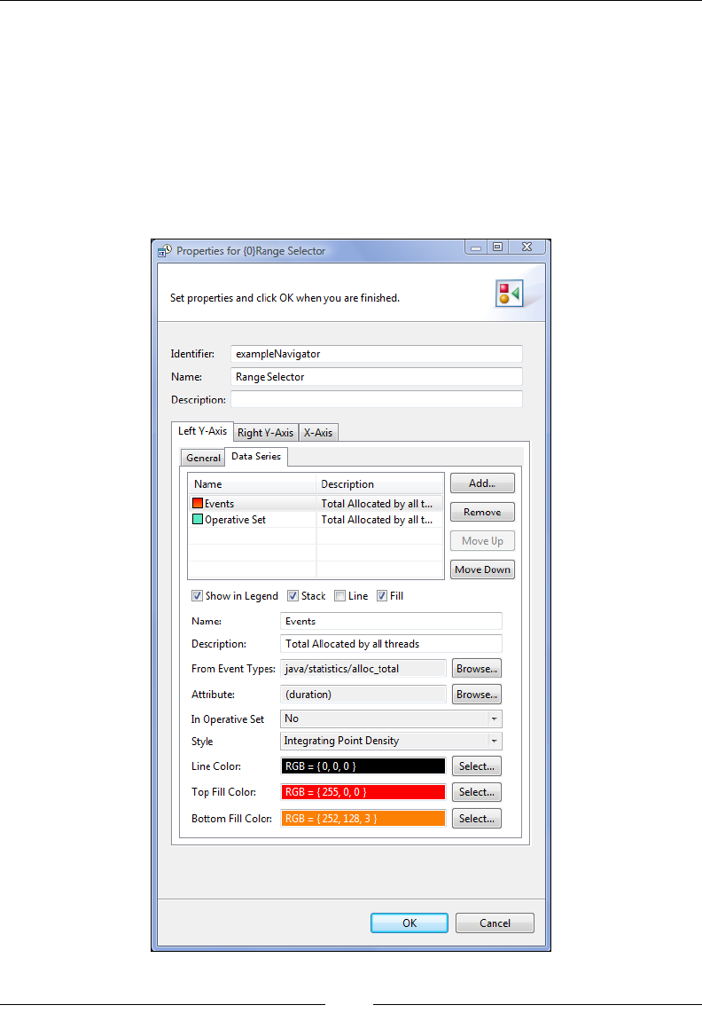
JRockit Flight Recorder
[ 374 ]
As we want a backdrop of events to make up the tab, we need to congure it to
show the number of ongoing events. We do this by adding the duration attribute
for the event types used in our other components. In this case, this is the same event
type as in the chart. We use the Integrating Point Density style. The range selectors
actually contain two stacked series with different colors for each event attribute
being shown—one for the events in the operative set, and one for the ones that are
not in the operative set. This is to allow visual feedback when events used in the tab
are included in the operative set. We must therefore add the attribute twice, with
different colors and with In Operative Set set to No and Yes respectively.
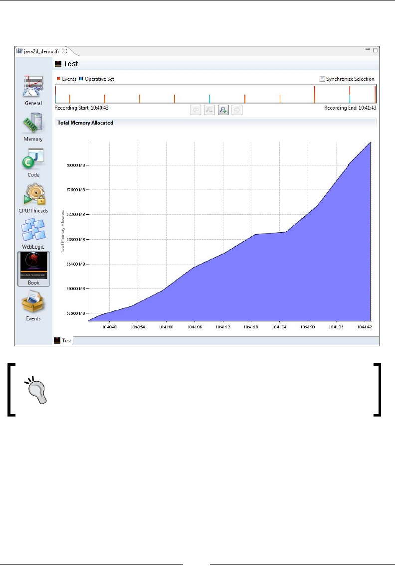
Chapter 9
[ 375 ]
This concludes the example. The resulting tab can be seen in the following
screenshot, with a few of the events added to the operative set:
The easiest way to nd out how to use other components available in
the Flight Recorder designer is to enter design mode and see how they
are being used in the original Flight Recorder user interface.
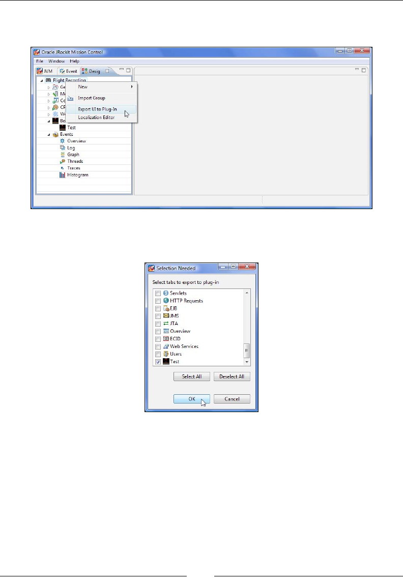
JRockit Flight Recorder
[ 376 ]
To export the newly designed tab to a plug-in, so that it can be shared with others,
rst close the tab. This will make the tree view of the different tabs visible again.
From the root node, select Export UI to Plug-In. This brings up a dialog where the tabs
available for export are listed.
Normally, only the tabs changed and/or added should be selected. In our example,
we will only add the Test tab. After clicking OK, we will be presented with a dialog
where the plug-in ID and version can be selected. Take care to always increase the
plug-in version for newer releases of your additions, as they will otherwise
be overridden by older versions.
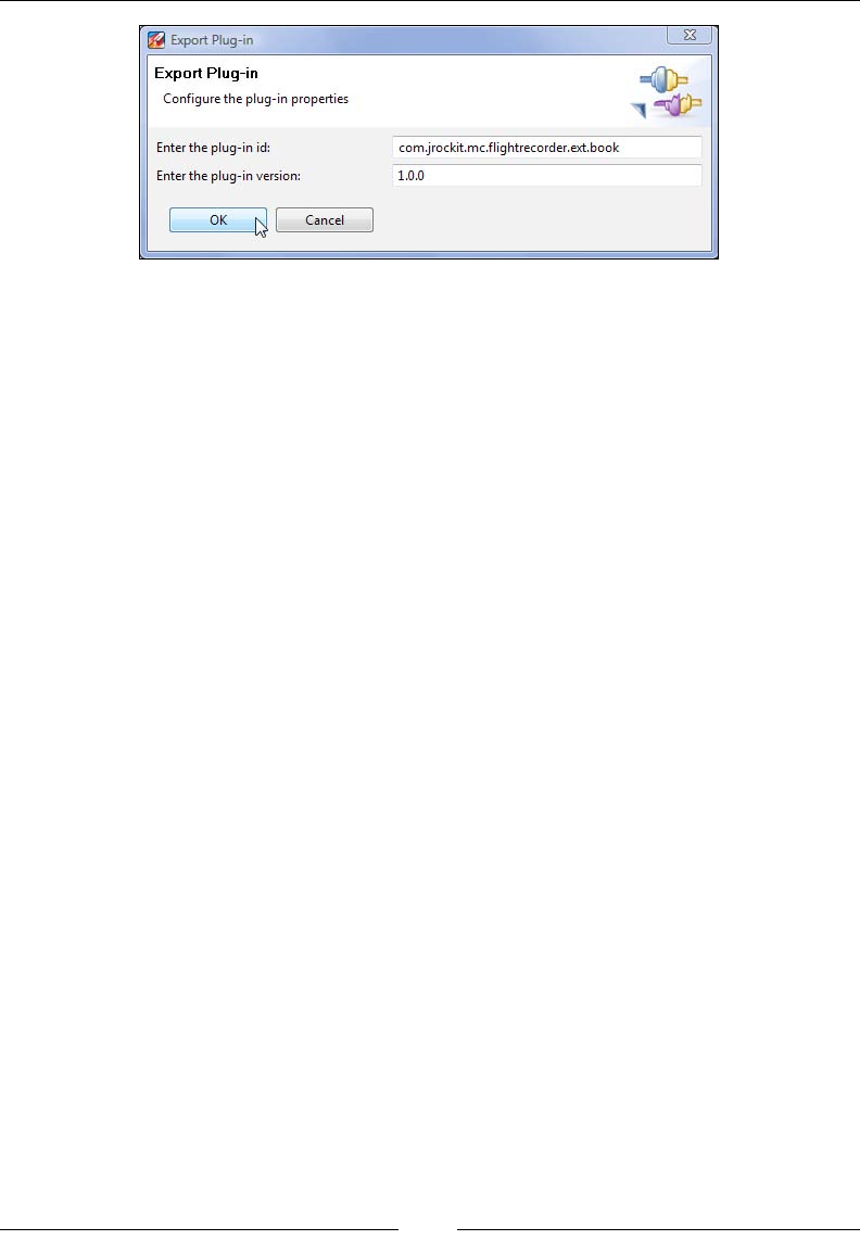
Chapter 9
[ 377 ]
After clicking on OK, a le dialog will be presented where you can choose where to
store the new plug-in. The plug-in will be saved as a jar le.
The resulting jar le can be shared with friends and colleagues, either through an
update site, or by simply dropping the le in the JROCKIT_HOME/missioncontrol/
plugins folder.
Summary
In this chapter, JRockit Flight Recorder was introduced. The new data model and the
notion of events and data producers were explained. It was shown how to capture
ight recordings, and various ways to control the Flight Recorder itself were explained.
Advanced concepts in the ight recording wizard were shown, such as how to control
the enablement and the options of any single event type. The main differences to the
old JRockit Analyzer were discussed, such as:
• The new range selector
• New event types such as the exception event
• Changes to the operative set
• The relational key
• How to do old JRA (LAT) style latency analysis in Flight Recorder
• Changes to some of the memory-related tabs
We also explained how anyone can add custom events to ight recordings through
a standard Java API available in the JRockit runtime jar.
Finally, the unsupported design mode was introduced, where the user interface of the
Flight Recorder can be customized and even extended. We also showed how to use the
design mode to export customizations to plug-ins that can be shared with others.
In the next chapter, we will discuss how the JRockit Mission Control Memory Leak
Detection Tool can be used for hunting down memory leaks in Java applications.

The Memory Leak Detector
As described in the chapter on memory management, the Java runtime provides
a simplied memory model for the programmer. The developer does not need to
reserve memory from the operating system for storing data, nor does he need
to worry about returning the memory once the data is no longer in use.
Working with a garbage collected language could easily lead to the hasty conclusion
that resource management is a thing of the past, and that memory leaks are impossible.
Nothing could be further from the truth. In fact, memory leaks are so common in Java
production systems that many IT departments have surrendered. Recurring scheduled
restarts of Java production systems are now all too common.
In this chapter, you will learn:
• What we mean by a Java memory leak
• How to detect a memory leak
• How to nd the cause of a memory leak using the JRockit Memory
Leak Detector
A Java memory leak
Whenever allocated memory is no longer in use in a program, it should be returned
to the system. In a garbage collected language such as Java, quite contrary to static
languages such as C, the developer is free from the burden of doing this explicitly.
However, regardless of paradigm, whenever allocated memory that is no longer
in use is not returned to the system, we get the dreaded memory leak. Eventually,
enough memory leaks in a program will cause it to run out of memory and break.

The Memory Leak Detector
[ 380 ]
Memory leaks in static languages
In static languages, memory management may be even more complex than just
recognizing the need to explicitly free allocated memory. We must also know when
it is possible to deallocate memory without breaking other parts of the application.
In the absence of automatic memory management, this can sometimes be difcult.
For example, let's say there is a service from which address records can be retrieved.
An address is stored as a data structure in memory for easy access. If modules A, B,
and C use this address service, they may all concurrently reference the same address
structure for a record.
If one of the modules decides to free the memory of the record once it is done, all the
other modules will fail and the program will crash. Consequently, we need a rm
allocation and deallocation discipline, possibly combined with some mechanism to let
the service know once every module is done with the address record. Until this is the
case, it cannot be explicitly freed. As has been previously discussed, one approach is
to manually implement some sort of reference counting in the record itself to ensure
that it can be reclaimed once all modules are nished with it. This may in turn require
synchronization and will add complexity to the program. To put it simply, sometimes,
in order to achieve proper memory hygiene in static languages, the programmer may
have to implement code that behaves almost like a garbage collector.
Memory leaks in garbage collected languages
In Java, or any garbage collected language, this complexity goes away. The
programmer is free to create objects and the garbage collector is responsible for
reclaiming them. In our hypothetical program, once the address record is no longer
in use, the garbage collector can reclaim its memory. However, even with automatic
memory management, there can still be memory leaks. This is the case if references
to objects that are no longer used in the program are still kept alive.
The authors once heard of a memory leak in Java being referred to as an
unintentional object retention. This is a pretty good name. The program is keeping
a reference to an object that should not be referenced anymore. There are many
different situations where this can occur.
Perhaps the leaked object has been put in a cache, but never removed from the cache
when the object is no longer in use. If you, as a developer, do not have full control over
an object life cycle, you should probably use a weak reference-based approach. As has
previously been discussed, the java.util.WeakHashMap class is ideal for caches.
Chapter 10
[ 381 ]
Be aware that weak references is not a one-size-ts-all answer to
getting rid of memory leaks in caches. Sometimes, developers misuse
weak collections, for instance, by putting values in a WeakHashMap
that indirectly reference their keys.
In application containers, such as a J2EE server, where multiple classloaders are
used, special care must be taken so that classes are not dependency injected into
some framework and then forgotten about. The symptom would typically show
up as every re-deployment of the application leaking memory.
Detecting a Java memory leak
It is all too common to nd out about a memory leak by the JVM stopping due to an
OutOfMemoryError. Before releasing a Java-based product, it should generally be
tested for memory leaks. The standard use cases should be run for some duration,
and the live set should be measured to see that no memory is leaking. In a good test
setup, this is automated and tests are performed at regular intervals.
We got overcondent and failed to heed our own advice in JRockit
Mission Control 4.0.0. Normally, we use the Memory Leak Detector
to check that editors are reclaimed properly in JRockit Mission
Control during end testing. This testing was previously done by the
developers themselves, and had failed to nd its way into the formal test
specications. As a consequence, we would leak an editor each time a
console or a Memleak editor was opened. The problem was resolved, of
course, using the Memory Leak Detector.
A memory leak in Java can typically be detected by using the Management Console
to look at the live set attribute. It is important to know that a live set increase over
a shorter period of time does not necessarily have to be indicative of a memory
leak. It could be the case that the load of the Java application has changed, that the
application is serving more users than before, or any other reason that may trigger
the need to use more memory. However, if the trend is consistent, there is very
likely a problem that should be investigated.
There are primarily two different ways of doing detailed heap analysis:
• Online heap analysis, using the JRockit Memory Leak Detector
• Ofine heap analysis from a heap dump
The Memory Leak Detector
[ 382 ]
For online analysis, trend analysis data is collected by piggybacking on the garbage
collector. This is virtually without overhead since the mark phase of a GC already
needs to traverse all live objects on the heap. The resulting heap graph is all the data
we need to do a proper trend analysis for object allocation.
The heap dump format used by JRockit is the same as produced by
the Java Virtual Machine Tool Interface (JVMTI) based heap proler
HPROF, included with the JDK. Consequently, the dumps produced by
JRockit can be analyzed in all tools supporting the HPROF format. For
more information about HPROF, see the following le in the JRockit JDK:
JROCKIT_HOME/demo/jvmti/hprof/src/manual.html
For more information about JVMTI, see the JDK Documentation:
http://java.sun.com/javase/6/docs/platform/jvmti/
jvmti.html
Memleak technology
The JRockit Mission Control Memory Leak Detector, or Memleak for short, is a
dynamic tool that can be attached to a running JRockit instance. Memleak can be used
to track how heap memory usage in the Java runtime changes over time for each type
(class) in the system. It can also nd out which types have instances pointing to a
certain other type, or to nd out which instances are referring a certain other instance.
Allocation tracing can be enabled to track allocations of a certain type of object. This
all sounds complicated, but it is actually quite easy to use and supported by a rich
graphical user interface. Before we show how to use it to resolve memory leaks, we
need to discuss some of the architectural consequences of how Memleak is designed.
• Trend analysis is very cheap: Data is collected as part of the normal garbage
collection mark phase. As mentioned, this is a surprisingly fast operation.
When the tool is running, every normal garbage collection will collect the
necessary data. In order to ensure timely data collection, the tool will also, by
default, trigger a garbage collection every ten seconds if no normal garbage
collection has taken place. To make the tool even less intrusive, this setting
can be changed in the preferences.
• Regardless of client hardware, you will be able to do the analysis:
Connecting to a server with a multi-gigabyte heap from a puny laptop
is not a problem.
Chapter 10
[ 383 ]
• Events and changes to the heap can be observed as they happen: This is
both a strength and a weakness. It is very powerful to be able to interact with
the application whilst observing it, for example to see which operation is
responsible for certain behavior, or to introspect some object at the same time
as performing operations on it. It also means that objects can become eligible
for garbage collection as they are being studied. Then further operations
involving the instances are impossible.
• No off-line analysis is possible: This can be a problem if you want to get a
second opinion on a memory leak from someone who can't be readily given
access to your production system. Fortunately, the R28 version of JRockit can
do standard HPROF heap dumps that can be analyzed in other tools, such as
Eclipse MAT, if required.
Note that HPROF dumps contain the contents of the heap. If the system
from which the HPROF dump was generated contains sensitive data, that
data will be readily accessible by anyone getting access to the dump. Be
careful when sharing dumps.
Tracking down the leak
Finding the cause of memory leaks can be very tricky, and tracking down complex
leaks frequently involves using several tools in conjunction. The application is
somehow keeping references to objects that should no longer be in use. What's worse,
the place in the code where the leaked instance was allocated does not necessarily have
to be co-located with the place in the code pertaining to the leak. We need to analyze
the heap to nd out what is going on.
To start Memleak, simply select the JVM to connect to in the JVM Browser and choose
Memleak from the context menu.
Only one Memleak instance can be connected to any given JVM
at a time.
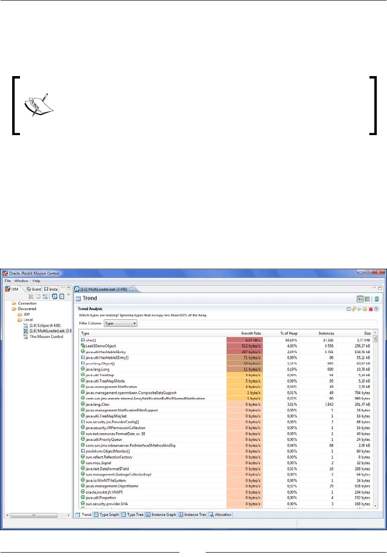
The Memory Leak Detector
[ 384 ]
In Memleak, the trend table can help detect even slow leaks. It does this by building a
histogram by type (class), and by collecting data points about the number of instances
of every type over time. A least squares approximation on the sizes over time is then
calculated, and the corresponding growth rate in bytes per second is displayed.
In JRockit Mission Control 4.1.0, this algorithm will be a little bit more
sophisticated, as it will also incorporate the correlation to the size of the
live set over time. The types that have the highest tendency to grow as
the live set is growing are more likely to be the ones causing a leak.
The trend table can usually be helpful in nding good candidates for memory leaks.
In the trend table, classes with a high growth rate are colored red—higher color
intensity means higher growth rate. We can also see how many instances of
the class there are, and how much memory they occupy.
In the program being analyzed in the following example, it would seem that char
arrays are leaking. Not only are they colored deep red and at the top of the trend
analysis table, signifying a suspected memory leak, but they also have the one of
the highest growth rates of any type in the system.
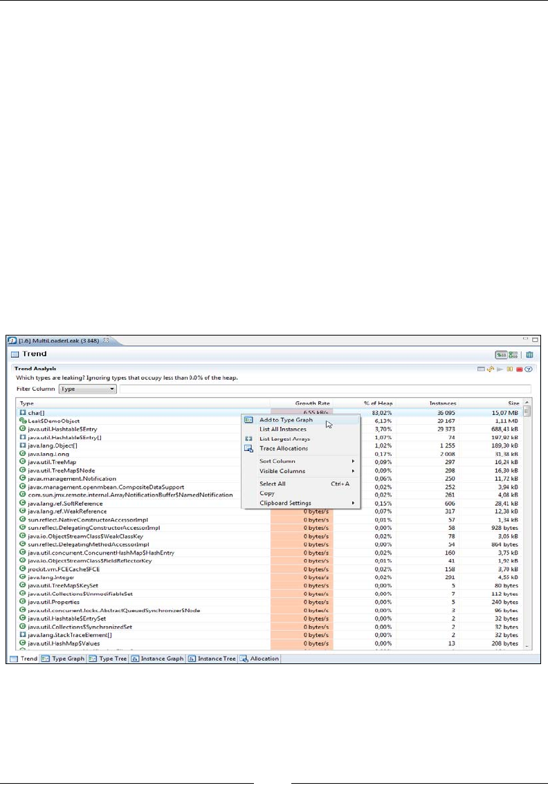
Chapter 10
[ 385 ]
It would also seem, to a lesser extent, that classes related to the types
Leak$DemoObject and Hashtable are leaking.
In total, we seem to be leaking about 7.5 KB per second.
(6.57*1,024+512+307+71+53+11)/1,024 ≈ 7.5
The JVM was started with a maximum heap size of 256 MB, and the used live
set was about 20 MB (the current size of the live set was checked with the
Management Console).
(256 – 20) *1,024 / 7.5 ≈ 32,222 seconds ≈ 537 minutes ≈ 22 hours
If left unchecked, this memory leak would, in about 22 hours, result in an
OutOfMemoryError that would take down the JVM and the application it is running.
This gives us plenty of time to nd out who is holding on to references to the
suspected leaking objects. To nd out what is pointing to leaking char arrays, right
click on the type in the trend table and click on Add to Type Graph, as shown in the
following screenshot:
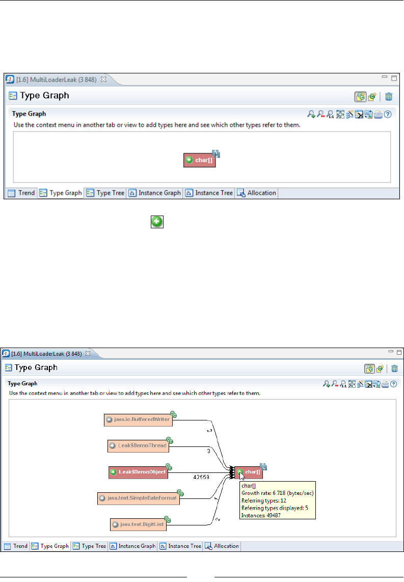
The Memory Leak Detector
[ 386 ]
This will add the selected class to the Type Graph tab and automatically switch to
that tab. The tab is not a type graph in the sense of an inheritance hierarchy, but
rather a graph showing how instances of classes point to other classes. The Type
Graph will appear with the selected class, as shown in the following screenshot:
Clicking on the little plus sign ( ) to the left of the class name will help us nd
out what other types are referring to this type. We call this expanding the node.
Every click will expand another ve classes, starting with the ones that leak the
most memory rst.
In the Type Graph, just like in the trend table, types that are growing over time will
be colored red—the redder, the higher the leak rate.
As we, in this example, want to nd out what is ultimately holding on to references
to the character arrays, we expand the char[] node.
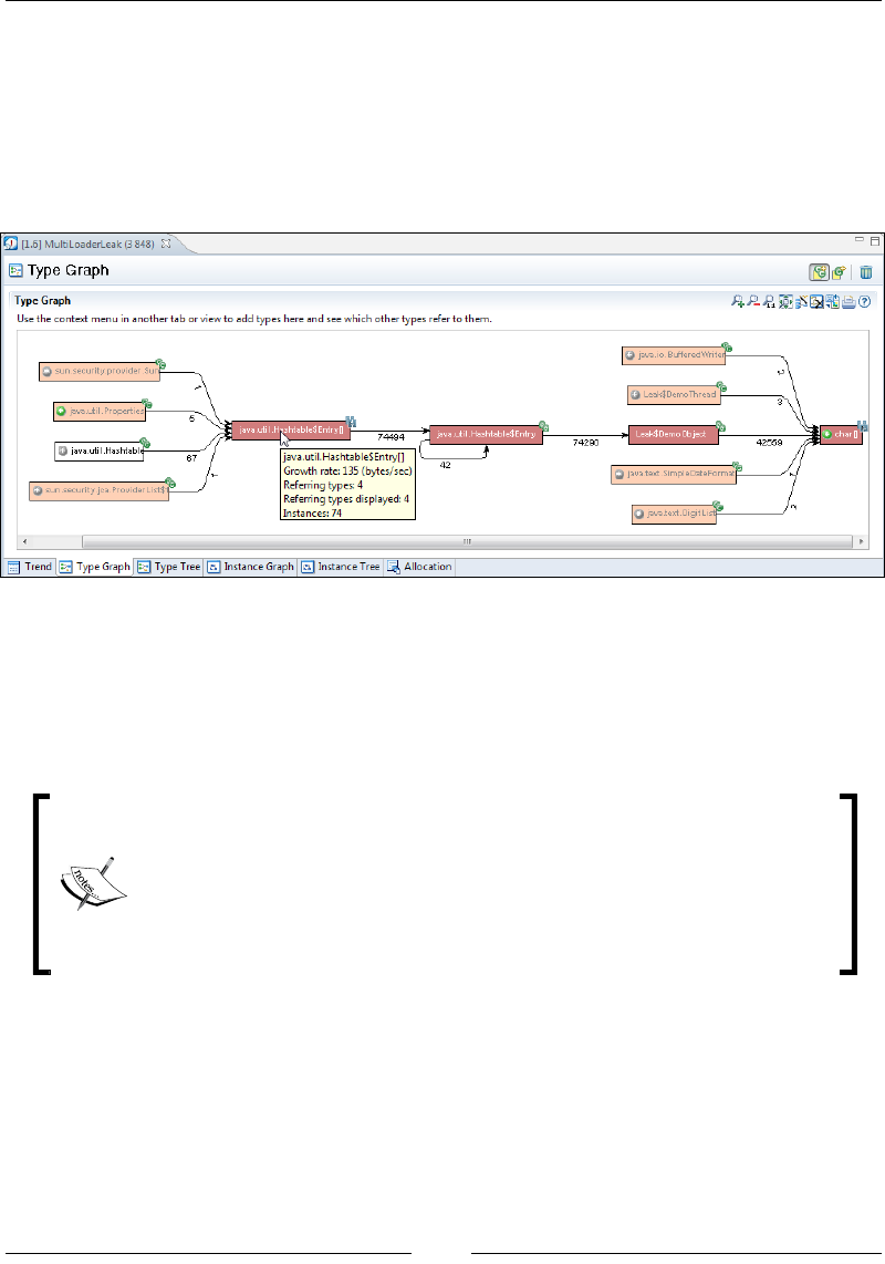
Chapter 10
[ 387 ]
Expanding the char[] node reveals that there is only one other type (or rather
instances of that type) that also seem to be leaking and have references to char
arrays—the inner class DemoObject of the conspicuously named Leak class.
Expanding the Leak$DemoObject node until we don't seem to be nding any
more leaking types reveals that the application seems to be abusing some sort
of Hashtable, as shown in the next screenshot:
The next step would be to nd the particular instance of Hashtable that is being
misused. This can be done in different ways. In this example, it would seem that
the leaking of the char arrays is due to the leaking of the Leak$DemoObjects.
We would therefore like to start by listing the Hashtable$Entry instances that
point to Leak$DemoObject.
Classes declared inside other classes in Java, for example
the Entry class in Hashtable, have the naming format
OuterClass$InnerClass in the bytecode, and this is the way they
show up in our proling tools—in our example, Hashtable$Entry
and Leak$DemoObject. This is because when inner (nested) classes
were introduced in the Java language, Sun Microsystems didn't want
to change the JVM specication as well.
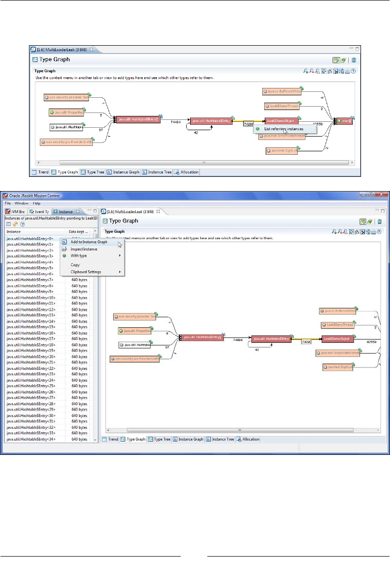
The Memory Leak Detector
[ 388 ]
To list instances that are part of a particular relationship, simply right click on the
relation and select List Referring Instances, as shown in the following screenshot:
This brings up the instances view, to the left of the Memleak editor, where the
instances pointing from Hashtable entries to demo objets are listed. An instance can
be added to the instance graph by right clicking on the instance, and selecting Add
to Instance Graph from the context menu. This will bring up a graph similar to the
Type Graph, but this time showing the reference relationships between instances.
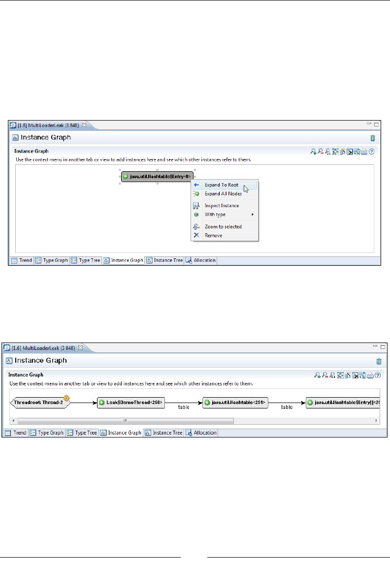
Chapter 10
[ 389 ]
Once the Instance Graph is up, we need to nd out what is keeping the instance
alive. In other words, who is referring the instance, keeping it from being garbage
collected? In previous versions of Memleak, this was sometimes a daunting task,
especially when searching in large object hierarchies. As of JRockit Mission Control
4.0.0, there is a menu alternative for letting JRockit automatically look for the path
back to the root referrer. Simply right click on the instance and click on Expand to
Root, as shown in the next screenshot. This will expand the graph all the way back
to the root.
As shown in the following screenshot, expanding to root for our example reveals
that there is a thread named Thread-2 that holds on to an instance of the inner class
DemoThread of the class Leak. In the DemoThread instance, there is a eld named
table that refers to a Hashtable containing our leaked DemoObject.
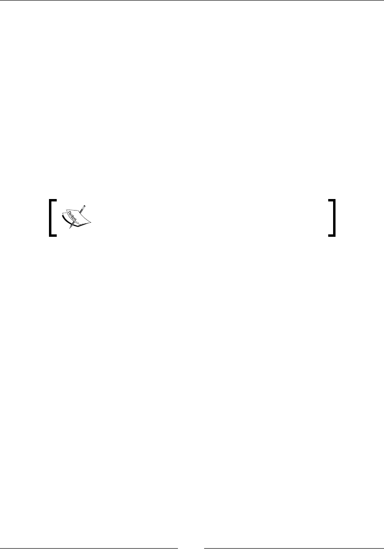
The Memory Leak Detector
[ 390 ]
When running in Eclipse, it is possible to view the code that manipulates the
table eld, by selecting View Type Source from the context menu on the
Leak$DemoThread nodes. In this example, we'd nd a programming error:
for (int i = 0; i <= 100; i++) {
put(total + i);
}
for (int i = 0; i < 100; i++) {
remove(total + i);
}
As an equals sign is missing from the second loop header, more objects are placed
in the Hashtable than are removed from it. If we make sure that we call remove as
many times as we call put, the memory leak would go away.
The complete examples for this chapter can be found
in the code bundle that comes with this book.
To summarize, the text book recipe for hunting down memory leaks is:
1. Find one of the leaking instances.
2. Find a path to the root referrer from the leaking instance.
3. Eliminate whatever is causing the reference to be kept alive.
4. If there still is a leak, start over from 1.
Of course, nding an instance that is unnecessarily kept alive can be quite tricky.
One way to home in on unwanted instances is to only look at instances participating
in a certain reference relationship. In the previous example, we chose to look at char
arrays that were only being pointed to by DemoObjects. Also, the most interesting
relationships to look for are usually found where leaking types and non-leaking
types meet. In the Type Graph for the example, we can see that once we expand
beyond the Hastable$Entry array, object growth rates are quite neutral. Thus,
the leak is quite likely due to someone misusing a Hashtable.
It is common for collection types to be misused, thereby causing memory leaks.
Many collections are implemented using arrays. If not dealt with, the memory leak
will typically cause these arrays to grow larger and larger. Therefore, another way of
quickly homing in on the offending instance is to list the largest arrays in the system.
In the example, we can easily nd the Hashtable holding on to the DemoObjects by
running the leaking application for a while. Use the List Largest Arrays operation on
the array of Hashtable entries, as shown in the next screenshot.
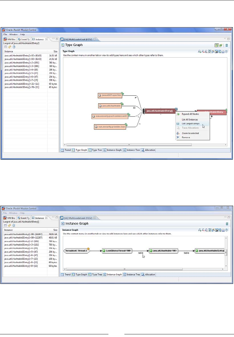
Chapter 10
[ 391 ]
If all else fails, statistics will be on your side the longer you wait, as more and more
heap space will be occupied by the leaking objects.
Both of the largest Hashtable$Entry arrays are leaking. Adding any one of them
to the Instance Graph and expanding it to the root referrer will yield the same
result, implicating the instance eld table in the Leak$DemoThread class.
This is illustrated in the following screenshot:
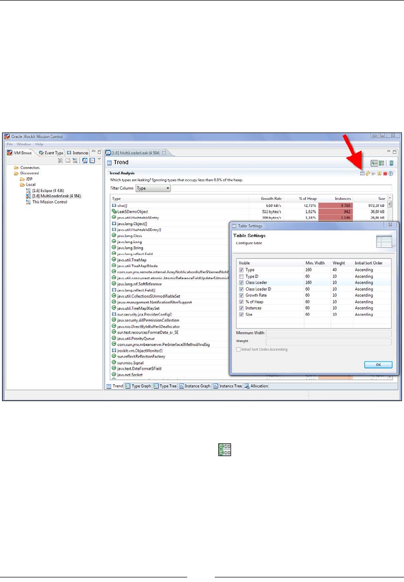
The Memory Leak Detector
[ 392 ]
A look at classloader-related information
In our next example, there are actually three different classloaders running almost the
same code—two with the memory leak and one that actually behaves well. This is
to illustrate how things can look in an application server, where different versions
of the same application can be running. In Memleak, just like with the other tools in
JRockit Mission Control, the tables can be congured to show more information. To
see classloader-related information in the table, edit the Table Settings as shown in
the following screenshot:
Memleak will, by default, aggregate classes with the same name in the same row. To
make Memleak differentiate between classes loaded by different classloaders, click
on the Individually show each loaded class ( ) button.
In the next screenshot, the trend table is shown for all classes with names containing
the string Demo. As can be seen, there are three classloaders involved, but only two of
them are leaking instances of Leak$DemoObject.
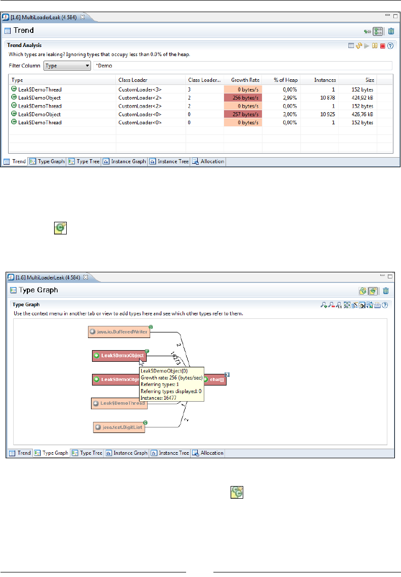
Chapter 10
[ 393 ]
The option of splitting the classes per classloader is also available in the Type Graph.
The Type Graph can be congured to use a separate node for each loaded class,
when expanding a node. Simply click on the Use a separate node for each loaded
class icon ( ) in the Type Graph. Following is a screenshot showing the rst
expansion of the char[] node when using separate nodes for each class. The bracket
after the class name contains the classloader ID.
It is possible to switch back to aggregating the nodes again by clicking on the
Combine classes with same class name button ( ). Note that the setting will not
change the state of the currently visible nodes. Only nodes that are expanded after
changing the setting are affected.
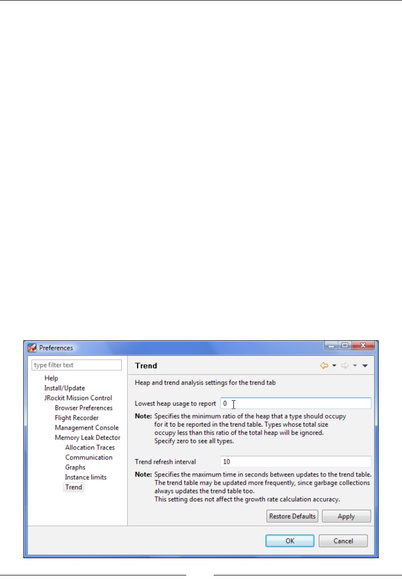
The Memory Leak Detector
[ 394 ]
Interactive memory leak hunting
Another way of using the Memleak tool is to validate a hypothesis about memory
management in an application. Such a hypothesis could for example be "when I
remove all contacts from my contact list, no Contact objects should be left in the
system". Because of the interactive nature of the Memleak tool, this is a very powerful
way of nding leaks, especially in an interactive application. A huge amount of such
scenarios can be tested without interruptions caused by, for example, dumping heaps
to les. If done well and with enough systems knowledge, nding the leaks can be a
very quick business.
For example, consider a simple address book application. The application is a
self-contained Swing application implemented in a single class named AddressBook.
The class contains a few inner classes, of which one is the representation of a
contact—AddressBook$Contact. In the application, we can add and remove
contacts in the address book. One hypothesis we may want to test is that we
do not leak contacts.
The Memleak tool normally only shows types that occupy more than 0.1 percent of
the heap, or the amount of data in the general case would be overwhelming. We are
normally not interested in types not heavily involved in leaks, and as time passes,
the interesting ones tend to occupy quite a lot of the heap anyway. However, most
leaks usually only occupy a tiny fraction of the heap until the leaking application has
run for quite some time. In order to detect memory leaks earlier, this setting can be
changed to 0 so that all types are shown, regardless of their used heap space. This
can be done in the preferences, as shown in the following screenshot:
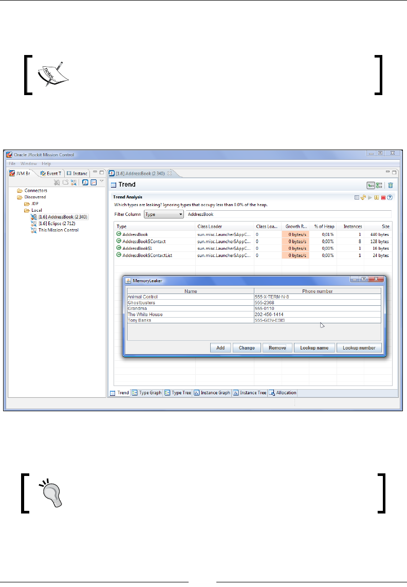
Chapter 10
[ 395 ]
We then lter out the classes related to the hypothesis that we want to test and watch
how they behave while we run the application.
Remember from Chapter 7, The Management Console, that the lter
boxes in JRockit Mission Control can use regular expressions by
entering the prex regexp.
In the following screenshot, three addresses have been removed from the
AddressBook, but the number of Contact instances remain at the original eight:
Removing all of them will still leave all eight of the original AddressBook$Contact
instances in the system. There is indeed a memory leak.
To get the Memleak tool to react faster to the changes on the heap,
the trend refresh interval (shown in the preference screenshot
earlier) can be lowered.
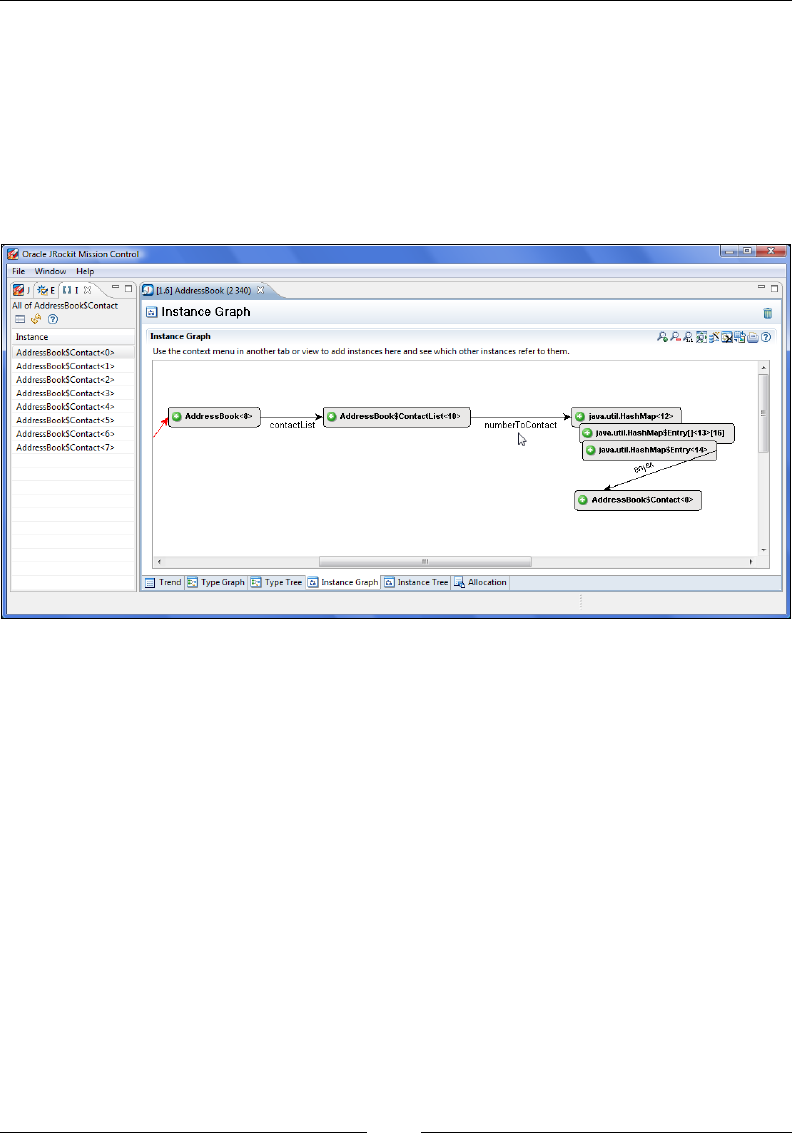
The Memory Leak Detector
[ 396 ]
Now, as all the remaining instances are unintentionally retained, drilling down into
any of them will be sufcient for tracking down the leak. Simply click on List all
instances from the context menu in the trend table and then add any of the instances
to the Instance Graph. The path to root referrer in the example reveals that the contacts
are retained in some sort of index map named numberToContact. The developer of the
application should be familiar with this structure and know where to look for it in the
code. If we ensure that we remove the Contact objects from the index map as well as
from the contact list, the leak will go away.
The recipe for interactively testing for memory leaks is:
1. Formulate a hypothesis, such as "When I close my Eclipse PHP Editor, I
expect the editor instance and the instances associated with it to go away".
2. Filter out the classes of interest in the trend table.
3. See how they are freed and allocated as the hypothesis is tested.
4. If a memory leak is found, it is usually quite easy to nd a leaking instance
and locate the problem by tracing the path to the root referrer.
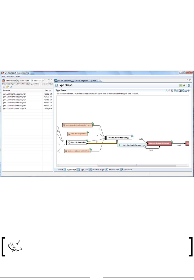
Chapter 10
[ 397 ]
The general purpose heap analyzer
Yet another way to use the Memleak tool is as a general purpose heap analyzer.
The Types panel shows relationships between the types (classes) on the Java heap.
It can also list the specic instances in such a relationship. In the next example, we've
found a peculiar cycle in our Type Graph. We can see that there are instances of
Hashtable entries that are actually pointing back to their Hashtable. To list just
the instances of Hashtable$Entry pointing to Hashtable, we simply right click on
the number in the reference relation (see the following screenshot), and select List
referring instances.
We have now, with a few clicks, been able to list all the Hashtable instances in the
system that contain Hashtables. It is also easy to determine exactly where they are
located in the system. Simply select an instance, add it to the Instance Graph and
trace the shortest path back to the root referrer. Doing this for the rst instance will
reveal that it is located in the com.sun.jmx.mbeanserver.RepositorySupport. Of
course, having Hashtables that contain Hashtables is not a crime; this merely serves
as an example of the versatility of the Memleak tool.
You need a 1.5-based JDK to see the Hashtables containing Hashtables
for this example. In a 1.6-based JDK, the design has changed.
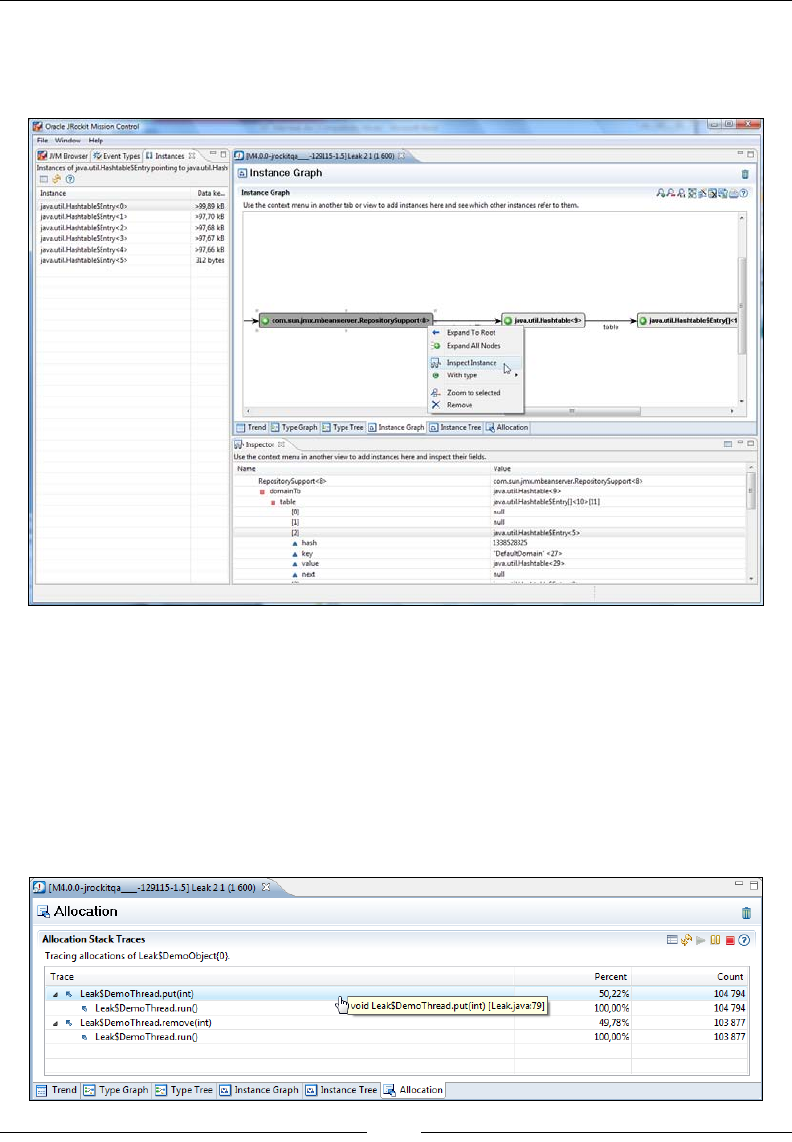
The Memory Leak Detector
[ 398 ]
Any instance can be inspected in Memleak. Next, we inspect the instance of com.
sun.jmx.mbeanserver.RepositorySupport to verify that it indeed contains
Hashtable instances.
Allocation traces
The last major feature in Memleak to be discussed in this book, is the ability to
turn on allocation tracing for any given type. To, for instance, nd out where the
Leak$DemoObjects are being allocated in our previous example, simply right click
on the type and then click on Trace Allocations. The example has been tailored to
do allocations in the vicinity of the code that causes the actual leak (note that this is
normally not the case).
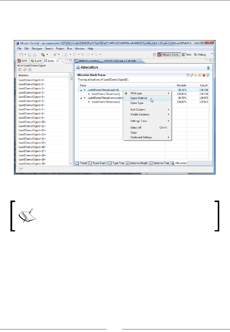
Chapter 10
[ 399 ]
As can be readily seen from the screenshot, we are invoking put more often than
remove. If we are running Memleak from inside Eclipse, we can jump directly
to the corresponding line in the Leak class by right clicking on the stack frame
and then clicking on Open Method from the context menu.
Allocation traces can only be enabled for one type (class) at a time.
A word of caution: Enabling allocation traces for types with a
high allocation pressure can introduce signicant overhead. For
example, it is, in general, a very bad idea to enable allocation traces
for java.lang.Strings.
Troubleshooting Memleak
If you have trouble connecting to your JVM with Memleak, it is probably due to
Memleak requiring an extra port. Communication using Memleak, unlike other tools
in the JRockit Mission Control suite, is only initiated over JMX. Memleak requires the
internal MemLeak Server (MLS) to be running in the JVM.
When starting Memleak, a run request is sent over JMX. The MLS will then be started
and a communication port is returned. The client stops communicating over JMX
after startup and instead uses the proprietary Memory Leak Protocol (MLP) over the
communication port.
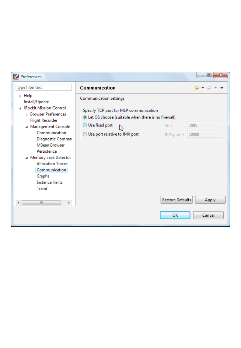
The Memory Leak Detector
[ 400 ]
The MLS was built as a native server in JRockit, as the original idea was to be able
to run the MLS when running out of Java heap, similar to the way that a heap dump
can be triggered when running out of memory. We wanted to introduce a ag that
would suspend the JVM on OutOfMemoryErrors and then launch the MLS. This was
unfortunately never implemented.
It is possible to specify which port to use for MLS in the initial request over JMX.
This can be set in the preferences, as shown in the following screenshot:
Also worth noting is:
• There can only be one client connected to MLS at any given time
• When a client disconnects, the MLS will automatically shut down

Chapter 10
[ 401 ]
Summary
In this chapter, we have shown how to use the JRockit Mission Control Memory
Leak Detector to detect and nd the root cause for Java memory leaks. We have also
discussed the advantages and disadvantages of the Memory Leak Detector in various
use cases.
It has been demonstrated how the Memory Leak Detector can be used to detect even
quite slow memory leaks. We have also shown how the Memory Leak Detector
can be used in an interactive manner to quickly test particular operations in an
application that may be prone to memory leaks.
We have explained how the Memory Leak Detector can also be used as an interactive
general purpose heap analyzer to both nd relationships between different types on
the heap, as well as for inspecting the contents of any instance on the heap.
Finally, we showed how to troubleshoot the most common problems associated with
using the tool.

JRCMD
This chapter is dedicated to JRCMD—one of the simplest tools in the JRockit
distribution. JRCMD is a small command-line tool that can be used to interact with
a running JRockit instance. It can also be used to list all running instances of the
JRockit JVM on a system.
In this chapter, you will learn:
• How to use JRCMD to list the locally running JVMs on your machine
• How to use JRCMD to execute diagnostic commands on one or all JVMs
running locally on your machine
• How to override the SIGQUIT signal handler to make JRockit run diagnostic
commands of your choice instead of printing stack dumps, which is the
default action
• How to utilize JRCMD to solve various tasks such as:
° Heap analysis
° Exception proling
° Native memory tracking
° Controlling the management server lifecycle
° Controlling JRockit Flight Recorder from the command line
The last part of this chapter is in a format that makes it usable as a JRCMD reference.
The reference part lists the various diagnostic commands in alphabetical order,
complete with examples.

JRCMD
[ 404 ]
Introduction
Sometimes a command-line utility is exactly the right tool for the job. You may
want to send commands to JVMs in batch scripts, or you may be operating in a very
secure environment and only have a command line at your disposal through SSH.
Whatever the reason, JRCMD is a small and powerful tool for sending commands to
locally running instances of the JRockit JVM from the command line.
The basic usage pattern is to rst execute JRCMD with no arguments to list the
JVMs currently running on the system. The JVMs will be listed by operating system
Process ID (PID) followed by the class name of the main class of the Java application
running in the JVM.
For example:
C:\>JROCKIT_HOME\bin\jrcmd
2416 com.jrockit.mc.rcp.start.MCMain
19344 jrockit.tools.jrcmd.JrCmd
In the previous example, there were two JVM instances running when JRCMD
was executed—an instance running JRockit Mission Control and, as JRCMD is
a Java application too, the JVM running JRCMD itself.
The JRockit instance on which to execute the command is selected by passing its
PID as the rst argument to JRCMD. A special case is passing PID 0, in which case
JRCMD will attempt to execute the command on all the JVMs it can nd. As different
versions of JRockit may be running at the same time and may support different sets
of commands, not all commands may be available for all versions of JRockit. Normally,
a specic PID should be selected. In addition, two instances of the same JRockit version
may also export different sets of diagnostic commands depending on command-line
parameters and conguration.
To list the commands available in a specic instance of JRockit, the help command
is used, as illustrated by the following example:
C:\>JROCKIT_HOME\bin\jrcmd 2416 help
2416:
The following commands are available:
kill_management_server
start_management_server
print_object_summary
memleakserver
...
For more information about a specific command use 'help <command>'.
Parameters to commands are optional unless otherwise stated.
Chapter 11
[ 405 ]
The following examples assume that the bin directory in JROCKIT_HOME is on
the path.
The commands that JRCMD can execute are commonly referred to as the JRockit
Diagnostic Commands, as that is what they are called when accessed through
the JRockit Management API (JMAPI) or the custom JRockit JMX MBeans
(JMXMAPI).
The diagnostic commands can be invoked in several different ways. JMAPI
and JMXMAPI can be used to invoke them programmatically, from Java.
This will be discussed in Chapter 12, Using the JRockit Management APIs.
Overriding SIGQUIT
Diagnostic commands can also be invoked by overriding the default behavior of the
SIGQUIT process signal. Recollect from Chapter 4 that the default behavior of a JVM
receiving a SIGQUIT is to write a thread dump containing the current state of all the
threads to the console. One way of sending a SIGQUIT signal to the JVM process is
to press Ctrl + Break (Windows), or Ctrl + \ (Linux), in the shell where the Java
process was started. On *NIX-systems, executing kill -3 <PID> or kill -QUIT
<PID> from a shell is an alternative way of issuing a SIGQUIT to a process with a
given ID.
To override the SIGQUIT behavior of JRockit with a custom command sequence;
put the list of commands to be executed in a plain text le and name it ctrlhandler.
act. The le needs to be placed into the lib folder of JRockit distribution or the
current directory of the JVM process. The presence of a crtlhandler.act le
overrides the behavior of the SIGQUIT signal and makes it execute your diagnostic
commands instead of producing the normal thread stack dump. Following is an
example of a ctrlhandler.act le:
version
print_threads
print_object_summary
A ctrlhandler.act le can be passed to JRCMD using the –f option. This option
causes JRCMD to read the commands to execute from the ctrlhandler.act le.
The diagnostic commands were originally dubbed
"control break handlers".

JRCMD
[ 406 ]
Following is an example using the –f option with the ctrlhandler.act le from the
previous example:
C:\>jrcmd 7736 -f c:\tmp\ctrlhandler.act
7736:
Oracle JRockit(R) build R28.0.0-670-129329-1.6.0_17
-20100219-2122-windows-ia32,
compiled mode
GC mode: Garbage collection optimized for short pausetimes,
strategy: genconcon
===== FULL THREAD DUMP ===============
Mon Mar 01 15:53:40 2010
Oracle JRockit(R) R28.0.0-670-129329-1.6.0_17-20100219-2122-windows-ia32
"Main Thread" id=1 idx=0x4 tid=7420 prio=6 alive, in native
at org/eclipse/swt/internal/win32/OS.WaitMessage()Z(Native Method)
at org/eclipse/swt/widgets/Display.sleep(Display.java:4220)
at org/eclipse/ui/application/WorkbenchAdvisor.eventLoopIdle
(WorkbenchAdviso
r.java:364)
at org/eclipse/ui/internal/Workbench.runEventLoop(Workbench.java:2385)
at org/eclipse/ui/internal/Workbench.runUI(Workbench.java:2348)
-- end of trace
===== END OF THREAD DUMP ===============
--------- Detailed Heap Statistics: ---------
39.1% 8232k 140800 +8232k [C
13.5% 2840k 121192 +2840k java/lang/String
10.1% 2135k 2933 +2135k [Ljava/util/HashMap$Entry;
5.5% 1161k 49568 +1161k java/util/HashMap$Entry
4.2% 889k 8136 +889k java/lang/Class
4.1% 869k 18430 +869k [I
4.0% 841k 15322 +841k [Ljava/lang/Object;
2.0% 414k 299 +414k [B
1.3% 281k 12015 +281k java/util/ArrayList
1.2% 256k 4698 +256k org/eclipse/core/internal
/registry/ReferenceMap$Soft
Ref
1.1% 241k 1843 +241k [[C
0.6% 136k 2907 +136k java/util/HashMap
0.6% 130k 275 +130k [Ljava/util/Hashtable$Entry;
0.6% 116k 2407 +116k [Ljava/lang/String;
21054kB total ---
--------- End of Detailed Heap Statistics ---

Chapter 11
[ 407 ]
Special commands
Not all the diagnostic commands are available by default. There are, for example,
commands to force JRockit to crash (and dump core) and for instantiating any class
in the system implementing the java.lang.Runnable interface and then calling
the start method of the instances. For added security, these kinds of commands
are disabled by default and must be enabled by setting command-specic system
properties in JRockit on startup.
A command can be enabled by specifying the system property jrockit.ctrlbreak.
enable<command>=[true|false]. For example:
-Djrockit.ctrlbreak.enableforce_crash=true
-Djrockit.ctrlbreak.enablerun_class=true
Limitations of JRCMD
The tools.jar in the JDK contains an API for attaching to a running JVM—the
Java Attach API. This is the API used by Mission Control to automatically detect
the locally running JVMs. The same framework is also utilized by JRCMD to invoke
diagnostic commands.
When a JVM is started, an entry will be created in the temporary directory of the
user starting the JVM process. These entries can then be used by JRCMD, through
the Java Attach API, to nd the JVMs started by the same user as the one running
JRCMD. For this to be secure, the Attach API relies on a properly set up temporary
directory on a le system with per-le access rights. This means that if the folder
is on an insecure le system, such as FAT; JRCMD will not work. It also means
that the user running JRCMD and the user running the Java process must be the
same. Another implication is that a Java process running as a service on Windows
will not be reachable from a JRCMD started from the desktop—they are running
in different environments.
When a JRockit process is started as root and then has its ownership changed to a
less privileged user, JRCMD will not be able to communicate properly with that
process anymore due to security restrictions. Root will be able to list the process, but
any attempt to send a command will be interpreted as a SIGQUIT and print a thread
dump instead. The less privileged user will not be able to list the process, but if the
PID of the process is known, commands can still be sent to it.
The rest of this chapter is dedicated to explaining some commonly used
diagnostic commands.

JRCMD
[ 408 ]
JRCMD command reference
The commands are presented in alphabetical order to make it easier to use the
following section as a standalone reference. If a command is specic to either
JRockit R28 or JRockit R27, its section header is annotated with version information.
No version information is given for commands that work on both R27 and R28.
check_ightrecording (R28)
This command is used to check the state of the JRockit Flight Recorder engine.
For more information on JRockit Flight Recorder, see Chapter 8, The Runtime
Analyzer, and Chapter 9, The Flight Recorder. The corresponding command for R27 is
checkjrarecording. This command normally always returns at least one ongoing
recording. This is because most versions of R28 run with a low overhead recording
always enabled. As there can be multiple recordings running in parallel, the
command takes as argument the ID of the recording for which to retrieve the status.
If -1 or no argument is supplied, the status of all ongoing recordings will be shown.
The recordings can also be referenced by name through the name parameter. The
continuously running recording, where available, can for example be referred
to by the name continuous.
For example:
C:\>jrcmd 6328 check_flightrecording name=continuous verbose=true
6328:
Recording : id=0 name="continuous" duration=0s (running)
http://www.oracle.com/jrockit/jvm/:
java/alloc/accumulated/thread : disabled period=1000
java/alloc/accumulated/total : enabled period=0
java/alloc/object/in_new_tla : disabled threshold=10000000
java/alloc/object/outside_tla : disabled threshold=10000000
java/exception/stats : enabled period=1000
java/exception/throw : disabled period=1000
java/file/read : disabled threshold=10000000
java/file/write : disabled threshold=10000000
java/monitor/enter : disabled threshold=10000000
java/monitor/profile : disabled period=1000
java/monitor/wait : disabled threshold=10000000
java/socket/read : disabled threshold=10000000
java/socket/write : disabled threshold=10000000

Chapter 11
[ 409 ]
java/thread/end : enabled period=0
java/thread/park : disabled threshold=10000000
java/thread/sleep : disabled threshold=10000000
java/thread/start : enabled period=0
vm/class/load : disabled threshold=10000000
vm/class/memory/free : enabled threshold=0
If the verbose argument is set to false, the listing simply consists of one line per
recording, with recording id, name, and duration. The verbose listing, as shown in
this example, lists all the active event producers, and for each producer the status
for each event type. The listing starts with the recording name and the status for the
recording. In the previous example, it can be seen that the continuous recording
is active and that its ID is 0. We can see that for the http://www.oracle.com/
jrockit/jvm/ producer, there are quite a few event types available, and that only
some of them are enabled.
See start_ightrecording, stop_ightrecording and dump_ightrecording.
checkjrarecording (R27)
This is a very simple command that is useful together with the startjrarecording
command. It is used for checking if there is already an active ongoing recording in a
JRockit instance. If a JRA recording is currently in progress, the options used when
that recording was initiated will be shown. The following example shows the result
of running the checkjrarecording command nine seconds into a JRA recording.
C:\>jrcmd 5516 checkjrarecording
5516:
JRA is running a recording with the following options:
filename=D:\myrecording.jra, recordingtime=120s, methodsampling=1,
gcsampling=1, heapstats=1, nativesamples=0, methodtraces=1,
sampletime=5,zip=1, hwsampling=0, delay=0s, tracedepth=64
threaddump=1, threaddumpinterval=0s, latency=1,
latencythreshold=20ms, cpusamples=1, cpusampleinterval=1s
The recording was started 9 seconds ago.
There are 111 seconds left of the recording.
The JRA recording was started using the command line from the startjrarecording
example, given later in this chapter
See startjrarecording and stopjrarecording.

JRCMD
[ 410 ]
command_line
Sometimes it can be useful to be able to examine the command line that launched
a particular JVM. Perhaps a JVM subsystem, like the garbage collector, is behaving
peculiarly because a parameter was set to a suboptimal value at startup. Or maybe
we want to nd out how the management agent was initialized on the command
line—for example, was SSL really enabled, and if so, was the keystore really the
right one?
The command_line command shows the parameters a JVM was started with. Note
that the command line is reconstructed from what was actually supplied to the JVM
from the launcher, and may include parameters that were not explicitly passed to the
JVM by the user.
Following is an example of what can be shown if the command is executed on
an instance of JRockit running JRockit Mission Control, with some additional
parameters set:
C:\>jrcmd 2416 command_line
2416:
Command Line: -Denv.class.path=.;C:\Program Files\
Java\jre6\lib\ext\QTJava.zip -Dapplication.home=C:\jrockits\R28.0.0_
R28.0.0-547_1.6.0 -client -Djrockit.ctrlbreak.enableforce_crash=true
-Dsun.java.launcher=SUN_STANDARD com.jrockit.mc.rcp.start.MCMain
-Xmx512m -Xms64m -Xmanagement:port=4712,ssl=false,authenticate=false
dump_ightrecording (R28)
This command is useful for retrieving the contents of an ongoing recording without
having to halt it. The idea is to never stop the continuous recording that is enabled
by default in the JVM (for most versions of R28). The command basically clones the
recording, stops the cloned recording, and writes it to disk.
For example:
C:\>jrcmd 7420 dump_flightrecording recording=0
copy_to_file=my_continuous_snapshot.jfr.gz compress_copy=true
This example takes the JRockit Flight Recorder recording with ID 0, clones it, stops
the clone, and writes the contents to the le my_continous_snapshot.jfr.gz, as
specied by the copy_to_file argument. The recording with ID 0 is normally the
continuous recording that is always running in the JVM. The recording to clone
can also be specied by name using the name parameter, in this case, we would use
name=continuous. As the compress_copy argument was set to true, the resulting
le will be gzip compressed.

Chapter 11
[ 411 ]
See start_ightrecording, stop_ightrecording, and check_ightrecording.
heap_diagnostics (R28)
The heap_diagnostics command provides detailed information about the
heap usage in a virtual machine, including information on reference object
usage. Executing the command triggers a full garbage collection during which
the information is gathered. The command takes no arguments and returns the
diagnostic information.
The output contains three main sections.
The rst section in the diagnostic dump lists some general information about the
system, such as available memory and heap usage.
C:\>jrcmd 7420 heap_diagnostics
7420:
Invoked from diagnosticcommand
======== BEGIN OF HEAPDIAGNOSTIC =========================
Total memory in system: 3706712064 bytes
Available physical memory in system: 1484275712 bytes
-Xmx (maximal heap size) is 1073741824 bytes
Heapsize: 65929216 bytes
Free heap-memory: 8571400 bytes
The next section, Detailed Heap Statistics, is basically the same output as
from the print_object_summary command, but without the optional points-to
information. Also, there is no cut-off for this summary—all classes in the system will
be listed, so expect the result to be quite long. There is one line of output per class in
the system.
• The rst column is how large a part of the heap all instances of the
class occupies.
• The second column is the amount of memory in kilobytes that instances of
this class take up.
• The third column is the total number of instances of the class currently live
in the system.
• The fourth column is the delta from the last invocation of the command.
• The fth and last column is the name of the class. In our example, most of
the heap is occupied by char arrays ([C).

JRCMD
[ 412 ]
--------- Detailed Heap Statistics: ---------
25.9% 3179k 37989 +0k [C
9.6% 1178k 2210 +0k [I
7.4% 912k 38943 +0k java/lang/String
7.4% 906k 265 +0k [B
6.2% 764k 6994 +0k java/lang/Class
...
12257kB total ---
--------- End of Detailed Heap Statistics ---
The next section, Reference Objects statistics, contains detailed information
on the use of reference objects, such as weak references. The reference objects are
also listed per type (class). Under each type, there is a listing grouped by what
objects they point to, or in the case of nalizers, their declaration type.
• The rst column states how many instances there are in total.
• The second column states how many instances are still reachable.
• The third column shows how many instances are unreachable and thus
eligible for garbage collection.
• The fourth column states how many reference objects were activated, or
found non-reachable, during this GC.
• The fth column shows how many reference objects were activated before
this GC. This usually refers to the last GC before the one triggered by the
command, but if the reference objects are put in reference queues, they
can hang around for quite some time and will remain in this group until
removed from the queue.
• The sixth column shows how many instances are pointing to null.
• The seventh and last column shows what type of instances the reference object
is pointing to, or in the case of nalizers, where the nalizer was declared.
----- Reference Objects statistics separated per class -----
Total Reach Act PrevAct Null
----- ----- --- ------- ----
Soft References:
637 81 0 4 552 Total for all Soft References
java/lang/ref/SoftReference =>
559 7 0 0 552 Total
552 0 0 0 552 => null
2 2 0 0 0 => [Ljava/lang/reflect/Constructor;
1 1 0 0 0 =>

Chapter 11
[ 413 ]
org/eclipse/osgi/internal/baseadaptor/DefaultClassLoader
1 1 0 0 0 => [Ljava/lang/String;
1 1 0 0 0 => java/util/jar/Manifest
1 1 0 0 0 => java/lang/StringCoding$StringDecoder
1 1 0 0 0 => sun/font/FileFontStrike
java/util/ResourceBundle$BundleReference =>
44 42 0 2 0 Total
31 31 0 0 0 => java/util/ResourceBundle$1
11 11 0 0 0 => java/util/PropertyResourceBundle
2 0 0 2 0 => null
org/eclipse/core/internal/registry/ReferenceMap$SoftRef =>
21 20 0 1 0 Total
20 20 0 0 0 =>
org/eclipse/osgi/framework/internal/core/BundleHost
1 0 0 1 0 => null
sun/misc/SoftCache$ValueCell =>
1 0 0 1 0 Total
1 0 0 1 0 => null
Weak References:
3084 2607 0 236 241 Total for all Weak References
java/lang/ref/WeakReference =>
1704 1463 0 0 241 Total
765 765 0 0 0 => java/lang/String
330 330 0 0 0 => java/lang/Class
241 0 0 0 241 => null
Phantom References:
6 6 0 0 0 Total for all Phantom References

JRCMD
[ 414 ]
java/lang/ref/PhantomReference =>
6 6 0 0 0 Total
5 5 0 0 0 => java/lang/Object
1 1 0 0 0 => sun/dc/pr/Rasterizer
Cleared Phantom:
9 9 0 0 0 Total for all Cleared Phantom
jrockit/vm/ObjectMonitor =>
9 9 0 0 0 Total
2 2 0 0 0 =>
org/eclipse/osgi/framework/eventmgr/EventManager$EventThread
1 1 0 0 0 => java/util/TaskQueue
Finalizers:
197 197 0 0 0 Total for all Finalizers
88 88 0 0 0 => java/util/zip/ZipFile
55 55 0 0 0 => java/util/zip/Inflater
18 18 0 0 0 => java/awt/Font
14 14 0 0 0 => java/lang/ClassLoader$NativeLibrary
Weak Handles:
12309 12309 0 0 0 Total for all Weak Handles
9476 9476 0 0 0 =>
org/eclipse/osgi/internal/baseadaptor/DefaultClassLoader
1850 1850 0 0 0 => java/lang/String
Soft reachable referents not used for at least 198.332 s cleared.
4 SoftReferences were soft alive but not reachable
(when found by the GC),
0 were both soft alive and reachable, and 633 were not soft alive.
----- End of Reference Objects statistics -----
======== END OF HEAPDIAGNOSTIC ==========================
In this example, we can see that most of the weak references in the system point
to Strings. The weak references are the ones referenced by java.lang.ref.
WeakReference. There are in total 3,084 weak references in the system, of which
2,607 are reachable. For soft references, we can see that the current objects pointed
out by soft references survived for at least 198 seconds.
Chapter 11
[ 415 ]
The heap_diagnostics command is quite useful for doing coarse grained analysis
of the use of reference objects and for getting statistics on heap usage. However, it
is usually easier to use the JRockit Mission Control Memleak Tool and/or JRockit
Flight Recorder.
See print_object_summary.
hprofdump (R28)
Sometimes it can be useful to dump the heap for ofine analysis, as opposed to the
online analysis available through the Memleak tool in JRockit Mission Control. As of
version R28, JRockit can produce heap dumps in the popular HPROF format. There
are quite a few memory analysis tools available that operate on HPROF dumps, for
instance the excellent Eclipse Memory Analyzer Tool (MAT).
For example:
C:\>jrcmd 7772 hprofdump filename=mydump.hprof
segment_threshold=2G segment_size=1G
7772:
Wrote dump to mydump.hprof
The segment_threshold and segment_size arguments can be used to split the
dump into several smaller les whenever the heap usage is larger than convenient.
In the previous example, the split would occur if the heap usage was more than
two gigabytes, and JRockit would then attempt to dump the memory in several one
gigabyte chunks.
Note that the segment_threshold and segment_size
arguments should only be used with a tool that supports JAVA
PROFILE 1.0.2 HPROF dumps.
The les will be written to the JROCKIT_HOME directory. The lename is optional—if
no lename is provided, a date-stamped le name will be provided, for example:
C:\>jrcmd 7772 hprofdump
7772:
Wrote dump to heapdump_Tue_Sep_22_19_09_16_2009
See memleakserver and oom_diagnostics.

JRCMD
[ 416 ]
kill_management_server
This command is used to shut down the external management server. Note that the
command is not called "stop_management_server". This is purely for legacy reasons.
Once upon a time any command name that began with "stop" was interpreted as a
command to stop parsing the ctrlhandler.act le.
The kill_management_server command takes no arguments.
C:\>jrcmd 7772 kill_management_server
7772:
See start_mangement_server.
list_vmags (R28)
Certain JVM parameters can be set on the command line using the
–XX:<Flag>=<value> syntax. As explained in Chapter 1, these parameters
are known as VM ags, and can be listed using the list_vmflags command.
For example:
C:\>jrcmd 7772 list_vmflags describe=true alias=true
Global:
UnlockDiagnosticVMOptions = false (default, writeable)
- Enable processing of flags relating to field diagnostics
UnlockInternalVMOptions = false (default)
- Enable processing of internal, unsupported flags
Class:
FailOverToOldVerifier = true (default, writeable)
- Fail over to old verifier when split verifier fails
UseVerifierClassCache = true (default)
- Try to cache java.lang.Class lookups for old verifier.
UseClassGC = true (default)
(Alias: -Xnoclassgc)
- Allow GC of Java classes
...
Threads:
UseThreadPriorities = false (default)
- Use native thread priorities
DeferThrSuspendLoopCount = 4000 (default, writeable)
- Number of iterations in safepoint loop until we try blocking
...

Chapter 11
[ 417 ]
There are quite a lot of ags available, so only a short subset is shown in this example.
Some of the ags are writable and can be changed at runtime using the set_vmflag
command. Other VM ags can only be set at startup.
For advanced users, access to JVM internal ags can be enabled by
adding –XX:UnlockInternalVMOptions=true to the JVM startup
parameters. Use at your own risk.
See set_vmag.
lockprole_print
This command is only available if the JVM is running with lock proling enabled, by
using –XX:UseLockProfiling=true and/or –XX:UseNativeLockProfiling=true,
as described in Chapter 4. It outputs a lock prole similar to the one available in
JRockit Mission Control.
C:\>jrcmd 1442 lockprofile_print
1442:
Class, Lazy Banned, Thin Uncontended, Thin Contended, Lazy Reservation,
Lazy lock, Lazy Reverted, Lazy Coop-Reverted, Thin Recursive, Fat
Uncontended, Fat Contended, Fat Recursive, Fat Contended Sleep,
Reserve Bit Uncontended, Reserve Bit Contended
[B, false, 0, 0, 1, 0, 0, 0, 0, 0, 0, 0, 0, 0, 0
java/lang/Thread, false, 11, 0, 3, 0, 0, 0, 0, 0, 0, 0, 0, 0, 0
java/security/Permissions, false, 0, 0, 2, 2, 0, 0, 0, 0, 0, 0, 0, 0, 0
java/util/Hashtable, false, 0, 0, 34, 524, 1, 0, 0, 0, 0, 0, 0, 0, 0
java/lang/Class, false, 0, 0, 24, 77, 2, 0, 0, 0, 0, 0, 0, 0, 0
java/lang/Object, false, 1, 0, 11, 139572, 1, 0, 0, 1, 0, 0, 0, 6, 0
java/lang/StringBuffer, false, 0, 0, 137, 773, 0, 0, 0, 0, 0, 0, 0, 0, 0
sun/nio/cs/StandardCharsets,
false, 0, 0, 1, 0, 0, 0, 0, 0, 0, 0, 0, 0, 0
java/util/Properties, false, 0, 0, 5, 479, 0, 0, 0, 0, 0, 0, 0, 0, 0
java/lang/ThreadGroup, false, 0, 0, 3, 16, 1, 0, 0, 0, 0, 0, 0, 0, 0
java/lang/ref/Reference$ReferenceHandler,
false, 0, 0, 1, 0, 0, 0, 0, 0, 0, 0, 0, 0, 0
sun/security/provider/Sun,
false, 0, 0, 39, 5589, 0, 0, 0, 0, 0, 0, 0, 0, 0
java/io/PrintStream, false, 0, 0, 7, 7818, 0, 0, 0, 0, 0, 0, 0, 0, 0
java/net/URL, false, 0, 0, 70, 68, 0, 0, 0, 0, 0, 0, 0, 0, 0
java/io/ByteArrayInputStream,

JRCMD
[ 418 ]
false, 0, 0, 47, 1115, 0, 0, 0, 0, 0, 0, 0, 0, 0
java/util/logging/Logger, false, 0, 0, 2, 18, 0, 0, 0, 0, 0, 0, 0, 0, 0
jrockit/vm/CharBufferThreadLocal,
false, 0, 0, 2, 0, 1, 0, 0, 0, 0, 0, 0, 0, 0
java/security/Provider$Service,
false, 0, 0, 1, 0, 0, 0, 0, 0, 0, 0, 0, 0, 0
java/lang/Runtime, false, 0, 0, 1, 0, 0, 0, 0, 0, 0, 0, 0, 0, 0
java/lang/reflect/Field, false, 0, 0, 8, 8, 0, 0, 0, 0, 0, 0, 0, 0, 0
java/util/Random, false, 0, 0, 6, 18556549, 1, 0, 0, 0, 0, 0, 0, 0, 0
See lockprole_reset.
lockprole_reset
This command is only available if the JVM is running with lock proling enabled, by
using –XX:UseLockProfiling=true and/or –XX:UseNativeLockProfiling=true, as
described in Chapter 4. It resets all prole counters to zero for the current lock prole.
See lockprole_print.
memleakserver
This command is for starting and stopping the native Memory Leak Server
(MLS). The JRockit Memory Leak Detector uses its own native server, the MLS, for
communication. This server is normally automatically started over JMX, but sometimes
it may make sense to start the server explicitly. It may, for instance, be necessary to
start only the MLS without starting the JMX agent. The memleakserver command
can be used to control the lifecycle of the MLS. The command works as a toggle;
executing the command twice will rst start the MLS and then shut it down.
The following example starts the MLS on port 7899:
C:\>jrcmd 5516 memleakserver port=7899
5516:
Memleak started at port 7899.
Executing the command again will shut down the server.
C:\>jrcmd 5516 memleakserver port=7899
5516:
Stopping the server does not produce any output.
See hprofdump.

Chapter 11
[ 419 ]
oom_diagnostics (R27)
This command was renamed heap_diagnostics in R28.
See heap_diagnostics.
print_class_summary
Sometimes it can be helpful to know if a certain class has been loaded by the JVM.
For example, dynamic class loading may be used with an SPI framework, and
when it fails to work as expected, a useful start may be to nd out if the classes that
should have been contributed by the framework were even loaded at all. One way of
nding this out would be to have the JVM dump the names of all the loaded classes
in the system and grep for the specic class being sought. Executing print_class_
summary simply dumps the names of the classes like this:
C:\>jrcmd 5516 print_class_summary
5516:
- Class Summary Information starts here
class java/lang/Object
*class java/util/Vector$1
*class sun/util/calendar/CalendarUtils
*class sun/util/calendar/ZoneInfoFile$1
*class sun/util/calendar/ZoneInfoFile
*class sun/util/calendar/TzIDOldMapping
*class java/util/TimeZone$1
*class java/util/TimeZone
**class java/util/SimpleTimeZone
**class sun/util/calendar/ZoneInfo
*class sun/util/calendar/CalendarDate
**class sun/util/calendar/BaseCalendar$Date
***class sun/util/calendar/Gregorian$Date
*class sun/util/calendar/CalendarSystem
**class sun/util/calendar/AbstractCalendar
***class sun/util/calendar/BaseCalendar
****class sun/util/calendar/Gregorian
...

JRCMD
[ 420 ]
As can be seen from the previous example, the output is sorted in the form of an
inheritance tree, with the stars denoting the depth in the tree. The following example
shows how to nd all loaded classes containing the string LoadAnd on a *NIX system:
$ jrcmd 5516 print_class_summary | grep LoadAnd
*class LoadAndDeadlock
**class LoadAndDeadlock$LockerThread
**class LoadAndDeadlock$AllocThread
print_codegen_list
This command shows the length of the code generation queue and the optimization
queue in a JVM at the current time. An optional boolean argument, list, can
be given to also show the contents of the queues, i.e. a list of methods and their
generation order for the optimizer and the JIT.
C:\>jrcmd 1442 print_codegen_list list=true
1442:
-------------------------------------------------------
format: <position> <directive no> <method description>
strategies: q=quick, n=normal, o=optimize
JIT queue: 0 methods in queue
OPT queue:
0: 1 java/math/BigDecimal.<init>(Ljava/math/BigInteger;JII)V
1: 1 java/math/BigDecimal.add
(Ljava/math/BigDecimal;)Ljava/math/BigDecimal;
2: 1 java/lang/String.<init>([C)V
3: 1 java/util/TreeMap$NavigableSubMap.size()I
4: 1 java/util/TreeMap$NavigableSubMap.setLastKey()V
5: 1 jrockit/vm/Strings.compare(Ljava/lang/String;Ljava/lang/String;)I
6: 1 com/sun/org/apache/xerces/internal/dom/CharacterDataImpl.
setNodeValueInternal(Ljava/lang/String;Z)V
7: 1 com/sun/org/apache/xerces/internal/dom/
CoreDocumentImpl.changed()V
8: 1 java/lang/String.getChars(II[CI)V
9: 1 com/sun/org/apache/xerces/internal/dom/NodeImpl.appendChild
(Lorg/w3c/dom/Node;)Lorg/w3c/dom/Node;
10: 1 spec/jbb/Warehouse.getAddress()Lspec/jbb/Address;
11: 1 jrockit/vm/ArrayCopy.copy_checks_done2
(Ljava/lang/Object;ILjava/lang/Object;II)V
12 methods in queue

Chapter 11
[ 421 ]
print_memusage (R27)
As has been explained in previous chapters, JRockit uses memory for things other
than just the Java heap. Sometimes, when too much memory is in use by the Java
heap, JRockit can run out of native memory. The print_memusage command is very
useful for nding out how JRockit is utilizing system memory. Here is an example of
the memory usage for a JRockit JVM running an Eclipse instance:
C:\>jrcmd 484536 print_memusage
484536:
[JRockit] memtrace is collecting data...
[JRockit] *** 0th memory utilization report
(all numbers are in kbytes)
Total mapped ;;;;;;;1298896
; Total in-use ;;;;;; 438768
;; executable ;;;;; 28460
;;; java code ;;;; 5952; 20.9%
;;;; used ;;; 5647; 94.9%
;; shared modules (exec+ro+rw) ;;;;; 35912
;; guards ;;;;; 528
;; readonly ;;;;; 25936
;; rw-memory ;;;;; 376392
;;; Java-heap ;;;; 262144; 69.6%
;;; Stacks ;;;; 3472; 0.9%
;;; Native-memory ;;;; 110775; 29.4%
;;;; java-heap-overhead ;;; 8206
;;;; codegen memory ;;; 896
;;;; classes ;;; 43008; 38.8%
;;;;; method bytecode ;; 4477
;;;;; method structs ;; 3895 (#83104)
;;;;; constantpool ;; 18759
;;;;; classblock ;; 1596
;;;;; class ;; 3041 (#8403)
;;;;; other classdata ;; 8280
;;;;; overhead ;; 34
;;;; threads ;;; 24; 0.0%
;;;; malloc:ed memory ;;; 22647; 20.4%
;;;;; codeinfo ;; 1231

JRCMD
[ 422 ]
;;;;; codeinfotrees ;; 429
;;;;; exceptiontables ;; 125
;;;;; metainfo/livemaptable ;; 5883
;;;;; codeblock structs ;; 2
;;;;; constants ;; 14
;;;;; livemap global tables ;; 994
;;;;; callprof cache ;; 0
;;;;; paraminfo ;; 146 (#1979)
;;;;; strings ;; 8376 (#148622)
;;;;; strings(jstring) ;; 0
;;;;; typegraph ;; 2009
;;;;; interface implementor list ;; 40
;;;;; thread contexts ;; 19
;;;;; jar/zip memory ;; 5378
;;;;; native handle memory ;; 19
;;;; unaccounted for memory ;;; 36017; 32.5%;1.59
---------------------!!!
From the listing, we can see that the JRockit process has reserved more than a gigabyte
of memory. This may sound excessive, but JRockit is only using less than 429 MB of the
allocated gigabyte. Out of those, around 60 percent is used for the Java heap.
The listing is hierarchical—each allocation node has sub-nodes (for example "malloc:ed
memory" is used for native structure inside the JVM: livemaps, the type graph, and
so on). The percentage notation listed in the margin may seem a little bit confusing
at rst, as it is calculated as a percentage of the total of the parent node. There is no
percentage calculated for the topmost nodes—the 60 percent used by the Java heap
mentioned in the previous example was calculated manually and not given by the
printout (262,144/438,768 * 100 = 59.7%)
This command may come in handy for tracking down a native memory leak. Such
a memory leak can, for example, be caused by a native agent like a third party
JVMTI agent.
print_memusage (R28)
Similar to the R27 version of this command, print_memusage in R28 is used for nding
out how JRockit is utilizing its memory. In R28, the command has been improved.

Chapter 11
[ 423 ]
This command is very useful to nd out why the JRockit process is running out of
memory. The cause is usually unintentional object retention, as described in Chapter
10, but sometimes the reason is not directly related to objects on the Java heap.
Mismanagement of native resources can also cause leaks. Common examples are
having an excessive number of java.util.zip.GZIPOutputStreams open, class
loaders holding on to classes, or leaks in third-party JNI code
For example:
C:\>jrcmd 7772 print_memusage
7772:
Total mapped 1281284KB (reserved=1002164KB)
- Java heap 1048576KB (reserved=932068KB)
- GC tables 35084KB
- Thread stacks 11520KB (#threads=27)
- Compiled code 5696KB (used=5490KB)
- Internal 840KB
- OS 67712KB
- Other 48048KB
- JRockit malloc 29184KB (malloced=27359KB #275574)
- Native memory tracking 1024KB (malloced=537KB #11)
- Java class data 33600KB (malloced=33471KB #41208)
The rst column contains the name of a memory space and the second column shows
how much memory is mapped for that space. The third column contains details. In the
previous example, we can conclude that most of the memory is occupied by the Java
heap, which would normally be the case.
When tracking native memory leaks, it is useful to look at how much the memory
usage changes over time. The argument baseline is used to establish a point from
which to start measuring.
The scale argument modies the unit of the amounts of memory in the printout.
The default is kilobytes.
For example, use scale=M to get the units in megabytes instead:
C:\>jrcmd 7772 print_memusage scale=M baseline
7772:
Total mapped 1252MB (reserved=978MB)
- Java heap 1024MB (reserved=910MB)
- GC tables 34MB
- Thread stacks 11MB (#threads=27)
- Compiled code 5MB (used=5MB)
- Internal 0MB
- OS 66MB

JRCMD
[ 424 ]
- Other 47MB
- JRockit malloc 28MB (malloced=26MB #275601)
- Native memory tracking 1MB (malloced=0MB #11)
- Java class data 32MB (malloced=32MB #41208)
The baseline argument can be used to perform differential analysis. Once print_
memusage is executed with the baseline argument, subsequent calls will include
differentials against the baseline. For example:
C:\>jrcmd 7772 print_memusage scale=M
7772:
Total mapped 1282MB +30MB (reserved=984MB +6MB)
- Java heap 1024MB (reserved=910MB)
- GC tables 34MB
- Thread stacks 14MB +3MB (#threads=35 +8)
- Compiled code 6MB +1MB (used=6MB)
- Internal 0MB
- OS 70MB +4MB
- Other 49MB +2MB
- JRockit malloc 41MB +13MB (malloced=34MB
+8MB #330019 +54418)
- Native memory tracking 2MB (malloced=1MB #21 +10)
- Java class data 38MB +6MB (malloced=38MB
+6MB #48325 +7117)
In this case we can see that, after the baseline was set, the process mapped in
another 30 MB of memory, of which six more were reserved. We added another
eight threads, and JRockit allocated an additional 8 MB. There is now in total 330,019
malloc objects on the JRockit native heap, an increase of 54,418. This resulted in a 13
MB increase in virtual memory usage.
A malloc object is the result of a native memory allocation mechanism
from within the JVM similar to the malloc system call. For example,
code like the following might create a malloc object on the native heap,
increasing the number of malloc objects by one.
void * foo = malloc(512);
Symmetrically, a call like free(foo) will decrease the number of
malloc objects by one, thus returning the number of malloc objects to the
original count.

Chapter 11
[ 425 ]
To reset baseline and continue getting the readouts without the comparisons, the
reset argument is used:
C:\>jrcmd 7772 print_memusage reset
The argument trace_alloc_sites enables tracing of allocation sites where native
allocations are made. Set trace_alloc_sites to 1 to enable tracing, and to 0 to
disable it. To trace all allocations, even the ones occurring during startup of the JVM,
the environment variable TRACE_ALLOC_SITES can be set to 1, as an override.
Once tracing has been enabled, memory allocations can then be displayed with
different levels of detail using the level argument. If a baseline has been set,
only the sites where changes have occurred are listed. For example:
C:\>jrcmd 5784 print_memusage level=1
5784:
Total mapped 1300092KB +25040KB (reserved=
1090888KB -7496KB)
- Java heap 1048576KB (reserved=
1008068KB -11020KB)
- GC tables 35084KB
- Thread stacks 14336KB +3840KB (#threads=32 +9)
- Compiled code 4928KB +1152KB (used=4774KB +1209KB)
- Internal 1416KB +256KB
- OS 83040KB +2048KB
- Other 50312KB +2448KB
- JRockit malloc 27200KB +7424KB (malloced=25807KB
+6236KB #266150 +63919)
balance 44KB +9KB (#23 +5)
breakpoints 9KB -8KB (#37 -255)
breaktable 8KB +2KB (#13 +3)
codealloc 56KB +25KB (#1037 +502)
codeblock 143KB +39KB (#2567 +686)
codeinfo 1224KB +351KB (#22300 +6404)
codeinfotree 400KB +126KB (#74 +18)
dynarray 116KB +30KB (#2058 +392)
finalhandles 3KB +2KB (#14 +7)
hashtable 32KB +32KB (#5 +3)
implchange 982KB +354KB (#20920 +7556)
javalock 279KB +266KB (#4477 +4092)

JRCMD
[ 426 ]
libcache 245KB +47KB (#9473 +1840)
libconstraints 22KB +3KB (#464 +75)
lifecycle 14KB +4KB (#33 +9)
livemap_system 1083KB +305KB (#25117 +5207)
memleak_trends 544KB +544KB (#5809 +5809)
memleakserver 96KB +96KB (#2906 +2906)
metainfo 7669KB +1916KB (#21935 +6416)
In the previous example, the JRockit Mission Control Memleak tool was started on
a JVM monitoring itself between the invocations of the command. It can be seen
how the Memleak modules have allocated a small amount of native memory.
Raising the level to 4, even the source code lines in the JVM responsible for the
allocations can be determined:
C:\>jrcmd 5784 print_memusage level=4
5784:
Total mapped 1310708KB +35656KB (reserved=1083664KB -14720KB)
- Java heap 1048576KB (reserved=1002572KB -16516KB)
- GC tables 35084KB
108KB
+32KB (#27 +8)
update_trends memleak_trends.c: 364 592KB
+592KB (#3612 +3612)
update_trends memleak_trends.c: 365 84KB
+84KB (#3612 +3612)
create_id_from_object memleakserver.c: 170 25KB
+25KB (#1 +1)
create_id_from_classp memleakserver.c: 217 116KB
Finally, the print_memusage command can be used to display a memory map of
various JVM subsystems and libraries that are loaded, including third-party libraries.
This is done by passing the displayMap argument.
C:\>jrcmd 5784 print_memusage displayMap
5784:
Total mapped 1311220KB +36168KB (reserved=1083664KB -
14720KB)
- Java heap 1048576KB (reserved=1002572KB -
16516KB)
- GC tables 35084KB

Chapter 11
[ 427 ]
- Thread stacks 14592KB +4096KB (#threads=33 +10)
- Compiled code 5824KB +2048KB (used=5634KB +2069KB)
- Internal 1160KB
- OS 83180KB +2188KB
- Other 52660KB +4796KB
- JRockit malloc 30464KB +10688KB (malloced=29618KB
+10047KB #302842 +100611)
- Native memory tracking 2112KB +1088KB (malloced=1035KB
+582KB #672 +308)
- Java class data 37568KB +11264KB (malloced=37537KB
+11243KB #45413 +14104)
++++++++++++++++++++++++++++++++++++++++++++++++++++++++++++++++++++++++
CODE Compiled code rwx 0x0000000007ef0000 (128KB)
...
MSP JRockit malloc (179/266) rw 0x0000000008150000 (64KB)
THREAD Stack 6952 rwx 0x0000000008d80000 (12KB)
...
INT TLA memcache rw 0x000000000e330000 (64KB)
HEAP Java heap rw 0x0000000010040000 (46004KB)
HEAP Java heap reserved 0x0000000012d2d000.(1002572KB)
OS *awt.dll r x 0x000000006d0b1000
...
++++++++++++++++++++++++++++++++++++++++++++++++++++++++++++++++++++++++
Lowest accessible address 00010000
Highest accessible address 7FFEFFFF
Amount free virtual memory 786016KB
6 free vm areas in range 4KB - 8KB totalling > 24KB
7 free vm areas in range 8KB - 16KB totalling > 76KB
24 free vm areas in range 16KB - 32KB totalling >528KB
281 free vm areas in range 32KB - 64KB totalling > 15MB
3 free vm areas in range 64KB - 128KB totalling >236KB
9 free vm areas in range 128KB - 256KB totalling > 1MB
5 free vm areas in range 256KB - 512KB totalling > 1MB
7 free vm areas in range 512KB - 1MB totalling > 4MB
8 free vm areas in range 1MB - 2MB totalling > 11MB

JRCMD
[ 428 ]
2 free vm areas in range 2MB - 4MB totalling > 4MB
5 free vm areas in range 4MB - 8MB totalling > 30MB
1 free vm areas in range 8MB - 16MB totalling > 11MB
5 free vm areas in range 16MB - 32MB totalling >103MB
1 free vm areas in range 32MB - 64MB totalling > 51MB
1 free vm areas in range 64MB - 128MB totalling > 67MB
1 free vm areas in range 128MB - 256MB totalling >135MB
1 free vm areas in range 256MB - 512MB totalling >326MB
As can be seen in the previous example, the chunks of memory are categorized as:
• THREAD: Thread related, for example thread stacks.
• INT: Internal use, for example pointer pages.
• HEAP: Chunk used by JRockit for the Java heap.
• OS: Mapped directly from the operating system, such as third party DLLs
or shared objects.
• MSP: Memory space. A memory space is a native heap with a specic
purpose, for example native memory allocation inside the JVM.
• GC: Garbage collection related, for example live bits.
print_object_summary
This command shows how memory on the heap is used on a per-class basis. It can
be used as a simple memory leak detection tool. Of course, the JRockit Mission
Control Memory Leak Detector is far superior to this command, but it can still be
useful when it, for some reason, is not feasible to use the Memory Leak Detector.
There could, for instance, be a policy restriction which forbids the opening of an
MLS server (see Chapter 10, The Memory Leak Detector).
The print_object_summary command prints a histogram of all the instances on the
heap on a per-class basis, together with a differential value of how the memory usage
has changed since the last invocation of the command.
C:\>jrcmd 6328 print_object_summary
6328:
--------- Detailed Heap Statistics: ---------
22.1% 2697k 34813 +2697k [C
14.3% 1744k 373 +1744k [B
14.2% 1736k 3220 +1736k [Ljava/lang/Object;
11.8% 1443k 2177 +1443k [I

Chapter 11
[ 429 ]
6.9% 839k 35833 +839k java/lang/String
5.6% 682k 6240 +682k java/lang/Class
2.6% 314k 13429 +314k java/util/HashMap$Entry
2.0% 242k 3218 +242k [Ljava/util/HashMap$Entry;
1.2% 149k 3185 +149k java/util/HashMap
1.0% 126k 5406 +126k java/util/Hashtable$Entry
0.9% 106k 2844 +106k [Ljava/lang/String;
0.8% 98k 1396 +98k java/lang/reflect/Field
0.5% 65k 844 +65k java/lang/reflect/Method
0.5% 64k 190 +64k [S
12192kB total ---
--------- End of Detailed Heap Statistics ---
The output contains one line per class that has instances on the heap.
• The rst column shows how large a part of the heap all instances of the
class occupies.
• The second column lists the total size occupied by the instances of the
specic class.
• The third column lists the number of instances of the specic class.
• The fourth column shows the change in size from the rst invocation of the
command. For the rst invocation, the second and fourth columns should be
the same.
• The fth column contains the name of the class.
The types are listed in the formal Java descriptor format. For more information on
this format, please see The Java Language Specication on the Internet.
Normally, only types occupying more than 0.5 percent of the heap will be listed.
To change this cutoff value, set the cutoff option to a value equal to the percentage
value times 1,000. For example, to set it to 1.2 percent, set the cutoff to 1,200.
The print_object_summary command can do other tricks. The "points-to"
parameters can be used to nd out who is referring to all those char arrays in the
previous example. A maximum of eight "points-to" parameters specifying different
types are supported. They are somewhat unimaginatively named name1 through
name8, and are called "points-to" as the type entered as argument will list the types
having instances that in turn points to the argument type.

JRCMD
[ 430 ]
The following example lists all the types that have instances that point to char arrays
and strings that occupy more than 0.1 percent of the heap:
C:\>jrcmd 6352 print_object_summary cutoffpointsto=100
name1=[C name2=java/lang/String
The result would look something like this:
--------- Detailed Heap Statistics: ---------
42.0% 10622k 116820 +0k [C
11.3% 2851k 121648 +0k java/lang/String
6.0% 1520k 3676 +0k [Ljava/util/HashMap$Entry;
4.1% 1033k 18906 +12k org/eclipse/core/internal/
registry/ReferenceMap$SoftRef
3.5% 890k 38001 +0k java/util/HashMap$Entry
3.2% 800k 7323 +0k java/lang/Class
3.0% 747k 19820 +0k [Ljava/lang/String;
2.9% 741k 10063 +0k [I
2.9% 738k 15765 +0k org/eclipse/core/internal/
registry/ConfigurationElement
2.8% 699k 15469 +0k [Ljava/lang/Object;
1.1% 284k 262 +0k [B
1.0% 241k 4411 +1k org/eclipse/osgi/internal/
resolver/ExportPackageDescriptionImpl
0.7% 173k 7408 +0k org/osgi/framework/Version
0.7% 171k 3653 +0k java/util/HashMap
0.6% 148k 734 +0k [Ljava/util/Hashtable$Entry;
0.5% 129k 2 +0k [Lorg/eclipse/core/internal/
registry/ReferenceMap$IEntry;
25273kB total ---
[C is pointed to from:
99.6% 121713 java/lang/String
0.2% 270 [[C
java/lang/String is pointed to from:
37.2% 98288 [Ljava/lang/String;
15.6% 41274 java/util/HashMap$Entry
11.9% 31530 org/eclipse/core/internal/registry/
ConfigurationElement
7.2% 19067 [Ljava/lang/Object;
--------- End of Detailed Heap Statistics ---

Chapter 11
[ 431 ]
In the previous example, we can see that most of our char arrays are being
referenced by strings, and that our strings are mostly being referenced by
string arrays. No surprise there.
This command is usually employed to give an idea of the heap usage distribution. It
can also be used to keep track of the types growing over time and for doing points-to
analysis on such growing types to nd memory leaks. However, if possible, the JRockit
Mission Control Memory Leak Detector (Memleak) should be used for this kind of
analysis, being both easier and more powerful to use.
See heap_diagnostics.
print_properties
This command prints the initial properties from when the JVM was started, a set
of JRockit specic VM properties, and the current state of the system properties.
The output is in three sections, one for each property type. Each section has a header
and a footer. Following is an example:
C:\>jrcmd 6012 print_properties
6012:
=== Initial Java properties: ===
java.vm.specification.name=Java Virtual Machine Specification
java.vm.vendor.url.bug=http://edocs.bea.com/
jrockit/go2troubleshooting.html
java.home=D:\demos_3.1\jrmc_3.1\jre
java.vm.vendor.url=http://www.bea.com/
java.vm.specification.version=1.0
file.encoding=Cp1252
java.vm.info=compiled mode
...
=== End Initial Java properties ===
=== VM properties: ===
jrockit.alloc.prefetch=true
jrockit.alloc.redoprefetch=true
jrockit.vm=D:\demos_3.1\jrmc_3.1\jre\bin\jrockit\jvm.dll
jrockit.alloc.pfd=448
jrockit.alloc.pfl=64
jrockit.alloc.cs=512
jrockit.vm.dir=D:\demos_3.1\jrmc_3.1\jre\bin\jrockit
jrockit.alloc.cleartype=0
=== End VM properties ===
JRCMD
[ 432 ]
=== Current Java properties: ===
java.vm.vendor.url.bug=http://edocs.bea.com/
jrockit/go2troubleshooting.html
java.runtime.name=Java(TM) 2 Runtime Environment, Standard Edition
sun.boot.library.path=D:\demos_3.1\jrmc_3.1\jre\bin
java.vm.version=R27.6.3-40_o-112056-1.5.0_17-20090318-2104-windows-ia32
java.vm.vendor=BEA Systems, Inc.
java.vendor.url=http://www.bea.com/
path.separator=;
java.vm.name=BEA JRockit(R)
file.encoding.pkg=sun.io
user.country=SE
...
=== End Current Java properties ===
Duplicates may be found when using grep or similar tools to lter
out properties. This is because the sought property may be in both
the initial and current section.
print_threads
This is the default SIGQUIT handler. It prints the stack trace for all threads. There
are many different tools in the market for analyzing such thread dumps, but the
most powerful way to analyze thread latency and blocking behavior is to either
use the Latency Analysis part of the JRockit Runtime Analyzer or JRockit Flight
Recorder. Even the JRockit Management Console can be used for simple analysis
and for discovering deadlocked threads and information about them. This was
covered in the previous chapters.
For example:
C:\>jrcmd 7420 print_threads
7420:
===== FULL THREAD DUMP ===============
Mon Sep 28 00:08:56 2009
Oracle JRockit(R) R28.0.0-547-121310-1.6.0_14-20090918-2121-windows-ia32

Chapter 11
[ 433 ]
"Main Thread" id=1 idx=0x4 tid=7776 prio=6 alive, in native
at org/eclipse/swt/internal/win32/OS.WaitMessage()Z
(Native Method)[optimized]
at org/eclipse/swt/widgets/Display.sleep(Display.java:4220)[inlined]
at org/eclipse/ui/application/WorkbenchAdvisor.eventLoopIdle
(WorkbenchAdvisor.java:364)[optimized]
at org/eclipse/ui/internal/Workbench.runEventLoop(Workbench.java:2385)
at ...
-- end of trace
"State Data Manager" id=13 idx=0x38 tid=7596
prio=5 alive, sleeping, native_waiting, daemon
at java/lang/Thread.sleep(J)V(Native Method)[optimized]
at org/eclipse/osgi/internal/baseadaptor/
StateManager.run(StateManager.java:297)
at java/lang/Thread.run(Thread.java:619)
at jrockit/vm/RNI.c2java(IIIII)V(Native Method)[optimized]
-- end of trace
...
"JFR request timer" id=34 idx=0x84 tid=2624
prio=5 alive, waiting, native_blocked, daemon
-- Waiting for notification on: java/util/
TaskQueue@0x1202F238[fat lock]
at jrockit/vm/Threads.waitForNotifySignal
(JLjava/lang/Object;)Z(Native Method)[optimized]
at java/lang/Object.wait(J)V(Native Method)
at java/lang/Object.wait(Object.java:485)
at java/util/TimerThread.mainLoop(Timer.java:483)
^-- Lock released while waiting: java/util/
TaskQueue@0x1202F238[fat lock]
at java/util/TimerThread.run(Timer.java:462)
at jrockit/vm/RNI.c2java(IIIII)V(Native Method)[optimized]
-- end of trace
===== END OF THREAD DUMP ===============

JRCMD
[ 434 ]
The default version of the command prints the normal thread stack dump, that
is a stack dump with no native frames. To include native frames in the thread
dumps, pass the argument nativestack=true. To include information about locks
implemented by classes in the java.util.concurrent package, pass the argument
concurrentlocks=true.
print_utf8pool
This command lists all the UTF-8 constants currently in the JVM, for example class
names, method names and string constants.
The following example lists the URLs in the constant pool.
$ jrcmd 3824 print_utf8pool | grep http
"http://www.w3.org/TR/xinclude": refs=2, len=29
"http://apache.org/xml/properties/internal/
symbol-table": refs=12, len=54
refs is the number of references to the constant and len is the length of the constant
in bytes.
print_vm_state
The print_vm_state command outputs the state of the JVM in a format similar
to the dump le that is normally emitted when a JRockit instance crashes.
For example:
C:\>jrcmd 7420 print_vm_state
7420:
Uptime : 0 days, 02:35:53 on Tue Sep 22 19:14:39 2009
Version : Oracle JRockit(R) R28.0.0-547-121310
-1.6.0_14-20090918-2121-windows-ia32
CPU : Intel Core 2 SSE SSE2 SSE3 SSSE3 SSE4.1 Core Intel64
Number CPUs : 2
Tot Phys Mem : 3706712064 (3534 MB)
OS version : Microsoft Windows Vista version 6.0 Service Pack 2
(Build 6002) (32-bit)
Thread System: Windows Threads
Java locking : Lazy unlocking enabled (class banning) (transfer banning)
State : JVM is running
Command Line : -Denv.class.path=.;C:\Program Files\
Java\jre6\lib\ext\QTJava.zip -Dapplication.home=C:\
jrockits\R28.0.0_R28.0.0-547_1.6.0 -client -
XX:UnlockInternalVMOptions=true -Dsun.java.launcher=

Chapter 11
[ 435 ]
SUN_STANDARD com.jrockit.mc.rcp.start.MCMain
java.home : C:\jrockits\R28.0.0_R28.0.0-547_1.6.0\jre
j.class.path : C:\jrockits\R28.0.0_R28.0.0-
547_1.6.0/missioncontrol/mc.jar
j.lib.path : C:\jrockits\R28.0.0_R28.0.0-
...
StackOverFlow: 0 StackOverFlowErrors have occured
OutOfMemory : 0 OutOfMemoryErrors have occured
C Heap : Good; no memory allocations have failed
GC Strategy : Mode: pausetime, with strategy: singleconcon
(basic strategy: singleconcon)
GC Status : OC is not running. Last finished OC was OC#369.
Heap : 0x10040000 - 0x17207000 (Size: 113 MB)
Compaction : (no compaction area)
CompRefs : References are 32-bit.
Loaded modules:
0000000000400000-000000000043afff C:\jrockits\
R28.0.0_R28.0.0-547_1.6.0\bin\jrmc.exe
0000000077d30000-0000000077e56fff C:\Windows\
system32\ntdll.dll
00000000763f0000-00000000764cbfff C:\Windows\system32\kernel32.dll
0000000077a30000-0000000077accfff C:\Windows\system32\USER32.dll
0000000077400000-000000007744afff C:\Windows\system32\GDI32.dll
0000000077ea0000-0000000077f65fff C:\Windows\system32\ADVAPI32.dll
...
00000000764e0000-00000000765a2fff C:\Windows\system32\RPCRT4.dll
000000006d3e0000-000000006d3fefff C:\jrockits\
R28.0.0_R28.0.0-547_1.6.0\jre\bin\java.dll
The dump contains diagnostic information about the state of the JVM, such as
version information, locking paradigm, thread system, various paths, and the
addresses of the loaded modules and libraries.
See heap_diagnostics.
run_optle (R27)
As described in the code generation chapter, directive les can be used to start the
JVM with a set of directives to the JVM optimization manager. The directive les can
also be applied at run time by issuing the run_optfile diagnostic command. The
command takes a single argument, filename—the le name of the directive le to be
loaded. The directive le format for R27 differs from the one in R28. The R27 format
is undocumented, and the only use case scenario where you are likely to encounter
the run_optfile command in R27 is in interaction with JRockit support.

JRCMD
[ 436 ]
run_optle (R28)
The R28 version of run_optfile for R28 can take several arguments. The most
important one is the filename argument that species a directive le for the JVM
as in R27. The directive le format for R28 is undocumented and subject to change
without notice. Some limited examples of how to use directive les are given in
Chapter 2, but this should by no means be considered complete.
The run_optfile command can also be used to re-compile selected methods with
a given compilation strategy.
The following example will re-generate the java.util.ArrayList.get method
using the optimized code generation strategy:
C:\>jrcmd 7736 run_optfile method=java.util.ArrayList.get*
strategy=opt disass=false
runnalization
This command forces the JVM to execute a call to java.lang.System.
runFinalization(), that is, hints to the runtime that any available nalizers should
be run.
runsystemgc
This command forces a full garbage collection.
Forcing a garbage collection is very rarely necessary. The JVM is good at deciding
when to garbage collect. If the user interferes, the most probable result is a
performance penalty. There are, however, rare cases when explicitly invoking
the garbage collector may be helpful. Such cases may, for example, include using
verbose GC logs to look at memory usage or live set usage, and not wanting to wait
for a GC to occur.
If executed with no arguments, the runsystemgc command defaults to performing
only a nursery collection. No compaction of the heap will take place.
To do a full garbage collection, the full argument needs to be set to true, as shown
in the following example. When forcing a full garbage collection, an exceptional
compaction will take place, which means that the entire heap will be compacted.
C:\>jrcmd 4748 runsystemgc full=true
4748:
The runsystemgc command does not return any result.

Chapter 11
[ 437 ]
set_vmag (R28)
This command sets an individual VM ag. It takes the name of the VM ag and its
new value.
For example:
C:\>jrcmd 7772 set_vmflag flag=DumpOnCrash value=false
7772:
Upon successful completion, the command does not return any message. Only
writeable VM ags can be changed this way. If an attempt to change the value
of a read-only ag is made, an error message is returned. For example:
C:\>jrcmd 7772 set_vmflag flag=DisableAttachMechanism value=true
7772:
Not a writeable flag "DisableAttachMechanism"
To set the value of a VM ag that is not writeable at runtime, use the
–XX:<Flag>=<value> syntax when starting the JVM.
See list_vmags.
start_ightrecording (R28)
The start_flightrecording command starts a JRockit Flight Recorder recording.
It can be used to start a continuous recording, that is a recording with no end time,
or a timed recording that lasts for a specic duration. The recording can be
congured using a number of named templates located in the JROCKIT_HOME/jre/
lib/jfr folder. The les are in JSON format and can be copied and altered to create
new templates.
For example:
C:\>jrcmd 7420 start_flightrecording name=MyRecording settings=
jra.jfs duration=30s filename=my_recording.jfr.gz compress=true
7420:
Started recording 5
The previous example starts a recording using the jra.jfs template. The recording
will last for 30 seconds, after which a le will be emitted to the JROCKIT_HOME
directory, named my_recording.jfr.gz. The le will be gzip compressed.
JRCMD
[ 438 ]
Using the check_flightrecording command to check on the recording after it has
started, should look something like this:
C:\>jrcmd 7420 check_flightrecording
7420:
Recording : id=0 name="continuous" duration=0s (running)
Recording : id=5 name="MyRecording" duration=30s
dest="my_recording.jfr.gz" compress=true (running)
Once the 30 seconds have passed, the state of the recording will go from running
to stopped and the recording le will be emitted.
Some templates are meant to be additive, that is they contain settings that are
supposed to be used in addition to one of the base templates. The only way to
identify such a template is currently by looking at the comment at the top of the
le. If it starts with "Additional settings", the le is meant to be used together
with one of the base settings. For instance, using the default template with
additional lock information would look like this:
C:\>jrcmd 7420 start_flightrecording name=DefaultAndLocks
settings=default.fls settings=lock.fls duration=30s
filename=defaultAndLocks.jfr.gz compress=true
The simplest way of starting, conguring, and retrieving JRockit Flight Recorder
(JFR) recordings for analysis is to use the JRockit Mission Control client. For more
information on how to do this, please refer to Chapter 9, The Flight Recorder.
Compressing les may cause additional overhead, but will
reduce the size of the resulting le.
See check_ightrecording, dump_ightrecording, and stop_ightrecording
start_management_server
This command starts the external management agent without having to edit startup
scripts and then restarting the JVM. It works almost exactly the same way as the
–Xmanagement JVM parameters used to start up the management agent.
Starting up an application server and deploying a J2EE application can take a
considerable amount of time. There is usually a warm-up period involved to get
everything properly optimized. Once everything is up and running, it is usually
very annoying to realize that the necessary ags to start up the management agent
were forgotten in the startup script. If the server is running in production, the next
opportunity to take the server ofine to restart it with a modied set of startup
parameters may be quite far away.
Chapter 11
[ 439 ]
The following example starts up the external management agent on port 4711 with
SSL and authentication turned off and autodiscovery (JDP) turned on. Note that
for SSL and authentication to work properly with this command, the password.
properties le and a key store must be set up in advance. Please see the document
Monitoring and Management Using JMX Technology on the Oracle Sun Developer
Network website.
C:\>jrcmd 473528 start_management_server ssl=false
authenticate=false port=4711 autodiscovery=true
2416:
If everything goes well, this command will produce no output.
The start_management_server command will always start the
local management agent, and the local management agent cannot be
shut down once it has been started.
See kill_management_server.
startjrarecording (R27)
The simplest way of starting and retrieving JRockit Runtime Analyzer (JRA)
recordings for analysis is to use the JRockit Mission Control client. For more
information on how to do this, please see Chapter 8, The Runtime Analyzer.
Sometimes, however, using the JRockit Mission Control client may not be an
option. The environment may not allow JMX connections, or perhaps a JDK 1.4
based version of JRockit is used. In those cases, the startjrarecording diagnostic
command is very useful. The following example starts a JRA-recording on the
JRockit process with PID 5516. The duration of the recording will be two minutes
and it will start after an initial delay of 30 seconds.
When sampling an application that utilizes a large framework or runs in an
enterprise container, such as WebLogic Server, call stack depths can be quite large.
In such cases, increasing the trace depth is usually a good idea. The trace depth in
the following example has been increased to 64.

JRCMD
[ 440 ]
The sampletime option denotes how often the threads should be sampled. As this
is a relatively short recording, the sample time has been compressed to every ve
milliseconds. The latency recording has been turned on to provide latency events.
C:\>jrcmd 5516 startjrarecording filename=C:\myrecording.jra
recordingtime=120 delay=30 tracedepth=64 sampletime=5 latency=true
5516:
JRA recording started.
When the recording command has been sent, the JVM upon which the recording has
been started should print something like the following to the console (stdout):
[INFO ][jra ] Delaying JRA recording for 30 seconds.
[INFO ][jra ] Starting JRA recording with these options:
filename=D:\myrecording.jra, recordingtime=120s, methodsampling=1,
gcsampling=1, heapstats=1, nativesamples=0, methodtraces=1,
sampletime=5, zip=1, hwsampling=0 delay=30s, tracedepth=64
threaddump=1, threaddumpinterval=0s, latency=1,
latencythreshold=20ms, cpusamples=1, cpusampleinterval=1s
Once the recording is done, it should print something similar to this:
[INFO ][jra ] Zipped the recording file.
[INFO ][jra ] Finished recording. Results written to
C:\myrecording.jra.
See checkjrarecording and stopjrarecording.
stop_ightrecording (R28)
This command stops an ongoing JRockit Flight Recorder recording. The recording
to stop can either be identied by name (name) or ID (recording).
For example:
C:\>jrcmd 7420 stop_flightrecording recording=10
7420:
By default, the data will be saved to le when the recording is stopped. If the data is
unwanted, pass the argument discard=true. The stop_flightrecording command
will remove the recording from the listed recordings in check_flightrecording. So,
the command can be used to clean out information about old recordings that are no
longer of interest.
See check_ightrecording, dump_ightrecording, start_ightrecording.

Chapter 11
[ 441 ]
timestamp
This command prints a timestamp for a JVM and displays how long it has
been running.
C:\>jrcmd 6012 print_properties
6012:
==== Timestamp ==== uptime: 0 days, 00:04:39 time:
Sun Jan 24 15:47:42 2010
verbosity
This is a command for controlling the logging for the different logging modules in
JRockit. The command can be used to change the logging level for a specic module,
to redirect the output stream of the logger and to decorate the logging output.
Running the verbosity command without arguments will list all the available
logging modules with their current status.
C:\demos_3.1>jrcmd 4504 verbosity
4504:
Current logstatus:
jrockit : level=WARN, decorations=201, sanity=NONE
memory (gc) : level=WARN, decorations=201, sanity=NONE
nursery (yc) : level=WARN, decorations=201, sanity=NONE
model : level=WARN, decorations=201, sanity=NONE
devirtual : level=WARN, decorations=201, sanity=NONE
codegen (code) : level=WARN, decorations=201, sanity=NONE
native (jni) : level=WARN, decorations=201, sanity=NONE
thread : level=WARN, decorations=201, sanity=NONE
opt : level=WARN, decorations=201, sanity=NONE
The rst word on a line is the module name. The word in parenthesis after the
module name, if there is one, is an alias that can also be used to refer to the module.
The following example shows how to enable verbose logging for the code generator
in a similar fashion as described at the end of Chapter 2. This is equivalent to the
output generated by starting the JVM with the ag -Xverbose:codegen.
C:\>jrcmd 5556 verbosity set=codegen=INFO
5556:
Current logstatus:
jrockit : level=WARN, decorations=201, sanity=NONE
memory (gc) : level=WARN, decorations=201, sanity=NONE
nursery (yc) : level=WARN, decorations=201, sanity=NONE
model : level=WARN, decorations=201, sanity=NONE
devirtual : level=WARN, decorations=201, sanity=NONE
codegen (code) : level=INFO, decorations=201, sanity=NONE
As can be seen from the previous example, verbosity responds by listing the
new log status.
The verbosity command can also be used to do exception proling. Exception
proling is used to nd out where the exceptions in an application occur.
Prior to the R28 version of JRockit and the exception proling capabilities of the
Flight Recorder, logging was the only possible, if somewhat tedious, way of doing
exception proling. As can be realized, this is just a somewhat more exible way
of running JRockit with –Xverbose:exceptions as described in Chapter 5.
The following example shows how to enable and disable exception proling. It also
shows how to use decorations. Leaving decorations empty will default to decorating
the output with timestamp, module, and PID.
C:\>jrcmd 6064 verbosity set=exceptions=info decorations=module
6064:
Current logstatus:
The resulting log for the JRockit process on which the diagnostic command is
executed will contain an entry for every exception thrown. The example simply
throws an ExceptionThrowerException every now and then with the message
"Throw me!".
[excepti] ExceptionThrowerException: Throw me!
[excepti] ExceptionThrowerException: Throw me!
JRockit can also display the stack traces for thrown exceptions. Simply set the
logging level to debug as shown in the following command-line execution:
D:\>jrcmd 6064 verbosity set=exceptions=debug decorations=module
6064:
Current logstatus:
This will result in each exception line being followed by the stack trace showing
exactly where the exception was thrown. This is the same behavior as is achieved
by running JRockit with –Xverbose:exceptions=debug.
[excepti] ExceptionThrowerException: Throw me!
at jrockit/vm/Reflect.fillInStackTrace0
(Ljava/lang/Throwable;)V(Native Method)
at java/lang/Throwable.fillInStackTrace()
Ljava/lang/Throwable;(Native Method)
at java/lang/Throwable.<init>(Throwable.java:196)
at java/lang/Exception.<init>(Exception.java:41)

Chapter 11
[ 443 ]
at ExceptionThrowerException.<init>(ExceptionThrowerException.java:5)
at ExceptionThrower.throwMe(ExceptionThrower.java:24)
at ExceptionThrower.doStuff(ExceptionThrower.java:20)
at ExceptionThrower.loop(ExceptionThrower.java:11)
at ExceptionThrower.main(ExceptionThrower.java:4)
at jrockit/vm/RNI.c2java(IIIII)V(Native Method)
--- End of stack trace
This can be done at runtime, even in production systems. If log level is reverted
to its original form after the analysis is complete, no overhead will remain.
version
This command is quite useful when there is a need to nd out what exact version
of JRockit an application is running on, without having to restart it. When, for
example, the JRockit JVM has been started as a service, and no console is available,
this command is probably one of the easiest ways to nd out the version number.
The version command takes no arguments.
C:\>%JAVA_HOME%\bin\jrcmd 2416 version
2416:
BEA JRockit(R) (build R27.6.2-20_o-108500-1.6.0_05-
20090120-1116-windows-ia32, compiled mode)
Summary
This chapter showed how the JRCMD command-line utility can be used for listing
and sending diagnostic commands to one or more locally running instances of the
JRockit JVM.
Examples introducing basic usage patterns as well as detailed examples for the most
common commands were presented.
Most of this chapter can readily be employed as an alphabetical reference guide
to the JRCMD commands.
Using the JRockit
Management APIs
There are various ways to access the JRockit management features programmatically,
all of them more or less unsupported. As the APIs in question are unsupported,
they are subject to change between JRockit releases or even to disappear entirely.
This means that dependencies on these APIs may break between releases of JRockit.
Because the APIs can be quite useful, this chapter will nevertheless show a few
different ones, with their applications.
In this chapter, you will learn:
• How to use the JRockit Management API (JMAPI) to access runtime
information in the JRockit JVM
• How to instantiate and access the JMX-based JRockit Management API
(JMXMAPI) for various versions of JRockit
JMAPI is partly deprecated as of JRockit R28 and JMXMAPI is
unsupported in all JRockit versions. This chapter is for informational
purposes only—illustrating that having the power of the JVM at your
ngertips can be great fun.
JMAPI
The rst API we will discuss is called JMAPI, short for the JRockit Management
API. It is a lightweight Java-only API which provides in-process access to various
management features. This API has existed since very early versions of JRockit.
However, parts of the API were marked as deprecated in R28.0.0 and its future
is uncertain.
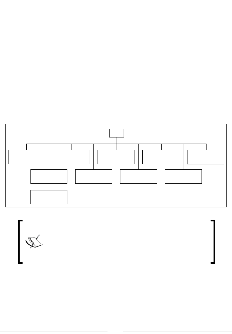
Using the JRockit Management APIs
[ 446 ]
JMAPI was the JVM-side API that enabled the functionality of the earliest versions of
the JRockit Management Console. In fact, even today, if a connection is established to
a 1.4 version of JRockit, a proprietary internal protocol called the Rockit Management
Protocol (RMP) will be used. This protocol will, in turn, use JMAPI to gather data and
change the various runtime parameters of the JVM.
The next few pages contain various examples of things that can be done using JMAPI.
The easiest way to compile the examples is to use the JRockit JDK. This requires no
special conguration, as the necessary classes are available in the JRockit rt.jar that
is part of the JRockit JDK. The examples can also be compiled by including jmapi.jar,
that contains all the interface declarations, in your class path. The jmapi.jar is not
part of the JDK, but is distributed by Oracle on request.
Using JMAPI for simple tasks is very easy. Use the com.bea.jvm.JVMFactory class
to get an instance implementing the JVM interface. From the JVM interface a number
of different subsystems can be reached.
JVM
ClassLibrary CompilationSystem DiagnosticCommand LoggingSystem Machine
MemorySystem OperatingSystem ProfilingSystem ThreadSystem
GarbageCollector
For readers who reacted on the com.bea part in the package
name—JMAPI predates the 2008 Oracle acquisition of BEA
Systems, and is used in other Oracle products as well as in
third-party products. As JMAPI was supported in JRockit R27
and earlier releases, the package name cannot be changed
without breaking existing products utilizing JMAPI.
Let us begin with a simple example that writes the current CPU load on the console
ten times with a one second delay between each printout:
import com.bea.jvm.JVMFactory;
public class JMAPITest {
public static void main(String[] args) throws InterruptedException {

Chapter 12
[ 447 ]
for (int i = 0; i < 10; i++) {
System.out.println(
String.format("CPU load is %3.2f%%",
JVMFactory.getJVM().getMachine().getCPULoad() * 100.0));
Thread.sleep(1000);
}
}
}
Access permissions to JMAPI are very coarse-grained; access is either permitted
or not allowed at all. If the code needs access to JMAPI when a security manager
is active, it must be granted the com.bea.jvm.ManagementPermission
"createInstance".
The following security policy statement grants access to JMAPI for all code:
grant {
permission com.bea.jvm.ManagementPermission "createInstance";
};
For more information on how to use permissions and policies, see:
http://java.sun.com/j2se/1.5.0/docs/guide/security/
permissions.html
JMAPI examples
JMAPI can be used to gather a lot of information about the operating
environment. The following code example prints some information about
the available network interfaces:
for (NIC nic : JVMFactory.getJVM().getMachine().getNICs()) {
System.out.println(
nic.getDescription() + " MAC:" +
nic.getMAC() + " MTU:" + nic.getMTU());
}
It is also possible to change various aspects of the runtime parameters using
JMAPI. The following piece of code will attempt to change the JRockit process
afnity to only one CPU:
private static void bindToFirstCPU(JVM jvm) {
Collection<CPU> cpus = jvm.getProcessAffinity();
CPU cpu = cpus.iterator().next();
Collection<CPU> oneCpu = new LinkedList<CPU>();
oneCpu.add(cpu);
jvm.suggestProcessAffinity(oneCpu);
}

Using the JRockit Management APIs
[ 448 ]
This can be compared to using the command-line ag –XX:BindToCPUs, for
controlling CPU afnity. The ag was introduced in Chapter 5, Benchmarking and
Tuning.
Other aspects such as the pause time target, the heap size, and the nursery size can
also be changed as follows:
MemorySystem ms = JVMFactory.getJVM().getMemorySystem();
ms.suggestHeapSize(1024*1024*1024);
ms.getGarbageCollector().setPauseTimeTarget(30);
ms.getGarbageCollector().setNurserySize(256*1024*1024);
Some features in JMAPI are a result of direct demands from customers with
specialized setups. There is, in particular, one peculiar feature that comes to mind—it
is possible to force the JRockit process to instantly terminate if it runs out of memory,
instead of throwing an OutOfMemoryError.
ms.setExitOnOutOfMemory(true);
It is also possible to do simple method proling using JMAPI. The following example
enables proling for the method java.io.StringWriter.append(CharSequence).
The example executes it for a number of String instances, after which the number of
invocations and the average time it took to invoke the method will be printed.
import java.io.StringWriter;
import java.lang.reflect.Method;
import com.bea.jvm.JVMFactory;
import com.bea.jvm.MethodProfileEntry;
import com.bea.jvm.ProfilingSystem;
public class MethodProfilerExample {
public static void main(String[] args) throws Exception {
String longString = generateLongString();
ProfilingSystem profiler = JVMFactory.getJVM()
.getProfilingSystem();
Method appendMethod = StringWriter.class.getMethod(
"append", CharSequence.class);
MethodProfileEntry mpe = profiler
.newMethodProfileEntry(appendMethod);
mpe.setInvocationCountEnabled(true);
mpe.setTimingEnabled(true);
String total = doAppends(10000, longString);
long invocationCount = mpe.getInvocations();
long invocationTime = mpe.getTiming();

Chapter 12
[ 449 ]
System.out.println("Did " + invocationCount
+ " invocations");
System.out.println("Average invocation time was "
+ (invocationTime * 1000.0d)
/ invocationCount + " microseconds");
System.out.println("Total string length "
+ total.length());
}
private static String doAppends(int count, String longString) {
StringWriter writer = new StringWriter();
for (int i = 0; i < count; i++) {
writer.append(longString);
}
return writer.toString();
}
private static String generateLongString() {
StringWriter sw = new StringWriter(1000);
for (int i = 0; i < 1000; i++) {
// Build a string containing the characters
// A to Z repeatedly.
sw.append((char) (i % 26 + 65));
}
return sw.toString();
}
}
The previous example is slightly simplied. Normally, proling could already have
been enabled for the method, and thus the counter and timing information already
available in the MethodProfileEntry should be stored before the proling run is
started and subtracted from the total when it is nished.
Recall the diagnostic commands that were introduced in Chapter 7, The Management
Console and Chapter 11, JRCMD. All diagnostic commands are available through
JMAPI, and can be accessed through the DiagnosticCommand subsystem. Here is
an example that prints the object summary histogram on stdout, in effect
programmatically executing the diagnostic command print_object_summary:
import com.bea.jvm.DiagnosticCommand;
import com.bea.jvm.JVMFactory;
public class ObjectSummary {
public static void main(String[] args)
throws InterruptedException {
DiagnosticCommand dc = JVMFactory.getJVM()
.getDiagnosticCommand();
String output = dc.execute("print_object_summary");
Using the JRockit Management APIs
[ 450 ]
System.out.println(output);
}
}
Finally, JMAPI also contains powerful class pre-processing and redenition features.
The following example redenes the bytecode of the classes as they are loaded, by
calling transformByteCode for each class:
ClassLibrary cl = JVMFactory.getJVM().getClassLibrary();
cl.setClassPreProcessor(new ClassPreProcessor() {
@Override
public byte[] preProcess(ClassLoader cl,
String className,
byte[] arg) {
System.out.println("Pre-processing class " + className);
return transformByteCode(arg);
}
});
There can only be one active preprocessor in use at any given time. By using the
method redefineClass in the class library, it is also possible to redene already
loaded classes.
JMAPI can be used for much more than the examples listed here. In
the interest of not spending too much time on describing deprecated
and unsupported features, we have chosen to keep this chapter short.
The full javadocs for JMAPI can be requested by Oracle customers.
JMXMAPI
The other management API available in JRockit is JMXMAPI. JMXMAPI can be seen
as a JMX-based version of JMAPI, even though there is not a one-to-one mapping
between the two. JMXMAPI is currently not supported and is subject to change
between releases, without notice.
The name space (domain) of the MBeans for JMXMAPI has changed with every major
JRockit release. With R28, it was changed once again due to the Oracle acquisition.
Even though it is highly unlikely that Oracle will be acquired, as we have the luxury of
not yet supporting the API, expect it to continue to change for a while. The JMXMAPI
MBeans were originally co-located with the java.lang.management MBeans (see
Chapter 7) in R26.x, but were later relocated to the bea.jrockit.management domain
and nally moved to the oracle.jrockit.management domain. The best version-
independent way to access a certain feature of JMX is by using the RJMX proxy layer
introduced at the end of the Management Console chapter.

Chapter 12
[ 451 ]
To access JMXMAPI, the JRockitConsoleMBean must rst be loaded. This can easily
be done programmatically, by using the MBeanServerConnection.
For R27.x versions of JRockit:
someMBeanServerConnection.createMBean
("bea.jrockit.management.JRockitConsole", null);
For R28.x versions of JRockit:
someMBeanServerConnection.createMBean
("oracle.jrockit.management.JRockitConsole", null);
With the Management Console proxy layer, this is done automatically.
The set of MBeans are organized as one per functional area. For the R28
version of JRockit, MBeans are also dynamically created for each ongoing
JRockit Flight Recording.
Following is a table describing the different MBeans available:
JMXMAPI MBeans
MBean name Description
Compilation Information from the JIT compiler.
DiagnosticCommand Enables access to the JVM internal diagnostic commands, see
Chapter 11, JRCMD.
GarbageCollector Information from the garbage collector, allows some degree of
control over the garbage collector.
JRockitConsole Functionality specically for the Management Console, such as
the "dump heap" operation. Creating this MBean will instantiate
and register the rest of the API.
Log Controlling and getting information from the JRockit logging
subsystem.
Memleak For controlling the Memleak server.
Memory For accessing information about physical memory.
PerfCounters A dynamically generated MBean listing all of the internally
available performance counters, described later in this chapter.
Proler For controlling the method proler.
Runtime For reading CPU information, CPU load, and for controlling CPU
afnity.
Threading Thread-related information. Currently only contains MBean
operations, that is no MBean attributes.

Using the JRockit Management APIs
[ 452 ]
In R28, there is also a supported JMX-based API for starting and controlling JRockit
Flight Recordings. This is located under com.oracle.jrockit. The entry point for
that API is the FlightRecorder MBean. This API is not part of JMXMAPI.
The JRockit internal performance counters
Most of JMXMAPI exposes MBeans implementing static interfaces. There is
however one that is dynamically generated—the PerfCountersMBean. JRockit
uses a number of internal performance counters for proling and diagnostic
purposes.The PerfCountersMBean contains an attribute for every internal
performance counter in JRockit.
As JMXMAPI is not yet supported, the dynamically generated
PerfCountersMBean is not supported either. However, there
is an internal distinction between the counters. The jrockit.*
counters can be considered to be even less supported than the
oracle.* counters.
The following table describes some of the most important counters available in
4.0/R28.x (at the time of writing, there are 139 different counters available):
Counter Description
java.cls.loadedClasses The number of classes loaded since the start of
the JVM.
java.cls.unloadedClasses The number of classes unloaded since the start
of the JVM.
java.property.java.class.path The class path of the JVM.
java.property.java.endorsed.
dirs
The endorsed dirs. See the Endorsed Standards
Override Mechanism on the Internet at
http://java.sun.com/javase/6/docs
/technotes/guides/standards/index.
html.
java.property.java.ext.dirs The extension dirs that are searched for JAR
les that should be automatically put on the
classpath. See the Java Documentation for
java.ext.dirs. More information on the
Extension Mechanism can be found here:
http://java.sun.com/j2se/1.4.2/docs
/guide/extensions/spec.html
java.property.java.home The root of the JDK or JRE installation.
java.property.java.library.path The library path used to nd user libraries.

Chapter 12
[ 453 ]
Counter Description
java.property.java.vm.version The JRockit version.
java.rt.vmArgs The list of VM arguments.
java.threads.daemon The number of running daemon threads.
java.threads.live The total number of running threads.
java.threads.livePeak The peak number of threads that have been
running since JRockit was started.
java.threads.nonDaemon The number of non-daemon threads running.
java.threads.started The total number of threads started since the
start of JRockit.
jrockit.gc.latest.heapSize The current heap size in bytes.
jrockit.gc.latest.nurserySize The current nursery size in bytes.
jrockit.gc.latest.
oc.compaction.time
How long, in ticks, the last compaction lasted.
Reset to 0 if compaction is skipped.
jrockit.gc.latest.
oc.heapUsedAfter
Used heap at the end of the last OC, in bytes.
jrockit.gc.latest.
oc.heapUsedBefore
Used heap at the start of the last OC, in bytes.
jrockit.gc.latest.oc.number The number of OCs that have occurred so far.
jrockit.gc.latest.
oc.sumOfPauses
The pause time for the last OC, in ticks.
jrockit.gc.latest.oc.time The time the last OC took, in ticks.
jrockit.gc.latest.
yc.sumOfPauses
The pause time for the last YC, in ticks.
jrockit.gc.latest.yc.time The time the last YC took, in ticks.
jrockit.gc.max.
oc.individualPause
The longest OC pause so far, in ticks.
jrockit.gc.max.
yc.individualPause
The longest YC pause so far, in ticks.
jrockit.gc.total.oc.compaction.
externalAborted
Number of aborted external compactions so
far.
jrockit.gc.total.oc.compaction.
internalAborted
Number of aborted internal compactions so far.
jrockit.gc.total.oc.compaction.
internalSkipped
Number of skipped internal compactions so
far.
jrockit.gc.total.oc.compaction.
time
The total time spent doing compaction so far,
in ticks.

Using the JRockit Management APIs
[ 454 ]
Counter Description
jrockit.gc.total.oc.ompaction.
externalSkipped
Number of skipped external compactions so
far.
jrockit.gc.total.oc.pauseTime The sum of all OC pause times so far, in ticks.
jrockit.gc.total.oc.time The total time spent doing OC so far, in ticks.
jrockit.gc.total.pageFaults The number of page faults that have occurred
during GC so far.
jrockit.gc.total.yc.pauseTime The sum of all YC pause times, in ticks.
jrockit.gc.total.
yc.promotedObjects
The number of objects that all YCs have
promoted.
jrockit.gc.total.
yc.promotedSize
The total number of bytes that all YCs have
promoted.
jrockit.gc.total.yc.time The total time spent in YCs, in ticks.
oracle.ci.jit.count The number of methods JIT compiled.
oracle.ci.jit.timeTotal The total time spent JIT compiling, in ticks.
oracle.ci.opt.count The number of methods optimized.
oracle.ci.opt.timeTotal The total time spent optimizing, in ticks.
oracle.rt.counterFrequency Used to convert ticks values to seconds.
Many of these counters are excellent choices for attributes to plot in the Management
Console. Also, be aware that many values are in ticks. To convert them to seconds,
divide by the value in the oracle.rt.counterFrequency counter.
To nd out which counters are in ticks, enable the Description column in the MBean
Browser by editing the table properties as shown in the following screenshot:
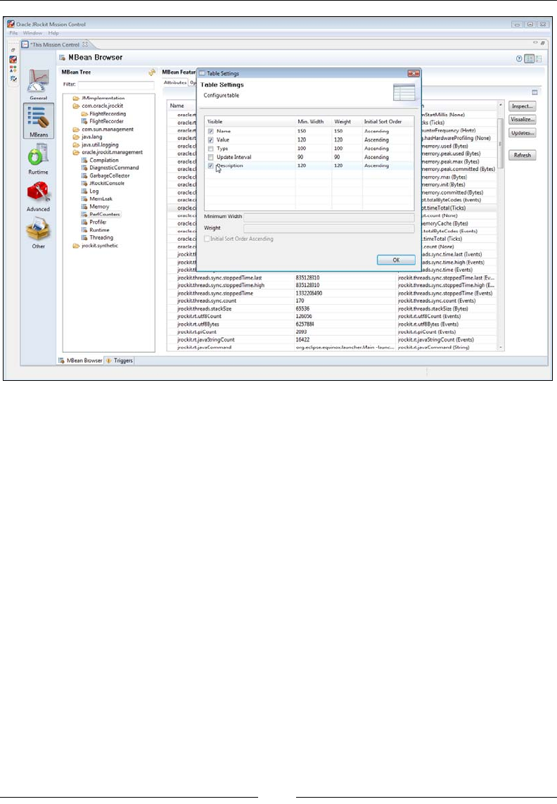
Chapter 12
[ 455 ]
The unit will be listed at the end of the description, as can be seen (you may need a
magnier) in the rightmost column in the attribute table behind the Table Settings
dialog in the screenshot.
An example—building a remote version of
JRCMD
JMXMAPI is accessed through standard JMX mechanisms (as described in Chapter
7). Consequently, the API is easily accessed remotely through the platform MBean
server and the standard remote JMX agent. As described in Chapter 11, a limitation
of JRCMD is that it can only attach to JRockit instances running locally on the same
machine as where JRCMD is executed. It can also only access JRockit instances
running as the same user as the one invoking JRCMD. Using JMXMAPI, we can
write a remote version of JRCMD that overcomes these limitations.
import java.lang.management.ManagementFactory;
import java.net.MalformedURLException;
import java.util.HashMap;
import java.util.Iterator;
import java.util.Map;

Using the JRockit Management APIs
[ 456 ]
import javax.management.Attribute;
import javax.management.InstanceNotFoundException;
import javax.management.MBeanAttributeInfo;
import javax.management.MBeanServerConnection;
import javax.management.ObjectName;
import javax.management.remote.JMXConnector;
import javax.management.remote.JMXConnectorFactory;
import javax.management.remote.JMXServiceURL;
/**
* Simple code example on how to execute
* ctrl-break handlers remotely.
*
* Usage:
* RemoteJRCMD -host -port -user -pass -command []
*
* All arguments are optional. If no command is
* specified, all performance counters and their
* current values are listed.
*
* @author Marcus Hirt
*/
public final class RemoteJRCMD {
private final static String KEY_CREDENTIALS =
"jmx.remote.credentials";
private final static String JROCKIT_PERFCOUNTER_MBEAN_NAME =
"oracle.jrockit.management:type=PerfCounters";
private final static String JROCKIT_CONSOLE_MBEAN_NAME =
"oracle.jrockit.management:type=JRockitConsole";
private final static String[] SIGNATURE =
new String[] {"java.lang.String"};
private final static String DIAGNOSTIC_COMMAND_MBEAN_NAME =
"oracle.jrockit.management:type=DiagnosticCommand";
public static void main(String[] args)
throws Exception {
HashMap<String, String> commandMap =
parseArguments(args);
executeCommand(
commandMap.get("-host"),
Integer.parseInt(commandMap.get("-port")),
commandMap.get("-user"),
commandMap.get("-password"),
commandMap.get("-command"));
}

Chapter 12
[ 457 ]
private static HashMap<String, String> parseArguments(
String[] args) {
HashMap<String, String> commandMap =
new HashMap<String, String>();
commandMap.put("-host", "localhost");
commandMap.put("-port", "7091");
for (int i = 0; i < args.length; i++) {
if (args[i].startsWith("-")) {
StringBuilder buf = new StringBuilder();
int j = i + 1;
while (j < args.length && !args[j].startsWith("-")) {
buf.append(" ");
buf.append(args[j++]);
}
commandMap.put(args[i], buf.toString().trim());
i = j - 1;
}
}
return commandMap;
}
@SuppressWarnings("unchecked")
public static void executeCommand(
String host, int port, String user,
String password, String command)
throws Exception {
MBeanServerConnection server = null;
JMXConnector jmxc = null;
Map<String, Object> map = null;
if (user != null || password != null) {
map = new HashMap<String, Object>();
final String[] credentials = new String[2];
credentials[0] = user;
credentials[1] = password;
map.put(KEY_CREDENTIALS, credentials);
}
// Use same convention as Sun. localhost:0 means
// "VM, monitor thyself!"
if (host.equals("localhost") && port == 0) {
server = ManagementFactory.getPlatformMBeanServer();
} else {
jmxc = JMXConnectorFactory.newJMXConnector(
createConnectionURL(host, port), map);
jmxc.connect();

Using the JRockit Management APIs
[ 458 ]
server = jmxc.getMBeanServerConnection();
}
System.out.println("Connected to " + host+ ":" + port);
try {
server.getMBeanInfo(new ObjectName(
JROCKIT_CONSOLE_MBEAN_NAME));
} catch (InstanceNotFoundException e1) {
server.createMBean(
"oracle.jrockit.management.JRockitConsole", null);
}
if (command == null) {
ObjectName perfCounterObjectName = new ObjectName(
JROCKIT_PERFCOUNTER_MBEAN_NAME);
System.out.println("Listing all counters...");
MBeanAttributeInfo[] attributes = server.getMBeanInfo(
perfCounterObjectName).getAttributes();
System.out.println("Counter\tValue\n=======\t====");
String[] attributeNames = new String[attributes.length];
for (int i = 0; i < attributes.length; i++) {
attributeNames[i] = attributes[i].getName();
}
Iterator valueIter = server.getAttributes(
perfCounterObjectName,
attributeNames).iterator();
while (valueIter.hasNext()) {
Attribute attr = (Attribute) valueIter.next();
System.out.println(attr.getName() + "\t=\t"
+ attr.getValue());
}
} else {
System.out.println("Invoking the ctrl-break command '"
+ command + "'...");
ObjectName consoleObjectName = new ObjectName(
DIAGNOSTIC_COMMAND_MBEAN_NAME);
Object[] params = new Object[1];
params[0] = command;
System.out.println("The CtrlBreakCommand returned: \n"
+ server.invoke(consoleObjectName,

Chapter 12
[ 459 ]
"execute", params,
SIGNATURE));
}
if (jmxc != null) {
jmxc.close();
}
}
private static JMXServiceURL createConnectionURL(
String host, int port)
throws MalformedURLException {
return new JMXServiceURL("rmi", "", 0,
"/jndi/rmi://" + host + ":"
+ port + "/jmxrmi");
}
}
The command uses the following syntax:
java RemoteJRCMD –command <command string> -host <host>
-port <port>
Where:
• <command string> is the diagnostic command as you would write it using
JRCMD, for example "start_flightrecording name=MyRecording
duration=30s".
• <host> is the name of the host where the JVM that we want to connect to
is running, for instance localhost.
• <port> is the port number on the JRockit machine where the remote JMX
agent (the RMI Registry) is listening. See the section Starting JRockit for remote
management in Chapter 6, JRockit Mission Control. The default port is 7091.
The following command-line example would list all the performance counters and
their values on localhost using the default port (7091):
java RemoteJRCMD
The following command-line example would list all available commands
on a JRockit running on the host bitsy, using port 4711:
java RemoteJRCMD -command help -host bitsy -port 4711

Using the JRockit Management APIs
[ 460 ]
The following command-line example would start a 30 second ight recording on
a JRockit running on localhost on the default port (7091), writing the resulting
recording to the designated le:
java RemoteJRCMD -command start_flightrecording
name=myrecording filename=c:\tmp\myrecording.jfr
duration=30s
Summary
In this chapter, two of the JRockit internal management APIs were described. Both
APIs grant access to internal JRockit functionality, such as performance metrics.
They also make it possible to programmatically manipulate a running JRockit JVM.
JMAPI is a local Java API that was fully supported in JRockit versions prior to R28.
Parts of JMAPI was deprecated in R28, and the future of JMAPI is undecided at the
time of this writing.
JMXMAPI is an unsupported JMX-based API consisting of several MBeans deployed
in the platform MBean server. As the API is JMX-based, standard JMX mechanisms
can be used to allow remote access.
Even though the APIs are currently (mostly) unsupported, there are situations
where they can be quite useful. An example implementing a remote version of
JRCMD was demonstrated.

JRockit Virtual Edition
Virtualization, the practice of running software on emulated hardware, has
emerged rapidly as an important concept in the last few years. The main benets
of virtualization are that hardware resource utilization can be maximized and that
resource management is made simpler. However, as virtualization is yet another
abstraction layer between the application and the actual hardware, it may also
introduce extra overhead.
This chapter deals with the product JRockit Virtual Edition; a new piece of technology
that is part of the JRockit product family. Throughout this chapter, the terms JRockit
Virtual Edition and the short form JRockit VE are used interchangeably.
JRockit VE enables the user to run Java in a virtualized environment without an
operating system, removing large amounts of the overhead typically associated
with virtualization. JRockit VE is a separate product that contains the minimum
components necessary to run a Java application in a virtualized environment—a
small lightweight OS-like kernel and a JRockit JRE.
JRockit VE can run any Java application, but initially, the most likely way in which
users will encounter JRockit VE is as part of the WebLogic Server on JRockit Virtual
Edition product (WLS on JRockit VE). WLS on JRockit VE is basically a prepackaged
instance of a WebLogic Server installation, in virtual machine image form. A virtual
machine image is a binary image that contains a virtual machine conguration,
software, and a le system. The image is intended for deployment on a specic
virtualization platform, such as Oracle VM Server.
This chapter, being a technical introduction to JRockit VE, concentrates on the
virtualization layer and the technology behind the JRockit VE product. It will
not discuss specic software stacks built on top of JRockit VE.

JRockit Virtual Edition
[ 462 ]
As this is a chapter about recently productized or emerging technology,
details, names, concepts, and implementations can be counted on to
change more rapidly than technology covered in other chapters of this
book. The chapter may also contain forward-looking statements that
will not be implemented. The fundamental concepts, however, remain
the same. Online documentation should always be consulted for the
freshest information on any product.
From this chapter you will learn:
• About virtualization as a concept and some common terms used for different
kinds of virtualization.
• What a hypervisor is, the different types of hypervisors, and the most
important hypervisors in the market today.
• The advantages and disadvantages of virtualizing a software stack and how
to get the most out of the advantages.
• About specic issues with virtualizing Java and how the JRockit
Virtual Edition product simplies the virtualization process and
enhances performance.
• About the concept of virtual machine images.
• What the future has in store—can virtualization overhead be reduced
further or even removed, making virtualization an even more powerful tool?
Can a virtualized application even run faster than on physical hardware,
given the right environment?
Introduction to virtualization
Virtualization is a word that has been used in many contexts over the years.
However, it always concerns abstracting a physical resource as a virtual one. It is
not a new concept. Virtual memory on a per-process basis is the main schoolbook
example, present in all operating systems. Partitions on a single hard drive that
each look like separate physical drives to an operating system are also technically
virtualization. But the buzz the last few years has been about virtualizing everything
in a physical machine. This is not a new concept either, it goes back at least as far as
to IBM in the 1960s. Not until recently, however, has virtualization proven itself as
a way to increase resource utilization and manageability in the server room.
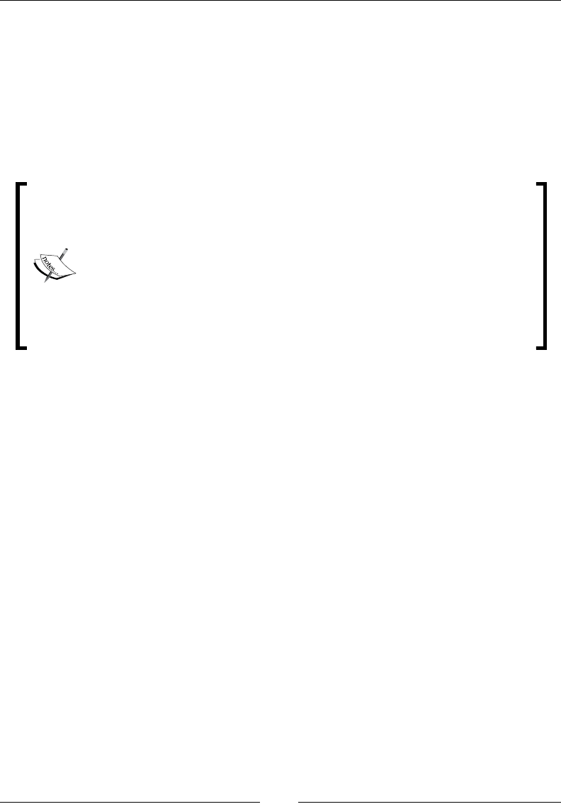
Chapter 13
[ 463 ]
Virtualization, for the purposes of this book, is the practice of running a platform (such
as an operating system) or an individual application on virtual hardware, emulated
in software. The virtual hardware typically looks like actual physical hardware to
the running platform or application. An entity deployed on a virtual system is often
referred to as a guest. The piece of software that enables multiple guests, for example
operating systems, to run on a single system is called a hypervisor. A hypervisor can
help the guest by, for example, supplying device drivers that are tailored to run in a
virtualized environment and thus improve performance for the guest.
What actually hides behind the physical hardware camouage varies,
depending on the type of resource being virtualized. For example, what
looks like a physical hard drive is typically a le, or collection of les
on a server somewhere. What looks like four available physical CPUs
is actually an amount of timeshare on an unknown number of existing
CPUs. What looks like 1 GB of memory is actually the claim to part of
a larger amount of physical memory. Some hypervisors even allow the
guests to overcommit memory within their limited allocation space.
But to the guest this does not matter, it only sees what it believes to be
physical hardware (with some exceptions).
Virtualization is becoming increasingly important, mainly because it makes it
possible to use existing physical machines more efciently. If the CPU on a physical
machine is idle, for example while waiting for I/O, those CPU cycles that could
have been used for execution are wasted in the idle time. Multiplexing several
guests on the same hardware makes it possible for those idle CPU cycles to be used
for other guests until the I/O request returns. Naturally, when several guests (for
example operating systems) run at the same time, another performance penalty
may result from additional context switching. However, it is an undeniable fact that
virtualization makes more efcient use of the available hardware. This is attractive
also from the power consumption angle, in a world that is becoming increasingly
environmentally conscious.
Virtualization falls into several categories, mostly having to do with the layer of
exposure to the underlying platform. While there is some confusion in terminology
here, let us start by introducing some common concepts and explain how they will
be used in this book. Virtualization is a complex area—the following is a simplied
version of the world.

JRockit Virtual Edition
[ 464 ]
Full virtualization
Full virtualization means that all sensitive functionality of an underlying platform is
emulated by the hypervisor—for example device interaction and memory mapping.
This makes it possible to deploy any unmodied software as a guest, the guest
believing that it is actually executing on physical hardware.
This is implemented on a platform that lacks explicit hardware support for
virtualization, by letting the hypervisor trap sensitive (privileged) instructions
executed by the guest and emulate them in a sandboxed environment.
Full virtualization can also be hardware-assisted, for example the Intel VT or
AMD-V technologies have CPU-specic support for running several operating
systems at once. Hardware-supported virtualization dramatically reduces the
emulation overhead in a hypervisor. Lately, other pieces of hardware than the
CPU have also been equipped with virtualization support. One example would
be network cards with built-in hardware support for virtualization.
Large performance benets to virtualization have been achieved with hardware
support. This seems to indicate that full virtualization is rapidly becoming the main
virtualization paradigm in the market.
Paravirtualization
Paravirtualization is used to refer to a virtualized environment where the guest needs
to know about the underlying hypervisor. Typically, in a paravirtualized environment,
privileged actions need to be explicitly requested by the guest through calls to a
public hypervisor API. This means that the guest has to communicate with a lower
abstraction layer and consequently needs to know that it is virtualized.
Paravirtualization removes some of the exibility of virtualization, as the guest
(for example an operating system) needs to be modied before virtual deployment.
An advantage might be that unnecessary layers of abstraction can be scaled away,
enabling additional performance improvements at the price of less exibility.
Also, the end user rarely has to worry about the implementation of the underlying
hypervisor. For example, on Xen, which originally was a paravirtualization-only
hypervisor, the main use case is to run pre-packaged operating systems that
have already been modied for paravirtualization. The user typically deploys his
application on top of these.
With the emergence of high-performance hardware support for full virtualization,
it is the authors' opinion that paravirtualization is becoming less important.

Chapter 13
[ 465 ]
Other virtualization keywords
There are several other keywords in the virtualization area that have many
different meanings, for example partial virtualization. Partial virtualization and
paravirtualization are sometimes used interchangeably, but partial virtualization
may also mean virtualizing only specic parts of the underlying hardware. For
example, the term has been used to describe binary translation tools such as Rosetta
on the Macintosh, enabling software compiled for PowerPC to run on Intel hardware.
Partial virtualization may or may not require hardware support. Concepts like virtual
memory in an operating system can also fall under the category partial virtualization.
Operating system level virtualization is another term that pops up from time to
time. This typically describes some kind of isolation mechanism built into an OS for
dividing the OS into separate instances, protected from one another, making them
look like they are running on different physical machines. Solaris Containers is
probably the most well-known example.
Hypervisors
Recall that the hypervisor is the software layer that makes virtualization possible
(optionally with the aid of explicit hardware support). The hypervisor provides an
idealized view of a physical machine. All "dangerous operations" that would break
the abstraction, such as device interaction and memory mapping, are trapped and
emulated by the hypervisor.
Just as there are different types of virtualization, there are different types of
hypervisors. Again, terminology is rather complicated. For the purposes of this
book, we will discriminate only between hosted hypervisors and native hypervisors.
Hosted hypervisors
A hosted hypervisor typically runs as a standard process in an ordinary operating
system. As mentioned earlier, sensitive (kernel mode) operations performed by
the guest are typically emulated or JIT-interpreted by the hypervisor. User mode
operations can often execute directly as part of the hosted hypervisor process, but
may also be emulated or JIT-interpreted when applicable.
The main advantage with a hosted hypervisor is that it is typically very easy to
install and use—just another application in your operating system. Usually, the
performance of a hosted hypervisor is not up to server-side requirements, but
this is not its main purpose.

JRockit Virtual Edition
[ 466 ]
Real world example—large parts of this book were developed and
written on a Macintosh, where no JRockit version currently exists.
For the purpose of producing JRockit examples, the author has used
the hosted hypervisor VMware Fusion to run a Linux version of
JRockit on his home computer.
VMware Player is an example of a simple hosted hypervisor. Oracle VirtualBox
is another.
Native hypervisors
A native hypervisor requires no host operating system. It can be installed directly on
physical hardware out of the box. Hardware device drivers can be provided by the
hypervisor, either in a special virtual machine for isolation (for example in Oracle
VM- and Xen-based solutions) or as part of the hypervisor itself (for example in
VMware ESX).
Typically, a native hypervisor is much more efcient than a hosted hypervisor.
Oracle VM and the VMware ESX product suite are two examples of native
hypervisors, who, although their approaches to virtualization are different,
both fulll the criterion that they install directly on physical hardware.
Hypervisors in the market
There are several mature hypervisors available in the quickly-changing market.
Xen is an open source hypervisor, originally developed at the University of
Cambridge. Xen later turned into the company XenSource Inc., and was acquired
by Citrix Corporation in 2007. Citrix release their own commercial server-grade Xen
systems with extra APIs, along with several management tools. The Xen hypervisor
itself continues to be available for free, under public open source license.
Xen has, because of its free nature, been widely used in several virtualization
frameworks, and has been turned into native hypervisors, Oracle VM being one
of them. Oracle VM is an Oracle Enterprise Linux-based operating system with
Xen at the bottom, and a native hypervisor.
Xen was originally a paravirtualized solution. In other words, it required that
the guests know that they are virtualized so that they can interact with the
hypervisor. For example, Linux kernels that should run on paravirtualized Xen
need to be specially compiled. The trend lately, however, seems to be that Xen is
moving away from the paravirtualized metaphor towards an environment with
support for unmodied guests. This requires hardware virtualization support.

Chapter 13
[ 467 ]
VMware corporation, one of the rst players in the virtualization eld, has several
virtualization products, both native and hosted hypervisors. Most notable are
VMware Workstation (VMware Fusion on Macintosh), VMware ESX and VMware
ESXi. These are commercial products. VMware also makes a stripped-down version
of VMware Workstation available for free, called VMware Player that does not
provide support for creating and conguring your own virtual machines, but
allows you to run an existing virtual guest. VMware also has a hosted virtualization
platform called VMware Server. It is available for free.
Microsoft corporation has developed the Hyper-V virtualization framework,
designed to work with Windows Server that is already a widely adopted technology.
Hyper-V requires hardware virtualization support.
KVM (Kernel-based Virtual Machine) is an open source hypervisor project, licensed
under the GNU Public License, driven by RedHat.
Parallels Inc. produces desktop and server virtualization software for Macintosh,
Windows, and Linux.
Also worth mentioning is VirtualBox, an independent virtualization package
containing its own hypervisor. It is targeted at desktop, server, and embedded use.
VirtualBox was originally developed by the German company Innotek, who were
acquired by Sun Microsystems, who in turn are now part of Oracle Corporation.
Advantages of virtualization
The main advantage of virtualization is, as we have mentioned, more efcient
resource utilization. Several guests can compete for all resources of one physical
machine. When one guest is idle, another guest may run. Virtualization may
substantially decrease the idle time in the server room.
Another advantage is that virtualization further enables the "cloud computing"
metaphor. As virtualized guests may be suspended, migrated to other physical
machines, and resumed, an entire machine park can be abstracted as a cloud of
computational power, on which deployments of applications may be made. This
is usually facilitated through different management frameworks.

JRockit Virtual Edition
[ 468 ]
Another, somewhat overlooked, but very important application
for virtualization is keeping legacy applications alive. A common
nightmare in IT is having to retire old hardware on which legacy
applications with no forward compatibility are hosted. This
requires porting the applications to new platforms, either requiring
complete rewrites or ending up with Frankenstein-type solutions
such as COBOL to (unreadable) Java converters. Virtualizing the
old hardware instead will make it possible to continue running the
legacy application for some time, while guring out how to replace
it in a less stressful manner.
Disadvantages of virtualization
The main problem with virtualization is, of course, the extra overhead introduced
by another abstraction layer, the hypervisor, in the stack between application and
hardware. While hardware resource usage indeed gets more optimal in a virtualized
environment, there are costs associated both with running several guests at once
on a piece of physical hardware as well as with the extra overhead incurred by the
hypervisor abstraction layer.
Now consider the case of a Java application in a virtual environment. For a standard,
non-virtualized local Java application, the JVM provides one layer of abstraction
against the hardware. The operating system on which the JVM runs provides
another. The hypervisor layer that is responsible for emulating the virtual hardware
below the OS adds yet another zone of abstraction between the application and its
actual execution as native code.
We can try to make each layer of abstraction as thin and efcient as possible, but
we can't make them go away altogether. For example, using hardware support to
implement the hypervisor will decrease the virtualization overhead. However, we
are still dealing with emulating physical hardware for the virtualized application.
This naturally incurs overhead anyway.
Virtualizing Java
Let us now discuss the implications of running an industrial strength Java
application server in a virtualized environment. Consider the following gure
that illustrates the entire stack from the application server down to the hardware.
Between the Java application and the hardware on which it ultimately executes,
we have a JVM, a general purpose OS (for example Oracle Enterprise Linux), and
a Hypervisor (such as Oracle VM).
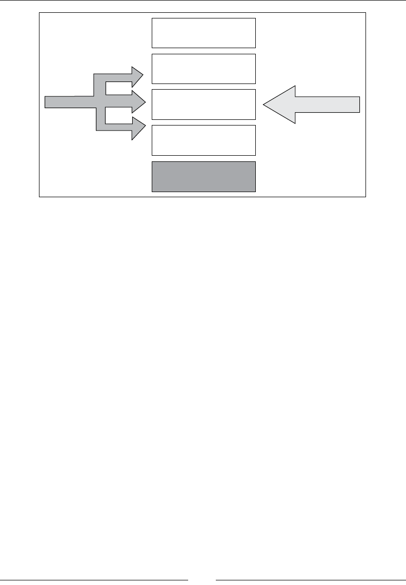
Chapter 13
[ 469 ]
Triple Virtualization
Application Server
JVM
OS
Hypervisor
Hardware
General purpose OS
The application server, for example Oracle WebLogic, is a typical Java application
that needs a JVM to execute. The JVM provides abstraction against the operating
system on which the application server is deployed. This is obviously because the
same WebLogic shipment should run equally as well on Linux as on Windows or
Solaris—this is the whole point of Java. The price of the convenience of write
once / run anywhere is thus paid for by the JVM abstraction layer.
Under the JVM is an operating system that the JVM must know how to interact with.
This requires multiple JVM back-ends for multiple operating systems. For example,
on *NIX-style operating systems, pages in memory are allocated differently than
on Microsoft Windows, with different system calls (mmap versus VirtualAlloc).
The thread API typically also differs between operating systems (POSIX threads
versus Windows threads). Thus, the JVM needs OS-specic modules in order to
facilitate the execution of the same Java application on different operating systems.
Consequently, the operating system itself forms another abstraction layer under the
virtual machine.
So, what is the role of a general purpose operating system? The OS abstracts the
hardware, making it easier to interact with it programmatically. We can hardly
expect a C++ application developer to implement his own synchronization for a
particular chipset using atomic assembly instructions or to write his own thread
representation. Instead, the OS provides library calls for these kinds of tasks.
Thus, the OS forms a second level of abstraction under the JVM.
And nally, in a virtualized world, the hypervisor—while making it possible to
run multiple sandboxed operating systems on the same machine—forms a third
abstraction layer before we get to the actual hardware.
JRockit Virtual Edition
[ 470 ]
All these abstraction layers need to communicate with each other. There is overhead
here, especially as talking to a lower layer usually requires some kind of privileged
action that takes time, destroys caches, and preempts other tasks.
However, if the sole responsibility of the virtualized operating system is to run the
JVM, whose sole responsibility in turn is to run the Java application server, don't the
various levels of abstraction seem unnecessary and quite wasteful? Why would we
need a full-edged OS such as Microsoft Windows in the middle of our stack, when
all we do is run a Java program? The Java program, assuming that it is 100 percent
pure Java, doesn't know anything about Microsoft Windows and doesn't use any
OS-specic mechanisms. If the Java program is an application server with no GUI,
do we even need the functionality to display graphics on screen? If all users and
access controls necessary to interact with the system are handled by a model inside
the application server, do we even need an OS?
We can make the observation that a JVM is not so far removed from an OS as one
might think. It implements JDK library calls to support threads and synchronization.
It handles memory management and so on. Without stretching the metaphor too
tightly, a JVM is just like a special-purpose virtual operating system.
Maybe a direct-to-hypervisor JVM isn't such a bad idea?
Introducing JRockit Virtual Edition
The case can be made that if there was a way to reap the benets of virtualized
Java without the overhead, much would be gained. If the layers between Java and
hardware are kept small enough, there is not just performance to be had, but also
the added benet of simplicity and security. The solution proposed by the JRockit
architects is the product JRockit Virtual Edition, or JRockit VE for short.
As a proof of concept back in 2005, we wrote a linker that told us
what symbols a JVM deprived of its operating system was missing.
The discovery that the list was really quite short was the start of the
JRockit VE project.
JRockit VE consists of the JRockit JRE, a collection of pure Java services (for example
an SSH daemon), and nally a thin OS-like layer that runs on top of the hypervisor.
This layer provides all of the very limited amount of OS functionality that a JVM
needs. It is known as the JRockit VE kernel.
JRockit VE is currently available only on x86 platforms.
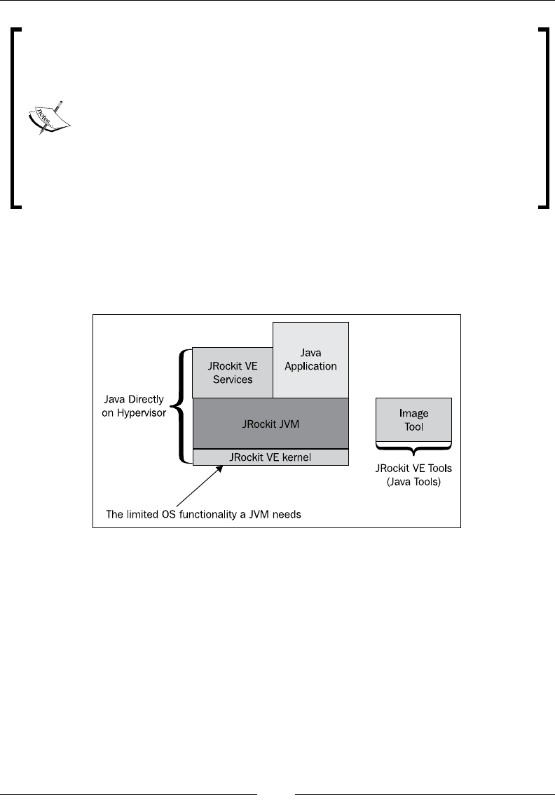
Chapter 13
[ 471 ]
The commercial versions of the JRockit VE virtualization framework
currently only ship with support for running on top of the Oracle VM
native hypervisor (and consequently on top of Xen). JRockit VE may,
however, also support other hypervisors in the future.
It has always been our design philosophy, as it should be in a virtualization
stack, that the target platform for the JRockit VE kernel is hardware and not
a hypervisor. The JRockit VE kernel with a small built-in E1000 network
driver can boot from a USB stick and run Java applications on any x86
machine out of the box (It is doubtful, however, why this demo, except for
the fact that it is really cool, would illustrate any benets of JRockit VE in
cloud computing, but we'll get to that).
JRockit VE also comes with a tool for creating and manipulating Java applications
that are to run in a virtualized environment, the Image Tool. When a Java
application is virtualized and packaged for use with JRockit VE, it is referred
to as a virtual machine image.
The previous gure illustrates the stack, as it looks for a Java application deployed
on JRockit VE. Services like SSH run in Java land, along with the Java application.
The JRockit JVM sits on top of the JRockit VE kernel layer that provides all OS
functionality needed by the JVM.
Let us now look closely at the JRockit VE kernel to understand both why
implementing it is a much smaller undertaking than writing a complete OS,
and what functionality we need to make available to the layers above.
JRockit Virtual Edition
[ 472 ]
The JRockit VE kernel
JRockit Virtual Edition removes the need for an OS under the JVM and makes
it possible to run Java directly on top of a hypervisor. Currently, an unmodied
Linux version of the JRockit JVM can run directly on top of the JRockit VE kernel.
This is, however, expected to change for future releases and the JRockit VE kernel
is expected to turn into its own JVM platform, requiring a special version of the
JVM. This is to further decrease the number of abstraction layers in the stack and to
provide additional simplicity of implementation. The only reason that the JRockit VE
kernel currently emulates a Linux API upwards has been the lack of development
time to create an additional platform for the JRockit JVM.
The fact that the JRockit JVM currently is a Linux distribution does
not impact performance negatively or constrain it to Java-on-Linux
levels. The JRockit VE kernel can do plenty with the OS layer to
provide a much more ideal execution environment for the Linux JVM.
With a specialized JVM, performance will improve even further.
The JRockit VE kernel is conceptually very much like an OS, but far from the real
deal. It contains its own thread implementation, scheduler, support for le systems,
memory allocation mechanisms, and so on, but is vastly less complex than an
operating system.
For one thing, the JRockit VE kernel can run only one process—the JRockit JVM.
Also, as a JVM is an inherently secure sandboxed execution environment, we do
not need to worry about malicious Java code causing, for example, deliberate buffer
overruns. Bytecode verication and all other security aspects of validating executing
Java code is handled for us by the JVM already.
An important constraint here is that JRockit VE needs to disallow the execution
of arbitrary native code, as there is no way to determine what it does. This is both
a functionality and a security concern. Native code can contain operating system
calls that only work on a standard operating system and it may also perform any,
potentially insecure, task. Disallowing native code, however, tends to be a small
price to pay in a modern Java-based server environment. Therefore, JNI is not
supported on JRockit VE.
Another example of the limited functionality is the lack of advanced paging
mechanisms that would be present in any general purpose OS. The JRockit VE
kernel runs just one process and needs just one virtual address space.
The following gure illustrates the various modules in the JRockit VE kernel. They
include, among other things, le system implementations, device driver stubs
that communicate with the hypervisor, block cache mechanisms, a self-contained
network stack, simple memory management systems, and a thread scheduler.
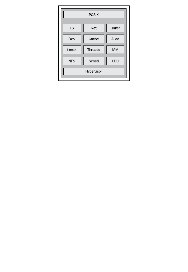
Chapter 13
[ 473 ]
The JRockit VE kernel, in its exposed APIs is very *NIX-like. As stated, a distribution
of JRockit for Linux can run unmodied on top of the JRockit VE kernel, but this
only means that the very limited amount of Linux APIs that JRockit needs have
been implemented in the kernel, not that the kernel is Linux-compatible in any way.
Typically, the APIs available to the JVM look like POSIX system calls, but have less
generic functionality. Given that future JRockit versions become JRockit VE aware,
we could avoid most kludges caused by pretending to be Linux. One example of this
would be not having to emulate parts of /proc le system in the kernel, as this is the
way JRockit on Linux collects information on memory layout. We would also like
to remove some OS calls, such as mmap, that look like POSIX calls in JRockit VE, but
are not. The standard POSIX version of mmap is very complex, but in JRockit VE only
the specic use cases that JRockit for Linux needs have to be implemented. Porting
JRockit to an explicit JRockit VE platform would not be too complex an undertaking
as all operating system calls in the JVM already exist in a well-dened platform
abstraction layer.
In conclusion, it is important not to be taken aback by thinking about the concept
of the JRockit VE kernel as a small lightweight OS. It is much less than that and
large parts of the complexities required for an operating system are not needed
in our kernel. The need to implement and maintain a set of device drivers, in
operating systems such as Linux, which is a much larger task than maintaining
the actual kernel code, is made unnecessary as JRockit VE requires a hypervisor
to run on. The hypervisor will take care of device drivers where necessary and
abstract physical hardware for us. The complete JRockit VE kernel module is
only around 130,000 lines of C code, large parts making up the network stack.

JRockit Virtual Edition
[ 474 ]
The virtual machine image concept and
management frameworks
The "virtual cloud" is a hot buzzword right now. It is a fairly simple concept
to understand—a vast blob of Internet-connected computing resources that
can be harnessed without the need to care about individual congurations
and individual machines.
A Java application installed on a physical machine is also a well-known concept.
Most cloud solutions today use some kind of management framework that handles
application deployments in the cloud, removing the need for individual machines
through abstraction, which makes plenty of sense—"the cloud is the computer".
Typically, management frameworks are used to deploy entire self-contained guest
operating systems, for example virtual Linux distributions, in a server cloud.
A concrete example of a management framework in cloud computing
is the Oracle VM Manager software that is part of the Oracle VM native
hypervisor. Oracle VM Manager allows the administrator to congure
and group clusters of servers in the cloud and deploy virtual machine
images on them.
JRockit Virtual Edition originally started out with an ambition to look like "local
Java". This meant starting the virtual application and deploying it in the cloud with
command line on a local machine. On the local machine, it would look like the virtual
application was executing locally, instead of remotely. This was accomplished by,
among other things, feeding back JVM console output to the local console. It turned
out that this was a very complicated concept to understand and it also led to some
degree of confusion: where is an application actually running?
After alpha releases, and user testing, the JRockit VE team decided to go the other
way instead—local Java applications should be turned into virtual machine images.
These are binary blobs ready for cloud deployment through existing management
frameworks like Oracle VM Manager. Controlling the virtual machine image, such
as changing its virtual hardware layout and migrating it across server pools, are
examples of functionality provided already by the management framework.
Virtual machine images, in the general case, can contain any machine conguration
with any operating system. A JRockit VE virtual machine image consists of a
complete virtual machine specication and setup for a Java application along with
a le system containing said Java application.
Chapter 13
[ 475 ]
We can think of distributing a virtual machine image containing, for example,
WebLogic Server to a customer, as shipping the customer a physical machine. On its
hard disk is a preinstalled version of WebLogic Server good to go, and all the user
needs to do is plug the machine into a power outlet, attach a network cable, and start it
up. The main difference in the case of the virtual machine image is that we don't ship
the physical machine along with the installed software. We only ship the specication of
the machine—how much memory does it have, how many CPUs—and a cloned image
of its hard disk. The cloud will provide the resources necessary for emulating the
machine in order to run the application. This is what virtualization is all about.
Thus, virtual machine images also remove the need for installing software. Preinstalled
software in virtual machines can be deployed directly. This is one of the reasons that
virtualization can help reduce IT costs in an organization.
A virtual machine image can be generated from scratch, or assembled, by
applying the Image Tool that ships with JRockit VE to a locally installed
application. Instances of this image can then be deployed directly into
your server cloud. We call this the "physical to virtual" use case. Another
use case, however, is for the customer to run software that is shipped in
the form of an already assembled virtual machine image (for example
WLS on JRockit VE), available from an OEM or software vendor, and not
create images of his own.
Many aspects of the machine specication for an existing virtual machine image, for
example the amount of memory available to the virtual machine, can be manipulated
ofine with the JRockit VE Image Tool as well as from the management framework.
The virtual machine environment for the virtualized application can vary from being
very simple to very complex.
A JRockit VE virtual machine image with a minimum conguration can simply be
auto-generated. Typically, the Image Tool only needs to know things like disk size,
number of CPUs, and amount of memory in the virtual machine. The JRockit VE
kernel requires at least one network interface to work. When booting, the kernel
will try to use the DHCP protocol, if available, to congure networking. This makes
setup very simple and portable. If DHCP is unavailable on your network, explicit
conguration of the virtual network cards needs to be done.
The local le system in the virtual machine image is part of the generated disk image
and available to the virtualized Java application once it runs.

JRockit Virtual Edition
[ 476 ]
The following example shows a very simple, but fully sufcient, conguration le
for a JRockit VE virtual machine specication. It describes a virtual machine image
that executes a HelloWorld Java program. The virtual machine image can be created
using the Image Tool. Similar conguration les can be obtained by querying an
existing virtual machine image for its specication.
The JRockit VE cong le format is totally hypervisor agnostic.
<?xml version="1.0" encoding="UTF-8"?>
<!-- helloworld.xml -->
<jrockitve-imagetool-config xmlns:xsi="http://
www.w3.org/2001/XMLSchema-instance"xsi:noNamespaceSchemaLocation=
"jrockitve-imagetool-config.xsd" version="5.1">
<jrockitve-config memory="512 MB" cpus="1">
<storage>
<disks>
<disk id="root" size="256 MB"/>
</disks>
<mounts>
<mount>
<mount-point>/</mount-point>
<disk>root</disk>
</mount>
</mounts>
</storage>
<vm-name>helloworld-vm</vm-name>
<java-arguments>-Xmx256M HelloWorld</java-arguments>
<network>
<nics>
<nic/>
</nics>
</network>
</jrockitve-config>
<jrockitve-filesystem-imports>
<copy from="~/myLocalApp/HelloWorld/*" to="/"/>
</jrockitve-filesystem-imports>
</jrockitve-imagetool-config>
The conguration describes a machine with 512 MB of RAM and one CPU. The
machine contains one hard drive that is 256 MB in size. The virtual machine, once
the image is deployed, will show up as helloworld-vm in various management
frameworks. At boot time, the JRockit VE kernel will invoke JRockit. JRockit then
executes the HelloWorld program, whose .class le (and possibly other resources)
are placed in the root directory of the hard drive in the virtual machine. The virtual

Chapter 13
[ 477 ]
machine contains one network card (NIC). As no explicit conguration other than
that which exists is given, the JRockit VE kernel will use DHCP to establish things
like the IP address for the virtual machine when it boots.
Following are a few command-line examples, illustrating using the Image Tool to
assemble a virtual machine image and to modify it before deployment. The default
behavior is to create a standard Xen or Oracle VM conguration, consisting of a
hypervisor-specic vm.cfg le and a system image, system.img, with the virtual
hard drive containing the Java application, the JRockit JRE, and the JRockit VE
kernel. The following example creates a virtual machine image from the
previous specication:
hastur:marcus$ java -jar jrockitve-imagetool.jar
Usage: java -jar jrockitve-imagetool.jar [options]
-h, --help [<option_name>]
-c, --create-config [<config_file.xml>] [<vm_name>]
--create-full-config [<config_file.xml>] [<vm_name>]
-r, --reconfigure <vm_cfg> <op> <field> [<parameter>]*
--reconfigure-service <vm_cfg> <service-name>
<op> <field> [<parameter>]*
-f, --file <vm_cfg> <operation> [<parameter>]*
--get-log <vm_cfg> [<output file>]
--repair <vm_cfg> [<auto|prompt|check>]
-p, --patch <vm_cfg> <patch_file>
-a, --assemble <config.xml> <output_dir> [<hypervisor>]
-d, --disassemble <vm_cfg> <output_dir>
-v, --version [<vm_cfg>|<jrockitve_image>]
-l, --log (#) <quiet|brief|verbose|debug>
--force (#)
Options marked "#" are not standalone.
They must be used together with other options
hastur:marcus$ java -jar jrockitve-imagetool.jar
--assemble helloworld.xml /tmp/outputdir
Assembling the image...

JRockit Virtual Edition
[ 478 ]
| |
.............................
Wrote 127 MB
Done
hastur:marcus$ ls -lart /tmp/outputdir/
total 327688
drwxrwxrwt 18 root 612 Aug 29 11:09
-rw-r--r-- 1 marcus 270 Aug 29 11:10 vm.cfg
-rw-r--r-- 1 marcus 268435456 Aug 29 11:10 system.img
drwxr-xr-x 4 marcus 136 Aug 29 11:10
hastur:marcus$ java -jar jrockitve-imagetool.jar
--reconfigure /tmp/outputdir/vm.cfg get java-arguments
-Xmx256M HelloWorld
hastur:marcus$ cat /tmp/outputdir/vm.cfg
# OracleVM config file for 'helloworld-vm'.
# Can be used with 'xm <start|create> [-c] vm.cfg'
#
# note that Xen requires an absolute path to the image!
name="helloworld-vm"
bootloader="/usr/bin/pygrub"
memory=512
disk=['tap:aio:/OVS/seed_pool/helloworld-vm/system.img,sda1,w']
vif=['']
on_crash="coredump-destroy"
Given an assembled virtual machine image, we can use the JRockit VE Image Tool
to query and recongure its virtual machine specication. In the following example,
we retrieve and change the number of virtual CPUs that should be available in the
virtual machine. This will cause changes to the underlying hypervisor specic cong
le and possibly to the contents of the image (in our example system.img). An
assembled image is always uniquely identied by its hypervisor specic cong le
(in our case vm.cfg for Oracle VM or Xen).
Chapter 13
[ 479 ]
hastur:marcus$ java -jar jrockitve-imagetool.jar
--reconfigure /tmp/outputdir/vm.cfg get cpus
1
hastur:marcus$ java -jar jrockitve-imagetool.jar
--reconfigure /tmp/outputdir/vm.cfg set cpus 4
Done
hastur:marcus$ cat /tmp/outputdir/vm.cfg
# OracleVM config file for 'helloworld-vm'.
# Can be used with 'xm <start|create> [-c] vm.cfg'
#
# note that Xen requires an absolute path to the image!
name="helloworld-vm"
bootloader="/usr/bin/pygrub"
memory=512
disk=['tap:aio:/OVS/seed_pool/helloworld-vm/system.img,sda1,w']
vif=['']
vcpus=4 #<--- we now have 4 virtual CPUs
on_crash="coredump-destroy"
An assembled virtual machine image can also be reduced to its
component parts and disassembled by the Image Tool, but this
use case (virtual to physical), exactly like the assembly use case
(physical to virtual), is not the only one available to end customers.
We also assume that end customers, to some extent, will work with
prepackaged virtual machine images that can be recongured and
manipulated with the Image Tool.
Aside from manipulating a virtual machine image, the Image Tool can also be
used to patch an image, with bugxes or upgrades to the software within, such
as the JRockit VE kernel or WebLogic Server. Thus, a pre-packaged virtual machine
image can be upgraded by vendor xes without the need for taking it apart.

JRockit Virtual Edition
[ 480 ]
The Image Tool can also be used for a number of other common ofine manipulation
tasks such as extracting log le information from the virtual application or enabling
services such as SSH that come pre-installed in every JRockit VE image. Even though
the patch framework fully supports patch version control and rollbacks, an implicit
safety mechanism in patching machine images is apparent given that an image is just
a couple of les on disk: backing up the image is just a matter of copying the les
somewhere. Should anything go wrong, they can be easily restored.
Following is another example of querying a JRockit VE virtual machine image for its
installed services and enabling one of them—the previously mentioned SSH daemon:
hastur:marcus$ java -jar jrockitve-imagetool.jar -r
/tmp/outputdir/vm.cfg get installed-services
sshd (An SSH2 implementation with SCP and SFTP support)
jmxstat (JRockitVE kernel statistics MBean)
sysstat (JRockitVE kernel sysstat statistics)
hastur:marcus$ java -jar jrockitve-imagetool.jar -r
/tmp/outputdir/vm.cfg get enabled-services
None
hastur:marcus$ java -jar jrockitve-imagetool.jar -r
/tmp/outputdir/vm.cfg enable service sshd
Done
hastur:marcus$ java -jar jrockitve-imagetool.jar -r
/tmp/outputdir/vm.cfg get enabled-services
sshd (An SSH2 implementation with SCP and SFTP support)
When the SSH service is enabled in a running virtual machine image, the
virtual machine will answer SCP and SFTP requests, given some precongured
authentication policy.
Finally, the Image Tool can be used to manipulate the le system of a virtual machine
image, for example by allowing creation and removal of les and directories. The
Image Tool also supports that les from a local le system can be placed in the image
and conversely, that les from the image can be copied to a local le system.

Chapter 13
[ 481 ]
hastur:marcus$ java -jar jrockitve-imagetool.jar
--file /tmp/outputdir/vm.cfg ls /
[Feb 04 2010] boot/
[Feb 04 2010] jrockitve/
[Feb 04 2010] lost+found/
[Feb 04 16:00 498 bytes] HelloWorld.class
[Feb 04 16:00 358 bytes] VERSION
Done
hastur:marcus$ java -jar jrockitve-imagetool.jar
--file /tmp/outputdir/vm.cfg get HelloWorld.* /tmp
Done
hastur:marcus$ ls –l /tmp/HelloWorld*
-rw-r--r-- marcus wheel 489 Feb 14 15:36 /tmp/HelloWorld.class
Benets of JRockit VE
There are several advantages to using JRockit VE as a specialized virtualization
solution for Java. The main ones are:
• Performance and better resource utilization
• Simplicity
• Manageability
• Security
We will discuss them in order.
Performance and better resource utilization
Increased performance in JRockit VE stems from two general areas, the rst one
being (as we have already mentioned), the removal of unnecessary abstraction
layers. With a specialized Java environment for virtualization, some of the "triple
virtualization" caused by a combination of JVM, OS, and hypervisor is removed.
JRockit Virtual Edition
[ 482 ]
The other side to virtual Java performance with JRockit VE is even more
interesting—there are several areas where being the link between the hypervisor
and the JVM can provide us with information that, if correctly used, may outperform
standard virtualized operating systems or even in the right environment (although
it might sound too good to be true), physical hardware. We will address these
intriguing issues in the section A look ahead—can virtual be faster than real at the end
of this chapter.
Getting rid of "Triple virtualization"
In a normal operating system, certain operations, such as system calls, need to run
in more privileged modes on the hardware. Modern hardware typically has some
kind of hierarchical protection domains. All code executes in one of these domains.
They go from least privileged access (userland) to most privileged (kernel). On x86
hardware, these protection domains are referred to as rings, and a more privileged
operation is said to be running in a ring with lower ring number. Ring 0 is the most
privileged level and corresponds to kernel access. Non-trusted user code, on the
other hand, must run in a less privileged ring. As soon as the user code needs to
execute a privileged operation, such as a system call, the CPU needs to change rings,
which is a very expensive operation, requiring synchronization and potentially
destroying all caches.
As the JRockit VE kernel contains OS-like subsystems of its own and because it
relies on the hypervisor for hardware interaction, there is nothing stopping it from
executing mostly in Ring 3, userland on x86, reducing (but not altogether removing)
the need for ring transitions.
Here is a hypervisor implementation detail, that may provide
further insight into how protection domains work—a virtualized
guest operating system on x86 typically runs its kernel operations
in Ring 1, leaving the more privileged Ring 0 to the hypervisor. This
doesn't matter to the guest.
The following gure illustrates the execution path of a network system call in a JVM
running on a normal Linux operating system compared to doing the same in the
JRockit VE kernel. The dashed vertical lines are the time axes.
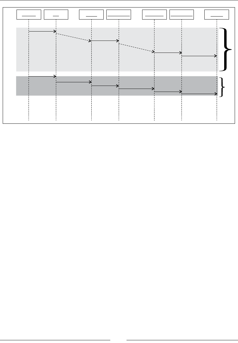
Chapter 13
[ 483 ]
java.net libc TCP/IP DeviceDriver Hypervisor E1000
transmit
signal backdoor
“trap” IOPort
DeviceDriver
send send(ring3 - ring0)
transmit signal
signal
transmit
transmit
send
send
Normal OSJRockit VE
The system call starts with Java code calling a function in the java.net package.
Control is then transferred gradually through the layers, down to the actual
hardware, where the network driver executes assembly instructions. The dashed
lines correspond to expensive privileged operations, such as ring changes, needing
to take place. The overhead for doing the same thing in JRockit VE is vastly smaller.
Hopefully, this makes a case that virtualization overhead can be aggressively
reduced if the OS is replaced with a more specialized layer. This is what gives
JRockit VE a unique and attractive selling point. One of the biggest problems
with implementing cloud computing, as discussed early in this chapter, is the
performance loss incurred from going virtual. By replacing the operating system
layer, JRockit VE can signicantly reduce that overhead, when compared to
traditional virtualization solutions.
Memory footprint
The JRockit VE kernel is a self-contained boot image that is just a few megabytes in
size. This small amount of storage, except for a few conguration les and the JRE,
is all the space in a JRockit VE-based virtual machine image not taken up by user
code. A modern operating system, even a JeOS (Just enough OS) implementation,
is on the order of several hundred megabytes in its simplest install.
The small size of a JRockit VE system and its kernel ensures that the amount of
system memory in the virtual machine that can be used for running the actual Java
application (i.e. resources available to the JVM) is maximized. This is most important
on 32-bit setups, which still is a fairly common virtual machine representation in a
cloud conguration.

JRockit Virtual Edition
[ 484 ]
Manageability
Manageability comes in two avors—ofine manageability, on the virtual machine
image level, and online manageability, the ability to deploy and control a running
virtual machine image in a cloud computing environment.
For an undeployed JRockit VE virtual machine image, all interaction with its "outside
world" is handled by the Image Tool that is shipped with the JRockit VE product and
its derived products, such as WLS on JRockit VE. Any aspect of a JRockit VE virtual
machine image, le system, virtual machine conguration, enabled services, and so on,
can be manipulated ofine with the Image Tool in a hypervisor agnostic way.
The other very visible aspect of manageability is the virtual machine image concept.
Given that a JRockit VE virtual machine image conforms to a known hypervisor
format, it may be introduced into another resource management system, such as
Oracle VM Manager.
Oracle VM Manager already exists as a product today. The typical use case is that
it enables the administrator to work with several virtualized versions of Oracle
Enterprise Linux. It requires little or no modication to work with other kinds of
virtual appliances in virtual machine images—for example instances of WLS on
JRockit VE, that are packaged on top of JRockit VE. To the management framework,
one of these "WebLogic blobs" will look the same as any other virtualized guest. The
ability to t into existing virtualization management frameworks makes adoption
problems for JRockit VE a non-issue. We have seamlessly removed the standard
operating system layer from the virtual machine image.
Simplicity and security
It may not be a universal truth that security follows simplicity, but with JRockit VE
we shall see that this is the case.
A full-edged operating system is a complex beast. It needs to be, as it contains a
jungle of system daemons and user applications such as web browsers and e-mail
programs. It also has to provide a generic multi-tasking environment and enable
multiple processes to co-exist. There are usually several entry points to a remote
workstation running a standard OS, such as open ports for network services, login
protocols, and so on.
As the kernel layer in JRockit VE provides only the bare necessities required to
run a JVM, the inherent complexity of the system is orders of magnitude smaller.
As mentioned, there is only one preinstalled service, sitting on top of the kernel,
allowing remote access—a 100 percent pure Java SSH daemon. This service is also
disabled by default. It needs to be explicitly enabled by the creator of a JRockit VE

Chapter 13
[ 485 ]
virtual machine image in order to work. With the low number of entry points from
the outside world, no native code allowed, and the JVM handling verication of all
potentially malicious Java code, security is by design much better than that which
can be provided in a more complex environment.
Also, as previously mentioned, the "OS" itself, the JRockit VE kernel, can only run
one process—the JVM. So, we have no process and resource separation problems
that can make JRockit VE more insecure.
The JVM maintains the security of an executing Java application according to the
Java Virtual Machine specication. Given that native code is banned, the sandboxed
JVM model can fully protect us against buffer overruns and malicious code. No other
memory protection is needed for the running Java program than the intrinsic one
provided by the JVM. So, by excluding native code from our execution model, we get
both simplicity and security at the same time.
A generic operating system also normally allows several users with different access
control levels. This has to be supported down to the process and le system levels. The
JRockit VE "OS" allows zero users. The only user is the implicit process owner of the
JVM. Managing users is left to the Java application. The typical use case, running an
application server, is ideal, as it usually contains an intrinsic implementation for user
accounts and access rights. Outsourcing user access controls to the Java application
server neither causes a restriction for our common use cases nor a security problem.
Conguring a generic operating system requires several utilities or conguration
les. Conguring JRockit VE virtual machine images requires modifying and
applying changes from just one conguration le that works auto-generated out of
the box, or using an existing management framework.
Approximate number of JRockit VE JeOS Linux
Cong Files 1 100 1,000
Commands 10 500 3,000
Command/Kernel Params 100 10,000 50,000
Admin tools 1 200 500
Size (MB) 3(*) 200 1,000
Average ratio to JRockit VE 1 50 500
Consider the previous table that presents a very rough comparison of the complexity
between a full-edged OS (a server Linux distribution), a stripped down "Just
Enough OS" Linux distribution (or JeOS), and an application running on JRockit VE.
Keeping a small system secure is feasible, but it gets exponentially more difcult
when size and complexity grows.
JRockit Virtual Edition
[ 486 ]
*We need to ship the JRE as well, but let us for the sake of argument consider it a
userland application on the same level as the Java application. This is technically true.
Constraints and limitations of JRockit VE
The two major limitations of JRockit VE are lack of JNI support and lack of GUI.
As has been mentioned, the JRockit VE kernel supports only pure Java. This is
because allowing arbitrary native code would obviously require massive security
efforts and a more "complete" operating system. This is not too much of a problem,
as these days most well-written Java applications for the server side are 100 percent
pure Java and perform well on modern JVMs to boot. The lack of JNI support turns
out to be a non-issue. While we still execute native code in the form of libraries
that the JVM may need, this is native code known not to perform any dangerous or
unimplemented operations.
JRockit VE can currently only export information through its console, not through a
GUI. The console is limited to text output only, i.e. writes to System.out and System.
err. Console output can also be redirected to log les in the local le systems or to NFS
shares on the network. Applications with graphical user interfaces are consequently
not supported. Again, for the server side this turns out not to be much of a problem.
A look ahead—can virtual be faster than
real?
Performance potential doesn't just end with successfully removing or slimming down
unnecessary layers. If we control the operating system layer and the JVM knows how
to talk to it, several previously unavailable pieces of information can be propagated to
the JVM, vastly extending the power of an adaptive runtime.
This section is more speculative in nature than the rest of the chapter.
While not all of the techniques described herein have been proven
feasible in the real world, they still form part of the basis of our belief
that high performance virtualization has a bright future indeed.
Quality of hot code samples
One example of where performance potential can be had would be in the increased
quality of samples for hot code. Recall from Chapter 2, Adaptive Code Generation that
the more samples; the better the quality of code optimizations. When we run our own
scheduler and completely control all threads in the system, such as is the case in the

Chapter 13
[ 487 ]
JRockit VE kernel, the sampling overhead goes down dramatically. There is no longer
a need to use expensive OS calls (and ring transitions) to halt all threads in order to
nd out where in Java their instruction pointers are. Compare this to using green
threads for the thread implementation in the JVM, as introduced in Chapter 4. Starting
and stopping green threads carries very little overhead as OS threads are not part of
the equation. That way, the JRockit VE thread implementation has a lot in common
with a green thread approach.
The quality of samples for JRockit VE is potentially comparable to hardware-based
sampling, also discussed in the chapter on code generation. This helps the JVM make
more informed optimization decisions and enables it to work with higher precision in
the number of samples required for different levels of reoptimization.
Adaptive heap resizing
Another example of performance potential in the virtual stack would be enabling
adaptive heap resizing for the JVM.
Most hypervisors support the concept of ballooning. Ballooning provides a way for
the hypervisor and the guest to communicate about memory usage, without breaking
the sandboxing between several guests running on one machine. This is typically
implemented with a balloon driver showing up to the guest as a fake virtual device.
This can be used by the hypervisor to hint to a guest that it needs more memory.
This can be done by "inating" the balloon driver, making it take up more memory.
Through the balloon driver, the guest can efciently get and interpret the message,
"release some more memory, or I'll swap you" from the hypervisor, when memory is
scarce and needs to be claimed for other guests.
Ballooning may also enable overcommitment of memory, i.e. the appearance that the
guests together actually use more memory than is physically available to the hardware.
This can be a powerful mechanism given that this leads to no actual swapping.
As the Java heap part of the total memory of the virtual machine is orders of
magnitude larger than the native memory taken up by the JRockit VE kernel, it follows
that the most efcient way to release or claim memory from the hypervisor is to shrink
or grow the Java heap. If our hypervisor reports, via the balloon driver, that memory
pressure is too high, the JVM should support shrinking its heap through an external
API call ("external" meaning exported to the JRockit VE kernel from the JVM). Possibly,
this needs to involve triggering a heap compaction rst.
The other way around, if too much time is spent in GC, the JVM should ask the kernel
if it is possible to claim more memory from the hypervisor. These "memory hint"
library calls that are no-ops on platforms outside JRockit VE, are unique to JRockit and
JRockit VE. They will be part of the platform abstraction layer that the JVM uses for the
JRockit VE platform.

JRockit Virtual Edition
[ 488 ]
Traditional operating systems have no way of hinting to a process that it should
release memory or use more. This opens a whole new chapter in adaptive memory
management. JRockit VE is thus able to make sure that the running JVM (its single
process) uses exactly the right amount of memory, returns unused memory quickly
so other guests on the same hardware can claim it, and avoids swapping by
dramatically reducing heap size if resources start to be scarce. This makes JRockit VE
ideal for Java in a virtualized environment—it quickly adapts to changing situations
and maximizes memory utilization even between different guests.
Inter-thread page protection
Removing a traditional operating system from the layer between the JVM
and the hardware can also bring other, perhaps rather surprising, benets.
Consider the standard OS concepts of threads versus processes. It is, by denition,
the case that threads share the same virtual memory in a process. There is no
inherent memory protection between threads in the same process. Different
processes, however, cannot readily access each others' memory. Now, assume
that instead, each thread could reserve memory that would be protected from
other threads in the same process as well as from other processes. If a thread tried
to access another process-local thread's protected memory with such a mechanism
in place, a page fault could be generated. This is similar to when trying to access
protected memory in a standard OS. This, more ne-grained, level of page protection
is not available in any normal operating system. However, JRockit VE can easily
implement it by changing the concept of what a thread is.
Implementing a quick and transparent process-local page protection scheme in the
JVM is impossible in a standard operating system, but quite simple when the JVM
is tightly integrated with an OS layer like JRockit VE kernel. Oracle has led several
patents on this technology.
To illustrate why this would be useful, we can come up with at least two use cases,
where inter-thread (intra-process) page protection would be a very powerful feature
for a Java platform.
Improved garbage collection
As we have already discussed in Chapter 3, there are plenty of benets to thread
local object allocation in Java, partly because we avoid repeatedly ushing out new
Java objects to the heap, which requires synchronization.
Also recall that many objects in Java die young and can be kept in a nursery for
added garbage collection throughput. However, it turns out that several Java
applications also tend to exhibit a behavior where many objects are allocated locally

Chapter 13
[ 489 ]
in one thread, and then garbage collected before they are seen by (or made available
to) other threads in the executing Java program.
It follows that if we had a low-overhead way of extending the thread local allocation
areas to smaller self-contained thread local heaps, for objects that have not been seen
by other threads yet, immense performance benets might theoretically be gained.
Trivially, a thread local heap could be garbage collected in a lock free manner—the
problem is maintaining the contract that only thread local objects may exist inside
it. If all objects were thread local, a complete latency-free and pauseless GC would
be possible. Obviously, this is not the case. Thread local heaps could also be garbage
collected independently of each other, which would further decrease latency.
Along with the thread local heaps, a global heap (as usual, taking up the largest
part of the system memory) would exist for objects that can be seen by more than
one thread at the same time. The global heap would be subject to standard garbage
collection. Objects in the global heap would be allowed to point out objects in the
thread local heaps as long as the GC is extended to keep track of any global to
local references.
The main problem with this approach would be to detect if an object changes
visibility. Any eld store or eld load involving a thread local object can make it
visible to another thread, and consequently to the rest of the system. This would
disqualify it from its thread local heap and it would have to be promoted to the
global heap. For necessary simplicity, no two objects on different thread local
heaps can be allowed to refer to each other.
In order to maintain this contract in a standard JVM, running on a standard OS, we
would need some kind of expensive read and write barrier code each time we try to
access a eld in an object. The barrier code would check if the accessor is a different
thread than the object creator. If this is the case, and if the object has not been seen by
other threads before, it would have to be promoted to the common global heap. If the
object is still thread local, that is just being accessed by its creating thread, it can still
remain in the thread local heap.
The pseudocode for the barriers might look something like this:
//someone reads an object from "x.field"
void checkReadAccess(Object x) {
int myTid = getThreadId();
//if this object is thread local & belongs to another
//thread, evacuate it to global heap
if (!x.isOnGlobalHeap() && !x.internalTo(myTid)) {
x.evacuateToGlobalHeap();
}
}
JRockit Virtual Edition
[ 490 ]
//someone writes object "y" to "x.field"
void checkWriteAccess(Object x, Object y) {
if (x.isOnGlobalHeap() && !y.isOnGlobalHeap()) {
GC.registerGlobalToLocalReference(x, y);
}
}
At least on a 64-bit machine, where address space is vast and readily available, a
simple way to identify objects belonging to a particular thread local heap would be
to use a few bits in the virtual address of an object to tag it with a thread ID. Read
and write barriers would then be only a few short assembly instructions for the fast
case—check that the object is still thread local. However, even if all accesses were
thread local, the check would still incur a code overhead, and make use of precious
registers. Each read and write barrier, i.e. each Java eld access, would require the
execution of extra native instructions. Naturally, the overhead for the slow case
would be even more signicant.
Research by Österdahl and others has proven that the barrier overhead makes it
impractical to implement thread local garbage collection in a JVM running in a
general purpose OS. However, if we had access to a page protection mechanism
on a thread level instead of a process level, at least the read barrier would become
extremely lightweight. Accessing an object on a thread local heap from a different
thread could be made to trigger a fault that the system can trap. This would require
no explicit barrier code.
Naturally, even with much more efcient read and write barriers,
thread local GC would also increase the total performance overhead in
applications where objects need to be frequently promoted to the global
heap. The classic producer/consumer example, where objects created
by one thread are continuously exported to another would be the
simplest, completely inappropriate application for thread local GC.
However, hopefully, it turns out that in the same way that many
applications lend themselves well to generational GC, many
applications contain large numbers of thread local objects that are
never exposed to the rest of the system before being garbage collected.
The approach described in this section seems nice, in that it ts well with the
"gambling" approach used in many areas of an adaptive runtime—assume thread
locality that is cheap, and take the penalty if proven wrong. Although this all sounds
well and good, an industrial strength implementation of thread local garbage collection
would be fairly complex, and not enough research has been done to determine if it
would be of practical use.

Chapter 13
[ 491 ]
Concurrent compaction
Another application of inter-thread memory protection would be for jobs that are
hard to parallelize without massive amounts of synchronization. One example would
be heap compaction in the garbage collector. Recall that compaction is an expensive
operation as it involves working with objects whose references potentially span the
entire heap. Compaction using several threads also requires synchronization to do an
object trace, and thus is hard to parallelize properly. Even if we split the heap up into
several parts and assign compaction responsibilities to different threads, continuous
checks are needed when tracing references to see that one compacting thread doesn't
interfere with the work of another.
A concurrent compaction operation would potentially be a lot easier and faster if
the interference check was handled implicitly by inter-thread page protection. In
the event that one compacting thread tried to interfere with the work of another,
this could be communicated by a page protection fault rather than with an explicit
check compiled into the GC code. Then the compaction algorithm would potentially
require less synchronization.
Summary
This chapter briey covered virtualization and hypervisors to provide a background
for understanding the JRockit Virtual Edition product family. Virtualization is the
practice of running software on emulated, virtualized, hardware, and may potentially
increase the resource utilization of a machine park. Virtualization also typically
comes with some overhead because of the hardware emulation. A virtualized
piece of software, for example an operating system, is called a guest. The two most
important types of virtualization are full virtualization, where the guest does not
know it is virtualized and can run unmodied in the virtualized environment, and
paravirtualization that requires the guest to use a communication layer with the
underlying system.
The piece of code making it possible to run multiple guests on a single piece of
hardware is called a hypervisor. Except for "faking" the hardware to the guest and
handling context switching between guests, it can help provide services like device
drivers. Hypervisors are either hosted, running as standard operating system
applications, or native, installed on bare metal hardware.
JRockit Virtual Edition works by removing the need for a standard general
purpose operating system layer in a virtual application stack. Thereby, it increases
the performance of a virtualized system. JRockit Virtual Edition can be likened to
an operating system that is only able to run a single process—the JVM. Having to
provide only the functionality the JVM needs, JRockit VE is vastly simpler than
any general purpose operating system. This provides both speed and security.

JRockit Virtual Edition
[ 492 ]
Ofine manageability of virtualized software running on top of JRockit VE is
handled by the Image Tool that is part of the JRockit VE product suite. Online
manageability and deployment is handled by a hypervisor-specic management
framework, such as Oracle VM Manager.
Finally, this chapter discussed how to potentially gain even more power and
performance in virtualized Java environments, given the prerequisite that we
completely control everything between the hypervisor and the Java application.
Our longterm goal is to provide virtual environments for Java that actually
perform better than physical ones. We believe this can be done.

Bibliography
Abuaiadh, Diab, Yoav Ossia, Erez Petrank, and Uri Silbershtein. An efcient parallel
heap compaction algorithm. ACM SIGPLAN Notices, 2004.
Adamson, Alan, David Dagastine, and Stefan Särne. SPECjbb2005—A year in the life of
a benchmark. 2007 SPEC Benchmark Workshop, SPEC, 2007.
Adl-Tabatabai, Ali-Reza, Richard L. Hudson, Mauricio J. Serrano, and Sreenivas
Subramoney. Prefetch injection based on hardware monitoring and object metadata. ACM
SIGPLAN Notices, 2004: 267-276.
Aho, Alfred, Ravi Sethi, and Jeffrey D. Ullman. Compilers: Principles, Techniques, and
Tools. Addison Wesley, 1986.
Allen, Randy, and Ken Kennedy. Optimizing Compilers for Modern Architectures: A
Dependence-based Approach. 1st Edition. Morgan Kaufmann, 2001.
Alpern, B, et al. The Jalapeño virtual machine. IBM Systems Journal (IBM) 39, no. 1
(2000): 211-238.
AMD Corporation. AMD Virtualization.
http://www.amd.com/us/products/technologies/virtualization/Pages/
virtualization.aspx (accessed December 31, 2009).
Apple Corporation. Apple—Rosetta. http://www.apple.com/rosetta/
(accessed January 1, 2010).
Bacon, David F., Clement R. Attanasio, Han B. Lee, V.T. Rajan, and Stephen Smith.
Java without the coffee breaks: a nonintrusive multiprocessor garbage collector. Proceedings
of the ACM SIGPLAN 2001 conference on Programming language design and
implementation, 2001: 92-103.
Bacon, David F., Perry Cheng, and V.T. Rajan. A real-time garbage collector with low
overhead and consistent utilization. ACM SIGPLAN Notices, 2003: 285-298.

Bibliography
[ 494 ]
Bacon, David F., Ravi Konuru, Chet Murthy, and Mauricio Serrano. Thin locks:
featherweight synchronization for Java. Proceedings of the ACM SIGPLAN 1998
conference on Programming language design and implementation, 1998: 258-268.
Bacon, David, et al. The "Double-Checked Locking is Broken" Declaration.
http://www.cs.umd.edu/~pugh/java/memoryModel/DoubleCheckedLocking.
html (accessed December 31, 2009).
Barabash, Katherine, Yoav Ossia, and Erez Petrank. Mostly concurrent garbage
collection revisited. Proceedings of the 18th annual ACM SIGPLAN conference on
Object-oriented programing, systems, languages, and applications, 2003: 255-268.
Bergamaschi, F, et al. The Java Community Process(SM) Program - JSR:s Java
Specication Requests—detail JSR# 174. http://jcp.org/en/jsr/detail?id=174
(accessed January 1, 2010).
Blackburn, Stephen M., et al. The DaCapo benchmarks: Java benchmarking development
and analysis. ACM SIGPLAN Notices, 2006: 169-190.
Blanchet, Bruno. Escape analysis for JavaTM: Theory and practice. ACM Transactions on
Programming Languages and Systems (TOPLAS), 2003: 713-775.
Bloch, Joshua. Effective Java. 2nd Edition. Prentice Hall, 2008.
Bodik, Rastislav, Rajiv Gupta, and Vivek Sarkar. ABCD: eliminating array
bounds checks on demand. Proceedings of the ACM SIGPLAN 2000 conference on
Programming language design and implementation, 2000: 321-333.
Boehm, Hans-J., Alan J. Demers, and Scott Shenker. Mostly parallel garbage collection.
ACM SIGPLAN Notices, 1991: 157-164.
Box, Don, and Chris Sells. Essential .NET, Volume I: The Common Language Runtime.
Addison-Wesley Professional, 2002.
Chaitin, Gregory. Register allocation and spilling via graph coloring. ACM SIGPLAN
Notices, 1982: 66-74.
Chaitin, Gregory J., Mark A. Auslander, K. Ashok Chandra, John Cocke, Martin
E. Hopkins, and Peter W. Markstein. Register allocation via coloring. Computer
Languages, 1981: 47-57.
Choi, Jong-Deok, Manish Gupta, Mauricio J. Serrano, Vugranam C. Sreedhar, and
Samuel P. Midkiff. Stack allocation and synchronization optimizations for Java using escape
analysis. ACM Transactions on Programming Languages and Systems (TOPLAS),
2003: 876-910.

Appendix A
[ 495 ]
Chynoweth, Michael, and Mary R. Lee. Implementing Scalable Atomic Locks for
Multi-Core Intel® EM64T and IA32 Architectures. Intel corporation. November 9, 2009.
http://software.intel.com/en-us/articles/implementing-scalable-
atomic-locks-for-multi-core-intel-em64t-and-ia32-architectures/
(accessed January 31, 2010).
Cooper, Keith, and Linda Torczon. Engineering a Compiler. 1st Edition. Morgan
Kaufmann, 2003.
Cormen, Thomas H., Charles E. Leiserson, Ronald R. Rivest, and Clifford Stein.
Introduction to Algorithms. McGraw-Hill, 2003.
Cox, J. Stan, Aaron Quirk, Derik Inglis, Nikoli Grcevski, and Piyush Agarwal. IBM®
WebSphere® Application Server WAS V7 64-bit performance—Introducing WebSphere
Compressed Reference Technology. IBM. IBM. November 14, 2008.
ftp://public.dhe.ibm.com/software/webserver/appserv/was/WAS_V7_64-
bit_performance.pdf (accessed January 31, 2010).
Cytron, Ron, Jeanne Ferrante, Barry K. Rosen, Mark N. Wegman, and Kenneth
Zadeck. Efciently computing static single assignment form and the control dependence
graph. ACM Transactions on Programming Languages and Systems (TOPLAS), 1991:
451-490.
The DaCapo Research Group. DaCapo Benchmarks Home Page.
http://dacapobench.org/ (accessed January 1, 2010).
Dahlstedt, Joakim, and Peter Lönnebring. System and method for using native code
interpretation to move threads to a safe state in a runtime environment. USA Patent
7,080,374. July 18, 2006.
Deneau, Tom. How JVMs use Escape Analysis to Improve Application Performance. AMD
Corporation. 2008.
http://developer.amd.com/documentation/articles/pages/01302008_jvm.
aspx (accessed December 31, 2009).
Dibble, P, et al. The Java Community Process(SM) Program—JSRs: Java Specication
Requests—detail JSR# 1. 2006. http://jcp.org/en/jsr/detail?id=1 (accessed
December 31, 2009).
Dice, David. Biased Locking in HotSpot. August 18, 2006.
http://blogs.sun.com/dave/entry/biased_locking_in_hotspot
(accessed December 31, 2009).
Dice, David, Mark Moir, and William Scherer. Quickly Reacquirable Locks. 2006.

Bibliography
[ 496 ]
Domani, Tamar, Gal Goldshtein, Elliot K. Kolodner, Ethan Lewis, Erez Petrank, and
Dafna Sheinwald. Thread-local heaps for Java. Proceedings of the 3rd international
symposium on Memory management. Berlin, Germany: ACM, 2002. 76-87.
Eclipse. PDE. http://www.eclipse.org/pde/ (accessed April 20, 2010).
Fink, Stephen J., and Feng Qian. Design, implementation and evaluation of adaptive
recompilation with on-stack replacement. ACM International Conference Proceeding
Series, 2003: 241-252.
Goetz, Brian. Java theory and practice: Fixing the Java Memory Model, Part 1.
http://www.ibm.com/developerworks/library/j-jtp03304/
(accessed December 31, 2009).
Goetz, Brian, Tim Peierls, Joshua Bloch, Joseph Bowbeer, David Holmes, and Doug
Lea. Java Concurrency in Practice. Addison-Wesley, 2006.
Gosling, James, Bill Joy, Guy Steele, and Gilad Bracha. The JavaTM Language
Specication. 3rd Edition. Addison-Wesley, 2005.
Gough, John. Compiling for the .NET Common Language Runtime (CLR). Prentice Hall,
2001.
Grove, David. Ramblings on Object Models. January 11, 2006.
http://moxie.sourceforge.net/meetings/20060111/grove-ngvm.pdf
(accessed January 10, 2010).
von Hagen, William. The Denitive Guide to GCC. 2nd Edition. Apress, 2006.
Hirt, Marcus. Marcus Hirt's Oracle Blog. Oracle Corporation.
http://blogs.oracle.com/hirt (accessed April 20, 2010).
Hirt, Marcus. Oracle JRockit Mission Control Overview. Oracle. 2008.
http://www.oracle.com/technology/products/jrockit/pdf/missioncontrol_
whitepaper_june08.pdf (accessed April 20, 2010).
Hyde, Paul. Java Thread Programming. 1st Edition. Sams, 1999.
Intel Corporation. Intel® 64 and IA-32 Architecture Software Developer's Manuals.
http://www.intel.com/products/processor/manuals/
(accessed January 1, 2010).
—Intel® Itanium® Processor Family - Technical Documents.
http://www.intel.com/design/itanium/documentation.htm
(accessed January 1, 2010).

Appendix A
[ 497 ]
—Intel(R) VTune—Intel® Software Network.
http://software.intel.com/en-us/intel-vtune/ (accessed January 1, 2010).
—Virtualization technologies from Intel.
http://www.intel.com/technology/virtualization/
(accessed December 31, 2009).
Jones, Richard, and Rafael D. Lins. Garbage Collection: Algorithms for Automatic
Dynamic Memory Management. Wiley, 1996.
Kawahito, Motohiro, Hideaki Komatsu, and Toshio Nakatani. Effective sign extension
elimination for Java. ACM Transactions on Programming Languages and Systems
(TOPLAS), 2006: 106-133.
Kotzmann, Thomas, Christian Wimmer, Hanspeter Mössenböck, Thomas Rodriguez,
Kenneth Russell, and David Cox. Design of the Java HotSpot™ client compiler for Java 6.
ACM Transactions on Architecture and Code Optimization (TACO), 2008.
KVM. http://www.linux-kvm.org/page/Main_Page (accessed January 1, 2010).
Lagergren, Marcus. Experience Talk—"QA Infrastructure—Meeting commercial
robustness criteria". January 11, 2006.
http://moxie.sourceforge.net/meetings/20060111/lagergren-ngvm.pdf
(accessed December 31, 2009).
Lagergren, Marcus. System and method for iterative code optimization using adaptive size
metrics. USA Patent 7,610,580. 2009.
Lea, Doug. Concurrent Programming in JavaTM: Design Principles and Patterns. 2nd
Edition. Prentice Hall, 1999.
Lea, Doug. The JSR-133 Cookbook for Compiler Writers. 2008.
http://g.oswego.edu/dl/jmm/cookbook.html (accessed December 31, 2009).
Lindholm, Tim, and Frank Yellin. The JavaTM Virtual Machine Specication. 2nd Edition.
Prentice Hall, 1999.
Low, Douglas. Java Control Flow Obfuscation. Master's Thesis, University of Auckland,
Auckland, 1998.
Lueh, Guei-Yuan, Thomas Gross, and Ali-Reza Adl-Tabatabai. Fusion-based register
allocation. ACM Transactions on Programming Languages and Systems (TOPLAS),
2000: 431-470.
Lueh, Guei-Yuan, Thomas Gross, and Ali-Reza Adl-Tabatabai. Global Register
Allocation Based on Graph Fusion. Lecture Notes in Computer Science, 1996: 246-265.

Bibliography
[ 498 ]
Manson, Jeremy, and Brian Goetz. JSR 133 (Java Memory Model) FAQ. 2004.
http://www.cs.umd.edu/users/pugh/java/memoryModel/jsr-133-faq.html
(accessed December 31, 2009).
Manson, Jeremy, William Pugh, and Sarita V. Adve. The Java memory model.
Proceedings of the 32nd ACM SIGPLAN-SIGACT symposium on Principles of
programming languages, 2005: 378-391.
Microsoft Corporation. Microsoft: Hyper-V Server Homepage.
http://www.microsoft.com/hyper-v-server/ (accessed January 1, 2010).
Muchnick, Steven. Advanced Compiler Design and Implementation. 1st Edition. Morgan
Kaufmann, 1997.
Nicholas, Ethan. Understanding Weak References | Java.net.
http://weblogs.java.net/blog/2006/05/04/understanding-weak-references
(accessed December 31, 2009).
Nolan, Godfrey. Decompiling Java. 1st Edition. Apress, 2004.
Oaks, Scott, and Henry Wong. Java Threads. 3rd Edition. O'Reilly, 2004.
Öhrström, Fredrik. Fredrik Öhrström's blog. Oracle Corporation. December 2009.
http://blogs.oracle.com/ohrstrom/ (accessed December 31, 2009).
Oracle Corporation. Deterministic Garbage Collection: Unleash the Power of Java with
Oracle JRockit Real Time. Oracle Corporation. 2008.
http://www.oracle.com/appserver/docs/jrockit-deterministic-garbage-
whitepaper.pdf.
—Oracle JRockit. http://www.oracle.com/technology/products/jrockit/index.
html (accessed December 31, 2009).
—Oracle JRockit Webdocs. http://download.oracle.com/docs/cd/E13150_01/
jrockit_jvm/jrockit/webdocs/index.html (accessed December 31, 2009).
—Oracle VM | Oracle Virtualization. http://www.oracle.com/virtualization/
(accessed January 1, 2010).
Ossia, Yoav, Ori Ben-Yitzakh, Irit Goft, Elliot K. Kolodner, Victor Leikehman, and
Avi Owshanko. A parallel, incremental and concurrent GC for servers. ACM SIGPLAN
Notices, 2002: 129-140.

Appendix A
[ 499 ]
Österdahl, Henrik. A Thread-Local Heap Management System for a JVM using
Read- and Write-Barriers. Master's Thesis, Stockholm, Sweden: Royal Institute
of Technology, 2005.
Parallels. http://www.parallels.com (accessed February 20, 2010).
Printezis, Tony, and David Detlefs. A generational mostly-concurrent garbage collector.
ACM SIGPLAN Notices, 2001: 143-154.
Pugh, William. The Java Memory Model.
http://www.cs.umd.edu/~pugh/java/memoryModel/
(accessed December 31, 2009).
Pugh, W, et al. The Java Community Process(SM) Program—JSR:s Java Specication
Requests—detail JSR# 133. 2004. http://jcp.org/en/jsr/detail?id=133
(accessed December 31, 2009).
Ravenbrook Corporation. The Memory Management Glossary. Ravenbrook. December
04, 2001. http://www.memorymanagement.org/glossary/
(accessed December 31, 2009).
Rivest, Ron R. RFC 1321 (rfc1321)—The MD5 Message-Digest Algorithm. 1992.
http://www.faqs.org/rfcs/rfc1321.html (accessed December 31, 2009).
Rose, J, et al. The Java Community Process(SM) Program—JSR:s: Java Specication
Requests—detail JSR# 292. 2009. http://jcp.org/en/jsr/detail?id=292
(accessed December 31, 2009).
Ruf, Erik. Effective Synchronization Removal for Java. ACM SIGPLAN Notices, 2000:
208-218.
Shiv, Kumar, Ravi Iyer, Chris Newburn, Joakim Dahlstedt, Marcus Lagergren,
and Olof Lindholm. Impact of JIT/JVM Optimizations on Java Application Performance.
Proceedings of the Seventh Workshop on Interaction between Compilers and
Computer Architectures. ACM, 2003. 5.
Siegwart, David, and Martin Hirzel. Improving locality with parallel hierarchical copying
GC. Proceedings of the 5th international symposium on Memory management.
Ottawa, Ontario, CA: ACM, 2006. 52-63.
sipstone.org. SIP Stone—Benchmarking SIP Server Performance.
http://www.sipstone.org (accessed January 1, 2010).
SPARC International. SPARC Architecture Manual Version 9. Edited by David L.
Weaver and Tom Germond. Prentice Hall, 1993.

Bibliography
[ 500 ]
Spec Corporation. SPECjAppServer2004.
http://www.spec.org/jAppServer2004/ (accessed January 1, 2010).
—SPECjbb2005. http://www.spec.org/jbb2005/ (accessed January 1, 2010).
—SPECjEnterprise2010. 2010.
http://www.spec.org/jEnterprise2010 (accessed February 13, 2010).
—SPECjvm2008. http://www.spec.org/jvm2008 (accessed January 1, 2010).
Sun Microsystems. Java HotSpot Garbage Collection.
http://java.sun.com/javase/technologies/hotspot/gc/g1_intro.jsp
(accessed December 31, 2009).
Ubuntu Server Edition JeOS | Ubuntu.
http://www.ubuntu.com/products/whatisubuntu/serveredition/jeos
(accessed January 1, 2010).
Ungar, David. Generation Scavenging: A non-disruptive high performance storage
reclamation algorithm. ACM SIGPLAN Notices, May 1984: 157-167.
VirtualBox. http://www.virtualbox.org/ (accessed January 1, 2010).
VMware corporation. http://www.vmware.com/ (accessed January 1, 2010).
Wikipedia. Double-checked locking—Wikipedia, the free encyclopedia.
http://en.wikipedia.org/wiki/Double-checked_locking
(accessed December 31, 2009).
—JAD (JAva Decompiler)—Wikipedia, the free encyclopedia.
http://en.wikipedia.org/wiki/JAD_(JAva_Decompiler)
(accessed December 31, 2009).
—Just enough operating system—Wikipedia, the free encyclopedia.
http://en.wikipedia.org/wiki/Just_enough_operating_system
(accessed January 1, 2010).
—Non-Uniform Memory Access—Wikipedia, the free encyclopedia.
http://en.wikipedia.org/wiki/Non-Uniform_Memory_Access
(accessed December 31, 2009).
—Page (computer memory)—Wikipedia, the free encyclopedia.
http://en.wikipedia.org/wiki/Huge_pages#Huge_pages
(accessed January 1, 2010).
—Virtual memory—Wikipedia, the free encyclopedia.
http://en.wikipedia.org/wiki/Virtual_memory
(accessed February 20, 2010).

Appendix A
[ 501 ]
—Virtualization—Wikipedia, the free encyclopedia.
http://en.wikipedia.org/wiki/Virtualization
(accessed January 1, 2010).
XenSource. http://www.xen.org/ (accessed January 1, 2010).
Zorn, Benjamin. Barrier Methods for Garbage Collection. University of Colorado at
Boulder, 1990.

Glossary
Abstract syntax tree
An Abstract Syntax Tree (AST) is a representation that the compiler frontend can
derive from code, provided that it is structured and unobfuscated. Each node in the
AST represents a high-level language construct, such as a loop or an assignment. The
AST contains no cycles.
Java bytecode is unstructured and can express more than Java source code, sometimes
making it impossible to use it to derive an AST. Thus, the JRockit IR representations
are always graphs instead of trees.
See also IR.
Access le
In JMX, an access le species the access rights of different roles. It is normally
located in JROCKIT_HOME/jre/lib/management/jmxremote.access.
See also Password le and JMX.
Adaptive code generation
Adaptive code generation is the practice of generating code in an adaptive
environment, such as just in time or as part of mixed mode interpretation.
Typically, this involves reoptimizing code for performance using runtime
feedback. A Java Virtual Machine can be an adaptive environment for code
generation while a statically compiled system cannot.
See also JIT compilation and Mixed mode interpretation.

Glossary
[ 504 ]
Adaptive memory management
Automatic memory management is the concept of using some kind of runtime
memory management, such as a garbage collector. Adaptive memory management,
the way the term is used in this book, extends this further by using runtime feedback
to control the behavior of the garbage collector for optimum performance.
Agent
In this book, "agent" either refers to the JMX agent or the ight recorder engine
depending on context.
See also JMX and JRockit Flight Recorder.
Ahead-of-time compilation
Usually, ahead-of-time compilation is the process of compiling all or several
methods in a system way before they are to be executed. An example would
be a C++ compiler that generates a binary executable.
See also JIT compilation.
Allocation proling
This is a JRockit Management Console feature that allows the user to view in real-time
how much memory the different threads in an application are allocating. There are also
allocation proling events in the JRockit Flight Recorder, allowing the user to
view things like the amount of allocation per thread and allocation histograms on a
per-type basis.
AST
See Abstract syntax tree.
Atomic instructions
An atomic instruction is guaranteed to be either fully executed or not executed at
all, with respect to any consumer of its result. Compared to a normal instruction,
which may be executed out-of-order and with weaker memory semantics depending
on hardware model, an atomic instruction is usually orders of magnitude slower to
execute. An example of a common atomic instruction on many CPU architectures is
compare and swap.
See also compare and swap.

Appendix B
[ 505 ]
Automatic memory management
For our purposes, automatic memory management is the concept of using a garbage
collector in a runtime system.
Balloon driver
In a virtual environment, the hypervisor can sometimes use a mechanism called a
balloon driver, in the form of a virtual device driver, to implicitly communicate the
amount of memory available in the outside system to the guest. This way hints that a
guest should release memory or risk being swapped out, can be delivered across the
virtualization abstraction barrier.
See Virtualization, Guest, Hypervisor.
Basic block
A basic block is the smallest control ow unit in an intermediate representation of a
compiler. Typically, the basic block contains zero or more instructions and has the
characteristic that if one of the instructions in the basic block is executed, the others
are guaranteed to be executed as well.
See also Control ow graph.
Benchmark driver
A benchmark driver is usually a machine or collection of machines that injects load
into a benchmark, but its work is not measured as part of the actual transaction time
of the main operation in the benchmark.
Biased locking
See Lazy unlocking.
Bytecode
Bytecode is a platform-independent binary representation of source code. In Java,
the format of compiled Java is known as Java bytecode. Java bytecode consists of
operations that are one byte in length, together with their operands of variable size.
Bytecode is less structured than Java source code, in that it can use arbitrary gotos
and other constructs not available in Java source code. Consequently, it can also
express more programs than Java source code.

Glossary
[ 506 ]
Bytecode interpretation
Bytecode interpretation is the process of executing a program in bytecode form by
emulating the bytecode instructions on a virtual execution stack, along with the
current state of the VM, such as contents of local variables. Interpreted bytecodes
get to execution faster than if bytecode has to be compiled to native code rst, but
runtime performance is very poor.
Call proling
Call proling typically involves inserting invocation counters in the JIT code to gure
out how often a method call is executed, or inserting code that helps to compute a call
graph. The collected proling information is used to aid various code optimizations,
for example to help pick better inlining candidates.
See also Adaptive code generation and JIT compilation.
Card
For our purposes, typically, a structure representing a section of the heap. The entire
heap is represented by a number of cards—the card table. The card table is used in
generational GC to determine which parts of the old space are dirtied, that is, may
have references pointing back to the young space.
See also Write barrier and Generational garbage collection.
Card Table
See Card.
CAS
See Compare and swap.
Class block
A class block is JRockit-specic terminology referring to the piece of type information
that has to be pointed out by each object header.
See also Object header.
Class garbage collection
Class garbage collection is the process of getting rid of class information in the JVM.
This happens if a class has been unloaded and no java.lang.ClassLoader or piece
of code references the class or its methods anymore.

Appendix B
[ 507 ]
Client-side template
JRockit Mission Control client-side templates are in Java property le format. They are
used to control the event settings of a recording. The templates are fully resolved, that
is they do not contain wildcards. The templates are also versioned.
See also Event settings and Server-side template.
Cloud
A cloud is a somewhat fuzzy concept describing a large amount of (possibly
virtualized) distributed computing power on which applications can be deployed.
Instead of a xed number of "beige boxes" of different varieties, a collection of
servers may be viewed as one large resource pool of computing power.
See also Virtualization.
Code generation queue
The code generation queue is JRockit-specic terminology for the ordered code
generation requests that need to be executed by the JVM in order to keep a Java
program running. The queue is consumed by one or several code generator threads
depending on conguration.
See also Optimization queue.
Color
For our purposes, a color is an identifying characteristic of a node in either register
allocation or in tracing GC algorithms.
In a graph coloring register allocator, variables in use at the same time are represented
as adjoining nodes in a graph. The problem of assigning a limited number of registers
to a potentially very large set of virtual variables can be reduced to coloring this graph
so that no adjoining nodes have the same color. The number of available colors in this
case equals the number of available physical registers.
Color can also refer to node characteristics in the search graph in a tracing GC. Mark
and sweep typically uses a set of colors to identify which parts of the object graph
have been traversed in a GC.
See also Register allocation and Tracing garbage collection.

Glossary
[ 508 ]
Compaction
Compaction is a method to reduce heap fragmentation. Through compaction, objects
are moved to form contiguous "live regions" of heap space, so that the case where there
are plenty of small "holes" of free space disappears. Full heap compaction is hard to do
without stopping the execution of a concurrently running Java program.
See also Fragmentation.
Compare and swap
This is a common atomic instruction that exists on many CPU architectures.
(x86: cmpxchg, SPARC: cas). It compares a value in memory with a value in a register,
and if they match, overwrites the value in memory with a third value. If successful,
the operation sets a status ag that can be used for branching. This can be used to
efciently implement spinlocks.
See also Atomic instruction and Spinlock.
Compressed references
For our purposes, compressed references refer to an implementation of the Java
object model where references to objects in the executing application are smaller
than system-wide pointers. For example, if a heap is less than 4 GB on a 64-bit
machine, it can still be fully addressed by 32 bits, making it unnecessary to use 64
bits for each object reference in the runtime. This generally creates less overhead
loading and dereferencing pointers to Java objects and can provide signicant
speedups to a program.
See also Reference compression and Reference decompression.
Concurrent garbage collection
Concurrent GC is a term used in this book to refer to any kind of garbage collection
that can largely take place at the same time as a Java program is executing.
See also Parallel garbage collection.

Appendix B
[ 509 ]
Conservative garbage collection
This is the approach of treating everything that looks like an object pointer as an actual
object pointer in the GC, avoiding the need to store metainfo about object liveness.
The downside to this approach is that it is slow, because extra checks are needed. For
example, we trivially know that 17 is not a pointer, since it is outside the heap space,
but 0x471148 might well be an object, if it is in the heap range, but could equally
well be a constant. Conservative GC also potentially suffers from unintentional object
retention if a constant happens to point to an object on the heap. It also severely limits
the ability to move objects in memory.
See also Exact garbage collection, Livemap, and Safepoint.
Constant pool
The constant pool is the section of a Java .class le where constants such as strings
and large integers are stored for all methods in the class.
Continuous JRA
The concept name for JRockit Flight Recorder was "continuous JRA" during its
early development.
See also JRockit Flight Recorder.
Control ow graph
A Control Flow Graph (CFG), is a program description that shows the possible paths
through a program as a graph (usually with nodes being basic blocks). An edge
between nodes in a control ow graph is some kind of jump, for example a goto, a
conditional jump, a table switch, or just a fallthrough.
See also Basic block.
CPU proling
CPU proling is a feature that can be enabled in the JRockit Management Console. It
makes CPU usage information available on a per-thread basis.
Critical section
A critical section is a piece of code that can only be executed by one thread at a
time. Locks (such as a synchronized block) around the critical section are used
to implement this.

Glossary
[ 510 ]
Dead code
Code that exists in a program but will never be executed is dead. If the compiler can
prove this, it usually removes the dead code from the compiled program.
Deadlock
If two threads are blocked, each holding part of a resource and each needing the other
part of the resource to unblock, a deadlock has occurred. In this situation, none of
the threads will ever wake up, since they are both blocked waiting for the rest of the
resource to become available. While always fatal, a deadlock, at least when the locks
involved are fat, consumes no CPU cycles.
See also Fat lock and Livelock.
Deadlock detection
Deadlock detection is a feature in the JRockit Management Console. It can be used
for detecting deadlocked threads.
See also Deadlock.
Design mode
Design mode is an unsupported mode of running the JRockit Flight Recorder client.
It allows direct access to the tools used to build the user interface. Design mode can
be used to customize the GUI, make additions to it, and to export the changes as
plug-ins that can be shared with others.
See also Run mode.
Deterministic garbage collection
This book uses the term deterministic GC to refer to the low latency garbage collector
that comes as part of the JRockit Real Time product.
See also Latency and Soft real-time.
Diagnostic command
Diagnostic commands can be sent to the JRockit JVM using JRCMD, the
DiagnosticCommand MBean and/or JMAPI.
See also JRCMD and JMAPI.

Appendix B
[ 511 ]
Double-checked locking
Double-checked locking is the attempt to avoid lock acquisition overhead by rst
checking the locking criterion in an unsafe manner before taking the lock. This is
strongly discouraged, since it may behave differently, or not work at all, across
memory models.
See also Java memory model.
Driver
See Benchmark driver.
Editor
A fundamental concept in the Rich Client Platform, the editor normally occupies the
central part of the RCP application and provides the central view of the data opened.
See also Rich client platform.
Escape analysis
Escape analysis is a code optimization that determines how wide the scope for
a particular object is, and potentially removes that object. If it can be proven that
an object only exists in a nite scope and doesn't "escape" from it, for example by
being passed as a parameter to method calls within the scope, the object need not
be allocated and can be represented as its elds as local variables instead. This saves
allocation overhead. This is equivalent to allocating an object on the stack instead of
on the heap in languages like C++.
Event
In the JRA latency analysis tool and in JRockit Flight Recorder, an event is a set of data
associated with a point in time. Some events also have a duration, that is an end time
as well as a start time. An event also has an event type describing the event.
See also Event type.
Event attribute
An event contains a number of named values. Each of these named values is called
an attribute. Event attributes are also referred to as event elds.
See also Event.
Event eld
See Event attribute.

Glossary
[ 512 ]
Event settings
Event settings control which event types to record, and other properties such as what
threshold to use and whether or not to record stacktraces and thread information.
See also Client-side template and Server-side template.
Event type
An event type describes a type of event in JRockit Flight Recorder. The event type
contains information about the different event elds and other metadata such as the
event path, name and description. The relationship between event types and events
can be thought of as the relationship between classes and instances.
Exact garbage collection
This is the opposite of conservative garbage collection. In exact garbage collection, the
runtime needs to provide enough metadata so that it is known which registers and
positions on the local stack frames contain object pointers. Then the garbage collector
doesn't need to guess if a pointer-like value really is a pointer or not, trading some
memory overhead for the metainfo for faster and more complete GC execution.
See also Conservative garbage collection.
Exact proling
Exact proling means instrumenting code to get exact proling results, such as
timing every single method invocation or counting every single method call in
an application. This typically incurs runtime overhead.
See also Sample-based proling.
Extension point
In Eclipse Equinox (OSGi) terminology, an extension point denes a way that
another plug-in can contribute functionality. For example, there is an extension point
in the JRockit Management Console that allows third-party plug-ins to implement
new tabs. An entity that contributes to an extension point is called an extension.
Fairness
When all threads in a system receive an equal share of the time quantas in which to
execute, they are said to be scheduled fairly. This may not necessarily be an attractive
property, since frequent context switches incur overhead. However, in many cases, it
is important that thread spread for processing is evenly distributed.

Appendix B
[ 513 ]
Fat lock
A fat lock is a more intelligent, and consequently more complex, lock implementation
than a thin lock. The implementation usually involves putting threads to sleep when
they are waiting for the lock and keeping a priority queue of candidates who want the
lock. Fat locks are more optimal for frequently contended locks or locks that are held
for a long time, since they are less CPU-intensive.
See also Thin lock.
Fragmentation
Fragmentation is the degradation in allocation behavior and available allocation
space that is caused by lots of small heap "holes" where objects have been previously
garbage collected. If the heap is full of holes and all of them are fairly small, it might
be the case that there is no place to put a freshly allocated larger object, even if the
total amount of free space is a signicant part of the total heap size. Fragmentation is
one of the hardest problems to solve concurrently and efciently in modern garbage
collectors. It is always addressed with some kind of compaction.
See also Compaction.
Free list
The free list is the structure that the runtime uses to keep track of available heap
space. Typically, the free list points to holes in the heap where new objects can be
allocated. The free list keeps track of the holes in a manner that can range from a
simple linked list to more priority and size-based approaches. Each time a new
object goes on the heap, the free list is used to nd a hole of free space where it ts.
See also Fragmentation.
Full virtualization
Full virtualization is the practice of using a virtual machine that looks like physical
hardware to a guest, and requires no modication of the guest in question.
See also Virtualization and Guest.
GC heuristic
A GC heuristic is a set of rules determining how the settings for the garbage collector
should look. Examples of heuristics are throughput and pausetime.
See also GC strategy.

Glossary
[ 514 ]
GC pause ratio
The term GC pause ratio is used in JRockit Mission Control to refer to the total time
quota between running application code and stopping the world in the garbage
collector. Note that the application runtime is wall clock time and may include
latencies such as swapping to disk.
GC strategy
In the JRockit garbage collector, especially in versions prior to R27, this refers to the
GC behavior used to best fulll a heuristic. In JMAPI the strategy is dened as the
triple: nursery (on/off), mark phase behavior (parallel/concurrent) and sweep phase
behavior (parallel/concurrent).
See GC heuristic, Parallel garbage collection, and Concurrent garbage collection.
Generation
A generation is a part of the total heap. Typically, objects are placed in a particular
generation depending on their age (time since they were created).
See also Heap and Generational garbage collection.
Generational garbage collection
Generational GC is the practice of splitting the heap into two or more regions, or
generations. Objects are allocated in a "young generation" or "nursery" that is typically
smaller than the main part of the heap. The nursery is frequently garbage collected,
and because of its small size, this is quicker than garbage collecting the "old space".
Given that most objects are temporary in nature and die young, generational GC is a
good memory management optimization. However, generational GC usually adds
some kind of overhead for write barriers, which are needed to keep track of references
from the old space to the nursery during nursery GC.
See also Nursery, Old space, Young space, and Write barrier.
Graph coloring
Graph coloring is an algorithm used in register allocation for computing register
assignments. Variables in use (live) at the same time are treated as connected nodes in
a graph. The register allocator tries to color the graph using as few colors as possible,
so that no adjoining nodes have the same color. If the number of colors used at any
given point exceeds the number of available physical registers in the machine, spill
code needs to be generated. Graph coloring is NP-hard but can be approximated in
quadratic time, still making it one of the most computationally intensive algorithms in
a code generation pipeline.
See also Color, Register allocation, Graph fusion, and Spilling.

Appendix B
[ 515 ]
Graph fusion
Graph fusion is an extended variant of graph coloring. The IR is split into
sub-regions by some heuristic (typically hotness). The regions are then graph-colored
independently and fused afterwards. This process needs to produce shufe code on
the edges between the regions, so that the register assignments of one region map
to those of another. If the hotness criteria are good enough, so that the algorithm
can start with the hottest parts of the code, this becomes a powerful algorithm. This
is because it has the property that less spill code/shufe code is generated at nodes
that are processed early.
See also Color, Register allocation, Graph coloring, and Spilling.
Green threads
Green threads is the practice of using one instance of an underlying thread
representation (such as an OS thread) to represent several threads of a higher
abstraction layer (such as java.lang.Threads). While this is simple and fast for
uncomplicated applications, there are plenty of problems with this approach. The
most serious one has to do with handling threads and the acquisition of locks. In
native code, where no control can be exerted over the threads, or when threads are
waiting for I/O, deadlocks can occur. If the need arises to put a green thread to
sleep, usually the entire OS thread below it has to go to sleep as well, trapping all
other green threads in that particular OS thread.
See also NxM threads.
Guard page
A guard page is a special page in memory that has its OS-level page protection bit
set. Thus, trying to dereference the page will throw an exception. This is used, for
example, as a mechanism to detect stack overows by keeping guard pages at the
end of the stack. It can also be used for implementing safepoints, by protecting a
previously unprotected guard page that is dereferenced from the generated code
at a given safepoint. This makes the runtime throw an exception the next time that
safepoint is reached, and control can be halted in a structured manner.
See also Safepoint and Livemap.
Guest
A self-contained system, such as an operating system, that runs on top of a hypervisor
is referred to as a guest. Several guests can run on top of one hypervisor, but this setup
is normally not visible to the guests, who, in the case of full virtualization, each believe
themselves to be running directly on physical hardware.
See also Virtualization and Hypervisor.

Glossary
[ 516 ]
Hard real-time
The qualier "hard" in "hard real-time" is used to refer to environments with real-time
requirements that require exact control over latencies. This is often not necessary for
a Java server-side application, where soft real-time demands, i.e. a quality of service
levels of latencies rather than explicit control over the GC typically is enough.
See also Soft real-time.
Hardware prefetching
Hardware prefetching is prefetching implemented in the underlying hardware,
typically when a CPU heuristically tries to prefetch appropriate data before it is
accessed, without interaction from the running program.
See also Prefetching and Software prefetching.
Heap
For our purposes, the heap is the space in memory reserved for Java objects in the
Java Virtual Machine.
See also Native memory.
HIR
HIR stands for High Level Intermediate Representation. In JRockit, this is what the
bytecode rst turns into, when generating native code from bytecode. JRockit HIR
is a directed control ow graph with basic blocks as nodes. Each basic block contains
zero or more operations, which in turn may use other operations as operands.
JRockit HIR is, like Java, completely platform-independent.
See also MIR, LIR, IR, Register allocation, and Native code.
Hosted hypervisor
A hosted hypervisor is a hypervisor that runs as a user application in an existing
operating system.
See also Hypervisor.
Hypervisor
A hypervisor is a piece of software that enables multiple operating systems, also
known as guests, to run concurrently on a physical machine, providing some
degree of physical hardware abstraction to each of the guests.
See also Virtualization, Guest, Native hypervisor, and Hosted hypervisor.

Appendix B
[ 517 ]
Inlining
Inlining is a code optimization that saves call overhead by copying callee code into
a caller. Done right, this is a very powerful mechanism. However, if inlining is done
overoptimistically or for too many cold calls, problems such as instruction cache
misses will arise.
Intermediate representation
Intermediate Representation (IR) is the format that a compiler uses to represent
code internally. Typically, this is neither the compiled language, nor the native code,
but something more generic in between. An IR format should lend itself well to
optimization and transforms. In JRockit, the intermediate representation has several
tiers, the top tiers looking more like Java code, and the bottom tiers looking more like
native code. This is a fairly standard approach.
See also HIR, MIR, LIR, Register allocation, and Native code.
Internal pointer
For our purposes, an internal pointer is a Java object reference that has been offset
so that it points into an object rather than to the actual object header where the object
starts in memory. While this construct needs to be treated specially by the garbage
collector, it is useful when generating high-performance code, to implement things
like array traversal. Internal pointers are also necessary on platforms with limited
addressing modes, such as IA-64.
IR
See Intermediate representation.
Invocation counters
Invocation counters are an instrumentation mechanism for the detection of hot
code. Typically, an invocation counter is implemented as a piece of code, compiled
into a method header, that increments a value in memory. Thus, each invocation
of the method will lead to the counter being incremented. An adaptive runtime
can regularly scan the counters to see if they have reached threshold values, which
would qualify the method for reoptimization. Invocation counters are quite a
coarse tool for hotspot detection and should probably be combined with some
other mechanism, for example thread sampling.
See also Exact proling and Thread sampling.

Glossary
[ 518 ]
Java bytecode
See Bytecode.
Java Memory Model
Since Java is a platform-independent language, care has to be taken when executing
the same Java program on different CPU architectures. If bytecode loads and stores
were simply mapped to native loads and stores, the semantics of the Java program
would change between platforms, usually because some platforms impose stronger
memory ordering than others.
In order to guarantee that memory operations in Java are interpreted the same way
on different architectures, a Java Memory Model exists. It species the semantics of
memory accesses in Java. When Java rst came out, this model was rather broken,
but was later made consistent, through the work of JSR-133.
See also JSR-133.
JFR
See JRockit Flight Recorder.
JIT compilation
JIT compilation stands for Just In Time Compilation. This is the process of compiling
a method to native code only just before it is to be executed for the rst time.
See also Static compilation and Ahead-of-time compilation.
JMAPI
JMAPI stands for the JRockit Management API. This is a proprietary JVM management
API, used to monitor the JVM and modify its behavior at run time. It was the very rst
JVM management API in existence, well before any standardization had taken place in
this area. JMAPI was partially deprecated in JRockit R28 and will be phased out and
replaced by JMXMAPI.
See also JMXMAPI.
JMX
Java Management Extensions (JMX) is a standard for monitoring and managing
Java applications.
See also MBean.

Appendix B
[ 519 ]
JMXMAPI
JSR-174 introduced a standardized, JMX-based, management API for JVMs. The
JRockit specic extensions to that API are known internally as the JMXMAPI. It is a
set of MBeans that expose JRockit-specic behavior that is used by JRockit Mission
Control. In JRockit, JMXMAPI has been around since R27, where it superseded the
JSR-174 implementation from R26. JMXMAPI is not yet ofcially supported and has
so far changed with every major release of JRockit.
See also JMX, JSR-174, and MBean.
JRA
See JRockit Runtime Analyzer.
JRCMD
JRCMD is a small command-line utility distributed with the JRockit runtime. It is
used to send diagnostic commands to locally running instances of JRockit. JRCMD
can be found in the JROCKIT_HOME/bin folder. The name JRCMD is short for
JRockit CoMmanD.
See also Diagnostic command.
JRMC
See JRockit Mission Control.
JRockit
JRockit is the umbrella name for a number of different technologies aimed at
improving the runtime performance and manageability of Java applications. The
JRockit JVM is the agship product under the JRockit brand. Other products that are
included under the JRockit brand are JRockit Virtual Edition, JRockit Real Time, and
JRockit Mission Control.
JRockit Flight Recorder
JRockit Flight Recorder (JFR) is the main proling and diagnostics tool in JRockit
R28/JRockit Mission Control 4.0 and later. The ight recorder can continuously
record proling data both in memory buffers and to disk.
JRockit Memory Leak Detector
The JRockit Memory Leak Detector (also known as Memleak) is the memory leak
detection and cause analysis tool in the JRockit Mission Control tools suite. The
memory leak detector can also be used for other kinds of more general heap analysis.

Glossary
[ 520 ]
JRockit Mission Control
JRockit Mission Control (JRMC) is the JRockit tools and manageability suite. It can
be used to manage, monitor, and prole applications running on the JRockit JVM. It
also includes a tool for tracking down memory leaks.
See also JRockit Memory Leak Detector, JRockit Runtime Analyzer, and JRockit
Flight Recorder.
JRockit Runtime Analyzer
The JRockit Runtime Analyzer (JRA) is the main proling tool in JRockit R27 and
earlier versions. Since R27.3, JRA also contains a powerful latency analyzer. This is
useful for understanding why a program is idle at certain points during its runtime.
The JRockit Runtime Analyzer was superseded by JRockit Flight Recorder in
JRockit R28.
See also JRockit Flight Recorder.
JSR
A JSR is a Java Specication Request. The Java language and its APIs are subject
to change by means of a semi-open process, called the Java Community Process.
Whenever a change is to be implemented to the Java standard, it is described in a
JSR and subject to a community process with votes. Things like the new Java
Memory Model (JSR-133) and support for dynamic languages (JSR-292) are
examples of well-known JSRs.
JSR-133
JSR-133 is the now-completed JSR that aimed to solve the initial problems with the
Java Memory Model.
See also JSR and Java Memory Model.
JSR-174
JSR-174 was created to improve and standardize monitoring and management of
the Java runtime. JSR-174 resulted in the java.lang.management package and the
platform MBean server. The JSR is now completed and is implemented in Java 5.0
and later.
See also JSR, MBean server.

Appendix B
[ 521 ]
JSR-292
JSR-292 proposes modications to the Java language and the bytecode specication
in order to better support compiling dynamic languages (for example Ruby) to
bytecode and executing them in a JVM.
See also JSR.
JVM Browser
The tree view to the left in JRockit Mission Control is called the JVM Browser.
It shows the JVMs that Mission Control can connect to.
See also JRockit Mission Control.
Keystore
A keystore is used in public key cryptography. It contains both public and private
keys and is protected by a passphrase.
See also Truststore.
Lane
A lane is a track in the JRockit Flight Recorder Events | Graph tab. JRockit Flight
Recorder places all event types with the same parent in the same lane. Thus, it is
a good idea to ensure that the events of event types under the same parent in the
event path do not overlap in time in the same thread.
See also Event.
Large pages
Large pages is a mechanism available in all modern operating systems. With large
pages, a virtual address page is increased from the order of several kilobytes to the
order of several megabytes. The benet is that virtual address translation gets sped
up, since there are less misses in the translation lookaside buffer. The downside
is that the size of the smallest addressable unit increases dramatically, which may
cause native memory fragmentation.
See also Native memory.

Glossary
[ 522 ]
Latency
Latency is the cost of performing a transaction, not useful to the transaction itself. This
can be, for example, code generation costs and memory management costs in the VM,
required for a transaction in a Java application to complete. Unpredictable latencies
cause trouble, since it is hard to determine load levels over time. Sometimes, it is better
to pay for predictable latencies with lower total throughput.
See also Stopping the world, Deterministic garbage collection, Concurrent garbage
collection, and Parallel garbage collection.
Latency threshold
Timed events in JRockit Flight Recorder have a threshold setting. If the duration of
the event is lower than this threshold, it will not be recorded.
See also JRockit Flight Recorder.
Lazy unlocking
Lazy unlocking is also sometimes known as biased locking. This is an optimization of
lock behavior that works if the assumption is valid that many locks are thread local,
albeit possibly frequently taken and released. In lazy unlocking, the runtime gambles
that locks are likely to remain thread local. When a lock is released for the rst time,
the runtime may choose not to unlock it, treating the unlock as a no-op. When the lock
is later reacquired by the same thread, that lock also becomes a no-op. The worst case
is, of course, if another thread tries to acquire the lazy locked monitor. In that case, it
needs to be converted to a normal lock or forcefully unlocked to preserve semantics.
Consequently, locks that are "ping ponging" back and forth, repeatedly being acquired
and released by different threads are ill-suited for lazy unlocking.
A lazy unlocking implementation typically contains various heuristics to make it
perform more optimally in a changing environment, for example, by banning its
application on certain objects or certain object types that have too frequently needed
to be forcefully unlocked.
LIR
LIR stands for Low Level Intermediate Representation. This is the lowest tier
of the JRockit internal representation of Java code. LIR contains constructs like
hardware registers and hardware-specic addressing modes. LIR may or may
not be register-allocated. Register-allocated LIR maps directly to native code for
the current platform.
See also HIR, MIR, Register allocation, Native code, and IR.

Appendix B
[ 523 ]
Livelock
When two threads actively compete to acquire an entire resource, where both
already hold parts of it without releasing it, we get a livelock. A livelock costs
CPU time since the threads competing for the resource do not sleep, but rather
make repeated failed attempts to acquire the resource.
See also Deadlock.
Livemap
A livemap is a piece of compiler-generated metainfo. It keeps track of which registers
and positions on a local stack frame contain objects at a given program point. This is
used for exact garbage collection.
See also Exact garbage collection.
Live object
An object that is in the root set or referred to by other live objects is live. The terms
"live" and "in use" are used interchangeably. A live object may not be garbage
collected.
See also Root set.
Live set
Live set usually refers to the space in memory that live objects are occupying on
the heap.
See also Live object.
Live Set + Fragmentation
In effect, this is the amount of heap space that is "in use". This term is used in JRockit
Mission Control and determines the lower boundary of the amount of heap memory
required to run an application at all.
Lock deation
Lock deation is the practice of, possibly heuristically and based on runtime feedback,
turning a fat lock into a thin lock. Normally, this is done because a lock previously
agged as contended isn't anymore.
See also Lock ination, Fat lock, and Thin lock.

Glossary
[ 524 ]
Lock fusion
Lock fusion is the process of having the code generator turn two lock/unlock regions
that use the same monitor, into a wider one. This is optimal if just a small amount
of side-effect-free code exists between them. Lock fusion is one way of reducing the
overhead from many frequent acquisitions and releases of a particular monitor. Lazy
unlocking is another.
See also Lazy unlocking.
Lock ination
Lock ination is the practice of, possibly heuristically and based on runtime
feedback, turning a thin lock into a fat lock. Normally, this is done because a
lock previously thought to be uncontended isn't anymore.
See also Lock deation, Fat lock, and Thin lock.
Lock pairing
In Java bytecode, there no implicit way of keeping track of which particular
monitorenter instruction(s) (locks) are paired with which particular monitorexit
instruction(s) (unlocks), even though this is explicit and undeniable in Java source
code. In order to perform some lock operations quickly and in order to support, for
example lazy unlocking and recursive locking with low overhead, it is a good idea
to let the code generator try to gure out which locks correspond to which unlocks.
This is done in JRockit and is referred to as lock pairing. Lock pairing involves
associating lock and unlock instructions with a "lock token", uniquely identifying
the lock/unlock pair.
See also Lazy unlocking, Recursive locking, and Lock token.
Lock token
A lock token is a unique token associated with a lock/unlock pair (or tuple), as
determined by lock pairing. Typically, a lock token consists of the object pointer to
the Java monitor object with a few extra bits of information at the least signicant byte,
keeping track of how this monitor is currently locked. Examples of information that
is stored can be "thin locked", "fat locked", or "locked recursively". The lock token can
also ag the lock or unlock instruction as "unmatched" if it isn't possible to determine
where the other half of the lock/unlock tuple is. This is unusual but possible, due to
the nature of Java bytecode, and makes for slower synchronization than with paired
lock tokens.
See also Lock pairing.

Appendix B
[ 525 ]
Lock word
The lock word is the bits in an object header that contain lock acquisition information
about the particular object. In JRockit some GC information resides here as well.
See also Object header.
Mark and sweep
Mark and sweep is a tracing garbage collector algorithm that follows live object
references in order to establish a live set. Then it removes all untraversed objects
that are known not to be live after all references have been traced. The phases of
mark and sweep can be parallelized with varying degrees of efciency. Mark and
sweep is the basis of virtually all garbage collectors in commercial JVMs today.
See also Tracing garbage collection.
Master password
The master password is used to encrypt and decrypt the passwords stored in JRockit
Mission Control.
MBean
MBeans are part of the instrumentation-level JMX specication. An MBean is a
managed bean—a Java object representing a resource to be managed. An MBean
has attributes that can be read, operations that can be invoked, and notications
that can be emitted.
See, for example, the J2SE management documentation for more information
on MBeans at http://java.sun.com/j2se/1.5.0/docs/guide/management/
overview.html#mbeans.
MBean server
The MBean server is a core component of the JMX infrastructure, managing the life
cycle of MBeans and exposing them to consumers through connectors.
See also JMX and MBean.
MD5
MD5 is a well-known hash function.

Glossary
[ 526 ]
Memleak
Memleak is short for the JRockit Memory Leak Detector included in JRockit
Mission Control.
See also JRockit Memory Leak Detector.
Memory Model
See Java memory model.
Method garbage collection
Method garbage collection is also known as garbage collection of code throughout
this book. This refers to the process of getting rid of code buffers full of native
code that is no longer in use, for example since the methods in question have
been reoptimized or regenerated due to invalidated assumptions.
Micro benchmark
A micro benchmark has a small and well-understood workload. Micro benchmarks
can be used for testing performance improvements or for performance
regression testing.
MIR
MIR stands for Middle Level Intermediate Representation. In JRockit, this is what the
bytecode turns into before most platform-independent optimizations are applied. MIR
is a directed control ow graph with basic blocks as nodes. Each basic block contains
zero or more operations that may only use variables as operands. This is similar to
"three address code", the main IR form for most classic compilers. JRockit MIR
is, like Java, completely platform-independent.
See also HIR, LIR, Register allocation, Native code, and IR.
Mixed mode interpretation
Mixed mode interpretation is the act of using bytecode interpretation to execute most
parts of a Java program in a JVM, but with added repower from a JIT compiler. The
compiler optimizes methods that the runtime knows are hot, i.e. called frequently or
where the program spends large amounts of its time.
See also Bytecode interpretation, Java bytecode, and JIT compilation.

Appendix B
[ 527 ]
Monitor
A monitor is a class object or a generic instance object that can be used for
synchronization. This means using it as the constraining resource when
several threads want to access a critical section.
See also Critical section.
Name mangling
Name mangling is a bytecode obfuscation technique that replaces names of methods
and elds in compiled code with auto generated, less meaningful ones, to prevent an
adversary from decompiling the program.
See also Obfuscation.
Native code
Native code, in this book, is used interchangeably to mean either assembly language
or machine code. Native code is the specic language of a particular hardware
architecture, such as x86.
Native hypervisor
A native hypervisor is a hypervisor that installs directly on bare metal hardware.
See also Hypervisor.
Native memory
Native memory, the way the term is used in this book, means the parts of memory
used by the runtime for purposes other than Java heap. This can be space for code
buffers or system memory that is "malloced" when the runtime needs to acquire
space for internal data structures.
See also Heap.
Native threads
Native threads (sometimes referred to as OS threads) is the thread implementation
provided by a particular platform or operating system. One example is POSIX
threads on Linux.

Glossary
[ 528 ]
Non-contiguous heaps
This is the practice of keeping the Java heap in several non-adjacent chunks of system
memory. Non-contiguous heaps require additional bookkeeping, but can vastly
increase the amount of available heap space in environments where, for example,
the operating system resides in the middle of the address space. This is mostly
relevant on 32-bit architectures where the amount of address space is limited.
NxM threads
NxM threads are a variant of green threads, where several native threads (n) contain
several green threads (m). This implementation fares a little better than green threads
when it comes to issues like deadlocks and blocking I/O, but it is generally not
improvement enough to be used in modern commercial JVM environments.
See also Green threads.
NUMA
NUMA stands for Non-Uniform Memory Architecture and is a relatively new
concept in computer hardware. In order to save bus bandwidth, a NUMA
conguration divides the responsibility for parts of the physical address space
between several CPUs. A memory operation on a CPU's own part of memory is
faster than a memory operation on a different CPU's part of memory which has
to be marshalled one or more hops across the bus to the other CPU.
NUMA presents a challenge for adaptive memory management, since object
placement on the heap placement becomes much more of an issue.
Nursery
See Young space.
Obfuscation
Java code obfuscation is the act of deliberately modifying bytecode so that it will
be harder to reverse engineer. Changing names (name mangling) is not harmful
to performance, but may of course still cause problems for debuggers. Changing
control ow to use constructs not available in Java source code, however, may
confuse or break JIT compilers and optimizers. This should be avoided.
See also Name mangling.

Appendix B
[ 529 ]
Object header
In a JVM, each object needs to keep track of some meta info, such as its class, its GC
state and if it is used as a monitor in a lock operation. This information is referenced
so frequently that it makes little sense to store it anywhere other than in the header
of the object itself, accessible by dereferencing the object pointer. Typically, an object
header contains lock state, garbage collection state, and type information.
See also Lock word and Class block.
Object pooling
Object pooling is the practice of avoiding allocation overhead by not allowing
objects to be garbage collected. Typically, this is done by having the program reuse
objects instead of allocating new ones. This is accomplished by keeping dead object
references in a pool to prevent them from being garbage collected. Object pooling
is generally discouraged since it interferes with GC heuristics and will make
short-lived objects seem like long-lived ones to the memory system.
Old space
In generational GC, the main part of the heap, where objects are placed after being
evacuated from the young space(s) when they grow too old, is called the old space.
On-stack replacement
On-stack replacement is the process of switching out code while it is being executed,
and replacing it with new code (possibly because of optimization or invalidation).
JRockit does not support on-stack replacement. Rather, it waits until the method in
question has nished executing until exchanging it for new code. This can lead to
some surprising behavior in badly written benchmarks, but turns out to be not much
of an issue in "the real world".
Operative set
The operative set is a user-dened set of events in JRockit Mission Control. It is
mainly used to lter and to carry the results of a search from one tab to another.
The operative set is also used when nding events related to each other through
event attributes with a relational key.
See also Relational key.

Glossary
[ 530 ]
Optimization queue
The optimization queue is JRockit-specic terminology for the queue of code
generation requests that need to be executed by the JVM in order to generate new
(and better) code for hot methods. The queue is consumed by one to several code
optimizer threads, depending on conguration.
See also Code generation queue.
Out of the box behavior
Starting a program with default or no extra conguration should ideally be the only
thing required in an adaptive runtime. Runtime feedback should provide the system
with whatever extra information it needs, making it possible for it to achieve a steady
state, optimum behavior, and correct heap size without user intervention. This is
sadly enough not always the case in the real world, so good out of the box behavior
is a hot research topic for JVMs.
Overprovisioning
Overprovisioning is the practice of deploying applications on more hardware than
strictly needed, in order to be able to handle usage spikes.
OS threads
See Native threads.
Page protection
Page protection is the practice of making a page in virtual memory unreadable or
non-executable (if it contains code). Accessing the page in the forbidden manner
triggers an exception. Page protection can be used for all manner of applications,
such as detecting stack overows, enabling cheap safepoints in Java code where
threads can be halted, and for switching out old code that is no longer in use
instead of executing it..
See also Guard page and Safepoint.
Parallel garbage collection
Parallel GC, in this book, is a term used to refer to any kind of garbage collection
that tries to maximize throughput, without considering latency. This typically leads
to unpredictable pauses, since garbage collection when a Java program is halted is
algorithmically very much simpler and more parallelizable than when optimizing
for low latencies.
See also Latency, Deterministic garbage collection, and Concurrent garbage collection.

Appendix B
[ 531 ]
Paravirtualization
Paravirtualization is virtualization where the guest needs to know about the
underlying hypervisor, and typically uses an agreed-upon API to communicate
with the hypervisor.
See also Full virtualization and Virtualization.
Password le
In JMX, the password le contains the denitions and passwords for different roles. It
is normally located in JROCKIT_HOME/jre/lib/management/jmxremote.password.
See also Access le.
PDE
PDE is short for Plug-in Development Environment, an Eclipse IDE feature facilitating
the development of Equinox (OSGi) plug-ins. The PDE provides wizards and
templates for generating boilerplate code for new plug-ins, as well as extension points
for adding new templates and wizards.
See also Extension point.
Perspective
A perspective is RCP terminology for a predened conguration of views. For
example, there is a JRockit Mission Control perspective with the views most
commonly used from JRockit Mission Control. Window | Reset Perspective
from the main menu can be used to revert to the default conguration.
See also Rich client platform.
Phantom References
See Soft references.
Prefetching
Prefetching is the act of retrieving memory into cache lines ahead of time, before the
memory is to be accessed. While a prefetch is a slow operation, this doesn't necessarily
matter if enough time (unrelated instructions to be executed) exists between the
prefetch and the memory access in question. Then, the latency caused by the prefetch
will be hidden, and the memory access will be orders of magnitude faster, since the
memory is guaranteed to be in the cache upon access.
Prefetching can be done implicitly by the CPU (hardware prefetching) or explicitly by
the programmer, by placing prefetch instructions in the code (software prefetching).

Glossary
[ 532 ]
Software prefetching is often done heuristically by the compiler. In JRockit it is used,
for example, to access TLA space for object allocation and in optimized code before
large amounts of eld accesses take place. Placing prefetch instructions in the wrong
locations can be detrimental to performance.
See also Thread local area, Hardware prefetching, and Software prefetching.
Producer
In JRockit Flight Recorder terminology, a producer (or event producer) is an entity
that provides a namespace and type denitions for events.
See Event and Event type.
Promotion
Promotion is the act of moving an object reference to a different, more permanent,
area of memory. The term is used, for example, both for moving objects from a
Thread Local Area (TLA) to the heap and from a younger generation to an older
generation on the heap.
See also Generational garbage collection and Thread local area.
RCP
See Rich client platform.
Read barrier
A read barrier is usually a small piece of code generated by the compiler next to that
of a eld load. This might be needed for certain kinds of garbage collectors or, for
example, to determine if an object that started out thread local is still thread local, or if
the eld load was executed by a different thread than the one who created the object.
See also Write barrier.
Real-time
For our purposes, "real-time" refers to the need to control latencies in a runtime
environment, i.e. soft real-time.
See also Soft real-time and Hard real-time.
Recording agent
See Recording engine.

Appendix B
[ 533 ]
Recording engine
The recording engine is the part of JRockit Flight Recorder that is built into JRockit.
It handles I/O, memory buffers, and provides an API for controlling the lifecycle of
recordings. It is also known as the recording agent.
Recursive lock
Java permits a lock to be acquired multiple times before being unlocked. Consider, for
example, the case where one synchronized method in an object inlines another. The
synchronization mechanisms in the VM must handle this, and consequently keep some
kind of ag or reference count in order to determine which lock or unlock is the "real"
one and which should be treated as a no-op.
See also Lock pairing and Lock token.
Reference compression
Reference compression is the function that turns a native size reference into a smaller
one in an environment where compressed references are used.
See also Compressed references and Reference decompression.
Reference counting
Reference counting is a method of garbage collection that works by keeping a
reference count in each object, tracking the number of referrers to that particular
object. Trivially, when there are zero referrers left, the object may be garbage
collected. Reference counting is simple to implement but has the intrinsic
weakness that cyclic data structures, where several objects have mutual
references, can never be garbage collected.
See also Tracing garbage collection.
Reference decompression
Reference decompression is the function that turns a compressed reference back
into its native form (unpacking the reference) in an environment where compressed
references are used.
See also Compressed references and Reference compression.

Glossary
[ 534 ]
Register allocation
Register allocation is the process of turning IR into a more platform-dependent
representation by assigning hardware registers to virtual registers/variables.
Normally, there exist fewer hardware registers than variables in the program, and if
more registers than available have to be in use at the same time, the register allocator
will have to "spill" some of them to memory (typically, the user stack). This adds
execution overhead to the generated code since additional instructions are used for
the spills. Optimal register allocation is a non-trivial and computationally intensive
problem.
See also Spilling.
Relational key
The relational key is metadata for event type attributes, specifying a relationship
between different event types. The value of the relational key for an event type
attribute is in URI format. The value of the actual attribute is then used to
link the events together.
Rich client platform
This is the Eclipse-based rich client application platform. The core of the Eclipse
platform can be used to build applications other than IDEs, using technologies
such as the Eclipse OSGi implementation Equinox and the Standard Widget
Toolkit (SWT). The JRockit Mission Control client is built on Eclipse RCP.
Role
A role is part of the security framework in JMX for remote monitoring and
management. A role is associated with access rights. To be functional, a role
must have an entry in both the password and access les.
See also JMX, Password le, and Access le.
Rollforwarding
Rollforwarding is a mechanism used in older versions of JRockit (pre R28) to bring a
halted thread to a safepoint by emulating the instructions that remain before the next
safepoint, modifying the context of the stopped thread.
See also Livemap and Safepoint.

Appendix B
[ 535 ]
Root set
Any tracing garbage collector starts out with a set of objects that are reachable "from
the beginning". This usually means the objects present in registers and on the local
stack frame in the thread context of the Java threads that are stopped for garbage
collection. The root set also contains global data, such as objects in static elds.
See also Livemap and Tracing garbage collection.
Run mode
Run mode is the default mode of running the JRockit Flight Recorder user interface.
See also Design mode.
Safepoint
A safepoint is a place in Java code where a Java thread may halt its execution. The
safepoint contains information for the runtime that isn't available in other places,
such as which registers contain objects (needed by the GC). The safepoint also
guarantees that everything in the thread context is either an object, an internal
pointer to an object or not an object. No intermediate states exist.
See also Livemap.
Samples
Samples are data collected over a period of time that, with enough resolution,
accurately describe the behavior of a program, i.e. where the program spends its
time. A fundamental building block for adaptive runtimes is a system that
produces enough samples of high enough quality.
Sample-based proling
Sample-based proling is the practice of using a statistically representative subset of
all possible data, or samples, to prole an application. If done right, this usually leads
to much less proling overhead and better information than alternative techniques.
See also Exact proling.
Semaphore
A semaphore is a synchronization mechanism that provides functionality built on
the semantics of wait and notify. Every object in Java is equipped with wait and
notify methods.

Glossary
[ 536 ]
Executing wait in a synchronized context tells the executing thread to go to sleep and
wait to be woken up by a notication request. Executing notify in a synchronized
context tells the scheduler to wake any other thread waiting on the monitor.
notifyAll in Java does the same, but wakes up all waiting threads—whoever gets
to the monitor rst gets to execute, the rest must go back to sleep. notifyAll is
generally safer to use since it avoids deadlocks better. Naturally, it comes with
some additional overhead.
See also Deadlock and Monitor.
Server-side template
A server-side template is information in JSON format, used to control the event
settings of a JRockit Flight Recorder recording.
See also Event settings and Client-side template.
Soft real-time
The qualier "soft" in soft real-time is used to refer to real-time environments that
require some kind of control over latencies, but not an exact bound for every pause.
Typically, soft real-time involves specifying a quality of service level for latencies
that is not to be exceeded. The JRockit Real Time garbage collection policies support
this (deterministic GC).
See also Hard real-time.
Soft references
Soft references are Java object classes that are to be treated specially by the garbage
collector. Besides from standard "strong" references, there are soft references, weak
references, and phantom references, all of which provide different levels of reachability
than a standard reference. Soft and weak references are allowed to be garbage collected
if memory is scarce, and are typically referenced by a wrapper object. A wrapper object
is normally a Reference instance. Thus, soft and weak references may automatically
be removed from a wrapper object by the GC if no other references exist. Phantom
references, never reachable from their wrapper objects, can be used to implement
nalization with safer semantics.
Software prefetching
Software prefetching is prefetching implemented by explicitly placing prefetch
instructions in program code.
See also Hardware prefetching and Prefetching.

Appendix B
[ 537 ]
Spilling
A register allocator needs to map a large number of variables to a smaller number of
physical registers. If a larger number of variables are in use at the same time than the
number of available registers, spilling needs to take place, i.e. some variables have
to be moved to memory. Typically, they are moved to positions on the stack frame
of the method that is being generated. Spill move instructions to and from memory
are inserted at appropriate places in the code. Large amounts of spill code leads to
performance loss.
See also Register allocation and Atomic instructions.
Spinlock
A spinlock is a small lock implementation that typically consists of an atomic check
and a conditional jump, forming a small loop that burns CPU cycles as long as
the lock is blocking thread execution. Spinlocks are a good and a simple way to
implement uncontended locks that are known to be held for a short time only. For
most other applications, spinlocks are suboptimal.
See also Thin lock and Fat lock.
SSA form
SSA (Single Static Assignment) form is a transform domain for intermediate code
where each variable can be written to only once. This makes several optimizations
and data ow analyses easier. The transform is possible since SSA form denes a
join operator, Φ, that takes an arbitrary number of sources and one destination. The
operator denes the destination to be "any of the source variables". Since Φ cannot
be expressed as native code on any hardware architecture, SSA form has to be
transformed back to normal form before code emission.
Static compilation
Static compilation refers to compilation in a static environment, typically before
the program is run and no runtime feedback is available. Static compilation is the
way languages like C++ are compiled, ahead of time. Static compilation has the
advantage that whole program analyses are known to be true forever because the
runtime cannot change the program adaptively and that compile time overhead may
be large (since compile time doesn't impact total execution time). Thus, the compiler
becomes more efcient. The disadvantage is that an adaptive runtime can provide
far better information to base optimization decisions on and optimize for changing
program behavior over time.
See also Ahead-of-time compilation, Adaptive code generation, and JIT compilation.

Glossary
[ 538 ]
Stop and copy
Stop and copy is a tracing garbage collector technique that partitions the heap into
two equally sized halves that are never in use at the same time. The tracing algorithm
that computes the live set incrementally moves the live objects to the other heap half
during garbage collection, providing the intrinsic property of compaction. After the
GC, the other heap half, with the freshly moved objects, is used as the new heap. This
algorithm is fairly simple to implement, but obviously wasteful of memory.
See also Tracing garbage collection, Compaction, and Fragmentation.
Stopping the world
Stopping the world refers to the need to halt a thread that is executing application
code. This may be needed for internal runtime work. An example of such work is
non-concurrent garbage collection. This is a major source of latency in an application.
Another source of latency is the application itself when it does things other than
execute code, such as waiting for I/O.
See also Latency.
Strong references
This is the standard object reference in Java. The qualier "strong" is rarely used. If it
is, this is just to contrast normal (strong) references to soft/weak references.
See also Soft references.
SWT
SWT stands for Standard Widget Toolkit. This is the user interface toolkit library
used by the Eclipse RCP platform, and consequently also by JRockit Mission Control.
See also RCP.
Synthetic attribute
A synthetic attribute does not correspond to a real attribute in a JMX MBean. The
synthetic attribute is a client-side construct in the JRockit Mission Control console.
See also JMX and MBean.
Tab group
A tab group is a set of tabs in the JRockit Mission Control GUI, grouped together.
See also Tab group toolbar.

Appendix B
[ 539 ]
Tab group toolbar
The tab group toolbar is to the left in the JRockit Mission Control Console, JRA, and
JRockit Flight Recorder editors.
See also Tab group.
Thin lock
A thin lock is a small and simple lock implementation, designed to be optimal
for locks that are never contended and quickly released. Thin locks are often
implemented as spinlocks.
See also Fat lock and Spinlock.
Thread local allocation
Thread local allocation is the concept of rst allocating new objects in a thread local
area, and then promoting them to the heap en masse when the area is full or when
otherwise optimal.
See also Thread local area.
Thread local area
A Thread Local Area (TLA) is a small thread local buffer used for allocation in the
runtime. The use of TLAs may signicantly decrease object allocation overhead,
since allocating objects in the TLA requires no synchronization. When a thread
local buffer is full, it has to be promoted to the ordinary heap.
Thread local heap
A thread local heap is an extension of the thread local area concept. GC can be
implemented with several largish thread local heaps and a global heap. This is
benecial if most objects are temporary as well as thread local. In that case, they
never need to be put on the global heap, which is subject to more synchronization.
Usually, the cost of a thread local garbage collection policy is quite high for
everything but quite specic applications. This is because both read barriers and
write barriers are required to keep track of if an object is still thread local or if it
has been exposed to other threads. There are however environments, such as in
a specialized OS layer, where this overhead can be somewhat reduced.
See also Generational garbage collection and Thread local area.

Glossary
[ 540 ]
Thread pooling
Thread pooling is the practice of keeping a number of threads alive in a resource
pool and reusing them when they nish executing instead of allocating new threads.
This may or may not be a good idea depending on the situation and underlying
thread model.
Thread sampling
Thread sampling is a hotspot detection method that works by periodically examining
where in a program the executing threads spend their time. Typically, threads are
stopped and their instruction pointers are cross-referenced against a table of known
methods/regions. Enough samples in a given method means that the method is hot
and should be optimized. Thread sampling can, if the number of samples is large
enough, also be used on a more ne-grained level, determining which code paths
or regions inside a method are hotter than others.
Throughput
Throughput is usually a measurement of the average number of transaction units per
time unit. No heed is usually taken to deviations in this value as long as the average
is maximized.
See also Latency and Parallel garbage collection.
TLA
See Thread local area.
Tracing garbage collection
Tracing garbage collection is any GC technique that uses an algorithm to traverse
object references on the heap, following them from one object to another. This is done
in order to establish the set of live objects. After the trace, unreachable objects are
known to be dead and can be garbage collected.
See also Mark and sweep and Stop and copy.

Appendix B
[ 541 ]
Trampoline
A trampoline is a mechanism used, for example, in JIT compilation without
interpretation. A trampoline is usually a piece of native code placed in memory that
"pretends" to be a fully compiled method. When the method is called, the trampoline
is executed. The trampoline contains code that makes the called method generate
itself and then dispatches control to the freshly generated code. Future calls to the
trampoline are back patched to go directly to the real method. When no more calls
are relayed through the trampoline, its code buffer can be reclaimed.
See also Method garbage collection and JIT compilation.
Trigger action
A trigger action is simply a custom or predened action to take when a trigger rule
is invoked in the JRockit Management Console.
See also Trigger rule.
Trigger condition
A trigger condition is what makes a trigger rule re. It may contain an attribute
value and a condition, for example "trigger when the CPU load is over 90% for
two minutes".
See also Trigger rule.
Trigger constraint
A trigger constraint limits when a trigger rule may re, for example only between
8 AM and 5 PM.
See also Trigger rule.
Trigger rule
A trigger rule in the Management Console consists of a trigger condition, a trigger
action, and optionally, one or more trigger constraints.
See also Trigger condition, Trigger action, and Trigger constraint.
Truststore
The truststore is a repository for the certicates of trusted parties.
See also Keystore.

Glossary
[ 542 ]
Virtualization
Virtualization is the process of running a guest (such as an operating system) on top
of virtualized/emulated hardware through the use of a hypervisor. This enables the
concurrent execution of several operating systems on one piece of physical hardware.
Potentially, this makes machine resource usage more efcient. Virtualization is also
used to turn a server room of physical machines into an abstract "computing cloud",
accessible through some unifying management framework.
See also Guest, Hypervisor, Full virtualization, and Paravirualization.
Virtual machine image
For our purposes, a virtual machine image is a preinstalled application and a
hardware description—a setup ready for virtualization. It typically consists of a
hypervisor-specic conguration le and one or more disk images containing a
pre-installed application to run. Sometimes, the virtual machine image is referred
to as virtual image or virtual appliance.
See also Virtualization.
Volatile elds
A volatile qualier on a eld in Java imposes stricter memory semantics. Declaring
a eld volatile guarantees that all threads immediately see the same contents of the
eld after it has been written to.
See also Java Memory Model.
Warm up round
A benchmark warm up round executes a (possibly smaller) run of the main benchmark
payload operation. This is used in benchmarking to give adaptive runtimes enough
time to achieve a steady state and to eliminate deviation from the main measurements.
The main measurements are done later, when warm up is complete.
Weak reference
See Soft references.

Appendix B
[ 543 ]
Write barrier
A write barrier is usually a small piece of code generated by the compiler next to that
of a eld store. This is needed when the semantics of a eld store affect other parts of
the system. For example, in generational GCs, it is common to use some kind of write
barrier to ag which parts of the entire heap have been written to, or "dirtied". This is
because the GC not only needs to trace references pointing from a young generation
to the old generation, but the other way around as well. Trivially, there would be no
performance benet from generational GC if the entire old space had to be traversed
for each nursery collection. Better instead to pay the price of a few extra instructions
of write barrier code for each eld store.
See also Read barrier, Generational GC, Old space, and Young space.
Young space
A young space is a partition (or several partitions) of the heap, typically orders of
magnitude smaller than the entire heap, where new objects are allocated. The young
space is garbage collected separately. This works well when there are plenty of
temporary or short-lived objects, which is often the case. This is because the smaller
young space can be garbage collected more frequently than the rest of the heap. If
objects live longer than a preset amount of time, for example, if they survive one
young space collection, they are promoted to another partition of the heap that is
less frequently garbage collected.
In this book, the terms "young space" and "nursery" are used interchangeably.
See also Generational garbage collection.
Index
Symbols
com.oracle.management.jmxremote.cong.
le property 241
com.oracle.management.jmxremote.ssl.
enabled protocols = <values>
property 239
-designer option 366
-Xgc ag 120
-Xgc:gencon 120
-Xgc:genpar 120
-XgcPrio ag 119
-Xgc:singlecon 120
-Xgc:singlepar 120
-Xmanagement command-line switch 235
-Xmanagement ags, JRockit R28
authenticate = [true|false] 238
autodiscovery = [true|false] 238
cong.le = <path> 238
local = [true|false] 238
port = <int> 238
registry.ssl = [true|false] 238
remote = [true|false] 238
rmiserver.port = <int> 238
ssl = [true|false] 238
-Xms ag 119
-Xmx ags 119
-XpauseTarget ag 110
-XpauseTarget option 197
-Xss ag 168
-Xverbose
refobj ag 208
-Xverbose:codegen switch 44
-Xverbose:exceptions=debug 357
-Xverbose:gcpause 119
-Xverbose:locks ag 162
-XX:UseLargePagesForCode option 206
-XX:AllowSystemGC=false ag 116
-XX:BindToCPUs, command line ag 448
-XX:BindToCPUs ag 202
-XXcompressedRefs ag 120
-XX:[+|-]FlightRecorder 337
-XX:FlightRecorderOptions 339
-XX:JITThreads=<n> option 66
-XX:OptFile=<lename> ag 67
-XX:StartFlightRecording parameter 339
-XX:+UnlockDiagnosticVMOptions,
command-line switch 67
-XX:UseAdaptiveFatSpin ag 168
-XX:UseCallProling ag 202
-XX:UseLargePagesForHeap option 206
-XX:UseLazyUnlocking ag 163
-XX:UseLockProling ag 166
A
Abstract Syntax Tree. See AST
Access Control Lists. See ACL
Access le, JMX 503
ACL 241
adaptive code generation. See also JIT
compilation
adaptive code generation. See also mixed
mode
adaptive code generation
about 29, 503
assumptions 33
dynamic program, optimizing 31-33
hotness, determining 30
total execution time, aspects 30
adaptive memory management 72, 504
addEvent() call 363

[ 546 ]
Advanced tab group
about 276
diagnostic commands 281, 282
exception count 280, 281
Method Proler 277-280
Method Proler, caveats 279
agent. See also JMX
agent. See also JRockit Flight Recorder
agent 504
ahead-of-time analysis 27
ahead-of-time compilation 26, 504
allocation proling
enabling 276
Applet 20
AST
about 38
advantages 38, 39
atomic instruction. See also JIT compare and
swap
atomic instruction 125, 504
automatic memory management
about 72, 505
advantages 73
speeding up 95
automatic memory management,
speeding up
4-GB barrier 97, 98
32-bit system 97, 98
64-bit system 98
adaptability 105, 107
cache friendliness 100
large pages 104
NUMA 102
reference compression 98
reference decompression 99
TLA 96, 97
B
balloon driver. See also hypervisor
balloon driver. See also guest
balloon driver. See also virtualization
balloon driver 505
ballooning concept 487
basic block balloon driver. See also control
ow graph
benchmark
about 505
creating 175
industry standard benchmarks 187
measure area, selecting 183
benchmark, creating
measuring, multiple times 179
measuring, outside the system 177, 178
micro benchmarks 179
points 176
warm-up rounds, allowing 183
benchmarking
about 171
best practices 206
cavets 193
reasons 172
benchmarking, best practices
-XXaggressive ag 207
bad algorithms 209, 210
bad data structures 209, 210
contented locks 212
heap memory 215, 216
large objects 214, 215
multiple nalizers 207
multiple reference objects 207, 208
multiple threads 211
native memory 215, 216
object pooling 208
System.gc, misuse 211
unnecessary exceptions 212-214
unwanted intrinsic properties 210, 211
benchmarking, reasons
commercial success 175
easier problem domains 174, 175
micro benchmark 174
performance goals 172, 173
performance regression testing 173, 174
regression testing, maintain
performance 173
regression testing, maintain stability 173
biased locking. See lazy unlocking
bookeeping, tasks
generated code, assumptions 48
object information, for garbage collector 48
source code, preserving 48
variable information, preserving 48
bytecode execution
interpretation 24, 25
JIT compilation 27, 28

[ 547 ]
mixed mode interpretation 28
static compilation 26
bytecode format, JVM
about 22
constant pool 24
operands 23
operations 23
bytecode interpretation 21, 506
bytecode, JIT compiler
obfuscating 36
unstructured control ow, allowing 35
working with 34, 35
C
cache friendliness
alignment 102
hardware prefetching 101
software prefetching 101
call proling. See also adaptive code
generation
call proling. See also JIIT compilation
call proling 506
callee save 86
callee-save registers 57
cards. See also generational garbage
collection
cards. See also write barrier
cards 89, 506
card table. See cards
CAS. See also atomic instruction
CAS. See also spinlock
CAS 506, 508
CFG 509
check_ightrecording command 408, 409
checkjrarecording command 409
class block. See also object header
class block 125
class garbage collection 506
ClassCastExceptions 358
classloader-related information
classes, splitting 393
table settings 392
client-side template. See also server-side
templates
client-side template. See also event
client-side template 507
cloud. See also virtualization
cloud 507
code generation, JRockit
about 64
command-lines ags 64
directive les 67-69
code generation queue. See also
optimization queue
code generation queue 46, 507
code generation, tuning
call proling 202, 203
code optimizations, turning off 203
lazy unlocking 204
lock deation 204, 205
lock ination 204, 205
locks, tuning 204
optimization thread number, changing 203
thread priorities, enforcing 204
threads, tuning 204
cold method 27
color. See also register allocation
color. See also tracing garbage collection
color 507
com.bea.jvm.JVMFactory class 446
command_line command 410
command line options, JRockit
-Xss ag 168
-Xverbose:locks ag 162
-XX:UseAdaptiveFatSpin ag 168
-XX:UseLazyUnlocking ag 163
-XX:UseLockProling ag 166
non-standard options 14
standardized options 14
system properties 13
command-lines ags
-XnoOpt 66
-Xverbose:codegen 64-66
-Xverbose:opt 69
-XX:JITThreads=<n> option 66
command-line switches, JRockit memory
management
-XgcPrio ag 119
-Xverbose:gc 118
GC strategy, specifying 120
heap size, setting 119
com.oracle.jrockit.jfr API 361
com.oracle.jrockit.jfr.DurationEvent 361

[ 548 ]
com.oracle.jrockit.jfr.InstantEvent 361
com.oracle.jrockit.jfr.RequestableEvent 361
com.oracle.jrockit.jfr.TimedEvent 361
com.oracle.management.autodiscovery.
address property 236
com.oracle.management.autodiscovery.
name property 237
com.oracle.management.autodiscovery.
period property 236
com.oracle.management.autodiscovery.
targetport property 237
com.oracle.management.autodiscovery
= [true|false] property 241
com.oracle.management.autodiscovery.ttl
property 236
com.oracle.management.jmxremote.access.
le = <path> property 240
com.oracle.management.jmxremote.
authenticate = [true|false] property
240
com.oracle.management.jmxremote.login.
cong = <cong entry> property 240
com.oracle.management.jmxremote.
password.le = <path> property 240
com.oracle.management.jmxremote.port
= <int> property 239
com.oracle.management.jmxremote.registry.
ssl = [true|false] property 239
com.oracle.management.jmxremote.
rmiserver.port = <int> property 239
com.oracle.management.jmxremote.ssl.
need.client.auth = [true|false]
property 240
com.oracle.management.jmxremote.ssl
= [true|false property 239
com.oracle.management.jmxremote
= [true|false] property 239
com.oracle.management.snmp.acl.le
= <path> property 241
com.oracle.management.snmp.acl
= [true|false] property 241
com.oracle.management.snmp.
interface=<inetaddress> property 241
com.oracle.management.snmp.port = <int>
property 241
com.oracle.management.snmp.trap = <int>
property 241
compaction. See fragmentation
compaction 76, 508
Compare And Swap. See CAS
compressed references. See also reference
compression
compressed references. See also reference
decompression
compressed references 508
com.sun.management.jmxremote.ssl.
enabled.cipher.suites = <values>
property 239
concurrent garbage collection 508
conservative garbage collection. See exact
garbage collecon
conservative garbage collection. See also
livemap
conservative garbage collection. See also
safepoint
conservative garbage collection 508
control ow graph. See CFG
constant pool 509
constant propagation 59
contended lock 127
continuous JRA. See also JRockit Flight
Recorder
continuous JRA 333, 509
continuous=[true|false] option 338
copy propagation 59
CPU proling 509
critical section 509
crtlhandler.act le 405
custom events
creating 361-365
D
Dead code 60, 510
deadlock. See also fat lock
deadlockv. See also livelock
deadlock 126, 510
deadlock detection. See also deadlock
deadlock detection 275, 510
debuggability 43
debug problems
deadlocks 126
livelocks 126
plain crashes 126

[ 549 ]
design mode. See also run mode
design mode 510
determininstic garbage collection. See
also latency
determininstic garbage collection. See also
so real-me,
determininstic garbage collection 510
diagnostic commands. See also JMAPI
diagnostic commands. See also JRCMD
diagnostic commands 510
direct call 31
disk=[true|false] option 338
dispatch table 31
DMS 342
double-checked locking. See also Java
memory model 511
double checked locking 160, 161
driver. See benchmark driver
dump_ightrecording command 410
duration events
Garbage Collection event 334
E
ECID 352
editor. See also rich client platform
editor 511
Entry class 387
escape analysis 30, 511
event producers 335
events. See also event type
events
about 334, 511
duration events 334
event producer 335
event types 335
instant events 335
requestable events 335
timed events 334
event attribute
event Field. See event attribute
event Field 511
event settings. See also client-side template
event settings. See also server-side template
event settings 512
event types 335, 512
exact garbage collection. See also
conservative garbage collection
exact garbage collection 512
exact proling. See also sample-based
proling
exact proling 512
executing Java threads, halting
conservative garbage collector 83
exact garbage collector 83
livemaps 84-86
Execution Context ID. See ECID
Experimental Update Site 246, 247
extension point 512
externalPercentage ag 198
F
fairness, 512
fat lock. See also thin lock
fat lock 513
false optimization
object pooling, types 116
Flight Recorder. See also JRockit Flight
Recorder
Flight Recorder
client, extending 366
enabling 336
GUI builder, accessing 366, 368
in design mode 368
in JRockit Mission Control 340
in run mode 368
new group, adding 369
Placement Path group 370
properties tab group 370
range selector, adding space to 371
recording engine 337
Flight Recorder, in JRockit Mission Control
about 340
advanced wizard concept 345-348
client-side templates 341
Dump Recording dialog 344
Flight Recorder Control view 340, 343
interval of recording 345
ast part of recording 345
whole recording 345
forbid bit 157

[ 550 ]
fragmentation. See also compaction
fragmentation 75, 513
full virtualization. See also guest
full virtualization. See also virtualizaon
full virtualization 513
G
GadgetMaker class 161
garbage collection
executing Java threads, halting 81
generational garbage collections 88
in JRockit 92
low latency, optimizing for 91
real-time 107
reference counting 77
throughput, optimizing for 91
tracing 77
tracing, techniques 77
tracing techniques, mark and sweep 78, 80
tracing techniques, stop and copy 80, 81
write barriers 88, 89
garbage collection, in JRockit
external compaction 95
internal compaction 95
nursery collections 93
old collections 93
permanent generations 94
generational garbage collections
multi generation nurseries 88
GC heuristic. See also GC strategy
GC heuristic 513
GC pause ratio 514
GC strategy. See concurrent garbage
collection
GC strategy. See parallel garbage collection
GC strategy. See also GC heuristic
GC strategy 514
generation. See also generational garbage
collection
generation. See also heap
generation 514
generational garbage collection. See also
Nursery
generational garbage collection. See also
young space
generational garbage collection. See also
write barrier
generational garbage collection 514
generic tuning
compressed references 205
large pages 206
getAreaFromRadius method 63
globalbuffersize=[size] option 338
graph coloring. See also spilling
graph coloring. See also graph fusion
graph coloring. See also register allocation
graph coloring. See also color
graph coloring 59, 514
graph fusion. See also spilling
graph fusion. See also graph coloring
graph fusion. See also register allocation
graph fusion. See also color
graph fusion. 59, 515
global heap 489
green threads. See also NxM threads
green threads 515
guard page. See also livemap
guard page. See also safepoint
guard page 515
guest. See also hypervisor
guest. See also virtualization
guest 515
H
hard real-time. See also soft real-time
hard real-time 516
hardware prefetching. See also prefetching
hardware prefetching. See also software
prefetching.
hardware prefetching 516
heap. See also native memory
heap
about 72, 516
non-contibuous heap
spliting, into memory addresses 75, 76
heap_diagnostics command 411- 415
heap management
compaction 76
fragmentation 75
objects, allocating 74, 75

[ 551 ]
objects, releasing 74, 75
Heisenberg effect 221
help command 404
High Level Intermediate Representation.
See HIR
HIR 516
hosted hypervisor. See also hypervisor
hosted hypervisor 516
hot method 27
hot methods list 221
hotness, determining
hardware-based sampling 31
invocation counters 30
thread sampling, using 31
hprofdump command 415
hypervisor. See also guest
hypervisor. See also virtualization
hypervisor. See also hosted hypervisor
hypervisor. See also native hypervisor
hypervisor
about 463, 465, 516
hosted hypervisor 465
Hyper-V virtualization framework 467
KVM 467
native hypervisor 466
Parallels Inc 467
VirtualBox 467
VMware corporation 467
Xen 466
I
indirect calls 31
industry standard benchmarks
about 187
DaCapo 192
real world applications 193
SipStone 192
SPEC 188
inlining 48
instance graph 388
instant events
Event Settings Changed events 335
Exception events 335
Intermediate Representation. See JRockit IR
format
inter-thread page protection, JVM
about 488
concurrent compaction 491
improved garbage collection 488-490
internal pointer 517
invocation counters. See also exact proling
invocation counters. See also thread
sampling
invocation counters 517
IR. See also Intemediate representation
IR. See also native code
IR. See also register allocation
IR. See also LIR
IR. See also MIR
IR. See also HIR
IR 517
J
JAAS 240
Java
memory leak 379
synchronization 124
synchronization, implementing 139
virtualizing 468, 469
Java API
java.lang.Thread class 129, 130
java.util.concurrent package 130, 131
semaphore 131, 132
synchronized keyword 129
volatile keyword 133, 134
Java Authentication and Authorization
Service. See JAAS
Java Blocking 356
Java bytecode implementation
about 146, 147
lock, pairing 148-150
monitorenter 146
montorexit 146
java.cls.loadedClasses 452
java.cls.unloadedClasses 452
Java Compatibility Kit. See JCK
java.lang.Object class 131
java.lang.ref.WeakReference class 113
java.lang.Thread class 124, 129, 130
Java Management Extensions. See JMX
Java memory API
about 112
nalize method 112

[ 552 ]
JVM behavior, differences 116
phantom references 114, 115
references 113, 115
soft reference 114
weak reference 113
Java memory leak
about 379
classloader-related information 392, 393
detecting 381, 382
in garbage collected languages 380, 381
in static languages 380
testing, recipe 396
tracking 383-391
Java Memory Model
about 135, 136
immutability 138
issues 136, 137
JSR-133 138, 139
javap command 22
java.property.java.class.path 452
java.property.java.endorsed.dirs 452
java.property.java.ext.dirs 452
java.property.java.home 452
java.property.java.library.path 452
java.property.java.vm.version 453
java.rt.vmArgs 453
JavaScript Object Notation. See JSON
Java Specication Request. See JSR
java.threads.daemon 453
java.threads.live 453
java.threads.livePeak 453
java.threads.nonDaemon 453
java.threads.started 453
java.util.concurrent package
about 130, 131
BlockingQueue 130
java.util.Vector class 155
java.util.WeakHashMap class 114
Java virtualization
about 468, 469
assembled virtual machine 475
disassembled virtual machine 479
JRockit Virtual Edition 470
management framework 474-479
virtual machine image concept 474
Java Virtual Machine. See JVM
Java Virtual Machine Tool Interface. See
JVMTI
JConsole
about 283
running 283
JDP
about 226, 236
system properties 239
JIT 21
JIT compilation. See also ahead of time
compilation.
JIT compilation. See also static compilation
JIT compilation 518
JIT compiler
bytecode optimizers 37
bytecode, working with 34, 35
optimization location 41
JMAPI
about 226, 405, 445
example 446-450
using 446
JMX. See also MBean
JMX
about 25, 518
Management Console 252
JMX, architecture
agent level 225
diagrammatic representation 225
instrumentation level 225
remote management level 225
JMX Management Console 252, 253
JMXMAPI. See also JMAPI
JMXMAPI
about 405, 450, 519
accessing 451
internal performance counters 452-455
MBeans 451
remote JRCMD, building 455-459
jmxremote.access le 245
join operator 58
JRA
.jfr extension 295
analysing 298
customer collaboration 294
differences 348
jra extension 294
recordings, controlling 295

[ 553 ]
JRA analysis
code tab 310
code tab, hot methods tab 312, 314
code tab, optimization tab 314, 315
code tab, overview tab 310-312
general tab 299
general tab, overview tab 299
general tab, recording tab 300
general tab, system tab 301
latency tab 321
memory tab 302
memory tab, Garbage Collection statistics
306, 308
memory tab, Garbage Collection table
302-305
memory tab, heap contents 309
memory tab, Object Statistics 309, 310
memory tab, overview tab 302
Operative Set, using 327-330
Thread/Locks tab 315
Thread/Locks tab, Java locks tab 318, 319
Thread/Locks tab, JVM locks tab 320
Thread/Locks tab, overview tab 316, 317
Thread/Locks tab, Threads tab 317-320
JRA, differences
exception proling 357, 358
latency 354-356
memory 359, 360
operative set 351
range selector 349, 350
relational key 351-353
JRCMD
about 404
command reference 408
limitations 407
JRCMD, command reference
check_ightrecording command 408, 409
checkjrarecording command 409
command_line command 410
dump_ightrecording command 410
heap_diagnostics command 411-415
hprofdump command 415
kill_management_server command 416
list_vmags command 416
lockprole_print 417, 418
lockprole_reset 418
memleakserver command 418
oom_diagnostics command 419
print_class_summary command 419, 420
print_codegen_list 420
print_memusage command 421-427
print_object_summary command 428-431
print_properties command 431, 432
print_threads command 432, 434
print_utf8pool command 434
print_vm_state command 434, 435
runnalization 436
run_optle command 435, 436
runsystemgc command 436
set_vmag command 437
tart_ightrecording command 437
startjrarecording command 439
start_management_server command 438
stop_ightrecording command 440
timestamp 441
verbosity command 441, 442
version command 443
JRE
adaptive memory management 72
JRMC. See also JRockit Flight Recorder
JRMC. See also JRockit Runtime Analyzer
JRMC. See also JRockit Memory Leak Detector
JRMC 519
JRockit
about 219
code generation, controlling 64
command-line ags 162
command line options 13
external compaction 198
forbid bit 157
garbage collection 92
help options 17
internal compaction 198
Java object layout design 125
JDK version 16
JMAPI 445
JMXMAPI 450
JRCMD 403
JVM version 16
lock token 148
lock word 143-145
memory management 117
migrating to 13, 14
Mission Control version 16

[ 554 ]
SIGQUIT, overriding 405
versions 15, 16
virtualization 461
JRockit code pipeline
about 42
bootstrapping 44
byte code interpreter, non availability 43
compile-only strategy, problem 43
HIR, generating 51-53
Low-level IR (LIR) 54
method generation 49
Middle-level IR (MIR) 53
native code emission 57
register allocation 54-57
runtime code generation 44
stages 51
JRockit Diagnostic Commands. See JRCMD
JRockit Discovery Protocol. See JDP
JRockit Flight Recorder
about 333, 519
analysis tool 334
design mode 334
recording engine 334
jrockit.gc.latest.heapSize 453
jrockit.gc.latest.oc.compaction.time 453
jrockit.gc.latest.oc.heapUsedAfter 453
jrockit.gc.latest.oc.heapUsedBefore 453
jrockit.gc.latest.oc.number 453
jrockit.gc.latest.oc.sumOfPauses 453
jrockit.gc.latest.oc.time 453
jrockit.gc.latest.yc.sumOfPauses 453
jrockit.gc.latest.yc.time 453
jrockit.gc.max.oc.individualPause 453
jrockit.gc.max.yc.individualPause 453
jrockit.gc.total.oc.compaction.external
Aborted 453
jrockit.gc.total.oc.compaction.internal
Aborted 453
jrockit.gc.total.oc.compaction.
internalSkipped 453
jrockit.gc.total.oc.compaction.time 453
jrockit.gc.total.oc.ompaction.
externalSkipped 454
jrockit.gc.total.oc.pauseTime 454
jrockit.gc.total.oc.time 454
jrockit.gc.total.pageFaults 454
jrockit.gc.total.yc.pauseTime 454
jrockit.gc.total.yc.promotedObjects 454
jrockit.gc.total.yc.promotedSize 454
jrockit.gc.total.yc.time 454
JRockit IR format
about 49
control ow 50
data ow 49
exceptions 50
JRockit JMX MBeans. See JMXMAPI
JRockit JVM
enabling, for remote management 235, 236
obtaining 11
optimizations 191
supported platform matrix 12, 13
JRockit Management API. See JMAPI
JRockit memory management
advanced switches 121
basic command-line switches 118
compressed references 120
JRockit Mission Control
classical recording 296
client-side components 226, 227
connections, hostname issues 245, 246
connections, troubleshooting 243-245
debugging 247-249
exact proling 222
exception proling 223
Experimental Update Site 246
Flight Recorder 340
full recording 295
heap analysis 223
history 220
hotspots, nding 223
JMX, architecture 225
JRockit Flight Recorder, tools 224
JRockit Management Console, tools 224
latencies, tracking 223
Memory Leak Detection, tools 224
memory proling 223
memory system, tuning 224
minimal overhead recording 295
plug-in version 4.0.0 breakdown 228
real time recording 295
recordings, customizing 297, 298
running, in secure environment 241, 242
running, inside Eclipse 232-235
running, on Windows 12

[ 555 ]
sampling-based proling 221, 222
server-side APIs 226
standalone version, running 230-232
terminology 228, 229
using 223
JRockit Mission Control Console
extending 284-291
JRockit Mission Control Memory Leak
Detector. See Memleak
JRockit R28
compressed references 100
JRockit Real Time
about 108, 109
soft real-time approach 109, 110
working 111
JRockit Runtime Analyzer. See JRA
JRockit Virtual Edition
about 470, 471
benets 481
constraints 486
Image Tool 471
kernel 472, 473
virtual machine image 471
JRockit Virtual Edition, benets
manageability 484
performance 481, 483
resource utilization 481
security 485
simplicity 484
JSON 67
JSR 22
JSR-133. See also Java Memory Model
JSR-133. See also JSR
JSR-133 138, 139, 520
Just-In-Time compilation. See JIT
JVM
about 21
adaptive heap resizing 487
bytecode format 22
bytecodes, converting to native codes 21
bytecodes, executing 24
hot code samples quality 486
inter-thread page protection 488
recording engine 335
stack machine 21
JVMTI 382
K
keep area 94
Kernel-based Virtual Machine. See KVM
Keystore. See also truststore
Keystore 521
kill_management_server command 416
KVM 467
L
lane. See also native memory
lane 521
latency. See also concurrent garbage
collection.
latency.. See also deterministic garbage
collection
latency. See also parallel garbage collection
latency
about 354, 522
Java latencies 355
traces 355
latency event 322
latency tab, JRA analysis
about 321
Graph tab 324, 325
histogram tab 327
latency event 322
log tab 323
operative set 322
overview tab 322
Range Selector 322
Threads tab 325
Traces tab 326
latency threshold 522
lazy unlocking
about 155, 158, 523
class, banning 157
complexity 157, 158
controlling, -XX:UseLazyUnlocking
used 163
implementing 156
object, banning 157
results 158
LIR. See also HIR
LIR. See also register allocation
LIR. See also MIR

[ 556 ]
LIR. See also IR
LIR. See also native code
LIR 522
list_vmags command 416, 417
livelock 126
live set. See also live object
live object. See also deadlock
live object 523
livemaps. See also exact garbage collection
livemaps
about 48, 84, 85, 523
rollforwarding 86
live set attribute 381
loadWebApp(…) method 356
local variables 21
lock coarsening. See lock fusion
lock deation 153
lock fusion. See lazy unlocking
lock fusion 154
lock heuristics
-XX:UseAdaptiveFatSpin, using 168
controlling 168
lock ination. See also lock deation
lock ination. See also thin lock
lock ination. See also fat lock
lock ination 152, 524
lock pairing. See also lock token
lock pairing. See also recursive locking
lock pairing. See also lazy unlocking
lock pairing 524
lockprole_print command 167, 417, 418
lockprole_reset command 167
lock proling
about 166
enabling, -XX:UseLockProling used
166, 167
JRCMD, using 167
lock queue
spinlock 141
lock token
lock token. See also lock pairing
lock token. See also object header
lock token 524
Low Level Intermediate Representation.
See LIR
LIR 522
locks
about 123
examining, -Xverbose:locks used 162
fairness 143
lock word 143-145
locks, synchronization implementation
fat locks 143
thin locks 141
thin locks, spin locks 141, 142
lock token 148, 149
lock word 124
M
malloc object 424
Management Console
about 251
Advanced tab group 276
extension point 284
form page 284
General tab group 254-261
General tab group, actions 256
MBeans tab group 261
Other group tab 283
Other group tab, JConsole 283
Runtime tab group 271
using 253
Mark and sweep. See tracing garbage
collection
master password 525
MBean
about 23
URL 23
MBean server. See also MBean
MBean server. See also JMX
MBean server 525
MD5 hash funcon 525
Memleak. See also JRockit Memory Leak
Detector
Memory Model. See Java memory model
method garbage collection 23
micro benchmark 23
Middle Level Intermediate Representation.
See MIR
MIR. See also IR
MIR. See also native code
MIR. See also register allocation

[ 557 ]
MIR. See also LIR
MIR. See also HIR
MIR 526
mixed mode 526
maxage=[nanotime] option 338
maxchunksize=[size] option 338
maxsize=[size] option 338
MBeans
about 261
MBeans Browser 262-265
triggers 266-271
md5_F method
in bytecode format 51, 52
md5 hash function 49
measure area, selecting
other issues 187
power consumption 186
scalability 185, 186
throughput 184
throughput, with latency 184
throughput, with response time 184
Memleak
about 382
allocating traces, turning on 398, 399
architectural consequences 382, 383
feature 397, 398
trend table 384
troubleshooting 399, 400
using 394, 395
using, as general purpose heap analyzer
397, 398
Memleak Protocol. See MLP
memleakserver command 418
Memory Leak Detector tool 73
memory management, tuning
compaction algorithm 197-199
CPU afnity 202
GC algorithm 197
GC strategies 200
GC threads 201
heap sizes 197
large objects 200
NUMA 202
nursery size 200
System.gc, tweaking 199
thread local size 200
message port 132
micro benchmarks
about 174-181
on-stack replacement 181
startup time 182
MLP 226, 399
MLS 399
modied union set 94
monitor 124
N
name mangling. See also obfuscation
name mangling 36
Non-Uniform Memory Access. See NUMA
NUMA
about 102, 104
node conguration 103
native code 24
native hypervisor. See hypervisor
native memory. See also heap
native threads 25
non-contiguous heaps 25
nursery. See young space
NxM threads. See also green threads
NxM threads 528
numglobalbuffers=[num] option 338
nurseries 88
O
observer effect 221
obfuscation. See also name mangling
obfuscation 36
object header. See also class block
object header. See also lock word
object header 529
object pooling 26
old space 26
on-stack replacement 27
operative set. See also relational key
operative set 529
on-stack replacement 47
oom_diagnostics command 419
opcode 22
optimization problems
about 126
latency analysis 127, 128
optimization queue 46

[ 558 ]
optimized code
HIR 58
LIR 59
MIR 58
overview 58
working 60-63
oracle.ci.jit.count 454
oracle.ci.jit.timeTotal 454
oracle.ci.opt.count 454
oracle.ci.opt.timeTotal 454
Oracle Dynamic Monitoring System.
See DMS
Oracle Enterprise Manager 252
oracle.rt.counterFrequency 454
Oracle WebLogic Diagnostics Framework.
See WLDF
overprovisioning 317
P
page protection. See also safepoint
page protection. See also guard page
page protection 530
parallel garbage collection 530
password.properties le 244
password le. See also access le
password le 531
PDE. See also extension point
perspective. See also rich client platform
Phantom References. See soft references
prefetching. See also software prefetching
prefetching. See also hardware prefetching
prefetching. See also Thread Lock Area
prefetching 531
PDE 246, 285
PDE Integraon Plug-in 284
performance issues, problems
Java, not siver bullet 217
live data in large amounts 216
wrong heap size 216
perspective 229
PID 404
plain crashes 126
platform independence language
benet 20
Plug-in Development Environment. See PDE
pre-multiplier 261
print_class_summary command 419
print_codegen_list 420
print_memusage command 421-428
print_object_summary command 428, 431
print_properties command 431
print_threads command 432, 434
print_utf8pool command 434
print_vm_state command 434, 435
Process ID. See PID
R
reader/writer lock 131
real-time garbage collection
hard real-time 107
JRockit Real Time 108
oft real-time 109
recording agent. See recording engine
recording engine
about 335, 336
conguring, options used 337, 338
highly optimized time stamping of events,
examples 336
recording facility, examples 335
stack traces, examples 335
threshold, examples 335
recursive locking 153
redeneClass method
example 450
register allocation 54
relational key
about 351-353
GCID, URL 351
renegade threads 150
repository=[dir] option 337
requestable events
CPU Load Sample event 335
Reset to default button 256
Rockit Management Protocol. See RMP
RMP 446
rollforwarding
advantage 86
disadvantage 87
root set 77
runnalization 436
run_optle command 435
runsystemgc command 436

[ 559 ]
runtime code generation
bookkeeping, tasks 48
on-stack replacement 47
optimization requests 47
synchronous requests 46
trampolines 45, 46
Runtime tab group
about 271
memory 273
memory, GC heuristic 274
system properties 272, 273
Threads tab 275, 276
S
safe point 535
semaphore
about 131
working, in Java 132, 133
server-side templates 338
Session Initiation Protocol. See SIP
settings=[name|lepath] option 337
set_vmag command 437
SIGQUIT
overriding 405, 406
software prefetching 536
soft real-time 536
soft references 536
Single Static Assignment. See SSA
SIP 192
SPEC
about 158, 188
SPECjAppServer 189, 190
SPECjbb suite 190, 191
SPECjbb suite, downsides 191
SPECjEnterprise2010 suite 189, 190
SPECjvm suite 188
spilling 54
spinlock 33
SSA 58
stack traces
Ctrl-Break, using 163-165
SIGQUIT, using 163-165
Standard Performance Evaluation
Corporation. See SPEC
start_ightrecording command 437, 438
StartFlightRecording option 339
startjrarecording command 439, 440
start_management_server command 438
static compilation. See also adaptive code
generation
static compilation. See also JIT compilation.
static compilation. See also ahead-of-time
compilation
static compilation 537
stop_ightrecording command 440
SUT 189
stop and copy 538
synchronization
cavets 159, 160
optimizing 152
synchronization implementation, in Java
about 139
compare and exchange instruction 139
intrinsic calls 140
Java bytecode implementation 146
lock prex, using 139
locks 141
memory fence instructions 140
on micro-architecture level 141
synchronization optimiztion
about 152
lazy unlocking 155
lock deation 153
lock fusion 154
lock ination 152
recursive locking 153
synchronized keyword
using 129
synthetic attributes 265
System.currentTimeMillis 192
System.gc method 116
System Under Test. See SUT
T
tab group toolbar 230
thin lock 216
trampoline. See also JIT compilation
trampoline. See also method garbage
collection
trampoline 541
thread
about 123

[ 560 ]
cavets 159, 160
double checked locking 160, 161
optimizing 152
stack size setup, -Xss ag using 168
Thread.resume 159
Thread.stop 159
Thread.suspend 159
threadbuffersize=[size] option 338
thread implementation, in Java
green threads 150
green threads, n x m thread model 151
Java bytecode implementation 146
Java Memory Model 135
OS threads 151
OS threads, thread pooling 152
Thread Local Areas. See TLA
thread sampling 540
thread local queues 93
timed events
Java Sleep 334
Java Wait 334
timestamp 441
TLA 96
TLB 104
tracing garbage collection. See also stop
and copy.
tracing garbage collection. See also mark
and sweep
tracing garbage collection 540
trampolines 45
transfer bits 156
Translation Lookaside Buffer. See TLB
trigger action. See also trigger rule
trigger action 541
trigger condition. See also trigger rule
trigger condition 541
trigger constraint. See also trigger rule
trigger rule 541
trigger constraint 541
triple virtualization
getting rid of 482, 483
tuning
about 194
code generation 202
generic tuning 205
memory management 196
out of box behavior 194, 195
selecting 196
U
UMA 102
Uniform Memory Access. See UMA
unintentional object retention 380
user dened connection 256
V
valueChanged method 291
verbosity command 441, 442
version command 443
virtualization
about 462, 463
advantages 467
disadvantages 468
full virtualization 464
guest 463
hypervisor 463, 465
operating system level virtualization 465
paravirtualization 464
partial virtualization 465
virtual hardware 463
virtual memory 462
Virtual memory 462
volatile elds. See also Java Memory Model
volatile elds 542
volatile keyword 133, 134
W
wait queue 143
warm-up time 176
weak references 412
Weblogic Server on JRockit Virtual Edition.
See WLS on JRVE
WLDF 342
WLS on JRVE 461
write barrier. See also young space
write barrier. See also old space
write barrier. See also generational garbage
collection
write barrier. See also read barrier
write barrier 87, 543

[ 561 ]
workbench
about 228
editors window 228
views window 228
X
XXcompaction:abortable ag 198
XXcompaction ag 197
XX:DisableOptsAfter=<time> 66
XXgcThreads option 201
Y
young space. See also generational garbage
collection
young space 543

Thank you for buying
Oracle JRockit
About Packt Publishing
Packt, pronounced 'packed', published its rst book "Mastering phpMyAdmin for Effective
MySQL Management" in April 2004 and subsequently continued to specialize in publishing
highly focused books on specic technologies and solutions.
Our books and publications share the experiences of your fellow IT professionals in adapting
and customizing today's systems, applications, and frameworks. Our solution based books
give you the knowledge and power to customize the software and technologies you're using
to get the job done. Packt books are more specic and less general than the IT books you have
seen in the past. Our unique business model allows us to bring you more focused information,
giving you more of what you need to know, and less of what you don't.
Packt is a modern, yet unique publishing company, which focuses on producing quality,
cutting-edge books for communities of developers, administrators, and newbies alike. For
more information, please visit our website: www.packtpub.com.
About Packt Enterprise
In 2010, Packt launched two new brands, Packt Enterprise and Packt Open Source, in order
to continue its focus on specialization. This book is part of the Packt Enterprise brand, home
to books published on enterprise software – software created by major vendors, including
(but not limited to) IBM, Microsoft and Oracle, often for use in other corporations. Its titles
will offer information relevant to a range of users of this software, including administrators,
developers, architects, and end users.
Writing for Packt
We welcome all inquiries from people who are interested in authoring. Book proposals
should be sent to author@packtpub.com. If your book idea is still at an early stage and you
would like to discuss it rst before writing a formal book proposal, contact us; one of our
commissioning editors will get in touch with you.
We're not just looking for published authors; if you have strong technical skills but no writing
experience, our experienced editors can help you develop a writing career, or simply get some
additional reward for your expertise.
Oracle SOA Suite Developer's
Guide
ISBN: 978-1-847193-55-1 Paperback: 652 pages
Design and build Service-Oriented Architecture
Solutions with the Oracle SOA Suite 10gR3
1. A hands-on guide to using and applying the
Oracle SOA Suite in the delivery of real-world
SOA applications.
2. Detailed coverage of the Oracle Service Bus,
BPEL Process Manager, Web Service Manager,
Rules, Human Workow, and Business Activity
Monitoring.
3. Master the best way to combine / use
each of these different components in the
implementation of a SOA solution.
Getting Started With Oracle
SOA Suite 11g R1 – A Hands-On
Tutorial
ISBN: 978-1-847199-78-2 Paperback: 482 pages
Fast track your SOA adoption – Build a service-
oriented composite application in just hours!
1. Offers an accelerated learning path for the
much anticipated Oracle SOA Suite 11g release
2. Beginning with a discussion of the evolution
of SOA, this book sets the stage for your SOA
learning experience
3. Includes a comprehensive overview of the
Oracle SOA Suite 11g Product Architecture
Please check www.PacktPub.com for information on our titles
JDBC 4.0 and Oracle JDeveloper
for J2EE Development
ISBN: 978-1-847194-30-5 Paperback: 444 pages
A J2EE developer's guide to using Oracle
JDeveloper's integrated database features
to build data-driven applications
1. Develop your Java applications using JDBC and
Oracle JDeveloper
2. Explore the new features of JDBC 4.0
3. Use JDBC and the data tools in Oracle
JDeveloper
4. Congure JDBC with various application
servers
5. Build data-driven applications quickly
and easily
Oracle VM Manager 2.1.2
ISBN: 978-1-847197-12-2 Paperback: 244 pages
Manage a Flexible and Elastic Data Center with
Oracle VM Manager
1. Learn quickly to install Oracle VM Manager
and Oracle VM Servers
2. Learn to manage your Virtual Data Center
using Oracle VM Manager
3. Import VMs from the Web, template,
repositories, and other VM formats such
as VMware
4. Learn powerful Xen Hypervisor utilities such
as xm, xentop, and virsh
5. A practical hands-on book with step-by-step
instructions
Please check www.PacktPub.com for information on our titles
