PSOPT Manual R4
User Manual:
Open the PDF directly: View PDF ![]() .
.
Page Count: 437 [warning: Documents this large are best viewed by clicking the View PDF Link!]
- Introduction to PSOPT
- What is PSOPT
- PSOPTuser's group
- What is new in Release 4
- General problem formulation
- Overview of the Legendre and Chebyshev pseudospectral methods
- Pseudospectral approximations
- Interpolation and the Lagrange polynomial
- Polynomial expansions
- Legendre polynomials and numerical quadrature
- Interpolation and Legendre polynomials
- Approximate differentiation
- Approximating a continuous function using Chebyshev polynomials
- Differentiation with Chebyshev polynomials
- Numerical quadrature with the Chebyshev-Gauss-Lobatto method
- Differentiation with reduced round-off errors
- The pseudospectral discretizations used in PSOPT
- Parameter estimation problems
- Alternative local discretizations
- External software libraries used by PSOPT
- Supported platform
- Repository and home page
- Release numbering
- Installing and compiling PSOPT
- Limitations and known issues
- Defining optimal control and estimation problems for PSOPT
- Interface data structures
- Required functions
- Specifying a parameter estimation problem
- Automatic scaling
- Differentiation
- Generation of initial guesses
- Evaluating the discretization error
- Mesh refinement
- Implementing multi-segment problems
- Other auxiliary functions available to the user
- cross function
- dot function
- get_delayed_state function
- get_delayed_control function
- get_interpolated_state function
- get_interpolated_control function
- get_control_derivative function
- get_state_derivative function
- get_initial_states function
- get_final_states function
- get_initial_controls function
- get_final_controls function
- get_initial_time function
- get_final_time function
- auto_link function
- auto_link_2 function
- auto_phase_guess function
- linear_interpolation function
- smoothed_linear_interpolation function
- spline_interpolation function
- bilinear_interpolation function
- smooth_bilinear_interpolation function
- spline_2d_interpolation function
- smooth_heaviside function
- smooth_sign function
- smooth_fabs function
- integrate function
- product_ad functions
- sum_ad function
- subtract_ad function
- inverse_ad function
- rk4_propagate function
- rkf_propagate function
- resample_trajectory function
- Pre-defined constants
- Standard output
- Implementing your own problem
- Examples of using PSOPT
- Alp rider problem
- Brachistochrone problem
- Breakwell problem
- Bryson-Denham problem
- Bryson's maximum range problem
- Catalytic cracking of gas oil
- Catalyst mixing problem
- Coulomb friction
- DAE index 3 parameter estimation problem
- Delayed states problem 1
- Dynamic MPEC problem
- Geodesic problem
- Goddard rocket maximum ascent problem
- Hang glider
- Hanging chain problem
- Heat difussion problem
- Hypersensitive problem
- Interior point constraint problem
- Isoperimetric constraint problem
- Lambert's problem
- Lee-Ramirez bioreactor
- Li's parameter estimation problem
- Linear tangent steering problem
- Low thrust orbit transfer
- Manutec R3 robot
- Minimum swing control for a container crane
- Minimum time to climb for a supersonic aircraft
- Missile terminal burn maneouvre
- Moon lander problem
- Multi-segment problem
- Notorious parameter estimation problem
- Predator-prey parameter estimation problem
- Rayleigh problem with mixed state-control path constraints
- Obstacle avoidance problem
- Reorientation of an asymmetric rigid body
- Shuttle re-entry problem
- Singular control problem
- Time varying state constraint problem
- Two burn orbit transfer
- Two link robotic arm
- Two-phase path tracking robot
- Two-phase Schwartz problem
- Vehicle launch problem
- Zero propellant maneouvre of the International Space Station
PSOPT Optimal Control Solver
User Manual
Release 4.0.0 build 2019.02.24
Victor M. Becerra
Email: v.m.becerra@ieee.org
http://www.psopt.org
Copyright c
2019 Victor M. Becerra
Disclaimer
This software is provided “as is” and is distributed free of charge. It comes
with no warrantees of any kind. See the license terms for more details.
The author does hope, however, that users will find this software useful for
research and other purposes.
1

Licensing Agreement
The software package PSOPT is distributed under the GNU Lesser General
Public License version 2.1. Users of the software must abide by the terms
of the license.
GNU LESSER GENERAL PUBLIC LICENSE
Version 2.1, February 1999
Copyright (C) 1991, 1999 Free Software Foundation, Inc.
51 Franklin Street, Fifth Floor, Boston, MA 02110-1301 USA
Everyone is permitted to copy and distribute verbatim copies
of this license document, but changing it is not allowed.
[This is the first released version of the Lesser GPL. It also counts
as the successor of the GNU Library Public License, version 2, hence
the version number 2.1.]
Preamble
The licenses for most software are designed to take away your
freedom to share and change it. By contrast, the GNU General Public
Licenses are intended to guarantee your freedom to share and change
free software--to make sure the software is free for all its users.
This license, the Lesser General Public License, applies to some
specially designated software packages--typically libraries--of the
Free Software Foundation and other authors who decide to use it. You
can use it too, but we suggest you first think carefully about whether
this license or the ordinary General Public License is the better
strategy to use in any particular case, based on the explanations below.
When we speak of free software, we are referring to freedom of use,
not price. Our General Public Licenses are designed to make sure that
you have the freedom to distribute copies of free software (and charge
for this service if you wish); that you receive source code or can get
it if you want it; that you can change the software and use pieces of
it in new free programs; and that you are informed that you can do
these things.
To protect your rights, we need to make restrictions that forbid
distributors to deny you these rights or to ask you to surrender these
rights. These restrictions translate to certain responsibilities for
you if you distribute copies of the library or if you modify it.
For example, if you distribute copies of the library, whether gratis
or for a fee, you must give the recipients all the rights that we gave
2

you. You must make sure that they, too, receive or can get the source
code. If you link other code with the library, you must provide
complete object files to the recipients, so that they can relink them
with the library after making changes to the library and recompiling
it. And you must show them these terms so they know their rights.
We protect your rights with a two-step method: (1) we copyright the
library, and (2) we offer you this license, which gives you legal
permission to copy, distribute and/or modify the library.
To protect each distributor, we want to make it very clear that
there is no warranty for the free library. Also, if the library is
modified by someone else and passed on, the recipients should know
that what they have is not the original version, so that the original
author’s reputation will not be affected by problems that might be
introduced by others.
Finally, software patents pose a constant threat to the existence of
any free program. We wish to make sure that a company cannot
effectively restrict the users of a free program by obtaining a
restrictive license from a patent holder. Therefore, we insist that
any patent license obtained for a version of the library must be
consistent with the full freedom of use specified in this license.
Most GNU software, including some libraries, is covered by the
ordinary GNU General Public License. This license, the GNU Lesser
General Public License, applies to certain designated libraries, and
is quite different from the ordinary General Public License. We use
this license for certain libraries in order to permit linking those
libraries into non-free programs.
When a program is linked with a library, whether statically or using
a shared library, the combination of the two is legally speaking a
combined work, a derivative of the original library. The ordinary
General Public License therefore permits such linking only if the
entire combination fits its criteria of freedom. The Lesser General
Public License permits more lax criteria for linking other code with
the library.
We call this license the "Lesser" General Public License because it
does Less to protect the user’s freedom than the ordinary General
Public License. It also provides other free software developers Less
of an advantage over competing non-free programs. These disadvantages
are the reason we use the ordinary General Public License for many
libraries. However, the Lesser license provides advantages in certain
special circumstances.
For example, on rare occasions, there may be a special need to
encourage the widest possible use of a certain library, so that it becomes
a de-facto standard. To achieve this, non-free programs must be
allowed to use the library. A more frequent case is that a free
library does the same job as widely used non-free libraries. In this
case, there is little to gain by limiting the free library to free
software only, so we use the Lesser General Public License.
In other cases, permission to use a particular library in non-free
programs enables a greater number of people to use a large body of
free software. For example, permission to use the GNU C Library in
non-free programs enables many more people to use the whole GNU
operating system, as well as its variant, the GNU/Linux operating
system.
3

Although the Lesser General Public License is Less protective of the
users’ freedom, it does ensure that the user of a program that is
linked with the Library has the freedom and the wherewithal to run
that program using a modified version of the Library.
The precise terms and conditions for copying, distribution and
modification follow. Pay close attention to the difference between a
"work based on the library" and a "work that uses the library". The
former contains code derived from the library, whereas the latter must
be combined with the library in order to run.
GNU LESSER GENERAL PUBLIC LICENSE
TERMS AND CONDITIONS FOR COPYING, DISTRIBUTION AND MODIFICATION
0. This License Agreement applies to any software library or other
program which contains a notice placed by the copyright holder or
other authorized party saying it may be distributed under the terms of
this Lesser General Public License (also called "this License").
Each licensee is addressed as "you".
A "library" means a collection of software functions and/or data
prepared so as to be conveniently linked with application programs
(which use some of those functions and data) to form executables.
The "Library", below, refers to any such software library or work
which has been distributed under these terms. A "work based on the
Library" means either the Library or any derivative work under
copyright law: that is to say, a work containing the Library or a
portion of it, either verbatim or with modifications and/or translated
straightforwardly into another language. (Hereinafter, translation is
included without limitation in the term "modification".)
"Source code" for a work means the preferred form of the work for
making modifications to it. For a library, complete source code means
all the source code for all modules it contains, plus any associated
interface definition files, plus the scripts used to control compilation
and installation of the library.
Activities other than copying, distribution and modification are not
covered by this License; they are outside its scope. The act of
running a program using the Library is not restricted, and output from
such a program is covered only if its contents constitute a work based
on the Library (independent of the use of the Library in a tool for
writing it). Whether that is true depends on what the Library does
and what the program that uses the Library does.
1. You may copy and distribute verbatim copies of the Library’s
complete source code as you receive it, in any medium, provided that
you conspicuously and appropriately publish on each copy an
appropriate copyright notice and disclaimer of warranty; keep intact
all the notices that refer to this License and to the absence of any
warranty; and distribute a copy of this License along with the
Library.
You may charge a fee for the physical act of transferring a copy,
and you may at your option offer warranty protection in exchange for a
fee.
2. You may modify your copy or copies of the Library or any portion
of it, thus forming a work based on the Library, and copy and
4

distribute such modifications or work under the terms of Section 1
above, provided that you also meet all of these conditions:
a) The modified work must itself be a software library.
b) You must cause the files modified to carry prominent notices
stating that you changed the files and the date of any change.
c) You must cause the whole of the work to be licensed at no
charge to all third parties under the terms of this License.
d) If a facility in the modified Library refers to a function or a
table of data to be supplied by an application program that uses
the facility, other than as an argument passed when the facility
is invoked, then you must make a good faith effort to ensure that,
in the event an application does not supply such function or
table, the facility still operates, and performs whatever part of
its purpose remains meaningful.
(For example, a function in a library to compute square roots has
a purpose that is entirely well-defined independent of the
application. Therefore, Subsection 2d requires that any
application-supplied function or table used by this function must
be optional: if the application does not supply it, the square
root function must still compute square roots.)
These requirements apply to the modified work as a whole. If
identifiable sections of that work are not derived from the Library,
and can be reasonably considered independent and separate works in
themselves, then this License, and its terms, do not apply to those
sections when you distribute them as separate works. But when you
distribute the same sections as part of a whole which is a work based
on the Library, the distribution of the whole must be on the terms of
this License, whose permissions for other licensees extend to the
entire whole, and thus to each and every part regardless of who wrote
it.
Thus, it is not the intent of this section to claim rights or contest
your rights to work written entirely by you; rather, the intent is to
exercise the right to control the distribution of derivative or
collective works based on the Library.
In addition, mere aggregation of another work not based on the Library
with the Library (or with a work based on the Library) on a volume of
a storage or distribution medium does not bring the other work under
the scope of this License.
3. You may opt to apply the terms of the ordinary GNU General Public
License instead of this License to a given copy of the Library. To do
this, you must alter all the notices that refer to this License, so
that they refer to the ordinary GNU General Public License, version 2,
instead of to this License. (If a newer version than version 2 of the
ordinary GNU General Public License has appeared, then you can specify
that version instead if you wish.) Do not make any other change in
these notices.
Once this change is made in a given copy, it is irreversible for
that copy, so the ordinary GNU General Public License applies to all
subsequent copies and derivative works made from that copy.
This option is useful when you wish to copy part of the code of
5

the Library into a program that is not a library.
4. You may copy and distribute the Library (or a portion or
derivative of it, under Section 2) in object code or executable form
under the terms of Sections 1 and 2 above provided that you accompany
it with the complete corresponding machine-readable source code, which
must be distributed under the terms of Sections 1 and 2 above on a
medium customarily used for software interchange.
If distribution of object code is made by offering access to copy
from a designated place, then offering equivalent access to copy the
source code from the same place satisfies the requirement to
distribute the source code, even though third parties are not
compelled to copy the source along with the object code.
5. A program that contains no derivative of any portion of the
Library, but is designed to work with the Library by being compiled or
linked with it, is called a "work that uses the Library". Such a
work, in isolation, is not a derivative work of the Library, and
therefore falls outside the scope of this License.
However, linking a "work that uses the Library" with the Library
creates an executable that is a derivative of the Library (because it
contains portions of the Library), rather than a "work that uses the
library". The executable is therefore covered by this License.
Section 6 states terms for distribution of such executables.
When a "work that uses the Library" uses material from a header file
that is part of the Library, the object code for the work may be a
derivative work of the Library even though the source code is not.
Whether this is true is especially significant if the work can be
linked without the Library, or if the work is itself a library. The
threshold for this to be true is not precisely defined by law.
If such an object file uses only numerical parameters, data
structure layouts and accessors, and small macros and small inline
functions (ten lines or less in length), then the use of the object
file is unrestricted, regardless of whether it is legally a derivative
work. (Executables containing this object code plus portions of the
Library will still fall under Section 6.)
Otherwise, if the work is a derivative of the Library, you may
distribute the object code for the work under the terms of Section 6.
Any executables containing that work also fall under Section 6,
whether or not they are linked directly with the Library itself.
6. As an exception to the Sections above, you may also combine or
link a "work that uses the Library" with the Library to produce a
work containing portions of the Library, and distribute that work
under terms of your choice, provided that the terms permit
modification of the work for the customer’s own use and reverse
engineering for debugging such modifications.
You must give prominent notice with each copy of the work that the
Library is used in it and that the Library and its use are covered by
this License. You must supply a copy of this License. If the work
during execution displays copyright notices, you must include the
copyright notice for the Library among them, as well as a reference
directing the user to the copy of this License. Also, you must do one
of these things:
6

a) Accompany the work with the complete corresponding
machine-readable source code for the Library including whatever
changes were used in the work (which must be distributed under
Sections 1 and 2 above); and, if the work is an executable linked
with the Library, with the complete machine-readable "work that
uses the Library", as object code and/or source code, so that the
user can modify the Library and then relink to produce a modified
executable containing the modified Library. (It is understood
that the user who changes the contents of definitions files in the
Library will not necessarily be able to recompile the application
to use the modified definitions.)
b) Use a suitable shared library mechanism for linking with the
Library. A suitable mechanism is one that (1) uses at run time a
copy of the library already present on the user’s computer system,
rather than copying library functions into the executable, and (2)
will operate properly with a modified version of the library, if
the user installs one, as long as the modified version is
interface-compatible with the version that the work was made with.
c) Accompany the work with a written offer, valid for at
least three years, to give the same user the materials
specified in Subsection 6a, above, for a charge no more
than the cost of performing this distribution.
d) If distribution of the work is made by offering access to copy
from a designated place, offer equivalent access to copy the above
specified materials from the same place.
e) Verify that the user has already received a copy of these
materials or that you have already sent this user a copy.
For an executable, the required form of the "work that uses the
Library" must include any data and utility programs needed for
reproducing the executable from it. However, as a special exception,
the materials to be distributed need not include anything that is
normally distributed (in either source or binary form) with the major
components (compiler, kernel, and so on) of the operating system on
which the executable runs, unless that component itself accompanies
the executable.
It may happen that this requirement contradicts the license
restrictions of other proprietary libraries that do not normally
accompany the operating system. Such a contradiction means you cannot
use both them and the Library together in an executable that you
distribute.
7. You may place library facilities that are a work based on the
Library side-by-side in a single library together with other library
facilities not covered by this License, and distribute such a combined
library, provided that the separate distribution of the work based on
the Library and of the other library facilities is otherwise
permitted, and provided that you do these two things:
a) Accompany the combined library with a copy of the same work
based on the Library, uncombined with any other library
facilities. This must be distributed under the terms of the
Sections above.
b) Give prominent notice with the combined library of the fact
that part of it is a work based on the Library, and explaining
7

where to find the accompanying uncombined form of the same work.
8. You may not copy, modify, sublicense, link with, or distribute
the Library except as expressly provided under this License. Any
attempt otherwise to copy, modify, sublicense, link with, or
distribute the Library is void, and will automatically terminate your
rights under this License. However, parties who have received copies,
or rights, from you under this License will not have their licenses
terminated so long as such parties remain in full compliance.
9. You are not required to accept this License, since you have not
signed it. However, nothing else grants you permission to modify or
distribute the Library or its derivative works. These actions are
prohibited by law if you do not accept this License. Therefore, by
modifying or distributing the Library (or any work based on the
Library), you indicate your acceptance of this License to do so, and
all its terms and conditions for copying, distributing or modifying
the Library or works based on it.
10. Each time you redistribute the Library (or any work based on the
Library), the recipient automatically receives a license from the
original licensor to copy, distribute, link with or modify the Library
subject to these terms and conditions. You may not impose any further
restrictions on the recipients’ exercise of the rights granted herein.
You are not responsible for enforcing compliance by third parties with
this License.
11. If, as a consequence of a court judgment or allegation of patent
infringement or for any other reason (not limited to patent issues),
conditions are imposed on you (whether by court order, agreement or
otherwise) that contradict the conditions of this License, they do not
excuse you from the conditions of this License. If you cannot
distribute so as to satisfy simultaneously your obligations under this
License and any other pertinent obligations, then as a consequence you
may not distribute the Library at all. For example, if a patent
license would not permit royalty-free redistribution of the Library by
all those who receive copies directly or indirectly through you, then
the only way you could satisfy both it and this License would be to
refrain entirely from distribution of the Library.
If any portion of this section is held invalid or unenforceable under any
particular circumstance, the balance of the section is intended to apply,
and the section as a whole is intended to apply in other circumstances.
It is not the purpose of this section to induce you to infringe any
patents or other property right claims or to contest validity of any
such claims; this section has the sole purpose of protecting the
integrity of the free software distribution system which is
implemented by public license practices. Many people have made
generous contributions to the wide range of software distributed
through that system in reliance on consistent application of that
system; it is up to the author/donor to decide if he or she is willing
to distribute software through any other system and a licensee cannot
impose that choice.
This section is intended to make thoroughly clear what is believed to
be a consequence of the rest of this License.
12. If the distribution and/or use of the Library is restricted in
certain countries either by patents or by copyrighted interfaces, the
original copyright holder who places the Library under this License may add
8

an explicit geographical distribution limitation excluding those countries,
so that distribution is permitted only in or among countries not thus
excluded. In such case, this License incorporates the limitation as if
written in the body of this License.
13. The Free Software Foundation may publish revised and/or new
versions of the Lesser General Public License from time to time.
Such new versions will be similar in spirit to the present version,
but may differ in detail to address new problems or concerns.
Each version is given a distinguishing version number. If the Library
specifies a version number of this License which applies to it and
"any later version", you have the option of following the terms and
conditions either of that version or of any later version published by
the Free Software Foundation. If the Library does not specify a
license version number, you may choose any version ever published by
the Free Software Foundation.
14. If you wish to incorporate parts of the Library into other free
programs whose distribution conditions are incompatible with these,
write to the author to ask for permission. For software which is
copyrighted by the Free Software Foundation, write to the Free
Software Foundation; we sometimes make exceptions for this. Our
decision will be guided by the two goals of preserving the free status
of all derivatives of our free software and of promoting the sharing
and reuse of software generally.
NO WARRANTY
15. BECAUSE THE LIBRARY IS LICENSED FREE OF CHARGE, THERE IS NO
WARRANTY FOR THE LIBRARY, TO THE EXTENT PERMITTED BY APPLICABLE LAW.
EXCEPT WHEN OTHERWISE STATED IN WRITING THE COPYRIGHT HOLDERS AND/OR
OTHER PARTIES PROVIDE THE LIBRARY "AS IS" WITHOUT WARRANTY OF ANY
KIND, EITHER EXPRESSED OR IMPLIED, INCLUDING, BUT NOT LIMITED TO, THE
IMPLIED WARRANTIES OF MERCHANTABILITY AND FITNESS FOR A PARTICULAR
PURPOSE. THE ENTIRE RISK AS TO THE QUALITY AND PERFORMANCE OF THE
LIBRARY IS WITH YOU. SHOULD THE LIBRARY PROVE DEFECTIVE, YOU ASSUME
THE COST OF ALL NECESSARY SERVICING, REPAIR OR CORRECTION.
16. IN NO EVENT UNLESS REQUIRED BY APPLICABLE LAW OR AGREED TO IN
WRITING WILL ANY COPYRIGHT HOLDER, OR ANY OTHER PARTY WHO MAY MODIFY
AND/OR REDISTRIBUTE THE LIBRARY AS PERMITTED ABOVE, BE LIABLE TO YOU
FOR DAMAGES, INCLUDING ANY GENERAL, SPECIAL, INCIDENTAL OR
CONSEQUENTIAL DAMAGES ARISING OUT OF THE USE OR INABILITY TO USE THE
LIBRARY (INCLUDING BUT NOT LIMITED TO LOSS OF DATA OR DATA BEING
RENDERED INACCURATE OR LOSSES SUSTAINED BY YOU OR THIRD PARTIES OR A
FAILURE OF THE LIBRARY TO OPERATE WITH ANY OTHER SOFTWARE), EVEN IF
SUCH HOLDER OR OTHER PARTY HAS BEEN ADVISED OF THE POSSIBILITY OF SUCH
DAMAGES.
END OF TERMS AND CONDITIONS
9
Contents
1 Introduction to PSOPT 14
1.1 What is PSOPT ......................... 14
1.1.1 Why use PSOPT and what alternatives exist ..... 15
1.2 PSOPT user’s group ....................... 17
1.2.1 About the author ..................... 17
1.2.2 Contacting the author .................. 17
1.2.3 How you can help .................... 17
1.3 What is new in Release 4 .................... 18
1.4 General problem formulation .................. 19
1.5 Overview of the Legendre and Chebyshev pseudospectral meth-
ods ................................. 20
1.5.1 Introduction to pseudospectral optimal control . . . . 20
1.6 Pseudospectral approximations ................. 22
1.6.1 Interpolation and the Lagrange polynomial . . . . . . 22
1.6.2 Polynomial expansions .................. 22
1.6.3 Legendre polynomials and numerical quadrature . . . 23
1.6.4 Interpolation and Legendre polynomials ........ 25
1.6.5 Approximate differentiation ............... 26
1.6.6 Approximating a continuous function using Cheby-
shev polynomials ..................... 28
1.6.7 Differentiation with Chebyshev polynomials ...... 31
1.6.8 Numerical quadrature with the Chebyshev-Gauss-Lobatto
method .......................... 31
1.6.9 Differentiation with reduced round-off errors ..... 32
1.7 The pseudospectral discretizations used in PSOPT ..... 32
1.7.1 Costate estimates ..................... 37
1.7.2 Discretizing a multiphase problem ........... 37
1.8 Parameter estimation problems ................. 38
1.8.1 Single phase case ..................... 39
1.8.2 Multi-phase case ..................... 40
1.8.3 Statistical measures on parameter estimates ...... 41
1.8.4 Remarks on parameter estimation ........... 41
1.9 Alternative local discretizations ................ 42
10
1.9.1 Trapezoidal method ................... 43
1.9.2 Hermite-Simpson method ................ 44
1.9.3 Central difference method ................ 45
1.9.4 Costate estimates with local discretizations . . . . . . 45
1.10 External software libraries used by PSOPT ......... 45
1.10.1 BLAS and CLAPACK (or LAPACK) ......... 45
1.10.2 DMatrix library ..................... 46
1.10.3 SuiteSparse ........................ 46
1.10.4 LUSOL .......................... 46
1.10.5 IPOPT .......................... 46
1.10.6 ADOL-C ......................... 46
1.10.7 GNUplot (optional) ................... 47
1.11 Supported platform ........................ 47
1.12 Repository and home page .................... 47
1.13 Release numbering ........................ 47
1.14 Installing and compiling PSOPT ............... 48
1.14.1 Ubuntu Linux 18.4 .................... 48
1.15 Limitations and known issues .................. 48
2 Defining optimal control and estimation problems for PSOPT 51
2.1 Interface data structures ..................... 51
2.2 Required functions ........................ 51
2.2.1 endpoint cost function ................. 52
2.2.2 integrand cost function ................ 53
2.2.3 dae function ....................... 54
2.2.4 events function ..................... 55
2.2.5 linkages function .................... 56
2.2.6 Main function ....................... 57
2.3 Specifying a parameter estimation problem .......... 71
2.4 Automatic scaling ........................ 72
2.5 Differentiation .......................... 73
2.6 Generation of initial guesses ................... 73
2.7 Evaluating the discretization error ............... 74
2.8 Mesh refinement ......................... 75
2.8.1 Manual mesh refinement ................. 75
2.8.2 Automatic mesh refinement with pseudospectral grids 75
2.8.3 Automatic mesh refinement with local collocation . . 77
2.8.4 L
A
T
E
X code generation .................. 79
2.9 Implementing multi-segment problems ............. 80
2.10 Other auxiliary functions available to the user ......... 82
2.10.1 cross function ...................... 82
2.10.2 dot function ....................... 82
2.10.3 get delayed state function .............. 82
2.10.4 get delayed control function ............. 83
11
2.10.5 get interpolated state function ........... 84
2.10.6 get interpolated control function ......... 84
2.10.7 get control derivative function ........... 85
2.10.8 get state derivative function ............ 85
2.10.9 get initial states function ............. 86
2.10.10 get final states function ............... 86
2.10.11 get initial controls function ............ 86
2.10.12 get final controls function ............. 87
2.10.13 get initial time function ............... 87
2.10.14 get final time function ................ 87
2.10.15 auto link function ................... 88
2.10.16 auto link 2 function .................. 88
2.10.17 auto phase guess function ............... 89
2.10.18 linear interpolation function ............ 89
2.10.19 smoothed linear interpolation function ...... 90
2.10.20 spline interpolation function ............ 90
2.10.21 bilinear interpolation function .......... 91
2.10.22 smooth bilinear interpolation function ..... 92
2.10.23 spline 2d interpolation function ......... 92
2.10.24 smooth heaviside function .............. 93
2.10.25 smooth sign function .................. 93
2.10.26 smooth fabs function .................. 93
2.10.27 integrate function ................... 94
2.10.28 product ad functions .................. 95
2.10.29 sum ad function ..................... 95
2.10.30 subtract ad function .................. 96
2.10.31 inverse ad function .................. 96
2.10.32 rk4 propagate function ................ 96
2.10.33 rkf propagate function ................ 97
2.10.34 resample trajectory function ............ 99
2.11 Pre-defined constants ....................... 99
2.12 Standard output ......................... 99
2.13 Implementing your own problem ................100
2.13.1 Building the user code from Linux ...........100
3 Examples of using PSOPT 101
3.1 Alp rider problem ........................101
3.2 Brachistochrone problem .....................106
3.3 Breakwell problem ........................114
3.4 Bryson-Denham problem .....................121
3.5 Bryson’s maximum range problem ...............127
3.6 Catalytic cracking of gas oil ...................133
3.7 Catalyst mixing problem .....................138
3.8 Coulomb friction .........................144
12
3.9 DAE index 3 parameter estimation problem ..........149
3.10 Delayed states problem 1 ....................155
3.11 Dynamic MPEC problem ....................161
3.12 Geodesic problem .........................167
3.13 Goddard rocket maximum ascent problem ...........175
3.14 Hang glider ............................181
3.15 Hanging chain problem ......................189
3.16 Heat difussion problem ......................193
3.17 Hypersensitive problem .....................201
3.18 Interior point constraint problem ................206
3.19 Isoperimetric constraint problem ................211
3.20 Lambert’s problem ........................216
3.21 Lee-Ramirez bioreactor .....................223
3.22 Li’s parameter estimation problem ...............229
3.23 Linear tangent steering problem .................236
3.24 Low thrust orbit transfer ....................240
3.25 Manutec R3 robot ........................252
3.26 Minimum swing control for a container crane .........271
3.27 Minimum time to climb for a supersonic aircraft .......276
3.28 Missile terminal burn maneouvre ................288
3.29 Moon lander problem ......................294
3.30 Multi-segment problem ......................300
3.31 Notorious parameter estimation problem ............306
3.32 Predator-prey parameter estimation problem .........311
3.33 Rayleigh problem with mixed state-control path constraints . 316
3.34 Obstacle avoidance problem ...................321
3.35 Reorientation of an asymmetric rigid body ...........329
3.36 Shuttle re-entry problem .....................335
3.37 Singular control problem .....................342
3.38 Time varying state constraint problem .............351
3.39 Two burn orbit transfer .....................356
3.40 Two link robotic arm .......................376
3.41 Two-phase path tracking robot .................380
3.42 Two-phase Schwartz problem ..................388
3.43 Vehicle launch problem ......................394
3.44 Zero propellant maneouvre of the International Space Station 409
13
Chapter 1
Introduction to PSOPT
1.1 What is PSOPT
PSOPT is an open source optimal control package written in C++ that uses
direct collocation methods. These methods solve optimal control problems
by approximating the time-dependent variables using global or local poly-
nomials. This allows to discretize the differential equations and continuous
constraints over a grid of nodes, and to compute any integrals associated
with the problem using well known quadrature formulas. Nonlinear pro-
gramming then is used to find local optimal solutions. PSOPT is able to
deal with problems with the following characteristics:
•Single or multiphase problems
•Continuous time nonlinear dynamics
•General endpoint constraints
•Nonlinear path constraints (equalities or inequalities) on states and/or
control variables
•Integral constraints
•Interior point constraints
•Bounds on controls and state variables
•General cost function with Lagrange and Mayer terms.
•Free or fixed initial and final conditions
•Linear or nonlinear linkages between phases
•Fixed or free initial time
•Fixed or free final time
14
•Optimisation of static parameters
•Parameter estimation problems with sampled measurements
•Differential equations with delayed variables.
The implementation has the following features:
•Automatic scaling
•Automatic first and second derivatives using the ADOL-C library
•Numerical differentiation by using sparse finite differences
•Automatic mesh refinement
•Automatic identification of the Jacobian and Hessian sparsity.
•DAE formulation, so that differential and algebraic constraints can be
implemented in the same C++ function.
PSOPT has interfaces to the following NLP solver:
•IPOPT: an open source C++ implementation of an interior point
method for large scale problems. See https://projects.coin-or.org/Ipopt
for further details.
1.1.1 Why use PSOPT and what alternatives exist
These are some reasons why users may wish to use PSOPT :
•Users who for any reason do not have access to commercial optimal
control solvers and wish to employ a free open source package for op-
timal control which does not need a proprietary software environment
to run.
•Users who need to link an optimal control solver from stand alone
applications written in C++ or other programming languages.
•Users who want to do research with the software, for instance by im-
plementing their own problems, or by customising the code.
PSOPT does not require a commercial software environment to run on,
or to be compiled. PSOPT is fully compatible with the gcc compiler, and
has been developed under Linux, a free operating system. Note also that the
default NLP solver (IPOPT) requires a sparse linear solver from a range of
options, some of which are available at no cost. The author has personally
used free linear solver MUMPS.
There are commercial tools for solving large scale optimal control prob-
lems. Some modern commercial tools include:
15
•SOCS developed by J.T. Betts from Boeing, which is a well known
tool that is able to solve very large optimal control problems and uses
a direct transcription method. See:
http://www.boeing.com/phantom/socs/
•GESOP developed by Astos Solutions GmbH, Germany, which uses
various methods for solving complex optimal control problems and
includes a graphical user interface. See:
http://www.astos.de/products/gesop
•PROPT, developed by P. E. Rutquist and M. M. Edvall from Tom-
lab Optimization, which runs under Matlab and uses pseudospectral
methods. See:
http://www.tomdyn.com
•DIDO, developed by I.M. Ross from the Postgraduate Naval School in
Monterey, California, is a package that runs under Matlab and uses
pseudospectral methods. See:
http://www.elissar.biz/DIDO.html
•GPOPS-II [33], which has been developed by Anil Rao (University of
Florida) and co-workers. GPOPS-II uses pseudospectral methods and
requires Matlab. GPOPS-II. See:
http://www.gpops2.com/
Other software tools implementing direct transcription methods for op-
timal control include:
•DIRCOL , authored by O. von Stryk, which is a Fortran 77 based tool
that uses a direct collocation method. See:
http://www.sim.informatik.tu-darmstadt.de/sw/dircol/dircol.html
•DYNOPT, authored by M. Fikar and M. Cizniar, which is a Matlab
based tool that uses orthogonal collocation on finite elements. See:
http://www.kirp.chtf.stuba.sk/ fikar/research/dynopt/dynopt.htm
16
1.2 PSOPT user’s group
A user’s group has been created with the purpose of enabling users to share
their experiences with using PSOPT , and to keep a public record of ex-
changes with the author. It is also a way of being informed about the latest
developments with PSOPT and to ask for help. Membership is free and
open. The PSOPT user’s group is located at:
http://groups.google.com/group/psopt-users-group
1.2.1 About the author
Victor M. Becerra obtained his first degree in Electrical Engineering in 1990
from Simon Bolivar University, Caracas Venezuela. Between 1989 and 1991
he worked in power systems analysis and control in CVG Edelca, Caracas.
He obtained his PhD for his work on the development of nonlinear optimal
control methods from City University, London, in 1994. Between 1994 and
1999 he was a Research Fellow at the Control Engineering Research Centre
at City University, London. Between 2000 and 2015 he was an academic
at the School of Systems Engineering, University of Reading, UK, where
he became a Professor of Automatic Control in 2012. Between 2011 and
2012, he was seconded at the Ford Motor Company in Dunton, Essex, with
funding by the Royal Academy of Engineering, where he developed methods
for the calibration of gasoline engine oil temperature dynamic models. In
2015, he took the position of Professor of Power Systems Engineering at
the University of Portsmouth, UK. He is a Senior Member of the IEEE, a
Senior Member of the AIAA, and a Fellow of the Institute of Engineering
and Technology. During his career, he has received research funding from
the EPSRC, the Royal Academy of Engineering, the European Union, the
Knowledge Transfer Partnership programme, Innovate UK and UK industry.
He has published over 140 research papers and two books. His web site is:
https://sites.google.com/a/port.ac.uk/victor-becerra/home.
1.2.2 Contacting the author
The author is open to discussing with users potential research collaboration
leading to publications, academic exchanges, or joint projects. He can be
contacted directly for help on the installation and use of the software. His
email address is: v.m.becerra@ieee.org.
1.2.3 How you can help
You may help improve PSOPT in a number of ways.
•Sending bug reports.
•Sending corrections to the documentation.
17
•Discussing with the author ways to improve the computational aspects
or capabilities of the software.
•Sending to the author proposed modifications to the source code, for
consideration to be included in a future release of PSOPT .
•Sending source code with new examples which may be included (with
due acknowledgement) in future releases of PSOPT .
•Porting the software to new architectures.
•If you have had a good experience with PSOPT , tell your students
or colleagues about it.
•Quoting the use of PSOPT in your scientific publications. This doc-
ument may be referenced as follows:
–Becerra, V.M. (2010). ”Solving complex optimal control prob-
lems at no cost with PSOPT”. Proc. IEEE Multi-conference on
Systems and Control, Yokohama, Japan, September 7-10, 2010,
pp. 1391-1396
–Becerra, V.M. (2010). PSOPT Optimal Control Solver User Man-
ual. Release 3. Available: http://code.google.com/p/psopt/
downloads/list
•Developing interfaces to other NLP solvers.
1.3 What is new in Release 4
1. PSOPT now builds on the latest long term Ubuntu release, which is
Ubuntu 18.04.
2. Support of newer versions of IPOPT and ADOL-C.
3. Fixing of various memory leaks (with thanks to Flavio Santes)
4. Improvements and corrections to local mesh refinement procedure (with
thanks to Emmanuel Schneider)
5. General improvements to the code.
6. Fixing of various bugs (with thanks to Flavio Santes and Emmanuel
Schneider)
7. Support for a newer version of GNUPLOT.
8. Additional examples
18
9. Removed official support for SNOPT solver (this can be reinstated by
users, if desired. The source code for the old interface is still there but
it does not work at present)
10. Removed support for Microsoft Windows (this can be reinstated by
users if desired. The old Makefiles are still part of the distribution,
but they have not been updated)
1.4 General problem formulation
PSOPT solves the following general optimal control problem with Npphases:
Problem P1
Find the control trajectories, u(i)(t), t ∈[t(i)
0, t(i)
f], state trajectories x(i)(t), t ∈
[t(i)
0, t(i)
f], static parameters p(i), and times t(i)
0, t(i)
f,i= 1, . . . , Np, to minimise
the following performance index:
J=
Np
X
i=1 "ϕ(i)[x(i)(t(i)
f), p(i), t(i)
f] + Zt(i)
f
t(i)
0
L(i)[x(i)(t), u(i)(t), p(i), t]dt#
subject to the differential constraints:
˙x(i)(t) = f(i)[x(i)(t), u(i)(t), p(i), t], t ∈[t(i)
0, t(i)
f],
the path constraints
h(i)
L≤h(i)[x(i)(t), u(i)(t), p(i), t]≤h(i)
U, t ∈[t(i)
0, t(i)
f],
the event constraints:
e(i)
L≤e(i)[x(i)(t(i)
0), u(i)(t(i)
0), x(i)(t(i)
f), u(i)(t(i)
f), p(i), t(i)
0, t(i)
f]≤e(i)
U,
the phase linkage constraints:
Ψl≤Ψ[x(1)(t(1)
0), u(1)(t(1)
0),
x(1)(t(1)
f), u(1)(t(1)
f), p(1), t(1)
0, t(1)
f,
x(2)(t(2)
0), u(2)(t(2)
0)
,x(2)(t(2)
f), u(2)(t(2)
f), p(2), t(2)
0, t(2)
f,
.
.
.
x(Np)(t(Np)
0), u(Np)(t(Np)
0),
x(Np)(t(Np)
f), u(Np)(t(Np)
f)), p(Np), t(Np)
0, t(Np)
f]≤Ψu
19

the bound constraints:
u(i)
L≤ui(t)≤u(i)
U, t ∈[t(i)
0, t(i)
f],
x(i)
L≤xi(t)≤x(i)
U, t ∈[t(i)
0, t(i)
f],
p(i)
L≤p(i)≤p(i)
U,
t(i)
0≤t(i)
0≤¯
t(i)
0,
t(i)
f≤t(i)
f≤¯
t(i)
f,
and the following constraints:
t(i)
f−t(i)
0≥0,
where i= 1, . . . , Np, and
u(i): [t(i)
0, t(i)
f]→ Rn(i)
u
x(i): [t(i)
0, t(i)
f]→ Rn(i)
x
p(i)∈ Rn(i)
p
ϕ(i):Rn(i)
x× Rn(i)
x× Rn(i)
p× R × R → R
L(i):Rn(i)
x× Rn(i)
u× Rn(i)
p×[t(i)
0, t(i)
f]→ R
f(i):Rn(i)
x× Rn(i)
u× Rn(i)
p×[t(i)
0, t(i)
f]→ Rn(i)
x
h(i):Rn(i)
x× Rn(i)
u× Rn(i)
p×[t(i)
0, t(i)
f]→ Rn(i)
h
e(i):Rn(i)
x× Rn(i)
u× Rn(i)
x× Rn(i)
u× <n(i)
p× R × R → Rn(i)
e
Ψ : UΨ→ Rnψ
(1.1)
where Uψis the domain of function Ψ.
A multiphase problem like P1is defined and discussed in the book by
Betts [3].
1.5 Overview of the Legendre and Chebyshev pseu-
dospectral methods
1.5.1 Introduction to pseudospectral optimal control
Pseudospectral methods were originally developed for the solution of par-
tial differential equations and have become a widely applied computational
tool in fluid dynamics [12,11]. Moreover, over the last 15 years or so,
pseudospectral techniques have emerged as important computational meth-
ods for solving optimal control problems [16,17,19,35,25]. While finite
20
difference methods approximate the derivatives of a function using local in-
formation, pseudospectral methods are, in contrast, global in the sense that
they use information over samples of the whole domain of the function to
approximate its derivatives at selected points. Using these methods, the
state and control functions are approximated as a weighted sum of smooth
basis functions, which are often chosen to be Legendre or Chebyshev poly-
nomials in the interval [−1,1], and collocation of the differential-algebraic
equations is performed at orthogonal collocation points, which are selected
to yield interpolation of high accuracy. One of the main appeals of pseu-
dospectral methods is their exponential (or spectral) rate of convergence,
which is faster than any polynomial rate. Another advantage is that with
relatively coarse grids it is possible to achieve good accuracy [41]. In cases
where global collocation is unsuitable (for example, when the solution ex-
hibits discontinuities), multi-domain pseudospectral techniques have been
proposed, where the problem is divided into a number of subintervals and
global collocation is performed along each subinterval [11].
Pseudospectral methods directly discretize the original optimal control
problem to formulate a nonlinear programming problem, which is then
solved numerically using a sparse nonlinear programming solver to find ap-
proximate local optimal solutions. Approximation theory and practice shows
that pseudospectral methods are well suited for approximating smooth func-
tions, integrations, and differentiations [10,41], all of which are relevant to
optimal control problems. For differentiation, the derivatives of the state
functions at the discretization nodes are easily computed by multiplying
a constant differentiation matrix by a matrix with the state values at the
nodes. Thus, the differential equations of the optimal control problem are
approximated by a set of algebraic equations. The integration in the cost
functional of an optimal control problem is approximated by well known
Gauss quadrature rules, consisting of a weighted sum of the function values
at the discretization nodes. Moreover, as is the case with other direct meth-
ods for optimal control, it is easy to represent state and control dependent
constraints.
The Legendre pseudospectral method for optimal control problems was
originally proposed by Elnagar and co-workers in 1995 [16]. Since then,
authors such as Ross, Fahroo and co-workers have analysed, extended and
applied the method. For instance, convergence analysis is presented in [26],
while an extension of the method to multi-phase problems is given in [35].
An application that has received publicity is the use of the Legendre pseu-
dospectral method for generating real time trajectories for a NASA space-
craft maneouvre [25]. The Chebyshev pseudospectral method for optimal
control problems was originally proposed in 1988 [43]. Fahroo and Ross
proposed an alternative method for trajectory optimisation using Cheby-
shev polynomials [19].
Some details on approximating continuous functions using Legendre and
21

Chebyshev polynomials are given below. Interested readers are referred to
[10] for further details.
1.6 Pseudospectral approximations
1.6.1 Interpolation and the Lagrange polynomial
It is a well known fact in numerical analysis [9] that if τ0, τ1, . . . , τNare
N+ 1 distinct numbers and fis a function whose values are given at those
numbers, then a unique polynomial P(τ) of degree at most Nexists with
f(τk) = P(τk),for k= 0,1, . . . , N
This polynomial is given by:
P(τ) =
N
X
k=0
f(τk)Lk(τ)
where
Lk(τ) =
N
Y
i=0,i6=k
τ−τi
τk−τi
(1.2)
P(τ) is known as the Lagrange interpolating polynomial and Lk(τ) are
known as Lagrange basis polynomials.
1.6.2 Polynomial expansions
Assume that {pk}k=0,1,... is a system of algebraic polynomials, with degree
of pk=k, that are mutually orthogonal over the interval [−1,1] with respect
to a weight function w:
Z1
−1
pk(τ)pm(τ)w(τ)dτ= 0,for m6=k
Define L2
w[−1,1] as the space of functions where the norm:
||v||w=Z1
−1|v(τ)|2w(τ)dτ1/2
is finite. A function f∈L2
w[−1,1] in terms of the system {pk}can be
represented as a series expansion:
f(τ) =
∞
X
k=0
ˆ
fkpk(τ)
22

where the coefficients of the expansion are given by:
ˆ
fk=1
||pk||2Z1
−1
f(τ)pk(τ)w(τ)dτ(1.3)
The truncated expansion of ffor a given Nis:
PNf(τ) =
N
X
k=0
ˆ
fkpk(τ)
This type of expansion is at the heart of spectral and pseudospectral meth-
ods.
1.6.3 Legendre polynomials and numerical quadrature
A particular class of orthogonal polynomials are the Legendre polynomials,
which are the eigenfunctions of a singular Sturm-Liouville problem [10]. Let
LN(τ) denote the Legendre polynomial of order N, which may be generated
from:
LN(τ) = 1
2NN!
dN
dτN(τ2−1)N
Legendre polynomials are orthogonal over [-1,1] with the weight function
w= 1. Examples of Legendre polynomials are:
L0(τ) = 1
L1(τ) = τ
L2(τ) = 1
2(3τ2−1)
L3(τ) = 1
2(5τ3−3τ)
Figure 1.1 illustrates the Legendre polynomials LN(τ) for N= 0,1,2,4,5,10.
Let τk,k= 0, . . . , N be the Lagrange-Gauss-Lobatto (LGL) nodes, which
are defined as τ0=−1, τN= 1, and τk, being the roots of ˙
LN(τ) in the
interval [−1,1] for k= 1,2, . . . , N −1. There are no explicit formulas to
compute the roots of ˙
LN(τ), but they can be computed using known numer-
ical algorithms. For example, for N= 20, the LGL nodes τk, k = 0,...,20
are shown in Figure 1.2.
Note that if h(τ) is a polynomial of degree ≤2N−1, its integral over
τ∈[−1,1] can be exactly computed as follows:
Z1
−1
h(τ)dτ =
N
X
k=0
h(τk)wk(1.4)
where τk,k= 0, . . . , N are the LGL nodes and the weights wkare given by:
wk=2
N(N+ 1)
1
[LN(τk)]2, k = 0, . . . , N. (1.5)
23
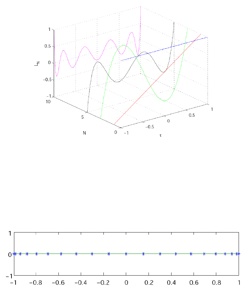
Figure 1.1: Illustration of the Legendre polynomials LN(τ) for N=
0,1,2,4,5,10.
Figure 1.2: Illustration of the Legendre Gauss Lobatto (LGL) nodes for
N= 20.
24

If L(τ) is a general smooth function, then for a suitable N, its integral
over τ∈[−1,1] can be approximated as follows:
Z1
−1
L(τ)dτ ≈
N
X
k=0
L(τk)wk(1.6)
The LGL nodes are selected to yield highly accurate numerical integrals.
For example, consider the definite integral
Z1
−1
etcos(t)dt
The exact value of this integral to 7 decimal places is 1.9334214. For N= 3
we have τ= [−1,−0.4472,0.4472,1], w= [0.1667,0.8333,0.8333,0.1667],
hence
Z1
−1
etcos(t)dt ≈wTh(τ)=1.9335
so that the error is O(10−5). On the other hand, if N= 5, then the approx-
imate value is 1.9334215, so that the error is O(10−7).
1.6.4 Interpolation and Legendre polynomials
The Legendre-Gauss-Lobatto quadrature motivates the following expression
to approximate the weights of the expansion (1.3):
ˆ
fk≈˜
fk=1
γk
N
X
j=0
f(τj)Lk(τj)wj
where
γk=
N
X
j=0
L2
k(τj)wj
It is simple to prove (see [23]) that with these weights, function f: [−1,1] →
<can be interpolated over the LGL nodes as a discrete expansion using
Legendre polynomials:
INf(τ) =
N
X
k=0
˜
fkLk(τ) (1.7)
such that
INf(τj) = f(τj) (1.8)
25

Because INf(τ) is an interpolant of f(τ) at the LGL nodes, and since the
interpolating polynomial is unique, we may express INf(τ) as a Lagrange
interpolating polynomial:
INf(τ) =
N
X
k=0
f(τk)Lk(τ) (1.9)
so that the expressions (1.7) and (1.9) are mathematically equivalent. Ex-
pression (1.9) is computationally advantageous since, as discussed below, it
allows to express the approximate values of the derivatives of the function f
at the nodes as a matrix multiplication. It is possible to write the Lagrange
basis polynomials Lk(τ) as follows [23]:
Lk(τ) = 1
N(N+ 1)LN(τk)
(τ2−1) ˙
LN(τ)
τ−τk
The use of polynomial interpolation to approximate a function using
the LGL points is known in the literature as the Legendre pseudospectral
approximation method. Denote fN(τ) = INf(τ). Then, we have:
f(τ)≈fN(τ) =
N
X
k=0
f(τk)Lk(τ) (1.10)
It should be noted that Lk(τj) = 1 if k=jand Lk(τj)=0, if k6=j, so
that:
fN(τk) = f(τk) (1.11)
Regarding the accuracy and error estimates of the Legendre pseudospec-
tral approximation, it is well known that for smooth functions f(τ), the rate
of convergence of fN(τ) to f(τ) at the collocation points is faster than any
power of 1/N . The convergence of the pseudospectral approximations used
by PSOPT has been analysed by Canuto et al [10].
Figure 1.3 shows the degree Ninterpolation of the function f(τ) =
1/(1 + τ+ 15τ2) in (N+ 1) equispaced and LGL points for N= 20. With
increasing N, the errors increase exponentially in the equispaced case (this
is known as the Runge phenomenon) whereas in the LGL case they decrease
exponentially.
1.6.5 Approximate differentiation
The derivatives of fN(τ) in terms of f(τ) at the LGL points τkcan be
obtained by differentiating Eqn. (1.10). The result can be expressed as a
matrix multiplication, such that:
˙
f(τk)≈˙
fN(τk) =
N
X
i=0
Dkif(τi)
26
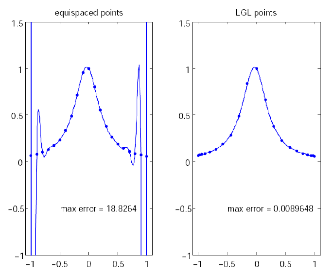
Figure 1.3: Illustration of polynomial interpolation over equispaced and LGL
nodes
.
27

where
Dki =
−LN(τk)
LN(τi)
1
τk−τiif k6=i
N(N+ 1)/4 if k=i= 0
−N(N+ 1)/4 if k=i=N
0 otherwise
(1.12)
which is known as the differentiation matrix.
For example, this is the Legendre differentiation matrix for N= 5.
D=
7.5000 −10.1414 4.0362 −2.2447 1.3499 −0.5000
1.7864 0 −2.5234 1.1528 −0.6535 0.2378
−0.4850 1.7213 0 −1.7530 0.7864 −0.2697
0.2697 −0.7864 1.7530 0 −1.7213 0.4850
−0.2378 0.6535 −1.1528 2.5234 0 −1.7864
0.5000 −1.3499 2.2447 −4.0362 10.1414 −7.5000
Figure 1.4 shows the Legendre differentiation of f(t) = sin(5t2) for N=
20 and N= 30. Note the vertical scales in the error curves. Figure 1.5 shows
the maximum error in the Legendre differentiation of f(t) = sin(5t2) as a
function of N. Notice that the error initially decreases very rapidly until
such high precision is achieved (accuracy in the order of 10−12) that round
off errors due to the finite precision of the computer prevent any further
reductions. This phenomenon is known as spectral accuracy.
1.6.6 Approximating a continuous function using Chebyshev
polynomials
PSOPT also has facilities for pseudospectral function approximation using
Chebyshev polynomials. Let TN(τ) denote the Chebyshev polynomial of
order N, which may be generated from:
TN(τ) = cos(Ncos−1(τ)) (1.13)
Let τk,k= 0, . . . , N be the Chebyshev-Gauss-Lobatto (CGL) nodes in the
interval [−1,1], which are defined as τk=−cos(πk/N) for k= 0,1, . . . , N.
Given any real-valued function f(τ) : [−1,1] → <, it can be approxi-
mated by the Chebyshev pseudospectral method:
f(τ)≈fN(τ) =
N
X
k=0
f(τk)ϕk(τ) (1.14)
where the Lagrange interpolating polynomial ϕk(τ) is defined by:
ϕk(τ) = (−1)k+1
N2¯ck
(1 −τ2)˙
TN(τ)
τ−τk
(1.15)
28
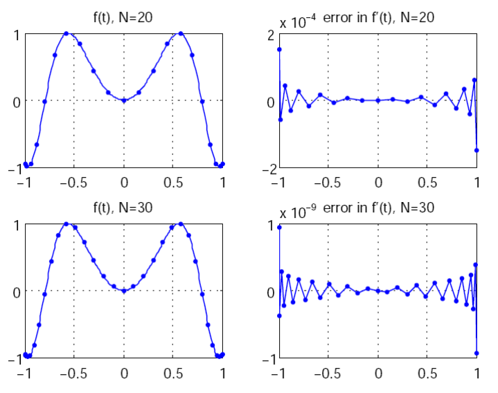
Figure 1.4: Legendre differentiation of f(t) = sin(5t2) for N= 20 and
N= 30.
29
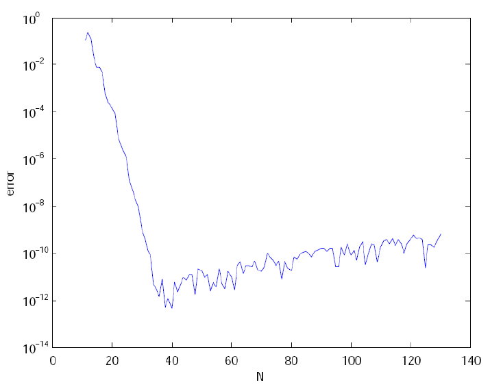
Figure 1.5: Maximum error in the Legendre differentiation of f(t) = sin(5t2)
as a function of N.
30
where
¯ck=2k= 0, N
1 1 ≤k≤N−1(1.16)
It should be noted that ϕk(τj) = 1 if k=jand ϕk(τj)=0, if k6=j, so
that:
fN(τk) = f(τk) (1.17)
1.6.7 Differentiation with Chebyshev polynomials
The derivatives of fN(τ) in terms of f(τ) at the CGL points τkcan be
obtained by differentiating (1.14). The result can be expressed as a matrix
multiplication, such that:
˙
f(τk)≈˙
FN(τk) =
N
X
i=0
Dkif(τi) (1.18)
where
Dki =
¯ck
2¯ci
(−1)k+i
sin[(k+i)π/2N] sin[(k−i)π/2N]if k6=i
τk
2 sin2[kπ/N]if i≤k=i≤N−1
−2N2+1
6if k=i= 0
2N2+1
6if k=i=N
(1.19)
which is known as the differentiation matrix.
1.6.8 Numerical quadrature with the Chebyshev-Gauss-Lobatto
method
Note that if h(τ) is a polynomial of degree ≤2N−1, its weighted integral
over τ∈[−1,1] can be exactly computed as follows:
Z1
−1
g(τ)h(τ)dτ =
N
X
k=0
h(τk)wk(1.20)
where τk,k= 0, . . . , N are the CGL nodes, d the weights wkare given by:
wk=π
2N, k = 0, . . . , N.
π
N, k = 1, . . . , N −1(1.21)
and g(τ) is a weighting function given by:
g(τ) = 1
√1−τ2(1.22)
If L(τ) is a general smooth function, then for a suitable N, its weighted
integral over τ∈[−1,1] can be approximated as follows:
Z1
−1
g(τ)L(τ)dτ ≈
N
X
k=0
L(τk)wk(1.23)
31
1.6.9 Differentiation with reduced round-off errors
The following differentiation matrix, which offers reduced round-off errors
[10], is employed optionally by PSOPT . It can be used both with Legrendre
and Chebyshed points.
Djl =
−δl
δj
(−1)j+l
τj−τlj6=l
N
P
i=0,i6=j
δi
δj
(−1)i+j
τj−τij=l(1.24)
1.7 The pseudospectral discretizations used in PSOPT
To illustrate the pseudospectral discretizations employed in PSOPT , con-
sider the following single phase continuous optimal control problem:
Problem P2
Find the control trajectories, u(t), t ∈[t0, tf], state trajectories x(t), t ∈
[t0, tf], static parameters p, and times t0, tf, to minimise the following per-
formance index:
J=ϕ[x(t0), x(tf), p, t0, tf] + Ztf
t0
L[x(t), u(t), p, t]dt
subject to the differential constraints:
˙x(t) = f[x(t), u(t), p, t], t ∈[t0, tf],
the path constraints
hL≤h[x(t), u(t), p, t]≤hU, t ∈[t0, tf]
the event constraints:
eL≤e[x(t0), u(t0), x(tf), u(tf), p, t0, tf]≤eU,
the bound constraints on states and controls:
uL≤u(t)≤uU, t ∈[t0, tf],
xL≤x(t)≤xU, t ∈[t0, tf],
and the constraints:
t0≤t0≤¯
t0,
tf≤tf≤¯
tf,
tf−t0≥0,
32

where
u: [t0, tf]→ Rnu
x: [t0, tf]→ Rnx
p∈ Rnp
ϕ:Rnx× Rnx× Rnp× R × R → R
L:Rnx× Rnu× Rnp×[t0, tf]→ R
f:Rnx× Rnu× Rnp×[t0, tf]→ Rnx
h:Rnx× Rnu× Rnp×[t0, tf]→ Rnh
e:Rnx× Rnu× Rnx× Rnu× <np× R × R → Rne
(1.25)
By introducing the transformation:
τ←2
tf−t0
t−tf+t0
tf−t0
,
it is possible to write problem P3using a new independent variable τin the
interval [−1,1], as follows:
Problem P3
Find the control trajectories, u(τ), τ ∈[−1,1], state trajectories x(τ), τ ∈
[−1,1], and times t0, tf, to minimise the following performance index:
J=ϕ[x(−1), x(1), p, t0, tf] + tf−t0
2Z1
−1
L[x(t), u(t), p, t]dτ
subject to the differential constraints:
˙x(τ) = tf−t0
2f[x(τ), u(τ), p, τ], τ ∈[−1,1],
the path constraints
hL≤h[x(τ), u(τ), p, τ]≤hU, τ ∈[−1,1]
the event constraints:
eL≤e[x(−1), u(−1), x(1), u(1), p, t0, tf]≤eU,
the bound constraints on controls and states:
uL≤u(τ)≤uU, τ ∈[−1,1],
xL≤x(τ)≤xU, τ ∈[−1,1],
and the constraints:
t0≤t0≤¯
t0,
33

tf≤tf≤¯
tf,
tf−t0≥0,
The description below refers to the Legendre pseudospectral approxima-
tion method. The procedure employed with the Chebyshev approximation
method is very similar. In the Legendre pseudospectral approximation of
problem P3, the state x(τ), τ∈[−1,1] is approximated by the N-order
Lagrange polynomial xN(τ) based on interpolation at the Legendre-Gauss-
Lobatto (LGL) quadrature nodes, so that:
x(τ)≈xN(τ) =
N
X
k=0
x(τk)φk(τ) (1.26)
Moreover, the control u(τ), τ∈[−1,1] is similarly approximated using
an interpolating polynomial:
u(τ)≈uN(τ) =
N
X
k=0
u(τk)φk(τ) (1.27)
Note that, from (1.11), xN(τk) = x(τk) and uN(τk) = u(τk). The derivative
of the state vector is approximated as follows:
˙x(τk)≈˙xN(τk) =
N
X
i=0
DkixN(τi), i = 0,...N (1.28)
where Dis the (N+ 1) ×(N+ 1) the differentiation matrix given by (??).
Define the following nu×(N+ 1) matrix to store the trajectories of the
controls at the LGL nodes:
UN=
u1(τ0)u1(τ1). . . u1(τN)
u2(τ0)u2(τ1). . . u2(τN)
.
.
..
.
....,.
.
.
unu(τ0)unu(τ1). . . unu(τN)
(1.29)
Define the following nx×(N+ 1) matrices to store, respectively, the
trajectories of the states and their derivatives at the LGL nodes:
XN=
x1(τ0)x1(τ1). . . x1(τN)
x2(τ0)x2(τ1). . . x2(τN)
.
.
..
.
....,.
.
.
xnx(τ0)xnx(τ1). . . xnx(τN)
(1.30)
34

and
˙
XN=
˙x1(τ0) ˙x1(τ1). . . ˙x1(τN)
˙x2(τ0) ˙x2(τ1). . . ˙x2(τN)
.
.
..
.
....,.
.
.
˙xnx(τ0) ˙xnx(τ1). . . ˙xnx(τN)
(1.31)
From (1.28), XNand ˙
XNare related as follows:
˙
XN=XNDT(1.32)
Now, form the following nx×(N+ 1) matrix with the right hand side of
the differential constraints evaluated at the LGL nodes:
FN=t0−tf
2
f1(xN(τ0), uN(τ0), p, τ0). . . f1(xN(τN), uN(τN), p, τN)
f2(xN(τ0), uN(τ0), p, τ0). . . f2(xN(τN), uN(τN), p, τN)
.
.
.....
.
.
fnx(xN(τ0), uN(τ0), p, τ0). . . fnx(xN(τN), uN(τN), p, τN)
(1.33)
Now, define the differential defects at the collocation points as the nx×
(N+ 1) matrix:
ζN=˙
XN−FN=XNDT−FN(1.34)
Define the matrix of path constraint function values evaluated at the
LGL nodes:
HN=
h1(xN(τ0), uN(τ0), p, τ0). . . h1(xN(τN), p, uN(τN), τN)
h2(xN(τ0), uN(τ0), p, τ0). . . h2(xN(τN), uN(τN), p, τN)
.
.
.....
.
.
hnh(xN(τ0), uN(τ0), p, τ0). . . hnh(xN(τN), uN(τN), p, τN)
(1.35)
The objective function of P3is approximated as follows:
J=ϕ[x(−1), x(1), p, t0, tf] + tf−t0
2Z1
−1
L[x(τ), u(τ), p, τ]dτ
≈ϕ[xN(−1), xN(1), p, t0, tf] + tf−t0
2
N
X
k=0
L[xN(τk), uN(τk), p, τk]wk
(1.36)
where the weights wkare defined in (1.5).
We are now ready to express problem P3as a nonlinear programming
problem, as follows.
35

Problem P4
min
yF(y) (1.37)
subject to:
Gl≤G(y)≤Gu
yl≤y≤yu
(1.38)
The decision vector y, which has dimension ny= (nu(N+ 1) + nx(N+
1) + np+ 2), is constructed as follows:
y=
vec(UN)
vec(XN)
p
t0
tf
(1.39)
The objective function is:
F(y) = ϕ[xN(−1), xN(1), p, t0, tf] + tf−t0
2
N
X
k=0
L[xN(τk), uN(τk), p, τk]wk
(1.40)
while the constraint function G(y), which is of dimension ng=nx(N+ 1) +
nh(N+ 1) + ne+ 1, is given by:
G(y) =
vec(ζN)
vec(HN)
e[xN(−1), uN(−1), xN(1), uN(1), p, t0, tf]
tf−t0
,(1.41)
The constraint bounds are given by:
Gl=
0nx(N+1)
stack(hL, N + 1)
eL
(t0−tf)
, Gu
0nx(N+1)
stack(hU, N + 1)
eU
0
,(1.42)
and the bounds on the decision vector are given by:
yl=
stack(ul, N + 1)
stack(xL, N + 1)
pL
t0
tf
, yu
stack(uU, N + 1)
stack(xU, N + 1)
pU
t0
tf
,(1.43)
where vec(A) forms a nm-column vector by vertically stacking the columns
of the n×mmatrix A, and stack(x, n) creates a mn-column vector by
stacking ncopies of column m-vector x.
36
1.7.1 Costate estimates
Legendre approximation method
PSOPT implements the following approximation for the costates λ(τ)∈
<nx, τ ∈[−1,1] associated with P3[18]:
λ(τ)≈λN(τ) =
N
X
k=0
λ(τk)φk(τ), τ ∈[−1,1] (1.44)
The costate values at the LGL nodes are given by:
λ(τk) = ˜
λk
wk
, k = 0,...N (1.45)
where wkare the weights given by (1.5), and ˜
λk∈ <nx,k= 0, . . . , N are the
KKTs multiplier associated with the collocation constraints vec(ζN) = 0.
The KKT multipliers can normally be obtained from the NLP solver, which
allows PSOPT to return estimates of the costate trajectories at the LGL
nodes.
It is known from the literature [18] that the costate estimates in the
Legendre discretization method sometimes oscillate around the true values.
To mitigate this, the estimates are smoothed by taking a weighted average
for the estimats at kusing the costate estimates at k−1, kand k+1 obtained
from (1.44).
Chebyshev approximation method
PSOPT implements the following approximation for the costates λ(τ)∈
<nx, τ ∈(−1,1) associated with P3at the CGL nodes [32]:
λ(τk) = ˜
λk
q1−τ2
kwk
, k = 0,...N −1 (1.46)
where wkare the weights given by (1.21), and ˜
λk∈ <nx,k= 0, . . . , N are
the KKTs multiplier associated with the collocation constraints vec(ζN) = 0.
Since (1.46) is singular for τ0=−1 and τN= 1, the estimates of the co-
states at τ=±1 are found using linear extrapolation. The costate estimates
are also smoothed as described in 1.7.1
1.7.2 Discretizing a multiphase problem
It now becomes straightforward to describe the discretization used by PSOPT in
the case of P1, a problem with multiple phases, to form a nonlinear program-
37
ming problem like P4. The decision variables of the NLP associated with
P1are given by:
y=
vec(UN,(1))
vec(XN,(1))
p(1)
t(1)
0
t(1)
f
.
.
.
vec(UN,(Np))
vec(XN,(Np))
p(Np)
t(Np)
0
t(Np)
f
(1.47)
where Npis the number of phases in the problem, and the superindex in
parenthesis indicates the phase to which the variables belong. The constraint
function G(y) is given by:
G(y) =
vec(ζN,(1))
vec(HN,(1))
e[xN,(1)(−1), uN,(1)(−1), xN,(1)(1), uN,(1)(1), p(1), t(1)
0, t(1)
f]
t(1)
f−t(1)
0
.
.
.
vec(ζN,(Np))
vec(HN,(Np))
e[xN,(Np)(−1), uN,(Np)(−1), xN,(Np)(1), uN,(Np)(1), p(Np), t(Np)
0, t(Np)
f]
t(Np)
f−t(Np)
0
Ψ
,
(1.48)
where Ψ corresponds to the linkage constraints associated with the problem,
evaluated at y.
Based on the problem information, it is straightforward (but not shown
here) to form the bounds on the decision variables yl,yuand the bounds
on the constraints function Gl, Guto complete the definition of the NLP
problem associated with P1.
1.8 Parameter estimation problems
A parameter estimation problem arises when it is required to find values
for parameters associated with a model of a system based on observations
38

from the actual system. These are also called inverse problems. The ap-
proach used in the PSOPT implementation uses the same techniques used
for solving optimal control problems, with a special objective function used
to measure the accuracy of the model for given parameter values.
1.8.1 Single phase case
For the sake of simplicity consider first a single phase problem defined over
t0≤t≤tfwith the dynamics given by a set of ODEs:
˙x=f[x(t), u(t), p, t]
the path constraints
hL≤h[x(t), u(t), p, t]≤hU
the event constraints
eL≤e[x(t0), u(t0), x(tf), u(tf), p, t0, tf]≤eU
Consider the following model of the observations (or measurements) taken
from the system:
y(θ) = g[x(θ), u(θ), p, θ]
where g:Rnx× Rnu× Rnp× R → Rnois the observations function, and
y(θ)∈ Rnois the estimated observation at sampling instant θ. Assume
that {˜y}ns
k=1 is a sequence of nsobservations corresponding to the sampling
instants {θk}ns
k=1.
The objective is to choose the parameter vector p∈ Rnpto minimise the
cost function:
J=1
2
ns
X
k=1
no
X
j=1
r2
j,k
where the residual rj,k ∈ R is given by:
rj,k =wj,k[gj[x(θk), u(θk), p, θk]−˜yj,k]
where wj,k ∈ R, j = 1, . . . , no, k = 1, . . . , nsis a positive residual weight, gj
is the j-th element of the vector observations function g, and ˜yj,k is the j-th
element of the actual observation vector at time instant θk.
Note that in the parameter estimation case the times t0and tfare as-
sumed to be fixed. The sampling instants need not coincide with the collo-
cation points, but they must obey the relationship:
t0≤θk≤tf, k = 1, . . . , ns
39

1.8.2 Multi-phase case
In the case of a problem with Npphases, let t(i)
0≤t≤t(i)
fbe the intervals
for each phase, with the dynamics given by a set of ODEs:
˙x(i)=f(i)[x(t)(i), u(i)(t), p(i), t]
the path constraints
h(i)
L≤h(i)[x(i)(t), u(i)(t), p(i), t]≤h(i)
U
the event constraints
e(i)
L≤e(i)[x(i)(t0), u(i)(t0), x(i)(tf), u(i)(tf), p(i), t(i)
0, t(i)
f]≤e(i)
U
Consider the following model of the observations (or measurements) taken
from the system for each phase:
y(i)(θ(i)
k) = g(i)[x(i)(θ(i)
k), u(i)(θ(i)
k), p(i), θ(i)
k]
where g(i):Rn(i)
x× Rn(i)
u× Rn(i)
p× R → Rn(i)
ois the observations function
for each phase, and y(i)(θ(i)
k)∈ Rn(i)
ois the estimated observation at sam-
pling instant θ(i)
k. Assume that ˜y(i)n(i)
s
k=1 is a sequence of n(i)
sobservations
corresponding to the sampling instants nθ(i)
kon(i)
s
k=1.
The objective is to choose the set of parameter vectors p(i)∈ Rn(i)
p, i ∈
[1, Np] to minimise the cost function:
J=1
2
Np
X
i=1
n(i)
s
X
k=1
n(i)
o
X
j=1 hr(i)
j,ki2
where the residual r(i)
j,k ∈ R is given by:
r(i)
j,k =w(i)
j,k[g(i)
j[x(θ(i)
k), u(i)(θ(i)
k), p(i), θ(i)
k]−˜y(i)
j]
where w(i)
j,k ∈ R is a positive residual weight, g(i)
jis the j-th element of the
vector observations function g(i), and ˜y(i)
jis the j-th element of the actual
observation vector at time instant θ(i)
k
Note that in the parameter estimation case the times t(i)
0and t(i)
fare
assumed to be fixed. The sampling instants need not coincide with the
collocation points, but they must obey the relationship:
t(i)
0≤θ(i)
k≤t(i)
f, k = 1, . . . , n(i)
s
40

1.8.3 Statistical measures on parameter estimates
PSOPT computes a residual matrix [r(i)
j,k] for each phase iand for the final
value of the estimated parameters in all phases ˆp∈ Rnp, where each element
of the residual matrix is related to an individual measurement sample and
observation within a phase. PSOPT also computes the covariance matrix
C∈ Rnp×npof the parameter estimates using the method described in [27],
which uses a QR decomposition of the Jacobian matrix of the equality and
active inequality constraints, together with the Jacobian matrix of the resid-
ual vector function (a stack of the elements of the residual matrices for all
phases) with respect to all decision variables. In addition PSOPT computes
95% confidence intervals on the estimated parameters. The upper and lower
limits of the confidence interval around the estimated value for parameter
ˆpiare computed from [30]:
δi=±t1−(α/2)
Ns−nppCii (1.49)
where Nsis the total number of individual samples, npis the number of
parameters, tis the inverse two tailed cumulative t-distribution with confi-
dence level α, and N−npdegrees of freedom.
The residual matrix, the covariance matrix and the confidence intervals
can be used to refine the parameter estimation problem. For instance, if
the resulting confidence interval of one particular parameter is found to be
small, the value of this parameter can be fixed by the user in a subsequent
run, which may improve the estimates other parameters being estimated and
reduces the possibility of having an overdetermined problem (i.e. a problem
with too many parameters to be estimated). See [37] pages 210-211 for more
details.
Notice, however, that the statistical analysis performed is based on a
linearization of the model. As a result, the validity of the statistical anal-
ysis is dependent on the quality of the linearization and the curvature of
the underlying functions being linearized, so care must be taken with the
interpretation of results of the statistical analysis of the parameter estimates
[37].
1.8.4 Remarks on parameter estimation
•In contrast to continuous optimal control problems, the kind of pa-
rameter estimation problem considered involves the evaluation of the
objective at a finite number of sampling points. Internally, the values
of the state and controls are interpolated over the collocation points
to find estimated values at the sampling points. The type of interpo-
lation employed depends on the collocation method specified by the
user.
41
•Note that the sampling instants do not have to be sorted in ascending
or descending order. Because of this, it is possible to accommodate
problems with non-simultaneous observations of different variables by
stacking the measured data and sampling instants for the different
variables.
•It is possible to use an alternative objective function where the resid-
uals are weighted with the covariance of the measurements simply by
multiplying the observations function and the measurements vectors
by the square root of the covariance matrix, see [4], page 221 for more
details.
•When defining parameter estimation problems, the user needs to en-
sure that the underlying nonlinear programming problem has sufficient
degrees of freedom. This is particularly important as it is common for
parameter estimation problems not to involve any control variables.
The number of degrees of freedom is the difference between the number
of decision variables and the total number of equality and active in-
equality constraints. For example, in the case of a single phase problem
having nxdifferential states, nucontrol variables (or algebraic states),
nhequality path constraints, and neequality event constraints, the
number of relevant constraints is given by:
nc=nx(N+ 1) + nh(N+ 1) + ne+ 1
where Nis the degree of the polynomial approximation (in the case
of a pseudospectral discretization). The number of decision variables
is given by:
ny=nu(N+ 1) + nx(N+ 1) + np+ 2
The difference is:
ny−nc= (nu−nh)(N+ 1) + np+ 1 −ne
For the problem to be solvable it is important that ny−nc≥0,
ideally ny−nc≥1. The total numbers of constraints and deci-
sion variables are always reported in the terminal window when a
PSOPT problem is run. It should be noted that the nonlinear pro-
gramming solver (IPOPT) may modify the numbers by eliminating
redundant constraints or decision variables. These modifications are
also visible when a problem is run.
1.9 Alternative local discretizations
Direct collocation methods that use local information to approximate the
functions associated with an optimal control problem are well established [3].
42

Sometimes, it may be convenient for users to compare the performance and
solutions obtained by means of the pseudospectral methods implemented in
PSOPT , with local discretization methods. Also, if a given problem can-
not be solved by means of a pseudospectral discretization, the user has the
option to try the local discretizations implemented in PSOPT . The main
impact of using a local discretization method as opposed to a pseudospectral
discretization method, is that the resulting Jacobian and Hessian matrices
needed by the NLP solver are more sparse with local methods, which facil-
itates the NLP solution. This becomes more noticeable as the number of
grid points increases. The disadvantage of using a local method is that the
spectral accuracy in the discretization of the differential constraints offered
by pseudospectral methods is lost. Moreover, the accuracy of Gauss type in-
tegration employed in pseudospectral methods is also lost if pseudospectral
grids are not used.
Note also that local mesh refinement methods are well established. These
methods concentrate more grid points in areas of greater activity in the func-
tion, which helps improve the local accuracy of the solution. The trapezoidal
method has an accuracy of O(h2), while the Hermite-Simpson method has
an accuracy of O(h4), where his the local interval between grid points. Both
the trapezoidal and Hermite-Simpson discretization methods are widely used
in computational optimal control, and have solve many challenging problems
[3]. When the user selects the trapezoidal or Hermite-Simpson discretiza-
tions, and if the initial grid points are not provided, the grid is started with
equal spacing between grid points. In these two cases any integrals asso-
ciated with the problem are computed using the trapezoidal and Simpson
quadrature method, respectively.
Additionally, an option is provided to use a differentiation matrix based
on the central difference method (which has an accuracy of O(h2)) in con-
junction with pseudospectral grids. The central differences option uses either
the LGL or the Chebyshev points and Gauss-type quadrature.
The local discretizations implemented in PSOPT are described below.
For simplicity, the phase index has been omitted and reference is made to
single phase problems. However, the methods can also be used with multi-
phase problems.
1.9.1 Trapezoidal method
With the trapezoidal method [3], the defect constraints are computed as
follows:
ζ(τk) = x(τk+1)−x(τk)−hk
2(fk+fk+1),(1.50)
where ζ(τk)∈ <nxis the vector of differential defect constraints at node
τk,k= 0, . . . , N −1, hk=τk+1 −τk,fk=f[(τk), u(τk), p, τk], fk+1 =
43
f[x(τk+1), u(τk+1), p, τk+1]. This gives rise to nxNdifferential defect con-
straints. In this case, the decision vector for single phase problems is given
by equation (1.39), so that it is the same as the one used in the Legendre
and Chebyshev methods.
1.9.2 Hermite-Simpson method
With the Hermite-Simpson method [3], the defect constraints are computed
as follows:
ζ(τk) = x(τk+1)−x(τk)−hk
6(fk+ 4 ¯
fk+1 +fk+1),(1.51)
where
¯
fk+1 =f[¯xk+1,¯uk+1, p, τk+hk
2]
¯xk+1 =1
2(x(τk) + x(τk+1)) + hk
8(fk−fk+1)
where ζ(τk)∈ <nxis the vector of differential defect constraints at node
τk,k= 0, . . . , N −1, hk=τk+1 −τk,fk=f[(τk), u(τk), p, τk], fk+1 =
f[x(τk+1), u(τk+1), p, τk+1], and ¯uk+1 = ¯u(τk+1) is a vector of midpoint con-
trols (which are also decision variables). This gives rise to nxNdifferential
defect constraints. In this case, the decision vector for single phase problems
is given by
y=
vec(UN)
vec(XN)
p
vec( ¯
UN)
t0
tf
(1.52)
with
¯
UN=
¯u1(τ1) ¯u1(τ2). . . ¯u1(τN)
¯u2(τ1) ¯u2(τ2). . . ¯u2(τN)
.
.
..
.
....,.
.
.
¯unu(τ1) ¯unu(τ2). . . ¯unu(τN)
(1.53)
so that this decision vector is different from the one used in the Legendre
and Chebyshev methods as it includes the midpoint controls.
44

1.9.3 Central difference method
This method computes the differential defect constraints using equation
(1.34), but using a (N+ 1) ×(N+ 1) differentiation matrix given by:
D0,0=−1/h0
D0,1= 1/h0
Di−1,i = 1/(hi+hi−1), i = 2,...N
Di−1,i−2=−1/(hi+hi−1)i= 2,...N
DN,N−1=−1/hN−1
DN,N = 1/hN−1
where hk=τk+1 −τk. The method uses forward differences at τ0, backward
differences at τN, and central differences at τk,k= 1, . . . , N −1. In this case,
the decision vector for single phase problems is given by equation (1.39), so
that it is the same as the one used in the Legendre and Chebyshev methods.
Notice that this discretization has less accuracy at both ends of the interval.
This is compensated by the use of pseudospectral grids, which concentrate
more grid points at both ends of the interval.
1.9.4 Costate estimates with local discretizations
In the case of the trapezoidal and Hermite-Simpson discretizations, the
costates at the discretization nodes are approximated according to the fol-
lowing equation:
λ(tk+1
2)≈˜
λk
2hk
, k = 0,...N −1
where λ(tk+1
2) is the costate estimate at the midpoint in the interval between
tkand tk+, ˜
λk∈ <nxis the vector of Lagrange multiplers obtained from
the nonlinear programming solver corresponding to the differential defect
constraints, and hk=tk+1 −tk.
In the case of the central-differences discretization, the costates are es-
timated as described in section 1.7.1.
1.10 External software libraries used by PSOPT
PSOPT relies on various of libraries to perform a number of tasks.
1.10.1 BLAS and CLAPACK (or LAPACK)
These are standard and widely used linear algebra packages which can be
downloaded in source and binary form from http://www.netlib.org. Some
current Linux distrubutions, such as Ubuntu, make it very easy to install
both BLAS and LAPACK libraries using a package manager.
45
1.10.2 DMatrix library
This is a C++ matrix library developed by the author which is included with
the distrubution. DMatrix and SparseMatrix objects are used internally in
the implementation, while DMatrix objects are used as part of the interface.
Documentation on the use of this library is included with the distribution,
under the directory psopt-4.0.0 /dmatrix/doc, although the essential use
of the DMatrix objects is quite intuitive and can be learned from the ex-
amples given in this document. The DMatrix library makes direct use of
LAPACK, SuiteSparse and LUSOL functions.
1.10.3 SuiteSparse
This is an open source sparse matrix computation library written in C by
T. Davis [14], which can be downloaded from
http://faculty.cse.tamu.edu/davis/suitesparse.html
1.10.4 LUSOL
This is an open source sparse LU factorisation library written by M.A. Saun-
ders and co-workers [21], which can be downloaded from
http://www.stanford.edu/group/SOL/software/lusol/lusol.zip
1.10.5 IPOPT
IPOPT is an open source C++ package for large-scale nonlinear optimiza-
tion, which uses an interior point method [44]. IPOPT is the default nonlin-
ear programming algorithm used by PSOPT . IPOPT can be downloaded
from
https://projects.coin-or.org/Ipopt
The current release of PSOPT uses IPOPT version 3.12.12.
Note that the installation script also installs the linear algebra library
MUMPS and the matrix odering algorithm METIS, which are used by
IPOPT.
1.10.6 ADOL-C
ADOL-C is a library for the automatic differentiation of C++ code. It al-
lows to compute automatically the gradients and sparse Jacobians required
by PSOPT . At the heart of the ADOL-C library is the “adouble” data
type, which can be mostly treated as a C++ “double”. A copy of ADOL-C
is included with the distribution of PSOPT . Some current Linux distru-
butions, such as Ubuntu, make it very easy to install the ADOL-C library
and headers using a package manager. It can also be downloaded from:
https://projects.coin-or.org/ADOL-C
46
The current release of PSOPT uses ADOL-C version 2.6.3.
An important thing to keep in mind is that if an intermediate variable
within a C++ function depends on one or more adouble variables, it should
be declared as adouble. Conversely, if a C++ variable within a function
does not depend on any adouble variables, it can be declared as the usual
double type.
Note that the installation script also install the graph colouring library
COLPACK, which is used by ADOL-C.
1.10.7 GNUplot (optional)
Gnuplot is a portable command-line driven interactive data and function
plotting utility which runs on many computer platforms. The software is
freely distributed. The source code can be downloaded from the following
page:
http://www.gnuplot.info
Some current Linux distrubutions, such as Ubuntu, make it very easy to
install GNUplot using a package manager.
1.11 Supported platform
The current release of PSOPT has been successfully compiled under the
following operating system and compiler:
•Ubuntu Linux version 18.04. It has been tested on Intel based PC’s
under the 64 bit variant of this operating system using the GCC compiler
version 7.3.0, which is installed with the above release of Ubuntu.
It is possible that PSOPT will also compile and work on earlier versions
of the above operating system and compiler, but time and resources do not
allow for testing all possible combinations.
1.12 Repository and home page
The downloadable PSOPT distribution is held in its GitHub page:
https://github.com/PSOPT/psopt
An web page is maintained to provide general information about PSOPT :
http://www.psopt.org.
1.13 Release numbering
PSOPT release numbering is sequential increasing by 1 with every release.
The versio control software Git may provide additional tags to identify re-
leases and builds.
47

1.14 Installing and compiling PSOPT
1.14.1 Ubuntu Linux 18.4
To install PSOPT on a Ubuntu 18.04 distribution, simply download the
installation script install-ubuntu-18.04.sh from the GitHub page:
https://github.com/PSOPT/psopt
and execute it from a terminal window. This script will install and down-
load all the required libraries and programmes from the Ubuntu repository,
and also will download, compile and install other software libraries that
are needed. You will need the root password to perform and complete the
installation.
The installation process will create the following directory structure un-
der the home folder.
psopt-4.0.0
- dmatrix
- - src
- - examples
- - doc
- - include
- PSOPT
- - src
- - examples
- - doc
The installation process will generate a number of exacutables within
the various directories under the psopt-4.0.0 /PSOPT/examples directory.
It will also run one of the examples as a test. You will see a plot appearing
on the screen.
After successful compilation, PSOPT is ready to be used. To see some
of the examples running, move to the appropriate directory and run the
executable file. For example, to run the “launch” example, do as follows:
$cd PSOPT/examples/launch
$./launch
1.15 Limitations and known issues
1. The discretization techniques used by PSOPT give approximate solu-
tions for the state and control trajectories. The software is intended to
be used for problems where the control variables are continuous (within
a phase) and the state variables have continuous derivatives (within a
phase). If within a phase the solution to the optimal control problem is
of a different nature, the results may be incorrect or the optimization
algorithm may fail to converge. Furthermore, PSOPT may not be
48
suitable for solving problems involving differential-algebraic equations
with index greater than one. Some of these issues can be avoided by
reformulating the problem to have several phases.
2. The solution obtained by PSOPT corresponds to a local minimum of
the discretized optimization problem. If the problem is suspected to
have several local minima, then it may be worth trying various initial
guesses.
3. The automatic scaling procedures work well for all the examples pro-
vided. However, note that the scaling of variables depends on the user
provided bounds. If these bounds are not adequate for the problem,
then the resulting scaling may be poor and this may lead to incorrect
results or convergence problems. In some cases, users may need to
provide the scaling factors manually to obtain satisfactory results.
4. The automatic mesh refinement procedures require an initial guess for
the number of nodes in the global case (the number and/or initial
distribution of nodes in the local case). If this initial guess is not
adequate (e.g. the grid is too coarse or to dense), the mesh refine-
ment procedure may fail to converge. In some cases, the user may
need to manually tune some of the parameters of the mesh refinement
procedure to achieve satisfactory results.
5. The efficiency with which the optimal control problem is solved de-
pends in a good deal on the correct formulation of the problem. Un-
suitable formulations may lead to trouble in finding a solution. More-
over, if the constraints are such that the problem is infeasible or if
for any other reason the solution does not exist, then the nonlinear
programming algorithm will fail.
6. The user supplied functions which define the cost function, DAE’s,
event and linkage constraints, are all assumed to be continuous and to
have continuous first and second derivatives. Non-differentiable func-
tions may cause covergence problems to the optimization algorithm.
Moreover, it is known that discontinuities in the second derivatives
may also cause convergence problems.
7. Only single phase problems are supported if the dynamics involve de-
lays in the states or controls.
8. Note that the constraints associated with the problem are only en-
forced at the discretization nodes, not in the interval between the
nodes.
9. When the problem requires a large number of nodes (say over 200)
the nonlinear programming algorithm may have problems to converge
49
if global collocation is being used. This may be due to numerical
difficulties within the nonlinear programming solver as the Jacobian
(and Hessian) matrices may not be sufficiently sparse. This occurs
because the pseudospectral differentiation matrices are dense. When
faced with this problem the user may wish to try the local collocation
options availble within PSOPT , or to split the problem into multiple
segments to increase the sparsity of the derivatives. Note that the
sparsity of the Jacobian and Hessian matrices is problem dependent.
10. The co-state approximations resulting from the Legendre pseudospec-
tral method are not as accurate as those obtained by means of the
Gauss pseudospectral method [2]. Moreover, the co-state approxima-
tions obtained by PSOPT using the Chebyshev pseudospectral meth-
ods are rather innacurate close to the edges of the time interval within
each phase. Also the co-state approximation used in the the case
of local discretizations (trapezoidal, Hermite-Simpson) converges at a
lower rate (is less accurate) than the states or the controls.
11. Sometimes there are crashes when computing sparse derivatives with
ADOL-C if the number of NLP variables is very large. This can be
avoided by switching to numerical differentiation.
50
Chapter 2
Defining optimal control and
estimation problems for
PSOPT
Defining an optimal control or parameter estimation problem involves spec-
ifying all the necessary values and functions that are needed to solve the
problem. With PSOPT , this is done by implementing C++ functions
(e.g. the cost function), and assigning values to data structures which are
described below. Once a PSOPT has obtained a solution, the relevant vari-
ables can be obtained by interrogating a data structure.
2.1 Interface data structures
The role of each structure used in the PSOPT interface is summarised be-
low.
•Problem data structure: This structure is used to specify problem
information, including the number of phases and pointers to the rel-
evant functions, as well as phase related information such as number
of states, controls, parameters, number of grid points, bounds on vari-
ables (e.g. state bounds), and functions (e.g. path function bounds).
•Algorithm data structure: This is used to control the solution algo-
rithm and to pass parameters to the NLP solver.
•Solution data structure: This is used to store the resulting variables
of a PSOPT run.
2.2 Required functions
Table 2.1 lists and describes the parameters used by the interface functions.
51

Parameter Type Role Description
controls adouble* input Array of intantaneous controls
derivatives adouble* output Array of intantaneous state derivatives
eadouble* output Array of event constraints
final_states adouble* input Array of final states within a phase
initial_states adouble* input Array of initial states within a phase
iphase int input Phase index (starting from 1)
linkages adouble* output Array of linkage constraints
parameters adouble* input Array of static parameters within a phase
states adouble* input Array of intantaneous states within a phase
time adouble input Instant of time within a phase
t0 adouble input Initial phase time
tf adouble input final phase time
xad adouble* input vector of scaled decision variables
workspace Workspace* input Pointer to workspace structure
Table 2.1: Description of parameters used by the PSOPT interface func-
tions
2.2.1 endpoint cost function
The purpose of this function is to specify the terminal costs φi[·], i=
1, . . . , N. The function prototype is as follows:
adouble endpoint_cost(adouble* initial_states,
adouble* final_states,
adouble* parameters,
adouble& t0, adouble& tf,
adouble* xad, int iphase,
Workspace* workspace)
The function should return the value of the end point cost, depending on
the value of phase index iphase, which takes on values between 1 and
problem.nphases.
Example of writing the endpoint cost function for a single phase problem
with the following endpoint cost:
ϕ(x(tf)) = x1(tf)2+x2(tf)2(2.1)
adouble endpoint_cost(adouble* initial_states,
adouble* final_states,
adouble* parameters,
adouble& t0, adouble& tf,
adouble* xad, int iphase,
52

Workspace* workspace)
{
adouble x1f = final_states[ CINDEX(1) ];
adouble x2f = final_states[ CINDEX(2) ];
return ( x1f*x1f + x2f*x2f);
}
2.2.2 integrand cost function
The purpose of this function is to specify the integrand costs Li[·] for each
phase as a function of the states, controls, static parameters and time. The
function prototype is as follows:
adouble integrand_cost(adouble* states,
adouble* controls,
adouble* parameters,
adouble& time,
adouble* xad,
int iphase,
Workspace* workspace)
The function should return the value of the integrand cost, depending on the
phase index iphase, which takes on values between 1 and problem.nphases.
Example of writing the integrand cost for a single phase problem with
Lgiven by:
L(x(t), u(t), t) = x1(t)2+x2(t)2+ 0.01u(t)2(2.2)
adouble integrand_cost(adouble* states,
adouble* controls,
adouble* parameters,
adouble& time,
adouble* xad,
int iphase,
Workspace* workspace)
{
adouble x1 = states[ CINDEX(1) ];
adouble x2 = states[ CINDEX(2) ];
adouble u = controls[ CINDEX(1) ];
53

return ( x1*x1 + x2*x2 + 0.01*u*u );
}
If the problem does not involve any cost integrand, the user may sim-
ply not register any cost_integrand function, or register it as follows:
problem.cost_integrand=NULL.
2.2.3 dae function
This function is used to speficy the time derivatives of the states ˙x(i)=
fi[·] for each phase as a function of the states themselves, controls, static
parameters, and time, as well as the algebraic functions related to the path
constraints. Its prototype is as follows:
void dae(adouble* derivatives,
adouble* path,
adouble* states,
adouble* controls,
adouble* parameters,
adouble& time,
adouble* xad,
int iphase,
Workspace* workspace)
This is an example of writing the dae function for a single phase problem
with the following state equations and path constraints:
˙x1=x2
˙x2=−3 exp(x1)−4x2+u
0≤x2
1+x2
2≤1
(2.3)
Note that the bounds are specified separately.
void dae(adouble* derivatives,
adouble* path,
adouble* states,
adouble* controls,
adouble* parameters,
adouble& time,
adouble* xad,
int iphase,
54

Workspace* workspace)
{
adouble x1 = states[ CINDEX(1) ];
adouble x2 = states[ CINDEX(2) ];
adouble u = controls[ CINDEX(1) ];
derivatives[ CINDEX(1) ] = x2;
derivatives[ CINDEX(2) ] = -3*exp(x1)-4*x2+u;
path[ CINDEX(1) ] = x1*x1 + x2*x2
}
2.2.4 events function
This function is used to speficy the values of the event constraint functions
ei[·] for each phase. Its prototype is as follows:
void events(adouble* e,
adouble* initial_states,
adouble* final_states,
adouble* parameters,
adouble& t0,
adouble& tf,
int iphase,
Workspace* workspace)
The following is an example of writing the events function for a single
phase problem with the event constraints:
1 = e1(t0) = x1(t0)
2 = e2(t0) = x2(t0)
−0.1≤e3(t0) = x1(tf)x2(tf)≤0.1
(2.4)
Note that the bounds are specified separately.
void events(adouble* e,
adouble* initial_states,
adouble* final_states,
adouble* parameters,
adouble& t0,
adouble& tf,
int iphase,
Workspace* workspace)
{
adouble x1i = initial_states[ CINDEX(1) ];
55

adouble x2i = initial_states[ CINDEX(2) ];
adouble x1f = final_states[ CINDEX(1) ];
adouble x2f = final_states[ CINDEX(2) ];
e[ CINDEX(1) ] = x1i;
e[ CINDEX(2) ] = x2i;
e[ CINDEX(3) ] = x1f*x2f;
}
2.2.5 linkages function
This function is used to speficy the values of the phase linkage constraint
functions Ψ[·]. Its prototype is as follows:
void linkages( adouble* linkages,
adouble* xad,
Workspace* workspace)
The following is an example of writing the linkages function for a two
phase problem with two states in each phase and with the linkage con-
straints:
0=Ψ1=x(0)
1(t(1)
f)−x(2)
1(t(2)
i)
0=Ψ2=x(1)
2(t(1)
f)−x(2)
2(t(2)
i)
0=Ψ3=t(1)
f−t(2)
i
(2.5)
Note that the bounds are specified separately. These type of state
and time continuity constraint can be entered automatically by using the
auto link function as shown below.
void linkages( adouble* linkages, adouble* xad, Workspace* workspace)
{
int index = 0;
// Link phases 1 and 2
auto_link( linkages, &index, xad, 1, 2 );
}
It is of course also possible to implement more general linkage con-
straints, as illustrated through the following example.
56

Consider a two phase problem with two states in each phase and with
the nonlinear linkage constraints:
0 = Ψ1=x(1)
1(t(1)
f)−sin[x(2)
1(t(2)
i)]
0 = Ψ2=x(1)
2(t(1)
f)−cos[x(2)
2(t(2)
i)]
0 = Ψ3=t(1)
f−t(2)
i
(2.6)
void linkages( adouble* linkages, adouble* xad, Workspace* workspace)
{
adouble xf_p0[ 2 ];
adouble xi_p1[ 2 ];
adouble tf_p0;
adouble ti_p1;
get_final_states( xf_p0, xad, 1 );
get_initial_states( xf_p1, xad, 2 );
tf_p0 = get_final_time( xad, 1);
ti_p1 = get_initial_time( xad, 2);
linkages[CINDEX(1)]=xf_p0[CINDEX(1)]-sin(xi_p1[CINDEX(1)]);
linkages[CINDEX(2)]=xf_p0[CINDEX(2)]-cos(xi_p1[CINDEX(2)]);
linkages[CINDEX(3)]=tf_p0 - ti_p1;
}
2.2.6 Main function
Declaration of data structures
The main() function is used to declare and initialise the problem,solution,
and algorithm data structures, to call the PSOPT algorithm, and to post-
process the results. To declare the data structures the user may wish to use
the following commands:
Alg algorithm;
Sol solution;
Prob problem;
Problem level information
The user should then define the problem name as follows:
problem.name = "My problem";
The number of phases and the number of linkage constraints should be
declared afterwards. For example, for a single phase problem:
57
problem.nphases=1;
problem.nlinkages=0;
This declaration should be followed by the following function call, which
initialises problem level structures.
psopt_level1_setup(problem);
Phase level information
After this, the user needs to specify phase level parameters using the follow-
ing syntax:
problem.phases(iphase).nstates = INTEGER;
problem.phases(iphase).ncontrols = INTEGER;
problem.phases(iphase).nevents = INTEGER;
problem.phases(iphase).npath = INTEGER;
problem.phases(iphase).nodes = INTEGER OR STRING;
The number of nodes in the grid can be speficied as a single value (e.g.
30), or a character string with the node sequence to be tried (if manual mesh
refinement is being used): “[30, 50, 60]”.
Once the phase level dimensions have been specified it is necessary to
call the following function:
psopt_level2_setup(problem, algorithm);
Phase bounds information
The syntax to enter state bounds is as follows:
problem.phases(iphase).bounds.lower.states(j) = REAL;
problem.phases(iphase).bounds.upper.states(j) = REAL;
where iphase is a phase index between 1 and problem.nphases, and jis
an index between 1 and problem.phases(iphase).nstates.
The syntax to enter control bounds is as follows:
problem.phases(iphase).bounds.lower.controls(j) = REAL;
problem.phases(iphase).bounds.upper.controls(j) = REAL;
where jis an index between 1 and problem.phases(iphase).ncontrols.
The syntax to enter event bounds is as follows:
problem.phases(iphase).bounds.lower.events(j) = REAL;
problem.phases(iphase).bounds.upper.events(j) = REAL;
58
where jis an index between 1 and problem.phases(iphase).nevents.
The bounds on the start time for each phase are entered using the fol-
lowing syntax:
problem.phases(iphase).bounds.lower.StartTime = REAL;
problem.phases(iphase).bounds.upper.StartTime = REAL;
The bounds on the end time for each phase are entered using the follow-
ing syntax:
problem.phases(iphase).bounds.lower.EndTime = REAL;
problem.phases(iphase).bounds.upper.EndTime = REAL;
Linkage bounds information
The syntax to enter linkage bounds values is as follows:
problem.bounds.lower.linkage(j) = REAL;
problem.bounds.upper.linkage(j) = REAL;
jis an index between 1 and problem.nlinkages. The default value of the
linkage bounds is zero.
Specifying the initial guess for each phase
The user may wish to specify an initial guess for the solution, rather than
allowing PSOPT to determine the initial guess automatically. The user
may specify any of the following for each phase: the control vector history,
the state vector history and the time vector corresponding to the control
and state histories, as well as a guess for the static parameter vector.
To specify the initial guesses for each phase, the user needs to create
DMatrix objects to hold the initial guesses, and then assign the addresses
of these objects to relevant pointers within the Guess structure.
The syntax to specify the initial guess in a particular phase is as follows:
problem.phases(iphase).guess.controls = uGuess;
problem.phases(iphase).guess.states = xGuess;
problem.phases(iphase).guess.parameters = pGuess;
problem.phases(iphase).guess.time = tGuess;
where uGuess, xGuess, pGuess and tGuess are DMatrix objects that contain
the relevant guesses. Users may find it useful to employ the functions zeros,
ones, and linspace to specify the initial guesses.
59

For example, the following code creates an object to store an initial
control guess with 20 grid points, and assigns zeros to it.
DMatrix uGuess = zeros(1, 20);
The following code defines a linear history in the interval [10,15] for the
first state, and a constant history for the second state, for a system with
two states assuming 20 grid points:
DMatrix xGuess(2,20);
xGuess(1,colon()) = linspace( 10, 15, 20);
xGuess(2,colon()) = 10*ones( 1, 20);
The following code defines a time vector with equally spaced values in
the interval [0,10] assuming 20 grid points:
DMatrix tGuess = linspace( 0, 10, 20);
Scaling information
The user may wish to supply the scaling factors rather than allowing PSOPT to
compute them automatically.
Scaling factors for controls, states, event constraints, derivatives, path
constraints, and time for each phase can be entered as follows:
problem.phases(iphase).scale.controls(j) = REAL;
problem.phases(iphase).scale.states(j) = REAL;
problem.phases(iphase).scale.events(j) = REAL;
problem.phases(iphase).scale.defects(j) = REAL;
problem.phases(iphase).scale.time = REAL;
The scaling factor for the objective function is entered as follows:
problem.scale.objective = REAL;
Scaling factors for the linkage constraints are entered as follows:
problem.scale.linkage(j) = REAL;
Passing user data to the interface functions
It is possible to pass user data to the different interface functions by using a
void pointer that is a member of the problem data structure. This is good
programming practice, as it helps avoid the use of global or static variables.
60

For example, the user could define a data structure to encapsulate some
key data values, such as:
typedef struct{
double c1;
double c2;
double c3;
} Mydata;
In the main function, an instance of this data structure can be allocated:
Mydata* md = (Mydata*) malloc(sizeof(Mydata));
and its elements given values:
md->c1 = 1.0;
md->c2 = 100.0;
md->c3 = 1000.0;
In the main() function, after the problem data structure has been de-
clared, then the pointer to the instance of the Mydata data structure can be
stored in the user_data member of the problem data structure, as follows:
problem.user_data = (void*) md;
Finally, the user can access this data from within the interface functions.
For example, to access the data from within the integrand_cost function,
the following can be done:
adouble integrand_cost(adouble* states,
adouble* controls,
adouble* parameters,
adouble& time,
adouble* xad,
int iphase,
Workspace* workspace)
{
adouble x1 = states[ CINDEX(1) ];
61

adouble x2 = states[ CINDEX(2) ];
adouble u = controls[ CINDEX(1) ];
Mydata* md = (Mydata*) workspace->problem->user_data;
double c1 = md->c1;
double c2 = md->c2;
double c3 = md->c3;
return ( c1*x1*x1 + c2*x2*x2 + c3*u*u );
}
Specifying algorithm options
Algorithm options and parameters can be specified as follows:
algorithm.nlp_method = STRING;
algorithm.scaling = STRING;
algorithm.defect_scaling = STRING;
algorithm.derivatives = STRING;
algorithm.collocation_method = STRING;
algorithm.nlp_iter_max = INTEGER;
algorithm.nlp_tolerance = REAL;
algorithm.print_level = INTEGER;
algorithm.jac_sparsity_ratio = REAL;
algorithm.hess_sparsity_ratio = REAL;
algorithm.hessian = STRING;
algorithm.mesh_refinement = STRING;
algorithm.ode_tolerance = REAL;
algorithm.mr_max_iterations = INTEGER;
algorithm.mr_min_extrapolation_points = INTEGER;
algorithm.mr_initial_increment = INTEGER;
algorithm.mr_kappa = REAL;
algorithm.mr_M1 = INTEGER;
algorithm.switch_order = INTEGER;
algorithm.mr_max_increment_factor = REAL;
Note that:
•algorithm.nlp_method takes the (only) option “IPOPT” (default).
•algorithm.scaling takes the options “automatic” (default) or “user”.
62
•algorithm.defect_scaling takes the options “state-based” (default)
or “jacobian-based”.
•algorithm.derivatives takes the options “automatic” (default) or
“numerical”.
•algorithm.collocation_method takes the options “Legendre” (de-
fault), “Chebyshev”, “trapezoidal”, or “Hermite-Simpson”.
•algorithm.diff_matrix takes the options “standard” (default), “reduced-
roundoff”, or “central-differences”.
•algorithm.print_level takes the values 1 (default), which causes
PSOPT and the NLP solver to print information on the screen, or 0
to supress all output.
•algorithm.nlp_tolerance is a real positive number that is used as a
tolerance to check convergence of the NLP solver (default 10−6).
•algorithm.jac_sparsity_ratio is a real number in the interval (0,1]
which indicates the maximum Jacobian density, which is ratio of nonzero
elements to the total number of elements of the NLP constraint Jaco-
bian matrix (default 0.5).
•algorithm.hess_sparsity_ratio is a real number in the interval
(0,1] which indicates the maximum Hessian density, ratio of nonzero
elements to the total number of elements of the NLP Hessian matrix
(default 0.2).
•algorithm.hessian takes the options “reduced-memory” or “exact”.
The “exact” option is only used together with the IPOPT NLP solver.
•algorithm.nsteps_error_integration is an integer number that
gives the number of integration steps to be taken within each interval
when calculating the relative ODE error. The default value is 10.
•algorithm.mesh_refinement takes the values “manual” (default) or
“automatic”.
•algorithm.ode_tolerance is a small real value that is used as one
of the stopping criteria for mesh refinement. If the maximum relative
ODE error falls below this value, the mesh refinement iterations are
terminated. The default value is 10−3.
•algorithm.mr_max_iterations is a positive integer with the maxi-
mum number of mesh refinement iterations (default 7).
63
•algorithm.mr_min_extrapolation_points is the minimum number
points to use to calculate the regression that is employed to extrapolate
the number of nodes. This is only used if a global collocation method
is employed (default 2).
•algorithm.mr_initial_increment is a positive integer with the ini-
tial increment in the number of nodes. This is only used if a global
collocation method is employed (default 10).
•algorithm.mr_kappa is a positive real number used by the local mesh
refinement algorithm (default 0.1).
•algorithm.mr_M1 is a positive integer used by the local mesh refine-
ment algorithm (default 5).
•algorithm.switch_order is a positive integer indicating the local
mesh refinement iteration after which the order is switched from 2
(trapezoidal) to 4 (Hermite-Simpson). If the entered value is zero, then
the order is not switched and the collocation method specified through
the option algorithm.collocation_method is used in all mesh refine-
ment iterations. This option only applies if a local collocation method
is specified (default 2).
•algorithm.mr_max_increment_factor is a positive real number in
the range (0,1] used by the mesh refinement algorithms (default 0.4).
Calling PSOPT
Once everything is ready, then the psopt algorithm can be called as follows:
psopt(problem, solution, algorithm);
Error checking
PSOPT will set solution.error flag to “true” if an run time error is
caught. This flag can be checked for errors so that appropriate action can
be taken once PSOPT returns. A diagostic message will be printed on the
screen. The diagnostic message can also be recovered from solution.error message.
Moreover, the error message is printed to file error message.txt.PSOPT checks
automatically many of the user supplied parameters and will return an er-
ror if an inconsisetency is found. The following example shows a call to
PSOPT , followed by error checking (in this case, the program exits with
code 1 if the error flag is true).
psopt(problem, solution, algorithm);
if (solution.error_flag)
{
64

exit(1);
}
Postprocessing the results
The psopt() function returns the results of the optimisation within the
solution data structure. The results may then be post-processed.
For example, to save the time, control and state vectors of the first phase,
the user may use the following commands:
DMatrix x = solution.get_states_in_phase(1);
DMatrix u = solution.get_controls_in_phase(1);
DMatrix t = solution.get_time_in_phase(1);
x.Save("x.dat");
u.Save("u.dat");
t.Save("t.dat");
Plotting with the GNUplot interface
If the software GNUplot is available in the system where PSOPT is being
run, then the user may employ the plot(),multiplot(),surf(),plot3()
and polar() functions, which constitute a simple interface to GNUplot im-
plemented within the PSOPT library.
The prototype of the plot() function is as follows:
void plot(DMatrix& x,
DMatrix& y,
const string& title,
char* xlabel,
char* ylabel,
char* legend=NULL,
char* terminal=NULL,
char* output=NULL);
where xis a column or row vector with nelements and yis a matrix with
one either row or column dimension equal to n.xlabel is a string with the
label for the x-axis, ylabel is a string with the label for y-axis, legend is a
string with the legends for each curve that is plotted, separated by commas.
terminal is a string with the GNUplot terminal to be used (see Table 2.2),
and output is a string with the filename to be used for the output, if any.
65

The function is overloaded, such that the user may plot together curves
generated from different x, y pairs, up to three pairs. The additional proto-
types are as follows:
void plot(DMatrix& x1, DMatrix& y1,
DMatrix& x2, DMatrix& y2,
const string& title,
char* xlabel,
char* ylabel,
char* legend=NULL,
char* terminal=NULL,
char* output=NULL);
void plot(DMatrix& x1, DMatrix& y1,
DMatrix& x2, DMatrix& y2,
DMatrix& x3, DMatrix& y3,
const string& title,
char* xlabel,
char* ylabel,
char* legend=NULL,
char* terminal=NULL,
char* output=NULL);
For example, if the user wishes to display a plot of the control trajec-
tories of a system with two control variables which have been stored in
DMatrix object “u”, and assuming that the corresponding time vector has
been stored in DMatrix object “t”, then an example of the syntax to call
the plot()function is:
plot(t,u,"Control variable","time (s)", "u", "u1 u2");
It is also possible to save plots to graphical files supported by GNU-
plot. For example, to save the above plot to an encapsulated postscript file
(instead of displaying it), the command is as follows:
plot(t,u,"Control variable", "time (s)", "u", "u1 u2",
"postscript eps", "filename.eps");
The function spplot() allows to plot one or more curves together with
one or more sets of isolated points (without joining the dots). This can
be useful, for example, to compare how an estimated continuous variable
compares with experimental data points. The prototype is as follows:
66

void spplot(DMatrix& x1, DMatrix& y1,
DMatrix& x2, DMatrix& y2,
const string& title,
char* xlabel,
char* ylabel,
char* legend=NULL,
char* terminal=NULL,
char* output=NULL);
where x1 is a column or row vector with n1elements and y1 is a matrix with
one either row or column dimension equal to n1. The pair (x1, y1) is used
to generate curve(s). x2 is a column or row vector with n2elements and y2
is a matrix with one either row or column dimension equal to n2. The pair
(x2, y2) is used to plot data points.
For example, if the user wishes to display a curve on the basis of the pair
(t,y1) and on the same plot compare with experimental points stored in the
pair (te ,ye), then an example of the syntax to call the spplot()function
is:
plot(t,y,te, ye, "Data fit for y","time (s)", "u", "y ye");
The multiplot() function allows the user to plot on a single window an
array of sub-plots, having one curve per subplot. The function prototype is
as follows:
void multiplot(DMatrix& x,
DMatrix& y,
const string& title,
char* xlabel,
char* ylabel,
char* legend,
int nrows=0,
int ncols=0,
char* terminal=NULL,
char* output=NULL ) ;
where xis a column or row vector with nelements and yis a matrix with one
either row or column dimension equal to n,xlabel should be a string with
the common label for the x-axis of all subplots, ylabel should be a string
with the labels for all y-axes of all subplots, separated by spaces, nrows is
the number of rows of the array of subplots, ncols is the number of columns
of the array of subplots. If nrows and ncols are not provided, then the array
67

of subplots has a single column. Note that the product nrows*ncols should
be equal to n, which is the number of curves to be plotted.
For example, if the user wishes to display an array of subplots of the state
trajectories of a system with four state variables which have been stored in
DMatrix object “y”, and assuming that the corresponding time vector has
been stored in DMatrix object “t”, then an example of the syntax to call
the multiplot()function is:
multiplot(t,y,"State variables","time (s)",
"y1 y2 y3 y4", "y1 y2 y3 y4");
In the above case, a 4 ×1 array of sub-plots is produced. If a 2 ×2 array
of sub-plots is required, then the following command can be used:
multiplot(t,y,"State variables","time (s)",
"y1 y2 y3 y4", "y1 y2 y3 y4", 2, 2);
The function surf() plots the colored parametric surface defined by
three matrix arguments. The prototype of the surf() function is as follows:
void surf(DMatrix& x,
DMatrix& y,
DMatrix& z,
const string& title,
char* xlabel,
char* ylabel,
char* zlabel,
char* terminal=NULL,
char* output=NULL,
char* view=NULL);
Here view is a character string with two constants <rot_x>,<rot_y> (e.g.
“50,60”), where rot_x is an angle in the interval [0,180] degrees, and rot_y
is an angle in the interval [0,360] degrees. This is used to set the viewing
angle of the surface plot.
For example, if the user wishes to display a surface plot of a N×M
matrix Zwith respect to the 1 ×Nvector Xand the 1 ×Mvector Y,
stored, respectively, in DMatrix objects “z”, “x” and “y”, then an example
of the syntax to call the surf()function is:
surf(x, y, z, "Title", "x-label", "y-label", "z-label");
68

The function plot3() plots a 3D parametric curve defined by three vec-
tor arguments. The prototype of the plot3() function is as follows:
void plot3(DMatrix& x,
DMatrix& y,
DMatrix& z,
const string& title,
char* xlabel,
char* ylabel,
char* zlabel,
char* terminal=NULL,
char* output=NULL
char* view = NULL);
Here view is a character string with two constants <rot_x>,<rot_y> (e.g.
“50,60”), where rot_x is an angle in the interval [0,180] degrees, and rot_y
is an angle in the interval [0,360] degrees. This is used to set the viewing
angle of the 3D plot.
For example, if the user wishes to display a 3D parametric curve of a
1×Nvector Zwith respect to the 1 ×Nvector Xand the 1 ×Mvector Y,
stored, respectively, in DMatrix objects “z”, “x” and “y”, then an example
of the syntax to call the plot3()function is:
plot3(x, y, z, "Title", "x-label", "y-label", "z-label");
The function polar() plots a polar curve defined by two vector argu-
ments. The prototype of the polar() function is as follows:
void polar(DMatrix& theta,
DMatrix& r,
const string& title,
char* legend=NULL,
char* terminal=NULL,
char* output=NULL);
For example, if the user wishes to display a polar plot using a of a 1 ×N
vector θ(the angle values in radians), and a 1×Nvector r(the corresponding
values of the radius), stored, respectively, in DMatrix objects “theta” and
“r”, then an example of the syntax to call the polar()function is:
polar(theta, r, "Title");
69

Terminal Description
postscript eps Encapsulated postscript
pdf Adobe portable document format (pdf)
Jpeg jpg graphical format
Png png graphical format
latex LaTeX graphical code
Table 2.2: Some of the available GNUplot output graphical formats
The polar() function is overloaded so that the user may plot together up
to three different polar curves. The additional prototypes are given below.
For two polar curves:
void polar(DMatrix& theta,
DMatrix& r,
DMatrix& theta2,
DMatrix& r2,
const string& title,
char* legend=NULL,
char* terminal=NULL,
char* output=NULL);
For three polar curves.
void polar(DMatrix& theta,
DMatrix& r,
DMatrix& theta2,
DMatrix& r2,
DMatrix& theta3,
DMatrix& r3,
const string& title,
char* legend=NULL,
char* terminal=NULL,
char* output=NULL);
Some common GNUplot terminals (graphical formats) are given in Table
2.2. See the GNUplot documentation for further details on the keywords
needed to specify different graphical formats.
http://www.gnuplot.info/documentation.html
70
2.3 Specifying a parameter estimation problem
To use the parameter estimation facilities implemented in PSOPT for prob-
lems where the observation function is defined, and where there is a set of
observed data at given sampling points (see section 1.8). The user needs to
specify, for each phase, the number of observed variables and the number of
sampling points:
problem.phases(iphase).nobserved = INTEGER;
problem.phases(iphase).nsamples = INTEGER;
where nobserved is the number of simultaneous measurements taking place
at each sampling node, and nsamples is the total number of sampling
nodes. The above parameters should be entered before calling the func-
tion psopt_level2_setup(problem, algorithm). After this, additional
information may be entered:
problem.phases(iphase).observation_nodes = DMatrix;
problem.phases(iphase).observations = DMatrix;
problem.phases(iphase).residual_weights = DMatrix;
where observation_nodes is a 1×nsamples matrix, observations is a
nobserved ×nsamples matrix, residual_weights is a 1×nobserved \times nsamples
matrix. The residual_weights matrix is by default full of ones.
If parameter estimation data for a particular phase is saved in a text file
with the column format specified below, then an auxiliary function, which
is described below, can be used to load the data:
< Time > < Obs. # 1> < Weight # 1> ... <Obs. # n> < Weight # n>
where each column is separated by either tabs or spaces, the first column
contains the time stamps of the samples, the second column contains the
observations of the first variable, the third column contains the weights for
each observation of the first variable, and so on. It is then possible to
load observation nodes, observations, and residual weights and assign them
to the appropriate fields of the problem structure by using the function
load_parameter_estimation_data, whose prototype is given below.
void load_parameter_estimation_data() (
Prob& problem,
int iphase,
char* filename
);
Note that the user should not register the problem.end_point_cost
or the problem.integrand_cost functions, but the user needs to register
problem.observation_function. The prototype of this function is as fol-
lows:
71
void observation_function(
adouble* observations,
adouble* states,
adouble* controls,
adouble* parameters,
adouble& time_k,
int k,
adouble* xad,
int iphase );
where on output the function should return the array of observed variables
corresponding to sampling index kat sampling instant time_k. The rest of
the interface is the same as for general optimal control problems.
2.4 Automatic scaling
If the user specifies the option algorithm.scaling as “automatic”, then
PSOPT will calculate scaling factors as follows.
1. Scaling factors for controls, states, static parameters, and time, are
computed based on the user supplied bounds for these variables. For
finite bounds, the variables are scaled such that their original value
multipled by the scaling factor results in a number within the range
[−1,1]. If any of the bounds is greater or equal than the constant inf,
then the variable is scaled to lie within the intervals, [−inf,1], [1,inf]
or [−inf,inf].The constant inf is defined in the include file psopt.h
as 1 ×10¹⁹.
2. Scaling factors for all constraints (except for the differential defect
constraints) are computed as follows. The scaling factor for the i-th
constraint is the reciprocal of the norm of the i-th row of the Jacobian
of the constraints (Betts, 2001). If the computed norm is zero, then
the scaling factor is set to 1.
3. The scaling factors of each differential defect constraint is by default
equal to the scaling factor of the corresponding state by default (Betts,
2001). However, if algorithm.defect_scaling is set to “jacobian-
based”, then the scaling factors of the differential defect constraints
are computed as is done for the other constraints.
4. The scaling factor for the objective function is the reciprocal of the
norm of the gradient of the objective function evaluated at the initial
guess. If the norm of the objective function at the initial guess is zero,
then the scaling factor of the objective function is set to one.
72

2.5 Differentiation
Users are encouraged to use, whenever possible, the automatic differentiation
facilities provided by the ADOL-C library. The use of automatic derivatives
is the default behaviour, but it may be specified explicitly by setting the
derivatives option to “automatic”. PSOPT uses the ADOL-C drivers
for sparsity determination, Jacobian and gradient evaluation. Automatic
derivatives are more accurate than numerical derivatives as they are free of
truncation errors. Moreover, PSOPT works faster when using automatic
derivatives.
There may be cases, however, where it is preferrable or necessary to use
numerical derivatives. If the user specifies the option algorithm.derivatives
as “numerical”, then PSOPT will calculate the derivatives required by the
nonlinear programming algorithm as follows.
1. If IPOPT is being used for optimization, then the Jacobian of the con-
straints is computed by using sparse finite differences, such that groups
of variables are perturbed simultaneously [13]. It is assumed that the
Jacobian of the constraint function G(y) is divided into constant and
variable terms as follows:
∂G(y)
∂y =A+∂g(y)
∂y (2.7)
where matrices Aand ∂g(y)/∂y do not have non-zero elements with
the same indices. The constant part Aof the constraint Jacobian is
estimated first, and only the variable part of the jacobian ∂g(y)/∂y is
estimated by sparse finite differences.
The gradient of the objective function is computed by perturbing one
variable at a time. Normally the central difference formula is used,
but if the perturbed variable is at (or very close to) one of its bounds,
then the forward or backward difference formulas are employed.
2.6 Generation of initial guesses
If no guesses are supplied by the user, then PSOPT computes the initial
guess for the unspecified decision variables as follows. Each variable is as-
sumed to be constant and equal to the mean value of its bounds, provided
none of the bounds is defined as inf or -inf. If only one of the bounds
is inf or -inf, then the variable is initialized with the value of the other
bound. If the upper and lower bounds are inf and -inf, respectively, then
the variable is initialized at zero.
The variables that are initialized automatically for each phase include:
the control variables, the state variables, the static parameters, the initial
time, and the final time.
73

The user may also compute initial guesses for the state variables by
propagating the differential equations associated with the problem. Two
auxiliary functions are provided for this purpose. See section 2.10 for more
details.
2.7 Evaluating the discretization error
PSOPT evaluates the discretization error using a method adopted from [3].
Define the error in the differential equation as a function of time:
(t) = ˙
˜x(t)−f[˜x(t),˜u(t), p, t]
where ˜xis an interpolated value of the state vector given the grid point
values of the state vector, ˜xis an estimate of the derivative of the state
vector given the state vector interpolant, and ˜uis an interpolated value of
the control vector given the grid points values of the control vector. The
type of interpolation used depends on the collocation method employed. For
Legendre and Chebyshev methods, the interpolation done by the Lagrange
interpolant. For Trapezoidal and Hermite-Simpson methods and central
difference methods, cubic spline interpolation is used. The absolute local
error corresponding to state ion a particular interval t∈[tk, tk+1], is defined
as follows:
ηi,k =Ztk+1
tk|i(t)|dt
where the integral is computed using the composite Simpson method. The
default number of integration steps for each interval is 10, but this can be
changed by means of the input parameter algorithm.nsteps_error_integration.
The relative local error is defined as:
k= max
i
ηi,k
wi+ 1
where
wi=N
max
k=1 |˜xi,k|,|˙
˜xi,k|
After each PSOPT run, the sequence kfor each phase is available
through the solution structure as follows:
epsilon = solution.get_relative_local_error_in_phase(iphase)
where epsilon is a DMatrix object. The error sequence can be analysed by
the user to assess the quality of the discretization. This information may be
useful to aid the mesh refinement process.
Additionally, the maximum value of the sequence kfor each phase is
printed in the solution summary at the end of an execution.
74

2.8 Mesh refinement
2.8.1 Manual mesh refinement
Manual mesh refinement, which is the default option, is performed by inter-
polating a previous solution based on n1nodes, into a new mesh based on n2
nodes, where n2> n1, and using the interpolated solution as an initial guess
for a new optimization. If global collocation is being used, PSOPT employs
Lagrange polynomials to perform the interpolation associated with mesh re-
finement. If local collocation is being used, PSOPT employs cubic splines
to perform the interpolation. The variables which are interpolated include
the controls, states and Lagrange multipliers associated with the differential
defect constraints, which are related to the co-states. The other decision
variables (start and final times, and static parameters) do not need to be
interpolated.
To perform mesh refinement, the user must supply the desired sequence
of grid points (or nodes) for each phase through a string constant with the
values separated by commas which is assigned to
problem.phases(iphase).nodes
The number of mesh refinements to be carried out is one less than the
amount of nodes to be tried. Note that the number of nodes to be tried
must be the same in all phases (but not necessarily their value).
For example to try the sequence 10, 20 and 50 nodes in phase iphase,
then the following command specifies that:
problem.phases(iphase).nodes = "[10, 20, 50]";
If the user wishes to try only a single grid size (with no mesh refinement),
this is specified by providing a single value as follows:
problem.phases(iphase).nodes = INTEGER;
In problems with more than one phase, the length of the node sequence
to be tried needs to be the same in each phase, but the actual grid sizes
need not be the same betweeen phases.
2.8.2 Automatic mesh refinement with pseudospectral grids
If a global collocation method is being used and algorithm.mesh_refinement
is set to "automatic", then, mesh refinement is carried out as described be-
low. PSOPT will compute the maximum discretization error (i,m)for every
phase iat every mesh refinement iteration m, as described in Section 2.7.
75

The method is based on a nonlinear least squares fit of the maximum
discretization error for each phase with respect to the mesh size:
ˆyi=ϕ1θ1+θ2
where ˆyiis an estimate of log((i)), ϕ1= log(N), θ1and θ2are parameters
which are estimated based on the mesh refinement history. This is equivalent
to modelling the dependency of (i)with respect to the number of nodes Ni
as follows:
(i)=C1
Nm
i
where m=−θ1,C= exp(θ2). This dependency relates to the upper bound
on the L2norm of the interpolation error given in [10]. Given a desired
tolerance max, this approximation is applied when the discretization error
has been reduced for at least two iterations to find an extrapolated number
of nodes which reduces the discretization error by a factor of 0.25.
The user specifies an initial number of nodes for each phase, as follows:
problem.phases(iphase).nodes = INTEGER.
The user may also specify values for the following parameters which
control the mesh refinement procedure. The default values are those shown:
Maximum discretization error, max:
algorithm.ode_tolerance = 1.e-3;
Maximum increment factor, F:
algorithm.mr_max_increment_factor = 0.4;
Maximum number of mesh refinement interations, mmax:
algorithm.mr_max_iterations = 7;
Minimum number of extrapolation points:
algorithm.mr_min_extrapolation_points = 3;
Initial increment for the number of nodes, ∆N0:
algorithm.mr_initial_increment = 10;
The mesh refinement algorithm is decribed below.
1. Set the iteration index m= 1.
2. If m>mmax, terminate.
76

3. Solve the nonlinear programming problem for the current mesh, and
find the maximum discretization error (i,m)for each phase i.
4. If (i,m)< max for all phases, terminate.
5. The increment in the number of nodes in each phase i, denoted by
∆Ni, is computed as follows:
(a) If m<mmin then ∆Ni= ∆N0
(b) if (i,m)has increased in the last two iterations, then ∆Ni= 5
(c) if (i,m)has decreased in at least the last two iterations, compute
the parameters θ1and θ2by solving a least squares problem based
on the monotonic part of the mesh refinement history, then ∆Ni
is computed as follows:
∆Ni= max int exp yd−θ2
θ1−Ni,∆Nmax
where yd= max(log(0.25(i,m)),log(0.99max)), and
∆Nmax =F Ni
where Fis the maximum increment factor.
6. Increment the number of nodes in the mesh for each phase:
Ni←Ni+ ∆Ni
7. Set m←m+ 1, and go back to step 2.
2.8.3 Automatic mesh refinement with local collocation
If a local collocation method (trapezoidal, Hermite-Simpson) is being used,
and algorithm.mesh_refinement is set to "automatic", then, mesh re-
finement is carried out as described below. PSOPT will compute the dis-
cretization error (i,m)for every phase iat every mesh refinement iteration
m, as described in Section 2.7. The method is based on the mesh refine-
ment algorithm described by Betts [3]. If the current discretization method
is trapezoidal, then the order p= 2, otherwise if the current method is
Hermite-Simpson, then p= 4. Conversely, if pchanges from 2 to 4, then
the discretization method is changed from trapezoidal to Hermite-Simpson.
The user specifies an initial number of nodes for each phase, as follows:
problem.phases(iphase).nodes = INTEGER.
The user may also specify values for the following parameters which
control the mesh refinement procedure. The default values are those shown:
Maximum discretization error, max:
77

algorithm.ode_tolerance = 1.e-3;
Minimum increment factor, κ:
algorithm.mr_kappa = 0.1;
Maximum increment factor, ρ:
algorithm.mr_max_increment_factor = 0.4;
Maximum number of mesh refinement interations, mmax:
algorithm.mr_max_iterations = 7;
Maximum nodes to add within a single interval, M1:
algorithm.mr_M1 = 5;
Define M0= min(M1, κNi) + 1, where Niis the current number of nodes
in phase i. The local mesh refinement algorithm is as follows.
1. Set the iteration index m= 1.
2. If m>mmax, terminate.
3. Solve the nonlinear programming problem for the current mesh, and
find the discretization error (i,m)
kfor each interval kand each phase i.
4. If maxk(i,m)
k< max for all phases, terminate the mesh refinement
iterations.
5. Select the primary order for the new mesh:
(a) If p < 4 and α≤2¯(i,m), where ¯(i,m)is the average discretization
error in phase i.
(b) Otherwise, if p < 4 and i > 2, then set p= 4.
6. Estimate the order reduction. The current and previous grid are com-
pared and the order reduction rkis computed for each interval in each
phase. The order reduction is computed from:
rk= max[0,min(nint(ˆrk), p)]
where
ˆrk=p+ 1 −θk/ηk
1 + Ik
where nint() is the nearest integer function, Ikis the number of points
being added to interval k,ηkis the estimated discretization error
within interval kof the old grid, after the subdivision, and θkis the
discretization error on the old grid before the subdivision.
78

7. Construct the new mesh.
(a) Compute the interval αwith maximum error within phase i:
(i)
α= max
k(i,m)
k
(b) Terminate step 7 if
i. M0nodes have been added, and
ii. the error is below the tolerance in each phase: (i)
α< max
and Iα= 0, or
iii. the predicted error is well below the tolerance (i)
α< κmax
and 0 ≤Iα< M1, or
iv. ρ(Ni−1) nodes have been added, or
v. M1nodes have been added to a single interval.
(c) Add one node to interval α, so that Iα←Iα+ 1.
(d) Update the predicted error for interval αusing
α←α1
1 + Ikp−rk+1
(e) Return to step 7(a).
8. Set m←m+ 1 and go back to step 2.
2.8.4 L
A
T
E
X code generation
L
A
T
E
X code is generated automatically producing a table with a summary
of information about the mesh refinement process. It may be useful to in-
clude this summary in publications that incorporate results generated with
PSOPT . A file named mesh_statistics_$$$.tex is automatically cre-
ated, unless algorithm.print_level is set to zero, where $$$ represents
the characters of problem.outfilename which occur to the left of the file
extension point “.”.
To include the generated table in a L
A
T
E
X document, simply use the
command:
\input{mesh_statistics_$$$.tex}
The generated table includes a caption associated with the problem
name as set through problem.name, as well as a label which is gener-
ated by concatenating the string "mesh_stats_" with the characters of
problem.outfilename which occur to the left of the file extension point
“.”. The caption and label can easily be changed to suit the user require-
ments by editing or renaming the generated file. A key to the abbreviations
used in the file is also printed. The abbreviations for the discretization
methods used are described in Table 2.3
79
Abbreviation Description
LGL-ST LGL nodes with standard differentiation matrix
given by equation (1.12)
LGL-RR LGL nodes with reduced round-off differentia-
tion matrix given by equation (1.24)
LGL-CD LGL nodes with reduced central-differences dif-
ferentiation matrix given by equation (1.24)
CGL-ST CLG nodes with standard differentiation matrix
given by equation (1.19)
CGL-RR LGL nodes with reduced round-off differentia-
tion matrix given by equation (1.24)
CGL-CD LGL nodes with reduced central-differences dif-
ferentiation matrix given by equation (1.24)
TRP Trapezoidal discretization, see equation (1.50)
H-S Hermite-Simpson discretization, see equation
(1.51)
Table 2.3: Description of the abbreviations used for the discretization meth-
ods which are shown in the automatically generated L
A
T
E
X table
2.9 Implementing multi-segment problems
Sometimes, it is useful for computational or other reasons to define a multi-
segment problem. A multi-segment problem is an optimal control prob-
lem with multiple sequential phases that has the same dynamics and path
constraints in each phase. The multi-segment facilities implemented in
PSOPT allow the user to specify multi-segment problems in an easier way
than defining a multi-phase problem. Special functions are called automat-
ically to patch consecutive segments and ensure state and time continuity
across the segment boundaries.
To specify a multi-segment problem the it is necessary to create a data
structure of the type MSdata (in addition to the problem,algorithm and
solution structures) and assign values to its elements as follows:
MSdata msdata;
msdata.nsegments = INTEGER;
msdata.nstates = INTEGER;
msdata.ncontrols = INTEGER;
msdata.nparameters = INTEGER;
msdata.npath = INTEGER;
msdata.n_initial_events = INTEGER;
msdata.n_final_events = INTEGER;
msdata.nodes = INTEGER OR STRING;
80
msdata.continuous_controls = BOOLEAN
If it is desired to enforce control continuity across the segment bound-
aries, then set msdata.continuous_controls to true. By default the con-
trols are allowed to be discontinuous across the segment boundaries.
The number of nodes per segment can be speficied as follows (note that
it is possible to create grids with segments that have different number of
nodes):
•as a single value (e.g. 30), such that the same number of nodes is
employed in each segment.
•If algorithm.mesh_refinement is set to "manual", a character string
can be entered with the node sequence to be tried per segment as part
of a manual mesh refinement strategy (e.g. “[30, 50, 60]” ). Here
the number of values corresponds to the number of mesh refinement
iterations to be performed. It is assumed that the same node sequence
is tried for each segment. If algorithm.mesh_refinement is set to
"automatic", then only the first value of the specified sequence is
used to start the automatic mesh refinement iterations.
•If algorithm.mesh_refinement is set to "manual", a matrix can be
entered, such that each row of the matrix corresponds to the node
sequence to be tried in the corresponding segment (a character string
can be used to enter the matrix, e.g. “[30, 50, 60; 10, 15, 20; 5, 10,
15]”, noting the semicolons that separate the rows). Here the num-
ber of rows corresponds to the number of segments, and the number
of columns corresponds to the number of manual mesh refinement it-
erations to be performed. If algorithm.mesh_refinement is set to
"automatic", then only the first value of the specified sequence for
each segment is used to start the automatic mesh refinement itera-
tions.
After this, the following function should be called:
multi_segment_setup(problem, algorithm, msdata);
The upper and lower bounds on the relevant event times of the problem
(start time for each segment, and end time for the last segment) can be
entered as follows:
problem.bounds.lower.times = DMATRIX OR STRING;
problem.bounds.upper.times = DMATRIX OR STRING;
where entered value specifies the time bounds in the following order:
[t(1)
0, t(2)
0, . . . , t(Np)
0, t(Np)
f]
81

At this point, the bound information for segment 1 (phase 1) can be en-
tered (bounds for states, controls, event constraints, path constraints, and
parameters), as described in section 2.2.6. This should be followed by the
bound information for the event constraints of the last phase or segment. Af-
ter entering the bound information, the auxiliary function auto_phase_bounds
should be called as follows:
auto_phase_bounds(problem);
The initial guess for the solution can be specified by a call to the function
auto_phase_guess. See section 2.10.
See section 3.30 for an example on the use of the multi-segment facilities
available within PSOPT .
2.10 Other auxiliary functions available to the user
PSOPT implements a number of auxiliary functions to help the user define
optimal control problems. Most (but not all) of these functions are suitable
for use with automatic differentiation. All the functions can also be used
with numerical differentiation. See the examples section for further details
on the use of these functions.
2.10.1 cross function
This function takes two arrays of adoubles xand y, each of dimension 3,
and returns in array z(also of dimension 3) the result of the vector cross
product of xand y. The prototype of the function is as follows:
void cross(adouble* x, adouble* y, adouble* z);
2.10.2 dot function
This function takes two arrays of adoubles xand y, each of dimension n,
and returns the dot product of xand y. The prototype of the function is as
follows:
adouble dot(adouble* x, adouble* y, int n);
2.10.3 get delayed state function
This function allows the user to implement DAE’s with delayed states. Use
only in single-phase problems. Its prototype is as follows:
82

void get_delayed_state(adouble* delayed_state,
int state_index,
int iphase,
adouble& time,
double delay,
adouble* xad);
The function parameters are as follows:
•delayed_state: on output, the variable pointed by this pointer con-
trains the value of the delayed state.
•state_index: is the index of the state vector whose delayed value is
to be found (starting from 1).
•iphase: is the phase index (starting from 1).
•time: is the value of the current instant of time within the phase.
•delay: is the value of the delay.
•xad: is the vector of scaled decision variables.
2.10.4 get delayed control function
This function allows the user to implement DAE’s with delayed controls.
Use only in single-phase problems. Its prototype is as follows:
void get_delayed_control(adouble* delayed_control,
int control_index,
int iphase,
adouble& time,
double delay,
adouble* xad);
•delayed_control: on output, the variable pointed by this pointer
contrains the value of the delayed state.
•control_index: is the index of the control vector whose delayed value
is to be found (starting from 1).
•iphase: is the phase index (starting from 1).
•time: is the value of the current instant of time within the phase.
•delay: is the value of the delay.
•xad: is the vector of scaled decision variables.
83

2.10.5 get interpolated state function
This function allows the user to obtain interpolated values of the state at
arbitrary values of time within a phase. Its prototype is as follows:
void get_interpolated_state(adouble* interp_state,
int state_index,
int iphase,
adouble& time,
adouble* xad);
•interp_state: on output, the variable pointed by this pointer con-
trains the value of the interpolated state.
•state_index: is the index of the state vector whose interpolated value
is to be found (starting from 1).
•iphase: is the phase index (starting from 1).
•time: is the value of the current instant of time within the phase.
•xad: is the vector of scaled decision variables.
2.10.6 get interpolated control function
This function allows the user to obtain interpolated values of the control at
arbitrary values of time within a phase. Its prototype is as follows:
void get_interpolated_control(adouble* interp_control,
int control_index,
int iphase,
adouble& time,
adouble* xad);
•interp_control: on output, the variable pointed by this pointer con-
tains the value of the interpolated control.
•control_index: is the index of the control vector whose interpolated
value is to be found (starting from 1).
•iphase: is the phase index (starting from 1).
•time: is the value of the current instant of time within the phase.
•xad: is the vector of scaled decision variables.
84

2.10.7 get control derivative function
This function allows the user to obtain the value of the derivative of a
specified control variable at arbitrary values of time within a phase. Its
prototype is as follows:
void get_control_derivative(adouble* control_derivative,
int control_index,
int iphase,
adouble& time,
adouble* xad)
•control_derivative: on output, the variable pointed by this pointer
contains the value of the control derivative.
•control_index: is the index of the control vector whose interpolated
value is to be found (starting from 1).
•iphase: is the phase index (starting from 1).
•time: is the value of the current instant of time within the phase.
•xad: is the vector of scaled decision variables.
2.10.8 get state derivative function
This function allows the user to obtain the value of the derivative of a spec-
ified state variable at arbitrary values of time within a phase. Its prototype
is as follows:
void get_state_derivative(adouble* control_derivative,
int state_index,
int iphase,
adouble& time,
adouble* xad)
•state_derivative: on output, the variable pointed by this pointer
contains the value of the state derivative.
•state_index: is the index of the state vector whose interpolated value
is to be found (starting from 1).
•iphase: is the phase index (starting from 1).
•time: is the value of the current instant of time within the phase.
•xad: is the vector of scaled decision variables.
85
2.10.9 get initial states function
This function allows the user to obtain the values of the states at the initial
time of a phase. Its prototype is as follows:
void get_initial_states(adouble* states, adouble* xad, int iphase);
•states: on output, this array contains the values of the initial states
within the specified phase.
•iphase: is the phase index (starting from 1).
•xad: is the vector of scaled decision variables.
2.10.10 get final states function
This function allows the user to obtain the values of the states at the final
time of a given phase. Its prototype is as follows:
void get_initial_states(adouble* states, adouble* xad, int iphase);
•states: on output, this array contains the values of the final states
within the specified phase.
•iphase: is the phase index (starting from 1).
•xad: is the vector of scaled decision variables.
2.10.11 get initial controls function
This function allows the user to obtain the values of the controls at the
initial time of a phase. Its prototype is as follows:
void get_initial_controls(adouble* controls, adouble* xad, int iphase);
•controls: on output, this array contains the values of the initial con-
trols within the specified phase.
•iphase: is the phase index (starting from 1).
•xad: is the vector of scaled decision variables.
86

2.10.12 get final controls function
This function allows the user to obtain the values of the controls at the final
time of a given phase. Its prototype is as follows:
void get_initial_controls(adouble* controls, adouble* xad, int iphase);
•controls: on output, this array contains the values of the final con-
trols within the specified phase.
•iphase: is the phase index (starting from 1).
•xad: is the vector of scaled decision variables.
2.10.13 get initial time function
This function allows the user to obtain the value of the initial time of a given
phase. Its prototype is as follows:
adouble get_initial_time(adouble* xad, int iphase);
•iphase: is the phase index (starting from 1).
•xad: is the vector of scaled decision variables.
•The function returns the value of the initial time within the specified
phase as an adouble type.
2.10.14 get final time function
This function allows the user to obtain the value of the final time of a given
phase. Its prototype is as follows:
adouble get_final_time(adouble* xad, int iphase);
•iphase: is the phase index (starting from 1).
•xad: is the vector of scaled decision variables.
•The function returns the value of the final time within a phase as an
adouble type.
87

2.10.15 auto link function
This function allows the user to automatically link two phases by generating
suitable state and time continuity constraints. It is assumed that the number
of states in the two phases being linked is the same. The function is intended
to be called from within the user supplied linkages function. Each call to
auto link generates an additional number of linkage constraints given by
the number of states being linked plus one.
The function prototype is as follows:
void auto_link(adouble* linkages,
int* index,
adouble* xad,
int iphase_a,
int iphase_b);
•linkages: on output, this is the updated array of linkage constraint
values.
•index: on input, the variable pointed to by this pointer contains the
next value of the linkages array to be updated. On output, this value
is updated to be used in the next call to the auto_link function. The
first time the function is called, the value should be 0.
•xad: is the vector of scaled decision variables.
•iphase_a: is the phase index (starting from 1) of one phase to be
linked.
•iphase_b: is the phase index (starting from 1) of the other phase to
be linked.
2.10.16 auto link 2 function
This function works in a simular way as the auto link function, but it also
forces the control variables to be continuous at the boundaries. It requires
a match in the number of states and in the number of controls between
the phases being linked. Each call to auto link 2 generates an additional
number of linkage constraints given by the number of states plus the number
of controls, plus one.
The function prototype is as follows:
void auto_link_2(adouble* linkages,
int* index,
adouble* xad,
int iphase_a,
int iphase_b);
88

•linkages: on output, this is the updated array of linkage constraint
values.
•index: on input, the variable pointed to by this pointer contains the
next value of the linkages array to be updated. On output, this value
is updated to be used in the next call to the auto_link_2 function.
The first time the function is called, the value should be 0.
•xad: is the vector of scaled decision variables.
•iphase_a: is the phase index (starting from 1) of one phase to be
linked.
•iphase_b: is the phase index (starting from 1) of the other phase to
be linked.
2.10.17 auto phase guess function
This function allows the user to automatically specify the initial guess in a
multi-segment problem. The function prototype is as follows:
void auto_phase_guess(Prob& problem,
DMatrix& controls,
DMatrix& states,
DMatrix& param,
DMatrix& time);
so that the controls, states, time and static parameters are specified as if
the problem was single-phase.
2.10.18 linear interpolation function
This function interpolates a point defined function using classical linear in-
terpolation. The function is not suitable for automatic differentiation, so it
should only be used with numerical differentiation. This is useful when the
problem involves tabular data. The function prototype is as follows:
void linear_interpolation(adouble* y,
adouble& x,
DMatrix& pointx,
DMatrix& pointy,
int npoints);
•y: on output, the variable pointed to by this pointer contains the
interpolated function value.
89

•x: is the value of the independent variable for which the interpolated
function value is sought.
•pointx: is the DMatrix object of independent data points.
•pointy: is a DMatrix object of dependent data points.
•npoints: is the number of points in the data objects pointx and
pointy.
2.10.19 smoothed linear interpolation function
This function interpolates a point defined function using a smoothed linear
interpolation. The method used avoids joining sharp corners between adja-
cent linear segments. Instead, smooothed pulse functions are used to join
the segments. The function is suitable for automatic differentiation. This is
useful when the problem involves tabular data. The function prototype is
as follows:
void smoothed_linear_interpolation(adouble* y,
adouble& x,
DMatrix& pointx,
DMatrix& pointy,
int npoints);
•y: on output, the variable pointed to by this pointer contains the
interpolated function value.
•x: is the value of the independent variable for which the interpolated
function value is sought.
•pointx: is the DMatrix object of independent data points.
•pointy: is a DMatrix object of dependent data points.
•npoints: is the number of points in the data objects pointx and
pointy.
2.10.20 spline interpolation function
This function interpolates a point defined function using cubic spline inter-
polation. The function is not suitable for automatic differentiation, so it
should only be used with numerical differentiation. This is useful when the
problem involves tabular data. The function prototype is as follows:
void spline_interpolation( adouble* y,
adouble& x,
90

DMatrix& pointx,
DMatrix& pointy,
int npoints);
•y: on output, the variable pointed to by this pointer contains the
interpolated function value.
•x: is the value of the independent variable for which the interpolated
function value is sought.
•pointx: is the DMatrix object of independent data points.
•pointy: is a DMatrix object of dependent data points.
•npoints: is the number of points in the data objects pointx and
pointy.
2.10.21 bilinear interpolation function
The function interpolates functions of two variables on a regular grid using
the classical bilinear interpolation method. This is useful when the problem
involves tabular data. The function prototype is as follows.
void bilinear_interpolation(adouble* z,
adouble& x,
adouble& y,
DMatrix& X,
DMatrix& Y,
DMatrix& Z)
•z: on output the adouble variable pointed to by this pointer contains
the interpolated function value.
•The adouble pair of variables (x,y) represents the point at which the
interpolated value of the function is returned.
•X: is a vector (DMatrix object) of dimension nxpoints ×1.
•Y: is a vector (DMatrix object) of dimension nypoints ×1.
•Z: is a matrix (DMatrix object) of dimensions nxpoints ×nypoints.
Each element Z(i,j) corresponds to the pair ( X(i), Y(j) )
The function does not deal with sparse data. This function does not
allow the use of automatic differentiation, so it should only be used with
numerical differentiation.
91

2.10.22 smooth bilinear interpolation function
The function interpolates functions of two variables on a regular grid using
the a smoothed bilinear interpolation method which allows the use of auto-
matic differentiation. This is useful when the problem involves tabular data.
The function prototype is as follows.
void smooth_bilinear_interpolation(adouble* z,
adouble& x,
adouble& y,
DMatrix& X,
DMatrix& Y,
DMatrix& Z)
•z: on output the adouble variable pointed to by this pointer contains
the interpolated function value.
•The adouble pair of variables (x,y) represents the point at which the
interpolated value of the function is returned.
•X: is a vector (DMatrix object) of dimension nxpoints ×1.
•Y: is a vector (DMatrix object) of dimension nypoints ×1.
•Z: is a matrix (DMatrix object) of dimensions nxpoints ×nypoints.
Each element Z(i,j) corresponds to the pair ( X(i), Y(j) )
The function does not deal with sparse data.
2.10.23 spline 2d interpolation function
The function interpolates functions of two variables on a regular grid using
the a cubic spline interpolation method. This is useful when the problem
involves tabular data. The function prototype is as follows.
void spline_2d_interpolation(adouble* z,
adouble& x,
adouble& y,
DMatrix& X,
DMatrix& Y,
DMatrix& Z)
•z: on output the adouble variable pointed to by this pointer contains
the interpolated function value.
•The adouble pair of variables (x,y) represents the point at which the
interpolated value of the function is returned.
92

•X: is a vector (DMatrix object) of dimension nxpoints ×1.
•Y: is a vector (DMatrix object) of dimension nypoints ×1.
•Z: is a matrix (DMatrix object) of dimensions nxpoints ×nypoints.
Each element Z(i,j) corresponds to the pair ( X(i), Y(j) )
The function does not deal with sparse data. This function does not
allow the use of automatic differentiation, so it should only be used with
numerical differentiation.
2.10.24 smooth heaviside function
This function implements a smooth version of the Heaviside function H(x),
defined as H(x) = 1, x > 0, H(x) = 0 otherwise. The approximation is
implemented as follows:
H(x)≈0.5(1 + tanh(x/a)) (2.8)
where a > 0 is a small real number. The function prototype is as follows:
adouble smooth_heaviside(adouble x, double a);
2.10.25 smooth sign function
This function implements a smooth version of the function sign(x), defined
as sign(x)=1, x > 0, sign(x) = −1, x < 0, and sign(0) = 0. The approxi-
mation is implemented as follows:
sign(x)≈tanh(x/a) (2.9)
where a > 0 is a small real number. The function prototype is as follows:
adouble smooth_sign(adouble x, double a);
See the examples section for further details on usage of this function.
2.10.26 smooth fabs function
This function implements a smooth version of the absolute value function
|x|. The approximation is implemented as follows:
|x| ≈ px2+a2(2.10)
where a > 0 is a small real number. The function prototype is as follows:
adouble smooth_fabs(adouble x, double a);
93
2.10.27 integrate function
The integrate function computes the numerical quadrature Qof a scalar
function gover the a single phase as a function of states, controls, static
parameters and time.
Q=Zt(i)
f
t(i)
0
g[x(i)(t), u(i)(t), p(i), t]dt (2.11)
The integration is done using the Gauss-Lobatto method. This is useful, for
example, to incorporate constraints involving integrals over a phase, which
can be included as additional event constraints:
Ql≤Zt(i)
f
t(i)
0
g[x(i)(t), u(i)(t), p(i), t]dt ≤Qu(2.12)
Function integrate has the following prototype:
adouble integrate(
adouble (*integrand)(adouble*,
adouble*,
adouble*,
adouble&,
adouble*,int),
adouble* xad,
int iphase )
•integrand: this is a pointer to the function to be integrated.
•xad: is the vector of scaled decision variables.
•iphase: is the phase index (starting from 1).
•The function returns the value of the integral as an adouble type.
The user needs to implement separately the integrand function, which
must have the prototype:
adouble integrand( adouble* states,
adouble* controls,
adouble* parameters,
adouble& time,
adouble* xad,
int iphase)
•states: this is an array of instantaneous states.
94

•controls: is an array of instantaneous controls.
•parameters: is an array of static parameter values.
•time: is the value of the current instant of time within the phase.
•xad: is the vector of scaled decision variables.
•iphase: is the phase index (starting from 1).
•the function must return the value of the integrand function given the
supplied parameters as an adouble type.
2.10.28 product ad functions
There are two versions of this function. The first version has the prototype:
void product_ad(const DMatrix& A,
const adouble* x,
int nx,
adouble* y);
This function multiplies a constant matrix stored in DMatrix object A
by adouble vector stored in array x, which has length nx, and returns the
result in adouble array y.
The second version has the prototype:
void product_ad(adouble* Apr,
adouble* Bpr,
int na,
int ma,
int nb,
int mb,
adouble* ABpr);
This function multiplies the (na ×nb) matrix stored column by column
in adouble array Apr, by the (nb ×mb) matrix stored column by column
in adouble array Bpr. The result is stored (column by column) in adouble
array ABpr.
2.10.29 sum ad function
This function adds a matrix or vector stored columnwise in adouble array a,
to a matrix or vector of the same dimensions stored columnwise in adouble
array b. Both arrays are assumed to have a total of nelements. The result
is returned in adouble array c. The function prototype is as follows.
95
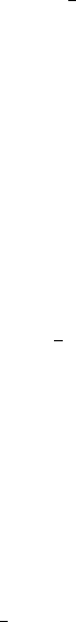
void sum_ad(const adouble* a,
const adouble*b,
int n,
adouble* c);
2.10.30 subtract ad function
This function subtracts a matrix or vector stored columnwise in adouble
array a, to a matrix or vector of the same dimensions stored columnwise in
adouble array b. Both arrays are assumed to have a total of nelements. The
result is returned in adouble array c. The function prototype is as follows.
void subtract_ad(const adouble* a,
const adouble*b,
int n,
adouble* c);
2.10.31 inverse ad function
This function computes the inverse of an n×nsquare matrix stored colum-
nwise in adouble array a. The result is returned in adouble array ainv,
also using columnwise storage. The function prototype is as follows.
void inverse_ad(adouble* a,
int n,
adouble* ainv)
2.10.32 rk4 propagate function
This function may be used to generate an initial guess for the state trajec-
tory by propagating the dynamics using 4th order Runge-Kutta integration.
Note that no bounds are considered on states or controls and that any path
constraints specified in function dae() are ignored. The user needs to spec-
ify a control trajectory and the corresponding time vector. The function
prototype is as follows:
void rk4_propagate( void (*dae)(),
DMatrix& control_trajectory,
DMatrix& time_vector,
DMatrix& initial_state,
DMatrix& parameters,
Prob & problem,
int iphase,
DMatrix& state_trajectory);
•dae is a pointer to the problem’s dae function;
96

•control_trajectory is a DMatrix object of dimensions
problem.phases(iphase).ncontrols ×M
with the initial guess for the controls.
•time_vector is a DMatrix object of dimensions 1 ×Mwith the time
instants that correspond to each element of control_trajectory.
•initial_state is a DMatrix object of dimensions
problem.phases(iphase).nstates ×1
with the value of the initial state vector.
•parameters is a DMatrix object of dimensions
problem.phases(iphase).nparameters ×1
with given values for the static parameters.
•problem is a Prob structure.
•iphase is the phase index.
•state_trajectory is a DMatrix object with dimensions
problem.phases(iphase).nstates ×M
which on output contains the result of the of the propagation. The
values of the states correspond to the time vector time_vector.
2.10.33 rkf propagate function
This function may be used to generate an initial guess for the state trajectory
by propagating the dynamics using the Runge-Kutta-Fehlberg method with
variable step size and relative local truncation error within a given tolerance.
Note that no bounds are considered on states or controls and that any path
constraints specified in function dae() are ignored. The user needs to specify
a control trajectory and the corresponding time vector, as well as minimum
and maximum values for the integration step size, and a tolerance. Note
that the function throws an error if the minimum step size is violated. The
function prototype is as follows:
void rkf_propagate( void (*dae)(),
DMatrix& control_trajectory,
DMatrix& time_vector,
DMatrix& initial_state,
DMatrix& parameters,
double tolerance,
double hmin,
double hmax,
97
Prob & problem,
int iphase,
DMatrix& state_trajectory,
DMatrix& new_time_vector,
DMatrix& new_control_trajectory);
•dae is a pointer to the problem’s dae function;
•control_trajectory is a DMatrix object of dimensions
problem.phases(iphase).ncontrols ×M
with the initial guess for the controls.
•time_vector is a DMatrix object of dimensions 1 ×Mwith the time
instants that correspond to each element of control_trajectory.
•initial_state is a DMatrix object of dimensions
problem.phases(iphase).nstates ×1
with the value of the initial state vector.
•parameters is a DMatrix object of dimensions
problem.phases(iphase).nparameters ×1
with given values for the static parameters.
•tolerance is a positive value for the tolerance against which the max-
imum relative error in the state vector is compared.
•hmin is the minimum integration step size.
•hmax is the maximum integration step size.
•problem is a Prob structure.
•iphase is the phase index.
•state_trajectory is a DMatrix object with dimensions
problem.phases(iphase).nstates ×M
which on output contains the result of the of the propagation. The
values of the states correspond to the time vector new_time_vector.
•new_time_vector is a DMatrix object with dimensions 1 ×N
which on output contains the time values of the propagation.
•new_control_trajectory is a DMatrix object with dimensions
problem.phases(iphase).nstates ×N
which on output containts interpolated values of the control trajectory
corresponding to the time vector new_time_vector. Linear interpola-
tion is employed.
98

2.10.34 resample trajectory function
This function resamples a trajectory given new values of the time vector
using natural cubic spline interpolation.
void resample_trajectory(DMatrix& Y,
DMatrix& t,
DMatrix& Ydata,
DMatrix& tdata )
•Yis, on output, a DMatrix object with dimensions ny×Nwith the
interpolated values of the dependent variable.
•tis a DMatrix object of dimensions 1 ×Nwith the values of the
independent variable at which the interpolated values are required.
The elements of this vector should be monotonically increasing, i.e.
t(j+1) > t(j). The following restrictions should be satisfied: t(1)
≥tdata(1), and t(N) ≤tdata(M).
•Ydata is a DMatrix object of dimensions ny×Mwith the data values
of the dependent variable.
•tdata is a DMatrix object of dimensions 1 ×Mwith the data values
of the independent variable. The elements of this vector should be
monotonically increasing, i.e. t(j+1) > t(j).
2.11 Pre-defined constants
The following constants are defined within the header file psopt.h:
•pi: defined as 3.141592653589793;
•inf: defined as 1 ×10¹⁹.
2.12 Standard output
PSOPT will by default produce output information on the screen as it runs.
PSOPT will produce a short file with a summary of information named with
the string provided in algorithm.outfilelname. This file contains the
problem name, the total CPU time spent, the NLP solver used, the optimal
value of the objective function, the values of the endpoint cost function and
cost integrals, the initial and final time, the maximum discretization error,
and the output string from the NLP solver.
Additionally, every time a PSOPT excutable is run, it will produce
a file named psopt_solution_$$$.txt ($$$ represents the characters of
99

problem.outfilename which occur to the left of the file extension point
“.”). This file contains the problem name, time stamps, a summary of the
algorithm options used, and results obtained, the final grid points, the final
control variables, the final state variables, the final static parameter values.
The file also contains a summary of all constraints functions associated with
the NLP problem, including their final scaled value, bounds, and scaling
factor used; a summary of the final NLP decision variables, including their
final unscaled values, bounds and scaling factors used; and a summary of the
mesh refinement process. An indication is given at the end of a constraint
line, or decision variable line, if a scaled constraint function or scaled deci-
sion variable is within algorithm.nlp_tolerance of one of its bounds, or if
a scaled constraint function or scaled decision variable has violated one of its
bounds by more than algorithm.nlp_tolerance. For parameter estima-
tion problems this file also contains the covariance matrix of the parameter
vector, and the 95% confidence interval for each estimated parameter.
L
A
T
E
X code to produce a table with a summary of the mesh refinement
process is also automatically generated as described in section 2.8.4.
If algorithm.print_level is set to zero, then no output is produced.
2.13 Implementing your own problem
A template C++ file named user.cxx is provided in the directory
psopt-4.0.0 /PSOPT/examples/user
This file can be modified by the user to implement their own problem.
and an executable can then be built easily.
2.13.1 Building the user code from Linux
After modifying the user.cxx code, open a command prompt and cd to the
base directory of the PSOPT installation. Then simply type
$cd PSOPT/examples/user
$make user
If no compilation errors occur, an executable named user should be
created in the directory psopt-4.0.0 /PSOPT/examples/user.
100
Chapter 3
Examples of using PSOPT
The following examples have been mostly selected from the literature such
that their solution can be compared with published results by consulting
the references provided.
3.1 Alp rider problem
Consider the following optimal control problem, which is known in the lit-
erature as the Alp rider problem [3]. It is known as Alp rider because the
minimum of the objective function forces the states to ride the path con-
straint. Minimize the cost functional
J=Z20
0
(100(x2
1+x2
2+x2
3+x2
4)+0.01(u2
1+u2
2))dt(3.1)
subject to the dynamic constraints
˙x1=−10x1+u1+u2
˙x2=−2x2+u1+ 2u2
˙x3=−3x3+ 5x4+u1−u2
˙x4= 5x3−3x4+u1+ 3u2
(3.2)
the path constraint
x2
1+x2
2+x2
3+x2
4−3p(t, 3,12)−3p(t, 6,10)−3p(t, 10,16)−8p(t, 15,4)−0.01 ≤0
(3.3)
101

where the exponential peaks are p(t, a, b) = e−b(t−a)2, and the boundary
conditions are given by:
x1(0) = 2
x2(0) = 1
x3(0) = 2
x4(0) = 1
x1(20) = 2
x2(20) = 3
x3(20) = 1
x4(20) = −2
(3.4)
The PSOPT code that solves this problem is shown below.
//////////////////////////////////////////////////////////////////////////
//////////////// alpine_rider.cxx /////////////////////
//////////////////////////////////////////////////////////////////////////
//////////////// PSOPT Example /////////////////////
//////////////////////////////////////////////////////////////////////////
//////////////////////////////////////////////////////////////////////////
//////// Title: Alp rider problem ////////////////
//////// Last modified: 09 February 2009 ////////////////
//////// Reference: Betts (2001) ////////////////
//////// (See PSOPT handbook for full reference) ////////////////
//////////////////////////////////////////////////////////////////////////
//////// Copyright (c) Victor M. Becerra, 2009 ////////////////
//////////////////////////////////////////////////////////////////////////
//////// This is part of the PSOPT software library, which////////////////
//////// is distributed under the terms of the GNU Lesser ////////////////
//////// General Public License (LGPL) ////////////////
//////////////////////////////////////////////////////////////////////////
#include "psopt.h"
//////////////////////////////////////////////////////////////////////////
/////////////////// Define auxiliary function ////////////////////////
//////////////////////////////////////////////////////////////////////////
adouble pk( adouble t, double a, double b)
{
return exp(-b*(t-a)*(t-a));
}
//////////////////////////////////////////////////////////////////////////
/////////////////// Define the end point (Mayer) cost function //////////
//////////////////////////////////////////////////////////////////////////
adouble endpoint_cost(adouble* initial_states, adouble* final_states,
adouble* parameters,adouble& t0, adouble& tf,
adouble* xad, int iphase, Workspace* workspace)
{
return 0;
}
//////////////////////////////////////////////////////////////////////////
/////////////////// Define the integrand (Lagrange) cost function //////
//////////////////////////////////////////////////////////////////////////
adouble integrand_cost(adouble* states, adouble* controls,
adouble* parameters, adouble& time, adouble* xad,
int iphase, Workspace* workspace)
{
adouble x1 = states[CINDEX(1)];
adouble x2 = states[CINDEX(2)];
adouble x3 = states[CINDEX(3)];
adouble x4 = states[CINDEX(4)];
adouble u1 = controls[CINDEX(1)];
adouble u2 = controls[CINDEX(2)];
adouble L;
102

L = 100.0*( x1*x1 + x2*x2 + x3*x3 + x4*x4 ) + 0.01*( u1*u1 + u2*u2 );
return L;
}
//////////////////////////////////////////////////////////////////////////
/////////////////// Define the DAE’s ////////////////////////////////////
//////////////////////////////////////////////////////////////////////////
void dae(adouble* derivatives, adouble* path, adouble* states,
adouble* controls, adouble* parameters, adouble& time,
adouble* xad, int iphase, Workspace* workspace)
{
adouble x1 = states[CINDEX(1)];
adouble x2 = states[CINDEX(2)];
adouble x3 = states[CINDEX(3)];
adouble x4 = states[CINDEX(4)];
adouble u1 = controls[CINDEX(1)];
adouble u2 = controls[CINDEX(2)];
adouble t = time;
derivatives[CINDEX(1)] = -10*x1 + u1 + u2;
derivatives[CINDEX(2)] = -2*x2 + u1 + 2*u2;
derivatives[CINDEX(3)] = -3*x3 + 5*x4 + u1 - u2;
derivatives[CINDEX(4)] = 5*x3 - 3*x4 + u1 + 3*u2;
path[0] = x1*x1 + x2*x2 + x3*x3 + x4*x4
- 3*pk(t,3,12) - 3*pk(t,6,10) - 3*pk(t,10,6) - 8*pk(t,15,4)
- 0.01;
}
////////////////////////////////////////////////////////////////////////////
/////////////////// Define the events function ////////////////////////////
////////////////////////////////////////////////////////////////////////////
void events(adouble* e, adouble* initial_states, adouble* final_states,
adouble* parameters,adouble& t0, adouble& tf, adouble* xad,
int iphase, Workspace* workspace)
{
adouble x1i = initial_states[ CINDEX(1) ];
adouble x2i = initial_states[ CINDEX(2) ];
adouble x3i = initial_states[ CINDEX(3) ];
adouble x4i = initial_states[ CINDEX(4) ];
adouble x1f = final_states[ CINDEX(1) ];
adouble x2f = final_states[ CINDEX(2) ];
adouble x3f = final_states[ CINDEX(3) ];
adouble x4f = final_states[ CINDEX(4) ];
e[ CINDEX(1) ] = x1i;
e[ CINDEX(2) ] = x2i;
e[ CINDEX(3) ] = x3i;
e[ CINDEX(4) ] = x4i;
e[ CINDEX(5) ] = x1f;
e[ CINDEX(6) ] = x2f;
e[ CINDEX(7) ] = x3f;
e[ CINDEX(8) ] = x4f;
}
///////////////////////////////////////////////////////////////////////////
/////////////////// Define the phase linkages function ///////////////////
///////////////////////////////////////////////////////////////////////////
void linkages( adouble* linkages, adouble* xad, Workspace* workspace)
{
// No linkages as this is a single phase problem
}
////////////////////////////////////////////////////////////////////////////
/////////////////// Define the main routine ///////////////////////////////
////////////////////////////////////////////////////////////////////////////
int main(void)
{
103

////////////////////////////////////////////////////////////////////////////
/////////////////// Declare key structures ////////////////////////////////
////////////////////////////////////////////////////////////////////////////
Alg algorithm;
Sol solution;
Prob problem;
////////////////////////////////////////////////////////////////////////////
/////////////////// Register problem name ////////////////////////////////
////////////////////////////////////////////////////////////////////////////
problem.name = "Alp rider problem";
problem.outfilename = "alpine.txt";
////////////////////////////////////////////////////////////////////////////
//////////// Define problem level constants & do level 1 setup ////////////
////////////////////////////////////////////////////////////////////////////
problem.nphases = 1;
problem.nlinkages = 0;
psopt_level1_setup(problem);
/////////////////////////////////////////////////////////////////////////////
///////// Define phase related information & do level 2 setup ////////////
/////////////////////////////////////////////////////////////////////////////
problem.phases(1).nstates = 4;
problem.phases(1).ncontrols = 2;
problem.phases(1).nevents = 8;
problem.phases(1).npath = 1;
problem.phases(1).nodes = "[120]";
psopt_level2_setup(problem, algorithm);
////////////////////////////////////////////////////////////////////////////
/////////////////// Enter problem bounds information //////////////////////
////////////////////////////////////////////////////////////////////////////
problem.phases(1).bounds.lower.states = "[-4.0, -4.0, -4.0, -4.0]";
problem.phases(1).bounds.upper.states = "[ 4.0, 4.0, 4.0, 4.0]";
problem.phases(1).bounds.lower.controls = "[ -500.0, -500 ]";
problem.phases(1).bounds.upper.controls = "[ 500.0, 500 ]";
problem.phases(1).bounds.lower.events = "[2.0, 1.0, 2.0, 1.0, 2.0, 3.0, 1.0, -2.0]";
problem.phases(1).bounds.upper.events = problem.phases(1).bounds.lower.events;
problem.phases(1).bounds.upper.path = 100.0;
problem.phases(1).bounds.lower.path = 0.0;
problem.phases(1).bounds.lower.StartTime = 0.0;
problem.phases(1).bounds.upper.StartTime = 0.0;
problem.phases(1).bounds.lower.EndTime = 20.0;
problem.phases(1).bounds.upper.EndTime = 20.0;
////////////////////////////////////////////////////////////////////////////
/////////////////// Register problem functions ///////////////////////////
////////////////////////////////////////////////////////////////////////////
problem.integrand_cost = &integrand_cost;
problem.endpoint_cost = &endpoint_cost;
problem.dae = &dae;
problem.events = &events;
problem.linkages = &linkages;
////////////////////////////////////////////////////////////////////////////
/////////////////// Define & register initial guess ///////////////////////
////////////////////////////////////////////////////////////////////////////
104

int nnodes = problem.phases(1).nodes(1);
DMatrix x_guess = zeros(4,nnodes);
x_guess(1,colon()) = linspace(2,1,nnodes);
x_guess(2,colon()) = linspace(2,3,nnodes);
x_guess(3,colon()) = linspace(2,1,nnodes);
x_guess(4,colon()) = linspace(1,-2,nnodes);
problem.phases(1).guess.controls = zeros(2,nnodes);
problem.phases(1).guess.states = x_guess;
problem.phases(1).guess.time = linspace(0.0,20.0,nnodes+1);
////////////////////////////////////////////////////////////////////////////
/////////////////// Enter algorithm options //////////////////////////////
////////////////////////////////////////////////////////////////////////////
algorithm.nlp_iter_max = 1000;
algorithm.nlp_tolerance = 1.e-6;
algorithm.nlp_method = "IPOPT";
algorithm.scaling = "automatic";
algorithm.derivatives = "automatic";
algorithm.jac_sparsity_ratio = 0.20;
algorithm.collocation_method = "Legendre";
algorithm.diff_matrix = "central-differences";
algorithm.mesh_refinement = "automatic";
algorithm.mr_max_increment_factor = 0.3;
algorithm.defect_scaling = "jacobian-based";
////////////////////////////////////////////////////////////////////////////
/////////////////// Now call PSOPT to solve the problem //////////////////
////////////////////////////////////////////////////////////////////////////
psopt(solution, problem, algorithm);
////////////////////////////////////////////////////////////////////////////
/////////// Extract relevant variables from solution structure //////////
////////////////////////////////////////////////////////////////////////////
DMatrix x = solution.get_states_in_phase(1);
DMatrix u = solution.get_controls_in_phase(1);
DMatrix t = solution.get_time_in_phase(1);
////////////////////////////////////////////////////////////////////////////
/////////// Save solution data to files if desired ////////////////////////
////////////////////////////////////////////////////////////////////////////
x.Save("x.dat");
u.Save("u.dat");
t.Save("t.dat");
////////////////////////////////////////////////////////////////////////////
/////////// Plot some results if desired (requires gnuplot) ///////////////
////////////////////////////////////////////////////////////////////////////
plot(t,x(1,colon()),problem.name+": state", "time (s)", "state","x1");
plot(t,x(2,colon()),problem.name+": state", "time (s)", "state","x2");
plot(t,x(3,colon()),problem.name+": state", "time (s)", "state","x3");
plot(t,x(4,colon()),problem.name+": state", "time (s)", "state","x4");
plot(t,u(1,colon()),problem.name+": control","time (s)", "control", "u1");
plot(t,u(2,colon()),problem.name+": control","time (s)", "control", "u2");
plot(t,x(1,colon()),problem.name+": state x1", "time (s)", "state","x1",
"pdf", "alpine_state1.pdf");
plot(t,x(2,colon()),problem.name+": state x2", "time (s)", "state","x2",
"pdf", "alpine_state2.pdf");
105

plot(t,x(3,colon()),problem.name+": state x3", "time (s)", "state","x2",
"pdf", "alpine_state3.pdf");
plot(t,x(4,colon()),problem.name+": state x4", "time (s)", "state","x2",
"pdf", "alpine_state4.pdf");
plot(t,u(1,colon()),problem.name+": control u1","time (s)", "control", "u1",
"pdf", "alpine_control1.pdf");
plot(t,u(2,colon()),problem.name+": control u1","time (s)", "control", "u2",
"pdf", "alpine_control2.pdf");
}
////////////////////////////////////////////////////////////////////////////
/////////////////////// END OF FILE ///////////////////////////////
////////////////////////////////////////////////////////////////////////////
The output from PSOPT is summarized in the box below and shown in
Figures 3.1-3.4 and Figures 3.5-3.6, which contain the elements of the state
and the control, respectively. Table ?? shows the mesh refinement history
for this problem.
PSOPT results summary
=====================
Problem: Alp rider problem
CPU time (seconds): 1.151346e+02
NLP solver used: IPOPT
PSOPT release number: 4.0
Date and time of this run: Thu Feb 21 15:28:52 2019
Optimal (unscaled) cost function value: 2.026847e+03
Phase 1 endpoint cost function value: 0.000000e+00
Phase 1 integrated part of the cost: 2.026847e+03
Phase 1 initial time: 0.000000e+00
Phase 1 final time: 2.000000e+01
Phase 1 maximum relative local error: 2.990169e-03
NLP solver reports: The problem has been solved!
3.2 Brachistochrone problem
Consider the following optimal control problem. Minimize the cost func-
tional
J=tf(3.5)
106
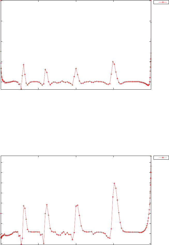
0
0.5
1
1.5
2
0 5 10 15 20
state
time (s)
Alp rider problem: state x1
x1
Figure 3.1: State x1(t) for the Alp rider problem
-0.5
0
0.5
1
1.5
2
2.5
3
3.5
0 5 10 15 20
state
time (s)
Alp rider problem: state x2
x2
Figure 3.2: State x2(t) for the Alp rider problem
107
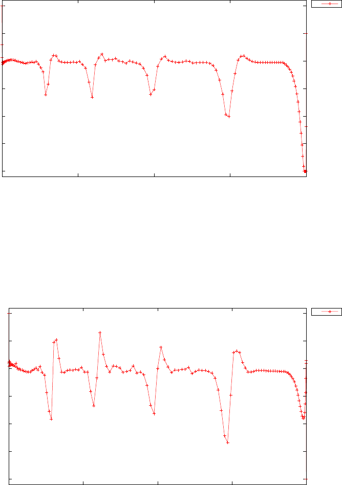
-4
-3
-2
-1
0
1
2
0 5 10 15 20
state
time (s)
Alp rider problem: state x3
x2
Figure 3.3: State x3(t) for the Alp rider problem
-2
-1.5
-1
-0.5
0
0.5
1
0 5 10 15 20
state
time (s)
Alp rider problem: state x4
x2
Figure 3.4: State x4(t) for the Alp rider problem
108
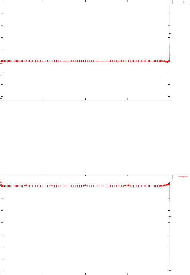
-300
-200
-100
0
100
200
300
400
500
0 5 10 15 20
control
time (s)
Alp rider problem: control u1
u1
Figure 3.5: Control u1(t) for the Alp rider problem
-350
-300
-250
-200
-150
-100
-50
0
0 5 10 15 20
control
time (s)
Alp rider problem: control u1
u2
Figure 3.6: Control u2(t) for the Alp rider problem
109

subject to the dynamic constraints
˙x=vsin(θ)
˙y=vcos(θ)
˙v=gcos(θ)
(3.6)
and the boundary conditions
x(0) = 0
y(0) = 0
v(0) = 0
x(tf)=2
y(tf) = 2
(3.7)
where g= 9.8. A version of this problem was originally formulated by
Johann Bernoulli in 1696 and is referred to as the Brachistochrone problem.
The PSOPT code that solves this problem is shown below.
//////////////////////////////////////////////////////////////////////////
////////////////// brac1.cxx ///////////////////////////
//////////////////////////////////////////////////////////////////////////
//////////////// PSOPT Example ////////////////////
//////////////////////////////////////////////////////////////////////////
//////////////////////////////////////////////////////////////////////////
//////// Title: Brachistochrone problem ////////////////
//////// Last modified: 04 January 2009 ////////////////
//////// Reference: Bryson and Ho (1975) ////////////////
//////// (See PSOPT handbook for full reference) ////////////////
//////////////////////////////////////////////////////////////////////////
//////// Copyright (c) Victor M. Becerra, 2009 ////////////////
//////////////////////////////////////////////////////////////////////////
//////// This is part of the PSOPT software library, which ///////////////
//////// is distributed under the terms of the GNU Lesser ////////////////
//////// General Public License (LGPL) ////////////////
//////////////////////////////////////////////////////////////////////////
#include "psopt.h"
//////////////////////////////////////////////////////////////////////////
/////////////////// Define the end point (Mayer) cost function //////////
//////////////////////////////////////////////////////////////////////////
adouble endpoint_cost(adouble* initial_states, adouble* final_states,
adouble* parameters,adouble& t0, adouble& tf,
adouble* xad, int iphase, Workspace* workspace)
{
return tf;
}
//////////////////////////////////////////////////////////////////////////
/////////////////// Define the integrand (Lagrange) cost function //////
//////////////////////////////////////////////////////////////////////////
adouble integrand_cost(adouble* states, adouble* controls, adouble* parameters,
adouble& time, adouble* xad, int iphase, Workspace* workspace)
{
return 0.0;
}
//////////////////////////////////////////////////////////////////////////
/////////////////// Define the DAE’s ////////////////////////////////////
//////////////////////////////////////////////////////////////////////////
void dae(adouble* derivatives, adouble* path, adouble* states,
adouble* controls, adouble* parameters, adouble& time,
adouble* xad, int iphase, Workspace* workspace)
{
adouble xdot, ydot, vdot;
110

adouble x = states[ CINDEX(1) ];
adouble y = states[ CINDEX(2) ];
adouble v = states[ CINDEX(3) ];
adouble theta = controls[ CINDEX(1) ];
xdot = v*sin(theta);
ydot = v*cos(theta);
vdot = 9.8*cos(theta);
derivatives[ CINDEX(1) ] = xdot;
derivatives[ CINDEX(2) ] = ydot;
derivatives[ CINDEX(3) ] = vdot;
}
////////////////////////////////////////////////////////////////////////////
/////////////////// Define the events function ////////////////////////////
////////////////////////////////////////////////////////////////////////////
void events(adouble* e, adouble* initial_states, adouble* final_states,
adouble* parameters,adouble& t0, adouble& tf, adouble* xad,
int iphase, Workspace* workspace)
{
adouble x0 = initial_states[ CINDEX(1) ];
adouble y0 = initial_states[ CINDEX(2) ];
adouble v0 = initial_states[ CINDEX(3) ];
adouble xf = final_states[ CINDEX(1)];
adouble yf = final_states[ CINDEX(2)];
e[ CINDEX(1) ] = x0;
e[ CINDEX(2) ] = y0;
e[ CINDEX(3) ] = v0;
e[ CINDEX(4) ] = xf;
e[ CINDEX(5) ] = yf;
}
///////////////////////////////////////////////////////////////////////////
/////////////////// Define the phase linkages function ///////////////////
///////////////////////////////////////////////////////////////////////////
void linkages( adouble* linkages, adouble* xad, Workspace* workspace)
{
// No linkages as this is a single phase problem
}
////////////////////////////////////////////////////////////////////////////
/////////////////// Define the main routine ///////////////////////////////
////////////////////////////////////////////////////////////////////////////
int main(void)
{
////////////////////////////////////////////////////////////////////////////
/////////////////// Declare key structures ////////////////////////////////
////////////////////////////////////////////////////////////////////////////
Alg algorithm;
Sol solution;
Prob problem;
////////////////////////////////////////////////////////////////////////////
/////////////////// Register problem name ////////////////////////////////
////////////////////////////////////////////////////////////////////////////
problem.name = "Brachistochrone Problem";
problem.outfilename = "brac1.txt";
////////////////////////////////////////////////////////////////////////////
//////////// Define problem level constants & do level 1 setup ////////////
////////////////////////////////////////////////////////////////////////////
problem.nphases = 1;
problem.nlinkages = 0;
psopt_level1_setup(problem);
/////////////////////////////////////////////////////////////////////////////
///////// Define phase related information & do level 2 setup /////////////
111

/////////////////////////////////////////////////////////////////////////////
problem.phases(1).nstates = 3;
problem.phases(1).ncontrols = 1;
problem.phases(1).nevents = 5;
problem.phases(1).npath = 0;
problem.phases(1).nodes = "[40]";
psopt_level2_setup(problem, algorithm);
////////////////////////////////////////////////////////////////////////////
/////////////////// Enter problem bounds information //////////////////////
////////////////////////////////////////////////////////////////////////////
problem.phases(1).bounds.lower.states = "[ 0; 0; 0]";
problem.phases(1).bounds.upper.states = "[20; 20; 20]";
problem.phases(1).bounds.lower.controls = 0.0;
problem.phases(1).bounds.upper.controls = 2*pi;
problem.phases(1).bounds.lower.events = "[0, 0, 0, 2, 2]";
problem.phases(1).bounds.upper.events = "[0, 0, 0, 2, 2]";
problem.phases(1).bounds.lower.StartTime = 0.0;
problem.phases(1).bounds.upper.StartTime = 0.0;
problem.phases(1).bounds.lower.EndTime = 0.0;
problem.phases(1).bounds.upper.EndTime = 10.0;
////////////////////////////////////////////////////////////////////////////
/////////////////// Register problem functions ///////////////////////////
////////////////////////////////////////////////////////////////////////////
problem.integrand_cost = &integrand_cost;
problem.endpoint_cost = &endpoint_cost;
problem.dae = &dae;
problem.events = &events;
problem.linkages = &linkages;
////////////////////////////////////////////////////////////////////////////
/////////////////// set scaling factors (optional) ////////////////////////
////////////////////////////////////////////////////////////////////////////
// problem.phases(1).scale.controls = 1.0*ones(1,1);
// problem.phases(1).scale.states = 1.0*ones(3,1);
// problem.phases(1).scale.events = 1.0*ones(5,1);
// problem.phases(1).scale.defects = 1.0*ones(3,1);
// problem.phases(1).scale.time = 1.0;
// problem.scale.objective = 1.0;
////////////////////////////////////////////////////////////////////////////
/////////////////// Define & register initial guess ///////////////////////
////////////////////////////////////////////////////////////////////////////
DMatrix x0(3,20);
x0(1,colon()) = linspace(0.0,1.0, 20);
x0(2,colon()) = linspace(0.0,1.0, 20);
x0(3,colon()) = linspace(0.0,1.0, 20);
problem.phases(1).guess.controls = ones(1,20);
problem.phases(1).guess.states = x0;
problem.phases(1).guess.time = linspace(0.0, 2.0, 20);
////////////////////////////////////////////////////////////////////////////
/////////////////// Enter algorithm options //////////////////////////////
////////////////////////////////////////////////////////////////////////////
algorithm.nlp_method = "IPOPT";
algorithm.scaling = "automatic";
algorithm.derivatives = "automatic";
algorithm.nlp_iter_max = 1000;
algorithm.nlp_tolerance = 1.e-6;
112

// algorithm.hessian = "exact";
algorithm.collocation_method = "Legendre";
////////////////////////////////////////////////////////////////////////////
/////////////////// Now call PSOPT to solve the problem /////////////////
////////////////////////////////////////////////////////////////////////////
psopt(solution, problem, algorithm);
if (solution.error_flag) exit(0);
////////////////////////////////////////////////////////////////////////////
/////////// Extract relevant variables from solution structure //////////
////////////////////////////////////////////////////////////////////////////
DMatrix x = solution.get_states_in_phase(1);
DMatrix u = solution.get_controls_in_phase(1);
DMatrix t = solution.get_time_in_phase(1);
DMatrix H = solution.get_dual_hamiltonian_in_phase(1);
DMatrix lambda = solution.get_dual_costates_in_phase(1);
////////////////////////////////////////////////////////////////////////////
/////////// Save solution data to files if desired ////////////////////////
////////////////////////////////////////////////////////////////////////////
x.Save("x.dat");
u.Save("u.dat");
t.Save("t.dat");
lambda.Save("p.dat");
////////////////////////////////////////////////////////////////////////////
/////////// Plot some results if desired (requires gnuplot) ///////////////
////////////////////////////////////////////////////////////////////////////
plot(t,x,problem.name + ": states", "time (s)", "states", "x y v");
plot(t,u,problem.name + ": control", "time (s)", "control", "u");
plot(t,H,problem.name + ": Hamiltonian", "time (s)", "H", "H");
plot(t,lambda,problem.name + ": costates", "time (s)", "lambda", "lambda_1 lambda_2 lambda_3");
plot(t,x,problem.name + ": states", "time (s)", "states", "x y v",
"pdf", "brac1_states.pdf");
plot(t,u,problem.name + ": control", "time (s)", "control", "u",
"pdf", "brac1_control.pdf");
plot(t,H,problem.name + ": Hamiltonian", "time (s)", "H", "H",
"pdf", "brac1_hamiltonian.pdf");
plot(t,lambda,problem.name + ": costates", "time (s)", "lambda", "lambda_1 lambda_2 lambda_3",
"pdf", "brac1_costates.pdf");
}
////////////////////////////////////////////////////////////////////////////
/////////////////////// END OF FILE ///////////////////////////////
////////////////////////////////////////////////////////////////////////////
The output from PSOPT is summarized in the box below and shown
in Figures 3.7,3.8, which contain the elements of the state, and the control
respectively.
PSOPT results summary
113
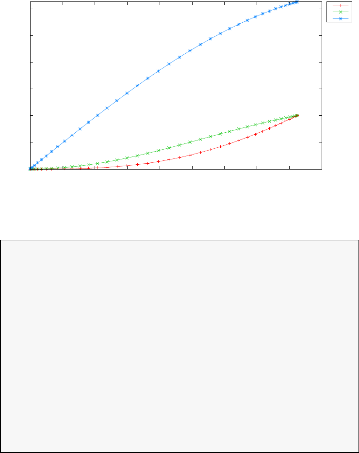
0
1
2
3
4
5
6
0 0.1 0.2 0.3 0.4 0.5 0.6 0.7 0.8 0.9
states
time (s)
Brachistochrone Problem: states
x
y
v
Figure 3.7: States for brachistochrone problem
=====================
Problem: Brachistochrone Problem
CPU time (seconds): 1.794096e+00
NLP solver used: IPOPT
PSOPT release number: 4.0
Date and time of this run: Thu Feb 21 16:06:01 2019
Optimal (unscaled) cost function value: 8.247591e-01
Phase 1 endpoint cost function value: 8.247591e-01
Phase 1 integrated part of the cost: 0.000000e+00
Phase 1 initial time: 0.000000e+00
Phase 1 final time: 8.247591e-01
Phase 1 maximum relative local error: 2.774874e-07
NLP solver reports: The problem has been solved!
3.3 Breakwell problem
Consider the following optimal control problem, which is known in the lit-
erature as the Breakwell problem [8]. The problem benefits from having
an analytical solution, which is reported (with some errors) in the book by
114
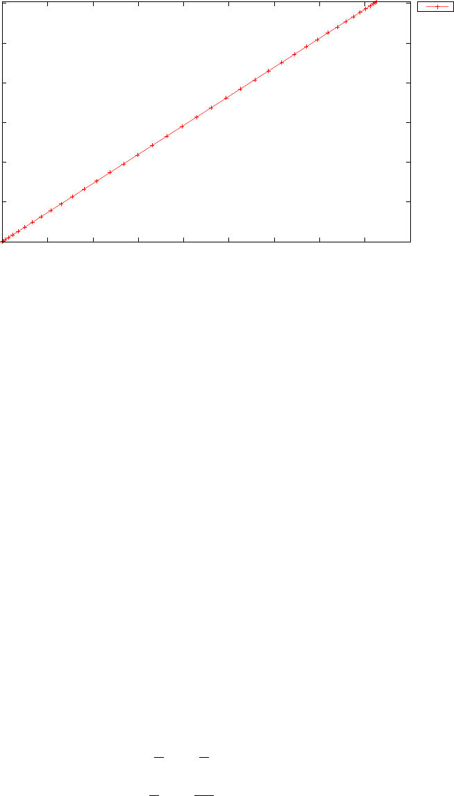
0
0.2
0.4
0.6
0.8
1
1.2
0 0.1 0.2 0.3 0.4 0.5 0.6 0.7 0.8 0.9
control
time (s)
Brachistochrone Problem: control
u
Figure 3.8: Control for brachistochrone problem
Bryson and Ho (1975). Minimize the cost functional.
J=Ztf
0
u(t)2dt(3.8)
subject to the dynamic constraints
˙x=v
˙v=u(3.9)
the state dependent constraint
x(t)≤l(3.10)
where l= 0.1, tf= 1. and the boundary conditions
x(0) = 0
v(0) = 1
x(tf)=0
v(tf) = −1
(3.11)
The analytical solution of the problem (valid for 0 ≤l≤1/6) is given
by:
u(t) =
−2
3l(1 −t
3l),0≤t≤3l
0,3l≤t≤1−3l
−2
3l(1 −1−t
3l),1−3l≤t≤1
(3.12)
115

x(t) =
l1−1−t
3l3,0≤t≤3l
l, 3l≤t≤1−3l
l1−1−1−t
3l3,1−3l≤t≤1
(3.13)
v(t) =
1−t
3l2,0≤t≤3l
0,3l≤t≤1−3l
1−1−t
3l2,1−3l≤t≤1
(3.14)
λx(t) =
2
9l2,0≤t≤3l
0,3l≤t≤1−3l
−2
9l2,1−3l≤t≤1
(3.15)
λv(t) =
2
3l(1 −t
3l),0≤t≤3l
0,3l≤t≤1−3l
2
3l(1 −1−t
3l),1−3l≤t≤1
(3.16)
where λx(t) and λv(t) are the costates. The analytical optimal value of the
objective function is J= 4/(9l)=4.4444444. The PSOPT code that solves
this problem is shown below.
//////////////////////////////////////////////////////////////////////////
//////////////// bryson_max_range.cxx /////////////////////
//////////////////////////////////////////////////////////////////////////
//////////////// PSOPT Example /////////////////////
//////////////////////////////////////////////////////////////////////////
//////////////////////////////////////////////////////////////////////////
//////// Title: Bryson maximum range problem ////////////////
//////// Last modified: 05 January 2009 ////////////////
//////// Reference: Bryson and Ho (1975) ////////////////
//////// (See PSOPT handbook for full reference) ////////////////
//////////////////////////////////////////////////////////////////////////
//////// Copyright (c) Victor M. Becerra, 2009 ////////////////
//////////////////////////////////////////////////////////////////////////
//////// This is part of the PSOPT software library, which////////////////
//////// is distributed under the terms of the GNU Lesser ////////////////
//////// General Public License (LGPL) ////////////////
//////////////////////////////////////////////////////////////////////////
#include "psopt.h"
//////////////////////////////////////////////////////////////////////////
/////////////////// Define the end point (Mayer) cost function //////////
//////////////////////////////////////////////////////////////////////////
adouble endpoint_cost(adouble* initial_states, adouble* final_states,
adouble* parameters,adouble& t0, adouble& tf,
adouble* xad, int iphase, Workspace* workspace)
{
return (0);
}
//////////////////////////////////////////////////////////////////////////
/////////////////// Define the integrand (Lagrange) cost function //////
//////////////////////////////////////////////////////////////////////////
adouble integrand_cost(adouble* states, adouble* controls, adouble* parameters,
adouble& time, adouble* xad, int iphase, Workspace* workspace)
{
adouble u = controls[0];
return 0.5*u*u;
}
116

//////////////////////////////////////////////////////////////////////////
/////////////////// Define the DAE’s ////////////////////////////////////
//////////////////////////////////////////////////////////////////////////
void dae(adouble* derivatives, adouble* path, adouble* states,
adouble* controls, adouble* parameters, adouble& time,
adouble* xad, int iphase, Workspace* workspace)
{
adouble xdot, vdot;
double g = 1.0;
double a = 0.5*g;
adouble x = states[ CINDEX(1) ];
adouble v = states[ CINDEX(2) ];
adouble u = controls[ CINDEX(1) ];
xdot = v;
vdot = u;
derivatives[ CINDEX(1) ] = xdot;
derivatives[ CINDEX(2) ] = vdot;
}
////////////////////////////////////////////////////////////////////////////
/////////////////// Define the events function ////////////////////////////
////////////////////////////////////////////////////////////////////////////
void events(adouble* e, adouble* initial_states, adouble* final_states,
adouble* parameters,adouble& t0, adouble& tf, adouble* xad,
int iphase, Workspace* workspace)
{
adouble x0 = initial_states[ CINDEX(1) ];
adouble v0 = initial_states[ CINDEX(2) ];
adouble xf = final_states[ CINDEX(1) ];
adouble vf = final_states[ CINDEX(2) ];
e[ CINDEX(1) ] = x0;
e[ CINDEX(2) ] = v0;
e[ CINDEX(3) ] = xf;
e[ CINDEX(4) ] = vf;
}
///////////////////////////////////////////////////////////////////////////
/////////////////// Define the phase linkages function ///////////////////
///////////////////////////////////////////////////////////////////////////
void linkages( adouble* linkages, adouble* xad, Workspace* workspace)
{
// No linkages as this is a single phase problem
}
////////////////////////////////////////////////////////////////////////////
/////////////////// Define the main routine ///////////////////////////////
////////////////////////////////////////////////////////////////////////////
int main(void)
{
////////////////////////////////////////////////////////////////////////////
/////////////////// Declare key structures ////////////////////////////////
////////////////////////////////////////////////////////////////////////////
Alg algorithm;
Sol solution;
Prob problem;
////////////////////////////////////////////////////////////////////////////
/////////////////// Register problem name ////////////////////////////////
////////////////////////////////////////////////////////////////////////////
problem.name = "Breakwell Problem";
problem.outfilename = "breakwell.txt";
117

////////////////////////////////////////////////////////////////////////////
//////////// Define problem level constants & do level 1 setup ////////////
////////////////////////////////////////////////////////////////////////////
problem.nphases = 1;
problem.nlinkages = 0;
psopt_level1_setup(problem);
/////////////////////////////////////////////////////////////////////////////
///////// Define phase related information & do level 2 setup ////////////
/////////////////////////////////////////////////////////////////////////////
problem.phases(1).nstates = 2;
problem.phases(1).ncontrols = 1;
problem.phases(1).nevents = 4;
problem.phases(1).npath = 0;
problem.phases(1).nodes = "[200]";
psopt_level2_setup(problem, algorithm);
////////////////////////////////////////////////////////////////////////////
/////////////////// Declare DMatrix objects to store results //////////////
////////////////////////////////////////////////////////////////////////////
DMatrix x, u, t;
DMatrix lambda, H;
////////////////////////////////////////////////////////////////////////////
/////////////////// Enter problem bounds information //////////////////////
////////////////////////////////////////////////////////////////////////////
double xL = -2.0;
double vL = -2.0;
double xU = 0.1;
double vU = 2.0;
double uL = -10.0;
double uU = 10.0;
double x0 = 0.0;
double v0 = 1.0;
double xf = 0.0;
double vf = -1.0;
problem.phases(1).bounds.lower.states(1) = xL;
problem.phases(1).bounds.lower.states(2) = vL;
problem.phases(1).bounds.upper.states(1) = xU;
problem.phases(1).bounds.upper.states(2) = vU;
problem.phases(1).bounds.lower.controls(1) = uL;
problem.phases(1).bounds.upper.controls(1) = uU;
problem.phases(1).bounds.lower.events(1) = x0;
problem.phases(1).bounds.lower.events(2) = v0;
problem.phases(1).bounds.lower.events(3) = xf;
problem.phases(1).bounds.lower.events(4) = vf;
problem.phases(1).bounds.upper.events(1) = x0;
problem.phases(1).bounds.upper.events(2) = v0;
problem.phases(1).bounds.upper.events(3) = xf;
problem.phases(1).bounds.upper.events(4) = vf;
problem.phases(1).bounds.lower.StartTime = 0.0;
problem.phases(1).bounds.upper.StartTime = 0.0;
problem.phases(1).bounds.lower.EndTime = 1.0;
problem.phases(1).bounds.upper.EndTime = 1.0;
////////////////////////////////////////////////////////////////////////////
/////////////////// Register problem functions ///////////////////////////
////////////////////////////////////////////////////////////////////////////
118

problem.integrand_cost = &integrand_cost;
problem.endpoint_cost = &endpoint_cost;
problem.dae = &dae;
problem.events = &events;
problem.linkages = &linkages;
////////////////////////////////////////////////////////////////////////////
/////////////////// Define & register initial guess ///////////////////////
////////////////////////////////////////////////////////////////////////////
int nnodes = problem.phases(1).nodes(1);
int ncontrols = problem.phases(1).ncontrols;
int nstates = problem.phases(1).nstates;
DMatrix x_guess = zeros(nstates,nnodes);
x_guess(1,colon()) = x0*ones(1,nnodes);
x_guess(2,colon()) = v0*ones(1,nnodes);
problem.phases(1).guess.controls = zeros(ncontrols,nnodes);
problem.phases(1).guess.states = x_guess;
problem.phases(1).guess.time = linspace(0.0,1.0,nnodes);
////////////////////////////////////////////////////////////////////////////
/////////////////// Enter algorithm options //////////////////////////////
////////////////////////////////////////////////////////////////////////////
algorithm.nlp_iter_max = 1000;
algorithm.nlp_tolerance = 1.e-6;
algorithm.nlp_method = "IPOPT";
algorithm.scaling = "automatic";
algorithm.derivatives = "automatic";
// algorithm.hessian = "exact";
// algorithm.mesh_refinement = "automatic";
algorithm.collocation_method = "Hermite-Simpson";
// algorithm.diff_matrix = "central-differences";
// algorithm.defect_scaling = "jacobian-based";
algorithm.nlp_tolerance = 1.e-6;
////////////////////////////////////////////////////////////////////////////
/////////////////// Now call PSOPT to solve the problem /////////////////
////////////////////////////////////////////////////////////////////////////
psopt(solution, problem, algorithm);
////////////////////////////////////////////////////////////////////////////
/////////// Extract relevant variables from solution structure //////////
////////////////////////////////////////////////////////////////////////////
DMatrix muE;
x = solution.get_states_in_phase(1);
u = solution.get_controls_in_phase(1);
t = solution.get_time_in_phase(1);
lambda = solution.get_dual_costates_in_phase(1);
H = solution.get_dual_hamiltonian_in_phase(1);
muE = solution.get_dual_events_in_phase(1);
////////////////////////////////////////////////////////////////////////////
/////////// Compute the analytical solution, which is valid when the //////
/////////// state constraint x<=l, with 0<=l<=1/6. In this case l=0.1 /////
/////////// The analytical solution is given (with some errors) in /////
/////////// the book by Bryson and Ho (1975), pages 121-122. /////
////////////////////////////////////////////////////////////////////////////
double l = 0.1;
double t1 = 3*l;
double t2 = 1.0-3*l;
int nn = length(t);
DMatrix ua(1,nn), xa(2,nn), pa(2,nn);
for(int i=1;i <=nn;i++) {
119

if (t(i)<t1) {
ua(1,i) = -2.0/(3.0*l)*(1.0-t(i)/(3.0*l));
xa(1,i) = l*( 1.0 - pow( (1.0-t(i)/(3.0*l)), 3.0) ) ;
xa(2,i) = pow( 1.0 - t(i)/(3.0*l), 2.0);
pa(1,i) = 2.0/(9.0*l*l);
pa(2,i) = 2.0/(3.0*l)*(1.0-t(i)/(3*l));
}
else if (t(i)>=t1 && t(i)<t2) {
ua(1,i) = 0.0;
xa(1,i) = l;
xa(2,i) = 0.0;
pa(1,i) = 0.0;
pa(2,i) = 0.0;
}
else if (t(i)>=t2) {
ua(1,i) = -2.0/(3*l)*(1.0-(1.0-t(i))/(3.0*l));
xa(1,i) = l*(1.0 - pow( (1.0-(1.0-t(i))/(3.0*l)), 3.0));
xa(2,i) = -pow(1.0-(1.0-t(i))/(3.0*l), 2.0) ;
pa(1,i) = -2.0/(9.0*l*l);
pa(2,i) = 2.0/(3.0*l)*(1.0-(1.0-t(i))/(3*l));
}
}
////////////////////////////////////////////////////////////////////////////
/////////// Save solution data to files if desired ////////////////////////
////////////////////////////////////////////////////////////////////////////
x.Save("x.dat");
u.Save("u.dat");
t.Save("t.dat");
lambda.Save("p.dat");
H.Save("H.dat");
////////////////////////////////////////////////////////////////////////////
/////////// Plot some results if desired (requires gnuplot) ///////////////
////////////////////////////////////////////////////////////////////////////
plot(t,x,t,xa,problem.name+": states", "time (s)", "states","x v xa va");
plot(t,u,t,ua,problem.name+": controls","time (s)", "control", "u ua");
plot(t,lambda,t,pa, problem.name+": costates","time (s)", "costates", "l_x l_v la_x la_v");
plot(t,H,problem.name+": Hamiltonian","time (s)", "H", "H");
plot(t,x,t,xa,problem.name+": states", "time (s)", "states","x v xa va", "pdf", "breakwell_states.pdf");
plot(t,u,t,ua,problem.name+": control","time (s)", "control", "u ua", "pdf", "breakwell_control.pdf");
plot(t,lambda,t,pa, problem.name+": costates","time (s)", "costates", "l_x l_v la_x la_v", "pdf", "breakwell_costates.pdf");
}
////////////////////////////////////////////////////////////////////////////
/////////////////////// END OF FILE ///////////////////////////////
////////////////////////////////////////////////////////////////////////////
The output from PSOPT is summarized in the following box and shown
in Figures 3.9 and 3.10, which contain the elements of the state and the
control, respectively, and Figure 3.11 which shows the costates. The figures
include curves with the analytical solution for each variable, which is very
close to the computed solution.
120
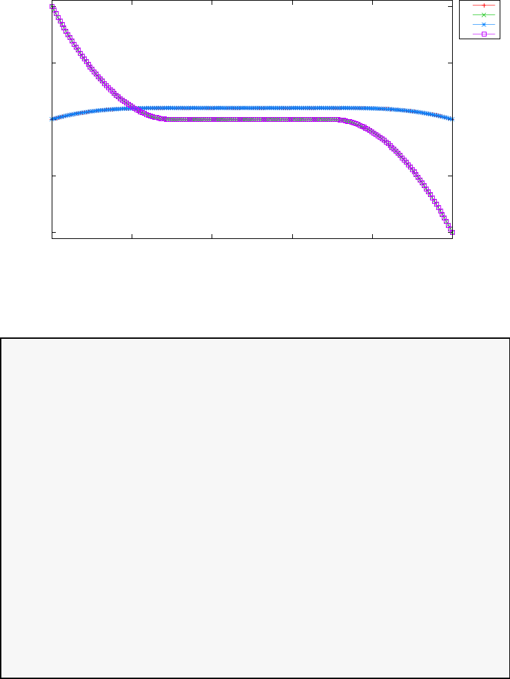
-1
-0.5
0
0.5
1
0 0.2 0.4 0.6 0.8 1
states
time (s)
Breakwell Problem: states
x
v
xa
va
Figure 3.9: States for Breakwell problem
PSOPT results summary
=====================
Problem: Breakwell Problem
CPU time (seconds): 3.840152e+00
NLP solver used: IPOPT
PSOPT release number: 4.0
Date and time of this run: Thu Feb 21 17:08:09 2019
Optimal (unscaled) cost function value: 4.444441e+00
Phase 1 endpoint cost function value: 0.000000e+00
Phase 1 integrated part of the cost: 4.444441e+00
Phase 1 initial time: 0.000000e+00
Phase 1 final time: 1.000000e+00
Phase 1 maximum relative local error: 8.294815e-06
NLP solver reports: The problem has been solved!
3.4 Bryson-Denham problem
Consider the following optimal control problem, which is known in the lit-
erature as the Bryson-Denham problem [7]. Minimize the cost functional
121
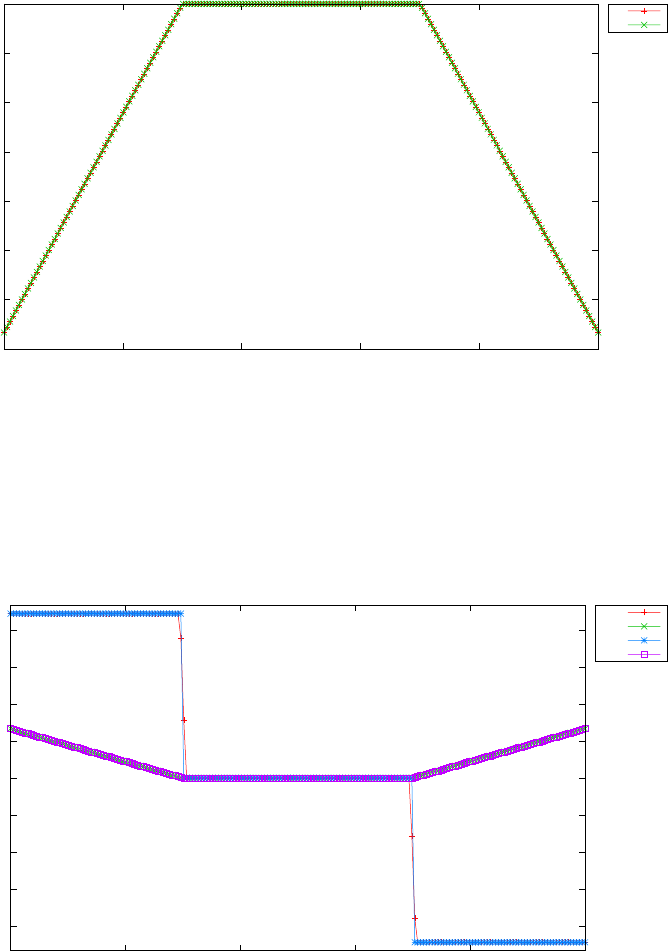
-7
-6
-5
-4
-3
-2
-1
0
0 0.2 0.4 0.6 0.8 1
control
time (s)
Breakwell Problem: control
u
ua
Figure 3.10: Control for Breakwell problem
-20
-15
-10
-5
0
5
10
15
20
0 0.2 0.4 0.6 0.8 1
costates
time (s)
Breakwell Problem: costates
l_x
l_v
la_x
la_v
Figure 3.11: Costates for Breakwell problem
122

J=x3(tf) (3.17)
subject to the dynamic constraints
˙x1=x2
˙x2=u
˙x3=1
2u2
(3.18)
the state bound
0≤x1≤1/9 (3.19)
and the boundary conditions
x1(0) = 0
x2(0) = 1
x3(0) = 0
x1(tf)=0
x2(tf) = −1
(3.20)
The PSOPT code that solves this problem is shown below.
//////////////////////////////////////////////////////////////////////////
//////////////// PSOPT Example ////////////////////
//////////////////////////////////////////////////////////////////////////
//////////////////////////////////////////////////////////////////////////
//////// Title: Bryson-Denham problem ////////////////
//////// Last modified: 05 January 2009 ////////////////
//////// Reference: GPOPS Handbook ////////////////
//////// (See PSOPT handbook for full reference) ///////////////
//////////////////////////////////////////////////////////////////////////
//////// Copyright (c) Victor M. Becerra, 2009 ////////////////
//////////////////////////////////////////////////////////////////////////
//////// This is part of the PSOPT software library, which ///////////////
//////// is distributed under the terms of the GNU Lesser ////////////////
//////// General Public License (LGPL) ////////////////
//////////////////////////////////////////////////////////////////////////
#include "psopt.h"
//////////////////////////////////////////////////////////////////////////
/////////////////// Define the end point (Mayer) cost function //////////
//////////////////////////////////////////////////////////////////////////
adouble endpoint_cost(adouble* initial_states, adouble* final_states,
adouble* parameters,adouble& t0, adouble& tf,
adouble* xad, int iphase, Workspace* workspace)
{
adouble x3f = final_states[ CINDEX(3) ];
return x3f;
}
//////////////////////////////////////////////////////////////////////////
/////////////////// Define the integrand (Lagrange) cost function //////
//////////////////////////////////////////////////////////////////////////
adouble integrand_cost(adouble* states, adouble* controls,
adouble* parameters, adouble& time, adouble* xad,
int iphase, Workspace* workspace)
{
return 0.0;
}
//////////////////////////////////////////////////////////////////////////
123

/////////////////// Define the DAE’s ////////////////////////////////////
//////////////////////////////////////////////////////////////////////////
void dae(adouble* derivatives, adouble* path, adouble* states,
adouble* controls, adouble* parameters, adouble& time,
adouble* xad, int iphase, Workspace* workspace )
{
adouble x1 = states[CINDEX(1)];
adouble x2 = states[CINDEX(2)];
adouble x3 = states[CINDEX(3)];
adouble u = controls[CINDEX(1)];
derivatives[ CINDEX(1) ] = x2;
derivatives[ CINDEX(2) ] = u;
derivatives[ CINDEX(3) ] = u*u/2;
}
////////////////////////////////////////////////////////////////////////////
/////////////////// Define the events function ////////////////////////////
////////////////////////////////////////////////////////////////////////////
void events(adouble* e, adouble* initial_states, adouble* final_states,
adouble* parameters,adouble& t0, adouble& tf, adouble* xad,
int iphase, Workspace* workspace)
{
adouble x10 = initial_states[ CINDEX(1) ];
adouble x20 = initial_states[ CINDEX(2) ];
adouble x30 = initial_states[ CINDEX(3) ];
adouble x1f = final_states[ CINDEX(1) ];
adouble x2f = final_states[ CINDEX(2) ];
e[ CINDEX(1) ] = x10;
e[ CINDEX(2) ] = x20;
e[ CINDEX(3) ] = x30;
e[ CINDEX(4) ] = x1f;
e[ CINDEX(5) ] = x2f;
}
///////////////////////////////////////////////////////////////////////////
/////////////////// Define the phase linkages function ///////////////////
///////////////////////////////////////////////////////////////////////////
void linkages( adouble* linkages, adouble* xad, Workspace* workspace)
{
// No linkages as this is a single phase problem
}
////////////////////////////////////////////////////////////////////////////
/////////////////// Define the main routine ///////////////////////////////
////////////////////////////////////////////////////////////////////////////
int main(void)
{
////////////////////////////////////////////////////////////////////////////
/////////////////// Declare key structures ////////////////////////////////
////////////////////////////////////////////////////////////////////////////
Alg algorithm;
Sol solution;
Prob problem;
////////////////////////////////////////////////////////////////////////////
/////////////////// Register problem name ////////////////////////////////
////////////////////////////////////////////////////////////////////////////
problem.name = "Bryson-Denham Problem";
problem.outfilename = "bryden.txt";
////////////////////////////////////////////////////////////////////////////
//////////// Declare problem level constants & do level 1 setup ///////////
////////////////////////////////////////////////////////////////////////////
problem.nphases = 1;
problem.nlinkages = 0;
124

psopt_level1_setup(problem);
/////////////////////////////////////////////////////////////////////////////
///////// Define phase related information & do level 2 setup /////////////
/////////////////////////////////////////////////////////////////////////////
problem.phases(1).nstates = 3;
problem.phases(1).ncontrols = 1;
problem.phases(1).nevents = 5;
problem.phases(1).npath = 0;
problem.phases(1).nodes = "[10, 50]";
psopt_level2_setup(problem, algorithm);
////////////////////////////////////////////////////////////////////////////
/////////////////// Declare DMatrix objects to store results //////////////
////////////////////////////////////////////////////////////////////////////
DMatrix x, u, t;
DMatrix lambda, H;
////////////////////////////////////////////////////////////////////////////
/////////////////// Enter problem bounds information //////////////////////
////////////////////////////////////////////////////////////////////////////
problem.phases(1).bounds.lower.states(1) = 0.0;
problem.phases(1).bounds.lower.states(2) = -10.0;
problem.phases(1).bounds.lower.states(3) = -10.0;
problem.phases(1).bounds.upper.states(1) = 1.0/9.0;
problem.phases(1).bounds.upper.states(2) = 10.0;
problem.phases(1).bounds.upper.states(3) = 10.0;
problem.phases(1).bounds.lower.controls(1) = -10.0;
problem.phases(1).bounds.upper.controls(1) = 10.0;
problem.phases(1).bounds.lower.events(1) = 0.0;
problem.phases(1).bounds.lower.events(2) = 1.0;
problem.phases(1).bounds.lower.events(3) = 0.0;
problem.phases(1).bounds.lower.events(4) = 0.0;
problem.phases(1).bounds.lower.events(5) = -1.0;
problem.phases(1).bounds.upper.events(1) = 0.0;
problem.phases(1).bounds.upper.events(2) = 1.0;
problem.phases(1).bounds.upper.events(3) = 0.0;
problem.phases(1).bounds.upper.events(4) = 0.0;
problem.phases(1).bounds.upper.events(5) = -1.0;
problem.phases(1).bounds.lower.StartTime = 0.0;
problem.phases(1).bounds.upper.StartTime = 0.0;
problem.phases(1).bounds.lower.EndTime = 0.0;
problem.phases(1).bounds.upper.EndTime = 50.0;
////////////////////////////////////////////////////////////////////////////
/////////////////// Register problem functions ///////////////////////////
////////////////////////////////////////////////////////////////////////////
problem.integrand_cost = &integrand_cost;
problem.endpoint_cost = &endpoint_cost;
problem.dae = &dae;
problem.events = &events;
problem.linkages = &linkages;
////////////////////////////////////////////////////////////////////////////
/////////////////// Define & register initial guess ///////////////////////
////////////////////////////////////////////////////////////////////////////
DMatrix x0(3,10);
x0(1,colon()) = linspace(0.0, 0.0, 10);
x0(2,colon()) = linspace(1.0,-1.0, 10);
x0(3,colon()) = linspace(0.0, 0.0, 10);
problem.phases(1).guess.controls = zeros(1,10);
problem.phases(1).guess.states = x0;
problem.phases(1).guess.time = linspace(0.0, 0.5, 10);
125

////////////////////////////////////////////////////////////////////////////
/////////////////// Enter algorithm options //////////////////////////////
////////////////////////////////////////////////////////////////////////////
algorithm.nlp_method = "IPOPT";
algorithm.scaling = "automatic";
algorithm.derivatives = "automatic";
algorithm.nlp_iter_max = 1000;
algorithm.nlp_tolerance = 1.e-6;
////////////////////////////////////////////////////////////////////////////
/////////////////// Now call PSOPT to solve the problem /////////////////
////////////////////////////////////////////////////////////////////////////
psopt(solution, problem, algorithm);
////////////////////////////////////////////////////////////////////////////
/////////// Extract relevant variables from solution structure //////////
////////////////////////////////////////////////////////////////////////////
x = solution.get_states_in_phase(1);
u = solution.get_controls_in_phase(1);
t = solution.get_time_in_phase(1);
lambda = solution.get_dual_costates_in_phase(1);
H = solution.get_dual_hamiltonian_in_phase(1);
////////////////////////////////////////////////////////////////////////////
/////////// Save solution data to files if desired ////////////////////////
////////////////////////////////////////////////////////////////////////////
x.Save("x.dat");
u.Save("u.dat");
t.Save("t.dat");
lambda.Save("lambda.dat");
H.Save("H.dat");
////////////////////////////////////////////////////////////////////////////
/////////// Plot some results if desired (requires gnuplot) ///////////////
////////////////////////////////////////////////////////////////////////////
plot(t,x,problem.name, "time (s)", "states", "x1 x2 x3");
plot(t,u, problem.name ,"time (s)", "control", "u");
plot(t,lambda, problem.name ,"time (s)", "lambda", "1 2 3");
plot(t,x,problem.name, "time (s)", "states", "x1 x2 x3",
"pdf", "bryden_states.pdf");
plot(t,u, problem.name ,"time (s)", "control", "u",
"pdf", "bryden_control.pdf");
plot(t,lambda, problem.name ,"time (s)", "lambda", "1 2 3",
"pdf", "bryden_lambda.pdf");
}
////////////////////////////////////////////////////////////////////////////
/////////////////////// END OF FILE ///////////////////////////////
////////////////////////////////////////////////////////////////////////////
The output from PSOPT is summarized in the following box and shown
in Figures 3.12 and 3.13, which contain the elements of the state and the
control, respectively.
PSOPT results summary
126
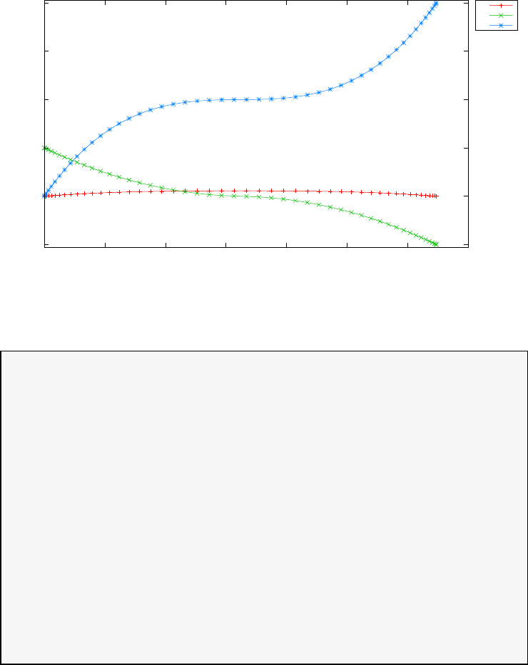
-1
0
1
2
3
4
0 0.1 0.2 0.3 0.4 0.5 0.6 0.7
states
time (s)
Bryson-Denham Problem
x1
x2
x3
Figure 3.12: States for Bryson Denham problem
=====================
Problem: Bryson-Denham Problem
CPU time (seconds): 2.550521e+00
NLP solver used: IPOPT
PSOPT release number: 4.0
Date and time of this run: Thu Feb 21 15:31:41 2019
Optimal (unscaled) cost function value: 3.999539e+00
Phase 1 endpoint cost function value: 3.999539e+00
Phase 1 integrated part of the cost: 0.000000e+00
Phase 1 initial time: 0.000000e+00
Phase 1 final time: 6.474067e-01
Phase 1 maximum relative local error: 6.431444e-05
NLP solver reports: The problem has been solved!
3.5 Bryson’s maximum range problem
Consider the following optimal control problem, which is known in the lit-
erature as the Bryson’s maximum range problem [7]. Minimize the cost
functional
J=x(tf) (3.21)
127
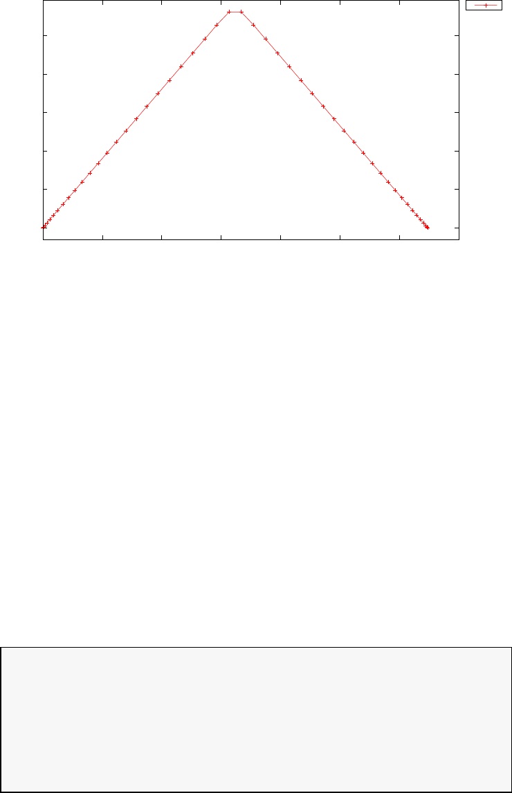
-6
-5
-4
-3
-2
-1
0 0.1 0.2 0.3 0.4 0.5 0.6 0.7
control
time (s)
Bryson-Denham Problem
u
Figure 3.13: Control for Bryson Denham problem
subject to the dynamic constraints
˙x=vu1
˙y=vu2
˙v=a−gu2
(3.22)
the path constraint
u2
1+u2
2= 1 (3.23)
and the boundary conditions
x(0) = 0
y(0) = 0
v(0) = 0
y(tf)=0.1
(3.24)
where tf= 2, g= 1 and a= 0.5g. The PSOPT code that solves this
problem is shown below.
//////////////////////////////////////////////////////////////////////////
//////////////// bryson_max_range.cxx /////////////////////
//////////////////////////////////////////////////////////////////////////
//////////////// PSOPT Example /////////////////////
//////////////////////////////////////////////////////////////////////////
//////////////////////////////////////////////////////////////////////////
//////// Title: Bryson maximum range problem ////////////////
//////// Last modified: 05 January 2009 ////////////////
//////// Reference: Bryson and Ho (1975) ////////////////
//////// (See PSOPT handbook for full reference) ////////////////
//////////////////////////////////////////////////////////////////////////
//////// Copyright (c) Victor M. Becerra, 2009 ////////////////
128

//////////////////////////////////////////////////////////////////////////
//////// This is part of the PSOPT software library, which////////////////
//////// is distributed under the terms of the GNU Lesser ////////////////
//////// General Public License (LGPL) ////////////////
//////////////////////////////////////////////////////////////////////////
#include "psopt.h"
//////////////////////////////////////////////////////////////////////////
/////////////////// Define the end point (Mayer) cost function //////////
//////////////////////////////////////////////////////////////////////////
adouble endpoint_cost(adouble* initial_states, adouble* final_states,
adouble* parameters,adouble& t0, adouble& tf,
adouble* xad, int iphase, Workspace* workspace)
{
adouble x = final_states[0];
return (-x);
}
//////////////////////////////////////////////////////////////////////////
/////////////////// Define the integrand (Lagrange) cost function //////
//////////////////////////////////////////////////////////////////////////
adouble integrand_cost(adouble* states, adouble* controls, adouble* parameters,
adouble& time, adouble* xad, int iphase, Workspace* workspace)
{
return 0.0;
}
//////////////////////////////////////////////////////////////////////////
/////////////////// Define the DAE’s ////////////////////////////////////
//////////////////////////////////////////////////////////////////////////
void dae(adouble* derivatives, adouble* path, adouble* states,
adouble* controls, adouble* parameters, adouble& time,
adouble* xad, int iphase, Workspace* workspace)
{
adouble xdot, ydot, vdot;
double g = 1.0;
double a = 0.5*g;
adouble x = states[ CINDEX(1) ];
adouble y = states[ CINDEX(2) ];
adouble v = states[ CINDEX(3) ];
adouble u1 = controls[ CINDEX(1) ];
adouble u2 = controls[ CINDEX(2) ];
xdot = v*u1;
ydot = v*u2;
vdot = a-g*u2;
derivatives[ CINDEX(1) ] = xdot;
derivatives[ CINDEX(2) ] = ydot;
derivatives[ CINDEX(3) ] = vdot;
path[ CINDEX(1) ] = (u1*u1) + (u2*u2);
}
////////////////////////////////////////////////////////////////////////////
/////////////////// Define the events function ////////////////////////////
////////////////////////////////////////////////////////////////////////////
void events(adouble* e, adouble* initial_states, adouble* final_states,
adouble* parameters,adouble& t0, adouble& tf, adouble* xad,
int iphase, Workspace* workspace)
{
adouble x0 = initial_states[ CINDEX(1) ];
adouble y0 = initial_states[ CINDEX(2) ];
adouble v0 = initial_states[ CINDEX(3) ];
adouble xf = final_states[ CINDEX(1) ];
adouble yf = final_states[ CINDEX(2) ];
e[ CINDEX(1) ] = x0;
e[ CINDEX(2) ] = y0;
e[ CINDEX(3) ] = v0;
e[ CINDEX(4) ] = yf;
129

}
///////////////////////////////////////////////////////////////////////////
/////////////////// Define the phase linkages function ///////////////////
///////////////////////////////////////////////////////////////////////////
void linkages( adouble* linkages, adouble* xad, Workspace* workspace)
{
// No linkages as this is a single phase problem
}
////////////////////////////////////////////////////////////////////////////
/////////////////// Define the main routine ///////////////////////////////
////////////////////////////////////////////////////////////////////////////
int main(void)
{
////////////////////////////////////////////////////////////////////////////
/////////////////// Declare key structures ////////////////////////////////
////////////////////////////////////////////////////////////////////////////
Alg algorithm;
Sol solution;
Prob problem;
////////////////////////////////////////////////////////////////////////////
/////////////////// Register problem name ////////////////////////////////
////////////////////////////////////////////////////////////////////////////
problem.name = "Bryson Maximum Range Problem";
problem.outfilename = "brymr.txt";
////////////////////////////////////////////////////////////////////////////
//////////// Define problem level constants & do level 1 setup ////////////
////////////////////////////////////////////////////////////////////////////
problem.nphases = 1;
problem.nlinkages = 0;
psopt_level1_setup(problem);
/////////////////////////////////////////////////////////////////////////////
///////// Define phase related information & do level 2 setup ////////////
/////////////////////////////////////////////////////////////////////////////
problem.phases(1).nstates = 3;
problem.phases(1).ncontrols = 2;
problem.phases(1).nevents = 4;
problem.phases(1).npath = 1;
problem.phases(1).nodes = "[20]";
psopt_level2_setup(problem, algorithm);
////////////////////////////////////////////////////////////////////////////
/////////////////// Declare DMatrix objects to store results //////////////
////////////////////////////////////////////////////////////////////////////
DMatrix x, u, t;
DMatrix lambda, H;
////////////////////////////////////////////////////////////////////////////
/////////////////// Enter problem bounds information //////////////////////
////////////////////////////////////////////////////////////////////////////
double xL = -10.0;
double yL = -10.0;
double vL = -10.0;
double xU = 10.0;
double yU = 10.0;
double vU = 10.0;
double u1L = -10.0;
double u2L = -10.0;
double u1U = 10.0;
double u2U = 10.0;
double x0 = 0.0;
130

double y0 = 0.0;
double v0 = 0.0;
double yf = 0.1;
problem.phases(1).bounds.lower.states(1) = xL;
problem.phases(1).bounds.lower.states(2) = yL;
problem.phases(1).bounds.lower.states(3) = vL;
problem.phases(1).bounds.upper.states(1) = xU;
problem.phases(1).bounds.upper.states(2) = yU;
problem.phases(1).bounds.upper.states(3) = vU;
problem.phases(1).bounds.lower.controls(1) = u1L;
problem.phases(1).bounds.lower.controls(2) = u2L;
problem.phases(1).bounds.upper.controls(1) = u1U;
problem.phases(1).bounds.upper.controls(2) = u2U;
problem.phases(1).bounds.lower.events(1) = x0;
problem.phases(1).bounds.lower.events(2) = y0;
problem.phases(1).bounds.lower.events(3) = v0;
problem.phases(1).bounds.lower.events(4) = yf;
problem.phases(1).bounds.upper.events(1) = x0;
problem.phases(1).bounds.upper.events(2) = y0;
problem.phases(1).bounds.upper.events(3) = v0;
problem.phases(1).bounds.upper.events(4) = yf;
problem.phases(1).bounds.upper.path(1) = 1.0;
problem.phases(1).bounds.lower.path(1) = 1.0;
problem.phases(1).bounds.lower.StartTime = 0.0;
problem.phases(1).bounds.upper.StartTime = 0.0;
problem.phases(1).bounds.lower.EndTime = 2.0;
problem.phases(1).bounds.upper.EndTime = 2.0;
////////////////////////////////////////////////////////////////////////////
/////////////////// Register problem functions ///////////////////////////
////////////////////////////////////////////////////////////////////////////
problem.integrand_cost = &integrand_cost;
problem.endpoint_cost = &endpoint_cost;
problem.dae = &dae;
problem.events = &events;
problem.linkages = &linkages;
////////////////////////////////////////////////////////////////////////////
/////////////////// Define & register initial guess ///////////////////////
////////////////////////////////////////////////////////////////////////////
int nnodes = problem.phases(1).nodes(1);
int ncontrols = problem.phases(1).ncontrols;
int nstates = problem.phases(1).nstates;
DMatrix x_guess = zeros(nstates,nnodes);
x_guess(1,colon()) = x0*ones(1,nnodes);
x_guess(2,colon()) = y0*ones(1,nnodes);
x_guess(3,colon()) = v0*ones(1,nnodes);
problem.phases(1).guess.controls = zeros(ncontrols,nnodes);
problem.phases(1).guess.states = x_guess;
problem.phases(1).guess.time = linspace(0.0,2.0,nnodes);
////////////////////////////////////////////////////////////////////////////
/////////////////// Enter algorithm options //////////////////////////////
////////////////////////////////////////////////////////////////////////////
algorithm.nlp_iter_max = 1000;
algorithm.nlp_tolerance = 1.e-4;
algorithm.nlp_method = "IPOPT";
algorithm.scaling = "automatic";
131

algorithm.derivatives = "automatic";
algorithm.mesh_refinement = "automatic";
algorithm.collocation_method = "trapezoidal";
// algorithm.defect_scaling = "jacobian-based";
algorithm.ode_tolerance = 1.e-6;
////////////////////////////////////////////////////////////////////////////
/////////////////// Now call PSOPT to solve the problem /////////////////
////////////////////////////////////////////////////////////////////////////
psopt(solution, problem, algorithm);
////////////////////////////////////////////////////////////////////////////
/////////// Extract relevant variables from solution structure //////////
////////////////////////////////////////////////////////////////////////////
x = solution.get_states_in_phase(1);
u = solution.get_controls_in_phase(1);
t = solution.get_time_in_phase(1);
lambda = solution.get_dual_costates_in_phase(1);
H = solution.get_dual_hamiltonian_in_phase(1);
////////////////////////////////////////////////////////////////////////////
/////////// Save solution data to files if desired ////////////////////////
////////////////////////////////////////////////////////////////////////////
x.Save("x.dat");
u.Save("u.dat");
t.Save("t.dat");
lambda.Save("lambda.dat");
H.Save("H.dat");
////////////////////////////////////////////////////////////////////////////
/////////// Plot some results if desired (requires gnuplot) ///////////////
////////////////////////////////////////////////////////////////////////////
plot(t,x,problem.name+": states", "time (s)", "states","x y v");
plot(t,u,problem.name+": controls","time (s)", "controls", "u_1 u_2");
plot(t,x,problem.name+": states", "time (s)", "states","x y v",
"pdf", "brymr_states.pdf");
plot(t,u,problem.name+": controls","time (s)", "controls", "u_1 u_2",
"pdf", "brymr_controls.pdf");
}
////////////////////////////////////////////////////////////////////////////
/////////////////////// END OF FILE ///////////////////////////////
////////////////////////////////////////////////////////////////////////////
The output from PSOPT is summarized in the box below and shown
in Figures 3.14 and 3.15, which contain the elements of the state and the
control, respectively.
PSOPT results summary
=====================
Problem: Bryson Maximum Range Problem
CPU time (seconds): 7.753865e+00
NLP solver used: IPOPT
PSOPT release number: 4.0
Date and time of this run: Sun Feb 24 07:04:55 2019
132
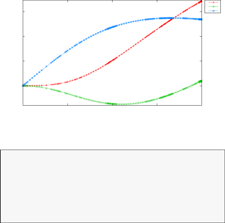
0
0.5
1
1.5
0 0.5 1 1.5 2
states
time (s)
Bryson Maximum Range Problem: states
x
y
v
Figure 3.14: States for Bryson’s maximum range problem
Optimal (unscaled) cost function value: -1.712319e+00
Phase 1 endpoint cost function value: -1.712319e+00
Phase 1 integrated part of the cost: 0.000000e+00
Phase 1 initial time: 0.000000e+00
Phase 1 final time: 2.000000e+00
Phase 1 maximum relative local error: 1.170448e-04
NLP solver reports: The problem has been solved!
3.6 Catalytic cracking of gas oil
Consider the following optimization problem, which involves finding optimal
static parameters subject to dynamic constraints [15]. Minimize
J=
21
X
i=1
(y1(ti)−ym,1(i))2+ (y2(ti)−ym,2(i))2(3.25)
subject to the dynamic constraints
˙y1=−(θ1+θ3)y2
1
˙y2=θ1y2
1−θ2y2(3.26)
133
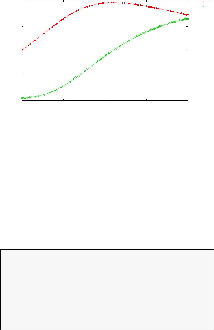
-1
-0.5
0
0.5
1
0 0.5 1 1.5 2
controls
time (s)
Bryson Maximum Range Problem: controls
u_1
u_2
Figure 3.15: Controls for Bryson’s maximum range problem
the parameter constraint
θ1≥0
θ2≥0
θ3≥0
(3.27)
Note that, given the nature of the problem, the parameter estimation
facilities of PSOPT are used in this example. In this case, the observations
function is simple:
g(x(t), u(t), p, t) = [y1y2]T
The PSOPT code that solves this problem is shown below. The code
includes the values of the measurement vectors ym,1, and ym,2, as well as
the vector of sampling instants θi, i = 1,...,21.
//////////////////////////////////////////////////////////////////////////
////////////////// cracking.cxx ////////////////////////////
//////////////////////////////////////////////////////////////////////////
//////////////// PSOPT Example ////////////////////
//////////////////////////////////////////////////////////////////////////
//////////////////////////////////////////////////////////////////////////
//////// Title: Catalytic Cracking of Gas Oil ////////////////
//////// Last modified: 15 January 2009 ////////////////
//////// Reference: Users guide for DIRCOL ////////////////
//////// (See PSOPT handbook for full reference) ///////////////
//////////////////////////////////////////////////////////////////////////
//////// Copyright (c) Victor M. Becerra, 2009 ////////////////
//////////////////////////////////////////////////////////////////////////
//////// This is part of the PSOPT software library, which ///////////////
//////// is distributed under the terms of the GNU Lesser ////////////////
//////// General Public License (LGPL) ////////////////
//////////////////////////////////////////////////////////////////////////
134

#include "psopt.h"
//////////////////////////////////////////////////////////////////////////
/////////////////// Define the observation function //////////
//////////////////////////////////////////////////////////////////////////
void observation_function( adouble* observations,
adouble* states, adouble* controls,
adouble* parameters, adouble& time, int k,
adouble* xad, int iphase, Workspace* workspace)
{
observations[ CINDEX(1) ] = states[ CINDEX(1) ];
observations[ CINDEX(2) ] = states[ CINDEX(2) ];
}
//////////////////////////////////////////////////////////////////////////
/////////////////// Define the DAE’s ////////////////////////////////////
//////////////////////////////////////////////////////////////////////////
void dae(adouble* derivatives, adouble* path, adouble* states,
adouble* controls, adouble* parameters, adouble& time,
adouble* xad, int iphase, Workspace* workspace)
{
adouble y1 = states[CINDEX(1)];
adouble y2 = states[CINDEX(2)];
adouble theta1 = parameters[ CINDEX(1) ];
adouble theta2 = parameters[ CINDEX(2) ];
adouble theta3 = parameters[ CINDEX(3) ];
derivatives[CINDEX(1)] = -(theta1 + theta3)*y1*y1;
derivatives[CINDEX(2)] = theta1*y1*y1 - theta2*y2;
}
////////////////////////////////////////////////////////////////////////////
/////////////////// Define the events function ////////////////////////////
////////////////////////////////////////////////////////////////////////////
void events(adouble* e, adouble* initial_states, adouble* final_states,
adouble* parameters,adouble& t0, adouble& tf, adouble* xad,
int iphase, Workspace* workspace)
{
// No events
}
///////////////////////////////////////////////////////////////////////////
/////////////////// Define the phase linkages function ///////////////////
///////////////////////////////////////////////////////////////////////////
void linkages( adouble* linkages, adouble* xad, Workspace* workspace)
{
// No linkages as this is a single phase problem
}
////////////////////////////////////////////////////////////////////////////
/////////////////// Define the main routine ///////////////////////////////
////////////////////////////////////////////////////////////////////////////
int main(void)
{
DMatrix y1meas, y2meas, tmeas;
// Measured values of y1
y1meas = "[1.0,0.8105,0.6208,0.5258,0.4345,0.3903,0.3342,0.3034, \
0.2735,0.2405,0.2283,0.2071,0.1669,0.153,0.1339,0.1265, \
0.12,0.099,0.087,0.077,0.069]";
// Measured values of y2
y2meas = "[0.0,0.2,0.2886,0.301,0.3215,0.3123,0.2716,0.2551,0.2258, \
0.1959,0.1789,0.1457,0.1198,0.0909,0.0719,0.0561,0.046, \
0.028,0.019,0.014,0.01]";
// Sampling instants
tmeas = "[0.0,0.025,0.05,0.075,0.1,0.125,0.15,0.175,0.2,0.225,0.25, \
135

0.3,0.35,0.4,0.45,0.5,0.55,0.65,0.75,0.85,0.95]";
////////////////////////////////////////////////////////////////////////////
/////////////////// Declare key structures ////////////////////////////////
////////////////////////////////////////////////////////////////////////////
Alg algorithm;
Sol solution;
Prob problem;
////////////////////////////////////////////////////////////////////////////
/////////////////// Register problem name ////////////////////////////////
////////////////////////////////////////////////////////////////////////////
problem.name = "Catalytic cracking of gas oil";
problem.outfilename = "cracking.txt";
////////////////////////////////////////////////////////////////////////////
//////////// Define problem level constants & do level 1 setup ////////////
////////////////////////////////////////////////////////////////////////////
problem.nphases = 1;
problem.nlinkages = 0;
psopt_level1_setup(problem);
/////////////////////////////////////////////////////////////////////////////
///////// Define phase related information & do level 2 setup /////////////
/////////////////////////////////////////////////////////////////////////////
problem.phases(1).nstates = 2;
problem.phases(1).ncontrols = 0;
problem.phases(1).nevents = 0;
problem.phases(1).npath = 0;
problem.phases(1).nparameters = 3;
problem.phases(1).nodes = "[80]";
problem.phases(1).nobserved = 2;
problem.phases(1).nsamples = 21;
psopt_level2_setup(problem, algorithm);
////////////////////////////////////////////////////////////////////////////
//////////// Enter estimation information ////////////
////////////////////////////////////////////////////////////////////////////
problem.phases(1).observation_nodes = tmeas;
problem.phases(1).observations = (y1meas && y2meas);
problem.phases(1).residual_weights = ones(2,21);
////////////////////////////////////////////////////////////////////////////
/////////////////// Declare DMatrix objects to store results //////////////
////////////////////////////////////////////////////////////////////////////
DMatrix x, p, t;
////////////////////////////////////////////////////////////////////////////
/////////////////// Enter problem bounds information //////////////////////
////////////////////////////////////////////////////////////////////////////
problem.phases(1).bounds.lower.states(1) = 0.0;
problem.phases(1).bounds.lower.states(2) = 0.0;
problem.phases(1).bounds.upper.states(1) = 2.0;
problem.phases(1).bounds.upper.states(2) = 2.0;
problem.phases(1).bounds.lower.parameters(1) = 0.0;
problem.phases(1).bounds.lower.parameters(2) = 0.0;
problem.phases(1).bounds.lower.parameters(3) = 0.0;
problem.phases(1).bounds.upper.parameters(1) = 20.0;
problem.phases(1).bounds.upper.parameters(2) = 20.0;
problem.phases(1).bounds.upper.parameters(3) = 20.0;
problem.phases(1).bounds.lower.StartTime = 0.0;
problem.phases(1).bounds.upper.StartTime = 0.0;
136

problem.phases(1).bounds.lower.EndTime = 0.95;
problem.phases(1).bounds.upper.EndTime = 0.95;
////////////////////////////////////////////////////////////////////////////
/////////////////// Register problem functions ///////////////////////////
////////////////////////////////////////////////////////////////////////////
problem.dae = &dae;
problem.events = &events;
problem.linkages = &linkages;
problem.observation_function = & observation_function;
////////////////////////////////////////////////////////////////////////////
/////////////////// Define & register initial guess ///////////////////////
////////////////////////////////////////////////////////////////////////////
DMatrix state_guess(2, 40);
state_guess(1,colon()) = linspace(1.0,0.069, 40);
state_guess(2,colon()) = linspace(0.30,0.01, 40);
problem.phases(1).guess.states = state_guess;
problem.phases(1).guess.time = linspace(0.0, 0.95, 40);
problem.phases(1).guess.parameters = zeros(3,1);
////////////////////////////////////////////////////////////////////////////
/////////////////// Enter algorithm options //////////////////////////////
////////////////////////////////////////////////////////////////////////////
algorithm.nlp_method = "IPOPT";
algorithm.scaling = "automatic";
algorithm.derivatives = "automatic";
// algorithm.collocation_method = "Hermite-Simpson";
algorithm.nlp_iter_max = 1000;
algorithm.nlp_tolerance = 1.e-4;
algorithm.jac_sparsity_ratio = 0.52;
////////////////////////////////////////////////////////////////////////////
/////////////////// Now call PSOPT to solve the problem //////////////////
////////////////////////////////////////////////////////////////////////////
psopt(solution, problem, algorithm);
////////////////////////////////////////////////////////////////////////////
/////////// Extract relevant variables from solution structure //////////
////////////////////////////////////////////////////////////////////////////
x = solution.get_states_in_phase(1);
t = solution.get_time_in_phase(1);
p = solution.get_parameters_in_phase(1);
////////////////////////////////////////////////////////////////////////////
/////////// Save solution data to files if desired ////////////////////////
////////////////////////////////////////////////////////////////////////////
x.Save("x.dat");
t.Save("t.dat");
p.Print("Estimated parameters");
////////////////////////////////////////////////////////////////////////////
/////////// Plot some results if desired (requires gnuplot) ///////////////
////////////////////////////////////////////////////////////////////////////
plot(t,x,problem.name, "time (s)", "states", "y1 y2");
plot(t,x,problem.name, "time (s)", "states", "y1 y2",
"pdf", "cracking_states.pdf");
}
////////////////////////////////////////////////////////////////////////////
/////////////////////// END OF FILE ///////////////////////////////
////////////////////////////////////////////////////////////////////////////
The output from PSOPT is summarized in the box below and shown in
Figure 3.16, which shows the states of the system. The optimal parameters
137

found were:
θ1= 11.40825702
θ2= 8.123367918
θ3= 1.668727477
(3.28)
PSOPT results summary
=====================
Problem: Catalytic cracking of gas oil
CPU time (seconds): 5.681664e+00
NLP solver used: IPOPT
PSOPT release number: 4.0
Date and time of this run: Thu Feb 21 16:06:49 2019
Optimal (unscaled) cost function value: 4.326398e-03
Phase 1 endpoint cost function value: 4.326398e-03
Phase 1 integrated part of the cost: 0.000000e+00
Phase 1 initial time: 0.000000e+00
Phase 1 final time: 9.500000e-01
Phase 1 maximum relative local error: 6.513072e-10
NLP solver reports: The problem has been solved!
3.7 Catalyst mixing problem
Consider the following optimal control problem, which attempts to deter-
mine the optimal mixing policy of two catalysts along the length of a tubular
plug flow reactor involving several reactions [38]. The catalyst mixing prob-
lem is a typical bang-singular-bang problem. Minimize the cost functional
J=−1 + x1(tf) + x2(tf) (3.29)
subject to the dynamic constraints
˙x1=u(10x2−x1)
˙x2=u(x1−10x2)−(1 −u)x2(3.30)
the boundary conditions
x1(0) = 1
x2(0) = 0
x1(tf)≤0.95
(3.31)
138
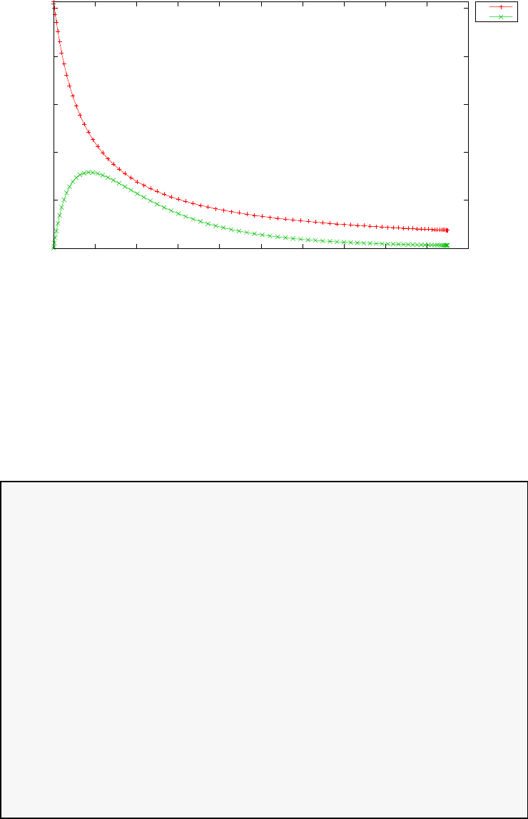
0
0.2
0.4
0.6
0.8
1
0 0.1 0.2 0.3 0.4 0.5 0.6 0.7 0.8 0.9 1
states
time (s)
Catalytic cracking of gas oil
y1
y2
Figure 3.16: States for catalytic cracking of gas oil problem
and the box constraints:
0.9≤x1(t)≤1.0
0≤x2(t)≤0.1
0≤u(t)≤1
(3.32)
where tf= 1. The PSOPT code that solves this problem is shown below.
//////////////////////////////////////////////////////////////////////////
////////////////// catmix.cxx //////////////////////////
//////////////////////////////////////////////////////////////////////////
//////////////// PSOPT Example ////////////////////
//////////////////////////////////////////////////////////////////////////
//////////////////////////////////////////////////////////////////////////
//////// Title: Catalyst mixing problem ////////////////
//////// Last modified: 26 January 2009 ////////////////
//////// Reference: Vassiliadis (1999) ////////////////
//////// (See PSOPT handbook for full reference) ////////////////
//////////////////////////////////////////////////////////////////////////
//////// Copyright (c) Victor M. Becerra, 2009 ////////////////
//////////////////////////////////////////////////////////////////////////
//////// This is part of the PSOPT software library, which ///////////////
//////// is distributed under the terms of the GNU Lesser ////////////////
//////// General Public License (LGPL) ////////////////
//////////////////////////////////////////////////////////////////////////
#include "psopt.h"
//////////////////////////////////////////////////////////////////////////
/////////////////// Define the end point (Mayer) cost function //////////
//////////////////////////////////////////////////////////////////////////
adouble endpoint_cost(adouble* initial_states, adouble* final_states,
adouble* parameters,adouble& t0, adouble& tf,
adouble* xad, int iphase, Workspace* workspace)
{
adouble x1f = final_states[ CINDEX(1) ];
adouble x2f = final_states[ CINDEX(2) ];
139

return -(1.0-x1f-x2f);
}
//////////////////////////////////////////////////////////////////////////
/////////////////// Define the integrand (Lagrange) cost function //////
//////////////////////////////////////////////////////////////////////////
adouble integrand_cost(adouble* states, adouble* controls,
adouble* parameters, adouble& time, adouble* xad,
int iphase, Workspace* workspace)
{
return 0.0;
}
//////////////////////////////////////////////////////////////////////////
/////////////////// Define the DAE’s ////////////////////////////////////
//////////////////////////////////////////////////////////////////////////
void dae(adouble* derivatives, adouble* path, adouble* states,
adouble* controls, adouble* parameters, adouble& time,
adouble* xad, int iphase, Workspace* workspace)
{
adouble xdot, ydot, vdot;
adouble x1 = states[ CINDEX(1) ];
adouble x2 = states[ CINDEX(2) ];
adouble u = controls[ CINDEX(1) ];
derivatives[ CINDEX(1) ] = u*(10*x2-x1);
derivatives[ CINDEX(2) ] = u*(x1-10*x2) - (1-u)*x2;
}
////////////////////////////////////////////////////////////////////////////
/////////////////// Define the events function ////////////////////////////
////////////////////////////////////////////////////////////////////////////
void events(adouble* e, adouble* initial_states, adouble* final_states,
adouble* parameters,adouble& t0, adouble& tf, adouble* xad,
int iphase, Workspace* workspace)
{
adouble x10 = initial_states[ CINDEX(1)];
adouble x20 = initial_states[ CINDEX(2) ];
adouble x1f = final_states[ CINDEX(1) ];
e[ CINDEX(1) ] = x10;
e[ CINDEX(2) ] = x20;
e[ CINDEX(3) ] = x1f;
}
///////////////////////////////////////////////////////////////////////////
/////////////////// Define the phase linkages function ///////////////////
///////////////////////////////////////////////////////////////////////////
void linkages( adouble* linkages, adouble* xad, Workspace* workspace)
{
// No linkages as this is a single phase problem
}
////////////////////////////////////////////////////////////////////////////
/////////////////// Define the main routine ///////////////////////////////
////////////////////////////////////////////////////////////////////////////
int main(void)
{
////////////////////////////////////////////////////////////////////////////
/////////////////// Declare key structures ////////////////////////////////
////////////////////////////////////////////////////////////////////////////
Alg algorithm;
Sol solution;
Prob problem;
////////////////////////////////////////////////////////////////////////////
/////////////////// Register problem name ////////////////////////////////
////////////////////////////////////////////////////////////////////////////
problem.name = "Catalyst mixing roblem";
problem.outfilename = "catmix.txt";
140

////////////////////////////////////////////////////////////////////////////
//////////// Define problem level constants & do level 1 setup ////////////
////////////////////////////////////////////////////////////////////////////
problem.nphases = 1;
problem.nlinkages = 0;
psopt_level1_setup(problem);
/////////////////////////////////////////////////////////////////////////////
///////// Define phase related information & do level 2 setup /////////////
/////////////////////////////////////////////////////////////////////////////
problem.phases(1).nstates = 2;
problem.phases(1).ncontrols = 1;
problem.phases(1).nevents = 3;
problem.phases(1).npath = 0;
problem.phases(1).nodes = 40;
psopt_level2_setup(problem, algorithm);
////////////////////////////////////////////////////////////////////////////
/////////////////// Declare DMatrix objects to store results //////////////
////////////////////////////////////////////////////////////////////////////
DMatrix x, u, t;
DMatrix lambda, H;
////////////////////////////////////////////////////////////////////////////
/////////////////// Enter problem bounds information //////////////////////
////////////////////////////////////////////////////////////////////////////
problem.phases(1).bounds.lower.states(1) = 0.9;
problem.phases(1).bounds.lower.states(2) = 0.0;
problem.phases(1).bounds.upper.states(1) = 1.0;
problem.phases(1).bounds.upper.states(2) = 0.1;
problem.phases(1).bounds.lower.controls(1) = 0.0;
problem.phases(1).bounds.upper.controls(1) = 1.0;
problem.phases(1).bounds.lower.events(1) = 1.0;
problem.phases(1).bounds.lower.events(2) = 0.0;
problem.phases(1).bounds.lower.events(3) = 0.0;
problem.phases(1).bounds.upper.events(1) = 1.0;
problem.phases(1).bounds.upper.events(2) = 0.0;
problem.phases(1).bounds.upper.events(3) = 0.95;
problem.phases(1).bounds.lower.StartTime = 0.0;
problem.phases(1).bounds.upper.StartTime = 0.0;
problem.phases(1).bounds.lower.EndTime = 1.0;
problem.phases(1).bounds.upper.EndTime = 1.0;
////////////////////////////////////////////////////////////////////////////
/////////////////// Register problem functions ///////////////////////////
////////////////////////////////////////////////////////////////////////////
problem.integrand_cost = &integrand_cost;
problem.endpoint_cost = &endpoint_cost;
problem.dae = &dae;
problem.events = &events;
problem.linkages = &linkages;
////////////////////////////////////////////////////////////////////////////
/////////////////// Define & register initial guess ///////////////////////
////////////////////////////////////////////////////////////////////////////
DMatrix u0(1,40);
DMatrix x0(3,40);
141

DMatrix t0 = linspace(0.0, 1.0, 40);
x0(1,colon()) = ones(1,40) - 0.085*t0;
x0(2,colon()) = 0.05*t0;
u0 = ones(1,40)- t0;
problem.phases(1).guess.controls = u0;
problem.phases(1).guess.states = x0;
problem.phases(1).guess.time = t0;
////////////////////////////////////////////////////////////////////////////
/////////////////// Enter algorithm options //////////////////////////////
////////////////////////////////////////////////////////////////////////////
algorithm.nlp_method = "IPOPT";
algorithm.scaling = "automatic";
algorithm.derivatives = "automatic";
algorithm.nlp_iter_max = 1000;
algorithm.nlp_tolerance = 1.e-6;
////////////////////////////////////////////////////////////////////////////
/////////////////// Now call PSOPT to solve the problem /////////////////
////////////////////////////////////////////////////////////////////////////
psopt(solution, problem, algorithm);
////////////////////////////////////////////////////////////////////////////
/////////// Extract relevant variables from solution structure //////////
////////////////////////////////////////////////////////////////////////////
x = solution.get_states_in_phase(1);
u = solution.get_controls_in_phase(1);
t = solution.get_time_in_phase(1);
lambda = solution.get_dual_costates_in_phase(1);
H = solution.get_dual_hamiltonian_in_phase(1);
////////////////////////////////////////////////////////////////////////////
/////////// Save solution data to files if desired ////////////////////////
////////////////////////////////////////////////////////////////////////////
x.Save("x.dat");
u.Save("u.dat");
t.Save("t.dat");
lambda.Save("lambda.dat");
H.Save("H.dat");
////////////////////////////////////////////////////////////////////////////
/////////// Plot some results if desired (requires gnuplot) ///////////////
////////////////////////////////////////////////////////////////////////////
plot(t,x,problem.name + ": states", "time (s)", "states", "x1 x2");
plot(t,u,problem.name + ": control", "time (s)", "control", "u");
plot(t,x,problem.name + ": states", "time (s)", "states", "x1 x2",
"pdf", "catmix_states.pdf");
plot(t,u,problem.name + ": control", "time (s)", "control", "u",
"pdf", "catmix_control.pdf");
}
////////////////////////////////////////////////////////////////////////////
/////////////////////// END OF FILE ///////////////////////////////
////////////////////////////////////////////////////////////////////////////
The output from PSOPT is summarised in the box below and shown
in Figures 3.17 and 3.18, which contain the elements of the state and the
control, respectively.
142
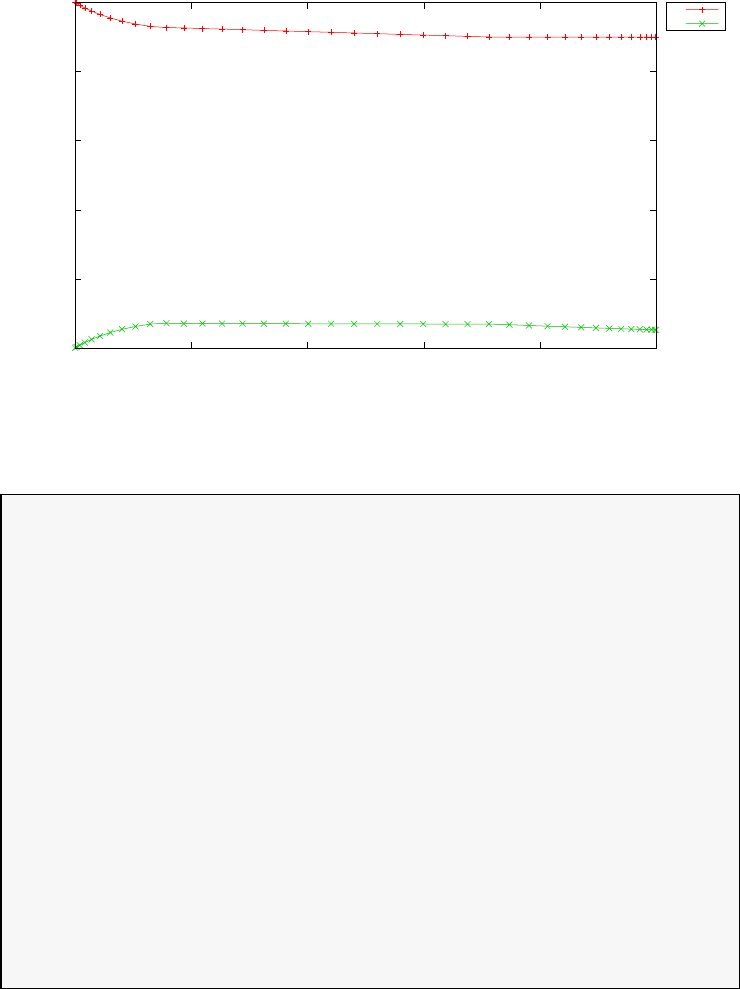
0
0.2
0.4
0.6
0.8
1
0 0.2 0.4 0.6 0.8 1
states
time (s)
Catalyst mixing roblem: states
x1
x2
Figure 3.17: States for catalyist mixing problem
PSOPT results summary
=====================
Problem: Catalyst mixing roblem
CPU time (seconds): 1.268127e+00
NLP solver used: IPOPT
PSOPT release number: 4.0
Date and time of this run: Thu Feb 21 16:06:22 2019
Optimal (unscaled) cost function value: -4.805320e-02
Phase 1 endpoint cost function value: -4.805320e-02
Phase 1 integrated part of the cost: 0.000000e+00
Phase 1 initial time: 0.000000e+00
Phase 1 final time: 1.000000e+00
Phase 1 maximum relative local error: 1.092831e-04
NLP solver reports: The problem has been solved!
143
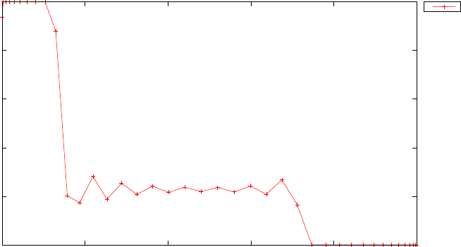
0
0.2
0.4
0.6
0.8
1
0 0.2 0.4 0.6 0.8 1
control
time (s)
Catalyst mixing roblem: control
u
Figure 3.18: Control for catalyst mixing problem
3.8 Coulomb friction
Consider the following optimal control problem, which consists of a system
that exhibits Coulomb friction [29]. Minimize the cost:
J=tf(3.33)
subject to the dynamic constraints
¨q1= (−(k1−k2)q1+k2q2−µsign( ˙q1) + u1)/m1
¨q2= (k2q1−k2q2−µsign( ˙q2) + u2)/m2(3.34)
and the boundary conditions
q1(0) = 0
˙q1(0) = −1
q2(0) = 0
˙q2(0) = −2
q1(tf) = 1
˙q1(tf) = 0
q2(tf) = 2
˙q2(tf)=0
(3.35)
where k1= 0.95, k2=0.85, µ= 1.0, m1=1.1, m2=1.2. The PSOPT code
that solves this problem is shown below.
144

//////////////////////////////////////////////////////////////////////////
////////////////// coulomb.cxx //////////////////////////
//////////////////////////////////////////////////////////////////////////
//////////////// PSOPT Example /////////////////////
//////////////////////////////////////////////////////////////////////////
//////////////////////////////////////////////////////////////////////////
//////// Title: Coulumb friction problem ////////////////
//////// Last modified: 04 January 2009 ////////////////
//////// Reference: Driessen and Sadegh (2000) ////////////////
//////// (See PSOPT handbook for full reference) ////////////////
//////////////////////////////////////////////////////////////////////////
//////// Copyright (c) Victor M. Becerra, 2009 ///////////////
//////////////////////////////////////////////////////////////////////////
//////// This is part of the PSOPT software library, which ///////////////
//////// is distributed under the terms of the GNU Lesser ///////////////
//////// General Public License (LGPL) ///////////////
//////////////////////////////////////////////////////////////////////////
#include "psopt.h"
//////////////////////////////////////////////////////////////////////////
/////////////////// Define the end point (Mayer) cost function //////////
//////////////////////////////////////////////////////////////////////////
adouble endpoint_cost(adouble* initial_states, adouble* final_states,
adouble* parameters,adouble& t0, adouble& tf,
adouble* xad, int iphase, Workspace* workspace)
{
return tf;
}
//////////////////////////////////////////////////////////////////////////
/////////////////// Define the integrand (Lagrange) cost function //////
//////////////////////////////////////////////////////////////////////////
adouble integrand_cost(adouble* states, adouble* controls,
adouble* parameters, adouble& time, adouble* xad,
int iphase, Workspace* workspace)
{
return 0.0;
}
//////////////////////////////////////////////////////////////////////////
/////////////////// Define the DAE’s ////////////////////////////////////
//////////////////////////////////////////////////////////////////////////
void dae(adouble* derivatives, adouble* path, adouble* states,
adouble* controls, adouble* parameters, adouble& time,
adouble* xad, int iphase, Workspace* workspace)
{
adouble q1 = states[ CINDEX(1) ];
adouble q1dot = states[ CINDEX(2) ];
adouble q2 = states[ CINDEX(3) ];
adouble q2dot = states[ CINDEX(4) ];
adouble u1 = controls[ CINDEX(1) ];
adouble u2 = controls[ CINDEX(2) ];
double k1 = 0.95;
double k2 = 0.85;
double mu = 1.0;
double m1 = 1.1;
double m2 = 1.2;
double epsilon = 0.01;
derivatives[ CINDEX(1) ] = q1dot;
derivatives[ CINDEX(2) ] = ( (-k1-k2)*q1+k2*q2-mu*smooth_sign(q1dot,epsilon)+u1 )/m1;
derivatives[ CINDEX(3) ] = q2dot;
derivatives[ CINDEX(4) ] = ( k2*q1-k2*q2-mu*smooth_sign(q2dot,epsilon)+u2 )/m2;
}
////////////////////////////////////////////////////////////////////////////
/////////////////// Define the events function ////////////////////////////
////////////////////////////////////////////////////////////////////////////
void events(adouble* e, adouble* initial_states, adouble* final_states,
adouble* parameters,adouble& t0, adouble& tf, adouble* xad,
int iphase, Workspace* workspace)
{
145

adouble q1_0 = initial_states[ CINDEX(1) ];
adouble q1dot_0 = initial_states[ CINDEX(2) ];
adouble q2_0 = initial_states[ CINDEX(3) ];
adouble q2dot_0 = initial_states[ CINDEX(4) ];
adouble q1_f = final_states[ CINDEX(1) ];
adouble q1dot_f = final_states[ CINDEX(2) ];
adouble q2_f = final_states[ CINDEX(3) ];
adouble q2dot_f = final_states[ CINDEX(4) ];
e[ CINDEX(1) ] = q1_0;
e[ CINDEX(2) ] = q1dot_0;
e[ CINDEX(3) ] = q2_0;
e[ CINDEX(4) ] = q2dot_0;
e[ CINDEX(5) ] = q1_f;
e[ CINDEX(6) ] = q1dot_f;
e[ CINDEX(7) ] = q2_f;
e[ CINDEX(8) ] = q2dot_f;
}
///////////////////////////////////////////////////////////////////////////
/////////////////// Define the phase linkages function ///////////////////
///////////////////////////////////////////////////////////////////////////
void linkages( adouble* linkages, adouble* xad, Workspace* workspace)
{
// No linkages as this is a single phase problem
}
////////////////////////////////////////////////////////////////////////////
/////////////////// Define the main routine ///////////////////////////////
////////////////////////////////////////////////////////////////////////////
int main(void)
{
////////////////////////////////////////////////////////////////////////////
/////////////////// Declare key structures ////////////////////////////////
////////////////////////////////////////////////////////////////////////////
Alg algorithm;
Sol solution;
Prob problem;
////////////////////////////////////////////////////////////////////////////
/////////////////// Register problem name ////////////////////////////////
////////////////////////////////////////////////////////////////////////////
problem.name = "Coulomb friction problem";
problem.outfilename = "coulomb.txt";
////////////////////////////////////////////////////////////////////////////
//////////// Define problem level constants & do level 1 setup ////////////
////////////////////////////////////////////////////////////////////////////
problem.nphases = 1;
problem.nlinkages = 0;
psopt_level1_setup(problem);
/////////////////////////////////////////////////////////////////////////////
///////// Define phase related information & do level 2 setup /////////////
/////////////////////////////////////////////////////////////////////////////
problem.phases(1).nstates = 4;
problem.phases(1).ncontrols = 2;
problem.phases(1).nevents = 8;
problem.phases(1).npath = 0;
problem.phases(1).nodes = 40;
psopt_level2_setup(problem, algorithm);
////////////////////////////////////////////////////////////////////////////
/////////////////// Enter problem bounds information //////////////////////
////////////////////////////////////////////////////////////////////////////
double q1_0 = 0.0;
146

double dotq1_0 = -1.0;
double q2_0 = 0.0;
double dotq2_0 = -2.0;
double q1_f = 1.0;
double dotq1_f = 0.0;
double q2_f = 2.0;
double dotq2_f = 0.0;
problem.phases(1).bounds.lower.states(1) = -2.0;
problem.phases(1).bounds.lower.states(2) = -20.0;
problem.phases(1).bounds.lower.states(3) = -2.0;
problem.phases(1).bounds.lower.states(4) = -20.0;
problem.phases(1).bounds.upper.states(1) = 2.0;
problem.phases(1).bounds.upper.states(2) = 20.0;
problem.phases(1).bounds.upper.states(3) = 2.0;
problem.phases(1).bounds.upper.states(4) = 20.0;
problem.phases(1).bounds.lower.controls(1) = -4.0;
problem.phases(1).bounds.lower.controls(2) = -4.0;
problem.phases(1).bounds.upper.controls(1) = 4.0;
problem.phases(1).bounds.upper.controls(2) = 4.0;
problem.phases(1).bounds.lower.events(1) = q1_0;
problem.phases(1).bounds.lower.events(2) = dotq1_0;
problem.phases(1).bounds.lower.events(3) = q2_0;
problem.phases(1).bounds.lower.events(4) = dotq2_0;
problem.phases(1).bounds.lower.events(5) = q1_f;
problem.phases(1).bounds.lower.events(6) = dotq1_f;
problem.phases(1).bounds.lower.events(7) = q2_f;
problem.phases(1).bounds.lower.events(8) = dotq2_f;
problem.phases(1).bounds.upper.events(1) = q1_0;
problem.phases(1).bounds.upper.events(2) = dotq1_0;
problem.phases(1).bounds.upper.events(3) = q2_0;
problem.phases(1).bounds.upper.events(4) = dotq2_0;
problem.phases(1).bounds.upper.events(5) = q1_f;
problem.phases(1).bounds.upper.events(6) = dotq1_f;
problem.phases(1).bounds.upper.events(7) = q2_f;
problem.phases(1).bounds.upper.events(8) = dotq2_f;
problem.phases(1).bounds.lower.StartTime = 0.0;
problem.phases(1).bounds.upper.StartTime = 0.0;
problem.phases(1).bounds.lower.EndTime = 1.8;
problem.phases(1).bounds.upper.EndTime = 4.0;
////////////////////////////////////////////////////////////////////////////
/////////////////// Register problem functions ///////////////////////////
////////////////////////////////////////////////////////////////////////////
problem.integrand_cost = &integrand_cost;
problem.endpoint_cost = &endpoint_cost;
problem.dae = &dae;
problem.events = &events;
problem.linkages = &linkages;
////////////////////////////////////////////////////////////////////////////
/////////////////// Define & register initial guess ///////////////////////
////////////////////////////////////////////////////////////////////////////
DMatrix x0(4,40);
x0(1,colon()) = linspace(q1_0,q1_f, 40);
x0(2,colon()) = linspace(dotq1_0, dotq1_f, 40);
x0(3,colon()) = linspace(q2_0, q2_f, 40);
x0(4,colon()) = linspace(dotq2_0, dotq2_f, 40);
problem.phases(1).guess.controls = zeros(2,40);
problem.phases(1).guess.states = x0;
problem.phases(1).guess.time = linspace(0.0, 4.0,40);
////////////////////////////////////////////////////////////////////////////
/////////////////// Enter algorithm options //////////////////////////////
////////////////////////////////////////////////////////////////////////////
147

algorithm.nlp_method = "IPOPT";
algorithm.scaling = "automatic";
algorithm.derivatives = "automatic";
algorithm.nlp_iter_max = 1000;
algorithm.nlp_tolerance = 1.e-6;
////////////////////////////////////////////////////////////////////////////
/////////////////// Now call PSOPT to solve the problem //////////////////
////////////////////////////////////////////////////////////////////////////
psopt(solution, problem, algorithm);
if (solution.error_flag) exit(0);
////////////////////////////////////////////////////////////////////////////
/////////// Extract relevant variables from solution structure //////////
////////////////////////////////////////////////////////////////////////////
DMatrix x, u, t;
x = solution.get_states_in_phase(1);
u = solution.get_controls_in_phase(1);
t = solution.get_time_in_phase(1);
////////////////////////////////////////////////////////////////////////////
/////////// Save solution data to files if desired ////////////////////////
////////////////////////////////////////////////////////////////////////////
x.Save("x.dat");
u.Save("u.dat");
t.Save("t.dat");
////////////////////////////////////////////////////////////////////////////
/////////// Plot some results if desired (requires gnuplot) ///////////////
////////////////////////////////////////////////////////////////////////////
DMatrix q12 = x(1,colon()) && x(3,colon());
plot(t,q12,problem.name + ": states q1 and q2",
"time (s)", "states", "q1 q2");
plot(t,u,problem.name + ": controls", "time (s)", "control", "u1 u2");
plot(t,q12,problem.name + ": states q1 and q2",
"time (s)", "states", "q1 q2",
"pdf", "coulomb_states.pdf");
plot(t,u,problem.name + ": controls", "time (s)", "controls", "u1 u2",
"pdf", "coulomb_control.pdf");
}
////////////////////////////////////////////////////////////////////////////
/////////////////////// END OF FILE ///////////////////////////////
////////////////////////////////////////////////////////////////////////////
The output from PSOPT summarised in the box below and shown in
Figures 3.19 and 3.20, which contain the elements of the state and the
control, respectively.
PSOPT results summary
=====================
Problem: Coulomb friction problem
CPU time (seconds): 1.905840e+00
NLP solver used: IPOPT
PSOPT release number: 4.0
148
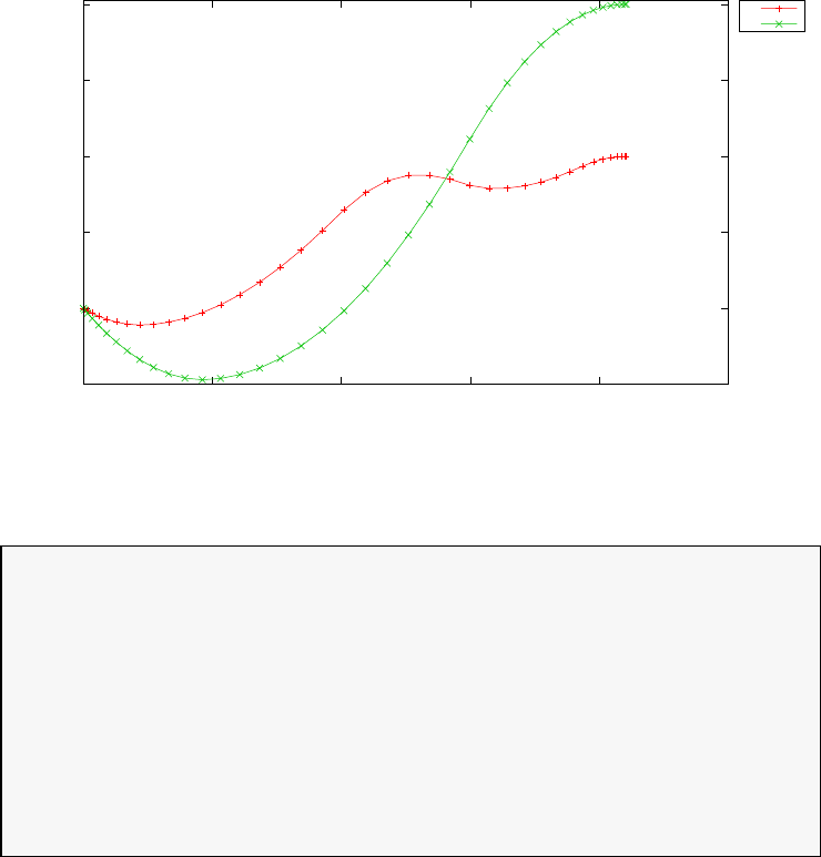
0
0.5
1
1.5
2
0 0.5 1 1.5 2 2.5
states
time (s)
Coulomb friction problem: states q1 and q2
q1
q2
Figure 3.19: States for Coulomb friction problem
Date and time of this run: Thu Feb 21 17:28:32 2019
Optimal (unscaled) cost function value: 2.104992e+00
Phase 1 endpoint cost function value: 2.104992e+00
Phase 1 integrated part of the cost: 0.000000e+00
Phase 1 initial time: 0.000000e+00
Phase 1 final time: 2.104992e+00
Phase 1 maximum relative local error: 7.858415e-03
NLP solver reports: The problem has been solved!
3.9 DAE index 3 parameter estimation problem
Consider the following parameter estimation problem, which involves a differential-
algebraic equation of index 3 with four differential states and one algebraic
state [37].
The dynamics consists of the differential equations
˙x1(t) = x3(t)
˙x2(t) = x4(t)
˙x3(t) = λ(t)x1(t)
˙x4(t) = λ(t)x2(t)
(3.36)
149
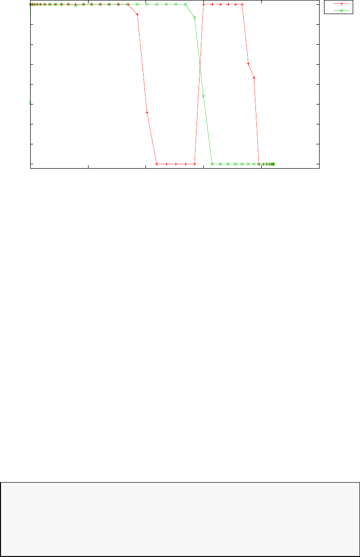
-4
-3
-2
-1
0
1
2
3
4
0 0.5 1 1.5 2 2.5
controls
time (s)
Coulomb friction problem: controls
u1
u2
Figure 3.20: Controls for Coulomb friction problem
and the algebraic equation
0 = L2−x1(t)2−x2(t)2(3.37)
where xj(t), j = 1,...,4 are the differential states, λ(t) is an algebraic state
(note that algebraic states are treated as control variables), and Lis a
parameter to be estimated.
The observations function is given by:
y1=x1
y2=x2
(3.38)
And the following least squares objective is minimised:
J=
ns
X
k=1 (y1(tk)−ˆy1(tk))2+ (y2(tk)−ˆy2(tk))2(3.39)
where ns= 20, t1= 0.5 and t20 = 10.0.
The PSOPT code that solves this problem is shown below.
//////////////////////////////////////////////////////////////////////////
////////////////// ident1.cxx ////////////////////////////
//////////////////////////////////////////////////////////////////////////
//////////////// PSOPT Example ////////////////////
//////////////////////////////////////////////////////////////////////////
//////////////////////////////////////////////////////////////////////////
//////// Title: DAE Index 3 ////////////////
//////// Last modified: 07 June 2011 ////////////////
150

//////// Reference: Schittkowski (2002) ////////////////
//////// (See PSOPT handbook for full reference) ///////////////
//////////////////////////////////////////////////////////////////////////
//////// Copyright (c) Victor M. Becerra, 2011 ////////////////
//////////////////////////////////////////////////////////////////////////
//////// This is part of the PSOPT software library, which ///////////////
//////// is distributed under the terms of the GNU Lesser ////////////////
//////// General Public License (LGPL) ////////////////
//////////////////////////////////////////////////////////////////////////
#include "psopt.h"
//////////////////////////////////////////////////////////////////////////
/////////////////// Define the observation function //////////
//////////////////////////////////////////////////////////////////////////
void observation_function( adouble* observations,
adouble* states, adouble* controls,
adouble* parameters, adouble& time, int k,
adouble* xad, int iphase, Workspace* workspace)
{
observations[ CINDEX(1) ] = states[ CINDEX(1) ];
observations[ CINDEX(2) ] = states[ CINDEX(2) ];
}
//////////////////////////////////////////////////////////////////////////
/////////////////// Define the DAE’s ////////////////////////////////////
//////////////////////////////////////////////////////////////////////////
void dae(adouble* derivatives, adouble* path, adouble* states,
adouble* controls, adouble* parameters, adouble& time,
adouble* xad, int iphase, Workspace* workspace)
{
// Variables
adouble x1, x2, x3, x4, L, OMEGA, LAMBDA;
adouble dx1, dx2, dx3, dx4;
// Differential states
x1 = states[CINDEX(1)];
x2 = states[CINDEX(2)];
x3 = states[CINDEX(3)];
x4 = states[CINDEX(4)];
// Algebraic variables
LAMBDA = controls[CINDEX(1)];
// Parameters
L = parameters[CINDEX(1)];
// Differential equations
dx1 = x3;
dx2 = x4;
dx3 = LAMBDA*x1;
dx4 = LAMBDA*x2;
derivatives[ CINDEX(1) ] = dx1;
derivatives[ CINDEX(2) ] = dx2;
derivatives[ CINDEX(3) ] = dx3;
derivatives[ CINDEX(4) ] = dx4;
// algebraic equation
path[ CINDEX(1) ] = L*L - x1*x1 - x2*x2;
}
////////////////////////////////////////////////////////////////////////////
/////////////////// Define the events function ////////////////////////////
////////////////////////////////////////////////////////////////////////////
void events(adouble* e, adouble* initial_states, adouble* final_states,
adouble* parameters,adouble& t0, adouble& tf, adouble* xad,
151

int iphase, Workspace* workspace)
{
// no events
return;
}
///////////////////////////////////////////////////////////////////////////
/////////////////// Define the phase linkages function ///////////////////
///////////////////////////////////////////////////////////////////////////
void linkages( adouble* linkages, adouble* xad, Workspace* workspace)
{
// No linkages as this is a single phase problem
}
////////////////////////////////////////////////////////////////////////////
/////////////////// Define the main routine ///////////////////////////////
////////////////////////////////////////////////////////////////////////////
int main(void)
{
////////////////////////////////////////////////////////////////////////////
/////////////////// Declare key structures ////////////////////////////////
////////////////////////////////////////////////////////////////////////////
Alg algorithm;
Sol solution;
Prob problem;
////////////////////////////////////////////////////////////////////////////
/////////////////// Register problem name ////////////////////////////////
////////////////////////////////////////////////////////////////////////////
problem.name = "DAE Index 3";
problem.outfilename = "dae_i3.txt";
////////////////////////////////////////////////////////////////////////////
//////////// Define problem level constants & do level 1 setup ////////////
////////////////////////////////////////////////////////////////////////////
problem.nphases = 1;
problem.nlinkages = 0;
psopt_level1_setup(problem);
/////////////////////////////////////////////////////////////////////////////
///////// Define phase related information & do level 2 setup /////////////
/////////////////////////////////////////////////////////////////////////////
problem.phases(1).nstates = 4;
problem.phases(1).ncontrols = 1;
problem.phases(1).nevents = 0;
problem.phases(1).npath = 1;
problem.phases(1).nparameters = 1;
problem.phases(1).nodes = "[10,20,30]";
problem.phases(1).nobserved = 2;
problem.phases(1).nsamples = 20;
psopt_level2_setup(problem, algorithm);
////////////////////////////////////////////////////////////////////////////
//////////// Load data for parameter estimation ////////////
////////////////////////////////////////////////////////////////////////////
int iphase = 1;
load_parameter_estimation_data(problem, iphase, "dae_i3.dat");
problem.phases(1).observation_nodes.Print("observation nodes");
problem.phases(1).observations.Print("observations");
problem.phases(1).residual_weights.Print("weights");
////////////////////////////////////////////////////////////////////////////
/////////////////// Declare DMatrix objects to store results //////////////
////////////////////////////////////////////////////////////////////////////
DMatrix x, u, p, t;
152

////////////////////////////////////////////////////////////////////////////
/////////////////// Enter problem bounds information //////////////////////
////////////////////////////////////////////////////////////////////////////
problem.phases(1).bounds.lower.states(1) = -2.0;
problem.phases(1).bounds.lower.states(2) = -2.0;
problem.phases(1).bounds.lower.states(3) = -2.0;
problem.phases(1).bounds.lower.states(4) = -2.0;
problem.phases(1).bounds.upper.states(1) = 2.0;
problem.phases(1).bounds.upper.states(2) = 2.0;
problem.phases(1).bounds.upper.states(3) = 2.0;
problem.phases(1).bounds.upper.states(4) = 2.0;
problem.phases(1).bounds.lower.controls(1) = -10.0;
problem.phases(1).bounds.upper.controls(1) = 10.0;
problem.phases(1).bounds.lower.parameters(1) = 0.0;
problem.phases(1).bounds.upper.parameters(1) = 5.0;
problem.phases(1).bounds.lower.path(1) = 0.0;
problem.phases(1).bounds.upper.path(1) = 0.0;
problem.phases(1).bounds.lower.StartTime = 0.5;
problem.phases(1).bounds.upper.StartTime = 0.5;
problem.phases(1).bounds.lower.EndTime = 10.0;
problem.phases(1).bounds.upper.EndTime = 10.0;
////////////////////////////////////////////////////////////////////////////
/////////////////// Register problem functions ///////////////////////////
////////////////////////////////////////////////////////////////////////////
problem.dae = &dae;
problem.events = &events;
problem.linkages = &linkages;
problem.observation_function = & observation_function;
////////////////////////////////////////////////////////////////////////////
/////////////////// Define & register initial guess ///////////////////////
////////////////////////////////////////////////////////////////////////////
int nnodes = (int) problem.phases(1).nsamples;
DMatrix state_guess(4, nnodes);
DMatrix control_guess(1,nnodes);
DMatrix param_guess(1,1);
state_guess(1,colon()) = problem.phases(1).observations(1,colon());
state_guess(2,colon()) = problem.phases(1).observations(2,colon());
state_guess(3,colon()) = ones(1,nnodes);
state_guess(4,colon()) = ones(1,nnodes);
control_guess(1,colon()) = zeros(1,nnodes);
param_guess = 0.5;
problem.phases(1).guess.states = state_guess;
problem.phases(1).guess.time = problem.phases(1).observation_nodes;
problem.phases(1).guess.parameters = param_guess;
problem.phases(1).guess.controls = control_guess;
////////////////////////////////////////////////////////////////////////////
/////////////////// Enter algorithm options //////////////////////////////
////////////////////////////////////////////////////////////////////////////
algorithm.nlp_method = "IPOPT";
algorithm.scaling = "automatic";
algorithm.derivatives = "automatic";
algorithm.collocation_method = "Legendre";
algorithm.jac_sparsity_ratio = 0.50;
////////////////////////////////////////////////////////////////////////////
/////////////////// Now call PSOPT to solve the problem //////////////////
////////////////////////////////////////////////////////////////////////////
psopt(solution, problem, algorithm);
153

////////////////////////////////////////////////////////////////////////////
/////////// Extract relevant variables from solution structure //////////
////////////////////////////////////////////////////////////////////////////
x = solution.get_states_in_phase(1);
u = solution.get_controls_in_phase(1);
t = solution.get_time_in_phase(1);
p = solution.get_parameters_in_phase(1);
////////////////////////////////////////////////////////////////////////////
/////////// Save solution data to files if desired ////////////////////////
////////////////////////////////////////////////////////////////////////////
x.Save("x.dat");
u.Save("u.dat");
t.Save("t.dat");
p.Print("Estimated parameter");
////////////////////////////////////////////////////////////////////////////
/////////// Plot some results if desired (requires gnuplot) ///////////////
////////////////////////////////////////////////////////////////////////////
DMatrix tm;
DMatrix ym;
tm = problem.phases(1).observation_nodes;
ym = problem.phases(1).observations;
plot(t,x(1,colon()),tm,ym(1,colon()),problem.name, "time (s)", "state x1", "x1 yhat1");
plot(t,x(2,colon()),tm,ym(2,colon()),problem.name, "time (s)", "state x2", "x2 yhat2");
plot(t,u,problem.name, "time (s)", "algebraic state u", "u");
plot(t,x(1,colon()),tm,ym(1,colon()),problem.name, "time (s)", "state x1", "x1 yhat1",
"pdf", "x1.pdf");
plot(t,x(2,colon()),tm,ym(2,colon()),problem.name, "time (s)", "state x2", "x2 yhat2",
"pdf", "x2.pdf");
plot(t,u,problem.name, "time (s)", "algebraic state lambda", "lambda", "pdf", "lambda.pdf");
}
////////////////////////////////////////////////////////////////////////////
/////////////////////// END OF FILE ///////////////////////////////
////////////////////////////////////////////////////////////////////////////
The output from PSOPT summarised in the box below and shown in
Figures 3.21 and 3.22, which compare the observations with the estimated
outputs, and 3.23, which shows the algebraic state. The exact solution to
the problem is L= 1 and λ(t) = −1. The numerical solution obtained is
L= 1.000000188 and λ(t) = −0.999868. The 95% confidence interval for
the estimated parameter is [0.9095289,1.090471]
PSOPT results summary
=====================
Problem: DAE Index 3
CPU time (seconds): 1.046000e+01
NLP solver used: IPOPT
154
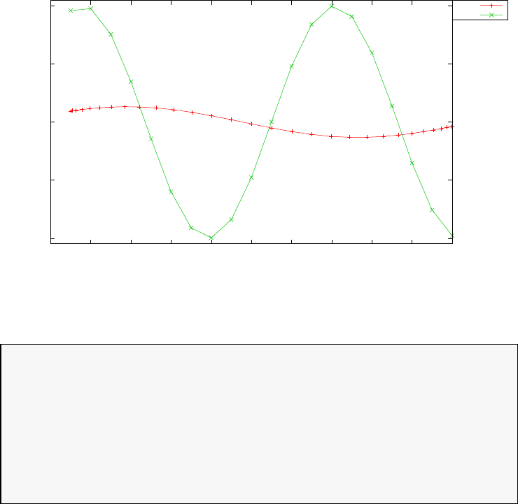
-1
-0.5
0
0.5
1
0 1 2 3 4 5 6 7 8 9 10
state x1
time (s)
DAE Index 3
x1
yhat1
Figure 3.21: State x1and observations
Optimal (unscaled) cost function value: 1.965352e+01
Phase 1 endpoint cost function value: 1.965352e+01
Phase 1 integrated part of the cost: 0.000000e+00
Phase 1 initial time: 5.000000e-01
Phase 1 final time: 1.000000e+01
Phase 1 maximum relative local error: 8.341290e-08
NLP solver reports: The problem solved!
3.10 Delayed states problem 1
Consider the following optimal control problem, which consists of a linear
system with delays in the state equations [29]. Minimize the cost functional:
J=x3(tf) (3.40)
subject to the dynamic constraints
˙x1=x2(t)
˙x2=−10x1(t)−5x2(t)−2x1(t−τ)−x2(t−τ) + u(t)
˙x3= 0.5(10x2
1(t) + x2
2(t) + u2(t))
(3.41)
155
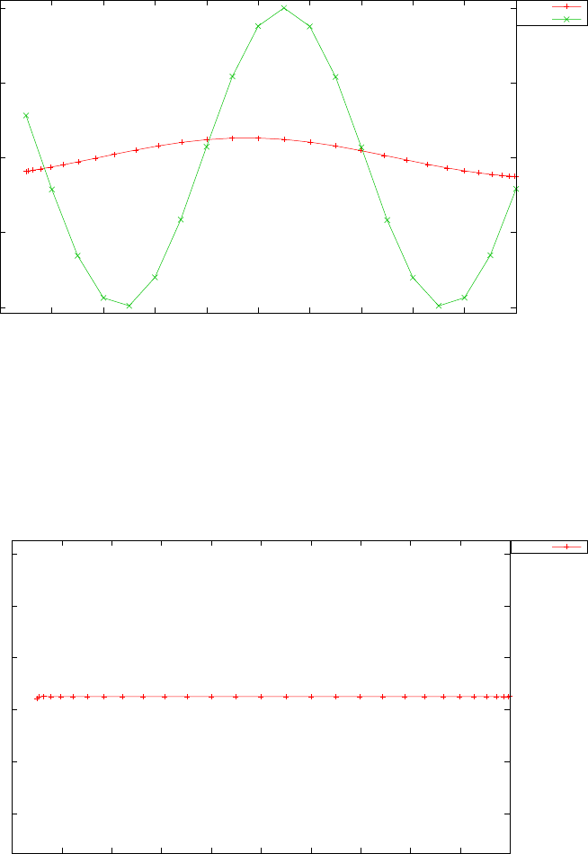
-1
-0.5
0
0.5
1
0 1 2 3 4 5 6 7 8 9 10
state x2
time (s)
DAE Index 3
x2
yhat2
Figure 3.22: State x2and observations
-0.31
-0.305
-0.3
-0.295
-0.29
-0.285
0 1 2 3 4 5 6 7 8 9 10
algebraic state lambda
time (s)
DAE Index 3
lambda
Figure 3.23: Algebraic state λ(t)
156

and the boundary conditions
x1(0) = 1
x2(0) = 1
x3(0) = 0
(3.42)
where tf= 5 and τ= 0.25. The PSOPT code that solves this problem is
shown below.
//////////////////////////////////////////////////////////////////////////
//////////////// delay1.cxx /////////////////////
//////////////////////////////////////////////////////////////////////////
//////////////// PSOPT Example ////////////////////
//////////////////////////////////////////////////////////////////////////
//////////////////////////////////////////////////////////////////////////
//////// Title: Time delay problem ////////////////
//////// Last modified: 09 January 2009 ////////////////
//////// Reference: Luus (2002) ////////////////
//////// (See PSOPT handbook for full reference) ////////////////
//////////////////////////////////////////////////////////////////////////
//////// Copyright (c) Victor M. Becerra, 2009 ////////////////
//////////////////////////////////////////////////////////////////////////
//////// This is part of the PSOPT software library, which ///////////////
//////// is distributed under the terms of the GNU Lesser ////////////////
//////// General Public License (LGPL) ////////////////
//////////////////////////////////////////////////////////////////////////
#include "psopt.h"
//////////////////////////////////////////////////////////////////////////
/////////////////// Define the end point (Mayer) cost function //////////
//////////////////////////////////////////////////////////////////////////
adouble endpoint_cost(adouble* initial_states, adouble* final_states,
adouble* parameters,adouble& t0, adouble& tf,
adouble* xad, int iphase, Workspace* workspace)
{
adouble x3f = final_states[CINDEX(3)];
return x3f;
}
//////////////////////////////////////////////////////////////////////////
/////////////////// Define the integrand (Lagrange) cost function //////
//////////////////////////////////////////////////////////////////////////
adouble integrand_cost(adouble* states, adouble* controls,
adouble* parameters, adouble& time, adouble* xad,
int iphase, Workspace* workspace)
{
return 0.0;
}
//////////////////////////////////////////////////////////////////////////
/////////////////// Define the DAE’s ////////////////////////////////////
//////////////////////////////////////////////////////////////////////////
void dae(adouble* derivatives, adouble* path, adouble* states,
adouble* controls, adouble* parameters, adouble& time,
adouble* xad, int iphase, Workspace* workspace)
{
adouble x1delayed, x2delayed;
double tau = 0.25;
adouble x1 = states[CINDEX(1)];
adouble x2 = states[CINDEX(2)];
adouble x3 = states[CINDEX(3)];
get_delayed_state( &x1delayed, 1, iphase, time, tau, xad, workspace);
get_delayed_state( &x2delayed, 2, iphase, time, tau, xad, workspace);
adouble u = controls[CINDEX(1)];
derivatives[CINDEX(1)] = x2;
derivatives[CINDEX(2)] = -10*x1-5*x2-2*x1delayed-x2delayed+u;
157

// [uncomment the line below for approximate solution]
// derivatives[CINDEX(2)] = (-12*x1+(2*tau-6)*x2+u)/(1-tau);
derivatives[CINDEX(3)] = 0.5*(10*x1*x1+x2*x2+u*u);
}
////////////////////////////////////////////////////////////////////////////
/////////////////// Define the events function ////////////////////////////
////////////////////////////////////////////////////////////////////////////
void events(adouble* e, adouble* initial_states, adouble* final_states,
adouble* parameters,adouble& t0, adouble& tf, adouble* xad,
int iphase, Workspace* workspace)
{
adouble x10 = initial_states[CINDEX(1)];
adouble x20 = initial_states[CINDEX(2)];
adouble x30 = initial_states[CINDEX(3)];
e[CINDEX(1)] = x10;
e[CINDEX(2)] = x20;
e[CINDEX(3)] = x30;
}
///////////////////////////////////////////////////////////////////////////
/////////////////// Define the phase linkages function ///////////////////
///////////////////////////////////////////////////////////////////////////
void linkages( adouble* linkages, adouble* xad, Workspace* workspace)
{
// No linkages as this is a single phase problem
}
////////////////////////////////////////////////////////////////////////////
/////////////////// Define the main routine ///////////////////////////////
////////////////////////////////////////////////////////////////////////////
int main(void)
{
////////////////////////////////////////////////////////////////////////////
/////////////////// Declare key structures ////////////////////////////////
////////////////////////////////////////////////////////////////////////////
Alg algorithm;
Sol solution;
Prob problem;
////////////////////////////////////////////////////////////////////////////
/////////////////// Register problem name ////////////////////////////////
////////////////////////////////////////////////////////////////////////////
problem.name = "Time delay problem 1";
problem.outfilename = "delay1.txt";
////////////////////////////////////////////////////////////////////////////
//////////// Define problem level constants & do level 1 setup ////////////
////////////////////////////////////////////////////////////////////////////
problem.nphases = 1;
problem.nlinkages = 0;
psopt_level1_setup(problem);
/////////////////////////////////////////////////////////////////////////////
///////// Define phase related information & do level 2 setup ////////////
/////////////////////////////////////////////////////////////////////////////
problem.phases(1).nstates = 3;
problem.phases(1).ncontrols = 1;
problem.phases(1).nevents = 3;
problem.phases(1).npath = 0;
problem.phases(1).nodes = "[30]";
psopt_level2_setup(problem, algorithm);
////////////////////////////////////////////////////////////////////////////
158

/////////////////// Declare DMatrix objects to store results //////////////
////////////////////////////////////////////////////////////////////////////
DMatrix x, u, t;
DMatrix lambda, H;
////////////////////////////////////////////////////////////////////////////
/////////////////// Enter problem bounds information //////////////////////
////////////////////////////////////////////////////////////////////////////
double x1L = -100.0;
double x2L = -100.0;
double x3L = -100.0;
double x1U = 100.0;
double x2U = 100.0;
double x3U = 100.0;
double uL = -100.0;
double uU = 100.0;
problem.phases(1).bounds.lower.states(1) = x1L;
problem.phases(1).bounds.lower.states(2) = x2L;
problem.phases(1).bounds.lower.states(3) = x3L;
problem.phases(1).bounds.upper.states(1) = x1U;
problem.phases(1).bounds.upper.states(2) = x2U;
problem.phases(1).bounds.upper.states(3) = x3U;
problem.phases(1).bounds.lower.controls(1) = uL;
problem.phases(1).bounds.upper.controls(1) = uU;
problem.phases(1).bounds.lower.events(1) = 1.0;
problem.phases(1).bounds.lower.events(2) = 1.0;
problem.phases(1).bounds.lower.events(3) = 0.0;
problem.phases(1).bounds.upper.events(1) = 1.0;
problem.phases(1).bounds.upper.events(2) = 1.0;
problem.phases(1).bounds.upper.events(3) = 0.0;
problem.phases(1).bounds.lower.StartTime = 0.0;
problem.phases(1).bounds.upper.StartTime = 0.0;
problem.phases(1).bounds.lower.EndTime = 5.0;
problem.phases(1).bounds.upper.EndTime = 5.0;
////////////////////////////////////////////////////////////////////////////
/////////////////// Register problem functions ///////////////////////////
////////////////////////////////////////////////////////////////////////////
problem.integrand_cost = &integrand_cost;
problem.endpoint_cost = &endpoint_cost;
problem.dae = &dae;
problem.events = &events;
problem.linkages = &linkages;
////////////////////////////////////////////////////////////////////////////
/////////////////// Define & register initial guess ///////////////////////
////////////////////////////////////////////////////////////////////////////
DMatrix x0(3,60);
x0(1,colon()) = linspace(1.0,1.0, 60);
x0(2,colon()) = linspace(1.0,1.0, 60);
x0(3,colon()) = linspace(0.0,0.0, 60);
problem.phases(1).guess.controls = zeros(1,60);
problem.phases(1).guess.states = x0;
problem.phases(1).guess.time = linspace(0.0,5.0, 60);
////////////////////////////////////////////////////////////////////////////
/////////////////// Enter algorithm options //////////////////////////////
////////////////////////////////////////////////////////////////////////////
algorithm.nlp_method = "IPOPT";
algorithm.scaling = "automatic";
algorithm.derivatives = "automatic";
algorithm.nlp_iter_max = 1000;
algorithm.nlp_tolerance = 1.e-6;
159

algorithm.collocation_method = "Hermite-Simpson";
// algorithm.mesh_refinement = "automatic";
////////////////////////////////////////////////////////////////////////////
/////////////////// Now call PSOPT to solve the problem /////////////////
////////////////////////////////////////////////////////////////////////////
psopt(solution, problem, algorithm);
////////////////////////////////////////////////////////////////////////////
/////////// Extract relevant variables from solution structure //////////
////////////////////////////////////////////////////////////////////////////
x = solution.get_states_in_phase(1);
u = solution.get_controls_in_phase(1);
t = solution.get_time_in_phase(1);
////////////////////////////////////////////////////////////////////////////
/////////// Save solution data to files if desired ////////////////////////
////////////////////////////////////////////////////////////////////////////
x.Save("x.dat");
u.Save("u.dat");
t.Save("t.dat");
////////////////////////////////////////////////////////////////////////////
/////////// Plot some results if desired (requires gnuplot) ///////////////
////////////////////////////////////////////////////////////////////////////
plot(t,x,problem.name, "time (s)", "states", "x1 x2 x3");
plot(t,u,problem.name, "time (s)", "control", "u");
plot(t,x,problem.name, "time (s)", "states", "x1 x2 x3",
"pdf", "delay1_states.pdf");
plot(t,u,problem.name, "time (s)", "control", "u",
"pdf", "delay1_controls.pdf");
}
The output from PSOPT summarised in the box below and shown in
Figures 3.24 and 3.25, which contain the elements of the state and the
control, respectively.
PSOPT results summary
=====================
Problem: Time delay problem 1
CPU time (seconds): 1.624518e+00
NLP solver used: IPOPT
PSOPT release number: 4.0
Date and time of this run: Thu Feb 21 15:59:52 2019
Optimal (unscaled) cost function value: 2.526875e+00
Phase 1 endpoint cost function value: 2.526875e+00
Phase 1 integrated part of the cost: 0.000000e+00
Phase 1 initial time: 0.000000e+00
Phase 1 final time: 5.000000e+00
Phase 1 maximum relative local error: 1.848000e-02
160
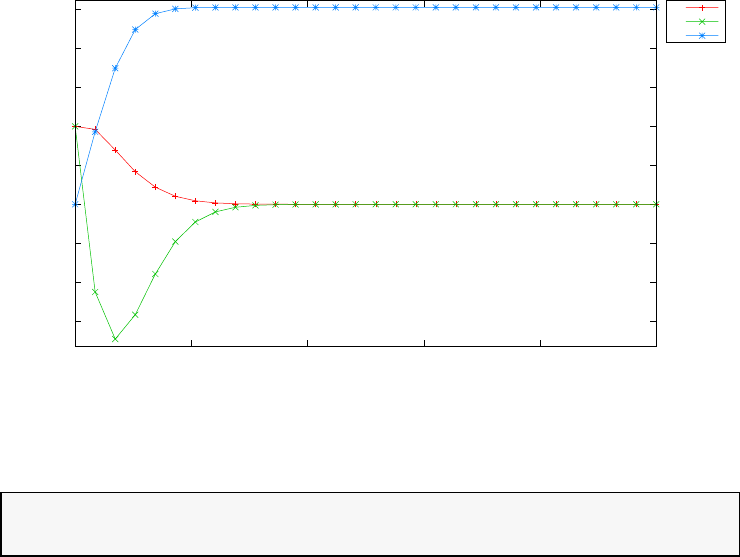
-1.5
-1
-0.5
0
0.5
1
1.5
2
2.5
0 1 2 3 4 5
states
time (s)
Time delay problem 1
x1
x2
x3
Figure 3.24: States for time delay problem 1
NLP solver reports: The problem has been solved!
3.11 Dynamic MPEC problem
Consider the following optimal control problem, which involves special han-
dling of a system with a discontinuous right hand side [4]. Minimize the
cost functional:
J= [y(2) −5/3]2+Z2
0
y2(t)dt(3.43)
subject to
˙y= 2 −sgn(y)(3.44)
and the boundary condition
y(0) = −1(3.45)
Note that there is no control variable, and the analytical solution of this
problem satisfies ˙y(t)=3,0≤t≤1/3, and ˙y(t)=1,1/3≤t≤2.
In order to handle the discontinuous right hand side, the problem is
converted into the following equivalent problem, which has three algebraic
(control) variables. This type of problem is known in the literature as a
161
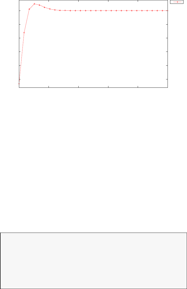
-0.5
-0.4
-0.3
-0.2
-0.1
0
0 1 2 3 4 5
control
time (s)
Time delay problem 1
u
Figure 3.25: Control for time delay problem 1
dynamic MPEC problem.
J= [y(2) −5/3]2+Z2
0y2(t) + ρ{p(t)[s(t) + 1] + q(t)[1 −s(t)]}dt(3.46)
subject to
˙y= 2 −sgn(y)
0 = −y(t)−p(t) + q(t)(3.47)
the boundary condition
y(0) = −1(3.48)
and the bounds: −1≤s(t)≤1,
0≤p(t),
0≤q(t).
(3.49)
The PSOPT code that solves this problem is shown below.
//////////////////////////////////////////////////////////////////////////
//////////////// bryson_max_range.cxx /////////////////////
//////////////////////////////////////////////////////////////////////////
//////////////// PSOPT Example /////////////////////
//////////////////////////////////////////////////////////////////////////
//////////////////////////////////////////////////////////////////////////
//////// Title: Dynamic MPEC problem ////////////////
//////// Last modified: 27 May 2011 ////////////////
//////// Reference: Betts (2010) ////////////////
//////// (See PSOPT handbook for full reference) ////////////////
//////////////////////////////////////////////////////////////////////////
//////// Copyright (c) Victor M. Becerra, 2009 ////////////////
//////////////////////////////////////////////////////////////////////////
162

//////// This is part of the PSOPT software library, which////////////////
//////// is distributed under the terms of the GNU Lesser ////////////////
//////// General Public License (LGPL) ////////////////
//////////////////////////////////////////////////////////////////////////
#include "psopt.h"
//////////////////////////////////////////////////////////////////////////
/////////////////// Define the end point (Mayer) cost function //////////
//////////////////////////////////////////////////////////////////////////
adouble endpoint_cost(adouble* initial_states, adouble* final_states,
adouble* parameters,adouble& t0, adouble& tf,
adouble* xad, int iphase, Workspace* workspace)
{
adouble y_f = final_states[ CINDEX(1) ];
return pow( y_f - (5.0/3.0) , 2.0);
}
//////////////////////////////////////////////////////////////////////////
/////////////////// Define the integrand (Lagrange) cost function //////
//////////////////////////////////////////////////////////////////////////
adouble integrand_cost(adouble* states, adouble* controls, adouble* parameters,
adouble& time, adouble* xad, int iphase, Workspace* workspace)
{
adouble y = states[ CINDEX(1) ];
adouble s = controls[ CINDEX(1) ];
adouble p = controls[ CINDEX(2) ];
adouble q = controls[ CINDEX(3) ];
adouble retval;
double rho = 1.e3;
retval = y*y + rho*( p*(s+1.0)+ q*(1.0-s));
return retval;
}
//////////////////////////////////////////////////////////////////////////
/////////////////// Define the DAE’s ////////////////////////////////////
//////////////////////////////////////////////////////////////////////////
void dae(adouble* derivatives, adouble* path, adouble* states,
adouble* controls, adouble* parameters, adouble& time,
adouble* xad, int iphase, Workspace* workspace)
{
adouble y = states[ CINDEX(1) ];
adouble ydot;
adouble s = controls[ CINDEX(1) ];
adouble p = controls[ CINDEX(2) ];
adouble q = controls[ CINDEX(3) ];
ydot = 2.0 -s;
derivatives[ CINDEX(1) ] = ydot;
path[ CINDEX(1) ] = -y - p + q;
}
////////////////////////////////////////////////////////////////////////////
/////////////////// Define the events function ////////////////////////////
////////////////////////////////////////////////////////////////////////////
void events(adouble* e, adouble* initial_states, adouble* final_states,
adouble* parameters,adouble& t0, adouble& tf, adouble* xad,
int iphase, Workspace* workspace)
{
adouble y0 = initial_states[ CINDEX(1) ];
163

e[ CINDEX(1) ] = y0;
}
///////////////////////////////////////////////////////////////////////////
/////////////////// Define the phase linkages function ///////////////////
///////////////////////////////////////////////////////////////////////////
void linkages( adouble* linkages, adouble* xad, Workspace* workspace)
{
// No linkages as this is a single phase problem
}
////////////////////////////////////////////////////////////////////////////
/////////////////// Define the main routine ///////////////////////////////
////////////////////////////////////////////////////////////////////////////
int main(void)
{
////////////////////////////////////////////////////////////////////////////
/////////////////// Declare key structures ////////////////////////////////
////////////////////////////////////////////////////////////////////////////
Alg algorithm;
Sol solution;
Prob problem;
////////////////////////////////////////////////////////////////////////////
/////////////////// Register problem name ////////////////////////////////
////////////////////////////////////////////////////////////////////////////
problem.name = "Dynamic MPEC problem";
problem.outfilename = "mpec.txt";
////////////////////////////////////////////////////////////////////////////
//////////// Define problem level constants & do level 1 setup ////////////
////////////////////////////////////////////////////////////////////////////
problem.nphases = 1;
problem.nlinkages = 0;
psopt_level1_setup(problem);
/////////////////////////////////////////////////////////////////////////////
///////// Define phase related information & do level 2 setup ////////////
/////////////////////////////////////////////////////////////////////////////
problem.phases(1).nstates = 1;
problem.phases(1).ncontrols = 3;
problem.phases(1).nevents = 1;
problem.phases(1).npath = 1;
problem.phases(1).nodes = "[20]";
psopt_level2_setup(problem, algorithm);
////////////////////////////////////////////////////////////////////////////
/////////////////// Declare DMatrix objects to store results //////////////
////////////////////////////////////////////////////////////////////////////
DMatrix y, controls, s, p, q, t;
////////////////////////////////////////////////////////////////////////////
/////////////////// Enter problem bounds information //////////////////////
////////////////////////////////////////////////////////////////////////////
double y0 = -1.0;
problem.phases(1).bounds.lower.states(1) = -10.0;
problem.phases(1).bounds.upper.states(1) = 10.0;
problem.phases(1).bounds.lower.controls(1) = -1.0;
problem.phases(1).bounds.lower.controls(2) = 0.0;
problem.phases(1).bounds.lower.controls(3) = 0.0;
164

problem.phases(1).bounds.upper.controls(1) = 1.0;
problem.phases(1).bounds.upper.controls(2) = inf;
problem.phases(1).bounds.upper.controls(3) = inf;
problem.phases(1).bounds.lower.events(1) = y0;
problem.phases(1).bounds.upper.events(1) = y0;
problem.phases(1).bounds.upper.path(1) = 0.0;
problem.phases(1).bounds.lower.path(1) = 0.0;
problem.phases(1).bounds.lower.StartTime = 0.0;
problem.phases(1).bounds.upper.StartTime = 0.0;
problem.phases(1).bounds.lower.EndTime = 2.0;
problem.phases(1).bounds.upper.EndTime = 2.0;
////////////////////////////////////////////////////////////////////////////
/////////////////// Register problem functions ///////////////////////////
////////////////////////////////////////////////////////////////////////////
problem.integrand_cost = &integrand_cost;
problem.endpoint_cost = &endpoint_cost;
problem.dae = &dae;
problem.events = &events;
problem.linkages = &linkages;
////////////////////////////////////////////////////////////////////////////
/////////////////// Define & register initial guess ///////////////////////
////////////////////////////////////////////////////////////////////////////
int nnodes = problem.phases(1).nodes(1);
int ncontrols = problem.phases(1).ncontrols;
int nstates = problem.phases(1).nstates;
DMatrix x_guess = zeros(nstates,nnodes);
x_guess(1,colon()) = y0*ones(1,nnodes);
problem.phases(1).guess.controls = zeros(ncontrols,nnodes);
problem.phases(1).guess.states = x_guess;
problem.phases(1).guess.time = linspace(0.0,2.0,nnodes);
////////////////////////////////////////////////////////////////////////////
/////////////////// Enter algorithm options //////////////////////////////
////////////////////////////////////////////////////////////////////////////
algorithm.nlp_iter_max = 1000;
algorithm.nlp_tolerance = 1.e-4;
algorithm.nlp_method = "IPOPT";
algorithm.scaling = "automatic";
algorithm.derivatives = "automatic";
algorithm.mesh_refinement = "automatic";
algorithm.collocation_method = "trapezoidal";
// algorithm.defect_scaling = "jacobian-based";
algorithm.ode_tolerance = 1.e-6;
////////////////////////////////////////////////////////////////////////////
/////////////////// Now call PSOPT to solve the problem /////////////////
////////////////////////////////////////////////////////////////////////////
psopt(solution, problem, algorithm);
////////////////////////////////////////////////////////////////////////////
/////////// Extract relevant variables from solution structure //////////
////////////////////////////////////////////////////////////////////////////
y = solution.get_states_in_phase(1);
controls = solution.get_controls_in_phase(1);
t = solution.get_time_in_phase(1);
s = controls(1,colon());
p = controls(2,colon());
q = controls(3,colon());
165

////////////////////////////////////////////////////////////////////////////
/////////// Save solution data to files if desired ////////////////////////
////////////////////////////////////////////////////////////////////////////
y.Save("y.dat");
controls.Save("controls.dat");
t.Save("t.dat");
////////////////////////////////////////////////////////////////////////////
/////////// Plot some results if desired (requires gnuplot) ///////////////
////////////////////////////////////////////////////////////////////////////
plot(t,y,problem.name+": state", "time (s)", "state","y");
plot(t,s,problem.name+": algebraic variable s","time (s)", "s", "s");
plot(t,p,problem.name+": algebraic variable p","time (s)", "p", "p");
plot(t,q,problem.name+": algebraic variable q","time (s)", "q", "q");
plot(t,y,problem.name+": state", "time (s)", "state","y",
"pdf", "y.pdf");
plot(t,s,problem.name+": algebraic variable s","time (s)", "s", "s",
"pdf", "s.pdf");
plot(t,p,problem.name+": algebraic variable p","time (s)", "p", "p",
"pdf", "p.pdf");
plot(t,q,problem.name+": algebraic variable q","time (s)", "q", "q",
"pdf", "q.pdf");
}
////////////////////////////////////////////////////////////////////////////
/////////////////////// END OF FILE ///////////////////////////////
////////////////////////////////////////////////////////////////////////////
The output from PSOPT summarised in the box below and shown in
Figures 3.26,3.27,3.28, and 3.29.
PSOPT results summary
=====================
Problem: Dynamic MPEC problem
CPU time (seconds): 4.031824e+00
NLP solver used: IPOPT
PSOPT release number: 4.0
Date and time of this run: Thu Feb 21 16:00:52 2019
Optimal (unscaled) cost function value: 1.653464e+00
Phase 1 endpoint cost function value: 3.770062e-07
Phase 1 integrated part of the cost: 1.653464e+00
Phase 1 initial time: 0.000000e+00
Phase 1 final time: 2.000000e+00
Phase 1 maximum relative local error: 1.842153e-06
NLP solver reports: The problem has been solved!
166
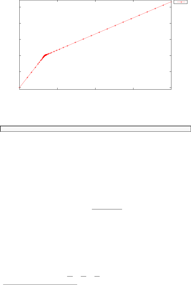
-1
-0.5
0
0.5
1
1.5
0 0.5 1 1.5 2
state
time (s)
Dynamic MPEC problem: state
y
Figure 3.26: State yfor dynamic MPEC problem
3.12 Geodesic problem
This problem is about calculating the geodesic curve 1that joins two points
on Earth using optimal control. The problem is posed in the form of esti-
mating the shortest fligh path for an airliner to fly from New Yorks’s JFK
to London’s LHR airport.
The formulation is as follows. Find the trajectories for the elevation and
azimuth angles θ(t) and φ(t)∈[0, tf] to minimize the cost functional
J=Ztf
0p˙x2+ ˙y2+ ˙z2dt (3.50)
subject to the dynamic constraints
˙x=Vsin(θ) cos(φ)
˙y=Vsin(θ) sin(φ)
˙z=Vcos(θ)
(3.51)
The path constraint, which corresponds to the Earth’s spheroid 2shape:
x2
a2+y2
a2+z2
b2−1.0 = 0 (3.52)
1See http://mathworld.wolfram.com/Geodesic.html
2See http://mathworld.wolfram.com/Ellipsoid.html
167
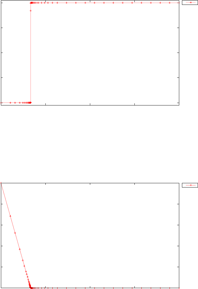
-1
-0.5
0
0.5
1
0 0.5 1 1.5 2
s
time (s)
Dynamic MPEC problem: algebraic variable s
s
Figure 3.27: Algebraic variable sfor dynamic MPEC problem
0
0.2
0.4
0.6
0.8
1
0 0.5 1 1.5 2
p
time (s)
Dynamic MPEC problem: algebraic variable p
p
Figure 3.28: Algebraic variable pfor dynamic MPEC problem
168
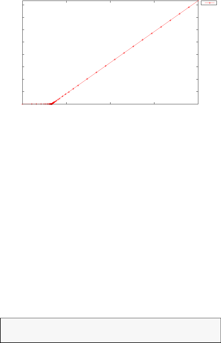
0
0.2
0.4
0.6
0.8
1
1.2
1.4
1.6
0 0.5 1 1.5 2
q
time (s)
Dynamic MPEC problem: algebraic variable q
q
Figure 3.29: Algebraic variable qfor dynamic MPEC problem
the boundary conditions, which correspond to the geographical coordinates
of LHR (51.4700◦N, 0.4543◦W) and JFK (40.6413◦N, 73.7781◦W)
x(0) = x0
y(0) = y0
z(0) = z0
x(tf) = xf
y(tf) = yf
z(tf) = zf
(3.53)
and the control bounds
0≤θ(t)≤π
0≤φ(t)≤2π(3.54)
where x, y, z are the Cartesian coordinates (in km) with origin on the centre
of Earth, tis time in hours, V= 900 km/h corresponds to the cruising
speed of a typical airliner, a= 6384 km is the Earth’s semi-major axis,
and b= 6353 km is the Earth’s semi-minor axis, which is the length of the
Earth’s axis of rotation from the north pole to the south pole. For simplicity,
the altitude of the aircraft is neglected.
The PSOPT code that solves this problem is shown below.
//////////////////////////////////////////////////////////////////////////
//////////////// geodesic.cxx /////////////////////
//////////////////////////////////////////////////////////////////////////
169

//////////////// PSOPT Example ////////////////////
//////////////////////////////////////////////////////////////////////////
//////////////////////////////////////////////////////////////////////////
//////// Title: Geodesic calculation problem ////////////////
//////// Last modified: 22 February 2019 ////////////////
//////// Reference: PROPT User’s Guide ////////////////
//////// (See PSOPT handbook for full reference) ////////////////
//////////////////////////////////////////////////////////////////////////
//////// Copyright (c) Victor M. Becerra, 2019 ////////////////
//////////////////////////////////////////////////////////////////////////
//////// This is part of the PSOPT software library, which ///////////////
//////// is distributed under the terms of the GNU Lesser ////////////////
//////// General Public License (LGPL) ////////////////
//////////////////////////////////////////////////////////////////////////
#include "psopt.h"
typedef struct {
double V;
double a;
double b;
} Constants;
//////////////////////////////////////////////////////////////////////////
/////////////////// Define the end point (Mayer) cost function //////////
//////////////////////////////////////////////////////////////////////////
adouble endpoint_cost(adouble* initial_states, adouble* final_states,
adouble* parameters,adouble& t0, adouble& tf,
adouble* xad, int iphase,Workspace* workspace)
{
return 0;
}
//////////////////////////////////////////////////////////////////////////
/////////////////// Define the integrand (Lagrange) cost function //////
//////////////////////////////////////////////////////////////////////////
adouble integrand_cost(adouble* states, adouble* controls,
adouble* parameters, adouble& time, adouble* xad,
int iphase, Workspace* workspace)
{
Constants* C = (Constants*) workspace->user_data;
double V = C->V;
adouble theta = controls[ CINDEX(1) ];
adouble phi = controls[ CINDEX(2) ];
// These are the components of the velocity vector in spherical coordinates.
adouble dxdt = V*sin(theta)*cos(phi);
adouble dydt = V*sin(theta)*sin(phi);
adouble dzdt = V*cos(theta);
// The integrand is the norm of the speed vector
adouble L = sqrt( pow(dxdt,2.0) + pow(dydt,2.0)+pow(dzdt,2.0) );
return L;
}
//////////////////////////////////////////////////////////////////////////
/////////////////// Define the DAE’s ////////////////////////////////////
//////////////////////////////////////////////////////////////////////////
void dae(adouble* derivatives, adouble* path, adouble* states,
adouble* controls, adouble* parameters, adouble& time,
adouble* xad, int iphase, Workspace* workspace)
{
Constants* C = (Constants*) workspace->user_data;
adouble x = states[ CINDEX(1) ];
adouble y = states[ CINDEX(2) ];
adouble z = states[ CINDEX(3) ];
double V = C->V; // Speed
double a = C->a; // Semi-major axis
double b = C->b; // Semi-minor axis
// These are the angles of the velocity vector in spherical coordinates
adouble theta = controls[ CINDEX(1) ];
170

adouble phi = controls[ CINDEX(2) ];
// Simple kinematic equations of motion in spherical coordinates
adouble dxdt = V*sin(theta)*cos(phi);
adouble dydt = V*sin(theta)*sin(phi);
adouble dzdt = V*cos(theta);
derivatives[ CINDEX(1) ] = dxdt;
derivatives[ CINDEX(2) ] = dydt;
derivatives[ CINDEX(3) ] = dzdt;
// This is the geodesic constraint to stay on the surface of the spheroid
path[ CINDEX(1) ] = x*x/(a*a) + y*y/(a*a) + z*z/(b*b) - 1.0;
}
////////////////////////////////////////////////////////////////////////////
/////////////////// Define the events function ////////////////////////////
////////////////////////////////////////////////////////////////////////////
void events(adouble* e, adouble* initial_states, adouble* final_states,
adouble* parameters,adouble& t0, adouble& tf, adouble* xad,
int iphase, Workspace* workspace)
{
adouble x0 = initial_states[ CINDEX(1) ];
adouble y0 = initial_states[ CINDEX(2) ];
adouble z0 = initial_states[ CINDEX(3) ];
adouble xf = final_states[ CINDEX(1) ];
adouble yf = final_states[ CINDEX(2) ];
adouble zf = final_states[ CINDEX(3) ];
e[ CINDEX(1) ] = x0;
e[ CINDEX(2) ] = y0;
e[ CINDEX(3) ] = z0;
e[ CINDEX(4) ] = xf;
e[ CINDEX(5) ] = yf;
e[ CINDEX(6) ] = zf;
}
///////////////////////////////////////////////////////////////////////////
/////////////////// Define the phase linkages function ///////////////////
///////////////////////////////////////////////////////////////////////////
void linkages( adouble* linkages, adouble* xad, Workspace* workspace)
{
// No linkages as this is a single phase problem
}
////////////////////////////////////////////////////////////////////////////
/////////////////// Define the main routine ///////////////////////////////
////////////////////////////////////////////////////////////////////////////
int main(void)
{
////////////////////////////////////////////////////////////////////////////
/////////////////// Declare key structures ////////////////////////////////
////////////////////////////////////////////////////////////////////////////
Alg algorithm;
Sol solution;
Prob problem;
////////////////////////////////////////////////////////////////////////////
/////////////////// Register problem name ////////////////////////////////
////////////////////////////////////////////////////////////////////////////
problem.name = "Geodesic problem";
problem.outfilename = "geodesic.txt";
////////////////////////////////////////////////////////////////////////////
//////////// Define problem level constants & do level 1 setup ////////////
////////////////////////////////////////////////////////////////////////////
problem.nphases = 1;
171

problem.nlinkages = 0;
psopt_level1_setup(problem);
/////////////////////////////////////////////////////////////////////////////
///////// Define phase related information & do level 2 setup ////////////
/////////////////////////////////////////////////////////////////////////////
problem.phases(1).nstates = 3;
problem.phases(1).ncontrols = 2;
problem.phases(1).nevents = 6;
problem.phases(1).npath = 1;
problem.phases(1).nodes = "[30]";
psopt_level2_setup(problem, algorithm);
////////////////////////////////////////////////////////////////////////////
/////////////////// Enter problem bounds information //////////////////////
////////////////////////////////////////////////////////////////////////////
Constants* C = new Constants;
problem.user_data = (void*) C;
C->V = 900.00; // Speed in km/h
C->a = 6384.0; // Earth’s semi-major axis in km
C->b = 6353.0; // Earth’s semi-minor axis in km
double a = C->a;
double b = C->b;
double xL = -a;
double yL = -a;
double zL = -b;
double xU = a;
double yU = a;
double zU = b;
double thetaL = 0.0;
double thetaU = pi;
double phiL = 0.0;
double phiU = 2.0*pi;
// Coordinates of LHR: 51.4700 N, 0.4543 W
double lat_lhr = 51.74*pi/180.0;
double lon_lhr = 0.4543*pi/180.0;
// Coordinates of JFK: 40.6413 N, 73.7781 W
double lat_jfk = 40.6413*pi/180.0;
double lon_jfk = 73.7781*pi/180.0;
// Below, theta=0 corresponds to 90 deg latitude north, growing positive towards the south
// while phi=0 corresponds to 0 longitude, growing positive towards the east.
double theta0 = pi/2.0 - lat_jfk; // Initial elevation angle, for JFK in New York
double phi0 = 2.0*pi - lon_jfk; // Initial azimuth angle, for JFK in New York
double thetaf = pi/2.0 - lat_lhr; // Final elevation angle, for LHR in London
double phif = 2.0*pi - lon_lhr; // Final azimuth angle, for LHR in London
// Here we calculate initial and final Cartesian coordinates using
// the parametric equations of the ellipsoid.
double x0 = a*sin(theta0)*cos(phi0);
double y0 = a*sin(theta0)*sin(phi0);
double z0 = b*cos(theta0);
double xf = a*sin(thetaf)*cos(phif);
double yf = a*sin(thetaf)*sin(phif);
double zf = b*cos(thetaf);
problem.phases(1).bounds.lower.states(1) = xL;
problem.phases(1).bounds.lower.states(2) = yL;
problem.phases(1).bounds.lower.states(3) = zL;
problem.phases(1).bounds.upper.states(1) = xU;
problem.phases(1).bounds.upper.states(2) = yU;
problem.phases(1).bounds.upper.states(3) = zU;
problem.phases(1).bounds.lower.controls(1) = thetaL;
problem.phases(1).bounds.upper.controls(1) = thetaU;
problem.phases(1).bounds.lower.controls(2) = phiL;
problem.phases(1).bounds.upper.controls(2) = phiU;
172

problem.phases(1).bounds.lower.events(1) = x0;
problem.phases(1).bounds.lower.events(2) = y0;
problem.phases(1).bounds.lower.events(3) = z0;
problem.phases(1).bounds.lower.events(4) = xf;
problem.phases(1).bounds.lower.events(5) = yf;
problem.phases(1).bounds.lower.events(6) = zf;
problem.phases(1).bounds.upper.events(1) = x0;
problem.phases(1).bounds.upper.events(2) = y0;
problem.phases(1).bounds.upper.events(3) = z0;
problem.phases(1).bounds.upper.events(4) = xf;
problem.phases(1).bounds.upper.events(5) = yf;
problem.phases(1).bounds.upper.events(6) = zf;
problem.phases(1).bounds.lower.path(1) = 0.0;
problem.phases(1).bounds.upper.path(1) = 0.0;
problem.phases(1).bounds.lower.StartTime = 0.0;
problem.phases(1).bounds.upper.StartTime = 0.0;
problem.phases(1).bounds.lower.EndTime = 3.0; // lower bound in hours
problem.phases(1).bounds.upper.EndTime = 10.0; // upper bound in hours
////////////////////////////////////////////////////////////////////////////
/////////////////// Register problem functions ///////////////////////////
////////////////////////////////////////////////////////////////////////////
problem.integrand_cost = &integrand_cost;
problem.endpoint_cost = &endpoint_cost;
problem.dae = &dae;
problem.events = &events;
problem.linkages = &linkages;
////////////////////////////////////////////////////////////////////////////
/////////////////// Define & register initial guess ///////////////////////
////////////////////////////////////////////////////////////////////////////
int nnodes = 30;
int ncontrols = problem.phases(1).ncontrols;
int nstates = problem.phases(1).nstates;
DMatrix u_guess = zeros(ncontrols,nnodes);
DMatrix x_guess = zeros(nstates,nnodes);
DMatrix time_guess = linspace(0.0,7.0,nnodes);
u_guess(1,colon()) = linspace(theta0,thetaf,nnodes);
u_guess(2,colon()) = linspace(phi0,phif,nnodes);
for (int i = 1;i<= nnodes;i++) {
x_guess(1,i) = a*sin(u_guess(1,i))*cos(u_guess(2,i));
x_guess(2,i) = a*sin(u_guess(1,i))*sin(u_guess(2,i));
x_guess(3,i) = b*cos(u_guess(1,i));
}
problem.phases(1).guess.controls = u_guess;
problem.phases(1).guess.states = x_guess;
problem.phases(1).guess.time = time_guess;
////////////////////////////////////////////////////////////////////////////
/////////////////// Enter algorithm options //////////////////////////////
////////////////////////////////////////////////////////////////////////////
algorithm.nlp_iter_max = 1000;
algorithm.nlp_tolerance = 1.e-4;
algorithm.nlp_method = "IPOPT";
algorithm.scaling = "automatic";
algorithm.derivatives = "automatic";
algorithm.collocation_method = "trapezoidal";
algorithm.mesh_refinement = "automatic";
////////////////////////////////////////////////////////////////////////////
173

/////////////////// Now call PSOPT to solve the problem /////////////////
////////////////////////////////////////////////////////////////////////////
psopt(solution, problem, algorithm);
////////////////////////////////////////////////////////////////////////////
/////////// Extract relevant variables from solution structure //////////
////////////////////////////////////////////////////////////////////////////
DMatrix states = solution.get_states_in_phase(1);
DMatrix controls = solution.get_controls_in_phase(1);
DMatrix t = solution.get_time_in_phase(1);
DMatrix x = states(1,colon());
DMatrix y = states(2,colon());
DMatrix z = states(3,colon());
DMatrix theta = controls(1,colon());
DMatrix phi = controls(2,colon());
////////////////////////////////////////////////////////////////////////////
/////////// Save solution data to files if desired ////////////////////////
////////////////////////////////////////////////////////////////////////////
x.Save("x.dat");
y.Save("y.dat");
z.Save("z.dat");
theta.Save("theta.dat");
phi.Save("phi.dat");
t.Save("t.dat");
////////////////////////////////////////////////////////////////////////////
/////////// Plot some results if desired (requires gnuplot) ///////////////
////////////////////////////////////////////////////////////////////////////
plot3(x(1,colon()), y(1,colon()), z(1,colon()),
"Geodesic problem", "x", "y", "z",
NULL, NULL, "30,97");
plot3(x(1,colon()), y(1,colon()), z(1,colon()),
"Geodesic problem", "x", "y", "z",
"pdf", "trajectory.pdf", "30,97");
plot(t,states,problem.name, "time (s)", "states", "x y z");
plot(t,controls,problem.name, "time (s)", "controls", "theta phi");
plot(t,states,problem.name, "time (s)", "states", "x y z",
"pdf", "geodesic_states.pdf");
plot(t,controls,problem.name, "time (s)", "controls", "theta phi",
"pdf", "geodesic_controls.pdf");
}
////////////////////////////////////////////////////////////////////////////
/////////////////////// END OF FILE ///////////////////////////////
////////////////////////////////////////////////////////////////////////////
The output from PSOPT is summarised in the box below and shown in
Figures 3.30,3.31 and 3.32, which show the flight path, the elements of the
state vector, and the elements of the control vector, respectively. Note that
PSOPT predicts that the length of the shortest flightpath is 5,540.4 km,
and the flight time is 6 hours 9 min.
174

PSOPT results summary
=====================
Problem: Geodesic problem
CPU time (seconds): 1.405730e+01
NLP solver used: IPOPT
PSOPT release number: 4.0
Date and time of this run: Fri Feb 22 08:38:37 2019
Optimal (unscaled) cost function value: 5.540469e+03
Phase 1 endpoint cost function value: 0.000000e+00
Phase 1 integrated part of the cost: 5.540469e+03
Phase 1 initial time: 0.000000e+00
Phase 1 final time: 6.156077e+00
Phase 1 maximum relative local error: 1.530431e-04
NLP solver reports: The problem has been solved!
3.13 Goddard rocket maximum ascent problem
Consider the following optimal control problem, which is known in the lit-
erature as the Goddard rocket maximum ascent problem [6]. Find tfand
T(t)∈[t0, tf] to minimize the cost functional
J=h(tf) (3.55)
subject to the dynamic constraints
˙v=1
m(T−D)−g
˙
h=v
˙m=−T
c
(3.56)
the boundary conditions:
v(0) = 0
h(0) = 1
m(0) = 1
m(tf)=0.6
(3.57)
the state bounds: 0.0≤v(t)≤2.0
1.0≤h(t)≤2.0
0.6≤m(t)≤1.0
(3.58)
175
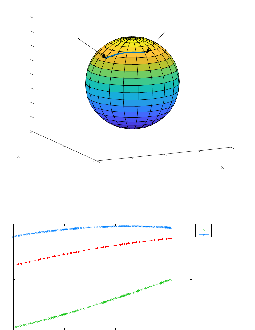
-8000
-6000
-4000
-1
-2000
0
2000
4000
z
6000
8000
x
10 401
0.5
10 4
y
0
-0.5
1-1
London
New York
Figure 3.30: Flight path for geodesic problem
-4000
-2000
0
2000
4000
0 1 2 3 4 5 6 7
states
time (s)
Geodesic problem
x
y
z
Figure 3.31: States for geodesic problem
176
0.8
1
1.2
1.4
1.6
0 1 2 3 4 5 6 7
controls
time (s)
Geodesic problem
theta
phi
Figure 3.32: Controls for geodesic problem
and the control bounds
0≤T(t)≤3.5 (3.59)
where D=D0v2exp(−βh)
g= 1/(h2),(3.60)
D0= 310, β= 500, and c= 0.5, 0.1≤tf≤1. The PSOPT code that
solves this problem is shown below.
//////////////////////////////////////////////////////////////////////////
////////////////// goddard.cxx /////////////////////////
//////////////////////////////////////////////////////////////////////////
//////////////// PSOPT Example ////////////////////
//////////////////////////////////////////////////////////////////////////
//////////////////////////////////////////////////////////////////////////
//////// Title: Goddard rocket maximum ascent ////////////////
//////// Last modified: 05 January 2009 ////////////////
//////// Reference: Bryson (1999) ////////////////
//////// (See PSOPT handbook for full reference) ////////////////
//////////////////////////////////////////////////////////////////////////
//////// Copyright (c) Victor M. Becerra, 2009 ////////////////
//////////////////////////////////////////////////////////////////////////
//////// This is part of the PSOPT software library, which ///////////////
//////// is distributed under the terms of the GNU Lesser ////////////////
//////// General Public License (LGPL) ////////////////
//////////////////////////////////////////////////////////////////////////
#include "psopt.h"
//////////////////////////////////////////////////////////////////////////
/////////////////// Define the end point (Mayer) cost function //////////
//////////////////////////////////////////////////////////////////////////
adouble endpoint_cost(adouble* initial_states, adouble* final_states,
adouble* parameters,adouble& t0, adouble& tf,
adouble* xad, int iphase, Workspace* workspace)
177

{
adouble hf = final_states[1];
return -hf;
}
//////////////////////////////////////////////////////////////////////////
/////////////////// Define the integrand (Lagrange) cost function //////
//////////////////////////////////////////////////////////////////////////
adouble integrand_cost(adouble* states, adouble* controls,
adouble* parameters, adouble& time, adouble* xad,
int iphase, Workspace* workspace)
{
return 0.0;
}
//////////////////////////////////////////////////////////////////////////
/////////////////// Define the DAE’s ////////////////////////////////////
//////////////////////////////////////////////////////////////////////////
void dae(adouble* derivatives, adouble* path, adouble* states,
adouble* controls, adouble* parameters, adouble& time,
adouble* xad, int iphase, Workspace* workspace)
{
adouble vdot, hdot, mdot;
adouble v = states[0];
adouble h = states[1];
adouble m = states[2];
adouble T = controls[0];
double c = 0.5;
double D0 = 310.0;
double beta = 500.0;
adouble g = 1.0/(h*h);
adouble D = D0*v*v*exp(-beta*h);
vdot = 1.0/m*(T-D)-g;
hdot = v;
mdot = -T/c;
derivatives[0] = vdot;
derivatives[1] = hdot;
derivatives[2] = mdot;
}
////////////////////////////////////////////////////////////////////////////
/////////////////// Define the events function ////////////////////////////
////////////////////////////////////////////////////////////////////////////
void events(adouble* e, adouble* initial_states, adouble* final_states,
adouble* parameters,adouble& t0, adouble& tf, adouble* xad,
int iphase, Workspace* workspace)
{
adouble vi = initial_states[0];
adouble hi = initial_states[1];
adouble mi = initial_states[2];
adouble mf = final_states[2];
e[0] = vi;
e[1] = hi;
e[2] = mi;
e[3] = mf;
}
///////////////////////////////////////////////////////////////////////////
/////////////////// Define the phase linkages function ///////////////////
///////////////////////////////////////////////////////////////////////////
void linkages( adouble* linkages, adouble* xad, Workspace* workspace)
{
178

}
////////////////////////////////////////////////////////////////////////////
/////////////////// Define the main routine ///////////////////////////////
////////////////////////////////////////////////////////////////////////////
int main(void)
{
////////////////////////////////////////////////////////////////////////////
/////////////////// Declare key structures ////////////////////////////////
////////////////////////////////////////////////////////////////////////////
Alg algorithm;
Sol solution;
Prob problem;
////////////////////////////////////////////////////////////////////////////
/////////////////// Register problem name ////////////////////////////////
////////////////////////////////////////////////////////////////////////////
problem.name = "Goddard Rocket Maximum Ascent";
problem.outfilename = "goddard.txt";
////////////////////////////////////////////////////////////////////////////
//////////// Declare problem level constants & setup phases //////////////
////////////////////////////////////////////////////////////////////////////
problem.nphases = 1;
problem.nlinkages = 0;
psopt_level1_setup(problem);
/////////////////////////////////////////////////////////////////////////////
///////// Define phase related information & setup PSOPT /////////////////
/////////////////////////////////////////////////////////////////////////////
problem.phases(1).nstates = 3;
problem.phases(1).ncontrols = 1;
problem.phases(1).nevents = 4;
problem.phases(1).npath = 0;
problem.phases(1).nodes = 20;
psopt_level2_setup(problem, algorithm);
////////////////////////////////////////////////////////////////////////////
/////////////////// Declare DMatrix objects to store results //////////////
////////////////////////////////////////////////////////////////////////////
DMatrix x,u,t;
////////////////////////////////////////////////////////////////////////////
/////////////////// Enter problem bounds information //////////////////////
////////////////////////////////////////////////////////////////////////////
double v_L = 0;
double h_L = 1.0;
double m_L = 0.6;
double v_U = 2.0;
double h_U = 2.0;
double m_U = 1.0;
double T_L = 0.0;
double T_U = 3.5;
double v_i = 0.0;
double h_i = 1.0;
double m_i = 1.0;
double m_f = 0.6;
problem.phases(1).bounds.lower.states(1) = v_L;
problem.phases(1).bounds.lower.states(2) = h_L;
problem.phases(1).bounds.lower.states(3) = m_L;
problem.phases(1).bounds.upper.states(1) = v_U;
problem.phases(1).bounds.upper.states(2) = h_U;
179

problem.phases(1).bounds.upper.states(3) = m_U;
problem.phases(1).bounds.lower.controls(1) = T_L;
problem.phases(1).bounds.upper.controls(1) = T_U;
problem.phases(1).bounds.lower.events(1) = v_i;
problem.phases(1).bounds.lower.events(2) = h_i;
problem.phases(1).bounds.lower.events(3) = m_i;
problem.phases(1).bounds.lower.events(4) = m_f;
problem.phases(1).bounds.upper.events(1) = v_i;
problem.phases(1).bounds.upper.events(2) = h_i;
problem.phases(1).bounds.upper.events(3) = m_i;
problem.phases(1).bounds.upper.events(4) = m_f;
problem.phases(1).bounds.lower.StartTime = 0.0;
problem.phases(1).bounds.upper.StartTime = 0.0;
problem.phases(1).bounds.lower.EndTime = 0.1;
problem.phases(1).bounds.upper.EndTime = 1.0;
////////////////////////////////////////////////////////////////////////////
/////////////////// Register problem functions ///////////////////////////
////////////////////////////////////////////////////////////////////////////
problem.integrand_cost = &integrand_cost;
problem.endpoint_cost = &endpoint_cost;
problem.dae = &dae;
problem.events = &events;
problem.linkages = &linkages;
////////////////////////////////////////////////////////////////////////////
/////////////////// Define & register initial guess ///////////////////////
////////////////////////////////////////////////////////////////////////////
DMatrix x0(3,20);
x0(1,colon()) = linspace(v_i,v_i, 20);
x0(2,colon()) = linspace(h_i,h_i, 20);
x0(3,colon()) = linspace(m_i,m_i, 20);
problem.phases(1).guess.controls = T_U*ones(1,20);
problem.phases(1).guess.states = x0;
problem.phases(1).guess.time = linspace(0.0, 15.0, 20);
////////////////////////////////////////////////////////////////////////////
/////////////////// Enter algorithm options //////////////////////////////
////////////////////////////////////////////////////////////////////////////
algorithm.nlp_method = "IPOPT";
algorithm.scaling = "automatic";
algorithm.derivatives = "automatic";
algorithm.nlp_iter_max = 1000;
algorithm.nlp_tolerance = 1.e-6;
algorithm.collocation_method = "trapezoidal";
algorithm.mesh_refinement = "automatic";
algorithm.mr_max_iterations = 5;
////////////////////////////////////////////////////////////////////////////
/////////////////// Now call PSOPT to solve the problem //////////////////
////////////////////////////////////////////////////////////////////////////
psopt(solution, problem, algorithm);
////////////////////////////////////////////////////////////////////////////
/////////// Extract relevant variables from solution structure //////////
////////////////////////////////////////////////////////////////////////////
x = solution.get_states_in_phase(1);
u = solution.get_controls_in_phase(1);
t = solution.get_time_in_phase(1);
////////////////////////////////////////////////////////////////////////////
180

/////////// Save solution data to files if desired ////////////////////////
////////////////////////////////////////////////////////////////////////////
x.Save("x.dat");
u.Save("u.dat");
t.Save("t.dat");
////////////////////////////////////////////////////////////////////////////
/////////// Plot some results if desired (requires gnuplot) ///////////////
////////////////////////////////////////////////////////////////////////////
plot(t,x,problem.name, "time (s)", "states", "v h m");
plot(t,u,problem.name, "time (s)", "control", "T");
plot(t,x,problem.name, "time (s)", "states", "v h m",
"pdf", "goddard_states.pdf");
plot(t,u,problem.name, "time (s)", "control", "T",
"pdf", "goddard_control.pdf");
}
////////////////////////////////////////////////////////////////////////////
/////////////////////// END OF FILE ///////////////////////////////
////////////////////////////////////////////////////////////////////////////
The output from PSOPT is summarised in the box below and shown
in Figures 3.33 and 3.34, which contain the elements of the state and the
control, respectively.
PSOPT results summary
=====================
Problem: Goddard Rocket Maximum Ascent
CPU time (seconds): 2.799138e+00
NLP solver used: IPOPT
PSOPT release number: 4.0
Date and time of this run: Thu Feb 21 17:15:41 2019
Optimal (unscaled) cost function value: -1.025336e+00
Phase 1 endpoint cost function value: -1.025336e+00
Phase 1 integrated part of the cost: 0.000000e+00
Phase 1 initial time: 0.000000e+00
Phase 1 final time: 2.605347e-01
Phase 1 maximum relative local error: 6.877099e-04
NLP solver reports: The problem has been solved!
3.14 Hang glider
This problem is about the range maximisation of a hang glider in the pres-
ence of a specified thermal draft [4]. Find tfand CL(t), t ∈[0, tf], to min-
181
0
0.2
0.4
0.6
0.8
1
0 0.05 0.1 0.15 0.2 0.25 0.3
states
time (s)
Goddard Rocket Maximum Ascent
v
h
m
Figure 3.33: States for Goddard rocket problem
0
0.5
1
1.5
2
2.5
3
3.5
0 0.05 0.1 0.15 0.2 0.25 0.3
control
time (s)
Goddard Rocket Maximum Ascent
T
Figure 3.34: Control for Goddard rocket problem
182
imise,
J=x(tf) (3.61)
subject to the dynamic constraints
˙x=vx
˙y=vy
˙vx=1
m(−Lsin η−Dcos η)
˙vy=1
m(Lcos η−Dsin η−W)
(3.62)
where CD=C0+kC2
L
vr=qv2
x+v2
y
D=1
2CDρSv2
r
L=1
2CLρSv2
r
X=x
R−2.52
ua=uM(1 −X) exp(−X)
Vy=vy−ua
sin η=Vy
vr
cos η=vx
vr
W=mg
(3.63)
The control is bounded as follows:
0≤CL≤1.4 (3.64)
and the following boundary conditions:
x(0) = 0, x(tf) = free
y(0) = 1000, y(tf) = 900
vx(0) = 13.227567500, vx(tf) = 13.227567500
vy(0) = −1.2875005200, vy(tf) = −1.2875005200
(3.65)
With the following parameter values:
uM= 2.5, m = 100.0
R= 100.0, S = 14,
C0= 0.034, ρ = 1.13
k= 0.069662, g = 9.80665
(3.66)
PSOPT code that solves this problem is shown below.
183

//////////////////////////////////////////////////////////////////////////
//////////////// glider.cxx /////////////////////
//////////////////////////////////////////////////////////////////////////
//////////////// PSOPT example /////////////////////
//////////////////////////////////////////////////////////////////////////
//////////////////////////////////////////////////////////////////////////
//////// Title: Hang glider problem ////////////////
//////// Last modified: 11 July 2009 ////////////////
//////// Reference: PROPT User Manual ////////////////
//////// ////////////////
//////////////////////////////////////////////////////////////////////////
//////// Copyright (c) Victor M. Becerra, 2009 ////////////////
//////////////////////////////////////////////////////////////////////////
//////// This is part of the PSOPT software library, which ///////////////
//////// is distributed under the terms of the GNU Lesser ////////////////
//////// General Public License (LGPL) ////////////////
//////////////////////////////////////////////////////////////////////////
#include "psopt.h"
//////////////////////////////////////////////////////////////////////////
/////////////////// Define the end point (Mayer) cost function //////////
//////////////////////////////////////////////////////////////////////////
adouble endpoint_cost(adouble* initial_states, adouble* final_states,
adouble* parameters,adouble& t0, adouble& tf,
adouble* xad, int iphase, Workspace* workspace)
{
adouble xf = final_states[CINDEX(1)];
return -(xf);
}
//////////////////////////////////////////////////////////////////////////
/////////////////// Define the integrand (Lagrange) cost function //////
//////////////////////////////////////////////////////////////////////////
adouble integrand_cost(adouble* states, adouble* controls, adouble* parameters,
adouble& time, adouble* xad, int iphase, Workspace* workspace)
{
return 0.0;
}
//////////////////////////////////////////////////////////////////////////
/////////////////// Define the DAE’s ////////////////////////////////////
//////////////////////////////////////////////////////////////////////////
void dae(adouble* derivatives, adouble* path, adouble* states,
adouble* controls, adouble* parameters, adouble& time,
adouble* xad, int iphase, Workspace* workspace)
{
adouble CL = controls[ CINDEX(1) ];
adouble x = states[ CINDEX(1) ];
adouble y = states[ CINDEX(2) ];
adouble vx = states[ CINDEX(3) ];
adouble vy = states[ CINDEX(4) ];
double m = 100.0, g = 9.80665;
double uM = 2.5, R = 100.0;
double C0 = 0.034, k = 0.069662;
double S = 14.0, rho = 1.13;
adouble sin_eta, cos_eta, D, L, CD, Vy, ua, X, vr, W;
CD = C0 + k*CL*CL;
vr = sqrt(vx*vx + vy*vy);
D = 0.5*CD*rho*S*vr*vr;
L = 0.5*CL*rho*S*vr*vr;
X = pow(x/R - 2.5, 2.0);
ua = uM*(1.0-X)*exp(-X);
Vy = vy-ua;
sin_eta = Vy/vr;
cos_eta = vx/vr;
184

W = m*g;
derivatives[ CINDEX(1) ] = vx;
derivatives[ CINDEX(2) ] = vy;
derivatives[ CINDEX(3) ] = 1.0/m*(-L*sin_eta - D*cos_eta );
derivatives[ CINDEX(4) ] = 1.0/m*( L*cos_eta - D*sin_eta - W);
}
////////////////////////////////////////////////////////////////////////////
/////////////////// Define the events function ////////////////////////////
////////////////////////////////////////////////////////////////////////////
void events(adouble* e, adouble* initial_states, adouble* final_states,
adouble* parameters,adouble& t0, adouble& tf, adouble* xad,
int iphase, Workspace* workspace)
{
adouble x_i = initial_states[ CINDEX(1) ];
adouble y_i = initial_states[ CINDEX(2) ];
adouble vx_i = initial_states[ CINDEX(3) ];
adouble vy_i = initial_states[ CINDEX(4) ];
adouble x_f = final_states[ CINDEX(1) ];
adouble y_f = final_states[ CINDEX(2) ];
adouble vx_f = final_states[ CINDEX(3) ];
adouble vy_f = final_states[ CINDEX(4) ];
e[ CINDEX(1) ] = x_i;
e[ CINDEX(2) ] = y_i;
e[ CINDEX(3) ] = vx_i;
e[ CINDEX(4) ] = vy_i;
e[ CINDEX(5) ] = y_f;
e[ CINDEX(6) ] = vx_f;
e[ CINDEX(7) ] = vy_f;
}
///////////////////////////////////////////////////////////////////////////
/////////////////// Define the phase linkages function ///////////////////
///////////////////////////////////////////////////////////////////////////
void linkages( adouble* linkages, adouble* xad, Workspace* workspace)
{
// Single phase problem
}
////////////////////////////////////////////////////////////////////////////
/////////////////// Define the main routine ///////////////////////////////
////////////////////////////////////////////////////////////////////////////
int main(void)
{
////////////////////////////////////////////////////////////////////////////
/////////////////// Declare key structures ////////////////////////////////
////////////////////////////////////////////////////////////////////////////
Alg algorithm;
Sol solution;
Prob problem;
////////////////////////////////////////////////////////////////////////////
/////////////////// Register problem name ////////////////////////////////
////////////////////////////////////////////////////////////////////////////
problem.name = "Hang glider problem";
problem.outfilename = "hang_glider.txt";
////////////////////////////////////////////////////////////////////////////
//////////// Define problem level constants & do level 1 setup ////////////
185

////////////////////////////////////////////////////////////////////////////
problem.nphases = 1;
problem.nlinkages = 0;
psopt_level1_setup(problem);
/////////////////////////////////////////////////////////////////////////////
///////// Define phase related information & do level 2 setup ////////////
/////////////////////////////////////////////////////////////////////////////
problem.phases(1).nstates = 4;
problem.phases(1).ncontrols = 1;
problem.phases(1).nevents = 7;
problem.phases(1).npath = 0;
problem.phases(1).nodes = "[30 40 50 80]";
psopt_level2_setup(problem, algorithm);
////////////////////////////////////////////////////////////////////////////
/////////////////// Enter problem bounds information //////////////////////
////////////////////////////////////////////////////////////////////////////
problem.phases(1).bounds.lower.states = "[0.0 0.0 0.0 -4.0]";
problem.phases(1).bounds.upper.states = "[1500.0 1100.0 15.0 4.0]";
problem.phases(1).bounds.lower.controls(1) = 0.0;
problem.phases(1).bounds.upper.controls(1) = 1.4;
problem.phases(1).bounds.lower.events="[0.0,1000.0,13.2275675,-1.28750052,900.00,13.2275675,-1.28750052 ]";
problem.phases(1).bounds.upper.events="[0.0,1000.0,13.2275675,-1.28750052,900.00,13.2275675,-1.28750052 ]";
problem.phases(1).bounds.lower.StartTime = 0.0;
problem.phases(1).bounds.upper.StartTime = 0.0;
problem.phases(1).bounds.lower.EndTime = 0.1;
problem.phases(1).bounds.upper.EndTime = 200.0;
////////////////////////////////////////////////////////////////////////////
/////////////////// Register problem functions ///////////////////////////
////////////////////////////////////////////////////////////////////////////
problem.integrand_cost = &integrand_cost;
problem.endpoint_cost = &endpoint_cost;
problem.dae = &dae;
problem.events = &events;
problem.linkages = &linkages;
////////////////////////////////////////////////////////////////////////////
/////////////////// Define & register initial guess ///////////////////////
////////////////////////////////////////////////////////////////////////////
int nnodes = problem.phases(1).nodes(1);
int ncontrols = problem.phases(1).ncontrols;
int nstates = problem.phases(1).nstates;
DMatrix state_guess = zeros(nstates,nnodes);
DMatrix control_guess = 1.0*ones(ncontrols,nnodes);
DMatrix time_guess = linspace(0.0,105.0,nnodes);
state_guess(1,colon()) = linspace(0.0, 1250, nnodes);
state_guess(2,colon()) = linspace(1000.0, 900.0, nnodes);
state_guess(3,colon()) = 13.23*ones(1,nnodes);
state_guess(4,colon()) = -1.288*ones(1,nnodes);
problem.phases(1).guess.states = state_guess;
problem.phases(1).guess.controls = control_guess;
problem.phases(1).guess.time = time_guess;
186

////////////////////////////////////////////////////////////////////////////
/////////////////// Enter algorithm options //////////////////////////////
////////////////////////////////////////////////////////////////////////////
algorithm.nlp_iter_max = 1000;
algorithm.nlp_tolerance = 1.e-6;
algorithm.nlp_method = "IPOPT";
algorithm.scaling = "automatic";
algorithm.derivatives = "automatic";
////////////////////////////////////////////////////////////////////////////
/////////////////// Now call PSOPT to solve the problem //////////////////
////////////////////////////////////////////////////////////////////////////
psopt(solution, problem, algorithm);
////////////////////////////////////////////////////////////////////////////
/////////// Extract relevant variables from solution structure //////////
////////////////////////////////////////////////////////////////////////////
DMatrix states, CL, t, x, y, speeds;
states = solution.get_states_in_phase(1);
CL = solution.get_controls_in_phase(1);
t = solution.get_time_in_phase(1);
////////////////////////////////////////////////////////////////////////////
/////////// Save solution data to files if desired ////////////////////////
////////////////////////////////////////////////////////////////////////////
states.Save("states.dat");
CL.Save("cL.dat");
t.Save("t.dat");
////////////////////////////////////////////////////////////////////////////
/////////// Plot some results if desired (requires gnuplot) ///////////////
////////////////////////////////////////////////////////////////////////////
x = states(1,colon());
y = states(2,colon());
speeds = (states(3,colon()) && states(4,colon()));
plot(x,y,problem.name+": trajectory","x [m]", "y [m]", "traj");
plot(t,speeds,problem.name+": speeds","time (s)", "speeds [m/s]", "dxdt dydt");
plot(t,CL,problem.name+": control","time (s)", "control", "CL");
plot(x,y,problem.name+": trajectory","x [m]", "y [m]", "traj", "pdf", "traj.pdf");
plot(t,speeds,problem.name+": speeds","time (s)", "speeds [m/s]", "dxdt dydt", "pdf", "velocities.pdf");
plot(t,CL,problem.name+": control - lift coefficient","time (s)", "CL", "CL", "pdf", "control.pdf");
}
////////////////////////////////////////////////////////////////////////////
/////////////////////// END OF FILE ///////////////////////////////
////////////////////////////////////////////////////////////////////////////
The output from PSOPT is summarised in the box below and shown in
Figures 3.35,3.36 and 3.37.
187
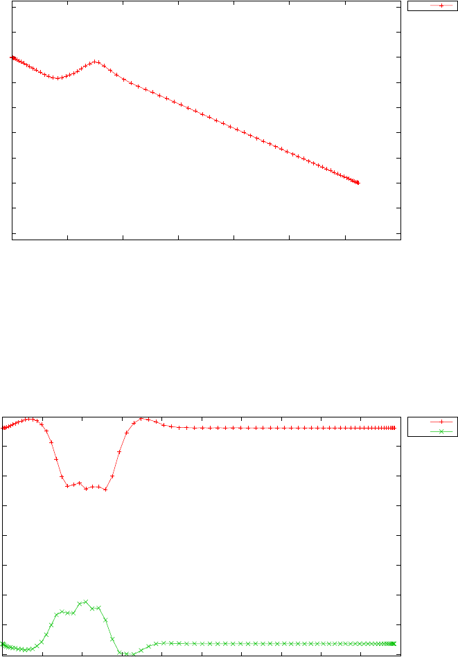
860
880
900
920
940
960
980
1000
1020
1040
0 200 400 600 800 1000 1200 1400
y [m]
x [m]
Hang glider problem: trajectory
traj
Figure 3.35: x−ytrajectory for hang glider
-2
0
2
4
6
8
10
12
0 10 20 30 40 50 60 70 80 90 100
speeds [m/s]
time (s)
Hang glider problem: speeds
dxdt
dydt
Figure 3.36: Velocities for hang glider
188
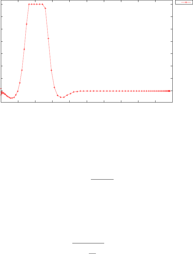
0.7
0.8
0.9
1
1.1
1.2
1.3
1.4
0 10 20 30 40 50 60 70 80 90 100
CL
time (s)
Hang glider problem: control - lift coefficient
CL
Figure 3.37: Lift coefficient for hang glider problem
3.15 Hanging chain problem
Consider the following optimal control problem, which includes an integral
constraint. Minimize the cost functional
J=Ztf
0xq1 + ( ˙x)2dt (3.67)
subject to the dynamic constraint
˙x=u(3.68)
the integral constraint:
Ztf
0
s1 + dx
dt 2
dt = 4 (3.69)
the boundary conditions
x(0) = 1
x(tf)=3 (3.70)
and the bounds: −20 ≤u(t)≤20
−10 ≤x(t)≤10 (3.71)
where tf= 1. The PSOPT code that solves this problem is shown below.
189

//////////////////////////////////////////////////////////////////////////
////////////////// chain.cxx ///////////////////////
//////////////////////////////////////////////////////////////////////////
//////////////// PSOPT Example ////////////////////
//////////////////////////////////////////////////////////////////////////
//////////////////////////////////////////////////////////////////////////
//////// Title: Hanging chain problem ////////////////
//////// Last modified: 29 January 2009 ////////////////
//////// Reference: ////////////////
//////// ////////////////
//////////////////////////////////////////////////////////////////////////
//////// Copyright (c) Victor M. Becerra, 2009 ////////////////
//////////////////////////////////////////////////////////////////////////
//////// This is part of the PSOPT software library, which ///////////////
//////// is distributed under the terms of the GNU Lesser ////////////////
//////// General Public License (LGPL) ////////////////
//////////////////////////////////////////////////////////////////////////
#include "psopt.h"
//////////////////////////////////////////////////////////////////////////
/////////////////// Define the end point (Mayer) cost function //////////
//////////////////////////////////////////////////////////////////////////
adouble endpoint_cost(adouble* initial_states, adouble* final_states,
adouble* parameters,adouble& t0, adouble& tf,
adouble* xad, int iphase, Workspace* workspace)
{
return 0.0;
}
//////////////////////////////////////////////////////////////////////////
/////////////////// Define the integrand (Lagrange) cost function //////
//////////////////////////////////////////////////////////////////////////
adouble integrand_cost(adouble* states, adouble* controls,
adouble* parameters, adouble& time, adouble* xad,
int iphase, Workspace* workspace)
{
adouble x = states[ CINDEX(1) ];
adouble dxdt = controls[ CINDEX(1) ];
adouble L = x*sqrt(1.0+ pow(dxdt,2.0));
return L;
}
//////////////////////////////////////////////////////////////////////////
/////////////////// Define the DAE’s ////////////////////////////////////
//////////////////////////////////////////////////////////////////////////
void dae(adouble* derivatives, adouble* path, adouble* states,
adouble* controls, adouble* parameters, adouble& time,
adouble* xad, int iphase, Workspace* workspace)
{
adouble xdot, ydot, vdot;
adouble x = states[ CINDEX(1) ];
adouble dxdt = controls[ CINDEX(1) ];
derivatives[ CINDEX(1) ] = dxdt;
}
////////////////////////////////////////////////////////////////////////////
/////////////////// Define the integrand of the integral constraint ///////
////////////////////////////////////////////////////////////////////////////
adouble integrand( adouble* states, adouble* controls, adouble* parameters,
adouble& time, adouble* xad, int iphase, Workspace* workspace)
{
adouble G;
adouble dxdt = controls[ CINDEX(1) ];
G = sqrt( 1.0 + pow(dxdt,2.0));
return G;
}
190

////////////////////////////////////////////////////////////////////////////
/////////////////// Define the events function ////////////////////////////
////////////////////////////////////////////////////////////////////////////
void events(adouble* e, adouble* initial_states, adouble* final_states,
adouble* parameters,adouble& t0, adouble& tf, adouble* xad,
int iphase, Workspace* workspace)
{
adouble x0 = initial_states[ CINDEX(1) ];
adouble xf = final_states[ CINDEX(1) ];
adouble Q;
// Compute the integral to be constrained
Q = integrate( integrand, xad, iphase, workspace );
e[ CINDEX(1) ] = x0;
e[ CINDEX(2) ] = xf;
e[ CINDEX(3) ] = Q;
}
///////////////////////////////////////////////////////////////////////////
/////////////////// Define the phase linkages function ///////////////////
///////////////////////////////////////////////////////////////////////////
void linkages( adouble* linkages, adouble* xad, Workspace* workspace)
{
// No linkages as this is a single phase problem
}
////////////////////////////////////////////////////////////////////////////
/////////////////// Define the main routine ///////////////////////////////
////////////////////////////////////////////////////////////////////////////
int main(void)
{
////////////////////////////////////////////////////////////////////////////
/////////////////// Declare key structures ////////////////////////////////
////////////////////////////////////////////////////////////////////////////
Alg algorithm;
Sol solution;
Prob problem;
////////////////////////////////////////////////////////////////////////////
/////////////////// Register problem name ////////////////////////////////
////////////////////////////////////////////////////////////////////////////
problem.name = "Hanging chain problem";
problem.outfilename = "chain.txt";
////////////////////////////////////////////////////////////////////////////
//////////// Define problem level constants & do level 1 setup ////////////
////////////////////////////////////////////////////////////////////////////
problem.nphases = 1;
problem.nlinkages = 0;
psopt_level1_setup(problem);
/////////////////////////////////////////////////////////////////////////////
///////// Define phase related information & do level 2 setup /////////////
/////////////////////////////////////////////////////////////////////////////
problem.phases(1).nstates = 1;
problem.phases(1).ncontrols = 1;
problem.phases(1).nevents = 3;
problem.phases(1).npath = 0;
problem.phases(1).nodes = "[20, 50]";
psopt_level2_setup(problem, algorithm);
191

////////////////////////////////////////////////////////////////////////////
/////////////////// Enter problem bounds information //////////////////////
////////////////////////////////////////////////////////////////////////////
problem.phases(1).bounds.lower.states(1) = -10.0;
problem.phases(1).bounds.upper.states(1) = 10.0;
problem.phases(1).bounds.lower.controls(1) = -20.0;
problem.phases(1).bounds.upper.controls(1) = 20.0;
problem.phases(1).bounds.lower.events(1) = 1.0;
problem.phases(1).bounds.lower.events(2) = 3.0;
problem.phases(1).bounds.lower.events(3) = 4.0;
problem.phases(1).bounds.upper.events(1) = 1.0;
problem.phases(1).bounds.upper.events(2) = 3.0;
problem.phases(1).bounds.upper.events(3) = 4.0;
problem.phases(1).bounds.lower.StartTime = 0.0;
problem.phases(1).bounds.upper.StartTime = 0.0;
problem.phases(1).bounds.lower.EndTime = 1.0;
problem.phases(1).bounds.upper.EndTime = 1.0;
////////////////////////////////////////////////////////////////////////////
/////////////////// Register problem functions ///////////////////////////
////////////////////////////////////////////////////////////////////////////
problem.integrand_cost = &integrand_cost;
problem.endpoint_cost = &endpoint_cost;
problem.dae = &dae;
problem.events = &events;
problem.linkages = &linkages;
////////////////////////////////////////////////////////////////////////////
/////////////////// Define & register initial guess ///////////////////////
////////////////////////////////////////////////////////////////////////////
problem.phases(1).guess.controls = 2.0*ones(1,30);
problem.phases(1).guess.states = linspace(1.0,3.0, 30);
problem.phases(1).guess.time = linspace(0.0,1.0, 30);
////////////////////////////////////////////////////////////////////////////
/////////////////// Enter algorithm options //////////////////////////////
////////////////////////////////////////////////////////////////////////////
algorithm.nlp_method = "IPOPT";
algorithm.scaling = "automatic";
algorithm.derivatives = "automatic";
algorithm.nlp_iter_max = 1000;
algorithm.nlp_tolerance = 1.e-6;
////////////////////////////////////////////////////////////////////////////
/////////////////// Now call PSOPT to solve the problem /////////////////
////////////////////////////////////////////////////////////////////////////
psopt(solution, problem, algorithm);
if (solution.error_flag) exit(0);
////////////////////////////////////////////////////////////////////////////
/////////// Extract relevant variables from solution structure //////////
////////////////////////////////////////////////////////////////////////////
DMatrix x, u, t;
x = solution.get_states_in_phase(1);
u = solution.get_controls_in_phase(1);
t = solution.get_time_in_phase(1);
192

////////////////////////////////////////////////////////////////////////////
/////////// Save solution data to files if desired ////////////////////////
////////////////////////////////////////////////////////////////////////////
x.Save("x.dat");
u.Save("u.dat");
t.Save("t.dat");
////////////////////////////////////////////////////////////////////////////
/////////// Plot some results if desired (requires gnuplot) ///////////////
////////////////////////////////////////////////////////////////////////////
plot(t,x,problem.name + ": state", "time (s)", "x", "x");
plot(t,u,problem.name + ": control", "time (s)", "u", "u");
plot(t,x,problem.name + ": state", "time (s)", "x", "x",
"pdf", "chain_state.pdf");
plot(t,u,problem.name + ": control", "time (s)", "u", "u",
"pdf", "chain_control.pdf");
}
////////////////////////////////////////////////////////////////////////////
/////////////////////// END OF FILE ///////////////////////////////
////////////////////////////////////////////////////////////////////////////
The output from PSOPT is summarized in the text box below and in
Figure 3.38, which illustrates the shape of the hanging chain.
PSOPT results summary
=====================
Problem: Hanging chain problem
CPU time (seconds): 2.032182e+00
NLP solver used: IPOPT
PSOPT release number: 4.0
Date and time of this run: Thu Feb 21 17:08:27 2019
Optimal (unscaled) cost function value: 5.068480e+00
Phase 1 endpoint cost function value: 0.000000e+00
Phase 1 integrated part of the cost: 5.068480e+00
Phase 1 initial time: 0.000000e+00
Phase 1 final time: 1.000000e+00
Phase 1 maximum relative local error: 2.362643e-06
NLP solver reports: The problem has been solved!
3.16 Heat difussion problem
This example can be viewed as a simplified model for the heating of a probe
in a kiln [3]. The dynamics are a spatially discretized form of a partial
193
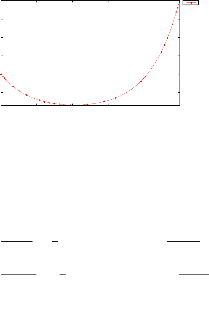
0.5
1
1.5
2
2.5
3
0 0.2 0.4 0.6 0.8 1
x
time (s)
Hanging chain problem: state
x
Figure 3.38: State for hanging chain problem
differential equation, which is obtained by using the method of the lines.
The problem is formulated on the basis of the state vector x= [x1, . . . , xM]T
and the control vector u= [v1, v2, v3]T, as follows
min
u(t)J=1
2ZT
0(xN(t)−xd(t))2+γv1(t)2dt
subject to the differential constraints
˙x1=1
(a1+a2x1)"q1+1
δ2(a3+a4x1)(x2−2x1+v2) + a4x2−x1
2δ2#
˙xi=1
(a1+a2xi)"qi+1
δ2(a3+a4xi)(xi+1 −2xi+xi−1) + a4xi+1 −xi−1
2δ2#
for i= 2, . . . , M −1
˙xM=1
(a1+a2xM)"qM+1
δ2(a3+a4xM)(v3−2xN+xM−1) + a4v3−xM−1
2δ2#
the path constraints
0 = g(x1−v1)−1
2δ(a3+a4x1)(x2−v2)
0 = 1
2δ(a3+a+ 4xM)(v3−xM−1)
the control bounds
uL≤v1≤uU
194

and the initial conditions for the states:
xi(0) = 2 + cos(πzi)
where
zi=i−1
M−1, i = 1, . . . , M
xd(t)=2−eρt
q(z, t) = ρ(a1+ 2a2) + π2(a3+ 2a4)eρt cos(πz)
−a4π2e2πt + (2a4π2+ρa2)e2ρt cos2(πz)
qi≡q(zi, t), i = 1, . . . , M
with the parameter values a1= 4, a2= 1, a3= 4, a4=−1, uU= 0.1,
ρ=−1, T= 0.5, γ= 10−3,g= 1, uL=−∞.
A spatial discretization given by M= 10 was used. The problem was
solved initially by using first 50 nodes, then the mesh was refined to 60
nodes, and an interpolation of the previous solution was employed as an
initial guess for the new solution.
The PSOPT code that solves this problem is shown below.
//////////////////////////////////////////////////////////////////////////
//////////////// heat.cxx /////////////////////
//////////////////////////////////////////////////////////////////////////
//////////////// PSOPT Template /////////////////////
//////////////////////////////////////////////////////////////////////////
//////////////////////////////////////////////////////////////////////////
//////// Title: Heat difussion process ////////////////
//////// Last modified: 09 July 2009 ////////////////
//////// Reference: Betts (2001) ////////////////
//////// ////////////////
//////////////////////////////////////////////////////////////////////////
//////// Copyright (c) Victor M. Becerra, 2009 ////////////////
//////////////////////////////////////////////////////////////////////////
//////// This is part of the PSOPT software library, which ////////////////
//////// is distributed under the terms of the GNU Lesser ////////////////
//////// General Public License (LGPL) ////////////////
//////////////////////////////////////////////////////////////////////////
#include "psopt.h"
//////////////////////////////////////////////////////////////////////////
/////////////////// Define the end point (Mayer) cost function //////////
//////////////////////////////////////////////////////////////////////////
#define N_DISCRETIZATION 10
adouble endpoint_cost(adouble* initial_states, adouble* final_states,
adouble* parameters,adouble& t0, adouble& tf,
adouble* xad, int iphase, Workspace* workspace)
{
return 0.0;
}
//////////////////////////////////////////////////////////////////////////
/////////////////// Define the integrand (Lagrange) cost function //////
//////////////////////////////////////////////////////////////////////////
adouble integrand_cost(adouble* states, adouble* controls, adouble* parameters,
adouble& time, adouble* xad, int iphase, Workspace* workspace)
{
195

int N = N_DISCRETIZATION;
double gamma = 1.0e-3;
double rho = -1.0;
adouble yd = 2.0-exp(rho*time);
adouble yN = states[ CINDEX(N) ];
adouble v1 = controls[ CINDEX(1) ];
return 0.5*( pow(yN-yd,2.0) + gamma*pow(v1,2.0) );
}
//////////////////////////////////////////////////////////////////////////
/////////////////// Define the DAE’s ////////////////////////////////////
//////////////////////////////////////////////////////////////////////////
void dae(adouble* derivatives, adouble* path, adouble* states,
adouble* controls, adouble* parameters, adouble& time,
adouble* xad, int iphase, Workspace* workspace)
{
adouble u;
double a1 = 4.0;
double a2 = 1.0;
double a3 = 4.0;
double a4 = -1.0;
double rho = -1.0;
double T = 0.5;
double g = 1.0;
int N = N_DISCRETIZATION;
int i;
double delta = 1.0/(N-1);
adouble* y = states;
adouble v1 = controls[ CINDEX(1) ];
adouble v2 = controls[ CINDEX(2) ];
adouble v3 = controls[ CINDEX(3) ];
adouble y1 = y[CINDEX(1)];
adouble y2 = y[CINDEX(2)];
adouble yN = y[CINDEX(N)];
adouble yNm1 = y[CINDEX(N-1)];
adouble x1 = 0;
adouble xN = 1;
adouble q1 = (rho*(a1+2*a2) + pi*pi*(a3+2*a4))*exp(rho*time)*cos(pi*x1)
- a4*pi*pi*exp(2*rho*time) + (2*a4*pi*pi+rho*a2)*exp(2*rho*time)*pow(cos(pi*x1),2.0);
adouble qN = (rho*(a1+2*a2) + pi*pi*(a3+2*a4))*exp(rho*time)*cos(pi*xN)
- a4*pi*pi*exp(2*rho*time) + (2*a4*pi*pi+rho*a2)*exp(2*rho*time)*pow(cos(pi*xN),2.0);
derivatives[ CINDEX(1) ] = 1.0/(a1+a2*y1)*(q1 +
(1.0/pow(delta,2.0))*(a3+a4*y1)*(y2-2*y1+v2)+a4*pow( (y2-v2)/(2*delta), 2.0) );
for(i=2;i<=(N-1);i++) {
adouble yi = y[CINDEX(i)];
adouble yim1 = y[CINDEX(i-1)];
adouble yip1 = y[CINDEX(i+1)];
adouble xi = ( (double) (i-1) ) /( (double) (N-1) );
adouble qi = (rho*(a1+2*a2) + pi*pi*(a3+2*a4))*exp(rho*time)*cos(pi*xi)
- a4*pi*pi*exp(2*rho*time) + (2*a4*pi*pi+rho*a2)*exp(2*rho*time)*pow(cos(pi*xi),2.0);
derivatives[CINDEX(i)]=1.0/(a1+a2*yi)*(qi + (1.0/pow(delta,2.0))*
(a3+a4*yi)*(yip1-2*yi+yim1)+a4*pow( (yip1-yim1)/(2*delta), 2.0) );
}
derivatives[ CINDEX(N) ] = 1.0/(a1+a2*yN)*(qN + (1.0/pow(delta,2.0))*
(a3+a4*yN)*(v3-2*yN+yNm1)+a4*pow( (v3-yNm1)/(2*delta), 2.0) );
path[CINDEX(1)] = g*(y1-v1) - (1.0/(2*delta))*(a3+a4*y1)*(y2-v2);
196

path[CINDEX(2)] = (1.0/(2*delta))*(a3+a4*yN)*(v3-yNm1);
}
////////////////////////////////////////////////////////////////////////////
/////////////////// Define the events function ////////////////////////////
////////////////////////////////////////////////////////////////////////////
void events(adouble* e, adouble* initial_states, adouble* final_states,
adouble* parameters,adouble& t0, adouble& tf, adouble* xad,
int iphase, Workspace* workspace)
{
int i;
int N = N_DISCRETIZATION;
for(i=1;i<= N; i++) {
e[CINDEX(i)] = initial_states[CINDEX(i)];
}
}
///////////////////////////////////////////////////////////////////////////
/////////////////// Define the phase linkages function ///////////////////
///////////////////////////////////////////////////////////////////////////
void linkages( adouble* linkages, adouble* xad, Workspace* workspace)
{
// Single phase problem
}
////////////////////////////////////////////////////////////////////////////
/////////////////// Define the main routine ///////////////////////////////
////////////////////////////////////////////////////////////////////////////
int main(void)
{
int N = N_DISCRETIZATION;
////////////////////////////////////////////////////////////////////////////
/////////////////// Declare key structures ////////////////////////////////
////////////////////////////////////////////////////////////////////////////
Alg algorithm;
Sol solution;
Prob problem;
////////////////////////////////////////////////////////////////////////////
/////////////////// Register problem name ////////////////////////////////
////////////////////////////////////////////////////////////////////////////
problem.name = "Heat diffusion process";
problem.outfilename = "heat.txt";
////////////////////////////////////////////////////////////////////////////
//////////// Define problem level constants & do level 1 setup ////////////
////////////////////////////////////////////////////////////////////////////
problem.nphases = 1;
problem.nlinkages = 0;
psopt_level1_setup(problem);
/////////////////////////////////////////////////////////////////////////////
///////// Define phase related information & do level 2 setup ////////////
/////////////////////////////////////////////////////////////////////////////
problem.phases(1).nstates = N;
problem.phases(1).ncontrols = 3;
problem.phases(1).nevents = N;
problem.phases(1).npath = 2;
problem.phases(1).nodes = "[20 50 60]";
197

psopt_level2_setup(problem, algorithm);
////////////////////////////////////////////////////////////////////////////
/////////////////// Enter problem bounds information //////////////////////
////////////////////////////////////////////////////////////////////////////
int i, j;
problem.phases(1).bounds.lower.states = zeros(N,1);
problem.phases(1).bounds.upper.states = 3.0*ones(N,1);
problem.phases(1).bounds.lower.controls(1) = 0.0;
problem.phases(1).bounds.lower.controls(2) = 0.0;
problem.phases(1).bounds.lower.controls(3) = 0.0;
problem.phases(1).bounds.upper.controls(1) = 0.1;
problem.phases(1).bounds.upper.controls(2) = 3.0;
problem.phases(1).bounds.upper.controls(3) = 3.0;
for(i = 1; i<= N; i++ ) {
double xi = ( (double) (i-1) ) /( (double) (N-1) );
double yI = 2.0+cos(pi*xi);
problem.phases(1).bounds.lower.events(i) = yI;
problem.phases(1).bounds.upper.events(i) = yI;
}
problem.phases(1).bounds.upper.path(1) = 0.0;
problem.phases(1).bounds.upper.path(2) = 0.0;
problem.phases(1).bounds.lower.path(1) = 0.0;
problem.phases(1).bounds.lower.path(2) = 0.0;
problem.phases(1).bounds.lower.StartTime = 0.0;
problem.phases(1).bounds.upper.StartTime = 0.0;
problem.phases(1).bounds.lower.EndTime = 0.5;
problem.phases(1).bounds.upper.EndTime = 0.5;
////////////////////////////////////////////////////////////////////////////
/////////////////// Register problem functions ///////////////////////////
////////////////////////////////////////////////////////////////////////////
problem.integrand_cost = &integrand_cost;
problem.endpoint_cost = &endpoint_cost;
problem.dae = &dae;
problem.events = &events;
problem.linkages = &linkages;
////////////////////////////////////////////////////////////////////////////
/////////////////// Define & register initial guess ///////////////////////
////////////////////////////////////////////////////////////////////////////
int nnodes = problem.phases(1).nodes(1);
int ncontrols = problem.phases(1).ncontrols;
int nstates = problem.phases(1).nstates;
DMatrix state_guess = zeros(nstates,nnodes);
DMatrix control_guess = zeros(ncontrols,nnodes);
DMatrix param_guess = zeros(0,0);
DMatrix time_guess = linspace(0,0.5,nnodes);
for(i = 1; i<= N; i++ ) {
double xi = ( (double) (i-1) ) /( (double) (N-1) );
double yI = 2.0+cos(pi*xi);
state_guess(i,colon()) = yI*ones(1,nnodes);
}
control_guess(1,colon()) = linspace(0.1,0.1, nnodes);
control_guess(2,colon()) = state_guess(1,colon());
control_guess(3,colon()) = state_guess(N,colon());
198

auto_phase_guess(problem, control_guess, state_guess, param_guess, time_guess);
////////////////////////////////////////////////////////////////////////////
/////////////////// Enter algorithm options //////////////////////////////
////////////////////////////////////////////////////////////////////////////
algorithm.nlp_iter_max = 1000;
algorithm.nlp_tolerance = 1.e-6;
algorithm.nlp_method = "IPOPT";
algorithm.scaling = "automatic";
algorithm.derivatives = "automatic";
algorithm.defect_scaling = "jacobian-based";
////////////////////////////////////////////////////////////////////////////
/////////////////// Now call PSOPT to solve the problem //////////////////
////////////////////////////////////////////////////////////////////////////
psopt(solution, problem, algorithm);
////////////////////////////////////////////////////////////////////////////
/////////// Extract relevant variables from solution structure //////////
////////////////////////////////////////////////////////////////////////////
DMatrix y, u, t;
y = solution.get_states_in_phase(1);
u = solution.get_controls_in_phase(1);
t = solution.get_time_in_phase(1);
////////////////////////////////////////////////////////////////////////////
/////////// Save solution data to files if desired ////////////////////////
////////////////////////////////////////////////////////////////////////////
y.Save("y.dat");
u.Save("u.dat");
t.Save("t.dat");
DMatrix x(N);
for(i = 1; i<= N; i++ ) {
x(i) = ( (double) (i-1) ) /( (double) (N-1) );
}
////////////////////////////////////////////////////////////////////////////
/////////// Plot some results if desired (requires gnuplot) ///////////////
////////////////////////////////////////////////////////////////////////////
plot(t,u(1,colon()),problem.name+": control","time (s)", "control", "u");
plot(t,u(1,colon()),problem.name+": control","time (s)", "control", "v1",
"pdf", "heat_control.pdf");
plot(t,y(1,colon()),problem.name+": state","time (s)", "state", "x1");
plot(t,y(1,colon()),problem.name+": state","time (s)", "state", "x1",
"pdf", "heat_state1.pdf");
plot(t,y(N,colon()),problem.name+": state","time (s)", "state", "xN");
plot(t,y(N,colon()),problem.name+": state","time (s)", "state", "xN",
"pdf", "heat_stateN.pdf");
surf(x, t, y, problem.name, "x", "t", "h");
surf(x, t, y, problem.name, "z", "t", "x", "pdf", "heat_surf.pdf");
}
////////////////////////////////////////////////////////////////////////////
/////////////////////// END OF FILE ///////////////////////////////
////////////////////////////////////////////////////////////////////////////
The output from PSOPT is summarized the box below. Figure 3.39
shows the control variable v1as a function of time. Figure 3.40 shows the
199
resulting temperature distribution.
PSOPT results summary
=====================
Problem: Heat diffusion process
CPU time (seconds): 3.369917e+01
NLP solver used: IPOPT
PSOPT release number: 4.0
Date and time of this run: Thu Feb 21 15:52:38 2019
Optimal (unscaled) cost function value: 4.417826e-05
Phase 1 endpoint cost function value: 0.000000e+00
Phase 1 integrated part of the cost: 4.417826e-05
Phase 1 initial time: 0.000000e+00
Phase 1 final time: 5.000000e-01
Phase 1 maximum relative local error: 1.629944e-05
NLP solver reports: The problem has been solved!
0.03
0.04
0.05
0.06
0.07
0.08
0 0.1 0.2 0.3 0.4 0.5
control
time (s)
Heat diffusion process: control
v1
Figure 3.39: Optimal control distribution for the heat diffusion process
200
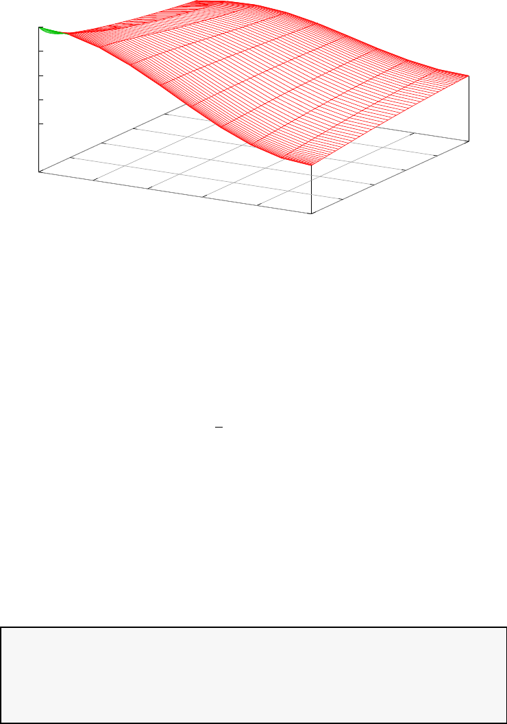
Heat diffusion process
0 0.2 0.4 0.6 0.8 1
z 0
0.1
0.2
0.3
0.4
0.5
t
1
1.5
2
2.5
3
x
Figure 3.40: Optimal temperature distribution for the heat diffusion process
3.17 Hypersensitive problem
Consider the following optimal control problem, which is known in the liter-
ature as the hypesensitive optimal control problem [34]. Minimize the cost
functional
J=1
2Ztf
0
[x2+u2]dt (3.72)
subject to the dynamic constraint
˙x=−x3+u(3.73)
and the boundary conditions
x(0) = 1.5
x(tf)=1 (3.74)
where tf= 50. The PSOPT code that solves this problem is shown below.
//////////////////////////////////////////////////////////////////////////
////////////////// hypersensitive.cxx /////////////////////////
//////////////////////////////////////////////////////////////////////////
//////////////// PSOPT Example ////////////////////
//////////////////////////////////////////////////////////////////////////
//////////////////////////////////////////////////////////////////////////
//////// Title: Hypersensitive problem ////////////////
201

//////// Last modified: 05 January 2009 ////////////////
//////// Reference: Rao and Mease (2000) ////////////////
//////// (See PSOPT handbook for full reference) ////////////////
//////////////////////////////////////////////////////////////////////////
//////// Copyright (c) Victor M. Becerra, 2009 ////////////////
//////////////////////////////////////////////////////////////////////////
//////// This is part of the PSOPT software library, which ///////////////
//////// is distributed under the terms of the GNU Lesser ////////////////
//////// General Public License (LGPL) ////////////////
//////////////////////////////////////////////////////////////////////////
#include "psopt.h"
//////////////////////////////////////////////////////////////////////////
/////////////////// Define the end point (Mayer) cost function //////////
//////////////////////////////////////////////////////////////////////////
adouble endpoint_cost(adouble* initial_states, adouble* final_states,
adouble* parameters,adouble& t0, adouble& tf,
adouble* xad, int iphase, Workspace* workspace)
{
return 0.0;
}
//////////////////////////////////////////////////////////////////////////
/////////////////// Define the integrand (Lagrange) cost function //////
//////////////////////////////////////////////////////////////////////////
adouble integrand_cost(adouble* states, adouble* controls,
adouble* parameters, adouble& time, adouble* xad,
int iphase, Workspace* workspace)
{
adouble x = states[0];
adouble u = controls[0];
adouble L = 0.5*( x*x + u*u );
return L;
}
//////////////////////////////////////////////////////////////////////////
/////////////////// Define the DAE’s ////////////////////////////////////
//////////////////////////////////////////////////////////////////////////
void dae(adouble* derivatives, adouble* path, adouble* states,
adouble* controls, adouble* parameters, adouble& time,
adouble* xad, int iphase, Workspace* workspace)
{
adouble x = states[0];
adouble u = controls[0];
adouble xdot = -pow(x,3) + u;
derivatives[0] = xdot;
}
////////////////////////////////////////////////////////////////////////////
/////////////////// Define the events function ////////////////////////////
////////////////////////////////////////////////////////////////////////////
void events(adouble* e, adouble* initial_states, adouble* final_states,
adouble* parameters,adouble& t0, adouble& tf, adouble* xad,
int iphase, Workspace* workspace)
{
adouble xi = initial_states[0];
adouble xf = final_states[0];
e[0] = xi;
e[1] = xf;
}
///////////////////////////////////////////////////////////////////////////
/////////////////// Define the phase linkages function ///////////////////
///////////////////////////////////////////////////////////////////////////
void linkages( adouble* linkages, adouble* xad, Workspace* workspace)
{
// No linkages as this is a single phase problem
}
202

////////////////////////////////////////////////////////////////////////////
/////////////////// Define the main routine ///////////////////////////////
////////////////////////////////////////////////////////////////////////////
int main(void)
{
////////////////////////////////////////////////////////////////////////////
/////////////////// Declare key structures ////////////////////////////////
////////////////////////////////////////////////////////////////////////////
Alg algorithm;
Sol solution;
Prob problem;
////////////////////////////////////////////////////////////////////////////
/////////////////// Register problem name ////////////////////////////////
////////////////////////////////////////////////////////////////////////////
problem.name = "Hypersensitive problem";
problem.outfilename = "hyper.txt";
////////////////////////////////////////////////////////////////////////////
//////////// Define problem level constants & do level 1 setup ////////////
////////////////////////////////////////////////////////////////////////////
problem.nphases = 1;
problem.nlinkages = 0;
psopt_level1_setup(problem);
/////////////////////////////////////////////////////////////////////////////
///////// Define phase related information & do level 2 setup ////////////
/////////////////////////////////////////////////////////////////////////////
problem.phases(1).nstates = 1;
problem.phases(1).ncontrols = 1;
problem.phases(1).nevents = 2;
problem.phases(1).npath = 0;
problem.phases(1).nodes = "[25, 50]";
psopt_level2_setup(problem, algorithm);
////////////////////////////////////////////////////////////////////////////
/////////////////// Enter problem bounds information //////////////////////
////////////////////////////////////////////////////////////////////////////
double xi = 1.5;
double xf = 1.0;
problem.phases(1).bounds.lower.states(1) = -50.0;
problem.phases(1).bounds.upper.states(1) = 50.0;
problem.phases(1).bounds.lower.controls(1) = -50.0;
problem.phases(1).bounds.upper.controls(1) = 50.0;
problem.phases(1).bounds.lower.events(1) = xi;
problem.phases(1).bounds.upper.events(1) = xi;
problem.phases(1).bounds.lower.events(2) = xf;
problem.phases(1).bounds.upper.events(2) = xf;
problem.phases(1).bounds.lower.StartTime = 0.0;
problem.phases(1).bounds.upper.StartTime = 0.0;
problem.phases(1).bounds.lower.EndTime = 50.0;
problem.phases(1).bounds.upper.EndTime = 50.0;
////////////////////////////////////////////////////////////////////////////
/////////////////// Register problem functions ///////////////////////////
////////////////////////////////////////////////////////////////////////////
problem.integrand_cost = &integrand_cost;
problem.endpoint_cost = &endpoint_cost;
203

problem.dae = &dae;
problem.events = &events;
problem.linkages = &linkages;
////////////////////////////////////////////////////////////////////////////
/////////////////// Define & register initial guess ///////////////////////
////////////////////////////////////////////////////////////////////////////
problem.phases(1).guess.controls = zeros(1,60);
problem.phases(1).guess.states = linspace(1,1,60);
problem.phases(1).guess.time = linspace(0.0,50.0,60);
////////////////////////////////////////////////////////////////////////////
/////////////////// Enter algorithm options //////////////////////////////
////////////////////////////////////////////////////////////////////////////
algorithm.nlp_method = "IPOPT";
algorithm.scaling = "automatic";
algorithm.derivatives = "automatic";
algorithm.nlp_iter_max = 1000;
algorithm.nlp_tolerance = 1.e-6;
// algorithm.ps_method = "none";
// algorithm.refinement_strategy = "TH";
// algorithm.mr_tolerance = 1.e-8;
// algorithm.mr_max_iterations = 8;
////////////////////////////////////////////////////////////////////////////
/////////////////// Now call PSOPT to solve the problem /////////////////
////////////////////////////////////////////////////////////////////////////
psopt(solution, problem, algorithm);
////////////////////////////////////////////////////////////////////////////
/////////// Extract relevant variables from solution structure //////////
////////////////////////////////////////////////////////////////////////////
DMatrix x = solution.get_states_in_phase(1);
DMatrix u = solution.get_controls_in_phase(1);
DMatrix t = solution.get_time_in_phase(1);
////////////////////////////////////////////////////////////////////////////
/////////// Save solution data to files if desired ////////////////////////
////////////////////////////////////////////////////////////////////////////
x.Save("x.dat");
u.Save("u.dat");
t.Save("t.dat");
////////////////////////////////////////////////////////////////////////////
/////////// Plot some results if desired (requires gnuplot) ///////////////
////////////////////////////////////////////////////////////////////////////
plot(t,x,problem.name + ": state", "time (s)", "state", "x");
plot(t,u,problem.name + ": control", "time (s)", "control", "u");
plot(t,x,problem.name + ": state", "time (s)", "state", "x", "pdf", "hyper_state.pdf");
plot(t,u,problem.name + ": control", "time (s)", "control", "u", "pdf", "hyper_control.pdf");
}
////////////////////////////////////////////////////////////////////////////
/////////////////////// END OF FILE ///////////////////////////////
////////////////////////////////////////////////////////////////////////////
204
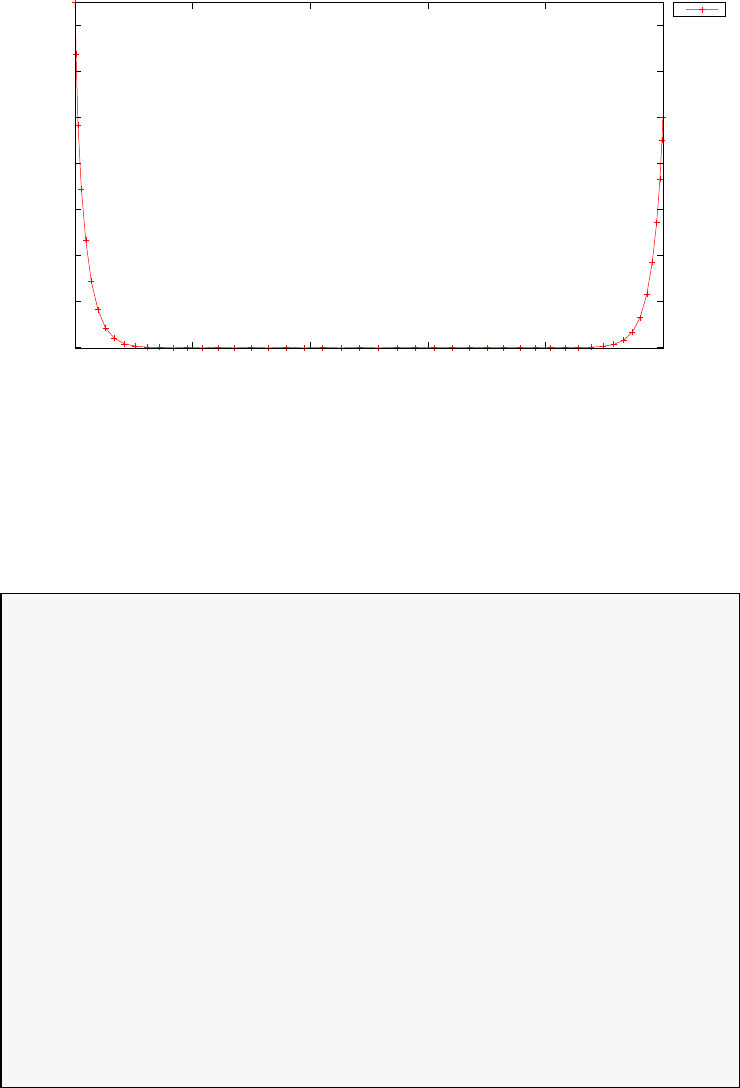
0
0.2
0.4
0.6
0.8
1
1.2
1.4
0 10 20 30 40 50
state
time (s)
Hypersensitive problem: state
x
Figure 3.41: State for hypersensitive problem
The output from PSOPT is summarized the box below and shown in
the following plots that contain the elements of the state and the control,
respectively.
PSOPT results summary
=====================
Problem: Hypersensitive problem
CPU time (seconds): 1.409098e+00
NLP solver used: IPOPT
PSOPT release number: 4.0
Date and time of this run: Thu Feb 21 16:00:11 2019
Optimal (unscaled) cost function value: 1.330826e+00
Phase 1 endpoint cost function value: 0.000000e+00
Phase 1 integrated part of the cost: 1.330826e+00
Phase 1 initial time: 0.000000e+00
Phase 1 final time: 5.000000e+01
Phase 1 maximum relative local error: 5.728533e-04
NLP solver reports: The problem has been solved!
205
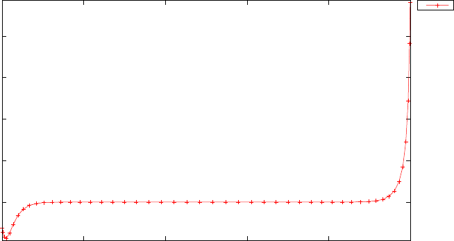
0
0.5
1
1.5
2
0 10 20 30 40 50
control
time (s)
Hypersensitive problem: control
u
Figure 3.42: Control for hypersensitive problem
3.18 Interior point constraint problem
Consider the following optimal control problem, which involves a scalar sys-
tem with an interior point constraint on the state [24]. Minimize the cost
functional
J=Z1
0
[x2+u2]dt (3.75)
subject to the dynamic constraint
˙x=u, (3.76)
the boundary conditions
x(0) = 1,
x(1) = 0.75,(3.77)
and the interior point constraint:
x(0.75) = 0.9.(3.78)
The problem is divided into two phases and the interior point constraint
is accommodated as an event constraint at the end of the first phase. The
PSOPT code that solves this problem is shown below.
206

//////////////////////////////////////////////////////////////////////////
////////////////// interior_point.cxx /////////////////////////
//////////////////////////////////////////////////////////////////////////
//////////////// PSOPT Example ////////////////////
//////////////////////////////////////////////////////////////////////////
//////////////////////////////////////////////////////////////////////////
//////// Title: Problem with interior point constraint ////////////////
//////// Last modified: 05 January 2009 ////////////////
//////// Reference: Miser Manual ////////////////
//////// (See PSOPT handbook for full reference) ////////////////
//////////////////////////////////////////////////////////////////////////
//////// Copyright (c) Victor M. Becerra, 2009 ////////////////
//////////////////////////////////////////////////////////////////////////
//////// This is part of the PSOPT software library, which ///////////////
//////// is distributed under the terms of the GNU Lesser ///////////////
//////// General Public License (LGPL) ///////////////
//////////////////////////////////////////////////////////////////////////
#include "psopt.h"
//////////////////////////////////////////////////////////////////////////
/////////////////// Define the end point (Mayer) cost function //////////
//////////////////////////////////////////////////////////////////////////
adouble endpoint_cost(adouble* initial_states, adouble* final_states,
adouble* parameters,adouble& t0, adouble& tf,
adouble* xad, int iphase, Workspace* workspace)
{
return 0.0;
}
//////////////////////////////////////////////////////////////////////////
/////////////////// Define the integrand (Lagrange) cost function ////////
//////////////////////////////////////////////////////////////////////////
adouble integrand_cost(adouble* states, adouble* controls, adouble* parameters,
adouble& time, adouble* xad, int iphase, Workspace* workspace)
{
adouble x = states[0];
adouble u = controls[0];
adouble L = x*x + u*u;
return L;
}
//////////////////////////////////////////////////////////////////////////
/////////////////// Define the DAE’s ////////////////////////////////////
//////////////////////////////////////////////////////////////////////////
void dae(adouble* derivatives, adouble* path, adouble* states,
adouble* controls, adouble* parameters, adouble& time,
adouble* xad, int iphase, Workspace* workspace)
{
adouble x = states[0];
adouble u = controls[0];
adouble xdot = u;
derivatives[0] = xdot;
}
////////////////////////////////////////////////////////////////////////////
/////////////////// Define the events function ////////////////////////////
////////////////////////////////////////////////////////////////////////////
void events(adouble* e, adouble* initial_states, adouble* final_states,
adouble* parameters,adouble& t0, adouble& tf, adouble* xad,
int iphase, Workspace* workspace)
{
adouble xi = initial_states[0];
adouble xf = final_states[0];
adouble x075;
if (iphase == 1) {
xi = initial_states[0];
x075 = final_states[0];
e[0] = xi;
e[1] = x075;
}
207

if (iphase == 2) {
xf = final_states[0];
e[0] = xf;
}
}
///////////////////////////////////////////////////////////////////////////
/////////////////// Define the phase linkages function ///////////////////
///////////////////////////////////////////////////////////////////////////
void linkages( adouble* linkages, adouble* xad, Workspace* workspace)
{
int index = 0;
auto_link(linkages, &index, xad, 1, 2, workspace );
}
////////////////////////////////////////////////////////////////////////////
/////////////////// Define the main routine ///////////////////////////////
////////////////////////////////////////////////////////////////////////////
int main(void)
{
////////////////////////////////////////////////////////////////////////////
/////////////////// Declare key structures ////////////////////////////////
////////////////////////////////////////////////////////////////////////////
Alg algorithm;
Sol solution;
Prob problem;
////////////////////////////////////////////////////////////////////////////
/////////////////// Register problem name ////////////////////////////////
////////////////////////////////////////////////////////////////////////////
problem.name = "Problem with interior point constraint";
problem.outfilename = "ipc.txt";
////////////////////////////////////////////////////////////////////////////
//////////// Define problem level constants & do level 1 setup ////////////
////////////////////////////////////////////////////////////////////////////
problem.nphases = 2;
problem.nlinkages = 2;
psopt_level1_setup(problem);
/////////////////////////////////////////////////////////////////////////////
///////// Define phase related information & do level 2 setup ////////////
/////////////////////////////////////////////////////////////////////////////
problem.phases(1).nstates = 1;
problem.phases(1).ncontrols = 1;
problem.phases(1).nevents = 2;
problem.phases(1).npath = 0;
problem.phases(1).nodes = 20;
problem.phases(2).nstates = 1;
problem.phases(2).ncontrols = 1;
problem.phases(2).nevents = 1;
problem.phases(2).npath = 0;
problem.phases(2).nodes = 20;
psopt_level2_setup(problem, algorithm);
////////////////////////////////////////////////////////////////////////////
/////////////////// Enter problem bounds information //////////////////////
////////////////////////////////////////////////////////////////////////////
double xi = 1;
double x075 = 0.9;
double xf = 0.75;
///////////// Phase 1 bounds ///////////////////
problem.phases(1).bounds.lower.states(1) = -1.0;
208

problem.phases(1).bounds.upper.states(1) = 1.0;
problem.phases(1).bounds.lower.controls(1) = -1.0;
problem.phases(1).bounds.upper.controls(1) = 1.0;
problem.phases(1).bounds.lower.events(1) = xi;
problem.phases(1).bounds.upper.events(1) = xi;
problem.phases(1).bounds.lower.events(2) = x075;
problem.phases(1).bounds.upper.events(2) = x075;
problem.phases(1).bounds.lower.StartTime = 0.0;
problem.phases(1).bounds.upper.StartTime = 0.0;
problem.phases(1).bounds.lower.EndTime = 0.75;
problem.phases(1).bounds.upper.EndTime = 0.75;
/////////////// Phase 2 bounds /////////////////
problem.phases(2).bounds.lower.states(1) = -1.0;
problem.phases(2).bounds.upper.states(1) = 1.0;
problem.phases(2).bounds.lower.controls(1) = -1.0;
problem.phases(2).bounds.upper.controls(1) = 1.0;
problem.phases(2).bounds.lower.events(1) = xf;
problem.phases(2).bounds.upper.events(1) = xf;
problem.phases(2).bounds.lower.StartTime = 0.75;
problem.phases(2).bounds.upper.StartTime = 0.75;
problem.phases(2).bounds.lower.EndTime = 1.0;
problem.phases(2).bounds.upper.EndTime = 1.0;
////////////////////////////////////////////////////////////////////////////
/////////////////// Register problem functions ///////////////////////////
////////////////////////////////////////////////////////////////////////////
problem.integrand_cost = &integrand_cost;
problem.endpoint_cost = &endpoint_cost;
problem.dae = &dae;
problem.events = &events;
problem.linkages = &linkages;
////////////////////////////////////////////////////////////////////////////
/////////////////// Define & register initial guess ///////////////////////
////////////////////////////////////////////////////////////////////////////
/////////////// Phase 1 initial guess /////////////////////////
problem.phases(1).guess.controls = zeros(1,20);
problem.phases(1).guess.states = linspace(xi,x075, 20);
problem.phases(1).guess.time = linspace(0.0, 0.75 , 20);
/////////////// Phase 2 initial guess //////////////////////////
problem.phases(2).guess.controls = zeros(1,20);
problem.phases(2).guess.states = linspace(x075,xf, 20);
problem.phases(2).guess.time = linspace(0.75, 1.0 , 20);
////////////////////////////////////////////////////////////////////////////
/////////////////// Enter algorithm options //////////////////////////////
////////////////////////////////////////////////////////////////////////////
algorithm.nlp_method = "IPOPT";
algorithm.scaling = "automatic";
algorithm.derivatives = "automatic";
algorithm.nlp_iter_max = 1000;
algorithm.nlp_tolerance = 1.e-6;
////////////////////////////////////////////////////////////////////////////
/////////////////// Now call PSOPT to solve the problem //////////////////
////////////////////////////////////////////////////////////////////////////
209

psopt(solution, problem, algorithm);
////////////////////////////////////////////////////////////////////////////
/////////// Extract relevant variables from solution structure //////////
////////////////////////////////////////////////////////////////////////////
DMatrix x, u, t;
x=solution.get_states_in_phase(1) || solution.get_states_in_phase(2);
u=solution.get_controls_in_phase(1)|| solution.get_controls_in_phase(2);
t=solution.get_time_in_phase(1) || solution.get_time_in_phase(2);
////////////////////////////////////////////////////////////////////////////
/////////// Save solution data to files if desired ////////////////////////
////////////////////////////////////////////////////////////////////////////
x.Save("x.dat");
u.Save("u.dat");
t.Save("t.dat");
////////////////////////////////////////////////////////////////////////////
/////////// Plot some results if desired (requires gnuplot) ///////////////
////////////////////////////////////////////////////////////////////////////
plot(t,x,problem.name + ": state", "time (s)", "state", "x");
plot(t,u,problem.name + ": control", "time (s)", "control", "u");
plot(t,x,problem.name + ": state", "time (s)", "state", "x",
"pdf", "ipc_state.pdf");
plot(t,u,problem.name + ": control", "time (s)", "control", "u", "pdf",
"ipc_control.pdf");
}
////////////////////////////////////////////////////////////////////////////
/////////////////////// END OF FILE ///////////////////////////////
////////////////////////////////////////////////////////////////////////////
The output from PSOPT is summarized the box below and shown in
the following plots that contain the elements of the state and the control,
respectively.
PSOPT results summary
=====================
Problem: Problem with interior point constraint
CPU time (seconds): 8.136300e-01
NLP solver used: IPOPT
PSOPT release number: 4.0
Date and time of this run: Thu Feb 21 16:08:24 2019
Optimal (unscaled) cost function value: 9.205314e-01
Phase 1 endpoint cost function value: 0.000000e+00
Phase 1 integrated part of the cost: 6.607877e-01
Phase 1 initial time: 0.000000e+00
Phase 1 final time: 7.500000e-01
210
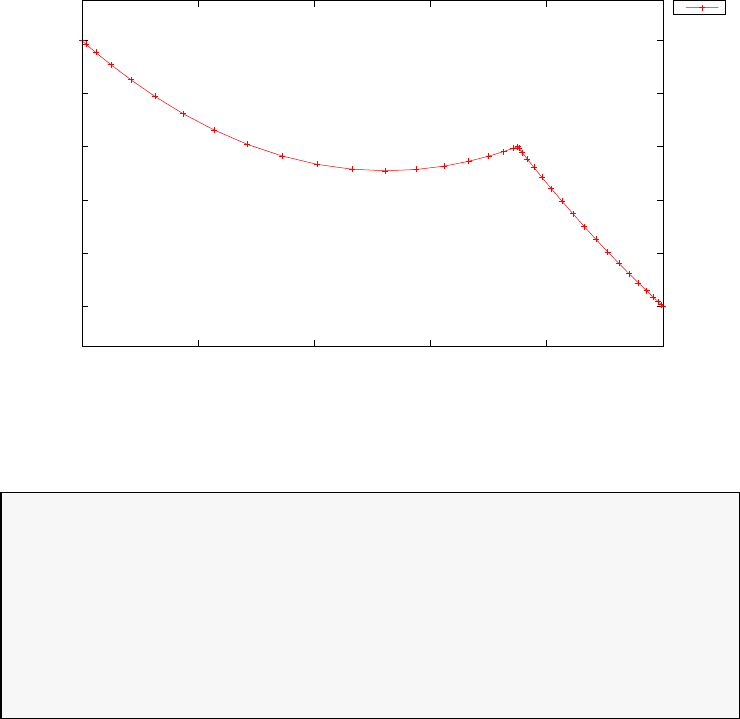
0.75
0.8
0.85
0.9
0.95
1
0 0.2 0.4 0.6 0.8 1
state
time (s)
Problem with interior point constraint: state
x
Figure 3.43: State for interior point constraint problem
Phase 1 maximum relative local error: 2.352899e-08
Phase 2 endpoint cost function value: 0.000000e+00
Phase 2 integrated part of the cost: 2.597438e-01
Phase 2 initial time: 7.500000e-01
Phase 2 final time: 1.000000e+00
Phase 2 maximum relative local error: 6.986779e-09
NLP solver reports: The problem has been solved!
3.19 Isoperimetric constraint problem
Consider the following optimal control problem, which includes an integral
constraint. Minimize the cost functional
J=Ztf
0
x2(t)dt (3.79)
subject to the dynamic constraint
˙x=−sin(x) + u(3.80)
the integral constraint:
Ztf
0
u2(t)dt = 10 (3.81)
211
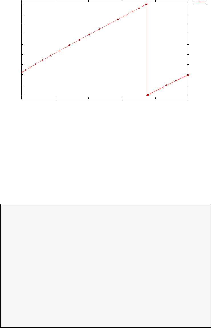
-0.7
-0.6
-0.5
-0.4
-0.3
-0.2
-0.1
0
0.1
0.2
0 0.2 0.4 0.6 0.8 1
control
time (s)
Problem with interior point constraint: control
u
Figure 3.44: Control for interior point constraint problem
the boundary conditions
x(0) = 1
x(tf)=0 (3.82)
and the bounds: −4≤u(t)≤4
−10 ≤x(t)≤10 (3.83)
where tf= 1. The PSOPT code that solves this problem is shown below.
//////////////////////////////////////////////////////////////////////////
////////////////// isoperimetric.cxx ///////////////////////
//////////////////////////////////////////////////////////////////////////
//////////////// PSOPT Example ////////////////////
//////////////////////////////////////////////////////////////////////////
//////////////////////////////////////////////////////////////////////////
//////// Title: Isoperimetric problem ////////////////
//////// Last modified: 29 January 2009 ////////////////
//////// Reference: ////////////////
//////// ////////////////
//////////////////////////////////////////////////////////////////////////
//////// Copyright (c) Victor M. Becerra, 2009 ////////////////
//////////////////////////////////////////////////////////////////////////
//////// This is part of the PSOPT software library, which ///////////////
//////// is distributed under the terms of the GNU Lesser ////////////////
//////// General Public License (LGPL) ////////////////
//////////////////////////////////////////////////////////////////////////
#include "psopt.h"
//////////////////////////////////////////////////////////////////////////
/////////////////// Define the end point (Mayer) cost function //////////
//////////////////////////////////////////////////////////////////////////
adouble endpoint_cost(adouble* initial_states, adouble* final_states,
adouble* parameters,adouble& t0, adouble& tf,
adouble* xad, int iphase, Workspace* workspace)
{
212

return 0.0;
}
//////////////////////////////////////////////////////////////////////////
/////////////////// Define the integrand (Lagrange) cost function //////
//////////////////////////////////////////////////////////////////////////
adouble integrand_cost(adouble* states, adouble* controls,
adouble* parameters, adouble& time, adouble* xad,
int iphase, Workspace* workspace)
{
adouble x = states[0];
adouble L = x;
return L;
}
//////////////////////////////////////////////////////////////////////////
/////////////////// Define the DAE’s ////////////////////////////////////
//////////////////////////////////////////////////////////////////////////
void dae(adouble* derivatives, adouble* path, adouble* states,
adouble* controls, adouble* parameters, adouble& time,
adouble* xad, int iphase, Workspace* workspace)
{
adouble xdot, ydot, vdot;
adouble x = states[ CINDEX(1) ];
adouble u = controls[ CINDEX(1) ];
derivatives[0] = -sin(x) + u;
}
////////////////////////////////////////////////////////////////////////////
/////////////////// Define the integrand of the integral constraint ///////
////////////////////////////////////////////////////////////////////////////
adouble integrand( adouble* states, adouble* controls, adouble* parameters,
adouble& time, adouble* xad, int iphase, Workspace* workspace)
{
adouble g;
adouble u = controls[ CINDEX(1) ];
g = u*u ;
return g;
}
////////////////////////////////////////////////////////////////////////////
/////////////////// Define the events function ////////////////////////////
////////////////////////////////////////////////////////////////////////////
void events(adouble* e, adouble* initial_states, adouble* final_states,
adouble* parameters,adouble& t0, adouble& tf, adouble* xad,
int iphase, Workspace* workspace)
{
adouble x0 = initial_states[ CINDEX(1) ];
adouble xf = final_states[ CINDEX(1) ];
adouble Q;
// Compute the integral to be constrained
Q = integrate( integrand, xad, iphase, workspace );
e[ CINDEX(1) ] = x0;
e[ CINDEX(2) ] = xf;
e[ CINDEX(3) ] = Q;
}
///////////////////////////////////////////////////////////////////////////
/////////////////// Define the phase linkages function ///////////////////
///////////////////////////////////////////////////////////////////////////
void linkages( adouble* linkages, adouble* xad, Workspace* workspace)
{
213

// No linkages as this is a single phase problem
}
////////////////////////////////////////////////////////////////////////////
/////////////////// Define the main routine ///////////////////////////////
////////////////////////////////////////////////////////////////////////////
int main(void)
{
////////////////////////////////////////////////////////////////////////////
/////////////////// Declare key structures ////////////////////////////////
////////////////////////////////////////////////////////////////////////////
Alg algorithm;
Sol solution;
Prob problem;
////////////////////////////////////////////////////////////////////////////
/////////////////// Register problem name ////////////////////////////////
////////////////////////////////////////////////////////////////////////////
problem.name = "Isoperimetric constraint problem";
problem.outfilename = "isoperimetric.txt";
////////////////////////////////////////////////////////////////////////////
//////////// Define problem level constants & do level 1 setup ////////////
////////////////////////////////////////////////////////////////////////////
problem.nphases = 1;
problem.nlinkages = 0;
psopt_level1_setup(problem);
/////////////////////////////////////////////////////////////////////////////
///////// Define phase related information & do level 2 setup /////////////
/////////////////////////////////////////////////////////////////////////////
problem.phases(1).nstates = 1;
problem.phases(1).ncontrols = 1;
problem.phases(1).nevents = 3;
problem.phases(1).npath = 0;
problem.phases(1).nodes = 50;
psopt_level2_setup(problem, algorithm);
////////////////////////////////////////////////////////////////////////////
/////////////////// Enter problem bounds information //////////////////////
////////////////////////////////////////////////////////////////////////////
problem.phases(1).bounds.lower.states(1) = -10;
problem.phases(1).bounds.upper.states(1) = 10;
problem.phases(1).bounds.lower.controls(1) = -4.0;
problem.phases(1).bounds.upper.controls(1) = 4.0;
problem.phases(1).bounds.lower.events(1) = 1.0;
problem.phases(1).bounds.lower.events(2) = 0.0;
problem.phases(1).bounds.lower.events(3) = 10.0;
problem.phases(1).bounds.upper.events(1) = 1.0;
problem.phases(1).bounds.upper.events(2) = 0.0;
problem.phases(1).bounds.upper.events(3) = 10.0;
problem.phases(1).bounds.lower.StartTime = 0.0;
problem.phases(1).bounds.upper.StartTime = 0.0;
problem.phases(1).bounds.lower.EndTime = 1.0;
problem.phases(1).bounds.upper.EndTime = 1.0;
////////////////////////////////////////////////////////////////////////////
/////////////////// Register problem functions ///////////////////////////
////////////////////////////////////////////////////////////////////////////
214

problem.integrand_cost = &integrand_cost;
problem.endpoint_cost = &endpoint_cost;
problem.dae = &dae;
problem.events = &events;
problem.linkages = &linkages;
////////////////////////////////////////////////////////////////////////////
/////////////////// Define & register initial guess ///////////////////////
////////////////////////////////////////////////////////////////////////////
problem.phases(1).guess.controls = zeros(1,30);
problem.phases(1).guess.states = zeros(1,30);
problem.phases(1).guess.time = linspace(0.0,1.0,30);
////////////////////////////////////////////////////////////////////////////
/////////////////// Enter algorithm options //////////////////////////////
////////////////////////////////////////////////////////////////////////////
algorithm.nlp_method = "IPOPT";
algorithm.scaling = "automatic";
algorithm.derivatives = "automatic";
algorithm.nlp_iter_max = 1000;
algorithm.nlp_tolerance = 1.e-6;
////////////////////////////////////////////////////////////////////////////
/////////////////// Now call PSOPT to solve the problem /////////////////
////////////////////////////////////////////////////////////////////////////
psopt(solution, problem, algorithm);
if (solution.error_flag) exit(0);
////////////////////////////////////////////////////////////////////////////
/////////// Extract relevant variables from solution structure //////////
////////////////////////////////////////////////////////////////////////////
DMatrix x, u, t;
x = solution.get_states_in_phase(1);
u = solution.get_controls_in_phase(1);
t = solution.get_time_in_phase(1);
////////////////////////////////////////////////////////////////////////////
/////////// Save solution data to files if desired ////////////////////////
////////////////////////////////////////////////////////////////////////////
x.Save("x.dat");
u.Save("u.dat");
t.Save("t.dat");
////////////////////////////////////////////////////////////////////////////
/////////// Plot some results if desired (requires gnuplot) ///////////////
////////////////////////////////////////////////////////////////////////////
plot(t,x,problem.name + ": state", "time (s)", "x", "x");
plot(t,u,problem.name + ": control", "time (s)", "u", "u");
plot(t,x,problem.name + ": state", "time (s)", "x", "x",
"pdf", "isop_state.pdf");
plot(t,u,problem.name + ": control", "time (s)", "u", "u",
"pdf", "isop_control.pdf");
}
////////////////////////////////////////////////////////////////////////////
/////////////////////// END OF FILE ///////////////////////////////
////////////////////////////////////////////////////////////////////////////
The output from PSOPT is summarized in the text box below and in
Figures 3.45 and 3.46, which show the optimal state and control, respec-
215
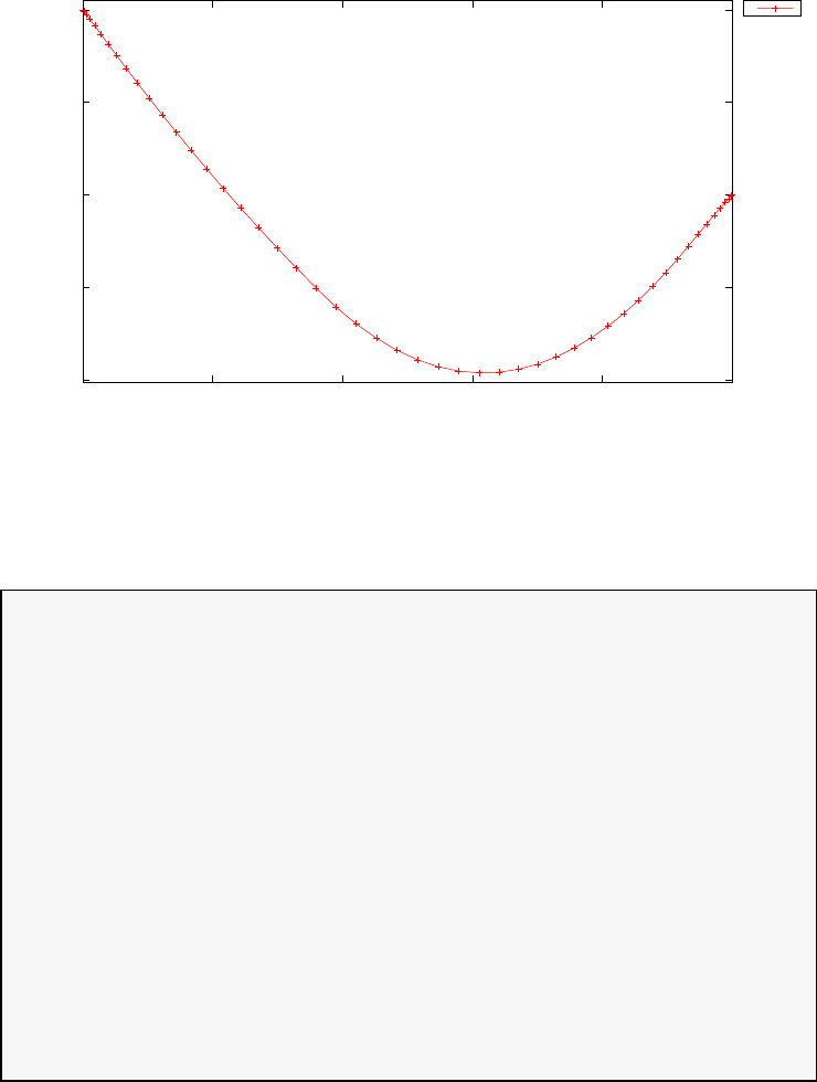
-1
-0.5
0
0.5
1
0 0.2 0.4 0.6 0.8 1
x
time (s)
Isoperimetric constraint problem: state
x
Figure 3.45: State for isoperimetric constraint problem
tively.
PSOPT results summary
=====================
Problem: Isoperimetric constraint problem
CPU time (seconds): 1.388097e+00
NLP solver used: IPOPT
PSOPT release number: 4.0
Date and time of this run: Thu Feb 21 17:16:14 2019
Optimal (unscaled) cost function value: -3.755058e-01
Phase 1 endpoint cost function value: 0.000000e+00
Phase 1 integrated part of the cost: -3.755058e-01
Phase 1 initial time: 0.000000e+00
Phase 1 final time: 1.000000e+00
Phase 1 maximum relative local error: 3.106352e-05
NLP solver reports: The problem has been solved!
3.20 Lambert’s problem
This example demonstrates the use of the PSOPT for a classical orbit deter-
mination problem, namely the determination of an orbit from two position
216
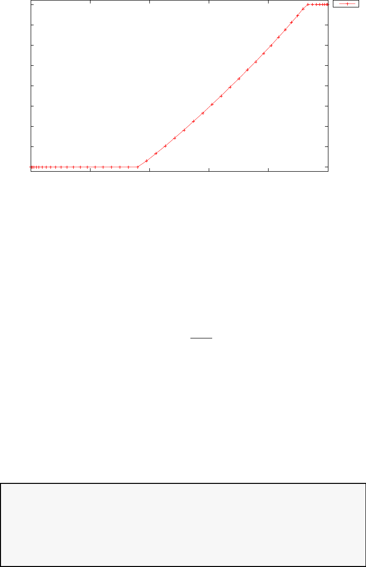
-4
-3
-2
-1
0
1
2
3
4
0 0.2 0.4 0.6 0.8 1
u
time (s)
Isoperimetric constraint problem: control
u
Figure 3.46: Control for isoperimetric constraint problem
vectors and time (Lambert’s problem) [42]. The problem is formulated as
follows. Find r(t)∈[0, tf] and v(t)∈[0, tf] to minimise:
J= 0 (3.84)
subject to
˙
r=v
˙
v=−µr
||r||3
(3.85)
with the boundary conditions:
r(0) = [15945.34E3,0.0,0.0]T
r(tf) = [12214.83899E3,10249.46731E3,0.0]T(3.86)
where r= [x, y, z]T(m) is a cartesian position vector, and v= [vx, vz, vz]Tis
the corresponding velocity vector, µ=GMe,G(m3/(kg s2)) is the universal
gravitational constant and Me(kg) is the mass of Earth.
The PSOPT code that solves this problem is shown below.
//////////////////////////////////////////////////////////////////////////
//////////////// lambert.cxx /////////////////////
//////////////////////////////////////////////////////////////////////////
//////////////// PSOPT Example /////////////////////
//////////////////////////////////////////////////////////////////////////
////////////////////////////////////////////////////////////////////////
//////// Title: Lambert problem ////////////////
//////// Last modified: 27 December 2009 ////////////////
//////// Reference: Vallado (2001), page 470 ////////////////
217

//////// (See PSOPT handbook for full reference) ////////////////
//////////////////////////////////////////////////////////////////////////
//////// Copyright (c) Victor M. Becerra, 2009 ////////////////
//////////////////////////////////////////////////////////////////////////
//////// This is part of the PSOPT software library, which ////////////////
//////// is distributed under the terms of the GNU Lesser ////////////////
//////// General Public License (LGPL) ////////////////
//////////////////////////////////////////////////////////////////////////
#include "psopt.h"
//////////////////////////////////////////////////////////////////////////
/////////////////// Define the end point (Mayer) cost function //////////
//////////////////////////////////////////////////////////////////////////
adouble endpoint_cost(adouble* initial_states, adouble* final_states,
adouble* parameters,adouble& t0, adouble& tf,
adouble* xad, int iphase, Workspace* workspace)
{
return 0.0;
}
//////////////////////////////////////////////////////////////////////////
/////////////////// Define the integrand (Lagrange) cost function //////
//////////////////////////////////////////////////////////////////////////
adouble integrand_cost(adouble* states, adouble* controls, adouble* parameters,
adouble& time, adouble* xad, int iphase, Workspace* workspace)
{
return 0.0;
}
//////////////////////////////////////////////////////////////////////////
/////////////////// Define the DAE’s ////////////////////////////////////
//////////////////////////////////////////////////////////////////////////
void dae(adouble* derivatives, adouble* path, adouble* states,
adouble* controls, adouble* parameters, adouble& time,
adouble* xad, int iphase, Workspace* workspace)
{
// Define constants:
double G = 6.6720e-11; // Universal gravity constant [m^3/(kg s^2)]
double Me = 5.9742e24; // Mass of earth;[kg]
double mu = G*Me; // [m^3/sec^2]
ADMatrix r(3), v(3);
// Extract individual variables
r(1) = states[ CINDEX(1) ];
r(2) = states[ CINDEX(2) ];
r(3) = states[ CINDEX(3) ];
v(1) = states[ CINDEX(4) ];
v(2) = states[ CINDEX(5) ];
v(3) = states[ CINDEX(6) ];
ADMatrix rdd(3);
adouble rr = sqrt( r(1)*r(1)+r(2)*r(2)+r(3)*r(3) );
adouble r3 = pow(rr,3.0);
rdd(1) = -mu*r(1)/r3;
rdd(2) = -mu*r(2)/r3;
rdd(3) = -mu*r(3)/r3;
derivatives[ CINDEX(1) ] = v(1);
derivatives[ CINDEX(2) ] = v(2);
derivatives[ CINDEX(3) ] = v(3);
derivatives[ CINDEX(4) ] = rdd(1);
derivatives[ CINDEX(5) ] = rdd(2);
derivatives[ CINDEX(6) ] = rdd(3);
}
////////////////////////////////////////////////////////////////////////////
218

/////////////////// Define the events function ////////////////////////////
////////////////////////////////////////////////////////////////////////////
void events(adouble* e, adouble* initial_states, adouble* final_states,
adouble* parameters,adouble& t0, adouble& tf, adouble* xad,
int iphase, Workspace* workspace)
{
adouble ri1 = initial_states[ CINDEX(1) ];
adouble ri2 = initial_states[ CINDEX(2) ];
adouble ri3 = initial_states[ CINDEX(3) ];
adouble rf1 = final_states[ CINDEX(1) ];
adouble rf2 = final_states[ CINDEX(2) ];
adouble rf3 = final_states[ CINDEX(3) ];
e[ CINDEX(1) ] = ri1;
e[ CINDEX(2) ] = ri2;
e[ CINDEX(3) ] = ri3;
e[ CINDEX(4) ] = rf1;
e[ CINDEX(5) ] = rf2;
e[ CINDEX(6) ] = rf3;
}
///////////////////////////////////////////////////////////////////////////
/////////////////// Define the phase linkages function ///////////////////
///////////////////////////////////////////////////////////////////////////
void linkages( adouble* linkages, adouble* xad, Workspace* workspace)
{
// auto_link_multiple(linkages, xad, N_PHASES);
}
////////////////////////////////////////////////////////////////////////////
/////////////////// Define the main routine ///////////////////////////////
////////////////////////////////////////////////////////////////////////////
int main(void)
{
////////////////////////////////////////////////////////////////////////////
/////////////////// Declare key structures ////////////////////////////////
////////////////////////////////////////////////////////////////////////////
Alg algorithm;
Sol solution;
Prob problem;
MSdata msdata;
////////////////////////////////////////////////////////////////////////////
/////////////////// Register problem name ////////////////////////////////
////////////////////////////////////////////////////////////////////////////
problem.name = "Lambert problem";
problem.outfilename = "lambert.txt";
////////////////////////////////////////////////////////////////////////////
//////////// Define problem level constants & do level 1 setup ////////////
////////////////////////////////////////////////////////////////////////////
problem.nphases = 1;
problem.nlinkages = 0;
psopt_level1_setup(problem);
/////////////////////////////////////////////////////////////////////////////
///////// Define phase related information & do level 2 setup ////////////
/////////////////////////////////////////////////////////////////////////////
problem.phases(1).nstates = 6;
problem.phases(1).ncontrols = 0;
219

problem.phases(1).nevents = 6;
problem.phases(1).nparameters = 6;
problem.phases(1).npath = 0;
problem.phases(1).nodes = "[100]";
psopt_level2_setup(problem, algorithm);
////////////////////////////////////////////////////////////////////////////
/////////////////// Enter problem bounds information //////////////////////
////////////////////////////////////////////////////////////////////////////
double r1i = 15945.34e3; // m
double r2i = 0.0;
double r3i = 0.0;
double r1f = 12214.83899e3; //m
double r2f = 10249.46731e3; //m
double r3f = 0.0;
double TF = 76.0*60.0; // seconds
problem.phases(1).bounds.lower.states(1) = -10*max(r1i,r1f);
problem.phases(1).bounds.lower.states(2) = -10*max(r2i,r2f);
problem.phases(1).bounds.lower.states(3) = -10*max(r3i,r3f);
problem.phases(1).bounds.upper.states(1) = 10*max(r1i,r1f);
problem.phases(1).bounds.upper.states(2) = 10*max(r2i,r2f);
problem.phases(1).bounds.upper.states(3) = 10*max(r3i,r3f);
problem.phases(1).bounds.lower.states(4) = -10*max(r1i,r1f)/TF;
problem.phases(1).bounds.lower.states(5) = -10*max(r1i,r1f)/TF;;
problem.phases(1).bounds.lower.states(6) = -10*max(r1i,r1f)/TF;;
problem.phases(1).bounds.upper.states(4) = 10*max(r1i,r1f)/TF;
problem.phases(1).bounds.upper.states(5) = 10*max(r2i,r2f)/TF;
problem.phases(1).bounds.upper.states(6) = 10*max(r3i,r3f)/TF;
problem.phases(1).bounds.lower.events(1) = r1i;
problem.phases(1).bounds.upper.events(1) = r1i;
problem.phases(1).bounds.lower.events(2) = r2i;
problem.phases(1).bounds.upper.events(2) = r2i;
problem.phases(1).bounds.lower.events(3) = r3i;
problem.phases(1).bounds.upper.events(3) = r3i;
problem.phases(1).bounds.lower.events(4) = r1f;
problem.phases(1).bounds.upper.events(4) = r1f;
problem.phases(1).bounds.lower.events(5) = r2f;
problem.phases(1).bounds.upper.events(5) = r2f;
problem.phases(1).bounds.lower.events(6) = r3f;
problem.phases(1).bounds.upper.events(6) = r3f;
problem.phases(1).bounds.lower.StartTime = 0.0;
problem.phases(1).bounds.upper.StartTime = 0.0;
problem.phases(1).bounds.lower.EndTime = TF;
problem.phases(1).bounds.upper.EndTime = TF;
////////////////////////////////////////////////////////////////////////////
/////////////////// Enter problem names and units //////////////////////
////////////////////////////////////////////////////////////////////////////
problem.phases(1).name.states(1) = "x position";
problem.phases(1).name.states(2) = "y position";
problem.phases(1).name.states(3) = "z position";
problem.phases(1).name.states(4) = "x velocity";
problem.phases(1).name.states(5) = "y velocity";
problem.phases(1).name.states(6) = "z velocity";
problem.phases(1).units.states(1) = "m";
problem.phases(1).units.states(2) = "m";
problem.phases(1).units.states(3) = "m";
problem.phases(1).units.states(4) = "m";
problem.phases(1).units.states(5) = "m/s";
problem.phases(1).units.states(6) = "m/s";
220

////////////////////////////////////////////////////////////////////////////
/////////////////// Register problem functions ///////////////////////////
////////////////////////////////////////////////////////////////////////////
problem.integrand_cost = &integrand_cost;
problem.endpoint_cost = &endpoint_cost;
problem.dae = &dae;
problem.events = &events;
problem.linkages = &linkages;
////////////////////////////////////////////////////////////////////////////
/////////////////// Define & register initial guess ///////////////////////
////////////////////////////////////////////////////////////////////////////
int nnodes = 20;
int ncontrols = problem.phases(1).ncontrols;
int nstates = problem.phases(1).nstates;
DMatrix x_guess = zeros(nstates,nnodes);
DMatrix time_guess = linspace(0.0,TF,nnodes);
x_guess(1,colon()) = linspace(r1i,r1f, nnodes);
x_guess(2,colon()) = linspace(r2i,r2f,nnodes);
x_guess(3,colon()) = linspace(r3i,r3f,nnodes);
x_guess(4,colon()) = linspace(r1i,r1f,nnodes)/TF;
x_guess(5,colon()) = linspace(r2i,r2f,nnodes)/TF;
x_guess(6,colon()) = linspace(r3i,r3f, nnodes)/TF;
problem.phases(1).guess.states = x_guess;
problem.phases(1).guess.time = time_guess;
////////////////////////////////////////////////////////////////////////////
/////////////////// Enter algorithm options //////////////////////////////
////////////////////////////////////////////////////////////////////////////
algorithm.nlp_iter_max = 1000;
algorithm.nlp_tolerance = 1.e-6;
algorithm.nlp_method = "IPOPT";
algorithm.scaling = "automatic";
algorithm.derivatives = "automatic";
algorithm.defect_scaling = "jacobian-based";
algorithm.collocation_method = "Hermite-Simpson";
////////////////////////////////////////////////////////////////////////////
/////////////////// Now call PSOPT to solve the problem //////////////////
////////////////////////////////////////////////////////////////////////////
psopt(solution, problem, algorithm);
////////////////////////////////////////////////////////////////////////////
/////////// Extract relevant variables from solution structure //////////
////////////////////////////////////////////////////////////////////////////
DMatrix x, u, t, xi, ui, ti;
x = solution.get_states_in_phase(1);
u = solution.get_controls_in_phase(1);
t = solution.get_time_in_phase(1);
////////////////////////////////////////////////////////////////////////////
/////////// Save solution data to files if desired ////////////////////////
////////////////////////////////////////////////////////////////////////////
x.Save("x.dat");
u.Save("u.dat");
t.Save("t.dat");
////////////////////////////////////////////////////////////////////////////
221

/////////// Plot some results if desired (requires gnuplot) ///////////////
////////////////////////////////////////////////////////////////////////////
DMatrix r1 = x(1,colon());
DMatrix r2 = x(2,colon());
DMatrix r3 = x(3,colon());
DMatrix v1 = x(4,colon());
DMatrix v2 = x(5,colon());
DMatrix v3 = x(6,colon());
DMatrix vi(3), vf(3);
vi(1) = v1(1);
vi(2) = v2(1);
vi(3) = v3(1);
vf(1) = v1("end");
vf(2) = v2("end");
vf(3) = v3("end");
vi.Print("Initial velocity vector [m/s]");
vf.Print("Final velocity vector [m/s]");
plot(t,r1,problem.name+": x", "time (s)", "x","x");
plot(t,r2,problem.name+": y", "time (s)", "x","y");
plot(t,r3,problem.name+": z", "time (s)", "z","z");
plot(r1,r2,problem.name+": x-y", "x (m)", "y (m)","y");
plot(r1,r2,problem.name+": x-y trajectory", "x (m)", "y (m)","y", "pdf", "lambert_xy.pdf");
plot3(r1,r2,r3,problem.name+": trajectory","x (m)", "y (m)", "z (m)");
}
////////////////////////////////////////////////////////////////////////////
/////////////////////// END OF FILE ///////////////////////////////
////////////////////////////////////////////////////////////////////////////
The output from PSOPT is summarized in the text box below and in
Figure 3.47, which show the trajectory from r(0) to r(tf), respectively.
PSOPT results summary
=====================
Problem: Lambert problem
CPU time (seconds): 2.985497e+00
NLP solver used: IPOPT
PSOPT release number: 4.0
Date and time of this run: Thu Feb 21 15:53:56 2019
Optimal (unscaled) cost function value: 0.000000e+00
Phase 1 endpoint cost function value: 0.000000e+00
Phase 1 integrated part of the cost: 0.000000e+00
Phase 1 initial time: 0.000000e+00
Phase 1 final time: 4.560000e+03
Phase 1 maximum relative local error: 3.440783e-05
NLP solver reports: The problem has been solved!
222
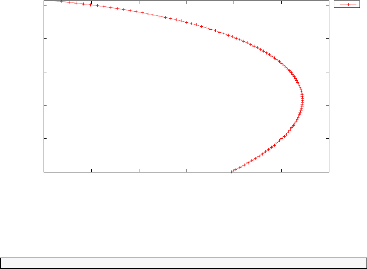
0
2e+06
4e+06
6e+06
8e+06
1e+07
1.2e+07 1.3e+07 1.4e+07 1.5e+07 1.6e+07 1.7e+07 1.8e+07
y (m)
x (m)
Lambert problem: x-y trajectory
y
Figure 3.47: Trajectory between the initial and final positions for Lambert’s
problem
The resulting initial and final velocity vectors are:
v(0) = [2058.902605,2915.961924,−6.878790137E −13]T
v(tf) = [−3451.55505,910.3192974,−6.878787164E −13]T(3.87)
3.21 Lee-Ramirez bioreactor
Consider the following optimal control problem, which is known in the lit-
erature as the Lee-Ramirez bioreactor [29,36]. Find tfand u(t)∈[0, tf] to
minimize the cost functional
J=−x1(tf)x4(tf) + Ztf
0
ρ[ ˙u1(t)2+ ˙u2(t)2]dt (3.88)
223

subject to the dynamic constraints
˙x1=u1+u2;
˙x2=g1x2−u1+u2
x1
x2;
˙x3= 100u1
x1−u1+u2
x1
x3−(g1/0.51)x2;
˙x4=Rfpx2−u1+u2
x1
x4;
˙x5= 4u2
x1−u1+u2
x1
x5;
˙x6=−k1x6;
˙x7=k2(1 −x7).
(3.89)
where tf= 10, ρ= 1/N , and Nis the number of discretization nodes,
k1= 0.09x5/(0.034 + x5);
k2=k1;
g1= (x3/(14.35 + x3(1.0 + x3/111.5)))(x6+ 0.22x7/(0.22 + x5));
Rfp = (0.233x3/(14.35 + x3(1.0 + x3/111.5)))((0.0005 + x5)/(0.022 + x5));
(3.90)
the initial conditions: x1(0) = 1
x2(0) = 0.1
x3(0) = 40
x4(0) = 0
x5(0) = 0
x6(0) = 1.0
x7(0) = 0
(3.91)
The PSOPT code that solves this problem is shown below.
//////////////////////////////////////////////////////////////////////////
//////////////// bioreactor.cxx /////////////////////
//////////////////////////////////////////////////////////////////////////
//////////////// PSOPT Template /////////////////////
//////////////////////////////////////////////////////////////////////////
//////////////////////////////////////////////////////////////////////////
//////// Title: Lee-Ramirez bioreactor ////////////////
//////// Last modified: 09 July 2009 ////////////////
//////// Reference: PROPT User Manual ////////////////
//////// ////////////////
//////////////////////////////////////////////////////////////////////////
//////// Copyright (c) Victor M. Becerra, 2009 ////////////////
//////////////////////////////////////////////////////////////////////////
//////// This is part of the PSOPT software library, which ///////////////
//////// is distributed under the terms of the GNU Lesser ////////////////
//////// General Public License (LGPL) ////////////////
//////////////////////////////////////////////////////////////////////////
#include "psopt.h"
224

//////////////////////////////////////////////////////////////////////////
/////////////////// Define the end point (Mayer) cost function //////////
//////////////////////////////////////////////////////////////////////////
adouble endpoint_cost(adouble* initial_states, adouble* final_states,
adouble* parameters,adouble& t0, adouble& tf,
adouble* xad, int iphase, Workspace* workspace)
{
adouble x1tf = final_states[CINDEX(1)];
adouble x4tf = final_states[CINDEX(4)];
return -(x1tf*x4tf);
}
//////////////////////////////////////////////////////////////////////////
/////////////////// Define the integrand (Lagrange) cost function //////
//////////////////////////////////////////////////////////////////////////
adouble integrand_cost(adouble* states, adouble* controls, adouble* parameters,
adouble& time, adouble* xad, int iphase, Workspace* workspace)
{
adouble u2 = controls[ CINDEX(2) ];
adouble dot_u1, dot_u2;
double Q = 0;
get_control_derivative( &dot_u1, 1, iphase, time, xad, workspace);
get_control_derivative( &dot_u2, 2, iphase, time, xad, workspace);
double rho = 0.1/get_number_of_nodes(*workspace->problem, iphase);
return (Q*u2 + rho*(dot_u1*dot_u1 + dot_u2*dot_u2));
}
//////////////////////////////////////////////////////////////////////////
/////////////////// Define the DAE’s ////////////////////////////////////
//////////////////////////////////////////////////////////////////////////
void dae(adouble* derivatives, adouble* path, adouble* states,
adouble* controls, adouble* parameters, adouble& time,
adouble* xad, int iphase, Workspace* workspace)
{
adouble u1 = controls[ CINDEX(1) ];
adouble u2 = controls[ CINDEX(2) ];
adouble x1 = states[ CINDEX(1) ];
adouble x2 = states[ CINDEX(2) ];
adouble x3 = states[ CINDEX(3) ];
adouble x4 = states[ CINDEX(4) ];
adouble x5 = states[ CINDEX(5) ];
adouble x6 = states[ CINDEX(6) ];
adouble x7 = states[ CINDEX(7) ];
adouble k1 = 0.09*x5/(0.034 + x5);
adouble k2 = k1;
adouble g1 = (x3/(14.35 + x3*(1.0+x3/111.5)))*(x6 + 0.22*x7/(0.22+x5));
adouble Rfp = (0.233*x3/(14.35 + x3*(1.0+x3/111.5)))*((0.0005+x5)/(0.022+x5));
derivatives[ CINDEX(1) ] = u1 + u2;
derivatives[ CINDEX(2) ] = g1*x2 - (u1+u2)/x1*x2;
derivatives[ CINDEX(3) ] = 100*u1/x1 - (u1+u2)/x1*x3 - g1/0.51*x2;
derivatives[ CINDEX(4) ] = Rfp*x2 - (u1+u2)/x1*x4;
derivatives[ CINDEX(5) ] = 4*u2/x1 - (u1+u2)/x1*x5;
derivatives[ CINDEX(6) ] = -k1*x6;
derivatives[ CINDEX(7) ] = k2*(1-x7);
225

}
////////////////////////////////////////////////////////////////////////////
/////////////////// Define the events function ////////////////////////////
////////////////////////////////////////////////////////////////////////////
void events(adouble* e, adouble* initial_states, adouble* final_states,
adouble* parameters,adouble& t0, adouble& tf, adouble* xad,
int iphase, Workspace* workspace)
{
int i;
for(i=1;i<= 7; i++) {
e[CINDEX(i)] = initial_states[CINDEX(i)];
}
}
///////////////////////////////////////////////////////////////////////////
/////////////////// Define the phase linkages function ///////////////////
///////////////////////////////////////////////////////////////////////////
void linkages( adouble* linkages, adouble* xad, Workspace* workspace)
{
// Single phase problem
}
////////////////////////////////////////////////////////////////////////////
/////////////////// Define the main routine ///////////////////////////////
////////////////////////////////////////////////////////////////////////////
int main(void)
{
////////////////////////////////////////////////////////////////////////////
/////////////////// Declare key structures ////////////////////////////////
////////////////////////////////////////////////////////////////////////////
Alg algorithm;
Sol solution;
Prob problem;
////////////////////////////////////////////////////////////////////////////
/////////////////// Register problem name ////////////////////////////////
////////////////////////////////////////////////////////////////////////////
problem.name = "Lee-Ramirez bioreactor";
problem.outfilename = "bioreactor.txt";
////////////////////////////////////////////////////////////////////////////
//////////// Define problem level constants & do level 1 setup ////////////
////////////////////////////////////////////////////////////////////////////
problem.nphases = 1;
problem.nlinkages = 0;
psopt_level1_setup(problem);
/////////////////////////////////////////////////////////////////////////////
///////// Define phase related information & do level 2 setup ////////////
/////////////////////////////////////////////////////////////////////////////
problem.phases(1).nstates = 7;
problem.phases(1).ncontrols = 2;
problem.phases(1).nevents = 7;
problem.phases(1).npath = 0;
problem.phases(1).nodes = "[20 35 50]";
psopt_level2_setup(problem, algorithm);
////////////////////////////////////////////////////////////////////////////
226

/////////////////// Enter problem bounds information //////////////////////
////////////////////////////////////////////////////////////////////////////
int i;
problem.phases(1).bounds.lower.states = -10.0*ones(7,1);
problem.phases(1).bounds.upper.states = "[10.0 10.0 50.0 10.0 10.0 10.0 10.0]";
problem.phases(1).bounds.lower.controls(1) = 0.0;
problem.phases(1).bounds.lower.controls(2) = 0.0;
problem.phases(1).bounds.upper.controls(1) = 1.0;
problem.phases(1).bounds.upper.controls(2) = 1.0;
problem.phases(1).bounds.lower.events = "[1.0 0.1 40.0 0.0 0.0 1.0 0.0]";
problem.phases(1).bounds.upper.events = "[1.0 0.1 40.0 0.0 0.0 1.0 0.0]";
problem.phases(1).bounds.lower.StartTime = 0.0;
problem.phases(1).bounds.upper.StartTime = 0.0;
problem.phases(1).bounds.lower.EndTime = 10.0;
problem.phases(1).bounds.upper.EndTime = 10.0;
////////////////////////////////////////////////////////////////////////////
/////////////////// Register problem functions ///////////////////////////
////////////////////////////////////////////////////////////////////////////
problem.integrand_cost = &integrand_cost;
problem.endpoint_cost = &endpoint_cost;
problem.dae = &dae;
problem.events = &events;
problem.linkages = &linkages;
////////////////////////////////////////////////////////////////////////////
/////////////////// Define & register initial guess ///////////////////////
////////////////////////////////////////////////////////////////////////////
int nnodes = problem.phases(1).nodes(1);
int ncontrols = problem.phases(1).ncontrols;
int nstates = problem.phases(1).nstates;
DMatrix state_guess = zeros(nstates,nnodes);
DMatrix control_guess = zeros(ncontrols,nnodes);
DMatrix param_guess = zeros(0,0);
DMatrix time_guess = linspace(0,10.0,nnodes);
state_guess(1,colon()) = 1.0*ones(1,nnodes);
state_guess(2,colon()) = 0.1*ones(1,nnodes);
state_guess(3,colon()) = 40.0*ones(1,nnodes);
state_guess(4,colon()) = 0.0*ones(1,nnodes);
state_guess(5,colon()) = 0.0*ones(1,nnodes);
state_guess(6,colon()) = 1.0*ones(1,nnodes);
state_guess(7,colon()) = 0.0*ones(1,nnodes);
control_guess(1,colon()) = time_guess/30.0;
control_guess(2,colon()) = zeros(1,nnodes);
auto_phase_guess(problem, control_guess, state_guess, param_guess, time_guess);
////////////////////////////////////////////////////////////////////////////
/////////////////// Enter algorithm options //////////////////////////////
////////////////////////////////////////////////////////////////////////////
algorithm.nlp_iter_max = 1000;
algorithm.nlp_tolerance = 1.e-5;
algorithm.nlp_method = "IPOPT";
algorithm.scaling = "automatic";
227

algorithm.derivatives = "automatic";
algorithm.defect_scaling = "jacobian-based";
algorithm.diff_matrix = "central-differences";
////////////////////////////////////////////////////////////////////////////
/////////////////// Now call PSOPT to solve the problem //////////////////
////////////////////////////////////////////////////////////////////////////
psopt(solution, problem, algorithm);
////////////////////////////////////////////////////////////////////////////
/////////// Extract relevant variables from solution structure //////////
////////////////////////////////////////////////////////////////////////////
DMatrix x, u, t;
x = solution.get_states_in_phase(1);
u = solution.get_controls_in_phase(1);
t = solution.get_time_in_phase(1);
////////////////////////////////////////////////////////////////////////////
/////////// Save solution data to files if desired ////////////////////////
////////////////////////////////////////////////////////////////////////////
x.Save("x.dat");
u.Save("u.dat");
t.Save("t.dat");
////////////////////////////////////////////////////////////////////////////
/////////// Plot some results if desired (requires gnuplot) ///////////////
////////////////////////////////////////////////////////////////////////////
plot(t,u,problem.name+": control","time (s)", "control 1", "u1 u2");
x(3,colon()) = x(3,colon())/10.0;
plot(t,x,problem.name+": state","time (s)", "state", "x1 x2 x3/10 x4 x5 x6 x7");
plot(t,u,problem.name+": control","time (s)", "control 1", "u1 u2",
"pdf", "bioreactor_controls.pdf");
x(3,colon()) = x(3,colon())/10.0;
plot(t,x,problem.name+": states","time (s)", "states", "x1 x2 x3/10 x4 x5 x6 x7",
"pdf", "bioreactor_states.pdf");
}
////////////////////////////////////////////////////////////////////////////
/////////////////////// END OF FILE ///////////////////////////////
////////////////////////////////////////////////////////////////////////////
The output from PSOPT is summarised in the box below and shown
in Figures 3.48 and 3.49, which contain the elements of the state and the
control, respectively.
PSOPT results summary
=====================
Problem: Lee-Ramirez bioreactor
CPU time (seconds): 7.344649e+01
228
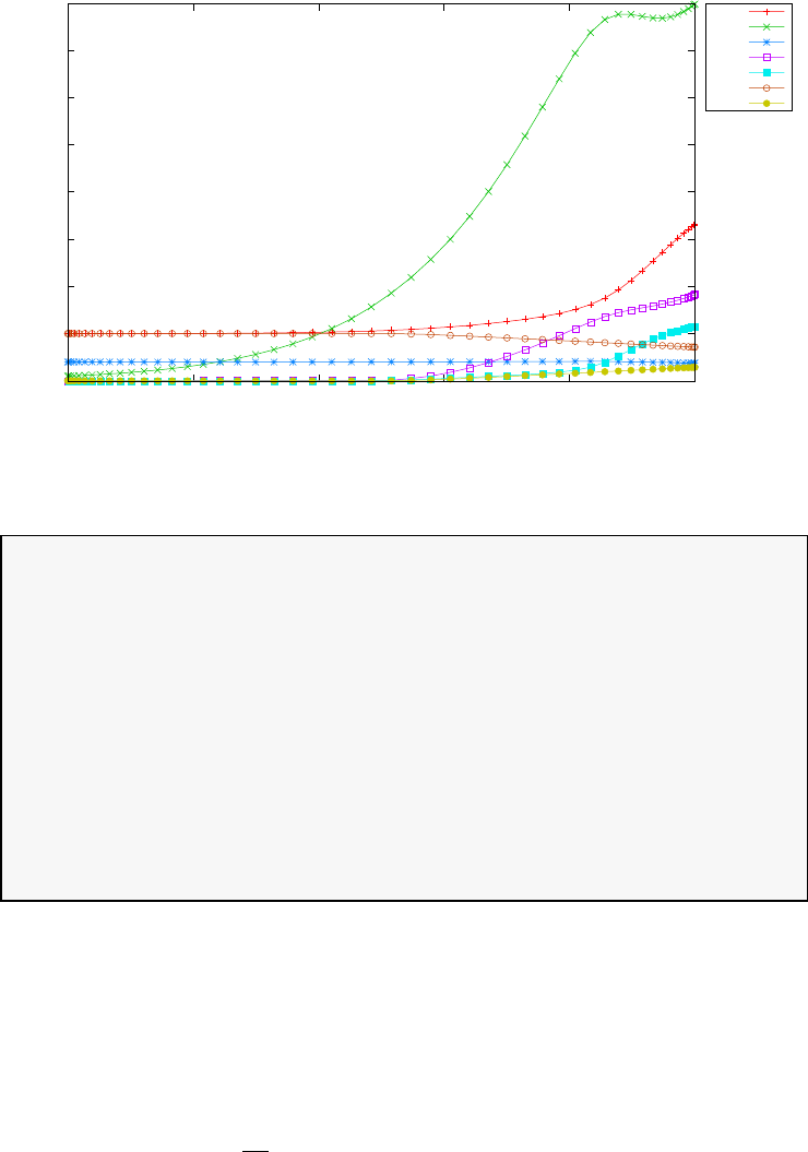
0
1
2
3
4
5
6
7
0 2 4 6 8 10
states
time (s)
Lee-Ramirez bioreactor: states
x1
x2
x3/10
x4
x5
x6
x7
Figure 3.48: States for the Lee-Ramirez bioreactor problem
NLP solver used: IPOPT
PSOPT release number: 4.0
Date and time of this run: Thu Feb 21 15:57:58 2019
Returned (unscaled) cost function value: -6.048409e+00
Phase 1 endpoint cost function value: -6.049249e+00
Phase 1 integrated part of the cost: 8.402028e-04
Phase 1 initial time: 0.000000e+00
Phase 1 final time: 1.000000e+01
Phase 1 maximum relative local error 2.082149e-03
NLP solver reports: *** The problem FAILED! - see screen output
3.22 Li’s parameter estimation problem
This is a parameter estimation problem with two parameters and three
observed variables, which is presented b Li et. al [28].
The dynamic equations are given by:
dx
dt =M(t, p)x+f(t), t ∈[0, π] (3.92)
with boundary condition:
x(0) + x(π) = (1 + eπ) [1,1,1]T
229
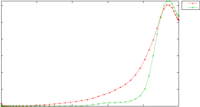
0
0.1
0.2
0.3
0.4
0.5
0.6
0 2 4 6 8 10
control 1
time (s)
Lee-Ramirez bioreactor: control
u1
u2
Figure 3.49: Control for the Lee-Ramirez bioreactor problem
where
M(t, p) =
p2−p1cos(p2t) 0 p2+p1sin(p2t)
0p10
−p2+p1sin(p2t) 0 p2+p1cos(p2t)
(3.93)
and
f(t) =
−1 + 19(cos(t)−sin(t))
−18
1−19(cos(t) + sin(t))
(3.94)
and the observation functions are:
g1=x1
g2=x2
g3=x3
(3.95)
The trajectories of the dynamic system is characterised by rapidly varying
fast and slow components if the difference between the two parameters p1
and p2is large, which may cause numerical problems to some ODE solvers.
The estimation data set is generated by adding Gaussian noise with
standard deviation 1 around the solution [x1(t), x2(t), x3(t)]T= [et, et, et]T,
with N= 33 equidistant samples within the interval t= [0, π]. The true
values of the parameters are p1= 19 and p2= 1. The weights of the three
observations are the same and equal to one.
The solution is found using Legendre discretisation with 40 grid points.
The code that solves the problem is shown below. The estimated parameter
values and their 95% confidence limits for ns= 129 samples are shown in
230

Table 3.22. Figure 3.50 shows the observations as well as the estimated
values of variable x1.
//////////////////////////////////////////////////////////////////////////
////////////////// param2.cxx ////////////////////////////
//////////////////////////////////////////////////////////////////////////
//////////////// PSOPT Example ////////////////////
//////////////////////////////////////////////////////////////////////////
//////////////////////////////////////////////////////////////////////////
//////// Title: Parameter estimation for ODE with 2 parameters //////////
//////// Last modified: 31 Jan 2014 ////////////////
//////// Reference: Li et al (2005) ////////////////
//////// (See PSOPT handbook for full reference) ///////////////
//////////////////////////////////////////////////////////////////////////
//////// Copyright (c) Victor M. Becerra, 2014 ////////////////
//////////////////////////////////////////////////////////////////////////
//////// This is part of the PSOPT software library, which ///////////////
//////// is distributed under the terms of the GNU Lesser ////////////////
//////// General Public License (LGPL) ////////////////
//////////////////////////////////////////////////////////////////////////
#include "psopt.h"
//////////////////////////////////////////////////////////////////////////
/////////////////// Define the observation function //////////
//////////////////////////////////////////////////////////////////////////
void observation_function( adouble* observations,
adouble* states, adouble* controls,
adouble* parameters, adouble& time, int k,
adouble* xad, int iphase, Workspace* workspace)
{
int i;
for (i=0; i<3; i++) {
observations[ i ] = states[ i ];
}
}
//////////////////////////////////////////////////////////////////////////
/////////////////// Define the DAE’s ////////////////////////////////////
//////////////////////////////////////////////////////////////////////////
void dae(adouble* derivatives, adouble* path, adouble* states,
adouble* controls, adouble* parameters, adouble& time,
adouble* xad, int iphase, Workspace* workspace)
{
// Variables
adouble x1, x2, x3, p1, p2, t;
// Differential states
x1 = states[CINDEX(1)];
x2 = states[CINDEX(2)];
x3 = states[CINDEX(3)];
// Parameters
p1 = parameters[CINDEX(1)];
p2 = parameters[CINDEX(2)];
t= time;
ADMatrix M(3,3), f(3,1), dxdt(3,1), x(3,1), y(3,1);
x(1,1) = x1; x(2,1) = x2; x(3,1) = x3;
M(1,1) = p2-p1*cos(p2*t); M(1,2) = 0.0; M(1,3) = p2 + p1*sin(p2*t);
M(2,1) = 0.0; M(2,2) = p1; M(2,3) = 0.0;
M(3,1) = -p2+p1*sin(p2*t); M(3,2) = 0.0; M(3,3) = p2 + p1*cos(p2*t);
f(1,1) = exp(t)*(-1.0 + 19.0*( cos(t) - sin(t) ) );
f(2,1) = exp(t)*(-18.0);
f(3,1) = exp(t)*(1.0 - 19.0*( cos(t) + sin(t) ) );
// Differential equations
231

product_ad(M, x, &y);
sum_ad(y, f, &dxdt );
derivatives[CINDEX(1)] = dxdt(1,1);
derivatives[CINDEX(2)] = dxdt(2,1);
derivatives[CINDEX(3)] = dxdt(3,1);
}
////////////////////////////////////////////////////////////////////////////
/////////////////// Define the events function ////////////////////////////
////////////////////////////////////////////////////////////////////////////
void events(adouble* e, adouble* initial_states, adouble* final_states,
adouble* parameters,adouble& t0, adouble& tf, adouble* xad,
int iphase, Workspace* workspace)
{
int i;
double rhs = 1.0 + exp(pi);
for (i=0; i<3; i++) {
e[i] = initial_states[i] + final_states[i] - rhs;
}
}
///////////////////////////////////////////////////////////////////////////
/////////////////// Define the phase linkages function ///////////////////
///////////////////////////////////////////////////////////////////////////
void linkages( adouble* linkages, adouble* xad, Workspace* workspace)
{
// No linkages as this is a single phase problem
}
////////////////////////////////////////////////////////////////////////////
/////////////////// Define the main routine ///////////////////////////////
////////////////////////////////////////////////////////////////////////////
int main(void)
{
////////////////////////////////////////////////////////////////////////////
/////////////////// Declare key structures ////////////////////////////////
////////////////////////////////////////////////////////////////////////////
Alg algorithm;
Sol solution;
Prob problem;
////////////////////////////////////////////////////////////////////////////
/////////////////// Register problem name ////////////////////////////////
////////////////////////////////////////////////////////////////////////////
problem.name = "Parameter estimation for ODE with two parameters";
problem.outfilename = "param2.txt";
////////////////////////////////////////////////////////////////////////////
//////////// Define problem level constants & do level 1 setup ////////////
////////////////////////////////////////////////////////////////////////////
problem.nphases = 1;
problem.nlinkages = 0;
psopt_level1_setup(problem);
/////////////////////////////////////////////////////////////////////////////
///////// Define phase related information & do level 2 setup /////////////
/////////////////////////////////////////////////////////////////////////////
problem.phases(1).nstates = 3;
problem.phases(1).ncontrols = 0;
problem.phases(1).nevents = 3;
problem.phases(1).npath = 0;
problem.phases(1).nparameters = 2;
232

problem.phases(1).nodes = 40;
problem.phases(1).nobserved = 3;
problem.phases(1).nsamples = 129;
psopt_level2_setup(problem, algorithm);
////////////////////////////////////////////////////////////////////////////
//////////// Load data for parameter estimation ////////////
////////////////////////////////////////////////////////////////////////////
int iphase = 1;
load_parameter_estimation_data(problem, iphase, "param2.dat");
problem.phases(1).observation_nodes.Print("observation nodes");
problem.phases(1).observations.Print("observations");
problem.phases(1).residual_weights.Print("weights");
////////////////////////////////////////////////////////////////////////////
/////////////////// Declare DMatrix objects to store results //////////////
////////////////////////////////////////////////////////////////////////////
DMatrix x, p, t;
////////////////////////////////////////////////////////////////////////////
/////////////////// Enter problem bounds information //////////////////////
////////////////////////////////////////////////////////////////////////////
problem.phases(1).bounds.lower.states(1) = 0.0;
problem.phases(1).bounds.lower.states(2) = 0.0;
problem.phases(1).bounds.lower.states(3) = 0.0;
problem.phases(1).bounds.upper.states(1) = 30.0;
problem.phases(1).bounds.upper.states(2) = 30.0;
problem.phases(1).bounds.upper.states(3) = 30.0;
problem.phases(1).bounds.lower.events(1) = 0.0;
problem.phases(1).bounds.lower.events(2) = 0.0;
problem.phases(1).bounds.lower.events(3) = 0.0;
problem.phases(1).bounds.upper.events(1) = 0.0;
problem.phases(1).bounds.upper.events(2) = 0.0;
problem.phases(1).bounds.upper.events(3) = 0.0;
problem.phases(1).bounds.lower.parameters(1) = 0.0;
problem.phases(1).bounds.lower.parameters(2) = 0.0;
problem.phases(1).bounds.upper.parameters(1) = 30.0;
problem.phases(1).bounds.upper.parameters(2) = 30.0;
problem.phases(1).bounds.lower.StartTime = 0.0;
problem.phases(1).bounds.upper.StartTime = 0.0;
problem.phases(1).bounds.lower.EndTime = pi;
problem.phases(1).bounds.upper.EndTime = pi;
////////////////////////////////////////////////////////////////////////////
/////////////////// Register problem functions ///////////////////////////
////////////////////////////////////////////////////////////////////////////
problem.dae = &dae;
problem.events = &events;
problem.linkages = &linkages;
problem.observation_function = & observation_function;
////////////////////////////////////////////////////////////////////////////
/////////////////// Define & register initial guess ///////////////////////
////////////////////////////////////////////////////////////////////////////
int nnodes = (int) problem.phases(1).nsamples;
DMatrix state_guess(3, nnodes);
DMatrix param_guess(2,1);
state_guess(1,colon()) = linspace(1.0, exp(pi), nnodes );
state_guess(2,colon()) = linspace(1.0, exp(pi), nnodes );
state_guess(3,colon()) = linspace(1.0, exp(pi), nnodes );
233

param_guess(1) = 19.0*1.5;
param_guess(2) = 1.0*1.5;
problem.phases(1).guess.states = state_guess;
problem.phases(1).guess.time = linspace(0.0, pi, nnodes);
problem.phases(1).guess.parameters = param_guess;
////////////////////////////////////////////////////////////////////////////
/////////////////// Enter algorithm options //////////////////////////////
////////////////////////////////////////////////////////////////////////////
algorithm.nlp_method = "IPOPT";
algorithm.scaling = "automatic";
algorithm.derivatives = "automatic";
algorithm.collocation_method = "Legendre";
// algorithm.mesh_refinement = "automatic";
// algorithm.defect_scaling = "jacobian-based";
// algorithm.nlp_iter_max = 1000;
algorithm.ode_tolerance = 1.e-4;
////////////////////////////////////////////////////////////////////////////
/////////////////// Now call PSOPT to solve the problem //////////////////
////////////////////////////////////////////////////////////////////////////
psopt(solution, problem, algorithm);
////////////////////////////////////////////////////////////////////////////
/////////// Extract relevant variables from solution structure //////////
////////////////////////////////////////////////////////////////////////////
x = solution.get_states_in_phase(1);
t = solution.get_time_in_phase(1);
p = solution.get_parameters_in_phase(1);
////////////////////////////////////////////////////////////////////////////
/////////// Save solution data to files if desired ////////////////////////
////////////////////////////////////////////////////////////////////////////
x.Save("x.dat");
t.Save("t.dat");
p.Print("Estimated parameters");
////////////////////////////////////////////////////////////////////////////
/////////// Plot some results if desired (requires gnuplot) ///////////////
////////////////////////////////////////////////////////////////////////////
DMatrix tm;
DMatrix ym;
tm = problem.phases(1).observation_nodes;
ym = problem.phases(1).observations;
spplot(t,x(1,colon()),tm,ym(1,colon()),problem.name, "time (s)", "state x1", "x1 y1");
spplot(t,x(2,colon()),tm,ym(2,colon()),problem.name, "time (s)", "state x2", "x2 y2");
spplot(t,x(3,colon()),tm,ym(3,colon()),problem.name, "time (s)", "state x3", "x3 y3");
spplot(t,x(1,colon()),tm,ym(1,colon()),problem.name, "time (s)", "state x1", "x1 y1", "pdf", "x1.pdf");
spplot(t,x(2,colon()),tm,ym(2,colon()),problem.name, "time (s)", "state x2", "x2 y2", "pdf", "x2.pdf");
spplot(t,x(3,colon()),tm,ym(3,colon()),problem.name, "time (s)", "state x3", "x3 y3", "pdf", "x3.pdf");
}
////////////////////////////////////////////////////////////////////////////
/////////////////////// END OF FILE ///////////////////////////////
////////////////////////////////////////////////////////////////////////////
234
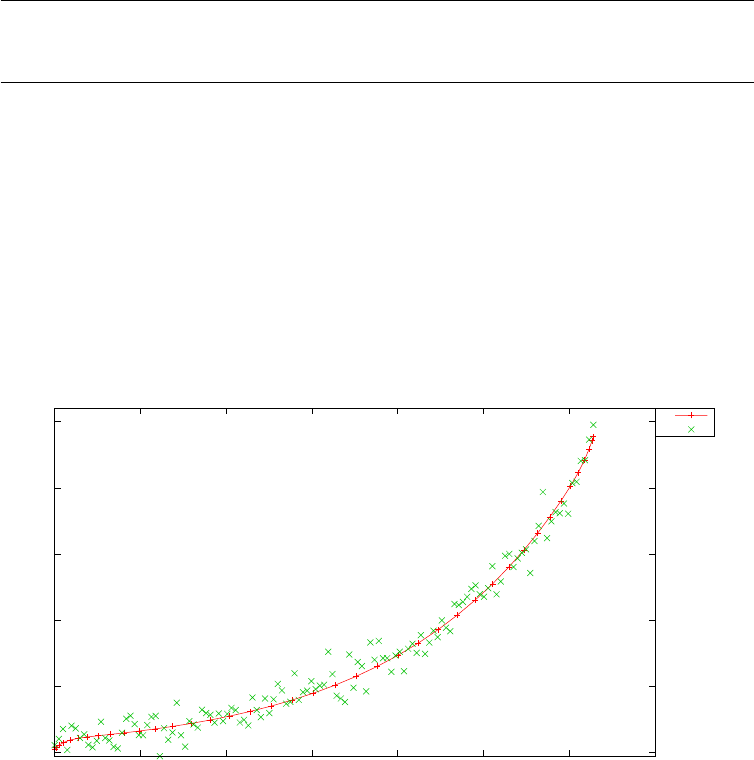
Table 3.1: Estimated parameter values and 95 percent statistical confidence
limits on estimated parameters
Parameter Low Confidence Limit Value High Confidence Limit
p11.907055e+01 1.907712e+01 1.908369e+01
p29.984900e-01 9.984990e-01 9.985080e-01
0
5
10
15
20
25
0 0.5 1 1.5 2 2.5 3 3.5
state x1
time (s)
Parameter estimation for ODE with two parameters
x1
y1
Figure 3.50: Observations and estimated state x1(t)
235

3.23 Linear tangent steering problem
Consider the following optimal control problem, which is known in the lit-
erature as the linear tangent steering problem [3]. Find tfand u(t)∈[0, tf]
to minimize the cost functional
J=tf(3.96)
subject to the dynamic constraints
˙x1=x2
˙x2=acos(u)
˙x3=x4
˙x4=asin(u)
(3.97)
the boundary conditions:
x1(0) = 0
x2(0) = 0
x3(0) = 0
x4(0) = 0
x2(tf) = 45.0
x3(tf)=5.0
x4(tf)=0.0
(3.98)
The PSOPT code that solves this problem is shown below.
//////////////////////////////////////////////////////////////////////////
////////////////// lts.cxx /////////////////////////////
//////////////////////////////////////////////////////////////////////////
//////////////// PSOPT Example ////////////////////
//////////////////////////////////////////////////////////////////////////
//////////////////////////////////////////////////////////////////////////
//////// Title: Linear tangent steering problem ////////////////
//////// Last modified: 16 February 2009 ////////////////
//////// Reference: Betts (2001) ////////////////
//////// (See PSOPT handbook for full reference) ////////////////
//////////////////////////////////////////////////////////////////////////
//////// Copyright (c) Victor M. Becerra, 2009 ////////////////
//////////////////////////////////////////////////////////////////////////
//////// This is part of the PSOPT software library, which ///////////////
//////// is distributed under the terms of the GNU Lesser ////////////////
//////// General Public License (LGPL) ////////////////
//////////////////////////////////////////////////////////////////////////
#include "psopt.h"
//////////////////////////////////////////////////////////////////////////
/////////////////// Define the end point (Mayer) cost function //////////
//////////////////////////////////////////////////////////////////////////
adouble endpoint_cost(adouble* initial_states, adouble* final_states,
adouble* parameters,adouble& t0, adouble& tf,
adouble* xad, int iphase, Workspace* workspace)
{
return tf;
}
//////////////////////////////////////////////////////////////////////////
/////////////////// Define the integrand (Lagrange) cost function //////
//////////////////////////////////////////////////////////////////////////
236

adouble integrand_cost(adouble* states, adouble* controls,
adouble* parameters, adouble& time, adouble* xad,
int iphase, Workspace* workspace)
{
return 0.0;
}
//////////////////////////////////////////////////////////////////////////
/////////////////// Define the DAE’s ////////////////////////////////////
//////////////////////////////////////////////////////////////////////////
void dae(adouble* derivatives, adouble* path, adouble* states,
adouble* controls, adouble* parameters, adouble& time,
adouble* xad, int iphase, Workspace* workspace)
{
adouble x1 = states[ CINDEX(1) ];
adouble x2 = states[ CINDEX(2) ];
adouble x3 = states[ CINDEX(3) ];
adouble x4 = states[ CINDEX(4) ];
adouble u = controls[ CINDEX(1) ];
double a = 100.0;
derivatives[ CINDEX(1) ] = x2;
derivatives[ CINDEX(2) ] = a*cos(u);
derivatives[ CINDEX(3) ] = x4;
derivatives[ CINDEX(4) ] = a*sin(u);
}
////////////////////////////////////////////////////////////////////////////
/////////////////// Define the events function ////////////////////////////
////////////////////////////////////////////////////////////////////////////
void events(adouble* e, adouble* initial_states, adouble* final_states,
adouble* parameters,adouble& t0, adouble& tf, adouble* xad,
int iphase, Workspace* workspace)
{
adouble x10 = initial_states[ CINDEX(1) ];
adouble x20 = initial_states[ CINDEX(2) ];
adouble x30 = initial_states[ CINDEX(3) ];
adouble x40 = initial_states[ CINDEX(4) ];
adouble x2f = final_states[ CINDEX(2) ];
adouble x3f = final_states[ CINDEX(3) ];
adouble x4f = final_states[ CINDEX(4) ];
e[ CINDEX(1) ] = x10;
e[ CINDEX(2) ] = x20;
e[ CINDEX(3) ] = x30;
e[ CINDEX(4) ] = x40;
e[ CINDEX(5) ] = x2f;
e[ CINDEX(6) ] = x3f;
e[ CINDEX(7) ] = x4f;
}
///////////////////////////////////////////////////////////////////////////
/////////////////// Define the phase linkages function ///////////////////
///////////////////////////////////////////////////////////////////////////
void linkages( adouble* linkages, adouble* xad, Workspace* workspace)
{
// No linkages as this is a single phase problem
}
////////////////////////////////////////////////////////////////////////////
/////////////////// Define the main routine ///////////////////////////////
////////////////////////////////////////////////////////////////////////////
int main(void)
{
////////////////////////////////////////////////////////////////////////////
/////////////////// Declare key structures ////////////////////////////////
////////////////////////////////////////////////////////////////////////////
Alg algorithm;
Sol solution;
Prob problem;
237

////////////////////////////////////////////////////////////////////////////
/////////////////// Register problem name ////////////////////////////////
////////////////////////////////////////////////////////////////////////////
problem.name = "Linear Tangent Steering Problem";
problem.outfilename = "lts.txt";
////////////////////////////////////////////////////////////////////////////
//////////// Define problem level constants & do level 1 setup ////////////
////////////////////////////////////////////////////////////////////////////
problem.nphases = 1;
problem.nlinkages = 0;
psopt_level1_setup(problem);
/////////////////////////////////////////////////////////////////////////////
///////// Define phase related information & do level 2 setup /////////////
/////////////////////////////////////////////////////////////////////////////
problem.phases(1).nstates = 4;
problem.phases(1).ncontrols = 1;
problem.phases(1).nevents = 7;
problem.phases(1).npath = 0;
problem.phases(1).nodes = "[10, 30]";
psopt_level2_setup(problem, algorithm);
////////////////////////////////////////////////////////////////////////////
/////////////////// Declare DMatrix objects to store results //////////////
////////////////////////////////////////////////////////////////////////////
DMatrix x, u, t;
DMatrix lambda, H;
////////////////////////////////////////////////////////////////////////////
/////////////////// Enter problem bounds information //////////////////////
////////////////////////////////////////////////////////////////////////////
problem.phases(1).bounds.lower.states(1) = -100.0;
problem.phases(1).bounds.lower.states(2) = -100.0;
problem.phases(1).bounds.lower.states(3) = -100.0;
problem.phases(1).bounds.lower.states(4) = -100.0;
problem.phases(1).bounds.upper.states(1) = 100.0;
problem.phases(1).bounds.upper.states(2) = 100.0;
problem.phases(1).bounds.upper.states(3) = 100.0;
problem.phases(1).bounds.upper.states(4) = 100.0;
problem.phases(1).bounds.lower.controls(1) = -pi/2.0;
problem.phases(1).bounds.upper.controls(1) = pi/2.0;
problem.phases(1).bounds.lower.events(1) = 0.0;
problem.phases(1).bounds.lower.events(2) = 0.0;
problem.phases(1).bounds.lower.events(3) = 0.0;
problem.phases(1).bounds.lower.events(4) = 0.0;
problem.phases(1).bounds.lower.events(5) = 45.0;
problem.phases(1).bounds.lower.events(6) = 5.0;
problem.phases(1).bounds.lower.events(7) = 0.0;
problem.phases(1).bounds.upper.events(1) = 0.0;
problem.phases(1).bounds.upper.events(2) = 0.0;
problem.phases(1).bounds.upper.events(3) = 0.0;
problem.phases(1).bounds.upper.events(4) = 0.0;
problem.phases(1).bounds.upper.events(5) = 45.0;
problem.phases(1).bounds.upper.events(6) = 5.0;
problem.phases(1).bounds.upper.events(7) = 0.0;
problem.phases(1).bounds.lower.StartTime = 0.0;
problem.phases(1).bounds.upper.StartTime = 0.0;
problem.phases(1).bounds.lower.EndTime = 0.0;
problem.phases(1).bounds.upper.EndTime = 1.0;
////////////////////////////////////////////////////////////////////////////
/////////////////// Register problem functions ///////////////////////////
////////////////////////////////////////////////////////////////////////////
238

problem.integrand_cost = &integrand_cost;
problem.endpoint_cost = &endpoint_cost;
problem.dae = &dae;
problem.events = &events;
problem.linkages = &linkages;
////////////////////////////////////////////////////////////////////////////
/////////////////// Define & register initial guess ///////////////////////
////////////////////////////////////////////////////////////////////////////
DMatrix x0(3,10);
x0(1,colon()) = linspace(0.0, 12.0, 10);
x0(2,colon()) = linspace(0.0, 45.0, 10);
x0(3,colon()) = linspace(0.0, 5.0, 10);
x0(3,colon()) = linspace(0.0, 0.0, 10);
problem.phases(1).guess.controls = ones(1,10);
problem.phases(1).guess.states = x0;
problem.phases(1).guess.time = linspace(0.0,1.0, 10);
////////////////////////////////////////////////////////////////////////////
/////////////////// Enter algorithm options //////////////////////////////
////////////////////////////////////////////////////////////////////////////
algorithm.nlp_method = "IPOPT";
algorithm.scaling = "automatic";
algorithm.derivatives = "automatic";
algorithm.nlp_iter_max = 1000;
algorithm.nlp_tolerance = 1.e-6;
////////////////////////////////////////////////////////////////////////////
/////////////////// Now call PSOPT to solve the problem /////////////////
////////////////////////////////////////////////////////////////////////////
psopt(solution, problem, algorithm);
if (solution.error_flag) exit(0);
////////////////////////////////////////////////////////////////////////////
/////////// Extract relevant variables from solution structure //////////
////////////////////////////////////////////////////////////////////////////
x = solution.get_states_in_phase(1);
u = solution.get_controls_in_phase(1);
t = solution.get_time_in_phase(1);
////////////////////////////////////////////////////////////////////////////
/////////// Save solution data to files if desired ////////////////////////
////////////////////////////////////////////////////////////////////////////
x.Save("x.dat");
u.Save("u.dat");
t.Save("t.dat");
////////////////////////////////////////////////////////////////////////////
/////////// Plot some results if desired (requires gnuplot) ///////////////
////////////////////////////////////////////////////////////////////////////
plot(t,x,problem.name + ": states", "time (s)", "states", "x1 x2 x3 x4");
plot(t,u,problem.name + ": control", "time (s)", "control", "u");
plot(t,x,problem.name + ": states", "time (s)", "states", "x1 x2 x3 x4",
"pdf", "lts_states.pdf");
plot(t,u,problem.name + ": control", "time (s)", "control", "u",
"pdf", "lts_control.pdf");
}
////////////////////////////////////////////////////////////////////////////
/////////////////////// END OF FILE ///////////////////////////////
////////////////////////////////////////////////////////////////////////////
239

The output from PSOPT is summarised in the box below and shown
in Figures 3.51 and 3.52, which contain the elements of the state and the
control, respectively.
PSOPT results summary
=====================
Problem: Linear Tangent Steering Problem
CPU time (seconds): 1.188370e+00
NLP solver used: IPOPT
PSOPT release number: 4.0
Date and time of this run: Thu Feb 21 17:16:35 2019
Optimal (unscaled) cost function value: 5.545709e-01
Phase 1 endpoint cost function value: 5.545709e-01
Phase 1 integrated part of the cost: 0.000000e+00
Phase 1 initial time: 0.000000e+00
Phase 1 final time: 5.545709e-01
Phase 1 maximum relative local error: 1.603284e-07
NLP solver reports: The problem has been solved!
3.24 Low thrust orbit transfer
The goal of this problem is to compute an optimal low thrust policy for an
spacecraft to go from a standard space shuttle park orbit to a specified final
orbit, while maximising the final weight of the spacecraft. The problem is
described in detail by Betts [3]. The problem is formulated as follows. Find
u(t) = [ur(t), uθ(t), uh(t)]T, t ∈[0, tf], the unknown throtle parameter τ, and
the final time tf, such that the following objective function is minimised:
J=−w(tf) (3.99)
subject to the dynamic constraints:
˙
y=A(y)∆ + b
˙w=−T[1 + 0.01τ]/Isp
(3.100)
the path constraint:
||u(t)||2= 1 (3.101)
240
0
5
10
15
20
25
30
35
40
45
0 0.1 0.2 0.3 0.4 0.5 0.6
states
time (s)
Linear Tangent Steering Problem: states
x1
x2
x3
x4
Figure 3.51: States for the linear tangent steering problem
-1
-0.5
0
0.5
1
0 0.1 0.2 0.3 0.4 0.5 0.6
control
time (s)
Linear Tangent Steering Problem: control
u
Figure 3.52: Control for the linear tangent steering problem
241

and the parameter bounds:
τL≤τ≤0 (3.102)
where y= [p, f, g, h, k, L, w]Tis the vector of modified equinoctial elements,
w(t) is the weight of the spacecraft, Isp is the specific impulse of the engine,
expressions for A(y) and bare given in [3], the disturbing acceleration ∆ is
given by:
∆=∆g+ ∆T(3.103)
where ∆gis the gravitational disturbing acceleration due to the oblatness
of Earth (given in [3]), and ∆Tis the thurst acceleration, given by:
∆T=g0T[1 + 0.01τ]
wu
where Tis the maximum thrust, and g0is the mass to weight conversion
factor.
The boundary conditions of the problem are given by:
p(tf) = 40007346.015232 ft
qf(tf)2+g(tf)2= 0.73550320568829
qh(tf)2+k(tf)2= 0.61761258786099
f(tf)h(tf) + g(tf)k(tf)=0
g(tf)h(tf)−k(tf)f(tf)=0
p(0) = 21837080.052835ft
f(0) = 0
g(0) = 0
h(0) = 0
h(0) = 0
k(0) = 0
L(0) = π(rad)
w(0) = 1 (lb)
(3.104)
and the values of the parameters are: g0= 32.174 (ft/sec2), Isp = 450
(sec), T= 4.446618 ×10⁻³(lb), µ= 1.407645794 ×10¹⁶ (ft3/sec2), Re=
20925662.73 (ft), J2= 1082.639 ×10−6,J3=−2.565 ×10⁻⁶,J4=−1.608 ×
10−6,τL=−50.
An initial guess was computed by forward propagation from the initial
conditions, assuming that the direction of the thrust vector is parallel to the
cartesian velocity vector, such that the initial control input was computed
as follows:
u(t) = QT
r
v
||v|| (3.105)
242

where Qris a matrix whose columns are the directions of the rotating radial
frame:
Qr=iriθih=hr
||r||
(r×v)×r
||r×v||||r||
(r×v)
||r×v|| i(3.106)
The problem was solved using local collocation (trapezoidal followed by
Hermite-Simpson) with automatic mesh refinement. The PSOPT code that
solves the problem is shown below.
//////////////////////////////////////////////////////////////////////////
//////////////// low_thrust.cxx /////////////////////
//////////////////////////////////////////////////////////////////////////
//////////////// PSOPT Example ////////////////////
//////////////////////////////////////////////////////////////////////////
//////////////////////////////////////////////////////////////////////////
//////// Title: Low thrust orbit transfer problem ////////////////
//////// Last modified: 16 February 2009 ////////////////
//////// Reference: Betts (2001) ////////////////
//////// (See PSOPT handbook for full reference) ///////////////
//////////////////////////////////////////////////////////////////////////
//////// Copyright (c) Victor M. Becerra, 2009 ////////////////
//////////////////////////////////////////////////////////////////////////
//////// This is part of the PSOPT software library, which ///////////////
//////// is distributed under the terms of the GNU Lesser ////////////////
//////// General Public License (LGPL) ////////////////
//////////////////////////////////////////////////////////////////////////
#include "psopt.h"
//////////////////////////////////////////////////////////////////////////
/////////////////// Define auxiliary functions //////////
//////////////////////////////////////////////////////////////////////////
adouble legendre_polynomial( adouble x, int n)
{
// This function computes the value of the legendre polynomials
// for a given value of the argument x and for n=0...5 only
adouble retval=0.0;
switch(n) {
case 0:
retval=1.0; break;
case 1:
retval= x; break;
case 2:
retval= 0.5*(3.0*pow(x,2)-1.0); break;
case 3:
retval= 0.5*(5.0*pow(x,3)- 3*x); break;
case 4:
retval= (1.0/8.0)*(35.0*pow(x,4) - 30.0*pow(x,2) + 3.0); break;
case 5:
retval= (1.0/8.0)*(63.0*pow(x,5) - 70.0*pow(x,3) + 15.0*x); break;
default:
error_message("legendre_polynomial(x,n) is limited to n=0...5");
}
return retval;
}
adouble legendre_polynomial_derivative( adouble x, int n)
{
// This function computes the value of the legendre polynomial derivatives
// for a given value of the argument x and for n=0...5 only.
adouble retval=0.0;
switch(n) {
case 0:
retval=0.0; break;
case 1:
retval= 1.0; break;
case 2:
retval= 0.5*(2.0*3.0*x); break;
243

case 3:
retval= 0.5*(3.0*5.0*pow(x,2)-3.0); break;
case 4:
retval= (1.0/8.0)*(4.0*35.0*pow(x,3) - 2.0*30.0*x ); break;
case 5:
retval= (1.0/8.0)*(5.0*63.0*pow(x,4) - 3.0*70.0*pow(x,2) + 15.0); break;
default:
error_message("legendre_polynomial_derivative(x,n) is limited to n=0...5");
}
return retval;
}
void compute_cartesian_trajectory(const DMatrix& x, DMatrix& xyz )
{
int npoints = x.GetNoCols();
xyz.Resize(3,npoints);
for(int i=1; i<=npoints;i++) {
double p = x(1,i);
double f = x(2,i);
double g = x(3,i);
double h = x(4,i);
double k = x(5,i);
double L = x(6,i);
double q = 1.0 + f*cos(L) + g*sin(L);
double r = p/q;
double alpha2 = h*h - k*k;
double X = sqrt( h*h + k*k );
double s2 = 1 + X*X;
double r1 = r/s2*( cos(L) + alpha2*cos(L) + 2*h*k*sin(L));
double r2 = r/s2*( sin(L) - alpha2*sin(L) + 2*h*k*cos(L));
double r3 = 2*r/s2*( h*sin(L) - k*cos(L) );
xyz(1,i) = r1;
xyz(2,i) = r2;
xyz(3,i) = r3;
}
}
//////////////////////////////////////////////////////////////////////////
/////////////////// Define the end point (Mayer) cost function //////////
//////////////////////////////////////////////////////////////////////////
adouble endpoint_cost(adouble* initial_states, adouble* final_states,
adouble* parameters,adouble& t0, adouble& tf,
adouble* xad, int iphase, Workspace* workspace)
{
if (iphase == 1) {
adouble w = final_states[CINDEX(7)];
return (-w);
}
else {
return (0);
}
}
//////////////////////////////////////////////////////////////////////////
/////////////////// Define the integrand (Lagrange) cost function //////
//////////////////////////////////////////////////////////////////////////
adouble integrand_cost(adouble* states, adouble* controls, adouble* parameters,
adouble& time, adouble* xad, int iphase, Workspace* workspace)
{
return 0.0;
}
//////////////////////////////////////////////////////////////////////////
/////////////////// Define the DAE’s ////////////////////////////////////
//////////////////////////////////////////////////////////////////////////
void dae(adouble* derivatives, adouble* path, adouble* states,
244

adouble* controls, adouble* parameters, adouble& time,
adouble* xad, int iphase, Workspace* workspace)
{
// Local integers
int i, j;
// Define constants:
double Isp = 450.0; // [sec]
double mu = 1.407645794e16; // [f2^2/sec^2]
double g0 = 32.174; // [ft/sec^2]
double T = 4.446618e-3; // [lb]
double Re = 20925662.73; // [ft]
double J[5];
J[2] = 1082.639e-6;
J[3] = -2.565e-6;
J[4] = -1.608e-6;
// Extract individual variables
adouble p = states[ CINDEX(1) ];
adouble f = states[ CINDEX(2) ];
adouble g = states[ CINDEX(3) ];
adouble h = states[ CINDEX(4) ];
adouble k = states[ CINDEX(5) ];
adouble L = states[ CINDEX(6) ];
adouble w = states[ CINDEX(7) ];
adouble* u = controls;
adouble tau = parameters[ CINDEX(1) ];
// Define some dependent variables
adouble q = 1.0 + f*cos(L) + g*sin(L);
adouble r = p/q;
adouble alpha2 = h*h - k*k;
adouble X = sqrt( h*h + k*k );
adouble s2 = 1 + X*X;
// r and v
adouble r1 = r/s2*( cos(L) + alpha2*cos(L) + 2*h*k*sin(L));
adouble r2 = r/s2*( sin(L) - alpha2*sin(L) + 2*h*k*cos(L));
adouble r3 = 2*r/s2*( h*sin(L) - k*cos(L) );
adouble rvec[3];
rvec[ CINDEX(1) ] = r1; rvec[ CINDEX(2)] = r2; rvec[ CINDEX(3) ] = r3;
adouble v1 = -(1.0/s2)*sqrt(mu/p)*( sin(L) + alpha2*sin(L) - 2*h*k*cos(L) + g - 2*f*h*k + alpha2*g);
adouble v2 = -(1.0/s2)*sqrt(mu/p)*( -cos(L) + alpha2*cos(L) + 2*h*k*sin(L) - f + 2*g*h*k + alpha2*f);
adouble v3 = (2.0/s2)*sqrt(mu/p)*(h*cos(L) + k*sin(L) + f*h + g*k);
adouble vvec[3];
vvec[ CINDEX(1) ] = v1; vvec[ CINDEX(2)] = v2; vvec[ CINDEX(3) ] = v3;
// compute Qr
adouble ir[3], ith[3], ih[3];
adouble rv[3];
adouble rvr[3];
cross( rvec, vvec, rv );
cross( rv, rvec, rvr );
adouble norm_r = sqrt( dot(rvec, rvec, 3) );
adouble norm_rv = sqrt( dot(rv, rv, 3) );
for (i=0; i<3; i++) {
ir[i] = rvec[i]/norm_r;
ith[i] = rvr[i]/( norm_rv*norm_r );
ih[i] = rv[i]/norm_rv;
}
adouble Qr1[3], Qr2[3], Qr3[3];
for(i=0; i< 3; i++)
245

{
// Columns of matrix Qr
Qr1[i] = ir[i];
Qr2[i] = ith[i];
Qr3[i] = ih[i];
}
// Compute in
adouble en[3];
en[ CINDEX(1) ] = 0.0; en[ CINDEX(2) ]= 0.0; en[ CINDEX(3) ] = 1.0;
adouble enir = dot(en,ir,3);
adouble in[3];
for(i=0;i<3;i++) {
in[i] = en[i] - enir*ir[i];
}
adouble norm_in = sqrt( dot( in, in, 3 ) );
for(i=0;i<3;i++) {
in[i] = in[i]/norm_in;
}
// Geocentric latitude angle:
adouble sin_phi = rvec[ CINDEX(3) ]/ sqrt( dot(rvec,rvec,3) ) ;
adouble cos_phi = sqrt(1.0- pow(sin_phi,2.0));
adouble deltagn = 0.0;
adouble deltagr = 0.0;
for (j=2; j<=4;j++) {
adouble Pdash_j = legendre_polynomial_derivative( sin_phi, j );
adouble P_j = legendre_polynomial( sin_phi, j );
deltagn += -mu*cos_phi/(r*r)*pow(Re/r,j)*Pdash_j*J[j];
deltagr += -mu/(r*r)* (j+1)*pow( Re/r,j)*P_j*J[j];
}
// Compute vector delta_g
adouble delta_g[3];
for (i=0;i<3;i++) {
delta_g[i] = deltagn*in[i] - deltagr*ir[i];
}
// Compute vector DELTA_g
adouble DELTA_g[3];
DELTA_g[ CINDEX(1) ] = dot(Qr1, delta_g,3);
DELTA_g[ CINDEX(2) ] = dot(Qr2, delta_g,3);
DELTA_g[ CINDEX(3) ] = dot(Qr3, delta_g,3);
// Compute DELTA_T
adouble DELTA_T[3];
for(i=0;i<3;i++) {
DELTA_T[i] = g0*T*(1.0+0.01*tau)*u[i]/w;
}
// Compute DELTA
adouble DELTA[3];
for(i=0;i<3;i++) {
DELTA[i] = DELTA_g[i] + DELTA_T[i];
}
adouble delta1= DELTA[ CINDEX(1) ];
adouble delta2= DELTA[ CINDEX(2) ];
adouble delta3= DELTA[ CINDEX(3) ];
// derivatives
adouble pdot = 2*p/q*sqrt(p/mu) * delta2;
adouble fdot = sqrt(p/mu)*sin(L) * delta1 + sqrt(p/mu)*(1.0/q)*((q+1.0)*cos(L)+f) * delta2
- sqrt(p/mu)*(g/q)*(h*sin(L)-k*cos(L)) * delta3;
246

adouble gdot = -sqrt(p/mu)*cos(L) * delta1 + sqrt(p/mu)*(1.0/q)*((q+1.0)*sin(L)+g) * delta2
+ sqrt(p/mu)*(f/q)*(h*sin(L)-k*cos(L)) * delta3;
adouble hdot = sqrt(p/mu)*s2*cos(L)/(2.0*q) * delta3;
adouble kdot = sqrt(p/mu)*s2*sin(L)/(2.0*q) * delta3;
adouble Ldot = sqrt(p/mu)*(1.0/q)*(h*sin(L)-k*cos(L))* delta3 + sqrt(mu*p)*pow( (q/p),2.);
adouble wdot = -T*(1.0+0.01*tau)/Isp;
derivatives[ CINDEX(1) ] = pdot;
derivatives[ CINDEX(2) ] = fdot;
derivatives[ CINDEX(3) ] = gdot;
derivatives[ CINDEX(4) ] = hdot;
derivatives[ CINDEX(5) ] = kdot;
derivatives[ CINDEX(6) ] = Ldot;
derivatives[ CINDEX(7) ] = wdot;
path[ CINDEX(1) ] = pow( u[CINDEX(1)] , 2) + pow( u[CINDEX(2)], 2) + pow( u[CINDEX(3)], 2);
}
////////////////////////////////////////////////////////////////////////////
/////////////////// Define the events function ////////////////////////////
////////////////////////////////////////////////////////////////////////////
void events(adouble* e, adouble* initial_states, adouble* final_states,
adouble* parameters,adouble& t0, adouble& tf, adouble* xad,
int iphase, Workspace* workspace)
{
int offset;
adouble pti = initial_states[ CINDEX(1) ];
adouble fti = initial_states[ CINDEX(2) ];
adouble gti = initial_states[ CINDEX(3) ];
adouble hti = initial_states[ CINDEX(4) ];
adouble kti = initial_states[ CINDEX(5) ];
adouble Lti = initial_states[ CINDEX(6) ];
adouble wti = initial_states[ CINDEX(7) ];
adouble ptf = final_states[ CINDEX(1) ];
adouble ftf = final_states[ CINDEX(2) ];
adouble gtf = final_states[ CINDEX(3) ];
adouble htf = final_states[ CINDEX(4) ];
adouble ktf = final_states[ CINDEX(5) ];
adouble Ltf = final_states[ CINDEX(6) ];
if (iphase==1) {
e[ CINDEX(1) ] = pti;
e[ CINDEX(2) ] = fti;
e[ CINDEX(3) ] = gti;
e[ CINDEX(4) ] = hti;
e[ CINDEX(5) ] = kti;
e[ CINDEX(6) ] = Lti;
e[ CINDEX(7) ] = wti;
}
if (1 == 1) offset = 7;
else offset = 0;
if (iphase == 1 ) {
e[ offset + CINDEX(1) ] = ptf;
e[ offset + CINDEX(2) ] = sqrt( ftf*ftf + gtf*gtf );
e[ offset + CINDEX(3) ] = sqrt( htf*htf + ktf*ktf );
e[ offset + CINDEX(4) ] = ftf*htf + gtf*ktf;
e[ offset + CINDEX(5) ] = gtf*htf - ktf*ftf;
}
}
///////////////////////////////////////////////////////////////////////////
/////////////////// Define the phase linkages function ///////////////////
///////////////////////////////////////////////////////////////////////////
void linkages( adouble* linkages, adouble* xad, Workspace* workspace)
{
// auto_link_multiple(linkages, xad, 1);
}
247

////////////////////////////////////////////////////////////////////////////
/////////////////// Define the main routine ///////////////////////////////
////////////////////////////////////////////////////////////////////////////
int main(void)
{
////////////////////////////////////////////////////////////////////////////
/////////////////// Declare key structures ////////////////////////////////
////////////////////////////////////////////////////////////////////////////
Alg algorithm;
Sol solution;
Prob problem;
MSdata msdata;
////////////////////////////////////////////////////////////////////////////
/////////////////// Register problem name ////////////////////////////////
////////////////////////////////////////////////////////////////////////////
problem.name = "Low thrust transfer problem";
problem.outfilename = "lowthrust.txt";
////////////////////////////////////////////////////////////////////////////
//////////// Define problem level constants & do level 1 setup ////////////
////////////////////////////////////////////////////////////////////////////
problem.nphases = 1;
problem.nlinkages = 0;
psopt_level1_setup(problem);
/////////////////////////////////////////////////////////////////////////////
///////// Define phase related information & do level 2 setup ////////////
/////////////////////////////////////////////////////////////////////////////
problem.phases(1).nstates = 7;
problem.phases(1).ncontrols = 3;
problem.phases(1).nparameters = 1;
problem.phases(1).nevents = 12;
problem.phases(1).npath = 1;
problem.phases(1).nodes = 80;
psopt_level2_setup(problem, algorithm);
////////////////////////////////////////////////////////////////////////////
/////////////////// Enter problem bounds information //////////////////////
////////////////////////////////////////////////////////////////////////////
double tauL = -50.0;
double tauU = 0.0;
double pti = 21837080.052835;
double fti = 0.0;
double gti = 0.0;
double hti = -0.25396764647494;
double kti = 0.0;
double Lti = pi;
double wti = 1.0;
double wtf_guess;
double SISP = 450.0;
double DELTAV = 22741.1460;
double CM2W = 32.174;
wtf_guess = wti*exp(-DELTAV/(CM2W*SISP));
double ptf = 40007346.015232;
double event_final_9 = 0.73550320568829;
double event_final_10 = 0.61761258786099;
double event_final_11 = 0.0;
double event_final_12_upper = 0.0;
double event_final_12_lower = -10.0;
248

problem.phases(1).bounds.lower.parameters(1) = tauL;
problem.phases(1).bounds.upper.parameters(1) = tauU;
problem.phases(1).bounds.lower.states(1) = 10.e6;
problem.phases(1).bounds.lower.states(2) = -0.20;
problem.phases(1).bounds.lower.states(3) = -0.10;
problem.phases(1).bounds.lower.states(4) = -1.0;
problem.phases(1).bounds.lower.states(5) = -0.20;
problem.phases(1).bounds.lower.states(6) = pi;
problem.phases(1).bounds.lower.states(7) = 0.0;
problem.phases(1).bounds.upper.states(1) = 60.e6;
problem.phases(1).bounds.upper.states(2) = 0.20;
problem.phases(1).bounds.upper.states(3) = 1.0;
problem.phases(1).bounds.upper.states(4) = 1.0;
problem.phases(1).bounds.upper.states(5) = 0.20;
problem.phases(1).bounds.upper.states(6) = 20*pi;
problem.phases(1).bounds.upper.states(7) = 2.0;
problem.phases(1).bounds.lower.controls(1) = -1.0;
problem.phases(1).bounds.lower.controls(2) = -1.0;
problem.phases(1).bounds.lower.controls(3) = -1.0;
problem.phases(1).bounds.upper.controls(1) = 1.0;
problem.phases(1).bounds.upper.controls(2) = 1.0;
problem.phases(1).bounds.upper.controls(3) = 1.0;
problem.phases(1).bounds.lower.events(1) = pti;
problem.phases(1).bounds.lower.events(2) = fti;
problem.phases(1).bounds.lower.events(3) = gti;
problem.phases(1).bounds.lower.events(4) = hti;
problem.phases(1).bounds.lower.events(5) = kti;
problem.phases(1).bounds.lower.events(6) = Lti;
problem.phases(1).bounds.lower.events(7) = wti;
problem.phases(1).bounds.lower.events(8) = ptf;
problem.phases(1).bounds.lower.events(9) = event_final_9;
problem.phases(1).bounds.lower.events(10) = event_final_10;
problem.phases(1).bounds.lower.events(11) = event_final_11;
problem.phases(1).bounds.lower.events(12) = event_final_12_lower;
problem.phases(1).bounds.upper.events(1) = pti;
problem.phases(1).bounds.upper.events(2) = fti;
problem.phases(1).bounds.upper.events(3) = gti;
problem.phases(1).bounds.upper.events(4) = hti;
problem.phases(1).bounds.upper.events(5) = kti;
problem.phases(1).bounds.upper.events(6) = Lti;
problem.phases(1).bounds.upper.events(7) = wti;
problem.phases(1).bounds.upper.events(8) = ptf;
problem.phases(1).bounds.upper.events(9) = event_final_9;
problem.phases(1).bounds.upper.events(10) = event_final_10;
problem.phases(1).bounds.upper.events(11) = event_final_11;
problem.phases(1).bounds.upper.events(12) = event_final_12_upper;
double EQ_TOL = 0.001;
problem.phases(1).bounds.upper.path(1) = 1.0+EQ_TOL;
problem.phases(1).bounds.lower.path(1) = 1.0-EQ_TOL;
problem.phases(1).bounds.lower.StartTime = 0.0;
problem.phases(1).bounds.upper.StartTime = 0.0;
problem.phases(1).bounds.lower.EndTime = 50000.0;
problem.phases(1).bounds.upper.EndTime = 100000.0;
////////////////////////////////////////////////////////////////////////////
/////////////////// Register problem functions ///////////////////////////
////////////////////////////////////////////////////////////////////////////
problem.integrand_cost = &integrand_cost;
problem.endpoint_cost = &endpoint_cost;
problem.dae = &dae;
problem.events = &events;
problem.linkages = &linkages;
////////////////////////////////////////////////////////////////////////////
/////////////////// Define & register initial guess ///////////////////////
249

////////////////////////////////////////////////////////////////////////////
int nnodes = 141;
int ncontrols = problem.phases(1).ncontrols;
int nstates = problem.phases(1).nstates;
DMatrix u_guess = zeros(ncontrols,nnodes);
DMatrix x_guess = zeros(nstates,nnodes);
DMatrix time_guess = linspace(0.0,86810.0,nnodes);
DMatrix param_guess = -25.0*ones(1,1);
u_guess.Load("U0.dat");
x_guess.Load("X0.dat");
time_guess.Load("T0.dat");
auto_phase_guess(problem, u_guess, x_guess, param_guess, time_guess);
////////////////////////////////////////////////////////////////////////////
/////////////////// Enter algorithm options //////////////////////////////
////////////////////////////////////////////////////////////////////////////
algorithm.nlp_iter_max = 1000;
algorithm.nlp_tolerance = 1.e-6;
algorithm.nlp_method = "IPOPT";
algorithm.scaling = "automatic";
algorithm.derivatives = "automatic";
algorithm.defect_scaling = "jacobian-based";
algorithm.jac_sparsity_ratio = 0.11; // 0.05;
algorithm.collocation_method = "trapezoidal";
algorithm.mesh_refinement = "automatic";
algorithm.mr_max_increment_factor = 0.2;
////////////////////////////////////////////////////////////////////////////
/////////////////// Now call PSOPT to solve the problem //////////////////
////////////////////////////////////////////////////////////////////////////
psopt(solution, problem, algorithm);
////////////////////////////////////////////////////////////////////////////
/////////// Extract relevant variables from solution structure //////////
////////////////////////////////////////////////////////////////////////////
DMatrix x, u, t;
x = solution.get_states_in_phase(1);
u = solution.get_controls_in_phase(1);
t = solution.get_time_in_phase(1);
t = t/3600.0;
DMatrix tau = solution.get_parameters_in_phase(1);
tau.Print("tau");
////////////////////////////////////////////////////////////////////////////
/////////// Save solution data to files if desired ////////////////////////
////////////////////////////////////////////////////////////////////////////
x.Save("x.dat");
u.Save("u.dat");
t.Save("t.dat");
////////////////////////////////////////////////////////////////////////////
/////////// Plot some results if desired (requires gnuplot) ///////////////
////////////////////////////////////////////////////////////////////////////
DMatrix x1 = x(1,colon())/1.e6;
DMatrix x2 = x(2,colon());
DMatrix x3 = x(3,colon());
DMatrix x4 = x(4,colon());
DMatrix x5 = x(5,colon());
DMatrix x6 = x(6,colon());
DMatrix x7 = x(7,colon());
250

DMatrix u1 = u(1,colon());
DMatrix u2 = u(2,colon());
DMatrix u3 = u(3,colon());
plot(t,x1,problem.name+": states", "time (h)", "p (1000000 ft)","p (1000000 ft)");
plot(t,x2,problem.name+": states", "time (h)", "f","f");
plot(t,x3,problem.name+": states", "time (h)", "g","g");
plot(t,x4,problem.name+": states", "time (h)", "h","h");
plot(t,x5,problem.name+": states", "time (h)", "k","k");
plot(t,x6,problem.name+": states", "time (h)", "L (rev)","L (rev)");
plot(t,x7,problem.name+": states", "time (h)", "w (lb)","w (lb)");
plot(t,u1,problem.name+": controls","time (h)", "ur", "ur");
plot(t,u2,problem.name+": controls","time (h)", "ut", "ut");
plot(t,u3,problem.name+": controls","time (h)", "uh", "uh");
plot(t,x1,problem.name+": states", "time (h)", "p (1000000 ft)","p (1000000 ft)",
"pdf","lowthr_x1.pdf");
plot(t,x2,problem.name+": states", "time (h)", "f","f",
"pdf","lowthr_x2.pdf");
plot(t,x3,problem.name+": states", "time (h)", "g","g",
"pdf","lowthr_x3.pdf");
plot(t,x4,problem.name+": states", "time (h)", "h","h",
"pdf","lowthr_x4.pdf");
plot(t,x5,problem.name+": states", "time (h)", "k","k",
"pdf","lowthr_x5.pdf");
plot(t,x6,problem.name+": states", "time (h)", "L (rev)","L (rev)",
"pdf","lowthr_x6.pdf");
plot(t,x7,problem.name+": states", "time (h)", "w (lb)","w (lb)",
"pdf","lowthr_x7.pdf");
plot(t,u1,problem.name+": controls","time (h)", "ur", "ur",
"pdf","lowthr_u1.pdf");
plot(t,u2,problem.name+": controls","time (h)", "ut", "ut",
"pdf","lowthr_u2.pdf");
plot(t,u3,problem.name+": controls","time (h)", "uh", "uh",
"pdf","lowthr_u3.pdf");
DMatrix r;
compute_cartesian_trajectory(x,r);
double ft2km = 0.0003048;
r = r*ft2km;
DMatrix rnew, tnew;
tnew = linspace(0.0, t("end"), 1000);
resample_trajectory( rnew, tnew, r, t );
plot3(rnew(1,colon()), rnew(2,colon()), rnew(3,colon()),
"Low thrust transfer trajectory", "x (km)", "y (km)", "z (km)",
NULL, NULL, "30,97");
plot3(rnew(1,colon()), rnew(2,colon()), rnew(3,colon()),
"Low thrust transfer trajectory", "x (km)", "y (km)", "z (km)",
"pdf", "trajectory.pdf", "30,97");
}
////////////////////////////////////////////////////////////////////////////
/////////////////////// END OF FILE ///////////////////////////////
251

Table 3.2: Mesh refinement statistics: Low thrust transfer problem
Iter DM M NV NC OE CE JE HE RHS max CPUa
1 TRP 80 803 653 1968 362 181 0 57558 2.208e-03 5.560e+00
2 TRP 98 983 797 118 119 110 0 23205 2.263e-03 4.060e+00
3 H-S 108 1404 984 145 146 141 0 47012 1.180e-03 7.650e+00
4 H-S 116 1508 1056 209 210 185 0 72660 3.514e-04 1.119e+01
CPUb- - - - - - - - - - 8.250e+00
- - - - - 2440 837 617 0 200435 - 3.671e+01
Key: Iter=iteration number, DM= discretization method, M=number of nodes, NV=number of vari-
ables, NC=number of constraints, OE=objective evaluations, CE = constraint evaluations, JE = Jacobian
evaluations, HE = Hessian evaluations, RHS = ODE right hand side evaluations, max = maximum relative
ODE error, CPUa= CPU time in seconds spent by NLP algorithm, CPUb= additional CPU time in seconds
spent by PSOPT
////////////////////////////////////////////////////////////////////////////
The output from PSOPT is summarised in the box below and shown in
Figures 3.53, to 3.58 and 3.59 to 3.61, which contain the modified equinoctial
elements and the controls, respectively.
PSOPT results summary
=====================
Problem: Low thrust transfer problem
CPU time (seconds): 4.712761e+01
NLP solver used: IPOPT
PSOPT release number: 4.0
Date and time of this run: Thu Feb 21 16:09:27 2019
Optimal (unscaled) cost function value: -2.203414e-01
Phase 1 endpoint cost function value: -2.203414e-01
Phase 1 integrated part of the cost: 0.000000e+00
Phase 1 initial time: 0.000000e+00
Phase 1 final time: 8.684094e+04
Phase 1 maximum relative local error: 5.604141e-04
NLP solver reports: The problem has been solved!
3.25 Manutec R3 robot
The DLR model 2 of the Manutec r3 robot, reported and validated by Otter
and co-workers [31,20], describes the motion of three links of the robot as
a function of the control input signals of the robot drive:
252
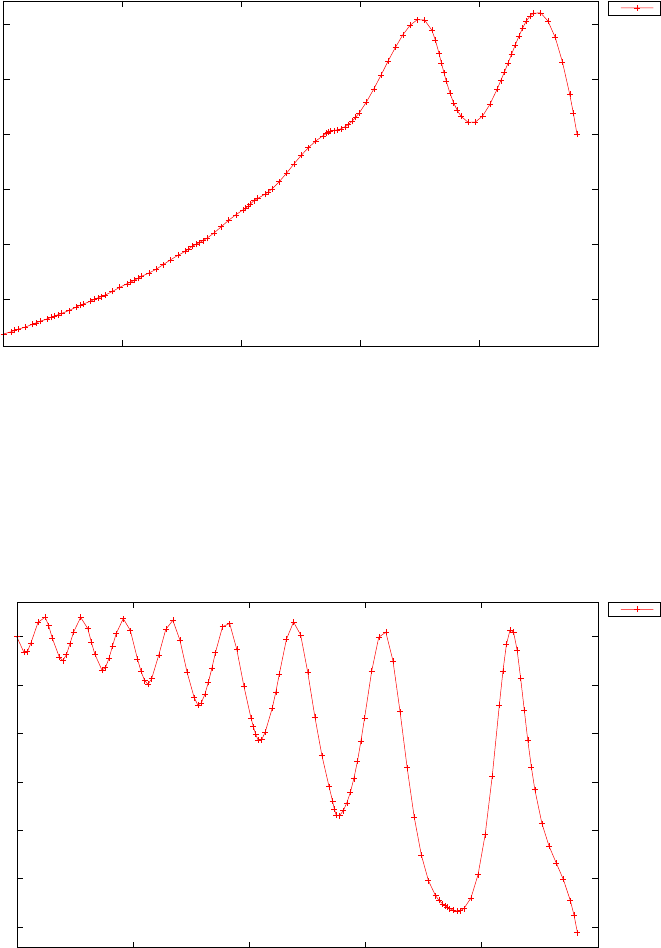
25
30
35
40
45
50
0 5 10 15 20 25
p (1000000 ft)
time (h)
Low thrust transfer problem: states
p
Figure 3.53: Modified equinoctial element p
-0.12
-0.1
-0.08
-0.06
-0.04
-0.02
0
0 5 10 15 20 25
f
time (h)
Low thrust transfer problem: states
f
Figure 3.54: Modified equinoctial element f
253
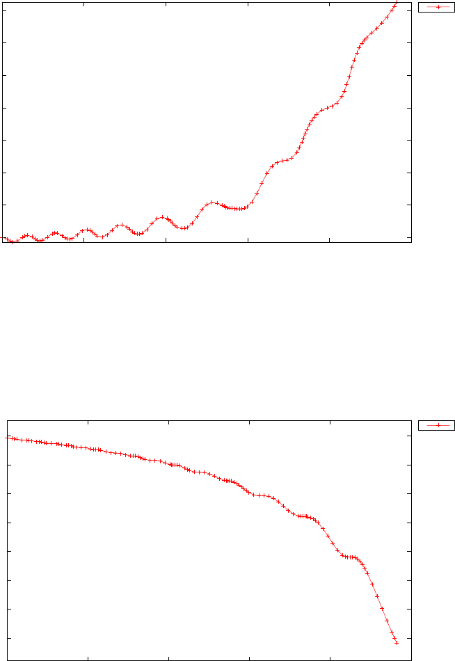
0
0.1
0.2
0.3
0.4
0.5
0.6
0.7
0 5 10 15 20 25
g
time (h)
Low thrust transfer problem: states
g
Figure 3.55: Modified equinoctial element g
-0.6
-0.55
-0.5
-0.45
-0.4
-0.35
-0.3
-0.25
0 5 10 15 20 25
h
time (h)
Low thrust transfer problem: states
h
Figure 3.56: Modified equinoctial element h
254
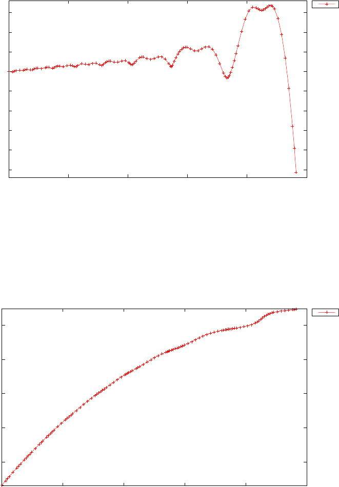
-0.1
-0.08
-0.06
-0.04
-0.02
0
0.02
0.04
0.06
0 5 10 15 20 25
k
time (h)
Low thrust transfer problem: states
k
Figure 3.57: Modified equinoctial element k
10
20
30
40
50
0 5 10 15 20 25
L (rev)
time (h)
Low thrust transfer problem: states
L
Figure 3.58: Modified equinoctial element L
255
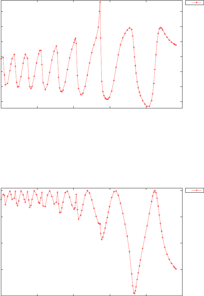
-0.4
-0.2
0
0.2
0.4
0.6
0.8
0 5 10 15 20 25
ur
time (h)
Low thrust transfer problem: controls
ur
Figure 3.59: Radial component of the thrust direction vector, ur
-1
-0.5
0
0.5
1
0 5 10 15 20 25
ut
time (h)
Low thrust transfer problem: controls
ut
Figure 3.60: Tangential component of the thrust direction vector, ut
256
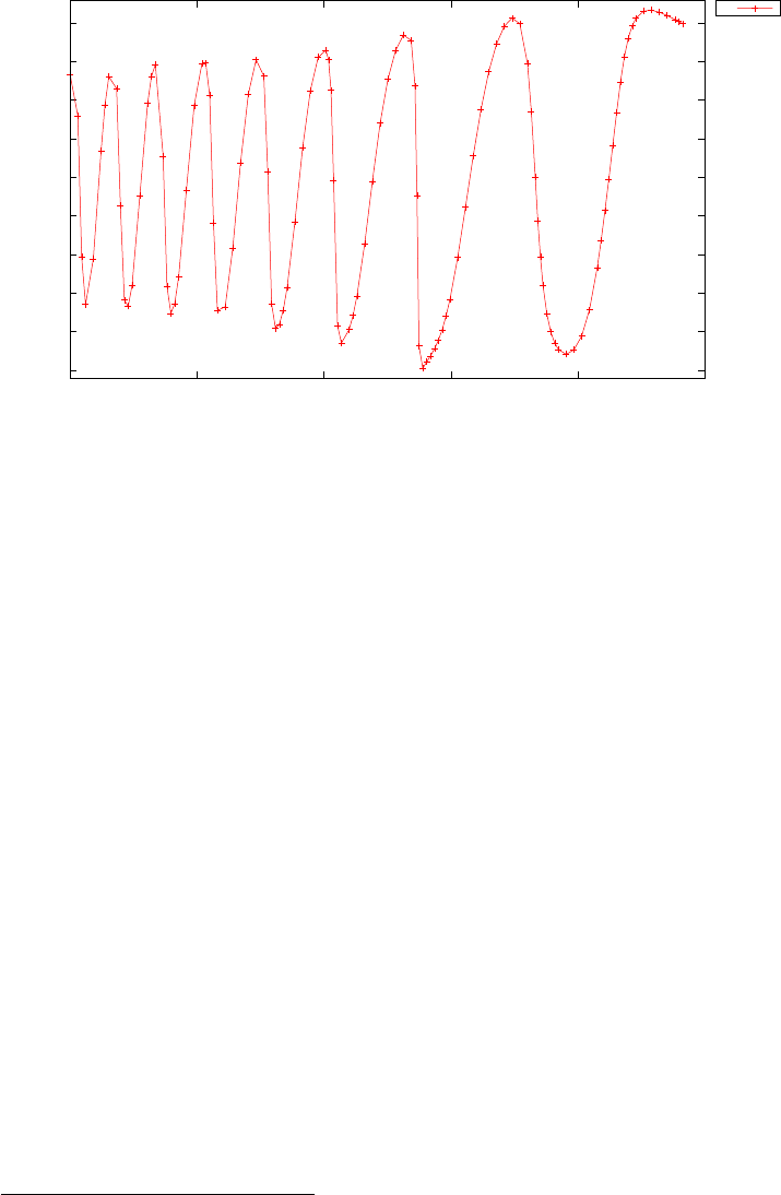
-1
-0.8
-0.6
-0.4
-0.2
0
0.2
0.4
0.6
0.8
0 5 10 15 20 25
uh
time (h)
Low thrust transfer problem: controls
uh
Figure 3.61: Normal component of the thrust direction vector, uh
M(q(t))¨
q(t) = V(q(t),˙
q(t)) + G(q(t)) + Du(t)
where q= [q1(t), q2(t), q3(t)]Tis the vector of relative angles between the
links, the normalized torque controls are u(t)=[u1(t), u2(t), u3(t)]T,Dis
a diagonal matrix with constant values, M(q) is a symmetric inertia ma-
trix, V(q(t),˙
q(t)) are the torques caused by coriolis and centrifugal forces,
G(q(t)) are gravitational torques. The model is described in detail in [31]
and is fully included in the code for this example3.
The example reported here consists of a minimum energy point to point
trajectory, so that the objective is to find tfand u(t)=[u1(t), u2(t), u3(t)]T,
t∈[0, tf] to minimise:
J=Ztf
0
u(t)Tu(t)dt(3.107)
The boundary conditions associated with the problem are:
q(0) = 0−1.5 0T
˙
q(0) = 0 0 0T
q(tf) = 1.0−1.95 1.0T
˙
q(tf) = 0 0 0T
(3.108)
3Dr. Martin Otter from DLR, Germany, has kindly authorised the author to publish
a translated form of subroutine R3M2SI as part of the PSOPT distribution.
257

The PSOPT code that solves this problem is shown below.
//////////////////////////////////////////////////////////////////////////
//////////////// manutec.cxx /////////////////////
//////////////////////////////////////////////////////////////////////////
//////////////// PSOPT example /////////////////////
//////////////////////////////////////////////////////////////////////////
//////////////////////////////////////////////////////////////////////////
//////// Title: Minimum time control of a Manutec R3 robot ///////
//////// Last modified: 25 January 2010 ////////////////
//////// Reference: Chettibi et al (2007) ////////////////
//////// ////////////////
//////////////////////////////////////////////////////////////////////////
//////// Copyright (c) Victor M. Becerra, 2009 ////////////////
//////////////////////////////////////////////////////////////////////////
//////// This is part of the PSOPT software library, which ///////////////
//////// is distributed under the terms of the GNU Lesser ////////////////
//////// General Public License (LGPL) ////////////////
//////////////////////////////////////////////////////////////////////////
#include "psopt.h"
// Set option to: 1 for minimum time problem
// 2 for minimum time with regularization
// 3 for minimum energy problem
#define OBJ_OPTION 3
typedef struct {
double g; // Gravity constant
double pl; // Point mass of load;
double Ia1; // Moment of inertia of arm 1, element (3,3)
DMatrix* Fc; // Voltage-force constant of motor
DMatrix* r; // Gear ratio of motor
DMatrix* Im; // Moment of inertia of motor
DMatrix* m; // Mass of arm 2 and 3
DMatrix* L; // Length of arm 2 and 3 (inc. tool)
DMatrix* com; // Center of mass coordinates of arm 2 and 3;
DMatrix* Ia; // Moment of inertia arm 2 and 3
} CONSTANTS_;
CONSTANTS_ CONSTANTS;
typedef struct {
adouble* qdd_ad;
adouble* F_ad;
adouble* qd_ad;
adouble* q_ad;
adouble* kw;
adouble* beta;
adouble* afor;
adouble* wabs;
adouble* zeta;
adouble* cosp;
adouble* ator;
adouble* sinp;
adouble* rhicm;
adouble* genvd ;
adouble* mrel12 ;
adouble* mrel22;
adouble* rhrel2;
adouble* workm3;
adouble* workm6;
adouble* works1;
adouble* works2;
adouble* workv3;
adouble* workv6;
adouble* cmhges;
adouble* ihhges;
adouble* inertc;
adouble* inertg;
adouble* inerth;
adouble* workam;
adouble* workas;
adouble* wworkm;
258

adouble* wworkv;
} VARS_;
VARS_ VARS;
void r3m2si(double *ml, adouble *aq, adouble *aqd,
adouble *fgen, adouble *aqdd, VARS_ *vars);
//////////////////////////////////////////////////////////////////////////
/////////////////// Define the end point (Mayer) cost function //////////
//////////////////////////////////////////////////////////////////////////
adouble endpoint_cost(adouble* initial_states, adouble* final_states,
adouble* parameters,adouble& t0, adouble& tf,
adouble* xad, int iphase, Workspace* workspace)
{
adouble retval;
if (OBJ_OPTION==1 || OBJ_OPTION==2 ) retval = tf;
else retval = 0.0;
return retval;
}
//////////////////////////////////////////////////////////////////////////
/////////////////// Define the integrand (Lagrange) cost function //////
//////////////////////////////////////////////////////////////////////////
adouble integrand_cost(adouble* states, adouble* controls, adouble* parameters,
adouble& time, adouble* xad, int iphase, Workspace* workspace)
{
adouble retval;
adouble* u = controls;
adouble* qdot = &states[3];
double rho;
if (OBJ_OPTION==1) rho = 0.0;
else if (OBJ_OPTION==2) rho = 1.e-5;
else if (OBJ_OPTION==3) rho = 1.0;
retval = rho*dot( u, u, 3 );
return (retval);
}
//////////////////////////////////////////////////////////////////////////
/////////////////// Define the DAE’s ////////////////////////////////////
//////////////////////////////////////////////////////////////////////////
void dae(adouble* derivatives, adouble* path, adouble* states,
adouble* controls, adouble* parameters, adouble& time,
adouble* xad, int iphase, Workspace* workspace)
{
int i;
double g = CONSTANTS.g;
DMatrix& Fc = *CONSTANTS.Fc;
DMatrix& r = *CONSTANTS.r;
DMatrix& Im = *CONSTANTS.Im;
DMatrix& m = *CONSTANTS.m;
double pl = CONSTANTS.pl;
DMatrix& L = *CONSTANTS.L;
DMatrix& com= *CONSTANTS.com;
double Ia1= CONSTANTS.Ia1;
DMatrix& Ia = *CONSTANTS.Ia;
adouble* F = VARS.F_ad;
adouble* qdd = VARS.qdd_ad;
adouble* qd = VARS.qd_ad;
259

adouble* q = VARS.q_ad;
double ml = pl;
for(i=0;i<3;i++) {
q[i] = states[i];
qd[i] = states[3+i];
F[i] = Fc(i+1)*controls[i];
}
r3m2si(&ml, q, qd, F, qdd, &VARS);
derivatives[CINDEX(1)] = qd[CINDEX(1)];
derivatives[CINDEX(2)] = qd[CINDEX(2)];
derivatives[CINDEX(3)] = qd[CINDEX(3)];
derivatives[CINDEX(4)] = qdd[CINDEX(1)];
derivatives[CINDEX(5)] = qdd[CINDEX(2)];
derivatives[CINDEX(6)] = qdd[CINDEX(3)];
}
////////////////////////////////////////////////////////////////////////////
/////////////////// Define the events function ////////////////////////////
////////////////////////////////////////////////////////////////////////////
void events(adouble* e, adouble* initial_states, adouble* final_states,
adouble* parameters,adouble& t0, adouble& tf, adouble* xad,
int iphase, Workspace* workspace)
{
int i;
for (i=0; i< 6; i++ ) {
e[ i ] = initial_states[ i ];
}
for (i=0; i< 6; i++ ) {
e[6 + i ] = final_states[ i ];
}
}
///////////////////////////////////////////////////////////////////////////
/////////////////// Define the phase linkages function ///////////////////
///////////////////////////////////////////////////////////////////////////
void linkages( adouble* linkages, adouble* xad, Workspace* workspace)
{
// Single phase problem
}
////////////////////////////////////////////////////////////////////////////
/////////////////// Define the main routine ///////////////////////////////
////////////////////////////////////////////////////////////////////////////
int main(void)
{
double g = 9.81; // Gravity constant [m/s2]
double pl= 0.0; // Point mass of load; [kg]
double Ia1 = 1.16; // Moment of inertia of arm 1, element (3,3) [kgm^2]
DMatrix Fc(3,1); Fc = "[-126.0;252.0; 72.0]"; // Voltage-force constant of motor [N*m/V]
DMatrix r(3,1); r = "[-105; 210; 60]"; // Gear ratio of motor
DMatrix Im(3,1); Im = "[1.3e-3; 1.3e-3; 1.3e-3]"; // Moment of inertia of motor [kg*m^2]
DMatrix m(2,1); m = "[56.5; 60.3]"; // Mass of arm 2 and 3 [kg]
DMatrix L(2,1); L = "[0.5; 0.98]"; // Length of arm 2 and 3 (inc. tool) [m]
DMatrix com(2,2); // Center of mass coordinates of arm 2 and 3; [m]
DMatrix Ia(4,2); // Moment of inertia arm 2 and 3 [kg*m^2]
com(1,1)=0.172; com(1,2)=0.028; com(2,1)=0.205; com(2,2)=0.202;
Ia(1,1)=2.58; Ia(1,2)=11.0;
Ia(2,1)=2.73; Ia(2,2)=8.0;
Ia(3,1)=0.64; Ia(3,2)=0.80;
260

Ia(4,1)=-0.46; Ia(4,2)=0.50;
Fc.Print("Fc");
r.Print("r");
Im.Print("Im");
m.Print("m");
L.Print("L");
com.Print("com");
Ia.Print("Ia");
CONSTANTS.g = g;
CONSTANTS.pl = pl;
CONSTANTS.Ia1 = Ia1;
CONSTANTS.Fc = &Fc;
CONSTANTS.r = &r;
CONSTANTS.Im = ℑ
CONSTANTS.m = &m;
CONSTANTS.L = &L;
CONSTANTS.com= &com;
CONSTANTS.Ia = &Ia;
VARS.qdd_ad = new adouble[3];
VARS.qd_ad = new adouble[3];
VARS.q_ad = new adouble[3];
VARS.F_ad = new adouble[3];
VARS.kw = new adouble[9];
VARS.beta = new adouble[18];
VARS.afor = new adouble[9];
VARS.wabs = new adouble[9];
VARS.zeta = new adouble[18];
VARS.cosp = new adouble[3];
VARS.ator = new adouble[9];
VARS.sinp = new adouble[3];
VARS.rhicm = new adouble[9];
VARS.genvd = new adouble[3];
VARS.mrel12 = new adouble[18];
VARS.mrel22 = new adouble[3];
VARS.rhrel2 = new adouble[3];
VARS.workm3 = new adouble[9];
VARS.workm6 = new adouble[180];
VARS.works1 = new adouble[12];
VARS.works2 = new adouble[6];
VARS.workv3 = new adouble[39];
VARS.workv6 = new adouble[24];
VARS.cmhges = new adouble[3];
VARS.ihhges = new adouble[9];
VARS.inertc = new adouble[27];
VARS.inertg = new adouble[108];
VARS.inerth = new adouble[27];
VARS.workam = new adouble[144];
VARS.workas = new adouble[40];
VARS.wworkm = new adouble[54];
VARS.wworkv = new adouble[9];
////////////////////////////////////////////////////////////////////////////
/////////////////// Declare key structures ////////////////////////////////
////////////////////////////////////////////////////////////////////////////
Alg algorithm;
Sol solution;
Prob problem;
////////////////////////////////////////////////////////////////////////////
/////////////////// Register problem name ////////////////////////////////
////////////////////////////////////////////////////////////////////////////
problem.name = "Manutec R3 robot problem";
problem.outfilename = "manutec.txt";
////////////////////////////////////////////////////////////////////////////
//////////// Define problem level constants & do level 1 setup ////////////
////////////////////////////////////////////////////////////////////////////
problem.nphases = 1;
problem.nlinkages = 0;
psopt_level1_setup(problem);
261

/////////////////////////////////////////////////////////////////////////////
///////// Define phase related information & do level 2 setup ////////////
/////////////////////////////////////////////////////////////////////////////
problem.phases(1).nstates = 6;
problem.phases(1).ncontrols = 3;
problem.phases(1).nevents = 12;
problem.phases(1).npath = 0;
problem.phases(1).nodes = "[20, 30, 40, 60, 80]";
psopt_level2_setup(problem, algorithm);
////////////////////////////////////////////////////////////////////////////
/////////////////// Enter problem bounds information //////////////////////
////////////////////////////////////////////////////////////////////////////
DMatrix qmax(1,3), qdmax(1,3), qddmax(1,3);
// Joint position limits in rad
qmax(1) = 2.97; qmax(2) = 2.01; qmax(3) = 2.86;
// Joint angular velocity limits in rad/s
qdmax(1) = 3.0; qdmax(2) = 1.5; qdmax(3) = 5.2;
problem.phases(1).bounds.lower.states = (-qmax || -qdmax);
problem.phases(1).bounds.upper.states = ( qmax || qdmax);
DMatrix umax(1,3);
// Control variable limits in V
umax(1) = 7.5; umax(2) = 7.5; umax(3) = 7.5;
problem.phases(1).bounds.lower.controls = -umax;
problem.phases(1).bounds.upper.controls = umax;
DMatrix qi(1,3), qf(1,3), qdi(1,3), qdf(1,3);
// Initial joint positions in rad
qi(1) = 0.0; qi(2) = -1.5; qi(3) = 0.0;
// Final joint positions in rad
qf(1) = 1.0; qf(2) = -1.95; qf(3) = 1.0;
// Initial joint velocities in rad/s
qdi = zeros(1,3);
// Final joint velocities in rad/s
qdf = zeros(1,3);
problem.phases(1).bounds.lower.events = (qi || qdi || qf || qdf);
problem.phases(1).bounds.upper.events = (qi || qdi || qf || qdf);
problem.phases(1).bounds.lower.StartTime = 0.0;
problem.phases(1).bounds.upper.StartTime = 0.0;
if (OBJ_OPTION==1 || OBJ_OPTION==2) {
problem.phases(1).bounds.lower.EndTime = 0.0;
problem.phases(1).bounds.upper.EndTime = 1.0;
}
else {
problem.phases(1).bounds.lower.EndTime = 0.53;
problem.phases(1).bounds.upper.EndTime = 0.53;
}
262

////////////////////////////////////////////////////////////////////////////
/////////////////// Register problem functions ///////////////////////////
////////////////////////////////////////////////////////////////////////////
problem.integrand_cost = &integrand_cost;
problem.endpoint_cost = &endpoint_cost;
problem.dae = &dae;
problem.events = &events;
problem.linkages = &linkages;
////////////////////////////////////////////////////////////////////////////
/////////////////// Define & register initial guess ///////////////////////
////////////////////////////////////////////////////////////////////////////
int nnodes = problem.phases(1).nodes(1);
int ncontrols = problem.phases(1).ncontrols;
int nstates = problem.phases(1).nstates;
DMatrix state_guess = zeros(nstates,nnodes);
DMatrix control_guess = zeros(ncontrols,nnodes);
DMatrix time_guess = linspace(0.0,0.53,nnodes);
state_guess(1,colon()) = linspace( qi(1), qf(1), nnodes );
state_guess(2,colon()) = linspace( qi(2), qf(2), nnodes );
state_guess(3,colon()) = linspace( qi(3), qf(3), nnodes );
state_guess(4,colon()) = linspace( qi(4), qf(4), nnodes );
state_guess(5,colon()) = linspace( qi(5), qf(5), nnodes );
state_guess(6,colon()) = linspace( qi(6), qf(6), nnodes );
problem.phases(1).guess.states = state_guess;
problem.phases(1).guess.controls = control_guess;
problem.phases(1).guess.time = time_guess;
////////////////////////////////////////////////////////////////////////////
/////////////////// Enter algorithm options //////////////////////////////
////////////////////////////////////////////////////////////////////////////
algorithm.nlp_iter_max = 1000;
algorithm.nlp_tolerance = 1.e-6;
algorithm.nlp_method = "IPOPT";
algorithm.scaling = "automatic";
algorithm.derivatives = "automatic";
algorithm.mesh_refinement = "automatic";
algorithm.ode_tolerance = 1.e-5;
algorithm.mr_max_iterations = 5;
////////////////////////////////////////////////////////////////////////////
/////////////////// Now call PSOPT to solve the problem //////////////////
////////////////////////////////////////////////////////////////////////////
psopt(solution, problem, algorithm);
////////////////////////////////////////////////////////////////////////////
/////////// Extract relevant variables from solution structure //////////
////////////////////////////////////////////////////////////////////////////
DMatrix x, u, t;
x = solution.get_states_in_phase(1);
u = solution.get_controls_in_phase(1);
t = solution.get_time_in_phase(1);
////////////////////////////////////////////////////////////////////////////
/////////// Save solution data to files if desired ////////////////////////
////////////////////////////////////////////////////////////////////////////
x.Save("x.dat");
u.Save("u.dat");
t.Save("t.dat");
DMatrix q = x( colon(1,3), colon() );
DMatrix qd= x( colon(4,6), colon() );
263

////////////////////////////////////////////////////////////////////////////
/////////// Plot some results if desired (requires gnuplot) ///////////////
////////////////////////////////////////////////////////////////////////////
plot(t,q,problem.name+": positions","t", "q (rad)", "q1 q2 q3");
plot(t,qd,problem.name+": velocities","t", "qdot (rad/s)", "qd1 qd2 qd3");
plot(t,u(1,colon()),problem.name+": control u1","time (s)", "control", "u1");
plot(t,u(2,colon()),problem.name+": control u2","time (s)", "control", "u2");
plot(t,u(3,colon()),problem.name+": control u3","time (s)", "control", "u3");
plot(t,q,problem.name+": positions","t", "q (rad)", "q1 q2 q3", "pdf",
"positions.pdf");
plot(t,qd,problem.name+": velocities","t", "qdot (rad/s)", "qd1 qd2 qd3", "pdf",
"velocities.pdf");
plot(t,u,problem.name+": controls","time (s)", "controls", "u1 u2 u3",
"pdf", "controls.pdf");
}
void r3m2si(double *ml, adouble *aq, adouble *aqd,
adouble *fgen, adouble *aqdd, VARS_ *vars)
{
adouble mhges;
adouble* kw = vars->kw;
adouble* beta = vars->beta;
adouble* afor = vars->afor;
adouble* wabs = vars->wabs;
adouble* zeta = vars->zeta;
adouble* cosp = vars->cosp;
adouble* ator = vars->ator;
adouble* sinp = vars->sinp;
adouble* rhicm = vars->rhicm;
adouble* genvd = vars->genvd;
adouble* mrel12 = vars->mrel12;
adouble* mrel22 = vars->mrel22;
adouble* rhrel2 = vars->rhrel2;
adouble* workm3 = vars->workm3;
adouble* workm6 = vars->workm6;
adouble* works1 = vars->works1;
adouble* works2 = vars->works2;
adouble* workv3 = vars->workv3;
adouble* workv6 = vars->workv6;
adouble* cmhges = vars->cmhges;
adouble* ihhges = vars->ihhges;
adouble* inertc = vars->inertc;
adouble* inertg = vars->inertg;
adouble* inerth = vars->inerth;
adouble* workam = vars->workam;
adouble* workas = vars->workas;
adouble* wworkm = vars->wworkm;
adouble* wworkv = vars->wworkv;
/* Simulation model equations of the Manutec r3 robot (DFVLR model 2) */
/* This is a modified C++ tranlation of the original Fortran subroutine R3M2SI */
/* by Otter and co-workers, published here with kind persmission from Dr. Martin Otter */
/* DSL, Germany */
/* Procedure purpose: */
/* This subroutine calculates the generalized accelerations (AQDD) for */
/* the Manutec r3 robot of the DFVLR model 2. This model is based on */
/* the following assumptions: */
/* - The last 3 joints (joints 4,5,6) of the robot hand do not move. */
/* This corresponds to the case that the brakes in these joints are */
/* blocked (joints 4,5,6 are taken into account in model 1). */
/* - The robot consists of a base body (the environment), three arms */
264

/* and three rotors. The rotors represent the inertia effects of the */
/* motors and of the wheels of the gear boxes. The rotors are */
/* embedded in the preceeding arms, e.g. the rotor 2, which drives */
/* arm2, is embedded in arm1. */
/* - Arms and rotors are considered to be rigid bodies. */
/* - Elasticity, backlash and friction in the gear boxes are neglected. */
/* - The motors are modelled as ideal voltage-torque converters */
/* without any dynamic effects. As input arguments of the subroutine */
/* the torques at the gear output (FGEN in <Nm>) must be given. If the */
/* voltage (U in <V>) at the input of the current regulator of the */
/* motor is given, FGEN must be calculated (before calling this */
/* subroutine) in the following way: */
/* FGEN(1) = -126.0*U(1) */
/* FGEN(2) = 252.0*U(2) */
/* FGEN(3) = 72.0*U(3) */
/* - At the robot’s tip a load mass (ML) is attached. It can range */
/* between 0 ... 15 kg. */
/* Given the actual value ML of the load mass, the joint angles AQ(i), */
/* the derivatives of the joint angles AQD(i), and the driving torques */
/* in the joints FGEN(i), the second derivatives of the joint angles */
/* AQDD(i) are calculated by this subroutine. */
/* Usage: */
/* CALL R3M2SI (ML, AQ, AQD, FGEN, AQDD) */
/* ML : IN, DOUBLE, <kg>, 0<=ML<=15 */
/* Load mass. */
/* AQ : IN, DOUBLE(3), <rad>, -2.97 <= AQ(1) <= 2.97 (+/- 170 deg), */
/* -2.01 <= AQ(2) <= 2.01 (+/- 115 deg), */
/* -2.86 <= AQ(3) <= 2.86 (+/- 164 deg) */
/* (The given limits are hardware constraints by limit switches). */
/* Vector of generalized coordinates (relative angles between */
/* two contigous robot arms). */
/* AQ(1) is not used in this subroutine, because it is not */
/* needed to calculate AQDD. */
/* AQD : IN, DOUBLE(3), <rad/sec>, */
/* -3.0 <= AQD(1) <= 3.0 (+/- 172 deg/sec), */
/* -1.5 <= AQD(2) <= 1.5 (+/- 86 deg/sec), */
/* -5.2 <= AQD(3) <= 5.2 (+/- 298 deg/sec) */
/* Derivative of AQ. */
/* FGEN : IN, DOUBLE(3), <Nm>, -945.0 <= FGEN(1) <= 945.0, */
/* -1890.0 <= FGEN(2) <= 1890.0, */
/* -540.0 <= FGEN(3) <= 540.0 */
/* Torque at the gear output. */
/* AQDD : OUT, DOUBLE(3), <rad/sec**2> */
/* Second derivative of AQ. */
/* Bibliography: */
/* A detailed description of the model, together with the body-data */
/* (mass, center of mass etc. of the arms and rotors) is given in */
/* Otter M., Tuerk S., Mathematical Model of the Manutec r3 Robot, */
/* (DFVLR Model No. 2), DFVLR - Oberpfaffenhofen, Institut fuer */
/* Dynamik der Flugsysteme, D-8031 Wessling, West Germany, */
/* corrected version april 1988. */
/* This subroutine was generated by the program MYROBOT. See */
/* Otter M., Schlegel S., Symbolic generation of efficient simulation */
/* codes for robots. 2nd European Simulation Multiconference, */
/* June 1-3, 1988, Nice. */
/* The underlying multibody algorithm is a modified version of */
/* Brandl H., Johanni R., Otter M., A very efficient algorithm for the */
/* simulation of robots and similar multibody systems without */
/* inversion of the mass matrix. IFAC/IFIP/IMACS International */
/* Symposium on Theory of Robots, december 3-5, 1986, Vienna. */
/* Remarks: */
/* - The limits given for the input variables are not checked in */
/* this subroutine. The user is responsible for proper data. */
/* - If a SINGLE PRECISION version of this subroutine is desired, just */
/* change all strings from DOUBLE PRECISION to REAL in the declaration */
/* part. */
/* Copyright: */
/* 1988 DFVLR - Institut fuer Dynamik der Flugsysteme */
/* Life cycle: */
265

/* 1988 APR M. Otter, S. Tuerk (DFVLR) : specified. */
/* 1988 APR M. Otter (DFVLR) : generated. */
/* 1988 APR M. Otter, C. Schlegel, S. Tuerk (DFVLR): tested. */
/* ----------------------------------------------------------------------- */
/* Statistical information (MySymbol-Version 1.2) */
/* ============================================== */
/* 1. Number of Operations: */
/* ------------------------ */
/* + - | * | / | sin | cos | sqrt| */
/* -----|-----|-----|-----|-----|-----| */
/* Without simplifications 3180| 3702| 26| 3| 3| 0| */
/* -----|-----|-----|-----|-----|-----| */
/* Terms simplified 222| 247| 23| 3| 3| 0| */
/* -----|-----|-----|-----|-----|-----| */
/* Unnecessary statements | | | | | | */
/* removed 140| 159| 17| 2| 2| 0| */
/* 2. Storage information: */
/* ----------------------- */
/* INTEGER | | */
/* words | | */
/* --------|---------| */
/* available storage 100000 | 100.0 % | */
/* --------|---------| */
/* array-elements 1412 | 1.4 % | */
/* --------|---------| */
/* double-numbers 104 | 0.1 % | */
/* --------|---------| */
/* statement buffer 2552 | 2.6 % | */
/* +++++++++++++++++++++++++++++++++++++++ */
/* used storage 4068 | 4.1 % | */
/* --------|---------| */
/* free storage 95932 | 95.9 % | */
/* ----------------------------------------------------------------------- */
/* cccccccccccccccccccccccc Procedural section cccccccccccccccccccccccccc */
/* Parameter adjustments */
--aqdd;
--fgen;
--aqd;
--aq;
/* Function Body */
workv3[14] = *ml * .98;
workv3[17] = workv3[14] + 12.1806;
mhges = *ml + 60.3;
cmhges[0] = 1.6884 / mhges;
cmhges[2] = workv3[17] / mhges;
workv3[20] = workv3[14] * .98;
ihhges[0] = workv3[20] + 7.8704812;
ihhges[4] = workv3[20] + 8.1077564;
sinp[1] = sin(aq[2]);
cosp[1] = cos(aq[2]);
wworkv[0] = mhges * cmhges[0];
wworkv[2] = mhges * cmhges[2];
wworkv[3] = cmhges[0] * wworkv[0];
wworkv[5] = cmhges[2] * wworkv[2];
wworkv[6] = wworkv[3] + wworkv[5];
wworkm[0] = wworkv[6] - wworkv[3];
wworkm[8] = wworkv[6] - wworkv[5];
wworkm[6] = -wworkv[0] * cmhges[2];
inertc[18] = ihhges[0] - wworkm[0];
inertc[22] = ihhges[4] - wworkv[6];
inertc[24] = -.0110568 - wworkm[6];
inertc[26] = .4372752 - wworkm[8];
sinp[2] = sin(aq[3]);
cosp[2] = cos(aq[3]);
/* ** The equations of motion have been generated with the algorithm */
/* ** of Brandl/Johanni/Otter (variant 6) */
/* ** Forward recursion -------------------------------------------------- */
/* -- Quantities of body 1 */
/* -- Quantities of body 2 */
wabs[4] = sinp[1] * aqd[1];
wabs[5] = cosp[1] * aqd[1];
workv3[1] = aqd[1] * aqd[2];
zeta[7] = cosp[1] * workv3[1];
zeta[8] = -sinp[1] * workv3[1];
kw[3] = aqd[2] * 4.9544125 - wabs[5] * 2.45219;
266

kw[4] = wabs[4] * 6.7759085;
kw[5] = aqd[2] * -2.45219 + wabs[5] * 2.311496;
/* -- Quantities of body 3 */
workv3[19] = -sinp[2] * cmhges[2];
workv3[20] = cosp[2] * cmhges[2];
workm3[4] = cosp[2] * inertc[22];
workm3[5] = sinp[2] * inertc[22];
workm3[7] = -sinp[2] * inertc[26];
workm3[8] = cosp[2] * inertc[26];
inertc[21] = -inertc[24] * sinp[2];
inertc[22] = workm3[4] * cosp[2] - workm3[7] * sinp[2];
inertc[24] *= cosp[2];
inertc[25] = workm3[4] * sinp[2] + workm3[7] * cosp[2];
inertc[26] = workm3[5] * sinp[2] + workm3[8] * cosp[2];
workv3[21] = mhges * cmhges[0];
workv3[22] = mhges * workv3[19];
workv3[23] = mhges * workv3[20];
workv3[24] = cmhges[0] * workv3[21];
workv3[25] = workv3[19] * workv3[22];
workv3[26] = workv3[20] * workv3[23];
workv3[27] = workv3[24] + workv3[25] + workv3[26];
inerth[18] = workv3[27] - workv3[24];
inerth[22] = workv3[27] - workv3[25];
inerth[26] = workv3[27] - workv3[26];
inerth[21] = -workv3[21] * workv3[19];
inerth[24] = -workv3[21] * workv3[20];
inerth[25] = -workv3[22] * workv3[20];
inerth[18] += inertc[18];
inerth[21] += inertc[21];
inerth[22] += inertc[22];
inerth[24] += inertc[24];
inerth[25] += inertc[25];
inerth[26] += inertc[26];
wabs[6] = aqd[3] + aqd[2];
workv3[1] = wabs[5] * aqd[3];
workv3[2] = -wabs[4] * aqd[3];
workv3[6] = wabs[4] * .5;
workv3[7] = -aqd[2] * .5;
workv3[9] = -wabs[5] * workv3[7];
workv3[10] = wabs[5] * workv3[6];
workv3[11] = aqd[2] * workv3[7] - wabs[4] * workv3[6];
rhicm[6] = mhges * cmhges[0];
rhicm[7] = mhges * workv3[19];
rhicm[8] = mhges * workv3[20];
kw[6] = inerth[18] * wabs[6] + inerth[21] * wabs[4] + inerth[24] * wabs[5]
;
kw[7] = inerth[21] * wabs[6] + inerth[22] * wabs[4] + inerth[25] * wabs[5]
;
kw[8] = inerth[24] * wabs[6] + inerth[25] * wabs[4] + inerth[26] * wabs[5]
;
ator[3] = -wabs[4] * kw[5] + wabs[5] * kw[4];
ator[4] = -wabs[5] * kw[3] + aqd[2] * kw[5];
ator[5] = -aqd[2] * kw[4] + wabs[4] * kw[3];
ator[6] = -wabs[4] * kw[8] + wabs[5] * kw[7];
ator[7] = -wabs[5] * kw[6] + wabs[6] * kw[8];
ator[8] = -wabs[6] * kw[7] + wabs[4] * kw[6];
workv3[15] = wabs[4] * rhicm[8] - wabs[5] * rhicm[7];
workv3[16] = wabs[5] * rhicm[6] - wabs[6] * rhicm[8];
workv3[17] = wabs[6] * rhicm[7] - wabs[4] * rhicm[6];
afor[6] = -wabs[4] * workv3[17] + wabs[5] * workv3[16];
afor[7] = -wabs[5] * workv3[15] + wabs[6] * workv3[17];
/* ** Backward recursion ------------------------------------------------- */
/* -- Quantities of body 3 */
mrel22[2] = inerth[18] + 4.68;
workv6[0] = ator[6] - inerth[21] * workv3[1] - inerth[24] * workv3[2] +
rhicm[8] * workv3[10] - rhicm[7] * workv3[11];
workv6[1] = ator[7] - inerth[22] * workv3[1] - inerth[25] * workv3[2] -
rhicm[8] * workv3[9] + rhicm[6] * workv3[11];
workv6[2] = ator[8] - inerth[25] * workv3[1] - inerth[26] * workv3[2] +
rhicm[7] * workv3[9] - rhicm[6] * workv3[10];
workv6[3] = afor[6] - rhicm[8] * workv3[1] + rhicm[7] * workv3[2] - mhges
* workv3[9];
workv6[4] = afor[7] - rhicm[6] * workv3[2] - mhges * workv3[10];
rhrel2[2] = fgen[3] + workv6[0];
mrel12[12] = inerth[18] + .078 + rhicm[8] * .5;
workv6[18] = workv6[0] - workv6[4] * .5;
workv6[19] = workv6[1] + workv6[3] * .5;
workm6[108] = inerth[18] - rhicm[8] * -.5;
workm6[112] = -rhicm[8] + mhges * -.5;
workm6[115] = inerth[22] + rhicm[8] * .5;
workm6[117] = rhicm[8] + mhges * .5;
inertg[36] = workm6[108] + 4.9544125 - workm6[112] * .5;
inertg[43] = workm6[115] + 6.7759085 + workm6[117] * .5;
267

inertg[48] = inerth[24] - 2.45219 - rhicm[6] * .5;
inertg[49] = inerth[25] - rhicm[7] * .5;
inertg[50] = inerth[26] + 2.311496;
inertg[60] = -11.5825 - rhicm[8] - mhges * .5;
inertg[62] = rhicm[6] + 9.718;
inertg[67] = -9.718 - rhicm[6];
beta[6] = ator[3] + workv6[18];
beta[7] = ator[4] + workv6[19];
beta[8] = ator[5] + workv6[2];
works2[0] = mrel12[12] / mrel22[2];
works2[1] = inerth[21] / mrel22[2];
works2[2] = inerth[24] / mrel22[2];
works2[4] = -rhicm[8] / mrel22[2];
works2[5] = rhicm[7] / mrel22[2];
inertg[36] -= mrel12[12] * works2[0];
inertg[42] = inerth[21] - mrel12[12] * works2[1];
inertg[43] -= inerth[21] * works2[1];
inertg[48] -= mrel12[12] * works2[2];
inertg[49] -= inerth[21] * works2[2];
inertg[50] -= inerth[24] * works2[2];
inertg[60] -= mrel12[12] * works2[4];
inertg[61] = -inerth[21] * works2[4];
inertg[62] -= inerth[24] * works2[4];
inertg[66] = rhicm[7] - mrel12[12] * works2[5];
inertg[67] -= inerth[21] * works2[5];
inertg[68] = -inerth[24] * works2[5];
beta[6] -= works2[0] * rhrel2[2];
beta[7] -= works2[1] * rhrel2[2];
beta[8] -= works2[2] * rhrel2[2];
/* -- Quantities of body 2 */
mrel22[1] = inertg[36] + 57.33;
workv6[0] = beta[6] - inertg[42] * zeta[7] - inertg[48] * zeta[8];
workv6[1] = beta[7] - inertg[43] * zeta[7] - inertg[49] * zeta[8];
workv6[2] = beta[8] - inertg[49] * zeta[7] - inertg[50] * zeta[8];
rhrel2[1] = fgen[2] + workv6[0];
works1[8] = sinp[1] * inertg[42] + cosp[1] * inertg[48];
works1[11] = sinp[1] * inertg[60] + cosp[1] * inertg[66];
workv6[14] = sinp[1] * workv6[1] + cosp[1] * workv6[2];
workas[30] = cosp[1] + sinp[1];
workas[31] = cosp[1] - sinp[1];
workas[33] = workas[30] * workas[31];
workas[32] = cosp[1] * sinp[1];
workas[34] = workas[32] + workas[32];
workas[0] = inertg[50] + inertg[43];
workas[1] = inertg[50] - inertg[43];
workas[4] = workas[0] / 2.;
workas[5] = workas[1] / 2.;
workas[8] = workas[33] * workas[5] + workas[34] * inertg[49];
workam[115] = workas[4] + workas[8];
workas[20] = inertg[68] + inertg[61];
workas[21] = inertg[68] - inertg[61];
workas[24] = workas[20] / 2.;
workas[25] = workas[21] / 2.;
workas[23] = -inertg[62] - inertg[67];
workas[27] = workas[23] / 2.;
workas[28] = workas[33] * workas[25] - workas[34] * workas[27];
workam[133] = workas[24] + workas[28];
inertg[14] = workam[115] + 1.16;
works2[2] = works1[8] / mrel22[1];
works2[5] = works1[11] / mrel22[1];
inertg[14] -= works1[8] * works2[2];
inertg[32] = workam[133] - works1[8] * works2[5];
beta[2] = workv6[14] - works2[2] * rhrel2[1];
/* -- Quantities of body 1 */
mrel22[0] = inertg[14] + 14.3325;
workv6[2] = beta[2] - inertg[32] * 9.81;
rhrel2[0] = fgen[1] + workv6[2];
/* ** Forward recursion -------------------------------------------------- */
/* -- Quantities of body 1 */
genvd[0] = rhrel2[0] / mrel22[0];
/* -- Quantities of body 2 */
rhrel2[1] = rhrel2[1] - works1[8] * genvd[0] - works1[11] * 9.81;
genvd[1] = rhrel2[1] / mrel22[1];
workv6[7] = zeta[7] + sinp[1] * genvd[0];
workv6[8] = zeta[8] + cosp[1] * genvd[0];
workv6[10] = sinp[1] * 9.81;
workv6[11] = cosp[1] * 9.81;
/* -- Quantities of body 3 */
rhrel2[2] = rhrel2[2] - mrel12[12] * genvd[1] - inerth[21] * workv6[7] -
inerth[24] * workv6[8] + rhicm[8] * workv6[10] - rhicm[7] *
workv6[11];
genvd[2] = rhrel2[2] / mrel22[2];
aqdd[1] = genvd[0];
268

Table 3.3: Mesh refinement statistics: Manutec R3 robot problem
Iter DM M NV NC OE CE JE HE RHS max CPUa
1 LGL-ST 20 182 133 43 43 35 0 860 4.676e-05 8.334e-01
2 LGL-ST 25 227 163 34 35 30 0 875 3.636e-05 3.836e-01
3 LGL-ST 35 317 223 12 13 12 0 455 2.787e-05 2.682e-01
4 LGL-ST 49 443 307 35 36 33 0 1764 7.655e-06 1.356e+00
CPUb- - - - - - - - - - 4.804e+00
- - - - - 124 127 110 0 3954 - 7.645e+00
Key: Iter=iteration number, DM= discretization method, M=number of nodes, NV=number of vari-
ables, NC=number of constraints, OE=objective evaluations, CE = constraint evaluations, JE = Jacobian
evaluations, HE = Hessian evaluations, RHS = ODE right hand side evaluations, max = maximum relative
ODE error, CPUa= CPU time in seconds spent by NLP algorithm, CPUb= additional CPU time in seconds
spent by PSOPT
aqdd[2] = genvd[1];
aqdd[3] = genvd[2];
return;
}
////////////////////////////////////////////////////////////////////////////
/////////////////////// END OF FILE ///////////////////////////////
////////////////////////////////////////////////////////////////////////////
The output from PSOPT is summarised in the box below and shown
in Figures 3.62,3.63 and 3.64, which contain the elements of the position
vector q(t), the velocity vector ˙
q(t), and the controls u(t), respectively. The
mesh refinement process is described in Table 3.3.
PSOPT results summary
=====================
Problem: Manutec R3 robot problem
CPU time (seconds): 7.645063e+00
NLP solver used: IPOPT
PSOPT release number: 4.0
Date and time of this run: Thu Feb 21 16:10:35 2019
Optimal (unscaled) cost function value: 2.040419e+01
Phase 1 endpoint cost function value: 0.000000e+00
Phase 1 integrated part of the cost: 2.040419e+01
Phase 1 initial time: 0.000000e+00
Phase 1 final time: 5.300000e-01
Phase 1 maximum relative local error: 7.655210e-06
NLP solver reports: The problem has been solved!
269
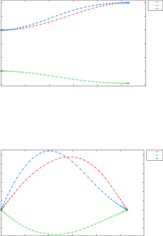
-2
-1.5
-1
-0.5
0
0.5
1
0 0.1 0.2 0.3 0.4 0.5 0.6
q (rad)
t
Manutec R3 robot problem: positions
q1
q2
q3
Figure 3.62: States q1, q2and q3for the Manutec R3 robot minimum energy
problem
-1
-0.5
0
0.5
1
1.5
2
2.5
3
0 0.1 0.2 0.3 0.4 0.5 0.6
qdot (rad/s)
t
Manutec R3 robot problem: velocities
qd1
qd2
qd3
Figure 3.63: States ˙q1,˙q2and ˙q3for the Manutec R3 robot minimum energy
problem
270
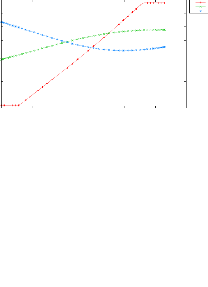
-6
-4
-2
0
2
4
6
0 0.1 0.2 0.3 0.4 0.5 0.6
controls
time (s)
Manutec R3 robot problem: controls
u1
u2
u3
Figure 3.64: Controls u1, u2and u3for the Manutec R3 robot minimum
energy problem
3.26 Minimum swing control for a container crane
Consider the following optimal control problem [40], which seeks to minimise
the load swing of a container crane, while the load is transferred from one
location to another. Find u(t)∈[0, tf] to minimize the cost functional
J= 4.5Ztf
0x2
3(t) + x2
6(t)dt (3.109)
subject to the dynamic constraints
˙x1= 9x4
˙x2= 9x5
˙x3= 9x6
˙x4= 9(u1+ 17.2656x3)
˙x5= 9u2
˙x6=−9
x2[u1+ 27.0756x3+ 2x5x6]
(3.110)
the boundary conditions
x1(0) = 0 x1(tf) = 10
x2(0) = 22 x2(tf) = 14
x3(0) = 0 x3(tf) = 0
x4(0) = 0 x4(tf)=2.5
x5(0) = −1x5(tf) = 0
x6(0) = 0 x6(tf) = 0
,(3.111)
271

and the bounds −2.83374 ≤u1(t)≤2.83374,
−0.80865 ≤u2(t)≤0.71265,
−2.5≤x4(t)≤2.5,
−1≤x5(t)≤1.
(3.112)
The PSOPT code that solves this problem is shown below.
//////////////////////////////////////////////////////////////////////////
////////////////// crane.cxx //////////////////////////
//////////////////////////////////////////////////////////////////////////
//////////////// PSOPT Example ////////////////////
//////////////////////////////////////////////////////////////////////////
//////////////////////////////////////////////////////////////////////////
//////// Title: Minimum Swing Control for Container Crane ////////////////
//////// Last modified: 06 February 2009 ////////////////
//////// Reference: Teo and Goh ////////////////
//////// (See PSOPT handbook for full reference) ///////////////
//////////////////////////////////////////////////////////////////////////
//////// Copyright (c) Victor M. Becerra, 2009 ////////////////
//////////////////////////////////////////////////////////////////////////
//////// This is part of the PSOPT software library, which ///////////////
//////// is distributed under the terms of the GNU Lesser ////////////////
//////// General Public License (LGPL) ////////////////
//////////////////////////////////////////////////////////////////////////
#include "psopt.h"
//////////////////////////////////////////////////////////////////////////
/////////////////// Define the end point (Mayer) cost function //////////
//////////////////////////////////////////////////////////////////////////
adouble endpoint_cost(adouble* initial_states, adouble* final_states,
adouble* parameters,adouble& t0, adouble& tf,
adouble* xad, int iphase, Workspace* workspace)
{
return 0;
}
//////////////////////////////////////////////////////////////////////////
/////////////////// Define the integrand (Lagrange) cost function //////
//////////////////////////////////////////////////////////////////////////
adouble integrand_cost(adouble* states, adouble* controls,
adouble* parameters, adouble& time, adouble* xad,
int iphase, Workspace* workspace)
{
adouble x3 = states[CINDEX(3)];
adouble x6 = states[CINDEX(6)];
return 4.5*( pow(x3,2) + pow(x6,2) );
}
//////////////////////////////////////////////////////////////////////////
/////////////////// Define the DAE’s ////////////////////////////////////
//////////////////////////////////////////////////////////////////////////
void dae(adouble* derivatives, adouble* path, adouble* states,
adouble* controls, adouble* parameters, adouble& time,
adouble* xad, int iphase, Workspace* workspace)
{
adouble xdot, ydot, vdot;
adouble x1 = states[ CINDEX(1) ];
adouble x2 = states[ CINDEX(2) ];
adouble x3 = states[ CINDEX(3) ];
adouble x4 = states[ CINDEX(4) ];
adouble x5 = states[ CINDEX(5) ];
adouble x6 = states[ CINDEX(6) ];
adouble u1 = controls[ CINDEX(1) ];
adouble u2 = controls[ CINDEX(2) ];
derivatives[ CINDEX(1) ] = 9*x4;
272

derivatives[ CINDEX(2) ] = 9*x5;
derivatives[ CINDEX(3) ] = 9*x6;
derivatives[ CINDEX(4) ] = 9*(u1 + 17.2656*x3);
derivatives[ CINDEX(5) ] = 9*u2;
derivatives[ CINDEX(6) ] = -(9/x2)*(u1 + 27.0756*x3 + 2*x5*x6);
}
////////////////////////////////////////////////////////////////////////////
/////////////////// Define the events function ////////////////////////////
////////////////////////////////////////////////////////////////////////////
void events(adouble* e, adouble* initial_states, adouble* final_states,
adouble* parameters,adouble& t0, adouble& tf, adouble* xad,
int iphase, Workspace* workspace)
{
adouble x10 = initial_states[ CINDEX(1) ];
adouble x20 = initial_states[ CINDEX(2) ];
adouble x30 = initial_states[ CINDEX(3) ];
adouble x40 = initial_states[ CINDEX(4) ];
adouble x50 = initial_states[ CINDEX(5) ];
adouble x60 = initial_states[ CINDEX(6) ];
adouble x1f = final_states[ CINDEX(1) ];
adouble x2f = final_states[ CINDEX(2) ];
adouble x3f = final_states[ CINDEX(3) ];
adouble x4f = final_states[ CINDEX(4) ];
adouble x5f = final_states[ CINDEX(5) ];
adouble x6f = final_states[ CINDEX(6) ];
e[ CINDEX(1) ] = x10;
e[ CINDEX(2) ] = x20;
e[ CINDEX(3) ] = x30;
e[ CINDEX(4) ] = x40;
e[ CINDEX(5) ] = x50;
e[ CINDEX(6) ] = x60;
e[ CINDEX(7) ] = x1f;
e[ CINDEX(8) ] = x2f;
e[ CINDEX(9) ] = x3f;
e[ CINDEX(10)] = x4f;
e[ CINDEX(11)] = x5f;
e[ CINDEX(12)] = x6f;
}
///////////////////////////////////////////////////////////////////////////
/////////////////// Define the phase linkages function ///////////////////
///////////////////////////////////////////////////////////////////////////
void linkages( adouble* linkages, adouble* xad, Workspace* workspace)
{
// No linkages as this is a single phase problem
}
////////////////////////////////////////////////////////////////////////////
/////////////////// Define the main routine ///////////////////////////////
////////////////////////////////////////////////////////////////////////////
int main(void)
{
////////////////////////////////////////////////////////////////////////////
/////////////////// Declare key structures ////////////////////////////////
////////////////////////////////////////////////////////////////////////////
Alg algorithm;
Sol solution;
Prob problem;
////////////////////////////////////////////////////////////////////////////
/////////////////// Register problem name ////////////////////////////////
////////////////////////////////////////////////////////////////////////////
problem.name = "Minimum swing control for a container crane";
problem.outfilename = "crane.txt";
////////////////////////////////////////////////////////////////////////////
//////////// Define problem level constants & do level 1 setup ////////////
273

////////////////////////////////////////////////////////////////////////////
problem.nphases = 1;
problem.nlinkages = 0;
psopt_level1_setup(problem);
/////////////////////////////////////////////////////////////////////////////
///////// Define phase related information & do level 2 setup /////////////
/////////////////////////////////////////////////////////////////////////////
problem.phases(1).nstates = 6;
problem.phases(1).ncontrols = 2;
problem.phases(1).nevents = 12;
problem.phases(1).npath = 0;
problem.phases(1).nodes = "[40, 60, 80]";
psopt_level2_setup(problem, algorithm);
////////////////////////////////////////////////////////////////////////////
/////////////////// Enter problem bounds information //////////////////////
////////////////////////////////////////////////////////////////////////////
problem.phases(1).bounds.lower.states(1) = -5.0;
problem.phases(1).bounds.lower.states(2) = -5.0;
problem.phases(1).bounds.lower.states(3) = -5.0;
problem.phases(1).bounds.lower.states(4) = -2.5;
problem.phases(1).bounds.lower.states(5) = -1.0;
problem.phases(1).bounds.lower.states(6) = -5.0;
problem.phases(1).bounds.upper.states(1) = 15.0;
problem.phases(1).bounds.upper.states(2) = 25.0;
problem.phases(1).bounds.upper.states(3) = 15.0;
problem.phases(1).bounds.upper.states(4) = 2.5;
problem.phases(1).bounds.upper.states(5) = 1.0;
problem.phases(1).bounds.upper.states(6) = 15.0;
problem.phases(1).bounds.lower.controls(1) = -2.83374;
problem.phases(1).bounds.lower.controls(2) = -0.80865;
problem.phases(1).bounds.upper.controls(1) = 2.83374;
problem.phases(1).bounds.upper.controls(2) = 0.71265;
// Initial states
problem.phases(1).bounds.lower.events(1) = 0.0;
problem.phases(1).bounds.lower.events(2) = 22.0;
problem.phases(1).bounds.lower.events(3) = 0.0;
problem.phases(1).bounds.lower.events(4) = 0.0;
problem.phases(1).bounds.lower.events(5) = -1.0;
problem.phases(1).bounds.lower.events(6) = 0.0;
// Final states
problem.phases(1).bounds.lower.events(7) = 10.0;
problem.phases(1).bounds.lower.events(8) = 14.0;
problem.phases(1).bounds.lower.events(9) = 0.0;
problem.phases(1).bounds.lower.events(10)= 2.5;
problem.phases(1).bounds.lower.events(11)= 0.0;
problem.phases(1).bounds.lower.events(12)= 0.0;
problem.phases(1).bounds.upper.events = problem.phases(1).bounds.lower.events;
problem.phases(1).bounds.lower.StartTime = 0.0;
problem.phases(1).bounds.upper.StartTime = 0.0;
problem.phases(1).bounds.lower.EndTime = 1.0;
problem.phases(1).bounds.upper.EndTime = 1.0;
////////////////////////////////////////////////////////////////////////////
/////////////////// Register problem functions ///////////////////////////
////////////////////////////////////////////////////////////////////////////
problem.integrand_cost = &integrand_cost;
problem.endpoint_cost = &endpoint_cost;
problem.dae = &dae;
problem.events = &events;
problem.linkages = &linkages;
274

////////////////////////////////////////////////////////////////////////////
/////////////////// Define & register initial guess ///////////////////////
////////////////////////////////////////////////////////////////////////////
DMatrix x0(6,20);
x0(1,colon()) = linspace(0.0,10.0, 20);
x0(2,colon()) = linspace(22.0,14.0, 20);
x0(3,colon()) = linspace(0.,0., 20);
x0(4,colon()) = linspace(0.,2.5, 20);
x0(5,colon()) = linspace(-1.0,0., 20);
x0(6,colon()) = linspace(0.,0., 20);
problem.phases(1).guess.controls = zeros(2, 20);
problem.phases(1).guess.states = x0;
problem.phases(1).guess.time = linspace(0.0, 1.0, 20); ;
////////////////////////////////////////////////////////////////////////////
/////////////////// Enter algorithm options //////////////////////////////
////////////////////////////////////////////////////////////////////////////
algorithm.nlp_method = "IPOPT";
algorithm.scaling = "automatic";
algorithm.derivatives = "automatic";
algorithm.nlp_iter_max = 1000;
algorithm.nlp_tolerance = 1.e-6;
algorithm.collocation_method = "Legendre";
////////////////////////////////////////////////////////////////////////////
/////////////////// Now call PSOPT to solve the problem /////////////////
////////////////////////////////////////////////////////////////////////////
psopt(solution, problem, algorithm);
////////////////////////////////////////////////////////////////////////////
/////////// Extract relevant variables from solution structure //////////
////////////////////////////////////////////////////////////////////////////
DMatrix x = solution.get_states_in_phase(1);
DMatrix u = solution.get_controls_in_phase(1);
DMatrix t = solution.get_time_in_phase(1);
////////////////////////////////////////////////////////////////////////////
/////////// Save solution data to files if desired ////////////////////////
////////////////////////////////////////////////////////////////////////////
x.Save("x.dat");
u.Save("u.dat");
t.Save("t.dat");
DMatrix x13 = x(colon(1,3), colon() );
DMatrix x46 = x(colon(4,6), colon() );
////////////////////////////////////////////////////////////////////////////
/////////// Plot some results if desired (requires gnuplot) ///////////////
////////////////////////////////////////////////////////////////////////////
plot(t,x13,problem.name + ": states x1, x2 and x3", "time (s)", "states", "x1 x2 x3");
plot(t,x46,problem.name + ": states x4, x5 and x6", "time (s)", "states", "x4 x5 x6");
plot(t,u,problem.name + ": controls", "time", "controls", "u1 u2");
plot(t,x13,problem.name + ": states x1, x2 and x3", "time (s)", "states", "x1 x2 x3",
"pdf", "crane_states13.pdf");
plot(t,x46,problem.name + ": states x4, x5 and x6", "time (s)", "states", "x4 x5 x6",
"pdf", "crane_states46.pdf");
plot(t,u,problem.name + ": controls", "time", "controls", "u1 u2",
"pdf", "crane_controls.pdf");
}
////////////////////////////////////////////////////////////////////////////
/////////////////////// END OF FILE ///////////////////////////////
275

////////////////////////////////////////////////////////////////////////////
The output from PSOPT is summarised in the box below and shown in
Figures 3.65,3.66 and 3.67, which contain the elements of the state x1to
x3,x4to x6, and the controls, respectively.
PSOPT results summary
=====================
Problem: Minimum swing control for a container crane
CPU time (seconds): 2.236445e+01
NLP solver used: IPOPT
PSOPT release number: 4.0
Date and time of this run: Thu Feb 21 17:14:50 2019
Optimal (unscaled) cost function value: 5.151343e-03
Phase 1 endpoint cost function value: 0.000000e+00
Phase 1 integrated part of the cost: 5.151343e-03
Phase 1 initial time: 0.000000e+00
Phase 1 final time: 1.000000e+00
Phase 1 maximum relative local error: 1.091430e-04
NLP solver reports: The problem has been solved!
3.27 Minimum time to climb for a supersonic air-
craft
Consider the following optimal control problem, which finds the minimum
time to climb to a given altitude for a supersonic aircraft [4]. Minimize the
cost functional
J=tf(3.113)
subject to the dynamic constraints
˙
h=vsin γ
˙v=1
m[T(M, h) cos α−D]−µ
(Re+h)2sin γ
˙γ=1
mv [T(M, h) sin α+L] + cos γhv
(Re+h)−µ
v(Re+h)2i
˙w=−T(M,h)
Isp
(3.114)
where his the altitude (ft), vis the velocity (ft/s), γis the flight path angle
(rad), wis the weight (lb), Lis the lift force, Dis the drag force (lb), Tis
276
0
5
10
15
20
0 0.2 0.4 0.6 0.8 1
states
time (s)
Minimum swing control for a container crane: states x1, x2 and x3
x1
x2
x3
Figure 3.65: States x1, x2and x3for minimum swing crane control problem
-1
-0.5
0
0.5
1
1.5
2
2.5
0 0.2 0.4 0.6 0.8 1
states
time (s)
Minimum swing control for a container crane: states x4, x5 and x6
x4
x5
x6
Figure 3.66: States x4, x5and x6for minimum swing crane control problem
277
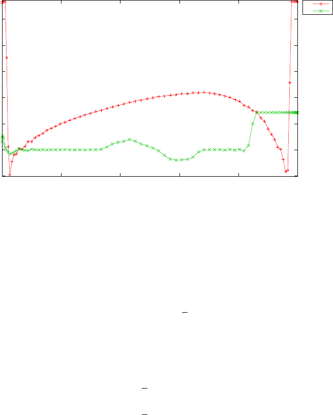
-0.5
0
0.5
1
1.5
2
2.5
0 0.2 0.4 0.6 0.8 1
controls
time
Minimum swing control for a container crane: controls
u1
u2
Figure 3.67: Controls for minimum swing crane control problem
the thrust (lb), M=v/c is the mach number, m=w/g0(slug) is the mass,
c(h) is the speed of sound (ft/s), Reis the radious of Earth, and µis the
gravitational constant. The control input αis the angle of attack (rad).
The speed of sound is given by:
c= 20.0468√θ(3.115)
where θ=θ(h) is the atmospheric temperature (K).
The aerodynamic forces are given by:
D=1
2CDSρv2
L=1
2CLSρv2
(3.116)
where CL=cLα(M)α
CD=cD0(M) + η(M)cLα(M)α2(3.117)
where CLand CDare aerodynamic lift and drag coefficients, Sis the aero-
dynamic reference area of the aircraft, and ρ=ρ(h) is the air density.
278

The boundary conditions are given by:
h(0) = 0 (ft),
h(tf) = 65600.0 (ft)
v(0) = 424.260 (ft/s),
v(tf) = 968.148 (ft/s)
γ(0) = γ(tf) = 0 (rad)
w(0) = 42000.0 lb
(3.118)
The parameter values are given by:
S= 530 (ft2),
Isp = 1600.0 (sec)
µ= 0.14046539 ×10¹⁷ (ft3/s2),
g0= 32.174 (ft/s2)
Re= 20902900 (ft)
(3.119)
The variables cLα(M), cD0(M), η(M) are interpolated from 1-D tabular
data which is given in the code and also in [4], using spline interpolation,
while the thrust T(M, h) is interpolated from 2-D tabular data given in the
code and in [4], using 2D spline interpolation.
The air density ρand the atmospheric temperature θwere calculated
using the US Standard Atmosphere Model 19764, based on the standard
temperature of 15 (deg C) at zero altitude and the standard air density of
1.22521 (slug/ft3) at zero altitude.
The PSOPT code that solves this problem is shown below.
//////////////////////////////////////////////////////////////////////////
////////////////// climb.cxx /////////////////////
//////////////////////////////////////////////////////////////////////////
//////////////// PSOPT Example ////////////////////
//////////////////////////////////////////////////////////////////////////
//////////////////////////////////////////////////////////////////////////
//////// Title: Minimum time to climb of a supersonic aircraft ///////////
//////// Last modified: 12 January 2009 ////////////////
//////// Reference: GPOPS Manual ////////////////
//////// (See PSOPT handbook for full reference) ///////////////
//////////////////////////////////////////////////////////////////////////
//////// Copyright (c) Victor M. Becerra, 2009 ////////////////
//////////////////////////////////////////////////////////////////////////
//////// This is part of the PSOPT software library, which ///////////////
//////// is distributed under the terms of the GNU Lesser ////////////////
//////// General Public License (LGPL) ////////////////
//////////////////////////////////////////////////////////////////////////
#include "psopt.h"
//////////////////////////////////////////////////////////////////////////
///////// Declare an auxiliary structure to hold local constants ////////
4see http://www.pdas.com/programs/atmos.f90
279

//////////////////////////////////////////////////////////////////////////
struct Constants {
double g0;
double S;
double Re;
double Isp;
double mu;
DMatrix* CLa_table;
DMatrix* CD0_table;
DMatrix* eta_table;
DMatrix* T_table;
DMatrix* M1;
DMatrix* M2;
DMatrix* h1;
DMatrix* htab;
DMatrix* ttab;
DMatrix* ptab;
DMatrix* gtab;
};
typedef struct Constants Constants_;
void atmosphere(adouble* alt,adouble* sigma,adouble* delta,adouble* theta, Constants_& CONSTANTS);
void atmosphere_model(adouble* rho, adouble* M, adouble v, adouble h, Constants_& CONSTANTS);
//////////////////////////////////////////////////////////////////////////
/////////////////// Define the end point (Mayer) cost function //////////
//////////////////////////////////////////////////////////////////////////
adouble endpoint_cost(adouble* initial_states, adouble* final_states,
adouble* parameters,adouble& t0, adouble& tf,
adouble* xad, int iphase, Workspace* workspace)
{
return tf;
}
//////////////////////////////////////////////////////////////////////////
/////////////////// Define the integrand (Lagrange) cost function //////
//////////////////////////////////////////////////////////////////////////
adouble integrand_cost(adouble* states, adouble* controls, adouble* parameters,
adouble& time, adouble* xad, int iphase, Workspace* workspace)
{
return 0.0;
}
//////////////////////////////////////////////////////////////////////////
/////////////////// Define the DAE’s ////////////////////////////////////
//////////////////////////////////////////////////////////////////////////
void dae(adouble* derivatives, adouble* path, adouble* states,
adouble* controls, adouble* parameters, adouble& time,
adouble* xad, int iphase, Workspace* workspace)
{
Constants_& CONSTANTS = *( (Constants_ *) workspace->problem->user_data );
adouble alpha = controls[ CINDEX(1)]; // Angle of attack (rad)
adouble h = states[ CINDEX(1) ]; // Altitude (ft)
adouble v = states[ CINDEX(2) ]; // Velocity (ft/s)
adouble gamma = states[ CINDEX(3) ]; // Flight path angle (rad)
adouble w = states[ CINDEX(4) ]; // weight (lb)
double g0 = CONSTANTS.g0;
double S = CONSTANTS.S;
double Re = CONSTANTS.Re;
double Isp = CONSTANTS.Isp;
double mu = CONSTANTS.mu;
DMatrix& M1 = *CONSTANTS.M1;
DMatrix& M2 = *CONSTANTS.M2;
DMatrix& h1 = *CONSTANTS.h1;
DMatrix& CLa_table = *CONSTANTS.CLa_table;
DMatrix& CD0_table = *CONSTANTS.CD0_table;
280

DMatrix& eta_table = *CONSTANTS.eta_table;
DMatrix& T_table = *CONSTANTS.T_table;
int lM1 = length(M1);
adouble rho;
adouble m = w/g0;
adouble M;
atmosphere_model( &rho, &M, v, h, CONSTANTS);
adouble CL_a, CD0, eta, T;
spline_interpolation( &CL_a, M, M1, CLa_table, lM1);
spline_interpolation( &CD0, M, M1, CD0_table, lM1);
spline_interpolation( &eta, M, M1, eta_table, lM1);
spline_2d_interpolation(&T, M, h, M2, h1, T_table, workspace);
// smooth_linear_interpolation( &CL_a, M, M1, CLa_table, lM1);
// smooth_linear_interpolation( &CD0, M, M1, CD0_table, lM1);
// smooth_linear_interpolation( &eta, M, M1, eta_table, lM1);
// smooth_bilinear_interpolation(&T, M, h, M2, h1, T_table);
// linear_interpolation( &CL_a, M, M1, CLa_table, lM1);
// linear_interpolation( &CD0, M, M1, CD0_table, lM1);
// linear_interpolation( &eta, M, M1, eta_table, lM1);
// bilinear_interpolation(&T, M, h, M2, h1, T_table);
adouble CL = CL_a*alpha;
adouble CD = CD0 + eta*CL_a*alpha*alpha;
adouble D = 0.5*CD*S*rho*v*v;
adouble L = 0.5*CL*S*rho*v*v;
adouble hdot = v*sin(gamma);
adouble vdot = 1.0/m*(T*cos(alpha)-D) - mu/pow(Re+h,2.0)*sin(gamma);
adouble gammadot = (1.0/(m*v))*(T*sin(alpha)+L) + cos(gamma)*(v/(Re+h)-mu/(v*pow(Re+h,2.0)));
adouble wdot = -T/Isp;
derivatives[ CINDEX(1) ] = hdot;
derivatives[ CINDEX(2) ] = vdot;
derivatives[ CINDEX(3) ] = gammadot;
derivatives[ CINDEX(4) ] = wdot;
}
////////////////////////////////////////////////////////////////////////////
/////////////////// Define the events function ////////////////////////////
////////////////////////////////////////////////////////////////////////////
void events(adouble* e, adouble* initial_states, adouble* final_states,
adouble* parameters,adouble& t0, adouble& tf, adouble* xad,
int iphase, Workspace* workspace)
{
adouble h0 = initial_states[CINDEX(1)];
adouble v0 = initial_states[CINDEX(2)];
adouble gamma0 = initial_states[CINDEX(3)];
adouble w0 = initial_states[CINDEX(4)];
adouble hf = final_states[CINDEX(1)];
adouble vf = final_states[CINDEX(2)];
adouble gammaf = final_states[CINDEX(3)];
e[ CINDEX(1) ] = h0;
e[ CINDEX(2) ] = v0;
e[ CINDEX(3) ] = gamma0;
e[ CINDEX(4) ] = w0;
e[ CINDEX(5) ] = hf;
e[ CINDEX(6) ] = vf;
e[ CINDEX(7) ] = gammaf;
}
281

///////////////////////////////////////////////////////////////////////////
/////////////////// Define the phase linkages function ///////////////////
///////////////////////////////////////////////////////////////////////////
void linkages( adouble* linkages, adouble* xad, Workspace* workspace)
{
// Single phase problem
}
////////////////////////////////////////////////////////////////////////////
/////////////////// Define the main routine ///////////////////////////////
////////////////////////////////////////////////////////////////////////////
int main(void)
{
////////////////////////////////////////////////////////////////////////////
/////////////////// Declare key structures ////////////////////////////////
////////////////////////////////////////////////////////////////////////////
Alg algorithm;
Sol solution;
Prob problem;
////////////////////////////////////////////////////////////////////////////
/////////////////// Register problem name ////////////////////////////////
////////////////////////////////////////////////////////////////////////////
problem.name = "Minimum time to climb for a supersonic aircraft";
problem.outfilename = "climb.txt";
////////////////////////////////////////////////////////////////////////////
//////////// Define problem level constants & do level 1 setup ////////////
////////////////////////////////////////////////////////////////////////////
problem.nphases = 1;
problem.nlinkages = 0;
psopt_level1_setup(problem);
/////////////////////////////////////////////////////////////////////////////
///////// Define phase related information & do level 2 setup ////////////
/////////////////////////////////////////////////////////////////////////////
problem.phases(1).nstates = 4;
problem.phases(1).ncontrols = 1;
problem.phases(1).nevents = 7;
problem.phases(1).npath = 0;
problem.phases(1).nodes = "[30,60]";
psopt_level2_setup(problem, algorithm);
////////////////////////////////////////////////////////////////////////////
/////////////////// Declare an instance of Constants structure /////////////
////////////////////////////////////////////////////////////////////////////
Constants_ CONSTANTS;
problem.user_data = (void*) &CONSTANTS;
////////////////////////////////////////////////////////////////////////////
/////////////////// Declare DMatrix objects to store results //////////////
////////////////////////////////////////////////////////////////////////////
DMatrix x, u, t, H;
////////////////////////////////////////////////////////////////////////////
/////////////////// Initialize CONSTANTS and //////////////////////////////
/////////////////// declare local variables //////////////////////////////
////////////////////////////////////////////////////////////////////////////
CONSTANTS.g0 = 32.174; // ft/s^2
CONSTANTS.S = 530.0; // ft^2
CONSTANTS.Re = 20902900.0; // ft
282

CONSTANTS.Isp = 1600.00; //s
CONSTANTS.mu = 0.14076539E17; // ft^3/s^2
DMatrix M1(1,9,
0.E0, .4E0, .8E0, .9E0, 1.E0, 1.2E0, 1.4E0, 1.6E0, 1.8E0);
DMatrix M2(1,10,
0.E0, .2E0, .4E0, .6E0, .8E0, 1.E0, 1.2E0, 1.4E0, 1.6E0, 1.8E0);
DMatrix h1(1,10,
0.E0, 5E3, 10.E3, 15.E3, 20.E3, 25.E3, 30.E3, 40.E3, 50.E3, 70.E3);
DMatrix CLa_table(1,9,
3.44E0, 3.44E0, 3.44E0, 3.58E0, 4.44E0, 3.44E0, 3.01E0, 2.86E0, 2.44E0);
DMatrix CD0_table(1,9,
.013E0, .013E0, .013E0, .014E0, .031E0, 0.041E0, .039E0, .036E0, .035E0);
DMatrix eta_table(1,9,
.54E0, .54E0, .54E0, .75E0, .79E0, .78E0, .89E0, .93E0, .93E0);
DMatrix T_table(10,10,
24200., 24000., 20300., 17300.,14500.,12200.,10200.,5700.,3400.,100.,
28000., 24600., 21100., 18100.,15200.,12800.,10700.,6500.,3900.,200.,
28300., 25200., 21900., 18700.,15900.,13400.,11200.,7300.,4400.,400.,
30800., 27200., 23800., 20500.,17300.,14700.,12300.,8100.,4900.,800.,
34500., 30300., 26600., 23200.,19800.,16800.,14100.,9400.,5600.,1100.,
37900., 34300., 30400., 26800.,23300.,19800.,16800.,11200.,6800.,1400.,
36100., 38000., 34900., 31300.,27300.,23600.,20100.,13400.,8300.,1700.,
34300., 36600., 38500., 36100.,31600.,28100.,24200.,16200.,10000.,2200.,
32500., 35200., 42100., 38700.,35700.,32000.,28100.,19300.,11900.,2900.,
30700., 33800., 45700., 41300.,39800.,34600.,31100.,21700.,13300.,3100. );
DMatrix htab(1,8,
0.0, 11.0, 20.0, 32.0, 47.0, 51.0, 71.0, 84.852);
DMatrix ttab(1,8,
288.15, 216.65, 216.65, 228.65, 270.65, 270.65, 214.65, 186.946);
DMatrix ptab(1,8,
1.0, 2.233611E-1, 5.403295E-2, 8.5666784E-3, 1.0945601E-3,
6.6063531E-4, 3.9046834E-5, 3.68501E-6);
DMatrix gtab(1,8, -6.5, 0.0, 1.0, 2.8, 0.0, -2.8, -2.0, 0.0);
M1.Print("M1");
M2.Print("M2");
h1.Print("h1");
CLa_table.Print("CLa_table");
CD0_table.Print("CD0_table");
eta_table.Print("eta_table");
T_table.Print("T_table");
CONSTANTS.M1 = &M1;
CONSTANTS.M2 = &M2;
CONSTANTS.h1 = &h1;
CONSTANTS.CLa_table = &CLa_table;
CONSTANTS.CD0_table = &CD0_table;
CONSTANTS.eta_table = &eta_table;
CONSTANTS.T_table = &T_table;
CONSTANTS.htab = &htab;
CONSTANTS.ttab = &ttab;
CONSTANTS.ptab = &ptab;
CONSTANTS.gtab = >ab;
double h0 = 0.0;
double hf = 65600.0;
double v0 = 424.26;
double vf = 968.148;
double gamma0 = 0.0;
double gammaf = 0.0;
double w0 = 42000.0;
double hmin = 0;
double hmax = 69000.0;
double vmin = 1.0;
double vmax = 2000.0;
double gammamin = -89.0*pi/180.0; // -89.0*pi/180.0;
283

double gammamax = 89.0*pi/180.0; // 89.0*pi/180.0;
double wmin = 0.0;
double wmax = 45000.0;
double alphamin = -20.0*pi/180.0;
double alphamax = 20.0*pi/180.0;
double t0min = 0.0;
double t0max = 0.0;
double tfmin = 200.0;
double tfmax = 500.0;
////////////////////////////////////////////////////////////////////////////
/////////////////// Enter problem bounds information //////////////////////
////////////////////////////////////////////////////////////////////////////
int iphase = 0;
problem.phase[iphase].bounds.lower.StartTime = t0min;
problem.phase[iphase].bounds.upper.StartTime = t0max;
problem.phase[iphase].bounds.lower.EndTime = tfmin;
problem.phase[iphase].bounds.upper.EndTime = tfmax;
problem.phase[iphase].bounds.lower.states(1) = hmin;
problem.phase[iphase].bounds.upper.states(1) = hmax;
problem.phase[iphase].bounds.lower.states(2) = vmin;
problem.phase[iphase].bounds.upper.states(2) = vmax;
problem.phase[iphase].bounds.lower.states(3) = gammamin;
problem.phase[iphase].bounds.upper.states(3) = gammamax;
problem.phase[iphase].bounds.lower.states(4) = wmin;
problem.phase[iphase].bounds.upper.states(4) = wmax;
problem.phase[iphase].bounds.lower.controls(1) = alphamin;
problem.phase[iphase].bounds.upper.controls(1) = alphamax;
// The following bounds fix the initial and final state conditions
problem.phase[iphase].bounds.lower.events(1) = h0;
problem.phase[iphase].bounds.upper.events(1) = h0;
problem.phase[iphase].bounds.lower.events(2) = v0;
problem.phase[iphase].bounds.upper.events(2) = v0;
problem.phase[iphase].bounds.lower.events(3) = gamma0;
problem.phase[iphase].bounds.upper.events(3) = gamma0;
problem.phase[iphase].bounds.lower.events(4) = w0;
problem.phase[iphase].bounds.upper.events(4) = w0;
problem.phase[iphase].bounds.lower.events(5) = hf;
problem.phase[iphase].bounds.upper.events(5) = hf;
problem.phase[iphase].bounds.lower.events(6) = vf;
problem.phase[iphase].bounds.upper.events(6) = vf;
problem.phase[iphase].bounds.lower.events(7) = gammaf;
problem.phase[iphase].bounds.upper.events(7) = gammaf;
////////////////////////////////////////////////////////////////////////////
/////////////////// Define & register initial guess ///////////////////////
////////////////////////////////////////////////////////////////////////////
int nnodes = problem.phases(1).nodes(1);
DMatrix stateGuess(4,nnodes);
stateGuess(1, colon()) = linspace(h0,hf,nnodes);
stateGuess(2, colon()) = linspace(v0,vf,nnodes);
stateGuess(3, colon()) = linspace(gamma0,gammaf,nnodes);
stateGuess(4, colon()) = linspace(w0,0.8*w0,nnodes);
problem.phases(1).guess.controls = zeros(1,nnodes);
problem.phases(1).guess.states = stateGuess;
problem.phases(1).guess.time = linspace(t0min, tfmax, nnodes);
////////////////////////////////////////////////////////////////////////////
/////////////////// Register problem functions ///////////////////////////
////////////////////////////////////////////////////////////////////////////
problem.integrand_cost = &integrand_cost;
284

problem.endpoint_cost = &endpoint_cost;
problem.dae = &dae;
problem.events = &events;
problem.linkages = &linkages;
////////////////////////////////////////////////////////////////////////////
/////////////////// Enter algorithm options //////////////////////////////
////////////////////////////////////////////////////////////////////////////
algorithm.nlp_method = "IPOPT";
algorithm.scaling = "automatic";
algorithm.derivatives = "numerical";
algorithm.collocation_method = "trapezoidal";
algorithm.nlp_iter_max = 1000;
algorithm.nlp_tolerance = 1.e-6;
algorithm.mesh_refinement = "automatic";
algorithm.mr_max_iterations = 4;
algorithm.defect_scaling = "jacobian-based";
////////////////////////////////////////////////////////////////////////////
/////////////////// Now call PSOPT to solve the problem //////////////////
////////////////////////////////////////////////////////////////////////////
psopt(solution, problem, algorithm);
////////////////////////////////////////////////////////////////////////////
/////////// Extract relevant variables from solution structure //////////
////////////////////////////////////////////////////////////////////////////
x = solution.get_states_in_phase(1);
u = solution.get_controls_in_phase(1);
t = solution.get_time_in_phase(1);
H = solution.get_dual_hamiltonian_in_phase(1);
DMatrix h = x(1,colon());
DMatrix v = x(2,colon());
DMatrix gamma = x(3,colon());
DMatrix w = x(4,colon());
////////////////////////////////////////////////////////////////////////////
/////////// Save solution data to files if desired ////////////////////////
////////////////////////////////////////////////////////////////////////////
x.Save("x.dat");
u.Save("u.dat");
t.Save("t.dat");
////////////////////////////////////////////////////////////////////////////
/////////// Plot some results if desired (requires gnuplot) ///////////////
////////////////////////////////////////////////////////////////////////////
plot(t,h/1000.0,problem.name + ": altitude", "time (s)", "altitude (x1,000 ft)", "h");
plot(t,v/100.0,problem.name + ": velocity", "time (s)", "velocity (x100 ft/s)", "v");
plot(t,gamma*180/pi,problem.name + ": flight path angle", "time (s)", "gamma (deg)", "gamma");
plot(t,w/10000.0,problem.name + ": weight", "time (s)", "w (x10,000 lb)", "w");
plot(t,u*180/pi,problem.name + ": angle of attack", "time (s)", "alpha (deg)", "alpha");
plot(t,h/1000.0,problem.name + ": altitude", "time (s)", "altitude (x1,000 ft", "h",
"pdf","climb_altitude.pdf");
plot(t,v/100.0,problem.name + ": velocity", "time (s)", "velocity (x100 ft/s)", "v",
"pdf","climb_velocity.pdf");
plot(t,gamma*180/pi,problem.name + ": flight path angle", "time (s)", "gamma (deg)", "gamma",
"pdf","climb_fpa.pdf");
plot(t,w/10000.0,problem.name + ": weight", "time (s)", "w (x10,000 lb)", "w", "pdf",
"weight.pdf");
plot(t,u*180/pi,problem.name + ": angle of attack", "time (s)", "alpha (deg)", "alpha",
"pdf", "alpha.pdf");
}
void atmosphere(adouble* alt,adouble* sigma,adouble* delta,adouble* theta, Constants_& CONSTANTS)
// US Standard Atmosphere Model 1976
// Adopted from original Fortran 90 code by Ralph Carmichael
285

// Fortran code located at: http://www.pdas.com/programs/atmos.f90
{
/*! -------------------------------------------------------------------------
! PURPOSE - Compute the properties of the 1976 standard atmosphere to 86 km.
! AUTHOR - Ralph Carmichael, Public Domain Aeronautical Software
! NOTE - If alt > 86, the values returned will not be correct, but they will
! not be too far removed from the correct values for density.
! The reference document does not use the terms pressure and temperature
! above 86 km.
IMPLICIT NONE
!============================================================================
! ARGUMENTS |
!============================================================================
alt ! geometric altitude, km.
sigma ! density/sea-level standard density
delta ! pressure/sea-level standard pressure
theta ! temperature/sea-level standard temperature
*/
/*!============================================================================
! LOCAL CONSTANTS |
!============================================================================
*/
double REARTH = 6369.0; // radius of the Earth (km)
double GMR = 34.163195; // hydrostatic constant
int NTAB=8; // number of entries in the defining tables
/*!============================================================================
! LOCAL VARIABLES |
!============================================================================
*/
int i,j,k; // counters
adouble h; // geopotential altitude (km)
adouble tgrad, tbase; // temperature gradient and base temp of this layer
adouble tlocal; // local temperature
adouble deltah; // height above base of this layer
/*!============================================================================
! LOCAL ARRAYS (1976 STD. ATMOSPHERE) |
!============================================================================
*/
DMatrix& htab = *CONSTANTS.htab;
DMatrix& ttab = *CONSTANTS.ttab;
DMatrix& ptab = *CONSTANTS.ptab;
DMatrix& gtab = *CONSTANTS.gtab;
//!----------------------------------------------------------------------------
h=(*alt)*REARTH/((*alt)+REARTH); //convert geometric to geopotential altitude
i=1;
j=NTAB; // setting up for binary search
while (j<=i+1) {
k=(i+j)/2; // integer division
if (h < htab(k)) {
j=k;
} else {
i=k;
}
}
tgrad=gtab(i); // i will be in 1...NTAB-1
tbase=ttab(i);
deltah=h-htab(i);
tlocal=tbase+tgrad*deltah;
*theta=tlocal/ttab(1); // temperature ratio
if (tgrad == 0.0) { // pressure ratio
*delta=ptab(i)*exp(-GMR*deltah/tbase);
} else {
*delta=ptab(i)*pow(tbase/tlocal, GMR/tgrad);
}
*sigma=(*delta)/(*theta); // density ratio
return;
}
void atmosphere_model(adouble* rho, adouble* M, adouble v, adouble h, Constants_& CONSTANTS)
{
double feet2meter = 0.3048;
double kgperm3_to_slug_per_feet3 = 0.062427960841/32.174049;
adouble alt, sigma, delta, theta;
286

Iter Method Nodes NV NC OE CE JE HE RHS max CPU(sec)
1 LGL-ST 80 322 247 747 746 89 0 59680 1.752e-03 8.020e+00
2 LGL-ST 90 362 277 70 71 55 0 6390 1.706e-03 6.890e+00
3 LGL-ST 100 402 307 28 29 28 0 2900 7.940e-04 4.810e+00
- - - - - 845 846 172 0 68970 - 1.972e+01
Key: Iter=iteration number, NV=number of variables, NC=number of constraints, OE=objective evalu-
ations, CE = constraint evaluations, JE = Jacobian evaluations, HE = Hessian evaluations, RHS = ODE
right hand side evaluations, max = maximum relative ODE error, CPU(sec) = CPU time in seconds spent by
nonlinear programming algorithm
Table 3.4: Mesh refinement statistics: Minimum time to climb for a super-
sonic aircraft
alt = h.value()*feet2meter/1000.0;
// Call the standard atmosphere model 1976
atmosphere(&alt, &sigma, &delta, &theta, CONSTANTS);
adouble rho1 = 1.22521 * sigma; // Multiply by standard density at zero altitude and 15 deg C.
rho1 = rho1*kgperm3_to_slug_per_feet3;
*rho = rho1;
adouble T;
adouble mach;
double TempStandardSeaLevel = 288.15; // in K, or 15 deg C.
T = theta*TempStandardSeaLevel;
adouble a = 20.0468 * sqrt(T); // Speed of sound in m/s.
a = a/feet2meter; // Speed of sound in ft/s
mach = v/a;
*M = mach;
return;
}
////////////////////////////////////////////////////////////////////////////
/////////////////////// END OF FILE ///////////////////////////////
////////////////////////////////////////////////////////////////////////////
The output from PSOPT is summarized in the box below and Figures
3.68, to 3.72. The results can be compared with those presented in [4]. Table
?? shows the mesh refinement history for this problem.
PSOPT results summary
=====================
Problem: Minimum time to climb for a supersonic aircraft
CPU time (seconds): 3.563276e+02
NLP solver used: IPOPT
PSOPT release number: 4.0
287
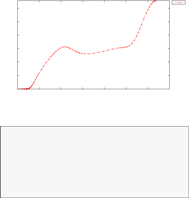
0
10
20
30
40
50
60
0 50 100 150 200 250 300 350
altitude (x1,000 ft
time (s)
Minimum time to climb for a supersonic aircraft: altitude
h
Figure 3.68: Altitude for minimum time to climb problem
Date and time of this run: Thu Feb 21 15:51:19 2019
Optimal (unscaled) cost function value: 3.188143e+02
Phase 1 endpoint cost function value: 3.188143e+02
Phase 1 integrated part of the cost: 0.000000e+00
Phase 1 initial time: 0.000000e+00
Phase 1 final time: 3.188143e+02
Phase 1 maximum relative local error: 1.665362e-03
NLP solver reports: The problem has been solved!
3.28 Missile terminal burn maneouvre
This example illustrates the design of a missile trajectory to strike a specified
target from given initial conditions in minimum time [39]. Figure 3.28 shows
the variables associated with the dynamic model of the missile employed in
this example, where γis the flight path angle, αis the angle of attack, Vis
the missile speed, xis the longitudinal position, his the altitude, Dis the
axial aerodynamic force, Lis the normal aerodynamic force, and Tis the
thrust.
The equations of motion of the missile are given by:
288
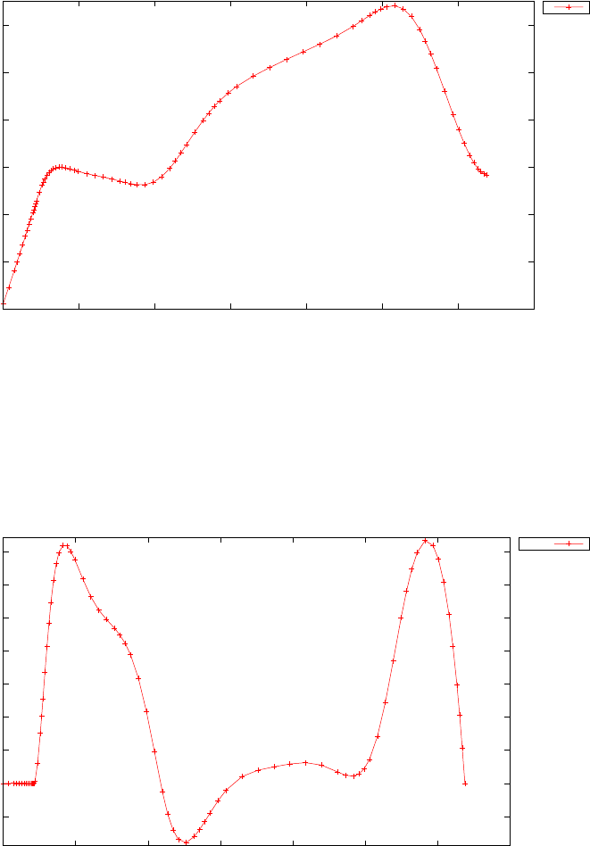
6
8
10
12
14
16
0 50 100 150 200 250 300 350
velocity (x100 ft/s)
time (s)
Minimum time to climb for a supersonic aircraft: velocity
v
Figure 3.69: Velocity for minimum time to climb problem
-5
0
5
10
15
20
25
30
35
0 50 100 150 200 250 300 350
gamma (deg)
time (s)
Minimum time to climb for a supersonic aircraft: flight path angle
gamma
Figure 3.70: Flight path angle for minimum time to climb problem
289
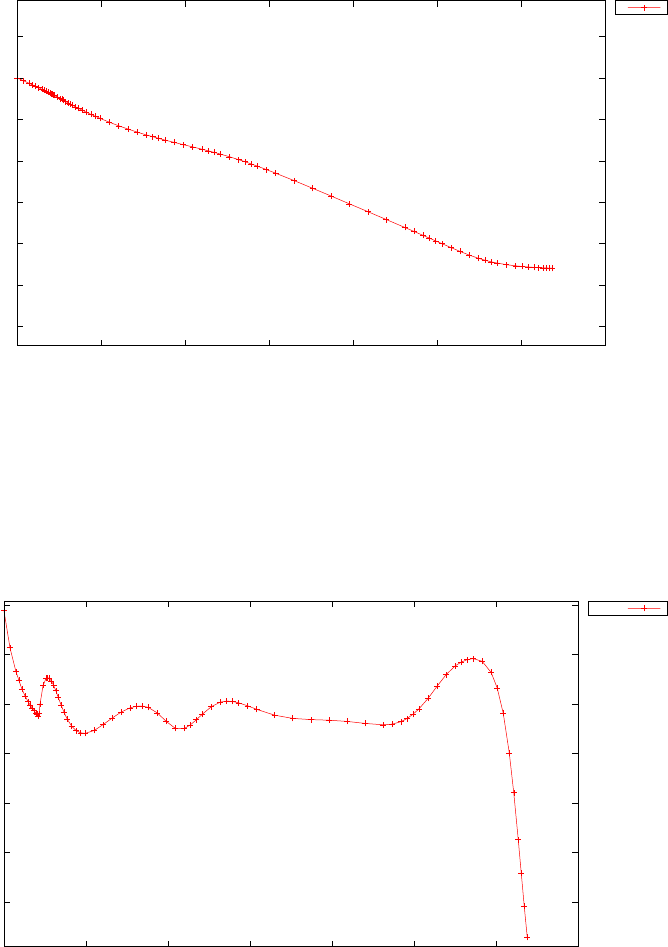
3.6
3.7
3.8
3.9
4
4.1
4.2
4.3
0 50 100 150 200 250 300 350
w (x10,000 lb)
time (s)
Minimum time to climb for a supersonic aircraft: weight
w
Figure 3.71: Weight for minimum time to climb problem
-6
-4
-2
0
2
4
6
0 50 100 150 200 250 300 350
alpha (deg)
time (s)
Minimum time to climb for a supersonic aircraft: angle of attack
alpha
Figure 3.72: Angle of attack (α) for minimum time to climb problem
290
T
thrust
L
normal aerodynamic
force
V
speed
xD
axial
aerodynamic
force
mg
weight
flight
path
angle
angle of attack
90º
90º
Figure 3.73: Ilustration of the variables associated with the missile model
291

˙γ=T−D
mg sin α+L
mV cos α−gcos γ
V
˙
V=T−D
mcos α−L
msin α−gcos γ
˙x=Vcos γ
˙
h=Vsin γ
where
D=1
2CdρV 2Sref
Cd=A1α2+A2α+A3
L=1
2ClρV 2Sref
Cl=B1α+B2
ρ=C1h2+C2h+C3
where all the model parameters are given in Table 3.5. The initial conditions
for the state variables are:
γ(0) = 0
V(0) = 272m/s
x(0) = 0m
h(0) = 30m
The terminal conditions on the states are:
γ(tf) = −π/2
V(tf) = 310m/s
x(tf) = 10000m
h(tf) = 0m
The problem constraints are given by:
200 ≤V≤310
1000 ≤T≤6000
−0.3≤α≤0.3
−4≤L
mg ≤4
h≥30 (for x≤7500m)
h≥0 (for x > 7500m)
292

Table 3.5: Parameters values of the missile model
Parameter Value Units
m1005 kg
g9.81 m/s2
Sref 0.3376 m2
A1-1.9431
A2-0.1499
A30.2359
B121.9
B20
C13.312 ×10−9kg/m5
C2−1.142 ×10⁻⁴kg/m4
C31.224 kg/m3
Note that the path constraints on the altitude are non-smooth. Given
that non-smoothness causes problems with nonlinear programming, the con-
straints on the altitude were approximated by a single smooth constraint:
H(x−7500))h(t) + [1 − H(x−7500)][h(t)−30] ≥0
where H(z) is a smooth version of the Heaviside function, which is computed
as follows:
H(z)=0.5(1 + tanh(z/))
where > 0 is a small number.
The problem is solved by using automatic mesh refinement starting with
50 nodes. The final solution, which is found after six mesh refinement iter-
ations, has 85 nodes. Figure 3.74 shows the missile altitude as a function
of the longitudinal position. Figures 3.75 and 3.76 show, respectively, the
missile speed and angle of attack as functions of time. The output from
PSOPT is summarised in the box below.
PSOPT results summary
=====================
Problem: Missile problem
CPU time (seconds): 4.394547e+00
NLP solver used: IPOPT
PSOPT release number: 4.0
Date and time of this run: Thu Feb 21 17:16:57 2019
293
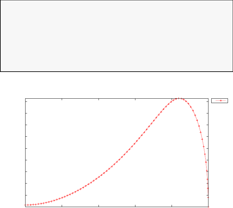
Optimal (unscaled) cost function value: 4.091759e+01
Phase 1 endpoint cost function value: 4.091759e+01
Phase 1 integrated part of the cost: 0.000000e+00
Phase 1 initial time: 0.000000e+00
Phase 1 final time: 4.091759e+01
Phase 1 maximum relative local error: 4.925376e-04
NLP solver reports: The problem has been solved!
0
200
400
600
800
1000
1200
1400
1600
1800
0 2000 4000 6000 8000 10000
h (m)
x (m)
Missile problem: altitude (m)
h
Figure 3.74: Missile altitude and a function of the longitudinal position
3.29 Moon lander problem
Consider the following optimal control problem, which is known in the litera-
ture as the moon lander problem [36]. Find tfand T(t)∈[0, tf] to minimize
the cost functional
J=Ztf
0
T(t)dt (3.120)
subject to the dynamic constraints
˙
h=v
˙v=−g+T/m
˙m=−T /E
(3.121)
294
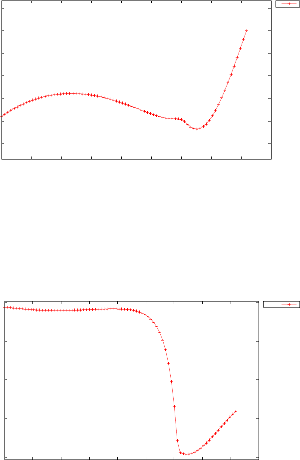
260
270
280
290
300
310
320
0 5 10 15 20 25 30 35 40 45
V (m/s)
time (s)
Missile problem: speed (m/s)
V
Figure 3.75: Missile speed as a function of time
-0.15
-0.1
-0.05
0
0.05
0 5 10 15 20 25 30 35 40 45
alpha (rad)
time (s)
Missile problem: angle of attack (rad)
alpha
Figure 3.76: Missile angle of attack as a function of time
295

the boundary conditions:
h(0) = 1
v(0) = −0.783
m(0) = 1
h(tf)=0.0
v(tf) = 0.0
(3.122)
and the bounds 0≤T(t)≤1.227
−20 ≤h(t)≤20
−20 ≤v(t)≤20
0.01 ≤m(t)≤1
0≤tf≤1000
(3.123)
where g= 1.0, and E= 2.349. The PSOPT code that solves this problem
is shown below.
//////////////////////////////////////////////////////////////////////////
////////////////// moonlander.cxx /////////////////////////
//////////////////////////////////////////////////////////////////////////
//////////////// PSOPT Example ////////////////////
//////////////////////////////////////////////////////////////////////////
//////////////////////////////////////////////////////////////////////////
//////// Title: Moonlander problem ////////////////
//////// Last modified: 05 January 2009 ////////////////
//////// Reference: PROPT Handbook ////////////////
//////// (See PSOPT handbook for full reference) ////////////////
//////////////////////////////////////////////////////////////////////////
//////// Copyright (c) Victor M. Becerra, 2009 ////////////////
//////////////////////////////////////////////////////////////////////////
//////// This is part of the PSOPT software library, which ///////////////
//////// is distributed under the terms of the GNU Lesser ////////////////
//////// General Public License (LGPL) ////////////////
//////////////////////////////////////////////////////////////////////////
#include "psopt.h"
//////////////////////////////////////////////////////////////////////////
/////////////////// Define the end point (Mayer) cost function //////////
//////////////////////////////////////////////////////////////////////////
adouble endpoint_cost(adouble* initial_states, adouble* final_states,
adouble* parameters,adouble& t0, adouble& tf,
adouble* xad, int iphase, Workspace* workspace)
{
return 0.0;
}
//////////////////////////////////////////////////////////////////////////
/////////////////// Define the integrand (Lagrange) cost function //////
//////////////////////////////////////////////////////////////////////////
adouble integrand_cost(adouble* states, adouble* controls, adouble* parameters,
adouble& time, adouble* xad, int iphase, Workspace* workspace)
{
adouble thrust = controls[0];
return thrust;
}
//////////////////////////////////////////////////////////////////////////
/////////////////// Define the DAE’s ////////////////////////////////////
//////////////////////////////////////////////////////////////////////////
void dae(adouble* derivatives, adouble* path, adouble* states,
adouble* controls, adouble* parameters, adouble& time,
296

adouble* xad, int iphase, Workspace* workspace)
{
adouble altitude_dot, speed_dot, mass_dot;
adouble altitude = states[0];
adouble speed = states[1];
adouble mass = states[2];
adouble thrust = controls[0];
double exhaust_velocity = 2.349;
double gravity = 1.0;
altitude_dot = speed;
speed_dot = -gravity + thrust/mass;
mass_dot = -thrust/exhaust_velocity;
derivatives[0] = altitude_dot;
derivatives[1] = speed_dot;
derivatives[2] = mass_dot;
}
////////////////////////////////////////////////////////////////////////////
/////////////////// Define the events function ////////////////////////////
////////////////////////////////////////////////////////////////////////////
void events(adouble* e, adouble* initial_states, adouble* final_states,
adouble* parameters,adouble& t0, adouble& tf, adouble* xad,
int iphase, Workspace* workspace)
{
adouble altitude_i = initial_states[0];
adouble speed_i = initial_states[1];
adouble mass_i = initial_states[2];
adouble altitude_f = final_states[0];
adouble speed_f = final_states[1];
e[0] = altitude_i;
e[1] = speed_i;
e[2] = mass_i;
e[3] = altitude_f;
e[4] = speed_f;
}
///////////////////////////////////////////////////////////////////////////
/////////////////// Define the phase linkages function ///////////////////
///////////////////////////////////////////////////////////////////////////
void linkages( adouble* linkages, adouble* xad, Workspace* workspace)
{
// No linkages as this is a single phase problem
}
////////////////////////////////////////////////////////////////////////////
/////////////////// Define the main routine ///////////////////////////////
////////////////////////////////////////////////////////////////////////////
int main(void)
{
////////////////////////////////////////////////////////////////////////////
/////////////////// Declare key structures ////////////////////////////////
////////////////////////////////////////////////////////////////////////////
Alg algorithm;
Sol solution;
Prob problem;
////////////////////////////////////////////////////////////////////////////
/////////////////// Register problem name ////////////////////////////////
////////////////////////////////////////////////////////////////////////////
problem.name = "Moon Lander Problem";
problem.outfilename = "moon.txt";
////////////////////////////////////////////////////////////////////////////
//////////// Define problem level constants & do level 1 setup ////////////
////////////////////////////////////////////////////////////////////////////
problem.nphases = 1;
problem.nlinkages = 0;
psopt_level1_setup(problem);
297

/////////////////////////////////////////////////////////////////////////////
///////// Define phase related information & do level 2 setup ////////////
/////////////////////////////////////////////////////////////////////////////
problem.phases(1).nstates = 3;
problem.phases(1).ncontrols = 1;
problem.phases(1).nevents = 5;
problem.phases(1).npath = 0;
problem.phases(1).nodes = 70;
psopt_level2_setup(problem, algorithm);
int nodes = 70;
////////////////////////////////////////////////////////////////////////////
/////////////////// Declare DMatrix objects to store results //////////////
////////////////////////////////////////////////////////////////////////////
DMatrix x, u, t;
DMatrix lambda, H;
////////////////////////////////////////////////////////////////////////////
/////////////////// Enter problem bounds information //////////////////////
////////////////////////////////////////////////////////////////////////////
double altitudeL = -20.0;
double speedL = -20.0;
double massL = 0.01;
double altitudeU = 20.0;
double speedU = 20.0;
double massU = 1.0;
double thrustL = 0.0;
double thrustU = 1.227;
double altitude_i = 1.0;
double speed_i = -0.783;
double mass_i = 1.0;
double altitude_f = 0.0;
double speed_f = 0.0;
problem.phases(1).bounds.lower.states(1) = altitudeL;
problem.phases(1).bounds.lower.states(2) = speedL;
problem.phases(1).bounds.lower.states(3) = massL;
problem.phases(1).bounds.upper.states(1) = altitudeU;
problem.phases(1).bounds.upper.states(2) = speedU;
problem.phases(1).bounds.upper.states(3) = massU;
problem.phases(1).bounds.lower.controls(1) = thrustL;
problem.phases(1).bounds.upper.controls(1) = thrustU;
problem.phases(1).bounds.lower.events(1) = altitude_i;
problem.phases(1).bounds.lower.events(2) = speed_i;
problem.phases(1).bounds.lower.events(3) = mass_i;
problem.phases(1).bounds.lower.events(4) = altitude_f;
problem.phases(1).bounds.lower.events(5) = speed_f;
problem.phases(1).bounds.upper.events = problem.phases(1).bounds.lower.events;
problem.phases(1).bounds.lower.StartTime = 0.0;
problem.phases(1).bounds.upper.StartTime = 0.0;
problem.phases(1).bounds.lower.EndTime = 0.0;
problem.phases(1).bounds.upper.EndTime = 1000.0;
////////////////////////////////////////////////////////////////////////////
/////////////////// Register problem functions ///////////////////////////
////////////////////////////////////////////////////////////////////////////
problem.integrand_cost = &integrand_cost;
problem.endpoint_cost = &endpoint_cost;
problem.dae = &dae;
problem.events = &events;
problem.linkages = &linkages;
////////////////////////////////////////////////////////////////////////////
298

/////////////////// Define & register initial guess ///////////////////////
////////////////////////////////////////////////////////////////////////////
DMatrix states_guess(3,nodes+1);
states_guess(1,colon()) = linspace(altitude_i, altitude_f, nodes+1);
states_guess(2,colon()) = linspace(speed_i, speed_f, nodes+1);
states_guess(3,colon()) = linspace(mass_i, massL, nodes+1);
problem.phases(1).guess.controls = 0.5*(thrustL+thrustU)*ones(1,nodes+1);
problem.phases(1).guess.states = states_guess;
problem.phases(1).guess.time = linspace(0.0, 1.5, nodes+1);
////////////////////////////////////////////////////////////////////////////
/////////////////// Enter algorithm options //////////////////////////////
////////////////////////////////////////////////////////////////////////////
algorithm.nlp_iter_max = 1000;
algorithm.nlp_tolerance = 1.e-6;
algorithm.nlp_method = "IPOPT";
algorithm.scaling = "automatic";
algorithm.derivatives = "automatic";
////////////////////////////////////////////////////////////////////////////
/////////////////// Now call PSOPT to solve the problem //////////////////
////////////////////////////////////////////////////////////////////////////
psopt(solution, problem, algorithm);
////////////////////////////////////////////////////////////////////////////
/////////// Extract relevant variables from solution structure //////////
////////////////////////////////////////////////////////////////////////////
x = solution.get_states_in_phase(1);
u = solution.get_controls_in_phase(1);
t = solution.get_time_in_phase(1);
lambda = solution.get_dual_costates_in_phase(1);
H = solution.get_dual_hamiltonian_in_phase(1);
////////////////////////////////////////////////////////////////////////////
/////////// Save solution data to files if desired ////////////////////////
////////////////////////////////////////////////////////////////////////////
x.Save("x.dat");
u.Save("u.dat");
t.Save("t.dat");
lambda.Save("lambda.dat");
H.Save("H.dat");
////////////////////////////////////////////////////////////////////////////
/////////// Plot some results if desired (requires gnuplot) ///////////////
////////////////////////////////////////////////////////////////////////////
plot(t,x,problem.name, "time (s)", "states", "altitude speed mass");
plot(t,u,problem.name, "time (s)", "control", "thrust");
plot(t,x,problem.name, "time (s)", "states", "altitude speed mass",
"pdf", "moon_states.pdf");
plot(t,u,problem.name, "time (s)", "control", "thrust",
"pdf", "moon_control.pdf");
}
////////////////////////////////////////////////////////////////////////////
/////////////////////// END OF FILE ///////////////////////////////
////////////////////////////////////////////////////////////////////////////
The output from PSOPT is summarised in the box below and shown
in Figures 3.77 and 3.78, which contain the elements of the state and the
control, respectively.
299
-1
-0.5
0
0.5
1
0 0.2 0.4 0.6 0.8 1 1.2 1.4
states
time (s)
Moon Lander Problem
altitude
speed
mass
Figure 3.77: States for moon lander problem
PSOPT results summary
=====================
Problem: Moon Lander Problem
CPU time (seconds): 5.159037e+00
NLP solver used: IPOPT
PSOPT release number: 4.0
Date and time of this run: Thu Feb 21 15:54:38 2019
Optimal (unscaled) cost function value: 1.420378e+00
Phase 1 endpoint cost function value: 0.000000e+00
Phase 1 integrated part of the cost: 1.420378e+00
Phase 1 initial time: 0.000000e+00
Phase 1 final time: 1.396972e+00
Phase 1 maximum relative local error: 5.386719e-05
NLP solver reports: The problem has been solved!
3.30 Multi-segment problem
Consider the following optimal control problem, where the optimal control
has a characteristic stepped shape [22]. Find u(t)∈[0,3] to minimize the
300
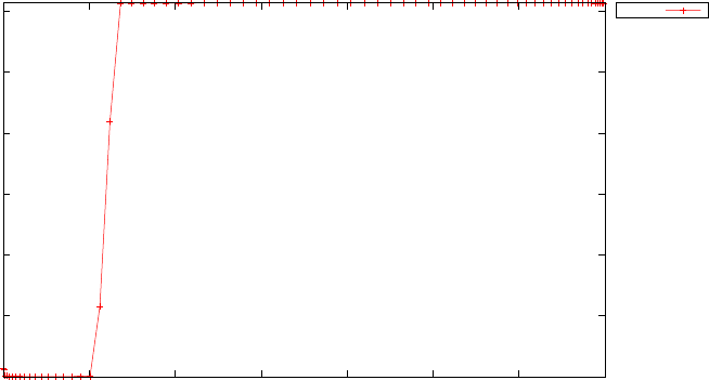
0
0.2
0.4
0.6
0.8
1
1.2
0 0.2 0.4 0.6 0.8 1 1.2 1.4
control
time (s)
Moon Lander Problem
thrust
Figure 3.78: Control for moon lander problem
cost functional
J=Z3
0
x(t)dt (3.124)
subject to the dynamic constraints
˙x=u(3.125)
the boundary conditions:
x(0) = 1
x(3) = 1 (3.126)
and the bounds −1≤u(t)≤1
x(t)≥0(3.127)
The analytical optimal control is given by:
u(t) =
−1, t ∈[0,1)
0, t ∈[1,2]
1, t ∈(2,3]
(3.128)
The problem has been solved using the multi-segment paradigm. Three
segments are defined in the code, such that the initial time is fixed at t(1)
0= 0,
the final time is fixed at t(3)
f= 3, and the intermediate junction times are
t(1)
f= 1, and t(2)
f= 2.
The PSOPT code that solves this problem is shown below.
301

//////////////////////////////////////////////////////////////////////////
//////////////// steps.cxx /////////////////////
//////////////////////////////////////////////////////////////////////////
//////////////// PSOPT example /////////////////////
//////////////////////////////////////////////////////////////////////////
//////////////////////////////////////////////////////////////////////////
//////// Title: Steps problem ////////////////
//////// Last modified: 12 July 2009 ////////////////
//////// Reference: Gong, Farhoo, and Ross (2008) ////////////////
//////// ////////////////
//////////////////////////////////////////////////////////////////////////
//////// Copyright (c) Victor M. Becerra, 2009 ////////////////
//////////////////////////////////////////////////////////////////////////
//////// This is part of the PSOPT software library, which ///////////////
//////// is distributed under the terms of the GNU Lesser ////////////////
//////// General Public License (LGPL) ////////////////
//////////////////////////////////////////////////////////////////////////
#include "psopt.h"
//////////////////////////////////////////////////////////////////////////
/////////////////// Define the end point (Mayer) cost function //////////
//////////////////////////////////////////////////////////////////////////
adouble endpoint_cost(adouble* initial_states, adouble* final_states,
adouble* parameters,adouble& t0, adouble& tf,
adouble* xad, int iphase, Workspace* workspace)
{
return 0.0;
}
//////////////////////////////////////////////////////////////////////////
/////////////////// Define the integrand (Lagrange) cost function //////
//////////////////////////////////////////////////////////////////////////
adouble integrand_cost(adouble* states, adouble* controls, adouble* parameters,
adouble& time, adouble* xad, int iphase, Workspace* workspace)
{
adouble x = states[ CINDEX(1) ];
return (x);
}
//////////////////////////////////////////////////////////////////////////
/////////////////// Define the DAE’s ////////////////////////////////////
//////////////////////////////////////////////////////////////////////////
void dae(adouble* derivatives, adouble* path, adouble* states,
adouble* controls, adouble* parameters, adouble& time,
adouble* xad, int iphase, Workspace* workspace)
{
adouble u = controls[CINDEX(1)];
derivatives[ CINDEX(1) ] = u;
}
////////////////////////////////////////////////////////////////////////////
/////////////////// Define the events function ////////////////////////////
////////////////////////////////////////////////////////////////////////////
void events(adouble* e, adouble* initial_states, adouble* final_states,
adouble* parameters,adouble& t0, adouble& tf, adouble* xad,
int iphase, Workspace* workspace)
{
adouble x1_i = initial_states[ CINDEX(1) ];
adouble x1_f = final_states[ CINDEX(1) ];
if ( iphase==1 ) {
e[ CINDEX(1) ] = x1_i;
}
else if ( iphase==3 ) {
302

e[ CINDEX(1) ] = x1_f;
}
}
///////////////////////////////////////////////////////////////////////////
/////////////////// Define the phase linkages function ///////////////////
///////////////////////////////////////////////////////////////////////////
void linkages( adouble* linkages, adouble* xad, Workspace* workspace)
{
}
////////////////////////////////////////////////////////////////////////////
/////////////////// Define the main routine ///////////////////////////////
////////////////////////////////////////////////////////////////////////////
int main(void)
{
////////////////////////////////////////////////////////////////////////////
/////////////////// Declare key structures ////////////////////////////////
////////////////////////////////////////////////////////////////////////////
Alg algorithm;
Sol solution;
Prob problem;
MSdata msdata;
////////////////////////////////////////////////////////////////////////////
/////////////////// Register problem name ////////////////////////////////
////////////////////////////////////////////////////////////////////////////
problem.name = "Steps problem";
problem.outfilename = "steps.txt";
////////////////////////////////////////////////////////////////////////////
//////////// Define problem level constants & do level 1 setup ////////////
////////////////////////////////////////////////////////////////////////////
msdata.nsegments = 3;
msdata.nstates = 1;
msdata.ncontrols = 1;
msdata.nparameters = 0;
msdata.npath = 0;
msdata.ninitial_events = 1;
msdata.nfinal_events = 1;
msdata.nodes = 20; // nodes per segment
multi_segment_setup(problem, algorithm, msdata );
////////////////////////////////////////////////////////////////////////////
/////////////////// Enter problem bounds information //////////////////////
////////////////////////////////////////////////////////////////////////////
problem.phases(1).bounds.lower.controls(1) = -1.0;
problem.phases(1).bounds.upper.controls(1) = 1.0;
problem.phases(1).bounds.lower.states(1) = 0.0;
problem.phases(1).bounds.upper.states(1) = 5.0;
problem.phases(1).bounds.lower.events(1) = 1.0;
problem.phases(3).bounds.lower.events(1) = 1.0;
problem.phases(1).bounds.upper.events=problem.phases(1).bounds.lower.events;
problem.phases(3).bounds.upper.events=problem.phases(3).bounds.lower.events;
problem.phases(1).bounds.lower.StartTime = 0.0;
problem.phases(1).bounds.upper.StartTime = 0.0;
problem.phases(3).bounds.lower.EndTime = 3.0;
problem.phases(3).bounds.upper.EndTime = 3.0;
// problem.bounds.lower.times = "[0.0, 1.0, 2.0, 3.0]";
// problem.bounds.upper.times = "[0.0, 1.0, 2.0, 3.0]";
303

problem.bounds.lower.times = "[0.0, 1.0, 2.0, 3.0]";
problem.bounds.upper.times = "[0.0, 1.0, 2.0, 3.0]";
auto_phase_bounds(problem);
////////////////////////////////////////////////////////////////////////////
/////////////////// Register problem functions ///////////////////////////
////////////////////////////////////////////////////////////////////////////
problem.integrand_cost = &integrand_cost;
problem.endpoint_cost = &endpoint_cost;
problem.dae = &dae;
problem.events = &events;
problem.linkages = &linkages;
////////////////////////////////////////////////////////////////////////////
/////////////////// Define & register initial guess ///////////////////////
////////////////////////////////////////////////////////////////////////////
int nnodes = problem.phases(1).nodes(1);
int ncontrols = problem.phases(1).ncontrols;
int nstates = problem.phases(1).nstates;
DMatrix state_guess = zeros(nstates,nnodes);
DMatrix control_guess = zeros(ncontrols,nnodes);
DMatrix time_guess = linspace(0.0,3.0,nnodes);
DMatrix param_guess;
state_guess(1,colon()) = linspace(1.0, 1.0, nnodes);
control_guess(1,colon()) = zeros(1,nnodes);
auto_phase_guess(problem, control_guess, state_guess, param_guess, time_guess);
////////////////////////////////////////////////////////////////////////////
/////////////////// Enter algorithm options //////////////////////////////
////////////////////////////////////////////////////////////////////////////
algorithm.nlp_iter_max = 1000;
algorithm.nlp_tolerance = 1.e-6;
algorithm.nlp_method = "IPOPT";
algorithm.scaling = "automatic";
algorithm.derivatives = "automatic";
algorithm.hessian = "exact";
algorithm.mesh_refinement = "automatic";
algorithm.ode_tolerance = 1.e-5;
////////////////////////////////////////////////////////////////////////////
/////////////////// Now call PSOPT to solve the problem //////////////////
////////////////////////////////////////////////////////////////////////////
psopt(solution, problem, algorithm);
////////////////////////////////////////////////////////////////////////////
/////////// Extract relevant variables from solution structure //////////
////////////////////////////////////////////////////////////////////////////
DMatrix x, u, t, xi, ui, ti;
x = solution.get_states_in_phase(1);
u = solution.get_controls_in_phase(1);
t = solution.get_time_in_phase(1);
for(int i=2;i<=problem.nphases;i++) {
xi = solution.get_states_in_phase(i);
ui = solution.get_controls_in_phase(i);
ti = solution.get_time_in_phase(i);
x = x || xi;
u = u || ui;
t = t || ti;
304

}
////////////////////////////////////////////////////////////////////////////
/////////// Save solution data to files if desired ////////////////////////
////////////////////////////////////////////////////////////////////////////
x.Save("x.dat");
u.Save("u.dat");
t.Save("t.dat");
////////////////////////////////////////////////////////////////////////////
/////////// Plot some results if desired (requires gnuplot) ///////////////
////////////////////////////////////////////////////////////////////////////
plot(t,x(1,colon()),problem.name+": state","time (s)", "x", "x");
plot(t,u(1,colon()),problem.name+": control","time (s)", "u", "u");
plot(t,x(1,colon()),problem.name+": state","time (s)", "x", "x",
"pdf", "steps_state.pdf");
plot(t,u(1,colon()),problem.name+": control","time (s)", "u", "u",
"pdf", "steps_control.pdf");
}
////////////////////////////////////////////////////////////////////////////
/////////////////////// END OF FILE ///////////////////////////////
////////////////////////////////////////////////////////////////////////////
The output from PSOPT is summarised in the box below and shown
in Figures 3.79 and 3.80, which contain the elements of the state and the
control, respectively.
PSOPT results summary
=====================
Problem: Steps problem
CPU time (seconds): 8.536780e-01
NLP solver used: IPOPT
PSOPT release number: 4.0
Date and time of this run: Thu Feb 21 17:24:35 2019
Optimal (unscaled) cost function value: 1.000010e+00
Phase 1 endpoint cost function value: 0.000000e+00
Phase 1 integrated part of the cost: 5.000034e-01
Phase 1 initial time: 0.000000e+00
Phase 1 final time: 1.000000e+00
Phase 1 maximum relative local error: 6.960834e-07
Phase 2 endpoint cost function value: 0.000000e+00
Phase 2 integrated part of the cost: 3.401579e-06
Phase 2 initial time: 1.000000e+00
Phase 2 final time: 2.000000e+00
305
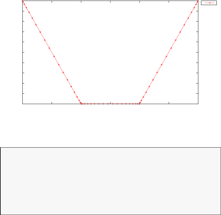
0
0.1
0.2
0.3
0.4
0.5
0.6
0.7
0.8
0.9
1
0 0.5 1 1.5 2 2.5 3
x
time (s)
Steps problem: state
x
Figure 3.79: State trajectory for the multi-segment problem
Phase 2 maximum relative local error: 4.856300e-06
Phase 3 endpoint cost function value: 0.000000e+00
Phase 3 integrated part of the cost: 5.000034e-01
Phase 3 initial time: 2.000000e+00
Phase 3 final time: 3.000000e+00
Phase 3 maximum relative local error: 6.961454e-07
NLP solver reports: The problem has been solved!
3.31 Notorious parameter estimation problem
Consider the following parameter estimation problem, which is known to be
challenging to single-shooting methods because of internal instability of the
differential equations [37]. Find p∈ < to minimize
J=
200
X
i=1
(y1(ti)−˜y1(i))2+ (y2(ti)−˜y2(i))2(3.129)
subject to the dynamic constraints
˙y1=y2
˙y2=µ2y1−(µ2+p2) sin(pt)(3.130)
306
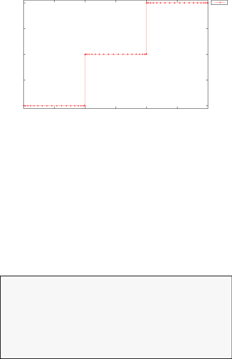
-1
-0.5
0
0.5
1
0 0.5 1 1.5 2 2.5 3
u
time (s)
Steps problem: control
u
Figure 3.80: Control trajectory for the multi-segment problem
where µ= 60.0, y1(0) = 0, y2(0) = π. The parameter estimation facilities
of PSOPT are used in this example. In this case, the observations function
is:
g(x(θk), u(θk), p, θk)=[y1(θk)y2(θk)]T
The PSOPT code that solves this problem is shown below. The code in-
cludes the generation of the measurement vectors ˜y1, and ˜y2by adding
Gaussian noise with standard deviation 0.05 to the exact solution of the
problem with p=π, which is given by:
y1(t) = sin(πt)
y2(t) = πcos(πt)
The code also defines the vector of sampling instants θi, i = 1,...,200 as a
uniform random samples in the interval [0,1].
//////////////////////////////////////////////////////////////////////////
////////////////// notorious.cxx ///////////////////////////
//////////////////////////////////////////////////////////////////////////
//////////////// PSOPT Example ////////////////////
//////////////////////////////////////////////////////////////////////////
//////////////////////////////////////////////////////////////////////////
//////// Title: Bock’s notorious parameter estimation problem ///////////
//////// Last modified: 08 April 2011 ////////////////
//////// Reference: Schittkowskit (2002) ////////////////
//////// (See PSOPT handbook for full reference) ///////////////
//////////////////////////////////////////////////////////////////////////
//////// Copyright (c) Victor M. Becerra, 2009 ////////////////
//////////////////////////////////////////////////////////////////////////
//////// This is part of the PSOPT software library, which ///////////////
//////// is distributed under the terms of the GNU Lesser ////////////////
//////// General Public License (LGPL) ////////////////
307

//////////////////////////////////////////////////////////////////////////
#include "psopt.h"
//////////////////////////////////////////////////////////////////////////
/////////////////// Define the observation function //////////
//////////////////////////////////////////////////////////////////////////
void observation_function( adouble* observations,
adouble* states, adouble* controls,
adouble* parameters, adouble& time, int k,
adouble* xad, int iphase, Workspace* workspace)
{
observations[ CINDEX(1) ] = states[ CINDEX(1) ];
observations[ CINDEX(2) ] = states[ CINDEX(2) ];
}
//////////////////////////////////////////////////////////////////////////
/////////////////// Define the DAE’s ////////////////////////////////////
//////////////////////////////////////////////////////////////////////////
void dae(adouble* derivatives, adouble* path, adouble* states,
adouble* controls, adouble* parameters, adouble& time,
adouble* xad, int iphase, Workspace* workspace)
{
adouble x1 = states[ CINDEX(1) ];
adouble x2 = states[ CINDEX(2) ];
adouble p = parameters[ CINDEX(1) ];
adouble t = time;
double mu = 60.0;
derivatives[CINDEX(1)] = x2;
derivatives[CINDEX(2)] = mu*mu*x1 - (mu*mu + p*p)*sin(p*t);
}
////////////////////////////////////////////////////////////////////////////
/////////////////// Define the events function ////////////////////////////
////////////////////////////////////////////////////////////////////////////
void events(adouble* e, adouble* initial_states, adouble* final_states,
adouble* parameters,adouble& t0, adouble& tf, adouble* xad,
int iphase, Workspace* workspace)
{
e[ 0 ] = initial_states[0];
e[ 1 ] = initial_states[1];
}
///////////////////////////////////////////////////////////////////////////
/////////////////// Define the phase linkages function ///////////////////
///////////////////////////////////////////////////////////////////////////
void linkages( adouble* linkages, adouble* xad, Workspace* workspace)
{
// No linkages as this is a single phase problem
}
////////////////////////////////////////////////////////////////////////////
/////////////////// Define the main routine ///////////////////////////////
////////////////////////////////////////////////////////////////////////////
int main(void)
{
int nobs =200;
// Generate true solution at sampling points and add noise
308

double sigma = 0.05;
DMatrix theta, y1m, y2m, ym;
theta = randu(1,nobs);
sort(theta);
y1m = sin( pi* theta ) + sigma*randn(1,nobs);
y2m = pi*cos( pi*theta ) + sigma*randn(1,nobs);
////////////////////////////////////////////////////////////////////////////
/////////////////// Declare key structures ////////////////////////////////
////////////////////////////////////////////////////////////////////////////
Alg algorithm;
Sol solution;
Prob problem;
////////////////////////////////////////////////////////////////////////////
/////////////////// Register problem name ////////////////////////////////
////////////////////////////////////////////////////////////////////////////
problem.name = "Bocks notorious parameter estimation problem";
problem.outfilename = "notorious.txt";
////////////////////////////////////////////////////////////////////////////
//////////// Define problem level constants & do level 1 setup ////////////
////////////////////////////////////////////////////////////////////////////
problem.nphases = 1;
problem.nlinkages = 0;
psopt_level1_setup(problem);
/////////////////////////////////////////////////////////////////////////////
///////// Define phase related information & do level 2 setup /////////////
/////////////////////////////////////////////////////////////////////////////
problem.phases(1).nstates = 2;
problem.phases(1).ncontrols = 0;
problem.phases(1).nevents = 2;
problem.phases(1).npath = 0;
problem.phases(1).nparameters = 1;
problem.phases(1).nodes = "[80]";
problem.phases(1).nobserved = 2;
problem.phases(1).nsamples = nobs;
psopt_level2_setup(problem, algorithm);
////////////////////////////////////////////////////////////////////////////
//////////// Enter estimation information ////////////
////////////////////////////////////////////////////////////////////////////
problem.phases(1).observation_nodes = (theta);
problem.phases(1).observations = (y1m && y2m);
////////////////////////////////////////////////////////////////////////////
/////////////////// Enter problem bounds information //////////////////////
////////////////////////////////////////////////////////////////////////////
problem.phases(1).bounds.lower.states(1) = -10.0;
problem.phases(1).bounds.lower.states(2) = -100.0;
problem.phases(1).bounds.upper.states(1) = 10.0;
problem.phases(1).bounds.upper.states(2) = 100.0;
problem.phases(1).bounds.lower.parameters(1) = -10.0;
problem.phases(1).bounds.upper.parameters(1) = 10.0;
problem.phases(1).bounds.lower.events(1) = 0.0;
309

problem.phases(1).bounds.upper.events(1) = 0.0;
problem.phases(1).bounds.lower.events(2) = pi;
problem.phases(1).bounds.upper.events(2) = pi;
problem.phases(1).bounds.lower.StartTime = 0.0;
problem.phases(1).bounds.upper.StartTime = 0.0;
problem.phases(1).bounds.lower.EndTime = 1.0;
problem.phases(1).bounds.upper.EndTime = 1.0;
////////////////////////////////////////////////////////////////////////////
/////////////////// Register problem functions ///////////////////////////
////////////////////////////////////////////////////////////////////////////
problem.dae = &dae;
problem.events = &events;
problem.linkages = &linkages;
problem.observation_function = & observation_function;
////////////////////////////////////////////////////////////////////////////
/////////////////// Define & register initial guess ///////////////////////
////////////////////////////////////////////////////////////////////////////
int nnodes = problem.phases(1).nodes(1);
DMatrix state_guess;
state_guess = zeros(2,nnodes);
problem.phases(1).guess.states = state_guess;
problem.phases(1).guess.time = linspace(0.0, 1.0, nnodes);
problem.phases(1).guess.parameters = 0.0;
////////////////////////////////////////////////////////////////////////////
/////////////////// Enter algorithm options //////////////////////////////
////////////////////////////////////////////////////////////////////////////
algorithm.nlp_method = "IPOPT";
algorithm.scaling = "automatic";
algorithm.derivatives = "automatic";
algorithm.collocation_method = "trapezoidal";
algorithm.nlp_iter_max = 200;
algorithm.nlp_tolerance = 1.e-4;
// algorithm.mesh_refinement = "automatic";
// algorithm.ode_tolerance = 1.e-6;
////////////////////////////////////////////////////////////////////////////
/////////////////// Now call PSOPT to solve the problem //////////////////
////////////////////////////////////////////////////////////////////////////
psopt(solution, problem, algorithm);
////////////////////////////////////////////////////////////////////////////
/////////////////// Declare DMatrix objects to store results //////////////
////////////////////////////////////////////////////////////////////////////
DMatrix states, x1, x2, p, t;
////////////////////////////////////////////////////////////////////////////
/////////// Extract relevant variables from solution structure //////////
////////////////////////////////////////////////////////////////////////////
states = solution.get_states_in_phase(1);
t = solution.get_time_in_phase(1);
p = solution.get_parameters_in_phase(1);
x1 = states(1,colon());
x2 = states(2,colon());
////////////////////////////////////////////////////////////////////////////
/////////// Save solution data to files if desired ////////////////////////
////////////////////////////////////////////////////////////////////////////
states.Save("states.dat");
t.Save("t.dat");
p.Print("Estimated parameter");
310

Abs(p-pi).Print("Parameter error");
////////////////////////////////////////////////////////////////////////////
/////////// Plot some results if desired (requires gnuplot) ///////////////
////////////////////////////////////////////////////////////////////////////
plot(theta,ym(1,colon()),t,x1,problem.name, "time (s)", "observed x1", "x1m x1");
plot(theta,ym(2,colon()),t,x2,problem.name, "time (s)", "observed x2", "x2m x2");
}
////////////////////////////////////////////////////////////////////////////
/////////////////////// END OF FILE ///////////////////////////////
////////////////////////////////////////////////////////////////////////////
The output from PSOPT is summarized in the box below. The optimal
parameter found was p= 3.141180, which is an approximation of πwith
an error of the order of 10−4. The 95% confidence interval of the estimated
parameter is [3.132363,3.149998].
PSOPT results summary
=====================
Problem: Bocks notorious parameter estimation problem
CPU time (seconds): 1.848284e+00
NLP solver used: IPOPT
PSOPT release number: 4.0
Date and time of this run: Thu Feb 21 17:06:04 2019
Optimal (unscaled) cost function value: 9.310255e-01
Phase 1 endpoint cost function value: 9.310255e-01
Phase 1 integrated part of the cost: 0.000000e+00
Phase 1 initial time: 0.000000e+00
Phase 1 final time: 1.000000e+00
Phase 1 maximum relative local error: 5.098817e-04
NLP solver reports: The problem has been solved!
3.32 Predator-prey parameter estimation problem
This is a well knowon model that describes the behaviour of predator and
prey species of an ecological system. The Letka-Volterra model system con-
sist of two differential equations [37].
The dynamic equations are given by:
˙x1=−p1x1+p2x1x2
˙x2=p3x2−p4x1x2
(3.131)
311

with boundary condition:
x1(0) = 0.4
x2(0) = 1
The observation functions are:
g1=x1
g2=x2
(3.132)
The measured data, with consists of ns= 10 samples over the interval t∈
[0,10], was constructed from simulations with parameter values [p1, p2, p3, p4] =
[1,1,1,1] with added noise. The weights of both observations are the same
and equal to one.
The solution is found using local discretisation (trapezoidal, Hermite-
Simpson) and automatic mesh refinement, starting with 20 grid points with
ODE tolerance 10−4. The code that solves the problem is shown below.
The estimated parameter values and their 95% confidence limits are shown
in Table 3.32. Figure 3.81 shows the observations as well as the estimated
values of variables x1and x2. The mesh statistics can be seen in Table 3.7
//////////////////////////////////////////////////////////////////////////
////////////////// predator.cxx ///////////////////////////
//////////////////////////////////////////////////////////////////////////
//////////////// PSOPT Example ////////////////////
//////////////////////////////////////////////////////////////////////////
//////////////////////////////////////////////////////////////////////////
//////// Title: Lotka-Volterra model parameter estimation //// //////////
//////// Last modified: 03 Jan 2014 ////////////////
//////// Reference: Schittkowski (2002) ////////////////
//////// (See PSOPT handbook for full reference) ///////////////
//////////////////////////////////////////////////////////////////////////
//////// Copyright (c) Victor M. Becerra, 2014 ////////////////
//////////////////////////////////////////////////////////////////////////
//////// This is part of the PSOPT software library, which ///////////////
//////// is distributed under the terms of the GNU Lesser ////////////////
//////// General Public License (LGPL) ////////////////
//////////////////////////////////////////////////////////////////////////
#include "psopt.h"
//////////////////////////////////////////////////////////////////////////
/////////////////// Define the observation function //////////
//////////////////////////////////////////////////////////////////////////
void observation_function( adouble* observations,
adouble* states, adouble* controls,
adouble* parameters, adouble& time, int k,
adouble* xad, int iphase, Workspace* workspace)
{
int i;
for (i=0; i<2; i++) {
observations[ i ] = states[ i ];
}
}
//////////////////////////////////////////////////////////////////////////
/////////////////// Define the DAE’s ////////////////////////////////////
//////////////////////////////////////////////////////////////////////////
void dae(adouble* derivatives, adouble* path, adouble* states,
adouble* controls, adouble* parameters, adouble& time,
adouble* xad, int iphase, Workspace* workspace)
312

{
// Variables
adouble x1, x2, p1, p2, p3, p4;
// Differential states
x1 = states[CINDEX(1)];
x2 = states[CINDEX(2)];
// Parameters
p1 = parameters[CINDEX(1)];
p2 = parameters[CINDEX(2)];
p3 = parameters[CINDEX(3)];
p4 = parameters[CINDEX(4)];
derivatives[CINDEX(1)] = -p1*x1 + p2*x1*x2;
derivatives[CINDEX(2)] = p3*x2 - p4*x1*x2;
}
////////////////////////////////////////////////////////////////////////////
/////////////////// Define the events function ////////////////////////////
////////////////////////////////////////////////////////////////////////////
void events(adouble* e, adouble* initial_states, adouble* final_states,
adouble* parameters,adouble& t0, adouble& tf, adouble* xad,
int iphase, Workspace* workspace)
{
int i;
for (i=0; i<2; i++) {
e[i] = initial_states[i];
}
}
///////////////////////////////////////////////////////////////////////////
/////////////////// Define the phase linkages function ///////////////////
///////////////////////////////////////////////////////////////////////////
void linkages( adouble* linkages, adouble* xad, Workspace* workspace)
{
// No linkages as this is a single phase problem
}
////////////////////////////////////////////////////////////////////////////
/////////////////// Define the main routine ///////////////////////////////
////////////////////////////////////////////////////////////////////////////
int main(void)
{
////////////////////////////////////////////////////////////////////////////
/////////////////// Declare key structures ////////////////////////////////
////////////////////////////////////////////////////////////////////////////
Alg algorithm;
Sol solution;
Prob problem;
////////////////////////////////////////////////////////////////////////////
/////////////////// Register problem name ////////////////////////////////
////////////////////////////////////////////////////////////////////////////
problem.name = "Predator-prey example";
problem.outfilename = "predator.txt";
////////////////////////////////////////////////////////////////////////////
//////////// Define problem level constants & do level 1 setup ////////////
////////////////////////////////////////////////////////////////////////////
problem.nphases = 1;
problem.nlinkages = 0;
psopt_level1_setup(problem);
313

/////////////////////////////////////////////////////////////////////////////
///////// Define phase related information & do level 2 setup /////////////
/////////////////////////////////////////////////////////////////////////////
problem.phases(1).nstates = 2;
problem.phases(1).ncontrols = 0;
problem.phases(1).nevents = 2;
problem.phases(1).npath = 0;
problem.phases(1).nparameters = 4;
problem.phases(1).nodes = 20;
problem.phases(1).nobserved = 2;
problem.phases(1).nsamples = 10;
psopt_level2_setup(problem, algorithm);
////////////////////////////////////////////////////////////////////////////
//////////// Load data for parameter estimation ////////////
////////////////////////////////////////////////////////////////////////////
int iphase = 1;
load_parameter_estimation_data(problem, iphase, "predator.dat");
problem.phases(1).observation_nodes.Print("observation nodes");
problem.phases(1).observations.Print("observations");
problem.phases(1).residual_weights.Print("weights");
////////////////////////////////////////////////////////////////////////////
/////////////////// Declare DMatrix objects to store results //////////////
////////////////////////////////////////////////////////////////////////////
DMatrix x, p, t;
////////////////////////////////////////////////////////////////////////////
/////////////////// Enter problem bounds information //////////////////////
////////////////////////////////////////////////////////////////////////////
problem.phases(1).bounds.lower.states(1) = 0.0;
problem.phases(1).bounds.lower.states(2) = 0.0;
problem.phases(1).bounds.upper.states(1) = 3.0;
problem.phases(1).bounds.upper.states(2) = 3.0;
problem.phases(1).bounds.lower.events(1) = 0.4;
problem.phases(1).bounds.lower.events(2) = 1.0;
problem.phases(1).bounds.upper.events(1) = 0.4;
problem.phases(1).bounds.upper.events(2) = 1.0;
problem.phases(1).bounds.lower.parameters(1) = -1.0;
problem.phases(1).bounds.lower.parameters(2) = -1.0;
problem.phases(1).bounds.lower.parameters(3) = -1.0;
problem.phases(1).bounds.lower.parameters(4) = -1.0;
problem.phases(1).bounds.upper.parameters(1) = 5.0;
problem.phases(1).bounds.upper.parameters(2) = 5.0;
problem.phases(1).bounds.upper.parameters(3) = 5.0;
problem.phases(1).bounds.upper.parameters(4) = 5.0;
problem.phases(1).bounds.lower.StartTime = 0.0;
problem.phases(1).bounds.upper.StartTime = 0.0;
problem.phases(1).bounds.lower.EndTime = 10.0;
problem.phases(1).bounds.upper.EndTime = 10.0;
////////////////////////////////////////////////////////////////////////////
/////////////////// Register problem functions ///////////////////////////
////////////////////////////////////////////////////////////////////////////
problem.dae = &dae;
problem.events = &events;
problem.linkages = &linkages;
problem.observation_function = & observation_function;
////////////////////////////////////////////////////////////////////////////
/////////////////// Define & register initial guess ///////////////////////
////////////////////////////////////////////////////////////////////////////
314

int nnodes = (int) problem.phases(1).nsamples;
DMatrix state_guess(3, nnodes);
DMatrix param_guess(2,1);
state_guess(1,colon()) = linspace(0.4, 0.4, nnodes );
state_guess(2,colon()) = linspace(1.0, 1.0, nnodes );
param_guess(1) = 0.8;
param_guess(2) = 0.8;
param_guess(3) = 1.5;
param_guess(4) = 1.5;
problem.phases(1).guess.states = state_guess;
problem.phases(1).guess.time = linspace(0.0, 10.0, nnodes);
problem.phases(1).guess.parameters = param_guess;
////////////////////////////////////////////////////////////////////////////
/////////////////// Enter algorithm options //////////////////////////////
////////////////////////////////////////////////////////////////////////////
algorithm.nlp_method = "IPOPT";
algorithm.scaling = "automatic";
algorithm.derivatives = "automatic";
algorithm.collocation_method = "trapezoidal";
algorithm.mesh_refinement = "automatic";
algorithm.ode_tolerance = 1.e-4;
////////////////////////////////////////////////////////////////////////////
/////////////////// Now call PSOPT to solve the problem //////////////////
////////////////////////////////////////////////////////////////////////////
psopt(solution, problem, algorithm);
////////////////////////////////////////////////////////////////////////////
/////////// Extract relevant variables from solution structure //////////
////////////////////////////////////////////////////////////////////////////
x = solution.get_states_in_phase(1);
t = solution.get_time_in_phase(1);
p = solution.get_parameters_in_phase(1);
////////////////////////////////////////////////////////////////////////////
/////////// Save solution data to files if desired ////////////////////////
////////////////////////////////////////////////////////////////////////////
x.Save("x.dat");
t.Save("t.dat");
p.Print("Estimated parameters");
////////////////////////////////////////////////////////////////////////////
/////////// Plot some results if desired (requires gnuplot) ///////////////
////////////////////////////////////////////////////////////////////////////
DMatrix tm;
DMatrix ym;
tm = problem.phases(1).observation_nodes;
ym = problem.phases(1).observations;
spplot(t,x,tm,ym,problem.name, "time (s)", "state x1", "x1 x2 y1 y2");
spplot(t,x,tm,ym,problem.name, "time (s)", "state x1", "x1 x2 y1 y2", "pdf", "x1x2.pdf");
}
////////////////////////////////////////////////////////////////////////////
/////////////////////// END OF FILE ///////////////////////////////
315
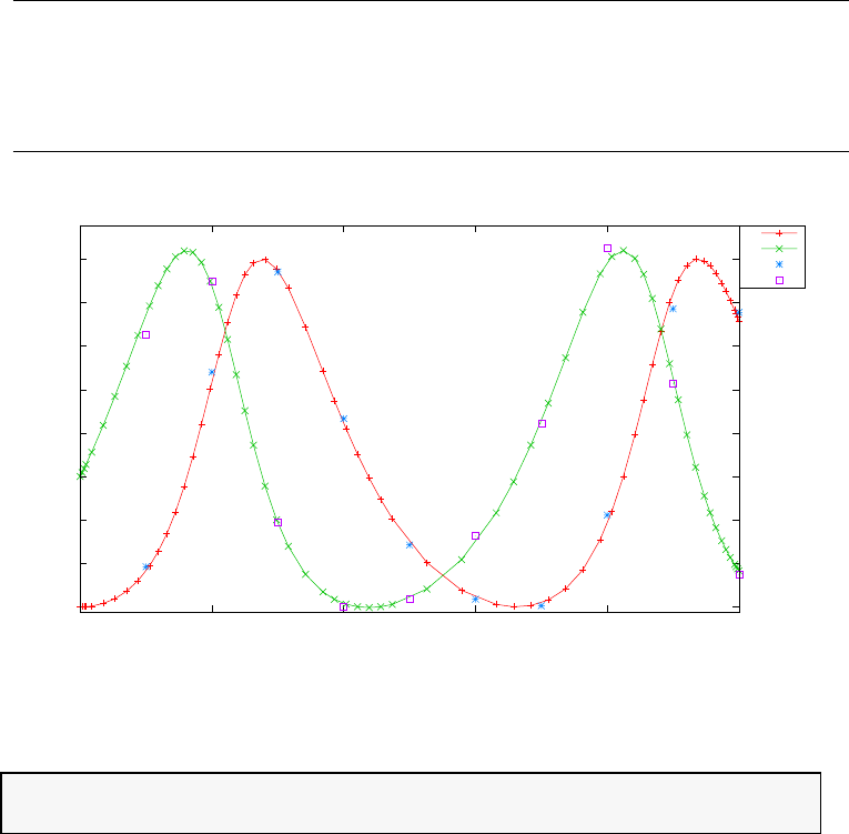
Table 3.6: Estimated parameter values and 95 percent statistical confidence
limits on estimated parameters
Parameter Low Confidence Limit Value High Confidence Limit
p17.166429e-01 9.837490e-01 1.250855e+00
p27.573469e-01 9.803930e-01 1.203439e+00
p37.287846e-01 1.016900e+00 1.305015e+00
p46.914964e-01 1.022702e+00 1.353909e+00
0.4
0.6
0.8
1
1.2
1.4
1.6
1.8
2
0 2 4 6 8 10
state x1
time (s)
Predator-prey example
x1
x2
y1
y2
Figure 3.81: Observations y1,y2and estimated states x1(t) and x2(t)
////////////////////////////////////////////////////////////////////////////
3.33 Rayleigh problem with mixed state-control
path constraints
Consider the following optimal control problem, which involves a path con-
straint in which the control and the state appear explicitly [4]. Find u(t)∈
[0, tf] to minimize the cost functional
J=Ztf
0x1(t)2+u(t)2dt(3.133)
316

Table 3.7: Mesh refinement statistics: Predator-prey example
Iter DM M NV NC OE CE JE HE RHS max CPUa
1 TRP 20 46 43 20 20 20 0 780 1.615e-02 4.000e-02
2 TRP 28 62 59 14 14 14 0 770 8.919e-03 4.000e-02
3 H-S 39 84 81 9 9 9 0 1035 1.670e-03 4.000e-02
4 H-S 54 114 111 11 11 11 0 1760 1.114e-04 5.000e-02
5 H-S 62 130 127 10 10 10 0 1840 3.985e-05 5.000e-02
CPUb- - - - - - - - - - 4.500e-01
- - - - - 64 64 64 0 6185 - 6.700e-01
Key: Iter=iteration number, DM= discretization method, M=number of nodes, NV=number of vari-
ables, NC=number of constraints, OE=objective evaluations, CE = constraint evaluations, JE = Jacobian
evaluations, HE = Hessian evaluations, RHS = ODE right hand side evaluations, max = maximum relative
ODE error, CPUa= CPU time in seconds spent by NLP algorithm, CPUb= additional CPU time in seconds
spent by PSOPT
subject to the dynamic constraints
˙x1=x2
˙x2=−x1+x2(1.4−px2
2)+4usin(θ)(3.134)
The path constraint:
u+x1
6≤0(3.135)
and the boundary conditions:
x1(0) = −5
x2(0) = −5(3.136)
where tf= 4.5, and p= 0.14. The PSOPT code that solves this problem
is shown below.
//////////////////////////////////////////////////////////////////////////
//////////////// PSOPT Example ////////////////////
//////////////////////////////////////////////////////////////////////////
//////////////////////////////////////////////////////////////////////////
//////// Title: Rayleigh problem ////////////////
//////// Last modified: 11 July 2011 ////////////////
//////// Reference: Betts (2010) ////////////////
//////// (See PSOPT handbook for full reference) ////////////////
//////////////////////////////////////////////////////////////////////////
//////// Copyright (c) Victor M. Becerra, 2011 ////////////////
//////////////////////////////////////////////////////////////////////////
//////// This is part of the PSOPT software library, which ///////////////
//////// is distributed under the terms of the GNU Lesser ////////////////
//////// General Public License (LGPL) ////////////////
//////////////////////////////////////////////////////////////////////////
#include "psopt.h"
//////////////////////////////////////////////////////////////////////////
/////////////////// Define the end point (Mayer) cost function //////////
//////////////////////////////////////////////////////////////////////////
adouble endpoint_cost(adouble* initial_states, adouble* final_states,
adouble* parameters,adouble& t0, adouble& tf,
adouble* xad, int iphase, Workspace* workspace)
{
return 0.0;
}
317

//////////////////////////////////////////////////////////////////////////
/////////////////// Define the integrand (Lagrange) cost function //////
//////////////////////////////////////////////////////////////////////////
adouble integrand_cost(adouble* states, adouble* controls,
adouble* parameters, adouble& time, adouble* xad,
int iphase, Workspace* workspace)
{
adouble x1 = states[CINDEX(1)];
adouble u = controls[CINDEX(1)];
return (u*u + x1*x1);
}
//////////////////////////////////////////////////////////////////////////
/////////////////// Define the DAE’s ////////////////////////////////////
//////////////////////////////////////////////////////////////////////////
void dae(adouble* derivatives, adouble* path, adouble* states,
adouble* controls, adouble* parameters, adouble& time,
adouble* xad, int iphase, Workspace* workspace)
{
adouble x1 = states[CINDEX(1)];
adouble x2 = states[CINDEX(2)];
adouble u = controls[CINDEX(1)];
double p = 0.14;
derivatives[ CINDEX(1) ] = x2;
derivatives[ CINDEX(2) ] = -x1 + x2*(1.4-p*x2*x2) + 4.0*u;
path[ CINDEX(1) ] = u + x1/6.0;
}
////////////////////////////////////////////////////////////////////////////
/////////////////// Define the events function ////////////////////////////
////////////////////////////////////////////////////////////////////////////
void events(adouble* e, adouble* initial_states, adouble* final_states,
adouble* parameters,adouble& t0, adouble& tf, adouble* xad,
int iphase, Workspace* workspace)
{
adouble x10 = initial_states[ CINDEX(1) ];
adouble x20 = initial_states[ CINDEX(2) ];
e[ CINDEX(1) ] = x10;
e[ CINDEX(2) ] = x20;
}
///////////////////////////////////////////////////////////////////////////
/////////////////// Define the phase linkages function ///////////////////
///////////////////////////////////////////////////////////////////////////
void linkages( adouble* linkages, adouble* xad, Workspace* workspace)
{
// No linkages as this is a single phase problem
}
////////////////////////////////////////////////////////////////////////////
/////////////////// Define the main routine ///////////////////////////////
////////////////////////////////////////////////////////////////////////////
int main(void)
{
////////////////////////////////////////////////////////////////////////////
/////////////////// Declare key structures ////////////////////////////////
////////////////////////////////////////////////////////////////////////////
Alg algorithm;
Sol solution;
Prob problem;
////////////////////////////////////////////////////////////////////////////
/////////////////// Register problem name ////////////////////////////////
////////////////////////////////////////////////////////////////////////////
318

problem.name = "Rayleigh problem";
problem.outfilename = "rayleigh.txt";
////////////////////////////////////////////////////////////////////////////
//////////// Declare problem level constants & do level 1 setup ///////////
////////////////////////////////////////////////////////////////////////////
problem.nphases = 1;
problem.nlinkages = 0;
psopt_level1_setup(problem);
/////////////////////////////////////////////////////////////////////////////
///////// Define phase related information & do level 2 setup /////////////
/////////////////////////////////////////////////////////////////////////////
problem.phases(1).nstates = 2;
problem.phases(1).ncontrols = 1;
problem.phases(1).nevents = 2;
problem.phases(1).npath = 1;
problem.phases(1).nodes = "[80]";
psopt_level2_setup(problem, algorithm);
////////////////////////////////////////////////////////////////////////////
/////////////////// Declare DMatrix objects to store results //////////////
////////////////////////////////////////////////////////////////////////////
DMatrix x, u, t;
DMatrix lambda, H, mu;
////////////////////////////////////////////////////////////////////////////
/////////////////// Enter problem bounds information //////////////////////
////////////////////////////////////////////////////////////////////////////
problem.phases(1).bounds.lower.states(1) = -10.0;
problem.phases(1).bounds.lower.states(2) = -10.0;
problem.phases(1).bounds.upper.states(1) = 10.0;
problem.phases(1).bounds.upper.states(2) = 10.0;
problem.phases(1).bounds.lower.controls(1) = -10.0;
problem.phases(1).bounds.upper.controls(1) = 10.0;
problem.phases(1).bounds.lower.events(1) = -5.0;
problem.phases(1).bounds.lower.events(2) = -5.0;
problem.phases(1).bounds.upper.events(1) = -5.0;
problem.phases(1).bounds.upper.events(2) = -5.0;
problem.phases(1).bounds.lower.path(1) = -100.0;
problem.phases(1).bounds.upper.path(1) = 0.0;
problem.phases(1).bounds.lower.StartTime = 0.0;
problem.phases(1).bounds.upper.StartTime = 0.0;
problem.phases(1).bounds.lower.EndTime = 4.5;
problem.phases(1).bounds.upper.EndTime = 4.5;
////////////////////////////////////////////////////////////////////////////
/////////////////// Register problem functions ///////////////////////////
////////////////////////////////////////////////////////////////////////////
problem.integrand_cost = &integrand_cost;
problem.endpoint_cost = &endpoint_cost;
problem.dae = &dae;
problem.events = &events;
problem.linkages = &linkages;
////////////////////////////////////////////////////////////////////////////
/////////////////// Define & register initial guess ///////////////////////
////////////////////////////////////////////////////////////////////////////
DMatrix x0(2,30);
x0(1,colon()) = -5.0*ones(1,30);
x0(2,colon()) = -5.0*ones(1, 30);
319

problem.phases(1).guess.controls = zeros(1,30);
problem.phases(1).guess.states = x0;
problem.phases(1).guess.time = linspace(0.0, 4.5, 30);
////////////////////////////////////////////////////////////////////////////
/////////////////// Enter algorithm options //////////////////////////////
////////////////////////////////////////////////////////////////////////////
////////////////////////////////////////////////////////////////////////////
/////////////////// Enter algorithm options //////////////////////////////
////////////////////////////////////////////////////////////////////////////
algorithm.nlp_method = "IPOPT";
algorithm.scaling = "automatic";
algorithm.derivatives = "automatic";
algorithm.collocation_method = "Hermite-Simpson";
algorithm.nlp_iter_max = 1000;
algorithm.nlp_tolerance = 1.e-10;
////////////////////////////////////////////////////////////////////////////
/////////////////// Now call PSOPT to solve the problem /////////////////
////////////////////////////////////////////////////////////////////////////
psopt(solution, problem, algorithm);
////////////////////////////////////////////////////////////////////////////
/////////// Extract relevant variables from solution structure //////////
////////////////////////////////////////////////////////////////////////////
x = solution.get_states_in_phase(1);
u = solution.get_controls_in_phase(1);
t = solution.get_time_in_phase(1);
lambda = solution.get_dual_costates_in_phase(1);
mu = solution.get_dual_path_in_phase(1);
H = solution.get_dual_hamiltonian_in_phase(1);
////////////////////////////////////////////////////////////////////////////
/////////// Save solution data to files if desired ////////////////////////
////////////////////////////////////////////////////////////////////////////
////////////////////////////////////////////////////////////////////////////
/////////// Plot some results if desired (requires gnuplot) ///////////////
////////////////////////////////////////////////////////////////////////////
plot(t,x,problem.name, "time (s)", "states", "x1 x2" );
plot(t,u,problem.name ,"time (s)", "control", "u" );
plot(t,lambda,problem.name ,"time (s)", "costates", "p1 p2");
plot(t,mu, problem.name,"time (s)", "mu", "mu");
plot(t,x,problem.name, "time (s)", "states", "x1 x2", "pdf", "rayleigh_states.pdf" );
plot(t,u,problem.name ,"time (s)", "control", "u", "pdf", "rayleigh_control.pdf" );
plot(t,lambda,problem.name ,"time (s)", "costates", "l1 l2", "pdf", "rayleigh_costates.pdf");
plot(t,mu, problem.name,"time (s)", "mu", "mu", "pdf", "rayleigh_mu.pdf");
}
////////////////////////////////////////////////////////////////////////////
/////////////////////// END OF FILE ///////////////////////////////
////////////////////////////////////////////////////////////////////////////
The output from PSOPT is summarised in the box below and shown in
Figures 3.82,3.83,3.85,3.85,3.85, which show, respectively, the trajectories
of the states, control, costates and path constraint multiplier. The results
are comparable to those presented by [4].
PSOPT results summary
320
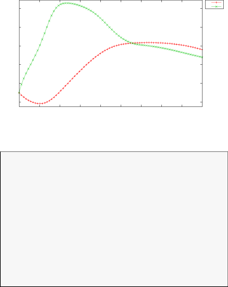
-6
-4
-2
0
2
4
0 0.5 1 1.5 2 2.5 3 3.5 4 4.5
states
time (s)
Rayleigh problem
x1
x2
Figure 3.82: States for Rayleigh problem
=====================
Problem: Rayleigh problem
CPU time (seconds): 1.295778e+00
NLP solver used: IPOPT
PSOPT release number: 4.0
Date and time of this run: Thu Feb 21 17:06:44 2019
Optimal (unscaled) cost function value: 4.477625e+01
Phase 1 endpoint cost function value: 0.000000e+00
Phase 1 integrated part of the cost: 4.477625e+01
Phase 1 initial time: 0.000000e+00
Phase 1 final time: 4.500000e+00
Phase 1 maximum relative local error: 2.329140e-03
NLP solver reports: The problem has been solved!
3.34 Obstacle avoidance problem
Consider the following optimal control problem, which involves finding an
optimal trajectory for a particle to travel from A to B while avoiding two
321
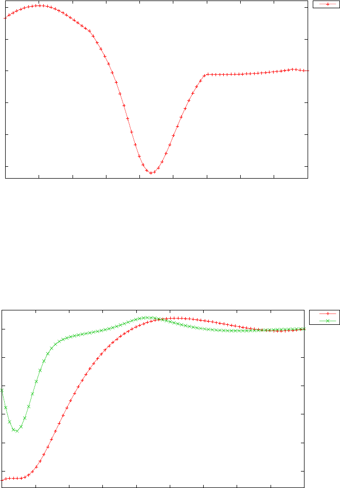
-1.5
-1
-0.5
0
0.5
1
0 0.5 1 1.5 2 2.5 3 3.5 4 4.5
control
time (s)
Rayleigh problem
u
Figure 3.83: Optimal control for Rayleigh problem
-10
-8
-6
-4
-2
0
0 0.5 1 1.5 2 2.5 3 3.5 4 4.5
costates
time (s)
Rayleigh problem
l1
l2
Figure 3.84: Costates for Rayleigh problem
322
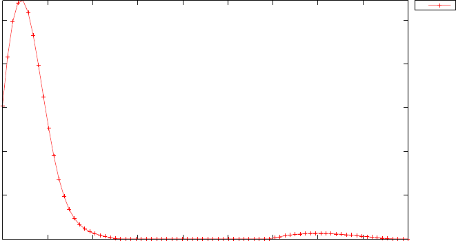
0
5
10
15
20
25
0 0.5 1 1.5 2 2.5 3 3.5 4 4.5
mu
time (s)
Rayleigh problem
mu
Figure 3.85: Path constraint multiplier for Rayleigh problem
forbidden regions [36]. Find θ(t)∈[0, tf] to minimize the cost functional
J=Ztf
0˙x(t)2+ ˙y(t)2dt (3.137)
subject to the dynamic constraints
˙x=Vcos(θ)
˙y=Vsin(θ)(3.138)
The path constraints:
(x(t)−0.4)2+ (y(t)−0.5)2≥0.1
(x(t)−0.8)2+ (y(t)−1.5)2≥0.1,(3.139)
and the boundary conditions:
x(0) = 0
y(0) = 0
x(tf)=1.2
y(tf) = 1.6
(3.140)
where tf= 1.0, and V= 2.138. The PSOPT code that solves this problem
is shown below.
323

//////////////////////////////////////////////////////////////////////////
//////////////// obstacle.cxx /////////////////////
//////////////////////////////////////////////////////////////////////////
//////////////// PSOPT Example ////////////////////
//////////////////////////////////////////////////////////////////////////
//////////////////////////////////////////////////////////////////////////
//////// Title: Obstacle avoidance problem ////////////////
//////// Last modified: 05 January 2009 ////////////////
//////// Reference: PROPT User’s Guide ////////////////
//////// (See PSOPT handbook for full reference) ////////////////
//////////////////////////////////////////////////////////////////////////
//////// Copyright (c) Victor M. Becerra, 2009 ////////////////
//////////////////////////////////////////////////////////////////////////
//////// This is part of the PSOPT software library, which ///////////////
//////// is distributed under the terms of the GNU Lesser ////////////////
//////// General Public License (LGPL) ////////////////
//////////////////////////////////////////////////////////////////////////
#include "psopt.h"
//////////////////////////////////////////////////////////////////////////
/////////////////// Define the end point (Mayer) cost function //////////
//////////////////////////////////////////////////////////////////////////
adouble endpoint_cost(adouble* initial_states, adouble* final_states,
adouble* parameters,adouble& t0, adouble& tf,
adouble* xad, int iphase,Workspace* workspace)
{
return 0;
}
//////////////////////////////////////////////////////////////////////////
/////////////////// Define the integrand (Lagrange) cost function //////
//////////////////////////////////////////////////////////////////////////
adouble integrand_cost(adouble* states, adouble* controls,
adouble* parameters, adouble& time, adouble* xad,
int iphase, Workspace* workspace)
{
double V = 2.138;
adouble theta = controls[ CINDEX(1) ];
adouble dxdt = V*cos(theta);
adouble dydt = V*sin(theta);
// adouble dxdt, dydt;
// get_state_derivative( &dxdt, 1, iphase, time, xad);
// get_state_derivative( &dydt, 2, iphase, time, xad);
adouble L = pow(dxdt,2.0) + pow(dydt,2.0);
return L;
}
//////////////////////////////////////////////////////////////////////////
/////////////////// Define the DAE’s ////////////////////////////////////
//////////////////////////////////////////////////////////////////////////
void dae(adouble* derivatives, adouble* path, adouble* states,
adouble* controls, adouble* parameters, adouble& time,
adouble* xad, int iphase, Workspace* workspace)
{
adouble x = states[ CINDEX(1) ];
adouble y = states[ CINDEX(2) ];
adouble theta = controls[ CINDEX(1) ];
double V = 2.138;
adouble dxdt = V*cos(theta);
adouble dydt = V*sin(theta);
derivatives[ CINDEX(1) ] = dxdt;
derivatives[ CINDEX(2) ] = dydt;
path[ CINDEX(1) ] = pow(x-0.4,2.0) + pow(y-0.5,2.0);
324

path[ CINDEX(2) ] = pow(x-0.8,2.0) + pow(y-1.5,2.0);
}
////////////////////////////////////////////////////////////////////////////
/////////////////// Define the events function ////////////////////////////
////////////////////////////////////////////////////////////////////////////
void events(adouble* e, adouble* initial_states, adouble* final_states,
adouble* parameters,adouble& t0, adouble& tf, adouble* xad,
int iphase, Workspace* workspace)
{
adouble x0 = initial_states[ CINDEX(1) ];
adouble y0 = initial_states[ CINDEX(2) ];
adouble xf = final_states[ CINDEX(1) ];
adouble yf = final_states[ CINDEX(2) ];
e[ CINDEX(1) ] = x0;
e[ CINDEX(2) ] = y0;
e[ CINDEX(3) ] = xf;
e[ CINDEX(4) ] = yf;
}
///////////////////////////////////////////////////////////////////////////
/////////////////// Define the phase linkages function ///////////////////
///////////////////////////////////////////////////////////////////////////
void linkages( adouble* linkages, adouble* xad, Workspace* workspace)
{
// No linkages as this is a single phase problem
}
////////////////////////////////////////////////////////////////////////////
/////////////////// Define the main routine ///////////////////////////////
////////////////////////////////////////////////////////////////////////////
int main(void)
{
////////////////////////////////////////////////////////////////////////////
/////////////////// Declare key structures ////////////////////////////////
////////////////////////////////////////////////////////////////////////////
Alg algorithm;
Sol solution;
Prob problem;
////////////////////////////////////////////////////////////////////////////
/////////////////// Register problem name ////////////////////////////////
////////////////////////////////////////////////////////////////////////////
problem.name = "Obstacle avoidance problem";
problem.outfilename = "obstacle.txt";
////////////////////////////////////////////////////////////////////////////
//////////// Define problem level constants & do level 1 setup ////////////
////////////////////////////////////////////////////////////////////////////
problem.nphases = 1;
problem.nlinkages = 0;
psopt_level1_setup(problem);
/////////////////////////////////////////////////////////////////////////////
///////// Define phase related information & do level 2 setup ////////////
/////////////////////////////////////////////////////////////////////////////
problem.phases(1).nstates = 2;
problem.phases(1).ncontrols = 1;
problem.phases(1).nevents = 4;
problem.phases(1).npath = 2;
problem.phases(1).nodes = "[20]";
psopt_level2_setup(problem, algorithm);
////////////////////////////////////////////////////////////////////////////
325

/////////////////// Enter problem bounds information //////////////////////
////////////////////////////////////////////////////////////////////////////
double xL = 0.0;
double yL = 0.0;
double xU = 2.0;
double yU = 2.0;
double thetaL = -10.0;
double thetaU = 10.0;
double x0 = 0.0;
double y0 = 0.0;
double xf = 1.2;
double yf = 1.6;
problem.phases(1).bounds.lower.states(1) = xL;
problem.phases(1).bounds.lower.states(2) = yL;
problem.phases(1).bounds.upper.states(1) = xU;
problem.phases(1).bounds.upper.states(2) = yU;
problem.phases(1).bounds.lower.controls(1) = thetaL;
problem.phases(1).bounds.upper.controls(1) = thetaU;
problem.phases(1).bounds.lower.events(1) = x0;
problem.phases(1).bounds.lower.events(2) = y0;
problem.phases(1).bounds.lower.events(3) = xf;
problem.phases(1).bounds.lower.events(4) = yf;
problem.phases(1).bounds.upper.events(1) = x0;
problem.phases(1).bounds.upper.events(2) = y0;
problem.phases(1).bounds.upper.events(3) = xf;
problem.phases(1).bounds.upper.events(4) = yf;
problem.phases(1).bounds.lower.path(1) = 0.1;
problem.phases(1).bounds.upper.path(1) = 100.0;
problem.phases(1).bounds.lower.path(2) = 0.1;
problem.phases(1).bounds.upper.path(2) = 100.0;
problem.phases(1).bounds.lower.StartTime = 0.0;
problem.phases(1).bounds.upper.StartTime = 0.0;
problem.phases(1).bounds.lower.EndTime = 1.0;
problem.phases(1).bounds.upper.EndTime = 1.0;
////////////////////////////////////////////////////////////////////////////
/////////////////// Register problem functions ///////////////////////////
////////////////////////////////////////////////////////////////////////////
problem.integrand_cost = &integrand_cost;
problem.endpoint_cost = &endpoint_cost;
problem.dae = &dae;
problem.events = &events;
problem.linkages = &linkages;
////////////////////////////////////////////////////////////////////////////
/////////////////// Define & register initial guess ///////////////////////
////////////////////////////////////////////////////////////////////////////
int nnodes = 30;
int ncontrols = problem.phases(1).ncontrols;
int nstates = problem.phases(1).nstates;
DMatrix u_guess = zeros(ncontrols,nnodes);
DMatrix x_guess = zeros(nstates,nnodes);
DMatrix time_guess = linspace(0.0,1.0,nnodes);
x_guess(1,colon()) = linspace(x0,xf,nnodes);
x_guess(2,colon()) = linspace(y0,yf,nnodes);
u_guess(1,colon()) = zeros(1,nnodes);
problem.phases(1).guess.controls = u_guess;
326

problem.phases(1).guess.states = x_guess;
problem.phases(1).guess.time = time_guess;
////////////////////////////////////////////////////////////////////////////
/////////////////// Enter algorithm options //////////////////////////////
////////////////////////////////////////////////////////////////////////////
algorithm.nlp_iter_max = 1000;
algorithm.nlp_tolerance = 1.e-4;
algorithm.nlp_method = "IPOPT";
algorithm.scaling = "automatic";
algorithm.derivatives = "automatic";
algorithm.collocation_method = "trapezoidal";
algorithm.mesh_refinement = "automatic";
algorithm.ode_tolerance = 1.0e-2;
////////////////////////////////////////////////////////////////////////////
/////////////////// Now call PSOPT to solve the problem /////////////////
////////////////////////////////////////////////////////////////////////////
psopt(solution, problem, algorithm);
////////////////////////////////////////////////////////////////////////////
/////////// Extract relevant variables from solution structure //////////
////////////////////////////////////////////////////////////////////////////
DMatrix states = solution.get_states_in_phase(1);
DMatrix theta = solution.get_controls_in_phase(1);
DMatrix t = solution.get_time_in_phase(1);
DMatrix mu = solution.get_dual_path_in_phase(1);
DMatrix lambda = solution.get_dual_costates_in_phase(1);
DMatrix x = states(1,colon());
DMatrix y = states(2,colon());
////////////////////////////////////////////////////////////////////////////
/////////// Save solution data to files if desired ////////////////////////
////////////////////////////////////////////////////////////////////////////
x.Save("obstacle_x.dat");
y.Save("obstacle_y.dat");
theta.Save("obstacle_theta.dat");
t.Save("obstacle_t.dat");
////////////////////////////////////////////////////////////////////////////
/////////// Plot some results if desired (requires gnuplot) ///////////////
////////////////////////////////////////////////////////////////////////////
DMatrix alpha = colon(0.0, pi/20, 2*pi);
DMatrix xObs1 = sqrt(0.1)*cos(alpha) + 0.4;
DMatrix yObs1 = sqrt(0.1)*sin(alpha) + 0.5;
DMatrix xObs2 = sqrt(0.1)*cos(alpha) + 0.8;
DMatrix yObs2 = sqrt(0.1)*sin(alpha) + 1.5;
plot(x,y,xObs1,yObs1,xObs2,yObs2,problem.name+": x-y trajectory",
"x", "y", "y obs1 obs2");
plot(x,y,xObs1,yObs1,xObs2,yObs2,problem.name+": x-y trajectory",
"x", "y", "y obs1 obs2",
"pdf", "obstacle_xy.pdf");
plot(t,theta, problem.name+": theta","t", "theta");
plot(t,mu, problem.name+": path constraint multipliers","t", "mu_1 mu_2");
plot(t,lambda, problem.name+": costates","t", "lambda_1 lambda_2");
}
////////////////////////////////////////////////////////////////////////////
/////////////////////// END OF FILE ///////////////////////////////
////////////////////////////////////////////////////////////////////////////
The output from PSOPT is summarised in the box below and shown in
327
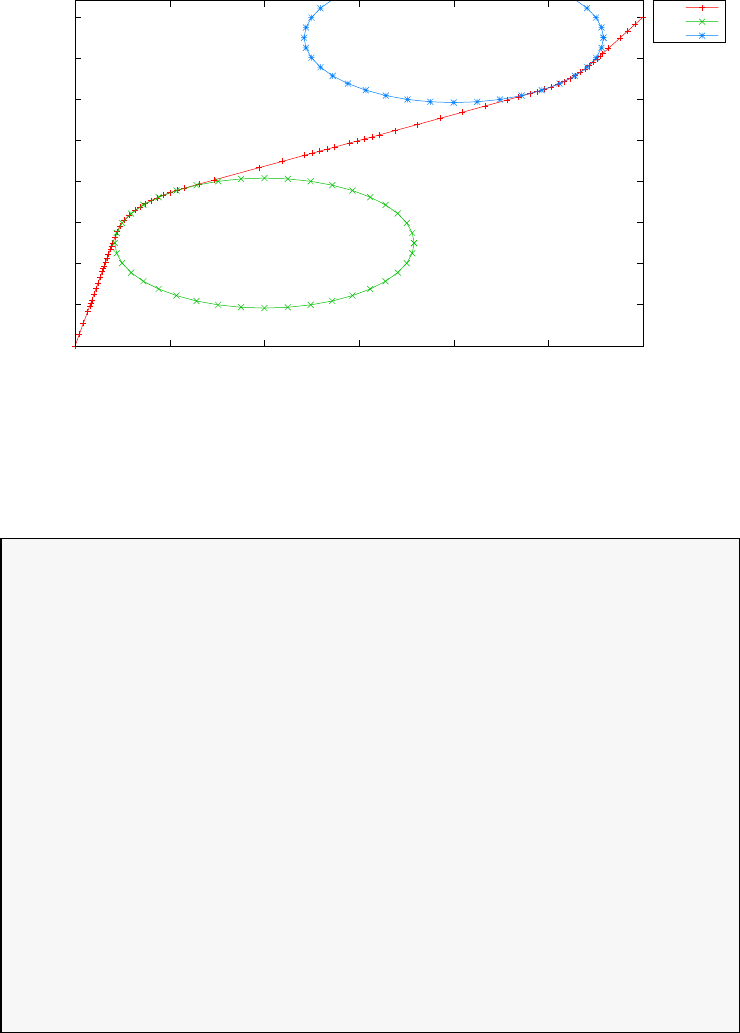
0
0.2
0.4
0.6
0.8
1
1.2
1.4
1.6
0 0.2 0.4 0.6 0.8 1 1.2
y
x
Obstacle avoidance problem: x-y trajectory
y
obs1
obs2
Figure 3.86: Optimal (x, y) trajectory for obstacle avoidance problem
Figure 3.86, which illustrates the optimal (x, y) trajectory of the particle.
PSOPT results summary
=====================
Problem: Obstacle avoidance problem
CPU time (seconds): 4.305481e+00
NLP solver used: IPOPT
PSOPT release number: 4.0
Date and time of this run: Thu Feb 21 17:17:27 2019
Optimal (unscaled) cost function value: 4.571044e+00
Phase 1 endpoint cost function value: 0.000000e+00
Phase 1 integrated part of the cost: 4.571044e+00
Phase 1 initial time: 0.000000e+00
Phase 1 final time: 1.000000e+00
Phase 1 maximum relative local error: 1.302550e-02
NLP solver reports: The problem has been solved!
328
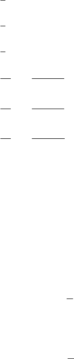
3.35 Reorientation of an asymmetric rigid body
Consider the following optimal control problem, which consists of the re-
orientation of an asymmetric rigid body in minimum time [4]. Find tf,
ˆ
u(t) = [u1(t), u2(t), u3(t), q4(t)]Tto minimize the cost functional
J=tf(3.141)
subject to the dynamic constraints
˙q1=1
2[ω1q4−ω2q3+ω3q2]
˙q2=1
2[ω1q3+ω2q4−ω3q1]
˙q3=1
2[−ω1q2+ω2q1+ω3q4]
˙ω1=u1
Ix−Iz−Iy
Ix
ω2ω3
˙ω2=u2
Iy−Ix−Iz
Iy
ω1ω3
˙ω3=u3
Iz−Iy−Ix
Iz
ω1ω2
(3.142)
The path constraint:
0 = q2
1+q2
2+q2
3+q2
4−1 (3.143)
the boundary conditions:
q1(0) = 0,
q2(0) = 0,
q3(0) = 0,
q4(0) = 1.0
q1(tf) = sin φ
2,
q2(tf) = 0,
q3(tf) = 0,
q4(tf) = cos φ
2
ω1(0) = 0,
ω2(0) = 0,
ω3(0) = 0,
ω1(tf) = 0,
ω2(tf) = 0,
ω3(tf) = 0,
(3.144)
329

where φ= 150 deg is the Euler axis rotation angle, q= [q1, q2, q3, q4]Tis
the quarternion vector, ω= [ω1, ω2, ω3]Tis the angular velocity vector, and
u= [u1, u2, u3]Tis the control vector. Note that in the implementation,
variable q4(t) is treated as an algebraic variable (i.e. as a control variable).
The variable bounds and other parameters are given in the code. The
PSOPT code that solves this problem is shown below.
//////////////////////////////////////////////////////////////////////////
//////////////// reorientation.cxx ////////////////////
//////////////////////////////////////////////////////////////////////////
//////////////// PSOPT example /////////////////////
//////////////////////////////////////////////////////////////////////////
//////////////////////////////////////////////////////////////////////////
//////// Title: Reorientation of an asymmetric rigid body ///////////////
//////// Last modified: 03 July 2010 ////////////////
//////// Reference: Fleming et al ////////////////
//////// ////////////////
//////////////////////////////////////////////////////////////////////////
//////// Copyright (c) Victor M. Becerra, 2010 ////////////////
//////////////////////////////////////////////////////////////////////////
//////// This is part of the PSOPT software library, which ///////////////
//////// is distributed under the terms of the GNU Lesser ////////////////
//////// General Public License (LGPL) ////////////////
//////////////////////////////////////////////////////////////////////////
#include "psopt.h"
//////////////////////////////////////////////////////////////////////////
/////////////////// Define the end point (Mayer) cost function //////////
//////////////////////////////////////////////////////////////////////////
adouble endpoint_cost(adouble* initial_states, adouble* final_states,
adouble* parameters,adouble& t0, adouble& tf,
adouble* xad, int iphase, Workspace* workspace)
{
return tf;
}
//////////////////////////////////////////////////////////////////////////
/////////////////// Define the integrand (Lagrange) cost function //////
//////////////////////////////////////////////////////////////////////////
adouble integrand_cost(adouble* states, adouble* controls, adouble* parameters,
adouble& time, adouble* xad, int iphase, Workspace* workspace)
{
return 0.0;
}
//////////////////////////////////////////////////////////////////////////
/////////////////// Define the DAE’s ////////////////////////////////////
//////////////////////////////////////////////////////////////////////////
void dae(adouble* derivatives, adouble* path, adouble* states,
adouble* controls, adouble* parameters, adouble& time,
adouble* xad, int iphase, Workspace* workspace)
{
adouble u1 = controls[ CINDEX(1) ];
adouble u2 = controls[ CINDEX(2) ];
adouble u3 = controls[ CINDEX(3) ];
adouble q4 = controls[ CINDEX(4) ];
adouble q1 = states[ CINDEX(1) ];
adouble q2 = states[ CINDEX(2) ];
adouble q3 = states[ CINDEX(3) ];
adouble omega1 = states[ CINDEX(4) ];
adouble omega2 = states[ CINDEX(5) ];
adouble omega3 = states[ CINDEX(6) ];
double Ix = 5621.0;
double Iy = 4547.0;
330

double Iz = 2364.0;
adouble dq1 = 0.5*( omega1*q4 - omega2*q3 + omega3*q2 );
adouble dq2 = 0.5*( omega1*q3 + omega2*q4 - omega3*q1 );
adouble dq3 = 0.5*(-omega1*q2 + omega2*q1 + omega3*q4 );
adouble domega1 = u1/Ix - ((Iz-Iy)/Ix)*omega2*omega3;
adouble domega2 = u2/Iy - ((Ix-Iz)/Iy)*omega1*omega3;
adouble domega3 = u3/Iz - ((Iy-Ix)/Iz)*omega1*omega2;
derivatives[ CINDEX(1) ] = dq1;
derivatives[ CINDEX(2) ] = dq2;
derivatives[ CINDEX(3) ] = dq3;
derivatives[ CINDEX(4) ] = domega1;
derivatives[ CINDEX(5) ] = domega2;
derivatives[ CINDEX(6) ] = domega3;
path[ CINDEX(1) ] = q1*q1 + q2*q2 + q3*q3 + q4*q4 - 1.0;
}
////////////////////////////////////////////////////////////////////////////
/////////////////// Define the events function ////////////////////////////
////////////////////////////////////////////////////////////////////////////
void events(adouble* e, adouble* initial_states, adouble* final_states,
adouble* parameters,adouble& t0, adouble& tf, adouble* xad,
int iphase, Workspace* workspace)
{
adouble q1i = initial_states[ CINDEX(1) ];
adouble q2i = initial_states[ CINDEX(2) ];
adouble q3i = initial_states[ CINDEX(3) ];
adouble omega1i = initial_states[ CINDEX(4) ];
adouble omega2i = initial_states[ CINDEX(5) ];
adouble omega3i = initial_states[ CINDEX(6) ];
adouble initial_controls[4], final_controls[4], q4i, q4f;
get_initial_controls( initial_controls, xad, iphase, workspace );
get_final_controls( final_controls , xad, iphase, workspace );
q4i = initial_controls[ CINDEX(4) ];
q4f = final_controls[ CINDEX(4) ];
adouble q1f = final_states[ CINDEX(1) ];
adouble q2f = final_states[ CINDEX(2) ];
adouble q3f = final_states[ CINDEX(3) ];
adouble omega1f = final_states[ CINDEX(4) ];
adouble omega2f = final_states[ CINDEX(5) ];
adouble omega3f = final_states[ CINDEX(6) ];
e[ CINDEX(1) ] = q1i;
e[ CINDEX(2) ] = q2i;
e[ CINDEX(3) ] = q3i;
e[ CINDEX(4) ] = q4i;
e[ CINDEX(5) ] = omega1i;
e[ CINDEX(6) ] = omega2i;
e[ CINDEX(7) ] = omega3i;
e[ CINDEX(8) ] = q1f;
e[ CINDEX(9) ] = q2f;
e[ CINDEX(10) ] = q3f;
e[ CINDEX(11) ] = q4f;
e[ CINDEX(12) ] = omega1f;
e[ CINDEX(13) ] = omega2f;
e[ CINDEX(14) ] = omega3f;
}
///////////////////////////////////////////////////////////////////////////
/////////////////// Define the phase linkages function ///////////////////
///////////////////////////////////////////////////////////////////////////
331

void linkages( adouble* linkages, adouble* xad, Workspace* workspace)
{
// Single phase problem
}
////////////////////////////////////////////////////////////////////////////
/////////////////// Define the main routine ///////////////////////////////
////////////////////////////////////////////////////////////////////////////
int main(void)
{
////////////////////////////////////////////////////////////////////////////
/////////////////// Declare key structures ////////////////////////////////
////////////////////////////////////////////////////////////////////////////
Alg algorithm;
Sol solution;
Prob problem;
////////////////////////////////////////////////////////////////////////////
/////////////////// Register problem name ////////////////////////////////
////////////////////////////////////////////////////////////////////////////
problem.name = "Reorientation of a rigid body";
problem.outfilename = "reorientation.txt";
////////////////////////////////////////////////////////////////////////////
//////////// Define problem level constants & do level 1 setup ////////////
////////////////////////////////////////////////////////////////////////////
problem.nphases = 1;
problem.nlinkages = 0;
psopt_level1_setup(problem);
/////////////////////////////////////////////////////////////////////////////
///////// Define phase related information & do level 2 setup ////////////
/////////////////////////////////////////////////////////////////////////////
problem.phases(1).nstates = 6;
problem.phases(1).ncontrols = 4;
problem.phases(1).nevents = 14;
problem.phases(1).npath = 1;
problem.phases(1).nodes = "[60]";
psopt_level2_setup(problem, algorithm);
////////////////////////////////////////////////////////////////////////////
/////////////////// Enter problem bounds information //////////////////////
////////////////////////////////////////////////////////////////////////////
problem.phases(1).bounds.lower.states = "[-1.0 -1.0 -1.0 -0.5 -0.5 -0.5]";
problem.phases(1).bounds.upper.states = "[ 1.0 1.0 1.0 0.5 0.5 0.5]";
problem.phases(1).bounds.lower.controls = "[-50.0 -50.0 -50.0 -1.0]";
problem.phases(1).bounds.upper.controls = "[ 50.0 50.0 50.0 1.0]";
problem.phases(1).bounds.lower.path(1) = 0.000;
problem.phases(1).bounds.upper.path(1) = 0.000;
DMatrix q0, qf, omega0, omegaf;
double phi = 150.0*(pi/180.0);
q0(1) = 0.0; q0(2) = 0.0; q0(3)=0.0; q0(4)=1.0;
qf(1) = sin(phi/2.0); qf(2) = 0.0; qf(3) = 0.0; qf(4) = cos(phi/2.0);
omega0 = zeros(1,3); omegaf = zeros(1,3);
332

problem.phases(1).bounds.lower.events = q0 || omega0 || qf || omegaf;
problem.phases(1).bounds.upper.events = problem.phases(1).bounds.lower.events;
problem.phases(1).bounds.lower.StartTime = 0.0;
problem.phases(1).bounds.upper.StartTime = 0.0;
problem.phases(1).bounds.lower.EndTime = 25.0;
problem.phases(1).bounds.upper.EndTime = 35.0;
////////////////////////////////////////////////////////////////////////////
/////////////////// Register problem functions ///////////////////////////
////////////////////////////////////////////////////////////////////////////
problem.integrand_cost = &integrand_cost;
problem.endpoint_cost = &endpoint_cost;
problem.dae = &dae;
problem.events = &events;
problem.linkages = &linkages;
////////////////////////////////////////////////////////////////////////////
/////////////////// Define & register initial guess ///////////////////////
////////////////////////////////////////////////////////////////////////////
int nnodes = problem.phases(1).nodes(1);
int ncontrols = problem.phases(1).ncontrols;
int nstates = problem.phases(1).nstates;
DMatrix state_guess = zeros(nstates,nnodes);
DMatrix control_guess = 50.0*ones(ncontrols,nnodes);
DMatrix time_guess = linspace(0.0,40,nnodes);
state_guess(1, colon() ) = linspace( q0(1), qf(1), nnodes );
state_guess(2, colon() ) = linspace( q0(2), qf(2), nnodes );
state_guess(3, colon() ) = linspace( q0(3), qf(3), nnodes );
control_guess(4, colon() )=linspace( q0(4), qf(4), nnodes );
state_guess(4, colon() ) = linspace( omega0(1), omegaf(1), nnodes );
state_guess(5, colon() ) = linspace( omega0(2), omegaf(2), nnodes );
state_guess(6, colon() ) = linspace( omega0(3), omegaf(3), nnodes );
problem.phases(1).guess.states = state_guess;
problem.phases(1).guess.controls = control_guess;
problem.phases(1).guess.time = time_guess;
////////////////////////////////////////////////////////////////////////////
/////////////////// Enter algorithm options //////////////////////////////
////////////////////////////////////////////////////////////////////////////
algorithm.nlp_iter_max = 1000;
algorithm.nlp_tolerance = 1.e-6;
algorithm.nlp_method = "IPOPT";
algorithm.scaling = "automatic";
algorithm.derivatives = "automatic";
algorithm.collocation_method = "trapezoidal";
algorithm.mesh_refinement = "automatic";
algorithm.ode_tolerance = 1.e-5;
////////////////////////////////////////////////////////////////////////////
/////////////////// Now call PSOPT to solve the problem //////////////////
////////////////////////////////////////////////////////////////////////////
psopt(solution, problem, algorithm);
////////////////////////////////////////////////////////////////////////////
/////////// Extract relevant variables from solution structure //////////
////////////////////////////////////////////////////////////////////////////
DMatrix states, controls, t, q1, q2, q3, q4, omega, u, q;
states = solution.get_states_in_phase(1);
controls = solution.get_controls_in_phase(1);
t = solution.get_time_in_phase(1);
q1 = states(1,colon());
333

q2 = states(2,colon());
q3 = states(3,colon());
q4 = controls(4, colon());
q = q1 && q2 && q3 && q4;
omega = states(colon(4,6), colon());
u = controls(colon(1,3), colon());
////////////////////////////////////////////////////////////////////////////
/////////// Save solution data to files if desired ////////////////////////
////////////////////////////////////////////////////////////////////////////
states.Save("states.dat");
controls.Save("controls.dat");
t.Save("t.dat");
////////////////////////////////////////////////////////////////////////////
/////////// Plot some results if desired (requires gnuplot) ///////////////
////////////////////////////////////////////////////////////////////////////
multiplot(t,q,problem.name+": quarternion","time (s)", "q1 q2 q3 q4", "q1 q2 q3 q4", 2, 2);
multiplot(t,u, problem.name+": controls", "time (s)", "u1 u2 u3", "u1 u2 u3");
multiplot(t,q,problem.name+": quarternion","time (s)", "q1 q2 q3 q4", "q1 q2 q3 q4", 2, 2,
"pdf", "reorientation_q.pdf");
multiplot(t,u, problem.name+": controls", "time (s)", "u1 u2 u3", "u1 u2 u3", 3, 1,
"pdf", "reorientation_u.pdf");
}
////////////////////////////////////////////////////////////////////////////
/////////////////////// END OF FILE ///////////////////////////////
////////////////////////////////////////////////////////////////////////////
The output from PSOPT is summarised in the box below and shown in
Figures 3.87 to 3.88, which contain the elements of the quarternion vector
q, and the control vector u= [u1, u2, u3]T, respectively.
PSOPT results summary
=====================
Problem: Reorientation of a rigid body
CPU time (seconds): 7.367546e+01
NLP solver used: IPOPT
PSOPT release number: 4.0
Date and time of this run: Thu Feb 21 17:23:02 2019
Optimal (unscaled) cost function value: 2.863041e+01
Phase 1 endpoint cost function value: 2.863041e+01
Phase 1 integrated part of the cost: 0.000000e+00
Phase 1 initial time: 0.000000e+00
334
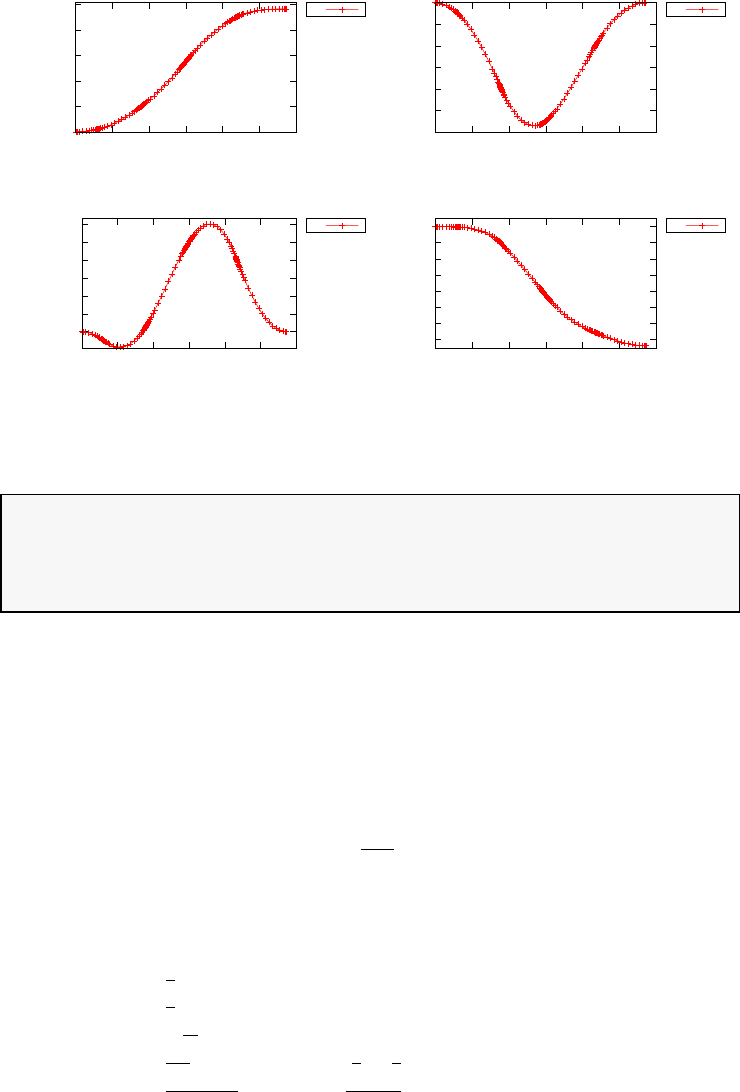
0
0.2
0.4
0.6
0.8
1
0 5 10 15 20 25 30
q1
time (s)
Reorientation of a rigid body: quarternion
q1
0
0.05
0.1
0.15
0.2
0.25
0.3
0 5 10 15 20 25 30
q2
time (s)
Reorientation of a rigid body: quarternion
q2
-0.6
-0.5
-0.4
-0.3
-0.2
-0.1
0
0 5 10 15 20 25 30
q3
time (s)
Reorientation of a rigid body: quarternion
q3
0.3
0.4
0.5
0.6
0.7
0.8
0.9
1
0 5 10 15 20 25 30
q4
time (s)
Reorientation of a rigid body: quarternion
q4
Figure 3.87: Quarternion vector elements for the reorientation problem
Phase 1 final time: 2.863041e+01
Phase 1 maximum relative local error: 1.772329e-05
NLP solver reports: The problem has been solved!
3.36 Shuttle re-entry problem
Consider the following optimal control problem, which is known in the lit-
erature as the shuttle re-entry problem [3]. Find tf,α(t) and β(t)∈[0, tf]
to minimize the cost functional
J=−180
πθ(tf) (3.145)
subject to the dynamic constraints
˙
h=vsin(γ)
˙
φ=v
rcos(γ) sin(ψ)/cos(θ)
˙m=v
rcos(γ) cos(ψ)
˙v=−D
m−gsin(γ)
˙γ=L
mv cos(β) + cos(γ)(v
r−g
v)
˙
ψ=1
mv cos(γ)Lsin(β) + v
rcos(θ)cos(γ) sin(ψ) sin(θ)
(3.146)
335
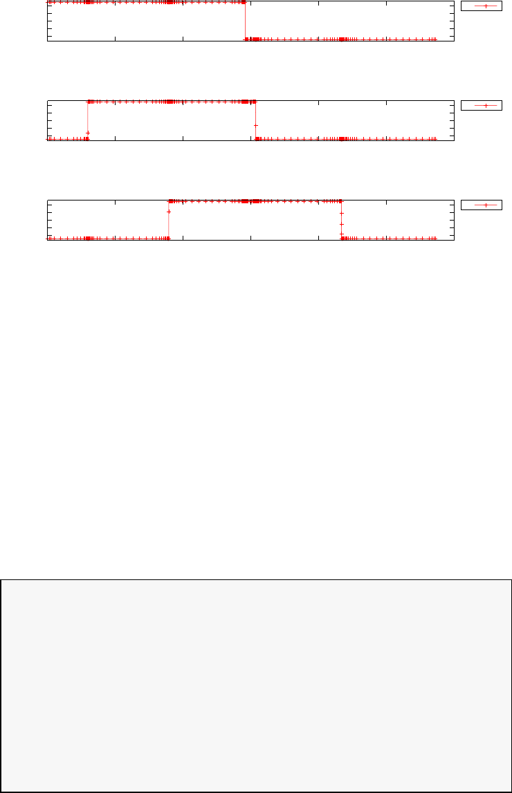
-40
-20
0
20
40
0 5 10 15 20 25 30
u1
time (s)
Reorientation of a rigid body: controls
u1
-40
-20
0
20
40
0 5 10 15 20 25 30
u2
time (s)
Reorientation of a rigid body: controls
u2
-40
-20
0
20
40
0 5 10 15 20 25 30
u3
time (s)
Reorientation of a rigid body: controls
u3
Figure 3.88: Control vector elements for the reorientation problem
the boundary conditions:
h(0) = 260000.0
φ(0) = −0.6572
θ(0) = 0.0
v(0) = 25600.0
γ(0) = −0.0175
h(tf) = 80000.0
v(tf) = 2500.0
γ(tf) = −0.0873
(3.147)
The variable bounds and other parameters are given in the code. The
PSOPT code that solves this problem is shown below.
//////////////////////////////////////////////////////////////////////////
////////////////// shuttle_reentry1.cxx //////////////////////
//////////////////////////////////////////////////////////////////////////
//////////////// PSOPT Example ////////////////////
//////////////////////////////////////////////////////////////////////////
//////////////////////////////////////////////////////////////////////////
//////// Title: Shuttle reentry problem ////////////////
//////// Last modified: 05 January 2009 ////////////////
//////// Reference: Betts (2001) ////////////////
//////// (See PSOPT handbook for full reference) ////////////////
//////////////////////////////////////////////////////////////////////////
//////// Copyright (c) Victor M. Becerra, 2009 ////////////////
//////////////////////////////////////////////////////////////////////////
//////// This is part of the PSOPT software library, which ///////////////
//////// is distributed under the terms of the GNU Lesser ///////////////
//////// General Public License (LGPL) ///////////////
//////////////////////////////////////////////////////////////////////////
#include "psopt.h"
336

//////////////////////////////////////////////////////////////////////////
////////////////// Define some local macros //////////////////////
//////////////////////////////////////////////////////////////////////////
#define H_INDX 1
#define PHI_INDX 2
#define THETA_INDX 3
#define V_INDX 4
#define GAMMA_INDX 5
#define PSI_INDX 6
#define ALPHA_INDX 1
#define BETA_INDX 2
#define DEG2RAD(x) (3.141592653589793*(x)/180.0)
//////////////////////////////////////////////////////////////////////////
/////////////////// Define the end point (Mayer) cost function //////////
//////////////////////////////////////////////////////////////////////////
adouble endpoint_cost(adouble* initial_states, adouble* final_states,
adouble* parameters,adouble& t0, adouble& tf,
adouble* xad, int iphase, Workspace* workspace)
{
adouble theta = final_states[THETA_INDX-1];
return (-theta*180/3.141592653589793);
}
//////////////////////////////////////////////////////////////////////////
/////////////////// Define the integrand (Lagrange) cost function //////
//////////////////////////////////////////////////////////////////////////
adouble integrand_cost(adouble* states, adouble* controls,
adouble* parameters,
adouble& time, adouble* xad,
int iphase, Workspace* workspace)
{
return 0.0;
}
//////////////////////////////////////////////////////////////////////////
/////////////////// Define the DAE’s ////////////////////////////////////
//////////////////////////////////////////////////////////////////////////
void dae(adouble* derivatives, adouble* path, adouble* states,
adouble* controls, adouble* parameters, adouble& time,
adouble* xad, int iphase, Workspace* workspace)
{
adouble alpha, beta;
adouble alt = states[H_INDX-1];
adouble lon = states[PHI_INDX-1];
adouble lat = states[THETA_INDX-1];
adouble vel = states[V_INDX-1];
adouble gamma = states[GAMMA_INDX-1];
adouble azi = states[PSI_INDX-1];
alpha = controls[ALPHA_INDX-1];
beta = controls[BETA_INDX-1];
double pi = 3.141592653589793;
double cr2d = 180.0/pi;
double weight = 203000.0;
double cm2w = 32.174;
double cea = 20902900.0;
double mu = 0.14076539e17;
double rho0 = 0.002378;
double href = 23800.0;
double cl0 = -0.20704;
double cl1 = 0.029244;
double cd0 = 0.07854;
double cd1 = -6.1592e-3;
double cd2 = 6.21408e-4;
double sref = 2690.0;
337

double mass = weight/cm2w;
adouble sgamma = sin(gamma);
adouble cgamma = cos(gamma);
adouble sazi = sin(azi);
adouble cazi = cos(azi);
adouble sbeta = sin(beta);
adouble cbeta = cos(beta);
adouble slat = sin(lat);
adouble clat = cos(lat);
adouble alphad = cr2d*alpha;
adouble radius = cea+alt;
adouble grav = mu/pow(radius,2);
adouble rhodns = rho0*exp(-alt/href);
adouble dynp = 0.5*(rhodns*pow(vel,2));
adouble subl = cl0+cl1*alphad;
adouble subd = cd0+((cd1+cd2*alphad)*alphad);
adouble drag = (dynp*subd)*sref;
adouble lift = (dynp*subl)*sref;
adouble vrelg = (vel/radius)-(grav/vel);
adouble d_alt_dt = vel*sgamma;
adouble d_lon_dt = ((vel*cgamma)*sazi)/(radius*clat);
adouble d_lat_dt = ((vel*cgamma)*cazi)/radius;
adouble d_vel_dt = (-(drag/mass)-(grav*sgamma));
adouble d_gamma_dt = ((lift*cbeta)/(mass*vel))+(cgamma*vrelg);
adouble d_azi_dt = ((lift*sbeta)/((mass*vel)*cgamma))
+ ((vel*cgamma)*(sazi*slat)/(radius*clat));
derivatives[H_INDX-1] = d_alt_dt ;
derivatives[PHI_INDX-1] = d_lon_dt ;
derivatives[THETA_INDX-1] = d_lat_dt ;
derivatives[V_INDX-1] = d_vel_dt ;
derivatives[GAMMA_INDX-1] = d_gamma_dt ;
derivatives[PSI_INDX-1] = d_azi_dt ;
}
////////////////////////////////////////////////////////////////////////////
/////////////////// Define the events function ////////////////////////////
////////////////////////////////////////////////////////////////////////////
void events(adouble* e, adouble* initial_states, adouble* final_states,
adouble* parameters,adouble& t0, adouble& tf, adouble* xad,
int iphase, Workspace* workspace)
{
adouble h0 = initial_states[H_INDX-1];
adouble phi0 = initial_states[PHI_INDX-1];
adouble theta0 = initial_states[THETA_INDX-1];
adouble v0 = initial_states[V_INDX-1];
adouble gamma0 = initial_states[GAMMA_INDX-1];
adouble psi0 = initial_states[PSI_INDX-1];
adouble hf = final_states[H_INDX-1];
adouble vf = final_states[V_INDX-1];
adouble gammaf = final_states[GAMMA_INDX-1];
e[H_INDX-1] = h0;
e[PHI_INDX-1] = phi0;
e[THETA_INDX-1] = theta0;
e[V_INDX-1] = v0;
e[GAMMA_INDX-1] = gamma0;
e[PSI_INDX-1] = psi0;
e[6] = hf;
e[7] = vf;
e[8] = gammaf;
}
///////////////////////////////////////////////////////////////////////////
/////////////////// Define the phase linkages function ///////////////////
///////////////////////////////////////////////////////////////////////////
void linkages( adouble* linkages, adouble* xad, Workspace* workspace)
{
338

// No linkages as this is a single phase problem
}
////////////////////////////////////////////////////////////////////////////
/////////////////// Define the main routine ///////////////////////////////
////////////////////////////////////////////////////////////////////////////
int main(void)
{
////////////////////////////////////////////////////////////////////////////
/////////////////// Declare key structures ////////////////////////////////
////////////////////////////////////////////////////////////////////////////
Alg algorithm;
Sol solution;
Prob problem;
////////////////////////////////////////////////////////////////////////////
/////////////////// Register problem name ////////////////////////////////
////////////////////////////////////////////////////////////////////////////
problem.name = "Shuttle re-entry problem";
problem.outfilename = "shuttle.txt";
////////////////////////////////////////////////////////////////////////////
//////////// Define problem level constants & do level 1 setup ////////////
////////////////////////////////////////////////////////////////////////////
problem.nphases = 1;
problem.nlinkages = 0;
psopt_level1_setup(problem);
/////////////////////////////////////////////////////////////////////////////
///////// Define phase related information & do level 2 setup /////////////
/////////////////////////////////////////////////////////////////////////////
problem.phases(1).nstates = 6;
problem.phases(1).ncontrols = 2;
problem.phases(1).nevents = 9;
problem.phases(1).npath = 0;
problem.phases(1).nodes = "[60 80]";
problem.phases(1).zero_cost_integrand = true;
psopt_level2_setup(problem, algorithm);
////////////////////////////////////////////////////////////////////////////
/////////////////// Declare DMatrix objects to store results //////////////
////////////////////////////////////////////////////////////////////////////
DMatrix x, u, t;
////////////////////////////////////////////////////////////////////////////
/////////////////// Enter problem bounds information //////////////////////
////////////////////////////////////////////////////////////////////////////
double hL = 0.0;
double hU = 300000.0;
double phiL = DEG2RAD(-45.0);
double phiU = DEG2RAD( 45.0);
double vL = 1000.0 ;
double vU = 40000.0 ;
double thetaL = DEG2RAD(-89.0) ;
double thetaU = DEG2RAD( 89.0) ;
double gammaL = DEG2RAD(-89.0) ;
double gammaU = DEG2RAD(89.0) ;
double psiL = DEG2RAD(-180.0);
double psiU = DEG2RAD(180.0) ;
double alphaL = DEG2RAD(-89.0) ;
double alphaU = DEG2RAD( 89.0) ;
double betaL = DEG2RAD(-90.0) ;
double betaU = DEG2RAD( 1.0) ;
double qU = 70.0;
double qL = -INF;
double h0 = 260000.0 ;
double v0 = 25600.0 ;
double phi0 = DEG2RAD(-0.5*75.3153) ;
double gamma0 = DEG2RAD(-1.0);
339

double theta0 = 0.0 ;
double psi0 = DEG2RAD(90.0) ;
double hf = 80000.0 ;
double vf = 2500.0 ;
double gammaf = DEG2RAD(-5.0);
double pi = 3.141592653589793;
problem.phases(1).bounds.lower.states(H_INDX) = hL;
problem.phases(1).bounds.lower.states(PHI_INDX) = phiL;
problem.phases(1).bounds.lower.states(THETA_INDX) = thetaL;
problem.phases(1).bounds.lower.states(V_INDX) = vL;
problem.phases(1).bounds.lower.states(GAMMA_INDX) = gammaL;
problem.phases(1).bounds.lower.states(PSI_INDX) = psiL;
problem.phases(1).bounds.upper.states(H_INDX) = hU;
problem.phases(1).bounds.upper.states(PHI_INDX) = phiU;
problem.phases(1).bounds.upper.states(THETA_INDX) = thetaU;
problem.phases(1).bounds.upper.states(V_INDX) = vU;
problem.phases(1).bounds.upper.states(GAMMA_INDX) = gammaU;
problem.phases(1).bounds.upper.states(PSI_INDX) = psiU;
problem.phases(1).bounds.lower.controls(ALPHA_INDX) = alphaL;
problem.phases(1).bounds.upper.controls(ALPHA_INDX) = alphaU;
problem.phases(1).bounds.lower.controls(BETA_INDX) = betaL;
problem.phases(1).bounds.upper.controls(BETA_INDX) = betaU;
problem.phases(1).bounds.lower.events(H_INDX) = h0;
problem.phases(1).bounds.lower.events(PHI_INDX) = phi0;
problem.phases(1).bounds.lower.events(THETA_INDX) = theta0;
problem.phases(1).bounds.lower.events(V_INDX) = v0;
problem.phases(1).bounds.lower.events(GAMMA_INDX) = gamma0;
problem.phases(1).bounds.lower.events(PSI_INDX) = psi0;
problem.phases(1).bounds.lower.events(7) = hf;
problem.phases(1).bounds.lower.events(8) = vf;
problem.phases(1).bounds.lower.events(9) = gammaf;
problem.phases(1).bounds.upper.events(H_INDX) = h0;
problem.phases(1).bounds.upper.events(PHI_INDX) = phi0;
problem.phases(1).bounds.upper.events(THETA_INDX) = theta0;
problem.phases(1).bounds.upper.events(V_INDX) = v0;
problem.phases(1).bounds.upper.events(GAMMA_INDX) = gamma0;
problem.phases(1).bounds.upper.events(PSI_INDX) = psi0;
problem.phases(1).bounds.upper.events(7) = hf;
problem.phases(1).bounds.upper.events(8) = vf;
problem.phases(1).bounds.upper.events(9) = gammaf;
problem.phases(1).bounds.lower.path(1) = qL;
problem.phases(1).bounds.upper.path(1) = qU;
problem.phases(1).bounds.lower.StartTime = 0.0;
problem.phases(1).bounds.upper.StartTime = 0.0;
problem.phases(1).bounds.lower.EndTime = 100.0;
problem.phases(1).bounds.upper.EndTime = 4000.0;
////////////////////////////////////////////////////////////////////////////
/////////////////// Register problem functions ///////////////////////////
////////////////////////////////////////////////////////////////////////////
problem.integrand_cost = &integrand_cost;
problem.endpoint_cost = &endpoint_cost;
problem.dae = &dae;
problem.events = &events;
problem.linkages = &linkages;
////////////////////////////////////////////////////////////////////////////
/////////////////// Define & register initial guess ///////////////////////
////////////////////////////////////////////////////////////////////////////
int nodes = (int) problem.phases(1).nodes(1);
340

DMatrix u_guess = ( zeros(1,nodes+1) && (DEG2RAD(1.0)*ones(1,nodes+1) ) );
DMatrix x_guess = zeros(6,nodes+1);
DMatrix time_guess;
x_guess(H_INDX,colon()) = linspace(h0, hf, nodes+1);
x_guess(PHI_INDX,colon()) = -0.5*DEG2RAD(90.0)*ones(1,nodes+1);
x_guess(THETA_INDX,colon()) = DEG2RAD(-89.0)*ones(1,nodes+1);
x_guess(V_INDX,colon()) = linspace(v0,vf, nodes+1);
x_guess(GAMMA_INDX,colon()) = linspace(gamma0, gammaf, nodes+1);
x_guess(PSI_INDX,colon()) = linspace(pi/2, -pi/2, nodes+1);
time_guess = linspace(0.0, 1000.0, nodes+1);
problem.phases(1).guess.controls = u_guess;
problem.phases(1).guess.states = x_guess;
problem.phases(1).guess.time = time_guess;
////////////////////////////////////////////////////////////////////////////
/////////////////// Enter algorithm options //////////////////////////////
////////////////////////////////////////////////////////////////////////////
algorithm.nlp_method = "IPOPT";
algorithm.nlp_iter_max = 1000;
algorithm.nlp_tolerance = 5e-6;
algorithm.scaling = "automatic";
algorithm.derivatives = "automatic";
algorithm.collocation_method = "trapezoidal";
algorithm.mesh_refinement = "automatic";
////////////////////////////////////////////////////////////////////////////
/////////////////// Now call PSOPT to solve the problem /////////////////
////////////////////////////////////////////////////////////////////////////
psopt(solution, problem, algorithm);
////////////////////////////////////////////////////////////////////////////
/////////// Extract relevant variables from solution structure //////////
////////////////////////////////////////////////////////////////////////////
x = solution.get_states_in_phase(1);
u = solution.get_controls_in_phase(1);
t = solution.get_time_in_phase(1);
////////////////////////////////////////////////////////////////////////////
/////////// Save solution data to files if desired ////////////////////////
////////////////////////////////////////////////////////////////////////////
x.Save("x.dat");
u.Save("u.dat");
t.Save("t.dat");
////////////////////////////////////////////////////////////////////////////
/////////// Plot some results if desired (requires gnuplot) ///////////////
////////////////////////////////////////////////////////////////////////////
DMatrix h = x(1,colon());
DMatrix phi = x(2,colon());
DMatrix theta = x(3,colon());
DMatrix v = x(4,colon());
DMatrix gamma = x(5,colon());
DMatrix psi = x(6,colon());
DMatrix alpha = u(1,colon());
DMatrix beta = u(2,colon());
plot(t,x(1,colon()),problem.name, "time (s)", "x1","altitude");
plot(t,u(1,colon()),problem.name,"time (s)", "alpha");
plot(t,u(2,colon()),problem.name,"time (s)", "beta");
plot(t,h, problem.name+": altitude", "time (s)", "h (ft)",
"altitude","pdf", "shutt_alt.pdf" );
plot(t,phi, problem.name+": longitude", "time (s)", "phi (rad)",
"longitude","pdf", "shutt_lon.pdf" );
plot(t,theta, problem.name+": latitude", "time (s)", "theta (rad)",
"latitude","pdf", "shutt_lat.pdf" );
341

plot(t,v, problem.name+": velocity", "time (s)", "v (ft/s)",
"velocity","pdf", "shutt_vel.pdf" );
plot(t,gamma, problem.name+": flight path angle", "time (s)", "gamma (rad)",
"fpa","pdf", "shutt_fpa.pdf" );
plot(t,psi, problem.name+": azimuth", "time (s)", "psi (rad)",
"azi","pdf", "shutt_azi.pdf" );
plot(t,alpha, problem.name+": alpha", "time (s)", "alpha (rad)",
"alpha","pdf", "shutt_alpha.pdf" );
plot(t,beta, problem.name+": beta", "time (s)", "beta (rad)",
"beta","pdf", "shutt_beta.pdf" );
}
////////////////////////////////////////////////////////////////////////////
/////////////////////// END OF FILE ///////////////////////////////
////////////////////////////////////////////////////////////////////////////
The output from PSOPT is summarised in the box below and shown in
Figures 3.89 to 3.96, which contain the elements of the state and the control
vectors.
PSOPT results summary
=====================
Problem: Shuttle re-entry problem
CPU time (seconds): 1.522294e+01
NLP solver used: IPOPT
PSOPT release number: 4.0
Date and time of this run: Thu Feb 21 15:55:18 2019
Optimal (unscaled) cost function value: -3.414119e+01
Phase 1 endpoint cost function value: -3.414119e+01
Phase 1 integrated part of the cost: 0.000000e+00
Phase 1 initial time: 0.000000e+00
Phase 1 final time: 2.008466e+03
Phase 1 maximum relative local error: 6.337462e-04
NLP solver reports: The problem has been solved!
3.37 Singular control problem
Consider the following optimal control problem, whose solution is known
to have a singular arc [29,36]. Find u(t), t ∈[0,1] to minimize the cost
342
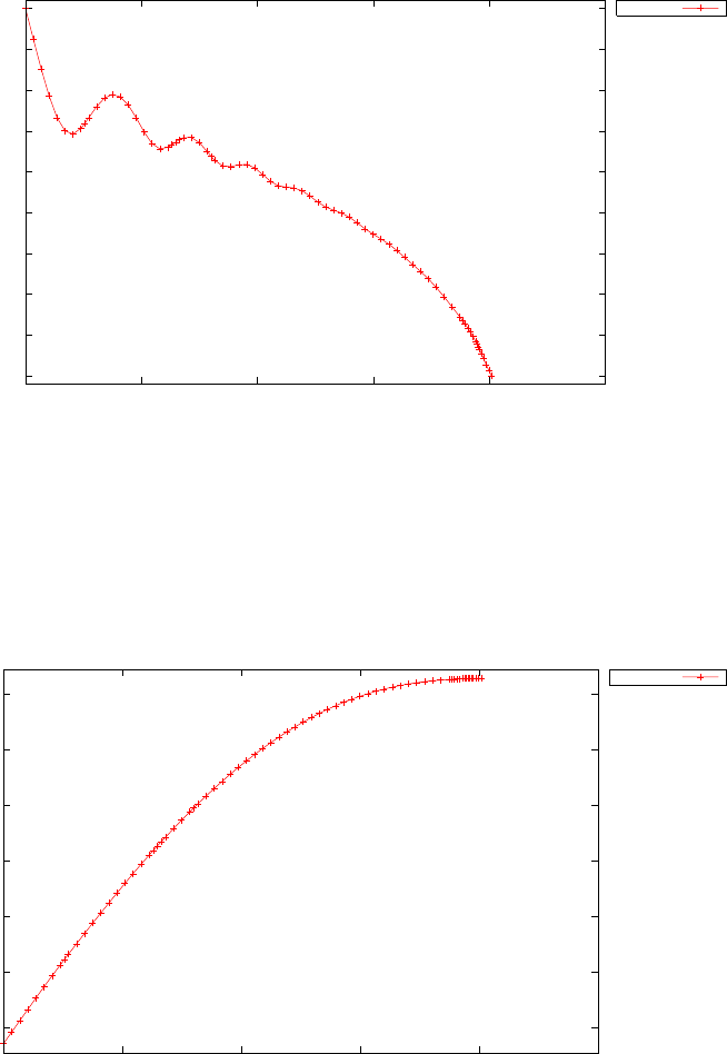
80000
100000
120000
140000
160000
180000
200000
220000
240000
260000
0 500 1000 1500 2000 2500
h (ft)
time (s)
Shuttle re-entry problem: altitude
altitude
Figure 3.89: Altitude h(t) for the shuttle re-entry problem
-0.6
-0.4
-0.2
0
0.2
0.4
0.6
0 500 1000 1500 2000 2500
phi (rad)
time (s)
Shuttle re-entry problem: longitude
longitude
Figure 3.90: Longitude φ(t) for the shuttle re-entry problem
343
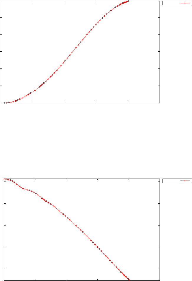
0
0.1
0.2
0.3
0.4
0.5
0 500 1000 1500 2000 2500
theta (rad)
time (s)
Shuttle re-entry problem: latitude
latitude
Figure 3.91: Latitude θ(t) for the shuttle re-entry problem
5000
10000
15000
20000
25000
0 500 1000 1500 2000 2500
v (ft/s)
time (s)
Shuttle re-entry problem: velocity
velocity
Figure 3.92: Velocity v(t) for the shuttle re-entry problem
344
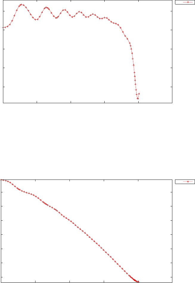
-0.08
-0.06
-0.04
-0.02
0
0 500 1000 1500 2000 2500
gamma (rad)
time (s)
Shuttle re-entry problem: flight path angle
fpa
Figure 3.93: Flight path angle γ(t) for the shuttle re-entry problem
0.2
0.4
0.6
0.8
1
1.2
1.4
0 500 1000 1500 2000 2500
psi (rad)
time (s)
Shuttle re-entry problem: azimuth
azi
Figure 3.94: Azimuth ψ(t) for the shuttle re-entry problem
345
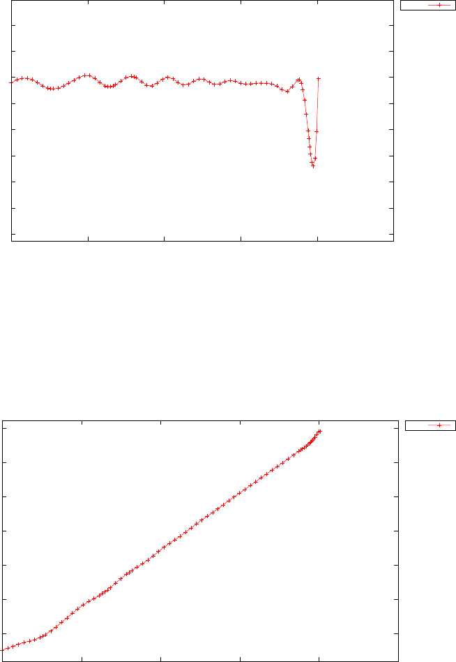
0.275
0.28
0.285
0.29
0.295
0.3
0.305
0.31
0.315
0 500 1000 1500 2000 2500
alpha (rad)
time (s)
Shuttle re-entry problem: alpha
alpha
Figure 3.95: Angle of attack α(t) for the shuttle re-entry problem
-1.2
-1
-0.8
-0.6
-0.4
-0.2
0
0 500 1000 1500 2000 2500
beta (rad)
time (s)
Shuttle re-entry problem: beta
beta
Figure 3.96: Bank angle β(t) for the shuttle re-entry problem
346

functional
J=Z1
0
[x2
1+x2
2+ 0.0005(x2+ 16x5−8−0.1x3u2)2]dt (3.148)
subject to the dynamic constraints
˙x1=x2
˙x2=−x3u+ 16t−8
˙x3=u
(3.149)
the boundary conditions:
x1(0) = 0
x2(0) = −1
x3(0) = √5
(3.150)
and the control bounds
−4≤u(t)≤10 (3.151)
The PSOPT code that solves this problem is shown below.
//////////////////////////////////////////////////////////////////////////
////////////////// singular5.cxx /////////////////////
//////////////////////////////////////////////////////////////////////////
//////////////// PSOPT Example ////////////////////
//////////////////////////////////////////////////////////////////////////
//////////////////////////////////////////////////////////////////////////
//////// Title: Singular problem ////////////////
//////// Last modified: 09 January 2009 ////////////////
//////// Reference: Luus (2002) ////////////////
//////// (See PSOPT handbook for full reference) ////////////////
//////////////////////////////////////////////////////////////////////////
//////// Copyright (c) Victor M. Becerra, 2009 ////////////////
//////////////////////////////////////////////////////////////////////////
//////// This is part of the PSOPT software library, which ///////////////
//////// is distributed under the terms of the GNU Lesser ////////////////
//////// General Public License (LGPL) ////////////////
//////////////////////////////////////////////////////////////////////////
#include "psopt.h"
//////////////////////////////////////////////////////////////////////////
/////////////////// Define the end point (Mayer) cost function //////////
//////////////////////////////////////////////////////////////////////////
adouble endpoint_cost(adouble* initial_states, adouble* final_states,
adouble* parameters,adouble& t0, adouble& tf,
adouble* xad, int iphase, Workspace* workspace)
{
return 0.0;
}
//////////////////////////////////////////////////////////////////////////
/////////////////// Define the integrand (Lagrange) cost function //////
//////////////////////////////////////////////////////////////////////////
adouble integrand_cost(adouble* states, adouble* controls,
adouble* parameters, adouble& time, adouble* xad,
int iphase, Workspace* workspace)
{
adouble x1 = states[ CINDEX(1) ];
adouble x2 = states[ CINDEX(2) ];
adouble x3 = states[ CINDEX(3) ];
347

adouble u = controls[ CINDEX(1) ];
adouble t = time;
adouble L;
L = x1*x1 + x2*x2 + 0.0005*pow(x2+16*t-8.0-0.1*x3*u*u,2.0);
return L;
}
//////////////////////////////////////////////////////////////////////////
/////////////////// Define the DAE’s ////////////////////////////////////
//////////////////////////////////////////////////////////////////////////
void dae(adouble* derivatives, adouble* path, adouble* states,
adouble* controls, adouble* parameters, adouble& time,
adouble* xad, int iphase, Workspace* workspace)
{
adouble x1 = states[ CINDEX(1) ];
adouble x2 = states[ CINDEX(2) ];
adouble x3 = states[ CINDEX(3) ];
adouble u = controls[ CINDEX(1) ];
adouble t = time;
derivatives[ CINDEX(1) ] = x2;
derivatives[ CINDEX(2) ] = -x3*u + 16*t - 8.0;
derivatives[ CINDEX(3) ] = u;
}
////////////////////////////////////////////////////////////////////////////
/////////////////// Define the events function ////////////////////////////
////////////////////////////////////////////////////////////////////////////
void events(adouble* e, adouble* initial_states, adouble* final_states,
adouble* parameters,adouble& t0, adouble& tf, adouble* xad,
int iphase, Workspace* workspace)
{
adouble x10 = initial_states[ CINDEX(1) ];
adouble x20 = initial_states[ CINDEX(2) ];
adouble x30 = initial_states[ CINDEX(3) ];
e[ CINDEX(1) ] = x10;
e[ CINDEX(2) ] = x20;
e[ CINDEX(3) ] = x30;
}
///////////////////////////////////////////////////////////////////////////
/////////////////// Define the phase linkages function ///////////////////
///////////////////////////////////////////////////////////////////////////
void linkages( adouble* linkages, adouble* xad, Workspace* workspace)
{
}
////////////////////////////////////////////////////////////////////////////
/////////////////// Define the main routine ///////////////////////////////
////////////////////////////////////////////////////////////////////////////
int main(void)
{
////////////////////////////////////////////////////////////////////////////
/////////////////// Declare key structures ////////////////////////////////
////////////////////////////////////////////////////////////////////////////
Alg algorithm;
Sol solution;
Prob problem;
MSdata msdata;
////////////////////////////////////////////////////////////////////////////
/////////////////// Register problem name ////////////////////////////////
////////////////////////////////////////////////////////////////////////////
problem.name = "Singular control 5";
problem.outfilename = "sing5.txt";
348

////////////////////////////////////////////////////////////////////////////
//////////// Define problem level constants & do level 1 setup ////////////
////////////////////////////////////////////////////////////////////////////
problem.nphases = 1;
problem.nlinkages = 0;
psopt_level1_setup(problem);
/////////////////////////////////////////////////////////////////////////////
///////// Define phase related information & do level 2 setup ////////////
/////////////////////////////////////////////////////////////////////////////
problem.phases(1).nstates = 3;
problem.phases(1).ncontrols = 1;
problem.phases(1).nevents = 3;
problem.phases(1).npath = 0;
problem.phases(1).nodes = "[80]";
psopt_level2_setup(problem, algorithm);
////////////////////////////////////////////////////////////////////////////
/////////////////// Enter problem bounds information //////////////////////
////////////////////////////////////////////////////////////////////////////
problem.phases(1).bounds.lower.states(1) = -inf;
problem.phases(1).bounds.lower.states(2) = -inf;
problem.phases(1).bounds.lower.states(3) = -inf;
problem.phases(1).bounds.upper.states(1) = inf;
problem.phases(1).bounds.upper.states(2) = inf;
problem.phases(1).bounds.upper.states(3) = inf;
problem.phases(1).bounds.lower.controls(1) = 0.0;
problem.phases(1).bounds.upper.controls(1) = 10.0;
problem.phases(1).bounds.lower.events(1) = 0.0;
problem.phases(1).bounds.lower.events(2) = -1.0;
problem.phases(1).bounds.lower.events(3) = -sqrt(5.0);
problem.phases(1).bounds.upper.events(1) = 0.0;
problem.phases(1).bounds.upper.events(2) = -1.0;
problem.phases(1).bounds.upper.events(3) = -sqrt(5.0);
problem.bounds.lower.times = "[0.0, 1.0]";
problem.bounds.upper.times = "[0.0, 1.0]";
////////////////////////////////////////////////////////////////////////////
/////////////////// Register problem functions ///////////////////////////
////////////////////////////////////////////////////////////////////////////
problem.integrand_cost = &integrand_cost;
problem.endpoint_cost = &endpoint_cost;
problem.dae = &dae;
problem.events = &events;
problem.linkages = &linkages;
////////////////////////////////////////////////////////////////////////////
/////////////////// Define & register initial guess ///////////////////////
////////////////////////////////////////////////////////////////////////////
DMatrix state_guess(3,20), control_guess(1,20), param_guess, time_guess;
state_guess(1,colon())= linspace(0.0, 0.0, 20);
state_guess(2,colon())= linspace(-1.0, -1.0, 20);
state_guess(3,colon())= linspace(-sqrt(5.0),-sqrt(5.0), 20);
control_guess = zeros(1,20);
time_guess = linspace(0.0, 1.0, 20);
auto_phase_guess(problem, control_guess, state_guess, param_guess, time_guess);
////////////////////////////////////////////////////////////////////////////
/////////////////// Enter algorithm options //////////////////////////////
////////////////////////////////////////////////////////////////////////////
349

algorithm.nlp_iter_max = 1000;
algorithm.nlp_tolerance = 1.e-7;
algorithm.nlp_method = "IPOPT";
algorithm.scaling = "automatic";
algorithm.derivatives = "automatic";
algorithm.defect_scaling = "jacobian-based";
// algorithm.collocation_method = "trapezoidal";
// algorithm.mesh_refinement = "automatic";
// algorithm.ode_tolerance = 5.e-3 ;
// algorithm.mr_max_iterations = 3;
////////////////////////////////////////////////////////////////////////////
/////////////////// Now call PSOPT to solve the problem /////////////////
////////////////////////////////////////////////////////////////////////////
psopt(solution, problem, algorithm);
////////////////////////////////////////////////////////////////////////////
/////////// Extract relevant variables from solution structure //////////
////////////////////////////////////////////////////////////////////////////
DMatrix x, u, t, xi, ui, ti;
x = solution.get_states_in_phase(1);
u = solution.get_controls_in_phase(1);
t = solution.get_time_in_phase(1);
////////////////////////////////////////////////////////////////////////////
/////////// Save solution data to files if desired ////////////////////////
////////////////////////////////////////////////////////////////////////////
x.Save("x.dat");
u.Save("u.dat");
t.Save("t.dat");
////////////////////////////////////////////////////////////////////////////
/////////// Plot some results if desired (requires gnuplot) ///////////////
////////////////////////////////////////////////////////////////////////////
plot(t,x,problem.name,"time (s)", "x");
plot(t,u,problem.name,"time (s)", "u");
plot(t,x,problem.name,"time (s)", "x","x1 x2 x3",
"pdf","sing5_states.pdf");
plot(t,u,problem.name,"time (s)", "u","u",
"pdf","sing5_control.pdf");
}
////////////////////////////////////////////////////////////////////////////
/////////////////////// END OF FILE ///////////////////////////////
////////////////////////////////////////////////////////////////////////////
The output from PSOPT is summarised in the box below and shown
in Figures 3.97 and 3.98, which contain the elements of the state and the
control, respectively.
PSOPT results summary
=====================
Problem: Singular control 5
CPU time (seconds): 6.808369e+00
NLP solver used: IPOPT
PSOPT release number: 4.0
Date and time of this run: Thu Feb 21 16:01:49 2019
350
-2
-1.5
-1
-0.5
0
0.5
1
1.5
0 0.2 0.4 0.6 0.8 1
x
time (s)
Singular control 5
x1
x2
x3
Figure 3.97: States for singular control problem
Optimal (unscaled) cost function value: 1.192562e-01
Phase 1 endpoint cost function value: 0.000000e+00
Phase 1 integrated part of the cost: 1.192562e-01
Phase 1 initial time: 0.000000e+00
Phase 1 final time: 1.000000e+00
Phase 1 maximum relative local error: 2.503060e-04
NLP solver reports: The problem has been solved!
3.38 Time varying state constraint problem
Consider the following optimal control problem, which involves a time vary-
ing state constraint [40]. Find u(t)∈[0,1] to minimize the cost functional
J=Z1
0
[x2
1(t) + x2
2(t)+0.005u2(t)]dt (3.152)
subject to the dynamic constraints
˙x1=x2
˙x2=−x2+u(3.153)
351
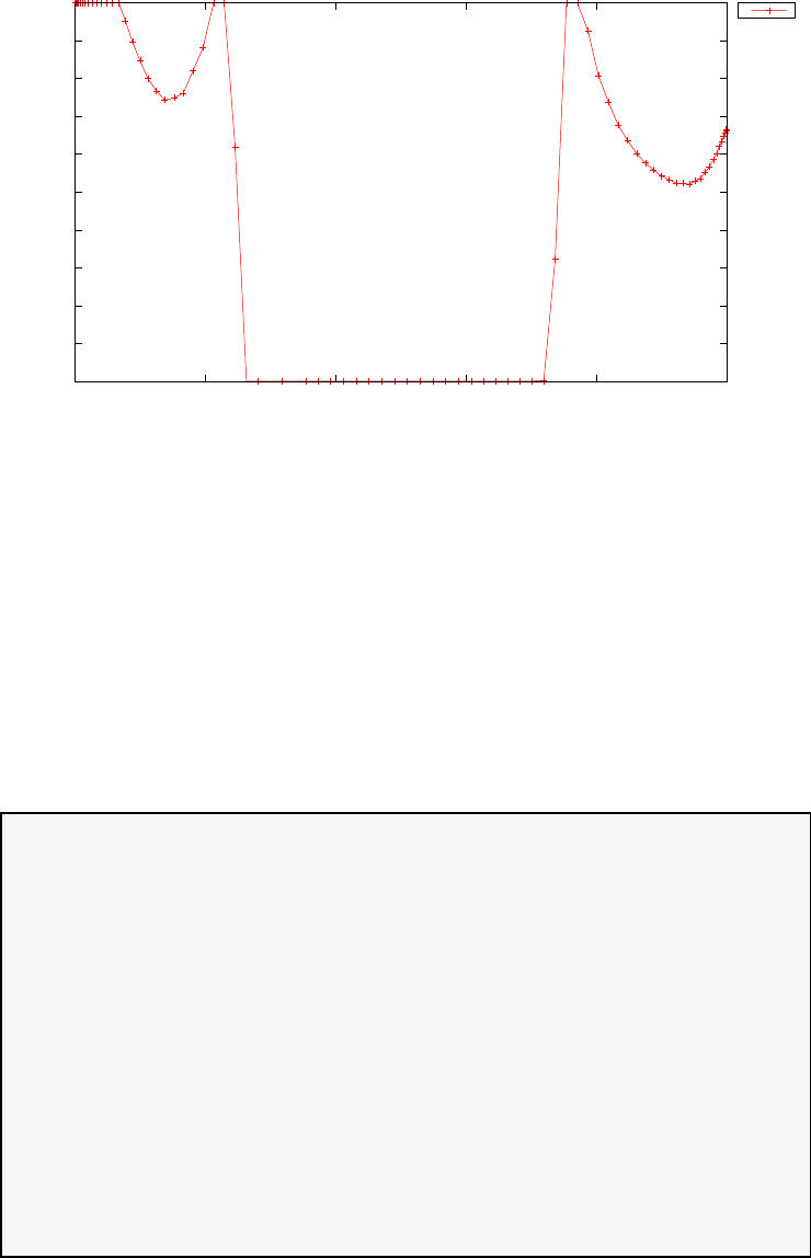
0
1
2
3
4
5
6
7
8
9
10
0 0.2 0.4 0.6 0.8 1
u
time (s)
Singular control 5
u
Figure 3.98: Control for singular control problem
the boundary conditions:
x1(0) = 0
x2(0) = −1(3.154)
and the path constraint
x2≤8(t−0.5)2−0.5(3.155)
The PSOPT code that solves this problem is shown below.
//////////////////////////////////////////////////////////////////////////
////////////////// statecon1.cxx /////////////////////
//////////////////////////////////////////////////////////////////////////
//////////////// PSOPT Example ////////////////////
//////////////////////////////////////////////////////////////////////////
//////////////////////////////////////////////////////////////////////////
//////// Title: Time varying state constraint problem ////////////////
//////// Last modified: 06 February 2009 ////////////////
//////// Reference: Teo et. al (1991) ////////////////
//////// (See PSOPT handbook for full reference) ///////////////
//////////////////////////////////////////////////////////////////////////
//////// Copyright (c) Victor M. Becerra, 2009 ////////////////
//////////////////////////////////////////////////////////////////////////
//////// This is part of the PSOPT software library, which ///////////////
//////// is distributed under the terms of the GNU Lesser ////////////////
//////// General Public License (LGPL) ////////////////
//////////////////////////////////////////////////////////////////////////
#include "psopt.h"
//////////////////////////////////////////////////////////////////////////
/////////////////// Define the end point (Mayer) cost function //////////
//////////////////////////////////////////////////////////////////////////
adouble endpoint_cost(adouble* initial_states, adouble* final_states,
adouble* parameters,adouble& t0, adouble& tf,
352

adouble* xad, int iphase, Workspace* workspace)
{
adouble retval = 0.0;
return retval;
}
//////////////////////////////////////////////////////////////////////////
/////////////////// Define the running (Lagrange) cost function ////////
//////////////////////////////////////////////////////////////////////////
adouble integrand_cost(adouble* states, adouble* controls,
adouble* parameters, adouble& time, adouble* xad,
int iphase, Workspace* workspace)
{
adouble x1 = states[0];
adouble x2 = states[1];
adouble u = controls[0];
return ( x1*x1 + x2*x2 + 0.005*u*u );
}
//////////////////////////////////////////////////////////////////////////
/////////////////// Define the DAE’s ////////////////////////////////////
//////////////////////////////////////////////////////////////////////////
void dae(adouble* derivatives, adouble* path, adouble* states,
adouble* controls, adouble* parameters, adouble& time,
adouble* xad, int iphase, Workspace* workspace)
{
adouble xdot, ydot, vdot;
adouble x1 = states[0];
adouble x2 = states[1];
adouble t = time;
adouble u = controls[0];
derivatives[0] = x2;
derivatives[1] = -x2 + u;
path[0] = -( 8.0*((t-0.5)*(t-0.5)) -0.5 - x2 );
}
////////////////////////////////////////////////////////////////////////////
/////////////////// Define the events function ////////////////////////////
////////////////////////////////////////////////////////////////////////////
void events(adouble* e, adouble* initial_states, adouble* final_states,
adouble* parameters,adouble& t0, adouble& tf, adouble* xad,
int iphase, Workspace* workspace)
{
adouble x10 = initial_states[0];
adouble x20 = initial_states[1];
e[0] = x10;
e[1] = x20;
}
///////////////////////////////////////////////////////////////////////////
/////////////////// Define the phase linkages function ///////////////////
///////////////////////////////////////////////////////////////////////////
void linkages( adouble* linkages, adouble* xad, Workspace* workspace)
{
// No linkages as this is a single phase problem
}
////////////////////////////////////////////////////////////////////////////
/////////////////// Define the main routine ///////////////////////////////
////////////////////////////////////////////////////////////////////////////
int main(void)
{
////////////////////////////////////////////////////////////////////////////
/////////////////// Declare key structures ////////////////////////////////
353

////////////////////////////////////////////////////////////////////////////
Alg algorithm;
Sol solution;
Prob problem;
////////////////////////////////////////////////////////////////////////////
/////////////////// Register problem name ////////////////////////////////
////////////////////////////////////////////////////////////////////////////
problem.name = "Time varying state constraint problem";
problem.outfilename= "stc1.txt";
////////////////////////////////////////////////////////////////////////////
//////////// Define problem level constants & do level 1 setup ////////////
////////////////////////////////////////////////////////////////////////////
problem.nphases = 1;
problem.nlinkages = 0;
psopt_level1_setup(problem);
/////////////////////////////////////////////////////////////////////////////
///////// Define phase related information & do level 2 setup ////////////
/////////////////////////////////////////////////////////////////////////////
problem.phases(1).nstates = 2;
problem.phases(1).ncontrols = 1;
problem.phases(1).nevents = 2;
problem.phases(1).npath = 1;
problem.phases(1).nodes = "[20 50]";
psopt_level2_setup(problem, algorithm);
////////////////////////////////////////////////////////////////////////////
/////////////////// Enter problem bounds information //////////////////////
////////////////////////////////////////////////////////////////////////////
problem.phases(1).bounds.lower.states(1) = -2.0;
problem.phases(1).bounds.lower.states(2) = -2.0;
problem.phases(1).bounds.upper.states(1) = 2.0;
problem.phases(1).bounds.upper.states(2) = 2.0;
problem.phases(1).bounds.lower.controls(1) = -20.0;
problem.phases(1).bounds.upper.controls(1) = 20.0;
problem.phases(1).bounds.lower.events(1) = 0.0;
problem.phases(1).bounds.lower.events(2) = -1.0;
problem.phases(1).bounds.upper.events(1) = 0.0;
problem.phases(1).bounds.upper.events(2) = -1.0;
problem.phases(1).bounds.upper.path(1) = 0.0;
problem.phases(1).bounds.lower.path(1) = -100.0;
problem.phases(1).bounds.lower.StartTime = 0.0;
problem.phases(1).bounds.upper.StartTime = 0.0;
problem.phases(1).bounds.lower.EndTime = 1.0;
problem.phases(1).bounds.upper.EndTime = 1.0;
////////////////////////////////////////////////////////////////////////////
/////////////////// Register problem functions ///////////////////////////
////////////////////////////////////////////////////////////////////////////
problem.integrand_cost = &integrand_cost;
problem.endpoint_cost = &endpoint_cost;
problem.dae = &dae;
problem.events = &events;
problem.linkages = &linkages;
////////////////////////////////////////////////////////////////////////////
354

/////////////////// Define & register initial guess ///////////////////////
////////////////////////////////////////////////////////////////////////////
problem.phases(1).guess.controls = zeros(2,20);
problem.phases(1).guess.states = zeros(2,20);
problem.phases(1).guess.time = linspace(0.0,1.0, 20);
////////////////////////////////////////////////////////////////////////////
/////////////////// Enter algorithm options //////////////////////////////
////////////////////////////////////////////////////////////////////////////
algorithm.scaling = "automatic";
algorithm.derivatives = "automatic";
algorithm.nlp_iter_max = 1000;
algorithm.nlp_tolerance = 1.e-4;
algorithm.nlp_method ="IPOPT";
////////////////////////////////////////////////////////////////////////////
/////////////////// Now call PSOPT to solve the problem /////////////////
////////////////////////////////////////////////////////////////////////////
psopt(solution, problem, algorithm);
////////////////////////////////////////////////////////////////////////////
/////////// Extract relevant variables from solution structure //////////
////////////////////////////////////////////////////////////////////////////
DMatrix x = solution.get_states_in_phase(1);
DMatrix u = solution.get_controls_in_phase(1);
DMatrix t = solution.get_time_in_phase(1);
////////////////////////////////////////////////////////////////////////////
/////////// Save solution data to files if desired ////////////////////////
////////////////////////////////////////////////////////////////////////////
x.Save("x.dat");
u.Save("u.dat");
t.Save("t.dat");
////////////////////////////////////////////////////////////////////////////
/////////// Plot some results if desired (requires gnuplot) ///////////////
////////////////////////////////////////////////////////////////////////////
// Generate points to plot the constraint boundary
DMatrix x2c = 8.0*((t-0.5)^2.0) -0.5*ones(1,length(t));
plot(t,x,t,x2c,"states","time (s)", "x", "x1 x2 constraint");
plot(t,u,"control","time (s)", "u");
plot(t,x,t,x2c,"states","time (s)", "x", "x1 x2 constraint",
"pdf", "stc1_states.pdf");
plot(t,u,"control","time (s)", "u", "u", "pdf","stc1_control.pdf");
}
////////////////////////////////////////////////////////////////////////////
/////////////////////// END OF FILE ///////////////////////////////
////////////////////////////////////////////////////////////////////////////
The output from PSOPT is summarised in the box below and shown in
Figures 3.99 and 3.100, which contain the elements of the states with the
boundary of the constraint on x2, and the control, respectively.
PSOPT results summary
=====================
Problem: Time varying state constraint problem
CPU time (seconds): 1.874042e+00
355
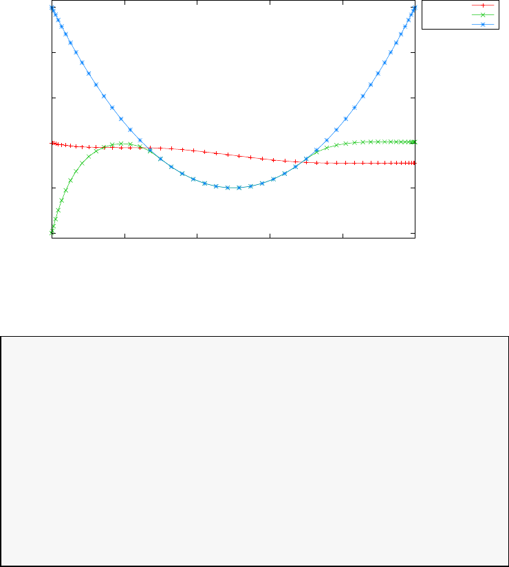
-1
-0.5
0
0.5
1
1.5
0 0.2 0.4 0.6 0.8 1
x
time (s)
states
x1
x2
constraint
Figure 3.99: States for time-varying state constraint problem
NLP solver used: IPOPT
PSOPT release number: 4.0
Date and time of this run: Thu Feb 21 17:07:14 2019
Optimal (unscaled) cost function value: 1.698182e-01
Phase 1 endpoint cost function value: 0.000000e+00
Phase 1 integrated part of the cost: 1.698182e-01
Phase 1 initial time: 0.000000e+00
Phase 1 final time: 1.000000e+00
Phase 1 maximum relative local error: 3.150532e-05
NLP solver reports: The problem has been solved!
3.39 Two burn orbit transfer
The goal of this problem is to compute a trajectory for an spacecraft to go
from a standard space shuttle park orbit to a geosynchronous final orbit.
It is assumed that the engines operate over two short periods during the
mission, and it is desired to compute the timing and duration of the burn
periods, as well as the instantaneous direction of the thrust during these
two periods, to maximise the final weight of the spacecraft. The problem is
described in detail by Betts [3]. The mission then involves four phases: coast,
burn, coast and burn. The problem is formulated as follows. Find u(t) =
356
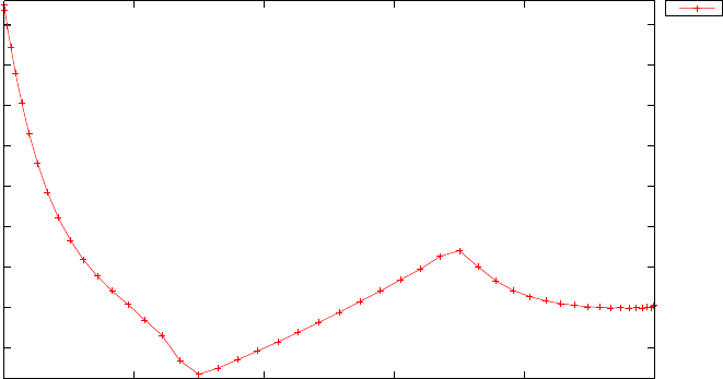
-2
0
2
4
6
8
10
12
14
0 0.2 0.4 0.6 0.8 1
u
time (s)
control
u
Figure 3.100: Control for time-varying state constraint problem
[θ(t), φ(t)]T, t ∈[t(1)
f, t(2)
f] and t∈[t(3)
f, t(4)
f], and the instants t(1)
f, t(2)
f, t(3)
f, t(4)
f
such that the following objective function is minimised:
J=−w(tf) (3.156)
subject to the dynamic constraints for phases 1 and 3:
˙
y=A(y)∆g+b(3.157)
the following dynamic constraints for phases 2 and 4:
˙
y=A(y)∆ + b
˙w=−T/Isp
(3.158)
and the following linkages between phases
y(t(1)
f) = y(t(2)
0)
y(t(2)
f) = y(t(3)
0)
y(t(3)
f) = y(t(4)
0)
t(1)
f=t(2)
0
t(2)
f=t(3)
0
t(3)
f=t(4)
0
w(t(2)
f) = w(t(4)
0)
(3.159)
357

where y= [p, f, g, h, k, L, w]Tis the vector of modified equinoctial elements,
wis the spacecraft weight, Isp is the specific impulse of the engine, Tis
the maximum thrust, expressions for A(y) and bare given in [3]. the
disturbing acceleration is ∆ = ∆g+ ∆T, where ∆gis the gravitational
disturbing acceleration due to the oblatness of Earth (given in [3]), and ∆T
is the thurst acceleration, given by:
∆T=QrQv
Tacos θcos φ
Tacos θsin φ
Tasin θ
(3.160)
where Ta(t) = g0T/w(t), g0is a constant, θis the pitch angle and φis the
yaw angle of the thurst, matrix Qvis given by:
Qv=v
||v||,v×r
||v×r||,v
||v|| ×v×r
||v×r||(3.161)
matrix Qris given by:
Qr=iriθih=hr
||r||
(r×v)×r
||r×v||||r||
(r×v)
||r×v|| i(3.162)
The boundary conditions of the problem are given by:
p(0) = 218327080.052835
f(0) = 0
g(0) = 0
h(0) = 0
h(0) = 0
k(0) = 0
L(0) = π(rad)
w(0) = 1 (lb)
p(tf) = 19323/σ +Re
f(tf)=0
g(tf)=0
h(tf)=0
k(tf)=0
(3.163)
and the values of the parameters are: g0= 32.174 (ft/sec2), Isp = 300
(sec), T= 1.2 (lb), µ= 1.407645794 ×10¹⁶ (ft3/sec2), Re= 20925662.73
(ft), σ= 1.0/6076.1154855643, J2= 1082.639 ×10−6,J3=−2.565 ×10⁻⁶,
J4=−1.608 ×10⁻⁶.
358

An initial guess was computed by forward propagation from the initial
conditions, assuming the following guesses for the controls and burn periods
[3]:
u(t) = 0.148637 ×10⁻²,−9.08446Tt∈[2840,21650]
u(t) = −0.136658 ×10−2,49.7892t∈[21650,21700] (3.164)
The problem was solved using local collocation (trapezoidal followed by
Hermite-Simpson) with automatic mesh refinement. The PSOPT code that
solves the problem is shown below.
//////////////////////////////////////////////////////////////////////////
//////////////// twoburn.cxx /////////////////////
//////////////////////////////////////////////////////////////////////////
//////////////// PSOPT Example /////////////////////
//////////////////////////////////////////////////////////////////////////
////////////////////////////////////////////////////////////////////////
//////// Title: two burn orbit transfer problem ////////////////
//////// Last modified: 07 February 2010 ////////////////
//////// Reference: Betts (2001) ////////////////
//////// (See PSOPT handbook for full reference) ////////////////
//////////////////////////////////////////////////////////////////////////
//////// Copyright (c) Victor M. Becerra, 2010 ////////////////
//////////////////////////////////////////////////////////////////////////
//////// This is part of the PSOPT software library, which ////////////////
//////// is distributed under the terms of the GNU Lesser ////////////////
//////// General Public License (LGPL) ////////////////
//////////////////////////////////////////////////////////////////////////
#include "psopt.h"
//////////////////////////////////////////////////////////////////////////
/////////////////// Define auxiliary functions //////////
//////////////////////////////////////////////////////////////////////////
adouble legendre_polynomial( adouble x, int n)
{
// This function computes the value of the legendre polynomials
// for a given value of the argument x and for n=0...5 only
adouble retval=0.0;
switch(n) {
case 0:
retval=1.0; break;
case 1:
retval= x; break;
case 2:
retval= 0.5*(3.0*pow(x,2)-1.0); break;
case 3:
retval= 0.5*(5.0*pow(x,3)- 3*x); break;
case 4:
retval= (1.0/8.0)*(35.0*pow(x,4) - 30.0*pow(x,2) + 3.0); break;
case 5:
retval= (1.0/8.0)*(63.0*pow(x,5) - 70.0*pow(x,3) + 15.0*x); break;
default:
error_message("legendre_polynomial(x,n) is limited to n=0...5");
}
return retval;
}
adouble legendre_polynomial_derivative( adouble x, int n)
{
// This function computes the value of the legendre polynomial derivatives
// for a given value of the argument x and for n=0...5 only.
adouble retval=0.0;
359

switch(n) {
case 0:
retval=0.0; break;
case 1:
retval= 1.0; break;
case 2:
retval= 0.5*(2.0*3.0*x); break;
case 3:
retval= 0.5*(3.0*5.0*pow(x,2)-3.0); break;
case 4:
retval= (1.0/8.0)*(4.0*35.0*pow(x,3) - 2.0*30.0*x ); break;
case 5:
retval= (1.0/8.0)*(5.0*63.0*pow(x,4) - 3.0*70.0*pow(x,2) + 15.0); break;
default:
error_message("legendre_polynomial_derivative(x,n) is limited to n=0...5");
}
return retval;
}
void compute_cartesian_trajectory(const DMatrix& x, DMatrix& xyz )
{
int npoints = x.GetNoCols();
xyz.Resize(3,npoints);
for(int i=1; i<=npoints;i++) {
double p = x(1,i);
double f = x(2,i);
double g = x(3,i);
double h = x(4,i);
double k = x(5,i);
double L = x(6,i);
double q = 1.0 + f*cos(L) + g*sin(L);
double r = p/q;
double alpha2 = h*h - k*k;
double X = sqrt( h*h + k*k );
double s2 = 1 + X*X;
double r1 = r/s2*( cos(L) + alpha2*cos(L) + 2*h*k*sin(L));
double r2 = r/s2*( sin(L) - alpha2*sin(L) + 2*h*k*cos(L));
double r3 = 2*r/s2*( h*sin(L) - k*cos(L) );
xyz(1,i) = r1;
xyz(2,i) = r2;
xyz(3,i) = r3;
}
}
//////////////////////////////////////////////////////////////////////////
/////////////////// Define the end point (Mayer) cost function //////////
//////////////////////////////////////////////////////////////////////////
adouble endpoint_cost(adouble* initial_states, adouble* final_states,
adouble* parameters,adouble& t0, adouble& tf,
adouble* xad, int iphase, Workspace* workspace)
{
if (iphase == 4) {
adouble w = final_states[CINDEX(7)];
return (-w);
}
else {
return (0);
}
}
//////////////////////////////////////////////////////////////////////////
/////////////////// Define the integrand (Lagrange) cost function //////
//////////////////////////////////////////////////////////////////////////
adouble integrand_cost(adouble* states, adouble* controls, adouble* parameters,
adouble& time, adouble* xad, int iphase, Workspace* workspace)
{
return 0.0;
}
360

//////////////////////////////////////////////////////////////////////////
/////////////////// Define the DAE’s ////////////////////////////////////
//////////////////////////////////////////////////////////////////////////
void dae(adouble* derivatives, adouble* path, adouble* states,
adouble* controls, adouble* parameters, adouble& time,
adouble* xad, int iphase, Workspace* workspace)
{
// Local integers
int i, j;
// Define constants:
double Isp = 300.0; // [sec]
double mu = 1.407645794e16; // [f2^2/sec^2]
double g0 = 32.174; // [ft/sec^2]
double Re = 20925662.73; // [ft]
double T = 1.2; // [lb]
double CM2W = 32.174;
double J[5];
J[2] = 1082.639e-6;
J[3] = -2.565e-6;
J[4] = -1.608e-6;
// Extract individual variables
adouble p = states[ CINDEX(1) ];
adouble f = states[ CINDEX(2) ];
adouble g = states[ CINDEX(3) ];
adouble h = states[ CINDEX(4) ];
adouble k = states[ CINDEX(5) ];
adouble L = states[ CINDEX(6) ];
adouble w;
adouble* u = controls;
// Define some dependent variables
adouble q = 1.0 + f*cos(L) + g*sin(L);
adouble r = p/q;
adouble alpha2 = h*h - k*k;
adouble X = sqrt( h*h + k*k );
adouble s2 = 1 + X*X;
// r and v
adouble r1 = r/s2*( cos(L) + alpha2*cos(L) + 2*h*k*sin(L));
adouble r2 = r/s2*( sin(L) - alpha2*sin(L) + 2*h*k*cos(L));
adouble r3 = 2*r/s2*( h*sin(L) - k*cos(L) );
adouble rvec[3];
rvec[ CINDEX(1) ] = r1; rvec[ CINDEX(2)] = r2; rvec[ CINDEX(3) ] = r3;
adouble v1 = -(1.0/s2)*sqrt(mu/p)*( sin(L) + alpha2*sin(L) - 2*h*k*cos(L) + g - 2*f*h*k + alpha2*g);
adouble v2 = -(1.0/s2)*sqrt(mu/p)*( -cos(L) + alpha2*cos(L) + 2*h*k*sin(L) - f + 2*g*h*k + alpha2*f);
adouble v3 = (2.0/s2)*sqrt(mu/p)*(h*cos(L) + k*sin(L) + f*h + g*k);
adouble vvec[3];
vvec[ CINDEX(1) ] = v1; vvec[ CINDEX(2)] = v2; vvec[ CINDEX(3) ] = v3;
// compute Qr
adouble ir[3], ith[3], ih[3];
adouble rv[3];
adouble rvr[3];
cross( rvec, vvec, rv );
cross( rv, rvec, rvr );
adouble norm_r = sqrt( dot(rvec, rvec, 3) );
adouble norm_rv = sqrt( dot(rv, rv, 3) );
for (i=0; i<3; i++) {
ir[i] = rvec[i]/norm_r;
ith[i] = rvr[i]/( norm_rv*norm_r );
361

ih[i] = rv[i]/norm_rv;
}
adouble Qr1[3], Qr2[3], Qr3[3];
for(i=0; i< 3; i++)
{
// Columns of matrix Qr
Qr1[i] = ir[i];
Qr2[i] = ith[i];
Qr3[i] = ih[i];
}
adouble Qv1[3], Qv2[3], Qv3[3];
adouble norm_v = sqrt( dot(vvec, vvec,3) );
for(i=0;i<3;i++)
{
Qv1[i] = vvec[i]/norm_v;
}
adouble vr[3];
cross( vvec, rvec, vr);
adouble norm_vr = sqrt( dot(vr, vr,3) );
for(i=0;i<3;i++)
{
Qv2[i] = vr[i]/norm_vr;
}
cross( Qv1, Qv2, Qv3 );
// Compute in
adouble en[3];
en[ CINDEX(1) ] = 0.0; en[ CINDEX(2) ]= 0.0; en[ CINDEX(3) ] = 1.0;
adouble enir = dot(en,ir,3);
adouble in[3];
for(i=0;i<3;i++) {
in[i] = en[i] - enir*ir[i];
}
adouble norm_in = sqrt( dot( in, in, 3 ) );
for(i=0;i<3;i++) {
in[i] = in[i]/norm_in;
}
// Geocentric latitude angle:
adouble sin_phi = rvec[ CINDEX(3) ]/ sqrt( dot(rvec,rvec,3) ) ;
adouble cos_phi = sqrt(1.0- pow(sin_phi,2.0));
adouble deltagn = 0.0;
adouble deltagr = 0.0;
for (j=2; j<=4;j++) {
adouble Pdash_j = legendre_polynomial_derivative( sin_phi, j );
adouble P_j = legendre_polynomial( sin_phi, j );
deltagn += -mu*cos_phi/(r*r)*pow(Re/r,j)*Pdash_j*J[j];
deltagr += -mu/(r*r)* (j+1)*pow( Re/r,j)*P_j*J[j];
}
// Compute vector delta_g
adouble delta_g[3];
for (i=0;i<3;i++) {
delta_g[i] = deltagn*in[i] - deltagr*ir[i];
}
// Compute vector DELTA_g
adouble DELTA_g[3];
DELTA_g[ CINDEX(1) ] = dot(Qr1, delta_g,3);
DELTA_g[ CINDEX(2) ] = dot(Qr2, delta_g,3);
DELTA_g[ CINDEX(3) ] = dot(Qr3, delta_g,3);
362

// Compute DELTA_T
adouble DELTA_T[3];
if (iphase == 1 || iphase==3) {
for(i=0;i<3;i++) {
DELTA_T[i] = 0.0;
}
}
else {
adouble Qr[9], Qrt[9], Qv[9], Tvel[3];
for(i=0;i<3;i++) {
Qr[i] = Qr1[i];
Qr[3+i] = Qr2[i];
Qr[6+i] = Qr3[i];
Qv[i] = Qv1[i];
Qv[3+i] = Qv2[i];
Qv[6+i] = Qv3[i];
}
transpose_ad(Qr, 3, 3, Qrt );
adouble theta = u[ CINDEX(1) ];
adouble phi = u[ CINDEX(2) ];
adouble Tvec[3];
w = states[CINDEX(7)];
adouble mass = w/CM2W;
adouble Tacc = T/mass;
Tvec[ CINDEX(1) ] = Tacc*cos(theta)*cos(phi);
Tvec[ CINDEX(2) ] = Tacc*cos(theta)*sin(phi);
Tvec[ CINDEX(3) ] = Tacc*sin(theta);
product_ad( Qv, Tvec, 3, 3, 3, 1, Tvel );
product_ad(Qrt, Tvel, 3, 3, 3, 1, DELTA_T );
}
// Compute DELTA
adouble DELTA[3];
for(i=0;i<3;i++) {
DELTA[i] = DELTA_g[i] + DELTA_T[i];
}
adouble delta1= DELTA[ CINDEX(1) ];
adouble delta2= DELTA[ CINDEX(2) ];
adouble delta3= DELTA[ CINDEX(3) ];
// derivatives
adouble pdot = 2*p/q*sqrt(p/mu) * delta2;
adouble fdot = sqrt(p/mu)*sin(L) * delta1 + sqrt(p/mu)*(1.0/q)*((q+1.0)*cos(L)+f) * delta2
- sqrt(p/mu)*(g/q)*(h*sin(L)-k*cos(L)) * delta3;
adouble gdot = -sqrt(p/mu)*cos(L) * delta1 + sqrt(p/mu)*(1.0/q)*((q+1.0)*sin(L)+g) * delta2
+ sqrt(p/mu)*(f/q)*(h*sin(L)-k*cos(L)) * delta3;
adouble hdot = sqrt(p/mu)*s2*cos(L)/(2.0*q) * delta3;
adouble kdot = sqrt(p/mu)*s2*sin(L)/(2.0*q) * delta3;
adouble Ldot = sqrt(p/mu)*(1.0/q)*(h*sin(L)-k*cos(L))* delta3 + sqrt(mu*p)*pow( (q/p),2.);
adouble wdot;
if (iphase==2 || iphase==4) {
wdot = -T/Isp;
}
else {
wdot = 0.0;
}
derivatives[ CINDEX(1) ] = pdot;
derivatives[ CINDEX(2) ] = fdot;
363

derivatives[ CINDEX(3) ] = gdot;
derivatives[ CINDEX(4) ] = hdot;
derivatives[ CINDEX(5) ] = kdot;
derivatives[ CINDEX(6) ] = Ldot;
if (iphase==2 || iphase==4) {
derivatives[ CINDEX(7) ] = wdot;
}
}
////////////////////////////////////////////////////////////////////////////
/////////////////// Define the events function ////////////////////////////
////////////////////////////////////////////////////////////////////////////
void events(adouble* e, adouble* initial_states, adouble* final_states,
adouble* parameters,adouble& t0, adouble& tf, adouble* xad,
int iphase, Workspace* workspace)
{
adouble pti = initial_states[ CINDEX(1) ];
adouble fti = initial_states[ CINDEX(2) ];
adouble gti = initial_states[ CINDEX(3) ];
adouble hti = initial_states[ CINDEX(4) ];
adouble kti = initial_states[ CINDEX(5) ];
adouble Lti = initial_states[ CINDEX(6) ];
adouble wti;
if (iphase==2) {
wti = initial_states[ CINDEX(7) ];
}
adouble ptf = final_states[ CINDEX(1) ];
adouble ftf = final_states[ CINDEX(2) ];
adouble gtf = final_states[ CINDEX(3) ];
adouble htf = final_states[ CINDEX(4) ];
adouble ktf = final_states[ CINDEX(5) ];
adouble Ltf = final_states[ CINDEX(6) ];
if (iphase==1) {
e[ CINDEX(1) ] = pti;
e[ CINDEX(2) ] = fti;
e[ CINDEX(3) ] = gti;
e[ CINDEX(4) ] = hti;
e[ CINDEX(5) ] = kti;
e[ CINDEX(6) ] = Lti;
}
if (iphase==2) {
e[ CINDEX(1) ] = wti;
}
if (iphase == 4) {
e[ CINDEX(1) ] = ptf;
e[ CINDEX(2) ] = ftf;
e[ CINDEX(3) ] = gtf;
e[ CINDEX(4) ] = htf;
e[ CINDEX(5) ] = ktf;
}
}
///////////////////////////////////////////////////////////////////////////
/////////////////// Define the phase linkages function ///////////////////
///////////////////////////////////////////////////////////////////////////
void linkages( adouble* linkages, adouble* xad, Workspace* workspace)
{
// Numeber of linkages:
// Boundary of phases 1,2: 6 state continuity + 1 time continuity
// Boundary of phases 2,3: 6 state continuity + 1 time continuity
// Boundary of phases 3,4: 6 state continuity + 1 time continuity
// 1 extra linkage w(tf2) = w(ti4)
// Total: 22 linkage constraints
adouble xf[7], xi[7], t0a, t0b, tfa, tfb, wtf2, wti4;
// Linking phases 1 and 2
364

get_final_states( xf, xad, 1, workspace );
get_initial_states( xi, xad, 2, workspace );
tfa = get_final_time( xad, 1, workspace );
t0b = get_initial_time( xad, 2, workspace );
linkages[ CINDEX(1) ] = xf[ CINDEX(1) ] - xi[ CINDEX(1) ];
linkages[ CINDEX(2) ] = xf[ CINDEX(2) ] - xi[ CINDEX(2) ];
linkages[ CINDEX(3) ] = xf[ CINDEX(3) ] - xi[ CINDEX(3) ];
linkages[ CINDEX(4) ] = xf[ CINDEX(4) ] - xi[ CINDEX(4) ];
linkages[ CINDEX(5) ] = xf[ CINDEX(5) ] - xi[ CINDEX(5) ];
linkages[ CINDEX(6) ] = xf[ CINDEX(6) ] - xi[ CINDEX(6) ];
linkages[ CINDEX(7) ] = t0b - tfa;
// Linking phases 2 and 3
get_final_states( xf, xad, 2, workspace );
get_initial_states( xi, xad, 3, workspace );
tfa = get_final_time( xad, 2, workspace );
t0b = get_initial_time( xad, 3, workspace );
wtf2 = xf[ CINDEX(7) ];
linkages[ CINDEX(8) ] = xf[ CINDEX(1) ] - xi[ CINDEX(1) ];
linkages[ CINDEX(9) ] = xf[ CINDEX(2) ] - xi[ CINDEX(2) ];
linkages[ CINDEX(10) ] = xf[ CINDEX(3) ] - xi[ CINDEX(3) ];
linkages[ CINDEX(11) ] = xf[ CINDEX(4) ] - xi[ CINDEX(4) ];
linkages[ CINDEX(12) ] = xf[ CINDEX(5) ] - xi[ CINDEX(5) ];
linkages[ CINDEX(13) ] = xf[ CINDEX(6) ] - xi[ CINDEX(6) ];
linkages[ CINDEX(14) ] = t0b - tfa;
// Linking phases 3 and 4
get_final_states( xf, xad, 3, workspace );
get_initial_states( xi, xad, 4, workspace );
tfa = get_final_time( xad, 3, workspace );
t0b = get_initial_time( xad, 4, workspace );
wti4 = xi[ CINDEX(7) ];
linkages[ CINDEX(15) ] = xf[ CINDEX(1) ] - xi[ CINDEX(1) ];
linkages[ CINDEX(16) ] = xf[ CINDEX(2) ] - xi[ CINDEX(2) ];
linkages[ CINDEX(17) ] = xf[ CINDEX(3) ] - xi[ CINDEX(3) ];
linkages[ CINDEX(18) ] = xf[ CINDEX(4) ] - xi[ CINDEX(4) ];
linkages[ CINDEX(19) ] = xf[ CINDEX(5) ] - xi[ CINDEX(5) ];
linkages[ CINDEX(20) ] = xf[ CINDEX(6) ] - xi[ CINDEX(6) ];
linkages[ CINDEX(21) ] = t0b - tfa;
// Linking the weight at the end of phase 2 with the weight at the beginning of phase 4
linkages[ CINDEX(22) ] = wtf2 - wti4;
}
////////////////////////////////////////////////////////////////////////////
/////////////////// Define the main routine ///////////////////////////////
////////////////////////////////////////////////////////////////////////////
int main(void)
{
////////////////////////////////////////////////////////////////////////////
/////////////////// Declare key structures ////////////////////////////////
////////////////////////////////////////////////////////////////////////////
Alg algorithm;
Sol solution;
Prob problem;
MSdata msdata;
////////////////////////////////////////////////////////////////////////////
/////////////////// Register problem name ////////////////////////////////
////////////////////////////////////////////////////////////////////////////
problem.name = "Two burn transfer problem";
problem.outfilename = "twoburn.txt";
////////////////////////////////////////////////////////////////////////////
//////////// Define problem level constants & do level 1 setup ////////////
365

////////////////////////////////////////////////////////////////////////////
problem.nphases = 4;
problem.nlinkages = 22;
psopt_level1_setup(problem);
/////////////////////////////////////////////////////////////////////////////
///////// Define phase related information & do level 2 setup ////////////
/////////////////////////////////////////////////////////////////////////////
problem.phases(1).nstates = 6;
problem.phases(1).ncontrols = 0;
problem.phases(1).nparameters = 0;
problem.phases(1).nevents = 6;
problem.phases(1).npath = 0;
problem.phases(1).nodes = 10;
problem.phases(2).nstates = 7;
problem.phases(2).ncontrols = 2;
problem.phases(2).nparameters = 0;
problem.phases(2).nevents = 1;
problem.phases(2).npath = 0;
problem.phases(2).nodes = 10;
problem.phases(3).nstates = 6;
problem.phases(3).ncontrols = 0;
problem.phases(3).nparameters = 0;
problem.phases(3).nevents = 0;
problem.phases(3).npath = 0;
problem.phases(3).nodes = 10;
problem.phases(4).nstates = 7;
problem.phases(4).ncontrols = 2;
problem.phases(4).nparameters = 0;
problem.phases(4).nevents = 5;
problem.phases(4).npath = 0;
problem.phases(4).nodes = 10;
psopt_level2_setup(problem, algorithm);
////////////////////////////////////////////////////////////////////////////
/////////////////// Enter problem bounds information //////////////////////
////////////////////////////////////////////////////////////////////////////
double pti = 21837080.052835;
double fti = 0.0;
double gti = 0.0;
double hti = -0.25396764647494;
double kti = 0.0;
double Lti = pi;
double wti = 1.0;
double SISP = 300.0;
double DELTAV2 = 8000;
double DELTAV4 = 3000;
double CM2W = 32.174;
double sigma = 1.0/6076.1154855643;
double Re = 20925662.73;
double wtf2 = wti*exp(-DELTAV2/(CM2W*SISP));
double wtf4 = wtf2*exp(-DELTAV4/(CM2W*SISP));
double ptf = 19323/sigma + Re;
double ftf = 0.0;
double gtf = 0.0;
double htf = 0.0;
double ktf = 0.0;
double D2R = pi/180.0;
// BOUNDS FOR PHASE 1
problem.phases(1).bounds.lower.states(1) = 10.e6;
problem.phases(1).bounds.lower.states(2) = -1;
366

problem.phases(1).bounds.lower.states(3) = -1;
problem.phases(1).bounds.lower.states(4) = -1;
problem.phases(1).bounds.lower.states(5) = -1;
problem.phases(1).bounds.lower.states(6) = pi;
problem.phases(1).bounds.upper.states(1) = 2e8;
problem.phases(1).bounds.upper.states(2) = 1;
problem.phases(1).bounds.upper.states(3) = 1;
problem.phases(1).bounds.upper.states(4) = 1;
problem.phases(1).bounds.upper.states(5) = 1;
problem.phases(1).bounds.upper.states(6) = 30*pi;
problem.phases(1).bounds.lower.events(1) = pti;
problem.phases(1).bounds.lower.events(2) = fti;
problem.phases(1).bounds.lower.events(3) = gti;
problem.phases(1).bounds.lower.events(4) = hti;
problem.phases(1).bounds.lower.events(5) = kti;
problem.phases(1).bounds.lower.events(6) = Lti;
problem.phases(1).bounds.upper.events(1) = pti;
problem.phases(1).bounds.upper.events(2) = fti;
problem.phases(1).bounds.upper.events(3) = gti;
problem.phases(1).bounds.upper.events(4) = hti;
problem.phases(1).bounds.upper.events(5) = kti;
problem.phases(1).bounds.upper.events(6) = Lti;
problem.phases(1).bounds.lower.StartTime = 0.0;
problem.phases(1).bounds.upper.StartTime = 0.0;
problem.phases(1).bounds.lower.EndTime = 2000.0;
problem.phases(1).bounds.upper.EndTime = 3000.0;
// BOUNDS FOR PHASE 2
problem.phases(2).bounds.lower.states(1) = 10.e6;
problem.phases(2).bounds.lower.states(2) = -1;
problem.phases(2).bounds.lower.states(3) = -1;
problem.phases(2).bounds.lower.states(4) = -1;
problem.phases(2).bounds.lower.states(5) = -1;
problem.phases(2).bounds.lower.states(6) = pi;
problem.phases(2).bounds.lower.states(7) = 0.0;
problem.phases(2).bounds.upper.states(1) = 2.e8;
problem.phases(2).bounds.upper.states(2) = 1;
problem.phases(2).bounds.upper.states(3) = 1;
problem.phases(2).bounds.upper.states(4) = 1;
problem.phases(2).bounds.upper.states(5) = 1;
problem.phases(2).bounds.upper.states(6) = 30*pi;
problem.phases(2).bounds.upper.states(7) = 2.0;
problem.phases(2).bounds.lower.controls(1) = -pi;
problem.phases(2).bounds.lower.controls(2) = -pi;
problem.phases(2).bounds.upper.controls(1) = pi;
problem.phases(2).bounds.upper.controls(2) = pi;
problem.phases(2).bounds.lower.events(1) = wti;
problem.phases(2).bounds.upper.events(1) = wti;
problem.phases(2).bounds.lower.StartTime = 2000;
problem.phases(2).bounds.upper.StartTime = 3000;
problem.phases(2).bounds.lower.EndTime = 2100;
problem.phases(2).bounds.upper.EndTime = 3100;
// BOUNDS FOR PHASE 3
problem.phases(3).bounds.lower.states(1) = 10.e6;
problem.phases(3).bounds.lower.states(2) = -1;
problem.phases(3).bounds.lower.states(3) = -1;
problem.phases(3).bounds.lower.states(4) = -1;
problem.phases(3).bounds.lower.states(5) = -1;
problem.phases(3).bounds.lower.states(6) = pi;
367

problem.phases(3).bounds.upper.states(1) = 2.e8;
problem.phases(3).bounds.upper.states(2) = 1.0;
problem.phases(3).bounds.upper.states(3) = 1.0;
problem.phases(3).bounds.upper.states(4) = 1.0;
problem.phases(3).bounds.upper.states(5) = 1.0;
problem.phases(3).bounds.upper.states(6) = 30*pi;
problem.phases(3).bounds.lower.StartTime = 2100;
problem.phases(3).bounds.upper.StartTime = 3100;
problem.phases(3).bounds.lower.EndTime = 21600;
problem.phases(3).bounds.upper.EndTime = 21800;
// BOUNDS FOR PHASE 4
problem.phases(4).bounds.lower.states(1) = 10.e6;
problem.phases(4).bounds.lower.states(2) = -1;
problem.phases(4).bounds.lower.states(3) = -1;
problem.phases(4).bounds.lower.states(4) = -1;
problem.phases(4).bounds.lower.states(5) = -1;
problem.phases(4).bounds.lower.states(6) = pi;
problem.phases(4).bounds.lower.states(7) = 0.0;
problem.phases(4).bounds.upper.states(1) = 2.e8;
problem.phases(4).bounds.upper.states(2) = 1;
problem.phases(4).bounds.upper.states(3) = 1;
problem.phases(4).bounds.upper.states(4) = 1;
problem.phases(4).bounds.upper.states(5) = 1;
problem.phases(4).bounds.upper.states(6) = 30*pi;
problem.phases(4).bounds.upper.states(7) = 2.0;
problem.phases(4).bounds.lower.controls(1) = -pi;
problem.phases(4).bounds.lower.controls(2) = -pi;
problem.phases(4).bounds.upper.controls(1) = pi;
problem.phases(4).bounds.upper.controls(2) = pi;
problem.phases(4).bounds.lower.events(1) = ptf;
problem.phases(4).bounds.lower.events(2) = ftf;
problem.phases(4).bounds.lower.events(3) = gtf;
problem.phases(4).bounds.lower.events(4) = htf;
problem.phases(4).bounds.lower.events(5) = ktf;
problem.phases(4).bounds.upper.events(1) = ptf;
problem.phases(4).bounds.upper.events(2) = ftf;
problem.phases(4).bounds.upper.events(3) = gtf;
problem.phases(4).bounds.upper.events(4) = htf;
problem.phases(4).bounds.upper.events(5) = ktf;
problem.phases(4).bounds.lower.StartTime = 21600;
problem.phases(4).bounds.upper.StartTime = 21800;
problem.phases(4).bounds.lower.EndTime = 21650;
problem.phases(4).bounds.upper.EndTime = 21900;
////////////////////////////////////////////////////////////////////////////
/////////////////// Register problem functions ///////////////////////////
////////////////////////////////////////////////////////////////////////////
problem.integrand_cost = &integrand_cost;
problem.endpoint_cost = &endpoint_cost;
problem.dae = &dae;
problem.events = &events;
problem.linkages = &linkages;
////////////////////////////////////////////////////////////////////////////
/////////////////// Define & register initial guess ///////////////////////
////////////////////////////////////////////////////////////////////////////
int nnodes;
int ncontrols;
int nstates;
int iphase;
DMatrix x_guess, u_guess, time_guess, param_guess, xini, xfinal;
// Phase 1
nnodes = problem.phases(1).nodes(1);
368

nstates = problem.phases(1).nstates;
iphase = 1;
x_guess = zeros(nstates,nnodes);
time_guess = linspace(0.0,2690,nnodes);
xini.Resize(6,1);
xini(1)= pti; xini(2)=fti;xini(3)=gti;xini(4)=hti;xini(5)=kti;xini(6)=Lti;
rk4_propagate( dae, u_guess, time_guess, xini, param_guess, problem, iphase, x_guess, NULL);
tra(x_guess).Print("x_guess(iphase=1)");
xfinal = x_guess(colon(),nnodes);
problem.phases(1).guess.states = x_guess;
problem.phases(1).guess.time = time_guess;
// Phase 2
nnodes = problem.phases(2).nodes(1);
nstates = problem.phases(2).nstates;
ncontrols = problem.phases(2).ncontrols;
iphase = 2;
u_guess = zeros(ncontrols,nnodes);
x_guess = zeros(nstates,nnodes);
time_guess = linspace(2690,2840,nnodes);
xini.Resize(7,1);
xini(1)= xfinal(1); xini(2)=xfinal(2);xini(3)=xfinal(3);xini(4)=xfinal(4);xini(5)=xfinal(5);xini(6)=xfinal(6);
xini(7)= wti;
u_guess(1,colon()) = 0.148637e-2*D2R*ones(1,nnodes);
u_guess(2,colon()) = -9.08446*D2R*ones(1,nnodes);
rk4_propagate( dae, u_guess, time_guess, xini, param_guess, problem, iphase, x_guess, NULL);
tra(x_guess).Print("x_guess(iphase=2)");
xfinal = x_guess(colon(),nnodes);
double wtf2__ = xfinal(7);
problem.phases(2).guess.states = x_guess;
problem.phases(2).guess.controls = u_guess;
problem.phases(2).guess.time = time_guess;
// Phase 3
nnodes = problem.phases(3).nodes(1);
nstates = problem.phases(3).nstates;
iphase = 3;
x_guess = zeros(nstates,nnodes);
time_guess = linspace(2840,21650,nnodes);
xini.Resize(6,1);
xini(1)= xfinal(1); xini(2)=xfinal(2);xini(3)=xfinal(3);xini(4)=xfinal(4);xini(5)=xfinal(5);xini(6)=xfinal(6);
rk4_propagate( dae, u_guess, time_guess, xini, param_guess, problem, iphase, x_guess, NULL);
tra(x_guess).Print("x_guess(iphase=3)");
xfinal = x_guess(colon(),nnodes);
problem.phases(3).guess.states = x_guess;
problem.phases(3).guess.time = time_guess;
// Phase 4
nnodes = problem.phases(4).nodes(1);
nstates = problem.phases(4).nstates;
ncontrols = problem.phases(4).ncontrols;
iphase = 4;
369

u_guess = zeros(ncontrols,nnodes);
x_guess = zeros(nstates,nnodes);
time_guess = linspace(21650,21700,nnodes);
u_guess(1,colon()) = -0.136658e-2*D2R*ones(1,nnodes);
u_guess(2,colon()) = 49.7892*D2R*ones(1,nnodes);
xini.Resize(7,1);
xini(1)= xfinal(1); xini(2)=xfinal(2);xini(3)=xfinal(3);xini(4)=xfinal(4);xini(5)=xfinal(5);xini(6)=xfinal(6);
xini(7)= wtf2__;
rk4_propagate( dae, u_guess, time_guess, xini, param_guess, problem, iphase, x_guess, NULL);
tra(x_guess).Print("x_guess(iphase=4)");
problem.phases(4).guess.states = x_guess;
problem.phases(4).guess.controls = u_guess;
problem.phases(4).guess.time = time_guess;
////////////////////////////////////////////////////////////////////////////
/////////////////// Enter algorithm options //////////////////////////////
////////////////////////////////////////////////////////////////////////////
algorithm.nlp_iter_max = 1000;
algorithm.nlp_tolerance = 1.e-6;
algorithm.nlp_method = "IPOPT";
algorithm.scaling = "automatic";
algorithm.derivatives = "automatic";
algorithm.defect_scaling = "jacobian-based";
algorithm.jac_sparsity_ratio = 0.11;
algorithm.collocation_method = "trapezoidal";
// algorithm.diff_matrix = "central-differences";
algorithm.mesh_refinement = "automatic";
algorithm.mr_max_iterations = 5;
algorithm.ode_tolerance = 1.0e-6;
////////////////////////////////////////////////////////////////////////////
/////////////////// Now call PSOPT to solve the problem //////////////////
////////////////////////////////////////////////////////////////////////////
psopt(solution, problem, algorithm);
////////////////////////////////////////////////////////////////////////////
/////////// Extract relevant variables from solution structure //////////
////////////////////////////////////////////////////////////////////////////
DMatrix x, t, w2, xi, w4, ti;
x = solution.get_states_in_phase(1);
t = solution.get_time_in_phase(1);
w2 = solution.get_states_in_phase(2);
w2 = w2(7,colon());
w4 = solution.get_states_in_phase(4);
w4 = w4(7,colon());
for(int i=2;i<=problem.nphases;i++) {
xi = solution.get_states_in_phase(i);
ti = solution.get_time_in_phase(i);
xi = xi(colon(1,6),colon());
x = x || xi;
t = t || ti;
}
DMatrix u_phase2 = solution.get_controls_in_phase(2);
DMatrix u_phase4 = solution.get_controls_in_phase(4);
DMatrix t2 = solution.get_time_in_phase(2);
DMatrix t4 = solution.get_time_in_phase(4);
370

////////////////////////////////////////////////////////////////////////////
/////////// Save solution data to files if desired ////////////////////////
////////////////////////////////////////////////////////////////////////////
// x.Save("x.dat");
// u.Save("u.dat");
// t.Save("t.dat");
////////////////////////////////////////////////////////////////////////////
/////////// Plot some results if desired (requires gnuplot) ///////////////
////////////////////////////////////////////////////////////////////////////
double R2D = 180/pi;
DMatrix x1 = x(1,colon())/1.e6;
DMatrix x2 = x(2,colon());
DMatrix x3 = x(3,colon());
DMatrix x4 = x(4,colon());
DMatrix x5 = x(5,colon());
DMatrix x6 = x(6,colon());
DMatrix x7 = x(7,colon());
DMatrix theta_phase2;
DMatrix theta_phase4;
DMatrix phi_phase2;
DMatrix phi_phase4;
DMatrix r;
theta_phase2 = u_phase2(1,colon())*R2D;
phi_phase2 = u_phase2(2,colon())*R2D;
theta_phase4 = u_phase4(1,colon())*R2D;
phi_phase4 = u_phase4(2,colon())*R2D;
compute_cartesian_trajectory(x,r);
r.Save("r.dat");
double ft2km = 0.0003048;
r = r*ft2km;
plot(t2,theta_phase2,problem.name+": thrust theta phase 2","time (s)", "theta (deg)", "theta");
plot(t2,phi_phase2,problem.name+": thrust phi phase 2","time (s)", "phi (deg)", "phi");
plot(t4,theta_phase4,problem.name+": thrust theta phase 4","time (s)", "theta (deg)", "theta");
plot(t4,phi_phase4,problem.name+": thrust phi phase 4","time (s)", "phi (deg)", "phi");
plot(t2,theta_phase2,problem.name+": thrust pitch angle phase 2","time (s)", "theta (deg)", "theta",
"pdf", "theta2.pdf");
plot(t2,phi_phase2,problem.name+": thrust angle phase 2","time (s)", "phi (deg)", "phi",
"pdf", "phi2.pdf");
plot(t4,theta_phase4,problem.name+": thrust pitch angle phase 4","time (s)", "theta (deg)", "theta",
"pdf", "theta4.pdf");
plot(t4,phi_phase4,problem.name+": thrust yaw angle phase 4","time (s)", "phi (deg)", "phi",
"pdf", "phi4.pdf");
plot3(r(1,colon()), r(2,colon()), r(3,colon()), "Two burn trasnfer trajectory", "x (km)", "y (km)", "z (km)",
NULL, NULL, "30,110");
plot3(r(1,colon()), r(2,colon()), r(3,colon()), "Two burn transfer trajectory", "x (km)", "y (km)", "z (km)",
"pdf", "trajectory.pdf", "30,110");
plot(r(1,colon()), r(2,colon()), "Two burn trajectory - projection on the equatorial plane",
"x (km)", "y (km)");
}
////////////////////////////////////////////////////////////////////////////
/////////////////////// END OF FILE ///////////////////////////////
////////////////////////////////////////////////////////////////////////////
371

The output from PSOPT is summarised in the box below. The controls
during the burn periods are shown Figures 3.101 to 3.104, which show the
control variables during phases 2 and 4, and Figure 3.105, which shows the
trajectory in cartesian co-ordinates.
PSOPT results summary
=====================
Problem: Two burn transfer problem
CPU time (seconds): 8.818389e+00
NLP solver used: IPOPT
PSOPT release number: 4.0
Date and time of this run: Thu Feb 21 15:55:48 2019
Optimal (unscaled) cost function value: -2.367249e-01
Phase 1 endpoint cost function value: 0.000000e+00
Phase 1 integrated part of the cost: 0.000000e+00
Phase 1 initial time: 0.000000e+00
Phase 1 final time: 2.609964e+03
Phase 1 maximum relative local error: 1.385002e-06
Phase 2 endpoint cost function value: 0.000000e+00
Phase 2 integrated part of the cost: 0.000000e+00
Phase 2 initial time: 2.609964e+03
Phase 2 final time: 2.751426e+03
Phase 2 maximum relative local error: 1.225041e-06
Phase 3 endpoint cost function value: 0.000000e+00
Phase 3 integrated part of the cost: 0.000000e+00
Phase 3 initial time: 2.751426e+03
Phase 3 final time: 2.163415e+04
Phase 3 maximum relative local error: 1.174820e-05
Phase 4 endpoint cost function value: -2.367249e-01
Phase 4 integrated part of the cost: 0.000000e+00
Phase 4 initial time: 2.163415e+04
Phase 4 final time: 2.168351e+04
Phase 4 maximum relative local error: 5.521144e-06
NLP solver reports: The problem has been solved!
372
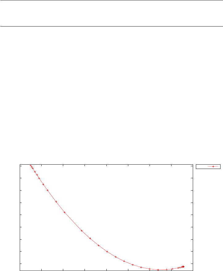
Iter Method Nodes NV NC OE CE JE HE RHS max CPUa
1 TRAPZ 40 308 298 637 636 20 0 48336 4.942e-02 2.400e-01
2 TRAPZ 56 428 402 25 26 23 0 2808 4.129e-03 3.600e-01
3 H-S 76 650 532 38 39 37 0 8580 1.568e-04 1.000e+00
4 H-S 104 888 714 46 47 41 0 14288 2.222e-05 1.590e+00
5 H-S 133 1132 902 66 67 57 0 26197 8.212e-06 2.880e+00
CPUb- - - - - - - - - - 3.786e+01
- - - - - 812 815 178 0 100209 - 4.393e+01
Key: Iter=iteration number, NV=number of variables, NC=number of constraints, OE=objective evalu-
ations, CE = constraint evaluations, JE = Jacobian evaluations, HE = Hessian evaluations, RHS = ODE right
hand side evaluations, max = maximum relative ODE error, CPUa= CPU time in seconds spent by NLP
algorithm, CPUb= additional CPU time in seconds spent by PSOPT
Table 3.8: Mesh refinement statistics: Two burn transfer problem
0.2
0.3
0.4
0.5
0.6
0.7
0.8
0.9
1
2600 2620 2640 2660 2680 2700 2720 2740 2760
theta (deg)
time (s)
Two burn transfer problem: thrust pitch angle phase 2
theta
Figure 3.101: Pitch angle during phase 2
373
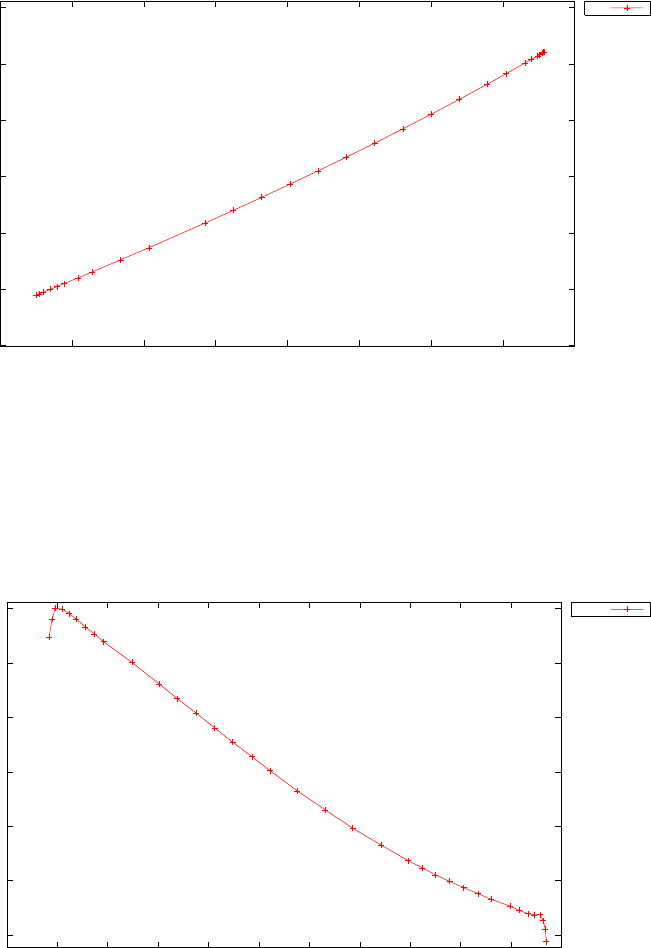
-9.5
-9
-8.5
-8
-7.5
-7
-6.5
2600 2620 2640 2660 2680 2700 2720 2740 2760
phi (deg)
time (s)
Two burn transfer problem: thrust angle phase 2
phi
Figure 3.102: Yaw angle during phase 2
-0.04
-0.02
0
0.02
0.04
0.06
0.08
21630 21635 21640 21645 21650 21655 21660 21665 21670 21675 21680 21685
theta (deg)
time (s)
Two burn transfer problem: thrust pitch angle phase 4
theta
Figure 3.103: Pitch angle during phase 4
374
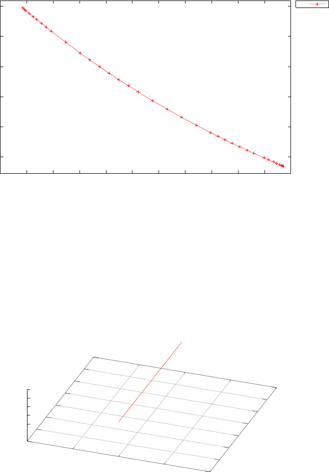
25
30
35
40
45
50
21630 21635 21640 21645 21650 21655 21660 21665 21670 21675 21680 21685
phi (deg)
time (s)
Two burn transfer problem: thrust yaw angle phase 4
phi
Figure 3.104: Yaw angle during phase 4
Two burn transfer trajectory
-7000
-6000
-5000
-4000
-3000
-2000
-1000
0
x (km)
-1
-0.5
0
0.5
1
y (km)
-0.001
-0.0005
0
0.0005
0.001
z (km)
Figure 3.105: Two burn transfer trajectory
375

3.40 Two link robotic arm
Consider the following optimal control problem [29]. Find tf, and u(t)∈
[0, tf] to minimize the cost functional
J=tf(3.165)
subject to the dynamic constraints
˙x1=sin(x3)( 9.0
4.0cos(x3)x2
1+2∗x2
2)+ 4.0
3.0(u1−u2)−3.0
2.0cos(x3)u2
31.0
36.0+9.0
4.0 sin2(x3)
˙x2=−(sin(x3)∗(7.0
2.0∗x2
1+9.0
4.0cos(x3)x2
2)−7.0
3.0u2+3.0
2.0cos(x3)(u1−u2))
31.0
36.0+9.0
4.0 sin2(x3)
˙x3=x2−x1
˙x4=x1
(3.166)
the boundary conditions:
x1(0) = 0 x1(tf) = 0
x2(0) = 0 x2(tf) = 0
x3(0) = 0.5x3(tf) = 0.5
x4(0) = 0.0x4(tf)=0.522
(3.167)
The control bounds: −1≤u1(t)≤1
−1≤u2(t)≤1(3.168)
The PSOPT code that solves this problem is shown below.
//////////////////////////////////////////////////////////////////////////
////////////////// twolinkarm.cxx //////////////////////////
//////////////////////////////////////////////////////////////////////////
//////////////// PSOPT Example ////////////////////
//////////////////////////////////////////////////////////////////////////
//////////////////////////////////////////////////////////////////////////
//////// Title: Two link arm problem ////////////////
//////// Last modified: 04 January 2009 ////////////////
//////// Reference: PROPT users guide ////////////////
//////// (See PSOPT handbook for full reference) ////////////////
//////////////////////////////////////////////////////////////////////////
//////// Copyright (c) Victor M. Becerra, 2009 ////////////////
//////////////////////////////////////////////////////////////////////////
//////// This is part of the PSOPT software library, which ///////////////
//////// is distributed under the terms of the GNU Lesser ////////////////
//////// General Public License (LGPL) ////////////////
//////////////////////////////////////////////////////////////////////////
#include "psopt.h"
//////////////////////////////////////////////////////////////////////////
/////////////////// Define the end point (Mayer) cost function //////////
//////////////////////////////////////////////////////////////////////////
adouble endpoint_cost(adouble* initial_states, adouble* final_states,
adouble* parameters,adouble& t0, adouble& tf,
adouble* xad, int iphase, Workspace* workspace)
{
376

return tf;
}
//////////////////////////////////////////////////////////////////////////
/////////////////// Define the integrand (Lagrange) cost function //////
//////////////////////////////////////////////////////////////////////////
adouble integrand_cost(adouble* states, adouble* controls,
adouble* parameters, adouble& time, adouble* xad,
int iphase, Workspace* workspace)
{
return 0.0;
}
//////////////////////////////////////////////////////////////////////////
/////////////////// Define the DAE’s ////////////////////////////////////
//////////////////////////////////////////////////////////////////////////
void dae(adouble* derivatives, adouble* path, adouble* states,
adouble* controls, adouble* parameters, adouble& time,
adouble* xad, int iphase, Workspace* workspace)
{
adouble xdot, ydot, vdot;
adouble x1 = states[ CINDEX(1) ];
adouble x2 = states[ CINDEX(2) ];
adouble x3 = states[ CINDEX(3) ];
adouble x4 = states[ CINDEX(4) ];
adouble u1 = controls[ CINDEX(1) ];
adouble u2 = controls[ CINDEX(2) ];
adouble num1 = sin(x3)*( (9.0/4.0)*cos(x3)*x1*x1+2*x2*x2 )
+ (4.0/3.0)*(u1-u2)-(3.0/2.0)*cos(x3)*u2;
adouble num2 = -(sin(x3)*((7.0/2.0)*x1*x1+(9.0/4.0)*cos(x3)*x2*x2)
-(7.0/3.0)*u2+(3.0/2.0)*cos(x3)*(u1-u2));
adouble den = 31.0/36.0 + 9.0/4.0*pow(sin(x3),2);
derivatives[ CINDEX(1) ] = num1/den;
derivatives[ CINDEX(2) ] = num2/den;
derivatives[ CINDEX(3) ] = x2 - x1;
derivatives[ CINDEX(4) ] = x1;
}
////////////////////////////////////////////////////////////////////////////
/////////////////// Define the events function ////////////////////////////
////////////////////////////////////////////////////////////////////////////
void events(adouble* e, adouble* initial_states, adouble* final_states,
adouble* parameters,adouble& t0, adouble& tf, adouble* xad,
int iphase, Workspace* workspace)
{
adouble x10 = initial_states[ CINDEX(1) ];
adouble x20 = initial_states[ CINDEX(2) ];
adouble x30 = initial_states[ CINDEX(3) ];
adouble x40 = initial_states[ CINDEX(4) ];
adouble x1f = final_states[ CINDEX(1) ];
adouble x2f = final_states[ CINDEX(2) ];
adouble x3f = final_states[ CINDEX(3) ];
adouble x4f = final_states[ CINDEX(4) ];
e[ CINDEX(1) ] = x10;
e[ CINDEX(2) ] = x20;
e[ CINDEX(3) ] = x30;
e[ CINDEX(4) ] = x40;
e[ CINDEX(5) ] = x1f;
e[ CINDEX(6) ] = x2f;
e[ CINDEX(7) ] = x3f;
e[ CINDEX(8) ] = x4f;
}
///////////////////////////////////////////////////////////////////////////
/////////////////// Define the phase linkages function ///////////////////
///////////////////////////////////////////////////////////////////////////
void linkages( adouble* linkages, adouble* xad, Workspace* workspace)
{
// No linkages as this is a single phase problem
377

}
////////////////////////////////////////////////////////////////////////////
/////////////////// Define the main routine ///////////////////////////////
////////////////////////////////////////////////////////////////////////////
int main(void)
{
////////////////////////////////////////////////////////////////////////////
/////////////////// Declare key structures ////////////////////////////////
////////////////////////////////////////////////////////////////////////////
Alg algorithm;
Sol solution;
Prob problem;
////////////////////////////////////////////////////////////////////////////
/////////////////// Register problem name ////////////////////////////////
////////////////////////////////////////////////////////////////////////////
problem.name = "Two link robotic arm";
problem.outfilename = "twolink.txt";
////////////////////////////////////////////////////////////////////////////
//////////// Define problem level constants & do level 1 setup ////////////
////////////////////////////////////////////////////////////////////////////
problem.nphases = 1;
problem.nlinkages = 0;
psopt_level1_setup(problem);
/////////////////////////////////////////////////////////////////////////////
///////// Define phase related information & do level 2 setup /////////////
/////////////////////////////////////////////////////////////////////////////
problem.phases(1).nstates = 4;
problem.phases(1).ncontrols = 2;
problem.phases(1).nevents = 8;
problem.phases(1).npath = 0;
problem.phases(1).nodes = 40;
psopt_level2_setup(problem, algorithm);
////////////////////////////////////////////////////////////////////////////
/////////////////// Declare DMatrix objects to store results //////////////
////////////////////////////////////////////////////////////////////////////
DMatrix x, u, t;
DMatrix lambda, H;
////////////////////////////////////////////////////////////////////////////
/////////////////// Enter problem bounds information //////////////////////
////////////////////////////////////////////////////////////////////////////
problem.phases(1).bounds.lower.states(1) = -2.0;
problem.phases(1).bounds.lower.states(2) = -2.0;
problem.phases(1).bounds.lower.states(3) = -2.0;
problem.phases(1).bounds.lower.states(4) = -2.0;
problem.phases(1).bounds.upper.states(1) = 2.0;
problem.phases(1).bounds.upper.states(2) = 2.0;
problem.phases(1).bounds.upper.states(3) = 2.0;
problem.phases(1).bounds.upper.states(4) = 2.0;
problem.phases(1).bounds.lower.controls(1) = -1.0;
problem.phases(1).bounds.lower.controls(2) = -1.0;
problem.phases(1).bounds.upper.controls(1) = 1.0;
problem.phases(1).bounds.upper.controls(2) = 1.0;
problem.phases(1).bounds.lower.events(1) = 0.0;
problem.phases(1).bounds.lower.events(2) = 0.0;
problem.phases(1).bounds.lower.events(3) = 0.5;
problem.phases(1).bounds.lower.events(4) = 0.0;
problem.phases(1).bounds.lower.events(5) = 0.0;
problem.phases(1).bounds.lower.events(6) = 0.0;
378

problem.phases(1).bounds.lower.events(7) = 0.5;
problem.phases(1).bounds.lower.events(8) = 0.522;
problem.phases(1).bounds.upper.events = problem.phases(1).bounds.lower.events;
problem.phases(1).bounds.lower.StartTime = 0.0;
problem.phases(1).bounds.upper.StartTime = 0.0;
problem.phases(1).bounds.lower.EndTime = 1.0;
problem.phases(1).bounds.upper.EndTime = 10.0;
////////////////////////////////////////////////////////////////////////////
/////////////////// Register problem functions ///////////////////////////
////////////////////////////////////////////////////////////////////////////
problem.integrand_cost = &integrand_cost;
problem.endpoint_cost = &endpoint_cost;
problem.dae = &dae;
problem.events = &events;
problem.linkages = &linkages;
////////////////////////////////////////////////////////////////////////////
/////////////////// Define & register initial guess ///////////////////////
////////////////////////////////////////////////////////////////////////////
DMatrix x0(4,40);
x0(1,colon()) = linspace(0.0,0.0, 40);
x0(2,colon()) = linspace(0.0,0.0, 40);
x0(3,colon()) = linspace(0.5,0.5, 40);
x0(4,colon()) = linspace(0.522,0.522, 40);
problem.phases(1).guess.controls = zeros(1,40);
problem.phases(1).guess.states = x0;
problem.phases(1).guess.time = linspace(0.0, 3.0, 40);
////////////////////////////////////////////////////////////////////////////
/////////////////// Enter algorithm options //////////////////////////////
////////////////////////////////////////////////////////////////////////////
algorithm.nlp_method = "IPOPT";
algorithm.scaling = "automatic";
algorithm.derivatives = "automatic";
algorithm.nlp_iter_max = 1000;
algorithm.nlp_tolerance = 1.e-6;
////////////////////////////////////////////////////////////////////////////
/////////////////// Now call PSOPT to solve the problem /////////////////
////////////////////////////////////////////////////////////////////////////
psopt(solution, problem, algorithm);
////////////////////////////////////////////////////////////////////////////
/////////// Extract relevant variables from solution structure //////////
////////////////////////////////////////////////////////////////////////////
x = solution.get_states_in_phase(1);
u = solution.get_controls_in_phase(1);
t = solution.get_time_in_phase(1);
////////////////////////////////////////////////////////////////////////////
/////////// Save solution data to files if desired ////////////////////////
////////////////////////////////////////////////////////////////////////////
x.Save("x.dat");
u.Save("u.dat");
t.Save("t.dat");
////////////////////////////////////////////////////////////////////////////
/////////// Plot some results if desired (requires gnuplot) ///////////////
////////////////////////////////////////////////////////////////////////////
plot(t,x,problem.name + ": states", "time (s)", "states", "x1 x2 x3 x4");
379

plot(t,u,problem.name + ": controls", "time (s)", "controls", "u1 u2");
plot(t,x,problem.name + ": states", "time (s)", "states", "x1 x2 x3 x4",
"pdf", "twolinkarm_states.pdf");
plot(t,u,problem.name + ": controls", "time (s)", "controls", "u1 u2",
"pdf", "twolinkarm_controls.pdf");
}
////////////////////////////////////////////////////////////////////////////
/////////////////////// END OF FILE ///////////////////////////////
////////////////////////////////////////////////////////////////////////////
The output from PSOPT is summarised in the box below and shown
in Figures 3.106 and 3.107, which contain the elements of the state and the
control, respectively.
PSOPT results summary
=====================
Problem: Two link robotic arm
CPU time (seconds): 1.080000e+00
NLP solver used: IPOPT
Optimal (unscaled) cost function value: 2.988662e+00
Phase 1 endpoint cost function value: 2.988662e+00
Phase 1 integrated part of the cost: 0.000000e+00
Phase 1 initial time: 0.000000e+00
Phase 1 final time: 2.988662e+00
Phase 1 maximum relative local error: 3.815633e-04
NLP solver reports: The problem solved!
3.41 Two-phase path tracking robot
Consider the following two-phase optimal control problem, which consists
of a robot following a specified path [38,36]. Find u(t)∈[0,2] to minimize
the cost functional
J=Z2
0
[100(x1−x1,ref )2+ 100(x2−x2,ref )2
+500(x3−x3,ref )2+ 500(x4−x4,ref )2]dt
(3.169)
380
-0.001
-0.0005
0
0.0005
0.001
0 0.5 1 1.5 2 2.5 3
states
time (s)
Two link robotic arm: states
x1
x2
x3
x4
Figure 3.106: States for two-link robotic arm problem
-0.001
-0.0005
0
0.0005
0.001
0 0.5 1 1.5 2 2.5 3
controls
time (s)
Two link robotic arm: controls
u1
u2
Figure 3.107: Controls for two link robotic arm problem
381

subject to the dynamic constraints
˙x1=x3
˙x2=x4
˙x3=u1
˙x4=u2
(3.170)
the boundary conditions:
x1(0) = 0 x1(2) = 0.5
x2(0) = 0 x2(2) = 0.5
x3(0) = 0.5x3(2) = 0
x4(0) = 0.0x4(2) = 0.5
(3.171)
where the reference signals are given by:
x1,ref =t
2(0 ≤t < 1),1
2(1 ≤t≤2)
x2,ref = 0 (0 ≤t < 1),t−1
2(1 ≤t≤2)
x3,ref =1
2(0 ≤t < 1),0 (1 ≤t≤2)
x4,ref = 0 (0 ≤t < 1),1
2(1 ≤t≤2)
(3.172)
The PSOPT code that solves this problem is shown below. The first phase
covers the period t∈[0,1], while the second phase covers the period t∈[1,2].
//////////////////////////////////////////////////////////////////////////
////////////////// twophase_robot.cxx ////////////////////////
//////////////////////////////////////////////////////////////////////////
//////////////// PSOPT Example ////////////////////
//////////////////////////////////////////////////////////////////////////
//////////////////////////////////////////////////////////////////////////
//////// Title: Two phase path tracking robot ////////////////
//////// Last modified: 09 January 2009 ////////////////
//////// Reference: PROPT Users Guide ////////////////
//////// (See PSOPT handbook for full reference) ////////////////
//////////////////////////////////////////////////////////////////////////
//////// Copyright (c) Victor M. Becerra, 2009 ////////////////
//////////////////////////////////////////////////////////////////////////
//////// This is part of the PSOPT software library, which ///////////////
//////// is distributed under the terms of the GNU Lesser ////////////////
//////// General Public License (LGPL) ////////////////
//////////////////////////////////////////////////////////////////////////
#include "psopt.h"
//////////////////////////////////////////////////////////////////////////
/////////////////// Define the end point (Mayer) cost function //////////
//////////////////////////////////////////////////////////////////////////
adouble endpoint_cost(adouble* initial_states, adouble* final_states,
adouble* parameters,adouble& t0, adouble& tf,
adouble* xad, int iphase, Workspace* workspace)
{
return 0.0;
}
//////////////////////////////////////////////////////////////////////////
/////////////////// Define the integrand (Lagrange) cost function //////
382

//////////////////////////////////////////////////////////////////////////
adouble integrand_cost(adouble* states, adouble* controls,
adouble* parameters, adouble& time, adouble* xad,
int iphase, Workspace* workspace)
{
adouble retval;
adouble x1, x2, x3, x4;
adouble x1ref, x2ref, x3ref, x4ref;
double w1, w2, w3, w4;
w1 = 100.0;
w2 = 100.0;
w3 = 500.0;
w4 = 500.0;
x1 = states[0];
x2 = states[1];
x3 = states[2];
x4 = states[3];
if (iphase==1) {
x1ref = time/2;
x2ref = 0.0;
x3ref = 0.5;
x4ref = 0.0;
}
if (iphase==2) {
x1ref = 0.5;
x2ref = (time-1.0)/2.0;
x3ref = 0.0;
x4ref = 0.5;
}
retval = w1*pow(x1-x1ref,2)+w2*pow(x2-x2ref,2)+w3*pow(x3-x3ref,2)+w4*pow(x4-x4ref,2);
return retval;
}
//////////////////////////////////////////////////////////////////////////
/////////////////// Define the DAE’s ////////////////////////////////////
//////////////////////////////////////////////////////////////////////////
void dae(adouble* derivatives, adouble* path, adouble* states,
adouble* controls, adouble* parameters, adouble& time,
adouble* xad, int iphase, Workspace* workspace)
{
adouble x3, x4, u1, u2;
x3 = states[2];
x4 = states[3];
u1 = controls[0];
u2 = controls[1];
derivatives[0] = x3;
derivatives[1] = x4;
derivatives[2] = u1;
derivatives[3] = u2;
}
////////////////////////////////////////////////////////////////////////////
/////////////////// Define the events function ////////////////////////////
////////////////////////////////////////////////////////////////////////////
void events(adouble* e, adouble* initial_states, adouble* final_states,
383

adouble* parameters,adouble& t0, adouble& tf, adouble* xad,
int iphase, Workspace* workspace)
{
adouble x1i, x2i, x3i, x4i;
adouble x1f, x2f, x3f, x4f;
if (iphase == 1)
{
x1i = initial_states[0];
x2i = initial_states[1];
x3i = initial_states[2];
x4i = initial_states[3];
e[0] = x1i;
e[1] = x2i;
e[2] = x3i;
e[3] = x4i;
}
else if (iphase == 2)
{
x1f = final_states[0];
x2f = final_states[1];
x3f = final_states[2];
x4f = final_states[3];
e[0] = x1f;
e[1] = x2f;
e[2] = x3f;
e[3] = x4f;
}
}
///////////////////////////////////////////////////////////////////////////
/////////////////// Define the phase linkages function ///////////////////
///////////////////////////////////////////////////////////////////////////
void linkages( adouble* linkages, adouble* xad, Workspace* workspace)
{
int index = 0;
auto_link( linkages, &index, xad, 1, 2, workspace );
}
////////////////////////////////////////////////////////////////////////////
/////////////////// Define the main routine ///////////////////////////////
////////////////////////////////////////////////////////////////////////////
int main(void)
{
////////////////////////////////////////////////////////////////////////////
/////////////////// Declare key structures ////////////////////////////////
////////////////////////////////////////////////////////////////////////////
Alg algorithm;
Sol solution;
Prob problem;
////////////////////////////////////////////////////////////////////////////
/////////////////// Register problem name ////////////////////////////////
////////////////////////////////////////////////////////////////////////////
problem.name = "Two phase path tracking robot";
problem.outfilename = "twophro.txt";
////////////////////////////////////////////////////////////////////////////
//////////// Define problem level constants & do level 1 setup ////////////
////////////////////////////////////////////////////////////////////////////
problem.nphases = 2;
problem.nlinkages = 5;
384

psopt_level1_setup(problem);
/////////////////////////////////////////////////////////////////////////////
///////// Define phase related information & do level 2 setup ///////////
/////////////////////////////////////////////////////////////////////////////
problem.phases(1).nstates = 4;
problem.phases(1).ncontrols = 2;
problem.phases(1).nevents = 4;
problem.phases(1).npath = 0;
problem.phases(2).nstates = 4;
problem.phases(2).ncontrols = 2;
problem.phases(2).nevents = 4;
problem.phases(2).npath = 0;
problem.phases(1).nodes = 30;
problem.phases(2).nodes = 30;
psopt_level2_setup(problem, algorithm);
////////////////////////////////////////////////////////////////////////////
/////////////////// Enter problem bounds information //////////////////////
////////////////////////////////////////////////////////////////////////////
double x1i = 0.0;
double x2i = 0.0;
double x3i = 0.5;
double x4i = 0.0;
double x1f = 0.5;
double x2f = 0.5;
double x3f = 0.0;
double x4f = 0.5;
// Phase 0 bounds
problem.phases(1).bounds.lower.states(1) = -10.0;
problem.phases(1).bounds.lower.states(2) = -10.0;
problem.phases(1).bounds.lower.states(3) = -10.0;
problem.phases(1).bounds.lower.states(4) = -10.0;
problem.phases(1).bounds.upper.states(1) = 10.0;
problem.phases(1).bounds.upper.states(2) = 10.0;
problem.phases(1).bounds.upper.states(3) = 10.0;
problem.phases(1).bounds.upper.states(4) = 10.0;
problem.phases(1).bounds.lower.controls(1) = -10.0;
problem.phases(1).bounds.upper.controls(1) = 10.0;
problem.phases(1).bounds.lower.controls(2) = -10.0;
problem.phases(1).bounds.upper.controls(2) = 10.0;
problem.phases(1).bounds.lower.events(1) = x1i;
problem.phases(1).bounds.lower.events(2) = x2i;
problem.phases(1).bounds.lower.events(3) = x3i;
problem.phases(1).bounds.lower.events(4) = x4i;
problem.phases(1).bounds.upper.events(1) = x1i;
problem.phases(1).bounds.upper.events(2) = x2i;
problem.phases(1).bounds.upper.events(3) = x3i;
problem.phases(1).bounds.upper.events(4) = x4i;
problem.phases(1).bounds.lower.StartTime = 0.0;
problem.phases(1).bounds.upper.StartTime = 0.0;
problem.phases(1).bounds.lower.EndTime = 1.0;
problem.phases(1).bounds.upper.EndTime = 1.0;
// Phase 1 bounds
problem.phases(2).bounds.lower.states(1) = -10.0;
problem.phases(2).bounds.lower.states(2) = -10.0;
problem.phases(2).bounds.lower.states(3) = -10.0;
problem.phases(2).bounds.lower.states(4) = -10.0;
problem.phases(2).bounds.upper.states(1) = 10.0;
problem.phases(2).bounds.upper.states(2) = 10.0;
385

problem.phases(2).bounds.upper.states(3) = 10.0;
problem.phases(2).bounds.upper.states(4) = 10.0;
problem.phases(2).bounds.lower.controls(1) = -10.0;
problem.phases(2).bounds.upper.controls(1) = 10.0;
problem.phases(2).bounds.lower.controls(2) = -10.0;
problem.phases(2).bounds.upper.controls(2) = 10.0;
problem.phases(2).bounds.lower.events(1) = x1f;
problem.phases(2).bounds.lower.events(2) = x2f;
problem.phases(2).bounds.lower.events(3) = x3f;
problem.phases(2).bounds.lower.events(4) = x4f;
problem.phases(2).bounds.upper.events(1) = x1f;
problem.phases(2).bounds.upper.events(2) = x2f;
problem.phases(2).bounds.upper.events(3) = x3f;
problem.phases(2).bounds.upper.events(4) = x4f;
problem.phases(2).bounds.lower.StartTime = 1.0;
problem.phases(2).bounds.upper.StartTime = 1.0;
problem.phases(2).bounds.lower.EndTime = 2.0;
problem.phases(2).bounds.upper.EndTime = 2.0;
////////////////////////////////////////////////////////////////////////////
/////////////////// Register problem functions ///////////////////////////
////////////////////////////////////////////////////////////////////////////
problem.integrand_cost = &integrand_cost;
problem.endpoint_cost = &endpoint_cost;
problem.dae = &dae;
problem.events = &events;
problem.linkages = &linkages;
////////////////////////////////////////////////////////////////////////////
/////////////////// Define & register initial guess ///////////////////////
////////////////////////////////////////////////////////////////////////////
int iphase;
DMatrix u0(2,30);
DMatrix x0(4,30);
DMatrix time_guess0 = linspace(0.0, 1.0 , 30);
DMatrix time_guess1 = linspace(1.0, 2.0 , 30);
iphase = 1;
u0 = zeros(2,30+1);
x0(1,colon()) = linspace(x1i,(x1i+x1f)/2, 30);
x0(2,colon()) = linspace(x2i,(x2i+x2f)/2, 30);
x0(3,colon()) = linspace(x3i,(x3i+x3f)/2, 30);
x0(4,colon()) = linspace(x4i,(x4i+x4f)/2, 30);
problem.phases(iphase).guess.controls = u0;
problem.phases(iphase).guess.states = x0;
problem.phases(iphase).guess.time = time_guess0;
iphase = 2;
u0 = zeros(2,30+1);
x0(1,colon()) = linspace((x1i+x1f)/2, x1f, 30);
x0(2,colon()) = linspace((x2i+x2f)/2, x2f, 30);
x0(3,colon()) = linspace((x3i+x3f)/2, x3f, 30);
x0(4,colon()) = linspace((x4i+x4f)/2, x4f, 30);
problem.phases(iphase).guess.controls = u0;
problem.phases(iphase).guess.states = x0;
problem.phases(iphase).guess.time = time_guess1;
////////////////////////////////////////////////////////////////////////////
/////////////////// Enter algorithm options //////////////////////////////
////////////////////////////////////////////////////////////////////////////
algorithm.nlp_method = "IPOPT";
algorithm.scaling = "automatic";
algorithm.derivatives = "automatic";
386

algorithm.hessian = "exact";
algorithm.nlp_iter_max = 1000;
algorithm.nlp_tolerance = 1.e-6;
////////////////////////////////////////////////////////////////////////////
/////////////////// Now call PSOPT to solve the problem /////////////////
////////////////////////////////////////////////////////////////////////////
psopt(solution, problem, algorithm);
////////////////////////////////////////////////////////////////////////////
/////////// Extract relevant variables from solution structure //////////
////////////////////////////////////////////////////////////////////////////
DMatrix xphase1 = solution.get_states_in_phase(1);
DMatrix uphase1 = solution.get_controls_in_phase(1);
DMatrix tphase1 = solution.get_time_in_phase(1);
DMatrix xphase2 = solution.get_states_in_phase(2);
DMatrix uphase2 = solution.get_controls_in_phase(2);
DMatrix tphase2 = solution.get_time_in_phase(2);
DMatrix x = (xphase1 || xphase2);
DMatrix u = (uphase1 || uphase2);
DMatrix t = (tphase1 || tphase2);
////////////////////////////////////////////////////////////////////////////
/////////// Save solution data to files if desired ////////////////////////
////////////////////////////////////////////////////////////////////////////
x.Save("x.dat");
u.Save("u.dat");
t.Save("t.dat");
////////////////////////////////////////////////////////////////////////////
/////////// Plot some results if desired (requires gnuplot) ///////////////
////////////////////////////////////////////////////////////////////////////
plot(t,x,problem.name, "time (s)", "states");
plot(t,u,problem.name, "time (s)", "control");
plot(t,x,problem.name+": states", "time (s)", "states", "x1 x2 x3 x4",
"pdf", "twophro_states.pdf");
plot(t,u,problem.name+": controls", "time (s)", "controls", "u1 u2",
"pdf", "twophro_controls.pdf" );
}
////////////////////////////////////////////////////////////////////////////
/////////////////////// END OF FILE ///////////////////////////////
////////////////////////////////////////////////////////////////////////////
The output from PSOPT is summarised in the box below and shown
in Figures 3.108 and 3.109, which contain the elements of the state and the
control, respectively.
PSOPT results summary
=====================
Problem: Two phase path tracking robot
CPU time (seconds): 1.759431e+00
NLP solver used: IPOPT
PSOPT release number: 4.0
387
0
0.1
0.2
0.3
0.4
0.5
0 0.5 1 1.5 2
states
time (s)
Two phase path tracking robot: states
x1
x2
x3
x4
Figure 3.108: States for two-phase path tracking robot problem
Date and time of this run: Thu Feb 21 17:07:41 2019
Optimal (unscaled) cost function value: 1.042568e+00
Phase 1 endpoint cost function value: 0.000000e+00
Phase 1 integrated part of the cost: 5.212840e-01
Phase 1 initial time: 0.000000e+00
Phase 1 final time: 1.000000e+00
Phase 1 maximum relative local error: 3.443287e-04
Phase 2 endpoint cost function value: 0.000000e+00
Phase 2 integrated part of the cost: 5.212840e-01
Phase 2 initial time: 1.000000e+00
Phase 2 final time: 2.000000e+00
Phase 2 maximum relative local error: 3.443298e-04
NLP solver reports: The problem has been solved!
3.42 Two-phase Schwartz problem
Consider the following two-phase optimal control problem [36]. Find u(t)∈
[0,2.9] to minimize the cost functional
J= 5(x1(tf)2+x2(tf)2)(3.173)
388
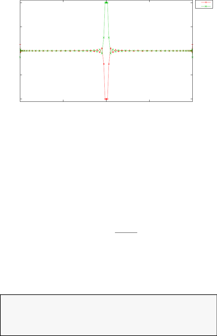
-10
-5
0
5
10
0 0.5 1 1.5 2
controls
time (s)
Two phase path tracking robot: controls
u1
u2
Figure 3.109: Control for two phase path tracking robot problem
subject to the dynamic constraints
˙x1=x2
˙x2=u−0.1(1 + 2x2
1)x2(3.174)
the boundary conditions:
x1(0) = 1
x2(0) = 1 (3.175)
and the constraints for t < 1:
1−9(x1−1)2−x2−0.4
0.32
≤0
−0.8≤x2
−1≤u≤1
(3.176)
The PSOPT code that solves this problem is shown below. The problem
has been divided into two phases. The first phase covers the period t∈[0,1],
while the second phase covers the period t∈[1,2.9].
//////////////////////////////////////////////////////////////////////////
////////////////// twophase_schwartz.cxx /////////////////////
//////////////////////////////////////////////////////////////////////////
//////////////// PSOPT Example ////////////////////
//////////////////////////////////////////////////////////////////////////
//////////////////////////////////////////////////////////////////////////
//////// Title: Two phase Schwartz problem ////////////////
389

//////// Last modified: 09 January 2009 ////////////////
//////// Reference: PROPT Users Guide ////////////////
//////// (See PSOPT handbook for full reference) ///////////////
//////////////////////////////////////////////////////////////////////////
//////// Copyright (c) Victor M. Becerra, 2009 ////////////////
//////////////////////////////////////////////////////////////////////////
//////// This is part of the PSOPT software library, which ///////////////
//////// is distributed under the terms of the GNU Lesser ////////////////
//////// General Public License (LGPL) ////////////////
//////////////////////////////////////////////////////////////////////////
#include "psopt.h"
//////////////////////////////////////////////////////////////////////////
/////////////////// Define the end point (Mayer) cost function //////////
//////////////////////////////////////////////////////////////////////////
adouble endpoint_cost(adouble* initial_states, adouble* final_states,
adouble* parameters,adouble& t0, adouble& tf,
adouble* xad, int iphase, Workspace* workspace)
{
adouble retval;
adouble x1f, x2f;
// Phase 1 cost
if ( iphase == 1)
{
retval = 0.0;
}
// Phase 2 cost
if( iphase == 2 ) {
x1f = final_states[0];
x2f = final_states[1];
retval = 5*(x1f*x1f + x2f*x2f);
}
return retval;
}
//////////////////////////////////////////////////////////////////////////
/////////////////// Define the integrand (Lagrange) cost function //////
//////////////////////////////////////////////////////////////////////////
adouble integrand_cost(adouble* states, adouble* controls,
adouble* parameters, adouble& time, adouble* xad,
int iphase, Workspace* workspace)
{
return 0.0;
}
//////////////////////////////////////////////////////////////////////////
/////////////////// Define the DAE’s ////////////////////////////////////
//////////////////////////////////////////////////////////////////////////
void dae(adouble* derivatives, adouble* path, adouble* states,
adouble* controls, adouble* parameters, adouble& time,
adouble* xad, int iphase, Workspace* workspace)
{
adouble x1 = states[0];
adouble x2 = states[1];
adouble u = controls[0];
derivatives[0] = x2;
derivatives[1] = u-0.1*(1+2*x1*x1)*x2;
if(iphase==1) {
path[0] = 1.0 - 9.0*((x1-1.0)*(x1-1.0))-((x2-0.4)*(x2-0.4))/(0.3*0.3);
}
390

}
////////////////////////////////////////////////////////////////////////////
/////////////////// Define the events function ////////////////////////////
////////////////////////////////////////////////////////////////////////////
void events(adouble* e, adouble* initial_states, adouble* final_states,
adouble* parameters,adouble& t0, adouble& tf, adouble* xad,
int iphase, Workspace* workspace)
{
adouble x1i = initial_states[0];
adouble x2i = initial_states[1];
if (iphase==1) {
e[0] = x1i;
e[1] = x2i;
}
}
///////////////////////////////////////////////////////////////////////////
/////////////////// Define the phase linkages function ///////////////////
///////////////////////////////////////////////////////////////////////////
void linkages( adouble* linkages, adouble* xad, Workspace* workspace)
{
int index = 0;
auto_link( linkages, &index, xad, 1, 2, workspace );
}
////////////////////////////////////////////////////////////////////////////
/////////////////// Define the main routine ///////////////////////////////
////////////////////////////////////////////////////////////////////////////
int main(void)
{
////////////////////////////////////////////////////////////////////////////
/////////////////// Declare key structures ////////////////////////////////
////////////////////////////////////////////////////////////////////////////
Alg algorithm;
Sol solution;
Prob problem;
////////////////////////////////////////////////////////////////////////////
/////////////////// Register problem name ////////////////////////////////
////////////////////////////////////////////////////////////////////////////
problem.name = "Two phase Schwartz problem";
problem.outfilename = "twophsc.txt";
////////////////////////////////////////////////////////////////////////////
//////////// Define problem level constants & do level 1 setup ////////////
////////////////////////////////////////////////////////////////////////////
problem.nphases = 2;
problem.nlinkages = 3;
psopt_level1_setup(problem);
/////////////////////////////////////////////////////////////////////////////
///////// Define phase related information & do level 2 setup ////////////
/////////////////////////////////////////////////////////////////////////////
problem.phases(1).nstates = 2;
problem.phases(1).ncontrols = 1;
problem.phases(1).nevents = 2;
problem.phases(1).npath = 1;
problem.phases(2).nstates = 2;
problem.phases(2).ncontrols = 1;
problem.phases(2).nevents = 0;
problem.phases(2).npath = 0;
problem.phases(1).nodes = 40;
problem.phases(2).nodes = 40;
391

psopt_level2_setup(problem, algorithm);
////////////////////////////////////////////////////////////////////////////
/////////////////// Enter problem bounds information //////////////////////
////////////////////////////////////////////////////////////////////////////
double x1L = -20.0;
double x2L_phase1 = -0.8;
double x2L_phase2 = -10.0;
double uL = -1.0;
double x1U = 10.0;
double x2U = 10.0;
double uU = 1.0;
double hL = -100.0;
double hU = 0.0;
// Phase 0 bounds
problem.phases(1).bounds.lower.states(1) = x1L;
problem.phases(1).bounds.lower.states(2) = x2L_phase1;
problem.phases(1).bounds.upper.states(1) = x1U;
problem.phases(1).bounds.upper.states(2) = x2U;
problem.phases(1).bounds.lower.controls(1) = uL;
problem.phases(1).bounds.upper.controls(1) = uU;
problem.phases(1).bounds.lower.events(1) = 1.0;
problem.phases(1).bounds.lower.events(2) = 1.0;
problem.phases(1).bounds.upper.events(1) = 1.0;
problem.phases(1).bounds.upper.events(2) = 1.0;
problem.phases(1).bounds.lower.path(1) = hL;
problem.phases(1).bounds.upper.path(1) = hU;
problem.phases(1).bounds.lower.StartTime = 0.0;
problem.phases(1).bounds.upper.StartTime = 0.0;
problem.phases(1).bounds.lower.EndTime = 1.0;
problem.phases(1).bounds.upper.EndTime = 1.0;
// Phase 1 bounds
problem.phases(2).bounds.lower.states(1) = x1L;
problem.phases(2).bounds.lower.states(2) = x2L_phase2;
problem.phases(2).bounds.upper.states(1) = x1U;
problem.phases(2).bounds.upper.states(2) = x2U;
problem.phases(2).bounds.lower.controls(1) = -50.0;
problem.phases(2).bounds.upper.controls(1) = 50.0;
problem.phases(2).bounds.lower.StartTime = 1.0;
problem.phases(2).bounds.upper.StartTime = 1.0;
problem.phases(2).bounds.lower.EndTime = 2.9;
problem.phases(2).bounds.upper.EndTime = 2.9;
////////////////////////////////////////////////////////////////////////////
/////////////////// Register problem functions ///////////////////////////
////////////////////////////////////////////////////////////////////////////
problem.integrand_cost = &integrand_cost;
problem.endpoint_cost = &endpoint_cost;
problem.dae = &dae;
problem.events = &events;
problem.linkages = &linkages;
////////////////////////////////////////////////////////////////////////////
/////////////////// Define & register initial guess ///////////////////////
////////////////////////////////////////////////////////////////////////////
int iphase;
DMatrix u0(1,40);
DMatrix x0(2,40);
392

DMatrix time_guess0 = linspace(0.0, 1.0 , 40);
DMatrix time_guess1 = linspace(1.0, 2.9 , 40);
iphase = 1;
u0 = zeros(1,40);
x0(1,colon()) = linspace(1.0,1.0, 40);
x0(2,colon()) = linspace(1.0,1.0, 40);
problem.phases(iphase).guess.controls = u0;
problem.phases(iphase).guess.states = x0;
problem.phases(iphase).guess.time = time_guess0;
iphase = 2;
u0 = zeros(1,40);
x0(1,colon()) = linspace(1.0,1.0, 40);
x0(2,colon()) = linspace(1.0,1.0, 40);
problem.phases(iphase).guess.controls = u0;
problem.phases(iphase).guess.states = x0;
problem.phases(iphase).guess.time = time_guess1;
////////////////////////////////////////////////////////////////////////////
/////////////////// Enter algorithm options //////////////////////////////
////////////////////////////////////////////////////////////////////////////
algorithm.nlp_method = "IPOPT";
algorithm.scaling = "automatic";
algorithm.derivatives = "automatic";
algorithm.nlp_iter_max = 1000;
algorithm.nlp_tolerance = 1.e-6;
////////////////////////////////////////////////////////////////////////////
/////////////////// Now call PSOPT to solve the problem /////////////////
////////////////////////////////////////////////////////////////////////////
psopt(solution, problem, algorithm);
////////////////////////////////////////////////////////////////////////////
/////////// Extract relevant variables from solution structure //////////
////////////////////////////////////////////////////////////////////////////
DMatrix xphase1 = solution.get_states_in_phase(1);
DMatrix uphase1 = solution.get_controls_in_phase(1);
DMatrix tphase1 = solution.get_time_in_phase(1);
DMatrix xphase2 = solution.get_states_in_phase(2);
DMatrix uphase2 = solution.get_controls_in_phase(2);
DMatrix tphase2 = solution.get_time_in_phase(2);
DMatrix x = (xphase1 || xphase2);
DMatrix u = (uphase1 || uphase2);
DMatrix t = (tphase1 || tphase2);
////////////////////////////////////////////////////////////////////////////
/////////// Save solution data to files if desired ////////////////////////
////////////////////////////////////////////////////////////////////////////
x.Save("x.dat");
u.Save("u.dat");
t.Save("t.dat");
////////////////////////////////////////////////////////////////////////////
/////////// Plot some results if desired (requires gnuplot) ///////////////
////////////////////////////////////////////////////////////////////////////
plot(t,x,problem.name, "time (s)", "states", "x1 x2");
plot(t,u,problem.name, "time (s)", "control", "u");
plot(t,x,problem.name, "time (s)", "states", "x1 x2",
"pdf", "twophsc_states.pdf");
plot(t,u,problem.name, "time (s)", "control", "u",
"pdf", "twophsc_control.pdf");
393

}
////////////////////////////////////////////////////////////////////////////
/////////////////////// END OF FILE ///////////////////////////////
////////////////////////////////////////////////////////////////////////////
The output from PSOPT is summarised in the box below and shown
in Figures 3.110 and 3.111, which contain the elements of the state and the
control, respectively.
PSOPT results summary
=====================
Problem: Two phase Schwartz problem
CPU time (seconds): 1.668786e+00
NLP solver used: IPOPT
PSOPT release number: 4.0
Date and time of this run: Thu Feb 21 17:25:06 2019
Optimal (unscaled) cost function value: 4.640127e-15
Phase 1 endpoint cost function value: 0.000000e+00
Phase 1 integrated part of the cost: 0.000000e+00
Phase 1 initial time: 0.000000e+00
Phase 1 final time: 1.000000e+00
Phase 1 maximum relative local error: 5.734565e-06
Phase 2 endpoint cost function value: 4.640127e-15
Phase 2 integrated part of the cost: 0.000000e+00
Phase 2 initial time: 1.000000e+00
Phase 2 final time: 2.900000e+00
Phase 2 maximum relative local error: 9.827730e-05
NLP solver reports: The problem has been solved!
3.43 Vehicle launch problem
This problem consists of the launch of a space vehicle. See [33,2] for a full
description of the problem. Only a brief description is given here. The flight
of the vehicle can be divided into four phases, with dry masses ejected from
the vehicle at the end of phases 1, 2 and 3. The final times of phases 1, 2
and 3 are fixed, while the final time of phase 4 is free. The optimal control
394
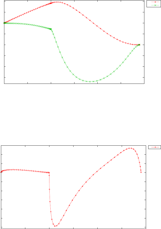
-1.5
-1
-0.5
0
0.5
1
1.5
2
0 0.5 1 1.5 2 2.5 3
states
time (s)
Two phase Schwartz problem
x1
x2
Figure 3.110: States for two-phase Schwartz problem
-6
-5
-4
-3
-2
-1
0
1
2
0 0.5 1 1.5 2 2.5 3
control
time (s)
Two phase Schwartz problem
u
Figure 3.111: Control for two-phase Schwartz problem
395

problem is to find the control, u, that minimizes the cost function
J=−m(4)(tf) (3.177)
In other words, it is desired to maximise the vehicle mass at the end of phase
4. The dynamics are given by:
˙
r=v
˙
v=−µ
krk3r+T
mu+D
m
˙m=−T
g0Isp
(3.178)
where r(t) = x(t)y(t)z(t)Tis the position, v=vx(t)vy(t)vz(t)T
is the Cartesian ECI velocity, µis the gravitational parameter, Tis the vac-
uum thrust, mis the mass, g0is the acceleration due to gravity at sea level,
Isp is the specific impulse of the engine, u=uxuyuzTis the thrust
direction, and D=DxDyDzTis the drag force, which is given by:
D=−1
2CDAref ρkvrelkvrel (3.179)
where CDis the drag coefficient, Aref is the reference area, ρis the atmo-
spheric density, and vrel is the Earth relative velocity, where vrel is given as
vrel =v−ω×r(3.180)
where ωis the angular velocity of the Earth relative to inertial space. The
atmospheric density is modeled as follows
ρ=ρ0exp[−h/h0] (3.181)
where ρ0is the atmospheric density at sea level, h=krk−Reis the altitude,
Reis the equatorial radius of the Earth, and h0is the density scale height.
The numerical values for these constants can be found in the code.
The vehicle starts on the ground at rest (relative to the Earth) at time
t0, so that the initial conditions are
r(t0) = r0=5605.2 0 3043.4Tkm
v(t0) = v0=0 0.4076 0 Tkm/s
m(t0) = m0= 301454 kg
(3.182)
The terminal constraints define the target transfer orbit, which is defined in
orbital elements as af= 24361.14 km,
ef= 0.7308,
if= 28.5 deg,
Ωf= 269.8 deg,
ωf= 130.5 deg
(3.183)
396

There is also a path constraint associated with this problem:
||u||2= 1 (3.184)
The following linkage constraints force the position and velocity to be
continuous and also account for discontinuity in the mass state due to the
ejections at the end of phases 1, 2 and 3:
r(p)(tf)−r(p+1)(t0) = 0,
v(p)(tf)−v(p+1)(t0) = 0,(p= 1,...,3)
m(p)(tf)−m(p)
dry −m(p+1)(t0)=0
(3.185)
where the superscript (p) represents the phase number.
The PSOPT code that solves this problem is shown below.
//////////////////////////////////////////////////////////////////////////
////////////////// launch.cxx //////////////////////
//////////////////////////////////////////////////////////////////////////
//////////////// PSOPT Example ////////////////////
//////////////////////////////////////////////////////////////////////////
//////////////////////////////////////////////////////////////////////////
//////// Title: Multiphase vehicle launch ////////////////
//////// Last modified: 05 January 2009 ////////////////
//////// Reference: GPOPS Manual ////////////////
//////// (See PSOPT handbook for full reference) ////////////////
//////////////////////////////////////////////////////////////////////////
//////// Copyright (c) Victor M. Becerra, 2009 ////////////////
//////////////////////////////////////////////////////////////////////////
//////// This is part of the PSOPT software library, which ///////////////
//////// is distributed under the terms of the GNU Lesser ////////////////
//////// General Public License (LGPL) ////////////////
//////////////////////////////////////////////////////////////////////////
#include "psopt.h"
//////////////////////////////////////////////////////////////////////////
/////////////////// Declare auxiliary functions ////////////////////////
//////////////////////////////////////////////////////////////////////////
void oe2rv(DMatrix& oe, double mu, DMatrix* ri, DMatrix* vi);
void rv2oe(adouble* rv, adouble* vv, double mu, adouble* oe);
//////////////////////////////////////////////////////////////////////////
///////// Declare an auxiliary structure to hold local constants ///////
//////////////////////////////////////////////////////////////////////////
struct Constants {
DMatrix* omega_matrix;
double mu;
double cd;
double sa;
double rho0;
double H;
double Re;
double g0;
double thrust_srb;
double thrust_first;
double thrust_second;
double ISP_srb;
double ISP_first;
double ISP_second;
};
typedef struct Constants Constants_;
//////////////////////////////////////////////////////////////////////////
397

/////////////////// Define the end point (Mayer) cost function //////////
//////////////////////////////////////////////////////////////////////////
adouble endpoint_cost(adouble* initial_states, adouble* final_states,
adouble* parameters,adouble& t0, adouble& tf,
adouble* xad, int iphase, Workspace* workspace)
{
adouble retval;
adouble mass_tf = final_states[6];
if (iphase < 4)
retval = 0.0;
if (iphase== 4)
retval = -mass_tf;
return retval;
}
//////////////////////////////////////////////////////////////////////////
/////////////////// Define the integrand (Lagrange) cost function //////
//////////////////////////////////////////////////////////////////////////
adouble integrand_cost(adouble* states, adouble* controls, adouble* parameters,
adouble& time, adouble* xad, int iphase, Workspace* workspace)
{
return 0.0;
}
//////////////////////////////////////////////////////////////////////////
/////////////////// Define the DAE’s ////////////////////////////////////
//////////////////////////////////////////////////////////////////////////
void dae(adouble* derivatives, adouble* path, adouble* states,
adouble* controls, adouble* parameters, adouble& time,
adouble* xad, int iphase, Workspace* workspace)
{
int j;
Constants_& CONSTANTS = *( (Constants_ *) workspace->problem->user_data );
adouble* x = states;
adouble* u = controls;
adouble r[3]; r[0]=x[0]; r[1]=x[1]; r[2]=x[2];
adouble v[3]; v[0]=x[3]; v[1]=x[4]; v[2]=x[5];
adouble m = x[6];
double T_first, T_second, T_srb, T_tot, m1dot, m2dot, mdot;
adouble rad = sqrt( dot( r, r, 3) );
DMatrix& omega_matrix = *CONSTANTS.omega_matrix;
adouble vrel[3];
for (j=0;j<3;j++)
vrel[j] = v[j] - omega_matrix(j+1,1)*r[0] -omega_matrix(j+1,2)*r[1] - omega_matrix(j+1,3)*r[2];
adouble speedrel = sqrt( dot(vrel,vrel,3) );
adouble altitude = rad-CONSTANTS.Re;
adouble rho = CONSTANTS.rho0*exp(-altitude/CONSTANTS.H);
double a1 = CONSTANTS.rho0*CONSTANTS.sa*CONSTANTS.cd;
adouble a2 = a1*exp(-altitude/CONSTANTS.H);
adouble bc = (rho/(2*m))*CONSTANTS.sa*CONSTANTS.cd;
adouble bcspeed = bc*speedrel;
adouble Drag[3];
for(j=0;j<3;j++) Drag[j] = - (vrel[j]*bcspeed);
adouble muoverradcubed = (CONSTANTS.mu)/(pow(rad,3));
398

adouble grav[3];
for(j=0;j<3;j++) grav[j] = -muoverradcubed*r[j];
if (iphase==1) {
T_srb = 6*CONSTANTS.thrust_srb;
T_first = CONSTANTS.thrust_first;
T_tot = T_srb+T_first;
m1dot = -T_srb/(CONSTANTS.g0*CONSTANTS.ISP_srb);
m2dot = -T_first/(CONSTANTS.g0*CONSTANTS.ISP_first);
mdot = m1dot+m2dot;
}
else if (iphase==2) {
T_srb = 3*CONSTANTS.thrust_srb;
T_first = CONSTANTS.thrust_first;
T_tot = T_srb+T_first;
m1dot = -T_srb/(CONSTANTS.g0*CONSTANTS.ISP_srb);
m2dot = -T_first/(CONSTANTS.g0*CONSTANTS.ISP_first);
mdot = m1dot+m2dot;
}
else if (iphase==3) {
T_first = CONSTANTS.thrust_first;
T_tot = T_first;
mdot = -T_first/(CONSTANTS.g0*CONSTANTS.ISP_first);
}
else if (iphase==4) {
T_second = CONSTANTS.thrust_second;
T_tot = T_second;
mdot = -T_second/(CONSTANTS.g0*CONSTANTS.ISP_second);
}
adouble Toverm = T_tot/m;
adouble thrust[3];
for(j=0;j<3;j++) thrust[j] = Toverm*u[j];
adouble rdot[3];
for(j=0;j<3;j++) rdot[j] = v[j];
adouble vdot[3];
for(j=0;j<3;j++) vdot[j] = thrust[j]+Drag[j]+grav[j];
derivatives[0] = rdot[0];
derivatives[1] = rdot[1];
derivatives[2] = rdot[2];
derivatives[3] = vdot[0];
derivatives[4] = vdot[1];
derivatives[5] = vdot[2];
derivatives[6] = mdot;
path[0] = dot( controls, controls, 3);
}
////////////////////////////////////////////////////////////////////////////
/////////////////// Define the events function ////////////////////////////
////////////////////////////////////////////////////////////////////////////
void events(adouble* e, adouble* initial_states, adouble* final_states,
adouble* parameters,adouble& t0, adouble& tf, adouble* xad,
int iphase, Workspace* workspace)
{
Constants_& CONSTANTS = *( (Constants_ *) workspace->problem->user_data );
adouble rv[3]; rv[0]=final_states[0]; rv[1]=final_states[1]; rv[2]=final_states[2];
adouble vv[3]; vv[0]=final_states[3]; vv[1]=final_states[4]; vv[2]=final_states[5];
adouble oe[6];
int j;
if(iphase==1) {
// These events are related to the initial state conditions in phase 1
for(j=0;j<7;j++) e[j] = initial_states[j];
}
if (iphase==4) {
// These events are related to the final states in phase 4
399

rv2oe( rv, vv, CONSTANTS.mu, oe );
for(j=0;j<5;j++) e[j]=oe[j];
}
}
///////////////////////////////////////////////////////////////////////////
/////////////////// Define the phase linkages function ///////////////////
///////////////////////////////////////////////////////////////////////////
void linkages( adouble* linkages, adouble* xad, Workspace* workspace)
{
double m_tot_first = 104380.0;
double m_prop_first = 95550.0;
double m_dry_first = m_tot_first-m_prop_first;
double m_tot_srb = 19290.0;
double m_prop_srb = 17010.0;
double m_dry_srb = m_tot_srb-m_prop_srb;
int index=0;
auto_link(linkages, &index, xad, 1, 2, workspace );
linkages[index-2]-= 6*m_dry_srb;
auto_link(linkages, &index, xad, 2, 3, workspace );
linkages[index-2]-= 3*m_dry_srb;
auto_link(linkages, &index, xad, 3, 4, workspace );
linkages[index-2]-= m_dry_first;
}
////////////////////////////////////////////////////////////////////////////
/////////////////// Define the main routine ///////////////////////////////
////////////////////////////////////////////////////////////////////////////
int main(void)
{
////////////////////////////////////////////////////////////////////////////
/////////////////// Declare key structures ////////////////////////////////
////////////////////////////////////////////////////////////////////////////
Alg algorithm;
Sol solution;
Prob problem;
////////////////////////////////////////////////////////////////////////////
/////////////////// Register problem name ////////////////////////////////
////////////////////////////////////////////////////////////////////////////
problem.name = "Multiphase vehicle launch";
problem.outfilename = "launch.txt";
////////////////////////////////////////////////////////////////////////////
/////////////////// Declare an instance of Constants structure /////////////
////////////////////////////////////////////////////////////////////////////
Constants_ CONSTANTS;
problem.user_data = (void*) &CONSTANTS;
////////////////////////////////////////////////////////////////////////////
//////////// Define problem level constants & do level 1 setup ////////////
////////////////////////////////////////////////////////////////////////////
problem.nphases = 4;
problem.nlinkages = 24;
psopt_level1_setup(problem);
/////////////////////////////////////////////////////////////////////////////
///////// Define phase related information & do level 2 setup ////////////
/////////////////////////////////////////////////////////////////////////////
problem.phases(1).nstates = 7;
400

problem.phases(1).ncontrols = 3;
problem.phases(1).nevents = 7;
problem.phases(1).npath = 1;
problem.phases(2).nstates = 7;
problem.phases(2).ncontrols = 3;
problem.phases(2).nevents = 0;
problem.phases(2).npath = 1;
problem.phases(3).nstates = 7;
problem.phases(3).ncontrols = 3;
problem.phases(3).nevents = 0;
problem.phases(3).npath = 1;
problem.phases(4).nstates = 7;
problem.phases(4).ncontrols = 3;
problem.phases(4).nevents = 5;
problem.phases(4).npath = 1;
problem.phases(1).nodes = "[5, 15]";
problem.phases(2).nodes = "[5, 15]";
problem.phases(3).nodes = "[5, 15]";
problem.phases(4).nodes = "[5, 15]";
psopt_level2_setup(problem, algorithm);
////////////////////////////////////////////////////////////////////////////
/////////////////// Declare DMatrix objects to store results //////////////
////////////////////////////////////////////////////////////////////////////
DMatrix x, u, t, H;
////////////////////////////////////////////////////////////////////////////
/////////////////// Initialize CONSTANTS and //////////////////////////////
/////////////////// declare local variables //////////////////////////////
////////////////////////////////////////////////////////////////////////////
double omega = 7.29211585e-5; // Earth rotation rate (rad/s)
DMatrix omega_matrix(3,3);
omega_matrix(1,1) = 0.0; omega_matrix(1,2) = -omega; omega_matrix(1,3)=0.0;
omega_matrix(2,1) = omega; omega_matrix(2,2) = 0.0; omega_matrix(2,3)=0.0;
omega_matrix(3,1) = 0.0; omega_matrix(3,2) = 0.0; omega_matrix(3,3)=0.0;
CONSTANTS.omega_matrix = &omega_matrix; // Rotation rate matrix (rad/s)
CONSTANTS.mu = 3.986012e14; // Gravitational parameter (m^3/s^2)
CONSTANTS.cd = 0.5; // Drag coefficient
CONSTANTS.sa = 4*pi; // Surface area (m^2)
CONSTANTS.rho0 = 1.225; // sea level gravity (kg/m^3)
CONSTANTS.H = 7200.0; // Density scale height (m)
CONSTANTS.Re = 6378145.0; // Radius of earth (m)
CONSTANTS.g0 = 9.80665; // sea level gravity (m/s^2)
double lat0 = 28.5*pi/180.0; // Geocentric Latitude of Cape Canaveral
double x0 = CONSTANTS.Re*cos(lat0); // x component of initial position
double z0 = CONSTANTS.Re*sin(lat0); // z component of initial position
double y0 = 0;
DMatrix r0(3,1, x0, y0, z0);
DMatrix v0 = omega_matrix*r0;
double bt_srb = 75.2;
double bt_first = 261.0;
double bt_second = 700.0;
double t0 = 0;
double t1 = 75.2;
double t2 = 150.4;
double t3 = 261.0;
double t4 = 961.0;
double m_tot_srb = 19290.0;
double m_prop_srb = 17010.0;
double m_dry_srb = m_tot_srb-m_prop_srb;
double m_tot_first = 104380.0;
double m_prop_first = 95550.0;
double m_dry_first = m_tot_first-m_prop_first;
double m_tot_second = 19300.0;
401

double m_prop_second = 16820.0;
double m_dry_second = m_tot_second-m_prop_second;
double m_payload = 4164.0;
double thrust_srb = 628500.0;
double thrust_first = 1083100.0;
double thrust_second = 110094.0;
double mdot_srb = m_prop_srb/bt_srb;
double ISP_srb = thrust_srb/(CONSTANTS.g0*mdot_srb);
double mdot_first = m_prop_first/bt_first;
double ISP_first = thrust_first/(CONSTANTS.g0*mdot_first);
double mdot_second = m_prop_second/bt_second;
double ISP_second = thrust_second/(CONSTANTS.g0*mdot_second);
double af = 24361140.0;
double ef = 0.7308;
double incf = 28.5*pi/180.0;
double Omf = 269.8*pi/180.0;
double omf = 130.5*pi/180.0;
double nuguess = 0;
double cosincf = cos(incf);
double cosOmf = cos(Omf);
double cosomf = cos(omf);
DMatrix oe(6,1, af, ef, incf, Omf, omf, nuguess);
DMatrix rout(3,1);
DMatrix vout(3,1);
oe2rv(oe,CONSTANTS.mu, &rout, &vout);
rout.Transpose();
vout.Transpose();
double m10 = m_payload+m_tot_second+m_tot_first+9*m_tot_srb;
double m1f = m10-(6*mdot_srb+mdot_first)*t1;
double m20 = m1f-6*m_dry_srb;
double m2f = m20-(3*mdot_srb+mdot_first)*(t2-t1);
double m30 = m2f-3*m_dry_srb;
double m3f = m30-mdot_first*(t3-t2);
double m40 = m3f-m_dry_first;
double m4f = m_payload;
CONSTANTS.thrust_srb = thrust_srb;
CONSTANTS.thrust_first = thrust_first;
CONSTANTS.thrust_second = thrust_second;
CONSTANTS.ISP_srb = ISP_srb;
CONSTANTS.ISP_first = ISP_first;
CONSTANTS.ISP_second = ISP_second;
double rmin = -2*CONSTANTS.Re;
double rmax = -rmin;
double vmin = -10000.0;
double vmax = -vmin;
////////////////////////////////////////////////////////////////////////////
/////////////////// Enter problem bounds information //////////////////////
////////////////////////////////////////////////////////////////////////////
int iphase;
problem.bounds.lower.times = "[0, 75.2, 150.4, 261.0, 261.0]";
problem.bounds.upper.times = "[0, 75.2, 150.4 261.0, 961.0]";
// Phase 1 bounds
iphase = 1;
problem.phases(iphase).bounds.lower.states(1) = rmin;
problem.phases(iphase).bounds.upper.states(1) = rmax;
problem.phases(iphase).bounds.lower.states(2) = rmin;
problem.phases(iphase).bounds.upper.states(2) = rmax;
problem.phases(iphase).bounds.lower.states(3) = rmin;
problem.phases(iphase).bounds.upper.states(3) = rmax;
problem.phases(iphase).bounds.lower.states(4) = vmin;
problem.phases(iphase).bounds.upper.states(4) = vmax;
problem.phases(iphase).bounds.lower.states(5) = vmin;
problem.phases(iphase).bounds.upper.states(5) = vmax;
402

problem.phases(iphase).bounds.lower.states(6) = vmin;
problem.phases(iphase).bounds.upper.states(6) = vmax;
problem.phases(iphase).bounds.lower.states(7) = m1f;
problem.phases(iphase).bounds.upper.states(7) = m10;
problem.phases(iphase).bounds.lower.controls(1) = -1.0;
problem.phases(iphase).bounds.upper.controls(1) = 1.0;
problem.phases(iphase).bounds.lower.controls(2) = -1.0;
problem.phases(iphase).bounds.upper.controls(2) = 1.0;
problem.phases(iphase).bounds.lower.controls(3) = -1.0;
problem.phases(iphase).bounds.upper.controls(3) = 1.0;
problem.phases(iphase).bounds.lower.path(1) = 1.0;
problem.phases(iphase).bounds.upper.path(1) = 1.0;
// The following bounds fix the initial state conditions in phase 0.
problem.phases(iphase).bounds.lower.events(1) = r0(1);
problem.phases(iphase).bounds.upper.events(1) = r0(1);
problem.phases(iphase).bounds.lower.events(2) = r0(2);
problem.phases(iphase).bounds.upper.events(2) = r0(2);
problem.phases(iphase).bounds.lower.events(3) = r0(3);
problem.phases(iphase).bounds.upper.events(3) = r0(3);
problem.phases(iphase).bounds.lower.events(4) = v0(1);
problem.phases(iphase).bounds.upper.events(4) = v0(1);
problem.phases(iphase).bounds.lower.events(5) = v0(2);
problem.phases(iphase).bounds.upper.events(5) = v0(2);
problem.phases(iphase).bounds.lower.events(6) = v0(3);
problem.phases(iphase).bounds.upper.events(6) = v0(3);
problem.phases(iphase).bounds.lower.events(7) = m10;
problem.phases(iphase).bounds.upper.events(7) = m10;
// Phase 2 bounds
iphase = 2;
problem.phases(iphase).bounds.lower.states(1) = rmin;
problem.phases(iphase).bounds.upper.states(1) = rmax;
problem.phases(iphase).bounds.lower.states(2) = rmin;
problem.phases(iphase).bounds.upper.states(2) = rmax;
problem.phases(iphase).bounds.lower.states(3) = rmin;
problem.phases(iphase).bounds.upper.states(3) = rmax;
problem.phases(iphase).bounds.lower.states(4) = vmin;
problem.phases(iphase).bounds.upper.states(4) = vmax;
problem.phases(iphase).bounds.lower.states(5) = vmin;
problem.phases(iphase).bounds.upper.states(5) = vmax;
problem.phases(iphase).bounds.lower.states(6) = vmin;
problem.phases(iphase).bounds.upper.states(6) = vmax;
problem.phases(iphase).bounds.lower.states(7) = m2f;
problem.phases(iphase).bounds.upper.states(7) = m20;
problem.phases(iphase).bounds.lower.controls(1) = -1.0;
problem.phases(iphase).bounds.upper.controls(1) = 1.0;
problem.phases(iphase).bounds.lower.controls(2) = -1.0;
problem.phases(iphase).bounds.upper.controls(2) = 1.0;
problem.phases(iphase).bounds.lower.controls(3) = -1.0;
problem.phases(iphase).bounds.upper.controls(3) = 1.0;
problem.phases(iphase).bounds.lower.path(1) = 1.0;
problem.phases(iphase).bounds.upper.path(1) = 1.0;
// Phase 3 bounds
iphase = 3;
problem.phases(iphase).bounds.lower.states(1) = rmin;
problem.phases(iphase).bounds.upper.states(1) = rmax;
problem.phases(iphase).bounds.lower.states(2) = rmin;
problem.phases(iphase).bounds.upper.states(2) = rmax;
problem.phases(iphase).bounds.lower.states(3) = rmin;
problem.phases(iphase).bounds.upper.states(3) = rmax;
problem.phases(iphase).bounds.lower.states(4) = vmin;
problem.phases(iphase).bounds.upper.states(4) = vmax;
problem.phases(iphase).bounds.lower.states(5) = vmin;
problem.phases(iphase).bounds.upper.states(5) = vmax;
403

problem.phases(iphase).bounds.lower.states(6) = vmin;
problem.phases(iphase).bounds.upper.states(6) = vmax;
problem.phases(iphase).bounds.lower.states(7) = m3f;
problem.phases(iphase).bounds.upper.states(7) = m30;
problem.phases(iphase).bounds.lower.controls(1) = -1.0;
problem.phases(iphase).bounds.upper.controls(1) = 1.0;
problem.phases(iphase).bounds.lower.controls(2) = -1.0;
problem.phases(iphase).bounds.upper.controls(2) = 1.0;
problem.phases(iphase).bounds.lower.controls(3) = -1.0;
problem.phases(iphase).bounds.upper.controls(3) = 1.0;
problem.phases(iphase).bounds.lower.path(1) = 1.0;
problem.phases(iphase).bounds.upper.path(1) = 1.0;
// Phase 4 bounds
iphase = 4;
problem.phases(iphase).bounds.lower.states(1) = rmin;
problem.phases(iphase).bounds.upper.states(1) = rmax;
problem.phases(iphase).bounds.lower.states(2) = rmin;
problem.phases(iphase).bounds.upper.states(2) = rmax;
problem.phases(iphase).bounds.lower.states(3) = rmin;
problem.phases(iphase).bounds.upper.states(3) = rmax;
problem.phases(iphase).bounds.lower.states(4) = vmin;
problem.phases(iphase).bounds.upper.states(4) = vmax;
problem.phases(iphase).bounds.lower.states(5) = vmin;
problem.phases(iphase).bounds.upper.states(5) = vmax;
problem.phases(iphase).bounds.lower.states(6) = vmin;
problem.phases(iphase).bounds.upper.states(6) = vmax;
problem.phases(iphase).bounds.lower.states(7) = m4f;
problem.phases(iphase).bounds.upper.states(7) = m40;
problem.phases(iphase).bounds.lower.controls(1) = -1.0;
problem.phases(iphase).bounds.upper.controls(1) = 1.0;
problem.phases(iphase).bounds.lower.controls(2) = -1.0;
problem.phases(iphase).bounds.upper.controls(2) = 1.0;
problem.phases(iphase).bounds.lower.controls(3) = -1.0;
problem.phases(iphase).bounds.upper.controls(3) = 1.0;
problem.phases(iphase).bounds.lower.path(1) = 1.0;
problem.phases(iphase).bounds.upper.path(1) = 1.0;
problem.phases(iphase).bounds.lower.events(1) = af;
problem.phases(iphase).bounds.lower.events(2) = ef;
problem.phases(iphase).bounds.lower.events(3) = incf;
problem.phases(iphase).bounds.lower.events(4) = Omf;
problem.phases(iphase).bounds.lower.events(5) = omf;
problem.phases(iphase).bounds.upper.events(1) = af;
problem.phases(iphase).bounds.upper.events(2) = ef;
problem.phases(iphase).bounds.upper.events(3) = incf;
problem.phases(iphase).bounds.upper.events(4) = Omf;
problem.phases(iphase).bounds.upper.events(5) = omf;
////////////////////////////////////////////////////////////////////////////
/////////////////// Define & register initial guess ///////////////////////
////////////////////////////////////////////////////////////////////////////
iphase = 1;
problem.phases(iphase).guess.states = zeros(7,5);
problem.phases(iphase).guess.states(1, colon()) = linspace( r0(1), r0(1), 5);
problem.phases(iphase).guess.states(2, colon()) = linspace( r0(2), r0(2), 5);
problem.phases(iphase).guess.states(3, colon()) = linspace( r0(3), r0(3), 5);
problem.phases(iphase).guess.states(4, colon()) = linspace( v0(1), v0(1), 5);
problem.phases(iphase).guess.states(5, colon()) = linspace( v0(2), v0(2), 5);
problem.phases(iphase).guess.states(6, colon()) = linspace( v0(3), v0(3), 5);
problem.phases(iphase).guess.states(7, colon()) = linspace( m10 , m1f , 5);
problem.phases(iphase).guess.controls = zeros(3,5);
problem.phases(iphase).guess.controls(1,colon()) = ones( 1, 5);
problem.phases(iphase).guess.controls(2,colon()) = zeros(1, 5);
problem.phases(iphase).guess.controls(3,colon()) = zeros(1, 5);
problem.phases(iphase).guess.time = linspace(t0,t1, 5);
404

iphase = 2;
problem.phases(iphase).guess.states = zeros(7,5);
problem.phases(iphase).guess.states(1, colon()) = linspace( r0(1), r0(1), 5);
problem.phases(iphase).guess.states(2, colon()) = linspace( r0(2), r0(2), 5);
problem.phases(iphase).guess.states(3, colon()) = linspace( r0(3), r0(3), 5);
problem.phases(iphase).guess.states(4, colon()) = linspace( v0(1), v0(1), 5);
problem.phases(iphase).guess.states(5, colon()) = linspace( v0(2), v0(2), 5);
problem.phases(iphase).guess.states(6, colon()) = linspace( v0(3), v0(3), 5);
problem.phases(iphase).guess.states(7, colon()) = linspace( m20 , m2f , 5);
problem.phases(iphase).guess.controls = zeros(3,5);
problem.phases(iphase).guess.controls(1,colon()) = ones( 1, 5);
problem.phases(iphase).guess.controls(2,colon()) = zeros(1, 5);
problem.phases(iphase).guess.controls(3,colon()) = zeros(1, 5);
problem.phases(iphase).guess.time = linspace(t1,t2, 5);
iphase = 3;
problem.phases(iphase).guess.states = zeros(7,5);
problem.phases(iphase).guess.states(1, colon()) = linspace( rout(1), rout(1), 5);
problem.phases(iphase).guess.states(2, colon()) = linspace( rout(2), rout(2), 5);
problem.phases(iphase).guess.states(3, colon()) = linspace( rout(3), rout(3), 5);
problem.phases(iphase).guess.states(4, colon()) = linspace( vout(1), vout(1), 5);
problem.phases(iphase).guess.states(5, colon()) = linspace( vout(2), vout(2), 5);
problem.phases(iphase).guess.states(6, colon()) = linspace( vout(3), vout(3), 5);
problem.phases(iphase).guess.states(7, colon()) = linspace( m30 , m3f , 5);
problem.phases(iphase).guess.controls = zeros(3,5);
problem.phases(iphase).guess.controls(1,colon()) = zeros( 1, 5);
problem.phases(iphase).guess.controls(2,colon()) = zeros( 1, 5);
problem.phases(iphase).guess.controls(3,colon()) = ones( 1, 5);
problem.phases(iphase).guess.time = linspace(t2,t3, 5);
iphase = 4;
problem.phases(iphase).guess.states = zeros(7,5);
problem.phases(iphase).guess.states(1, colon()) = linspace( rout(1), rout(1), 5);
problem.phases(iphase).guess.states(2, colon()) = linspace( rout(2), rout(2), 5);
problem.phases(iphase).guess.states(3, colon()) = linspace( rout(3), rout(3), 5);
problem.phases(iphase).guess.states(4, colon()) = linspace( vout(1), vout(1), 5);
problem.phases(iphase).guess.states(5, colon()) = linspace( vout(2), vout(2), 5);
problem.phases(iphase).guess.states(6, colon()) = linspace( vout(3), vout(3), 5);
problem.phases(iphase).guess.states(7, colon()) = linspace( m40 , m4f , 5);
problem.phases(iphase).guess.controls = zeros(3,5);
problem.phases(iphase).guess.controls(1,colon()) = zeros( 1, 5);
problem.phases(iphase).guess.controls(2,colon()) = zeros( 1, 5);
problem.phases(iphase).guess.controls(3,colon()) = ones( 1, 5);
problem.phases(iphase).guess.time = linspace(t3,t4, 5);
////////////////////////////////////////////////////////////////////////////
/////////////////// Register problem functions ///////////////////////////
////////////////////////////////////////////////////////////////////////////
problem.integrand_cost = &integrand_cost;
problem.endpoint_cost = &endpoint_cost;
problem.dae = &dae;
problem.events = &events;
problem.linkages = &linkages;
////////////////////////////////////////////////////////////////////////////
/////////////////// Enter algorithm options //////////////////////////////
////////////////////////////////////////////////////////////////////////////
algorithm.nlp_method = "IPOPT";
algorithm.scaling = "automatic";
algorithm.derivatives = "automatic";
405

algorithm.nlp_iter_max = 500;
// algorithm.mesh_refinement = "automatic";
// algorithm.collocation_method = "trapezoidal";
algorithm.ode_tolerance = 1.e-5;
////////////////////////////////////////////////////////////////////////////
/////////////////// Now call PSOPT to solve the problem //////////////////
////////////////////////////////////////////////////////////////////////////
psopt(solution, problem, algorithm);
////////////////////////////////////////////////////////////////////////////
/////////// Extract relevant variables from solution structure //////////
////////////////////////////////////////////////////////////////////////////
x = (solution.get_states_in_phase(1) || solution.get_states_in_phase(2) ||
solution.get_states_in_phase(3) || solution.get_states_in_phase(4) );
u = (solution.get_controls_in_phase(1) || solution.get_controls_in_phase(2) ||
solution.get_controls_in_phase(3) || solution.get_controls_in_phase(4) );
t = (solution.get_time_in_phase(1) || solution.get_time_in_phase(2) ||
solution.get_time_in_phase(3) || solution.get_time_in_phase(4) );
////////////////////////////////////////////////////////////////////////////
/////////// Save solution data to files if desired ////////////////////////
////////////////////////////////////////////////////////////////////////////
x.Save("x.dat");
u.Save("u.dat");
t.Save("t.dat");
////////////////////////////////////////////////////////////////////////////
/////////// Plot some results if desired (requires gnuplot) ///////////////
////////////////////////////////////////////////////////////////////////////
DMatrix r = x(colon(1,3),colon());
DMatrix v = x(colon(4,6),colon());
DMatrix altitude = Sqrt(sum(elemProduct(r,r)))/1000.0;
DMatrix speed = Sqrt(sum(elemProduct(v,v)));
plot(t,altitude,problem.name, "time (s)", "position (km)");
plot(t,speed,problem.name, "time (s)", "speed (m/s)");
plot(t,u,problem.name,"time (s)", "u");
plot(t,altitude,problem.name, "time (s)", "position (km)", "alt",
"pdf", "launch_position.pdf");
plot(t,speed,problem.name, "time (s)", "speed (m/s)", "speed",
"pdf", "launch_speed.pdf");
plot(t,u,problem.name,"time (s)", "u (dimensionless)", "u1 u2 u3",
"pdf", "launch_control.pdf");
}
////////////////////////////////////////////////////////////////////////////
////////////////// Define auxiliary functions //////////////////////////////
////////////////////////////////////////////////////////////////////////////
void rv2oe(adouble* rv, adouble* vv, double mu, adouble* oe)
{
int j;
adouble K[3]; K[0] = 0.0; K[1]=0.0; K[2]=1.0;
adouble hv[3];
cross(rv,vv, hv);
adouble nv[3];
cross(K, hv, nv);
adouble n = sqrt( dot(nv,nv,3) );
406

adouble h2 = dot(hv,hv,3);
adouble v2 = dot(vv,vv,3);
adouble r = sqrt(dot(rv,rv,3));
adouble ev[3];
for(j=0;j<3;j++) ev[j] = 1/mu *( (v2-mu/r)*rv[j] - dot(rv,vv,3)*vv[j] );
adouble p = h2/mu;
adouble e = sqrt(dot(ev,ev,3)); // eccentricity
adouble a = p/(1-e*e); // semimajor axis
adouble i = acos(hv[2]/sqrt(h2)); // inclination
#define USE_SMOOTH_HEAVISIDE
double a_eps = 0.1;
#ifndef USE_SMOOTH_HEAVISIDE
adouble Om = acos(nv[0]/n); // RAAN
if ( nv[1] < -DMatrix::GetEPS() ){ // fix quadrant
Om = 2*pi-Om;
}
#endif
#ifdef USE_SMOOTH_HEAVISIDE
adouble Om = smooth_heaviside( (nv[1]+DMatrix::GetEPS()), a_eps )*acos(nv[0]/n)
+smooth_heaviside( -(nv[1]+DMatrix::GetEPS()), a_eps )*(2*pi-acos(nv[0]/n));
#endif
#ifndef USE_SMOOTH_HEAVISIDE
adouble om = acos(dot(nv,ev,3)/n/e); // arg of periapsis
if ( ev[2] < 0 ) { // fix quadrant
om = 2*pi-om;
}
#endif
#ifdef USE_SMOOTH_HEAVISIDE
adouble om = smooth_heaviside( (ev[2]), a_eps )*acos(dot(nv,ev,3)/n/e)
+smooth_heaviside( -(ev[2]), a_eps )*(2*pi-acos(dot(nv,ev,3)/n/e));
#endif
#ifndef USE_SMOOTH_HEAVISIDE
adouble nu = acos(dot(ev,rv,3)/e/r); // true anomaly
if ( dot(rv,vv,3) < 0 ) { // fix quadrant
nu = 2*pi-nu;
}
#endif
#ifdef USE_SMOOTH_HEAVISIDE
adouble nu = smooth_heaviside( dot(rv,vv,3), a_eps )*acos(dot(ev,rv,3)/e/r)
+smooth_heaviside( -dot(rv,vv,3), a_eps )*(2*pi-acos(dot(ev,rv,3)/e/r));
#endif
oe[0] = a;
oe[1] = e;
oe[2] = i;
oe[3] = Om;
oe[4] = om;
oe[5] = nu;
return;
}
void oe2rv(DMatrix& oe, double mu, DMatrix* ri, DMatrix* vi)
{
double a=oe(1), e=oe(2), i=oe(3), Om=oe(4), om=oe(5), nu=oe(6);
double p = a*(1-e*e);
double r = p/(1+e*cos(nu));
DMatrix rv(3,1);
rv(1) = r*cos(nu);
rv(2) = r*sin(nu);
rv(3) = 0.0;
DMatrix vv(3,1);
vv(1) = -sin(nu);
407

vv(2) = e+cos(nu);
vv(3) = 0.0;
vv *= sqrt(mu/p);
double cO = cos(Om), sO = sin(Om);
double co = cos(om), so = sin(om);
double ci = cos(i), si = sin(i);
DMatrix R(3,3);
R(1,1)= cO*co-sO*so*ci; R(1,2)= -cO*so-sO*co*ci; R(1,3)= sO*si;
R(2,1)= sO*co+cO*so*ci; R(2,2)= -sO*so+cO*co*ci; R(2,3)=-cO*si;
R(3,1)= so*si; R(3,2)= co*si; R(3,3)= ci;
*ri = R*rv;
*vi = R*vv;
return;
}
////////////////////////////////////////////////////////////////////////////
/////////////////////// END OF FILE ///////////////////////////////
////////////////////////////////////////////////////////////////////////////
=
The output from PSOPT is summarised in the box below and shown in
Figures 3.112,3.113 and 3.114, which contain the trajectories of the altitude,
speed and the elements of the control vector, respectively.
PSOPT results summary
=====================
Problem: Multiphase vehicle launch
CPU time (seconds): 3.356515e+00
NLP solver used: IPOPT
PSOPT release number: 4.0
Date and time of this run: Thu Feb 21 16:00:31 2019
Optimal (unscaled) cost function value: -7.529661e+03
Phase 1 endpoint cost function value: 0.000000e+00
Phase 1 integrated part of the cost: 0.000000e+00
Phase 1 initial time: 0.000000e+00
Phase 1 final time: 7.520000e+01
Phase 1 maximum relative local error: 1.173524e-06
Phase 2 endpoint cost function value: 0.000000e+00
Phase 2 integrated part of the cost: 0.000000e+00
Phase 2 initial time: 7.520000e+01
Phase 2 final time: 1.504000e+02
Phase 2 maximum relative local error: 1.301765e-06
Phase 3 endpoint cost function value: 0.000000e+00
Phase 3 integrated part of the cost: 0.000000e+00
Phase 3 initial time: 1.504000e+02
Phase 3 final time: 2.610000e+02
408
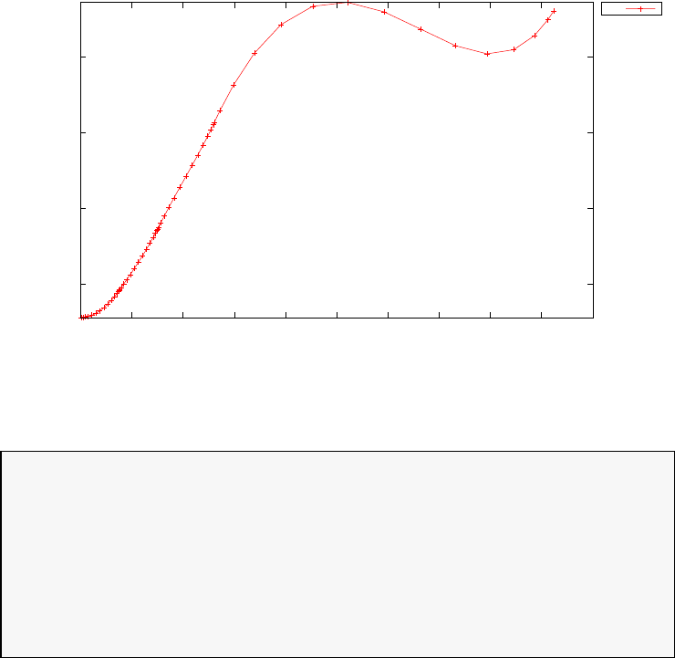
6400
6450
6500
6550
0 100 200 300 400 500 600 700 800 900 1000
altitude (km)
time (s)
Multiphase vehicle launch
alt
Figure 3.112: Altitude for the vehicle launch problem
Phase 3 maximum relative local error: 3.952037e-07
Phase 4 endpoint cost function value: -7.529661e+03
Phase 4 integrated part of the cost: 0.000000e+00
Phase 4 initial time: 2.610000e+02
Phase 4 final time: 9.241413e+02
Phase 4 maximum relative local error: 1.631374e-06
NLP solver reports: The problem has been solved!
3.44 Zero propellant maneouvre of the Interna-
tional Space Station
This problem illustrates the use of PSOPT for solving an optimal control
problem associated with the design of a zero propellant maneouvre for the in-
ternational space station by means of control moment gyroscopes (CMGs).
The example is based on the results presented in the thesis by Bhatt [5]
and also reported by Bedrossian and co-workers [1]. The original 90 and
180 degree maneouvres were computed using DIDO, and they were actu-
ally implemented on the International Space Station on 5 November 2006
and 2 January 2007, respectively, resulting in savings for NASA of around
US$1.5m in propellant costs. The dynamic model employed here does not
account for atmospheric drag as the atmosphere model used in the orig-
409
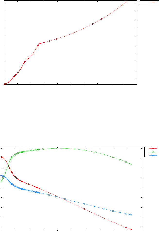
1000
2000
3000
4000
5000
6000
7000
8000
9000
10000
0 100 200 300 400 500 600 700 800 900 1000
speed (m/s)
time (s)
Multiphase vehicle launch
speed
Figure 3.113: Speed for the vehicle launch problem
-0.6
-0.4
-0.2
0
0.2
0.4
0.6
0.8
1
0 100 200 300 400 500 600 700 800 900 1000
u (dimensionless)
time (s)
Multiphase vehicle launch
u1
u2
u3
Figure 3.114: Controls for the vehicle launch problem
410

inal study is not available. Otherwise, the equations and parameters are
the same as those reported by Bhatt in his thesis. The effects of atmo-
spheric drag are, however, small, and the results obtained are comparable
with those given in Bhatt’s thesis. The implemented case corresponds with
a maneovure lasting 7200 seconds and using 3 CMG’s.
The problem is formulated as follows. Find qc(t)=[qc,1(t)qc,2(t)qc,3(t)qc,4]T,
t∈[t0, tf] and the scalar parameter γto minimise,
J= 0.1γ+Ztf
t0||u(t)||2dt(3.186)
subject to the dynamical equations:
˙
q(t) = 1
2T(q)(ω(t)−ωo(q))
˙ω(t) = J−1(τd(q)−ω(t)×(Jω(t)) −u(t))
˙
h(t) = u(t)−ω(t)×h(t)
(3.187)
the path constraints:
||q(t)||2
2= 1
||qc(t)||2
2= 1
||h(t)||2
2≤γ
||˙
h(t)||2
2=˙
h2
max
(3.188)
the parameter bounds
0≤γ≤h2
max (3.189)
and the boundary conditions:
q(t0) = ¯
q0ω(t0) = ωo(¯
q0)h(t0) = ¯
h0
q(tf) = ¯
qfω(tf) = ωo(¯
qf)h(tf) = ¯
hf(3.190)
where Jis a 3×3 inertia matrix, q= [q1, q2, q3, q4]Tis the quarternion vector,
ωis the spacecraft angular rate relative to an inertial reference frame and
expressed in the body frame, his the momentum, T(q) is given by:
T(q) =
−q2−q3−q4
q1−q4q3
q4q1−q2
−q3q2q1
(3.191)
uis the control force, which is given by:
u(t) = J(KP˜ε(q, qc) + KD˜ω(ω, qc)) (3.192)
where
˜ε(q,qc)=2T(qc)Tq
˜ω(ω, ωc) = ω−ωc
(3.193)
411

ωois given by:
ωo(q) = nC2(q) (3.194)
where nis the orbital rotation rate, Cjis the jcolumn of the rotation
matrix:
C(q) =
1−2(q2
3+q2
4) 2(q2q3+q1q4) 2(q2q4−q1q3)
2(q2q3−q1q4) 1 −2(q2
2+q2
4) 2(q3q4+q1q2)
2(q2q4+q1q3) 2(q3q4−q1q2) 1 −2(q2
2+q2
3)
(3.195)
τdis the disturbance torque, which in this case only incorporates the grav-
ity gradient torque τgg (the disturbance torque also incorporates the atmo-
spheric drag torque in the original study):
τd=τgg = 3n2C3(q)×(JC3(q)) (3.196)
The constant parameter values used were: n= 1.1461 ×10⁻³rad/s, hmax =
3×3600.0 ft-lbf-sec, ˙
hmax = 200.0 ft-lbf, t0= 0 s, tf= 7200 s, and
J=
18836544.0 3666370.0 2965301.0
3666370.0 27984088.0−1129004.0
2965301.0−1129004.0 39442649.0
slug −ft2(3.197)
The PSOPT code that solves this problem is shown below.
//////////////////////////////////////////////////////////////////////////
//////////////// zpm.cxx /////////////////////
//////////////////////////////////////////////////////////////////////////
//////////////// PSOPT Example /////////////////////
//////////////////////////////////////////////////////////////////////////
//////////////////////////////////////////////////////////////////////////
//////// Title: Zero propellant maneouvre problem ///////////////
//////// Last modified: 09 November 2009 ////////////////
//////// Reference: S.A. Bhatt (2007), Masters Thesis,////////////////
//////// Rice University, Houston TX ////////////////
//////////////////////////////////////////////////////////////////////////
//////// Copyright (c) Victor M. Becerra, 2009 ////////////////
//////////////////////////////////////////////////////////////////////////
//////// This is part of the PSOPT software library, which ///////////////
//////// is distributed under the terms of the GNU Lesser ////////////////
//////// General Public License (LGPL) ////////////////
//////////////////////////////////////////////////////////////////////////
#include "psopt.h"
// Set CASE below to 1: 6000 s maneouvre, or to 2: 7200 maneouvre
#define CASE 2
struct Constants {
DMatrix J;
double n;
double Kp;
double Kd;
double hmax;
};
typedef struct Constants Constants_;
static Constants_ CONSTANTS;
412

void Tfun( adouble T[][3], adouble *q )
{
adouble q1 = q[CINDEX(1)];
adouble q2 = q[CINDEX(2)];
adouble q3 = q[CINDEX(3)];
adouble q4 = q[CINDEX(4)];
T[CINDEX(1)][CINDEX(1)] = -q2 ; T[CINDEX(1)][CINDEX(2)] = -q3; T[CINDEX(1)][CINDEX(3)] = -q4;
T[CINDEX(2)][CINDEX(1)] = q1 ; T[CINDEX(2)][CINDEX(2)] = -q4; T[CINDEX(2)][CINDEX(3)] = q3;
T[CINDEX(3)][CINDEX(1)] = q4 ; T[CINDEX(3)][CINDEX(2)] = q1; T[CINDEX(3)][CINDEX(3)] = -q2;
T[CINDEX(4)][CINDEX(1)] = -q3; T[CINDEX(4)][CINDEX(2)] = q2; T[CINDEX(4)][CINDEX(3)] = q1;
}
void compute_omega0(adouble* omega0, adouble* q)
{
// This function computes the angular speed in the rotating LVLH reference frame
int i;
double n = CONSTANTS.n;
adouble C2[3];
adouble q1 = q[CINDEX(1)];
adouble q2 = q[CINDEX(2)];
adouble q3 = q[CINDEX(3)];
adouble q4 = q[CINDEX(4)];
C2[ CINDEX(1) ] = 2*(q2*q3 + q1*q4);
C2[ CINDEX(2) ] = 1.0-2.0*(q2*q2+q4*q4);
C2[ CINDEX(3) ] = 2*(q3*q4-q1*q2);
for (i=0;i<3;i++) omega0[i] = -n*C2[i];
}
void compute_control_torque(adouble* u, adouble* q, adouble* qc, adouble* omega )
{
// This function computes the control torque
//
double Kp = CONSTANTS.Kp; // Proportional gain
double Kd = CONSTANTS.Kd; // Derivative gain
double n = CONSTANTS.n; // Orbital rotation rate [rad/s]
int i, j;
DMatrix& J = CONSTANTS.J;
adouble T[4][3];
Tfun( T, q );
adouble Tc[4][3];
Tfun( Tc, qc );
adouble epsilon_tilde[3];
for(i=0;i<3;i++) {
epsilon_tilde[i] = 0.0;
for(j=0;j<4;j++) {
epsilon_tilde[i] += 2*Tc[j][i]*q[j];
}
}
adouble omega_c[3];
compute_omega0( omega_c, qc );
adouble omega_tilde[3];
for(i=0;i<3;i++) {
omega_tilde[i] = omega[i]-omega_c[i];
}
adouble uaux[3];
413

for(i=0;i<3;i++) {
uaux[i]= Kp*epsilon_tilde[i]+Kd*omega_tilde[i];
}
product_ad( J, uaux, 3, u );
}
void quarternion2Euler( DMatrix& phi, DMatrix& theta, DMatrix& psi, DMatrix& q)
{
// This function finds the Euler angles given the quarternion vector
//
long N = q.GetNoCols();
DMatrix q0 = q(1,colon());
DMatrix q1 = q(2,colon());
DMatrix q2 = q(3,colon());
DMatrix q3 = q(4,colon());
phi.Resize(1,N);
theta.Resize(1,N);
psi.Resize(1,N);
for(int i=1;i<=N;i++) {
phi(i)=atan2( 2*(q0(i)*q1(i) + q2(i)*q3(i)), 1.0-2.0*(q1(i)*q1(i)+q2(i)*q2(i)) );
theta(i)=asin( 2*(q0(i)*q2(i)-q3(i)*q1(i)) );
psi(i) = atan2( 2*(q0(i)*q3(i)+q1(i)*q2(i)), 1.0-2.0*(q2(i)*q2(i)+q3(i)*q3(i)) );
}
}
void compute_aerodynamic_torque(adouble* tau_aero, adouble& time )
{
// This function approximates the aerodynamic torque by using the model and
// parameters given in the following reference:
// A. Chun Lee (2003) "Robust Momemtum Manager Controller for Space Station Applications".
// Master of Arts Thesis, Rice University.
//
double alpha1[3] = {1.0, 4.0, 1.0};
double alpha2[3] = {1.0, 2.0, 1.0};
double alpha3[3] = {0.5, 0.5, 0.5};
adouble t = time;
double phi1 = 0.0;
double phi2 = 0.0;
double n = CONSTANTS.n;
for(int i=0;i<3;i++) {
// Aerodynamic torque in [lb-ft]
tau_aero[i] = alpha1[i] + alpha2[i]*sin( n*t + phi1 ) + alpha3[i]*sin( 2*n*t + phi2);
}
}
//////////////////////////////////////////////////////////////////////////
/////////////////// Define the end point (Mayer) cost function //////////
//////////////////////////////////////////////////////////////////////////
adouble endpoint_cost(adouble* initial_states, adouble* final_states,
adouble* parameters,adouble& t0, adouble& tf,
adouble* xad, int iphase, Workspace* workspace)
{
double end_point_weight = 0.1;
adouble gamma = parameters[ CINDEX(1) ];
return (end_point_weight*gamma);
}
//////////////////////////////////////////////////////////////////////////
/////////////////// Define the integrand (Lagrange) cost function //////
//////////////////////////////////////////////////////////////////////////
adouble integrand_cost(adouble* states, adouble* controls, adouble* parameters,
414

adouble& time, adouble* xad, int iphase, Workspace* workspace)
{
double running_cost_weight = 1.0;
adouble q[4]; // quarternion vector
adouble u[3]; // control torque
q[CINDEX(1)] = states[ CINDEX(1) ];
q[CINDEX(2)] = states[ CINDEX(2) ];
q[CINDEX(3)] = states[ CINDEX(3) ];
q[CINDEX(4)] = states[ CINDEX(4) ];
adouble omega[3]; // angular rate vector
omega[CINDEX(1)] = states[ CINDEX(5) ];
omega[CINDEX(2)] = states[ CINDEX(6) ];
omega[CINDEX(3)] = states[ CINDEX(7) ];
adouble qc[4]; // control vector
qc[CINDEX(1)] = controls[ CINDEX(1) ];
qc[CINDEX(2)] = controls[ CINDEX(2) ];
qc[CINDEX(3)] = controls[ CINDEX(3) ];
qc[CINDEX(4)] = controls[ CINDEX(4) ];
compute_control_torque(u,q,qc,omega);
return running_cost_weight*dot(u,u,3);
}
//////////////////////////////////////////////////////////////////////////
/////////////////// Define the DAE’s ////////////////////////////////////
//////////////////////////////////////////////////////////////////////////
void dae(adouble* derivatives, adouble* path, adouble* states,
adouble* controls, adouble* parameters, adouble& time,
adouble* xad, int iphase, Workspace* workspace)
{
int i,j;
double n = CONSTANTS.n; // Orbital rotation rate [rad/s]
adouble q[4]; // quarternion vector
q[CINDEX(1)] = states[ CINDEX(1) ];
q[CINDEX(2)] = states[ CINDEX(2) ];
q[CINDEX(3)] = states[ CINDEX(3) ];
q[CINDEX(4)] = states[ CINDEX(4) ];
adouble omega[3]; // angular rate vector
omega[CINDEX(1)] = states[ CINDEX(5) ];
omega[CINDEX(2)] = states[ CINDEX(6) ];
omega[CINDEX(3)] = states[ CINDEX(7) ];
adouble h[3]; // momentum vector
h[CINDEX(1)] = states[ CINDEX(8) ];
h[CINDEX(2)] = states[ CINDEX(9) ];
h[CINDEX(3)] = states[ CINDEX(10) ];
adouble qc[4]; // control vector
qc[CINDEX(1)] = controls[ CINDEX(1) ];
qc[CINDEX(2)] = controls[ CINDEX(2) ];
qc[CINDEX(3)] = controls[ CINDEX(3) ];
qc[CINDEX(4)] = controls[ CINDEX(4) ];
adouble C2[3], C3[3];
adouble u[3];
adouble gamma;
gamma = parameters[ CINDEX(1) ];
// Inertia matrix in slug-ft^2
415

DMatrix& J = CONSTANTS.J;
DMatrix Jinv; Jinv = inv(J);
adouble q1 = q[CINDEX(1)];
adouble q2 = q[CINDEX(2)];
adouble q3 = q[CINDEX(3)];
adouble q4 = q[CINDEX(4)];
C3[ CINDEX(1) ] = 2*(q2*q4 - q1*q3);
C3[ CINDEX(2) ] = 2*(q3*q4 + q1*q2);
C3[ CINDEX(3) ] = 1.0-2.0*(q2*q2 + q3*q3);
adouble T[4][3];
Tfun( T, q );
adouble qdot[4];
adouble omega0[3];
compute_omega0( omega0, q);
// Quarternion attitude kinematics
for(j=0;j<4;j++) {
qdot[j]=0;
for(i=0;i<3;i++) {
qdot[j] += 0.5*T[j][i]*(omega[i]-omega0[i]);
}
}
adouble Jomega[3];
product_ad( J, omega, 3, Jomega );
adouble omegaCrossJomega[3];
cross(omega,Jomega, omegaCrossJomega);
adouble F[3];
// Compute the torque disturbances:
adouble tau_grav[3], tau_aero[3];
adouble v1[3];
for(i=0;i<3;i++) {
v1[i] = 3*pow(n,2)*C3[i];
}
adouble JC3[3];
product_ad( J, C3, 3, JC3 );
//gravity gradient torque
cross( v1, JC3, tau_grav );
//Aerodynamic torque
compute_aerodynamic_torque(tau_aero, time );
for(i=0;i<3;i++) {
// Uncomment this section to ignore the aerodynamic disturbance torque
tau_aero[i] = 0.0;
}
adouble tau_d[3];
for (i=0;i<3;i++) {
tau_d[i] = tau_grav[i] + tau_aero[i];
}
416

compute_control_torque(u, q, qc, omega );
for (i=0;i<3;i++) {
F[i] = tau_d[i] - omegaCrossJomega[i] - u[i];
}
adouble omega_dot[3];
// Rotational dynamics
product_ad( Jinv, F, 3, omega_dot );
adouble OmegaCrossH[3];
cross( omega, h , OmegaCrossH );
adouble hdot[3];
//Momemtum derivative
for(i=0; i<3; i++) {
hdot[i] = u[i] - OmegaCrossH[i];
}
derivatives[CINDEX(1)] = qdot[ CINDEX(1) ];
derivatives[CINDEX(2)] = qdot[ CINDEX(2) ];
derivatives[CINDEX(3)] = qdot[ CINDEX(3) ];
derivatives[CINDEX(4)] = qdot[ CINDEX(4) ];
derivatives[CINDEX(5)] = omega_dot[ CINDEX(1) ];
derivatives[CINDEX(6)] = omega_dot[ CINDEX(2) ];
derivatives[CINDEX(7)] = omega_dot[ CINDEX(3) ];
derivatives[CINDEX(8)] = hdot[ CINDEX(1) ];
derivatives[CINDEX(9)] = hdot[ CINDEX(2) ];
derivatives[CINDEX(10)]= hdot[ CINDEX(3) ];
path[ CINDEX(1) ] = dot( q, q, 4);
path[ CINDEX(2) ] = dot( qc, qc, 4);
path[ CINDEX(3) ] = dot( h, h, 3 ) - gamma; // <= 0
path[ CINDEX(4) ] = dot( hdot, hdot,3); // <= hdotmax^2,
}
////////////////////////////////////////////////////////////////////////////
/////////////////// Define the events function ////////////////////////////
////////////////////////////////////////////////////////////////////////////
void events(adouble* e, adouble* initial_states, adouble* final_states,
adouble* parameters,adouble& t0, adouble& tf, adouble* xad,
int iphase, Workspace* workspace)
{
adouble q1_i = initial_states[CINDEX(1)];
adouble q2_i = initial_states[CINDEX(2)];
adouble q3_i = initial_states[CINDEX(3)];
adouble q4_i = initial_states[CINDEX(4)];
adouble omega1_i = initial_states[CINDEX(5)];
adouble omega2_i = initial_states[CINDEX(6)];
adouble omega3_i = initial_states[CINDEX(7)];
adouble h1_i = initial_states[CINDEX(8)];
adouble h2_i = initial_states[CINDEX(9)];
adouble h3_i = initial_states[CINDEX(10)];
adouble q1_f = final_states[CINDEX(1)];
adouble q2_f = final_states[CINDEX(2)];
adouble q3_f = final_states[CINDEX(3)];
adouble q4_f = final_states[CINDEX(4)];
adouble omega1_f = final_states[CINDEX(5)];
adouble omega2_f = final_states[CINDEX(6)];
adouble omega3_f = final_states[CINDEX(7)];
adouble h1_f = final_states[CINDEX(8)];
adouble h2_f = final_states[CINDEX(9)];
417

adouble h3_f = final_states[CINDEX(10)];
// Initial conditions
e[ CINDEX(1) ] = q1_i;
e[ CINDEX(2) ] = q2_i;
e[ CINDEX(3) ] = q3_i;
e[ CINDEX(4) ] = q4_i;
e[ CINDEX(5) ] = omega1_i;
e[ CINDEX(6) ] = omega2_i;
e[ CINDEX(7) ] = omega3_i;
e[ CINDEX(8) ] = h1_i;
e[ CINDEX(9) ] = h2_i;
e[ CINDEX(10)] = h3_i;
// Final conditions
e[ CINDEX(11) ] = q1_f;
e[ CINDEX(12) ] = q2_f;
e[ CINDEX(13) ] = q3_f;
e[ CINDEX(14) ] = q4_f;
e[ CINDEX(15) ] = omega1_f;
e[ CINDEX(16) ] = omega2_f;
e[ CINDEX(17) ] = omega3_f;
e[ CINDEX(18) ] = h1_f;
e[ CINDEX(19) ] = h2_f;
e[ CINDEX(20) ] = h3_f;
}
///////////////////////////////////////////////////////////////////////////
/////////////////// Define the phase linkages function ///////////////////
///////////////////////////////////////////////////////////////////////////
void linkages( adouble* linkages, adouble* xad, Workspace* workspace)
{
// Single phase
}
////////////////////////////////////////////////////////////////////////////
/////////////////// Define the main routine ///////////////////////////////
////////////////////////////////////////////////////////////////////////////
int main(void)
{
////////////////////////////////////////////////////////////////////////////
/////////////////// Declare key structures ////////////////////////////////
////////////////////////////////////////////////////////////////////////////
Alg algorithm;
Sol solution;
Prob problem;
CONSTANTS.Kp = 0.000128; // Proportional gain
CONSTANTS.Kd = 0.015846; // Derivative gain
double hmax; // maximum momentum magnitude in [ft-lbf-sec]
if (CASE==1) {
CONSTANTS.n = 1.1461E-3; // Orbital rotation rate [rad/s]
hmax = 4*3600.0; // 4 CMG’s
}
else if (CASE==2) {
CONSTANTS.n = 1.1475E-3;
hmax = 3*3600.0; // 3 CMG’s
}
CONSTANTS.hmax = hmax;
DMatrix& J = CONSTANTS.J;
J.Resize(3,3);
// Inertia matrix in slug-ft^2
418

if (CASE==1) {
J(1,1) = 17834580.0 ; J(1,2)= 2787992.0; J(1,3)= 2873636.0;
J(2,1) = 2787992.0 ; J(2,2)= 2773815.0; J(2,3)= -863810.0;
J(3,1) = 28736361.0 ; J(3,2)= -863810.0; J(3,3)= 38030467.0;
}
else if (CASE==2) {
J(1,1) = 18836544.0 ; J(1,2)= 3666370.0; J(1,3)= 2965301.0;
J(2,1) = 3666370.0 ; J(2,2)= 27984088.0; J(2,3)= -1129004.0;
J(3,1) = 2965301.0 ; J(3,2)= -1129004.0; J(3,3)= 39442649.0;
}
////////////////////////////////////////////////////////////////////////////
/////////////////// Register problem name ////////////////////////////////
////////////////////////////////////////////////////////////////////////////
problem.name = "Zero Propellant Maneouvre of the ISS";
problem.outfilename = "zpm.txt";
////////////////////////////////////////////////////////////////////////////
//////////// Define problem level constants & do level 1 setup ////////////
////////////////////////////////////////////////////////////////////////////
problem.nphases = 1;
problem.nlinkages = 0;
psopt_level1_setup(problem);
/////////////////////////////////////////////////////////////////////////////
///////// Define phase related information & do level 2 setup ////////////
/////////////////////////////////////////////////////////////////////////////
problem.phases(1).nstates = 10;
problem.phases(1).ncontrols = 4;
problem.phases(1).nevents = 20;
problem.phases(1).npath = 4;
problem.phases(1).nodes = "[20, 30, 40, 50, 60]";
problem.phases(1).nparameters = 1;
psopt_level2_setup(problem, algorithm);
////////////////////////////////////////////////////////////////////////////
/////////////////// Enter problem bounds information //////////////////////
////////////////////////////////////////////////////////////////////////////
// Control bounds
problem.phases(1).bounds.lower.controls(1) = -1.0;
problem.phases(1).bounds.lower.controls(2) = -1.0;
problem.phases(1).bounds.lower.controls(3) = -1.0;
problem.phases(1).bounds.lower.controls(4) = -1.0;
problem.phases(1).bounds.upper.controls(1) = 1.0;
problem.phases(1).bounds.upper.controls(2) = 1.0;
problem.phases(1).bounds.upper.controls(3) = 1.0;
problem.phases(1).bounds.upper.controls(4) = 1.0;
// state bounds
problem.phases(1).bounds.lower.states(1) = -1.0;
problem.phases(1).bounds.lower.states(2) = -0.2;
problem.phases(1).bounds.lower.states(3) = -0.2;
problem.phases(1).bounds.lower.states(4) = -1.0;
problem.phases(1).bounds.lower.states(5) = -1.E-2;
problem.phases(1).bounds.lower.states(6) = -1.E-2;
problem.phases(1).bounds.lower.states(7) = -1.E-2;
problem.phases(1).bounds.lower.states(8) = -8000.0;
problem.phases(1).bounds.lower.states(9) = -8000.0;
problem.phases(1).bounds.lower.states(10)= -8000.0;
problem.phases(1).bounds.upper.states(1) = 1.0;
problem.phases(1).bounds.upper.states(2) = 0.2;
problem.phases(1).bounds.upper.states(3) = 0.2;
problem.phases(1).bounds.upper.states(4) = 1.0;
problem.phases(1).bounds.upper.states(5) = 1.E-2;
419

problem.phases(1).bounds.upper.states(6) = 1.E-2;
problem.phases(1).bounds.upper.states(7) = 1.E-2;
problem.phases(1).bounds.upper.states(8) = 8000.0;
problem.phases(1).bounds.upper.states(9) = 8000.0;
problem.phases(1).bounds.upper.states(10)= 8000.0;
// Parameter bound
problem.phases(1).bounds.lower.parameters(1) = 0.0;
problem.phases(1).bounds.upper.parameters(1) = hmax*hmax;
// Event bounds
// Initial / Final condition values:
DMatrix q_i(4,1), q_f(4,1), omega_i(3,1), omega_f(3,1), h_i(3,1), h_f(3,1);
adouble q_ad[4], omega_ad[3];
// Initial conditions
if (CASE==1) {
q_i(1) = 0.98966;
q_i(2) = 0.02690;
q_i(3) = -0.08246;
q_i(4) = 0.11425;
q_ad[ CINDEX(1) ]=q_i(1);
q_ad[ CINDEX(2) ]=q_i(2);
q_ad[ CINDEX(3) ]=q_i(3);
q_ad[ CINDEX(4) ]=q_i(4);
compute_omega0( omega_ad, q_ad);
omega_i(1) = omega_ad[ CINDEX(1) ].value();
omega_i(2) = omega_ad[ CINDEX(2) ].value();
omega_i(3) = omega_ad[ CINDEX(3) ].value();
// omega_i(1) = -2.5410E-4;
// omega_i(2) = -1.1145E-3;
// omega_i(3) = 8.2609E-5;
h_i(1) = -496.0;
h_i(2) = -175.0;
h_i(3) = -3892.0;
}
else if (CASE==2) {
q_i(1) = 0.98996;
q_i(2) = 0.02650;
q_i(3) = -0.07891;
q_i(4) = 0.11422;
q_ad[ CINDEX(1) ]=q_i(1);
q_ad[ CINDEX(2) ]=q_i(2);
q_ad[ CINDEX(3) ]=q_i(3);
q_ad[ CINDEX(4) ]=q_i(4);
compute_omega0( omega_ad, q_ad);
omega_i(1) = omega_ad[ CINDEX(1) ].value();
omega_i(2) = omega_ad[ CINDEX(2) ].value();
omega_i(3) = omega_ad[ CINDEX(3) ].value();
// omega_i(1) = -2.5470E-4;
// omega_i(2) = -1.1159E-3;
// omega_i(3) = 8.0882E-5;
h_i(1) = 1000.0;
h_i(2) = -500.0;
h_i(3) = -4200.0;
}
// Final conditions
q_f(1) = 0.70531;
q_f(2) = -0.06201;
q_f(3) = -0.03518;
q_f(4) = -0.70531;
q_ad[ CINDEX(1) ]=q_f(1);
q_ad[ CINDEX(2) ]=q_f(2);
q_ad[ CINDEX(3) ]=q_f(3);
q_ad[ CINDEX(4) ]=q_f(4);
compute_omega0( omega_ad, q_ad);
omega_f(1) = omega_ad[ CINDEX(1) ].value();
omega_f(2) = omega_ad[ CINDEX(2) ].value();
omega_f(3) = omega_ad[ CINDEX(3) ].value();
420

// omega_f(1) = 1.1353E-3;
// omega_f(2) = 3.0062E-6;
// omega_f(3) = -1.5713E-4;
h_f(1) = -9.0;
h_f(2) = -3557.0;
h_f(3) = -135.0;
double DQ = 0.0001;
double DWF = 0.0;
double DHF = 0.0;
problem.phases(1).bounds.lower.events(1) = q_i(1)-DQ;
problem.phases(1).bounds.lower.events(2) = q_i(2)-DQ;
problem.phases(1).bounds.lower.events(3) = q_i(3)-DQ;
problem.phases(1).bounds.lower.events(4) = q_i(4)-DQ;
problem.phases(1).bounds.lower.events(5) = omega_i(1);
problem.phases(1).bounds.lower.events(6) = omega_i(2);
problem.phases(1).bounds.lower.events(7) = omega_i(3);
problem.phases(1).bounds.lower.events(8) = h_i(1);
problem.phases(1).bounds.lower.events(9) = h_i(2);
problem.phases(1).bounds.lower.events(10)= h_i(3);
problem.phases(1).bounds.lower.events(11) = q_f(1)-DQ;
problem.phases(1).bounds.lower.events(12) = q_f(2)-DQ;
problem.phases(1).bounds.lower.events(13) = q_f(3)-DQ;
problem.phases(1).bounds.lower.events(14) = q_f(4)-DQ;
problem.phases(1).bounds.lower.events(15) = omega_f(1)-DWF;
problem.phases(1).bounds.lower.events(16) = omega_f(2)-DWF;
problem.phases(1).bounds.lower.events(17) = omega_f(3)-DWF;
problem.phases(1).bounds.lower.events(18) = h_f(1)-DHF;
problem.phases(1).bounds.lower.events(19) = h_f(2)-DHF;
problem.phases(1).bounds.lower.events(20)= h_f(3)-DHF;
problem.phases(1).bounds.upper.events(1) = q_i(1)+DQ;
problem.phases(1).bounds.upper.events(2) = q_i(2)+DQ;
problem.phases(1).bounds.upper.events(3) = q_i(3)+DQ;
problem.phases(1).bounds.upper.events(4) = q_i(4)+DQ;
problem.phases(1).bounds.upper.events(5) = omega_i(1);
problem.phases(1).bounds.upper.events(6) = omega_i(2);
problem.phases(1).bounds.upper.events(7) = omega_i(3);
problem.phases(1).bounds.upper.events(8) = h_i(1);
problem.phases(1).bounds.upper.events(9) = h_i(2);
problem.phases(1).bounds.upper.events(10)= h_i(3);
problem.phases(1).bounds.upper.events(11) = q_f(1)+DQ;
problem.phases(1).bounds.upper.events(12) = q_f(2)+DQ;
problem.phases(1).bounds.upper.events(13) = q_f(3)+DQ;
problem.phases(1).bounds.upper.events(14) = q_f(4)+DQ;
problem.phases(1).bounds.upper.events(15) = omega_f(1)+DWF;
problem.phases(1).bounds.upper.events(16) = omega_f(2)+DWF;
problem.phases(1).bounds.upper.events(17) = omega_f(3)+DWF;
problem.phases(1).bounds.upper.events(18) = h_f(1)+DHF;
problem.phases(1).bounds.upper.events(19) = h_f(2)+DHF;
problem.phases(1).bounds.upper.events(20)= h_f(3)+DHF;
// Path bounds
double hdotmax = 200.0; // [ ft-lbf ]
double EQ_TOL = 0.0002;
problem.phases(1).bounds.lower.path(1) = 1.0-EQ_TOL;
problem.phases(1).bounds.upper.path(1) = 1.0+EQ_TOL;
problem.phases(1).bounds.lower.path(2) = 1.0-EQ_TOL;
problem.phases(1).bounds.upper.path(2) = 1.0+EQ_TOL;
problem.phases(1).bounds.lower.path(3) = -hmax*hmax;
problem.phases(1).bounds.upper.path(3) = 0.0;
problem.phases(1).bounds.lower.path(4) = 0.0;
problem.phases(1).bounds.upper.path(4) = hdotmax*hdotmax;
// Time bounds
double TFINAL;
if (CASE==1) {
TFINAL = 6000.0;
421

}
else {
TFINAL = 7200.0;
}
problem.phases(1).bounds.lower.StartTime = 0.0;
problem.phases(1).bounds.upper.StartTime = 0.0;
problem.phases(1).bounds.lower.EndTime = TFINAL;
problem.phases(1).bounds.upper.EndTime = TFINAL;
////////////////////////////////////////////////////////////////////////////
/////////////////// Register problem functions ///////////////////////////
////////////////////////////////////////////////////////////////////////////
problem.integrand_cost = &integrand_cost;
problem.endpoint_cost = &endpoint_cost;
problem.dae = &dae;
problem.events = &events;
problem.linkages = &linkages;
////////////////////////////////////////////////////////////////////////////
/////////////////// Define & register initial guess ///////////////////////
////////////////////////////////////////////////////////////////////////////
DMatrix time_guess = linspace(0.0, TFINAL, 50 );
DMatrix state_guess = zeros(10,50);
DMatrix control_guess = zeros(4,50);
DMatrix parameter_guess = hmax*hmax*ones(1,1);
control_guess(1, colon() ) = linspace( q_i(1), q_i(1), 50 );
control_guess(2, colon() ) = linspace( q_i(2), q_i(2), 50 );
control_guess(3, colon() ) = linspace( q_i(3), q_i(3), 50 );
control_guess(4, colon() ) = linspace( q_i(4), q_i(4), 50 );
state_guess(1, colon() ) = linspace( q_i(1), q_i(1), 50);
state_guess(2, colon() ) = linspace( q_i(2), q_i(2), 50);
state_guess(3, colon() ) = linspace( q_i(3), q_i(3), 50);
state_guess(4, colon() ) = linspace( q_i(4), q_i(4), 50);
state_guess(5, colon() ) = linspace( omega_i(1), omega_f(1), 50);
state_guess(6, colon() ) = linspace( omega_i(2), omega_f(2), 50);
state_guess(7, colon() ) = linspace( omega_i(3), omega_f(3), 50);
state_guess(8, colon() ) = linspace( h_i(1), h_f(1), 50);
state_guess(9, colon() ) = linspace( h_i(2), h_f(2), 50);
state_guess(10, colon()) = linspace( h_i(3), h_f(3), 50);
problem.phases(1).guess.controls = control_guess;
problem.phases(1).guess.states = state_guess;
problem.phases(1).guess.time = time_guess;
problem.phases(1).guess.parameters=parameter_guess;
////////////////////////////////////////////////////////////////////////////
/////////////////// Enter algorithm options //////////////////////////////
////////////////////////////////////////////////////////////////////////////
algorithm.nlp_iter_max = 1000;
algorithm.nlp_tolerance = 1.e-5;
algorithm.nlp_method = "IPOPT";
algorithm.scaling = "automatic";
algorithm.derivatives = "automatic";
algorithm.defect_scaling = "jacobian-based";
algorithm.jac_sparsity_ratio = 0.104;
////////////////////////////////////////////////////////////////////////////
/////////////////// Now call PSOPT to solve the problem //////////////////
////////////////////////////////////////////////////////////////////////////
psopt(solution, problem, algorithm);
422

////////////////////////////////////////////////////////////////////////////
/////////// Extract relevant variables from solution structure //////////
////////////////////////////////////////////////////////////////////////////
DMatrix states, controls, t;
states = solution.get_states_in_phase(1);
controls = solution.get_controls_in_phase(1);
t = solution.get_time_in_phase(1);
////////////////////////////////////////////////////////////////////////////
/////////// Save solution data to files if desired ////////////////////////
////////////////////////////////////////////////////////////////////////////
states.Save("states.dat");
controls.Save("controls.dat");
t.Save("t.dat");
DMatrix omega, h, q, phi, theta, psi, qc, euler_angles;
q = states( colon(1,4), colon() );
omega = states( colon(5,7), colon() );
h = states( colon(8,10),colon() );
qc = controls;
quarternion2Euler(phi, theta, psi, q);
euler_angles = phi && theta && psi;
adouble qc_ad[4], u_ad[3];
DMatrix u(3,length(t));
DMatrix hnorm(1,length(t));
DMatrix hi;
DMatrix hm = hmax*ones(1,length(t));
int i,j;
for (i=1; i<= length(t); i++ ) {
for(j=1;j<=3;j++) {
omega_ad[j-1] = omega(j,i);
}
for(j=1;j<=4;j++) {
q_ad[j-1] = q(j,i);
qc_ad[j-1]= qc(j,i);
}
compute_control_torque(u_ad, q_ad, qc_ad, omega_ad );
for(j=1;j<=3;j++) {
u(j,i) = u_ad[j-1].value();
}
hi = h(colon(),i);
hnorm(1,i) = enorm(hi);
}
omega = omega*(180.0/pi)*1000; // convert to mdeg/s
phi = phi*180.0/pi; theta=theta*180.0/pi; psi=psi*180.0/pi;
u.Save("u.dat");
euler_angles.Save("euler_angles.dat");
///////////////////////////////////////////////////////////////////////////
/////////// Plot some results if desired (requires gnuplot) ///////////////
////////////////////////////////////////////////////////////////////////////
plot(t,q,problem.name+" quarternion elements: q", "time (s)", "q", "q");
plot(t,qc,problem.name+" Control variables: qc", "time (s)", "qc", "qc");
plot(t,phi,problem.name+" Euler angles: phi", "time (s)", "angles (deg)", "phi");
423

plot(t,theta,problem.name+" Euler angles: theta", "time (s)", "angles (deg)", "theta");
plot(t,psi,problem.name+" Euler angle: psi", "time (s)", "psi (deg)", "psi");
plot(t,omega(1,colon()),problem.name+": omega 1","time (s)", "omega1", "omega1");
plot(t,omega(2,colon()),problem.name+": omega 2","time (s)", "omega2", "omega2");
plot(t,omega(3,colon()),problem.name+": omega 3","time (s)", "omega3", "omega3");
plot(t,h(1,colon()),problem.name+": momentum 1","time (s)", "h1", "h1");
plot(t,h(2,colon()),problem.name+": momentum 2","time (s)", "h2", "h2");
plot(t,h(3,colon()),problem.name+": momentum 3","time (s)", "h3", "h3");
plot(t,u(1,colon()),problem.name+": control torque 1","time (s)", "u1", "u1");
plot(t,u(2,colon()),problem.name+": control torque 2","time (s)", "u2", "u2");
plot(t,u(3,colon()),problem.name+": control torque 3","time (s)", "u3", "u3");
plot(t,hnorm,t,hm,problem.name+": momentum norm", "time (s)", "h", "h hmax");
plot(t,phi,problem.name+" Euler angles: phi", "time (s)", "angles (deg)", "phi",
"pdf", "zpm_phi.pdf" );
plot(t,theta,problem.name+" Euler angles: theta", "time (s)", "angles (deg)", "theta",
"pdf", "zpm_theta.pdf");
plot(t,psi,problem.name+" Euler angle: psi", "time (s)", "psi (deg)", "psi",
"pdf", "zpm_psi.pdf");
plot(t,omega(1,colon()),problem.name+": omega 1","time (s)", "omega1", "omega1",
"pdf", "zpm_omega1.pdf");
plot(t,omega(2,colon()),problem.name+": omega 2","time (s)", "omega2", "omega2",
"pdf", "zpm_omega2.pdf");
plot(t,omega(3,colon()),problem.name+": omega 3","time (s)", "omega3", "omega3",
"pdf", "zpm_omega3.pdf");
plot(t,h(1,colon()),problem.name+": momentum 1","time (s)", "h1", "h1",
"pdf", "zpm_h1.pdf");
plot(t,h(2,colon()),problem.name+": momentum 2","time (s)", "h2", "h2",
"pdf", "zpm_h2.pdf");
plot(t,h(3,colon()),problem.name+": momentum 3","time (s)", "h3", "h3",
"pdf", "zpm_h3.pdf");
plot(t,u(1,colon()),problem.name+": control torque 1","time (s)", "u1", "u1",
"pdf", "zpm_u1.pdf");
plot(t,u(2,colon()),problem.name+": control torque 2","time (s)", "u2", "u2",
"pdf", "zpm_u2.pdf");
plot(t,u(3,colon()),problem.name+": control torque 3","time (s)", "u3", "u3",
"pdf", "zpm_u3.pdf");
plot(t,hnorm,t,hm,problem.name+": momentum norm", "time (s)", "h (ft-lbf-sec)", "h hmax",
"pdf", "zpm_hnorm.pdf");
plot(t,u,problem.name+": control torques","time (s)", "u (ft-lbf)", "u1 u2 u3",
"pdf", "zpm_controls.pdf");
}
////////////////////////////////////////////////////////////////////////////
/////////////////////// END OF FILE ///////////////////////////////
////////////////////////////////////////////////////////////////////////////
The output from PSOPT is summarised in the box below and shown in
Figures 3.115 to 3.127..
424
-4
-2
0
2
4
6
8
0 1000 2000 3000 4000 5000 6000 7000 8000
angles (deg)
time (s)
Zero Propellant Maneouvre of the ISS Euler angles: phi
phi
Figure 3.115: Euler angle φ(roll)
PSOPT results summary
=====================
Problem: Zero Propellant Maneouvre of the ISS
CPU time (seconds): 5.996709e+01
NLP solver used: IPOPT
PSOPT release number: 4.0
Date and time of this run: Thu Feb 21 16:03:58 2019
Optimal (unscaled) cost function value: 6.680109e+06
Phase 1 endpoint cost function value: 5.238287e+06
Phase 1 integrated part of the cost: 1.441822e+06
Phase 1 initial time: 0.000000e+00
Phase 1 final time: 7.200000e+03
Phase 1 maximum relative local error: 1.008458e-03
NLP solver reports: The problem has been solved!
425
-10
-9
-8
-7
-6
-5
-4
-3
0 1000 2000 3000 4000 5000 6000 7000 8000
angles (deg)
time (s)
Zero Propellant Maneouvre of the ISS Euler angles: theta
theta
Figure 3.116: Euler angle θ(pitch)
-80
-60
-40
-20
0
0 1000 2000 3000 4000 5000 6000 7000 8000
psi (deg)
time (s)
Zero Propellant Maneouvre of the ISS Euler angle: psi
psi
Figure 3.117: Euler angle ψ(yaw)
426
-10
0
10
20
30
40
50
60
0 1000 2000 3000 4000 5000 6000 7000 8000
omega1
time (s)
Zero Propellant Maneouvre of the ISS: omega 1
omega1
Figure 3.118: Angular speed ω1(roll)
-60
-50
-40
-30
-20
-10
0
0 1000 2000 3000 4000 5000 6000 7000 8000
omega2
time (s)
Zero Propellant Maneouvre of the ISS: omega 2
omega2
Figure 3.119: Angular speed ω2(pitch)
427
-25
-20
-15
-10
-5
0
5
10
0 1000 2000 3000 4000 5000 6000 7000 8000
omega3
time (s)
Zero Propellant Maneouvre of the ISS: omega 3
omega3
Figure 3.120: Angular speed ω3(yaw)
-2000
0
2000
4000
6000
0 1000 2000 3000 4000 5000 6000 7000 8000
h1
time (s)
Zero Propellant Maneouvre of the ISS: momentum 1
h1
Figure 3.121: Momentum h1(roll)
428
-5000
-4000
-3000
-2000
-1000
0
1000
2000
3000
0 1000 2000 3000 4000 5000 6000 7000 8000
h2
time (s)
Zero Propellant Maneouvre of the ISS: momentum 2
h2
Figure 3.122: Momentum h2(pitch)
-4000
-2000
0
2000
4000
6000
0 1000 2000 3000 4000 5000 6000 7000 8000
h3
time (s)
Zero Propellant Maneouvre of the ISS: momentum 3
h3
Figure 3.123: Momentum h3(yaw)
429
-30
-20
-10
0
10
20
0 1000 2000 3000 4000 5000 6000 7000 8000
u1
time (s)
Zero Propellant Maneouvre of the ISS: control torque 1
u1
Figure 3.124: Control torque u1(roll)
-40
-35
-30
-25
-20
-15
-10
-5
0
0 1000 2000 3000 4000 5000 6000 7000 8000
u2
time (s)
Zero Propellant Maneouvre of the ISS: control torque 2
u2
Figure 3.125: Control torque u2(pitch)
430
-30
-25
-20
-15
-10
-5
0
5
10
0 1000 2000 3000 4000 5000 6000 7000 8000
u3
time (s)
Zero Propellant Maneouvre of the ISS: control torque 3
u3
Figure 3.126: Control torque u3(yaw)
3000
4000
5000
6000
7000
8000
9000
10000
11000
0 1000 2000 3000 4000 5000 6000 7000 8000
h (ft-lbf-sec)
time (s)
Zero Propellant Maneouvre of the ISS: momentum norm
h
hmax
Figure 3.127: Momentum norm ||h(t)||
431
Acknowledgements
The author is grateful to Dr. Martin Otter from the Institute for Robotics
and System Dynamics, DLR, Germany, for kindly allowing the publication
of a translated version of the DLR model 2 of the Manutec R3 robot (original
Fortran subroutine R3M2SI) with the distribution of PSOPT .
The author is also grateful to Naz Bedrossian from the Draper Labora-
tory (USA) for facilitating the thesis of S. Bhatt, where the dynamic model
of the International Space Station is described.
432
References
[1] N.S. Bedrossian, S. Bhatt, W. Kang, and I.M. Ross. Zero Propellant
Maneuver Guidance. IEEE Control Systems Magazine, 29:53–73, 2009.
[2] D. A. Benson. A Gauss Pseudospectral Transcription for Optimal Con-
trol. PhD thesis, MIT, Department of Aeronautics and Astronautics,
Cambridge, Mass., 2004.
[3] J. T. Betts. Practical Methods for Optimal Control Using Nonlinear
Programming. SIAM, 2001.
[4] J. T. Betts. Practical Methods for Optimal Control and Estimation
Using Nonlinear Programming. SIAM, 2010.
[5] S.A. Bhatt. Optimal reorientation of spacecraft using only control mo-
ment gyroscopes. Master’s thesis, Rice University, Houston, Texas,
2007.
[6] A.E. Bryson. Dynamic Optimization. Addison-Wesley, 1999.
[7] A.E. Bryson, M.N. Desai, and W.C. Hoffman. Energy-State Approx-
imation in Performance Optimization of Supersonic Aircraft. Journal
of Aircraft, 6:481–488, 1969.
[8] A.E. Bryson and Yu-Chi Ho. Applied Optimal Control. Halsted Press,
1975.
[9] R.L. Burden and J.D. Faires. Numerical Analysis. Thomson
Brooks/Cole, 2005.
[10] C. Canuto, M.Y. Hussaini, A. Quarteroni, and T.A. Zang. Spectral
Methods: Fundamentals in Single Domains. Springer-Verlag, Berlin,
2006.
[11] C. Canuto, M.Y. Hussaini, A. Quarteroni, and T.A. Zang. Spectral
Methods: Evolution to Complex Geometries and Applications to Fluid
Dynamics. Springer, Heidelberg, Germany, 2007.
433
[12] C.G. Canuto, M.Y. Hussaini, A. Quarteroni A., and T.A. Zang. Spectral
Methods in Fluid Dynamics. Springer-Verlag, 1988.
[13] A. R. Curtis, M. J. D. Powell, and J. K. Reid. On the Estimation of
Sparse Jacobian Matrices. Journal of the Institute of Mathematics and
Applications, 13:117–120, 1974.
[14] T. Davis. Direct Methods for Sparse Linear Systems. SIAM, 2006.
[15] E. D. Dolan and J. J. More. Benchmarking optimization software with
COPS 3.0. Argonne National Laboratory, 9700 South Cass Avenue,
Argonne, Illinois 60439, 2004.
[16] G. Elnagar, M. A. Kazemi, and M. Razzaghi. The Pseudospectral
Legendre Method for Discretizing Optimal Control Problems. IEEE
Transactions on Automatic Control, 40:1793–1796, 1995.
[17] F. Fahroo and I.M. Ross. Costate Estimation by a Legendre Pseu-
dospectral Method. Journal of Guidance, Control, and Dynamics,
24:270–277, 2001.
[18] F. Fahroo and I.M. Ross. Costate Estimation by a Legendre Pseu-
dospectral Method. Journal of Guidance, Control, and Dynamics,
24:270–277, 2002.
[19] F. Fahroo and I.M. Ross. Direct Trajectory Optimization by a Cheby-
shev Pseudospectral Method. Journal of Guidance Control and Dy-
namics, 25, 2002.
[20] J. Franke and M. Otter. The manutec r3 benchmark models for the
dynamic simulation of robots. Technical report, Institute for Robotics
and System Dynamics, DLR Oberpfaffenhofen, 1993.
[21] P.E. Gill, W. Murray, M.A. Saunders, and M.H. Wright. Maintaining
LU factors of a general sparse matrix. Linear Algebra and its Applica-
tions, 88/89:239–270, 1987.
[22] Q. Gong, F. Fahroo, and I.M. Ross. Spectral algorithms for pseu-
dospectral methods in optimal control. Journal of Guidance Control
and Dynamics, 31:460–471, 2008.
[23] J. Hesthaven, S. Gottlieb, and D. Gottlieb. Spectral Methods for Time-
Dependent Problems. Cambridge University Press, Cambridge, 2007.
[24] L.S. Jennings, M.E. Fisher, K.L. Teo, and C.J. Goh. MISER3 Optimal
Control Software Version 2.0 Theory and User Manual. Department
of Mathematics, The University of Western Australia, 2002.
434
[25] W. Kang and N. Bedrossian. Pseudospectral Optimal Control Theory
Makes Debut Flight, Saves nasa $1m in Under Three Hours. SIAM
News, 40, 2007.
[26] W. Kang, Q. Gong, I. M. Ross, and F. Fahroo. On the Convergence of
Nonlinear Optimal Control Using Pseudospectral Methods for Feedback
Linearizable Systems. International Journal of Robust and Nonlinear
Control, 17:1251–1277, 2007.
[27] E. Kostina, M.A. Saunders, and I. Schierle. Computation of covari-
ance matrices for constrained parameter estimation problems using lsqr.
Technical Report SOL-2009-1, Standford University, System Optimiza-
tion Laboratory, 2009.
[28] Z. Li, M. R. Osborne, and T. Prvan. Parameter estimation of ordinary
differential equations. IMA Journal of Numerical Analysis, 25:264–285,
2005.
[29] R. Luus. Iterative Dynamic Programming. Chapman and Hall / CRC,
2002.
[30] S. Marsili-Libelli, S. Guerrizio, and N. Checchi. Confidence regions
of estimated parameters for ecological systems. Ecological Modelling,
165:127–146, 2003.
[31] M. Otter and S. Turk. The dfvrl models 1 and 2 of the manutec r3
robot. Technical report, Institute for Robotics and System Dynamics,
DLR Oberpfaffenhofen, Germany, 1987.
[32] J.A. Pietz. Pseudospectral Collocation Methods for the Direct tran-
scription of Optimal Control Problems. Master’s thesis, Rice University,
Houston, Texas, 2003.
[33] A.V. Rao, D. Benson, G. Huntington, and C. Francolin. User’s manual
for GPOPS version 1.3: A Matlab package for dynamic optimization
using the Gauss pseudospectral method. 2008.
[34] A.V. Rao and K.D. Mease. Eigenvector Approximate Dichotomic Basis
Method for Solving Hyper- sensitive Optimal Control Problems. Opti-
mal Control Applications and Methods, 21:1–19, 2000.
[35] I.M. Ross and F. Fahroo. Pseudospectral Knotting Methods for Solving
Nonsmooth Optimal Control Problems. Journal of Guidance Control
and Dynamics, 27:397–405, 2004.
[36] P. E. Rutquist and M. M. Edvall. PROPT Matlab Optimal Control
Software. TOMLAB Optimization, 2009.
435
[37] K. Schittkowski. Numerical Data Fitting in Dynamical Systems. Kluwer
Academic Publishers, Dordrecht, The Netherlands, 2002.
[38] O. Von Stryk. User’s guide for DIRCOL (Version 2.1): A direct col-
location method for the numerical solution of optimal control problems.
Technical Report, Technische Universitat Munchen, 1999.
[39] S. Subchan and R. Zbikowski. Computational optimal control: tools
and practice. Wiley, 2009.
[40] K.L. Teo, C.J. Goh, and K.H. Wong. A Unified Computational Ap-
proach to Optimal Control Problems. Wiley, New York, 1991.
[41] Lloyd N. Trefethen. Spectral Methods in MATLAB. SIAM, Philadel-
phia, 2000.
[42] D.A. Vallado. Fundamentals of Astrodynamics and Applications.
Kluwer Academic Publishers, Dordrecht, The Netherlands, 2001.
[43] J. Vlassenbroeck and R. Van Doreen. A Chebyshev Technique for Solv-
ing Nonlinear Optimal Control Problems. IEEE Transactions on Au-
tomatic Control, 33:333–340, 1988.
[44] A. W¨achter and L. T. Biegler. On the Implementation of a Primal-Dual
Interior Point Filter Line Search Algorithm for Large-Scale Nonlinear
Programming. Mathematical Programming, 106:25–57, 2006.
436
