Para View Manual.v4.1
User Manual:
Open the PDF directly: View PDF ![]() .
.
Page Count: 433 [warning: Documents this large are best viewed by clicking the View PDF Link!]
Version 4.0
Contents
Articles
Introduction 1
About Paraview 1
Loading Data 9
Data Ingestion 9
Understanding Data 13
VTK Data Model 13
Information Panel 23
Statistics Inspector 27
Memory Inspector 28
Multi-block Inspector 32
Displaying Data 35
Views, Representations and Color Mapping 35
Filtering Data 70
Rationale 70
Filter Parameters 70
The Pipeline 72
Filter Categories 76
Best Practices 79
Custom Filters aka Macro Filters 82
Quantative Analysis 85
Drilling Down 85
Python Programmable Filter 85
Calculator 92
Python Calculator 94
Spreadsheet View 99
Selection 102
Querying for Data 111
Histogram 115
Plotting and Probing Data 116
Saving Data 118
Saving Data 118
Exporting Scenes 121
3D Widgets 123
Manipulating data in the 3D view 123
Annotation 130
Annotation 130
Animation 141
Animation View 141
Comparative Visualization 149
Comparative Views 149
Remote and Parallel Large Data Visualization 156
Parallel ParaView 156
Starting the Server(s) 159
Connecting to the Server 164
Distributing/Obtaining Server Connection Configurations 168
Parallel Rendering and Large Displays 172
About Parallel Rendering 172
Parallel Rendering 172
Tile Display Walls 178
CAVE Displays 180
Scripted Control 188
Interpreted ParaView 188
Python Scripting 188
Tools for Python Scripting 210
Batch Processing 212
In-Situ/CoProcessing 217
CoProcessing 217
C++ CoProcessing example 229
Python CoProcessing Example 236
Plugins 242
What are Plugins? 242
Included Plugins 243
Loading Plugins 245
Appendix 248
Command Line Arguments 248
Application Settings 255
List of Readers 264
List of Sources 293
List of Filters 308
List of Writers 397
How to build/compile/install 405
Building ParaView with Mesa3D 414
How to write parallel VTK readers 416
References
Article Sources and Contributors 423
Image Sources, Licenses and Contributors 425
Article Licenses
License 429
1
Introduction
About Paraview
What is ParaView?
ParaView is an open-source, multi-platform application for the visualization and analysis of scientific datasets,
primarily those that are defined natively in a two- or three-dimensional space including those that extend into the
temporal dimension.
The front end graphical user interface (GUI) has an open, flexible and intuitive user interface that still gives you
fine-grained and open-ended control of the data manipulation and display processing needed to explore and present
complex data as you see fit.
ParaView has extensive scripting and batch processing capabilities. The standard scripting interface uses the widely
used python programming language for scripted control. As with the GUI, the python scripted control is easy to
learn, including the ability to record actions in the GUI and save them out as succinct human readable python
programs. It is also powerful, with the ability to write scripted filters that run on the server that have access to every
bit of your data on a large parallel machine.
ParaView's data processing and rendering components are built upon a modular and scalable distributed-memory
parallel architecture in which many processors operate synchronously on different portions of the data. ParaView's
scalable architecture allows you to run ParaView directly on anything from a small netbook class machine up to the
world's largest supercomputer. However, the size of the datasets ParaView can handle in practice varies widely
depending on the size of the machine that ParaView's server components are run on. Thus people frequently do both,
taking advantage of ParaView's client/server architecture to connect to and control the supercomputer from the
netbook.
ParaView is meant to be easily extended and customized into new applications and be used by or make use of other
tools. Correspondingly there are a number of different interfaces to ParaView's data processing and visualization
engine, for example the web-based ParaViewWeb [1]. This book does not focus on these nor does it describe in great
detail the programmers' interface to the ParaView engine. The book instead focuses on understanding the standard
ParaView GUI based application.
About Paraview 2
User Interface
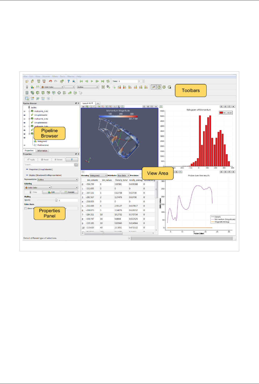
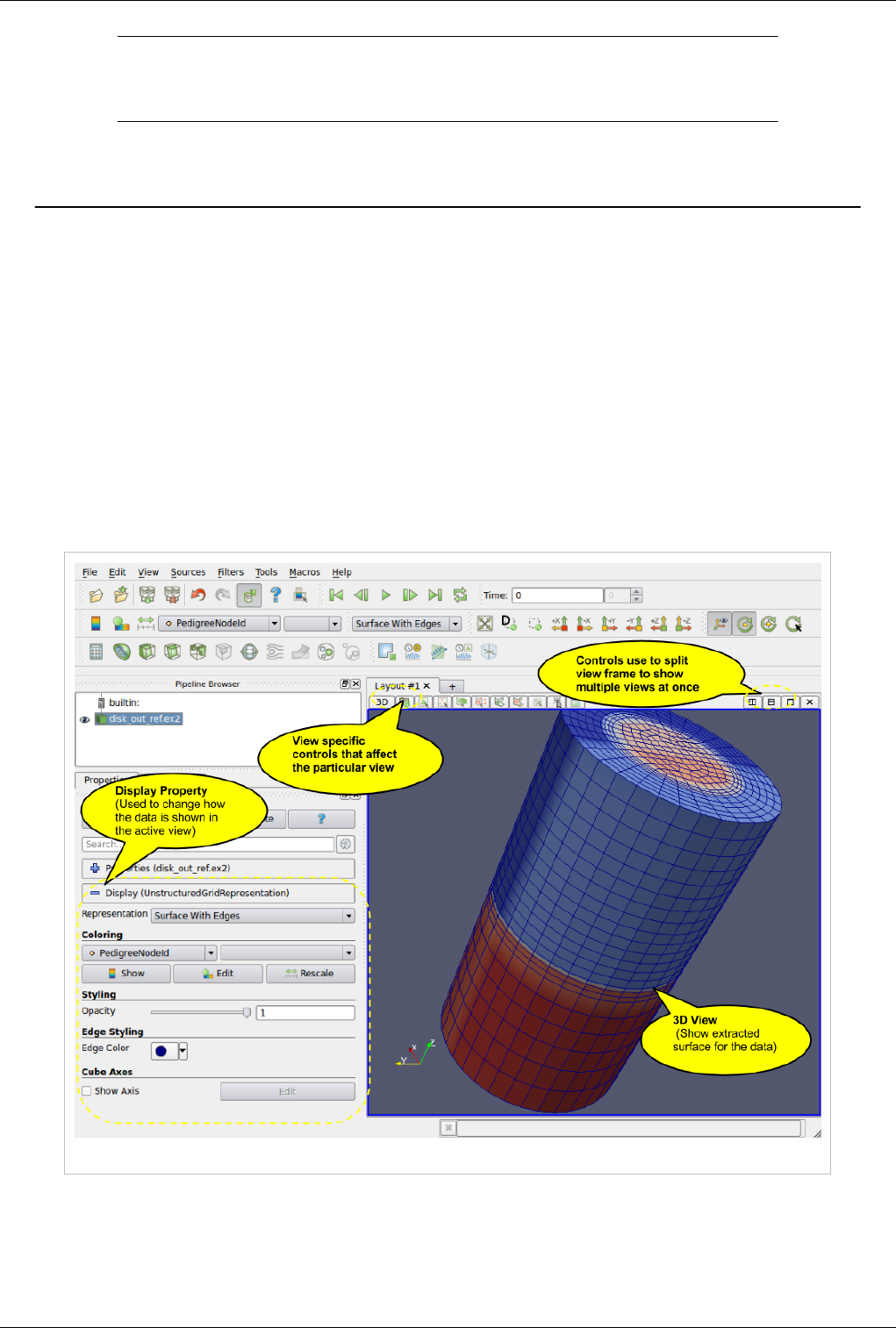
The different sections of ParaView's Graphical User Interface (GUI) are shown below. Of particular importance in
the following discussion are the:
• File and Filter menus which allow you to open files and manipulate data
• Pipeline Browser which displays the visualization pipeline
• Properties panel where you can can control any given module within the pipeline
• View area where data is displayed in one or more windows
Figure 1.1 ParaView GUI Overview
Modality
One very important thing to keep in mind when using ParaView is that the GUI is very modal. At any given time you
will have one "active" module within the visualization pipeline, one "active" view, and one "active" selection. For
example, when you click on the name of a reader or source within the Pipeline Browser, it becomes the active
module and the properties of that filter are displayed in the Properties panel. Likewise when you click within a
different view, that view becomes the active view and the visibility "eye" icons in the Pipeline Browser are changed
to show what filters are displayed within this View. These concepts will be described in detail in later chapters
(Multiple Views [2],Pipeline Basics [3],Selection [4]). For now you should be aware that the information displayed in
the GUI always pertains to these active entities.
About Paraview 3
Features
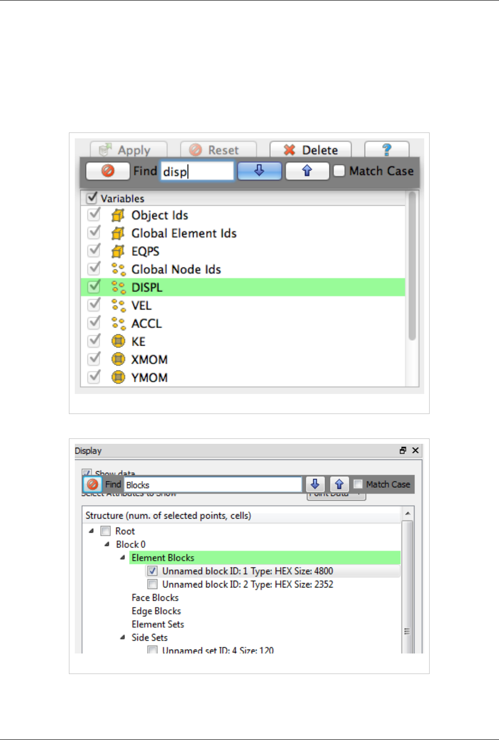
Modern graphical applications allow users to treat the GUI as a document where informations can be queried and
used by Copy/Paste from one place to another and that's precisely where we are heading to with ParaView. Typically
user can query any Tree/Table/List view widget in the UI by activating that component and by hitting the Ctrl+F or
Command+F on Mac keyboard shortcut, while the view widget is in focus. This will enable a dynamic widget
showing up which get illustrated in the following screenshot. This search-widget will be closed when the view
widget lost focus, or the Esc button is pressed, or the Close button on the search-widget is clicked.
Figure 1.2 Searching in lists
Figure 1.3 Searching in trees
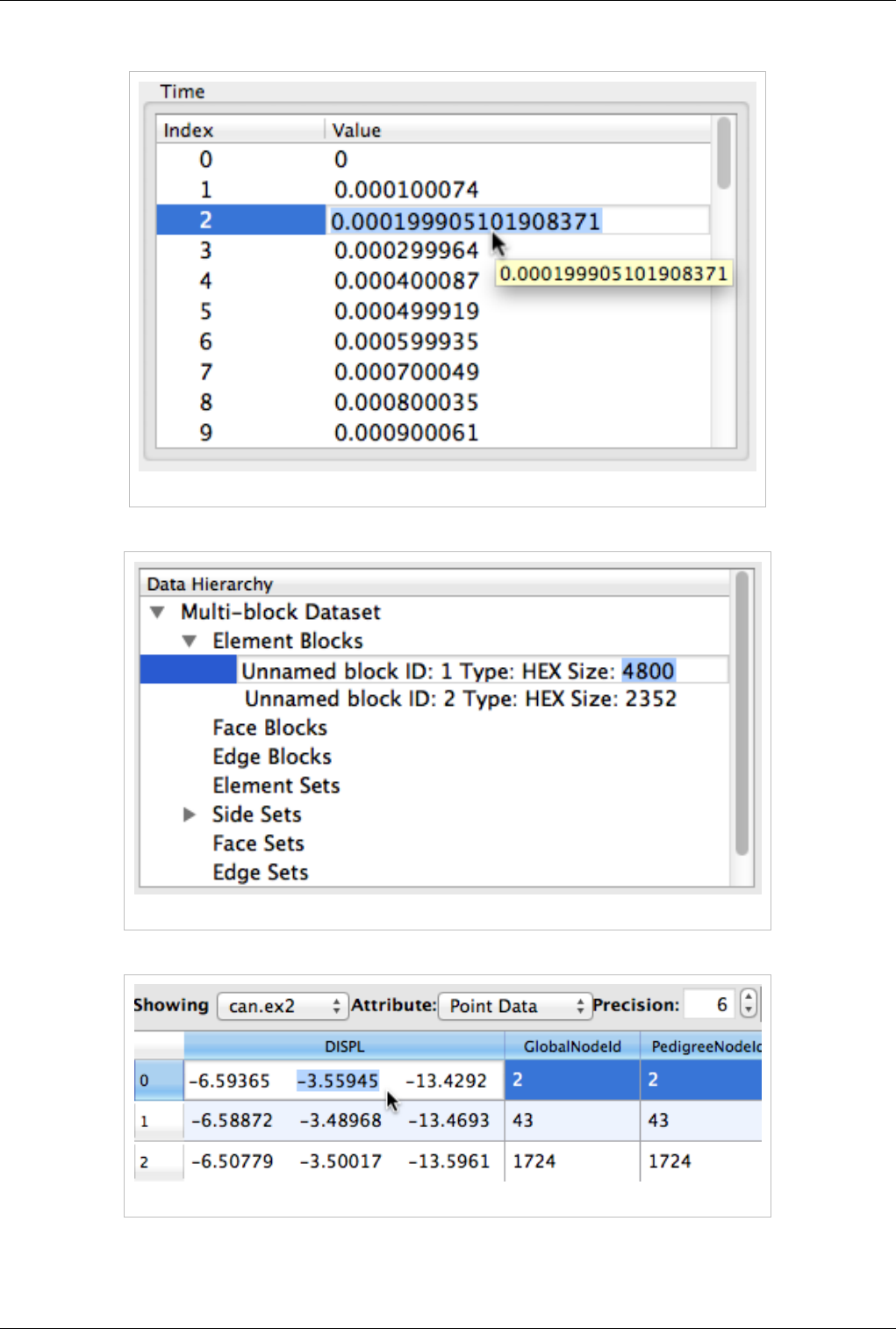
In order to retrieve data from spreadsheet or complex UI, you will need to double click on the area that you are
interested in and select the portion of text that you want to select to Copy. The set of screenshots below illustrate
About Paraview 5
Figure 1.7 Copying values from Information Tab
Basics of Visualization
Put simply, the process of visualization is taking raw data and converting it to a form that is viewable and
understandable to humans. This enables a better cognitive understanding of our data. Scientific visualization is
specifically concerned with the type of data that has a well-defined representation in 2D or 3D space. Data that
comes from simulation meshes and scanner data is well suited for this type of analysis.
There are three basic steps to visualizing your data: reading, filtering, and rendering. First, your data must be read
into ParaView. Next, you may apply any number of filters that process the data to generate, extract, or derive
features from the data. Finally, a viewable image is rendered from the data and you can then change the viewing
parameters or rendering modality for best the visual effect.
The Pipeline Concept
In ParaView, these steps are made manifest in a visualization pipeline. That is, you visualize data by building up a
set of modules, each of which takes in some data, operates on it, and presents the result as a new dataset. This begins
with a reader module that ingests data off of files on disk.
Reading data into ParaView is often as simple as selecting Open from the File menu, and then clicking the glowing
Accept button on the Properties panel. ParaView comes with support for a large number of file formats [5], and its
modular architecture makes it possible to add new file readers [6].
Once a file is read, ParaView automatically renders it in a view. In ParaView, a view is simply a window that shows
data. There are different types of views, ranging from qualitative computer graphics rendering of the data to
quantitative spreadsheet presentations of the data values as text. ParaView picks a suitable view type for your data
automatically, but you are free to change the view type, modify the rendering parameters of the data in the view, and
even create new views simultaneously as you see fit to better understand what you have read in. Additionally,
high-level meta information about the data including names, types and ranges of arrays, temporal ranges, memory
size and geometric extent can be found in the Information tab.
You can learn a great deal about a given dataset with a one element visualization pipeline consisting of just a reader
module. In ParaView, you can create arbitrarily complex visualization pipelines, including ones with multiple
readers, merging and branching pipelines. You build up a pipeline by choosing the next filter in the sequence from
the Filters menu. Once you click Accept, this new filter will read in the data produced by the formerly active filter
and perform some processing on that data. The new filter then becomes the active one. Filters then are created
differently from but operate in the same manner as readers. At all points you use the Pipeline Inspector to choose the
active filter and then the Properties panel to configure it.
The Pipeline Browser is where the overall visualization pipeline is displayed and controlled from. The Properties
panel is where the specific parameters of one particular module within the pipeline are displayed and controlled
from. The Properties panel has two sections: Properties section presents the parameters for the processing done
within that module, Display section presents the parameters of how the output of that module will be displayed in a
view (namely, the active view). There's also in Information panel, which presents the meta information about the
About Paraview 6
data produced by the module as described above.
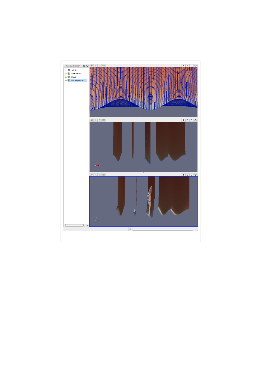
Figure 1.8 demonstrates a three-element visualization pipeline, where the output of each module in the the pipeline is
displayed in its own view. A reader takes in a vector field, defined on a curvilinear grid, which comes from a
simulation study of a wind turbine. Next a slice filter produces slices of the field on five equally spaced planes along
the X-axis. Finally, a warp filter warps those planes along the direction of the vector field, which primarily moves
the planes downwind but also shows some complexity at the location of the wind turbine.
Figure 1.8 A three-element visualization pipeline
There are more than one hundred filters available to choose from, all of which manipulate the data in different ways.
The full list of filters is available in the Appendix [5] and within the application under the Help menu. Note that many
of the filters in the menu will be grayed out and not selectable at any given time. That is because any given filter may
only operate on particular types of data. For example, the Extract Subset filter will only operate on structured data
sets so it is only enabled when the module you are building on top of produces image data, rectilinear grid data, or
structured grid data. (These input restrictions are also listed in the Appendix [7] and help menu). In this situation you
can often find a similar filter which does accept your data, or apply a filter which transforms your data into the
required format. In ParaView 3.10, you can ask ParaView to try to do the conversion for you automatically, by
clicking "Auto convert properties" in the application settings [8]. The mechanics of applying filters are described
fully in the Manipulating Data [9] chapter.

About Paraview 7
Making Mistakes
Frequently, new users of ParaView falter when they open their data, or apply a filter, and do not see it immediately
because they have not pressed the Apply button. ParaView was designed to operate on large datasets, for which any
given operation could take a long time to finish. In this situation you need the Apply button so that you have a
chance to be confident of your change before it takes effect. The highlighted Apply button is a reminder that the
parameters of one or more filters are out of sync with the data that you are viewing. Hitting the Apply button accepts
your change (or changes) whereas hitting the Reset button reverts the options back to the last time you hit Apply. If
you are working with small datasets, you may want to turn off this behavior with the Auto Accept setting under the
Application Settings [8].
The Apply behavior circumvents a great number of mistakes but not all of them. If you make some change to a filter
or to the pipeline itself and later find that you are not satisfied with the result, hit the Undo button. You can undo all
the way back to the start of your ParaView session and redo all the way forward if you like. You can also undo and
redo camera motion by using the camera undo and redo buttons located above each view window.
Persistent Sessions
If on the other hand you are satisfied with your visualization results, you may want to save your work so that you can
return to it at some future time. You can do so by using ParaView's Save State (File|Save State) and Save Trace
(Tools | Save Trace) features. In either case, ParaView produces human readable text files (XML files for State and
Python script for Trace) that can be restored or modified and restored later. This is very useful for batch processing,
which is discussed in the Python Scripting [10] chapter.
To save state means to save enough information about the ParaView session to restore it later and thus show exactly
the same result. ParaView does so by saving the current visualization pipeline and parameters of the filters within it.
If you turn on a trace recording when you first start using ParaView, saving a trace can be used for the same purpose
as saving state. However, a trace records all of your actions, including the ones that you later undo, as you do them.
It is a more exact recording of not only what you did, but how you did it. Traces are saved as python scripts, which
ParaView can play back in either batch mode or within an interactive GUI session. You can therefore use traces then
to automate repetitive tasks by recording just that action. It is also an ideal tool to learn ParaView's python scripting
API.
Client/Server Visualization
With small datasets it is usually sufficient to run ParaView as a single process on a small laptop or desktop class
machine. For large datasets, a single machine is not likely to have enough processing power and, much more
importantly, memory to process the data. In this situation you run an MPI parallel ParaView Server process on a
large machine to do computationally and memory expensive data processing and/or rendering tasks and then connect
to that server within the familiar GUI application.
When connected to a remote server the only difference you will see will be that the visualization pipeline displayed
in the Pipeline Browser will begin with the name of the server you are connected to rather than the word 'builtin'
which indicates that you are connected to a virtual server residing in the same process as the GUI. When connected
to a remote server, the File Open dialog presents the list of files that live on the remote machine's file system rather
than the client's. Depending on the server's capabilities, the data size and your application settings
(Edit|Settings|Render View|Server) the data will either be rendered remotely and pixels will be sent to the client or
the geometry will be delivered and rendered locally. Large data visualization is described fully in the Client Server
Visualization [11] Chapter.

About Paraview 8
References
[1] http:/ / www. paraview. org/ Wiki/ ParaViewWeb
[2] http:/ / paraview. org/ Wiki/ ParaView/ Displaying_Data#Multiple_Views
[3] http:/ / paraview. org/ Wiki/ ParaView/ UsersGuide/ Filtering_Data#Pipeline_Basics
[4] http:/ / paraview. org/ Wiki/ ParaView/ Users_Guide/ Selection
[5] http:/ / paraview. org/ Wiki/ ParaViewUsersGuide/ List_of_readers
[6] http:/ / paraview. org/ Wiki/ Writing_ParaView_Readers
[7] http:/ / paraview. org/ Wiki/ ParaViewUsersGuide/ List_of_filters
[8] http:/ / paraview. org/ Wiki/ ParaView/ Users_Guide/ Settings
[9] http:/ / paraview. org/ Wiki/ ParaView/ UsersGuide/ Filtering_Data
[10] http:/ / paraview. org/ Wiki/ ParaView/ Python_Scripting
[11] http:/ / paraview. org/ Wiki/ Users_Guide_Client-Server_Visualization

9
Loading Data
Data Ingestion
Introduction
Loading data is a fundamental operation in using ParaView for visualization. As you would expect, the Open option
from the File menu and the Open Button from the toolbar both allow you to load data into ParaView. ParaView
understands many scientific data file formats. The most comprehensive list is given in the List of Readers [5]
appendix. Because of ParaView's modular design it is easy to integrate new readers. If the formats you need are not
listed, ask the mailing list first to see if anyone has a reader for the format or, if you want to create your own readers
for ParaView see the Plugin HowTo [1] section and the Writing Readers [6] appendix of this book.
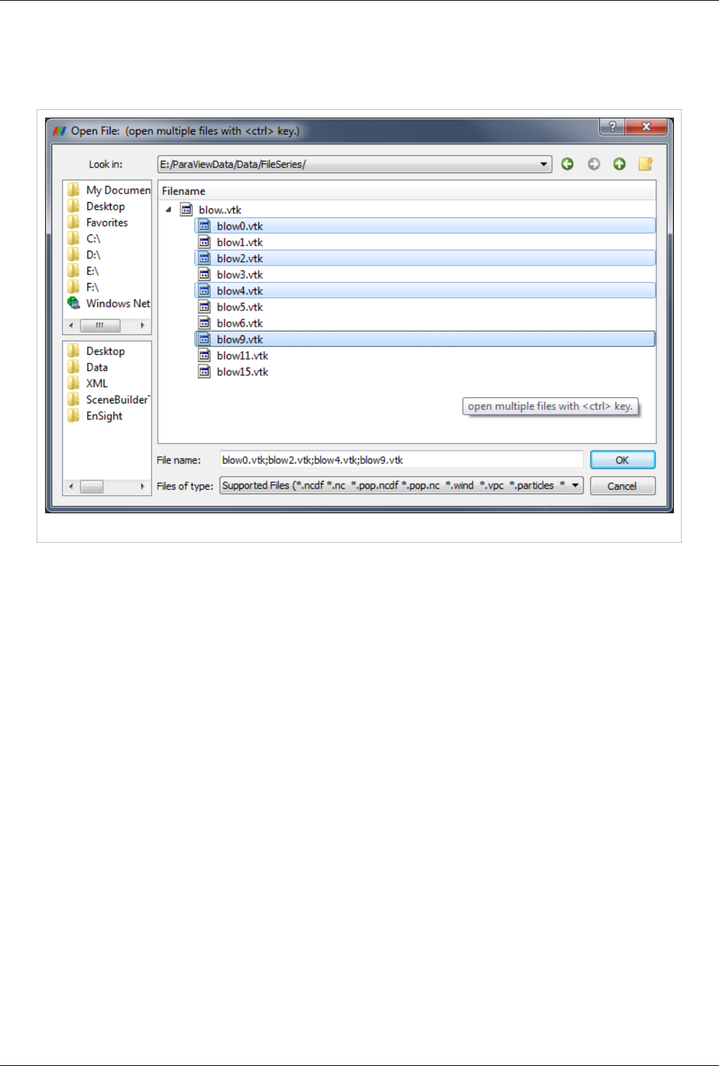
Opening File / Time Series
ParaView recognizes file series by using certain patterns in the name of files including:
• fooN.vtk
• foo_N.vtk
• foo-N.vtk
• foo.N.vtk
• Nfoo.vtk
• N.foo.vtk
• foo.vtk.N
• foo.vtk-sN
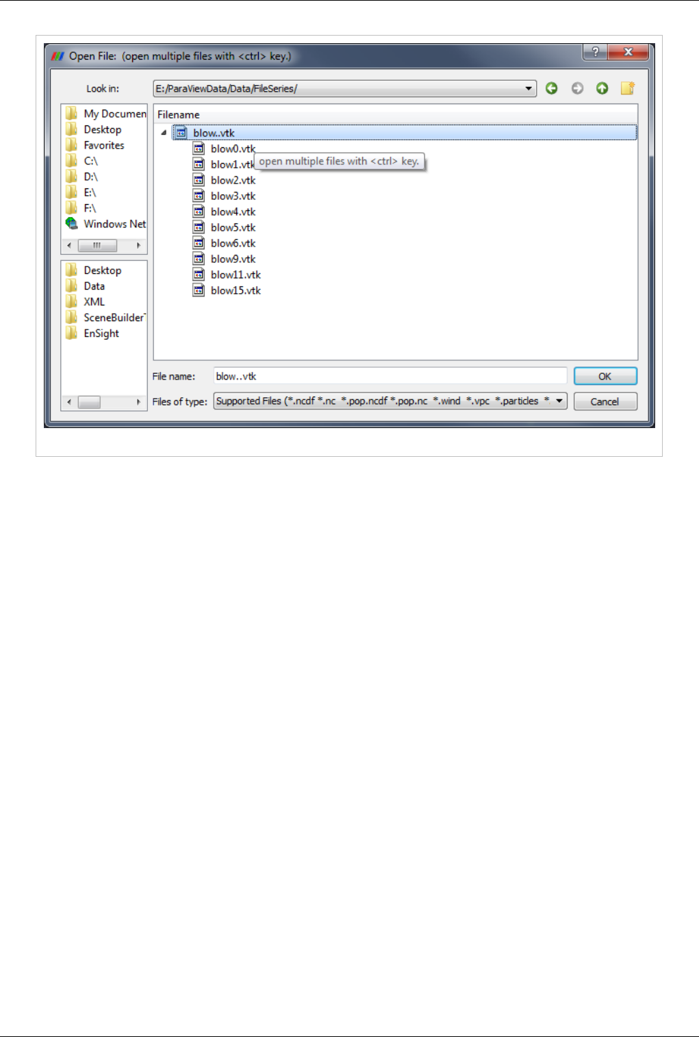
In the above file name examples, N is an integer (with any number of leading zeros). To load a file series, first make
sure that the file names match one of the patterns described above. Next, navigate to the directory where the file
series is. The file browser should look like Figure 2.1:
Data Ingestion 10
Figure 2.1 Sample browser when opening files
You can expand the file series by clicking on the triangle, as shown in the above diagram. Simply select the group
(in the picture named blow..vtk) and click OK. The reader will store all the filenames and treat each file as a time
step. You can now animate, use the annotate time filter, or do anything you can do with readers that natively support
time. If you want to load a single step of a file series just expand the triangle and select the file you are interested in.
Data Ingestion 11
Opening Multiple Files
ParaView supports loading multiple files as long as they exist in the same directory. Just hold the Ctrl key down
while selecting each file (Figure 2.2), or hold shift to select all files in a range.
Figure 2.2 Opening multiple files
State Files
Another option is to load a previously saved state file (File|Load State). This will return ParaView to its state at the
time the file was saved by loading data files, applying filters.
Advanced Data Loading
If you commonly load the same data into ParaView each time, you can streamline the process by launching
ParaView with the data command-line argument (--data=data_file).
Properties Panel
Note that opening a file is a two step process, and so you do not see any data after opening a data file. Instead, you
see that the Properties Panel is populated with several options about how you may want to read the data.
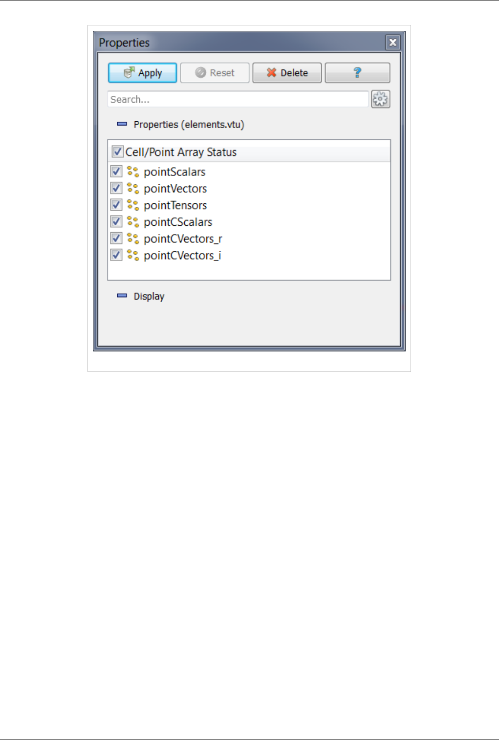
Data Ingestion 12
Figure 2.3 Using the Properties panel
Once you have enabled all the options on the data that you are interested in click the Apply button to finish loading
the data. For a more detailed explanation of the object inspector read the Properties Section .
References
[1] http:/ / www. paraview. org/ Wiki/ ParaView/ Plugin_HowTo#Adding_a_Reader
13
Understanding Data
VTK Data Model
Introduction
To use ParaView effectively, you need to understand the ParaView data model. This chapter briefly introduces the
VTK data model used by ParaView. For more details, refer to one of the VTK books.
The most fundamental data structure in VTK is a data object. Data objects can either be scientific datasets such
rectilinear grids or finite elements meshes (see below) or more abstract data structures such as graphs or trees. These
datasets are formed of smaller building blocks: mesh (topology and geometry) and attributes.
Mesh
Even though the actual data structure used to store the mesh in memory depends on the type of the dataset, some
abstractions are common to all types. In general, a mesh consists of vertices (points) and cells (elements, zones).
Cells are used to discretize a region and can have various types such a tetrahedra, hexahedra etc. Each cell contains a
set of vertices. The mapping from cells to vertices is called the connectivity. Note that even though it is possible to
define data elements such as faces and edges, VTK does not represent these explicitly. Rather, they are implied by a
cell's type and its connectivity. One exception to this rule is the arbitrary polyhedron which explicitly stores its faces.
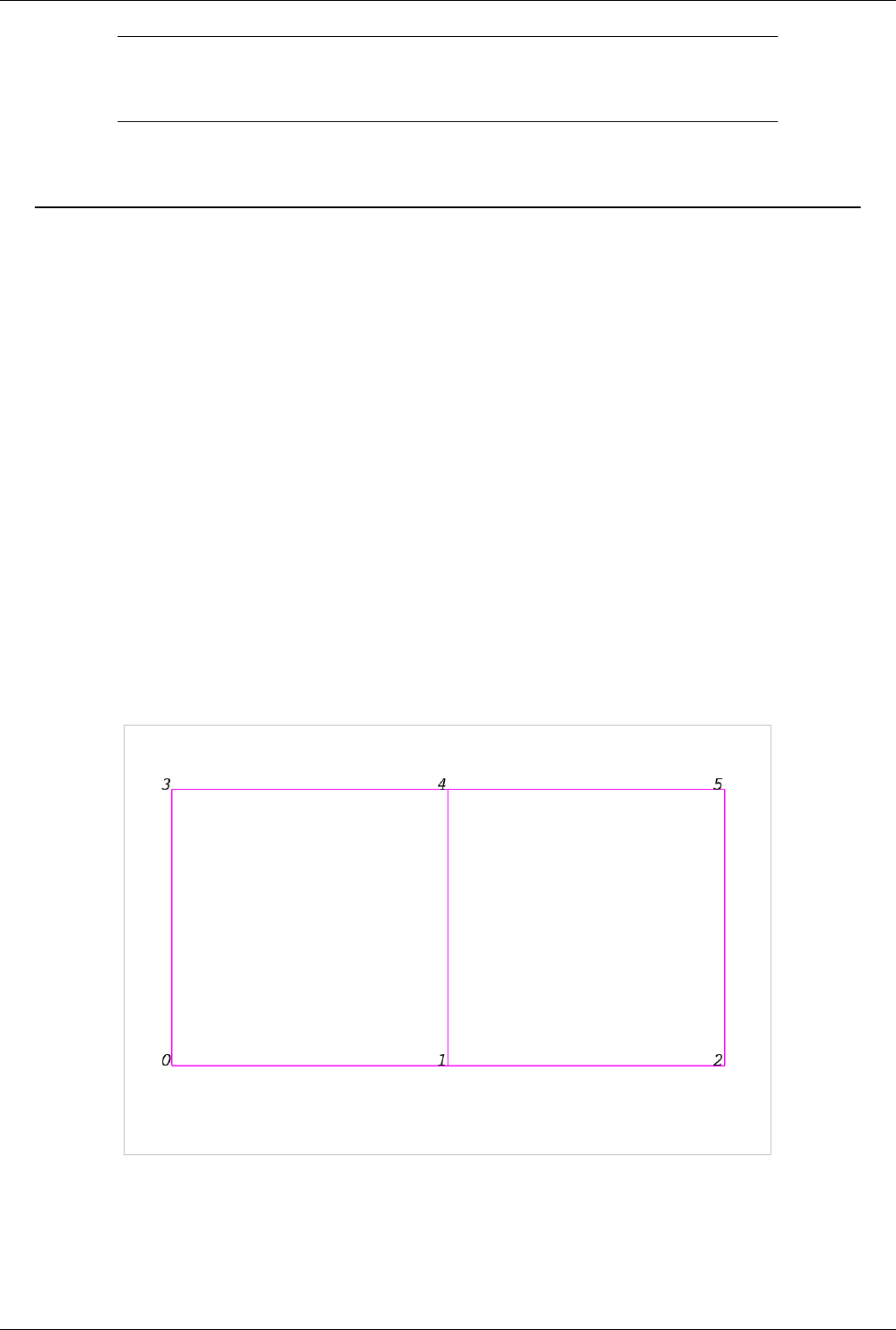
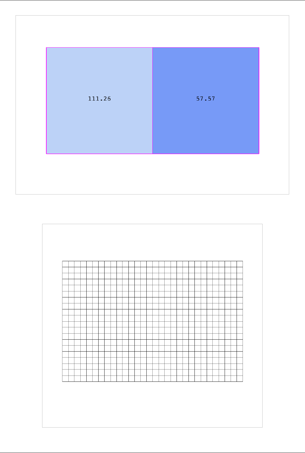
Figure 3.1 is an example mesh that consists of 2 cells. The first cell is defined by vertices (0, 1, 3, 4) and the second
cell is defined by vertices (1, 2, 4, 5). These cells are neighbors because they share the edge defined by the points (1,
4).
Figure 3.1 Example of a mesh
A mesh is fully defined by its topology and the spatial coordinates of its vertices. In VTK, the point coordinates may
be implicit or explicitly defined by a data array of dimensions (number_of_points x 3).
VTK Data Model 14
Attributes (fields, arrays)
An attribute (or a data array or field) defines the discrete values of a field over the mesh. Examples of attributes
include pressure, temperature, velocity and stress tensor. Note that VTK does not specifically define different types
of attributes. All attributes are stored as data arrays which can have an arbitrary number of components. ParaView
makes some assumptions in regards to the number of components. For example, a 3-component array is assumed to
be an array of vectors. Attributes can be associated with points or cells. It is also possible to have attributes that are
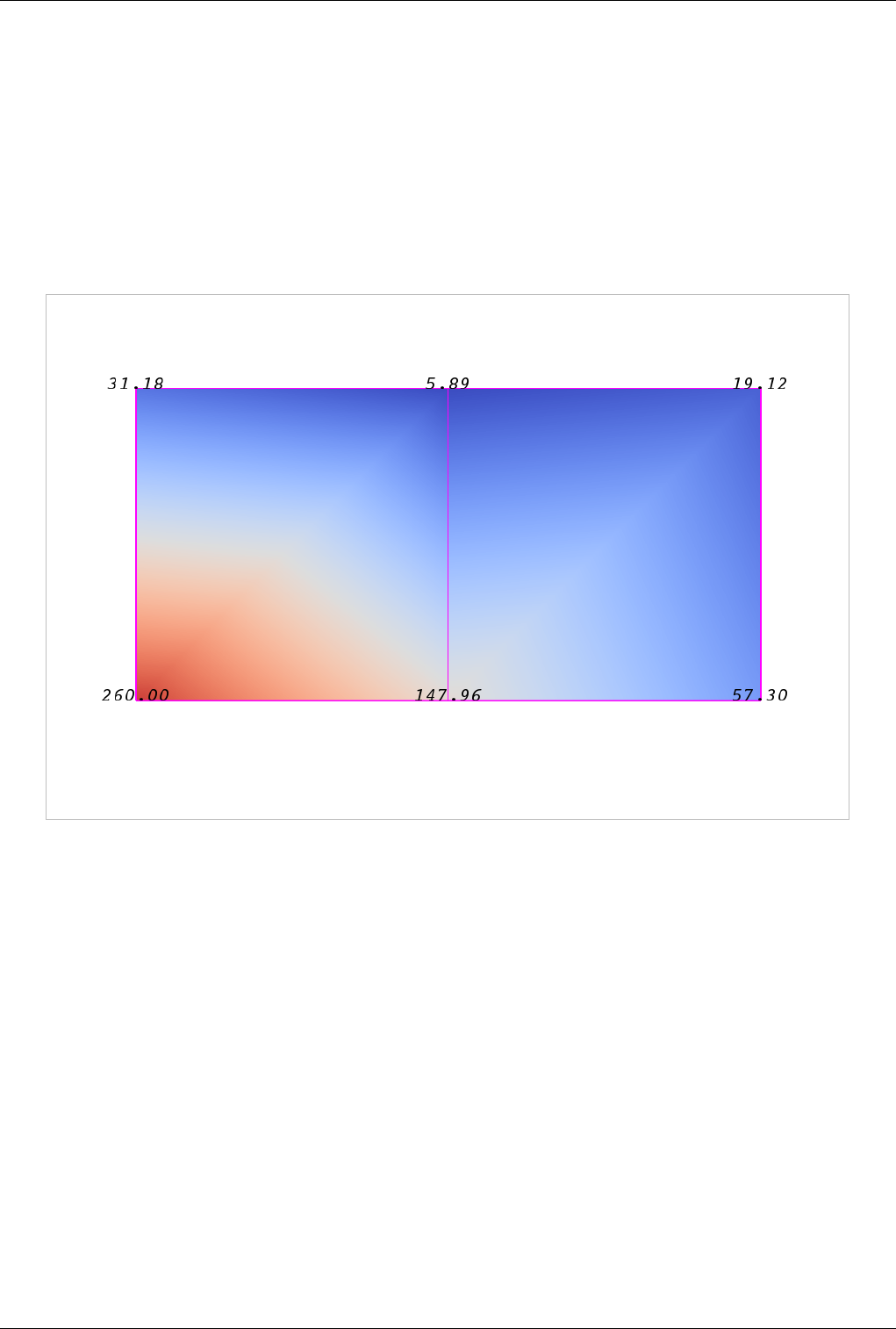
not associated with either. Figure 3.2 demonstrates the use of a point-centered attribute. Note that the attribute is only
defined on the vertices. Interpolation is used to obtain the values everywhere else. The interpolation functions used
depend on the cell type. See VTK documentation for details.
Figure 3.2 Point-centered attribute in a data array or field
Figure 3.3 demonstrates the use of a cell-centered attribute. Note that cell-centered attributes are assumed to be
constant over each cell. Due to this property, many filters in VTK cannot be directly applied to cell-centered
attributes. It is normally required to apply a Cell Data to Point Data filter. In ParaView, this filter is applied
automatically when necessary.
VTK Data Model 16
A uniform rectilinear grid, or image data, defines its topology and point coordinates implicitly. To fully define the
mesh for an image data, VTK uses the following:
• Extents - these define the minimum and maximum indices in each direction. For example, an image data of
extents (0, 9), (0, 19), (0, 29) has 10 points in the x-direction, 20 points in the y-direction and 30 points in the
z-direction. The total number of points is 10*20*30.
• Origin - this is the position of a point defined with indices (0, 0, 0)
• Spacing - this is the distance between each point. Spacing for each direction can defined independently
The coordinate of each point is defined as follows: coordinate = origin + index*spacing where coordinate, origin,
index and spacing are vectors of length 3.
Note that the generic VTK interface for all datasets uses a flat index. The (i,j,k) index can be converted to this flat
index as follows: idx_flat = k*(npts_x*npts_y) + j*nptr_x + i.
A uniform rectilinear grid consists of cells of the same type. This type is determined by the dimensionality of the
dataset (based on the extents) and can either be vertex (0D), line (1D), pixel (2D) or voxel (3D).
Due to its regular nature, image data requires less storage than other datasets. Furthermore, many algorithms in VTK
have been optimized to take advantage of this property and are more efficient for image data.
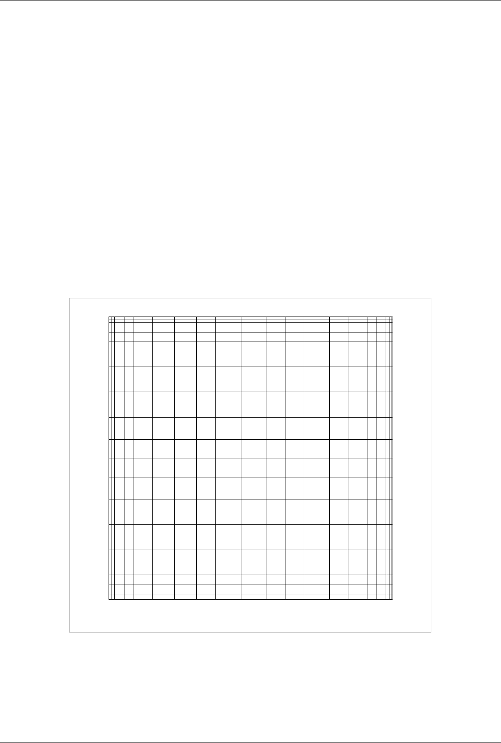
Rectilinear Grid
Figure 3.5 Rectilinear grid
A rectilinear grid such as Figure 3.5 defines its topology implicitly and point coordinates semi-implicitly. To fully
define the mesh for a rectilinear grid, VTK uses the following:
• Extents - these define the minimum and maximum indices in each direction. For example, a rectilinear grid of
extents (0, 9), (0, 19), (0, 29) has 10 points in the x-direction, 20 points in the y-direction and 30 points in the
z-direction. The total number of points is 10*20*30.

VTK Data Model 17
• Three arrays defining coordinates in the x-, y- and z-directions. These arrays are of length npts_x, npts_y and
npts_z. This is a significant savings in memory as total memory used by these arrays is npts_x+npts_y+npts_z
rather than npts_x*npts_y*npts_z.
The coordinate of each point is defined as follows: coordinate = (coordinate_array_x(i), coordinate_array_y(j),
coordinate_array_z(k))".
Note that the generic VTK interface for all datasets uses a flat index. The (i,j,k) index can be converted to this flat
index as follows: idx_flat = k*(npts_x*npts_y) + j*nptr_x + i.
A rectilinear grid consists of cells of the same type. This type is determined by the dimensionality of the dataset
(based on the extents) and can either be vertex (0D), line (1D), pixel (2D) or voxel (3D).
Curvilinear Grid (Structured Grid)
Figure 3.6 Curvilinear or structured grid
A curvilinear grid, such as Figure 3.6, defines its topology implicitly and point coordinates explicitly. To fully define
the mesh for a curvilinear grid, VTK uses the following:
• Extents - these define the minimum and maximum indices in each direction. For example, a curvilinear grid of
extents (0, 9), (0, 19), (0, 29) has 10*20*30 points regularly defined over a curvilinear mesh.
• An array of point coordinates. This arrays stores the position of each vertex explicitly.
The coordinate of each point is defined as follows: coordinate = coordinate_array(idx_flat)". The (i,j,k) index can
be converted to this flat index as follows: idx_flat = k*(npts_x*npts_y) + j*nptr_x + i.
A curvilinear grid consists of cells of the same type. This type is determined by the dimensionality of the dataset
(based on the extents) and can either be vertex (0D), line (1D), quad (2D) or hexahedron (3D).
VTK Data Model 18
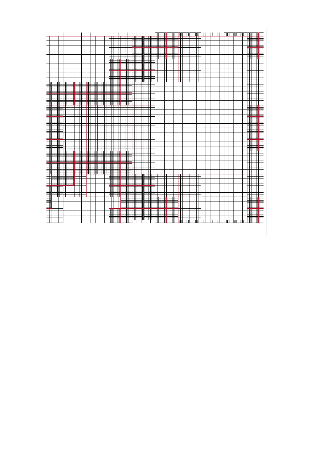
AMR Dataset
Figure 3.7 AMR dataset
VTK natively support Berger-Oliger type AMR (Adaptive Mesh Refinement) datasets, as shown in Figure 3.7. An
AMR dataset is essentially a collection of uniform rectilinear grids grouped under increasing refinement ratios
(decreasing spacing). VTK's AMR dataset does not force any constraint on whether and how these grids should
overlap. However, it provides support for masking (blanking) sub-regions of the rectilinear grids using an array of
bytes. This allows VTK to process overlapping grids with minimal artifacts. VTK can automatically generate the
masking arrays for Berger-Oliger compliant meshes.
VTK Data Model 19
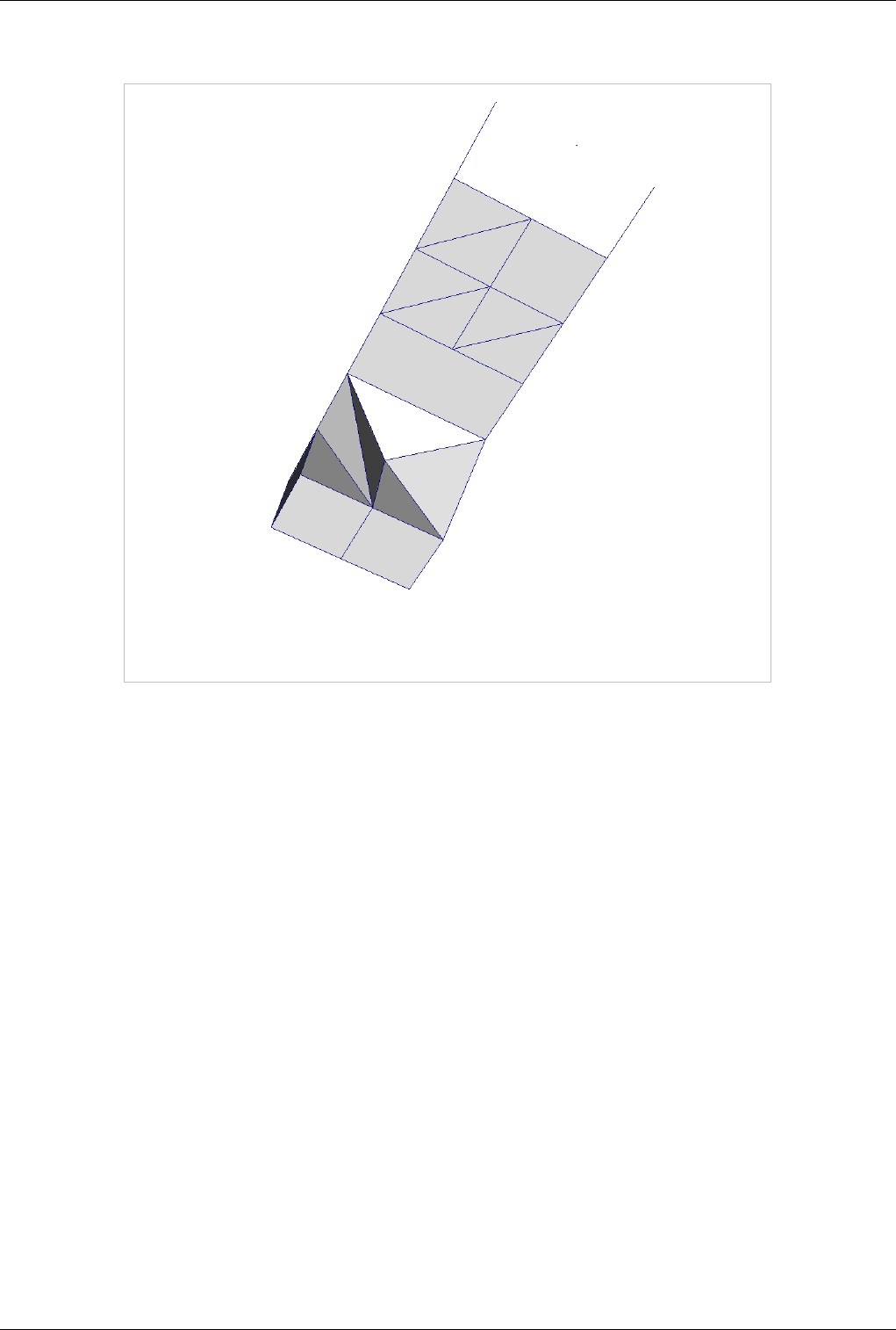
Unstructured Grid
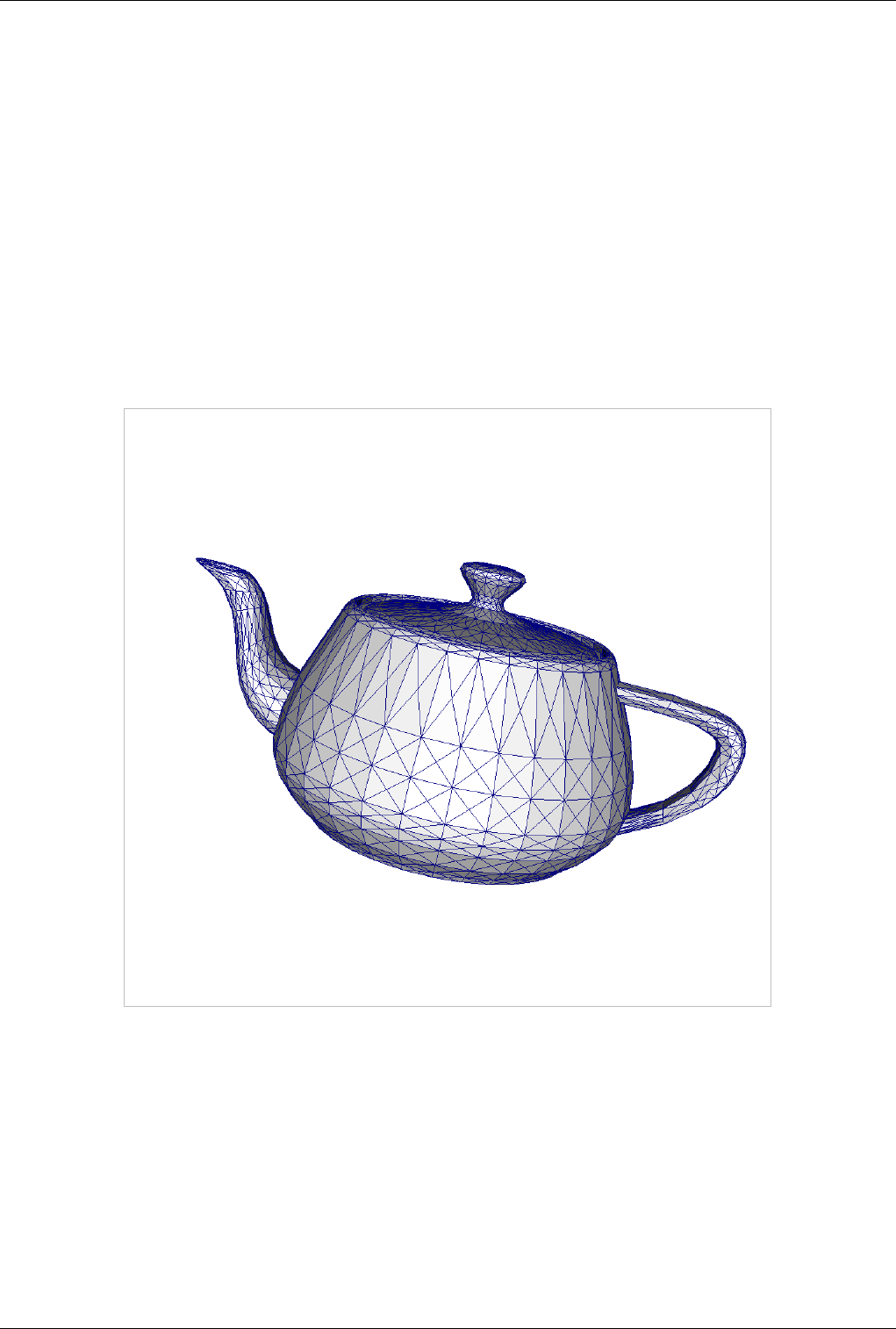
Figure 3.8 Unstructured grid
An unstructured grid such as Figure 3.8 is the most general primitive dataset type. It stores topology and point
coordinates explicitly. Even though VTK uses a memory-efficient data structure to store the topology, an
unstructured grid uses significantly more memory to represent its mesh. Therefore, use an unstructured grid only
when you cannot represent your dataset as one of the above datasets. VTK supports a large number of cell types, all
of which can exist (heterogeneously) within one unstructured grid. The full list of all cell types supported by VTK
can be found in the file vtkCellType.h in the VTK source code. Here is the list as of when this document was
written:
VTK_EMPTY_CELL VTK_VERTEX
VTK_POLY_VERTEX VTK_LINE
VTK_POLY_LINE VTK_TRIANGLE
VTK_TRIANGLE_STRIP VTK_POLYGON
VTK_PIXEL VTK_QUAD
VTK_TETRA VTK_VOXEL
VTK_HEXAHEDRON VTK_WEDGE
VTK_PYRAMID VTK_PENTAGONAL_PRISM
VTK_HEXAGONAL_PRISM VTK_QUADRATIC_EDGE
VTK_QUADRATIC_TRIANGLE VTK_QUADRATIC_QUAD
VTK_QUADRATIC_TETRA VTK_QUADRATIC_HEXAHEDRON
VTK_QUADRATIC_WEDGE VTK_QUADRATIC_PYRAMID
VTK Data Model 20
VTK_BIQUADRATIC_QUAD VTK_TRIQUADRATIC_HEXAHEDRON
VTK_QUADRATIC_LINEAR_QUAD VTK_QUADRATIC_LINEAR_WEDGE
VTK_BIQUADRATIC_QUADRATIC_WEDGE VTK_BIQUADRATIC_QUADRATIC_HEXAHEDRON
VTK_BIQUADRATIC_TRIANGLE VTK_CUBIC_LINE
VTK_CONVEX_POINT_SET VTK_POLYHEDRON
VTK_PARAMETRIC_CURVE VTK_PARAMETRIC_SURFACE
VTK_PARAMETRIC_TRI_SURFACE VTK_PARAMETRIC_QUAD_SURFACE
VTK_PARAMETRIC_TETRA_REGION VTK_PARAMETRIC_HEX_REGION
Many of these cell types are straightforward. For details, see VTK documentation.
Polygonal Grid (Polydata)
Figure 3.9 Polygonal grid
A polydata such as Figure 3.9 is a specialized version of an unstructured grid designed for efficient rendering. It
consists of 0D cells (vertices and polyvertices), 1D cells (lines and polylines) and 2D cells (polygons and triangle
strips). Certain filters that generate only these cell types will generate a polydata. Examples include the Contour and
Slice filters. An unstructured grid, as long as it has only 2D cells supported by polydata, can be converted to a
polydata using the Extract Surface filter. A polydata can be converted to an unstructured grid using Clean to Grid.
VTK Data Model 21
Table
Table 3.1
A table like Table 3.1 is a tabular dataset that consists of rows and columns. All chart views have been designed to
work with tables. Therefore, all filters that can be shown within the chart views generate tables. Also, tables can be
directly loaded using various file formats such as the comma separated values format. Tables can be converted to
other datasets as long as they are of the right format. Filters that convert tables include Table to Points and Table to
Structured Grid.
Multiblock Dataset
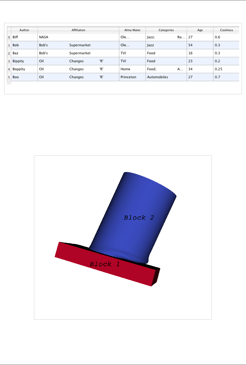
Figure 3.10 Multiblock dataset
You can think of a multi-block dataset as a tree of datasets where the leaf nodes are "simple" datasets. All of the data
types described above, except AMR, are "simple" datasets. Multi-block datasets are used to group together datasets
that are related. The relation between these datasets is not necessarily defined by ParaView. A multi-block dataset
can represent an assembly of parts or a collection of meshes of different types from a coupled simulation.
VTK Data Model 22
Multi-block datasets can be loaded or created within ParaView using the Group filter. Note that the leaf nodes of a
multi-block dataset do not all have to have the same attributes. If you apply a filter that requires an attribute, it will
be applied only to blocks that have that attribute.
Multipiece Dataset
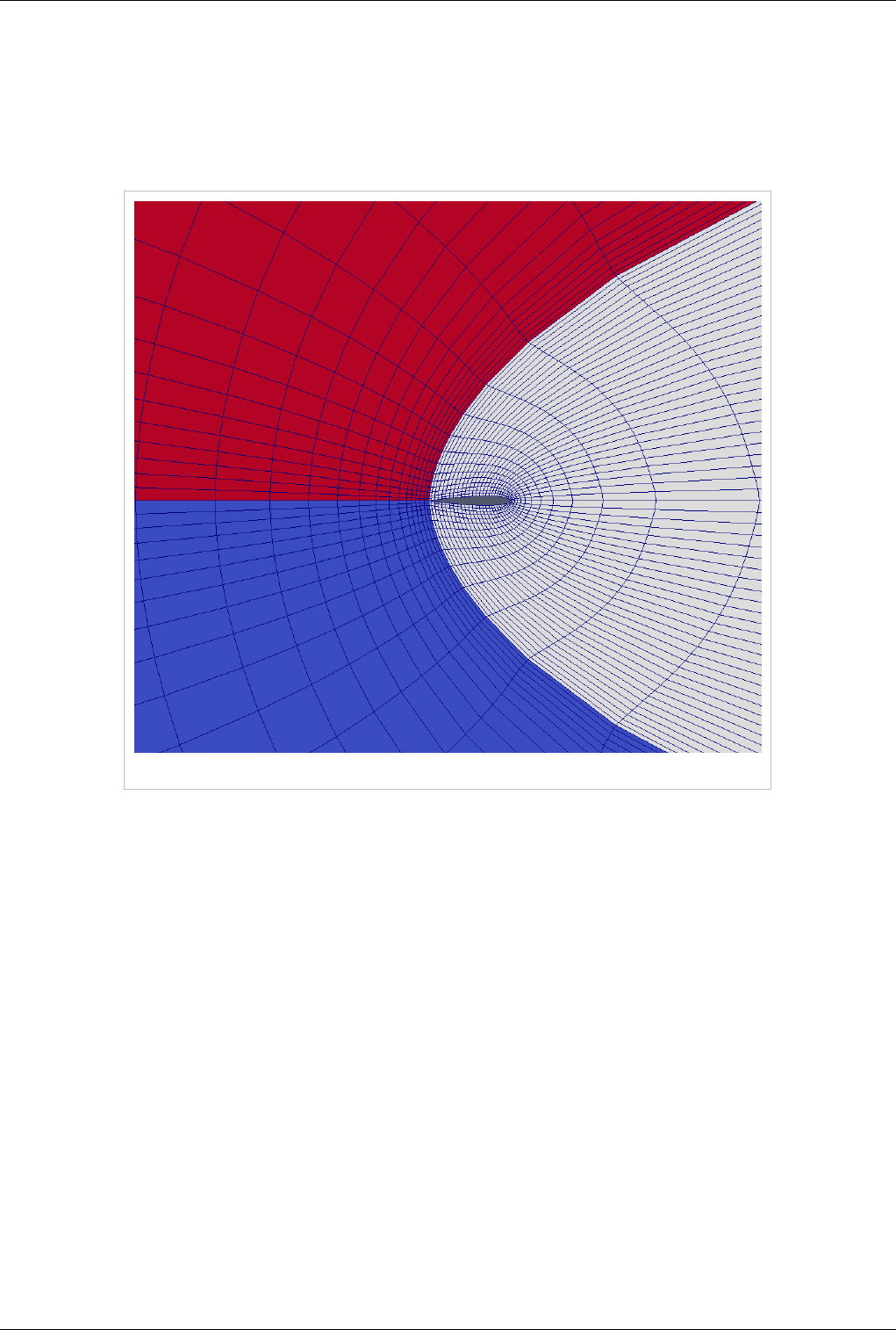
Figure 3.11 Multipiece dataset
Multi-piece datasets such as Figure 3.11 are similar to multi-block datasets in that they group together simple
datasets with one key difference. Multi-piece datasets group together datasets that are part of a whole mesh - datasets
of the same type and with same attributes. This data structure is used collect datasets produced by a parallel
simulation without having to append the meshes together. Note that there is no way to create a multi-piece dataset
within ParaView, but only by using certain readers. Furthermore, multi-piece datasets act, for the most part, as
simple datasets. For example, it is not possible to extract individual pieces or obtain information about them.
Information Panel 23
Information Panel
Introduction
Clicking on the Information button on the Object Inspector will take you to the Information Panel. The purpose of
this panel is to provide you with information about the output of the currently selected source, reader or filter. The
information on this panel is presented in several sections. We start by describing the sections that are applicable to
all dataset types then we describe data specific sections.
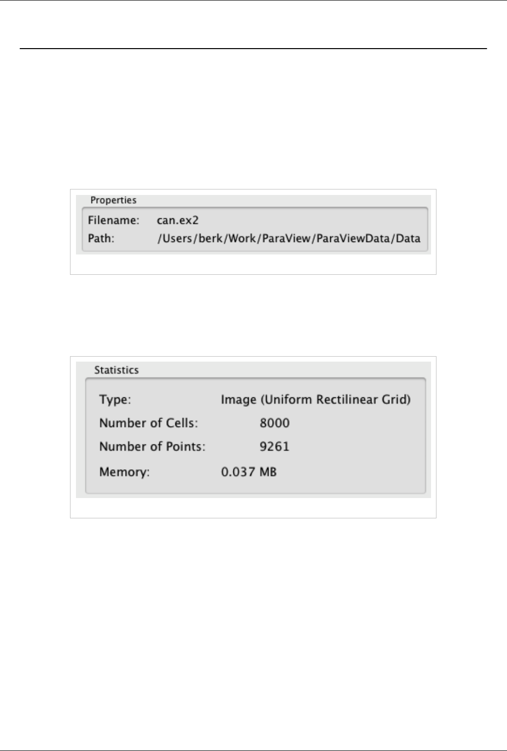
File Properties
Figure 3.12 File properties
If the current pipeline object is a reader, the top section will display the name of the file and its full path, as in Figure
3.12.
Data Statistics
Figure 3.13 Data statistics
The Statistics section displays high-level information about the dataset including the type, number of points and cells
and the total memory used. Note that the memory is for the dataset only and does not include memory used by the
representation (for example, the polygonal mesh that may represent the surface). All of this information is for the
current time step.

Information Panel 24
Array Information
Figure 3.14 Array information
The data shown in Figure 3.14 shows the association (point, cell or global), name, type and range of each array in the
dataset. In the example, the top three attributes are point arrays, the middle three are cell arrays and the bottom three
are global (field) arrays. Note that for vectors, the range of each component is shown separately. In case, the range
information does not fit the frame, the tooltip will display all of the values.
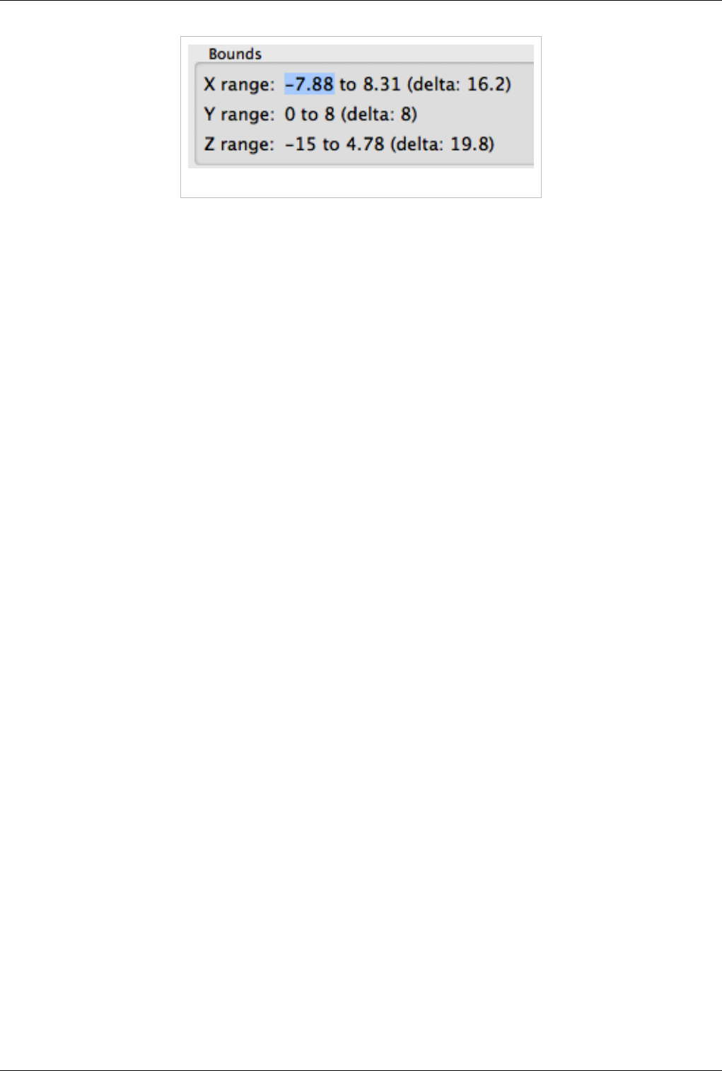
Bounds
Figure 3.15 Bounds information
The Bounds section will display the spatial bounds of the dataset. These are the coordinates of the smallest
axis-aligned hexahedron that contains the dataset as well as its dimensions, as in Figure 3.15.
Information Panel 25
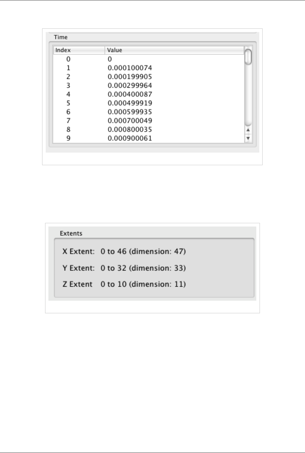
Timesteps
Figure 3.16 Time section showing timesteps
The Time section (see Figure 3.16) shows the index and value of all time steps available in a file or produceable by a
source. Note that this section display values only when a reader or source is selected even though filters downstream
of such sources also have time varying outputs. Also note that usually only one time step is loaded at a time.
Extents
Figure 3.17 Extents
The Extents section, seen in Figure 3.17, is available only for structured datasets (uniform rectilinear grid, rectilinear
grid and curvilinear grid). It displays the extent of all three indices that define a structured datasets. It also displays
the dimensions (the number of points) in each direction. Note that these refer to logical extents and the labels X
Extent, Y Extent and Z Extent can be somehow misleading for curvilinear grids.
Information Panel 26
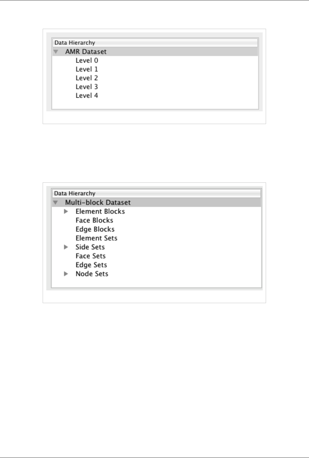
Data Hierarchy (AMR)
Figure 3.18 Data hierarchy for AMR
For AMR datasets, the Data Hierarchy section, Figure 3.18, shows the various refinement levels available in the
dataset. Note that you can drill down to each level by clicking on it. All of the other sections will immediately update
for the selected level. For information on the whole dataset, select the top parent called "AMR Dataset."
Data Hierarchy (Multi-Block Dataset)
Figure 3.19 Data hierarchy for multi-block datasets
For multi-block datasets, the Data Hierarchy section shows the tree that forms the multi-block dataset. By default,
only the first level children are shown. You can drill down further by clicking on the small triangle to the left of each
node. Note that you can drill down to each block by clicking on it. All of the other sections will immediately update
for the selected block. For information on the whole dataset, select the top parent called "Multi-Block Dataset".
Statistics Inspector 27
Statistics Inspector
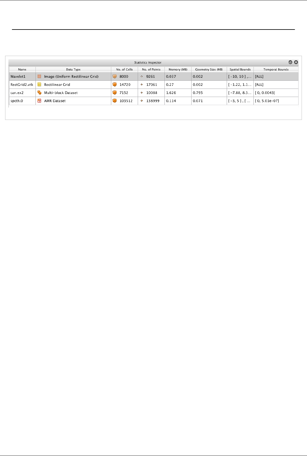
Statistics Inspector
Figure 3.20 The Statistics Inspector
The Statistics Inspector (View| Statistics Inspector) can be used to obtain high-level information about the data
produced by all sources, readers and filters in the ParaView pipeline. Some of this information is also available
through the Information panel. The information presented in the Statistics Inspector include the name of the pipeline
object that produced the data, the data type, the number of cells and points, memory used by the dataset, memory
used by the visual representation of the dataset (usually polygonal data), and the spatial bounds of the dataset (the
minimum and maximum time values for all available time steps).
Note that the selection in the Statistics Inspector is linked with the Pipeline Browser. Selecting an entry in the
Selection Inspector will update the Pipeline Browser and vice versa.
The Statics Inspector shows memory needed/used by every pipeline filter or source. However, it must be noted that
the actual memory used may still not align with this information due to the following caveats:
1. Shallow Copied Data: Several filters, such as Calculator, Shrink etc. that don't change the topology often pass
the attribute arrays without copying any of the heavy data (known as shallow copying). In that case though the
Statics Inspector will overestimate the memory used.
2. Memory for Data Datastructures: All data in VTK/ParaView is maintained in data-structures i.e.
vtkDataObject subclasses. Any data-structure requires memory. Generally, this memory needed is considerably
small compared to the heavy data i.e. the memory needed to save the topology, geometry, attribute arrays, etc.,
however in case of composite datasets and especially, AMR datasets with very large number of blocks in the
order of 100K blocks, the memory used for the meta-data starts growing and can no longer be ignored. The
Statistics Inspector as well as the Information Tab does not take this memory needed for datastructures into
consideration and hence in such cases underestimates the memory needed.
ParaView 3.14 adds "Memory Inspector" widget for users to directly inspect the memory used on all the ParaView
processes.
Memory Inspector 28
Memory Inspector
Memory Inspector
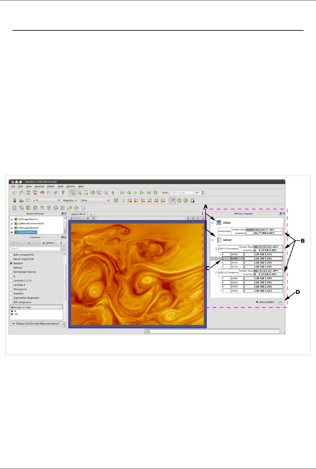
The ParaView Memory Inspector Panel provides users a convenient way to monitor ParaView's memory usage
during interactive visualization, and developers a point-and-click interface for attaching a debugger to local or
remote client and server processes. As explained earlier, both the Information panel, and the Statistics inspector are
prone to over and under estimate the total memory used for the current pipeline. The Memory Inspector addresses
those issues through direct queries to the operating system. A number of diagnostic statistics are gathered and
reported. For example, the total memory used by all processes on a per-host basis, the total cumulative memory use
by ParaView on a per-host basis, and the individual per-rank use by each ParaView process are reported. When
memory consumption reaches a critical level, either the cumulatively on the host or in an individual rank, the
corresponding GUI element will turn red alerting the user that they are in danger of potentially being shut down.
This potentially gives them a chance to save state and restart the job with more nodes avoiding loosing their work.
On the flip side, knowing when you're not close to using the full capacity of available memory can be useful to
conserver computational resources by running smaller jobs. Of course the memory foot print is only one factor in
determining the optimal run size.
Figure The main UI elements of the memory inspector panel. A: Process Groups, B: Per-Host statistics, C: Per-Rank statistics, and D: Update
controls.

Memory Inspector 29
User Interface and Layout
The memory inspector panel displays information about the current memory usage on the client and server hosts.
Figure 1 shows the main UI elements labeled A-D. A number of additional features are provided via specialized
context menus accessible from the Client and Server group's, Host's, and Rank's UI elements. The main UI elements
are:
A. Process Groups
Client
There is always a client group which reports statistics about the ParaView client.
Server
When running in client-server mode a server group reports statistics about the hosts where pvserver
processes are running.
Data Sever
When running in client-data-render server mode a data server group reports statistics about the hosts
where pvdataserver processes are running.
Render Sever
When running in client-data-render server mode a render server group reports statistics about the hosts
where pvrenderserver processes are running.
B. Per-Host Statistics
Per-host statics are reported for each host where a ParaView process is running. Hosts are organized by host
name which is shown in the first column. Two statics are reported: 1) total memory used by all processes on
the host, and 2) ParaView's cumulative usage on this host. The absolute value is printed in a bar that shows the
percentage of the total available used. On systems where job-wide resource limits are enforced, ParaView is
made aware of the limits via the PV_HOST_MEMORY_LIMIT environment variable in which case,
ParaView's cumulative percent used is computed using the smaller of the host total and resource limit.
C. Per-Rank Statistics
Per-rank statistics are reported for each rank on each host. Ranks are organized by MPI rank number and
process id, which are shown in the first and second columns. Each rank's individual memory usage is reported
as a percentage used of the total available to it. On systems where either job-wide or per process resource
limits are enforced, ParaView is made aware of the limits via the PV_PROC_MEMORY_LIMIT
environment variable or through standard usage of Unix resource limits. The ParaView rank's percent used is
computed using the smaller of the host total, job-wide, or Unix resource limits.
D. Update Controls
By default, when the panel is visible, memory use statistics are updated automatically as pipeline objects are
created, modified, or destroyed, and after the scene is rendered. Updates may be triggered manually by using
the refresh button. Automatic updates may be disabled by un-checking the Auto-update check box. Queries to
remote system have proven to be very fast even for fairly large jobs , hence the auto-update feature is enabled
by default.
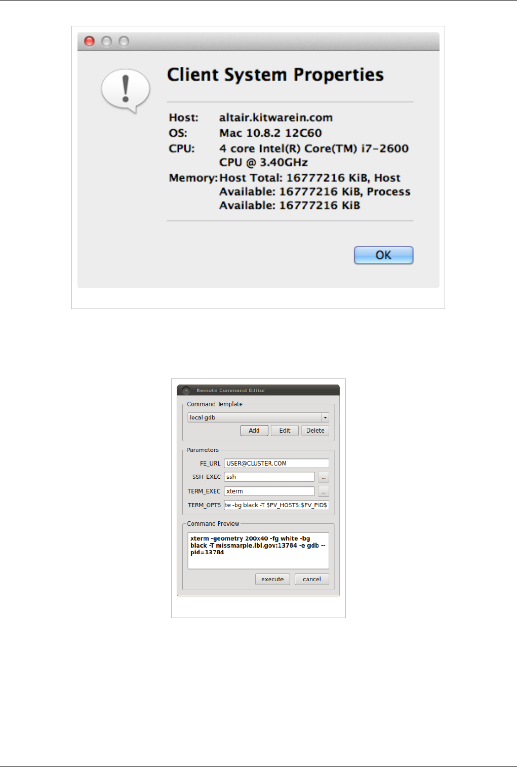
Host Properties Dialog
The Host context menu provides a Host properties dialog which reports various system details such as the OS
version, CPU version, and memory installed and available to the the host context and process context. While,
the Memory Inspector panel reports memory use as a percent of the available in the given context, the host
properties dialog reports the total installed and available in each context. Comparing the installed and available
memory can be used to determine if you are impacted by resource limits.
Memory Inspector 30
Figure: Host properties dialog
Advanced Debugging Features
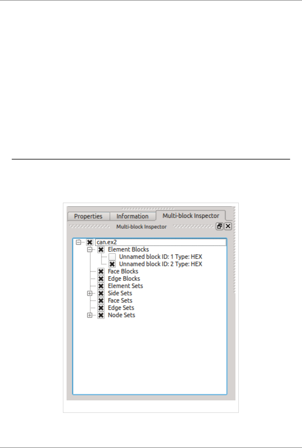
Remote Commands
Figure The remote command dialog.
The Memory Inspector Panel provides a remote (or local) command feature allowing one to execute a shell
command on a given host. This feature is exposed via a specialized Rank item context menu. Because we have
information such as a rank's process id, individual processes may be targeted. For example this allows one to quickly
attach a debugger to a server process running on a remote cluster. If the target rank is not on the same host as the
client then the command is considered remote otherwise it is consider local. Therefor remote commands are executed
via ssh while local commands are not. A list of command templates is maintained. In addition to a number of
pre-defined command templates, users may add templates or edit existing ones. The default templates allow one to:

Memory Inspector 31
• attach gdb to the selected process
• run top on the host of the selected process
• send a signal to the selected process
Prior to execution, the selected template is parsed and a list of special tokens are replaced with runtime determined
or user provide values. User provided values can be set and modified in the dialog's parameter group. The command,
with tokens replaced, is shown for verification in the dialog's preview pane.
The following tokens are available and may be used in command templates as needed:
$TERM_EXEC$
The terminal program which will be used execute commands. On Unix systems typically xterm is used, while
on Windows systems typically cmd.exe is used. If the program is not in the default path then the full path must
be specified.
$TERM_OPTS$
Command line arguments for the terminal program. On Unix these may be used to set the terminals window
title, size, colors, and so on.
$SSH_EXEC$
The program to use to execute remote commands. On Unix this is typically ssh, while on Windows one option
is plink.exe. If the program is not in the default path then the full path must be specified.
$FE_URL$
Ssh URL to use when the remote processes are on compute nodes that are not visible to the outside world. This
token is used to construct command templates where two ssh hops are made to execute the command.
$PV_HOST$
The hostname where the selected process is running.
$PV_PID$
The process-id of the selected process.
Note: On Window's the debugging tools found in Microsoft's SDK need to be installed in addition to Visual Studio
(eg. windbg.exe). The ssh program plink.exe for Window's doesn't parse ANSI escape codes that are used by Unix
shell programs. In general the Window's specific templates need some polishing.
Stack Trace Signal Handler
The Process Group's context menu provides a back trace signal handler option. When enabled, a signal handler is
installed that will catch signals such as SEGV, TERM, INT, and ABORT and print a stack trace before the process
exits. Once the signal handler is enabled one may trigger a stack trace by explicitly sending a signal. The stack trace
signal handler can be used to collect information about crashes, or to trigger a stack trace during deadlocks, when it's
not possible to ssh into compute nodes. Often sites that restrict users ssh access to compute nodes often provide a
way to signal a running processes from the login node. Note, that this feature is only available on systems the
provide support for POSIX signals, and currently we only have implemented stack-trace for GNU compatible
compilers.
Memory Inspector 32
Compilation and Installation Considerations
If the system on which ParaView will run has special resource limits enforced, such as job-wide memory use limits,
or non-standard per-process memory limits, then the system administrators need to provide this information to the
running instances of ParaView via the following environment variables. For example those could be set in the batch
system launch scripts.
PV_HOST_MEMORY_LIMIT
for reporting host-wide resource limits
PV_PROC_MEMORY_LIMIT
for reporting per-process memory limits that are not enforced via standard Unix resource limits.
A few of the debugging features (such as printing a stack trace) require debug symbols. These features will work
best when ParaView is built with CMAKE_BUILD_TYPE=Debug or for release builds
CMAKE_BUILD_TYPE=RelWithDebugSymbols.
Multi-block Inspector
Introduction
The Multi-Block Inspector panel allows users to change the rendering and display properties for individual blocks
within a multi-block data set.
Multi-block Inspector Panel
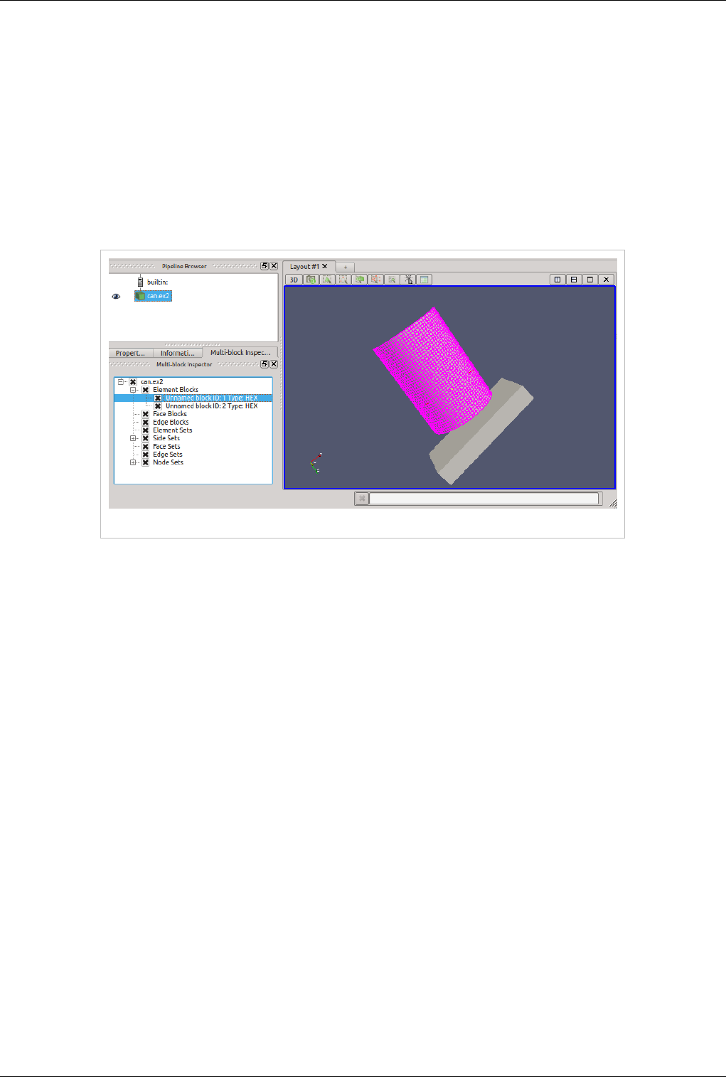
Multi-block Inspector 33
Block Visibility
The visibility of individual blocks can be changed by toggling the check box next to their name. By default, blocks
will inherit the visibility status of their parent block. Thus, changing the visibility of a non-leaf block will also
change the visibility of each child block.
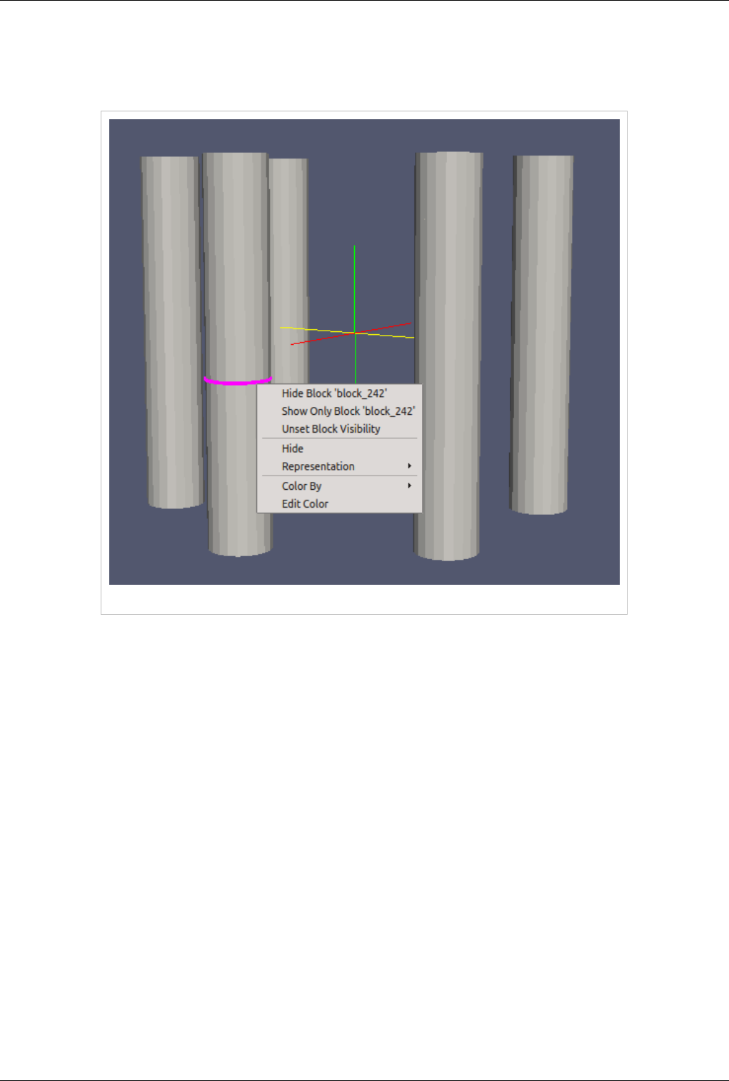
Selection Linking
Selections made in the render-view will be linked with the items in the multi-block inspector and visa versa. Using
block selection (keyboard shortcut: 'b') and clicking on a block will result in that block being highlighted in the tree
view.
Block Selection Linking
35
Displaying Data
Views, Representations and Color Mapping
This chapter covers different mechanisms in ParaView for visualizing data. Through these visualizations, users are
able to gain unique insight on their data.
Understanding Views
Views
When the ParaView application starts up, you see a 3D viewport with an axes at the center. This is a view. In
ParaView, views are frames in which the data can be seen. There are different types of views. The default view that
shows up is a 3D view which shows rendering of the geometry extracted from the data or volumes or slices in a 3D
scene. You can change the default view in the Settings dialog (Edit | Settings (in case of Mac OS X, ParaView |
Preferences)).
Figure 4.1 ParaView view screen
There may be parameters that are available to the user that control how the data is displayed e.g. in case of 3D view,
the data can be displayed as wireframes or surfaces, where the user selects the color of the surface or uses a scalar for
coloring etc. All these options are known as Display properties and are accessible from the Display tab in the Object
Views, Representations and Color Mapping 36
Inspector.
Since there can be multiple datasets shown in a view, as well as multiple views, the Display tabs shows the
properties for the active pipeline object (changed by using the Pipeline Browser, for example) in the active view.
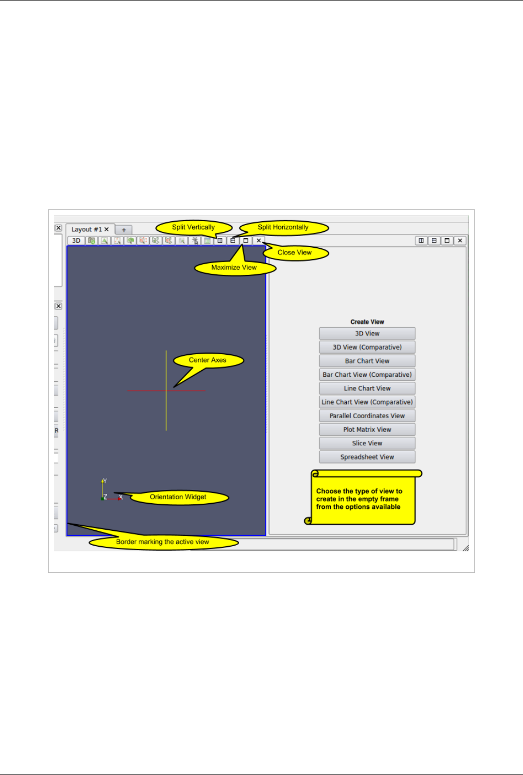
Multiple Views
ParaView supports showing multiple views side by side. To create multiple views, use the controls in the top right
corner of the view to split the frame vertically or horizontally. You can also maximize a particular view to
temporarily hide other views. Once a view-frame is split, you will see a list of buttons showing the different types of
views that you can create to place in that view. Simply click the button to create the view of your choice.
You can swap view position by dragging the title bar for a view frame and dropping it into the title bar for another
view.
Figure 4.2 View options in ParaView
Starting with ParaView 3.14, users can create multiple tabs to hold a grid of views. When in tile-display mode, only
the active tab is shown on the tile-display. Thus, this can be used as a easy mechanism for switching views shown on
a tile display for presentations.
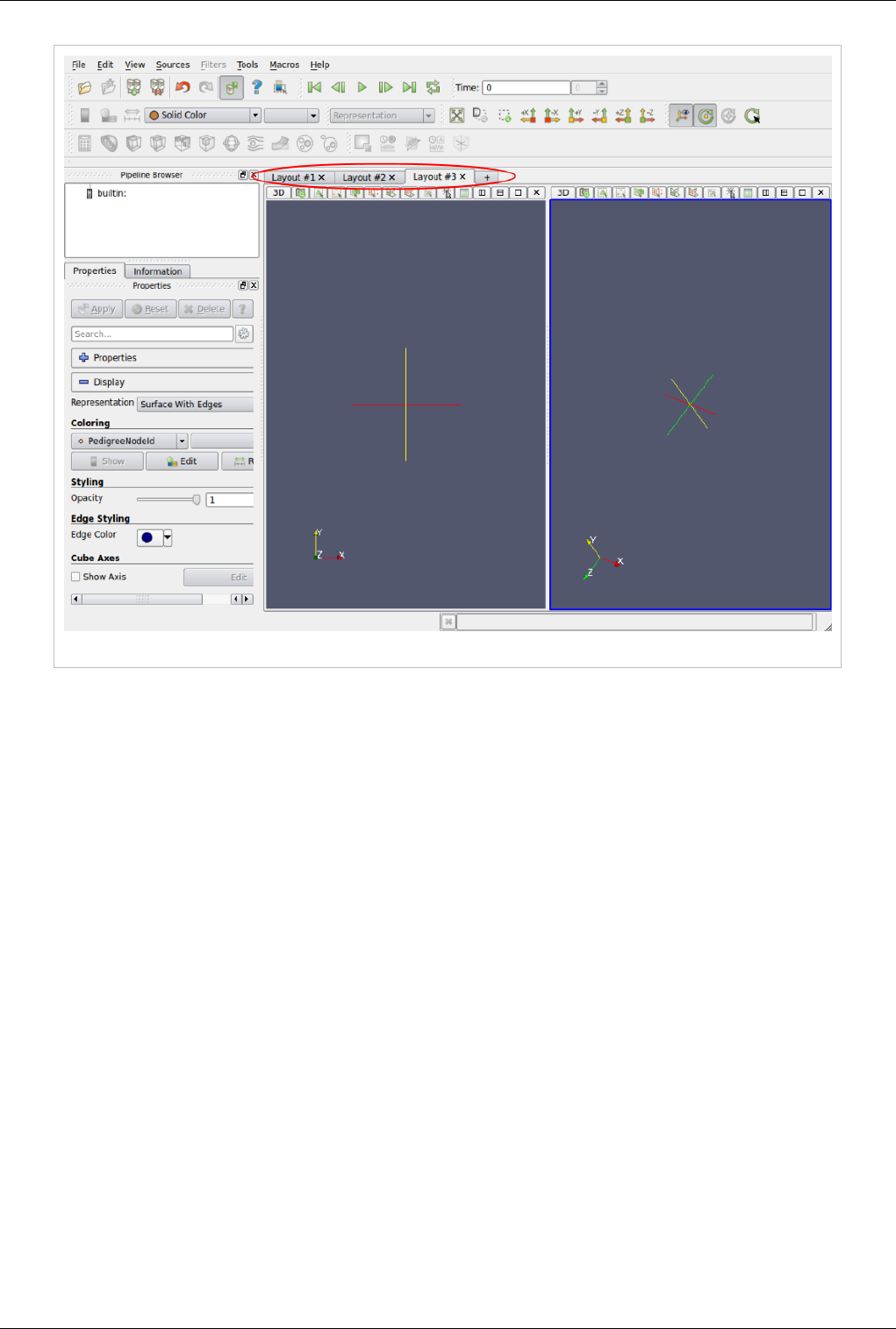
Views, Representations and Color Mapping 37
Figure 4.3 Multiple Tabs for laying out views in ParaView
Some filters, such as Plot Over Line may automatically split the view frame and show the data in a particular type of
view suitable for the data generated by the filter.
Active View
Once you have multiple views, the active view is indicated by a colored border around the view frame. Several
menus as well as toolbar buttons affect the active view alone. Additionally, they may become enabled/disabled based
on whether that corresponding action is supported by the active view.
The Display tab affects the active view. Similarly, the eye icon in the Pipeline Browser, next to the pipeline objects,
indicates the visibility state for that object in the active view.
When a new filter, source or reader is created, if possible it will be displayed by default in the active view, otherwise,
if will create a new view.
Views, Representations and Color Mapping 38
Types of Views
This section covers the different types of views available in ParaView. For each view, we will talk about the controls
available to change the view parameters using View Settings as well as the parameters associated with the Display
Tab for showing data in that view.
3D View
3D view is used to show the surface or volume rendering for the data in a 3D world. This is the most commonly used
view type.
When running in client-server mode, 3D view can render data either by bringing the geometry to the client and then
rendering it there or by rendering it on the server (possibly in parallel) and then delivering the composited images to
the client. Refer to the Client-Server Visualization chapter for details.
This view can also be used to visualize 2D dataset by switching its interaction mode to the 2D mode. This can be
achieved by clicking on the button labelled "3D" in the view local toolbar. The label will automatically turn to 2D
and the 2D interaction will be used as well as parallel projection.
Interaction
Interacting with the 3D view will typically update the camera. This makes it possible to explore the visualization
scene. The default buttons are shown in Table 4.1 and they can be changed using the Application Settings dialog.
Table 4.1
Modifier Left Button Middle Button Right Button
Rotate Pan Zoom
Shift Roll Rotate Pan
Control Zoom Rotate Zoom
This view can dynamically switch to a 2D mode and follow the interaction shown in Table 4.2 and they can be
changed using the Application Settings dialog.
Table 4.2
Modifier Left Button Middle Button Right Button
Pan Pan Zoom
Shift Zoom Zoom Zoom
Control Zoom Zoom Pan
This view supports selection. You can select cells or points either on the surface or those within a frustum. Selecting
cells or points makes it possible to extract those for further inspection or to label them. Details about data querying
and selection can be found the Quantitative analysis chapter.
Views, Representations and Color Mapping 39
View Settings
The View Settings dialog is accessible through the Edit | View Settings menu or the tool button in the left corner of
the view can be used to change the view settings per view.
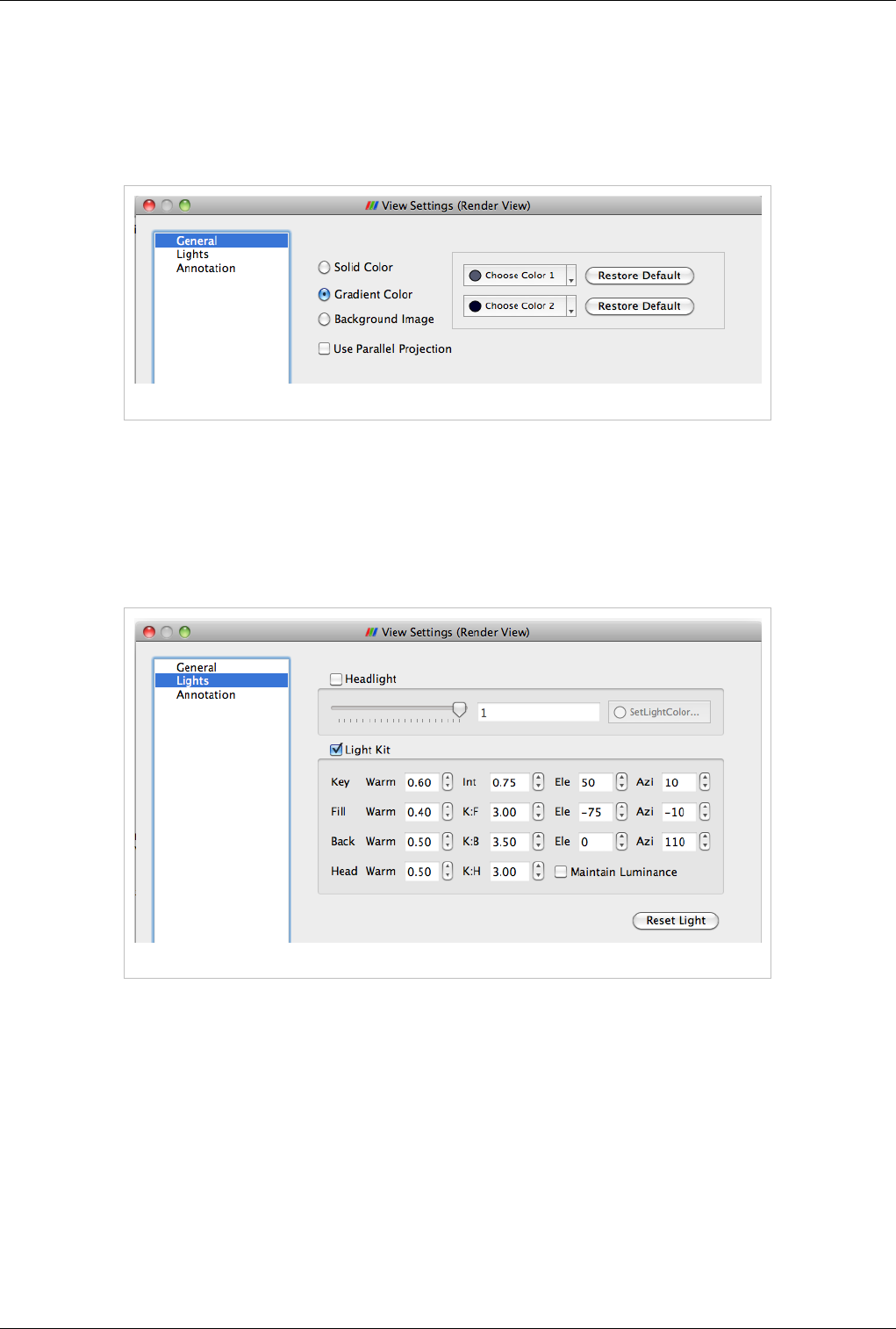
General
Figure 4.4 General tab in the View Settings menu
The General tab allows the user to choose the background color. You can use a solid color, gradient or a background
image.
By default the camera uses perspective projection. To switch to parallel projection, check the Use Parallel Projection
checkbox in this panel.
Lights
Figure 4.5 Lights tab in the View Settings menu
The 3D View requires lights to illumniate the geometry being rendered in the scene. You can control these lights
using this pane.

Views, Representations and Color Mapping 40
Annotation
Figure 4.6 Annotation tab in the View Settings menu
The annotation pane enables control of the visibility of the center axes and the orientation widget. Users can also
make the orientation widget interactive so that they can manually place the widget at location of their liking.
Display Properties
Users can control how the data from any source or filter is shown in this view using the Display tab. This section
covers the various options available to a user for controlling appearance of the rendering in the 3D view.
View
The View menu has three options for controlling how the data is viewed. These are described in Table 4.3.
Figure 4.6 View menu
Table 4.3
Name Usage
Visible Checkbox used to toggle the visibility of the data in the view. If it disabled, it implies that the data cannot be shown in this view.
Selectable Checkbox used to toggle whether the data gets selected when using the selection mechanism for selecting and sub-setting data.
Zoom to Data Click this button to zoom the camera so that the dataset is completely fits within the viewport.
Views, Representations and Color Mapping 41
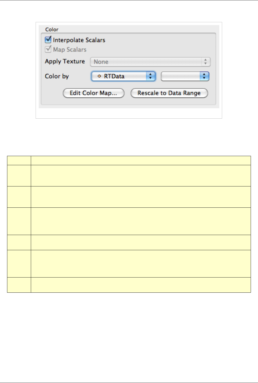
Color
Figure 4.8 Color options
The color group allows users to pick the scalar to color with or set a fixed solid color for the rendering. The options
in Figure 4.8 are described in detail in Table 4.4
Table 4.4
Name Usage
Interpolate
Scalars
If selected, the scalars will be interpolated within polygons and the scalar mapping happens on a per pixel basis. If not selected, then
color mapping happens at points and colors are interpolated which is typically less accurate. This only affects when coloring with
point arrays and has no effect otherwise. This is disabled when coloring using a solid color.
Map Scalars If the data array can be directly interpreted as colors, then you can uncheck this to not use any lookup table. Otherwise, when
selected, a lookup table will be used to map scalars to colors. This is disabled when the array is not of a type that can be interpreted as
colors (i.e. vtkUnsignedCharArray).
Apply
Texture
This feature makes it possible to apply a texture over the surface. This requires that the data has texture coordinates. You can use
filters like Texture Map to Sphere, Texture Map to Cylinder or Texture Map to Plane to generate texture coordinates when they are
not present in the data. To load a texture, select Load from the combo box which will pop up a dialog allowing you to choose an
image. Otherwise, select from already loaded textures listed in the combo box.
Color By This feature enables coloring of the surface/volume. Either choose the array to color with or set the solid color to use. When volume
rendering, solid coloring is not possible, you must choose the data array to volume render with.
Set solid
color
Used to set the solid color. This is available only when Color By is set to use Solid Color. ParaView defines a notion of a color
palette consisting of different color categories. To choose a color from one of these predefined categories, click the arrow next to this
button. It will open up a drop down with options to choose from. If you use a color from the palette, it is possible to globally change
the color by changing the color palette e.g. for printing or for display on screen etc.
Edit Color
Map...
You can edit the color map or lookup table by clicking the Edit Color Map button. It is only shown when an array is chosen in the
Color By combo-box.
Views, Representations and Color Mapping 42
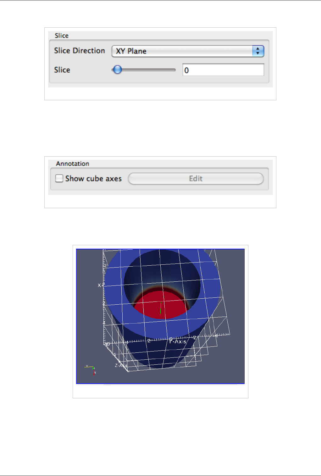
Slice
Figure 4.9 Slice options
The slice controls are available only for image datasets (uniform rectilinear grids) when the representation type is
Slice. The representation type is controlled using the Style group on the Display tab. These allow the user to pick the
slice direction as well as the slice offset.
Annotation
Figure 4.10 Annotation options
Cube axes is an annotation box that can be used to show a scale around the dataset. Use the Show cube axes
checkbox to toggle its visibility. You can further control the apperance of the cube axes by clicking Edit once the
cube-axes is visible.
Figure 4.11 Show cube axes example
Views, Representations and Color Mapping 43
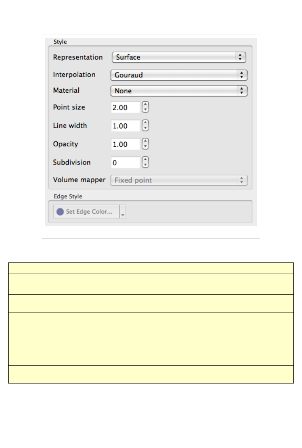
Style
Figure 4.12 shows the Style dialog box. The options in this dialog box are described in detail in Table 4.5 below.
Figure 4.12 Sytle dialog box
'Table 4.5
Name Usage
Representation Use this to change how the data is represented i.e. as a surface, volume, wireframe, points, or surface with edges.
Interpolation Choose the method used to shade the geometry and interpolate point attributes.
Point Size If your dataset contains points or vertices, this adjusts the diameter of the rendered points. It also affects the point size when
Representation is Points.
Line width If your dataset contains lines or edges, this scale adjusts the width of the rendered lines. It also affects the rendered line width
when Representation is Wireframe or Surface With Edges.
Opacity Set the opacity of the dataset's geometry. ParaView uses hardware-assisted depth peeling, whenever possible, to remove artifacts
due to incorrect sorting order of rendered primitives.
Volume
Mapper
When Representation is Volume, this combo box allows the user to choose a specific volume rendering technique. The techniques
available change based on the type of the dataset.
Set Edge Color This is available when Representation is Surface with Edges. It allows the user to pick the color to use for the edges rendered over
the surface.
Views, Representations and Color Mapping 44
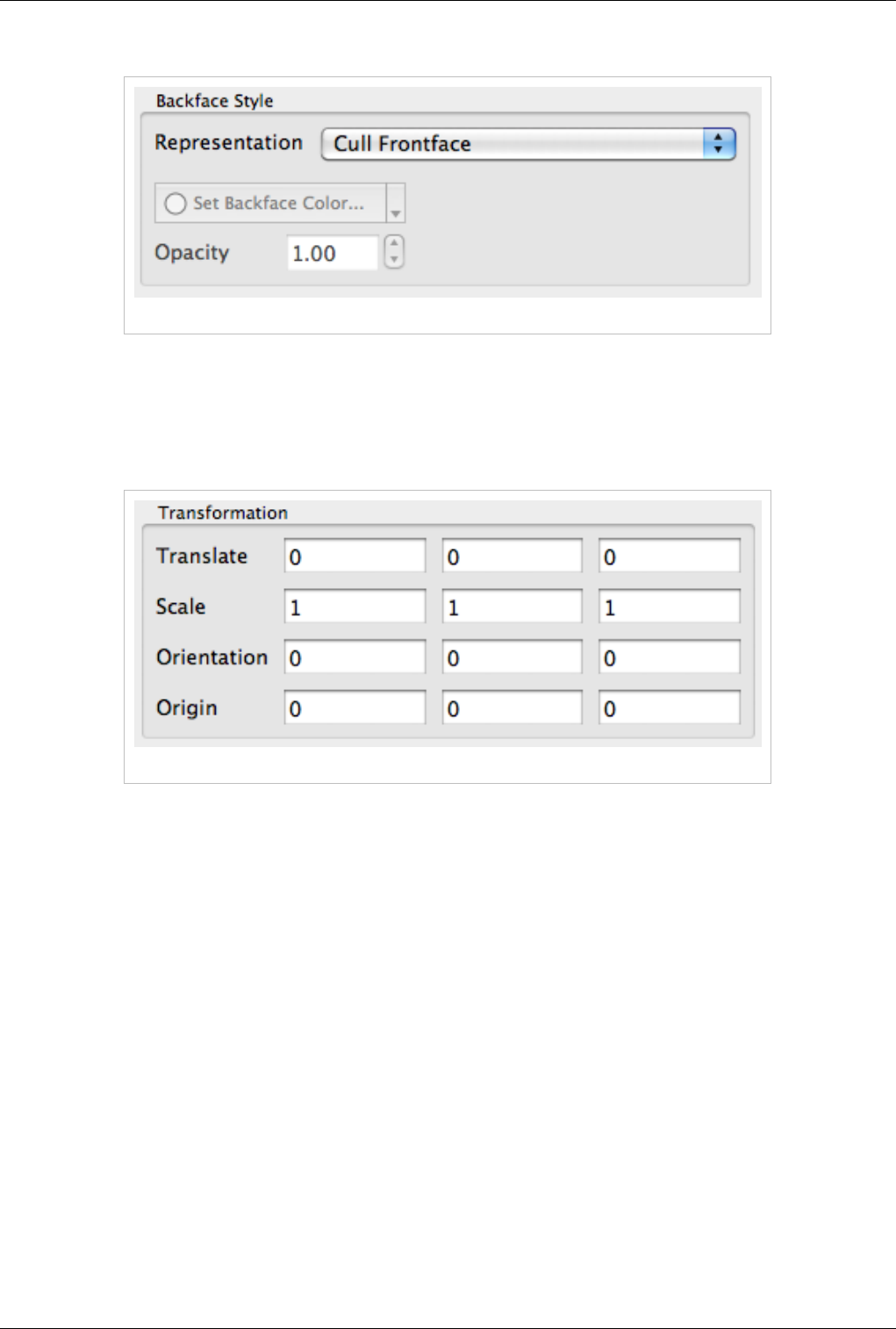
Backface Style
Figure 4.13 Backface Style dialog box
The Backface Style dialog box allows the user to define backface properties. In computer graphics, backface refers
to the face of a geometric primitive with the normal point away from the camera. Users can choose to hide the
backface or front face, or specify different characteristics for the two faces using these settings.
Transformation
Figure 4.14 Transformation dialog box
These settings allow the user to transform the rendered geometry, without actually transforming the data. Note that
since this transformation happens during rendering, any filters that you apply to this data source will still be working
on the original, untransformed data. Use the Transform filter if you want to transform the data instead.
2D View
This view does not exist anymore as it has been replaced by a more flexible 3D view that can switch from a 3D to
2D mode dynamically. For more information, please see the 3D view section.
Spreadsheet View
Spreadsheet View is used to inspect the raw data in a spreadsheet. When running in client-server mode, to avoid
delivering the entire dataset to the client for displaying in the spreadsheet (since the data can be very large), this view
streams only visible chunks of the data to the client. As the user scrolls around the spreadsheet, new data chunks are
fetched.
Unlike some other views, this view can only show one dataset at a time. For composite datasets, it shows only one
block at a time. You can select the block to show using the Display tab.
Views, Representations and Color Mapping 45
Interaction
In regards to usability, this view behaves like typical spreadsheets shown in applications like Microsoft Excel or
Apple Pages:
• You can scroll up and down to inspect new rows.
• You can sort any column by clicking on the header for the column. Repeated clicking on the column header
toggles the sorting order. When running in parallel, ParaView uses sophisticated parallel sorting algorithms to
avoid memory and communication overheads to sort large, distributed datasets.
• You can double-click on a column header to toggle a mode in which only that column is visible. This reduces
clutter when you are interested in a single attribute array.
• You can click on rows to select the corresponding elements i.e. cells or points. This is not available when in
"Show selected only mode." Also, when you create a selection in other views e.g. the 3D view, the rows
corresponding to the selected elements will be highlighted.
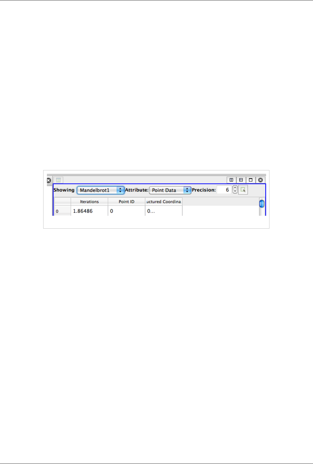
Header
Unlike other views, Spreadsheet View has a header. This header provides quick access to some of the commonly
used functionality in this view.
Figure 4.17 Spreadsheet View Header
Since this view can only show one dataset at a time, you can quickly choose the dataset to show using the Showing
combo box. You can choose the attribute type i.e. point attributes, cell attributes, to display using the Attribute
combo box. The Precision option controls the number of digits to show after decimal point for floating point
numbers. Lastly, the last button allows the user to enter the view in a mode where it only shows the selected rows.
This is useful when you create a selection using another view such as the 3D view and want to inspect the details for
the selected cells or points.
Views, Representations and Color Mapping 46
View Settings
Currently, no user settable settings are available for this view.
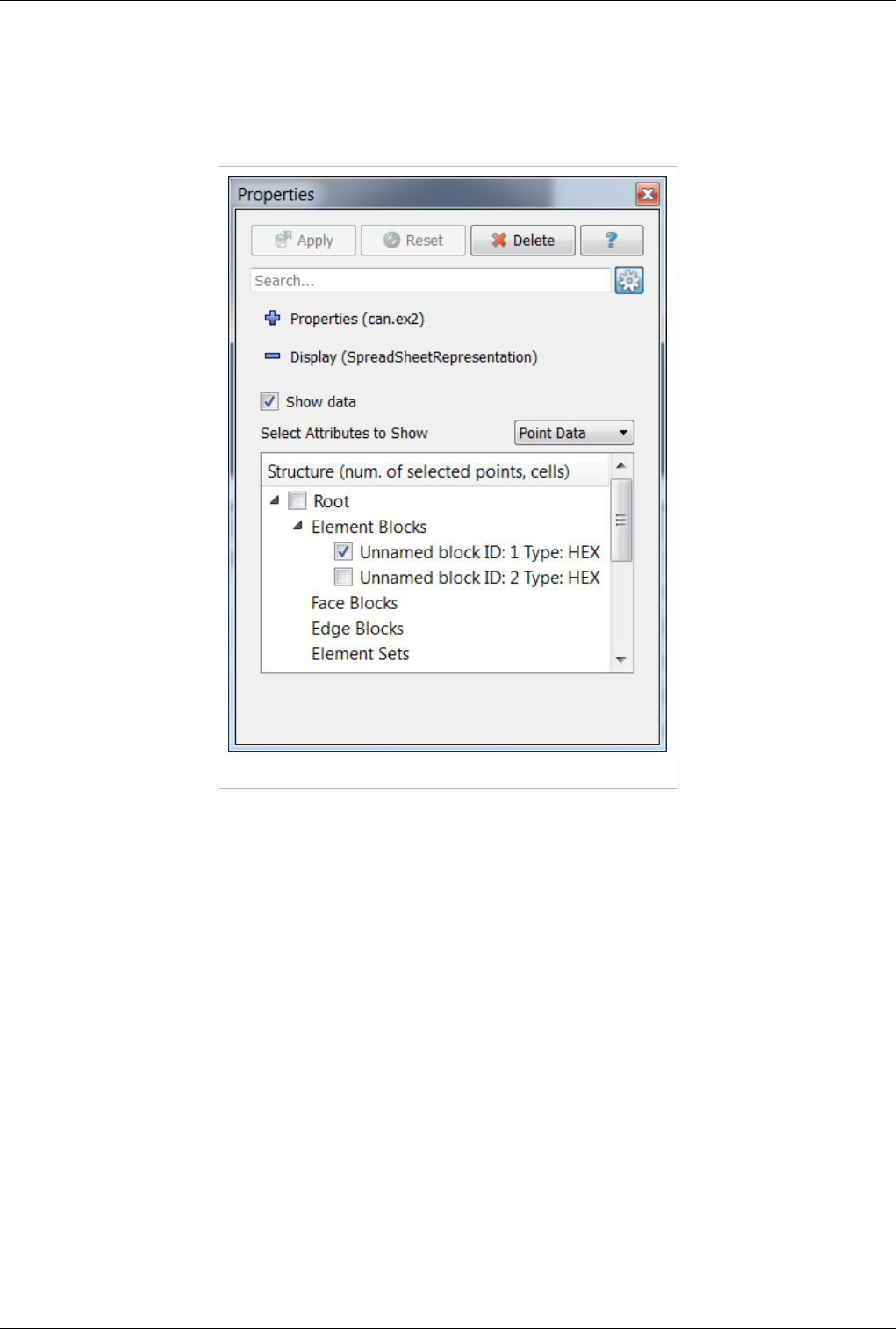
Display Properties
Figure 4.18 Display tab in the Object Inspector
The display properties for this view provide the same functionality as the header. Additionally, when dealing with
composite datasets, the display tab shows a widget allowing the user to choose the block to display in the view.
Line Chart View
A traditional 2D line plot is often the best option to show trends in small quantities of data. A line plot is also a good
choice to examine relationships between different data values that vary over the same domain.
Any reader, source, or filter that produces plottable data can be displayed in an XY plot view. ParaView stores its
plotable data in a table (vtkTable). Using the display properties, users can choose which columns in the table must be
plotted on the X and Y axes.
As with the other view types, what is displayed in the active XY plot view is displayed by and controllable with the
eye icons in the Pipeline Browser panel. When an XY plot view is active, only those filters that produce plotable
output have eye icons.
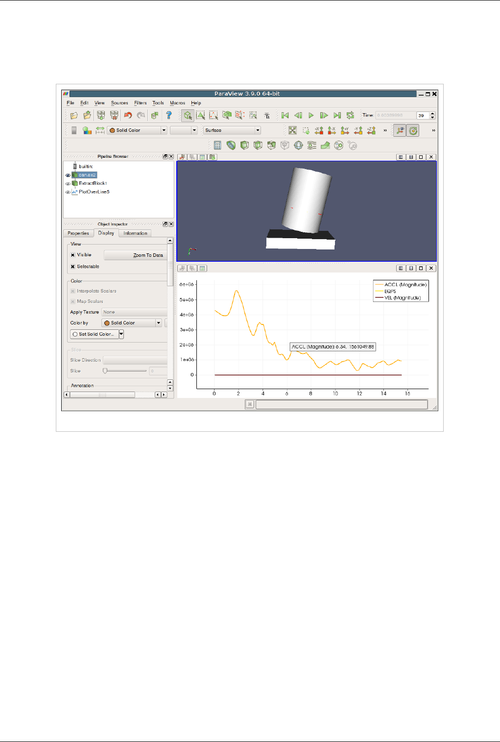
The XY plot view is the preferred view type for the Plot over Line, Plot Point over Time, Plot Cell over Time, Plot
Field Variable over Time, and Probe Location over Time filters. Creating any one of these filters will automatically
create an XY plot view for displaying its output. Figure 4.19 shows a plot of the data values within a volume as they
vary along three separate paths. The top curve comes from the line running across the center of the volume, where
the largest values lie. The other two curves come from lines running near the edges of the volume.
Views, Representations and Color Mapping 47
Unlike the 3D and 2D render view, the charting views are client-side views i.e. they deliver the data to be plotted to
the client. Hence ParaView only allows results from some standard filters such as Plot over Line in the line chart
view by default. However it is also possible to plot cell or point data arrays for any dataset by apply the Plot Data
filter.
Figure 4.19 Plot of data values within a volume
Interaction
The line chart view supports the following interaction modes:
•Right-click and drag to pan
•Left-click and drag to select
•Middle-click and drag to zoom to region drawn.
•Hover over any line in the plot to see the details for the data at that location.
To reset the view, use the Reset Camera button in the Camera Toolbar.
Views, Representations and Color Mapping 48
View Settings
The View Settings for Line Chart enable the user to control the appearance of the chart including titles, axes
positions etc. There are several pages available in this dialog. The General page controls the overall appearance of
the chart, while the other pages controls the appearance of each of the axes.
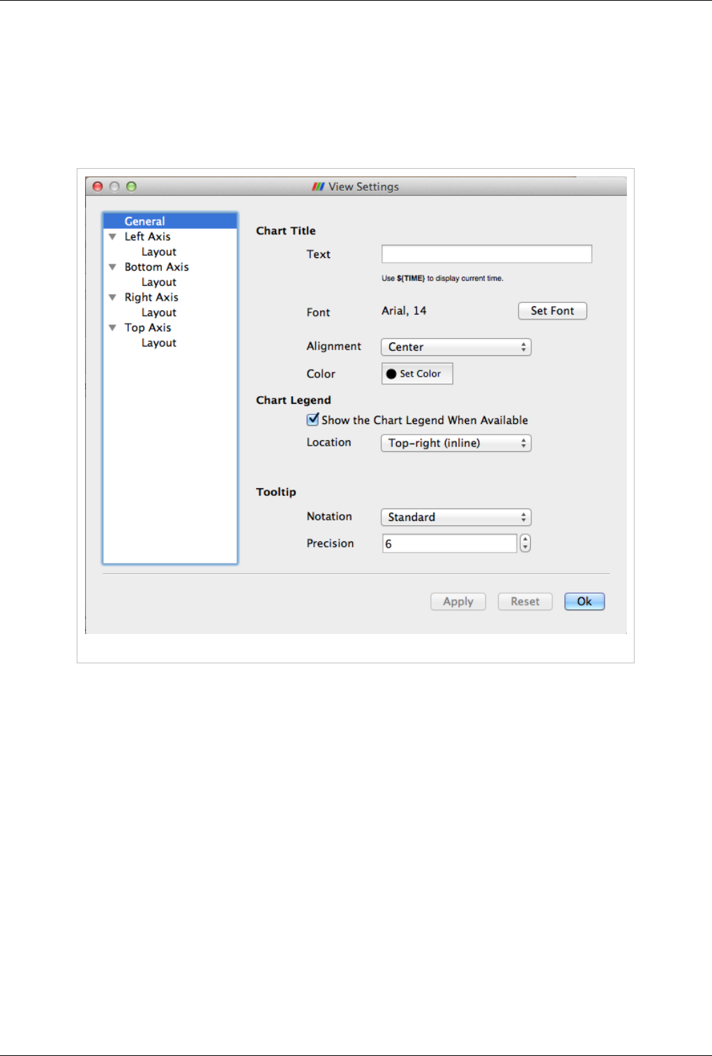
General Settings Page
Figure 4.20 General Settings panel
This page allows users to edit settings not related to any of the axes.
Chart Title
Specify the text and characteristics (such as color, font) for the title for the entire chart. To show the current
animation time in the title text, simply use the keyword ${TIME}.
Chart Legend
When data is plotted in the view, ParaView shows a legend. Users can change the location for the legend.
Tooltip
Specify the data formatting for the hover tooltips. The default Standard switches between scientific and fixed point
notations based on the data values.
Views, Representations and Color Mapping 49
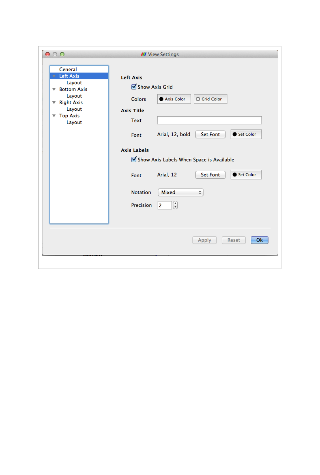
Axis Settings Page
On this page you can change the properties of a particular axis. Four pages are provided for each of the axes. By
clicking on the name of the axis, you can access the settings page for the corresponding axes.
Figure 4.21 Axis Settings panel
Left/Bottom/Right/Top Axis
• Show Axis Grid: controls whether a grid is to be drawn perpendicular to this axis
• Colors: controls the axis and the grid color
Axis Title
Users can choose a title text and its appearance for the selected axis.
Axis Labels
Axis labels refers to the labels drawn at tick marks along the axis. Users can control whether the labels are rendered
and their appearance including color, font and formatting. User can control the locations at which the labels are
rendered on the Layout page for the axis.
• Show Axis Labels When Space is Available : controls label visibility along this axis
• Font and Color: controls the label font and color
• Notation: allows user to choose between Mixed, Scientific and Fixed point notations for numbers
• Precision: controls precision after '.' in Scientific and Fixed notations
Views, Representations and Color Mapping 50
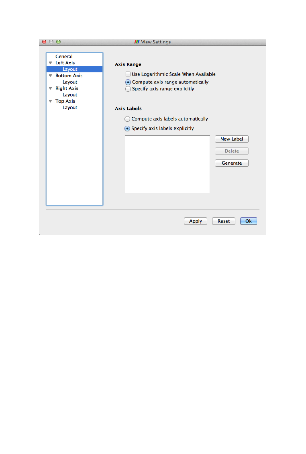
Axis Layout Page
This page allows the user to change the axis range as well as label locations for the axis.
Figure 4.22 Axis Layout panel
Axis Range
Controls how the data is plotted along this axis.
• Use Logarithmic Scale When Available: Check this to use a log scale unless the data contains numbers <= 0.
• Compute axis range automatically: Select this button to let the chart use the optimal range and spacing for this
axis. The chart will adjust the range automatically every time the data displayed in the view changes.
• Specify axis range explicitly: Select this button to specify the axis range explicitly. When selected, user can enter
the minimum and maximum value for the axis. The range will not change even when the data displayed in the
view changes. However, if the user manually interacts with the view (i.e. pans, or zooms), then the range
specified is updated based on the user's interactions.
Views, Representations and Color Mapping 51
Axis Labels
Controls how the labels are rendered along this axis. Users can control the labeling independently of the axis range.
• Compute axis labels automatically: Select this button to let the chart pick label locations optimally based on the
viewport size and axis range.
• Specify axis labels explicitly: Select this button to explicitly specify the data values at which labels should be
drawn.
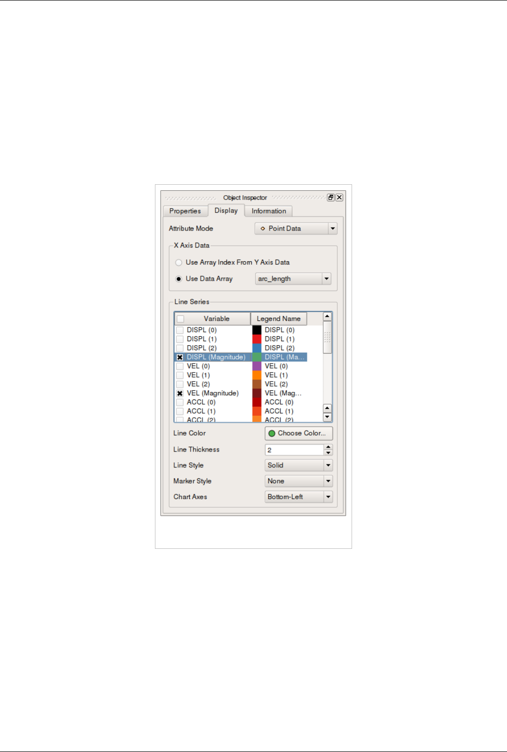
Display Properties
Display Properties for the Line Chart view allow the user to choose what arrays are plotted along which of the axes
and the appearance for each of the lines such as its color, thickness and style.
Figure 4.24 Display Properties within the Object
Inspector
• Attribute Mode: pick which attribute arrays to plot i.e. point arrays, cell arrays, etc.
• X Axis Data: controls the array to use as the X axis.
• Use Array Index From Y Axis Data: when checked, results in ParaView using the index in data-array are
plotted on Y as the X axis.
• Use Data Array: when checked the user can pick an array to be interpreted as the X coordinate.
• Line Series: controls the properties of each of the arrays plotted along the Y axis.
• Variable: check the variable to be plotted.
• Legend Name: click to change the name used in the legend for this array.
Select any of the series in the list to change following properties for that series. You can select multiple entries to
change multiple series.

Views, Representations and Color Mapping 52
• Line Color: controls the color for the series.
• Line Thickness: controls the thickness for the series.
• Line Style: controls the style for the line.
• Marker Style: controls the style used for those markers, which can be placed at every data point.
Bar Chart View
Traditional 2D graphs present some types of information much more readily than 3D renderings do; they are usually
the best choice for displaying one and two dimensional data. The bar chart view is very useful for examining the
relative quantities of different values within data, for example.
The bar chart view is used most frequently to display the output of the histogram filter. This filter divides the range
of a component of a specified array from the input data set into a specified number of bins, producing a simple
sequence of the number of values in the range of each bin. A bar chart is the natural choice for displaying this type of
data. In fact, the bar chart view is the preferred view type for the histogram filter. Filters that have a preferred view
type will create a view of the preferred type whenever they are instantiated.
When the new view is created for the histogram filter, the pre-existing 3D view is made smaller to make space for
the new chart view. The chart view then becomes the active view, which is denoted with a red border around the
view in the display area. Clicking on any view window makes it the active view. The contents of the Object
Inspector and Pipeline Browser panels change and menu items are enabled or disabled whenever a different view
becomes active to reflect the active view’s settings and available controls. In this way, you can independently control
numerous views. Simply make a view active, and then use the rest of the GUI to change it. By default, the changes
you make will only affect the active view.
As with the 3D View, the visibility of different datasets within a bar chart view is displayed and controlled by the
eye icons in the Pipeline Browser. The bar chart view can only display datasets that contain chartable data, and when
a bar chart view is active, the Pipeline Browser will only display the eye icon next to those datasets that can be
charted.
ParaView stores its chartable data in 1D Rectilinear Grids, where the X locations of the grid contain the bin
boundaries, and the cell data contain the counts within each bin. Any source or filter that produces data in this format
can be displayed in the bar chart view. Figure 4.25 shows a histogram of the values from a slice of a data set.
The Edit View Options for chart views dialog allows you to create labels, titles, and legends for the chart and to
control the range and scaling of each axis.
The Interaction, Display Properties as well as View Settings for this view and similar to those for the Line Chart.
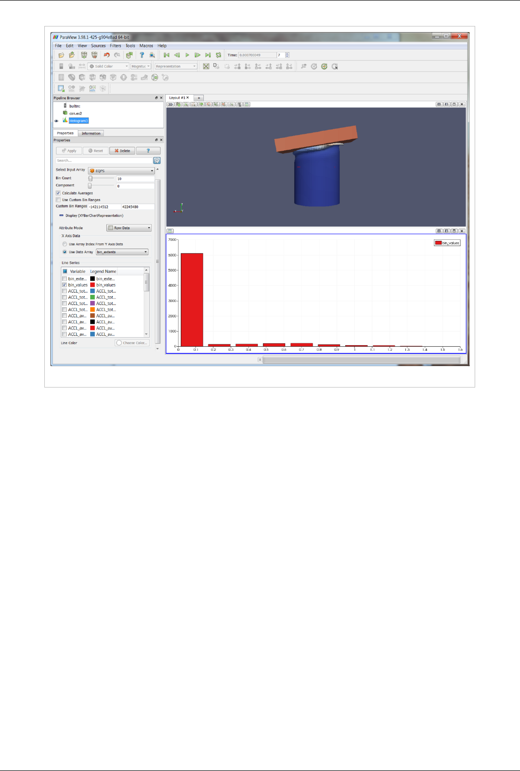
Views, Representations and Color Mapping 53
Figure 4.25 Histogram of values from a slice of a dataset
Plot Matrix View
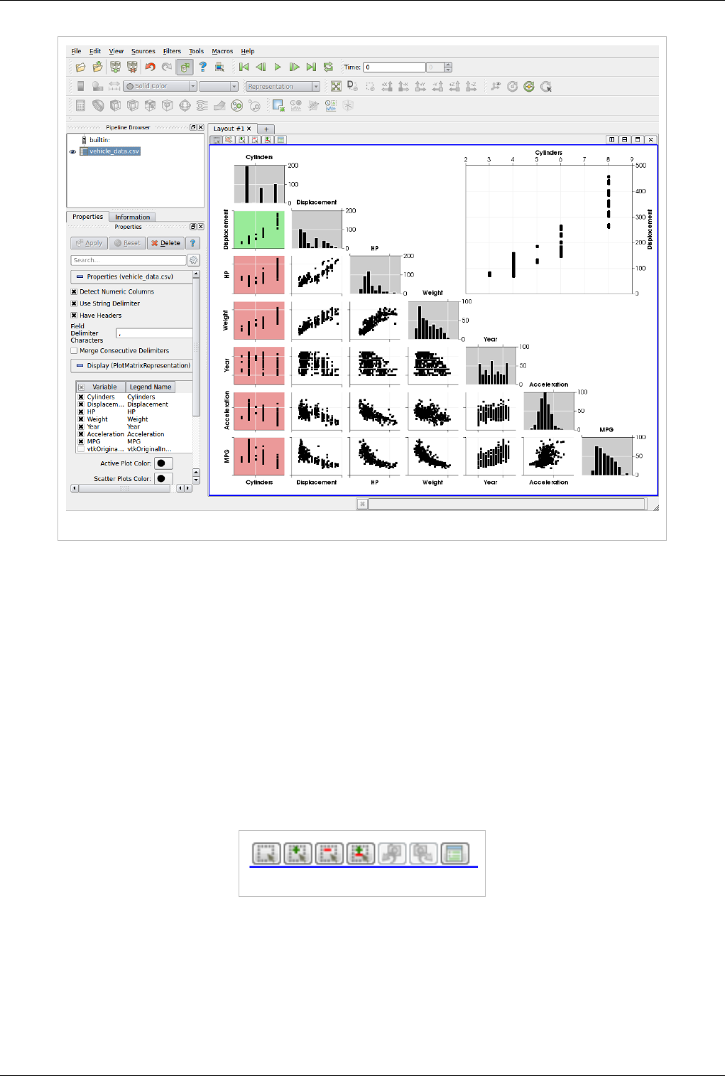
The new Plot-Matrix-View (PMV) allows visualization of multiple dimensions of your data in one compact form. It
also allows you to spot patterns in the small scatter plots, change focus to those plots of interest and perform basic
selection. It is still at an early stage, but the basic features should already be useable, including iterative selection for
all charts (add, remove and toggle selections with Ctrl or Shift modifiers on mouse actions too).
The PMV can be used to manage the array of plots and the vtkTable mapping of columns to input of the charts. Any
filters or sources with an output of vtkTable type should be able to use the view type to display their output. The
PMV include a scatter plot, which consists of charts generated by plotting all vtkTable columns against each other,
bar charts (histograms) of vtkTable columns, and an active plot which shows the active chart that is selected in the
scatter plot. The view offer offers new selection interactions to the charts, which will be describe below in details.
As with the other view types, what is displayed in the active PMV is displayed by and controllable with the eye icons
in the Pipeline Browser panel. Like XY chart views, the PMVs are also client-side views i.e. they deliver the data to
be plotted to the client.
Views, Representations and Color Mapping 54
Plot Matrix View Plots of data values in a vtkTable
Interaction
The scatter plot does not support direct user interactions on its charts, except click. When clicking any charts within
the scatter plot, the active plot (The big chart in the top right corner) will be updated to show the selected chart and
user can interact with the big chart as described below.
The Active Plot in PMV supports the following interaction modes: By default,
•Left-click and drag to pan
•Middle-button to zoom
•Hover over any point in the plot to see the details for the data at that location.
There are also four type of selection mode will change the default user interactions. These mode can be invoked by
clicking one the buttons shown at the top left corner of the PMV window, where the "View Setting" and camera
buttons are.
Selection Modes
•Start Selection will make Left-click and drag to select
•Add selection will select and add to current selection
•Subtract selection will subtract from current selection
•Toggle selection will toggle current selection
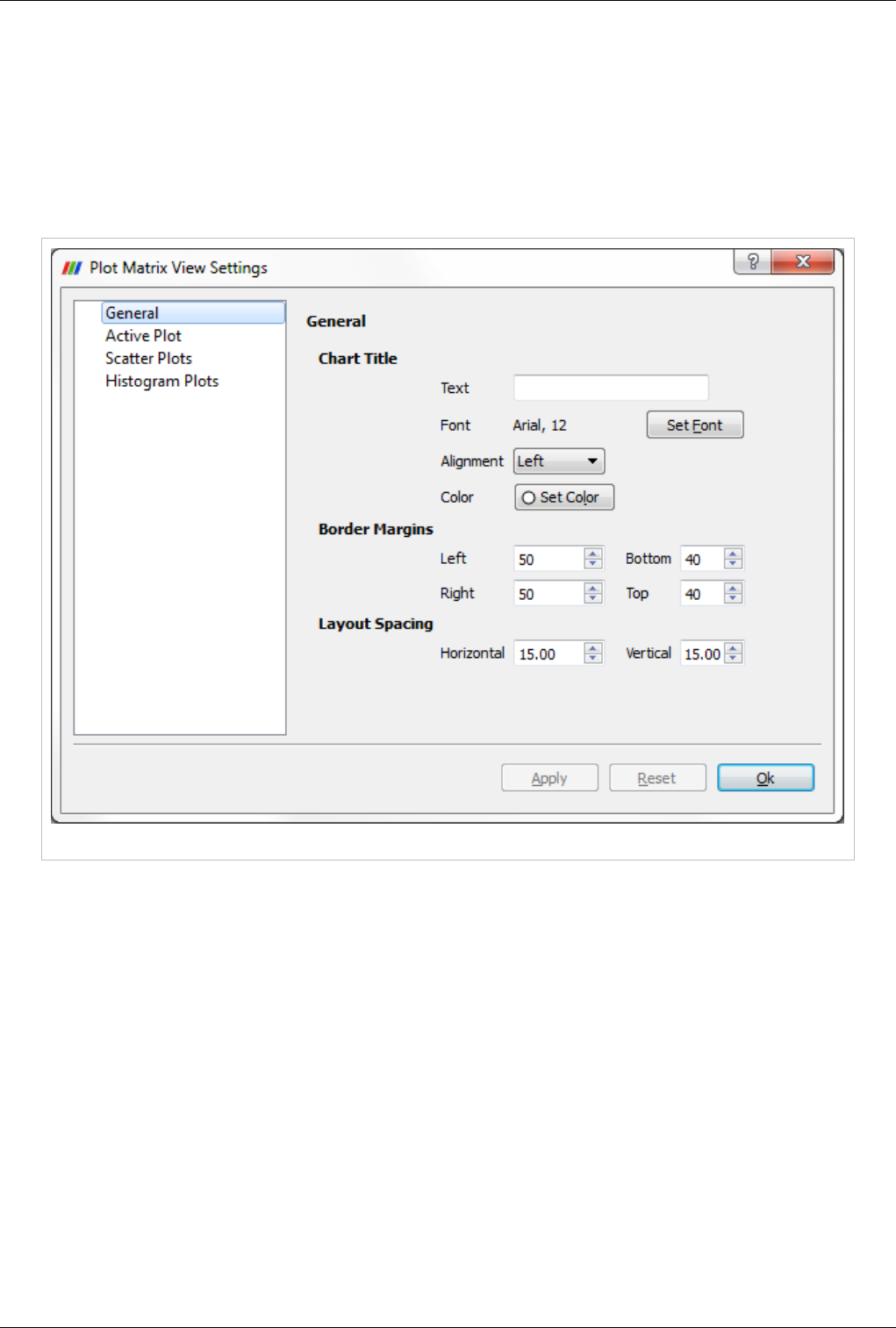
Views, Representations and Color Mapping 55
View Settings
The View Settings for PMV enable the user to control the appearance of the PMV including titles of the active plot,
the plot/histogram colors, the border margin and gutter size of the scatter plot, etc. There are several pages available
in this dialog. The General page controls the overall appearance of the chart, while the other pages controls the
appearance of other of each plot types.
General Settings Page
Plot Matrix View General Settings
This page allows users to change the title, border margins and layout spacings. To show the current animation time
in the title text, simply use the keyword ${TIME}. Users can further change the font and alignment for the title.
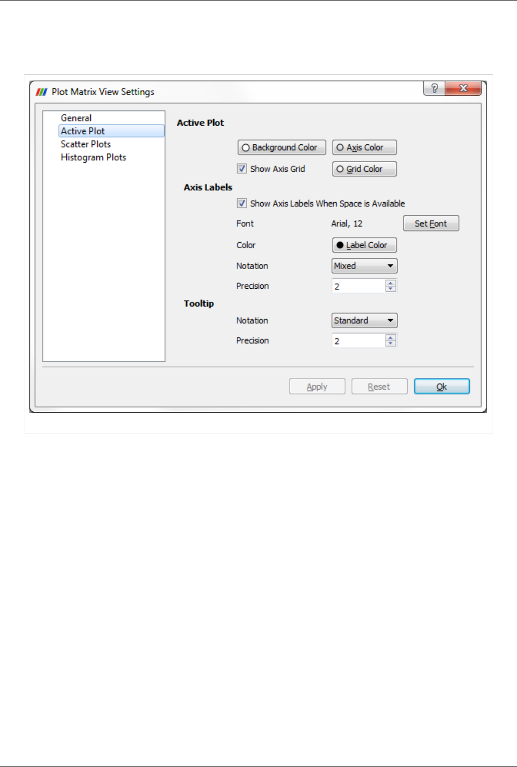
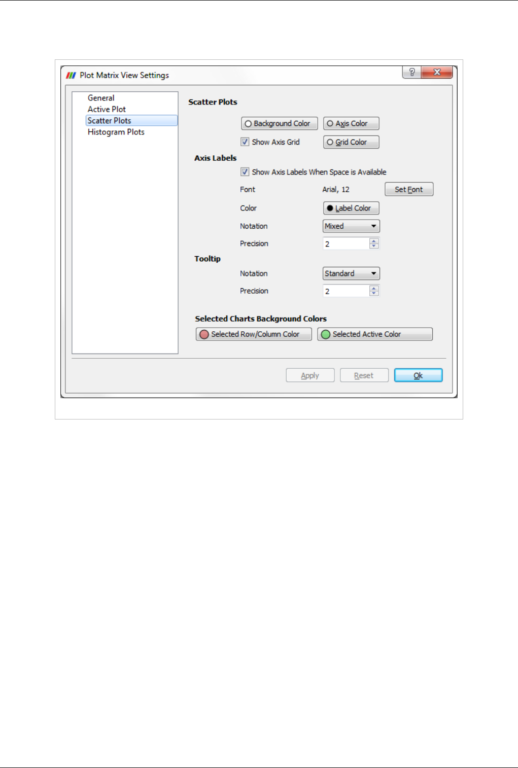
Views, Representations and Color Mapping 57
Scatter Plot Settings Page
This page allows the user to change the same settings as the Active Plot, and also color for selected charts.
Plot Matrix View Scatter Plot Settings
•Selected Row/Column Color is for the charts has the same row or column as the selected chart.
•Selected Active Color is for the selected chart.
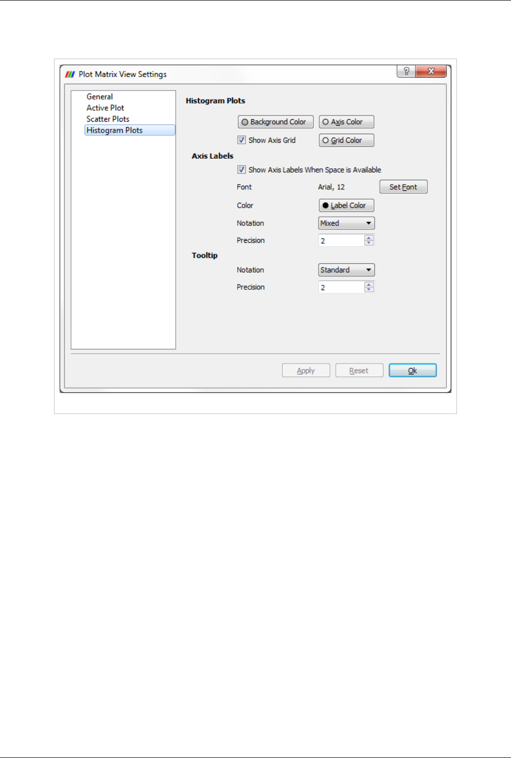
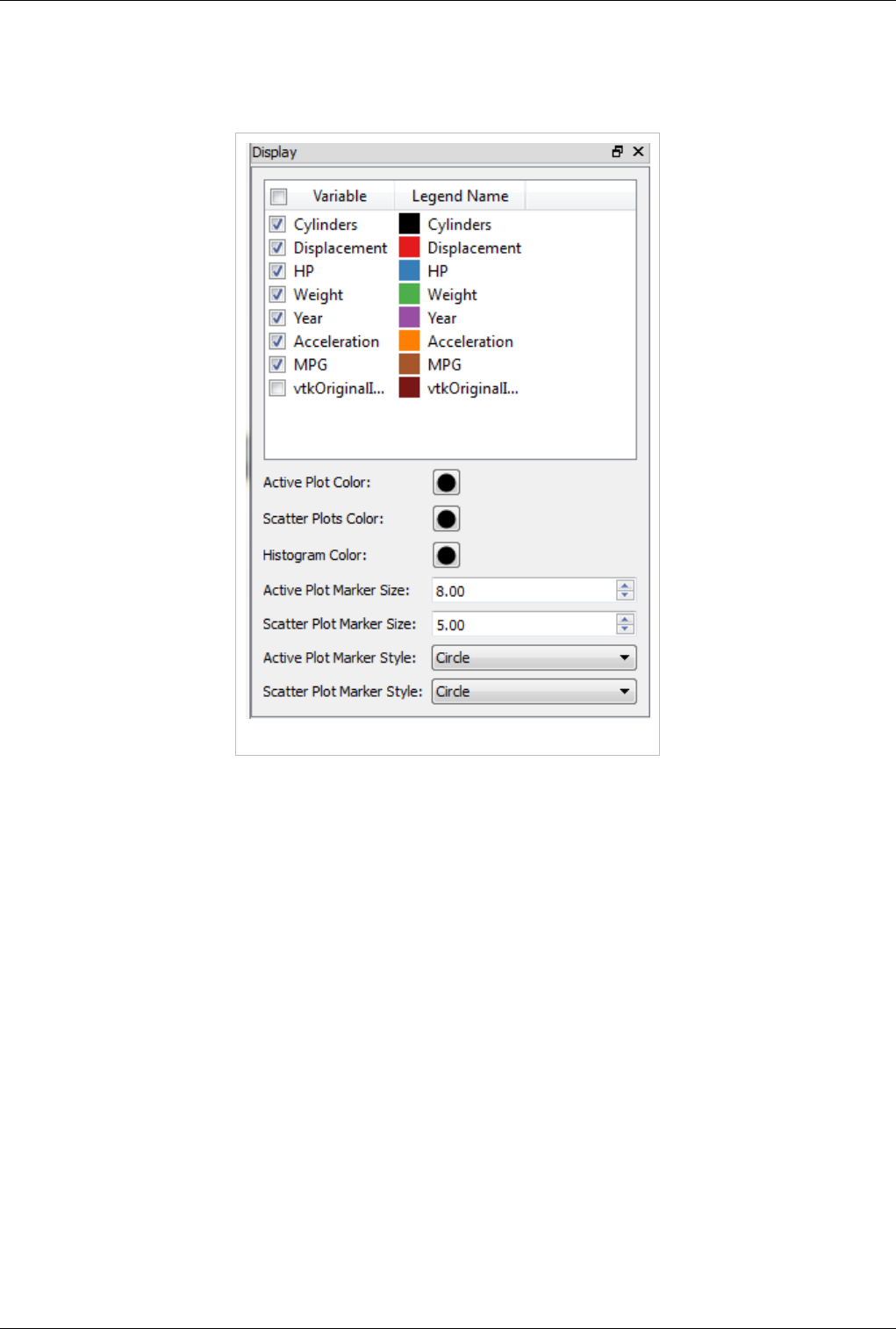
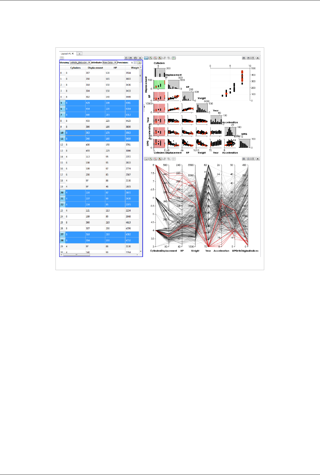
Views, Representations and Color Mapping 60
Linked Selections
The point selections made in the Active Plot (top right chart) will be displayed in the bottom left triangle (scatter
plots). Also, the selection is linked with other view types too.
Plot Matrix View Linked Selection
Slice View
The Slice View allow the user to slice along the three axis (X,Y,Z) any data that get shown into it. The range of the
scale for each axis automatically update to fit the bounding box of the data that is shown. By default no slice is
created and the user will face as a first step just an empty Outline representation.
• In order to Add a new slice along an axis, just double click between the axis and the 3D view for the axis you are
interested in at the position you want.
• To Remove a slice, double click on the triangle that represent that slice on a given axis.
• To toggle the 'Visibility of a slice, right click on the triangle that represent that slice on a given axis.
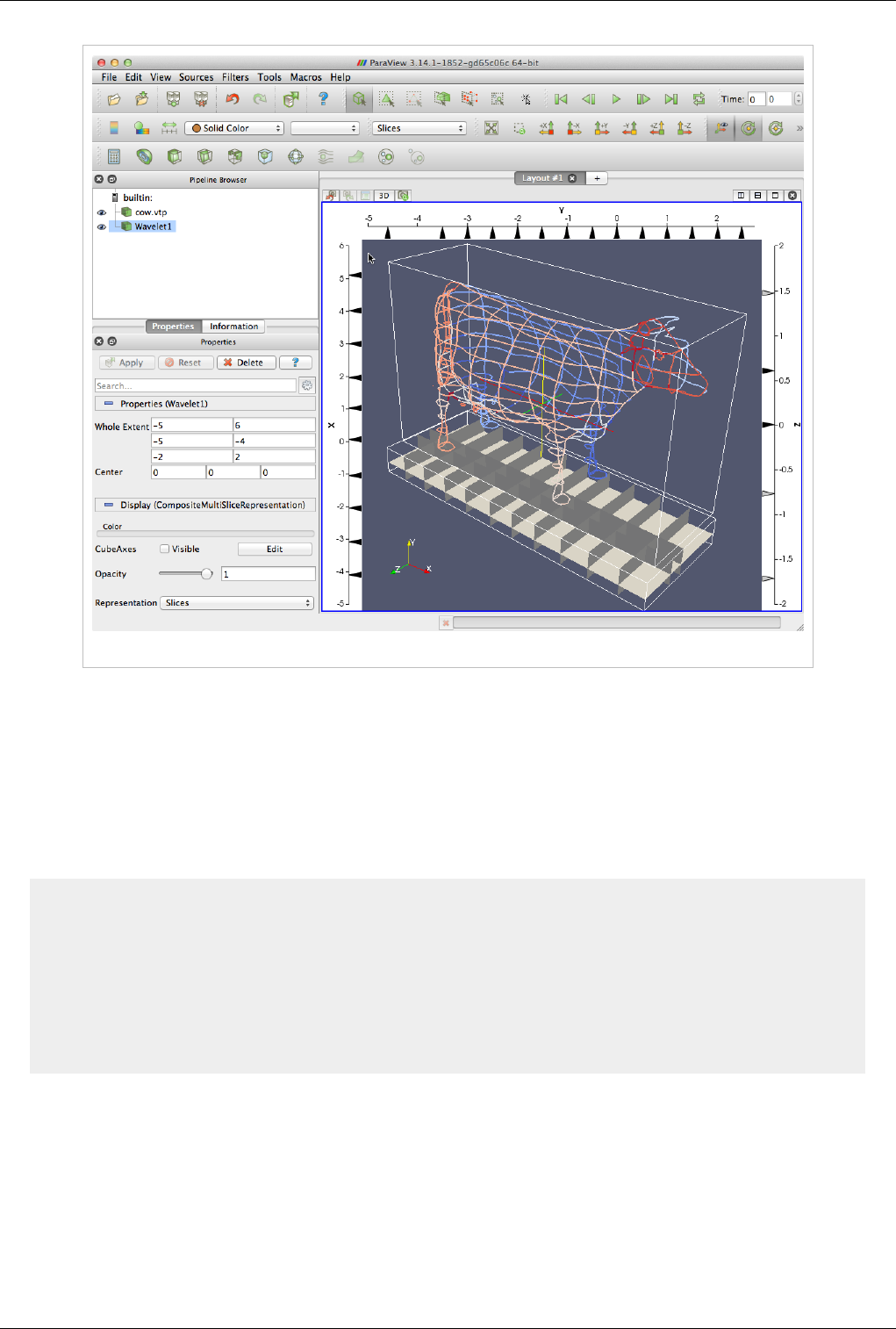
Views, Representations and Color Mapping 61
Slice View of a the Cow (Surface mesh) and the Wavelet (Image Data)
A video going over its usage can be seen at the following address: https:/ / vimeo. com/ 50316342
Python usage
The Slice View can easily be managed through Python. To do so, you will need to get a reference to the view proxy
and then you will be able to change the slice location of the representations that are shown in the view by just
changing the property for each axis. The following code snippet illustrate a usage through the Python shell inside
ParaView.
> multiSliceView = GetRenderView()
> Wavelet()
> Show()
> multiSliceView.XSlicesValues = [-2.5, -2, -1, 0, 5]
> multiSliceView.YSlicesValues = range(-10,10,2)
> multiSliceView.ZSlicesValues = []
> Render()
Moreover, from Python you can even change slice origins and normals. Here is the list of property that you can
change with their default values:
• XSlicesNormal = [1,0,0]
• XSlicesOrigin = [0,0,0]
• XSlicesValues = []
• YSlicesNormal = [0,1,0]
• YSlicesOrigin = [0,0,0]
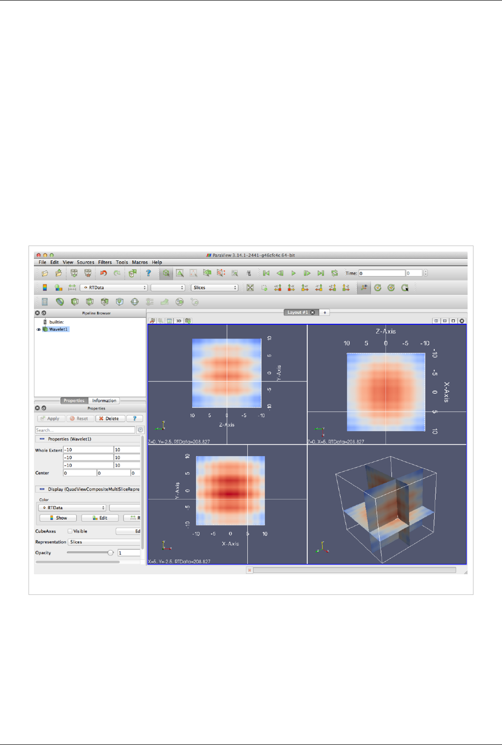
Views, Representations and Color Mapping 62
• YSlicesValues = []
• ZSlicesNormal = [0,0,1]
• ZSlicesOrigin = [0,0,0]
• ZSlicesValues = []
The Python integration can be seen in video here: https:/ / vimeo. com/ 50316542
Quad View
The Quad View come from a plugin that is provided along with ParaView. That view allow the user to slice along 3
planes any data that get shown into it. A point widget is used to represent the planes intersection across all the view
and can be grabbed and moved regardless the view we are interacting with. Information such as intersection position
for each axis is represented with a text label in each of the slice view. The slice views behave as 2D views by
providing pan and zoom interaction as well as parallel projection. In the bottom-right quarter there is a regular 3D
view that can contains the objects that are sliced but this object can be shown using a regular representations or the
"Slices" one which will show an Outline with the corresponding 3 cuts inside it.
Quad View
A video going over its usage can be seen at the following address: http:/ / vimeo. com/ 50320103 That view also
provide a dedicated option panel that allow the user to customize the cutting plane normals as well as the view up of
the slice views. Moreover, the slice origin can be manually entered in that panel for greater precision.
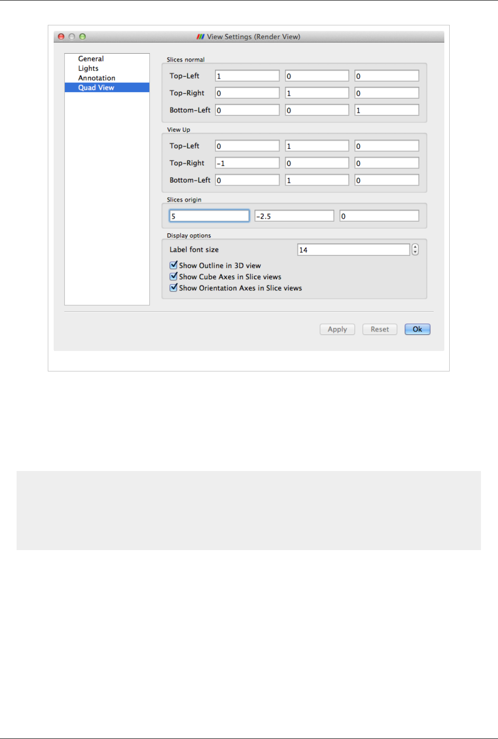
Views, Representations and Color Mapping 63
Quad View Option Panel
Python Usage
The Quad View can easily be managed through Python. To do so, you will need to get a reference to the view proxy
and then you will be able to change the slice location of the representations that are shown in the view by just
changing the view properties. The following code snippet illustrate a usage through the Python shell inside
ParaView.
> quadView = GetRenderView()
> Wavelet()
> Show()
> quadView.SlicesCenter = [1,2,3]
> Render()
Moreover, from Python you can change also the slice normals. Here is the list of property that you can change with
their default values:
• SlicesCenter = [0,0,0]
• TopLeftViewUp = [0,1,0]
• TopRightViewUp = [-1,0,0]
• BottomLeftViewUp = [0,1,0]
• XSlicesNormal = [1,0,0]
• XSlicesValues = [0]
• YSlicesNormal = [0,1,0]
• YSlicesValues = [0]
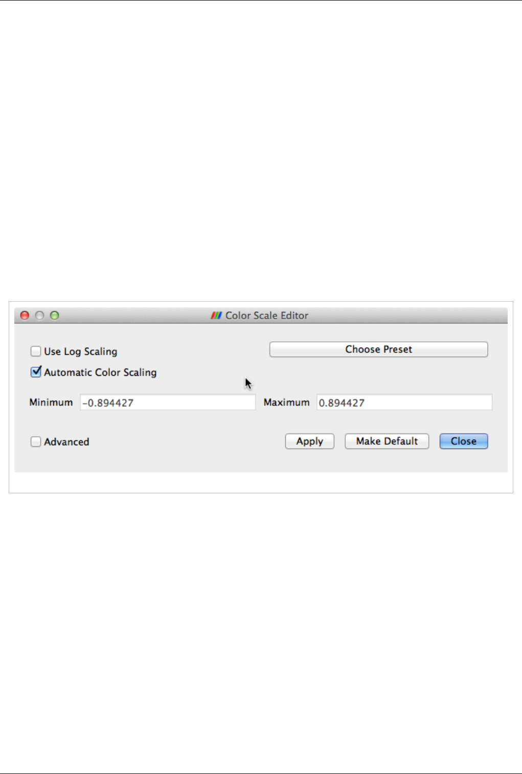
Views, Representations and Color Mapping 64
• ZSlicesNormal = [0,0,1]
• ZSlicesValues = [0]
And the layout is as follow:
• TopLeft = X
• TopRight = Y
• BottomLeft = Z
Color Transfer Functions
The interface for changing the color mapping and properties of the scalar bar is accessible from the Display tab of
the Object Inspector. Pressing the Edit Color Map button displays the interface for manipulating the color map and
scalar bar. The UI of Color Scale Editor as been both simplified and improved in many way. The first time the Color
Editor get shown, it will appear in its simple mode which appears to be enough for most ParaView users. Although,
in order to get full control on the Color Mapping in ParaView, you will need to select the Advanced checkbox. For
volume representation, the UI was fully revisited for a better management but for other type of representations, the
color editor is pretty much the same except that some buttons are rearranged and there are two more UI components
added. The status of the Advanced checkbox is kept into ParaView internal settings therefore the next time you get
back to the Color Editor it will allow come back the way you use it.
Simplified Color Editor

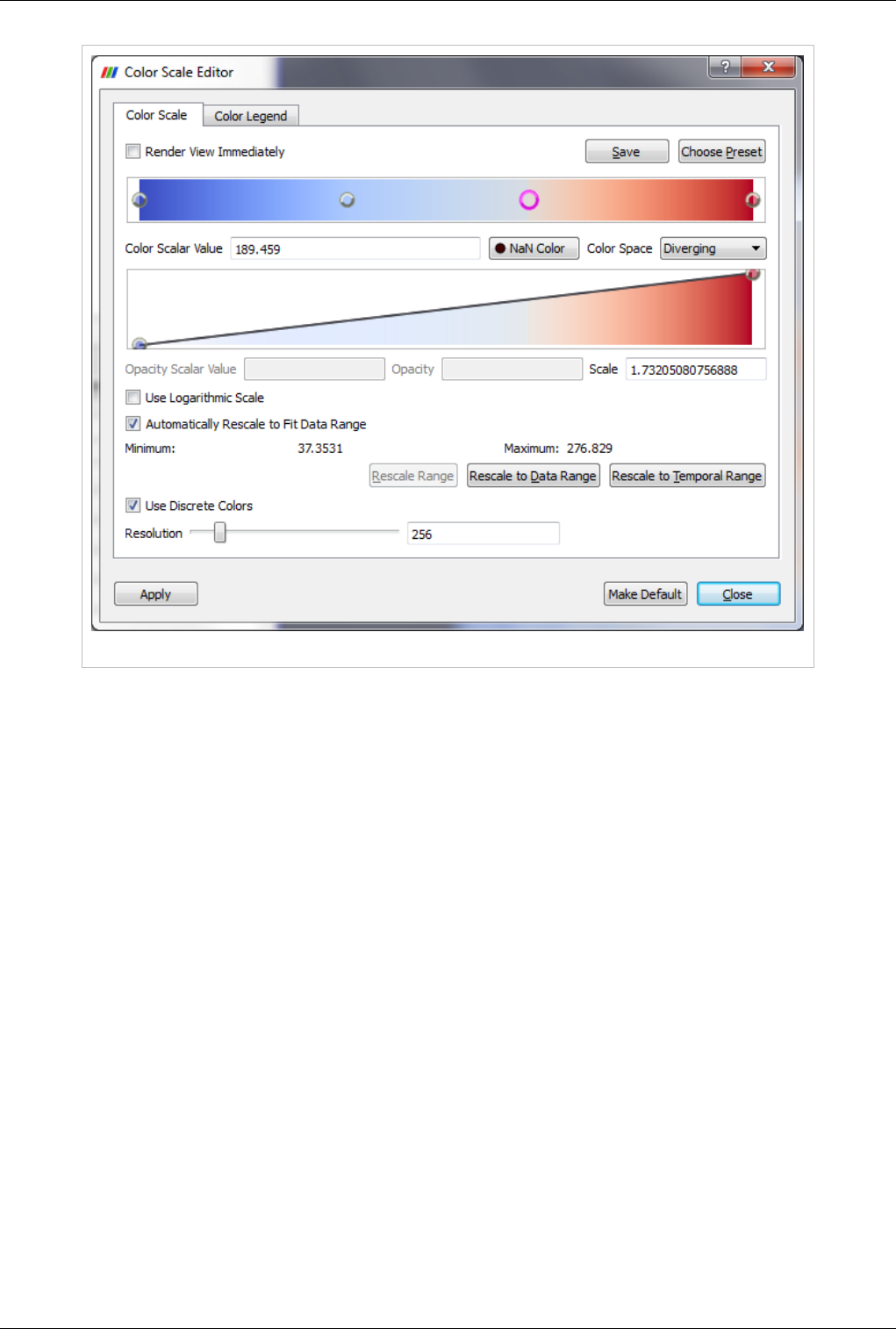
Views, Representations and Color Mapping 66
Advanced Volume Color Editor
The two new UI controls are "Render View Immediately" checkbox and "Apply" button so that users can have
control whether the render views should be updated immediately while editing the color transfer functions. This is
very helpful when working with very large dataset.
The main changes for the color editor is the separation of editing opacity function from the color-editing function for
volume representation. For surface representation, only one color-editing widget will show up (see screenshot
"Surface Color Editor"), which is essentially the same as before. The scalar range of this color map editor is shown
below the Automatically Rescale to Fit Data Range check box. The leftmost sphere corresponds to the minimum
scalar value, and the rightmost one corresponds to the maximum. Any interior nodes correspond to values between
these two extremes. New nodes may be added to the color editor by left-clicking in the editor; this determines the
scalar value associated with the node, but that value may be changed by typing a new value in the Scalar Value text
box below the color map editor or by clicking and dragging a node. The scalar value for a particular node may not be
changed such that it is less than that for a node left of it or greater than that for a node right of it.
When volume rendering (see screenshot "Volume Color Editor", two function-editing widgets will show up: the top
color-editing widget behave the same as for surface representation, which is used for editing scalar colors; the
second one is the new opacity-editing widget for editing opacity only. The vertical height of a node indicates its
opacity. Also, as in the color-editing widget, the leftmost sphere corresponds to the minimum scalar value, and the
rightmost one corresponds to the maximum. Any interior nodes correspond to values between these two extremes.
Again, new nodes may be added to the opacity-editor by left-clicking in the editor; this determines the scalar value
associated with the node, but that value may be changed by typing a new value in the Scalar Value text box below
the opacity editor or by clicking and dragging a node. Some new features are added to edit the opacity function (see
below screenshot "Opacity Function Editor", which is the same editor as "Volume Color Editor", but resized
vertically to have more space to show the opacity-editor)
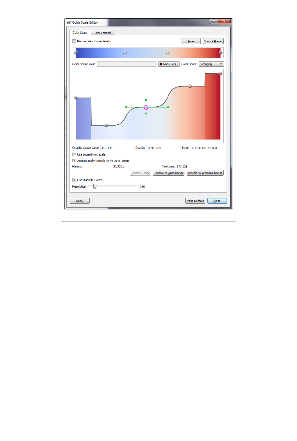
Views, Representations and Color Mapping 67
Opacity Function Editor
When a node is double-clicked in the opacity editor, four green handle widgets will be displayed based on the middle
point position and curve sharpness between this node and the nodes before and after it. When the mouse is moved
over the green sphere handle, it will become active (its center changes to magenta color) and can be dragged to
adjust the middle point position (horizontal handle) or curve sharpness (vertical handle). To exit this mode, just click
on another node.
When a node in the color-editor is clicked, it becomes highlighted (i.e., drawn larger than the other spheres in the
editor). In the "Volume Color Editor" above, the third node from the left has been selected. Clicking again on the
selected node displays a color selector from which you may select a new color for the node. The new color will also
be applied to the opacity-editor. Pressing the ‘d’ or Delete key while a node is selected removes that node from the
color-editor. Only the endpoint nodes may not be deleted. The same is true for removing nodes from opacity-editor.
For surface rendering, opacity is determined for an entire data set, not based on the underlying scalar values.
Below the color-editor is a text box for changing the scalar value associated with a given node. Only the scalar value
is associated with surface rendering. The scalar values at the endpoints may only be changed if the Automatically
Rescale to Fit Data Range check box (discussed later in this section) is unmarked. When volume rendering, there are
a set of three text boxes below opacity-editor that you may specify the scalar value, its opacity and scale per node in
the editor for the selected node. In volume rendering, the opacity is accumulated as you step through the volume
being rendered. The Scale value determines the unit distance over which the opacity is accumulated.
There are also controls to specify the color space and any color map preset you wish to save or use. The color spaces
available are RGB (red, green, blue), HSV (hue, saturation, value), Wrapped HSV, and CIELAB (a more
perceptually linear color space). The color space determines how the colors are interpolated between specified
values; the colors at the color map (or transfer function) editor nodes will remain the same regardless of the color
space chosen. If wrapped HSV is used, the interpolation will use the shortest path in hue, even going through the
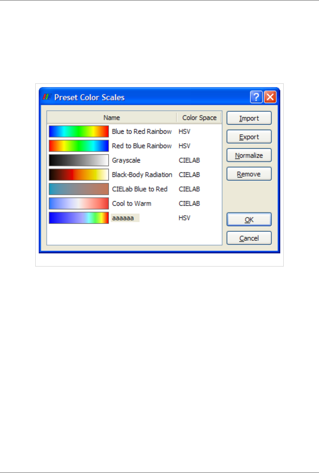
Views, Representations and Color Mapping 68
value hue = 0. For non-wrapped HSV, the hue interpolation will not pass through 0. A hue of zero sets the color to
red.
In addition to choosing the color space and modifying the color map or transfer function nodes, you may also create
and load preset color scales. When volume rendering, only the color map is stored; the scalar-to-opacity mapping is
not. To store your current settings as a preset, click the Save button. In the dialog box that appears, you may enter a
name for your new preset. By default, the scalar values from the data array being used are stored in the preset. If you
wish these values to be normalized between 0 and 1, press the Normalize button.
Figure 4.27 Dialog for selecting color scale presets
Any presets you save, in addition to the default ones provided by ParaView, are available by pressing the Choose
Preset button, causing the dialog shown below to be displayed. Selecting a preset and clicking OK causes the current
color map to be set to the chosen preset. Any user-defined presets may be normalized (as discussed above) or
removed from the list of presets entirely using the Normalize and Remove buttons, respectively. The default presets
are already normalized and may not be removed from the application.
Any of the color scale presets may be exported to a file using the Export button in the above dialog. The resulting
file(s) may then be copied to another computer for use with ParaView on a different machine. In order to load presets
that are stored in such files, press the Import button on the above dialog, and navigate to the desired color preset file.
If the current dataset is colored by an array of vectors, the Component menu will be enabled. It determines whether
the data is colored by a single vector component (X, Y, or Z) or by the vector’s Magnitude (the default). If the data is
colored by a single-component (scalar) array, then the Component menu is disabled.
If Use Logarithmic Scale is checked, then instead of the scalar values in the data array being used directly to
determine the colors, the base-10 logarithm of the data array values is computed, and the resulting value is used for
extracting a color from the color map. If the data array contains values for which a logarithm would produce invalid
results (i.e., any values less than or equal to 0), the range for the color map is changed to [0, 10] so that the logarithm
produces valid results.
By default, any data attribute that has been used to color a dataset currently loaded in ParaView, and whose name
and number of components match that of the array selected in the Color by menu, contributes to the range of the
color map. To change this behavior, first uncheck the Automatically Rescale to Fit Data Range check box. This
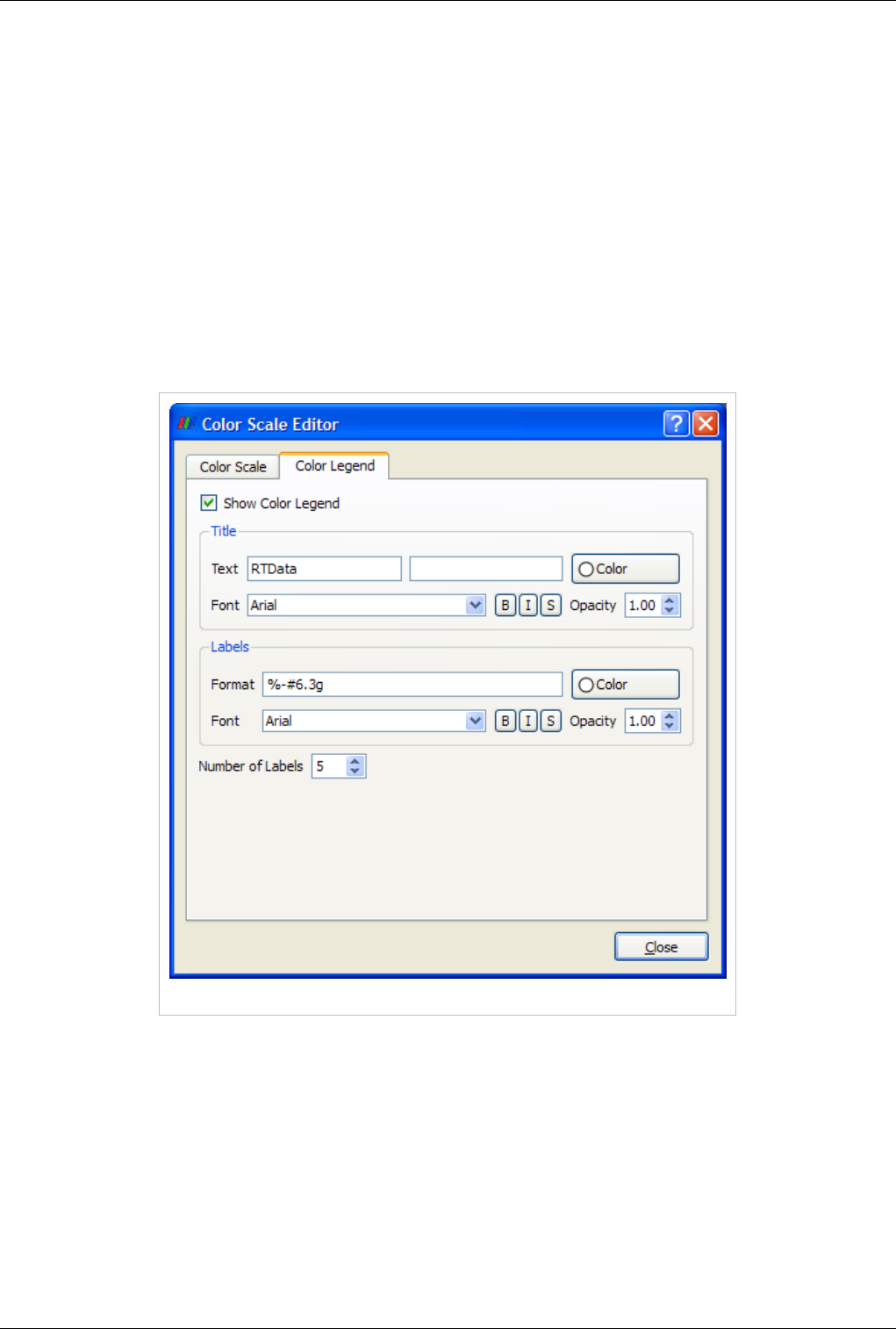
Views, Representations and Color Mapping 69
ensures that the range of the color map is not reset when the range of the data attribute changes. The minimum and
maximum values of the color map can be overridden by pressing the Rescale Range button, entering different
Minimum and Maximum values in the dialog that appears, and pressing Rescale. This rescales all the nodes in the
color map so that the scalar values lie at the same normalized positions. Alternatively, you may modify the scalar
values of any node (including the endpoints if Automatically Rescale to Fit Data Range is off) by clicking a node to
highlight it and typing a new value in the Scalar Value entry box. By changing the minimum and maximum color
map values, it is possible to manually specify what range of data values the color map will cover. Pressing the
Rescale to Data Range button on the Color Scale tab of the Color Scale Editor sets the range to cover only the
current data set.
If Use Discrete Colors is checked, the Resolution slider at the bottom of the dialog specifies the number of colors to
use in the color map. The scale ranges from 2 to 256 (the default). The fewer the number of colors, the larger the
range each color covers. This is useful if the data attribute has a small number of distinct values or if larger ranges of
the array values should be mapped to the same color.
Figure 4.28 Scalar Bar controls

70
Filtering Data
Rationale
Manipulating Data
In the course of either searching for information within data or in preparing images for publication that explain data,
it is often necessary to process the raw data in various ways. Examples include slicing into the data to make the
interior visible, extracting regions that have particular qualities, and computing statistical measurements from the
data. All of these operations involving taking in some original data and using it to compute some derived quantities.
This chapter explains how you control the data processing portion of ParaView's visualization pipeline to do such
analyses.
A filter is the basic tool that you use to manipulate data. If data is a noun, then a filter is the verb that operates on the
data. Filters operate by ingesting some data, processing it and producing some other data. In the abstract sense a data
reader is a filter as well because it ingests data from the file system. ParaView creates filters when you open data
files and instantiate new filters form the Filters menu. The set of filters you create becomes your visualization
pipeline, and that pipeline is shown in ParaView's Pipeline Browser.
Filter Parameters
Filter Parameters
Each time a dataset is opened from a file, a source is selected, a filter is applied, or an existing reader, source, or
filter (hereafter simply referred to as filter) is selected in the Pipeline Browser, ParaView updates the Object
Inspector for the corresponding output dataset. The Object Inspector has three tabs. In this chapter we are primarily
concerned with the Properties tab. The Display tab gives you control over the visual characteristics of the data
produced by the filter as displayed in the active view. The Information tab presents meta-information about the data
produced by the filter.
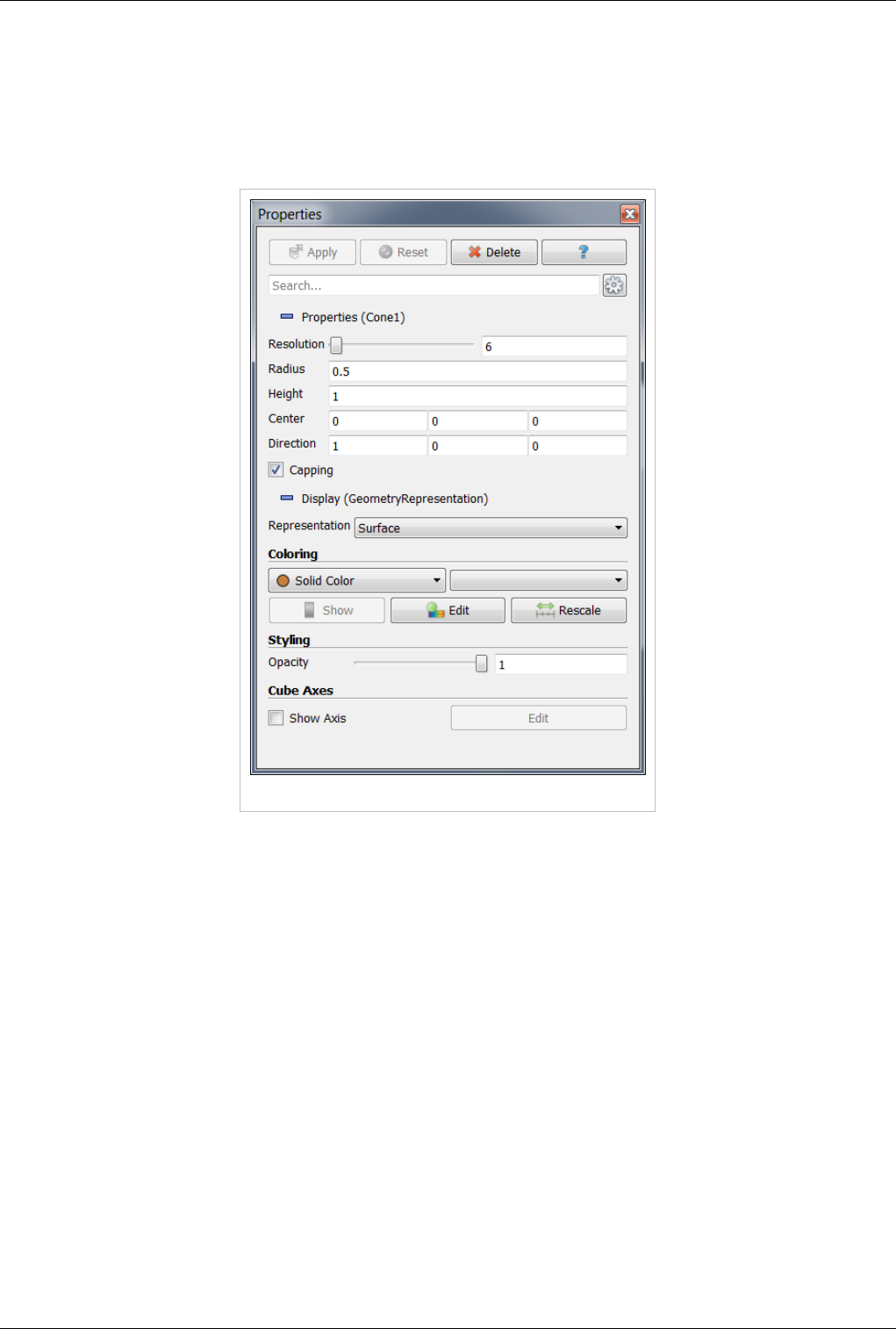
Filter Parameters 71
Properties
From the Properties tab you modify the parameters of the filter, fine tuning what it produces from its input (if any).
For example, a filter that extracts an isocontour will have a control with which to set the isovalue (or isovalues) to
extract at. The specific controls and information provided on the tab then are specific to the particular vtkAlgorithm
you are working with, but all filters have at least the Apply, Reset, Delete and ? (help) controls.
Figure 5.1 Sample properties tab for a cone source
The help button brings up the documentation for the filter in ParaView's help system in which the input restrictions
to the filter, output type generated by the filter, and descriptions of each parameter are listed. The same information
is repeated in the Appendices 1, 2 of this book.
The Delete button removes this filter from the pipeline. The delete button is only enabled when there are no filters
further down the pipeline that depend on this filter's output. You have to either use the Pipeline Browser and Object
Inspector in conjunction to delete the dependent parts of the pipeline or use Delete All from the Edit menu.
When a reader, source, or filter is first selected, the associated data set is not immediately created. By default (unless
you turn on Auto-Accept in ParaView's settings) the filter will not run until you hit the Apply button. When you do
press apply, ParaView sends the values shown on the Properties tab to the data processing engine and then the
pipeline is executed. This delayed commit behavior is important when working with large data, for which any given
action might take a long time to finish.
Until you press Apply and any other time that the values shown on the GUI do not agree with what was last sent to
the server, the the Apply button will be highlighted (in blue or green depending on your operating system). In this
state the Reset button is also enabled. Pressing that returns the GUI to the last committed state, which gives you an
easy way to cancel mistakes you've made before they happen.

Filter Parameters 72
The specific parameter control widgets vary from filter to filter and sometimes vary depending on the exact input to
the filter. Some filters have no parameters at all and others have many. Many readers present the list and type of
arrays in the file, and allow you to pick some or all of them as you need. In all cases the widgets shown on the
Properties tab give you control over exactly what the filter does. If you are unsure of what they do, remember to hit
the ? button to see the documentation for that filter.
Note that ParaView attempts to provide reasonable default settings for the parameter settings and to some extent
guards against invalid entries. A numeric entry box will not let you type in non-numerical values for example.
Sliders and spin boxes typically have minimum and maximum limits built in. In some cases though you may want to
ignore these default limits. Whenever there is a numeric entry beside the widget, you are able to manually type in
any number you need to.
Some filter parameters are best manipulated directly in the 3D View window with the mouse. For example, the Slice
filter extracts slices from the data that lie on a set of parallel planes oriented in space. This type of world space
interactive control is what 3D Widgets are for. The textual controls in the Properties Tab and the displayed state of
the 3D widgets are always linked so that changing either updates the other. You can of course use the Reset button to
revert changes you make from either place.
The Pipeline
Managing the Pipeline
Data manipulation in ParaView is fairly unique because of the underlying pipeline architecture that it inherits from
VTK. Each filter takes in some data and produces something new from it. Filters do not directly modify the data that
is given to them and instead copy unmodified data through via reference (so as to conserve memory) and augment
that with newly generated or changed data. The fact that input data is never altered in place means that unlike many
visualization tools, you can apply several filtering operations in different combinations to your data during a single
ParaView session. You see the result of each filter as it is applied, which helps to guide your data exploration work,
and can easily display any or all intermediate pipeline outputs simultaneously.
The Pipeline Browser depicts ParaView's current visualization pipeline and allows you to easily navigate to the
various readers, sources, and filters it contains. Connecting an initial data set loaded from a file or created from a
ParaView source to a filter creates a two filter long visualization pipeline. The initial dataset read in becomes the
input to the filter, and if needed the output of that filter can be used as the input to a subsequent filter.
For example, suppose you create a sphere in ParaView by selecting Sphere from the Sources menu. In this example,
the sphere is the initial data set. Next create a Shrink filter from the Alphabetical submenu of the Filters menu.
Because the sphere source was the active filter when the shrink filter was created, the shrink filter operates on the
sphere source's output. Optionally, use the Properties tab of the Object Inspector to set initial parameters of the
shrink filter and then hit Apply. Next create an Elevation filter to filter the output of the shrink filter and hit Apply
again. You have just created a simple three element linear pipeline in ParaView. You will now see the following in
the Pipeline Browser.
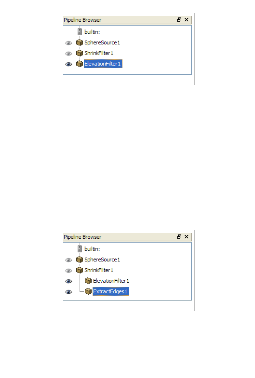
The Pipeline 73
Figure 5.2 Linear pipeline
Within the Pipeline Browser, to the left of each entry is an "eye" icon indicating whether that dataset is currently
visible. If there is no eye icon, it means that the data produced by that filter is not compatible with the active view
window. Otherwise, a dark eye icon indicates that the data set is visible. When a dataset is viewable but currently
invisible, its icon is drawn in light gray. Clicking on the eye icon toggles the visibility of the corresponding data set.
In the above example, all three filters are potentially visible, but only the ElevationFilter is actually being displayed.
The ElevationFilter is also highlighted in blue, indicating that it is the "active" filter. Since it is the "active" filter, the
Object Inspector reflects its content and the next filter created will use it as the input.
You can always change parameters of any filter in the pipeline after it has been applied. Left-click on the filter in the
Pipeline Browser to make it active. The Properties, Display, and Information tabs always reflect the active filter.
When you make changes in the Properties tab and apply your changes, all filters beyond the changed one are
automatically updated. Double-clicking the name of one of the filters causes the name to become editable, enabling
you to change it to something more meaningful than the default chosen by ParaView.
By default, each filter you add to the pipeline becomes the active filter, which is useful when making linear
pipelines. Branching pipelines are also very useful. The simplest way to make one is to click on some other, further
upstream filter in the pipeline before you create a new filter. For example, select ShrinkFilter1 in the Pipeline
Browser then apply Extract Edges from the Alphabetical submenu of the Filters menu. Now the output of the shrink
filter is being used as the input to both the elevation and extract edges filters. You will see the following in the
Pipeline Browser.
Figure 5.3 Branching Pipeline
Right-clicking a filter in the Pipeline Browser displays a context menu from which you can do several things. For
reader modules you can use this to load a new data file. All modules can be saved (the filter and the parameters) as a
Custom Filter (see the last section of this chapter), or deleted if it is at the end of the visualization pipeline. For filter
modules, you can also use this menu to change the input to the filter, and thus rearrange the visualization pipeline.
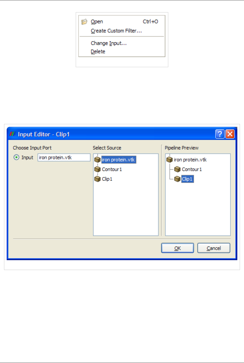
The Pipeline 74
Figure 5.4 Context menu in the Pipeline Browser
To rearrange the pipeline select Change Input from the context menu. That will bring up the Input Editor dialog box
as shown in Figure 5.5. The name of the dialog box reflects the filter that you are moving. The middle Select Source
pane shows the pipeline as it stands currently and uses this pane to select a filter to move the chosen filter on to. This
pane only allows you to choose compatible filters, i.e., ones that produce data that can be ingested by the filter you
are moving. It also does not allow you to create loops in the pipeline. Left-click to make your choice from the
allowed set of filters and then the rightmost Pipeline Preview pane will show what the pipeline will look like once
you commit your change. Click OK to do so or Cancel to abort the move.
Figure 5.5 Input Editor dialog shown while moving an elevation filter to operate directly on a reader.
Some filters require more than one input. (See the discussion of merging pipelines below). For those the leftmost
input port pane of the dialog shows more than one port. Use that together with the Select Source pane to specify each
input in turn.
Conversely, some filters produce more than one output. Thus another way to make a branching pipeline is to open a
reader that produces multiple distinct data sets, for example the SLAC reader that produces both a polygonal output
and a structured data field output. Whenever you have a branching pipeline keep in mind that it is important to select
the proper branch on which to extend the pipeline. For example, if you want to apply a filter like the Extract Subset
filter, which operates only on structured data, you click on the reader's structured data output and make that the
active one, if the SLAC reader's polygonal output was selected.
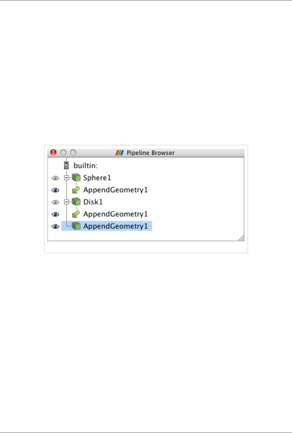
The Pipeline 75
Some filters that produce multiple datasets do so in a different way. Instead of producing several fundamentally
distinct data sets, they produce a single composite dataset which contains many sub data sets. See the Understanding
Data chapter for an explanation of composite data sets. With composite data it is usually best to treat the entire group
as one entity. Sometimes though, you want to operate on a particular set of sub datasets. To do that apply the Extract
Block filter. This filter allows you to pick the desired sub data set(s). Next apply the filter you are interested in to the
extract filters output. An alternative is to hit 'B' to use Block Selection in a 3D View and then use the Extract
Selection filter.
Pipelines merge as well, whenever they contain filters that take in more than one input to produce their own output
(or outputs). There are in fact two different varieties of merging filters. The Append Geometry and Group Data Sets
filters are examples of the first kind. These filters take in any number of fundamentally similar datasets. Append for
example takes in one or more polygonal datasets and combines them into a single large polygonal dataset. Group
takes in a set of any type of datasets and produces a single composite dataset. To use this type of merging filter,
select more than one filter within the Pipeline Browser by left clicking to select the first input and then shift-left
clicking to select the rest. Now create the merging filter from the Filters menu as usual. The pipeline in this case will
look like the one in Figure 5.6.
Figure 5.6 Merging pipelines
Other filters take in more than one, fundamentally different data sets. An example is the Resample with Dataset filter
which takes in one dataset (the Input) that represents a field in space to sample values from and another data set (the
Source) to use as a set of locations in space to sample the values at. Begin this type of merge by choosing either of
the two inputs as the active filter and then creating the merging filter from the Filters menu. A modified version of
the Change Input dialog shown in Figure 5.5 results (this one that lacks a Pipeline Preview pane). Click on either of
the ports listed in the Available Inputs pane and specify an input for it from the Select Input pane. Then switch to the
other input in the Available Inputs port and choose the other input on the Select Input pane. When you are satisfied
with your choices click OK on the dialog and then Apply on the Pipeline Browser to create the merging filter.
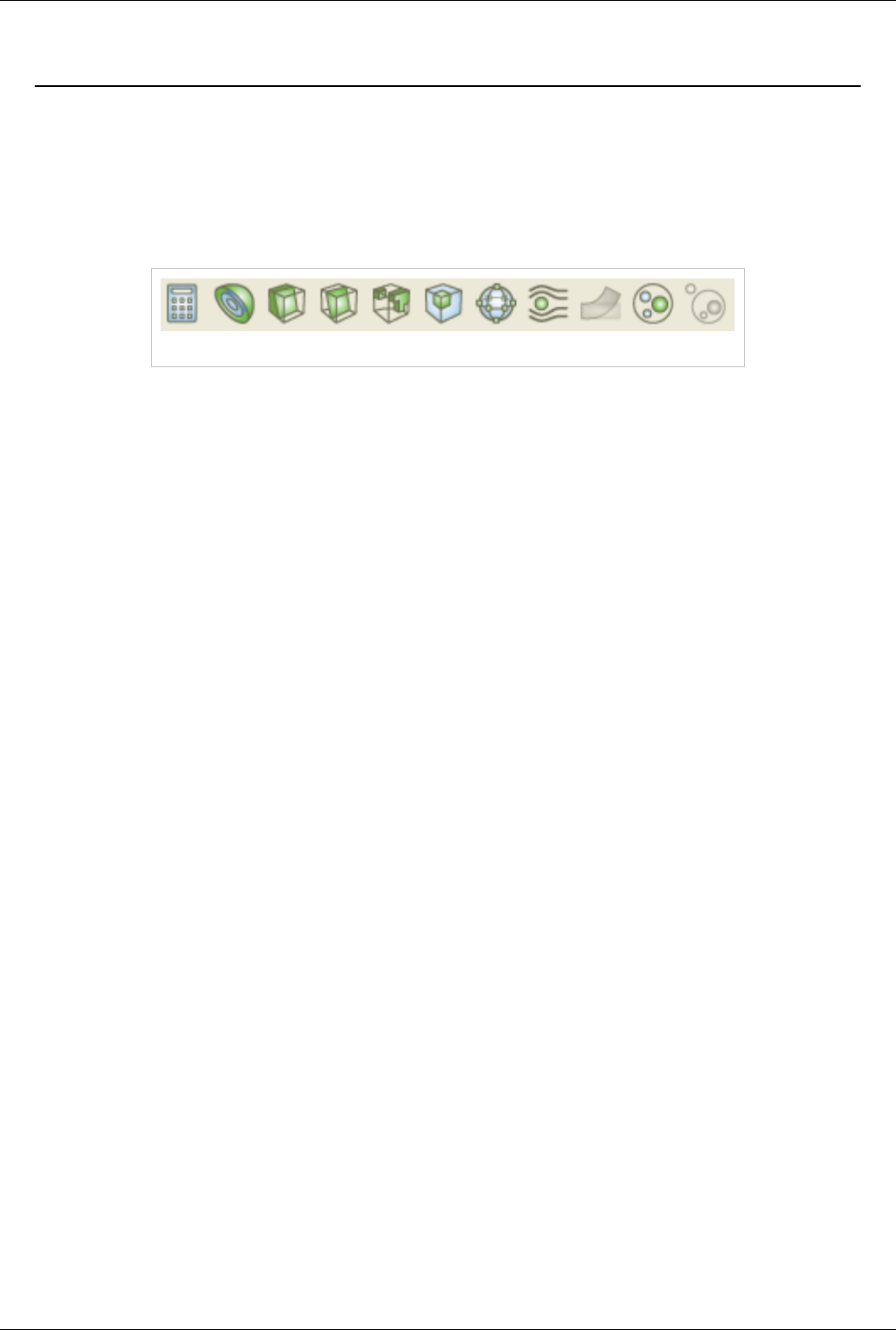
Filter Categories 76
Filter Categories
Available Filters
There are many filters available in ParaView (1) (and even more in VTK). Because ParaView has a modular
architecture, it is routine for people to add additional filters(2). Some filters have obscure purposes and are rarely
used, but others are more general purpose and used very frequently. These most common filters are found easily on
the Common (View|Toolbars) toolbar.
Figure 5.7 Common Filters Toolbar
These filters include:
•Calculator - Evaluates a user-defined expression on a per-point or per-cell basis (3)
•Contour - Extracts the points, curves, or surfaces where a scalar field is equal to a user-defined value. This
surface is often also called an isosurface.
•Clip - Intersects the geometry with a half space. The effect is to remove all the geometry on one side of a
user-defined plane.
•Slice - Intersects the geometry with a plane. The effect is similar to clipping except that all that remains is the
geometry where the plane is located.
•Threshold - Extracts cells that lie within a specified range of a scalar field.
•Extract Subset - Extracts a subset of a grid by defining either a volume of interest or a sampling rate.
•Glyph - Places a glyph, a simple shape, on each point in a mesh. The glyphs may be oriented by a vector and
scaled by a vector or scalar.
•Stream Tracer - Seeds a vector field with points and then traces those seed points through the (steady state)
vector field.
•Warp - Displaces each point in a mesh by a given vector field.
•Group Datasets - Combines the output of several pipeline objects into a single multi block dataset.
•Group Extract Level - Extract one or more items from a multi block dataset.
These eleven filters are a small sampling of what is available in ParaView.
In the alphabetical submenu of the Filters menu you will find all of the filters that are useable in your copy of
ParaView. Currently there are mote than one hundred of them, so to make them easier to find the Filters menu is
organized into submenus. These submenus are organized as follows.
•Recent - The filters you've used recently.
•Common - The common filters. This is the same set of filters as on the common filters toolbar.
•Cosmology - This contains filters developed at LANL for cosmology research.
•Data Analysis - The filters designed to retrieve quantitative values from the data. These filters compute data on
the mesh, extract elements from the mesh, or plot data.
•Statistics - This contains filters that provide descriptive statistics of data, primarily in tabular form.
•Temporal - Filters that analyze or modify data that changes over time.
All filters can work on data that changes over time because they are re-executed at each time step. Filters in this
category have the additional capability to inspect and make use of or even modify the temporal dimension.
•Alphabetical - Many filters do not fit into the above categories so all filters can be found here (see Figure 5.8).
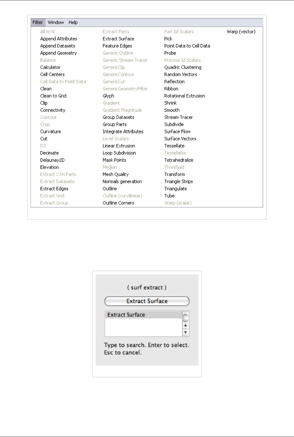
Filter Categories 77
Figure 5.8 A portion of the Alphabetical submenu of the Filters menu.
Searching through these lists of filters, particularly the full alphabetical list, can be cumbersome. To speed up the
selection of filters, you should use the quick launch dialog. Choose the first item from the filters menu, or
alternatively press either CTRL and SPACE BAR (Windows or Linux) or ALT and SPACE BAR (Macintosh) together
to bring up the Quick Launch dialog. As you type in words or word fragments the dialog lists the filters whose
names contain them. Use the up and down arrow key to select from among them and hit ENTER to create the filter.
Figure 5.9 Quick Launch
Why can't I apply the filter I want?
Note that many of the filters in the menu will be grayed out and not selectable at any given time. That is because any
given filter may only operate on particular types of data. For example, the Extract Subset filter will only operate on
structured datasets so it is only enabled when the module you are building on top of produces image data, rectilinear

Filter Categories 78
grid data, or structured grid data. Likewise, the contour filter requires scalar data and cannot operate directly on
datasets that have only vectors. The input restrictions for all filters are listed in the Appendix and help menus.
When the filter you want is not available you should look for a similar filter which will accept your data or apply an
intermediate filter which transforms your data into the required format. In ParaView 3.10 you can also ask ParaView
to try to do the conversion for you automatically by clicking "Auto convert Properties" in the application settings.
What does that filter do?
A description of what each filter does, what input data types it accepts and what output data types it produces can be
found in the Appendix and help menus. For a more complete understanding, remember that most ParaView filters
are simply VTK algorithms, each of which is documented online in the VTK (http:/ / www. vtk. org/ doc/ release/ 5.
6/ html/ classes. html) and ParaView (http:/ / www. paraview. org/ ParaView3/ Doc/ Nightly/ html/ classes. html)
Doxygen wiki pages.
When you are exploring a given dataset, you do not want to have to hunt through the detailed descriptions of all of
the filters in order to find the one filter that is needed at any given moment. It is useful then to be aware of the
general high-level taxonomy of the different operations that the filters can be logically grouped into.
These are:
• Attribute Manipulation : Manipulates the field aligned, point aligned and cell aligned data values and in general
derive new aligned quantities, including Curvature, Elevation, Generate IDs, Generate Surface Normals, Gradient,
Mesh Quality, Principal Component Analysis, and Random Vectors.
• Geometric Manipulation : Operates on or manipulates the shape of the data in a spatial context, including Reflect,
Transform, and Warp
• Topological operations : Manipulates the connected structure of the data set itself, usually creating or destroying
cells, for instance to reduce the data sets memory size while leaving it in the same place in space, including Cell
Centers, Clean, Decimate, Extract Surface, Quadric Clustering, Shrink, Smooth, and Tetrahedralize.
• Sampling : Computes new datasets that represent some essential features from the datasets that they take as input,
including Clip, Extract Subset, Extract Selection, Glyph, Streamline, Probe, Plot, Histogram, and Slice.
• Data Type Conversion : Converts between the various VTK data structures VTK Data Model and joins or splits
entire data structures, including Append DataSets, Append Geometry, Extract Blocks, Extract AMR Blocks, and
Group DataSets.
• White Box Filters : Performs arbitrary processing as specified at runtime by you the user, including the Calculator
and Python Programmable filters.

Best Practices 79
Best Practices
Avoiding Data Explosion
The pipeline model that ParaView presents is very convenient for exploratory visualization. The loose coupling
between components provides a very flexible framework for building unique visualizations, and the pipeline
structure allows you to tweak parameters quickly and easily.
The downside of this coupling is that it can have a larger memory footprint. Each stage of this pipeline maintains its
own copy of the data. Whenever possible, ParaView performs shallow copies of the data so that different stages of
the pipeline point to the same block of data in memory. However, any filter that creates new data or changes the
values or topology of the data must allocate new memory for the result. If ParaView is filtering a very large mesh,
inappropriate use of filters can quickly deplete all available memory. Therefore, when visualizing large datasets, it is
important to understand the memory requirements of filters.
Please keep in mind that the following advice is intended only for when dealing with very large amounts of data and
the remaining available memory is low. When you are not in danger of running out of memory, the following advice
is not relevant.
When dealing with structured data, it is absolutely important to know what filters will change the data to
unstructured. Unstructured data has a much higher memory footprint, per cell, than structured data because the
topology must be explicitly written out. There are many filters in ParaView that will change the topology in some
way, and these filters will write out the data as an unstructured grid, because that is the only dataset that will handle
any type of topology that is generated. The following list of filters will write out a new unstructured topology in its
output that is roughly equivalent to the input. These filters should never be used with structured data and should be
used with caution on unstructured data.
•Append Datasets
•Append Geometry
•Clean
•Clean to Grid
•Connectivity
•D3
•Delaunay 2D/3D
•Extract Edges
•Linear Extrusion
•Loop Subdivision
•Reflect
•Rotational Extrusion
•Shrink
•Smooth
•Subdivide
•Tessellate
•Tetrahedralize
•Triangle Strips
•Triangulate
Technically, the Ribbon and Tube filters should fall into this list. However, as they only work on 1D cells in poly
data, the input data is usually small and of little concern.
This similar set of filters also outputs unstructured grids, but also tends to reduce some of this data. Be aware though
that this data reduction is often smaller than the overhead of converting to unstructured data. Also note that the

Best Practices 80
reduction is often not well balanced. It is possible (often likely) that a single process may not lose any cells. Thus,
these filters should be used with caution on unstructured data and extreme caution on structured data.
•Clip
•Decimate
•Extract Cells by Region
•Extract Selection
•Quadric Clustering
•Threshold
Similar to the items in the preceding list, Extract Subset performs data reduction on a structured dataset, but also
outputs a structured dataset. So the warning about creating new data still applies, but you do not have to worry about
converting to an unstructured grid.
This next set of filters also outputs unstructured data, but it also performs a reduction on the dimension of the data
(for example 3D to 2D), which results in a much smaller output. Thus, these filters are usually safe to use with
unstructured data and require only mild caution with structured data.
•Cell Centers
•Contour
•Extract CTH Fragments
•Extract CTH Parts
•Extract Surface
•Feature Edges
•Mask Points
•Outline (curvilinear)
•Slice
•Stream Tracer
The filters below do not change the connectivity of the data at all. Instead, they only add field arrays to the data. All
the existing data is shallow copied. These filters are usually safe to use on all data.
•Block Scalars
•Calculator
•Cell Data to Point Data
•Curvature
•Elevation
•Generate Surface Normals
•Gradient
•Level Scalars
•Median
•Mesh Quality
•Octree Depth Limit
•Octree Depth Scalars
•Point Data to Cell Data
•Process Id Scalars
•Random Vectors
•Resample with dataset
•Surface Flow
•Surface Vectors
•Texture Map to...
•Transform

Best Practices 81
•Warp (scalar)
•Warp (vector)
This final set of filters either add no data to the output (all data of consequence is shallow copied) or the data they
add is generally independent of the size of the input. These are almost always safe to add under any circumstances
(although they may take a lot of time).
•Annotate Time
•Append Attributes
•Extract Block
•Extract Datasets
•Extract Level
•Glyph
•Group Datasets
•Histogram
•Integrate Variables
•Normal Glyphs
•Outline
•Outline Corners
•Plot Global Variables Over Time
•Plot Over Line
•Plot Selection Over Time
•Probe Location
•Temporal Shift Scale
•Temporal Snap-to-Time-Steps
•Temporal Statistics
There are a few special case filters that do not fit well into any of the previous classes. Some of the filters, currently
Temporal Interpolator and Particle Tracer, perform calculations based on how data changes over time. Thus, these
filters may need to load data for two or more instances of time, which can double or more the amount of data needed
in memory. The Temporal Cache filter will also hold data for multiple instances of time. Keep in mind that some of
the temporal filters such as the Temporal Statistics and the filters that plot over time may need to iteratively load all
data from disk. Thus, it may take an impractically long amount of time even if does not require any extra memory.
The Programmable Filter is also a special case that is impossible to classify. Since this filter does whatever it is
programmed to do, it can fall into any one of these categories.
Culling Data
When dealing with large data, it is best to cull out data whenever possible and do so as early as possible. Most large
data starts as 3D geometry and the desired geometry is often a surface. As surfaces usually have a much smaller
memory footprint than the volumes that they are derived from, it is best to convert to a surface early on. Once you do
that, you can apply other filters in relative safety.
A very common visualization operation is to extract isosurfaces from a volume using the Contour filter. The Contour
filter usually outputs geometry much smaller than its input. Thus, the Contour filter should be applied early if it is to
be used at all. Be careful when setting up the parameters to the Contour filter because it still is possible for it to
generate a lot of data. which can happen if you specify many isosurface values. High frequencies such as noise
around an isosurface value can also cause a large, irregular surface to form.
Another way to peer inside of a volume is to perform a Slice on it. The Slice filter will intersect a volume with a
plane and allow you to see the data in the volume where the plane intersects. If you know the relative location of an
interesting feature in your large dataset, slicing is a good way to view it.

Best Practices 82
If you have little a-priori knowledge of your data and would like to explore the data without the long memory and
processing time for the full dataset, you can use the Extract Subset filter to subsample the data. The subsampled data
can be dramatically smaller than the original data and should still be well load balanced. Of course, be aware that
you may miss small features if the subsampling steps over them and that once you find a feature you should go back
and visualize it with the full data set.
There are also several features that can pull out a subset of a volume: Clip, Threshold, Extract Selection, and Extract
Subset can all extract cells based on some criterion. Be aware, however, that the extracted cells are almost never well
balanced; expect some processes to have no cells removed. All of these filters, with the exception of Extract Subset,
will convert structured data types to unstructured grids. Therefore, they should not be used unless the extracted cells
are of at least an order of magnitude less than the source data.
When possible, replace the use of a filter that extracts 3D data with one that will extract 2D surfaces. For example, if
you are interested in a plane through the data, use the Slice filter rather than the Clip filter. If you are interested in
knowing the location of a region of cells containing a particular range of values, consider using the Contour filter to
generate surfaces at the ends of the range rather than extract all of the cells with the Threshold filter. Be aware that
substituting filters can have an effect on downstream filters. For example, running the Histogram filter after
Threshold will have an entirely different effect then running it after the roughly equivalent Contour filter.
Custom Filters aka Macro Filters
Macros (aka Custom Filters)
It often happens that once you figure out how to do some specific data processing task, you want to repeat it often.
You may, for example, want to reuse particular filters with specific settings (for example complicated calculator or
programmable filter expressions) or even entire pipeline sections consisting on new datasets without having to
manually enter the parameters each time.
You can do this via the clever use of state files or more conveniently python scripts and python macros (1) . Saving,
editing and reusing state files gives you the ability to recreate entire ParaView sessions, but not fine enough control
for small, repeatedly reused tasks. Python Tracing does give you fine grained control, but this assumes that you have
python enabled in your copy of ParaView (which is usually but not always the case) and that you remember to turn
on Trace recording before you did whatever it was that you want to play back. Both techniques largely require that
you think like a programmer when you initially create and setup the scripts. Another alternative is to use ParaView's
Custom Filters which let you create reusable meta-filters strictly within the GUI.
A Custom Filter is a black box filter that encapsulates one or more filters in a sub-pipeline and exposes only those
parameters from that sub-pipeline that the Custom Filter creator chose to make available. For example, if you capture
a ten element pipeline in your Custom Filter where each filter happened to have eight parameters, you could choose
to expose anywhere from zero to eighty parameters in your Custom Filter's Properties tab.
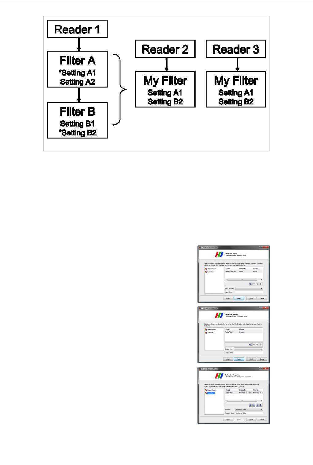
Custom Filters aka Macro Filters 83
Figure 5.10 Custom Filter concept
Once you have set up some pipeline that performs the data processing that you want to reuse, the process of creating
a Custom Filter consists of three steps. First, select one or more filters from the Pipeline Browser using the mouse.
Second, from the Tools menu select Create Custom Filter. From that dialog choose the filter in your chosen
sub-pipeline who's input is representative of where you want data to enter into your Custom Filter. This is usually the
topmost filter. If you are creating a multi-input filter, click the + button to add additional inputs and configure them
in the same way. Clicking Next brings you to a similar dialog in which you choose the outputs of your Custom Filter.
Third, click Next again to get to the last dialog, where you specify which parameters of the internal filters you want
to expose to the eventual user of the custom filter. You can optionally give each parameter a descriptive label here as
well. The three dialogs are shown below.
Step 1: configure one or more inputs to your new filter.
Step 2: configure one or more outputs of your new filter.
Step 3: identify and name the controls you want to expose of your new filter.
Figure 5.11 Creating a Custom Filter

Custom Filters aka Macro Filters 84
Once you create a Custom Filter it is added to the Alphabetical sub menu of the Filters menu. It is automatically
saved in ParaView's settings, so the next time you start ParaView on the same machine you can use it just like any of
the other filters that came with your copy of ParaView. Custom Filters are treated no differently than other filters in
ParaView and are saveable and restorable in state files and python scripts. If you find that you no longer need some
Custom Filter and want to get rid of it, use the Manage Custom Filters dialog box under the Tools menu to remove it.
If, on the other hand, you find that a Custom Filter is very useful, you may instead want to give it to a colleague. On
that same dialog are controls for exporting and importing Custom Filters. When you save a Custom Filter you are
prompted for a location and filename to save the filter in. The file format is a simple XML text file that you can
simply email or otherwise deliver.
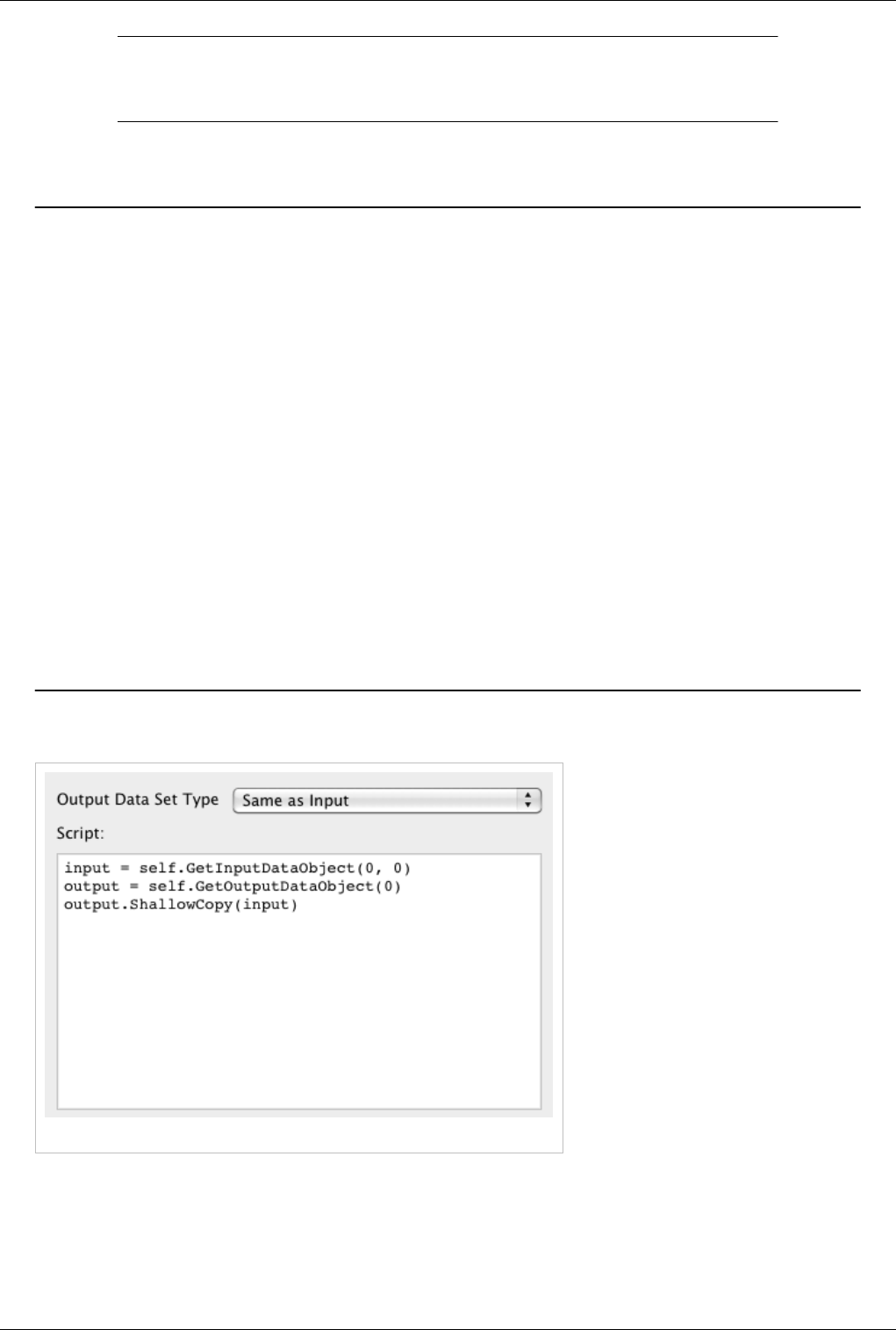
85
Quantative Analysis
Drilling Down
ParaView 2 was almost entirely a qualitative analysis tool. It was very good at drawing pictures of large scientific
datasets so that you could view the data and tell if it looked "right," but it was not easy to use for finding hard
quantitative information about the data and verifying that that was the case. The recommended use was to use
ParaView to visualize, interact with and subset your data and then export the result into a format that could be
imported by a different tool. A major goal of ParaView 3 has been to add quantitative analysis capabilities to turn it
into a convenient and comprehensive tool in which you can visualize, interact with and drill all the way down into
the data.
These capabilities vary from semi-qualitative ones such as the Ruler source and Cube Axis representation (see
Users_Guide_Annotation) to Selection which allows you to define and extract arbitrary subsets of the data based, to
the spreadsheet view which presents the data in textual form. Taken together with features like the statistical analysis
filters, calculator filters, 2D plot and chart views and programmable filters (which give you the ability to run
arbitrary code on the server and have access to every data point) these give you the ability to inspect the data from
the highest level view all the way down to the hard numbers.
This chapter describes the various tools that ParaView gives you to support quantitative analysis.
Python Programmable Filter
Introduction
Figure 6.1
The Programmable Filter is a
ParaView filter that processes one or
more input datasets based on a Python
script provided by the user. The
parameters of the filter include the
output data type, the script and a toggle
that controls whether the input arrays
are copied to the output. This chapter
introduces the use of the
Programmable Filter and gives a
summary of the API available to the
user.
Note that the Programmable Filter
depends on Python. All ParaView
binaries distributed by Kitware are
built with Python enabled. If you have
built ParaView yourself, you have to make sure that PARAVIEW_ENABLE_PYTHON is turned on when
configuring the ParaView build.

Python Programmable Filter 86
Since the entire VTK API as well as any module that can be imported through Python is available through this filter,
we can only skim the surface of what can be accomplished with this filter here. If you are not familiar with Python,
we recommend first taking a look at one of the introductory guides such as the official Python Tutorial [1]. If you are
going to do any programming beyond the very basics, we recommend reading up on the VTK API. The VTK
website [2] has links to VTK books and online documentation. For reference, you may need to look at the VTK class
documentation [3]. There is also more information about the Programmable Filter and some good recipes on the
ParaView Wiki (Python_Programmable_Filter).
Basic Use
Requirements:
1. You are applying Programmable Filter to a "simple" dataset and not a composite dataset such as multi-block or
AMR.
2. You have NumPy installed.
The most basic reason to use the Programmable Filter is to add a new array by deriving it from arrays in the input,
which can also be achieved by using the Python Calculator. One reason to use the Programmable Filter instead may
be that the calculation is more involved and trying to do it in one expression may be difficult. Another reason may be
that you need access to a program flow construct such as if or for. The Programmable Filter can be used to do
everything the Calculator does and more.
Note: Since what is described here builds on some of the concepts introduced in the Python Calculator section,
please read it first if you are not familiar with the Calculator.
If you leave the "Output Dataset Type" parameter in the default setting of "Same as Input," the Programmable Filter
will copy the topology and geometry of the input to the output before calling your Python script. Therefore, if you
Apply the filter without filling the script, you should see a copy of the input without any of its arrays in the output. If
you also check the Copy Arrays option, the output will have all of the input arrays. This behavior allows you to focus
on creating new arrays without worrying about the mesh.
Create a Sphere source and then apply the Programmable Filter and use the following script.
normals = inputs[0].PointData['Normals']
output.PointData.append(normals[:,0], "Normals_x")
This should create a sphere with an array called "Normals_x". There a few things to note here:
• You cannot refer to arrays directly by name as in the Python Calculator. You need to access arrays using the
.PointData and .CellData qualifiers.
• Unlike the Python Calculator, you have to explicitly add an array to the output using the append function. Note
that this function takes the name of the array as the second argument.
You can use any of the functions available in the Calculator in the Programmable Filter. For example, the following
code creates two new arrays and adds them to the output.
normals = inputs[0].PointData['Normals']
output.PointData.append(sin(normals[:,0]), "sin of Normals_x")
output.PointData.append(normals[:,1] + 1, "Normals_y + 1")

Python Programmable Filter 87
Intermediate Use
Mixing VTK and NumPy APIs
The previous examples demonstrate how the Programmable Filter can be used as an advanced Python Calculator.
However, the full power of the Programmable Filter can only be harnessed by using the VTK API. The following is
a simple example. Create a Sphere source and apply the Programmable Filter with the following script.
input = inputs[0]
newPoints = vtk.vtkPoints()
numPoints = input.GetNumberOfPoints()
for i in range(numPoints):
x, y, z = input.GetPoint(i)
newPoints.InsertPoint(i, x, y, 1 + z*0.3)
output.SetPoints(newPoints)
Start with creating a new instance of vtkPoints:
newPoints = vtk.vtkPoints()
vtkPoints is a data structure that VTK uses to store the coordinates of points. Next, loop over all points of the input
and insert a new point in the output with coordinates (x, y, 1+z*0.3)
for i in range(numPoints):
x, y, z = input.GetPoint(i)
newPoints.InsertPoint(i, x, y, 1 + z*0.3)
Finally, replace the output points with the new points we created using the following:
output.SetPoints(newPoints)
Note: Python is an interpreted language and Python scripts do not execute as efficiently as compiled C++ code.
Therefore, using a for loop that iterates over all points or cells may be a significant bottleneck when processing large
datasets.
The NumPy and VTK APIs can be mixed to achieve good performance. Even though this may seem a bit
complicated at first, it can be used with great effect. For instance, the example above can be rewritten as follows.
from paraview.vtk.dataset_adapter import numpyTovtkDataArray
input = inputs[0]
newPoints = vtk.vtkPoints()
zs = 1 + input.Points[:,2]*0.3
coords = hstack([input.Points[:,0:2],zs])
newPoints.SetData(numpyTovtkDataArray(coords))
output.SetPoints(newPoints)

Python Programmable Filter 88
Even though this produces exactly the same result, it is much more efficient because the for loop was moved it from
Python to C. Under the hood, NumPy uses C and Fortran for tight loops.
If you read the Python Calculator documentation, this example is straightforward except the use of
numpyTovtkDataArray(). First, note that you are mixing two APIs here: the VTK API and NumPy. VTK and
NumPy uses different types of objects to represents arrays. The basic examples previously used carefully hide this
from you. However, once you start manipulating VTK objects using NumPy, you have to start converting objects
between two APIs. Note that for the most part this conversion happens without "deep copying" arrays, for example
copying the raw contents from one memory location to another. Rather, pointers are passed between VTK and
NumPy whenever possible.
The dataset_adapter provides two methods to do the conversions described above:
• vtkDataArrayToVTKArray: This function creates a NumPy compatible array from a vtkDataArray. Note that
VTKArray is actually a subclass of numpy.matrix and can be used anywhere matrix can be used. This function
always copies the pointer and not the contents. Important: You should not directly change the values of the
resulting array if the argument is an array from the input.
• numpyTovtkDataArray: Converts a NumPy array (or a VTKArray) to a vtkDataArray. This function copies the
pointer if the argument is a contiguous array. There are various ways of creating discontinuous arrays with
NumPy including using hstack and striding. See NumPy documentation for details.
Multiple Inputs
Like the Python Calculator, the Programmable Filter can accept multiple inputs. First, select two or more pipeline
objects in the pipeline browser and then apply the Programmable Filter. Then each input can be accessed using the
inputs[] variable. Note that if the Output Dataset Type is set to Same as Input, the filter will copy the mesh from the
first input to the output. If Copy Arrays is on, it will also copy arrays from the first input. As an example, the
following script compares the Pressure attribute from two inputs using the difference operator.
output.append(inputs[1].PointData['Pressure'] -
inputs[0].PointData['Pressure'], "difference")
Dealing with Composite Datasets
Thus far, none of the examples used apply to multi-block or AMR datasets. When talking about the Python
Calculator, you did not have to differentiate between simple and composite datasets. This is because the calculator
loops over all of the leaf blocks of composite datasets and applies the expression to each one. Therefore, inputs in an
expression are guaranteed to be simple datasets. On the other hand, the Programmable Filter does not perform this
iteration and passes the input, composite or simple, as it is to the script. Even though this makes basic scripting
harder for composite datasets, it provides enormous flexibility.
To work with composite datasets you need to know how to iterate over them to access the leaf nodes.
for block in inputs[0]:
print block
Here you iterate over all of the non-NULL leaf nodes (i.e. simple datasets) of the input and print them to the Output
Messages console. Note that this will work only if the input is multi-block or AMR.
When Output Dataset Type is set to "Same as Input," the Programmable Filter will copy composite dataset to the
output - it will copy only the mesh unless Copy Arrays is on. Therefore, you can also iterate over the output. A
simple trick is to turn on Copy Arrays and then use the arrays from the output when generating new ones. Below is
an example. You should use the can.ex2 file from the ParaView testing dataset collection.
Python Programmable Filter 89
def process_block(block):
displ = block.PointData['DISPL']
block.PointData.append(displ[:,0], "displ_x")
for block in output:
process_block(block)
Alternatively, you can use the MultiCompositeDataIterator to iterate over the input and output block simultaneously.
The following is equivalent to the previous example:
def process_block(input_block, output_block):
displ = input_block.PointData['DISPL']
output_block.PointData.append(displ[:,0], "displ_x")
from paraview.vtk.dataset_adapter import MultiCompositeDataIterator
iter = MultiCompositeDataIterator([inputs[0], output])
for input_block, output_block in iter:
process_block(input_block, output_block)
Advanced
Changing Output Type
Thus far, all of the examples discussed depended on the output type being the same as input and that the
Programmable Filter copied the input mesh to the output. If you set the output type to something other than Same as
Input, the Programmable Filter will create an empty output of the type we specified but will not copy any
information. Even though it may be more work, this provides a lot of flexibility. Since this is approaching the realm
of VTK filter authoring, a very simple example is used. If you are already familiar with VTK API, you will realize
that this is a great way of prototyping VTK filters. If you are not, reading up on VTK is recommended.
Create a Wavelet source, apply a Programmable Filter, set the output type to vtkTable and use the following script:
rtdata = inputs[0].PointData['RTData']
output.RowData.append(min(rtdata), 'min')
output.RowData.append(max(rtdata), 'max')
Here, you added two columns to the output table. The first one has one value - minimum of RTData - and the second
one has the maximum of RTData. When you apply this filter, the output should automatically be shown in a
Spreadsheet view. You could also use this sort of script to chart part of the input data. For example, the output of the
following script can be display as a line chart.
rtdata = inputs[0].PointData['RTData']
output.RowData.append(rtdata, 'rtdata')
Changing the output type is also often necessary when using VTK filters within the script, which is demonstrated in
the following section.
Python Programmable Filter 90
Dealing with Structured Data Output
A curvilinear gris, for instance a bluntfin.vts from the ParaView testing data, is used as a good example. If you
would like to volume render a subset of this grid, since as of 3.10, ParaView does not support volume rendering of
curvilinear grids, you have two choices:
• Resample to an image data
• Convert to unstructured grid
This example demonstrates how to resample to image data using the Programmable Filter. This can be accomplished
using the Resample with Dataset filter, but it is a good example nevertheless. Start with loading bluntfin.vts, then
apply the Programmable Filter. Make sure to set the output type to vtkImageData. Here is the script:
pinput = vtk.vtkImageData()
pinput.SetExtent(0, 10, 0, 10, 0, 10)
pinput.SetOrigin(0, 1, 0)
pinput.SetSpacing(0.5, 0.5, 0.5)
probe = vtk.vtkProbeFilter()
probe.SetInput(pinput)
input_copy = inputs[0].NewInstance()
input_copy.UnRegister(None)
input_copy.ShallowCopy(inputs[0].VTKObject)
probe.SetSource(input_copy)
probe.Update()
output.ShallowCopy(probe.GetOutput())
Note: See the next section for details about using a VTK filter within the Programmable Filter.
If you already applied, you may notice that the output looks much bigger than it should be because an important
piece is missing. You need to use the following as the RequestInformation script:
from paraview.util import SetOutputWholeExtent
SetOutputWholeExtent(self, [0, 10, 0, 10, 0, 10])
VTK expects that all data sources and filters that produce structured data (rectilinear or curvilinear grids) to provide
meta data about the logical extents of the output dataset before full execution. Thus the RequestInformation is called
by the Programmable Filter before execution and is where you should provide this meta data. This is not required if
the filter is simply copying the mesh as the meta data would have been provided by another pipeline object upstream.
However, if you are using the Programmable Filter to produce a structured data with a different mesh than the input,
you need to provide this information.
The RequestUpdateExtent script can be used to augment the request that propagates upstream before execution. This
is used to ask for a specific data extent, for example. This is an advanced concept and is not discussed further here.
Python Programmable Filter 91
Using VTK Filters with Programmable Filter
The previous example demonstrated how you can use a VTK filter (vtkProbeFilter in this case) from with the
Programmable Filter. We will explain that example in more detail here.
pinput = vtk.vtkImageData()
pinput.SetExtent(0, 10, 0, 10, 0, 10)
pinput.SetOrigin(0, 1, 0)
pinput.SetSpacing(0.5, 0.5, 0.5)
probe = vtk.vtkProbeFilter()
probe.SetInput(pinput)
input_copy = inputs[0].NewInstance()
input_copy.UnRegister(None)
input_copy.ShallowCopy(inputs[0].VTKObject)
probe.SetSource(input_copy)
probe.Update()
output.ShallowCopy(probe.GetOutput())
There are two important tricks to use a VTK filter from another VTK filter. First, do not directly set the input to the
outer filter as the input of the inner filter. (It is difficult to explain why without getting into VTK pipeline
mechanics). Instead, make a shallow copy as follows:
input_copy = inputs[0].NewInstance()
input_copy.UnRegister(None)
input_copy.ShallowCopy(inputs[0].VTKObject)
The UnRegister() call is essential to avoid memory leaks.
The second trick is to use ShallowCopy() to copy the output of the internal filter to the output of the outer filter as
follows:
output.ShallowCopy(probe.GetOutput())
This should be enough to get you started. There are a large number of VTK filters so it is not possible to describe
them here. Refer to the VTK documentation for more information.
References
[1] http:/ / docs. python. org/ tutorial/
[2] http:/ / www. vtk. org
[3] http:/ / www. vtk. org/ doc/ release/ 5. 6/ html/
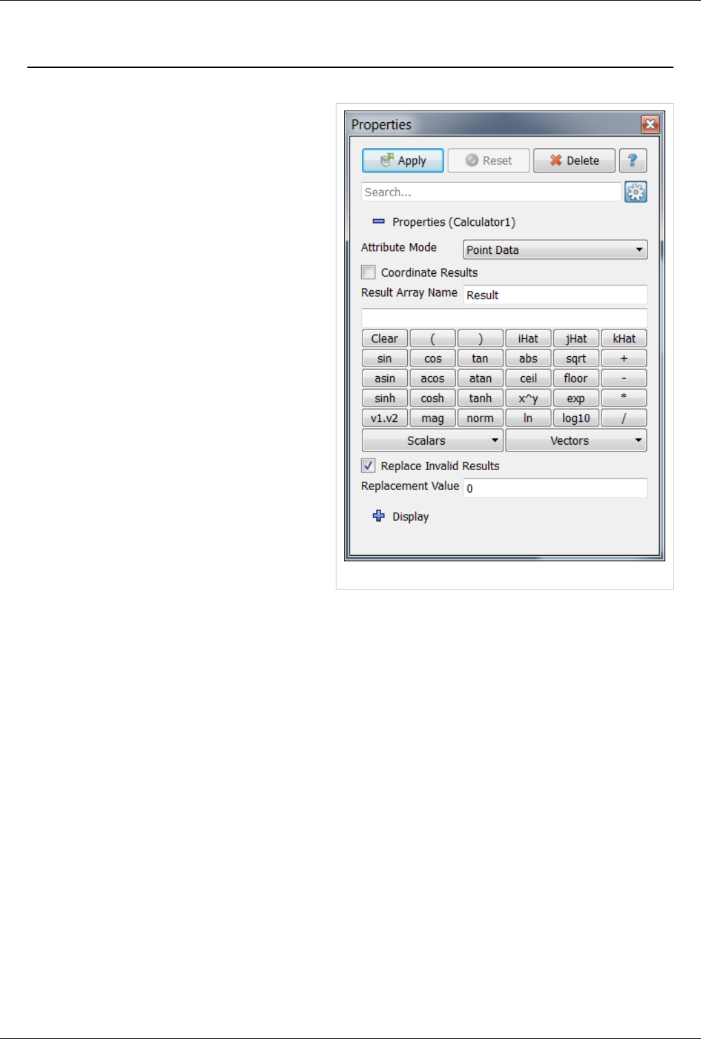
Calculator 92
Calculator
Figure 6.2
Basics
The Calculator Filter can be use to calculate derived
quantities from existing attributes. The main
parameter of the Calculator is an expression that
describes how to calculate the derived quantity. You
can enter this expression as free-form text or using
some of the shortcuts (buttons and menus provided).
There are some "hidden" expressions for which there
are no buttons. Operands that are accessible only by
typing in the function name include:
• min(expr1, expr2) Returns the lesser of the two
scalar expressions
• max(expr1, expr2) Returns the greater of the two
scalar expressions
• cross(expr1, expr2) Returns the vector cross
product of the two vector expressions
• sign(expr) Returns -1, 0 or 1 depending if the
scalar expression is less than, equal to or greater
than zero respectively
• if(condition,true_expression,false_expression)
Evaluates the conditional expression and then
evaluates and returns one of the two expressions
•> Numerical "greater than" conditional test
•< Numerical "less than" conditional test
•= Numerical "equal to" conditional test
•& Boolean "and" test conjunction
•| Boolean "or" test conjunction
Note: It is recommended that you use the Python Calculator instead of Calculator if possible. The Python Calculator
is more flexible, has more functions and is more efficient. However, it requires that ParaView is compiled with
Python support and that NumPy is installed.
Create a Wavelet source and then apply the Calculator using "1" as the expression. Note: You can enter an
expression by clicking in the expression entry box and typing. This should create a point array called "Result" in the
output. A few things to note:
• The Calculator copies the input mesh to the output. It is possible to have the calculator change the point
coordinates, which is discussed.
• The expression is calculated for each element in the output point or cell data (depending on the Attribute Mode).
Next, change the expression to be "5 * RTData" and the Result Array Name to be "5 times rtdata" (without the
quotes). If you change to surface representation and color by the new array, you will notice that the filter calculated
"5 * RTData" at each point.
The main use case for the Calculator is to utilize one or more input arrays to calculate derived quantities. The
Calculator can either work on point centered attributes or cell centered attributes (but not both). In order to help enter

Calculator 93
the names of the input arrays, the Calculator provides two menus accessible through the "Scalars" and "Vectors"
buttons. If you select an array name from either menus, it will be inserted to the expression entry box at the cursor
location. You can also use the other buttons to enter any of the functions available to the Calculator.
Working with Vectors
To start with an example, create a Wavelet source then apply the Random Vectors filter. Next, apply the Calculator.
Now look at the Scalars and Vectors menus on the Object Inspector panel. You will notice that BrownianVectors
shows up under Vectors, whereas BrownianVectors_X, _Y and _Z show up under scalars. The Calculator allows
access to individual components of vectors using this naming convention. So if you use BrownianVectors_X as the
expression, the Calculator will extract the first component of the BrownianVectors attribute. All of the Calculator's
functions are applicable to vectors. Most of these functions treat the vector attributes the same as scalars, mainly
applying the same functions to all components of all elements. However, the following functions work only on
vectors:
•v1 . v2 : Dot product of two vectors. Returns a scalar.
•norm : Creates a new array that contains normalized versions of the input vectors.
•mag : Returns the magnitude of input vectors.
You may have noticed that four calculator buttons on the Object Inspector are not actually functions. Clear is
straightforward. It cleans the expression entry box. iHat, jHat and kHat on the other hand are not as clear. These
represent unit vectors in X, Y and Z directions. They can be used to construct vectors from scalars. Take for example
the case where you want to set the Z component of BrownianVectors from the previous example to 0. The
expression to do that is "BrownianVectors_X *iHat+BrownianVectors_Y*jHat+0*kHat". This expression multiplies
the X unit vector with the X component of the input vector, the Y unit vector with the Y component, and the Z unit
vector with 0 and add them together. You can use this sort of expression to create vectors from individual
components of a vector if the reader loaded them separately, for example. Note: You did not really need the 0*kHat
bit, which was for demonstration.
Working with Point Coordinates
You may have noticed that one point-centered vector and its three components are always available in the
Calculator. This vector is called "coords" and represents the point coordinates. You can use this array in your
expression like any other array. For instance, in the previous example you could use "mag(coords)*RTData" to scale
RTData with the distance of the point to the origin.
It is also possible to change the coordinates of the mesh by checking the "Coordinate Results" box. Note that this
does not work for rectilinear grids (uniform and non-uniform) since their point coordinates cannot be adjusted
one-by-one. Since the previous examples used a uniform rectilinear grid, you cannot use them. Instead, start with the
Sphere source, then use this expression: "coords+2*iHat". Make sure to check he "Coordinate Results" box. The
output of the Calculator should be a shifted version of the input sphere.
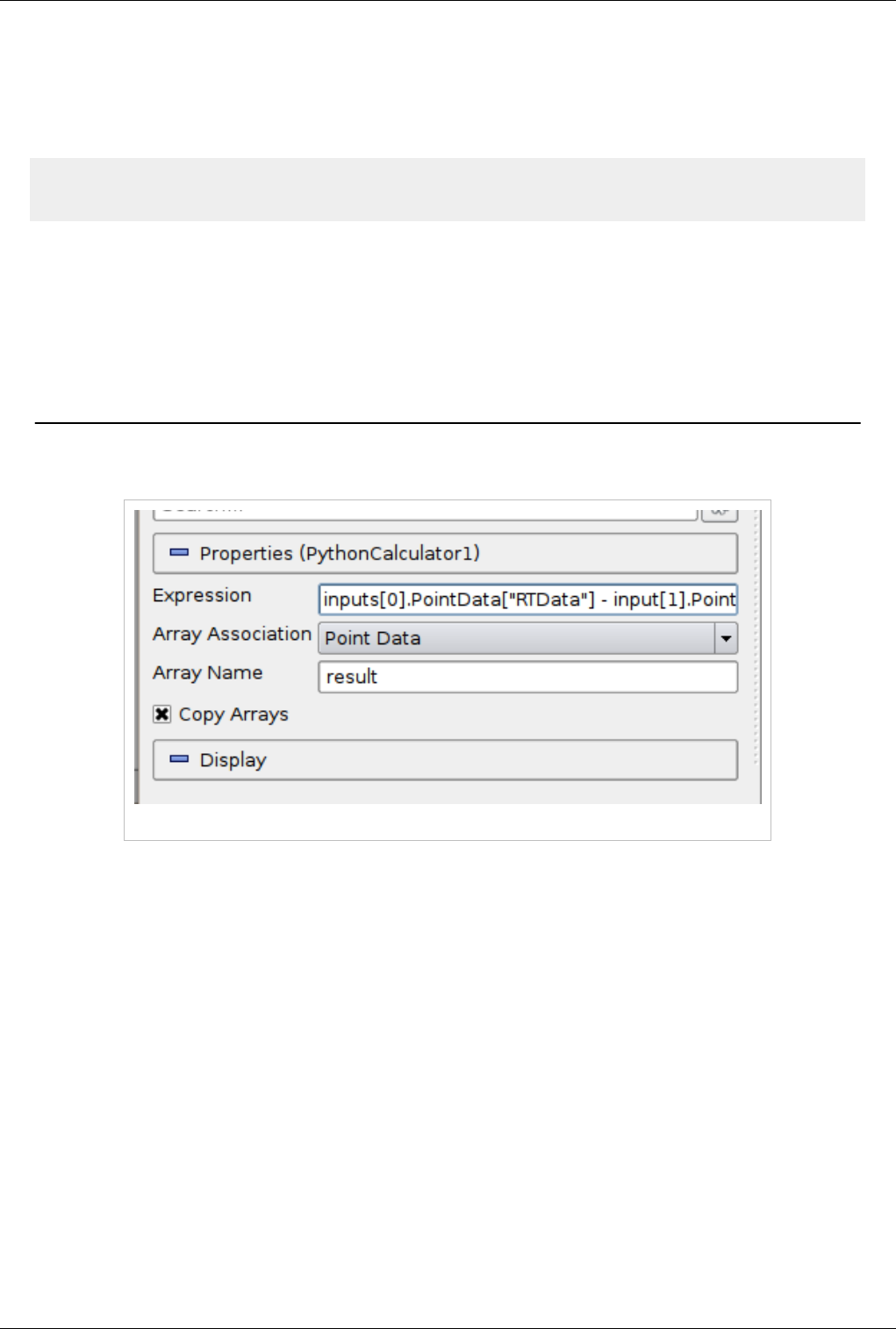
Calculator 94
Dealing with Invalid Results
Certain functions are not applicable to certain arguments. For example, sqrt() works only on positive numbers since
the calculator does not support complex numbers. Unless the "Replace invalid results" option is turned on, an
expression that tries to evaluate the square root of a negative number will return an error such as this:
ERROR: In /Users/berk/Work/ParaView/git/VTK/Common/vtkFunctionParser.cxx, line 697
vtkFunctionParser (0x128d97730): Trying to take a square root of a negative value
However, if you turn on the "Replace invalid results" option, the calculator will silently replace the result of the
invalid expression with the value specified in "Replacement value". Note that this will happen only when the
expression result is an invalid result so some of the output points (or cells) may have the Replacement Value whereas
others may have valid results.
Python Calculator
Introduction
Figure 6.3
The Python Calculator is a ParaView filter that processes one or more input arrays based on an expression provided
by the user to produce a new output array. The parameters of the filter include the expression, the association of the
output array (Point or Cell Data), the name of output array and a toggle that controls whether the input arrays are
copied to the output. This section introduces the use of the Python Calculator and provides a list of functions
available to the user.
Note that the Python Calculator depends on Python and NumPy. All ParaView binaries distributed by Kitware are
built with these to enable the calculator. If you have built ParaView yourself, you have to make sure that NumPy is
installed and that PARAVIEW_ENABLE_PYTHON is turned on when configuring the ParaView build.

Python Calculator 95
Basic Tutorial
Start by creating a Sphere source and applying the Python Calculator to it. As the first expression, use the following
and apply:
5
This should create an array name "result" in the output point data. Note that this is an array that has a value of 5 for
each point. When the expression results in a single value, the calculator will automatically make a constant array.
Next, try the following:
Normals
Now the "result" array should be the same as the input array Normals. As described in detail later, various functions
are available through the calculator. For example, the following is a valid expression.
sin(Normals) + 5
It is very important to note that the Python Calculator has to produce one value per point or cell depending on the
Array Association parameter. Most of the functions described here apply individually to all point or cell values and
produce an array the same dimensions as the input. However, some of them (such as min() and max()) produce
single values.
Accessing Data
There are several ways of accessing input arrays within expressions. The simplest way is to access it by name:
sin(Normals) + 5
This is equivalent to:
sin(inputs[0].PointData['Normals']) + 5
The example above requires some explanation. Here inputs[0] refer to the first input (dataset) to the filter. Python
Calculator can accept multiple inputs. Each input can be accessed as inputs[0], inputs[1], ... You can access the point
or cell data of an input using the .PointData or .CellData qualifiers. You can then access individual arrays within the
point or cell data containers using the [] operator. Make sure to use quotes or double-quotes around the array name.
Arrays that have names with certain characters (such as space, +, -, *, /) in their name can only be accessed using this
method.
Certain functions apply directly on the input mesh. These filters expect an input dataset as argument. For example,
area(inputs[0])
For data types that explicitly define the point coordinates, you can access the coordinates array using the .Points
qualifier. The following extracts the first component of the coordinates array:
inputs[0].Points[:,0]
Note that certain data types, mainly image data (uniform rectilinear grid) and rectilinear grid, point coordinates are
defined implicitly and cannot be accessed as an array.

Python Calculator 96
Comparing Multiple Datasets
The Python Calculator can be used to compare multiple datasets, as shown by the following example.
1. Go to the Menu Bar, and select File > Disconnect to clear the Pipeline.
2. Select Source > Mandelbrot, and then click Apply, which will set up a default version of the Mandelbrot Set. The
data for this set are stored in a 251x251 scalar array.
3. Select Source > Mandelbrot again, and then go to the Properties panel and set the Maximum Number of Iterations
to 50. Click Apply, which will set up a different version of the Mandelbrot Set, represented by the same size
array.
4. Hold the Shift key down and select both of the Mandelbrot entries in the Pipeline Inspector, and then go to the
Menu Bar and select Filter > Python Calculator. The two Mandelbrot entries will now be shown as linked, as
inputs, to the Python Calculator.
5. In the Properties panel for the Python Calculator filter, enter the following into the Expression box:
inputs[1].PointData['Iterations'] - inputs[0].PointData['Iterations']
This expression specifies the difference between the second and first Mandelbrot arrays. The result is saved in a new
array called 'results'. The prefixes in the names for the array variables, inputs[1] and inputs[0], refer to the first and
second Mandelbrot entries, respectively, in the Pipeline. PointData specifies that the inputs contain point values. The
quoted label 'Iterations' is the local name for these arrays. Click Apply to initiate the calculation.
Click the Display tab in the Properties panel for the Python Calculator, and go to the first tab to the right of the
'Color by' label. Select the item results in that tab, which will cause the display window to the right to show the
results of the expression we entered in the Python Calculator. The scalar values representing the difference between
the two Mandelbrot arrays are represented by colors that are set by the current color map (see Edit Color Map... for
details).
There are a few things to note:
• Python Calculator will always copy the mesh from the first input to its output.
• All operations are applied point by point. In most cases, this requires that the input meshes (topology and
geometry) are the same. At the least, it requires that the inputs have the same number of points and cells.
• In parallel execution mode, the inputs have to be distributed exactly the same way across processes.
Basic Operations
The Python calculator supports all of the basic arithmetic operations using the +, -, * and / operators. These are
always applied element-by-element to point and cell data including scalars, vectors and tensors. These operations
also work with single values. For example, the following adds 5 to all components of all Normals.
Normals + 5
The following adds 1 to the first component, 2 to the second component and 3 to the third component:
Normals + [1,2,3]
This is specially useful when mixing functions that return single values. For example, the following normalizes the
Normals array:
(Normals - min(Normals))/(max(Normals) - min(Normals))
A common use case in a calculator is to work on one component of an array. This can be accomplished with the
following:
Normals[:, 0]

Python Calculator 97
The expression above extracts the first component of the Normals vector. Here, : is a placeholder for "all elements".
One element can be extracted by replacing : with an index. For example, the following creates a constant array from
the first component of the normal of the first point:
Normals[0, 0]
Whereas the following assigns the normal of the first point to all points:
Normals[0, :]
It is also possible to merge multiple scalars into an array using the hstack() function:
hstack([velocity_x, velocity_y, velocity_z])
Note the use of square brackets ([]).
Under the cover, the Python Calculator uses NumPy. All arrays in the expression are compatible with NumPy arrays
and can be used where NumPy arrays can be used. For more information on what you can do with these arrays,
consult with the NumPy book, which can be downloaded here [1].
Functions
The following is a list of functions available in the Python Calculator. Note that this list is partial since most of the
NumPy and SciPy functions can be used in the Python Calculator. Many of these functions can take single values or
arrays as argument.
abs (x) : Returns the absolute value(s) of x.
add (x, y): Returns the sum of two values. x and y can be single values or arrays. Same as x+y.
area (dataset) : Returns the surface area of each cell in a mesh.
aspect (dataset) : Returns the aspect ratio of each cell in a mesh.
aspect_gamma (dataset) : Returns the aspect ratio gamma of each cell in a mesh.
condition (dataset) : Returns the condition number of each cell in a mesh.
cross (x, y) : Returns the cross product for two 3D vectors from two arrays of 3D vectors.
curl (array): Returns the curl of an array of 3D vectors.
divergence (array): Returns the divergence of an array of 3D vectors.
divide (x, y): Element by element division. x and y can be single values or arrays. Same as x/y.
det (array) : Returns the determinant of an array of 2D square matrices.
determinant (array) : Returns the determinant of an array of 2D square matrices.
diagonal (dataset) : Returns the diagonal length of each cell in a dataset.
dot (a1, a2): Returns the dot product of two scalars/vectors of two array of scalars/vectors.
eigenvalue (array) : Returns the eigenvalue of an array of 2D square matrices.
eigenvector (array) : Returns the eigenvector of an array of 2D square matrices.
exp (x): Returns power(e, x).
global_max(array): Returns the maximum value of an array of scalars/vectors/tensors among all process. Not yet
supported for multi-block and AMR datasets.
global_mean (array) : Returns the mean value of an array of scalars/vectors/tensors among all process. Not yet
supported for multi-block and AMR datasets.

Python Calculator 98
global_min(array): Returns the minimum value of an array of scalars/vectors/tensors among all process. Not yet
supported for multi-block and AMR datasets.
gradient(array): Returns the gradient of an array of scalars/vectors.
inv (array) : Returns the inverse an array of 2D square matrices.
inverse (array) : Returns the inverse of an array of 2D square matrices.
jacobian (dataset) : Returns the jacobian of an array of 2D square matrices.
laplacian (array) : Returns the jacobian of an array of scalars.
ln (array) : Returns the natural logarithm of an array of scalars/vectors/tensors.
log (array) : Returns the natural logarithm of an array of scalars/vectors/tensors.
log10 (array) : Returns the base 10 logarithm of an array of scalars/vectors/tensors.
max (array): Returns the maximum value of the array as a single value. Note that this function returns the
maximum within a block for AMR and multi-block datasets, not across blocks/grids. Also, this returns the maximum
within each process when running in parallel.
max_angle (dataset) : Returns the maximum angle of each cell in a dataset.
mag (a) : Returns the magnigude of an array of scalars/vectors.
mean (array) : Returns the mean value of an array of scalars/vectors/tensors.
min (array) : Returns the minimum value of the array as a single value. Note that this function returns the minimum
within a block for AMR and multi-block datasets, not across blocks/grids. Also, this returns the minimum within
each process when running in parallel.
min_angle (dataset) : Returns the minimum angle of each cell in a dataset.
mod (x, y): Same as remainder (x, y).
multiply (x, y): Returns the product of x and y. x and y can be single values or arrays. Note that this is an element by
element operation when x and y are both arrays. Same as x * y.
negative (x): Same as -x.
norm (a) : Returns the normalized values of an array of scalars/vectors.
power (x, a): Exponentiation of x with a. Here both x and a can either be a single value or an array. If x and y are
both arrays, a one-by-one mapping is used between two arrays.
reciprocal (x): Returns 1/x.
remainder (x, y): Returns x − y*floor(x/y). x and y can be single values or arrays.
rint (x): Rounds x to the nearest integer(s).
shear (dataset) : Returns the shear of each cell in a dataset.
skew (dataset) : Returns the skew of each cell in a dataset.
square (x): Returns x*x.
sqrt (x): Returns square root of x.
strain (array) : Returns the strain of an array of 3D vectors.
subtract (x, y): Returns the difference between two values. x and y can be single values or arrays. Same as x - y.
surface_normal (dataset) : Returns the surface normal of each cell in a dataset.
trace (array) : Returns the trace of an array of 2D square matrices.
volume (dataset) : Returns the volume normal of each cell in a dataset.
vorticity(array): Returns the vorticity/curl of an array of 3D vectors.
vertex_normal (dataset) : Returns the vertex normal of each point in a dataset.

Python Calculator 99
Trigonometric Functions
Below is a list of supported triginometric functions.
sin (x)
cos (x)
tan (x)
arcsin (x)
arccos (x)
arctan (x)
hypot (x1, x2)
sinh(x)
cosh (x)
tanh (x)
arcsinh (x)
arccosh (x)
arctanh (x)
References
[1] http:/ / www. tramy. us/ guidetoscipy. html
Spreadsheet View
In several cases it is very useful to look at the raw dataset. This is where the Spreadsheet view is particularly useful.
Spreadsheet View allows users to explore the raw data in a spreadsheet-like display. Users can inspect cells and
points and data values associated with these using this view. This makes it a very useful for drilling down into the
data.
Spreadsheet View, as the name suggests, is a view that users can create by splitting the main view frame in the
application client-area. Refer to the chapter on Views for details on views. Spreadsheet View can only show one
dataset at a time. However, users can use ParaView’s multi-view capabilities to create multiple spreadsheet views for
inspecting different datasets.
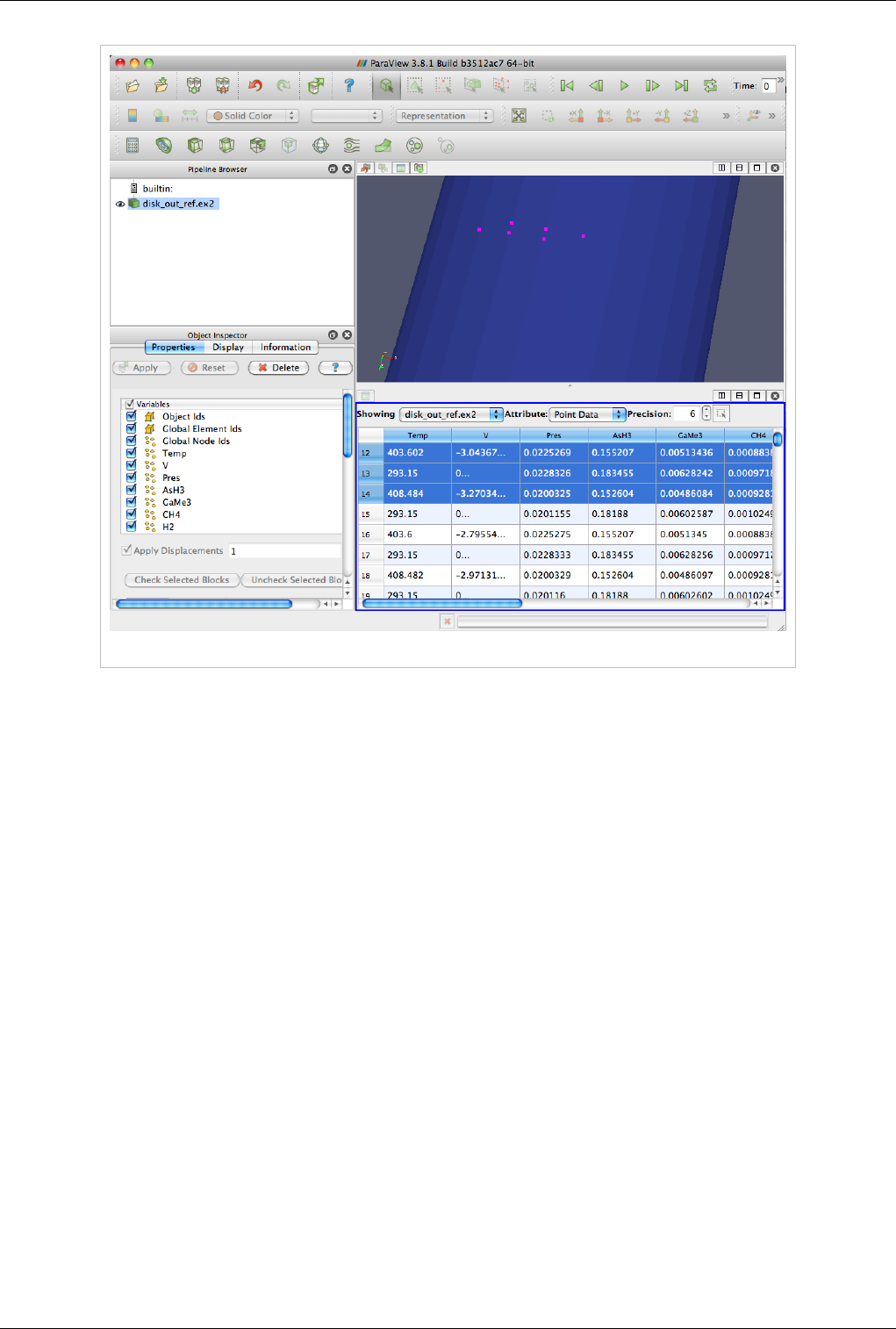
Spreadsheet View 100
Figure 6.4 Spreadsheet View
Inspecting Large Datasets
Spreadsheet View is a client-only view i.e. it delivers the necessary data to the client when running in client-server
mode. Additionally, it is not available through Python scripting (except when running through the Pyhton shell
provided by the ParaView application) or batch scripting. Furthermore, when running on a tile-display, the area
covered by the spreadsheet on the client simply shows up as a blank region on the tiles.
Unlike complex views like the 3D render view that can generate the renderings on the server and simply deliver
images to the client, the spreadsheet view requires that the data is available on the client. This can be impractical
when inspecting large datasets since the client may not even have enough memory, even if infinite bandwidth is
assumed. To address such issues, the Spreadsheet View streams the data to the client, only fetching the data for the
row currently visible in the viewport.

Spreadsheet View 101
Double Precision
Using the precision spin-box in the view header, users can control the precision for floating point numbers. The
value determines the number of significant digits after the decimal point.
Selection with Spreadsheet View
Spreadsheet view, in many ways, behaves like typical spreadsheet applications. You can scroll, select rows using
mouse clicks, arrow keys and modifiers like Shift and Ctrl keys, or sort columns by clicking on the header.
Additionally, you can double-click on a column header to toggle the maximization of a column for better readability.
On selecting rows the corresponding cells or points will get selected and ParaView will highlight those in other
views, such as the 3D view. Conversely, when you make a selection in the 3D View or the chart views, one of the
rows corresponding to the selected cells/points will be highlighted in the spreadsheet view. Of course, for the view to
highlight the selection, the selected dataset must be the one that is being shown in the spreadsheet view. To make it
easier to inspect just the selected elements, you check the “Show only selected” button on the view header.
When in “Show only Selected” mode, you can no longer create selections on the spreadsheet view. You have to use
the other views to make the selection and the spreadsheet view will automatically update to show the details for the
items that got selected.
Spreadsheet view can show data associated with cells, points or even field data. To choose what attribute the view
shows, you can use the attribute-type combo-box. The selection created by the view depends on the attribute-type,
i.e. if a user selects in the view when attribute type is “Points”, points in the dataset will be selected. The spreadsheet
view also performs selection conversions if possible, i.e. if you select a cell in the 3D view, but spreadsheet view is
setup to show points, then the view will highlight the points that form the selected cell.
The spreadsheet view may add several additional data columns that may not be present in the actual data. These data
columns are either derived information such as the (i, j, k) coordinates for structured data or provide additional
information about the data, e.g. block index for composite datasets, or provide additional information about the data
distribution such as process-id when connected to a parallel server (pvserver or pvdataserver).
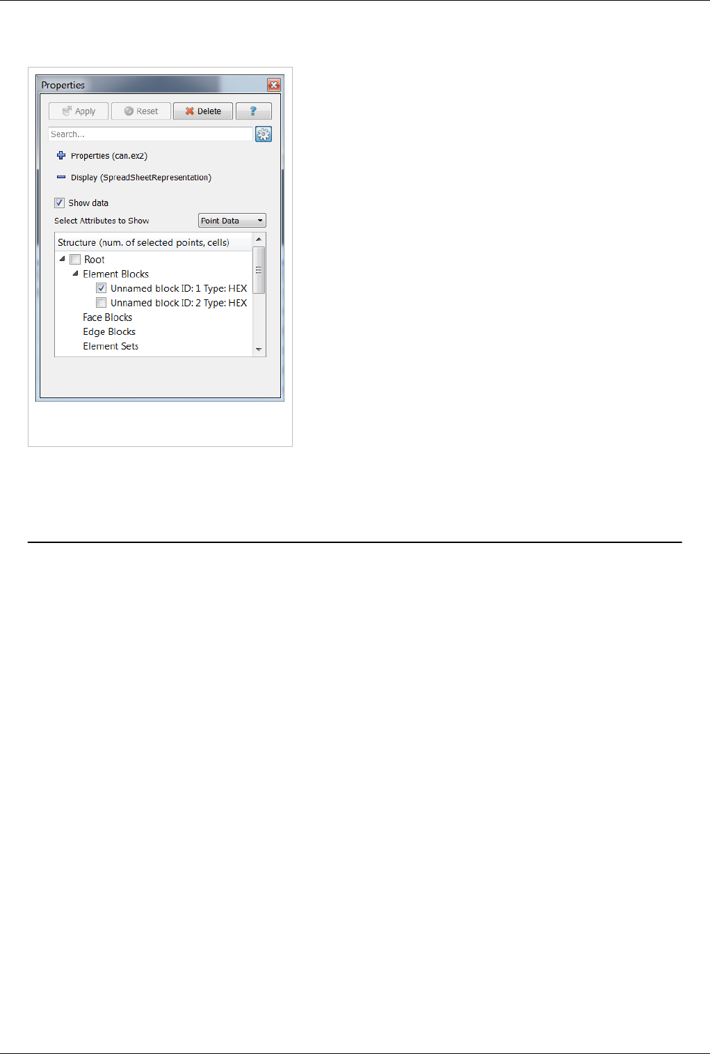
Spreadsheet View 102
Working with Composite Datasets
Figure 6.5 Properties panel showing widget to select
the block to display
Spreadsheet view works seamlessly with different kinds of dataset
types including composite datasets such as multi-block datasets or
AMR datasets. When dealing with composite datasets, the view
shows one block at a time. Users can choose the block to inspect
by using the Display section of the Properties panel.
Selection
Selection is the mechanism for identifying a subset of a dataset by using user-specified criteria. This subset can be a
set of points, cells or a block of composite dataset. This functionality allows users to focus on a smaller subset that is
important. For example, the elements of a finite-element mesh that have pressure above a certain threshold can be
identified very easily using the threshold selection. Furthermore, this selection can be converted to a set of global
element IDs in order to plot the attribute values of those elements over time.
This section discusses the mechanism for creating selections using Views and Selection Inspector. The following
section details another powerful and flexible mechanism of creating selection using queries.
ParaView supports a single active selection. This selection is associated with a data source (here data source refers to
any reader, source or filter) and is shown in every view that displays the data source’s output. This article uses a
use-case driven approach to demonstrate how this selection can be described and used. The next section introduces
the main GUI components that are used in the article and subsequent sections address different use cases.
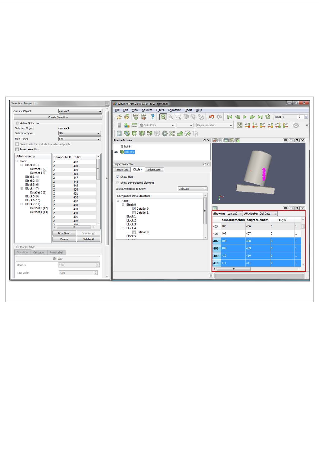
Selection 103
Selection Inspector
ParaView provides a selection inspector (referred to simply as the inspector in this article) to inspect and edit the
details about the active selection. You can toggle the inspector visibility from the View menu. The inspector can be
used to create a new active selection, view/edit the properties of the active selection as well as change the way the
selection is displayed in the 3D window e.g. change the color, show labels etc.
Spreadsheet View
Figure 6.6 Spreadsheet View in ParaView showing the display tab for a source producing a multi-block dataset. The selected cells are highlighted in
the 3D view as well as the spreadsheet view. The active selection can be inspected using the selection inspector.
Spreadsheet View provides data exploration capabilities. One of the common complaints many users have is not
being able to look at the raw data directly. Spreadsheet view provides exactly that. It allows the user to look at the
raw cell data, point data or field data associated with a dataset. For more details on how to use the Spreadsheet View,
please refer to Spreadsheet View Chapter.
Create a Selection
This section covers different ways of creating a selection.
Select cells/points on the Surface
One of the simplest use-cases is to select cells or points on the surface of the dataset. It is possible to select surface
cells by drawing a rubber-band on the 3D view. With the 3D view showing the dataset active, click on Select Cells
(or Points) On in the Selection Controls toolbar or under the Edit menu (you can also use the ‘S’ key a shortcut for
‘Select Cells On’). This will put ParaView into a selection mode. In this mode, click and drag over the surface of the
dataset in the active view to select the cells (or points) on the surface. If anything was selected, it will be highlighted
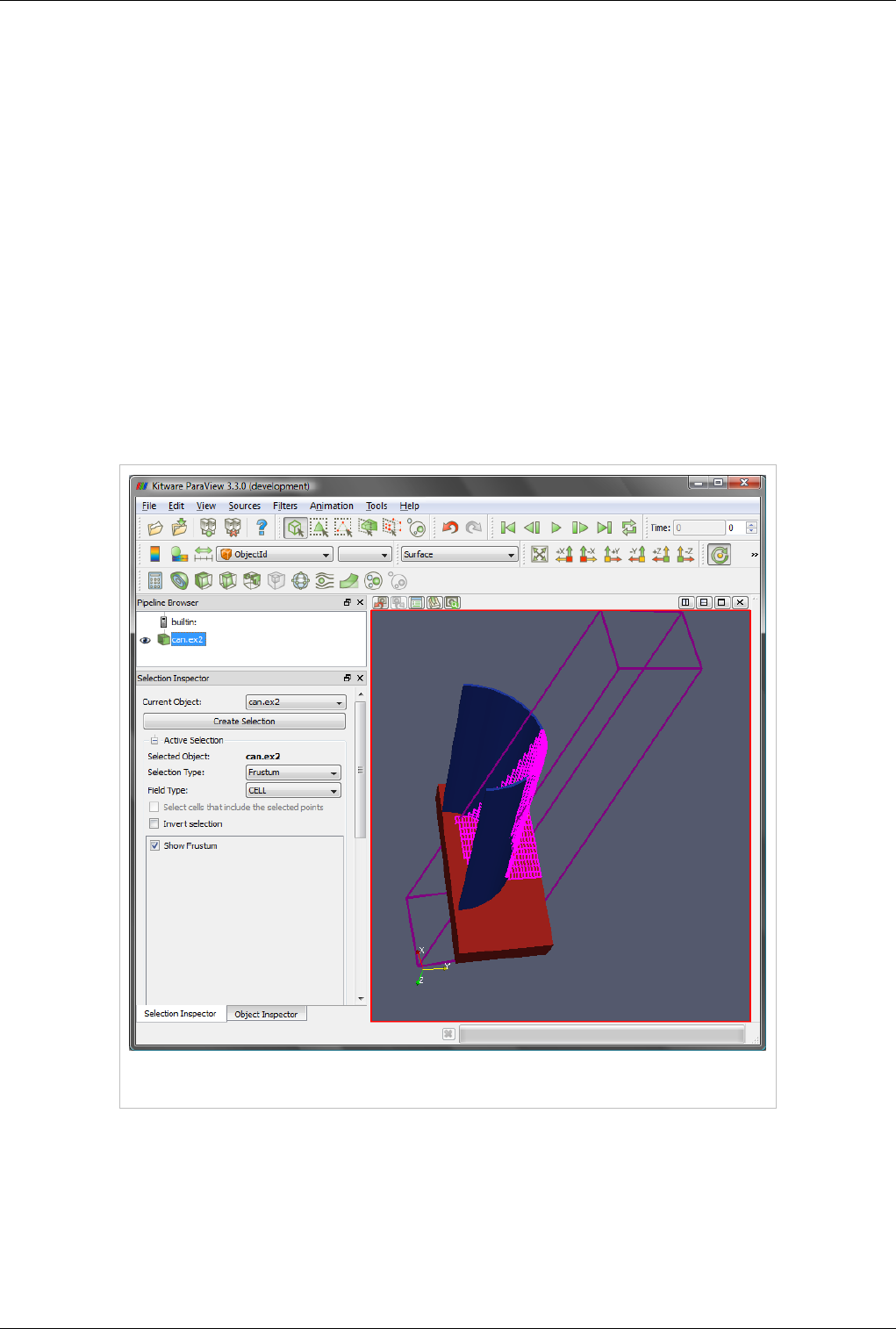
Selection 104
in all the views showing the data and the source producing the selected dataset will become active in the Pipeline
Browser. ParaView supports selecting only one source at a time. Hence, even if you draw the rubber band such that
it covers data from multiple sources, only one of them will be selected (the one that has the largest number of
selected cells or points).
As mentioned earlier, when data from a source is selected, all the views displaying the data show the selection. This
includes spreadsheet view as well. If the spreadsheet view will show cell or point attributes of the selected data, then
it will highlight the corresponding rows. When selecting points, the spreadsheet view will show the selection only if
point attributes are being displayed. When selecting cells, it will highlight the cells in the cell attribute mode, and
highlight the points forming the cells in the point attribute mode. For any decent sized dataset, it can be a bit tricky to
locate the selected rows. In that case, the Show only selected elements on the display tab can be used to hide all the
rows that were not selected.
When selecting cells (or points) on the surface, ParaView determines the cell (or point) IDs for each of the cell (or
point) rendered within the selection box. The selection is simply the IDs for cells (or points) thus determined.
Select cells/points using a Frustum
Figure 6.7: Selection using a Frustum. Note that all cells that lie within the specified frustum are selected. The
selection inspector shows the details of the selection.
This is similar to selecting on the surface except that instead of selecting the cells (or points) on the surface of the
dataset, it selects all cells (or points) that lie within the frustum formed by extruding the rectangular rubber band
drawn on the view into 3D space. To perform a frustum selection, use Select Cells (or Points) Through in the
Selection Controls toolbar or under the Edit menu. As with surface selection, the selected cells/points are shown in
all the views in which the data is shown including the spreadsheet view. Unlike surface selection, the indices of the
cells or points are not computed after a frustum selection. Instead ParaView performs intersections to identify the
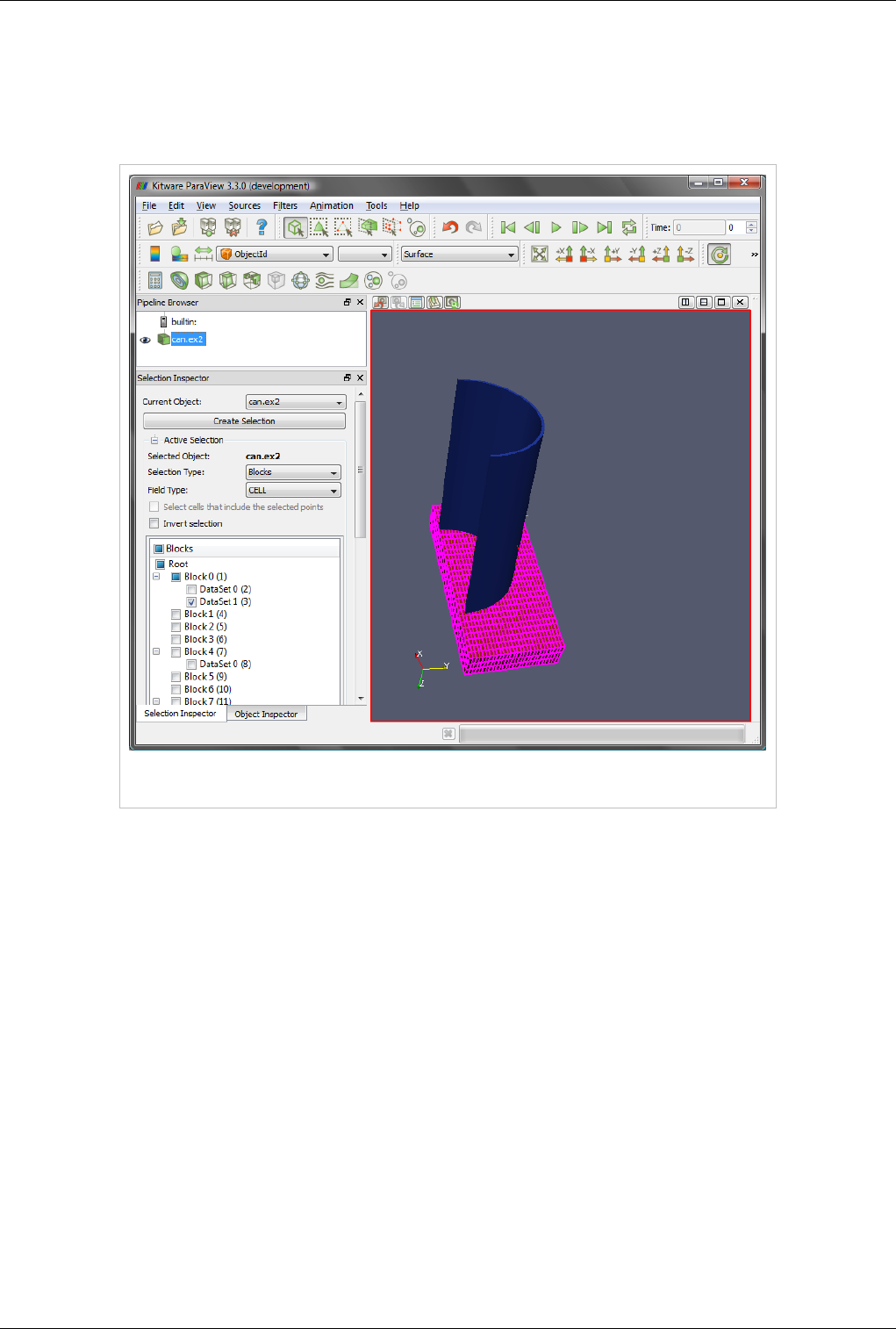
Selection 105
cells (or points) that lie within the frustum. Note that this selection can produce a very large selection and thus may
be time consuming and can increase the memory usage significantly.
Select Blocks in a Composite Dataset
Figure 6.8: Selecting a block in multi-block dataset. All the cells in the selected block are highlighted. The
selection inspector shows the selected block.
Composite datasets are multi-block or AMR (adaptive mesh refinement) datasets. In the case of multi-block datasets,
each block may represent different components of a large assembly e.g. tires, chassis, etc. for a car dataset. Just like
selecting cells or points, it is possible to select entire blocks. To enter the block selection mode use Select Block in
the Selection Controls toolbar or under the Edit menu (you can also use the ‘B’ key as a shortcut for Select Block).
Once in block selection mode, you can simply click on the block in the 3D view to select a single block or click and
drag to select multiple blocks. When a block is selected, its surface cells will be highlighted.
Select using the Spreadsheet View
Thus far the examples have looked at defining the selection on the 3D view. This section focuses on how to create
selections using the spreadsheet view. As discussed earlier, the spreadsheet view simply shows the raw cell (point or
field) data in a table. Each row represents a unique cell (or point) from the dataset. Like with any other spreadsheet
application, you can select a cell (or a point) by simply clicking on the row to select. You can expand the selection
using Ctrl, Shift keys while clicking. If the spreadsheet view is currently showing point attributes, then selecting it
will create a point based selection. Similarly, if it is showing cell attributes then it will create a cell based selection.
Selection cannot be created when showing field attributes which are not associated with any cell or point.
All views showing a selected dataset show the selection. The spreadsheet view showing the data from a source
selected in the 3D view highlights the corresponding cells/points. Conversely, when creating a selection in the
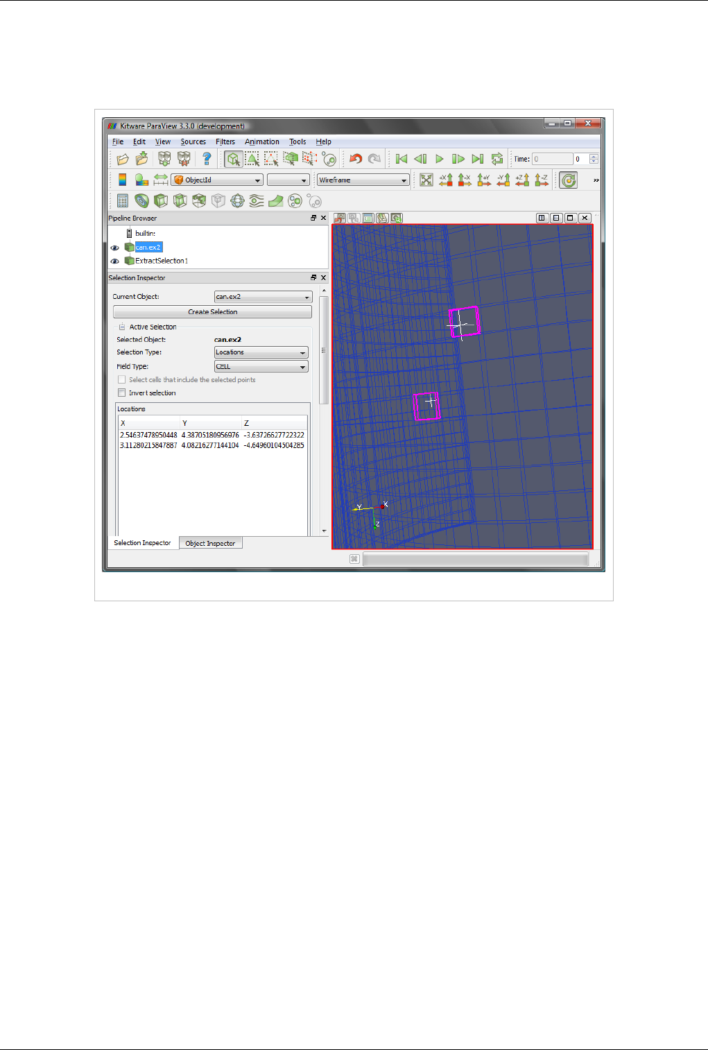
Selection 106
spreadsheet view, the corresponding cell (or point) gets highlighted in all the 3D views showing the source.
Select using the Selection Inspector
Figure 6.9: Location based selection showing the cross hairs used to specify the locations.
Sometimes you may want to tweak the selection or create a new selection with a known set of cell (or point) IDs or
create selections based of value of any array or location etc. This is possible using the Selection Inspector.
Whenever a selection is created in any of the views, it becomes the active selection. The active selection is always
shown in the Selection Inspector. For example, if you select cells on the surface of a dataset, then as shown in Figure
6.8, the selection inspector will show indices for the cells selected.
The selection inspector has three sections: the topmost Current Object and Create Selection are used to choose the
source whose output you want to create a selection on. The Active Selection group shows the details of the active
selection, if any. The Display Style group makes it possible to change the way the selection in shown in the active
3D view.
To create a new selection, choose the source whose output needs to be selected in the Current Object combo-box and
then hit Create Selection. An empty selection will be created and its properties will be shown in the active selection
group. Alternatively, you can use any of the methods described earlier to create a selection; it will still be shown in
the selection inspector.
When you select cells (or points) on the surface or using the spreadsheet view, the selection type is set to IDs.
Creating a frustum selection results in a selection with the selection type set to Frustum, while selecting a block in a
composite dataset creates a Block selection. Field Type indicates whether cells or points are to be selected.
In the active selection group, Selection Type indicates the type of the active selection. You can change the type by
choosing one of the available options.

Selection 107
As shown in Figure 6.8 for IDs selection, the inspector lists all the selected cell or point indices. You can edit the list
of ids to add or remove values. When connected to a parallel server, cell or point ids are not unique. Hence, you have
to additionally specify the process number for each cell or point ID. Process number -1 implies that the cell (or point)
at the given index is selected on all processes. For multi-block datasets, you also need to indicate the block to which
the cell or point belongs. For AMR datasets, you need to specify the (AMR level, index) pair.
As shown in Figure 6.6, for Frustum selection, currently only the Show Frustum option is available. When this
option is turned on, ParaView shows the selection frustum in the 3D view. In the future, we will implement a 3D
widget to modify the frustum.
As shown in Figure 6.8, for Block selection, the full composite tree is shown in the inspector with the selected blocks
checked. Using the selection inspector you can create a selection based on thresholds for scalars in the dataset.
Choose the scalar array and then add value ranges for the selected cells (or points).
The Selection Inspector can be used to create location-based selection. When field type is CELL, cells at the
indicated 3D locations will be selected. When field type is POINT, the point closest to the location within a certain
threshold is selected. If Select cells that include the selected points is checked, then all the cells that contain the
selected point are selected. It is possible to specify more than one location. To aid in choosing positions, you can turn
the Show location widgets option on. As a result, ParaView will show cross hairs in the active 3D view, which can
be moved interactively, as shown in Figure 6.6.
The Selection Inspector also provides a means to create global ID-based selection. These are similar to index based
selection however since global IDs are unique across all processes and blocks, you do not need to specify any
additional as needed by the ID-based selection.
Convert Selections
The Selection Inspector can also be used to convert a selection of one type to another. With some valid active
selection present, if you change the selection type then ParaView will try to convert the current selection to the new
type, still preserving the cells (or points) that were selected, if possible. For example, if you create a frustum-based
selection and then change the selection type to IDs, ParaView will determine the indices for all the cells (or points)
that lie with the frustum and initialize the new index-based selection with those indices. Note that the number of cells
or points that get selected in frustum selection mode can potentially be very large; hence this conversion can be slow
and memory expensive. Similarly, if the dataset provides global IDs, then it is possible to convert between IDs
selection and global ID-based selection. i It is not possible to convert between all types of selections due to obvious
reasons. Conversions between ID-based and global ID-based selections, conversions from frustum to ID-based
selections, and conversions from frustum to global ID-based selections are supported by the Selection Inspector.
Label Selected Cell/Points
Once an active selection is created, you can label the cells or points or their associated values in a 3D view. This can
be done using the Selection Inspector. At the bottom of the selection inspector panel, there are two tabs, Cell Label
and Point Label, which can be used to change the cell or point label visibility and other label attributes such color,
font etc. These tabs are enabled only if the active view is a 3D view. Any changes made in the Display Style group
(including the labels) only affect the active 3D view.

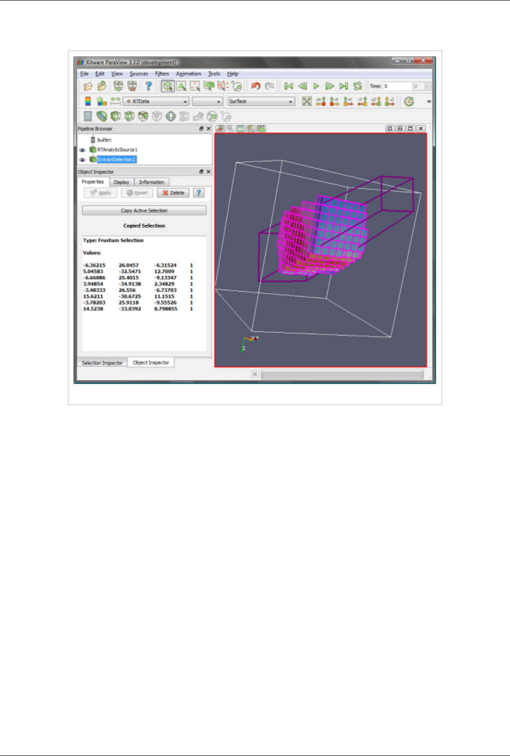
Selection 109
Extract Selection
Figure 6.11: Extract selection using a frustum selection
Selection makes it possible to highlight and observe regions of interest. Often, once a region of interest has been
identified, users would like to apply additional operations on it, such as apply filters to only the selected section of
the data. This can be achieved using the Extract Selection filter. To set the selection to extract, create a selection
using any of the methods already described. Then apply the extract selection filter to the source producing the
selected data. To copy the active selection to the filter, use the Copy Active Selection button. You can change the
active selection at any time and update the filter to use it by using this button. Figure 6.7 shows the extract selection
filter applied after a frustum selection operation. Now, you can treat this as any other data source and apply filters to
it, save state, save data etc.
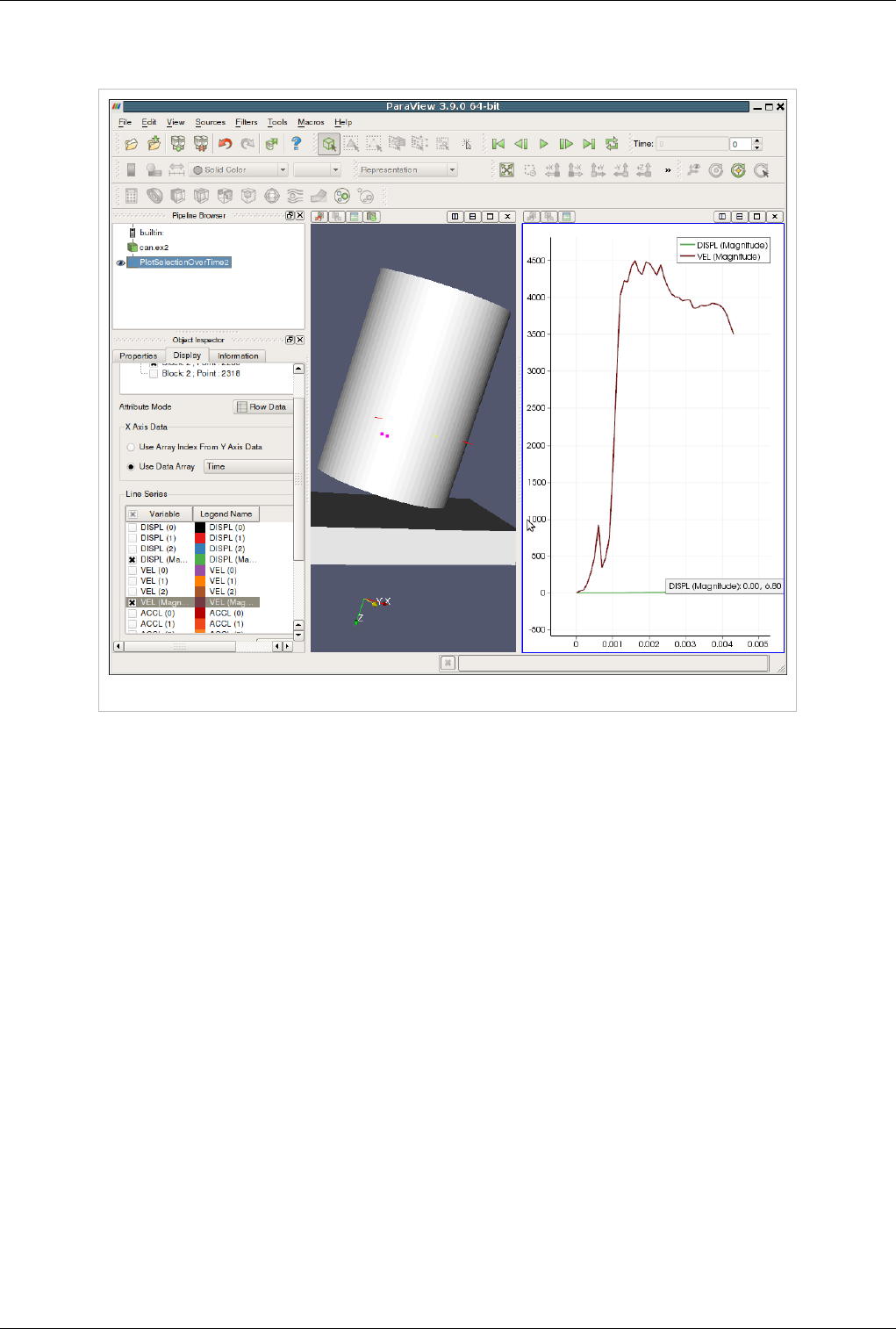
Selection 110
Plot Selection over Time
Figure 6.12: Plot selection over time.
For time varying datasets, you may want to analyze how the data variables change over time for a particular cell or a
point. This can be done using the Plot Selection Over Time filter. This filter is similar to the Extract Selection filter,
except that it extracts the selection for all time-steps provided by the data source (typically a reader) and accumulates
the values for all the cell (or point) attributes over time. Since the selection can comprise of multiple cells or points,
the display tab provides the Select Block widget which can be used to select the cell or point to plot, as shown in
Figure [6]. Currently only one cell (or point) can be plotted at once in the same xy-plot view. You can create
multiple plot views to show multiple plots simultaneously.
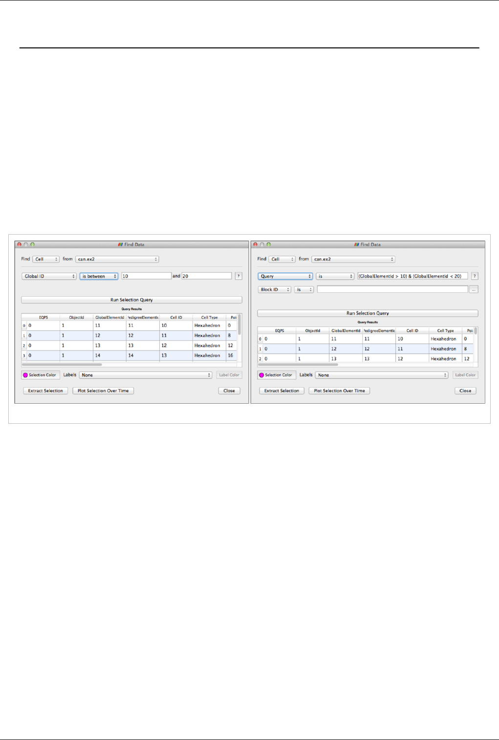
Querying for Data 111
Querying for Data
Find Data Dialog
As previously described, Selection is a mechanism in ParaView for sub-setting and focusing on a particular elements
in the dataset. Different views provides different mechanisms for selecting elements, for example, you can select
visible cells or points using the 3D View. Another mechanism for creating selections is by specifying a selection
criteria. For example, suppose you want to select all cells where the pressure value is between a certain threshold. In
such cases, you can use the Find Data dialog. The Find Data dialog performs a dual role: not only does it enable
specifying the selection criteria but also show details of the selected elements in a spreadsheet. This makes it easier
to inspect the selected elements.
To open the Find Data dialog, go to Edit|Find Data.
Figure 6.13 Query based on field "Global ID" / Query based on Python expression (Generated by the query on the left)
When to use Find Data
This feature is useful when you run into situations where you want to know the cell or the point at which a certain
condition happens For example:
• What are the cells at which PRESSURE >= 12?
• What are the points with TEMP values in the range (12, 133)?
• Locate the cell at ID 122, in Block 2.
This feature provides a convenient way of creating selections based on certain criteria that can then be extracted from
the data if needed.
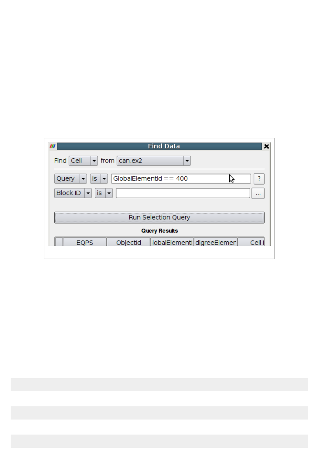
Querying for Data 112
Using the Find Data dialog
The dialog is designed to be used in two distinct operations:
• Define the selection criteria or query
• Process the selected cells/points e.g. show labels in active 3D view, extract selection etc.
You must define the selection query and then execute the query, using the Run Query button before being able to
inspect or process the selected elements.
Defining the Query
First, decide what type of elements you are interested in selecting, that is cells or points and from what data source.
This can be done using the following combo boxes. Note that as you change these, any previous selections/queries
will be cleared.
Figure 6.14 Find Data options
Next, you must define the query string. The syntax for specifying the query string is similar to the expressions used
in the Python Calculator. In fact, ParaView indeed uses Python and numpy under the covers to parse the queries.
In addition, based on the data type and the nature of the current session, there may be additional rows that allow
users to qualify the selection using optional parameters such as process number (when running in parallel), or block
number (for composite datasets).
Once you have defined your query, hit Run Query button to execute the query. If any elements get selected, then
they will be shown in the spreadsheet in this dialog. Also, if any of the views are showing in the dataset that is
selected, then they will be highlighted the selected elements as well, just like regular view-based selection.
Sample Queries
• Select elements with a particular id
id == 100
• Select elements given a list of ids
contains(id, [100,101, 102])
or
in1d(id, [100,101, 102])
• Select elements with matching a criteria with element arrays Temp and V.

Querying for Data 113
Temp > 200
or
Temp == 200
or
contains(Temp, [200,300,400])
or
(Temp > 300) & (Temp < 400) # don't forget the parenthesis
or
(Temp > 300) | (mag(V) > 0)
• Select cells with cell volume matching certain criteria
volume(cell) > 0
or
volume(cell) == max(volume(cell))
Rules for defining queries
• For the element type chosen, every element array becomes available as a field with same name as the array. Thus,
if you are selecting points and the dataset has point arrays named "Temp" and "pressure", then you can construct
queries using these arrays.
• Special fields id (corresponding to element id), cell (corresponding to the cell), dataset (corresponding to the
dataset) are available and can be used to compute quantities to construct queries e.g. to compare volume of cells,
use volume(cell).
• Queries can be combined using operators '&' and '|'.
Query generator
The combobox allow the user to create queries in a more intuitive but in a more limited way. Although, this could be
useful specially when you want to learn how to write more complex query. To do so, you will need to execute your
selection by using a field directly from the combobox instead of the "Query" key word. Any selection execution will
internally generate a Query string which can be seen by switching back to the "Query" combobox value. Such query
can then be used as part of a more complex one if needed.
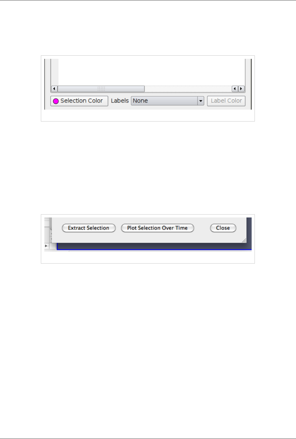
Querying for Data 114
Displaying the Selection
Once a query is executed, the selected elements will be highlighted in all views where the selected data is visible. If
the active view is a 3D view, you can choose whether the show labels for selected elements as well as the color to
use for showing the selected elements using the controls on the Find Data dialog itself.
Figure 6.15
Extracting the Selection
The results of a query are temporary. They get replaced when a new query is executed or when the user creates a
selection using any of the selection mechanisms. Sometimes, however, users may want to further analyze the
selected elements such as apply more filters to only the selected elements, or plot the change in attributes on the
selected elements over time. In that case, you should extract the selection. That creates a new filter that is setup to
run the query on its input and produce a dataset matching the selection criteria. Both Extract Selection and Plot
Selection Over Time are filters available through the Filters menu. The Find Data dialog provides shortcut buttons to
quickly create those filters and set then up with the selection criteria chosen.
Figure 6.16
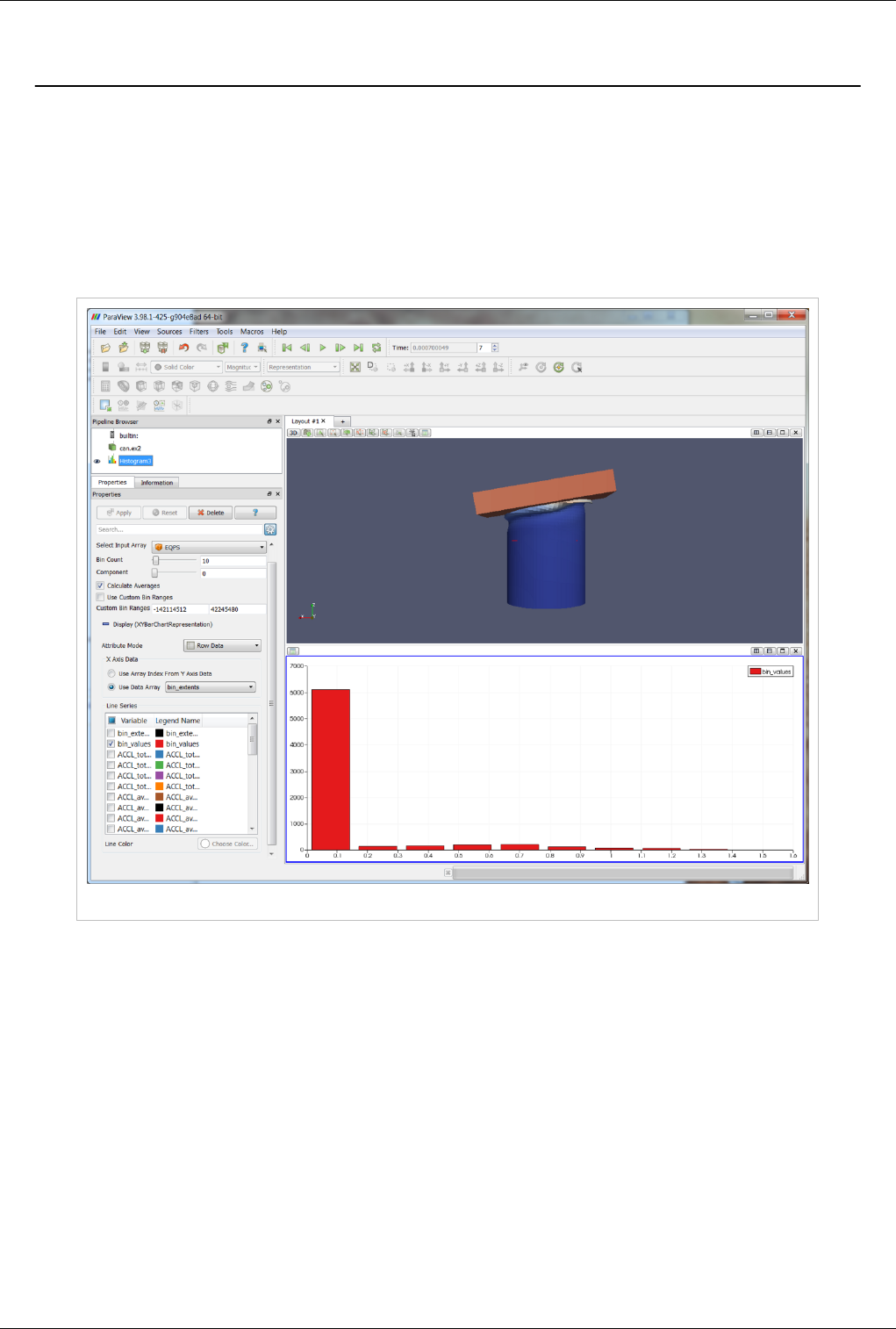
Histogram 115
Histogram
The Histogram filter produces output indicating the number of occurrences of each value from a chosen data array. It
takes in a vtkDataObject but the object must have either point or cell data to operate on. The filter cannot be directly
used with a table but the Table to Points filter can be used to convert the table to a polydata for input into the
Histogram filter. The bar chart is the default view for the output of the Histogram filter. Other views that can be used
are the line chart view, parallel coordinate view, and spreadsheet view. The chart views are useful for observing
trends in the data while the spreadsheet view is useful for seeing exact numbers. An example Histogram filter output
in a bar chart view is shown in Figure 6.17.
Figure 6.17 Histogram filter output in bar chart view
Options for the Histogram filter are:
• Which array to process. This can be either a point data array or a cell data array. For arrays with more than one
component, the user can specify which component to compute with respect to. The default is the first component.
• The number of bins to put the results in as well as the range the bins should be divided from.
• An option to average other field information of the same type for each of the bins.
• Which variables are to be displayed in the view. This is under the Display section on the Properties panel.
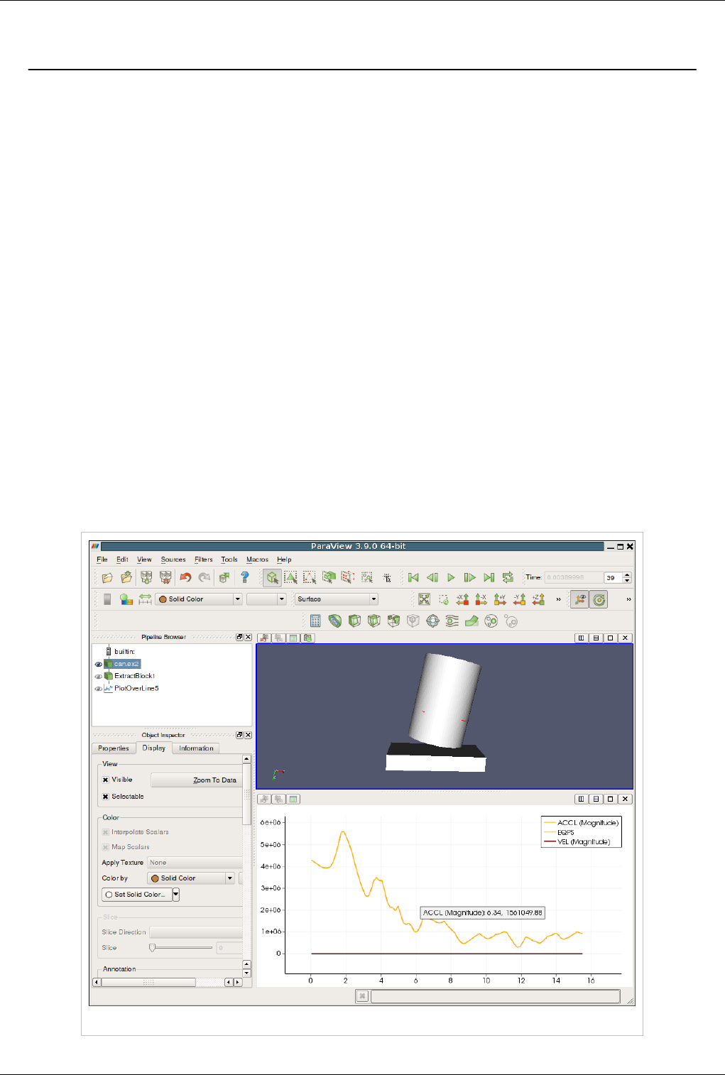
Plotting and Probing Data 116
Plotting and Probing Data
There are multiple ways of probing a dataset for point or cell values. The simplest is the Probe Location filter.
Additionally, there are a variety of filters to plot data with respect to time, location, or grid object ID.
Probe Filter
The probe filter can be used to query a dataset for point or cell data.
Options for the probe filter are:
• Show Point button is used to show where the center of the sphere is for generating the probe points.
• Center on bounds will place the sphere center at the center of the dataset's bounds.
• The sphere center can either be set in the properties tab of the object inspector or in the 3D view with the mouse
cursor. To choose a new point in the 3D view window, press P and then click on the desired point. Note that the
Show Point option must be selected in order to activate the point widget.
The output for this filter is a single cell comprised of a set of points in a vtkPolyData.
Line Plots
The line plots have similar control functionality for displaying the results. These options are in the Display tab of the
Object Inspector and include selecting which point and/or cell data to include in the plot, what should be used as the
x axis values (e.g. point/cell index or a specified point or cell data array), and plot preferences such as line thickness
and marker style. See the line chart view section for more information on setting the display properties for these
filters. An example line plot is shown in Figure 6.18..
Figure 6.18 A Line Plot

Plotting and Probing Data 117
Plot Data / Scatter Plot
The Plot Data filter and Scatter Plot filter are very similar in functionality, with the Scatter Plot filter being a
deprecated version of the Plot Data filter. The main difference is that the Scatter Plot filter's output is a 1D rectilinear
grid while the Plot Data filter's output is the same type as the input.
The Plot Data filter plots point or cell data over the entire data set. By default, the X axis values are determined with
respect to their point or cell index.
Plot Over Line
The Plot Over Line filter is used to plot point data over a specified straight line. The Plot Over Line filter will not
display cell data over the line so the user can use the Cell Data to Point Data filter to convert cell data to point data in
order to use this filter for viewing desired cell data.
The line geometry can specified either by setting the points in the Properties tab of the Object Inspector or by
pressing P and selecting the beginning and ending points of the line. Note that the Show Line option must be selected
to activate the line widget. The resolution option is used to specify at how many evenly spaced points on the line to
query the dataset for information on the point data.
Plot on Sorted Lines
The Plot on Sorted Lines filter is used when polydata with line cell types have been extracted from a dataset and the
user wants to see how point data varies over the line. This filter orders the lines by their connectivity instead of their
point index. The output of the filter is a multiblock with a block for each contiguous line.
Plot on Intersection Curves
The Plot on Intersection Curves filter is used to plot point data where the data set intersects the given polygonal slice
object. The results is a multiblock of polydatas where each block represents a contiguous set of cells. Note that the
polydatas will only have 1D cell types. Thus if the slice type object intersection with the data set has 2D geometry
the filter will take the boundary of the slice type object in order to reduce down to 1D geometry. If the slice type is a
sphere that is wholly contained in a volumetric dataset then the filter parameters are invalid and no lines will be
output.
Plot Selection Over Time
The Plot Selection Over Time filter can be used to visualize the variation of point or cell data from a selection with
respect to time. The selection should be made on the dataset of the filter that precedes the Plot Selection Over Time
filter in the pipeline in order to ensure that the proper points or cells are selected. Note that information for only a
single point or cell can be plotted at a time.
Plot Global Variables Over Time
The Plot Global Variables Over Time filter plots field data that is defined over time. Filters must be set up explicitly
to provide the proper information as this will not work for field data in general. As an example, see the Exodus
reader in ParaView.
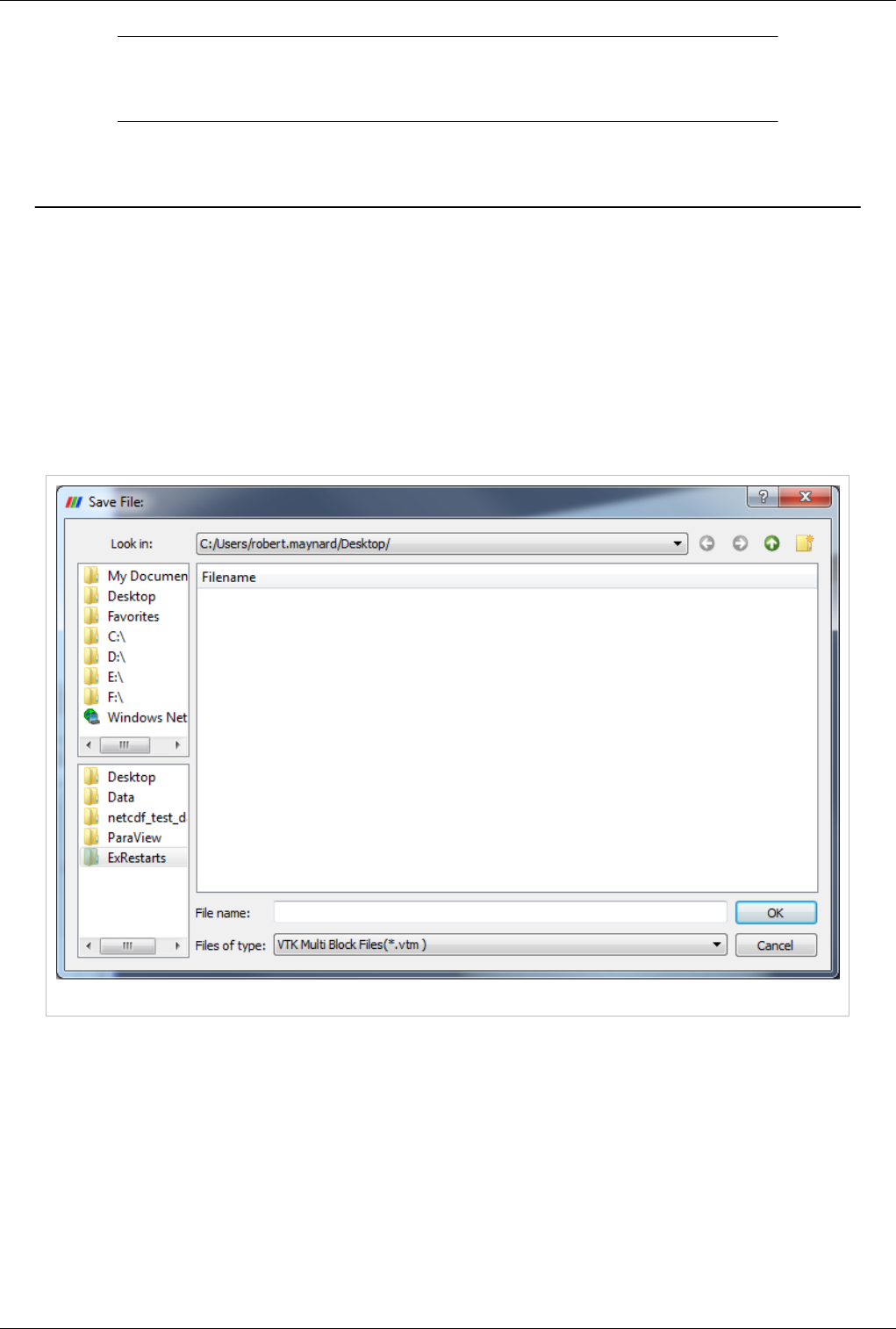
118
Saving Data
Saving Data
Saving Data
Once you have created a visualization of your data in ParaView, you can save the resulting work as raw data, or an
image, movie, or geometry.
Save raw data
Any object in the ParaView pipeline browser can be saved to a data file by selecting Save Data from the File menu.
The available file types will change based on the dataset type of the current dataset. The file formats in which
ParaView can save data are listed on List of Writers
Figure 7.1 Saving Files in ParaView
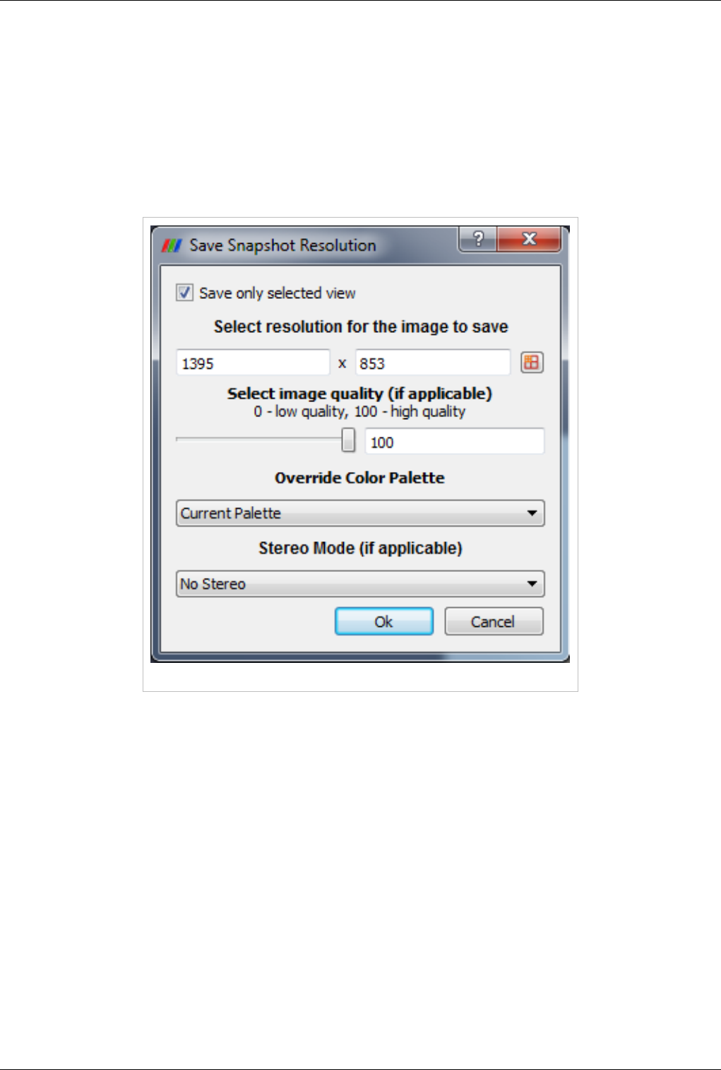
Saving Data 119
Save screenshots
ParaView allows the user to save either the active view or all the views. The resulting image will be saved on the
client machine, even when running with a remote server. The dialog allows you to control the following:
• Image size
• Aspect ratio of the image
• Image quality
• Color palette
• Stereo mode
Figure 7.2 Save Snapshot Resolution Dialog Box
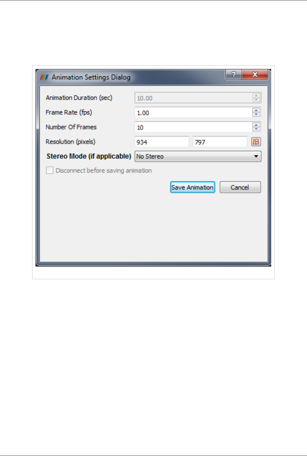
Saving Data 120
Save Animation
Once you have created an animation of your data, you can save the animation to disk either as a series of images
(one per animation frame) or as a movie file. The animation will contain all the visible views.
To do this, select Save Animation from the File menu. The Animation Settings Dialog then appears, which lets you
set properties for the recorded animation.
Figure 7.3 Animation Settings Dialog Box
Once you press the Save Animation button, a save file dialog box will allow you to choose where to save your image
or movie file(s). Enter a file name then select an image file type (.jpg, .tif, or .png) or a movie file type (.avi).
Once you choose a file name, the animation will play from beginning to end, and the animation frames generated
will be used to create the selected type of image or movie file(s). While the image is playing the render window in
ParaView will not update with the correct frame.
If you are connected to a remote server then the Disconnect Before Saving Animation checkbox will be enabled. If
you select this before saving the animation, then the ParaView client will disconnect from the server immediately,
and the server will continue generating and saving images until the animation completes. When it is finished
recording the animation, the server will shut down.
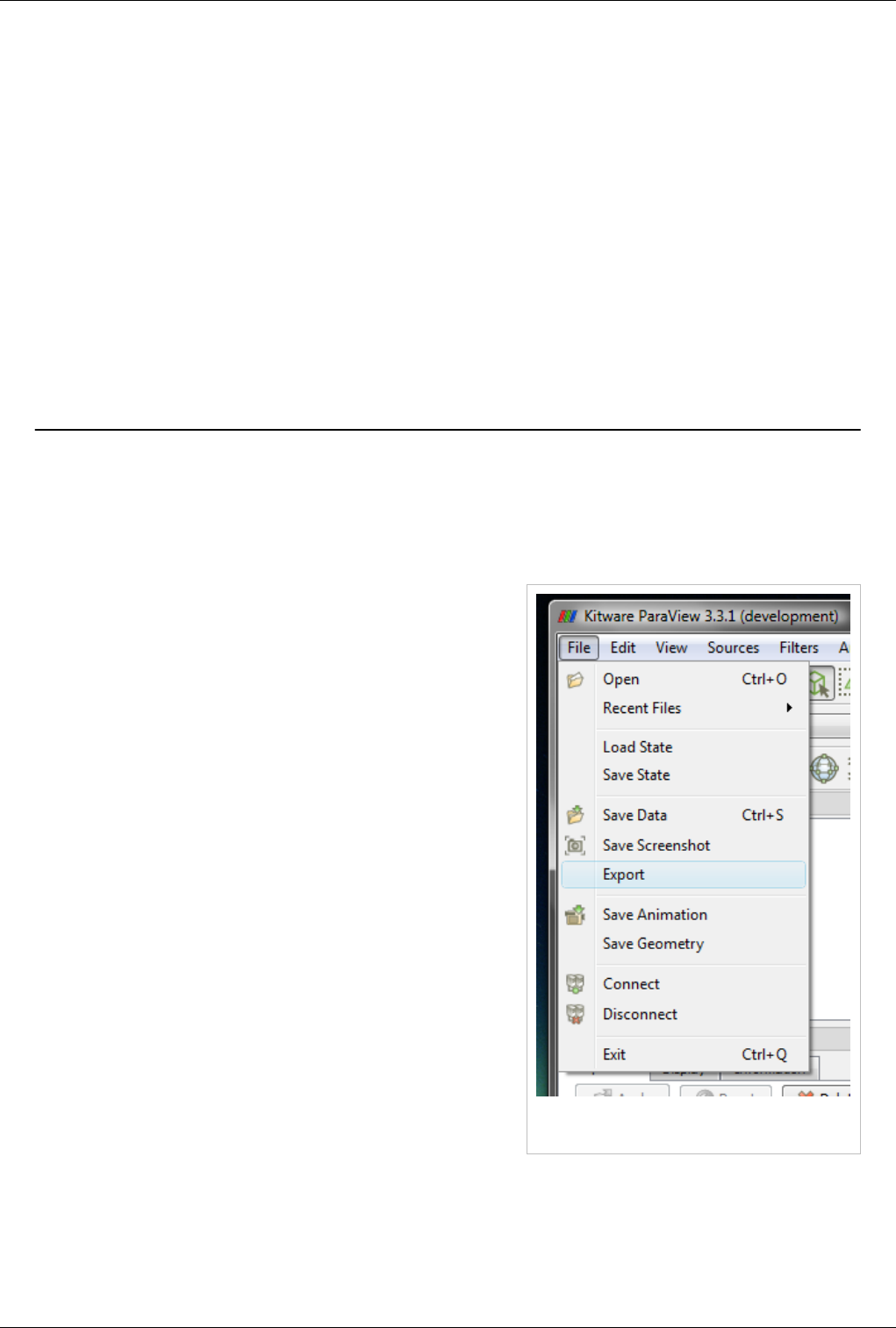
Saving Data 121
Save geometries
In addition to saving images of each time step in your animation, you may also wish to save the geometry itself.
Select Save Geometry from the File menu to do this. This will cause a file navigation dialog box to be displayed.
Navigate to the location where you wish to save the geometry, and enter a file name. You must save your data using
ParaView’s .pvd file format.
Unlike an animation, save geometry will only save the visible geometry of the active view for each time step. The
resulting .pvd file will contain a pointer to each of these files, which are saved in a folder with the same as the .pvd
file.
You can later reload the .pvd file into ParaView as a time varying dataset. If multiple datasets were displayed while
the animation was running, they will be grouped together as a multi-block dataset for each time step. If you then
want to operate on the parts individually, run the Extract Blocks filter to select the appropriate block(s).
Exporting Scenes
ParaView provides functionality to export any scene set up with polygonal data (i.e without volume rendering).
Currently X3D [1] (ASCII as well as binary), VRML (Virtual Reality Modeling Language) [2], and POV-Ray [3] are
supported. To export a scene, set up the scene in a 3D view. Only one view can be exported at a time. With the view
to be exported active, choose File | Export. A new HTML/WebGL exporter is also now available in
ParaView/master or in ParaView 4 as a plugin.
Figure 7.4 Export option in the File menu can be used
to export the scene set up in a 3D view
The file-open dialog will list the available types. The type is
determined based on the extensions of the file written out:
• *.vrml -- VRML [4]
• *.x3d -- X3D ASCII [5]
• *.x3db -- X3D Binary [5]
• *.pov -- POV-Ray [6]
• *.html -- Using WebGL to render a surfacique 3D scene into a
web page. Static Standalone WebGL example from
ParaViewWeb [7]

Exporting Scenes 122
ParaView: [Welcome | Site Map [8]]
References
[1] http:/ / www. web3d. org/ x3d/
[2] http:/ / www. web3d. org/ x3d/ vrml
[3] http:/ / www. povray. org/
[4] http:/ / www. vtk. org/ doc/ nightly/ html/ classvtkVRMLExporter. html
[5] http:/ / www. vtk. org/ doc/ nightly/ html/ classvtkX3DExporter. html
[6] http:/ / www. vtk. org/ doc/ nightly/ html/ classvtkPOVExporter. html
[7] http:/ / paraviewweb. kitware. com/ PWApp/ WebGL?name=mummy-state& button=View
[8] http:/ / www. paraview. org/ Wiki/ Category:ParaView
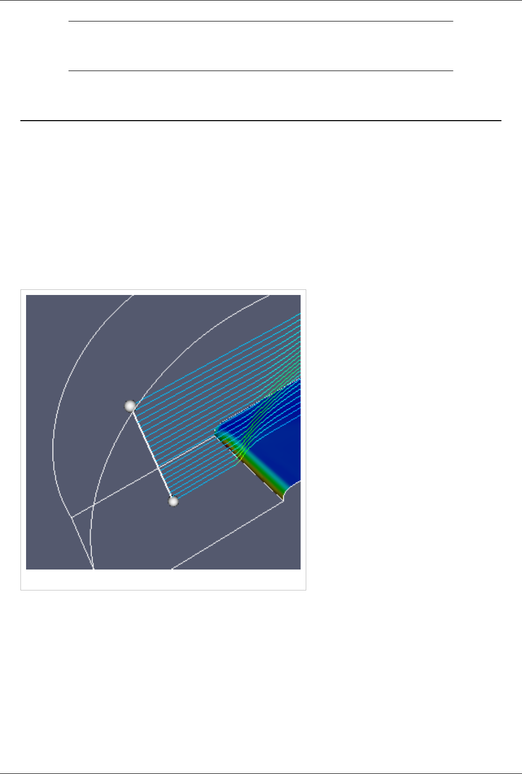
123
3D Widgets
Manipulating data in the 3D view
3D Widgets
In addition to being controlled manually through entry boxes, sliders, etc., parameters of some of the filters and
sources in ParaView can be changed interactively by manipulating 3D widgets in a 3D view. Often the 3D widgets
are used to set the parameters approximately, and then the manual controls are used for fine-tuning these values. In
the manual controls for each 3D widget, there is a check box for toggling whether the 3D widget is drawn in the
scene. The label for the check box depends on the type of 3D widget being used. The following 3D widgets are
supported in ParaView.
Line Widget
Figure 8.1 Line Widget Results
The line widget is used to set the orientation
and the position of a line. It is used in both
the stream tracer and elevation filters. The
position of the line can be changed by
clicking on any point on the line, except the
endpoints, and dragging. To position the
widget accurately, the user may need to
change the camera position as well. Holding
Shift while interacting will restrict the
motion of the line widget to one of the X, Y,
or Z planes. (The plane chosen is the one
most closely aligned with the direction of
the initial mouse movement.) To move one
of the endpoints, simply use one of the point
widgets on each end of the line. These are
marked by spheres that become red when
clicked. You can also reposition the
endpoints by pressing the “P” key; the
endpoint nearest to the mouse cursor will be
placed at the position on the dataset surface
beneath the mouse position. Left-clicking
while the cursor is over the line and dragging will reposition the entire line. Doing the same with the right mouse
button causes the line to resize. Upward mouse motion increases the length of the line; downward motion decreases
it.
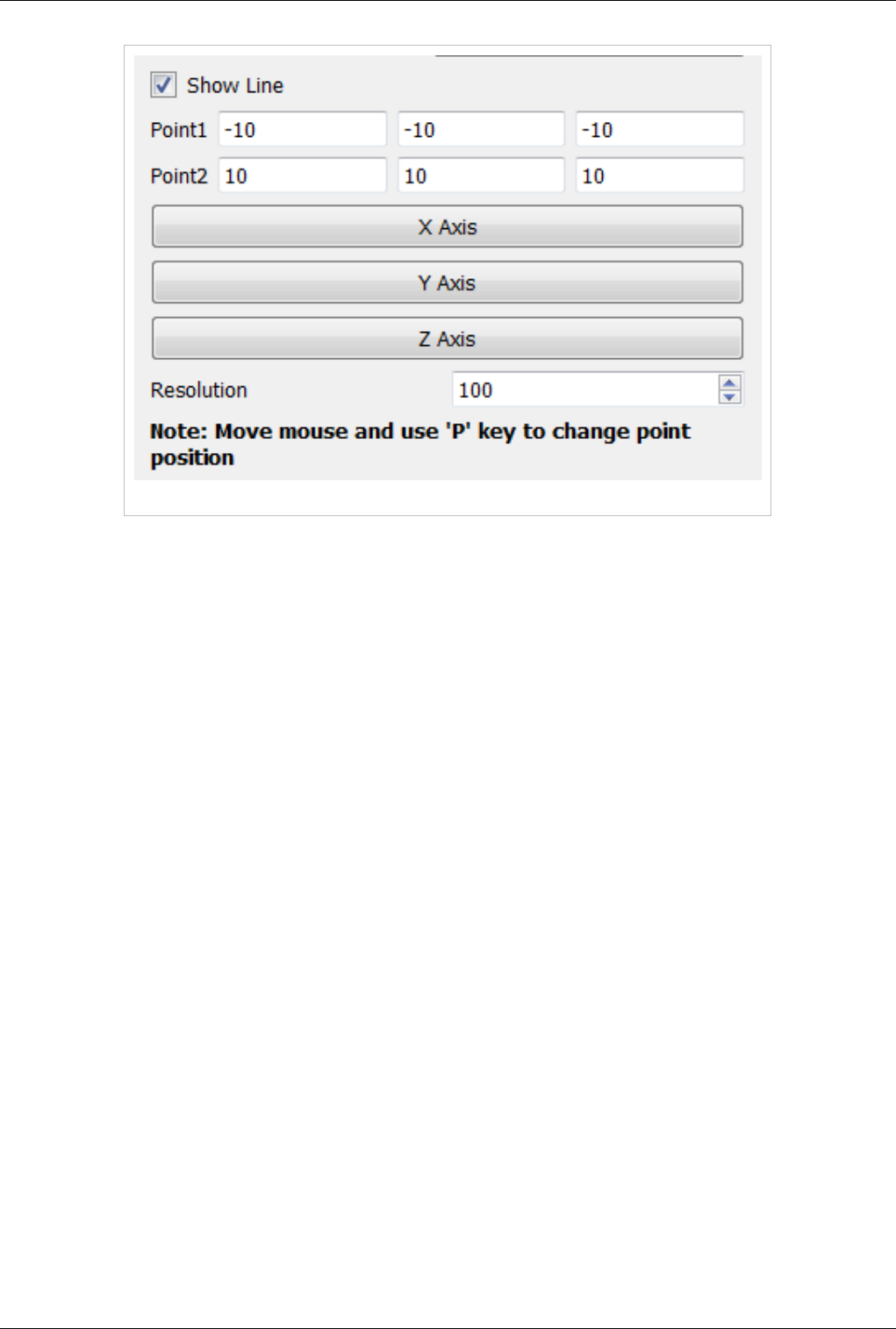
Manipulating data in the 3D view 124
Figure 8.2 Line Widget User Interface
The show line check box toggles the visibility of the line in the 3D view.
The controls shown in Figure 8.2 can be used to precisely set the endpoint coordinates and resolution of the line. The
X Axis, Y Axis, and Z Axis buttons cause the line to be along the selected axis and pass through the center of the
bounds of the dataset.
Depending on the source or filter using this widget, the resolution spin box may not be displayed. The value of the
resolution spin box determines the number of segments composing the line.
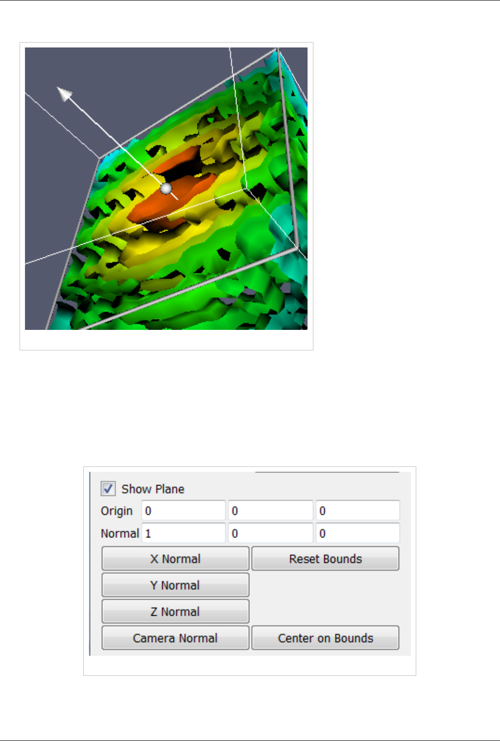
Manipulating data in the 3D view 125
Plane Widget
Figure 8.3 The Plane Widget
The plane widget is used for clipping
and cutting. The plane can be moved
parallel to its normal by left-clicking
on any point on the plane except the
line center and dragging.
Right-clicking on the plane, except on
the normal line center, and dragging
scales the plane widget. Upward mouse
motion increases the size of the plane;
downward motion decreases it. The
plane normal can be changed by
manipulating one of the point widgets
(displayed as cones that become red
when clicked) at each end of the
normal vector.
Shown in Figure 8.4, the standard user
interface for this widget provides entry
boxes for setting the center position
(Origin) and the normal direction of the
plane as well as toggling the plane
widget’s visibility (using the show
plane check box). Buttons are provided
for positioning the plane at the center of the bounding box of the dataset (Center on Bounds) and for aligning the
plane’s normal with the normal of the camera (Camera Normal), the X axis, the Y axis, or the Z axis (X Normal, Y
Normal, and Z Normal, respectively). If the bounds of the dataset being operated on change, then you can use the
Reset Bounds button to cause the bounding box for the plane widget to match the new bounds of the dataset and
reposition the origin of the plane at the center of the new bounds. Using only the Center on Bounds button in this
case would move the origin to the center of the new bounds, but the bounds of the widget would not be updated.
Figure 8.4 Plane widget user interface
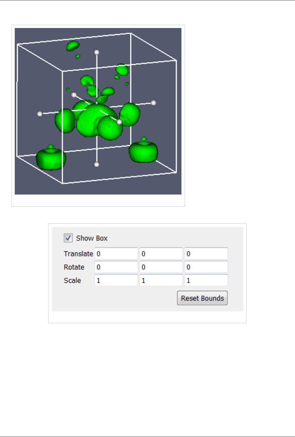
Manipulating data in the 3D view 126
Box Widget
Figure 8.5 Box Widget
The box widget is used for clipping and
transforming datasets. Each face of the
box can be positioned by moving the
handle (sphere) on that face. Moving
the handle at the center of the box
causes the whole box to be moved.
This can also be achieved by holding
Shift while interacting. The box can be
rotated by clicking and dragging with
the left mouse button on a face (not at
the handle) of the box. Clicking and
dragging inside the box with the right
mouse button uniformly scales the box.
Dragging upward increases the box’s
size; downward motion decreases it.
Traditional user interface controls,
shown in Figure 8.6, are also provided
if more precise control over the
parameters of the box is needed. These
controls provide the user with entry
boxes and thumb wheels or sliders to
specify translation, scaling, and orientation in three dimensions.
Figure 8.6 Box widget user interface
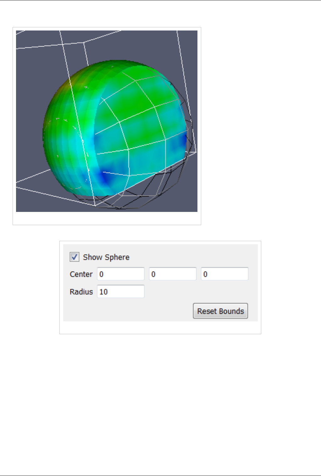
Manipulating data in the 3D view 127
Sphere Widget
Figure 8.7 Sphere Widget
The sphere widget is used in clipping
and cutting. The sphere can be moved
by left-clicking on any point on the
sphere and dragging. The radius of the
sphere is manipulated by right-clicking
on any point on the sphere and
dragging. Upward mouse motion
increases the sphere’s radius;
downward motion decreases it.
As shown in Figure 8.8, the center and
radius can also be set manually from
the entry boxes on the user interface.
There is also a button to position the
sphere at the center of the bounding
box of the current dataset.
Figure 8.8 Sphere widget user interface
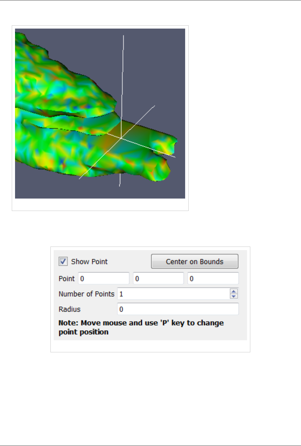
Manipulating data in the 3D view 128
Point Widget
Figure 8.9 Point Widget
The point widget is used to set the
position of a point or the center of a
point cloud. It is used by the Stream
Tracer, Probe Location and Probe
Location over Time filters. The
position of the point can be changed by
left-clicking anywhere on it and
dragging. Right-clicking and dragging
anywhere on the widget changes the
size of the point widget in the scene.
To position the widget accurately, the
user may need to change the camera
position as well. Holding Shift while
interacting will restrict the motion of
the point to one of the X, Y or Z
planes. The plane chosen is the one that
is most closely aligned with the
direction of the initial mouse
movement.
As shown in Figure 8.10, entry boxes
allow the user to specify the
coordinates of the point, and a button is provided to position the point at the center of the bounds of the current
dataset. If the point widget is being used to position a point cloud instead of a single point, entry boxes are also
provided to specify the radius of the point cloud and the number of points the cloud contains.
Figure 8.10 Point widget user interface
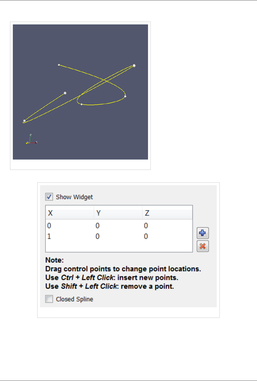
Manipulating data in the 3D view 129
Spline Widget
Figure 8.11 Spline Widget
The spline widget is used to define a path
through 3D space. It is used by the Spline
Source source and in the Camera animation
dialog. The widget consists of a set of
control points, shown as spheres in the 3D
scene that can be clicked on with the mouse
and dragged perpendicular to the viewing
direction. The points are ordered and the
path through them defines a smoothly
varying path through 3D space.
As shown in Figure 8.12, the text control
box for the spline widget allows you to add
or delete control points and specify their
locations exactly. You can hide or show the
widget and can choose to close the spline to
create a loop, which adds a path segment
from the last control point back to the first.
Figure 8.12 Spline widget user interface
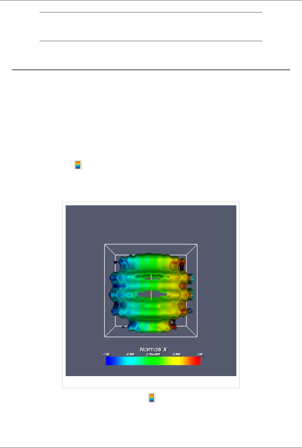
130
Annotation
Annotation
Annotation
In ParaView, there are several ways to annotate the data to better understand or explain it. Several of the annotations
can be interactively placed in the 3D scene. The parameters of the annotations are controlled using traditional user
interface elements. Some types of annotation are discussed in other parts of this book. See the section on Selection
for information about labeling selected points or cells in a data set.
Scalar Bar
The most straightforward way to display a scalar bar (or color legend) in the active 3D view is to use the Color
Legend Visibility button on the Active Variables Control toolbar. When the data set selected in the Pipeline
Browser is being colored by a variable (i.e., something other than Solid Color is selected in the Color by menu on the
Display tab), this button is active. Clicking it toggles the visibility (in the selected 3D view) of a scalar bar showing
the mapping from data values to colors for that variable.
Figure 9.1 Scalar Bar displaying X-component of Normals
Clicking the Edit Color Map button to the right of the Color Legend button brings up the Color Scale Editor
dialog. As described in the Displaying Data [1] chapter, you have precise control over the mapping between data
values and visible colors on the Color Scale tab of that dialog.
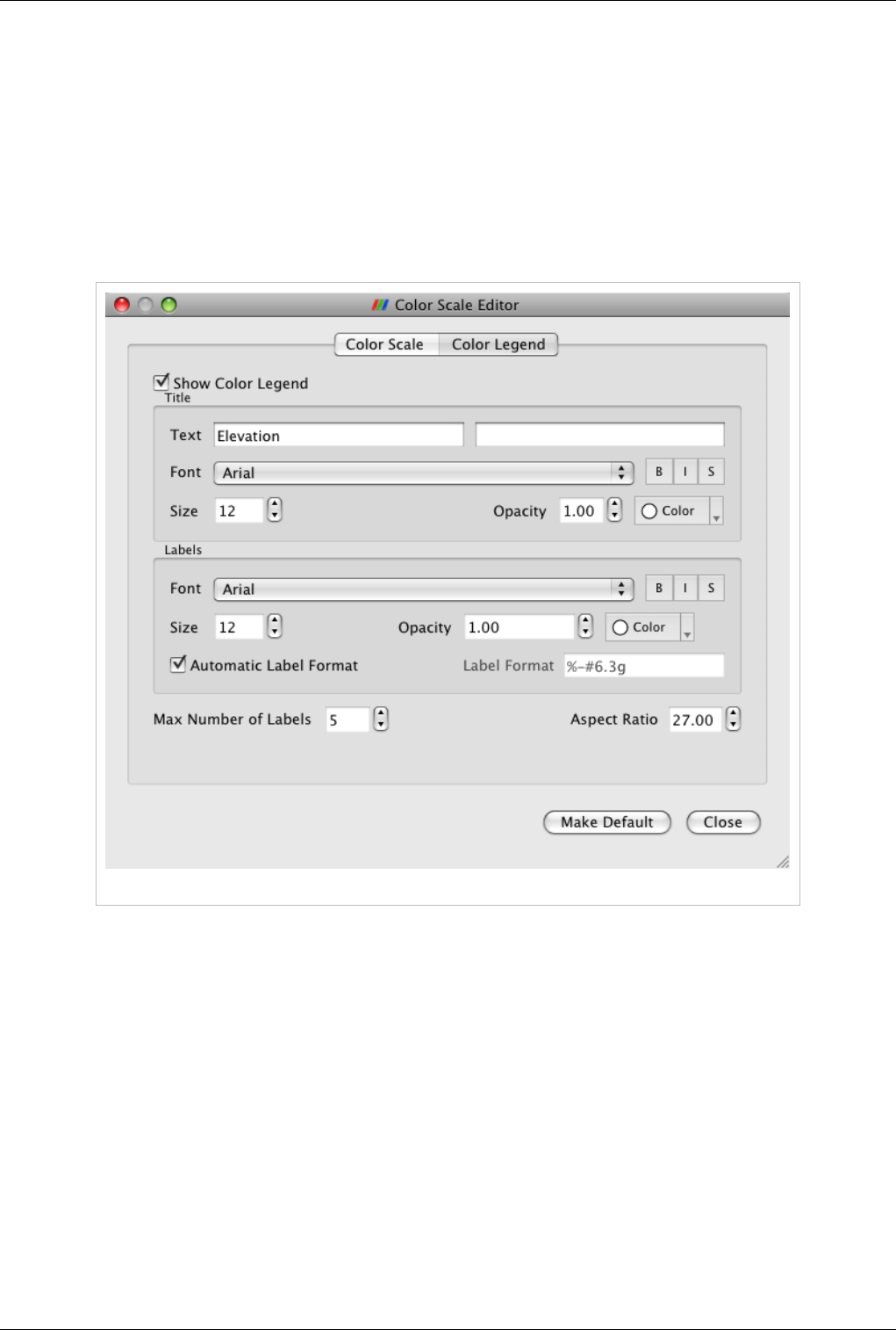
Annotation 131
On the Color Legend tab, there are several different parameters that allow you to control the appearance of the color
legend itself. First is the Show Color Legend check box which toggles the visibility of the scalar bar (color legend) in
the 3D view. This has the same effect as using the color legend visibility button. Below the Show Color Legend
check button are the controls for displaying the title and labels on the scalar bar. In the Title section, the Text entry
box specifies the label that appears above the scalar bar. It defaults to the name of the array used for coloring the data
set. If the current data set is being colored by a vector array, the value of the second entry box defaults to specifying
how the color is determined from the vector (i.e.,X, Y, Z, or Magnitude). The entry box labeled Labels contains
formatting text specifying the form of the scalar bar labels (numbers). The format specification used is the same as
that used by the print function in C++.
Figure 9.2 The color legend tab of the Color Scale Editor dialog
Below each of the Title and Labels entry boxes are controls for determining how the title and labels will be drawn in
the display area. The leftmost control is a menu for choosing the font; the available fonts are Arial (the default),
Courier, and Times. Next are three formatting attribute buttons controlling whether the text is boldfaced, italicized,
or shadowed. The next interface control is a spin box for controlling the text’s opacity. It ranges from 0 (transparent)
to 1 (opaque).
At the bottom of this tab is a Number of Labels spin box. This determines how many scalar-value labels will be
shown alongside the scalar bar. To the right of that is an Aspect Ratio spin box which allows you to make the scalar
bar relatively thinner or thicker.
When the scalar bar is displayed in the 3D scene, it can be positioned and resized interactively, similar to interacting
with 3D widgets. Clicking and dragging the scalar bar with the left mouse button repositions it in the display area. If
the scalar bar begins to move beyond the left-or-right side of the display area, it is reoriented vertically. If it is
moving off-screen at the top or bottom of the display area then it is reoriented in a horizontal direction. The scalar
bar can be resized by left-clicking and dragging any of its sides or corners.
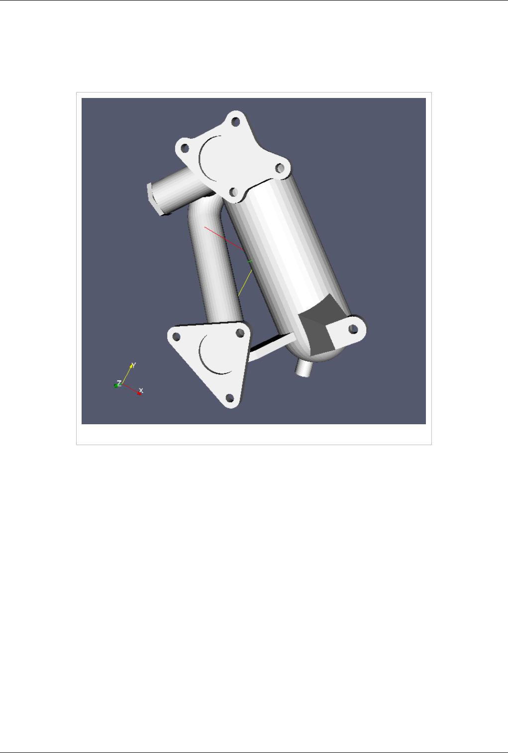
Annotation 132
Orientation Axes
When interacting with data in ParaView, it can be difficult to determine how the data set is oriented in 3D. To
remedy this problem, a marker showing labeled 3D axes (i.e., orientation axes) can be displayed. The orientation of
the axes matches that of the data, and the axes reorient themselves as the camera is rotated about the 3D scene.
Figure 9.3 3D Orientation Axes
The user interface controls for the orientation axes are located in the Annotation section of the View Settings dialog
(Edit|View Settings) for the 3D view. The check-box beside the Orientation Axes label toggles the visibility of the
orientation axes. The Interactive check box controls whether the orientation axes can be repositioned and resized
through mouse interaction, similar to interacting with 3D widgets. Left-clicking and dragging the orientation axes
repositions them in the 3D view. When the orientation axes are in interactive mode, a bounding rectangle (outline) is
displayed around the axes when the mouse moves over them. Left-clicking and dragging on the edges of this outline
resizes the orientation axes.
From the Set Outline Color button (enabled when Interactive is checked), you can change the color used for
displaying the bounding rectangle. This is useful for making the outline more visible if its current color is similar to
the color of the background or any object behind the outline (if the orientation axes are placed in front of a data set).
The orientation axes are always drawn in front of any data set occupying the same portion of the 3D view. The Axis
Label Color button allows you to change the color of the labels for the three axes. The reasons for changing the color
of the axis labels are similar to those for changing the outline color.
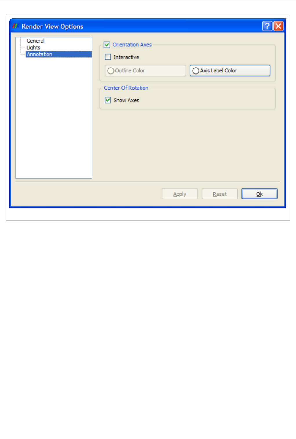
Annotation 133
Figure 9.4 User interface controls for orientation axes (in 3D view's view settings dialog)
Center of Rotation
On the same dialog box, you also have control over whether or not the center of rotation should be annotated. This
annotation demarcates the location in which the camera rotates. ParaView uses the center of the initial data set
loaded into the pipeline as the default value. You can control this placement and display of the center of rotation
display via the Center Axes Control toolbar (View|Toolbars|Center Axes Control). If you need to specify an exact
coordinate you may do so via the Adjust Camera dialog exposed by the rightmost button on the left set of buttons
above the 3D view.
Text Display
Often users want to display additional text in the 3D view (e.g., when generating a still image or an animation). In
ParaView, there are a variety of ways to do this, all through the use of sources and filters. The Text source displays
2D text in the 3D scene, the 3D Text source does the same for 3D text, and the Annotate Time filter shows the
current time using a text annotation in the 3D view.
Text Source
The Text source allows you display arbitrary 2D text on top of a 3D view. It is available from the Sources menu. On
its Properties tab, enter whatever text you wish to be displayed in the Text entry area, and press the Apply button.
Once the text has been added to the 3D view, you can reposition it by left-clicking and dragging the text. (A
bounding box will be displayed around the text.) By default, the text is displayed in the lower left corner of the 3D
view.
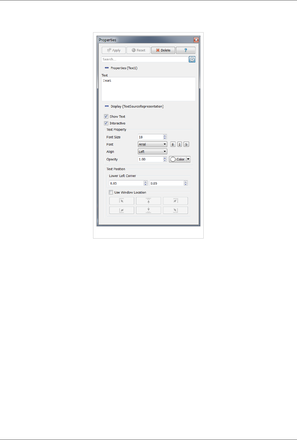
Annotation 134
The Display section on the Properties panel for the Text source is different than for most other sources and filters
displayed in the 3D view. Specific controls are given for positioning the text and setting various font properties.
Figure 9.5 Properties panel for the Text source
The first check box, Show Text, toggles the visibility of the text in the 3D view. This corresponds to the eye icon in
the Pipeline Browser for this source. The Interactive check box below it determines whether the text may be
interactively repositioned by clicking and dragging in the 3D view.
The Text Property section of the Properties panel allows you to specify various parameters relating to the font used
for displaying the text. The Font Size spin box determines how large the letters in the text will be. The Font menu
determines which font type will be used: Ariel, Courier, or Times. The three buttons beside this menu indicate
whether the text will be drawn boldfaced, italicized, and/or using shadows. The Align menu specifies whether the
text will be left, center, or right-aligned within its bounds box. The Opacity spin box determines how opaque the text
appears. An opacity value of 0 corresponds to completely transparent text, while an opacity value of 1 means
completely opaque text. The Color button beside the Opacity spin box allows you to choose a color for the text.
The Text Position of the Properties panel is used for specifying exactly where in the 3D view the text appears. If Use
Window Location is unchecked, then the Lower Left Corner section is active. The two spin boxes provided
determine the X and Y coordinates of the lower left corner of the bounding box of the text, specified in normalized
coordinates (starting from the lower left corner of the view).
If Use Window Location is checked, then the six buttons in that section of the interface become available. They
allow you to choose various locations within the view for anchoring the text. Using the top row of buttons, you may
place the text in the upper left corner, in the top center of the view, or in the upper right corner. The bottom row of
button behaves similarly for the bottom portion of the 3D view.
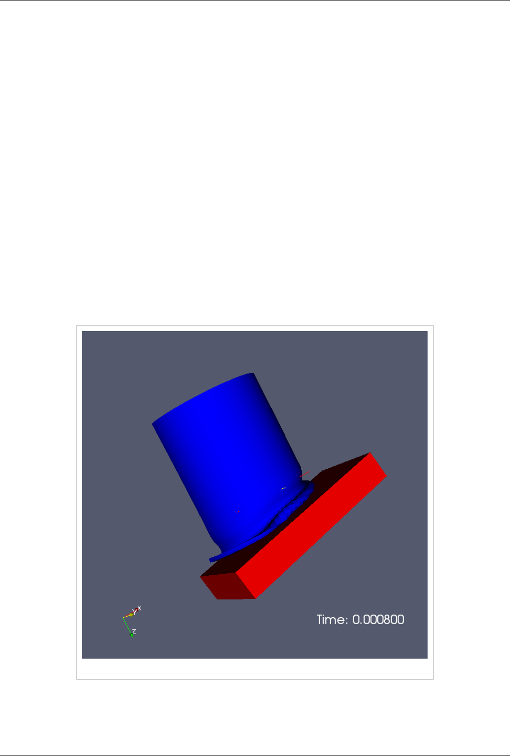
Annotation 135
3D Text Source
Whereas the Text source positions text in 2D, overlaying the 3D scene, the 3D Text source places text in the 3D
scene. The text is affected by rotation, panning, and zooming as is any other object in the 3D scene.
You can control the placement of the 3D text in two ways. First, the Display tab for all sources and filters shown in a
3D view have controls to position, translate, rotate, and scale the object via textual controls. However, it is often
easier to use a the Transform filter for the same purpose. The transform filter allows you to drag, rotate and scale the
object via either the 3D widget in the scene, or via the text controls on its Properties tab.
Annotate Time
The Annotate Time source and filter are useful for labeling a time-varying data set or animation with ParaView’s
current time in a 3D view. The distinction between the two is somewhat abstract. VTK's temporal support works by
have the pipeline request data for a particular time; the text source displays exactly this. VTK's sources and filters are
allowed to produce data at different times (usually nearby producing data that changes over a step function in time).
The annotate time filter shows the data produces by an given filter.
In either case, the annotated time value is drawn as a 2D label, similar to the output of the Text source. The
Properties tab for this filter provides a single text box labeled Format. From this text box, you may specify a format
string (print style) indicating how the label will appear in the scene. As with the output of the Text source, this label
may be interactively repositioned in the scene. The Display tab for this source is the same as the one for the Text
source; it is described earlier in this section.
Figure 9.6 Using the Annotate Time filter to display the current time in a time-varying data set

Annotation 136
Other sources as Annotations
Most of the other items in the Sources menu can also be used for annotation of the 3D scene. Placement of these is
similar to placement of the 3D Text source. In particular the 2D Glyph, Ruler, and Outline sources are frequently
used for annotation.
As the name implies, the ruler allows for some quantitative measurement of the data. The ruler produces a Line
widget in the 3D scene. It is most effective to use the 'P' key to place the two ends of the line in the 3D scene in turn.
When placed the Properties tab, the ruler lists the length of the line you've placed in space. In Figure 9.7, a ruler is
being used to measure the distance between the cows horns.
Cube Axes
Finally, in the Display section of the Properties tab of any object shown in a 3D view, you can toggle the display of a
Cube Axes Display. Like the ruler source, the cube axes allows you to inspect to world space extent of objects in the
scene. When this display is enabled, a gridded, labelled bounding box is drawn around the object that lets you
quickly determine the world space extent in each dimension of the object. That box is generally Axis aligned but as
been extended to support arbitrary axis. In case of arbitrary axis, the source or the filter needs to provide such
meta-information to the CubeAxes.
Figure 9.7 Cube Axes of a sheared cube and Rulers used to measure a cow and its horns
Pressing the Edit button next to the enable check box brings up a dialog that lets you customize the presentation of
the axes display. You have one tab on this dialog for each of the three axes. Use the Title entry to specify a label.
Use the Show Axes check box to enable or disable the given axes. Show Ticks and Show Minor Ticks let you
customize the division markers along the axis. Show Grid Lines extends the major tick marks so that they completely
surround the object. The Original bounds as range allow to rescale your object inside the Display section without
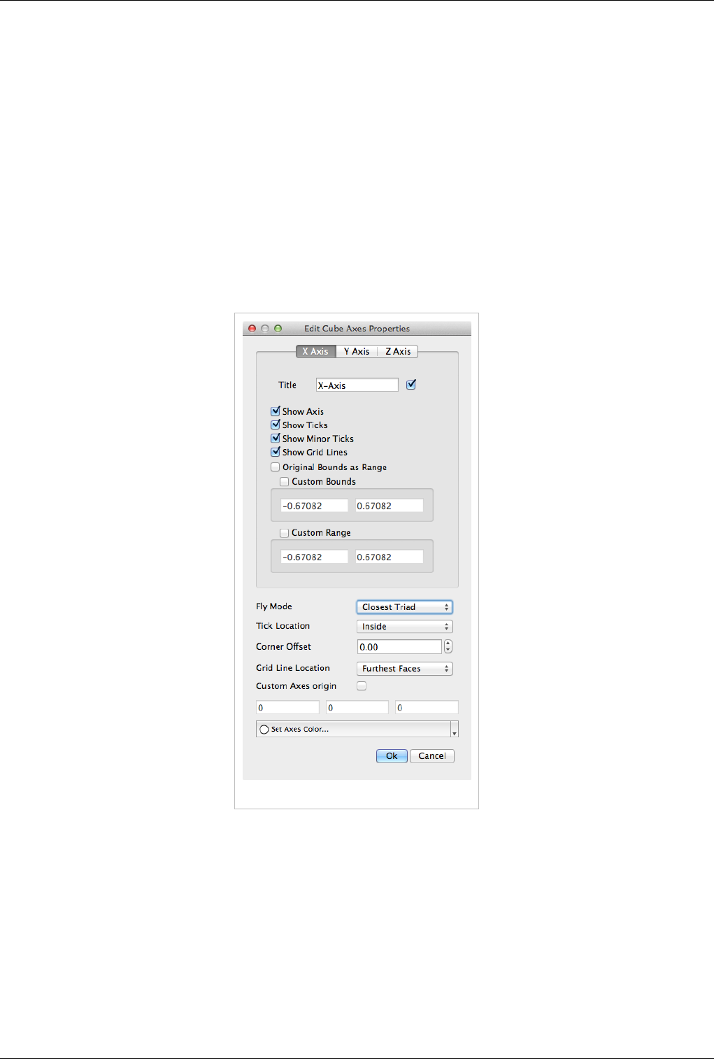
Annotation 137
changing the ruler legend. The Custom Bounds entry allows you to specify your own extent for that cube axis where
as the Custom Range only change the range of the values that are used as label.
At the bottom of the dialog box are controls over all three axes. The Fly Mode drop-down controls the way the axes
are drawn on different axes dependent on the camera orientation. Outer Edges draws opposing edges so as to space
the annotation as widely as possible. Closest Triad and Furthest Triad draw the nearest and furthest corners
respectively. The two static options lock the choice of edges to draw so that they do not change as the camera moves.
Tick Location draws the tick marks inward toward the center of the object, outward away from the center, or in both
directions simultaneously. Corner Offset puts some space between the actual bounds and the displayed axes, which
is useful for minimizing visual clutter. The Grid line location allow to either show the Grid Lines around the whole
object or choose if you only want to see them on the front or on the back of the object that you are looking at. The
visibility of the grid lines automatically update when you rotate your object. (In figure 9.7, we set that value to:
Furthest Faces) Finally, you have control over the color of the axes through the Set Axes Color pop-up color
selector.
Figure 9.8 Edit Cube Axes Dialog
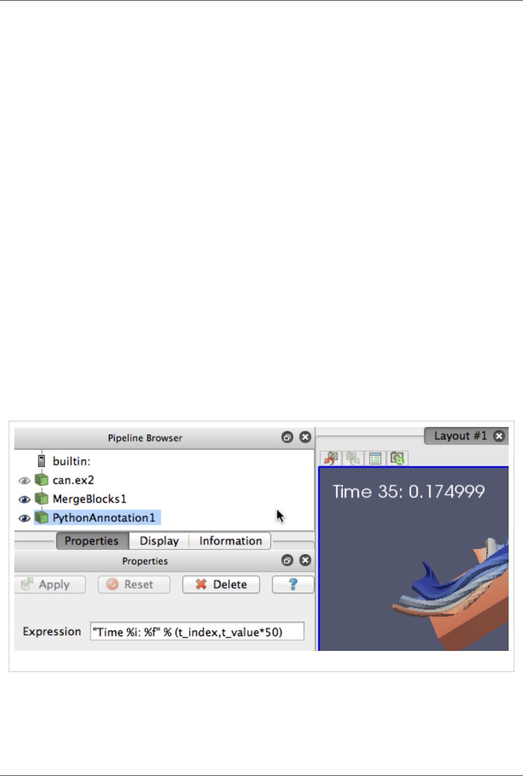
Annotation 138
Python annotation filter
This filter uses Python to calculate an expression. It depends heavily on the numpy and paraview.vtk modules. To
use the parallel functions, mpi4py is also necessary. The expression is evaluated and the resulting string or value is
going to be output in a 2D text.
This filter tries to make it easy for the user to write expressions by defining certain variables. The filter tries to assign
each array to a variable of the same name. If the name of the array is not a valid Python variable, it has to be
accessed through a dictionary called arrays (i.e. arrays['array_name']).
The Python expression evaluated during execution. FieldData arrays are direclty available through their name. Here
is the list of available variables that can be used as is:
• input: represent the input of that filter.
• inputMB: represent an array of block if 'input' is a Multi-block dataset.
• t_value or time_value: represent the real time of the data that is provided by the input.
• t_steps or time_steps: is an array with all the possible value available for the time.
• t_range or time_range: is an array composed with the minimum and maximum time.
• t_index or time_index: represent the index of the time_value inside the time_steps array.
• input.FieldData, input.PointData, input.CellData: are shortcut to access any data array from the input.
Here is a set of expressions that can be used with the can.ex2 dataset once the multi block has been merged:
• "Momentum: (%f, %f, %f)" % (XMOM[t_index,0], YMOM[t_index,0], ZMOM[t_index,0]) )
• QA_Records[20,:8]
• input.PointData['DISPL'][0:3,0] : Display component 0 of the first 3 DISPL points data.
• input.PointData['DISPL'][0:3] : Display full vector of the first 3 DISPL points data.
• input.PointData['DISPL'][0] : Display full vector of the first DISPL points data.
• input.PointData['DISPL'] [ [ 0,10,20,30 ] ] : Display full vector of the DISPL points data [0,10,20,30].
The following example illustrate some time expression:
Figure 9.9 Python Annotation Filter showing time information
The following example illustrate a complex text generation composed of several data field.
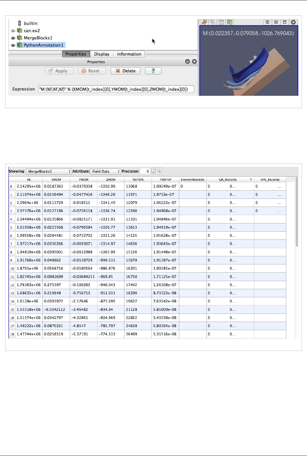
Annotation 139
Figure 9.10 Python Annotation Filter showing field data
In order to understand what can be done, here is the list of fields that are available in the can.ex2 dataset. In fact to
highlight the easy access of the field data, the following expression are exactly the same, but as you can see the
second way of writing it is much shorter:
• input.FieldData['KE'][0,0] <=> KE[0,0]
• input.FieldData['QA_Records'][0,0:5] <=> QA_Records[0,0:5]
Figure 9.11 Available fields in can.ex2
Global annotation filter
This filter rely on the Python Annotation Filter to extract and show a field value inside the view but in a very simple
and intuitive manner. Moreover, if the selected field, like shown in the following figure, has the same number of
elements than the time, we assume it's time dependent and automatically update it's value to match the time index. If
you are feeling limited by that filter, you can always go back to the Python Annotation Filter to achieve a more
complex data annotation.
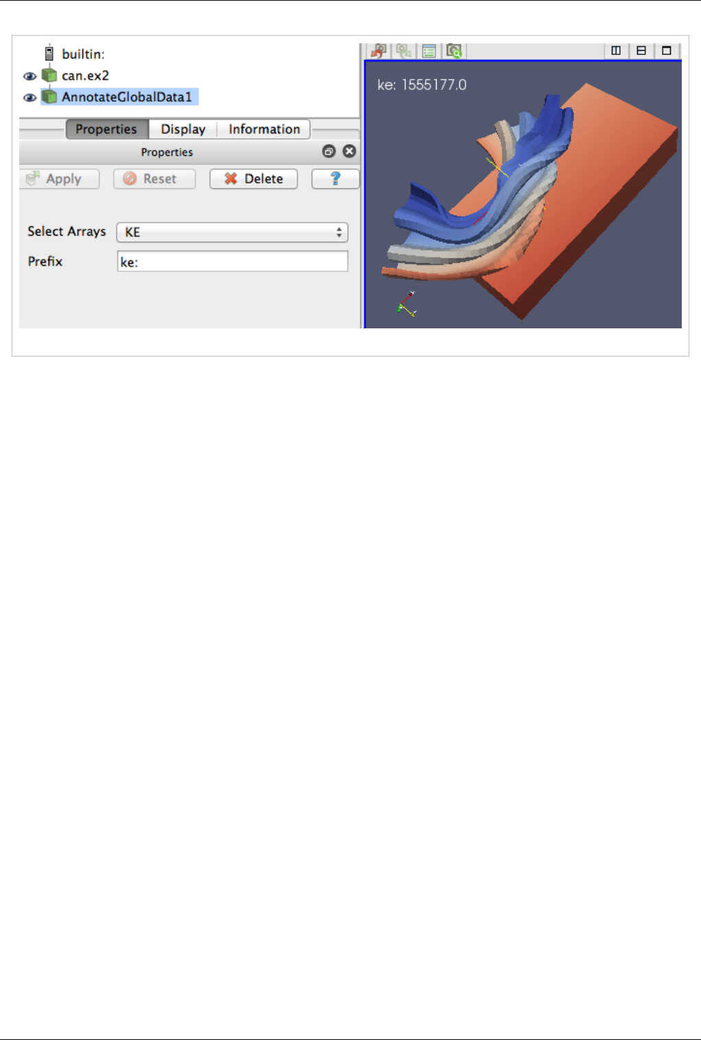
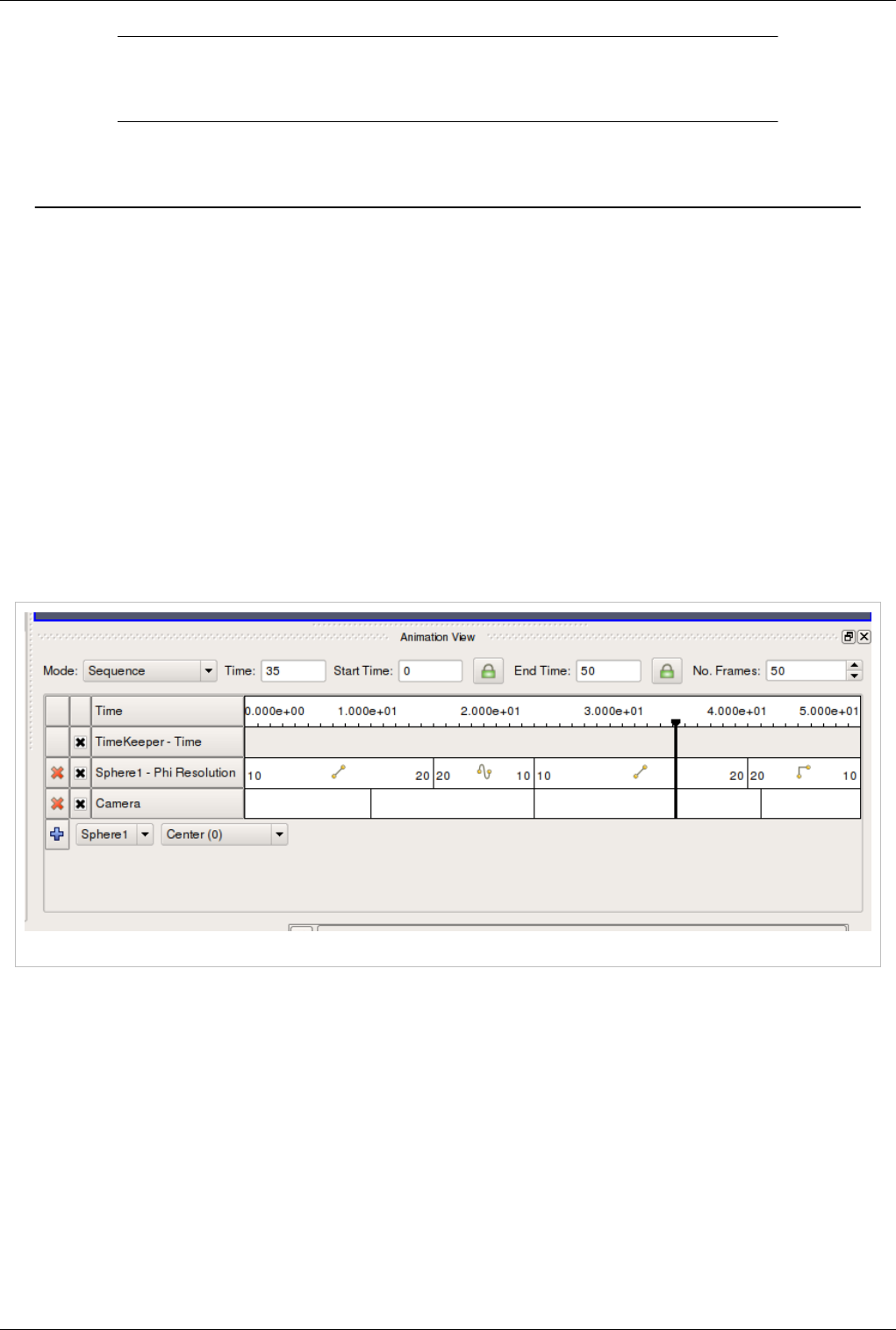
141
Animation
Animation View
In ParaView, you can create animations by recording a series of keyframes. At each keyframe, you set values for the
properties of the readers, sources, and filters that make up the visualization pipeline, as well as the position and
orientation of the camera. Once you have chosen the parameters, you can play through the animation. When you play
the animation, you can cache the geometric output of the visualization pipeline in memory. When you subsequently
replay the animation, playback will be much faster, because very little computation must be done to generate the
images. Also, the results of the animation can be saved to image files (one image per animation frame) or to a movie
file. The geometry rendered at each frame can also be saved in ParaView’s PVD file format, which can be loaded
back into ParaView as a time varying data set.
Animation View
Animation View is the user interface used to create animations by adding keyframes. It is modeled similar to popular
animation and key-frame editing application with ability to create tracks for animating multiple parameters. The
Animation View is accessible from the View menu.
Figure 10.1 Animation View
As seen in Figure 10.1, this view is presented as a table. Above the table are the controls that administers how time
progresses in the animation. These were discussed previously. Within the table, the tracks of the animation appear as
rows, and animation time is presented as increasing from left-to-right. The first row in the table, simply labeled
Time, shows the total span of time that the animation can cover. The current displayed time is indicated both in the
Time field at the top and with a thick, vertical, draggable line within the table.
Along the left side of the Animation View is an expandable list of the names of the animation tracks (i.e., a particular
object and property to animate). You choose a data source and then a particular property of the data source in the
bottom row. To create an animation track with keyframes for that property, click the "+" on the left-hand side; this
will create a new track. In the figure, tracks already exist for SphereSource1’s Phi Resolution property and for the
camera’s position. To delete a track, press the X button. You can temporarily disable a track by un-checking the
check box on the right of the track. To enter values for the property, double-click within the white area to the right of
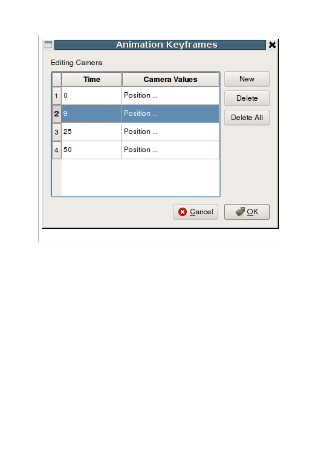
Animation View 142
the track name. This will bring up the Animation Keyframes dialog. Double-clicking in the camera entry brings up a
dialog like the one in Figure 10.2.
Figure 10.2 Editing the camera track
From the Animation Keyframes dialog, you can press New to create new keyframes or press Delete or Delete All to
delete some or all of them. Clicking New will add a new row to the table. In any row, you can click within the Time
column to choose a particular time for the keyframe and click in the right-hand column to enter values for the
parameter. The exact user interface components that let you set values for the property at the keyframe time vary.
When available, you can change the interpolation between two keyframes by double-clicking on the central
interpolation column.
Within the tracks of the Animation View, the place in time where each keyframe occurs is shown as a vertical line.
The values chosen for the property at that time and the interpolation function used between that value and the next
are shown as text when appropriate. In previous figure for example, the sphere resolution begins at 10 and then
changes to 20 varying by linear interpolation between them. The camera values are too lengthy to show as text so
they are not displayed in the track, but we can easily see that there are four keyframes spaced throughout the
animation. The vertical lines in the tracks themselves are draggable, so you can easily adjust the time at which each
keyframe occurs.
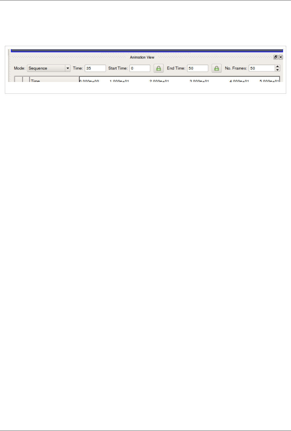
Animation View 143
Animation View Header
The Animation View has a header-bar that lets you control some properties of the animation itself, as you can see in
Figure 10.3.
Figure 10.3 Animation View Header
Mode controls the animation playback mode. ParaView supports 3 modes for playing animation. In Sequence mode,
the animation is played as a sequence of images (or frames) generated one after the other and rendered in immediate
succession. The number of frames is controlled by the No. Frames spinbox at the end of the header. Note that the
frames are rendered as fast as possible. Thus, the viewing frame rate depends on the time needed to generate and
render each frame.
In Real Time mode, the Duration spinbox (replacing the No. Frames spinbox) indicates the time in seconds over
which the entire animation should run. Each frame is rendered using the current wall clock time in seconds relative
to the start time. The animation runs for nearly the number of seconds specified by the Duration (secs) spinbox. In
turn, the number of frames actually generated (or rendered) depends on the time to generate (or render) each frame.
In Snap To TimeSteps mode, the number of frames in the animation is determined by the number of time values in
the data set being animated. This is the animation mode used for ParaView's default animations: playing through the
time values in a data set one after the other. Default animations are created by ParaView when a data set with time
values is loaded; no action is required by the user to create the animation. Note that using this mode when no
time-varying data is loaded will result in no animation at all.
In Sequence mode, the final item in the header is the No. Frames spinbox. This spinbox lets you pick the total
number of frames for the animation. Similarly in Real Time mode, the final line lets you choose the duration of the
animation. In Snap To TimeSteps mode, the total number of frames is dictated by the data set, and therefore the
spinbox is disabled.
The Time entry-box shows the current animation time which is same as shown by a vertical marker in this view. You
can change the current animation time by either entering a value in this box, if available, or dragging the vertical
marker. The Start Time and End Time entry-boxes display the start and end times for the animation. By default,
when you load time varying data sets, the start and end times are automatically adjusted to cover the entire time
range present in the data. The lock check-buttons to the right of the Start Time and End Time widgets will prevent
this from happening, so that you can ensure that your animation covers a particular time domain of your choosing.
Animating Time-Varying Data
When you load time-varying data, ParaView automatically creates a default animation that allows you to play
through the temporal domain of the data without manually creating an animation to do so. With the Animation View,
you can uncouple the data time from the animation time so that you can create keyframes that manipulate the data
time during animation as well.
If you double-click in the TimeKeeper – Time track, the Animation Keyframes dialog, an example of which is
shown in Figure below, appears. In this dialog, you can make data time progress in three fundamentally different
ways. If the Animation Time radio-button is selected, the data time will be tied to and scaled with the animation time
so that as the animation progresses, you will see the data evolve naturally. You can select Constant Time instead if
you want to ignore the time varying nature of the data. In this case, you choose a particular time value at which the
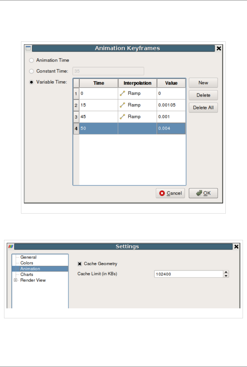
Animation View 144
data will be displayed for the duration of the animation. Finally, you can select the Variable Time radio-button to
have full control over data time and control it as you do any other animatible property in the visualization pipeline.
In the example shown in Figure 10.4 below, time is made to progress forward for the first 15 frames of the
animation, backward for the next 30, and finally forward for the final 15.
Figure 10.4 Controlling Data Time with keyframes
Animation Settings
Figure 10.5 Animation Settings
Additional animation properties can be changed using the Animation page in the Edit|Settings dialog. Using these
settings seen in Figure 10.5, you can control whether geometry must be cached to improve playback performance
during looping, as well as the maximum size of geometry to cache to avoid memory overflows.
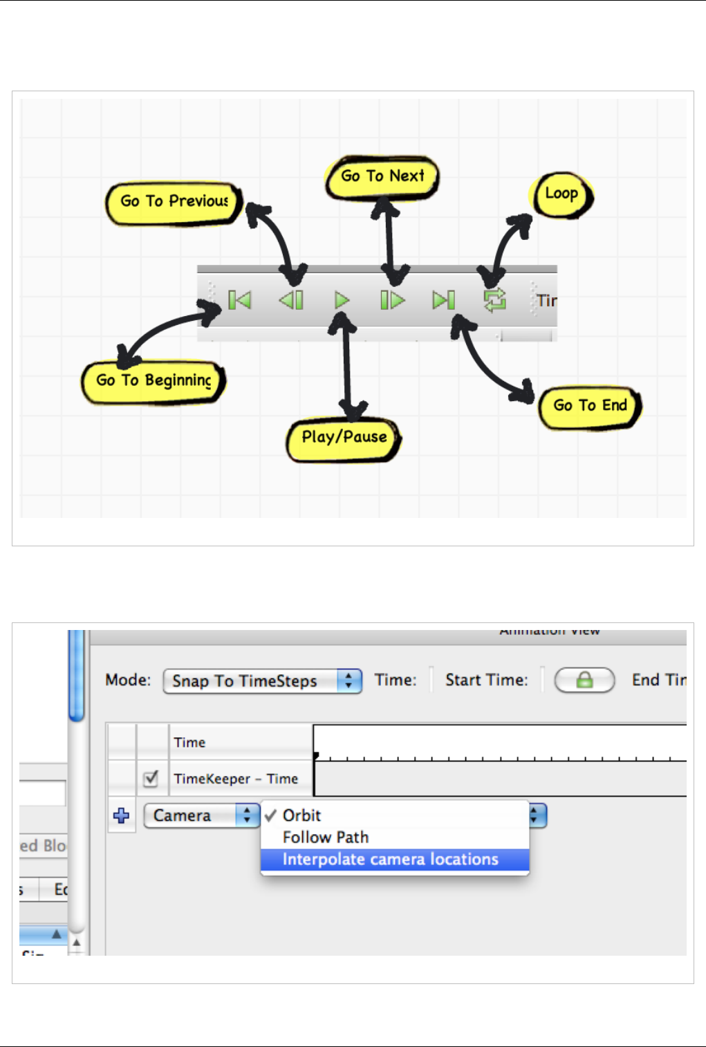
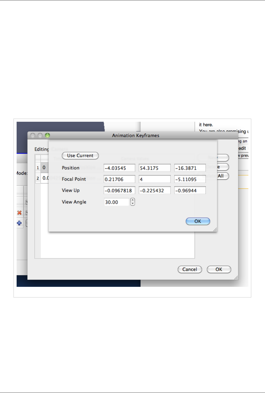
Animation View 146
Just like you can change parameters on sources and filters in an animation, you can also change the camera
parameters. As seen above in Figure 10.7, you can add animation tracks to animate the camera for all the 3D render
views in the setup separately. To add a camera animation track for a view, with the view selected, click on the "+"
button after choosing Camera from the first drop-down. The second drop down allows users to choose how to
animate the camera. There are three possible options each of which provides different mechanisms to specify the
keyframes. It's not possible to change the mode after the animation track has been added, but you can simply delete
the track and create a new one.
Interpolate Camera Locations
In this mode, the user specifies camera position, focal point, view angle, and up direction at each keyframe. The
animation player interpolates between these specified locations. As with other parameters, to edit the keyframes,
double-click on the track. It is also possible to capture the current location as a keyframe by using the Use Current
button.
Figure 10.8 Setting animation parameters
It can be quite challenging to add keyframes correctly and frequently to ensure that the animation results in a smooth
visualization using this mode.
Orbit
This mode makes it possible to quickly create a camera animation in which the camera revolves around an object(s)
of interest. Before adding the Camera track, select the object(s) in the pipeline browser that you want to revolve
around; then choose Orbit from the Camera combo-box in the Animation View and hit "+". This will pop-up a dialog
where you can edit the orbit parameters such as the center of revolution, normal for the plane of revolution, and the
origin (i.e. a point on the plane where the revolution begins). By default, the Center is the center of the bounds of the
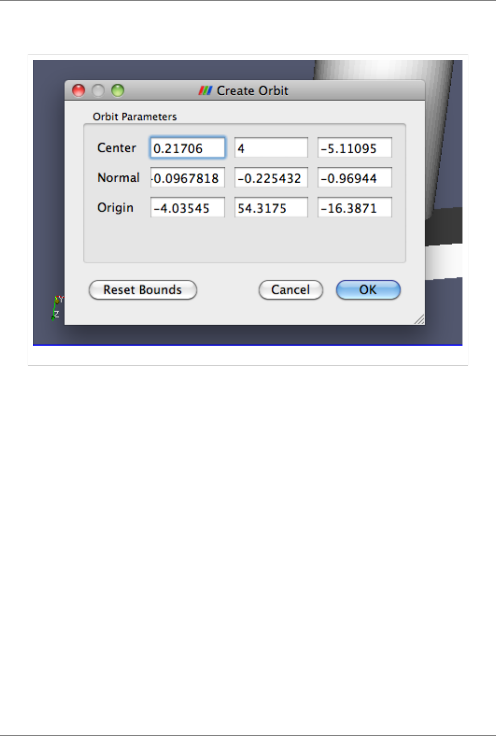
Animation View 147
selected objects, Normal is the current up direction used by the camera while the origin is the current camera
position.
Figure 10.9 Creating a camera orbit
Follow Path
In this mode, users get the opportunity to specify the path taken by the camera position and camera focal point. By
default, the path is set-up to orbit around the selected objects. Users can then edit the keyframe to change the paths.
Figure 10.10 shows the dialog for editing these paths for a keyframe. When Camera Position or Camera Focus is
selected, a widget is shown in the 3D view that can be used to set the path. Use Ctrl+Left Click to insert new control
points, and Shift+Left Click to remove control points. You can also toggle when path should be closed or not.
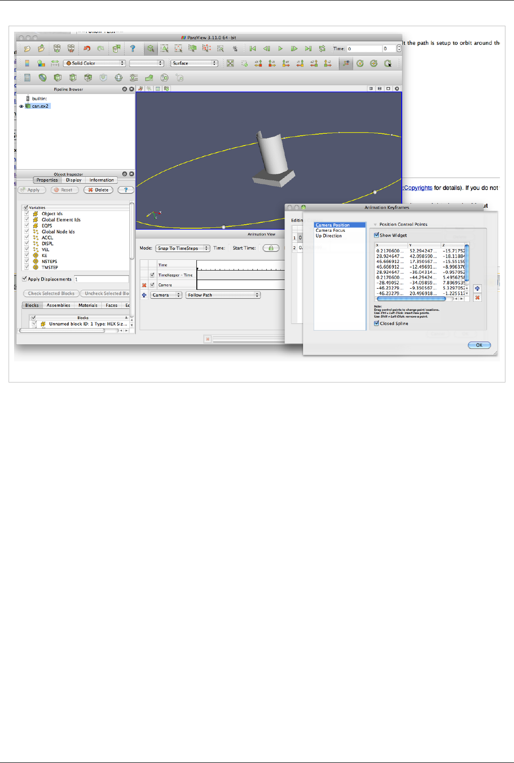
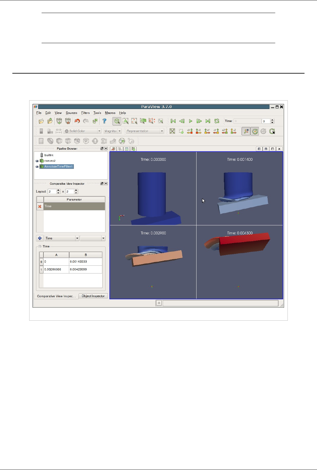
149
Comparative Visualization
Comparative Views
Introduction
Figure 11.1 Comparative Views
ParaView provides a collection of views that can be used to display a set of visualization on a regular grid. These
views are referred to as Comparative Views. Comparative Views can be used to display results from a parameter
study or to perform parameter studies within ParaView.
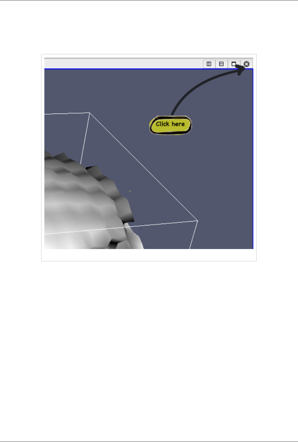
Comparative Views 150
Quick Start
We will start with a short tutorial. Later sections will describe Comparative Views in more detail. First, start a
Wavelet source. Next, apply a Contour filter; then close the default 3D view by clicking on the small "x" on the
upper-right corner of the view, as shown in Figure 11.2.
Figure 11.2 Closing
This should bring up an empty view with several buttons for selecting the view type. Select 3D View (Comparative).
Now you should see an empty 2x2 grid in the view. Next, turn on the visibility of the Contour filter. You should see
the output of the Contour filter in all four views. To vary the contour value across the grid, bring up the Comparative
View Inspector (View|Comparative View Inspector). This inspector allows you to configure the parameters of the
Comparative View.
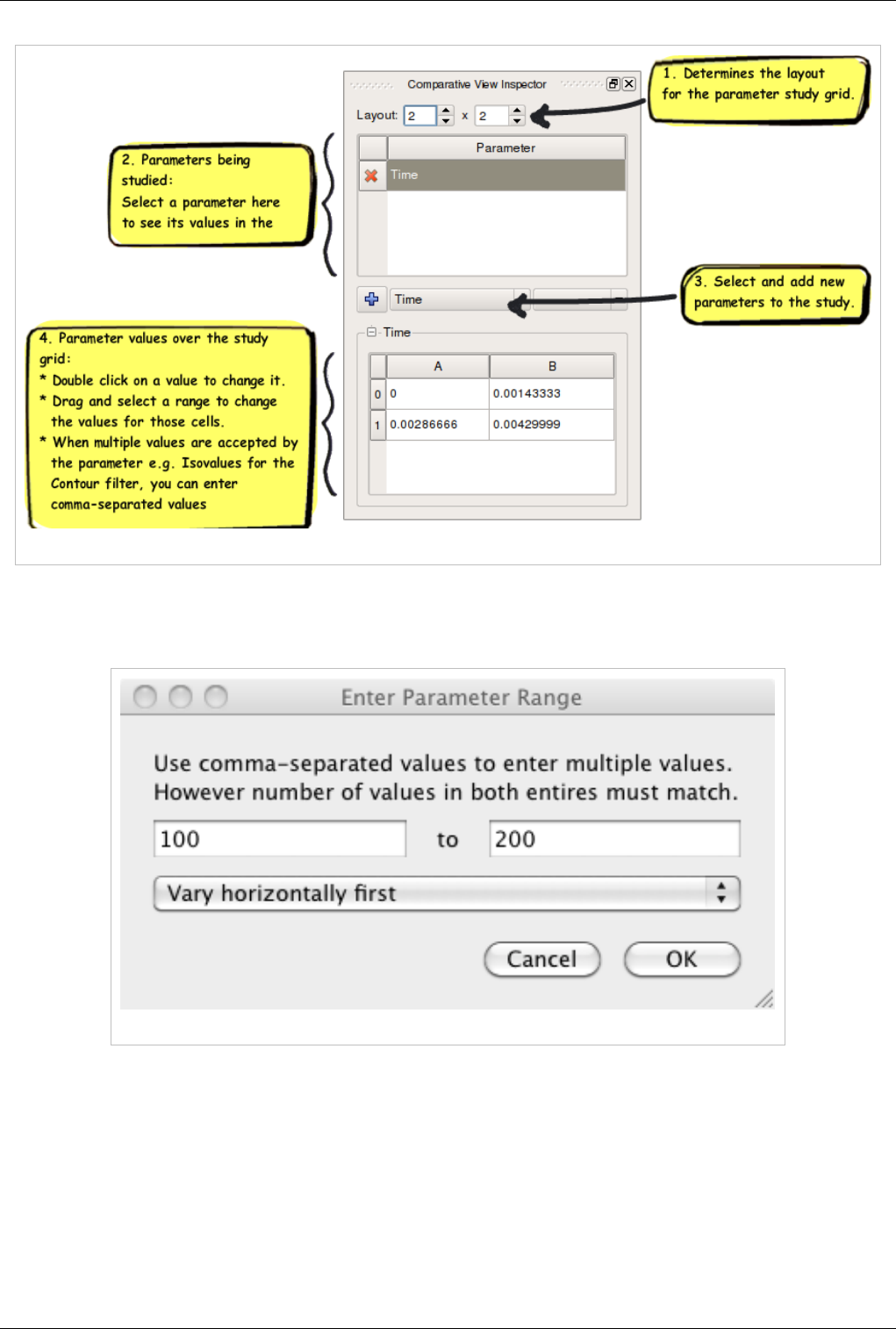
Comparative Views 151
Figure 11.3 Comparative View panel
From the drop-down menu, select Contour1. The parameter should be set to Isosurfaces. If it is not, change it. Next,
in the grid that has the numbers, click on the upper left value and drag it to the lower right value. This should bring
up the following dialog. Enter 100 and 200 for the two values.
Figure 11.4 Comparative View parameter range
When you click OK, the Comparative View should update and you should see something like Figure 11.5 below.

Comparative Views 152
Figure 11.5 Comparative View parameter output
View
There are three types of Comparative Views:
• Comparative 3D View
• Comparative Line Chart View
• Comparative Bar Chart View
All of these views contain sub-views laid-out in an m-by-n grid where m and n are determined by the Comparative
View Inspector settings. The type of the sub-view depends on the type of the comparative view: 3D View for
comparative view, line chart for line chart comparative view etc. Each sub-view displays the output from the same
pipeline objects, depending on what is set visible in the Pipeline Inspector. The only things that change from
view-to-view are the parameters that are varied through the Comparative View Inspector. Furthermore, the view
settings are synchronized between all sub-views. For example, changing the camera in one 3D sub-view will cause
the camera on all other sub-views to change.
Note: Not all features of the single views are supported in their comparative siblings. For example, it is not possible
to perform surface selection on a Comparative 3D View.
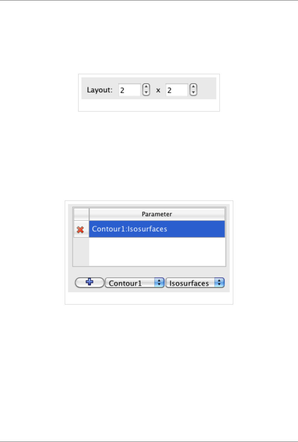
Comparative Views 153
Comparative View Inspector
The Comparative View Inspector (View|Comparative View Inspector) is where you can configure all of the
parameters of comparative views. Note that if you have more than one comparative view, the Inspector will change
the setting of the active one. Below we describe various parts of the Comparative View Inspector.
Layout
File 11.6 Layout widget
The layout widget seen above in Figure 11.6 allows you to configure the number of sub-views within a comparative
view. The first value controls how many cells there are in the horizontal direction whereas the second value controls
how many cells there are in the vertical direction. Note that if you already set-up one or more parameters to vary in
the view, the Inspector will try to maintain your values when you adjust the size as much as possible. If you
manually entered any individual values, they will not change when you add more rows or columns. On the other
hand, all values that have been automatically computed based on a range will be updated as the number of cells
change.
Parameter Selection
File 11.7 Parameter selection
This widget allows you to add new parameters to vary and also to select a property if more than one is available. To
add a property, first select the pipeline object from the first menu, then select its parameter from the second value.
Once you are done with the selection, click on the "+" button to add the parameter. This parameter will now show in
the list of parameters. To delete a parameter from the list, click on the corresponding "x" on the left side of the
parameter selection widget. Note that once you add a new parameter, ParaView will try to assign good default values
to each cell. For example, if you add Contour:Isosurfaces, ParaView will assign values ranging from minimum scalar
value to maximum scalar value.
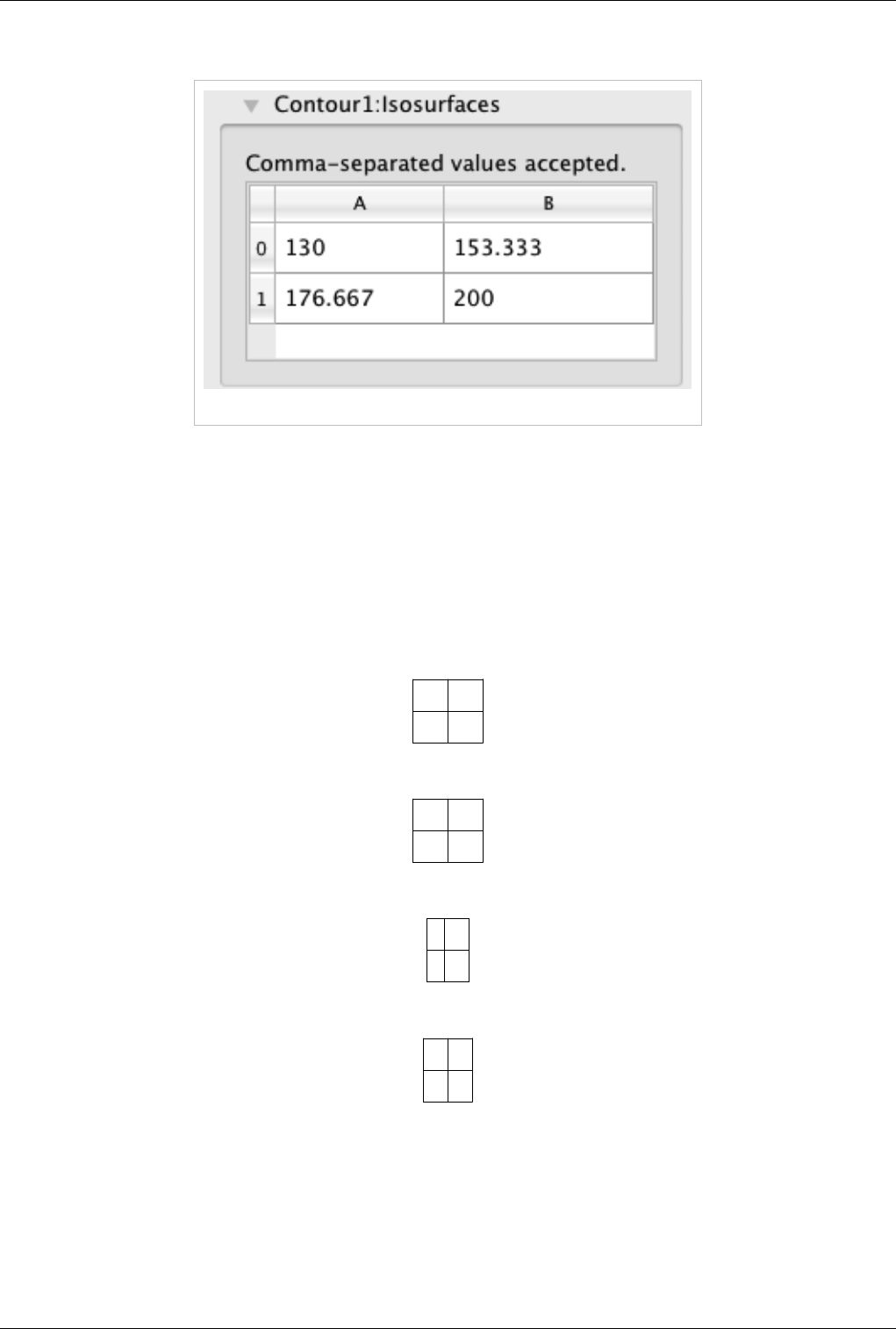
Comparative Views 154
Editing Parameter Values
Figure 11.8 Parameter editing in the spreadsheet widget
You can edit the parameter values using the spreadsheet widget. You can either:
• Change individual value by double clicking on a cell and editing it.
• Change a group of cells by clicking on the first one and dragging it to the last one. ParaView will then ask you to
enter minimum and maximum values. If you selected cells that span more than one direction, it will also ask you
to choose which way values vary.
Let's examine the range selection a bit further. Say that you selected a 2x2 area of cells and entered 0 for the
minimum and 10 for the maximum.
If you select Vary Horizontally First, the values will be:
0 3.33
6.66 10
If you select, Vary Vertically First, the values will be:
0 6.66
3.33 10
If you select, Vary Only Horizontally, the value will be:
0 10
0 10
If you select, Vary Only Vertically, the value will be:
0 0
10 10
The last two options may sound useless. Why have multiple cells with the same values? However, if you consider
that more than one parameter can be varied in a comparative view, you will realize how useful they are. For
example, you can change parameter A horizontally while varying parameter B vertically to create a traditional
spreadsheet of views.

Comparative Views 155
Performance
Computational
ParaView will run the pipeline connected to all visible pipeline objects for each cell serially. Therefore, the time to
create a Comparative Visualization of N cells should be on the order of N times the time to create the visualization of
one cell.
Memory
ParaView will only store what is needed to display the results for each cell except the last one. The last cell will
contain the representation as well as the full dataset, same as any single view. For example, when using the surface
representation, the total memory used will be the total of memory used by the geometry in each cell plus the memory
used by the dataset of the last cell.

156
Remote and Parallel Large Data
Visualization
Parallel ParaView
Parallel ParaView
One of the main purposes of ParaView is to allow users to create visualizations of large data sets that reside on
parallel systems without first collecting the data to a single machine. Transferring the data is often slow and wasteful
of disk resources, and the visualization of large data sets can easily overwhelm the processing and especially
memory resources of even high-performance workstations. This chapter first describes the concepts behind the
parallelism in ParaView. We then discuss in detail the process of starting-up ParaView's parallel server components.
Lastly, we explain how a parallel visualization session is initiated from within the user interface. Parallel rendering is
an essential part of parallel ParaView, so essential that we've given it its own chapter in this version of the book.
The task of setting up a cluster for visualization is unfortunately outside of the scope of this book. However, there
are several online resources that will help to get you started including:
• http:/ / paraview. org/ Wiki/ Setting_up_a_ParaView_Server,
• http:/ / www. iac. es/ sieinvens/ siepedia/ pmwiki. php?n=HOWTOs. ParaviewInACluster
• http:/ / paraview. org/ Wiki/ images/ a/ a1/ Cluster09_PV_Tut_Setup. pdf

Parallel ParaView 157
Parallel Structure
ParaView has three main logical components: client, data server, and render server. The client is responsible for the
GUI and is the interface between you the user and ParaView as a whole. The data server reads in files and processes
the data through the pipeline. The render server takes the processed data and renders it to present the results to you.
Figure 12.1 Parallel Architecture
The three logical components can be combined in various different configurations. When ParaView is started, the
client is connected to what is called the built-in server; in this case, all three components exist within the same
process. Alternatively, you can run the server as an independent program and connect a remote client to it, or run the
server as a standalone parallel batch program without a GUI. In this case, the server process contains both the data
and render server components. The server can also be started as two separate programs: one for the data server and
one for the render server. The server programs are data-parallel programs that can be run as a set of independent
processes running on different CPUs. The processes use MPI to coordinate their activities as each works on different
pieces of the data.

Parallel ParaView 158
Figure 12.2 Common Configurations of the logical components
Client
The client is responsible for the user interface of the application. ParaView’s general-purpose client was written to
make powerful visualization and analysis capabilities available from an easy-to-use interface. The client component
is a serial program that controls the server components through the Server Manager API.
Data Server
The data server is primarily constructed from VTK readers, sources, and filters. It is responsible for reading and/or
generating data, processing it, and producing geometric models that the render server and client will display. The
data server exploits data parallelism by partitioning the data, adding ghost levels around the partitions as needed, and
running synchronous parallel filters. Each data server process has an identical VTK pipeline, and each process is told
which partition of the data it should load and process. By splitting the data, ParaView is able to use the entire
aggregate system memory and thus make large data processing possible.
Render Server
The render server is responsible for rendering the geometry. Like the data server, the render server can be run in
parallel and has identical visualization pipelines (only the rendering portion of the pipeline) in all of its processes.
Having the ability to run the render server separately from the data server allows for an optimal division of labor
between computing platforms. Most large computing clusters are primarily used for batch simulations and do not
have hardware rendering resources. Since it is not desirable to move large data files to a separate visualization
system, the data server can run on the same cluster that ran the original simulation. The render server can be run on a
separate visualization cluster that has hardware rendering resources.

Parallel ParaView 159
It is possible to run the render server with fewer processes than the data server but never more. Visualization clusters
typically have fewer nodes than batch simulation clusters, and processed geometry is usually significantly smaller
than the original simulation dump. ParaView repartitions the geometric models on the data server before they are
sent to the render server.
MPI Availability
Until recently, in order to use ParaView's parallel processing features, you needed to build ParaView from the source
code as described in the Appendix. This was because there are many different versions of MPI, the library
ParaView’s servers use internally for parallel communication, and for high-performance computer users it is
extremely important to use the version that is delivered with your networking hardware.
As of ParaView 3.10 however, we have begun to package MPI with our binary releases. If you have a multi-core
workstation, you can now simply turn on the Use Multi-Core setting under ParaView's Settings to make use of all of
them. This option makes Parallel Data Server mode the default configuration, which can be very effective when you
are working on computationally bound intensive processing tasks.
Otherwise, and when you need to run ParaView on an actual distributed memory cluster, you need to start-up the
various components and establish connections between them as is described in the next section.
Starting the Server(s)
Client / Server Mode
Client / Server Mode refers to a parallel ParaView session in which data server and render server components reside
within the same set of processes, and the client is completely separate. The pvserver executable combines the two
server components into one process.
You can run pvserver as a serial process on a single machine. If ParaView was compiled with parallel support, you
can also run it as an MPI parallel program on a group of machines. Instructions for starting a program with MPI are
implementation and system-dependent, so contact your system administrator for information about starting an
application with MPI. With the MPICH implementation of MPI, the command to start the server in parallel usually
follows the format shown here:
mpirun –np number_of_processes path_to/pvserver arguments for pvserver
By default, pvserver will start and then wait for the client to connect to it. See the next section for a full description.
Briefly, to make the connection, select Connection from the File menu, select (or make and then select) a
configuration for the server, and click Connect. Note that you must start the server before the client attempts to
connect to it.
If the computer running the server is behind a firewall, it is useful to have the server initiate the connection instead of
the client. The ‑-reverse-connection (or -rc) command-line option tells the server to do this. The server must know
the name of the machine to which it should connect; this is specified with the --client-host (or -ch) argument. Note
that when the connection is reversed, you must start the client and instruct it to wait for a connection before the
server attempts to connect to it.
The client-to-server connection is made over TCP, using a default port of 11111. If your firewall puts restrictions on
TCP ports, you may want to choose a different port number. In the client dialog, simply choose a port number in the
Port entry of the Configure New Server dialog. Meanwhile, give pvserver the same port number by including
--server-port (or –sp) in its command-line argument list.
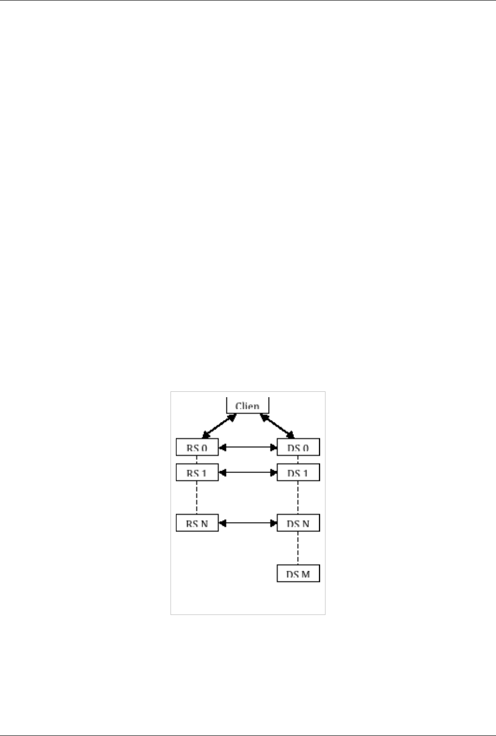
Starting the Server(s) 160
An example command line to start the server and have it initiate the connection to a particular client on a particular
port number is given below:
pvserver –rc –ch=magrathea –sp=26623
Render/Server Mode
The render server allows you to designate a separate group of machines (i.e., apart from the data server and the
client) to perform rendering. This parallel mode lets you use dedicated rendering machines for parallel rendering
rather than relying on the data server machines, which may have limited or no rendering capabilities. In ParaView,
the number of machines (N) composing the render server must be no more than the number (M) composing the data
server.
Note that it is true that some large installations with particularly high-performing, parallel rendering resources it can
be very efficient to run ParaView in Render/Server Mode. However, we have found in practice that it is almost
always the case that the data transfer time between the two servers overwhelms the speed gained by rendering on the
dedicated graphics cluster. For this reason, we typically recommend that you combine the data and render servers
together as one component, and either render in software via Mesa on the data processing cluster or do all of the
visualization processing directly on the GPU cluster.
If you still want to break-up the data processing and rendering tasks, there are two sets of connections that must be
made for ParaView to run in render-server mode. The first connection set is between the client and the first node of
each of the data and render servers. The second connection set is between the nodes of the render server and the first
n nodes of the data server. Once all of these connections are established, they are bi-directional. The diagram in
Figure 12.3 depicts the connections established when ParaView is running in render server mode. Each double-ended
arrow indicates a bi-directional TCP connection between pairs of machines. The dashed lines represent MPI
connections between all machines within a server. In all the diagrams in this section, the render server nodes are
denoted by RS 0, RS 1, …, RS N. The data server nodes are similarly denoted by DS 0, DS 1, …, DS N, …, DS M.
Figure 12.3 Connections required in render
server mode
The establishment of connections between client and servers can either be forward (from client-to-servers) or reverse
(from servers-to-client). Likewise, the connections between render server and data server nodes can be established
either from the data server to the render server, or from the render server to the data server.
The main reason for reversing the direction of any of the initial connections is that machines behind firewalls are
able to initiate connections to machines outside the firewall, but not vice versa. If the data server is behind a firewall,
the data server should initiate the connection with the client, and the data server nodes should connect to the render

Starting the Server(s) 161
server nodes. If the render server is behind the firewall instead, both servers should initiate connections to the client,
but the render server nodes should initiate the connections with the nodes of the data server.
In the remaining diagrams in this section, each arrow indicates the direction in which the connection is initially
established. Double-ended arrows indicate bi-directional connections that have already been established. In the
example command lines, optional arguments are enclosed in []’s. The rest of this section will be devoted to
discussing the two connections required for running ParaView in render server mode.
Connection 1: Connecting the client and servers
The first connection that must be established is between the client and the first node of both the data and render
servers. By default, the client initiates the connection to each server, as shown in Figure 12.4. In this case, both the
data server and the render server must be running before the client attempts to connect to them.
Figure 12.4 Starting ParaView in
render-server mode using standard
connections
To establish the connections shown above, do the following. First, from the command line of the machine that will
run the data server, enter pvdataserver to start it. Next, from the command line of the machine that will run the
render server, enter pvrenderserver to start the render server. Now, from the machine that will run the client, start the
client application, and connect to the running servers, as described in section 1.2 and summarized below.
Start ParaView and select Connect from the File menu to open the Choose Server dialog. Select Add Server to open
the Configure New Server dialog. Create a new server connection with a Server Type of Client / Data Server /
Render Server. Enter the machine names or IP addresses of the server machines in the Host entries. Select Configure,
and then in the Configure Server dialog, choose Manual. Save the server configuration and connect to it. At this
point, ParaView will establish the two connections. This is similar to running ParaView in client/server mode, but
with the addition of a render server.
The connection between the client and the servers can also be initiated by the servers. As explained above, this is
useful when the servers are running on machines behind a firewall. In this case, the client must be waiting for both
servers when they start. The diagram indicating the initial connections is shown in Figure 12.5.
Figure 12.5 Reversing the connections
between the servers and the client
To establish the connections shown above, start by opening the Configure New Server dialog on the client. Choose
Client|Data Server|Render Server (reverse connection) for the Server Type in the Configure New Server dialog.
Next, add both --reverse-connection (-rc) and --client-host (-ch) to the command lines for the data server and render
server. The value of the --client-host parameter is the name or IP address of the machine running the client. You can
use the default port numbers for these connections, or you can specify ports in the client dialog by adding the
--data-server-port (–dsp) and --render-server-port (–rsp) command-line arguments to the data server and render
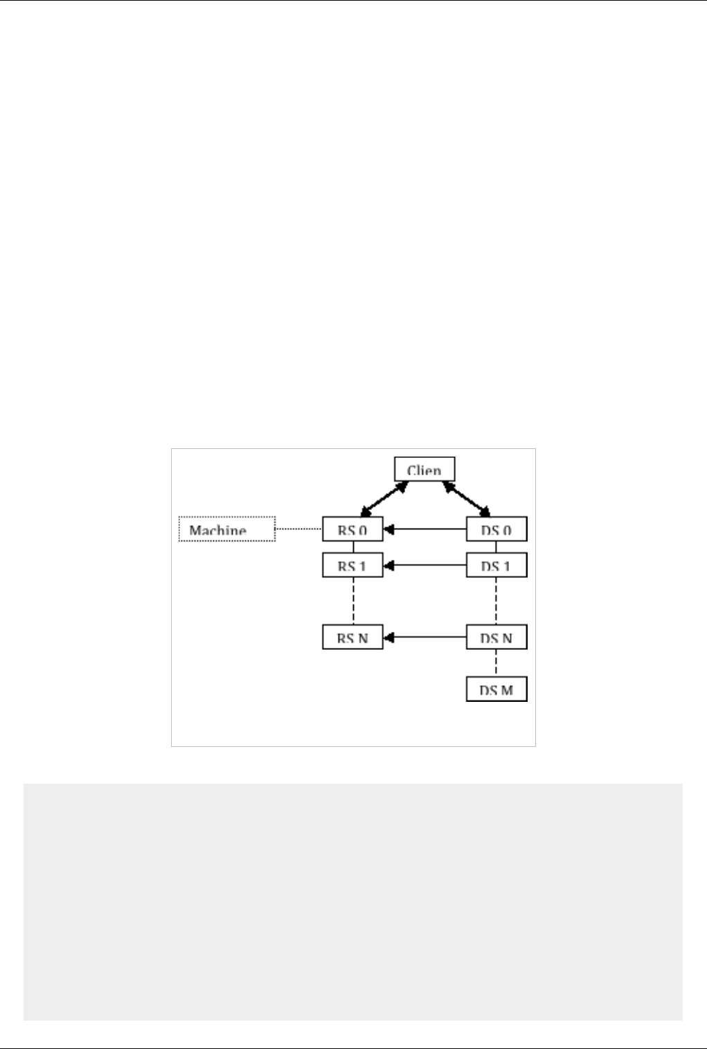
Starting the Server(s) 162
server command lines. The port numbers for each server must agree with the corresponding Port entries in the
dialog, and they must be different from each other.
For the remainder of this chapter, -rc will be used instead of --reverse-connection when the connection between the
client and the servers is to be reversed.
Connection 2: Connecting the render and data servers
After the connections are made between the client and the two servers, the servers will establish connections with
each other. In parallel runs, this server-to-server connection is a set of connections between all N nodes of the render
server and the first N nodes of the data server. By default, the data server initiates the connection to the render server,
but this can be changed with a configuration file. The format of this file is described below.
The server that initiates the connection must know the name of the machine running the other server and the port
number it is using. In parallel runs, each node of the connecting server must know the name of the machine for the
corresponding process in the other server to which it should connect. The port numbers are randomly assigned, but
they can be assigned in the configuration file as described below.
The default set of connections is illustrated in Figure 12.6. To establish these connections, you must give the data
server the connection information discussed above, which you specify within a configuration file. Use the
--machines (–m) command line argument to tell the data server the name of the configuration file. In practice, the
same file should be given to all three ParaView components. This ensures that the client, the render server, and the
data server all agree on the network parameters.
Figure 12.6 Initializing the connection from the data server to the render
server
An example network configuration file, called machines.pvx in this case, is given below:
<?xml version="1.0" ?>
<pvx>
<Process Type="client">>
</Process>
<Process Type="render-server">
<Option Name="render-node-port" Value="1357"/>
<Machine Name="rs_m1"
Environment="DISPLAY=rs_m1:0"/>
<Machine Name="rs_m2"

Starting the Server(s) 163
Environment="DISPLAY=rs_m2:0"/>
</Process>
<Process Host="data-server">
<Machine Name="ds_m1" />
<Machine Name="ds_m2" />
<Machine Name="ds_m3" />
<Machine Name="ds_m4" />
</Process>
</pvx>
Sample command-line arguments that use the configuration file above to initiate the network illustrated in Figure
12.6 are given below:
mpirun –np 2 pvdataserver –m=machines.pvx
mpirun –np 2 pvrenderserver -m=machines.pvx
paraview –m=machines.pvx
It should be noted that the machine configuration file discussed here is a distinct entity and has a different syntax
from the server configuration file discussed at the end of the next section. That file is read only by the client; the file
discussed here will be given to the client and both servers.
In the machine file above, the render-node-port entry in the render server’s XML element tells the render server the
port number on which it should listen for a connection from the data server, and it tells the data server what port
number it should attempt to contact. This entry is optional and if it does not appear in the file, the port number will
be chosen automatically. Note that it is not possible to assign port numbers to individual machines within the server;
all will be given the same port number or use the automatically-chosen one. Note also that each render server
machine is given a display environment variable in this file. This is not required to establish the connections, but it is
helpful if you need to assign particular X11 display names to the various render server nodes.
The initial connection between the nodes of the two servers is made from the data server to the render server. You
can reverse this such that the render server nodes connect to the corresponding nodes of the data server instead as
shown in Figure 12.7.
Figure 12.7 Reversing the connection between the servers and client and
connecting the render server to the data server

Starting the Server(s) 164
Typically, when the server connection is reversed, the direction of the connection between the client and the servers
is also reversed (e.g., if the render server is behind a firewall). In this case, the render server must have the machine
names and a connection port number to connect to the data server. The same XML file is used for this arrangement
as is with the standard connection. The only difference in this case is that the render-node-port entry, if it is used,
must appear in the data server’s XML element instead of the render server’s element. Example command-line
arguments to initiate this type of network are given here:
paraview –m=machines.pvx
mpirun –np M pvdataserver –m=machines.pvx -rc -ch=client
mpirun –np N pvrenderserver –m=machines.pvx -rc -ch=client
Connecting to the Server
Connecting the Client
You establish connections between the independent programs that make up parallel ParaView from within the
client’s user interface. The user interface even allows you to spawn the external programs and then automatically
connect to them. Once you specify the information that ParaView needs to connect or spawn and connect to the
server components, ParaView saves it to make it easy to reuse the same server configuration at a later time. Some
visualization centers provide predefined configurations, which makes it trivial to connect to a server that is tailored
to that center by simply choosing one from a list in ParaView's GUI.
The Choose Server dialog shown in Figure 12.8 is the starting point for making and using server configurations. The
Connect entry on ParaView client’s File menu brings it up. The dialog shows the servers that you have previously
configured. To connect to a server, click its name to select it; then click the Connect button at the bottom of the
dialog box. To make changes to settings for a server, select it and click Edit Server. To remove a server from the list,
select it and click Delete Server.
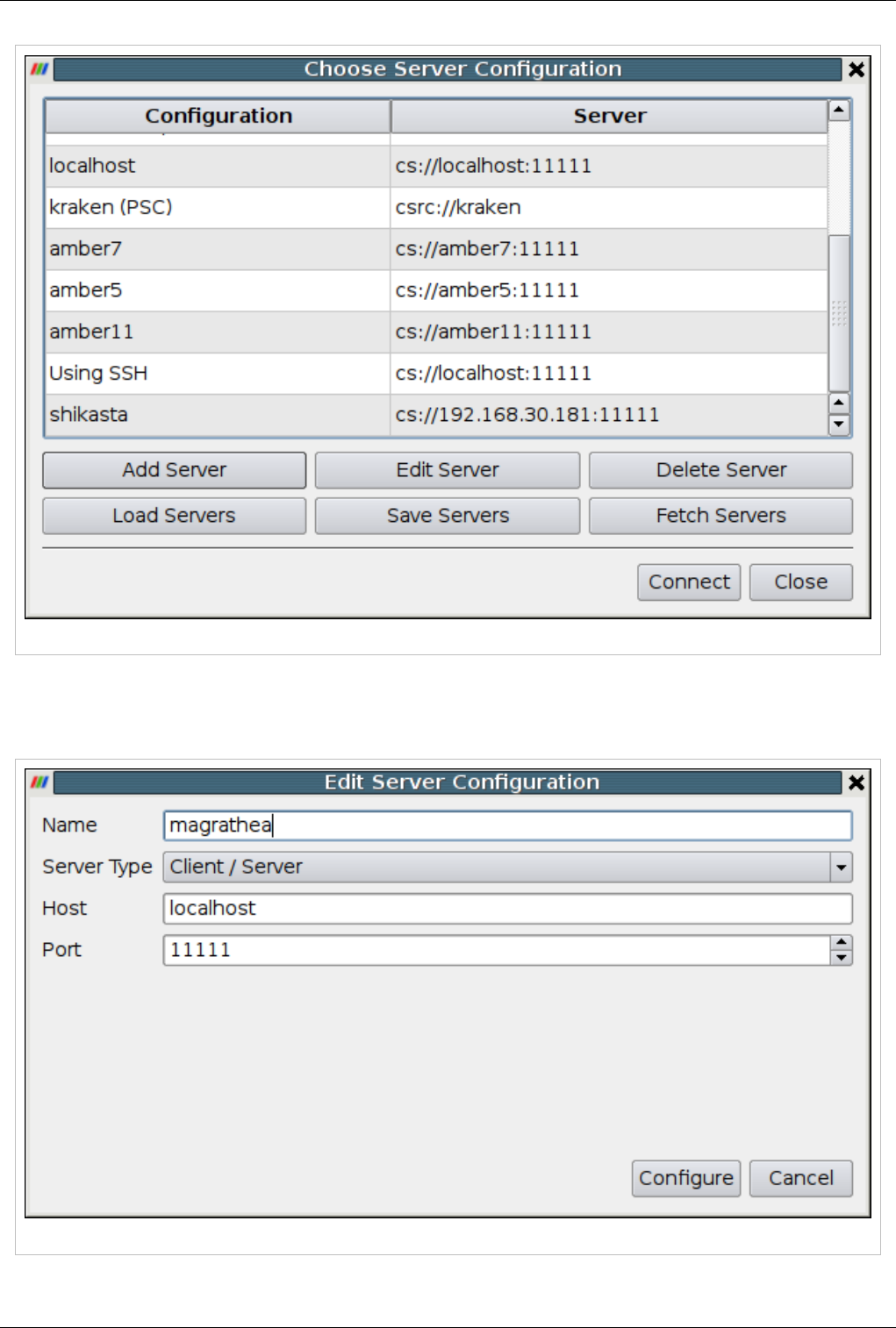
Connecting to the Server 165
Figure 12.8 The Choose Server dialog establishes connections to configured servers
To configure a new server connection, click the Add Server button to add it to the list. The dialog box shown below
will appear. Enter a name in the first text entry box; this is the name that will appear in the Choose Server dialog
(shown above).
Figure 12.9 Configuring a new server
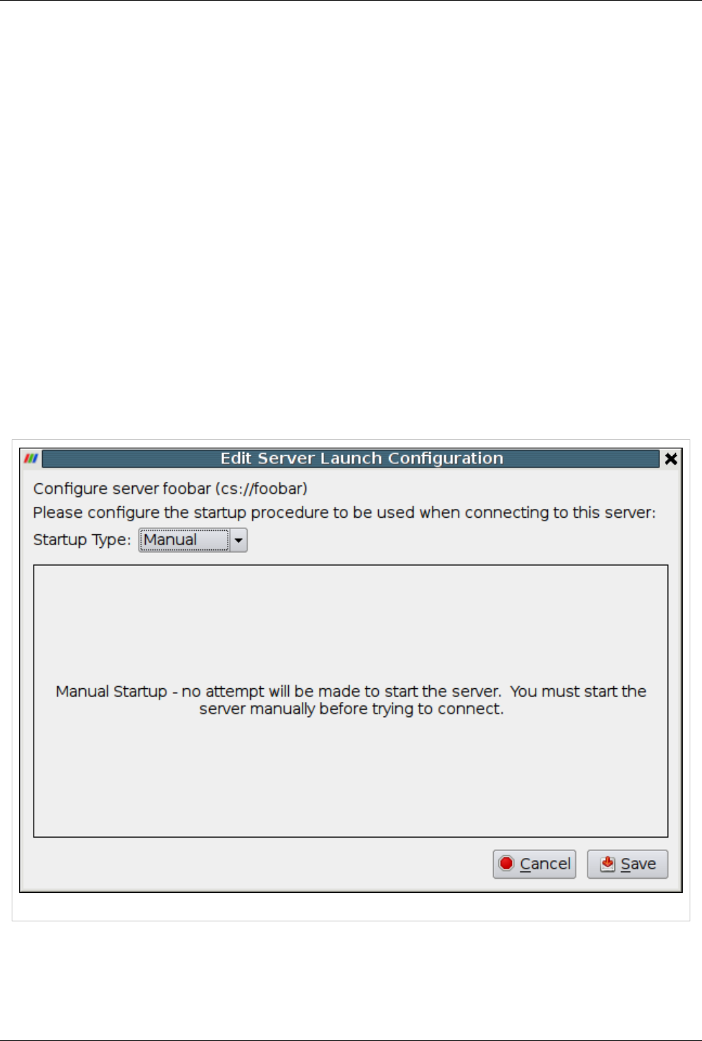
Connecting to the Server 166
Next, select the type of connection you wish to establish from the Server Type menu. The possibilities are as
follows. The “reverse connection” entries mean that the server connects to the client instead of the client connecting
to the server. This may be necessary when the server is behind a firewall. Servers are usually run with multiple
processes and on a machine other than where the client is running.
•Client / Server: Attach the ParaView client to a server.
•Client / Server (reverse connection): Connect a server to the ParaView client.
•Client / Data Server / Render Server: Attach the ParaView client to separate data and render servers.
•Client / Data Server / Render Server (reverse connection): Attach both a data and a render server to the
ParaView client.
In either of the client / server modes, you must specify the name or IP address of the host machine (node 0) for the
server. You may also enter a port number to use, or you may use the default (11111). If you are running in client /
data server / render server mode, you must specify one host machine for the data server and another for the render
server. You will also need two port numbers. The default one for the data server is 11111; the default for the render
server is 22221.
When all of these values have been set, click the Configure button at the bottom of the dialog. This will cause the
Configure Server dialog box, shown in Figure 12.10, to appear. You must first specify the start-up type. The options
are Command and Manual. Choose Manual to connect to a server that has been started or will be started externally,
on the command line for instance, outside of the ParaView user interface. After selecting Manual, click the Save
button at the bottom of the dialog.
Figure 12.10 Configure the server manually. It must be started outside of ParaView
If you choose the Command option, in the text window labeled "Execute an external command to start the server:,"
you must give the command(s) and any arguments for starting the server. This includes commands to execute a
command on a remote machine (e.g., ssh) and to run the server in parallel (e.g., mpirun). You may also specify an

Connecting to the Server 167
amount of time to wait after executing the startup command(s) and before making the connection between the client
and the server(s). (See the spin box at the bottom of the dialog.) When you have finished, click the Save button at the
bottom of the dialog.
Figure 12.11 Enter a command that will launch a new server
Clicking the Save button in the Configure Server dialog will return you to the Choose Server dialog (shown earlier in
this section). The server you just configured will now be in the list of servers you may choose from. Thereafter,
whenever you run ParaView, you can connect to any of the servers that you have configured. You can also give the
ParaView client the –-server=server_config_name command-line argument to make it automatically connect to any
of the servers from the list when it starts.
You can save and/or load server configurations to and/or from a file using the Save Servers and Load Servers
buttons, respectively, on the Choose Server dialog. This is how some visualization centers provide system-wide
server configurations to allow the novice user to simply click his or her choice and connect to an already configured
ParaView server. The format of the XML file for saving the server configurations is discussed online at http:/ /
paraview. org/ Wiki/ Server_Configuration.
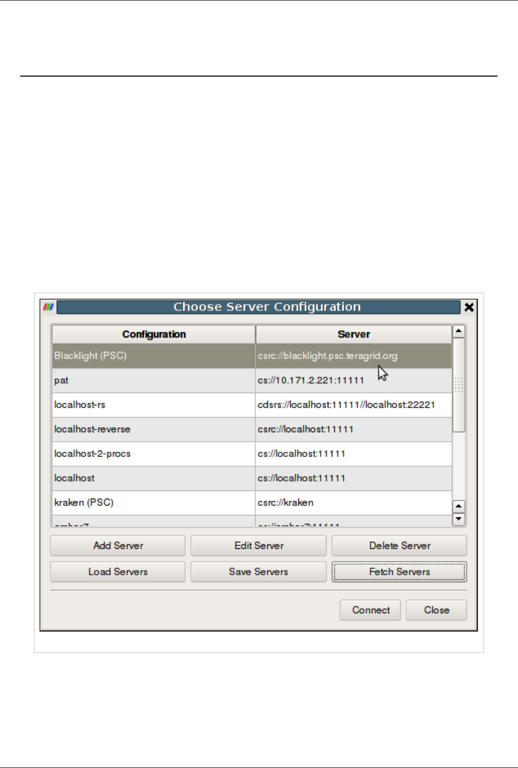
Distributing/Obtaining Server Connection Configurations 168
Distributing/Obtaining Server Connection
Configurations
Motivation
Server configuration (PVSC) files are used to simplify connecting to remote servers. The configuration XMLs can be
used to hide all the complexities dealing with firewalls, setting up ssh tunnels, launching jobs using PBS or other job
scheduler. However, with ParaView versions 3.12 and earlier, there is no easy way of sharing configuration files,
besides manually passing them around. With ParaView 3.14, it is now possible for site maintainers to distribute
PVSC files by putting them on a web-server. Users can simply add the URL to the list of locations to fetch the PVSC
files from. ParaView will provide the user with a list of available configurations that the user can then choose import
locally.
User Interface
To fetch the pvsc files from a remote server, go to the Server Connect dialog, accessible from File | Connect menu.
Figure 1 Server Connect Dialog
Click on the Fetch Servers button (new in v3.14). ParaView will access existing URLs to obtain the list of
configurations, if any and list them on the Fetch Server Configurations page.
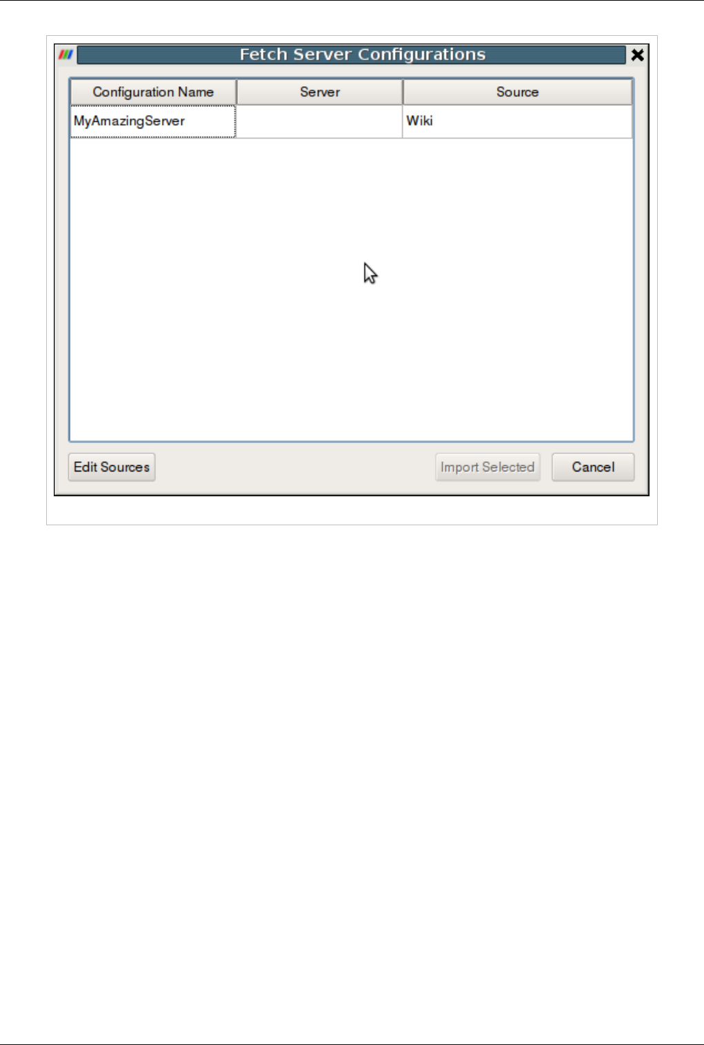
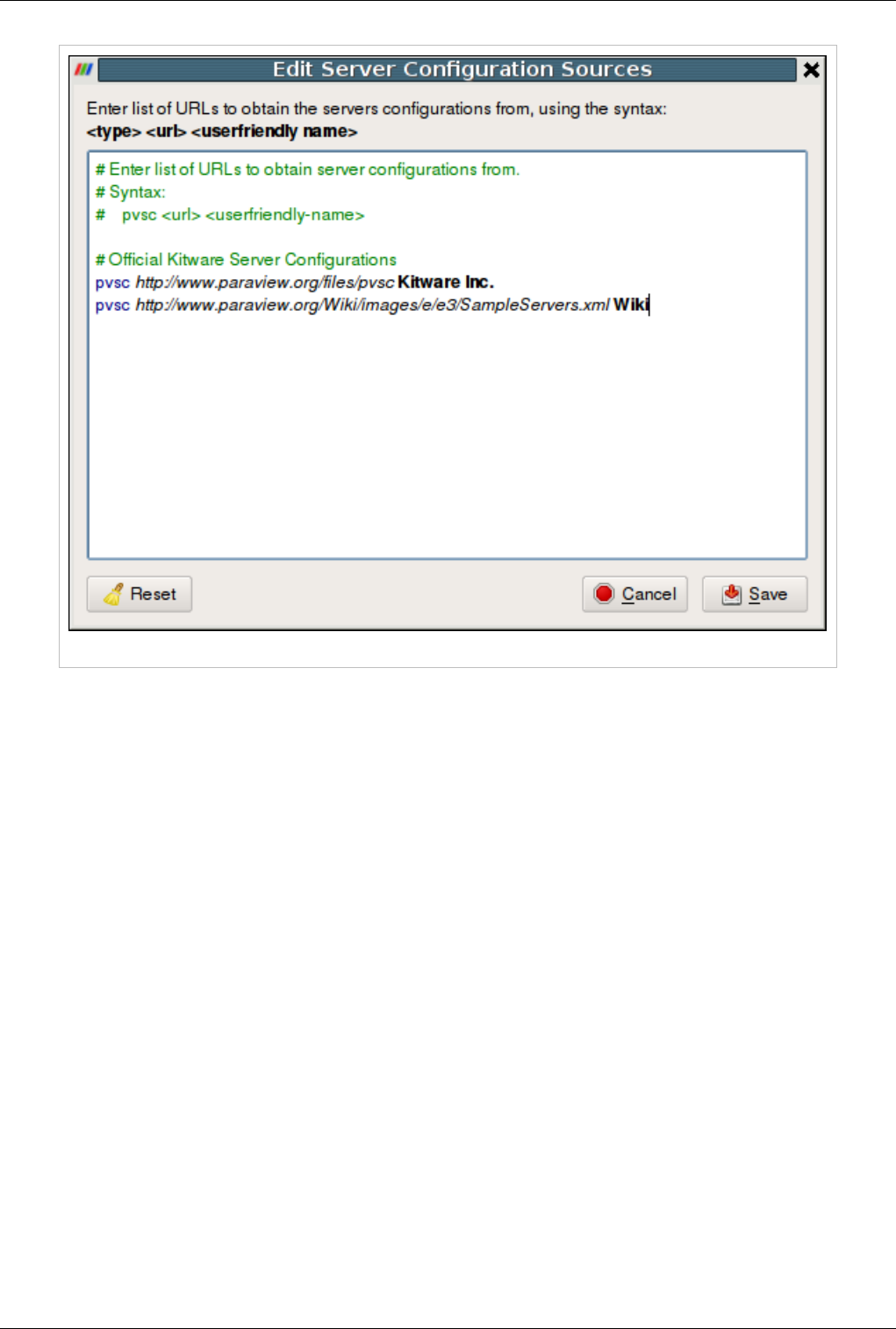
Distributing/Obtaining Server Connection Configurations 170
Figure 3 Edit Server Configuration Sources
Click Save will save the changes and cause ParaView to fetch the configurations from the updated URLs. Once the
updated configurations are listed on the Fetch Server Configuration Page, simply select and Import the
configurations you would like to use and they are then accessible from the standard server's list shown in the Server
Connect dialog.
URL Search Sequence
For each URL specified, ParaView tries that following paths until the first path that returns valid XML file.
1. {URL}
2. {URL}/v{MAJOR_VERSION}.{MINOR_VERSION}/{CLIENT OS}/servers.pvsc
3. {URL}/v{MAJOR_VERSION}.{MINOR_VERSION}/{CLIENT OS}/servers.xml
4. {URL}/v{MAJOR_VERSION}.{MINOR_VERSION}/servers.pvsc
5. {URL}/v{MAJOR_VERSION}.{MINOR_VERSION}/servers.xml
6. {URL}/servers.pvsc
7. {URL}/servers.xml
Where:
•{URL} : the URL specified
•{MAJOR_VERSION} : major version number of the ParaView client e.g. for ParaView 3.14, it will be 3.
•{MINOR_VERSION} : minor version number of the ParaView client e.g. for ParaView 3.14, it will be 14
•{CLIENT_OS} : Either win32, macos, or nix based of the client OS.
This search sequence makes it easy for PVSC maintainers to provide different pvsc files based on the client OS, if
needed. It also enables partial specialization e.g. if the maintainer wants to provide a special pvsc for ParaView 3.14

Distributing/Obtaining Server Connection Configurations 171
on windows but a common pvsc for all other version and/or platforms, then he simply sets up the webserver
directory structure as follows:
1. {URL}/v3.14/win32/servers.pvsc
2. {URL}/servers.pvsc
And advertises to his users simply the {URL} to use as a configuration source.

172
Parallel Rendering and Large Displays
About Parallel Rendering
One of ParaView's strengths is its ability to off-load the often demanding rendering task. By offload, we mean that
ParaView allows you to connect to a remote machine, ideally one that is closer to the data and to high-end rendering
hardware, to do the rendering on that machine and still interact with the data from a convenient location.
Abstracting away the location where rendering takes place opens up many possibilities. First, it opens up the
possibility to parallelize the job of rendering to make it possible to render huge data sets at interactive rates.
Rendering is done in the parallel Render Server component, which may be part of, or separate from, the parallel Data
Server component. In the next section, we describe how parallel rendering works and explain the controls you have
over it. Second, huge datasets often require high-resolution displays to view the intricate details within while
maintaining a high-level view to maintain context. In the following section, we explain how ParaView can be used to
drive tile display walls. Lastly, with the number of displays free to vary, it becomes possible to use ParaView to
drive multi-display Virtual Reality systems. That is described in the final section of this chapter.
Parallel Rendering
X Forwarding - Not a Good Idea
Parallel Rendering implies that many processors have some context to render their pixels into. Even though X11
forwarding might be available, you should not run the client remotely and forward its X calls. ParaView will be far
more efficient if you let it directly handle the data transfer between local and remote machines. When doing
hardware accelerated rendering in GPUs, this implies having X11 or Windows display contexts (either off-screen of
on-screen). Otherwise. this implies using off-screen Mesa (OSMesa) linked in to ParaView to do the rendering
entirely off-screen into software buffers.
Onscreen GPU Accelerated Rendering via X11 Connections
One of the most common problems people have with setting up the ParaView server is allowing the server processes
to open windows on the graphics card on each process' node. When ParaView needs to do parallel rendering, each
process will create a window that it will use to render. This window is necessary because you need the "x" window
before you can create an OpenGL context on the graphics hardware.
There is a way around this. If you are using the Mesa as your OpenGL implementation, then you can also use the
supplemental OSMesa library to create an OpenGL context without an "x" window. However, Mesa is strictly a CPU
rendering library so, use the OSMesa solution if and only if your server hardware does not have rendering
hardware. If your cluster does not have graphics hardware, then compile ParaView with OSMesa support and use
the --use-offscreen-rendering flag when launching the server.
Assuming that your cluster does have graphics hardware, you will need to establish the following three things:
1. Have xdm run on each cluster node at start-up. Although xdm is almost always run at startup on workstation
installations, it is not as commonplace to be run on cluster nodes. Talk to your system administrators for help in
setting this up.
Parallel Rendering 173
2. Disable all security on the "x" server. That is, allow any process to open a window on the "x" server without
having to log-in. Again, talk to your system administrators for help.
3. Use the -display flag for pvserver to make sure that each process is connecting to the display localhost:0
(or just :0).
To enable the last condition, you would run something like:
mpirun -np 4 ./pvserver -display localhost:0
An easy way to test your setup is to use the glxgears program. Unlike pvserver, it will quickly tell you (or,
rather, fail to start) if it cannot connect to the local "x" server.
mpirun -np 4 /usr/X11R6/bin/glxgears -display localhost:0
Offscreen Software Rendering via OSMesa
When running ParaView in a parallel mode, it may be helpful for the remote rendering processes to do their
rendering in off-screen buffers. For example, other windows may be displayed on the node(s) where you are
rendering; if these windows cover part of the rendering window, depending on the platform and graphics
capabilities, they might even be captured as part of the display results from that node. A similar situation could occur
if more than one rendering process is assigned to a single machine and the processes share a display. Also, in some
cases, the remote rendering nodes are not directly connected to a display and otherwise if your cluster does not have
graphics hardware, then compile ParaView with OSMesa support and use the --use-offscreen-rendering flag when
launching the server.
The first step to compiling OSMesa support is to make sure that you are compiling with the Mesa 3D Graphics
Library [1]. It is difficult to tell an installation of Mesa from any other OpenGL implementation (although the
existence of an osmesa.h header and a libOSMesa library is a good clue). If you are not sure, you can always
download your own copy from http:/ / mesa3d. org. We recommend using either Mesa version 7.6.1 or 7.9.1.
There are three different ways to use Mesa as ParaView's openGL library:
• You can use it purely as a substitute for GPU enabled onscreen rendering. To do this, set the CMake variable
OPENGL_INCLUDE_DIR to point to the Mesa include directory (the one containing the GL subdirectory) and set
the OPENGL_gl_LIBRARY and OPENGL_glu_LIBRARY to the libGL and libGLU library files, respectively.
Variable Value Description
PARAVIEW_BUILD_QT_GUI ON
VTK_USE_COCOA ON Mac Only. X11 is not supported.
VTK_OPENGL_HAS_OSMESA OFF Disable off screen rendering.
OPENGL_INCLUDE_DIR <mesa include dir> Set this to the include directory in MESA.
OPENGL_gl_LIBRARY libGL Set this to the libGL.a or libGL.so file in MESA.
OPENGL_glu_LIBRARY libGLU Set this to the libGLU.a or libGLU.so file in MESA.
• You can use it as a supplement to on-screen rendering. This mode requires that you have a display (X11 is
running). In addition to specifying the GL library (which may be a GPU implementation of the Mesa one above),
you must tell ParaView where Mesa's OSMesa library is. Do that by turning the VTK_OPENGL_HAS_OSMESA
variable to ON. After you configure again, you will see a new CMake variable called OSMESA_LIBRARY. Set
this to the libOSMesa library file.

Parallel Rendering 174
Variable Value Description
PARAVIEW_BUILD_QT_GUI ON
VTK_USE_COCOA ON Mac Only. X11 is not supported.
VTK_OPENGL_HAS_OSMESA ON Turn this to ON to enable software rendering.
OSMESA_INCLUDE_DIR <mesa include dir> Set this to the include directory for MESA.
OPENGL_INCLUDE_DIR <mesa include dir> Set this to the include directory for MESA.
OPENGL_gl_LIBRARY libGL Set this to the libGL.a or libGL.so file.
OPENGL_glu_LIBRARY libGLU Set this to the libGLU.a or libGLU.so file.
OSMESA_LIBRARY libOSMesa Set this to the libOSMesa.a or libOSMesa.so file.
• You can use it for pure off-screen rendering, which is necessary when there is no display (or even X11 libraries).
To do this, make sure that the OPENGL_gl_LIBRARY variable is empty and that VTK_USE_X is off. Specify the
location of OSMesa and OPENGL_glu_LIBRARY as above and turn on the VTK_USE_OFFSCREEN variable.
Variable Value Description
PARAVIEW_BUILD_QT_GUI OFF When using offscreen rendering there is no gui
VTK_USE_COCOA OFF Mac only.
VTK_USE_X OFF
VTK_USE_OFFSCREEN ON
VTK_OPENGL_HAS_OSMESA ON Turn this to ON to enable Off Screen MESA.
OSMESA_INCLUDE_DIR <mesa include dir> Set this to the include directory for MESA.
OPENGL_INCLUDE_DIR <mesa include dir> Set this to the include directory for MESA.
OPENGL_gl_LIBRARY <empty> Set this to empty.
OPENGL_glu_LIBRARY libGLU Set this to the libGLU.a or libGLU.so file.
OSMESA_LIBRARY libOSMesa Set this to the libOSMesa.a or libOSMesa.so file.
Note that unless you ensure that VTK_USE_OFFSCREEN is ON, offscreen rendering will not take effect unless you
launch the server with the --use-offscreen-rendering flag or alternatively, set the PV_OFFSCREEN environment
variable on the server to one.
Compositing
Given that you are connected to a server that is capable of rendering, you have a choice of whether to do the
rendering remotely or to do it locally. ParaView’s server performs all data-processing tasks. This includes generation
of a polygonal representation of the full data set and of decimated LOD models. Once the data is generated on the
server, it is sometimes better to do the rendering remotely and ship pixels to the client for display; other times, it's
better to instead shift geometry to the client and have the client render it locally.
In many cases, the polygonal representation of the data set is much smaller than the original data set. In an extreme
case, a simple outline may be used to represent a very large structured mesh; in these instances, it may be better to
transmit the polygonal representation from the server to the client, and then let the client render it. The client can
render the data repeatedly, when the viewpoint is changed for instance, without causing additional network traffic.
Network traffic will only occur when the data changes. If the client workstation has high-performance rendering
hardware, it can sometimes render even large data sets interactively in this way.
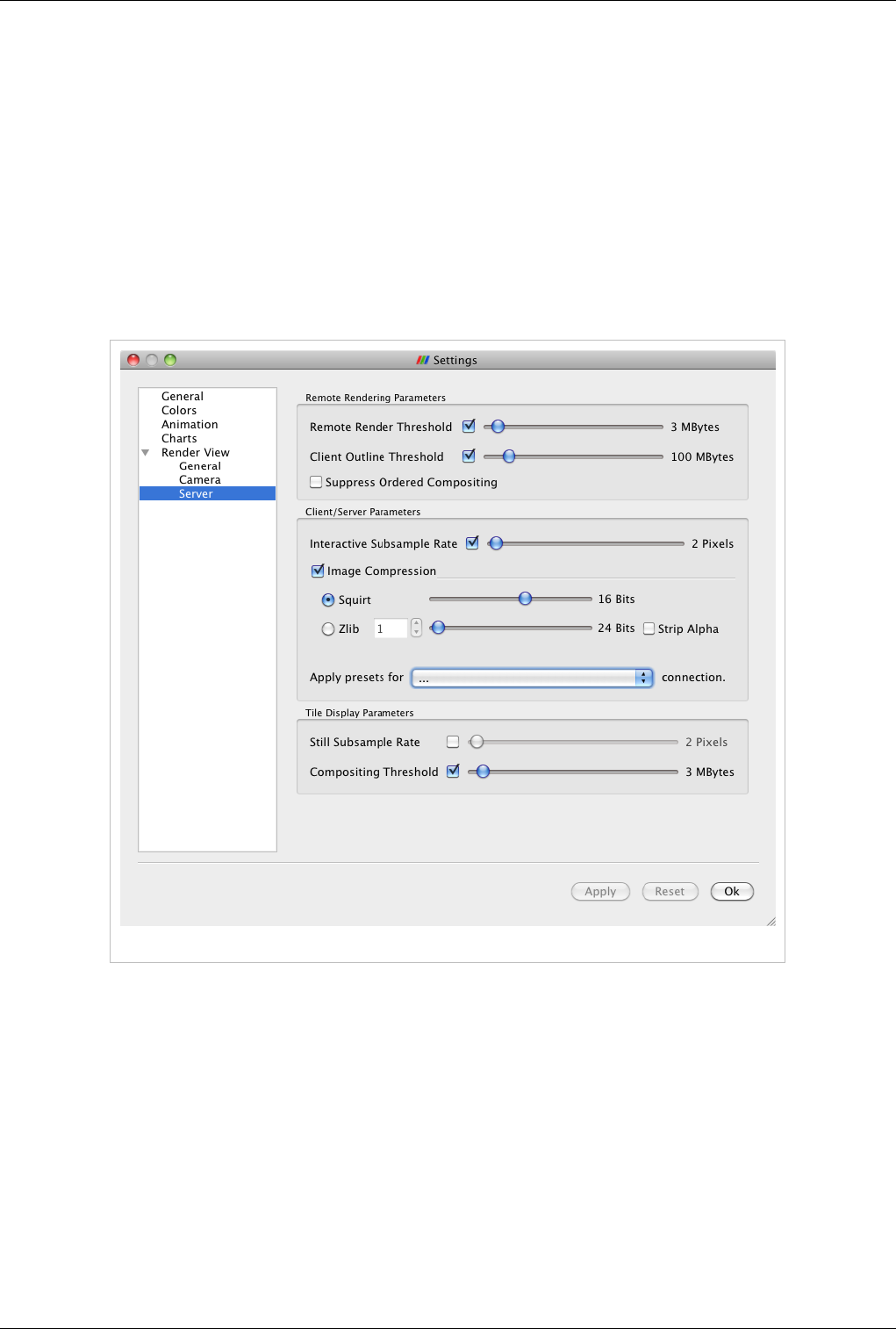
Parallel Rendering 175
The second option is to have each node of the server render its geometry and send the resulting images to the client
for display. There is a penalty per rendered frame for compositing images and sending the image across the network.
However, ParaView’s image compositing and delivery is very fast, and there are many options to ensure interactive
rendering in this mode. Therefore, although small models may be collected and rendered on the client interactively,
ParaView’s distributed rendering can render models of all sizes interactively.
ParaView automatically chooses a rendering strategy to achieve the best rendering performance. You can control the
rendering strategy explicitly, forcing rendering to occur entirely on the server or entirely on the client for example,
by choosing Settings from the Edit menu of ParaView. Double-click on Render View from the window on the
left-hand side of the Settings dialog, and then click on Server. The rendering strategy parameters shown in Figure
13.1 will now be visible. Here we explain in detail the most important of these controls. For an explanation of all
controls, see the Appendix.
Figure 13.1 Parallel rendering parameters
Remote Render Threshold: This slider determines how large the dataset must be in order for parallel rendering
with image compositing and delivery to be used (as opposed to collecting the geometry to the client). The value of
this slider is measured in megabytes. Only when the entire data set consumes more memory than this value will
compositing of images occur. If the check-box beside the Remote Render Threshold slider is unmarked, then
compositing will not happen; the geometry will always be collected. This is only a reasonable option when you can
be sure the dataset you are using is very small. In general, it is safer to move the slider to the right than to uncheck
the box.
ParaView uses IceT to perform image compositing. IceT is a parallel rendering library that takes multiple images
rendered from different portions of the geometry and combines them into a single image. IceT employs several
image-compositing algorithms, all of which are designed to work well on distributed memory machines. Examples
of two such image-compositing algorithms are depicted in Figure 13.2 and Figure 13.3. IceT will automatically
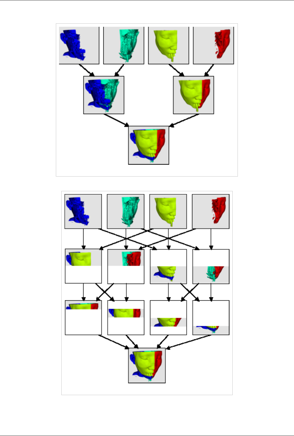
Parallel Rendering 176
choose a compositing algorithm based on the current workload and available computing resources.
File 13.2 Tree compositing on four processes
File 13.3 Binary swap on four processes
Interactive Subsample Rate: The time it takes to composite and deliver images is directly proportional to the size
of the images. The overhead of parallel rendering can be reduced by simply reducing the size of the images.

Parallel Rendering 177
ParaView has the ability to subsample images before they are composited and inflate them after they have been
composited. The Interactive Subsample Rate slider specifies the amount by which images are subsampled. This is
measured in pixels, and the subsampling is the same in both horizontal and vertical directions. Thus, a subsample
rate of two will result in an image that is ¼ the size of the original image. The image is scaled to full-size before it is
displayed on the user interface, so the higher the subsample rate, the more obviously pixilated the image will be
during interaction as demonstrated in Figure 13.4. When the user is not interacting with the data, no subsampling
will be used. If you want subsampling to always be off, unmark the check-box beside the Interactive Subsample Rate
slider.
[[File:ParaView_UsersGuide_NoSubsampling.png link=]] [[File:ParaView_UsersGuide_TwoPixelSubsampling.png link=]] [[File:ParaView_UsersGuide_EightPixelSubsampling.png link=]]
No Subsampling
Subsample
Rate: 2
pixels
Subsample Rate: 8 pixels
Figure 13.4 The effect of subsampling on image quality
Squirt Compression: When ParaView is run in client/server mode, it uses image compression to optimize the image
transfer. The compression uses an encoding algorithm optimized for images called SQUIRT (developed at Sandia
National Laboratories).
SQUIRT uses simple run-length encoding for its compression. A run-length image encoder will find sequences of
pixels that are all the same color and encode them as a single run length (the count of pixels repeated) and the color
value. ParaView represents colors as 24-bit values, but SQUIRT will optionally apply a bit mask to the colors before
comparing them. Although information is lost when this mask is applied, the sizes of the run lengths are increased
and the compression improves. The bit masks used by SQUIRT are carefully chosen to match the color sensitivity of
the human visual system. A 19-bit mask employed by SQUIRT greatly improves compression with little or no
noticeable image artifacts. Reducing the number of bits further can improve compression even more, but it can lead
to more noticeable color-banding artifacts.
The Squirt Compression slider determines the bit mask used during interactive rendering (i.e., rendering that occurs
while the user is changing the camera position or otherwise interacting with the data). During still rendering (when
the user is not interacting with the data), lossless compression is always used. The check-box to the left of the Squirt
Compression slider toggles whether the SQUIRT compression algorithm is used at all.
References
[1] http:/ / mesa3d. org

Tile Display Walls 178
Tile Display Walls
Tiled Display
ParaView’s parallel architecture makes it possible to visualize massive amounts of data interactively. When the data
is of sufficient resolution that parallel processing is necessary for interactive display, it is often the case that
high-resolution images are needed to inspect the data in adequate detail. If you have a 2D grid of display devices,
you can run ParaView in tiled display mode to take advantage of it.
To put ParaView in tiled display mode, give pvserver (or pvrenderserver) the X and Y dimensions of the 2D grid
with the --tile-dimensions-x (or -tdx) and --tile-dimensions-y (or ‑tdy) arguments. The X and Y dimensions default to
0, which disables tiled display mode. If you set only one of them to a positive value on the command line, the other
will be set to 1. In tiled display mode, there must be at least as many server (in client / server mode) or render server
(in client / data server / render server mode) nodes as tiles. The example below will create a 3x2 tiled display.
pvserver -tdx=3 -tdy=2
Unless you have a high-end display wall, it is likely that each monitor's bezel creates a gap between the images
shown in your tiled display. You can compensate for the bezel width by considering them to be like mullions on a
window. To do that, specify the size of the gap (in pixels) through the --tile-mullion-x (-tmx) and --tile-mullion-y
(-tmy) command line arguments.
The IceT library, which ParaView uses for its image compositing, has custom compositing algorithms that work on
tiled displays. Although compositing images for large tiled displays is a compute-intensive process, IceT reduces the
overall amount of work by employing custom compositing strategies and removing empty tiles from the
computation, as demonstrated in Figure 13.5. If the number of nodes is greater than the number of tiles, then the
image compositing work will be divided amongst all the processes in the render server. In general, rendering to a
tiled display will perform significantly better if there are many more nodes in the cluster than tiles in the display it
drives. It also greatly helps if the geometry to be rendered is spatially distributed. Spatially distributed data is broken
into contiguous pieces that are contained in small regions of space and are therefore rendered to smaller areas of the
screen. IceT takes advantage of this property to reduce the amount of work required to composite the final images.
ParaView includes the D3 filter, which redistributes data amongst the processors to ensure a spatially distributed
geometry and thus improves tiled rendering performance.
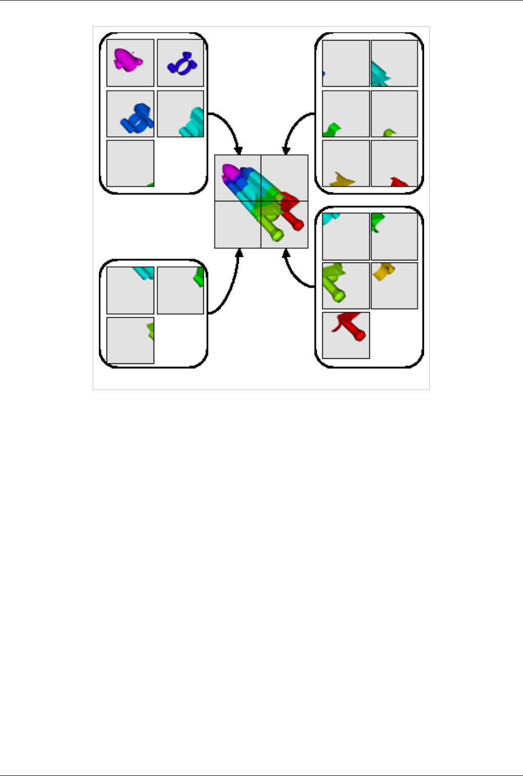
Tile Display Walls 179
Figure 13.5 Compositing images for 8 processes on a 4-tile display
Unlike other parallel rendering modes, composited images are not delivered to the client. Instead, image compositing
is reserved for generating images on the tiled display, and the desktop renders its own images from a lower
resolution version of the geometry to display in the UI. In Tiled Display Mode, ParaView automatically decimates
the geometry and sends it to the client to make this happen. However, when the data is very large, even a decimated
version of the geometry can overwhelm the client. In this case, ParaView will replace the geometry on the client with
a bounding box.
You have several controls at run-time over the tiled rendering algorithm that you can tune to maintain interactivity
while visualizing very large data on very high-resolution tiled displays. These are located on the Tile Display
Parameters section of the Render View / Server page of the application settings dialog. These controls are described
in the Application Settings section of the Appendix.
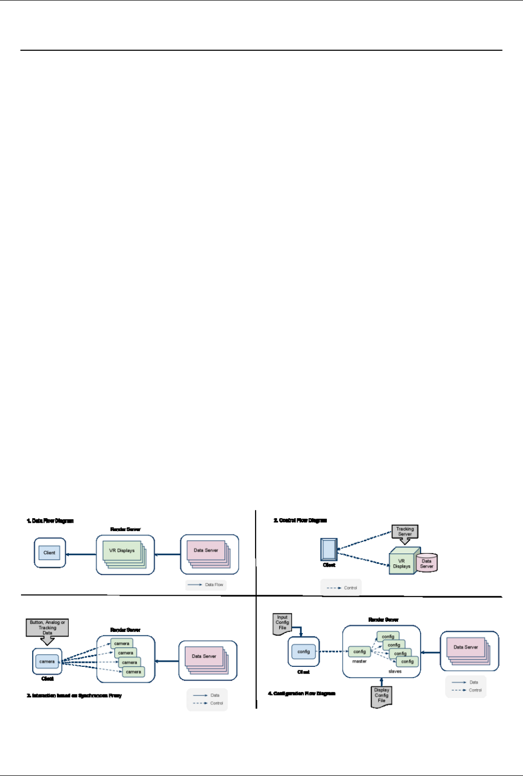
CAVE Displays 180
CAVE Displays
Introduction
• ParaView has basic support for visualization in CAVE-like/VR or Virtual Environments (VE).
• Like typical computing systems, VE's consists of peripheral displays (output) and input devices. However, unlike
regular systems, VE's keep track of the physical location of their IO devices with respect to an assumed base
coordinates in the physical room (room coordinates).
• Typically VE's consists of multiple stereoscopic displays that are configured based on the room coordinates.
These base coordinates also typically serve as the reference coordinate for tracked inputs commonly found in
VE's.
• VR support in ParaView includes the ability to
1. Configure displays (CAVE/Tiled Walls etc) and
2. The ability to configure inputs using VRPN/VRUI.
• ParaView can operate in a Client / Server fashion. The VR/CAVE module leverage this by assigning different
processes on the server to manage different displays. Displays are thus configured on the server side by passing a
*.pvx configuration XML file during start-up.
• The client acts as a central point of control. It can initiate the scene (visualization pipeline) and also relay tracked
interactions to each server process managing the displays. The VR plugin on the client side enables this. Device
and interaction style configurations are brought in through the ParaView state file (This will also have a GUI
component in the near future).
Architecture and Design Overview
The picture describes the data flow, control flow, synchronization and configuration aspects of ParaView designed
for VE's. The 4 compartments in the picture depicts the following ideas.
1. We leverage the Render Server mechanism to drive the various displays in a CAVE/VE.
2. Devices and control signals are relayed through the client using a plugin (VRPlugin)
3. Rendering and inputs are synchronized using synchronous proxy mechanism inherent in Paraview (PV).
4. Inputs are configured at the client end and displays are configured at the server end.

CAVE Displays 181
Process to Build, Configure and Run ParaView in VE (For ParaView 4.0 or
lower)
ParaView VR in 4.0
Process to Build, Configure and Run ParaView in VE (For ParaView 3.10 or
lower)
Enabling ParaView for VR is a five stage process.
1. Building ParaView with the required parameters.
2. Preparing the display configuration file.
3. Preparing the input configuration file.
4. Starting the server (with display config.pvx)
5. Starting the client (with input config.pvsm)
Building
Follow regular build instructions from http:/ / paraview. org/ Wiki/ ParaView:Build_And_Install. In addition
following steps needs to be performed
• Make sure Qt and MPI are installed cause they are required for building. If using VRPN make sure it is build and
installed as well.
• When configuring cmake enable BUILD_SHARED_LIB, PARAVIEW_BUILD_QT_GUI,
PARAVIEW_USE_MPI and PARAVIEW_BUILD_PLUGIN_VRPlugin .
• On Apple and Linux platforms the Plugin uses VRUI device daemon client as its default and on Windows VRPN
is the default.
• If you want to enable the other simply enable PARAVIEW_USE_VRPN or PARAVIEW_USE_VRUI .
• If VRPN is not found in the default paths then VRPN_INCLUDE_DIR and VRPN_LIBRARY may also need be
set.
Configuring Displays
The PV server is responsible for configuring displays. The display configuration is stored on a *.pvx file.
ParaView has no concept of units and therefore user have to make sure that the configuration values are in
the same measurements units as what tracker has producing. So for example if tracker data is in meters, then
everything is considered in meters, if feet then feet becomes the unit for configuration.
Structure of PVX Config File
<?xml version="1.0" ?>
<pvx>
<Process Type="server|dataserver|renderserver">
<!--
The only supported Type values are "server", "dataserver" or
"renderserver".
This controls which executable this configuration is applicable
to.
There can be multiple <Process /> elements in the same pvx file.
------------------------------------------------------
| Executable | Applicable Process Type |
| pvserver | server, dataserver, renderserver |
CAVE Displays 182
| pvrenderserver | server, renderserver |
| pvdataserver | server, dataserver |
------------------------------------------------------
-->
<EyeSeparation Value="0.065"/> <!-- Should be specified in the configuration file-->
<Machine Name="hostname"
Environment="DISPLAY=m1:0"
LowerLeft="-1.0 -1.0 -1.0"
LowerRight="1.0 -1.0 -1.0"
UpperRight="1.0 1.0 -1.0">
<!--
There can be multiple <Machine> elements in a <Process> element,
each one identifying the configuration for a process.
All attributes are optional.
name="hostname"
Environment: the environment for the process.
LowerLeft|LowerRight|UpperRight
-->
</Machine>
</Process>
</pvx>
Example Config.pvx
• The following example is for a six sided cave with origin at (0,0,0):
<?xml version="1.0" ?>
<pvx>
<Process Type="client" />
<Process Type="server">
<EyeSeparation Value="0.065"/>
<Machine Name="Front"
Environment="DISPLAY=:0"
LowerLeft=" -1 -1 -1"
LowerRight=" 1 -1 -1"
UpperRight=" 1 1 -1" />
<Machine Name="Right"
Environment="DISPLAY=:0"
LowerLeft=" 1 -1 -1"
LowerRight=" 1 -1 1"
UpperRight=" 1 1 1" />
<Machine Name="Left"
Environment="DISPLAY=:0"
LowerLeft=" -1 -1 1"
LowerRight="-1 -1 -1"
UpperRight="-1 1 -1"/>
<Machine Name="Top"
Environment="DISPLAY=:0"
LowerLeft=" -1 1 -1"

CAVE Displays 183
LowerRight=" 1 1 -1"
UpperRight=" 1 1 1"/>
<Machine Name="Bottom"
Environment="DISPLAY=:0"
LowerLeft=" -1 -1 1"
LowerRight=" 1 -1 1"
UpperRight=" 1 -1 -1"/>
<Machine Name="Back"
Environment="DISPLAY=:0"
LowerLeft=" 1 -1 1"
LowerRight="-1 -1 1"
UpperRight="-1 1 1"/>
</Process>
</pvx>
• A sample PVX is provided in ParaView/Documentation/cave.pvx. This can be used to play with different display
configurations.
Notes on PVX file usage
• PVX file should be specified as the last command line argument for any of the server processes.
• The PVX file is typically specified for all the executables whose environment is being changed using the PVX
file. In case of data-server/render-server configuration, if you are setting up the environment for the two processes
groups, then the PVX file must be passed as a command line option to both the executables: pvdataserver and
pvrenderserver.
• When running in parallel the file is read on all nodes, hence it must be present on all nodes.
• ParaView has no concept of units.
• Use tracker units as default unit for corner points values, eye separation and anything else that requires real
world units.
Configure Inputs
• Configuring inputs is a two step process
1. Define connections to one or more VRPN/VRUI servers.
2. Mapping data coming in from the server to ParaView interactor styles.
Device Connections
• Connections are clients to VRPN servers and or VRUI device daemons.
• Connection are defined using XML as follows.
<VRConnectionManager>
<VRUIConnection name="travel" address="localhost" port = "8555">
<Button id="0" name="1"/>
<Button id="1" name="2"/>
<Button id="2" name="3"/>
<Tracker id="0" name="head"/>
<Tracker id="1" name="wand"/>
<!-- you can also apply a transformation matrix to the tracking data: -->
<TrackerTransform value="
1 0 0 0

CAVE Displays 184
0 1 0 0
0 0 1 0
0 0 0 1"/>
</VRUIConnection>
<VRPNConnection name="spaceNav" address="device0@localhost">
<Analog id="0" name="channels"/>
</VRPNConnection>
</VRConnectionManager>
• VRConnectionManager can define multiple connection. Each connection can of of type VRUIConnection or
VRPNConnection.
• Each connection has a name associated with it. Also data coming in from these connection can be given specific
names.
• In our example above a VRUI connection is defined and named travel. We also define a name to the tracking data
on this connection calling it head. We can henceforth refer to this data using a dotted notation as follows
travel.head
• Like all data being read into the system can be assigned some virtual names which will be used down the line.
• Following is a pictorial representation of the process.
Interaction Styles
• Interactor styles define certain fixed sets of interaction that we usually perform in VE's.
• There are fixed number of hand-coded interaction styles.
•vtkVRStyleTracking maps tracking data to a certain paraview proxy object.
•vtkVRStyleGrabNUpdateMatrix takes button press and updates some transformation based on incoming
tracking data.
•vtkVRStyleGrabNTranslateSliceOrigin takes a button press and updates a position based on the position of
the tracked input.
•vtkVRStyleGrabNRotateSliceNormal takes a button press and updates a vector based on the orientation of
the tracked input.
• Interactor styles are specified using the following XML format.
<VRInteractorStyles>
<Style class="vtkVRStyleTracking" set_property="RenderView1.HeadPose">
<Tracker name="travel.head"/>
</Style>
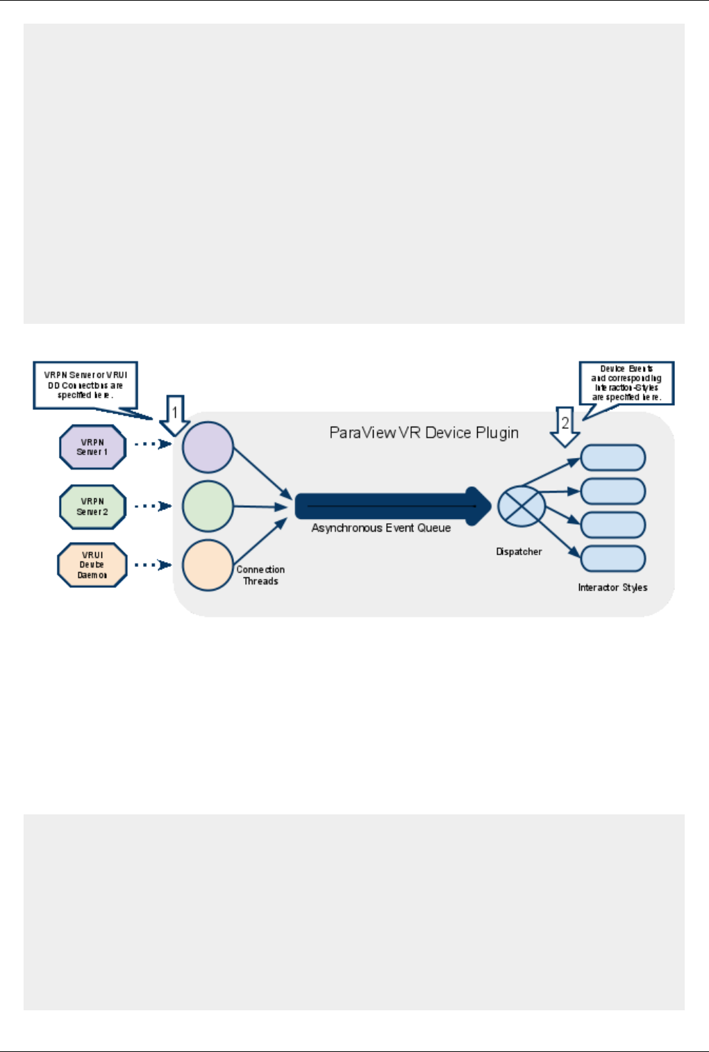
CAVE Displays 185
<Style class="vtkVRStyleGrabNUpdateMatrix" set_property="RenderView1.WandPose">
<Tracker name="travel.wand"/>
<Button name="travel.1"/>
<MatrixProperty name="RenderView1.WandPose"/>
</Style>
<Style class="vtkVRStyleGrabNTranslateSliceOrigin" origin="CutFunction.Origin">
<Button name="travel.2"/>
<Tracker name="travel.wand"/>
</Style>
<Style class="vtkVRStyleGrabNRotateSliceNormal" normal="CutFunction.Normal">
<Button name="travel.3"/>
<Tracker name="travel.wand"/>
</Style>
</VRInteractorStyles>
• The following is a pictorial representation of the entire process.
Piggy-Backing the state file
• The VRPlugin uses the state loading mechanism to read its configuration. This was just a quick and dirty way and
will most probably be replaced with different method (perhaps a GUI even).
• More about the state file can be found here [1].
• A state file is a representation of the visualization pipeline in PV.
• So the first step before configuring the inputs is to load and create a scene in PV.
• Export the corresponding state into a state file (config.pvsm). A state file has an extention *.pvsm with content as
follows
<ParaView>
<ServerManagerState version="3.11.1">
.....
.....
</ServerManagerState>
<ViewManager>
.....
</ViewManager>
</ParaView>

CAVE Displays 186
• We extend the state file to introduce the VRConnectionManager and VRInteractorStyles tags as follows
<ParaView>
<ServerManagerState version="3.11.1">
.....
.....
</ServerManagerState>
<!-- Start Append state file ----- -->
<VRConnectionManager>
<VRUIConnection ...
</VRConnectionManager>
<VRInteractorStyles>
<Style ...
</VRInteractorStyles>
<!-- End Append state file -------- -->
<ViewManager>
.....
</ViewManager>
</ParaView>
• Now our state file not only contains the scene but also the device interaction configuration (config.pvsm).
Start Server
• On a terminal run the server (For example we want to run 6 processes each driving one display in the cave.
Change the number of process according to the number of displays).
# PV_ICET_WINDOW_BORDERS=1 mpiexec -np 6 ./pvserver /path/to/ConfigFile.pvx
Note: PV_ICET_WINDOW_BORDERS=1 disables the full-screen mode and instead opens up a 400x400 window.
Remove this environment variable to work in full-screen mode.
Start Client
• Open another terminal to run the client. (note: this client connects to the server which open up 6 windows
according to the config given in cave.pvx). Change the stereo-type according to preference (see # ./paraview
--help).
# ./paraview --stereo --stereo-type=Anaglyph --server=localhost
• --server=localhost connects the client to the server.
• Enable the VRPlugin on the client.
• Load the updated state file (config.pvsm) specifying VRPN or VRUI client connection and interaction styles.


188
Scripted Control
Interpreted ParaView
The ParaView client provides an easy-to-use GUI in which to visualize data with the standard window, menu, and
button controls. Driving ParaView with a mouse is intuitive, but is not easily reproducible and exact as is required
for repetitive analysis and scientific result reproducibility. For this type of work, it is much better to use ParaView's
scripted interface. This is an an alternative control path that works alongside of, or as a replacement for, the GUI.
ParaView's native scripted interface uses the Python programming language. The interface allows one to
programatically control ParaView's back-end data processing and rendering engines. Note that this level of control is
distinct from the Python Programmable Filter discussed in the Quantitative Analysis Chapter. That is a white, box
filter that runs in parallel within the server and has direct access to each individual element of the data. Here we are
discussing client-side python control where you control the entire pipeline, which may or may not include Python
Programmable Filters.
In this chapter, we discuss first ParaView's python scripted interface, which follows the same idioms as and thus is
operated similarly to the way one works in the GUI. Next, we discuss the ParaView's python tools, which make it
even easier to use ParaView python scripts, including the ability to record script files from GUI actions and to
augment the GUI with them. Lastly we discuss batch processing with ParaView.
Python Scripting
Note: This document if based on ParaView 3.6 or higher. If you are using 3.4, go to the history page and select the
version from May 13, 2009.
ParaView and Python
ParaView offers rich scripting support through Python. This support is available as part of the ParaView client
(paraview), an MPI-enabled batch application (pvbatch), the ParaView python client (pvpython), or any other
Python-enabled application. Using Python, users and developers can gain access to the ParaView engine called
Server Manager.
Note: Server Manager is a library that is designed to make it easy to build distributed client-server applications.
This document is a short introduction to ParaView's Python interface. You may also visit the Python recipes page for
some examples.
Quick Start - a Tutorial
Getting Started
To start interacting with the Server Manager, you have to load the "simple" module. This module can be loaded from
any python interpreter as long as the necessary files are in PYTHONPATH. These files are the shared libraries
located in the paraview binary directory and python modules in the paraview directory: paraview/simple.py,
paraview/vtk.py etc. You can also use either pvpython (for stand-alone or client/server execution), pvbatch (for

Python Scripting 189
non-interactive, distributed batch processing) or the python shell invoked from Tools|Python Shell using the
ParaView client to execute Python scripts. You do not have to set PYTHONPATH when using these.
This tutorial will be using the python integrated development environment IDLE. PYTHONPATH is set to the
following:
/Users/berk/work/paraview3-build/lib:/Users/berk/work/paraview3-build/lib/site-packages
Note: For older versions of ParaView this was
/Users/berk/work/paraview3-build/bin:/Users/berk/work/paraview3-build/Utilities/VTKPythonWrapping/site-packages
--Andy.bauer 24 January 2013, or
/Users/berk/work/paraview3-build/bin:/Users/berk/work/paraview3-build/Utilities/VTKPythonWrapping
--Andy.bauer 23 July 2010.
You may also need to set your path variable for searching for shared libraries (i.e. PATH on Windows and
LD_LIBRARY_PATH on Unix/Linux/Mac). The corresponding LD_LIBRARY_PATH would be:
/Users/berk/work/paraview3-build/lib (/Users/berk/work/paraview3-build/bin for versions before 3.98)
(Under WindowsXP for a debug build of paraview, set both PATH and PYTHONPATH environment variables to
include ${BUILD}/lib/Debug and ${BUILD}/lib/site-packages to make it work.)
When using a Mac to use the build tree in IDLE, start by loading the servermanager module:
>>> from paraview.simple import *
Note: Importing the paraview module directly is deprecated, although still possible for backwards compatibility.
This document refers to the simple module alone.
In this example, we will use ParaView in the stand-alone mode. Connecting to a ParaView server running on a
cluster is covered later in this document.
Tab-completion
The Python shell in the ParaView Qt client provides auto-completion. One can also use IDLE, for example to enable
auto-completion. To use auto-completion in pvpython, one can use the tips provided at [1].
In summary, you need to create a variable PYTHONSTARTUP as (in bash):
export PYTHONSTARTUP = /home/<username>/.pythonrc
where .pythonrc is:
# ~/.pythonrc
# enable syntax completion
try:
import readline
except ImportError:
print "Module readline not available."
else:
import rlcompleter
readline.parse_and_bind("tab: complete")
That is it. Tab completion works just as in any other shell.

Python Scripting 190
Creating a Pipeline
The simple module contains many functions to instantiate sources, filters, and other related objects. You can get a
list of objects this module can create from ParaView's online help (from help menu or here: http:/ / paraview. org/
OnlineHelpCurrent/ )
Start by creating a Cone object:
>>> cone = Cone()
You can get some documentation about the cone object using help().
>>> help(cone)
Help on Cone in module paraview.servermanager object:
class Cone(SourceProxy)
| The Cone source can be used to add a polygonal cone to the 3D
scene. The output of the
Cone source is polygonal data.
|
| Method resolution order:
| Cone
| SourceProxy
| Proxy
| __builtin__.object
|
| Methods defined here:
|
| Initialize = aInitialize(self, connection=None)
|
|
----------------------------------------------------------------------
| Data descriptors defined here:
|
| Capping
| If this property is set to 1, the base of the cone will be
capped with a filled polygon.
Otherwise, the base of the cone will be open.
|
| Center
| This property specifies the center of the cone.
|
| Direction
| Set the orientation vector of the cone. The vector does not
have to be normalized. The cone
will point in the direction specified.
|
| Height
| This property specifies the height of the cone.
|

Python Scripting 191
| Radius
| This property specifies the radius of the base of the cone.
|
| Resolution
| This property indicates the number of divisions around the
cone. The higher this number, the
closer the polygonal approximation will come to representing a cone,
and the more polygons it will
contain.
|
|...
This gives you a full list of properties. Check what the resolution property is set to:
>>> cone.Resolution
6
You can increase the resolution as shown below:
>>> cone.Resolution = 32
Alternatively, we could have specified a value for resolution when creating the object:
>>> cone = Cone(Resolution=32)
You can assign values to any number of properties during construction using keyword arguments: You can also
change the center.
>>> cone.Center
[0.0, 0.0, 0.0]
>>> cone.Center = [1, 2, 3]
Vector properties such as this one support setting and retrieval of individual elements, as well as slices (ranges of
elements):
>>> cone.Center[0:2] = [2, 4]
>>> cone.Center
[2.0, 4.0, 3.0]
Next, apply a shrink filter to the cone:
>>> shrinkFilter = Shrink(cone)
>>> shrinkFilter.Input
<paraview.servermanager.Cone object at 0xaf701f0>
At this point, if you are interested in getting some information about the output of the shrink filter, you can force it to
update (which will also cause the execution of the cone source). For details about VTK's demand-driven pipeline
model used by ParaView, see one of the VTK books.
>>> shrinkFilter.UpdatePipeline()
>>> shrinkFilter.GetDataInformation().GetNumberOfCells()
33L
>>> shrinkFilter.GetDataInformation().GetNumberOfPoints()
128L
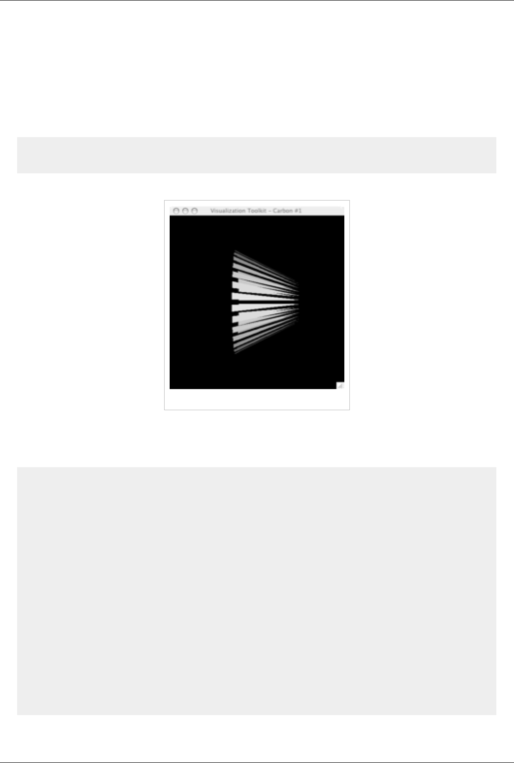
Python Scripting 192
We will cover the DataInformation class in more detail later.
Rendering
Now that you've created a small pipeline, render the result. You will need two objects to render the output of an
algorithm in a scene: a representation and a view. A representation is responsible for taking a data object and
rendering it in a view. A view is responsible for managing a render context and a collection of representations.
Simple creates a view by default. The representation object is created automatically with Show().
>>> Show(shrinkFilter)
>>> Render()
Et voila:
Figure 14.1 Server manager snapshot
In example Figure 14.1, the value returned by Cone() and Shrink() was assigned to Python variables and used to
build the pipeline. ParaView keeps track of the last pipeline object created by the user. This allows you to
accomplish everything you did above using the following code:
>>> from paraview.simple import *
# Create a cone and assign it as the active object
>>> Cone()
<paraview.servermanager.Cone object at 0x2910f0>
# Set a property of the active object
>>> SetProperties(Resolution=32)
# Apply the shrink filter to the active object
# Shrink is now active
>>> Shrink()
<paraview.servermanager.Shrink object at 0xaf64050>
# Show shrink
>>> Show()
<paraview.servermanager.UnstructuredGridRepresentation object at 0xaf57f90>
# Render the active view
>>> Render()
<paraview.servermanager.RenderView object at 0xaf57ff0>

Python Scripting 193
This was a quick introduction to the paraview.simple module. In the following sections, we will discuss the Python
interface in more detail and introduce more advanced concepts.
paraview.simple Module
The simple module is a ParaView component written using Python on top of the Server Manager C++ library. Its
purpose is to make it easier to create ParaView data analysis and visualization pipelines using Python. The simple
module can be loaded from Python interpreters running in several applications.
•pvpython: The pvpython application, distributed with the ParaView application suite, is a Python client to the
ParaView servers. It supports interactive execution as well as batch execution.
•pvbatch: The pvbatch application, also distributed with the ParaView application suite, is a Python application
designed to run batch scripts on distributed servers. When ParaView is compiled with MPI, pvbatch can be
launched as an MPI program. In this mode, the first node will load a Python script specified as a command-line
argument and execute it using a special built-in connection on all nodes. This application does not support
interactive execution.
•paraview: Python scripts can be run from the paraview client using the Python shell that is invoked from
Tools|Python Shell. The Python shell supports interactive mode as well as loading of scripts from file.
•External Python interpreter: Any Python-capable application can load the paraview.simple module if the right
environment is configured. For this to work, you either have to install the paraview Python modules (including
the right shared libraries) somewhere in sys.path or you have to set PYTHONPATH to point to the right locations.
Overview
The paraview.simple module contains several Python classes designed to be Python-friendly, as well as all classes
wrapped from the C++ Server Manager library. The following sections cover the usage of this module and
occasionally the paraview.servermanager module, which is lower level.
Connecting to a Server
ParaView can run in two modes: stand-alone and client/server where the server is usually a visualization cluster. In
this section, we discuss how to establish a connection to a server when using ParaView in the client/server mode. If
you are using the ParaView graphical interface, you should use Connect from the File menu to connect to a server. If
you are using ParaView from a Python shell (not the Python console that is part of the graphical interface), you need
to use servermanager.Connect() to connect a server. Note: you cannot connect to the ParaView application from a
stand-alone Python shell. You can only connect to a server. This method takes four arguments, all of which have
default values.
def Connect(ds_host=None, ds_port=11111, rs_host=None, rs_port=11111)
When connecting to a server (pvserver), specify only the first two arguments. These are the server name (or IP
address) and port number.
When connecting to a data-server/render-server pair, you have to specify all four arguments. The first two are the
host name (or IP address) and port number of the data server, the last two those of the render server. Here are some
examples:
# Connect to pvserver running on amber1 (first node of our test cluster)
# using the default port 11111
>>> Connect(‘amber1’)

Python Scripting 194
# Connect to pvdataserver running on the amber cluster, pvrenderserver
# running on Berk’s desktop
>>> Connect(‘amber1’, 12000, ‘kamino’, 11111)
Note: Connect() will return None on failure. To be safe, you should check the return value of Connect().
Getting Help
You can access the documentation of all Proxy types by using Python's built-in help.
>>> help(paraview.simple.Cone)
Help on function CreateObject in module paraview.simple:
CreateObject(*input, **params)
The Cone source can be used to add a polygonal cone to the 3D
scene. The output of the
Cone source is polygonal data.
To get the full documentation, you have to create an instance.
>>> c = Cone()
>>> help(c)
This documentation is automatically generated from the Server Manager configuration files. It is identical to the
class documentation found under the ParaView Help menu, as well as here: http:/ / paraview. org/
OnlineHelpCurrent/ . Beyond this document and the online help, there are a few useful documentation sources:
• The ParaView Guide: http:/ / www. kitware. com/ products/ paraviewguide. html
• The ParaView Wiki: http:/ / paraview. org/ Wiki/ ParaView
• The ParaView source documentation: http:/ / www. paraview. org/ doc/
If you are interested in learning more about the Visualization Toolkit that is at the foundation of ParaView, visit
http:/ / vtk. org.
Proxies and Properties
Proxies
The VTK Server Manager design uses the Proxy design pattern (See Design Patterns: Elements of Reusable
Object-Oriented Software by Erich Gamma, Richard Helm, Ralph Johnson and John Vlissides for details). Quoting
from Wikipedia: “A proxy, in its most general form, is a class functioning as an interface to another thing. The other
thing could be anything: a network connection, a large object in memory, a file, or some other resource that is
expensive or impossible to duplicate”. In the case of Server Manager, a Proxy object acts as a proxy to one-or-more
VTK objects. Most of the time, these are server-side objects and are distributed to the server nodes. Proxy objects
allow you to interact with these objects as if you directly have access to them, manipulate them, and obtain
information about them. When creating visualization pipelines, you create proxies instead of VTK objects.
>>> sphereSource = vtk.vtkSphereSource() # VTK-Python script
>>> sphereSourceP = Sphere() # ParaView script
A proxy also provides an interface to modify the properties of the objects it maintains. For example, instead of:

Python Scripting 195
>>> sphereSource.SetCenter(1.0, 1.0, 0.0)
you can write the following:
>>> sphere.Center = [1.0, 1.0, 0.0]
When a pipeline object proxy is created, it is set as the active object. You can also set an object as the active one.
This is equivalent to clicking-on an object in the pipeline browser.
>>> c = Cone()
<paraview.servermanager.Cone object at 0xaf73090>
>>> GetActiveSource()
<paraview.servermanager.Cone object at 0xaf73090>
>>> Shrink()
<paraview.servermanager.Shrink object at 0xb4f8610>
# Make the cone active
>>> SetActiveSource(c)
When dealing with objects created through the graphical interface or by loading a state, it is useful to be able to
search through existing pipeline objects. To accomplish this, you can use GetSources() and FindSource().
GetSources() returns a dictionary of (name, id) object pairs. Since multiple objects can have the same name, the
(name,id) pair identifies objects uniquely. FindSource() returns an object given its name. If there are more than one
objects with the same name, the first one is returned.
>>> Cone()
<paraview.servermanager.Cone object at 0xaf73090>
>>> GetActiveSource()
<paraview.servermanager.Cone object at 0xaf73090>
>>> Shrink()
<paraview.servermanager.Shrink object at 0xb4f8610>
>>> SetActiveSource(c)
To delete pipeline objects, you need to use the Delete() function. Simply letting a Python variable go out of scope is
not enough to delete the object. Following the example above:
# Delete the cone source
>>> Delete(c)
# To fully remove the cone from memory, get rid of the
# variable too
>>> del c
Properties
Property objects are used to read and modify the properties of pipeline objects. Each proxy has a list of properties
defined in the Server Manager configuration files. The property interface of the Server Manager C++ library is
somewhat cumbersome. Here is how you can set the radius property of a sphere source:
>>> rp = sphere.GetProperty("Radius")
>>> rp.SetElement(0, 2)
1
>>> sphere.UpdateProperty("Radius")

Python Scripting 196
The servermanager module makes property access much easier by defining Python property accessors for property
objects:
>>> sphere.Radius = 3
Here, Radius is a Python property which, when a value is assigned to it, calls
sphere.SetPropertyWithName("Radius",3). Properties can also passed to the function creating the object:
>>> cone = Cone(Radius=0.5, Center=[1, 0.5, 0])
<paraview.servermanager.Cone object at 0xaf73090>
You can also use the SetProperties() function to set property values.
>>> SetProperties(cone, Radius=0.2, Center=[2, 0.5, 0])
If the first argument is not specified, the active object is used. You also use SetDisplayProperties() and
SetViewProperties() to set display (representation) and view properties respectively.
All Property classes define the following methods:
• __len__()
• __getitem__()
• __setitem__()
• __getslice__()
• __setslice__()
• GetData()
• SetData().
Therefore, all of the following are supported:
>>> sphere.Center
[0.0, 0.0, 0.0]
>>> sphere.Center[0] = 1
>>> sphere.Center[0:3] = [1,2,3]
>>> sphere.Center[0:3]
[1.0, 2.0, 3.0]
>>> len(sphere.Center)
3
ProxyProperty and InputProperty also define
• append()
• __delitem__()
• __delslice__()
to support del() and append(), similar to Python list objects.
VectorProperty is used for scalars, vectors and lists of integer and floating point numbers as well as strings. Most
properties of this type are simple. Examples include Sphere.Radius (double scalar), Sphere.Center (vector of
doubles), a2DGlyph.Filled (boolean), a2DGlyph.GlyphType (enumeration), a3DText.Text (string), and
Contour.Isosurfaces (list of doubles). Some properties may be more complicated because they map to C++ methods
with mixed argument types. Two good examples of this case are Glyph.Scalars and ExodusIIReader.PointVariables.
>>> reader = ExodusIIReader(FileName='.../can.ex2')
# These variables are currently selected
>>> reader.PointVariables
['DISPL', 'VEL', 'ACCL']

Python Scripting 197
# These are available in the file
>>> reader.PointVariables.Available
['DISPL', 'VEL', 'ACCL']
# Enable the DISPL array only
>>> reader.PointVariables = ['DISPL']
# Force read
>>> reader.UpdatePipeline()
# Now check the output. Note: GlobalNodeId is generated automatically
by the reader.
>>> reader.PointData[:]
[Array: GlobalNodeId, Array: PedigreeNodeId, Array: DISPL]
This example demonstrates the use of ExodusIIReader.PointVariables. This is a VectorProperty that represents a list
of array names. The underlying C++ function has a signature of SetPointResultArrayStatus(const char* name, int
flag). This method is usually called once per array to enable or disable it (i.e. to set whether the reader will read a
particular array).
Glyph.Scalars is a bit more complicated. This property allows the developer to select the scalar array with which to
scale the glyphs.
>>> sph = Sphere()
>>> elev=Elevation(sph)
# Glyph the points of the sphere with spheres
>>> glyph=Glyph(elev, GlyphType='Sphere')
# Scale the glyph with the Elevation array
>>> glyph.Scalars = 'Elevation'
>>> glyph.Scalars
['POINTS', 'Elevation']
# The above shows the association of the array as well as its name.
# In this case, the array is associated with POINTS as it has to be
# since Glyph cannot scale by cell arrays. We could have done:
>>> glyph.Scalars = ['POINTS', 'Elevation']
# Enable scaling by scalars
>>> glyph.ScaleMode = 'scalar'
Here the property Scalars maps to SetInputArrayToProcess(int idx, int port, int connection, int fieldAssociation,
const char *name), which has four integer arguments (some of which are enumeration) and one string argument (see
vtkAlgorithm documentation for details).
Properties are either regular (push) or information (pull) properties. Information properties do not have a VTK
method associated with them and are responsible for getting information from the server. A good example of an
information property is TimestepValues, which returns all time steps available in a file (if the reader supports time).
>>> reader = ExodusIIReader(FileName='.../can.ex2')
>>> reader.TimestepValues
[0.0, 0.00010007373930420727, 0.00019990510190837085,
0.00029996439116075635, 0.00040008654468692839,
0.00049991923151537776, 0.00059993512695655227, 0.00070004, ...]
You can obtain a list of properties a proxy supports by using help(). However, this does not allow introspection
programmatically. If you need to obtain information about a proxy’s properties programmatically, you can use a

Python Scripting 198
property iterator:
>>> for prop in glyph:
print type(prop), prop.GetXMLLabel()
<class 'paraview.servermanager.InputProperty'> Input
<class 'paraview.servermanager.VectorProperty'> Maximum Number of Points
<class 'paraview.servermanager.VectorProperty'> Random Mode
<class 'paraview.servermanager.ArraySelectionProperty'> Scalars
<class 'paraview.servermanager.ArraySelectionProperty'> Vectors
<class 'paraview.servermanager.VectorProperty'> Orient
<class 'paraview.servermanager.VectorProperty'> Set Scale Factor
<class 'paraview.servermanager.EnumerationProperty'> Scale Mode
<class 'paraview.servermanager.InputProperty'> Glyph Type
<class 'paraview.servermanager.VectorProperty'> Mask Points
The XMLLabel is the text display by the graphical user-interface. Note that there is a direct mapping from the
XMLLabel to the property name. If you remove all spaces from the label, you get the property name. You can use
the PropertyIterator object directly.
>>> it = iter(s)
>>> for i in it:
print it.GetKey(), it.GetProperty()
Domains
The Server Manager provides information about values that are valid for properties. The main use of this information
is for the user-interface to provide good ranges and choices in enumeration. However, some of this information is
also very useful for introspection. For example, enumeration properties look like simple integer properties unless a
(value, name) pair is associated with them. The Server Manager uses Domain objects to store this information. The
contents of domains may be loaded from xml configuration files or computed automatically. For example:
>>> s = Sphere()
>>> Show(s)
>>> dp = GetDisplayProperties(s)
>>> dp.Representation
'Surface'
# The current representation type is Surface. What other types
# are available?
>>> dp.GetProperty("Representation").Available
['Outline', 'Points', 'Wireframe', 'Surface', 'Surface With Edges']
# Choose outline
>>> dp.Representation = 'Outline'

Python Scripting 199
Source Proxies
Source proxies are proxies that represent pipeline objects (For more information about VTK pipelines, see the VTK
books: http:/ / vtk. org/ buy-books. php''). They have special properties to connect them as well as special method to
query the meta-data of their output. To connect a source proxy to another, use one of its input properties.
# Either
>>> glyph = Glyph(elev)
# or
>>> glyph.Input = elev
The SourceProxy class provides several additional properties and methods that are specific to pipelines (See
vtkSMSourceProxy documentation for a full list).
•UpdatePipelineInformation(): This method calls UpdateInformation() on the VTK algorithm. It also calls
UpdatePropertyInformation() to update any information properties.
•UpdatePipeline(): This method calls Update() on the VTK algorithm causing a pipeline execution if the pipeline
changed. Another way of causing pipeline updates is to render. The render view updates all connected pipelines.
•GetDataInformation(): This method is used to obtain meta-data about one output. It is discussed further below.
• PointData and CellData properties discussed below.
There are two common ways of getting meta-data information from a proxy: information properties and
DataInformation. Information properties are updated automatically every time UpdatePropertyInformation() and
UpdatePipelineInformation() are called. All you have to do is read the data from the property as usual. To get a
DataInformation object from a source proxy use GetDataInformation(port=0). By default, this method returns data
information for the first output. You can pass an optional port number to get information for another output. You can
get detailed documentation on DataInformation by using help() and by reading online documentation for
vtkPVDataInformation (http:/ / www. paraview. org/ doc/ nightly/ html/ classvtkPVDataInformation. html''). Here
are the use of some common methods:
>>> di = glyph.GetDataInformation(0)
>>> di
<paraview.servermanager.DataInformation object at 0x2d0920d0>
>>> glyph.UpdatePipeline()
# Get the data type.
>>> di.GetDataClassName()
'vtkPolyData'
# Get information about point data.
>>> pdi = di.PointData
# We are now directly accessing the wrapper for a VTK class
>>> len(pdi)
1
# Get information for a point array
>>> ai = pdi[0]
>>> ai.GetRange(0)
(0.0, 0.5)
When meta-data is not enough and you need access to the raw data, you can use Fetch() to bring it to the client side.
Note that this function is provided by the servermanager module. Fetch() has three modes:
• Append all of the data together and bring it to the client (only available for polygonal and unstructured datasets).
Note: Do not do this if data is large otherwise the client will run out of memory.

Python Scripting 200
• Bring data from a given process to the client.
• Use a reduction algorithm and bring its output to the client. For example, find the minimum value of an attribute.
Here is a demonstration:
>>> from paraview.simple import *
>>> Connect("kamino")
Connection (kamino:11111)
>>> s = Sphere()
# Get the whole sphere. DO NOT DO THIS IF THE DATA IS LARGE otherwise
# the client will run out of memory.
>>> allsphere = servermanager.Fetch(s)
getting appended
use append poly data filter
>>> allsphere.GetNumberOfPolys()
96
# Get the piece of the sphere on process 0.
>>> onesphere = servermanager.Fetch(s, 0)
getting node 0
>>> onesphere.GetNumberOfPolys()
48
# Apply the elevation filter so that we have a useful scalar array.
>>> elev = Elevation(s)
# We will use the MinMax algorithm to compute the minimum value of
# elevation. MinMax will be first applied on each processor. The results
# will then be gathered to the first node. MinMax will be then applied
# to the gathered results.
# We first create MinMax without an input.
>>> mm = MinMax(None)
# Set it to compute min
>>> mm.Operation = "MIN"
# Get the minimum
>>> mindata = servermanager.Fetch(elev, mm, mm)
applying operation
# The result is a vtkPolyData with one point
>>> mindata.GetPointData().GetNumberOfArrays()
2
>>> a0 = mindata.GetPointData().GetArray(1)
>>> a0.GetName()
'Elevation'
>>> a0.GetTuple1(0)
0.0

Python Scripting 201
Representations and Views
Once a pipeline is created, it can be rendered using representations and views. A view is essentially a “window” in
which multiple representations can be displayed. When the view is a VTK view (such as RenderView), this
corresponds to a collection of objects including vtkRenderers and a vtkRenderWindow. However, there is no
requirement for a view to be a VTK view or to render anything. A representation is a collection of objects, usually a
pipeline, that takes a data object, converts it to something that can be rendered, and renders it. When the view is a
VTK view, this corresponds to a collection of objects including geometry filters, level-of-detail algorithms,
vtkMappers and vtkActors. The simple module automatically creates a view after connecting to a server (including
the built-in connection when using the stand-alone mode). Furthermore, the simple module creates a representation
the first time a pipeline object is displayed with Show(). It is easy to create new views.
>>> view = CreateRenderView()
CreateRenderView() is a special method that creates the render view appropriate for the ActiveConnection (or for
another connection specified as an argument). It returns a sub-class of Proxy. Like the constructor of Proxy, it can
take an arbitrary number of keyword arguments to set initial values for properties. Note that ParaView makes the
view that was created last the active view. When using Show() without a view argument, the pipeline is shown in the
active view. You can get a list of views as well as the active view as follows:
>>> GetRenderViews()
[<paraview.servermanager.RenderView object at 0xaf64ef0>, <paraview.servermanager.RenderView object at 0xaf64b70>]
>>> GetActiveView()
<paraview.servermanager.RenderView object at 0xaf64b70>
You can also change the active view using SetActiveView().
Once you have a render view, you can use pass it to Show in order to select in which view a pipeline object is
displayed. You can also pass it to Render() to select which view is rendered.
>>> Show(elev, GetRenderViews()[1])
<paraview.servermanager.GeometryRepresentation object at 0xaf64e30>
>>> Render(GetRenderViews()[1])
Notice that Show() returns a representation object (aka DisplayProperties in the simple module). This object can be
used to manipulate how the pipeline object is displayed in the view. You can also access the display properties of an
object using GetDisplayProperties().
>>> dp = GetDisplayProperties(elev)
>>> dp
<paraview.servermanager.GeometryRepresentation object at 0xaf649d0>
Display properties and views have a large number of documented properties some of which are poorly documented.
We will cover some them here.
>>> from paraview.simple import *
# Create a simple pipeline
>>> sph = Sphere()
>>> elev = Elevation(sph)
>>> Show(elev)
>>> Render()
# Set the representation type of elev
>>> dp = GetDisplayProperties(elev)
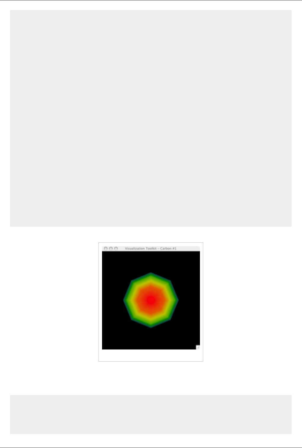
Python Scripting 202
>>> dp.Representation = 'Points'
# Here is how you get the list of representation types
>>> dp.GetProperty("Representation").Available
['Outline', 'Points', 'Wireframe', 'Surface', 'Surface With Edges']
>>> Render()
# Change the representation to wireframe
>>> dp.Representation = 'Wireframe'
>>> Render()
# Let’s get some information about the output of the elevation
# filter. We want to color the representation by one of it’s
# arrays.
# Second array = Elevation. Interesting. Let’s use this one.
>>> ai = elev.PointData[1]
>>> ai.GetName()
'Elevation'
# What is its range?
>>> ai.GetRange()
(0.0, 0.5)
# To color the representation by an array, we need to first create
# a lookup table. We use the range of the Elevation array
>>> dp.LookupTable = MakeBlueToRedLT(0, 0.5)
>>> dp.ColorAttributeType = 'POINT_DATA'
>>> dp.ColorArrayName = 'Elevation' # color by Elevation
>>> Render()
Here is the result:
Figure 14.2 Object displayed in a view
Once you create a scene, you will probably want to interact with the camera and ResetCamera() is likely to be
insufficient. In this case, you can directly get the camera from the view and manipulate it. GetActiveCamera()
returns a VTK object (not a proxy) with which you can interact.
>>> camera = GetActiveCamera()
>>> camera
<libvtkCommonPython.vtkCamera vtkobject at 0xe290>
>>> camera.Elevation(45)
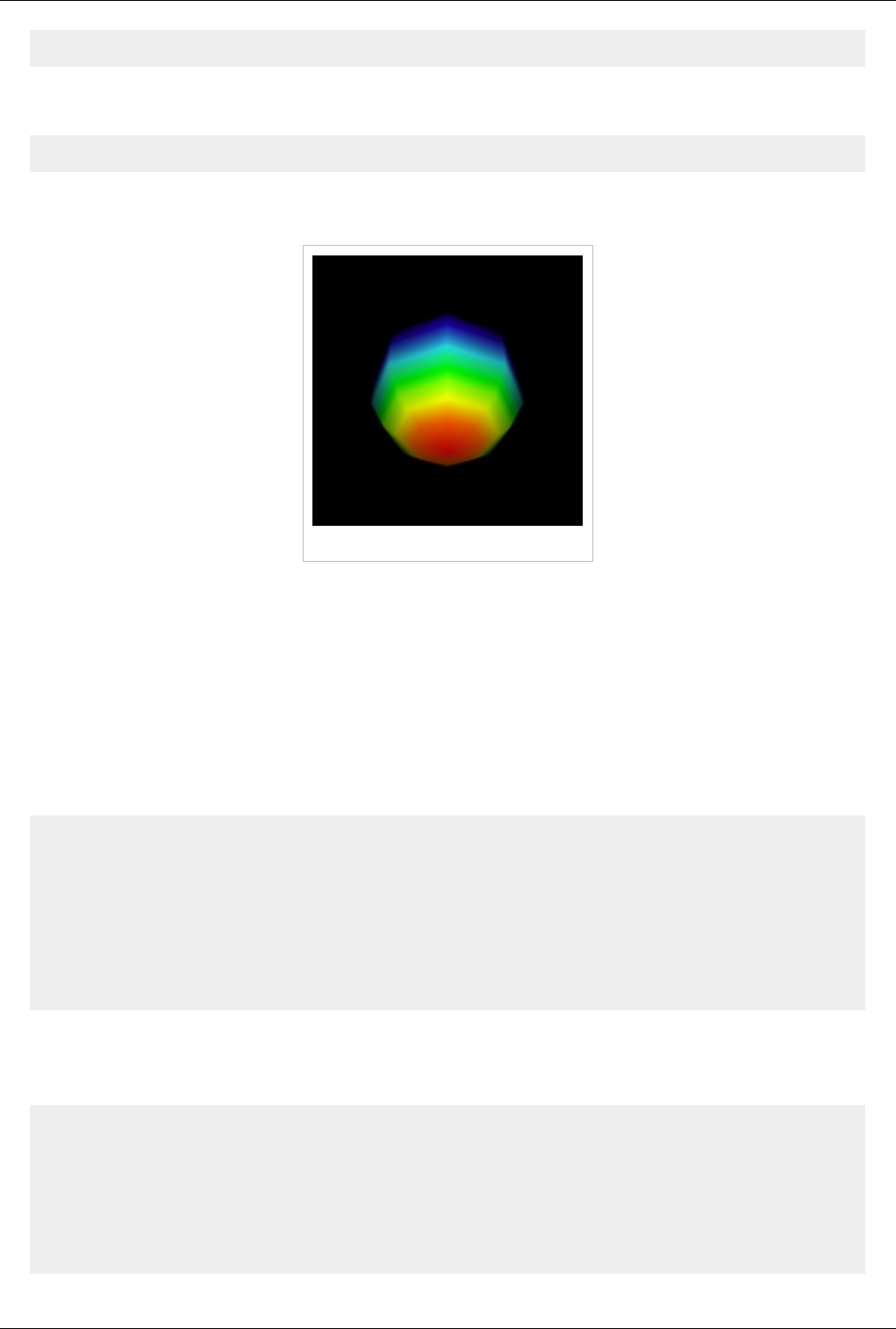
Python Scripting 203
>>> Render()
Another common thing to do is to save the view as an image. For this purpose, you can use the WriteImage() method
provided by the view:
>> WriteImage("/Users/berk/image.png")
The resulting image.png looks like this. See the documentation for WriteImage() for details on choosing file type, as
well as a magnification factor to save images larger than the view size.
Figure 14.3 Saving a view as an image
Advanced Concepts
Dealing with lookup tables
As shown earlier, you can use MakeBlueToRedLt(min, max) to create a lookup table. However, this simply creates a
new lookup table that the GUI won't be aware of. In the ParaView Qt application, we have special lookup table
management that ensures that the same lookup table is used for all arrays with same name and number of
components. To reproduce the same behavior in Python, use GetLookupTableForArray().
def GetLookupTableForArray(arrayname, num_components, **params):
"""Used to get an existing lookuptable for a array or to create one
if none
exists. Keyword arguments can be passed in to initialize the LUT if
a new
one is created. Returns the lookup table."""
....
This will create a new lookup table and associate it with that array, if none already exists. Any default arguments to
be passed to the lookup table if a new one is created, can be specified as additional parameters. You can always
change the properties on the lookup table returned by this function.
# To color the representation by an array, we need to first create
# a lookup table. We use the range of the Elevation array
>>> dp.LookupTable = GetLookupTableForArray("Elevation", 1,
RGBPoints = [min, 0, 0, 1, max, 1, 0, 0],
ColorSpace = "HSV")
>>> dp.ColorAttributeType = 'POINT_DATA'

Python Scripting 204
>>> dp.ColorArrayName = 'Elevation' # color by Elevation
>>> Render()
Loading State and Manipulating It
Let’s say you created a complicated visualization using the paraview application and now you want to make slight
changes to it and run it in a loop as a batch script. What do you do? The best way of dealing with this is to save your
visualization state and then load it from Python. Let’s say you have a state file saved as myteststate.pvsm:
>>> from paraview.simple import *
# Load the state
>>> servermanager.LoadState("/Users/berk/myteststate.pvsm")
# Make sure that the view in the state is the active one
>>> SetActiveView(GetRenderView())
# Now render
>>> Render()
# Get the list of sources
>>> GetSources()
{('Sphere1', '5'): <paraview.servermanager.Sphere object at 0xaf80e30>,
('Shrink1', '11'): <paraview.servermanager.Shrink object at 0xaf80df0>,
('Cone1', '8'): <paraview.servermanager.Cone object at 0xaf80cf0>}
# Change the resolution of the cone and render again
>>> FindSource("Cone1").Resolution = 32
>>> Render()
You can also save state.
>>> from paraview.simple import *
>>> sph = Sphere()
>>> Render()
>>> servermanager.SaveState("/Users/berk/pythonstate.pvsm")
Dealing with Time
If a reader or a filter supports time, it is easy to request a certain time step from Python. All time requests are set on
views that then propagate them to the representations which then propagate them to the visualization pipeline. Here
is an example demonstrating how a time request can be made:
>>> Show(ExodusIIReader(FileName=".../can.ex2"))
>>> Render()
# Get a nice view angle
>>> cam = GetActiveCamera()
>>> cam.Elevation(45)
>>> Render()
# Check the current view time
>>> view = GetActiveView()
>>> view.ViewTime
0.0
>>> reader = GetActiveSource()
>>> reader.TimestepValues

Python Scripting 205
[0.0, 0.00010007373930420727, 0.00019990510190837085,
0.00029996439116075635, 0.00040008654468692839,
...]
>>> tsteps = reader.TimestepValues
# Let’s be fancy and use a time annotation filter. This will show the
# current time value of the reader as text in the corner of the view.
>>> annTime = AnnotateTimeFilter(reader)
# Show the filter
>>> Show(annTime)
# Look at a few time steps. Note that the time value is requested not
# the time step index.
>>> view.ViewTime = tsteps[2]
>>> Render()
>>> view.ViewTime = tsteps[4]
>>> Render()
Animating
Server Manager has a complicated animation engine based on keyframes and scenes. This section will introduce a
few simple ways of animating your visualization. If you have a time-aware reader, you can animate it with
AnimateReader().
>>> reader = ExodusIIReader(FileName=“.../can.ex2”)
>>> Show(reader)
>>> Render()
>>> c = GetActiveCamera()
>>> c.Elevation(95)
# Animate over all time steps. Note that we are not passing the optional
# 3rd argument here. If you pass a filename as the 3rd argument,
# AnimateReader will create a movie.
>>> AnimateReader(reader)
# Save the animation to an avi file
>>> AnimateReader(reader, filename=".../movie.avi")
To animate properties other than time, you can use regular keyframes.
ParaView 3.8.0 and earlier
Although the following script will work with 3.8.1 and later, it's not the recommended way since the changes done
so will not be reflected in the GUI. Refer to the following sub-section for the recommended style for 3.8.1 and later
versions.
>>> Sphere()
>>> Show()
>>> Render()
# Create an animation scene
>>> scene = servermanager.animation.AnimationScene()
# Add one view
>>> scene.ViewModules = [GetActiveView()]

Python Scripting 206
# Create a cue to animate the StartTheta property
>>> cue = servermanager.animation.KeyFrameAnimationCue()
>>> cue.AnimatedProxy = GetActiveSource()
>>> cue.AnimatedPropertyName = "StartTheta"
# Add it to the scene's cues
>>> scene.Cues = [cue]
# Create 2 keyframes for the StartTheta track
>>> keyf0 = servermanager.animation.CompositeKeyFrame()
>>> keyf0.Interpolation = 'Ramp'
# At time = 0, value = 0
>>> keyf0.KeyTime = 0
>>> keyf0.KeyValues= [0]
>>> keyf1 = servermanager.animation.CompositeKeyFrame()
# At time = 1.0, value = 200
>>> keyf1.KeyTime = 1.0
>>> keyf1.KeyValues= [200]
# Add keyframes.
>>> cue.KeyFrames = [keyf0, keyf1]
>>> scene.Play()
# Some properties you can change
#
# Number of frames used in Sequence mode
# scene.NumberOfFrames = 100
#
# Or you can use real time mode
# scene.PlayMode = 'Real Time'
# scene.Duration = 20
ParaView 3.8.1 onwards
The following script will only work with ParaView versions 3.8.1 and later. It is now the recommended way for
accessing animation scenes and tracks since the updates are reflected in the GUI when running through the Python
shell from the ParaView application.
>>> Sphere()
>>> Show()
>>> Render()
# Get the application-wide animation scene
>>> scene = GetAnimationScene()
# Get the animation track for animating "StartTheta" on the active
source.
# GetAnimationTrack() creates a new track if none exists.
Python Scripting 207
>>> cue = GetAnimationTrack("StartTheta")
# Create 2 keyframes for the StartTheta track
>>> keyf0 = CompositeKeyFrame()
>>> keyf0.Interpolation = 'Ramp'
# At time = 0, value = 0
>>> keyf0.KeyTime = 0
>>> keyf0.KeyValues= [0]
>>> keyf1 = CompositeKeyFrame()
# At time = 1.0, value = 200
>>> keyf1.KeyTime = 1.0
>>> keyf1.KeyValues= [200]
# Add keyframes.
>>> cue.KeyFrames = [keyf0, keyf1]
>>> scene.Play()
# Some properties you can change
#
# Number of frames used in Sequence mode
# scene.NumberOfFrames = 100
#
# Or you can use real time mode
# scene.PlayMode = 'Real Time'
# scene.Duration = 20
GetAnimationTrack Usages
# Typical usage
>>> track = GetAnimationTrack("Center", 0, sphere) or
>>> track = GetAnimationTrack(sphere.GetProperty("Radius")) or
# this returns the track to animate visibility of the active source in
# all views.
>>> track = GetAnimationTrack("Visibility")
# For animating properties on implicit planes etc., use the following
# signatures:
>>> track = GetAnimationTrack(slice.SliceType.GetProperty("Origin"), 0) or
>>> track = GetAnimationTrack("Origin", 0, slice.SliceType)

Python Scripting 208
Loading Data Files
As seen throughout this document, you can always load a data file by explicitly creating the reader that can read the
data file as follows:
>>> reader = ExodusIIReader(FileName=“.../can.ex2”)
Alternatively, starting with ParaView 3.8, you can use OpenDataFile() function to let ParaView pick a reader using
the extension of the file.
>>> reader = OpenDataFile(“.../can.ex2”)
Writing Data Files (ParaView 3.9 or later)
To create a writer to write the output from a source, one can use the following:
from paraview.simple import *
# Specifying the source explicitly
>>> writer= CreateWriter("/.../filename.vtk", source)
# Using the active source
>>> writer= CreateWriter("/.../filename.vtk")
# Writing data from a particular output port
>>> writer= CreateWriter("/.../filename.vtk",
servermanager.OutputPort(source, 1))
# Now one change change the ivars on the writer
# To do the actual writing, use:
>>> writer.UpdatePipeline()
Exporting CSV Data
To export a csv from the cell or point data associated with a source, one can use the following:
>>> writer = CreateWriter(".../foo.csv", source)
>>> writer.FieldAssociation = "Points" # or "Cells"
>>> writer.UpdatePipeline()
>>> del writer
Updating View Layout
Starting with ParaView 3.14, Python scripts can be used to update view layout.
Every tab in the central frame of the ParaView application is represented by layout proxy. To obtain a map of layout
proxies present, use the GetLayouts().
>>> GetLayouts()
{('ViewLayout1', '264'): <paraview.servermanager.ViewLayout object at 0x2e5b7d0>}
To get the layout corresponding to the active view (or a particular view), use the GetLayout() function.
Python Scripting 209
>>> GetLayout()
<paraview.servermanager.ViewLayout object at 0x2e5b7d0>
>>>
>>> GetLayout(GetActiveView())
<paraview.servermanager.ViewLayout object at 0x2e5b7d0>
To split the cell containing a particular view, either horizontally or vertically, use:
>>> layout.SplitViewVertical(view = GetActiveView())
>>> layout.SplitViewHorizontal(view = GetActiveView(), fraction = 0.7)
To resize a cell containing a particular view:
>>> location = layout.GetViewLocation(view)
>>> layout.SetSplitFraction(location, 0.3)
To maximize a particular view
>>> location = layout.GetViewLocation(view)
>>> layout.MaximizeCell(location)
There are a host of other methods that are available that can help with layout of the views. Refer to the API exposed
by vtkSMViewLayoutProxy. The API is fully accessible through Python.
To create a new tab, one can use the following piece of code:
new_layout =
servermanager.misc.ViewLayout(registrationGroup="layouts")
ParaView: [Welcome | Site Map [8]]
References
[1] http:/ / www. razorvine. net/ blog/ user/ irmen/ article/ 2004-11-22/ 17

Tools for Python Scripting 210
Tools for Python Scripting
New Tools with Python
If ParaView has been compiled with the Python wrapping, some advanced features become available to the user such
as:
• Accessing a Python Shell
• Trace recording
• Macros
• Save ParaView state as a Python script
Those features can be reached from the Tools menu for the Shell and Trace access.
The management of macros is done inside the Macros menu.
To save the state as a Python script, go to the File menu and choose Save State without forgetting to switch the file
type to be Python *.py.
Macros
Macros allow the user to define a Python script as built-in actions that become accessible from the Macros menu or
directly inside the Toolbar.
Once a local file is defined as a macro (by clicking-on Create New Macro) the given file is copied inside the user
specific ParaView directory. No reference is kept to the original file. Therefore, if you keep editing the original file,
the changes won't affect the macro itself.
The macros list is built dynamically at the ParaView start-up by listing the content of the ParaView/Macros
directory, as well as the user specific ParaView/Macros directory. Note: if you want to rename a macro, rename the
file in one of the given directory.
Deleted macros DO NOT delete the files, but just rename them with a "." before the original file name and the file
stays in the same directory.
Macros are displayed in the macros menu and the macros toolbar. The macros toolbar can be shown/hidden from the
ParaView main menu: View|Toolbars|Macro Toolbar. The toolbar may be hidden by default.
Note: Python is not initialized until you open the Python shell for the first time. If you run a macro from the macro
toolbar or menu before the Python shell has been opened for the first time, you will notice a slight delay as Python
initializes itself. You should see a wait cursor while Python is initializing.
CAUTION: If this section is not relevant for your ParaView version, please read the previous version of that page in
history. This is for ParaView 3.10.
Trace
Trace as been introduced in ParaView 3.6.2 as a new module. It can be imported with "from paraview import
smtrace," but normally the user never needs to directly use the trace module. The trace menu items provides
everything for controlling trace:
•Start trace - Starts trace. If an active trace was previously started, it will be stopped, cleared, and restarted.
•Stop trace- Stops trace. The trace output generated so far will not be cleared until trace is started again or the
Python shell is reset. Some internal trace data structures hold references to C++ objects, so if you want to make
sure everything is cleaned up try resetting the shell.
•Edit trace- Opens the built in editor, creates a new document, and fills it with the current trace output.
•Save trace- Opens a prompt for the user to specify a file name and saves trace to disk.

Tools for Python Scripting 211
TIP: It's a good idea to stop trace before executing a trace script you just recorded. You can click the Disconnect
Server button in the ParaView toolbar. This will clear the current pipeline objects, stop trace, and reset the Python
interpreter.
TIP: Trace only records property values as they are modified. If you have initialized a render view or a color lookup
table prior to starting trace then the generated trace script may not perfectly reflect the state of the view or lookup
table. For best results, start trace before performing any other actions. Also, see the CaptureAllProperties flag in the
Trace Verbosity section below.
Trace Verbosity
Because of the way the GUI initializes certain proxies, some parts of the trace will be more verbose than others. For
example, every time a data representation is created, seven or eight properties related to selection are modified. It
might be a nice feature to provide the user with a way to specify property suppressions.
Trace can run with different verbose levels. In full property verbose mode, trace records all properties of a proxy
when the proxy is registered. Normally, trace only records properties when they are modified from their default
values. Control over the verbosity level is not currently available in the GUI, but you can start trace manually in
verbose mode using the Python shell:
from paraview import smtrace
smtrace.start_trace(CaptureAllProperties=True)
# actions in the gui
smtrace.stop_trace()
Known Issues with Trace
It is possible to perform actions in the GUI that do not translate properly to Trace. Here is a list of things that do not
currently work:
• Views other than 3D render view (also have not tested MPI render view)
• Time
• The start/stop trace buttons are not synced if trace is started manually from Python
New Built-in Editor
For convenience, there is a new built-in script editor. When the editor is opened on OSX, the editor's menu-bar
temporarily replaces ParaView's menu-bar. If this becomes too obtrusive, the menu could be replaced by toolbar
buttons. It might be a nice feature to allow the user to specify a command to launch an external editor.
New C++ API
New classes have been introduced under Qt/Python. They depend on classes in Qt/Core but not Qt/Components. A
new class named pqPythonManager is available globally through the pqApplicationCore instance:
pqPythonManager* manager = qobject_cast<pqPythonManager*>(
pqApplicationCore::instance()->manager("PYTHON_MANAGER"));
The Python manager has a public method:
pqPythonDialog* pythonShellDialog();

Tools for Python Scripting 212
Calling this method will return the Python shell. Python will be initialized on the first call to this method and the
returned pqPythonDialog will be ready to use. pqPythonDialog offers public methods for executing Python files and
strings of Python code.
If you plan to call methods in the Python C API, you must make the Python interpreter active:
pqPythonDialog* dialog = manager->pythonShellDialog();
dialog->shell()->makeCurrent();
// Calls to python c api
dialog->shell()->releaseControl();
When the Python interpreter is reset, pqPythonDialog emits a signal interpreterInitialized(). The pqPythonManager
listens for this signals and imports the ParaView modules. So when this signal is triggered, it is not guaranteed that
ParaView Python modules have been imported yet. After the ParaView Python modules are imported, the
pqPythonManager emits a signal paraviewPythonModulesImported().
Batch Processing
Batch Processing
ParaView's pvbatch and pvpython command line executables substitute a Python interpreter for the Qt GUI interface
that most users control ParaView's back-end data processing and rendering engine through. Either may be used for
batch processing, that is to replay Visualization sessions in an exact, easily repeated way. The input to either comes
in the form of the same Python script that was described in the previous section.
Of the two, pvbatch is more specialized for batch processing and suited to running in an offline mode on dedicated
data-processing supercomputers because:
• It does not take commands from the terminal, which is usually unavailable on this class of machines.
Therefore you must supply a filename of the script you want pvbatch to execute.
• It is permanently joined to the back-end server and thus does not require TCP socket connections to it.
Therefore, in the scripts that you give to pvbatch, it is not possible to Disconnect() from the paired server or
Connect()to a different one.
• It can be run directly as an MPI parallel program in which all pvbatch processes divide the work and cooperate.
Therefore, you typically start pvbatch like this:
[mpiexec -N <numprocessors>] pvbatch [args-for-pvbatch] script-filename [args-for-script]
Creating the Input Deck
There are at least three ways to create a batch script.
The hardest one is writing it by hand using the syntax described in the previous section. You can, of course, use any
text editor for this. However, you will probably be more productive if you set up a more fully-featured Python IDE
like Idle or the Python shell within the ParaView GUI so that you have access to interactive documentation, tab
completion, and quick preview capabilities. Another alternative is to let the ParaView GUI client record all of your
actions into a Python script by using the Python Trace feature. Later, you can easily tweak the recorded script once
you become familiar with ParaView's Python syntax. The third, and to longtime ParaView users the most traditional

Batch Processing 213
way, is to instead record a ParaView state file and then load that via a small Python script as demonstrated in the first
example below.
Examples
Loading a State File and Saving a Rendered Result
>>> from paraview.simple import *
# Load the state
>>> servermanager.LoadState("/Users/berk/myteststate.pvsm")
At this point, you have a working pipeline instantiated on the server that you can use introspection on to access and
then arbitrarily control anything within. At the core, ParaView is a visualization engine, so we will demonstrate by
simply generate and saving an image.
# Make sure that the view in the state is the active one so we don't
have to refer to it by name.
>>> SetActiveView(GetRenderView())
# Now render and save.
>>> Render()
>>> WriteImage("/Users/berk/image.png")
Parameter Study
Parameter studies are one example of how batch processing can be extremely useful. In a parameter study,
one-or-more pipeline parameters (for example: a filename, a timestep, or a filter property) are varied across some
range but an otherwise identical script is replayed numerous times and results are saved. After the suite of sessions
complete, the set of results are easy to compare. For this type of work, it is helpful to write a higher-level script that
varies the parameter; each value spawns off a pvbatch session where the parameter gets passed in as an argument to
the ParaView Python script.
The following is a slightly condensed version of a hierarchical set of scripts written during a benchmark study. This
benchmark is an example of a parameter study in which the number of triangles rendered in the scene is varied.
Afterward, we examine the output to determine how the rendering rate differs as a function of that parameter change.
This top-level script varies the number of triangles and then submits parallel jobs to the cluster's PBS batch queue.
See the qsub manpages or ask your system administrators for the exact syntax of the submission command.
RUNID=0
NNODES=8
TLIMIT=10
for NUMTRIS in 10 20 30 40 50
do
mkdir ~/tmp/run${RUNID}
qsub -N run${RUNID} \
-l "walltime=0:${TLIMIT}:0.0
select=${NNODES}:ncpus=8:arch=wds024c" \
-j eo -e ~/tmp/run${ID}/outstreams.log \
-v "RUNID=${ID} NNODES=${NNODES} NUMTRIS=${NUMTRIS}" \
~/level2.sh
Batch Processing 214
let RUNID+=1
done
The second level script is executed whenever it gets to the top of PBS's priority queue. It examines the parameters it
is given and then runs ParaView's pvbatch executable with them. It also does some bookkeeping tasks that are
helpful when debugging the batch submission process.
echo "RUN NUMBER=${RUNID}"
#setup MPI environment
source ${HOME}/openmpipaths.sh
#prepare and run the parallel pvbatch program for the parameter value
we are given
batch_command="${HOME}/ParaView-3.8.1/build/bin/pvbatch
${HOME}/level3.py -# ${RUNID} -nt ${NUMTRIS}"
mpirun -np $NNODES --hostfile $PBS_NODEFILE $batch_command
#move the results to more permanent storage
mv /tmp/bench* ${HOME}/tmp/run${DDM_RUNNUM}
The final level is the script that is executed by pvbatch.
from paraview.simple import *
from optparse import OptionParser
import paraview.benchmark
import math
import sys
import time
parser = OptionParser()
parser.add_option("-#", "--runid", action="store",
dest="runid",type="int",
default=-1, help="an identifier for this run")
parser.add_option("-nt", "--triangles", action="store",
dest="triangles",type="int",
default=1, help="millions of triangles to render")
(options, args) = parser.parse_args()
print "########################################"
print "RUNID = ", options.runid
print "START_TIME = ", time.localtime()
print "ARGS = ", sys.argv
print "OPTIONS = ", options
print "########################################"
paraview.benchmark.maximize_logs()
TS = Sphere()

Batch Processing 215
side=math.sqrt(options.triangles*1000000/2)
TS.PhiResolution = side
TS.ThetaResolution = side
dr = Show()
view.UseImmediateMode = 0
view = Render()
cam = GetActiveCamera()
for i in range(0,50):
cam.Azimuth(3)
Render()
WriteImage('/tmp/bench_%d_image_%d.jpg' % (options.runid, i))
print "total Polygons:" +
str(dr.SMProxy.GetRepresentedDataInformation(0).GetPolygonCount())
print "view.ViewSize:" + str(view.ViewSize)
paraview.benchmark.get_logs()
logname="/tmp/bench_" + str(options.runid) + "_rawlog.txt"
paraview.benchmark.dump_logs(logname)
print "#######"
print "END_TIME = ", time.localtime()
Large Data Example
Another important example is for visualizing extremely large datasets that can not be easily worked with
interactively. In this setting, the user first constructs a visualization of a small but representative data set. This
typically takes place by recording a session in the standard GUI client running on some small and easily-accessed
machine. Later, the user changes the file name property of the reader in the recorded session file. Finally, the user
submits the script to a larger machine, which performs the visualization offline and saves results for later inspection.
It's essential to substitute the file name and location of the original small dataset with the name and locations of the
large one. There are two ways to do this.
The first way is to directly edit the file name in either the ParaView state file or the Python script where it is loaded.
The task is made easier by the fact that all readers conventionally name the input file name property "FileName".
Standard Python scripts are well described in other sections, so we will describe ParaView state files here instead. A
ParaView state file has the extension ".pvsm" and the internal format is a text-based XML file. Simply open the
pvsm file in a text editor, search for FileName, and replace all occurrences of the old with the new.
For reference, the portion of a pvsm file that specifies a reader's input file is:
<Proxy group="sources" type="LegacyVTKFileReader" id="160" servers="1">
<Property name="FileNameInfo" id="160.FileNameInfo" number_of_elements="1">
<Element index="0" value="/Data/molar.vtk"/>
</Property>
<Property name="FileNames" id="160.FileNames" number_of_elements="1">
<Element index="0" value="/Data/molar.vtk"/>
<Domain name="files" id="160.FileNames.files"/>

Batch Processing 216
</Property>
<Property name="TimestepValues" id="160.TimestepValues"/>
<SubProxy name="Reader" servers="1"/>
</Proxy>
The second way is to set-up the pipeline and then use introspection to find and then change the file name. This
approach is easier to parameterize, but somewhat more fragile since not all readers respond well to having their
names changed once established. You should use caution and try to change the file name before the pipeline first
runs. Otherwise, more readers will be confused and you will also waste time processing the smaller file. When
loading state files, the proper place to do this is immediately after the LoadState command. For Python scripts, the
place to do this is as near to the creation of the reader as possible, and certainly before any Update or Render
commands. An example of how to do this follows:
>>> from paraview.simple import *
# Load the state
>>> servermanager.LoadState("/Users/berk/myteststate.pvsm")
# Now the pipeline will be instantiated but it will not have updated
yet.
# You can programmatically obtain the reader from the pipeline starting
with this command, which lists all readers, sources and filters in the
pipeline.
>>> GetSources()
#{('box.ex2', '274'): <paraview.servermanager.ExodusIIReader object at 0x21b3eb70>}
# But it is easier if you note that readers are typically named
according to the name of the file that they are created for.
>>> reader = FindSource('box.ex2')
#Now you can change the filename with these two commands:
>>> reader.FileName = ['/path_to/can.ex2']
>>> reader.FileNameChanged()
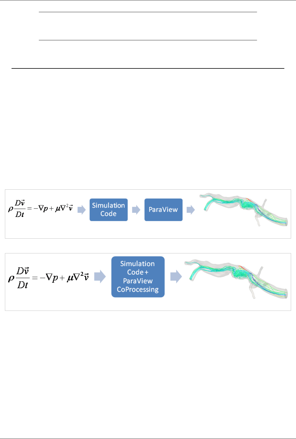
217
In-Situ/CoProcessing
CoProcessing
Background
Several factors are driving the growth of simulations. Computational power of computer clusters is growing, while
the price of individual computers is decreasing. Distributed computing techniques allow hundreds, or even
thousands, of computer nodes to participate in a single simulation. The benefit of this computational power is that
simulations are getting more accurate and useful for predicting complex phenomena. The downside to this growth is
the enormous amounts of data that need to be saved and analyzed to determine the results of the simulation. The
ability to generate data has outpaced our ability to save and analyze the data. This bottleneck is throttling our ability
to benefit from our improved computing resources. Simulations save their states only very infrequently to minimize
storage requirements. This coarse temporal sampling makes it difficult to notice some complex behavior. To get past
this barrier, ParaView can now be easily used to integrate post-processing/visualization directly with simulation
codes. This feature is called co-processing in ParaView and the difference between workflows when using
co-processing can be seen in the figures below.
Figure 15.1 Full Workflow
Figure 15.1 Workflow With Co-Processing
Technical Objectives
The main objective of the co-processing toolset is to integrate core data processing with the simulation to enable
scalable data analysis, while also being simple to use for the analyst. The tool set has two main parts:
•An extensible and flexible co-processing library: The co-processing library was designed to be flexible enough
to be embedded in various simulation codes with relative ease. This flexibility is critical, as a library that requires
a lot of effort to embed cannot be successfully deployed in a large number of simulations. The co-processing
library is also easily-extended so that users can deploy new analysis and visualization techniques to existing
co-processing installations.
•Configuration tools for co-processing configuration: It is important for users to be able to configure the
co-processor using graphical user interfaces that are part of their daily work-flow.

CoProcessing 218
Note: All of this must be done for large data. The co-processing library will almost always be run on a distributed
system. For the largest simulations, the visualization of extracts may also require a distributed system (i.e. a
visualization cluster).
Overview
The toolset can be broken up into two distinct parts, the library part that links with the simulation code and a
ParaView GUI plugin that can be used to create Python scripts that specify what should be output from the
simulation code. Additionally, there are two roles for making co-processing work with a simulation code. The first is
the developer that does the code integration. The developer needs to know the internals of the simulation code along
with the co-processing library API and VTK objects used to represent grids and field data. The other is the user
which needs to know how to create the scripts and/or specify the parameters for pre-created scripts in order to extract
out the desired information from the simulation. Besides the information below, there are tutorials available.
Build Directions
As mentioned above, the two components for doing co-processing are a client-side plugin and a server-side library. It
is recommended that they be compiled separately, but from the same ParaView source revision/release. This is
because currently the client-side configuration tools outputs Python code for the server-side library to use. Differing
ParaView versions may have different Python interfaces to objects causing simulation co-processed runs to fail.
ParaView Co-Processing Script Generator Plugin
The plugin for generating Python scripts for co-processing is a client-side plugin. The CMake option to turn-on the
script generator plugin is PARAVIEW_BUILD_PLUGIN_CoProcessingScriptGenerator. Note: since this is a
client-side plugin, the PARAVIEW_BUILT_QT_GUI option must be on.
Co-Processing Library
The directions for building the co-processing library can be a bit more complex. We assume that it will be built on a
cluster or supercomputer. Complexities may arise from having to build Mesa, use off-screen rendering, build static
libraries, and/or cross-compiling [1]. We won't go into those details here, but refer interested people to the ParaView
[2] and VTK [3] wikis.
The additional flags that should be turned on for coprocessing include:
•BUILD_SHARED_LIBS: Should normally be set to ON unless you're compiling on a machine that doesn't
support shared libs (e.g. IBM BG/L).
•PARAVIEW_ENABLE_PYTHON: Set to ON in order to use the scripts created from the co-processing plugin.
Note: For the 3.10 release, this is not required to be on.
•PARAVIEW_USE_MPI: Set the ParaView server to use MPI to run in parallel. Also, check that the proper
version of MPI is getting used.
•CMAKE_BUILD_TYPE: Should be set to Release in order to optimize the ParaView code.
•PARAVIEW_ENABLE_COPROCESSING: The CMake option to build the co-processing libraries.
•BUILD_COPROCESSING_ADAPTORS: The CMake option to turn on code that may be useful for creating
the simulation code adaptor.
•BUILD_FORTRAN_COPROCESSING_ADAPTORS: The CMake option to turn-on code that may be useful
for creating an adapter for a simulation code written in Fortran or C.
•PYTHON_ENABLE_MODULE_vtkCoProcessorPython: On by default.
•BUILD_PYTHON_COPROCESSING_ADAPTOR: Experimental code.
If ParaView was build with python enabled, the co-processing library can be tested on the installed system with the
CTest command ctest -R CoProcessing. The CoProcessingTestPythonScript test does an actual coprocessing run and

CoProcessing 219
the CoProcessingPythonScriptGridPlot and CoProcessingPythonScriptPressurePlot test verify the output is correct.
There are parallel versions of the coprocessing runs as well that run with multiple processes.In addition, looking at
the code for this test is a useful beginning point for learning to use the co-processing library.
If you are using Mesa, the following options should be used:
•PARAVIEW_BUILD_QT_GUI: set to OFF
•VTK_OPENGL_HAS_OSMESA: Set to ON.
•VTK_USE_X: Set to OFF.
•OSMESA_INCLUDE_DIR and OPENGL_INCLUDE_DIR: Make sure these are not set to the OpenGL
directory location of the header files.
•OSMESA_LIBRARY: Set this to the Mesa library.
•OPENGL_gl_LIBRARY and OPENGL_glu_LIBRARY: These should not be set.
Refer to ParaView And Mesa 3D for more details on building with Mesa.
Running the Co-Processing Script Generator
After starting the ParaView client, go to Tools|Manage Plugins, highlight CoProcessingPlugin, and click Load
Selected. Alternatively, if you expect to be using this plugin often, you can tell ParaView to automatically load it by
clicking to the left of CoProcessingPlugin to expand the list and choose the Auto Load option. This will add a
CoProcessing and Writers menu to the GUI.
Once the plugin is loaded, load a simulation result into ParaView that is similar to the run you wish to do
co-processing with. Normally the result will be for a discretization of the same geometry and contain the same field
variables (or at least all of the field variables you wish to examine) as the simulation grid that co-processing will be
performed on. The only difference between these two grids will be that the grid used for the co-processing run will
be at a much higher resolution. In the picture below, a pipeline is shown for a result from a PHASTA (A CFD code
led by Ken Jansen at the University of Colorado) simulation of incompressible flow through an aortic aneurysm. The
simulation results include the velocity and pressure fields, and was done on a grid with 235,282 cells and 45,175
points. It is important to use the same names for the field arrays as will be used in the grids the co-processing library
will be working with. The filters specify which fields to use by their name and problems will occur if the filters
cannot find the correct array. The pipeline computes the vorticity, takes 20 slices through the domain, and extracts
the surface of the grid.
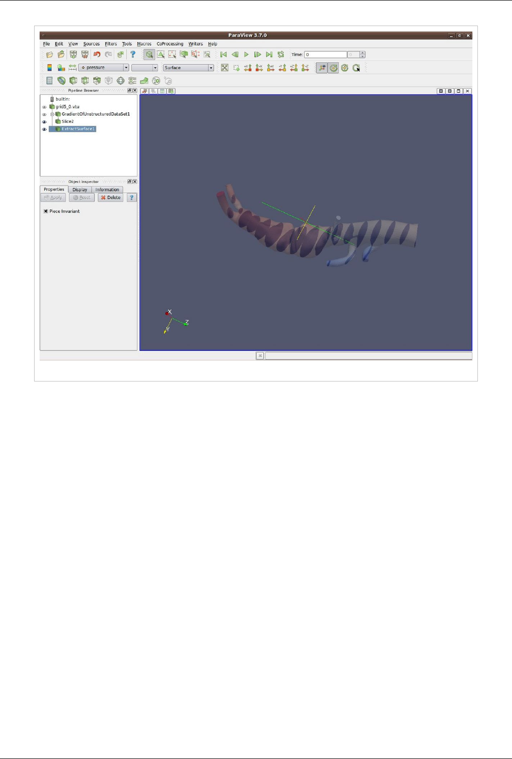
CoProcessing 220
Figure 15.2 Phasta Pipeline
Once the pipeline is set-up, the writers must be added to use for the filters that results are desired from. This is done
by selecting the appropriate writer to output the results from each desired filter. In this example, a
ParallelPolyDataWriter is created for the Slice filter and the ExtractSurface filter. For the writer for the Slice filter
we set the name of the file to be slice_%t.pvtp where %t will get replaced with the time step each time it is output.
We also set the write frequency to be every fifth time step. Figure 15.3 below shows this.
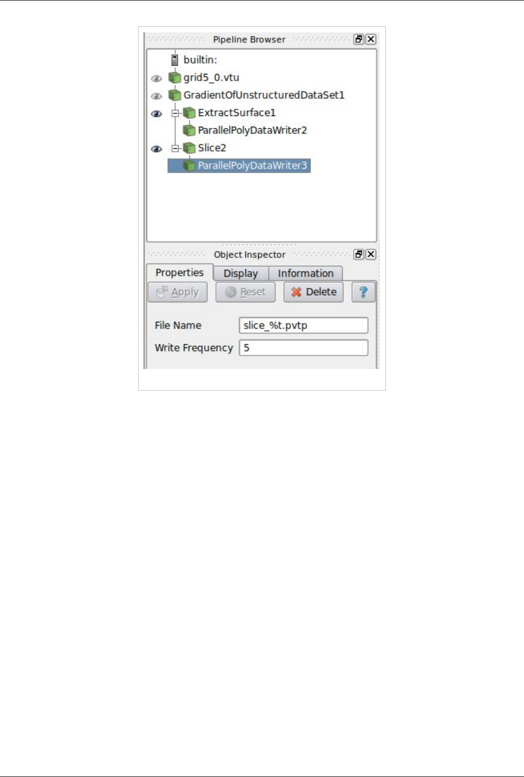
CoProcessing 221
Figure 15.3 Phasta Pipeline with Writers
Similarly, we do the same for the writer for the ExtractSurface filter but we want to use a different file name and we
can set a different write frequency if desired.
Note that when we hit enter we get the error message Cannot show the data in the current view although the view
reported that it can show the data. This message can be ignored and is already entered as a bug to fix in ParaView.
The final step is to go through the CoProcessing->Export State wizard to associate the grid with a name that the
python script uses and specify a file name for the script. The steps are:
1. Export Co-Processing State Click Next to proceed.
2. Select Simulation Inputs Choose which grids to use by highlighting the grid and clicking Add, then click Next.
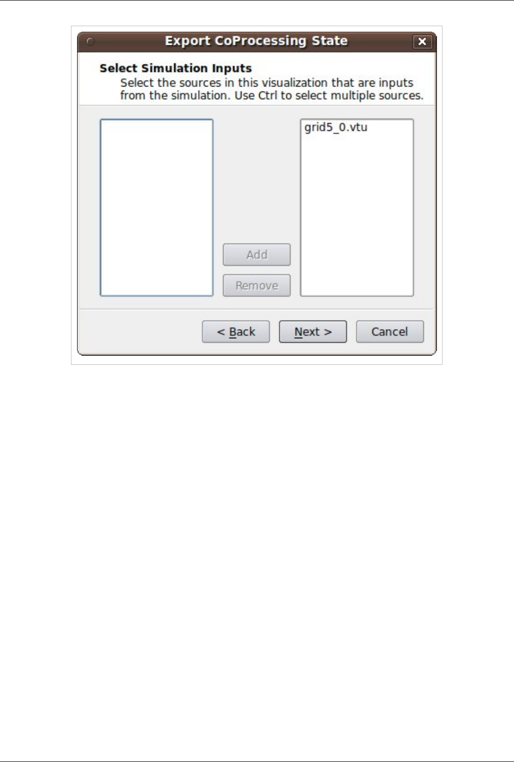
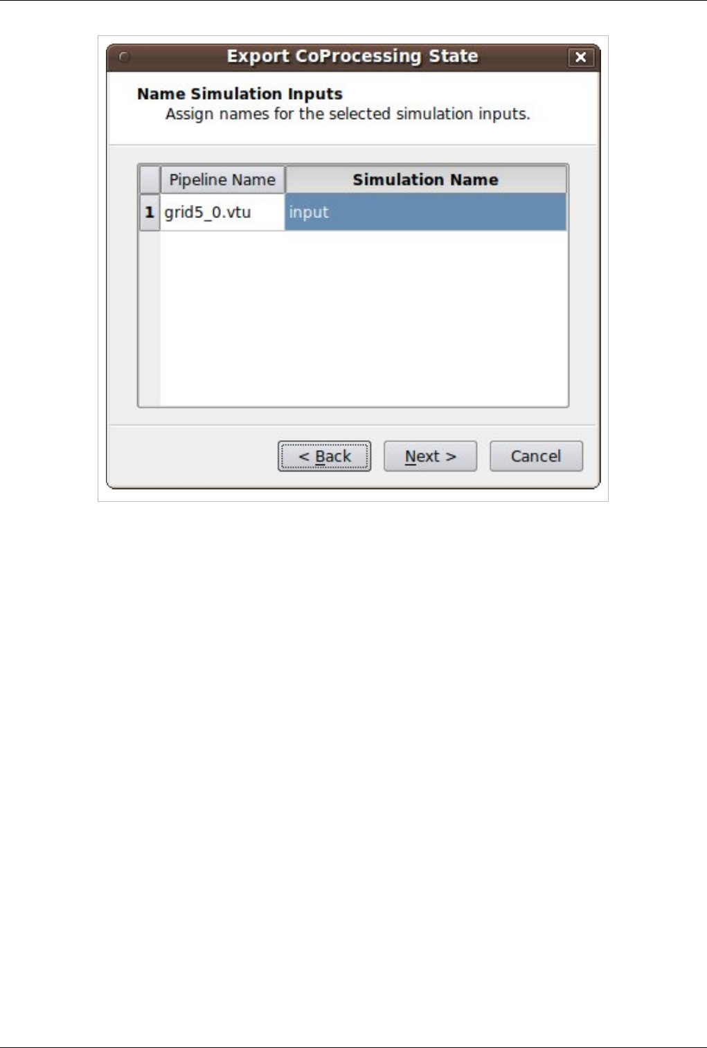
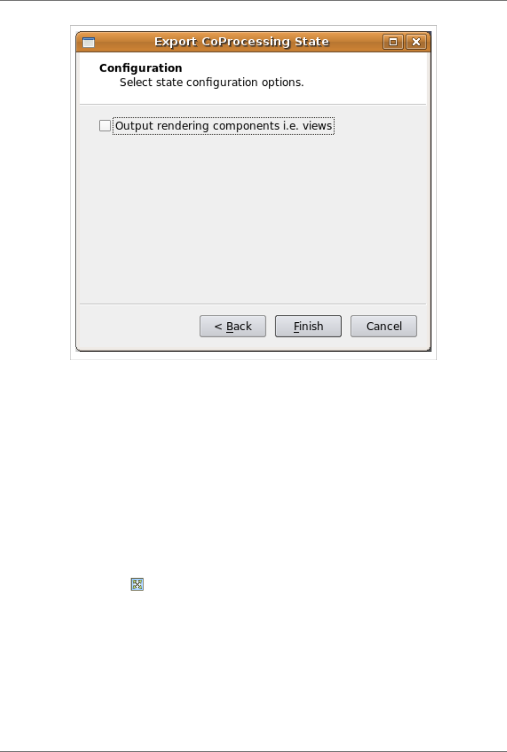
CoProcessing 224
If we do want to output images in addition to any writers we may have specified, check "Output rendering
components i.e. views" and fill in the proper information. For image output with pseudo-coloring field data, the
range may not be known ahead of time or it may change as the simulation proceeds. For these cases, the user can
check the "Rescale to Data Range" to ensure that a reasonable scale is uses to color the data by. Note that this applies
to all views to be consistent with ParaView. For situations where there are multiple views, the user can switch
through the views to set output parameters for each individual view. The parameters are:
1. Image Type: a list of the available image formats to output as that the user can select from.
2. File Name: the user can specify the name of the outputted screen shot. Note that %t will be replaced by the actual
time step in the output file name.
3. Write Frequency: similar to outputting geometry, the user should specify how often the screen shot image will be
generated.
4. Magnification: an integer value for specifying how much to enlarge the outputted image.
5. Fit to Screen: if the geometry is changing the user may not be able to properly position the camera for the desired
screen shot. Checking this option will fit the geometry to screen before the screen shot is taken. This is the same
action as clicking on the icon in the ParaView GUI.
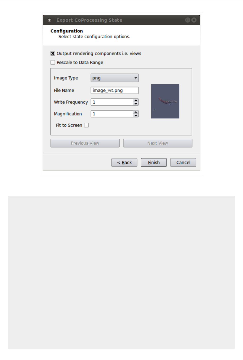
CoProcessing 225
5. Save Server State: Specify the file name the script is to be saved as.
The resulting python script should look something like:
try: paraview.simple
except: from paraview.simple import *
cp_writers = []
def RequestDataDescription(datadescription):
"Callback to populate the request for current timestep"
timestep = datadescription.GetTimeStep()
if (timestep % 5 == 0) or (timestep % 200 == 0) :
datadescription.GetInputDescriptionByName('input').AllFieldsOn()
datadescription.GetInputDescriptionByName('input').GenerateMeshOn()
def DoCoProcessing(datadescription):
"Callback to do co-processing for current timestep"
global cp_writers
cp_writers = []

CoProcessing 226
timestep = datadescription.GetTimeStep()
grid5_0_vtu = CreateProducer( datadescription, "input" )
GradientOfUnstructuredDataSet1 = GradientOfUnstructuredDataSet(
guiName="GradientOfUnstructuredDataSet1", ScalarArray=['POINTS',
'velocity'], ResultArray
Name='Vorticity', ComputeVorticity=1, FasterApproximation=0 )
Slice2 = Slice( guiName="Slice2",
SliceOffsetValues=[-10.23284210526316, -8.8684631578947375,
-7.5040842105263152, -6.1397052631578966, -4.77532631578947
43, -3.4109473684210529, -2.0465684210526316, -0.68218947368421201,
0.68218947368420935, 2.0465684210526316, 3.4109473684210521,
4.7753263157894743, 6.139705
263157893, 7.5040842105263152, 8.8684631578947375, 10.23284210526316,
11.597221052631578, 12.961600000000001], SliceType="Plane" )
SetActiveSource(GradientOfUnstructuredDataSet1)
ExtractSurface1 = ExtractSurface( guiName="ExtractSurface1",
PieceInvariant=1 )
SetActiveSource(Slice2)
ParallelPolyDataWriter3 = CreateWriter( XMLPPolyDataWriter,
"slice_%t.pvtp", 5 )
SetActiveSource(ExtractSurface1)
ParallelPolyDataWriter2 = CreateWriter( XMLPPolyDataWriter,
"surface_%t.pvtp", 200 )
Slice2.SliceType.Origin = [-2.8049160242080688, 2.1192346811294556,
1.7417440414428711]
Slice2.SliceType.Offset = 0.0
Slice2.SliceType.Normal = [0.0, 0.0, 1.0]
for writer in cp_writers:
if timestep % writer.cpFrequency == 0:
writer.FileName = writer.cpFileName.replace("%t",
str(timestep))
writer.UpdatePipeline()
def CreateProducer(datadescription, gridname):
"Creates a producer proxy for the grid"
if not datadescription.GetInputDescriptionByName(gridname):
raise RuntimeError, "Simulation input name '%s' does not exist" %
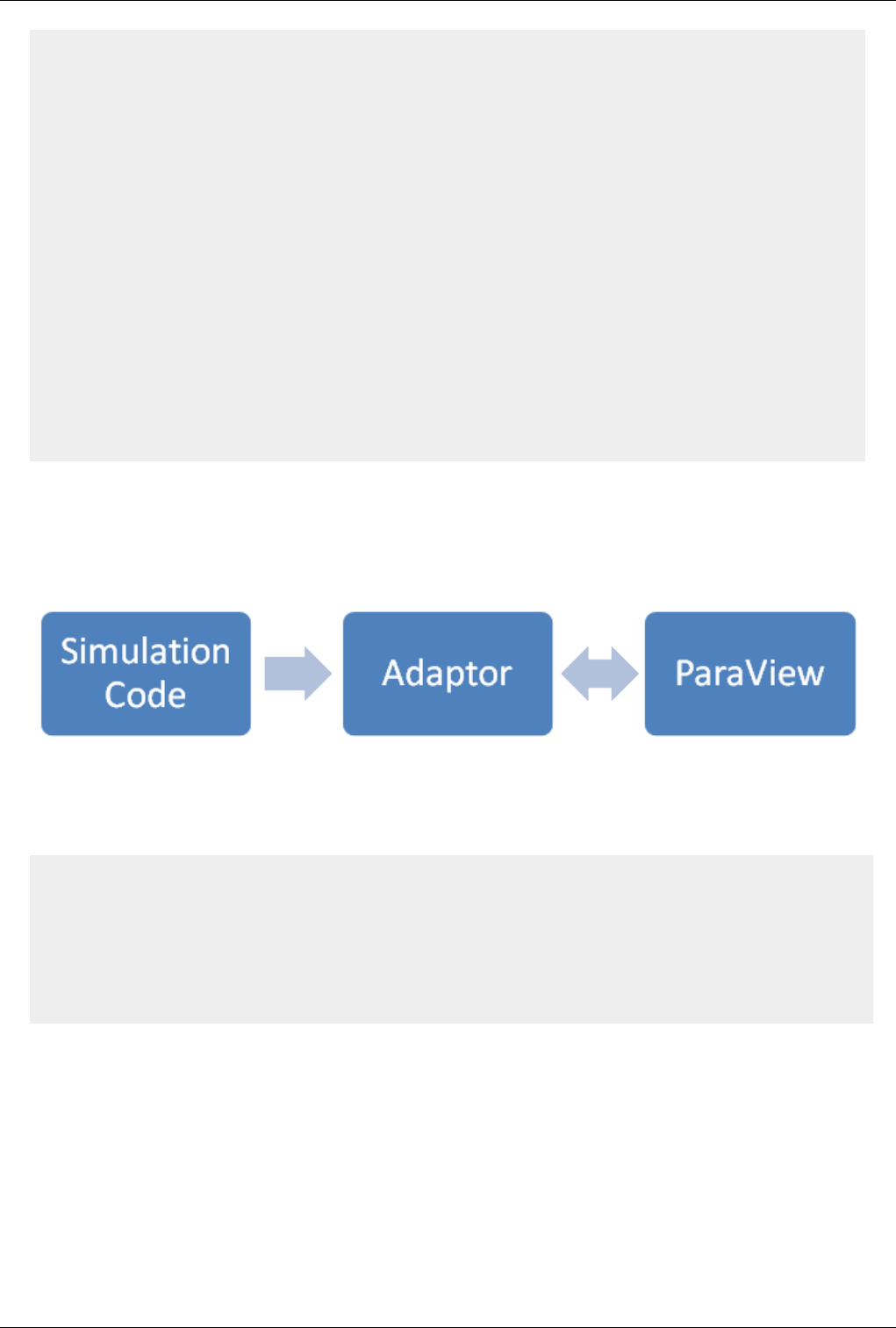
CoProcessing 227
gridname
grid = datadescription.GetInputDescriptionByName(gridname).GetGrid()
producer = TrivialProducer()
producer.GetClientSideObject().SetOutput(grid)
producer.UpdatePipeline()
return producer
def CreateWriter(proxy_ctor, filename, freq):
global cp_writers
writer = proxy_ctor()
writer.FileName = filename
writer.add_attribute("cpFrequency", freq)
writer.add_attribute("cpFileName", filename)
cp_writers.append(writer)
return writer
Creating the Adaptor
The largest amount of work in getting co-processing working with a simulation code is usually creating the adaptor
that can pass a VTK data set or composite data set with fields specified over it. A simple view of the program control
is
By doing it like this, there is minimal modification to the simulation code (only calls to the adaptor like Initialize,
Finalize, and CoProcess). The adaptor deals with the coprocessing library as well as creating VTK data structures
from the simulation code as needed. The general flow for the simulation code and where it calls the adaptor would
look like:
initialize coprocessor
for i in number of time steps
compute simulation information at time step i
call coprocessing library
coprocessing library determines if any coprocessing needs to be performed at time step i
finalize coprocessor
The interactions between the adaptor and ParaView are mostly done through the vtkCPProcessor class.
Documentation for this and the other classes in the coprocessing library are in the ParaView online documentation [4]
as well as grouped in a module [5]. Details on the specific steps are provided below.

CoProcessing 228
Initialize the Co-Processor
To initialize the co-processor, a vtkCPProcessor object must be created. This object should not be deleted until the
finalization step. After creating a vtkCPProcessor object, you must call vtkCPProcessor::Initialize() to initialize the
coprocessing library. The next step is to create vtkCPPipeline objects. These objects are used to represent the VTK
pipelines that will be used to generate the output data. Most users will probably only use the
vtkCPPythonScriptPipeline class that derives from vtkCPPipeline since that pipeline is the one that is used with the
python scripts generated from the coprocessing plugin. vtkCPPythonScriptPipeline::Initialize() takes in the python
script name with the full path and sets up the ParaView python interpretor.
Call the Co-Processor to Execute the Desired Filters
Most users will have a single call to the adaptor at the end of each simulation time step. This will pass in the
simulation data structures to create the VTK data structures from. The created VTK data structures will be an object
that derives from vtkDataObject. First though we want to check if we actually need to do any co-processing during
this call. The simulation code will not know this information. Because of this, the simulation code should call the
adaptor every time step. The adaptor gets the information about what data is needed for executing the
vtkCPPipelines for each call. This is done in vtkCPProcessor::RequestDataDescription() by going through all of the
vtkCPPipeline objects and querying them for what is needed. vtkCPProcessor::RequestDataDescription() takes in a
vtkCPDataDescription object that contains information about the current simulation time and time step. The method
returns 0 if no coprocessing information needs to be computed during the call and 1 otherwise. If no coprocessing
needs to be performed then the adaptor should return control back to the simulation code.
If co-processing is requested then the adaptor needs to make sure that the VTK grids and fields are up to date. Upon
return from vtkCPProcessor::RequestDataDescription(), the vtkCPDataDescription object will have information on
what is needed by the pipelines in order to successfully execute them during this call to the adaptor. This information
is stored for each co-processing input (the data objects that are given identifier names in the plugin) and accessed
through the vtkCPDataDescription as vtkCPInputDataDescription objects. The vtkCPInputDataDescription objects
specify whether or not they require a grid and if so which fields they require. These objects are also used to pass the
VTK data objects created in the adaptor to the pipeline by using the vtkCPInputDataDescription::SetGrid() method.
The final step in this call to the adaptor is then to perform the actual co-processing by calling the
vtkCPProcessor::CoProcess() method.
Finalize the Co-Processor
Finalization entails calling vtkCPProcessor::Finalize() and cleaning up any remaining VTK objects by calling
Delete();
While initially there may seem to be a significant hurdle to overcome in order to implement the adaptor for
co-processing, the user only needs to know enough information to create the VTK data objects from their own
simulation data structures. The adaptor can be made computationally efficient by taking advantage of intimate
knowledge of the simulation code and knowing that VTK filters will not modify input data. Examples include:
• Only creating the VTK grid in the first call to the adaptor if the grid is not changing topologically or
geometrically.
• Using the SetArray() method to build vtkDataArray objects that use existing memory used by the simulation code
instead of allocating and copying existing memory.
Finally, we suggest looking at either the C++ coprocessing example and/or the python coprocessing example to see
how the entire co-processing flow works. Additonally, the code in
ParaView3/CoProcessing/CoProcessor/Testing/Cxx/PythonScriptCoProcessingExample.cxx is also worth a look.
This is used to test the co-processing library and can be run with the command "ctest -R CoProcessing".

CoProcessing 229
References
[1] http:/ / paraview. org/ Wiki/ Cross_compiling_ParaView3_and_VTK
[2] http:/ / paraview. org/ Wiki/ ParaView
[3] http:/ / www. vtk. org/ Wiki/ VTK
[4] http:/ / www. paraview. org/ ParaView3/ Doc/ Nightly/ html/ classes. html
[5] http:/ / www. paraview. org/ ParaView3/ Doc/ Nightly/ html/ group__CoProcessing. html
C++ CoProcessing example
This example is used to demonstrate how the co-processing library can be used with a C++ based simulation code. In
the ParaView/CoProcessing/Adaptors/FortranAdaptors directory there is code useful for integrating C or Fortran
based simulation codes withthe co-processing library. Note that this example requires MPI to be available on your
system. The executable takes in a python coprocessing script and a number of time steps to be run for. Note to
remember to set your system environment properly. See [[1]] for details.
CoProcessingExample.cxx
#include "vtkCPDataDescription.h"
#include "vtkCPInputDataDescription.h"
#include "vtkCPProcessor.h"
#include "vtkCPPythonScriptPipeline.h"
#include "vtkElevationFilter.h"
#include "vtkPolyData.h"
#include "vtkSmartPointer.h"
#include "vtkSphereSource.h"
#include "vtkXMLUnstructuredGridReader.h"
#include <mpi.h>
#include <string>
class DataGenerator {
public:
DataGenerator()
{
this->Sphere = vtkSmartPointer<vtkSphereSource>::New();
this->Sphere->SetThetaResolution(30);
this->Sphere->SetPhiResolution(30);
int procId;
MPI_Comm_rank(MPI_COMM_WORLD, &procId);
this->Sphere->SetCenter(procId*4.0, 0, 0);
this->Elevation = vtkSmartPointer<vtkElevationFilter>::New();
this->Elevation->SetInputConnection(this->Sphere->GetOutputPort());
this->Index = 0;
}
vtkSmartPointer<vtkPolyData> GetNext()
{

C++ CoProcessing example 230
double radius = fabs(sin(0.1 * this->Index));
this->Index++;
this->Sphere->SetRadius(1.0 + radius);
this->Elevation->Update();
vtkSmartPointer<vtkPolyData> ret = vtkSmartPointer<vtkPolyData>::New();
ret->DeepCopy(this->Elevation->GetOutput());
return ret;
}
protected:
int Index;
vtkSmartPointer<vtkSphereSource> Sphere;
vtkSmartPointer<vtkElevationFilter> Elevation;
};
int main(int argc, char* argv[])
{
if (argc < 3)
{
printf("Usage: %s <python coprocessing script> <number of time steps>\n", argv[0]);
return 1;
}
// we assume that this is done in parallel
MPI_Init(&argc, &argv);
std::string cpPythonFile = argv[1];
int nSteps = atoi(argv[2]);
vtkCPProcessor* processor = vtkCPProcessor::New();
processor->Initialize();
vtkCPPythonScriptPipeline* pipeline =
vtkCPPythonScriptPipeline::New();
// read the coprocessing python file
if(pipeline->Initialize(cpPythonFile.c_str()) == 0)
{
cout << "Problem reading the python script.\n";
return 1;
}
processor->AddPipeline(pipeline);
pipeline->Delete();
if (nSteps == 0)
{
return 0;
}

C++ CoProcessing example 231
// create a data source, typically this will come from the adaptor
// but here we use generator to create it ourselves
DataGenerator generator;
// do coprocessing
double tStart = 0.0;
double tEnd = 1.0;
double stepSize = (tEnd - tStart)/nSteps;
vtkCPDataDescription* dataDesc = vtkCPDataDescription::New();
dataDesc->AddInput("input");
for (int i = 0; i < nSteps; ++i)
{
double currentTime = tStart + stepSize*i;
// set the current time and time step
dataDesc->SetTimeData(currentTime, i);
// check if the script says we should do coprocessing now
if(processor->RequestDataDescription(dataDesc) != 0)
{
// we are going to do coprocessing so use generator to
// create our grid at this timestep and provide it to
// the coprocessing library
vtkSmartPointer<vtkDataObject> dataObject =
generator.GetNext();
dataDesc->GetInputDescriptionByName("input")->SetGrid(dataObject);
processor->CoProcess(dataDesc);
}
}
dataDesc->Delete();
processor->Finalize();
processor->Delete();
MPI_Finalize();
return 0;
}

C++ CoProcessing example 232
CMakeLists.txt
cmake_minimum_required(VERSION 2.6)
PROJECT(CoProcessingExample)
FIND_PACKAGE(ParaView REQUIRED)
INCLUDE(${PARAVIEW_USE_FILE})
ADD_EXECUTABLE(CoProcessingExample CoProcessingExample.cxx)
TARGET_LINK_LIBRARIES(CoProcessingExample vtkCoProcessorImplementation)
Python Scripts
The first python script below is used to just output the actual results of the example. This would correspond to a
simulation run with a coarse grid in order to set up coprocessing runs for larger grids where outputting the entire
simulation results can be computationally prohibitive.
try: paraview.simple
except: from paraview.simple import *
def RequestDataDescription(datadescription):
"Callback to populate the request for current timestep"
timestep = datadescription.GetTimeStep()
input_name = 'input'
if (timestep % 1 == 0) :
datadescription.GetInputDescriptionByName(input_name).AllFieldsOn()
datadescription.GetInputDescriptionByName(input_name).GenerateMeshOn()
else:
datadescription.GetInputDescriptionByName(input_name).AllFieldsOff()
datadescription.GetInputDescriptionByName(input_name).GenerateMeshOff()
def DoCoProcessing(datadescription):
"Callback to do co-processing for current timestep"
cp_writers = []
timestep = datadescription.GetTimeStep()
grid = CreateProducer( datadescription, "input" )
ParallelPolyDataWriter1 = CreateWriter( XMLPPolyDataWriter,
"input_grid_%t.pvtp", 1, cp_writers )
for writer in cp_writers:
if timestep % writer.cpFrequency == 0:
writer.FileName = writer.cpFileName.replace("%t",
str(timestep))

C++ CoProcessing example 233
writer.UpdatePipeline()
# explicitly delete the proxies -- we do it this way to avoid
problems with prototypes
tobedeleted = GetNextProxyToDelete()
while tobedeleted != None:
Delete(tobedeleted)
tobedeleted = GetNextProxyToDelete()
def GetNextProxyToDelete():
proxyiterator = servermanager.ProxyIterator()
for proxy in proxyiterator:
group = proxyiterator.GetGroup()
if group.find("prototypes") != -1:
continue
if group != 'timekeeper' and group.find("pq_helper_proxies") ==
-1 :
return proxy
return None
def CreateProducer(datadescription, gridname):
"Creates a producer proxy for the grid"
if not datadescription.GetInputDescriptionByName(gridname):
raise RuntimeError, "Simulation input name '%s' does not exist"
% gridname
grid =
datadescription.GetInputDescriptionByName(gridname).GetGrid()
producer = TrivialProducer()
producer.GetClientSideObject().SetOutput(grid)
producer.UpdatePipeline()
return producer
def CreateWriter(proxy_ctor, filename, freq, cp_writers):
writer = proxy_ctor()
writer.FileName = filename
writer.add_attribute("cpFrequency", freq)
writer.add_attribute("cpFileName", filename)
cp_writers.append(writer)
return writer
This second script is still rather simple and only performs a cut on the input from the simulation code. It
demonstrates though how desired results can be obtained while performing coprocessing at specified time steps.
try: paraview.simple
except: from paraview.simple import *
def RequestDataDescription(datadescription):
"Callback to populate the request for current timestep"

C++ CoProcessing example 234
timestep = datadescription.GetTimeStep()
input_name = 'input'
if (timestep % 5 == 0) :
datadescription.GetInputDescriptionByName(input_name).AllFieldsOn()
datadescription.GetInputDescriptionByName(input_name).GenerateMeshOn()
else:
datadescription.GetInputDescriptionByName(input_name).AllFieldsOff()
datadescription.GetInputDescriptionByName(input_name).GenerateMeshOff()
def DoCoProcessing(datadescription):
"Callback to do co-processing for current timestep"
cp_writers = []
timestep = datadescription.GetTimeStep()
grid = CreateProducer( datadescription, "input" )
Clip2 = Clip( guiName="Clip2", InsideOut=0, UseValueAsOffset=0,
Scalars=['POINTS', 'Elevation'], Value=0.0, ClipType="Plane" )
Clip2.ClipType.Normal = [0.0, 1.0, 0.0]
Clip2.ClipType.Origin = [1.9999999105930328, 0.0, 0.0]
Clip2.ClipType.Offset = 0.0
ParallelUnstructuredGridWriter2 = CreateWriter(
XMLPUnstructuredGridWriter, "Cut_%t.pvtu", 5, cp_writers )
for writer in cp_writers:
if timestep % writer.cpFrequency == 0:
writer.FileName = writer.cpFileName.replace("%t",
str(timestep))
writer.UpdatePipeline()
# explicitly delete the proxies -- we do it this way to avoid
problems with prototypes
tobedeleted = GetNextProxyToDelete()
while tobedeleted != None:
Delete(tobedeleted)
tobedeleted = GetNextProxyToDelete()
def GetNextProxyToDelete():
proxyiterator = servermanager.ProxyIterator()
for proxy in proxyiterator:
group = proxyiterator.GetGroup()
if group.find("prototypes") != -1:
continue
if group != 'timekeeper' and group.find("pq_helper_proxies") ==

C++ CoProcessing example 235
-1 :
return proxy
return None
def CreateProducer(datadescription, gridname):
"Creates a producer proxy for the grid"
if not datadescription.GetInputDescriptionByName(gridname):
raise RuntimeError, "Simulation input name '%s' does not exist"
% gridname
grid =
datadescription.GetInputDescriptionByName(gridname).GetGrid()
producer = TrivialProducer()
producer.GetClientSideObject().SetOutput(grid)
producer.UpdatePipeline()
return producer
def CreateWriter(proxy_ctor, filename, freq, cp_writers):
writer = proxy_ctor()
writer.FileName = filename
writer.add_attribute("cpFrequency", freq)
writer.add_attribute("cpFileName", filename)
cp_writers.append(writer)
return writer
References
[1] http:/ / paraview. org/ Wiki/ ParaView/ Python_Scripting#Getting_Started

Python CoProcessing Example 236
Python CoProcessing Example
This example is used to demonstrate how the co-processing library can be used with a python based simulation code.
Note that this example requires MPI to be available on your system as well as pyMPI to initialize and finalize MPI
from the python script. The executable takes in a python co-processing script and a number of time steps to be run
for. Note to remember to set your system environment properly. See [[1]] for details.
Serial python driver code
import sys
if len(sys.argv) != 3:
print "command is 'python <python driver code> <script name> <number of time steps>'"
sys.exit(1)
import paraview
import paraview.vtk as vtk
def coProcess(grid, time, step, scriptname):
import vtkCoProcessorPython # import libvtkCoProcessorPython for
older PV versions
if scriptname.endswith(".py"):
scriptname =
scriptname[0:len(scriptname)-3]#scriptname.rstrip(".py")
try:
cpscript = __import__(scriptname)
except:
print 'Cannot find ', scriptname, ' -- no coprocessing will be
performed.'
return
datadescription = vtkCoProcessorPython.vtkCPDataDescription()
datadescription.SetTimeData(time, step)
datadescription.AddInput("input")
cpscript.RequestDataDescription(datadescription)
inputdescription =
datadescription.GetInputDescriptionByName("input")
if inputdescription.GetIfGridIsNecessary() == False:
return
inputdescription.SetGrid(grid)
inputdescription.SetWholeExtent(grid.GetWholeExtent())
cpscript.DoCoProcessing(datadescription)
try:
numsteps = int(sys.argv[2])
except ValueError:
print 'the last argument should be a number, setting the number of
time steps to 10'
Python CoProcessing Example 237
numsteps = 10
for step in range(numsteps):
# assume simulation time starts at 0
time = step/float(numsteps)
# create the input to the coprocessing library. normally
# this will come from the adaptor
imageData = vtk.vtkImageData()
imageData.SetOrigin(0, 0, 0)
imageData.SetSpacing(.1, .1, .1)
imageData.SetExtent(0, 10, 0, 12, 0, 12)
imageData.SetWholeExtent(imageData.GetExtent())
pointArray = vtk.vtkDoubleArray()
pointArray.SetNumberOfTuples(imageData.GetNumberOfPoints())
for i in range(imageData.GetNumberOfPoints()):
pointArray.SetValue(i, i)
pointArray.SetName("pointData")
imageData.GetPointData().AddArray(pointArray)
# "perform" coprocessing. results are outputted only if
# the passed in script says we should at time/step
coProcess(imageData, time, step, sys.argv[1])
Parallel python driver code
import sys
if len(sys.argv) != 3:
print "command is 'mpirun -np <#> pyMPI parallelexample.py <script name> <number of time steps>'"
sys.exit(1)
import paraview
import paraview.vtk as vtk
import mpi
mpi.initialized()
import paraview
import libvtkParallelPython
import paraview.simple
import vtk
# set up ParaView to properly use MPI
pm = paraview.servermanager.vtkProcessModule.GetProcessModule()
globalController = pm.GetGlobalController()
if globalController == None or
globalController.IsA("vtkDummyController") == True:
globalController = vtk.vtkMPIController()

Python CoProcessing Example 238
globalController.Initialize()
globalController.SetGlobalController(globalController)
def coProcess(grid, simtime, simstep, scriptname):
# the name of the library was changed so for previous version of
ParaView
# you have to import libvtkCoProcessorPython instead of
vtkCoProcessorPython
#import libvtkCoProcessorPython as vtkCoProcessorPython
import vtkCoProcessorPython
if scriptname.endswith(".py"):
scriptname =
scriptname[0:len(scriptname)-3]#scriptname.rstrip(".py")
try:
cpscript = __import__(scriptname)
except:
print 'Cannot find ', scriptname, ' -- no coprocessing will be
performed.'
return
datadescription = vtkCoProcessorPython.vtkCPDataDescription()
datadescription.SetTimeData(simtime, simstep)
datadescription.AddInput("input")
cpscript.RequestDataDescription(datadescription)
inputdescription = datadescription.GetInputDescriptionByName("input")
if inputdescription.GetIfGridIsNecessary() == False:
return
import paraview.simple
extents = grid.GetWholeExtent()
inputdescription.SetWholeExtent(extents)
inputdescription.SetGrid(grid)
cpscript.DoCoProcessing(datadescription)
def createGrid(time):
"""
Create a vtkImageData and a point data field called 'pointData'.
time is used to make the field time varying. The grid is
partitioned in slices in the x-direction here but that is
not required.
"""
imageData = vtk.vtkImageData()
imageData.Initialize()
imageData.SetOrigin(0, 0, 0)
imageData.SetSpacing(.1, .1, .1)
imageData.SetWholeExtent(0, 2*mpi.size, 0, 5, 0, 5)
imageData.SetExtent(mpi.rank*2, (mpi.rank+1)*2, 0, 5, 0, 5)
pointArray = vtk.vtkDoubleArray()

Python CoProcessing Example 239
pointArray.SetNumberOfTuples(imageData.GetNumberOfPoints())
for i in range(imageData.GetNumberOfPoints()):
pointArray.SetValue(i, i+time)
pointArray.SetName("pointData")
imageData.GetPointData().AddArray(pointArray)
return imageData
try:
numsteps = int(sys.argv[2])
except ValueError:
print 'the last argument should be a number, setting the number of
time steps to 10'
numsteps = 10
for step in range(numsteps):
# assume simulation time starts at 0
time = step/float(numsteps)
# create the input to the coprocessing library. normally
# this will come from the adaptor
grid = createGrid(time)
# "perform" coprocessing. results are outputted only if
# the passed in script says we should at time/step
coProcess(grid, time, step, sys.argv[1])
globalController.SetGlobalController(None)
globalController = None
mpi.finalized()
Sample coprocessing script
try: paraview.simple
except: from paraview.simple import *
def RequestDataDescription(datadescription):
"Callback to populate the request for current timestep"
timestep = datadescription.GetTimeStep()
input_name = 'input'
if (timestep % 1 == 0) :
datadescription.GetInputDescriptionByName(input_name).AllFieldsOn()
datadescription.GetInputDescriptionByName(input_name).GenerateMeshOn()
else:

Python CoProcessing Example 240
datadescription.GetInputDescriptionByName(input_name).AllFieldsOff()
datadescription.GetInputDescriptionByName(input_name).GenerateMeshOff()
def DoCoProcessing(datadescription):
"Callback to do co-processing for current timestep"
cp_writers = []
timestep = datadescription.GetTimeStep()
grid = CreateProducer( datadescription, "input" )
ImageWriter1 = CreateWriter( XMLPImageDataWriter,
"input_grid_%t.pvti", 1, cp_writers )
for writer in cp_writers:
if timestep % writer.cpFrequency == 0:
writer.FileName = writer.cpFileName.replace("%t",
str(timestep))
writer.UpdatePipeline()
# explicitly delete the proxies -- we do it this way to avoid
problems with prototypes
tobedeleted = GetNextProxyToDelete()
while tobedeleted != None:
Delete(tobedeleted)
tobedeleted = GetNextProxyToDelete()
def GetNextProxyToDelete():
proxyiterator = servermanager.ProxyIterator()
for proxy in proxyiterator:
group = proxyiterator.GetGroup()
if group.find("prototypes") != -1:
continue
if group != 'timekeeper' and group.find("pq_helper_proxies") ==
-1 :
return proxy
return None
def CreateProducer(datadescription, gridname):
"Creates a producer proxy for the grid"
if not datadescription.GetInputDescriptionByName(gridname):
raise RuntimeError, "Simulation input name '%s' does not exist"
% gridname
grid =
datadescription.GetInputDescriptionByName(gridname).GetGrid()
producer = PVTrivialProducer()
producer.GetClientSideObject().SetOutput(grid)
if grid.IsA("vtkImageData") == True or

Python CoProcessing Example 241
grid.IsA("vtkStructuredGrid") == True or grid.IsA("vtkRectilinearGrid")
== True:
extent =
datadescription.GetInputDescriptionByName(gridname).GetWholeExtent()
producer.WholeExtent= [ extent[0], extent[1], extent[2],
extent[3], extent[4], extent[5] ]
producer.UpdatePipeline()
return producer
def CreateWriter(proxy_ctor, filename, freq, cp_writers):
writer = proxy_ctor()
writer.FileName = filename
writer.add_attribute("cpFrequency", freq)
writer.add_attribute("cpFileName", filename)
cp_writers.append(writer)
return writer

242
Plugins
What are Plugins?
Introduction
ParaView comes with plethora of functionality bundled in: several readers, multitude of filters, quite a few different
types of views etc. However, it is not uncommon for developers to add new functionality to ParaView. For example
to add support for their new file format, incorporate a new filter, etc. ParaView makes it possible to add new
functionlity by using an extensive plugin mechanism.
Plugins can be used to extend ParaView in several ways:
• Add new readers
• Add new writers
• Add new filters
• Add new GUI components
• Add new views
• Add new representations
Plugin Types
Plugins are distributed as shared libraries (*.so on Unix, *.dylib on Mac, *.dll on Windows etc). For a plugin to be
loadable in ParaView, it must be built with the same version of ParaView as it is expected to be deployed on. Plugins
can be classified into two broad categories:
• Server-side plugins
These are plugins that extend the algorithmic capabilities for ParaView eg. new filters, readers, writers etc.
Since in ParaView data is processed on the server-side, these plugins need to be loaded on the server.
• Client-side plugins
These are plugins that extend the ParaView GUI eg. property panels for new filters, toolbars, views etc. These
plugins need to be loaded on the client.
Oftentimes a plugin has both server-side as well as client-side components to it eg. a plugin that adds a new filter and
a property panel that goes with that filter. Such plugins need to be loaded both on the server as well as the client.
Generally, users don't have to worry whether a plugin is a server-side or client-side plugin. Simply load the plugin on
the server as well as the client. ParaView will include relevant components from plugin on each of the processes.

Included Plugins 243
Included Plugins
Included Plugins
ParaView comes with a collection of plugins that the community has developed.
• Adios
Loads pixie format files written with the Adios library. This reader support the staging capability of Adios
which allow the user to pipe simulation kernels to post-processing tools : such as ParaView throw MPI
communication channel and follow in live the computation with no disk IO.
• Eye Dome Lighting
A non-photorealistic shading technique designed at EDF (France) to improve depth perception in scientific
visualization images.
It relies on efficient post-processing passes implemented on the GPU with GLSL shaders in order to achieve
interactive rendering.
• CoProcessingPlugin
Adds extensions to enable exporting state files that can be used by ParaView CoProcessing library.
• Force Time
Overrides the VTK time requests. This can be used to create complex animation with different datasets
following independent times evolutions.
Note: As this filter overrides the time requests, time-aware filters such as PathLines or PlotOverTime will not
behave correctly if they are inserted in a pipeline after this filter.
• H5PartReader
The H5Part Reader plugin adds support for reading particle datasets stored in H5Part format. H5Part is a
simple wrapper around the HDF5 library and provides a number of convenience functions to manage time
steps and access field arrays. The reader supports parallel reading of data using hyperslabs, when used with
ParaView compiled with MPI and HDF5 with parallel IO enabled, the reader automatically uses hyperslabs to
read portions of data on each process.
• Nifti
Reades time varying volumetric/image data from ANALYZE. Supports single (.nii) and dual (.img & .hdr) file
storage including zlib compression.
Able to write out ascii or binary files.
• Manta View
A view that uses the University of Utah's Manta Real Time Ray Tracer instead of OpenGL for rendering
surfaces
Kitware Source Article [1]
• Moments
Contains a set of filters that helps analysis of flux and circulation fields. Flux fields are defined on 2D cells
and describe flows through the area of the cell. Circulation fields are defined on 1D cells and describes flows
in the direction of the cell.
• PointSprite
Adds a renderer for point geometry - in particular particle based datasets (though any point based data may be
rendered using the provided painter). The plugin permits 3 modes of rendering, which are (in increasing order

Included Plugins 244
of complexity), Simple points, texture mapped sprites, and GPU raytraced spheres. The simple point mode
allows the user to select a scalar array for the opacity on a per point basis. The texture mode adds support for
opacity and radius per point (particle) which is drawn using a user supplied texture (a sphere is provided by
default). The GPU mode differs by evaluating a quadric ray/sphere intersection that allow objects to intersect
correctly rather than ‘popping’ in and out of view as sprites do. Transfer function editors can be used to map
radius/opacity values if simple non-linear lookups are required
• SierraPlotTools
Adds toolbar buttons to carry out convenience macros such as toggling the background color between white
and black, switching between surface and surface with edges display mode, and opening a wizard for
generating plots of global, nodal, or element variables over time. This plugin works on Exodus data only
• SLACTools
An extension that streamline ParaView's user interface for Stanford Linear Accelerator users.
• Streaming View
Views that render in many streamed passes to reduce memory footprint and provide multiresolution rendering.
This plugin replaces the Streaming and Adaptive ParaView derived applications.
Kitware Source Article [2]
• SurfaceLIC
Adds support for Line Integral Convolution over arbitrary surfaces.
• Prism Plugin
A Sandia contributed plugin for verification and debugging of simulation results. The plugin reads SESAME
files to determine the inverse mapping from cartesian to phase space and allows users to visually debug
simulations. Sesame files hold material model data (Equations of State, Opacities, Conductivities) in a tabular
format as described by http:/ / t1web. lanl. gov/ doc/ SESAME_3Ddatabase_1992. html.
• pvblot
Implementation of a Sandia National Labs scripting language on top of ParaView.
• VisTrails
The VisTrails plugin for ParaView incorporates the provenance management capabilities of VisTrails into
ParaView.
All of the actions a user performs while building and modifying a pipeline in ParaView are captured by the
plugin. This allows navigation of all of the pipeline versions that have previously been explored.
For more information about this plugin see [3]
• WebGL Exporter
The WebGL exporter plugin brings the ParaViewWeb WebGL code to ParaView to allow a 3D scene to be
exported into a standalone HTML page.
• NonOrthogonalSource
This plugin illustrate how to add FieldData to your dataset to customize the CubeAxis that should be presented
along with your data.
Typically this plugin allow a creation of a cube that can be sheared by the user by changing some parameters.
By doing so, the CubeAxes can follow the generated shape by creating axis along non-orthogonal axis.
Moreover, the cube axis can be replaced altogether by a single 3D crossed axis.
That plugin can also be used just to provide a customized cube axes inside you 3D scene without changing any
of your original reader of filter with those extra-annotation.

Included Plugins 245
• QuadView
This plugin add a new view into ParaView that allow the user to interactively move a 3D point that will be
used to cut the 3D data along 3 planes. Each cut result will be presented inside a 2D view next to each other.
More informations can be found here [4].
• UncertaintyRenderingPlugin
Adds a Uncertainty Surface representation which is able to display both data values and data uncertainties on a
surface.
References
[1] http:/ / www. kitware. com/ products/ html/ RenderedRealismAtNearlyRealTimeRates. html
[2] http:/ / www. kitware. com/ products/ html/ MultiResolutionStreamingInVTKAndParaView. html
[3] http:/ / www. vistrails. org/ index. php/ ParaView_Plugin
[4] http:/ / paraview. org/ Wiki/ ParaView/ Displaying_Data#Quad_View
Loading Plugins
Loading Plugins
There are three ways for loading plugins:
• Using the GUI (Plugin Manager)
Plugins can be loaded into ParaView using the Plugin Manager accessible from Tools | Manage
Plugins/Extensions menu. The Plugin Manager has two sections for loading local plugins and remote plugins
(enabled only when connected to a server). To load a plugin on the local as well as remote side, simply browse
to the plugin shared library. If the loading is successful, the plugin will appear in the list of loaded plugins. The
Plugin manager also lists the paths it searched to load plugins automatically.
The Plugin Manager remembers all loaded plugins, so next time to load the plugin, simply locate it in the list
and click "Load Selected" button.
You can set up ParaView to automatically load the plugin at startup (in case of client-side plugins) or on
connecting to the server (in case of server-side plugins) by checking the "Auto Load" checkbox on a loaded
plugin.
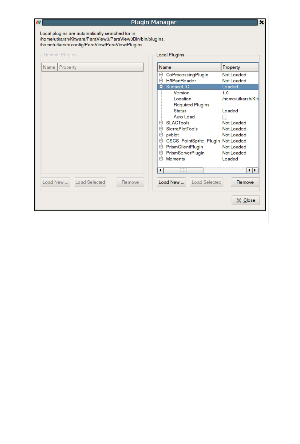
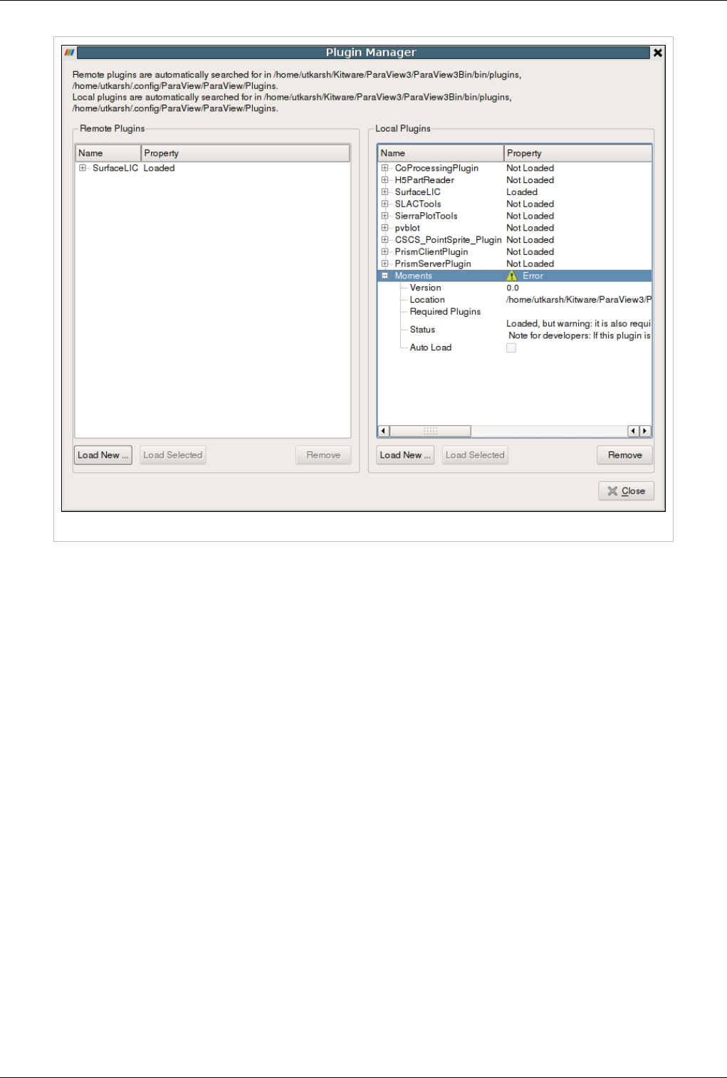
Loading Plugins 247
Figure 16.2: Plugin Manager when connected to a server showing loaded plugins on the local as well as remote sites.
• Using environment variable (Auto-loading plugins)
If one wants ParaView to automatically load a set of plugins on startup, one can use the PV_PLUGIN_PATH
environment variable. PV_PLUGIN_PATH can be used to list a set of directories (separated by colon (:) or
semi-colon (;)) which ParaView will search on startup to load plugins. This enviromnent variable needs to be
set on both the client node to load local plugins as well as the remote server to load remote plugins. Note that
plugins in PV_PLUGIN_PATH are always auto-loaded irrespective of the status of the "Auto Load" checkbox
in the Plugin Manager.
• Placing the plugins in a recognized location. Recognized locations are:
• A plugins subdirectory beneath the directory containing the paraview client or server executables. This can be
a system-wide location if installed as such.
• A Plugins subdirectory in the user's home area. On Unix/Linux/Mac,
$HOME/.config/ParaView/ParaView<version>/Plugins. On Windows
%APPDATA$\ParaView\ParaView<version>\Plugins.

248
Appendix
Command Line Arguments
Command-Line Arguments and Environment Variables
The following is a list of options available when running ParaView from the command line. When two options are
listed, separated by a comma, either of them can be used to achieve the specified result. Unless otherwise specified,
all command-line options are used on the client program. Following the list of command-line options is a set of
environment variables ParaView recognizes.
General Options
• --data : Load the specified data file into ParaView (--data=data_file).
• --disable-registry, -dr : Launch ParaView in its default state; do not load any preferences saved in ParaView’s
registry file.
• --help, /? : Display a list of the command-line arguments and their descriptions.
• --version, -V : Display ParaView’s version number, and then exit.
Client-Server Options
• --server, -s : Tell the client process where to connect to the server. The default is ‑‑server =localhost. This
command-line option is used on the client.
• --client-host, -ch : Tell the server process(es) where to connect to the client. The default is ‑‑client-host=localhost.
This command-line option is used on the server(s).
• --server-port, -sp : Specify the port to use in establishing a connection between the client and the server. The
default is --server-port=11111. If used, this argument must be specified on both the client and the server
command lines, and the port numbers must match.
• --data-server-port, -dsp : Specify the port to use in establishing a connection between the client and the data
server. The default is --data-server-port=11111. If used, this argument must be specified on both the client and the
data server command lines, and the port numbers must match.
• --render-server-port, -rsp : Specify the port to use in establishing a connection between the client and the render
server. The default is --render-server-port=22221. If used, this argument must be specified on both the client and
the render server command lines, and the port numbers must match.
• --reverse-connection, -rc : Cause the data and render servers to connect to the client. When using this option, the
client, data server, and render server (if used) must be started with this command-line argument, and you should
start the client before starting either server.
• --connect-id : Using a connect ID is a security feature in client-server mode. To use this feature, pass this
command-line argument with the same ID number to the client and server(s). If you do not pass the same ID
number, the server(s) will be shut down.
• --machines, -m : Use this command-line argument to pass in the network configuration file for the render server.
See section Error: Reference source not found for a description of this file.

Command Line Arguments 249
Rendering Options
• --stereo : Enable stereo rendering in ParaView.
• --stereo-type: Set the stereo rendering type. Options are:
• Crystal Eyes
• Red-Blue
• Interlaced ( Default )
• Dresden
• Anaglyph
• Checkerboard
• --tile-dimensions-x, -tdx : Specify the number of tiles in the horizontal direction of the tiled display
(‑‑tile‑dimensions-x=number_of_tiles). This value defaults to 0. To use this option, you must be running in
client/server or client/data server/render server mode, and this option must be specified on the client command
line. Setting this option to a value greater than 0 will enable the tiled display. If this argument is set to a value
greater than 0 and -tdy (see below) is not set, then -tdy will default to 1.
• --tile-dimensions-y, -tdy : Specify the number of tiles in the vertical direction of the tiled display
(‑‑tile‑dimensions-y=number_of_tiles). This value defaults to 0. To use this option, you must be running in
client/server or client/data server/render server mode, and this option must be specified on the client command
line. Setting this option to a value greater than 0 will enable the tiled display. If this argument is set to a value
greater than 0 and -tdx (see above) is not set, then -tdx will default to 1.
• --tile-mullion-x, -tmx : Specify the spacing (in pixels) between columns in tiled display images.
• --tile-mullion-y, -tmy : Specify the spacing (in pixels) between rows in tiled display images.
• --use-offscreen-rendering : Use offscreen rendering on the satellite processes. On unix platforms, software
rendering or mangled Mesa must be used with this option.
• --disable-composite, -dc : Use this command-line option if the data server does not have rendering resources and
you are not using a render server. All the rendering will then be done on the client.
Executable help
paraview --help
--connect-id=opt Set the ID of the server and client to make sure
they match.
--cslog=opt ClientServerStream log file.
--data=opt Load the specified data. To specify file series
replace the numeral with a '.' eg. my0.vtk, my1.vtk...myN.vtk becomes
my..vtk
--data-directory=opt Set the data directory where test-case data are.
--disable-light-kit When present, disables light kit by default.
Useful for dashboard tests.
--disable-registry
-dr Do not use registry when running ParaView (for
testing).

Command Line Arguments 250
--exit Exit application when testing is done. Use for
testing.
--help
/? Displays available command line arguments.
--machines=opt
-m=opt Specify the network configurations file for the
render server.
--multi-servers Allow client to connect to several pvserver
--script=opt Set a python script to be evaluated on startup.
--server=opt
-s=opt Set the name of the server resource to connect
with when the client starts.
--server-url=opt
-url=opt Set the server-url to connect with when the
client starts. --server (-s) option supersedes this option, hence one
should only use one of the two options.
--state=opt Load the specified statefile (.pvsm).
--stereo Tell the application to enable stereo rendering
--stereo-type=opt Specify the stereo type. This valid only when
--stereo is specified. Possible values are "Crystal Eyes", "Red-Blue",
"Interlaced", "Dresden", "Anaglyph", "Checkerboard"
--test-baseline=opt Add test baseline. Can be used multiple times to
specify multiple baselines for multiple tests, in order.
--test-directory=opt Set the temporary directory where test-case
output will be stored.
--test-master (For testing) When present, tests master
configuration.
--test-script=opt Add test script. Can be used multiple times to
specify multiple tests.
--test-slave (For testing) When present, tests slave
configuration.
--test-threshold=opt Add test image threshold. Can be used multiple
Command Line Arguments 251
times to specify multiple image thresholds for multiple tests in order.
--version
-V Give the version number and exit.
pvbatch --help
--cslog=opt ClientServerStream log file.
--help
/? Displays available command line arguments.
--machines=opt
-m=opt Specify the network configurations file for the render server.
--symmetric
-sym When specified, the python script is processed symmetrically on all processes.
--use-offscreen-rendering Render offscreen on the satellite processes. This option only works with software rendering or mangled mesa on Unix.
--version
-V Give the version number and exit.
pvpython --help
--connect-id=opt Set the ID of the server and client to make sure
they match.
--cslog=opt ClientServerStream log file.
--data=opt Load the specified data. To specify file series
replace the numeral with a '.' eg. my0.vtk, my1.vtk...myN.vtk becomes
my..vtk
--help
/? Displays available command line arguments.
--machines=opt
-m=opt Specify the network configurations file for the
render server.
--multi-servers Allow client to connect to several pvserver
--state=opt Load the specified statefile (.pvsm).
--stereo Tell the application to enable stereo rendering
--stereo-type=opt Specify the stereo type. This valid only when
--stereo is specified. Possible values are "Crystal Eyes", "Red-Blue",

Command Line Arguments 252
"Interlaced", "Dresden", "Anaglyph", "Checkerboard"
--version
-V Give the version number and exit.
pvserver --help
--client-host=opt
-ch=opt Tell the data|render server the host name
of the client, use with -rc.
--connect-id=opt Set the ID of the server and client to make
sure they match.
--cslog=opt ClientServerStream log file.
--disable-composite
-dc Use this option when rendering resources
are not available on the server.
--help
/? Displays available command line arguments.
--machines=opt
-m=opt Specify the network configurations file for
the render server.
--multi-clients Allow server to keep listening for serveral
client toconnect to it and share the same visualization session.
--reverse-connection
-rc Have the server connect to the client.
--server-port=opt
-sp=opt What port should the combined server use to
connect to the client. (default 11111).
--tile-dimensions-x=opt
-tdx=opt Size of tile display in the number of
displays in each row of the display.
--tile-dimensions-y=opt
-tdy=opt Size of tile display in the number of
displays in each column of the display.
--tile-mullion-x=opt
-tmx=opt Size of the gap between columns in the tile
display, in Pixels.

Command Line Arguments 253
--tile-mullion-y=opt
-tmy=opt Size of the gap between rows in the tile
display, in Pixels.
--timeout=opt Time (in minutes) since connecting with a
client after which the server may timeout. The client typically shows
warning messages before the server times out.
--use-offscreen-rendering Render offscreen on the satellite
processes. This option only works with software rendering or mangled
mesa on Unix.
--version
-V Give the version number and exit.
pvdataserver --help
--client-host=opt
-ch=opt Tell the data|render server the host name of
the client, use with -rc.
--connect-id=opt Set the ID of the server and client to make
sure they match.
--cslog=opt ClientServerStream log file.
--data-server-port=opt
-dsp=opt What port data server use to connect to the
client. (default 11111).
--help
/? Displays available command line arguments.
--machines=opt
-m=opt Specify the network configurations file for
the render server.
--multi-clients Allow server to keep listening for serveral
client toconnect to it and share the same visualization session.
--reverse-connection
-rc Have the server connect to the client.
--timeout=opt Time (in minutes) since connecting with a
client after which the server may timeout. The client typically shows
warning messages before the server times out.

Command Line Arguments 254
--version
-V Give the version number and exit.
pvrenderserver --help
--client-host=opt
-ch=opt Tell the data|render server the host name of the client, use with -rc.
--connect-id=opt Set the ID of the server and client to make sure they match.
--cslog=opt ClientServerStream log file.
--help
/? Displays available command line arguments.
--machines=opt
-m=opt Specify the network configurations file for the render server.
--render-server-port=opt
-rsp=opt What port should the render server use to connect to the client. (default 22221).
--reverse-connection
-rc Have the server connect to the client.
--tile-dimensions-x=opt
-tdx=opt Size of tile display in the number of displays in each row of the display.
--tile-dimensions-y=opt
-tdy=opt Size of tile display in the number of displays in each column of the display.
--tile-mullion-x=opt
-tmx=opt Size of the gap between columns in the tile display, in Pixels.
--tile-mullion-y=opt
-tmy=opt Size of the gap between rows in the tile display, in Pixels.
--use-offscreen-rendering Render offscreen on the satellite processes. This option only works with software rendering or mangled mesa on Unix.
--version
-V Give the version number and exit.

Command Line Arguments 255
Environment Variables
In addition to the command-line options previously listed, ParaView also recognizes the following environment
variables.
• PV_DISABLE_COMPOSITE_INTERRUPTS If this variable is set to 1, it is not possible to interrupt the
compositing of images in parallel rendering. Otherwise it is interruptible through mouse interaction.
• PV_ICET_WINDOW_BORDERS Setting this variable to 1 when running ParaView in tiled display mode using
IceT causes the render window for each tile to be the same size as the display area in ParaView’s main application
window. (Normally each render window fills the whole screen when tiled display mode is used.) This feature is
sometimes useful when debugging ParaView.
• PV_PLUGIN_PATH If you have shared libraries containing plugins you wish to load in ParaView at startup, set
this environment variable to the path for these libraries.
• PV_SOFTWARE_RENDERING This environment variable has the same effect as setting both the
‑‑use‑software‑rendering and --use-satellite-software environment variables.
• VTK_CLIENT_SERVER_LOG If set to 1, a log file will be created for the ParaView client, server, and render
server. The log files will contain any client-server streams sent to the corresponding client, server, or render
server.
• PV_DEBUG_PANELS If set to 1 a debug message will be printed with an explaination as to why each property
widget in the properties panel was created.
Application Settings
Application Settings
Application wide settings are saved in-between sessions so that every time you start ParaView on the same machine
you get the same behaviors. The settings are stored in an XML file that resides at
%APPDATA%\ParaView\ParaViewVERSION.ini on Windows and ~/.config/ParaView/ParaViewVERSION.ini on
all other platforms. If you need to restore ParaView's default settings you can either move this file or run with the
--disable-registry argument.
These settings are managed via the settings dialog. On Macintosh, this is reached from the Preferences entry in the
ParaView menu. On Unix, Linux, and Windows systems it is reached from the Settings entry on the Edit menu.
These settings are program wide and are not to be confused with the View settings found under the Edit menu. Those
settings are specific to each View window and are discussed in the Displaying Data [1] chapter.
The following figures show the various pages within the settings dialog. Choose from among them by clicking on the
page list toward the left. Click on the arrow to expose the three sub pages in the Render View settings category.
Some plugins add their own pages to the dialog but we do not discuss them here and instead refer you to any
documentation that comes along with the plugin. Do note though that most settings are documented within the
application via tool tips.
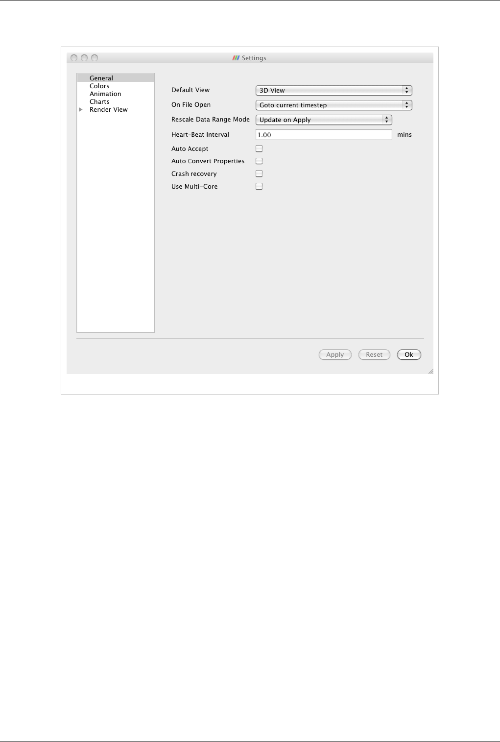
Application Settings 256
General
Figure 17.1 General Preferences
•Default View: Choose the View window type that ParaView initially shows when it starts up and connects to any
server.
•On File Open: Control the time step shown by default when ParaView opens a file with multiple time steps.
•Rescale Data Range Mode: Controls how color lookup tables are adjusted when data ranges change
•Heart-Beat Interval: Sets the length of time between keep alive messages that the client sends to the remote
server which prevents the TCP connection between the two machines from shutting down.
•Auto Accept: Makes every change take effect immediately rather than requiring you to click the Apply button.
•Auto Convert Properties: Tells ParaView to do some data conversions automatically so that more filters are
immediately applicable to the data you have at hand.
•Crash Recovery: Tells ParaView to save a record of each action you take so that you can easily recover your
work if ParaView crashes mid-session.
•Use Multi-Core: Tells ParaView to spawn an MPI parallel server on the same machine that is running the GUI,
so to better take advantage of multi-core machines on processing bound problems.
•Use Strict Load Balancing: Tells ParaView to not use its own extents translators.
•Specular Highlighting with Scalar Coloring: Tells ParaView to enable specular highlighting even when
coloring data by scalar values.
•Disable Splash Screen: Tells ParaView to not show its splash screen when starting.
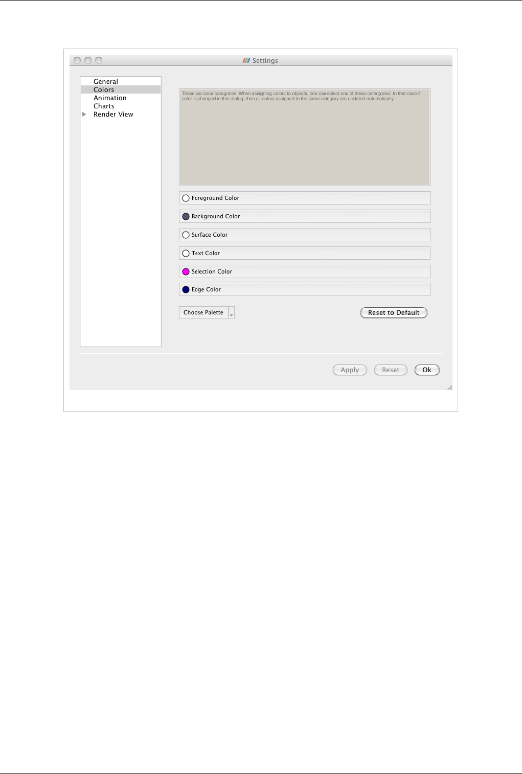
Application Settings 257
Colors
Figure 17.2 Color Preferences
When setting up visualizations, most datasets in the visualization are typically colored using scalar colors. However,
there may be items in the setup that are simply colored using a solid color including text and other annotations. Also
by default ParaView uses a grey background, so the default colors chosen for objects tends to be setup so that it
looks appropriate on the grey background. However, when saving a screenshot for printing, you may prefer to white
background, for example. In that case, it can be tedious to go to every object and change its color to work with the
new background color.
To make it easier to change colors on the fly, ParaView defines color categories. Users can choose to assign a color
category to any object when specifying a color using the category menu on most color-chooser buttons, as shown
below.
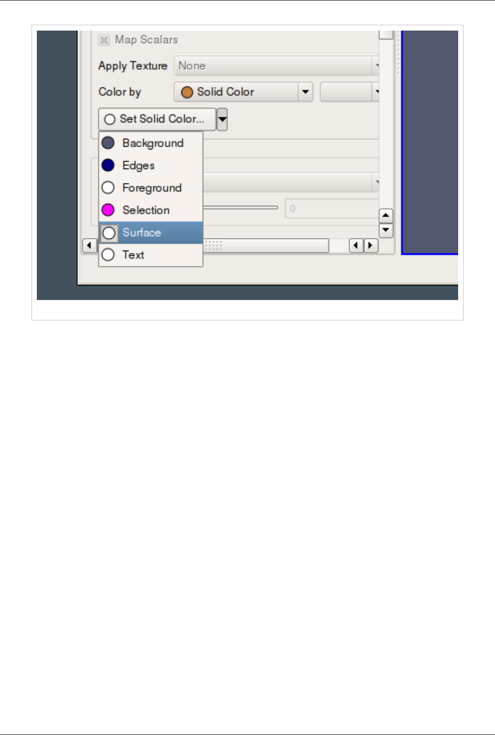
Application Settings 258
Figure 17.3 Color Category Menu on the Display Tab
Following associations are setup by default:
•Foreground color: Outlines and wireframes.
•Background color: Background color in render views.
•Surface color: Solid color to surfaces.
•Text color: Color to 2D text.
•Selection color: Color used to show highlighted/selected elements in render view.
•Edge color: Used for edges in Surface With Edges mode.
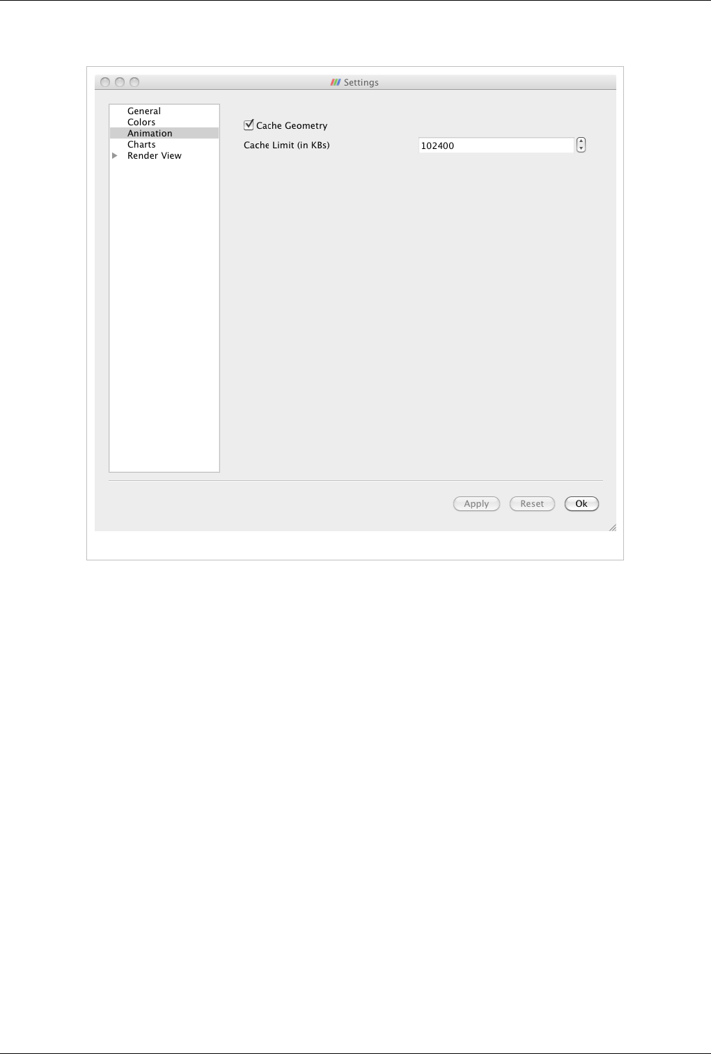
Application Settings 259
Animation
Figure 17.4 Animation Preferences
•Cache Geometry: When checked, this allows ParaView to save and later reuse, rather than regenerate, visible
geometry during animation playback to speed-up replay.
•Cache Limit: This is the maximum size of the animation playback geometry cache (on each node when in
parallel).

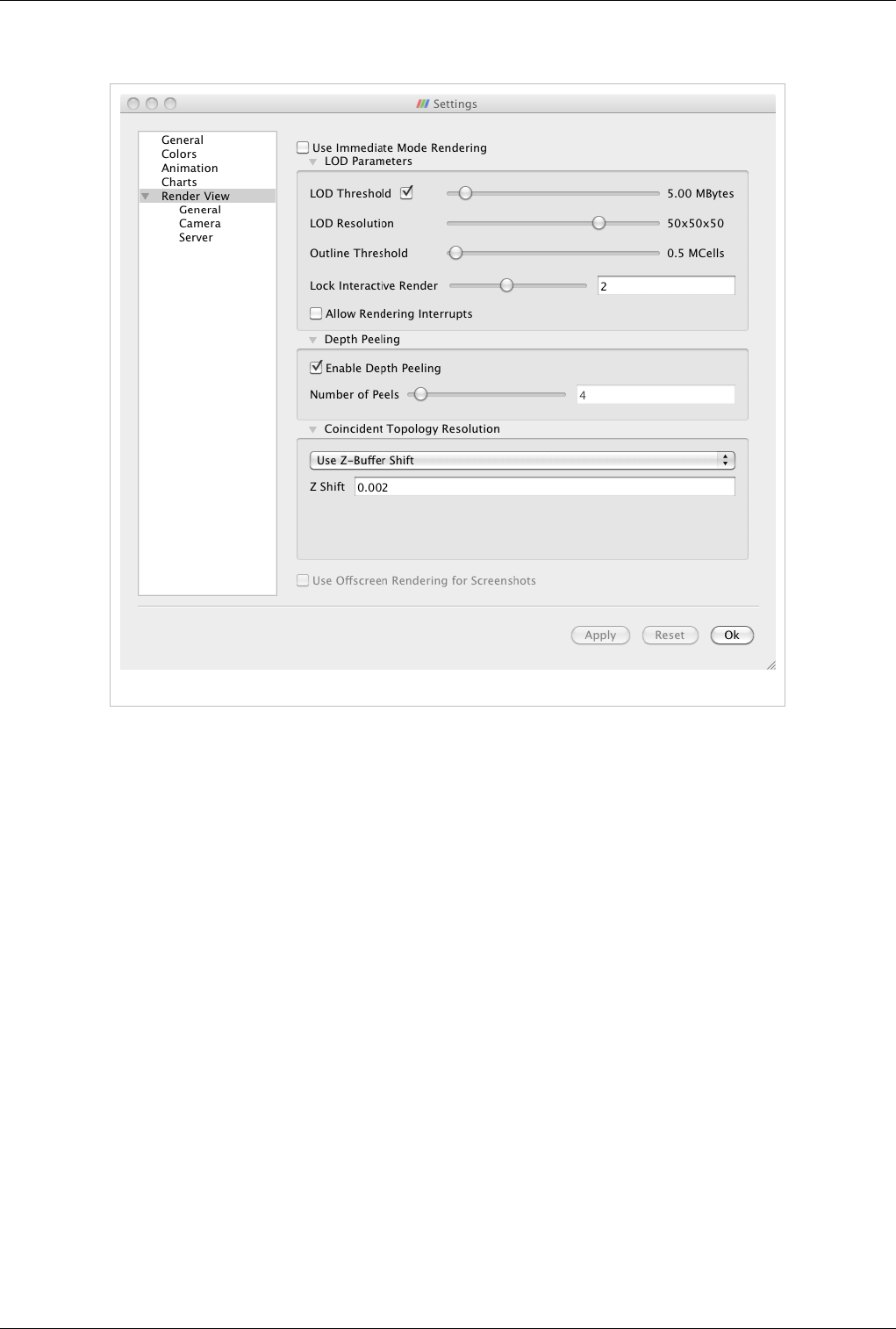
Application Settings 261
Render View General
Figure 17.6 General Render View Preferences
•Use Immediate Mode Rendering: Controls whether OpenGL display lists are used or not. This is generally only
faster only when rendering relatively small amounts of geometry.
The LOD Parameters settings control if, when, and to what extent ParaView will down sample the data it draws
while you move the mouse to maintain interactivity. The algorithm by which ParaView down samples the data is
known as quadric clustering.
•LOD Threshold: Rendered data that is smaller than the specified size is not down sampled.
•LOD Resolution: When data is down sampled, this controls how coarsely.
•Outline threshold: Data that is larger than this threshold is drawn only as a bounding box while you move the
camera.
•Lock Interactive Render: Controls how long ParaView waits after you have released the mouse and finished
moving the camera before it returns to a full resolution render.
•Allow Rendering Interrupts: Makes the drawing process interuptable so that you can move the camera
immediately, without having to wait for a potentially slow full resolution render to complete.
The Depth Peeling settings control the algorithm that ParaView uses (given a sufficiently capable GPU) to draw
translucent geometry correctly.
•Enable Depth Peeling: Controls whether ParaView will try to use the (potentially slow) depth peeling algorithm.
•Number of Peels: Controls the number of passes in the rendering algorithm. A higher number of peels produces
quality images, but increases rendering time.
The Coincident Topology Resolution settings control the method that ParaView uses to draw co-planar polygons in a
non conflicting way (to avoid z-tearing in graphics terminology). Changes to these parameters do not take effect
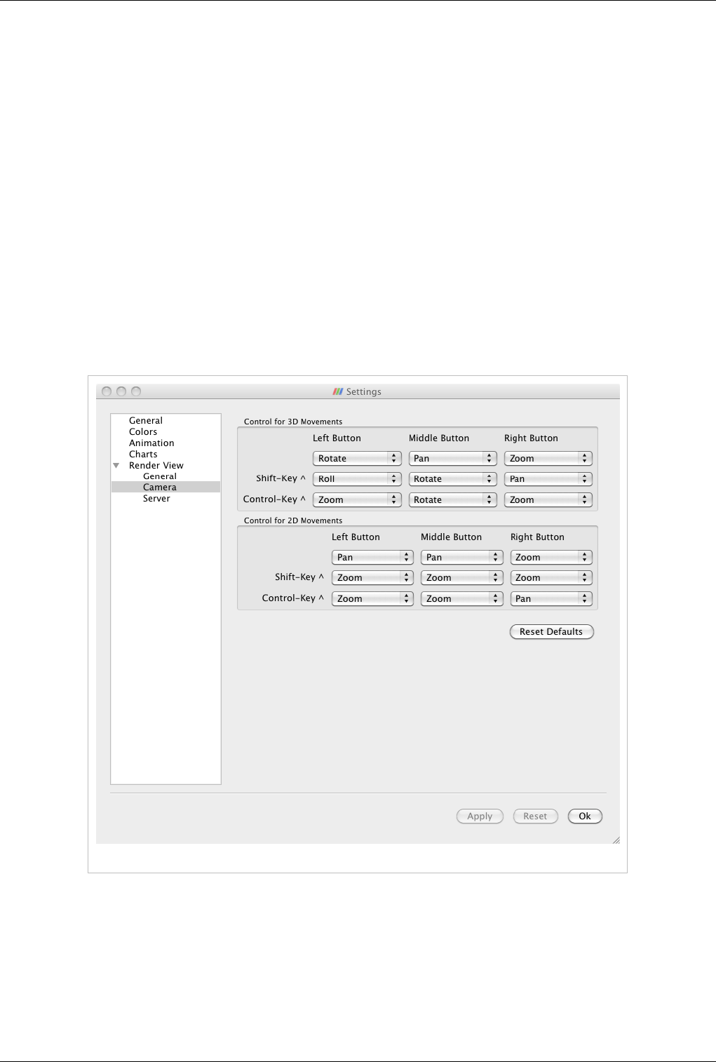
Application Settings 262
until ParaView is restarted.
The pull-down menu allows you to choose between various algorithms that deal with z-tearing.
•Do Nothing: Does not attempt to resolve overlapping geometry
•Use Z-Buffer Shift: Adjusts OpenGL's Z direction scaling to draw one object slightly in front of the other. The Z
Shift property controls the amount of offset.
•Use Polygon Offset: Adjusts polygon locations (by calling glPolygonOffset()) for the same purpose. For an
explanation of the Factor and Units parameters, see http:/ / www. opengl. org/ resources/ faq/ technical/
polygonoffset. htm. The Offset Faces parameters control whether filled polygons are moved rather than the points
and edges.
•Use Offscreen Rendering for Screenshots: This checkbox is enabled only when offscreen rendering is available.
It tells ParaView to generate images that are being captured as screenshots in offscreen contexts. On some
platforms this is necessary to avoid accidentally capturing overlapping pixels (such as a mouse pointer) from the
operating system.
Render View Camera
Figure 17.7 Camera Preferences
These settings allow you to assign particular key/mouse press combinations to various camera moving controls.
There are two sets of settings. Control for 3D Movements pertain to the 3D View. Control for 2D Movements pertain
to the 2D View.
In the 3D View controls you can assign the following motions to any combination of left, middle, or right mouse
button press and no, shift, or control key press.
•Pan
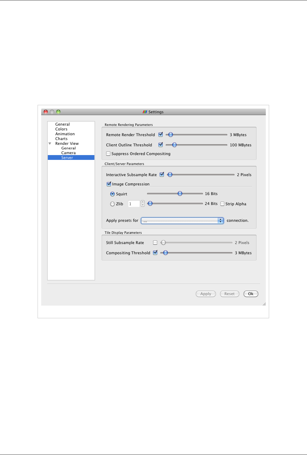
Application Settings 263
•Roll
•Rotate
•Multi-Rotate
•Zoom
Rotation is not possible in the 2D View, which lacks a down direction to move about. So in this area you can only
choose from Pan and Zoom.
Clicking Reset Defaults restores the button assignments to the factory settings.
Render View Server
Figure 17.8 Server Preferences
These settings control how and where rendering happens when you are connected to a remote server.
The Remote Rendering Parameters are controls that generally affect the break-up of rendering work between the
remote server and the local client machine.
•Remote Render Theshold: Geometry that is smaller than the set value will be delivered to the client for local
rendering. Data that is larger than the set value will be rendered remotely and pixels will be sent instead.
•Client Outline Threshold: While the camera is being manipulated and the geometry is being rendered locally, or
in tiled display mode when it is being rendered both locally and remotely, data that is larger than this threshold
will be rendered as a bounding box to maintain interactivity
•Suppress Ordered Compositing: This setting turns of the relatively slow transfer of data that must happen in
parallel in order to render translucent geometry (as in volume rendering for instance) correctly.
The Client/Server Parameters section has controls that affect how pixels are transferred between the render server
and the client while the data is being rendered remotely and images rather than geometry are being delivered to the

Application Settings 264
client. The Apply presets for ... menu allows you to choose from a set of default settings which are generally
well-suited to particular network connection bandwidths.
•Interactive Subsample Rate: This setting controls how coarsely the image is down sampled to maintain
interactivity while the camera is being manipulated.
•Image Compression: Enables compression of images during interaction. You can choose from either of the two
image compression algorithms:
•Squirt: Chooses IceT's native squirt image compression algorithm. The slider to the right controls the colorspace
fidelity of the compression and conversely the interactive responsiveness.
•Zlib: Chooses the ZLib library's compression algorithm instead. The spin box to the right specifies a compression
level (1 through 9). The slider controls the colorspace fidelity. The Strip Alpha checkbox removes the Opacity
channel (if any) from the shipped images.
The Tile Display Parameters section contains controls that take effect when doing tiled display wall rendering.
•Still Subsample Rate: This puts a screen space coarseness limit on the normally full-resolution rendering that
happens once you release the mouse after moving the camera. Image compositing time can prevent interactivity
when working with large displays. This limit allows you to preview your results quickly and then choose to
render truly full-resolution results only once when you are satisfied with the preview.
•Compositing Threshold: This threshold allows you to get faster rendering times in the circumstance that you are
visualizing relatively small datasets on large tiled displays. When the geometry size is below the threshold, the
geometry is broadcast to all nodes in the render server. After this broadcast, the relatively slow tiled image
compositing algorithm is entirely omitted.
List of Readers
AVS UCD Reader
Reads binary or ASCII files stored in AVS UCD format.The AVS UCD reader reads binary or ASCII files stored in
AVS UCD format. The default file extension is .inp. The output of this reader is unstructured grid. This supports
reading a file series.
Property Description Default
Value(s)
Restrictions
FileNameInfo
(FileNameInfo)
FileNames (FileNames) The list of files to be read by the reader. If more than one file is specified, the
reader will switch to file series mode in which it will pretend that it can support
time and provide one file per time step.
The value(s) must be a
filename (or filenames).
TimestepValues
(TimestepValues)
Available timestep values.
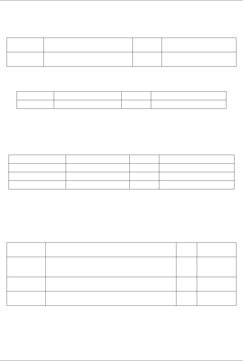
List of Readers 265
BYU Reader
Reads Movie.BYU files to produce polygonal data.The BYU reader reads data stored in Movie.BYU format. The
expected file extension is .g. The datasets resulting from reading these files are polygonal.
Property Description Default
Value(s)
Restrictions
FileName
(FileName)
This property specifies the file name for the BYU
reader.
The value(s) must be a filename (or
filenames).
CML Molecule Reader
Property Description Default Value(s) Restrictions
FileName (FileName) This property specifies the CML file name The value(s) must be a filename (or filenames).
COSMO Reader
Reads a cosmology file into a vtkUnstructuredGrid.The Cosmology reader reads a binary file of particle location,
velocity, and id creating a vtkUnstructuredGrid. The default file extension is .cosmo. Reads LANL Cosmo format or
Gadget format.
Property Description Default Value(s) Restrictions
FileNameInfo (FileNameInfo)
FileName (FileName) The list of files to be read by the reader. The value(s) must be a filename (or filenames).
TimestepValues (TimestepValues) Available timestep values.
CSV Reader
Reads a Delimited Text values file into a 1D rectilinear grid.The CSV reader reads a Delimited Text values file into
a 1D rectilinear grid. If the file was saved using the CSVWriter, then the rectilinear grid's points and point data can
be restored as well as the cell data. Otherwise all the data in the CSV file is treated as cell data. The default file
extension is .csv as well as .txt. This can read file series as well.
Property Description Default
Value(s)
Restrictions
FileName (FileName) The list of files to be read by the reader. Each file is expected to be a csv file. If
more than one file is specified, the reader will switch to file series mode in which it
will pretend that it can support time and provide one file per time step.
The value(s) must be a
filename (or
filenames).
FileNameInfo
(FileNameInfo)
TimestepValues
(TimestepValues)
Available timestep values.
List of Readers 266
DEM Reader
Reads a DEM (Digital Elevation Model) file.The DEM reader reads Digital Elevation Model files containing
elevation values derived from the U. S. Geologic Survey. The default file extension is .dem. This reader produces
uniform rectilinear (image/volume) data output.
Property Description Default
Value(s)
Restrictions
FileName
(FileName)
This property specifies the file name for the DEM (Digital
Elevation Map) reader.
The value(s) must be a filename (or
filenames).
ENZO AMR Particles Reader
Reads AMR particles from an ENZO datasetThe Enzo particles reader loads particle simulation data stored in Enzo
HDF5 format. The output of this reader is MultiBlock dataset where each block is a vtkPolyData that holds the
particles (points) and corresponding particle data.
Property Description Default Value(s) Restrictions
FileNameInfo (FileNameInfo)
FileNames (FileNames) The list of files to be read by the reader. The value(s) must be a filename (or filenames).
TimestepValues (TimestepValues) Available timestep values.
EnSight Master Server Reader
Reads files in EnSight's Master Server format.The EnSight Master Server reader reads EnSight's parallel files. The
master file ususally has a .sos extension and may point to multiple .case files. The output is a multi-block dataset.
Property Description Default
Value(s)
Restrictions
CaseFileName
(CaseFileName)
This property specifies the name of the .sos file for the
EnSight Master Server reader.
The value(s) must be a filename (or
filenames).
ByteOrder (ByteOrder) This property indicates the byte order of the binary file(s). 0 The value(s) is an enumeration of the
following:
• BigEndian (0)
• LittleEndian (1)
TimestepValues
(TimestepValues)
Available timestep values.
SetTimeValue
(SetTimeValue)
This property indicates which time value to read. 0.0
CellArrayInfo
(CellArrayInfo)
Cell Arrays
(CellArrayStatus)
This property lists which cell-centered arrays to read. The list of array names is provided
by the reader.
PointArrayInfo
(PointArrayInfo)
Point Arrays
(PointArrayStatus)
This property lists which point-centered arrays to read. The list of array names is provided
by the reader.
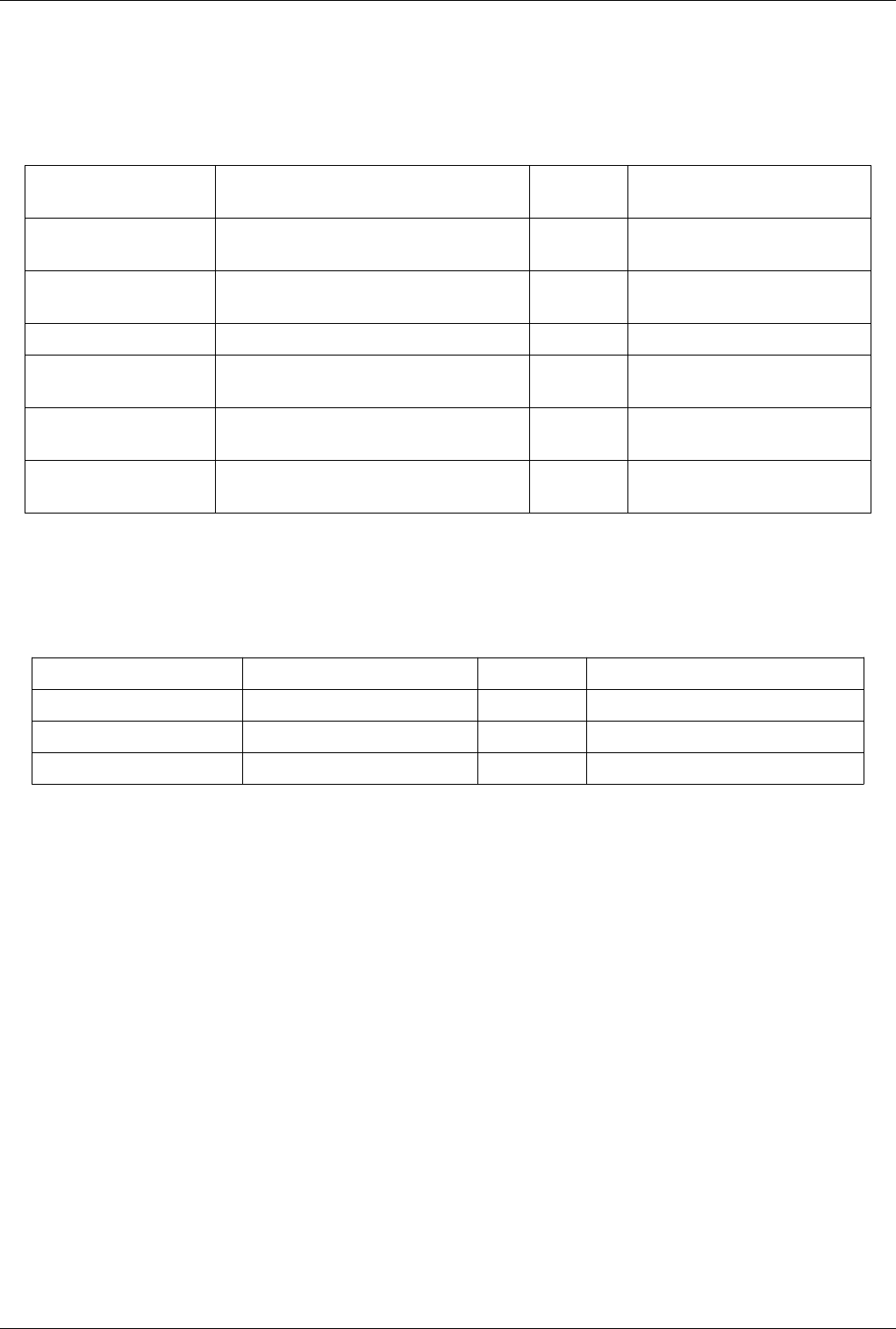
List of Readers 267
EnSight Reader
Reads EnSight 6 and Gold files.The EnSight reader reads files in the format produced by CEI's EnSight. EnSight 6
and Gold files (both ASCII and binary) are supported. The default extension is .case. The output of this reader is a
multi-block dataset.
Property Description Default
Value(s)
Restrictions
CaseFileName
(CaseFileName)
This property specifies the case file name for the
EnSight reader.
The value(s) must be a filename (or
filenames).
TimestepValues
(TimestepValues)
Available timestep values.
CellArrayInfo (CellArrayInfo)
Cell Arrays (CellArrayStatus) This property lists which cell-centered arrays to read. The list of array names is provided by
the reader.
PointArrayInfo
(PointArrayInfo)
Point Arrays
(PointArrayStatus)
This property lists which point-centered arrays to
read.
The list of array names is provided by
the reader.
Enzo Reader
Read hierarchical box dataset from an Enzo file. This Enzo reader loads data stored in Enzo format. The output of
this reader is a hierarchical-box dataset.
Property Description Default Value(s) Restrictions
FileNameInfo (FileNameInfo)
FileNames (FileNames) The list of files to be read by the reader. The value(s) must be a filename (or filenames).
TimestepValues (TimestepValues) Available timestep values.
ExodusIIReader
Reads an Exodus II file to produce an unstructured grid.The Exodus reader loads Exodus II files and produces an
unstructured grid output. The default file extensions are .g, .e, .ex2, .ex2v2, .exo, .gen, .exoII, .exii, .0, .00, .000, and
.0000. The file format is described fully at: http:/ / endo. sandia. gov/ SEACAS/ Documentation/ exodusII. pdf. Each
Exodus file contains a single set of points with 2-D or 3-D coordinates plus one or more blocks, sets, and maps.
Block group elements (or their bounding edges or faces) of the same type together. Sets select subsets (across all the
blocks in a file) of elements, sides of elements (which may be of mixed dimensionality), bounding faces of
volumetric elements, or bounding edges of volumetric or areal elements. Each block or set may have multiple result
variables, each of which defines a value per element, per timestep. The elements (cells), faces of elements (when
enumerated in face blocks), edges of elements (when enumerated in edge blocks), and nodes (points) in a file may be
assigned an arbitrary integer number by an element map, face map, edge map, or node map, respectively. Usually,
only a single map of each type exists and is employed to assign a unique global ID to entities across multiple files
which partition a large mesh for a distributed-memory calculation. However here may be multiply maps of each type
and there are no constraints which force the integers to be unique. The connectivity of elements is constant across all
of the timesteps in any single Exodus II file. However, multiple files which specify a single time-evolution of a mesh
may be used to represent meshes which exhibit changes in connectivity infrequently.

List of Readers 268
Property Description Default
Value(s)
Restrictions
FileNameInfo (FileNameInfo)
FileName (FileName) This property specifies the file name for the Exodus
reader.
The value(s) must be a filename (or
filenames).
UseMetaFile (UseMetaFile) This hidden property must always be set to 1 for this
proxy to work.
0 Accepts boolean values (0 or 1).
TimestepValues
(TimestepValues)
FLASH AMR Particles Reader
Reads AMR particles from FLASH datasetThe Flash particles reader loads particle simulation data stored in Flash
format. The output of this reader is a MultiBlock dataset where each block is vtkPolyData that holds the particles and
corresponding particle data.
Property Description Default Value(s) Restrictions
FileNameInfo (FileNameInfo)
FileNames (FileNames) The list of files to be read by the reader. The value(s) must be a filename (or filenames).
TimestepValues (TimestepValues) Available timestep values.
FacetReader
Reads ASCII files stored in Facet format.The Facet Reader reads files in Facet format: a simple ASCII file format
listing point coordinates and connectivity between these points. The default file extension is .facet. The output of the
Facet Reader is polygonal.
Property Description Default
Value(s)
Restrictions
FileName
(FileName)
This property specifies the file name for the Facet
reader.
The value(s) must be a filename (or
filenames).
Flash Reader
Read hierarchical box dataset from a Flash dataset. This Flash reader loads data stored in Enzo format. The output of
this reader is a hierarchical-box dataset.
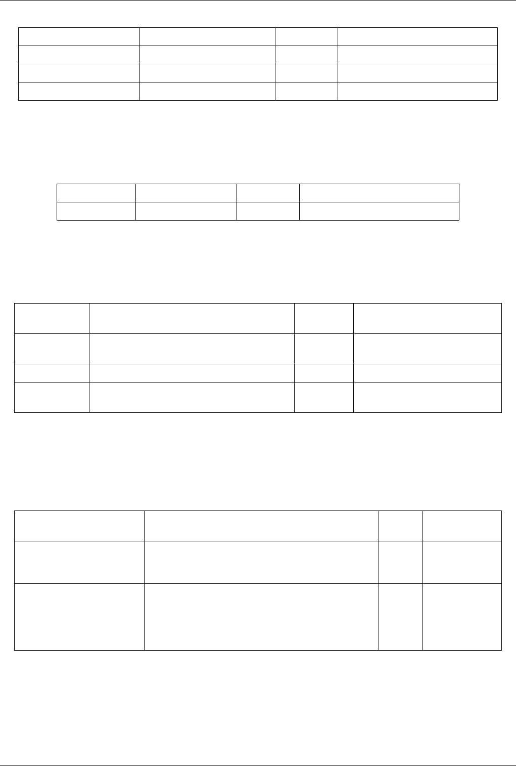
List of Readers 269
Property Description Default Value(s) Restrictions
FileNameInfo (FileNameInfo)
FileNames (FileNames) The list of files to be read by the reader. The value(s) must be a filename (or filenames).
TimestepValues (TimestepValues) Available timestep values.
Fluent Case Reader
Reads a dataset in Fluent file format. FLUENTReader creates an unstructured grid dataset. It reads .cas and .dat files
stored in FLUENT native format (or a file series of the same.
Property Description Default Value(s) Restrictions
FileName (FileName) The name of the files to load. The value(s) must be a filename (or filenames).
Gaussian Cube Reader
Produce polygonal data by reading a Gaussian Cube file.The Gaussian Cube reader produces polygonal data by
reading data files produced by the Gaussian software package. The expected file extension is .cube.
Property Description Default
Value(s)
Restrictions
FileName
(FileName)
This property specifies the file name for the Gaussian Cube
reader.
The value(s) must be a filename (or
filenames).
HBScale (HBScale) A scaling factor to compute bonds with hydrogen atoms. 1.0
BScale (BScale) A scaling factor to compute bonds between non-hydrogen
atoms
1.0
Image Reader
Reads raw regular rectilinear grid data from a file. The dimensions and type of the data must be specified. The Image
reader reads raw, regular, rectilinear grid (image/volume) data from a file. Because no metadata is provided, the user
must specify information about the size, spacing, dimensionality, etc. about the dataset.
Property Description Default
Value(s)
Restrictions
FilePrefix (FilePrefix) The text string contained in this property specifies the file prefix
(directory plus common initial part of file name) for the raw binary
uniform rectilinear grid dataset.
The value(s) must be
a filename (or
filenames).
FilePattern (FilePattern) The text string contained in the property specifies the format string to
determine the file names necessary for reading this dataset. In creating
the filenames, %s will be replaced by the prefix and %d by a digit
which represents the slice number in Z. The format string is the same
as that used by printf.
%s

List of Readers 270
DataScalarType (DataScalarType) The value of this property indicates the scalar type of the
pixels/voxels in the file(s): short, int, float ...
4 The value(s) is an
enumeration of the
following:
• char (2)
• unsigned char (3)
• short (4)
• unsigned short (5)
• int (6)
• unsigned int (7)
• long (8)
• unsigned long (9)
• float (10)
• double (11)
DataByteOrder (DataByteOrder) This property indicates the byte order of the binary file(s). 0 The value(s) is an
enumeration of the
following:
• BigEndian (0)
• LittleEndian (1)
FileDimensionality
(FileDimensionality)
This property indicates whether the file(s) in this dataset contain slices
(2D) or volumes (3D).
3 The value(s) is an
enumeration of the
following:
• 2 (2)
• 3 (3)
DataOrigin (DataOrigin) The coordinate contained in this property specifies the position of the
point with index (0,0,0).
0.0 0.0 0.0
DataSpacing (DataSpacing) This property specifies the size of a voxel in each dimension. 1.0 1.0 1.0
DataExtent (DataExtent) This property specifies the minimum and maximum index values of
the data in each dimension (xmin, xmax, ymin, ymax, zmin, zmax).
0 0 0 0 0 0
NumberOfScalarComponents
(NumberOfScalarComponents)
This property specifies the number of components the scalar value at
each pixel or voxel has (e.g., RGB - 3 scalar components).
1
ScalarArrayName
(ScalarArrayName)
This property contains a text string listing a name to assign to the
point-centered data array read.
ImageFile
FileLowerLeft (FileLowerLeft) This property determines whether the data originates in the lower left
corner (on) or the upper left corner (off). Most scientific data is
written with a right-handed axes that originates in the lower left
corner. However, several 2D image file formats write the image from
the upper left corner.
1 Accepts boolean
values (0 or 1).
JPEG Series Reader
Reads a series of JPEG files into an time sequence of image datas.The JPEG series reader reads JPEG files. The
output is a time sequence of uniform rectilinear (image/volume) dataset. The default file extension is .jpg or .jpeg.

List of Readers 271
Property Description Default
Value(s)
Restrictions
FileNames (FileNames) The list of files to be read by the reader. If more than one file is specified, the
reader will switch to file series mode in which it will pretend that it can support
time and provide one file per time step.
The value(s) must be a
filename (or filenames).
TimestepValues
(TimestepValues)
Available timestep values.
LSDynaReader
Read LS-Dyna databases (d3plot).This reader reads LS-Dyna databases.
Property Description Default
Value(s)
Restrictions
FileName (FileName) Set the file name for the LSDyna reader. The value(s) must be a filename
(or filenames).
TimestepValues (TimestepValues)
SolidArrayInfo (SolidArrayInfo)
Solid Arrays (SolidArrayStatus) Select which solid arrays to read. The list of array names is
provided by the reader.
ThickShellArrayInfo
(ThickShellArrayInfo)
Thick Shell Arrays
(ThickShellArrayStatus)
Select which thick shell arrays to read. The list of array names is
provided by the reader.
ShellArrayInfo (ShellArrayInfo)
Shell Arrays (ShellArrayStatus) Select which shell arrays to read. The list of array names is
provided by the reader.
RigidBodyArrayInfo
(RigidBodyArrayInfo)
Rigid Body Arrays
(RigidBodyArrayStatus)
Select which rigid body arrays to load. The list of array names is
provided by the reader.
RoadSurfaceArrayInfo
(RoadSurfaceArrayInfo)
Road Surface Arrays
(RoadSurfaceArrayStatus)
Select which road surface arrays to read. The list of array names is
provided by the reader.
BeamArrayInfo (BeamArrayInfo)
Beam Arrays (BeamArrayStatus) Select which beam arrays to read. The list of array names is
provided by the reader.
ParticleArrayInfo
(ParticleArrayInfo)
Particle Arrays (ParticleArrayStatus) Select which particle arrays to read. The list of array names is
provided by the reader.
PointArrayInfo (PointArrayInfo)
Point Arrays (PointArrayStatus) Select which point-centered arrays to read. The list of array names is
provided by the reader.
PartArrayInfo (PartArrayInfo)
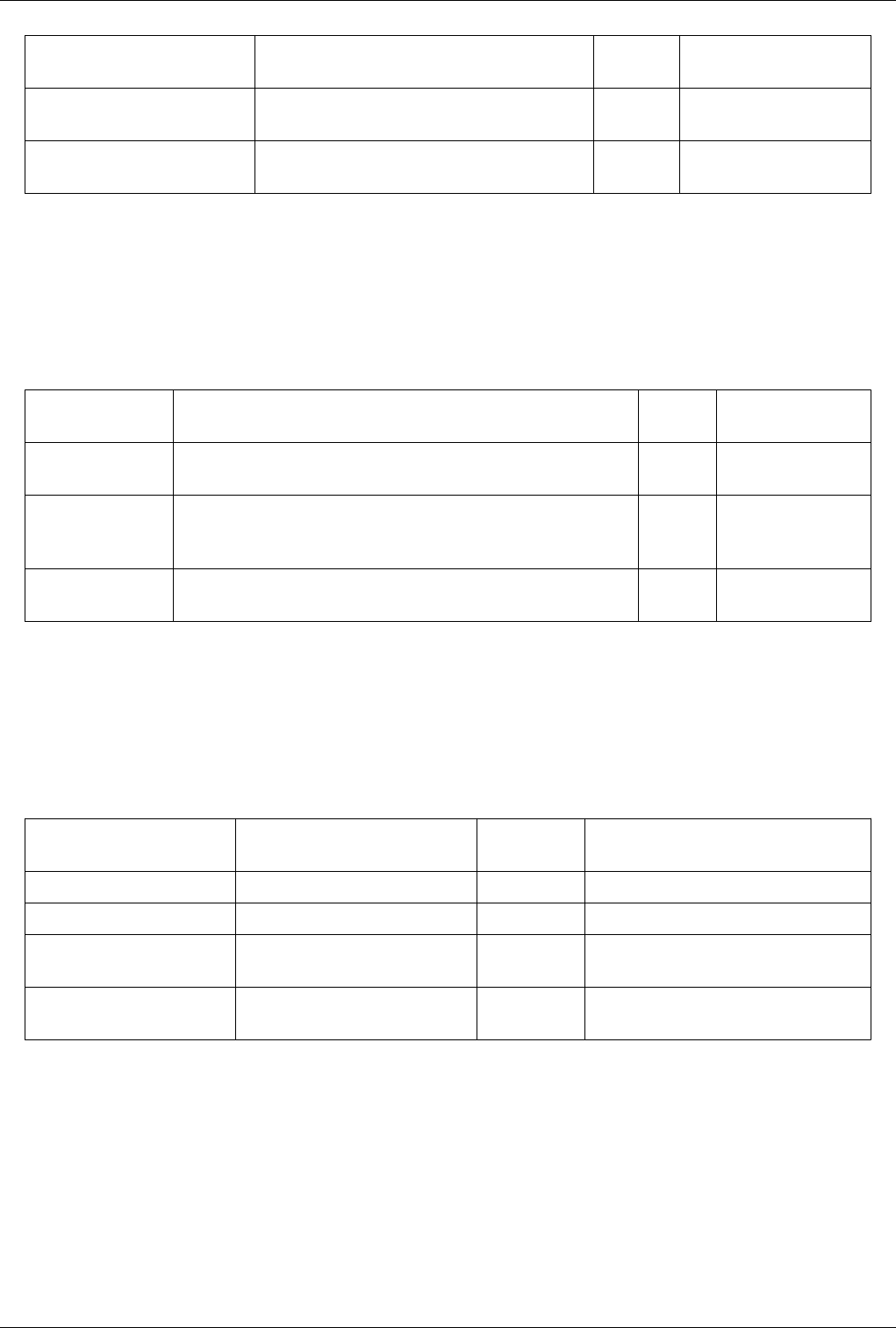
List of Readers 272
Part Arrays (PartArrayStatus) Select which part arrays to read. The list of array names is
provided by the reader.
DeformedMesh (DeformedMesh) Should the mesh be deformed over time (if the Deflection
node array is set to load)?
1 Accepts boolean values (0 or
1).
RemoveDeletedCells
(RemoveDeletedCells)
Should cells that have been deleted (failed structurally,
for example) be removed from the mesh?
1 Accepts boolean values (0 or
1).
Legacy VTK Reader
Reads files stored in VTK's legacy file format.The Legacy VTK reader loads files stored in VTK's legacy file format
(before VTK 4.2, although still supported). The expected file extension is .vtk. The type of the dataset may be
structured grid, uniform rectilinear grid (image/volume), non-uniform rectiinear grid, unstructured grid, or
polygonal. This reader also supports file series.
Property Description Default
Value(s)
Restrictions
FileNameInfo
(FileNameInfo)
FileNames (FileNames) The list of files to be read by the reader. If more than one file is specified, the
reader will switch to file series mode in which it will pretend that it can support
time and provide one file per time step.
The value(s) must be a
filename (or filenames).
TimestepValues
(TimestepValues)
Available timestep values.
MFIXReader
Reads a dataset in MFIX file format. vtkMFIXReader creates an unstructured grid dataset. It reads a restart file and a
set of sp files. The restart file contains the mesh information. MFIX meshes are either cylindrical or rectilinear, but
this reader will convert them to an unstructured grid. The sp files contain transient data for the cells. Each sp file has
one or more variables stored inside it.
Property Description Default
Value(s)
Restrictions
FileName (FileName) Set the file name for the MFIX reader. The value(s) must be a filename (or filenames).
CellArrayInfo (CellArrayInfo)
Cell Arrays (CellArrayStatus) Select which cell-centered arrays to
read.
The list of array names is provided by the
reader.
TimestepValues
(TimestepValues)
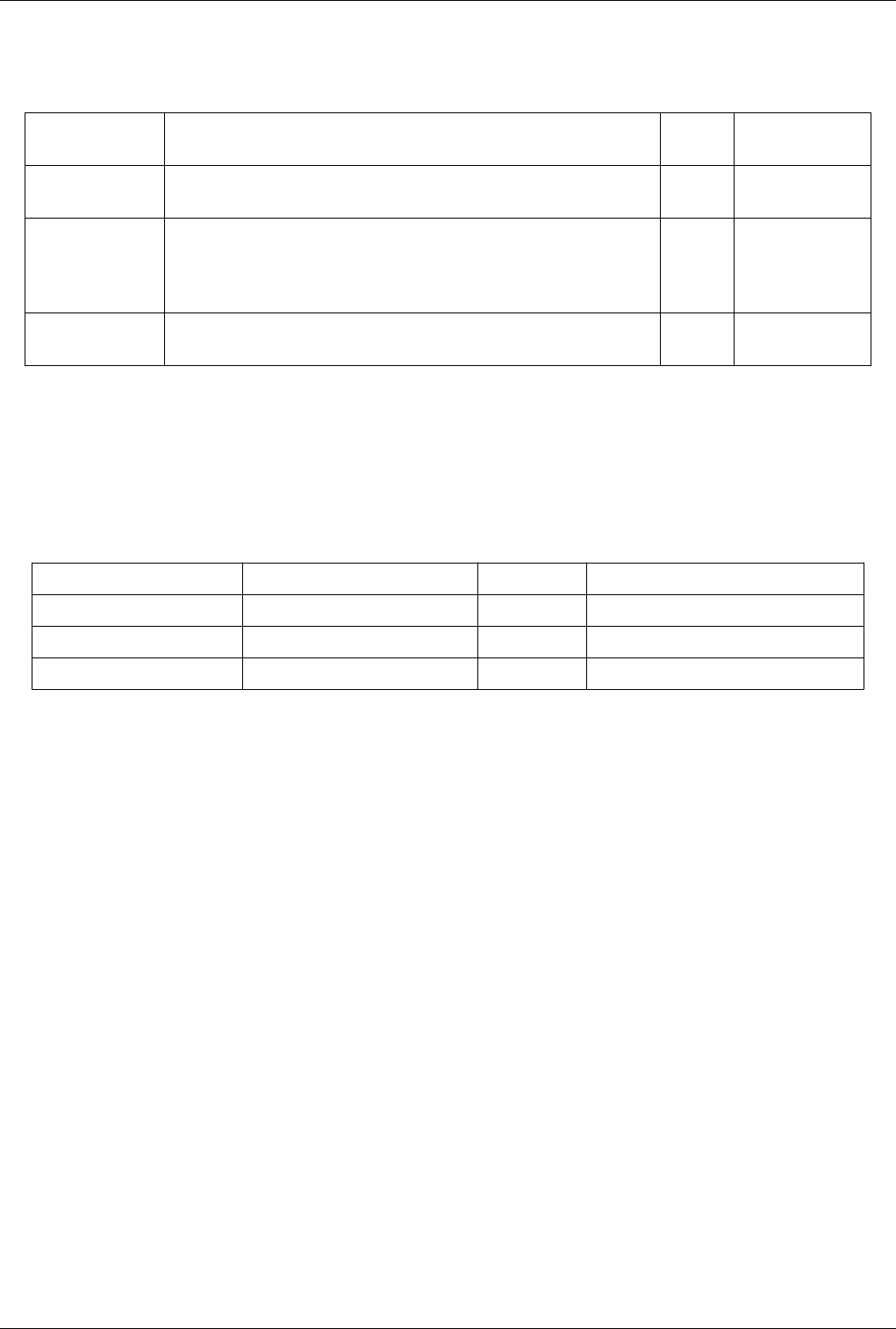
List of Readers 273
Meta File Series Reader
Reads a series of meta images.Read a series of meta images. The file extension is .mhd
Property Description Default
Value(s)
Restrictions
FileNameInfo
(FileNameInfo)
FileNames
(FileNames)
The list of files to be read by the reader. Each file is expected to be in the meta
format. The standard extension is .mhd. If more than one file is specified, the reader
will switch to file series mode in which it will pretend that it can support time and
provide one file per time step.
The value(s) must be
a filename (or
filenames).
TimestepValues
(TimestepValues)
Available timestep values.
NetCDF CAM reader
Reads unstructured grid data from NetCDF files. There are 2 files, a points+fields file which is set as FileName and a
cell connectivity file set as ConnectivityFileName. This reader reads in unstructured grid data from a NetCDF file.
The grid data is in a set of planes as quadrilateral cells. The reader creates hex cells in order to create a volumetric
grid.
Property Description Default Value(s) Restrictions
FileNameInfo (FileNameInfo)
FileName (FileName) The list of files to be read by the reader. The value(s) must be a filename (or filenames).
TimestepValues (TimestepValues) Available timestep values.
NetCDF MPAS reader
Reads unstructured grid MPAS data from a file. This reader reads unstructured grid MPAS data from a file. It creates
a dual grid It assumes the grid is in the global domain. By default, it creates a spherical view of vertical layer 0. It
assumes it is ocean data. It gives several options to change the view to multilayer (all vertical layers will have a
thickness determined by the value in the slider), lat/lon projection or atmospheric (vertical layers go out away from
the center of the sphere, instead of down towards the center as they do for ocean data). It doesn't handle data in the
rectangular domain. This is not a parallel reader. It expects one .nc file of data. It can display cell or vertex-centered
data, but not edge data. When converted to the dual grid, cell-centered data becomes vertex-centered and vice-versa.
NOTES: When using this reader, it is important that you remember to do the following: 1. When changing a selected
variable, remember to select it also in the drop down box to color by. It doesn't color by that variable automatically
2. When selecting multilayer sphere view, start with layer thickness around 100,000 3. When selecting multilayer
lat/lon view, start with layer thickness around 10 4. Always click the -Z orientation after making a switch from
lat/lon to sphere, from single to multilayer or changing thickness. 5. Be conservative on the number of changes you
make before hitting Apply, since there may be bugs in this reader. Just make one change and then hit Apply. For
problems, contact Christine Ahrens (cahrens@lanl.gov)

List of Readers 274
Property Description Default
Value(s)
Restrictions
FileName (FileName) This property specifies the file name to read. It should be an MPAS format
NetCDF file ending in .nc.
The value(s) must
be a filename (or
filenames).
PointArrayInfo
(PointArrayInfo)
PointArrayStatus
(PointArrayStatus)
This property lists which NetCDF dual-grid point variables to load. The list of array
names is provided
by the reader.
CellArrayInfo (CellArrayInfo)
CellArrayStatus
(CellArrayStatus)
This property lists which NetCDF dual-grid cell variables to load. The list of array
names is provided
by the reader.
ProjectLatLon (ProjectLatLon) This property indicates whether to view the data in the lat/lon projection. 0 Accepts boolean
values (0 or 1).
ShowMultilayerView
(ShowMultilayerView)
This property indicates whether to show multiple layers in one view, with each
vertical level having the same thickness, specified by the layer thickness slider.
For ocean data, the layers correspond to data at vertical level whose number
increases towards the center of the sphere. For atmospheric data, the layers
correspond to data at vertical levels increasing away from the center.
0 Accepts boolean
values (0 or 1).
IsAtmosphere (IsAtmosphere) This property indicates whether data is atmospheric. Checking this ensures the
vertical levels will go up away from the sphere instead of down towards the
center.
0 Accepts boolean
values (0 or 1).
LayerThicknessRangeInfo
(LayerThicknessRangeInfo)
Layer Thickness
(LayerThickness)
This property specifies how thick the layer should be if viewing the data in
multilayer view. Each layer corresponds to a vertical level. A good starting
point is 100,000 for the spherical view and 10 for the lat/lon projection. Click
on -Z after applying this change, since the scale may change drastically.
10
CenterLonRangeInfo
(CenterLonRangeInfo)
Center Longitude (CenterLon) This property specifies where the center will be viewed for a lat/lon projection. 180
VerticalLevelRangeInfo
(VerticalLevelRangeInfo)
VerticalLevel (VerticalLevel) This property specifies which vertical level is viewed if not in multilayer view.
Only the data for that vertical level will be viewed. The grid is essentially the
same for each vertical level, however at some ocean levels, especially the
lower ones, due to the topography, the grid becomes more sparse where there is
land.
0
TimestepValues
(TimestepValues)
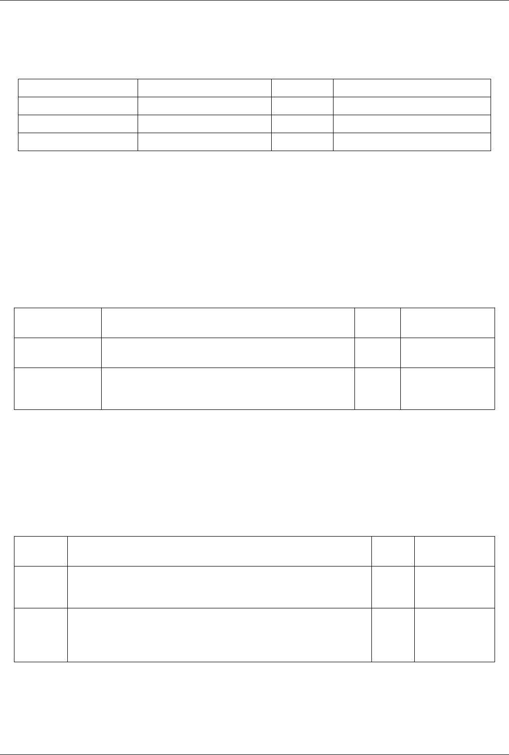
List of Readers 275
NetCDF POP reader
Reads rectilinear grid data from a NetCDF POP file. The reader reads regular rectilinear grid (image/volume) data
from a NetCDF file.
Property Description Default Value(s) Restrictions
FileNameInfo (FileNameInfo)
FileName (FileName) The list of files to be read by the reader. The value(s) must be a filename (or filenames).
TimestepValues (TimestepValues) Available timestep values.
NetCDF Reader
Reads regular arrays from netCDF files. Will also read any topological information specified by the COARDS and
CF conventions.Reads arrays from netCDF files into structured VTK data sets. In the absence of any other
information, the files will be read as image data. This reader will also look for meta information specified by the CF
convention that specify things like topology and time. This information can cause the output to be a nonuniform
rectilinear grid or curvilinear (structured) grid. Details on the CF convention can be found at http:/ / cf-pcmdi. llnl.
gov/ . It should be noted that the CF convention is a superset of the COARDS convention, so COARDS conventions
will also be recognized.
Property Description Default
Value(s)
Restrictions
FileName (FileName) The name of the files to load. The value(s) must be a
filename (or filenames).
TimestepValues
(TimestepValues)
This magic property sends time information to the animation panel.
ParaView will then automatically set up the animation to visit the time steps
defined in the file.
Nrrd Reader
Reads raw image files with Nrrd meta data.The Nrrd reader reads raw image data much like the Raw Image Reader
except that it will also read metadata information in the Nrrd format. This means that the reader will automatically
set information like file dimensions. There are several limitations on what type of nrrd files we can read. This reader
only supports nrrd files in raw format. Other encodings like ascii and hex will result in errors. When reading in
detached headers, this only supports reading one file that is detached.
Property Description Default
Value(s)
Restrictions
FileName
(FileName)
The name of the file to read (or the meta data file that will point to the actual file). The value(s) must be a
filename (or
filenames).
Data VOI
(DataVOI)
The data volume of interest (VOI). The VOI is a sub-extent of the data that you want loaded.
Setting a VOI is useful when reading from a large data set and you are only interested in a
small portion of the data. If left containing all 0's, then the reader will load in the entire data
set.
0 0 0 0 0 0

List of Readers 276
OpenFOAMReader
Reads OpenFOAM data files, producing multi-block dataset.The OpenFOAM reader reads OpenFOAM data files
and outputs multi-block datasets. Mesh information and time dependent data are supported. The OpenFOAM format
is described fully at http:/ / www. openfoam. com/ docs/ user/ basic-file-format. php
Property Description Default
Value(s)
Restrictions
FileName (FileName) This property specifies the file name for the
reader.
The value(s) must be a
filename (or filenames).
CaseType (CaseType) The property indicates whether decomposed mesh
or reconstructed mesh should be read
1 The value(s) is an
enumeration of the following:
• Decomposed Case (0)
• Reconstructed Case (1)
Create cell-to-point filtered data
(CreateCellToPoint)
Create point data from cell data. Beware: the
filter does not do inverse distance weighting.
1 Accepts boolean values (0 or
1).
Add dimensional units to array names
(AddDimensionsToArrayNames)
Read dimensional units from field data and add
them to array names as human-readable string.
0 Accepts boolean values (0 or
1).
TimestepValues (TimestepValues)
PatchArrayInfo (PatchArrayInfo)
MeshRegions (MeshRegions) The list of array names is
provided by the reader.
CellArrayInfo (CellArrayInfo)
CellArrays (CellArrays) The list of array names is
provided by the reader.
PointArrayInfo (PointArrayInfo)
PointArrays (PointArrays) The list of array names is
provided by the reader.
LagrangianArrayInfo (LagrangianArrayInfo)
LagrangianArrays (LagrangianArrays) The list of array names is
provided by the reader.
Cache mesh (CacheMesh) Cache the OpenFOAM mesh between GUI
selection changes.
1 Accepts boolean values (0 or
1).
Decompose polyhedra (DecomposePolyhedra) Decompose polyhedra into tetrahedra and
pyramids.
1 Accepts boolean values (0 or
1).
List timesteps according to controlDict
(ListTimeStepsByControlDict)
List time directories listed according to the
settings in controlDict.
0 Accepts boolean values (0 or
1).
Lagrangian positions are in OF 1.3 binary
format (PositionsIsIn13Format)
Set if Lagrangian positions files are in
OpenFOAM 1.3 binary format.
0 Accepts boolean values (0 or
1).
Read zones (ReadZones) Read point/face/cell-Zones? 0 Accepts boolean values (0 or
1).
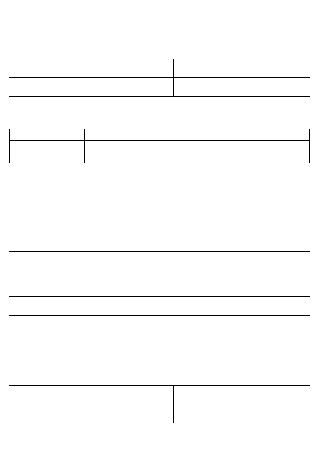
List of Readers 277
PDB Reader
Reads PDB molecule files.The PDB reader reads files in the format used by the Protein Data Bank (an archive of
experimentally determined three-dimensional structures of biological macromolecules). The expected file extension
is .pdb. The output datasets are polygonal.
Property Description Default
Value(s)
Restrictions
FileName
(FileName)
This property specifies the file name for the PDB
reader.
The value(s) must be a filename (or
filenames).
PLOT3D Meta-File Reader
Property Description Default Value(s) Restrictions
FileName (FileName) This property specifies the meta file name The value(s) must be a filename (or filenames).
TimestepValues (TimestepValues) Available timestep values.
PLOT3D Reader
Reads ASCII or binary PLOT3D files.PLOT3D is a plotting package developed at NASA. The PLOT3D reader can
read both ASCII and binary PLOT3D files. The default file extension for the geometry files is .xyz, and the default
file extension for the solution files is .q. The output of this reader is a multi-block dataset containing curvilinear
(structured grid) datasets.
Property Description Default
Value(s)
Restrictions
QFileName
(QFileName)
The list of .q (solution) files for the PLOT3D reader. There can be more than one. If
more that one file is specified, the reader will switch to file-series mode in which it
will pretend that it can support time and provide one file per time step.
The value(s) must be a
filename (or
filenames).
FileNameInfo
(FileNameInfo)
TimestepValues
(TimestepValues)
Available timestep values.
PLY Reader
Reads files stored in Stanford University's PLY polygonal file format.The PLY reader reads files stored in the PLY
polygonal file format developed at Stanford University. The PLY files that ParaView can read must have the
elements "vertex" and "face" defined. The "vertex" elements must have the propertys "x", "y", and "z". The "face"
elements must have the property "vertex_indices" defined. The default file extension for this reader is .ply.
Property Description Default
Value(s)
Restrictions
FileName
(FileName)
This property specifies the file name for the PLY
reader.
The value(s) must be a filename (or
filenames).
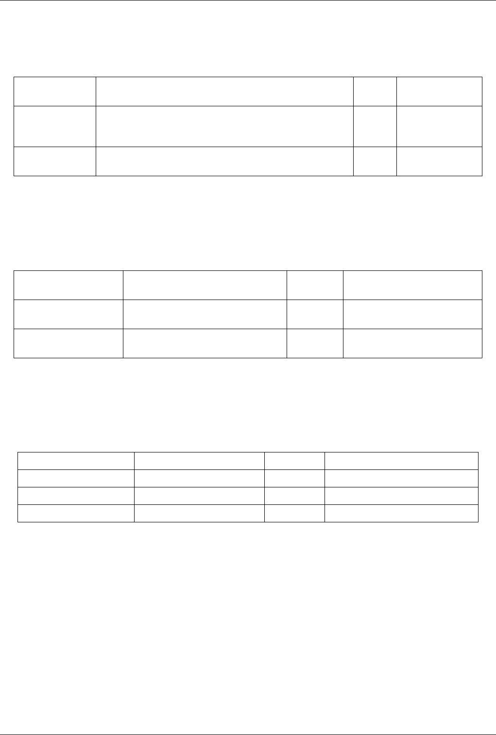
List of Readers 278
PNG Series Reader
Reads a PNG file into an image data.The PNG reader reads PNG (Portable Network Graphics) files, and the output is
a uniform rectilinear (image/volume) dataset. The default file extension is .png.
Property Description Default
Value(s)
Restrictions
FileNames (FileNames) The list of files to be read by the reader. If more than one file is specified, the
reader will switch to file series mode in which it will pretend that it can support
time and provide one file per time step.
The value(s) must be a
filename (or filenames).
TimestepValues
(TimestepValues)
Available timestep values.
PVD Reader
Load a dataset stored in ParaView's PVD file format.The PVD reader reads data stored in ParaView's PVD file
format. The .pvd file is essentially a header file that collects together other data files stored in VTK's XML-based file
format.
Property Description Default
Value(s)
Restrictions
FileName (FileName) This property specifies the file name for the PVD
reader.
The value(s) must be a filename (or
filenames).
TimestepValues
(TimestepValues)
Available timestep values.
Parallel NetCDF POP reader
Reads rectilinear grid data from a NetCDF POP file in parallel. The reader reads regular rectilinear grid
(image/volume) data from a NetCDF file. Only a subset of the processes actually read the file and these processes
communicate the data to other processes.
Property Description Default Value(s) Restrictions
FileNameInfo (FileNameInfo)
FileName (FileName) The list of files to be read by the reader. The value(s) must be a filename (or filenames).
TimestepValues (TimestepValues) Available timestep values.
Particles Reader
Reads particle data.vtkParticleReader reads either a binary or a text file of particles. Each particle can have
associated with it an optional scalar value. So the format is: x, y, z, scalar (all floats or doubles). The text file can
consist of a comma delimited set of values. In most cases vtkParticleReader can automatically determine whether the
file is text or binary. The data can be either float or double. Progress updates are provided. With respect to binary
files, random access into the file to read pieces is supported.
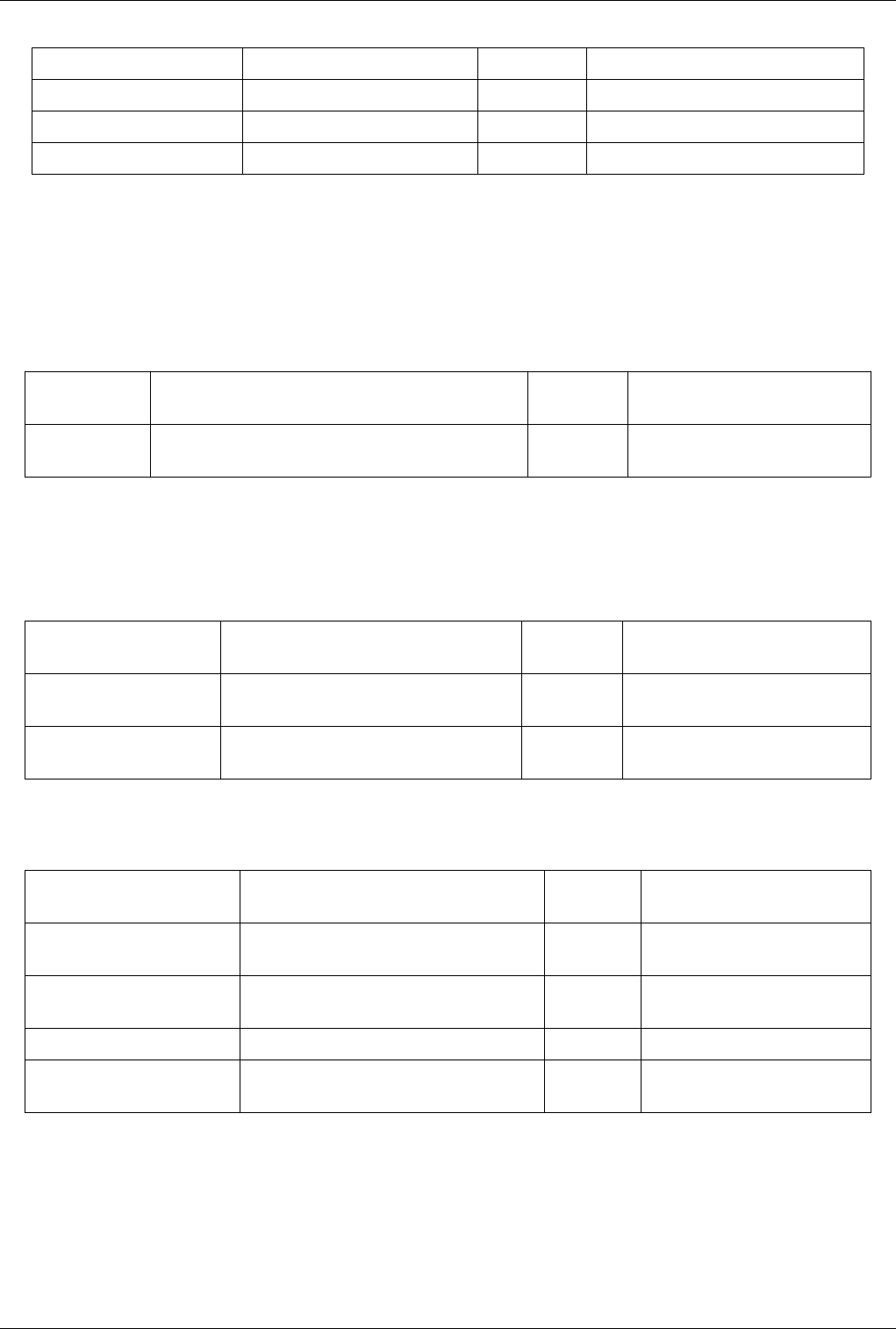
List of Readers 279
Property Description Default Value(s) Restrictions
FileName (FileName) The list of files to be read by the reader. The value(s) must be a filename (or filenames).
FileNameInfo (FileNameInfo)
TimestepValues (TimestepValues) Available timestep values.
Partitioned Legacy VTK Reader
Reads files stored in VTK partitioned legacy format.The Partitioned Legacy VTK reader loads files stored in VTK's
partitioned legac file format (before VTK 4.2, although still supported). The expected file extension is .pvtk. The
type of the dataset may be structured grid, uniform rectilinear grid (image/volume), non-uniform rectilinear grid,
unstructured grid, or polygonal.
Property Description Default
Value(s)
Restrictions
FileName
(FileName)
This property specifies the file name for the Partitioned Legacy
VTK reader.
The value(s) must be a filename (or
filenames).
Phasta Reader
Reads the parallel Phasta meta-file and the underlying Phasta files. This Phasta reader reads files stored in the Phasta
(a CFD package) format. The expected file extension is .pht. The output of this reader is a multipiece data set.
Property Description Default
Value(s)
Restrictions
FileName (FileName) This property specifies the file name for the Phasta
reader.
The value(s) must be a filename (or
filenames).
TimestepValues
(TimestepValues)
Available timestep values.
RTXMLPolyDataReader
Property Description Default
Value(s)
Restrictions
FileName (FileName) Set the file name for the real-time VTK polygonal
dataset reader.
The value(s) must be a filename (or
filenames).
Location (Location) Set the data directory containing real time data files. The value(s) must be a filename (or
filenames).
NextFileName (NextFileName)
NewDataAvailable
(NewDataAvailable)
2
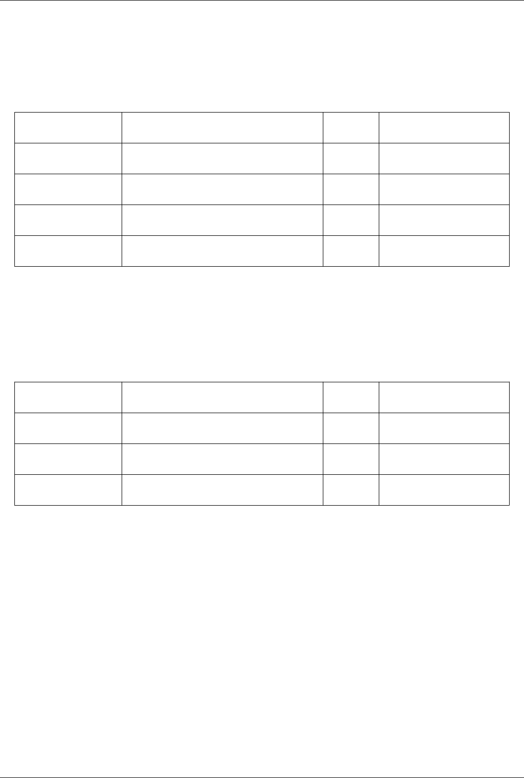
List of Readers 280
Restarted Sim Exodus Reader
Reads collections of Exodus output files from simulations that were restarted. When a simulation that outputs exodus
files is restarted, typically you get a new set of output files. When you read them in your visualization, you often
want to string these file sets together as if it was one continuous dump of files. This reader allows you to specify a
metadata file that will implicitly string the files together.
Property Description Default
Value(s)
Restrictions
FileNameInfo
(FileNameInfo)
FileName (FileName) This points to a special metadata file that lists the output
files for each restart.
The value(s) must be a filename (or
filenames).
UseMetaFile (UseMetaFile) This hidden property must always be set to 1 for this proxy
to work.
1 Accepts boolean values (0 or 1).
TimestepValues
(TimestepValues)
Restarted Sim Spy Plot Reader
Reads collections of SPCTH files from simulations that were restarted. When a CTH simulation is restarted,
typically you get a new set of output files. When you read them in your visualization, you often want to string these
file sets together as if it was one continuous dump of files. This reader allows you to specify a metadata file that will
implicitly string the files together.
Property Description Default
Value(s)
Restrictions
FileName (FileName) This points to a special metadata file that lists the output
files for each restart.
The value(s) must be a filename (or
filenames).
UseMetaFile (UseMetaFile) This hidden property must always be set to 1 for this proxy
to work.
1 Accepts boolean values (0 or 1).
TimestepValues
(TimestepValues)
SESAME Reader
Reads SESAME data files, producing rectilinear grids.The SESAME reader reads SESAME data files, and outputs
rectilinear grids. The expected file extension is .sesame.

List of Readers 281
Property Description Default
Value(s)
Restrictions
FileName (FileName) This property specifies the file name for the
SESAME reader.
The value(s) must be a filename (or
filenames).
TableId (TableId) This proeprty indicates which table to read. -1 The value(s) is an enumeration of the
following:
TableIds (TableIds)
TableArrayInfo
(TableArrayInfo)
SLAC Data Reader
A reader for a data format used by Omega3p, Tau3p, and several other tools used at the Standford Linear Accelerator
Center (SLAC). The underlying format uses netCDF to store arrays, but also imposes several conventions to form an
unstructured grid of elements.
Property Description Default
Value(s)
Restrictions
MeshFileName
(MeshFileName)
The name of the mesh file to load. The value(s) must be
a filename (or
filenames).
ModeFileName
(ModeFileName)
The name of the mode files to load. The points in the mode file should be the
same as the mesh file.
The value(s) must be
a filename (or
filenames).
ReadInternalVolume
(ReadInternalVolume)
If on, read the internal volume of the data set. 0 Accepts boolean
values (0 or 1).
ReadExternalSurface
(ReadExternalSurface)
If on, read the external surfaces of the data set. 1 Accepts boolean
values (0 or 1).
ReadMidpoints
(ReadMidpoints)
If on, reads midpoint information for external surfaces and builds quadratic
surface triangles.
0 Accepts boolean
values (0 or 1).
TimestepValues
(TimestepValues)
This magic property sends time information to the animation panel. ParaView
will then automatically set up the animation to visit the time steps defined in the
file.
TimeRange (TimeRange) This magic property sends time range information to the animation panel.
ParaView uses this information to set the range of time for the animation. This
property is important for when there are no timesteps but you still want to give
ParaView a range of values to use.
FrequencyScale
(FrequencyScale)
Sets the scale factor for each mode. By default, each scale factor is set to 1.
FrequencyScaleInfo
(FrequencyScaleInfo)
PhaseShift (PhaseShift) Sets the phase offset for each mode. By default, shift is set to 0.
PhaseShiftInfo
(PhaseShiftInfo)
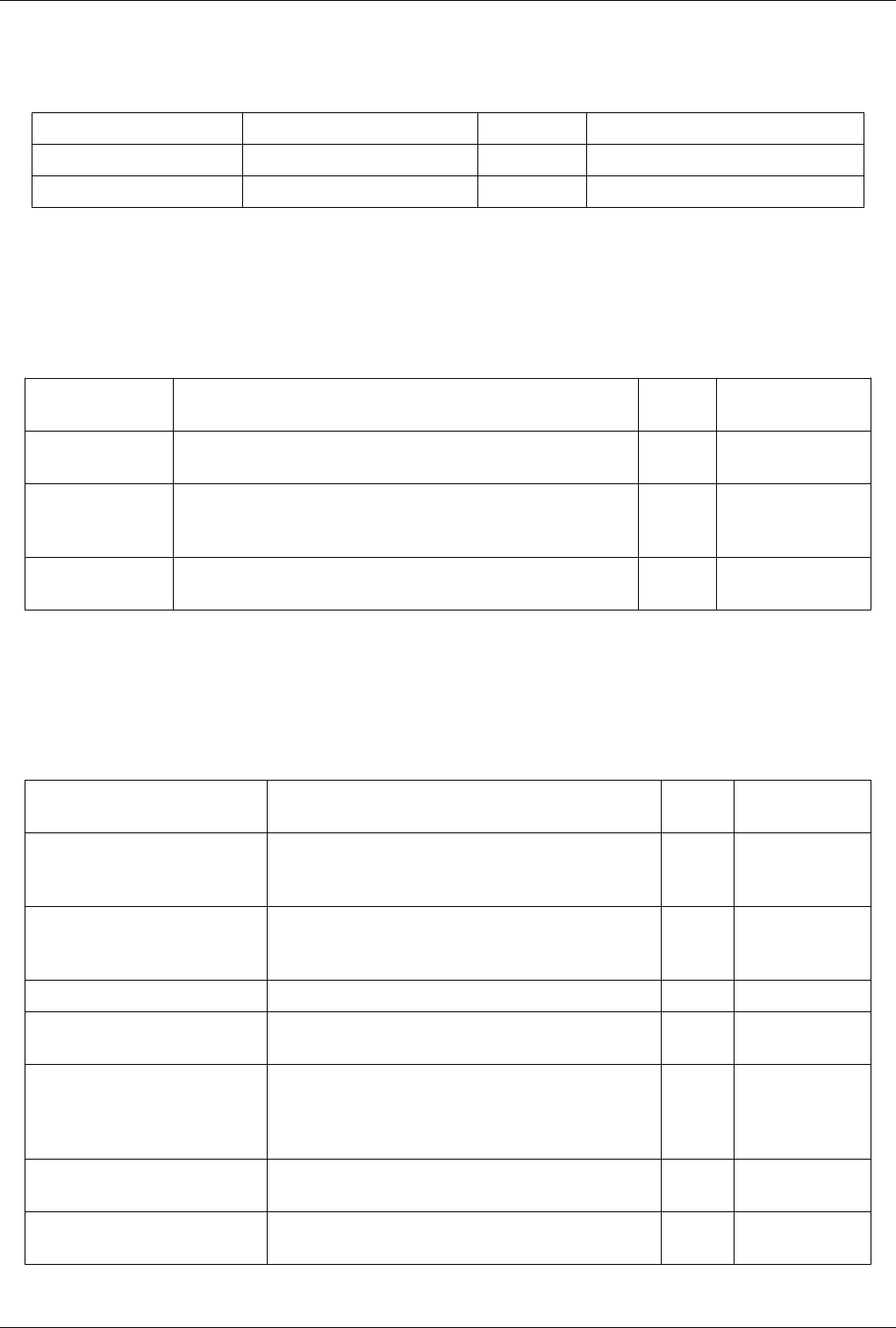
List of Readers 282
SLAC Particle Data Reader
The SLAC Particle data reader.
Property Description Default Value(s) Restrictions
FileName (FileName) A list of files to be read in a time series. The value(s) must be a filename (or filenames).
TimestepValues (TimestepValues) Available timestep values.
STL Reader
Reads ASCII or binary stereo lithography (STL) files.The STL reader reads ASCII or binary stereo lithography
(STL) files. The expected file extension is .stl. The output of this reader is a polygonal dataset. This reader also
supports file series.
Property Description Default
Value(s)
Restrictions
FileNameInfo
(FileNameInfo)
FileNames (FileNames) The list of files to be read by the reader. If more than one file is specified, the
reader will switch to file series mode in which it will pretend that it can support
time and provide one file per time step.
The value(s) must be a
filename (or filenames).
TimestepValues
(TimestepValues)
Available timestep values.
Spy Plot Reader
Reads files in the SPCTH Spy Plot file format.The Spy Plot reader loads an ASCII meta-file called the "case" file
(extension .spcth). The case file lists all the binary files containing the dataset. This reader produces hierarchical
datasets.
Property Description Default
Value(s)
Restrictions
Cell Arrays (CellArrayStatus) This property lists which cell-centered arrays to read. The list of array
names is provided by
the reader.
FileName (FileName) This property specifies the file name for the Spy Plot reader. The value(s) must be
a filename (or
filenames).
TimestepValues (TimestepValues) Available timestep values.
DownConvertVolumeFraction
(DownConvertVolumeFraction)
If this property is set to 0, the type of the volume fraction is float; is
set to 1, the type is unsigned char.
1 Accepts boolean
values (0 or 1).
ComputeDerivedVariables
(ComputeDerivedVariables)
If this property is set to 1, the reader will convert derived variables
like material density for the materials that the user has selected. For
Density the user needs to have selected Material Mass and Material
Volume Fraction.
1 Accepts boolean
values (0 or 1).
DistributeFiles (DistributeFiles) In parallel mode, if this property is set to 1, the reader will
distribute files or blocks.
1 Accepts boolean
values (0 or 1).
GenerateLevelArray
(GenerateLevelArray)
If this property is set to 1, a cell array will be generated that stores
the level of each block.
0 Accepts boolean
values (0 or 1).
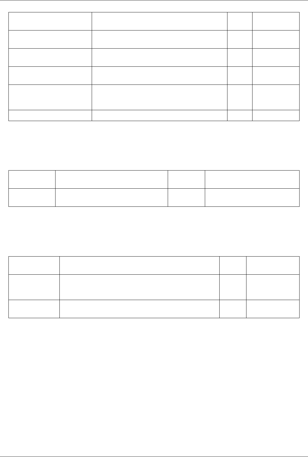
List of Readers 283
GenerateActiveBlockArray
(GenerateActiveBlockArray)
If this property is set to 1, a cell array will be generated that stores
the active status of a block.
0 Accepts boolean
values (0 or 1).
GenerateTracerArray
(GenerateTracerArray)
If this property is set to 1, a cell array will be generated that stores
the coordinates of any tracers.
0 Accepts boolean
values (0 or 1).
GenerateMarkers (GenerateMarkers) If this property is set to 1, a second output will be created using the
markers data stored in the file.
0 Accepts boolean
values (0 or 1).
GenerateBlockIdArray
(GenerateBlockIdArray)
If this property is set to 1, a cell array will be generated that stores a
unique blockId for each block.
0 Accepts boolean
values (0 or 1).
MergeXYZComponents
(MergeXYZComponents)
If this property is set to 1, cell arrays named (for example) X
velocity, Y velocity and Z velocity will be combined into a single
vector array named velocity.
1 Accepts boolean
values (0 or 1).
CellArrayInfo (CellArrayInfo)
TIFF Reader
Reads a TIFF file into an image data.The TIFF reader reads TIFF (Tagged Image File Format) files, and the output is
a uniform rectilinear (image/volume) dataset. The default file extension is .tiff.
Property Description Default
Value(s)
Restrictions
FileName
(FileName)
This property specifies the file name for the TIFF
reader.
The value(s) must be a filename (or
filenames).
TIFF Series Reader
Reads a series of TIFF files into an time sequence of image datas.The TIFF series reader reads TIFF files. The output
is a time sequence of uniform rectilinear (image/volume) dataset. The default file extension is .tif or .tiff.
Property Description Default
Value(s)
Restrictions
FileNames (FileNames) The list of files to be read by the reader. If more than one file is specified, the
reader will switch to file series mode in which it will pretend that it can support
time and provide one file per time step.
The value(s) must be a
filename (or filenames).
TimestepValues
(TimestepValues)
Available timestep values.
Tecplot Reader
Reads files in the Tecplot ASCII file format. The Tecplot reader extracts multiple zones (blocks) of data from a
Tecplot ASCII file, in which a zone is stored in either point packing mode (i.e., tuple-based, with only point data
supported) or block packing mode (i.e., component-based, with point data and cell data supported). The output of the
reader is a vtkMultiBlockDataset, of which each block is either a vtkStructuredGrid or a vtkUnstructuredGrid. This
supports reading a file series.
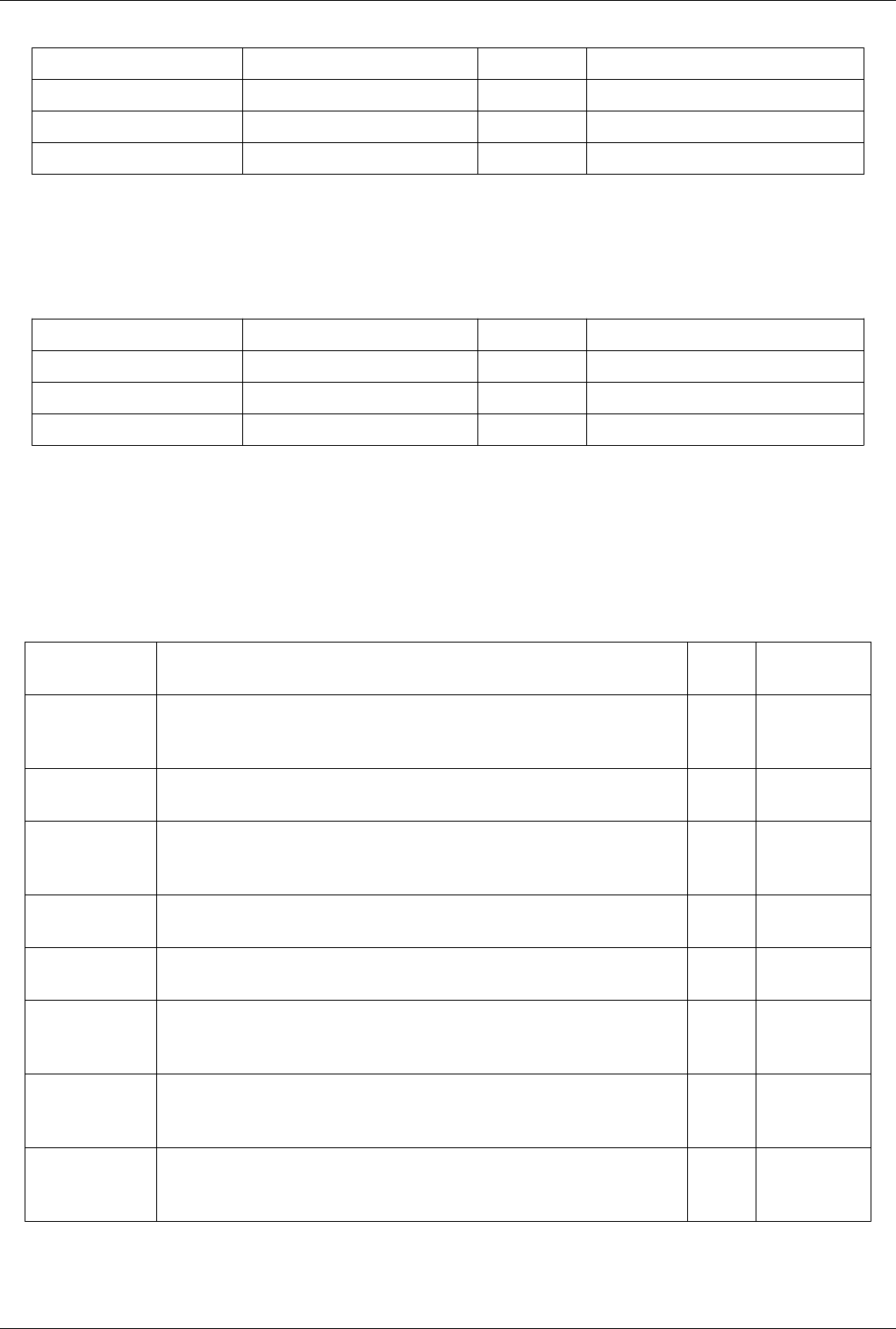
List of Readers 284
Property Description Default Value(s) Restrictions
FileNames (FileNames) The list of files to be read by the reader. The value(s) must be a filename (or filenames).
FileNameInfo (FileNameInfo)
TimestepValues (TimestepValues) Available timestep values.
Unstructured NetCDF POP reader
Reads rectilinear grid data from a NetCDF POP file and converts it into unstructured data. The reader reads regular
rectilinear grid (image/volume) data from a NetCDF file and turns it into an unstructured spherical grid.
Property Description Default Value(s) Restrictions
FileNameInfo (FileNameInfo)
FileName (FileName) The list of files to be read by the reader. The value(s) must be a filename (or filenames).
TimestepValues (TimestepValues) Available timestep values.
VPIC Reader
Reads distributed VPIC files into an ImageData.VPIC is a 3D kinetic plasma particle-in-cell simulation. The input
file (.vpc) opened by the VPIC reader is an ASCII description of the data files which are written one file per
processor, per category and per time step. These are arranged in subdirectories per category (field data and
hydrology data) and then in time step subdirectories.
Property Description Default
Value(s)
Restrictions
FileName
(FileName)
ASCII .vpc file describes locations of data files, grid sizes, time step sizes and type and
order of data written to the files.
The value(s) must
be a filename (or
filenames).
PointArrayInfo
(PointArrayInfo)
Point Arrays
(PointArrayStatus)
Variables written to the data files are described in the .vpc file and are presented for
selection. Only selected variables are loaded for a time step.
The list of array
names is provided
by the reader.
TimestepValues
(TimestepValues)
Stride (SetStride) VPIC data may be very large and not all is needed for effective visualization. Setting the
stride selects every nth data item within the files for display.
1 1 1
DefaultXExtent
(DefaultXExtent)
VPIC data is written one file per simulation processor. This coarse map of files is used in
partitioning files between visualizing processors so that each ParaView processor has its
own set of files to display. Default extent is all files available.
DefaultYExtent
(DefaultYExtent)
VPIC data is written one file per simulation processor. This coarse map of files is used in
partitioning files between visualizing processors so that each ParaView processor has its
own set of files to display. Default extent is all files available.
DefaultZExtent
(DefaultZExtent)
VPIC data is written one file per simulation processor. This coarse map of files is used in
partitioning files between visualizing processors so that each ParaView processor has its
own set of files to display. Default extent is all files available.

List of Readers 285
X Extent (XExtent) VPIC data is written one file per simulation processor. This coarse map of files is used in
partitioning files between visualizing processors so that each ParaView processor has its
own set of files to display. Ghost cell overlap is handled within the reader. To limit the
View of VPIC information the extent in the X dimension of "files" can be specified. Only
the files selected will be displayed and they will be partitioned between the visualizing
processors, allowing a higher resolution over a smaller area.
-1 -1
Y Extent (YExtent) VPIC data is written one file per simulation processor. This coarse map of files is used in
partitioning files between visualizing processors so that each ParaView processor has its
own set of files to display. Ghost cell overlap is handled within the reader. To limit the
View of VPIC information the extent in the Y dimension of "files" can be specified. Only
the files selected will be displayed and they will be partitioned between the visualizing
processors, allowing a higher resolution over a smaller area.
-1 -1
Z Extent (ZExtent) VPIC data is written one file per simulation processor. This coarse map of files is used in
partitioning files between visualizing processors so that each ParaView processor has its
own set of files to display. Ghost cell overlap is handled within the reader. To limit the
View of VPIC information the extent in the Z dimension of "files" can be specified. Only
the files selected will be displayed and they will be partitioned between the visualizing
processors, allowing a higher resolution over a smaller area.
-1 -1
VRML Reader
Load the geometry from a VRML 2.0 file.The VRML reader loads only the geometry from a VRML (Virtual Reality
Modeling Language) 2.0 file. The expected file extension is .wrl. The output of this reader is a polygonal dataset.
Property Description Default
Value(s)
Restrictions
FileName
(FileName)
This property specifies the file name for the VRML
reader.
The value(s) must be a filename (or
filenames).
Wavefront OBJ Reader
Reads Wavefront .OBJ files to produce polygonal and line data.The OBJ reader reads data stored in Wavefront .OBJ
format. The expected file extension is .obj, the datasets resulting from reading these files are polygons and lines.
Property Description Default
Value(s)
Restrictions
FileName
(FileName)
This property specifies the file name for the OBJ
reader.
The value(s) must be a filename (or
filenames).
WindBlade reader
Reads WindBlade/Firetec simulation files possibly including wind turbines and topology files. WindBlade/Firetec is
a simulation dealing with the effects of wind on wind turbines or on the spread of fires. It produces three outputs - a
StructuredGrid for the wind data fields, a StructuredGrid for the ground topology, and a PolyData for turning turbine
blades. The input file (.wind) opened by the WindBlade reader is an ASCII description of the data files expected.
Data is accumulated by the simulation processor and is written one file per time step. WindBlade can deal with
topology if a flag is turned on and expects (x,y) data for the ground. It also can deal with turning wind turbines from
other time step data files which gives polygon positions of segments of the blades and data for each segment.

List of Readers 286
Property Description Default
Value(s)
Restrictions
Filename (Filename) ASCII .wind file describes locations of data files, grid sizes and variable deltas,
time step sizes, whether topology is used, whether turbines are used, and type
and order of data written to the files.
The value(s) must be a
filename (or filenames).
TimestepValues
(TimestepValues)
PointArrayInfo
(PointArrayInfo)
Point Arrays
(PointArrayStatus)
Variables written to the data files are described in the .wind file and are
presented for selection. Only selected variables are loaded for a time step.
The list of array names is
provided by the reader.
XDMF Reader
Reads XDMF (eXtensible Data Model and Format) files.The XDMF reader reads files in XDMF format. The
expected file extension is .xmf. Metadata is stored in the XDMF file using an XML format, and large attribute arrays
are stored in a corresponding HDF5 file. The output may be unstructured grid, structured grid, or rectiliner grid. See
http:/ / www. xdmf. org for a description of the file format.
Property Description Default
Value(s)
Restrictions
FileName (FileName) This property specifies the file name for the XDMF reader. The value(s) must be a
filename (or filenames).
TimestepValues
(TimestepValues)
PointArrayInfo
(PointArrayInfo)
Point Arrays
(PointArrayStatus)
This property lists which point-centered arrays to read. The list of array names is
provided by the reader.
CellArrayInfo
(CellArrayInfo)
Cell Arrays
(CellArrayStatus)
This property lists which cell-centered arrays to read. The list of array names is
provided by the reader.
SetInfo (SetInfo)
Sets (SetStatus) Select the sets to be loaded from the dataset, if any. The list of array names is
provided by the reader.
GridInfo (GridInfo)
SILTimeStamp
(SILTimeStamp)
0
Grids (GridStatus) Controls which particular data sets to read from a file that contains many
data sets inside a composite data set collection.
Stride (Stride) If loading structured data, this property indicate the number of indices per
dimension (X, Y, or Z) to skip between each point included in this output.
1 1 1
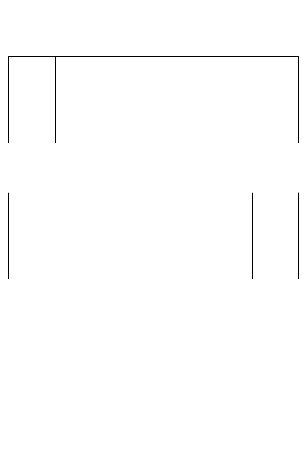
List of Readers 287
XML Hierarchical Box Data reader
Reads a VTK XML-based data file containing a hierarchical dataset containing vtkUniformGrids. The XML
Hierarchical Box Data reader reads VTK's XML-based file format containing a vtkHierarchicalBoxDataSet. The
expected file extensions is either .vthb or .vth.
Property Description Default
Value(s)
Restrictions
FileNameInfo
(FileNameInfo)
FileName (FileName) The list of files to be read by the reader. Each file is expected to be in the VTK XML
polygonal dataset format. The standard extension is .vtp. If more than one file is
specified, the reader will switch to file series mode in which it will pretend that it can
support time and provide one file per time step.
The value(s) must be
a filename (or
filenames).
TimestepValues
(TimestepValues)
Available timestep values.
XML Image Data Reader
Reads serial VTK XML image data files.The XML Image Data reader reads the VTK XML image data file format.
The standard extension is .vti. This reader also supports file series.
Property Description Default
Value(s)
Restrictions
FileNameInfo
(FileNameInfo)
FileName (FileName) The list of files to be read by the reader. Each file is expected to be in the VTK XML
image data format. The standard extension is .vti. If more than one file is specified, the
reader will switch to file series mode in which it will pretend that it can support time
and provide one file per time step.
The value(s) must be
a filename (or
filenames).
TimestepValues
(TimestepValues)
Available timestep values.
XML MultiBlock Data Reader
Reads a VTK XML multi-block data file and the serial VTK XML data files to which it points.The XML
Multi-Block Data reader reads the VTK XML multi-block data file format. XML multi-block data files are
meta-files that point to a list of serial VTK XML files. When reading in parallel, this reader will distribute
sub-blocks among processors. The expected file extensions are .vtm and .vtmb.

List of Readers 288
Property Description Default
Value(s)
Restrictions
FileNameInfo
(FileNameInfo)
FileName (FileName) The list of files to be read by the reader. Each file is expected to be in the VTK XML
polygonal dataset format. The standard extension is .vtp. If more than one file is
specified, the reader will switch to file series mode in which it will pretend that it can
support time and provide one file per time step.
The value(s) must be
a filename (or
filenames).
TimestepValues
(TimestepValues)
Available timestep values.
XML Partitioned Image Data Reader
Reads the summary file and the associated VTK XML image data files. The XML Partitioned Image Data reader
reads the partitioned VTK image data file format. It reads the partitioned format's summary file and then the
associated VTK XML image data files. The expected file extension is .pvti. This reader also supports file series.
Property Description Default
Value(s)
Restrictions
FileNameInfo
(FileNameInfo)
FileName (FileName) The list of files to be read by the reader. Each file is expected to be in the partitioned
VTK XML image data format. The standard extension is .pvti. If more than one file is
specified, the reader will switch to file series mode in which it will pretend that it can
support time and provide one file per time step.
The value(s) must be
a filename (or
filenames).
TimestepValues
(TimestepValues)
Available timestep values.
XML Partitioned Polydata Reader
Reads the summary file and the assicoated VTK XML polydata files.The XML Partitioned Polydata reader reads the
partitioned VTK polydata file format. It reads the partitioned format's summary file and then the associated VTK
XML polydata files. The expected file extension is .pvtp. This reader also supports file series.
Property Description Default
Value(s)
Restrictions
FileNameInfo
(FileNameInfo)
FileName
(FileName)
The list of files to be read by the reader. Each file is expected to be in the partitioned
VTK XML polygonal dataset format. The standard extension is .pvtp. If more than one
file is specified, the reader will switch to file series mode in which it will pretend that it
can support time and provide one file per time step.
The value(s) must be
a filename (or
filenames).
TimestepValues
(TimestepValues)
Available timestep values.
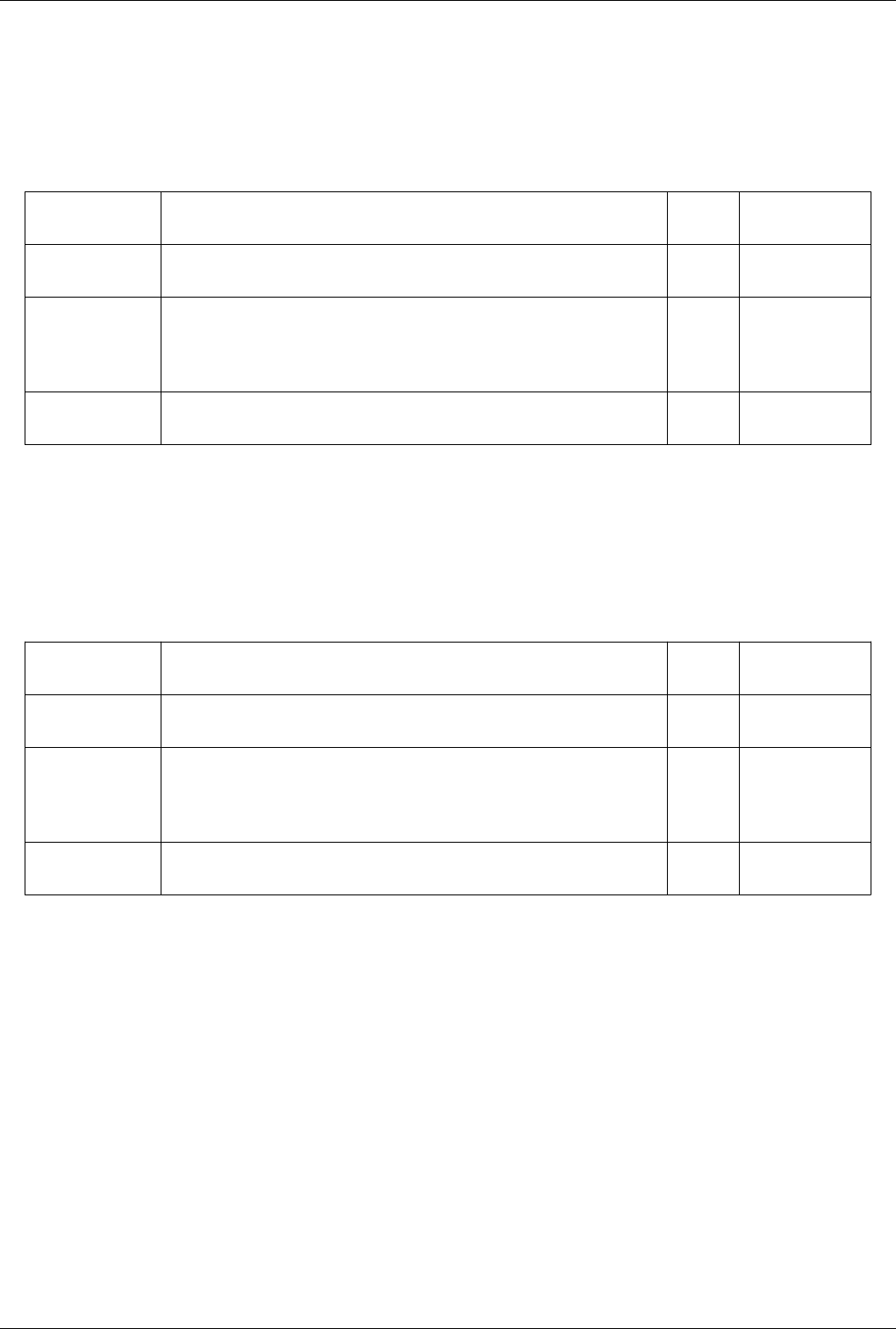
List of Readers 289
XML Partitioned Rectilinear Grid Reader
Reads the summary file and the associated VTK XML rectilinear grid data files. The XML Partitioned Rectilinear
Grid reader reads the partitioned VTK rectilinear grid file format. It reads the partitioned format's summary file and
then the associated VTK XML rectilinear grid files. The expected file extension is .pvtr. This reader also supports
file series.
Property Description Default
Value(s)
Restrictions
FileNameInfo
(FileNameInfo)
FileName
(FileName)
The list of files to be read by the reader. Each file is expected to be in the partitioned
VTK XML rectilinear grid data format. The standard extension is .pvtr. If more than
one file is specified, the reader will switch to file series mode in which it will pretend
that it can support time and provide one file per time step.
The value(s) must be
a filename (or
filenames).
TimestepValues
(TimestepValues)
Available timestep values.
XML Partitioned Structured Grid Reader
Reads the summary file and the associated VTK XML structured grid data files. The XML Partitioned Structured
Grid reader reads the partitioned VTK structured grid data file format. It reads the partitioned format's summary file
and then the associated VTK XML structured grid data files. The expected file extension is .pvts. This reader also
supports file series.
Property Description Default
Value(s)
Restrictions
FileNameInfo
(FileNameInfo)
FileName
(FileName)
The list of files to be read by the reader. Each file is expected to be in the partitioned
VTK XML structured grid data format. The standard extension is .pvts. If more than
one file is specified, the reader will switch to file series mode in which it will pretend
that it can support time and provide one file per time step.
The value(s) must be
a filename (or
filenames).
TimestepValues
(TimestepValues)
Available timestep values.
XML Partitioned Unstructured Grid Reader
Reads the summary file and the associated VTK XML unstructured grid data files. The XML Partitioned
Unstructured Grid reader reads the partitioned VTK unstructured grid data file format. It reads the partitioned
format's summary file and then the associated VTK XML unstructured grid data files. The expected file extension is
.pvtu. This reader also supports file series.

List of Readers 290
Property Description Default
Value(s)
Restrictions
FileNameInfo
(FileNameInfo)
FileName
(FileName)
The list of files to be read by the reader. Each file is expected to be in the partitioned
VTK XML unstructured grid data format. The standard extension is .pvtu. If more than
one file is specified, the reader will switch to file series mode in which it will pretend
that it can support time and provide one file per time step.
The value(s) must be
a filename (or
filenames).
TimestepValues
(TimestepValues)
Available timestep values.
XML PolyData Reader
Reads serial VTK XML polydata files.The XML Polydata reader reads the VTK XML polydata file format. The
standard extension is .vtp. This reader also supports file series.
Property Description Default
Value(s)
Restrictions
FileNameInfo
(FileNameInfo)
FileName (FileName) The list of files to be read by the reader. Each file is expected to be in the VTK XML
polygonal dataset format. The standard extension is .vtp. If more than one file is
specified, the reader will switch to file series mode in which it will pretend that it can
support time and provide one file per time step.
The value(s) must be
a filename (or
filenames).
TimestepValues
(TimestepValues)
Available timestep values.
XML Rectilinear Grid Reader
Reads serial VTK XML rectilinear grid data files.The XML Rectilinear Grid reader reads the VTK XML rectilinear
grid data file format. The standard extension is .vtr. This reader also supports file series.
Property Description Default
Value(s)
Restrictions
FileNameInfo
(FileNameInfo)
FileName (FileName) The list of files to be read by the reader. Each file is expected to be in the VTK XML
rectilinear grid data format. The standard extension is .vtr. If more than one file is
specified, the reader will switch to file series mode in which it will pretend that it can
support time and provide one file per time step.
The value(s) must be
a filename (or
filenames).
TimestepValues
(TimestepValues)
Available timestep values.
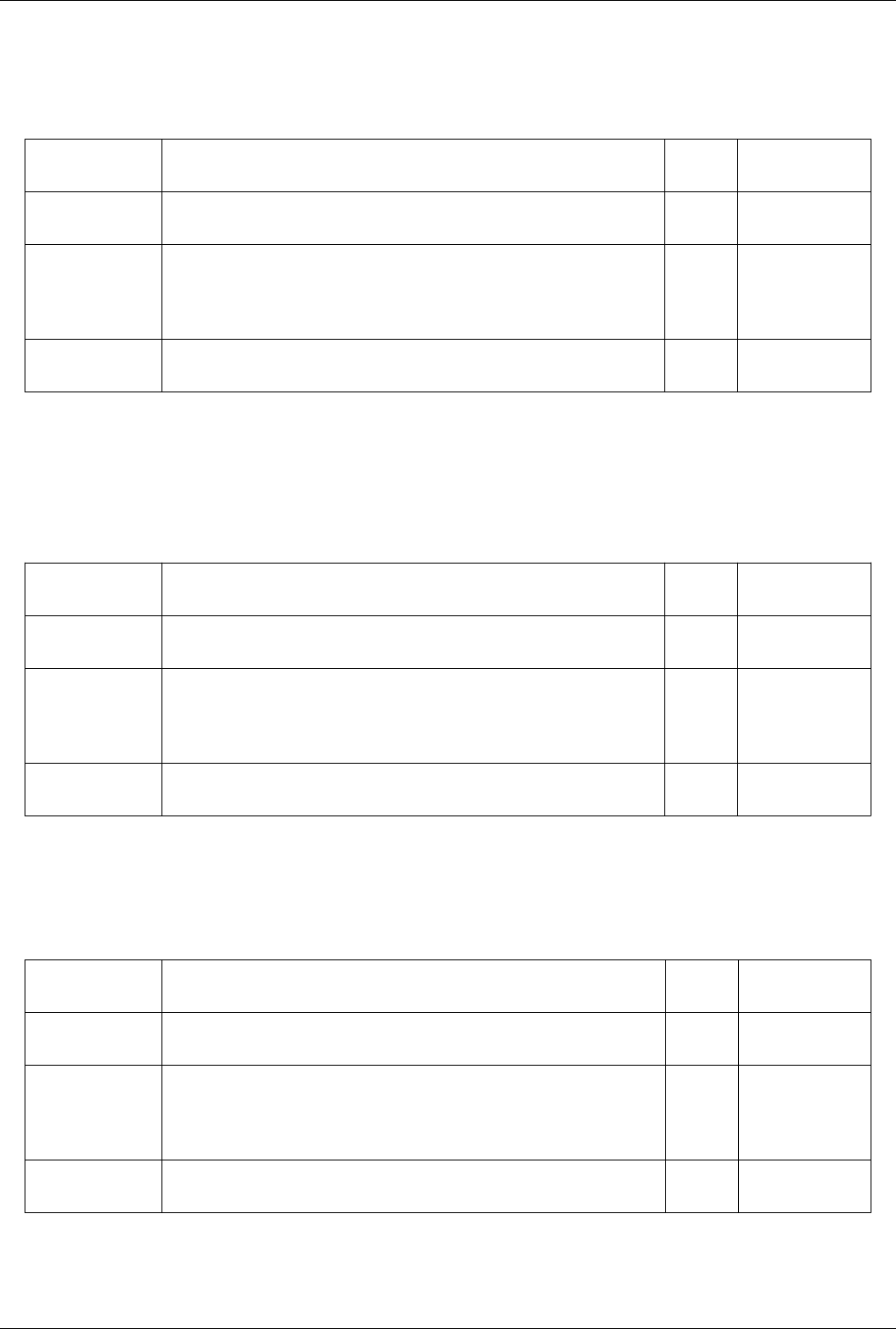
List of Readers 291
XML Structured Grid Reader
Reads serial VTK XML structured grid data files.The XML Structured Grid reader reads the VTK XML structured
grid data file format. The standard extension is .vts. This reader also supports file series.
Property Description Default
Value(s)
Restrictions
FileNameInfo
(FileNameInfo)
FileName (FileName) The list of files to be read by the reader. Each file is expected to be in the VTK XML
structured grid data format. The standard extension is .vts. If more than one file is
specified, the reader will switch to file series mode in which it will pretend that it can
support time and provide one file per time step.
The value(s) must be
a filename (or
filenames).
TimestepValues
(TimestepValues)
Available timestep values.
XML UniformGrid AMR Reader
Reads a VTK XML-based data file containing a AMR datasets . This reader reads Overlapping and
Non-Overlapping AMR datasets in VTK XML format. This reader reads the newer version of the format. For
version 1.0 and less, use XMLHierarchicalBoxDataReader. The expected file extensions is either .vthb or .vth.
Property Description Default
Value(s)
Restrictions
FileNameInfo
(FileNameInfo)
FileName (FileName) The list of files to be read by the reader. Each file is expected to be in the VTK XML
polygonal dataset format. The standard extension is .vtp. If more than one file is
specified, the reader will switch to file series mode in which it will pretend that it can
support time and provide one file per time step.
The value(s) must be
a filename (or
filenames).
TimestepValues
(TimestepValues)
Available timestep values.
XML Unstructured Grid Reader
Reads serial VTK XML unstructured grid data files. The XML Unstructured Grid reader reads the VTK XML
unstructured grid data file format. The standard extension is .vtu. This reader also supports file series.
Property Description Default
Value(s)
Restrictions
FileNameInfo
(FileNameInfo)
FileName (FileName) The list of files to be read by the reader. Each file is expected to be in the VTK XML
unstructured grid data format. The standard extension is .vtu. If more than one file is
specified, the reader will switch to file series mode in which it will pretend that it can
support time and provide one file per time step.
The value(s) must be
a filename (or
filenames).
TimestepValues
(TimestepValues)
Available timestep values.
List of Readers 292
XYZ Reader
Reads XYZ molecular data files into a polygonal dataset.The XYZ reader reads XYZ molecular data files. The
expected file extension is .xyz. The output of this reader is a polygonal dataset.
Property Description Default
Value(s)
Restrictions
FileName
(FileName)
This property specifies the file name for the XYZ reader. The value(s) must be a filename (or
filenames).
TimeStep
(TimeStep)
This property specifies the timestep the XYZ reader should
load.
0
proSTAR (STARCD) Reader
Reads geometry in proSTAR (STARCD) file format. ProStarReader creates an unstructured grid dataset. It reads
.cel/.vrt files stored in proSTAR (STARCD) ASCII format.
Property Description Default
Value(s)
Restrictions
FileName (FileName) Set the file name for the proSTAR (STARCD)
reader.
The value(s) must be a filename (or
filenames).
ScaleFactor
(ScaleFactor)
Scaling factor for the points 1
spcth history reader
Reads an spcth history file where each row translates into a single time step and the columns are points, materials
and properties.
Property Description Default
Value(s)
Restrictions
FileName (FileName) This property specifies the file name for the VRML
reader.
The value(s) must be a filename
(or filenames).
CommentCharacter
(CommentCharacter)
This property lists the characters that is used as the first
character on comment lines
%
Delimeter (Delimeter) Character that is used as the delimeter. ,
TimestepValues
(TimestepValues)
Available timestep values.
List of Sources 293
List of Sources
2D Glyph
Create a 2D glyph (e.g., arrow, cross, dash, etc.)The 2D Glyph source is used for generating a family of 2D glyphs,
each of which lies in the x-y plane. The output of the 2D Glyph source is polygonal data.
Property Description Default
Value(s)
Restrictions
GlyphType
(GlyphType)
This property specifies the type of the 2D glyph. 9 The value(s) is an
enumeration of the following:
• Vertex (1)
• Dash (2)
• Cross (3)
• ThickCross (4)
• Triangle (5)
• Square (6)
• Circle (7)
• Diamond (8)
• Arrow (9)
• ThickArrow (10)
• HookedArrow (11)
• EdgeArrow (12)
Filled (Filled) If the value of this property is 1, the 2D glyph will be a filled polygon; otherwise,
only the edges (line segments) will be included in the output. This only applies to
closed 2D glyphs.
0 Accepts boolean values (0 or
1).
Center (Center) Set the x, y, z coordinates of the origin of the 2D glyph. 0.0 0.0 0.0
3D Text
3D geometric representation of a text stringThe 3D Text source displays a text string as polygonal data.
Property Description Default
Value(s)
Restrictions
Text
(Text)
This property contains the text string to be displayed. The ASCII alphanumeric characters a-z, A-Z, and
0-9 are supported; so are ASCII punctuation marks. The only supported control character is "\n", which
inserts a new line in the text string.
3D Text
AMR GaussianPulse Source
Create AMR dataset w/ Gaussian PulseAMR dataset source, used for generating sample Berger-Collela AMR dataset
with a Gaussian Pulse field at the center.
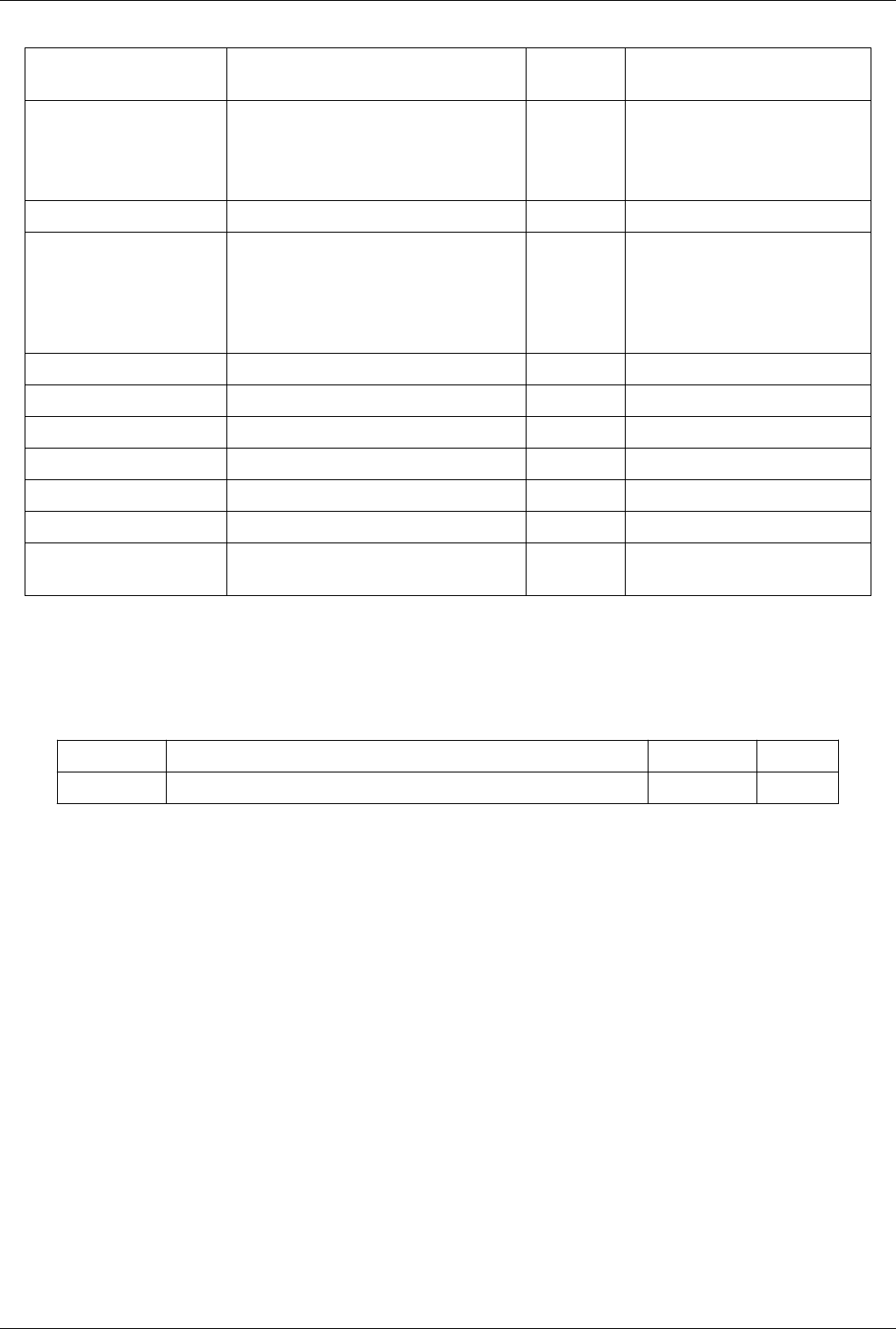
List of Sources 294
Property Description Default
Value(s)
Restrictions
Dimension (Dimension) Sets the desired dimension for the AMR dataset to
generate.
3 The value(s) is an enumeration of the
following:
• 2D (2)
• 3D (3)
Root Spacing (Root Spacing) Set the spacing at level 0. 0.5
RefinementRatio
(RefinementRatio)
Sets the desired dimension for the AMR dataset to
generate.
2 The value(s) is an enumeration of the
following:
• 2 (2)
• 3 (3)
• 4 (4)
XPulseOrigin (XPulseOrigin) Set x-coordinate for the pulse origin 0.0
YPulseOrigin (YPulseOrigin) Set y-coordinate for the pulse origin 0.0
ZPulseOrigin (ZPulseOrigin) Set z-coordinate for the pulse origin 0.0
XPulseWidth (XPulseWidth) Set x-coordinate for the pulse Width 0.5
YPulseWidth (YPulseWidth) Set y-coordinate for the pulse Width 0.5
ZPulseWidth (ZPulseWidth) Set z-coordinate for the pulse Width 0.5
PulseAmplitude
(PulseAmplitude)
Sets the amplitude of the pulse 0.5
Annotate Time
Shows the animation time as text annnotation in the view.The Annotate Time source can be used to show the
animation time in text annotation.
Property Description Default Value(s) Restrictions
Format (Format) This property specifies the format used to display the input time (using printf style). Time: %f
Arrow
3D arrow with a long cylindrical shaft and a cone for the tipThe Arrow source appends a cylinder to a cone to form a
3D arrow. The length of the whole arrow is 1.0 unit. The output of the Arrow source is polygonal data. This
polygonal data will not contain normals, so rendering of the arrow will be performed using flat shading. The
appearance of the arrow can be improved without significantly increasing the resolution of the tip and shaft by
generating normals. (Use Normals Generation filter).
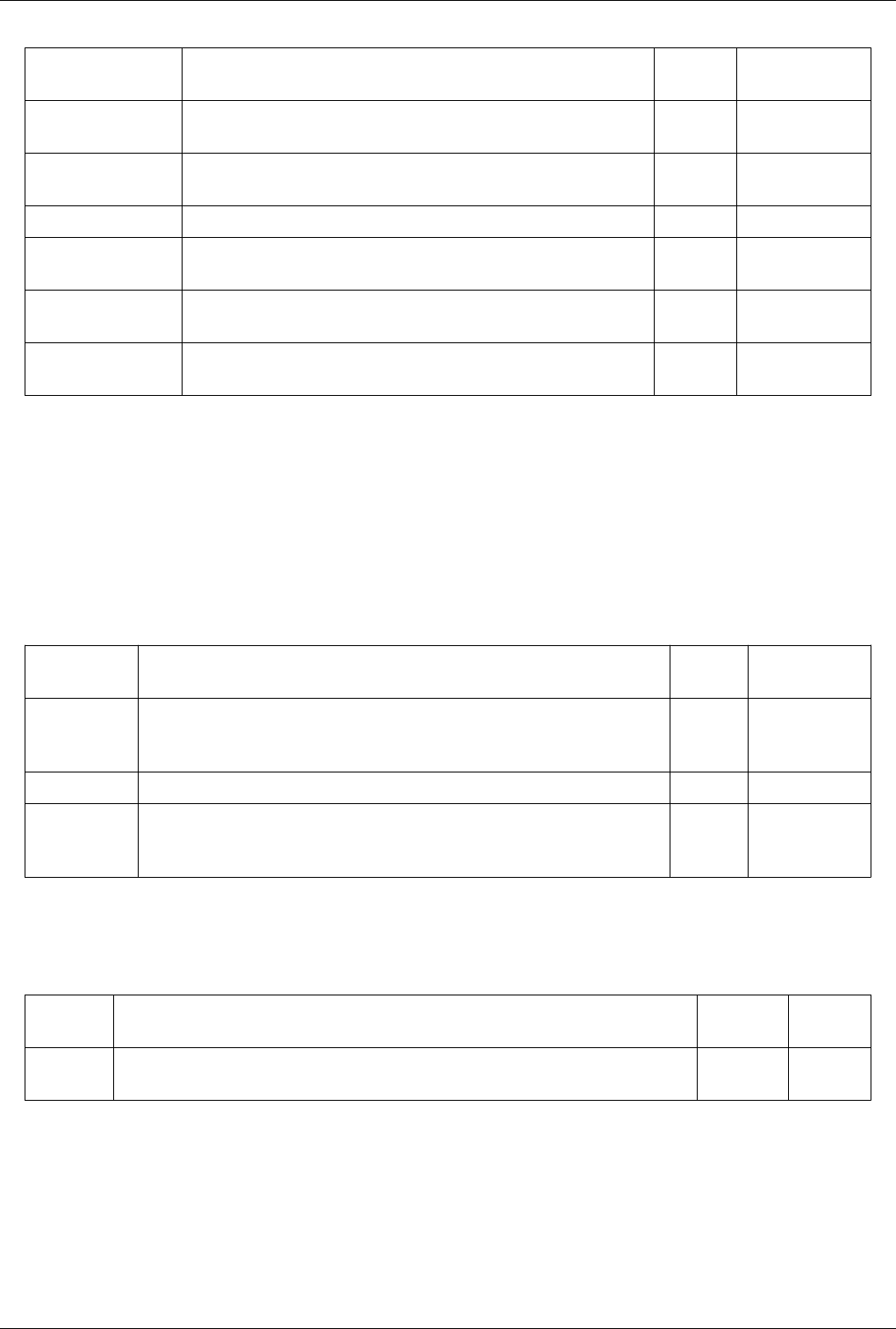
List of Sources 295
Property Description Default
Value(s)
Restrictions
TipResolution
(TipResolution)
This property specifies the number of faces in the representation of the tip of the
arrow (the cone). As the resolution increases, the cone will become smoother.
6
TipRadius (TipRadius) This property specifies the radius of the widest part of the tip of the arrow (the
cone).
0.1
TipLength (TipLength) This property specifies the length of the tip. 0.35
ShaftResolution
(ShaftResolution)
This property specifies the number of faces of the shaft of the arrow (the
cylinder). As the resolution increases, the cylinder will become smoother.
6
ShaftRadius
(ShaftRadius)
This property specifies the radius of the shaft of the arrow (the cylinder). 0.03
Invert (Invert) Inverts the arrow direction. 0 Accepts boolean
values (0 or 1).
Axes
Three lines representing the axes - red line along X, green line along Y, and blue line along Z The Axes source can
be used to add a representation of the coordinate system axes to the 3D scene. The X axis will be drawn as a blue
line, the Y axis as a green line, and the Z axis as a red line. The axes can be drawn either as three lines drawn in the
positive direction from the origin or as three lines crossing at the origin (drawn in both the positive and negative
directions). The output of the Axes source is polygonal data. This polygonal data has a scalar per line so that the
lines can be colored. It also has normals defined.
Property Description Default
Value(s)
Restrictions
ScaleFactor
(ScaleFactor)
By default the axes lines have a length of 1 (or 1 in each direction, for a total length of 2, if
value of the Symmetric property is 1). Increasing or decreasing the value of this property
will make the axes larger or smaller, respectively.
1.0
Origin (Origin) The values of this property set the X, Y, and Z coordinates of the origin of the axes. 0.0 0.0 0.0
Symmetric
(Symmetric)
When this property is set to 1, the axes extend along each of the positive and negative
directions for a distance equal to the value of the Scale Factor property. When set to 0, the
axes extend only in the positive direction.
0 Accepts boolean
values (0 or 1).
BlockSelectionSource
BlockSelectionSource is a source producing a block-based selection used to select blocks from a composite dataset.
Property Description Default
Value(s)
Restrictions
Blocks
(Blocks)
The list of blocks that will be added to the selection produced by the selection source. The blocks are
identified using their composite index (flat index).
0
List of Sources 296
Box
Create a box with specified X, Y, and Z lengths.The Box source can be used to add a box to the 3D scene. The
output of the Box source is polygonal data containing both normals and texture coordinates.
Property Description Default Value(s) Restrictions
XLength (XLength) This property specifies the length of the box in the X direction. 1.0
YLength (YLength) This property specifies the length of the box in the Y direction. 1.0
ZLength (ZLength) This property specifies the length of the box in the Z direction. 1.0
Center (Center) This property specifies the center of the box. 0.0 0.0 0.0
CompositeDataIDSelectionSource
CompositeDataIDSelectionSource used to create an ID based selection for composite datasets (Multiblock or
HierarchicalBox dataset).
Property Description Default
Value(s)
Restrictions
IDs
(IDs)
The list of IDs that will be added to the selection produced by the selection source. This takes 3-tuple of
values as (flat-index, process number, id).
0 0 0
Cone
Create a 3D cone of a given radius and height.The Cone source can be used to add a polygonal cone to the 3D scene.
The output of the Cone source is polygonal data.
Property Description Default
Value(s)
Restrictions
Resolution
(Resolution)
This property indicates the number of divisions around the cone. The higher this number,
the closer the polygonal approximation will come to representing a cone, and the more
polygons it will contain.
6
Radius (Radius) This property specifies the radius of the base of the cone. 0.5
Height (Height) This property specifies the height of the cone. 1.0
Center (Center) This property specifies the center of the cone. 0.0 0.0 0.0
Direction
(Direction)
Set the orientation vector of the cone. The vector does not have to be normalized. The cone
will point in the direction specified.
1.0 0.0 0.0
Capping
(Capping)
If this property is set to 1, the base of the cone will be capped with a filled polygon.
Otherwise, the base of the cone will be open.
1 Accepts boolean
values (0 or 1).

List of Sources 297
Cylinder
Create a 3D cylinder of a given radius and height.The Cylinder source can be used to add a polygonal cylinder to the
3D scene. The output of the Cylinder source is polygonal data containing both normals and texture coordinates.
Property Description Default
Value(s)
Restrictions
Resolution
(Resolution)
This property indicates the number of divisions around the cylinder. The higher this number,
the closer the polygonal approximation will come to representing a cylinder, and the more
polygons it will contain.
6
Height (Height) This property specifies the height of the cylinder (along the y axis). 1.0
Radius (Radius) This property specifies the radius of the cylinder. 0.5
Center (Center) This property specifies the coordinate value at the center of the cylinder. 0.0 0.0 0.0
Capping
(Capping)
If this property is set to 1, the ends of the cylinder will each be capped with a closed
polygon. Otherwise, the ends of the cylinder will be open.
1 Accepts boolean
values (0 or 1).
Data Object Generator
Parses a string to produce composite data objects consisting of simple templated datasets. vtkDataObjectGenerator
parses a string and produces dataobjects from the dataobject template names it sees in the string. For example, if the
string contains "ID1" the generator will create a vtkImageData. "UF1", "RG1", "SG1", "PD1", and "UG1" will
produce vtkUniformGrid, vtkRectilinearGrid, vtkStructuredGrid, vtkPolyData and vtkUnstructuredGrid respectively.
"PD2" will produce an alternate vtkPolydata. You can compose composite datasets from the atomic ones listed
above - "MB{}" or "HB[]". "MB{ ID1 PD1 MB{} }" for example will create a vtkMultiBlockDataSet consisting of
three blocks: image data, poly data, multi-block (empty). Hierarchical Box data sets additionally require the notion
of groups, declared within "()" braces, to specify AMR depth. "HB[ (UF1)(UF1)(UF1) ]" will create a
vtkHierarchicalBoxDataSet representing an octree that is three levels deep, in which the firstmost cell in each level is
refined.
Property Description Default
Value(s)
Restrictions
Program
(Program)
This property contains the string that is parsed to determine the structured of the output data
object to produce.
ID1
Disk
Create a 3D disk with a specified inner and outer radius.The Disk source can be used to add a polygonal disk to the
3D scene. The output of the Disk source is polygonal data.
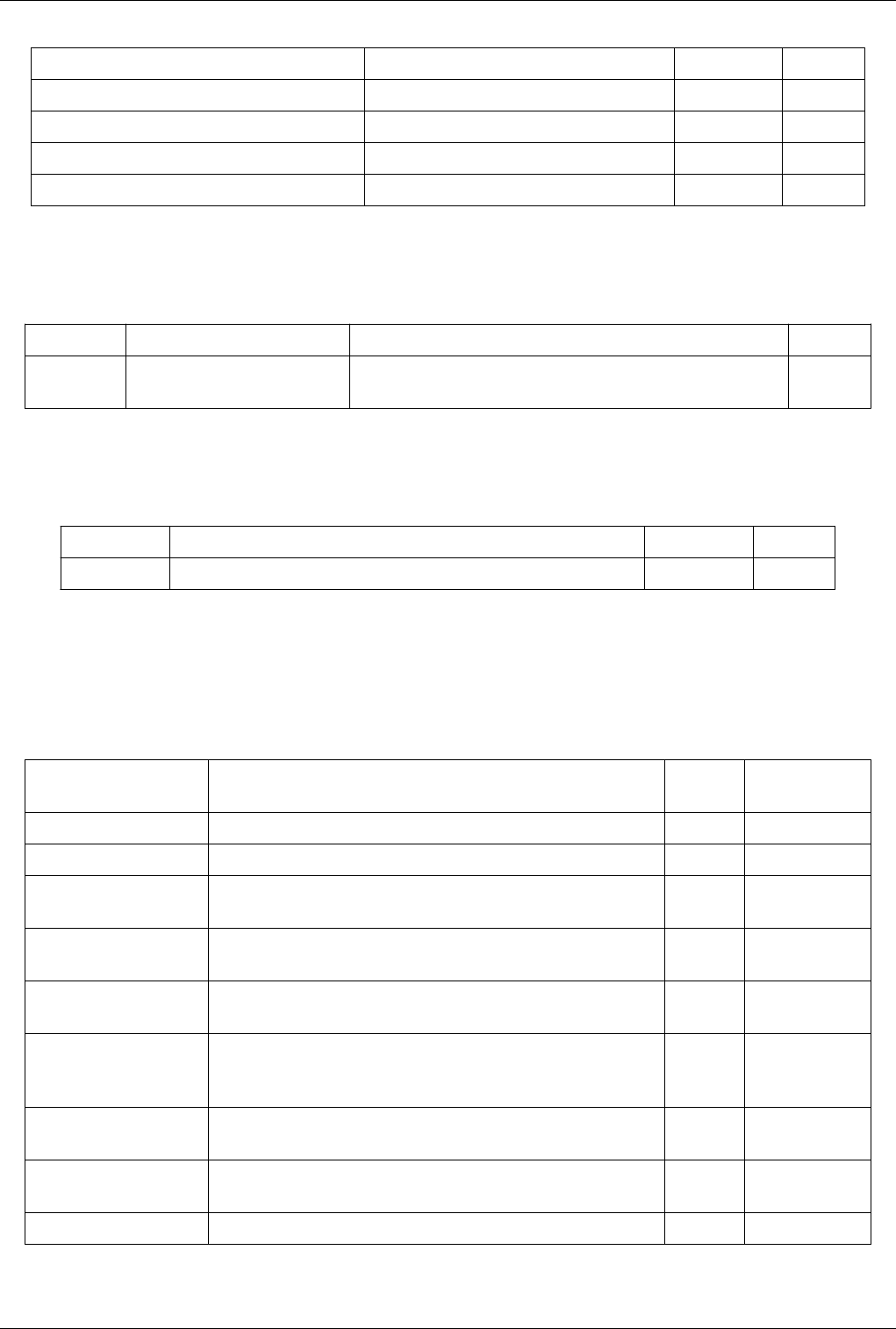
List of Sources 298
Property Description Default Value(s) Restrictions
InnerRadius (InnerRadius) Specify inner radius of hole in disc. 0.5
OuterRadius (OuterRadius) Specify outer radius of disc. 1.0
RadialResolution (RadialResolution) Set the number of points in radial direction. 8
CircumferentialResolution (CircumferentialResolution) Set the number of points in circumferential direction. 8
FrustumSelectionSource
FrustumSelectionSource is a source producing a frustum selection.
Property Description Default Value(s) Restrictions
Frustum
(Frustum)
Vertices that define a frustum for the
selection source.
0.0 0.0 1.0 0.0 0.0 0.0 0.0 0.0 0.0 1.0 1.0 0.0 0.0 1.0 0.0 0.0 1.0 0.0 1.0 0.0
1.0 0.0 0.0 0.0 1.0 1.0 1.0 0.0 1.0 1.0 0.0 0.0
GlobalIDSelectionSource
GlobalIDSelectionSource is a source producing a global ID based selection.
Property Description Default Value(s) Restrictions
Global IDs (IDs) The list of IDs that will be added to the selection produced by the selection source. 0
Hierarchical Fractal
Test source for AMR with HierarchicalDataSetThe Hierarchical Fractal source is a collection of uniform grids. All
have the same dimensions. Each block has a different origin and spacing. This source uses the Mandelbrot source to
create cell data. The fractal array is scaled to look like a volume fraction.
Property Description Default
Value(s)
Restrictions
Dimensions (Dimensions) This property specifies the X, Y, Z cell dimensions of a block. 10
FractalValue (FractalValue) The value of this property will be mapped to 0.5 for use as a volume fraction. 9.5
MaximumLevel
(MaximumLevel)
This property specifies how many levels of refinement should be included in
this hierarchical dataset.
5
GhostLevels (GhostLevels) This property specifies whether ghost levels should be generated at processor
boundaries.
1 Accepts boolean
values (0 or 1).
TwoDimensional
(TwoDimensional)
If this property is set to 1, the generated dataset will be 2D; otherwise it will be
3D.
1 Accepts boolean
values (0 or 1).
Asymetric (Asymetric) If this property is set to 0, all the blocks will be the same size. If it is set to 1,
an asymmetric dataset will be created: some blocks will have an X dimension
that is larger by 2 units.
0 Accepts boolean
values (0 or 1).
RectilinearGrids
(RectilinearGrids)
If this property is set to 1, the hierarchical dataset will contain rectilinear grids;
otherwise it will contain uniform grids.
0 Accepts boolean
values (0 or 1).
TimeStepRangeInfo
(TimeStepRangeInfo)
TimeStep (TimeStep) This property specifies the timestep to use for this dataset. 0
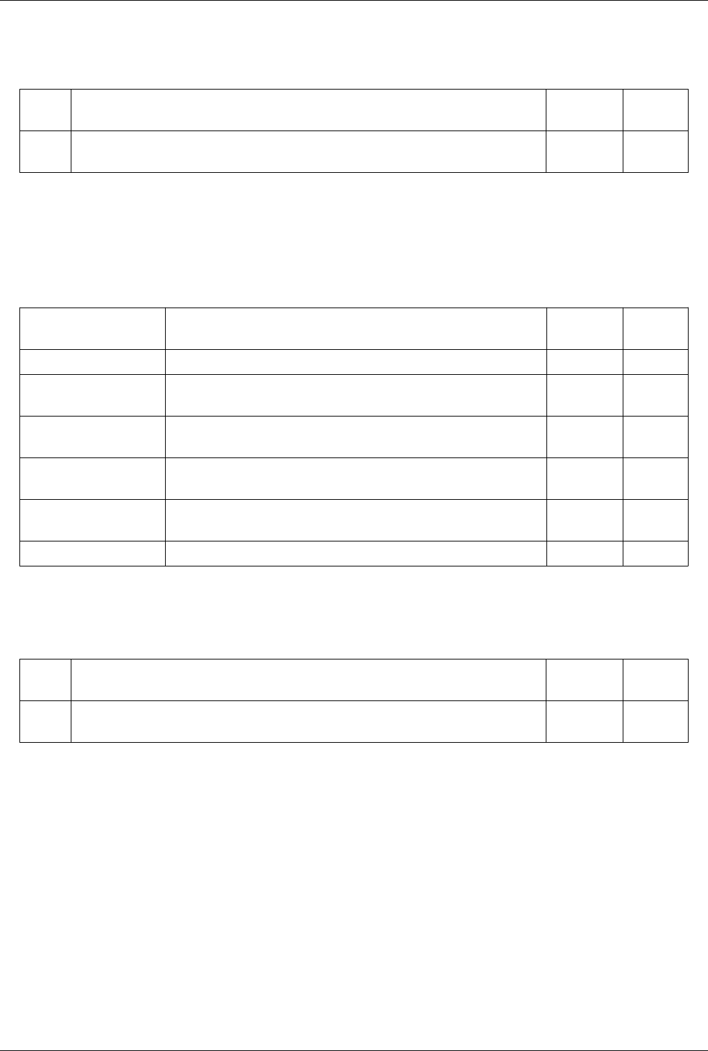
List of Sources 299
HierarchicalDataIDSelectionSource
HierarchicalDataIDSelectionSource used to create an ID based selection for HierarchicalBox datasets.
Property Description Default
Value(s)
Restrictions
IDs
(IDs)
The list of IDs that will be added to the selection produced by the selection source. This takes 3-tuple of
values as (level, index, id).
0 0 0
Hyper Tree Grid
Hyper tree grid representing a tree-based AMR data setThis source uses input parameters, most notably a string
descriptor, to generate a vtkHyperTreeGrid instance representing the corresponding a tree-based AMR grid with
arbitrary rectilinear geometry and either binary or ternary subdivision.
Property Description Default
Value(s)
Restrictions
Dimension (Dimension) This property specifies the dimensionality of the hyper tree grid. 3
GridSize (GridSize) The three values in this property specify the number of root cells in each dimension
of the hyper tree grid.
1 1 1
GridScale (GridScale) The three values in this property specify the scale of the root cells in each
dimension of the hyper tree grid.
1 1 1
BranchFactor (BranchFactor) This property specifies the subdivision scheme (binary or ternary) of the hyper tree
grid.
2
MaximumLevel
(MaximumLevel)
The value of this property specifies the maximum number of levels in the hyper
tree grid.
1
Descriptor (Descriptor) This property specifies the string used to describe the hyper tree grid. .
IDSelectionSource
IDSelectionSource is a source producing a ID based selection. This cannot be used for selecting composite datasets.
Property Description Default
Value(s)
Restrictions
IDs
(IDs)
The list of IDs that will be added to the selection produced by the selection source. This takes pairs of
values as (process number, id).
0 0
Line
This source creates a line between two points. The resolution indicates how many segments are in the line.The Line
source can be used to interactively (using a 3D widget) or manually (using the entries on the user interface) add a
line to the 3D scene. The output of the Line source is polygonal data.
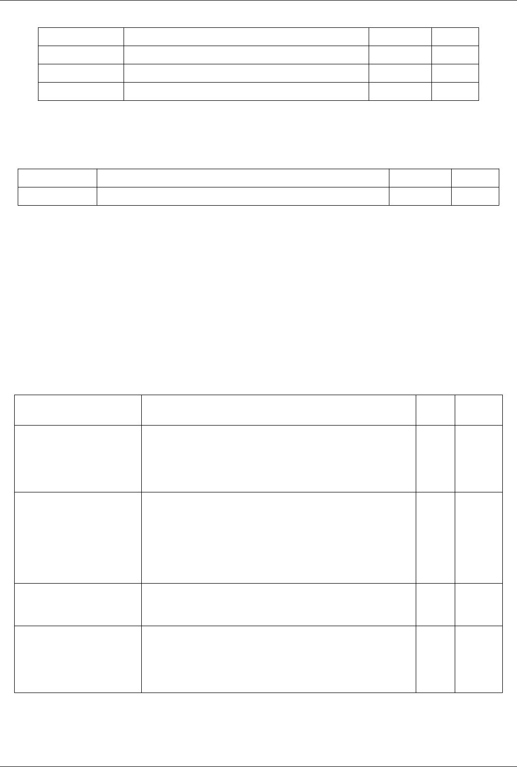
List of Sources 300
Property Description Default Value(s) Restrictions
Point1 (Point1) This property controls the coordinates of the first endpoint of the line. -0.5 0.0 0.0
Point2 (Point2) This property controls the coordinates of the second endpoint of the line. 0.5 0.0 0.0
Resolution (Resolution) This property specifies the number of pieces into which to divide the line. 6
LocationSelectionSource
LocationSelectionSource is used to create a location based selection.
Property Description Default Value(s) Restrictions
Locations (Locations) The list of locations that will be added to the selection produced by the selection source. 0 0 0
Mandelbrot
Representation (unsigned char) of the Mandlebrot set in up to 3 dimensionsThe Mandelbrot source can be used to
add a uniform rectilinear grid with scalar values derived from the Mandelbrot set to the 3D scene. The equation used
is z = z^2 + C (where z and C are complex, and C is a constant). The scalar values in the grid are the number of
iterations of the equation it takes for the magnitude of the value to become greater than 2. In the equation, the initial
value of z is 0. By default, the real component of C is mapped onto the X axis; the imaginary component of C is
mapped onto the Y axis; and the imaginary component of the initial value is mapped onto the Z axis. If a
two-dimensional extent is specified, the resulting image will be displayed. If a three-dimensional extent is used, then
the bounding box of the volume will be displayed. The output of the Mandelbrot source is image (uniform
rectilinear) data.
Property Description Default
Value(s)
Restrictions
WholeExtent (WholeExtent) The six values in the property indicate the X, Y, and Z extent of the output data.
The first two numbers are the minimum and maximum X extent; the next two are
the minimum and maximum Y extent; and the final two are the minimum and
maximum Z extent. The numbers are inclusive, so values of 0, 250, 0, 250, 0, 0
indicate that the dimensions of the output will be 251 x 251 x 1.
0 250 0
250 0 0
ProjectionAxes (ProjectionAxes) The three values in this property allow you to specify the projection from the 4D
space used by the Mandelbrot set to the axes of the 3D volume. By default, the
real component of C (represented by 0) is mapped to the X axis; the imaginary
component of C (represented by 1) is mapped to the Y axis; and the real
component of X, the initial value (represented by 2) is mapped to the Z axis. The
imaginary component of X is represented by 3. All values entered must be
between 0 and 3, inclusive.
0 1 2
OriginCX (OriginCX) The four values of this property indicate (in order) the components of C (real and
imaginary) and the components of the initial value, X (real and imaginary).
-1.75
-1.25 0.0
0.0
SizeCX (SizeCX) The four values of this property indicate the length of the output in each of the
four dimensions (the real and imaginary components of C and the real and
imaginary components of X). The three dimensions specified in the Projection
Axes property will determine which of these values specify the length of the axes
in the output.
2.5 2.5
2.0 1.5
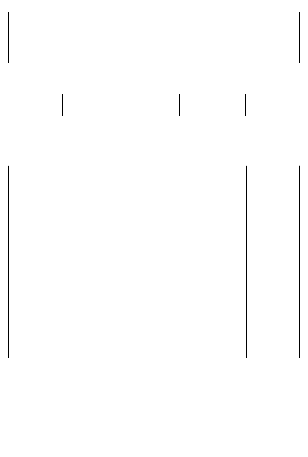
List of Sources 301
Maximum Number of Iterations
(MaximumNumberOfIterations)
The value of this property specifies the limit on computational iterations (i.e., the
maximum number of iterations to perform to determine if the value will go above
2). Values less than 2.0 after the specified number of iterations are considered in
the fractal set.
100
SubsampleRate (SubsampleRate) This property specifies the rate at which to subsample the volume. The extent of
the dataset in each dimension will be divided by this value.
1
NetworkImageSource
Property Description Default Value(s) Restrictions
FileName (FileName) Set the name of image file to load.
Octree Fractal
Test source for octree with Mandelbrot fractalCreate an octree from a Mandelbrot fractal. See the Mandelbrot source
for a description of the variables used.
Property Description Default
Value(s)
Restrictions
Dimension (Dimension) This property specifies the dimensionality of the fractal: 1D - Binary tree line,
2D - Quadtree plane, 3D - Octree volume.
2
MaximumLevel (MaximumLevel) This property specifies the maximum refinement level for the grid. 5
MinimumLevel (MinimumLevel) This property specifies the minimum refinement level for the grid. 3
ProjectionAxes (ProjectionAxes) This property indicates which axes of the dataset to display. See Mandelbrot
source for a description of the possible axes.
0 1 2
OriginCX (OriginCX) This property specifies the imaginary and real values for C (constant) and X
(initial value). See Mandelbrot source for a description of the C and X
variables.
-1.75
-1.25 0.0
0.0
SizeCX (SizeCX) The four values of this property indicate the length of the output in each of the
four dimensions (the real and imaginary components of C and the real and
imaginary components of X). The three dimensions specified in the Projection
Axes property will determine which of these values specify the length of the
axes in the output.
2.5 2.5 2.0
1.5
Maximum Number of Iterations
(MaximumNumberOfIterations)
The value of this property specifies the limit on computational iterations (i.e.,
the maximum number of iterations to perform to determine if the value will go
above 2). Values less than 2.0 after the specified number of iterations are
considered in the fractal set.
100
Threshold (Threshold) This property specifies a threshold value that determines when to subdivide a
leaf node.
2.0
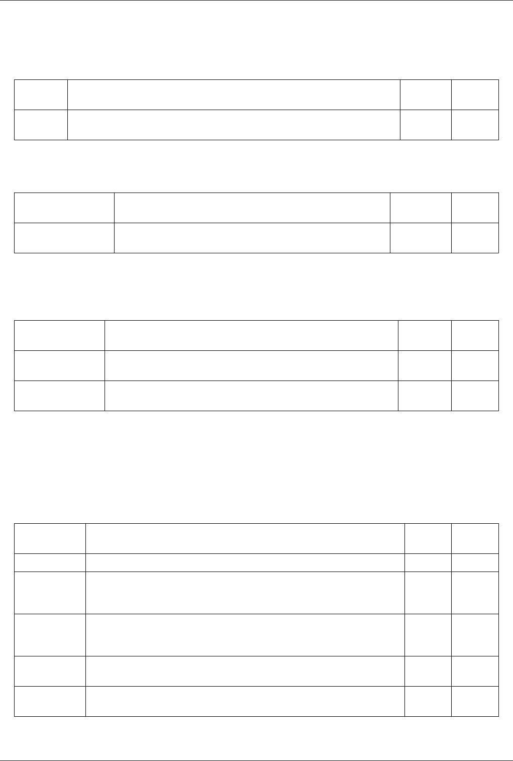
List of Sources 302
Outline
3D outline of the specified bounds.The Outline source creates an axis aligned bounding box given the user-specified
minimum and maximum coordinates for each axis.
Property Description Default
Value(s)
Restrictions
Bounds
(Bounds)
The values of this property specify the minimum and maximum X, Y, and Z coordinates (X min, X
max, Y min, Y max, Z min, Z max) for drawing the outline.
0 1 0 1 0 1
PVTrivialProducer
Property Description Default
Value(s)
Restrictions
WholeExtent
(WholeExtent)
The values of this property specify the whole extent of the topologically regular
grid.
0 -1 0 -1 0 -1
PedigreeIDSelectionSource
PedigreeIDSelectionSource is a source producing a pedigree ID based selection.
Property Description Default
Value(s)
Restrictions
Pedigree IDs (IDs) The list of integer IDs that will be added to the selection produced by the selection
source, specified by the pair (domain, id).
id 0
Pedigree String IDs
(StringIDs)
The list of string IDs that will be added to the selection produced by the selection source,
specified by the pair (domain, id).
id foo
Plane
Create a parallelogram given an origin and two points. The resolution indicates the number of division along each
axis of the plane. The Plane source can be used to add a polygonal parallelogram to the 3D scene. Unlike the sphere,
cone, and cylinder sources, the parallelogram is exactly represented at the lowest resolution, but higher resolutions
may be desired if this plane is to be used as an input to a filter. The output of the Plane source is polygonal data.
Property Description Default
Value(s)
Restrictions
Origin (Origin) This property specifies the 3D coordinate of the origin (one corner) of the plane. -0.5 -0.5 0.0
Point1 (Point1) This property specifies the 3D coordinate a second corner of the parallelogram. The line
connecting this point and that specified by the Origin property define one edge of the
parallelogram (its X axis).
0.5 -0.5 0.0
Point2 (Point2) This property specifies the 3D coordinate a third corner of the parallelogram. The line
connecting this point and that specified by the Origin property define a second edge of the
parallelogram (its Y axis).
-0.5 0.5 0.0
XResolution
(XResolution)
This property specifies the number of divisions along the X axis of the parallelogram. 1
YResolution
(YResolution)
This property specifies the number of divisions along the Y axis of the parallelogram. 1
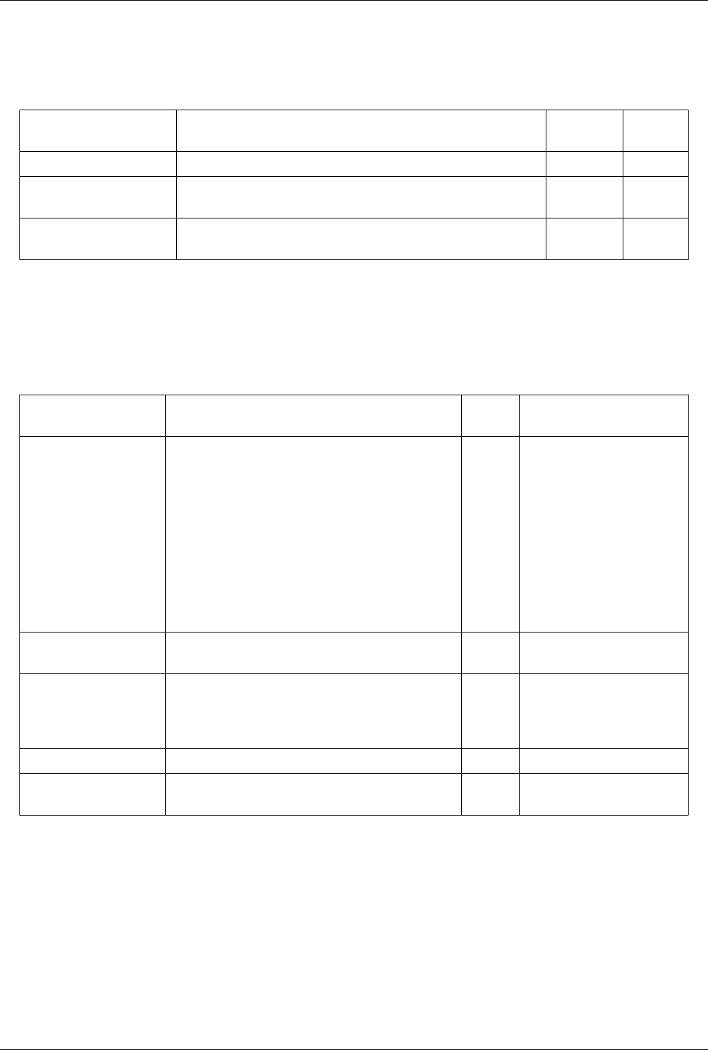
List of Sources 303
Point Source
Create a point cloud of a certain size, radius, and center.The point source creates a specified number of points within
a given radius about a specified center point.
Property Description Default
Value(s)
Restrictions
Center (Center) This property specifies the 3D coordinates of the center of the point cloud. 0.0 0.0 0.0
NumberOfPoints
(NumberOfPoints)
This property specifies the number of points in the point cloud. 1
Radius (Radius) This property specifies the radius of the point cloud, measured from the value of
the Center property.
0.0
Programmable Source
Executes a user supplied python script to produce an output dataset. This source will execute a python script to
produce an output dataset. The source keeps a copy of the python script in Script, and creates Interpretor, a python
interpretor to run the script upon the first execution.
Property Description Default
Value(s)
Restrictions
OutputDataSetType
(OutputDataSetType)
The value of this property determines the dataset type for the
output of the programmable source.
0 The value(s) is an enumeration of
the following:
• vtkPolyData (0)
• vtkStructuredGrid (2)
• vtkRectilinearGrid (3)
• vtkUnstructuredGrid (4)
• vtkImageData (6)
• vtkMultiblockDataSet (13)
• vtkHierarchicalBoxDataSet
(15)
• vtkTable (19)
Script (Script) This property contains the text of a python program that the
programmable source runs.
Script (RequestInformation)
(InformationScript)
This property is a python script that is executed during the
RequestInformation pipeline pass. Use this to provide
information such as WHOLE_EXTENT to the pipeline
downstream.
Parameters (Parameters)
PythonPath (PythonPath) A semi-colon (;) separated list of directories to add to the python
library search path.
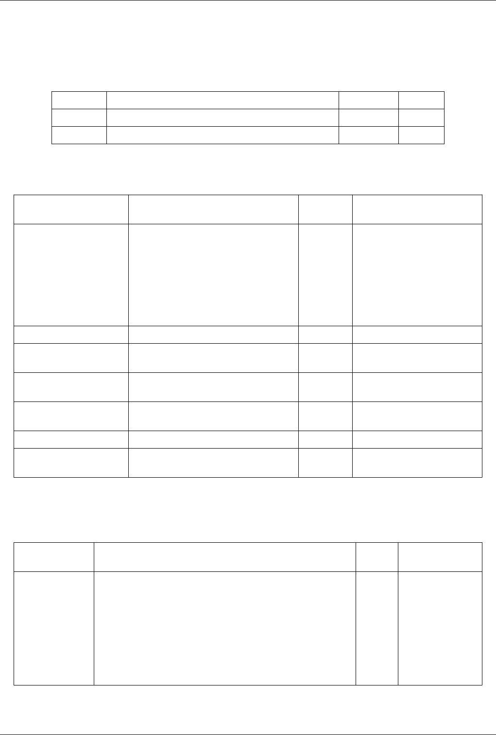
List of Sources 304
Ruler
This is a line source that can be used to measure distance between two pointsThe ruler can be used to interactively
(using a 3D widget) or manually (using the entries on the user interface) specify two points and then determine the
distance between the two points. To place points on the surface of any dataset, one can use the 'p' key shortcut.
Property Description Default Value(s) Restrictions
Point1 (Point1) This property controls the coordinates of the first endpoint of the line. -0.5 0.0 0.0
Point2 (Point2) This property controls the coordinates of the second endpoint of the line. 0.5 0.0 0.0
SelectionQuerySource
Property Description Default
Value(s)
Restrictions
FieldType (FieldType) The location of the array the selection came from
(ex, point, cell).
0 The value(s) is an enumeration of the
following:
• CELL (0)
• POINT (1)
• FIELD (2)
• VERTEX (3)
• EDGE (4)
• ROW (5)
QueryString (QueryString)
CompositeIndex
(CompositeIndex)
-1
HierarchicalLevel
(HierarchicalLevel)
-1
HierarchicalIndex
(HierarchicalIndex)
-1
ProcessID (ProcessID) -1
UserFriendlyText
(UserFriendlyText)
Reconstructs the query as a user friendly text eg.
"IDs >= 12".
SelectionSourceBase
Internal proxy used to define the common API for Selection Source proxies. Do not use.
Property Description Default
Value(s)
Restrictions
FieldType (FieldType) The location of the array the selection came from (ex, point, cell). 0 The value(s) is an
enumeration of the
following:
• CELL (0)
• POINT (1)
• FIELD (2)
• VERTEX (3)
• EDGE (4)
• ROW (5)
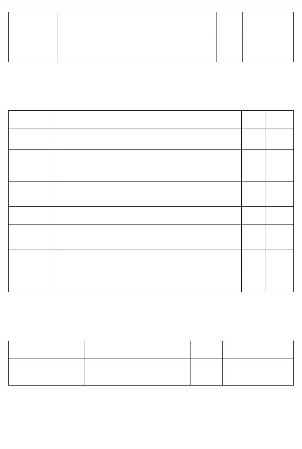
List of Sources 305
ContainingCells
(ContainingCells)
When field type is POINT, this controls whether single vertex cells will be
produced for each selected point, or whether the cells that contain each selected
point will be produced. When field type is CELL this has no effect.
0 Accepts boolean values
(0 or 1).
InsideOut (InsideOut) When this property is false the selection describes everything that should be
extracted. When this is true the selection describes everything that should NOT be
extracted.
0 Accepts boolean values
(0 or 1).
Sphere
Create a 3D sphere given a center and radius.The Sphere source can be used to add a polygonal sphere to the 3D
scene. The output of the Sphere source is polygonal data with point normals defined.
Property Description Default
Value(s)
Restrictions
Center (Center) This property specifies the 3D coordinates for the center of the sphere. 0.0 0.0 0.0
Radius (Radius) This property specifies the radius of the sphere. 0.5
ThetaResolution
(ThetaResolution)
The value of this property represents the number of divisions between Start Theta and End
Theta around the sphere. (See the Start Theta and End Theta properties.) The theta divisions are
similar to longitude lines on the earth. The higher the resolution, the closer the approximation
will come to a sphere, and the more polygons there will be.
8
StartTheta
(StartTheta)
To form a complete sphere, the value of this property should be 0 degrees, and the value of the
End Theta property should be 360 degrees. The value of this property can be adjusted to form
only a portion of a sphere.
0
EndTheta (EndTheta) The value of this property can be adjusted to form only a portion of a sphere. This value is
measured in degrees.
360
PhiResolution
(PhiResolution)
The value of this property represents the number of divisions between Start Phi and End Phi on
the sphere. (See the Start Phi and End Phi properties.) The phi divisions are similar to latitude
lines on the earth.
8
StartPhi (StartPhi) To form a complete sphere, the value of this property should be 0 degrees, and the value of the
End Phi property should be 180 degrees. The value of this property can be adjusted to form only
a portion of a sphere. Set the starting angle (in degrees) in the latitudinal direction.
0
EndPhi (EndPhi) The value of this property can be adjusted to form only a portion of a sphere. The value is
measured in degrees.
180
SplineSource
Tessellate parametric functions.This class tessellates parametric functions. The user must specify how many points
in the parametric coordinate directions are required (i.e., the resolution), and the mode to use to generate scalars.
Property Description Default
Value(s)
Restrictions
Parametric Function
(ParametricFunction)
Property used to reference the parametric function as
data generator.
The value can be one of the
following:
• Spline (parametric_functions)
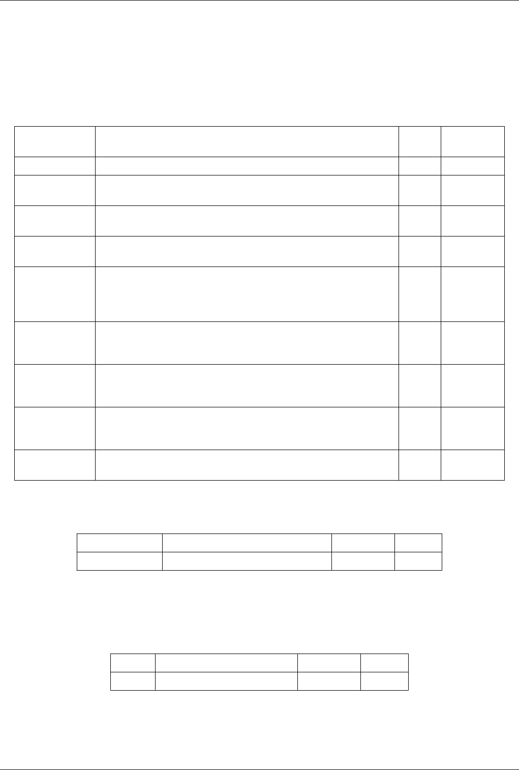
List of Sources 306
Superquadric
Create a superquadric according to the theta and phi roundness parameters. This one source can generate a wide
variety of 3D objects including a box, a sphere, or a torus. The Superquadric source can be used to add a polygonal
superquadric to the 3D scene. This source can be used to create a wide variety of shapes (e.g., a sphere, a box, or a
torus) by adjusting the roundness parameters. The output of the Superquadric source is polygonal data with point
normals and texture coordinates defined.
Property Description Default
Value(s)
Restrictions
Center (Center) This property specifies the 3D coordinates of the center of the superquadric. 0.0 0.0 0.0
Scale (Scale) The three values in this property are used to scale the superquadric in X, Y, and Z. The
surface normals will be computed correctly even with anisotropic scaling.
1.0 1.0 1.0
ThetaResolution
(ThetaResolution)
The value of this property represents the number of divisions in the theta (longitudinal)
direction. This value will be rounded to the nearest multiple of 8.
16
PhiResolution
(PhiResolution)
The value of this property represents the number of divisions in the phi (latitudinal)
direction. This number will be rounded to the nearest multiple of 4.
16
Thickness
(Thickness)
If the value of the Toroidal property is 1, this value represents the thickness of the
superquadric as a value between 0 and 1. A value close to 0 leads to a thin object with a
large hole, and a value near 1 leads to a thick object with a very small hole. Changing the
thickness does not change the outer radius of the superquadric.
0.3333
ThetaRoundness
(ThetaRoundness)
This property defines the roundness of the superquadric in the theta (longitudinal)
direction. A value of 0 represents a rectangular shape, a value of 1 represents a circular
shape, and values greater than 1 produce higher order shapes.
1
PhiRoundness
(PhiRoundness)
This property defines the roundness in the phi (latitudinal) direction. A value of 0
represents a rectangular shape, a value of 1 represents a circular shape, and values greater
than 1 produce higher order shapes.
1
Size (Size) The value of this property represents the isotropic size of the superquadric. Note that both
the Size and Thickness properties control coefficients of superquadric generation, so the
value of this property may not exactly describe the size of the superquadric.
0.5
Toroidal (Toroidal) If the value of this property is 0, the generated superquadric will not contain a hole (i.e.,
the superquadric will be ellipsoidal). Otherwise, a toroidal object is generated.
1 Accepts boolean
values (0 or 1).
Test3DWidget
Property Description Default Value(s) Restrictions
Resolution (Resolution) Set the number of faces used to generate the cone. 6
Text
The Text source generates a table containing text.The Text source is used to generate a 1x1 vtkTable with a single
text string.
Property Description Default Value(s) Restrictions
Text (Text) This property specifies the text to display. Text
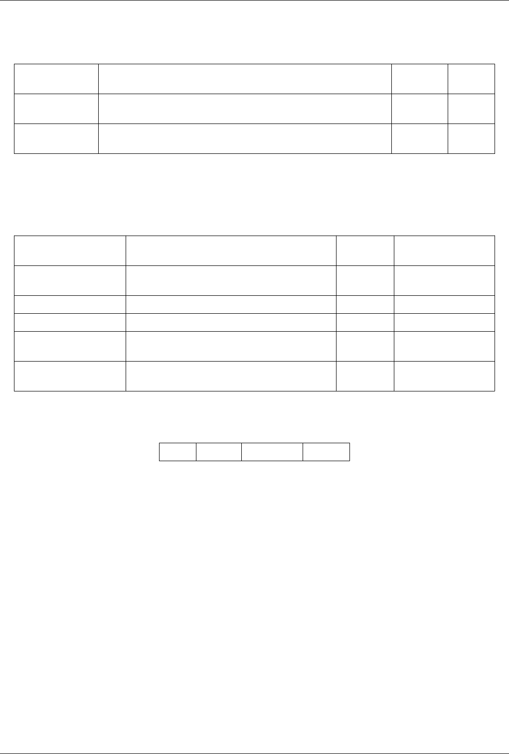
List of Sources 307
ThresholdSelectionSource
ThresholdSelectionSource is used to create a threshold based selection.
Property Description Default
Value(s)
Restrictions
Thresholds
(Thresholds)
The list of thresholds that will be added to the selection produced by the selection source.
ArrayName
(ArrayName)
For threshold and value selection, this controls the name of the scalar array that will be
thresholded within.
none
Time Source
Produces a single cell uniform grid with data values that vary over a sin(t) wave from t=0 to t=1 (radian).Produces a
single cell uniform grid with data values that vary over a sin(t) wave from t=0 to t=1 (radian).
Property Description Default
Value(s)
Restrictions
Analytic (Analytic) Makes the time source produce discrete steps of or an analytic
sin wave.
0 Accepts boolean values (0 or
1).
X Amplitude (X Amplitude) Controls how far the data set moves along X over time. 0.0
Y Amplitude (Y Amplitude) Controls how far the data set moves along Y over time. 0.0
Growing (Growing) Makes the time source grow and shrink along Y over time. 0 Accepts boolean values (0 or
1).
TimestepValues
(TimestepValues)
TrivialProducer
Property Description Default Value(s) Restrictions
Wavelet
Create a regular rectilinear grid in up to three dimensions with values varying according to a periodic function. The
Wavelet source can be used to create a uniform rectilinear grid in up to three dimensions with values varying
according to the following periodic function. OS = M * G * (XM * sin(XF * x) + YM * sin(YF * y) + ZM * cos(ZF
• z)) OS is the output scalar; M represents the maximum
value; G represents the Gaussian; XM, YM, and ZM are the X, Y, and Z magnitude values; and XF, YF, and ZF are
the X, Y, and Z frequency values. If a two-dimensional extent is specified, the resulting image will be displayed. If a
three-dimensional extent is used, then the bounding box of the volume will be displayed.

List of Sources 308
Property Description Default
Value(s)
Restrictions
Whole Extent
(WholeExtent)
The six values in this property indicate the X, Y, and Z extent of the output data. The first
two values represent the minimum and maximum X indices, the next two are the
minimum and maximum Y indices, and the last two are the minimum and maximum Z
indices.
-10 10 -10
10 -10 10
Center (Center) This property specifies the 3D coordinates of the center of the dataset. 0.0 0.0 0.0
Maximum (Maximum) This parameter specifies the maximum value (M) of the function. 255.0
XFreq (XFreq) This property specifies the natural frequency in X (XF in the equation). 60.0
YFreq (YFreq) This property specifies the natural frequency in Y (YF in the equation). 30.0
ZFreq (ZFreq) This property specifies the natural frequency in Z (ZF in the equation). 40.0
XMag (XMag) This property specifies the wave amplitude in X (XM in the equation). 10.0
YMag (YMag) This property specifies the wave amplitude in Y (YM in the equation). 18.0
ZMag (ZMag) This property specifies the wave amplitude in Z (ZM in the equation). 5.0
StandardDeviation
(StandardDeviation)
This property specifies the standard deviation of the Gaussian used in computing this
function.
0.5
SubsampleRate
(SubsampleRate)
This property specifies the rate at which to subsample the volume. The extent of the
dataset in each dimension will be divided by this value. (See the Whole Extent property.)
1
List of Filters
AMR Contour
Iso surface cell array.
Property Description Default
Value(s)
Restrictions
Input (Input) This property specifies the input of the filter. Accepts input of following types:
• vtkCompositeDataSet
The dataset much contain a field
array (cell)
with 1 component(s).
SelectMaterialArrays
(SelectMaterialArrays)
This property specifies the cell arrays from which
the contour filter will compute contour cells.
An array of scalars is required.
Volume Fraction Value
(VolumeFractionSurfaceValue)
This property specifies the values at which to
compute the isosurface.
0.1
Capping (Capping) If this property is on, the the boundary of the data
set is capped.
1 Accepts boolean values (0 or 1).
DegenerateCells (DegenerateCells) If this property is on, a transition mesh between
levels is created.
1 Accepts boolean values (0 or 1).
MultiprocessCommunication
(MultiprocessCommunication)
If this property is off, each process executes
independantly.
1 Accepts boolean values (0 or 1).
SkipGhostCopy (SkipGhostCopy) A simple test to see if ghost values are already set
properly.
1 Accepts boolean values (0 or 1).
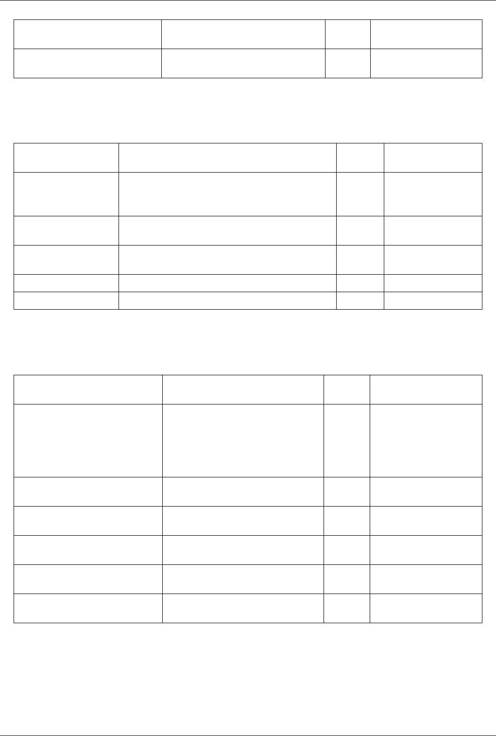
List of Filters 309
Triangulate (Triangulate) Use triangles instead of quads on capping
surfaces.
1 Accepts boolean values (0 or 1).
MergePoints (MergePoints) Use more memory to merge points on the
boundaries of blocks.
1 Accepts boolean values (0 or 1).
AMR CutPlane
Planar Cut of an AMR grid datasetThis filter creates a cut-plane of the
Property Description Default
Value(s)
Restrictions
Input (Input) This property specifies the input for this filter. Accepts input of following
types:
• vtkOverlappingAMR
UseNativeCutter
(UseNativeCutter)
This property specifies whether the ParaView's generic dataset
cutter is used instead of the specialized AMR cutter.
0 Accepts boolean values (0 or
1).
LevelOfResolution
(LevelOfResolution)
Set maximum slice resolution. 0
Center (Center) 0.5 0.5 0.5
Normal (Normal) 0 0 1
AMR Dual Clip
Clip with scalars. Tetrahedra.
Property Description Default
Value(s)
Restrictions
Input (Input) This property specifies the input of the filter. Accepts input of following types:
• vtkCompositeDataSet
The dataset much contain a field
array (cell)
with 1 component(s).
SelectMaterialArrays
(SelectMaterialArrays)
This property specifies the cell arrays from which
the clip filter will compute clipped cells.
An array of scalars is required.
Volume Fraction Value
(VolumeFractionSurfaceValue)
This property specifies the values at which to
compute the isosurface.
0.1
InternalDecimation (InternalDecimation) If this property is on, internal tetrahedra are
decimation
1 Accepts boolean values (0 or 1).
MultiprocessCommunication
(MultiprocessCommunication)
If this property is off, each process executes
independantly.
1 Accepts boolean values (0 or 1).
MergePoints (MergePoints) Use more memory to merge points on the
boundaries of blocks.
1 Accepts boolean values (0 or 1).
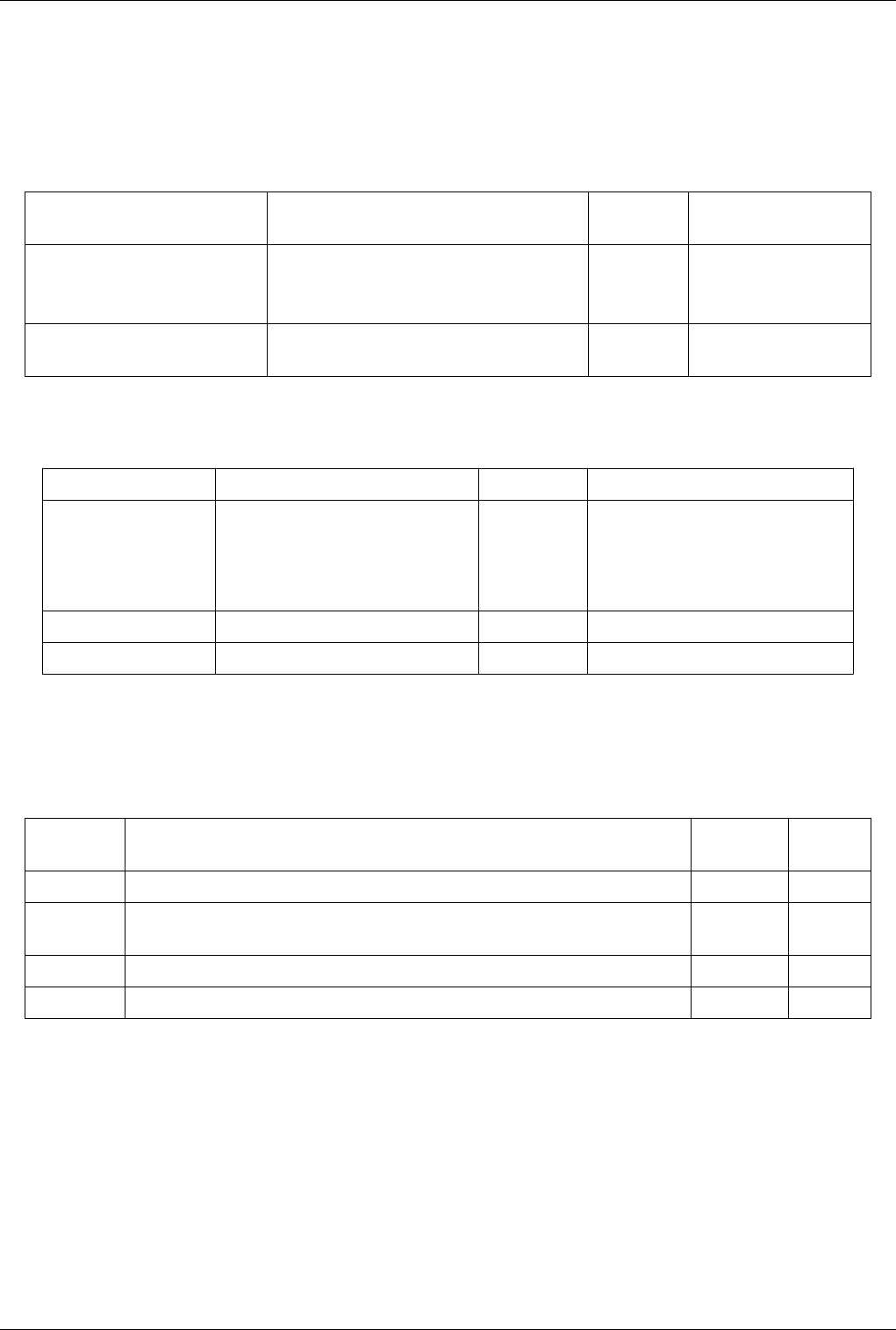
List of Filters 310
All to N
Redistribute data to a subset of available processes.The All to N filter is available when ParaView is run in parallel.
It redistributes the data so that it is located on the number of processes specified in the Number of Processes entry
box. It also does load-balancing of the data among these processes. This filter operates on polygonal data and
produces polygonal output.
Property Description Default
Value(s)
Restrictions
Input (Input) Set the input to the All to N filter. Accepts input of following
types:
• vtkPolyData
Number of Processes
(NumberOfProcesses)
Set the number of processes across which to split the
input data.
1
Annotate Global Data
Property Description Default Value(s) Restrictions
Input (Input) Set the input of the filter. Accepts input of following types:
• vtkDataSet
The dataset much contain a field array (none)
with 1 component(s).
SelectArrays (SelectArrays) Choose arrays that is going to be displayed
Prefix (Prefix) Text that is used as a prefix to the field value Value is:
Annotate Time Filter
Shows input data time as text annnotation in the view.The Annotate Time filter can be used to show the data time in
a text annotation.
Property Description Default
Value(s)
Restrictions
Input (Input) This property specifies the input dataset for which to display the time.
Format
(Format)
The value of this property is a format string used to display the input time. The format string is
specified using printf style.
Time: %f
Shift (Shift) The amount of time the input is shifted (after scaling). 0.0
Scale (Scale) The factor by which the input time is scaled. 1.0
Append Attributes
Copies geometry from first input. Puts all of the arrays into the output. The Append Attributes filter takes multiple
input data sets with the same geometry and merges their point and cell attributes to produce a single output
containing all the point and cell attributes of the inputs. Any inputs without the same number of points and cells as
the first input are ignored. The input data sets must already be collected together, either as a result of a reader that
loads multiple parts (e.g., EnSight reader) or because the Group Parts filter has been run to form a collection of data
sets.
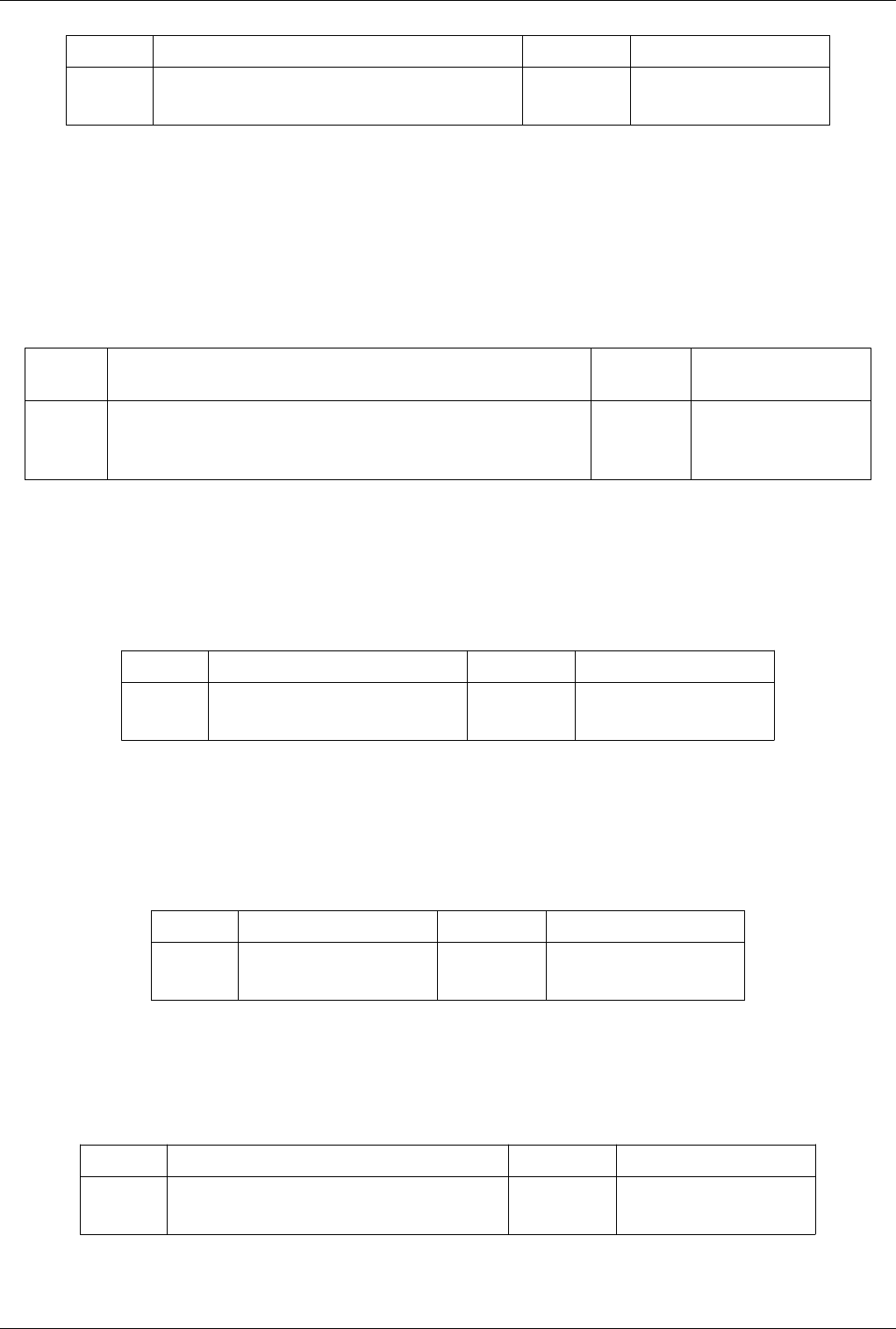
List of Filters 311
Property Description Default Value(s) Restrictions
Input (Input) This property specifies the input to the Append Attributes filter. Accepts input of following types:
• vtkDataSet
Append Datasets
Takes an input of multiple datasets and output has only one unstructured grid.The Append Datasets filter operates on
multiple data sets of any type (polygonal, structured, etc.). It merges their geometry into a single data set. Only the
point and cell attributes that all of the input data sets have in common will appear in the output. The input data sets
must already be collected together, either as a result of a reader that loads multiple parts (e.g., EnSight reader) or
because the Group Parts filter has been run to form a collection of data sets.
Property Description Default
Value(s)
Restrictions
Input
(Input)
This property specifies the datasets to be merged into a single dataset by the
Append Datasets filter.
Accepts input of following
types:
• vtkDataSet
Append Geometry
Takes an input of multiple poly data parts and output has only one part.The Append Geometry filter operates on
multiple polygonal data sets. It merges their geometry into a single data set. Only the point and cell attributes that all
of the input data sets have in common will appear in the output.
Property Description Default Value(s) Restrictions
Input (Input) Set the input to the Append Geometry filter. Accepts input of following types:
• vtkPolyData
Balance
Balance data among available processes.The Balance filter is available when ParaView is run in parallel. It does
load-balancing so that all processes have the same number of cells. It operates on polygonal data sets and produces
polygonal output.
Property Description Default Value(s) Restrictions
Input (Input) Set the input to the Balance filter. Accepts input of following types:
• vtkPolyData
Block Scalars
The Level Scalars filter uses colors to show levels of a multiblock dataset.The Level Scalars filter uses colors to
show levels of a multiblock dataset.
Property Description Default Value(s) Restrictions
Input (Input) This property specifies the input to the Level Scalars filter. Accepts input of following types:
• vtkMultiBlockDataSet
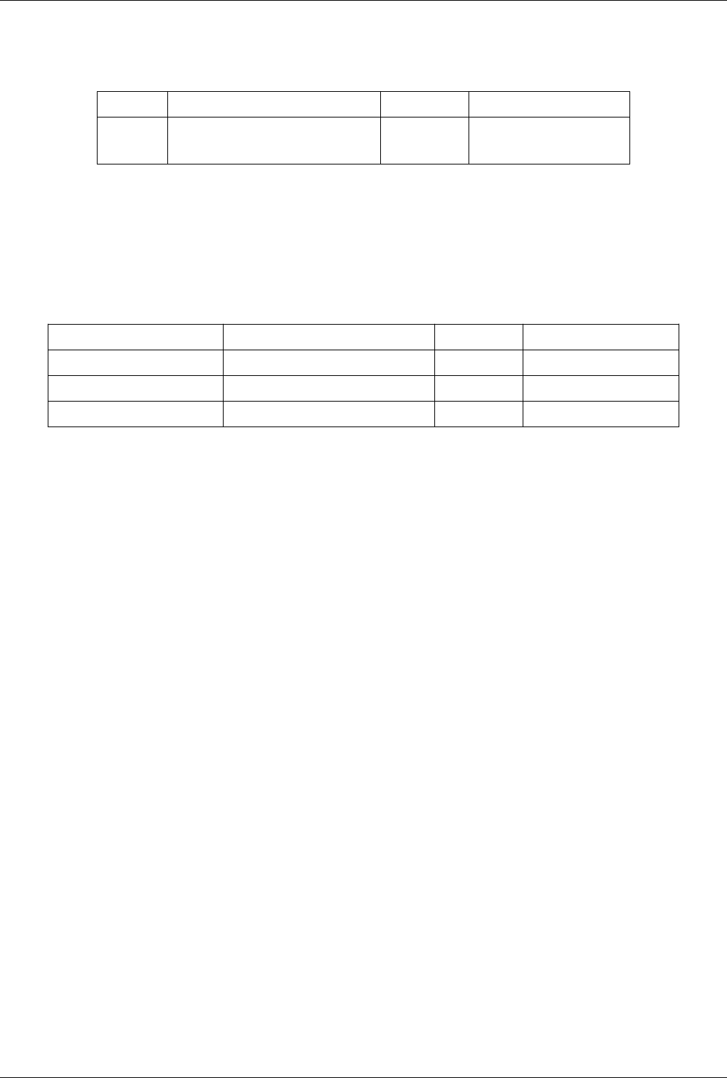
List of Filters 312
CTH Surface
Not finished yet.
Property Description Default Value(s) Restrictions
Input (Input) This property specifies the input of the filter. Accepts input of following types:
• vtkCompositeDataSet
CacheKeeper
vtkPVCacheKeeper manages data cache for flip book animations. When caching is disabled, this simply acts as a
pass through filter. When caching is enabled, is the current time step has been previously cached then this filter shuts
the update request, otherwise propagates the update and then cache the result for later use. The current time step is
set using SetCacheTime().
Property Description Default Value(s) Restrictions
Input (Input) Set the input to the Update Suppressor filter.
CacheTime (CacheTime) 0.0
CachingEnabled (CachingEnabled) Toggle whether the caching is enabled. 1 Accepts boolean values (0 or 1).
Calculator
Compute new attribute arrays as function of existing arrays.The Calculator filter computes a new data array or new
point coordinates as a function of existing scalar or vector arrays. If point-centered arrays are used in the
computation of a new data array, the resulting array will also be point-centered. Similarly, computations using
cell-centered arrays will produce a new cell-centered array. If the function is computing point coordinates, the result
of the function must be a three-component vector. The Calculator interface operates similarly to a scientific
calculator. In creating the function to evaluate, the standard order of operations applies. Each of the calculator
functions is described below. Unless otherwise noted, enclose the operand in parentheses using the ( and ) buttons.
Clear: Erase the current function (displayed in the read-only text box above the calculator buttons). /: Divide one
scalar by another. The operands for this function are not required to be enclosed in parentheses. *: Multiply two
scalars, or multiply a vector by a scalar (scalar multiple). The operands for this function are not required to be
enclosed in parentheses. -: Negate a scalar or vector (unary minus), or subtract one scalar or vector from another. The
operands for this function are not required to be enclosed in parentheses. +: Add two scalars or two vectors. The
operands for this function are not required to be enclosed in parentheses. sin: Compute the sine of a scalar. cos:
Compute the cosine of a scalar. tan: Compute the tangent of a scalar. asin: Compute the arcsine of a scalar. acos:
Compute the arccosine of a scalar. atan: Compute the arctangent of a scalar. sinh: Compute the hyperbolic sine of a
scalar. cosh: Compute the hyperbolic cosine of a scalar. tanh: Compute the hyperbolic tangent of a scalar. min:
Compute minimum of two scalars. max: Compute maximum of two scalars. x^y: Raise one scalar to the power of
another scalar. The operands for this function are not required to be enclosed in parentheses. sqrt: Compute the
square root of a scalar. e^x: Raise e to the power of a scalar. log: Compute the logarithm of a scalar (deprecated.
same as log10). log10: Compute the logarithm of a scalar to the base 10. ln: Compute the logarithm of a scalar to the
base 'e'. ceil: Compute the ceiling of a scalar. floor: Compute the floor of a scalar. abs: Compute the absolute value
of a scalar. v1.v2: Compute the dot product of two vectors. The operands for this function are not required to be
enclosed in parentheses. cross: Compute cross product of two vectors. mag: Compute the magnitude of a vector.
norm: Normalize a vector. The operands are described below. The digits 0 - 9 and the decimal point are used to enter
constant scalar values. iHat, jHat, and kHat are vector constants representing unit vectors in the X, Y, and Z
directions, respectively. The scalars menu lists the names of the scalar arrays and the components of the vector
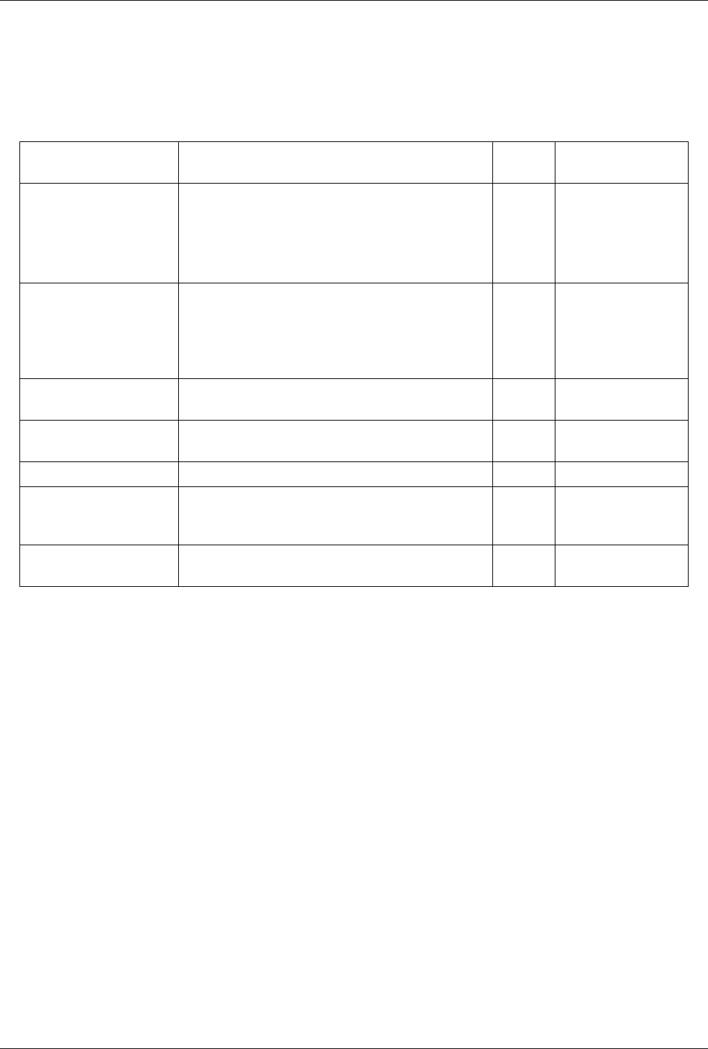
List of Filters 313
arrays of either the point-centered or cell-centered data. The vectors menu lists the names of the point-centered or
cell-centered vector arrays. The function will be computed for each point (or cell) using the scalar or vector value of
the array at that point (or cell). The filter operates on any type of data set, but the input data set must have at least
one scalar or vector array. The arrays can be either point-centered or cell-centered. The Calculator filter's output is of
the same data set type as the input.
Property Description Default
Value(s)
Restrictions
Input (Input) This property specifies the input dataset to the Calculator filter. The
scalar and vector variables may be chosen from this dataset's arrays.
Accepts input of following
types:
• vtkDataSet
The dataset much contain a
field array ()
AttributeMode (AttributeMode) This property determines whether the computation is to be
performed on point-centered or cell-centered data.
1 The value(s) is an
enumeration of the
following:
• Point Data (1)
• Cell Data (2)
CoordinateResults
(CoordinateResults)
The value of this property determines whether the results of this
computation should be used as point coordinates or as a new array.
0 Accepts boolean values (0
or 1).
ResultArrayName
(ResultArrayName)
This property contains the name for the output array containing the
result of this computation.
Result
Function (Function) This property contains the equation for computing the new array.
Replace Invalid Results
(ReplaceInvalidValues)
This property determines whether invalid values in the computation
will be replaced with a specific value. (See the ReplacementValue
property.)
1 Accepts boolean values (0
or 1).
ReplacementValue
(ReplacementValue)
If invalid values in the computation are to be replaced with another
value, this property contains that value.
0.0
Cell Centers
Create a point (no geometry) at the center of each input cell.The Cell Centers filter places a point at the center of
each cell in the input data set. The center computed is the parametric center of the cell, not necessarily the geometric
or bounding box center. The cell attributes of the input will be associated with these newly created points of the
output. You have the option of creating a vertex cell per point in the outpuut. This is useful because vertex cells are
rendered, but points are not. The points themselves could be used for placing glyphs (using the Glyph filter). The
Cell Centers filter takes any type of data set as input and produces a polygonal data set as output.

List of Filters 314
Property Description Default
Value(s)
Restrictions
Input (Input) This property specifies the input to the Cell Centers filter. Accepts input of following
types:
• vtkDataSet
VertexCells
(VertexCells)
If set to 1, a vertex cell will be generated per point in the output. Otherwise
only points will be generated.
0 Accepts boolean values (0
or 1).
Cell Data to Point Data
Create point attributes by averaging cell attributes.The Cell Data to Point Data filter averages the values of the cell
attributes of the cells surrounding a point to compute point attributes. The Cell Data to Point Data filter operates on
any type of data set, and the output data set is of the same type as the input.
Property Description Default
Value(s)
Restrictions
Input (Input) This property specifies the input to the Cell Data to Point Data filter. Accepts input of
following types:
• vtkDataSet
The dataset much
contain a field array
(cell)
PassCellData
(PassCellData)
If this property is set to 1, then the input cell data is passed through to the output;
otherwise, only the generated point data will be available in the output.
0 Accepts boolean
values (0 or 1).
PieceInvariant
(PieceInvariant)
If the value of this property is set to 1, this filter will request ghost levels so that the
values at boundary points match across processes. NOTE: Enabling this option might
cause multiple executions of the data source because more information is needed to
remove internal surfaces.
0 Accepts boolean
values (0 or 1).
Clean
Merge coincident points if they do not meet a feature edge criteria.The Clean filter takes polygonal data as input and
generates polygonal data as output. This filter can merge duplicate points, remove unused points, and transform
degenerate cells into their appropriate forms (e.g., a triangle is converted into a line if two of its points are merged).
Property Description Default
Value(s)
Restrictions
Input (Input) Set the input to the Clean filter. Accepts input of
following types:
• vtkPolyData
PieceInvariant
(PieceInvariant)
If this property is set to 1, the whole data set will be processed at once so that
cleaning the data set always produces the same results. If it is set to 0, the data set can
be processed one piece at a time, so it is not necessary for the entire data set to fit into
memory; however the results are not guaranteed to be the same as they would be if
the Piece invariant option was on. Setting this option to 0 may produce seams in the
output dataset when ParaView is run in parallel.
1 Accepts boolean
values (0 or 1).
Tolerance (Tolerance) If merging nearby points (see PointMerging property) and not using absolute
tolerance (see ToleranceIsAbsolute property), this property specifies the tolerance for
performing merging as a fraction of the length of the diagonal of the bounding box of
the input data set.
0.0
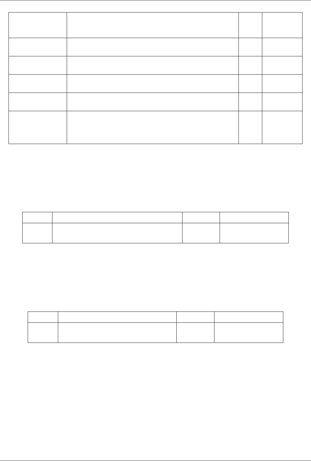
List of Filters 315
AbsoluteTolerance
(AbsoluteTolerance)
If merging nearby points (see PointMerging property) and using absolute tolerance
(see ToleranceIsAbsolute property), this property specifies the tolerance for
performing merging in the spatial units of the input data set.
1.0
ToleranceIsAbsolute
(ToleranceIsAbsolute)
This property determines whether to use absolute or relative (a percentage of the
bounding box) tolerance when performing point merging.
0 Accepts boolean
values (0 or 1).
ConvertLinesToPoints
(ConvertLinesToPoints)
If this property is set to 1, degenerate lines (a "line" whose endpoints are at the same
spatial location) will be converted to points.
1 Accepts boolean
values (0 or 1).
ConvertPolysToLines
(ConvertPolysToLines)
If this property is set to 1, degenerate polygons (a "polygon" with only two distinct
point coordinates) will be converted to lines.
1 Accepts boolean
values (0 or 1).
ConvertStripsToPolys
(ConvertStripsToPolys)
If this property is set to 1, degenerate triangle strips (a triangle "strip" containing only
one triangle) will be converted to triangles.
1 Accepts boolean
values (0 or 1).
PointMerging
(PointMerging)
If this property is set to 1, then points will be merged if they are within the specified
Tolerance or AbsoluteTolerance (see the Tolerance and AbsoluteTolerance
propertys), depending on the value of the ToleranceIsAbsolute property. (See the
ToleranceIsAbsolute property.) If this property is set to 0, points will not be merged.
1 Accepts boolean
values (0 or 1).
Clean Cells to Grid
This filter merges cells and converts the data set to unstructured grid.Merges degenerate cells. Assumes the input
grid does not contain duplicate points. You may want to run vtkCleanUnstructuredGrid first to assert it. If duplicated
cells are found they are removed in the output. The filter also handles the case, where a cell may contain degenerate
nodes (i.e. one and the same node is referenced by a cell more than once).
Property Description Default Value(s) Restrictions
Input (Input) This property specifies the input to the Clean Cells to Grid filter. Accepts input of following types:
• vtkUnstructuredGrid
Clean to Grid
This filter merges points and converts the data set to unstructured grid.The Clean to Grid filter merges points that are
exactly coincident. It also converts the data set to an unstructured grid. You may wish to do this if you want to apply
a filter to your data set that is available for unstructured grids but not for the initial type of your data set (e.g.,
applying warp vector to volumetric data). The Clean to Grid filter operates on any type of data set.
Property Description Default Value(s) Restrictions
Input (Input) This property specifies the input to the Clean to Grid filter. Accepts input of following types:
• vtkDataSet
ClientServerMoveData
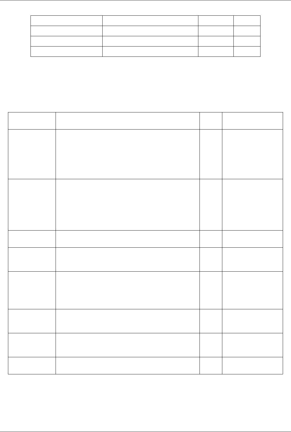
List of Filters 316
Property Description Default Value(s) Restrictions
Input (Input) Set the input to the Client Server Move Data filter.
OutputDataType (OutputDataType) 0
WholeExtent (WholeExtent) 0 -1 0 -1 0 -1
Clip
Clip with an implicit plane. Clipping does not reduce the dimensionality of the data set. The output data type of this
filter is always an unstructured grid.The Clip filter cuts away a portion of the input data set using an implicit plane.
This filter operates on all types of data sets, and it returns unstructured grid data on output.
Property Description Default
Value(s)
Restrictions
Input (Input) This property specifies the dataset on which the Clip filter will operate. Accepts input of following
types:
• vtkDataSet
The dataset much contain a
field array ()
with 1 component(s).
Clip Type
(ClipFunction)
This property specifies the parameters of the clip function (an implicit
plane) used to clip the dataset.
The value can be one of the
following:
• Plane (implicit_functions)
• Box (implicit_functions)
• Sphere (implicit_functions)
• Scalar (implicit_functions)
InputBounds
(InputBounds)
Scalars
(SelectInputScalars)
If clipping with scalars, this property specifies the name of the scalar array
on which to perform the clip operation.
An array of scalars is
required.The value must be
field array name.
Value (Value) If clipping with scalars, this property sets the scalar value about which to
clip the dataset based on the scalar array chosen. (See SelectInputScalars.) If
clipping with a clip function, this property specifies an offset from the clip
function to use in the clipping operation. Neither functionality is currently
available in ParaView's user interface.
0.0 The value must lie within the
range of the selected data
array.
InsideOut (InsideOut) If this property is set to 0, the clip filter will return that portion of the dataset
that lies within the clip function. If set to 1, the portions of the dataset that
lie outside the clip function will be returned instead.
0 Accepts boolean values (0 or
1).
UseValueAsOffset
(UseValueAsOffset)
If UseValueAsOffset is true, Value is used as an offset parameter to the
implicit function. Otherwise, Value is used only when clipping using a
scalar array.
0 Accepts boolean values (0 or
1).
Crinkle clip
(PreserveInputCells)
This parameter controls whether to extract entire cells in the given region or
clip those cells so all of the output one stay only inside that region.
0 Accepts boolean values (0 or
1).

List of Filters 317
Clip Closed Surface
Clip a polygonal dataset with a plane to produce closed surfaces This clip filter cuts away a portion of the input
polygonal dataset using a plane to generate a new polygonal dataset.
Property Description Default
Value(s)
Restrictions
Input (Input) This property specifies the dataset on which the Clip filter will operate. Accepts input of following
types:
• vtkPolyData
The dataset much contain a
field array (point)
with 1 component(s).
Clipping Plane
(ClippingPlane)
This property specifies the parameters of the clipping plane used to clip
the polygonal data.
The value can be one of the
following:
• Plane (implicit_functions)
GenerateFaces
(GenerateFaces)
Generate polygonal faces in the output. 1 Accepts boolean values (0 or
1).
GenerateOutline
(GenerateOutline)
Generate clipping outlines in the output wherever an input face is cut by
the clipping plane.
0 Accepts boolean values (0 or
1).
Generate Cell Origins
(ScalarMode)
Generate (cell) data for coloring purposes such that the newly generated
cells (including capping faces and clipping outlines) can be distinguished
from the input cells.
0 The value(s) is an enumeration
of the following:
• None (0)
• Color (1)
• Label (2)
InsideOut (InsideOut) If this flag is turned off, the clipper will return the portion of the data that
lies within the clipping plane. Otherwise, the clipper will return the
portion of the data that lies outside the clipping plane.
0 Accepts boolean values (0 or
1).
Clipping Tolerance
(Tolerance)
Specify the tolerance for creating new points. A small value might incur
degenerate triangles.
0.000001
Base Color (BaseColor) Specify the color for the faces from the input. 0.10 0.10
1.00
Clip Color (ClipColor) Specifiy the color for the capping faces (generated on the clipping
interface).
1.00 0.11
0.10
Clip Generic Dataset
Clip with an implicit plane, sphere or with scalars. Clipping does not reduce the dimensionality of the data set. This
output data type of this filter is always an unstructured grid. The Generic Clip filter cuts away a portion of the input
data set using a plane, a sphere, a box, or a scalar value. The menu in the Clip Function portion of the interface
allows the user to select which implicit function to use or whether to clip using a scalar value. Making this selection
loads the appropriate user interface. For the implicit functions, the appropriate 3D widget (plane, sphere, or box) is
also displayed. The use of these 3D widgets, including their user interface components, is discussed in section 7.4. If
an implicit function is selected, the clip filter returns that portion of the input data set that lies inside the function. If
Scalars is selected, then the user must specify a scalar array to clip according to. The clip filter will return the
portions of the data set whose value in the selected Scalars array is larger than the Clip value. Regardless of the
selection from the Clip Function menu, if the Inside Out option is checked, the opposite portions of the data set will
be returned. This filter operates on all types of data sets, and it returns unstructured grid data on output.
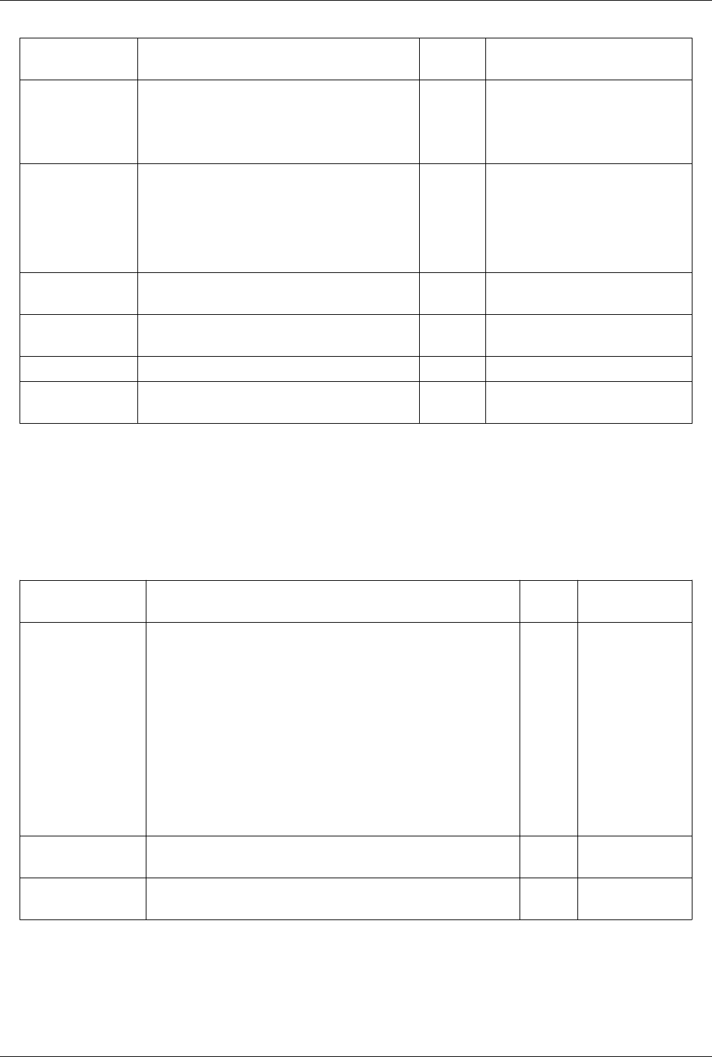
List of Filters 318
Property Description Default
Value(s)
Restrictions
Input (Input) Set the input to the Generic Clip filter. Accepts input of following types:
• vtkGenericDataSet
The dataset much contain a field array
(point)
Clip Type
(ClipFunction)
Set the parameters of the clip function. The value can be one of the following:
• Plane (implicit_functions)
• Box (implicit_functions)
• Sphere (implicit_functions)
• Scalar (implicit_functions)
InputBounds
(InputBounds)
Scalars
(SelectInputScalars)
If clipping with scalars, this property specifies the name of
the scalar array on which to perform the clip operation.
An array of scalars is required.The value
must be field array name.
InsideOut (InsideOut) Choose which portion of the dataset should be clipped away. 0 Accepts boolean values (0 or 1).
Value (Value) If clipping with a scalar array, choose the clipping value. 0.0 The value must lie within the range of the
selected data array.
Compute Derivatives
This filter computes derivatives of scalars and vectors. CellDerivatives is a filter that computes derivatives of scalars
and vectors at the center of cells. You can choose to generate different output including the scalar gradient (a vector),
computed tensor vorticity (a vector), gradient of input vectors (a tensor), and strain matrix of the input vectors (a
tensor); or you may choose to pass data through to the output.
Property Description Default
Value(s)
Restrictions
Input (Input) This property specifies the input to the filter. Accepts input of
following types:
• vtkDataSet
The dataset much
contain a field array
(point)
with 1 component(s).
The dataset much
contain a field array
(point)
with 3 component(s).
Scalars
(SelectInputScalars)
This property indicates the name of the scalar array to differentiate. An array of scalars is
required.
Vectors
(SelectInputVectors)
This property indicates the name of the vector array to differentiate. 1 An array of vectors is
required.
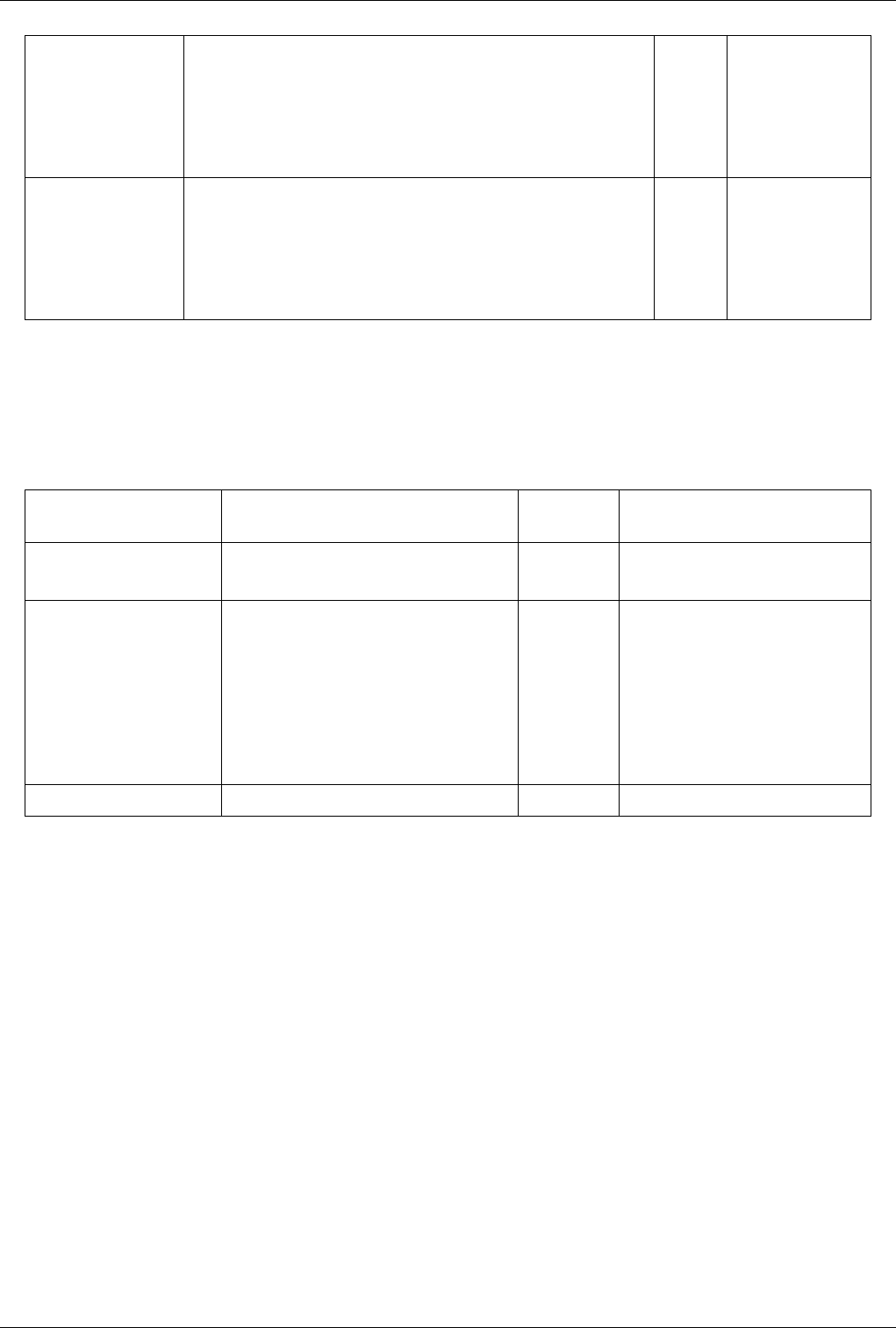
List of Filters 319
OutputVectorType
(OutputVectorType)
This property Controls how the filter works to generate vector cell data. You can
choose to compute the gradient of the input scalars, or extract the vorticity of the
computed vector gradient tensor. By default, the filter will take the gradient of
the input scalar data.
1 The value(s) is an
enumeration of the
following:
• Nothing (0)
• Scalar Gradient (1)
• Vorticity (2)
OutputTensorType
(OutputTensorType)
This property controls how the filter works to generate tensor cell data. You can
choose to compute the gradient of the input vectors, or compute the strain tensor
of the vector gradient tensor. By default, the filter will take the gradient of the
vector data to construct a tensor.
1 The value(s) is an
enumeration of the
following:
• Nothing (0)
• Vector Gradient (1)
• Strain (2)
Connectivity
Mark connected components with integer point attribute array.The Connectivity filter assigns a region id to
connected components of the input data set. (The region id is assigned as a point scalar value.) This filter takes any
data set type as input and produces unstructured grid output.
Property Description Default
Value(s)
Restrictions
Input (Input) This property specifies the input to the
Connectivity filter.
Accepts input of following types:
• vtkDataSet
ExtractionMode
(ExtractionMode)
Controls the extraction of connected surfaces. 5 The value(s) is an enumeration of the
following:
• Extract Point Seeded Regions (1)
• Extract Cell Seeded Regions (2)
• Extract Specified Regions (3)
• Extract Largest Region (4)
• Extract All Regions (5)
• Extract Closes Point Region (6)
ColorRegions (ColorRegions) Controls the coloring of the connected regions. 1 Accepts boolean values (0 or 1).
Contingency Statistics
Compute a statistical model of a dataset and/or assess the dataset with a statistical model. This filter either computes
a statistical model of a dataset or takes such a model as its second input. Then, the model (however it is obtained)
may optionally be used to assess the input dataset. This filter computes contingency tables between pairs of
attributes. This result is a tabular bivariate probability distribution which serves as a Bayesian-style prior model.
Data is assessed by computing <ul> <li> the probability of observing both variables simultaneously; <li> the
probability of each variable conditioned on the other (the two values need not be identical); and <li> the pointwise
mutual information (PMI). </ul> Finally, the summary statistics include the information entropy of the observations.
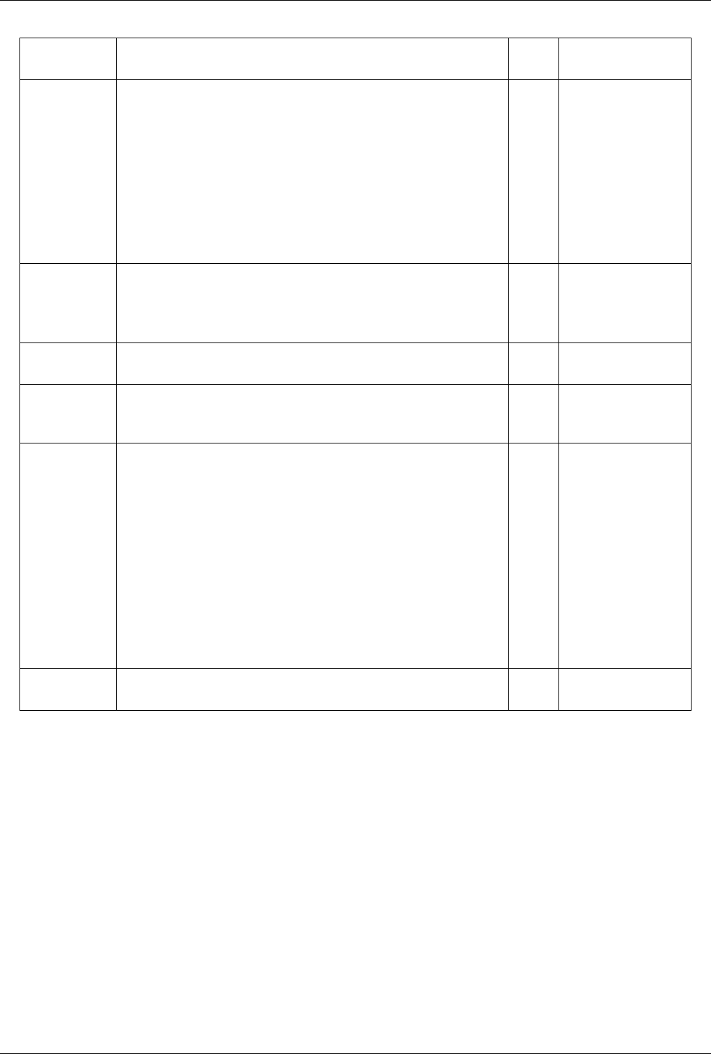
List of Filters 320
Property Description Default
Value(s)
Restrictions
Input (Input) The input to the filter. Arrays from this dataset will be used for computing statistics
and/or assessed by a statistical model.
Accepts input of following
types:
• vtkImageData
• vtkStructuredGrid
• vtkPolyData
• vtkUnstructuredGrid
• vtkTable
• vtkGraph
The dataset much contain a
field array ()
ModelInput
(ModelInput)
A previously-calculated model with which to assess a separate dataset. This input is
optional.
Accepts input of following
types:
• vtkTable
• vtkMultiBlockDataSet
AttributeMode
(AttributeMode)
Specify which type of field data the arrays will be drawn from. 0 The value must be field
array name.
Variables of
Interest
(SelectArrays)
Choose arrays whose entries will be used to form observations for statistical analysis.
Task (Task) Specify the task to be performed: modeling and/or assessment. <ol> <li> "Detailed
model of input data," creates a set of output tables containing a calculated statistical
model of the <b>entire</b> input dataset;</li> <li> "Model a subset of the data,"
creates an output table (or tables) summarizing a <b>randomly-chosen subset</b> of
the input dataset;</li> <li> "Assess the data with a model," adds attributes to the first
input dataset using a model provided on the second input port; and</li> <li> "Model
and assess the same data," is really just operations 2 and 3 above applied to the same
input dataset. The model is first trained using a fraction of the input data and then the
entire dataset is assessed using that model.</li> </ol> When the task includes
creating a model (i.e., tasks 2, and 4), you may adjust the fraction of the input dataset
used for training. You should avoid using a large fraction of the input data for
training as you will then not be able to detect overfitting. The <i>Training
fraction</i> setting will be ignored for tasks 1 and 3.
3 The value(s) is an
enumeration of the
following:
• Detailed model of input
data (0)
• Model a subset of the
data (1)
• Assess the data with a
model (2)
• Model and assess the
same data (3)
TrainingFraction
(TrainingFraction)
Specify the fraction of values from the input dataset to be used for model fitting. The
exact set of values is chosen at random from the dataset.
0.1
Contour
Generate isolines or isosurfaces using point scalars.The Contour filter computes isolines or isosurfaces using a
selected point-centered scalar array. The Contour filter operates on any type of data set, but the input is required to
have at least one point-centered scalar (single-component) array. The output of this filter is polygonal.

List of Filters 321
Property Description Default
Value(s)
Restrictions
Input (Input) This property specifies the input dataset to be used by the contour filter. Accepts input of following types:
• vtkDataSet
The dataset much contain a field
array (point)
with 1 component(s).
Contour By
(SelectInputScalars)
This property specifies the name of the scalar array from which the
contour filter will compute isolines and/or isosurfaces.
An array of scalars is required.The
value must be field array name.
ComputeNormals
(ComputeNormals)
If this property is set to 1, a scalar array containing a normal value at
each point in the isosurface or isoline will be created by the contour
filter; otherwise an array of normals will not be computed. This
operation is fairly expensive both in terms of computation time and
memory required, so if the output dataset produced by the contour filter
will be processed by filters that modify the dataset's topology or
geometry, it may be wise to set the value of this property to 0. Select
whether to compute normals.
1 Accepts boolean values (0 or 1).
ComputeGradients
(ComputeGradients)
If this property is set to 1, a scalar array containing a gradient value at
each point in the isosurface or isoline will be created by this filter;
otherwise an array of gradients will not be computed. This operation is
fairly expensive both in terms of computation time and memory
required, so if the output dataset produced by the contour filter will be
processed by filters that modify the dataset's topology or geometry, it
may be wise to set the value of this property to 0. Not that if
ComputeNormals is set to 1, then gradients will have to be calculated,
but they will only be stored in the output dataset if ComputeGradients is
also set to 1.
0 Accepts boolean values (0 or 1).
ComputeScalars
(ComputeScalars)
If this property is set to 1, an array of scalars (containing the contour
value) will be added to the output dataset. If set to 0, the output will not
contain this array.
0 Accepts boolean values (0 or 1).
GenerateTriangles
(GenerateTriangles)
This parameter controls whether to produce triangles in the output.
Warning: Many filters do not properly handle non-trianglular polygons.
1 Accepts boolean values (0 or 1).
Isosurfaces
(ContourValues)
This property specifies the values at which to compute
isosurfaces/isolines and also the number of such values.
The value must lie within the range
of the selected data array.
Point Merge Method
(Locator)
This property specifies an incremental point locator for merging
duplicate / coincident points.
The value can be one of the
following:
• MergePoints
(incremental_point_locators)
• IncrementalOctreeMergePoints
(incremental_point_locators)
• NonMergingPointLocator
(incremental_point_locators)
Contour Generic Dataset
Generate isolines or isosurfaces using point scalars.The Generic Contour filter computes isolines or isosurfaces using
a selected point-centered scalar array. The available scalar arrays are listed in the Scalars menu. The scalar range of
the selected array will be displayed. The interface for adding contour values is very similar to the one for selecting
cut offsets (in the Cut filter). To add a single contour value, select the value from the New Value slider in the Add
value portion of the interface and click the Add button, or press Enter. To instead add several evenly spaced
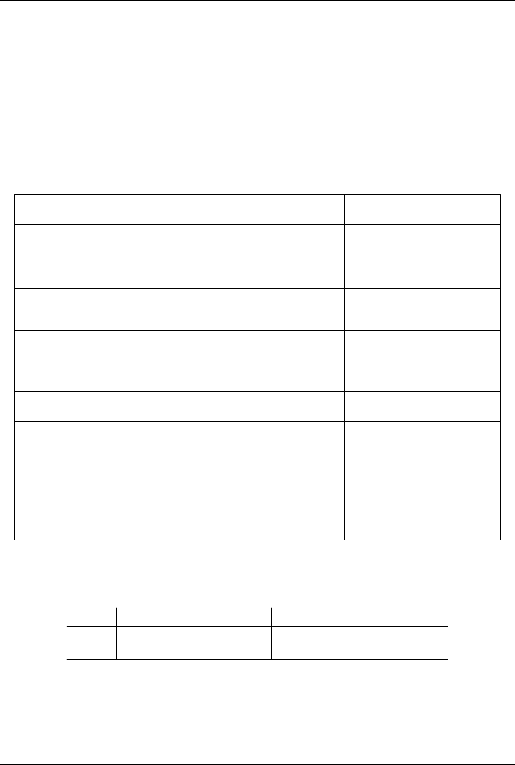
List of Filters 322
contours, use the controls in the Generate range of values section. Select the number of contour values to generate
using the Number of Values slider. The Range slider controls the interval in which to generate the contour values.
Once the number of values and range have been selected, click the Generate button. The new values will be added to
the Contour Values list. To delete a value from the Contour Values list, select the value and click the Delete button.
(If no value is selected, the last value in the list will be removed.) Clicking the Delete All button removes all the
values in the list. If no values are in the Contour Values list when Accept is pressed, the current value of the New
Value slider will be used. In addition to selecting contour values, you can also select additional computations to
perform. If any of Compute Normals, Compute Gradients, or Compute Scalars is selected, the appropriate
computation will be performed, and a corresponding point-centered array will be added to the output. The Generic
Contour filter operates on a generic data set, but the input is required to have at least one point-centered scalar
(single-component) array. The output of this filter is polygonal.
Property Description Default
Value(s)
Restrictions
Input (Input) Set the input to the Generic Contour filter. Accepts input of following types:
• vtkGenericDataSet
The dataset much contain a field array (point)
with 1 component(s).
Contour By
(SelectInputScalars)
This property specifies the name of the scalar array
from which the contour filter will compute isolines
and/or isosurfaces.
An array of scalars is required.The value must
be field array name.
ComputeNormals
(ComputeNormals)
Select whether to compute normals. 1 Accepts boolean values (0 or 1).
ComputeGradients
(ComputeGradients)
Select whether to compute gradients. 0 Accepts boolean values (0 or 1).
ComputeScalars
(ComputeScalars)
Select whether to compute scalars. 0 Accepts boolean values (0 or 1).
Isosurfaces
(ContourValues)
This property specifies the values at which to compute
isosurfaces/isolines and also the number of such values.
The value must lie within the range of the
selected data array.
Point Merge Method
(Locator)
This property specifies an incremental point locator for
merging duplicate / coincident points.
The value can be one of the following:
• MergePoints (incremental_point_locators)
• IncrementalOctreeMergePoints
(incremental_point_locators)
• NonMergingPointLocator
(incremental_point_locators)
Convert AMR dataset to Multi-block
Convert AMR to Multiblock
Property Description Default Value(s) Restrictions
Input (Input) This property specifies the input for this filter. Accepts input of following types:
• vtkOverlappingAMR
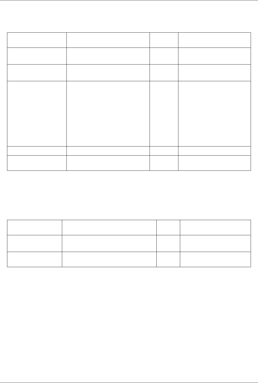
List of Filters 323
ConvertSelection
Converts a selection from one type to another.
Property Description Default
Value(s)
Restrictions
DataInput (DataInput) Set the vtkDataObject input used to convert the
selection.
Accepts input of following types:
• vtkDataObject
Input (Input) Set the selection to convert. Accepts input of following types:
• vtkSelection
OutputType (OutputType) Set the ContentType for the output. 5 The value(s) is an enumeration of the
following:
• SELECTIONS (0)
• GLOBALIDs (1)
• PEDIGREEIDS (2)
• VALUES (3)
• INDICES (4)
• FRUSTUM (5)
• LOCATION (6)
• THRESHOLDS (7)
ArrayNames (ArrayNames)
MatchAnyValues
(MatchAnyValues)
0 Accepts boolean values (0 or 1).
Crop
Efficiently extract an area/volume of interest from a 2-d image or 3-d volume.The Crop filter extracts an
area/volume of interest from a 2D image or a 3D volume by allowing the user to specify the minimum and maximum
extents of each dimension of the data. Both the input and output of this filter are uniform rectilinear data.
Property Description Default
Value(s)
Restrictions
Input (Input) This property specifies the input to the Crop filter. Accepts input of following types:
• vtkImageData
OutputWholeExtent
(OutputWholeExtent)
This property gives the minimum and maximum point
index (extent) in each dimension for the output dataset.
0 0 0 0 0 0 The value(s) must lie within the
structured-extents of the input dataset.
Curvature
This filter will compute the Gaussian or mean curvature of the mesh at each point.The Curvature filter computes the
curvature at each point in a polygonal data set. This filter supports both Gaussian and mean curvatures. ; the type can
be selected from the Curvature type menu button.

List of Filters 324
Property Description Default
Value(s)
Restrictions
Input (Input) This property specifies the input to the Curvature filter. Accepts input of following
types:
• vtkPolyData
InvertMeanCurvature
(InvertMeanCurvature)
If this property is set to 1, the mean curvature calculation will be
inverted. This is useful for meshes with inward-pointing normals.
0 Accepts boolean values (0 or
1).
CurvatureType (CurvatureType) This propery specifies which type of curvature to compute. 0 The value(s) is an
enumeration of the following:
• Gaussian (0)
• Mean (1)
D3
Repartition a data set into load-balanced spatially convex regions. Create ghost cells if requested.The D3 filter is
available when ParaView is run in parallel. It operates on any type of data set to evenly divide it across the
processors into spatially contiguous regions. The output of this filter is of type unstructured grid.
Property Description Default
Value(s)
Restrictions
Input (Input) This property specifies the input to the D3 filter. Accepts input of
following types:
• vtkDataSet
BoundaryMode
(BoundaryMode)
This property determines how cells that lie on processor boundaries are handled. The
"Assign cells uniquely" option assigns each boundary cell to exactly one process,
which is useful for isosurfacing. Selecting "Duplicate cells" causes the cells on the
boundaries to be copied to each process that shares that boundary. The "Divide cells"
option breaks cells across process boundary lines so that pieces of the cell lie in
different processes. This option is useful for volume rendering.
0 The value(s) is an
enumeration of the
following:
• Assign cells
uniquely (0)
• Duplicate cells
(1)
• Divide cells (2)
Minimal Memory
(UseMinimalMemory)
If this property is set to 1, the D3 filter requires communication routines to use
minimal memory than without this restriction.
0 Accepts boolean
values (0 or 1).
Decimate
Simplify a polygonal model using an adaptive edge collapse algorithm. This filter works with triangles only. The
Decimate filter reduces the number of triangles in a polygonal data set. Because this filter only operates on triangles,
first run the Triangulate filter on a dataset that contains polygons other than triangles.
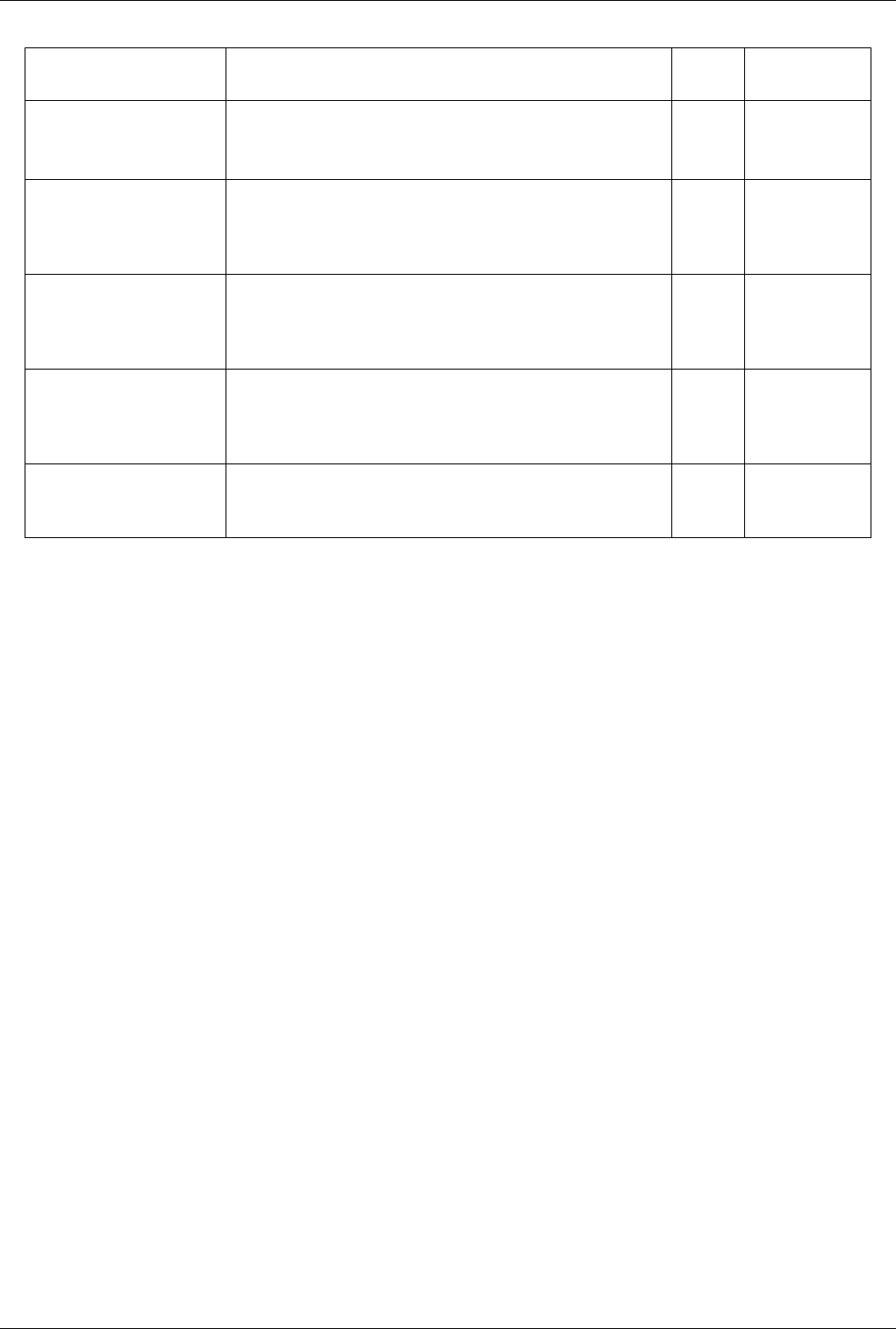
List of Filters 325
Property Description Default
Value(s)
Restrictions
Input (Input) This property specifies the input to the Decimate filter. Accepts input of
following types:
• vtkPolyData
TargetReduction
(TargetReduction)
This property specifies the desired reduction in the total number of polygons
in the output dataset. For example, if the TargetReduction value is 0.9, the
Decimate filter will attempt to produce an output dataset that is 10% the size
of the input.)
0.9
PreserveTopology
(PreserveTopology)
If this property is set to 1, decimation will not split the dataset or produce
holes, but it may keep the filter from reaching the reduction target. If it is set
to 0, better reduction can occur (reaching the reduction target), but holes in
the model may be produced.
0 Accepts boolean
values (0 or 1).
FeatureAngle (FeatureAngle) The value of this property is used in determining where the data set may be
split. If the angle between two adjacent triangles is greater than or equal to
the FeatureAngle value, then their boundary is considered a feature edge
where the dataset can be split.
15.0
BoundaryVertexDeletion
(BoundaryVertexDeletion)
If this property is set to 1, then vertices on the boundary of the dataset can be
removed. Setting the value of this property to 0 preserves the boundary of
the dataset, but it may cause the filter not to reach its reduction target.
1 Accepts boolean
values (0 or 1).
Delaunay 2D
Create 2D Delaunay triangulation of input points. It expects a vtkPointSet as input and produces vtkPolyData as
output. The points are expected to be in a mostly planar distribution. Delaunay2D is a filter that constructs a 2D
Delaunay triangulation from a list of input points. These points may be represented by any dataset of type
vtkPointSet and subclasses. The output of the filter is a polygonal dataset containing a triangle mesh. The 2D
Delaunay triangulation is defined as the triangulation that satisfies the Delaunay criterion for n-dimensional
simplexes (in this case n=2 and the simplexes are triangles). This criterion states that a circumsphere of each simplex
in a triangulation contains only the n+1 defining points of the simplex. In two dimensions, this translates into an
optimal triangulation. That is, the maximum interior angle of any triangle is less than or equal to that of any possible
triangulation. Delaunay triangulations are used to build topological structures from unorganized (or unstructured)
points. The input to this filter is a list of points specified in 3D, even though the triangulation is 2D. Thus the
triangulation is constructed in the x-y plane, and the z coordinate is ignored (although carried through to the output).
You can use the option ProjectionPlaneMode in order to compute the best-fitting plane to the set of points, project
the points and that plane and then perform the triangulation using their projected positions and then use it as the
plane in which the triangulation is performed. The Delaunay triangulation can be numerically sensitive in some
cases. To prevent problems, try to avoid injecting points that will result in triangles with bad aspect ratios (1000:1 or
greater). In practice this means inserting points that are "widely dispersed", and enables smooth transition of triangle
sizes throughout the mesh. (You may even want to add extra points to create a better point distribution.) If numerical
problems are present, you will see a warning message to this effect at the end of the triangulation process. Warning:
Points arranged on a regular lattice (termed degenerate cases) can be triangulated in more than one way (at least
according to the Delaunay criterion). The choice of triangulation (as implemented by this algorithm) depends on the
order of the input points. The first three points will form a triangle; other degenerate points will not break this
triangle. Points that are coincident (or nearly so) may be discarded by the algorithm. This is because the Delaunay
triangulation requires unique input points. The output of the Delaunay triangulation is supposedly a convex hull. In
certain cases this implementation may not generate the convex hull.
List of Filters 326
Property Description Default
Value(s)
Restrictions
Input (Input) This property specifies the input dataset to the Delaunay 2D filter. Accepts input of
following types:
• vtkPointSet
ProjectionPlaneMode
(ProjectionPlaneMode)
This property determines type of projection plane to use in performing the
triangulation.
0 The value(s) is an
enumeration of the
following:
• XY Plane (0)
• Best-Fitting Plane
(2)
Alpha (Alpha) The value of this property controls the output of this filter. For a non-zero
alpha value, only edges or triangles contained within a sphere centered at
mesh vertices will be output. Otherwise, only triangles will be output.
0.0
Tolerance (Tolerance) This property specifies a tolerance to control discarding of closely spaced
points. This tolerance is specified as a fraction of the diagonal length of
the bounding box of the points.
0.00001
Offset (Offset) This property is a multiplier to control the size of the initial, bounding
Delaunay triangulation.
1.0
BoundingTriangulation
(BoundingTriangulation)
If this property is set to 1, bounding triangulation points (and associated
triangles) are included in the output. These are introduced as an initial
triangulation to begin the triangulation process. This feature is nice for
debugging output.
0 Accepts boolean values
(0 or 1).
Delaunay 3D
Create a 3D Delaunay triangulation of input points. It expects a vtkPointSet as input and produces
vtkUnstructuredGrid as output.Delaunay3D is a filter that constructs a 3D Delaunay triangulation from a list of input
points. These points may be represented by any dataset of type vtkPointSet and subclasses. The output of the filter is
an unstructured grid dataset. Usually the output is a tetrahedral mesh, but if a non-zero alpha distance value is
specified (called the "alpha" value), then only tetrahedra, triangles, edges, and vertices lying within the alpha radius
are output. In other words, non-zero alpha values may result in arbitrary combinations of tetrahedra, triangles, lines,
and vertices. (The notion of alpha value is derived from Edelsbrunner's work on "alpha shapes".) The 3D Delaunay
triangulation is defined as the triangulation that satisfies the Delaunay criterion for n-dimensional simplexes (in this
case n=3 and the simplexes are tetrahedra). This criterion states that a circumsphere of each simplex in a
triangulation contains only the n+1 defining points of the simplex. (See text for more information.) While in two
dimensions this translates into an "optimal" triangulation, this is not true in 3D, since a measurement for optimality
in 3D is not agreed on. Delaunay triangulations are used to build topological structures from unorganized (or
unstructured) points. The input to this filter is a list of points specified in 3D. (If you wish to create 2D triangulations
see Delaunay2D.) The output is an unstructured grid. The Delaunay triangulation can be numerically sensitive. To
prevent problems, try to avoid injecting points that will result in triangles with bad aspect ratios (1000:1 or greater).
In practice this means inserting points that are "widely dispersed", and enables smooth transition of triangle sizes
throughout the mesh. (You may even want to add extra points to create a better point distribution.) If numerical
problems are present, you will see a warning message to this effect at the end of the triangulation process. Warning:
Points arranged on a regular lattice (termed degenerate cases) can be triangulated in more than one way (at least
according to the Delaunay criterion). The choice of triangulation (as implemented by this algorithm) depends on the
order of the input points. The first four points will form a tetrahedron; other degenerate points (relative to this initial
tetrahedron) will not break it. Points that are coincident (or nearly so) may be discarded by the algorithm. This is
List of Filters 327
because the Delaunay triangulation requires unique input points. You can control the definition of coincidence with
the "Tolerance" instance variable. The output of the Delaunay triangulation is supposedly a convex hull. In certain
cases this implementation may not generate the convex hull. This behavior can be controlled by the Offset instance
variable. Offset is a multiplier used to control the size of the initial triangulation. The larger the offset value, the
more likely you will generate a convex hull; and the more likely you are to see numerical problems. The
implementation of this algorithm varies from the 2D Delaunay algorithm (i.e., Delaunay2D) in an important way.
When points are injected into the triangulation, the search for the enclosing tetrahedron is quite different. In the 3D
case, the closest previously inserted point point is found, and then the connected tetrahedra are searched to find the
containing one. (In 2D, a "walk" towards the enclosing triangle is performed.) If the triangulation is Delaunay, then
an enclosing tetrahedron will be found. However, in degenerate cases an enclosing tetrahedron may not be found and
the point will be rejected.
Property Description Default
Value(s)
Restrictions
Input (Input) This property specifies the input dataset to the Delaunay 3D filter. Accepts input of
following types:
• vtkPointSet
Alpha (Alpha) This property specifies the alpha (or distance) value to control the output of
this filter. For a non-zero alpha value, only edges, faces, or tetra contained
within the circumsphere (of radius alpha) will be output. Otherwise, only
tetrahedra will be output.
0.0
Tolerance (Tolerance) This property specifies a tolerance to control discarding of closely spaced
points. This tolerance is specified as a fraction of the diagonal length of the
bounding box of the points.
0.001
Offset (Offset) This property specifies a multiplier to control the size of the initial, bounding
Delaunay triangulation.
2.5
BoundingTriangulation
(BoundingTriangulation)
This boolean controls whether bounding triangulation points (and associated
triangles) are included in the output. (These are introduced as an initial
triangulation to begin the triangulation process. This feature is nice for
debugging output.)
0 Accepts boolean
values (0 or 1).
Descriptive Statistics
Compute a statistical model of a dataset and/or assess the dataset with a statistical model. This filter either computes
a statistical model of a dataset or takes such a model as its second input. Then, the model (however it is obtained)
may optionally be used to assess the input dataset.<p> This filter computes the min, max, mean, raw moments M2
through M4, standard deviation, skewness, and kurtosis for each array you select.<p> The model is simply a
univariate Gaussian distribution with the mean and standard deviation provided. Data is assessed using this model by
detrending the data (i.e., subtracting the mean) and then dividing by the standard deviation. Thus the assessment is
an array whose entries are the number of standard deviations from the mean that each input point lies.
List of Filters 328
Property Description Default
Value(s)
Restrictions
Input (Input) The input to the filter. Arrays from this dataset will be used for computing statistics
and/or assessed by a statistical model.
Accepts input of following
types:
• vtkImageData
• vtkStructuredGrid
• vtkPolyData
• vtkUnstructuredGrid
• vtkTable
• vtkGraph
The dataset much contain a
field array ()
ModelInput
(ModelInput)
A previously-calculated model with which to assess a separate dataset. This input is
optional.
Accepts input of following
types:
• vtkTable
• vtkMultiBlockDataSet
AttributeMode
(AttributeMode)
Specify which type of field data the arrays will be drawn from. 0 The value must be field
array name.
Variables of
Interest
(SelectArrays)
Choose arrays whose entries will be used to form observations for statistical
analysis.
Task (Task) Specify the task to be performed: modeling and/or assessment. <ol> <li> "Detailed
model of input data," creates a set of output tables containing a calculated statistical
model of the <b>entire</b> input dataset;</li> <li> "Model a subset of the data,"
creates an output table (or tables) summarizing a <b>randomly-chosen subset</b> of
the input dataset;</li> <li> "Assess the data with a model," adds attributes to the
first input dataset using a model provided on the second input port; and</li> <li>
"Model and assess the same data," is really just operations 2 and 3 above applied to
the same input dataset. The model is first trained using a fraction of the input data
and then the entire dataset is assessed using that model.</li> </ol> When the task
includes creating a model (i.e., tasks 2, and 4), you may adjust the fraction of the
input dataset used for training. You should avoid using a large fraction of the input
data for training as you will then not be able to detect overfitting. The <i>Training
fraction</i> setting will be ignored for tasks 1 and 3.
3 The value(s) is an
enumeration of the
following:
• Detailed model of input
data (0)
• Model a subset of the
data (1)
• Assess the data with a
model (2)
• Model and assess the
same data (3)
TrainingFraction
(TrainingFraction)
Specify the fraction of values from the input dataset to be used for model fitting. The
exact set of values is chosen at random from the dataset.
0.1
Deviations should
be
(SignedDeviations)
Should the assessed values be signed deviations or unsigned? 0 The value(s) is an
enumeration of the
following:
• Unsigned (0)
• Signed (1)
Elevation
Create point attribute array by projecting points onto an elevation vector. The Elevation filter generates point scalar
values for an input dataset along a specified direction vector. The Input menu allows the user to select the data set to
which this filter will be applied. Use the Scalar range entry boxes to specify the minimum and maximum scalar value
to be generated. The Low Point and High Point define a line onto which each point of the data set is projected. The
minimum scalar value is associated with the Low Point, and the maximum scalar value is associated with the High
Point. The scalar value for each point in the data set is determined by the location along the line to which that point
projects.
List of Filters 329
Property Description Default
Value(s)
Restrictions
Input (Input) This property specifies the input dataset to the Elevation
filter.
Accepts input of following types:
• vtkDataSet
ScalarRange
(ScalarRange)
This property determines the range into which scalars will
be mapped.
0 1
Low Point (LowPoint) This property defines one end of the direction vector
(small scalar values).
0 0 0 The value must lie within the bounding box
of the dataset.
It will default to the min in each dimension.
High Point (HighPoint) This property defines the other end of the direction vector
(large scalar values).
0 0 1 The value must lie within the bounding box
of the dataset.
It will default to the max in each dimension.
Extract AMR Blocks
This filter extracts a list of datasets from hierarchical datasets.This filter extracts a list of datasets from hierarchical
datasets.
Property Description Default
Value(s)
Restrictions
Input (Input) This property specifies the input to the Extract Datasets
filter.
Accepts input of following
types:
• vtkUniformGridAMR
SelectedDataSets
(SelectedDataSets)
This property provides a list of datasets to extract.
Extract Attributes
Extract attribute data as a table.This is a filter that produces a vtkTable from the chosen attribute in the input
dataobject. This filter can accept composite datasets. If the input is a composite dataset, the output is a multiblock
with vtkTable leaves.
Property Description Default
Value(s)
Restrictions
Input (Input) This property specifies the input of the filter. Accepts input of
following types:
• vtkDataObject
FieldAssociation
(FieldAssociation)
Select the attribute data to pass. 0 The value(s) is an
enumeration of the
following:
• Points (0)
• Cells (1)
• Field Data (2)
• Vertices (4)
• Edges (5)
• Rows (6)

List of Filters 330
AddMetaData
(AddMetaData)
It is possible for this filter to add additional meta-data to the field data such as
point coordinates (when point attributes are selected and input is pointset) or
structured coordinates etc. To enable this addition of extra information, turn this
flag on. Off by default.
0 Accepts boolean values (0
or 1).
Extract Block
This filter extracts a range of blocks from a multiblock dataset.This filter extracts a range of groups from a
multiblock dataset
Property Description Default
Value(s)
Restrictions
Input (Input) This property specifies the input to the Extract Group filter. Accepts input of following
types:
• vtkMultiBlockDataSet
BlockIndices
(BlockIndices)
This property lists the ids of the blocks to extract from the input multiblock
dataset.
PruneOutput
(PruneOutput)
When set, the output mutliblock dataset will be pruned to remove empty
nodes. On by default.
1 Accepts boolean values (0
or 1).
MaintainStructure
(MaintainStructure)
This is used only when PruneOutput is ON. By default, when pruning the
output i.e. remove empty blocks, if node has only 1 non-null child block,
then that node is removed. To preserve these parent nodes, set this flag to
true.
0 Accepts boolean values (0
or 1).
Extract CTH Parts
Create a surface from a CTH volume fraction.Extract CTH Parts is a specialized filter for visualizing the data from a
CTH simulation. It first converts the selected cell-centered arrays to point-centered ones. It then contours each array
at a value of 0.5. The user has the option of clipping the resulting surface(s) with a plane. This filter only operates on
unstructured data. It produces polygonal output.
Property Description Default
Value(s)
Restrictions
Input (Input) This property specifies the input to the Extract
CTH Parts filter.
Accepts input of following
types:
• vtkDataSet
The dataset much contain a
field array (cell)
with 1 component(s).
Clip Type (ClipPlane) This property specifies whether to clip the
dataset, and if so, it also specifies the
parameters of the plane with which to clip.
The value can be one of the
following:
• None (implicit_functions)
• Plane (implicit_functions)
• Box (implicit_functions)
• Sphere
(implicit_functions)
Double Volume Arrays
(AddDoubleVolumeArrayName)
This property specifies the name(s) of the
volume fraction array(s) for generating parts.
An array of scalars is
required.
Float Volume Arrays
(AddFloatVolumeArrayName)
This property specifies the name(s) of the
volume fraction array(s) for generating parts.
An array of scalars is
required.

List of Filters 331
Unsigned Character Volume Arrays
(AddUnsignedCharVolumeArrayName)
This property specifies the name(s) of the
volume fraction array(s) for generating parts.
An array of scalars is
required.
Volume Fraction Value
(VolumeFractionSurfaceValue)
The value of this property is the volume
fraction value for the surface.
0.1
Extract Cells By Region
This filter extracts cells that are inside/outside a region or at a region boundary. This filter extracts from its input
dataset all cells that are either completely inside or outside of a specified region (implicit function). On output, the
filter generates an unstructured grid. To use this filter you must specify a region (implicit function). You must also
specify whethter to extract cells lying inside or outside of the region. An option exists to extract cells that are neither
inside or outside (i.e., boundary).
Property Description Default
Value(s)
Restrictions
Input (Input) This property specifies the input to the Slice filter. Accepts input of following
types:
• vtkDataSet
Intersect With
(ImplicitFunction)
This property sets the region used to extract cells. The value can be one of the
following:
• Plane (implicit_functions)
• Box (implicit_functions)
• Sphere
(implicit_functions)
InputBounds
(InputBounds)
Extraction Side
(ExtractInside)
This parameter controls whether to extract cells that are inside or
outside the region.
1 The value(s) is an enumeration
of the following:
• outside (0)
• inside (1)
Extract only intersected
(Extract only intersected)
This parameter controls whether to extract only cells that are on the
boundary of the region. If this parameter is set, the Extraction Side
parameter is ignored. If Extract Intersected is off, this parameter has no
effect.
0 Accepts boolean values (0 or
1).
Extract intersected
(Extract intersected)
This parameter controls whether to extract cells that are on the
boundary of the region.
0 Accepts boolean values (0 or
1).
Extract Edges
Extract edges of 2D and 3D cells as lines.The Extract Edges filter produces a wireframe version of the input dataset
by extracting all the edges of the dataset's cells as lines. This filter operates on any type of data set and produces
polygonal output.
Property Description Default Value(s) Restrictions
Input (Input) This property specifies the input to the Extract Edges filter. Accepts input of following types:
• vtkDataSet
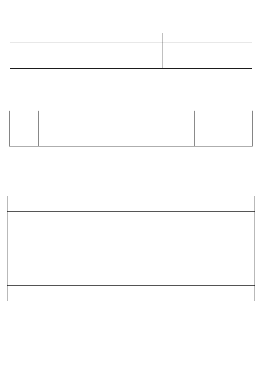
List of Filters 332
Extract Generic Dataset Surface
Extract geometry from a higher-order dataset Extract geometry from a higher-order dataset.
Property Description Default Value(s) Restrictions
Input (Input) Set the input to the Generic Geometry Filter. Accepts input of following types:
• vtkGenericDataSet
PassThroughCellIds (PassThroughCellIds) Select whether to forward original ids. 1 Accepts boolean values (0 or 1).
Extract Level
This filter extracts a range of groups from a hierarchical dataset.This filter extracts a range of levels from a
hierarchical dataset
Property Description Default Value(s) Restrictions
Input (Input) This property specifies the input to the Extract Group filter. Accepts input of following types:
• vtkUniformGridAMR
Levels (Levels) This property lists the levels to extract from the input hierarchical dataset.
Extract Selection
Extract different type of selections.This filter extracts a set of cells/points given a selection. The selection can be
obtained from a rubber-band selection (either cell, visible or in a frustum) or threshold selection and passed to the
filter or specified by providing an ID list.
Property Description Default
Value(s)
Restrictions
Input (Input) This property specifies the input from which the selection is extracted. Accepts input of
following types:
• vtkDataSet
• vtkTable
Selection (Selection) The input that provides the selection object. Accepts input of
following types:
• vtkSelection
PreserveTopology
(PreserveTopology)
If this property is set to 1 the output preserves the topology of its input and adds an
insidedness array to mark which cells are inside or out. If 0 then the output is an
unstructured grid which contains only the subset of cells that are inside.
0 Accepts boolean
values (0 or 1).
ShowBounds
(ShowBounds)
For frustum selection, if this property is set to 1 the output is the outline of the
frustum instead of the contents of the input that lie within the frustum.
0 Accepts boolean
values (0 or 1).
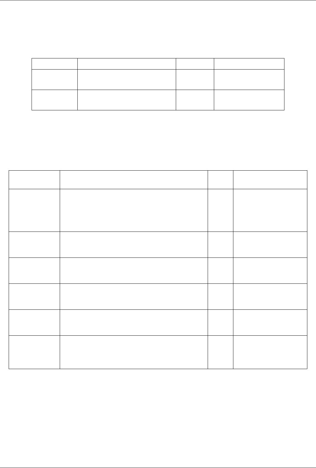
List of Filters 333
Extract Selection (internal)
This filter extracts a given set of cells or points given a selection. The selection can be obtained from a rubber-band
selection (either point, cell, visible or in a frustum) and passed to the filter or specified by providing an ID list. This
is an internal filter, use "ExtractSelection" instead.
Property Description Default Value(s) Restrictions
Input (Input) The input from which the selection is extracted. Accepts input of following types:
• vtkDataSet
Selection (Selection) The input that provides the selection object. Accepts input of following types:
• vtkSelection
Extract Subset
Extract a subgrid from a structured grid with the option of setting subsample strides.The Extract Grid filter returns a
subgrid of a structured input data set (uniform rectilinear, curvilinear, or nonuniform rectilinear). The output data set
type of this filter is the same as the input type.
Property Description Default
Value(s)
Restrictions
Input (Input) This property specifies the input to the Extract Grid filter. Accepts input of following types:
• vtkImageData
• vtkRectilinearGrid
• vtkStructuredPoints
• vtkStructuredGrid
VOI (VOI) This property specifies the minimum and maximum point indices along
each of the I, J, and K axes; these values indicate the volume of interest
(VOI). The output will have the (I,J,K) extent specified here.
0 0 0 0 0 0 The value(s) must lie within the
structured-extents of the input
dataset.
SampleRateI
(SampleRateI)
This property indicates the sampling rate in the I dimension. A value
grater than 1 results in subsampling; every nth index will be included in
the output.
1
SampleRateJ
(SampleRateJ)
This property indicates the sampling rate in the J dimension. A value
grater than 1 results in subsampling; every nth index will be included in
the output.
1
SampleRateK
(SampleRateK)
This property indicates the sampling rate in the K dimension. A value
grater than 1 results in subsampling; every nth index will be included in
the output.
1
IncludeBoundary
(IncludeBoundary)
If the value of this property is 1, then if the sample rate in any
dimension is greater than 1, the boundary indices of the input dataset
will be passed to the output even if the boundary extent is not an even
multiple of the sample rate in a given dimension.
0 Accepts boolean values (0 or 1).

List of Filters 334
Extract Surface
Extract a 2D boundary surface using neighbor relations to eliminate internal faces.The Extract Surface filter extracts
the polygons forming the outer surface of the input dataset. This filter operates on any type of data and produces
polygonal data as output.
Property Description Default
Value(s)
Restrictions
Input (Input) This property specifies the input to the Extract Surface filter. Accepts input of
following types:
• vtkDataSet
PieceInvariant (PieceInvariant) If the value of this property is set to 1, internal surfaces along process boundaries
will be removed. NOTE: Enabling this option might cause multiple executions of
the data source because more information is needed to remove internal surfaces.
1 Accepts boolean
values (0 or 1).
NonlinearSubdivisionLevel
(NonlinearSubdivisionLevel)
If the input is an unstructured grid with nonlinear faces, this parameter determines
how many times the face is subdivided into linear faces. If 0, the output is the
equivalent of its linear couterpart (and the midpoints determining the nonlinear
interpolation are discarded). If 1, the nonlinear face is triangulated based on the
midpoints. If greater than 1, the triangulated pieces are recursively subdivided to
reach the desired subdivision. Setting the value to greater than 1 may cause some
point data to not be passed even if no quadratic faces exist. This option has no
effect if the input is not an unstructured grid.
1
FOF/SOD Halo Finder
Property Description Default
Value(s)
Restrictions
Input (Input) This property specifies the input of the filter. Accepts input of following
types:
• vtkUnstructuredGrid
rL (physical box side length) (RL) The box side length used to wrap particles around if
they exceed rL (or less than 0) in any dimension
(only positive positions are allowed in the input, or
they are wrapped around).
100
overlap (shared point/ghost cell gap
distance) (Overlap)
The space (in rL units) to extend processor particle
ownership for ghost particles/cells. Needed for
correct halo calculation when halos cross processor
boundaries in parallel computation.
5
np (number of seeded particles in one
dimension, i.e., total particles = np^3)
(NP)
Number of seeded particles in one dimension.
Therefore, total simulation particles is np^3 (cubed).
256
bb (linking length) (BB) Linking length measured in units of interparticle
spacing and is dimensionless. Used to link particles
into halos for the friends-of-friends (FOF)
algorithm.
0.20
pmin (minimum particle threshold for an
FOF halo) (PMin)
Minimum number of particles (threshold) needed
before a group is called a friends-of-friends (FOF)
halo.
100
Copy FOF halo catalog to original
particles (CopyHaloDataToParticles)
If checked, the friends-of-friends (FOF) halo
catalog information will be copied to the original
particles as well.
0 Accepts boolean values (0 or
1).
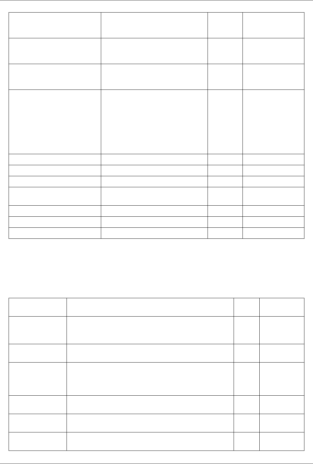
List of Filters 335
Compute the most bound particle
(ComputeMostBoundParticle)
If checked, the most bound particle for an FOF halo
will be calculated. WARNING: This can be very
slow.
0 Accepts boolean values (0 or
1).
Compute the most connected particle
(ComputeMostConnectedParticle)
If checked, the most connected particle for an FOF
halo will be calculated. WARNING: This can be
very slow.
0 Accepts boolean values (0 or
1).
Compute spherical overdensity (SOD)
halos (ComputeSOD)
If checked, spherical overdensity (SOD) halos will
be calculated in addition to friends-of-friends (FOF)
halos.
0 Accepts boolean values (0 or
1).
initial SOD center (SODCenterType) The initial friends-of-friends (FOF) center used for
calculating a spherical overdensity (SOD) halo.
WARNING: Using MBP or MCP can be very slow.
0 The value(s) is an
enumeration of the
following:
• Center of mass (0)
• Average position (1)
• Most bound particle (2)
• Most connected particle
(3)
rho_c (RhoC) rho_c (critical density) for SOD halo finding. 2.77536627e11
initial SOD mass (SODMass) The initial SOD mass. 1.0e14
minimum radius factor (MinRadiusFactor) Minimum radius factor for SOD finding. 0.5
maximum radius factor
(MaxRadiusFactor)
Maximum radius factor for SOD finding. 2.0
number of bins (SODBins) Number of bins for SOD finding. 20
minimum FOF size (MinFOFSize) Minimum FOF halo size to calculate an SOD halo. 1000
minimum FOF mass (MinFOFMass) Minimum FOF mass to calculate an SOD halo. 5.0e12
Feature Edges
This filter will extract edges along sharp edges of surfaces or boundaries of surfaces. The Feature Edges filter
extracts various subsets of edges from the input data set. This filter operates on polygonal data and produces
polygonal output.
Property Description Default
Value(s)
Restrictions
Input (Input) This property specifies the input to the Feature Edges filter. Accepts input of
following types:
• vtkPolyData
BoundaryEdges
(BoundaryEdges)
If the value of this property is set to 1, boundary edges will be extracted. Boundary
edges are defined as lines cells or edges that are used by only one polygon.
1 Accepts boolean
values (0 or 1).
FeatureEdges
(FeatureEdges)
If the value of this property is set to 1, feature edges will be extracted. Feature
edges are defined as edges that are used by two polygons whose dihedral angle is
greater than the feature angle. (See the FeatureAngle property.) Toggle whether to
extract feature edges.
1 Accepts boolean
values (0 or 1).
Non-Manifold Edges
(NonManifoldEdges)
If the value of this property is set to 1, non-manifold ediges will be extracted.
Non-manifold edges are defined as edges that are use by three or more polygons.
1 Accepts boolean
values (0 or 1).
ManifoldEdges
(ManifoldEdges)
If the value of this property is set to 1, manifold edges will be extracted. Manifold
edges are defined as edges that are used by exactly two polygons.
0 Accepts boolean
values (0 or 1).
Coloring (Coloring) If the value of this property is set to 1, then the extracted edges are assigned a
scalar value based on the type of the edge.
0 Accepts boolean
values (0 or 1).
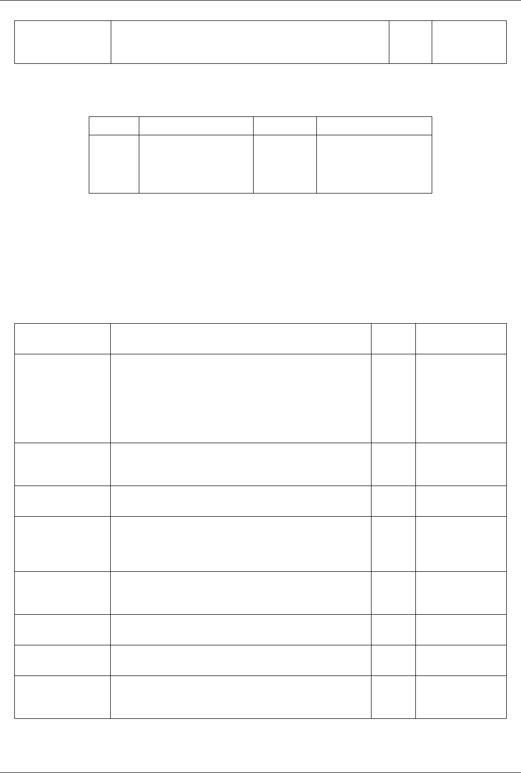
List of Filters 336
FeatureAngle
(FeatureAngle)
Ths value of this property is used to define a feature edge. If the surface normal
between two adjacent triangles is at least as large as this Feature Angle, a feature
edge exists. (See the FeatureEdges property.)
30.0
FlattenFilter
Property Description Default Value(s) Restrictions
Input (Input) Set the input to the Flatten Filter. Accepts input of following types:
• vtkPointSet
• vtkGraph
• vtkCompositeDataSet
Gaussian Resampling
Splat points into a volume with an elliptical, Gaussian distribution.vtkGaussianSplatter is a filter that injects input
points into a structured points (volume) dataset. As each point is injected, it "splats" or distributes values to nearby
voxels. Data is distributed using an elliptical, Gaussian distribution function. The distribution function is modified
using scalar values (expands distribution) or normals (creates ellipsoidal distribution rather than spherical). Warning:
results may be incorrect in parallel as points can't splat into other processor's cells.
Property Description Default
Value(s)
Restrictions
Input (Input) This property specifies the input to the filter. Accepts input of
following types:
• vtkDataSet
The dataset much contain
a field array (point)
with 1 component(s).
Resample Field
(SelectInputScalars)
Choose a scalar array to splat into the output cells. If ignore arrays is chosen,
point density will be counted instead.
An array of scalars is
required.The value must
be field array name.
Resampling Grid
(SampleDimensions)
Set / get the dimensions of the sampling structured point set. Higher values
produce better results but are much slower.
50 50 50
Extent to Resample
(ModelBounds)
Set / get the (xmin,xmax, ymin,ymax, zmin,zmax) bounding box in which the
sampling is performed. If any of the (min,max) bounds values are min >=
max, then the bounds will be computed automatically from the input data.
Otherwise, the user-specified bounds will be used.
0.0 0.0 0.0
0.0 0.0 0.0
Gaussian Splat Radius
(Radius)
Set / get the radius of propagation of the splat. This value is expressed as a
percentage of the length of the longest side of the sampling volume. Smaller
numbers greatly reduce execution time.
0.1
Gaussian Exponent
Factor (ExponentFactor)
Set / get the sharpness of decay of the splats. This is the exponent constant in
the Gaussian equation. Normally this is a negative value.
-5.0
Scale Splats
(ScalarWarping)
Turn on/off the scaling of splats by scalar value. 1 Accepts boolean values
(0 or 1).
Scale Factor (ScaleFactor) Multiply Gaussian splat distribution by this value. If ScalarWarping is on,
then the Scalar value will be multiplied by the ScaleFactor times the
Gaussian function.
1.0
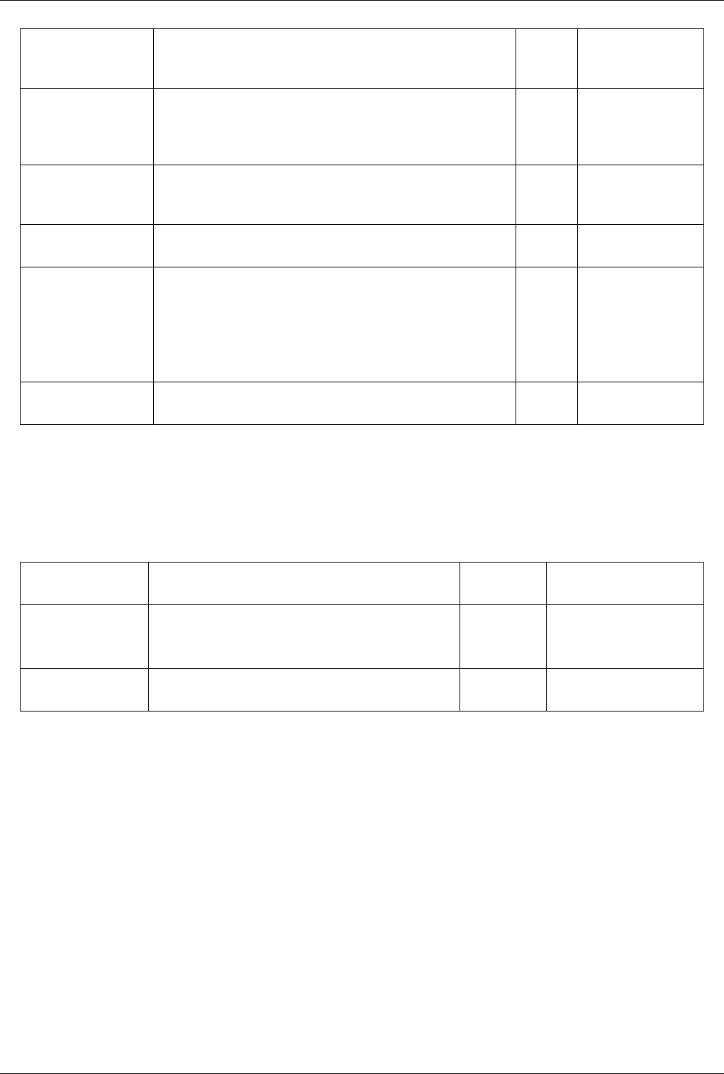
List of Filters 337
Elliptical Splats
(NormalWarping)
Turn on/off the generation of elliptical splats. If normal warping is on, then
the input normals affect the distribution of the splat. This boolean is used in
combination with the Eccentricity ivar.
1 Accepts boolean values
(0 or 1).
Ellipitical Eccentricity
(Eccentricity)
Control the shape of elliptical splatting. Eccentricity is the ratio of the major
axis (aligned along normal) to the minor (axes) aligned along other two axes.
So Eccentricity gt 1 creates needles with the long axis in the direction of the
normal; Eccentricity lt 1 creates pancakes perpendicular to the normal vector.
2.5
Fill Volume Boundary
(Capping)
Turn on/off the capping of the outer boundary of the volume to a specified
cap value. This can be used to close surfaces (after iso-surfacing) and create
other effects.
1 Accepts boolean values
(0 or 1).
Fill Value (CapValue) Specify the cap value to use. (This instance variable only has effect if the ivar
Capping is on.)
0.0
Splat Accumulation
Mode (Accumulation
Mode)
Specify the scalar accumulation mode. This mode expresses how scalar
values are combined when splats are overlapped. The Max mode acts like a
set union operation and is the most commonly used; the Min mode acts like a
set intersection, and the sum is just weird.
1 The value(s) is an
enumeration of the
following:
• Min (0)
• Max (1)
• Sum (2)
Empty Cell Value
(NullValue)
Set the Null value for output points not receiving a contribution from the
input points. (This is the initial value of the voxel samples.)
0.0
Generate Ids
Generate scalars from point and cell ids. This filter generates scalars using cell and point ids. That is, the point
attribute data scalars are generated from the point ids, and the cell attribute data scalars or field data are generated
from the the cell ids.
Property Description Default
Value(s)
Restrictions
Input (Input) This property specifies the input to the Cell Data to Point Data
filter.
Accepts input of following
types:
• vtkDataSet
ArrayName
(ArrayName)
The name of the array that will contain ids. Ids
Generate Quadrature Points
Create a point set with data at quadrature points. "Create a point set with data at quadrature points."
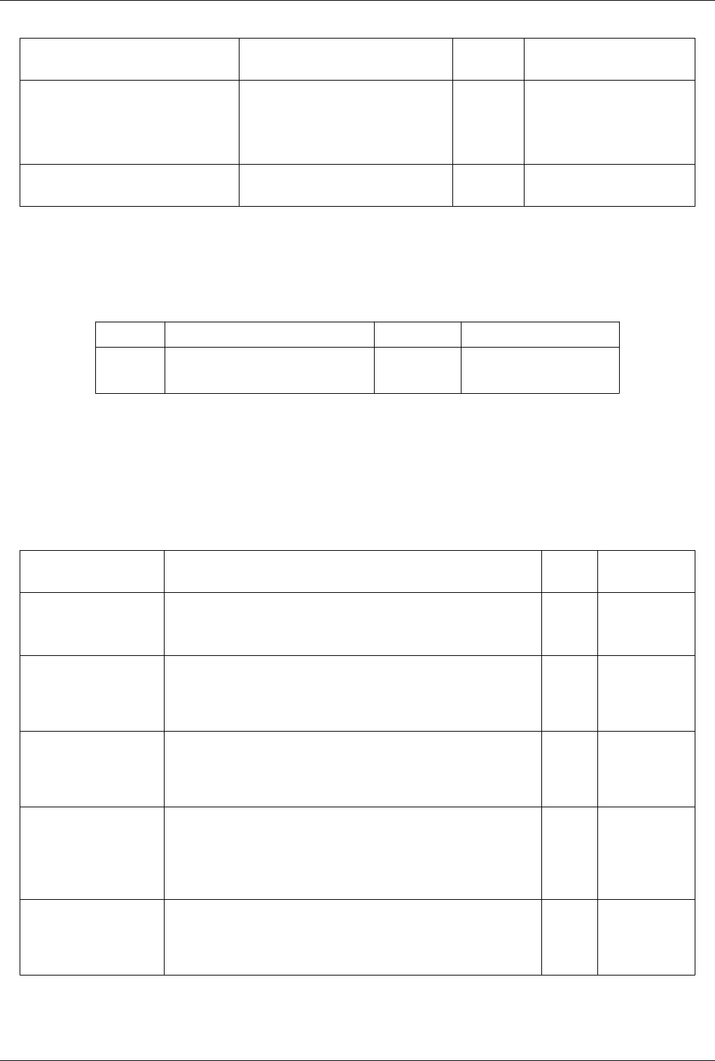
List of Filters 338
Property Description Default
Value(s)
Restrictions
Input (Input) This property specifies the input of the filter. Accepts input of following types:
• vtkUnstructuredGrid
The dataset much contain a field
array (cell)
Quadrature Scheme Def
(QuadratureSchemeDefinition)
Specifies the offset array from which we
generate quadrature points.
An array of scalars is required.
Generate Quadrature Scheme Dictionary
Generate quadrature scheme dictionaries in data sets that do not have them. Generate quadrature scheme dictionaries
in data sets that do not have them.
Property Description Default Value(s) Restrictions
Input (Input) This property specifies the input of the filter. Accepts input of following types:
• vtkUnstructuredGrid
Generate Surface Normals
This filter will produce surface normals used for smooth shading. Splitting is used to avoid smoothing across feature
edges.This filter generates surface normals at the points of the input polygonal dataset to provide smooth shading of
the dataset. The resulting dataset is also polygonal. The filter works by calculating a normal vector for each polygon
in the dataset and then averaging the normals at the shared points.
Property Description Default
Value(s)
Restrictions
Input (Input) This property specifies the input to the Normals Generation filter. Accepts input of
following types:
• vtkPolyData
FeatureAngle
(FeatureAngle)
The value of this property defines a feature edge. If the surface normal between
two adjacent triangles is at least as large as this Feature Angle, a feature edge
exists. If Splitting is on, points are duplicated along these feature edges. (See the
Splitting property.)
30
Splitting (Splitting) This property controls the splitting of sharp edges. If sharp edges are split
(property value = 1), then points are duplicated along these edges, and separate
normals are computed for both sets of points to give crisp (rendered) surface
definition.
1 Accepts boolean
values (0 or 1).
Consistency (Consistency) The value of this property controls whether consistent polygon ordering is
enforced. Generally the normals for a data set should either all point inward or all
point outward. If the value of this property is 1, then this filter will reorder the
points of cells that whose normal vectors are oriented the opposite direction from
the rest of those in the data set.
1 Accepts boolean
values (0 or 1).
FlipNormals (FlipNormals) If the value of this property is 1, this filter will reverse the normal direction (and
reorder the points accordingly) for all polygons in the data set; this changes
front-facing polygons to back-facing ones, and vice versa. You might want to do
this if your viewing position will be inside the data set instead of outside of it.
0 Accepts boolean
values (0 or 1).

List of Filters 339
Non-Manifold Traversal
(NonManifoldTraversal)
Turn on/off traversal across non-manifold edges. Not traversing non-manifold
edges will prevent problems where the consistency of polygonal ordering is
corrupted due to topological loops.
1 Accepts boolean
values (0 or 1).
ComputeCellNormals
(ComputeCellNormals)
This filter computes the normals at the points in the data set. In the process of
doing this it computes polygon normals too. If you want these normals to be
passed to the output of this filter, set the value of this property to 1.
0 Accepts boolean
values (0 or 1).
PieceInvariant
(PieceInvariant)
Turn this option to to produce the same results regardless of the number of
processors used (i.e., avoid seams along processor boundaries). Turn this off if
you do want to process ghost levels and do not mind seams.
1 Accepts boolean
values (0 or 1).
GeometryFilter
Property Description Default
Value(s)
Restrictions
Input (Input) Set the input to the Geoemtry Filter.
UseStrips (UseStrips) Toggle whether to generate faces containing triangle strips. This should render
faster and use less memory, but no cell data is copied.
0 Accepts boolean
values (0 or 1).
ForceStrips (ForceStrips) This makes UseStrips call Modified() after changing its setting to ensure that
the filter's output is immediatley changed.
0 Accepts boolean
values (0 or 1).
UseOutline (UseOutline) Toggle whether to generate an outline or a surface. 0 Accepts boolean
values (0 or 1).
NonlinearSubdivisionLevel
(NonlinearSubdivisionLevel)
Nonlinear faces are approximated with flat polygons. This parameter controls
how many times to subdivide nonlinear surface cells. Higher subdivisions
generate closer approximations but take more memory and rendering time.
Subdivision is recursive, so the number of output polygons can grow
exponentially with this parameter.
1
PassThroughIds
(PassThroughIds)
If on, the output polygonal dataset will have a celldata array that holds the cell
index of the original 3D cell that produced each output cell. This is useful for
cell picking.
1 Accepts boolean
values (0 or 1).
PassThroughPointIds
(PassThroughPointIds)
If on, the output polygonal dataset will have a pointdata array that holds the
point index of the original 3D vertex that produced each output vertex. This is
useful for picking.
1 Accepts boolean
values (0 or 1).
MakeOutlineOfInput
(MakeOutlineOfInput)
Causes filter to try to make geometry of input to the algorithm on its input. 0 Accepts boolean
values (0 or 1).
Glyph
This filter generates an arrow, cone, cube, cylinder, line, sphere, or 2D glyph at each point of the input data set. The
glyphs can be oriented and scaled by point attributes of the input dataset. The Glyph filter generates a glyph (i.e., an
arrow, cone, cube, cylinder, line, sphere, or 2D glyph) at each point in the input dataset. The glyphs can be oriented
and scaled by the input point-centered scalars and vectors. The Glyph filter operates on any type of data set. Its
output is polygonal. This filter is available on the Toolbar.

List of Filters 340
Property Description Default
Value(s)
Restrictions
Input (Input) This property specifies the input to the Glyph filter.
This is the dataset to which the glyphs will be
applied.
Accepts input of following types:
• vtkDataSet
The dataset much contain a field array (point)
with 1 component(s).
The dataset much contain a field array (point)
with 3 component(s).
Scalars (SelectInputScalars) This property indicates the name of the scalar array
on which to operate. The indicated array may be
used for scaling the glyphs. (See the SetScaleMode
property.)
An array of scalars is required.
Vectors (SelectInputVectors) This property indicates the name of the vector array
on which to operate. The indicated array may be
used for scaling and/or orienting the glyphs. (See
the SetScaleMode and SetOrient properties.)
1 An array of vectors is required.
Glyph Type (Source) This property determines which type of glyph will
be placed at the points in the input dataset.
Accepts input of following types:
• vtkPolyDataThe value can be one of the
following:
• ArrowSource (sources)
• ConeSource (sources)
• CubeSource (sources)
• CylinderSource (sources)
• LineSource (sources)
• SphereSource (sources)
• GlyphSource2D (sources)
GlyphTransform
(GlyphTransform)
The values in this property allow you to specify the
transform (translation, rotation, and scaling) to
apply to the glyph source.
The value can be one of the following:
• Transform2 (extended_sources)
Orient (SetOrient) If this property is set to 1, the glyphs will be
oriented based on the selected vector array.
1 Accepts boolean values (0 or 1).
Scale Mode (SetScaleMode) The value of this property specifies how/if the
glyphs should be scaled based on the point-centered
scalars/vectors in the input dataset.
1 The value(s) is an enumeration of the
following:
• scalar (0)
• vector (1)
• vector_components (2)
• off (3)
SetScaleFactor
(SetScaleFactor)
The value of this property will be used as a
multiplier for scaling the glyphs before adding them
to the output.
1.0 The value must lie within the range of the
selected data array.The value must lie within
the range of the selected data array. The value
must be less than the largest dimension of the
dataset multiplied by a scale factor of 0.1.
Maximum Number of Points
(MaximumNumberOfPoints)
The value of this property specifies the maximum
number of glyphs that should appear in the output
dataset if the value of the UseMaskPoints property
is 1. (See the UseMaskPoints property.)
5000
Mask Points (UseMaskPoints) If the value of this property is set to 1, limit the
maximum number of glyphs to the value indicated
by MaximumNumberOfPoints. (See the
MaximumNumberOfPoints property.)
1 Accepts boolean values (0 or 1).

List of Filters 341
RandomMode (RandomMode) If the value of this property is 1, then the points to
glyph are chosen randomly. Otherwise the point ids
chosen are evenly spaced.
1 Accepts boolean values (0 or 1).
KeepRandomPoints
(KeepRandomPoints)
If the value of this property is 1 and RandomMode
is 1, then the randomly chosen points to glyph are
saved and reused for other timesteps. This is only
useful if the coordinates are the same and in the
same order between timesteps.
0 Accepts boolean values (0 or 1).
Glyph With Custom Source
This filter generates a glyph at each point of the input data set. The glyphs can be oriented and scaled by point
attributes of the input dataset. The Glyph filter generates a glyph at each point in the input dataset. The glyphs can be
oriented and scaled by the input point-centered scalars and vectors. The Glyph filter operates on any type of data set.
Its output is polygonal. This filter is available on the Toolbar.
Property Description Default
Value(s)
Restrictions
Input (Input) This property specifies the input to the Glyph filter.
This is the dataset to which the glyphs will be
applied.
Accepts input of following types:
• vtkDataSet
The dataset much contain a field array (point)
with 1 component(s).
The dataset much contain a field array (point)
with 3 component(s).
Glyph Type (Source) This property determines which type of glyph will
be placed at the points in the input dataset.
Accepts input of following types:
• vtkPolyData
Scalars (SelectInputScalars) This property indicates the name of the scalar array
on which to operate. The indicated array may be
used for scaling the glyphs. (See the SetScaleMode
property.)
An array of scalars is required.
Vectors (SelectInputVectors) This property indicates the name of the vector array
on which to operate. The indicated array may be
used for scaling and/or orienting the glyphs. (See
the SetScaleMode and SetOrient properties.)
1 An array of vectors is required.
Orient (SetOrient) If this property is set to 1, the glyphs will be
oriented based on the selected vector array.
1 Accepts boolean values (0 or 1).
Scale Mode (SetScaleMode) The value of this property specifies how/if the
glyphs should be scaled based on the point-centered
scalars/vectors in the input dataset.
1 The value(s) is an enumeration of the
following:
• scalar (0)
• vector (1)
• vector_components (2)
• off (3)
SetScaleFactor
(SetScaleFactor)
The value of this property will be used as a
multiplier for scaling the glyphs before adding them
to the output.
1.0 The value must lie within the range of the
selected data array.The value must lie within
the range of the selected data array. The value
must be less than the largest dimension of the
dataset multiplied by a scale factor of 0.1.
Maximum Number of Points
(MaximumNumberOfPoints)
The value of this property specifies the maximum
number of glyphs that should appear in the output
dataset if the value of the UseMaskPoints property
is 1. (See the UseMaskPoints property.)
5000
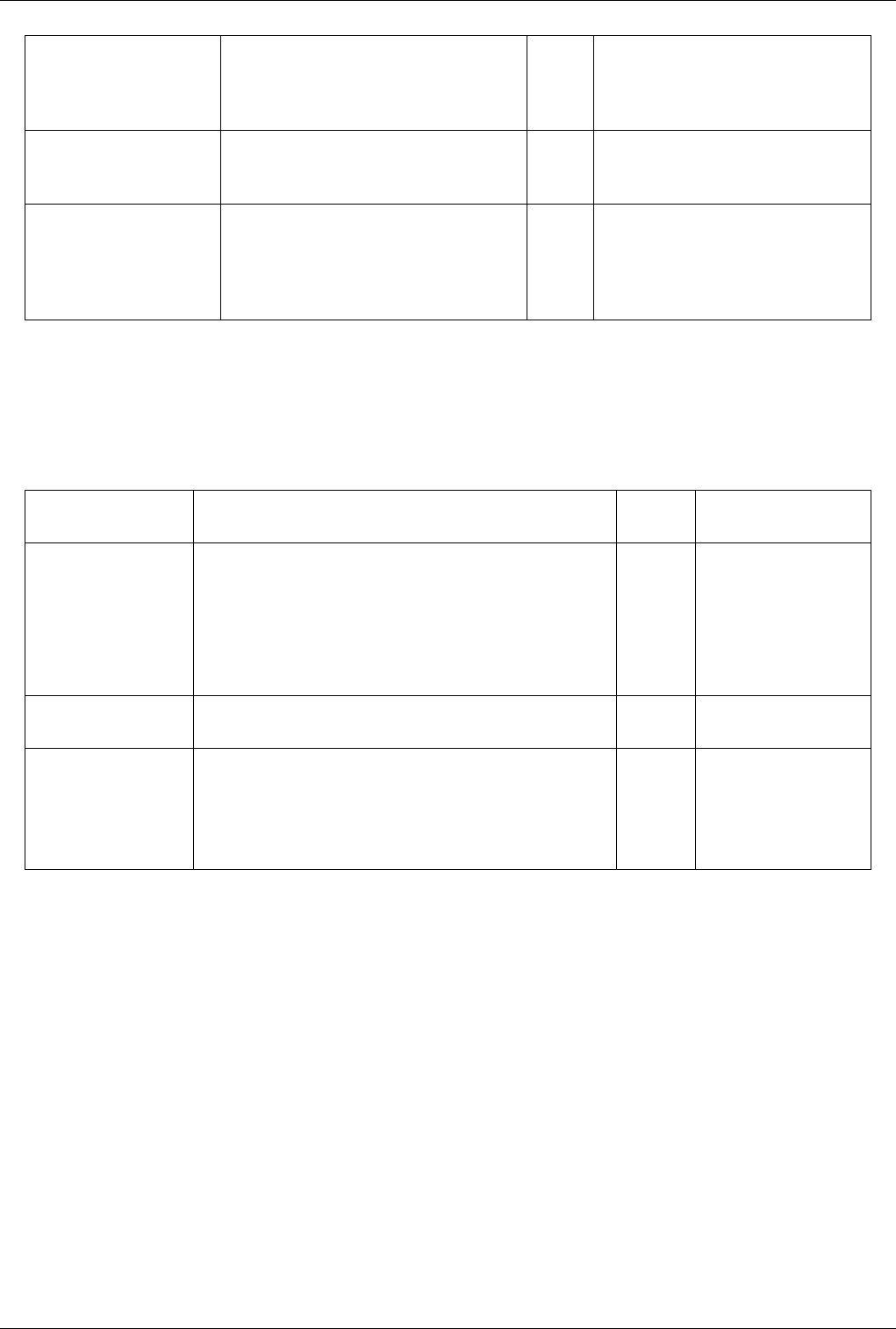
List of Filters 342
Mask Points (UseMaskPoints) If the value of this property is set to 1, limit the
maximum number of glyphs to the value indicated
by MaximumNumberOfPoints. (See the
MaximumNumberOfPoints property.)
1 Accepts boolean values (0 or 1).
RandomMode (RandomMode) If the value of this property is 1, then the points to
glyph are chosen randomly. Otherwise the point ids
chosen are evenly spaced.
1 Accepts boolean values (0 or 1).
KeepRandomPoints
(KeepRandomPoints)
If the value of this property is 1 and RandomMode
is 1, then the randomly chosen points to glyph are
saved and reused for other timesteps. This is only
useful if the coordinates are the same and in the
same order between timesteps.
0 Accepts boolean values (0 or 1).
Gradient
This filter computes gradient vectors for an image/volume.The Gradient filter computes the gradient vector at each
point in an image or volume. This filter uses central differences to compute the gradients. The Gradient filter
operates on uniform rectilinear (image) data and produces image data output.
Property Description Default
Value(s)
Restrictions
Input (Input) This property specifies the input to the Gradient filter. Accepts input of following
types:
• vtkImageData
The dataset much contain a
field array (point)
with 1 component(s).
SelectInputScalars
(SelectInputScalars)
This property lists the name of the array from which to compute the
gradient.
An array of scalars is
required.
Dimensionality
(Dimensionality)
This property indicates whether to compute the gradient in two
dimensions or in three. If the gradient is being computed in two
dimensions, the X and Y dimensions are used.
3 The value(s) is an
enumeration of the
following:
• Two (2)
• Three (3)
Gradient Magnitude
Compute the magnitude of the gradient vectors for an image/volume.The Gradient Magnitude filter computes the
magnitude of the gradient vector at each point in an image or volume. This filter operates on uniform rectilinear
(image) data and produces image data output.

List of Filters 343
Property Description Default
Value(s)
Restrictions
Input (Input) This property specifies the input to the Gradient Magnitude filter. Accepts input of following
types:
• vtkImageData
The dataset much contain a
field array (point)
with 1 component(s).
Dimensionality
(Dimensionality)
This property indicates whether to compute the gradient magnitude in two or
three dimensions. If computing the gradient magnitude in 2D, the gradients in X
and Y are used for computing the gradient magnitude.
3 The value(s) is an
enumeration of the
following:
• Two (2)
• Three (3)
Gradient Of Unstructured DataSet
Estimate the gradient for each point or cell in any type of dataset. The Gradient (Unstructured) filter estimates the
gradient vector at each point or cell. It operates on any type of vtkDataSet, and the output is the same type as the
input. If the dataset is a vtkImageData, use the Gradient filter instead; it will be more efficient for this type of
dataset.
Property Description Default
Value(s)
Restrictions
Input (Input) This property specifies the input to the Gradient (Unstructured) filter. Accepts input of
following types:
• vtkDataSet
The dataset much
contain a field array ()
Scalar Array
(SelectInputScalars)
This property lists the name of the scalar array from which to compute the
gradient.
An array of scalars is
required.The value must
be field array name.
ResultArrayName
(ResultArrayName)
This property provides a name for the output array containing the gradient
vectors.
Gradients
FasterApproximation
(FasterApproximation)
When this flag is on, the gradient filter will provide a less accurate (but
close) algorithm that performs fewer derivative calculations (and is
therefore faster). The error contains some smoothing of the output data and
some possible errors on the boundary. This parameter has no effect when
performing the gradient of cell data.
0 Accepts boolean values
(0 or 1).
ComputeVorticity
(ComputeVorticity)
When this flag is on, the gradient filter will compute the vorticity/curl of a
3 component array.
0 Accepts boolean values
(0 or 1).
VorticityArrayName
(VorticityArrayName)
This property provides a name for the output array containing the vorticity
vector.
Vorticity
ComputeQCriterion
(ComputeQCriterion)
When this flag is on, the gradient filter will compute the Q-criterion of a 3
component array.
0 Accepts boolean values
(0 or 1).
QCriterionArrayName
(QCriterionArrayName)
This property provides a name for the output array containing Q criterion. Q-criterion
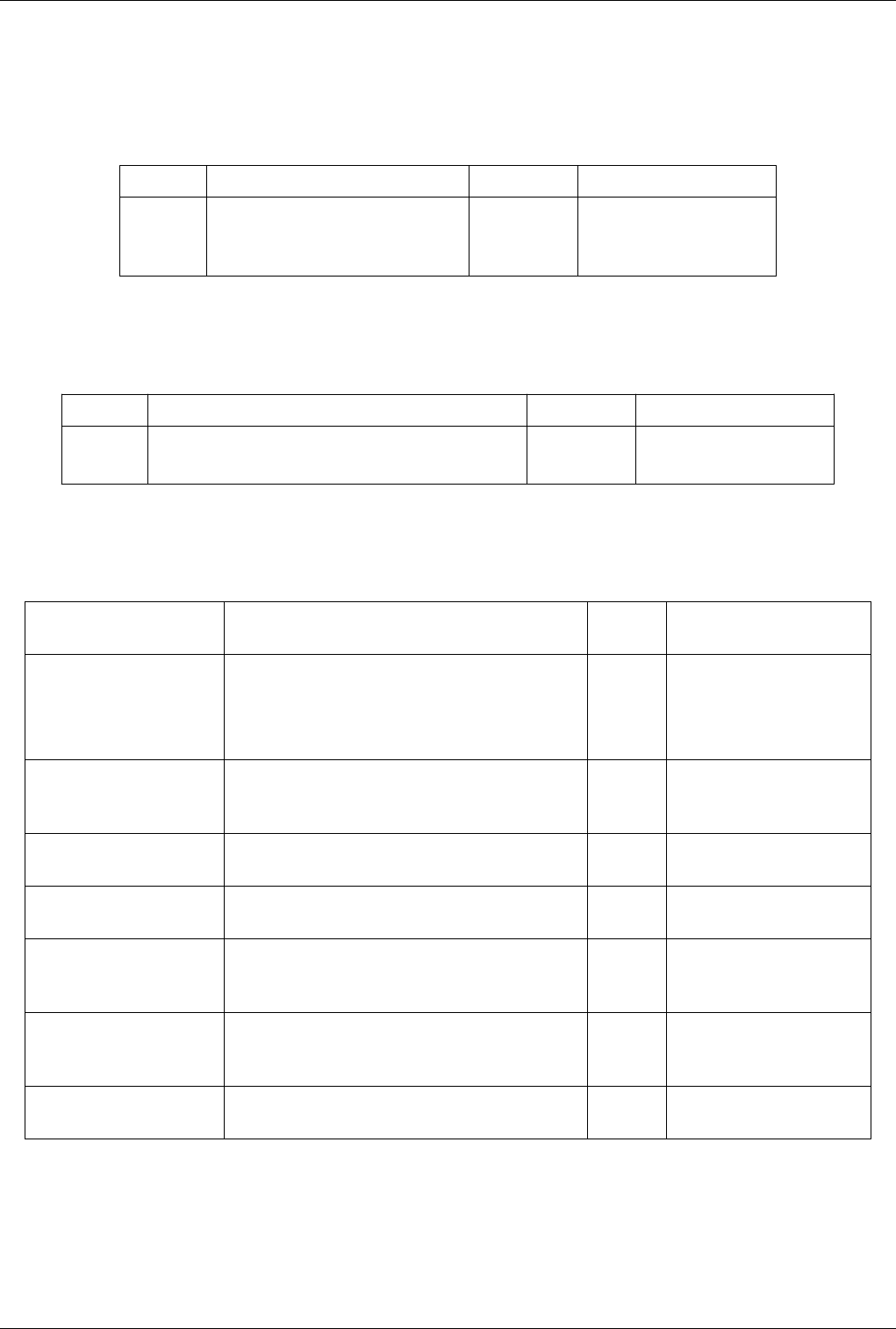
List of Filters 344
Grid Connectivity
Mass properties of connected fragments for unstructured grids.This filter works on multiblock unstructured grid
inputs and also works in parallel. It Ignores any cells with a cell data Status value of 0. It performs connectivity to
distict fragments separately. It then integrates attributes of the fragments.
Property Description Default Value(s) Restrictions
Input (Input) This property specifies the input of the filter. Accepts input of following types:
• vtkUnstructuredGrid
• vtkCompositeDataSet
Group Datasets
Group data sets. Groups multiple datasets to create a multiblock dataset
Property Description Default Value(s) Restrictions
Input (Input) This property indicates the the inputs to the Group Datasets filter. Accepts input of following types:
• vtkDataObject
Histogram
Extract a histogram from field data.
Property Description Default
Value(s)
Restrictions
Input (Input) This property specifies the input to the Histogram filter. Accepts input of following types:
• vtkDataSet
The dataset much contain a field
array ()
SelectInputArray
(SelectInputArray)
This property indicates the name of the array from which to
compute the histogram.
An array of scalars is
required.The value must be field
array name.
BinCount (BinCount) The value of this property specifies the number of bins for the
histogram.
10
Component (Component) The value of this property specifies the array component from
which the histogram should be computed.
0
CalculateAverages
(CalculateAverages)
This option controls whether the algorithm calculates averages
of variables other than the primary variable that fall into each
bin.
1 Accepts boolean values (0 or 1).
UseCustomBinRanges
(UseCustomBinRanges)
When set to true, CustomBinRanges will be used instead of
using the full range for the selected array. By default, set to
false.
0 Accepts boolean values (0 or 1).
CustomBinRanges
(CustomBinRanges)
Set custom bin ranges to use. These are used only when
UseCustomBinRanges is set to true.
0.0 100.0 The value must lie within the
range of the selected data array.
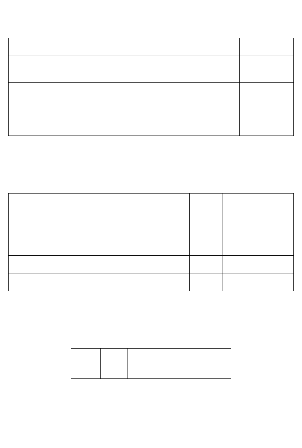
List of Filters 345
Image Data To AMR
Converts certain images to AMR.
Property Description Default
Value(s)
Restrictions
Input (Input) This property specifies the input to the Cell Data to
Point Data filter.
Accepts input of
following types:
• vtkImageData
Number of levels (NumberOfLevels) This property specifies the number of levels in the amr
data structure.
2
Maximum Number of Blocks
(MaximumNumberOfLevels)
This property specifies the maximum number of
blocks in the output amr data structure.
100
Refinement Ratio (RefinementRatio) This property specifies the refinement ratio between
levels.
2
Image Data To Uniform Grid
Create a uniform grid from an image data by specified blanking arrays. Create a vtkUniformGrid from a
vtkImageData by passing in arrays to be used for point and/or cell blanking. By default, values of 0 in the specified
array will result in a point or cell being blanked. Use Reverse to switch this.
Property Description Default
Value(s)
Restrictions
Input (Input) Accepts input of following types:
• vtkImageData
The dataset much contain a field
array ()
with 1 component(s).
SelectInputScalars
(SelectInputScalars)
Specify the array to use for blanking. An array of scalars is required.
Reverse (Reverse) Reverse the array value to whether or not a point or
cell is blanked.
0 Accepts boolean values (0 or 1).
Image Data to Point Set
The Image Data to Point Set filter takes an image data (uniform rectilinear grid) object and outputs an equivalent
structured grid (which as a type of point set). This brings the data to a broader category of data storage but only adds
a small amount of overhead. This filter can be helpful in applying filters that expect or manipulate point coordinates.
Property Description Default Value(s) Restrictions
Input (Input) Accepts input of following types:
• vtkImageData
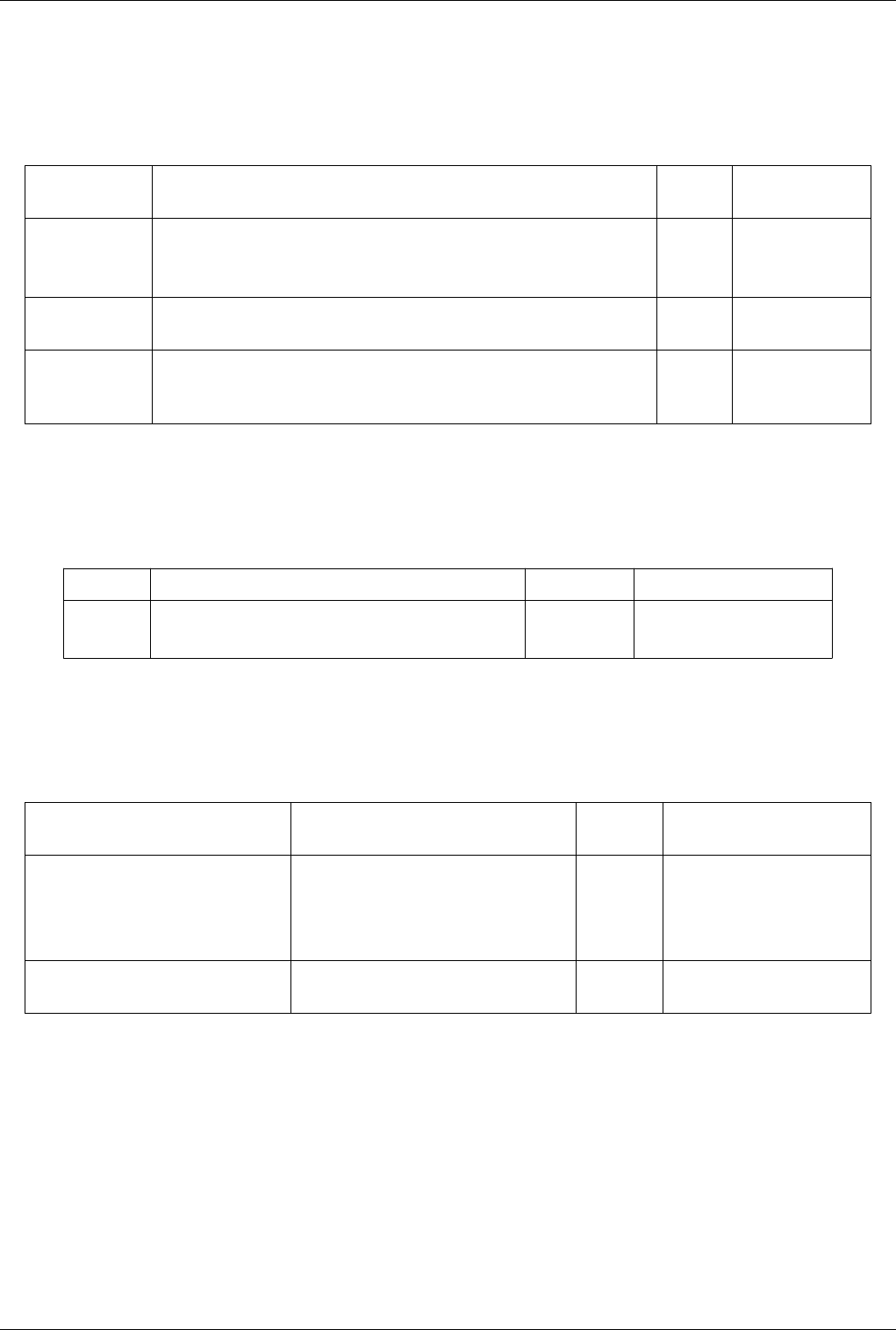
List of Filters 346
Image Shrink
Reduce the size of an image/volume by subsampling.The Image Shrink filter reduces the size of an image/volume
dataset by subsampling it (i.e., extracting every nth pixel/voxel in integer multiples). The sbsampling rate can be set
separately for each dimension of the image/volume.
Property Description Default
Value(s)
Restrictions
Input (Input) This property specifies the input to the Image Shrink filter. Accepts input of
following types:
• vtkImageData
ShrinkFactors
(ShrinkFactors)
The value of this property indicates the amount by which to shrink along each axis. 1 1 1
Averaging
(Averaging)
If the value of this property is 1, an average of neighborhood scalar values will be used
as the output scalar value for each output point. If its value is 0, only subsampling will
be performed, and the original scalar values at the points will be retained.
1 Accepts boolean
values (0 or 1).
Integrate Variables
This filter integrates cell and point attributes. The Integrate Attributes filter integrates point and cell data over lines
and surfaces. It also computes length of lines, area of surface, or volume.
Property Description Default Value(s) Restrictions
Input (Input) This property specifies the input to the Integrate Attributes filter. Accepts input of following types:
• vtkDataSet
Interpolate to Quadrature Points
Create scalar/vector data arrays interpolated to quadrature points. "Create scalar/vector data arrays interpolated to
quadrature points."
Property Description Default
Value(s)
Restrictions
Input (Input) This property specifies the input of the filter. Accepts input of following types:
• vtkUnstructuredGrid
The dataset much contain a field
array (cell)
Quadrature Scheme Def
(QuadratureSchemeDefinition)
Specifies the offset array from which we
interpolate values to quadrature points.
An array of scalars is required.
Intersect Fragments
The Intersect Fragments filter perform geometric intersections on sets of fragments. The Intersect Fragments filter
perform geometric intersections on sets of fragments. The filter takes two inputs, the first containing fragment
geometry and the second containing fragment centers. The filter has two outputs. The first is geometry that results
from the intersection. The second is a set of points that is an approximation of the center of where each fragment has
been intersected.

List of Filters 347
Property Description Default
Value(s)
Restrictions
Input (Input) This input must contian fragment geometry. Accepts input of following types:
• vtkMultiBlockDataSet
Source (Source) This input must contian fragment centers. Accepts input of following types:
• vtkMultiBlockDataSet
Slice Type
(CutFunction)
This property sets the type of intersecting geometry, and
associated parameters.
The value can be one of the
following:
• Plane (implicit_functions)
• Box (implicit_functions)
• Sphere (implicit_functions)
Iso Volume
This filter extracts cells by clipping cells that have point scalars not in the specified range. This filter clip away the
cells using lower and upper thresholds.
Property Description Default
Value(s)
Restrictions
Input (Input) This property specifies the input to the Threshold filter. Accepts input of following types:
• vtkDataSet
The dataset much contain a field array ()
with 1 component(s).
Input Scalars
(SelectInputScalars)
The value of this property contains the name of the scalar
array from which to perform thresholding.
An array of scalars is required.The value
must be field array name.
Threshold Range
(ThresholdBetween)
The values of this property specify the upper and lower
bounds of the thresholding operation.
0 0 The value must lie within the range of
the selected data array.
K Means
Compute a statistical model of a dataset and/or assess the dataset with a statistical model. This filter either computes
a statistical model of a dataset or takes such a model as its second input. Then, the model (however it is obtained)
may optionally be used to assess the input dataset.<p> This filter iteratively computes the center of k clusters in a
space whose coordinates are specified by the arrays you select. The clusters are chosen as local minima of the sum of
square Euclidean distances from each point to its nearest cluster center. The model is then a set of cluster centers.
Data is assessed by assigning a cluster center and distance to the cluster to each point in the input data set.
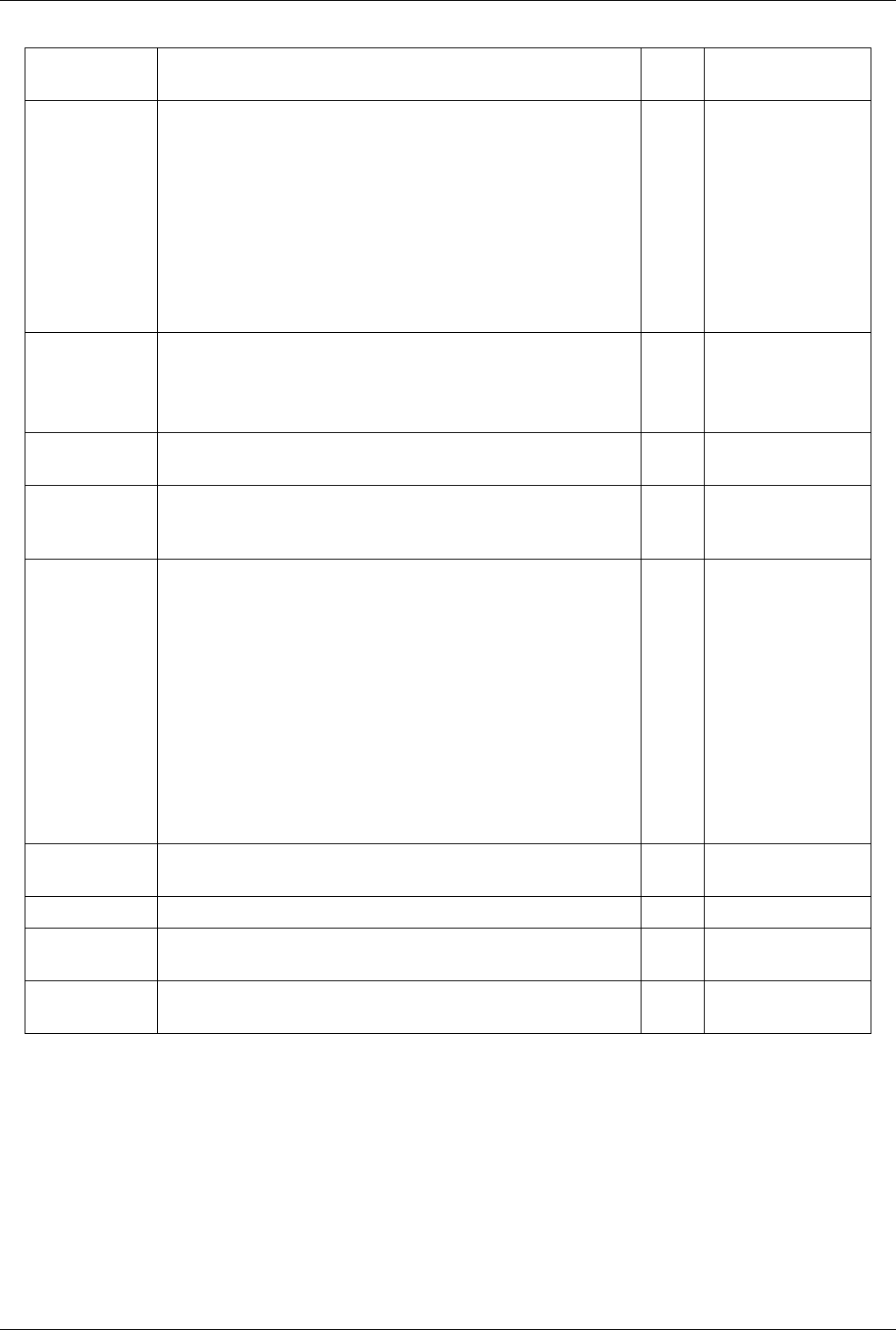
List of Filters 348
Property Description Default
Value(s)
Restrictions
Input (Input) The input to the filter. Arrays from this dataset will be used for computing statistics
and/or assessed by a statistical model.
Accepts input of following
types:
• vtkImageData
• vtkStructuredGrid
• vtkPolyData
• vtkUnstructuredGrid
• vtkTable
• vtkGraph
The dataset much contain a
field array ()
ModelInput
(ModelInput)
A previously-calculated model with which to assess a separate dataset. This input is
optional.
Accepts input of following
types:
• vtkTable
• vtkMultiBlockDataSet
AttributeMode
(AttributeMode)
Specify which type of field data the arrays will be drawn from. 0 The value must be field
array name.
Variables of
Interest
(SelectArrays)
Choose arrays whose entries will be used to form observations for statistical
analysis.
Task (Task) Specify the task to be performed: modeling and/or assessment. <ol> <li> "Detailed
model of input data," creates a set of output tables containing a calculated statistical
model of the <b>entire</b> input dataset;</li> <li> "Model a subset of the data,"
creates an output table (or tables) summarizing a <b>randomly-chosen subset</b>
of the input dataset;</li> <li> "Assess the data with a model," adds attributes to the
first input dataset using a model provided on the second input port; and</li> <li>
"Model and assess the same data," is really just operations 2 and 3 above applied to
the same input dataset. The model is first trained using a fraction of the input data
and then the entire dataset is assessed using that model.</li> </ol> When the task
includes creating a model (i.e., tasks 2, and 4), you may adjust the fraction of the
input dataset used for training. You should avoid using a large fraction of the input
data for training as you will then not be able to detect overfitting. The <i>Training
fraction</i> setting will be ignored for tasks 1 and 3.
3 The value(s) is an
enumeration of the
following:
• Detailed model of input
data (0)
• Model a subset of the
data (1)
• Assess the data with a
model (2)
• Model and assess the
same data (3)
TrainingFraction
(TrainingFraction)
Specify the fraction of values from the input dataset to be used for model fitting.
The exact set of values is chosen at random from the dataset.
0.1
k (K) Specify the number of clusters. 5
Max Iterations
(MaxNumIterations)
Specify the maximum number of iterations in which cluster centers are moved
before the algorithm terminates.
50
Tolerance
(Tolerance)
Specify the relative tolerance that will cause early termination. 0.01
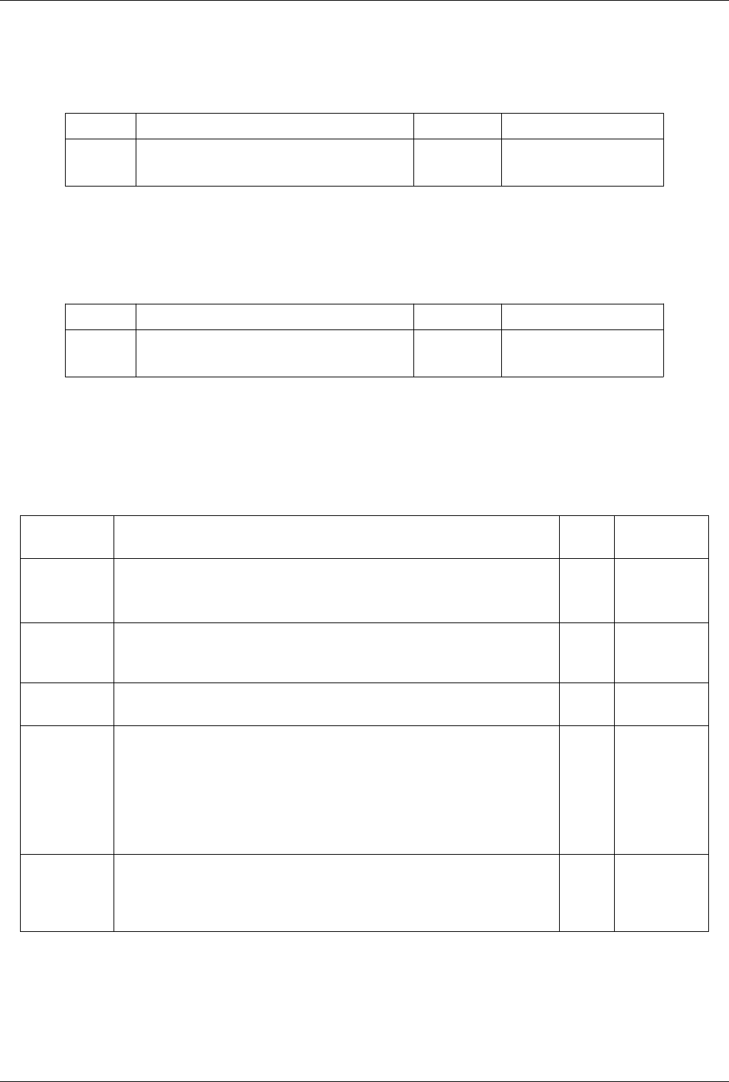
List of Filters 349
Level Scalars(Non-Overlapping AMR)
The Level Scalars filter uses colors to show levels of a hierarchical dataset.The Level Scalars filter uses colors to
show levels of a hierarchical dataset.
Property Description Default Value(s) Restrictions
Input (Input) This property specifies the input to the Level Scalars filter. Accepts input of following types:
• vtkNonOverlappingAMR
Level Scalars(Overlapping AMR)
The Level Scalars filter uses colors to show levels of a hierarchical dataset.The Level Scalars filter uses colors to
show levels of a hierarchical dataset.
Property Description Default Value(s) Restrictions
Input (Input) This property specifies the input to the Level Scalars filter. Accepts input of following types:
• vtkOverlappingAMR
Linear Extrusion
This filter creates a swept surface defined by translating the input along a vector.The Linear Extrusion filter creates a
swept surface by translating the input dataset along a specified vector. This filter is intended to operate on 2D
polygonal data. This filter operates on polygonal data and produces polygonal data output.
Property Description Default
Value(s)
Restrictions
Input (Input) This property specifies the input to the Linear Extrusion filter. Accepts input of
following types:
• vtkPolyData
ScaleFactor
(ScaleFactor)
The value of this property determines the distance along the vector the dataset will be
translated. (A scale factor of 0.5 will move the dataset half the length of the vector, and a scale
factor of 2 will move it twice the vector's length.)
1.0
Vector (Vector) The value of this property indicates the X, Y, and Z components of the vector along which to
sweep the input dataset.
0 0 1
Capping
(Capping)
The value of this property indicates whether to cap the ends of the swept surface. Capping
works by placing a copy of the input dataset on either end of the swept surface, so it behaves
properly if the input is a 2D surface composed of filled polygons. If the input dataset is a
closed solid (e.g., a sphere), then if capping is on (i.e., this property is set to 1), two copies of
the data set will be displayed on output (the second translated from the first one along the
specified vector). If instead capping is off (i.e., this property is set to 0), then an input closed
solid will produce no output.
1 Accepts boolean
values (0 or 1).
PieceInvariant
(PieceInvariant)
The value of this property determines whether the output will be the same regardless of the
number of processors used to compute the result. The difference is whether there are internal
polygonal faces on the processor boundaries. A value of 1 will keep the results the same; a
value of 0 will allow internal faces on processor boundaries.
0 Accepts boolean
values (0 or 1).
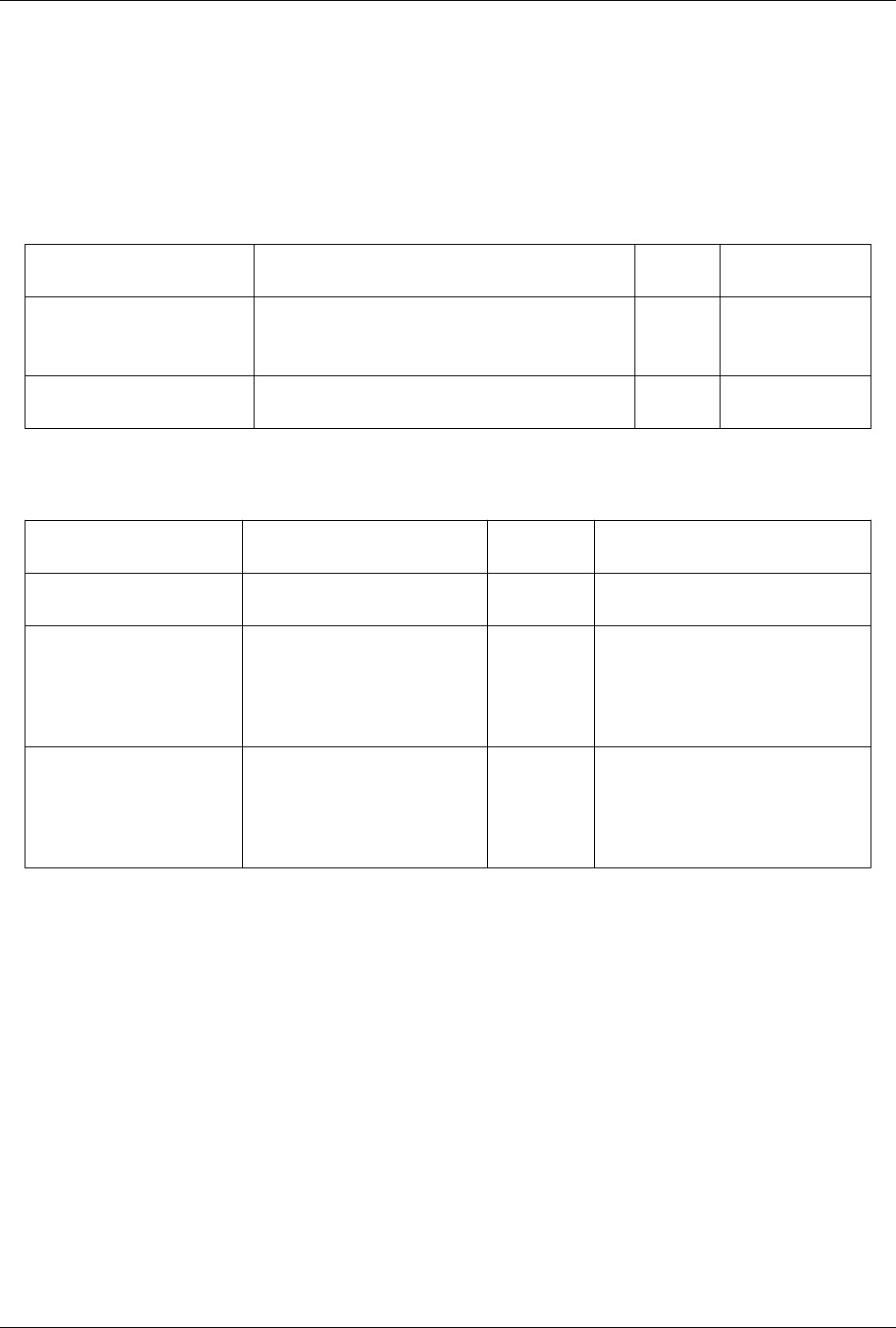
List of Filters 350
Loop Subdivision
This filter iteratively divides each triangle into four triangles. New points are placed so the output surface is smooth.
The Loop Subdivision filter increases the granularity of a polygonal mesh. It works by dividing each triangle in the
input into four new triangles. It is named for Charles Loop, the person who devised this subdivision scheme. This
filter only operates on triangles, so a data set that contains other types of polygons should be passed through the
Triangulate filter before applying this filter to it. This filter only operates on polygonal data (specifically triangle
meshes), and it produces polygonal output.
Property Description Default
Value(s)
Restrictions
Input (Input) This property specifies the input to the Loop Subdivision filter. Accepts input of
following types:
• vtkPolyData
Number of Subdivisions
(NumberOfSubdivisions)
Set the number of subdivision iterations to perform. Each
subdivision divides single triangles into four new triangles.
1
MPIMoveData
Property Description Default
Value(s)
Restrictions
Input (Input) Set the input to the MPI Move Data
filter.
MoveMode (MoveMode) Specify how the data is to be
redistributed.
0 The value(s) is an enumeration of the
following:
• PassThrough (0)
• Collect (1)
• Clone (2)
OutputDataType
(OutputDataType)
Specify the type of the dataset. none The value(s) is an enumeration of the
following:
• PolyData (0)
• Unstructured Grid (4)
• ImageData (6)
Mask Points
Reduce the number of points. This filter is often used before glyphing. Generating vertices is an option.The Mask
Points filter reduces the number of points in the dataset. It operates on any type of dataset, but produces only points /
vertices as output.
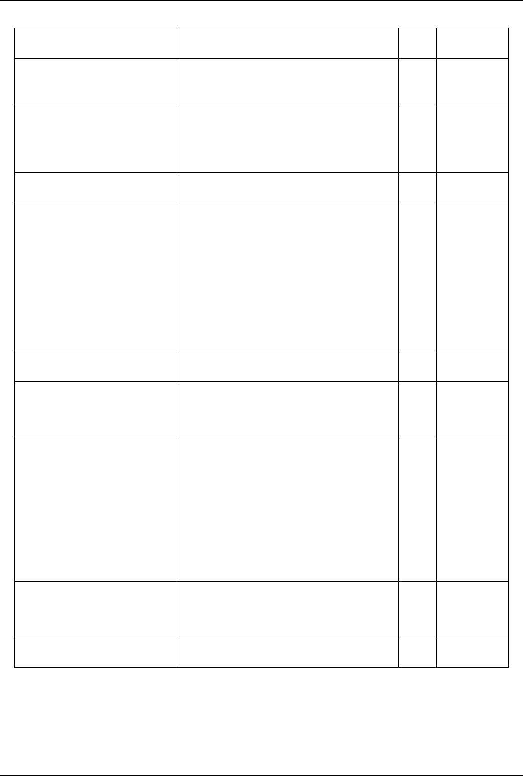
List of Filters 351
Property Description Default
Value(s)
Restrictions
Input (Input) This property specifies the input to the Mask Points filter. Accepts input of
following types:
• vtkDataSet
OnRatio (OnRatio) The value of this property specifies that every OnStride-th
points will be retained in the output when not using Random
(the skip or stride size for point ids). (For example, if the on
ratio is 3, then the output will contain every 3rd point, up to the
the maximum number of points.)
2
Maximum Number of Points
(MaximumNumberOfPoints)
The value of this property indicates the maximum number of
points in the output dataset.
5000
Proportionally Distribute Maximum
Number Of Points
(ProportionalMaximumNumberOfPoints)
When this is off, the maximum number of points is taken per
processor when running in parallel (total number of points =
number of processors * maximum number of points). When this
is on, the maximum number of points is proportionally
distributed across processors depending on the number of points
per processor ("total number of points" is the same as
"maximum number of points" maximum number of points per
processor = number of points on a processor
• maximum number of points / total number of points across
all processors
).
0 Accepts boolean
values (0 or 1).
Offset (Offset) The value of this property indicates the starting point id in the
ordered list of input points from which to start masking.
0
Random Sampling (RandomMode) If the value of this property is set to true, then the points in the
output will be randomly selected from the input in various ways
set by Random Mode; otherwise this filter will subsample point
ids regularly.
0 Accepts boolean
values (0 or 1).
Random Sampling Mode
(RandomModeType)
Randomized Id Strides picks points with random id increments
starting at Offset (the output probably isn't a statistically random
sample). Random Sampling generates a statistically random
sample of the input, ignoring Offset (fast - O(sample size)).
Spatially Stratified Random Sampling is a variant of random
sampling that splits the points into equal sized spatial strata
before randomly sampling (slow - O(N log N)).
0 The value(s) is an
enumeration of the
following:
• Randomized Id
Strides (0)
• Random
Sampling (1)
• Spatially
Stratified
Random
Sampling (2)
GenerateVertices (GenerateVertices) This property specifies whether to generate vertex cells as the
topography of the output. If set to 1, the geometry (vertices) will
be displayed in the rendering window; otherwise no geometry
will be displayed.
0 Accepts boolean
values (0 or 1).
SingleVertexPerCell (SingleVertexPerCell) Tell filter to only generate one vertex per cell instead of multiple
vertices in one cell.
0 Accepts boolean
values (0 or 1).

List of Filters 352
Material Interface Filter
The Material Interface filter finds volumes in the input data containg material above a certain material fraction. The
Material Interface filter finds voxels inside of which a material fraction (or normalized amount of material) is higher
than a given threshold. As these voxels are identified surfaces enclosing adjacent voxels above the threshold are
generated. The resulting volume and its surface are what we call a fragment. The filter has the ability to compute
various volumetric attributes such as fragment volume, mass, center of mass as well as volume and mass weighted
averages for any of the fields present. Any field selected for such computation will be also be coppied into the
fragment surface's point data for visualization. The filter also has the ability to generate Oriented Bounding Boxes
(OBB) for each fragment. The data generated by the filter is organized in three outputs. The "geometry" output,
containing the fragment surfaces. The "statistics" output, containing a point set of the centers of mass. The "obb
representaion" output, containing OBB representations (poly data). All computed attributes are coppied into the
statistics and geometry output. The obb representation output is used for validation and debugging puproses and is
turned off by default. To measure the size of craters, the filter can invert a volume fraction and clip the volume
fraction with a sphere and/or a plane.
Property Description Default
Value(s)
Restrictions
Input (Input) Input to the filter can be a hierarchical box data set containing image
data or a multi-block of rectilinear grids.
Accepts input of following
types:
• vtkNonOverlappingAMR
The dataset much contain a
field array (cell)
Select Material Fraction
Arrays (SelectMaterialArray)
Material fraction is defined as normalized amount of material per
voxel. It is expected that arrays containing material fraction data has
been down converted to a unsigned char.
An array of scalars is
required.
Material Fraction Threshold
(MaterialFractionThreshold)
Material fraction is defined as normalized amount of material per
voxel. Any voxel in the input data set with a material fraction greater
than this value is included in the output data set.
0.5
InvertVolumeFraction
(InvertVolumeFraction)
Inverting the volume fraction generates the negative of the material.
It is useful for analyzing craters.
0 Accepts boolean values (0 or
1).
Clip Type (ClipFunction) This property sets the type of clip geometry, and associated
parameters.
The value can be one of the
following:
• None (implicit_functions)
• Plane (implicit_functions)
• Sphere
(implicit_functions)
Select Mass Arrays
(SelectMassArray)
Mass arrays are paired with material fraction arrays. This means that
the first selected material fraction array is paired with the first
selected mass array, and so on sequentially. As the filter identifies
voxels meeting the minimum material fraction threshold, these
voxel's mass will be used in fragment center of mass and mass
calculation. A warning is generated if no mass array is selected for
an individual material fraction array. However, in that case the filter
will run without issue because the statistics output can be generated
using fragments' centers computed from axis aligned bounding
boxes.
An array of scalars is
required.
Compute volume weighted
average over:
(SelectVolumeWtdAvgArray)
Specifies the arrays from which to volume weighted average. For
arrays selected a volume weighted average is computed. The values
of these arrays are also coppied into fragment geometry cell data as
the fragment surfaces are generated.

List of Filters 353
Compute mass weighted
average over:
(SelectMassWtdAvgArray)
For arrays selected a mass weighted average is computed. These
arrays are also coppied into fragment geometry cell data as the
fragment surfaces are generated.
ComputeOBB (ComputeOBB) Compute Object Oriented Bounding boxes (OBB). When active the
result of this computation is coppied into the statistics output. In the
case that the filter is built in its validation mode, the OBB's are
rendered.
0 Accepts boolean values (0 or
1).
WriteGeometryOutput
(WriteGeometryOutput)
If this property is set, then the geometry output is written to a text
file. The file name will be coonstructed using the path in the "Output
Base Name" widget.
0 Accepts boolean values (0 or
1).
WriteStatisticsOutput
(WriteStatisticsOutput)
If this property is set, then the statistics output is written to a text
file. The file name will be coonstructed using the path in the "Output
Base Name" widget.
0 Accepts boolean values (0 or
1).
OutputBaseName
(OutputBaseName)
This property specifies the base including path of where to write the
statistics and gemoetry output text files. It follows the pattern
"/path/to/folder/and/file" here file has no extention, as the filter will
generate a unique extention.
Median
Compute the median scalar values in a specified neighborhood for image/volume datasets. The Median filter
operates on uniform rectilinear (image or volume) data and produces uniform rectilinear output. It replaces the scalar
value at each pixel / voxel with the median scalar value in the specified surrounding neighborhood. Since the median
operation removes outliers, this filter is useful for removing high-intensity, low-probability noise (shot noise).
Property Description Default
Value(s)
Restrictions
Input (Input) This property specifies the input to the Median filter. Accepts input of
following types:
• vtkImageData
The dataset much contain
a field array (point)
with 1 component(s).
SelectInputScalars
(SelectInputScalars)
The value of this property lists the name of the scalar array to use in computing
the median.
An array of scalars is
required.
KernelSize (KernelSize) The value of this property specifies the number of pixels/voxels in each
dimension to use in computing the median to assign to each pixel/voxel. If the
kernel size in a particular dimension is 1, then the median will not be computed
in that direction.
1 1 1
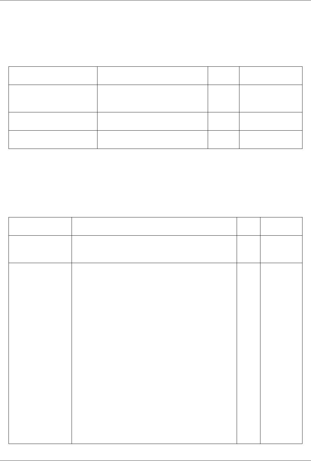
List of Filters 354
Merge Blocks
Appends vtkCompositeDataSet leaves into a single vtkUnstructuredGrid
vtkCompositeDataToUnstructuredGridFilter appends all vtkDataSet leaves of the input composite dataset to a single
unstructure grid. The subtree to be combined can be choosen using the SubTreeCompositeIndex. If the
SubTreeCompositeIndex is a leaf node, then no appending is required.
Property Description Default
Value(s)
Restrictions
Input (Input) Set the input composite dataset. Accepts input of following
types:
• vtkCompositeDataSet
SubTreeCompositeIndex
(SubTreeCompositeIndex)
Select the index of the subtree to be appended. For
now, this property is internal.
0
Merge Points (MergePoints) 1 Accepts boolean values (0 or
1).
Mesh Quality
This filter creates a new cell array containing a geometric measure of each cell's fitness. Different quality measures
can be chosen for different cell shapes.This filter creates a new cell array containing a geometric measure of each
cell's fitness. Different quality measures can be chosen for different cell shapes. Supported shapes include triangles,
quadrilaterals, tetrahedra, and hexahedra. For other shapes, a value of 0 is assigned.
Property Description Default
Value(s)
Restrictions
Input (Input) This property specifies the input to the Mesh Quality filter. Accepts input of
following types:
• vtkDataSet
TriangleQualityMeasure
(TriangleQualityMeasure)
This property indicates which quality measure will be used to evaluate triangle
quality. The radius ratio is the size of a circle circumscribed by a triangle's 3
vertices divided by the size of a circle tangent to a triangle's 3 edges. The edge
ratio is the ratio of the longest edge length to the shortest edge length.
2 The value(s) is an
enumeration of the
following:
• Area (28)
• Aspect Ratio
(1)
• Aspect
Frobenius (3)
• Condition (9)
• Distortion (15)
• Edge Ratio (0)
• Maximum
Angle (8)
• Minimum
Angle (6)
• Scaled
Jacobian (10)
• Radius Ratio
(2)
• Relative Size
Squared (12)
• Shape (13)
• Shape and Size
(14)

List of Filters 355
QuadQualityMeasure
(QuadQualityMeasure)
This property indicates which quality measure will be used to evaluate
quadrilateral quality.
0 The value(s) is an
enumeration of the
following:
• Area (28)
• Aspect Ratio
(1)
• Condition (9)
• Distortion (15)
• Edge Ratio (0)
• Jacobian (25)
• Maximum
Aspect
Frobenius (5)
• Maximum
Aspect
Frobenius (5)
• Maximum
Edge Ratio
(16)
• Mean Aspect
Frobenius (4)
• Minimum
Angle (6)
• Oddy (23)
• Radius Ratio
(2)
• Relative Size
Squared (12)
• Scaled
Jacobian (10)
• Shape (13)
• Shape and Size
(14)
• Shear (11)
• Shear and Size
(24)
• Skew (17)
• Stretch (20)
• Taper (18)
• Warpage (26)
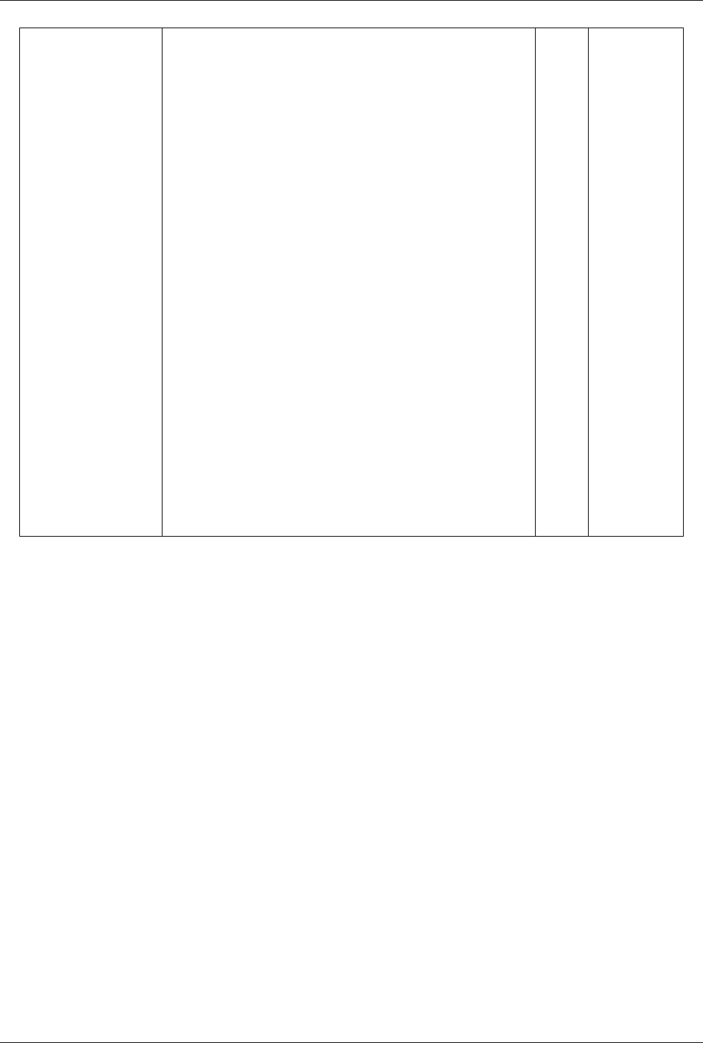
List of Filters 356
TetQualityMeasure
(TetQualityMeasure)
This property indicates which quality measure will be used to evaluate tetrahedral
quality. The radius ratio is the size of a sphere circumscribed by a tetrahedron's 4
vertices divided by the size of a circle tangent to a tetrahedron's 4 faces. The edge
ratio is the ratio of the longest edge length to the shortest edge length. The
collapse ratio is the minimum ratio of height of a vertex above the triangle
opposite it divided by the longest edge of the opposing triangle across all
vertex/triangle pairs.
2 The value(s) is an
enumeration of the
following:
• Edge Ratio (0)
• Aspect Beta
(29)
• Aspect Gamma
(27)
• Aspect
Frobenius (3)
• Aspect Ratio
(1)
• Collapse Ratio
(7)
• Condition (9)
• Distortion (15)
• Jacobian (25)
• Minimum
Dihedral Angle
(6)
• Radius Ratio
(2)
• Relative Size
Squared (12)
• Scaled
Jacobian (10)
• Shape (13)
• Shape and Size
(14)
• Volume (19)
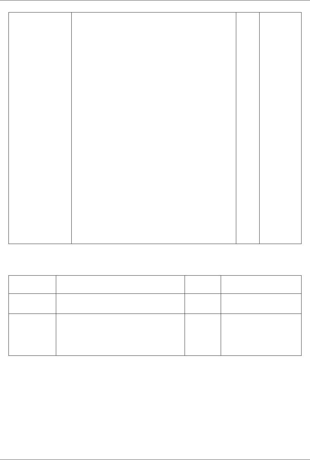
List of Filters 357
HexQualityMeasure
(HexQualityMeasure)
This property indicates which quality measure will be used to evaluate hexahedral
quality.
5 The value(s) is an
enumeration of the
following:
• Diagonal (21)
• Dimension (22)
• Distortion (15)
• Edge Ratio (0)
• Jacobian (25)
• Maximum
Edge Ratio
(16)
• Maximum
Aspect
Frobenius (5)
• Mean Aspect
Frobenius (4)
• Oddy (23)
• Relative Size
Squared (12)
• Scaled
Jacobian (10)
• Shape (13)
• Shape and Size
(14)
• Shear (11)
• Shear and Size
(24)
• Skew (17)
• Stretch (20)
• Taper (18)
• Volume (19)
MinMax
Property Description Default
Value(s)
Restrictions
Input (Input) Set the input to the Min Max filter. Accepts input of following types:
• vtkDataSet
Operation
(Operation)
Select whether to perform a min, max, or sum operation on the
data.
MIN The value(s) can be one of the
following:
• MIN
• MAX
• SUM
Multicorrelative Statistics
Compute a statistical model of a dataset and/or assess the dataset with a statistical model. This filter either computes
a statistical model of a dataset or takes such a model as its second input. Then, the model (however it is obtained)
may optionally be used to assess the input dataset.<p> This filter computes the covariance matrix for all the arrays
you select plus the mean of each array. The model is thus a multivariate Gaussian distribution with the mean vector
and variances provided. Data is assessed using this model by computing the Mahalanobis distance for each input
point. This distance will always be positive.<p> The learned model output format is rather dense and can be
confusing, so it is discussed here. The first filter output is a multiblock dataset consisting of 2 tables: <ol> <li> Raw
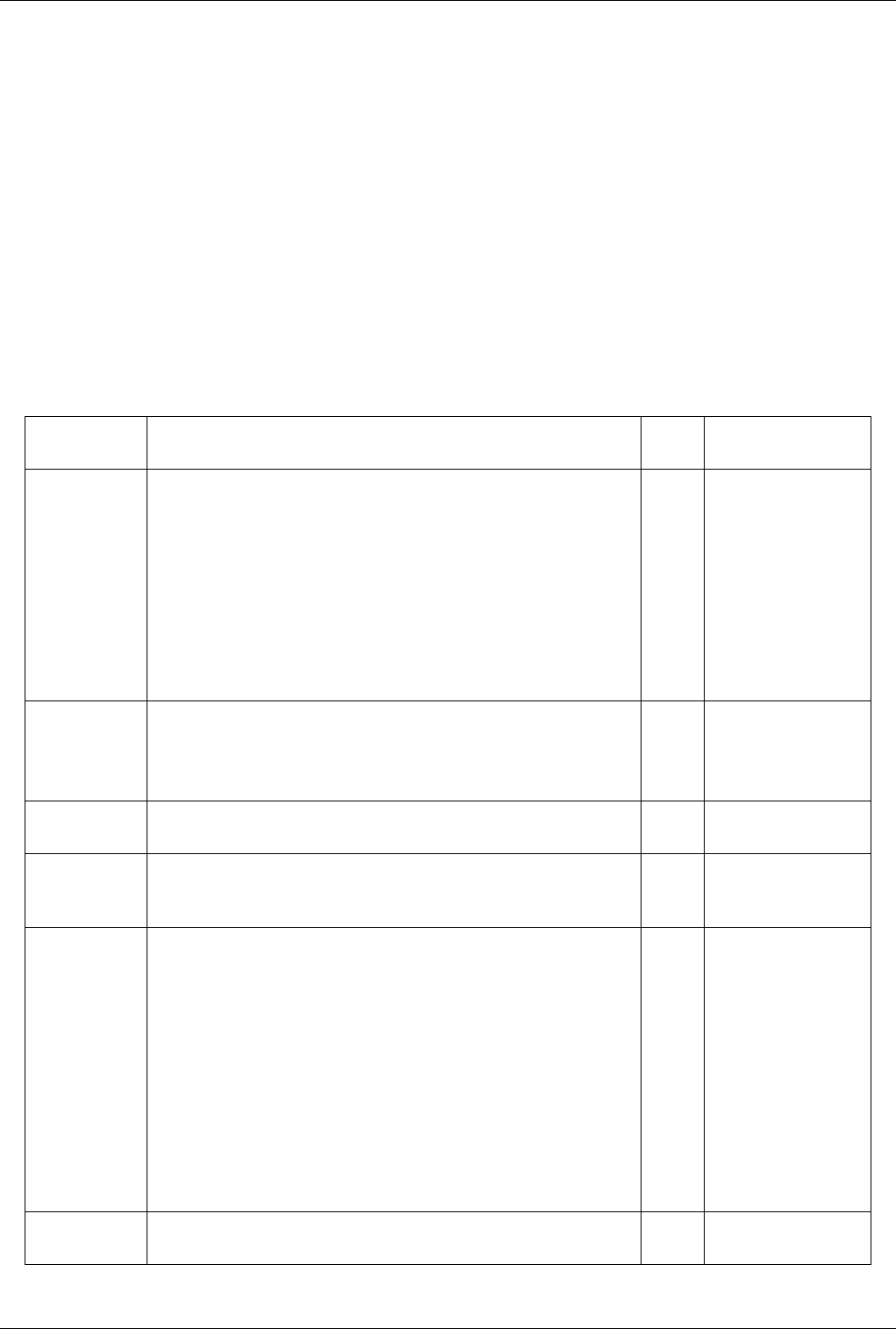
List of Filters 358
covariance data. <li> Covariance matrix and its Cholesky decomposition. </ol> The raw covariance table has 3
meaningful columns: 2 titled "Column1" and "Column2" whose entries generally refer to the N arrays you selected
when preparing the filter and 1 column titled "Entries" that contains numeric values. The first row will always
contain the number of observations in the statistical analysis. The next N rows contain the mean for each of the N
arrays you selected. The remaining rows contain covariances of pairs of arrays.<p> The second table (covariance
matrix and Cholesky decomposition) contains information derived from the raw covariance data of the first table.
The first N rows of the first column contain the name of one array you selected for analysis. These rows are followed
by a single entry labeled "Cholesky" for a total of N+1 rows. The second column, Mean contains the mean of each
variable in the first N entries and the number of observations processed in the final (N+1) row.<p> The remaining
columns (there are N, one for each array) contain 2 matrices in triangular format. The upper right triangle contains
the covariance matrix (which is symmetric, so its lower triangle may be inferred). The lower left triangle contains the
Cholesky decomposition of the covariance matrix (which is triangular, so its upper triangle is zero). Because the
diagonal must be stored for both matrices, an additional row is required — hence the N+1 rows and the final entry
of the column named "Column".
Property Description Default
Value(s)
Restrictions
Input (Input) The input to the filter. Arrays from this dataset will be used for computing statistics
and/or assessed by a statistical model.
Accepts input of following
types:
• vtkImageData
• vtkStructuredGrid
• vtkPolyData
• vtkUnstructuredGrid
• vtkTable
• vtkGraph
The dataset much contain a
field array ()
ModelInput
(ModelInput)
A previously-calculated model with which to assess a separate dataset. This input is
optional.
Accepts input of following
types:
• vtkTable
• vtkMultiBlockDataSet
AttributeMode
(AttributeMode)
Specify which type of field data the arrays will be drawn from. 0 The value must be field
array name.
Variables of
Interest
(SelectArrays)
Choose arrays whose entries will be used to form observations for statistical analysis.
Task (Task) Specify the task to be performed: modeling and/or assessment. <ol> <li> "Detailed
model of input data," creates a set of output tables containing a calculated statistical
model of the <b>entire</b> input dataset;</li> <li> "Model a subset of the data,"
creates an output table (or tables) summarizing a <b>randomly-chosen subset</b> of
the input dataset;</li> <li> "Assess the data with a model," adds attributes to the first
input dataset using a model provided on the second input port; and</li> <li> "Model
and assess the same data," is really just operations 2 and 3 above applied to the same
input dataset. The model is first trained using a fraction of the input data and then the
entire dataset is assessed using that model.</li> </ol> When the task includes
creating a model (i.e., tasks 2, and 4), you may adjust the fraction of the input dataset
used for training. You should avoid using a large fraction of the input data for
training as you will then not be able to detect overfitting. The <i>Training
fraction</i> setting will be ignored for tasks 1 and 3.
3 The value(s) is an
enumeration of the
following:
• Detailed model of input
data (0)
• Model a subset of the
data (1)
• Assess the data with a
model (2)
• Model and assess the
same data (3)
TrainingFraction
(TrainingFraction)
Specify the fraction of values from the input dataset to be used for model fitting. The
exact set of values is chosen at random from the dataset.
0.1
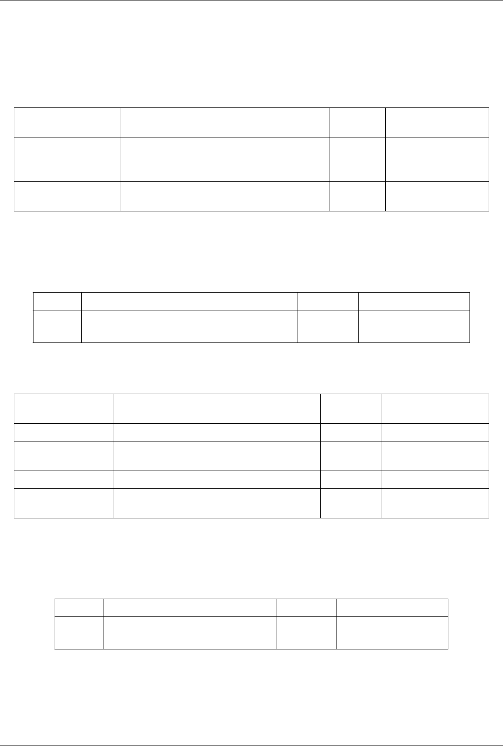
List of Filters 359
Octree Depth Limit
This filter takes in a octree and produces a new octree which is no deeper than the maximum specified depth
level.The Octree Depth Limit filter takes in an octree and produces a new octree that is nowhere deeper than the
maximum specified depth level. The attribute data of pruned leaf cells are integrated in to their ancestors at the cut
level.
Property Description Default
Value(s)
Restrictions
Input (Input) This property specifies the input to the Octree Depth Limit
filter.
Accepts input of following
types:
• vtkHyperOctree
MaximumLevel
(MaximumLevel)
The value of this property specifies the maximum depth of the
output octree.
4
Octree Depth Scalars
This filter adds a scalar to each leaf of the octree that represents the leaf's depth within the tree.The
vtkHyperOctreeDepth filter adds a scalar to each leaf of the octree that represents the leaf's depth within the tree.
Property Description Default Value(s) Restrictions
Input (Input) This property specifies the input to the Octree Depth Scalars filter. Accepts input of following types:
• vtkHyperOctree
OrderedCompositeDistributor
Property Description Default
Value(s)
Restrictions
Input (Input) Set the input to the Ordered Composite Distributor filter.
PassThrough
(PassThrough)
Toggle whether to pass the data through without compositing. 0 Accepts boolean values (0 or
1).
PKdTree (PKdTree) Set the vtkPKdTree to distribute with.
OutputType (OutputType) When not empty, the output will be converted to the given
type.
Outline
This filter generates a bounding box representation of the input.The Outline filter generates an axis-aligned bounding
box for the input dataset. This filter operates on any type of dataset and produces polygonal output.
Property Description Default Value(s) Restrictions
Input (Input) This property specifies the input to the Outline filter. Accepts input of following types:
• vtkDataSet

List of Filters 360
Outline Corners
This filter generates a bounding box representation of the input. It only displays the corners of the bounding box.The
Outline Corners filter generates the corners of a bounding box for the input dataset. This filter operates on any type
of dataset and produces polygonal output.
Property Description Default
Value(s)
Restrictions
Input (Input) This property specifies the input to the Outline Corners filter. Accepts input of
following types:
• vtkDataSet
CornerFactor
(CornerFactor)
The value of this property sets the size of the corners as a percentage of the
length of the corresponding bounding box edge.
0.2
Outline Curvilinear DataSet
This filter generates an outline representation of the input.The Outline filter generates an outline of the outside edges
of the input dataset, rather than the dataset's bounding box. This filter operates on structured grid datasets and
produces polygonal output.
Property Description Default Value(s) Restrictions
Input (Input) This property specifies the input to the outline (curvilinear) filter. Accepts input of following types:
• vtkStructuredGrid
Outline Generic DataSet
This filter generates a bounding box representation of the input.The Generic Outline filter generates an axis-aligned
bounding box for the input data set. The Input menu specifies the data set for which to create a bounding box. This
filter operates on generic data sets and produces polygonal output.
Property Description Default Value(s) Restrictions
Input (Input) Set the input to the Generic Outline filter. Accepts input of following types:
• vtkGenericDataSet
ParticlePath
Trace Particle Paths through time in a vector field. The Particle Trace filter generates pathlines in a vector field from
a collection of seed points. The vector field used is selected from the Vectors menu, so the input data set is required
to have point-centered vectors. The Seed portion of the interface allows you to select whether the seed points for this
integration lie in a point cloud or along a line. Depending on which is selected, the appropriate 3D widget (point or
line widget) is displayed along with traditional user interface controls for positioning the point cloud or line within
the data set. Instructions for using the 3D widgets and the corresponding manual controls can be found in section 7.4.
This filter operates on any type of data set, provided it has point-centered vectors. The output is polygonal data
containing polylines. This filter is available on the Toolbar.

List of Filters 361
Property Description Default
Value(s)
Restrictions
Input (Input) Specify which is the Input of the StreamTracer filter. Accepts input of
following types:
• vtkDataObject
The dataset much
contain a field array
(point)
with 3 component(s).
Seed Source (Source) Specify the seed dataset. Typically fron where the vector field integration
should begin. Usually a point/radius or a line with a given resolution.
Accepts input of
following types:
• vtkDataSet
TerminationTime
(TerminationTime)
Setting TerminationTime to a positive value will cause particles to
terminate when the time is reached. The units of time should be consistent
with the primary time variable.
0.0
TimestepValues (TimestepValues)
ForceReinjectionEveryNSteps
(ForceReinjectionEveryNSteps)
When animating particles, it is nice to inject new ones every Nth step to
produce a continuous flow. Setting ForceReinjectionEveryNSteps to a non
zero value will cause the particle source to reinject particles every Nth step
even if it is otherwise unchanged. Note that if the particle source is also
animated, this flag will be redundant as the particles will be reinjected
whenever the source changes anyway
0
SelectInputVectors
(SelectInputVectors)
Specify which vector array should be used for the integration through that
filter.
An array of vectors
is required.
ComputeVorticity
(ComputeVorticity)
Compute vorticity and angular rotation of particles as they progress 1 Accepts boolean
values (0 or 1).
DisableResetCache
(DisableResetCache)
Prevents cache from getting reset so that new computation always start
from previous results.
0 Accepts boolean
values (0 or 1).
ParticleTracer
Trace Particles through time in a vector field. The Particle Trace filter generates pathlines in a vector field from a
collection of seed points. The vector field used is selected from the Vectors menu, so the input data set is required to
have point-centered vectors. The Seed portion of the interface allows you to select whether the seed points for this
integration lie in a point cloud or along a line. Depending on which is selected, the appropriate 3D widget (point or
line widget) is displayed along with traditional user interface controls for positioning the point cloud or line within
the data set. Instructions for using the 3D widgets and the corresponding manual controls can be found in section 7.4.
This filter operates on any type of data set, provided it has point-centered vectors. The output is polygonal data
containing polylines. This filter is available on the Toolbar.
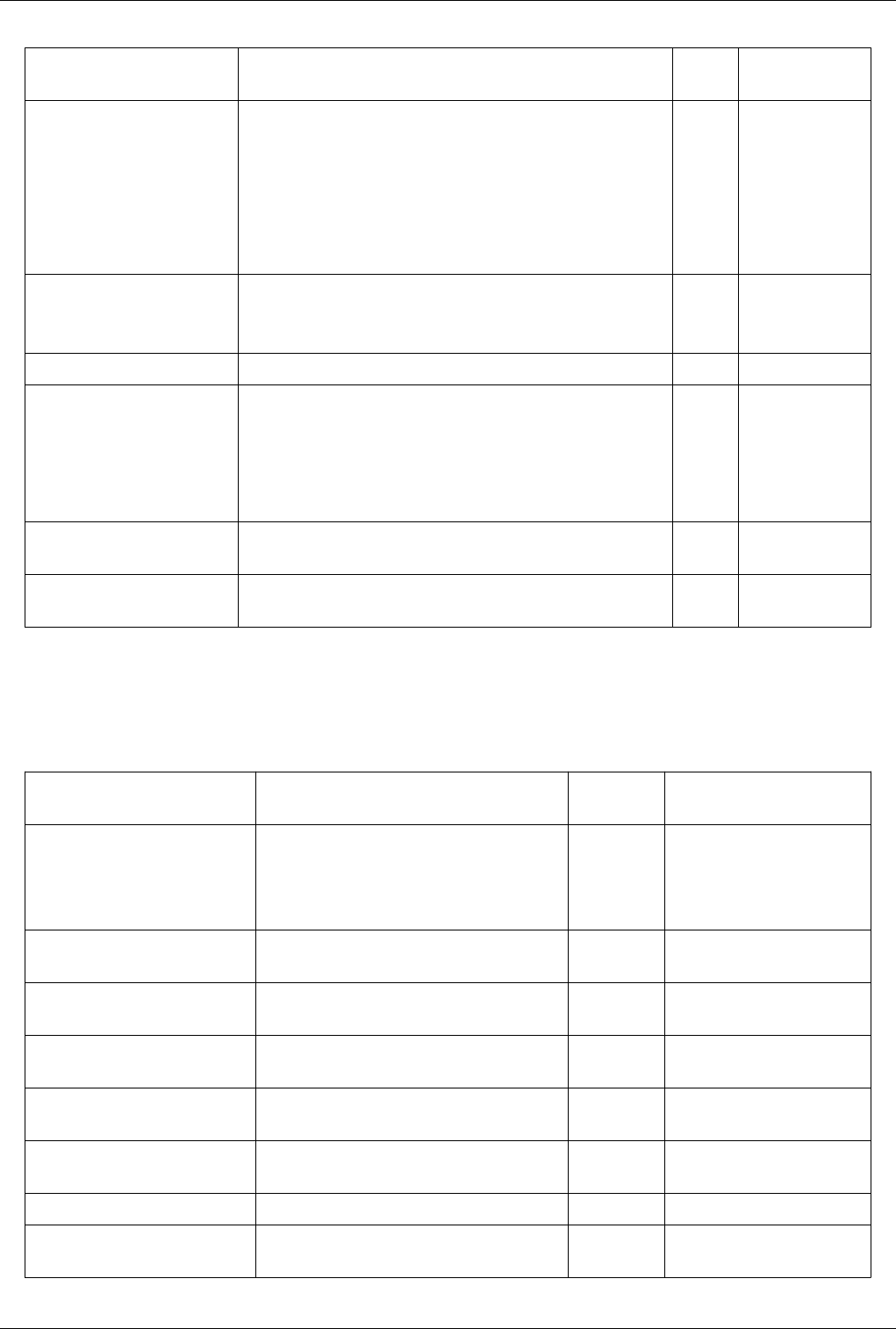
List of Filters 362
Property Description Default
Value(s)
Restrictions
Input (Input) Specify which is the Input of the StreamTracer filter. Accepts input of
following types:
• vtkDataObject
The dataset much
contain a field array
(point)
with 3 component(s).
Seed Source (Source) Specify the seed dataset. Typically fron where the vector field integration
should begin. Usually a point/radius or a line with a given resolution.
Accepts input of
following types:
• vtkDataSet
TimestepValues (TimestepValues)
ForceReinjectionEveryNSteps
(ForceReinjectionEveryNSteps)
When animating particles, it is nice to inject new ones every Nth step to
produce a continuous flow. Setting ForceReinjectionEveryNSteps to a non
zero value will cause the particle source to reinject particles every Nth step
even if it is otherwise unchanged. Note that if the particle source is also
animated, this flag will be redundant as the particles will be reinjected
whenever the source changes anyway
0
SelectInputVectors
(SelectInputVectors)
Specify which vector array should be used for the integration through that
filter.
An array of vectors
is required.
ComputeVorticity
(ComputeVorticity)
Compute vorticity and angular rotation of particles as they progress 1 Accepts boolean
values (0 or 1).
Pass Arrays
Pass specified point and cell data arrays. The Pass Arrays filter makes a shallow copy of the output data object from
the input data object except for passing only the arrays specified to the output from the input.
Property Description Default
Value(s)
Restrictions
Input (Input) Accepts input of following types:
• vtkDataObject
The dataset much contain a field
array ()
UseFieldTypes (UseFieldTypes) This hidden property must always be set to 1 for this
proxy to work.
1 Accepts boolean values (0 or 1).
AddPointArrayType
(AddPointArrayType)
This hidden property must always be set to 0 for this
proxy to work.
0 Accepts boolean values (0 or 1).
AddCellArrayType
(AddCellArrayType)
This hidden property must always be set to 1 for this
proxy to work.
1 Accepts boolean values (0 or 1).
AddFieldArrayType
(AddFieldArrayType)
This hidden property must always be set to 2 for this
proxy to work.
2 Accepts boolean values (0 or 1).
PointDataArrays
(AddPointDataArray)
Add a point array by name to be passed.
CellDataArrays (AddCellDataArray) Add a cell array by name to be passed.
FieldDataArrays
(AddFieldDataArray)
Add a field array by name to be passed.

List of Filters 363
Plot Data
Plot data arrays from the inputThis filter prepare arbitrary data to be plotted in any of the plots. By default the data is
shown in a XY line plot.
Property Description Default Value(s) Restrictions
Input (Input) The input. Accepts input of following types:
• vtkDataObject
Plot Global Variables Over Time
Extracts and plots data in field data over time. This filter extracts the variables that reside in a dataset's field data and
are defined over time. The output is a 1D rectilinear grid where the x coordinates correspond to time (the same array
is also copied to a point array named Time or TimeData (if Time exists in the input)).
Property Description Default Value(s) Restrictions
Input (Input) The input from which the selection is extracted. Accepts input of following types:
• vtkDataSet
Plot On Sorted Lines
Property Description Default Value(s) Restrictions
Input (Input) This property specifies the input to the Plot Edges filter. Accepts input of following types:
• vtkPolyData
Plot Selection Over Time
Extracts selection over time and then plots it. This filter extracts the selection over time, i.e. cell and/or point
variables at a cells/point selected are extracted over time The output multi-block consists of 1D rectilinear grids
where the x coordinate corresponds to time (the same array is also copied to a point array named Time or TimeData
(if Time exists in the input)). If selection input is a Location based selection then the point values are interpolated
from the nearby cells, ie those of the cell the location lies in.
Property Description Default
Value(s)
Restrictions
Input (Input) The input from which the selection is extracted. Accepts input of following
types:
• vtkDataSet
• vtkTable
• vtkCompositeDataSet
Selection (Selection) The input that provides the selection object. Accepts input of following
types:
• vtkSelection
Only Report Selection
Statistics (Only Report
Selection Statistics)
If this property is set to 1, the min, max, inter-quartile ranges, and (for numeric
arrays) mean and standard deviation of all the selected points or cells within
each time step are reported -- instead of breaking each selected point's or cell's
attributes out into separate time history tables.
0 Accepts boolean values (0
or 1).
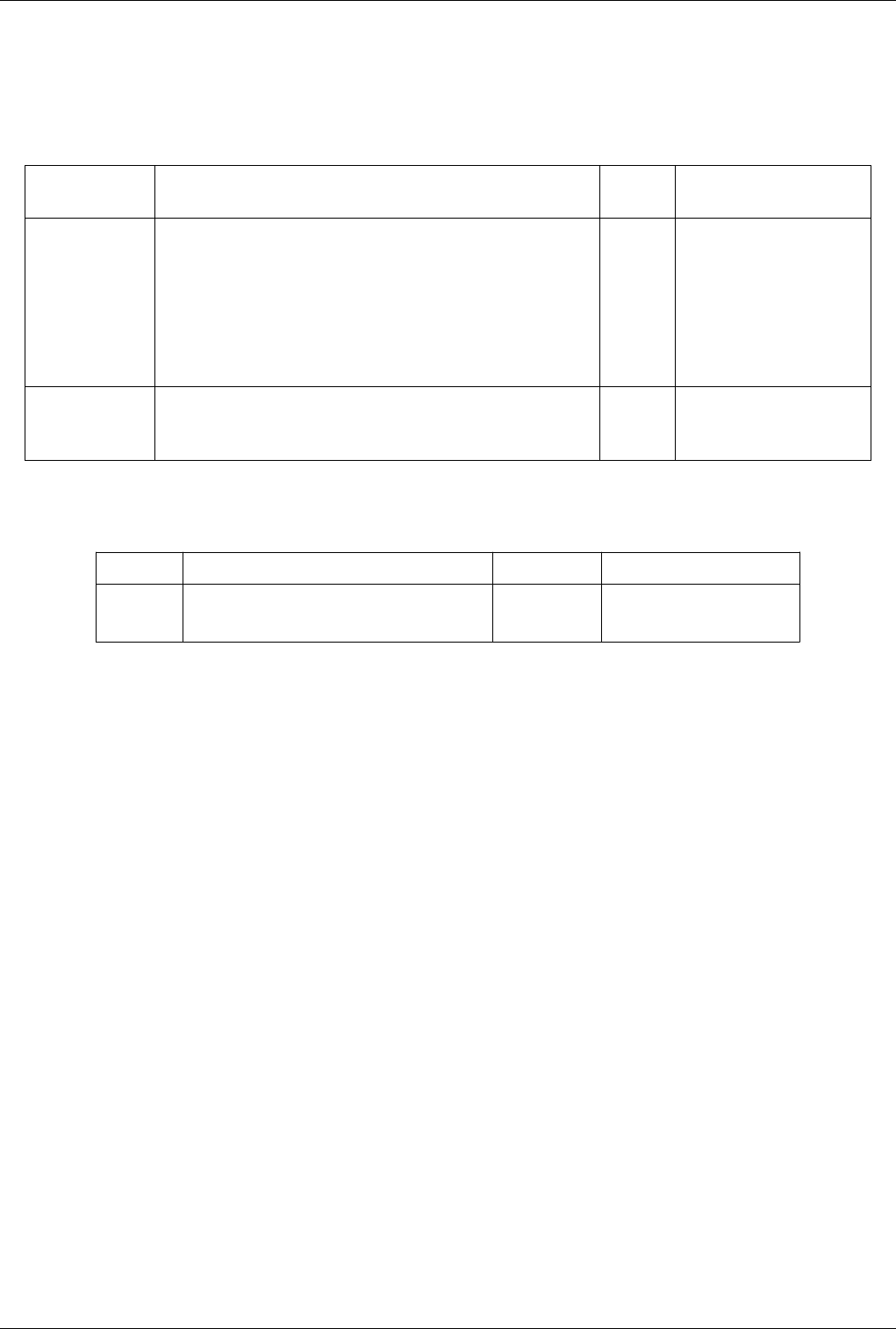
List of Filters 364
Point Data to Cell Data
Create cell attributes by averaging point attributes.The Point Data to Cell Data filter averages the values of the point
attributes of the points of a cell to compute cell attributes. This filter operates on any type of dataset, and the output
dataset is the same type as the input.
Property Description Default
Value(s)
Restrictions
Input (Input) This property specifies the input to the Point Data to Cell Data filter. Accepts input of following
types:
• vtkDataSetOnce set, the
input dataset cannot be
changed.
The dataset much contain a field
array (point)
PassPointData
(PassPointData)
The value of this property controls whether the input point data will be
passed to the output. If set to 1, then the input point data is passed through to
the output; otherwise, only generated cell data is placed into the output.
0 Accepts boolean values (0 or 1).
PolyLine To Rectilinear Grid
Property Description Default Value(s) Restrictions
Input (Input) Set the input to the Polyline to Rectilinear Grid filter. Accepts input of following types:
• vtkPolyData
Principal Component Analysis
Compute a statistical model of a dataset and/or assess the dataset with a statistical model. This filter either computes
a statistical model of a dataset or takes such a model as its second input. Then, the model (however it is obtained)
may optionally be used to assess the input dataset. <p> This filter performs additional analysis above and beyond the
multicorrelative filter. It computes the eigenvalues and eigenvectors of the covariance matrix from the
multicorrelative filter. Data is then assessed by projecting the original tuples into a possibly lower-dimensional
space. <p> Since the PCA filter uses the multicorrelative filter's analysis, it shares the same raw covariance table
specified in the multicorrelative documentation. The second table in the multiblock dataset comprising the model
output is an expanded version of the multicorrelative version. <p> As with the multicorrlative filter, the second
model table contains the mean values, the upper-triangular portion of the symmetric covariance matrix, and the
non-zero lower-triangular portion of the Cholesky decomposition of the covariance matrix. Below these entries are
the eigenvalues of the covariance matrix (in the column labeled "Mean") and the eigenvectors (as row vectors) in an
additional NxN matrix.

List of Filters 365
Property Description Default
Value(s)
Restrictions
Input (Input) The input to the filter. Arrays from this dataset will be used for computing
statistics and/or assessed by a statistical model.
Accepts input of following
types:
• vtkImageData
• vtkStructuredGrid
• vtkPolyData
• vtkUnstructuredGrid
• vtkTable
• vtkGraph
The dataset much contain a
field array ()
ModelInput
(ModelInput)
A previously-calculated model with which to assess a separate dataset. This
input is optional.
Accepts input of following
types:
• vtkTable
• vtkMultiBlockDataSet
AttributeMode
(AttributeMode)
Specify which type of field data the arrays will be drawn from. 0 The value must be field
array name.
Variables of Interest
(SelectArrays)
Choose arrays whose entries will be used to form observations for statistical
analysis.
Task (Task) Specify the task to be performed: modeling and/or assessment. <ol> <li>
"Detailed model of input data," creates a set of output tables containing a
calculated statistical model of the <b>entire</b> input dataset;</li> <li> "Model
a subset of the data," creates an output table (or tables) summarizing a
<b>randomly-chosen subset</b> of the input dataset;</li> <li> "Assess the data
with a model," adds attributes to the first input dataset using a model provided
on the second input port; and</li> <li> "Model and assess the same data," is
really just operations 2 and 3 above applied to the same input dataset. The model
is first trained using a fraction of the input data and then the entire dataset is
assessed using that model.</li> </ol> When the task includes creating a model
(i.e., tasks 2, and 4), you may adjust the fraction of the input dataset used for
training. You should avoid using a large fraction of the input data for training as
you will then not be able to detect overfitting. The <i>Training fraction</i>
setting will be ignored for tasks 1 and 3.
3 The value(s) is an
enumeration of the
following:
• Detailed model of
input data (0)
• Model a subset of the
data (1)
• Assess the data with a
model (2)
• Model and assess the
same data (3)
TrainingFraction
(TrainingFraction)
Specify the fraction of values from the input dataset to be used for model fitting.
The exact set of values is chosen at random from the dataset.
0.1
Normalization Scheme
(NormalizationScheme)
Before the eigenvector decomposition of the covariance matrix takes place, you
may normalize each (i,j) entry by sqrt( cov(i,i) * cov(j,j) ). This implies that the
variance of each variable of interest should be of equal importance.
2 The value(s) is an
enumeration of the
following:
• No normalization (0)
• Normalize using
covariances (3)
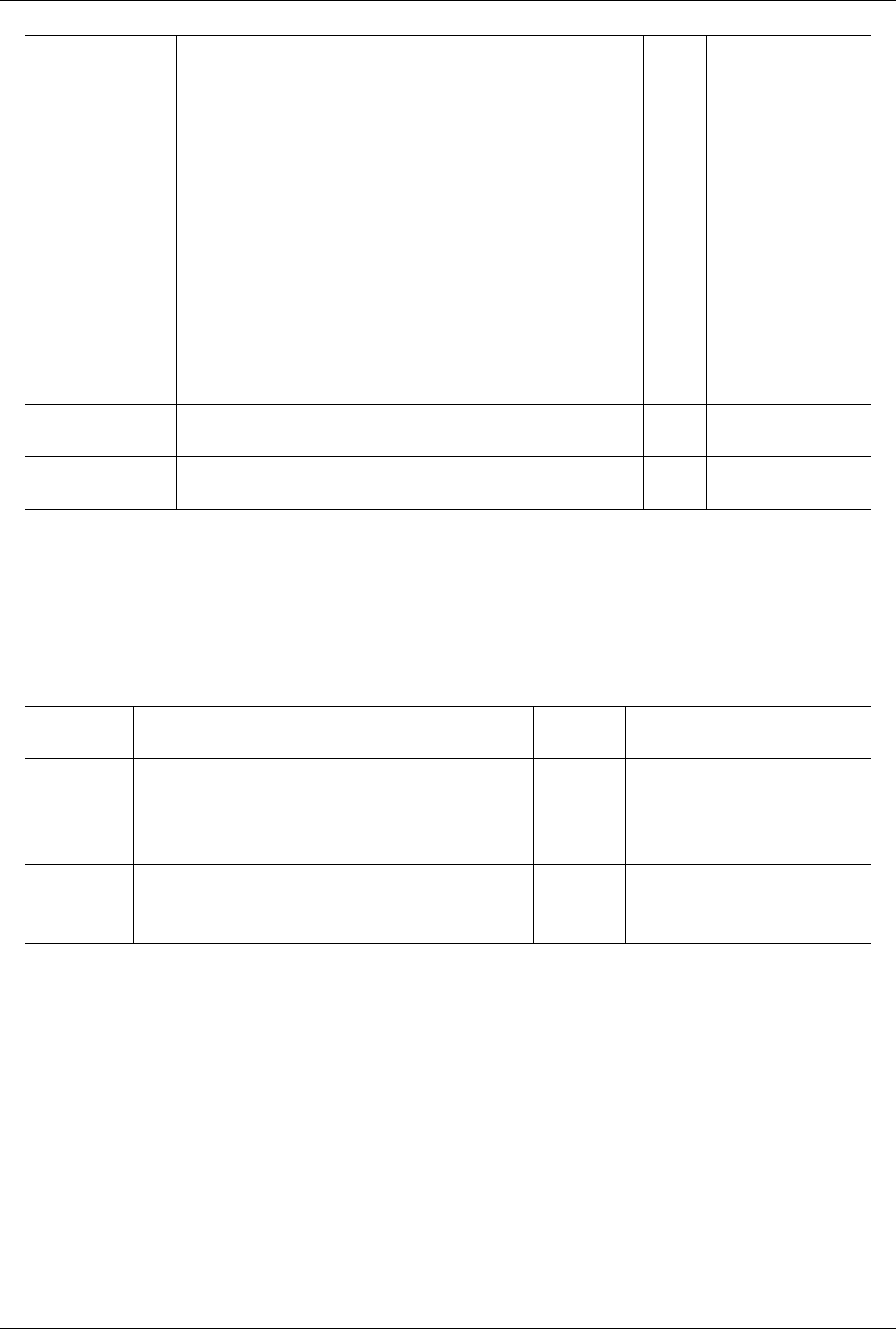
List of Filters 366
Basis Scheme
(BasisScheme)
When reporting assessments, should the full eigenvector decomposition be used
to project the original vector into the new space (Full basis), or should a fixed
subset of the decomposition be used (Fixed-size basis), or should the projection
be clipped to preserve at least some fixed "energy" (Fixed-energy basis)?<p> As
an example, suppose the variables of interest were {A,B,C,D,E} and that the
eigenvalues of the covariance matrix for these were {5,2,1.5,1,.5}. If the "Full
basis" scheme is used, then all 5 components of the eigenvectors will be used to
project each {A,B,C,D,E}-tuple in the original data into a new 5-components
space.<p> If the "Fixed-size" scheme is used and the "Basis Size" property is set
to 4, then only the first 4 eigenvector components will be used to project each
{A,B,C,D,E}-tuple into the new space and that space will be of dimension 4, not
5.<p> If the "Fixed-energy basis" scheme is used and the "Basis Energy"
property is set to 0.8, then only the first 3 eigenvector components will be used
to project each {A,B,C,D,E}-tuple into the new space, which will be of
dimension 3. The number 3 is chosen because 3 is the lowest N for which the
sum of the first N eigenvalues divided by the sum of all eigenvalues is larger
than the specified "Basis Energy" (i.e., (5+2+1.5)/10 = 0.85 > 0.8).
0 The value(s) is an
enumeration of the
following:
• Full basis (0)
• Fixed-size basis (1)
• Fixed-energy basis (2)
Basis Size (BasisSize) The maximum number of eigenvector components to use when projecting into
the new space.
2
Basis Energy
(BasisEnergy)
The minimum energy to use when determining the dimensionality of the new
space into which the assessment will project tuples.
0.1
Probe Location
Sample data attributes at the points in a point cloud. The Probe filter samples the data set attributes of the current
data set at the points in a point cloud. The Probe filter uses interpolation to determine the values at the selected point,
whether or not it lies at an input point. The Probe filter operates on any type of data and produces polygonal output
(a point cloud).
Property Description Default
Value(s)
Restrictions
Input (Input) This property specifies the dataset from which to obtain probe
values.
Accepts input of following types:
• vtkDataSet
• vtkCompositeDataSet
The dataset much contain a field array ()
Probe Type
(Source)
This property specifies the dataset whose geometry will be used in
determining positions to probe.
The value can be one of the following:
• FixedRadiusPointSource
(extended_sources)
Process Id Scalars
This filter uses colors to show how data is partitioned across processes.The Process Id Scalars filter assigns a unique
scalar value to each piece of the input according to which processor it resides on. This filter operates on any type of
data when ParaView is run in parallel. It is useful for determining whether your data is load-balanced across the
processors being used. The output data set type is the same as that of the input.
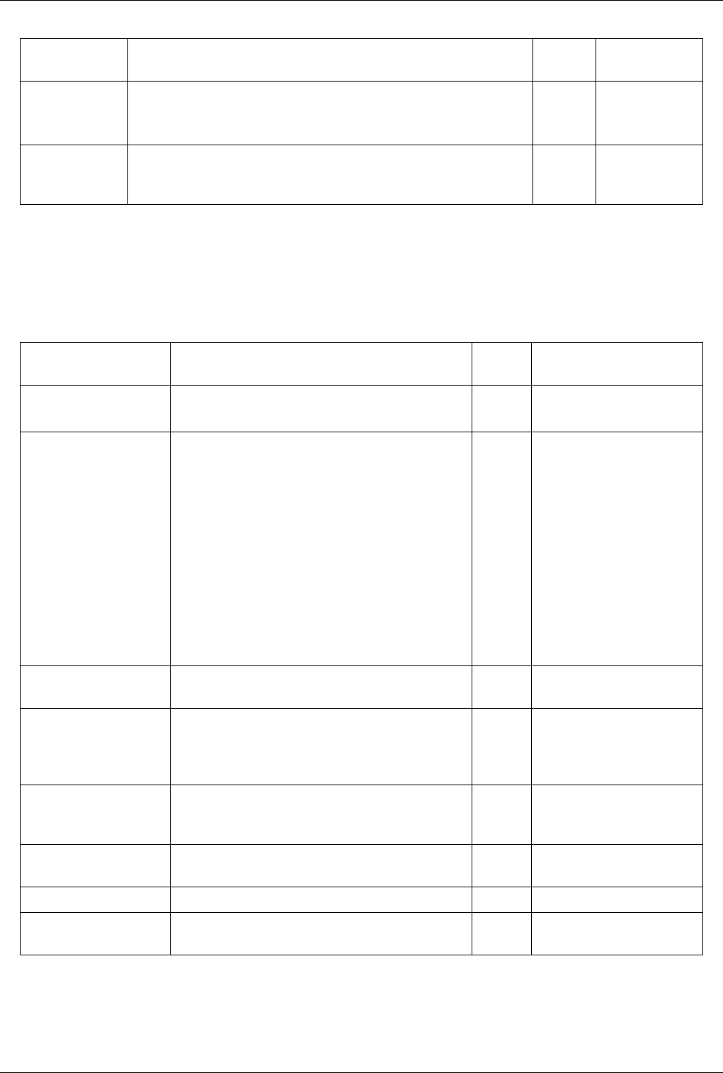
List of Filters 367
Property Description Default
Value(s)
Restrictions
Input (Input) This property specifies the input to the Process Id Scalars filter. Accepts input of
following types:
• vtkDataSet
RandomMode
(RandomMode)
The value of this property determines whether to use random id values for the various
pieces. If set to 1, the unique value per piece will be chosen at random; otherwise the
unique value will match the id of the process.
0 Accepts boolean
values (0 or 1).
Programmable Filter
Executes a user supplied python script on its input dataset to produce an output dataset. This filter will execute a
python script to produce an output dataset. The filter keeps a copy of the python script in Script, and creates
Interpretor, a python interpretor to run the script upon the first execution.
Property Description Default
Value(s)
Restrictions
Input (Input) This property specifies the input(s) to the programmable filter. Accepts input of following types:
• vtkDataObject
OutputDataSetType
(OutputDataSetType)
The value of this property determines the dataset type for the
output of the programmable filter.
8 The value(s) is an enumeration of
the following:
• Same as Input (8)
• vtkPolyData (0)
• vtkStructuredGrid (2)
• vtkRectilinearGrid (3)
• vtkUnstructuredGrid (4)
• vtkImageData (6)
• vtkUniformGrid (10)
• vtkMultiblockDataSet (13)
• vtkHierarchicalBoxDataSet
(15)
• vtkTable (19)
Script (Script) This property contains the text of a python program that the
programmable filter runs.
RequestInformation Script
(InformationScript)
This property is a python script that is executed during the
RequestInformation pipeline pass. Use this to provide
information such as WHOLE_EXTENT to the pipeline
downstream.
RequestUpdateExtent Script
(UpdateExtentScript)
This property is a python script that is executed during the
RequestUpdateExtent pipeline pass. Use this to modify the
update extent that your filter ask up stream for.
CopyArrays (CopyArrays) If this property is set to true, all the cell and point arrays from
first input are copied to the output.
0 Accepts boolean values (0 or 1).
Parameters (Parameters)
PythonPath (PythonPath) A semi-colon (;) separated list of directories to add to the
python library search path.
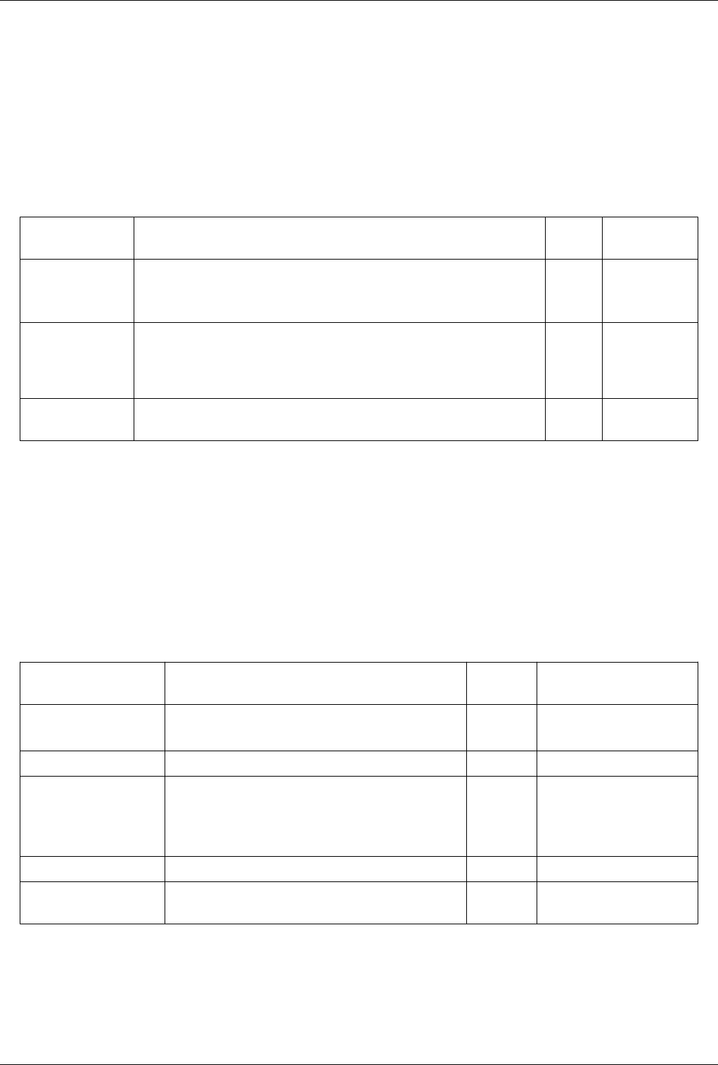
List of Filters 368
Python Annotation
This filter evaluates a Python expression for a text annotation This filter uses Python to calculate an expression. It
depends heavily on the numpy and paraview.vtk modules. To use the parallel functions, mpi4py is also necessary.
The expression is evaluated and the resulting scalar value or numpy array is added to the output as an array. See
numpy and paraview.vtk documentation for the list of available functions. This filter tries to make it easy for the user
to write expressions by defining certain variables. The filter tries to assign each array to a variable of the same name.
If the name of the array is not a valid Python variable, it has to be accessed through a dictionary called arrays (i.e.
arrays['array_name']).
Property Description Default
Value(s)
Restrictions
Input (Input) Set the input of the filter. Accepts input of
following types:
• vtkDataSet
Expression
(Expression)
The Python expression evaluated during execution. FieldData arrays are direclty
available through their name. Set of provided variables [input, t_value, t_steps, t_range,
t_index, FieldData, PointData, CellData] (i.e.: "Momentum: (%f, %f, %f)" %
(XMOM[t_index,0], YMOM[t_index,0], ZMOM[t_index,0]) )
AnnotationValue
(AnnotationValue)
Text that is used as annotation
Python Calculator
This filter evaluates a Python expressionThis filter uses Python to calculate an expression. It depends heavily on the
numpy and paraview.vtk modules. To use the parallel functions, mpi4py is also necessary. The expression is
evaluated and the resulting scalar value or numpy array is added to the output as an array. See numpy and
paraview.vtk documentation for the list of available functions. This filter tries to make it easy for the user to write
expressions by defining certain variables. The filter tries to assign each array to a variable of the same name. If the
name of the array is not a valid Python variable, it has to be accessed through a dictionary called arrays (i.e.
arrays['array_name']). The points can be accessed using the points variable.
Property Description Default
Value(s)
Restrictions
Input (Input) Set the input of the filter. Accepts input of following types:
• vtkDataSet
Expression (Expression) The Python expression evaluated during execution.
ArrayAssociation
(ArrayAssociation)
This property controls the association of the output array as well
as which arrays are defined as variables.
0 The value(s) is an enumeration of
the following:
• Point Data (0)
• Cell Data (1)
ArrayName (ArrayName) The name of the output array. result
CopyArrays (CopyArrays) If this property is set to true, all the cell and point arrays from
first input are copied to the output.
1 Accepts boolean values (0 or 1).

List of Filters 369
Quadric Clustering
This filter is the same filter used to generate level of detail for ParaView. It uses a structured grid of bins and merges
all points contained in each bin.The Quadric Clustering filter produces a reduced-resolution polygonal
approximation of the input polygonal dataset. This filter is the one used by ParaView for computing LODs. It uses
spatial binning to reduce the number of points in the data set; points that lie within the same spatial bin are collapsed
into one representative point.
Property Description Default
Value(s)
Restrictions
Input (Input) This property specifies the input to the Quadric Clustering filter. Accepts input of
following types:
• vtkPolyData
Number of Dimensions
(NumberOfDivisions)
This property specifies the number of bins along the X, Y, and Z axes of the data set. 50 50 50
UseInputPoints
(UseInputPoints)
If the value of this property is set to 1, the representative point for each bin is
selected from one of the input points that lies in that bin; the input point that
produces the least error is chosen. If the value of this property is 0, the location of
the representative point is calculated to produce the least error possible for that bin,
but the point will most likely not be one of the input points.
1 Accepts boolean
values (0 or 1).
UseFeatureEdges
(UseFeatureEdges)
If this property is set to 1, feature edge quadrics will be used to maintain the
boundary edges along processor divisions.
0 Accepts boolean
values (0 or 1).
UseFeaturePoints
(UseFeaturePoints)
If this property is set to 1, feature point quadrics will be used to maintain the
boundary points along processor divisions.
0 Accepts boolean
values (0 or 1).
CopyCellData
(CopyCellData)
If this property is set to 1, the cell data from the input will be copied to the output. 1 Accepts boolean
values (0 or 1).
UseInternalTriangles
(UseInternalTriangles)
If this property is set to 1, triangles completely contained in a spatial bin will be
included in the computation of the bin's quadrics. When this property is set to 0, the
filters operates faster, but the resulting surface may not be as well-behaved.
0 Accepts boolean
values (0 or 1).
Random Vectors
This filter creates a new 3-component point data array and sets it as the default vector array. It uses a random number
generator to create values.The Random Vectors filter generates a point-centered array of random vectors. It uses a
random number generator to determine the components of the vectors. This filter operates on any type of data set,
and the output data set will be of the same type as the input.
Property Description Default
Value(s)
Restrictions
Input (Input) This property specifies the input to the Random Vectors filter. Accepts input of following
types:
• vtkDataSet
MinimumSpeed
(MinimumSpeed)
This property specifies the minimum length of the random point
vectors generated.
0
MaximumSpeed
(MaximumSpeed)
This property specifies the maximum length of the random point
vectors generated.
1
List of Filters 370
Rectilinear Data to Point Set
The Rectilinear Grid to Point Set filter takes an rectilinear grid object and outputs an equivalent structured grid
(which as a type of point set). This brings the data to a broader category of data storage but only adds a small amount
of overhead. This filter can be helpful in applying filters that expect or manipulate point coordinates.
Property Description Default Value(s) Restrictions
Input (Input) Accepts input of following types:
• vtkRectilinearGrid
Rectilinear Grid Connectivity
Parallel fragments extraction and attributes integration on rectilinear grids. Extracts material fragments from
multi-block vtkRectilinearGrid datasets based on the selected volume fraction array(s) and a fraction isovalue and
integrates the associated attributes.
Property Description Default
Value(s)
Restrictions
Input (Input) This property specifies the input of the
filter.
Accepts input of following
types:
• vtkRectilinearGrid
• vtkCompositeDataSet
The dataset much contain a field
array (cell)
with 1 component(s).
Double Volume Arrays
(AddDoubleVolumeArrayName)
This property specifies the name(s) of the
volume fraction array(s) for generating
parts.
An array of scalars is required.
Float Volume Arrays (AddFloatVolumeArrayName) This property specifies the name(s) of the
volume fraction array(s) for generating
parts.
An array of scalars is required.
Unsigned Character Volume Arrays
(AddUnsignedCharVolumeArrayName)
This property specifies the name(s) of the
volume fraction array(s) for generating
parts.
An array of scalars is required.
Volume Fraction Value
(VolumeFractionSurfaceValue)
The value of this property is the volume
fraction value for the surface.
0.1
RectilinearGridGeometryFilter
Extracts geometry for a rectilinear grid. Output is a polydata dataset. RectilinearGridGeometryFilter is a filter that
extracts geometry from a rectilinear grid. By specifying appropriate i-j-k indices, it is possible to extract a point, a
curve, a surface, or a "volume". The volume is actually a (n x m x o) region of points. The extent specification is
zero-offset. That is, the first k-plane in a 50x50x50 rectilinear grid is given by (0,49, 0,49, 0,0).
Property Description Default Value(s) Restrictions
Input (Input) Set the input to the Rectilinear Grid Geometry filter. Accepts input of following types:
• vtkDataSet
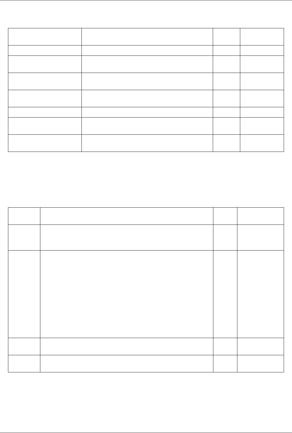
List of Filters 371
ReductionFilter
Property Description Default
Value(s)
Restrictions
Input (Input) Set the input to the Reduction filter.
PreGatherHelperName
(PreGatherHelperName)
Set the algorithm that runs on each node in parallel.
PostGatherHelperName
(PostGatherHelperName)
Set the algorithm that takes multiple inputs and produces a single
reduced output.
PostGatherHelper
(PostGatherHelper)
PreGatherHelper (PreGatherHelper)
PassThrough (PassThrough) If set to a non-negative value, then produce results using only the
node Id specified.
-1
GenerateProcessIds
(GenerateProcessIds)
If true, the filter will generate vtkOriginalProcessIds arrays indicating
the process id on which the cell/point was generated.
0 Accepts boolean
values (0 or 1).
Reflect
This filter takes the union of the input and its reflection over an axis-aligned plane.The Reflect filter reflects the
input dataset across the specified plane. This filter operates on any type of data set and produces an unstructured grid
output.
Property Description Default
Value(s)
Restrictions
Input (Input) This property specifies the input to the Reflect filter. Accepts input of
following types:
• vtkDataSet
Plane (Plane) The value of this property determines which plane to reflect across. If the value is X, Y, or
Z, the value of the Center property determines where the plane is placed along the specified
axis. The other six options (X Min, X Max, etc.) place the reflection plane at the specified
face of the bounding box of the input dataset.
0 The value(s) is an
enumeration of the
following:
• X Min (0)
• Y Min (1)
• Z Min (2)
• X Max (3)
• Y Max (4)
• Z Max (5)
• X (6)
• Y (7)
• Z (8)
Center
(Center)
If the value of the Plane property is X, Y, or Z, then the value of this property specifies the
center of the reflection plane.
0.0
CopyInput
(CopyInput)
If this property is set to 1, the output will contain the union of the input dataset and its
reflection. Otherwise the output will contain only the reflection of the input data.
1 Accepts boolean values
(0 or 1).
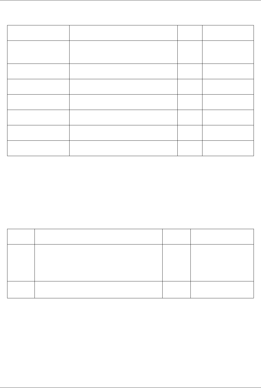
List of Filters 372
Resample AMR
Property Description Default
Value(s)
Restrictions
Input (Input) This property specifies the input for this filter. Accepts input of following
types:
• vtkOverlappingAMR
Demand-Driven Mode
(Demand-Driven Mode)
This property specifies whether the resampling filter will
operate in demand-driven mode or not.
1 Accepts boolean values (0 or
1).
TransferToNodes
(TransferToNodes)
This property specifies whether the solution will be transfered
to the nodes of the extracted region or the cells.
1 Accepts boolean values (0 or
1).
NumberOfPartitions
(NumberOfPartitions)
Set the number of subdivisions for recursive coordinate
bisection.
1
Number of Samples (Number of
Samples)
Sets the number of samples in each dimension 10 10 10
Min (Min) This property sets the minimum 3-D coordinate location by
which the particles will be filtered out.
0.0 0.0 0.0
Max (Max) This property sets the minimum 3-D coordinate location by
which the particles will be filtered out.
0.0 0.0 0.0
Resample With Dataset
Sample data attributes at the points of a dataset. Probe is a filter that computes point attributes at specified point
positions. The filter has two inputs: the Input and Source. The Input geometric structure is passed through the filter.
The point attributes are computed at the Input point positions by interpolating into the source data. For example, we
can compute data values on a plane (plane specified as Input) from a volume (Source). The cell data of the source
data is copied to the output based on in which source cell each input point is. If an array of the same name exists both
in source's point and cell data, only the one from the point data is probed.
Property Description Default
Value(s)
Restrictions
Input (Input) This property specifies the dataset from which to obtain probe values. Accepts input of following types:
• vtkDataSet
• vtkCompositeDataSet
The dataset much contain a field
array ()
Source
(Source)
This property specifies the dataset whose geometry will be used in
determining positions to probe.
Accepts input of following types:
• vtkDataSet

List of Filters 373
Ribbon
This filter generates ribbon surface from lines. It is useful for displaying streamlines.The Ribbon filter creates
ribbons from the lines in the input data set. This filter is useful for visualizing streamlines. Both the input and output
of this filter are polygonal data. The input data set must also have at least one point-centered vector array.
Property Description Default
Value(s)
Restrictions
Input (Input) This property specifies the input to the Ribbon filter. Accepts input of following
types:
• vtkPolyData
The dataset much contain a
field array (point)
with 3 component(s).
The dataset much contain a
field array (point)
with 1 component(s).
Scalars
(SelectInputScalars)
The value of this property indicates the name of the input scalar array used by
this filter. The width of the ribbons will be varied based on the values in the
specified array if the value of the Width property is 1.
An array of scalars is
required.
Vectors
(SelectInputVectors)
The value of this property indicates the name of the input vector array used by
this filter. If the UseDefaultNormal property is set to 0, the normal vectors for
the ribbons come from the specified vector array.
1 An array of vectors is
required.
Width (Width) If the VaryWidth property is set to 1, the value of this property is the minimum
ribbon width. If the VaryWidth property is set to 0, the value of this property is
half the width of the ribbon.
1 The value must be less than
the largest dimension of the
dataset multiplied by a scale
factor of 0.01.
Angle (Angle) The value of this property specifies the offset angle (in degrees) of the ribbon
from the line normal.
0
UseDefaultNormal
(UseDefaultNormal)
If this property is set to 0, and the input contains no vector array, then default
ribbon normals will be generated (DefaultNormal property); if a vector array
has been set (SelectInputVectors property), the ribbon normals will be set from
the specified array. If this property is set to 1, the default normal
(DefaultNormal property) will be used, regardless of whether the
SelectInputVectors property has been set.
0 Accepts boolean values (0 or
1).
DefaultNormal
(DefaultNormal)
The value of this property specifies the normal to use when the
UseDefaultNormal property is set to 1 or the input contains no vector array
(SelectInputVectors property).
0 0 1
VaryWidth
(VaryWidth)
If this property is set to 1, the ribbon width will be scaled according to the
scalar array specified in the SelectInputScalars property. Toggle the variation
of ribbon width with scalar value.
0 Accepts boolean values (0 or
1).
List of Filters 374
Rotational Extrusion
This filter generates a swept surface while translating the input along a circular path. The Rotational Extrusion filter
forms a surface by rotating the input about the Z axis. This filter is intended to operate on 2D polygonal data. It
produces polygonal output.
Property Description Default
Value(s)
Restrictions
Input (Input) This property specifies the input to the Rotational Extrusion filter. Accepts input of
following types:
• vtkPolyData
Resolution
(Resolution)
The value of this property controls the number of intermediate node points used in performing
the sweep (rotating from 0 degrees to the value specified by the Angle property.
12
Capping
(Capping)
If this property is set to 1, the open ends of the swept surface will be capped with a copy of the
input dataset. This works property if the input is a 2D surface composed of filled polygons. If the
input dataset is a closed solid (e.g., a sphere), then either two copies of the dataset will be drawn
or no surface will be drawn. No surface is drawn if either this property is set to 0 or if the two
surfaces would occupy exactly the same 3D space (i.e., the Angle property's value is a multiple
of 360, and the values of the Translation and DeltaRadius properties are 0).
1 Accepts boolean
values (0 or 1).
Angle (Angle) This property specifies the angle of rotation in degrees. The surface is swept from 0 to the value
of this property.
360
Translation
(Translation)
The value of this property specifies the total amount of translation along the Z axis during the
sweep process. Specifying a non-zero value for this property allows you to create a corkscrew
(value of DeltaRadius > 0) or spring effect.
0
DeltaRadius
(DeltaRadius)
The value of this property specifies the change in radius during the sweep process. 0
Scatter Plot
Creates a scatter plot from a dataset.This filter creates a scatter plot from a dataset.
Property Description Default Value(s) Restrictions
Input (Input) This property specifies the input to the filter. Accepts input of following types:
• vtkDataSet
Shrink
This filter shrinks each input cell so they pull away from their neighbors.The Shrink filter causes the individual cells
of a dataset to break apart from each other by moving each cell's points toward the centroid of the cell. (The centroid
of a cell is the average position of its points.) This filter operates on any type of dataset and produces unstructured
grid output.

List of Filters 375
Property Description Default
Value(s)
Restrictions
Input (Input) This property specifies the input to the Shrink filter. Accepts input of
following types:
• vtkDataSet
ShrinkFactor
(ShrinkFactor)
The value of this property determines how far the points will move. A value of 0
positions the points at the centroid of the cell; a value of 1 leaves them at their
original positions.
0.5
Slice
This filter slices a data set with a plane. Slicing is similar to a contour. It creates surfaces from volumes and lines
from surfaces.This filter extracts the portion of the input dataset that lies along the specified plane. The Slice filter
takes any type of dataset as input. The output of this filter is polygonal data.
Property Description Default
Value(s)
Restrictions
Input (Input) This property specifies the input to the Slice filter. Accepts input of following types:
• vtkDataSet
Slice Type (CutFunction) This property sets the parameters of the slice function. The value can be one of the following:
• Plane (implicit_functions)
• Box (implicit_functions)
• Sphere (implicit_functions)
InputBounds
(InputBounds)
Crinkle slice
(PreserveInputCells)
This parameter controls whether to extract the entire cells
that are sliced by the region or just extract a triangulated
surface of that region.
0 Accepts boolean values (0 or 1).
Triangulate the slice
(Triangulate the slice)
This parameter controls whether to produce triangles in the
output.
1 Accepts boolean values (0 or 1).
Slice Offset Values
(ContourValues)
The values in this property specify a list of current offset
values. This can be used to create multiple slices with
different centers. Each entry represents a new slice with its
center shifted by the offset value.
Determine the length of the dataset's
diagonal. The value must lie within
-diagonal length to +diagonal length.
Slice (demand-driven-composite)
This filter slices a data set with a plane. Slicing is similar to a contour. It creates surfaces from volumes and lines
from surfaces.This filter extracts the portion of the input dataset that lies along the specified plane. The Slice filter
takes any type of dataset as input. The output of this filter is polygonal data.

List of Filters 376
Property Description Default
Value(s)
Restrictions
Input (Input) This property specifies the input to the Slice filter. Accepts input of following types:
• vtkDataObject
Slice Type
(CutFunction)
This property sets the parameters of the slice function. The value can be one of the following:
• Plane (implicit_functions)
• Box (implicit_functions)
• Sphere (implicit_functions)
InputBounds
(InputBounds)
Slice Offset Values
(ContourValues)
The values in this property specify a list of current offset
values. This can be used to create multiple slices with different
centers. Each entry represents a new slice with its center
shifted by the offset value.
Determine the length of the dataset's diagonal.
The value must lie within -diagonal length to
+diagonal length.
Slice AMR data
Slices AMR DataThis filter slices AMR data.
Property Description Default
Value(s)
Restrictions
Input (Input) This property specifies the input for this filter. Accepts input of following types:
• vtkOverlappingAMR
ForwardUpstream
(ForwardUpstream)
This property specifies whether or not requests will be
propagated upstream.
0 Accepts boolean values (0 or 1).
EnablePrefetching
(EnablePrefetching)
This property specifies whether or not requests pre-fetching
of blocks of the next level will be enabled.
0 Accepts boolean values (0 or 1).
Level (Level) Set maximum slice resolution. 0
OffSet (OffSet) Set's the offset from the origin of the data-set 1.0
Normal (Normal) This property sets the normal of the slice. 0 The value(s) is an enumeration of the
following:
• X-Normal (1)
• Y-Normal (2)
• Z-Normal (3)
Slice Generic Dataset
This filter cuts a data set with a plane or sphere. Cutting is similar to a contour. It creates surfaces from volumes and
lines from surfaces.The Generic Cut filter extracts the portion of the input data set that lies along the specified plane
or sphere. From the Cut Function menu, you can select whether cutting will be performed with a plane or a sphere.
The appropriate 3D widget (plane widget or sphere widget) will be displayed. The parameters of the cut function can
be specified interactively using the 3D widget or manually using the traditional user interface controls. Instructions
for using these 3D widgets and their corresponding user interfaces are found in section 7.4. By default, the cut lies on
the specified plane or sphere. Using the Cut Offset Values portion of the interface, it is also possible to cut the data
set at some offset from the original cut function. The Cut Offset Values are in the spatial units of the data set. To add
a single offset, select the value from the New Value slider in the Add value portion of the interface and click the Add
button, or press Enter. To instead add several evenly spaced offsets, use the controls in the Generate range of values

List of Filters 377
section. Select the number of offsets to generate using the Number of Values slider. The Range slider controls the
interval in which to generate the offsets. Once the number of values and range have been selected, click the Generate
button. The new offsets will be added to the Offset Values list. To delete a value from the Cut Offset Values list,
select the value and click the Delete button. (If no value is selected, the last value in the list will be removed.)
Clicking the Delete All button removes all the values in the list. The Generic Cut filter takes a generic dataset as
input. Use the Input menu to choose a data set to cut. The output of this filter is polygonal data.
Property Description Default
Value(s)
Restrictions
Input (Input) Set the input to the Generic Cut filter. Accepts input of following types:
• vtkGenericDataSet
Cut Type
(CutFunction)
Set the parameters to the implicit function used for cutting. The value can be one of the following:
• Plane (implicit_functions)
• Box (implicit_functions)
• Sphere (implicit_functions)
InputBounds
(InputBounds)
Slice Offset Values
(ContourValues)
The values in this property specify a list of current offset
values. This can be used to create multiple slices with different
centers. Each entry represents a new slice with its center
shifted by the offset value.
Determine the length of the dataset's diagonal.
The value must lie within -diagonal length to
+diagonal length.
Smooth
This filter smooths a polygonal surface by iteratively moving points toward their neighbors. The Smooth filter
operates on a polygonal data set by iteratively adjusting the position of the points using Laplacian smoothing.
(Because this filter only adjusts point positions, the output data set is also polygonal.) This results in better-shaped
cells and more evenly distributed points. The Convergence slider limits the maximum motion of any point. It is
expressed as a fraction of the length of the diagonal of the bounding box of the data set. If the maximum point
motion during a smoothing iteration is less than the Convergence value, the smoothing operation terminates.
Property Description Default
Value(s)
Restrictions
Input (Input) This property specifies the input to the Smooth filter. Accepts input of
following types:
• vtkPolyData
Number of Iterations
(NumberOfIterations)
This property sets the maximum number of smoothing iterations to perform. More
iterations produce better smoothing.
20
Convergence
(Convergence)
The value of this property limits the maximum motion of any point. It is expressed
as a fraction of the length of the diagonal of the bounding box of the input dataset.
If the maximum point motion during a smoothing iteration is less than the value of
this property, the smoothing operation terminates.
0.0

List of Filters 378
StreakLine
Trace Streak lines through time in a vector field. The Particle Trace filter generates pathlines in a vector field from a
collection of seed points. The vector field used is selected from the Vectors menu, so the input data set is required to
have point-centered vectors. The Seed portion of the interface allows you to select whether the seed points for this
integration lie in a point cloud or along a line. Depending on which is selected, the appropriate 3D widget (point or
line widget) is displayed along with traditional user interface controls for positioning the point cloud or line within
the data set. Instructions for using the 3D widgets and the corresponding manual controls can be found in section 7.4.
This filter operates on any type of data set, provided it has point-centered vectors. The output is polygonal data
containing polylines. This filter is available on the Toolbar.
Property Description Default
Value(s)
Restrictions
Input (Input) Specify which is the Input of the StreamTracer filter. Accepts input of
following types:
• vtkDataObject
The dataset much
contain a field array
(point)
with 3 component(s).
Seed Source (Source) Specify the seed dataset. Typically fron where the vector field integration
should begin. Usually a point/radius or a line with a given resolution.
Accepts input of
following types:
• vtkDataSet
TerminationTime
(TerminationTime)
Setting TerminationTime to a positive value will cause particles to
terminate when the time is reached. The units of time should be consistent
with the primary time variable.
0.0
TimestepValues (TimestepValues)
ForceReinjectionEveryNSteps
(ForceReinjectionEveryNSteps)
When animating particles, it is nice to inject new ones every Nth step to
produce a continuous flow. Setting ForceReinjectionEveryNSteps to a non
zero value will cause the particle source to reinject particles every Nth step
even if it is otherwise unchanged. Note that if the particle source is also
animated, this flag will be redundant as the particles will be reinjected
whenever the source changes anyway
1
SelectInputVectors
(SelectInputVectors)
Specify which vector array should be used for the integration through that
filter.
An array of vectors
is required.
ComputeVorticity
(ComputeVorticity)
Compute vorticity and angular rotation of particles as they progress 1 Accepts boolean
values (0 or 1).
DisableResetCache
(DisableResetCache)
Prevents cache from getting reset so that new computation always start
from previous results.
0 Accepts boolean
values (0 or 1).
Stream Tracer
Integrate streamlines in a vector field.The Stream Tracer filter generates streamlines in a vector field from a
collection of seed points. Production of streamlines terminates if a streamline crosses the exterior boundary of the
input dataset. Other reasons for termination are listed for the MaximumNumberOfSteps, TerminalSpeed, and
MaximumPropagation properties. This filter operates on any type of dataset, provided it has point-centered vectors.
The output is polygonal data containing polylines.

List of Filters 379
Property Description Default
Value(s)
Restrictions
Input (Input) This property specifies the input to the Stream Tracer filter. Accepts input of following
types:
• vtkDataSet
The dataset much contain a
field array (any)
with 3 component(s).
Vectors (SelectInputVectors) This property contains the name of the vector array from
which to generate streamlines.
An array of vectors is required.
InterpolatorType
(InterpolatorType)
This property determines which interpolator to use for
evaluating the velocity vector field. The first is faster though
the second is more robust in locating cells during streamline
integration.
0 The value(s) is an enumeration
of the following:
• Interpolator with Point
Locator (0)
• Interpolator with Cell
Locator (1)
IntegrationDirection
(IntegrationDirection)
This property determines in which direction(s) a streamline is
generated.
2 The value(s) is an enumeration
of the following:
• FORWARD (0)
• BACKWARD (1)
• BOTH (2)
IntegratorType
(IntegratorType)
This property determines which integrator (with increasing
accuracy) to use for creating streamlines.
2 The value(s) is an enumeration
of the following:
• Runge-Kutta 2 (0)
• Runge-Kutta 4 (1)
• Runge-Kutta 4-5 (2)
Integration Step Unit
(IntegrationStepUnit)
This property specifies the unit for
Minimum/Initial/Maximum integration step size. The Length
unit refers to the arc length that a particle travels/advects
within a single step. The Cell Length unit represents the step
size as a number of cells.
2 The value(s) is an enumeration
of the following:
• Length (1)
• Cell Length (2)
Initial Step Length
(InitialIntegrationStep)
This property specifies the initial integration step size. For
non-adaptive integrators (Runge-Kutta 2 and Runge-Kutta 4),
it is fixed (always equal to this initial value) throughout the
integration. For an adaptive integrator (Runge-Kutta 4-5), the
actual step size varies such that the numerical error is less
than a specified threshold.
0.2
Minimum Step Length
(MinimumIntegrationStep)
When using the Runge-Kutta 4-5 ingrator, this property
specifies the minimum integration step size.
0.01
Maximum Step Length
(MaximumIntegrationStep)
When using the Runge-Kutta 4-5 ingrator, this property
specifies the maximum integration step size.
0.5
Maximum Steps
(MaximumNumberOfSteps)
This property specifies the maximum number of steps,
beyond which streamline integration is terminated.
2000
Maximum Streamline
Length
(MaximumPropagation)
This property specifies the maximum streamline length (i.e.,
physical arc length), beyond which line integration is
terminated.
1.0 The value must be less than the
largest dimension of the dataset
multiplied by a scale factor of
1.0.
Terminal Speed
(TerminalSpeed)
This property specifies the terminal speed, below which
particle advection/integration is terminated.
0.000000000001

List of Filters 380
MaximumError
(MaximumError)
This property specifies the maximum error (for Runge-Kutta
4-5) tolerated throughout streamline integration. The
Runge-Kutta 4-5 integrator tries to adjust the step size such
that the estimated error is less than this threshold.
0.000001
ComputeVorticity
(ComputeVorticity)
Specify whether or not to compute vorticity. 1 Accepts boolean values (0 or 1).
Seed Type (Source) The value of this property determines how the seeds for the
streamlines will be generated.
The value can be one of the
following:
• PointSource
(extended_sources)
• HighResLineSource
(extended_sources)
Stream Tracer For Generic Datasets
Integrate streamlines in a vector field.The Generic Stream Tracer filter generates streamlines in a vector field from a
collection of seed points. The vector field used is selected from the Vectors menu, so the input data set is required to
have point-centered vectors. The Seed portion of the interface allows you to select whether the seed points for this
integration lie in a point cloud or along a line. Depending on which is selected, the appropriate 3D widget (point or
line widget) is displayed along with traditional user interface controls for positioning the point cloud or line within
the data set. Instructions for using the 3D widgets and the corresponding manual controls can be found in section 7.4.
The Max. Propagation entry box allows you to specify the maximum length of the streamlines. From the Max.
Propagation menu, you can select the units to be either Time (the time a particle would travel with steady flow) or
Length (in the data set's spatial coordinates). The Init. Step Len. menu and entry specify the initial step size for
integration. (For non-adaptive integrators, Runge-Kutta 2 and 4, the initial step size is used throughout the
integration.) The menu allows you to specify the units. Time and Length have the same meaning as for Max.
Propagation. Cell Length specifies the step length as a number of cells. The Integration Direction menu determines
in which direction(s) the stream trace will be generated: FORWARD, BACKWARD, or BOTH. The Integrator Type
section of the interface determines which calculation to use for integration: Runge-Kutta 2, Runge-Kutta 4, or
Runge-Kutta 4-5. If Runge-Kutta 4-5 is selected, controls are displayed for specifying the minimum and maximum
step length and the maximum error. The controls for specifying Min. Step Len. and Max. Step Len. are the same as
those for Init. Step Len. The Runge-Kutta 4-5 integrator tries to choose the step size so that the estimated error is less
than the value of the Maximum Error entry. If the integration takes more than Max. Steps to complete, if the speed
goes below Term. Speed, if Max. Propagation is reached, or if a boundary of the input data set is crossed, integration
terminates. This filter operates on any type of data set, provided it has point-centered vectors. The output is
polygonal data containing polylines.
Property Description Default
Value(s)
Restrictions
Input (Input) Set the input to the Generic Stream
Tracer filter.
Accepts input of following types:
• vtkGenericDataSet
The dataset much contain a field array (point)
with 3 component(s).
Seed Type (Source) The value of this property determines
how the seeds for the streamlines will be
generated.
The value can be one of the following:
• PointSource (extended_sources)
• HighResLineSource (extended_sources)

List of Filters 381
Vectors (SelectInputVectors) This property contains the name of the
vector array from which to generate
streamlines.
An array of vectors is required.
MaximumPropagation
(MaximumPropagation)
Specify the maximum streamline length. 1.0 The value must be less than the largest
dimension of the dataset multiplied by a scale
factor of 1.0.
InitialIntegrationStep
(InitialIntegrationStep)
Specify the initial integration step. 0.5
IntegrationDirection
(IntegrationDirection)
This property determines in which
direction(s) a streamline is generated.
2 The value(s) is an enumeration of the
following:
• FORWARD (0)
• BACKWARD (1)
• BOTH (2)
IntegratorType (IntegratorType) This property determines which
integrator (with increasing accuracy) to
use for creating streamlines.
2 The value(s) is an enumeration of the
following:
• Runge-Kutta 2 (0)
• Runge-Kutta 4 (1)
• Runge-Kutta 4-5 (2)
MaximumError (MaximumError) Set the maximum error allowed in the
integration. The meaning of this value
depends on the integrator chosen.
0.000001
MinimumIntegrationStep
(MinimumIntegrationStep)
Specify the minimum integration step. 0.01
IntegrationStepUnit
(IntegrationStepUnit)
Choose the unit to use for the integration
step.
2 The value(s) is an enumeration of the
following:
• Time (0)
• Length (1)
• Cell Length (2)
MaximumIntegrationStep
(MaximumIntegrationStep)
Specify the maximum integration step. 0.01
MaximumNumberOfSteps
(MaximumNumberOfSteps)
Specify the maximum number of steps
used in the integration.
2000
TerminalSpeed (TerminalSpeed) If at any point the speed is below this
value, the integration is terminated.
0.000000000001
Stream Tracer With Custom Source
Integrate streamlines in a vector field.The Stream Tracer filter generates streamlines in a vector field from a
collection of seed points. Production of streamlines terminates if a streamline crosses the exterior boundary of the
input dataset. Other reasons for termination are listed for the MaximumNumberOfSteps, TerminalSpeed, and
MaximumPropagation properties. This filter operates on any type of dataset, provided it has point-centered vectors.
The output is polygonal data containing polylines. This filter takes a Source input that provides the seed points.

List of Filters 382
Property Description Default
Value(s)
Restrictions
Input (Input) This property specifies the input to the Stream Tracer filter. Accepts input of following
types:
• vtkDataSet
The dataset much contain a
field array (point)
with 3 component(s).
Vectors (SelectInputVectors) This property contains the name of the vector array from which
to generate streamlines.
An array of vectors is
required.
IntegrationDirection
(IntegrationDirection)
This property determines in which direction(s) a streamline is
generated.
2 The value(s) is an
enumeration of the
following:
• FORWARD (0)
• BACKWARD (1)
• BOTH (2)
IntegratorType
(IntegratorType)
This property determines which integrator (with increasing
accuracy) to use for creating streamlines.
2 The value(s) is an
enumeration of the
following:
• Runge-Kutta 2 (0)
• Runge-Kutta 4 (1)
• Runge-Kutta 4-5 (2)
Integration Step Unit
(IntegrationStepUnit)
This property specifies the unit for Minimum/Initial/Maximum
integration step size. The Length unit refers to the arc length that
a particle travels/advects within a single step. The Cell Length
unit represents the step size as a number of cells.
2 The value(s) is an
enumeration of the
following:
• Length (1)
• Cell Length (2)
Initial Step Length
(InitialIntegrationStep)
This property specifies the initial integration step size. For
non-adaptive integrators (Runge-Kutta 2 and Runge-Kutta 4), it
is fixed (always equal to this initial value) throughout the
integration. For an adaptive integrator (Runge-Kutta 4-5), the
actual step size varies such that the numerical error is less than a
specified threshold.
0.2
Minimum Step Length
(MinimumIntegrationStep)
When using the Runge-Kutta 4-5 ingrator, this property specifies
the minimum integration step size.
0.01
Maximum Step Length
(MaximumIntegrationStep)
When using the Runge-Kutta 4-5 ingrator, this property specifies
the maximum integration step size.
0.5
Maximum Steps
(MaximumNumberOfSteps)
This property specifies the maximum number of steps, beyond
which streamline integration is terminated.
2000
Maximum Streamline Length
(MaximumPropagation)
This property specifies the maximum streamline length (i.e.,
physical arc length), beyond which line integration is terminated.
1.0 The value must be less than
the largest dimension of the
dataset multiplied by a scale
factor of 1.0.
Terminal Speed
(TerminalSpeed)
This property specifies the terminal speed, below which particle
advection/integration is terminated.
0.000000000001
MaximumError
(MaximumError)
This property specifies the maximum error (for Runge-Kutta 4-5)
tolerated throughout streamline integration. The Runge-Kutta 4-5
integrator tries to adjust the step size such that the estimated error
is less than this threshold.
0.000001
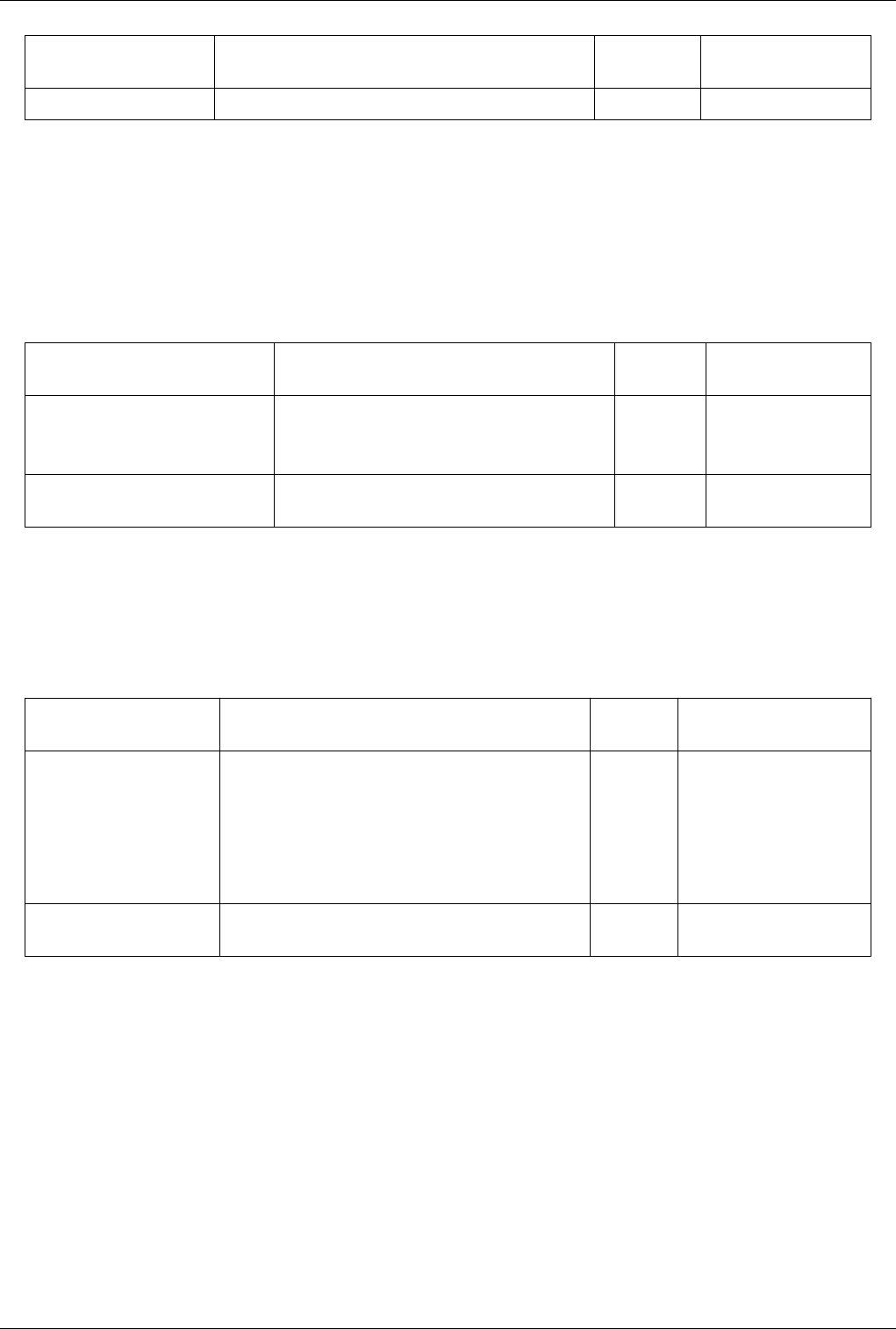
List of Filters 383
ComputeVorticity
(ComputeVorticity)
Specify whether or not to compute vorticity. 1 Accepts boolean values (0
or 1).
Seed Source (Source) This property specifies the input used to obtain the seed points.
Subdivide
This filter iteratively divide triangles into four smaller triangles. New points are placed linearly so the output surface
matches the input surface. The Subdivide filter iteratively divides each triangle in the input dataset into 4 new
triangles. Three new points are added per triangle -- one at the midpoint of each edge. This filter operates only on
polygonal data containing triangles, so run your polygonal data through the Triangulate filter first if it is not
composed of triangles. The output of this filter is also polygonal.
Property Description Default
Value(s)
Restrictions
Input (Input) This parameter specifies the input to the Subdivide filter. Accepts input of following
types:
• vtkPolyData
Number of Subdivisions
(NumberOfSubdivisions)
The value of this property specifies the number of
subdivision iterations to perform.
1
Surface Flow
This filter integrates flow through a surface. The flow integration fitler integrates the dot product of a point flow
vector field and surface normal. It computes the net flow across the 2D surface. It operates on any type of dataset and
produces an unstructured grid output.
Property Description Default
Value(s)
Restrictions
Input (Input) This property specifies the input to the Surface Flow filter. Accepts input of following
types:
• vtkDataSet
The dataset much contain a
field array (point)
with 3 component(s).
SelectInputVectors
(SelectInputVectors)
The value of this property specifies the name of the input
vector array containing the flow vector field.
An array of vectors is required.
Surface Vectors
This filter constrains vectors to lie on a surface. The Surface Vectors filter is used for 2D data sets. It constrains
vectors to lie in a surface by removing components of the vectors normal to the local surface.
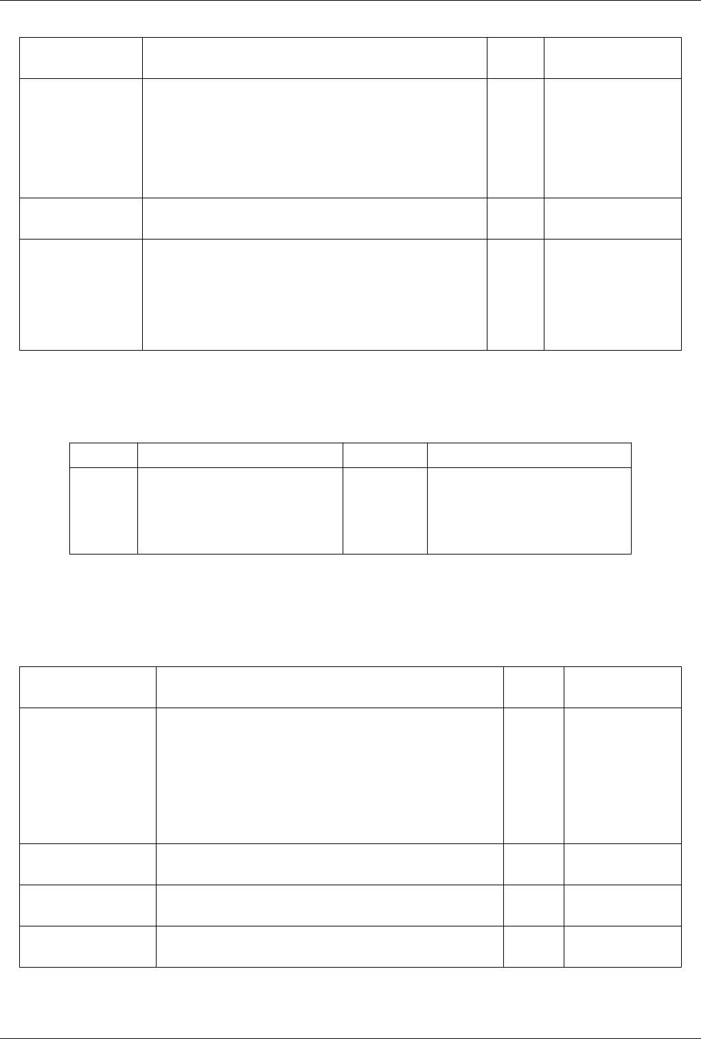
List of Filters 384
Property Description Default
Value(s)
Restrictions
Input (Input) This property specifies the input to the Surface Vectors filter. Accepts input of following
types:
• vtkDataSet
The dataset much contain a
field array (point)
with 3 component(s).
SelectInputVectors
(SelectInputVectors)
This property specifies the name of the input vector array to process. An array of vectors is
required.
ConstraintMode
(ConstraintMode)
This property specifies whether the vectors will be parallel or perpendicular
to the surface. If the value is set to PerpendicularScale (2), then the output
will contain a scalar array with the dot product of the surface normal and the
vector at each point.
0 The value(s) is an
enumeration of the
following:
• Parallel (0)
• Perpendicular (1)
• PerpendicularScale (2)
Table FFT
Performs the Fast Fourier Transform on the columns of a table.
Property Description Default Value(s) Restrictions
Input (Input) This property specifies the input of the filter. Accepts input of following types:
• vtkTable
The dataset much contain a field array (row)
with 1 component(s).
Table To Points
Converts table to set of points.The TableToPolyData filter converts a vtkTable to a set of points in a vtkPolyData.
One must specifies the columns in the input table to use as the X, Y and Z coordinates for the points in the output.
Property Description Default
Value(s)
Restrictions
Input (Input) This property specifies the input.. Accepts input of
following types:
• vtkTable
The dataset much
contain a field array
(row)
with 1 component(s).
XColumn (XColumn) This property specifies which data array is going to be used as the X
coordinate in the generated polydata dataset.
YColumn (YColumn) This property specifies which data array is going to be used as the Y
coordinate in the generated polydata dataset.
ZColumn (ZColumn) This property specifies which data array is going to be used as the Z
coordinate in the generated polydata dataset.
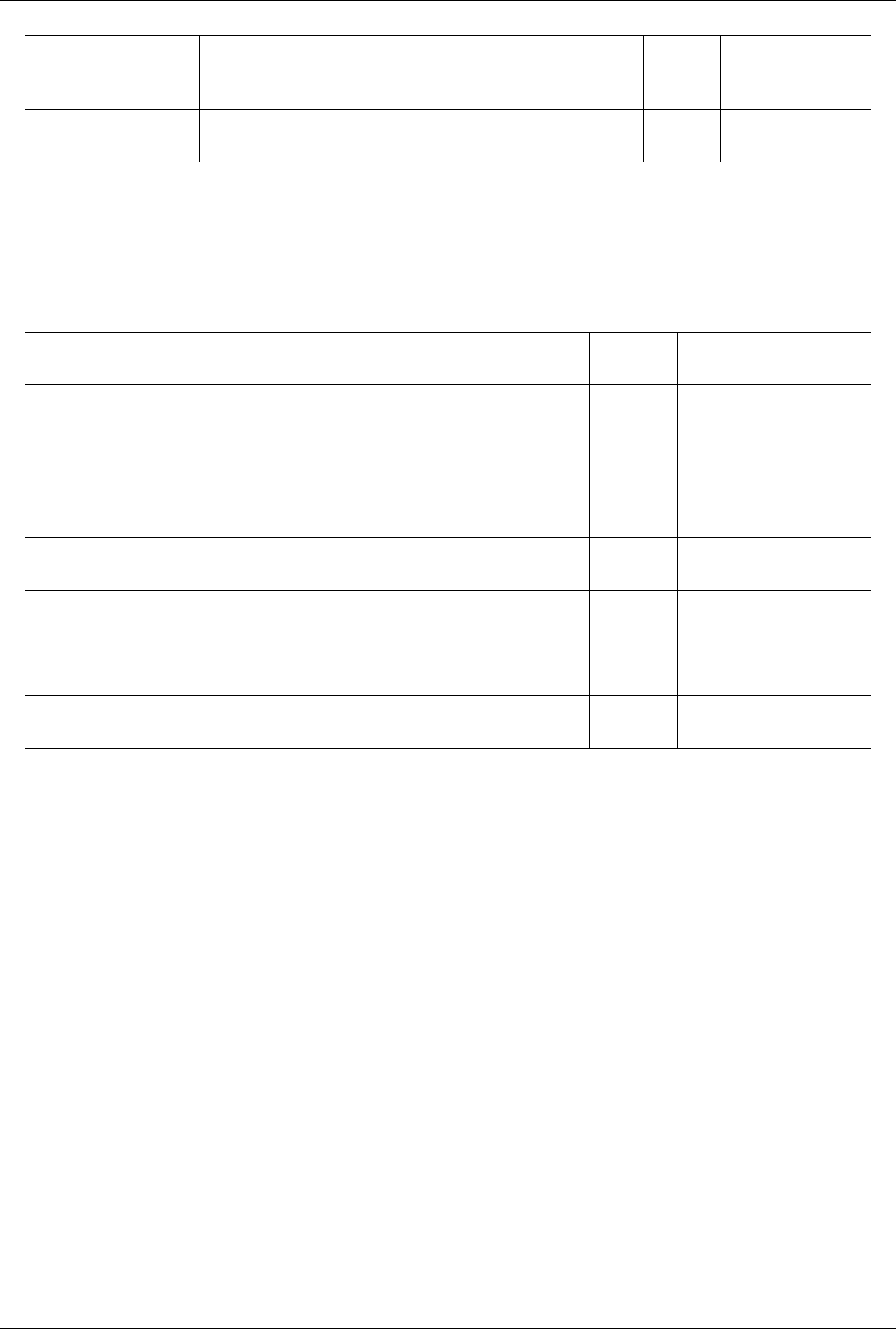
List of Filters 385
2D Points (Create2DPoints) Specify whether the points of the polydata are 3D or 2D. If this is set to true
then the Z Column will be ignored and the z value of each point on the
polydata will be set to 0. By default this will be off.
0 Accepts boolean values
(0 or 1).
KeepAllDataArrays
(KeepAllDataArrays)
Allow user to keep columns specified as X,Y,Z as Data arrays. By default
this will be off.
0 Accepts boolean values
(0 or 1).
Table To Structured Grid
Converts to table to structured grid.The TableToStructuredGrid filter converts a vtkTable to a vtkStructuredGrid.
One must specifies the columns in the input table to use as the X, Y and Z coordinates for the points in the output,
and the whole extent.
Property Description Default
Value(s)
Restrictions
Input (Input) This property specifies the input.. Accepts input of following
types:
• vtkTable
The dataset much contain a
field array (row)
with 1 component(s).
WholeExtent
(WholeExtent)
0 0 0 0 0 0
XColumn (XColumn) This property specifies which data array is going to be used as the X
coordinate in the generated polydata dataset.
YColumn (YColumn) This property specifies which data array is going to be used as the Y
coordinate in the generated polydata dataset.
ZColumn (ZColumn) This property specifies which data array is going to be used as the Z
coordinate in the generated polydata dataset.
Temporal Cache
Saves a copy of the data set for a fixed number of time steps.The Temporal Cache can be used to save multiple
copies of a data set at different time steps to prevent thrashing in the pipeline caused by downstream filters that
adjust the requested time step. For example, assume that there is a downstream Temporal Interpolator filter. This
filter will (usually) request two time steps from the upstream filters, which in turn (usually) causes the upstream
filters to run twice, once for each time step. The next time the interpolator requests the same two time steps, they
might force the upstream filters to re-evaluate the same two time steps. The Temporal Cache can keep copies of both
of these time steps and provide the requested data without having to run upstream filters.

List of Filters 386
Property Description Default
Value(s)
Restrictions
Input (Input) This property specifies the input of the Temporal Cache filter. Accepts input of
following types:
• vtkDataObject
CacheSize (CacheSize) The cache size determines the number of time steps that can be cached at one
time. The maximum number is 10. The minimum is 2 (since it makes little sense
to cache less than that).
2
TimestepValues
(TimestepValues)
Temporal Interpolator
Interpolate between time steps.The Temporal Interpolator converts data that is defined at discrete time steps to one
that is defined over a continuum of time by linearly interpolating the data's field data between two adjacent time
steps. The interpolated values are a simple approximation and should not be interpreted as anything more. The
Temporal Interpolator assumes that the topology between adjacent time steps does not change.
Property Description Default
Value(s)
Restrictions
Input (Input) This property specifies the input of the Temporal Interpolator. Accepts input of
following types:
• vtkDataObject
DiscreteTimeStepInterval
(DiscreteTimeStepInterval)
If Discrete Time Step Interval is set to 0, then the Temporal Interpolator will
provide a continuous region of time on its output. If set to anything else, then the
output will define a finite set of time points on its output, each spaced by the
Discrete Time Step Interval. The output will have (time range)/(discrete time step
interval) time steps. (Note that the time range is defined by the time range of the
data of the input filter, which may be different from other pipeline objects or the
range defined in the animation inspector.) This is a useful option to use if you have
a dataset with one missing time step and wish to 'file-in' the missing data with an
interpolated value from the steps on either side.
0.0
TimestepValues
(TimestepValues)
TimeRange (TimeRange)
Temporal Particles To Pathlines
Creates polylines representing pathlines of animating particles Particle Pathlines takes any dataset as input, it
extracts the point locations of all cells over time to build up a polyline trail. The point number (index) is used as the
'key' if the points are randomly changing their respective order in the points list, then you should specify a scalar that
represents the unique ID. This is intended to handle the output of a filter such as the TemporalStreamTracer.
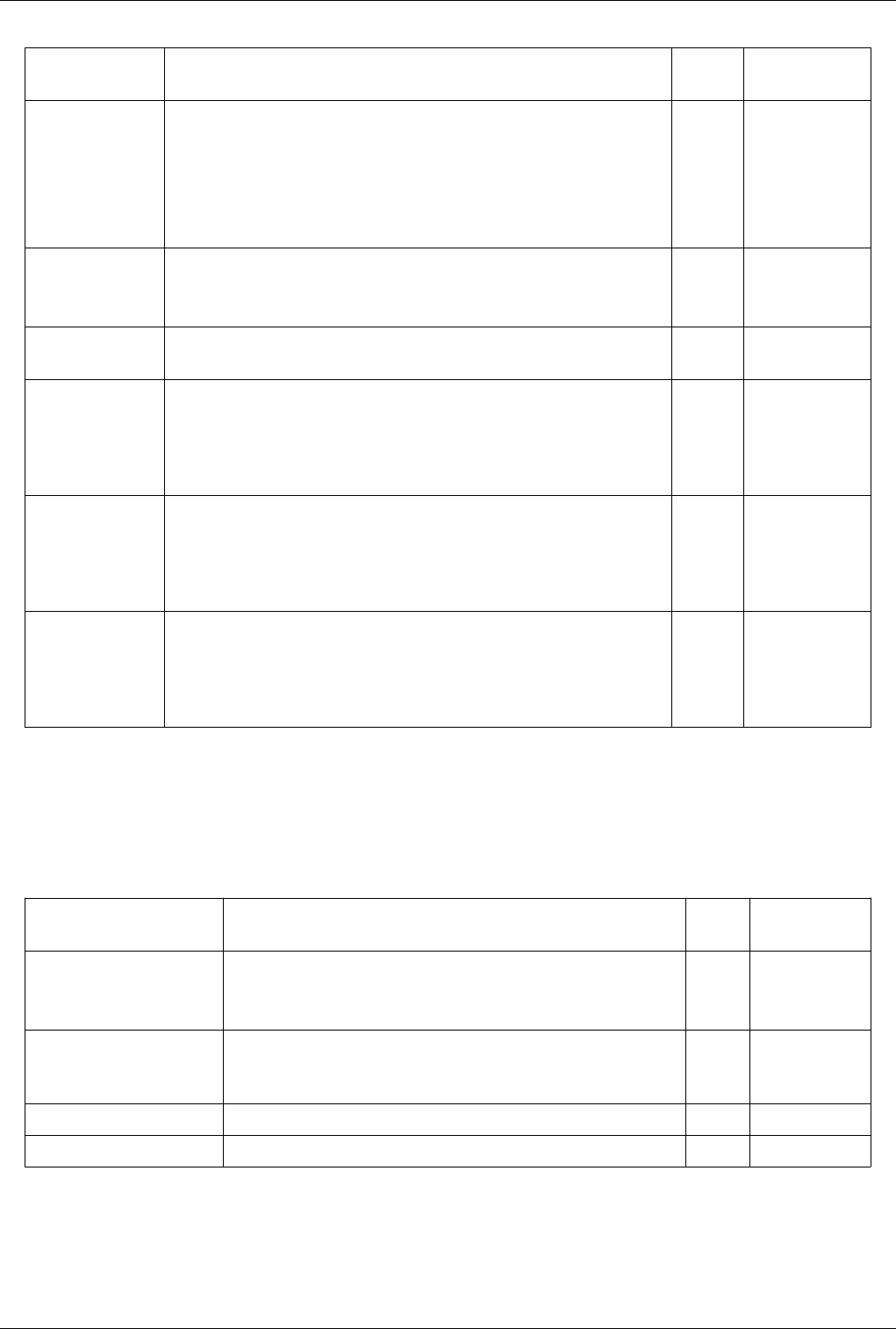
List of Filters 387
Property Description Default
Value(s)
Restrictions
Input (Input) The input cells to create pathlines for. Accepts input of
following types:
• vtkPointSet
The dataset much
contain a field array
(point)
Selection (Selection) Set a second input, which is a selection. Particles with the same Id in the selection as the
primary input will be chosen for pathlines Note that you must have the same
IdChannelArray in the selection as the input
Accepts input of
following types:
• vtkDataSet
MaskPoints
(MaskPoints)
Set the number of particles to track as a ratio of the input. Example: setting MaskPoints
to 10 will track every 10th point.
100
MaxTrackLength
(MaxTrackLength)
If the Particles being traced animate for a long time, the trails or traces will become
long and stringy. Setting the MaxTraceTimeLength will limit how much of the trace is
displayed. Tracks longer then the Max will disappear and the trace will apppear like a
snake of fixed length which progresses as the particle moves. This length is given with
respect to timesteps.
25
MaxStepDistance
(MaxStepDistance)
If a particle disappears from one end of a simulation and reappears on the other side, the
track left will be unrepresentative. Set a MaxStepDistance{x,y,z} which acts as a
threshold above which if a step occurs larger than the value (for the dimension), the
track will be dropped and restarted after the step. (ie the part before the wrap around
will be dropped and the newer part kept).
1.0 1.0 1.0
IdChannelArray
(IdChannelArray)
Specify the name of a scalar array which will be used to fetch the index of each point.
This is necessary only if the particles change position (Id order) on each time step. The
Id can be used to identify particles at each step and hence track them properly. If this
array is set to "Global or Local IDs", the global point ids are used if they exist or the
point index is otherwise.
Global or
Local IDs
An array of scalars
is required.
Temporal Shift Scale
Shift and scale time values.The Temporal Shift Scale filter linearly transforms the time values of a pipeline object by
applying a shift and then scale. Given a data at time t on the input, it will be transformed to time t*Shift + Scale on
the output. Inversely, if this filter has a request for time t, it will request time (t-Shift)/Scale on its input.
Property Description Default
Value(s)
Restrictions
Input (Input) The input to the Temporal Shift Scale filter. Accepts input of
following types:
• vtkDataObject
PreShift (PreShift) Apply a translation to the data before scaling. To convert T{5,100} to T{0,1}
use Preshift=-5, Scale=1/95, PostShift=0 To convert T{5,105} to T{5,10} use
Preshift=-5, Scale=5/100, PostShift=5
0.0
PostShift (PostShift) The amount of time the input is shifted. 0.0
Scale (Scale) The factor by which the input time is scaled. 1.0
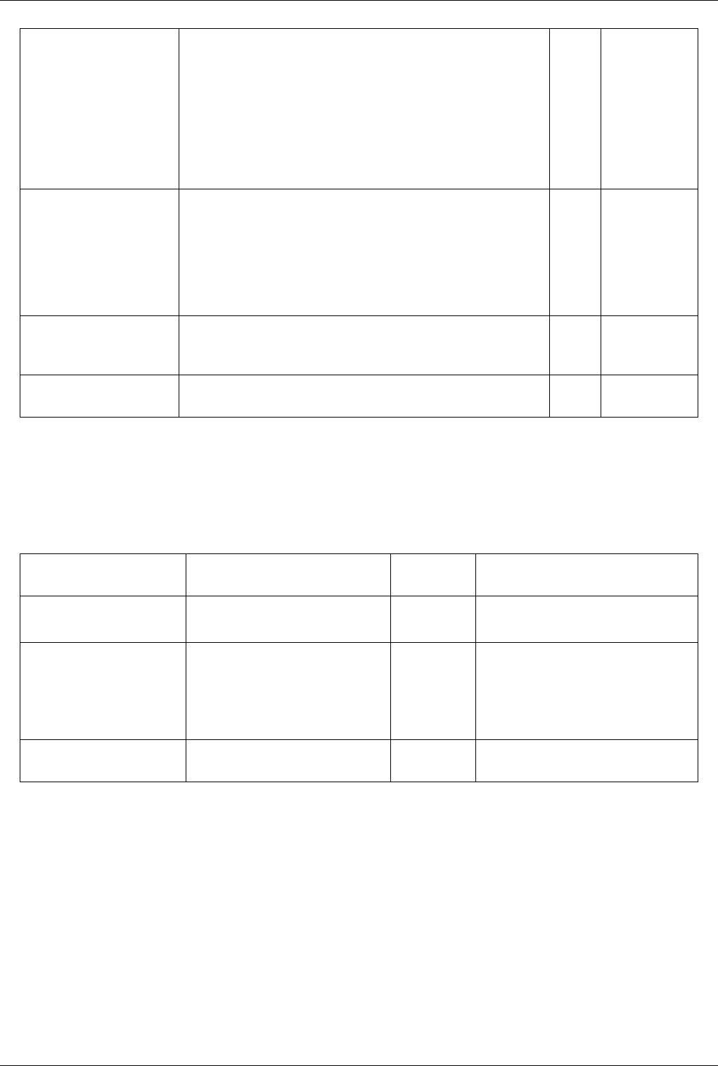
List of Filters 388
Periodic (Periodic) If Periodic is true, requests for time will be wrapped around so that the source
appears to be a periodic time source. If data exists for times {0,N-1}, setting
periodic to true will cause time 0 to be produced when time N, 2N, 2N etc is
requested. This effectively gives the source the ability to generate time data
indefinitely in a loop. When combined with Shift/Scale, the time becomes
periodic in the shifted and scaled time frame of reference. Note: Since the input
time may not start at zero, the wrapping of time from the end of one period to
the start of the next, will subtract the initial time - a source with T{5..6}
repeated periodicaly will have output time {5..6..7..8} etc.
0 Accepts boolean
values (0 or 1).
PeriodicEndCorrection
(PeriodicEndCorrection)
If Periodic time is enabled, this flag determines if the last time step is the same
as the first. If PeriodicEndCorrection is true, then it is assumed that the input
data goes from 0-1 (or whatever scaled/shifted actual time) and time 1 is the
same as time 0 so that steps will be 0,1,2,3...N,1,2,3...N,1,2,3 where step N is
the same as 0 and step 0 is not repeated. When this flag is false the data is
assumed to be literal and output is of the form 0,1,2,3...N,0,1,2,3... By default
this flag is ON
1 Accepts boolean
values (0 or 1).
MaximumNumberOfPeriods
(MaximumNumberOfPeriods)
If Periodic time is enabled, this controls how many time periods time is
reported for. A filter cannot output an infinite number of time steps and
therefore a finite number of periods is generated when reporting time.
1.0
TimestepValues
(TimestepValues)
Temporal Snap-to-Time-Step
Modifies the time range/steps of temporal data. This file modifies the time range or time steps of the data without
changing the data itself. The data is not resampled by this filter, only the information accompanying the data is
modified.
Property Description Default
Value(s)
Restrictions
Input (Input) This property specifies the input of the
filter.
Accepts input of following types:
• vtkDataObject
SnapMode (SnapMode) Determine which time step to snap to. 0 The value(s) is an enumeration of the
following:
• Nearest (0)
• NextBelowOrEqual (1)
• NextAboveOrEqual (2)
TimestepValues
(TimestepValues)
Temporal Statistics
Loads in all time steps of a data set and computes some statistics about how each point and cell variable changes
over time.Given an input that changes over time, vtkTemporalStatistics looks at the data for each time step and
computes some statistical information of how a point or cell variable changes over time. For example,
vtkTemporalStatistics can compute the average value of "pressure" over time of each point. Note that this filter will
require the upstream filter to be run on every time step that it reports that it can compute. This may be a time
consuming operation. vtkTemporalStatistics ignores the temporal spacing. Each timestep will be weighted the same
regardless of how long of an interval it is to the next timestep. Thus, the average statistic may be quite different from
an integration of the variable if the time spacing varies.

List of Filters 389
Property Description Default
Value(s)
Restrictions
Input (Input) Set the input to the Temporal Statistics filter. Accepts input of following
types:
• vtkDataSet
ComputeAverage (ComputeAverage) Compute the average of each point and cell
variable over time.
1 Accepts boolean values (0
or 1).
ComputeMinimum (ComputeMinimum) Compute the minimum of each point and cell
variable over time.
1 Accepts boolean values (0
or 1).
ComputeMaximum (ComputeMaximum) Compute the maximum of each point and cell
variable over time.
1 Accepts boolean values (0
or 1).
ComputeStandardDeviation
(ComputeStandardDeviation)
Compute the standard deviation of each point and
cell variable over time.
1 Accepts boolean values (0
or 1).
Tessellate
Tessellate nonlinear curves, surfaces, and volumes with lines, triangles, and tetrahedra.The Tessellate filter
tessellates cells with nonlinear geometry and/or scalar fields into a simplicial complex with linearly interpolated field
values that more closely approximate the original field. This is useful for datasets containing quadratic cells.
Property Description Default
Value(s)
Restrictions
Input (Input) This property specifies the input to the Tessellate filter. Accepts input of
following types:
• vtkPolyData
• vtkDataSet
• vtkUnstructuredGrid
OutputDimension (OutputDimension) The value of this property sets the maximum dimensionality of the
output tessellation. When the value of this property is 3, 3D cells
produce tetrahedra, 2D cells produce triangles, and 1D cells
produce line segments. When the value is 2, 3D cells will have
their boundaries tessellated with triangles. When the value is 1, all
cells except points produce line segments.
3
ChordError (ChordError) This property controls the maximum chord error allowed at any
edge midpoint in the output tessellation. The chord error is
measured as the distance between the midpoint of any output edge
and the original nonlinear geometry.
1e-3
Field Error (FieldError2) This proeprty controls the maximum field error allowed at any
edge midpoint in the output tessellation. The field error is
measured as the difference between a field value at the midpoint of
an output edge and the value of the corresponding field in the
original nonlinear geometry.
Maximum Number of Subdivisions
(MaximumNumberOfSubdivisions)
This property specifies the maximum number of times an edge
may be subdivided. Increasing this number allows further
refinement but can drastically increase the computational and
storage requirements, especially when the value of the
OutputDimension property is 3.
3
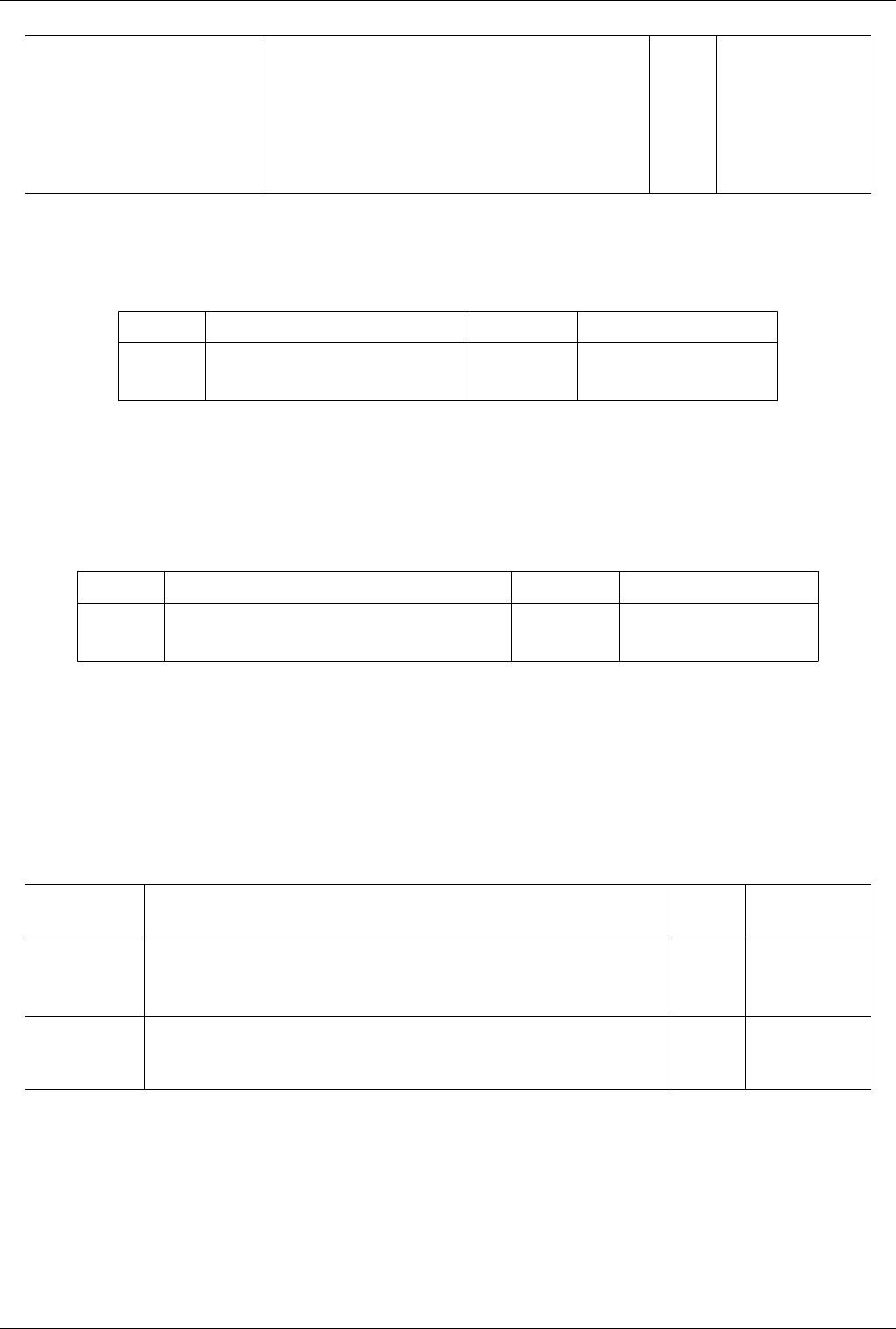
List of Filters 390
MergePoints (MergePoints) If the value of this property is set to 1, coincident vertices will be
merged after tessellation has occurred. Only geometry is
considered during the merge and the first vertex encountered is the
one whose point attributes will be used. Any discontinuities in
point fields will be lost. On the other hand, many operations, such
as streamline generation, require coincident vertices to be merged.
Toggle whether to merge coincident vertices.
1 Accepts boolean values
(0 or 1).
Tessellate Generic Dataset
Tessellate a higher-order datasetTessellate a higher-order dataset.
Property Description Default Value(s) Restrictions
Input (Input) Set the input to the Generic Tessellator filter. Accepts input of following types:
• vtkGenericDataSet
Tetrahedralize
This filter converts 3-d cells to tetrahedrons and polygons to triangles. The output is always of type unstructured
grid.The Tetrahedralize filter converts the 3D cells of any type of dataset to tetrahedrons and the 2D ones to
triangles. This filter always produces unstructured grid output.
Property Description Default Value(s) Restrictions
Input (Input) This property specifies the input to the Tetrahedralize filter. Accepts input of following types:
• vtkDataSet
Texture Map to Cylinder
Generate texture coordinates by mapping points to cylinder. This is a filter that generates 2D texture coordinates by
mapping input dataset points onto a cylinder. The cylinder is generated automatically. The cylinder is generated
automatically by computing the axis of the cylinder. Note that the generated texture coordinates for the s-coordinate
ranges from (0-1) (corresponding to angle of 0->360 around axis), while the mapping of the t-coordinate is
controlled by the projection of points along the axis.
Property Description Default
Value(s)
Restrictions
Input (Input) Set the input to the Texture Map to Cylinder filter. Accepts input of
following types:
• vtkDataSet
PreventSeam
(PreventSeam)
Control how the texture coordinates are generated. If Prevent Seam is set, the s-coordinate
ranges from 0->1 and 1->0 corresponding to the theta angle variation between 0->180 and
180->0 degrees. Otherwise, the s-coordinate ranges from 0->1 between 0->360 degrees.
1 Accepts boolean
values (0 or 1).
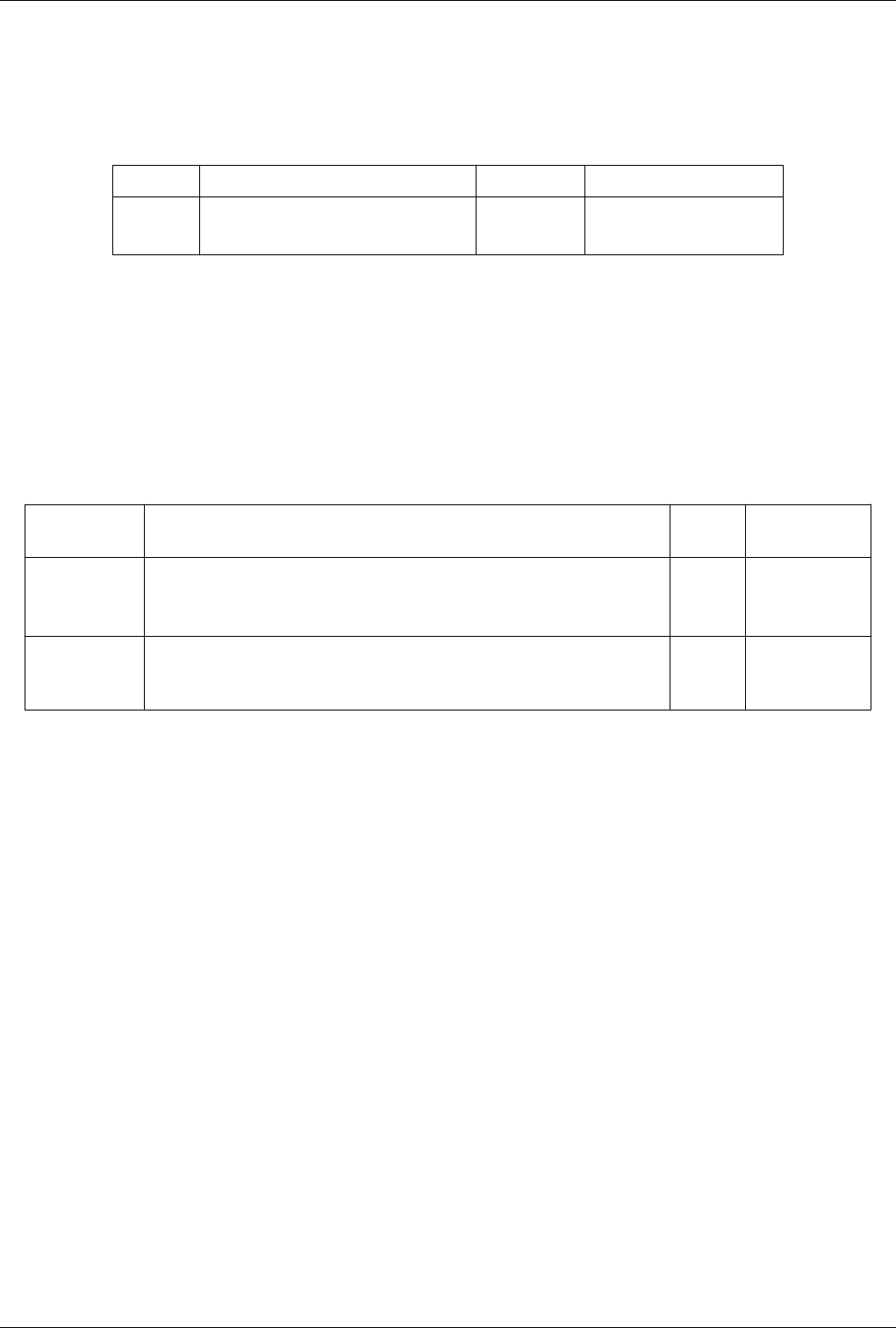
List of Filters 391
Texture Map to Plane
Generate texture coordinates by mapping points to plane. TextureMapToPlane is a filter that generates 2D texture
coordinates by mapping input dataset points onto a plane. The plane is generated automatically. A least squares
method is used to generate the plane automatically.
Property Description Default Value(s) Restrictions
Input (Input) Set the input to the Texture Map to Plane filter. Accepts input of following types:
• vtkDataSet
Texture Map to Sphere
Generate texture coordinates by mapping points to sphere. This is a filter that generates 2D texture coordinates by
mapping input dataset points onto a sphere. The sphere is generated automatically. The sphere is generated
automatically by computing the center i.e. averaged coordinates, of the sphere. Note that the generated texture
coordinates range between (0,1). The s-coordinate lies in the angular direction around the z-axis, measured
counter-clockwise from the x-axis. The t-coordinate lies in the angular direction measured down from the north pole
towards the south pole.
Property Description Default
Value(s)
Restrictions
Input (Input) Set the input to the Texture Map to Sphere filter. Accepts input of
following types:
• vtkDataSet
PreventSeam
(PreventSeam)
Control how the texture coordinates are generated. If Prevent Seam is set, the s-coordinate
ranges from 0->1 and 1->0 corresponding to the theta angle variation between 0->180 and
180->0 degrees. Otherwise, the s-coordinate ranges from 0->1 between 0->360 degrees.
1 Accepts boolean
values (0 or 1).
Threshold
This filter extracts cells that have point or cell scalars in the specified range. The Threshold filter extracts the
portions of the input dataset whose scalars lie within the specified range. This filter operates on either point-centered
or cell-centered data. This filter operates on any type of dataset and produces unstructured grid output. To select
between these two options, select either Point Data or Cell Data from the Attribute Mode menu. Once the Attribute
Mode has been selected, choose the scalar array from which to threshold the data from the Scalars menu. The Lower
Threshold and Upper Threshold sliders determine the range of the scalars to retain in the output. The All Scalars
check box only takes effect when the Attribute Mode is set to Point Data. If the All Scalars option is checked, then a
cell will only be passed to the output if the scalar values of all of its points lie within the range indicated by the
Lower Threshold and Upper Threshold sliders. If unchecked, then a cell will be added to the output if the specified
scalar value for any of its points is within the chosen range.

List of Filters 392
Property Description Default
Value(s)
Restrictions
Input (Input) This property specifies the input to the Threshold filter. Accepts input of
following types:
• vtkDataSet
The dataset much
contain a field array ()
with 1 component(s).
Scalars (SelectInputScalars) The value of this property contains the name of the scalar array from which
to perform thresholding.
An array of scalars is
required.The value
must be field array
name.
Threshold Range
(ThresholdBetween)
The values of this property specify the upper and lower bounds of the
thresholding operation.
0 0 The value must lie
within the range of the
selected data array.
AllScalars (AllScalars) If the value of this property is 1, then a cell is only included in the output if
the value of the selected array for all its points is within the threshold. This is
only relevant when thresholding by a point-centered array.
1 Accepts boolean
values (0 or 1).
UseContinuousCellRange
(UseContinuousCellRange)
If off, the vertex scalars are treated as a discrete set. If on, they are treated as
a continuous interval over the minimum and maximum. One important "on"
use case: When setting lower and upper threshold equal to some value and
turning AllScalars off, the results are cells containing the iso-surface for that
value. WARNING: Whether on or off, for higher order input, the filter will
not give accurate results.
0 Accepts boolean
values (0 or 1).
Transform
This filter applies transformation to the polygons.The Transform filter allows you to specify the position, size, and
orientation of polygonal, unstructured grid, and curvilinear data sets.
Property Description Default
Value(s)
Restrictions
Input (Input) This property specifies the input to the Transform filter. Accepts input of following
types:
• vtkPointSet
• vtkImageData
• vtkRectilinearGrid
Transform
(Transform)
The values in this property allow you to specify the transform (translation,
rotation, and scaling) to apply to the input dataset.
The value can be one of the
following:
• Transform3
(extended_sources)
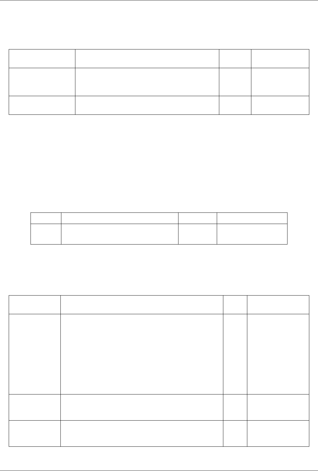
List of Filters 393
Triangle Strips
This filter uses a greedy algorithm to convert triangles into triangle stripsThe Triangle Strips filter converts triangles
into triangle strips and lines into polylines. This filter operates on polygonal data sets and produces polygonal output.
Property Description Default
Value(s)
Restrictions
Input (Input) This property specifies the input to the Triangle Strips filter. Accepts input of following
types:
• vtkPolyData
MaximumLength
(MaximumLength)
This property specifies the maximum number of triangles/lines to
include in a triangle strip or polyline.
1000
Triangulate
This filter converts polygons and triangle strips to basic triangles.The Triangulate filter decomposes polygonal data
into only triangles, points, and lines. It separates triangle strips and polylines into individual triangles and lines,
respectively. The output is polygonal data. Some filters that take polygonal data as input require that the data be
composed of triangles rather than other polygons, so passing your data through this filter first is useful in such
situations. You should use this filter in these cases rather than the Tetrahedralize filter because they produce different
output dataset types. The filters referenced require polygonal input, and the Tetrahedralize filter produces
unstructured grid output.
Property Description Default Value(s) Restrictions
Input (Input) This property specifies the input to the Triangulate filter. Accepts input of following types:
• vtkPolyData
Tube
Convert lines into tubes. Normals are used to avoid cracks between tube segments.The Tube filter creates tubes
around the lines in the input polygonal dataset. The output is also polygonal.
Property Description Default
Value(s)
Restrictions
Input (Input) This property specifies the input to the Tube filter. Accepts input of following
types:
• vtkPolyData
The dataset much contain a
field array (point)
with 1 component(s).
The dataset much contain a
field array (point)
with 3 component(s).
Scalars
(SelectInputScalars)
This property indicates the name of the scalar array on which to operate. The
indicated array may be used for scaling the tubes. (See the VaryRadius
property.)
An array of scalars is
required.
Vectors
(SelectInputVectors)
This property indicates the name of the vector array on which to operate. The
indicated array may be used for scaling and/or orienting the tubes. (See the
VaryRadius property.)
1 An array of vectors is
required.
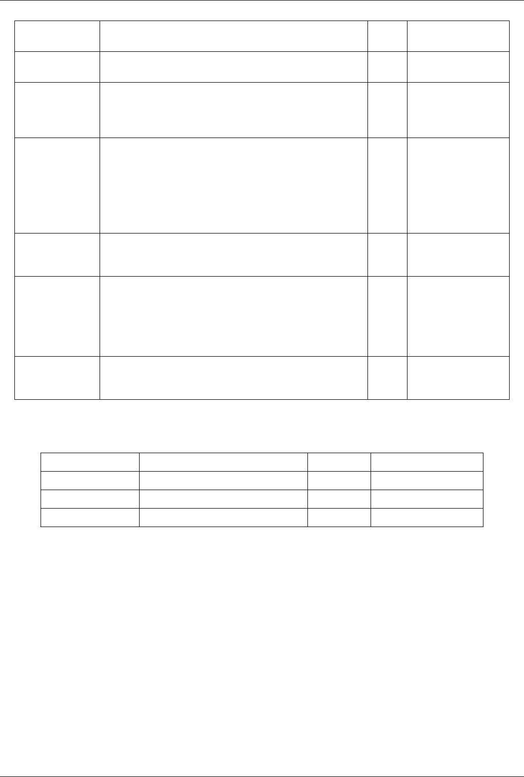
List of Filters 394
Number of Sides
(NumberOfSides)
The value of this property indicates the number of faces around the
circumference of the tube.
6
Capping (Capping) If this property is set to 1, endcaps will be drawn on the tube. Otherwise the
ends of the tube will be open.
1 Accepts boolean values (0 or
1).
Radius (Radius) The value of this property sets the radius of the tube. If the radius is varying
(VaryRadius property), then this value is the minimum radius.
1.0 The value must be less than
the largest dimension of the
dataset multiplied by a scale
factor of 0.01.
VaryRadius
(VaryRadius)
The property determines whether/how to vary the radius of the tube. If varying
by scalar (1), the tube radius is based on the point-based scalar values in the
dataset. If it is varied by vector, the vector magnitude is used in varying the
radius.
0 The value(s) is an
enumeration of the
following:
• Off (0)
• By Scalar (1)
• By Vector (2)
• By Absolute Scalar (3)
RadiusFactor
(RadiusFactor)
If varying the radius (VaryRadius property), the property sets the maximum
tube radius in terms of a multiple of the minimum radius. If not varying the
radius, this value has no effect.
10
UseDefaultNormal
(UseDefaultNormal)
If this property is set to 0, and the input contains no vector array, then default
ribbon normals will be generated (DefaultNormal property); if a vector array
has been set (SelectInputVectors property), the ribbon normals will be set from
the specified array. If this property is set to 1, the default normal
(DefaultNormal property) will be used, regardless of whether the
SelectInputVectors property has been set.
0 Accepts boolean values (0 or
1).
DefaultNormal
(DefaultNormal)
The value of this property specifies the normal to use when the
UseDefaultNormal property is set to 1 or the input contains no vector array
(SelectInputVectors property).
0 0 1
UpdateSuppressor2
Property Description Default Value(s) Restrictions
Input (Input) Set the input to the Update Suppressor filter.
Enabled (Enabled) Toggle whether the update suppressor is enabled. 1 Accepts boolean values (0 or 1).
UpdateTime (UpdateTime) none
Warp By Scalar
This filter moves point coordinates along a vector scaled by a point attribute. It can be used to produce carpet plots.
The Warp (scalar) filter translates the points of the input data set along a vector by a distance determined by the
specified scalars. This filter operates on polygonal, curvilinear, and unstructured grid data sets containing
single-component scalar arrays. Because it only changes the positions of the points, the output data set type is the
same as that of the input. Any scalars in the input dataset are copied to the output, so the data can be colored by
them.

List of Filters 395
Property Description Default
Value(s)
Restrictions
Input (Input) This property specifies the input to the Warp (scalar) filter. Accepts input of following
types:
• vtkPointSet
• vtkImageData
• vtkRectilinearGrid
The dataset much contain a
field array (point)
with 1 component(s).
Scalars
(SelectInputScalars)
This property contains the name of the scalar array by which to warp the
dataset.
An array of scalars is
required.
ScaleFactor
(ScaleFactor)
The scalar value at a given point is multiplied by the value of this property to
determine the magnitude of the change vector for that point.
1.0
Normal (Normal) The values of this property specify the direction along which to warp the
dataset if any normals contained in the input dataset are not being used for
this purpose. (See the UseNormal property.)
0 0 1
UseNormal
(UseNormal)
If point normals are present in the dataset, the value of this property toggles
whether to use a single normal value (value = 1) or the normals from the
dataset (value = 0).
0 Accepts boolean values (0 or
1).
XY Plane (XYPlane) If the value of this property is 1, then the Z-coordinates from the input are
considered to be the scalar values, and the displacement is along the Z axis.
This is useful for creating carpet plots.
0 Accepts boolean values (0 or
1).
Warp By Vector
This filter displaces point coordinates along a vector attribute. It is useful for showing mechanical deformation. The
Warp (vector) filter translates the points of the input dataset using a specified vector array. The vector array chosen
specifies a vector per point in the input. Each point is translated along its vector by a given scale factor. This filter
operates on polygonal, curvilinear, and unstructured grid datasets. Because this filter only changes the positions of
the points, the output dataset type is the same as that of the input.
Property Description Default
Value(s)
Restrictions
Input (Input) This property specifies the input to the Warp (vector) filter. Accepts input of following
types:
• vtkPointSet
• vtkImageData
• vtkRectilinearGrid
The dataset much contain a field
array (point)
with 3 component(s).
Vectors
(SelectInputVectors)
The value of this property contains the name of the vector array by
which to warp the dataset's point coordinates.
An array of vectors is required.
ScaleFactor
(ScaleFactor)
Each component of the selected vector array will be multiplied by the
value of this property before being used to compute new point
coordinates.
1.0
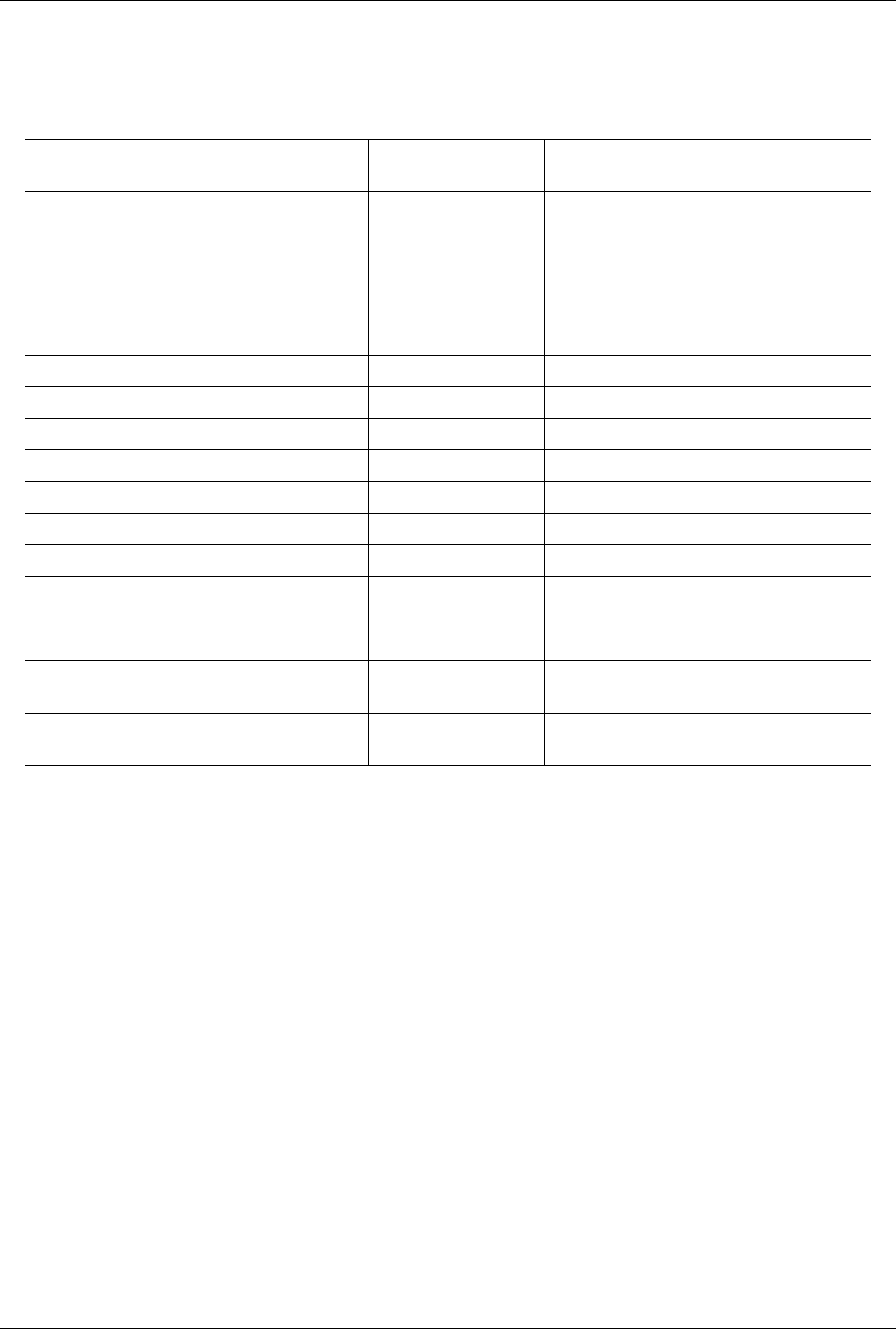
List of Filters 396
Youngs Material Interface
Computes linear material interfaces in 2D or 3D mixed cells produced by eulerian or ALE simulation codes
Computes linear material interfaces in 2D or 3D mixed cells produced by Eulerian or ALE simulation codes
Property Description Default
Value(s)
Restrictions
Input (Input) Accepts input of following types:
• vtkCompositeDataSet
The dataset much contain a field array (cell)
with 1 component(s).
The dataset much contain a field array (cell)
with 3 component(s).
InverseNormal (InverseNormal) 0 Accepts boolean values (0 or 1).
ReverseMaterialOrder (ReverseMaterialOrder) 0 Accepts boolean values (0 or 1).
OnionPeel (OnionPeel) 1 Accepts boolean values (0 or 1).
AxisSymetric (AxisSymetric) 1 Accepts boolean values (0 or 1).
FillMaterial (FillMaterial) 1 Accepts boolean values (0 or 1).
UseFractionAsDistance (UseFractionAsDistance) 0 Accepts boolean values (0 or 1).
VolumeFractionRange (VolumeFractionRange) 0.01 0.99
NumberOfDomainsInformation
(NumberOfDomainsInformation)
VolumeFractionArrays (VolumeFractionArrays) An array of scalars is required.
NormalArrays (NormalArrays) An array of vectors is required.The value must be field
array name.
OrderingArrays (OrderingArrays) An array of scalars is required.The value must be field
array name.
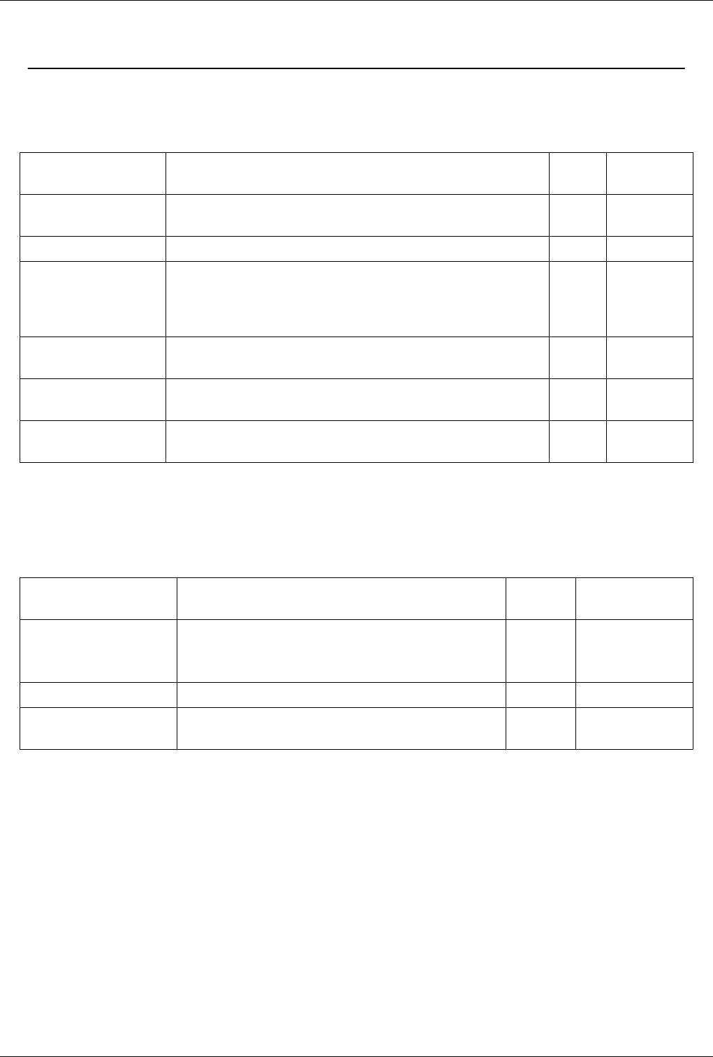
List of Writers 397
List of Writers
AnimationSceneImageWriter
Internal writer to used paraview uses when it disconnects the GUI.
Property Description Default
Value(s)
Restrictions
Magnification
(Magnification)
The magnification factor to use for the saved animation. 1
FileName (FileName) The name of the file to save the animation into.
FrameRate (FrameRate) Get/Set the frame rate to use for saving the animation. This frame rate is the frame
rate that gets saved in the movie file generated, if applicable. If does not affect the
FrameRate set on the animation scene at all. In other words, this is the playback
frame rate and not the animation generation frame rate.
0
PlaybackTimeWindow
(PlaybackTimeWindow)
Time range to write -1 1
Compression (Compression) Turns on(the default) or off compression for FFMEG (AVI on Linux and Mac)
backend.
1 Accepts boolean
values (0 or 1).
StartFileCount
(StartFileCount)
0
CSVWriter
Writer to write CSV filesWriter to write CSV files from table. In parallel, it delivers the table to the root node and
then saves the CSV. For composite datasets, it saves multiple csv files.
Property Description Default
Value(s)
Restrictions
Input (Input) The input filter/source whose output dataset is to written to the file. Accepts input of
following types:
• vtkTable
FileName (FileName) The name of the file to be written.
WriteAllTimeSteps
(WriteAllTimeSteps)
When WriteAllTimeSteps is turned ON, the writer is executed once for
each time step available from the reader.
0 Accepts boolean values
(0 or 1).
DataSetCSVWriter
Writer to write CSV filesWriter to write CSV files from any dataset. Set FieldAssociation to choose whether cell
data/point data needs to be saved. In parallel, it delivers the table to the root node and then saves the CSV. For
composite datasets, it saves multiple csv files.
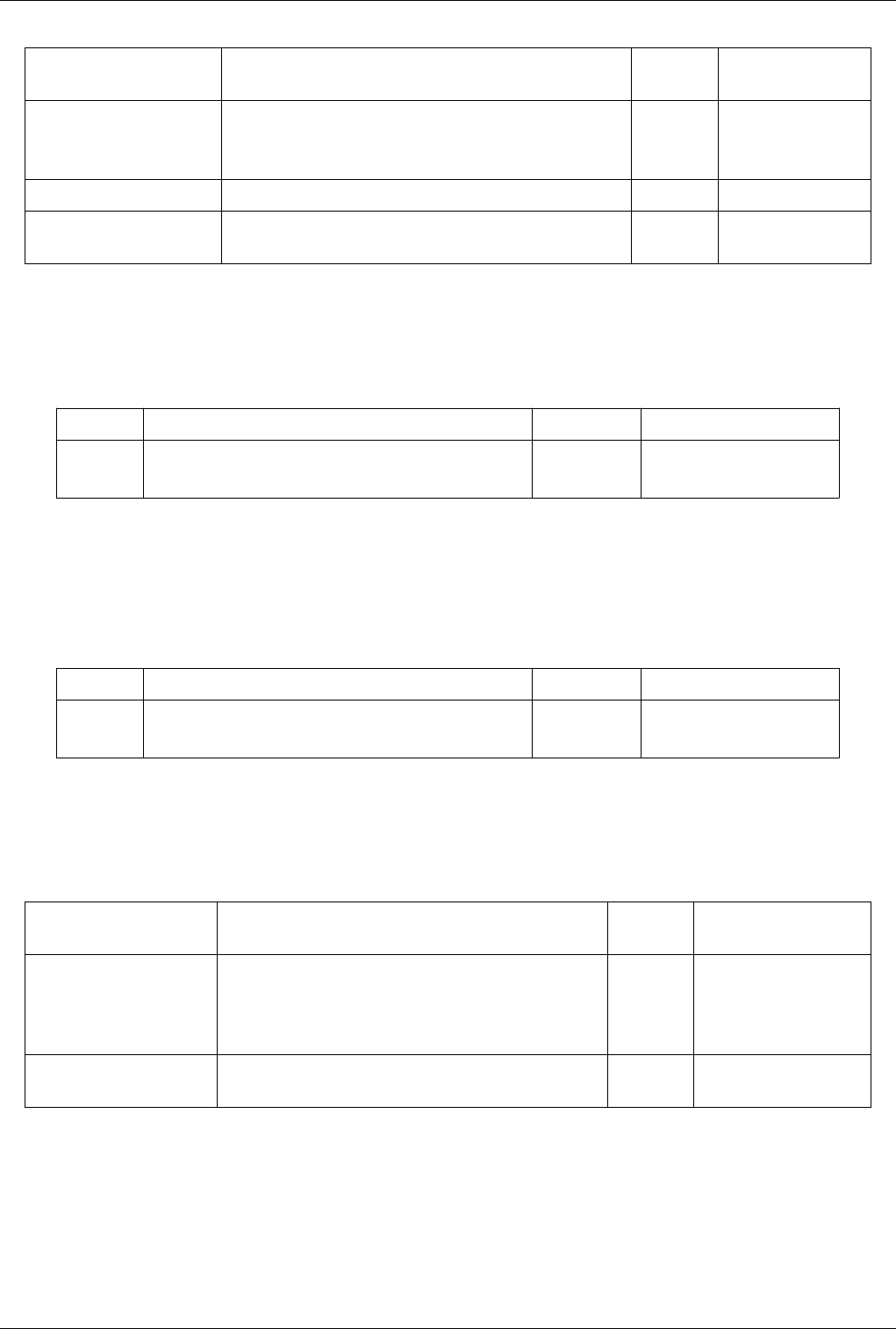
List of Writers 398
Property Description Default
Value(s)
Restrictions
Input (Input) The input filter/source whose output dataset is to written to the file. Accepts input of
following types:
• vtkDataSet
FileName (FileName) The name of the file to be written.
WriteAllTimeSteps
(WriteAllTimeSteps)
When WriteAllTimeSteps is turned ON, the writer is executed once
for each timestep available from the reader.
0 Accepts boolean values
(0 or 1).
DataSetWriter
Write any type of data object in a legacy vtk data file. Writer to write any type of data object in a legacy vtk data file.
Cannot be used for parallel writing.
Property Description Default Value(s) Restrictions
Input (Input) The input filter/source whose output dataset is to written to the file. Accepts input of following types:
• vtkDataObject
EnSightWriter
Write unstructured grid data as an EnSight file. Writer to write unstructured grid data as an EnSight file. Binary files
written on one system may not be readable on other systems. Be sure to specify the endian-ness of the file when
reading it into EnSight.
Property Description Default Value(s) Restrictions
Input (Input) The input filter/source whose output dataset is to written to the file. Accepts input of following types:
• vtkUnstructuredGrid
ExodusIIWriter
Write Exodus II files.Writer to write Exodus II files. Refere to http:/ / endo. sandia. gov/ SEACAS/ for more
information about the Exodus II format.
Property Description Default
Value(s)
Restrictions
Input (Input) The input filter/source whose output dataset is to written to the file. Accepts input of following
types:
• vtkCompositeDataSet
• vtkDataSet
WriteAllTimeSteps
(WriteAllTimeSteps)
When WriteAllTimeSteps is turned ON, the writer is executed
once for each time step available from the reader.
0 Accepts boolean values (0 or
1).
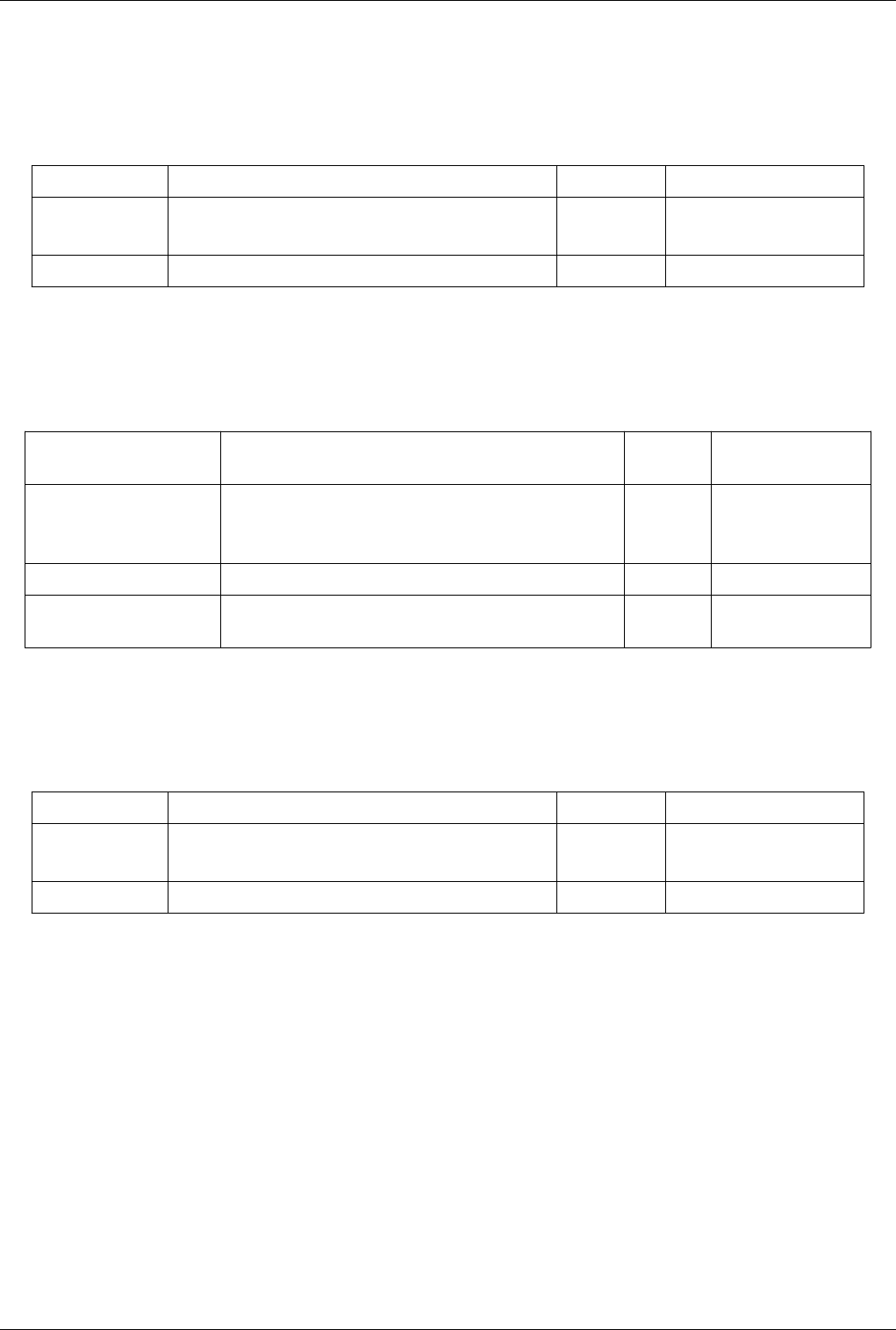
List of Writers 399
MetaImageWriter
Write a binary UNC meta image data.Writer to write a binary UNC meta image data. This is a fairly simple yet
powerful format consisting of a text header and a binary data section. MetaImage headers are expected to have
extension: ".mha" or ".mhd"
Property Description Default Value(s) Restrictions
Input (Input) The input filter/source whose output dataset is to written to the file. Accepts input of following types:
• vtkImageData
FileName (FileName) The name of the file to be written.
PDataSetWriter
Writer that writes polydata as legacy vtk files. Writer to write any type of data object in a legacy vtk data file. This
version is used when running in parallel. It gathers data to first node and saves one file.
Property Description Default
Value(s)
Restrictions
Input (Input) The input filter/source whose output dataset is to written to the file. Accepts input of
following types:
• vtkDataObject
FileName (FileName) The name of the file to be written.
WriteAllTimeSteps
(WriteAllTimeSteps)
When WriteAllTimeSteps is turned ON, the writer is executed once
for each timestep available from the reader.
0 Accepts boolean values (0
or 1).
PNGWriter
Write image data as a PNG file.Writer to write image data as a PNG file. It supports 1 to 4 component data of
unsigned char or unsigned short.
Property Description Default Value(s) Restrictions
Input (Input) The input filter/source whose output dataset is to written to the file. Accepts input of following types:
• vtkImageData
FileName (FileName) The name of the file to be written.
PPLYWriter
Write polygonal data in Stanford University PLY format. Writer to write polygonal data in Stanford University PLY
format. The data can be written in either binary (little or big endian) or ASCII representation. As for PointData and
CellData, vtkPLYWriter cannot handle normals or vectors. It only handles RGB PointData and CellData. This
version is used when running in parallel. It gathers data to first node and saves one file.
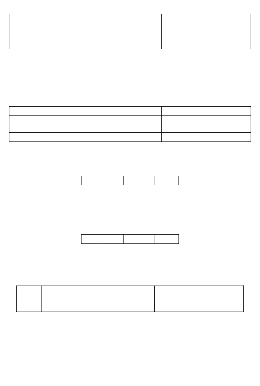
List of Writers 400
Property Description Default Value(s) Restrictions
Input (Input) The input filter/source whose output dataset is to written to the file. Accepts input of following types:
• vtkPolyData
FileName (FileName) The name of the file to be written.
PSTLWriter
Write stereo lithography files.STLWriter writes stereo lithography (.stl) files in either ASCII or binary form. Stereo
lithography files only contain triangles. If polygons with more than 3 vertices are present, only the first 3 vertices are
written. Use TriangleFilter to convert polygons to triangles. This version of the reader is used when running in
parallel. It gathers all the geometry to first node and saves 1 file.
Property Description Default Value(s) Restrictions
Input (Input) The input filter/source whose output dataset is to written to the file. Accepts input of following types:
• vtkPolyData
FileName (FileName) The name of the file to be written.
XMLDataSetWriterBase
Base for all XML-based file-series writers.
Property Description Default Value(s) Restrictions
XMLHierarchicalBoxDataWriter
(DEPRECATED) Write a hierarchical box dataset in a xml-based vtk data file. (DEPRECATED) Writer to write a
hierarchical box in a xml-based vtk data file. Can be used for parallel writing as well as serial writing. This is
deprecated. Use XMLUniformGridAMRWriter instead.
Property Description Default Value(s) Restrictions
XMLHyperOctreeWriter
Write unstructured grid in a xml-based vtk data file. Writer to write unstructured grid in a xml-based vtk data file.
Cannot be used for parallel writing.
Property Description Default Value(s) Restrictions
Input (Input) The input filter/source whose output dataset is to written to the file. Accepts input of following types:
• vtkHyperOctree
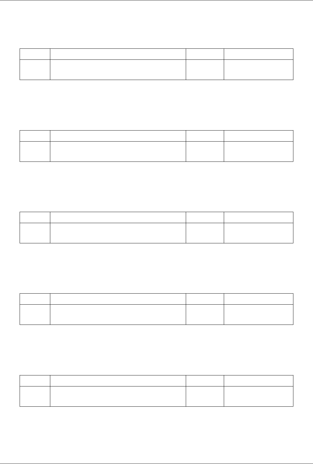
List of Writers 401
XMLImageDataWriter
Write image data in a xml-based vtk data file. Writer to write image data in a xml-based vtk data file. Cannot be used
for parallel writing.
Property Description Default Value(s) Restrictions
Input (Input) The input filter/source whose output dataset is to written to the file. Accepts input of following types:
• vtkImageData
XMLMultiBlockDataWriter
Write a multiblock in a xml-based vtk data file. Writer to write a multiblock dataset in a xml-based vtk data file. Can
be used for parallel writing as well as serial writing.
Property Description Default Value(s) Restrictions
Input (Input) The input filter/source whose output dataset is to written to the file. Accepts input of following types:
• vtkMultiBlockDataSet
XMLPImageDataWriter
Write image data in a xml-based vtk data file. Writer to write image data in a xml-based vtk data file. Can be used
for parallel writing.
Property Description Default Value(s) Restrictions
Input (Input) The input filter/source whose output dataset is to written to the file. Accepts input of following types:
• vtkImageData
XMLPPolyDataWriter
Write polydata in a xml-based vtk data file. Writer to write polydata in a xml-based vtk data file. Can be used for
parallel writing.
Property Description Default Value(s) Restrictions
Input (Input) The input filter/source whose output dataset is to written to the file. Accepts input of following types:
• vtkPolyData
XMLPRectilinearGridWriter
Write rectilinear grid in a xml-based vtk data file. Writer to write rectilinear grid in a xml-based vtk data file. Can be
used for parallel writing.
Property Description Default Value(s) Restrictions
Input (Input) The input filter/source whose output dataset is to written to the file. Accepts input of following types:
• vtkRectilinearGrid
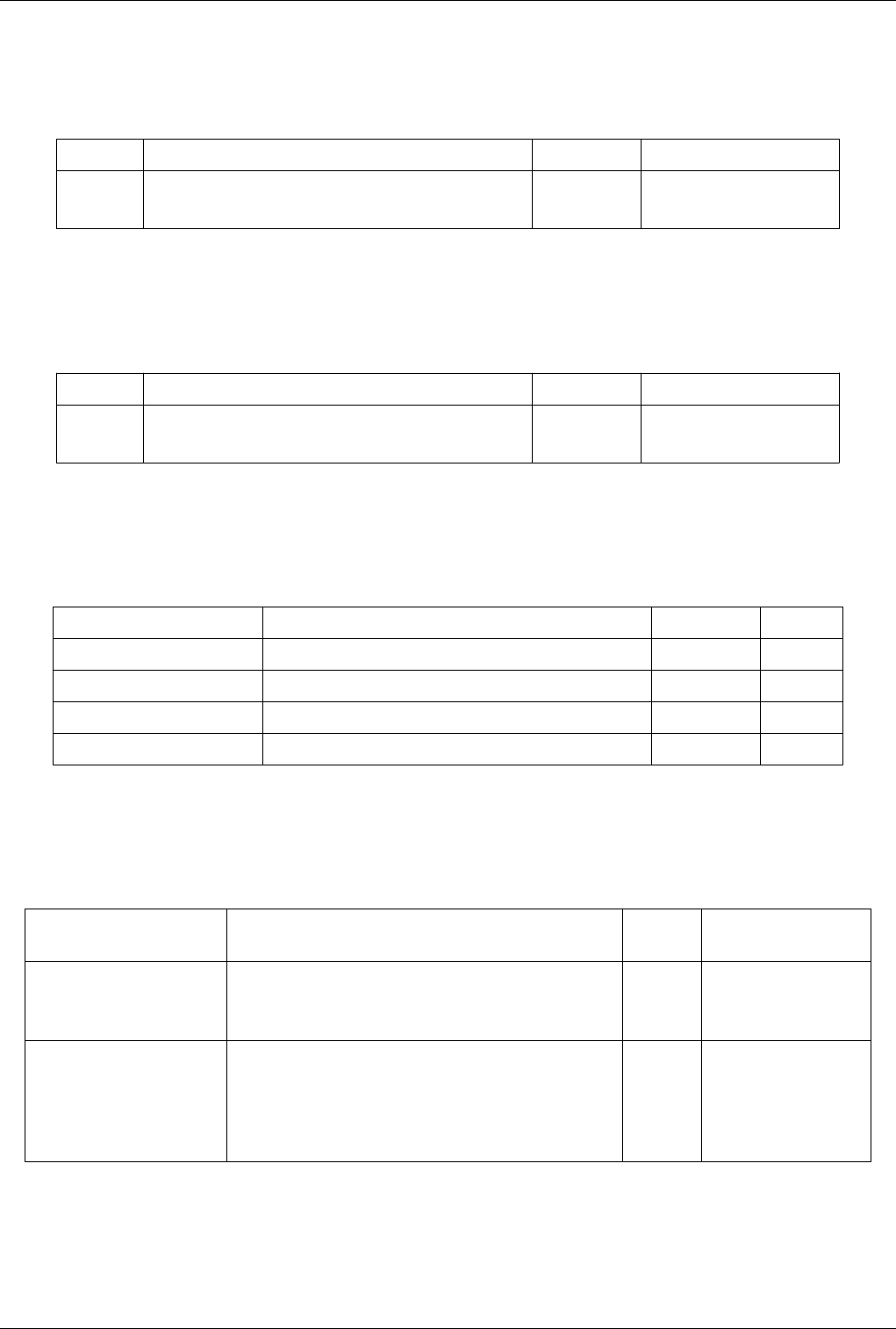
List of Writers 402
XMLPStructuredGridWriter
Write structured grid in a xml-based vtk data file. Writer to write structured grid in a xml-based vtk data file. Can be
used for parallel writing.
Property Description Default Value(s) Restrictions
Input (Input) The input filter/source whose output dataset is to written to the file. Accepts input of following types:
• vtkStructuredGrid
XMLPUnstructuredGridWriter
Write unstructured grid in a xml-based vtk data file. Writer to write unstructured grid in a xml-based vtk data file.
Can be used for parallel writing.
Property Description Default Value(s) Restrictions
Input (Input) The input filter/source whose output dataset is to written to the file. Accepts input of following types:
• vtkUnstructuredGrid
XMLPVAnimationWriter
Internal writer proxy used when saving animation geometry to save all parts of the current source to the file with
pieces spread across the server processes.
Property Description Default Value(s) Restrictions
Representations (Representations) The input filter/source whose output dataset is to written to the file.
FileName (FileName) Name of the file to write.
WriteTime (WriteTime) Write each time step in the animation 0.0
ErrorCode (ErrorCode)
XMLPVDWriter
Write ParaView data files (pvd).Writer to write ParaView data files (pvd). It is used to save all pieces of a
source/filter to a file with pieces spread across the server processes.
Property Description Default
Value(s)
Restrictions
Input (Input) The input filter/source whose output dataset is to written to the files. Accepts input of following
types:
• vtkDataSet
HeaderType (HeaderType) Set the binary data header word type. The default is UInt32. Set to
UInt64 when storing arrays requiring 64-bit indexing.
32 The value(s) is an
enumeration of the
following:
• UInt32 (32)
• UInt64 (64)
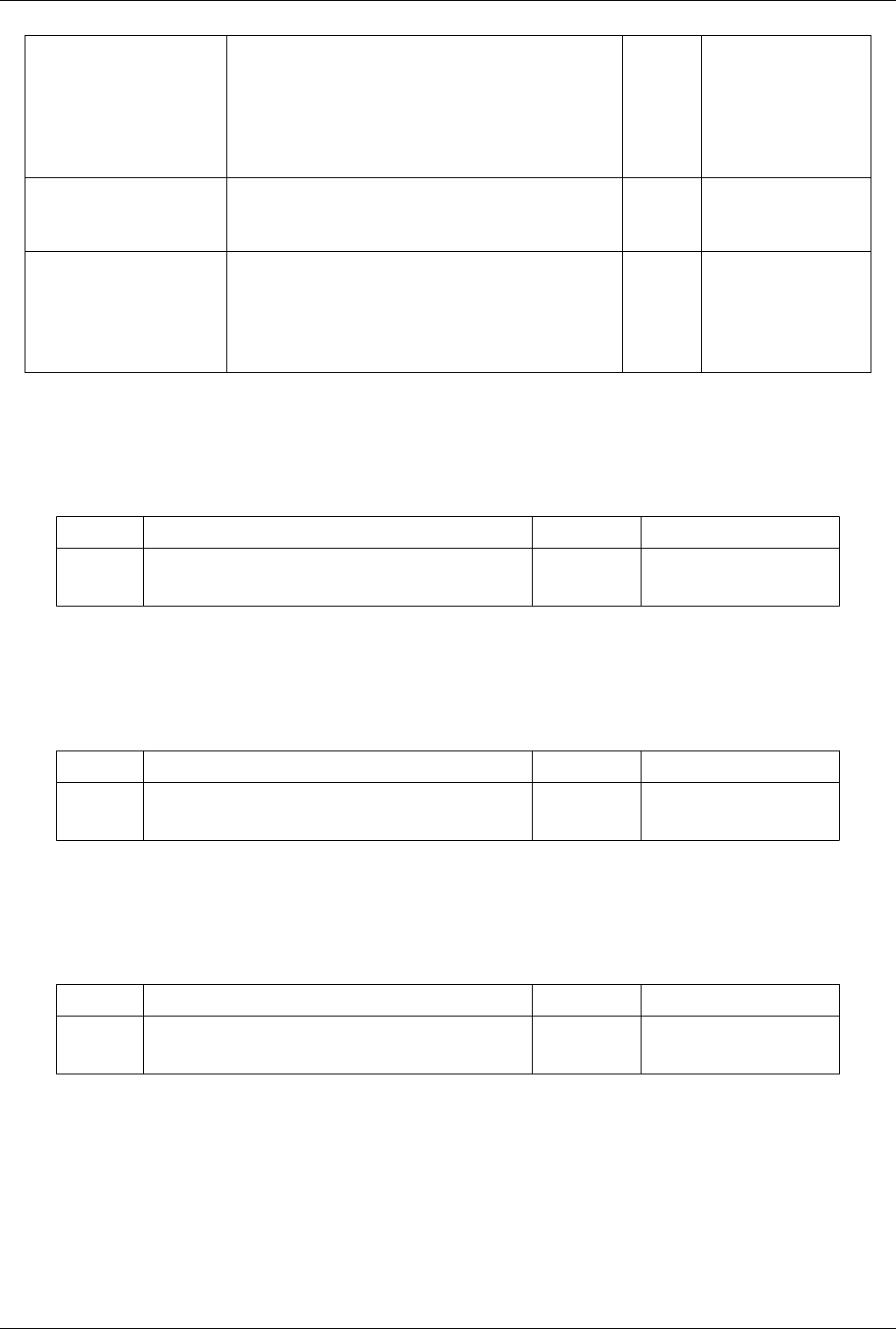
List of Writers 403
DataMode (DataMode) The mode uses for writing the file's data i.e. ascii, binary, appended
binary.
2 The value(s) is an
enumeration of the
following:
• Ascii (0)
• Binary (1)
• Appended (2)
EncodeAppendedData
(EncodeAppendedData)
When EncodeAppendedData is turned ON, the writer uses base64
encoding when writing binary data (only if appended mode is
selected).
0 Accepts boolean values (0
or 1).
CompressorType
(CompressorType)
The compression algorithm used to compress binary data (appended
mode only).
0 The value(s) is an
enumeration of the
following:
• None (0)
• ZLib (1)
XMLPolyDataWriter
Write poly data in a xml-based vtk data file. Writer to write poly data in a xml-based vtk data file. Cannot be used
for parallel writing.
Property Description Default Value(s) Restrictions
Input (Input) The input filter/source whose output dataset is to written to the file. Accepts input of following types:
• vtkPolyData
XMLRectilinearGridWriter
Write rectilinear grid in a xml-based vtk data file. Writer to write rectilinear grid in a xml-based vtk data file. Cannot
be used for parallel writing.
Property Description Default Value(s) Restrictions
Input (Input) The input filter/source whose output dataset is to written to the file. Accepts input of following types:
• vtkRectilinearGrid
XMLStructuredGridWriter
Write structured grid in a xml-based vtk data file. Writer to write structured grid in a xml-based vtk data file. Cannot
be used for parallel writing.
Property Description Default Value(s) Restrictions
Input (Input) The input filter/source whose output dataset is to written to the file. Accepts input of following types:
• vtkStructuredGrid
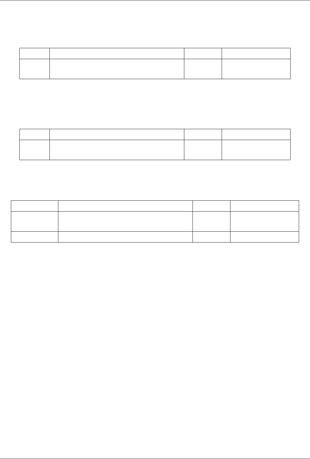
List of Writers 404
XMLUniformGridAMRWriter
Write a amr dataset in a xml-based vtk data file. Writer to write an AMR data-set (overlapping/non-overlapping) in a
xml-based vtk data file. Can be used for parallel writing as well as serial writing.
Property Description Default Value(s) Restrictions
Input (Input) The input filter/source whose output dataset is to written to the file. Accepts input of following types:
• vtkUniformGridAMR
XMLUnstructuredGridWriter
Write unstructured grid in a xml-based vtk data file. Writer to write unstructured grid in a xml-based vtk data file.
Cannot be used for parallel writing.
Property Description Default Value(s) Restrictions
Input (Input) The input filter/source whose output dataset is to written to the file. Accepts input of following types:
• vtkUnstructuredGrid
XdmfWriter
Write data in Xdmf files.Writer to write data in eXtensible Data Model and Format *(XDMF) files.
Property Description Default Value(s) Restrictions
Input (Input) The input filter/source whose output dataset is to written to the file. Accepts input of following types:
• vtkDataSet
FileName (FileName) The name of the file to be written.

How to build/compile/install 405
How to build/compile/install
Introduction
This page is applicable for ParaView 3.98 and above. For ParaView 3.14.1 and earlier versions, refer to the
past version [1] of this document.
This page describes how to build and install ParaView. It covers both the released and the development versions,
both Unix-type systems (Linux, HP-UX, Solaris, Mac), as well as Windows.
ParaView depends on several open source tools and libraries such as Python, Qt, CGNS, HDF5, etc. Some of these
are included in the ParaView source itself (e.g. HDF5), while others are expected to be present on the machine on
which ParaView is being built (e.g. Python, Qt, CGNS). Based on whether you want to build ParaView along with
all the external tools it needs or you want to build the external tools yourself (or use versions already available on
your system), there are two ways to build ParaView from source.
1. To build ParaView complete with all the dependencies it needs, use the ParaView Super-Build instructions.
2. To build ParaView source itself by providing existing installations/builds of the external depencies, typical for
developers, use the instructions on this page.
Prerequisites
• The ParaView build process requires CMake [2] version 2.8.8 or higher and a working compiler. On Unix-like
operating systems, it also requires Make, while on Windows it requires Visual Studio (8 or later).
• Building ParaView's user interface requires Qt [3], version 4.7.* (4.8.* is recommended). To compile ParaView,
either the LGPL or commercial versions of Qt may be used.
• In order to run ParaView in parallel, MPI [4], [5] is also required.
• In order to use scripting, Python is required [6].
Download And Install CMake
CMake is a tool that makes cross-platform building simple. On several systems it will probably be already installed.
If it is not, please use the following instructions to install it. If CMake does not exist on the system, and there are no
pre-compiled binaries, use the instructions below on how to build it. Use the most recent source or binary version of
CMake from the CMake web site.
Using Binaries
There are several precompiled binaries available at the CMake download page [7].
How to build/compile/install 406
On Unix-like operating systems
Let's say on Linux, download the appropriate version and follow these instructions:
• Download: [8]
cd $HOME
wget http://www.cmake.org/files/v2.8/cmake-2.8.8-Linux-i386.tar.gz
mkdir software
cd software
tar xvfz ../cmake-2.8.8-Linux-i386.tar.gz
• Now you have the directory $HOME/software/cmake-2.8.8-Linux-i386/bin, and inside there are executables
cmake and ccmake.
• You can also install CMake in the /usr/local or /opt by untaring and copying sub-directories. The rest of the
instructions will assume the executables are in your $PATH.
On Windows
• Download the installer:
[9]
• Follow the installation
instructions
On Windows, if you
are not
administrator
• Download: [10]
• Uncompress into some
directory
• Optional: create a
shortcut on the desktop.
Build Your Own CMake
On Unix-like operating systems
Download the source code: [11]
cd $HOME
wget http://www.cmake.org/files/v2.8/cmake-2.8.8.tar.gz
tar xvfz cmake-2.8.8.tar.gz
cd cmake-2.8.8
./configure --prefix=$HOME/software
make
make install
• Again, you can install it in /usr/local or /opt by changing the prefix.
On Windows
To build CMake on windows, a previous version of CMake is
required. This can be downloaded from the Cmake download
page: [12].
Download And Install Qt
ParaView uses Qt as its GUI library. Qt is required whenever the ParaView client is built.
• As stated above, the LGPL of Qt can be found at [13].
• For source code, use the latest stable version of qt-everywhere-opensource-src-VERSION.[tar.gz or zip or
dmg]. If this gives you trouble, version 4.8.2 is known to work.
• For binaries, use the latest stable version of qt-PLATFORM-opensource-VERSION.[tar.gz or zip or dmg]. If
this gives you trouble, version 4.8.2 is known to work. When downloading binaries, ensure that your compiler
version matches the Qt compiler indicated.

How to build/compile/install 407
Download And Install ffmpeg (.avi) movie libraries
When the ability to write .avi files is desired, and writing these files is not supported by the OS, ParaView can attach
to an ffmpeg library. This is generally true for Linux. Ffmpeg library source code is found here: [14]
Download And Install MESA 3D libraries
ParaView uses the OpenGL graphics drivers and card from a user's workstation. When you want to run ParaView's
servers on a platform that does not include hardware OpenGL support, you must use MESA to emulate this hardware
in software. Mesa is open source, and it can be downloaded from here: [15].
There is a known problem with MESA version 7.8.2 and ParaView. This has been reported to the MESA team.
Version 7.7.1 has been tested and seems to work correctly as well as 7.9.
Build as follows:
• make realclean
• make TARGET (for instance, make linux-x86-64)
Note - some platforms will complain during ParaView compiles about needing fPIC. In the configs directory, copy
your platform file to another custom file, edit it, and add -fPIC to the compile lines. For instance, cp linux-x86-64
linux-x86-64-fPIC.
For more elaborate discussion on building with Mesa/OSMesa support, refer to ParaView And Mesa_3D.
Download ParaView Source Code
If you are trying to build a ParaView release, download it from the release page. For the development version, please
follow the instructions below for checking it out from git.
Download The Release
Don't forget that you can always just download the binaries from the ParaView download page [16]. This page
contains binaries for several platforms and the source code for the releases.
Note: debian build
List of packages to build ParaView on Debian:
libphonon-dev libphonon4 qt4-dev-tools libqt4-core libqt4-gui qt4-qmake libxt-dev g++ gcc cmake-curses-gui
libqt4-opengl-dev mesa-common-dev
With MPI (using openmpi, you can use any other flavour):
openmpi-common openmpi-bin libopenmpi-dev
With Python:
python-dev

How to build/compile/install 408
Checkout Development Version from git
Note that you may need to download and install a git client, here: [17]
On Unix-like operating systems
Prepare directory for download
# mkdir $HOME/projects
# cd $HOME/projects
To download the source code
# git clone git://paraview.org/ParaView.git ParaView
# cd ParaView
# git checkout -b trunk origin/master
# git submodule init
# git submodule update
To update the code
# git fetch origin
# git rebase origin/master
#git submodule update
On Windows
We recommend msysgit [18]. msysgit provides an msys shell that
has the appropriate environment set up for using git and it's tools.
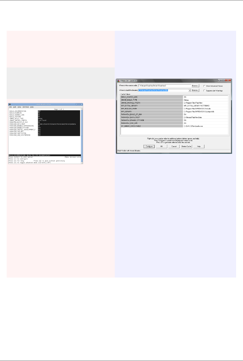
How to build/compile/install 409
Configure ParaView With CMake
• Always use a separate build directory. Do not build in the source directory.
On Unix-like systems
• Use ccmake (Curses CMake GUI) from the CMake installed
location. CCMake is a Curses based GUI for CMake. To run it
go to the build directory and specify as an argument the src
directory.
mkdir $HOME/projects/ParaView-bin
cd $HOME/projects/ParaView-bin
ccmake $HOME/projects/ParaView3
About CCMake (Curses CMake GUI)
• Iterative process.
• Select values, run configure (c key).
• Set the settings, run configure, set the settings, run configure,
etc.
• Repeat until all values are set and the generate option is
available (g key).
• Some variables (advanced variables) are not visible right away.
• To see advanced varables, toggle to advanced mode (t key).
• To set a variable, move the cursor to the variable and press enter.
• If it is a boolean (ON/OFF) it will flip the value.
• If it is string or file, it will allow editing of the string.
• For file and directories, the <tab> key can be used to
complete.
• To search for a variable press '/' key; to repeat the search, press
the 'n' key.
On Windows
• Use CMakeSetup from the CMake install location.
• Make sure to select the appropriate source and the build directory.
• Also, make sure to pick the appropriate generator (on Visual Studio 6,
pick the Visual Studio 6 generator). Some CMake versions will ask you
to select the generator the first time you press Configure instead of
having a drop-down menu in the main dialog.
About CMakeSetup (Windows CMake GUI)
• Iterative process.
• Select values, press the Configure button.
• Set the settings, run configure, set the settings, run configure, etc.
• Repeat until all values are set and the OK button becomes available.
• Some variables (advanced variables) are not visible right away.
• To see advanced varables, toggle to advanced mode ("Show Advanced
Values" toggle).
• To set the value of a variable, click on that value.
• If it is boolean (ON/OFF), a drop-down menu will appear for
changing the value.
• If it is file or directory, an ellipsis button will appear ("...") on the far
right of the entry. Clicking this button will bring up the file or
directory selection dialog.
• If it is a string, it will become an editable string.
ParaView Settings
How to build/compile/install 410
Variable Description
BUILD_SHARED_LIBS If ON, use shared libraries. This way executables are smaller, but you have to make sure the shared libraries
are on every system on the cluster. This option should be set to ON if you plan on using plugins for ParaView
(there ways to use plugins in static builds of ParaView for advanced users).
PARAVIEW_USE_MPI Turn this to ON to enable MPI. Other MPI options will not be available until you turn this on.
MPI_C_LIBRARIES Paths to the MPI libraries (such as /usr/lib/libmpi.so). Should be found by default, but you may have to set it.
Certain mpi implementations need more than one library. All the libraries can be specified by separating them
with a ';'. (see the note below)
MPI_C_INCLUDE_PATH Path to MPI includes (such as /usr/include/mpi). Again, this should be found by default.
PARAVIEW_ENABLE_PYTHON Makes Python client scripting and the Python programmable filter available.
PARAVIEW_BUILD_QT_GUI Flag to enable/disable the building of the ParaView Qt-based client. This option is useful when building
ParaView on server nodes or when we are only interested in the Python client, as it avoids building of the Qt
client thus does not require Qt. ON by default.
QT_QMAKE_EXECUTABLE Path to Qt's qmake executable (such as /usr/local/bin/qmake). CMake uses this to locate the rest of the
required Qt executables, headers and libraries.
PARAVIEW_ENABLE_FFMPEG Enable FFMPEG support (UNIX only)
PARAVIEW_USE_VISITBRIDGE Enable VisItBridge that adds support for additional file formats (requires Boost)
Note for MPI settings: If your MPI variables aren't set automatically (usually the case if the compiler wrapper
[mpicxx] is not in the path or in some standard directory), toggle advanced options and set MPI_COMPILER
variable to the full path of your mpi compiler (usually mpicxx), and configure. This should set all the required MPI
variables. If not, then you might need to enter them manually.
If you get an error such as "mpi.h: no such file or directory" then set the CMAKE_C_FLAGS= -lmpi and the
CMAKE_CXX_FLAGS= -lmpi++ . This is in addition to the MPI variables.
Finish Configuring ParaView
Using CCMake
• Once all configuration options are set, you should be able to
just run <generate> (g key).
Using CMakeSetup
• Once all configuration options are set, you should be able to just run
<generate>, by clicking the "OK" button.
Build ParaView
You can now build ParaView using the appropriate build system.
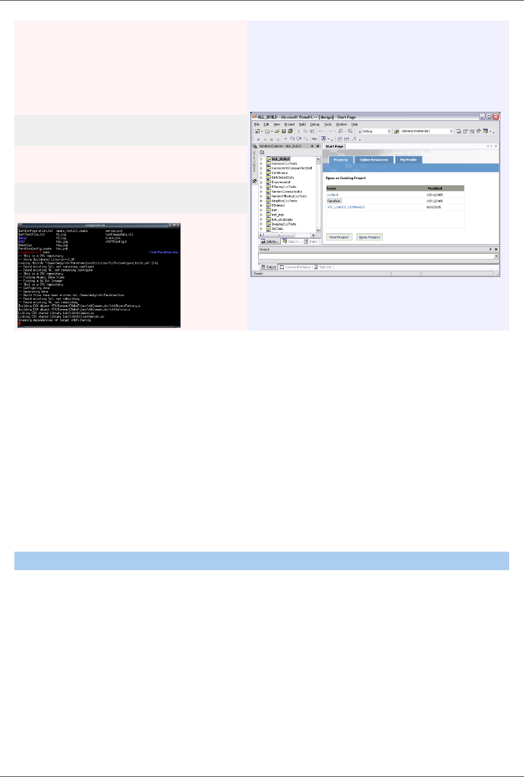
How to build/compile/install 411
Using Make
CMake will now generate Make files. These make files have all
dependencies and all rules to build ParaView on this system. You
should not however try to move the build directory to another
location on this system or to another system.
Once you have makefiles you should be able to just type:
make
• If you are on multi-processor system (let's say four processor),
you can type:
make -j 4
Using Visual Studio
CMake will now create Visual Studio project files. Before you open Visual
Studio, be sure that the Qt .dlls are in your path. You should now be able to
open the ParaView project (or workspace) file. Make sure to select the
appropriate build type (Debug, Release, ...). To build ParaView, simply build
the ALL_BUILD target.
Install ParaView
ParaView can be run directly from the build directory. That said, for production environments, it should be installed
in some system location.
For that purpose simply follow these instructions to install to an appropriate location. (these need to be updated for
Windows). Note that ParaView is designed to install what it builds. Thus only the libraries and executables that
ParaView builds are installed. For example, these instructions will not install Qt or ffmpeg libraries to the specified
location. If you are interested in creating a binary package that is complete and can be distributed to other
users/systems, you may want to refer to ParaView Super-Build.
CMake Variables
Some of the CMake variables that affect installation rules are:
Variable Value Description
CMAKE_INSTALL_PREFIX <path> Set this to the root of the location where you want ParaView to be installed. For
unix based systems, ParaView will be installed under bin/ lib/ directories under this
install prefix. This option is not available on Mac OSX.
CMAKE_BUILD_TYPE Release Unless you want to end up with debug install, set this to Release.
PARAVIEW_INSTALL_DEVELOPMENT_FILES OFF/ON To install development files, including headers, so that developers can build
plugins/custom-applications using the installed version of ParaView, set this to
ON. Currently, this option is not available on Mac OSX or Windows.
MACOSX_APP_INSTALL_PREFIX <path> Set this to the location where you want ParaView to install the app bundle on
"make install". This option is only available on Mac OSX

How to build/compile/install 412
Installing
Following the configuration, simply run 'make' to compile and build.
On Unix-like operating systems:
make install
This will install all the relevant files in directories under the
CMAKE_INSTALL_PREFIX. The executables are installed in
${CMAKE_INSTALL_PREFIX}/bin and the libraries are installed in
${CMAKE_INSTALL_PREFIX}/lib/paraview-${major}.${minor}.
On Windows:
<to be decided>
On Mac:
make install
This will create an app bundle in the directory
specified by
MACOSX_APP_INSTALL_PREFIX. This
app bundle will have the main application
executable under APP/Contents/MacOS,
libraries under APP/Contents/Libraries,
plugins under APP/Contents/Plugins, and
additional executables such as the server
executables and python executables under
APP/Conents/bin.
Notes on Mac OSX
On Mac OSX, "make install" will install an app bundle to the location specified by
MACOSX_APP_INSTALL_PREFIX. This app will contain all the ParaView libraries, plugins, python scripts, etc.
that were built by ParaView. You can move this app around on the same machine like a regular app and it will work
without any problems. Note, however, that this is not a redistributable app bundle. You cannot ship this off to your
friend and expect it to work. This app does not include any *external dependencies*, such Qt libraries, or Python
libraries, and has references to the versions that you used to build ParaView. This is not unique to Mac OSX, but to
all other plaforms as well. "make install" is used to install runtimes to be used on the same machine. To generate
redistributable packages, refer to ParaView Super-Build instructions.
Miscellaneous Comments
• Build trees of ParaView on non-Windows systems, always have RPATH information embedded in the binaries.
When a make install is performed or CPACK is used, all RPATH information is stripped from the binaries in the
install tree (expect for paths to external libraries). By default ParaView builds forwarding executables (launchers)
that are installed in the bin directory. These binaries properly set up the environment to launch the equivalent
executable in the lib/paraview-x.y directory.
• If you are compiling a MESA version of the ParaView server, start the server with the --use-offscreen-memory
flag.
Notes
Environment Variables
If you build with shared libraries, you may have to add the Qt directory to you PATH environment variables to run
ParaView. With Windows, one way to do so is to open up the environment variables dialog by clicking through
Start|Control Panel|System|Advanced|Environment Variables. From that dialog, add a new user variable called
PATH with a value of C:\Qt\4.8.2\bin. For other operating systems, add Qt/4.8.2/lib to your LD_LIBRARY_PATH
environment variable.

How to build/compile/install 413
Frequently Asked Questions
"make install" does not install ffmpeg and other libraries as it did with 3.14.1 and earlier. Is this a bug?
This is a deliberate change. It was decided that ParaView should install only what it builds. Since ParaView doesn't
build ffmpeg, it doesn't add install rules to install it. If you are interested in creating a package that includes all files
ParaView depends on so that you can distribute to other, refer to ParaView Super-Build. That is supposed to do
exactly that.
How do I generate a distributable ParaView package?
Refer to ParaView Super-Build. That is the process we use to generate the official binaries that are distributed on
paraview.org. It streamlines the process of building all the depedencies for ParaView and then packaging them into
installables or tarballs.
Do I need BUILD_SHARED_LIBS set to be ON if I want to enable Python scripting?
No. In ParaView 3.14.1 and earlier, this was indeed the case, ParaView required that BUILD_SHARED_LIBS was
ON if Python support was to be enabled. That is no longer the case. BUILD_SHARED_LIBS and
PARAVIEW_ENABLE_PYTHON can now be managed independently.
ParaView: [Welcome | Site Map [8]]
References
[1] http:/ / paraview. org/ Wiki/ index. php?title=ParaView:Build_And_Install& oldid=46445
[2] http:/ / www. cmake. org
[3] http:/ / qt. nokia. com
[4] http:/ / www-unix. mcs. anl. gov/ mpi/
[5] http:/ / www. lam-mpi. org/
[6] http:/ / www. python. org
[7] http:/ / www. cmake. org/ cmake/ resources/ software. html
[8] http:/ / www. cmake. org/ files/ v2. 8/ cmake-2. 8. 8-Linux-i386. tar. gz
[9] http:/ / www. cmake. org/ files/ v2. 8/ cmake-2. 8. 8-win32-x86. exe
[10] http:/ / www. cmake. org/ files/ v2. 8/ cmake-2. 8. 8-win32-x86. zip
[11] http:/ / www. cmake. org/ files/ v2. 8/ cmake-2. 8. 8. tar. gz
[12] http:/ / www. cmake. org/ HTML/ Download. html
[13] http:/ / qt. nokia. com/ downloads
[14] http:/ / www. ffmpeg. org/
[15] http:/ / www. mesa3d. org/
[16] http:/ / paraview. org/ paraview/ resources/ software. php
[17] http:/ / git-scm. com/
[18] http:/ / code. google. com/ p/ msysgit

Building ParaView with Mesa3D 414
Building ParaView with Mesa3D
ParaView requires OpenGL libraries for rendering. For machines with sophisticated graphics cards, the OpenGL
libraries are typically provided by the device drivers for those cards. However, on certain machines such as
supercomputers without specialized graphics hardware, one has to rely on software-based rendering alternatives such
as Mesa. Mesa is an open-source implementation of the OpenGL specification.
Mesa can be configured to work within different environments ranging from software emulation to complete
hardware acceleration when supported GPUs are present. This discussion only applies to Mesa with software
emulation on linux-based systems.
When to use Mesa
Some of the use-cases when one would build ParaView with Mesa are:
1. You are building on a machine where X Window System is not available.
2. You are building on a machine that has X, but you does not have graphics hardware or you still want to use
software emulation for various reasons.
In case of (1) you'll have to build with OSMesa support. With newer versions of Mesa (>= 7.9), ParaView can be
built with OSMesa only when the Qt GUI is disabled. Refer to #ParaView with Offscreen Mesa
In case of (2) you can configure Mesa with X support. Unlike with OSMesa, in this configuration, one can build both
the server-executables as well as the Qt client, and both will use Mesa for rendering. Refer to #ParaView with Mesa.
ParaView with Mesa
This section describes the compilation process for machines with X. With newer versions of Mesa (>= 7.9) it is NOT
possible to build with OSMesa support as well.
Configuring Mesa
Download Mesa libraries from Mesa3D website [1]. For ParaView, only MesaLib package is required.
Configure and build Mesa based as described on Mesa3D website [2].
The recommended steps are:
./configure --with-driver=xlib --prefix={MESA_INSTALL_PREFIX}
make
make install

Building ParaView with Mesa3D 415
Configuring ParaView
Configure ParaView as described on ParaView:Build And Install. The only cmake variables that need to be updated
are:
OPENGL_INCLUDE_DIR = {MESA_INSTALL_PREFIX}/include
OPENGL_gl_LIBRARY = {MESA_INSTALL_PREFIX}/lib/libGL.[so|a]
OPENGL_glu_LIBRARY = {MESA_INSTALL_PREFIX}/lib/libGLU.[so|a]
• IF AND ONLY IF* Mesa version < 7.9, one can also set the following cmake variables and build ParaView with
OSMesa support. In this case, pvserver --use-offscreen-rendering will use OSMesa.
VTK_OPENGL_HAS_OSMESA = ON
OSMESA_INCLUDE_DIR = {MESA_INSTALL_PREFIX}/include
OSMESA_LIBRARY = {MESA_INSTALL_PREFIX}/lib/libOSMesa.[so|a]
The rest on the configure and build process for ParaView remains as described on ParaView:Build And Install.
ParaView with Offscreen Mesa
If you Mesa version < 7.9, simply follow the instructions described in the previous section. However, if you have
Mesa version >=7.9, it's not possible to build ParaView with onscreen and offscreen Mesa support at the same time.
Without onscreen support, one cannot build the Qt application. So if you need the Qt application as well server
executables with offscreen support, you'll have to do two separate builds when using Mesa version >=7.9.
The following discussion only applies to Mesa >= 7.9 (although it should work with older versions too).
Configuring Mesa
Download Mesa libraries from Mesa3D website [1]. For ParaView, only MesaLib package is required.
Configure and build Mesa based as described on Mesa3D website [2].
The recommended steps are:
./configure --with-driver=xlib --prefix={MESA_INSTALL_PREFIX}
make
make install
Alternatively, one can use the following configure line. The only difference is that it does not build a libGL.[so|a]
file. This keeps us from accidentally linking with that library which can result in segfaults when running ParaView.
./configure --with-driver=osmesa --prefix={MESA_INSTALL_PREFIX}
make
make install
Configuring ParaView
Configure ParaView as described on ParaView:Build And Install. The only cmake variables that need to be updated
are:
PARAVIEW_BUILD_QT_GUI = OFF
OPENGL_INCLUDE_DIR = {MESA_INSTALL_PREFIX}/include
OPENGL_gl_LIBRARY = <empty> -- ENSURE THAT THIS IS EMPTY.
OPENGL_glu_LIBRARY = {MESA_INSTALL_PREFIX}/lib/libGLU.[so|a]

Building ParaView with Mesa3D 416
VTK_OPENGL_HAS_OSMESA = ON
OSMESA_INCLUDE_DIR = {MESA_INSTALL_PREFIX}/include
OSMESA_LIBRARY = {MESA_INSTALL_PREFIX}/lib/libOSMesa.[so|a]
VTK_USE_X = OFF
Some of these CMake variables don't show up until a few configure steps and it can be tricky to change their values
afterwords. So when running cmake for the first time, one can use the following command:
ccmake -D PARAVIEW_BUILD_QT_GUI:BOOL=OFF -D VTK_USE_X:BOOL=OFF -D VTK_OPENGL_HAS_OSMESA:BOOL=ON {PARAVIEW_SOURCE_DIR}
The rest on the configure and build process for ParaView remains as described on ParaView:Build And Install.
References
[1] http:/ / mesa3d. org/ download. html
[2] http:/ / mesa3d. org/ install. html
How to write parallel VTK readers
Writing ParaView Readers
If the format of your data files is not one supported by default in ParaView (see section Error: Reference source not
found), you will either need to convert your files to a format ParaView can read, or you must write your own data
file reader for ParaView. The reader must operate within a standard VTK pipeline. In this chapter, we will discuss
integrating the new reader class into VTK, including outlining which C++ methods should be implemented for the
reader to work properly. The necessary user interface and server manager XML will be described. Creating parallel
readers and readers that output multiple parts will also be covered. For VTK information beyond the scope of the
chapter, see The VTK User's Guide by Kitware, Inc.
Integrating with VTK
VTK is written in C++, and new readers should also be written in this language. A reader plays the role of a source
in a VTK pipeline, and must be implemented as a class deriving from vtkAlgorithm or one of its subclasses. The best
choice for the immediate superclass of a new reader depends on the reader's output type. For example, a reader
producing an instance of vtkPolyData may derive from vtkPolyDataAlgorithm to simplify its implementation. In
order for a reader to function properly within VTK's pipeline mechanism, it must be able to respond to standard
requests. This is implemented by overriding one or more of the following methods from the chosen superclass.
The interface to these methods utilizes vtkInformation objects, which are heterogeneous maps storing key/value
pairs. Many of these methods have the same three arguments. The first argument is of type vtkInformation* and
contains at least one key specifying the request itself. The second argument is of type vtkInformationVector** and
stores information about the input connections to the algorithm. This can be ignored by readers because they have no
input connections. The third argument is of type vtkInformationVector* and contains one vtkInformation object for
each output port of the algorithm. Most readers will have only one output port, but some may have multiple output
ports (see the next section). All output information and data from the reader will be stored in one of these
information objects.
ProcessRequest: This method is the entry point into a vtkAlgorithm through which the pipeline makes requests. A
reader may override this method and implement responses to all requests. The method should be placed in the public
section of the reader class. It should return 1 for success and 0 for failure. Full documentation of this method is

How to write parallel VTK readers 417
beyond the scope of this chapter. Most readers should derive from one of the output-type-specific classes and
implement the request-specific methods described below.
RequestInformation: This method is invoked by the superclass's ProcessRequest implementation when it receives
a REQUEST_INFORMATION request. In the output port, it should store information about the data in the input file.
For example, if the reader produces structured data, then the whole extent should be set here (shown below).
int vtkExampleReader::RequestInformation(
vtkInformation*, vtkInformationVector**,
vtkInformationVector* outVec)
{
vtkInformation* outInfo = outVec->GetInformationObject(0);
int extent[6];
// ... read file to find available extent ...
//store that in the pipeline
outInfo->Set
(vtkStreamingDemandDrivenPipeline::WHOLE_EXTENT(), extent, 6);
// ... store other information ...
return 1;
}
This method is necessary when configuring a reader to operate in parallel. (This will be further discussed later in this
chapter.) It should be placed in the protected section of the reader class. The method should return 1 for success and
0 for failure.
RequestData: This method is invoked by the superclass's ProcessRequest implementation when it receives a
REQUEST_DATA request. It should read data from the file and store it in the corresponding data object in the
output port. The output data object will have already been created by the pipeline before this request is made. The
amount of data to read may be specified by keys in the output port information. For example, if the reader produces
vtkImageData, this method might look like this.
int vtkExampleReader::RequestData(
vtkInformation*, vtkInformationVector**,
vtkInformationVector* outVec)
{
vtkInformation* outInfo = outVec->GetInformationObject(0);
vtkImageData* outData = vtkImageData::SafeDownCast
(outInfo->Get(vtkDataObject::DATA_OBJECT()));
int extent[6] = {0,-1,0,-1,0,-1};
outInfo->Get
(vtkStreamingDemandDrivenPipeline::UPDATE_EXTENT(), extent);
outData->SetExtent(extent);
// ... read data for this extent from the file ...

How to write parallel VTK readers 418
return 1;
}
The method should be placed in the protected section of the reader class. It should return 1 for success and 0 for
failure.
CanReadFile: The purpose of this method is to determine whether this reader can read a specified data file. Its input
parameter is a const char* specifying the name of a data file. In this method, you should not actually read the data
but determine whether it is the correct format to be read by this reader. This method should return an integer value: 1
indicates that the specified file is of the correct type; 0 indicates it is not. It is not absolutely required that this method
be implemented, but ParaView will make use of it if it exists.
SetFileName: This method allows you to specify the name of the data file to be loaded by your reader. The method
is not required to have this exact name, but a method with this functionality must be implemented. The easiest way
to implement SetFileName is with a vtkSetStringMacro in the header file for this class. (There is also an associated
vtkGetStringMacro for implementing GetFileName.) This method handles allocating an array to contain the file
name and lets the reader know that the pipeline should be updated when the name is changed.
vtkSetStringMacro(FileName);
When using this macro, you must also add a FileName instance variable of type char* in the protected section of this
class. In the constructor for your reader, assign FileName the value NULL before you use SetFileName for the first
time. In the destructor for your reader, call SetFileName(0)to free the file name storage.
Multi-Group (Multi-Block and AMR) Readers
As of VTK 5.0 and ParaView 2.4, multi-block and AMR datasets are supported. Multi-group readers follow the
same guidelines as described in the previous sections. For convenience, you can subclass multi-block readers from
vtkMultiBlockDataSetAlgorithm and AMR readers from vtkHierarchicalDataSetAlgorithm. If you do not sub-class
from one of these classes, make sure to implement the CreateDefaultExecutive(), FillOutputPortInformation(), and
FillInputPortInformation() methods appropriately. (You can use vtkMultiBlockDataSetAlgorithm as a starting
point.) Two good examples of multi-group dataset readers are vtkMultiBlockPLOT3DReader and
vtkXMLHierarchicalDataReader.
Parallel Readers
Unless otherwise specified, a VTK reader used in ParaView will cause the entire data set to be read on the first
process. ParaView will then redistribute the data to the other processes. It is more desirable to have ParaView do the
reading in parallel as well, so that the data set is already appropriately divided across the processors. Changes should
be made in two methods for ParaView readers to operate in parallel: RequestInformation and RequestData. Exactly
which changes should be made depends on whether structured or unstructured data set types are to be read.
Structured
In RequestInformation for readers of structured data (vtkStructuredGrid, vtkRectilinearGrid, or vtkImageData), the
WHOLE_EXTENT key should be set on the output information object, so that downstream filters can take into
account the overall dimensions of the data. The WHOLE_EXTENT is specified using six parameters: the minimum
and maximum index along each of the three coordinate axes (imin, imax, jmin, jmax, kmin, kmax or a single int array of
length 6) for the entire data set. Example C++ code demonstrating this is shown below.

How to write parallel VTK readers 419
int vtkDEMReader::RequestInformation (
vtkInformation * vtkNotUsed(request),
vtkInformationVector ** vtkNotUsed( inputVector ),
vtkInformationVector *outputVector)
{
vtkInformation* outInfo =
outputVector->GetInformationObject(0);
int extent[6];
//Read entire extent from file.
...
outInfo->Set
(vtkStreamingDemandDrivenPipeline::WHOLE_EXTENT(), extent,6);
return 1;
}
Before doing any processing in the RequestData method, first get the UPDATE_EXTENT from the output
information object. This key contains the sub-extent of the WHOLE_EXTENT for which the current process is
responsible. The current process is responsible for filling in the data values for the update extent that is returned. An
example of doing this is shown below.
int vtkDEMReader::RequestData(
vtkInformation* vtkNotUsed( request ),
vtkInformationVector** vtkNotUsed( inputVector ),
vtkInformationVector* outputVector)
{
// get the data object and find out what part we need to
// read now
vtkInformation *outInfo = outputVector->GetInformationObject(0);
int subext[6];
outInfo->Get
(vtkStreamingDemandDrivenPipeline::UPDATE_EXTENT(),
subext);
//read that part of the data in from the file
//and put it in the output data
...
return 1;
}

How to write parallel VTK readers 420
Unstructured
In the unstructured case (vtkPolyData or vtkUnstructuredGrid), the MAXIMUM_NUMBER_OF_PIECES key
should be set on the output information object in RequestInformation. This specifies the maximum number of pieces
that can be generated from the file. If this reader can only read the entire data set, then the maximum number of
pieces should be set to 1. If the input file can be read into as many pieces as needed (i.e., one per processor), the
maximum number of pieces should be set to -1, as shown below.
outInfo->Set(vtkStreamingDemandDrivenPipeline::MAXIMUM_NUMBER_OF_PIECES(),
-1);
In the RequestData method, the reader should first get the UPDATE_NUMBER_OF_PIECES and
UPDATE_PIECE_NUMBER from the output information object. The value returned from getting the
UPDATE_NUMBER_OF_PIECES specifies the number of pieces into which the output data set will be broken.
Getting UPDATE_PIECE_NUMBER returns the piece number (0 to UPDATE_NUMBER_OF_PIECES-1) for
which the current process is responsible. The reader should use this information to determine which part of the
dataset the current process should read. Example code that demonstrates this is shown below.
int vtkUnstructuredGridReader::RequestData(
vtkInformation *,
vtkInformationVector **,
vtkInformationVector *outputVector)
{
vtkInformation *outInfo = outputVector->GetInformationObject(0);
int piece, numPieces;
piece = outInfo->Get
(vtkStreamingDemandDrivenPipeline::UPDATE_PIECE_NUMBER());
numPieces = outInfo->Get
(vtkStreamingDemandDrivenPipeline::UPDATE_NUMBER_OF_PIECES());
//skip to proper offset in the file and read piece
...
return 1;
}
It is possible that your data file can only be broken into a specified number of pieces, and that this number is
different than the number of processors being used (i.e., the result of getting UPDATE_NUMBER_OF_PIECES). If
the number of processors is larger than the possible number of pieces, then each processor beyond the number of
available pieces should produce an empty output by calling Initialize() on the output. If the number of processors is
smaller than the number of pieces, you should internally redistribute the extra data across the processors. For
example, if your dataset can produce ten pieces, and you are using five processors for reading, then process 0 could
read pieces zero and five; process 1 could read pieces one and six; etc.

How to write parallel VTK readers 421
Required XML
To use your new reader within ParaView, you must write XML code for the server manager and for the client. The
server-side XML for ParaView's readers is located in the file Servers/ServerManager/Resources/readers.xml. When
ParaView is compiled, the server manager XML code for a reader is used to create a proxy object for it. The
ParaView client accesses the VTK class for the reader on the server through the proxy. Below is an excerpt from the
server manager XML code for vtkXMLPolyDataReader. A few parts of this XML code segment are particularly
worth noting, and more extensive information about server manager XML code can be found in section Error:
Reference source not found.
First, notice the StringVectorProperty element named "FileName". It has a command attribute called "SetFileName".
ParaView uses this property to tell the reader what file it should examine. This is done very early in the lifetime of a
reader. Typically, ParaView code will give the reader a filename and then call the reader's CanReadFile method. If
CanReadFile succeeds, ParaView will first call RequestInformation to get general information about the data within
the file, and then call RequestData to read the actual data and produce a vtkDataObject.
The second notable portion of the XML code below is two properties that let the user choose particular arrays to load
from the data file. When ParaView sees them, it creates a section on the Properties tab for the reader that lets the user
select from the available cell-centered data arrays. In the following discussion, one can simply replace 'cell' with
'point' in order to let the user choose from the available, point-centered arrays.
The StringVectorProperty named "CellArrayStatus" lets the ParaView client call the SetCellArrayStatus method on
the server. The SetCellArrayStatus method is how the reader is told what it should do with each of the arrays the data
file contains. It takes two parameters; the first is the name of the array, and the second is an integer indicating
whether to read the array (1) or not (0).
The StringVectorProperty named 'CellArrayInfo' is an information property; that is, one through which the ParaView
client gathers information from the server. The ParaView client uses it to gather the names of the cell-centered arrays
from the reader. (See the nested Property sub-element in CellArrayStatus's ArraySelectionDomain element.) In order
for this collection to work, two methods are implemented in the reader. GetNumberOfCellArrays returns the number
(an int) of cell-centered arrays in the data file. This method does not accept any parameters. GetCellArrayName
takes a single parameter the array's index (starting from 0). This method returns the name of the array (a const char*)
with this index or NULL if the array has no name or if the index is larger than the number of arrays.
<SourceProxy name="XMLPolyDataReader"
class="vtkXMLPolyDataReader"
label="XML Polydata reader">
<StringVectorProperty name="FileName"
command="SetFileName"
animateable="0"
number_of_elements="1">
<FileListDomain name="files"/>
</StringVectorProperty>
<StringVectorProperty name="CellArrayInfo"
information_only="1">
<ArraySelectionInformationHelper attribute_name="Cell"/>
</StringVectorProperty>
<StringVectorProperty name="CellArrayStatus"
command="SetCellArrayStatus"
number_of_elements="0"

How to write parallel VTK readers 422
repeat_command="1" number_of_elements_per_command="2"
element_types="2 0"
information_property="CellArrayInfo"
label="Cell Arrays">
<ArraySelectionDomain name="array_list">
<RequiredProperties>
<Property name="CellArrayInfo"
function="ArrayList"/>
</RequiredProperties>
</ArraySelectionDomain>
</StringVectorProperty>
</SourceProxy>
The client-side XML is extremely simple. The purpose of the client-side XML is to enable readers from the
server-side XML and to associate file extensions with them. In the case where multiple readers can read files that
have the same file extensions, the CanReadFile method is called on each one in order to choose the correct one for
each data file. The client-side XML file for readers is located in
Qt/Components/Resources/XML/ParaViewReaders.xml. The portion of that file related to XMLPolyDataReader
follows.
<Reader name="XMLPolyDataReader"
extensions="vtp"
file_description="VTK PolyData Files">
</Reader>
An alternative to modifying the ParaView source code directly is to use ParaView's plugin architecture. With a
plugin, the same C++ source code and XML content must be written, but it is kept outside of the ParaView source
code proper and is compiled separately from ParaView. Plugins are discussed in chapter Error: Reference source not
found.

Article Sources and Contributors 423
Article Sources and Contributors
About Paraview ƒSource: http://paraview.org/Wiki/index.php?oldid=52569 ƒContributors: DaveDemarle, Jourdain, Katie.osterdahl, Robert Maynard, Utkarsh, Yumin, 3 anonymous edits
Data Ingestion ƒSource: http://paraview.org/Wiki/index.php?oldid=52651 ƒContributors: Katie.osterdahl, Partyd, Rmaynard, Robert Maynard, Sebastien.jourdain, Utkarsh, 1 anonymous edits
VTK Data Model ƒSource: http://paraview.org/Wiki/index.php?oldid=47855 ƒContributors: Berk, Chris.hyatt, Katie.osterdahl, 4 anonymous edits
Information Panel ƒSource: http://paraview.org/Wiki/index.php?oldid=48063 ƒContributors: Berk, Katie.osterdahl, Zack, 1 anonymous edits
Statistics Inspector ƒSource: http://paraview.org/Wiki/index.php?oldid=52570 ƒContributors: Katie.osterdahl, Utkarsh, 1 anonymous edits
Memory Inspector ƒSource: http://paraview.org/Wiki/index.php?oldid=49595 ƒContributors: Burlen, Jourdain, Utkarsh
Multi-block Inspector ƒSource: http://paraview.org/Wiki/index.php?oldid=51810 ƒContributors: Kyle.lutz
Views, Representations and Color Mapping ƒSource: http://paraview.org/Wiki/index.php?oldid=52721 ƒContributors: DaveDemarle, Jourdain, Katie.osterdahl, Utkarsh, Yumin
Rationale ƒSource: http://paraview.org/Wiki/index.php?oldid=40503 ƒContributors: DaveDemarle, Katie.osterdahl, 7 anonymous edits
Filter Parameters ƒSource: http://paraview.org/Wiki/index.php?oldid=40504 ƒContributors: DaveDemarle, Katie.osterdahl
The Pipeline ƒSource: http://paraview.org/Wiki/index.php?oldid=40506 ƒContributors: DaveDemarle, Katie.osterdahl
Filter Categories ƒSource: http://paraview.org/Wiki/index.php?oldid=40524 ƒContributors: DaveDemarle, Katie.osterdahl
Best Practices ƒSource: http://paraview.org/Wiki/index.php?oldid=40528 ƒContributors: DaveDemarle, Katie.osterdahl
Custom Filters aka Macro Filters ƒSource: http://paraview.org/Wiki/index.php?oldid=43101 ƒContributors: Chris.hyatt, DaveDemarle, Katie.osterdahl
Drilling Down ƒSource: http://paraview.org/Wiki/index.php?oldid=40530 ƒContributors: Katie.osterdahl, 1 anonymous edits
Python Programmable Filter ƒSource: http://paraview.org/Wiki/index.php?oldid=40533 ƒContributors: Berk, Katie.osterdahl
Calculator ƒSource: http://paraview.org/Wiki/index.php?oldid=40549 ƒContributors: Berk, DaveDemarle, Katie.osterdahl
Python Calculator ƒSource: http://paraview.org/Wiki/index.php?oldid=52571 ƒContributors: Andy.bauer, Berk, Foret37, Katie.osterdahl, Utkarsh, 8 anonymous edits
Spreadsheet View ƒSource: http://paraview.org/Wiki/index.php?oldid=52657 ƒContributors: Katie.osterdahl, Utkarsh
Selection ƒSource: http://paraview.org/Wiki/index.php?oldid=40666 ƒContributors: DaveDemarle, Katie.osterdahl, Utkarsh
Querying for Data ƒSource: http://paraview.org/Wiki/index.php?oldid=49312 ƒContributors: Jourdain, Katie.osterdahl, Utkarsh
Histogram ƒSource: http://paraview.org/Wiki/index.php?oldid=52659 ƒContributors: Andy.bauer, Katie.osterdahl, Utkarsh
Plotting and Probing Data ƒSource: http://paraview.org/Wiki/index.php?oldid=40747 ƒContributors: Andy.bauer, Katie.osterdahl
Saving Data ƒSource: http://paraview.org/Wiki/index.php?oldid=40748 ƒContributors: Katie.osterdahl, Rmaynard, Robert Maynard
Exporting Scenes ƒSource: http://paraview.org/Wiki/index.php?oldid=48778 ƒContributors: Jourdain, Katie.osterdahl, Utkarsh, 1 anonymous edits
Manipulating data in the 3D view ƒSource: http://paraview.org/Wiki/index.php?oldid=31924 ƒContributors: DaveDemarle, Katie.osterdahl
Annotation ƒSource: http://paraview.org/Wiki/index.php?oldid=31926 ƒContributors: DaveDemarle, Jourdain, Katie.osterdahl, Katie.sharkey, Utkarsh
Animation View ƒSource: http://paraview.org/Wiki/index.php?oldid=39791 ƒContributors: Katie.sharkey, Rmaynard, Utkarsh
Comparative Views ƒSource: http://paraview.org/Wiki/index.php?oldid=39803 ƒContributors: Berk, Katie.sharkey, 3 anonymous edits
Parallel ParaView ƒSource: http://paraview.org/Wiki/index.php?oldid=43653 ƒContributors: DaveDemarle, Katie.osterdahl, Katie.sharkey, Sebastien.jourdain, 1 anonymous edits
Starting the Server(s) ƒSource: http://paraview.org/Wiki/index.php?oldid=43660 ƒContributors: DaveDemarle, Katie.osterdahl, Katie.sharkey
Connecting to the Server ƒSource: http://paraview.org/Wiki/index.php?oldid=43661 ƒContributors: DaveDemarle, Katie.osterdahl, Katie.sharkey
Distributing/Obtaining Server Connection Configurations ƒSource: http://paraview.org/Wiki/index.php?oldid=49155 ƒContributors: DaveDemarle, Utkarsh
About Parallel Rendering ƒSource: http://paraview.org/Wiki/index.php?oldid=39856 ƒContributors: Katie.sharkey, 1 anonymous edits
Parallel Rendering ƒSource: http://paraview.org/Wiki/index.php?oldid=51702 ƒContributors: DaveDemarle, Katie.osterdahl, Katie.sharkey, Partyd, 3 anonymous edits
Tile Display Walls ƒSource: http://paraview.org/Wiki/index.php?oldid=43662 ƒContributors: DaveDemarle, Katie.osterdahl, Katie.sharkey
CAVE Displays ƒSource: http://paraview.org/Wiki/index.php?oldid=49045 ƒContributors: Aashish.chaudhary, Alexisylchan, Jzarl, Katie.sharkey, Nikhil, 2 anonymous edits
Interpreted ParaView ƒSource: http://paraview.org/Wiki/index.php?oldid=39891 ƒContributors: Katie.sharkey, 1 anonymous edits
Python Scripting ƒSource: http://paraview.org/Wiki/index.php?oldid=51228 ƒContributors: Andy.bauer, Berk, DaveDemarle, Daviddoria, Katie.osterdahl, Katie.sharkey, Newacct, Themiwi,
Tmjung, Utkarsh, Zack, 2 anonymous edits
Tools for Python Scripting ƒSource: http://paraview.org/Wiki/index.php?oldid=40018 ƒContributors: Katie.sharkey, Patmarion, Sebastien.jourdain
Batch Processing ƒSource: http://paraview.org/Wiki/index.php?oldid=40023 ƒContributors: DaveDemarle, Katie.sharkey
CoProcessing ƒSource: http://paraview.org/Wiki/index.php?oldid=49185 ƒContributors: Andy.bauer, Katie.osterdahl, Katie.sharkey, Matthew.bowman, Patmarion, Utkarsh
C++ CoProcessing example ƒSource: http://paraview.org/Wiki/index.php?oldid=48740 ƒContributors: Andy.bauer
Python CoProcessing Example ƒSource: http://paraview.org/Wiki/index.php?oldid=45620 ƒContributors: Andy.bauer
What are Plugins? ƒSource: http://paraview.org/Wiki/index.php?oldid=37753 ƒContributors: DaveDemarle, Rmaynard, Robert Maynard, 1 anonymous edits
Included Plugins ƒSource: http://paraview.org/Wiki/index.php?oldid=49151 ƒContributors: DaveDemarle, Jourdain, Kyle.lutz, Robert Maynard, Zack, 3 anonymous edits
Loading Plugins ƒSource: http://paraview.org/Wiki/index.php?oldid=46063 ƒContributors: DaveDemarle, Katie.osterdahl, Utkarsh
Command Line Arguments ƒSource: http://paraview.org/Wiki/index.php?oldid=48451 ƒContributors: DaveDemarle, Kyle.lutz, Robert Maynard, Sebastien.jourdain, Utkarsh

Article Sources and Contributors 424
Application Settings ƒSource: http://paraview.org/Wiki/index.php?oldid=42310 ƒContributors: DaveDemarle, Katie.sharkey, Kyle.lutz, Utkarsh
List of Readers ƒSource: http://paraview.org/Wiki/index.php?oldid=52716 ƒContributors: DaveDemarle, Jourdain, Katie.sharkey, Sebastien.jourdain, Utkarsh
List of Sources ƒSource: http://paraview.org/Wiki/index.php?oldid=52717 ƒContributors: Jourdain, Katie.sharkey, Sebastien.jourdain, Utkarsh
List of Filters ƒSource: http://paraview.org/Wiki/index.php?oldid=52718 ƒContributors: DaveDemarle, Jourdain, Sebastien.jourdain, Utkarsh
List of Writers ƒSource: http://paraview.org/Wiki/index.php?oldid=52719 ƒContributors: DaveDemarle, Jourdain, Katie.sharkey, Sebastien.jourdain, Utkarsh
How to build/compile/install ƒSource: http://paraview.org/Wiki/index.php?oldid=49157 ƒContributors: Amy, Andy, Andy.bauer, Berk, Brad.king, DaveDemarle, David.Thompson, Erdwolf,
Jrcho, Katie.sharkey, Nikhil, Partyd, Pratikm, RicardoReis, Sly, Thunderrabbit, Tiffiw, Utkarsh, Wascott
Building ParaView with Mesa3D ƒSource: http://paraview.org/Wiki/index.php?oldid=49184 ƒContributors: Utkarsh
How to write parallel VTK readers ƒSource: http://paraview.org/Wiki/index.php?oldid=48062 ƒContributors: DaveDemarle, Katie.sharkey, Zack, 1 anonymous edits

Image Sources, Licenses and Contributors 425
Image Sources, Licenses and Contributors
File:ParaView_UsersGuide_ParaViewLogo.png ƒSource: http://paraview.org/Wiki/index.php?title=File:ParaView_UsersGuide_ParaViewLogo.png ƒLicense: unknown ƒContributors:
Sebastien.jourdain
Image:ParaView_UsersGuide_ParaViewGUIOverview.png ƒSource: http://paraview.org/Wiki/index.php?title=File:ParaView_UsersGuide_ParaViewGUIOverview.png ƒLicense: unknown
ƒContributors: Nikhil, Sebastien.jourdain, Utkarsh
Image:FindText.png ƒSource: http://paraview.org/Wiki/index.php?title=File:FindText.png ƒLicense: unknown ƒContributors: Jourdain
Image:SearchText.png ƒSource: http://paraview.org/Wiki/index.php?title=File:SearchText.png ƒLicense: unknown ƒContributors: Yumin
Image:ParaViewCopyPaste3.png ƒSource: http://paraview.org/Wiki/index.php?title=File:ParaViewCopyPaste3.png ƒLicense: unknown ƒContributors: Jourdain
Image:ParaViewCopyPaste1.png ƒSource: http://paraview.org/Wiki/index.php?title=File:ParaViewCopyPaste1.png ƒLicense: unknown ƒContributors: Jourdain
Image:ParaViewCopyPaste4.png ƒSource: http://paraview.org/Wiki/index.php?title=File:ParaViewCopyPaste4.png ƒLicense: unknown ƒContributors: Jourdain
Image:ParaViewCopyPaste2.png ƒSource: http://paraview.org/Wiki/index.php?title=File:ParaViewCopyPaste2.png ƒLicense: unknown ƒContributors: Jourdain
Image:ParaView_UsersGuide_PipelineExample.png ƒSource: http://paraview.org/Wiki/index.php?title=File:ParaView_UsersGuide_PipelineExample.png ƒLicense: unknown ƒContributors:
DaveDemarle, Nikhil
Image:ParaView_UG_FileSeries.png ƒSource: http://paraview.org/Wiki/index.php?title=File:ParaView_UG_FileSeries.png ƒLicense: unknown ƒContributors: Robert Maynard
Image:ParaView_UG_MultipleFileOpen.png ƒSource: http://paraview.org/Wiki/index.php?title=File:ParaView_UG_MultipleFileOpen.png ƒLicense: unknown ƒContributors: Robert Maynard
Image:ParaView_UG_FileLoadObjectInspector.png ƒSource: http://paraview.org/Wiki/index.php?title=File:ParaView_UG_FileLoadObjectInspector.png ƒLicense: unknown ƒContributors:
Robert Maynard, Utkarsh
Image:ParaView_UG_Cells.png ƒSource: http://paraview.org/Wiki/index.php?title=File:ParaView_UG_Cells.png ƒLicense: unknown ƒContributors: Berk
Image:ParaView_UG_Cells_with_values.png ƒSource: http://paraview.org/Wiki/index.php?title=File:ParaView_UG_Cells_with_values.png ƒLicense: unknown ƒContributors: Berk
Image:ParaView_UG_Cells_with_cvalues.png ƒSource: http://paraview.org/Wiki/index.php?title=File:ParaView_UG_Cells_with_cvalues.png ƒLicense: unknown ƒContributors: Berk
Image:ParaView_UG_Image.png ƒSource: http://paraview.org/Wiki/index.php?title=File:ParaView_UG_Image.png ƒLicense: unknown ƒContributors: Berk
Image:ParaView_UG_Rectilinear.png ƒSource: http://paraview.org/Wiki/index.php?title=File:ParaView_UG_Rectilinear.png ƒLicense: unknown ƒContributors: Berk
Image:ParaView_UG_Curvilinear.png ƒSource: http://paraview.org/Wiki/index.php?title=File:ParaView_UG_Curvilinear.png ƒLicense: unknown ƒContributors: Berk
Image:ParaView_UG_AMR.png ƒSource: http://paraview.org/Wiki/index.php?title=File:ParaView_UG_AMR.png ƒLicense: unknown ƒContributors: Berk
Image:ParaView_UG_Unstructured.png ƒSource: http://paraview.org/Wiki/index.php?title=File:ParaView_UG_Unstructured.png ƒLicense: unknown ƒContributors: Berk
Image:ParaView_UG_Polydata.png ƒSource: http://paraview.org/Wiki/index.php?title=File:ParaView_UG_Polydata.png ƒLicense: unknown ƒContributors: Berk
Image:ParaView_UG_Table.png ƒSource: http://paraview.org/Wiki/index.php?title=File:ParaView_UG_Table.png ƒLicense: unknown ƒContributors: Berk
Image:ParaView_UG_Multiblock.png ƒSource: http://paraview.org/Wiki/index.php?title=File:ParaView_UG_Multiblock.png ƒLicense: unknown ƒContributors: Berk
Image:ParaView_UG_Multipiece.png ƒSource: http://paraview.org/Wiki/index.php?title=File:ParaView_UG_Multipiece.png ƒLicense: unknown ƒContributors: Berk
Image:ParaView_UG_Info_Properties.png ƒSource: http://paraview.org/Wiki/index.php?title=File:ParaView_UG_Info_Properties.png ƒLicense: unknown ƒContributors: Berk
Image:ParaView_UG_Info_Statistics.png ƒSource: http://paraview.org/Wiki/index.php?title=File:ParaView_UG_Info_Statistics.png ƒLicense: unknown ƒContributors: Berk
Image:ParaView_UG_Info_Arrays.png ƒSource: http://paraview.org/Wiki/index.php?title=File:ParaView_UG_Info_Arrays.png ƒLicense: unknown ƒContributors: Berk
Image:ParaView_UG_InfoBounds.png ƒSource: http://paraview.org/Wiki/index.php?title=File:ParaView_UG_InfoBounds.png ƒLicense: unknown ƒContributors: Berk
Image:ParaView_UG_Info_Temporal.png ƒSource: http://paraview.org/Wiki/index.php?title=File:ParaView_UG_Info_Temporal.png ƒLicense: unknown ƒContributors: Berk
Image:ParaView_UG_Info_Extents.png ƒSource: http://paraview.org/Wiki/index.php?title=File:ParaView_UG_Info_Extents.png ƒLicense: unknown ƒContributors: Berk
Image:ParaVIew_UG_Info_Amr.png ƒSource: http://paraview.org/Wiki/index.php?title=File:ParaVIew_UG_Info_Amr.png ƒLicense: unknown ƒContributors: Berk
Image:ParaView_UG_Info_Multiblock.png ƒSource: http://paraview.org/Wiki/index.php?title=File:ParaView_UG_Info_Multiblock.png ƒLicense: unknown ƒContributors: Berk
Image:ParaView_UG_Statistics_inspector.png ƒSource: http://paraview.org/Wiki/index.php?title=File:ParaView_UG_Statistics_inspector.png ƒLicense: unknown ƒContributors: 1 anonymous
edits
Image:Meminsp-pv-gui.png ƒSource: http://paraview.org/Wiki/index.php?title=File:Meminsp-pv-gui.png ƒLicense: unknown ƒContributors: Burlen
File:PV_MemoryInspectorProperties.png ƒSource: http://paraview.org/Wiki/index.php?title=File:PV_MemoryInspectorProperties.png ƒLicense: unknown ƒContributors: Jourdain
File:Meminsp-remote-command.png ƒSource: http://paraview.org/Wiki/index.php?title=File:Meminsp-remote-command.png ƒLicense: unknown ƒContributors: Burlen
Image:MultiBlockInspector1.png ƒSource: http://paraview.org/Wiki/index.php?title=File:MultiBlockInspector1.png ƒLicense: unknown ƒContributors: Kyle.lutz
Image:MultiBlockInspectorSelection.png ƒSource: http://paraview.org/Wiki/index.php?title=File:MultiBlockInspectorSelection.png ƒLicense: unknown ƒContributors: Kyle.lutz
Image:MultiBlockInspectorContextMenu.png ƒSource: http://paraview.org/Wiki/index.php?title=File:MultiBlockInspectorContextMenu.png ƒLicense: unknown ƒContributors: Kyle.lutz
Image:ParaViewDisplayingDataFigure1.png ƒSource: http://paraview.org/Wiki/index.php?title=File:ParaViewDisplayingDataFigure1.png ƒLicense: unknown ƒContributors: Nikhil, Utkarsh
Image:ParaViewDisplayingDataFigure2.png ƒSource: http://paraview.org/Wiki/index.php?title=File:ParaViewDisplayingDataFigure2.png ƒLicense: unknown ƒContributors: Nikhil, Utkarsh
Image:paraview.multitabs.png ƒSource: http://paraview.org/Wiki/index.php?title=File:Paraview.multitabs.png ƒLicense: unknown ƒContributors: Nikhil, Utkarsh
Image:ViewSettingsGeneral.png ƒSource: http://paraview.org/Wiki/index.php?title=File:ViewSettingsGeneral.png ƒLicense: unknown ƒContributors: Utkarsh
Image:ViewSettingsLights.png ƒSource: http://paraview.org/Wiki/index.php?title=File:ViewSettingsLights.png ƒLicense: unknown ƒContributors: Utkarsh
Image:ViewSettingsAnnotation.png ƒSource: http://paraview.org/Wiki/index.php?title=File:ViewSettingsAnnotation.png ƒLicense: unknown ƒContributors: Utkarsh
Image:3DViewDisplayView.png ƒSource: http://paraview.org/Wiki/index.php?title=File:3DViewDisplayView.png ƒLicense: unknown ƒContributors: Utkarsh
Image:3DViewDisplayColor.png ƒSource: http://paraview.org/Wiki/index.php?title=File:3DViewDisplayColor.png ƒLicense: unknown ƒContributors: Utkarsh
Image:3DViewDisplaySlice.png ƒSource: http://paraview.org/Wiki/index.php?title=File:3DViewDisplaySlice.png ƒLicense: unknown ƒContributors: Utkarsh
Image:3DViewDisplayCubeAxes.png ƒSource: http://paraview.org/Wiki/index.php?title=File:3DViewDisplayCubeAxes.png ƒLicense: unknown ƒContributors: Utkarsh
Image:ParaViewDisplayingDataCubeAxes.png ƒSource: http://paraview.org/Wiki/index.php?title=File:ParaViewDisplayingDataCubeAxes.png ƒLicense: unknown ƒContributors: Utkarsh
Image:3DViewDisplayStyle.png ƒSource: http://paraview.org/Wiki/index.php?title=File:3DViewDisplayStyle.png ƒLicense: unknown ƒContributors: Utkarsh
Image:3DViewDisplayBackface.png ƒSource: http://paraview.org/Wiki/index.php?title=File:3DViewDisplayBackface.png ƒLicense: unknown ƒContributors: Utkarsh
Image:3DViewDisplayTransform.png ƒSource: http://paraview.org/Wiki/index.php?title=File:3DViewDisplayTransform.png ƒLicense: unknown ƒContributors: Utkarsh
File:ParaViewUsersGuideSpreadsheetViewHeader.png ƒSource: http://paraview.org/Wiki/index.php?title=File:ParaViewUsersGuideSpreadsheetViewHeader.png ƒLicense: unknown
ƒContributors: Utkarsh
File:ParaViewUsersGuideSpreadsheetView2.png ƒSource: http://paraview.org/Wiki/index.php?title=File:ParaViewUsersGuideSpreadsheetView2.png ƒLicense: unknown ƒContributors:
Utkarsh
Image:ParaViewUsersGuideLineChartView.png ƒSource: http://paraview.org/Wiki/index.php?title=File:ParaViewUsersGuideLineChartView.png ƒLicense: unknown ƒContributors: Utkarsh
Image:ParaViewUsersGuideChartSettingsGeneral.png ƒSource: http://paraview.org/Wiki/index.php?title=File:ParaViewUsersGuideChartSettingsGeneral.png ƒLicense: unknown
ƒContributors: Utkarsh
Image:ParaViewUsersGuideChartSettingsAxis.png ƒSource: http://paraview.org/Wiki/index.php?title=File:ParaViewUsersGuideChartSettingsAxis.png ƒLicense: unknown ƒContributors:
Utkarsh
Image:ParaViewUsersGuideChartSettingsAxisLayout.png ƒSource: http://paraview.org/Wiki/index.php?title=File:ParaViewUsersGuideChartSettingsAxisLayout.png ƒLicense: unknown
ƒContributors: Utkarsh
Image:ParaViewUsersGuideChartDisplayProperties.png ƒSource: http://paraview.org/Wiki/index.php?title=File:ParaViewUsersGuideChartDisplayProperties.png ƒLicense: unknown
ƒContributors: Utkarsh

Image Sources, Licenses and Contributors 426
Image:ParaViewUsersGuideBarChartView.png ƒSource: http://paraview.org/Wiki/index.php?title=File:ParaViewUsersGuideBarChartView.png ƒLicense: unknown ƒContributors: Utkarsh
Image:plotmatrix-view.png ƒSource: http://paraview.org/Wiki/index.php?title=File:Plotmatrix-view.png ƒLicense: unknown ƒContributors: Nikhil, Yumin
Image:plotmatrix-view-selection.png ƒSource: http://paraview.org/Wiki/index.php?title=File:Plotmatrix-view-selection.png ƒLicense: unknown ƒContributors: Yumin
Image:plotmatrix-view-general.png ƒSource: http://paraview.org/Wiki/index.php?title=File:Plotmatrix-view-general.png ƒLicense: unknown ƒContributors: Yumin
Image:plotmatrix-view-active.png ƒSource: http://paraview.org/Wiki/index.php?title=File:Plotmatrix-view-active.png ƒLicense: unknown ƒContributors: Yumin
Image:plotmatrix-view-scatter.png ƒSource: http://paraview.org/Wiki/index.php?title=File:Plotmatrix-view-scatter.png ƒLicense: unknown ƒContributors: Yumin
Image:plotmatrix-view-histogram.png ƒSource: http://paraview.org/Wiki/index.php?title=File:Plotmatrix-view-histogram.png ƒLicense: unknown ƒContributors: Yumin
Image:plotmatrix-view-display.png ƒSource: http://paraview.org/Wiki/index.php?title=File:Plotmatrix-view-display.png ƒLicense: unknown ƒContributors: Yumin
Image:plotmatrix-view-linkedselection.png ƒSource: http://paraview.org/Wiki/index.php?title=File:Plotmatrix-view-linkedselection.png ƒLicense: unknown ƒContributors: Yumin
File:SliceView-general.png ƒSource: http://paraview.org/Wiki/index.php?title=File:SliceView-general.png ƒLicense: unknown ƒContributors: Jourdain
File:QuadView-general.png ƒSource: http://paraview.org/Wiki/index.php?title=File:QuadView-general.png ƒLicense: unknown ƒContributors: Jourdain
File:QuadView-options.png ƒSource: http://paraview.org/Wiki/index.php?title=File:QuadView-options.png ƒLicense: unknown ƒContributors: Jourdain
File:ColorEditor-simple.png ƒSource: http://paraview.org/Wiki/index.php?title=File:ColorEditor-simple.png ƒLicense: unknown ƒContributors: Jourdain
File:ColorEditor-general.png ƒSource: http://paraview.org/Wiki/index.php?title=File:ColorEditor-general.png ƒLicense: unknown ƒContributors: Yumin
File:ColorEditor-vol.png ƒSource: http://paraview.org/Wiki/index.php?title=File:ColorEditor-vol.png ƒLicense: unknown ƒContributors: Yumin
File:ColorEditor-tf.png ƒSource: http://paraview.org/Wiki/index.php?title=File:ColorEditor-tf.png ƒLicense: unknown ƒContributors: Yumin
File:ParaView_UsersGuide_PresetColorScalesDialog.png ƒSource: http://paraview.org/Wiki/index.php?title=File:ParaView_UsersGuide_PresetColorScalesDialog.png ƒLicense: unknown
ƒContributors: Sebastien.jourdain
File:ParaView_UsersGuide_ColorScaleEditorColorLegend.png ƒSource: http://paraview.org/Wiki/index.php?title=File:ParaView_UsersGuide_ColorScaleEditorColorLegend.png ƒLicense:
unknown ƒContributors: Sebastien.jourdain
File:ParaView_UsersGuide_PropertiesTabExample.png ƒSource: http://paraview.org/Wiki/index.php?title=File:ParaView_UsersGuide_PropertiesTabExample.png ƒLicense: unknown
ƒContributors: DaveDemarle, Sebastien.jourdain, Utkarsh
File:ParaView_UsersGuide_LinearPipeline.png ƒSource: http://paraview.org/Wiki/index.php?title=File:ParaView_UsersGuide_LinearPipeline.png ƒLicense: unknown ƒContributors:
Sebastien.jourdain
File:ParaView_UsersGuide_branchingPipeline2.png ƒSource: http://paraview.org/Wiki/index.php?title=File:ParaView_UsersGuide_branchingPipeline2.png ƒLicense: unknown ƒContributors:
Sebastien.jourdain
File:ParaView_UsersGuide_PipelineBrowserContextMenu.png ƒSource: http://paraview.org/Wiki/index.php?title=File:ParaView_UsersGuide_PipelineBrowserContextMenu.png ƒLicense:
unknown ƒContributors: Sebastien.jourdain
File:ParaView_UsersGuide_ChangeInputDialog.png ƒSource: http://paraview.org/Wiki/index.php?title=File:ParaView_UsersGuide_ChangeInputDialog.png ƒLicense: unknown ƒContributors:
Sebastien.jourdain
File:ParaView_UsersGuide_mergingPipeline.png ƒSource: http://paraview.org/Wiki/index.php?title=File:ParaView_UsersGuide_mergingPipeline.png ƒLicense: unknown ƒContributors:
DaveDemarle
File:ParaView_UsersGuide_CommonFiltersToolbar.png ƒSource: http://paraview.org/Wiki/index.php?title=File:ParaView_UsersGuide_CommonFiltersToolbar.png ƒLicense: unknown
ƒContributors: Sebastien.jourdain
File:ParaView_UsersGuide_FilterMenu.png ƒSource: http://paraview.org/Wiki/index.php?title=File:ParaView_UsersGuide_FilterMenu.png ƒLicense: unknown ƒContributors:
Sebastien.jourdain
File:ParaView_UsersGuide_QuickLaunchDialog.png ƒSource: http://paraview.org/Wiki/index.php?title=File:ParaView_UsersGuide_QuickLaunchDialog.png ƒLicense: unknown
ƒContributors: 1 anonymous edits
Image:ParaView_UsersGuide_CustomFilterConcept.png ƒSource: http://paraview.org/Wiki/index.php?title=File:ParaView_UsersGuide_CustomFilterConcept.png ƒLicense: unknown
ƒContributors: 1 anonymous edits
File:ParaView_UsersGuide_CustomFilterInputs.png ƒSource: http://paraview.org/Wiki/index.php?title=File:ParaView_UsersGuide_CustomFilterInputs.png ƒLicense: unknown ƒContributors:
1 anonymous edits
File:ParaView_UsersGuide_CustomFilterOutputs.png ƒSource: http://paraview.org/Wiki/index.php?title=File:ParaView_UsersGuide_CustomFilterOutputs.png ƒLicense: unknown
ƒContributors: 1 anonymous edits
File:ParaView_UsersGuide_CustomFilterParameters.png ƒSource: http://paraview.org/Wiki/index.php?title=File:ParaView_UsersGuide_CustomFilterParameters.png ƒLicense: unknown
ƒContributors: 1 anonymous edits
Image:ParaView_UG_ProgrammableFilter.png ƒSource: http://paraview.org/Wiki/index.php?title=File:ParaView_UG_ProgrammableFilter.png ƒLicense: unknown ƒContributors: Berk
Image:ParaView_UG_Calculator.png ƒSource: http://paraview.org/Wiki/index.php?title=File:ParaView_UG_Calculator.png ƒLicense: unknown ƒContributors: Berk, Utkarsh
Image:ParaView_UG_Python_calculator.png ƒSource: http://paraview.org/Wiki/index.php?title=File:ParaView_UG_Python_calculator.png ƒLicense: unknown ƒContributors: Utkarsh, 1
anonymous edits
File:ParaViewUsersGuideSpreadsheetView.png ƒSource: http://paraview.org/Wiki/index.php?title=File:ParaViewUsersGuideSpreadsheetView.png ƒLicense: unknown ƒContributors: Utkarsh
Image:ParaViewUsersGuideSpreadsheetView2.png ƒSource: http://paraview.org/Wiki/index.php?title=File:ParaViewUsersGuideSpreadsheetView2.png ƒLicense: unknown ƒContributors:
Utkarsh
Image:Selection1.png ƒSource: http://paraview.org/Wiki/index.php?title=File:Selection1.png ƒLicense: unknown ƒContributors: Utkarsh
Image:Selection2.png ƒSource: http://paraview.org/Wiki/index.php?title=File:Selection2.png ƒLicense: unknown ƒContributors: Utkarsh
Image:Selection3.png ƒSource: http://paraview.org/Wiki/index.php?title=File:Selection3.png ƒLicense: unknown ƒContributors: Utkarsh
Image:Selection4.png ƒSource: http://paraview.org/Wiki/index.php?title=File:Selection4.png ƒLicense: unknown ƒContributors: Utkarsh
File:ParaView_UsersGuide_LabeledSelection.png ƒSource: http://paraview.org/Wiki/index.php?title=File:ParaView_UsersGuide_LabeledSelection.png ƒLicense: unknown ƒContributors:
DaveDemarle, Sebastien.jourdain
Image:Selection5.png ƒSource: http://paraview.org/Wiki/index.php?title=File:Selection5.png ƒLicense: unknown ƒContributors: Utkarsh
Image:Selection6.png ƒSource: http://paraview.org/Wiki/index.php?title=File:Selection6.png ƒLicense: unknown ƒContributors: Utkarsh
File:ParaViewUsersGuideFindDataDialog.png ƒSource: http://paraview.org/Wiki/index.php?title=File:ParaViewUsersGuideFindDataDialog.png ƒLicense: unknown ƒContributors: Jourdain,
Utkarsh
Image:ParaViewUsersGuideFindDataHeader.png ƒSource: http://paraview.org/Wiki/index.php?title=File:ParaViewUsersGuideFindDataHeader.png ƒLicense: unknown ƒContributors: Utkarsh
Image:ParaViewUsersGuideFindDataSelectionControls.png ƒSource: http://paraview.org/Wiki/index.php?title=File:ParaViewUsersGuideFindDataSelectionControls.png ƒLicense: unknown
ƒContributors: Utkarsh
Image:ParaViewUsersGuideFindDataFooter.png ƒSource: http://paraview.org/Wiki/index.php?title=File:ParaViewUsersGuideFindDataFooter.png ƒLicense: unknown ƒContributors: Utkarsh
Image:ParaView_UsersGuide_SaveParaViewWindowDialog.png ƒSource: http://paraview.org/Wiki/index.php?title=File:ParaView_UsersGuide_SaveParaViewWindowDialog.png ƒLicense:
unknown ƒContributors: Robert Maynard, Sebastien.jourdain
Image:ParaView_UG_ScreenshotDialog.png ƒSource: http://paraview.org/Wiki/index.php?title=File:ParaView_UG_ScreenshotDialog.png ƒLicense: unknown ƒContributors: Robert Maynard
Image:ParaView_UG_SaveAnimation.png ƒSource: http://paraview.org/Wiki/index.php?title=File:ParaView_UG_SaveAnimation.png ƒLicense: unknown ƒContributors: Robert Maynard
Image:Export.png ƒSource: http://paraview.org/Wiki/index.php?title=File:Export.png ƒLicense: unknown ƒContributors: Utkarsh
File:Paraview_UsersGuide_PVLineWidget.png ƒSource: http://paraview.org/Wiki/index.php?title=File:Paraview_UsersGuide_PVLineWidget.png ƒLicense: unknown ƒContributors:
DaveDemarle
File:ParaView_UsersGuide_LineWidgetUI.png ƒSource: http://paraview.org/Wiki/index.php?title=File:ParaView_UsersGuide_LineWidgetUI.png ƒLicense: unknown ƒContributors:
DaveDemarle, Utkarsh

Image Sources, Licenses and Contributors 427
File:ParaView_UsersGuide_planeWidget.png ƒSource: http://paraview.org/Wiki/index.php?title=File:ParaView_UsersGuide_planeWidget.png ƒLicense: unknown ƒContributors:
Sebastien.jourdain
File:ParaView_UsersGuide_planeWidgetUI.png ƒSource: http://paraview.org/Wiki/index.php?title=File:ParaView_UsersGuide_planeWidgetUI.png ƒLicense: unknown ƒContributors:
Sebastien.jourdain, Utkarsh
File:ParaView_UsersGuide_boxWidget.png ƒSource: http://paraview.org/Wiki/index.php?title=File:ParaView_UsersGuide_boxWidget.png ƒLicense: unknown ƒContributors:
Sebastien.jourdain
File:ParaView_UsersGuide_boxWidgetUI.png ƒSource: http://paraview.org/Wiki/index.php?title=File:ParaView_UsersGuide_boxWidgetUI.png ƒLicense: unknown ƒContributors:
Sebastien.jourdain, Utkarsh
File:ParaView_UsersGuide_sphereWidget.png ƒSource: http://paraview.org/Wiki/index.php?title=File:ParaView_UsersGuide_sphereWidget.png ƒLicense: unknown ƒContributors:
Sebastien.jourdain
File:ParaView_UsersGuide_sphereWidgetUI.png ƒSource: http://paraview.org/Wiki/index.php?title=File:ParaView_UsersGuide_sphereWidgetUI.png ƒLicense: unknown ƒContributors:
Sebastien.jourdain, Utkarsh
File:ParaView_UsersGuide_pointWidget.png ƒSource: http://paraview.org/Wiki/index.php?title=File:ParaView_UsersGuide_pointWidget.png ƒLicense: unknown ƒContributors:
Sebastien.jourdain
File:ParaView_UsersGuide_pointWidgetUI.png ƒSource: http://paraview.org/Wiki/index.php?title=File:ParaView_UsersGuide_pointWidgetUI.png ƒLicense: unknown ƒContributors:
Sebastien.jourdain, Utkarsh
File:ParaView_UsersGuide_splineWidget.png ƒSource: http://paraview.org/Wiki/index.php?title=File:ParaView_UsersGuide_splineWidget.png ƒLicense: unknown ƒContributors: DaveDemarle
File:ParaView_UsersGuide_splineWidgetUI.png ƒSource: http://paraview.org/Wiki/index.php?title=File:ParaView_UsersGuide_splineWidgetUI.png ƒLicense: unknown ƒContributors:
DaveDemarle, Utkarsh
File:ParaView_UsersGuide_ColorLegendButton.png ƒSource: http://paraview.org/Wiki/index.php?title=File:ParaView_UsersGuide_ColorLegendButton.png ƒLicense: unknown ƒContributors:
Sebastien.jourdain
File:ParaView_UsersGuide_scalarBar.png ƒSource: http://paraview.org/Wiki/index.php?title=File:ParaView_UsersGuide_scalarBar.png ƒLicense: unknown ƒContributors: Sebastien.jourdain
File:ParaView_UsersGuide_colorLegendDialog.png ƒSource: http://paraview.org/Wiki/index.php?title=File:ParaView_UsersGuide_colorLegendDialog.png ƒLicense: unknown ƒContributors:
DaveDemarle
File:ParaView_UsersGuide_OrientationAxes.png ƒSource: http://paraview.org/Wiki/index.php?title=File:ParaView_UsersGuide_OrientationAxes.png ƒLicense: unknown ƒContributors:
Sebastien.jourdain
File:ParaView_UsersGuide_OrientationAxesUI.png ƒSource: http://paraview.org/Wiki/index.php?title=File:ParaView_UsersGuide_OrientationAxesUI.png ƒLicense: unknown ƒContributors:
Sebastien.jourdain
File:ParaView_UsersGuide_TextDisplayTab.png ƒSource: http://paraview.org/Wiki/index.php?title=File:ParaView_UsersGuide_TextDisplayTab.png ƒLicense: unknown ƒContributors:
DaveDemarle, Sebastien.jourdain, Utkarsh
File:ParaView_UsersGuide_AnnotateTime.png ƒSource: http://paraview.org/Wiki/index.php?title=File:ParaView_UsersGuide_AnnotateTime.png ƒLicense: unknown ƒContributors:
Sebastien.jourdain
File:ParaView_UsersGuide_cubeAxes_and_Ruler.png ƒSource: http://paraview.org/Wiki/index.php?title=File:ParaView_UsersGuide_cubeAxes_and_Ruler.png ƒLicense: unknown
ƒContributors: DaveDemarle, Jourdain
File:ParaView_UsersGuide_cubeAxes_UI.png ƒSource: http://paraview.org/Wiki/index.php?title=File:ParaView_UsersGuide_cubeAxes_UI.png ƒLicense: unknown ƒContributors:
DaveDemarle, Jourdain
File:ParaView_UsersGuide_python_annotation_filter_time.png ƒSource: http://paraview.org/Wiki/index.php?title=File:ParaView_UsersGuide_python_annotation_filter_time.png ƒLicense:
unknown ƒContributors: Jourdain
File:ParaView_UsersGuide_python_annotation_filter_momentum.png ƒSource:
http://paraview.org/Wiki/index.php?title=File:ParaView_UsersGuide_python_annotation_filter_momentum.png ƒLicense: unknown ƒContributors: Jourdain
File:ParaView_UsersGuide_python_annotation_filter_table.png ƒSource: http://paraview.org/Wiki/index.php?title=File:ParaView_UsersGuide_python_annotation_filter_table.png ƒLicense:
unknown ƒContributors: Jourdain
File:ParaView_UsersGuide_global_annotation_filter.png ƒSource: http://paraview.org/Wiki/index.php?title=File:ParaView_UsersGuide_global_annotation_filter.png ƒLicense: unknown
ƒContributors: Jourdain
File:ParaViewUsersGuideAnimationView.png ƒSource: http://paraview.org/Wiki/index.php?title=File:ParaViewUsersGuideAnimationView.png ƒLicense: unknown ƒContributors: Utkarsh
File:ParaViewUsersGuideAnimationKeyframes.png ƒSource: http://paraview.org/Wiki/index.php?title=File:ParaViewUsersGuideAnimationKeyframes.png ƒLicense: unknown ƒContributors:
Utkarsh
File:ParaViewUsersGuideAnimationViewHeader.png ƒSource: http://paraview.org/Wiki/index.php?title=File:ParaViewUsersGuideAnimationViewHeader.png ƒLicense: unknown
ƒContributors: Utkarsh
File:ParaViewUsersGuideAnimationKeyframesTime.png ƒSource: http://paraview.org/Wiki/index.php?title=File:ParaViewUsersGuideAnimationKeyframesTime.png ƒLicense: unknown
ƒContributors: Utkarsh
File:ParaViewUsersGuideAnimationSettings.png ƒSource: http://paraview.org/Wiki/index.php?title=File:ParaViewUsersGuideAnimationSettings.png ƒLicense: unknown ƒContributors:
Utkarsh
Image:ParaViewUsersGuideVCR.png ƒSource: http://paraview.org/Wiki/index.php?title=File:ParaViewUsersGuideVCR.png ƒLicense: unknown ƒContributors: Utkarsh
File:ParaViewUsersGuideAddCameraTrack.png ƒSource: http://paraview.org/Wiki/index.php?title=File:ParaViewUsersGuideAddCameraTrack.png ƒLicense: unknown ƒContributors: Utkarsh
File:ParaViewUsersGuideCameraLocations.png ƒSource: http://paraview.org/Wiki/index.php?title=File:ParaViewUsersGuideCameraLocations.png ƒLicense: unknown ƒContributors: Utkarsh
File:ParaViewUsersGuideCameraOrbit.png ƒSource: http://paraview.org/Wiki/index.php?title=File:ParaViewUsersGuideCameraOrbit.png ƒLicense: unknown ƒContributors: Utkarsh
File:ParaViewUsersGuideCameraPath.png ƒSource: http://paraview.org/Wiki/index.php?title=File:ParaViewUsersGuideCameraPath.png ƒLicense: unknown ƒContributors: Utkarsh
File:ParaViewComparativeView.jpg ƒSource: http://paraview.org/Wiki/index.php?title=File:ParaViewComparativeView.jpg ƒLicense: unknown ƒContributors: Utkarsh
File:ParaView_UG_CV_Close.png ƒSource: http://paraview.org/Wiki/index.php?title=File:ParaView_UG_CV_Close.png ƒLicense: unknown ƒContributors: Berk
File:ComparativeVisPanelMarkup.png ƒSource: http://paraview.org/Wiki/index.php?title=File:ComparativeVisPanelMarkup.png ƒLicense: unknown ƒContributors: Utkarsh
File:ParaView_UG_CV_Parameter_range.png ƒSource: http://paraview.org/Wiki/index.php?title=File:ParaView_UG_CV_Parameter_range.png ƒLicense: unknown ƒContributors: Berk
File:ParaView_UG_CV_View.png ƒSource: http://paraview.org/Wiki/index.php?title=File:ParaView_UG_CV_View.png ƒLicense: unknown ƒContributors: Berk
Image:ParaView_UG_CV_Layout.png ƒSource: http://paraview.org/Wiki/index.php?title=File:ParaView_UG_CV_Layout.png ƒLicense: unknown ƒContributors: Berk
File:ParaView_UG_CV_Parameter_selection.png ƒSource: http://paraview.org/Wiki/index.php?title=File:ParaView_UG_CV_Parameter_selection.png ƒLicense: unknown ƒContributors: Berk
File:ParaView_UG_CV_Parameter_values.png ƒSource: http://paraview.org/Wiki/index.php?title=File:ParaView_UG_CV_Parameter_values.png ƒLicense: unknown ƒContributors: Berk
File:ParaView_UsersGuide_parallel_architecture.png ƒSource: http://paraview.org/Wiki/index.php?title=File:ParaView_UsersGuide_parallel_architecture.png ƒLicense: unknown
ƒContributors: DaveDemarle
file:ParaView_UsersGuide_common_configurations.png ƒSource: http://paraview.org/Wiki/index.php?title=File:ParaView_UsersGuide_common_configurations.png ƒLicense: unknown
ƒContributors: DaveDemarle
File:ParaView_UsersGuide_RenderServerConnections.png ƒSource: http://paraview.org/Wiki/index.php?title=File:ParaView_UsersGuide_RenderServerConnections.png ƒLicense: unknown
ƒContributors: DaveDemarle
File:ParaView_UsersGuide_RenderServerConnectionsStartNormal.png ƒSource:
http://paraview.org/Wiki/index.php?title=File:ParaView_UsersGuide_RenderServerConnectionsStartNormal.png ƒLicense: unknown ƒContributors: DaveDemarle
File:ParaView_UsersGuide_RenderServerConnectionsStartReverse.png ƒSource:
http://paraview.org/Wiki/index.php?title=File:ParaView_UsersGuide_RenderServerConnectionsStartReverse.png ƒLicense: unknown ƒContributors: DaveDemarle
File:ParaView_UsersGuide_RenderDataServerConnectionsStartNormal.png ƒSource:
http://paraview.org/Wiki/index.php?title=File:ParaView_UsersGuide_RenderDataServerConnectionsStartNormal.png ƒLicense: unknown ƒContributors: DaveDemarle

Image Sources, Licenses and Contributors 428
File:ParaView_UsersGuide_RenderDataServerConnectionsStartReverse.png ƒSource:
http://paraview.org/Wiki/index.php?title=File:ParaView_UsersGuide_RenderDataServerConnectionsStartReverse.png ƒLicense: unknown ƒContributors: DaveDemarle
File:ParaView_UsersGuide_ConfigureServerDialog.png ƒSource: http://paraview.org/Wiki/index.php?title=File:ParaView_UsersGuide_ConfigureServerDialog.png ƒLicense: unknown
ƒContributors: Sebastien.jourdain, Utkarsh
File:ParaView_UsersGuide_ConfigureNewServerDialog.png ƒSource: http://paraview.org/Wiki/index.php?title=File:ParaView_UsersGuide_ConfigureNewServerDialog.png ƒLicense:
unknown ƒContributors: Sebastien.jourdain, Utkarsh
File:ParaView_UsersGuide_ConfigureServerManualDialog.png ƒSource: http://paraview.org/Wiki/index.php?title=File:ParaView_UsersGuide_ConfigureServerManualDialog.png ƒLicense:
unknown ƒContributors: Sebastien.jourdain, Utkarsh
File:ParaView_UsersGuide_ConfigureServerCommandDialog.png ƒSource: http://paraview.org/Wiki/index.php?title=File:ParaView_UsersGuide_ConfigureServerCommandDialog.png
ƒLicense: unknown ƒContributors: Sebastien.jourdain, Utkarsh
Image:Server connect dialog.png ƒSource: http://paraview.org/Wiki/index.php?title=File:Server_connect_dialog.png ƒLicense: unknown ƒContributors: Utkarsh
Image:fetch_server_configurations.png ƒSource: http://paraview.org/Wiki/index.php?title=File:Fetch_server_configurations.png ƒLicense: unknown ƒContributors: Utkarsh
Image:edit_server_configuration_sources.png ƒSource: http://paraview.org/Wiki/index.php?title=File:Edit_server_configuration_sources.png ƒLicense: unknown ƒContributors: Utkarsh
File:ParaView_UsersGuide_settings_server.png ƒSource: http://paraview.org/Wiki/index.php?title=File:ParaView_UsersGuide_settings_server.png ƒLicense: unknown ƒContributors:
DaveDemarle
File:ParaView_UsersGuide_TreeComposite.png ƒSource: http://paraview.org/Wiki/index.php?title=File:ParaView_UsersGuide_TreeComposite.png ƒLicense: unknown ƒContributors:
DaveDemarle
File:ParaView_UsersGuide_BinarySwap.png ƒSource: http://paraview.org/Wiki/index.php?title=File:ParaView_UsersGuide_BinarySwap.png ƒLicense: unknown ƒContributors: DaveDemarle
File:ParaView_UsersGuide_TileComposite.png ƒSource: http://paraview.org/Wiki/index.php?title=File:ParaView_UsersGuide_TileComposite.png ƒLicense: unknown ƒContributors:
DaveDemarle
File:VRArch.png ƒSource: http://paraview.org/Wiki/index.php?title=File:VRArch.png ƒLicense: unknown ƒContributors: Nikhil
File:ConnectionConfiguration (1).png ƒSource: http://paraview.org/Wiki/index.php?title=File:ConnectionConfiguration_(1).png ƒLicense: unknown ƒContributors: Nikhil
File:ParaviewVRPluginWorkflow.png ƒSource: http://paraview.org/Wiki/index.php?title=File:ParaviewVRPluginWorkflow.png ƒLicense: unknown ƒContributors: Nikhil
File:Servermanager_snapshot.png ƒSource: http://paraview.org/Wiki/index.php?title=File:Servermanager_snapshot.png ƒLicense: unknown ƒContributors: Berk
Image:SMView.png ƒSource: http://paraview.org/Wiki/index.php?title=File:SMView.png ƒLicense: unknown ƒContributors: Berk
Image:Image.jpg ƒSource: http://paraview.org/Wiki/index.php?title=File:Image.jpg ƒLicense: unknown ƒContributors: Berk
File:FullWorkFlow.png ƒSource: http://paraview.org/Wiki/index.php?title=File:FullWorkFlow.png ƒLicense: unknown ƒContributors: Andy.bauer
File:CoProcessingWorkFlow.png ƒSource: http://paraview.org/Wiki/index.php?title=File:CoProcessingWorkFlow.png ƒLicense: unknown ƒContributors: Andy.bauer
File:phastaPipeline.jpg ƒSource: http://paraview.org/Wiki/index.php?title=File:PhastaPipeline.jpg ƒLicense: unknown ƒContributors: Andy.bauer
File:phastaPipelineWithWriters.jpg ƒSource: http://paraview.org/Wiki/index.php?title=File:PhastaPipelineWithWriters.jpg ƒLicense: unknown ƒContributors: Andy.bauer
Image:cpExport1.jpg ƒSource: http://paraview.org/Wiki/index.php?title=File:CpExport1.jpg ƒLicense: unknown ƒContributors: Andy.bauer
Image:cpExport2.jpg ƒSource: http://paraview.org/Wiki/index.php?title=File:CpExport2.jpg ƒLicense: unknown ƒContributors: Andy.bauer
Image:noRendering.png ƒSource: http://paraview.org/Wiki/index.php?title=File:NoRendering.png ƒLicense: unknown ƒContributors: Andy.bauer
Image:pqResetCamera32.png ƒSource: http://paraview.org/Wiki/index.php?title=File:PqResetCamera32.png ƒLicense: unknown ƒContributors: Andy.bauer
Image:outputRendering2.png ƒSource: http://paraview.org/Wiki/index.php?title=File:OutputRendering2.png ƒLicense: unknown ƒContributors: Andy.bauer
File:CoProcessorFlow.png ƒSource: http://paraview.org/Wiki/index.php?title=File:CoProcessorFlow.png ƒLicense: unknown ƒContributors: Andy.bauer
Image:LocalPlugin_Manager.png ƒSource: http://paraview.org/Wiki/index.php?title=File:LocalPlugin_Manager.png ƒLicense: unknown ƒContributors: Utkarsh
Image:RemotePlugin_Manager.png ƒSource: http://paraview.org/Wiki/index.php?title=File:RemotePlugin_Manager.png ƒLicense: unknown ƒContributors: Utkarsh
Image:ParaView_UsersGuide_settings_general.png ƒSource: http://paraview.org/Wiki/index.php?title=File:ParaView_UsersGuide_settings_general.png ƒLicense: unknown ƒContributors:
DaveDemarle
Image:ParaView_UsersGuide_settings_colors.png ƒSource: http://paraview.org/Wiki/index.php?title=File:ParaView_UsersGuide_settings_colors.png ƒLicense: unknown ƒContributors:
DaveDemarle
Image:ParaViewUsersGuideColorCategoryMenu.png ƒSource: http://paraview.org/Wiki/index.php?title=File:ParaViewUsersGuideColorCategoryMenu.png ƒLicense: unknown ƒContributors:
Utkarsh
Image:ParaView_UsersGuide_settings_animation.png ƒSource: http://paraview.org/Wiki/index.php?title=File:ParaView_UsersGuide_settings_animation.png ƒLicense: unknown ƒContributors:
DaveDemarle
Image:ParaView_UsersGuide_settings_charts.png ƒSource: http://paraview.org/Wiki/index.php?title=File:ParaView_UsersGuide_settings_charts.png ƒLicense: unknown ƒContributors:
DaveDemarle
Image:ParaView_UsersGuide_settings_renderview_general.png ƒSource: http://paraview.org/Wiki/index.php?title=File:ParaView_UsersGuide_settings_renderview_general.png ƒLicense:
unknown ƒContributors: DaveDemarle
Image:ParaView_UsersGuide_settings_camera.png ƒSource: http://paraview.org/Wiki/index.php?title=File:ParaView_UsersGuide_settings_camera.png ƒLicense: unknown ƒContributors:
DaveDemarle
Image:ParaView_UsersGuide_settings_server.png ƒSource: http://paraview.org/Wiki/index.php?title=File:ParaView_UsersGuide_settings_server.png ƒLicense: unknown ƒContributors:
DaveDemarle
Image:Brpv ccmake.png ƒSource: http://paraview.org/Wiki/index.php?title=File:Brpv_ccmake.png ƒLicense: unknown ƒContributors: Andy, Utkarsh
Image:Brpv cmakesetup.png ƒSource: http://paraview.org/Wiki/index.php?title=File:Brpv_cmakesetup.png ƒLicense: unknown ƒContributors: Andy
Image:Brpv make.png ƒSource: http://paraview.org/Wiki/index.php?title=File:Brpv_make.png ƒLicense: unknown ƒContributors: Andy
Image:Brpv visualstudio71.png ƒSource: http://paraview.org/Wiki/index.php?title=File:Brpv_visualstudio71.png ƒLicense: unknown ƒContributors: Andy

