Statistical Inference Course Project Part 2: Basic Inferential Data Analysis Instructions Part2
User Manual:
Open the PDF directly: View PDF ![]() .
.
Page Count: 6

Statistical Inference Course Project - Part 2: Basic
Inferential Data Analysis Instructions
Omer Shechter
October 13, 2018
Overview
Analyze the ToothGrowth data in the R datasets package ToothGrowth {dataset } Provide : The Effect of
Vitamin C on Tooth Growth in Guinea Pigs
Description
The response is the length of odontoblasts (cells responsible for tooth growth) in 60 guinea pigs. Each animal
received one of three dose levels of vitamin C (0.5, 1, and 2 mg/day) by one of two delivery methods, orange
juice or ascorbic acid (a form of vitamin C and coded as VC).
A data frame with 60 observations on 3 variables.
[,1] len numeric Tooth length [,2] supp factor Supplement type (VC or OJ). [,3] dose numeric Dose in
milligrams/day
Data Analyzes
This part includes the data loading, and initial data analyzes.
Load required libraries.
library(ggplot2)
library(datasets)
library(UsingR)
## Loading required package: MASS
## Loading required package: HistData
## Loading required package: Hmisc
## Loading required package: lattice
## Loading required package: survival
## Loading required package: Formula
##
## Attaching package: 'Hmisc'
## The following objects are masked from 'package:base':
##
## format.pval, units
##
## Attaching package: 'UsingR'
## The following object is masked from 'package:survival':
##
## cancer
1

library(kableExtra)
A preliminary review of the data.
dim(ToothGrowth)
## [1] 60 3
head(ToothGrowth)
## len supp dose
## 1 4.2 VC 0.5
## 2 11.5 VC 0.5
## 3 7.3 VC 0.5
## 4 5.8 VC 0.5
## 5 6.4 VC 0.5
## 6 10.0 VC 0.5
Check how much samples we have for each test.
table(ToothGrowth$supp)
##
## OJ VC
## 30 30
table(ToothGrowth$dose)
##
## 0.5 1 2
## 20 20 20
The methods of providing the Vitamins and the amount is equally split along the 60 guinea pigs Half of the
guinea pigs got the Vitamin via orange juice and half via ascorbic acid.
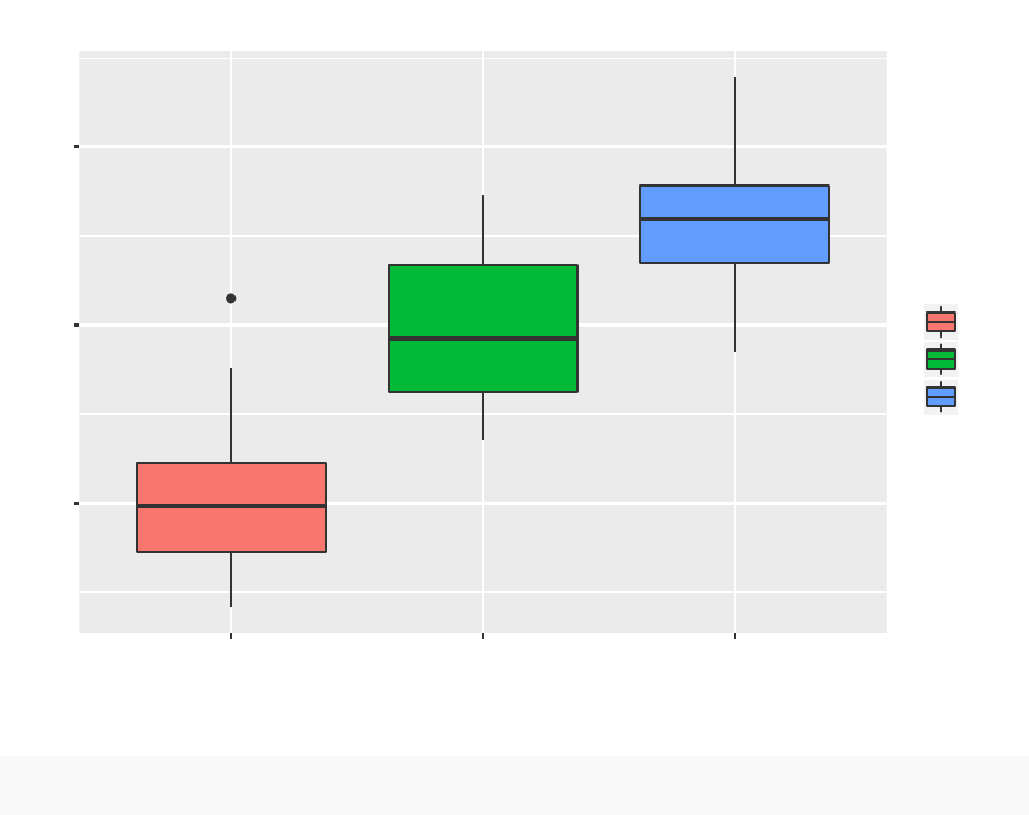
Plot some basic graph to get some view of the data
Plot the ratio len ~dose
ToothGrowth$dose<-as.factor(ToothGrowth$dose)
theme_update(plot.title = element_text(hjust = 0.5))
ggplot(ToothGrowth, aes(x=dose, y=len, group=(dose))) +
geom_boxplot(aes(fill=dose)) +ggtitle(" Len of Odontoblasts ~ Dose")
2
10
20
30
0.5 1 2
dose
len
dose
0.5
1
2
Len of Odontoblasts ~ Dose
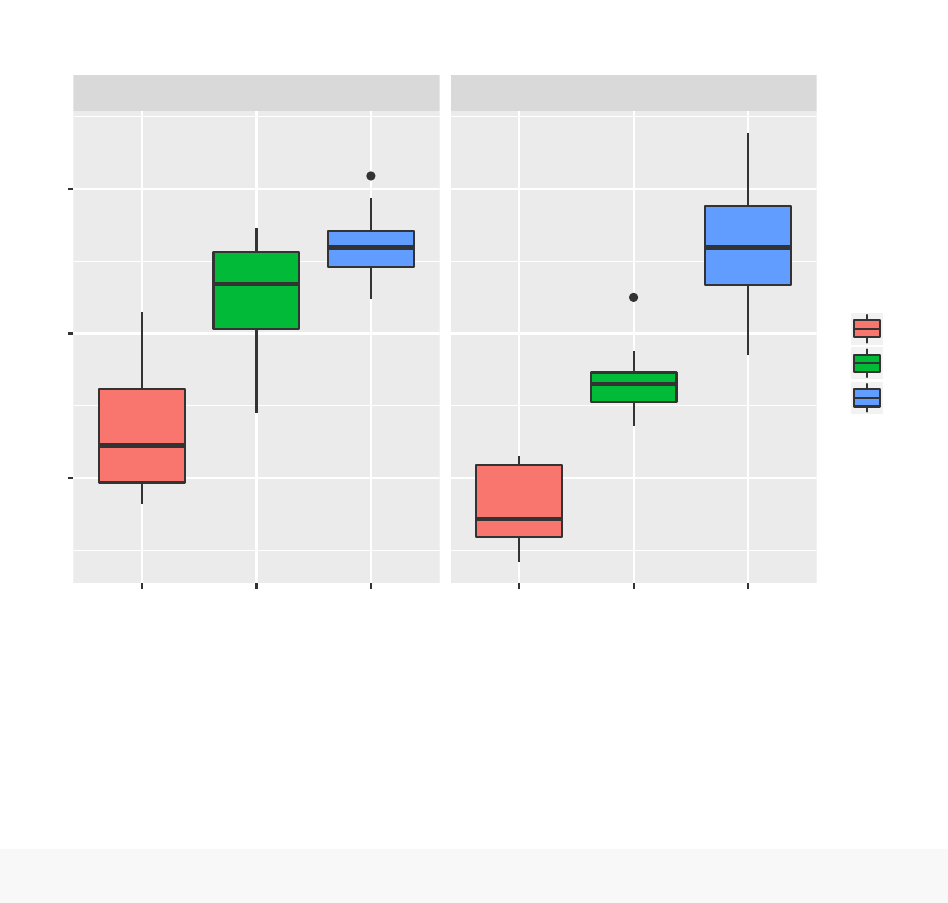
plot the ratio len ~ dose , and split according to the delivery method.
ggplot(ToothGrowth, aes(x=dose, y=len, group=(dose))) +geom_boxplot(aes(fill=dose)) +
ggtitle(" Len of Odontoblasts ~ Dose \n Partitioned by delivery methods ")+facet_grid(. ~supp)
3
OJ
VC
0.5 1 2 0.5 1 2
10
20
30
dose
len
dose
0.5
1
2
Len of Odontoblasts ~ Dose
Partitioned by delivery methods
Hypothesis and Confidence Interval
This section contains several Hypothesis checking and illustration of a confidence interval.
Hypothesis I Null hypothesis , The Supplement type (VC or OJ) doesn’t impact the Tooth length
H0 -> Mean of Length for VC = Mean of Length for OJ H1 -> Mean of Length for VC != Mean of Length
for OJ
t.test(ToothGrowth$len[ToothGrowth$supp=="OJ"],ToothGrowth$len[ToothGrowth$supp=="VC"],
mu=0,var.equal = FALSE,alternative=c("two.sided"))
##
## Welch Two Sample t-test
##
## data: ToothGrowth$len[ToothGrowth$supp == "OJ"] and ToothGrowth$len[ToothGrowth$supp == "VC"]
## t = 1.9153, df = 55.309, p-value = 0.06063
## alternative hypothesis: true difference in means is not equal to 0
## 95 percent confidence interval:
## -0.1710156 7.5710156
## sample estimates:
## mean of x mean of y
## 20.66333 16.96333
As it can be seen the p-value = 0.06063 > .005 and , we can see that 0 is in the confidence interval -0.1710156
7.5710156. So the Null Hypothesis can’t be rejected, and we can assume that there is no difference between
the two Supplement types when we measure their impact of the length of the tooth.
4

Hypothesis II Check the impact of the amount of Dose on Tooth’s length. The Null Hypothesis is that
increasing the Dose doesn’t impact the length of the tooth.
Compare amount .5 and 1
res<-t.test(ToothGrowth$len[ToothGrowth$dose==.5],ToothGrowth$len[ToothGrowth$dose==1],mu=0,var.equal = FALSE,alternative=c("two.sided"))
P_Values<-res$p.value
Conf_Intervals_Low<-res$conf.int[1]
Conf_Intervals_High<-res$conf.int[2]
res
##
## Welch Two Sample t-test
##
## data: ToothGrowth$len[ToothGrowth$dose == 0.5] and ToothGrowth$len[ToothGrowth$dose == 1]
## t = -6.4766, df = 37.986, p-value = 1.268e-07
## alternative hypothesis: true difference in means is not equal to 0
## 95 percent confidence interval:
## -11.983781 -6.276219
## sample estimates:
## mean of x mean of y
## 10.605 19.735
Compare amount 1 and 2
res<-t.test(ToothGrowth$len[ToothGrowth$dose==1],ToothGrowth$len[ToothGrowth$dose==2],
mu=0,var.equal = FALSE,alternative=c("two.sided"))
P_Values<-c(P_Values,res$p.value)
Conf_Intervals_Low<-c(Conf_Intervals_Low,res$conf.int[1])
Conf_Intervals_High<-c(Conf_Intervals_High,res$conf.int[2])
res
##
## Welch Two Sample t-test
##
## data: ToothGrowth$len[ToothGrowth$dose == 1] and ToothGrowth$len[ToothGrowth$dose == 2]
## t = -4.9005, df = 37.101, p-value = 1.906e-05
## alternative hypothesis: true difference in means is not equal to 0
## 95 percent confidence interval:
## -8.996481 -3.733519
## sample estimates:
## mean of x mean of y
## 19.735 26.100
Compare amount 0.5 and 2
res<-t.test(ToothGrowth$len[ToothGrowth$dose==.5],ToothGrowth$len[ToothGrowth$dose==2],mu=0,var.equal = FALSE,alternative=c("two.sided"))
P_Values<-c(P_Values,res$p.value)
Conf_Intervals_Low<-c(Conf_Intervals_Low,res$conf.int[1])
Conf_Intervals_High<-c(Conf_Intervals_High,res$conf.int[2])
res
##
## Welch Two Sample t-test
##
## data: ToothGrowth$len[ToothGrowth$dose == 0.5] and ToothGrowth$len[ToothGrowth$dose == 2]
## t = -11.799, df = 36.883, p-value = 4.398e-14
## alternative hypothesis: true difference in means is not equal to 0
5

## 95 percent confidence interval:
## -18.15617 -12.83383
## sample estimates:
## mean of x mean of y
## 10.605 26.100
Present the results in a table.
Dose_Comparison_Values<-c("0.5<->1.0","1.0<->2.0","0.5<->2")
df<-data.frame(Dose_Comparison_Values)
df<-(cbind(df,P_Values))
df<-(cbind(df,Conf_Intervals_Low))
df<-(cbind(df,Conf_Intervals_High))
kable(df) %>%
kable_styling(bootstrap_options = "striped",full_width = F, position = "left")
Dose_Comparison_Values P_Values Conf_Intervals_Low Conf_Intervals_High
0.5<->1.0 1.00e-07 -11.983781 -6.276219
1.0<->2.0 1.91e-05 -8.996481 -3.733519
0.5<->2 0.00e+00 -18.156167 -12.833834
As it can be seen from the table the P_Values are very low (<..05) It means that we need to reject the Null
Hypothesis. Increasing the dose impact the length of the teeth.
Conclusions
1.There is no clear and direct impact of the two Supplement type (VC or OJ), it means that we
don’t see any preferred method that impact the teeth length.
2. There is an impact of the Dose amount on the teeth length.
6
