Systems Architecture Ing With The Arcadia Method Pascal Roques A Practical Guide To Capella ISTE%2
User Manual:
Open the PDF directly: View PDF ![]() .
.
Page Count: 294 [warning: Documents this large are best viewed by clicking the View PDF Link!]
- Front Cover
- Systems Architecture Modeling with the Arcadia Method: A Practical Guide to Capella
- Copyright
- Contents
- Foreword
- Preface
- 1. Reminders for the Arcadia Method
- 2. Capella: A System Modeling Solution
- 3. Complete Example of Modeling with Capella: Operational Analysis
- 4. Complete Example of Modeling with Capella: System Analysis
- 4.1. Main concepts and diagrams
- 4.2. Going from the Operational level to the System level
- 4.3. System Capabilities
- 4.4. Functional Analysis at the System level
- 4.5. Functional Chains at the System level
- 4.6. Allocation of Functions to the System or to Actors
- 4.7. System-level Scenarios
- 4.8. Modes and States at the System level
- 4.9. Data modeling at the System level
- 5. Complete Example of Modeling with Capella: Logical Architecture
- 6. Complete Example of Modeling with Capella: Physical Architecture
- 6.1. Main concepts and diagrams
- 6.2. Moving from the Logical level to the Physical level
- 6.4. Allocating the Functions to the Physical Components
- 6.5. Functional Chains on the Physical level
- 6.6. Return to the Physical Components and the structural links
- 6.7. Integrating Specialty Viewpoints
- 6.8. Replicable and Replica Elements
- 7. Complete Example of Modeling with Capella: EPBS
- Conclusion: Capella’s Key Strengths
- Bibliography
- Index
- Back Cover
Systems Architecture Modeling with the Arcadia Method
This page intentionally left blank

Implementation of Model Based System Engineering Set
coordinated by
Pascal Roques
Systems Architecture
Modeling with the
Arcadia Method
A Practical Guide to Capella
Pascal Roques
First published 2018 in Great Britain and the United States by ISTE Press Ltd and Elsevier Ltd
Apart from any fair dealing for the purposes of research or private study, or criticism or review, as
permitted under the Copyright, Designs and Patents Act 1988, this publication may only be reproduced,
stored or transmitted, in any form or by any means, with the prior permission in writing of the publishers,
or in the case of reprographic reproduction in accordance with the terms and licenses issued by the
CLA. Enquiries concerning reproduction outside these terms should be sent to the publishers at the
undermentioned address:
ISTE Press Ltd Elsevier Ltd
27-37 St George’s Road The Boulevard, Langford Lane
London SW19 4EU Kidlington, Oxford, OX5 1GB
UK UK
www.iste.co.uk www.elsevier.com
Notices
Knowledge and best practice in this field are constantly changing. As new research and experience
broaden our understanding, changes in research methods, professional practices, or medical treatment
may become necessary.
Practitioners and researchers must always rely on their own experience and knowledge in evaluating and
using any information, methods, compounds, or experiments described herein. In using such information
or methods they should be mindful of their own safety and the safety of others, including parties for
whom they have a professional responsibility.
To the fullest extent of the law, neither the Publisher nor the authors, contributors, or editors, assume any
liability for any injury and/or damage to persons or property as a matter of products liability, negligence
or otherwise, or from any use or operation of any methods, products, instructions, or ideas contained in
the material herein.
For information on all our publications visit our website at http://store.elsevier.com/
© ISTE Press Ltd 2018
The rights of Pascal Roques to be identified as the author of this work have been asserted by him in
accordance with the Copyright, Designs and Patents Act 1988.
British Library Cataloguing-in-Publication Data
A CIP record for this book is available from the British Library
Library of Congress Cataloging in Publication Data
A catalog record for this book is available from the Library of Congress
ISBN 978-1-78548-168-0
Printed and bound in the UK and US

Contents
Foreword ..................................... ix
Preface ...................................... xi
Chapter 1. Reminders for the Arcadia Method ........... 1
1.1. Novelties, strengths and principles .................. 1
1.1.1. History ................................ 1
1.1.2. Founding principles ........................ 2
1.2. Architecture levels and associated concepts ............ 5
1.2.1. Overview .............................. 5
1.2.2. Operational Analysis ....................... 7
1.2.3. System Analysis .......................... 9
1.2.4. Logical Architecture ........................ 11
1.2.5. Physical Architecture ....................... 13
1.2.6. EPBS ................................. 15
1.3. Main types of Arcadia diagrams ................... 16
1.3.1. Data Flow diagrams ........................ 17
1.3.2. Architecture diagrams ....................... 17
1.3.3. Scenario diagrams ......................... 19
1.3.4. Mode and State diagrams ..................... 20
1.3.5. Breakdown diagrams ....................... 22
1.3.6. Class diagrams ........................... 22
1.3.7. Capability diagrams ........................ 23

vi Systems Architecture Modeling with the Arcadia Method
Chapter 2. Capella: A System Modeling Solution ......... 25
2.1. Radius considered and stakes involved ................ 25
2.2. Principles of the tool .......................... 28
2.2.1. Principles of the man–machine interface ............ 28
2.2.2. Model element versus graphical object ............. 30
2.2.3. Integrated methodological guidance ............... 35
2.2.4. Different natures of diagrams ................... 37
2.2.5. Additional information on the diagrams ............. 43
2.2.6. Embedded requirements management solution ........ 47
Chapter 3. Complete Example of Modeling with Capella:
Operational Analysis ............................. 51
3.1. Presentation of the case study and project creation ......... 51
3.1.1. Presentation of the EOLE case study .............. 51
3.1.2. Creation of the EOLE project ................... 52
3.2. Operational Analysis .......................... 55
3.2.1. Main concepts and diagrams ................... 55
3.2.2. Operational Capabilities and Entities .............. 58
3.2.3. Operational Activities and Interactions ............. 60
3.2.4. Allocation of Activities to the Operational Entities . . . ... 63
3.2.5. Additional diagrams and concepts ................ 68
Chapter 4. Complete Example of Modeling with
Capella: System Analysis .......................... 75
4.1. Main concepts and diagrams ...................... 75
4.2. Going from the Operational level to the System level ....... 76
4.3. System Capabilities ........................... 80
4.4. Functional Analysis at the System level ............... 82
4.5. Functional Chains at the System level ................ 89
4.6. Allocation of Functions to the System or to Actors ........ 96
4.7. System-level Scenarios ......................... 118
4.8. Modes and States at the System level ................ 137
4.9. Data modeling at the System level .................. 151
Chapter 5. Complete Example of Modeling with
Capella: Logical Architecture ....................... 177
5.1. Main concepts and diagrams ...................... 177
5.2. Moving from the System level to the Logical level ........ 178
5.3. Logical Components .......................... 182
5.4. Allocation of the Logical Functions ................. 187

Contents vii
5.5. System to Subsystem Transition ................... 191
5.6. Scenarios on the Logical level .................... 198
5.7. Logical subcomponents ........................ 204
Chapter 6. Complete Example of Modeling with
Capella: Physical Architecture ...................... 209
6.1. Main concepts and diagrams ..................... 209
6.2. Moving from the Logical level to the Physical level ....... 210
6.3. Physical Components ......................... 215
6.4. Allocating the Functions to the Physical Components ...... 220
6.5. Functional Chains on the Physical level .............. 232
6.6. Return to the Physical Components and the structural links ... 235
6.7. Integrating Specialty Viewpoints................... 241
6.8. Replicable and Replica Elements .................. 246
Chapter 7. Complete Example of Modeling
with Capella: EPBS .............................. 259
7.1. Main concepts and diagrams ..................... 259
7.2. Moving from the Physical level to the EPBS level ........ 260
7.3. Configuration Item ........................... 261
7.4. Traceability between Configuration Items and
Physical Components ............................ 263
Conclusion ................................... 267
Bibliography .................................. 273
Index ........................................ 275
This page intentionally left blank

Foreword
The Arcadia method appeared during the year 2007 as part of the
Thales Airborne Systems: this structured engineering method, which
aimed to define and validate the architectural design of complex
systems, was immediately followed by the Melody Advance tool,
which aided its implementation.
The method has since demonstrated its benefits in all of Thales’
areas of excellence (Defense, Space, Aeronautics, Land transport,
Security, etc.) providing structure to the collaborative work of those
involved, who are often numerous during the definition phase of the
system. The Arcadia method and the Melody Advance tool have
progressively been deployed within the Group, and later externally.
After going public, Melody Advance entered the world of Open
Source software, under the name Capella.
Pascal has followed this deployment since the early stages of the
project, and his collaboration with Thales University, which started 10
years ago, continues to this day, namely in the form of training that he
provides on the Arcadia method and the Melody Advance/Capella
tool.
Capella provides specific solutions to the problems of System
Engineers and System Architects. It allows for the construction and
maintenance of global and coherent systemic visions that integrate
operational, system, logical and physical views, as well as the
associated viewpoints of all stakeholders.

x Systems Architecture Modeling with the Arcadia Method
This book will allow you to experience Capella, and there is
nothing better for this than a practical case… As Albert Einstein said:
“Knowledge is experience, everything else is just
information”.
The example that illustrates all of the aspects involved in the
implementation of Capella is EOLE, a balloon probe system whose
main goal is to provide meteorological data to different types of users.
It is representative through:
– its multiple stakeholders and user types;
– its various types of component (hardware, software, etc.);
– its types of functional and non-functional requirements.
It is this same case study that highlights the training provided by
Thales University, which puts trainees very quickly into concrete
situations.
Since 2008, Pascal has trained more than 1,200 Thales employees
in the different sites in France and Europe (more than 100 sessions). It
is this passion and his qualities as a teacher that will guide you
throughout this logical and structured application of Capella.
So jump right in and follow Pascal in the fascinating experience of
modeling.
Odile MORNAS
Thales Global Services
INCOSE ESEP Certified

Preface
Aims of this book
The Arcadia modeling method was designed by Thales for its own
needs. Since 2011 it has been applied to a growing number of projects
over a variety of domains (avionic, rail systems, defense systems in all
environments, satellite systems and ground stations, communication
systems, etc.) and in many different countries.
This method is supported in its modeling aspect by a dedicated tool
that responds to the constraints present during full-scale deployment
in an operating context. This tool, called Capella (Melody Advance
internally in Thales), is currently available free of charge for the
system engineering community as an Open Source solution
(www.polarsys.org/capella/).
My goal in this work is the introduction of this new environment
for modeling in system engineering. Based on my experience as a
modeling consultant in a number of domains, my pedagogical
experience as an UML and SysML trainer for over 15 years, and as a
provider of training with Melody Advance within the Thales group
(more than 120 training sessions in France and in Europe, more than
1,500 trainees), I hope to show the advantages and assets of the
Capella tool based on the Arcadia method.
This book is first of all aimed at system engineering professionals,
those who are in charge of complex systems, both material and

xii Systems Architecture Modeling with the Arcadia Method
software, whether in the domains of aeronautics, space, energy,
transport, defense, automotive, etc.
Structure of the book
Chapter 1 constitutes a reminder of the Arcadia method, described
in detail in another book from the same series: “Model-based System
and Architecture Engineering with the Arcadia Method” [VOI 18].
Chapter 2 presents the stakes and principles involved with the
Capella tool, which implements the Arcadia method. First, we shall
establish the perimeter that is targeted by the tool, as well as its origin.
Next we shall describe the principles behind the human–machine
interface, as well as the varying nature of the diagrams involved.
Chapters 3–7 demonstrate concrete use of the Capella tool (and
therefore also the Arcadia method) in a realistic case study from
Operational Analysis to EPBS. The difficulty in system engineering is
often finding a case study that is representative enough, but not too
complex or too specific to a single technical domain. In the context of
this book, we have reused and adapted an example that we used over a
hundred times during Capella training sessions carried out first at
Thales, and later outside of Thales.
The conclusion provides a summary of the important points
regarding the Capella tool and presents its “under construction”
ecosystem mainly based on the collaborative project Clarity
(www.clarity-se.org/) and the future Capella IC (Industry
Consortium).
Acknowledgments
This work would doubtless not have seen the light of day without
the support of the Clarity project, as part of which I was asked to write
a book on the Capella tool, with the objective of spreading awareness
about it. A big thanks first of all to Daniel Exertier (Thales Corporate)
for involving me in this adventure, and to all the others from Thales
with whom I have worked over the course of these many years as a

Preface xiii
trainer with the internal tool Melody Advance. While there are too
many to name all of them here, I would like to thank in particular
Jean-Luc Voirin (Thales Airborne Systems) and Stéphane Bonnet
(Thales Corporate); Philippe Lugagne, Stéphanie Cheutin and Laetitia
Saoud (Thales Alenia Space in Toulouse); as well as Patricia Pancher
and Odile Mornas (Thales University).
Thank you to my technical proofreaders for their astute comments:
– Olivier Casse (expert in embedded system modeling languages
and tools, veteran of I-Logix/Telelogic and Atego/Artisan);
– Jérôme Montigny (Capella evangelist with Continental
Automotive in Toulouse);
– Benoit Viaud (Clarity project member with Artal in Toulouse).
Pascal ROQUES
October 2017
This page intentionally left blank

1
Reminders for the Arcadia Method
1.1. Novelties, strengths and principles
1.1.1. History
System engineers have been making use of modeling techniques
for a long time. Structured analysis and design technique (SADT) and
structured analysis for real time (SA/RT) are some of the best known
of these, and date back to the 1980s. There are many other approaches
based on Petri nets or finite state machines. However, these techniques
are also limited by their range and expressivity, as well as by the
difficulty in integrating them with other formalisms and with
requirements.
The rise of UML [ROQ 04] in the world of software and the
industrial effort toward developing the tools that accompany it have
naturally led to its use being considered in system engineering.
However, due to a design process that was strongly influenced by its
intended use in object programming, the language was, at least in the
early versions, not particularly adapted to modeling complex systems,
and was therefore not well suited to system engineering.
An interesting attempt was the publication of a UML variant for
system engineering in 2006–2007. This new language, called SysML
[CAS 18], was strongly inspired by version 2 of UML, but added the
possibility of representing system requirements, non-software
elements (mechanical, hydraulic, sensors, etc.), physical equations,

2 Systems Architecture Modeling with the Arcadia Method
continuous flows (matter, energy, etc.) and allocations. Unfortunately,
in practice it has been shown that the filiation of the SysML language
to UML often leads to difficulty in terms of comprehension and use
for system engineers who are not also computer scientists.
This is the reason that led Thales to define the Arcadia method
[VOI 16, VOI 17], along with its underlying formalism, for its own
needs. It has been applied since 2011 in a growing number of projects
across a great variety of domains (avionics, railway systems, defense
systems in all fields, air traffic control, command control, area
surveillance, complex sensor systems, satellite systems and ground
stations, communications systems, etc.), and in many countries
(France, Germany, United Kingdom, Italy, Australia, Canada, etc.).
The modeling aspect of the method is supported by a dedicated
tool that responds to the constraints involved with full-scale
application in an operational context. This tool, called Capella
(Melody Advance internally at Thales), is currently freely available
for the engineering community as an Open Source application.
1.1.2. Founding principles
Today’s complex systems are limited by a number of requirements
or constraints, often concurrently, and sometimes contradictorily:
functional requirements (services expected by the users), and non-
functional requirements (security, operating safety, mass, scalability,
cost, etc.). The initial engineering phases of such systems are critical
as they condition the aptitude of the architecture used to answer the
needs of the clients, as well as the proper distribution of the
requirements toward the components, arising from the architecture
used. In order to properly handle delays and costs, it is vital to be able
to verify the adequacy of the solution with regard to needs from the
system design phase, and to minimize the risk of coming across
limitations of the solution – thus jeopardizing the architecture – at a
more or less advanced stage of development, or even during
integration or qualification of the system.
Current practice in systems engineering in the last few years has
made use (and rightly so) of a formalization of needs and expectations

Reminders for the Arcadia Method 3
expressed by the client, in the form of textual requirements, which are
then traced (manually) during realization to justify them in relation to
the client needs. The limitations of this approach arise mainly from the
fact that non-formalized, textual requirements make it harder to verify
their coherence and their completeness. Moreover, they are confined to
the expression of need and are therefore poorly adapted to describing
the solution and to mastering its complexity, or to structuring the
engineering. This is one of the reasons that led Thales to the
development and deployment of an innovative approach called Arcadia.
Arcadia is a structured engineering method aimed at defining and
validating the architecture of complex systems. It favors collaborative
work between all stakeholders – of which there are often many –
involved in the engineering (or definition) phase of the system. It
allows for iterations to be carried out from the definition phase that
will help converge the architecture toward congruence with all of the
needs identified.
Textual requirements are still present and used as a main
contribution toward expressing need at the start of the engineering
process. As such, Arcadia takes its place as a major support for
engineering and its control, relying on a formalization of the analysis
of need, whether operational, functional, or non-functional
(functions expected of the system, functional chains, etc.), and on
the definition/justification of the architecture based on this
functional analysis.
The general principles of Arcadia are the following:
– all of the engineering stakeholders share the same methodology,
the same information, the same description of the need and the
product in the form of a shared model;
– each specialized type of engineering (for example security,
performance, cost and mass) is formalized as a “viewpoint” in relation
to the requirements from which the proposed architecture is then
verified;
– the rules for the anticipated verification of the architecture are
established in order to verify the architecture as soon as possible;
4 Systems Architecture Modeling with the Arcadia Method
– co-engineering between the different levels of engineering is
supported by the joint elaboration of models, and the models of the
different levels and specialties are deducted/validated/linked one to
the other.
To summarize, Arcadia possesses innovative characteristics that
are yet to be properly demonstrated in its domain:
– it covers all of the structuring activities of engineering, from
capturing the operational needs of the client to integration/
verification/validation (IVV);
– it takes into account the multiple levels of engineering, as well as
the efficient collaboration between them (system, subsystem,
software, hardware, etc.);
– it integrates coengineering with specialty engineering types
(security, safety, performance, interfaces, logistics, etc.) and of IVV;
– it is based on the use of models that are not only descriptive, but
also able to validate the definition and the properties of the
architecture, and that constitute the main support for coengineering
between the teams involved;
– it has successfully passed the test of applicability in real-size
projects and in constrained operational situations, as it is currently
being used in several dozen large projects in various divisions (and
countries) of Thales.
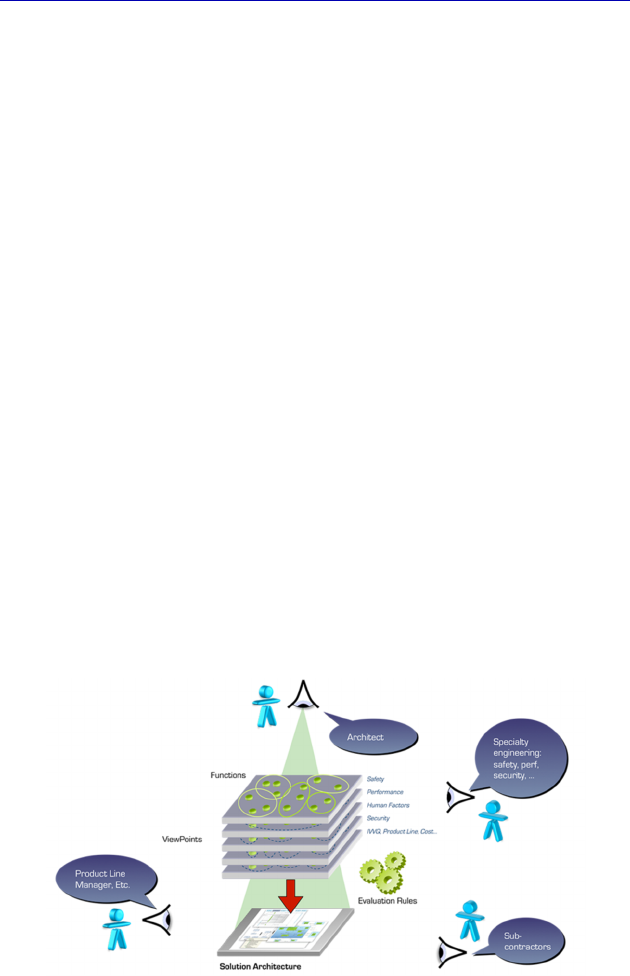
Figure 1.1. Coengineering with Arcadia

Reminders for the Arcadia Method 5
1.2. Architecture levels and associated concepts
1.2.1. Overview
NOTE.– The vocabulary that we shall explain in the following sections
is the one used in version 1.1 of the Capella tool.
The different working levels of Arcadia are the following:
– OPERATIONAL ANALYSIS: “What the users of the system
need to accomplish”:
- analysis of the issues of operational users by identifying the
actors that must interact with the system, their activities and their
interactions with each other.
– ANALYSIS OF THE SYSTEM NEEDS: “What the system has
to accomplish for the users”:
- external functional analysis as a response to identify the system
functions needed by its users (e.g. “calculate the optimal path” and
“detect a threat”), limited by the non-functional properties asked for.
– LOGICAL ARCHITECTURE: “How the system will work to
fulfill expectations”:
- internal functional system analysis: which are the subfunctions
that must be carried out and put together to establish the “user”
functions identified during the previous stage;
- identification of the logical components that carry out these
internal subfunctions, by integrating the non-functional constraints
that we choose to deal with at this level.
– PHYSICAL ARCHITECTURE: “How the system will be
developed and built”:
- the goal of this level is the same as that of the logical
architecture, except that it defines the final architecture of the system
as it must be created;
- it adds the functions required by the implementation and by the
technical choices, and highlights behavioral components (e.g. software
components) that carry out these functions. These behavioral
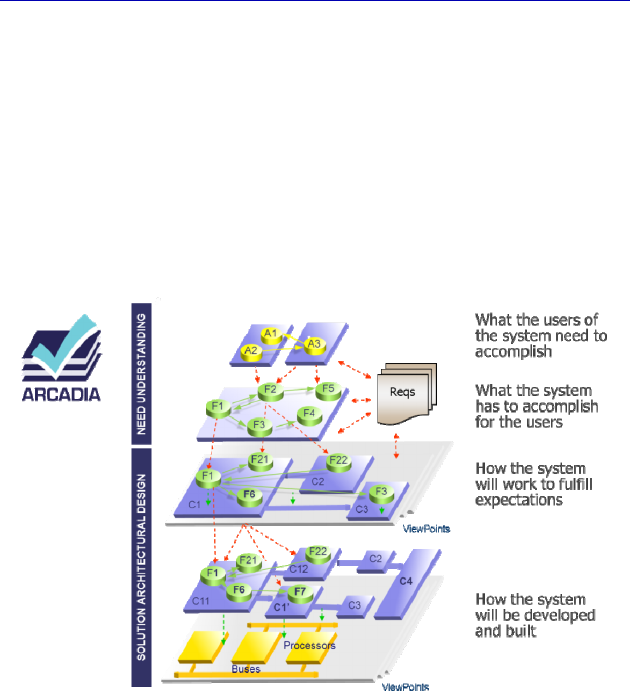
6 Systems Architecture Modeling with the Arcadia Method
components are then implemented using implementation components
(e.g. processor board), which provide the necessary material
resources.
– EPBS (End Product Breakdown Structure) AND
INTEGRATION CONTRACTS: “What is expected from the provider
of each component”:
- this step deduces from the physical architecture the conditions
that each component must fulfill to satisfy the architecture design
constraints and limitations, established in the previous phases.
Figure 1.2. The main engineering levels of Arcadia
It must be noted that the method does not always have to be top-
down in nature, but can also perfectly be bottom-up, for example if we
start with an existing system that is to be worked on. The question
relates more to architectural levels than to phases or steps.
Moreover, not all architectural levels are mandatory for all
projects. Operational Analysis, Logical Architecture and EPBS are
considered to be optional, depending on the complexity of the system
under study and the goals of the model.

Reminders for the Arcadia Method 7
1.2.2. Operational Analysis
The highest level of the Arcadia method is Operational Analysis
(“what the users of the future system need to accomplish”). The goal
here is to focus on the identification of the needs and objectives of
future users of the system in order to guarantee the adequacy of the
system faced with these operational needs.
NOTE.– At this level, the system is not (yet) recognized as a modeling
element. It will only be recognized as such from the System Analysis
level onward.
This level can be treated as a model of the jobs of future users:
what are their activities, what roles must they fulfill and under which
operational scenarios?
The main concepts proposed by Arcadia at this level are as
follows:
– Operational Capability: capability of an organization to provide a
high level service leading to an operational objective being reached
(for example Provide weather forecasts, etc.);
– Operational Entity: entity belonging to the real world
(organization, existing system, etc.) whose role is to interact with the
system being studied or with its users (for example Crew, Ship, etc.);
– Operational Actor: particular case of a (human) non-
decomposable operational entity (for example Pilot, etc.);
– Operational Activity: process step carried out in order to reach a
precise objective by an operational entity, which might need to use the
future system in order to do so (for example Detect a threat, Collect
meteorological data, etc.);
– Operational Interaction: exchange of information or of
unidirectional matter between operational activities (for example
meteorological data, etc.);
– Operational Process: series of activities and of interactions that
contribute toward an operational capability.
8 Systems Architecture Modeling with the Arcadia Method
– Operational Scenario: scenario that describes the behavior of
entities and and/or operational activities in the context of an
operational capability. It is commonly represented as a sequence
diagram, with the vertical axis representing time.
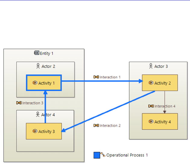
Figure 1.3. Diagram showing the main concepts behind Operational Analysis.
For a color version of the figure, see www.iste.co.uk/roques/arcadia.zip
In Figure 1.3, first of all we can see the structural elements (gray
rectangles), i.e. the Entities and the Actors. An Operational Actor is a
human and non-decomposable Operational Entity. An Entity can
contain other Entities or Actors, like Entity 1, which contains the
Actors 2 and 4. Next, we can see the Activities (orange rectangles),
within the Actors or Entities: this is the allocation relation. One or
several Activities can be associated with a same Entity or Actor. This
is the case with Activity 2 and Activity 4, which are associated with
Actor 3. Between the Activities we can see the Interactions, or
operational exchanges (orange arrows). A succession of Activities and
Interactions constitutes an Operational Process. This is the case for the
Operational Process 1 in the figure, which is made up of the sequences
of Interactions 1–3. This Operational Process is represented both by a
blue square on the diagram, and also by the bold and blue Interactions

Reminders for the Arcadia Method 9
involved, as well as the source and target Activities (here the same
Activity 1).
Other more advanced concepts are also available if needed:
Operational Role, Communication Mean, Mode and State, Exchange
Item, Class, etc. We shall discuss some of these throughout the case
study presented in Chapter 3.
1.2.3. System Analysis
System Analysis involves the identification of the Capabilities and
Functions of the system that will satisfy the operational needs (“what
the system must accomplish for the users”).
This involves carrying out an external functional analysis of the
system under study in order to identify the System Functions required
by the users (e.g. “calculate the optimal itinerary”, “detect a threat”)
from the response, under the constraint of the non-functional
properties ordered.
NOTE.– The System is identified as a modeling element at this level. It
is a “black box” containing no other structural elements, only
allocated Functions.
The main concepts proposed by Arcadia at this level are as
follows:
– System: organized group of elements that function as a unit
(black box) and respond to the needs of the users. The System owns
Component Ports that allow it to interact with the external Actors;
– Actor: any element that is external to the System (human or non-
human) that interacts with it. (for example Pilot, Test operator, etc.);
– System Capability: capability of the System to provide a high-
level service allowing it to carry out an operational objective (for
example provide meteorological data, etc.);
– Function: behavior or service provided by the System or by an
Actor (for example detect a threat, measure altitude, etc.). A Function
10 Systems Architecture Modeling with the Arcadia Method
owns Function Ports that allow it to communicate with the other
Functions. A Function can be split into subfunctions;
– Functional Exchange: unidirectional exchange of information or
of matter between two Functions, linking two Function Ports;
– Component Exchange: connection between the System and one
of its external Actors, allowing circulation of Functional Exchanges;
– Scenario: dynamic occurrence describing how the System and its
Actors interact in the context of a System Capability. It is commonly
represented in the form of a sequence diagram, with the vertical axis
representing time;
– Functional Chain: element of the model that enables a specific
path to be designated among all possible paths (using certain
Functions and Functional Exchanges). This is particularly useful for
assigning constraints (latency, criticality, etc.), as well as organizing
tests.
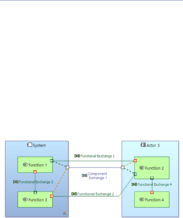
Figure 1.4. Diagram showing the main concepts behind System Analysis.
For a color version of the figure, see www.iste.co.uk/roques/arcadia.zip
In Figure 1.4, we can first of all see the structural elements (blue
rectangles), i.e. the System and the Actors. An Actor is an entity that
is external to the System (human or not). Next we can see the
Functions (green rectangles), which are inside the System or the
Actors: this is the allocation relation. One or several Functions can be
allocated to the same structural element. This is the case for Functions

Reminders for the Arcadia Method 11
2 and 4, which are allocated to Actor 3, as well as for Functions 1 and
3, which are allocated to the System. The Functional Exchanges
(green arrows) are represented between the Functions, linking a
Function Port of the output of a Function (green square) to a Function
Port of the input of another Function (orange square). One or more
Functional Exchanges can be allocated to the same Component
Exchange (blue line). This is the case for Functional Exchanges 1 and
2, which are both allocated to the Component Exchange 1, as shown
by the dotted line linking the Function Ports to the Component Ports.
A Component Exchange has to link the System to one of its Actors,
via Component Ports (white squares), which can be uni- or
bidirectional. In the case of Figure 1.4, the Ports are bidirectional,
since the Functional Exchanges are of opposite directions.
Other more advanced concepts are also available if needed:
Mission, Mode and State, Exchange Item, Class, Interface, etc. We
will discuss several of these in the context of the case study in
Chapter 4.
1.2.4. Logical Architecture
The level of Logical Architecture aims to identify Logical
Components inside the System (“how the system will work to fulfill
expectations”), their relations and their content, independently of any
considerations of technology or implementation.
Next an internal functional analysis of the system must be carried
out: the subfunctions required to carry out the System Functions
chosen during the previous phase must be identified; next, a split into
Logical Components to which these internal subfunctions will be
allocated must be determined, all the while integrating the non-
functional constraints that have been chosen for processing at this
level.
The main concepts proposed by Arcadia at this level are as
follows:
– Logical Component: structural element within the System, with
structural Ports to interact with the other Logical Components and the
12 Systems Architecture Modeling with the Arcadia Method
external Actors. A Logical Component can have one or more Logical
Functions. It can also be subdivided into Logical subcomponents;
– Logical Actor: any element that is external to the System (human
or non-human) and that interacts with it (for example Pilot,
Maintenance operator, etc.).
– Logical Function: behavior or service provided by a Logical
Component or by a Logical Actor. A Logical Function has Function
Ports that allow it to communicate with the other Logical Functions. A
Logical Function can be subdivided into Logical subfunctions;
– Functional Exchange: a unidirectional exchange of information
or matter between two Logical Functions, linking two Function Ports;
– Component Exchange: connection between the Logical
Components and/or the Logical Actors, allowing circulation of the
Functional Exchanges;
– Logical Scenario: dynamic occurrence describing the interactions
between Logical Components and Logical Actors in the context of a
Capability. It is commonly represented as a sequence diagram, with
the vertical axis representing the time axis;
– Functional Chain: element of the model that enables a specific path
to be designated among all possible paths (using certain Functions and
Functional Exchanges). This is particularly useful for assigning
constraints (latency, criticality, etc.), as well as organizing tests;
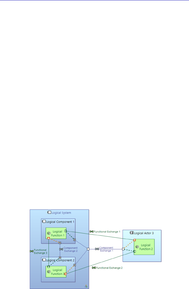
Figure 1.5. Diagram showing the main concepts behind Logical Architecture.
For a color version of the figure, see www.iste.co.uk/roques/arcadia.zip

Reminders for the Arcadia Method 13
In Figure 1.5, we can first of all see the structural elements (blue
rectangles), i.e. the Logical Components (contained in overarching
box that represents the System at the Logical level) and the Actors.
Next, we can see the Functions (green rectangles), within the Logical
Components or the Actors: this is the allocation relation. The
Functional Exchanges are represented between the Functions, always
linking a Function Port from a Function output to a Function Port
from the input of another Function. A Component Exchange either
links the Logical System to one of its Actors, or a Logical Component
directly to an external Actor, or two Logical Components via
Component Ports (uni- or bidirectional). In the case of Figure 1.5, the
Ports of Component Exchange 2 that link the two Logical
Components inside the System are unidirectional, since only one
Functional Exchange is allocated to it. On the other hand, Component
Exchange 1, which still links Actor 3 to the System, is now delegated
to the two Logical Components via unidirectional Component Ports,
each belonging to a different Logical Component. This mechanism
allows us to finely specify the responsibilities of each Logical
Component by attaching it to the responsibilities of the System level.
Other more advanced concepts are also available if needed:
Mission, Mode and State, Exchange Item, Class, Interface, etc. We
shall discuss some of these during the case study presented in
Chapter 5.
1.2.5. Physical Architecture
The objective of this level is the same as for Logical Architecture,
except that it defines the final architecture of the system, and how it
must be carried out (“how the system will be built”).
It adds the Functions required for implementation, as well as the
technical choices, and highlights two types of Physical Component:
– Behavior Physical Component: Physical Component tasked with
Physical Functions and therefore carrying out part of the behavior of
the System (for example software component, data server, etc.);
14 Systems Architecture Modeling with the Arcadia Method
– Node (or Implementation) Physical Component: Physical
Component that provides the material resources needed for one or
several Behavior Components (for example processor, router, OS,
etc.).
At this level, the main concepts proposed by Arcadia are similar to
those of the Logical Architecture: Physical Function, Functional
Exchange, Physical Component, Physical Actor, etc. However, there
are some additional concepts, notably:
– Physical Port: non-oriented port that belongs to an Implementation
Component (or Node). The structural port (Component Port), on the
other hand, has to belong to a Behavior Component;
– Physical Link: non-oriented material connection between
Implementation Components (or Nodes). The Component Exchange
remains a connection between Behavior Components. A Physical Link
allows one or several Component Exchanges to take place (for
example Ethernet cable, USB cable, etc.);
– Physical Path: organized succession of Physical Links enabling a
Component Exchange to go through several Implementation
Components (or Nodes).
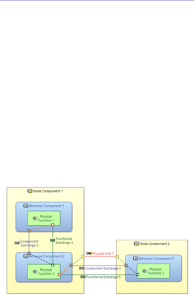
Figure 1.6. Diagram showing the main concepts behind Physical Architecture.
For a color version of the figure, see www.iste.co.uk/roques/arcadia.zip

Reminders for the Arcadia Method 15
In Figure 1.6, we can first of all see the Node Components (yellow
rectangles). Next, we can see the Behavior Components (blue
rectangles) deployed over each Node. Finally, we can see the
Functions (green rectangles) inside the Behavior Components: this is
the allocation relation. The Functional Exchanges are represented
between the Functions, always linking a Function Port from a
Function output to a Function Port from the input of another Function.
A Component Exchange links either a Behavior Physical Component
to an external Actor, or two Behavior Physical Components, via
Component Ports (uni or bidirectional). One or more Functional
Exchanges can be allocated to the same Component Exchange. Next,
the Component Exchanges can themselves pass through Physical
Links (red lines), linking two Physical Ports (yellow squares) of Node
Components. This is the case in Figure 1.6, where Functional
Exchange 5 is allocated to Component Exchange 4, which passes
through the Physical Link 1.
Other more advanced concepts are also available if needed:
Mission, Mode and State, Exchange Item, Class, Interface, etc. We
shall discuss some of these in the context of the case study presented
later in this work (Chapter 6).
1.2.6. EPBS
This level aims to deduce, from the Physical Architecture,
the conditions that each Component must satisfy to comply with the
constraints and choice of design of the architecture identified in
the previous phases (“what is expected from the provider of each
component”). The Physical Components are often grouped into larger
Configuration Items that are easier to manage in terms of industrial
organization and responsibilities.
The number of concepts proposed by Arcadia at this level is much
smaller than for other levels. This is due to the fact that the main
concept of this level is the Configuration Item, which can be divided
into:
– System CI: system-type configuration item;
16 Systems Architecture Modeling with the Arcadia Method
– Prime Item CI: decomposable configuration item;
– CSCI: computer software configuration item;
– HWCI: hardware configuration item;
– NDI: non-developed configuration item;
– COTS: component off the shelf.
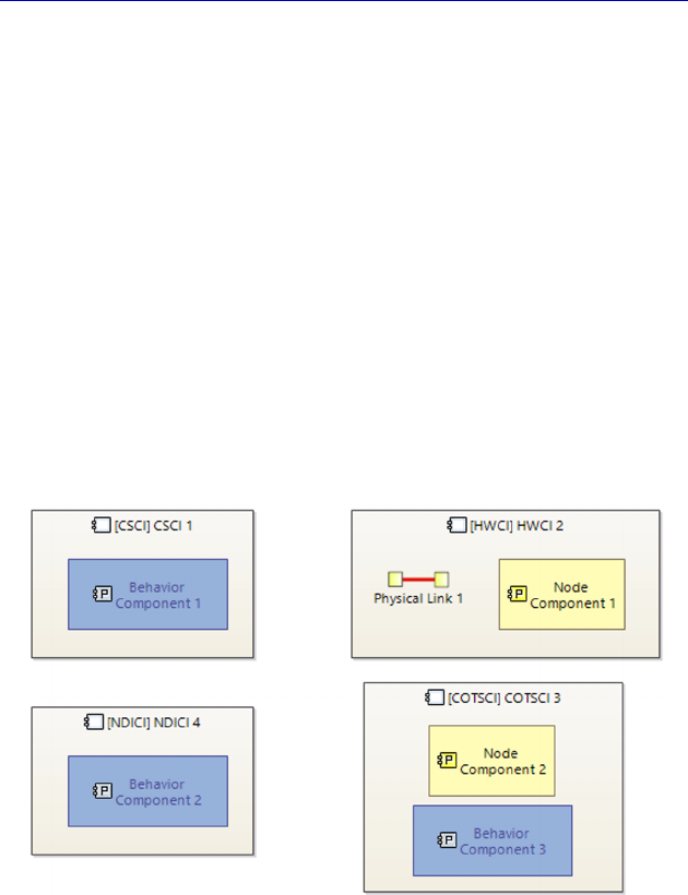
In Figure 1.7, we can see four Configuration Items (gray
rectangles). The first one, CSCI 1, is a software Configuration Item,
carrying out Behavior Component 1. The second item, HWCI 2, is a
material Configuration Item, carrying out Node Component 1, as well
as Physical Link 1. The third, COTSCI 3, is an off the shelf
Configuration Item, carrying out both Node Component 2 as well as
Behavior Component 3. Finally, the fourth, NDICI 4 is a non-
developed Configuration Item, carrying out Behavior Component 2.
Figure 1.7. Diagram showing the main concepts behind EPBS. For a color
version of the figure, see www.iste.co.uk/roques/arcadia.zip
1.3. Main types of Arcadia diagrams
This section provides an overview of the main types of diagrams
defined by Arcadia and supported by Capella. This is not an
Reminders for the Arcadia Method 17
exhaustive list of all of the diagrams available for each level of
engineering, but rather a characterization of the different diagrams
proposed.
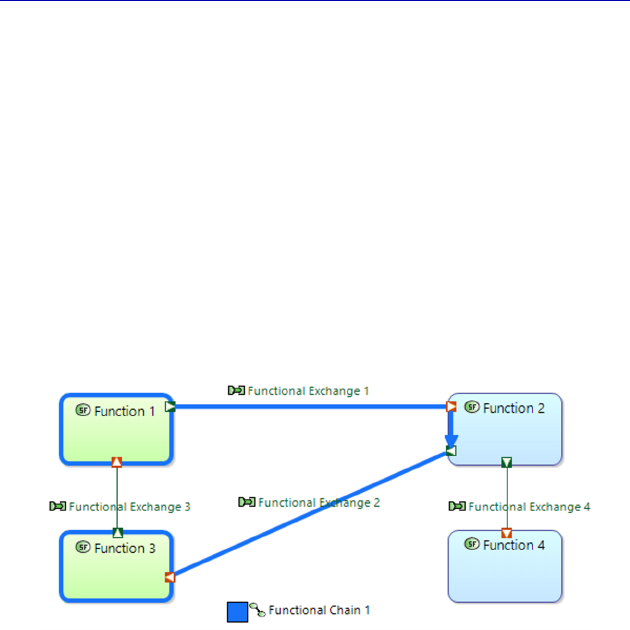
1.3.1. Data Flow diagrams
The Data Flow diagrams are available at all levels in Arcadia. They
represent the information dependency network between Functions.
These diagrams provide a diverse set of mechanisms for managing
complexity: simplified links calculated between the high-level
Functions, the categorization of Exchanges, etc. The Functional
Chains can be represented as highlighted paths.
Figure 1.8. Simple example of a Data flow diagram at
the System level (SDFB), with a Functional Chain. For a color
version of the figure, see www.iste.co.uk/roques/arcadia.zip
1.3.2. Architecture diagrams
Architecture diagrams are used in all phases of engineering in
Arcadia. Their main goal is to show the allocation of Functions to
Components.
Functional Chains can be shown as highlighted paths. In System
Analysis, these diagrams contain a box that represents the System
under study and the Actors surrounding it.
18 Systems Architecture Modeling with the Arcadia Method
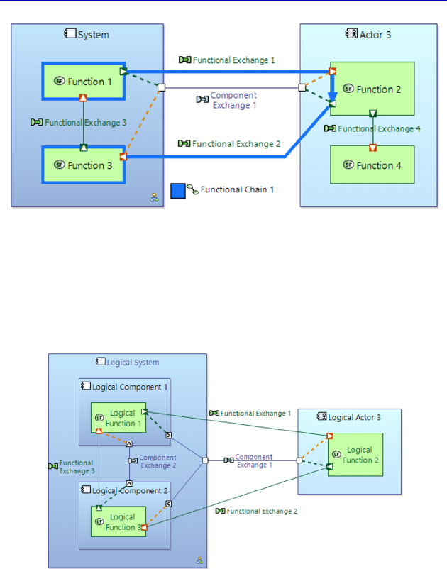
Figure 1.9. Simple example of an Architecture diagram at
the System level (SAB), with a Functional Chain. For a color
version of the figure, see www.iste.co.uk/roques/arcadia.zip
In Logical Architecture, these diagrams show the constitutive
elements of the System. These are called Logical Components.
Figure 1.10. Simple example of an Architecture diagram
at the Logical level (LAB). For a color version of
the figure, see www.iste.co.uk/roques/arcadia.zip
In Physical Architecture, these diagrams also show the deployment
of Behavior Components over the Node Components that provide
them with resources.

Reminders for the Arcadia Method 19
Figure 1.11. Simple example of an Architecture diagram
at the Physical level (PAB). For a color version of the
figure, see www.iste.co.uk/roques/arcadia.zip
1.3.3. Scenario diagrams
Scenario diagrams show the vertical sequence of the messages
passed between elements (lifelines) and are largely inspired by the
UML/SysML sequence diagram.
A lifeline (Instance Role, in Capella) is the representation of the
existence of a model element that participates in the scenario
involved. It has a name that reflects the name of the model element
referenced and is represented graphically by a dotted vertical line. A
Message is a unidirectional communication item between lifelines that
triggers a behavior in the receiver.
Capella provides several types of Scenario diagrams: Functional
Scenarios (the lifelines are Functions), Exchange Scenarios (the
lifelines are Components/Actors, while the sequence Messages are
Functional Exchanges or Component Exchanges), Interface Scenarios
(the lifelines are Components/Actors, while the sequence Messages
are Exchange Items). Modes, States and Functions can also be shown
in these diagrams.
20 Systems Architecture Modeling with the Arcadia Method
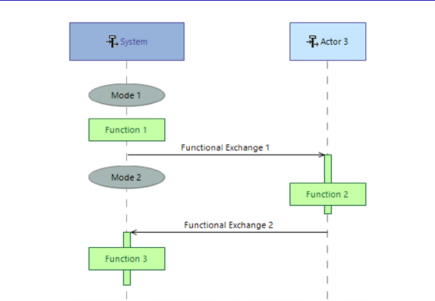
Figure 1.12. Simple example of a diagram for
an Exchange Scenario at the System level (SES)
A Scenario can call upon “subscenarios”, defined elsewhere
through a reference inserted between successive Exchanges along the
time axis.
N
OTE
.– For more information on this type of diagram, the reader can
refer to the following work: Modélisation de systèmes complexes avec
SysML [CAS 18].
1.3.4. Mode and State diagrams
Mode and State diagrams are graphical representations of state
machines inspired by UML/SysML. A state machine is a set of States
linked together by Transitions. A Transition describes the reaction of a
structural item when an event takes place (usually the item changes its
State, but not always). A Transition contains a source State, a Trigger
and a target State. It can also include a Guard Condition and an Effect.
Reminders for the Arcadia Method 21
N
OTE
.– Modes and States cannot exist together in the same machine.
A Mode is an expected behavior, in the context of certain chosen
conditions, of the System or of one of its Components, or of an Actor
or an Operational Entity. A State is a behavior that is experienced by
the System or one of its Components, or by an Actor or an Operational
Entity, under certain conditions that are imposed by the environment.
The term “State” will be used to the end of this section.
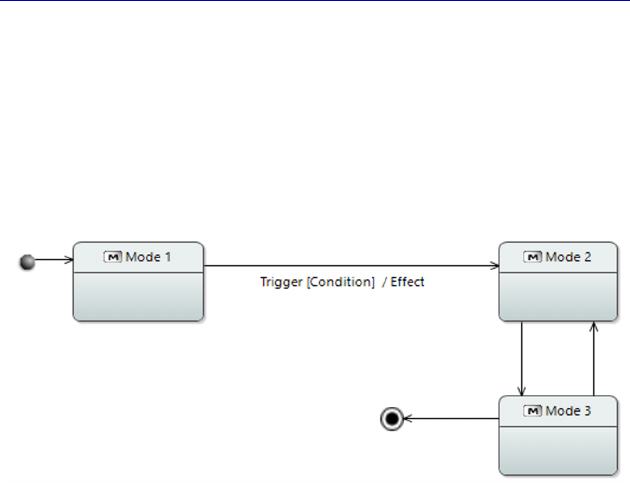
Figure 1.13. Simple example of a Mode and State diagram (MSM)
On top of the succession of “normal” States that correspond to the
life cycle of a structural element, the diagram also shows two pseudo-
states:
– the Initial State of the diagram corresponds to the creation of the
structural element;
– the Final State of the diagram corresponds to the destruction of
the structural element.
Modes/States/Transitions can be linked to Functions, Functional
Exchanges, Exchange Items, etc.
N
OTE
.– For more information on this type of diagram, the reader can
refer to the following work: Modélisation de systèmes complexes avec
SysML [CAS 18].
22 Systems Architecture Modeling with the Arcadia Method
1.3.5. Breakdown diagrams
Breakdown diagrams represent hierarchies of either Functions or
Components at all levels of engineering.
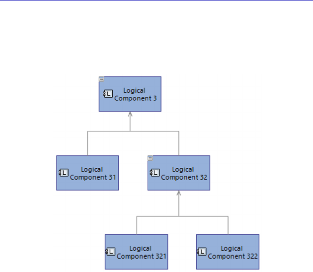
Figure 1.14. Simple example of Component
decomposition diagram at the Logical level (LCBD)
1.3.6. Class diagrams
Capella provides advanced mechanisms for modeling data
structures at a stated level of precision and for linking them to
Functional Exchanges, Component or Function Ports, Interfaces, etc.
The Capella Class diagram draws heavily on the UML class
diagram. Many of the same UML concepts are present: Class,
Enumeration, Type, Property, Association, Aggregation, Composition,
Generalization, Package, etc. More specific concepts are also present,
however, in order to model the communication model, notably the
Exchange Items.
Reminders for the Arcadia Method 23
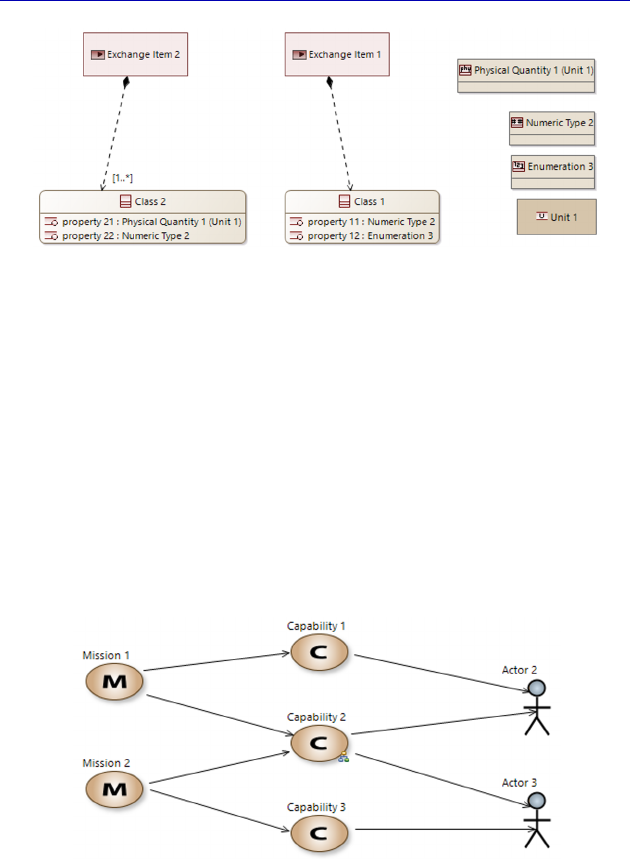
Figure 1.15. Simple example of a Class diagram (CDB)
N
OTE
.– For information on this type of diagram, the reader can refer
to the following work: UML 2 par la pratique – Études de cas et
exercices corrigés [ROQ 04].
1.3.7. Capability diagrams
Capability diagrams are available at every engineering phase in
Arcadia, but are particularly useful in Operational Analysis and
System Analysis. They can highlight the relations between Missions,
Capabilities and Actors.
Figure 1.16. Simple example of a Capability diagram
at the System level (SMCB)
We shall use all of these diagram types at least once in the
following chapters as we go through the case study.
This page intentionally left blank

2
Capella: A System Modeling Solution
2.1. Radius considered and stakes involved
The goal of Arcadia is to contribute to the transformation of
engineering by providing an engineering environment that offers a
model-based procedure, rather than one based on documents, driven
by a process, and which delivers effective coengineering by
construction. To this end, the operational engineering experts at
Thales have defined a unified language for modeling architectures in
the group and have developed the associated toolbox, Capella, since
2007.
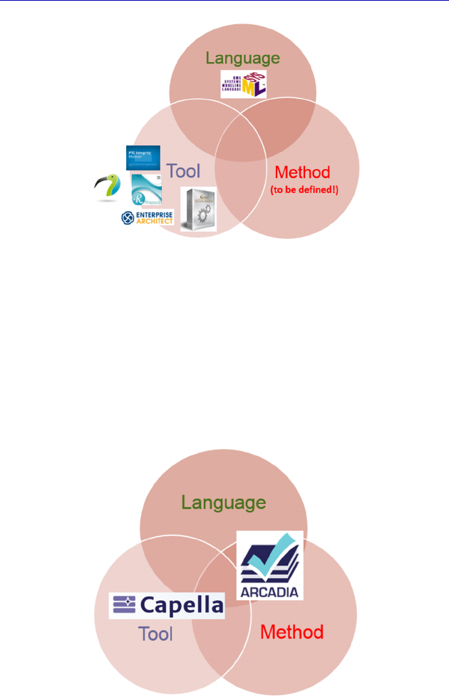
Unlike most companies that have tried to apply model based
systems engineering (MBSE), Thales did not start by choosing a tool,
for example Rational Rhapsody (IBM), MagicDraw (NoMagic) or
Enterprise Architect (Sparx Systems), etc., with a language like
systems modeling language (SysML). Experience shows that in such
cases the system engineers have difficulties in getting started, as they
lack both a methodological approach, which is not provided by
SysML [VOI 16], and support tools. It is only during a later phase – if
in the meantime the projects have not given up on modeling – that an
approach adapted to the context can be developed. Even then, a
toolbox still needs to be created, starting off with the commercial tool,
which is often the source of unplanned extra costs….
26 Systems Architecture Modeling with the Arcadia Method
Figure 2.1. “Classic” MBSE with SysML
Thales started by defining a modeling method in order to improve
its engineering practices: Arcadia. This method, which is based on
functional analysis familiar to all system engineers, and on the
allocation of functions to architecture components, implicitly defines a
modeling language. As a result, the associated tool, Capella, knows
both the language and the method, without requiring any extra thought
or development.
Figure 2.2. MBSE with Arcadia/Capella
Capella: A System Modeling Solution 27
Capella proposes similar ergonomics to tools like
PowerPoint/Visio and Excel. As a result, the resulting environment is
intuitive and allows engineers to concentrate on defining their
architectures, rather than spending time learning and exploiting
complex generic modeling languages such as UML or SysML in order
to specify their needs. As it is dedicated to the underlying Arcadia
method, Capella also guides engineers through their activities,
something that generic modeling tools do not offer.
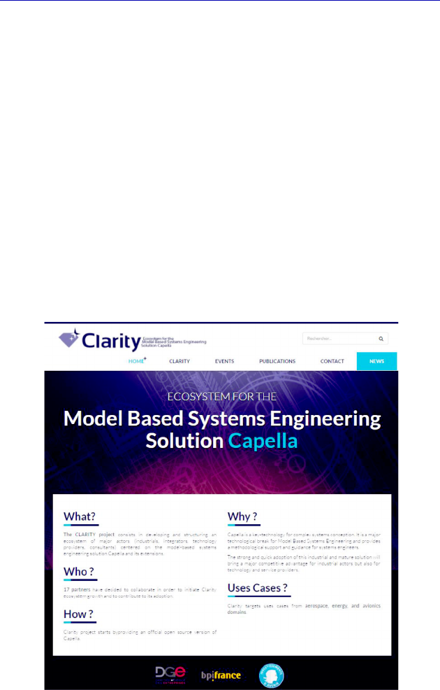
In 2015, the solution was provided as Open Source within the
industry working-group PolarSys of the Eclipse Foundation, as part of
the French collaborative Clarity project (www.clarity-se.org/),
supported by BPI France. As a result, users of Capella benefit from 10
years of concrete feedback regarding the use of the Arcadia method
and the associated tool (Melody Advance internally) with Thales
projects.
Figure 2.3. Welcome page of the Clarity project Website
28 Systems Architecture Modeling with the Arcadia Method
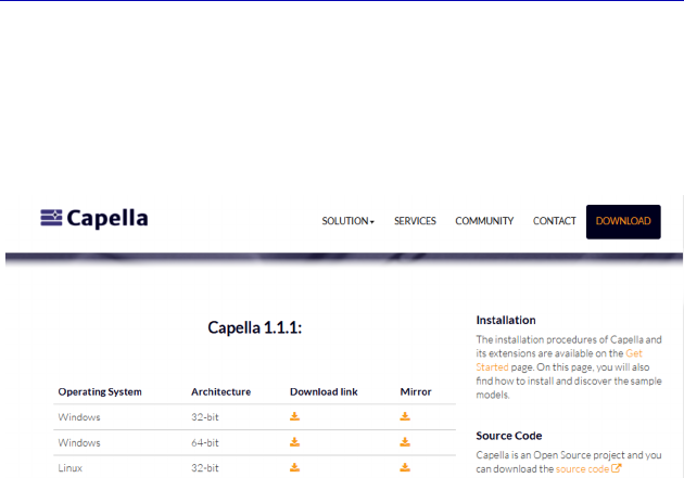
Capella has its own life cycle. A major version, providing new
functionalities, is released at the end of each year, while several
“minor” versions, providing patches for bugs, are released throughout
the year. The download page can be found at www.polarsys.org/
capella/download.html.
Figure 2.4. Download page of the Capella Website
2.2. Principles of the tool
2.2.1. Principles of the man–machine interface
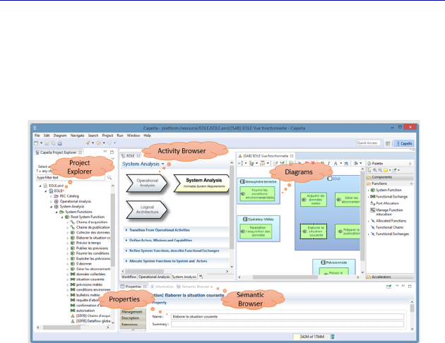
At the opening or creation of a Capella project, the interface of the
tool is presented to the user. This contains different predefined zones
(shown in the following), which we shall use many times during the
case study in the following chapters. However, the user can modify
the organization of the windows according to their preferences, by
sliding/moving zones, hiding some of the views, or by showing others
(command Window – Show View – etc.).
– The “Activity Browser” area exposes the user to the different
engineering phases used in the modeling of their architecture, with
shortcuts to create new diagrams linking to the engineering phase in
question; this view also facilitates the “transition” between
engineering phases in order to create realization links between the
phases and their associated items.
Capella: A System Modeling Solution 29
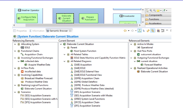
– The “Semantic Browser” area allows the user to browse through
the model with ease: for any item selected in the “project” area or on
any diagram, the semantic browser area presents the user with all of
the references that surround this item, i.e. its containment or reference
relations, as well as all of the diagrams in which the element appears.
Figure 2.5. Overview of the Capella interface. For a color version
of the figure, see www.iste.co.uk/roques/arcadia.zip
– The more typical “Project Explorer” area is a tree diagram of the
Capella model, and contains all of the semantic items and diagrams
created by the user.
– The “Diagram” area presents a graphical view of an extract of the
model and allows the model to be edited in terms of creation,
modifications, item deletion, as well as modifications to the
organization or appearance of items in the diagram. The palette shown
on the right depends on the type of diagram involved.
– The “Properties” zone, which shows all of the given properties
for a selected item in the model or in a diagram.
30 Systems Architecture Modeling with the Arcadia Method
Figure 2.6. Window of the Semantic Browser
2.2.2. Model element versus graphical object
A key difference between a drawing tool, like Powerpoint or Visio,
and a modeling tool lies in the coexistence of (but strong distinction
between) graphical objects and model elements.
A Capella diagram contains a set of graphical objects that can be
moved, resized, deleted, etc. Examples of graphical objects are the
green rectangles of Functions, the blue rectangles of Components, the
lines of Functional or Component Exchanges, etc. However, each
graphical object in a Capella diagram is actually the visual
representation of a model element. It is these model elements that
carry the semantic information: name, type, etc. Most importantly, a
single model element can be represented by different graphical objects
in different diagrams.
In the example below, in the project explorer on the left we have
shown a Logical Component called “Airborne Subsystem”. This
unique modeling element is represented on the right in three different
diagrams:
– an Architecture diagram (LAB) where it is shown with an
allocated Function (green rectangle inside);
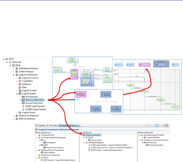
Capella: A System Modeling Solution 31
– a Scenario diagram (LES) where it is shown as a vertical line
exchanging Messages (horizontal arrows) with other Components or
Logical Actors;
– a Breakdown diagram (LCBD) where it is shown alone, as it
does not contain any Logical subcomponents.
Figure 2.7. Distinction between model element and graphical
object (example). For a color version of the figure, see
www.iste.co.uk/roques/arcadia.zip
The “Airborne Subsystem” modeling element is also represented at
the bottom of the Semantic Browser, where it is shown at the center,
while all of the other elements linked to it are shown in the left and
right columns. The three diagrams in which it is shown graphically are
marked in the center column.
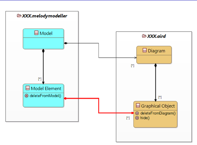
A slightly more sophisticated way of representing this distinction
between model elements and graphical objects is provided in Figure
2.8, also produced using Capella (Class Diagram Blank).
32 Systems Architecture Modeling with the Arcadia Method
Figure 2.8. Distinction between model element
and graphical object (concepts). For a color version
of the figure, see www.iste.co.uk/roques/arcadia.zip
By default, a Capella model is stored in two files. As a
simplification, the “.melodymodeller” can be said to contain the
model elements and their relations, while the “.aird” contains the
diagrams and the graphical objects. The fundamental point is
represented by the red double arrow that links the model elements on
the left with the graphical objects on the right.
A model element can be linked to none or several graphical
objects. It is possible to create a model element without going through
a diagram, and therefore without any graphical representation. This is
quite rare, but permissible if there is no need for graphical
communication around this element.
A graphical object is itself always linked to a single model
element. There is one exception to this rule: graphical notes (in the
form of little yellow “post-its”), which can be placed on any diagram
as a purely graphical comment.
Capella: A System Modeling Solution 33
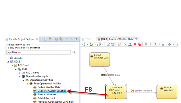
N
OTE
.– Selecting a graphical object in a diagram and pressing the F8
key (or right clicking: Show in Capella Explorer) results in the model
element being shown in the Project Explorer.
Figure 2.9. From graphical object to model element (F8)
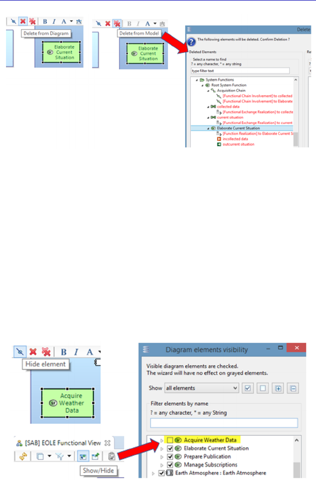
It is very important to properly understand the two possible types
of deletion:
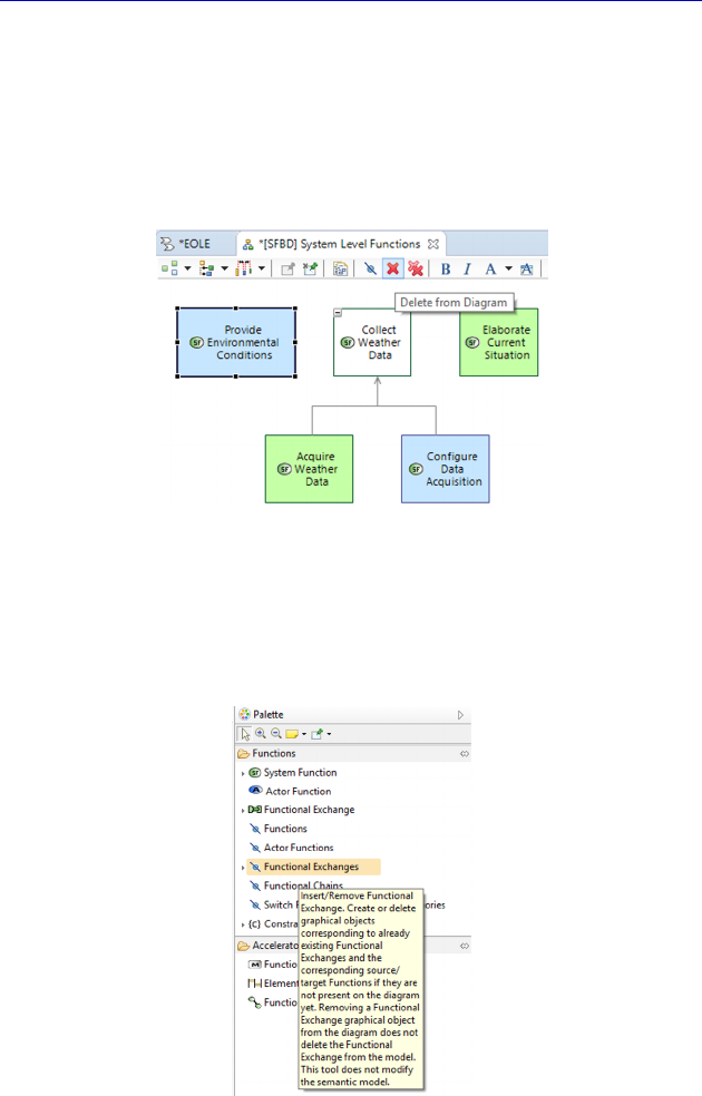
– deletion of a graphical object (Delete from Diagram): command
that is applied to a graphical object in the diagram, and therefore does
not modify the model itself. The dependent graphical objects (links,
ports, etc.) are also deleted. Note that even if the last graphical
representation of a model element is destroyed, it continues to exist
and can be reinserted into a diagram later on;
– deletion of a model element (Delete from Model): command
applied to a graphical object in a diagram, or on a model element in
the project explorer that is applied to the model element involved.
This command changes the model itself and can lead to a cascade of
deletions, as the deletion of a Function automatically leads to the
deletion of the ingoing and outgoing Functional Exchanges, its Ports,
its allocation relation with structural items, etc. All linked graphical
objects are also deleted from all of the diagrams involved.
The importance of the deletion of a model element is signaled by
Capella in the form of a window that pops up to show which other
model elements would also be permanently erased.
34 Systems Architecture Modeling with the Arcadia Method
Figure 2.10. Distinction between the deletion of
a model element and a graphical object
A graphical object can also be hidden (Hide element), rather than
completely deleted from the diagram. The difference with deletion is
subtle: the graphical object is still present, but no longer visible. The
dependent graphical objects (links, ports, etc.) are also hidden. There
is a Show/Hide button in the palette at the top of the diagram.
N
OTE
.– Do not overuse the “Hide” feature: the graphical object still
exists and weighs down the “.aird” file. Its use must be punctual, for
example to temporarily mask an object without losing the graphical
work (position, size, etc.), before bringing it back to the diagram.
Figure 2.11. Distinction between hiding and deleting a graphical object
Capella: A System Modeling Solution 35
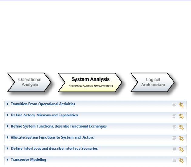
2.2.3. Integrated methodological guidance
Capella has an integrated methodological guide in the form of the
Activity Explorer. This lists the various activities and the different
diagrams that can be carried out at the relevant level of engineering,
for example in this case System Analysis. Figure 2.12 first shows the
activities, and then each activity shows the relevant diagrams.
Figure 2.12. Methodological activities of the “System Analysis” level
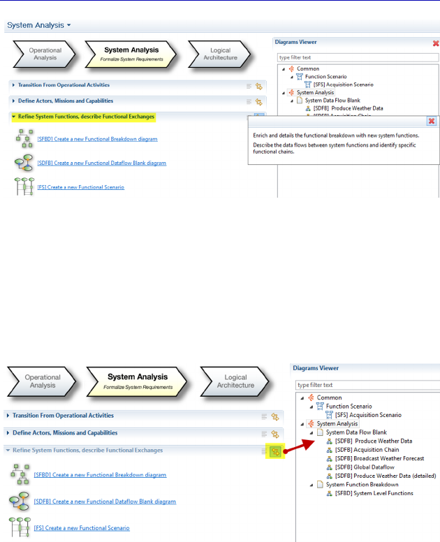
For example, if we open the Refine System Functions activity,
Capella proposes three types of diagram:
– a Functional Breakdown diagram (SFBD), which allows for the
creation of Functions and subfunctions;
– a Data Flow diagram (SDFB), which allows for the creation of
Functions and subfunctions, and for them to be linked through
Functional Exchanges;
– a Functional Scenario diagram (FS), which also allows for the
creation of Functions and Functional Exchanges.
36 Systems Architecture Modeling with the Arcadia Method
Figure 2.13. Methodological activity in detail
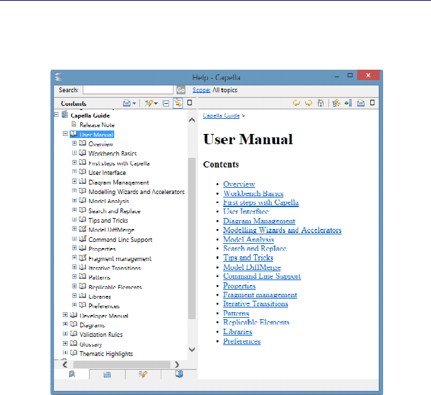
Capella offers the possibility of filtering the diagrams in the
“Diagrams Viewer” against a single methodological activity in order
to reduce the number of visible diagrams. For example, here we can
filter over the chosen activity, and thus only see the SFBD, SDFB or
FS diagrams.
Figure 2.14. Filtering of the diagrams by methodological activity
It must be noted that the tool provides a rather complete online
help section, which can be accessed via the Help–Help Contents
menu. The window that opens provides a large amount of information;
what interests us here is the Capella Guide, which contains the
Release Note, the User Manual, but also a Developer Manual (for
Capella: A System Modeling Solution 37
Capella Studio), a list of diagrams and validation rules, as well as a
glossary.
Figure 2.15. Capella online help
N
OTE
.– If the Activity Explorer is closed accidentally, it can always be
opened again by right clicking on the .aird in the Project Explorer.
2.2.4. Different natures of diagrams
At each engineering level in Arcadia, Capella proposes a large
number of very similar diagrams. In section 1.3, we mentioned the
main types of diagram in terms of methodology. Another
classification can be made from the tool point of view. The
management rules of the different natures of the diagrams, especially
in the case of a model element being added, are characterized by
precise rules that we shall describe below.

38 Systems Architecture Modeling with the Arcadia Method
We shall first distinguish the three natures of the most frequent
diagrams in Capella, using their specific denomination:
– Breakdown (xxBD);
– Blank (xxB);
– Scenario (xxS).
The Breakdown diagrams (written xxBD) represent tree diagrams
of either functions or components, at all levels of engineering. We can
name for example:
– the Operational level: OABD (activities), OEBD (entities);
– the System level: SFBD (functions);
– the Logical level: LFBD (functions), LCBD (components);
– the Physical level: PFBD (functions), PCBD (components);
– the EPBS level: CIBD (configuration items).
NOTE.– These diagrams always represent the current state of the
model and are updated automatically by default. As soon as a
Breakdown type diagram element model is created, whether by
another type of diagram or by the explorer, the Breakdown is updated
automatically. Breakdown diagrams are designed to be complete, even
though some elements can be hidden (Hide element) in order to
simplify it. However, the command Delete from Diagram is switched
off by default, as the diagram is automatically updated the next time it
is opened….
Blank diagrams, written xxB, are usually the most common in a
Capella model. They exist at all levels of engineering. We can name
for example:
– the Operational level: OAIB (activities and interactions), OCB
(capabilities), OAB (architecture), ORB (roles), CDB (classes);
– the System level: SDFB (functions), CB/MCB (missions and
capabilities), SAB (architecture), CDB (classes);
– the Logical level: LDFB (functions), LAB (architecture), CDB
(classes);
Capella: A System Modeling Solution 39
– the Physical level: PDFB (functions), PAB (architecture), CDB
(classes);
– the EPBS level: EAB (architecture).
N
OTE
.– Unlike the previous ones, these diagrams are not meant to be
comprehensive and are not automatically updated. They are empty on
creation, hence the name Blank, even if model elements of a
compatible type already exist. It is the modeler who decides which
subset of compatible model elements they are going to represent
graphically, as a function of who is reading the diagram, and what
their objectives are.
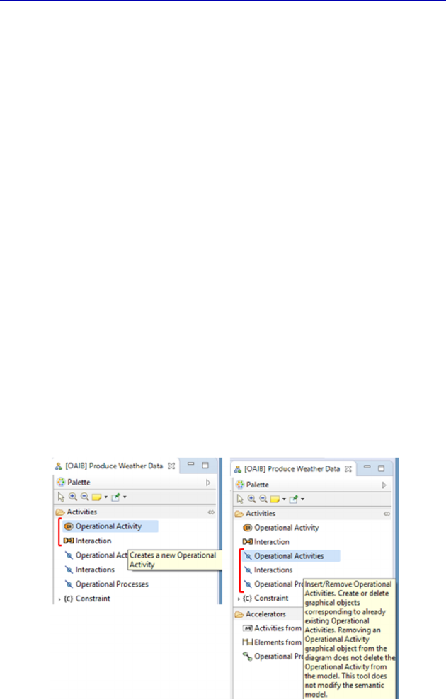
As a result, in this type of diagram the modeler can either:
– create a graphical object by also creating a model element (thus
modifying the model);
– insert an existing model element into the diagram so as to only
create a new graphical object (therefore without modifying the
model).
The distinction between these two choices can be seen
systematically in the palettes of the Blank diagrams, as shown in
Figure 2.16.
Figure 2.16. Creation or insertion of model elements in a Blank

40 Systems Architecture Modeling with the Arcadia Method
NOTE.– When a compatible model element is created, whether by
another diagram or by the explorer, the Blank diagram is not updated
automatically. However, the links between elements, such as
Functional Exchanges, etc., only appear automatically if the source
and the target of the links are already present on the diagram. These
management rules had been tested and approved by Thales projects as
being the most effective long before Capella was made available as
Open Source.
The Scenario diagrams (written xxS) are also present for all
engineering levels. We can name for example:
– Operational level: OAS (activities), OES (entities);
– System level: SFS (functions), SES (exchanges), SIS (interfaces);
– Logical level: LFS (functions), LES (exchanges), LIS
(interfaces);
– Physical level: PFS (functions), PES (exchanges), PIS
(interfaces);
– EPBS level: EIS (interfaces).
The Scenario diagram in Capella is very close to the UML/SysML
sequence diagram [CAS 18]. It shows a vertical sequence of Messages
passed from model element to model element (called lifeline in
UML/SysML). However, Capella provides several types of Scenario
diagrams: Functional Scenarios (the lifelines are Functions), Exchange
Scenarios (the lifelines are Components/Actors while the sequence
Messages are Functional or Component Exchanges), Interface
Scenarios (the lifelines are Components/Actors while the sequence
Messages are Exchange Items).
NOTE.– It must noted that the model elements that appear in a
Scenario diagram are references to other model elements. For
example, the vertical lines of Actors and the horizontal Messages in
the Exchange Scenarios refer, respectively, to the Actors and to the
Functional Exchanges of the model. By selecting a graphical object in
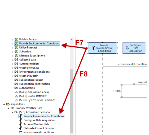
Capella: A System Modeling Solution 41
a Scenario diagram and by pressing F8 (or right clicking: Show in
Capella Explorer), we get the model element contained in the
Scenario represented in the Project Explorer. By instead pressing F7,
we get the referenced model element.
Figure 2.17. Model elements referenced in a Scenario
As a result, deletion is a bit more complex: note that the model
element deleted by the Delete from Model is the same as the one
contained in the scenario, and not the one referenced. Moreover, if the
referenced element is deleted, the choice that has been made involves
displaying a graphical element in the scenario that no longer points to
any model element, showing an error that needs to be corrected. It
would be very dangerous to also destroy all the elements in the
scenarios by cascade, following the deletion of an actor or of a
function, as the modeler would have no simple way to detect the
scenario changes.
In the example from Figure 2.17, by deciding to delete the
Function and not only the vertical line in the Scenario, we would
obtain an updated diagram with Invalid feature as name
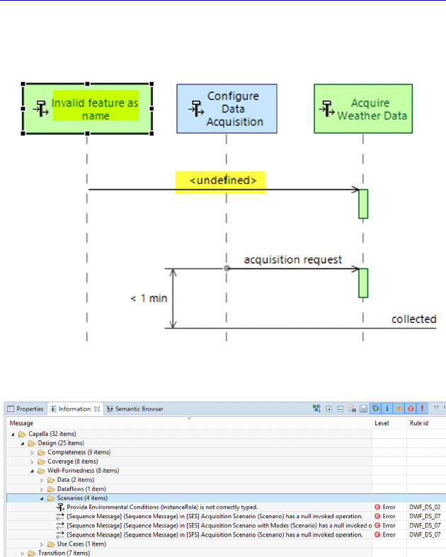
42 Systems Architecture Modeling with the Arcadia Method
and undefined indications for the orphan graphical objects. A model
validation would invariably result in associated errors.
Figure 2.18. Orphan elements in a Scenario
Figure 2.19. Errors linked to orphan elements in a scenario
N
OTE
.– The Scenario diagram is the only one that does not allow a
Delete from Diagram or a Hide Element to be carried out on the
vertical lines or on the horizontal messages. This is a very particular
diagram, since the model elements being handled are local to the
Scenario in question and are only represented by a single graphical
object.
Capella: A System Modeling Solution 43
2.2.5. Additional information on the diagrams
In the previous section, we discussed the management rules
involved in the different natures of diagrams, particularly in the case
of a model element being added.
For example, we explained that Breakdown diagrams are
automatically updated, as soon as a relevant model element is created,
whether by another type of diagram or by the explorer. We have also
explained that in Blank type diagrams, the links between elements
such as Functional Exchanges etc. only appear automatically if the
source and the target of the links are already present on the diagram.
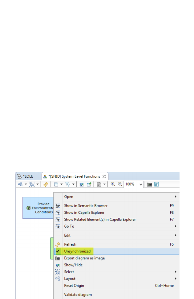
There is an advanced method for voluntarily blocking these
automatic updates. This can be in the interest of performance levels in
very large models, or simply to more precisely control what appears in
each diagram. By default, the diagrams are said to be synchronized,
but they can be desynchronized in order to update them when and how
the modeler desires. This is done by ticking a property of the diagram
called Unsynchronized by right clicking at the back of the diagram.
Figure 2.20. Example of desynchronization of a Breakdown diagram
44 Systems Architecture Modeling with the Arcadia Method
In the previous example of a Function Breakdown diagram at the
System level (SFBD), we can now see that the command Delete from
Diagram is active, contrary to what we had previously explained for
Breakdown diagrams. Most importantly, if a Function is added to a
Data Flow diagram (SDFB), this function will not automatically
appear in the SFBD.
Figure 2.21. Modification of the available commands
following desynchronization of a Breakdown diagram
In the same way, if we place the Unsynchronized property on a
Blank diagram, the links do not appear automatically.
Figure 2.22. Command for inserting functional exchanges
Capella: A System Modeling Solution 45
In this way, we can choose whether to insert them or not based on
the objectives of each individual diagram.
N
OTE
.– By default, use of the command Insert/Remove Functional
Exchanges in a Blank diagram does not make sense. It only becomes
useful once the diagram has been desynchronized. In the same way,
the Delete from Diagram command is only active for the links
(Functional Exchanges, etc.) if the diagram has been desynchronized.
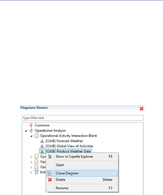
We must also add the possibility of “cloning” a diagram, for
example to derive a simplified view from it by deleting certain
graphical objects, or by masking certain element types using filters
predefined by Capella. We will make use of this command several
times during the case study.
Figure 2.23. Diagram cloning command
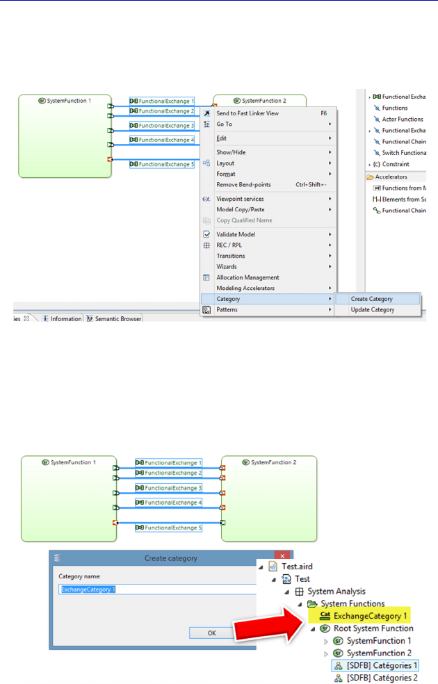
Another very useful concept for dealing with the complexity of the
diagrams is that of Category. Starting with a set of Functional
Exchanges, Component Exchanges or Physical Links, a new model
element can be created that allows for a graphical synthesis of the
multiple links to take place. This concept is available at the System
Analysis level, as well as at the Logical and Physical Architecture
levels.
46 Systems Architecture Modeling with the Arcadia Method
Let us look at the simple example of two System Functions with
multiple Functional Exchanges, such as in Figure 2.24. Here, we can
ask for the creation of a Category in order to carry out the synthesis.
Figure 2.24. Contextual Category creation command
The category ExchangeCategory 1 thus created is a new model
element that appears in the project explorer at the same level as the
technical element Root System Function.
Figure 2.25. Result of Category creation
Capella: A System Modeling Solution 47
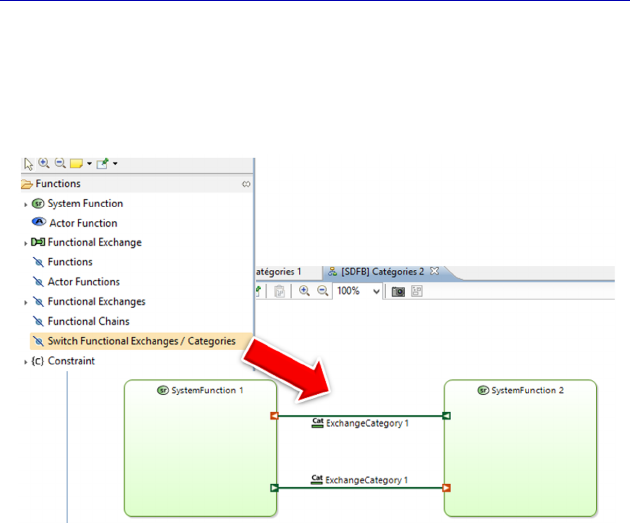
It is then possible to request to visualize the Category instead of the
set of links that it represents, thus simplifying the diagram in question.
This is done through the Switch Functional Exchanges/Categories
command in the palette.
Figure 2.26. On demand Category display
The concept of Category is particularly useful at the level of
Physical Architecture in order to synthesize the multiple Physical
Links between two Node Components, connecting pins between
electrical components for example.
2.2.6. Embedded requirements management solution
In the same way that the SysML language [CAS 18] integrates the
concept of Requirement in order to improve traceability between
requirements and design elements or test cases, Capella proposes a
simple embedded solution for managing requirements.
The goal here is obviously not to completely replace a requirement
management tool such as IBM Doors (https://en.wikipedia.org/wiki/
Rational_DOORS), but rather to propose a simple and integrated
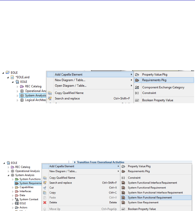
48 Systems Architecture Modeling with the Arcadia Method
alternative for defining requirements that allows them to later be
linked to any model element: Function, Functional Chain, Capability,
etc.
In Capella, first a specific package must be created in the Project
Explorer called Requirements Pkg in order to create Requirements
later.
Figure 2.27. Requirements package creation command
It is then possible to create Requirement-type model elements.
Capella proposes a certain number of predefined variations:
Functional Requirement, Non-Functional Requirement, etc.
Figure 2.28. Requirement creation command
A Requirement created in this way possesses a relatively complete
and specific property sheet, allowing the verification method or the
unique requirement identifier to be specified, for instance. In our
example, we shall create a Requirement at the System level in terms
of the performance of meteorological data acquisition.
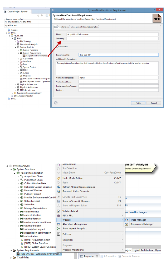
Capella: A System Modeling Solution 49
Figure 2.29. Property sheet of a Requirement
A Capella Requirement can then be linked to either any other
model Requirement (Requirement Manager), or to any model element
(Trace Manager), at any level of Arcadia. This is therefore a very
flexible embedded traceability management solution.
Figure 2.30. Contextual menu for Requirement traceability
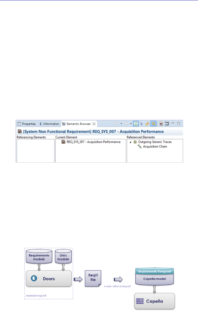
50 Systems Architecture Modeling with the Arcadia Method
In our case study, we might want to link this performance
requirement to:
– the Function “Acquire Weather Data”;
– the Functional Chain “Acquisition Chain”;
– the Capability “Produce Weather Data”;
– the constraint “acquisition max duration”.
All of these model elements are discussed in Chapter 4. As an
example, let us link the Requirement to the acquisition Functional
Chain. The link created by the contextual menu Wizards–Trace
Manager can then be seen in the Semantic Browser.
Figure 2.31. Generic traceability link in the Semantic Browser
A more finalized solution of Requirements management is being
developed and will be available in the near future as a specific
viewpoint (a beta version is already available on the Capella
Website). Notably, this tool will allow us to import a set of existing
requirements from a specialized requirements management tool such
as Doors, using the standardized format ReqIF.
Figure 2.32. Future Requirements viewpoint
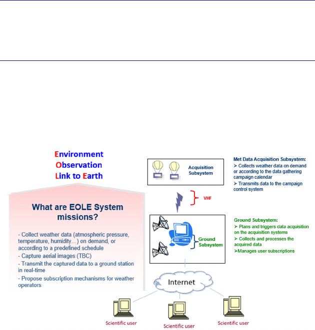
3
Complete Example of Modeling with
Capella: Operational Analysis
3.1. Presentation of the case study and project creation
3.1.1. Presentation of the EOLE case study
Figure 3.1. Simplified specifications of the “EOLE” system

52 Systems Architecture Modeling with the Arcadia Method
The example used to illustrate the main aspects involved in putting
Capella into practice is “EOLE”, a sounding weather balloon system,
whose main goal is to provide meteorological data for various
scientific users.
Although simple, the EOLE system is, nonetheless, representative
of the issues regarding systems engineering due to its:
– multiple stakeholders and user types;
– different types of components (hardware, software, etc.);
– different types of functional and non-functional requirements.
This same case study has been used since 2008 to illustrate the
Thales University’s own training programs, quickly thrusting the
trainees into concrete situations.
It is also used in Capella training programs organized by PRFC
(www.prfc.fr/formation/capella-in-action/). More than 120 training
sessions have been successfully delivered, consolidating the
pedagogical value of the “EOLE” case study over the years.
The reader can obtain more information on the subject on
Wikipedia: en.wikipedia.org/wiki/Weather_balloon.
NOTE.– The purpose of this book is not to provide an ideal
“correction” for this case study in terms of its execution, but rather to
illustrate the main possible uses of the Capella tool and the underlying
Arcadia method. The modeling process that we shall go through
together is therefore strongly influenced by this teaching objective. Do
not forget that a good model is a model that provides satisfactory
answers to predefined questions.
3.1.2. Creation of the EOLE project
Once Capella has been started, there are two ways to create a new
project. The first involves using the Welcome window and clicking on
New Capella Project.
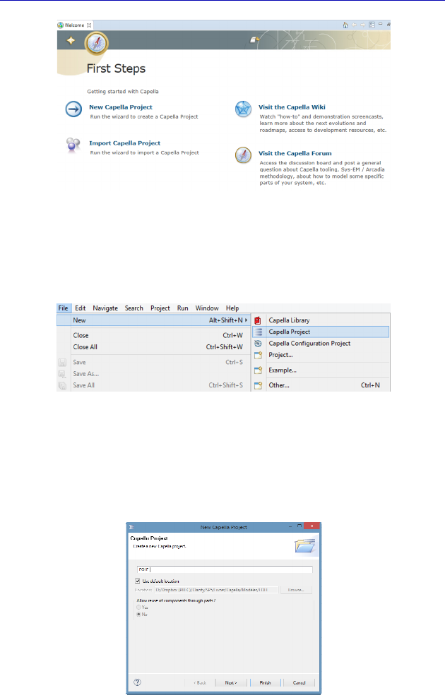
Complete Example of Modeling with Capella: Operational Analysis 53
Figure 3.2. Welcome window on opening Capella
The second way involves activating the same command by going
through the File menu in the toolbar on top.
Figure 3.3. Creation of a new project through the “File” menu
The project must then be named, avoiding names already taken in
the same workspace, and possibly changing the directory where it is
stored (by unticking Use default location).
Figure 3.4. First window in new project creation
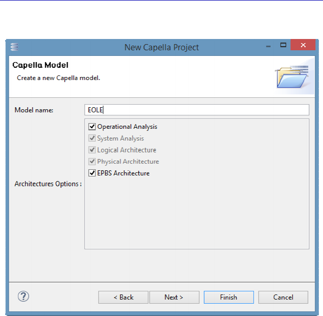
54 Systems Architecture Modeling with the Arcadia Method
Then click on Next > to select the desired Arcadia levels.
Figure 3.5. Second window in new project creation
All levels are selected by default. Only the first (Operational
Analysis) and the last level (EPBS) are optional in the tool. This is
because realization links can only be established between two
successive levels. Click on Finish to finalize creation of the model.
N
OTE
.– Even if the Logical Architecture is optional in the Arcadia
method, it is not with the Capella tool. To overcome this issue, the
tool offers automatic transitions that allow the Logical level to be
initialized from the System level in a few clicks.
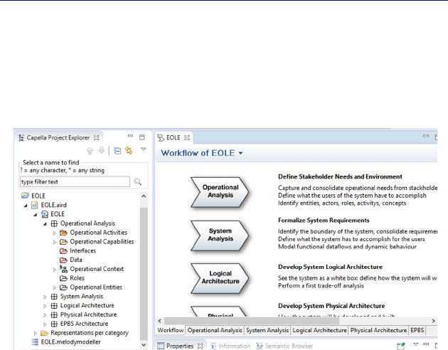
Complete Example of Modeling with Capella: Operational Analysis 55
The model obtained in this way contains a first level of folders that
correspond to the selected engineering levels. Next, each level
contains subfolders for their major concepts. For example, at the
Operational Analysis level there are folders for Activities,
Capabilities, Entities, etc.
Figure 3.6. Result of the creation of a new project
The engineering levels and corresponding activities are also
recalled in the main window where the diagrams are shown, with an
Activity Explorer type diagram created automatically. In this case, it is
called “Workflow of EOLE”.
3.2. Operational Analysis
3.2.1. Main concepts and diagrams
Capella has an integrated methodological guide in the form of the
Activity Explorer. This lists the various activities and the different
diagrams that can be produced at the relevant engineering level, which
in this case is Operational Analysis. Figures 3.7–3.9 first state these
activities, and then the possible diagrams.
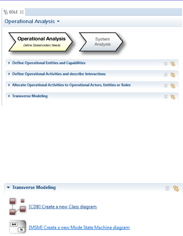
56 Systems Architecture Modeling with the Arcadia Method
Figure 3.7. Methodological activities of the “Operational Analysis” level
We shall not discuss the Transverse Modeling group at this level,
which contains the Mode and State diagrams, as well as the Class
diagrams for data modeling. This methodological activity exists at
each Arcadia level (except EPBS), hence the name of Transverse
Modeling. We shall make the most of System Analysis to look at this
further.
Figure 3.8. “Transverse” Capella diagrams
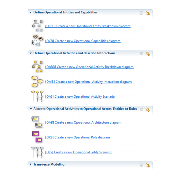
Complete Example of Modeling with Capella: Operational Analysis 57
Figure 3.9. Capella diagrams at the “Operational Analysis” level
N
OTE
.– Although Arcadia is a method, the modeling process is
completely flexible. The methodological activities presented in the
Activity Explorer are nearly all optional and can be carried out in any
order, and this is also the case for the diagrams.
We are therefore going to make an arbitrary but reasoned choice
for the realization of diagrams at each level of engineering. Here, we
shall start by defining high-level objectives, called Operational
Capabilities. We shall provide details regarding these Capabilities
through a network of Operational Activities that exchange
Interactions. Next, we will complete the analysis by allocating the
Activities to Operational Entities. Last, we shall discuss additional
concepts, such as Operational Scenarios, Operational Processes, etc.
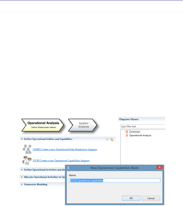
58 Systems Architecture Modeling with the Arcadia Method
3.2.2. Operational Capabilities and Entities
Operational Analysis involves carrying out domain modeling, often
called business modeling, independently of the future system to be
realized. The idea is to voluntarily break from the system under study,
by going back up a level, in order to return to the “real” needs of the
various stakeholders.
How can this need be characterized synthetically in the domain of
meteorology? We can start by identifying Operational Capabilities, for
example: “Produce Meteorological Data” and “Forecast Weather”,
which has surely been the ultimate goal for millennia.
To do this, we create an OCB (Operational Capabilities Blank).
Figure 3.10. Creation of an Operational Capability Blank (OCB) diagram
The diagram created is empty by default (Blank). It allows not only
for the creation of Operational Capabilities, but also of Operational
Entities and Actors, and the numerous relations between them. Let us
start with the two Operational Capabilities mentioned above. We can
link them to entities/actors of the domain as they are discovered. For
example, the Capability, “Forecast Weather” involves an Operational
Actor “Forecaster”; “Produce Meteorological Data” involves a
“Weather Operator”. Note that for the moment the goal is not to be
exhaustive, and we shall return to the diagram later.
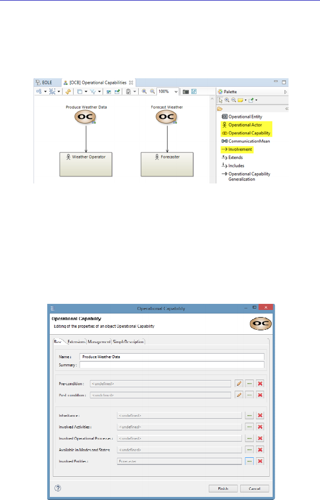
Complete Example of Modeling with Capella: Operational Analysis 59
N
OTE
.– The modeling process is intrinsically iterative and incremental.
The different types of diagrams allow the subject to be tackled from
other viewpoints: concepts discovered in one diagram allow others to
be completed.
Figure 3.11. First version of the Operational Capability Blank (OCB) diagram
If we open the property sheet of an Operational Capability (OC),
we see that it can be linked to other concepts such as Activities,
Processes, Modes and States, etc. The Involved Entities field has
automatically been filled in by Capella as a result of the relations
(involvement) created in the diagram.
Figure 3.12. Property sheet of an Operational Capability (OC)
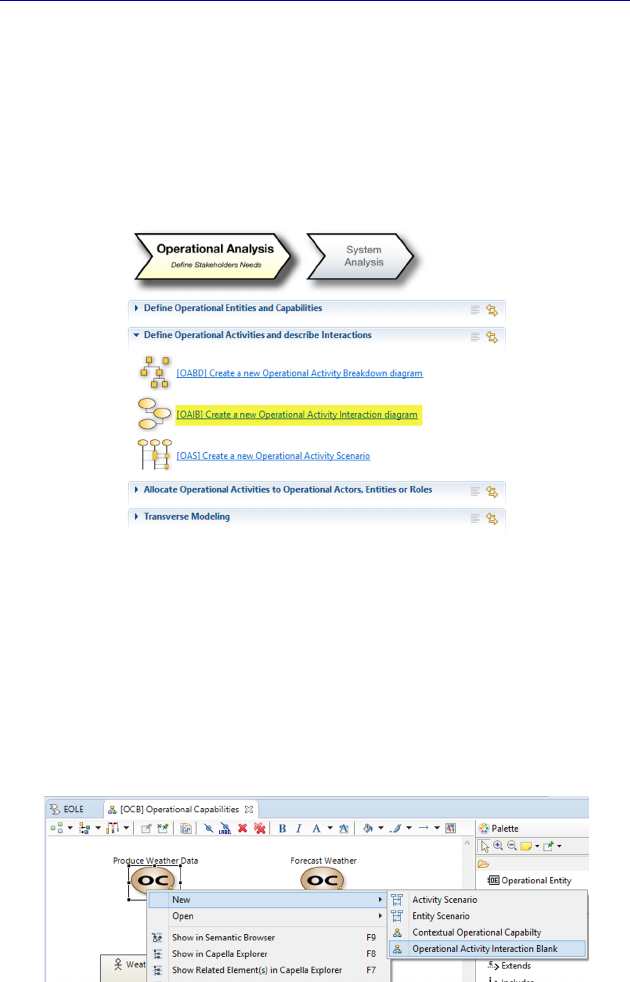
60 Systems Architecture Modeling with the Arcadia Method
3.2.3. Operational Activities and Interactions
For each OC, we shall create a set of Activities linked together by
Interactions. The type of diagram chosen is a Data Flow diagram
between Activities, called OAIB (Operational Activity Interaction
Blank). However, it is also possible to proceed in a different manner,
for example by describing Operational Scenarios instead.
Figure 3.13. Creation of a diagram showing Operational Activities
and Interactions (OAIB)
It is not always necessary to go through the Activity Explorer in
order to create a new diagram. In this case, we could have created a
contextual diagram by right clicking on an OC. The advantage is that
the diagram created in this way automatically takes on the name of the
Capability, instead of the default name.
Figure 3.14. Creation of an OAIB diagram through the contextual menu
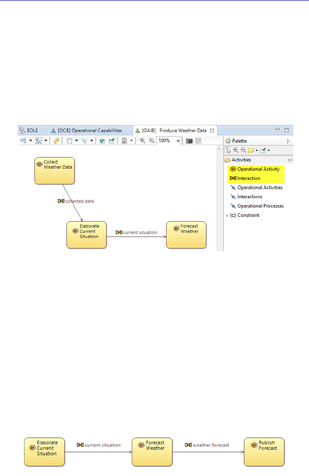
Complete Example of Modeling with Capella: Operational Analysis 61
The diagram created is empty by default (Blank). It allows us to
create Operational Activities, as well as the Interactions that link
them.
We can thus create a first series of Activities, with inputs and
outputs that link them, as in the figure below. This could be the result
of a preliminary work meeting with experts in the domain, for
example.
Figure 3.15. First version of the contextual OAIB with
the Capability “Produce Weather Data”
N
OTE
.– An Interaction can only be shown on a diagram if its target
and source Activities are present. This is why we have shown the
Activity “Forecast Weather” in the first diagram, to show the output
“current situation”, even though this Activity is clearly the central
Activity of the other OC. Let us not forget that one modeling element
can easily appear in several diagrams.
We do the same for the second Capability by adding a new activity
“Publish Forecast”.
Figure 3.16. Contextual OAIB with the Capability “Forecast Weather”
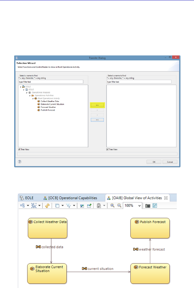
62 Systems Architecture Modeling with the Arcadia Method
It is then very easy to create a third OAIB, this time from the
Activity Explorer, bringing together all of the Activities. These only
need to be inserted into the empty diagram using the palette command
Insert/Remove Operational Activities by pressing on the Add all
elements button.
Figure 3.17. Insertion of all Operational Activities in a global OAIB
Figure 3.18. Global OAIB obtained by insertion of all Operational Activities
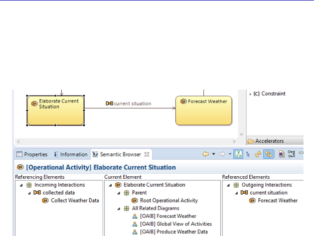
Complete Example of Modeling with Capella: Operational Analysis 63
In order to visualize the diagrams in which each modeling element
does or does not appear, the most efficient way is always to go via the
Semantic Browser. If, for example, we select the Activity “Elaborate
current situation”, we can see that it is represented graphically in the
three OAIB.
Figure 3.19. Activity selection in the Semantic Browser
3.2.4. Allocation of Activities to the Operational Entities
Capella offers a feature of methodological verification through its
validation rules. A first opportunity to put this into practice is already
available here: Activities (just like Functions at the lower levels) must
be allocated to structural elements, which in Operational Analysis is to
Operational Entities or Actors.
There are several verification methods available to us. We can ask
for the complete validation of the model, of an engineering level or
even of only a folder of the project explorer, by right clicking.
The results of the validation are then shown as requested by type in
the Information window, located beside the Semantic Browser and
below the diagrams, after clicking OK on the pop-up window of the
Validation Problems. The rules folders must be opened progressively
in order to show the results in detail.
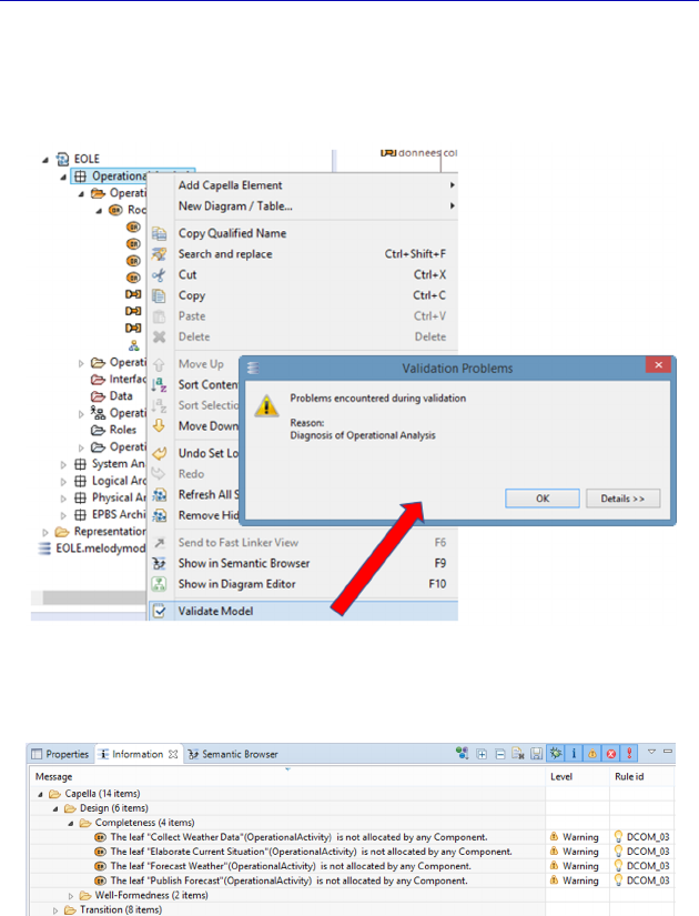
64 Systems Architecture Modeling with the Arcadia Method
Here, we will only look at the group called Completeness, which
informs us that the four Activities are not allocated to any structural
element.
Figure 3.20. Application of the command “Validate Model” in the Project
Explorer at the Operational level
Figure 3.21. Results from the validation of the Operational Activities
All of the validation rules are accessible via the menu Window –
Preferences – Model Validation – Constraints – Capella. These can
be turned on or off one by one or by group.
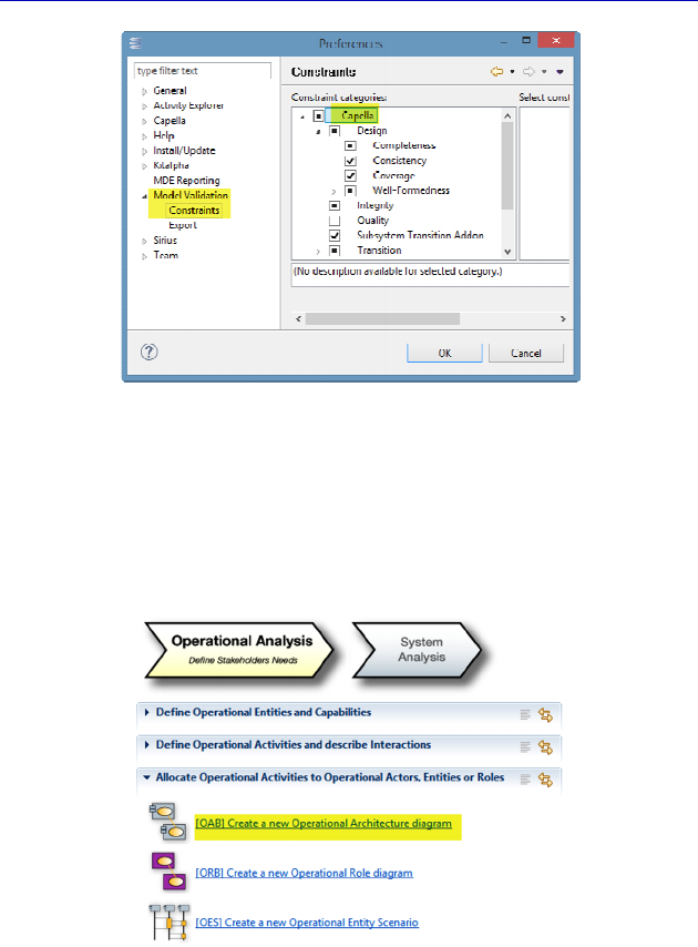
Complete Example of Modeling with Capella: Operational Analysis 65
Figure 3.22. Capella validation rules
In order to allocate the Activities, we create a particular type of
diagram, which is probably the most important type at each level of
engineering: an Architecture Blank diagram (xAB). This is therefore
here an Operational Architecture Blank (OAB).
Figure 3.23. Creation of an Operational Architecture Blank (OAB) diagram
The diagram created is empty by default (Blank). It allows for both
Operational Entities and/or Actors, as well as Activities, to be created,
and for the allocation of Activities to Entities to be managed.
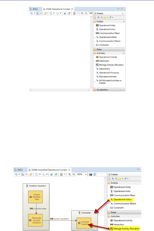
66 Systems Architecture Modeling with the Arcadia Method
Figure 3.24. Palette of the Operational Architecture Blank (OAB) diagram
At each level of Arcadia, this is the type of diagram that offers the
most complex palette. Even when hiding the Roles group (an
advanced concept that we will not use) and the Accelerators group,
there are many other commands left in the palette.
We first insert the Entities/Actors already created during the
Operational Capabilities diagram. Next, we allocate to them the
obvious Activities, using the Manage Activity Allocation button.
Figure 3.25. Start of the Operational Architecture Blank (OAB) diagram. For a
color version of the figure, see www.iste.co.uk/roques/arcadia.zip
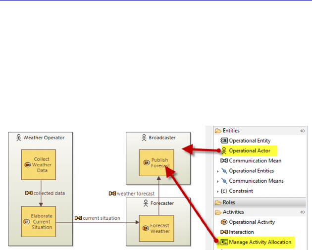
Complete Example of Modeling with Capella: Operational Analysis 67
N
OTE
.– It is worth noting that existing Interactions only appear if the
target and source Activities are already present in the diagram (and the
Unsynchronized property has not been ticked).
We still need to allocate the activity “Publish Forecast”, but to do
this we need to create a new Operational Actor, the “Broadcaster”, as
this is a different job profile from the forecaster and the weather
operator.
Figure 3.26. Follow-on of the Operational Architecture Blank (OAB) diagram.
For a color version of the figure, see www.iste.co.uk/roques/arcadia.zip
Furthermore, we also want to show that these three profiles all
belong to the same organization: “Weather Services Provider”. To do
this, we create an Operational Entity that can contain the three Actors.
The containment relation is created by sliding them around in the
rectangle of the Entity. We also add an Operational Actor that does
not belong to the same organization, who will use the forecasts. To
finish off, we can add a final Operational Entity that represents the
Earth’s atmosphere and which provides the environmental conditions.
N
OTE
.– The physical environment is often an important Actor at the
System Analysis level, but should not be forgotten in Operational
Analysis.
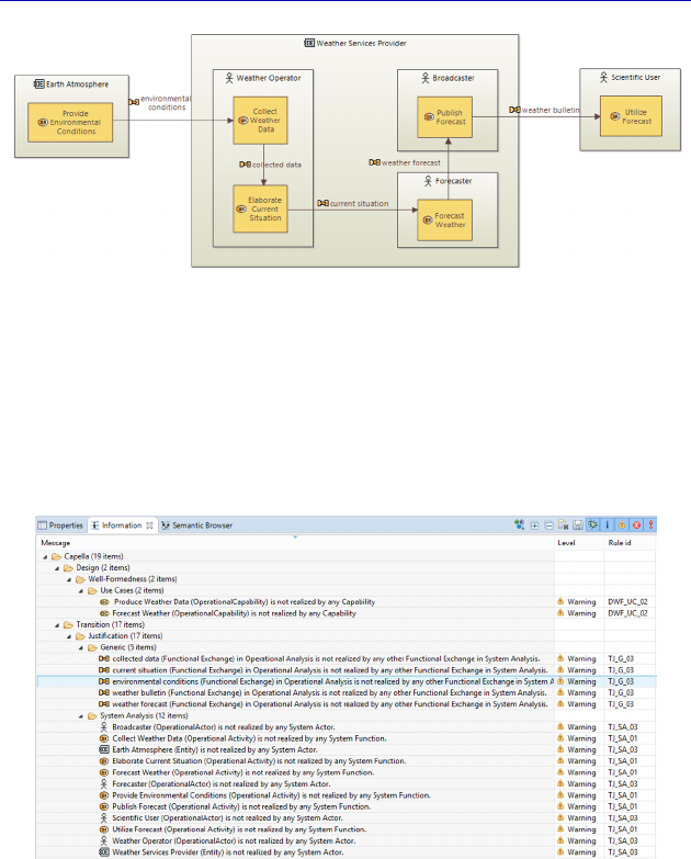
68 Systems Architecture Modeling with the Arcadia Method
Figure 3.27. Remainder and end of the Operational Architecture
diagram (OAB). For a color version of the figure, see
www.iste.co.uk/roques/arcadia.zip
We can now make sure that the model validation is only issuing
“transition warnings”, relating to missing realization links with future
elements of System level.
Figure 3.28. Results from the validation of the Operational Analysis
3.2.5. Additional diagrams and concepts
In this section, we shall introduce two new types of diagrams. First,
a breakdown diagram, of which there can be two types in Operational
Analysis: an Activity Breakdown diagram (OABD) or an Entity
Breakdown diagram (OEBD).
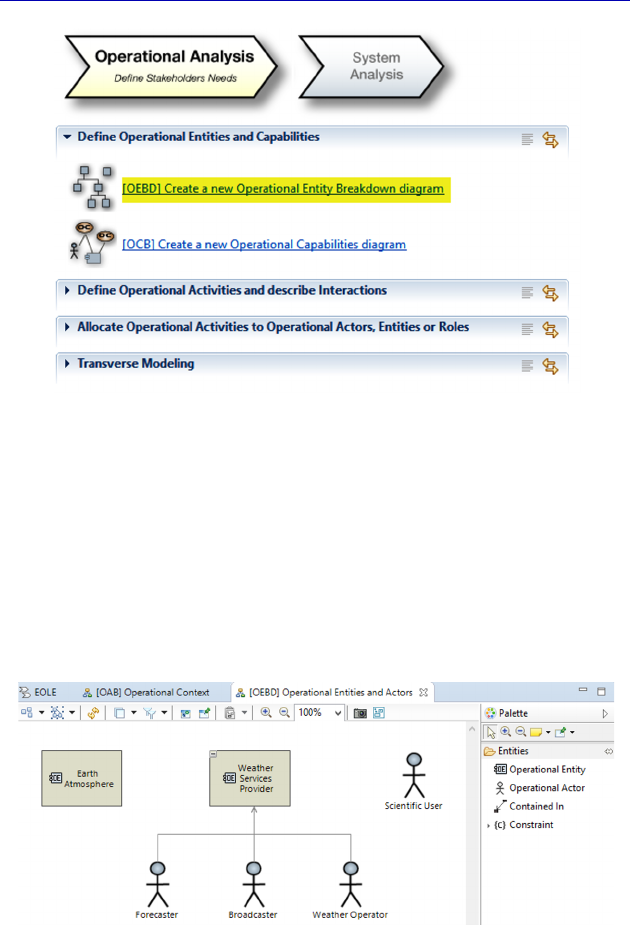
Complete Example of Modeling with Capella: Operational Analysis 69
Figure 3.29. Creation of an Entity Breakdown diagram (OEBD)
For our case study, there was no need to break down the Activities
into subactivities. However, we wanted to introduce an Operational
Entity that tied together a number of Operational Actors, which is
often the case when modeling an organization. As a result, if we ask
Capella to produce the breakdown diagram of the entities (OEBD –
Operational Entity Breakdown) after making our OAB, the OEBD is
generated and updated automatically.
Figure 3.30. Breakdown diagram of the Operational Entities (OEBD)
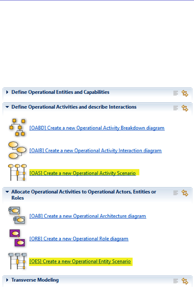
70 Systems Architecture Modeling with the Arcadia Method
The palettes of breakdown diagrams are the simplest in Capella.
They only allow for the creation of one particular type of modeling
element (with possible variation, such as Entity/Actor in this case) and
only the containment relation.
The second type of diagram that we shall introduce is now called a
Scenario. In Operational Analysis, there can be two types of Scenario
diagram: diagrams with the Activities as vertical lines (OAS) or with
the Entities or Actors (OES).
Figure 3.31. The two types of diagram for Operational Scenarios
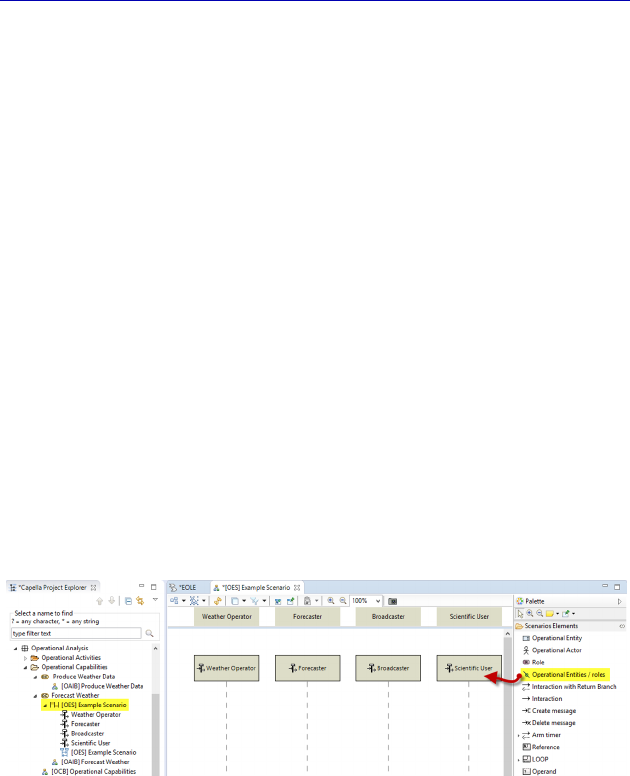
Complete Example of Modeling with Capella: Operational Analysis 71
In order to illustrate our understanding of the domain, let us take
the example of an OES. This way, we can show the process
represented in the Data Flow or Architecture diagrams, but focusing
more on the chronological aspects.
N
OTE
.– A Scenario diagram is linked to a Scenario type model
element in Capella, which is itself always tied to a Capability.
When we create an OES, Capella makes us choose to which
Capability to link it. Let us choose the OC “Forecast Weather”, for
example. The Scenario diagram is very powerful and close to the
UML/SysML sequence diagram. The palette therefore offers a very
large number of possible commands.
We start by inserting Operational Actors we are interested in. We
could also create new ones if any were missing.
Next, we choose the type of messages that are passed along the
vertical lines. These can correspond to Interactions, which is the most
intuitive, but they can also reference communication means, or
“timers”, etc. We choose to use existing Interactions.
Figure 3.32. Start of Scenario diagram (OES)
We can also represent the execution of the Activities along the
vertical lines to which they are allocated, using the command
Insert/Remove Activity from the palette.
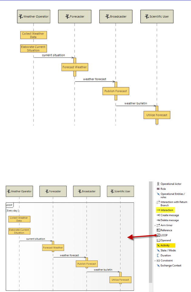
72 Systems Architecture Modeling with the Arcadia Method
Figure 3.33. Follow-on of the Scenario diagram (OES)
In order to illustrate what can be expressed by the Scenario
diagram, we can add a LOOP Fragment, which indicates that the
process represented is repeated every day.
Figure 3.34. Remainder and end of the Scenario diagram (OES). For a color
version of the figure, see www.iste.co.uk/roques/arcadia.zip
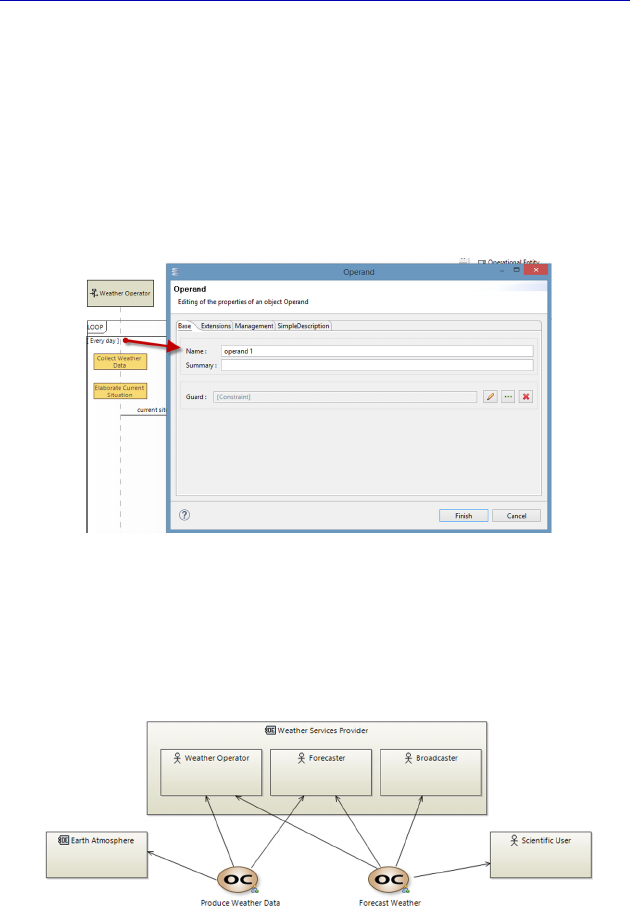
Complete Example of Modeling with Capella: Operational Analysis 73
N
OTE
.– To edit the loop condition, first the Operand property sheet
contained within it must be opened, and then we must go to the field
called Guard. In the Guard field, the command represented by the
crayon icon must be activated, called Create a new element. This
opens a new window called Opaque Expression. The body of this
expression is not edited in the Name field, but by clicking on Linked
Text, and by typing text on the right. This is a general mechanism for
entering constraints, which we shall see again later.
Figure 3.35. Editing the Operand property sheet
Following this work, which can be done with a Scenario for the
other OC, we can return to the Capability Blank diagram (OCB) to
show all of the Actors/Entities, and then to add the relevant links.
Figure 3.36. Remainder and end of the Capability Blank diagram (OCB)
Modeling work is fundamentally iterative and incremental!
This page intentionally left blank
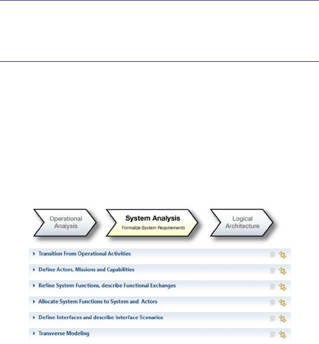
4
Complete Example of Modeling with
Capella: System Analysis
4.1. Main concepts and diagrams
Capella has a methodological guide in the form of the Activity
Explorer. This lists the various activities and diagrams that can be
carried out at the relevant engineering level, which in this case is
System Analysis. Figure 4.1 shows the activities; throughout the case
study we shall describe the different possible diagrams.
Figure 4.1. Methodological activities of the “System Analysis” level
N
OTE
.– Although Arcadia is a method, the modeling process remains
completely flexible. The methodological activities presented in the

76 Systems Architecture Modeling with the Arcadia Method
Activity Explorer are nearly all optional, and can be executed in any
chosen order; the same is true for diagrams.
We shall therefore make another arbitrary – but reasoned – choice
here in terms of the diagram realization. We start by defining high-
level objectives, called System Capabilities. We shall expand on these
Capabilities using Data Flow diagrams between Functions. Next we
shall complete the System Analysis by producing the Architecture
diagram, which involves allocating the Functions to the System or to
the external Actors. We shall finish off the analysis with a description
of the Scenarios, Modes and States, and by starting to model the data.
4.2. Going from the Operational level to the System level
The Operational Analysis shown previously involved creating a
domain model, independently of the future system to be realized. The
idea was to voluntarily create a level of abstraction from the system
under study in order to focus on the “real” needs of the different
stakeholders.
The System Analysis level, on the other hand, requires the
following questions to be answered:
– What must the system do?
– What is the external interface of the system?
In order to answer the first question, the expected behavior is
mainly modeled as Functions. We can obviously also make use of
Scenarios and Mode and State diagrams, if necessary.
In order to answer the second question, all of the external Actors
(human or not) and data/matter flows must be identified. The
Architecture Blank diagram (SAB) will be very useful here for
showing what enters the System from the Actors and what exits the
System via the Actors.
Using all of the Operational Activities identified in Chapter 3
(those represented in the OAB of Figure 3.27, for example), a
systematic approach is to ask whether each Activity will be realized
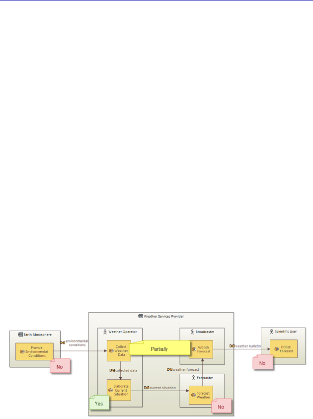
Complete Example of Modeling with Capella: System Analysis 77
by the system in its entirety, partially, or not at all. The result at the
System Analysis level can be formalized as follows:
– entirely: the Activity becomes a Function of the same name,
allocated to the System;
– partially: the Activity must be broken down into several
Functions, some of which are allocated to the System and others to at
least one Actor;
– not at all: the Activity becomes a Function of the same name,
allocated to an Actor.
N
OTE
.– The decision to realize a given Activity is a project decision,
influenced by the client requirements, budget, delays, technical
feasibility, etc. Neither Arcadia nor Capella can make the decision on
the architect’s behalf.
If we apply this principle, starting with the OAB, a project meeting
might lead to the decisions represented in Figure 4.2. Note that we have
decided not to intervene in the forecast itself, which is always carried
out by the forecaster. However, the system will have to provide a
current situation, in the desired format, and recover the forecasts. This
choice therefore entails interface requirements for the future system.
Figure 4.2. Choice of Activity realization by the system. For a color
version of the figure, see www.iste.co.uk/roques/arcadia.zip
To initialize the System level while making the most of the work
carried out at the Operational level, Capella provides a set of very
useful tools, called “Transitions”. These allow us to recover a System
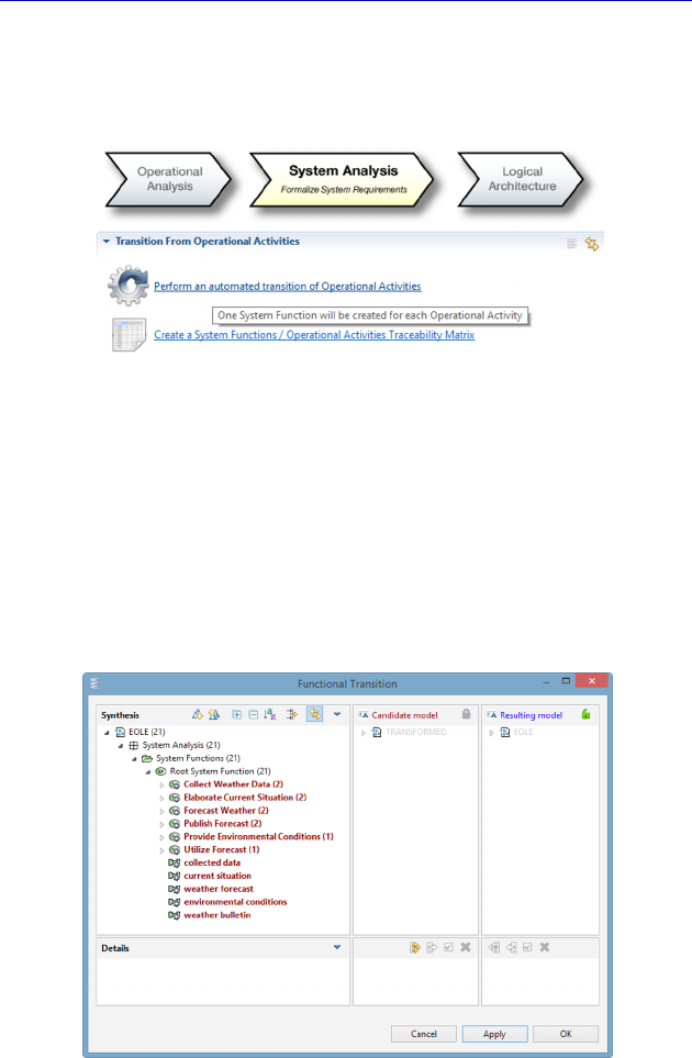
78 Systems Architecture Modeling with the Arcadia Method
level Function from each of the Operational Activities while
maintaining the flows, or an Actor of the System level from each of
the Entities/Actors of the Operational level, etc.
Figure 4.3. Functional transition tool between Operational and System levels
These transition commands can be accessed through the Activity
Explorer, and more precisely in the contextual menu of a folder, or of
a model element in the Project Explorer. The user can control what
the tool creates at the System level with great precision by selecting a
subset of possible elements in a Diff/merge type dialog window. In
simple cases, this can be done by clicking the Apply button to select
and apply everything without making any changes.
Figure 4.4. Dialog window for functional transition
between Operational and System levels
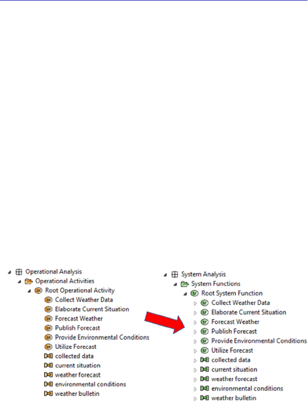
Complete Example of Modeling with Capella: System Analysis 79
N
OTE
.– All of the transitions proposed by Capella are top/down, going
toward the engineering level that is immediately inferior. It must be
noted that the transitions are iterative and incremental, which is very
handy for complex projects. If a System Function, or even an
Operational Activity, is found to be missing during work on the
Physical Architecture, good practice would involve adding the missing
element to the highest relevant level, and then applying several
successive transitions in order to recover the lowest level where it is
missing. The tool does not erase the additions and refinements brought
to the lower levels.
By clicking on Apply, a new window appears, listing all of the
transformations to be carried out on the model. In our case, Capella
creates System level Functions and Functional Exchanges, but also
Function Ports to link the Functional Exchanges. While Operational
Activities do not have ports in order to maximize simplicity, from the
System level onward, Functions possess function input or output
Ports, to which the Functional Exchanges are connected.
Figure 4.5. Result of functional transition in the Project Explorer
In order to check whether Capella has properly created the Ports and
added a realization link to each Activity, we select one of the System
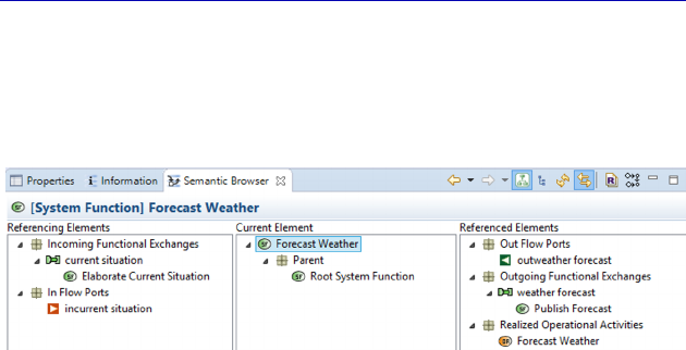
80 Systems Architecture Modeling with the Arcadia Method
level Functions in the Semantic Browser. Here, we can clearly see the
new input and output Ports, as well as the realization link to the
Operational Activity of the same name.
Figure 4.6. Result of functional transition in the Semantic Browser
4.3. System Capabilities
The Operational Analysis above involved creating a domain
model, independently of the future system to be realized. The idea was
to voluntarily create a level of abstraction from the system under study
in order to focus on the “real” needs of the different stakeholders.
Following a project meeting like the one mentioned in section 4.2, we
decide to leave the forecasting activity outside of the system, at least
for the first version.
N
OTE
.– Operational Analysis is useful for referring to the “need” in its
entirety, independently of the realization choices made at any given
moment. This allows opportunities to be identified for subsequent
system versions, i.e. preparing the work of weather forecasting, or even
controlling it fully, as soon as this becomes possible technologically
(computational power, artificial intelligence, etc.).
In our example, System Capabilities are less extensive than
Operational Capabilities in terms of cover. However, here we can also
use a transition command in order to benefit from automatic
realization links.
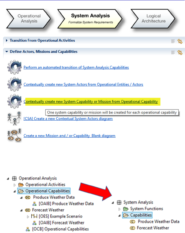
Complete Example of Modeling with Capella: System Analysis 81
Figure 4.7. Transition tool of Capabilities between
Operational and System levels
Figure 4.8. Result of transition of Capabilities in the Project Explorer
Now we only have to rename the second Capability to reduce its
field of action. We can call it: “Broadcast Weather Forecast”. Just like
for the Operational level, we will start by working on the Data Flow
diagrams, here between Functions, called SDFB. This is particularly
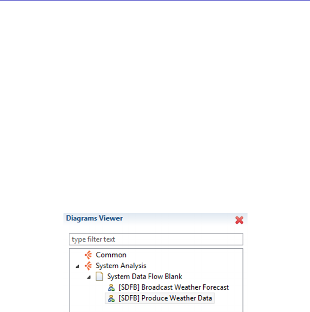
82 Systems Architecture Modeling with the Arcadia Method
important as there are Functions that must be broken down due to
partial allocation to the system.
N
OTE
(Arcadia Rule).– Only “leaf” Functions (those that are not
broken down) can have input/output Ports. As soon as a Function is
broken down into subfunctions, we therefore have to work on the
assignment of Functional Exchanges to the subfunctions of the parent
Function.
Let us create two contextual diagrams, one for each System
Capability, through the contextual menu in the Project Explorer (New
Diagram/Table… System Data Flow Blank). Note that this way, the
diagram automatically takes on the name of each Capability. This can
be checked in the Diagrams Viewer, on the right of the Activity
Explorer window.
Figure 4.9. Result of the creation of diagrams in the Diagram Viewer
4.4. Functional Analysis at the System level
For the first Capability, “Produce Weather Data”, the central
Function is “Collect Weather Data”. Instead of manually inserting the
Functions that can be chosen using the palette’s Insert/Remove
Functions button, we can instead ask Capella to automatically create
the SDFB by inserting the Function, as well as all those connected to
it. To do this, the diagram must be made contextual to the chosen
Function using a property field of the diagram: Contextual Elements.
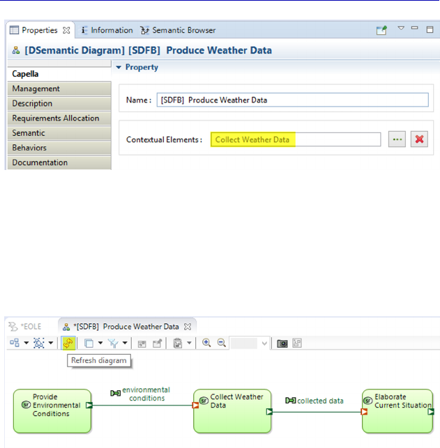
Complete Example of Modeling with Capella: System Analysis 83
Figure 4.10. Diagram made contextual to a chosen Function
Asking Capella to refresh the diagram (F5 key or Refresh diagram
button from the top bar) will automatically fill the diagram. After a
couple of quick touches to improve the graphical representation, we
obtain Figure 4.11.
Figure 4.11. Result of refreshing the contextual diagram. For a color
version of the figure, see www.iste.co.uk/roques/arcadia.zip
N
OTE
.– As opposed to a classical Blank, the contextual diagram is
updated automatically. In particular, as soon as a new Function has
additional Exchanges with “Collect Weather Data”, it automatically
appears in this contextual SDFB, which it would not have otherwise.
We must now keep up our work by breaking down the “Collect”
Function and by working on the Functional Exchanges, since only leaf
Functions can have Ports. This is the only case where we recommend
changing the fill color of a Function: for broken down Functions, we
recommend changing them to white in order to differentiate them
properly.
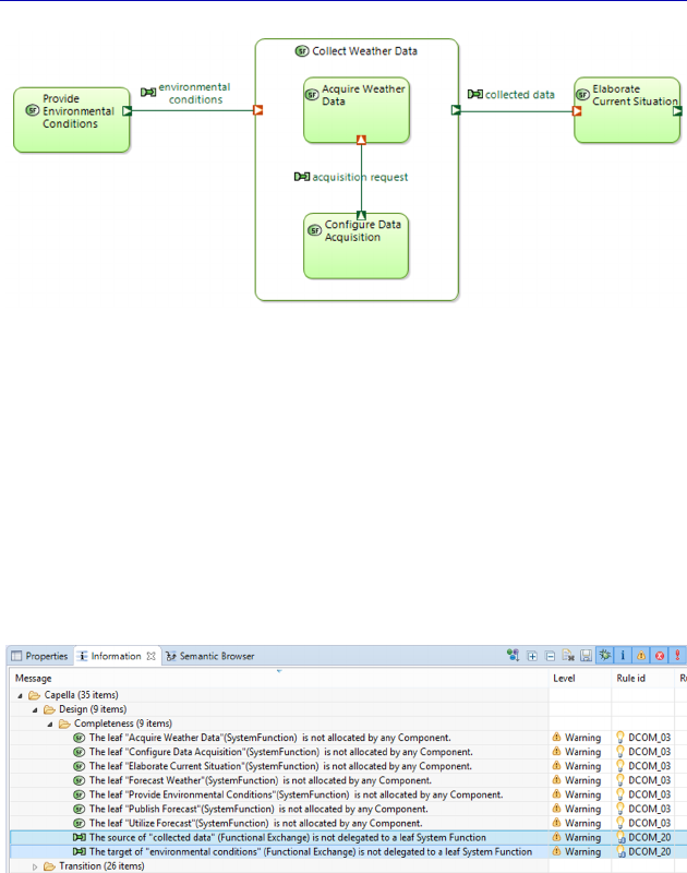
84 Systems Architecture Modeling with the Arcadia Method
Figure 4.12. Start of functional breakdown. For a color version
of the figure, see www.iste.co.uk/roques/arcadia.zip
Just after the first breakdown step, we must check that the model
validation highlights the expected errors. As anticipated, there are
transition warnings, marking that the elements of the System level
have not been realized by the elements of the Logical Architecture
level. There are also warnings telling us that the Functions have not
yet been allocated. There are two new warnings regarding the Ports of
the parent Function that must be delegated to its subfunctions.
Figure 4.13. Results of validation after the start of functional breakdown
The model becomes correct simply by moving the Ports of the
parent Function toward subfunction “Acquire”.
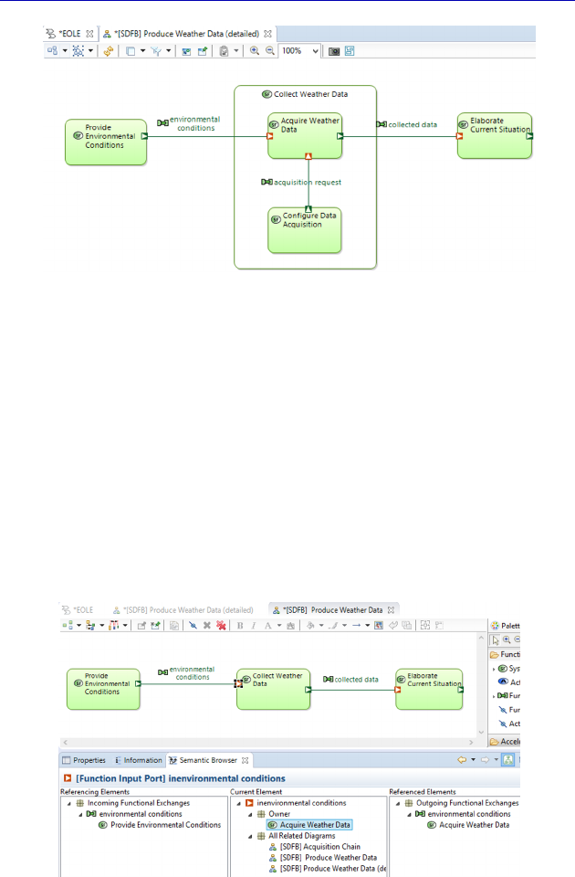
Complete Example of Modeling with Capella: System Analysis 85
Figure 4.14. End of functional breakdown on SDFB. For a color
version of the figure, see www.iste.co.uk/roques/arcadia.zip
An advantage of Capella is that it allows the modeler to keep
showing the parent Function without its subfunctions on a higher level
diagram, aimed at a different audience. This can be achieved by
cloning the diagram (from the Diagrams Viewer) and using the
Insert/Remove Functions button of the palette inside the parent
Function. Capella then shows the Ports of the subfunctions on the
boundary of the parent Function. The model is unchanged, as it is only
a calculated graphical representation. This can be verified by the
activating the Semantic Browser.
Figure 4.15. SDFB showing higher level view (without subfunctions). For a
color version of the figure, see www.iste.co.uk/roques/arcadia.zip
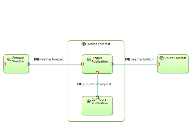
86 Systems Architecture Modeling with the Arcadia Method
In a similar fashion, let us make a second contextual SDFB around
the second Function to be broken down: “Publish forecast”.
Figure 4.16. Second functional breakdown diagram. For a color
version of the figure, see www.iste.co.uk/roques/arcadia.zip
N
OTE
.– Note that these two SDFB diagrams involve different
Functions. In the free version of Capella, only one person can modify
the model at any given moment: the tool is said to be a “single user”
tool. A multiuser version also exists: Team for Capella [BON 16],
which is distributed by Obeo (www.obeo.fr/en/capella-professional-
offer). This version would have allowed us to create both diagrams in
parallel in the same model.
Note also that the appearance of a Function in the functional
diagram attached to a Capability implies the automatic creation of a
semantic exploitation link between this Function and the Capability.
The Involved Functions field in the properties field of a Capability is
thus filled automatically by Capella, and the link can be seen in the
Semantic Browser.
We will now create a third SDFB that gathers together all of the
leaf Functions in order to visualize the System level global data flow.
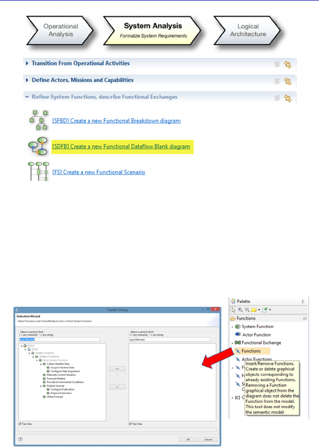
Complete Example of Modeling with Capella: System Analysis 87
Figure 4.17. Creation of a new Data Flow diagram (SDFB)
This can be achieved with only a few clicks with Capella. Once the
empty diagram has been created using the Activity Explorer, we insert
all of the leaf Functions into the diagram using the Selection Wizard of
the transfer dialog.
Figure 4.18. Insertion of all leaf Functions in the global SDFB
We use the double arrow to move all of the Functions to the right,
and then move the two broken-down Functions back to the left.
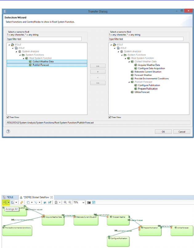
88 Systems Architecture Modeling with the Arcadia Method
Figure 4.19. Removing the non-leaf Functions in global SDFB
Activating the Arrange Selection command in all of the graphical
objects present in the diagram, or using the Arrange All command,
immediately results in a usable diagram.
Figure 4.20. Initial version of global SDFB. For a color version
of the figure, see www.iste.co.uk/roques/arcadia.zip
Resizing the Functions and slightly moving the ports quickly
provides us with a graphical oversight that we can work with. In the
meantime, we can check that there are not unused Ports, as the
diagram is no longer partial, unlike the two previous ones.
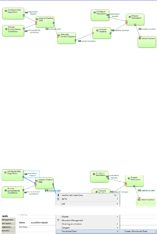
Complete Example of Modeling with Capella: System Analysis 89
Figure 4.21. Improved version of global SDFB. For a color version
of the figure, see www.iste.co.uk/roques/arcadia.zip
4.5. Functional Chains at the System level
Functional data flow refers to all of the dependencies that exist
between Functions. A Functional Chain represents a set path in this
global data flow. It is particularly useful for describing the expected
behavior of the system in a given context, and therefore for piloting
verification/validation tests. Functional Chains are also often used to
express non-functional constraints in functional paths, such as latency,
criticality, confidentiality, redundancy, etc.
To create a Functional Chain with Capella, a succession of
Functional Exchanges must be selected (the source and target
Functions are selected implicitly), and then the contextual menu must
be activated.
Figure 4.22. Creation of a Functional Chain in an SDFB. For a color
version of the figure, see www.iste.co.uk/roques/arcadia.zip
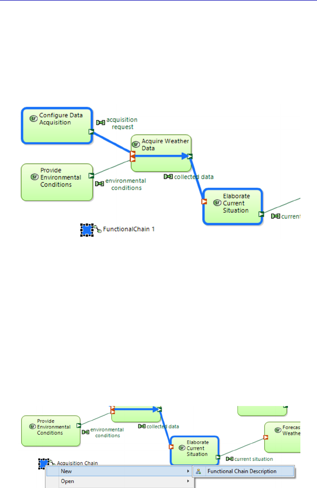
90 Systems Architecture Modeling with the Arcadia Method
This results in both a new modeling element, represented by a
square and called FunctionalChain 1, and graphical additions to the
data flow. The source Function is surrounded, as is the target
Function, and arrows are added between the input and output Ports of
the intermediate Functions in order to materialize the direction of the
selected path.
Figure 4.23. Results of the creation of a Functional Chain. For a color
version of the figure, see www.iste.co.uk/roques/arcadia.zip
Note that the Functional Chain can be found in the Project
Explorer under the technical element Root System Function, at the
same level as the System Functions.
To modify an existing Functional Chain, a specific contextual
diagram, called a Functional Chain Description, must be used. This
diagram can be created with a right click of New Diagram/Table on
the square, or on the element in the Project Explorer.
Figure 4.24. Contextual creation of a Functional Chain Description diagram.
For a color version of the figure, see www.iste.co.uk/roques/arcadia.zip
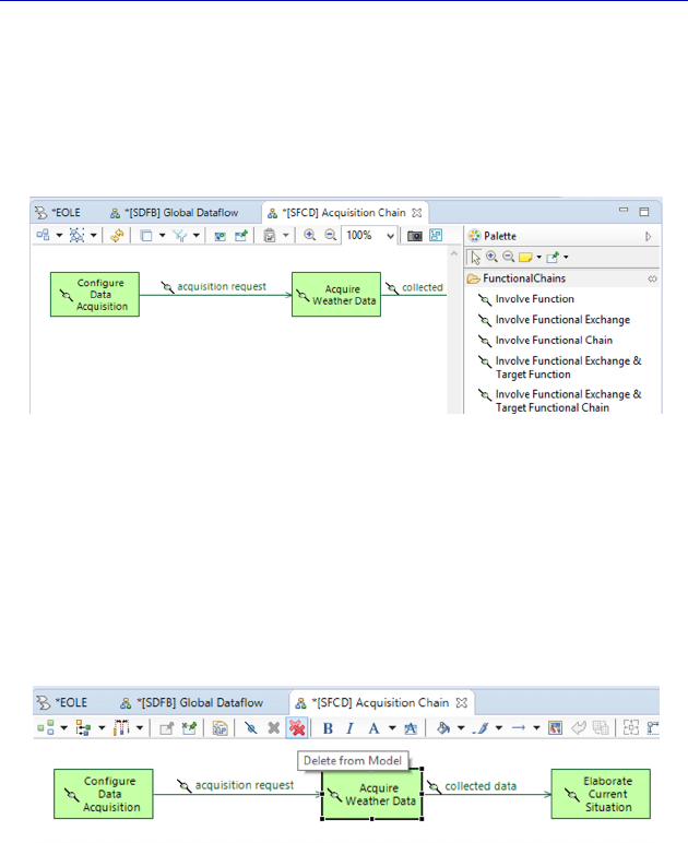
Complete Example of Modeling with Capella: System Analysis 91
The diagram obtained is quite unique. It is always synchronized
with the current state of the Chain’s definition in the model. The
model elements present in the diagram are not themselves Functions
and Functional Exchanges, but rather references to these elements,
called Functional Chain Involvement.
Figure 4.25. Description diagram of a Functional Chain. For a color
version of the figure, see www.iste.co.uk/roques/arcadia.zip
We can therefore add or remove “links” in order to modify the
Chain. Let us take a look at what happens if we destroy the central
link of the acquisition Chain. To do this, the command Delete From
Model must be applied to the Functional Chain Involvement called
“Acquire”.
Figure 4.26. Destruction of a link in an FCD. For a color version
of the figure, see www.iste.co.uk/roques/arcadia.zip
N
OTE
.– The command Delete From Diagram is not active in this type
of diagram, just like in the Blank. As the diagram is still synchronized,
the elements would automatically reappear when it is opened again. The
confirmation window following Delete From Model shows that it is
indeed the links that are being destroyed, and not the Functions or
Exchanges.
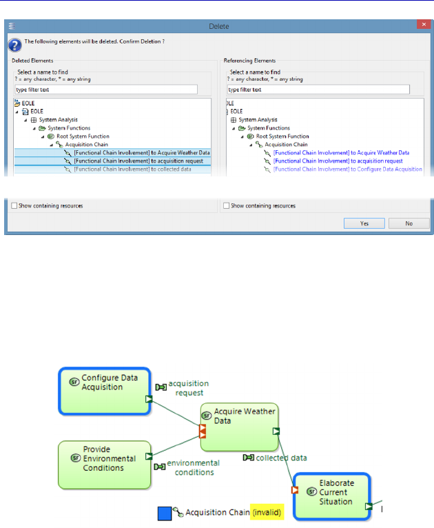
92 Systems Architecture Modeling with the Arcadia Method
Figure 4.27. Delete from model in an FCD
By opening the global SDFB, we can see that the Functional Chain
has automatically been updated. Moreover, the tool clearly shows that
the chain is now invalid.
Figure 4.28. Invalid Functional Chain shown in an SDFB. For a
color version of the figure, see www.iste.co.uk/roques/arcadia.zip
Using the command Undo, we can return to the previous, valid,
state of the Functional Chain. In fact, we want to add the Function
“Provide Env. Conditions” and the associated Exchange at the
entrance to the Chain. To do this, the Function must first be added to
the Chain using the command Involve Function, and then the
Exchange is added using the command Involve Functional Exchange.
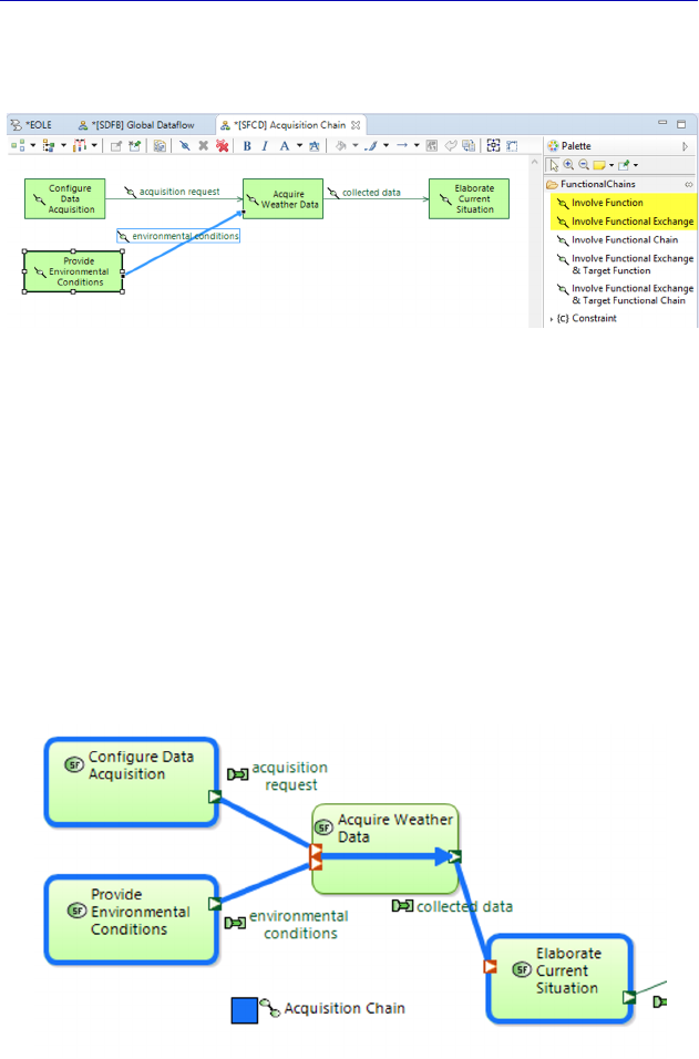
Complete Example of Modeling with Capella: System Analysis 93
Note that the tool only proposes Exchanges that already exist in the
model.
Figure 4.29. Adding links to an FCD. For a color version
of the figure, see www.iste.co.uk/roques/arcadia.zip
N
OTE
.– A link in a Functional Chain can be another Functional Chain.
Use the Involve Functional Chain command to insert an existing Chain
into a new overarching Chain. This approach is very useful in bottom-
up assembly of reusable Physical Components that have their own
simple Chains and contribute to the creation of a composite Functional
Chain.
Going back to the Data Flow diagram, we can see that the
Functional Chain has automatically been updated.
Figure 4.30. Modified Functional Chain updated in the SDFB. For a color
version of the figure, see www.iste.co.uk/roques/arcadia.zip
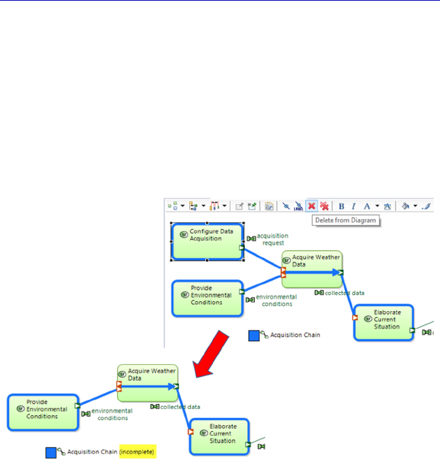
94 Systems Architecture Modeling with the Arcadia Method
N
OTE
.– We have seen that a Functional Chain can become invalid
following the modification of its constituent model elements. It can also
appear as incomplete in a diagram, for example if the command Delete
From Diagram is applied to one of its links. Remember that the
command Delete From Diagram does not modify the model, but acts
only on the graphical objects present in the current diagram.
Removing one of the chain’s functions from the previous SDFB
causes the tool to consider it incomplete, after a Refresh Diagram.
Figure 4.31. Incomplete Functional Chain shown in an SDFB. For a color
version of the figure, see www.iste.co.uk/roques/arcadia.zip
We will also create a second Functional Chain, involving
publication this time. The two Chains can appear in the same diagram.
It can often be useful to create one Data Flow diagram per
Functional Chain for the purpose of documentation. Instead of
manually inserting the Functions and Exchanges that participate in a
given Chain, Capella allows us to automatically create this type of
diagram by using a command from the palette of the group
Accelerators called Functional Chain Elements. After choosing the
Chain involved in the selection dialog, the command Arrange
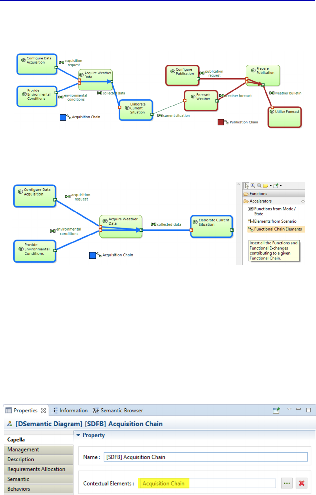
Complete Example of Modeling with Capella: System Analysis 95
Selection is applied, and Capella produces the minimal diagram
containing only the elements that belong to the Chain.
Figure 4.32. SDFB showing two Functional Chains. For a color
version of the figure, see www.iste.co.uk/roques/arcadia.zip
Figure 4.33. SDFB of a Functional Chain created automatically by an
Accelerator. For a color version of the figure, see
www.iste.co.uk/roques/arcadia.zip
N
OTE
.– If we want the diagram to be updated when the Functional
Chain is modified, we must remember to make it contextual by once
again using Contextual Elements. Otherwise, seeing as the diagram
involved is a Blank, any new Functions involved in the chain will not be
shown automatically.
Figure 4.34. SDFB of a Functional Chain made contextual
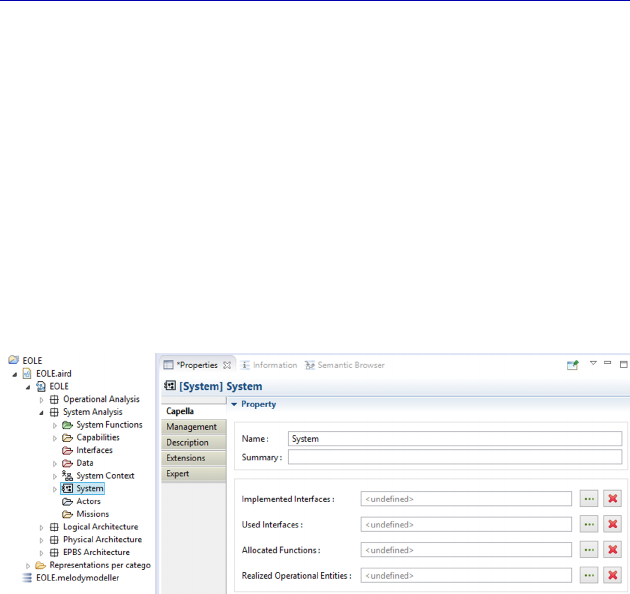
96 Systems Architecture Modeling with the Arcadia Method
4.6. Allocation of Functions to the System or to Actors
In order to continue the Functional Analysis, we must now carry
out Function Allocation. At the System Analysis level, Functions can
only be allocated to the System itself, which is considered a “black
box”, or to one of the external Actors.
For the moment, there are no Actors at this level: the Actors folder
is empty; however, Capella automatically creates a model element
called System when the project is first initialized. We can rename it
EOLE for example.
Figure 4.35. System model element in the Project Explorer
Several possibilities are available for creating the Actors (as is
often the case). Obviously the Actors of the System level could be
manually created directly in the Architecture Blank diagram (SAB), or
beforehand in another more specific diagram, called Contextual
System Actors (CSA), or even in a Capabilities Diagram (CB, or
MCB). However, seeing as we have previously carried out an
Operational Analysis, we can make use of another transition
command, which allows us to recover Operational Entities/Actors and
to automatically make them Actors at the System level, with the same
name and realization link for each.
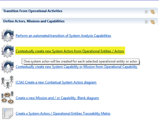
Complete Example of Modeling with Capella: System Analysis 97
Figure 4.36. Actor transition tool between Operational and System levels
The user can control what the tool creates at the System level, first
by selecting a subset of Operational Entities/Actors in a selection
dialog, and later more precisely by selecting elements in a Diff/merge
dialog window. Here, the first window allows us to reject the entity
“Weather Services Provider”, which does not interact directly with the
System (but only through the human profiles that it contains). To do
this, we must allow for multiple disjointed selections through the Ctrl
key.
In simple cases, the user can directly click on the Apply button to
select everything. Here, we shall use this to illustrate finer ways of
guiding the transition. By default, Capella offers to keep the same
allocations between Functions and System Actors as those present at
the Operational level. As a result, keeping the same allocations for the
Activities that we have decided to have carried out by the system only
partially (such as “Collect Weather Data”), or completely (such as
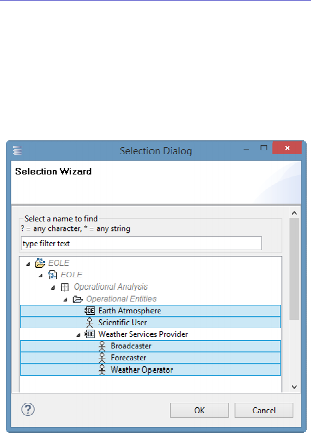
98 Systems Architecture Modeling with the Arcadia Method
“Elaborate Current Situation”), is not desirable. We could of course
apply all of the proposed transformations, and modify the allocations
that propagate to the System level. We will use the Diff/merge
interface in order to only propagate those allocations of Activities
carried out completely by the Actors, i.e. “Forecast Weather”,
“Provide Environmental Conditions” and “Utilize Forecast”. To do
this, we shall act on the Component Function Allocation elements that
appear under the Actors in the left window.
Figure 4.37. Selection window for transition of
Actors between Operational and System levels
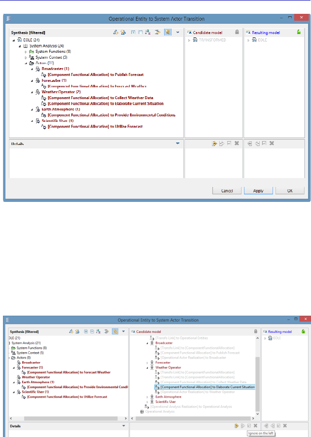
Complete Example of Modeling with Capella: System Analysis 99
Figure 4.38. Dialog window for transition of Actors
between Operational and System levels
The allocations for undesired Functions must be removed by
selecting them, and then in the central window (Candidate model)
ticking the Ignore on the left button. They then disappear from the left
area.
Figure 4.39. Removing some of the allocation transitions
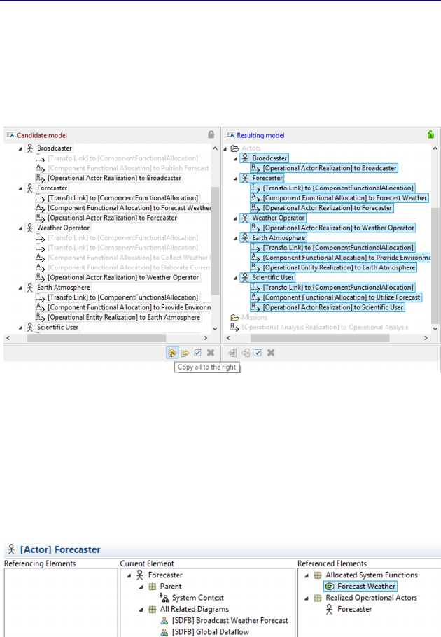
100 Systems Architecture Modeling with the Arcadia Method
If we now apply the changes by clicking on OK, the undesired
allocations are not propagated. To be certain before applying, it is also
possible to see the result beforehand. This can be done by clicking on
the command Copy all to the right, which fills the window on the right
(Resulting Model).
Figure 4.40. Prediction of the transition result
In order to verify the correct application of the transitions,
everything can be checked in the Project Explorer, and especially in
the Semantic Browser. The five System Actors have been created, and
if these are selected one by one, we can see if a Function has been
allocated to them or not.
Figure 4.41. Verification of the result of transition
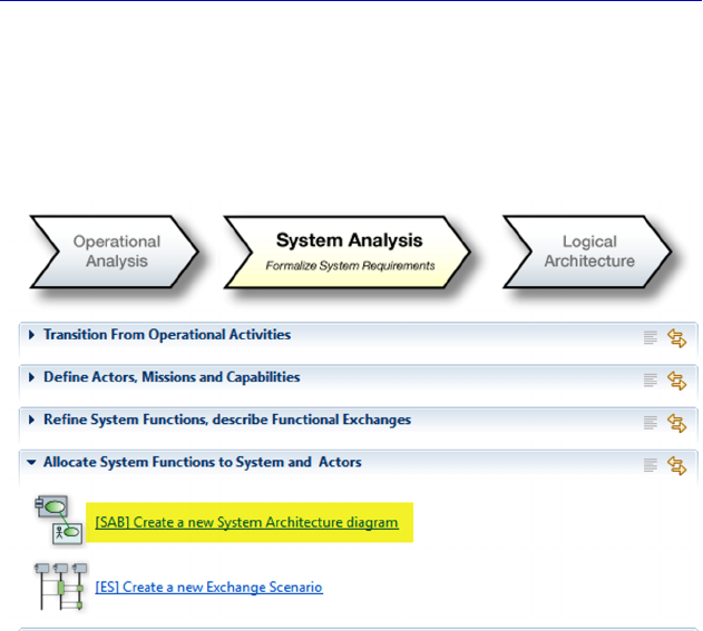
Complete Example of Modeling with Capella: System Analysis 101
We can now proceed to allocating the remaining Functions. The
most obvious way of doing this is to create an Architecture Blank
diagram (SAB) and to graphically allocate the Functions in the System
or the Actors using the Manage Function Allocation command from
the SAB palette.
Figure 4.42. Creation of an Architecture
Blank diagram at the System level (SAB)
NOTE.– Although the SAB is a Blank diagram, it is not empty. Capella
works perfectly in tune with Arcadia and knows that it would be
pointless to realize an Architecture diagram at this level without
showing the System. As a result, Capella inserts it automatically so
that we do not need to. However, the SAB can be partial: we must
choose which Actors we want to show.
We decide to insert all of the Actors: we will make a global
diagram, given the low level of complexity of the subject. We can
always simplify the SAB later, by cloning it and splitting it into
groups of Actors, or by applying filters.
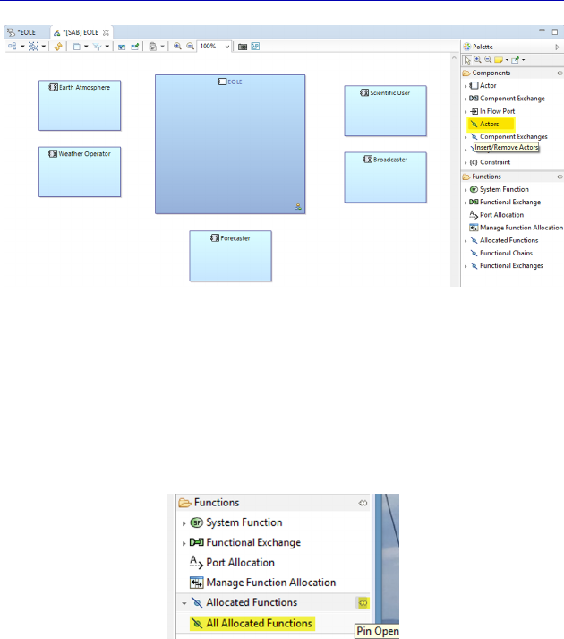
102 Systems Architecture Modeling with the Arcadia Method
Figure 4.43. Start of Architecture Blank diagram (SAB). For a color
version of the figure, see www.iste.co.uk/roques/arcadia.zip
We can already start by inserting the Functions allocated to the
Actors by transition. Capella provides a shortcut for this: the Insert All
Allocated Functions command in the palette under the command
Insert Allocated Functions.
Figure 4.44. Example of command list in the palette
N
OTE
.– Remember that an arrowhead in front of a command from the
palette means that similar commands are available by “opening” the
arrow. The list can then be “pinned”, using the Pin Open button located
on the right.
With a single click at the back of the diagram from the command
Insert All Allocated Functions (outside of the Actors and of the
System), Capella inserts all of the allocated Functions to all of the
elements. If we had clicked inside an Actor, Capella would have
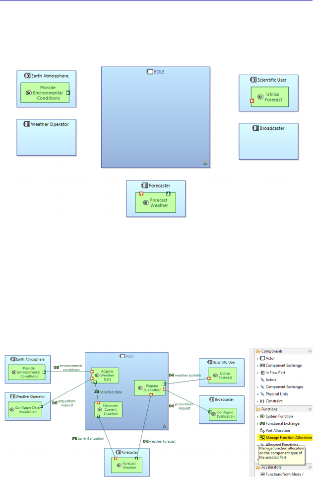
Complete Example of Modeling with Capella: System Analysis 103
inserted all of the Functions allocated to this Actor, without proposing
a dialog window that would have appeared with the other command,
Insert Allocated Functions.
Figure 4.45. More of the Architecture Blank diagram (SAB). For a color
version of the figure, see www.iste.co.uk/roques/arcadia.zip
We can now move on to allocating the remaining Functions. This
is achieved by graphically allocating the Functions in the System or
the Actors with the button Manage Function Allocation from the SAB
palette. Note that Functional Exchanges automatically appear as soon
as the target and source Functions are present in the diagram.
Figure 4.46. Function allocation in the Architecture Blank diagram (SAB). For
a color version of the figure, see www.iste.co.uk/roques/arcadia.zip

104 Systems Architecture Modeling with the Arcadia Method
NOTE (Arcadia Rule).– Only “leaf” Functions (Functions that are not
broken down) can be allocated. As soon as a Function is broken down
into subfunctions, it can no longer be selected in the allocation dialog
windows. Arcadia does not allow a Function to be allocated several
times either.
Capella imposes these rules in the allocation dialogs, helping to
avoid methodological errors in construction. To check that we have
allocated all of the system Functions, we can therefore try to apply the
command Manage Function Allocation again to any structural
element. If the choice of selection is empty, this means that all of the
Functions have been allocated. The model validation can, of course,
also be used.
We still need to allocate the Functional Exchanges. In the same
way that the Functions must be allocated to the System and to the
Actors, we must also allocate the Functional Exchanges to structural
links between the System and the Actors, called Component
Exchanges.
NOTE (Arcadia Rule).– At every level of Arcadia, a Functional
Exchange between two Functions allocated to two Behavioral
Components must be allocated to a single Component Exchange
between these two Components. This Component Exchange references
all of the Functional Exchanges that it implements. In general, a
Component Exchange is made up of a synthesis of several Functional
Exchanges that it implements and gathers together. The direction of
the Component Exchange is purely conventional, but the general rule is
that the direction of the Exchange is from the provider toward the user
of the main data exchanged.
Before carrying out this work, we shall make our model slightly
more complex by adding a “Subscribe” Function for the user and a
“Manage Subscriptions” Function in EOLE. This can be done directly
in the SAB, without having to go back into a Data Flow diagram (or
any other type of diagram).
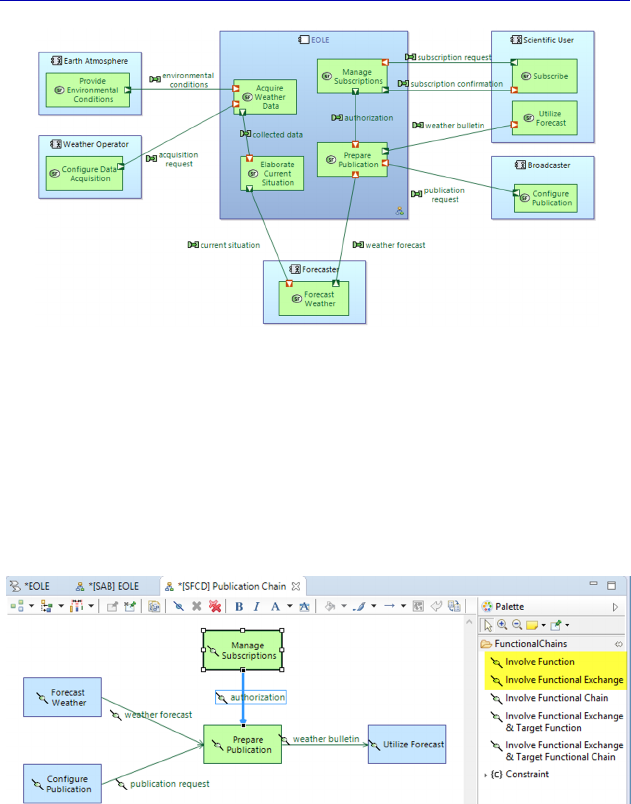
Complete Example of Modeling with Capella: System Analysis 105
Figure 4.47. Adding subscription management to the SAB. For a color
version of the figure, see www.iste.co.uk/roques/arcadia.zip
We have created two Functions and three Functional Exchanges to
start representing the management of subscriptions in a simple
manner. We must also add the Function “Manage Subscriptions” into
the Functional Chain of publication. This can be done by editing the
corresponding SFCD.
Figure 4.48. Updating the publication Chain. For a color version
of the figure, see www.iste.co.uk/roques/arcadia.zip
N
OTE
.–
In Figure 4.48, some of the Functions are no longer green,
unlike what has been the case in all of the diagrams so far. The reason
for this is that, since some of the Functions have been allocated to
Actors, Capella represents them automatically in the same color as the
Actors, so light blue. It is important to distinguish the Functions under
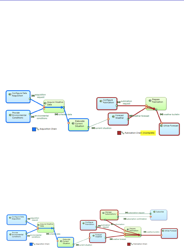
106 Systems Architecture Modeling with the Arcadia Method
the responsibility of the System from those that are allocated to external
Actors. However, apart from in Architecture diagrams, no graphical
clue can tell us this: as a result, Capella takes care of it automatically.
This is yet another reason to not manually change the color of the
Functions in diagrams, except possibly for broken-down Functions,
which cannot be allocated.
While we are here, if we open up the global SDFB again, we can see
that the publication Chain is now marked as incomplete, since the Blank
diagram is not automatically updated when Functions are added.
Figure 4.49. Global SDFB with incomplete publication chain. For a color
version of the figure, see www.iste.co.uk/roques/arcadia.zip
We need to insert the new Functions in order to preserve the
exhaustive aspect of this particular diagram. Note that if we had made
a specific diagram for the publication Chain, and if we had made it
contextual to the chain, it would automatically be updated and
complete.
Figure 4.50. Completed global SDFB. For a color version
of the figure, see www.iste.co.uk/roques/arcadia.zip
Let us go back to the allocation of Functional Exchanges to
Component Exchanges. We must start creating a first Component
Exchange between the weather operator and EOLE. We use the
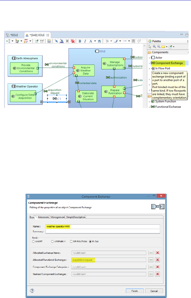
Complete Example of Modeling with Capella: System Analysis 107
Component Exchange tool of the palette, which by default creates a
Component Exchange and two Ports in the direction of the line.
Figure 4.51. Creation of a first Component Exchange in the SAB. For a color
version of the figure, see www.iste.co.uk/roques/arcadia.zip
We rename this Component Exchange, for example “Weather
Operator HMI”, and follow on by allocating it the Functional
Exchange “acquisition request”. If we later add an EOLE response to
the model, or image requests, etc., we can pass all of these functional
flows through the same Component Exchange, as long as they have
similar non-functional properties.
Figure 4.52. Property sheet of a Component Exchange
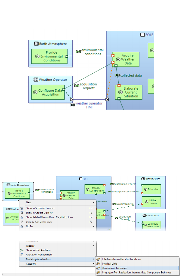
108 Systems Architecture Modeling with the Arcadia Method
The allocation relation appears in the diagram as dotted lines
linking the Function Ports to the Component Ports.
Figure 4.53. Exchange allocation in the SAB. For a color version
of the figure, see www.iste.co.uk/roques/arcadia.zip
Another way of creating Component Exchanges is to ask Capella
via a Modeling Accelerator called Component Exchanges. This
automatically creates a Component Exchange by Functional
Exchange, giving it the same name and realizing the allocation.
Figure 4.54. Creation of a Component Exchange through an Accelerator. For
a color version of the figure, see www.iste.co.uk/roques/arcadia.zip
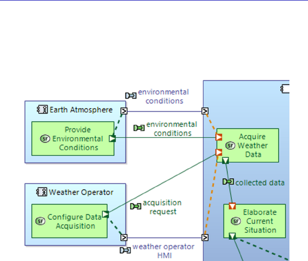
Complete Example of Modeling with Capella: System Analysis 109
The result is immediate. We might need to rename the
Component Exchange, especially if it gathers several of the Functional
Exchanges.
Figure 4.55. Result of the creation of a Component Exchange by Accelerator.
For a color version of the figure, see www.iste.co.uk/roques/arcadia.zip
There are two functional flows that circulate between the forecaster
and EOLE. We can therefore choose to make them both pass through
the same bidirectional Component Exchange, or on the contrary to
make each of them to pass through a different Component Exchange.
The question is the following: do these functional flows have different
non-functional properties (volume, frequency, confidentiality, etc.)? If
they do, it is better to separate the Component Exchanges, otherwise
there is no need.
N
OTE
(Arcadia Rule).– Arcadia demands that Functional Exchanges be
unidirectional. A Function Port is either an input or an output, and this
property cannot be modified in Capella. On the other hand, a
Component Exchange can be uni- or bi-directional. In fact, it is the
Component Ports whose direction property can be edited: in, out, inout.
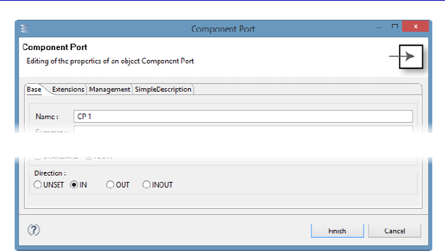
110 Systems Architecture Modeling with the Arcadia Method
Figure 4.56. Property sheet of a Component Port
In our example, the two flows: “current situation” and “weather
forecast” are similar in terms of volume, frequency, etc. We can
therefore decide to go through the same bidirectional Component
Exchange.
To create this exchange, there are two options, which are equal in
terms of the number of clicks and speed:
– create a unidirectional Exchange with the palette, and then
modify each of the Ports by going through an inout;
– first create two bidirectional Ports with the palette, and then an
Exchange going through these two Ports.
We can then rename the Component Exchange and allocate it both
functional flows. In the same way, we can also create a unidirectional
Component Exchange between “Broadcaster” and EOLE.
We have significantly advanced the allocation of Functional
Exchanges to Component Exchanges. Our example here was made
quite simple on purpose. Imagine a real project with several dozen
Functional Exchanges: how can we easily find out if we have
forgotten to allocate some of the Functional Exchanges? In Capella
diagrams there exists a number of filters, depending on the level of
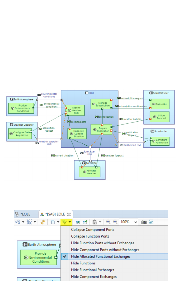
Complete Example of Modeling with Capella: System Analysis 111
engineering and the type of diagram. Most of these filters aim to
simplify the diagrams for publication, and later we shall look at how
these are used, but some of them are aimed more at highlighting the
level of progress of the diagram, and as a result are only temporary.
To answer the previous question, we can ask Capella to temporarily
hide the Functional Exchanges that have already been allocated in
order to show only those that still need to be allocated. As soon as the
work is done, we can take the filter off. This filter is located in the top
panel, which appears when the diagram has been selected. It is called
Hide Allocated Functional Exchanges.
Figure 4.57. SAB in intermediate state. For a color version
of the figure, see www.iste.co.uk/roques/arcadia.zip
Figure 4.58. Apply a temporary filter to the SAB
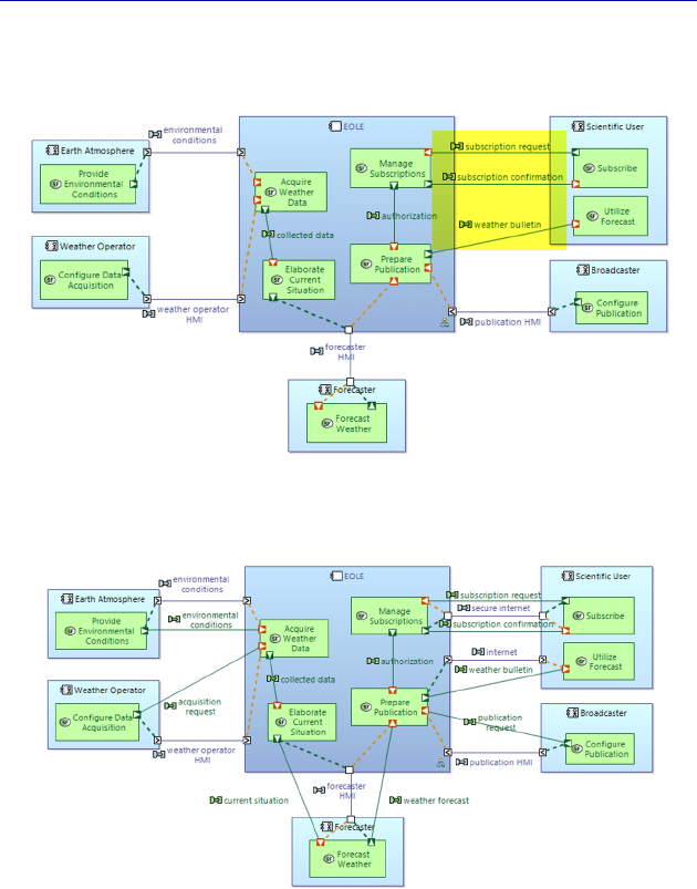
112 Systems Architecture Modeling with the Arcadia Method
After the filter has been applied, only the three Functional
Exchanges between the scientific user and EOLE are shown.
Figure 4.59. Filter applied to intermediate SAB. For a color version
of the figure, see www.iste.co.uk/roques/arcadia.zip
Figure 4.60. Complete SAB. For a color version
of the figure, see www.iste.co.uk/roques/arcadia.zip
These three Functional Exchanges allow us to illustrate a classical
problem encountered in the allocation of Exchanges. Let us assume
that the two Functional Exchanges involved in subscriptions must
absolutely be secure, as money might be involved, while this might
not be the case for the last Functional Exchange. There is therefore a
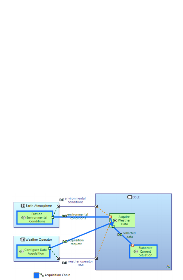
Complete Example of Modeling with Capella: System Analysis 113
good reason to separate these Functional Exchanges into two different
Component Exchanges, one secure and the other not. This way, we
can visually represent different interface requirements. Once the filter
is removed, we are left with the complete SAB.
N
OTE
.– A Function can only be allocated once. Similarly, a Functional
Exchange can only be allocated to one Component Exchange. Once
the weather bulletin has been allocated to the Internet, as in the previous
example, Capella only offers the two other Functional Exchanges for
the secure Internet.
In our simple example the complete diagram is still printable, but
for a complex project this is rarely the case. A way must therefore be
found to publish partial versions of the complete diagram, providing
coherent content for a specific predefined reader type. A first solution
would be to make a split along the two Functional Chains.
To achieve this, we can clone the diagram twice, insert each
Functional Chain into a cloned diagram, and then delete from the
diagram all of the elements that do not participate in the chain
involved. To make each diagram clearer, we can then apply the filters:
Hide Function Ports without Exchanges, Hide Component Ports
without Exchanges. This quickly results in the following two partial
diagrams (Figure 4.61 and 4.62).
Figure 4.61. Partial SAB on the acquisition Chain. For a color version
of the figure, see www.iste.co.uk/roques/arcadia.zip
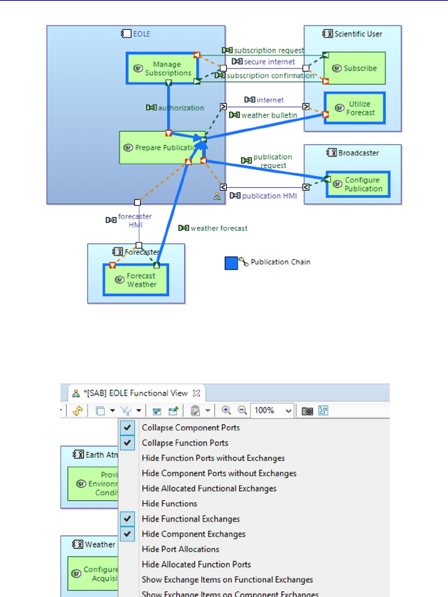
114 Systems Architecture Modeling with the Arcadia Method
Figure 4.62. Partial SAB on the publication Chain. For a color
version of the figure, see www.iste.co.uk/roques/arcadia.zip
Figure 4.63. Filters for a purely functional view of the SAB
Another possibility involves keeping all of the Actors, but deleting
different types of model elements from the diagram. For example, we
can provide a purely functional view of the System by hiding all of the
Exchanges and all of the Ports. Only a few seconds are needed to
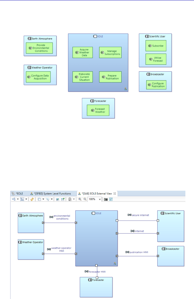
Complete Example of Modeling with Capella: System Analysis 115
apply the four filters shown in Figure 4.63 to a new clone of the SAB,
and thus to obtain a purely functional view of the System.
Figure 4.64. Purely functional view of the SAB. For a color version
of the figure, see www.iste.co.uk/roques/arcadia.zip
On the other hand, in a new SAB we can choose to hide the
Functions so as to only show the Component Exchanges. With a
single click (by selecting the filter Hide Functions), we immediately
obtain Figure 4.65, which shows the external interface of the System.
Figure 4.65. Purely external view of the SAB. For a color version
of the figure, see www.iste.co.uk/roques/arcadia.zip
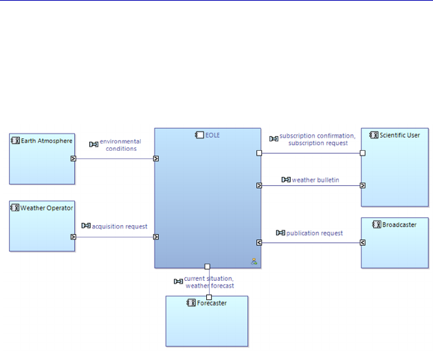
116 Systems Architecture Modeling with the Arcadia Method
An interesting possibility involves asking Capella to show the
names of the allocated Functional Exchanges instead of those of the
Component Exchanges. This is done by applying an extra filter, Show
Allocated Functional Exchanges on Component Exchanges, and then
refreshing the diagram.
Figure 4.66. Extended external view of the SAB. For a color version
of the figure, see www.iste.co.uk/roques/arcadia.zip
N
OTE
.– Remember that it is often useful to be able to distinguish
between the work diagrams and the diagrams used for communicating.
A work diagram can be complex, but can be used by the modeler as a
complete overview, shown on a big screen, while using the graphical
capabilities of the tool: zoom, Outline window, etc. These work
diagrams are not meant to be communicated, and even less printed. The
modeler will have to extract from them the diagrams to be
communicated by using the cloning, masking and filtering capabilities
of Capella in order to provide each reader with the relevant and required
level of information.
To finish off this part of the Functional Analysis, we ask the tool to
automatically generate the tree view of the functional breakdown at
the System level. To do this, we go back to the Activity Explorer and
ask for a Functional Breakdown diagram (SFBD).
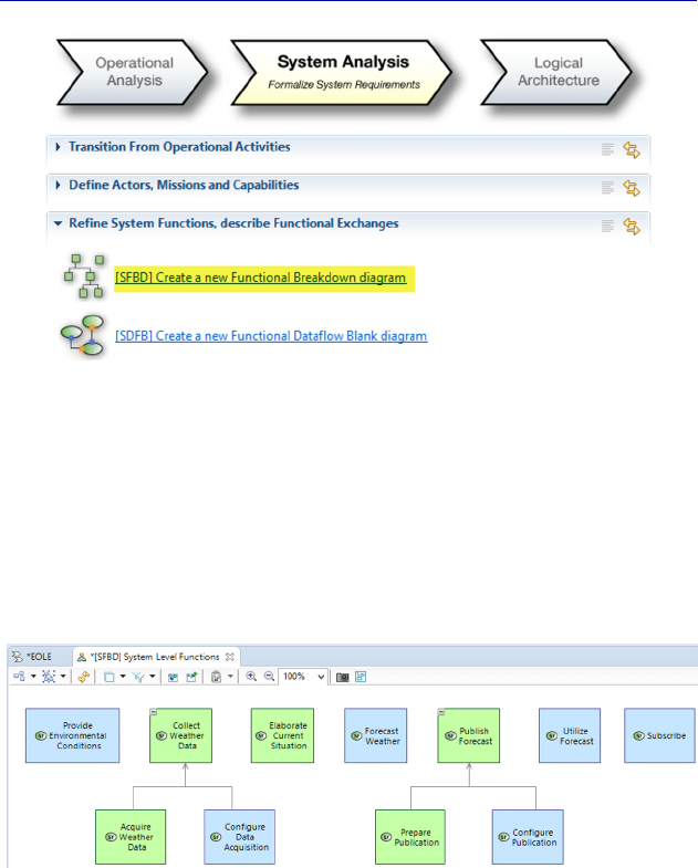
Complete Example of Modeling with Capella: System Analysis 117
Figure 4.67. Creating a Functional Breakdown
Diagram at the System level (SFBD)
N
OTE
.– The Breakdown diagram behaves oppositely to Blank
diagrams. It is not created empty, and instead automatically contains all
of the relevant model elements of the type involved (at the Arcadia level
involved). Moreover, it is systemically updated when a new model
element is created in another diagram or from the Project Explorer.
Figure 4.68. System level Functional Breakdown Diagram (SFBD). For a
color version of the figure, see www.iste.co.uk/roques/arcadia.zip
Remember that the Functions in light blue are those that have been
allocated to the Actors. Good practice involves manually changing the
color of the parent Functions that can no longer be allocated to white,
such as “Collect” and “Publish” in our example. In this way, the only
Functions that are still in green are those allocated to the System.
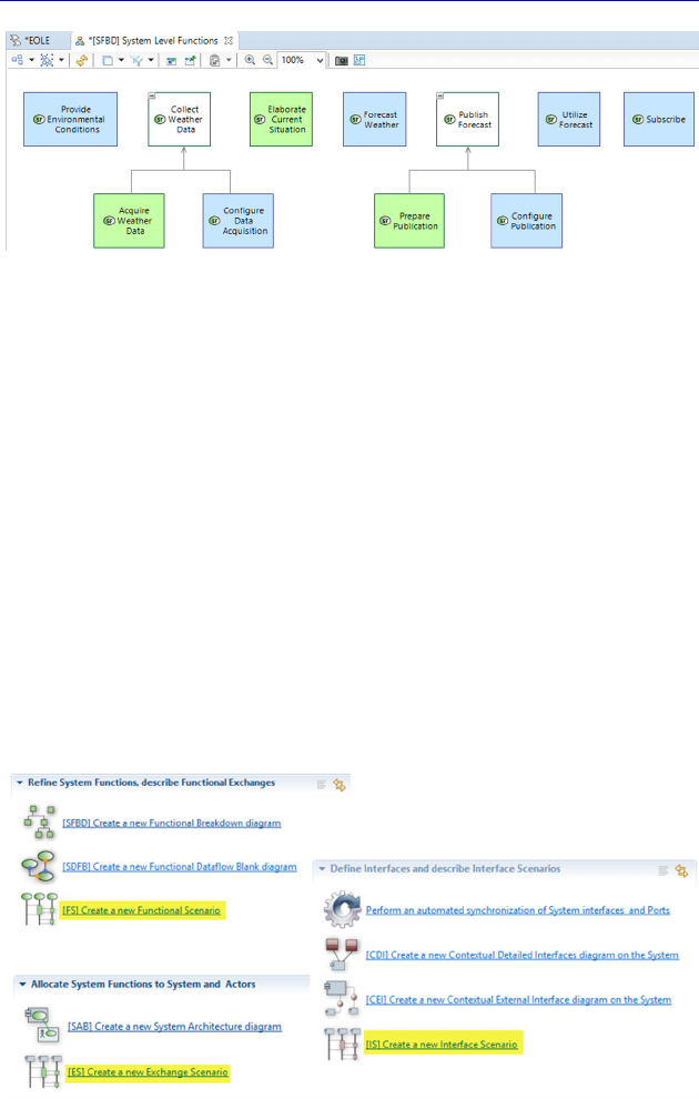
118 Systems Architecture Modeling with the Arcadia Method
Figure 4.69. Modified Functional Breakdown Diagram (SFBD). For a color
version of the figure, see www.iste.co.uk/roques/arcadia.zip
4.7. System-level Scenarios
We have already seen that Capella provides several types of
Scenario diagrams at each level of Arcadia:
– Functional Scenarios (FSs): the lifelines are Functions;
– Exchange Scenarios (ESs): the lifelines are Components/Actors,
while the sequence messages are Functional or Component Exchanges;
– Interface Scenarios (ISs): the lifelines are also Components/
Actors but the sequence messages are Exchange Items.
We can find all three types of Scenarios at the System Analysis
level in the Activity Explorer.
Figure 4.70. Scenario diagrams at the System level
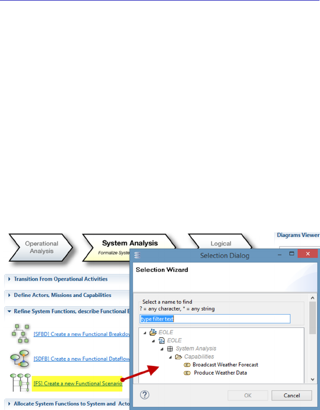
Complete Example of Modeling with Capella: System Analysis 119
N
OTE
(Arcadia Rule).– A Scenario describes the behavior of the System
in the context of a particular Capability. Even if we do not wish to use
this concept, Capella automatically creates a Capability the first time a
Scenario is created, unless of course Capabilities already exist. In this
case, Capella asks to choose one Capability to attach the new Scenario.
Let us start with the simplest Scenario type: the Functional
Scenario.
We start by creating as an example a Scenario involving the
Functional Chain of acquisition. We are therefore going to attach it to
the Capability “Produce Weather Data”. The Functional Scenario is a
type of chronological System Data Flow Blank. The Functions are
represented by vertical lines (instead of rectangles), and the Functional
Exchanges are represented by horizontal arrows ordered sequentially
from top to bottom.
Figure 4.71. Creating a Functional Scenario diagram
N
OTE
.– Functional Scenario diagrams are given a name by default like:
[FS] Scenario. Good practice involves adding the first letter of the level,
and of course then giving a more meaningful name to the Scenario, such
as [SFS] Acquisition Scenario.
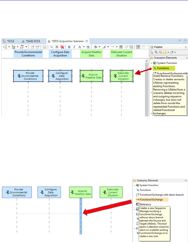
120 Systems Architecture Modeling with the Arcadia Method
To insert the Functions that we are interested in, we can drag and
drop them from the Project Explorer, or insert them using the
Insert/Remove Functions button in the palette.
Figure 4.72. Insertion of Functions in a Functional Scenario diagram. For a
color version of the figure, see www.iste.co.uk/roques/arcadia.zip
Next we create horizontal messages by selecting existing
Functional Exchanges using the Functional Exchange tool in the
palette.
Figure 4.73. Creating messages in a Functional Scenario diagram. For a
color version of the figure, see www.iste.co.uk/roques/arcadia.zip
Capella only allows us to select the Functional Exchanges that
already exist in the model. As a result, here it only proposes
“environmental conditions”.
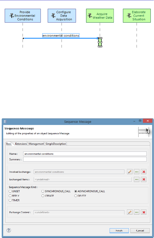
Complete Example of Modeling with Capella: System Analysis 121
Figure 4.74. First message created in the Functional Scenario diagram. For a
color version of the figure, see www.iste.co.uk/roques/arcadia.zip
N
OTE
.– Scenario diagrams in Capella are very similar to the
UML/SysML sequence diagrams [CAS 18]. We can therefore create
messages with return, “synchronous/asynchronous” types, etc., and use
Combined Fragments, duration constraints, etc. We shall illustrate most
of these options in examples later in the book at different levels of
engineering. The property sheet of a message is provided in Figure 4.75.
Figure 4.75. Property sheet of a message
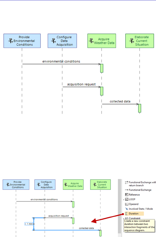
122 Systems Architecture Modeling with the Arcadia Method
By completing the scenario diagram in order to make it compatible
with the corresponding Data Flow diagram, we obtain the following
diagram.
Figure 4.76. Completed Functional Scenario diagram. For a color version
of the figure, see www.iste.co.uk/roques/arcadia.zip
Let us illustrate, for example, the concept of duration constraints.
As in UML/SysML, it is possible to specify a time constraint between
two messages in a Scenario diagram. Using the Duration button in the
palette, we can create a constraint by selecting a source message and a
target message.
Figure 4.77. Creation of a duration constraint. For a color version
of the figure, see www.iste.co.uk/roques/arcadia.zip
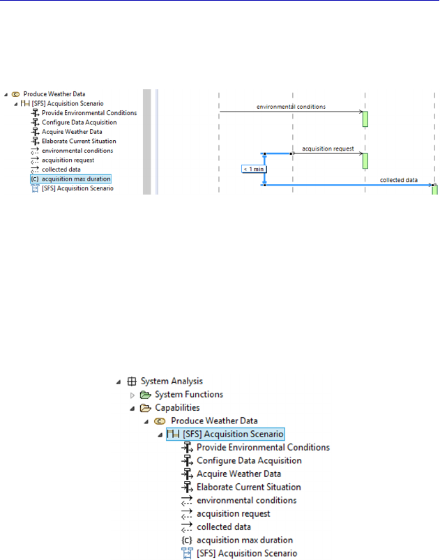
Complete Example of Modeling with Capella: System Analysis 123
This constraint is a model element on its own and not only a
graphical object. Its name appears in the Project Explorer, and its
value in the diagram.
Figure 4.78. Duration constraint in the explorer and the diagram. For a color
version of the figure, see www.iste.co.uk/roques/arcadia.zip
It is good practice to then rename the model element “Scenario” in
the Project Explorer with the name of the diagram created, as shown
in Figure 4.79. Note that the explorer shows the vertical lines,
messages and constraints, which are all model elements in their own
right, under the Scenario, which is itself under a Capability.
Figure 4.79. Scenario and its model element in the Explorer
We shall now create an ES diagram. This can of course be done by
going through the Activity Explorer, as shown previously, and creating
a new Scenario manually. Another option involves using an
interesting Capability of the Capella tool, which can automatically
initialize an ES from a Functional Scenario.
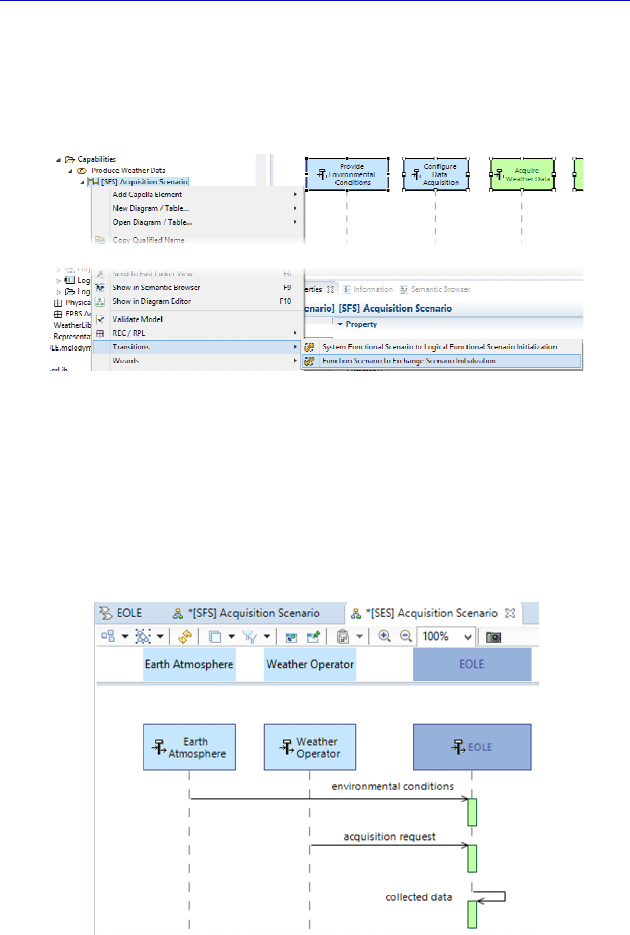
124 Systems Architecture Modeling with the Arcadia Method
For this, we must position ourselves on the Scenario, either in the
diagram that we have just created, or in the Project Explorer, and
activate a contextual command with the right click: Transitions –
Function Scenario to Exchange Scenario Initialization.
Figure 4.80. Contextual transition of a Functional Scenario. For a color
version of the figure, see www.iste.co.uk/roques/arcadia.zip
The result of this initialization is a new ES, with the same
horizontal messages, but only three vertical lines corresponding to the
structural elements (here the System or the Actors) instead of the
Functions.
Figure 4.81. Exchange Scenario obtained automatically
by transition of a Functional Scenario. For a color version
of the figure, see www.iste.co.uk/roques/arcadia.zip
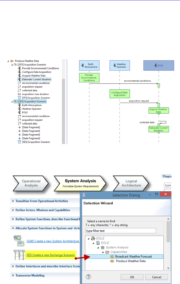
Complete Example of Modeling with Capella: System Analysis 125
We just need to create the diagram, and rename the vertical lines in
the Project Explorer (they are given the same name following the
transition as those in the Functional Scenario). We can also show the
Functions on the vertical lines, if we so desire. Capella helps the
modeler and proposes only Functions allocated to the elements
represented by vertical lines.
Figure 4.82. Complete Exchange Scenario. For a color version
of the figure, see www.iste.co.uk/roques/arcadia.zip
Figure 4.83. Creation of a second Exchange Scenario
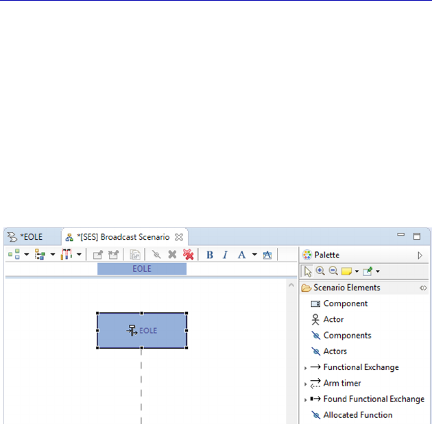
126 Systems Architecture Modeling with the Arcadia Method
We will now create a second diagram, this time via the Activity
Explorer. This Scenario involves the other Capability of broadcasting
weather forecast. It allows us to illustrate the concept of a fragment,
which comes from UML/SysML.
N
OTE
.– The ES diagram at the SA level (SES) is the only one that is
not empty. It always contains a vertical line representing the System
as a “black box”, in the same way that an Architecture diagram at the
System level (SAB) always contains the System. However, most of the
time a subset of Actors is enough for the Scenario involved. We will
have to insert them into each Scenario diagram.
Figure 4.84. System level Exchange Scenario after creation
In this Scenario, first we will represent the nominal subscription
sequence of the scientific user. To do this, we insert the Actor in
question and select the relevant Functional Exchanges. By adding the
corresponding Functions, we obtain the start of a Scenario, as shown
in Figure 4.85.
We shall now describe a repetitive behavior: every day the System
publishes information on the weather, which the user can receive as
they have a subscription. For this, we shall use a Combined Fragment,
which is of the Loop type, with a frequency of “every day”.
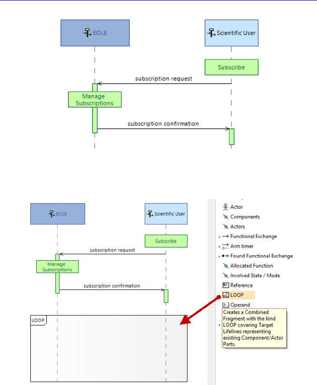
Complete Example of Modeling with Capella: System Analysis 127
Figure 4.85. Start of the “broadcast” Exchange Scenario. For a color
version of the figure, see www.iste.co.uk/roques/arcadia.zip
Figure 4.86. Creating a Loop fragment. For a color version
of the figure, see www.iste.co.uk/roques/arcadia.zip
The fragment itself is a model element, with its own property
sheet. Moreover, there is no standard graphical command that can be
used to make it big or smaller horizontally: instead the semantic field
Covered Instance Roles has to be modified. The vertical lines in the
Scenarios are called Instance Roles in Capella (and Lifelines in
UML/SysML).
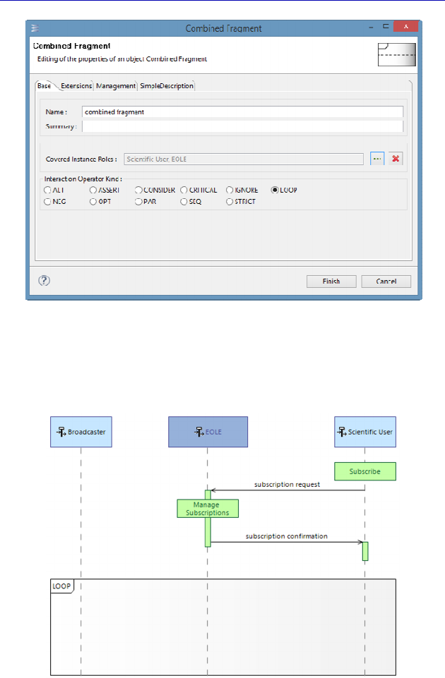
128 Systems Architecture Modeling with the Arcadia Method
Figure 4.87. Fragment property sheet
We add the Actor “Broadcaster” into the Scenario and include it in
the daily loop.
Figure 4.88. Adding an Actor to the fragment. For a color version
of the figure, see www.iste.co.uk/roques/arcadia.zip
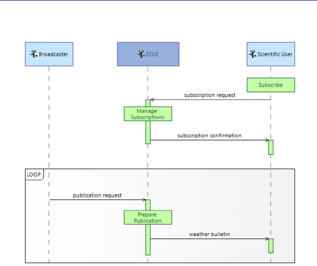
Complete Example of Modeling with Capella: System Analysis 129
We can now complete the Scenario as shown in Figure 4.89.
Figure 4.89. Completed broadcast Exchange Scenario. For a color
version of the figure, see www.iste.co.uk/roques/arcadia.zip
N
OTE
.– The concept of Combined Fragment comes directly from
UML/SysML. Each fragment contains an operator and can be split into
operands. The main operands are:
– loop: the fragment can be executed several times, and the guard
condition states the iteration;
– opt: optional. The fragment is only executed if the condition provided
is true;
– alt: alternative operands. Only the operand containing the true
condition is executed;
– par: parallel operands. All of the operands are executed in parallel.
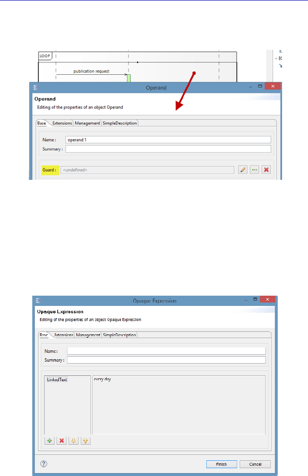
130 Systems Architecture Modeling with the Arcadia Method
In our example, in order to mark that the loop takes place every
day, we must edit the unique operand contained in the Loop fragment.
Figure 4.90. Property sheet of a fragment operand
The creation of a condition (also called Guard) is done through a
new property sheet and an Opaque Expression type element. This is
also a concept coming from UML/SysML that allows us to simply
express a constraint in any given language. Do not forget to click on
LinkedText when editing constraints.
Figure 4.91. Property sheet of an Opaque Expression
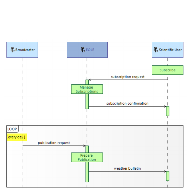
Complete Example of Modeling with Capella: System Analysis 131
The text of the condition is shown at the top left of the operand, in
brackets.
Figure 4.92. Completed Fragment. For a color version
of the figure, see www.iste.co.uk/roques/arcadia.zip
Up to here we have used existing model elements to create vertical
lines or horizontal messages in the Scenarios. It is perfectly possible to
create these model elements directly from a scenario diagram. For
example, we can add an Actor to the model by creating an Instance
Role (instead of inserting an existing Actor).
Capella automatically creates the two model elements, the first as
an Instance Role in the Scenario and the second as an Actor in the
Actors folder.
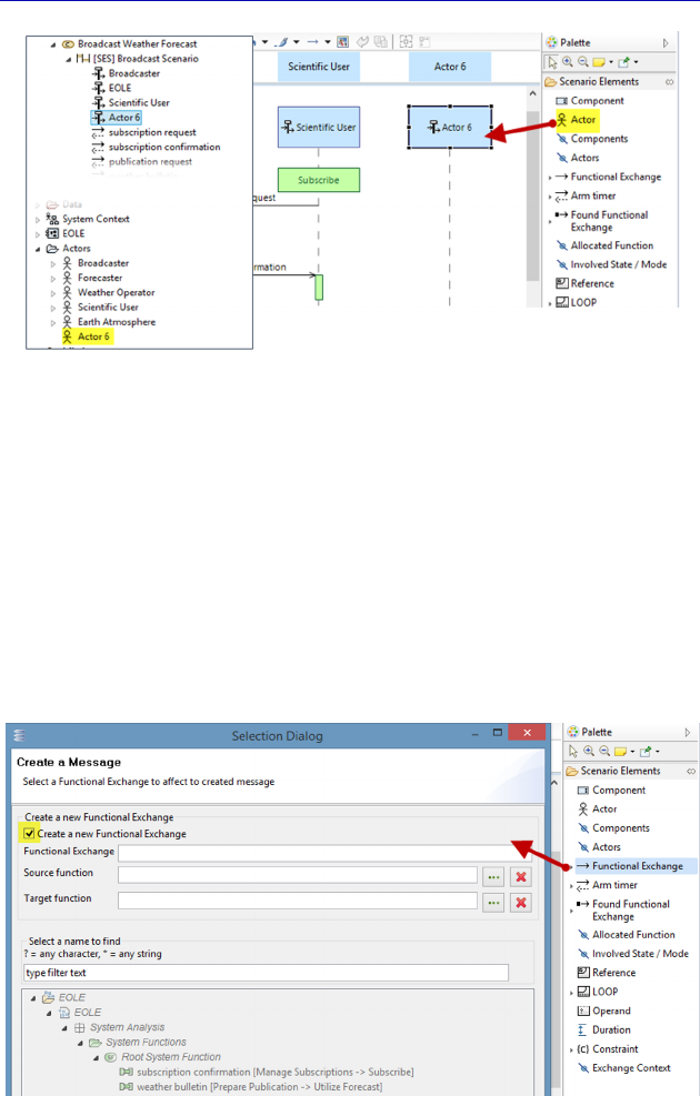
132 Systems Architecture Modeling with the Arcadia Method
Figure 4.93. Creation of an Actor from a Scenario. For a color
version of the figure, see www.iste.co.uk/roques/arcadia.zip
In our case study, we might instead need to create new Functional
Exchanges to model the subscription process. For example, this might
involve asking the scientific user for a card payment and waiting for
their reply. Rather than going back to a Data Flow diagram, or an
Architecture diagram, adding Functional Exchanges and possibly
Functions, it is also possible here to do everything from a Scenario
diagram. Instead of selecting an existing Exchange, we move into
“creation” mode by ticking the Create a new Functional Exchange box.
Figure 4.94. Creation of a Functional Exchange from a Scenario
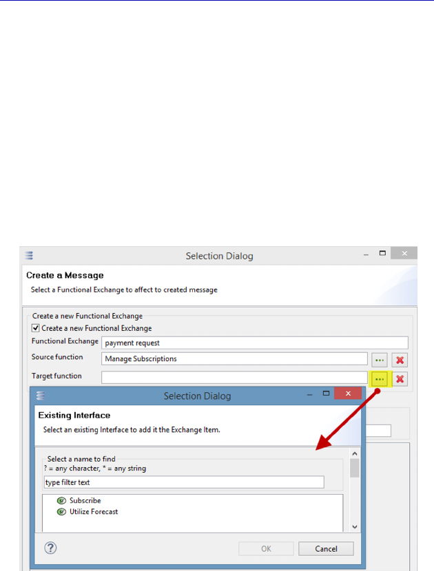
Complete Example of Modeling with Capella: System Analysis 133
To create a Functional Exchange we will need more than a name.
Capella knows that a Functional Exchange always links two
Functions. We must therefore first fill the two fields Source Function
and Target Function, and click on OK.
Here again, Capella helps the modeler: it knows the existing
Functions that have already been allocated to the vertical lines
between which we want to create a message. In our example, the two
Functions are “Utilize Forecast” and “Subscribe” for the scientific
user, who is the receiver of the message. For the Source Function, it is
the four EOLE Functions. Of course, we have chosen the Function
“Manage Subscriptions”.
Figure 4.95. Choice of Target and Source Functions
during creation of a Functional Exchange from a Scenario
With this simple maneuver, the modeler has not only created a
message in the Scenario, but also a new Functional Exchange in the
model.
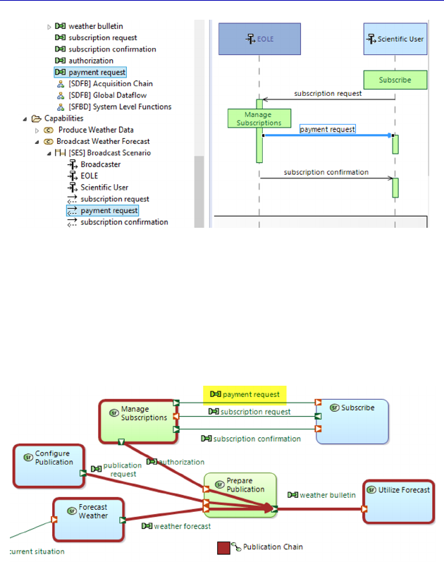
134 Systems Architecture Modeling with the Arcadia Method
Figure 4.96. Creation of a Functional Exchange
from a message in a Scenario. For a color version
of the figure, see www.iste.co.uk/roques/arcadia.zip
Note that this new Functional Exchange appears automatically in
all of the Blank diagrams where the source and target Functions are
present. This is the case for the [SDFB] global data flow, for example.
Figure 4.97. Automatic adding of the Functional Exchange in an SDFB. For a
color version of the figure, see www.iste.co.uk/roques/arcadia.zip
This is also the case for the Architecture diagram (SAB), but here
we can see that the new Functional Exchange still needs to be
allocated to a Component Exchange. We can add it to an existing
Component Exchange, typically here “secure Internet”, or consider
creating a new one.
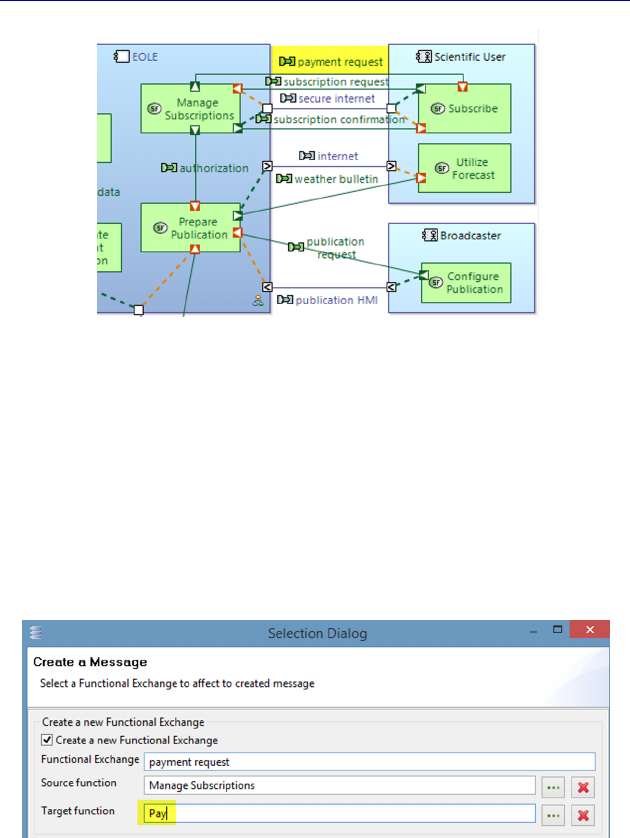
Complete Example of Modeling with Capella: System Analysis 135
Figure 4.98. Automatic adding of the Functional Exchange in an SAB. For a
color version of the figure, see www.iste.co.uk/roques/arcadia.zip
To finish off this topic, we will demonstrate that it is even possible
to create new Functions from a Scenario diagram.
In the previous step, during the creation of the “payment request”
message, instead of selecting one of the existing Functions of the
Actor, we will create a new one, by simply writing a Function name in
the corresponding field.
Figure 4.99. Creation of a Target Function during
creation of a Functional Exchange from a Scenario
We can see that Capella has not only created a message in the
Scenario and a Functional Exchange in the model, but has also created
a new Function.
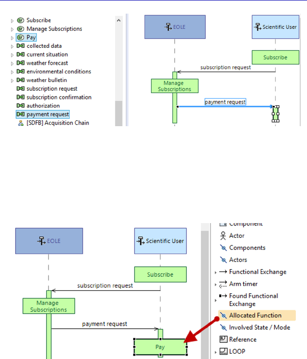
136 Systems Architecture Modeling with the Arcadia Method
Figure 4.100. Result of the creation of a Target Function during creation of a
Functional Exchange from a Scenario. For a color version
of the figure, see www.iste.co.uk/roques/arcadia.zip
This new Function can immediately be used to appear on the
vertical line to which it is allocated, i.e. the scientific user.
Figure 4.101. Adding the new Target Function to the Scenario. For a color
version of the figure, see www.iste.co.uk/roques/arcadia.zip
N
OTE
.– This ability to create Actors, Functional Exchanges and even
Functions from Scenarios is very interesting. Scenario diagrams are
often used in the area of telecommunication for example, but also by
many people who find it more instinctive and easier to specify and
design a System from real stories (Scenarios). This was indeed the
objective of Jacobson’s Use Cases technique, which is integrated in
UML/SysML [CAS 18].

Complete Example of Modeling with Capella: System Analysis 137
4.8. Modes and States at the System level
Mode and State diagrams are graphical representations of State
Machines inspired from UML/SysML.
Arcadia allows a State Machine to be associated with any structural
element:
– Entity/Operational Actor;
– System/Actor;
– Logical Component/Logical Actor;
– Physical Component/Physical Actor.
The expected behavior of the System is often specified as a State
Machine, particularly if the System must react to events coming from
Actors in a set order. An Operational Entity can have a State Machine
if it is standardized “business” knowledge for example, which could
later be of consequence for our System under study. Some Physical
Components often need State Machines to indicate under which States
their Functions are available. For example, in our case study, at the
Physical level, the helium balloon does not have the same behavior at
ground level as in the air, out of reach, etc.
Let us quickly present the main concepts used. First the notion of
State or Mode. In UML/SysML, a State represents a situation during
the lifetime of a block during which:
– it satisfies a certain condition;
– it executes a certain behavior;
– or it expects a certain event.
NOTE.– Arcadia proposes two similar concepts: State and Mode. The
use of one or the other is a methodological choice in the context of the
project or the company. A fairly widespread difference among system
engineers involves considering that the System Mode depends on a
choice, often of an operator, while the State is the result of that which
has happened to the System. In this way, we would talk of a manual
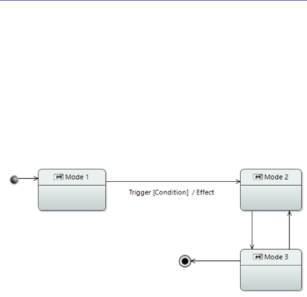
138 Systems Architecture Modeling with the Arcadia Method
mode, a semiautomatic mode, but of a default state. Unfortunately, there
is no normalized definition of these two concepts. We therefore have to
choose whichever word is the most relevant for our context and will
connect most with the readers of the model. The two concepts cannot be
mixed together in the same diagram.
States (or Modes) are linked together by Transitions. A Transition
describes the reaction of a structural element when an event takes
place (the element usually changes State as a result, but this is not
always the case). A transition contains a source State, a Trigger and a
target State. It can also include a Guard Condition as well as an Effect.
Figure 4.102. Basic notation of Mode and State diagram (MSM)
On top of the succession of “normal” States corresponding to the
life cycle of a structural element, the State diagram also contains two
pseudo-states:
– the initial State of the State diagram corresponds to the creation
of the element;
– the final State of the State diagram corresponds to the destruction
of the element.
In particular, this allows us to model the issue of managing the end
of the life cycle for a System or a Component.
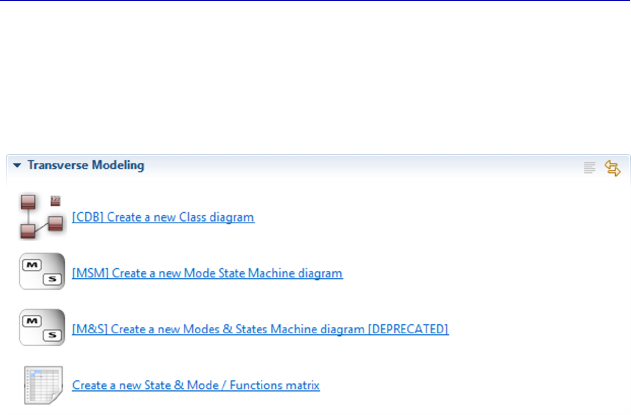
Complete Example of Modeling with Capella: System Analysis 139
In our case study, we are going to associate a simple Mode
machine with the EOLE System. To do this, we go back to the Activity
Explorer and into the section “Transverse Modeling”, to create a
Mode State Machine (MSM) diagram.
Figure 4.103. Creation of a Mode State Machine (MSM) diagram
N
OTE
.– Capella 1.1 proposes two versions of the Mode and State
diagram. This is a very powerful and complex diagram in UML/SysML,
and is still evolving in Capella. Capella 1.1 has notably added the
possibility of creating concurrent regions (to represent parallelism
between States), which was not possible in previous versions. For
compatibility reasons, the old and new diagrams exist alongside each
other for the moment.
When we ask for the creation of a MSM, Capella opens a selection
window, proposing all of the structural elements of the Arcadia level
involved, which in this case are the System and the Actors. We choose
the EOLE system.
We shall not go into detail regarding all of the concepts offered in
this type of diagram, and instead focus on only the most important
ones. First, we create three Modes for the System: Inactive,
Operational and Acquisition, and Transitions between these Modes.
Inactive is the initial Mode.
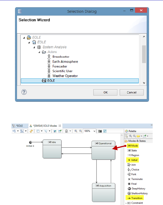
140 Systems Architecture Modeling with the Arcadia Method
Figure 4.104. Selection window for the creation of a Mode diagram
Figure 4.105. Start of the Mode diagram
We have hidden the names of the regions by activating the Hide
Region names filter on the diagram. We could also hide the name of
the initial pseudo-state by selecting it, and then applying the Hide
label command. Let us stop for a moment on the concept of Mode,
and open its property sheet. It contains a certain number of specific
fields, with concepts that come from UML/SysML:
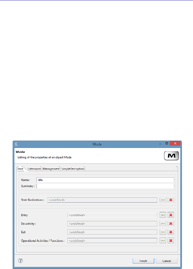
Complete Example of Modeling with Capella: System Analysis 141
– Entry: An entry Effect represents an Effect that is executed each
time the Mode/State is entered into. This allows us to factorize a same
Effect that is set off by all of the transitions that enter into the
Mode/State.
– Do activity: In opposition to Effects that are instantaneous,
durable activities have a duration, can be interrupted and are always
associated with Modes/States.
– Exit: An exit Effect represents an Effect that is executed every
time that the Mode/State is exited. This allows us to factorize a same
Effect that is set off by all of the transitions that exit the Mode/State.
The last field, however, called Operational Activities/Functions is
specific to Arcadia and does not come from UML/SysML. It allows us
to declare which Functions (or Activities at the Operational level) are
available in the Mode in question.
Figure 4.106. Property sheet of a Mode
Note that this relation is also visible in the Property sheet of
Functions. We can therefore indicate, for example, that the Function
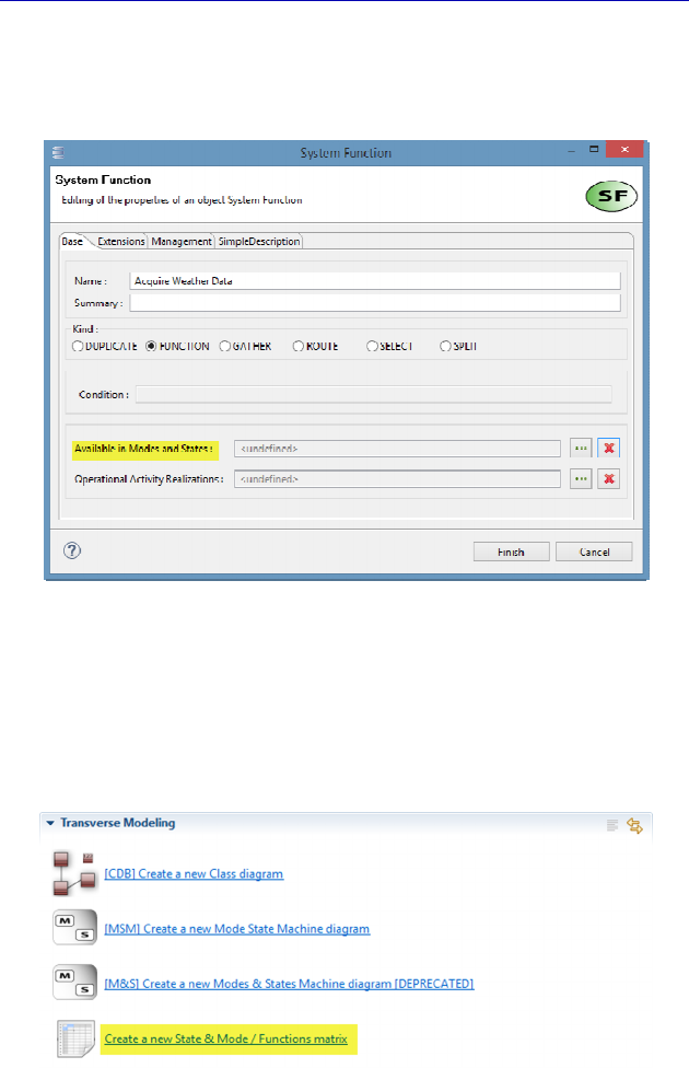
142 Systems Architecture Modeling with the Arcadia Method
“Acquire Weather Data” is available in the “Acquisition” mode. The
relation is now in the model, and will be shown in the property sheet
of the “Acquisition” Mode next time that it is opened.
Figure 4.107. Return to the property sheet of a Function
There is also a third way to access these relations between
Modes/States and Functions: a matrix that is generated by Capella
from the model, but which is itself also editable. It can be accessed via
the Activity Explorer, still in the “Transverse Modeling” section.
Figure 4.108. Creation of a Mode/Functions matrix
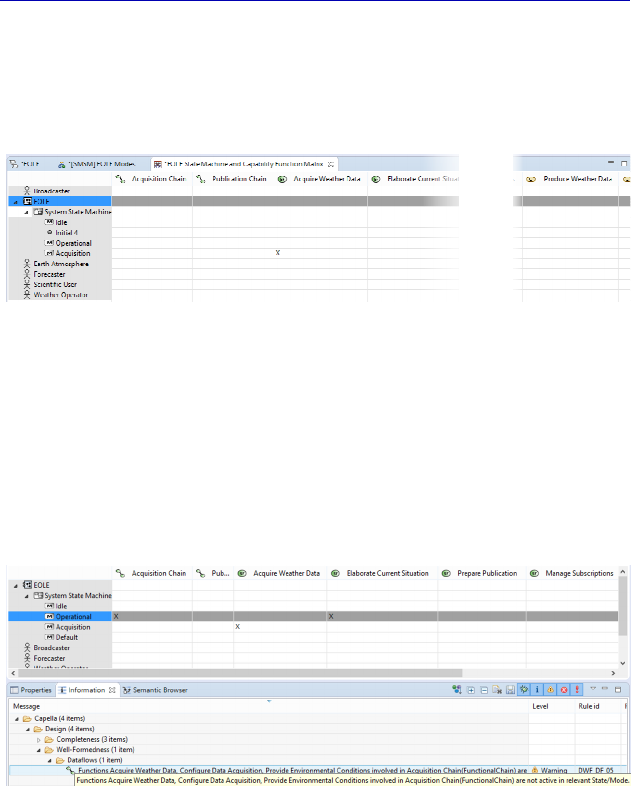
Complete Example of Modeling with Capella: System Analysis 143
This matrix contains the structural elements in lines, with their
possible Modes and States. It places the Functions in the columns, as
well as the Functional Chains and the Capabilities. The availability
relation is marked by an “X”.
Figure 4.109. Example of a Mode/Functions matrix
In this way, it is possible to quickly complete these availability
relations by simply adding “X”’s to the relevant cells. Note that if a
Functional Chain is declared to be available in a certain Mode or
State, Capella verifies that all of the Functions involved in the Chain
are also declared available in the same Mode or State, issuing a
warning if this is not the case, as shown Figure 4.110.
Figure 4.110. Mode/Functions and Functional Chain incoherence warning
N
OTE
.– Capella proposes various matrices at all levels of Arcadia.
Notably, we can mention realization matrices between levels, which are
very practical for rapidly declaring a large number of traceability
relations, typically in the context of a bottom-up modeling process.
Allocation matrices also present the advantage of providing a synthetic
view of the allocation of Functions to structural elements. Careful
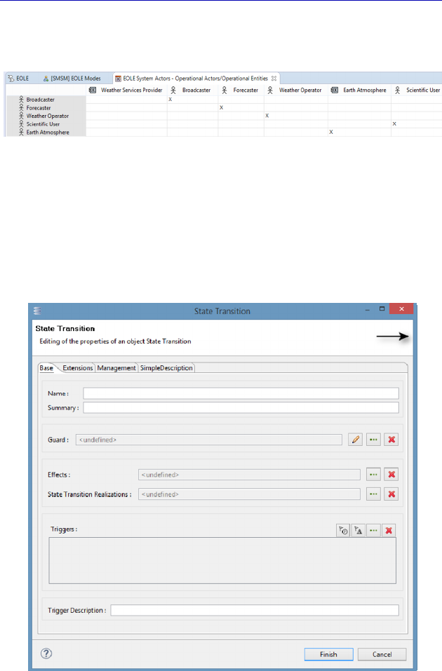
144 Systems Architecture Modeling with the Arcadia Method
though, as editing these allocation matrices modifies the model and the
corresponding Architecture diagrams as a result.
Figure 4.111. Example of an Operational Entities/System Actors matrix
In the previous matrix, we can immediately see that the
Operational Entity called “Weather Services Provider” is not realized
by a System level Actor, while all the other operational structural
elements are realized. Remember that this choice was made
knowingly in our case study, and we accept the due warning.
Figure 4.112. Property sheet of a transition
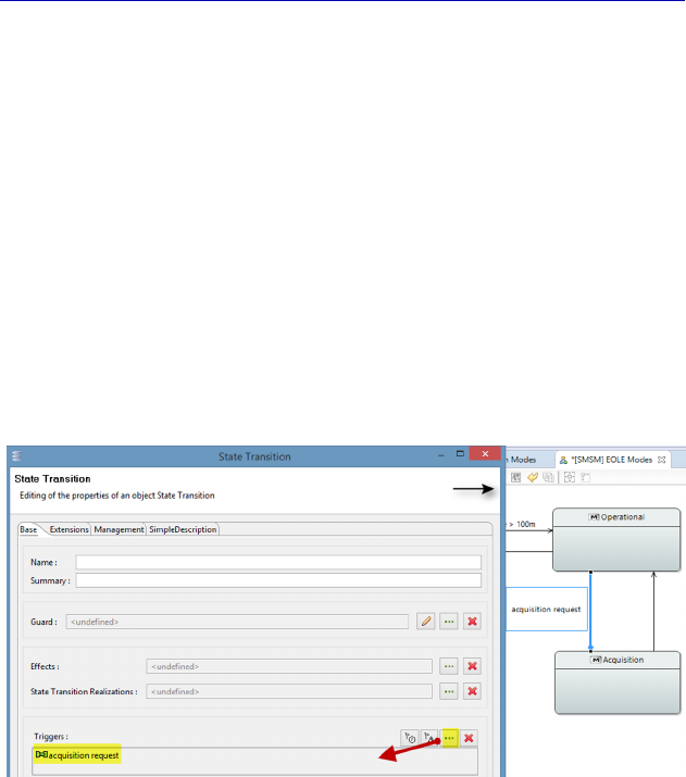
Complete Example of Modeling with Capella: System Analysis 145
Let us go back now to the concept of transition between Modes and
States. Remember that a transition describes the reaction of a
structural element when an event takes place. It has a source State, a
Trigger and a target State. It can also contain a Guard Condition and
an Effect, as shown on figure 4.112.
Let us start with the Trigger. In the current version of Capella, it
can be named by free text in the “Trigger Description” field. It is good
practice to use an existing model element, such as a Functional
Exchange, for example, in the Triggers field. In our example, let us
express the fact that the system goes from the “Operational” mode to
the “Acquisition” mode with each “acquisition request”. To do this,
we must choose the Functional Exchange in the selection window of
the Triggers field.
Figure 4.113. Choice of a Trigger among the existing model elements
N
OTE
.– Capella is meant to be very close to UML/SysML with regard
to the State diagram. A trigger can therefore also be a Time Event or a
Change Event. A Time Event is modeled using either the keyword
“after”, followed by an expression that represents duration, counted
from the entrance into the current State, or the keyword “at”, followed
by an expression that represents an absolute time. Change Events are
modeled using the keyword “when”, followed by a Boolean expression,
in which the passing from false to true sets off the transition.
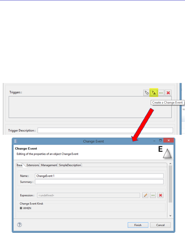
146 Systems Architecture Modeling with the Arcadia Method
For example, here we shall use the notion of Change Event to
express the fact that the EOLE system moves into “Operational” mode
as soon as the altitude of the balloon is greater than 100 m. This is
obviously a simplification for teaching purposes….
To create a Change Event, we must click on the flag with a triangle
in the Triggers field (the clock on the side lets us create a Time
Event). A property sheet then opens, allowing us to edit the name and
the expression of the Change Event.
Figure 4.114. Creation of a Change Event Trigger
We edit the expression field by using the name of the associated
constraint, and we name the event in order to be able to find it within
the Project Explorer.
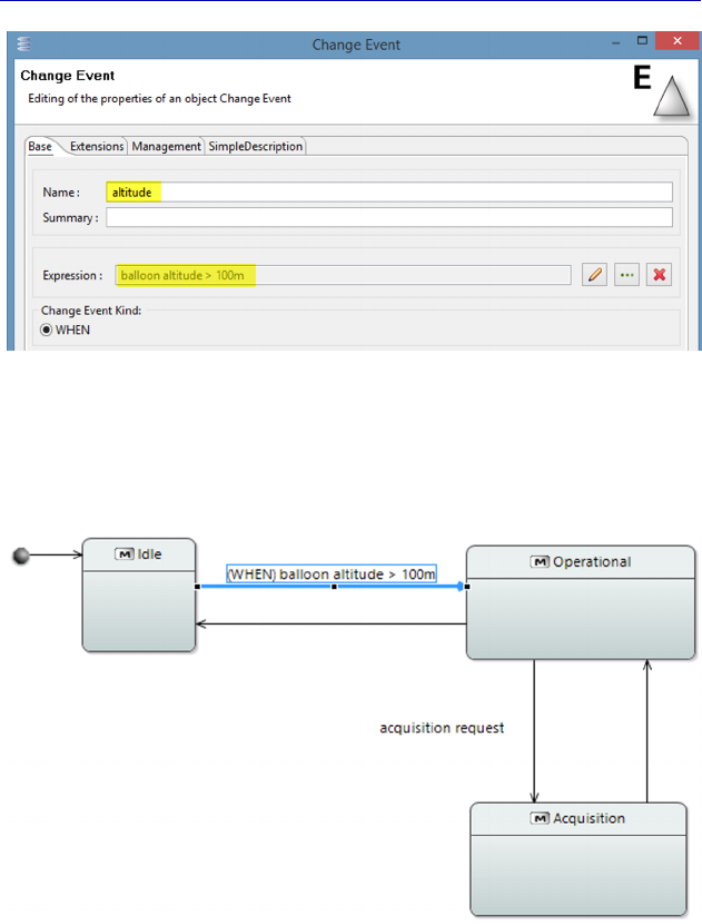
Complete Example of Modeling with Capella: System Analysis 147
Figure 4.115. Finalization of a Change Event Trigger
The Mode and State diagram is updated, and the keyword WHEN
appears automatically in front of the constraint.
Figure 4.116. Follow-up of the System Mode and State diagram. For a color
version of the figure, see www.iste.co.uk/roques/arcadia.zip
To complete this diagram, we shall express the fact that the
“Acquisition” Mode effectively corresponds to the execution of the
corresponding Function, and not only to its availability. To do this, we
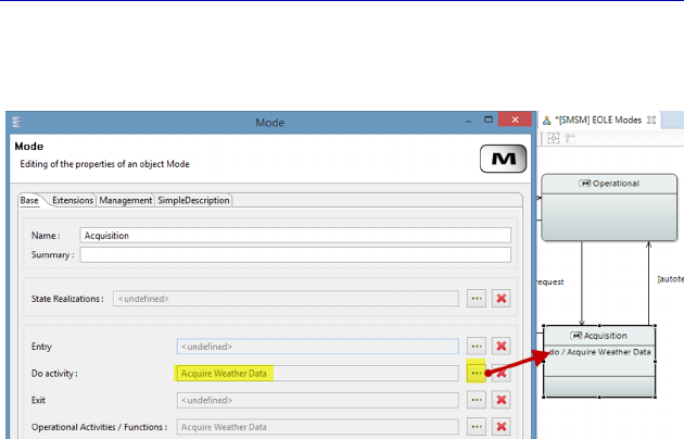
148 Systems Architecture Modeling with the Arcadia Method
open the property sheet of the “Acquisition” Mode and choose the
function “Acquire Weather Data” in the Do activity field.
Figure 4.117. Example of a durable activity in a Mode or State
In UML/SysML, durable activities have a duration, can be
interrupted and are always associated with the States, in contrast to
Effects on Transitions. The normal end of a finite activity, called
completion transition (or automatic transition), is represented in
UML/SysML without an event or keyword. In our case study, the
transition from “Acquisition” to “Operational” Mode is a good
example.
N
OTE
.– The word “activity” used previously comes from UML/SysML
vocabulary, and more or less represents a treatment or transformation. It
must not be confused with the more specific concept of Arcadia
Operational Activity.
Let us go back to the other concepts that are available in a
transition, starting with the notion of Condition or Guard. In
UML/SysML, a guard condition is a Boolean expression that must be
true when the event takes place for the transition to be triggered. It is
written between brackets. It can involve the values of the block in
question, as well as the parameters of the trigger. Several transitions
starting from the same source State with the same event must have
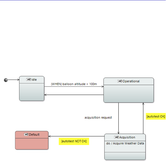
Complete Example of Modeling with Capella: System Analysis 149
different guard conditions in order to guarantee the determinism of the
behavior.
We are going to add a Guard to our State diagram. We assume that
at the end of acquisition, an autotest takes place. If this autotest is OK,
the system returns to the “Operational” Mode. However, if the autotest
fails, the system enters a new Mode called “Fault”. We just need to
edit the Guard field of the existing completion transition and add a
Boolean expression.
Figure 4.118. Adding conditions to the System Mode and State diagram. For
a color version of the figure, see www.iste.co.uk/roques/arcadia.zip
We must now discuss the concept of Effect in order to complete
our overview of the modeling concepts linked to the notion of
Transition. In UML/SysML, a Transition can specify an optional
behavior carried out by the structural element when the Transition is
triggered. This behavior is called “Effect”: this can be a simple action
or sequence of actions (a UML action can represent the updating of a
value, an operation call, as well as the sending of a signal to another
element). Execution of the Effect is unitary and no other additional
events can be treated while it is running.
With Capella 1.1, the concept of Effect can only be linked to the
initializing of the execution of a Function of the structural element
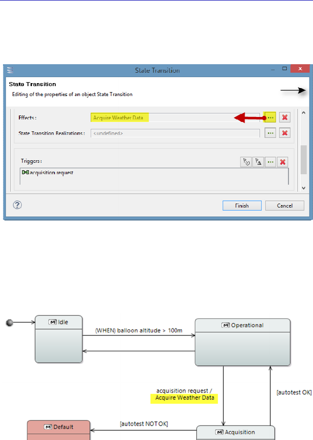
150 Systems Architecture Modeling with the Arcadia Method
involved. In our example, instead of placing the function “Acquire
Weather Data” in the Do activity field, we can consider its launching
to be the transition Effect triggered by the acquisition request.
Figure 4.119. Adding an Effect to a transition
These two ways of modeling are quite similar, although the notion
of durable activity is more in line with the completion transitions of
our example.
Figure 4.120. Adding an Effect to the System Mode and State diagram
To conclude this section on the Mode and State diagram, it must be
added that Modes/States can also be made to appear in ES diagrams.
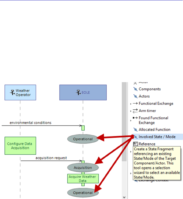
Complete Example of Modeling with Capella: System Analysis 151
Indeed, it can be useful to specify the Mode of the different structural
elements at the start of the Scenario, at the end, or at intermediate
stages. This is particularly interesting when the Scenario has been
described for the purpose of testing, and allows specification of
preconditions, postconditions, etc., that the tester will have to verify.
In our example with a nominal acquisition Scenario, the System must
be in the “Operational” Mode for the Scenario to make sense. The
System then goes into “Acquisition” Mode, and then back into
“Operational” Mode.
Figure 4.121. Adding System Modes and States to the Scenario diagram. For
a color version of the figure, see www.iste.co.uk/roques/arcadia.zip
4.9. Data modeling at the System level
An important part of system engineering involves ensuring
coherence between the data managed in the system and the data
exchanged with external actors. In order to unambiguously describe
these exchanges, the data, information, matter flow, etc., must be
formalized. Beyond this description, an important engineering task
involves avoiding multiple definitions for a single piece of data in
different areas of the system. Hence, the need to declare that several
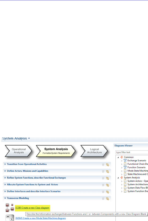
152 Systems Architecture Modeling with the Arcadia Method
exchanges should carry the same type of data, without having to
redefine the shared data for each exchange.
It is in this context that Capella provides advanced mechanisms for
modeling data structures with the desired level of precision, and links
them to Functional Exchanges, Function or Component Ports,
Interfaces, etc.
N
OTE
(Arcadia Rule).– It must be noted that this data modeling is
transverse to all levels of Arcadia. In particular, a Type defined at the
System Analysis level can be used at all of the lower levels, down to the
Physical Architecture level. It is therefore not necessary to carry out a
“transition” of the definitions of Types, as is done for Functions or
Actors, for example. The opposite is not true: a Type defined at a given
Arcadia level cannot be used at higher levels.
Definitions of Exchange Items (EIs), Classes, Types, etc., are
mainly established in Capella through diagrams called Class Diagram
Blanks. These CDB are available at every level of abstraction in
Arcadia and are placed under the theme of “Transverse Modeling”
(just like Mode and State diagrams).
Figure 4.122. Creation of a Class diagram
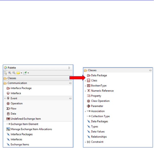
Complete Example of Modeling with Capella: System Analysis 153
There are two main categories of concepts in this type of diagram:
– Communication elements: EIs and Interfaces;
– Type definitions: basic Types, Classes, relations between
Classes.
These two categories of concepts are taken into account in a
division of the CDB’s palette into two different groups.
Figure 4.123. Palette of the Class diagram (CDB)
N
OTE
.–
The Class diagram palette is very comprehensive, and we most
likely will not need to use all of the concepts on offer in any of our
projects. Moreover, the property sheets of these model elements are also
very extensive, allowing those who wish to develop their formalizations
in great depth. Do not forget to adapt your modeling effort to your
objectives, without getting distracted by all of the options provided by
Arcadia and Capella….
Let us start by considering the communication elements and, in
particular, the EIs. An EI has a name and a communication
mechanism. It defines a coherent set of data in terms of use in a
certain context, of a communication principle, as well as of non-
functional properties and of transport simultaneity.
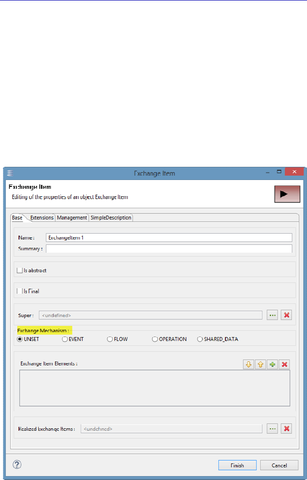
154 Systems Architecture Modeling with the Arcadia Method
There are four predefined communication mechanisms in
ARCADIA:
– EVENT: asynchronous mechanism where an event is sent by an
element and received by one or several others;
– FLOW: flow of matter, energy, etc. or data;
– OPERATION: process carried out by an element and invoked by
another;
– SHARED DATA: data modified by an element and read by
others.
Figure 4.124. Property sheet of an Exchange Item (EI)
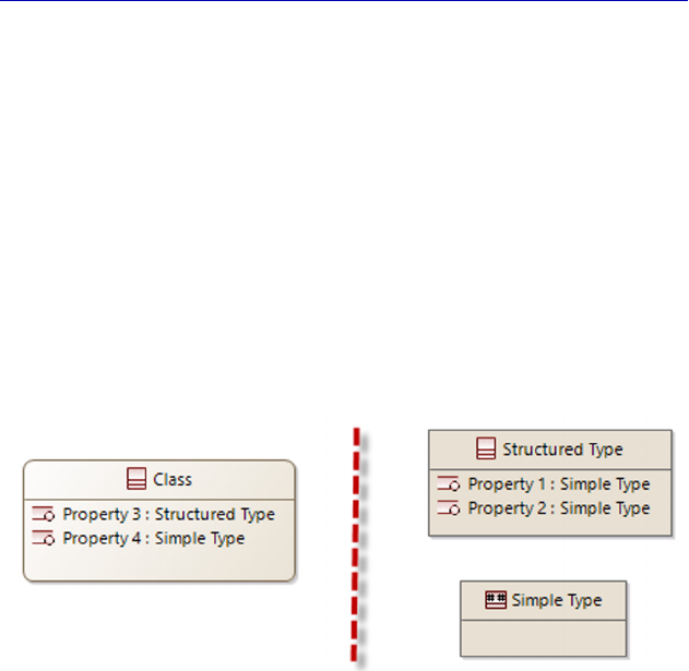
Complete Example of Modeling with Capella: System Analysis 155
In the first stages of the engineering process, the communication
mechanism applied to a given EI might not be known or decided
upon. In such a case, the UNSET “joker” could be used. The choice of
communication mechanism can be refined later using the property
sheet of the EI.
Each EI refers to one or several Types of data, via the EI Elements.
We shall return to this a bit later.
We shall look now at the definitions of the Types proposed by
Capella: Classes, Structured Types, Simple Types. The vocabulary
used comes from UML, and the very name of the “Class diagram” is a
direct reference to it.
Figure 4.125. Definitions of Types in Capella. For a color version
of the figure, see www.iste.co.uk/roques/arcadia.zip
The simple Types predefined by Capella are as follows:
BooleanType, Enumeration, NumericType, StringType and
PhysicalQuantity. Careful, BooleanLiteral and EnumerationLiteral
help define Boolean Type and Enumeration, while Unit helps to
define PhysicalQuantity.
Simple types cannot have properties. If we want to define
Structured Types, the Class button in the palette must be used, and
then the Class must be specified as primitive (tick the box Is
Primitive). The other “Primitive” Classes then play the role of
structured Types, and can in turn type the properties of the “true”
Classes.
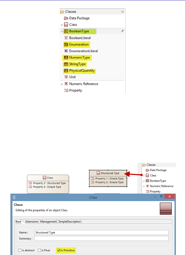
156 Systems Architecture Modeling with the Arcadia Method
Figure 4.126. The basic Types predefined by Capella
To make the analogy with UML, the concept of Primitive Class
corresponds to that of DataType in UML, whose instances have no
identity, unlike for Classes. Classes in Capella can be linked together
through associations, aggregations, compositions or generalizations,
as in UML [ROQ 04].
Figure 4.127. Creation of a Structured Type with Capella. For a color
version of the figure, see www.iste.co.uk/roques/arcadia.zip
We can now go back to the concept of EI Element, which links EIs
to Classes and Types.
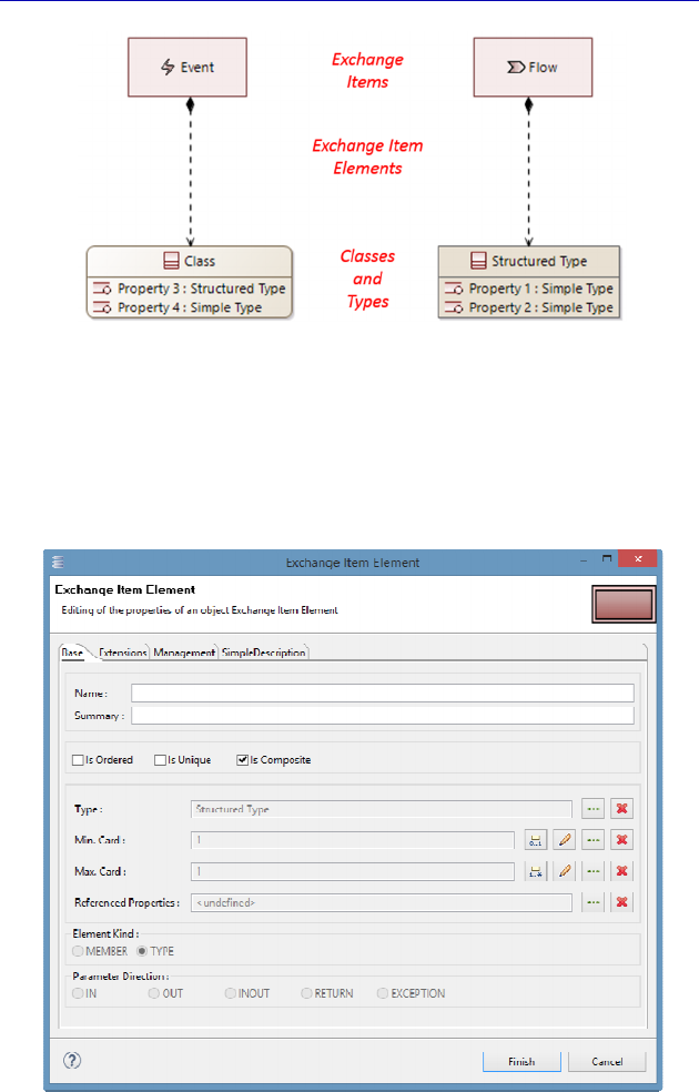
Complete Example of Modeling with Capella: System Analysis 157
Figure 4.128. Relations between EI and Types in Capella. For a color
version of the figure, see www.iste.co.uk/roques/arcadia.zip
It must be noted that the EI Element is itself a model element, with
its own property sheet, which is also quite complex (but here again,
there is no need to use all of it…).
Figure 4.129. Property sheet of an Exchange Item Element
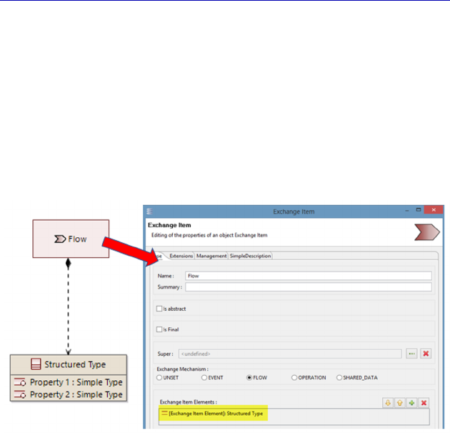
158 Systems Architecture Modeling with the Arcadia Method
By default, the Is Composite box is ticked, meaning the EI in
question will really contain the elements typed by the target Type. The
default cardinality is exactly 1, but the fields Min. Card and Max Card
allow us to specify an optionality (min = 0), or on the contrary, a
multiplicity (max > 1). The notion of PARAMETER is particularly
useful for EIs for which the exchange mechanism is OPERATION.
The links between the EI and the EI Elements are shown in the
property sheet of the EI.
Figure 4.130. Return to the property sheet of an Exchange Item
We return now to our case study in order to more concretely
illustrate the concepts explained previously. We are going to create a
few Simple Types, one Structured Type and some Classes, as well as
some EIs. But rather than doing everything in our EOLE model, we
are going to take the opportunity to introduce the concept of Capella
library.
Simply put, a Capella library is a Capella project that can be
referenced by other projects. The basic idea is to allow, within a given
project, the separation of reusable model elements, so that they can be
referenced later in various projects. These reusable elements are
mainly definitions of Types and Classes of the domain, as well as
basic Physical Components unique to a given domain. This list is not
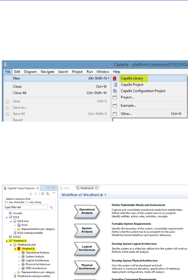
Complete Example of Modeling with Capella: System Analysis 159
restrictive; however, a library can contain the same model elements
and the same Arcadia levels as classical projects.
To create a Capella library, there is a specific command that must
be applied: File – New – Capella Library. Note that a project cannot
be transformed into a library in version 1.1 of Capella.
Figure 4.131. Creating a Capella library
As stated, the model thus created is entirely similar to a classical
Capella model, apart from the different icons in front of the project
and model root. As for any Capella project, we could have unticked
the Operational Analysis and EPBS levels.
Figure 4.132. Result of the creation of a Capella library
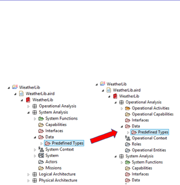
160 Systems Architecture Modeling with the Arcadia Method
We have seen that Type definitions can be used at the level at
which they were declared, as well as at all lower levels. It is therefore
good practice to declare the reusable Types of the domain at the
highest Arcadia level, which is Operational Analysis. Moreover, it can
noted that by default Capella proposes a certain number of basic
Types at the System level in a subfolder called Predefined Types
located in the folder called Data. In light of the comment made above,
we shall move the folder to the Operational level.
Figure 4.133. File reorganization in the Explorer
It must be noted that Capella does not usually leave much room for
reorganizing folders (called “packages”) in the Project Explorer, in an
attempt to maintain model coherence. It would indeed be very
dangerous to be able to move Logical Components to other levels, etc.
However, definitions of Types, Classes, EIs, etc., can be easily
reorganized if necessary, for example by sliding-moving folders in the
Project Explorer.
We shall now create a new subfolder in the predefined Data
package, which we call “Domain Types” using the contextual
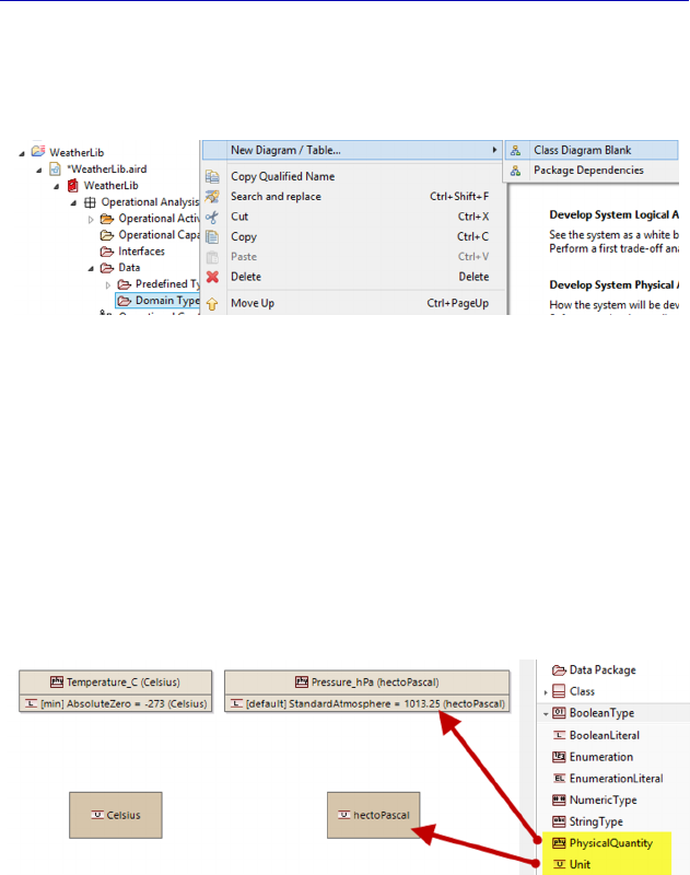
Complete Example of Modeling with Capella: System Analysis 161
command Add Capella Element–Data Pkg. It is in this subfolder that
we place the Class diagram (CDB) through the contextual menu.
Figure 4.134. Creation of packages and
diagrams in the explorer
In this Class diagram, we are going to create:
– Two Units: Celsius and hectoPascal;
– Two Physical Quantities: Temperature_C, Pressure_hPa;
– Two Numeric Types: Hour and Minute;
– One Structured Type: Timestamp.
Figure 4.135. Creation of Units and Physical Quantities. For a color
version of the figure, see www.iste.co.uk/roques/arcadia.zip
Note the extensiveness of the basic Type property sheet, and even
of the Literal Values.
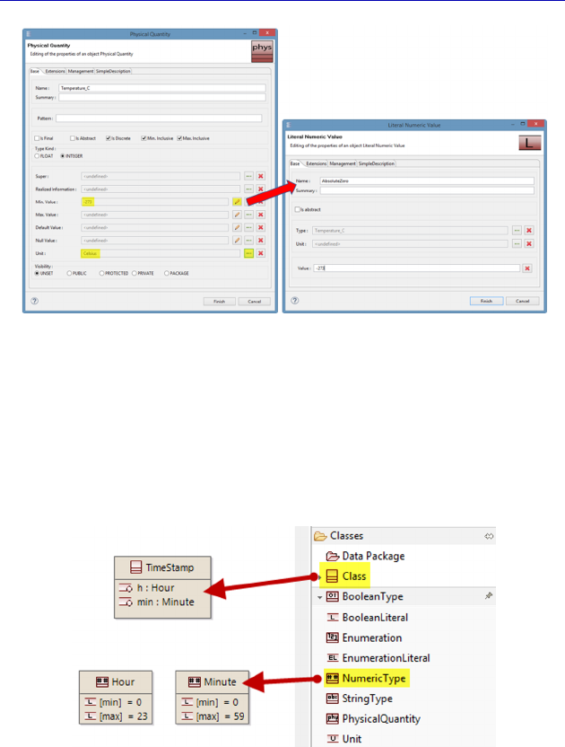
162 Systems Architecture Modeling with the Arcadia Method
Figure 4.136. Property sheet of a Physical Quantity
Numeric Types have the same property sheet as Physical
Quantities, except for the missing Unit field. To create a Structured
Type, as explained before, we must use the concept of Class, and tick
Is Primitive. The two properties in the Class are then added using the
palette (Property).
Figure 4.137. Creation of a Structured Type in the library. For a color
version of the figure, see www.iste.co.uk/roques/arcadia.zip
We shall now return to our EOLE project and create some EIs to
describe the three functional flows of the acquisition Chain. We shall
create a flow of air particles coming from the atmosphere, and
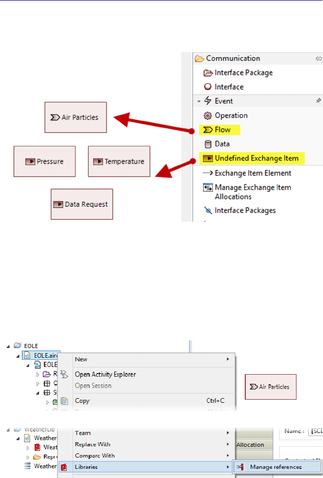
Complete Example of Modeling with Capella: System Analysis 163
exchanges of unspecified mechanism for the acquisition request and
for the measurement of temperature and pressure.
Figure 4.138. Creating Exchange Items in the EOLE project. For a color
version of the figure, see www.iste.co.uk/roques/arcadia.zip
We must now link these EIs to Classes or Types. However, to do
this, we must have access to Types defined in the domain library. This
requires referencing the library in our project. Capella allows us do
this by right clicking on the “.aird” file in the Project Explorer.
Figure 4.139. Referencing a library in a project
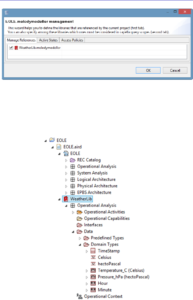
164 Systems Architecture Modeling with the Arcadia Method
Figure 4.140. Referencing a library in a project (continued)
The library becomes visible inside the project, and all of the model
elements that are defined within it are accessible if the different
Arcadia levels are compatible.
Figure 4.141. Referencing a library in a project (end)
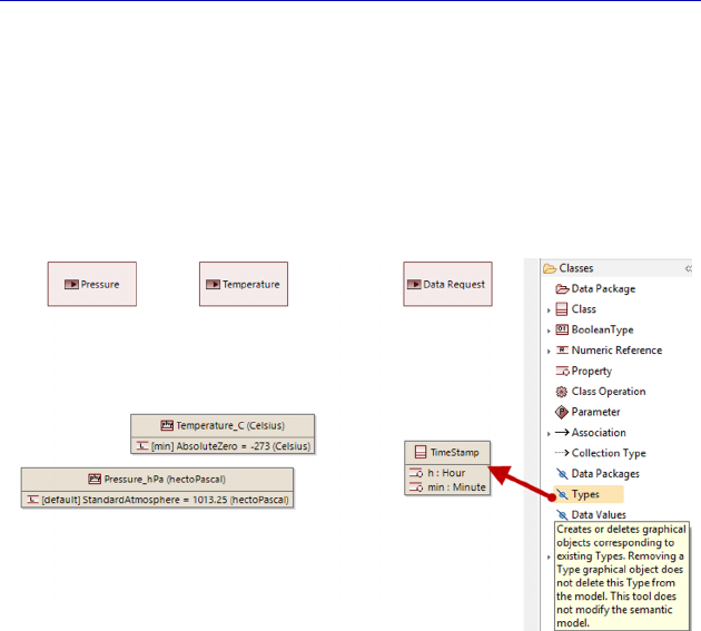
Complete Example of Modeling with Capella: System Analysis 165
We can now use the Types of the domain library, such as the
Simple Types “Temperature_C” and “Pressure_hPa”, as well as the
Structured Type “Timestamp” for our new Class “DataRequest”. To
insert the library Types into our diagram, the command Insert/Remove
Types from the palette is used. We now not only have access to the
Types defined in the EOLE model, but also those from the referenced
library, at the Operational and System levels.
Figure 4.142. Insertion of library Types into the project CDB. For a color
version of the figure, see www.iste.co.uk/roques/arcadia.zip
The class “DataRequest” will have two Timestamp type properties,
called “requestTime” and “captureTime”, the latter of which is
optional. The capture time only needs to be stated if capture is
performed on demand, otherwise it takes place at a fixed time. The
property sheet of a Class Property allows specification of min and
max cardinalities (1 by default). By moving the min cardinality from 1
to 0, we are specifying an optional Property.
N
OTE
.– Once again, note the breadth of this property sheet, which
allows us to specify a default value, a null value, etc., as well as
characteristics that are close to object programming language, such as Is
Static, Is abstract or Visibility. Because of the Capella Studio
environment, it is indeed possible to develop code generators from the
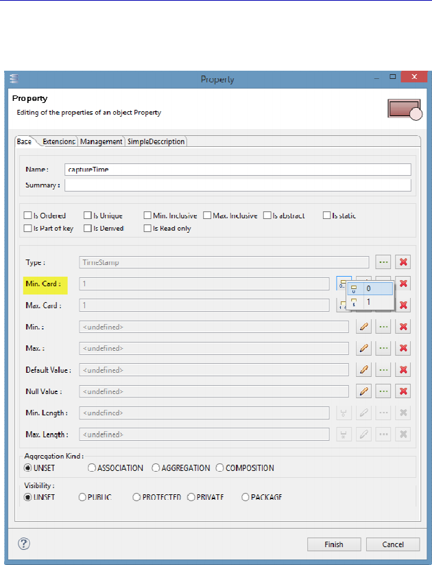
166 Systems Architecture Modeling with the Arcadia Method
information contained in a Capella model, even if this is not the main
objective of this type of system modeling.
Figure 4.143. Property sheet of a Class Property
We must now link our EIs to Types and Classes that define their
content through several EI Elements. This can be done either
graphically in the Class diagram, or through the property sheet of the
EI.
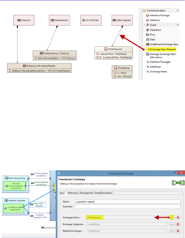
Complete Example of Modeling with Capella: System Analysis 167
Figure 4.144. Finalizing the Class diagram. For a color version
of the figure, see www.iste.co.uk/roques/arcadia.zip
The last step of our little exercise is to link the Functional
Exchanges and the EIs. The simplest way to do this is to select the
Functional Exchanges involved in a diagram or the Project Explorer
and to open their property sheet. Going back to the complete SAB for
example, we double-click on the “acquisition request” FE. The first
field of the sheet is called Exchanged Items and allows us to select the
EIs that interest us.
Figure 4.145. Link between Functional Exchange and Exchange Item. For a
color version of the figure, see www.iste.co.uk/roques/arcadia.zip
We thus associate the “Data Request” EI with the “acquisition
request” FE, the “Air Particles” EI with the “environmental
conditions” FE and the two “Pressure” and “Temperature” EIs with
the “collected data” FE. The Architecture diagram itself is not
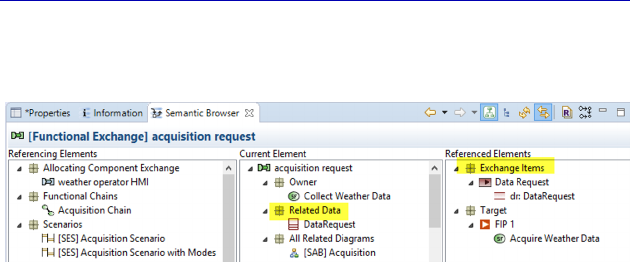
168 Systems Architecture Modeling with the Arcadia Method
modified, but all of the chain of linked concepts can be seen in the
Semantic Browser.
Figure 4.146. Links between concepts seen in the Semantic Browser. For a
color version of the figure, see www.iste.co.uk/roques/arcadia.zip
We have thus allocated EIs to Functional Exchanges, but Arcadia
actually recommends allocating EIs to each Function Port in order to
characterize the content that the Function could produce or could
need.
N
OTE
.– At least one EI should be allocated to each Function Port. This
EI could be shared between several Ports, and actually should be shared
by the two Ports at the extremities of a Functional Exchange. If a
Function Port has several EIs, then it should be specified on each
Functional Exchange connected to it, which are the elements that are
actually conveyed, which must be coherent with those of the Ports
connected by the Exchange. Capella proposes a Modeling Accelerator
to propagate the EIs of a Functional Exchange toward each of the
Function Ports: Propagate Exchange Items to Function Ports.
We have stated that the Architecture Blank diagram (SAB) was
unchanged graphically. However, there is a way of displaying the EIs
in this type of diagram. To achieve this, we apply an additional filter:
Show Exchange Items on Functional Exchanges. After a Refresh on
the diagram (F5), we obtain the following figure, where the EIs appear
in brackets, instead of the names of the Functional Exchange involved.
This is finest level of detail that can be achieved in this type of
diagram.
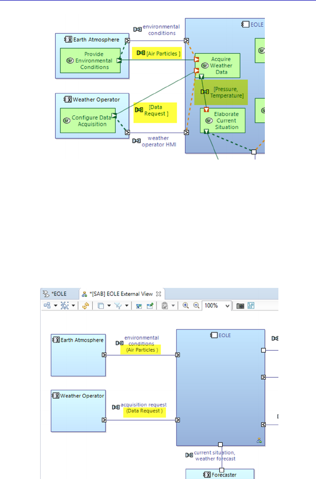
Complete Example of Modeling with Capella: System Analysis 169
Figure 4.147. Exchange Items instead of Functional Exchanges. For a color
version of the figure, see www.iste.co.uk/roques/arcadia.zip
In a similar fashion, let us now go back to the SAB showing the
external exchanges, and apply the additional filter: Show Exchange
Items on Component Exchanges. After a Refresh of the diagram (F5),
we obtain the following figure, where the EI appear in parentheses
after the name of the FE involved.
Figure 4.148. Adding EI to the SAB of the external exchanges. For a color
version of the figure, see www.iste.co.uk/roques/arcadia.zip
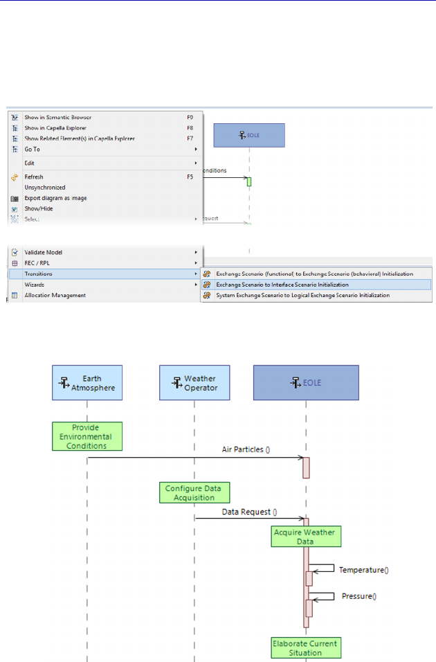
170 Systems Architecture Modeling with the Arcadia Method
Continuing on the subject of EIs, we must state that it is also
possible to make them appear in scenarios, called Interface Scenarios
(IS). Capella is even capable of automatically initializing an IS from
an ES.
Figure 4.149. Initializing an IS from an ES
Figure 4.150. Example of IS finalization from an ES. For a color version
of the figure, see www.iste.co.uk/roques/arcadia.zip
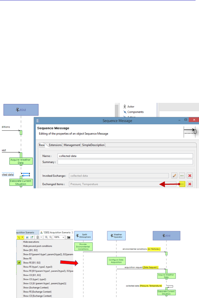
Complete Example of Modeling with Capella: System Analysis 171
We go back to our “[SES] Acquisition scenario”, and apply the
command: Transitions – Exchange Scenario to Interface Scenario
Initialization through the contextual menu. Capella will create a new
Scenario, where the vertical lines and the Functions are preserved. All
that is left to do is to add the horizontal messages, which represent EIs
and no longer FEs, as is shown in Figure 4.150.
We could also have stated earlier in the process, from the SES
onward, which EIs are carried by the messages. This is particularly
interesting when a Functional Exchange contains several EIs: it allows
us to choose which subset is present in the scenario involved.
Figure 4.151. Details on the EIs of a message in an ES
With the right filter, the EIs can now be seen in the SES.
Figure 4.152. Displaying the EIs of a message in an ES. For a color version
of the figure, see www.iste.co.uk/roques/arcadia.zip
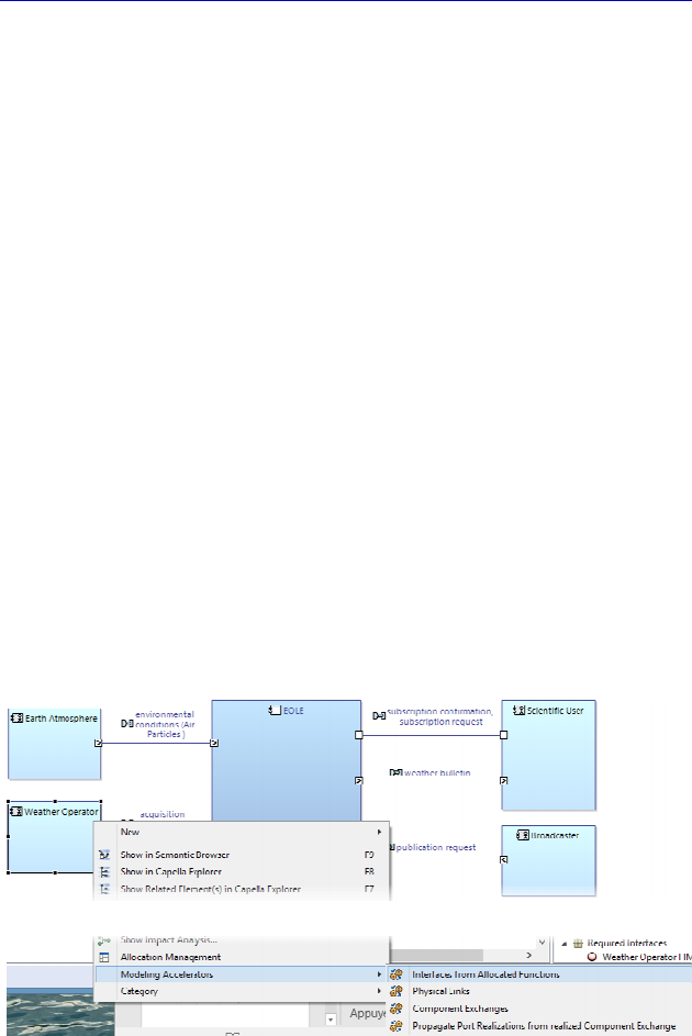
172 Systems Architecture Modeling with the Arcadia Method
Note that if we have associated EIs to messages from the SES
onward, the transition of the ES to an IS preserves the EIs and
automatically generates the Scenario, as shown in Figure 4.150.
To finish off on the subject of EIs, we can add that it is also
possible to group them into Interfaces. Capella proposes this concept
to any modelers who might want it, and it is very similar to the
concept that exists in UML and in certain object-oriented
programming languages.
N
OTE
(Arcadia Rule).– An Interface is a collection of EIs, semantically
coherent, that allow two Components (and the System and the Actors),
to communicate along a communication “contract” shared between
them. At least one Interface should be allocated to each Component Port
of a component to characterize the EIs that the component can produce
or that it needs. An Interface can be shared by several Components, and
in fact should be shared by the two Component Ports of the
Components at the extremities of a Component Exchange.
Capella is able to automatically calculate the Interfaces of a
structural element from its Function allocations. This is a sophisticated
new accelerator called Interfaces from Allocated Functions. Let us try
it first on an Actor from our case study: the weather operator.
Figure 4.153. Use of a new modeling accelerator. For a color version
of the figure, see www.iste.co.uk/roques/arcadia.zip
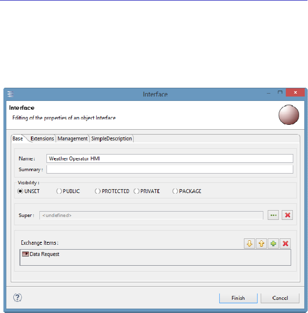
Complete Example of Modeling with Capella: System Analysis 173
Capella has created an Interface called “Weather Operator HMI” in
the Interfaces package, from the name of the Component Exchange.
This Interface contains a reference to the EI “Data Request”, which
leaves the weather operator to go toward EOLE.
Figure 4.154. Property sheet of an Interface
We can do the same for the Actor “Earth Atmosphere”, and
Capella creates a second Interface “Environmental Conditions”, which
contains the EI “Air Particles”. It is then possible to ask Capella to
automatically create two new types of diagram:
– Contextual Component Detailed Interface (CDI);
– Contextual Component External Interface (CEI).
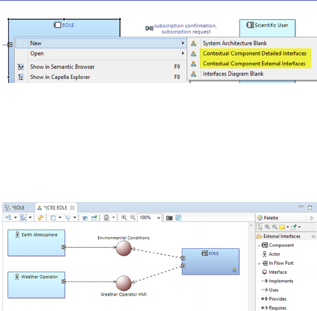
174 Systems Architecture Modeling with the Arcadia Method
Figure 4.155. Contextual Interface diagrams
Although we have only created a few EIs in our case study,
Capella is able to generate the following diagrams (Figures 1.156
and 1.157), which reflect the current state of the model. The CEI
shows the Interfaces of a specific structural element as well as the
other connected elements.
Figure 4.156. CEI for EOLE. For a color version
of the figure, see www.iste.co.uk/roques/arcadia.zip
N
OTE
(Arcadia Rule).– An interaction role describes the operating
instructions of an Interface for a Component by qualifying the
allocation of the Interface to a Component Port of the Component. A
role is therefore given to a Port and an Interface. In the largely
majoritarian case of dependency from the data (matter, flow, messages,
events, shared data, etc.), only two roles are defined: the role
(implements/provides) of the provider and the role (uses/requires) of the
consumer.
In our example, EOLE provides the Interfaces used by the Actors.
This means that the System is able to receive the data created by the
Actors and react to it.
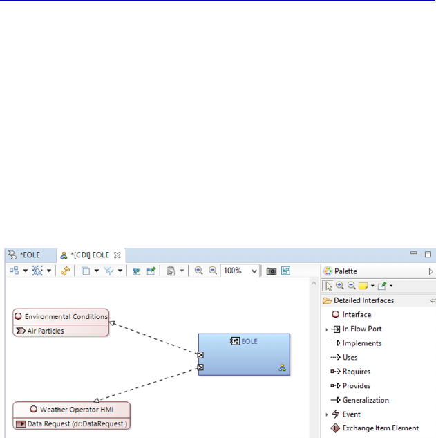
Complete Example of Modeling with Capella: System Analysis 175
N
OTE
.–
EOLE receives the data and flows from the Actors, yet also
provides the Interfaces. The notions of provide/use for interfaces come
from object concepts, and particularly from UML. They are not very
intuitive for a systems engineer without a computer science
background. The graphical notation also comes directly from the
UML component diagram [ROQ 04]: dashed arrow for dependency,
and dashed line with a triangular arrowhead at the end for
implementation.
The other Interface diagram is the CDI, which shows the details of
provided or required Interfaces of a structural element, i.e. all of the
EIs referenced.
Figure 4.157. CDI for EOLE. For a color version
of the figure, see www.iste.co.uk/roques/arcadia.zip
This page intentionally left blank
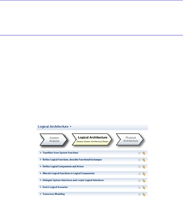
5
Complete Example of Modeling with
Capella: Logical Architecture
5.1. Main concepts and diagrams
Capella integrates methodological guiding in the form of Activity
Explorer. This lists the different activities and the different diagrams
that can be made in terms of the engineering level concerned. In this
case, this is namely Logical Architecture. Figure 5.1 first specifies the
activities, and then we will detail the possible diagrams throughout the
case study.
Figure 5.1. Methodological activities in terms of Logical Architecture
NOTE.– Be careful, let us recall that even if Arcadia is a method, the
modeling process is totally flexible. The methodological activities

178 Systems Architecture Modeling with the Arcadia Method
presented in Activity Explorer are almost all optional and can be used
in any order, as well as for diagrams.
We will therefore make an arbitrary but reasoned choice again
here, for creating diagrams. We will start by automatically recovering
the Functions and Actors issued from the System level to start our
Logical level. Then, inside the System, we will create perennial
Logical Components that are independent from any technological
choice. At the same time, we will decide on allocating Logical level
Functions to these components, and we may be led to break down the
Functions issued from the System level or to complete them. We will
then work on the Ports and the Component Exchanges issued from the
System level that we will delegate to the Logical Components and we
will add internal Component Exchanges, if necessary.
To keep in line with the book’s aim, we will make modeling
choices that enable the case study to maintain its simplicity. The
model of the real project would certainly be more complex.
5.2. Moving from the System level to the Logical level
The previous System Analysis consisted of functionally analyzing
the System seen as a “black box” to specify its expected behavior, as
well as exhaustively identifying important external exchanges with the
Actors.
Logical Architecture, on the other hand, starts to “open the box” to
identify structural elements called Logical Components as well as
their properties and relations. The important rule to comply with is to
force ourselves to exclude all technological considerations or
implementation choices. This will be the very objective of the
Physical Architecture to define the “true” concrete components, which
will constitute the System.
Excluding all technological considerations as a design choice will
not however prevent us from beginning to take the Non-Functional
Constraints into account. Operating Safety, Performance, etc.,
requirements can thus lead us to group the Functions together in
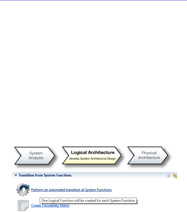
Complete Example of Modeling with Capella: Logical Architecture 179
different Components. In the same way, the Product Line Engineering
(PLE) problem must begin to be considered from this level onwards to
separate the “generic” and reusable Logical Components of the
Logical Components specific to the current project. Finally, good
important practice can be outlined as follows: Logical Architecture
must be stable throughout the whole duration of the project. This will
probably not be the case for Physical Architecture, especially if the
System must have a long life-span, due to the technological novelties
that will occur and the new Physical Components that may cause large
parts of the architecture to be called into question.
To start the Logical level from the work performed on the System
level, Capella proposes transitions like those that we used when we
went from the Operational Analysis to the System Analysis. We can
thus create as many Logical Functions as System Functions, while
also keeping the Functional Exchanges and the Functional Chains. We
apply this first transition based on the Activity Explorer.
Figure 5.2. Transition tool for the Functions to the Logical level
We are now looking at a simple transition case, and pressing on the
“Apply” button will allow us to recover everything in one go. The
result is visible in the Project Explorer where model elements now
exist in the Logical Functions folder.
Let us recall that Capella automatically creates a Realization Link
between each Logical element (Function, Functional Exchange,
Functional Chain) and the Source System element. We also recall that
the transitions are iterative and incremental and that if we notice that a
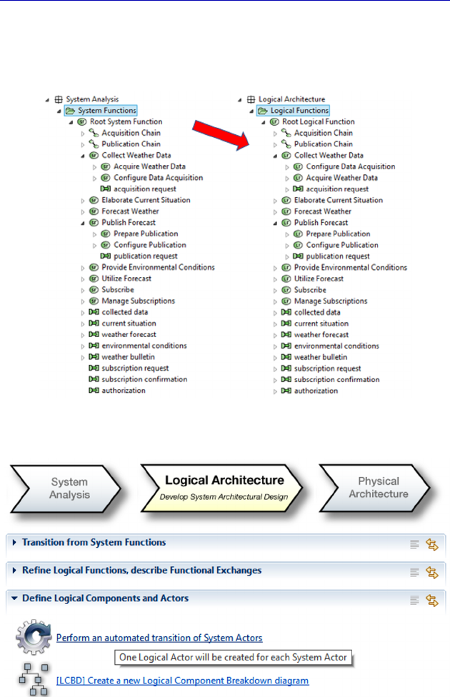
180 Systems Architecture Modeling with the Arcadia Method
System Function is missing when working on the Logical level, we
must absolutely add it to the System level and apply the
transition again.
Figure 5.3. Result of the Functional Transition in Project Explorer
Figure 5.4. Transition tool for the Actors to the Logical level
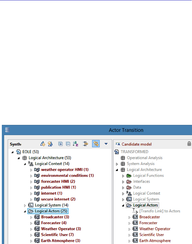
Complete Example of Modeling with Capella: Logical Architecture 181
We now apply the transition of the external Actors. In most cases,
the Actors identified on the System level will be exactly the same as
on the Logical and Physical levels. The automatic transition (iterative
and incremental) is thus particularly useful for this type of model
element.
We are here looking at a simple transition case, and pressing on the
Apply button will allow us to recover everything in one go. The result
is visible in the Project Explorer where the model elements now exist
in the Logical Actors folder. Capella also automatically recovers the
Component Ports and the Component Exchanges between the System
and the Actors, which will ease the Logical Architecture work
enormously later. It also keeps the Allocations of Functional
Exchanges to Component Exchanges.
Figure 5.5. Dialogue for the Actor Transition tool to the Logical level
In the Project Explorer, we will check that we have properly
recovered the Actors and the Component Exchanges. The Ports are
not visible in the Project Explorer by default, but nevertheless they
are in the Semantic Browser, as well as the Allocation and Realization
relations.
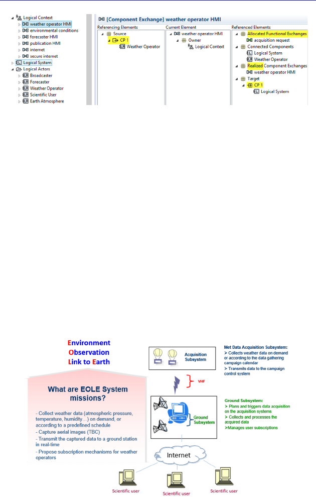
182 Systems Architecture Modeling with the Arcadia Method
Figure 5.6. Verification of the Actor transition result
5.3. Logical Components
As indicated above, the Logical Architecture starts by identifying
structural elements called Logical Components by forcing ourselves to
exclude all technological consideration or implementation choice.
In our case study, we have known from the beginning that the
System will contain two Subsystems: an acquisition Subsystem “in the
air” and a processing Subsystem on the ground. We are not yet talking
about a helium balloon, which is an implementation choice that is part
of the Physical Architecture world. By the way, it is good practice to
name the Logical Components and Physical Components differently,
and only attributing the names containing references to a precise
technology to the Physical Components.
Figure 5.7. Reminder of the EOLE System’s design brief
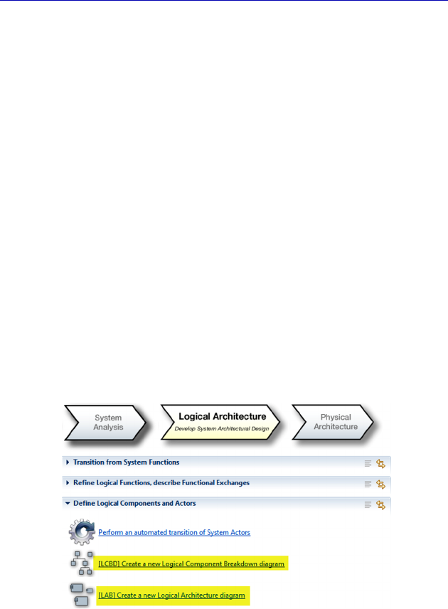
Complete Example of Modeling with Capella: Logical Architecture 183
NOTE (Arcadia Rule).– Be careful. The notion of Subsystem does not
exist in Arcadia. In System Analysis, we can only have a single model
element called System. If we want to model Subsystems, we need to
be on an internal, Logical or Physical, Architecture Level. If we want
to be able to then consider each Subsystem as a full member System,
with its own System Analysis, Logical then Physical Architecture, we
must model each Subsystem in a specific Capella model. The ideal
being to maintain coherency between the external Exchanges of the
different Subsystems in the “global” model of the encompassing
System. This is exactly what allows us to do the System to Subsystem
Transition add-on, which can be downloaded from the Website
www.polarsys.org/capella/download.html. We will illustrate these
very interesting capabilities further in this chapter on Logical
Architecture.
So, we are going to create two Logical Components corresponding
to the two Subsystems. To do this, we can use a Breakdown diagram
(LCBD) or directly use an Architecture diagram (LAB). We could
even start from an Exchange Scenario (LES) and by creating vertical
lines representing new Components, as explained in the System level.
Figure 5.8. Diagrams for creating Logical Components
The most efficient way here is to start directly from the
Architecture Diagram, especially as the Breakdown diagram can be
performed automatically by Capella, a posteriori. Like in the case of
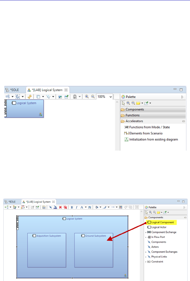
184 Systems Architecture Modeling with the Arcadia Method
the Architecture diagram on the System level (System Architecture
Blank (SAB)), the LAB will not be empty either. As a matter of fact,
Capella automatically inserts a box representing the System on the
Logical level (Logical System) that enables the Component Ports and
the Component Exchanges issued from the Actor Transition to
materialize. The Logical System thus constitutes a very practical
“reminder” that prevents us from forgetting to delegate the external
Ports to the Components. Once more, Capella makes the modeler’s
life easy because of its thorough knowledge of the Arcadia approach.
Figure 5.9. Beginning of the Logical Architecture Blank diagram (LAB)
We are going to create two Logical Components inside the Logical
System by expanding and centering the same.
Figure 5.10. Creating Logical Components in LAB
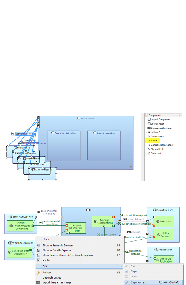
Complete Example of Modeling with Capella: Logical Architecture 185
N
OTE
.– In the case of the EOLE System, the box representing the
Logical System will no longer exist in Logical and Physical
Architecture. In the end, the only concrete structural containers will be
the balloon and the ground station. Thus, we can change the color of
the Logical System to indicate that it is not really a Component and
must no longer have Ports by the time our work is finished. Be
careful: if the System on the Physical level still had a concrete
external envelope, this would not be the same, and the external Ports
would need to be conserved until the end.
Before moving onto allocating the Functions, we insert the Actors
already in the diagram. We note that the Component Exchanges issued
from the Transition automatically appear in the diagram.
Figure 5.11. Inserting the Logical Actors in the LAB
Figure 5.12. Copy of the format of an SAB. For a color version
of the figure, see www.iste.co.uk/roques/arcadia.zip
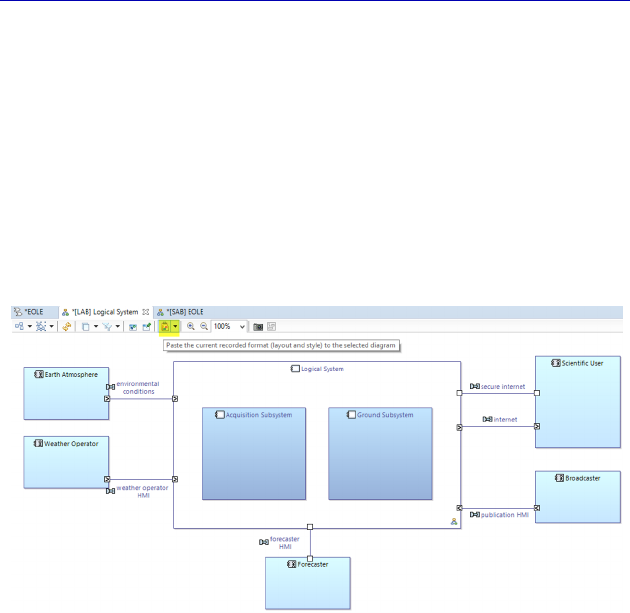
186 Systems Architecture Modeling with the Arcadia Method
The graphic positioning of the Actors is far from optimal, and
unfortunately even still with the Arrange All command in the diagram.
In contrast, there is an efficient way to remedy this by copying and
pasting the layout of a diagram like the System level. To do this, we
will go back to the complete SAB and call upon the context-sensitive
Edit–Copy format command, as in Figure 5.12.
We are now going to paste the format in the LAB. After having
spread the Actors and changed the color of the Logical System as
indicated, we obtain the following diagram (Figure 5.13).
Figure 5.13. LAB continued. For a color version of
the figure, see www.iste.co.uk/roques/arcadia.zip
N
OTE
.– An interesting alternative for obtaining an LAB diagram,
which graphically resembles a similar diagram of the System level
(SAB), consists of using the accelerator called Initialization from
existing diagram, visible in the Palette of Figure 5.9. We have not
proceeded thus as, depending on the Capella version, this accelerator
does not always work perfectly. In the current version (1.1.1), the box
of the Logical System is still at the top left of the diagram, whereas the
Actors are positioned properly. Thus, the Ports of the Logical System
and the Component Exchanges are not well placed. As soon as this
minor problem is corrected, the accelerator will be the most efficient
means of creating an LAB based on an SAB.
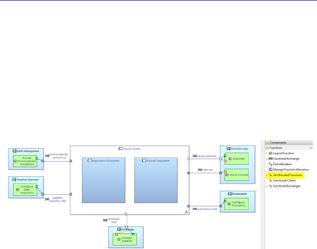
Complete Example of Modeling with Capella: Logical Architecture 187
5.4. Allocation of the Logical Functions
We have indicated that the Transition from the Actors conserved
their Function Allocations. We can therefore very easily insert them
into the LAB diagram using the same System level Palette
command: Insert All Allocated Functions. We could also have inserted
the Functions before applying the format copy–paste to save time, but
we can still do it again by selecting the Actors in the SAB before
copying the format.
Figure 5.14. Inserting the Functions allocated to the Actors in the LAB.
For a color version of the figure, see www.iste.co.uk/roques/arcadia.zip
N
OTE
.– We note that the Functions that were allocated to EOLE in the
System level are currently not allocated. Capella knows that we have
transitioned them either to allocate them to one of the Logical
Components, or to break them down and allocate their subfunctions. It
is therefore necessary that they are not yet allocated so as to be able to
make one choice or another. It therefore would have hardly been wise
to allocate them automatically to the Logical System ….
We will now proceed to Allocate each Function of the System to
one of the Logical Components. Our example will voluntarily remain
very simple, even simplistic, for educational purposes. For example,
we could have started to break down the “Acquire Data” Function
according to the types of different data (temperature, pressure, etc.),
but we will only do it on the Physical level. Similarly, we should have
started to process the communication needs between the ground and
the airborne, as the Weather Operator will probably not be able to
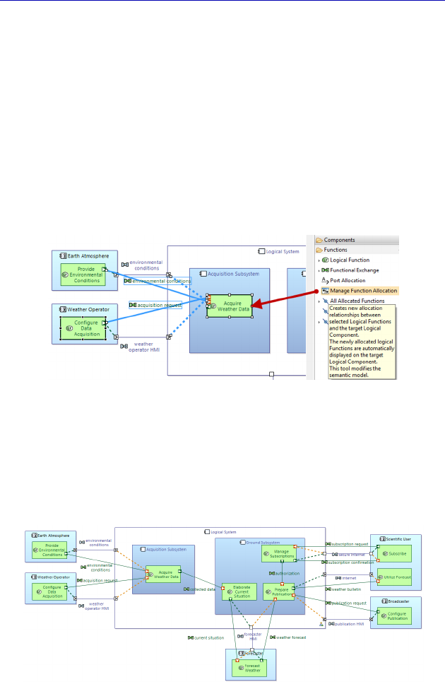
188 Systems Architecture Modeling with the Arcadia Method
communicate directly with the Acquisition Subsystem, but instead
through the Ground Subsystem.
Thus, we simply allocate the “Acquire Meteorological Data”
Function to the Acquisition Component, and the three other Functions
to the Ground Component. To do this, we will use the Manage
Function Allocation command of the LAB Palette. Note that the
Functional Exchanges are automatically displayed as soon as their
target and source Functions are shown in the diagram. The transition
from the System level has also conserved the allocations from the
Functional Exchanges to the Component Exchanges.
Figure 5.15. Beginning of the Function allocation to the Logical Components.
For a color version of the figure, see www.iste.co.uk/roques/arcadia.zip
We complete the Allocation before graphically improving the
diagram. By moving the Ports and optimizing the placing of the
Functions, we quickly end up with the following diagram (Figure 5.16).
Figure 5.16. End of Functions Allocation to the Logical Components. For a
color version of the figure, see www.iste.co.uk/roques/arcadia.zip
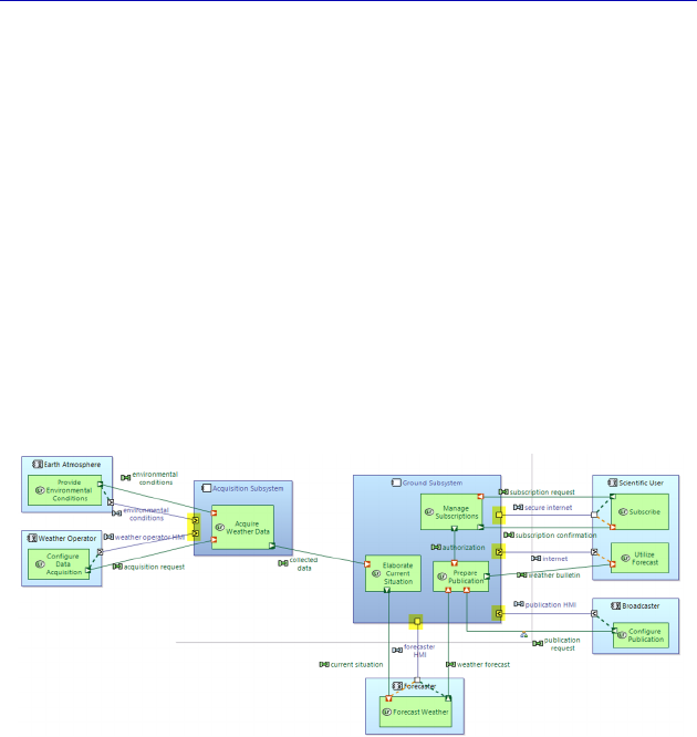
Complete Example of Modeling with Capella: Logical Architecture 189
Like in the upper level, we can easily verify that we have allocated
all the Functions. To do this, you just need to try to apply the Manage
Function Allocation command to any structural element again: if the
selection choice is empty, this means that all the Functions have been
allocated. Of course, the Model Validation can also be used.
We previously indicated that in our case, the Logical System does
not really exist and above all, allows the Component Ports and the
Component Exchanges issued from the Transition from the Actors to
materialize. Thus, it constitutes a very practical “reminder’” that
prevents us from forgetting to delegate the external Ports to the
Components, which we will now do. To do this, we just need to drag-
drop the Component Ports from the border of the Logical System
toward the Logical Component concerned.
Figure 5.17. Dropping the external Ports on the Logical Components. For a
color version of the figure, see www.iste.co.uk/roques/arcadia.zip
We verify that the Logical System no longer has any Ports. To do
this, we will also change the color of its contour so that it almost no
longer appears. We will also complete the Allocations of the
Functional Ports, which were lost by dragging the Component Ports.
To do this, we just need to open the Property Sheet of a Component
Port and to select the Function Ports concerned in the Allocated Ports
field.
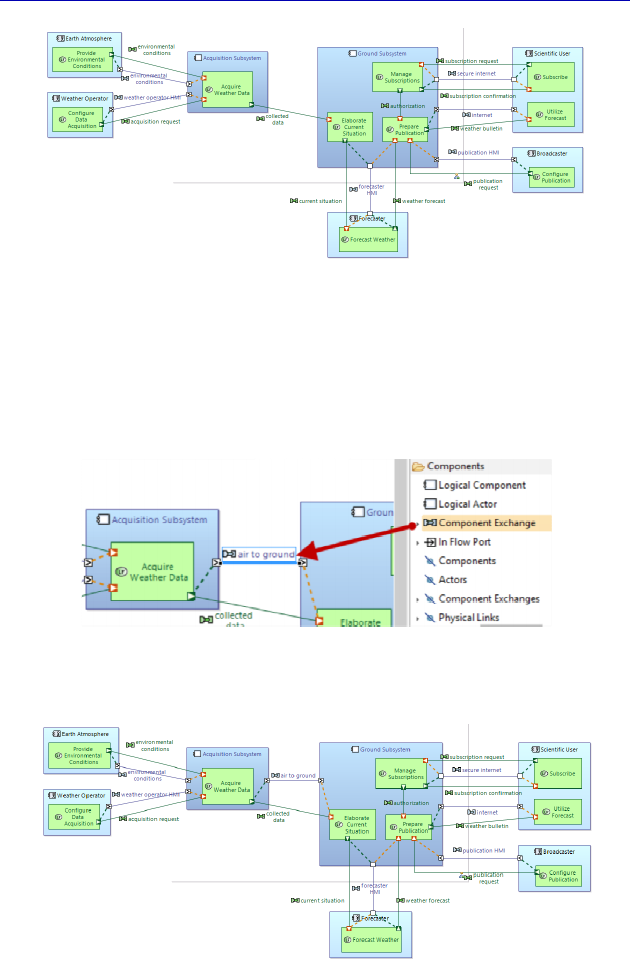
190 Systems Architecture Modeling with the Arcadia Method
Figure 5.18. Finalizing the dropping of the external Ports. For a color version
of the figure, see www.iste.co.uk/roques/arcadia.zip
On this level, we see that the Functional Exchange “collected data”
crosses the borders of the two Components. It is therefore necessary to
create a new internal Component Exchange to allocate it.
Figure 5.19. Creating an internal Component Exchange. For a color version
of the figure, see www.iste.co.uk/roques/arcadia.zip
Figure 5.20. Finalized LAB. For a color version of the figure, see
www.iste.co.uk/roques/arcadia.zip
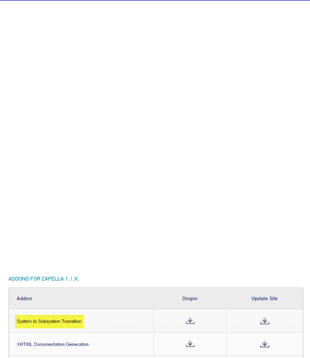
Complete Example of Modeling with Capella: Logical Architecture 191
The finalized diagram (Figure 5.20) becomes relatively complex,
and it could be useful to clone it, and then from this, we derive two
partial diagrams, each centered on a Subsystem.
5.5. System to Subsystem Transition
However, beyond the graphic simplification, we may want to
delegate the modeling of each Subsystem to a different team, perhaps
even to subcontracting companies. In this case, it would be very
desirable to consider each Subsystem as a System in turn, with its own
Capella model starting at the SA level. The Arcadia approach can
effectively be applied recursively up to the level of the detail desired:
System of Systems (SoS), complex System, Subsystem, equipment.
The ideal being to maintain coherence between the external
exchanges of the different Subsystems in the “global” model of the
encompassing System that we have just performed. This is exactly
what allows us to do the System to Subsystem Transition add-on,
which can be downloaded from the Capella Website.
Figure 5.21. Downloading space for Capella add-ons
If we select a Logical Component (or a Physical Component), it is
possible to ask the tool to start a new Capella Model of the selected
Component. The Component in question becomes the System model
element of the SA level of the new model; the Actors and Components
to which it was connected become the Actors of the System level in
the new model. The Functions, Functional Chains, Types, Exchange
Items (EI), Scenarios, etc., are also propagated toward the models of
the Subsystems.
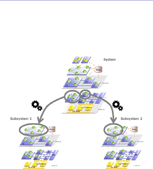
192 Systems Architecture Modeling with the Arcadia Method
The modeler in charge of each Subsystem must consider the SA
Level of its Component as imposed by the global System level, but it is
completely free to perform the Logical Architecture and the Physical
Architecture of the Subsystem in turn. This transition is also iterative
and incremental, which enables the modifications of interfaces between
the Subsystems to be managed efficiently by applying again the
transition of the System level toward the Subsystems.
Figure 5.22. Principle of the System to Subsystem add-on. For a
color version of the figure, see www.iste.co.uk/roques/arcadia.zip
We illustrate the use of this add-on on our case study. We imagine
that we want to design and develop the two Acquisition and Ground
Subsystems by different teams, or even to subcontract them completely.
It is therefore possible to stop the global “System” model on the current
detail level, and to perform two transitions, one for each Subsystem.
We are going to perform the transition for the Acquisition
Subsystem. After having installed the add-on as indicated in the
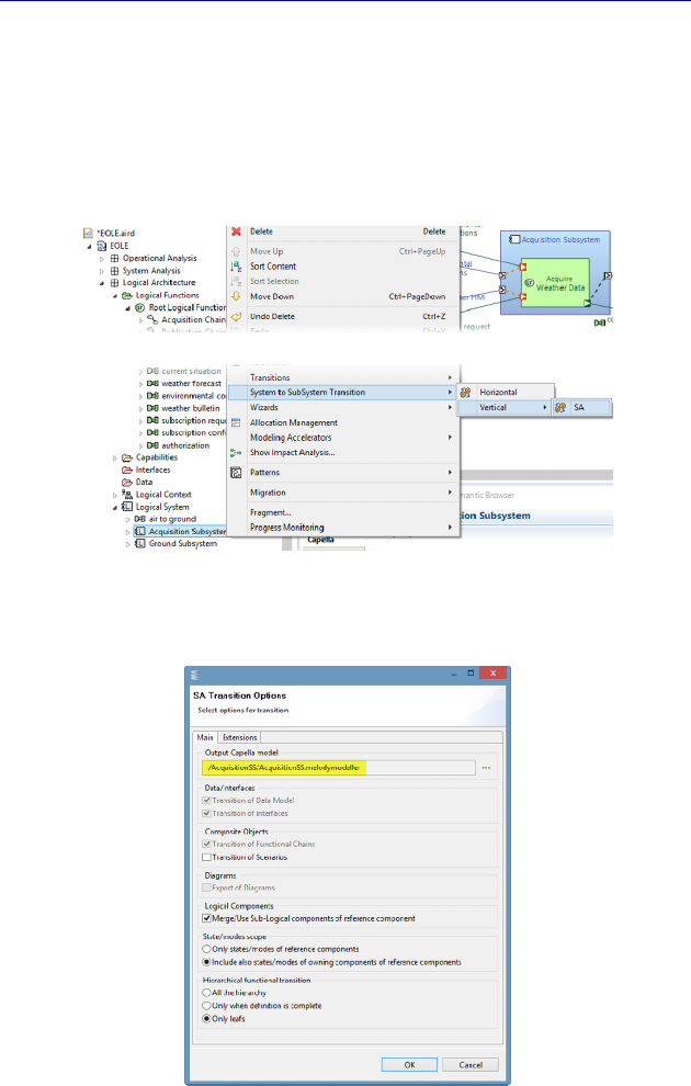
Complete Example of Modeling with Capella: Logical Architecture 193
illustration procedure, we have an additional command at our disposal
in the Project Explorer by right clicking on a Logical (or
Physical) Component: System to Subsystem Transition. There are even
two possibilities, the horizontal transition being just an extraction of a
component toward a new model but staying within the same Arcadia
level. We are going to perform the so-called vertical transition.
Figure 5.23. Context-sensitive call of the System
to Subsystem Transition command
Figure 5.24. System to Subsystem Transition command options
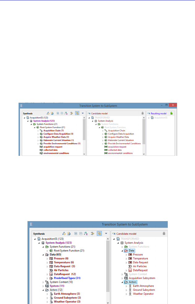
194 Systems Architecture Modeling with the Arcadia Method
Capella then opens a window (Figure 5.24) that enables the
transition to be guided. In particular, we are going to specify whether
a new project needs to be created or if an existing project is to be used.
For example, we will create a new project called “Acquisition SS”,
with only the mandatory Arcadia levels SA, LA and PA.
Capella then opens a diff/merge type window, like for the
transitions between levels inside a same model, to allow the modeler
to ignore certain model elements if they wish. We can see that the
Functions and Functional Exchanges linked to the acquisition are well
proposed, as well as the acquisition Chain.
Figure 5.25. Previsualization window of the transition
In the same way, the Exchange Items and Types used in these
Functional Exchanges are exported, as well as the two Actors bound
to the Acquisition Subsystem. The other Subsystem (Ground)
becomes an Actor in turn.
Figure 5.26. Previsualization window of the transition continued
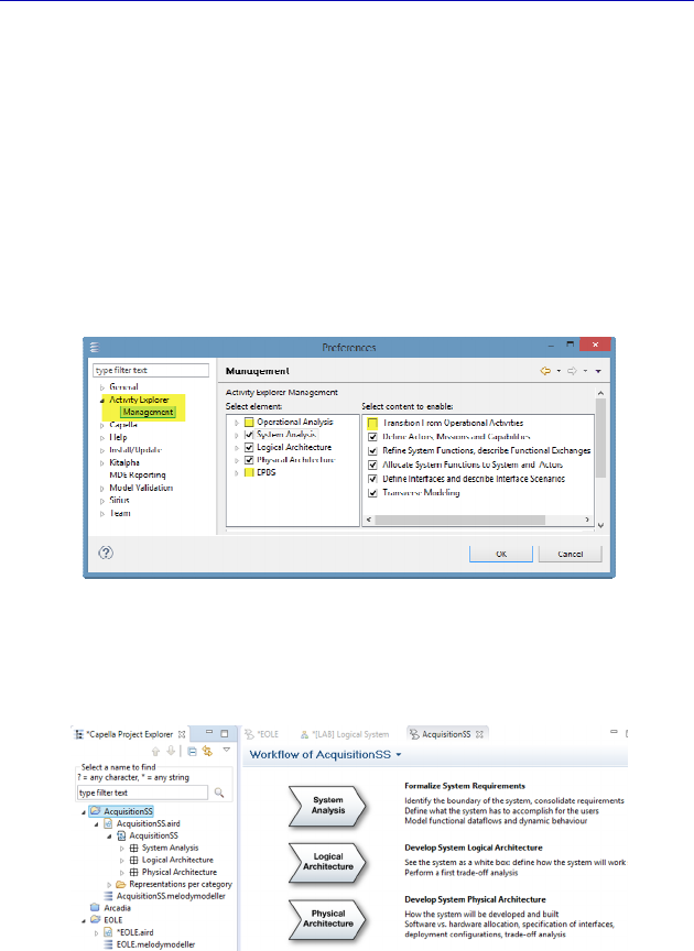
Complete Example of Modeling with Capella: Logical Architecture 195
The result is the creation of a new Capella model, visible in the
Project Explorer and its Activity Explorer.
N
OTE
(Arcadia Rule).– By default, the Activity Explorer contains all
the Arcadia levels, even if we have chosen to remove the optional
levels when creating the project. To hide OA and EPBS in our
example, we just need to modify the project preferences with the
command Window – Preferences – Activity Explorer – Management
and untick the unwanted levels. It is even possible to hide certain
specific fields for the remaining levels.
Figure 5.27. Configuring the Activity Explorer display
The result of hiding it is immediately visible.
Figure 5.28. Result of the Activity Explorer configuration
We now open this new “Acquisition SS” model to verify that it
contains the model elements wanted, and to quickly create some
useful diagrams. The SAB diagram will be particularly relevant: we
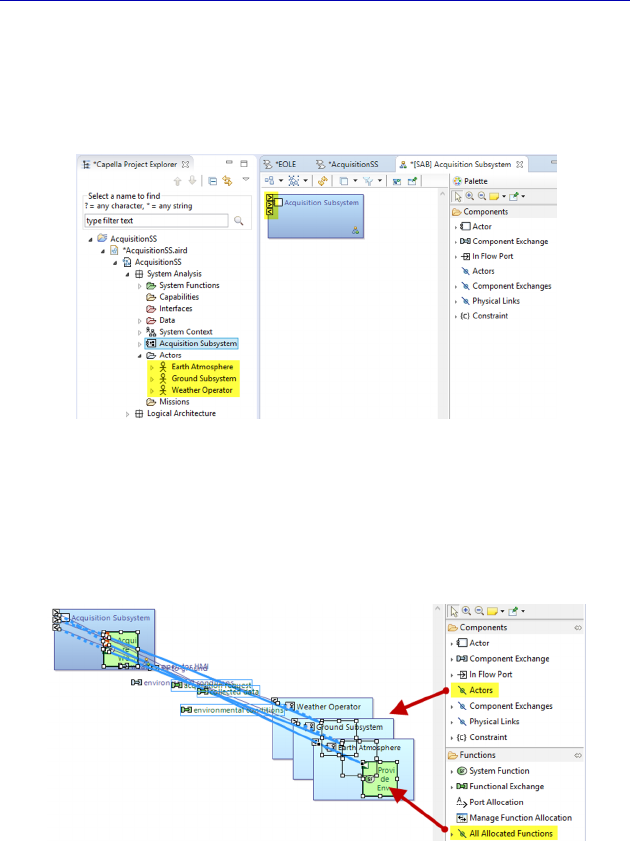
196 Systems Architecture Modeling with the Arcadia Method
will see the Acquisition Subsystem with its Functions, surrounded by
Actors and their Functions, with the Functional Exchanges and the
Component Exchanges. When creating the SAB, the Acquisition
Subsystem automatically appears with its Component Ports.
Figure 5.29. Beginning of the SAB of the Acquisition SS
We are going to insert the Actors (Insert/Remove Actors), then all
the Functions at once (Insert All Allocated Functions). The Functional
Exchanges and the Component Exchanges appear automatically.
Figure 5.30. Inserting the Actors and the Functions in the SAB
Once the formatting is improved, we can definitely see that the SAB
resembles a subset of the encompassing model’s LAB, with the
difference being that the second Subsystem became an Actor for the
first.
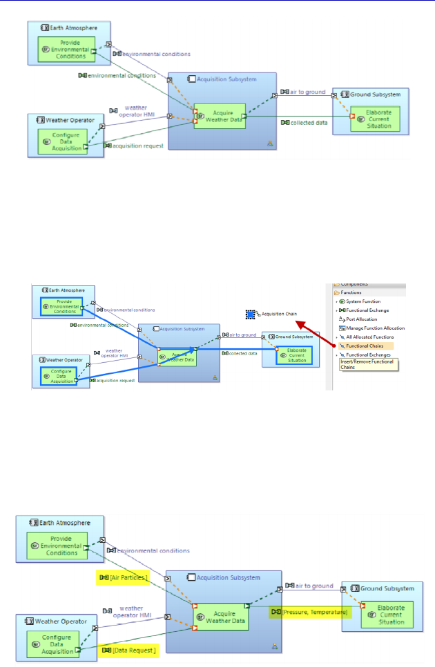
Complete Example of Modeling with Capella: Logical Architecture 197
Figure 5.31. Finalizing the SAB of the Subsystem. For a color version of the
figure, see www.iste.co.uk/roques/arcadia.zip
We can even add the Acquisition Functional Chain that was
automatically transitioned with the Subsystem.
Figure 5.32. Display of the Functional Chain in the SAB. For a color version of
the figure, see www.iste.co.uk/roques/arcadia.zip
The EI associated with the Functional Exchanges have been
conserved, as can be verified by applying the adequate filter.
Figure 5.33. Display of the EI on the FE in the SAB. For a color
version of the figure, see www.iste.co.uk/roques/arcadia.zip
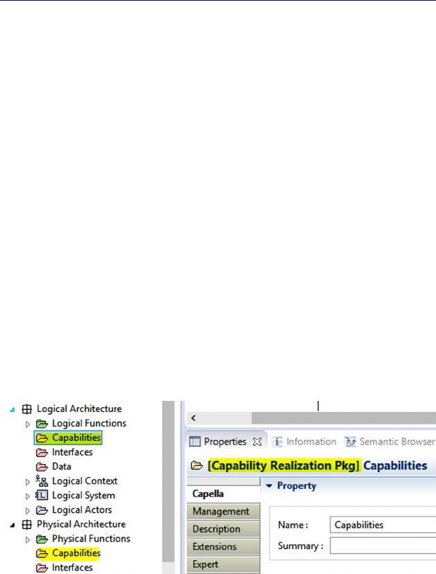
198 Systems Architecture Modeling with the Arcadia Method
This transition toward a new model has been performed for
educational purposes, to give a concrete illustration of the add-on use.
In the rest of the book, we will continue with the EOLE model in a
unique model until the EPBS.
5.6. Scenarios on the Logical level
In this section, we only use Exchange Scenarios mainly to show
Capella’s capabilities to set up a Scenario based on another from the
upper level. We have illustrated the three types of Scenario
(Functional, Exchange, Interface) in sections 4.7 and 4.9.
NOTE (Arcadia rule).– A Logical (or Physical) Scenario describes the
Logical (or Physical) Components within the framework of a
particular System Capability. On these two levels, we therefore also
find a Capabilities folder for structuring the Scenarios. However, we
note that these are not new Capabilities, but rather the realization of
System level Capabilities. Moreover, if we bother to look more
closely, the folder is actually called Capability Realization Pkg and
the Capabilities contained are called Capability Realizations.
Figure 5.34. Capabilities folder on the LA and PA levels
Let us start again from the System level acquisition Exchange
Scenario (SES).
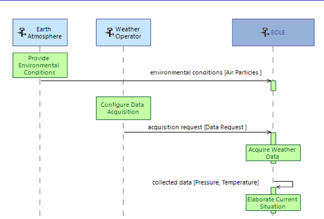
Complete Example of Modeling with Capella: Logical Architecture 199
Figure 5.35. Reminder of the System level acquisition Exchange Scenario
The Logical Actors will be the same as the System level; however,
the EOLE vertical line will be replaced by the necessary and sufficient
subset of Logical Components following the Logical Functions
allocation. In this example, we need two Components because the
“Acquire Weather Data” Function is performed by the Acquisition
Subsystem and the “Elaborate Current Situation” Function is
performed by the Ground Subsystem. On the other hand, in the
broadcast SES (Figure 4.89), the “Ground” Subsystem would be
sufficient.
Capella knows the System level Scenario. It knows how to travel
through the realization links between the Logical Functions and the
System Functions and it knows the allocation of the Logical Functions
to the Logical Components. The tool is thus capable of proposing an
automatic initialization of a Logical level Scenario based on a System
level Scenario. This will obviously also be the case between Logical
and Physical levels.
So, we ask the tool to perform this initialization by positioning
ourselves either in the previous diagram or in the Scenario in Project
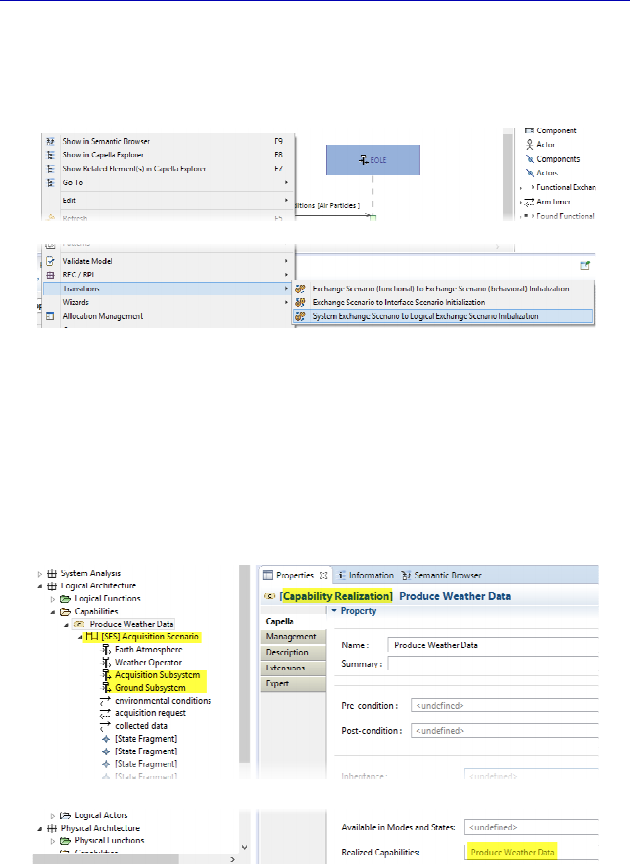
200 Systems Architecture Modeling with the Arcadia Method
Explorer, and by activating the contextual command: Transitions –
System Exchange Scenario to Logical Exchange Scenario
Initialization.
Figure 5.36. Transition from the System level Exchange Scenario
After the transition, Capella first created a Capability Realization
with the same name as the System Capability, and an Exchange
Scenario also with the same name as the SES. The vertical lines of the
Logical Scenario represent the same Actors plus the two Logical
Components as anticipated.
Figure 5.37. Result of the transition from the System Scenario in Explorer
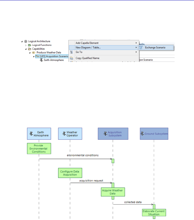
Complete Example of Modeling with Capella: Logical Architecture 201
Now all we need to do is rename the Scenario in LES and create
the diagram using the contextual command: New Diagram/Table… –
Exchange Scenario.
Figure 5.38. Creating the Logical Scenario diagram
The Scenario diagram thus created is automatically displayed as in
Figure 5.39. We note that the “collected data” message, which is
reflexive at the System level, now goes from the Acquisition
Subsystem to the Ground Subsystem.
Figure 5.39. Automatically initialized Logical Scenario diagram. For a color
version of the figure, see www.iste.co.uk/roques/arcadia.zip
We note that the Function displays have been kept, and positioned
on the right Component. We also note that the EI associated with the
messages have also been preserved. It is thus possible to show the EI
on the FE by applying the same filter as the System level.
It would be entirely possible to now add Constraints or even new
Messages or new Functions corresponding to the created model
elements based on the Logical level. Therefore, the command is called
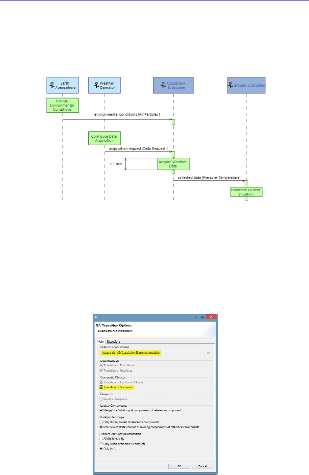
202 Systems Architecture Modeling with the Arcadia Method
“initialization”: it ensures that the exchanges are coherent with the Actors,
but allows enrichment on the level concerned. We are going to create a
Duration Constraint, as we did to the System level on the Functional
Scenario, but this time on the execution of the Acquisition Function.
Figure 5.40. Completed Logical Scenario diagram. For a color
version of the figure, see www.iste.co.uk/roques/arcadia.zip
To complete the illustration of the System to Subsystem transition
possibilities, we try to apply this transition again by ticking the
Transition of Scenarios option. This time, a Capability and a Scenario
are created in the target model of the Subsystem.
Figure 5.41. Additional option of the System to Subsystem transition. For a
color version of the figure, see www.iste.co.uk/roques/arcadia.zip
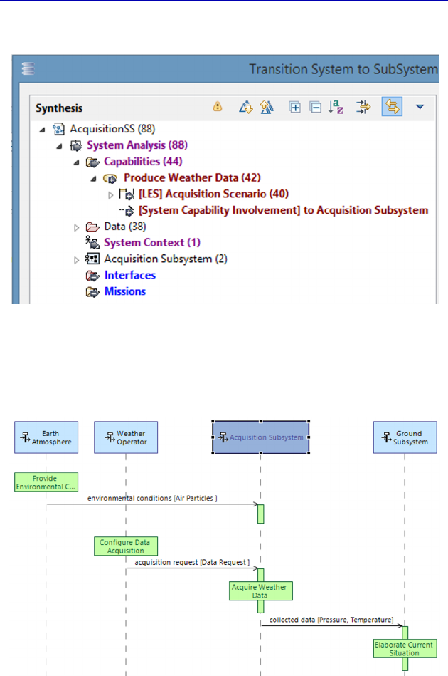
Complete Example of Modeling with Capella: Logical Architecture 203
The incremental transition opens a diff/merge type window.
Figure 5.42. Incremental application of the Subsystem transition
Now we just need to rename the Scenario and ask Capella to create
the corresponding diagram.
Figure 5.43. Subsystem Scenario generated by transition. For a color
version of the figure, see www.iste.co.uk/roques/arcadia.zip
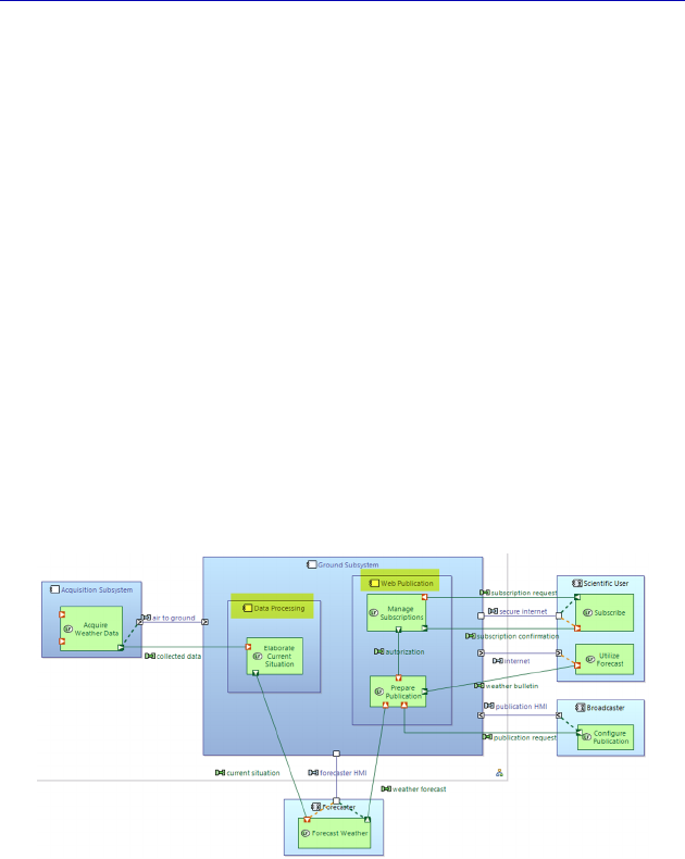
204 Systems Architecture Modeling with the Arcadia Method
5.7. Logical subcomponents
To complete this small and fast synopsis of the Logical
Architecture level, let us study the case in which a Logical Component
breaks down into subcomponents. This happens quite frequently on
real projects and brings about some intricacies when delegating
Component Ports, which we will illustrate in our EOLE example.
We are going to start from the Architecture diagram and simplify it
by only keeping the Actors and Components, which are connected to
the Ground Subsystem. Then, we are going to create two logical
subcomponents inside the Ground Subsystem: a data-processing
Component and a web publication Component. With a simple drag –
drop, we are going to allocate the “Elaborate Current Situation”
Function to the data-processing Component, and the “Prepare
Publication” and “Manage Subscriptions” Functions to the web
publication Component. The result of this preliminary work is given
in Figure 5.44.
Figure 5.44. Structural breakdown of the Ground Subsystem. For a color
version of the figure, see www.iste.co.uk/roques/arcadia.zip
N
OTE
(Arcadia rule).– The Functions breakdown and the Components
breakdown are not governed by the same Arcadia rules. We
have already seen that the broken down Functions should no longer
have input/output Ports: only the leaf (or terminal) Functions can have
Function Ports and can be allocated. This is not the same for the
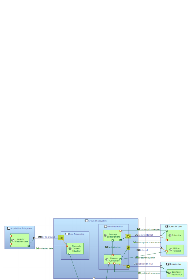
Complete Example of Modeling with Capella: Logical Architecture 205
Components. The Logical (or Physical) Components that are broken
down can, nevertheless, still possess Component Ports as such, which
it will need for connecting the Ports of their subcomponents. It is quite
easy to understand the use of this rule for Physical Components. It is
applied in the same way in Logical Architecture. However, this is not
obligatory, and certain Components may not have external Ports: this
is a modeling choice.
Therefore, there are two types of modeling possible for our Ground
Subsystem:
– either by considering that it is only a pure container, like the
Logical System in our example, and that only the subcomponents
possess Component Ports;
– or by considering that the Subsystem keeps its own Ports, which
will allow it to apply a System/Subsystem transition when required,
but the subcomponents also have their Component Ports, connected to
the first.
We are going to illustrate the two alternative solutions in the
following. If we first assume that the Ground Subsystem is only a pure
container, we will just need to drag–drop each of its ports toward the
adequate subcomponent. A difficulty will occur in terms of the two-
way Port connected to the Forecaster, and we will see the solution in
the following. We have changed the color of the Ground Subsystem to
white so as to visually reinforce the subcomponents.
Figure 5.45. First solution: Ground Subsystem as a pure container. For a
color version of the figure, see www.iste.co.uk/roques/arcadia.zip
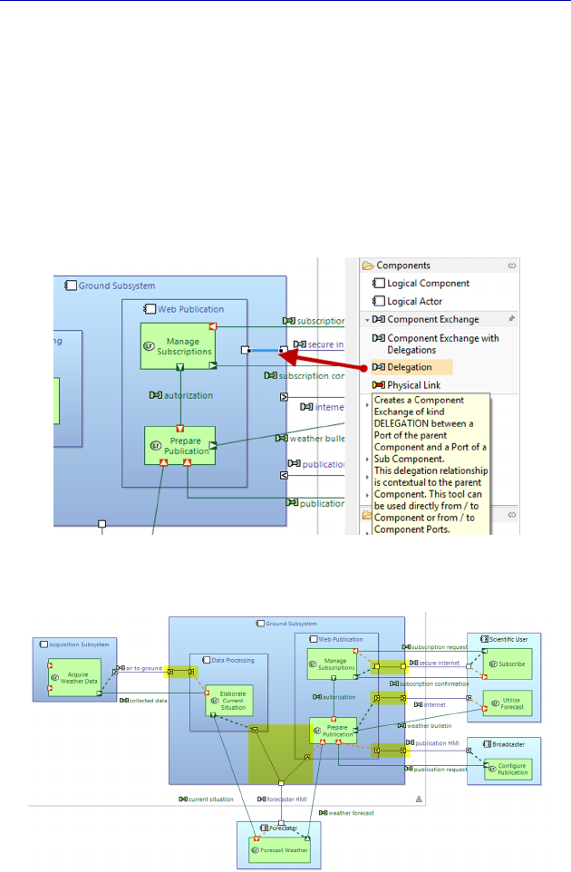
206 Systems Architecture Modeling with the Arcadia Method
The second solution is a bit more complex and calls upon a new
concept: Delegation. As a matter of fact, we are going to leave the
Component Ports on the Ground Subsystem, and “delegate” them to
the subcomponents. To do this, Capella proposes a specific command
in the palette, under Component Exchange, called Delegation. This
command, activated from a Port of the container Component, creates a
new Port in the same direction on the contained Component and
connects it to the first one by a Component Exchange of kind
Delegation.
Figure 5.46. Delegation connector
Figure 5.47. Second solution: Port Delegation. For a color version
of the figure, see www.iste.co.uk/roques/arcadia.zip

Complete Example of Modeling with Capella: Logical Architecture 207
If we repeat this work on all the Ports of the Subsystem and
finalize all the Functional Port allocations, we end up with Figure 5.47.
NOTE.– A “classic” Component Exchange connects two Ports of
opposite directions. A Delegation-type Component Exchange connects
two Ports of the same direction. Capella knows this and creates Ports
in the right direction every time.
This page intentionally left blank
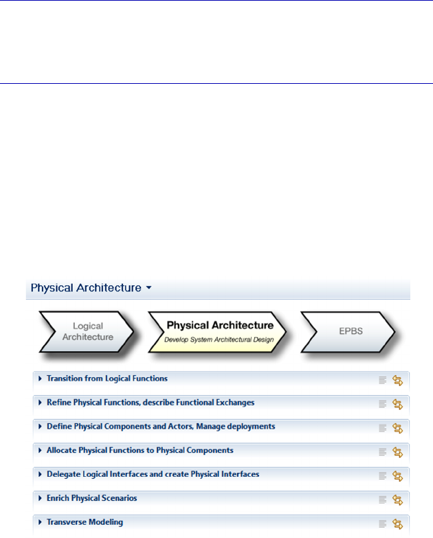
6
Complete Example of Modeling with
Capella: Physical Architecture
6.1. Main concepts and diagrams
Capella integrates a methodological guide in the form of the
Activity Explorer. This lists the different activities and the different
diagrams that can be created on the relevant engineering level, namely
here Physical Architecture. Figure 6.1 specifies the activities first, and
then we will detail the diagrams possible as the case study unwinds.
Figure 6.1. Methodological activities from the “Physical Architecture” level

210 Systems Architecture Modeling with the Arcadia Method
NOTE.– Warning: we recall that even if Arcadia is a method, the
modeling process is totally flexible. The methodological activities
presented in the Activity Explorer are almost all optional and may be
created in any order whatsoever, just as for diagrams.
So, again here, we are going to make an arbitrary but reasoned
choice for creating the diagrams. We will start by automatically
recovering the Functions and the Actors issued from the Logical level
to start our Physical level. We will then create concrete Physical
Components inside the system by making the technological choices
this time. At the same time, we will decide to allocate the Physical
level Functions to these components, and we may be led to break
down the Functions issued from the Logical level or to complete them.
In keeping with the book’s goal, we will make some modeling
choices that allow the case study to retain its simplicity. The model of
the real project would obviously be more complex.
6.2. Moving from the Logical level to the Physical level
The previous Logical Architecture started by “opening the black
box” in order to identify the structural elements called Logical
Components, as well as their properties and relations. The important
rule that we have followed is to ensure that you exclude all
technological considerations or implementation choices on this level.
This is exactly the objective of the Physical Architecture in defining
the “real” concrete components that comprise the system.
To start the Physical level based on the Logical level, Capella
proposes transitions similar to those that we used when we went from
the Operational Analysis to the System Analysis, then from the
System Analysis to the Logical Architecture. Thus, we can create as
many Physical Functions as Logical Functions, by also keeping the
Functional Exchanges and Functional Chains. We apply this first
transition based on the Activity Explorer.
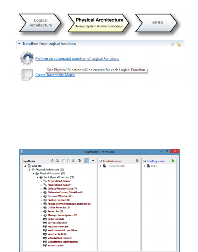
Complete Example of Modeling with Capella: Physical Architecture 211
Figure 6.2. Functional Transition tool toward the Physical level
Here again, we are looking at a simple transition case, and pressing
on the Apply button will enable us to recover everything in one go.
The result is visible in the Project Explorer in which some model
elements now exist in the Physical Functions folder.
Figure 6.3. Functional Transition dialogue window
We recall that Capella automatically creates a realization link
between each Physical element (Function, Functional Exchange,
Functional Chain) and the corresponding Logical element. We also
recall that the transitions are iterative and incremental and if in
working on the Physical level, we notice that a Logical Function is
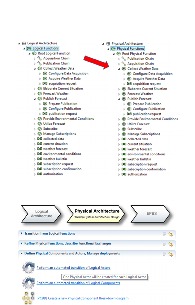
212 Systems Architecture Modeling with the Arcadia Method
missing, perhaps a System Function, it is absolutely essential to roll
back to the highest level so as to add it and then apply the
transition again.
Figure 6.4. Result of the Functional Transition in Project Explorer
Figure 6.5. Transition tool from the Actors toward the Physical level
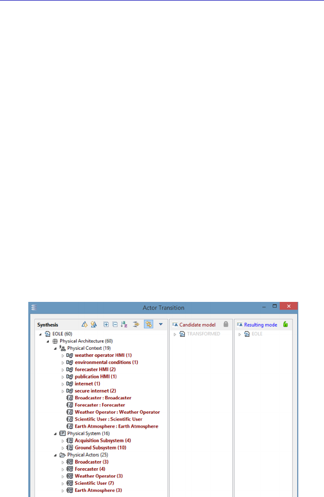
Complete Example of Modeling with Capella: Physical Architecture 213
We now apply the transition of the external Actors (Figure 6.5). In
most cases, the Actors identified on the Logical level will be exactly
the same on the Physical level. The automatic transition (iterative and
incremental) is therefore once again particularly useful for this type of
model element.
Here, we are looking again at a simple transition case, and pressing
on the Apply button could enable us to recover everything in one go.
But to simplify the model for educational purposes, we will restrict the
transition.
As a matter of fact, Capella also proposes to recover the
Component Ports and the Component Exchanges between the System,
which here means the Logical Components, and the Actors. In fact, it
also proposes to recover the Logical Components, and to transform
them into Behavior Physical Components. Yet, we prefer to
completely master creating the Behavior Components on the Physical
level: the granularity level will be finer than in the Logical level, the
names refer to the technological choices, etc. Therefore, we are going
to prevent the transition from the Logical Components and the
Component Exchanges with the Actors.
Figure 6.6. Dialogue for the transition of Actors toward the Logical level
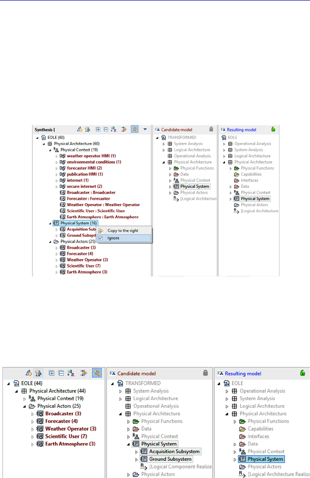
214 Systems Architecture Modeling with the Arcadia Method
NOTE.– It is possible to finely master the automatic descending
transitions proposed by Capella. Once we master the transitional
diff/merge type interface, it is easy to limit the transition to a subset of
elements, knowing that we will always be able to complete it later.
We are simply going to choose to ignore the transition from the
Logical Components by right clicking on Ignore on the container of
the proposed Behavior Components: Physical System.
Figure 6.7. Action on the transition of Components toward the Physical level
The Ignore action will modify the Resulting model with respect to
the Candidate model, and will prevent the transition from the
Behavior Components, as desired.
Figure 6.8. Following the action for the non-transition of Components
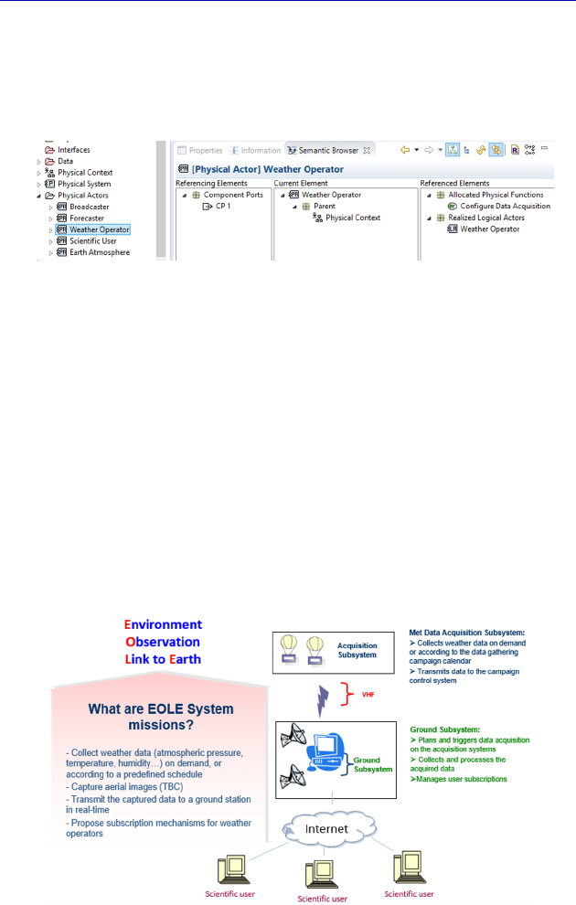
Complete Example of Modeling with Capella: Physical Architecture 215
The result of the transition is then visible in Project Explorer
where the model elements now exist in the folder Physical Actors, to
which the Physical Functions are allocated, to the image of the
Logical and System levels.
Figure 6.9. Verification of the Actors’ transition result
6.3. Physical Components
In our case study, from the beginning, we know that the system
will contain two subsystems: an Acquisition Subsystem “in the air”
for which the state of the art consists of using a sounding balloon
inflated with helium and a Ground Processing Subsystem. On the
Logical level, we have not yet spoken about technological choices,
which is now contrary to the objective of Physical Architecture. We
recall that it is good practice to name the Logical and Physical
Components differently, and to attribute names containing references
to a technology specific only to Physical Components.
Figure 6.10. Recall of the “EOLE” system design brief
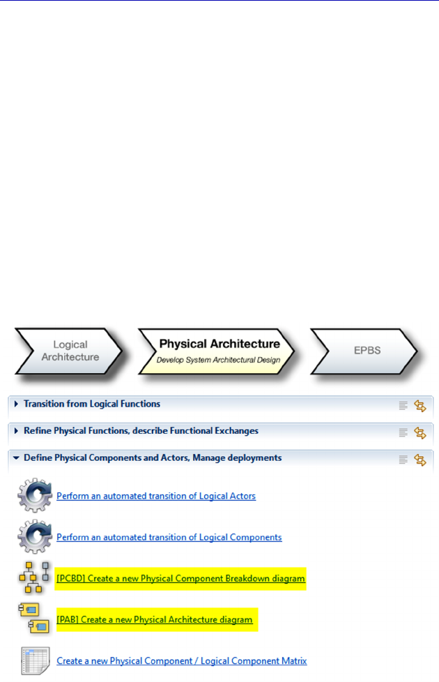
216 Systems Architecture Modeling with the Arcadia Method
NOTE (Arcadia rule).– There are two types of Physical Components in
Arcadia. A Behavior Physical Component is a component of the
System, responsible for performing some of the Functions assigned to
the system, by interacting with other Behavior Components and with
that of the external Actors. A Node Physical Component is a
component that hosts a certain number of Behavior Components, by
providing them with the resources required for them to operate and
interact with their environment. A Behavior Component is hosted by
one single Node Physical Component.
We are therefore going to first create two Node Physical
Components corresponding to the two subsystems as well as
subcomponents of the same type, for example a probe holder in the
sounding balloon, and two computer servers in the ground station. To
do this, we can use a Physical Component Breakdown diagram
(PCBD) or a Physical Architecture Blank (PAB) diagram directly.
Figure 6.11. Diagrams for creating Physical Components
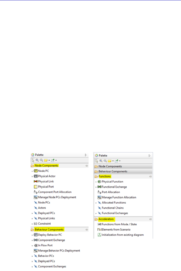
Complete Example of Modeling with Capella: Physical Architecture 217
The most efficient method here is to start directly with the
Architecture diagram, especially as the Breakdown diagram may be
realized automatically by Capella later. Unlike the upper levels, the
PAB will be empty at first.
The palette on the right is the most complex of all the diagrams
proposed by Capella. As a matter of fact, in this type of diagram, we
are going to be able to manipulate three types of concepts:
– Node Physical Components (yellow rectangles), which may
contain other Node Components;
– Behavior Physical Components (blue rectangles), which will be
deployed on the Node Physical Components;
– Physical Functions (green rectangles), which will be allocated to
the Behavior Physical Components.
And we often find additional accelerators in the last group of
commands.
Figure 6.12. PAB (Physical Architecture Blank) Palette. For a color
version of the figure, see www.iste.co.uk/roques/arcadia.zip
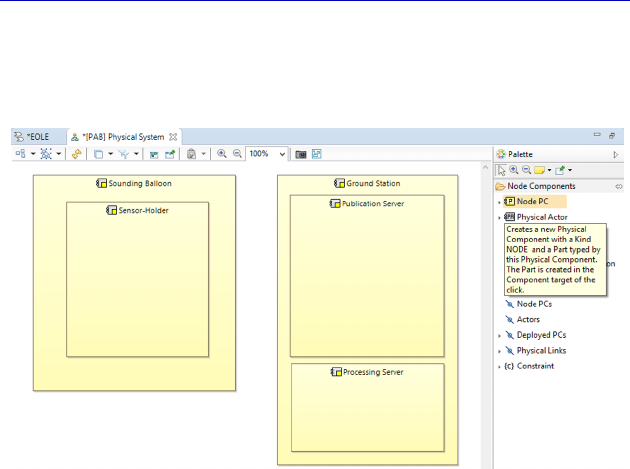
218 Systems Architecture Modeling with the Arcadia Method
So, let us start by creating the Node Physical Components in order
to then deploy Behavior Physical Components to which the system’s
Functions will be allocated. A first draft is shown by Figure 6.13.
Figure 6.13. First draft of the PAB with the Node Components. For a color
version of the figure, see www.iste.co.uk/roques/arcadia.zip
If we open the Property Sheet of a Physical Component, we note
that the “Behavior/Node” nature is a postcreation modifiable property,
and that there is also a Physical Component Kind property that allows
the component type to be specified: software, hardware, computer,
etc. For example, here, the two servers of the ground station will be
marked as Hardware Computer.
N
OTE
.– It is possible to model a Person type Physical Component.
This is particularly useful for a system whose operators are
stakeholders, from the client’s viewpoint. In this case, as the system
operators are inside it, they must not be modeled as Actors of the
System level, but rather as internal Components, on the Logical and
Physical levels. Warning: the man–machine interfaces of the operators
will not be visible on the System Analysis level, unlike those of the
end users.
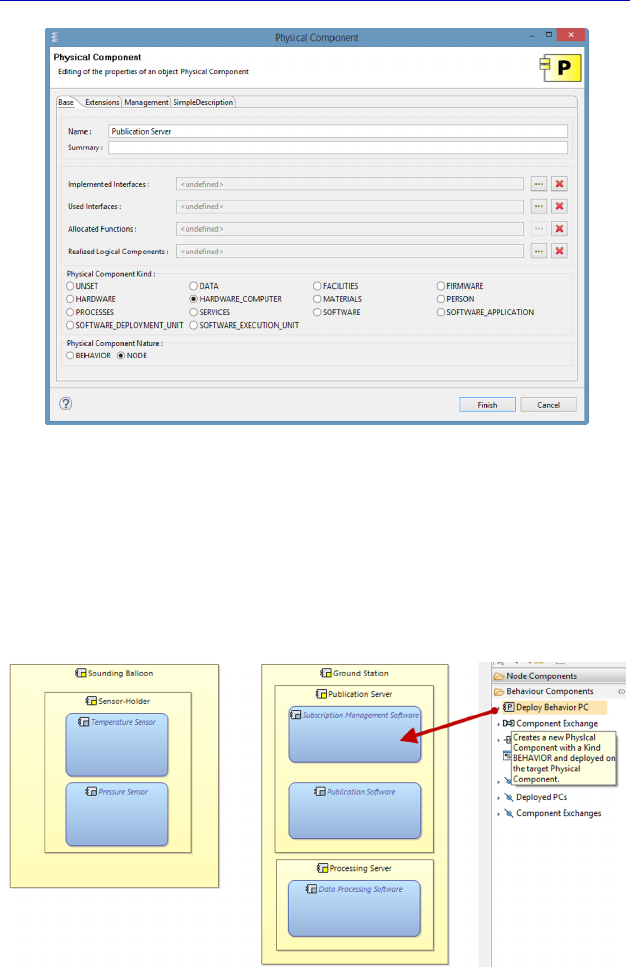
Complete Example of Modeling with Capella: Physical Architecture 219
Figure 6.14. Property Sheet of a Physical Component
We continue by creating and deploying Behavior Components on
the Node Components because of the Deploy Behavior PC command
of the PAB palette. For example, we are going to deploy two different
sensors on the sensor holder, as well as the software applications in
the servers of the ground station.
Figure 6.15. Deployment of Behavior Components. For a color version
of the figure, see www.iste.co.uk/roques/arcadia.zip
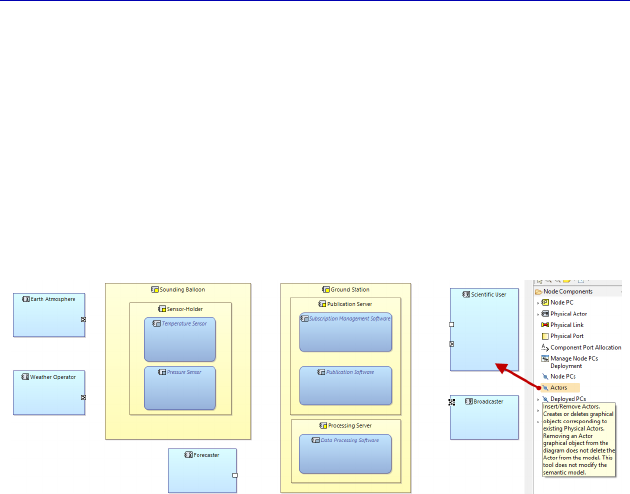
220 Systems Architecture Modeling with the Arcadia Method
N
OTE
(Arcadia rule).– We recall the rules associated with the
deployment relation. A Behavior Component is hosted by one and
only one Node Physical Component. In contrast, a Node Physical
Component may host several Behavior Components.
We can complete the PAB by inserting the Physical Actors
automatically recovered by the transition. Note that the transition also
propagated the Actor Ports, even if we have chosen not to recover the
Logical Components and the associated Component Exchanges.
Figure 6.16. Inserting the Physical Actors in the PAB. For a color
version of the figure, see www.iste.co.uk/roques/arcadia.zip
All we have to do now is to add the Functions. Those of the Actors
have been recovered automatically by the descending transition: we
just need to insert them graphically (Insert Allocated Functions
command on the palette). Those of the System have also been
automatically recovered by the descending transition but will need to
be allocated to one single Behavior Physical Component (Manage
Function Allocation command on the palette).
6.4. Allocating the Functions to the Physical Components
We have indicated that the Actors’ transition has kept their
Function allocations. We can therefore easily insert them into the PAB
diagram using the same command of the palette as on the Logical
level: Insert All Allocated Functions. However, beware: unlike the
upper levels where the command worked on the background of the
diagram, this time they need to be applied to each Actor. Then, we can
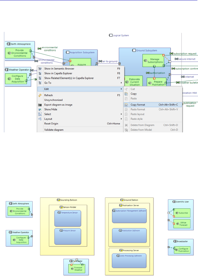
Complete Example of Modeling with Capella: Physical Architecture 221
copy–paste the format from the LAB onwards to position the
Functions and their Ports automatically.
Figure 6.17. Copying the LAB format
We then obtain the following diagram. Note that we could even
have avoided manually repositioning the Actors, by taking advantage
of the format copy–paste from the LAB after having inserted the
Actors in bulk then their Functions.
Figure 6.18. PAB continued. For a color version of the
figure, see www.iste.co.uk/roques/arcadia.zip
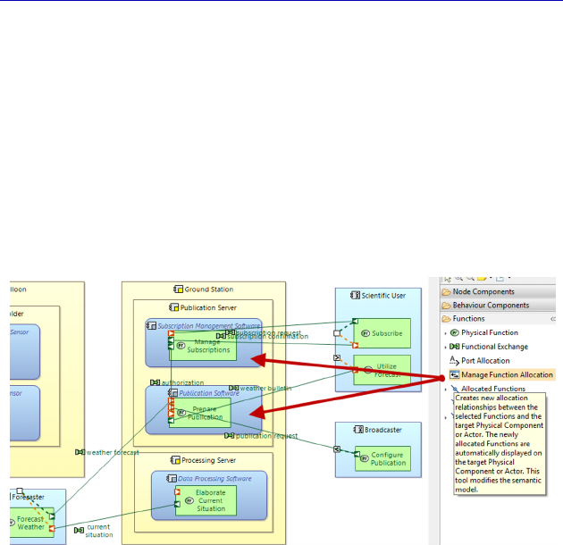
222 Systems Architecture Modeling with the Arcadia Method
We are now going to allocate each Function of the system to one of
the Behavior Components. Our example will still be purposefully very
simple, perhaps simplistic, for educational purposes. So, we start by
allocating the three Physical Functions from the ground station into
each Behavior Component. To do this, we use the Manage Function
Allocation command from the PAB palette. Note that the Functional
Exchanges are automatically displayed as soon as their target and
source Functions are shown on the diagram. By giving the three
Functions an optimal size, we quickly come to the fragment in
Figure 6.19.
Figure 6.19. Start of the Functional allocation. For a color version
of the figure, see www.iste.co.uk/roques/arcadia.zip
The Functional Ports are, by default, positioned starting from the
upper left corner of each Function, which leads to an undesired cross-
over of Functional Exchanges. Yet, there is a very effective command
in this instance for asking Capella to automatically position them:
Arrange Connected Ports on the diagram itself (Figure 6.20).
To simplify the diagram for the rest of the manipulation, we are
going to hide the Component Ports, which will also hide the Port
allocations on the Actors, by applying the Collapse Component Ports
filter (Figure 6.21).
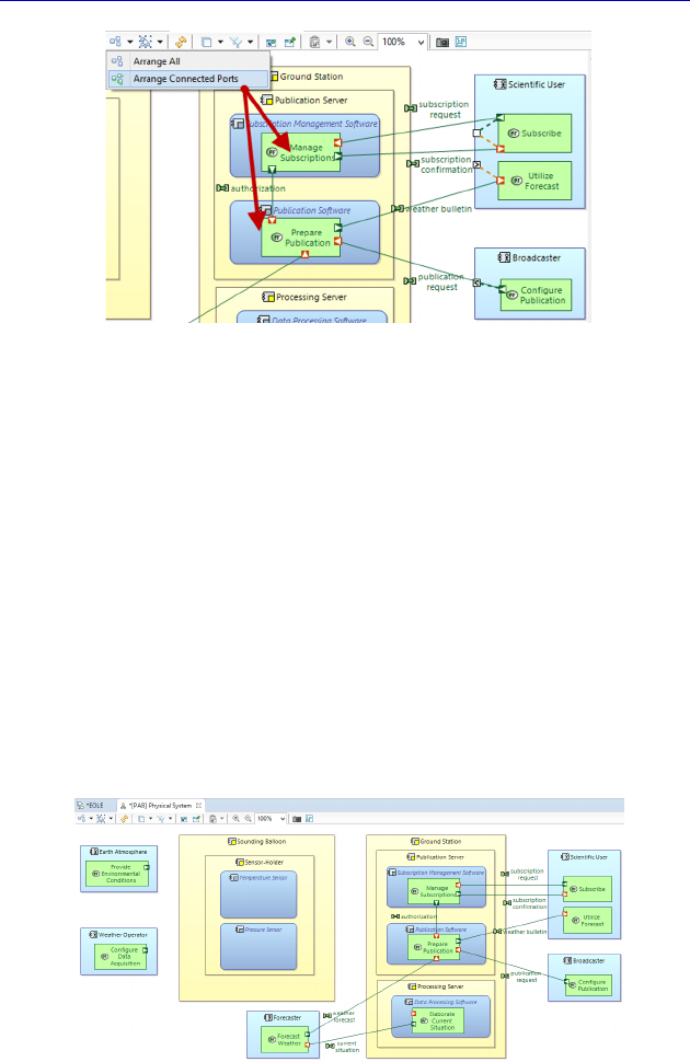
Complete Example of Modeling with Capella: Physical Architecture 223
Figure 6.20. Applying the Arrange Connected Ports command. For a color
version of the figure, see www.iste.co.uk/roques/arcadia.zip
We have one Function left to allocate: “Acquire data”. However,
we cannot continue further here, because this Function cannot be
allocated to several Components. We therefore need to break it down
according to the different types of data manipulated: temperature,
pressure, etc.
To do this, we must change the diagram type and go back to a
Physical Data Flow Blank (PDFB). In this new diagram, we are going
to insert the Function to be broken down, as well as all the Functions
connected to it, then create as many sub-Functions as types of
meteorological data, then work on the data flows, because only the
“leaf” Functions may possess Function Ports.
Figure 6.21. PAB continued with the Component Ports filtered. For a color
version of the figure, see www.iste.co.uk/roques/arcadia.zip
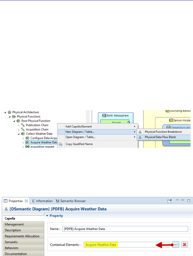
224 Systems Architecture Modeling with the Arcadia Method
Instead of manually inserting the Functions that we can choose
because of the Insert/Remove Functions button from the palette, we
recall that it is possible to ask Capella to automatically construct the
PDFB by inserting the Function to be broken down, as well as all
those that are connected to it. To do this, we just need to make the
diagram contextual with the Function chosen by the properties field of
the diagram: Contextual Elements.
We first select the “Acquire Weather Data” Function in Capella’s
Project Explorer, then by right clicking, we ask Capella to create a
Physical Data Flow Blank. Therefore, the diagram thus created will
automatically have the name of the selected Function.
Figure 6.22. Contextual creation of the PDFB
We then position the Contextual Elements field on this same
Function.
Figure 6.23. Diagram made contextual using the Function to breakdown
We just need to ask Capella to refresh the diagram (F5 key or the
Refresh diagram button of the upper ribbon) so that the diagram fills
automatically. After a few quick manipulations to improve the image,
we end up with Figure 6.24.
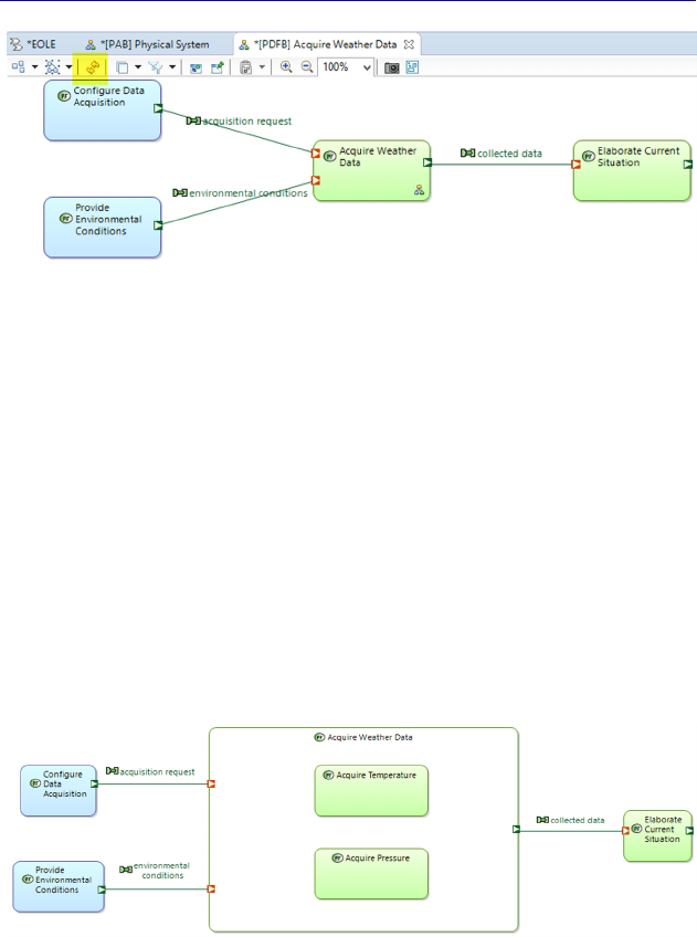
Complete Example of Modeling with Capella: Physical Architecture 225
Figure 6.24. Result from refreshing the contextual diagram
Now we need to continue our work in breaking down the
“Acquire” Function. We remind you that we recommend changing the
filling color of the Functions which are broken down, and to make
them white to properly differentiate them.
However, unlike what we were able to do when moving from the
Operational Analysis to the System Analysis, it is not enough here to
shift the Ports from the parent Function to one of the sub-Functions.
As a matter of fact, each sub-Function consumes and produces a part
of the parent Function’s inputs and outputs. We are going to need to
call upon the somewhat particular Functions, which are predefined by
Arcadia in order to break down or assemble data flows.
Figure 6.25. Start of the Functional breakdown
The collected data at the output of the “Acquire” Function is in part
produced by the different sub-Functions (let us not forget that we will
also need to acquire the humidity, the wind speed, etc.). We therefore
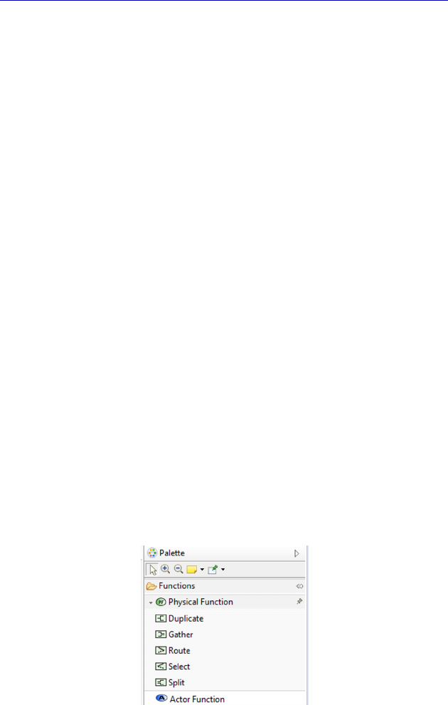
226 Systems Architecture Modeling with the Arcadia Method
need to add a new Function that will group together these different
data. Arcadia defines five types of flow control Functions that we will
detail hereafter.
N
OTE
(Arcadia rule).– As we have already raised, the data flow
describes the functional dependencies between Functions, via
Functional Exchanges connected to the Function Ports. In certain
cases, it may be necessary to define the path conditions more
precisely, by using flow control Functions, intermediaries between
source(s) and recipient(s):
– to specify a simultaneous broadcast from an exchange source to
several recipients, we define a Duplicate Function that transmits the
same Exchange Items to all recipients;
– to specify the broadcasting of some of the Exchange Items to
each recipient selectively, a Split Function that channels each part to a
separate recipient;
– to specify the selection of one among several potential recipients, a
Route Function that transmits (generally under conditions) the exchange
received on its unique input to one and only one of its outputs;
– to specify the combination of items of several exchanges issued
from different sources, a Gather Function to constitute a single
Exchange fusing those received from different sources;
– to specify the selection of one source among several, a Select
Function, which only channels the exchange issued from the selected
source (generally under conditions).
Figure 6.26. Control Functions predefined by Arcadia
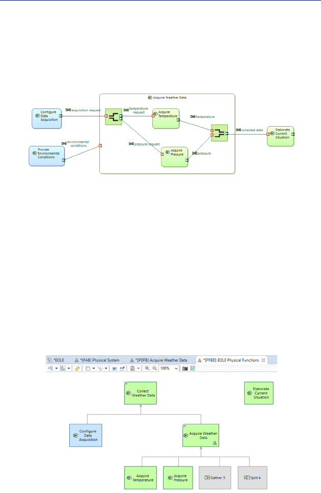
Complete Example of Modeling with Capella: Physical Architecture 227
In our example, we are therefore going to use Gather for the
“collected data” output, and Split for the “acquisition request” input.
We can move the output Port from the parent Function to a Gather
output and the input Port into a Split input. We also need to create new
and finer Functional Exchanges for sub-Functions input/output.
Figure 6.27. Functional breakdown continued. For a color version
of the figure, see www.iste.co.uk/roques/arcadia.zip
For the minute, we are purposefully going to leave out the
environmental conditions issue for which a Duplicate appears to be
completely indicated. We continue by asking Capella to create a
Physical Functional Breakdown diagram (PFBD). In this diagram, we
can see that the two acquisition sub-Functions, but also the two
control Functions, appear automatically because this type of diagram
is always up to date. The control Functions appear in gray, rather than
in blue or green, and their name has automatically been created by
Capella, which will lead us to give them more significant names.
Figure 6.28. Functional Breakdown diagram (PFBD) . For a color
version of the figure, see www.iste.co.uk/roques/arcadia.zip
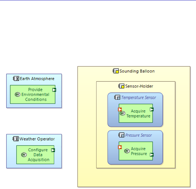
228 Systems Architecture Modeling with the Arcadia Method
We can now go back to the Architecture diagram (PAB) and
allocate the acquisition sub-Functions to the corresponding sensor.
However, this time, the Functional Exchanges do not display
automatically as their target and source Functions are missing on the
diagram. As a matter of fact, the control Functions are full part
Functions: they therefore must also be allocated.
Figure 6.29. Functional allocation continued
To allocate a Function, we need a Behavior Component. It is clear
that the gathering of collected data must in fact be performed in the
balloon, and probably also the splitting of the requests. The only two
Behavior Components in the balloon are the different sensors, so we
need some transverse intelligence, which could be performed using a
specific software Component. This new software Component must
also be deployed in turn. Yet, we only have one sensor holder and the
structure of the balloon. Then, we are also missing a light hardware
support that enables this new software Component to be deployed,
such as a Raspberry Pi type nanocomputer, for example. We
consequently update the PAB on the sounding balloon part.
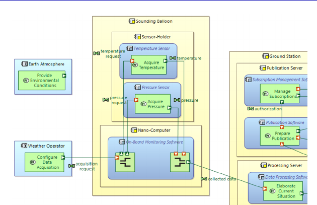
Complete Example of Modeling with Capella: Physical Architecture 229
Figure 6.30. End of Functional allocation. For a color version of
the figure, see www.iste.co.uk/roques/arcadia.zip
N
OTE
.–.What we have just done perfectly illustrates one of the strong
points of Arcadia’s methodological approach. As a matter of fact,
because of the Functional Analysis approach and the precision
required in the Functional Exchanges, we were led to create new
Physical Functions. Thus, we were forced to consequently complete
the structural design by adding new Behavior Physical Components
and Nodes in order to finish the necessary allocation of the Functions.
In summary, the Functional Analysis enabled us to find the necessary
and sufficient architecture Components [VOI 16].
We are now going back to the “environmental conditions”
Functional Exchange that we had left out of the Data Flow diagram
(PDFB). If we add a Duplicate type control Function to duplicate this
exchange to the two acquisition sub-Functions, we will also need to
allocate this additional Function. However, the duplication is done
naturally by the “Earth Atmosphere” rather than by designing it inside the
sounding balloon. So, this leads the external Actor modeling to be made
more complex, without delivering real added value to the architecture
model. We are therefore going to use a simpler solution, consisting of
duplicating the Functional Exchange by making it part of the same
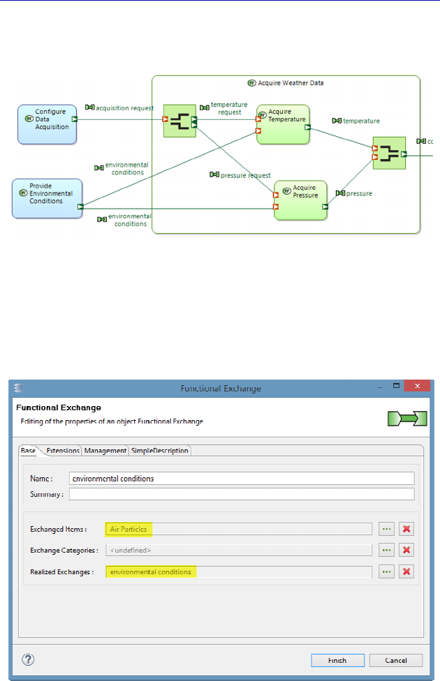
230 Systems Architecture Modeling with the Arcadia Method
output port. We only lose the precision of simultaneity delivered by
the Duplicate Function, but to simplify the model.
Figure 6.31. End of work on the Functional Exchanges in the PDFB. For a
color version of the figure, see www.iste.co.uk/roques/arcadia.zip
To reinforce the coherency between the two exchanges, we are
going to specify that they transport the same Exchange Item and
realize the same Logical Exchange.
Figure 6.32. Specifications on the duplicated Functional Exchanges
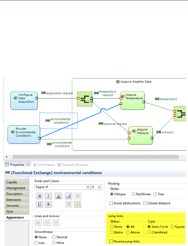
Complete Example of Modeling with Capella: Physical Architecture 231
If we go back to the PDFB, two Functional Exchanges cross over
to the left of the acquisition sub-Functions. It is possible to improve
the graphic appearance of the intersection by using the Appearance –
Jump Links property of one of the two Exchanges, as shown in Figure
6.33. By default, the Jump Links are disabled (none). We need to
activate them (all) on the selected feature, and then we can modify the
style (semicircle, square, chamfered) and possibly reverse the jumping
direction.
Figure 6.33. Graphic improvement of the line intersection. For a color
version of the figure, see www.iste.co.uk/roques/arcadia.zip
We now open the PAB again: the Functional Exchanges
automatically appeared and the diagram is complete.
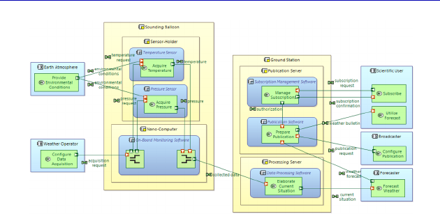
232 Systems Architecture Modeling with the Arcadia Method
Figure 6.34. Functional finalization of the PAB. For a color
version of the figure, see www.iste.co.uk/roques/arcadia.zip
6.5. Functional Chains on the Physical level
We had created two Functional Chains on the System level (see
section 4.5): “Acquisition Chain” and “Publication Chain”. The
successive functional transitions from the System level to the Logical
level, and then from the Logical level to the Physical level, simply
cloned the chains identically. On the Logical level, we had not
modified the data flow, the Logical Chains therefore continue to be
valid. However, on the Physical level, we have broken down the
“Acquire Weather Data” Function and detailed the Functional
Exchanges with respect to the sub-Functions. It is therefore
foreseeable that the “Acquisition Chain” will become invalid, but not
the “Publication” one. We check it by inserting the two Chains onto
the PAB (Figure 6.35), because of the Insert Functional Chains
command on the palette.
As predicted, Capella clearly indicates that the Acquisition Chain
is now invalid, but not the Publication one, whose constituting items
we have not modified. We are therefore going to have to work on the
Acquisition Chain in order to make the Physical level valid again. To
do this, we must create a specific contextual diagram, called a
Functional Chain Description (FCD), by right clicking on the square
in the diagram or on the element in the Project Explorer (Figure 6.36).
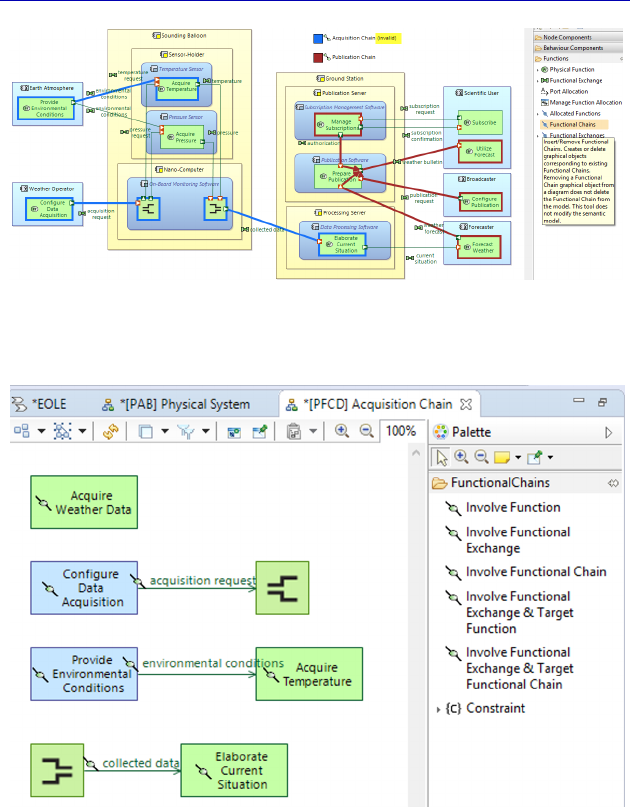
Complete Example of Modeling with Capella: Physical Architecture 233
Figure 6.35. Visualization of the Functional Chains. For a color
version of the figure, see www.iste.co.uk/roques/arcadia.zip
Figure 6.36. Diagram of Acquisition Chain Description
The diagram generated thus by Capella clearly shows that there is
more than one chain, and that we will need to reconnect the scattered
pieces.
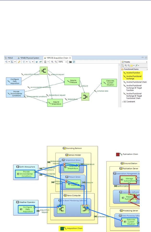
234 Systems Architecture Modeling with the Arcadia Method
We start by removing the link referring to the broken down
Function (Delete from Model command). Then, we add the missing
sub-Function: “Acquire Pressure” (Involve Function command). All
we need to do now is to connect the sub-Functions using the Involve
Functional Exchange command. Note that Capella only proposes the
existing Functional Exchanges, which prevents errors and accelerates
the modeler’s work.
Figure 6.37. Modification of the Acquisition Chain
Now we just need to go back to the PAB to verify that the
Functional Chain has become valid again.
Figure 6.38. Visualization of the amended Functional Chain. For a color
version of the figure, see www.iste.co.uk/roques/arcadia.zip
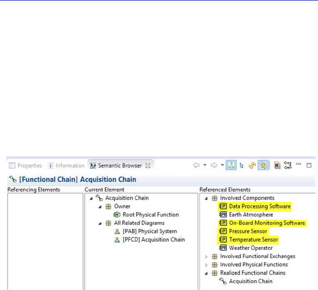
Complete Example of Modeling with Capella: Physical Architecture 235
On the System level, we indicated that the concept of Functional
Chain is particularly useful for running verification/validation tests, as
well as for expressing non-Functional constraints, such as latency,
criticality, confidentiality, redundancy, etc. On the Physical level, as
the Functions that participate in a Chain are all allocated to one single
Behavior Physical Component, we can know exactly which
Components are necessary and sufficient to ensure the Chain
concerned. This information is very important in an incremental
delivery process, for example. Capella directly displays the list of
Components and Actors implied in the Semantic Browser window.
Figure 6.39. Visualization of the Components implied in a Functional Chain
6.6. Return to the Physical Components and the structural
links
We now return to the PAB. We finished the functional analysis and
the allocation of Functions to Components. However, there is still a
lot of work to do here to finalize the PAB, in particular creating the
necessary Component Exchanges between the Behavior Physical
Components, as well as the corresponding Physical Links between the
Node Physical Components.
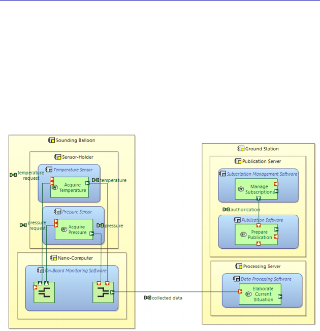
236 Systems Architecture Modeling with the Arcadia Method
For simplicity purposes, we are only going to use a particular
example to illustrate the approach that needs to be applied to the
whole Physical level. We are thus going to focus on the Functional
Exchange between the sounding balloon and the ground station:
“collected data”. To do this, we are first going to clone the PAB, and
simplify this new diagram by removing all the Actors (Delete from
Diagram command). This simplified PAB, representing the inside of
the EOLE Physical System, is shown in Figure 6.40.
Figure 6.40. Simplified PAB not showing the Actors. For a color
version of the figure, see www.iste.co.uk/roques/arcadia.zip
The “collected data” Functional Exchange must be allocated to a
Component Exchange. To do this, we need to create this Component
Exchange between the “On-Board Monitoring Software” and “Data
Processing Software” Components. We name it “balloon to ground”
and proceed to allocate the Functional Exchange. We can complete its
definition by positioning a realization link toward the Logical level
Component Exchange.
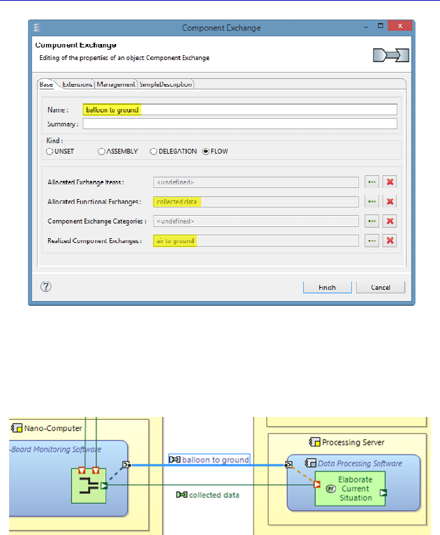
Complete Example of Modeling with Capella: Physical Architecture 237
Figure 6.41. Definition of the Component Exchange
The result of the allocation appears in the PAB, in the same way as
for the previous Arcadia levels.
Figure 6.42. Visualization of the Functional Exchange allocation
This Component Exchange must in turn be allocated to a Physical
Link between Node Physical Components. We could simply create a
VHF-type Physical Link between the nanocomputer and the
processing server, and then allocate the Component Exchange, as
shown in Figure 6.43.
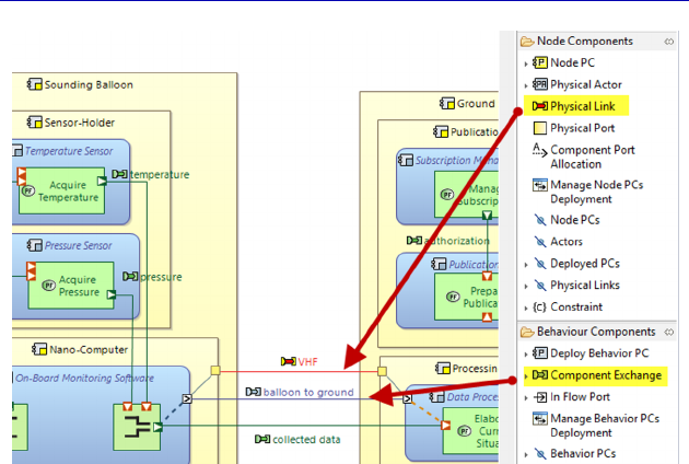
238 Systems Architecture Modeling with the Arcadia Method
Figure 6.43. Visualization of a Physical Link and the allocated
Component Exchange. For a color version of the figure, see
www.iste.co.uk/roques/arcadia.zip
N
OTE
(Arcadia rule).– A Physical Link is a means of communication,
transport or channeling between two Node Physical Components, used
as a support for the Component Exchanges. A Physical Link connects
two Physical Ports of two Components. It can directly connect the
subcomponents to each other.
A Physical Port is a connection point of a Node Physical
Component with its environment. A Physical Port is not oriented. A
Physical Port refers to the Behavior Components hosted by its Node
Physical Component, which are accessible through it. A Component
Port must be allocated to a single Physical Port, as soon as there is a
Component Exchange toward the outside of the Component connected
to it.
A more complete solution, which allows us to use an additional
Arcadia concept further, consists of introducing the radio
emission/reception Components, and then to connect a series of
Physical Links by means of a Physical Path.
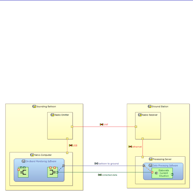
Complete Example of Modeling with Capella: Physical Architecture 239
N
OTE
(Arcadia rule).– A Physical Path is an ordered set of references
to Physical Links, defining a continued path likely to channel one or
several Component Exchanges between Components not connected by
one single Physical Link. A Physical Path refers to the Component
Exchanges that it transports.
We start by creating additional Node Components, as well as the
three Physical Links to connect them. Note that it is not obligatory to
model Behavior Components and Functions inside the new Node
Components, because we are focusing on the Physical Links: the
modeling may be partial.
Figure 6.44. Adding Node Components and Physical Links
We wish to allocate the “balloon to ground” Component Exchange
to the ordered set of Physical Links starting from the nanocomputer
and ending with the processing server, rather than the “VHF” Physical
link. To do this, we are going to create a Physical Path by successively
selecting the three Links and activating a contextual menu by right
clicking on the Functional Chain creation model: Physical Path –
Create a Physical Path. The result is also a new model element
represented by a blue square as well as graphic additions on the Links
and Physical Ports.
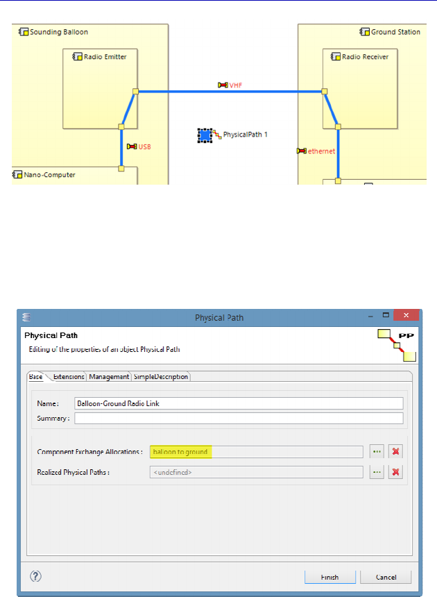
240 Systems Architecture Modeling with the Arcadia Method
Figure 6.45. Result of creating a Physical Path. For a color
version of the figure, see www.iste.co.uk/roques/arcadia.zip
We now rename the Physical Path and directly allocate the
Component Exchange to it because of the Property sheet.
Figure 6.46. Property sheet of a Physical Path. For a color
version of the figure, see www.iste.co.uk/roques/arcadia.zip
The diagram automatically updates by making the allocation link
appear between the Component Ports and the Physical Ports.
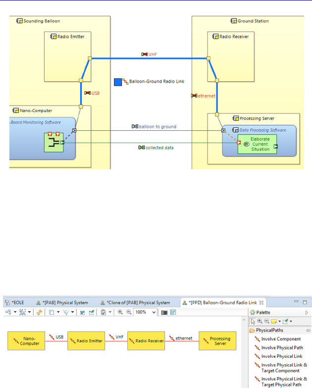
Complete Example of Modeling with Capella: Physical Architecture 241
Figure 6.47. Allocating the Component Exchange to the Physical Path. For a
color version of the figure, see www.iste.co.uk/roques/arcadia.zip
N
OTE
.– If we want to modify an existing Physical Path, we absolutely
must use a specific contextual diagram, called Physical Path
Description (PPD), like for Functional Chains. To create this diagram,
we just need to right click on the square in the diagram, or on the
model element in Project Explorer.
Figure 6.48. Contextual diagram of the Physical Path Description
6.7. Integrating Specialty Viewpoints
We recall that the Specialty Viewpoints are available in all the
Arcadia engineering levels, even if they are mainly used in Physical
Architecture. It would be very strange to evaluate the mass and
performance of Logical Components whose implementation choices
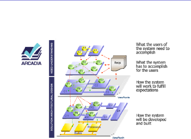
242 Systems Architecture Modeling with the Arcadia Method
have not been completed. However, a Product Line Viewpoint, or that
of Operational Safety, has its rightful place from Logical Architecture
onwards.
Figure 6.49. Recall of the architecture levels with the Viewpoints
So that a modeler can use a specialty Viewpoint, an expert of the
specialty and the profession concerned needs to specify it first, then a
software developer needs to implement it using Capella Studio
[HEL 16].
N
OTE
.– The subject of developing specialty Viewpoints exceeds the
framework of this book. Interested readers may refer to the specialized
website, at: wiki.polarsys.org/Capella/Studio.
We simply specify that a Viewpoint first defines the extensions
specific to the model elements manipulated by Capella. We are going
to take the Basic Mass Viewpoint, provided as standard since Capella
1.0, as an example in the rest of this section. This Viewpoint adds
additional properties of current mass and maximum mass to the
Physical Components (Behavior and Nodes). It also adds a new group
of commands in the palette of the Architecture (PAB) diagram.
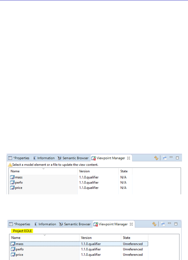
Complete Example of Modeling with Capella: Physical Architecture 243
A Viewpoint can then define specific algorithms that can be
executed automatically or upon request. The Basic Mass Viewpoint
automatically calculates the current mass of a containing Component
by adding the sum of masses of its contained Components to it.
According to the result of these algorithms, the Viewpoint can specify
more or less sophisticated conditional graphic annotations. The Basic
Mass Viewpoint simply compares the current mass of a Component
with its maximum mass and makes it red if the threshold has been
exceeded.
We are going to illustrate these principles in our case study by
focusing on the mass of the sounding balloon. We start by activating
the Basic Mass Viewpoint on our model. To do this, we first installed
the Viewpoint by following the installation procedure explained on
Capella Wiki. Then, we must reference the Viewpoint on our model.
To do this, we are going to open the Viewpoint Manager because of
the Window – Show View – Other – Kitalpha command. The
Viewpoint Manager then appears next to the Semantic Browser.
Figure 6.50. Activating the Viewpoint Manager window
Figure 6.51. Selecting a model for the Viewpoint Manager
The correctly installed Viewpoints are visible, but noted as N/A
(Figure 6.50). Notice that we have installed the three Viewpoints
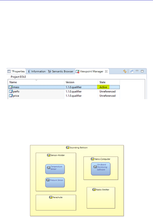
244 Systems Architecture Modeling with the Arcadia Method
currently provided on the Capella site: Basic Mass, Basic
Performance, Basic Price. We first have to select a model as indicated
in the Viewpoint Manager window. We select our EOLE project in
Capella Project Explorer. The Viewpoints are now noted as
Unreferenced (Figure 6.51).
To activate a Viewpoint, we just need to right click on Reference
on the property noted as Unreferenced. The chosen Viewpoint then
moves to the active state.
Figure 6.52. Activating the chosen Viewpoint
We are going to create a new PAB in order to show the sounding
balloon and its constituents. We add a parachute for regulatory
security reasons.
Figure 6.53. New PAB focused on the sounding balloon
A Viewpoint is used on a particular diagram by selecting it in the
Layers command at the top of the diagram.
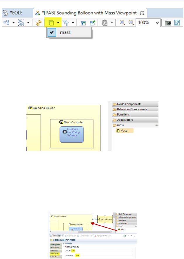
Complete Example of Modeling with Capella: Physical Architecture 245
Figure 6.54. Selecting the Viewpoint on the PAB
A new group of commands automatically appears in the palette of
the diagram on the right. This basic Viewpoint in fact only adds a
single command called Mass and which is now applicable to all the
Physical Component type model elements.
Figure 6.55. Adding commands in the PAB palette
Let us suppose that our design brief requires the balloon and
accessories set not to exceed a total mass of 1.5 kg. We are going to
assign a mass of 500 g to the “Balloon” Node Component,
corresponding to its physical sheath, and a maximum mass of 1,500 g.
Figure 6.56. Starting to use a Viewpoint on PAB. For a color
version of the figure, see www.iste.co.uk/roques/arcadia.zip
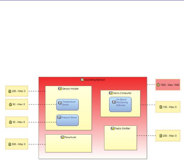
246 Systems Architecture Modeling with the Arcadia Method
We continue to assign values to the contained Components by the
sounding balloon. When each new value is entered, the current mass
of the sounding balloon still increments as much. If this value exceeds
the maximum of 1,500, the color of the Component automatically
turns red: we will need to find Components that weigh less. But in this
case, they may be more expensive and we will need to check that we
are not exceeding the maximum price, by applying the Basic Price
Viewpoint.
Figure 6.57. Visualization of the mass Viewpoint effect on a PAB. For a
color version of the figure, see www.iste.co.uk/roques/arcadia.zip
By successively applying several Viewpoints on the same Physical
model, the architect will have an effective means of finding the best
compromise possible between different architecture solutions, while
having the specialty experts work on the same architecture reference.
6.8. Replicable and Replica Elements
A Replicable Element Collection (REC) is a set of model elements,
identified as a patron (a model in the current sense of the term) for
constructing multiple replicas (or RPL), which are maintained in
conformity with it.

Complete Example of Modeling with Capella: Physical Architecture 247
This concept enables one to take account of the similarity
expression needs between model elements. Indeed, it may be
necessary to formalize several model elements of the same type and to
prevent one from being modified accidentally. This need appears in all
types of domains and model elements: Functional Chains need to be
repeated for security reasons, networks’ generic Components,
duplicated processing cards in architecture, etc.
Capella thus enables one to:
– specify, at a given time of the modeling process that a set of
model elements must be replicated as a whole;
– constitute a type based on this whole, called REC;
– transform the source elements into a specimen of this type
(RPL);
– create other replicas or specimens freely, based on REC;
– maintain the different replicas synchronized with the REC, and
propagate possible evolutions from some to others (RPL updates on
the REC evolution, propagation of the chosen evolutions of an RPL,
etc.).
NOTE.– This mechanism is a little different to that found in software
engineering (type/instances), particularly because we generally start
by creating a replica, and we then promote it into a REC. Or even
because an REC may be any set of Capella elements, possibly astride
several engineering levels.
We are going to illustrate the possibilities offered by Capella in a
small and simple example taken from the EOLE case study. Let us
suppose that we want to launch two balloons throughout the day: for
example, one at midday and the other at midnight, for which the data
will be collected by the same ground station. On a new PAB, we wish
to represent the two balloons and their relations with the same receiver
station.
We start by isolating the sounding balloon that we want to reuse in
a new diagram created for this occasion. The sounding balloon
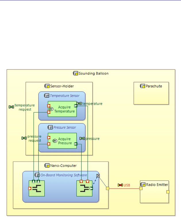
248 Systems Architecture Modeling with the Arcadia Method
contains Node Components, some of which contain deployed
Behavior Components, with Functions allocated to the same. There
are also non-connected input and output Ports, both on Functions, the
Behavior Components and the Node Components. In particular, we
verify that the Functional Ports have associated Exchange Items, even
if we are being far from exhaustive on this part started on the System
Analysis level (see section 4.9).
Figure 6.58. Isolating of the reusable sounding balloon model on a PAB.
For a color version of the figure, see www.iste.co.uk/roques/arcadia.zip
We go back to the Data Flow (PDFB) diagram where we had
broken down the “Acquire Weather Data” Function. A specific filter
enables us to display Exchange Items associated with the Functional
Exchanges.
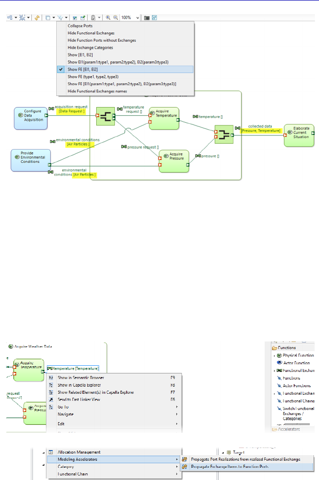
Complete Example of Modeling with Capella: Physical Architecture 249
Figure 6.59. Exchange Items display on the PDFB
In particular, we can see that the pressure and temperature
Exchange Items are missing on the exchanges at the acquisition sub-
Functions output. Even when we are going to add them, the
corresponding Function Ports will still not be given a type. Indeed, we
recall that the association of Exchange Items to a Functional Exchange
does not automatically propagate them to Function Ports. Capella
proposes a very useful Modeling Accelerator for this: Propagate
Exchange Items to Function Ports.
Figure 6.60. Using a propagation Modeling Accelerator
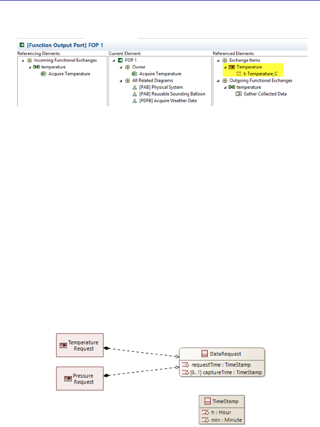
250 Systems Architecture Modeling with the Arcadia Method
The propagation result is easily verified in the Semantic Browser.
Figure 6.61. Visualization of the Exchange Items propagation
N
OTE
.– It is important to give the Function Ports a type and not only
the Functional Exchanges if we wish to reuse the Functions. As a
matter of fact, the input/output Function Ports are part of the Function
definition, unlike the Functional Exchanges that connect the two
Functions.
To illustrate the fact that we can perfectly add new Exchange Items
at the Physical level, while referencing the Types created at an upper
level, we are going to create a “Temperature Request” and a “Pressure
Request” similar to the “Data Request” previously first created on the
System Analysis level. For this purpose, we create a new Class
Diagram Blank (PCDB). We can also insert the “Timestamp” Type
coming from the library.
Figure 6.62. Definition of new Exchange Items at the Physical level
We can associate these new Exchange Items to the input Ports of
the acquisition sub-Functions to end the process. All the Function
Ports of the sounding balloon Functions are now associated with at
least one Exchange Item.
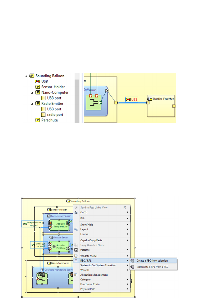
Complete Example of Modeling with Capella: Physical Architecture 251
Good practice consists of also renaming the Component Ports and
the Physical Ports of the reusable elements, even if their names do not
appear in the diagram. For the radio emitter in our example, the input
port is a USB port and the output port is a radio port. We can choose
to make these Ports appear in the Capella Project Explorer on the left
because of the Customize View command (they do not appear by
default).
Figure 6.63. Renaming Physical Ports
Once this preparatory work has been finished, we can promote this
sounding balloon as a Replicable Element (REC). To do this, we must
be careful when selecting it as well as the model elements that it
contains, then by a contextual menu (right clicking), applying the
REC/RPL – Create a REC from selection command.
Figure 6.64. REC creation command. For a color version
of the figure, see www.iste.co.uk/roques/arcadia.zip
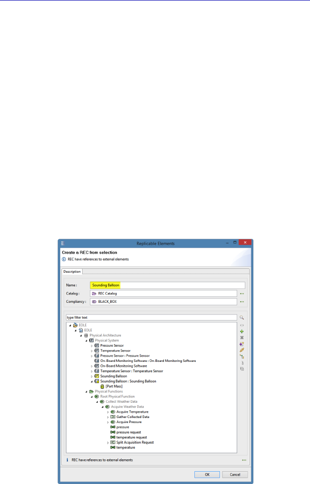
252 Systems Architecture Modeling with the Arcadia Method
Capella then opens a window that allows us to refine the settings of
the REC creation, by naming it, and by possibly removing the selected
model elements (Figure 6.65). For example, we may want to remove
the properties brought on by applying a specialty Viewpoint, to make
the REC more generic. Or otherwise to conserve them to evaluate the
effect of redundancy on the mass and the price of the system set, etc.
The replicable element will be positioned in a catalog that is
automatically created in the model, or selected by the modeler. It is
also possible to specify a conformity property among three possible
values: Black_Box (default), Constraint_Reuse, Inheritancy_Reuse.
This property is not yet used in Version 1.1.
NOTE.– Do not hesitate to refer to Capella Online Help, which is very
valuable for advanced points, such as the replicable elements: Help –
Help Contents – Capella Guide – User Manual – Replicable
Elements.
Figure 6.65. Settings window of an REC creation
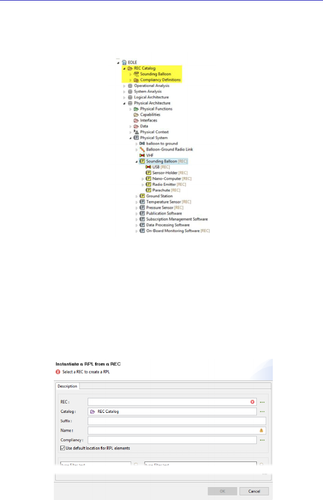
Complete Example of Modeling with Capella: Physical Architecture 253
The first result of creating the REC is seen in the Project Explorer
on the left, as shown in Figure 6.66.
Figure 6.66. Result of creating an REC
So, we can now reuse this REC by creating two replicas (RPL) of it
connected to the ground station in a new PAB. In this new diagram,
we are going to use the contextual command: REC/RPL – Instantiate
a RPL from a REC. A window opens in order to configure the replica
creation.
Figure 6.67. RPL creation window
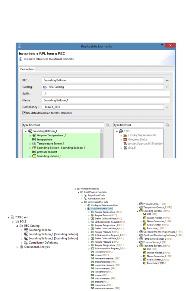
254 Systems Architecture Modeling with the Arcadia Method
We can choose the REC to be instantiated by specifying its catalog
and adding a suffix to the elements of the replicas requiring it. We
can number the sounding balloons, for example, to distinguish them.
Figure 6.68. Instantiating the first replica
Figure 6.69. Result of creating the RPL in Explorer
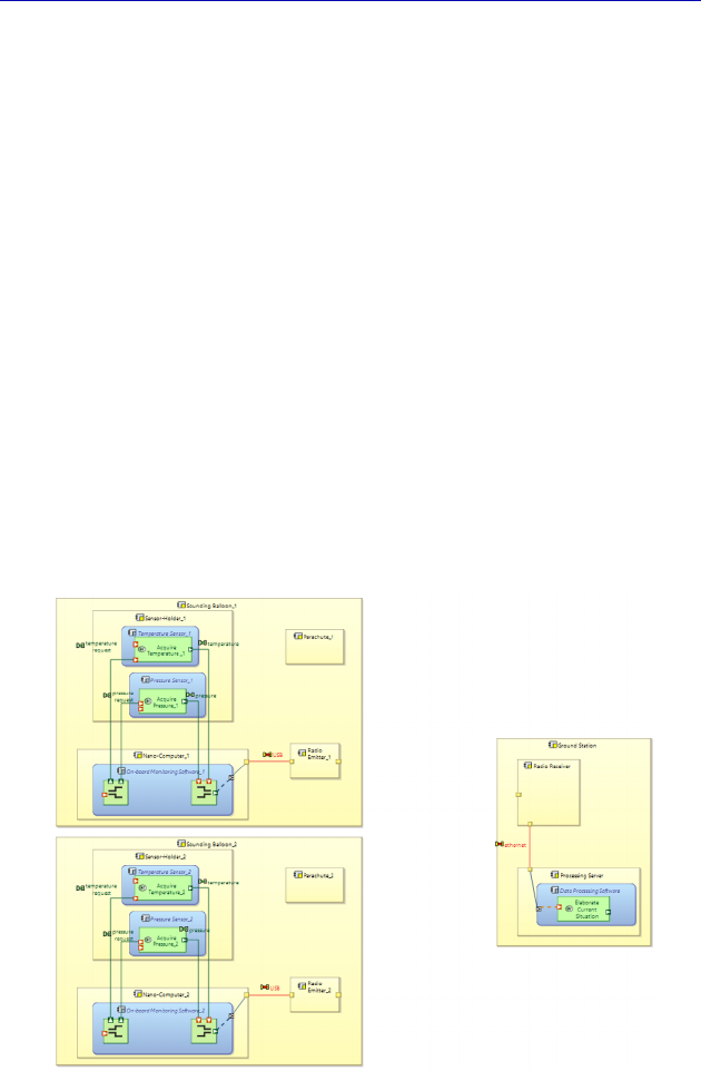
Complete Example of Modeling with Capella: Physical Architecture 255
Creating two replicas is clearly manifested in Project Explorer
because of the suffixes, but also to the acronyms [REC] and [RPL]
that appear behind the name of the model elements (Figure 6.69).
We can now insert both replicas in a new PAB and connect them to
the ground station. For each replica, we first need to insert the Node
Components, and then the Behavior Components deployed, then the
allocated Functions. We do not worry about the graphic positioning,
as Capella allows us a format copy–paste (Edit – Copy format) based
on the diagram where the reusable sounding balloon was represented.
Once the two sounding balloon replicas have been inserted, we can
insert the ground station. We note that it would have also been
possible to create a replicable element for the ground station,
particularly if we had wished to represent several stations at different
geographical positions.
Thus, in Figure 6.70, we show two sounding balloons and one
ground station before connecting the different Components.
Figure 6.70. Inserting the RPL into a new PAB. For a color
version of the figure, see www.iste.co.uk/roques/arcadia.zip
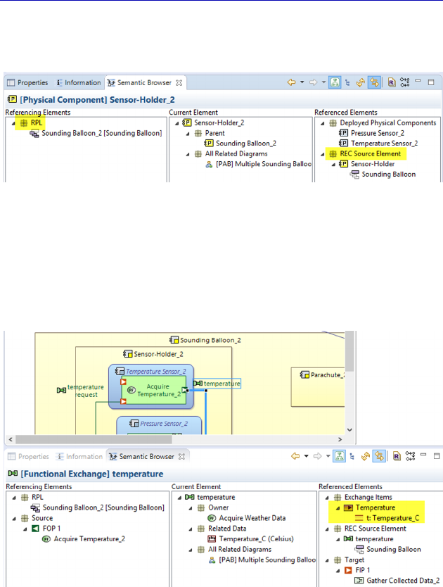
256 Systems Architecture Modeling with the Arcadia Method
As usual, the Semantic Explorer clearly indicates the relations
between the replicas (RPL) and the replicable element (REC).
Figure 6.71. Relation of the RPL and REC in the Semantic Explorer
Note that the Semantic Explorer also indicates that the
“temperature” Functional Exchange of each RPL always carries the
“Temperature” Exchange Item referring to the “Temperature_C
(Celsius)” Type, even it that has not been included in the REC.
Figure 6.72. Conserving the link with the Exchange Items and the Types.
For a color version of the figure, see www.iste.co.uk/roques/arcadia.zip
We just need to connect the two sounding balloons to the ground
station, as shown in Figure 6.73.
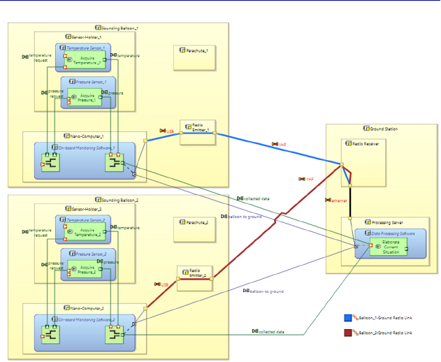
Complete Example of Modeling with Capella: Physical Architecture 257
Figure 6.73. RPL Connection to the ground station. For a color
version of the figure, see www.iste.co.uk/roques/arcadia.zip
N
OTE
.– To prevent having to manually create the connections again,
good practice consists of also creating an REC for the ground station,
even if we only instantiate it once. As a matter of fact, when a pair of
REC is connected by Functional and Component Exchanges and
Physical Links, it is possible to propagate these connections between
the corresponding RPL via the Update Connections command.
This page intentionally left blank
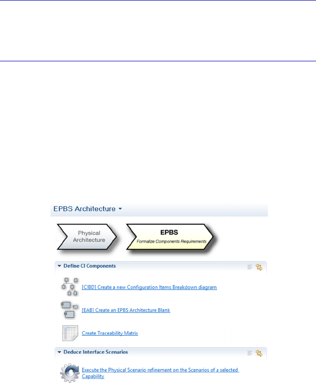
7
Complete Example of Modeling
with Capella: EPBS
7.1. Main concepts and diagrams
Capella integrates methodological guidance under the form of
Activity Explorer. This lists the different activities and diagrams that
can be made on the engineering level concerned; in this case, this is
namely EPBS (End Product Breakdown Structure). Figure 7.1
describes the activities and diagrams that are possible.
Figure 7.1. Methodological activities and diagrams on the “EPBS” level
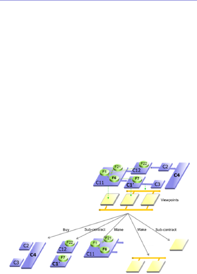
260 Systems Architecture Modeling with the Arcadia Method
N
OTE
.– This level is much lower than the four previous ones, in terms
of concepts, diagrams and methodological activities. In certain recent
Arcadia presentations, it is no longer even represented as an
engineering level, but rather as an “industrial organization” viewpoint
on physical architecture.
7.2. Moving from the Physical level to the EPBS level
This level aims to use the Physical Architecture to deduce the
conditions that each component must fulfill to satisfy the design
constraints and architecture choices, identified in the previous phases
(“what is expected of the provider of each component”). The Physical
Components are often gathered into Configuration Items that are
larger and more practical to manage, in terms of industrial
organization and responsibilities. The classic problem consists of
asking ourselves whether we are going to make the component, reuse
a similar one, buy it off the shelf, or subcontract it out, etc.
Figure 7.2. From the Physical Architecture to the EPBS. For a color
version of the figure, see www.iste.co.uk/roques/arcadia.zip
N
OTE
.– Unlike the previous levels, Capella does not currently propose
any transition to initialize EPBS based on the Physical Architecture.

Complete Example of Modeling with Capella: EPBS 261
7.3. Configuration Item
A Configuration Item is a part of the system, to be acquired or
designed and produced, in as many copies as required by the Physical
Architecture, and which will be assembled with other items to
constitute each of the system’s copies. Several physical Configuration
Items may be gathered into a Prime Item, thus defining the product
tree. The system is most often at the root of the tree defined thus.
This general concept can thus be shrunk into:
– System CI: system type configuration item;
– Prime Item CI: configuration item that can be broken down;
– CSCI: software type configuration item;
– HWCI: hardware type configuration item;
– NDI: non-developed configuration item;
– COTS: Component Off The Shelf configuration item.
In our case study, we have known from the beginning that the
system will contain two Subsystems: an airborne acquisition
Subsystem for which the state of the art consists of using a sounding
balloon inflated in helium and a ground processing Subsystem. It is
therefore natural to make two Prime Items on the first level. We will
then list the necessary Configuration Items in the form of a product
tree, and therefore on a breakdown diagram (CIBD).
For example, we are going to decide that we will buy the sounding
balloons off the shelf (COTS), as well as the sensors and the
parachute, but we will make the on-board software. We could also
decide to subcontract the on-ground software applications. With all
these hypotheses, and by using fictitious product names, the simplified
product tree could resemble the following diagram (Figure 7.3).
NOTE.– The colors were added manually; all the Configuration Items
have the same color by default.
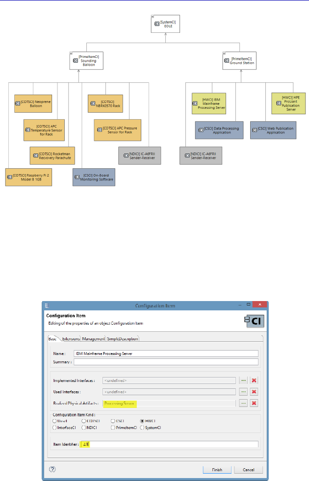
262 Systems Architecture Modeling with the Arcadia Method
Figure 7.3. Simplified example of EPBS for EOLE. For a color
version of the figure, see www.iste.co.uk/roques/arcadia.zip
For each Configuration Item, we can add a unique identifier, as
well as specifying the traceability with the Physical Components. For
example, we will open the property sheet of the “IBM Mainframe
processing server”.
Figure 7.4. Property sheet of a Configuration Item
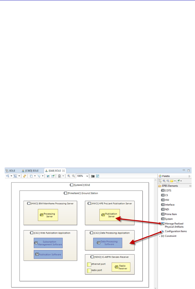
Complete Example of Modeling with Capella: EPBS 263
7.4. Traceability between Configuration Items and Physical
Components
This traceability can be established in different ways. Of course,
we can open the property sheet of each Configuration Item and fill the
Realized Physical Artifacts field, but also use other possibilities:
– edit the Traceability Matrix proposed in the Activity Explorer;
– create an EPBS Architecture Blank (EAB);
– use the Fast Linker window.
We are going to illustrate these three possibilities one by one;
however, the simplest and the most efficient is the Traceability
Matrix.
We start by creating the EAB Architecture Blank diagram. It allows
us to create or insert the Configuration Items, then add the realization
relations and to show the Physical Components inside the CI. We
sketch the diagram on the ground station for now.
Figure 7.5. Start of the Architecture Blank diagram (EAB). For a
color version of the figure, see www.iste.co.uk/roques/arcadia.zip
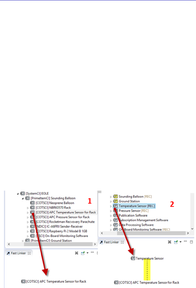
264 Systems Architecture Modeling with the Arcadia Method
N
OTE
.– The Configuration Items can realize one or several Physical
Components, but also Physical Ports and Links. We have shown it in
the previous diagram for the “IC-A6FRII sender-receiver” NDICI.
Another way to proceed consists of using the Fast Linker. This is a
particular window, which was created when Capella was opened at the
bottom left. If it was closed, we just need to activate it again by the
Window – Show View – Fast Linker menu.
We can send an item into the Fast Linker by sliding/moving from
the Project Explorer or the Semantic Browser, or by activating a
contextual command on a model element of type: right click/Send to
Fast Linker View (F6).
If the model element can accept links, it remains visible in the Fast
Linker. Otherwise, it is rejected. As soon as another element is put
into the Fast Linker, Capella verifies if it can be linked with the first
one and then automatically creates the link or rejects it. If several links
are possible, a window of choice is proposed to the user.
We show an example for creating the automatic realization link
into two steps for the temperature sensor, as shown in Figure 7.6.
Figure 7.6. Use example of the Fast Linker
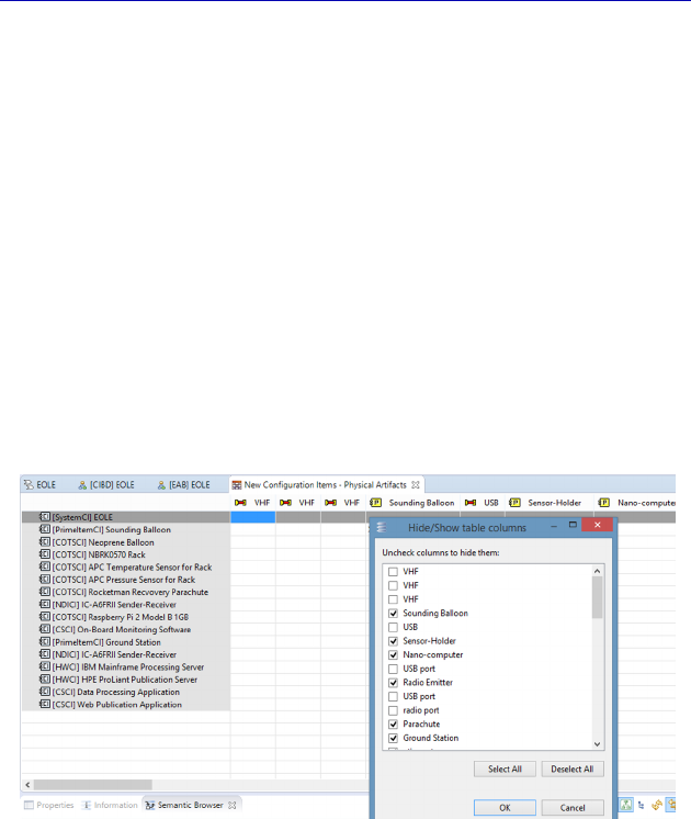
Complete Example of Modeling with Capella: EPBS 265
But as we said, the most efficient is probably to work directly on
the Traceability Matrix, calculated by Capella according to the
existing relations and that can be edited easily. We go back into
Activity Explorer and we click on Create Traceability Matrix. The
matrix obtained is rather raw and contains all the traceable physical
elements as columns: Node and Behavior Components, Ports and
Physical Links.
N
OTE
.– The matrix takes all the physical elements into account, both
those of the REC and those of RPL. The elements that we do not need
must be filtered so as to make the matrix more usable.
Therefore, we are going to hide some of the columns that are not
useful because of the Hide/Show table columns command, which is
applied by right clicking on the matrix.
Figure 7.7. Preparing the EPBS/PA traceability matrix
We can also hide the lines corresponding to the PrimeItem type
items to obtain the following matrix, which is very clearly truncated to
the right.
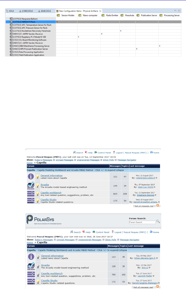
266 Systems Architecture Modeling with the Arcadia Method
Figure 7.8. Filling the EPBS/PA traceability matrix
We therefore finish our work on the EOLE case study in the hope
that it encourages you to delve deeper into the various possibilities
offered by Capella.
It is clear that we did not have the sufficient space in this first book
to go further into some of the tool’s advanced features; however, we
endeavor to do it by yourself with the precious help of the Online
help, as well as the Users Forum available on the Capella Website.
Figure 7.9. Capella Users Forum

Conclusion
Capella’s Key Strengths
Summary of key strengths
We hope that the previous chapters, and the work on the case study
in particular, will have convinced you of Capella’s numerous key
strengths.
We will attempt to briefly summarize the main points that
distinguish it from other UML/SysML modeling tools on the market:
– integrated methodological guide (Activity Explorer);
– Semantic Browser;
– integrated validation of Arcadia methodological rules (Validate
Model);
– help with managing complexity (ability to hide complexity,
filters, calculated links, accelerators, etc.);
– iterative and incremental interlevel transitions;
– iterative and incremental system/subsystem transitions;
– semantic color grid.
In short, not only does Capella efficiently know a modeling
language, but also a methodological approach (Arcadia).
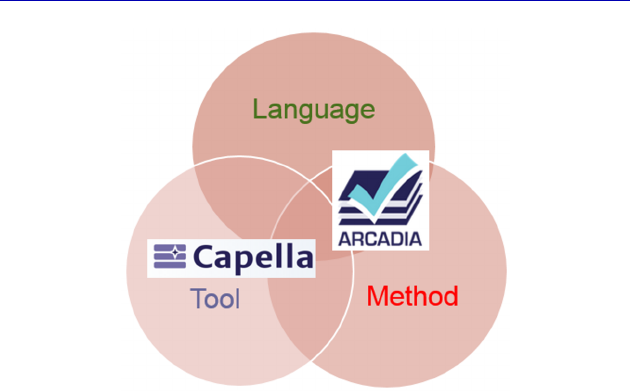
268 Systems Architecture Modeling with the Arcadia Method
MBSE with Arcadia/Capella
The Capella ecosystem
With a lack of satisfying solutions on the market, the Thales group
chose to pour its in-house modeling technologies into Open Source in
order to create a de facto standard, to hatch an ecosystem and to
contribute to funding the innovation.
Logically, the Eclipse foundation, whose tools already underlied
the arsenal of engineers at Thales, became involved. This foundation
constitutes an Open Source community recognized in software
development. Historically, under the aegis of technology providers,
the foundation replaced users at the forefront, especially in today’s
industry. Eclipse working groups were created for this purpose,
including PolarSys (www.polarsys.org), who initially sought to
entrench the works carried out within the framework of OPEES and
TopCased, another Open Source modeling platform for on-board
systems (driven by Airbus in particular).
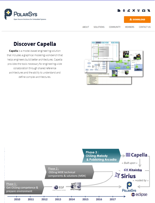
Conclusion 269
The Polarsys Website: https://www.polarsys.org/
With the support of Obeo, a French SME that is well known in the
Eclipse world, Thales proceeded to implement the whole of its
technological platform and its modeling components within the
Kitalpha project in Open Source to provide a complete technological
foundation.
The Open Source implementation by Thales
Thales’ goals are numerous:
– to be able to share models with clients or subcontractors for
communication or even contracting purposes;
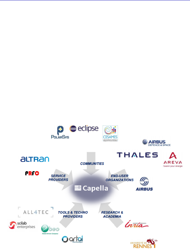
270 Systems Architecture Modeling with the Arcadia Method
– to guarantee the continuity of the investment already made
through de facto standardization;
– to share the development and maintenance costs with other
partners;
– to continue to improve the method and the tool because of greater
and more varied experience feedback.
The ultimate motivation is for it to constitute a complete ecosystem
with users, technology providers, service providers, academics and
researchers, etc. The first ecosystem was set up within the framework
of the aforementioned Clarity [BOU 16] project, which was started in
September 2014 to be finished at the end of 2017, with the
stakeholders, as shown in below figure.
The stakeholders of the initial ecosystem, Clarity
There is a European follow-up to this Clarity project on the cards
with many additional stakeholders, and which should kick off at the
beginning of 2018.
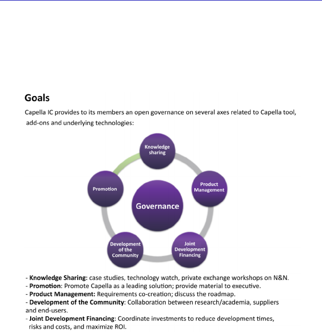
Conclusion 271
Moreover, a Capella Industry Consortium based on the existing
Papyrus IC model is currently being created in order to bring all of the
parties involved in the Capella ecosystem together, with open
governance. For more information, the reader can visit the Website:
www.polarsys.org/capella/industry-consortium.html.
The goals of the Capella Industry Consortium
This page intentionally left blank

Bibliography
[BON 16] BONNET S., “Capella Team: Live collaborative modeling with Sirius”,
SiriusCon, Paris, France, 2016.
[BOU 16] BOUDJENNAH C., “Capella: the Birth of an Industrial Ecosystem”, CSD&M,
Paris, France, 2016.
[CAS 18] C
ASSE O., SysML in Action with Cameo Systems Modeler, ISTE Press,
London and Elsevier, Oxford, 2018.
[HEL 16] HELLEBOID M., LANGLOIS B., “Viewpoint: the making of Customizing
Capella with Capella Studio in 20 minutes”, EclipseCon France, Toulouse,
France, 2016.
[ROQ 04] ROQUES P., UML in Practice: The Art of Modeling Software Systems
Demonstrated through Worked Examples and Solutions, Wiley, 2004.
[VOI 16] VOIRIN J.L., BONNET S., EXERTIER D. et al., “Simplifying (and enriching)
SysML to perform functional analysis and model instances”, INCOSE IS,
Edinburgh, Scotland, 2016.
[VOI 18] VOIRIN J.L., Model-based System and Architecture Engineering with the
Arcadia Method, ISTE Press, London and Elsevier, Oxford, 2018.
This page intentionally left blank

Index
A, B
accelerator, 94, 108, 168, 186,
249
Activity Explorer, 35, 37, 55, 195
Actor, 213
add-on, 192
allocation, 108
Function, 63, 96, 188, 220
Arcadia, 2, 3, 5, 16
Architecture
Logical, 11, 177
Physical, 13, 209
Basic Mass, 242
Blank, 38
diagram, 38
C
Capability Realization, 198
Capella Studio, 242
cardinality, 158, 165
catalog, 252
category, 45
CDB, 153, 161, 165, 250
CDI, 175
CEI, 174
Change Event, 146
CIBD, 261
clarity, 27
class, 155
cloner, 45, 85, 113
Component
Behavior, 216
Exchange, 190
Host, 216
Logical, 182
Physical, 215
condition, 130, 148
Configuration Item, 260, 261
COTS, 261
D
data modeling, 151
delegation, 206
deployment, 220
diagrams
architecture, 17, 65, 183, 184
capability, 23
class, 22, 152
contextual, 82
data flow, 17
decomposition, 22, 38, 68, 117
desynchronized, 43
modes and states, 20, 138, 140

276 Systems Architecture Modeling with the Arcadia Method
scenario, 19, 40, 70, 118, 201
Diagrams Viewer, 36, 82
E, F, G
EAB, 263
effects, 149
entry, 141
exit, 141
engineering levels, 5, 6
EOLE, 51
EPBS, 15
EPBS, 259
ES, 123
exchange, 153, 162, 167
Component, 107, 109, 206
Functional, 104, 109, 132, 167
Item, 162
Fast Linker, 264
FCD, 90, 93, 105, 232
filter, 110, 112, 115, 171
filtering of the diagrams, 36
fragment, 72, 126, 129
FS, 119
function, 76, 135, 211
Control, 226
“leaf”, 82, 104
Logical, 187
Physical, 217
Functional
Analysis, 82
Chain, 89, 232
Incomplete Functional, 94,
106
Invalid Functional, 92
guard, 73, 130, 148
H, I, J, L
Hide, 34
interface, 172
human-machine, 28
IS, 170
Jump Link, 231
LAB, 184
LES, 201
library, 158, 163
logical subcomponents, 204
M, N, O
Manage Function Allocation,
103, 188
matrix, 143
Traceability, 265
Modes/States and Functions,
142
MBSE, 25
message, 121
methodological guide, 35
mode, 137
model
element versus graphical
object, 30
validation, 84
MSM, 139
NODE, 218
OAB, 65
OAIB, 60
OCB, 58, 73
OEBD, 69
OES, 71
online help, 36, 252
Opaque Expression, 130

Index 277
Operational
Activities and Interactions, 60
Activity, 60
Analysis, 7, 51
Capability, 58
Entity, 58
P, R
PAB, 216, 220, 222, 228, 231,
234, 237, 244, 246, 248, 255
Package, 160
PDFB, 223, 224, 230, 248
PFBD, 227
Physical
Link, 238
Path, 238, 239
PolarSys, 27
Ports
Functional, 250
Physical, 238
Structural, 109
PPD, 241
project creation, 52
realization of System level
capabilities, 198
REC, 247, 251
replica, 253
Replicable Element, 246, 251
ReqIF, 50
Requirement, 2, 47
RPL, 247, 253
S
SAB, 113, 115, 134, 169, 195
scenario, 71, 118, 123, 198
Interface Scenario, 170
SDFB, 82, 86, 88, 89, 93, 106,
134
Semantic Browser, 80, 85, 168,
235, 250, 256
SES, 126, 150, 171
SFBD, 116
SFS, 119
Specialty Viewpoint, 241
State, 137
transitions, 138, 145
Structured Type, 155, 162
subsystem, 183
suppression, 33, 41
SysML, 1, 25, 121, 129, 137, 145
System
Analysis, 9, 75
Capability, 80
System to Subsystem
Transition, 191
T, U, V
team for Capella, 86
time constraint, 122
Trace Manager, 49
transition, 78, 80, 96, 124 179,
200, 211
Trigger, 145
type, 155
UML, 1, 121, 129, 137, 145, 156,
172, 175
Unsynchronized, 43
Users Forum, 266
Viewpoint, 50, 241, 24
Manager, 243
This page intentionally left blank