Installing And Running PebbleCounts Pebble Counts Manual
PebbleCounts_Manual_2019-04-23
User Manual:
Open the PDF directly: View PDF ![]() .
.
Page Count: 24

Installing and Running PebbleCounts March 2019
Table of Contents
1 Introduction 3
2 Soware Citation 3
3 License 3
3.1 Disclaimer.......................................... 3
4 Quick note on imagery and running PebbleCounts 4
4.1 The PebbleCountsAuto Function . . . . . . . . . . . . . . . . . . . . . . . . . . . . . 4
5 Installation 4
5.0.1 ForWindows.................................... 5
5.0.2 ForMacandLinuxUsers.............................. 5
6 Overview 6
6.1 PebbleCounts: K-means with Manual Selection (KMS) . . . . . . . . . . . . . . . . . . 6
6.1.1 KMS Detailed Processing Steps . . . . . . . . . . . . . . . . . . . . . . . . . . 7
6.2 PebbleCountsAuto: Automatic with Image Filtering (AIF) . . . . . . . . . . . . . . . . 9
6.2.1 AIF Detailed Processing Steps . . . . . . . . . . . . . . . . . . . . . . . . . . . 10
7 Command-line Programs and Variables 12
7.1 Calculate Camera Resolution . . . . . . . . . . . . . . . . . . . . . . . . . . . . . . . 12
7.1.1 ExampleUse .................................... 12
7.2 PebbleCounts(KMS) .................................... 13
7.3 PebbleCountsAuto(AIF) .................................. 15
7.4 Detail On Some PebbleCounts and PebbleCountsAuto Variables . . . . . . . . . . . . 16
8 PebbleCounts (KMS) Step-by-Step Example 18
8.1 An important note on clicking! . . . . . . . . . . . . . . . . . . . . . . . . . . . . . . . 22
9 PebbleCountsAuto (AIF) Step-by-Step Example 22
10 Ouput Files 23
Ben Purinton (purinton@uni-potsdam.de) 2

Installing and Running PebbleCounts March 2019
1 Introduction
This guide will walk you through the installation and running of PebbleCounts at the command-
line. PebbleCounts is a Python based application for the identification and sizing of gravel from
either orthorectified, georeferenced (
UTM projected
) images with known resolution or simple non-
orthorectified images taken from directly overhead with the image resolution approximated by the
camera parameters and shot height. It is a semi-automated program in that edge detection and k-
means segmentation are performed automatically, but the user must interactively hand-click the well
outlined pebbles and ignore the bad results. For the detailed background and validation (in addition
to the suggested use), check out the open-source publication accompanying the algorithm:
Purinton, B. and Bookhagen, B.: Introducing PebbleCounts: A grain-sizing tool for photo surveys of
dynamic gravel-bed rivers, Earth Surf. Dynam. Discuss., https://doi.org/10.5194/esurf-2019-20, in
review, 2019
and cite it if you use the results in your own work.
2 Soware Citation
Purinton, Benjamin; Bookhagen, Bodo (2019): PebbleCounts: a Python grain-sizing algorithm for
gravel-bed river imagery. V. 1.0. GFZ Data Services. http://doi.org/10.5880/fidgeo.2019.007
3 License
GNU General Public License, Version 3, 29 June 2007
Copyright ©2019 Benjamin Purinton, University of Potsdam, Potsdam, Germany
PebbleCounts is free soware: you can redistribute it and/or modify it under the terms of the GNU Gen-
eral Public License as published by the Free Soware Foundation, either version 3 of the License, or (at
your option) any later version. PebbleCounts is distributed in the hope that it will be useful, but WITH-
OUT ANY WARRANTY; without even the implied warranty of MERCHANTABILITY or FITNESS FOR A PARTIC-
ULAR PURPOSE. See the GNU General Public License for more details. You should have received a copy
of the GNU General Public License along with this program. If not, see http://www.gnu.org/licenses/.
3.1 Disclaimer
PebbleCounts is a free (released under GNU General Public License v3.0) and open-source application
written by a geologist / amateur programmer. If you have any problems contact me purinton@uni-
Ben Purinton (purinton@uni-potsdam.de) 3

Installing and Running PebbleCounts March 2019
potsdam.de and I can help!
4 Quick note on imagery and running PebbleCounts
Georeferenced ortho-photos should be in a
UTM projection
, providing the scale in meters. You can use
the gdal command line utilities to translate rasters between various projections. Because PebbleCounts
doesn’t allow you to save work in the middle of clicking it’s recommended that you don’t use images
covering areas of more than 2 by 2 meters or so. Furthermore, the algorithm is most eective on images
of 0.8-1.2 mm/pixel resolution, where a lower cuto of 20-pixels is appropriate. Resampling can also
be accomplished quickly in gdal. For higher resolution (< 0.8 mm/pixel) imagery it’s recommended
not to go above 1 by 1 meter areas, particularly if there are many < 1 cm pebbles. If you want to cover a
larger area simply break the image into smaller parts and process each individually, so you can give
yourself a break. If at anytime you want to end the application simply press CTRL + C.
4.1 The PebbleCountsAuto Function
In addition to the manual-clicking version of PebbleCounts based on k-means segmentation, we have
also developed and included an automated version that has higher uncertainties. We recommend using
PebbleCounts in a subset of data to validate larger areas run in PebbleCountsAuto. The description of
the automatic algorithm and uncertainties can be found in the publication (
PUBLICATION DOI TO BE
ADDED).
5 Installation
The first step is downloading the GitHub repository somewhere on your computer, and unzipping
it. There you will find the Python algorithms (e.g.,
PebbleCounts.py
), an
environment.yml
file
containing the Python dependencies for quick installs with
conda
on Windows, a folder
example_data
with two example images one orthorectified and the other raw, and a folder
docs
containing this
manual.
For newcomers to Python, no worries! Installation should be a cinch on most machines. First, you’ll
want the Miniconda Python package manager to setup a new Python environment for running the
algorithm (see this good article on Python package management). Download either the 32- or 64-bit
Miniconda installer of Python 3.x then follow the instructions (either using the .exe file for Windows,
.pkg
for Mac, or
bash installer
for Linux). Add Miniconda to the system
PATH
variable when
prompted.
Ben Purinton (purinton@uni-potsdam.de) 4
Installing and Running PebbleCounts March 2019
PebbleCounts has a number of important dependencies including gdal for georeferenced raster manip-
ulation, openCV for image manipulation and GUI operation, scikit-image for filtering and measuring,
scikit-learn for k-means segmentation, shapely for geometry operations, along with a number of
standard Python libraries including numpy,scipy,matplotlib, and tkinter.
5.0.1 For Windows
Once you’ve got
conda
commands installed, you can open a command-line terminal and create a
conda environment with:
conda create --name pebblecounts python=3.6 opencv shapely \
scikit-image scikit-learn numpy gdal scipy matplotlib tk
Or just use the .yml file provided with:
conda env create -f environment.yml
and once installation is complete (and assuming no errors during the install) activate the new environ-
ment to run PebbleCounts by:
activate pebblecounts
Deactivate the environment to exit anytime by:
deactivate
5.0.2 For Mac and Linux Users
Those using Mac OS or Linux shouldn’t have much trouble modifying the above commands slightly
(just add a leading
conda
to the
activate
and
deactivate
commands above). Also we need to
install opencv separately from within the virtual environment using the pip package manager.
Similar to the above, once you have conda installed we create the virtual environment:
conda create --name pebblecounts python=3.6 shapely \
scikit-image scikit-learn numpy gdal scipy matplotlib tk
and once installation is complete (and assuming no errors during the install) activate the new environ-
ment by:
conda activate pebblecounts
Ben Purinton (purinton@uni-potsdam.de) 5

Installing and Running PebbleCounts March 2019
We’ve le out the opencv package which must be installed with the following
pip
command in the
activated pebblecounts environment:
pip install opencv-python
Deactivate the environment to exit anytime by:
conda deactivate
Issues with opencv on Mac and Linux
Note that installing openCV and getting it to function properly can be a pain sometimes, especially
in the case of Linux. In that case it is recommended to find some instructions for installing openCV’s
Python API for your specific Linux operating system online.
6 Overview
6.1 PebbleCounts: K-means with Manual Selection (KMS)
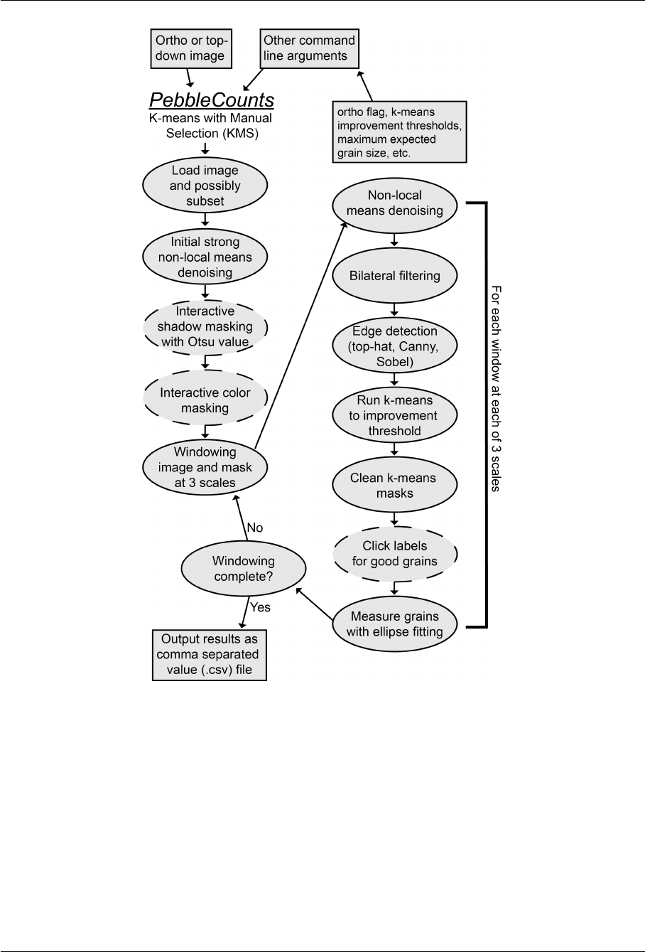
PebbleCounts using the K-means with Manual Selection (KMS) approach can be summed up in the flow
chart shown in Figure 1. To briefly summarize, PebbleCounts pre-processes the image by allowing the
user to subset the full scene, then interactively mask shadows (interstices between grains) and color
(for instance sand). Following this, PebbleCounts windows the scene at three dierent scales with the
window size determined by the input resolution and expected maximum longest-axis (a-axis) grain
size provided by the user. This multi-scale approach allows the algorithm to “burrow” through the
grain-size distribution beginning by removing the largest grains and ending on the smallest, with the
medium sizes in between. At each window the algorithm filters the image, detects edges, and employs
k-means segmentation to get an approximate cleaned-up mask of potential separate pebbles. The
window is then shown with the mask overlain and the user is able to click the
good
looking grains and
leave out the
bad
ones (see Figure 6). These grains are then measured via ellipse fitting to retrieve the
long- and short-axis and orientation. This process is iterated through each window and the output
from the counting is provided as a comma separated value (.csv) file for user manipulation.
Ben Purinton (purinton@uni-potsdam.de) 6
Installing and Running PebbleCounts March 2019
Figure 1:
Flowchart of PebbleCounts. The boxes are user supplied input or output from the algorithm.
Dashed lines indicate a user input step during processing, either entering and checking values or
clicking.
6.1.1 KMS Detailed Processing Steps
Below is an in-depth description of each processing step applied by PebbleCounts. For those wishing
to proceed with counting without the full story, go ahead to the
Command-line Options
and then the
Ben Purinton (purinton@uni-potsdam.de) 7

Installing and Running PebbleCounts March 2019
Step-by-Step Example sections below! For the nitty-gritty breakdown, follow along:
1.
PebbleCounts begins with the input of georeferenced ortho or simple top-down imagery at
the command-line along with a number of variable flags. Most of the 20 variables do not need
modification, but see their descriptions below to decide.
2.
The image is loaded (and possibly subset with a click-and-drag rectangle) and initially denoised
with a strong non-local means denoising filter to smooth color.
3.
The Otsu value for gray-scale thresholding is assessed and the user is asked to supply a percentage
of this Otsu value for masking out shadows between grains. The resulting mask is then checked
by the user and re-evaluated with a new percentage value, for instance if the value is too high
thus causing some of the darker grains to also be masked.
4.
The image is displayed and the user can click on a color that should be masked (e.g., uniform
colored brown sand or vegetation patches). The masking is accomplished via a narrow range
applied to the HSV color-space around the clicked pixel. The user has the opportunity to accept
or reject the additional mask and add more color masks if the full range of interest has not
been included. For georeferenced imagery, a binary GeoTi and a vector polygon shapefile of
the sand mask are output at this step. Together, the shadow and color mask provide an initial
segmentation of the grains in the image.
5.
Following these pre-processing steps, the image and shadow/color mask are windowed at three
dierent scales corresponding to approximately 10, 3, and 2 times the longest expected grain in
the image. Each of these windows is passed through steps 6-14.
6.
Non-local means denoising on the CIELab converted image with the color (chromaticity) filtered
but the brightness (luminance) un-altered. This provides a more uniform color for mottled grains.
7.
Bilateral filtering on the CIELab chromaticity bands. This filtering technique reduces noise in an
image while preserving high-gradient edges between grains.
8.
Edge detection steps applied to the original gray-scale image. This includes black top-hat and
Sobel filtering, aer which a suggested threshold of 90% is applied to only extract the strongest
edges, and Canny edge detection. At each of these steps the associated edge mask is feature-
AND (see textbook by John C. Russ) operated with the shadow/color mask to add additional
segmentation details where there is some overlap to definite inter-granular interstices, while
avoiding over segmentation caused by intra-granular noise.
9.
Masked pixels are eliminated from the analysis and an N*4 dimensional vector (Nis the number
of pixels) is formed with the smoothed CIELab a* (green-red) and b* (blue-yellow) chromaticity
bands and the Xand Ycoordinate of the pixel in image space. The chromaticity (a* and b*) is
rescaled between 0 and 1 and the Xand Yis rescaled by a user supplied scaling factor suggested
at 0.5. This allows the color information to have a larger influence on clustering in the k-means
step, thus avoiding some over-segmentation of larger grains.
10.
This N*4, rescaled vector is passed to the k-means algorithm, which iteratively clusters the
Ben Purinton (purinton@uni-potsdam.de) 8

Installing and Running PebbleCounts March 2019
pixels by color and spatial location and checks the overall inertia of the clusters then repeats
the clustering with centers shied until the improvement in subsequent inertia is less than a
threshold fractional percentage. This threshold improvement is suggested to be 0.01 for the first,
large scale and 0.1 for the medium and fine scale.
11.
When the improvement threshold is met, the vector is transformed back into image space,
maintaining the k-means labels. Each of these labels is then separately selected and cleaned up
via a combination of binary erosion, dilation, removal of small objects, and clearing of border-
touching elements. Any labels below the lower cuto value (e.g., 20-pixel b-axis length) are
eliminated. The cleaned label masks are then combined into a final potential grain mask.
12.
The potential grain mask is now displayed over the original RGB color image and the user is
asked to click labels that contain single, well-defined grains. Here it is suggested that any grain
mask that contains the majority of the grain (particularly the edges of the grain) is selected, even
if the k-means segmentation led to jagged edges and over-segmentation within the grain. This is
because the final ellipse fitting ignores these holes and fits to the largest area covered by the
mask label.
13.
Each of the labels with a user-selected point clicked inside of it is analyzed for region properties
to extract the grain centroid, area, and the following parameters of an ellipse fit to the region:
minor and major axis length, area of the ellipse (for providing a misfit value against the area
of the grain), and orientation of the ellipse measured from -pi/2 to pi/2 relative to the positive
x-axis (orientation=0) in Cartesian coordinates.
14.
The clicked regions are then added to the shadow/color mask and the processing is repeated
from step 6 on the next window or beginning at the next of the three scales.
15.
Following all windowing, the results of each grain are output as a comma separated value text file.
The measurements are given in pixel and metric units by multiplying the pixel amounts by the
image resolution in meters per pixel. In case of a UTM projected georeferenced image, the UTM
X (Easting) and Y (Northing) coordinates of the grain centroid are also provided. Additionally,
from the color mask a fractional percentage of the image that was masked by the HSV range is
provided in the output file (e.g., the percentage sand) along with the fractional percentage of the
image that was not measured (so combined shadows and grains not identified by PebbleCounts).
6.2 PebbleCountsAuto: Automatic with Image Filtering (AIF)
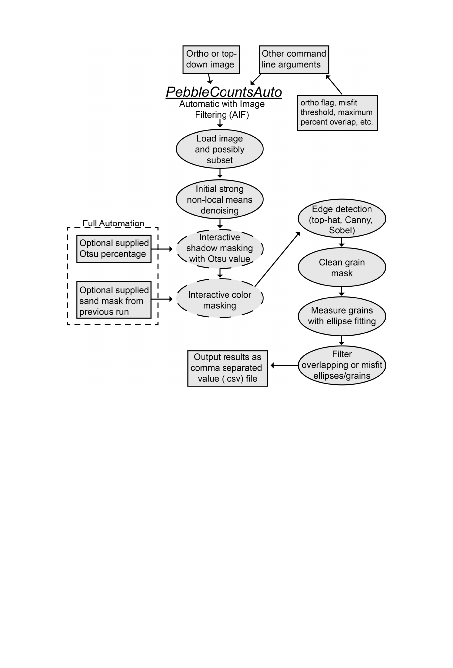
PebbleCountsAuto using the Automatic with Image Filtering (AIF) approach can be summed up in
the flow chart shown in Figure 2. To briefly summarize, PebbleCountsAuto pre-processes the image
by allowing the user to subset the full scene, then interactively mask shadows (interstices between
grains) and color (for instance sand). Following this, the algorithm detects edges, cleans the mask,
and filters suspect grains. The remaining grains are then measured via ellipse fitting to retrieve the
long- and short-axis and orientation and the output from the counting is provided as a .csv file for user
Ben Purinton (purinton@uni-potsdam.de) 9
Installing and Running PebbleCounts March 2019
manipulation.
Figure 2: Flowchart of PebbleCountsAuto. The boxes are user supplied input or output from the
algorithm. Dashed lines indicate a user input step during processing, either entering and checking
values or clicking.
6.2.1 AIF Detailed Processing Steps
Below is an in-depth description of each processing step applied by PebbleCountsAuto:
1.
PebbleCountsAuto begins with the input of georeferenced ortho or simple top-down imagery at
the command-line along with a number of variable flags. Most of the 15 variables do not need
modification, but see their descriptions below to decide.
2.
The image is loaded (and possibly subset with a click-and-drag rectangle) and initially denoised
with a strong non-local means denoising filter to smooth color.
3.
The Otsu value for gray-scale thresholding is assessed and the user is asked to supply a percentage
of this Otsu value for masking out shadows between grains. The resulting mask is then checked
Ben Purinton (purinton@uni-potsdam.de) 10

Installing and Running PebbleCounts March 2019
by the user and re-evaluated with a new percentage value, for instance if the value is too high
thus causing some of the darker grains to also be masked.
4.
The image is displayed and the user can click on a color that should be masked (e.g., uniform
colored brown sand or vegetation patches). The masking is accomplished via a narrow range
applied to the HSV color-space around the clicked pixel. The user has the opportunity to accept
or reject the additional mask and add more color masks if the full range of interest has not
been included. For georeferenced imagery, a binary GeoTi and a vector polygon shapefile of
the sand mask are output at this step. Together, the shadow and color mask provide an initial
segmentation of the grains in the image.
5.
Following these pre-processing steps, edge detection steps are applied to the original gray-scale
image. This includes black top-hat and Sobel filtering, aer which a suggested threshold of
90% is applied to only extract the strongest edges, and Canny edge detection. At each of these
steps the associated edge mask is feature-AND (see textbook by John C. Russ) operated with
the shadow/color mask to add additional segmentation details where there is some overlap to
definite inter-granular interstices, while avoiding over segmentation caused by intra-granular
noise.
6.
The resulting potential grain labels are cleaned up via a combination of binary erosion, dilation,
removal of small objects, and clearing of border-touching elements. Any labels below the lower
cuto value (e.g., 20-pixel b-axis length) are eliminated.
7.
Each of the remaining labels are analyzed for region properties to extract the grain centroid, area,
and the following parameters of an ellipse fit to the region: minor and major axis length, area
of the ellipse (for providing a misfit value against the area of the grain), and orientation of the
ellipse measured from -pi/2 to pi/2 relative to the positive x-axis (orientation=0) in Cartesian
coordinates.
8.
The grains are then filtered to remove suspect grains in a three step process, where a yes answer
to any step eliminates the grain:
•(A) Does the centroid fall within another ellipse?
•(B)
Does the ellipse overlap with any neighboring ellipses above some threshold? (15% works
well)
•(C)
Is the percent misfit (ellipse area vs. grain-mask area) above some threshold? (30% works
well)
9.
Following filtering, the results of each grain are output as a comma separated value text file.
The measurements are given in pixel and metric units by multiplying the pixel amounts by the
image resolution in meters per pixel. In case of a UTM projected georeferenced image, the UTM X
(Easting) and Y (Northing) coordinates of the grain centroid are also provided. Additionally, from
the color mask a fractional percentage of the image that was masked by the HSV range is provided
Ben Purinton (purinton@uni-potsdam.de) 11

Installing and Running PebbleCounts March 2019
in the output file (e.g., the percentage sand) along with the fractional percentage of the image
that was not measured (so combined shadows and grains not identified by PebbleCountsAuto).
7 Command-line Programs and Variables
Great you’ve got it installed! Hopefully that is, we’re about to find out! The first step to running the
soware is navigating to the directory where the three scripts live. On Windows that might look like:
cd C:\Users\YourName\PebbleCounts
Just replace everything aer
cd
with the path on your computer to the downloaded
PebbleCounts
folder.
7.1 Calculate Camera Resolution
First o, if the imagery you intend to use is not orthorectified and georeferenced you’ll want to calculate
the approximate ground resolution of the photos in millimeters per pixel. To do so you can run the
script
calculate_camera_resolution.py
at the command line. Parameters to be provided can
be listed with python calculate_camera_resolution.py -h. Here they all are:
usage:calculate_camera_resolution.py [-h] [-focal FOCAL] [-height HEIGHT]
[-sensorHW SENSORHW [SENSORHW ...]]
[-imageHW IMAGEHW [IMAGEHW ...]]
optional arguments:
-h, --help show this help message and exit
-focal FOCAL Camera focal length in millimeters
-height HEIGHT Photo capture height in meters
-sensorHW SENSORHW [SENSORHW ...]
The height and width of the internal camera sensor in
millimeters
-imageHW IMAGEHW [IMAGEHW ...]
The height and width of the photography in pixels
7.1.1 Example Use
Let’s say I have a photo that I took from a height of 1.5 meters at a camera focal length of 35 mm. The
camera has a sensor size of 15 by 26 mm and was shot at 24 MP resolution, providing a 4000 pixel high
by 6000 pixel wide picture. My command would look like this:
Ben Purinton (purinton@uni-potsdam.de) 12

Installing and Running PebbleCounts March 2019
python calculate_camera_resolution.py -focal 35 -height 1.5 -sensorHW 15 26 -imageHW \
4000 6000
And the output printed to the screen would be:
Focal length 35.00 mm;Shot from 1.50 m;Sensor size (15.00, 26.00) mm;Image size \
(4000, 6000) pixels:
The field of view is 0.64 by 1.11 m
approximate (x,y)resolution in mm/pixel = (0.1607, 0.1857)
average resolution in mm/pixel = 0.1732
And I could then pass this resolution (0.1732) to the PebbleCounts.py script.
Note on Shot Height:
If you aren’t sure exactly what height the image was shot from, use an approxi-
mate value. Even for dierences of up to 1 m in shot height the ground resolution for most cameras will
change by less than 0.2 mm, and thus have a negligible eect on the resulting grain sizes measured.
7.2 PebbleCounts (KMS)
The code can be run from the command-line with
python PebbleCounts.py ...
Parameters to be provided can be listed with python PebbleCounts.py -h. Here they all are:
usage:PebbleCounts.py [-h] [-im IM] [-ortho ORTHO]
[-input_resolution INPUT_RESOLUTION] [-subset SUBSET]
[-sand_mask SAND_MASK] [-otsu_threshold OTSU_THRESHOLD]
[-maxGS MAXGS] [-cutoff CUTOFF]
[-min_sz_factors MIN_SZ_FACTORS [MIN_SZ_FACTORS ...]]
[-win_sz_factors WIN_SZ_FACTORS [WIN_SZ_FACTORS ...]]
[-improvement_ths IMPROVEMENT_THS [IMPROVEMENT_THS ...]]
[-coordinate_scales COORDINATE_SCALES [COORDINATE_SCALES...]]
[-overlaps OVERLAPS [OVERLAPS ...]]
[-first_nl_denoise FIRST_NL_DENOISE]
[-nl_means_chroma_filts NL_MEANS_CHROMA_FILTS \
[NL_MEANS_CHROMA_FILTS ...]]
[-bilat_filt_szs BILAT_FILT_SZS [BILAT_FILT_SZS ...]]
[-tophat_th TOPHAT_TH] [-sobel_th SOBEL_TH]
[-canny_sig CANNY_SIG] [-resize RESIZE]
Ben Purinton (purinton@uni-potsdam.de) 13

Installing and Running PebbleCounts March 2019
optional arguments:
-h, --help show this help message and exit
-im IM The image to use including the path to folder and
extension.
-ortho ORTHO 'y'if geo-referenced ortho-image,'n'if not.Supply
input resolution if 'n'.
-input_resolution INPUT_RESOLUTION
If image is not ortho-image,input the calculated
resolution from calculate_camera_resolution.py
-subset SUBSET 'y'to interactively subset the image,'n'to use
entire image.DEFAULT='n'
-sand_mask SAND_MASK The name with the path to folder and extension to a
sand mask GeoTiff if one already exists.
-otsu_threshold OTSU_THRESHOLD
Percentage of Otsu value to threshold by.Supplied to
skip the interactive thresholding step.
-maxGS MAXGS Maximum expected longest axis grain size in meters.
DEFAULT=0.3
-cutoff CUTOFF Cutoff factor (minimum b-axis length)in pixels for
found pebbles.DEFAULT=20
-min_sz_factors MIN_SZ_FACTORS [MIN_SZ_FACTORS ...]
Factors to multiply cutoff value by at each scale.
DEFAULT=[50, 5, 1]
-win_sz_factors WIN_SZ_FACTORS [WIN_SZ_FACTORS ...]
Factors to multiply maximum grain-size (in pixels)by
at each scale.DEFAULT=[10, 3, 2]
-improvement_ths IMPROVEMENT_THS [IMPROVEMENT_THS ...]
Improvement threshold values for each window scale
that tells k-means when to halt.DEFAULT=[0.01, 0.1,
0.1]
-coordinate_scales COORDINATE_SCALES [COORDINATE_SCALES ...]
Fraction to scale X/Y coordinates by in k-means.
DEFAULT=[0.5, 0.5, 0.5]
-overlaps OVERLAPS [OVERLAPS ...]
Fraction of overlap between windows at the different
scales.DEFAULT=[0.5, 0.3, 0.1]
-first_nl_denoise FIRST_NL_DENOISE
Initial denoising non-local means chromaticity
filtering strength.DEFAULT=5
-nl_means_chroma_filts NL_MEANS_CHROMA_FILTS [NL_MEANS_CHROMA_FILTS ...]
Non-local means chromaticity filtering strength for
the different scales.DEFAULT=[3, 2, 1]
Ben Purinton (purinton@uni-potsdam.de) 14

Installing and Running PebbleCounts March 2019
-bilat_filt_szs BILAT_FILT_SZS [BILAT_FILT_SZS ...]
Size of bilateral filtering windows for the different
scales.DEFAULT=[9, 5, 3]
-tophat_th TOPHAT_TH Top percentile threshold to take from tophat filter
for edge detection.DEFAULT=0.9
-sobel_th SOBEL_TH Top percentile threshold to take from sobel filter for
edge detection.DEFAULT=0.9
-canny_sig CANNY_SIG Canny filtering sigma value for edge detection.
DEFAULT=2
-resize RESIZE Value to resize windows by should be between 0and 1.
DEFAULT=0.8
7.3 PebbleCountsAuto (AIF)
The code can be run from the command-line with
python PebbleCountsAuto.py ...
Parameters to be provided can be listed with
python PebbleCountsAuto.py -h
. Here they all are:
usage:PebbleCountsAuto.py [-h] [-im IM] [-ortho ORTHO]
[-input_resolution INPUT_RESOLUTION]
[-subset SUBSET] [-sand_mask SAND_MASK]
[-otsu_threshold OTSU_THRESHOLD] [-cutoff CUTOFF]
[-percent_overlap PERCENT_OVERLAP]
[-misfit_threshold MISFIT_THRESHOLD]
[-min_size_threshold MIN_SIZE_THRESHOLD]
[-first_nl_denoise FIRST_NL_DENOISE]
[-tophat_th TOPHAT_TH] [-sobel_th SOBEL_TH]
[-canny_sig CANNY_SIG] [-resize RESIZE]
optional arguments:
-h, --help show this help message and exit
-im IM The image to use including the path to folder and
extension.
-ortho ORTHO 'y'if geo-referenced ortho-image,'n'if not.Supply
input resolution if 'n'.
-input_resolution INPUT_RESOLUTION
If image is not ortho-image,input the calculated
resolution from calculate_camera_resolution.py
-subset SUBSET 'y'to interactively subset the image,'n'to use
entire image.DEFAULT='n'
Ben Purinton (purinton@uni-potsdam.de) 15

Installing and Running PebbleCounts March 2019
-sand_mask SAND_MASK The name with the path to folder and extension to a
sand mask GeoTiff if one already exists.
-otsu_threshold OTSU_THRESHOLD
Percentage of Otsu value to threshold by.Supplied to
skip the interactive thresholding step.
-cutoff CUTOFF Cutoff factor (minimum b-axis length)in pixels for
found pebbles.DEFAULT=20
-percent_overlap PERCENT_OVERLAP
Maximum allowable overalp percentage between
neighboring ellipses for filtering suspect grains.
DEFAULT=15
-misfit_threshold MISFIT_THRESHOLD
Maximum allowable percentage misfit between ellipse
and grain mask for filtering suspect grains.
DEFAULT=30
-min_size_threshold MIN_SIZE_THRESHOLD
Minimum area of grain (in pixels)to be considered in
count.Used to clean the grain mask. 10 is good for ~1
mm/pixel images, 20 for < 0.8 mm/pixel.DEFAULT=10
-first_nl_denoise FIRST_NL_DENOISE
Initial denoising non-local means chromaticity
filtering strength.DEFAULT=5
-tophat_th TOPHAT_TH Top percentile threshold to take from tophat filter
for edge detection.DEFAULT=0.9
-sobel_th SOBEL_TH Top percentile threshold to take from sobel filter for
edge detection.DEFAULT=0.9
-canny_sig CANNY_SIG Canny filtering sigma value for edge detection.
DEFAULT=2
-resize RESIZE Value to resize windows by should be between 0and 1.
DEFAULT=0.8
7.4 Detail On Some PebbleCounts and PebbleCountsAuto Variables
Here’s a bit more detail on some of the less obvious inputs to clarify:
•-subset
allows the user to run or ignore the interactive subsetting step by a click-and-drag
rectangle.
•-sand_mask
allows the user to input a binary GeoTi sand mask that already exists for the
image, as output by a previous run of
PebbleCounts.py
or
PebbleCountsAuto.py
, to skip
the interactive step.
Ben Purinton (purinton@uni-potsdam.de) 16

Installing and Running PebbleCounts March 2019
•-otsu_threshold
allows the user to input a percentage of the Otsu value to use for shadow
thresholding to skip the interactive step.
•-resize
controls the pop-up window size for the GUI. If you notice the window is too small to
see the grains then use a high value like 0.9, but if the image is partially o-screen you should try
lowering the value to around 0.7.
•-maxGS
is the expected size in meters of longest axis (a-axis) of the largest pebble in the im-
age based on some field knowledge (rounded up to the nearest 0.05 m). This value is used
during the windowing to set the appropriate sizes at the three scales in conjunction with the
-win_sz_factors input.
•-cutoff
is the algorithm’s lower limit on b-axis measurement given in pixels. The default value
of 20 is what we found to be reliable for accurate distribution measurement. This value is also
used by the -min_sz_factors input to cleanup the mask at each of the three window scales.
•-improvement_ths
is the fractional percentage (from 0-1) that k-means uses to assess conver-
gence and stopping. The default values are probably good here.
•-coordinate_scales
is the fractional percentage (from 0-1) to scale the x,y coordinates of
each pixel compared with the color information in the k-means segmentation. Since we want
to allow for anisotropic grains covering large areas if they have semi-uniform color, we want
to scale the relative importance of pixel location by approximately 50% of the color, hence the
default values of 0.5 at each scale.
•-nl_means_chroma_filts
is the level of chromaticity filtering to apply during non-local means
denoising, which should be reduced at each scale. Higher values lead to more smoothing of
the image and a cartoonish appearance. The default values should again be good here. The
-first_nl_denoise
does the same filtering on the entire image as a first step and should be
le high (default=5), unless the user notes over-smoothing in the image, in which case lower this
value to 2 or 3.
•-bilat_filt_szs
is the square window size to apply for bilateral filtering, with the aim of
further smoothing the image while preserving interstices between the grains. The size of this
filter window should be reduced with the windowing scale. The default values are also good
here.
•-tophat_th
,
-sobel_th
, and
-canny_sig
are the tophat filter percentile threshold, Sobel
filter percentile threshold, and Canny edge detection smoothing standard deviation. These
are the values used on edge detection from the gray-scale image and are probably good at the
default value. The same value is used for each scale.
Ben Purinton (purinton@uni-potsdam.de) 17
Installing and Running PebbleCounts March 2019
8 PebbleCounts (KMS) Step-by-Step Example
1.
Depending on whether you’re going to use an ortho or non-ortho image (and default or modified
arguments) run one of the following commands (
Note:
While all of the default arguments can be
modified at the command line, it is recommended to stick mostly to the default values. In most
cases, only the maximum expected grain-size need to be modified for dierent images given
0.8-1.2 mm/pixel imagery. For < 0.8 mm/pixel resolution imagery, it may be necessary to double
the -min_sz_factors default values to provide more clean clicking masks.):
•Ortho With Default Arguments:
(Be sure to set the
-ortho
flag to
y
and the resolution will be
automatically read by gdal)
python PebbleCounts.py -im example_data\ortho_resolution_1.2mmPerPix.tif -ortho y
•Ortho With Modified Arguments: (Increase maximum expected grain size.)
python PebbleCounts.py -im example_data\ortho_resolution_1.2mmPerPix.tif -ortho y \
-maxGS 0.4
•Non-ortho Imagery With Default Arguments:
(Be sure to set the
-ortho
flag to
n
and also
provide the
-input_resolution
in mm/pixel, which can be found as in the above section
Calculate Camera Resolution.)
python PebbleCounts.py -im example_data\nonortho_resolution_0.63mmPerPix.tif -ortho n \
-input_resolution 0.63
•Non-ortho Imagery With Modified Arguments:
(Decrease maximum expected grain size.
Also, since the resolution of this image is < 0.8 mm/pixel, I’ve doubled the default values for
-min_sz_factors)
python PebbleCounts.py -im example_data\nonortho_resolution_0.63mmPerPix.tif -ortho n \
-input_resolution 0.63 -maxGS 0.2 -min_sz_factors 100 10 2
2.
If you do subset (
-subset
flag set to non-default
y
value), click and drag a box on the pop-up
window and press the spacebar to close the window again.
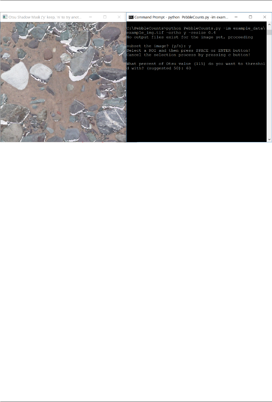
3.
Input a percentage (0-100) of the Otsu shadow threshold value, then press enter. This will open
a pop-up window displaying the image with the Otsu mask in white. On the keyboard press r
to flash the original un-masked image, yto accept the mask and move on, and nto close the
window and enter a new value (Figure 3). This step is skipped if a value for
-otsu_threshold
is provided in the initial command.
Ben Purinton (purinton@uni-potsdam.de) 18
Installing and Running PebbleCounts March 2019
Figure 3: Otsu thresholding of the image with an entered value 0-100. Press rto flash the original
image, yto accept the mask, or nto try a dierent value.
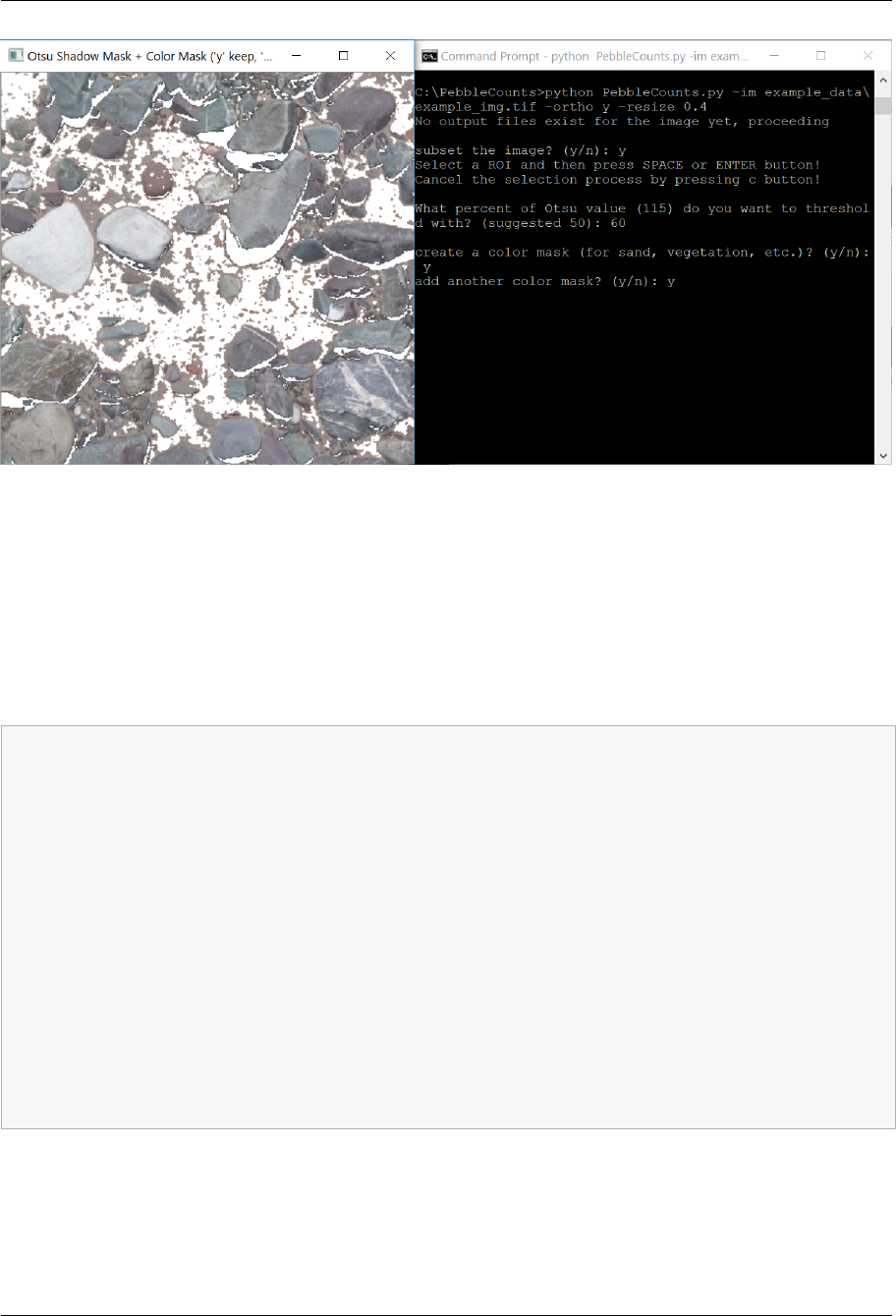
4.
Is there a color you want to mask out in the scene? Maybe the sand is a uniform color distinct
from the pebbles. If so, then in the next step enter
y
, which will bring up another pop-up window.
With the window active, you can press qto close it if you decide not to color mask and rto flash
the original image (Figure 4). Once you click a point in the window with a color you’d like to
mask a second pop-up will open displaying the result of applying a mask to this color. Press yto
accept the mask or nto close it and try another click in the first window (Figure 4). Pressing y
here will return you to the command prompt where you can finish color masking by entering
n
or adding additional color masks by entering
y
. This step is skipped if a path to a binary sand
mask GeoTi for -sand_mask is provided in the initial command.
Ben Purinton (purinton@uni-potsdam.de) 19
Installing and Running PebbleCounts March 2019
Figure 4:
Color masking clicking window. Click on a color you want to mask to open a second window
and check it. Press qto close window or rto flash the original image. Press yto accept or nto try a
dierent click in the previous window.
5.
Aer these couple interactive steps, PebbleCounts will take over the automated windowing,
filtering, edge detection, and k-means segmentation at each window, aer which a new window
with the mask will open (Figure 5). The command prompt should look something like this:
Beginning k-means segmentation
Scale 1of 3
Window 1of 1
Non-local means filtering
Bilateral filtering
Black tophat edge detection
Canny edge detection
Sobel edge detection
Running k-means
Current number of clusters: 2, total inertia: 59896.391
Current number of clusters: 3, total inertia: 48804.694
.
Current number of clusters:X,total inertia:XXXX
Cleaning up k-means mask
Ben Purinton (purinton@uni-potsdam.de) 20
Installing and Running PebbleCounts March 2019
Figure 5: Automated segmentation via edge detection and k-means clustering and pop-up window.
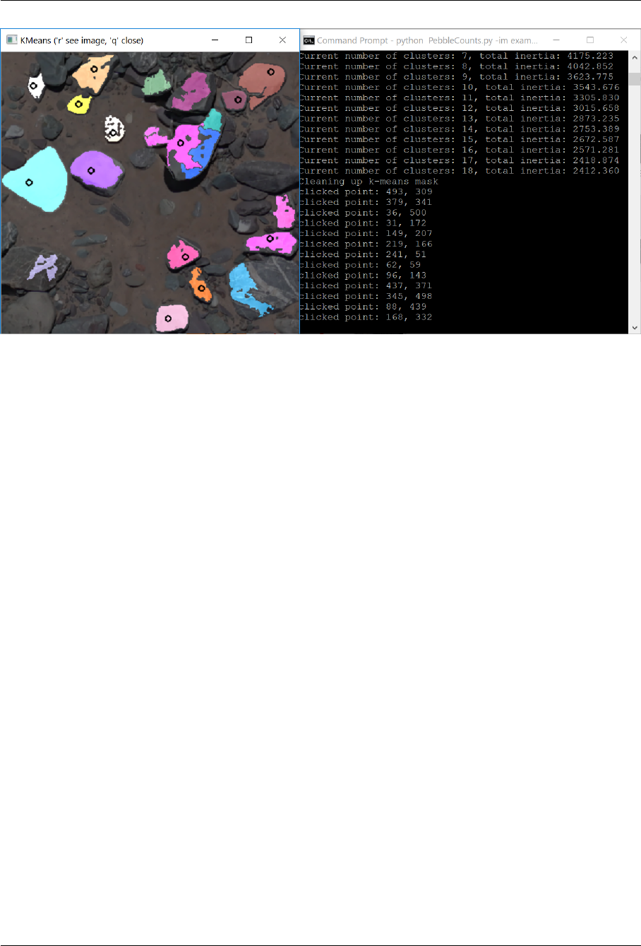
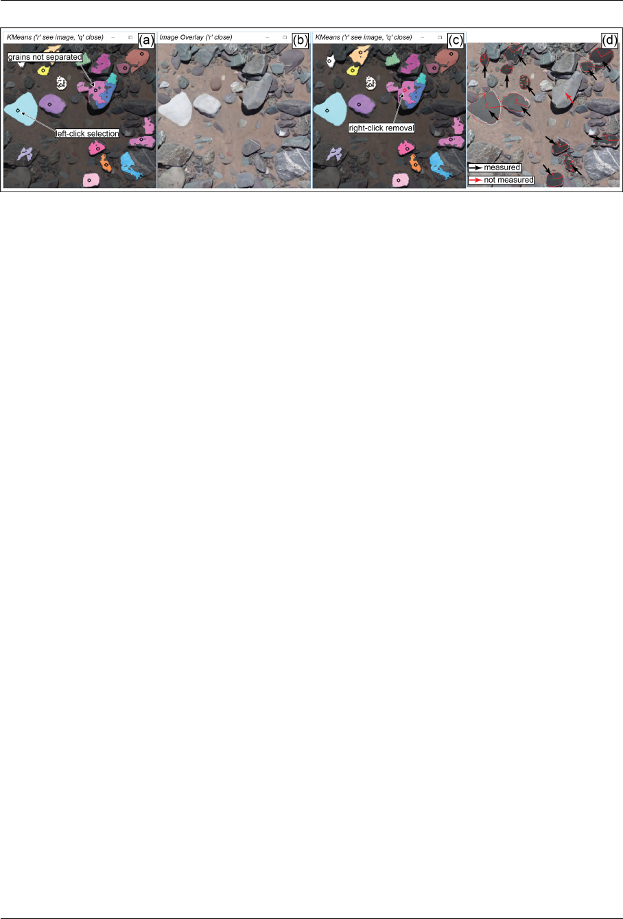
6.
Aer the mask is cleaned a new window will open where you need to click the good looking
grains and ignore the bad ones (Figure 6). Le clicking anywhere on the image will produce a
black circle at that point, meaning that you’ve selected all the pixels in this connected region
as one grain. A right click anywhere on the image will remove the last click and exchange the
black circle for a red one, indicating this area will not be considered (unless of course you add
another le click to the region). Overlay the original image to help decide what is and is not a
well delineated grain by pressing ronce to open the image and ragain to close the image and
return to the mask. Once you are satisfied with your clicks press qto close the window and
automatically move on to the next window and/or scale. The clicked grains will be automatically
measured and added to the final output.
Ben Purinton (purinton@uni-potsdam.de) 21
Installing and Running PebbleCounts March 2019
Figure 6: (a) Interactive k-means mask clicking window. A le click adds a pebble region and black
circle. Pressing qwill close the image and continue segmentation on the next window. (b) Pressing r
opens the original image to check the mask against, ragain to close the original image. (c) Right click
anywhere on the image to remove the last clicked point and replace the black circle with a red one. (d)
Shows the final ellipses fit to each of the clicked regions.
7.
Repeat the clicking on each window that pops up (see the command window for what number
window out of the full number you are on). With a little practice this will go quickly. Aer the
windows are done the results will be saved out and you can repeat from step 1 with another
image.
8.1 An important note on clicking!
As shown in Figure 6, PebbleCounts does not provide a perfect segmentation. Two errors you will
commonly note are:
1.
Under-segmentation of overlapping grains. Avoid clicking these regions or the resulting ellipse
will be fit to many grains.
2.
Over-segmentation of single grains. Here it is up to the user to decide which part of the segmented
grain (if any) to select. If the mask covers the majority of the grain despite some holes or shrinkage,
then it is advisable to select the grain, since the final ellipse will be fit to the full region covered.
Even if the center of a grain is entirely missing from the mask, if the ends of the grain are in the
same mask then the fit ellipse will approximate the grain well.
9 PebbleCountsAuto (AIF) Step-by-Step Example
The processing of PebbleCountsAuto follows the above steps 1-4, with the option to skip the Otsu
and color masking steps using the
-otsu_threshold
and
-sand_mask
command-line variables.
Ben Purinton (purinton@uni-potsdam.de) 22
Installing and Running PebbleCounts March 2019
PebbleCountsAuto is otherwise entirely automated. Thus we only provide a few examples of command-
line entries for using this algorithm:
•Ortho With Default Arguments:
(Be sure to set the
-ortho
flag to
y
and the resolution will be
automatically read by gdal)
python PebbleCountsAuto.py -im example_data\ortho_resolution_1.2mmPerPix.tif -ortho y
•Ortho With Modified Arguments:
(Decrease Sobel and Tophat thresholds to provide more edge
detection and decrease the misfit threshold to reduce potential bad measurements.)
python PebbleCounts.py -im example_data\ortho_resolution_1.2mmPerPix.tif -ortho y \
-tophat_th 0.85 -sobel_th 0.85 -misfit_threshold 20
•Non-ortho Imagery With Default Arguments:
(Be sure to set the
-ortho
flag to
n
and also
provide the
-input_resolution
in mm/pixel, which can be found as in the above section
Calculate Camera Resolution.)
python PebbleCounts.py -im example_data\nonortho_resolution_0.63mmPerPix.tif -ortho n \
-input_resolution 0.63
•Non-ortho Imagery With Modified Arguments:
(Double the default value for
-min_size_threshold
since the resolution is < 0.8 mm/pixel. Also decrease the Sobel and Tophat thresholds to provide
more edge detection given the higher resolution.)
python PebbleCounts.py -im example_data\nonortho_resolution_0.63mmPerPix.tif -ortho n \
-input_resolution 0.63 -min_size_threshold 20 -tophat_th 0.85 -sobel_th 0.85
10 Ouput Files
PebbleCounts(Auto) saves out a few outputs in the same folder that the image resides:
•csv: filename_PebbleCounts(Auto)_CSV.csv
•label image (georeferenced if original is): filename_PebbleCounts(Auto)_LABELS.tif
•figure showing results: filename_PebbleCounts(Auto)_FIGURE.png
And if the input is georeferenced imagery:
•binary GeoTi: filename_PebbleCounts(Auto)_SandMask_TIFF.tif
•
and vector shapefile of the sand mask:
filename_PebbleCounts(Auto)_SandMask_SHP.shp
Ben Purinton (purinton@uni-potsdam.de) 23
Installing and Running PebbleCounts March 2019
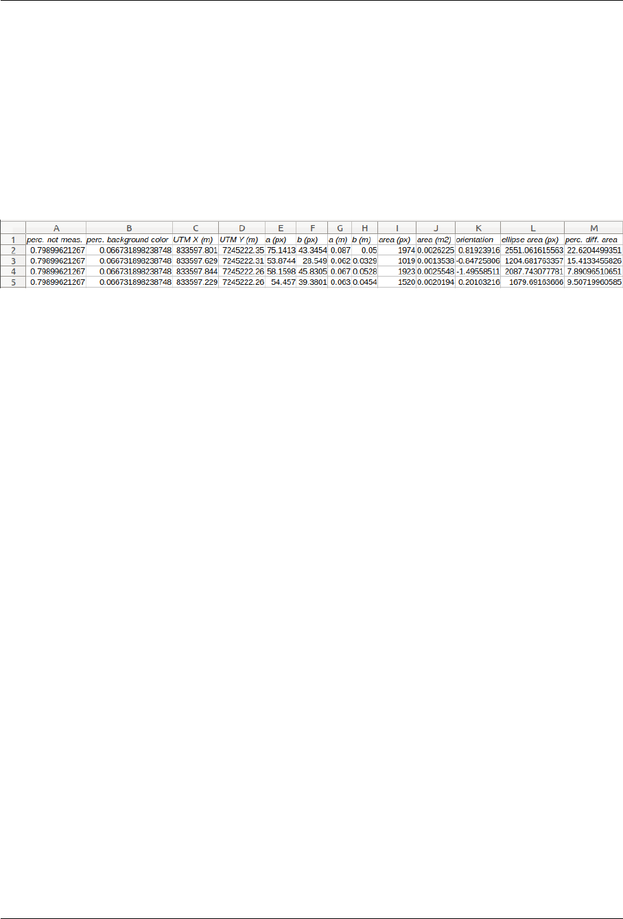
The results .csv has an entry for each grain (Figure 7) showing the fraction of the scene not measured
(combined background shadow and unmeasured grains) the fraction of the scene that was selected
by the color mask as background color (e.g., sand) and each grains’ characteristics including a- and
b-axis of the fit ellipse in pixels and in meters, the area covered by the grain mask in pixels and square
meters, the orientation of the fit ellipse measured from -pi/2 to pi/2 relative to the positive x-axis
(orientation=0) in cartesian coordinates, the area of the ellipse, and the percent misfit between the
ellipse and the grain given by the percentage dierence in area. If the input imagery is georeferenced
the UTM Northing (Y) and Easting (X) coordinates of the pebble’s centroid are be provided.
Figure 7:
Example .csv file output by algorithms for a georeferenced image. The perc. not meas. is the
fractional percentage of the image that was either shadows or not measured and perc. background
color is the fractional percentage of the image that was masked during interactive HSV color selection
(e.g., for sand). Also, perc. di. area is the percentage dierence in area between the ellipse (ellipse
area (px)) and grain (area (px)), or the approximate misfit of the ellipse.
Ben Purinton (purinton@uni-potsdam.de) 24
