Diploma.dvi Ph D Manual
User Manual:
Open the PDF directly: View PDF ![]() .
.
Page Count: 69
University of Ljubljana
Faculty of Electrotechnical Engineering
Vitomir ˇ
Struc
The PhD face recognition toolbox
Toolbox description and user manual
Ljubljana, 2012
Thanks
I would like to thank Alpineon Ltd and the Slovenian Research Agency (ARRS) for
funding the postdoctoral project BAMBI (Biometric face recognition in ambient
intelligence environments, Z2-4214), which made the PhD face recognition toolbox
possible.
Foreword
The PhD (Pretty helpful Development functions for) face recognition toolbox is
a collection of Matlab functions and scripts intended to help researchers working
in the field of face recognition. The toolbox was produced as a byproduct of my
research work and is freely available for download.
The PhD face recognition toolbox includes implementations of some of the
most popular face recognition techniques, such as Principal Component Anal-
ysis (PCA), Linear Discriminant Analysis (LDA), Kernel Principal Component
Analysis (KPCA), Kernel Fisher Analysis (KFA). It features functions for Ga-
bor filter construction, Gabor filtering, and all other tools necessary for building
Gabor-based face recognition techniques.
In addition to the listed techniques there are also a number of evaluation tools
available in the toolbox, which make it easy to construct performance curves and
performance metrics for the face recognition you are currently assessing. These
tools allow you to compute ROC (Receiver Operating Characteristics) curves,
EPC (Expected performance curves) curves, and CMC (cumulative match score
curves) curves.
Most importantly (especially for beginners in this field), the toolbox also con-
tains several demo scripts that demonstrate how to build and evaluate a complete
face recognition system. The demo scripts show how to align the face images,
how to extract features from the aligned, cropped and normalized images, how
to classify these features and finally how to evaluate the performance of the
complete system and present the results in the form of performance curves and
corresponding performance metrics.
This document describes the basics of the toolbox, from installation to usage.
It contains some simple examples of the usage of each function and the corre-
sponding results. However, for more information on the theoretical background
of the functions, the reader is referred to papers from the literature, which is vast.
Hence, it shouldn’t be to difficult to find the information you are looking for.
As a final word, I would like to say that I have written this document really
fast and have not had the time to proof read it. So please excuse any typos or
awkward formulations you may find.

Contents
1. Installing the toolbox 2
1.1 Installation using the supplied script . . . . . . . . . . . . . . . . 2
1.2 Manual installation . . . . . . . . . . . . . . . . . . . . . . . . . . 3
1.3 Validating the installation . . . . . . . . . . . . . . . . . . . . . . 3
2. Acknowledging the Toolbox 6
3. Toolbox description 7
3.1 The utils folder ............................ 8
3.1.1 The compute kernel matrix PhD function . . . . . . . . . 8
3.1.2 The construct Gabor filters PhD function . . . . . . . . 9
3.1.3 The register face based on eyes function . . . . . . . . 10
3.1.4 The resize pc comps PhD function . . . . . . . . . . . . . 12
3.2 The plots folder............................ 13
3.2.1 The plot CMC PhD function ................. 13
3.2.2 The plot EPC PhD function ................. 14
3.2.3 The plot ROC PhD function ................. 15
3.3 The eval folder ............................ 17
3.3.1 The produce EPC PhD function ............... 17
3.3.2 The produce CMC PhD function ............... 18
3.3.3 The produce ROC PhD function ............... 19
3.3.4 The evaluate results PhD function . . . . . . . . . . . . 20
3.4 The features folder .......................... 26
3.4.1 The filter image with Gabor bank PhD function . . . . . 27
3.4.2 The produce phase congruency PhD function . . . . . . . 28
iv
Contents v
3.4.3 The perform lda PhD function ............... 30
3.4.4 The perform pca PhD function ............... 31
3.4.5 The linear subspace projection PhD function . . . . . . 32
3.4.6 The perform kpca PhD function............... 33
3.4.7 The perform kfa PhD function ............... 33
3.4.8 The nonlinear subspace projection PhD function . . . . 34
3.5 The classification folder ....................... 35
3.5.1 The return distance PhD function . . . . . . . . . . . . . 36
3.5.2 The nn classification PhD function . . . . . . . . . . . 36
3.6 The demos folder ........................... 38
3.6.1 Running the demo scripts (important!!) . . . . . . . . . . . 40
3.6.2 The face registration demo script . . . . . . . . . . . . 41
3.6.3 The construct Gabors and display bank demo script . . 41
3.6.4 The Gabor filter face image demo script . . . . . . . . . 41
3.6.5 The phase cogruency from image demo script . . . . . . . 42
3.6.6 The perform XXX demo scripts................ 44
3.6.7 The XXX face recognition and evaluation demo scripts 45
3.6.8 The gabor XXX face recognition and evaluation demo
scripts ............................. 47
3.6.9 The phase congruency XXX face recognition... scripts . 49
3.6.10 The preprocessINFace gabor KFA face recognition...
script.............................. 52
3.7 The bibs folder ............................ 55
4. Using the Help 56
4.1 Toolbox and folder help . . . . . . . . . . . . . . . . . . . . . . . 56
4.2 Functionhelp ............................. 56
5. The PhD toolbox homepage 58
6. Change Log 60
7. Conclusion 61

Contents 1
References 63

1. Installing the toolbox
The PhD toolbox comes compressed in a ZIP archive or TAR ball. Before you
can use it you first have to uncompress the archive into a folder of your choice.
Once you have done that a new folder named PhD tool should appear and in this
folder seven additional directories should be present, namely, utils,plots,features,
eval,demos,classification and bibs. In most of these folders you should find a
Contents.m file with a list and short descriptions of Matlab functions that should
be featured in each of the seven folders.
1.1 Installation using the supplied script
When you are ready to install the toolbox, run Matlab and change your current
working directory to the directory PhD tools, or in case you have renamed the
directory, to the directory containing the files of the toolbox. Here, you just type
into Matlabs command prompt:
install PhD
The command will trigger the execution of the the corresponding install
script, which basically just adds all directories of the toolbox to Matlabs search
path. The installation script was tested with Matlab version 7.11.0.584 (R2010b)
on a 64-bit Windows 7 installation.
Note that the install script was not tested on Linux machines. Nevertheless,
I see no reason why the toolbox should not work on Linux as well. The only
difficulty could be the installation of the toolbox due to potential difficulties with
the path definitions. In case the install script fails (this applies for Linux and
Windows users alike), you can perform the necessary steps manually as described
in the next section.
2

1.2 Manual installation 3
1.2 Manual installation
The installation of the toolbox using the provided script can sometimes fail. If
the script fails due to path related issues, try adding the path to the toolbox
folder and corresponding subfolders manually. In Matlabs main command
window choose:
File →Set Path →Add with Subfolders.
When a new dialogue window appears navigate to the directory contain-
ing the toolbox, select it and click OK. Choose Save in the Set Path window and
then click Close. This procedure adds the necessary paths to Matlabs search
path. If you have followed all of the above steps, you should have successfully
installed the toolbox and are ready to use it.
If you are attempting to add the toolbox folders and subfolders to Matlabs
search path manually, make sure that you have administrator (or root) privileges,
since these are commonly required for changing the pathdef.m file, where Matlabs
search paths are stored.
1.3 Validating the installation
The PhD toolbox features a script, which aims at validating the installation
process of the toolbox. This may come in handy if you encountered errors or
warnings during the automatic installation process or attempted to install the
toolbox manually. The script should be run from the base directory of the toolbox
to avoid possible name clashes.
To execute the validation script type the following command into Matlabs
command window:
check PhD install
The script will test all (or most) techniques contained in the toolbox. This
procedure may take quite some time depending on the speed and processing
power of your machine, so please be patient. Several warnings may be printed
to the command window during the validation process. This is simply a conse-
quence of dummy data that is being used for the validation. The warnings do
not indicate any errors in the installation process and can be ignored. If the in-
stallation completed successfully, you should see a report similar to the one below:

4Installing the toolbox
|===========================================================|
VALIDATION REPORT:
Function ‘‘register face based on eyes’’ is working properly.
Function ‘‘construct Gabor filters PhD’’ is working properly.
Function ‘‘compute kernel matrix PhD’’ is working properly.
Function ‘‘resize pc comps PhD’’ is working properly.
Function ‘‘plot ROC PhD’’ is working properly.
Function ‘‘plot EPC PhD’’ is working properly.
Function ‘‘plot CMC PhD’’ is working properly.
Function ‘‘filter image with Gabor bank PhD’’ is working properly.
Function ‘‘linear subspace projection PhD’’ is working properly.
Function ‘‘nonlinear subspace projection PhD’’ is working properly.
Function ‘‘produce phase congruency PhD’’ is working properly.
Function ‘‘perform pca PhD’’ is working properly.
Function ‘‘perform lda PhD’’ is working properly.
Function ‘‘perform kpca PhD’’ is working properly.
Function ‘‘perform kfa PhD’’ is working properly.
Function ‘‘produce ROC PhD’’ is working properly.
Function ‘‘produce EPC PhD’’ is working properly.
Function ‘‘produce CMC PhD’’ is working properly.
Function ‘‘evaluate results PhD’’ is working properly.
Function ‘‘return distance PhD’’ is working properly.
Function ‘‘nn classification PhD’ is working properly.
|===========================================================|
SUMMARY:
All functions from the toolbox are working ok.
|===========================================================|
In case the installation has (partially) failed, the report will explicitly show,
which functions are not working properly. In most cases the toolbox should work
just fine.

1.3 Validating the installation 5
Note that the check PhD install script was not initially meant to be an
install validation script. The script was written to test whether all functions from
the toolbox work correctly (i.e., with different combinations of input arguments).
Basically, it was used for debugging the toolbox. However, due to the fact that
the script tests all (or most) functions from the toolbox, it can equally well serve
as an installation validation script.
2. Acknowledging the Toolbox
Any paper or work published as a result of research conducted by using the code
in the toolbox or any part of it must include the following two publications in
the reference section:
V. ˇ
Struc and N Paveˇsi´c, ”The Complete Gabor-Fisher Classifier for Robust Face Recognition”,
EURASIP Advances in Signal Processing, pp. 26, 2010, doi=10.1155/2010/847680.
and
V. ˇ
Struc and N. Paveˇsi´c, ”Gabor-Based Kernel Partial-Least-Squares Discrimination
Features for Face Recognition”, Informatica (Vilnius), vol. 20, no. 1, pp. 115–138, 2009.
BibTex files for the above publications are contained in the bibs folder
and are stored as ’ACKNOWL1.bib’ and ’ACKNOWL2.bib’, respectively.
6
3. Toolbox description
The functions and scripts contained in the toolbox were produced as a byproduct
of my research work. I have added a header to each of the files containing some
examples of the usage of the functions and a basic description of the functions
functionality. However, I made no effort in optimizing the code in terms of speed
and efficiency. I am aware that some of the implementations could be significantly
speeded up, but unfortunately I have not yet found the time to do so. I am sharing
the code contained in the toolbox to make life easier for researcher working in the
field of face recognition and students starting to get familiar with face recognition
and its challenges.
The PhD (Pretty helpful Development functions for) face recognition toolbox
in its current form is a collection of useful functions that implement:
•four subspace projection techniques:
–principal component analysis (PCA) - linear technique,
–linear discriminant analysis (LDA) - linear technique,
–kernel principal component analysis (KPCA) - non-linear technique,
–kernel Fisher analysis (KFA) - non-linear technique,
•Gabor filter construction and Gabor filtering techniques,
•phase congruency based feature extraction techniques,
•techniques for constructing three types of performance graphs:
–Expected performance curves (EPC),
–Receiver Operating Characteristics (ROC) curves,
–Cumulative Match Score curves (CMC),
•face registration techniques (based on eye coordinates),
•nearest neighbor based classification techniques, and
•several demo scripts.
7

8Toolbox description
The toolbox contains seven folders, named, utils,plots,features,eval,classi-
fication,demos and bibs. In the remainder of this chapter we will focus on the
description of the contents of each of these folders.
3.1 The utils folder
The folder named utils contains utility (auxilary) functions that in most cases
are intended to be used on their own. Instead they provide some functionality to
higher level functions of the toolbox. The following functions are featured in the
utils folder:
•compute kernel matrix PhD,
•construct Gabor filters PhD,
•register face based on eyes, and
•resize pc comps PhD.
A basic description of the functionality of the above listed functions is given
in the remainder of this document.
3.1.1 The compute kernel matrix PhD function
The compute kernel matrix PhD function is an utility function used by the
non-linear subspace projection techniques KPCA and KFA. It constructs kernel
matrices from the input data using the specified kernel function. The function
has the following prototype:
kermat = compute kernel matrix PhD(X,Y,kernel type,kernel args).
Here, Xand Ydenote the input data based on which the kernel matrix
kermat is computed. kernel type denotes the type of the kernel function
to use when computing the kernel matrix1, and kernel args stands for the
corresponding arguments of the selected kernel function. If you type
help compute kernel matrix PhD
1Currently only polynomial, fractional power polynomial, and sigmoidal kernel functions are
supported.

3.1 The utils folder 9
you will get additional information on the function together with several
examples of usage.
An example of the use of the function is shown below:
kermat = compute kernel matrix PhD(X,Y,’poly’,[1 2]);;
The example code computes a kernel matrix based on the input data ma-
trices Xand Yusing a polynomial function of the following form:
kermat = (XTY+ 1)2,(3.1)
where 1 and 2 were provided as input arguments. As a result the code returns
the computed kernel matrix kermat.
3.1.2 The construct Gabor filters PhD function
The construct Gabor filters PhD function is an auxilary function that can
be used to construct a filter bank of complex Gabor filters. The function
can be called with only a small number of input arguments, in which case
the default values for the filter bank parameters are used for the construc-
tion. These default parameters correspond to the most common parameters
used in conjunction with face images of size 128 ×128 pixels. Optionally, you
can provide your own filter bank parameters. The complete function prototype is:
fbank = construct Gabor filters PhD(norie, nscale, size, fmax, ni,
gamma, separation);.
The function returns a structure fbank, which contains the spatial and
frequency representations of the constructed Gabor filter bank as well as
some meta-data. The input arguments of the function represent filter bank
parameters, which are in detail described in the help section of the function.
More information on the parameters can also be found in the literature, e.g.,
[11].
If you type
help construct Gabor filters PhD
you will get additional information on the function together with several
examples of usage.
10 Toolbox description
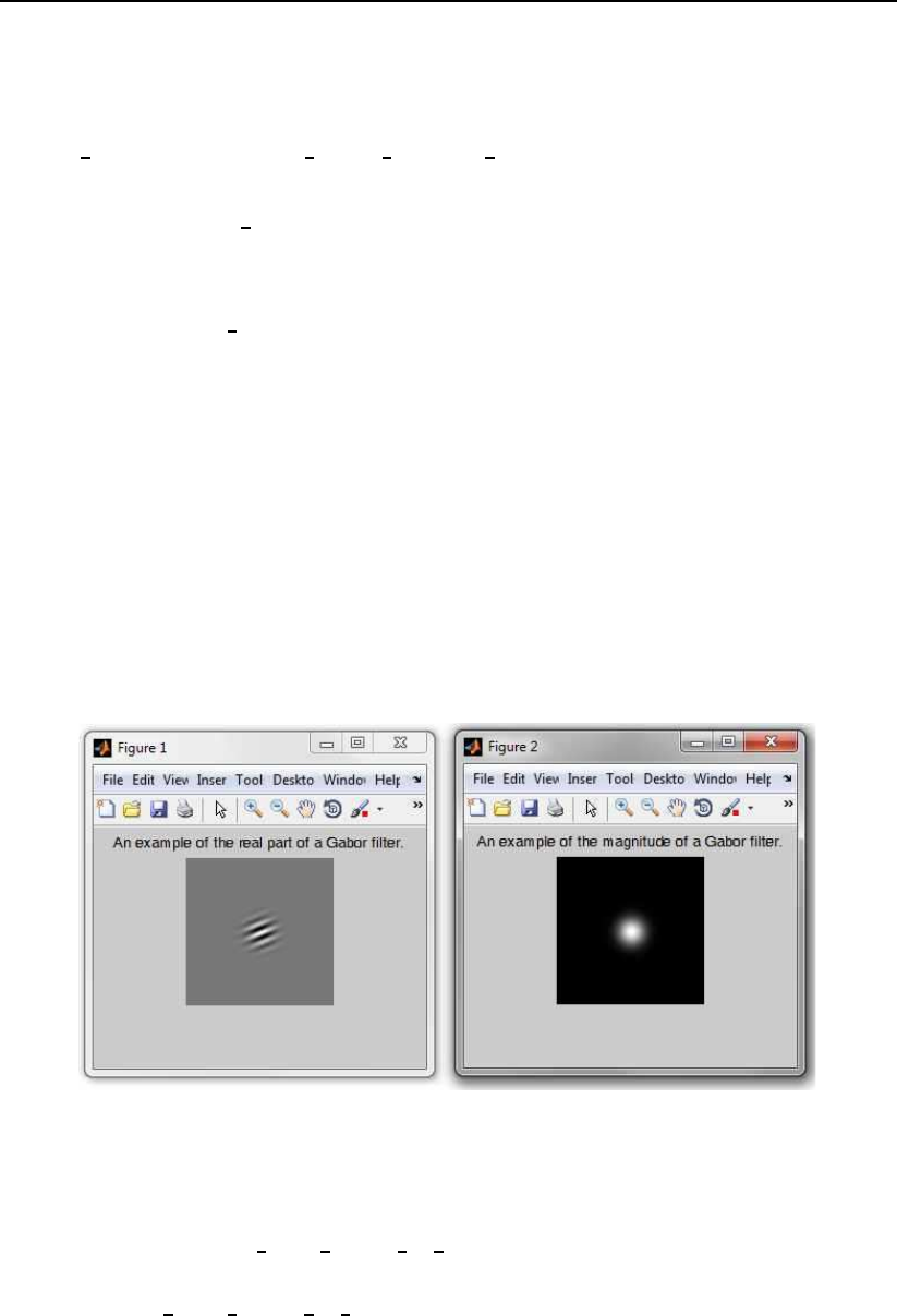
An example of the use of the function is shown below:
filter bank = construct Gabor filters PhD(8, 5, [128 128]);
figure
imshow(real(filter bank.spatial3,4(64:64+128,64:64+128)),[])
title(’An example of the real part of a Gabor filter.’)
figure
imshow(abs(filter bank.spatial3,4(64:64+128,64:64+128)),[])
title(’An example of the magnitude of a Gabor filter.’)
The code constructs a Gabor filter bank comprising filters of 8 orienta-
tions and 5 scales, which is intended to be used with facial images of size
128 ×128 pixels. It then presents an example of the real part and an example of
the magnitude of one of the filters from the bank.
When running the above sample code you should get an result that looks like
this:
Figure 3.1: The result of the above code
3.1.3 The register face based on eyes function
The register face based on eyes function is one of the few functions from
the utils that is actually meant to be used on its own. The function extracts the
facial region from an image given the eye center coordinates and normalizes the
image in terms of geometry and size. Thus, it rotates the image in such a way,
that the face is upright, then crops the facial region and finally rescales it to a

3.1 The utils folder 11
standard size. If the input image is a color image, the extracted region is also
an color image (the same applies to grey-scale images). The function has the
following prototype:
Y= register face based on eyes(X,eyes,size1).
Here, Xdenotes the input image, from which to extract the face, eyes de-
notes a structure with eye coordinates, and size1 denotes a parameter that
controls to which size the images is rescaled in the final stage of the extraction
procedure. The function returns the cropped and geometrically normalized face
area Y.
If you type
help register face based on eyes
you will get additional information on the function together with several
examples of usage.
An example of usage of the function is shown below. Here, the function
was applied to an sample image that is distributed togethre with the PhD toolbox:
eyes.x(1)=160;
eyes.y(1)=184;
eyes.x(2)=193;
eyes.y(2)=177;
X=imread(’sample image.bmp’);
Y = register face based on eyes(X,eyes,[128 100]);
figure,imshow(X,[]);
figure,imshow(uint8(Y),[]);
The code sets the coordinates structure eyes, reads in the image Xand
based on this input data extracts the face region Yfrom the input image, which
it then rescales to a size of 128 ×100. The result of the presented code is shown
in Fig.3.2
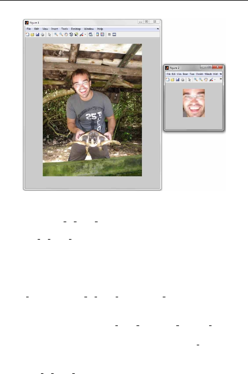
12 Toolbox description
Figure 3.2: Results of the sample code
3.1.4 The resize pc comps PhD function
The resize pc comps PhD function is not intended to be used on its own. It
resizes the phase congruency components and concatenates them into a high
dimensional feature vector. The description of the function in this document is
only present to provide some hints on its functionality. The function has the
following prototype:
feature vector = resize pc comps PhD(pc, down fak);.
Here, pc denotes the computed phase congruency components that were
computed using the function produce phase congruency PhD.down fak denotes
the down-sampling factor by which to down-sample the phase congruency
components before concatenating them into the final feature vector. If you
type
help resize pc comps PhD
you will get additional information on the function together with several
examples of usage.

3.2 The plots folder 13
An example of the use of the function is shown below:
X=double(imread(’sample face.bmp’));
filter bank = construct Gabor filters PhD(8,5, [128 128]);
[pc,EO] = produce phase congruency PhD(X,filter bank);
feature vector extracted from X = resize pc comps PhD(pc, 32);
The code reads the image named sample image.bmp into the variable X, com-
putes phase congruency features from it and employs the resize pc comps PhD
to construct an feature vector from the computed phase congruency components.
3.2 The plots folder
The folder named plots contains functions for plotting different performance
curves. In the current version of the toolbox three performance curves are sup-
ported, namely, ROC, EPC, and CMC curves.The folder contains the following
functions:
•plot CMC PhD,
•plot EPC PhD, and
•plot ROC PhD.
A basic description of the functionality of the above listed functions is given
in the remainder of this section.
3.2.1 The plot CMC PhD function
The plot CMC PhD function plots the so-called CMC (Cumulative Match Score
Curve) curve based on the data computed with the produce CMC PhD function
from the PhD face recognition toolbox. The function is very similar to Matlabs’
native plot function, except for the fact that it automatically assigns labels to
the graphs axis and presents the x-axis in a log (base-10) scale. The function
has the following prototype:
h=plot CMC PhD(rec rates, ranks, color, thickness).
If you type
14 Toolbox description
help plot CMC PhD
you will get additional information on the function together with several
examples of usage.
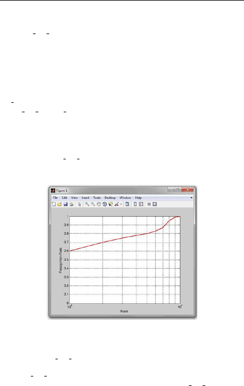
An example of the use of the function is shown below:
ranks = 1:10;
rec rates = [0.6 0.7 0.75 0.78 0.8 0.83 0.87 0.95 0.99 1];
h=plot CMC PhD(rec rates, ranks);
axis([1 10 0 1])
The code first creates some dummy data for plotting and then plots this
data using the plot CMC PhD function. The results of this sample code is an
CMC curve as shown in Fig. 3.3.
Figure 3.3: An example of a CMC curve created with the sample code.
3.2.2 The plot EPC PhD function
The plot EPC PhD function plots the so-called EPC (Expected Performance
Curve) curve based on the data computed with the produce EPC PhD function
from the PhD face recognition toolbox. The function is very similar to Matlabs’

3.2 The plots folder 15
native plot function, except for the fact that it automatically assigns labels to
the graphs axis. The function has the following prototype:
h=plot EPC PhD(alpha,errors, color, thickness).
If you type
help plot EPC PhD
you will get additional information on the function together with several
examples of usage.
An example of the use of the function is shown below:
% we generate the scores through a random generator
true scores = 0.5 + 0.9*randn(1000,1);
false scores = 3.5 + 0.9*randn(1000,1);
[ver rate, miss rate, rates] = produce ROC PhD(true scores,
false scores);
true scores1 = 0.6 + 0.8*randn(1000,1);
false scores1 = 3.3 + 0.8*randn(1000,1);
[alpha,errors,rates and threshs] = produce EPC PhD(true scores,
false scores,true scores1,false scores1,rates,20);
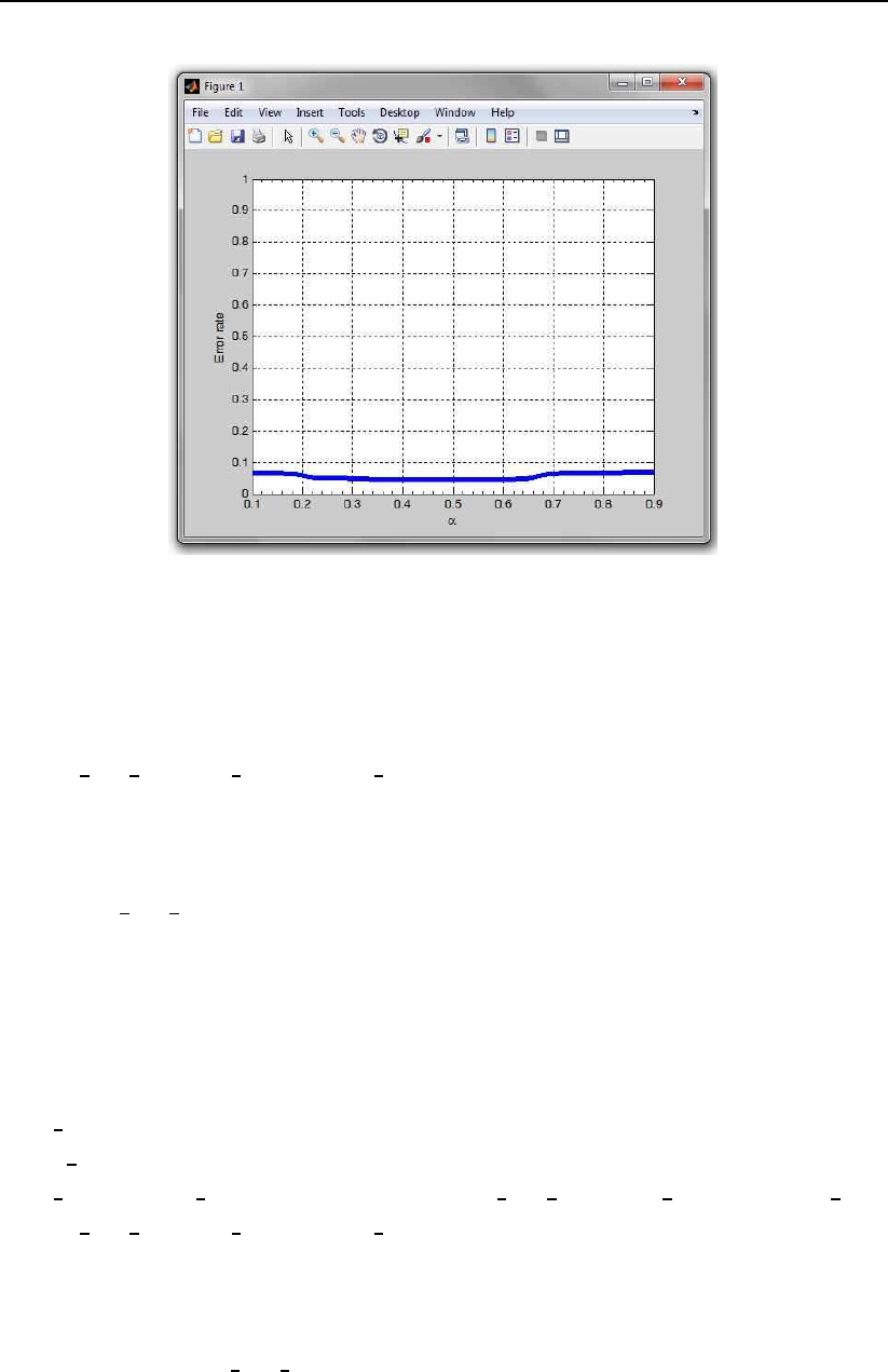
h=plot EPC PhD(alpha, errors,’b’,4);
The code first creates some dummy data for plotting and then plots this
data using the plot EPC PhD function. The results of this sample code is an
EPC curve as shown in Fig. 3.4.
3.2.3 The plot ROC PhD function
The plot ROC PhD function plots the so-called ROC (Receiver Operating
Characteristics) curve based on the data computed with the produce ROC PhD
function from the PhD face recognition toolbox. The function is very similar to
Matlabs’ native plot function, except for the fact that it automatically assigns
labels to the graphs axis and presents the x-axis in a log (base-10) scale. The
function has the following prototype:
16 Toolbox description
Figure 3.4: An example of an EPC curve created with the sample code.
h=plot ROC PhD(ver rate, miss rate, color, thickness).
If you type
help plot ROC PhD
you will get additional information on the function together with several
examples of usage.
An example of the use of the function is shown below:
true scores = 0.5 + 0.9*randn(1000,1);
false scores = 3.5 + 0.9*randn(1000,1);
[ver rate, miss rate, rates] = produce ROC PhD(true scores,false scores);
h=plot ROC PhD(ver rate, miss rate);
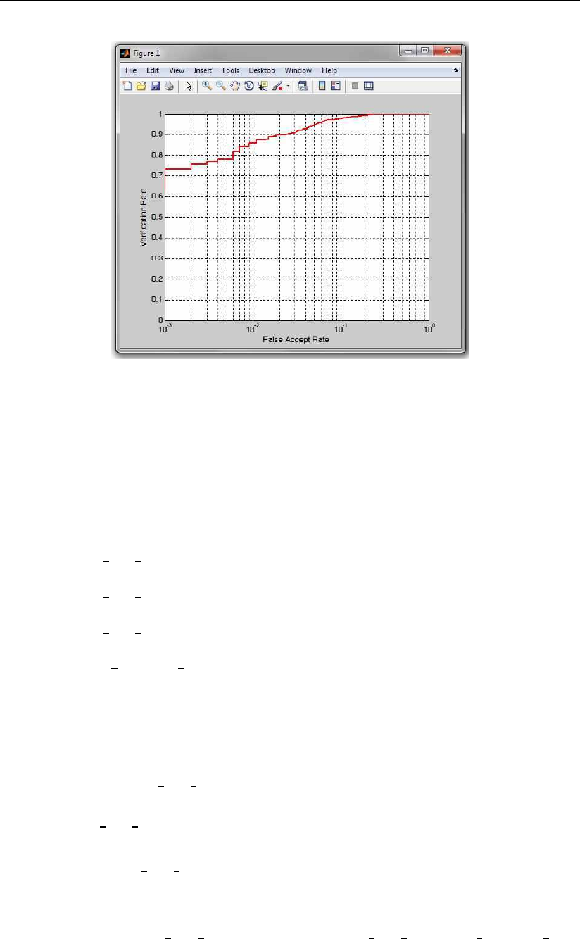
The code first creates some dummy data for plotting and then plots this
data using the plot ROC PhD function. The results of this sample code is an
ROC curve as shown in Fig. 3.5.
3.3 The eval folder 17
Figure 3.5: An example of a ROC curve created with the sample code.
3.3 The eval folder
The folder named eval contains functions for constructing different performance
curves and evaluating the classification results (creating performance metrics).
The folder contains the following functions:
•produce EPC PhD,
•produce CMC PhD,
•produce ROC PhD, and
•evaluate results PhD.
A basic description of the functionality of the above listed functions is given
in the remainder of this section.
3.3.1 The produce EPC PhD function
The produce EPC PhD function generates the so-called EPC (Expected Per-
formance Curve) curve from the input data. The generated data can then be
used with the plot EPC PhD function to produce a plot of the EPC curve. The
function has the following prototype:
[alpha,errors,rates and threshs1] = produce EPC PhD(true d,false d,

18 Toolbox description
true e,false e,rates and threshs,points).
If you type
help produce EPC PhD
you will get additional information on the function together with several
examples of usage.
Note that it not the goal of this document to describe the idea of EPC curves.
For that, the interested reader is referred to [2].
An example of the use of the function is shown below:
true scores = 0.5 + 0.9*randn(1000,1);
false scores = 3.5 + 0.9*randn(1000,1);
[ver rate, miss rate, rates] = produce ROC PhD(true scores,false scores);
true scores1 = 0.6 + 0.8*randn(1000,1);
false scores1 = 3.3 + 0.8*randn(1000,1);
[alpha,errors,rates and threshs] =
produce EPC PhD(true scores,false scores,true scores1,false scores1,rates,20);
The code first creates some dummy data and based on it computes ROC
curve parameters. This step can be omitted, but is used to compute the rates
structure, which is an optional input argument to the produce EPC PhD and is
needed, when some performance metrics (stored in rates and threshs) should
be computed together with the EPC data. In the final stage, the code computes
the EPC curve data alpha and errors as well as some performance metrics
(rates and threshs).
3.3.2 The produce CMC PhD function
The produce CMC PhD function generates the so-called CMC (Cumulative Match
score Curve) curve from the input data. The generated data can then be used
with the plot CMC PhD function to produce a plot of the CMC curve. The
function has the following prototype:
[rec rates, ranks] = produce CMC PhD(results).
Note here that the output rec rates contains the recognition rates for

3.3 The eval folder 19
different ranks. If you are interested in the rank one recognition rate, you can
retrieve it by typing:
rec rates(1).
If you type
help produce CMC PhD
you will get additional information on the function together with several
examples of usage.
An example of the use of the function is shown below:
training data = randn(100,30);
training ids(1:15) = 1:15;
training ids(16:30) = 1:15;
test data = randn(100,15);
test ids = 1:15;
results = nn classification PhD(training data, training ids,
test data, test ids, size(test data,1)-1, ’euc’);
[rec rates, ranks] = produce CMC PhD(results);
h=plot CMC PhD(rec rates, ranks);
The code first creates some dummy feature vectors with corresponding la-
bels, classifies them using the nn classification PhD function from the PhD
toolbox, then produces the CMC curve and finally plots the results.
3.3.3 The produce ROC PhD function
The produce ROC PhD function generates the so-called ROC (Receiver Operating
Characteristics) curve from the input data. The generated data can then be
used with the plot ROC PhD function to produce a plot of the ROC curve. The
function has the following prototype:
[ver rate, miss rate, rates and threshs] = produce ROC PhD(true scores,
false scores, resolution).
Note here that the produce ROC PhD function in addition to the

20 Toolbox description
rates and threshs, which contains several performance metrics, produces
two a vector of verification rates ver rate and a vector of miss rates miss rate,
which are used by the plot ROC PhD to generate a graphical representation of
the ROC curve. The plotting function produces a ROC curve that plots the
verification rate against the miss rate, with the latter being represented on log
(base-10) scale. However, several researcher prefer to plot false acceptance rate
(FAR) against the false rejection rate (FRR) using linear scales on both axes.
You can do that, by typing:
plot(1-ver rate, miss rate)
grid on
xlabel(’False rejection rate (FRR)’)
ylabel(’False acceptance rate (FAR)’)
If you type
help produce ROC PhD
you will get additional information on the function together with several
examples of usage.
An example of the use of the function is shown below:
true scores = 0.5 + 0.9*randn(1000,1);
false scores = 3.5 + 0.9*randn(1000,1);
[ver rate, miss rate, rates] = produce ROC PhD(true scores,false scores,5000);
The code first creates some dummy data and then uses the produce ROC PhD
function to compute the ROC curve data.
3.3.4 The evaluate results PhD function
The evaluate results PhD functions is one of the more complex functions in
the PhD face recognition toolbox. The function provides a way of automatically
evaluate the recognition results of your experiments that were produced using the
nn classification PhD function from the toolbox and are stored in an appro-
priate format. The function itself contains an extensive help section and several
examples of usage. Its use is also demonstrated in several demo scripts contained

3.3 The eval folder 21
in the demos folder of the PhD toolbox.
The function automatically generates all performance curves currently sup-
ported in the toolbox and produces several performance metrics for identification
as well as verification experiments. All the function does is extracting data from
the similarity matrix and meta-data produced by the nn classification PhD
function and calling other evaluation functions from the toolbox. Note that it
also produces DET curves if you have installed NISTs DETware before calling
the function.
The function has the following prototype:
output = evaluate results PhD(results,decision mode,results1).
The function produces an output structure output that contains the fol-
lowing fields:
output.ROC ver rate ... a vector of verification rates
that represents y-axis data of the
computed ROC curve
output.ROC miss rate ... a vector of miss rates (false
acceptance rates) that represents
x-axis data of the computed ROC
curve
output.ROC char errors ... a structure of characteristic error
rates computed from the similarity
matrix; it contains the following
fields:

22 Toolbox description
.minHTER er ... the minimal achievable half total
error rate
.minHTER tr ... the decision threshold that ensures
the above minimal half total error
rate
.minHTER frr ... the false rejection error rate at
the minimal Half total error rate
.minHTER ver ... the verification rate at the minimal
half total error rate
.minHTER far ... the false acceptance error rate at
the minimal half total error rate
.EER er ... the equal error rate
.EER tr ... the decision threshold that ensures
the above equal error rate
.EER frr ... the false rejection error rate at
the equal error rate
.EER ver ... the verification rate at the equal
error rate
.FRR 01FAR er ... the half total error rate at the
operating point where FRR = 0.1*FAR
.FRR 01FAR tr ... the decision threshold that ensures
the above half total error rate of
FRR = 0.1*FAR
.FRR 01FAR frr ... the false rejection error rate at
the half total error rate of FRR =
0.1*FAR
.FRR 01FAR ver ... the verification rate at the half
total error rate of FRR = 0.1*FAR
.FRR 01FAR far ... the false acceptance error rate at
the half total error rate of FRR =
0.1*FAR
.FRR 10FAR er ... the half total error rate at the
operating point where FRR = 10*FAR

3.3 The eval folder 23
.FRR 10FAR tr ... the decision threshold that ensures
the above half total error rate of
FRR = 10*FAR
.FRR 10FAR frr ... the false rejection error rate at
the half total error rate of FRR =
10*FAR
.FRR 10FAR ver ... the verification rate at the half
total error rate of FRR = 10*FAR
.FRR 10FAR far ... the false acceptance error rate at
the half total error rate of FRR =
10*FAR
...
more ...
For more information on this
structure have a look at the
"rates and threshs" structure of
the "produce ROC PhD" function. The
two structures are identical.

24 Toolbox description
output.DET frr rate ... a vector of false rejection rates
that represent y-axis data of the
computed DET curve (this field is
only available if NISTs DETware is
installed)
output.DET far rate ... a vector of false acceptance rates
that represent x-axis data of the
computed DET curve (this field is
only available if NISTs DETware is
installed)
output.CMC rec rates ... a vector of recognition rates
that represent y-axis data of
the computed CMC curve; NOTE!!:
output.CMC rec rates(1) represents
the rank one recognition rate
output.CMC ranks ... a vector of ranks that corresponds
to the recognition rates in
"output.CMC rec rates"; the data
represents x-axis data of the
computed CMC curve
output.EPC charq errors ... a structure of characteristic
error rates on the EPC curve;
for a more detailed description
of this structure look at the
"rates and threshs1" output structure
of the "produce EPC PhD" function;
the two structures are identical
output.EPC alpha ... a vector of alpha values that
represents x-axis data of the
computed EPC curve; (this field
is only available if two results
structures obtained on test as well
as evaluation data are provided as
input to the function)

3.3 The eval folder 25
output.EPC errors ... a vector of error rates that
represents y-axis data of the
computed EPC curve; (this field
is only available if two results
structures obtained on test as well
as evaluation data are provided as
input to the function)
The most important input argument of the function is the results structure
obtained on some evaluation data using the nn classification PhD function.
The structure contains the some meta-data and more importantly a similar-
ity matrix created during the recognition experiments on the evaluation data.
Optionally, the function takes a second results1 structure obtained on some
test data that does not overlap with the evaluation data. This structure is
needed when creating EPC curves, but is not compulsory. The last argument
of the function is a string called decision mode and takes either the value of
decision mode=’images’ or decision mode=’ID’.
In the first case, i.e., decision mode=’images’, the performance graphs are cre-
1.02 0.97
0.41
1.34
0.78 0.98
0.98
1.45
0.44 0.44
0.57 0.57
1.87
0.12
.
.
.
.
.
.
.
.
.
.
.
.
.
.
.
.
.
.
.
.
.
.
.
.
.
.
.
.
.
.
.
.
.
Similarity matrix
(size: x )n m
image 1 (subject 1)
image 1 (subject 1)
image 2 (subject 2)
image 3 (subject 3)
image (subject )n H
image 2 (subject 1)
image 3 (subject 1)
image (subject )m M
Adds to result
(is considered in statistics)
Gallery images (database)
Probe images (test data)
Number of recognition
decisions: xn m
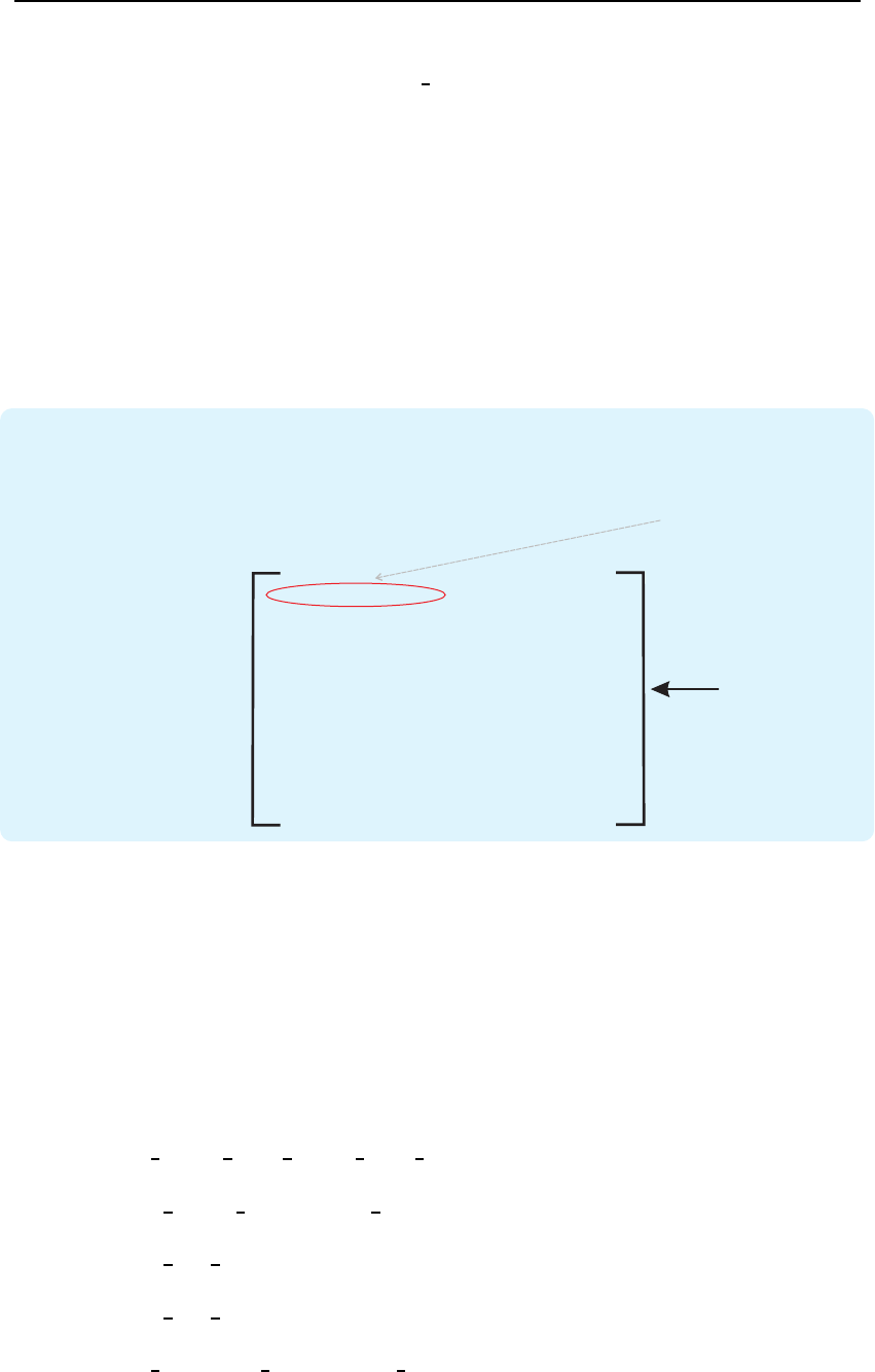
Figure 3.6: Visualization of the effect of the ”images“ decision mode.
ated as if each image in the database (gallery) is its own template. If we assume
that we have ntest images (probes) and mgallery images (belonging to Msub-
jects, where m > M), then the total number of experiments/recognition attempts
in this mode equals nm. Thus, the performance metrics are computed based on
pair-wise comparisons. Or in other words, even if we have several images for a
given subject available in the database, we conduct recognition experiments for
each individual image. The described procedure is visualized in Fig. 3.6.
26 Toolbox description
In the second case , i.e., decision mode=’ID’, the performance graphs and
metrics are created by treating all images of a given subject as this subjects
template. Thus, a given probe image (from some test data) is compared to all
images of a given gallery subject and the decision concerning the identity of the
probe images is made based on the all comparisons together. If we use the same
notation as in the previous example, then the number of experiments/recognition
attempts for the ”ID” mode equals nM. To put it differently, even if we have
several images of one subject in our database, we make only one classification
decision. The described procedure is visualized in Fig. 3.7.
1.02 0.97
0.41
1.34
0.78 0.98
0.98
1.45
0.44 0.44
0.57 0.57
1.87
0.12
.
.
.
.
.
.
.
.
.
.
.
.
.
.
.
.
.
.
.
.
.
.
.
.
.
.
.
.
.
.
.
.
.
Similarity matrix
(size: x )n m
image 1 (subject 1)
image 1 (subject 1)
image 2 (subject 2)
image 3 (subject 3)
image (subject )n H
image 2 (subject 1)
image 3 (subject 1)
image (subject )m M
Only one decision per
gallery subject adds to result
(combined result is considered in statistics)
Gallery images (database)
Probe images (test data)
Number of recognition
decisions: xn M
Figure 3.7: Visualization of the effect of the ”ID“ decision mode.
3.4 The features folder
As the name suggests, the folder named features contains feature extraction func-
tions. Specifically, the following functions are contained in the folder:
•filter image with Gabor bank PhD,
•produce phase congruency PhD,
•perform lda PhD,
•perform pca PhD,
•linear subspace projection PhD,

3.4 The features folder 27
•perform kpca PhD,
•perform kfa PhD, and
•nonlinear subspace projection PhD.
A basic description of the functionality of the above listed functions is given
in the remainder of this section.
3.4.1 The filter image with Gabor bank PhD function
The filter image with Gabor bank PhD function filters a facial image with a
filter bank of Gabor filters constructed using the construct Gabor filters PhD
function from the PhD toolbox. The function applies all filters to the input
image, computes the magnitude responses, down-samples each of the computed
magnitude responses and finally, concatenates the down-sampled magnitude
responses into a single feature vector. The function has the following prototype:
feature vector = filter image with Gabor bank PhD(image,
filter bank,down sampling factor).
Here, image denotes the input grey-scale image to be filters, filter bank stands
for the Gabor filter bank constructed using the construct Gabor filters PhD
function, and down sampling factor stands for the down-sampling factor by
which to down-sample the magnitude responses before concatenating them into
the resulting feature vector feature vector. Note that this function produces
feature vectors such as those used in [11], [6], or [5].
If you type
help filter image with Gabor bank PhD
you will get additional information on the function together with several
examples of usage.
An example of the use of the function is shown below:
img = imread(’sample face.bmp’);
[a,b,c] = size(img);
filter bank = construct Gabor filters PhD(8, 5, [a b]);
filtered image = filter image with Gabor bank PhD(img,filter bank,1);
num of pixels = sqrt(length(filtered image)/(8*5));
28 Toolbox description
figure,imshow(reshape(filtered image(14*num of pixels*num of pixels+
1:15*num of pixels*num of pixels),num of pixels,num of pixels),[]);
figure,imshow(reshape(filtered image(37*num of pixels*num of pixels+
1:38*num of pixels*num of pixels),num of pixels,num of pixels),[]);
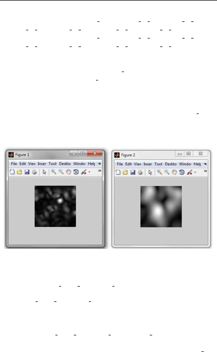
The code reads the image named sample face.bmp into the variable img,
and construct a filter bank filter bank of 40 Gabor filters and uses the bank
to filter the image. During the filtering operation, no down-sampling of the
magnitude responses is performed. Thus, we can visualize the magnitude
responses at full resolution. This is done in the last two lines of the example
code. The result of the above code is a feature vector named filtered image,
which can be used as input to subsequent operations (e.g., PCA, LDA, KFA,
etc.). The two figures produced by the code are also shown in Fig. 3.8
Figure 3.8: Examples of the magnitude responses produced by the example code.
3.4.2 The produce phase congruency PhD function
The produce phase congruency PhD function is a function that originates from
the web page of dr. Peter Kovesi [4]. It was modified to support the filter bank
format as used in the PhD toolbox. The function has the following prototype:
[pc,EO] = produce phase congruency PhD(X,filter bank,nscale);.
Here, Xdenotes the input grey-scale image to be filtered, filter bank

3.4 The features folder 29
stands for a Gabor filter bank compatible with the input image X(in terms of
dimensions) produced with the construct Gabor filters PhD function from
the PhD toolbox. nscale is an optional input argument, which allows to
compute the phase congruency features over less scales that are present in the
provided filter bank. The function return two output argument, i.e., pc and EO.
The first is a cell array containing the computed phase congruency components
for each orientation, while the second is a cell array of complex filter responses.
If you type
help produce phase congruency PhD
you will get additional information on the function together with several
examples of usage. The reader interested in phase congruency and its character-
istics is referred to [11] and [3].
An example of the use of the function is shown below:
X=double(imread(’sample face.bmp’));
filter bank = construct Gabor filters PhD(8,5, [128 128]);
[pc,EO] = produce phase congruency PhD(X,filter bank);
figure(1)
title(’Phase congruency at first filter orientation’)
imshow(pc{1},[])
figure(2)
title(’One of the magnitude responses of the filtering operation’)
imshow(abs(EO{5,5}),[])
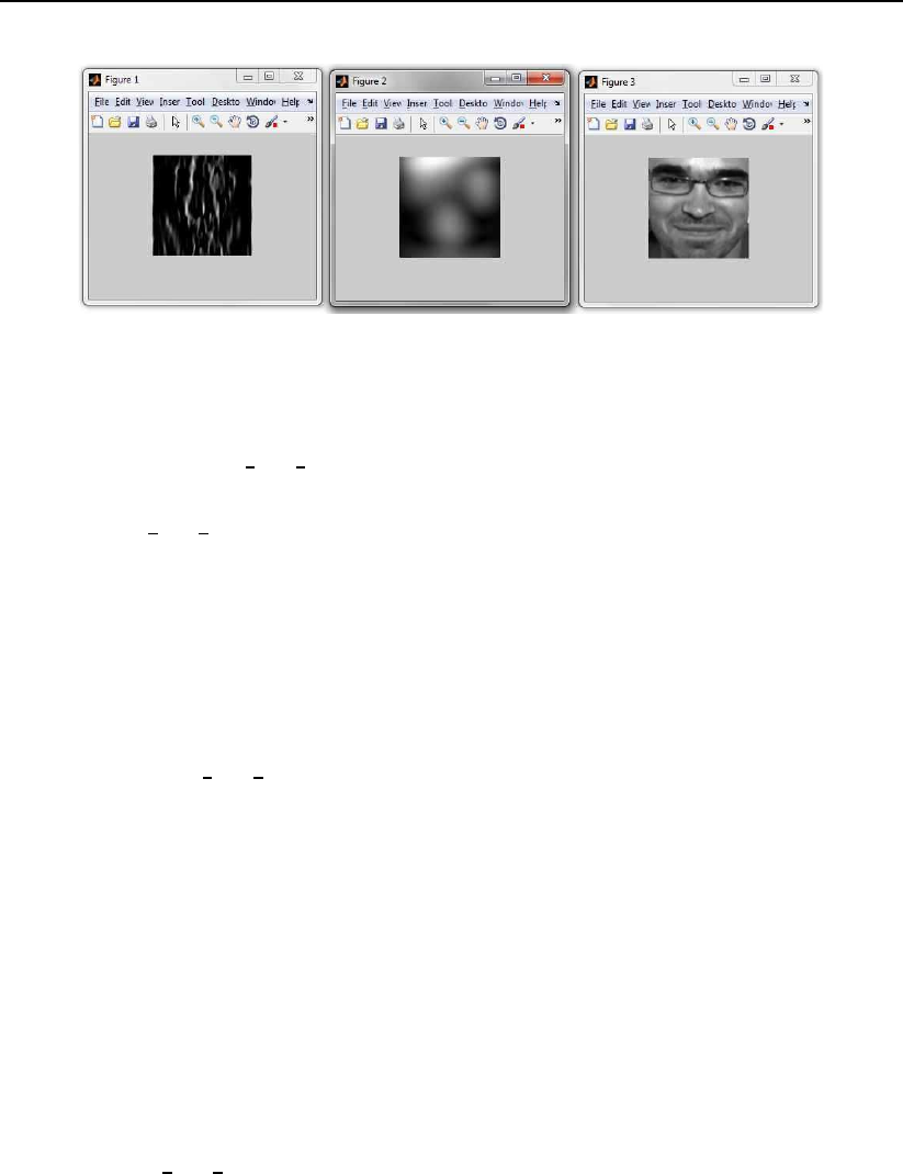
figure(3)
title(’Original input image’)
imshow(X,[])
The code reads the image named sample face.bmp into the variable X,
then constructs a compatible filter bank named filter bank and uses this filter
bank to compute the phase congruency components. In the last step it shows
the original input image, an example of the magnitude response of the filtering
and an example of a phase congruency component at a specific orientation. The
generated figures are also shown in Fig. 3.9.
30 Toolbox description
Figure 3.9: The result of the example code: a phase congruency component (left),
a magnitude response (middle), the input image (right)
3.4.3 The perform lda PhD function
The perform lda PhD function computes the LDA (Linear Discriminant Analy-
sis) subspace from the training data given in the input matrix X. The function
is basically an implementation of the Fisherface approach, which means that a
PCA (Principal component Analysis) step is performed prior to LDA to avoid
singularity issues due to a small number of training samples. The function has
the following prototype:
model = perform lda PhD(X,ids,n).
Here, Xdenotes an input matrix of training data, ids stands for a label
vector corresponding to the training data in X, and ndenotes the desired
dimensionality of the LDA subspace. Note, however, that ncannot exceed
M−1, where Mis the number of distinct classes (i.e., subject labels) in X. The
function returns an output structure model with the computed subspace and
some meta data. For more information on the theoretical background of the
Fisherface technique the reader is referred to [1].
If you type
help perform lda PhD
you will get additional information on the function together with several
examples of usage.
An example of the use of the function is shown below:
%In this example we generate the training data randomly and also
%generate the class labels manually; for a detailed example have a
%look at the LDA demo

3.4 The features folder 31
X = randn(300,100); %generate 100 samples with a dimension of 300
ids = repmat(1:25,1,4); %generate 25-class id vector
model = perform lda PhD(X,ids,24); %generate LDA model
The code first generates some random training data and stores in into a
variable called X. Next, its generates a corresponding label vector ids and finally,
it computes the LDA subspace and meta data, which is returned in the output
variable model.
3.4.4 The perform pca PhD function
The perform pca PhD function computes the PCA (Principal Component
Analysis) subspace from the training data given in the input matrix X. The
function is basically an implementation of the Eigenface approach, which was
presented in [9]. The function has the following prototype:
model = perform pca PhD(X,n).
Here, Xdenotes an input matrix of training data, and ndenotes the de-
sired dimensionality of the PCA subspace. Note, however, that ncannot exceed
min d, m −1, where dis the number of pixels (elements) of a single data sample
in the training matrix X, and mis the number of images (samples) in the training
data matrix X.
If you type
help perform pca PhD
you will get additional information on the function together with several
examples of usage.
An example of the use of the function is shown below:
%In this example we generate the training data randomly and
%set the number of retained components using the actual rank;
%for a detailed example have a look at the PCA demo
X=randn(300,100); %generate 100 samples with a dimension of 300
model = perform pca PhD(X,rank(X)-1); %generate PCA model

32 Toolbox description
The code first generates some random training data and stores in into a
variable called X. Next, its generates the PCA subspace and meta data (taking
into account the actual rank of the data matrix X), which is returned in the
output variable model.
3.4.5 The linear subspace projection PhD function
The linear subspace projection PhD function computes the subspace rep-
resentation of a single test image (sample) or matrix of test images (samples).
Hence, it uses the model generated by either the perform pca PhD function
or the perform lda PhD function to project new test data into the computed
subspace, where recognition is ultimately performed. The function has the
following prototype:
feat = linear subspace projection PhD(X, model, orthogon);.
Here, Xdenotes the input test data that needs to be projected into the
computed subspace defined by model. The third parameter orthogon is optional
and defines whether the computed subspace in model is orthogonal or not.
orthogon affects the way the subspace projection coefficients are computed and
consequently affects the speed of the computation.
If you type
help linear subspace projection PhD
you will get additional information on the function together with several
examples of usage.
An example of the use of the function is shown below:
%we randomly initialize the model with all of its fields; in
%practice this would be done using one of the appropriate
%functions
X = double(imread(’sample face.bmp’));
model.P = randn(length(X(:)),1); %random 10 dimensional model
model.dim = 10;
model.W = randn(length(X(:)),10);
feat = linear subspace projection PhD(X(:), model, 0);
The code reads the image named sample face.bmp into the variable X.
Next, its generates a random subspace model and uses this model to compute

3.4 The features folder 33
the subspace representation feat of the test image in X.
3.4.6 The perform kpca PhD function
The perform kpca PhD function computes the KPCA (Kernel Principal Com-
ponent Analysis) subspace from the training data given in the input matrix X.
The function is a non-linear variant of PCA and was first presented in [7]. The
function has the following prototype:
model = perform kpca PhD(X, kernel type, kernel args,n).
Here, Xdenotes an input matrix of training data, kernel type stands for the
type of kernel function to use (have a look at the compute kernel matrix PhD
function), kernel args denotes the arguments of the kernel function, and n
denotes the desired dimensionality of the KPCA subspace.
If you type
help perform kpca PhD
you will get additional information on the function together with several
examples of usage.
An example of the use of the function is shown below:
%In this example we generate the training data randomly; for a
%detailed example have a look at the KPCA demo
X=randn(300,100); %generate 100 samples with a dimension of 300
model = perform kpca PhD(X, ’poly’, [0 2], 90); %generate model
The code first generates some random training data and stores in into a
variable called X. Next, it computes the KPCA subspace and some meta-data,
which is returned in the output variable model. For constructing the subspace,
the code employs a polynomial kernel function.
3.4.7 The perform kfa PhD function
The perform kfa PhD function computes the KFA (Kernel Fisher Analysis)
subspace from the training data given in the input matrix X. The function is a
non-linear variant of LDA and was first presented in [5]. The function has the

34 Toolbox description
following prototype:
model = perform kfa PhD(X, ids, kernel type, kernel args,n);.
Here, Xdenotes an input matrix of training data, ids denotes a vector of
labels corresponding to the data in X,kernel type stands for the type of kernel
function to use (have a look at the compute kernel matrix PhD function),
kernel args denotes the arguments of the kernel function, and ndenotes the
desired dimensionality of the KFA subspace.
If you type
help perform kfa PhD
you will get additional information on the function together with several
examples of usage.
An example of the use of the function is shown below:
%In this example we generate the training data randomly; for a
%In this example we generate the training data randomly and also
%generate the class labels manually; for a detailed example have a
%look at the KFA demo
X=randn(300,100); %generate 100 samples with a dimension of 300
ids = repmat(1:25,1,4); %generate 25-class id vector
model = perform kfa PhD(X, ids, ’poly’, [0 2], 24); %generate model
The code first generates some random training data Xand corresponding
labels ids. It then computes the KFA subspace and returns it together with
some meta data in the output variable model. For constructing the subspace,
the code employs a polynomial kernel function.
3.4.8 The nonlinear subspace projection PhD function
The nonlinear subspace projection PhD function computes the subspace
representation of a single test image (sample) or matrix of test images (samples).
Hence, it uses the model generated by either the perform kpca PhD function
or the perform kfa PhD function to project new test data into the computed
subspace, where recognition is ultimately performed. The function has the
following prototype:

3.5 The classification folder 35
feat = nonlinear subspace projection PhD(X, model);.
Here, Xdenotes the input test data that needs to be projected into the
computed subspace defined by model. The function returns the subspace
representation of Xin the output matrix (or in case of a single input sample in X
in the output vector) feat.
If you type
help nonlinear subspace projection PhD
you will get additional information on the function together with several
examples of usage.
An example of the use of the function is shown below:
%we generate random training data for the example
X=double(imread(’sample face.bmp’));
training data = randn(length(X(:)),10);
model = perform kpca PhD(training data, ’poly’, [0 2]);
feat = nonlinear subspace projection PhD(X(:), model);
The code reads the image named sample face.bmp into the variable X
and then generates some training data of the appropriate dimensions. Based on
the generated training data, it computes a KPCA subspace and employs the
constructed KPCA model to compute the subspace projection coefficients of the
input image X. The coefficients are returned in the output variable feat.
3.5 The classification folder
The classification folder contains only two functions in the current version of
the PhD face recognition toolbox. Specifically, the following two functions are
contained in the folder:
•return distance PhD, and
•nn classification PhD.
A basic description of the functionality of the above listed functions is given
in the remainder of this section.

36 Toolbox description
3.5.1 The return distance PhD function
The return distance PhD function computes the distance (or similarity)
between two feature vectors. It is possible to use the function on its own if you
fill the need for it. The function currently supports four distance/similarity
measures, namely, the Euclidian distance, the City block distance, the cosine
similarity measure and the cosine mahalanobis (or whitened cosine) similarity
measure. The function has the following prototype:
d = return distance PhD(x,y,dist,covar).
Here, xand ydenote feature vectors the similarity of which needs to be
computed. dist stands for a string (’euc’,’ctb’,’cos’,’mahcos’) that specifies,
which distance/similarity measure to use and covar stands for the covariance
matrix of the training data that needs to be provided in case the ’mahcos’
similarity measure is selected.
If you type
help return distance PhD
you will get additional information on the function together with several
examples of usage.
An example of the use of the function is shown below:
%we generate the feature vectors ourselves
x = randn(1,20);
y = randn(1,20);
d = return distance PhD(x,y,’euc’);
The code first generates two random feature vectors xand yand then
calculates the distance dbetween them using the Euclidian distance measure.
3.5.2 The nn classification PhD function
The nn classification PhD function performs matching score calculation based
on the nearest neighbor classifier. The function has the following prototype:
results = nn classification PhD(train, train ids, test, test ids,

3.5 The classification folder 37
n, dist, match kind);.
Here train and test denote the training (gallery) and testing feature
vector matrices, train ids and test ids stand for corresponding label vectors n
represents the number of feature used in the calculations, dist (’cos’(default)
| ’euc’ | ’ctb’ | ’mahcos’) denotes the matching distance to use and
match kind (’all’ (default) | ’sep’) represents a string identifier control-
ling the matching procedure. The function returns a structure result, which
contains a similarity matrix of the matching procedure and some meta-data in
its fields.
If you type
help nn classification PhD
you will get additional information on the function together with several
examples of usage. The function features an extensive help section, where all
parameters and outputs are described in detail.
Before we proceed to the description of the next function, let us first ex-
plore the meaning of the match kind input argument. As already indicated
above, the argument can take to values either ’all’, which is the default or
’sep’. The first option should be used, when a similarity matrix needs to be
constructed, where all feature vectors from the training-feature-vector-matrix
train are matched against all feature vectors in the test-feature-vector-matrix
test. The similarity matrix generated by this option is stored in the results
structure under results.match dist. The structure can then be fed to the
evaluate results PhD, where performance graphs and metrics are computed
from the entire similarity matrix. The similarity matrix generates by the ’all’
is visualized in Fig. 3.10.
The second option ’sep’ should be used if you require non-overlapping image
sets for clients and impostor in your face verification experiments. In this case,
the code generate two similarity matrices as shown in Fig. 3.11.
The first similarity matrix is stored in the results.client dist and the second
in the results.imp dist fields of the output results structure. These two
similarity matrices are used by the evaluate results PhD function. Here it
should be noted, that CMC curves and all performance metrics with respect to
identification experiments are generated based on the client similarity matrix.
ROC and DET curves and corresponding verification error rates on the other
hand are computed by pooling FRR data from the client similarity matrix and
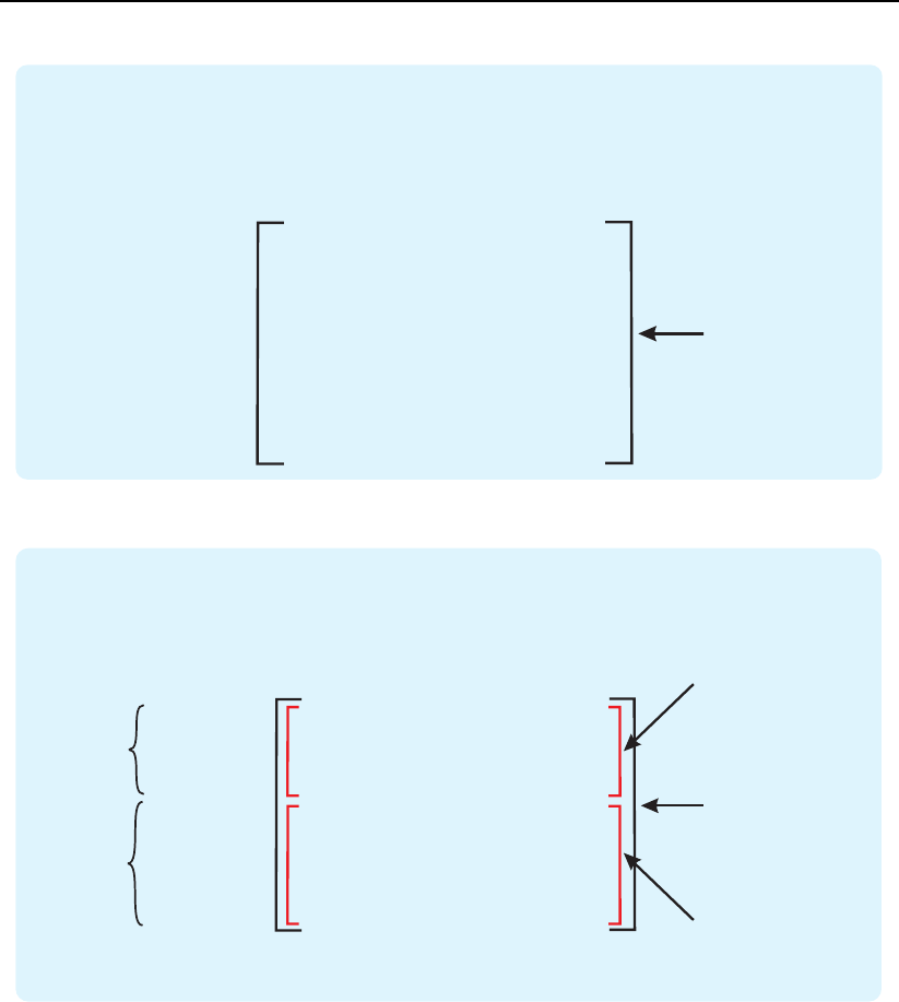
38 Toolbox description
1.02 0.97
0.41
1.34
0.78 0.98
0.98
1.45
0.44 0.44
0.57 0.57
1.87
0.12
.
.
.
.
.
.
.
.
.
.
.
.
.
.
.
.
.
.
.
.
.
.
.
.
.
.
.
.
.
.
.
.
.
Similarity matrix in
(size: x )
results.match_dist
n m
image 1 (subject 1)
image 1 (subject 1)
image 2 (subject 2)
image 3 (subject 3)
image (subject )n H
image 2 (subject 1)
image 3 (subject 1)
image (subject )m M
Gallery images (database, feature vectors from the matrix)train
Probe images (test data, feature vectors in matrix)test
Figure 3.10: An example of the similarity matrix generated by the all option.
1.02 0.97
0.41
1.34
0.78 0.98
0.98
1.45
0.44 0.44
0.57 0.57
1.87
0.12
.
.
.
.
.
.
.
.
.
.
.
.
.
.
.
.
.
.
.
.
.
.
.
.
.
.
.
.
.
.
.
.
.
Complete similarity
matrix (size: x )n m
Client similarity
matrix in
results.client_dist
Impostor similarity
matrix in
results.imp_dist
image 1 (subject 1)
image 1 (subject 1)
image 2 (subject 2)
image k (subject M)
image (subject )n H
image 2 (subject 1)
image 3 (subject 1)
image (subject )m M
Gallery images (database, feature vectors from the matrix)train
Probe images (test data, feature vectors in matrix)test
subjects also
in gallery
subjects not
in gallery
...
Figure 3.11: An example of the similarity matrix generated by the sep option.
FAR data from the impostor similarity matrix.
3.6 The demos folder
The demos folder is to many probably the most interesting folder in the PhD face
recognition toolbox. The folder contains several demo scripts, which demonstrate
how to build and evaluate complete face recognition systems and how to test your
algorithms on face image databases. In fact, most of the scripts contained in the
folder require a database to function. The database is not distributed with the
toolbox due to copyright issues, but can be easily downloaded from the web.

3.6 The demos folder 39
In this section we present a detailed description of the individual demo scripts
contained in the PhD toolbox (or at least the more interesting ones). These demo
scripts comprise:
•face registration demo
•construct Gabors and display bank demo
•Gabor filter face image demo
•phase cogruency from image demo
•perform pca demo
•perform lda demo
•perform kpca demo
•perform kfa demo
•gabor PCA face recognition and evaluation demo
•gabor LDA face recognition and evaluation demo
•gabor KPCA face recognition and evaluation demo
•gabor KFA face recognition and evaluation demo
•PCA face recognition and evaluation demo
•LDA face recognition and evaluation demo
•KPCA face recognition and evaluation demo
•KFA face recognition and evaluation demo
•phase congruency PCA face recognition and evaluation demo
•phase congruency LDA face recognition and evaluation demo
•phase congruency KPCA face recognition and evaluation demo
•phase congruency KFA face recognition and evaluation demo, and
•preprocessINFace gabor KFA face recognition and evaluation demo.
40 Toolbox description
3.6.1 Running the demo scripts (important!!)
It is very important to note that most of the demo scripts will not run of the box.
This means that you will have to download and unpack a database of face images,
on which the processing can be performed. The demo scripts of the PhD toolbox
were written for use with the ORL (AT&T) database, which can be obtained from
http://www.cl.cam.ac.uk/research/dtg/attarchive/facedatabase.html.
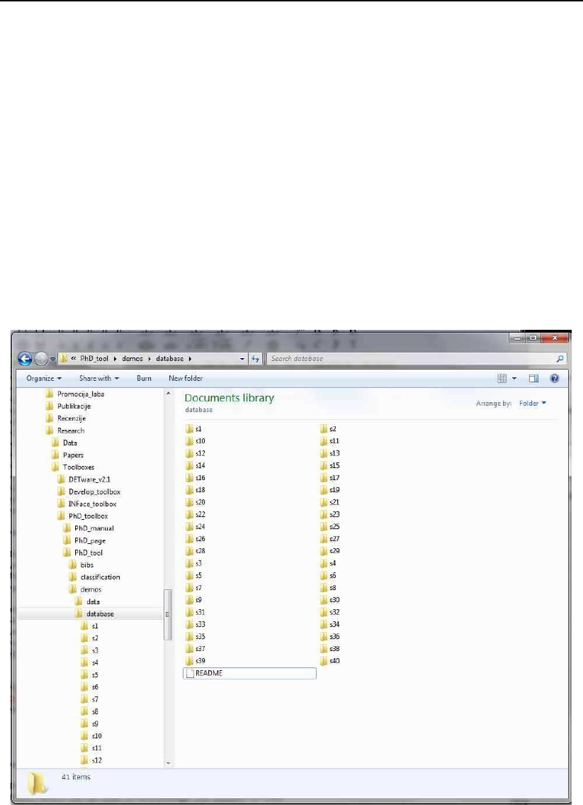
You have to download the archive containing the database and unpack it into
the database folder, which is waiting for you in the demos folder of the PhD face
recognition toolbox. Hence, after you have unpacked the database, the database
folder should something like this:
Figure 3.12: The database folder should contain 40 subfolders of 40 subjects from
the ORL database.
Once you have downloaded and unpacked the database change Matlabs cur-
rent working directory to the demos folder of the PhD face recognition toolbox
and run a demo script of your choice. This step is necessary, because the demos

3.6 The demos folder 41
folder is not added to Matlabs search path, when installing the toolbox, which in
turn is a consequence of the fact that all paths referring to the face image data
are given in relative terms from the demos directory and won’t work from any
other location.
If you have followed the above instructions all of the demo scripts should work
just fine and demonstrate how to use the functions contained in the PhD toolbox.
3.6.2 The face registration demo script
The face registration demo script demonstrates how to use the
register face based on eyes function to register (or to extract) a face
from an input image based on provided eye coordinates. It demonstrates two
different examples. In the first the coordinates are hard coded in the script and
in the second they are read from an external file. For more information on the
demo script have a look at its header.
3.6.3 The construct Gabors and display bank demo script
The script uses the construct Gabor filters PhD function from the PhD tool-
box to demonstrate how to construct a bank of Gabor filters for facial feature
extraction. The script constructs the default filter bank of 40 filters with 8 orien-
tations and 5 scales, with the filter parameters selected for optimal performance
with 128x128 pixel face images. The demo constructs the filter bank and then
displays the real parts, imaginary parts and magnitudes of the filters in the bank
as shown in Fig. 3.13. For more information on the demo script have a look at
its header.
3.6.4 The Gabor filter face image demo script
The script demonstrates how to filter an input image of size 128x128 pixels with a
filter bank of 40 Gabor filters. The demo constructs the filter bank, the filter the
image with all filter from the bank and finally displays the result of the filtering
in a Matlab figure. The entire process is repeated two times with different down-
scaling factors.
The result of the filtering process presented in the demo script is a set of
magnitude responses as shown in Fig. 3.14. For more information on the demo
script have a look at its header.

42 Toolbox description
Figure 3.13: Figure generated by the demo script: real parts of the filter bank (top),
imaginary parts of the filter bank (middle), magnitudes for different
filter scales (bottom)
3.6.5 The phase cogruency from image demo script
The script demonstrates how to compute the phase congruency for an input face
image. The demo first construct a filter bank of Gabor filters and then uses this
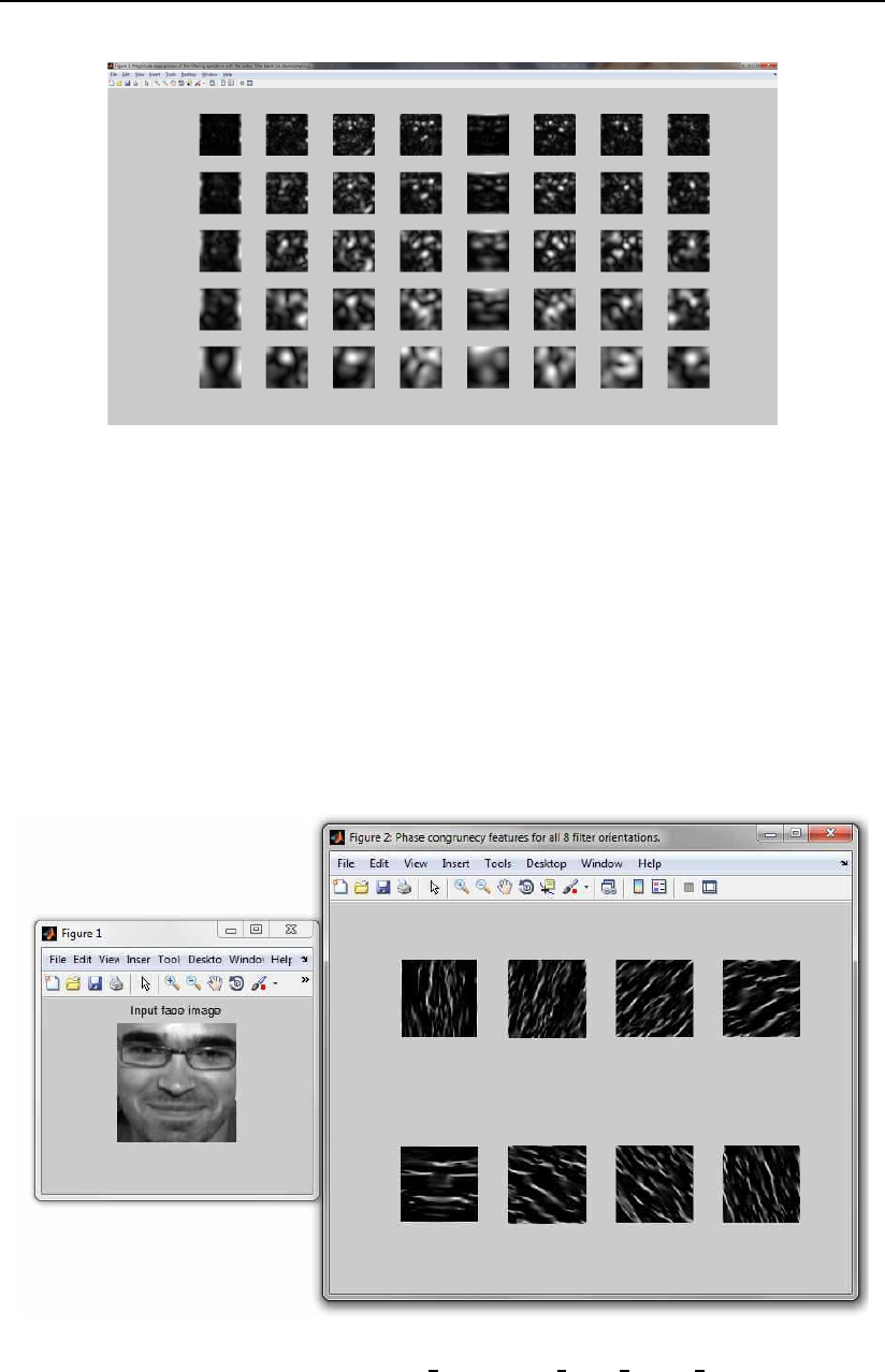
3.6 The demos folder 43
Figure 3.14: Magnitude responses of the filtering process performed by the demo
script.
bank to compute the phase congruency for each filter orientation in the filter
bank. At the end the results are display in a couple of figures.
The figures generated by the demo script are also shown in Fig. 3.15. For
more information on the demo script have a look at its header.
Figure 3.15: Results of the phase cogruency from image demo script.

44 Toolbox description
3.6.6 The perform XXX demo scripts
The perform XXX demo scripts, where XXX stands for either pca, lda, kpca or
kfa, demonstrate how to use the subspace projection technique functions2from
the PhD toolbox. Basically these scripts compute the selected subspace and then
show some results.
The demos assume that you have downloaded the ORL database and have
unpacked it to the /demos/database folder. This folder should now have the
following internal structure:
/demos/database/ — s1/
|— s2/
|— s3/
|— s4/
|— s5/
|— s6/
...
|— s40/
Each of the 40 subfolders should contain 10 images in PGM format. If you
have not downloaded and unpacked the ORL database at all or have unpacked
it into a different folder this demo will not work!!! Please follow the install
instructions in the install script or look at Section 3.6.1.
IMPORTANT!!!! Note that you must run all demo scripts in this toolbox
from the demos folder. This is particularly important, since some data needed
by the scripts is located in folders whose paths are specified relative to the demos
folder. If you run the scripts from anywhere else, the scripts may fail.
Since all four functions are relatively similar, we explore the functionality
of the perform XXX demo script family on a specific example and we select the
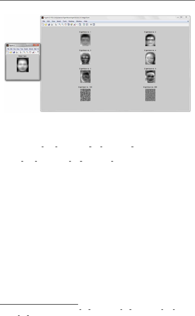
perform pca demo demo script for this purpose. The script first loads images
from the ORL database into a data matrix and then computes the PCA subspace.
Ultimately, the projection axes in image form (i.e., the Eigenfaces) and the mean
face are displayed in two figures as shown in Fig. 3.16
2These functions are: perform pca PhD,perform lda PhD,perform kpca PhD, and
perform kfa PhD
3.6 The demos folder 45
Figure 3.16: Examples of the generated figures: the mean face (left), a few eigen-
faces (right).
3.6.7 The XXX face recognition and evaluation demo scripts
The XXX face recognition and evaluation demo scripts, where XXX stands
for either pca, lda, kpca or kfa, demonstrate how to use the subspace projection
technique functions3from the PhD toolbox for real face recognition experiments
and how to evaluate them on a database. Basically these scripts load facial image
data from a database, partition it into appropriate image sets for training and
testing, compute the selected subspace, and perform recognition experiments. In
the end, the scripts generate several performance curves and performance metrics
for the conducted experiments.
The demos assume that you have downloaded the ORL database and have
unpacked it to the /demos/database folder. This folder should now have the
following internal structure:
/demos/database/ — s1/
|— s2/
|— s3/
|— s4/
|— s5/
|— s6/
3These functions are: perform pca PhD,perform lda PhD,perform kpca PhD, and
perform kfa PhD
46 Toolbox description
...
|— s40/
Each of the 40 subfolders should contain 10 images in PGM format. If you
have not downloaded and unpacked the ORL database at all or have unpacked
it into a different folder this demo will not work!!! Please follow the install
instructions in the install script or look at Section 3.6.1.
IMPORTANT!!!! Note that you must run all demo scripts in this toolbox
from the demos folder. This is particularly important, since some data needed
by the scripts is located in folders whose paths are specified relative to the demos
folder. If you run the scripts from anywhere else, the scripts may fail.
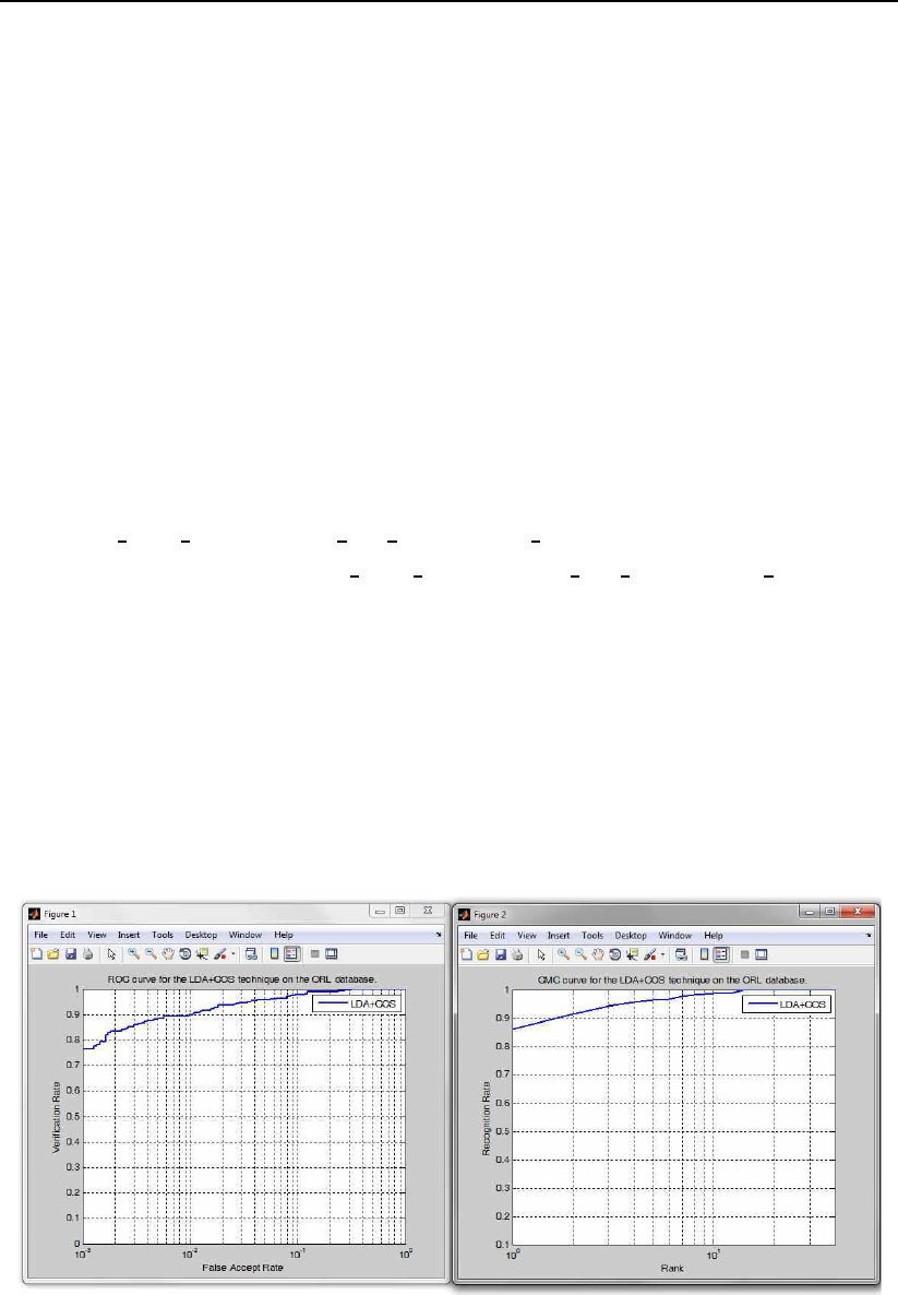
Since all four functions are relatively similar, we explore the functionality
of the XXX face recognition and evaluation demo script family on a specific
example and we select the LDA face recognition and evaluation demo demo
script for this purpose. The script first loads images from the ORL database into
a data matrix and then partitions this data into a training and test set. Next,
it computes the LDA subspace based on images from the training set and finally
performs recognition experiments using images from the test set. In the end, the
demo script generates a CMC and ROC curves and displays them in two separate
figures as shown in Fig. 3.17. Note that the script also generates a DET curve in
case you have installed NISTs DETware.
Figure 3.17: Examples of the generated figures: ROC curve (left), CMC (right).
In addition to the performance curves, the demo scripts also outputs some
performance metrics, which should look something like this:

3.6 The demos folder 47
=============================================================
SOME PERFORMANCE METRICS:
Identification experiments:
The rank one recognition rate equals (in %): 86.07%
Verification/authentication experiments:
The equal error rate equals (in %): 4.28%
The minimal half total error rate equals (in %): 4.09%
The verification rate at 1% FAR equals (in %): 90.00%
The verification rate at 0.1% FAR equals (in %): 76.43%
The verification rate at 0.01% FAR equals (in %): 64.29%
=============================================================
3.6.8 The gabor XXX face recognition and evaluation demo scripts
The gabor XXX face recognition and evaluation demo scripts, where XXX
stands for either pca, lda, kpca or kfa, demonstrate how to use the subspace
projection technique functions4from the PhD toolbox for real face recognition
experiments with Gabor magnitude features. Basically these scripts load facial
image data from a database, partition it into appropriate image sets for training
and testing, filter the images with a bank of Gabor filters, generate feature vec-
tors of Gabor magnitude features, compute the selected subspace, and perform
recognition experiments. In the end, the scripts generate several performance
curves and performance metrics for the conducted experiments.
The demos assume that you have downloaded the ORL database and have
unpacked it to the /demos/database folder. This folder should now have the
following internal structure:
/demos/database/ — s1/
|— s2/
|— s3/
|— s4/
|— s5/
4These functions are: perform pca PhD,perform lda PhD,perform kpca PhD, and
perform kfa PhD

48 Toolbox description
|— s6/
...
|— s40/
Each of the 40 subfolders should contain 10 images in PGM format. If you
have not downloaded and unpacked the ORL database at all or have unpacked
it into a different folder this demo will not work!!! Please follow the install
instructions in the install script or look at Section 3.6.1.
IMPORTANT!!!! Note that you must run all demo scripts in this toolbox
from the demos folder. This is particularly important, since some data needed
by the scripts is located in folders whose paths are specified relative to the demos
folder. If you run the scripts from anywhere else, the scripts may fail.
Since all four functions are relatively similar, we explore the func-
tionality of the gabor XXX face recognition and evaluation demo
script family on a specific example and we select the
gabor KPCA face recognition and evaluation demo demo script for this
purpose. The script first loads images from the ORL database into a data matrix
and then partitions this data into a training, evaluation and test set. Next, it
filters the images using a filter bank of 40 Gabor filters. Based on this process it
constructs feature vectors of Gabor magnitude features and computes the KPCA
subspace based on feature vectors from the training set and finally performs
recognition experiments using feature vectors from the test and evaluation sets.
In the end, the demo script generates a CMC, EPC and ROC curves and displays
them in three separate figures as shown in Fig. 3.18. Note that the script also
generates a DET curve in case you have installed NISTs DETware.
In addition to the performance curves, the demo scripts also outputs some
performance metrics, which should look something like this:
=============================================================
SOME PERFORMANCE METRICS:
Identification experiments:
The rank one recognition rate of the experiments equals (in %): 80.00%
Verification/authentication experiments on the evaluation data:
The equal error rate on the evaluation set equals (in %): 4.17%
The minimal half total error rate on the evaluation set equals (in %): 2.68%
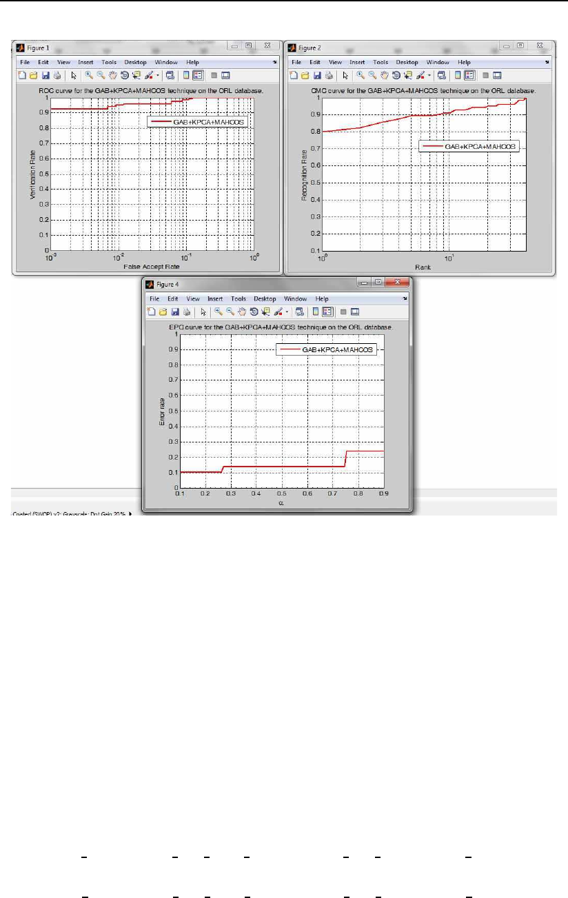
3.6 The demos folder 49
Figure 3.18: Examples of the generated figures: ROC curve (left), CMC (right),
EPC (bottom).
The verification rate at 1% FAR on the evaluation set equals (in %): 95.00%
The verification rate at 0.1% FAR on the evaluation set equals (in %): 92.50%
The verification rate at 0.01% FAR on the evaluation set equals (in %): 0.83%
Verification/authentication experiments on the test data (preset thresholds
on evaluation data):
The verification rate at 1% FAR on the test set equals (in %): 71.88%
The verification rate at 0.1% FAR on the test set equals (in %): 56.88%
=============================================================
The phase congruency XXX face recognition and evaluation demo scripts
The phase congruency XXX face recognition and evaluation demo scripts,
where XXX stands for either pca, lda, kpca or kfa, demonstrate how to use

50 Toolbox description
the subspace projection technique functions5from the PhD toolbox for real face
recognition experiments with Gabor phase congruency features. Basically these
scripts load facial image data from a database, partition it into appropriate im-
age sets for training and testing, filter the images with a bank of Gabor filters,
generate feature vectors of Gabor phase congruency features, compute the se-
lected subspace, and perform recognition experiments. In the end, the scripts
generate several performance curves and performance metrics for the conducted
experiments.
The demos assume that you have downloaded the ORL database and have
unpacked it to the /demos/database folder. This folder should now have the
following internal structure:
/demos/database/ — s1/
|— s2/
|— s3/
|— s4/
|— s5/
|— s6/
...
|— s40/
Each of the 40 subfolders should contain 10 images in PGM format. If you
have not downloaded and unpacked the ORL database at all or have unpacked
it into a different folder this demo will not work!!! Please follow the install
instructions in the install script or look at Section 3.6.1.
IMPORTANT!!!! Note that you must run all demo scripts in this toolbox
from the demos folder. This is particularly important, since some data needed
by the scripts is located in folders whose paths are specified relative to the demos
folder. If you run the scripts from anywhere else, the scripts may fail.
Since all four functions are relatively similar, we explore the functional-
ity of the phase congruency XXX face recognition and evaluation demo
script family on a specific example and we select the
phase congruency KFA face recognition and evaluation demo demo script
for this purpose. The script first loads images from the ORL database into a
data matrix and then partitions this data into a training, evaluation and test set.
Next, it filters the images using a filter bank of 40 Gabor filters. Based on this
process it constructs feature vectors of Gabor phase congruency features and
5These functions are: perform pca PhD,perform lda PhD,perform kpca PhD, and
perform kfa PhD
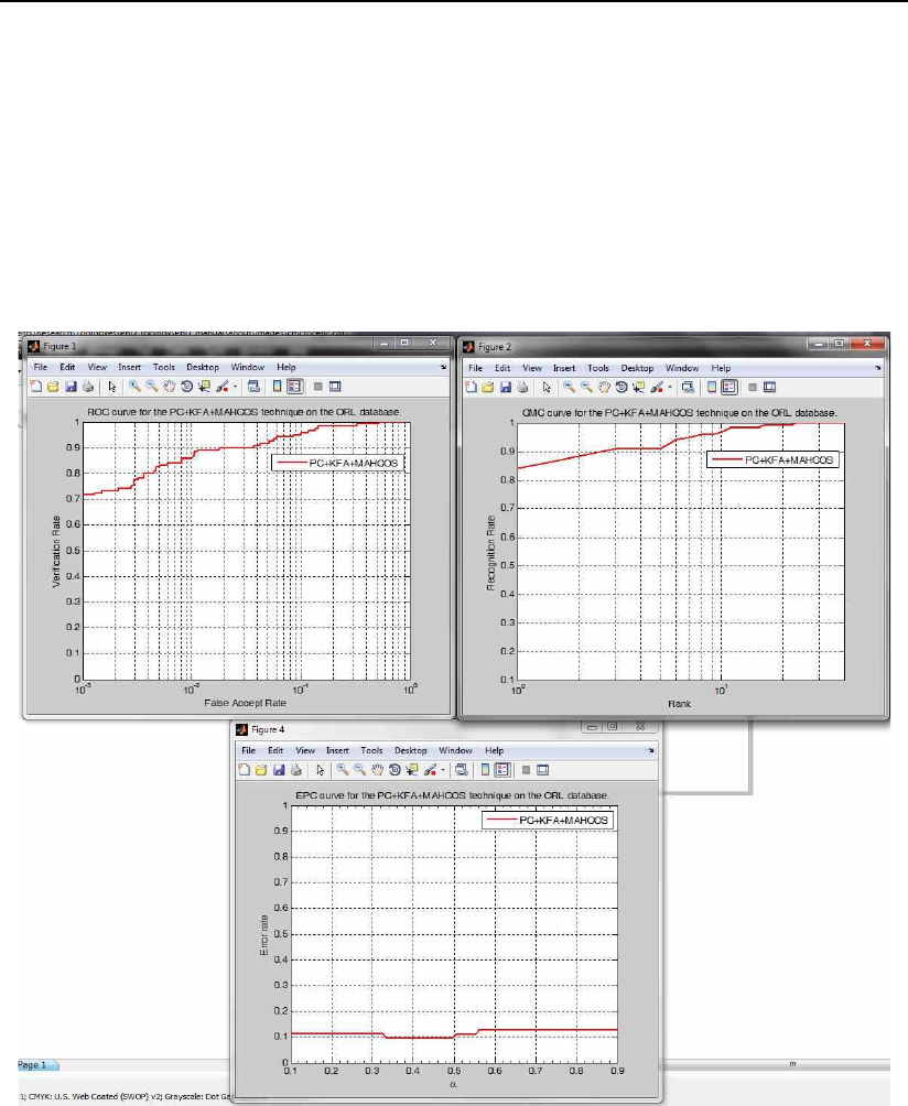
3.6 The demos folder 51
computes the KFA subspace based on feature vectors from the training set and
finally performs recognition experiments using feature vectors from the test and
evaluation sets. In the end, the demo script generates a CMC, EPC and ROC
curves and displays them in three separate figures as shown in Fig. 3.19. Note
that the script also generates a DET curve in case you have installed NISTs
DETware.
Figure 3.19: Examples of the generated figures: ROC curve (left), CMC (right),
EPC (bottom).
In addition to the performance curves, the demo scripts also outputs some
performance metrics, which should look something like this:
=============================================================
SOME PERFORMANCE METRICS:
Identification experiments:

52 Toolbox description
The rank one recognition rate of the experiments equals (in %): 84.17%
Verification/authentication experiments on the evaluation data:
The equal error rate on the evaluation set equals (in %): 5.94%
The minimal half total error rate on the evaluation set equals (in %): 5.90%
The verification rate at 1% FAR on the evaluation set equals (in %): 85.83%
The verification rate at 0.1% FAR on the evaluation set equals (in %): 71.67%
The verification rate at 0.01% FAR on the evaluation set equals (in %): 0.83%
Verification/authentication experiments on the test data (preset thresholds
on evaluation data):
The verification rate at 1% FAR on the test set equals (in %): 74.38%
The verification rate at 0.1% FAR on the test set equals (in %): 64.38%
=============================================================
The preprocessINFace gabor KFA face recognition and evaluation demo
script
The last demo script featured in the PhD face recognition toolbox is the
preprocessINFace gabor KFA face recognition and evaluation demo demo
scripts. The script demonstrates how to include functions from the INFace tool-
box for illumination invariant face recognition in a face recognition system con-
structed using the functions from the PhD toolbox. Basically these script loads
facial image data from a database, partitions it into appropriate image sets for
training and testing, preprocesses the images using a photometric normalization
technique from the INFace toolbox6, filters the images with a bank of Gabor fil-
ters, generates feature vectors of Gabor magnitude features, computes the KFA
subspace, and performs recognition experiments. In the end, the script generates
several performance curves and performance metrics for the conducted experi-
ments.
The demo assumes that you have downloaded the ORL database and have
unpacked it to the /demos/database folder. This folder should now have the
following internal structure:
/demos/database/ — s1/
|— s2/
|— s3/
6You can get the INFace toolbox from [10]

3.6 The demos folder 53
|— s4/
|— s5/
|— s6/
...
|— s40/
Each of the 40 subfolders should contain 10 images in PGM format. If you
have not downloaded and unpacked the ORL database at all or have unpacked
it into a different folder this demo will not work!!! Please follow the install
instructions in the install script or look at Section 3.6.1.
IMPORTANT!!!! Note that you must run all demo scripts in this toolbox
from the demos folder. This is particularly important, since some data needed
by the scripts is located in folders whose paths are specified relative to the demos
folder. If you run the scripts from anywhere else, the scripts may fail. You also
have to download and install the INFace toolbox or the demo script wont work
either.
The script first loads images from the ORL database into a data matrix and
then partitions this data into a training, evaluation and test set. Next, it photo-
metrically normalizes the face images using the Tan and Triggs [8] normalization
procedure. It then filters the normalized images using a filter bank of 40 Gabor
filters. Based on this process it constructs feature vectors of Gabor magnitude
features and computes the KFA subspace using feature vectors from the training
set. Finally, it performs recognition experiments using feature vectors from the
test and evaluation sets. In the end, the demo script generates a CMC, EPC and
ROC curves and displays them in three separate figures as shown in Fig. 3.20.
Note that the script also generates a DET curve in case you have installed NISTs
DETware.
In addition to the performance curves, the demo scripts also outputs some
performance metrics, which should look something like this:
=============================================================
SOME PERFORMANCE METRICS:
Identification experiments:
The rank one recognition rate of the experiments equals (in %): 95.00%
Verification/authentication experiments on the evaluation data:
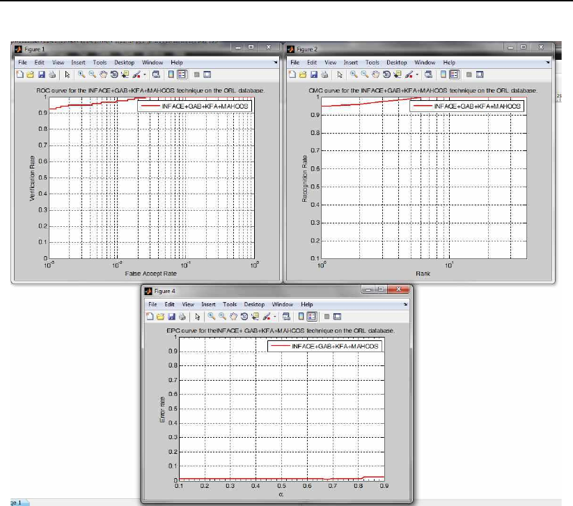
54 Toolbox description
Figure 3.20: Examples of the generated figures: ROC curve (left), CMC (right),
EPC (bottom).
The equal error rate on the evaluation set equals (in %): 1.67%
The minimal half total error rate on the evaluation set equals (in %): 1.30%
The verification rate at 1% FAR on the evaluation set equals (in %): 97.50%
The verification rate at 0.1% FAR on the evaluation set equals (in %): 92.50%
The verification rate at 0.01% FAR on the evaluation set equals (in %): 0.83%
Verification/authentication experiments on the test data (preset thresholds
on evaluation data):
The verification rate at 1% FAR on the test set equals (in %): 98.75%
The verification rate at 0.1% FAR on the test set equals (in %): 93.13%
=============================================================

3.7 The bibs folder 55
3.7 The bibs folder
The folder named bibs contains only two Latex bib files, which can be used to
acknowledge the toolbox in case you are using Latex. The two files are:
•ACKNOWL1.bib, and
•ACKNOWL2.bib.

4. Using the Help
The toolbox contains some basic help which offers additional information on each
of the functions and scripts in the PhD face recognition toolbox. The help in the
functions is intended to be used as supplementary information on the functionality
of the toolbox.
4.1 Toolbox and folder help
The most basic information on the toolbox can be accessed by typing:
help PhD tool,
or if you have changed the name of the folder:
help new folder name.
This command displays a list of folders in the toolbox and a basic description of
the functionality of each function and/or script in these folders.
You can also access only individual folder help by typing, e.g., for the features
folder:
help features.
4.2 Function help
To access the help of the individual functions (like always) just call the help
command followed by the name of the function of interest:
help function name.
56

4.2 Function help 57
All functions (and scripts) are equipped with an extensive help section de-
scribing the functionality of the function and also include a reference to the
paper, where the implemented technique was proposed or is explained.
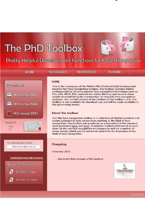
5. The PhD toolbox homepage
In addition to other repositories from where you might have downloaded the PhD
face recognition toolbox, the toolbox is also available from its official homepage.
The page can be accessed from:
http://luks.fe.uni-lj.si/sl/osebje/vitomir/face tools/PhDface/
However, since we are currently in the process of redesigning our labora-
tory web page, the final URL of the web site may still change.
Figure 5.1: Screenshot of the official website
Note that only the official website features the up to date version of the
58

59
toolbox with all bug fixes and most recent changes, while only major releases are
distributed to other repositories as well. Hence, if you have obtained the toolbox
from any other location that the official website, I suggest that you make sure
that you have obtained the most recent version.
6. Change Log
The current version of the PhD toolbox is v1.0, so there so Change Log needed
yet.
60
7. Conclusion
The current version of the toolbox (PhD toolbox v1.0) includes Matlab functions
that implement several popular face recognition techniques, evaluation tools,
performance graphs, and many more. If you have any questions or useful
suggestions with respect to the toolbox you are welcomed to contact me. You
can find my contact information by following the following link:
http://luks.fe.uni-lj.si/en/staff/vitomir/index.html.
Thank you for taking an interest in the PhD face recognition toolbox.
61

62 Conclusion
References
[1] P.N. Belhumeur, J.P. Hespanha, D.J. Kriegman. Eigenfaces vs. fisherfaces:
Recognition using class specific linear projection. Proc. of the 4th European
Conference on Computer Vision, ECCV’96, April.
[2] S. Bengio, J. Mariethoz. The expected performance curve: a new assess-
ment measure for person authentication. Proceedings of Odyssey 2004: The
Speaker and Language Recognition Workshop, 2004.
[3] P. Kovesi. Image features from phase congruency. Videre: A Journal
of Computer Vision Research. MIT Press, Vol. 1, No. 3, , 1999. http:
//mitpress.mit.edu/e-journals/Videre/001/v13.html.
[4] P. Kovesi. Computer vision functions for matlab. Website, 2012. http:
//www.csse.uwa.edu.au/~pk/Research/MatlabFns/index.html.
[5] C. Liu. Capitalize on dimensionality increasing techniques for improving face
recognition grand challenge performance. IEEE Transactions on Pattern
Analysis and Machine Intelligence, Vol. 28, No. 5, str. 725–737, 2006.
[6] C. Liu, H. Wechsler. Gabor feature based classification using the enhanced
fisher linear discriminant model for face recognition. IEEE Transactions on
Image Processing, Vol. 11, No. 4, str. 467–476, 2002.
[7] B. Scholkopf, A. Smola, K.R. Muller. Nonlinear component analysis as a
kernel eigenvalue problem. Technical Report No. 44, 1996. 18 pages.
[8] X. Tan, B. Triggs. Enhanced local texture sets for face recognition under
difficult lighting conditions. IEEE Transactions on Image Processing, Vol.
19, No. 6, str. 1635–1650, 2010.
[9] M. Turk, A. Pentland. Eigenfaces for recognition. Journal of Cognitive
Neurosicence, Vol. 3, No. 1, str. 71–86.
[10] V. ˇ
Struc. The matlab inface toolbox for illumination invariant face recog-
nition. Website, 2012. http://luks.fe.uni-lj.si/sl/osebje/vitomir/
face_tools/INFace/index.html.
63

64 References
[11] V. ˇ
Struc, N. Paveˇsi´c. The complete gabor-fisher classifier for robust face
recognition. EURASIP Advances in Signal Processing, Vol. 2010, str. 26,
2010.
