Phoenix Ing Language Reference Guide
User Manual:
Open the PDF directly: View PDF ![]() .
.
Page Count: 98
- Contents
- List of Tables
- Introduction
- Language Structure and Syntax
- Modeling project files
- General syntax conventions
- Reserved and user-defined variable names
- Modeling syntax
- Population PK model
- Closed-form models
- Transit Compartment models
- Action code
- Observations
- Math and special functions
- Dosing
- Covariates
- Modeling discontinuous events
- Discrete and distributed delays
- Sequence statements
- Group statements
- Sleep statements
- Time event switching in PML versus WinNonlin ASCII models
- Fixed effect parameter syntax
- Random effect parameter syntax
- Running NLME Engines in Command Line Mode
- PML Examples
- Phenobarbital
- Theophylline
- User-defined logistic model
- Structural parameters and QRPEM
- Additional examples
- Multinomial (ordered categorical)
- Time to event model (exponential)
- Time to event model (Weibull)
- Emax (Hill) model with exponent
- One-compartment IV bolus population PK
- One-compartment IV bolus, two parallel models with common fixed effects
- One-compartment model with sequence
- One-compartment model with sleep statement
- One-compartment first-order absorption model, compartment initialized with sequence
- One-compartment first-order absorption, closed-form
- One-compartment first-order absorption with lag time, closed-form
- One-compartment IV bolus with time-to-event outcome and PK observations
- Closed-Form and Matrix Exponent Computations
- Blocks, Statements, and Operators
- Reserved Words
- Supported Functions
- Index

Phoenix® Modeling
Language Reference
Guide
Applies to:
Phoenix WinNonlin® 8.1
Phoenix NLME™ 8.1

Phoenix Modeling Language Version 8.1
Phoenix® WinNonlin®, Phoenix NLME™, IVIVC Toolkit™, CDISC® Navigator, AutoPilot Toolkit™, Job Management System™
(JMS™), Pharsight Knowledgebase Server™ (PKS™), Trial Simulator™, Validation Suite™ copyright ©2005-2018, Certara, L.P. All
rights reserved. This software and the accompanying documentation are owned by Certara, L.P. The software and the accompanying docu-
mentation may be used only as authorized in the license agreement controlling such use. No part of this software or the accompanying doc-
umentation may be reproduced, transmitted, or translated, in any form or by any means, electronic, mechanical, manual, optical, or
otherwise, except as expressly provided by the license agreement or with the prior written permission of Certara, L.P.
This product may contain the following software that is provided to Certara, L.P. under license: Formula One® copyright 1993-2018 Open-
Text Corporation. All rights reserved. Microsoft® .NET Framework copyright 2018 Microsoft Corporation. All rights reserved. Tab Pro
ActiveX 2.0.0.45 copyright 1996-2018, GrapeCity, Inc. All rights reserved. Sentinel™ RMS 8.4.0.900 copyright 2006-2018 Gemalto NV.
All rights reserved. Microsoft XML Parser version 3.0 copyright 1998-2018 Microsoft Corporation. All rights reserved. Websites Screen-
shot DLL 1.6 copyright 2008-2018 WebsitesScreenshot.com. All rights reserved. Certara, L.P. has agreement to use and redistribute licenses
for the following software: Syncfusion Essential Studio Enterprise 15.4.0.17 copyright 2001-2018 Syncfusion Inc. All rights reserved. Min-
imal Gnu for Windows (MinGW, http://mingw.org/), copyright 2004-2018 Free Software Foundation, Inc. This product may also contain the
following royalty free software: DotNetbar 1.0.0.24030 (with custom code changes) copyright 1996-2018 DevComponents LLC. All rights
reserved. Xceed zip Library 2.0.116.0 copyright 1994-2018 Xceed Software Inc. All rights reserved. IMSL® copyright 2018 Rogue Wave
Software, Inc. All rights reserved.
Information in the documentation is subject to change without notice and does not represent a commitment on the part of Certara, L.P. The
documentation contains information proprietary to Certara, L.P. and is for use by its affiliates' and designates' customers only. Use of the
information contained in the documentation for any purpose other than that for which it is intended is not authorized. NONE OF CERTARA,
L.P., NOR ANY OF THE CONTRIBUTORS TO THIS DOCUMENT MAKES ANY REPRESENTATION OR WARRANTY, NOR SHALL ANY WARRANTY BE
IMPLIED, AS TO THE COMPLETENESS, ACCURACY, OR USEFULNESS OF THE INFORMATION CONTAINED IN THIS DOCUMENT, NOR DO THEY
ASSUME ANY RESPONSIBILITY FOR LIABILITY OR DAMAGE OF ANY KIND WHICH MAY RESULT FROM THE USE OF SUCH INFORMATION.
Destination Control Statement
All technical data contained in the documentation are subject to the export control laws of the United States of America. Disclosure to
nationals of other countries may violate such laws. It is the reader's responsibility to determine the applicable regulations and to comply with
them.
United States Government Rights
This software and accompanying documentation constitute “commercial computer software” and “commercial computer software docu-
mentation” as such terms are used in 48 CFR 12.212 (Sept. 1995). United States Government end users acquire the Software under the fol-
lowing terms: (i) for acquisition by or on behalf of civilian agencies, consistent with the policy set forth in 48 CFR 12.212 (Sept. 1995); or
(ii) for acquisition by or on behalf of units of the Department of Defense, consistent with the policies set forth in 48 CFR 227.7202-1 (June
1995) and 227.7202-3 (June 1995). The manufacturer is Certara, L.P., 100 Overlook Center, Suite 101, Princeton, New Jersey, 08540.
Trademarks
AutoPilot Toolkit, IVIVC Toolkit, Job Management System, JMS, NLME, Pharsight Knowledgebase Server, PKS, Phoenix, Trial Simula-
tor, Validation Suite, WinNonlin are trademarks or registered trademarks of Certara, L.P. NONMEM is a registered trademark of ICON
Development Solutions. S-PLUS is a registered trademark of Insightful Corporation. SAS and all other SAS Institute Inc. product or service
names are registered trademarks or trademarks of SAS Institute Inc. in the USA and other countries. Sentinel RMS is a trademark of
Gemalto NV. Microsoft, MS, .NET, SQL Server Compact Edition, the Internet Explorer logo, the Office logo, Microsoft Word, Microsoft
Excel, Microsoft PowerPoint®, Windows, the Windows logo, the Windows Start logo, and the XL design (the Microsoft Excel logo) are
trademarks or registered trademarks of Microsoft Corporation. Pentium 4 and Core 2 are trademarks or registered trademarks of Intel Cor-
poration. Adobe, Acrobat, Acrobat Reader, and the Adobe PDF logo are registered trademarks of Adobe Systems Incorporated. All other
brand or product names mentioned in this documentation are trademarks or registered trademarks of their respective companies or organiza-
tions.
Additional third party software acknowledgements
Software for Locally-Weighted Regression
The authors of this software are Cleveland, Grosse, and Shyu. Copyright © 1989, 1992 by AT&T. Permission to use, copy, modify, and dis-
tribute this software for any purpose without fee is hereby granted, provided that this entire notice is included in all copies of any software
which is or includes a copy or modification of this software and in all copies of the supporting documentation for such software.
This software is being provided “as is”, without any express or implied warranty. In particular, neither the authors nor AT&T make any rep-
resentation or warranty or any kind concerning the merchantability of this software or its fitness for any particular purpose.
LAPACK
Copyright © 1992-2007 The University of Tennessee. All rights reserved.
Redistribution and use in source and binary forms, with or without modification, are permitted provided that the following conditions are
met:
Redistributions of source code must retain the above copyright notice, this list of conditions and the following disclaimer.
Redistributions in binary form must reproduce the above copyright notice, this list of conditions and the following disclaimer listed in this
license in the documentation and/or other materials provided with the distribution.
Neither the name of the copyright holders nor the names of its contributors may be used to endorse or promote products derived from this
software without specific prior written permission.
This software is provided by the copyright holders and contributors “as is” and any express or implied warranties, including, but not limited
to, the implied warranties of merchantability and fitness for a particular purpose are disclaimed. In no event shall the copyright owner or
contributors be liable for any direct, indirect, incidental, special, exemplary, or consequential damages (including, but not limited to, pro-
curement of substitute goods or services; loss of use, data, or profits; or business interruption) however caused and on any theory of liability,
whether in contract, strict liability, or tort (including negligence or otherwise) arising in any way out of the use of this software, even if
advised of the possibility of such damage.
NLog
Copyright © 2004-2006 Jaroslaw Kowalski <jaak@jkowalski.net>. All rights reserved.
Redistribution and use in source and binary forms, with or without modification, are permitted provided that the following conditions are
met:
Redistributions of source code must retain the above copyright notice, this list of conditions and the following disclaimer.
Redistributions in binary form must reproduce the above copyright notice, this list of conditions and the following disclaimer in the docu-
mentation and/or other materials provided with the distribution.
Neither the name of Jaroslaw Kowalski nor the names of its contributors may be used to endorse or promote products derived from this soft-
ware without specific prior written permission.
This software is provided by the copyright holders and contributors “as is” and any express or implied warranties, including, but not limited
to, the implied warranties of merchantability and fitness for a particular purpose are disclaimed. In no event shall the copyright owner or
contributors be liable for any direct, indirect, incidental, special, exemplary, or consequential damages (including, but not limited to, pro-
curement of substitute goods or services; loss of use, data, or profits; or business interruption) however caused and on any theory of liability,
whether in contract, strict liability, or tort (including negligence or otherwise) arising in any way out of the use of this software, even if
advised of the possibility of such damage.


v
Contents
List of Tables . . . . . . . . . . . . . . . . . . . . . . . . . . . . . . . . . . . . . . . . . . ix
Chapter 1 Introduction . . . . . . . . . . . . . . . . . . . . . . . . . . . . . . . . . . . . . . . . . . .11
Certara contact information . . . . . . . . . . . . . . . . . . . . . . . . . . . . . . . . . . . . . 11
Chapter 2 Language Structure and Syntax . . . . . . . . . . . . . . . . . . . . . . . . . .13
Modeling project files . . . . . . . . . . . . . . . . . . . . . . . . . . . . . . . . . . . . . . . . . . 14
Data files. . . . . . . . . . . . . . . . . . . . . . . . . . . . . . . . . . . . . . . . . . . . . . . . . 14
Model files . . . . . . . . . . . . . . . . . . . . . . . . . . . . . . . . . . . . . . . . . . . . . . . 15
Column mappings. . . . . . . . . . . . . . . . . . . . . . . . . . . . . . . . . . . . . . . . . . 16
General syntax conventions . . . . . . . . . . . . . . . . . . . . . . . . . . . . . . . . . . . . . 20
Reserved and user-defined variable names. . . . . . . . . . . . . . . . . . . . . . . . . . 21
Modeling syntax . . . . . . . . . . . . . . . . . . . . . . . . . . . . . . . . . . . . . . . . . . . . . . 21
Population PK model . . . . . . . . . . . . . . . . . . . . . . . . . . . . . . . . . . . . . . . 21
Closed-form models . . . . . . . . . . . . . . . . . . . . . . . . . . . . . . . . . . . . . . . . 23
Transit Compartment models . . . . . . . . . . . . . . . . . . . . . . . . . . . . . . . . . 25
Action code. . . . . . . . . . . . . . . . . . . . . . . . . . . . . . . . . . . . . . . . . . . . . . . 27
Observations. . . . . . . . . . . . . . . . . . . . . . . . . . . . . . . . . . . . . . . . . . . . . . 29
Math and special functions. . . . . . . . . . . . . . . . . . . . . . . . . . . . . . . . . . . 37
Dosing. . . . . . . . . . . . . . . . . . . . . . . . . . . . . . . . . . . . . . . . . . . . . . . . . . . 38
Covariates. . . . . . . . . . . . . . . . . . . . . . . . . . . . . . . . . . . . . . . . . . . . . . . . 38
Modeling discontinuous events . . . . . . . . . . . . . . . . . . . . . . . . . . . . . . . 39
Discrete and distributed delays. . . . . . . . . . . . . . . . . . . . . . . . . . . . . . . . 40
Sequence statements. . . . . . . . . . . . . . . . . . . . . . . . . . . . . . . . . . . . . . . . 44
Group statements . . . . . . . . . . . . . . . . . . . . . . . . . . . . . . . . . . . . . . . . . . 46
Sleep statements . . . . . . . . . . . . . . . . . . . . . . . . . . . . . . . . . . . . . . . . . . . 47
Time event switching in PML versus WinNonlin ASCII models . . . . . 47
Fixed effect parameter syntax . . . . . . . . . . . . . . . . . . . . . . . . . . . . . . . . 47
Random effect parameter syntax . . . . . . . . . . . . . . . . . . . . . . . . . . . . . . 48
Chapter 3 Running NLME Engines in Command Line Mode . . . . . . . . . . . .51
Requirements and installation. . . . . . . . . . . . . . . . . . . . . . . . . . . . . . . . . . . . 52
Software requirements . . . . . . . . . . . . . . . . . . . . . . . . . . . . . . . . . . . . . . 52
Hardware requirements . . . . . . . . . . . . . . . . . . . . . . . . . . . . . . . . . . . . . 52
PML and multi-processor or multi-core computers . . . . . . . . . . . . . . . 52
Install the executables and examples . . . . . . . . . . . . . . . . . . . . . . . . . . . 53

Phoenix Modeling Language
Reference Guide
vi
Licensing . . . . . . . . . . . . . . . . . . . . . . . . . . . . . . . . . . . . . . . . . . . . . . . . 53
Run the example models. . . . . . . . . . . . . . . . . . . . . . . . . . . . . . . . . . . . . 53
Basic command line syntax . . . . . . . . . . . . . . . . . . . . . . . . . . . . . . . . . . . . . . 54
Input files. . . . . . . . . . . . . . . . . . . . . . . . . . . . . . . . . . . . . . . . . . . . . . . . . . . . 55
The lognlmeflags.asc control file . . . . . . . . . . . . . . . . . . . . . . . . . . . . . . 56
Running QRPEM in command line mode. . . . . . . . . . . . . . . . . . . . . . . . . . . 58
QRPEM control flags . . . . . . . . . . . . . . . . . . . . . . . . . . . . . . . . . . . . . . . 58
Chapter 4 PML Examples . . . . . . . . . . . . . . . . . . . . . . . . . . . . . . . . . . . . . . . . .61
Phenobarbital . . . . . . . . . . . . . . . . . . . . . . . . . . . . . . . . . . . . . . . . . . . . . . . . . 61
Data . . . . . . . . . . . . . . . . . . . . . . . . . . . . . . . . . . . . . . . . . . . . . . . . . . . . 61
Column mappings . . . . . . . . . . . . . . . . . . . . . . . . . . . . . . . . . . . . . . . . . 62
The model . . . . . . . . . . . . . . . . . . . . . . . . . . . . . . . . . . . . . . . . . . . . . . . 62
NONMEM control file . . . . . . . . . . . . . . . . . . . . . . . . . . . . . . . . . . . . . . 63
Theophylline . . . . . . . . . . . . . . . . . . . . . . . . . . . . . . . . . . . . . . . . . . . . . . . . . 63
Data . . . . . . . . . . . . . . . . . . . . . . . . . . . . . . . . . . . . . . . . . . . . . . . . . . . . 63
Column mappings . . . . . . . . . . . . . . . . . . . . . . . . . . . . . . . . . . . . . . . . . 64
The model . . . . . . . . . . . . . . . . . . . . . . . . . . . . . . . . . . . . . . . . . . . . . . . 64
NONMEM control file . . . . . . . . . . . . . . . . . . . . . . . . . . . . . . . . . . . . . . 65
User-defined logistic model. . . . . . . . . . . . . . . . . . . . . . . . . . . . . . . . . . . . . . 65
Data . . . . . . . . . . . . . . . . . . . . . . . . . . . . . . . . . . . . . . . . . . . . . . . . . . . . 65
Column mappings . . . . . . . . . . . . . . . . . . . . . . . . . . . . . . . . . . . . . . . . . 65
The model . . . . . . . . . . . . . . . . . . . . . . . . . . . . . . . . . . . . . . . . . . . . . . . 66
NONMEM control file . . . . . . . . . . . . . . . . . . . . . . . . . . . . . . . . . . . . . . 66
Structural parameters and QRPEM . . . . . . . . . . . . . . . . . . . . . . . . . . . . . . . . 67
Additional examples . . . . . . . . . . . . . . . . . . . . . . . . . . . . . . . . . . . . . . . . . . . 71
Multinomial (ordered categorical) . . . . . . . . . . . . . . . . . . . . . . . . . . . . . 72
Time to event model (exponential) . . . . . . . . . . . . . . . . . . . . . . . . . . . . . 72
Time to event model (Weibull). . . . . . . . . . . . . . . . . . . . . . . . . . . . . . . . 73
Emax (Hill) model with exponent. . . . . . . . . . . . . . . . . . . . . . . . . . . . . . 74
One-compartment IV bolus population PK . . . . . . . . . . . . . . . . . . . . . . 74
One-compartment IV bolus, two parallel models with common fixed effects75
One-compartment model with sequence. . . . . . . . . . . . . . . . . . . . . . . . . 75
One-compartment model with sleep statement. . . . . . . . . . . . . . . . . . . . 76
One-compartment first-order absorption model, compartment initialized with sequence76
One-compartment first-order absorption, closed-form . . . . . . . . . . . . . . 77
One-compartment first-order absorption with lag time, closed-form . . . 77
One-compartment IV bolus with time-to-event outcome and PK observations78
Appendix A Closed-Form and Matrix Exponent Computations . . . . . . . . . . .79
Closed-form computations . . . . . . . . . . . . . . . . . . . . . . . . . . . . . . . . . . . . . . 79
Matrix exponent. . . . . . . . . . . . . . . . . . . . . . . . . . . . . . . . . . . . . . . . . . . . . . . 80
Appendix B Blocks, Statements, and Operators . . . . . . . . . . . . . . . . . . . . . . .83
Blocks and statements . . . . . . . . . . . . . . . . . . . . . . . . . . . . . . . . . . . . . . . . . . 83
Expressions and operators . . . . . . . . . . . . . . . . . . . . . . . . . . . . . . . . . . . . . . . 88

Table of Contents
vii
Appendix C Reserved Words . . . . . . . . . . . . . . . . . . . . . . . . . . . . . . . . . . . . . . .89
Appendix D Supported Functions . . . . . . . . . . . . . . . . . . . . . . . . . . . . . . . . . . .91
Special functions. . . . . . . . . . . . . . . . . . . . . . . . . . . . . . . . . . . . . . . . . . . . . . 91
Math functions . . . . . . . . . . . . . . . . . . . . . . . . . . . . . . . . . . . . . . . . . . . . . . . 92
Index . . . . . . . . . . . . . . . . . . . . . . . . . . . . . . . . . . . . . . . . . . . . . . . . .97

Phoenix Modeling Language
Reference Guide
viii

ix
List of Tables
List of Tables . . . . . . . . . . . . . . . . . . . . . . . . . . . . . . . . . . . . . . . . . .ix
Chapter 1 Introduction . . . . . . . . . . . . . . . . . . . . . . . . . . . . . . . . . . . . . . . . . . 11
Chapter 2 Language Structure and Syntax . . . . . . . . . . . . . . . . . . . . . . . . . . 13
Dose cycle syntax . . . . . . . . . . . . . . . . . . . . . . . . . . . . . . . . . . . . . . . . . . . . . . . . . . . 18
Chapter 3 Running NLME Engines in Command Line Mode . . . . . . . . . . . . 51
Engine numbering . . . . . . . . . . . . . . . . . . . . . . . . . . . . . . . . . . . . . . . . . . . . . . . . . . . 54
Input files . . . . . . . . . . . . . . . . . . . . . . . . . . . . . . . . . . . . . . . . . . . . . . . . . . . . . . . . . . 55
Chapter 4 PML Examples . . . . . . . . . . . . . . . . . . . . . . . . . . . . . . . . . . . . . . . . 61
Observed values . . . . . . . . . . . . . . . . . . . . . . . . . . . . . . . . . . . . . . . . . . . . . . . . . . . . 73
Appendix A Closed-Form and Matrix Exponent Computations . . . . . . . . . . . 79
Appendix B Blocks, Statements, and Operators . . . . . . . . . . . . . . . . . . . . . . . 83
Supported statements . . . . . . . . . . . . . . . . . . . . . . . . . . . . . . . . . . . . . . . . . . . . . . . . 83
Supported operators . . . . . . . . . . . . . . . . . . . . . . . . . . . . . . . . . . . . . . . . . . . . . . . . . 88
Appendix C Reserved Words . . . . . . . . . . . . . . . . . . . . . . . . . . . . . . . . . . . . . . . 89
More common reserved variable names . . . . . . . . . . . . . . . . . . . . . . . . . . . . . . . . . . 89
Appendix D Supported Functions . . . . . . . . . . . . . . . . . . . . . . . . . . . . . . . . . . . 91
Special functions . . . . . . . . . . . . . . . . . . . . . . . . . . . . . . . . . . . . . . . . . . . . . . . . . . . . 91
Trigonometric functions . . . . . . . . . . . . . . . . . . . . . . . . . . . . . . . . . . . . . . . . . . . . . . . 92
Hyperbolic functions. . . . . . . . . . . . . . . . . . . . . . . . . . . . . . . . . . . . . . . . . . . . . . . . . . 93
Exponential and logarithmic functions . . . . . . . . . . . . . . . . . . . . . . . . . . . . . . . . . . . . 93
Power functions . . . . . . . . . . . . . . . . . . . . . . . . . . . . . . . . . . . . . . . . . . . . . . . . . . . . . 93
Error and gamma functions . . . . . . . . . . . . . . . . . . . . . . . . . . . . . . . . . . . . . . . . . . . . 93
Rounding and remainder functions . . . . . . . . . . . . . . . . . . . . . . . . . . . . . . . . . . . . . . 94
Floating-point manipulation functions . . . . . . . . . . . . . . . . . . . . . . . . . . . . . . . . . . . . 94
Minimum, maximum, difference functions . . . . . . . . . . . . . . . . . . . . . . . . . . . . . . . . . 94
Other functions available in math.h . . . . . . . . . . . . . . . . . . . . . . . . . . . . . . . . . . . . . . 95
Classification macro/functions . . . . . . . . . . . . . . . . . . . . . . . . . . . . . . . . . . . . . . . . . . 95


11
Chapter 1
Introduction
Phoenix Modeling Language capabilities and Certara contact
information
Phoenix is a software platform that provides a single environment in which to perform individual and
PK and PD modeling.
Phoenix is also designed to work efficiently with other Certara software, including Pharsight Knowl-
edgebase Server™ (PKS).
Phoenix supports model building through a graphical model-building environment, model libraries,
and a text-based modeling language with which users can describe, fit, and simulate models.
The language will support specification of input and/or output data, trial related settings such as dos-
ing and treatment sequence, as well as flexible model definitions for PK/PD and general NLME mod-
eling including survival analysis and modeling of categorical responses.
Phoenix will include the needed structures for seamless integration of modeling with trial simulation
and related analyses. It will draw on established practices in S-PLUS and NONMEM to make it
friendly for users familiar with those software packages.
Certara contact information
Technical Support
Consult the software documentation to address questions. If further assistance is needed, contact
Certara Support through e-mail or our web site.
E-mail: support@certara.com
Web: support.certara.com/support
For the most efficient service, e-mail a complete description of the problem, including copies of the
input data.
User Forum
Get tips and discuss Certara software with other users at:
https://support.certara.com/forums

Phoenix Modeling Language
Reference Guide
12
1

13
Chapter 2
Language Structure and Syntax
This chapter discusses the modeling language syntax and conventions in the following sections:
•“Modeling project files” on page 14
–“Data files” on page 14
–“Model files” on page 15
–“Column mappings” on page 16
•“General syntax conventions” on page 20
•“Reserved and user-defined variable names” on page 21
•“Modeling syntax” on page 21
–“Closed-form models” on page 23
–“Action code” on page 27
–“Observations” on page 29
–“Math and special functions” on page 37
–“Dosing” on page 38
–“Covariates” on page 38
–“Modeling discontinuous events” on page 39
–“Discrete and distributed delays” on page 40
–“Sequence statements” on page 44
–“Group statements” on page 46
–“Sleep statements” on page 47
–“Time event switching in PML versus WinNonlin ASCII models” on page 47
–“Fixed effect parameter syntax” on page 47
–“Random effect parameter syntax” on page 48
This manual assumes that the reader is familiar with C++ and S-PLUS syntax, conventions, and con-
cepts.
See Appendix B on page 83 for an alphabetized list of commands and functions.

Phoenix Modeling Language
Reference Guide
14
2
Modeling project files
Most modeling projects will use three ASCII files: a data file in *.dat, *.csv or *.txt format, a
*.txt file that maps the model data columns to Phoenix model columns, and a Phoenix model file in
*.mdl or *.txt format. The *.mdl extension is used as a convention to identify PML model files.
–“Data files” on page 14
–“Model files” on page 15
–“Column mappings” on page 16
Data files
The ASCII model data files *.dat, *.csv or *.txt are used for model fitting and the data can be
delimited by a space, a comma, or a tab. The first row should identify the column names, and must be
preceded by ##. For example, the first row of the example Theophylline dataset listed below looks like
this:
## id, wt, dose, time, conc.
Only the period “.” character is an acceptable decimal separator.
Caution: The column header line in a PML dataset must be preceded by ## or Phoenix will not recognize
the column headers.
Each subsequent row must contain data for each field. Use a period “.” to represent a null value. The
data for the first subject in the example Theophylline dataset thbates.dat are shown below.
thbates.dat
## xid wt dose time yobs
1 79.6 4.02 0 .74
1 79.6 4.02 .25 2.84
1 79.6 4.02 .57 6.57
1 79.6 4.02 1.12 10.5
1 79.6 4.02 2.02 9.66
1 79.6 4.02 3.82 8.58
1 79.6 4.02 5.1 8.36
1 79.6 4.02 7.03 7.47
1 79.6 4.02 9.05 6.89
1 79.6 4.02 12.12 5.94
1 79.6 4.02 24.37 3.28
Dataset row limitations:
The vast majority of memory is allocated and de-allocated dynamically as needed. In most cases,
peak total memory demands for the Phoenix engines are easily accommodated within the memory
available on modern computers (typically at least one gigabyte of memory per processor). However,
there are still a number of static limits on model parameters as follows.
•Maximum number of subjects = 120,000 (This limit applies to all engines except the nonpara-
metric engine, where the maximum number of subjects is 1000.)
•Maximum number of observations per subject = unlimited (See limit on total number of obser-
vations below.)
•Maximum total number of observations = 480,000

Language Structure and Syntax
Modeling project files
15
2
•Maximum number of thetas (fixed effects) = 1000 (This includes both fixed effects that are fro-
zen to a user-specified value, as well as free fixed effects that are included in the likelihood opti-
mization, which is given below as 401.)
•Maximum number of etas (random effects) = 101 (This is also the maximum dimension of the
Omega matrix in the diagonal case. Although, if Omega has a full or partial block structure, the
maximum dimension will be less (see remarks below for free parameters).)
•Maximum number of free parameters to be optimized = 401 (This includes both free fixed
effect, residual error model, and Omega parameters. Only non-zero Omega parameters on and
below the diagonal are counted against this limit. Thus a full block matrix with Neta random
effects will consume Neta*(Neta+1)/2 of these parameters, while a diagonal matrix will only con-
sume Neta parameters. Omega matrices with a block diagonal structure will fall somewhere in
between as determined by the particular block structure.
•Maximum number of QRPEM samples = no limit (Large values (e.g., > 100,000) may cause dif-
ficulties with total static + dynamic peak memory demands. Typical values of QRPEM sample size
range between 300 and 10,000 and should cause no problems.
•Maximum number of iterations = 10,000.
•Maximum number of covariate categories or occasions = 40.
Depending on the available memory and actual combination of model and run parameters, it is possi-
ble for very large models technically within the above static limits to require more dynamically allo-
cated memory than is available. However, this should be an extremely rare occurrence and the
overwhelming majority of population NLME models should easily fit.
Model files
The Phoenix model file is an ASCII text file that contains the model definition statements. It must fol-
low the general form:
mdl(variables){
statements
}
where mdl is the assigned model name. All models are called test by default, but users can rename
them. The (variables) parentheses are normally empty (), but they can contain a list of vari-
ables when the model is used in trial simulation. See “General syntax conventions” on page 20 and
“Modeling syntax” on page 21 for details of the available statements.
The model file for the Theophylline example is shown below. See “Modeling syntax” on page 21 for an
annotated example.
fm3theophx.mdl
fm1theo(){
# Theophylline model example coding
# One compartment model with first order absorption
# Single dose at time=0, explicit concentration prediction formula
covariate(dose,time)
fixef(
tvlKa = c(, 0.5,)
tvlKe = c(, -2.5,)
tvlCl = c(, -3.0,)
)
ranef(
diag(nlKa, nlCl) = c(1.0 1.0)
)

Phoenix Modeling Language
Reference Guide
16
2
stparm(
Ka = exp(tvlKa + nlKa)
Ke = exp(tvlKe)
)
V = Cl/Ke
cpred = dose
* Ka
/ (V * (Ka - Ke))
* (exp(-Ke * time) - exp(-Ka * time))
error (eps1 = c(.5))
observe(cObs = cpred + eps1)
}
This is an example model file of a well-known model, and it shows how to code an explicit closed-form
single-dose solution. Note that any text string that is initiated by '#' is treated as a comment and does
not affect model execution. Later examples show how to create models using differential equations,
which are more adaptable to multiple dosing regimens and to trial simulation.
The example above shows a style in which indentation is used consistently throughout. This makes
the model self-outlining for readability, and indicates a careful discipline, which makes errors less
likely.
Including files in the generated C code
If one or more of the following statement appears in the PML outside of the model definition:
include(“MyIncludeFile.h”)
test(){ # model definition
…
}
where MyIncludeFile.h is the name of any C-style include file (enclosed in double quotes), it
results in the following code being inserted near the top of the generated C file Model.c:
#include(“MyIncludeFile.h”)
This can be useful for purposes such as allowing access to additional functions that a user might
include in the compile-and-link step for models.
Column mappings
The column mapping file is an ASCII text file (*.txt) that contains a series of statements that define
the association between model concepts and columns in a dataset:
id(subject_id_column_name)
Example:
id(SubjectID)
says that “SubjectID” is the data column signifying the subject identifier. SubjectID is not used by
Phoenix, but the column mapping is still required. It is acceptable to map to a nonexistent column,
such as: id(zzzDummyID).
time(time_column_name)
Example:
time(T)
says that T is the data column signifying time. The time values can be either simple decimal num-
bers, or they can be in hh:mm[:sec] format, with an optional “AM” or “PM”. Note that 12:06AM =

Language Structure and Syntax
Modeling project files
17
2
0:06 = 0.1, and 1:30PM = 13:30 = 13.5. This formate works for hours, but it does not imply any
particular time units are being used. The AM and PM suffixes can be either lower or upper case.
Normally, time increases monotonically from one row to the next within each subject. If it does
not, an error message is generated. However, if there is a reset column, time is allowed to be
reset when that occurs. Also, if the /sort option is sent to the engine, data is automatically
sorted by subject ID and time, so data does not have to be initially ordered.
reset(reset_column_name = c(lowvalue, highvalue))
Example:
reset(RESET = c(3, 4))
says that RESET is the data column signifying a resetting of subject time. If the value in the reset
column is between three and four inclusive, time is allowed to be reset on that row. Also, all com-
partments in the model are reset to their initial values.
date(date_column_name[, format string [, century base]])
Examples:
date(DATE)
date(DATE, mdy)
date(DATE, mdy, 1980)
says that DATE is the data column signifying the date. The default format of the date is month-
day-year with arbitrary separators. If two digit years are given, they are assumed to be between
1980-2079, which is the default.
covr(covariate_name <- column_name)
Example:
covr(W <- BW)
says that BW is the data column signifying the model covariate W. If the model contains covariate
variables, then every covariate must be mapped in this way, or else an error message is gener-
ated.
fcovr(covariate_name <- column_name)
Example:
fcovr(W <- BW)
fcovr is identical to covr, except for the handling of covariate value changes. A covariate is set
whenever it has any non-null value in a data record. Normally if a covariate such as bodyweight
(BW) is set to value BW1 at time T1, and another value BW2 is set to a subsequent time point T2,
the second value BW2 holds during the interval (T1,T2), so it is carried back in time. Similarly,
BW1 holds at time T1 and during the period extending back from T1 to T0, the closest previous
time where the covariate is set.
If fcovr is used, the first value BW1 holds during the forward interval (T1,T2), and gets reset
to BW2 at time T2. However, if the covariate is interpolated, it doesn't matter if covr or fcovr
are used, because the value is linearly interpolated.
obs(observation_variable_name <- column_name)
Example:
obs(cObs <- Conc)
says that Conc is the data column signifying the model covariate W. Use the obs mapping for all
observation types such as observe, multi, count, event, and LL.

Phoenix Modeling Language
Reference Guide
18
2
Example:
obs(cObs <- Conc, bql = BQL)
also says that the data column BQL contains the flag specifying that the observed value is less
than or equal to the value in column Conc. To use this feature, it is also necessary that the BQL
option is used in the obs statement in the model.
mdv(mdv_column_name)
Example:
mdv(MDV)
says that MDV is the data column signifying “missing data values” for any observation. If this col-
umn is present, then on any given row it specifies if there are any missing observations on that
row. If the MDV value is 0 (zero) or “.”, then the observation on that row is present, otherwise it is
missing.
dose(dosepoint_name <- column_name)
Example:
dose(A1 <- Dose)
says that Dose is the data column signifying the amount of drug administered to dosepoint A1.
Example:
dose(A1 <- Dose, Rate)
also says that data column Rate specifies the infusion rate associated with the dose. If the rate
is zero or unspecified, then the dose is a bolus. The concepts “bolus” and “infusion” are not lim-
ited to the central compartment, but can apply to a dosepoint on any compartment, including an
absorption compartment.
There are also the statements dose1 and dose2, whose syntax is identical to dose. These
match up with the dosepoint1 and dosepoint2 statements in the model. This is because
there can be more than one dosepoint with the same name, so multiple dosepoints are referred to
by sequential numbers, such as dosepoint 1 and dosepoint 2. dose can be used as a synonym
for dose1, and dosepoint can be used as a synonym for dosepoint1.
ss(ss column_name, dose_cycle_description)
Examples:
ss(SS, 10 bolus(A1) 24 dt)
ss(SS, Dose bolus(A1) II dt)
ss(SS, 10 bolus(A1) 16 dt 10 bolus(A1) 8 dt)
says that SS is the data column that brings the model to steady-state. On a given row, if the value
in the SS column is other than 0 (zero) or “.”, the model is brought to steady state by running the
dose cycle description as many times as necessary.
ss(SS, 10 bolus(A1) 24 dt)
In the above example, the dose cycle is “administer 10 units of drug in a bolus to dosepoint A1,
and then wait 24 time units.” The dose cycle description has a very simple syntax in reverse pol-
ish notation (RPN). the syntax is:
Table 2-1. Dose cycle syntax
Option Definition
number provide a number for an ensuing operation.
column-name provide a column name for ensuing operation.
bolus (dosepoint) give the previous number as a bolus to a dosepoint.

Language Structure and Syntax
Modeling project files
19
2
When defining a dose cycle, there must be at least one dt statement. In general, a dt statement
should come at the end of the cycle, so that any infusions or time lags in the cycle finish before
the start of the next cycle. If a dose occurs on the same data row as an ss statement, then the
model is first brought to steady state, and then the dose is administered.
addl(ss_column_name, dose_cycle_description)
Examples:
addl(ADDL, 24 dt 10 bolus(A1))
addl(ADDL, II dt Dose bolus(A1))
says that ADDL is the data column signifying additional doses. On a given row, if the value in the
ADDL column is other than 0 (zero) or “.”, then additional dose cycles are given according to the
dose cycle description.
The syntax of the dose cycle description is the same as for ss. The dt statement should come
first in the dose cycle, since ADDL is usually specified on the same row as a dose, and it indicates
follow-on doses.
table(
[optional_file]
[optional_dosepoints]
[optional_covariates]
[optional_observations]
[optional_times]
variable_list
)
Example:
table(file="foo.csv"
time(0,10,seq(2,8,0.1))
dose(A1)
covr(BW)
obs(Conc)
BW, C, cObs, V, Ke
)
says a table is generated in file foo.csv, which consists of the variables BW, C, cObs, V, and
Ke, whose values are generated at times 0, 2, 2.1,… 7.9, 8, and 10. (Note that the seq operator
specifies a sequence of numbers, so seq(60,80,5) is shorthand for “60, 65, 70, 75, 80”). Val-
ues are also generated at the times of observations of Conc, when BW changes, and when a
dose is given to A1. The times do not need to be specified in order, because they are automati-
cally sorted. If multiple table statements are used, then multiple tables are generated.
dt sleep for the length of time of the preceding number
inf(dosepoint) take the previous two numbers as an amount and a rate and
give an infusion to a dosepoint.
bolus2, inf2 same as bolus and inf, but for dosepoint2.
value op value simple arithmetic operators. op = +, -, *, /, ^.
Table 2-1. Dose cycle syntax
Option Definition

Phoenix Modeling Language
Reference Guide
20
2
The following are the contents of a column mapping file for the Theophylline model example:
colstheo.txt
id(xid)
covr(dose<-dose)
covr(time<-time)
obs(cObs<-yobs)
General syntax conventions
• Variable names are case sensitive and cannot contain special characters such as a period “.”.
They can contain an underscore “_”, but if they do they are not compatible with S-PLUS syntax.
The first character of a variable name cannot be an underscore “_”.
• Column names are case sensitive and can contain special characters. However, if a column
name contains a blank space, the data must be given in CSV format, and a special argument, /
csv, must be given to the engine.
• Line boundaries are not significant. Statements can span multiple lines, except for comments.
Characters that denote comments include.
# comment... end-of-line (S-PLUS convention)
/* comment... */ (multi-line, non-nesting, C convention)
// comment... end-of-line (C++ convention)
• Block delimiters: { …} (curly brackets, S-PLUS convention)
• Statement delimiter: An optional semicolon (S-PLUS convention)
• Sub-statement delimiter: An optional comma
• Assignment operators:
“=” sign (S-PLUS convention)
“<-” (S-PLUS convention)
• Declaration of variables: Variable types are double precision so scoping is not needed (S-PLUS
convention). Variables are of two types:
–Declared variables are introduced by a declaration, such as deriv or real. These can be
changed at points in time, such as in sequence statements.
–Functional variables are introduced by being assigned at the top level of a model, such as C
= A1/V1. They are regarded as being computed “all of the time.”
• Model member reference: Models inherently act as structure. “$” is the model component refer-
ence operator (S-PLUS convention)
• Although the Phoenix Modeling Language uses the real variable for designating real numbers,
double is also acceptable.

Language Structure and Syntax
Reserved and user-defined variable names
21
2
Reserved and user-defined variable names
All of the variable names in the Phoenix Modeling Language can be user-defined. However, some
variable names are considered to be reserved for syntactical reasons. These words appear in the
model code as blue text.
The C++ runtime and math libraries use several reserved variable names. These names are listed in
Appendix C, “Reserved Words”. However, users are able to define the C++ runtime and math variable
names in any way they need.
Modeling syntax
•“Population PK model” on page 21
•“Closed-form models” on page 23
•“Transit Compartment models” on page 25
•“Action code” on page 27
•“Observations” on page 29
•“Math and special functions” on page 37
•“Dosing” on page 38
•“Covariates” on page 38
•“Modeling discontinuous events” on page 39
•“Sequence statements” on page 44
•“Sleep statements” on page 47
•“Time event switching in PML versus WinNonlin ASCII models” on page 47
•“Fixed effect parameter syntax” on page 47
•“Random effect parameter syntax” on page 48
Population PK model
The following example demonstrates the syntax for defining a population PK model.
1 mymodel(){
2 ## STRUCTURAL MODEL SECTION
3 deriv(aa = - aa * ka)
4 deriv(a1 = aa * ka - a1 * cl/v)
5 dosepoint(aa)
6 c = a1 / v
7 ## PARAMETER MODEL SECTION
8 stparm(
9 ka = tvKa * exp(nKa)
10 cl = tvCl * exp(nCl)
11 v = tvV * exp(nV)
12 )
13 fixef(
14 tvKa = c(, 10,)
15 tvCl = c(, 5,)
16 tvV = c(, 8,)

Phoenix Modeling Language
Reference Guide
22
2
17 )
18 ranef(
19 diag(nKa, nCl, nV) = c(1.0, 0.5, 0.6)
20 )
21 ## ERROR MODEL SECTION
22 error(eps1 = 0.01)
23 observe(cObs = c + eps1)
24 }
Lines 1-24 define a model called “mymodel.” It is a one-compartment, first-order model parameter-
ized by clearance and volume. The model statements can be roughly grouped into sections for struc-
tural, parameter, and error models. The model contains several user-defined and reserved names.
Line 3 gives the differential equation for the absorption compartment. It is read as “the derivative of
aa is -aa * ka.” The variable aa represents the amount of the drug in the absorption compart-
ment.
Line 4 gives the differential equation for amount in the central compartment, a1.
Important Note: PML works best when the right-hand-side of each differential equation has no
time-discontinuities. An example of a system which is time-discontinuous is:
deriv (a1 = -a1*cl/v)
cl = (t < t1 ? cl1:cl2)
This is time-discontinuous because clearance jumps at time t1 from cl1 to cl2 and it appears
on the right-hand-side of the differential equation for a1. This has the effect of causing the ODE
solver to step back and forth over time t1, in ever smaller steps, attempting to reduce its error. It
is much better to use the sequence statement (explained below), which can run the ODE solver
up to particular times (called change points), then perform some discontinuous modifications to
the model and run the ODE solver forward again. In fact, if Matrix Exponent is requested, it will
not run this code. It will switch to a different solver, because it requires that the system be not only
continuous, but linear between change points.
The use of t, representing time since the subject began processing, is discouraged, because it is
most often used in the above manner.
Line 5, the dosepoint statement, says that aa, the absorption compartment, can receive doses. If the
central compartment can also take doses, the model can include an additional dosepoint statement.
Line 6 is a simple assignment statement saying that concentration c in the central compartment is
equal to the amount in the central compartment a1 divided by volume v. This quantity is related to the
observed quantity in line 23.
Lines 8-12 identify the structural parameters and their associations with the fixed and random effects.
If a model is used for single-subject estimation, only the fixed effects are estimated. The model can
include any number of stparm statements. Structural parameter statements should only include fixed
effects, random effects, and covariates. They should not include variables that are evaluated as
assignment statements. Structural parameter statements are executed before anything else and
are only re-executed during a given iteration if a covariate changes, so any variables from assign-
ment statements will be undefined on the initial execution of the stparm statements, possibly leading
to model failure.
Lines 13-17 identify the population fixed effect parameters (thetas). It is recommended that a consis-
tent naming convention is used to make the model more easily understood by others. In this example,
variables representing typical values start with the letters “tv,” followed by a capitalized variable name,
such as tvCl for clearance or tvV for volume. The model can include any number of fixed effect
statements.

Language Structure and Syntax
Modeling syntax
23
2
After each fixed effect is an optional assignment, providing either a single number representing the
initial value of the parameter or a list of three numbers representing a lower bound, an initial value,
and an upper bound, in that order.
If the assignment is used, then the initial estimate must be provided. The lower and upper bound
values can be omitted, but the order must be maintained by using blank spaces and commas as
delimiters. The correct syntax is:
If one value is provided it is assumed that the lower and upper boundaries are not being supplied, but
the syntax must be correct. For example, tvA=c(1) does not work. However, users can omit the
parenthesis and use tvA=1, and the PML assumes that one is the initial value assigned to the
parameter.
Lines 18-20 identify the random effects (etas). In this model, there are three random effect variables
grouped into a single block, which causes a diagonal omega matrix to be estimated. The initial value
of the omega matrix is given as a list of numbers. Multiple blocks are supported. The model can
include any number of ranef statements.
Assignment statements are performed in the order that they are displayed in the model. Otherwise,
the statement order is flexible.
Line 22 identifies that there is an observational error variable (epsilon) called eps1, and its initial esti-
mate of standard deviation is given. Supplying the initial estimate of standard deviation is optional.
Models can include multiple error variables, but only one per observe statement.
Additional error variables are converted internally so that:
observe(Yobs = Y*(1+eps1)+eps2); error(eps1); error(eps2)
is equivalent to:
observe(Yobs = Y*(1+eps1)+eps2*eps1); error(eps1); fixef(eps2=c(0,1,))
Line 23 specifies the observed quantity cObs and says it is equal to the predicted concentration c
plus the error variable. The expression must contain one and only one error variable. Various PK and
PD error models can be expressed in this way.
Only a single error variable can be used in an observe statement such as the one on line 23. Com-
pound residual error models for any given observation, such as mixed additive and proportional, must
be built using a combination of fixed effects and a single error variable rather than multiple error vari-
ables.
For example, observe(cObs=c*(1+eps1)+eps1*scale1)is correct and
observe(cObs=c*(1+eps1)+eps2) is not correct.
Closed-form models
The PML contains built-in support for closed-form models with up to three compartments, and with
optional first order input, optional lag time, and optional bioavailability. The models are implemented
recursively so they can handle any combination of dosing scenarios.
Closed-form example (micro-constant parameterization):
cfMicro(A1, Ke)
Specifies a 1-compartment model. A1 is the amount in the central compartment, and Ke is the elimi-
nation rate parameter.
tvA=c( , 1, )
Initial estimate
Lower boundary
(empty)
Upper boundary
(empty)

Phoenix Modeling Language
Reference Guide
24
2
cfMicro(A1, Ke, K12, K21)
Specifies a 2-compartment model, same as the 1-compartment model, but with two additional param-
eters K12 and K21.
cfMicro(A1, Ke, K12, K21, K13, K31)
Specifies a 3-compartment model, same as the 2-compartment model, but with two additional param-
eters K13 and K31.
cfMicro(A1, Ke, first = (Aa = Ka))
Specifies first-order input to any of the models above. Aa is the amount in the absorption compart-
ment, and Ka is the absorption rate.
Closed-form example (macro-constant parameterization, WinNonlin-compatible):
cfMacro(A1, C1, A1Dose, A, Alpha, strip=A1Strip)
cfMacro(A1, C1, A1Dose, A, Alpha, B, Beta, strip=A1Strip)
cfMacro(A1, C1, A1Dose, A, Alpha, B, Beta, C, Gamma, strip=A1Strip)
Specifies 1, 2, and 3-compartment models, in which observed concentration C1 is modeled as the
exponential sum A*exp(-t*Alpha)+B*exp(-t*Beta)+C*exp(-t*Gamma). A1 is the dos-
ing target, but is not a variable that can be referred to in the model. A1Strip is the name of a covari-
ate specifying the “stripping dose” used to fit the model. The meaning, for example in the 2-
compartment case, is that at the time of initial dose, C1=(A+B)=A1Strip/V where V is not a
parameter in the model. V is implicitly equal to A1Strip/(A+B). A1Dose is a variable that records
the initial bolus amount. If the optional argument strip=A1Strip is not given, the initial bolus
amount is used as the stripping dose. The model can be used with any dosing sequence, but it is an
error if there is no specified stripping dose and no initial bolus.
cfMacro(Aa, C1, AaDose, A, Alpha, Ka, strip=A1Strip)
This model is the same as above except for the additional final parameter Ka, signifying first-order
absorption. In this case, the model without first-order absorption is convolved with the one-term first-
order absorption term, resulting in the final model. Everything else is the same as above.
Closed-form example (macro-constant parameterization, simple form):
cfMacro1(A, Alpha)
Specifies a 1-compartment model. A is the amount in the central compartment, and Alpha is the
elimination rate parameter. It can be used with any dosing sequence, but its response to a bolus dose
is A = D*exp(-t*Alpha).
cfMacro1(A, Alpha, B, Beta)
Specifies a 2-compartment model. A is the amount in the central compartment. It can be used with
any dosing sequence, but its response to a bolus dose is D*[(1-B)*exp(-t*Alpha) +
B*exp(-t*Beta)].
cfMacro1(A, Alpha, B, Beta, C, Gamma)
Specifies a 3-compartment model. A is the amount in the central compartment. It can be used with
any dosing sequence, but its response to a bolus dose is D*[(1-B-C)*exp(-t*Alpha) +
B*exp(-t*Beta) + C*exp(-t*Gamma)].
cfMacro1(A, Alpha, first = (Aa = Ka))
Any of the above models can be converted to first-order absorption by putting the following after the
other arguments.
, first = (Aa = Ka)
Aa is the amount in the absorption compartment, and Ka is the absorption rate. As above, A is the
amount in the central compartment. It can be used with any dosing sequence, and it allows dosing to
both Aa and A. (The model actually is two models superimposed, one is the base model, and the
other is the base model convolved with a first-order model.)
Language Structure and Syntax
Modeling syntax
25
2
Transit Compartment models
For modeling a time-delay as a sequence of transit compartments, there is the “transit” statement:
transit(<final compartment name>
, <mean transit time expression>
, <number of transit stages expression>
[, max = nnn]
[, in = <input rate expression>]
[, out = <output rate expression>]
)
For example, the following code models extravascular input with delay:
transit(Aa, mtt, ntr, max = 50, out = -Aa * Ka)
dosepoint(Aa)
deriv(A1 = Aa * Ka - A1 * Ke)
–Aa is the name of the final compartment in a hidden chain of 50 compartments.
–mtt is the structural parameter representing the mean transit lag time of drug compound in
the chain.
–ntr (minimum 0) is the structural parameter representing one less than the number of transit
stages. Fractional values as well as integer are accepted. Fractional values of ntr are
modeled by logarithmic interpolation, corrected so as to closely approximate a closed-form
solution.The role of the ntr parameter is to control the sigmoidicity of the rise of Aa in
response to a single dose, where higher values of ntr indicate faster rise time.
The flow rate parameter between compartments is ktr = (ntr+1)/mtt.
–
out is additional flow rate out of (or into) the final compartment Aa.
–in, if provided, represents additional flow rate into the same upstream compartment that
receives doses.
– Care should be taken in specifying “max = nnn”, because nnn determines the number of
additional hidden differential equations. The default is 50, and the maximum is truncated at
200. ntr is truncated to range between zero and nnn.
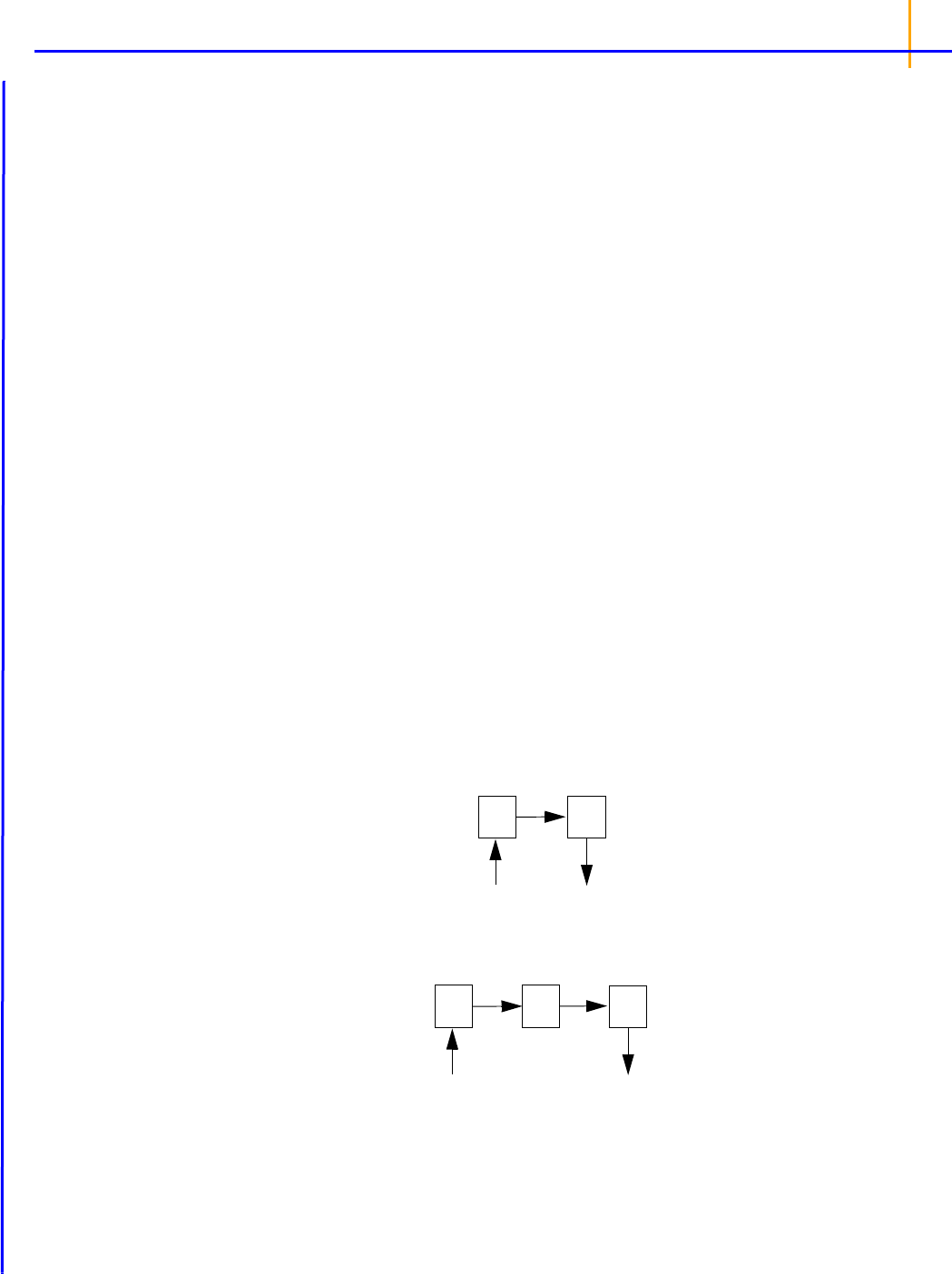
The following images illustrate how this can be visualized.
Figure 2-1. Model for ntr = 0 (the smallest possible value)
Figure 2-2. Model for ntr = 1
in out
0Aa
k
in out
01Aa
kk
Phoenix Modeling Language
Reference Guide
26
2
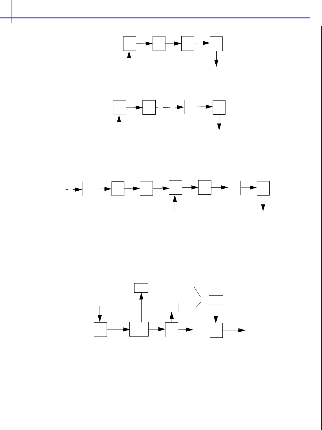
Figure 2-3. Model for ntr = 2
Figure 2-4. Model for ntr = more
The following model is implemented with extra upstream compartments, and ntr effectively chooses
which upstream compartment will be considered compartment 0 and will receive doses:
Figure 2-5. Model with extra upstream compartments
Doses go into compartment 0, as well as any additional rate given by the in keyword. The value is
read from the final compartment, which can have a supplemental output rate given by the out key-
word. (If artificial dosing is done, such as by saving Aa = Aa + d in a sequence statement, it is
understood as adding d to compartment 0, not to compartment Aa.)
The following model shows how the interpolation is done, where x is an auxiliary compartment.
Figure 2-6. Interpolation process
Disclaimer: In the case where ntr is an integer, the transit statement is completely accurate for
all inputs. If ntr is not an integer, but dosing consists of bolus doses sufficiently separated in time, it
is also completely accurate. However, if ntr is a small non-integer, like 0.5, and multiple boluses
occur close together or an infusion is given, the output in Aa is under-predicted by as much as 5%.
The under-prediction becomes progressively smaller as ntr increases, but is always zero if ntr is
an integer. This is an artifact of the interpolation formula used for fractional values of ntr.
in out
012Aa
kkk
in out
01ntr Aa
kk
in out
012Aa
kk
k
k
k
log
Dose
0xAa
kkka
log
exp
k
*(1-f)
ktr**C(n)
f
*
+
f = ntr - ntr
C(ntr) = Gamma(ntr+1) / Gamma (ntr+1) * (ntr+1)f
ntr

Language Structure and Syntax
Modeling syntax
27
2
Action code
This section discusses action code and what it does. Some basic action code statements include
dobefore, doafter, sequence, and sleep.
First, the framework within which action code works must be explained.
A PML model either is or is not truly time-based. A model is truly time-based if:
– It contains a deriv or a urinecpt statement.
– It implicitly contains a deriv statement, such as an event or count statement, which
causes the model to calculate a hidden differential equation that accumulates, or integrates,
the hazard rate.
– It contains a cfMicro or a cfMacro statement.
If a model is truly time-based, then it automatically contains a variable called t, and time is assumed
to be the independent variable. The model’s input dataset must contain columns for time values and
for any covariate values. Only truly time-based model can use multiple dose inputs.
If a model is not truly time-based, then covariates are its only inputs. Since the model does not auto-
matically know what the independent variable is, it must be specified via syntax in the observe state-
ment, such as:
observe(EObs(C) = …)
where the (C) tells the model that C is the independent variable.
In a non time-based model, there is no default variable for time (t) as there is for a time-based model.
To include this variable, the user needs to do one of the following:
– Change the model into a time-based model by including a statement such as:
deriv(foo = 0)
Or
– Make t a covariate (e.g., covariate(t), be sure to map t and include the following
statement to indicate the independent variable:
observe(Cobs(t) = C + CEps)
Or
– Make Time a covariate (e.g., covariate(Time)), then replace t with Time in the
model, and check the mapping.
Note: If C is not given on the same data row as EObs, that observation is ignored. If the user does not
specify the independent variable in the observe statement, as for example observe(EObs =
E*exp(eps)), observations of EObs are processed regardless, even though they are not asso-
ciated with a corresponding independent variable.
If a model is truly time-based, it executes in a recursive fashion. That means model execution con-
sists of a series of continuous simulation intervals, with stops between each interval.
In a continuous simulation interval, the state of the model evolves forward through time under control
of an ODE solver such as Matrix Exponent, Runge-Kutta (non-stiff), Gear (stiff, analytic and finite dif-
ference Jacobian), Closed-Form (no ODE solver used), or a combination of these four.
Discontinuous actions can occur during a stop between continuous simulation intervals. Discontinu-
ous actions include:
– delivering a dose into a compartment all at once as opposed to spreading the delivery over
time
– start of an infusion
– end of an infusion

Phoenix Modeling Language
Reference Guide
28
2
– taking of an observation
– setting a covariate value
– actions associated with an observation or dose, when they are specified with a dobefore
or doafter action block
– actions specified with any sequence block.
Variables in a model fall into categories, depending on whether they can or cannot be modified when
the model is stopped.
• Integrator variables (variables on the left side of deriv statements) such as compartment
amounts, can be modified when the model is stopped. When the model is simulating, these vari-
ables are controlled by the ODE solver.
• Variables introduced with the real keyword, such as real(G), can be modified when and only
when the model stops running.
• Variables introduced with only an assignment statement, such as C = A/V, cannot be mod-
ified when the model is stopped. The variables are considered to only be functions of the continu-
ous model state.
It is allowable to have multiple assignment statements assigned to the same variable, in which
case the order between them matters. For example: E = E0; E = E + E1; etc. This state-
ment is essentially a single assignment statement because all assignments could all be collapsed
into one assignment statement. Note that variables on the right-side of assignment statements
must be defined prior to their use.
A block refers to a pair of curly brackets {...} with zero or more statements in between them.
The sequence statement, of the form sequence{...}, specifies a sequence of actions to be per-
formed when the model is stopped. This sequence acts like a typical programming language
sequence in that order matters, because the sequence statements are performed one at a time, in
order.
Caution: In PML models, sequence and assignment statements are the only statements in which
order matters.
For all other statements in PML models, the order of the statements does not matter. This means that
the statements inside a sequence block are very different from other statements in PML models.
Sequence statements consist of:
– Assignments (only for variables that can be modified when the model is stopped)
– if(test-expression) statement-or-block [else statement-or-block]
– while(test-expression) statement-or-block
– sleep(duration-expression)
– function calls
These statements only run when the model is stopped. The model is considered to be “stopped”
before it is executed. This means that sequence statements are executed before the model is
“started”, and run until a sleep statement is encountered.
When a sleep statement is encountered, its argument, which is a delta-time, is calculated and then
the sequence stops executing. The sequence is then put into a queue until it is used at a future time.
At that time, the model stops, and the sequence block commences executing where it left off.
A model can contain multiple sequence blocks, and they are executed in a nearly parallel manner. If
there are multiple sequence blocks, no assumptions should be made about which block is exe-
cuted first.

Language Structure and Syntax
Modeling syntax
29
2
Because model execution stops for dose and observation events, actions can be performed at those
times. For example:
observe(CObs = C + eps, doafter = {A = 0;})
In this example, immediately after CObs is observed, variable A is set to 0 (zero), where A could be
the drug amount in a compartment. The action block consists of curly brackets {…} containing zero or
more statements. The statements can be optionally separated by semicolons.
Note: The statements allowed in the observe statement as the same as those allowed in the
sequence statement, except that sleep is not allowed in the observe statement.
Observations
Observations are the link between the model and the data. The model describes the relationships
between covariates, parameters, and variables. The data represent a random sampling of the system
that the model describes. The various types of observation statements that are available in the Phoe-
nix Modeling Language serve to build a statistical structure around the likelihood of a given set of
data.
Observation statements are used to build the likelihood function that is maximized during the model-
ing process. The observation statements indicate how to use the data in the context of the model.
–“Count statement for Count models” on page 29
–“Event statement for Survival models” on page 32
–“LL statement for Log Likelihood models” on page 34
–“Multi statement for Multinomial models” on page 34
–“Observe statement for Normal-inverse Gaussian Residual models” on page 37
–“Ordinal statement for Ordinal Responses” on page 37
–“Observation statement action codes:” on page 37
Count statement for Count models
count(observed variable, hazard expression[, options][, action code])
Similar to event, but instead of observing an occurrence variable, an occurrence count is
observed. The log-likelihood is based on a Poisson or Negative Binomial distribution whose mean
is the integrated hazard since the last observation. The options are:
, beta = <expression>
The presence of the beta option makes the distribution Negative Binomial, where the variance is
var = mean*[1+mean*alpha^power), and alpha=exp(beta)
, power = <expression>
Power of alpha, default(1). Zero-inflation can be applied to either the Poisson or Negative-Bino-
mial distributions, in one of two ways, by means of simply specifying the extra probability of zero,
by giving the zprob argument, or by giving an inverse link function with ilink and its argument
with linkp.
, zprob = <expression>
Zero-inflation probability, default(0) (incompatible with following two options)
, link = “ilogit”, “iprobit”
Or other inverse link function. If not specified, it is blank.
, linkp = <expression>
Argument to inverse link function

Phoenix Modeling Language
Reference Guide
30
2
, noreset
When present, this option will prevent the accumulated hazard from resetting after each observa-
tion.
For the default Poisson distribution, the mean and variance are equal. If that shows inadequate vari-
ance, use of the beta option, with optional power, may be indicated. Care should be taken, since if
the value of beta*power becomes too negative, that means the distribution is very close to Pois-
son and the Negative Binomial distribution may incur a performance cost.
Note: The Negative-Binomial Distribution log likelihood expression can generate unreasonable results
for reasonable cases. For example, if count data that is actually Poisson is used, the parameter r
in the usual (r,p) parameterization can become very large (and p becomes very small). The large
value of r can cause a problem in the log gamma function that is used in the evaluation. So such
data, which is completely reasonable, may give an unreasonable fit if care is not taken in how the
log likelihood is evaluated numerically.
All about Count models
Observing a count, such as the number of episodes of vertigo over a prior time interval of one week,
is also a hazard-based measurement. The simplest model of the count is called a Poisson distribu-
tion and it is closely related to the coin-toss process in the time-to-event model (discussed in “All
about Time-to-Event modeling” on page 32). In this model, the mean (average) count of events is
simply the accumulated hazard. One can think of the hazard as simply the average number of events
per time unit, so the longer the time, the more events. Also, in the Poisson distribution, the variance of
the event count is equal to the mean.
In some cases, if one tries to fit a distribution to the event counts, it is found that the variance is
greater than what a Poisson distribution would predict. In this case, it is usual to replace the Poisson
distribution with a Negative Binomial distribution, which is very similar to the Poisson, except that it
contains an additional parameter indicating how much to inflate the variance.
Another alternative is to notice that a count of 0 (zero) is more likely to occur than what would be
predicted by either a Poisson or Negative Binomial distribution. If so, this is called “zero inflation.” All
of these alternatives can be modeled with the count statement.
The simplest case is a Poisson-distributed count:
count(n, h)
where n is the name of the observed variable, taking any non-negative integer value. h is the hazard
expression, which can be time-varying.
To make it a Negative Binomial distribution, the beta keyword can be employed:
count(n, h, beta = b)
where b is the beta expression, taking any real value. The beta expression inflates the variance of the
distribution by a factor (1 + exp(b)), so if b is strongly negative, exp(b) is very small, so the
variance is inflated almost not at all. If b is zero or more, then exp(b) is one or more, so the vari-
ance is inflated by an appreciable factor. The reason for encoding the variance inflation this way is to
make it difficult to have a variance inflation factor too close to unity, because 1) that makes it equiva-
lent to Poisson, and 2) the computation of the log-likelihood can become very slow.
If the beta keyword is present, an additional optional keyword may be used, power:
count(n, h, beta = b, power = p)
in which case, the variance inflation factor is (1 + exp(b)^p), which gives a little more control
over the shape of the variance inflation function. If the power is not given, its default value is unity.

Language Structure and Syntax
Modeling syntax
31
2
Whether the Poisson or Negative Binomial distribution is used, zero-inflation is an option, by using the
zprob keyword:
count(n, h, zprob = z)
where z is the additional probability to be given to the response n = 0. Alternatively, the probability
can be given through a link function, using keywords ilink and linkp:
count(n, h, ilink = ilogit, linkp = x)
where x is any real-numbered value, meaning that ilogit(x) yields the probability to be used for
zero-inflation.
Count models can of course be written with the LL statement, but it can get complicated. In the simple
Poisson case, it is:
deriv(cumhaz = h)
LL(n, lpois(cumhaz, n), doafter = {cumhaz = 0})
where cumhaz is the accumulated hazard over the time interval since the preceding observation,
and n is the observed number of events in the interval. lpois is the built-in function giving the log-
likelihood of a Poisson distribution having mean cumhaz. After the observation, the accumulated
hazard must be reset to zero, in preparation for the following observation.
If the simple Poisson model is to be augmented with zero-inflation, it looks like this:
deriv(cumhaz = h)
LL(n, (n == 0 ? log(z + (1-z)*ppois(cumhaz, 0)):
log(1-z) + lpois(cumhaz, n)
)
, doafter = {cumhaz = 0}
)
where z is the excess probability of seeing zero. Think of it this way: before every observation, the
subject flips a coin. If it comes up “heads” (with probability z), then a count of zero is reported. If it
comes up “tails” (with probability 1-z), then the reported count is drawn from a Poisson distribution,
which might also report zero. So, if zero is seen, its probability is z + (1-z)*pois(cumhaz,
0), where pois is the Poisson probability function. On the other hand, if a count n > 0 is seen, the
coin must have come up “tails,” so the probability of that happening is (1-z)*pois(cumhaz, n).
The log-likelihood given in the LL statement is just the log of all that.
If it is desired to use the link function instead of z, z can be replaced by ilogit(x). (There are a
variety of built-in link functions, including iloglog, icloglog, and iprobit.)
If the Negative Binomial model is to be used, because Poisson does not have sufficient variance, in
place of:
lpois(cumhaz, n)
the expression:
lnegbin(cumhaz, beta, power, n)
is used instead, where the meaning of beta and power are as explained above. If beta is zero,
that means the variance is inflated by a factor of two. Typically, beta would be something estimated.
If it is not desired to use the power argument, the default power of one should be used.

Phoenix Modeling Language
Reference Guide
32
2
Event statement for Survival models
event(observed variable, expression [, action code])
Specifies an occur observed variable, which has two values: 1, which means the event
occurred, or 0, which means the event did not occur. The hazard is given by the expression.
The event statement creates a special hidden differential equation to accumulate, or integrate, the
hazard rate, which is defined by the expression in the second argument. This integration is reset
whenever the occur variable is observed, so the integral extends from the time t0 of the previous
occur observation to t1, the time of the current observation. Let cum_hazard = integral of the haz-
ard during the period [t0,t1]:
cum_hazard = .
Then the probability that an event will not occur in the period is: S=exp(-cum_hazard). There-
fore, if the period terminates with an observation occur = 0 at t1, the likelihood is S. If the period
terminates at t1 because an event occurred at time = t1 (occur = 1), then the likelihood is
S*hazard(t1), where hazard(t1) is the hazard rate at t1. These likelihood computations are
performed automatically whenever an occur observation is made.
Note: The observations of 0 (no event) can occur at pre-defined sampling points, but observations of 1
(event occurred) are made at the time of the event.
Event models are inherently time based, and require a mapping for a time value.
All about Time-to-Event modeling
Consider a process modeled as a series of coin-tosses, where at each toss, if the coin comes up
“heads,” that means an event occurred and the process stops. Otherwise, if it comes up “tails,” the
coin is tossed again. The graph below shows that process if the probability of “heads” is 0.1, and the
probability of “tails” is 0.9.
Figure 2-7. Coin toss probability graph
It is easy to see that the probability of getting to time 5 without getting a “heads” is 0.9 multiplied by
itself 5 times. Similarly, the probability of getting a “heads” at time 5 is 0.1 multiplied by the probability
of getting to time 4 without getting “heads” or 0.94 * 0.1.
To put it in symbols, if the probability of “heads” is p, then the probability of “heads” at time n is:
(1-p)(1-p) … n-1 times … (1-p) p
Since in model fitting the log of the probability is desired, and since, if p is small, log(1-p) is basically
-p, it can be said that the log of the probability of “heads” at time n is:
-p -p … n-1 times … -p + log(p)
Note that p does not have to be a constant. It can be different at one time versus another.
httd
t0
t1

Language Structure and Syntax
Modeling syntax
33
2
The concept of “hazard,” h, is simply probability per unit time. So if one cuts the time between tosses
in half, and also cuts the probability of “heads” in half, the process has the same hazard. It also has
much the same shape, except that the tossing times come twice as close together. In this way, the
time between tosses can become infinitesimal and the curve becomes smooth.
If one looks at it that way, then the probability that “heads” occurs at time t is just:
where the exponential part is the probability of no “heads” up to time t, and h(t) is the instantaneous
probability of “heads” occurring at time t. Again, note that hazard h(t) need not be constant over time.
If h(t) is simply h, then the above simplifies to the possibly more familiar:
The log of the probability is:
In other words, it consists of two parts. One part is the negative time integral of the hazard, and that
represents the log of the probability that nothing happened in the interval up to time t. The second part
is the log of the instantaneous hazard at time t, representing the probability that the event occurred at
time t. (Actually, this last term is as a protection against the possibility that h(t) is
zero.)
The event statement models this process. It is very simple:
event(occur, h)
where h is an arbitrary hazard function, and occur is the name of an observed variable. occur is
observed on one or more lines of the input data. If its value is 1 on a line having a particular time, that
means the event occurred at that time, and it did not occur any time prior, since the beginning or since
the time of the prior observation of occur.
If the observed value of occur is 0, that means the event did not happen in the prior time interval,
and it did not happen now. This is known as “right censoring” and is useful to represent if subjects, for
example, withdraw from a study with no information about what happens to them afterward. It is easy
to see how the log-likelihood of this is calculated. It is only necessary to omit the log(h) term.
Other kinds of censoring are possible. If occur equals 2, that means the event occurred one or more
times in the prior interval, but it is not known when or how many times. If occur is a negative number
like -3, that means the event occurred three times in the prior interval, but it is not known when.
There is a special value of occur, -999999, meaning there is no information at all about the prior
interval, as if the subject had amnesia. These are all variations on “interval censoring.” The log-likeli-
hoods for all these possibilities are easily understood as variations on the formulas above.
This can be done with the log-likelihood (LL) statement instead, as follows:
deriv(cumhaz = h)
LL(occur, -cumhaz + occur*log(h), doafter = {cumhaz = 0})
hxxd
0
t
–
exp ht
ht–hexp
hxxd
0
t
–
htexplog hxxd
0
t
–htlog+=
ht 10 8–
+log

Phoenix Modeling Language
Reference Guide
34
2
The deriv statement is a differential equation that integrates the hazard. The LL statement says that
variable occur is observed and it is either 1 (the event occurred) or 0 (it did not occur). It gives the
log-likelihood in either case. Then, after performing the observation, the accumulated hazard is set to
zero. This allows for the possibility of multiple occurrences.
LL statement for Log Likelihood models
LL(observed_variable, expression[, simulate = {simulation_code}]
[, action code])
This statement specifies there is an observed variable, and when it is observed, its log-likelihood is
the given expression. Optional action code is executed before or after the observation. If the “simu-
late” keyword is present, then during simulation or predictive check, the simulation code can assign a
value to the observed variable.
The following is an example of a time to event model, illustrating how simulate can work on the LL
statement.
covariate(DOSETOT,cycledays,uni01,timeforhistograms)
deriv(E = Kin *DOSETOT/cycledays - Kout * E)
sequence{E = E0}
real(u, i, prob)
LL(EObs
,-E + EObs*log(E) -lgamm(EObs+1)
, simulate = {
u = unif()
prob = 0
i = 0
prob = prob + exp(-E + i*log(E) -lgamm(i+1))
while(u >= prob){
prob = prob + exp(-E + i*log(E) -lgamm(i+1))
i = i + 1
}
EObs = i
}
)
In the example above, EObs is the observed variable and -E + EObs*log(E)
-lgamm(EObs+1) is the expression. The optional action follows the simulate keyword. It is sep-
arate from the last action code [, action code] (e.g. [,doafter={E=0}]).
Multi statement for Multinomial models
multi(observed variable, inverse link function(, expression)*
[, action code])
This statement specifies an integer-valued categorical observed variable. The name of an inverse
link function is given, such as ilogit. The next part of the statement is a series of offset
expressions in ascending order, such as C-X01 or C-X12, where X01 is the value of C that evenly
divides the response between zero and one, and X12 divides the response between one and two.
This relationship between offset expressions is illustrated below, but without using a variable in the
expression. The domain of the parameters X01 and X12 exists along the unbounded real line. The
goal is to divide the range of the inverse function (0,1) into the probabilities of the categorical observa-
tions. This preserves the constraint that the sum of the probabilities equals one.
In the illustration below, the first breakpoint, proceeding from left to right, is X01. The value of the
inverse function (ilogit, in this case) is taken at X01 and P0, which is the probability of the first cate-
gory, is P0 = ilogit(X01). The next breakpoint is X12, and the probability of observing the sec-
ond category is P1 = ilogit(X12) - ilogit(X01), which is the cumulative probability
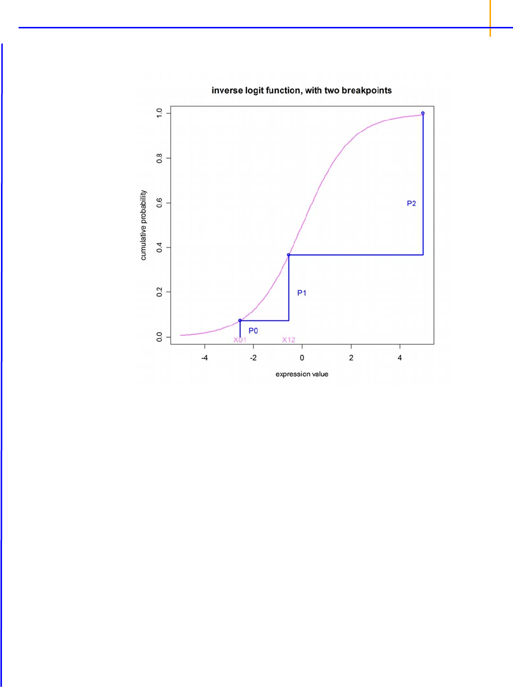
Language Structure and Syntax
Modeling syntax
35
2
between the first and second breakpoints. The third observation has probability P2 = 1 - P0 -
P1, which is the remainder of the cumulative probability.
Figure 2-8. Relationship between offset expressions
It is simple to extend the example beyond simple values of X01 and X12, to include a function of
covariates. Given the relationship between the category probabilities and the probabilities, it is easy to
why the initial estimates of the parameters should be given in such a way as to not cause the com-
puted values of any of the probabilities to be negative. It is imperative that initial conditions be chosen
carefully to ensure convergence.
All about Multinomial (ordered categorical) responses
Consider a model in which an observation can take values zero, one, and two. No matter what value
concentration C is, any value of the observation is possible, but C affects the relative probabilities of
the observed values. If C is low, the most likely observation is zero. If it is high, the most likely obser-
vation is two. In the middle, there is a value of C at which an observation of one is more likely than at
other values of C.
The following figure illustrates the concept. At any value of C, there is a probability of observing zero,
called p0. Similarly for one and two. The probability is given by the inverse of a link function, typically
logit. In this picture, there are two curves. The left-hand curve is ilogit(C - c1) and it is the
probability that the observation is ³1. The right-hand curve is ilogit(C - c2), and it is the proba-
bility that the observation is ³2. The probability of observing one (p1) is the difference between the
two curves. When doing model-fitting, the task is to find the optimum values c1 and c2. Note that c2
is the value of C at which the probability of observing two (p2) is exactly 1/2, and that c1 is the value
of C at which the probability of observing a value greater than or equal to one (p1+p2) is exactly 1/
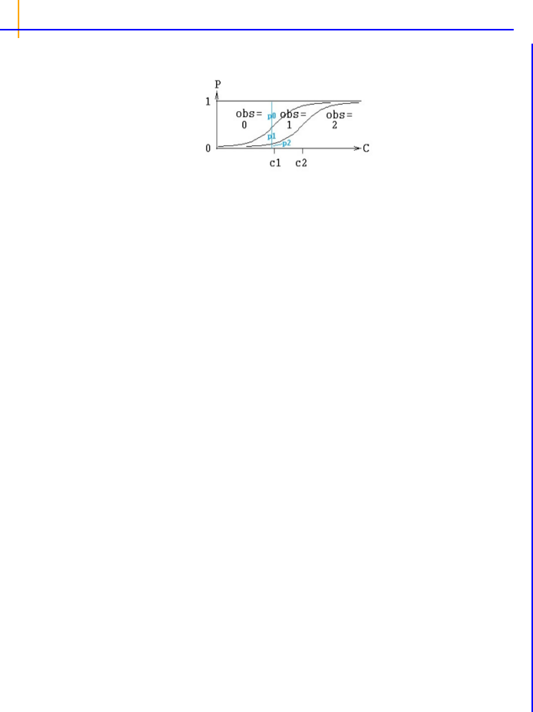
Phoenix Modeling Language
Reference Guide
36
2
2. Note also that c1 and c2 have to be in ascending order, resulting in the curves being in descend-
ing order.
Figure 2-9. Multinomial responses
There are statements in PML for modeling such a response: multi, and ordinal, and it can also
be done with the general log-likelihood statement, LL. The multi statement for the above picture is
this:
multi(obs, ilogit, C - c1, C - c2)
obs is the name of the observed variable, ilogit is the inverse link function, and the remaining two
arguments are the inputs to the inverse link function for each of the two curves. Since c1 and c2 are
in ascending order, the inputs for the curves, C - c1 and C - c2, are in descending order.
A more widely accepted way to express such a model is given by logistic regression, as in:
P(obs >= i) = ilogit(b*C + ai)
where b is a slope (scale) parameter, and each ai is an intercept parameter. The ordinal statement
expresses it this way:
ordinal(obs, ilogit, C, b, a1, a2)
where the ai are in ascending order. This is equivalent to the multi statement:
multi(obs, ilogit, -(b*C+a1), -(b*C+a2))
where, since the ai are in ascending order, the arguments -(b*C+ai) are in descending order, as
they must be for the multi statement.
To do all this with the log-likelihood statement (LL) requires calculating the probabilities oneself, as
shown below. Using the original parameterization with c1 and c2:
pge1 = ilogit(C - c1)
pge2 = ilogit(C - c2)
LL(obs, obs == 0 ? log(1 - pge1):
obs == 1 ? log(pge1 - pge2):
log(pge2 – 0)
)
The first statement computes the first curve, the probability that the observation is greater than or
equal to one, pge1. The second statement computes the second curve, the probability that the
observation is greater than or equal to two, pge2. Note that these are in descending order, because
the probability of observing two has to be less than (or equal to) the probability of observing one or
two.
The third statement says obs is the observed variable, and if its value is zero, then its log-likelihood is
the log of the probability of zero, where the probability of zero is one minus the probability of greater
than or equal to one, i.e., log(1 - pge1). Similarly, if the observation is one, its probability is
pge2 - pge1. Note that since pg1e > pge2, the probability of one is non-negative. Similarly, if
the observation is two, its probability is pge2 - pge3, where pge3 is zero because three is not a
possible observation.

Language Structure and Syntax
Modeling syntax
37
2
If, on the other hand, one were to use the typical slope-intercept parameterization from logistic regres-
sion, the first two lines of code would look like this:
pge1 = ilogit(-(b*C+a1))
pge2 = ilogit(-(b*C+a2))
and the LL statement would be the same.
Observe statement for Normal-inverse Gaussian Residual models
observe(observedVariable([independentVariable]) =
expression[, bql][, action code])
The above statement specifies that the observedVariable is a function of some prediction and
some Gaussian error. The bql option specifies that a lower limit of quantification can be applied to
this observation, allowing for occurrence observations to be included.
If action code is given, that indicates actions to be performed before or after each observation. If there
are no differential equations, the independentVariable for the observations can be specified.
This allows the Phoenix Model object to produce the appropriate output plots and worksheets.
For example, a Michaelis-Menten model of reaction kinetics can be written as:
observe(RxnRate (C) = Vmax*C/(C+Km) + eps)
Ordinal statement for Ordinal Responses
ordinal(observedVariable, inverseLinkFunction,
explanatoryVariable, beta, alpha0, alpha1, …)
For example:
ordinal(Y, ilogit, C, slope, intercept0, intercept1, …)
where the intercepts are in numerically ascending order. It fits the model:
P(Y ? i | C) = ilogit(C*slope + intercepti)
And if there are m values of Y, they are 0, 1, … m-1, and there are m-1 intercepts.
This is equivalent to the multi statement:
multi(Y, ilogit, -(C*slope+intercept0), -(C*slope+intercept1), …)
Observation statement action codes:
Action codes may be given, within an observation statement, which specify computations to make
either before or after an observation is made. For instance, if there is a urine compartment that is
emptied at each observation, part of the model may resemble this:
deriv(urineVol = gfr)
deriv(urine_amt = gfr*Cp*fu)
observe(Uvol = urineVol + epsUv, doafter={urineVol=0})
Math and special functions
Phoenix PML supports a majority of the intrinsic math functions in the Cmath.h library (see “Math
functions” on page 92 in Appendix D for a list of supported functions). In general, the function names
are the same or very similar to the Fortran (and hence NONMEM) names of the same functions.
There are some differences, however. For example, fabs(x), which applies to floating-point values,
computes the absolute value of x. Do not use ABS(x), the Fortran name for absolute value, as this
will give incorrect results when called with real number arguments.

Phoenix Modeling Language
Reference Guide
38
2
In addition to the Cmath.h library functions, Phoenix PML also supports a variety of special func-
tions that are useful in PK/PD modeling, such as the cumulative normal distribution phi(x), the
inverse cumulative normal distribution probit(x), the Lambert W-function lambertw(x) for
closed-form solutions to one-compartment Michaelis-Menten nonlinear elimination models, as well as
various link and inverse link functions, and some special functions useful for defining log likelihoods in
certain count-type models. A complete list is provided in Appendix A.
Function names are typically written in lower case. For example, functions like exp, sqrt, log, are
lower case, because PML uses the standard C library, in which lower case is the norm. This differs
from other programs like NONMEM, which are not case sensitive. Spelling a function name incor-
rectly will result in a linker error message saying the function is undefined.
If numeric constants are needed in the code, and there is a concern about possible performance of
calculating them, a simple way to include them is the following:
double(pi, e)
sequence {
pi = 3.1415926535897932384626433832795
e = 2.7182818284590452353602874713527
}
These are executed only once per subject, take essentially zero time to execute, and are far more
precise than can possibly be required.
Do not be concerned about the performance of secondary parameter calculations, such as half-life,
because those are only calculated once, after all model fitting is completed.
Dosing
Dosing can be specified in two places, the model file and the column definition file. For more, see
“Modeling project files” on page 14.
In the model, the dosepoint statement described under “Modeling syntax” on page 21 can contain
several options, including:
–tlag = expr dose delivery is delayed by expr
–duration = expr 0-order infusion spanning expr time units
–rate = expr 0-order infusion of expr units/time unit
–bioavail = expr expr is the fraction delivered
The dosepoint statement can also include statements to be executed before and/or after delivery of
the dose, as follows.
dobefore = block
doafter = block
Covariates
Covariates can be simple or interpolated. See “Modeling project files” on page 14 for more informa-
tion.
covariate(covariate_name)
This specifies that there is a covariate with the given name. For time-varying covariates, the
covariate statement extrapolates backward. So, for example, if a covariate is given at time =
1, 2, and 3 to be 10, 20, and 30, respectively, then the covariate value in [0,1] is 10, in [1,2] is 20,
and in [2,3] is 30.
fcovariate(covariate_name)

Language Structure and Syntax
Modeling syntax
39
2
This is the same as covariate, except that it also specifies the covariate has forward direction.
fcovariate extrapolates forward. So, for example, if a covariate is given at time = 1, 2, and 3
to be 10, 20, and 30, respectively, the fcovariate value for [1,2] is 10, for [2,3] is 20, and for times
beyond 3 (if any) it is 30. If no covariate value is given at time = 0, the fcovariate value for [0,1] is
also 10, as the first value propagates backward as well as forward.
There are actually two different ways to indicate forward direction, by using the fcovariate
statement in the model text, or by using fcovr in the column definition text (or both).
interpolate(covariate_name)
This also specifies that there is a covariate with the given name, however, the value of the covari-
ate varies linearly between time points at which it is set in time-based models. This feature should
be used with caution, because in some cases it makes a linear model nonlinear so it cannot use
the matrix exponent ODE solver.
This can happen in a simple PK model parameterized by Cl and V, if V is a function of bodyweight
BW, and BW is interpolated. Alternatively if the model is parameterized by Ke and V, it is not
affected because V does not enter the differential equations.
In a text model, if a covariate is categorical, its name must be followed by empty parentheses:
covariate(Form())
This informs the UI that the covariate is categorical, and thus available for stratification.
Modeling discontinuous events
There are many kinds of models involving discrete time-based events at which discontinuous
changes can occur in a model. The following is a partial example of an entero-hepatic reflux model.
1 deriv(a = -a*k10 - a*k1b + g*kg1)
# central cpt
2 deriv(b = a*k1b - qbg)
# bile cpt
3 deriv(g = qbg - g*kg1)
# gut cpt
4 real(qbg)
#qbg is flow rate from bile to gut
5 stparm(tCycle=…, tReflux=…)
# times are parameters
# introduce the time sequence:
6 real(i)
7 sequence{
8 i = 0;
9 while(i<10){
10 i = i + 1;
11 qbg = 0;
12 sleep(tCycle - tReflux);
13 qbg = (b/tReflux);
14 sleep(tReflux);
15 qbg = 0;
16 }
17 }
The model has three compartments: a for plasma, b for bile, and g for gut. Normally the compound
flows from gut to plasma and from plasma to bile, as well as flowing through the normal elimination

Phoenix Modeling Language
Reference Guide
40
2
path. There is also a flow from bile to gut, which is the reflux path. This is modeled as a zero-order
flow of rate qbg. The flow is turned on and off to model the reflux.
Lines 1-3 give the differential equations for the three compartments. The variable qbg is a variable
representing the flow rate from bile to gut, and it is initially zero.
Line 4 declares a variable, qbg, which will be used in some of the equations and statements.
Line 5 designates that there are two structural parameters giving the cycle time between reflux
events (tCycle) and the duration (tReflux) of each event.
Line 6 declares a variable, i, which will be used in some of the equations and statements.
Lines 7-17 are grouped with the sequence keyword. This introduces time-sequenced procedure
into the model.
Line 8 sets the initial value for the variable i to zero.
Line 9 groups the next six statements into a loop that will repeat up to 10 times.
Line 10 adds one to the value of i (number of iterations).
Line 11 sets the initial value for the variable qbg to zero.
Line 12 allows tCycle - tReflux time units to pass.
Line 13 turns on the reflux by setting qbg to the rate necessary to empty the bile compartment within
duration tReflux.
Lines 14-15 say to wait for tReflux time units, and then turn off the flow, after which the cycle
repeats.
Discrete and distributed delays
Transit compartment models, described by systems of ordinary differential equations (ODEs), have
been widely used to describe delayed outcomes in pharmacokinetics and pharmacodynamics stud-
ies. The obvious disadvantage for this type of model is it requires manually finding proper values for
the number of compartments, and hence it is time-consuming. It is also difficult, if not impossible, to
do population analysis using this model. In addition, it may require many differential equations to fit
the data and may not adequately describe some complex features.
To alleviate these advantages, a distributed delay approach was proposed in “Hu, Dunlavey, Guzy,
and Teuscher (2018)” to model delayed outcomes in pharmacokinetics and pharmacodynamics stud-
ies. It involves convolution of the signal to be delayed (S) and the probability density function (g) of the
delay time,
Thus, for the distributed delay approach, the delay time may vary among signal mediators (e.g., drug
molecules or cells), and hence it is a natural extension of the discrete delay approach that
in which case, where the delay time is assumed to be the same (i.e., ) for all signal mediators.
(1)
(2)
gSt –d
0
+
St –

Language Structure and Syntax
Modeling syntax
41
2
Differential equations involving discrete delays and/or distributed delays are called delay differential
equations (DDEs). The difference between ODEs and DDEs is that the future state of the system gov-
erned by ODEs is totally determined by its present value while for DDEs it is determined not only by
its present value, but also by its past. This means that, for DDEs, one has to specify the values of the
system state prior to the system starts (assuming throughout that the system starts at time zero). For
example, for the following differential equation with a distributed delay,
one has to specify the values of S(t) over all negative t; that is, one has to specify S0, which is often
called the history function.
It was shown in “Hu, Dunlavey, Guzy, and Teuscher (2018)” that the distributed delay approach is
general enough to incorporate a wide array of pharmacokinetic and pharmacodynamic models as
special cases, including transit compartment models, effect compartment models, indirect response
models with production either simulated or inhibited, typical absorption models (either zero-order or
first-order absorption), and a number of atypical (or irregular) absorption models (e.g., parallel first-
order, mixed first-order, and zero-order, inverse Gaussian, and Weibull absorption models). This was
done through assuming a specific distribution form for the delay time.
Specifically, transit compartment models are based on the assumption that the delay time is Erlang
distributed, with shape and rate parameters respectively determining the number of transit compart-
ments and the transition rate between the compartments. Note that Erlang distribution is a special
case of the gamma distribution, which allows for non-integer shape parameters. Hence, distributed
delay models with delay time assumed to be gamma distributed (referred to as gamma distributed
delay models) are natural extension of transit compartment models. Examples for extending transit
compartment models to their corresponding gamma distributed delay models can be found in “Hu,
Dunlavey, Guzy, and Teuscher (2018)” and “Krzyzanski, Hu, and Dunlavey (2018)”.
The delay function
The delay function in PML can be used for both discrete and gamma distributed delays, and its syntax
is given as follows:
delay(S, MeanDelayTime
[, shape = ShapeParam]
[, hist = HistExpression]
)
If the shape option is not provided, then it returns the value of S(t − MeanDelayTime). Otherwise, it
returns the value of “1” with g assumed to be the probability density function of a gamma distribution
with shape parameter being ShapeParam specified by the shape and mean being MeanDelayTime.
The hist option is used to specify the value of S prior to time 0; that is, if t < 0, then S(t) = HistExpres-
sion, which is required to be independent of time t, but can depend on variables that are defined at
time 0 for the subject, such as covariates, fixed and random effects. If the hist option is not provided,
then it is assumed that S(t) = 0 for t < 0.
It should be noted that the delay function relies on the fact that ODE solvers use shorter step sizes
in the vicinity of rapid changes. Hence, it will not work in the presence of methods that have large step
(3)
St ftSt gSt –d
0
+
t0
St
S0tt0
=
=

Phoenix Modeling Language
Reference Guide
42
2
sizes, such as matrix exponent or closed-form. Even though there is no restriction on the number of
delay functions put in a model, it should be used sparingly to avoid performance issue.
For the discrete delay function, the delay time can be estimated, and for the distributed delay case,
both the mean and shape parameter for the gamma distribution can be estimated. In addition, the
delay function can be put on the right-hand side of a differential equation, and hence can be used to
numerically solve a differential equation with either discrete delays or gamma distributed delays, no
matter whether the signal to be delayed, S, depends on model states or not. For example, the delay
function can be used to numerically solve the well-known Hutchinson equation (a logistic growth
model with a discrete delay):
where r denotes the intrinsic growth rate, K is the carrying capacity, and S0 is a positive constant. The
PML code for this model is given as follows:
deriv(S = r * S * (1 - delay(S, tau, hist = S0)/K))
sequence{S = S0}
The delay function can also be used to numerically solve the following logistic growth model with a
distributed delay:
where g is the probability distribution function of a gamma distribution with shape parameter being
ShapeParam and mean being MeanDelayTime. The PML code for this model is given as follows:
delayedS = delay(S, MeanDelayTime,
shape = ShapeParam,
hist = S0
)
deriv(S = r * S * (1 - delayedS/K))
sequence{S = S0}
A simple simulation of the logistic growth model with a gamma distributed delay, (5), is given in exam-
ple project LogisticGrowthModelWithGammaDistributedDelay.phxproj (located in
…\Examples\NLME). The project demonstrates that (5) can exhibit much richer dynamics than its
corresponding ODE.
(4)
(5)
(6)
S
·t rS t1St –
K
------------------
–
St S0–t0
=
=
S
·t rS t11
K
----gSt –d
0
+
–
St S0t0
=
=
S
·t rS t1St
K
---------
–
S0 S0
=
=

Language Structure and Syntax
Modeling syntax
43
2
For example, it may produce an oscillation around the carrying capacity while the corresponding ODE
cannot. In addition, adjusting the mean delay time can achieve the desired type of oscillations (either
damped or sustained oscillations).
The delayInfCpt statement
Note that, the signal to be delayed, S, in the delay function cannot contain dosing information from the
input data set. Hence, it cannot be used for the absorption delay case. To achieve this, a compartment
modeling statement, delayInfCpt, was added to PML with its syntax given as follows:
delayInfCpt(A, MeanDelayTime,
ShapeParamMinusOne
[, in = inflow]
[, out = outflow
)
where A denotes a compartment that can receive doses (from the input data set) through the dose-
point statement. Mathematically, this statement means:
Here S denotes all the input to be delayed, including the dose and the inflow specified by the in
option, with S(t) = 0 if t < 0, and g is the probability distribution function of a gamma distribution with
mean given by MeanDelayTime and shape parameter ν given by:
where ShapeParamMinusOne must be non-negative and is to prevent the shape parameter going
from less than one (which cause singularity of g at time 0). The outflow defined by the out option is
used to specify additional flow rates (either out of or into compartment A) that are not delayed.
There are two examples that demonstrate how to use delayInfCpt to model absorption delay. For
the first one, the delay time between the administration time of the drug and the time when the drug
molecules reach the central compartment is assumed to be gamma distributed with the mean given by
MeanDelayTime and shape parameter ν given by ν = ShapeParamMinusOne + 1. In addition, the
drug is assumed to be described by a one-compartment model with a first-order clearance rate. The
PML code for the structure model of this example is then given by:
# central compartment
delayInfCpt(A1, MeanDelayTime,
ShapeParamMinusOne,
out = - Cl * C
)
dosepoint(A1)
# drug concentration at the central compartment
C = A1 / V
The second example is about double sites of absorption, where the drug is assumed to be described
by a two-compartment model with a first-order elimination from the central compartment. In addition,
the delay time between the administration time of the drug and the time when the drug molecules
(7)
(8)
A
·t gSt –d
0
+
outflow t
A0
+
0
=
=
v ShapeParamMinusOne 1+=

Phoenix Modeling Language
Reference Guide
44
2
reach the central compartment is assumed to be gamma distributed for each pathway. The PML code
for the structure model of this example is then given by:
# 1st pathway contribution to the central compartment,
# where frac denotes the fraction of dose absorbed by
# the 1st pathway, and the remaining dose is
# absorbed by the 2nd pathway.
delayInfCpt(Ac1, MeanDelayTime1, ShapeParamMinusOne1,
out = -Cl * C - Cl2 * (C - C2)
)
dosepoint(Ac1, bioavail = frac)
# 2nd pathway contribution to the central compartment
delayInfCpt(Ac2, MeanDelayTime2, ShapeParamMinusOne2)
dosepoint(Ac2, bioavail = 1 - frac)
# Peripheral compartment
deriv(A2 = Cl2 * (C - C2))
# Drug concentration at the central compartment
C = (Ac1 + Ac2)/V
# Drug concentration at the peripheral compartment
C2 = A2/V2
The model fitting and visual predictive checks for the first example are demonstrated in the example
project ModelAbsorptionDelay_delayInfCpt.phxproj (located in …\Exam-
ples\NLME). The project results show that the shape parameter can be reliably estimated along
with the other parameters. In addition, standard diagnostic plots and visual predictive checks are
good.
References
Hu, Dunlavey, Guzy, and Teuscher (2018). A distributed delay approach for modeling delayed outcomes
in pharmacokinetics and pharmacodynamics studies. J Pharmacokinet Pharmacodyn. https://doi.org/
10.1007/s10928-018-9570-4.
Krzyzanski, Hu, and Dunlavey (2018). Evaluation of performance of distributed delay model for chemo-
therapy-induced myelosuppression. J Pharmacokinet Pharmacodyn. https://doi.org/10.1007/s10928-
018-9575-z.
Sequence statements
sequence(block)
Sequential execution is where there is a sequence of statements A, B, C, etc., where A executes first
in time, and only after A completes does B get to start, and so on. If control is sequential, then one
can have “if” statements and loops, and variables that act like counters. One can say “x = x + 1” and
know what it means, because it takes place at a point in time.
By contrast, in a PML model, the statements are not sequential, they are descriptive of the problem.
They do not take action at a point in time. Rather they apply “all the time”. So in PML code, outside of
sequence blocks (and assignment statements), relative order of statements does not matter.
The sequence statement denotes a series of expressions to evaluate or statements to process at
certain times in a time-based model. The incorporation of sequence blocks into PML allows handling
of models like entero-hepatic reflux in a general way.
Processing a block of expressions and statements in a sequence statement is started at the initial
time in the model, which is usually zero for differential equation models, and continues until the end of
the sequence block, or until a sleep statement is encountered.

Language Structure and Syntax
Modeling syntax
45
2
Initializing state:
In a sequence block, one can say:
sequence {
Aa = some_expression
A1 = some_other_expression
}
This sets the two state variables Aa and A1 to initial values, because the sequence block starts exe-
cuting immediately when the subject begins.
Take some action after some time has passed:
For example, to put in an extra dose at three time units after the subject has begun, and then yet
another three time units later, one could say:
sequence {
sleep(3)
Aa = Aa + some_dose_amount
sleep(3)
Aa = Aa + some_dose_amount
}
The sequence block starts when the subject starts, but the first thing it does is hit the sleep(3)
statement, which means “wake up again after three time units”.
When the three time units have passed, then it does the next thing, which is to add a dose to Aa.
Notice that an integrator variable like Aa can only be modified at particular points in time, so it can
only be modified inside a sequence block.
Then it sleeps for three more time units, gives another dose, and does nothing more.
If there is more than one sequence block, they run on parallel tracks and do not depend on the rela-
tive order in which the other sequence blocks do things. For example, if two sequence blocks both ini-
tialize things, one cannot depend on which one does the initialization first.
Do different things depending on different conditions:
The following sequence statement begins with sleeping for three time units, then checks if the
amount in compartment Aa is less than two. If the amount is less than two, then add a dose to com-
partment Aa. Otherwise, do something else or do nothing, depending on code that would appear after
the else line.
sequence {
sleep(3)
if (Aa < 2){
Aa = Aa + some_dose_amount
} else {
}
}
Do things repeatedly:
The following sequence statement says that, as long as t is less than 10, sleep three time units and
then add a dose.
sequence {
while(t < 10){
sleep(3)
Aa = Aa + some_dose_amount
}

Phoenix Modeling Language
Reference Guide
46
2
}
Alternatively, a variable can be declared that can be set to different values. Then a sequence state-
ment can be used to repeat the sleep + dose cycle ten times, as shown below:
real(i)
sequence {
i = 1
while(i <= 10){
sleep(3)
Aa = Aa + some_dose_amount
i = i + 1
}
}
Group statements
group(block)
The group statement ensures that the block assignment statements get executed prior to the
stparm statements.
There are two levels of a model:
• The structural level, which has compartments, doses, and observations, and parameters (called
structural parameters)
• The population level, which has typical values of parameters (fixed effects), inter-individual varia-
tion (random effects), covariates, and covariate effects (which are also fixed effects)
The statement that ties the two levels together is called stparm. It defines each structural parameter
as a function of fixed effects, covariates, and random effects for estimation and simulation.
Sometimes, to simplify the stparm statements, it is desirable to calculate parts of them outside in
separate statements. This cannot be done with ordinary assignment statements like A=B+C, but it
can be done inside a group statement, like group(A=B+C), where B and C can only be functions
of covariates and fixed effects. Then A is called a group parameter and it can be used in the right-
hand-side of an stparm statement. In situations with complex covariate effects, this can lead to sub-
stantial performance improvement, by avoiding frequent calls to math functions.
Example 1:
A covariate model can be defined in using standard PML, as follows:
stparm(V = ((Gender==0) ? tvV: tvV *dVdGender) * exp(nV))
If the user prefers separate lines, each group can be defined separately (by combining covariate val-
ues):
group(
tvVMale = tvV
tvVFemale = tvV *dVdGender
stparm(V = ((Gender==0) ? tvMale : tvFemale) * exp(nV))
)
Example 2:
The following calculates body surface area (BSA) in a group statement using covariates weight
(WT) and height (HT), and is only done when covariates change, not on every ODE evaluation. This
group statement avoids the calculation of BSA at each iteration of ODE solver steps.

Language Structure and Syntax
Modeling syntax
47
2
covariate(WT) # WT: body weight
covariate(HT) # HT: height
# BSA: body surface area
group(BSA = (WT^0.5378) * (HT^0.3964) * 0.024265)
Sleep statements
sleep(number)
This statement instructs the processing of the statements and expressions in the current sequence
block to stop for the amount of time specified by the number argument. The number argument is a rel-
ative time, not an absolute time.
The block inside a sequence statement can consist of multiple blocks controlled by logical switches.
For instance, in the example above, the expressions and statements inside the sequence statement
are contained within a while block which instructs the sequence to repeat itself through the entire
time period that observations are made.
It is important to use the sleep statement rather than tests against the time variable to ensure the sta-
bility of the algorithms. For example, write {sleep(10); A0=0} and not {if(t=10);A0=0}.
The latter does not function as is intended. For a model to work, the sequence statement must be
used any time a user would otherwise intend to write something like: if(t>=Tmax){do stuff}.
There can be multiple sequence statements in a model, and they are executed as if they were running
in parallel. No assumption should be made about which sequence statement is processed first. When
a reset is encountered in the data, due to mapping a reset column, the sequence statement(s) are
restarted.
Time event switching in PML versus WinNonlin ASCII models
The while or if statements that were required to switch between time events in the WinNonlin
ASCII model do not work as effectively as the sleep statement in the PML. Using the sequence
statement in conjunction with the sleep statement is the best way to switch between time events in
Phoenix text models.
If a user uses if statements to perform these tasks in the PML, the integrator can jump over the time
point of interest. The Jacobian matrix it computes will be very inaccurate because the derivatives are
different on each side of the discontinuity. The integrator goes back and forth trying to reduce the
compounding errors that it sees, which can cause the integrator to miss the time point of interest.
The stability that the sequence statement offers allows models to be solved more quickly and accu-
rately.
What the sequence statement with sleep statements does is stop the integrator at the appropriate
times to make state changes, like RESET or DOSING, or set time discontinuous variables.
Fixed effect parameter syntax
The fixef statement declares zero or more fixed effect parameters. There can be more than one
such statement in a model.
1 fixef(a
2 b = 6.02
3 c(freeze) = 3.14
4 d = c(0.01, 0.1, 5)
5 e = c(0.01, 0.1, 5)
6 f(enable=c(1)) = c(0.01, 0.1, 5)

Phoenix Modeling Language
Reference Guide
48
2
7)
In this example a, b, c, d, e, and f are fixed effect parameters.
Line 1 says that a is a fixed effect parameter.
Line 2 gives b an initial value of 6.02.
Line 3 gives c a fixed, non-estimated initial value.
Line 4 gives d an initial value of 0.1, and provides a lower bound of 0.01 and an upper bound of five.
Line 5 is like line 4.
Note: Any of the lower bounds or upper bounds can be omitted in the above statements.
Line 6 is like line 4, but the fixed effect f is enabled within an estimation run. This is used in covariate
effect modeling procedures. Enabling the fixed effect means that it is estimated. If a fixed effect is dis-
abled, that means its value is frozen to 0.0 and it is not estimated. There is a command-line argument,
/xe, that determines which variables are chosen to be disabled. If there is no such argument, all
fixed effects having an enable clause are disabled.
Rules for using boundaries and initial estimates:
If bounds are used, a log-transformation is used to find the values closest to the boundaries. Bound-
aries cannot be solved.
Note: It is best practice to try to solve the model without first using boundaries.
If a one-sided lower bound is used, then the log-transformation is:
If a one-sided upper bound is used, then the log-transformation is:
In the above equations, thetaY is the unconstrained transformed variable, and a < theta.
However, if a < theta <b, then:
Fixed effect initial values must be a numerical value. Functions, such as log or exponent, cannot be
used as initial estimates. The PML wants a numerical value, not a function. This is similar to how
NONMEM works.
Correct: Fixef tvV = C(, 0.7,)
Incorrect: Fixef = tvV = C(, log(C),)
Random effect parameter syntax
The ranef statement specifies zero or more random effect parameters and their covariance struc-
ture.
1 ranef(eta1
thetaY theta a–log=
thetaY a theta–log=
thetaY btheta–
theta a–
---------------------------
log=

Language Structure and Syntax
Modeling syntax
49
2
2 eta2 = 6
3 diag(eta3, eta4)
4 diag(eta5, eta6) = c(2, 3,)
5 same(eta7, eta8)
6 block(eta9, eta10)
7 block(eta11, eta12) = c(1, 2, 3)
8 block(eta13, eta14)(freeze) = c(1, 2, 3)
9 )
Line 1 says eta1 is a random effect parameter that has its own variance independent of the others
parameters. No upper or lower bounds are used, and the initial estimate of variance is one, the
default.
Line 2 says eta2 is independent and that the initial estimate of its variance is six. When no initial
estimate of variance value is given, the PML uses a default value of one.
Line 3 says eta3 and eta4 have a diagonal variance-covariance matrix. The initial estimate of vari-
ance is one, the default.
Line 4 is like line 3, and the function c of the diagonal variance-covariance matrix is given.
Line 5 says that eta7 and eta8 have the same diagonal variance-covariance matrix initial estimate
as line 4. Also, the covariance matrix is constrained to be the same as in the previous block. The ran-
dom effects are different, but drawn from the same distribution as those specified on line 4.
Line 6 says that eta9 and eta10 have a full variance-covariance matrix. The initial estimate of vari-
ance for both parameters is one, the default.
Line 7 is like line 6 and gives an initial estimate of the lower triangle of the matrix in row-wise order.
Line 8 is like line 7 and says that the matrix is fixed and is not estimated.

Phoenix Modeling Language
Reference Guide
50
2

51
Chapter 3
Running NLME Engines in
Command Line Mode
Using NLME and PML from the command line
The Phoenix Modeling Language (PML) supports model building through a text-based modeling lan-
guage that allows users to describe, fit, and simulate models.
The PML language supports specification of input and/or output data, trial related settings such as
dosing and treatment sequence, as well as flexible model definitions for PK/PD and general Nonlinear
Mixed Effects (NLME) modeling including survival analysis and modeling of categorical responses.
PML includes the necessary structures for seamless integration of modeling with trial simulation and
related analyses. PML draws on established practices in S-PLUS and NONMEM to make PML user-
friendly for people familiar with those software packages.
Users do not need to have Phoenix running in order to run PML models from the command
line. When Phoenix is installed, the files necessary to run PML models from the command line
are also installed.
This chapter describes how to operate the NLME engine in Windows command line mode using batch
scripts named RunNLME.bat and RunNLMEMPI.bat.
This chapter covers the following topics:
•“Requirements and installation” on page 52
–“Software requirements” on page 52
–“Hardware requirements” on page 52
–“PML and multi-processor or multi-core computers” on page 52
–“Install the executables and examples” on page 53
–“Licensing” on page 53
–“Run the example models” on page 53
•“Basic command line syntax” on page 54
•“Input files” on page 55
–“The lognlmeflags.asc control file” on page 56
–“QRPEM control flags” on page 58
•“Running QRPEM in command line mode” on page 58

Phoenix Modeling Language
Reference Guide
52
3
Requirements and installation
•“Software requirements” on page 52
•“Hardware requirements” on page 52
•“PML and multi-processor or multi-core computers” on page 52
•“Install the executables and examples” on page 53
•“Licensing” on page 53
•“Run the example models” on page 53
Software requirements
Phoenix Platform/WinNonlin 8.1
MinGW (Minimalist GNU for Windows) C++ compiler
For more on MinGW, see the MinGW Web site. MinGW is installed during the Phoenix installation
process. Only use the version of MinGW that comes with the Phoenix installation package.
Caution: Certara makes no guarantee that a different version of MinGW other than the one included in the
installer is compatible with Certara software.
Hardware requirements
• two Ghz. Intel-compatible CPU
• four gigabyte RAM minimum, but eight gigabytes is recommended
• 300 megabytes free harddrive space
PML and multi-processor or multi-core computers
PML supports parallel processing through the use of the Message Passing Interface (MPI).
– Use the RunNLMEMPI.bat batch file to run models using multiple processors or processor
cores.
– Users with multiple processor or multiple-core computers can install MPICH2, a free and
portable implementation of the Message Passing Interface.
– MPICH2 is installed as part of the Phoenix installation process during Complete Installation or
can be selected during Custom Installation.
– Or users can install MPICH2 themselves using the mpich2-1.4.1p1-win-x86-
64.msi installer, which is included with the Phoenix installation package.
– For more on MPICH2, visit the MPICH2 Web site.
– Installing MPICH2 is optional, and is not necessary for computers with one processor or one
processor core.

Running NLME Engines in Command Line Mode
Requirements and installation
53
3
Install the executables and examples
Run the setup.exe installation program that comes with the Phoenix installation package. For
more on installing Phoenix, see the Phoenix Getting Started Guide.
This installs the executables, DLLs, and C++ files needed to run the NLME engines in command
line mode into <Phoenix_install_dir>\application\lib\NLME\Executables.
A group of seven modeling examples are installed in separate subfolders in <Phoenix_in-
stall_dir>\application\Examples\NLME\Command Line. You can save a copy of the
Examples directory (installed with Phoenix) to your Phoenix project directory via the Project Set-
tings in the Phoenix Preferences dialog.
In addition to the model, column definition, and data files, each example folder includes three batch
files: Cmd.bat, RunNLME.bat, and RunNLMEMPI.bat.
Licensing
Caution: Command line users will need an NLME license and a PML license in order to run models from the
command line.
Users should follow the instructions that came with their licenses to use the Phoenix Licensing Wizard
for installing the PML license.
Run the example models
Note: The Command window used to execute the command line scripts must be Run as Administrator.
If running on a server, the user must be logged in as an administrator.
1. Navigate to …\Examples\NLME\Command Line\Model 1.
2. Double-click the file Cmd.bat, or right-click to Run as Administrator.
A Windows command line window is opened.
3. In the command window, navigate to the Model 1 subdirectory.
4. Run 500 iterations using engine 3 (-LB) on model lyon04.mdl with the column mapping file
COLS04.txt and the data file EMAX02.csv with this command:
RunNLME 3 500 lyon04.mdl COLS04.txt EMAX02.csv
The output is created in the Model 1 subdirectory.
Run example models 2 - 7:
1. Select the Model 2 subdirectory.
2. Double-click the file Cmd.bat, or right-click to Run as Administrator.
3. In the command window, navigate to the Model 2 subdirectory.
4. Run 500 iterations using engine 3 on model lyon05.mdl with the column mapping file
COLS05.txt and the data file EM01.csv with the command:
RunNLME 3 500 lyon05.mdl cols05.txt em01.csv
5. To run the models 3 - 7, open each model subdirectory and double-click Cmd.bat, or right-click to
Run as Administrator.

Phoenix Modeling Language
Reference Guide
54
3
6. Use the following statements to run each model from the command line:
Model 3:
RunNLME 5 200 fm1theo.mdl colstheo.txt ThBates.csv
Model 4:
RunNLME 5 200 fm3theo.mdl colstheo.txt ThBates.csv
Model 5:
RunNLME 5 200 pheno2.mdl colspheno2.txt pheno2.csv
RunNLME 5 200 pheno2.mdl colspheno2.txt phobs.csv
Model 6:
RunNLME 5 200 apolipo.mdl colsapolipo.txt apo2.csv
Model 7:
RunNLME 5 200 apolipo2.mdl colsapolipo.txt apo2.csv
Basic command line syntax
Note: The Command window used to execute the command line scripts must be Run as Administra-
tor.
The NLME command line statement has a basic syntax that is composed of six command line argu-
ments.
runNLME engine_number maxiterations model colmap data
where:
–runNLME: The name of the batch file used to call the compiler to compile the model, in this
case, the file is called runNLME.
–engine_number: The number corresponding to the specific engine to use with the model.
–maxiterations: An integer between zero and 10000 that specifies the maximum number
of iterations to run the main optimization routine in each engine. If maxiterations is zero,
no optimization is run but the model is evaluated at the initial solution defined in the model file
or restart file. In this case, the standard output files are written using the initial solution as the
Table 3-1. Engine numbering
Number Engine
1 QRPEM (Quasi-Random Parametric expectation-maximization)
2 IT2S-EM (Iterated 2-stage expectation-maximization)
3 FOCE L-B (First-Order Conditional Estimation, Lindstrom-
Bates)
4 FO (First Order)
5 General likelihood engine, which includes FOCE ELS
(Extended Least Squares), Laplacian, and adaptive Gaussian
quadrature methods. The default method is FOCE ELS. Method
selection is controlled by flags and parameters in file nlmef-
lags.asc.
6 Naive pooled
Running NLME Engines in Command Line Mode
Input files
55
3
fitted solution. Any post optimization computations such as a nonparametric analysis or a
standard error computation specified in nlmeflags*.asc are also run.
–model: Name of the model file.
–colmap: Name of a column mapping file that associates variable names in the model file
with column names in the data file. Use of quotes in this file is optional to allow otherwise non-
permitted column names to be resolved.
–data: Name of the data file.
For example,
runNLME 3 200 lyon04.mdl COLS04.txt EMAX02.csv
runs the FOCE L-B engine (engine number 3) on model file lyon04.mdl with the column mapping
file COLS04.txt and the data file EMAX02.csv for a maximum of 200 iterations.
Input files
The three mandatory input files are always designated in the command line.
An optional fourth control input file called nlmeflags.asc is used to set certain environmental
flags and tolerances to values other than the default values. If this file is not present in the command
line arguments, then the environmental flags and tolerances are set to their default values. The file is
created with every modeling run.
The format and default values of the nlmeflags.asc file are listed below. Every successful run of
the NLME engine creates a lognlmeflags.asc file which contains flags and values that can be
copied to the nlmeflags.asc file.
Copy the text from lognlmeflags.asc to nlmeflags.asc and change the applicable values
in order to create and use nlmeflags.asc file in a modeling run.
The optional fifth command line argument input file is called logrestart.asc. It is used to desig-
nate an initial starting solution other than that specified in the model file. Every successful run of the
NLME engine creates a logrestart.asc file which can then be used to initialize later runs.
The flag for controlling whether or not to use logrestart.asc is in the !iflagrestart line in
nlmeflags.asc.
Example usage for the command line arguments:
RunNLME 5 500 lyon04.mdl COLS04.txt EMAX02.csv nlmeflags.asc logrestart.asc
Table 3-2. Input files
File Purpose
model file mandatory command line argument 4
colmap file mandatory command line argument 5
data file mandatory command line argument 6
nlmeflags.asc optional control file
logrestart.asc optional restart file

Phoenix Modeling Language
Reference Guide
56
3
The lognlmeflags.asc control file
The standard lognlmeflags.asc control file consists of 11 lines with standard default values
specified as entries. The following lines are typical contents of a lognlmeflags.asc file:
0 !iflagnp (0 = do not run, otherwise # of nonparametric generations)
0 !iflagrestart (0 = no, 1 = start from solution in logrestart.asc)
1 !norderAGQ
1 !iflagfocehess (1 = foce, 0 = Laplacian numerical Hessian)
1 !iflagverbose (verbose mode is always used)
0 !iflagstderr (0 = none, 1 = central diff, 2 = forward diff)
1 -1 !METHODblup, NDIGITblup (expert usage, do not change)
1 7 !METHODlagl, NDIGITlagl (expert usage, do not change)
0.100D-02 !tolmodlinz (step size for model linearization by numerical
derivatives)
1 !iflagIEXP (1 = secant, 0 = hessian)
0.100D-01 !tolstderr (step size for numerical derivatives in standard error
computation)
0 !nrep_pcwres (0=do not run, otherwise # of replicates for pcwres
statistic)
0 !npresample (not currently used)
0 !niter_mapnp (0=do not run, otherwise # of MAP_NP iterations)
Note: If the nlmeflags.asc control file is not used then the default values are used. The file logn-
lmeflags.asc logs which values were used in a modeling run.
The control flags include:
•!iflagnp – Controls whether and how intensively to run a nonparametric analysis after the initial
parametric analysis is run.
– If iflagnp=0, no nonparametric analysis is run.
– If iflagnp>0, iflagnp designates the number of generations to run in the evolutionary
nonparametric algorithm.
– If iflagnp=1, optimal probabilities on support points placed at the parametric post hoc
estimates are computed.
– If iflagnp>1, support point positions are also optimized, but this can be computationally
intensive. The output of probabilities and support points is sent to the file
nparsupport.asc.
•!iflagrestart – Specifies the source of the initial solution.
– If iflagrestart=0, the initial solution consists of the starting values in the model file.
– If iflagrestart=1, the initial solution is read from the logrestart.asc file, which is
created during a previous run of the same model.
•!norderAGQ – Only applicable to engine five, and is ignored for other engines. This flag desig-
nates the number of adaptive Gaussian quadrature (AGQ) points along each random effects
dimension. The maximum value=40, but note that the total number of quadrature points is nor-
derAGQ^(number of random effects), so it is best practice to use a small integer,
unless the number of random effects is one.
– If norderAGQ=1, this corresponds to the Laplacian approximation.
– If norderAGQ<1, then adaptive Gaussian quadrature is used.

Running NLME Engines in Command Line Mode
Input files
57
3
Exceptions:
– If norderAGQ=1 and iflaghess=1, then the FOCE ELS (Extended Least Squares)
objective function is used, which is similar to NONMEM FOCE.
– If norderAGQ=1 and iflaghess=0, then the Laplacian objective function is used, which
is similar to NONMEM Laplacian objective function.
–norderAGQ>1 and iflaghess=1 creates an adaptive Gaussian quadrature with a
Gaussian kernel defined by the FOCE approximation.
–norderAGQ>1 and iflaghess=0 creates an adaptive Gaussian quadrature with a
Gaussian kernel defined by a numerical differentiation Hessian approximation.
•!iflagfocehess – Controls how the Hessian matrix is approximated.
– If iflagfocehess=1, the FOCE L-B approximation to compute the approximation to the
Hessian matrix of the joint log likelihood function for each individual.
– If iflagfocehess=0, the Hessian matrix is approximated by numerical differentiation.
•!iflagverbose – This value is always set to 1, so verbose mode always used.
•!iflagstderr – Controls the standard error computation.
– If iflagstderr=0, then no standard error computation is attempted.
– If iflagstderr=1, a standard error computation with central differences for the required
second derivatives of the log likelihood is attempted. This is much more computationally
intensive but more accurate than forward differences.
– If iflagstderr=2, forward differences are used.
– If iflagstderr>0, then the relative step size to be used is specified in !tolstderr.
•!METHODblup – Expert usage only. This flag specifies the optimization method (1=line search,
2=dogleg, 3= Levenberg-like trust region) to be used in the OPTIF9 routine for optimization of the
“blups,” which are post hoc estimates or modes of the joint likelihood function for each individual.
It is best practice to not deviate from the default.
•NDIGITblup – Expert usage only. This is an input of the estimate of the available accuracy of the
OPTIF9 blup objective function in terms of decimal places. It is best practice to not deviate
from the default.
•!METHODlagl – Similar to !METHODblup, but applicable to the OPTIF9 optimization of overall
likelihood function in engine five. It is not suggested to deviate from the default.
•NDIGITlagl – Similar to NDIGITblup, but applicable to the OPTIF9 optimization of overall likeli-
hood function in engine five. It is best practice to not deviate from the default.
•!tolmodlinz – Relative step size to use in numerical differentiation of the model function for FOCE
L-B linearization.
•!iflagIEXP – Specifies whether calculation of the likelihood function is too expensive or not to cal-
culate.
– If iflagIEXP=0, then the overall quasi-Newton optimization step assumes that the
likelihood function is not too “expensive” to evaluate and a numerical Hessian matrix is used
for the Newton step.
– If iflagIEXP=1, the overall likelihood function is assumed to be too “expensive” to
evaluate, which is almost always true for NLME estimation problems, and a secant
approximation is used. It is suggested that you always use iflagIEXP=1.
•!tolstderr – Relative step size to use in differentiation of log likelihood function for computation of
standard errors.

Phoenix Modeling Language
Reference Guide
58
3
•!nrep_pcwres – Controls whether or not the simulation based PCWRES statistic is computed in
the residuals table. If nrep_pcwres=0, the statistic is not computed. Otherwise, it is computed
using nrep_pcwres simulation replicates (maximum of 1000).
•!npresample – Not currently used.
•!niter_mapnp – Controls whether or not the MAP_NP procedure for improving initial fixed effect
guesses is used. If niter_mapnp=0, this option is not used. Otherwise, it is used for
niter_mapnp iterations (a reasonable value to use is niter_mapnp=3).
Running QRPEM in command line mode
The numerical engine code for the QRPEM engine is 1, so a typical command line invocation of
QRPEM with model file test.mdl, column mapping file cols1.txt, data file data1.txt, and a
maximum iteration limit of 200 takes the form:
runnlme.bat 1 200 test.mdl cols1.txt data1.txt
The output files for QRPEM are the same as for the other engines.
QRPEM control flags
In addition to the standard engine controls that can be provided in the file nlmeflags.asc dis-
cussed previously (see “The lognlmeflags.asc control file” on page 56) and which generally apply to
all engines, there are some QRPEM-specific controls that apply only to the QRPEM engine and that
are passed in a simple text file qrpemflags.asc.
Note: In UI mode, these controls are set in the Run Options tab.
As with nlmeflags.asc, if the qrpemflags.asc file is omitted, the default values of the vari-
ous QRPEM controls will be used. However, if the user wants to override any of the QRPEM default
control values, the qrpemflags.asc file must be provided in the current active directory (typically
the directory containing the model, mapping, and data files). A sample qrpemflags.asc file con-
taining default values of the controls is shown below and is also provided in …\Exam-
ples\NLME\Command Line.
300 ! Nsamp number of eta samples per subject
0 ! impsamptype type of importance sampling
0 ! impmapflag 0=no MAP assist after first iteration, 1=MAP step
on every iteration
0 ! iflagmcpem 0=QRPEM sampling, 1=MCPEM sampling
1 ! iflagscramble 0=none, 1=Owen, 2=Faure-Tezuka
10 ! NSIR sample size for estimating fixed effects not
associated with random effects
0.1d0 ! acceptance ratio
0 ! irunall - if irunall=1, all iterations will be run,
regardless of convergence behavior
0 ! Nburn - number of burn in iterations
0 ! ifreezeOmega - freeze Omega during burn-ins flag (0=no, 1=yes)
0 ! ipostrestart - posterior restart flag: 0=no, 1=use
posteriors from previous run if available
! end qrpemflags.asc

Running NLME Engines in Command Line Mode
Running QRPEM in command line mode
59
3
The QRPEM control flags include:
•Nsamp – The number of samples used to evaluate the posterior mean and covariance integrals
for each subject. Increasing this value will improve the accuracy of the integrals and the likelihood
evaluation, and generally will result in better (closer to the true maximum likelihood values)
parameter estimates, but will also increase execution time. The maximum permissible value is
30000.
•impsamptype – Specifies the importance sampling type:
– impsamptype = -2 – Use a defensive Gaussian mixture with 2 components.
– impsamptype = -3 – Use a defensive Gaussian mixture with 3 components.
– impsamptype = -0 – Use a standard Gaussian distribution (no mixture), also referred to as
multivariate normal (MVN).
– impsamptype = 1 – Use a multivariate Laplace distribution (MVL). The MVL distribution has
fatter tails than the corresponding normal distribution with the same mean and covariance
matrix.
– impsamptype = 2 – Use a direct sampling, which means to sample directly from the
N(0,Omega) population distribution, and not use any importance sampling at all.
– impsamptype > 2 – Use a multivariate T (MVT) with impsamptype degrees of freedom. A
value within the general range of four to 10 is recommended if an MVT distribution is desired.
Any values larger than this are not significantly different than the MVN distribution and will be
inefficient relative to simply using MVN. The T distribution has fatter tails that decay more
slowly than the corresponding MVN distribution. The MVT decay rate is governed by the
degrees of freedom – lower values correspond to slower decay and fatter tails.
The rationale for using MVL or MVT is to increase the sampling frequency from the target poste-
rior distribution tails in case that distribution has more slowly decaying tails than that of a multivar-
iate normal distribution. An alternative to using MVL or MVT to accomplish this is to use a lower
value of acceptance ratio, as discussed below.
•iflagmcpem – A binary 0/1 flag.
– Default = 0 or off.
– If set to 1, QR sampling is turned off and replaced by Monte Carlo random sampling. This
may be of interest for pedagogical purposes or if the most direct comparison possible is
desired with other MCPEM algorithms such as those found in NONMEM 7 or S-ADAPT.
However for production runs, using the default setting MCPEM = 0 is strongly recommended
to get the speed and accuracy advantages of QR sampling.
•iflagscramble – A numeric selector that determines whether and what type of ‘scrambling’ is
used. The possible values are 0 (no scrambling), 1 (Owen scrambling, the default), and 2 (Faure-
Tezuka scrambling). Scrambling is a technique that de-correlates the components of the quasi-
random sequence, making it look more random, without affecting the basic low discrepancy prop-
erty that improves the accuracy of QR relative to random sampling for numeric integration. In
some cases, use of scrambling can further improve the numerical accuracy of the integrals rela-
tive to a basic non-scrambled QR sequence.
•NSIR – Samples is an integer value (default=10) that determines the number of Sampling-Impor-
tance-Resampling points/per subject to include in the nonlinear log likelihood optimization that is
used to estimated fixed effects that appear in nonlinear covariate models, residual error models,
and any instance of a fixed effect that is not paired with a random effect in a structural parameter
definition. Increasing # SIR samples will improve the accuracy of these estimates but at higher
computational cost. The total number of samples is the product of # SIR samples and the number
of subjects. Thus with 100 subjects and the default value of # SIR samples = 10, a total of 1000
samples is used, which is usually more than adequate. Normally # SIR samples should only be

Phoenix Modeling Language
Reference Guide
60
3
increased if the number of subjects is small. The maximum value of # SIR samples is ISAMPLE,
the total number of sample points per subject.
•acceptance ratio – A real valued (default = 0.1) parameter that controls the ratio g of the covari-
ance matrix of the importance sampling distribution to the estimated covariance matrix of the
underlying posterior distribution through the formula:
where d is the number of random effects. To insure an adequate sampling in the tails of the target
posterior distribution, a > 1, corresponding to acceptance ratio < 1, is desired. Decreasing the
acceptance ratio increases and widens the tails of the importance sampling distribution. How-
ever, if this is taken too far, the sampling becomes very inefficient since most sample points will lie
in the tails far from the highest likelihood region and hence will be uninformative. Note that as an
alternative to decreasing acceptance ratio, one of the fatter tail distributions MVL or MVT can be
used.
•irunall – A binary (0 or 1) flag that, if set to 1, will cause all iterations that are requested on the
command line to be run. If irunall is set to its default value of 0, then iterations will be run until
either a) convergence is achieved, or b) the maximum number of iterations is hit. Thus setting
irunall in effect turns off application of the convergence criterion.
•Nburn – An integer that specifies how many burn in or preconditioning iterations are performed
before actual optimization steps are attempted. During these burn in iterations, only internal
parameter values related to the estimated means and covariances of the posteriors are changed,
but no changes are made to fixed or random effect parameter estimates. Generally, burn in itera-
tions are only necessary when evaluating the log likelihood at the initial estimate (this is done by
specifying zero iterations in the command line iteration limit), in which case about 15 burn in iter-
ations are usually adequate. During the burn in process, the reported log likelihood value at the
starting point will converge to an accurate estimate of the actual log likelihood at that point. The
default setting is zero burn in iterations.
•ifreezeomega – Modifies the meaning of Nburn. If ifreezeomega = 1, then Omega is frozen
during the burn in iterations.
•ipostrestart – The posterior restart flag.
– If ipostrestart=0, restart is not used.
– If ipostrestart=1, the final posterior means and covariance matrices from the
immediately preceding run are used to initiate the current run.
acceptance ratio 2d–
=

61
Chapter 4
PML Examples
Example models and comparable scripts in NONMEM
This chapter provides the following examples, modeled in both Phoenix and NONMEM.
–“Phenobarbital” on page 61: simple kinetics
–“Theophylline” on page 63: population modeling
–“User-defined logistic model” on page 65
–“Structural parameters and QRPEM” on page 67
The following section includes examples covering a range of functions.
–“Additional examples” on page 71
Phenobarbital
This example illustrates simple PK modeling for a one-compartment model with Cl (clearance) and V
(volume) parameterization, and multiple doses per subject.
Data
The subject data are contained in an ASCII file (*.dat). The headers and the first subject data read as
follows:
pheno.dat
## xid time dose wt apgr yobs
1 0.0 25.0 1.4 7 .
1 2.0 . 1.4 7 17.3
1 12.5 3.5 1.4 7 .
1 24.5 3.5 1.4 7 .
1 37.0 3.5 1.4 7 .
1 48.0 3.5 1.4 7 .
1 60.5 3.5 1.4 7 .
1 72.5 3.5 1.4 7 .
1 85.3 3.5 1.4 7 .
1 96.5 3.5 1.4 7 .
1 108.5 3.5 1.4 7 .
1 112.5 . 1.4 7 31.0

Phoenix Modeling Language
Reference Guide
62
4
Column mappings
The ASCII file containing column mappings reads as follows.
colspheno.txt
id(xid)
time(time)
dose(a < -dose)
covr(wt < -wt)
obs(cObs < -yobs)
The model
The Phoenix model file reads as follows.
phenophxexam.mdl
# One compartment model with IV bolus dosing
# Cl, V parameterization with differential equation
# formulation
Pheno(){
dosepoint(a)
covariate(wt) #wt is a covariate for Cl and V
deriv(a = -a*Cl/V)
c = a/V
fixef(
tvCl = c(0, 0.0001,)
wtCl = c(0, 0.005,)
tvV = c(0, 0.1,)
wtV = c(0, 1,)
)
ranef(
diag(nCl, nV) = c(0.1, 0.1,)
)
stparm(
Cl = (tvCl+wtCl*wt)*exp(nCl)
V = (tvV+wtV*wt)*exp(nV)
)
#NONMEM initial estimate for sigma variance is 10
#Phoenix initial estimate represents a standard deviation
#rather than a variance, so the equivalent initial estimate #is
#eps1 = sqrt(10) = 3.16
# error(eps1 = 3.16)
# observe(cObs = c + eps1)
}

PML Examples
Theophylline
63
4
NONMEM control file
The equivalent model, written as a NONMEM control file (*.ctl), would read as follows.
$PROBLEM PHENOBARB SIMPLE MODEL
$INPUT ID TIME AMT WGT APGR DV
$DATA pheno.dat
$SUBR ADVAN6
$MODEL COMP=(CENTRAL,DEFOBS,NOOFF)
$PK
TVCL = THETA(1) + WGT*THETA(2)
TVV = THETA(3) + WGT*THETA(4)
CL = TVCL*EXP(ETA(1))
V = TVV*EXP(ETA(2))
S1 = V
$THETA(0, 0.0001,)(0, 0.005,)(0, .1,)(0, 1,)
$OMEGA .1 .1
$DES
DADT(1) = -CL/V*A(1)
$ERROR
Y = F+EPS(1)
$SIGMA 10
$ESTIMATION METHOD=1 PRINT=5 POSTHOC
Theophylline
This example performs population PK modeling based on a one-compartment, first-order input PK
model.
Data
The subject data are contained in an ASCII file (*.dat). The headers and the first subject data read as
follows:
thbates.dat
## xid wt dose time yobs
1 79.6 4.02 0 0.74
1 79.6 4.02 0.25 2.84
1 79.6 4.02 0.57 6.57
1 79.6 4.02 1.12 10.5
1 79.6 4.02 2.02 9.66
1 79.6 4.02 3.82 8.58
1 79.6 4.02 5.1 8.36
1 79.6 4.02 7.03 7.47
1 79.6 4.02 9.05 6.89
1 79.6 4.02 12.12 5.94
1 79.6 4.02 24.37 3.28

Phoenix Modeling Language
Reference Guide
64
4
Column mappings
The ASCII file containing column mappings reads as follows.
colstheo.txt
id(xid)
covr(dose < -dose)
covr(time < -time)
obs(cObs < -yobs)
The model
The Phoenix model file reads as follows.
fm3theophx.mdl
#One compartment model with first order absorption with a
#single dose at time=0
#The use of an explicit prediction formula in the model text
#requires that dose and time are entered as covariates, that
#is, there is no defined compartment name in which to dose,
#and there is no implicit continuous time structure as in an
#ODE model.
theo(){
covariate(dose,time)
fixef(
tvlKe = c(, -2.5,)
tvlKa = c(, 0.1,)
tvlCl = c(, -3.0,)
)
ranef(
diag(nlKa, nlCl) = c(1.0, 1.0,)
)
stparm(
Ke = exp(tvlKe)
Ka = exp(tvlKa + nlKa)
Cl = exp(tvlCl + nlCl)
)
V = Cl/Ke
cpred = dose*Ka/(V*(Ka-Ke))*(exp(-Ke*time) - exp(
-Ka*time))
error(eps1 = 0.5)
observe(cObs = cpred + eps1)
}

PML Examples
User-defined logistic model
65
4
NONMEM control file
The equivalent model, written as a NONMEM control file (*.ctl), would read as follows.
$PROB THEOPHYLLINE POPULATION DATA
$INPUT ID WT DOSE TIME CP=DV
$DATA ThBates.dat
$PRED
KE=EXP(THETA(1))
KA=EXP(THETA(2) + ETA(1))
CL=EXP(THETA(3) + ETA(2))
F = DOSE*KA*KE/(CL*(KA - KE))*(EXP(-KE*TIME)-EXP(-KA*TIME))
Y = F + EPS(1)
$THETA -2.5 0.1 -3.0
$OMEGA 1 1
$SIGMA .5
$EST METHOD=1 MAXEVAL=450 PRINT=5
$COV
User-defined logistic model
This example illustrates a repeated measures logistic response. It is adapted from a logistic example
in the NONMEM archives. The data consist of the number of successes in 1000 simulated trials at a
given dose.
Data
The subject data are contained in an ASCII file (*.dat). The headers and the first subject data read as
follows:
logistic1000a.dat
## id dose frac ntrial
1 0.200000 0.269010 1000
1 0.600000 0.499010 1000
1 1.000000 0.625010 1000
1 1.400000 0.690010 1000
1 1.800000 0.735010 1000
Column mappings
The ASCII file containing column mappings reads as follows.
colslogistic.txt
id(id)
covr(dose < -dose)
covr(ntrial < -ntrial)
obs(cObs < -frac)

Phoenix Modeling Language
Reference Guide
66
4
The model
The Phoenix model file reads as follows.
logistic.mdl
logist2(){
covariate(dose,ntrial)
fixef(
gamma = c(0, 1,)
tvd50 = c(0, 1,)
)
ranef(
diag(neta1) = c(0.1)
)
stparm(
d50 = tvd50*exp(neta1)
)
a=gamma*log(dose/d50)
prob=exp(a)/(1+exp(a))
#note cObs is the fraction of successes observed in ntrial
#trials - corresponding count is ntrial*cObs
LL(cObs, ntrial*cObs*log(prob) + ntrial*(1 - cObs)*
log(1 - prob))
}
NONMEM control file
The equivalent model, written as a NONMEM control file (*.ctl), would read as follows.
$PROB Repeated measures logistic response
$DATA logistic1000a.dat
$INPUT ID DOSE DV NT
$PRED
GAMMA=THETA(1)
D50 = THETA(2)*EXP(ETA(1))
LDOS= LOG(DOSE)
A = GAMMA*LDOS - GAMMA*LOG(D50)
B = EXP(A)
P = B/(1 + B)
Y = -2*NT*(DV*LOG(P) + (1 - DV)*LOG(1 - P))
$THETA (0,1.) (0,1.)
$OMEGA .1
$EST NOABORT METH=1 LAPLACE -2LL PRINT=1
$COV

PML Examples
Structural parameters and QRPEM
67
4
Structural parameters and QRPEM
QRPEM (Quasi-Random Parametric Expectation) is an importance sampling-based EM engine in
Phoenix NLME that is based on the general EM paradigm of sampling the empirical Bayesian poste-
rior of each subject given the current estimate of the fixed and random effect parameters, and then
updating these parameters based on simple statistics computed from the samples. In particular, the
fixed effect updates are based on posterior sample means of the random effect samples. In the most
ideal case, each random effect is associated with a unique set of one or more fixed effects, and the
updates to the fixed effects can be made from simple means or a simple linear regression model on
the means of the corresponding sampled random effects.
Due the specific fixed effect update algorithm used by QRPEM, the correspondences between fixed
and random effects in the PML stparm statements that define structural parameters in the model
must be clear and restricted to a few acceptable types that are compatible with the fixed effect update
methodology. Thus some stparm statements in models that are acceptable for other engines cannot
be used directly with QRPEM. For example, non-linear covariate models within a PML stparm state-
ment are perfectly acceptable for other engines, but will not work with QRPEM. Attempting to execute
such a model with QRPEM will result in the error message (in the Core Status file in the Results tab)
FATAL ERROR IN QRPEM/IMPEM!
Model not suitable for QRPEM analysis
Possibly non linear covariate model or
some other unimplemented feature
Similarly, time varying covariates inside a stparm statement can be used freely with other engines
but not QRPEM. Attempting to run such a model will result in an error message that the selected
engine cannot work with covariate effects where the covariate(s) have multiple values within a given
subject, and will identify the variable covariate.
However, in such cases there is almost always an easy workaround that is based on splitting the
stparm statement or block into two parts, a conforming part that remains inside the stparm and is
acceptable to QRPEM, and a second nonconforming part, which is inserted into the body of the model
outside the stparm and contains the offending features.
This section describes the splitting technique and gives some examples. It also points to two ‘ready-
to-go’ working example projects (Remifen.phxproj and QRPEM_with_time_varying_co-
variate.phxproj) that illustrate the method. All such example NLME projects are in the directory
<Phoenix_install_dir>\application\Examples\NLME. You can save a copy of the
Examples directory (installed with Phoenix) to your Phoenix project directory via the Project Set-
tings in the Phoenix Preferences dialog.
The QRPEM method works most naturally and efficiently when all structural parameters in a model
can be expressed simply in terms of fixed effects and random effects in such a way that either the
structural parameter or its log is a normal random variable, and the mean of the normal random vari-
able is a linear function of fixed effects and random effects. This is essentially the same concept as
“mu-modeling” in NONMEM. When all the structural parameters are expressed this way, a very simple
and efficient EM update formula allows the fixed effects to be updated in by estimating the means of
the empirical Bayesian posterior distribution of each subject’s random effects by random or quasi-ran-
dom importance sampling. A simple linear regression of the estimated means with the fixed effects
(including any linear covariate models) as predictors provides the update.
For example, consider a simple volume of distribution structural parameter V. The most common way
to model this in an stparm statement (because V is inherently nonnegative) is one of the two alter-
native, but mathematically equivalent, lognormal forms.
a) stparm(V = tvV*exp(etaV))
Or
b) stparm(V = exp(tvlogV + etaV))

Phoenix Modeling Language
Reference Guide
68
4
But also the simple additive parameterization:
c) stparm(V = tvV + etaV)
fits the ‘mu-modeled’ framework of acceptable QRPEM structural parameters, although technically
this additive parameterization might be more suitable for a structural parameter that can be positive or
negative.
In both a) and b), log(V) is the normally distributed structural parameter, where in c) V is normally dis-
tributed. Clearly b) is mathematically equivalent to a) with tvV = exp(tvlogV). In the log normal
cases, either formulation a) or b) is can be used with QRPEM, which does the log transforms auto-
matically when it encounters case a). This contrasts with NONMEM, where only b) can be used in the
mu-modeled case.
A simple extension allows the mean of the structural parameter to include a linear function of covari-
ates. For example, suppose V includes a covariate on weight (here we assume a mean of 75 on
weight, and use wt-75 as the centered covariate):
d) stparm(V = exp(tvlogv + coefwt*(weight - 75) + etaV))
Or
e) stparm(V = tvV*exp(coefwt*(weight - 75) + etaV))
Then clearly log(V)~N(tvlogv + coefwt*(weight - 75), OmegaV), and the mean is
a linear function of the fixed effects tvlogV and coefwt, so the conditions for simple EM updates apply.
But there are a number of cases where this simple update formula breaks down.
Case 1 – Bare fixed effects
If a structural parameter enters the model as a ‘bare’ fixed effect that is not paired or associated with
a random effect, for example stparm(V = tvV), with no associated random effect, then that bare fixed
effect tvV cannot be estimated from the mean of a sampled empirical Bayesian posterior distribution,
since there is no posterior associated with V. Such bare fixed effects must be estimated from a direct
numerical optimization of a log likelihood function involving those parameters. Details are not pre-
sented here, but it is simply noted that such bare fixed effects are allowed within QRPEM ‘stparm’
statements, which automatically sets up the necessary log likelihood optimizations.
However, there are other cases that also cannot be handled, even if all the fixed effects are paired
with random effects. These require some restructuring to make them work in QRPEM. The two most
important are a) nonlinear covariate models, and b) covariate models with time-varying covariates,
whether linear or not in the fixed effects in the covariate model.
Case 2 – Nonlinear covariate models
Suppose a covariate model of the form:
f) stparm(V = tvV*(1 + coefwt*(weight - 75)) *exp(etaV))
is desired rather than one of the forms given in d) or e) above. Now the mean of log(V) is log(tvV
+ coefwt*(weight - 75)), which cannot be expressed as a linear function of fixed effects.
This is a common choice of covariate model, but cannot be accommodated within the simple “mu-
modeled” EM update framework.
All engines, other than QRPEM, allow such non-linear covariate models to be included within a
‘stparm’ statement. However, if QRPEM encounters such a ‘stparm’ statement, it will exit with an error
message as described above. But the above nonlinear covariate model can be run in QRPEM after a
simple restructuring. The non-linear covariate model must be broken into two parts, a standard log
normal ‘mu-modeled’ part:
stparm(Vbase = tvV*exp(etaV))

PML Examples
Structural parameters and QRPEM
69
4
and a non-linear part in the body of the model outside the stparm statement:
V = Vbase*(1 + coefwt*(weight - 75))
Note this reformulated ‘split’ covariate model is obviously mathematically equivalent to the original
model. Also, the common similar alternative version:
g) stparm(V = (tvV + coefwt*(weight - 75))*exp(etaV))
can be rewritten as:
stparm(V = tvV*(1 + coefwt/tvV)*(weight - 75)*exp(etaV))
and the ‘split version’ looks like:
stparm(Vbase = tvV*exp(etaV))
V = Vbase*(1 + coefwt2*(weight - 75))
where now, coefwt2 = coefwt/tvV.
An example of this splitting technique is included in the ‘ready-to-go’ project Remifen.phxproj in
the examples directory. The stparm block of the original model in ‘ELS_ FOCE_ Formulation’ in this
project has the form:
stparm(
V1TV = theta1 - theta7*(AGE - 40) + theta12*(LBM - 55)
V2TV = theta2 - theta8*(AGE - 40) + theta13*(LBM - 55)
V3TV = theta3
CL1TV = theta4 - theta9*(AGE - 40) + theta14*(LBM - 55)
CL2TV = theta5 - theta10*(AGE - 40)
CL3TV = theta6 - theta11*(AGE - 40)
V1 = V1TV*exp(eta1)
V2 = V2TV*exp(eta2)
V3 = V3TV*exp(eta3)
CL1 = CL1TV*exp(eta4)
CL2 = CL2TV*exp(eta5)
CL3 = CL3TV*exp(eta6)
K10 = CL1/V1
K12 = CL2/V1
K13 = CL3/V1
K21 = CL2/V2
K31 = CL3/V3
)
This will run correctly with the FOCE ELS engine, but not QRPEM since clearly this has multiple
instances of type of nonlinear covariate model of the type discussed in g) above. Another difficulty is
the inclusion of the assignment statements defining the rate constants K10, K12, K13, K21, and
K31, which are prohibited in stparm statements in correctly formulated QRPEM models.
The equivalent QRPEM-compatible ‘split version’ is:
stparm(
V1qr = theta1*exp(eta1)
V2qr = theta2*exp(eta2)
V3 = theta3*exp(eta3)
CL1qr = theta4*exp(eta4)
CL2qr = theta5*exp(eta5)
CL3qr = theta6*exp(eta6)
)
V1 = V1qr*(1 - theta7*(AGE - 40) + theta12*(LBM - 55))

Phoenix Modeling Language
Reference Guide
70
4
V2 = V2qr*(1 - theta8*(AGE - 40) + theta13*(LBM - 55))
CL1 = CL1qr*(1 - theta9*(AGE - 40) + theta14*(LBM - 55))
CL2 = CL2qr*(1 - theta10*(AGE - 40))
CL3 = CL3qr*(1 - theta11*(AGE - 40))
K10 = CL1/V1
K12 = CL2/V1
K13 = CL3/V1
K21 = CL2/V2
K31 = CL3/V3
The second main type of example where splitting is useful is time varying covariates where not all
instances of a covariate within a given individual have the same value. This violates some of the basic
assumptions that allow simple linear regression based updates even if the covariate model is linear.
Consider for example the linear covariate model in d) above:
stparm(V = exp(tvlogv + coefwt*(weight - 75) + etaV)
If the covariate weight has several different values within a single individual, then attempting to run
this otherwise acceptable model with QRPEM will fail with an error message describing the specific
offending time varying covariate.
However, the same simple basic splitting technique where the time-varying covariate is placed out-
side the stparm statement allows it to run in QRPEM:
stparm(Vbase = exp(tvlogv + etaV)
V = Vbase*exp(coefwt*(weight - 75))
An example of this is given in the example project QRPEM_with_time_varying_covari-
ate.phxproj. Here the basic model is a Cl/V parameterization of a simple one-compartment IV-
bolus case, where log(Cl) has a linear dependency on a covariate ‘scr’:
test(){
cfMicro(A1, Cl / V)
dosepoint(A1)
C = A1 / V
error(CEps = 1)
observe(CObs = C*(1 + CEps))
stparm(V = tvV*exp(nV))
stparm(Cl = tvCl*exp(scr*dCldscr + nCl))
fcovariate(scr)
fixef(tvV = c(, 2,))
fixef(tvCl = c(, 0.5,))
fixef(dCldscr(enable = c(0)) = c(, 1,))
ranef(diag(nV, nCl) = c(1, 1))
}
The model as written is acceptable for QRPEM if scr is not time-varying but rather has a fixed value
for each individual. The QRPEM_with_fixed_cov and ELSFOCE_with_fixed_cov models in this proj-
ect are set up to run QRPEM and FOCE ELS, respectively, on exactly this model for such a dataset
with fixed scr covariate. A second data set with a time-varying scr is also provided. Here exactly
the same model as above will run FOCE ELS correctly (model ELSFOCE_with_var_cov), but the
stparm for Cl must be split for QRPEM to work in this case (workflow (QRPEM_with_var_cov):
test(){
cfMicro(A1, Cl / V)
dosepoint(A1)
C = A1 / V
error(CEps = 1)

PML Examples
Additional examples
71
4
observe(CObs = C*(1 + CEps))
stparm(V = tvV*exp(nV))
stparm(Clbase = tvCl*exp(nCl))
#following moves time-varying covariate out of stparm statement
#and now model is acceptable for QRPEM
Cl = Clbase*exp(scr*dCldscr)
fcovariate(scr)
fixef(tvV = c(, 1,))
fixef(tvCl = c(, 0.5,))
fixef(dCldscr(c(, 1,))
ranef(diag(nV, nCl) = c(1, 1))
}
Finally, note that the split version can be run with the fixed covariate dataset, but it is more efficient to
use the un-split version when feasible. The splitting in effect forces the use of the less efficient log
likelihood optimization method to update the fixed effect dCldscr in the Cl covariate model,
whereas this can be updated with the more efficient linear regression technique in the un-split case.
Additional examples
This section provides example modeling code for the following cases.
–“Multinomial (ordered categorical)” on page 72
–“Time to event model (exponential)” on page 72
–“Time to event model (Weibull)” on page 73
–“Emax (Hill) model with exponent” on page 74
–“One-compartment IV bolus population PK” on page 74
–“One-compartment IV bolus, two parallel models with common fixed effects” on page 75
–“One-compartment model with sequence” on page 75
–“One-compartment model with sleep statement” on page 76
–“One-compartment first-order absorption model, compartment initialized with sequence” on
page 76
–“One-compartment first-order absorption, closed-form” on page 77
–“One-compartment first-order absorption with lag time, closed-form” on page 77
–“One-compartment IV bolus with time-to-event outcome and PK observations” on page 78

Phoenix Modeling Language
Reference Guide
72
4
Multinomial (ordered categorical)
category3(){
#observed values are one of three categories 0, 1, or 2
#probability of observing a higher category number increases #with
covariate x
covariate(x)
fixef(
x1 = c(0, 1.5,)
x12 = c(0, 1,)
)
ranef(nx1 = 0.25)
stparm(xx1 = x1 + nx1, xx2 = xx1 + x12)
#xx2 > xx1 since x12 > 0
y1 = x - xx1
y2 = x - xx2
#xx2 > xx1, so y1 > y2
#ilogit(y) = exp(y)/(1+exp(y)), built in function
p01 = ilogit(y1)
p12 = ilogit(y2)
#by construction, y2<y1, so 0<p12<p01<1
#p12 = prob(category2)
#p01 = prob(category 2) + prob(category 1)
#1 - p01 = prob(category 0)
LL(y, log(y == 0 ? 1 - p01:y == 1 ? p01 - p12:p12 - 0))
}
Time to event model (exponential)
Hazard model data for subject 1. Events occurred at time=1.72 and 2.43, then from 2.43 to 4.00 no
event occurred (right censored). The first record with an empty observation establishes the time of the
start of the first period.
## id time dose occur
1010.
1 1.72 10 1
1 2.43 10 1
1 4.00 10 0
#The above data says the event occurred at times 1.72 and
#2.43, then between times 2.43 and 4.00 it did not occur,
#so it is right-censored.
Model file:
hazard(){
covariate(dose)
fixef(
tvlHaz = c(, -2,)
dlHazdDose = c(-0.8, 1.2, 1.2)
)
stparm(haz = exp((tvlHaz+nlHaz)+dlHazdDose*dose))
ranef(nlHaz = 0.01)
#The hazard function haz (which here is a constant) is
#integrated over the current period by a hidden differential

PML Examples
Additional examples
73
4
#equation dcumhazard/dt = haz, which yields a survival
#probability of S = exp(-cumhazard). That integral is reset
#to zero after every observation.
#
#The likelihood (if the event occurred) is S*haz and S (if
#an event did not occur). This likelihood computation and
#the differential equation computation are automatically
#invoked by event(occur,haz).
event(occur, haz)
}
Interval censoring capabilities of the event statement are signified by observed values.
Time to event model (Weibull)
To model Weibull-distributed events, whether censored or not, if there is more than one event per sub-
ject, a decision must be made as to what time value to use for each observation. There are usually
two possibilities:
– Delta-time since prior observation (or start of subject)
– Delta-time since start of subject
This section shows how to do both possibilities.
First, Weibull has two structural parameters, which will be called lambda and k in this example.
lambda is the scale parameter. The larger the lambda, the larger the expected time to observation. k
is the shape parameter. The larger the k, the more sigmoidal the survival function. The hazard rate is
a function of these two parameters:
hazard = k/lambda * (T/lambda)^(k- 1)
where T is one of the two Delta-time values mentioned above.
To follow option 1, one could say:
hazard = k/lambda*(T/ lambda)^(k - 1)
deriv(T = 1) # take explicit control of time
deriv(cumhaz = hazard)
LL(flag, log(flag ? hazard*exp(-cumhaz):
exp(-cumhaz)), doafter = {cumhaz = 0; T = 0;})
Table 4-1. Observed values
Observed value Meaning
2 Indicates the end of an interval in which the event occurred
one or more times, but at unknown times. In this case
.
-1, -2, -… Indicates the end of an interval in which the event occurred
exactly n=1, or 2, or … times, where the time is unknown.
In this case, (a Poisson distribution).
Note: this is equivalent to a simple Poisson count model.
-999999 Indicates the end of an interval in which the event occurred
an unknown number of times, i.e., the subject was simply
out of contact with no information, so .
P1S–=
P cumhaznSn!=
P1=

Phoenix Modeling Language
Reference Guide
74
4
or use the built-in event statement:
hazard = k/lambda*(T/ lambda)^(k - 1)
deriv(T = 1)
event(occur, hazard, doafter = {T = 0;})
To follow option 2, one could say:
hazard = k/lambda*(T/lambda)^(k - 1)
deriv(T = 1)
deriv(cumhaz = hazard)
LL(occur, log(occur ? hazard*exp(-cumhaz):
exp(-cumhaz)))
# Notice that t could be used in place of T, and
# deriv(T = 1) could be removed.
Notice that the event statement can only be used in option 1 because it automatically resets the
accumulated hazard, where in option 2, that is not desired.
Emax (Hill) model with exponent
emaxhill(){
e = e0 + (emax - e0)*c^Power/(c^Power+ec50^Power)
fixef(
tvE0 = c(0, 2,)
tvEMax = c(0, 5,)
tvlEC50 = c(0, 1.1,)
tvPower = c(0, 1,)
)
covariate(c)
stparm(
e0 = tvE0 + nE0
emax = tvEMax + nEMax
ec50 = exp(tvlEC50 + nlEC50)
Power = tvPower #no random effect
)
ranef(nE0 = 1, nEMax = 2, nlEC50 = 1)
error(eps1 = 2)
observe(eObs = e + eps1)
}
One-compartment IV bolus population PK
ivbolus(){
dosepoint(a)
deriv(a = -a*ke)
#replace above line with “cfMicro(a, ke)” for closed form
#formulation
c = a/v
fixef(
tvlKe = c(, -4.6,)
tvlV = c(, 2.3,)
)
stparm(ke = exp(tvlKe + nlKe), v = exp(tvlV + nlV))

PML Examples
Additional examples
75
4
ranef(nlKe = 0.25, nlV = 0.25)
error(eps1 = 0.5) #initial estimate res err cv
#= 50%
observe(cObs = c*(1 + eps1)) #proportional
#residual error
}
One-compartment IV bolus, two parallel models with common fixed effects
ivboluspar(){
dosepoint(a1)
deriv(a1 = -a1*ke1)
c1 = a1/v1
dosepoint(a2)
deriv(a2 = -a2*ke2)
c2 = a2/v2
fixef(
tvlKe = c(, -4.6,)
tvlV = c(, 2.3,)
)
ranef(block(nlKe1, nlV1) = c(0.25, 0.01, 0.25)
same(nlKe2,nlV2))
stparm(ke1=exp(tvlKe + nlKe1), v1=exp(tvlV + nlV1))
stparm(ke2=exp(tvlKe + nlKe2), v2=exp(tvlV+nlV2))
error(eps1 = 1)
observe(cObs1 = c1 + eps1)
observe(cObs2 = c2 + eps1)
}
One-compartment model with sequence
onecompfoseq(){
deriv(a = -a*ke)
c = a/v
fixef(
tvlKe = c(, -4.6,)
tvlV = c(, 2.3,)
)
stparm(ke = exp(tvlKe + nlKe), v = exp(tvlV + nlV))
ranef(nlKe = 0.5, nlV = 0.5)
error(eps1 = 1)
observe(cObs = c + c*eps1) #proportional residual
#error
sequence {
a = 10 #sets initial value of compartment
#a to 10
#useful if all subjects have a single bolus dose of 10 at
#time=0
}
}

Phoenix Modeling Language
Reference Guide
76
4
One-compartment model with sleep statement
testmodel(){
deriv(a = -a*ke)
c = a/v
fixef(
tvlKe = c(, -4.6,)
tvlV = c(, 2.3,)
)
stparm(ke = exp(tvlKe + nlKe), v = exp(tvlV + nlV))
ranef(nlKe = 0.5, nlV = 0.5)
error(eps1 = 1)
observe(cObs = c + c*eps1)
sequence {
sleep(1) #sleep for time duration = 1
a = 10 #set compartment a to 10
#after sleep i.e., at time = 1
}
}
One-compartment first-order absorption model, compartment initialized with
sequence
onecmtfo(){
deriv(aa = -aa*ka)
deriv(a1 = aa*ka - a1*ke)
#replace above two lines with "cfMicro(aa, ke, first =
#(depot = ka))" to obtain faster closed form version
dosepoint(aa)
sequence {a1 = 4.8} #initializes compartment a1
#to 4.8
c = a1/v
stparm(
ka = exp(tvlKa + nlKa)
ke = exp(tvlKe + nlKe)
v = exp(tvlV + nlV)
)
ranef(nlKa = 0.25, nlKe = 0.25, nlV = 0.25)
fixef(
tvlKa = c(, -0.7,)
tvlKe = c(, -3,)
tvlV = c(, 2.3,)
)
error(eps1 = 1)
observe(cObs = c + eps1)
}

PML Examples
Additional examples
77
4
One-compartment first-order absorption, closed-form
onecmptfocf(){
cfMicro(a1, ke, first = (aa = ka))
#aa is an arbitrary name of the depot (dosing) compartment -
#not used elsewhere in the model.
dosepoint(aa)
c = a1/v
stparm(
ka = exp(tvlKa + nlKa)
ke = exp(tvlKe + nlKe)
v = exp(tvlV + nlV)
)
ranef(nlKa = 0.25, nlKe = 0.25, nlV = 0.25)
fixef(
tvlKa = c(, -0.7,)
tvlKe = c(, -3,)
tvlV = c(, 2.3,)
)
error(eps1 = 1)
observe(cObs = c + c*eps1)
}
One-compartment first-order absorption with lag time, closed-form
onecmptfolag(){
dosepoint(aa, tlag = tlag)
cfMicro(aa,ke,first = (depot = ka))
#faster evaluation than equivalent ODE system
#deriv(aa = -aa*ka)
#deriv(a1 = aa*ka - a1*ke)
c = a1/v
stparm(
ka = exp(tvlKa + nlKa)
tlag = exp(tvlTLag + nlTLag)
ke = exp(tvlKe + nlKe)
v = exp(tvlV + nlV)
)
ranef(nlKa = 0.25, nlTLag = 0.25, nlKe=0.25, nlV=0.25)
fixef(
tvlKa = c(, 1,)
tvlTLag = c(, 0.1,)
tvlKe = c(, -3,)
tvlV = c(, 2.3,)
)
error(eps1 = 1)
observe(cObs = c + c*eps1)
}

Phoenix Modeling Language
Reference Guide
78
4
One-compartment IV bolus with time-to-event outcome and PK observations
timetoeventconc(){
dosepoint(a)
deriv(a = -a*ke)
c = a/v
fixef(
tvlKe = c(, -4.6,)
tvlV = c(, 2.3,)
dHdC = c(0, 0.01,)
)
stparm(ke = exp(tvlKe + nlKe), v = exp(tvlV + nlV))
ranef(nlKe = 0.5, nlV = 0.5)
error(eps1 = 1)
observe(cObs = c + c*eps1)
#instantaneous hazard rate is assumed proportional to
#concentration c
#proportionality constant dHdC is a fixed effect to be
#estimated
event(occur, c*dHdC)
}
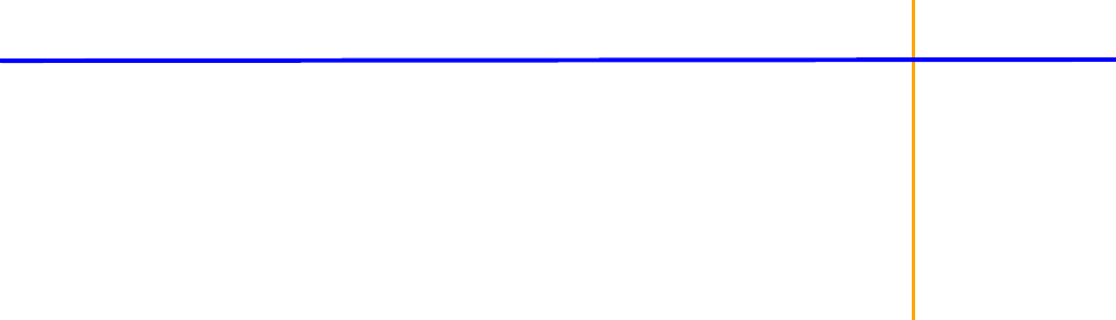
79
Appendix A
Closed-Form and Matrix Exponent
Computations
•“Closed-form computations” on page 79
•“Matrix exponent” on page 80
Closed-form computations
Closed form computations for 1, 2, and 3-compartment first-order library models with simple single
compartment dosing are handled recursively, where the model solution is defined by n residue param-
eters Ai which sum to one and exponential decay rates ai. These parameters are derived from micro
constants in the usual way via Laplace transforms assuming unit dose (including convolution with an
extra exponential for first-order input).
There is a “state vector” [s1(t),…,sn(t)] representing the model at any point in time, where each state
component is a term in the overall solution corresponding to a particular decay rate ai. Each separate
state evolves over time in the following way, where r is the infusion rate into a single predefined com-
partment:
The output value of the model, which is usually an amount in a specified compartment, at a point in
time is the sum of the state vector components:
When a bolus dose D is administered, the state is modified in the following way:
Regarding cfMicro models, the above description models the central compartment amount as a
function of input to the depot compartment, whether central or absorption. However, the actual imple-
mentation must take into account the following complicating factor.
Since, in general, models can depend on covariates that change discontinuously with time, the
closed-form models must not only model the central compartment as a function of dosing to the
depot, they must model every compartment as a function of every other compartment. The reason is
that, if a covariate is changed, three steps must be performed:
1. Record the amount in every compartment.
2. Empty the system and calculate the new parameters of the model.
sit si0eit–rAi
i
-----1eit–
–+=
yt sit
i
=
sit†
sit DAi
+=

Phoenix Modeling Language
Reference Guide
80
A
3. Put back the prior amounts into the compartments as if they were bolus doses, thus restoring all
compartments to their prior amounts.
If the model allows dosing to both central and absorption compartments, this is done using the above
scheme, since doses can go into both compartments.
In the steady-state case with bolus dose D given at intervals t, the solution takes the form:
Matrix exponent
The general N-compartment model governed by ordinary differential equations takes the form:
where y(t) =(y1(t), …, yN(t))T is an N-dimensional column vector of amounts in each compartment as a
function of time, f(y) is a column vector-valued function which gives the structural dependence of the
time derivatives of y on the compartment amounts, and r is an n-dimensional column vector of infu-
sion rates into the compartments. Note that as opposed to the closed form solution first-order models,
dosing can be made into any combination of compartments, and all of the compartments are mod-
eled.
To account for infusion rates, define the augmented system Y = [y, 1], and R = [r, 0]. In the special
first-order case, the equations are represented as:
where J is the Jacobian matrix:
J =
The partial derivatives are obtained by symbolic differentiation of f(Y). If any of them are not constant
over the given time interval, then matrix exponent cannot be used, and a numerical ODE solver is
used. The case where J is constant requires that the overall differential equation system is linear with
no explicit time dependencies - that is the system can be described by a series of fixed inter-compart-
mental rate constants which are the entries in the matrix J.
Note that any model (such as Michaelis-Menten) with at least one nonlinear flow does not satisfy the
constant J condition and must be solved with a numerical ODE solver.
Assuming J is a constant, the state vector Y evolves according to:
where eJt is defined by the Taylor series expansion I + Jt + (Jt)2/2! +… of the standard exponential
function. Standard math library routines are available for the computation of the matrix exponential.
These are faster and more accurate than the equivalent computation with a numerical ODE solver
and do not suffer from stiffness.
For steady state computations, regardless of whether a matrix exponential or numerical ODE solution
is used for the single dose case, repeated dosing cycles are made to allow the system to approach
sit DAieit–
1ei–
–=
y
·fy r+=
Y
·JY=
fy
i
yj
--------------ri
00
Yt eJtY0=

Closed-Form and Matrix Exponent Computations
Matrix exponent
81
A
steady state within a specified tolerance. An extrapolation technique known as Aitken acceleration is
used to accelerate the convergence of steady state computations so that usually only a few such
cycles are needed to achieve high accuracy steady state results.

Phoenix Modeling Language
Reference Guide
82
A

83
Appendix B
Blocks, Statements, and Operators
Alphabetical listings of supported elements
This section is a quick reference to supported elements in the modeling language.
–“Blocks and statements” on page 83
–“Expressions and operators” on page 88
Blocks and statements
Blocks are sets of statements grouped together inside curly brackets. Statements include assignment
of values and variables. Statements within the model (and within blocks) can span multiple lines of
code, and can be separated with (optional) semicolons.
In the following table:
var = a variable name
varlist = a list of variables, optionally separated by commas
numlist = a list of numbers, optionally separated by commas
assign = an assignment operator
expr = any numerical expression, including variable names, numbers and arithmetic operators
[ …] = indicates the content of the brackets is optional
| = represents “or” and separates options
* = means zero or more of an item can be displayed
+ = means one or more of an item can be displayed
statement = a statement of the form: variable = expression
Table B-1. Supported statements
Statement Purpose
cfMacro(id,parameters,
[strip=stripping_dose_covari-
ate])
Macro-parameter model of concentration, using optional
stripping dose.
cfMacro(id,parameters,
[first=abs_cpt_name])
Macro-parameter model of amount in central compart-
ment (cpt).
cfMicro(id,parameters,
[first=abs_cpt_name])
Micro-parameter model. See “One-compartment first-
order absorption, closed-form” on page 77.
count(var,expr[,action]) Defines an occurrence count.

Phoenix Modeling Language
Reference Guide
84
B
covariate(var(var)*) Defines one or more variables as covariates. Include an
empty pair of parentheses after the covariate name to
indicate that it is categorical.
covariate(dose,time,Gender())
delay(expression,
MeanDelayTime
[ , shape = ShapeExpression]
[ , hist = HistExpression])
Models delayed outcomes using convolution of the signal
to be delayed (S) and the probability density function (g)
of the delay time.
• MeanDelayTime: The value (positive) associated with
the mean delay time.
• ShapeExpression: The value (positive) representing
the shape parameter that defines the distribution of the
delay time.
• HistExpression: The value of the expression prior to
time 0.
Any number of delay functions can be included in a
model. The MeanDelayTime and shape parameters can
be estimated.
See also “Discrete and distributed delays” on page 40.
delayInfCpt(A,
MeanDelayTime,
ShapeParamMinusOne [ ,
in = inflow][ , out = outflow])
A statement related to a compartment (that can receive a
dose through a dosepoint statement) with all of its input
delayed (where the delay time is assumed to be gamma
distribution), including the rate of administered dose (if
provided) and the inflow specified by the “in” option (if
provided).
• A: Name of the compartment.
• MeanDelayTime: The value (positive) associated with
the mean delay time.
• ShapeParamMinusOne: The value (non-negative) rep-
resenting one less than the shape parameter that
defines the distribution of the delay time.
• out = outflow: (Optional) Represents the flow out of
compartment A.
• in = inflow: (Optional) Represents the additional inflow
that is delayed.
See also “Discrete and distributed delays” on page 40.
deriv(var assign expr) Defines a differential equation.
deriv(a = -a*Cl/V)
dosepoint| dosepoint2(id
[ tlag = expr]
[ duration = expr]
[ rate = expr])
Defines dosing. Example:
dosepoint(a1)
deriv(a1 = -a1*ke1)
c1 = a1/v1
dosepoint(a2)
deriv(a2 = -a2*ke2)
c2 = a2/v2
error(var(var)(*))
Table B-1. Supported statements
Statement Purpose

Blocks, Statements, and Operators
85
B
event(var,expr) Defines an unscheduled (e.g., adverse) event, where var
is an occur variable, expr is its hazard.
event(occur,haz)
The occur variable can be:
• 0 = did not occur
• 1 = occurred at the given time
• 2 = occurred at least once in the prior interval
• -n = occurred n times in the prior interval
• -999999 = no information about the prior interval
fixef(var
[()]
[ (enable = int)]
[ = ([lower bound],[ initial esti-
mate],[ upper bound])]
Defines variable(s) as fixed effects parameters, optionally
with a fixed value (), with optional initial estimate and
bounds.
fixef
tvE0 = c(1,2,3)
tvEMax = c(4,5,6)
tvlEC50 = c(0.09,1.1,2.0)
tvLambda = c(1,2,3)
See also “Fixed effect parameter syntax” on page 47.
interpolate(id(id) (*)) For more on the interpolate statement, see “Covariates”
on page 38.
LL(obsvar,expr) Defines log-likelihood where obsvar is the observation
variable, expr is its log-likelihood.
multi(var,invlink(,expr)*[
,action])
Defines an integer-valued categorical observation, where
invlink is an inverse link function and the rest is a series
of ascending offset expressions.
multi(Y,ilogit,-C*slope+intercept0,
-C*slope + intercept1), …)
observe(id1
[ (i d2)]
[ = expr]
[ ,bql]
[ ,dobefore = { …}]
[ ,doafter = { …}])
Defines predicted observations, where id1 is the Gauss-
ian prediction variable, id2 is the independent variable,
and expr is the value assigned to id1.
observe(cObs = cpred + eps1)
ordinal(var,invlink,input,slope,
(,intercept)*)
Variation on the multi statement.
ordinal(Y,ilogit,C,slope,intercept0,interc
ept1)
Table B-1. Supported statements
Statement Purpose
Phoenix Modeling Language
Reference Guide
86
B
Tmax = peak(Cmax = C)
or
Tmax = peak(Cmax = C, max)
or
Tmax = peak(Cmax = C, max =
(t < 6)) Or
Tmin = peak(Cmin = C, min)
or
Tmin = peak(Cmin = C, min = (t
>= 6))
where Cmax and Cmin are the
internal variables and do not
need defining.
Use in model code (not in a sequence block, doafter, or
dobefore).
Where Cmax, Tmax, Cmin, Tmin are variable names of
user choice, and C is any user-written expression.
Variables Tmax and Cmax are initially 0, and hold their
value until after a peak is detected.
After a peak is detected, variables Tmax and Cmax are
set to the peak of a cubic spline fitted to the points around
the peak, where the points are what is seen on the trajec-
tory of the differential equations.
If a subsequent peak is found, the process will only be
repeated if the peak is higher than the first.
If the keyword max is not included, it is assumed.
If the keyword min is included, it will look for a trough
rather than a peak.
Either keyword, max or min may be followed by a logical
expression, such as max=test. In that case, it test is true,
it looks for a peak. If test is false, it looks for the opposite.
peakreset(Cmax) Use in a sequence block, doafter, or dobefore.
This statement takes place at a point in time and will
reset the peak-finder, after which it can detect another
peak.
proc{ statement*}
ranef((block(varlist) = numlist)*) Defines variable(s) as random effects parameters,
optionally defining the covariance matrix.
ranef(nlKe = 0.01,nlV = 0.01)
ranef(eta1,eta2 = 6
diag(eta5,eta6) = c(1,3)
same(eta7,eta8)
block(eta11,eta12) = c(1,2,3)
)
See also “Random effect parameter syntax” on page 48.
section(<int>,section-stmt)
Table B-1. Supported statements
Statement Purpose

Blocks, Statements, and Operators
87
B
sequence{ statement*} Defines a block of statements to be executed together
and can contain conditional statements. It can contain
special statements:
•if statements set statements to be executed condi-
tional on expr being true
if(expr){statement*}
[ else if(expr){statement*}]*
[ else {statement*}]
•while statements set zero or more statements to be
executed while expr is true
while (expr){statement*}
•sleep statements pause computations for expr time
units. (The expr value for the sleep statement is a
relative time, not an absolute time.)
sleep (expr)
See “Modeling discontinuous events” on page 39, “One-
compartment model with sequence” on page 75, and
“One-compartment model with sleep statement” on
page 76.
stparm((var | var = expr) +) Defines one or more structural model parameters, var,
with optional values, expr.
stparm(
ka = exp(tvlKa + nlKa)
ke = exp(tvlKe + nlKe)
v = exp(tvlV + nlV)
)
urinecpt(var assign expr) Defines an elimination compartment. The urinecpt is like
deriv, except in a steady state dosing situation, urinecpt is
ignored.
Table B-1. Supported statements
Statement Purpose

Phoenix Modeling Language
Reference Guide
88
B
Expressions and operators
Expressions and other sub-statement entities can span multiple lines and can be separated by
optional commas. The following operators are supported. (The Phoenix Modeling Language follows
the C++/C syntax for function names.)
Table B-2. Supported operators
Operator Function
+ Addition
ka = exp(tvlKa + nlKa)
- Subtraction
deriv(a = -a*ke)
* Multiplication
deriv(a = -a*Cl/V)
/ Division
deriv(a = -a*Cl/V)
^ or ** Power
V = tvV*(W/70)^dVdW*exp(nV)
= or <- Assignment
>= Comparison: greater than or equal to
if(t> = Tmax)
<= Comparison: less than or equal to
== Comparison: equal to
LL(y, log(y == 0 ? 1 - p01:y == 1 ? p01 - p12:p12
- 0))
!= Comparison: not equal to
> Comparison: greater than
< Comparison: less than
<> Comparison: not equal
&& Logical: and
|| Logical: or
ln, log Natural log (log base e)
ln(x), log(x)
log10 Log base 10
log10(x)
fabs Absolute value
fabs(x)
? Switch
(cond) ? actionA:actionB

89
Appendix C
Reserved Words
Listing of reserved variable names
When building a model, the following should not be used as variable names:
– Words that already part of the Phoenix modeling language
– Words that are in the C runtime or C math libraries
– Words that are GNU library calls or GNU reserved words
If a reserved word is used, it will cause a compilation error when the model is being built and will
appear in the model code as blue text.
The table below lists some of the more common reserved words to avoid.
Table C-1. More common reserved variable names
block error ranef3
bioavail event rate
bolus first real
bql fixef repl
break for return
call gamma (Linux systems only) same
cfMacro goto secondary
cfMicro if section
char in sequence
continue include short
covariate infuse signed
count int sleep
default interpolate start
deriv interval stparm
diag join struct
do LL switch
doafter long tlag
dobefore mean uncertainty
dosepoint model unit
dosepoint1 multi units
dosepoint2 observe unsigned
dropout override urine

Phoenix Modeling Language
Reference Guide
90
C
duration proc urinecpt
else ranef wait
enable ranef1 while
enum ranef2
Table C-1. More common reserved variable names

91
Appendix D
Supported Functions
•“Special functions” on page 91
•“Math functions” on page 92
Special functions
The following special functions (with some duplicates of the intrinsic versions, but with different
names) are defined within the Phoenix PML language. The detailed C language code implementing
each can be found in <Phoenix_install_dir>\application\lib\NLME\Execut-
ables\mutil.c.
Table D-1. Special functions
Name Usage Definition
lnorm lnorm(x, std); log of probability density function of normal distribution
with mean ()=0. Since probability density of the nor-
mal distribution is f(x) = 1/(v(2)s)e^-((x-)^2/(2s^2)),
then assuming that = 0, log f(x) = -0.5 * (log2 +
log(s^2) + (x/s)^2).
lnegbin_rp
megnin_rp
lnegbin_rp(r, p, y);
rnegbin_rp(r, p);
neg. binomial, parameterized by r, p (LL)
(sample)
lnegbin
pnegbin
rnegbin
lnegbin(mean, beta, power,
y);
pnegbin(mean, beta, power,
y);
rnegbin(mean, beta, power);
neg. binom., param. by mean, beta (= log(alpha)),
power (LL)
(exp(LL))
(sample)
lpois
ppois
rpois
lpois(mean, int _x);
ppois(mean, int _x);
int rpois(lambda);
log(mean^n * exp(-mean)/n!) (LL)
(exp(LL))
(sample)
lgamm
factorial
lgamm(x);
factorial(x);
gamma function
x! = x*(x-1)*…*1
lphi
phi
probit
erfunc
lphi(x, v);
phi(x);
probit(p);
erfunc(x);
log(phi(x/stdev))
normal(0,1) cum. dist. function
inverse N(0,1) cum.dist. function
error function
lambertw lambertw(const z); inverse of x(y)=y*exp(y)

Phoenix Modeling Language
Reference Guide
92
D
Math functions
Phoenix PML supports a majority of the intrinsic math functions in the Cmath.h library. See the fol-
lowing tables for a list of supported functions. (Refer to http://www.cplusplus.com/reference/cmath/ for
more information on the Cmath.h library.)
–“Trigonometric functions” on page 92
–“Hyperbolic functions” on page 93
–“Exponential and logarithmic functions” on page 93
–“Power functions” on page 93
–“Error and gamma functions” on page 93
–“Rounding and remainder functions” on page 94
–“Floating-point manipulation functions” on page 94
–“Minimum, maximum, difference functions” on page 94
–“Other functions available in math.h” on page 95
–“Classification macro/functions” on page 95
–“Comparison macro/functions” on page 95
ilogit
iloglog
icloglog
iprobit
ilogit(x);
iloglog(x);
icloglog(x);
iprobit(x);
exp(x)/(exp(x)+1)
inverse log-log link function
inverse complementary log-log link function
inverse probit (same as phi(x))
unifToPois-
son
unifToPoisson(mean, r); convert uniform distribution to poisson
min
max
log10
abs
ln
min(x, y);
max(x, y);
log10(x);
abs(x);
ln(x);
minimum
maximum
log base10
absolute
natural log
CalcTMax CalcTMax(A, a, B, b, C, c); obtain Tmax for a macro-parameter model
vfwt vfwt(f, p); make an observation variance function
Table D-1. Special functions
Name Usage Definition
Table D-2. Trigonometric functions
Function Description
cos Compute cosine
sin Compute sine
tan Compute tangent
acos Compute arc cosine
asin Compute arc sine
atan Compute arc tangent
atan2 Compute arc tangent with two parameters

Supported Functions
Math functions
93
D
Table D-3. Hyperbolic functions
Function Description
cosh Compute hyperbolic cosine
sinh Compute hyperbolic sine
tanh Compute hyperbolic tangent
acosh Compute arc hyperbolic cosine
asinh Compute arc hyperbolic sine
atanh Compute arc hyperbolic tangent
Table D-4. Exponential and logarithmic functions
Function Description
exp Compute exponential function
ldexp Generate value from significand and exponent
log Compute natural logarithm
log10 Compute common logarithm
exp2 Compute binary exponential function
expm1 Compute exponential minus one
ilogb Integer binary logarithm
log1p Compute logarithm plus one
log2 Compute binary logarithm
logb Compute floating-point base logarithm
scalbn Scale significand using floating-point base exponent
scalbln Scale significand using floating-point base exponent
(long)
Table D-5. Power functions
Function Description
pow Raise to power
sqrt Compute square root
cbrt Compute cubic root
hypot Compute hypotenuse
Table D-6. Error and gamma functions
Function Description
erf Compute error function

Phoenix Modeling Language
Reference Guide
94
D
erfc Compute complementary error function
tgamma Compute gamma function
lgamma Compute log-gamma function
Table D-7. Rounding and remainder functions
Function Description
ceil Round up value
floor Round down value
fmod Compute remainder of division
trunc Truncate value
round Round to nearest
lround Round to nearest and cast to long integer
llround Round to nearest and cast to long long integer
rint Round to integral value
lrint Round and cast to long integer
llrint Round and cast to long long integer
nearbyint Round to nearby integral value
remain-
der
Compute remainder
Table D-8. Floating-point manipulation functions
Function Description
copysign Copy sign
nextafter Next representable value
nextfor-
ward
Next representable value toward precise value
Table D-9. Minimum, maximum, difference functions
Function Description
fdim Positive difference
fmax Maximum value
fmin Minimum value
Table D-6. Error and gamma functions
Function Description
Supported Functions
Math functions
95
D
Table D-10. Other functions available in math.h
Function Description
fabs Compute absolute value
abs Compute absolute value
fma Multiply-add
Table D-11. Classification macro/functions
Function Description
isfinite Is a finite value
isinf Is infinity
isnormal Is normal
signbit Sign bit (whether the sign of x is negative)
Table D-12. Comparison macro/functions
Function Description
isgreater Is greater
isgreatereq-
ual
Is greater or equal
isless Is less
islessequal Is less or equal
islessgreater Is less or greater
isunordered Is unordered

Phoenix Modeling Language
Reference Guide
96
D

97
Index
C
Closed-form
computations, 79
example, 77
syntax, 23
Column mappings, 16
Comments syntax, 20
Count statement, 29
Customer support, 11
D
Data input data, 14
delay function, 41
delayInfCpt statement, 43
Delays, 40
Discontinuous events, 39
Dosing syntax, 27
E
Emax, 74
Event statement, 32
Examples
closed-form, 77
Emax model, 74
first-order, 76
lag time, 77
logistic, 65
multinomial, 72
parallel, 75
phenobarbital, 61
population PK, 63, 74
sequence, 75
simple PK, 61
sleep, 76
theophylline, 63
time to event model (exponential), 72
time to event model (Weibull), 73
time-to-event, 78
Exponential time to event model, 72
F
Fixed effects
enabled or disabled, 47
syntax, 47
I
Including files in code, 16
L
Lag time example, 77
Limits for dataset rows, 14
LL statement, 34
Logistic model, 65
M
Macroconstants closed-form, 23
Matrix exponent, 80
Microconstants closed-form, 23
Model file, 15
Modeling syntax, 21
Multi statement, 34
Multinomial
example, 72
responses, 35

Phoenix Modeling Language
Reference Guide
98
O
Observe statement, 37
Operators, 88
Ordinal statement, 37
P
Parallel, 75
Phenobarbital example, 61
PK
example, 61
model syntax, 21
population example, 63, 74
PML examples, 61
R
Random effects syntax, 48
Responses, time-to-event, 78
S
Sequence, 75
Sleep statement, 76
Syntax
closed-form, 23
comments, 20
discrete events, 39
dosing, 27
fixed effects, 47
general, 20
modeling, 21
random effects, 48
T
Technical support, 11
Theophylline example, 63
Time to event model, 32
exponential, 72
Weibull, 73
U
User-defined model, 65
W
Weibull time to event model, 73
