Phyloscanner Manual

User Manual:

Open the PDF directly: View PDF .
Page Count: 27

I Inferring within- and between-host phylogenies in windows along the genome, using mapped reads
II Analysing within- and between-host phylogenies

phyloscanner

available from github.com/BDI-pathogens/phyloscanner

Coding lead by Chris Wymant and Matthew Hall,

with contributions from Oliver Ratmann and Christophe Fraser

This manual last updated October 22, 2018

next-gen

sequencing

gives reads

mapping

+ ... + ...

phyloscanner

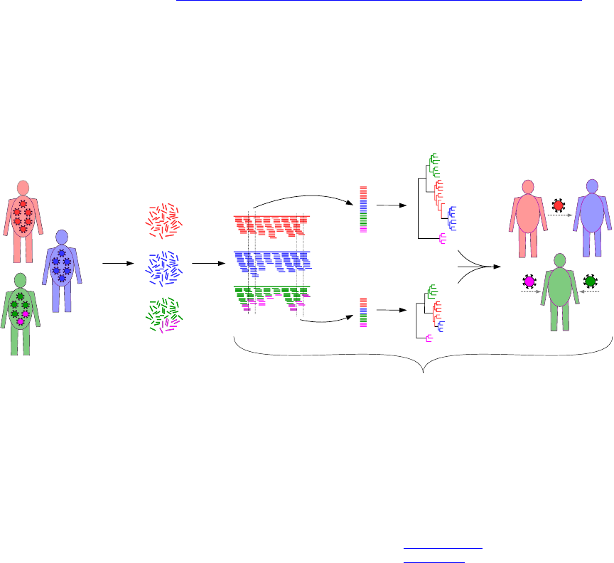
phyloscanner analyses pathogen genetic diversity and relationships between and within hosts at

once, in windows along the genome using mapped reads (fragments of DNA produced by next-generation

sequencing), or using phylogenies with multiple sequences per host previously generated by the user via

any method. An example showing its action on simulated data (which is included with the code) can be

seen at the GitHub repository linked to above.

If you have a query about phyloscanner, ask it publicly at the google group. If you have a problem

getting the code to run or think you’ve found a bug, please create a New issue on the GitHub repository.

The usual bug-reporting etiquette applies. For non-trivial bugs, to allow us to reproduce the problem it’s

helpful to have input that causes the problem. This needn’t be all your data. For example if one read in

a bam ﬁle is causing a problem, you could make a new bam ﬁle containing only that read, allowing us to

see the problem very quickly. Isolate the problem as much as you can ﬁrst – help us to help you! If you

get an error when you run phyloscanner as part of a larger piece of code you’ve written yourself (e.g.

a job submission script to a cluster), please don’t make us debug that – the error might be in your code

rather than ours. Isolate the problem to the relevant phyloscanner command.

If you use phyloscanner, please cite it [1] and its dependencies: SAMtools [2], MAFFT [3], RAxML [4] and

ggtree [5]. Details of these are found in the ﬁle CitationDetails.bib in phyloscanner’s InfoAndInputs

subdirectory.

Throughout the manual we’ll use phylogeny and tree interchangeably. Forgive us.

Contents

I Inferring within- and between-host phylogenies in windows along the

genome, using mapped reads 5

1 The basic command 5

1.1 ThePythonversionyouuse................................... 6

2 What do the window coordinates mean exactly? 6

3 What windows should I choose? 6

3.1 Start&end............................................ 6

3.2 Windowwidth .......................................... 7

3.3 Windowoverlap.......................................... 8

4 What output ﬁles are produced? 8

5 Optional arguments 10

5.1 Windowoptions ......................................... 10

5.2 Recommendedoptions...................................... 11

5.3 Readqualityoptions....................................... 12

5.4 Otherassortedoptions...................................... 12

5.5 Options for bioinformatic interrogation . . . . . . . . . . . . . . . . . . . . . . . . . . . . . 13

5.6 Partialprocessingoptions .................................... 14

5.7 Deprecatedoptions........................................ 14

II Analysing within- and between-host phylogenies 16

6 The basic command 16

7 Name format for input ﬁles 17

8 Output 17

9 Preparing the trees 17

10 Tip label and ﬁle suﬃx regular expressions 18

11 Branch length normalisation 18

11.1 Parallelising tools/CalculateTreeSizeInGenomeWindows.py ................ 19

12 Blacklisting 20

12.1Duplicateblacklisting ...................................... 20

12.2 Parsimony-based blacklisting for contaminants . . . . . . . . . . . . . . . . . . . . . . . . 20

12.3Dualinfectionblacklisting.................................... 21

12.4Userblacklisting ......................................... 21

12.5Downsampling .......................................... 21

12.6Pruningtheblacklist....................................... 21

13 Parsimony reconstruction 22

14 Summary statistics 23

15 Classiﬁcation of pairwise relationships 24

16 Pairwise relationship summary 25

17 Miscellaneous options 26

A tool in two parts

Conceptually, phyloscanner can be neatly split into two steps. Firstly, inferring phylogenies that contain

both within- and between-host diversity, in windows along the genome, using mapped reads as input.

Secondly, analysing those phylogenies or other similar ones (i.e. containing within- and between-host

diversity, but created however the user likes) in order to infer interesting things like transmission and

multiply infected individuals, and give summaries of diversity.

This conceptual split is reﬂected in the code: phyloscanner make trees.py runs the ﬁrst step and

phyloscanner analyse trees.R runs the second step. Why didn’t we merge the two steps into one?

•For some uses, step one may not be needed. For example if you don’t have mapped reads, but have

sequence data in another format. We presented an example of this in the phyloscanner paper: a

dataset consisting of multiple whole genomes of Streptococcus pneumoniae for each person carrying

the bacterium, obtained by separately sequencing multiple colonies.

•For some uses, step two may not be needed. Having extracted the within- and between-host diversity

information in each window (ﬁrst as a multiple sequence alignment and then as a phylogeny), you

might want to do your own totally diﬀerent analysis of it.

•Each step is controlled by parameters and options to tailor its usage to diﬀerent kinds of data, and

we don’t (yet) have a way to automatically optimise these for each data set, so you will need to

have a little play to explore what’s appropriate in your case. If you are running both steps, it’s

best to think ﬁrst about getting step one right ﬁrst, and then getting step two right. Step one is

primarily about bioinformatics, step two about phylogenetic analysis.

Note that to run either phyloscanner make trees.py or phyloscanner analyse trees.R, like run-

ning any executable ﬁle, you must either specify the full path to the executable (e.g.

/path/to/my/phyloscanner/code/phyloscanner make trees.py) or add the directory that contains

the executable to the $PATH environment variable in your terminal (google this if needed). In the manual

we’ll refer to scripts named like tools/SomeCode; such scripts live in the tools subdirectory inside the

main phyloscanner code directory.

Fun fact: step one was written by Chris, step two mostly by Matthew. We sat next to each other

while coding, and we hope that’s reﬂected in how easy it is to make the two steps work together. If it

isn’t, let us know.

Part I

Inferring within- and between-host

phylogenies in windows along the genome,

using mapped reads

1 The basic command

As input to phyloscanner make trees.py, you need to have generated ﬁles of mapped reads in bam

format – bam ﬁles henceforth. The bam format does not include the sequence to which the reads were

mapped – the reference – which we also need. With the initial $traditionally indicating that what follows

is a command to be run on the command line / in a terminal (i.e. don’t type that initial $), the basic

phyloscanner make trees.py command looks like

$ phyloscanner_make_trees.py ListOfMyInputFiles.csv --windows 1,300,301,600,...

where

•ListOfMyInputFiles.csv is a plain-text, comma-separated-variable (csv) format ﬁle in which the

ﬁrst column contains the bam ﬁles, the second column contains the corresponding reference ﬁles.

An optional third column, if present, contains aliases – things to rename each bam ﬁle to in

phyloscanner make trees.py output; if not present the base name of the bam, i.e. the ﬁle name

not including the directory path, will be used. e.g. This input ﬁle list might look like

PatientA.bam,PatientA ref.fasta,A

PatientB.bam,PatientB ref.fasta,B

Bam ﬁle base names, and aliases if present, must be unique and free of whitespace. Quotation marks

are interpreted as wrapping/protecting ﬁelds, allowing them to contain commas that are not ﬁeld

separators. You can generate this input ﬁle list however you like, including manually. The following

block of code illustrates how you might generate it automatically from the command line. It also

checks that your ﬁles exist, which phyloscanner make trees.py does anyway, but it’s always best

to catch your errors soonest.

$ for ID in PatientA PatientB PatientC; do

$ bam=MyBamsDir/"$ID".bam

$ ref=MyRefsDir/"$ID".fasta

$ if [[ ! -f "$bam" ]]; then

$ echo "$bam does not exist" >&2

$ break

$ elif [[ ! -f "$ref" ]]; then

$ echo "$ref does not exist" >&2

$ break

$ fi

$ echo "$bam","$ref","$ID"

$ done > MyPhyloscannerInputFile.csv

If those IDs were stored in a plain-text ﬁle MyIDs.txt separated by whitespace, you could replace

the ﬁrst line of that loop with

for ID in $(cat MyIDs.txt); do

•The --windows (or -W) option is used to specify an even number of comma-separated positive

integers: these are the coordinates of the windows to analyse, interpreted pairwise, i.e. the ﬁrst two

are the left and right edges of the ﬁrst window, the third and fourth are the left and right edges of

the second window, . . . i.e. in the above example we have windows 1-300, 301-600, . . .

You shouldn’t run multiple phyloscanner make trees.py commands simultaneously in the same direc-

tory, as it writes to and reads from ﬁles with ﬁxed names, so the commands could clash. If you’re running

multiple jobs in parallel on a computing cluster that starts jobs in the same place, ensure that each job

runs in a diﬀerent directory (e.g. using the mkdir and cd commands to make and change into a directory

speciﬁc to that job).

1.1 The Python version you use

Note that phyloscanner make trees.py can either be run like this:

phyloscanner make trees.py [input and options]

or like this:

python phyloscanner make trees.py [input and options]

In the former case, the version of Python used to execute phyloscanner make trees.py is whatever

version gets called when you simply run the command python in the terminal. In the latter case, you

can explicitly replace python by a speciﬁc version of Python on your machine, for example python2.7 or

/usr/bin/python. The version of Python that’s used must (a) be Python 2, not Python 3, and (b) contain

the Python dependencies described in phyloscanner/InfoAndInputs/InstallationNotesForMakingTrees.sh.

The version of Python used can be speciﬁed the same way for all of the Python tools in the tools sub-

directory.

2 What do the window coordinates mean exactly?

By default the references used for mapping, together with any extra references if included using the

--alignment-of-other-refs option, are all aligned together and window coordinates are interpreted

with respect to the alignment (i.e. position nrefers to the nth column of that alignment, which could

be a gap for some of the sequences). This alignment can be found in the ﬁle RefsAln.fasta after

running phyloscanner make trees.py, should you want to inspect it and possibly run again. You

can manually specify window coordinates with respect to this alignment, using the --windows option,

or have windows automatically chosen using --auto-window-params, which attempts to minimise the

aﬀect of insertions and deletions in the references on your window width and overlap preferences. Alter-

natively, if you are using the --alignment-of-other-refs option to include extra references, you can

use --pairwise-align-to to name one of these references to be a kind of reference reference: instead

of aligning of all the bam ﬁle references to each other, they will be sequentially and separately pairwise-

aligned to your named reference, and window coordinates are interpreted with respect to that named

reference (i.e. position nrefers to the position of the nth base of the named reference, not counting

any gaps inside the reference). Using the --pairwise-align-to option is expected to more stable than

--windows or --auto-window-params if your bam ﬁle references are many and diverse, since pairwise

alignment is easier than multiple sequence alignment. It also has the advantage that when running

phyloscanner make trees.py more than once with diﬀerent bam ﬁles, the coordinates mean the same

thing each time.

3 What windows should I choose?

I’m glad you asked. It’s important.

3.1 Start & end

You might as well fully cover the genomic region you’re interested in. That requires choosing where to

start and where to end. If you’re interested in the whole genome, the start is 1 and the end is the genome

length, or more precisely the length of the alignment of all references together (or the length of your

named reference if you used the --pairwise-align-to option). You may know that your reads don’t

start right at the beginning of the genome. If this is the case, a good place to start your ﬁrst window

would be the genome position at which you start having reads.

If your reads were generated by amplifying the sample using primers, the primers should ideally have

been trimmed from the reads as part of whatever bioinformatic pipeline produced your input bam ﬁles.

(This can be done for example using fastaq, which is called as part of the shiver pipeline.) Then a

sensible choice for the start of the ﬁrst window would be the ﬁrst position after the ﬁrst primer, and a

sensible choice for the end of the last window would be the last position before the last primer.

You might as well fully cover the genomic region you’re interested in. Let’s revisit that. In what

part of the genome would you like to do phylogenetics? Perhaps all of it. Then again, remember that

phylogenetics assumes neutral evolution at every included site. Though phyloscanner make trees.py

allows individual speciﬁed sites to be excised after alignment of all the reads from all the bam ﬁles,

there may be regions of the genome where selected sites are so dense that it’s simpler to skip the region

altogether. There may also be regions of the genome where there are so many insertions and deletions

(indels) that you’re sceptical that the reads will align correctly in the ﬁrst place. You can choose to

specify no windows covering such regions.

3.2 Window width

As well as choosing where your ﬁrst window should start and where your last one should end, you need

to choose how wide each window is. On the one hand, increasing the width of a window increases

its phylogenetic resolution. To see this eﬀect using just some existing reference sequences (forgetting

momentarily about any read data you have), the script tools/CalculateTreeSizeInGenomeWindows.py

could be useful: it calculates trees from references in sliding windows along the genome. (It then calculates

patristic distances, for a purpose discussed later in section 11.) You may be able to see from visual

inspection, or from some automated analysis of your own, that one’s ability to construct well-resolved

phylogenies increases with window width. On the other hand, a read must fully span a window to be

included in it, so the wider you make a window the fewer reads it will contain. To quantify this eﬀect,

you can run

$ tools/EstimateReadCountPerWindow.py ListOfMyInputFiles.csv

(where ListOfMyInputFiles.csv is the same ﬁle as we discussed at the top of section 1). This command

uses the information in each bam about the number of reads and how long1they are; it then estimates

the number of reads expected to span a window of width Wby assuming reads are distributed ran-

domly over the whole genome (ignoring the actual read location information in the bam ﬁles). If reads

are found to be paired, the calculation is also done in the context of phyloscanner make trees.py’s

--merge-paired-reads option, which merges each pair of reads into a single longer read if they over-

lap with each other (this will give exactly the same result as considering reads separately if reads in

a pair never overlap). The calculation is done as a function of W, showing how the number of reads

decreases monotonically2. A good choice of window width, roughly, would be as large as you can get

before the number of reads per window gets too low to make useful within-host phylogenies. Skip ahead

to section 3.3 if that’s good enough for you and you don’t want to think about it any more.

The --explore-window-widths option of phyloscanner make trees.py was written with the fol-

lowing balancing act in mind. If a window is too wide, too few reads overlap it, as discussed. However

if it is too small, there aren’t enough positions at which a variant can be observed and so few unique

reads will be observed in the window. Somewhere between these two extremes therefore maximises the

number of unique reads. The --explore-window-widths option reports, for each in a list of window

widths to try, a two-dimensional matrix of count values – the number of unique reads found in each

bam and in each successive window along the genome. One way of visually summarising this matrix

of counts as a function of window widths is to give the ﬁle containing this data as the argument to

tools/PlotExplorationOfWindowWidths.py, which calculates and plots various percentiles of the ma-

trix of counts. e.g. for a given window width, the 50th percentile of the counts means that half of all the

windows from all the bams had more unique sequences than this, and half had fewer. Anecdotally, for

our HIV data, I did not ﬁnd that maximising the number of unique sequences per window gave the best

results: manually examining phylogenies revealed that a larger window width produced more revealing

1In this particular instance we deﬁne read length as the length of the mapping reference covered by the read, from

its start to its end. This can diﬀer from the actual read length due to insertions or deletions in the read relative to the

reference. Deﬁning the read length this way is appropriate since we’re interested in reads spanning windows, and windows

get deﬁned relative to the reference. This length will also diﬀer from the nominal read length of your sequencing run (which

is typically one ﬁxed value) if the reads have been trimmed as part of bioinformatic processing, e.g. removing primers,

adapters, low-quality bases, or bits of the read that could not be mapped.

2The number of positions at which we could place a window of width Wequals the length of the reference −W+ 1.

The number of positions at which we could place a window of width Wsuch that it is wholly inside a read is the length of

the read −W+ 1. The probability of a randomly placed read overlapping a window of width Wis therefore (read length

−W+ 1) / (reference length −W+ 1). The number of reads and their diﬀerent lengths are ﬁxed in the data; increasing W

will decrease this probability (except for reads that span the entire reference).

trees. But this option can still be helpful for quantifying the decline in how many unique sequences you

get as window width is increased out towards the largest possible values.

The regular --explore-window-widths option calculates the number of unique reads after all read

processing has been done, including aligning the reads from all bams using maﬀt, and other options

you may have speciﬁed that aﬀect how many unique reads survive, for example --excision-coords,

--merging-threshold,--min-read-count,--quality-trim-ends,--min-internal-quality, and

--discard-improper-pairs options. The ﬁrst two of these can result in two or more unique reads

being merged into one; the rest can simply discard some reads. You could choose values for the

associated parameters immediately and then use --explore-window-widths, or else come back to

--explore-window-widths later on once you’ve got the hang of phyloscanner make trees.py and

investigated the eﬀect of those other options in your data.)

There is also the --explore-window-widths-speedy option which is almost identical: the diﬀerence

is that this counts the number of unique reads in the window straight away after they are extracted from

the bam, before any processing of them has been done (including aligning them all with mafft). If you

don’t care about read processing steps that change the number of unique reads, use this because it’s

faster.

Power users might want to optimise their own measure of phylogenetic information as a function of

window width; one of the ﬁrst metrics to pop into your head might be the mean bootstrap of all nodes in

the tree. That’s not advised because within a sample there may be many very similar sequences, and the

set of nodes connecting these may have poor bootstrap support, but this is not something that ought to

be penalised. Also in theory you might be able to increase the window width until only a single read is

found spanning the window in each patient; your bootstraps might then be great, because between-host

diversity is greater than that within-host, but you’ve thrown out all the within-host information.

3.3 Window overlap

How much should neighbouring windows overlap?

•A good, simple answer to this is zero, i.e. each window starts right after the previous one ends. e.g.

1-99, 100-199, 200-299, . . .

•Negative overlap means unused space in between windows, e.g. 1-99, 200-299, 400-499, . . . The only

reason for this is if you want to exclude certain parts of the genome. (Though it’s hard to imagine

that the regions you want to exclude are perfectly regularly spaced.)

•Positive overlap means the next window begins before the current one ends, e.g. 1-99, 50-149,

100-199, . . . There’s a redundancy in doing this, because you’re analysing the same information

multiple times. However there’s a little bit of stochasticity involved when performing algorithmic

multiple sequence alignment then phylogenetic inference, so even if two windows overlap heavily

some minor diﬀerences in the results could arise by chance. Positive overlap may therefore smooth

out some of this stochasticity, at the expense of additional compute time. (You’ll also need to take

into account the non-independency of overlapping windows if you interpret results from multiple

windows in a probabilistic framework.)

4 What output ﬁles are produced?

By default, those ﬁles that are produced for each window are grouped into subdirectories by ﬁle type.

•RefsAln.fasta. This contains the mapping reference from each bam ﬁle, together with any

extra references included with --alignment-of-other-refs. This alignment is not created if

--pairwise-align-to is used.

•AlignedReads/AlignedReadsInWindow X to Y.fasta (where Xand Yare window coordinates).

Contains the reads from all bam ﬁles in the window X-Y, after processing and alignment, but before

excision of any positions speciﬁed with --excision-coords. Reads are automatically assigned a

name of the form A read M count N, where Aidentiﬁes the bam from which the read came, Nis

the number of times that read was found (either identical copies of the same sequence, or merged

similar sequences if --merging-threshold is used), and Mis the rank of the read when they are

ordered by count (i.e. M= 1 is the most common read, M= 2 the second most common etc.)

•AlignedReads/AlignedReads PositionsExcised InWindow X to Y.fasta. Only produced if you

speciﬁed some positions to excise with --excision-coords, and at least one of those positions was

inside3the window X-Y. If this ﬁle exists, the tree in window X-Yis based on this alignment

(not AlignedReadsInWindow X to Y.fasta). Note that excising positions may result in reads that

were previously distinct becoming identical – if they diﬀered only at the excised positions. This is

checked after positions are excised, and reads from the same bam that have become identical are

merged with an updated count. Similarly, if the merging of similar reads (in addition to identical

reads) has been speciﬁed, the merging is rerun after excision of positions. If the excision of positions

results in reads becoming merged, clearly there will not be a one-to-one correspondence between

reads before and after excision: after merging there may be fewer unique reads, though with the

same total count.

•Consensuses/Consensuses InWindow X to Y.fasta. In this alignment, the set of unique reads re-

tained from each bam ﬁle is collapsed into a single sequence: their consensus (taking the most com-

mon base/gap at each position, weighting each unique read by its count). Note that in general this

consensus could diﬀer from the corresponding part of a consensus called using all reads mapped along

the full length of the reference, because the only reads retained by phyloscanner make trees.py

in a window are those fully spanning it. This process can result in some columns containing only

gaps; these columns are kept, so that the coordinates of this ﬁle match those of

AlignedReadsInWindow X to Y.fasta.

•Consensuses/Consensuses PositionsExcised InWindow X to Y.fasta. The consensus as previ-

ously, but with any speciﬁed positions to excise excised. Only produced if there are such positions.

•DiscardedReads/DiscardedReads A.bam, where A identiﬁes one of the input bams. Only produced

if --inspect-disagreeing-overlaps is used; see that option’s description in 5.5. These ﬁles will

be accompanied by DiscardedReads A ref.fasta (the reference for the bam ﬁle).

•DuplicationData/DuplicateReadCountsRaw InWindow X to Y.csv. Each row in this csv-format

ﬁle corresponds to one instance of exactly the same unique read being found in two diﬀerent bams,

before any processing of the reads (merging, excising positions etc.). The ﬁrst two columns show

the two bams involved, and the third and fourth columns show the count of the read in the two

bams. If a read is exactly duplicated in Ndiﬀerent bams, then there will be N(N−1)/2 associated

lines in this ﬁle – one for each diﬀerent pair of bams. See also the information in the next point.

These ﬁles will not be produced if --dont-check-duplicates is speciﬁed.

•DuplicationData/DuplicateReadCountsProcessed InWindow X to Y.csv. Each row in this csv-

format ﬁle corresponds to one instance of exactly the same unique read being found in at least

two diﬀerent bams, after all processing of the reads (merging, excising positions etc.). If the same

read is found in Ndiﬀerent bams, there will be one row for this, containing Nﬁelds separated by

commas (each row in general therefore has a diﬀerent number of columns, though 2 is the most

common). Each ﬁeld is the name of the read, assigned based on the bam in which it was found.

These ﬁles will not be produced if --dont-check-duplicates is speciﬁed.

Why is information about the duplication of reads checked and recorded twice, in these two diﬀerent

ﬁles? Duplication information after processing is easiest to work with, because it is the processed

reads that are used to infer phylogenies. However instances of exact duplication before any process-

ing of the reads is a better indicator of cross-sample contamination. Firstly because the options for

similarity-based merging of reads within each bam, and for a minimum read count for inclusion,

result in fewer unique reads to compare between bams. Secondly because excising positions makes

reads shorter and increases the possibility for genuine cross-sample duplication (i.e. not contami-

nation). Anecdotally, we found that being trigger-happy with deleting all codons associated with

HLA escape in a conserved part of the HIV genome resulted in considerable duplication in the reads

after processing that was not present before. Note that during both similarity-based merging of

reads and excision of positions (which is followed by merging newly identical reads), we lose track of

the original identity of reads, i.e. we don’t know what the correspondence is between reads before

processing and after processing.

3Note that if --pairwise-align-to is used, the window coordinates Xand Ymean the same thing as the excision coor-

dinates. If --pairwise-align-to is not used, the window coordinates Xand Ymean positions Xand Yin RefsAln.fasta

as discussed in section 2; therefore a position to excise, Z, being inside the window X-Yis not the same as X≤Z≤Y.

•DuplicationData/DuplicateReads contaminants InWindow X to Y.fasta. Only produced if

--contaminant-count-ratio is used; see that option’s description in section 5.7.

•ReadNames/ReadNames1 InWindow X to Y InBam A.txt. Only produced if --read-names-1 is used;

see that option’s description in section 5.5.

•ReadNames/ReadNames2 InWindow X to Y InBam A.csv. Only produced if --read-names-2 is used;

see that option’s description in section 5.5.

•RecombinationData/RecombinantReads InWindow X to Y.fasta. Only produced if

--check-recombination is used; see that option’s description in section 5.2.

Some temporary ﬁles are also written to the working directory; by default these are deleted. (They are

kept with --keep-temp-files.)

5 Optional arguments

Information about all optional arguments and what they do can also be seen by running

phyloscanner make trees.py with the --help option. That will give information guaranteed to be

synchronised to your current version of the code, as well as showing all option shorthands (e.g. --help =

-h); however we go into slightly more detail here. We particularly encourage you to familiarise yourself

with the Window options and Recommended options below, which are particularly important for running

phyloscanner make trees.py well.

5.1 Window options

You must choose exactly one of these: --windows,--auto-window-params,--explore-window-widths.

•--windows: used to specify a comma-separated series of paired coordinates deﬁning the boundaries

of the windows. e.g. specifying 1,300,301,600,601,900 would deﬁne windows 1-300, 301-600,

601-900.

•--auto-window-params: used to specify 2, 3 or 4 comma-separated integers controlling the auto-

matic creation of regular windows.

–The ﬁrst integer is the width you want windows to be. If the --pairwise-align-to option

is not being used, we create an alignment containing all references, as mentioned already. In

this case, we weight each column in this alignment by its non-gap fraction, so that windows in

which many references have gaps become correspondingly wider. If the --pairwise-align-to

option is being used, width is simply interpreted with respect to the named reference (i.e. a

width of Wmeans each window contains Wbases from that reference).

–The second is the overlap between the end of one window and the start of the next. This can

be negative, implying unused space in between windows; the recommended value of 0 means

each window starts right after the previous one ends.

–The third integer, if speciﬁed, is the start position for the ﬁrst window. If not speciﬁed, this

is 1.

–The fourth integer, if speciﬁed, is the end position for the last window. If not speciﬁed,

windows will continue up to the end of the reference or references.

•--explore-window-widths: use this option to explore how the number of unique reads found in

each bam ﬁle in each window, all along the genome, depends on the window width. After this option

specify a comma-separated list of integers. The ﬁrst integer is the starting position for stepping

along the genome, in case you’re not interested in the very beginning. Subsequent integers are

window widths to try. For example, if you speciﬁed 1000,100,150,200 we would count the number

of unique reads in windows 1000-1099, 1100-1199, 1200-1299, ... and in 1000-1149, 1150-1299, 1300-

1449 ... and in 1000-1199, 1200-1399, 1400-1599, ... where the dots denote continuation to the end

of the genome. Output is written to the ﬁle speciﬁed with the --explore-window-width-file

option.

•--explore-window-width-file: used to specify an output ﬁle for window width data, when the

--explore-window-widths option is used. Output is in csv format.

5.2 Recommended options

•--alignment-of-other-refs: used to specify an alignment of reference sequences for inclusion

with the reads, for comparison. These references need not be those used to produce the bam

ﬁles. This option is required if phyloscanner is to analyse the trees it produces (i.e if you are

going to run phyloscanner analyse trees.R after phyloscanner make trees.py). The full set

of processed, unaligned reads extracted from each window are aligned to the corresponding section

of the reference alignment using mafft --add.

•--pairwise-align-to: by default, phyloscanner make trees.py ﬁgures out where correspond-

ing windows are in diﬀerent bam ﬁles by creating a multiple sequence alignment containing all

of the mapping references used to create the bam ﬁles (plus any extra references included with

--alignment-of-other-refs), and window coordinates are interpreted with respect to this align-

ment. However using this option, the mapping references used to create the bam ﬁles are each sep-

arately pairwise aligned to one of the extra references included with --alignment-of-other-refs,

and window coordinates are interpreted with respect to this reference. The reference to use

should be speciﬁed after this option. Using this option is necessary if you want to run the

tools/CalculateTreeSizeInGenomeWindows.py script and feed its output into phyloscanner analyse trees.R

via its --normRefFileName option (see )

•--x-raxml: use this option to tell phyloscanner make trees.py how to run RAxML, including both

the executable (with the path to it if needed), and the options. If you do not specify anything, we

will try to ﬁnd the fastest RAxML exectuable available (ﬁrst raxmlHPC-AVX, then raxmlHPC-SSE3,

then raxmlHPC) and use the options -m GTRCAT -p 1 --no-seq-check. You will need to specify

something if the path to your RAxML executable is not contained in your PATH environment variable

(i.e. if you need to specify the path to the executable in order to run it), or if you want to use diﬀerent

RAxML options. -m tells RAxML which evolutionary model to use, and -p speciﬁes a random number

seed for the parsimony inferences; both are compulsory. You may include any other RAxML options in

this command (including multi-threading, provided you use one of the multi-threaded executables).

The set of things you specify with --x-raxml need to be surrounded with one pair of quotation

marks (so that they’re kept together as one option for phyloscanner make trees.py and only split

up for RAxML). If you include a path to your RAxML executable, it may not include whitespace, since

whitespace is interpreted as separating RAxML options. Do not include options relating to bootstraps:

use phyloscanner make trees.py’s --num-bootstraps and --bootstrap-seed options instead.

Do not include options relating to the naming of ﬁles.

•--merge-paired-reads: this is only relevant for paired-read data for which the mates in a pair

(sometimes) overlap with each other, but is very useful for such data. With this option, over-

lapping mates in a pair are merged into a single (longer) read. This allows wider windows to be

used, enhancing the phylogenetic resolution in a single window. Pairs will only be merged if they

agree on the bases in the overlap and where they have been mapped to; if the reads disagree, that

pair is discarded. Discarded pairs can be inspected by using --inspect-disagreeing-overlaps.

If reads are paired but never overlap, trying to merge them will do nothing except increase

phyloscanner make trees.py’s run time and memory usage; if you’re not sure about read pair

overlap (i.e. you don’t know the insert size distribution for your data), run

tools/EstimateReadCountPerWindow.py as discussed at the start of section 3.2.

•--check-recombination: calculate a metric of recombination for each sample’s set of reads in

each window. (Recommended only if you’re interested, of course.) How the metric is calculated:

for each possible set of three sequences, one is considered the putative recombinant and the other

two the parents. For each possible crossover point (the point at which recombination occurred), we

calculate dLas the diﬀerence between the Hamming distance from the recombinant to one parent

and the Hamming distance from the recombinant to the other parent, looking to the left of the

crossover point only; similarly we calculate dRlooking to the right of the crossover point only. dL

and dRare signed integers, such that their diﬀering in sign indicates that the left and right sides of

the recombinant look like diﬀerent parents. We maximise the diﬀerence between dLand dR(over

all possible sets of three sequences and all possible crossover points), take the smaller of the two

absolute values, and normalise it by half the length of the alignment of sequences. The resulting

metric is constrained to be between 0 and 1, inclusive. The maximum possible score of 1 is obtained

if and only if the two parents disagree at every site, the crossover point is exactly in the middle,

and either side of the crossover point the recombinant agrees perfectly with one of the parents e.g.

AAAAAAA

AAAACCC

CCCCCCC

Calculation time scales cubically with the number of unique sequences each sample has per window,

and so the option is turned oﬀ by default. You can save time by only turning it on only after you’ve

settled on the values of other parameters that aﬀect the number of unique sequences per window

(notably window width, a merging threshold and a minimum read count).

5.3 Read quality options

•--discard-improper-pairs: discard all reads that are were ﬂagged, at the time of mapping, as

improperly paired: in the wrong orientation, or one mate unmapped, or too far apart. For paired-

read data.

•--quality-trim-ends: used to specify a quality threshold for trimming the ends of reads. We trim

each read inwards until a base of this quality is met.

•--min-internal-quality: used to specify an internal quality threshold for reads. Reads are

allowed at most one base below this quality; any read with two or more bases below this quality

are discarded. (If used in conjunction with the --quality-trim-ends option, the trimming of

the ends is done ﬁrst.)

•--min-read-count: used to specify a minimum count for each unique read. Reads with a count

(i.e. the number of times that sequence was observed, after merging if merging is being done) less

than this value are discarded. The default value of 1 means all reads are kept. You might want to

discard rare reads to protect against sequencing error. Retaining fewer reads will also speed up all

subsequent processing and analysis of the reads.

5.4 Other assorted options

•--excision-coords: used to specify a comma-separated set of integer coordinates that will be

excised from the aligned reads before phylogenies are made. Useful for sites of non-neutral evolution,

which distort phylogenies. Requires the --excision-ref ﬂag.

•--excision-ref: used to specify the name of a reference (which must be present in the ﬁle you

specify with --alignment-of-other-refs) with respect to which the coordinates speciﬁed with

--excision-coords are interpreted. If you are also using the --pairwise-align-to option, you

must specify the same reference there and here.

•--merging-threshold-a: when multiple reads in the same bam ﬁle have exactly the same sequence,

phyloscanner make trees.py always collapses these to a single read with an associated count (i.e.

the number of times that exact sequence was found in distinct reads in the bam ﬁle). With this

option, similar reads are merged as well as identical reads. Use this option to specify a positive

integer as the threshold for merging. If read X diﬀers from read Y by this threshold or less, and X

has the smaller count, we keep only read Y and update its count to be the sum of the two counts.

Note that with --merging-threshold-a, if X is similar enough to Y for merging, but Y has already

been merged into Z, X will only be merged into Z too if X and Z are similar enough (contrast with

--merging-threshold-b below). What this algorithm does is to start with the most common read,

see if any less common reads are similar enough to into it, and if so remove those reads and use

their count to bolster the more common read. The procedure is repeated starting with the second

most common read, skipping any reads that have already been ‘used up’ in merging; then the third

most common read and so on.

•--merging-threshold-b: similar to --merging-threshold-a above, except that if X is similar

enough to Y for merging, but Y has already been merged into Z, X will automatically be merged

into Z. This algorithm eﬀectively partions the set of reads into groups such that each member of a

group is similar enough to at least one other group member (and each group can be split no further,

i.e. no read is similar enough to any read outside its own group), and uses only the read with the

highest count to represent each group. For the same value of the threshold, merging bwill merge

as much or more than merging a(i.e. bwill tend to result in fewer unique reads).

•--num-bootstraps: used to specify the number of bootstraps to be calculated for RAxML trees (by

default, none, i.e. only the maximum-likelihood tree is calculated).

•--bootstrap-seed: used to specify the random-number seed for running RAxML with bootstraps.

The default is 1.

•--output-dir: used to specify the name of a directory into which output ﬁles will be moved. If it

does not exist, it will be created; however we cannot create a new directory inside a directory that

does not yet exist. Temporary and output ﬁles are always created in the working directory, i.e. the

directory in which the phyloscanner make trees.py command was run, but with this option the

output ﬁles are copied to the speciﬁed directory at the end.

•--time: print the times taken by diﬀerent steps.

•--x-mafft: used to specify the command you need in order to run mafft. The default is simply

mafft; if your mafft executable is not in the $PATH environment variable for your terminal (google

this if you don’t know what it means) you will need to include the directory where this executable

lives, e.g. /path/to/where/I/installed/mafft/mafft.

•--x-samtools: used to specify the command you need in order to run samtools. The default is

simply samtools. See the points raised for the --x-mafft option above.

•--keep-output-together: by default, subdirectories are made for diﬀerent kinds of output. With

this option, all output ﬁles will be in the same directory (either the working directory, or whatever

you specify with --output-dir).

•--keep-temp-files: keep temporary ﬁles we create on the way (these are deleted by default).

5.5 Options for bioinformatic interrogation

Options for detailed bioinformatic interrogation of the input bam ﬁles, not intended for normal usage.

•--inspect-disagreeing-overlaps: with –merge-paired-reads, those pairs that overlap but dis-

agree are discarded. With this option, these discarded pairs are written to a bam ﬁle (one per

patient, with their reference ﬁle copied to the working directory) for your inspection.

•--read-names-1: produce a ﬁle for each window and each bam, listing the names (as they appear

in the input bam ﬁle) of the reads that phyloscanner make trees.py used. If you like this you

may also like tools/ExtractNamedReadsFromBam.py, which is run separately from the command

line (run it initially with --help for more information).

•--read-names-2: as --read-names-1, except the ﬁles will show the correspondence between read

names and which unique sequence they correspond to. This option cannot be used with either of the

--merging-threshold or --excision-coords options (because they change the correspondence

initially established between unique sequences and reads).

•--exact-window-start: normally phyloscanner make trees.py retrieves all reads that fully over-

lap a given window, i.e. starting at or anywhere before the window start, and ending at or anywhere

after the window end. If this option is used without --exact-window-end, the reads that are re-

trieved are those that start at exactly the start of the window, and end anywhere (ignoring all

the window end coordinates speciﬁed). If this option is used with --exact-window-end, for a

read to be kept it must start at exactly the window start AND end at exactly the window end.

If --merge-paired-reads is also used, this explanation applies to inserts (read pairs) instead of

individual reads.

•--exact-window-end: with this option, the reads that are retrieved are those that end at exactly

the end of the window. Read the --exact-window-start help.

•--recover-clipped-ends: the default behaviour of phyloscanner make trees.py is to keep only

reads that fully span the window in question. A read which is long enough in principle to reach

the edge of the window but is not mapped at its end, i.e. the end is clipped, will therefore not be

included. With this option, clipped ends are recovered by considering any bases at the ends of the

read that are unmapped to be mapped instead to 1 more than the base to their left (at the right

end) or 1 less than the base to their right (at the left end), iterating out from the centre. e.g. a

9bp read mapped to positions None,None,10,11,13,14,None,None,None (i.e. clipped on the left by

2bp, and on the right by 3bp, with a 1bp deletion in the middle), is taken to be mapped instead

to positions 8,9,10,11,13,14,15,16,17. In this example, if the window left edge is 8 or 9 and the

right edge is 15, 16 or 17, the read with its clipped ends recovered spans the window but the read

without clipped ends does not. WARNING: mapping software clips the ends of reads for a reason,

namely that that stretch of sequence does not look anything like the reference at that point. The

clipped sequence could be just junk, or genuine sample from a distant part of the genome (i.e. the

read is chimeric); in this case the clipped sequence should be discarded and not recovered. As such,

this option should not be used as part of normal phyloscanner make trees.py usage. Its intended

usage is speciﬁcally the following: you have identiﬁed a window in a bam ﬁle in which reads are

clipped, but you believe the reads to be correct, i.e. the clipping is an artefact of the mapper

being unable to ﬁnd the correct local alignment. You should combine this option with --no-trees

because the inclusion of clipped sequence, which by deﬁnition is very diﬀerent, increases the chance

of misalignment. You should inspect the aligned reads manually before doing anything else (and

hopefully get some insight into how the reference in this window should be changed in order to have

subsequent remapping get the local alignment right, in particular by contrasting the reference with

the consensus of the aligned reads).

5.6 Partial processing options

Options to only partially run phyloscanner make trees.py, stopping early or skipping steps.

•--align-refs-only: align the mapping references used to create the bam ﬁles (plus any extra

reference sequences speciﬁed with --alignment-of-other-refs), then quit without doing anything

else. The point of this is to allow inspection of that alignment, whose coordinates are used to

interpret window coordinates (unless --pairwise-align-to is used).

•--read-names-only: to be combined with --read-names-1 or --read-names-2: quit after writing

the read names to a ﬁle (which means the reads are not aligned).

•--no-trees: process and align the reads from each window, then quit without making trees.

•--dont-check-duplicates: don’t compare reads between samples to ﬁnd duplicates – a possible

indication of contamination. (By default this check is done.)

5.7 Deprecated options

Left in phyloscanner make trees.py for backward compatibility or interest.

•--contaminant-count-ratio: used to specify a numerical value which is interpreted in the follow-

ing way: if a sequence is found exactly duplicated between any two bam ﬁles, and is more common

in one than the other by a factor at least equal to this value, the rarer sequence is deleted and goes

instead into a separate contaminant read fasta ﬁle. This is considered deprecated because including

the exact duplicates in the tree and dealing with them during tree analysis is more convenient –

phyloscanner make trees.py does not need to be rerun if you change your mind about count

thresholds for removing duplicates – it also allows the oﬀending duplicates to be inspected in the

tree.

•--flag-contaminants-only: for each window, just ﬂag contaminant reads then move on (without

aligning reads or making a tree). Only makes sense with the --contaminant-count-ratio ﬂag.

•--forbid-read-repeats: using this option, if a read with the same name is found to span each of

a series of consecutive, overlapping windows, it is only used in the ﬁrst window. Consecutive means

next to each other in the order you speciﬁed. For example, if you speciﬁed windows 10-20, 15-25,

20-30 and 31-40, and there was a read that spanned all four windows (i.e. it started at or before

position 10 and ended at or after position 40), it would be used in window 10-20, not used in 15-25

because it spanned the last window, not used in 20-30 because it spanned the last window (even

though it was skipped there), and used in 31-40 because this window does not overlap with the last

one. NB with paired read data, mates in a pair have the same name; using this option without the

--merge-paired-reads option will mean at most one of the two mates will be used (in a given

window and consecutive overlapping windows), and with the --merge-paired-reads option mates

will be merged into a single read, which is used only the ﬁrst time it is encountered in consecutive

overlapping windows.

•--keep-overhangs: keep the part of the read that overhangs the edge of the window. (By default

this is trimmed, i.e. only the part of the read inside the window is kept.) Keeping overhangs means

that, within each bam ﬁle, reads that are identical inside the window but have diﬀerent overhangs

will not be merged into a single sequence (with a count greater than 1). Diﬀerences in overhangs

may be SNPs, or simply because the overhangs start or end at diﬀerent points; this option is

therefore a bit weird, because it’s nice to merge all reads that are identical inside the window of

interest.

•--ref-for-coords: if the --pairwise-align-to option is not used, then a multiple sequence

alignment is created with all the mapping references (used to create the bam ﬁles) plus any ex-

tra references included with --alignment-of-other-refs. By default, window coordinates are

interpreted with respect to this alignment, i.e. they are in the alignment coordinates. With this

option (–ref-for-coords), the multiple sequence alignment is still created but window coordinates

are interpreted with respect to a named reference, which must be one of those included with

--alignment-of-other-refs. Use this option to specify the name of the reference. This option

is deprecated because the --pairwise-align-to option also interprets window coordinates with

respect to a named reference, but without needing to construct a multiple sequence alignment –

using just pairwise alignment.

•--recombination-gap-aware: by default, when calculating Hamming distances for the recombi-

nation metric, positions with gaps are ignored. This means that e.g. the following three sequences

would have a metric of zero:

A-AAAAA

A-AAA-A

AAAAA-A

With this option, the gap character counts as a ﬁfth base and so (dis)agreement in gaps con-

tributes to Hamming distance. This increases sensitivity of the metric to cases where indels are

genuine signals of recombination, but decreases speciﬁcity, since misalignment may falsely suggest

recombination.

Part II

Analysing within- and between-host

phylogenies

The tree analysis procedure takes as input one or more phylogenies, and analyses them to reconstruct

transmission, and identify multiply infected individuals and contaminants. In order, the following steps

are performed:

1. Identify and exclude tree tips corresponding to reads that should not be used to reconstruct trans-

mission (blacklisting)

2. Perform an ancestral state reconstruction on each tree in turn, and use this to identify host sub-

graphs (contiguous regions of the phylogeny that have been assigned to the same host)

3. Calculate per-host summary statistics, and graph them across the genome if multiple trees are given

as input

4. In each tree, determine the relationship between each pair of hosts determined by the relative

positions of their subgraphs

5. Summarise these pairwise relationships over all trees (if more than one tree was given).

The code forms an Rpackage entitled phyloscannerR which appears as a subfolder in the phyloscanner

directory. The package manual can also be found in this directory and users who prefer to perform the

analysis within Ritself may wish to consult that. This package and its dependencies must be installed

prior to use, whether within Ror at the UNIX command line; all dependencies are available in CRAN

except for ggtree [5], which is part of Bioconductor.

To install phyloscannerR (and ggtree), use the command line to navigate to the “phyloscannerR”

subdirectory of the “phyloscanner” directory, then start Rand enter the following commands:

> install.packages("devtools")

> library(devtools)

> source("https://bioconductor.org/biocLite.R")

> biocLite("ggtree")

> install("../phyloscannerR", dependencies = T)

(Obviously if you have already installed ggtree then the second and third lines can be skipped.)

A single command line script, phyloscanner analyse trees.R, can be used to perform a full analysis.

Each step identiﬁed above also has its own standalone script, which can be used to, for example, analyse

multiple trees in parallel on a cluster. We do not document all the command line options for these

additional scripts here, and the user is directed to their --help options.

6 The basic command

The basic command for phyloscanner analyse trees.R is

$ phyloscanner_analyse_trees.R TreeInput OutputString ReconstructionModeArguments

OutputString is simply a string identifying all ﬁle output. The tree input can be either a single tree ﬁle or

a single string that begins all ﬁles (see below). For full instructions regarding

ReconstructionModeArguments, see section 13; for a quick start, s,0 gives a parsimony reconstruc-

tion with no within-host diversity penalty. However, be aware that this version of the algorithm will not

be aware of potential contamination.

7 Name format for input ﬁles

Tree ﬁles should be in Newick or Nexus format. These can be the product of

phyloscanner make trees.py, but need not be; the script will work on any set of trees if the tip labels

can be interpreted properly (see below). Each tree should reside in a single ﬁle.

The tree ﬁles, when the analysis is to be performed on multiple trees, are expected to all be located in

the same directory and have names that all begin with the same nonempty string. The remainders of the

ﬁle names, excluding the ﬁle extensions, are referred to as ﬁle suﬃxes. If the genome window approach

is used (i.e. each tree represents a window of the genome), the suﬃxes will be expected to contain

the coordinates of the genome window for each tree. (Output from phyloscanner make trees.py will

automatically be formatted in this way.) A regular expression described below (see section 10) is used

to identify these coordinates; if it fails to identify them, then the script will assume that the windowed

approach was not used.

Any accompanying per-window ﬁles speciﬁed in optional arguments are assumed to follow the same

pattern: a string beginning every ﬁle, the same set of suﬃxes, and a ﬁle extension. This will automatically

be the case for ﬁles produced by phyloscanner make trees.py: the values of the recombination metric

(see section 14), and the list of reads that are identical amongst diﬀerent hosts (see section 12.1). Any

user-speciﬁed blacklists (see section 12.4) must also have ﬁle names in this format.

Tree ﬁles are by default assumed to have .tree as a ﬁle extension and csv ﬁles .csv, but this can be

overridden with the --treeFileExtension and -csvFileExtension options.

If the analysis is instead to be performed on a single tree, the ﬁle name of that tree should be given

as the TreeInput argument instead. The same goes for any other ﬁles to be used as optional arguments.

8 Output

The default output of phyloscanner analyse trees.R varies depending on whether it is run on one or

multiple trees.

If the input is a single tree ﬁle, the default output is an annotated pdf version of that tree, a csv ﬁle

of summary statistics for the hosts present in that tree, and a csv ﬁle outlining the relationship between

each pair of hosts in that tree.

If the input is multiple trees, then the default output is an annotated pdf version of all trees, a csv ﬁle

of summary statistics for every host across all the trees, a pdf graphing those statistics across all trees,

and a csv ﬁle summarising which pairs of hosts meet the criteria for being closely related.

9 Preparing the trees

Two options determine processing of the phylogeny before any further operations are performed. A

named outgroup can be speciﬁed with --outgroupName; this is recommended unless the input trees are

known to be correctly rooted. It is always assumed that the lineage represented by the root of the

entire phylogeny was not present in any sampled host, even if no outgroup is given. Trees output by

phyloscanner make trees.py will need to be re-rooted

The output of many phylogeny reconstruction packages, including RAxML, is a binary phylogeny. While

multifurcations may seem to appear when the trees are viewed by eye, these will have a hidden binary

branching order. The branches connecting the nodes within these “multifurcations” may all be of an

extremely short but nonzero minimum length (in RAxML output) or actually zero length (in, e.g., PhyML

output). Since this branching order is largely arbitrary, it is recommended that these regions of the tree be

collapsed into genuine multifurcating nodes for phyloscanner analyse trees.R. A length threshold to

determine pairs of nodes that should be so collapsed can be speciﬁed with --multifurcationThreshold.

This is normally numerical, but if gis given it will be guessed from the trees itself. If the trees have

interpretable genome window coordinates, the smallest branch length will be compared to the branch

length corresponding to one SNP. If the former is smaller than 0.25 times the latter, the former will

be used as the threshold; if not, the tree is assumed to contain no multifurcations and no collapsing is

done. If no genome window coordinates are available, the shortest branch length is simply used as the

threshold. Before specifying gthe user should ideally ensure that the trees genuinely do contain apparent

multifurcations.

10 Tip label and ﬁle suﬃx regular expressions

The tip labels in the input phylogenies are expected to follow a regular expression that identiﬁes host

IDs, and optionally also read identiﬁers and read counts. The exact format is speciﬁed using a regular

expression with three capture groups: for host ID, read ID, and count. The count is expected to be

an integer. If a third group is not found then it assumed that every tip represents only a single read.

The default regular expression is "^(.*)_read_([0-9]+)_count_([0-9]+)$", but the user can specify an

alternative with the --tipRegex option. In plainer language, this is of the form “NAME read X count Y”

where NAME is the host name, X the read identiﬁer and Y the read count. The tip names of the

outgroup (if it exists), and of any other reference sequences that are included, should not match this

regular expression.

The default regex is appropriate for analysing trees output by phyloscanner make trees.py, when

each bam contains reads from a diﬀerent host. A diﬀerent regular expression may be required if

the input is not from phyloscanner make trees.py. It may also be required for trees output by

phyloscanner make trees.py if multiple bam ﬁles contain sequences derived from the same host, and

part of the bam ﬁle name identiﬁes the host. For example if you had three bam ﬁles named PatientA-1.bam,

PatientA-2.bam and PatientB-1.bam, where tips from the ﬁrst two are from the same host. Changing

the tip regex to "^(.*)-[0-9+]\\.bam_read_([0-9]+)_count_([0-9]+)$" means that the ﬁrst group

in the regex will match “PatientA”, “PatientA” and “PatientB” for the three bams respectively; all tips

from the ﬁrst two bams are then associated to the same host, PatientA.

Similarly, the set of ﬁle suﬃxes (see above) may contain genome window coordinates, and a regular

expression is used to identify these. Two capture groups are expected for the start and end of the window.

The default is "^\\D*([0-9]+)_to_([0-9]+)\\D*$". In plainer language this is any number of non-digit

characters, followed by “X to Y” where X is the window start and Y the end, followed by any number of

non-digit characters. An alternative can be speciﬁed with the --fileNameRegex option.

11 Branch length normalisation

Two hosts may be classiﬁed as closely linked by phyloscanner analyse trees.R on the grounds that

they have host subtrees separated by a patristic distance that lies below a given threshold. However

because we are often interested in a genomic window approach, a ﬁxed distance threshold for all trees

may not be appropriate because of variations in nucleotide diversity in diﬀerent areas of the genome.

This is because a distance threshold suggestive of a close epidemiological relationship in one window will

not be in others. To remedy this, phyloscanner analyse trees.R can be asked to normalise branch

lengths across windows.

One approach to generating appropriate normalisation values over the genome is implemented by the

script tools/CalculateTreeSizeInGenomeWindows.py. Run from the command line (see it’s --help

option for details on how) taking a whole-genome alignment of existing reference sequences as input,

it infers phylogenies in sliding windows, and characterises the size of the tree by taking the median of

the set of patristic distances between all pairs of references. One such value is obtained per window;

one value is then assigned to each integer position in the genome by taking the mean of the values

from those windows spanning this position (with windows chosen to overlap, so that multiple values

for each position should smooth some stochasticity in phylogenetic inference). Note that you must

specify one sequence in the alignment whose coordinates will be used to deﬁne genomic position; this

sequence must match the one you speciﬁed with --pairwise-align-to in phyloscanner make trees.py

if we are to use this information for branch length normalisation. This ensures that the coordinates in

the output of tools/CalculateTreeSizeInGenomeWindows.py and the coordinates in the output of

phyloscanner make trees.py (e.g. in the per-window ﬁle names) mean the same thing.

Q: what alignment of existing reference sequences should you use for this? A: ideally, one which is in

some sense representative of between-host diversity. We ﬁnd all pairwise patristic distances, so if your

set of sequences is biased to be overly representative of a particular subset, these patristic distances will

become biased towards zero. That said, all we’re interested in here is how patristic distances change

across the genome, not their absolute values.

The output from tools/CalculateTreeSizeInGenomeWindows.py, or alternatively any other csv ﬁle

containing genomic positions with associated normalisation constants, can be used with the

--normRefFileName option. This will scale all normalisation constants by the same factor such that

their mean is 1. A normalisation constant is then determined for each window by taking the mean of

the values for all positions in the window. This constant for the window is used to scale all branch

lengths in the tree for subsequent processing by phyloscanner analyse trees.R. The similar option

--normStandardiseGagPol, speciﬁc to HIV genomes, instead scales normalisation constants so that the

mean of the constants on the gag and pol genes is 1; distances anywhere in the genome are then inter-

pretable as standard distances in gag/pol.

The --normalisationConstants option is used to directly specify the normalisation to be used for

each tree ﬁle. If the argument is numerical, it is used as a normalising constant for every tree. If it is

instead the path to a .csv ﬁle, then this ﬁle is expected to consist of a ﬁrst column listing all input tree ﬁle

names, and a second of normalising constants. The presence of --normalisationConstants overrides

any other normalisation options, which will be disregarded.

The standalone script normalisation lookup writer.R can be used to separately write a .csv ﬁle

for use with the --normalisationConstants option using the procedure described in this section. This

is not normally necessary for use of phyloscanner analyse trees.R, but can be used as an argument

for other standalone scripts.

The normalisation is used for the parsimony reconstruction (see section 13) and for the identiﬁcation

of closely-related hosts (see sections 15 and 16). However, output trees have the same branch lengths as

input trees, and summary statistics (see section 14) are calculated using raw branch lengths.

11.1 Parallelising tools/CalculateTreeSizeInGenomeWindows.py

The --threads option of tools/CalculateTreeSizeInGenomeWindows.py can be used to specify multi-

ple threads, allows multiple windows to be analysed in parallel using multiple cores on the same machine.

Alternatively, power users may want to massively parallelise, e.g. over multiple diﬀerent machines on a

computing cluster. Read on if interested; skip ahead to section 12 if not. First choose your desired start,

end, window width and increment parameters. Then generate a set of

tools/CalculateTreeSizeInGenomeWindows.py commands, with each command running only a single

window, namely the window after the one of the previous command. For example say you wanted to start

at position 1000, end at 9000, have a window width of 300 and an increment of 10. Your ﬁrst window is

1000 −1299, your second is 1010 −1309, . . . and these can be run as separate commands thus:

$ tools/CalculateTreeSizeInGenomeWindows.py MyAln.fasta MyChosenSeqName \

1000 300 output_1000-1299 -E 1299

$ tools/CalculateTreeSizeInGenomeWindows.py MyAln.fasta MyChosenSeqName \

1010 300 output_1010-1309 -E 1309

...

Generating these commands is easily done as part of a loop, e.g.

$ for start in $(seq 1000 10 8700); do

$ end=$((start + 299))

$ command="tools/CalculateTreeSizeInGenomeWindows.py MyAln.fasta MyChosenSeqName"\

" $start 300 output_${start}-${end} -E $end"

$ done

and each command could be put inside a separate ﬁle to be run as a separate job. In this example, output

ﬁles will be produced named output 1000-1299 ByWindow.csv,output 1000-1299 ByWindow.csv,. . .;

these can be combined with

$ cat output_*_ByWindow.csv | sort -n | uniq > output_all_ByWindow.csv

(the sort and uniq commands preventing the csv header repeating). Finally, running

$ tools/FromPerWindowStatsToPerPositionStats.py output_all_ByWindow.csv \

> output_all_ByPosition.csv

converts the per-window tree sizes to per-position tree sizes, as required as input for the

--normRefFileName option of phyloscanner analyse trees.R.

(We used this approach for parallelisation, as we covered the HIV genome with windows of width 301

bp and an increment of 1 bp, necessitating 9179 windows. Running these as 9179 separate commands in

parallel on a cluster sped things up considerably.)

12 Blacklisting

Blacklisting refers to the exclusion of some tips in the phylogeny from the full analysis. This may be

done for a variety of reasons:

•Tips from suspected contaminant reads (i.e. for which we suspect the true host is not the recorded

host) should not be used to reconstruct transmission

•Possible multiple infections may complicate an analysis and the user may prefer to deal only with

the largest collection of reads from such a host

•Uneven tip or read counts between diﬀerent hosts have the potential to bias the inference of trans-

mission. The user may wish to remove some tips in order to mitigate this.

phyloscanner includes a number of utilities to perform blacklisting, all of which can be run as part of

phyloscanner analyse trees.R. The script does all blacklisting internally, but other scripts in the tools

directory of the phyloscanner code can be used to generate lists of suspect tips in an input phylogeny.

In addition, a script entitled phyloscanner clean alignment.R may be used to perform blacklisting and

remove blacklisted sequences from the input alignments without performing a full phyloscanner run; see

the --help for this for more details. The various types of blacklisting are listed below. All, except user

blacklisting, assume that the tree tips are annotated with read counts.

A CSV ﬁle listing every tip that was blacklisted in every tree, and why, will be output if the

--blacklistReport option is given to phyloscanner analyse trees.R.

12.1 Duplicate blacklisting

This procedure blacklists reads from one host which are identical to reads from another, but are present

in suﬃciently small numbers that it would be suspected that they are merely contaminants. It is enabled

with the --duplicateBlacklist option to phyloscanner analyse trees.R, which takes a single argu-

ment identifying the duplicate output ﬁles from phyloscanner make trees.py. Tips are blacklisted if

the corresponding sequence is exactly identical to the sequence for a tip from another host, and either

the raw read count from the former tip, or the ratio of the read count from the former tip to the read

count from the latter tip, is less than a speciﬁed threshold. The raw read count is speciﬁed with the -rwt

option and the ratio threshold with the -rtt option. It is acceptable to specify both. As the default

values for both are 0, nothing will be blacklisted unless at least one is given a positive value.

phyloscanner analyse trees.R will append “ X DUPLICATE” to the tip names of tips black-

listed by this procedure, which will appear in annotated tree output. The standalone R script is

duplicate blacklister.R.

12.2 Parsimony-based blacklisting for contaminants

While in many cases contaminant reads will be identical to those from another host in the dataset, the

user may not always be so fortunate; the contaminant may be from another dataset entirely, and hence

have no exact matches amongst the reads that are used to reconstruct the phylogeny. Similarly, a variant

may be sequenced from the dataset that is never assigned the correct host. The --parsimonyBlacklistK

option to phyloscanner analyse trees.R can be used to identify such tips, using the same parsimony

procedure that is employed for ancestral state reconstruction (see section 13, and the phyloscanner

paper). The single additional numerical argument to --parsimonyBlacklistK is the value of kused to

calculate a within-host diversity penalty.

We use this procedure because excessive amounts of within-host diversity may be just as suggestive of

contamination as of a genuine multiple infection. For each host in turn, the tree is pruned so that only the

tips from that host, and the outgroup, remain. (If no such outgroup is given,

phyloscanner analyse trees.R will attempt to ﬁnd one.) The reconstruction is them performed on

this pruned tree, using the kparameter speciﬁed with --parsimonyBlacklistK, and the result used to

see whether the tips of the tree were grouped into one subgraph or more than one subgraph. If the for-

mer, then the phylogeny does not suggest suﬃcient diversity within this host to suggest either a multiple

infection or contamination. If the latter, then one or the other is likely to be true. We suggest that a

subgraph is more likely to be contamination when it contains very few reads. The arguments used in

duplicate blacklisting are reused here. If the total number of reads associated with the tips in a sub-

graph is smaller than the raw threshold (--rawBlacklistThreshold), then all tips in the subgraph are

blacklisted. If the proportion of reads from the host that belong to a subgraph is smaller than the ratio

threshold (--ratioBlacklistThreshold), then all tips in that subgraph are blacklisted. The former

threshold is applied even if there is only one subgraph, in which case it is assumed that so few reads exist

from the host in question that all of them could well be contaminants, with genuine sequencing failing in

this part of the genome.

phyloscanner analyse trees.R will append “ X CONTAMINANT” to the tip names of tips black-

listed by this procedure, which will appear in annotated tree output. The standalone R script is

parsimony based blacklister.R.

12.3 Dual infection blacklisting

If the parsimony-based blacklisting procedure identiﬁes a host with suspicious amounts of within-host di-

versity where the smaller subgraphs have too many reads to be ﬂagged as likely contaminants, a dual infec-

tion (or larger multiple infection) may be suspected. The current version of

phyloscanner analyse trees.R is only able to summarise the relationships of such a host with the

neighbours of all its subgraphs in the transmission tree; it cannot separate the neighbours of each sub-

graph. This may result in spurious inferences being drawn, where a close neighbour to one subgraph and

a close neighbour to another are identiﬁed as closely related to each other. If this behaviour is regarded

as particularly undesirable, a suggested stopgap remedy is to assume that the subgraph with the largest

read count represents the same infection across the entire genome, and blacklist the rest.

The --dualBlacklist ﬂag, which can be used only if --parsimonyBlacklistK is also speciﬁed, will

do this blacklisting. phyloscanner analyse trees.R will append “ X DUAL” to the tip names of tips

blacklisted by this procedure, which will appear in annotated tree output. The standalone R script is

dual host blacklister.R.

12.4 User blacklisting

The user may wish to specify his or her own blacklist before phyloscanner analyse trees.R is run. A

separate plain text ﬁle for each window should be prepared, with a blacklisted tip on each line, ending

with the same ﬁle suﬃx as the corresponding tree ﬁle. The path to these ﬁles and the string beginning

each should be speciﬁed with the --userBlacklist option. These tips will be blacklisted from the start,

and phyloscanner analyse trees.R will append “ X USER” to tip labels.

12.5 Downsampling

The intention of the downsampling procedure is to ensure that the same numbers of reads are in-

cluded in the analysis from each host in the dataset. This is done by taking a random sample of

reads, without replacement, and blacklisting tips where the corresponding reads was never selected

at all. The --maxReadsPerHost option is used to specify a number of reads to downsample to. If

--blacklistUnderrepresented is speciﬁed then hosts without enough reads in totality are blacklisted,

but if it is absent then all tips from those hosts are retained.

phyloscanner analyse trees.R rewrites tip labels to reﬂect the number of times a tip was randomly

selected. “ X DOWNSAMPLED” is appended to tips that are blacklisted because the corresponding

reads were never selected, in which case the read count in the tip label will have been rewritten to 0.

“ X UNDERREPRESENTED” is appended to those that are blacklisted because they are from a host

without enough reads in total (if -dsb is given). The standalone R script is downsample reads.R.

12.6 Pruning the blacklist

Default behaviour is to leave blacklisted tips in the phylogeny; they are not annotated with any host and

are instead given the unsampled state in the parsimony reconstruction, but they remain so as to be exam-

ined in the annotated tree output. The --pruneBlacklist option to phyloscanner analyse trees.R

can be used to prune these tips instead, in which case they will not appear in output at all.

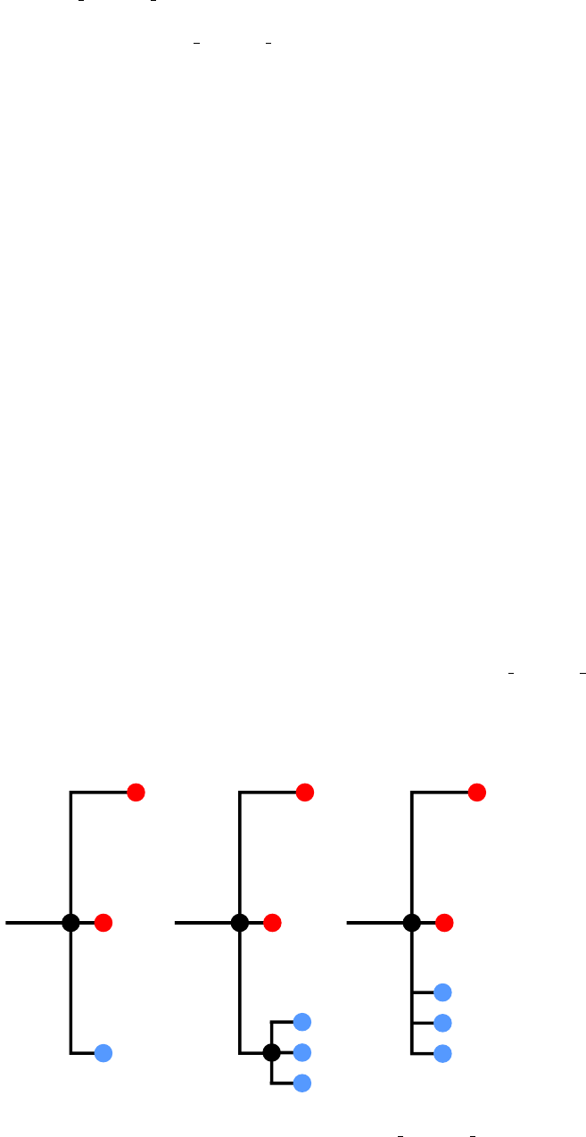
13 Parsimony reconstruction

The core of the phyloscanner analyse trees.R analysis is an ancestral state reconstruction of hosts to

internal nodes of each phylogeny. We oﬀer several algorithms for this; the exact one is speciﬁed with the

ﬁnal compulsory argument to phyloscanner analyse trees.R. For full details, see the supplementary

information of the phyloscanner paper.

•A fast, non-rigorous (for more than two hosts) adaptation of the procedure outlined in Romero-

Severson et al. (PNAS 2016). This is speciﬁed by r. It will not reliably reconstruct multiple

infections.

•A parsimony reconstruction using the Sankoﬀ algorithm that allows for an additional “unassigned”

state and can be conﬁgured to penalise the reconstruction of single infections to hosts which imply

unreasonable amounts of diversity. This is speciﬁed by two or three arguments, separated by

commas. The ﬁrst is s. The second is the value of the kparameter that penalises within-host

diversity; if this is set to 0 then no penalty is applied and the procedure is equivalent to standard

parsimony with the unassigned state. It is recommended that users explore their data to pick

suitable values of k, as it is likely to be pathogen- and sequencing method-dependent. As a rule

of thumb, it should be the reciprocal of a patristic distance so large that it would be surprising to

encounter a host with an infection so diverse that a phylogeny built from pathogen sequences from

just that host had a branch that long or longer, if the host was infected only once.

The latter parsimony reconstruction algorithm uses a very large matrix for large trees and occasionally R

will run out of memory; the argument --useff will cause the script to use the ff library instead, which

solves many memory issues at the cost of speed.

Of concern in either of the two proper parsimony reconstruction algorithms is used is how to handle

terminal branches of zero or negligible length. In particular, if a tip with a read count of nis connected

to its parent node by such a branch, should that tip be considered as one tip or ntips for the parsimony

reconstruction? As an illustrated example, see below. Phylogenetic software output, with minimum-

length branches collapsed to zero (see above) might appear as in diagram a) in Fig. 13 below, where

colours represent hosts and the numbers in the coloured tips read counts, while numbers on branches are

branch lengths (with zero-length branches displayed with nonzero lengths for clarity). The question is

whether a parsimony reconstruction should consider this clade as b), where all the reads represented by

the blue tip in a) form separate tips but their MRCA mis not the MRCA nof the entire clade, or b),

where the MRCAs are the same. Under simple parsimony, the cost of reconstructing nas red is 1 in b) and

3 in c), but the cost of reconstructing it as blue is 2 in both. By default, phyloscanner analyse trees.R

treats this situation as b), which is the same as ignoring read counts in the parsimony reconstruction

- as it will always be most parsimonious to reconstruct mas blue to avoid turning one transition into

three, the three blue tips can be ignored and the colour of mﬁxed, so we are back to diagram a) - but

the --readCountsMatterOnZeroLengthBranches option, if speciﬁed, will treat it as c) instead.

a) b) c)

nn n

Annotated versions of all input trees will be output by phyloscanner analyse trees.R, in pdf format

by default. The --outputNexusTree option can be used to make it provide these trees in Nexus format

instead.

The standalone R script to perform parsimony reconstruction is split hosts to subtrees.R.

14 Summary statistics

By default, phyloscanner analyse trees.R produces a csv ﬁle of summary statistics with the following

columns:

•id: the host ID for the statistics in this row.

•ﬁle suﬃx: the ﬁle suﬃx of the associated tree ﬁle.

•xcoord: used to draw the graphs (see below); this is the midpoint of the genome window if the

windowed approach is used, and the position of the ﬁle suﬃx in an alphabetical ordering if not.

•Tips: the number of tips from this host in this tree.

•Reads: the number of reads from this host in this tree (if read counts were not detected then this

column will be identical to the tip counts, as each tip is assumed to represent one read).

•Subgraphs: the number of subgraphs that the parsimony reconstruction identiﬁed for this host in

this tree.

•clades: the number of separate clades monophyletic clades from this host in this tree.

•overall.rtt: the mean patristic distance from tips from this host to the MRCA of the tips from this

host, weighted by read counts if these are given

•largest.rtt: the mean patristic distance from tips from the largest (by read count) subgraph from

the host to the MRCA of that subgraph, weighted by read counts if these are given.

•max.branch.length: the length of the longest branch in the tree obtained by pruning all tips from

the tree except the ones from this host.

•max.patristic.distance: the largest patristic distance between any pair of tips from this host.

•global.mean.pat.distance: the mean patristic distance between tips from this host.

•subgraph.mean.pat.distance: the mean patristic distance between tips in the largest subgraph.

•recombination.metric: this column only appears if the recombination metric ﬁles output by

phyloscanner make trees.py have been given to phyloscanner analyse trees.R using the

--recombinationFiles argument. It gives the value of the recombination metric for this host in

this tree.

•prop.gp.1 to prop.gp.X: A variable number of columns recording what proportion of the reads from

this host occur in each subgraph, ordered by size. The total number of columns is the largest

number of subgraphs present for any host in any tree (and so many columns will be 0 for most

hosts).

Also generated, if more than one phylogeny is given as input, is a pdf ﬁle graphing these statistics

across all trees for every host. Each host occupies a separate page in this ﬁle, with ﬁve or six graphs per

host:

1. Number of reads and number of tips

2. Number of subgraphs and number of clades

3. Mean root-to-tip distance in the largest subgraph and in the whole tree

4. Mean pairwise patristic distance in the largest subgraph and in the whole tree

5. The proportion of reads appearing in each subgraph

6. (If recombination metric ﬁles are speciﬁed with -R) The value of the recombination metric across

the genome

If the script could detect genome window coordinates from the ﬁle suﬃxes, and the starts and ends

of those windows occur regularly across the genome, these graphs will be annotated with light grey

rectangles for windows where a host is missing from a single window, and dark grey rectangles where a

window appears to be entirely missing (i.e. it had no tree ﬁle).

The standalone R script to produce summary statistics is summary statistics.R.

15 Classiﬁcation of pairwise relationships

The parsimony reconstruction has annotated all internal nodes in each phylogeny with either a host or

the unassigned state, and from this information, host subgraphs have been identiﬁed. The next step in

the script is to document the relationships between each pair of hosts in every tree. By default (when

the script is run on multiple tree ﬁles) this is done silently, but two types of output ﬁle can be generated.

The --collapsedTrees option produces the collapsed tree (see the phyloscanner paper), in csv

format. This ﬁle has four columns:

•The collapsed tree node ID, which is the host ID or “unassigned region” followed by -S and an

identifying number

•The collapsed tree node ID of that node’s unique host, or “root” if it has none

•The ID for the host, or “unassigned region”, associated with this node

•The ID for the host, or “unassigned region”, associated with the parent node

If the script is run on a single tree ﬁle only, the classiﬁcation csv ﬁle is produced by default, but the

collapsed tree is not.

The --allClassifications option produces per-tree csv ﬁles describing all pairwise relationships

between hosts. The columns of this ﬁle are as follows:

•host.1, host.2: the pair of hosts. The order does not signify anything on its own but is relevant to

interpretation of the path.classiﬁcation column.

•adjacent: This is TRUE if there exist two nodes, one each from subgraphs from the two hosts, such

that the path between the two traverses only nodes that are either also from these host subgraphs,

or unassigned. (In other words, it is possible to move through the phylogeny from one host to the

other without moving through the subgraph of another sampled patient.)

•contiguous: This is TRUE if for any two nodes, one each from subgraphs from the two hosts, the

path between the two intersects no nodes that are not either also from these host subgraphs, or

unassigned. This is similar to adjacent but a little stronger.

•paths12, paths21: paths12 is the number of nodes from host.2 in the collapsed tree which have an

ancestor that is from host.1, and paths21 is the opposite.

•nodes1, nodes2: these are the number of collapsed tree nodes for host.1 and host.2 respectively.

•path.classiﬁcation: this describes the topological relationship between the two hosts in the cablol-

lapsed tree:

–“none” indicates that no nodes from host.1 are ancestral to nodes from host.2 or vice versa

–“anc” indicates that there is only one node from host.2 and it is a descendant of a node from

host.1

–“desc” indicates that there is only one node from host.1 and it is a descendant of a node from

host.2

–“multiAnc” indicates that there is more than one node from host.2 and all are descended from

a node from host.1

–“multiDesc” indicates that there is more than one node from host.1 and all are descended from

a node from host.2

–“complex” indicates that none of the above are true (which is suggestive of an ancestral

relationship and often direct transmission, but with unknown direction)

•min.distance.between.subgraphs: this is the smallest patristic distance between a node in a host.1

subgraph and a host.2 subgraph

•normalised.min.distance.between.subgraphs: If the tree branch lengths were normalised, this is the

above distance but divided by the normalisation constant for this tree

The standalone script to classify pairwise host relationships is classify relationships.R.

16 Pairwise relationship summary

The next stage in the script is to gather the pairwise relationships between hosts in each window and

summarise this across the whole run. Pairs are inferred to be related in a tree if they are both adjacent

and (optionally) within the patristic distance threshold speciﬁed by the --distanceThreshold option.

If --distanceThreshold is not given then it is assumed to be inﬁnite and adjacency is the only criterion

that will be used to identify related pairs. If tree branch lengths were normalised then the distance

threshold is applied to normalised distances.

By default, two outputs are produced. The ﬁrst is a .csv ﬁle whose ﬁrst three columns are a pair of

hosts and a classiﬁcation of the topological relationship between the pair. Rows for pairs which are never

related at all or never show a particular topological relationship are omitted.

The --windowThreshold option is used to specify the minimum proportion of trees in which a pair

of hosts were found to be related to make rows for that pair appear in the output ﬁle. The default is 0.5,

meaning that only pairs that are related in at least half of the trees appear. If this is instead set to 0, all

relationships are reported if they ever occur at all.

The .csv ﬁle has the following columns:

•host.1, host.2: the two hosts.

•ancestry: the type of ancestry (see below).

•ancestry.tree.count: the number of trees in which this pair of hosts are related (by the deﬁnition

given above) and the relationship is of the type given under “ancestry”.

•both.exist: the number of trees in which both hosts are present.

•fraction: the number of windows showing this relationship over the number of windows where both

occur (“count” over “both.exist”), as text.

•any.relationship.tree.count: the number of trees in which this pair of hosts are related (by the

deﬁnition given above).

The ancestry relationships are as follows:

•“none”: no node in the collapsed tree from host.1 is descended from a node from host.2 or vice

versa.

•“trans”: there is just one collapsed tree node from host.2 and it is descended from a node from

host.1. Since they must be adjacent, this makes host.1 its immediate ancestor.

•“multi trans”: there is more than one collapsed tree node from host.2 and all are descended from

a node from host.1. This classiﬁcation only appears if the --allowMultiTrans option is given; if

not these relationships count as “complex”. This is because this relationship is less indicative of

the direction of transmission than “trans”; it may simply indicate that the tips from the two hosts

are very intermingled, and it is prone to bias introduced by diﬀerences in tip counts. By default,

the script is conservative and does not take this relationship as a signal of directionality. However,

as with “complex”, it is quite strongly indicative of direct transmission (Romero-Severson et al.

PNAS 2016).

•“complex”: where none of the above are true; if --allowMultiTrans is not speciﬁed then

“multi trans” relationships are also allocated “complex”.

The standalone script to summarise these relationships is transmission summary.R.

Unless the --skipSummaryGraph option is speciﬁed, a PDF ﬁle displaying a simpliﬁed summary of

between-patient relationships will also be produced. The dimensions of this plot (in inches) can be

controlled with the --summaryPlotDimensions options; the default here is 25 ×25 inches. If the output

plot is too small and cluttered, try using a larger number. The output here will simplify the between-

host relationships as in ﬁgure 4B of the phyloscanner paper, such that there is only one link between

any pair, and that link will appear as an arrow if the proportion of windows showing transmission in

that direction is above a threshold, but simply as a line otherwise. Links with arrows are labelled with

two numbers separated by a forward slash: the ﬁrst is the proportion of trees showing the directional

relationship implied by the arrow, while the second is the proportion of trees showing any relationship at

all. Links without arrows are just labelled with a the proportion showing any relationship. The default

threshold for the display of arrows is 0.33, but this can be overridden with the --directionThreshold

option. Links will only appear at all if a relationship occurs in more that the --windowThreshold option,

and it is required that --directionThreshold be less than or equal to --windowThreshold.

Graph visualisation is a complicated aﬀair, and we cannot ensure that this PDF ﬁle will always

display a satisfactory arrangement of nodes and labels. Users wishing to make their own graphs may

use an analysis package such as Cytoscape with the summary .csv ﬁle as input. A standalone script,

simplify graph.R, can be used to simplify the information in this ﬁle in the manner described above.

See the command line help for that script for more information.

17 Miscellaneous options

Remaining command line options are as follows:

•--verbose: Speciﬁes the level of verbose output. The default is “1”, which gives minimal output

to the command line. “0” gives no output and “2” full output.

•--noProgressBars: if present and --verbose is given, progress bars will not appear (useful when

the output stream is written to ﬁle).

•--outputDir: the directory to write output ﬁles into; if not speciﬁed this is the current working

directory.

•--pdfWidth: the width of the pdf tree ﬁle output

•--pdfRelHeight: the height, per tip, of the pdf tree ﬁle output

•--pdfScaleBarWidth: The width of the scale bar in the pdf tree ﬁle output (in the same units as

the branch lengths in the tree)

•--outputRDA: If present, an R list containing the objects used in the calculations is written as a

workspace image at the end of the script

•--seed: Two parts of the process may use randomisation: the downsampling, and occasional tie-

breaking in parsimony reconstruction.

•--overwrite: This option tells phyloscanner analyse trees.R to overwrite any existing output

ﬁle with the same names. This option sets a random number seed. The script will try to identify

this automatically, but this may not work on all systems.

References

[1] C. Wymant, M. Hall, O. Ratmann, D. Bonsall, T. Golubchik, M. de Cesare, A. Gall, M. Cornelissen,

C. Fraser, T. M. P. C. STOP-HCV Consortium, and T. B. Collaboration, “Phyloscanner: Infer-

ring transmission from within- and between-host pathogen genetic diversity,” Molecular Biology and

Evolution, vol. 35, no. 3, pp. 719–733, 2018.

[2] H. Li, B. Handsaker, A. Wysoker, T. Fennell, J. Ruan, N. Homer, G. Marth, G. Abecasis, R. Durbin,

and 1000 Genome Project Data Processing Subgroup, “The sequence alignment/map (sam) format

and samtools,” Bioinformatics, 2009.

[3] K. Katoh, K. Misawa, K. Kuma, and T. Miyata, “Maﬀt: a novel method for rapid multiple sequence

alignment based on fast fourier transform,” Nucleic Acids Research, vol. 30, no. 14, pp. 3059–3066,

2002.

[4] A. Stamatakis, “Raxml version 8: a tool for phylogenetic analysis and post-analysis of large phyloge-

nies,” Bioinformatics, vol. 30, no. 9, pp. 1312–1313, 2014.

[5] G. Yu, D. K. Smith, H. Zhu, Y. Guan, and T. T.-Y. Lam, “ggtree: an r package for visualization and

annotation of phylogenetic trees with their covariates and other associated data,” Methods in Ecology

and Evolution, vol. 8, no. 1, pp. 28–36, 2017.

Phyloscanner Manual

Navigation menu

Versions of this User Manual:

Views

Navigation