PhysicsReferenceManual.dvi Physics Reference Manual
User Manual:
Open the PDF directly: View PDF ![]() .
.
Page Count: 563 [warning: Documents this large are best viewed by clicking the View PDF Link!]
Physics Reference Manual
Version: geant4 10.3 (9 December 2016)
Contents
I Introduction 1
1 Introduction 2
1.1 Scope of This Manual . . . . . . . . . . . . . . . . . . . . . . . 2
1.2 Definition of Terms . . . . . . . . . . . . . . . . . . . . . . . . 2
2 Monte Carlo Methods 4
3 Particle Transport 6
3.1 True Step Length . . . . . . . . . . . . . . . . . . . . . . . . . 8
3.1.1 The Interaction Length or Mean Free Path . . . . . . . 8
3.1.2 Determination of the Interaction Point . . . . . . . . . 9
3.1.3 Step Limitations . . . . . . . . . . . . . . . . . . . . . 9
3.1.4 Updating the Particle Time . . . . . . . . . . . . . . . 10
3.2 Transportation . . . . . . . . . . . . . . . . . . . . . . . . . . 11
II Particle Decay 13
4 Decay 14
4.1 Mean Free Path for Decay in Flight . . . . . . . . . . . . . . . 14
4.2 Branching Ratios and Decay Channels . . . . . . . . . . . . . 14
4.2.1 G4PhaseSpaceDecayChannel . . . . . . . . . . . . . . . 15
4.2.2 G4DalitzDecayChannel . . . . . . . . . . . . . . . . . . 15
4.2.3 Muon Decay . . . . . . . . . . . . . . . . . . . . . . . . 16
4.2.4 Leptonic Tau Decay . . . . . . . . . . . . . . . . . . . 17
4.2.5 Kaon Decay . . . . . . . . . . . . . . . . . . . . . . . . 17
III Electromagnetic Interactions 19
5 Gamma Incident 20
5.1 Introduction . . . . . . . . . . . . . . . . . . . . . . . . . . . . 21
-10
5.1.1 General Interfaces . . . . . . . . . . . . . . . . . . . . . 21
5.2 Photoelectric Effect . . . . . . . . . . . . . . . . . . . . . . . . 23
5.2.1 Cross Section . . . . . . . . . . . . . . . . . . . . . . . 23
5.2.2 Final State . . . . . . . . . . . . . . . . . . . . . . . . 23
5.2.3 Relaxation . . . . . . . . . . . . . . . . . . . . . . . . . 24
5.3 Compton scattering . . . . . . . . . . . . . . . . . . . . . . . . 26
5.3.1 Cross Section . . . . . . . . . . . . . . . . . . . . . . . 26
5.3.2 Sampling the Final State . . . . . . . . . . . . . . . . . 27
5.3.3 Atomic shell effects . . . . . . . . . . . . . . . . . . . . 28
5.4 Gamma Conversion into an Electron - Positron Pair . . . . . . 30
5.4.1 Cross Section . . . . . . . . . . . . . . . . . . . . . . . 30
5.4.2 Final State . . . . . . . . . . . . . . . . . . . . . . . . 34
5.4.3 Ultra-Relativistic Model . . . . . . . . . . . . . . . . . 35
5.5 Gamma Conversion into a Muon - Anti-mu Pair . . . . . . . . 37
5.5.1 Cross Section and Energy Sharing . . . . . . . . . . . . 37
5.5.2 Parameterization of the Total Cross Section . . . . . . 40
5.5.3 Multi-differential Cross Section and Angular Variables 42
5.5.4 Procedure for the Generation of µ+µ−Pairs . . . . . . 44
6 Elastic scattering 52
6.1 Multiple Scattering . . . . . . . . . . . . . . . . . . . . . . . . 53
6.1.1 Introduction . . . . . . . . . . . . . . . . . . . . . . . . 53
6.1.2 Definition of Terms . . . . . . . . . . . . . . . . . . . . 54
6.1.3 Path Length Correction . . . . . . . . . . . . . . . . . 56
6.1.4 Angular Distribution . . . . . . . . . . . . . . . . . . . 58
6.1.5 Determination of the Model Parameters . . . . . . . . 58
6.1.6 Step Limitation Algorithm . . . . . . . . . . . . . . . . 60
6.1.7 Boundary Crossing Algorithm . . . . . . . . . . . . . . 62
6.1.8 Implementation Details . . . . . . . . . . . . . . . . . . 63
6.2 Discrete Processes for Charged Particles . . . . . . . . . . . . 66
6.3 Single Scattering . . . . . . . . . . . . . . . . . . . . . . . . . 68
6.3.1 Coulomb Scattering . . . . . . . . . . . . . . . . . . . . 68
6.3.2 Implementation Details . . . . . . . . . . . . . . . . . . 69
6.4 Ion Scattering . . . . . . . . . . . . . . . . . . . . . . . . . . . 71
6.4.1 Method . . . . . . . . . . . . . . . . . . . . . . . . . . 71
6.4.2 Implementation Details . . . . . . . . . . . . . . . . . . 75
6.5 Single Scattering, Screened Coulomb Potential and NIEL . . . 77
6.5.1 Nucleus–Nucleus Interactions . . . . . . . . . . . . . . 77
6.5.2 Nuclear Stopping Power . . . . . . . . . . . . . . . . . 79
6.5.3 Non-Ionizing Energy Loss due to Coulomb Scattering . 82
6.5.4 G4IonCoulombScatteringModel . . . . . . . . . . . . . 83
6.5.5 The Method . . . . . . . . . . . . . . . . . . . . . . . . 83
6.5.6 Implementation Details . . . . . . . . . . . . . . . . . . 84
6.6 Electron Screened Single Scattering and NIEL . . . . . . . . . 86
6.6.1 Scattering Cross Section of Electrons on Nuclei . . . . 86
6.6.2 Nuclear Stopping Power of Electrons . . . . . . . . . . 95
6.6.3 Non-Ionizing Energy-Loss of Electrons . . . . . . . . . 96
6.7 G4eSingleScatteringModel . . . . . . . . . . . . . . . . . . . . 97
6.7.1 The method . . . . . . . . . . . . . . . . . . . . . . . . 98
6.7.2 Implementation Details . . . . . . . . . . . . . . . . . . 100
7 Energy loss of Charged Particles 102
7.1 Mean Energy Loss . . . . . . . . . . . . . . . . . . . . . . . . 103
7.1.1 Method . . . . . . . . . . . . . . . . . . . . . . . . . . 103
7.1.2 General Interfaces . . . . . . . . . . . . . . . . . . . . . 104
7.1.3 Step-size Limit . . . . . . . . . . . . . . . . . . . . . . 104
7.1.4 Run Time Energy Loss Computation . . . . . . . . . . 106
7.1.5 Energy Loss by Heavy Charged Particles . . . . . . . . 108
7.2 Energy Loss Fluctuations . . . . . . . . . . . . . . . . . . . . . 110
7.2.1 Fluctuations in Thick Absorbers . . . . . . . . . . . . . 110
7.2.2 Fluctuations in Thin Absorbers . . . . . . . . . . . . . 111
7.2.3 Width Correction Algorithm . . . . . . . . . . . . . . . 113
7.2.4 Sampling of Energy Loss . . . . . . . . . . . . . . . . . 113
7.3 Correcting the Cross Section for Energy Variation . . . . . . 115
7.4 Conversion from Cut in Range to Energy Threshold . . . . . . 117
7.5 Photoabsorption ionization model . . . . . . . . . . . . . . . . 120
7.5.1 Cross Section for Ionizing Collisions . . . . . . . . . . . 120
7.5.2 Energy Loss Simulation . . . . . . . . . . . . . . . . . 122
7.5.3 Photoabsorption Cross Section at Low Energies . . . . 123
7.5.4 Status of this document . . . . . . . . . . . . . . . . . 124
8 Electron and Positron Incident 125
8.1 Ionization . . . . . . . . . . . . . . . . . . . . . . . . . . . . . 126
8.1.1 Method . . . . . . . . . . . . . . . . . . . . . . . . . . 126
8.1.2 Continuous Energy Loss . . . . . . . . . . . . . . . . . 126
8.1.3 Total Cross Section per Atom and Mean Free Path . . 128
8.1.4 Simulation of Delta-ray Production . . . . . . . . . . . 129
8.2 Bremsstrahlung . . . . . . . . . . . . . . . . . . . . . . . . . . 131
8.2.1 Seltzer-Berger bremsstrahlung model . . . . . . . . . . 131
8.2.2 Bremsstrahlung of high-energy electrons . . . . . . . . 134
8.3 Positron - Electron Annihilation . . . . . . . . . . . . . . . . . 139
8.3.1 Introduction . . . . . . . . . . . . . . . . . . . . . . . . 139
8.3.2 Cross Section . . . . . . . . . . . . . . . . . . . . . . . 139
8.3.3 Sampling the final state . . . . . . . . . . . . . . . . . 139
8.3.4 Sampling the Gamma Energy . . . . . . . . . . . . . . 140
8.4 Positron Annihilation into µ+µ−Pair in Media . . . . . . . . . 142
8.4.1 Total Cross Section . . . . . . . . . . . . . . . . . . . . 142
8.4.2 Sampling of Energies and Angles . . . . . . . . . . . . 142
8.5 Positron Annihilation into Hadrons . . . . . . . . . . . . . . . 146
8.5.1 Introduction . . . . . . . . . . . . . . . . . . . . . . . . 146
8.5.2 Cross Section . . . . . . . . . . . . . . . . . . . . . . . 146
8.5.3 Sampling the final state . . . . . . . . . . . . . . . . . 146
9 Low Energy Livermore 148
9.1 Introduction . . . . . . . . . . . . . . . . . . . . . . . . . . . . 149
9.1.1 Physics . . . . . . . . . . . . . . . . . . . . . . . . . . . 149
9.1.2 Data Sources . . . . . . . . . . . . . . . . . . . . . . . 149
9.1.3 Distribution of the Data Sets . . . . . . . . . . . . . . 150
9.1.4 Calculation of Total Cross Sections . . . . . . . . . . . 151
9.2 Compton Scattering . . . . . . . . . . . . . . . . . . . . . . . 152
9.2.1 Total Cross Section . . . . . . . . . . . . . . . . . . . . 152
9.2.2 Sampling of the Final State . . . . . . . . . . . . . . . 152
9.3 Compton Scattering by Linearly Polarized Gamma Rays . . . 154
9.3.1 The Cross Section . . . . . . . . . . . . . . . . . . . . . 154
9.3.2 Angular Distribution . . . . . . . . . . . . . . . . . . . 154
9.3.3 Polarization Vector . . . . . . . . . . . . . . . . . . . . 154
9.3.4 Unpolarized Photons . . . . . . . . . . . . . . . . . . . 155
9.4 Rayleigh Scattering . . . . . . . . . . . . . . . . . . . . . . . . 156
9.4.1 Total Cross Section . . . . . . . . . . . . . . . . . . . . 156
9.4.2 Sampling of the Final State . . . . . . . . . . . . . . . 156
9.5 Gamma Conversion . . . . . . . . . . . . . . . . . . . . . . . . 157
9.5.1 Total cross-section . . . . . . . . . . . . . . . . . . . . 157
9.5.2 Sampling of the final state . . . . . . . . . . . . . . . . 157
9.6 Pair production by Linearly Polarized Gamma Rays . . . . . . 159
9.6.1 Relativistic cross section for linearly polarized gamma
ray . . . . . . . . . . . . . . . . . . . . . . . . . . . . . 159
9.6.2 Spatial azimuthal distribution . . . . . . . . . . . . . . 160
9.6.3 Unpolarized Photons . . . . . . . . . . . . . . . . . . . 161
9.7 Triple Gamma Conversion . . . . . . . . . . . . . . . . . . . . 163
9.7.1 Method . . . . . . . . . . . . . . . . . . . . . . . . . . 163
9.7.2 Azimuthal Distribution for Electron Recoil . . . . . . . 163
9.7.3 Monte Carlo Simulation of the Asymptotic Expression 163
9.7.4 Algorithm for Non Polarized Radiation . . . . . . . . . 164
9.7.5 Algorithm for Polarized Radiation . . . . . . . . . . . . 166
9.7.6 Sampling of Energy . . . . . . . . . . . . . . . . . . . . 168
9.8 Photoelectric effect . . . . . . . . . . . . . . . . . . . . . . . . 170
9.8.1 Cross sections . . . . . . . . . . . . . . . . . . . . . . . 170
9.8.2 Sampling of the final state . . . . . . . . . . . . . . . . 170
9.8.3 Angular distribution of the emitted photoelectron . . . 170
9.9 Electron ionisation . . . . . . . . . . . . . . . . . . . . . . . . 173
9.10 Bremsstrahlung . . . . . . . . . . . . . . . . . . . . . . . . . . 175
9.10.1 Bremsstrahlung angular distributions . . . . . . . . . . 176
10 Low Energy Penelope 182
10.1 Penelope physics . . . . . . . . . . . . . . . . . . . . . . . . . 183
10.1.1 Introduction . . . . . . . . . . . . . . . . . . . . . . . . 183
10.1.2 Compton scattering . . . . . . . . . . . . . . . . . . . . 183
10.1.3 Rayleigh scattering . . . . . . . . . . . . . . . . . . . . 185
10.1.4 Gamma conversion . . . . . . . . . . . . . . . . . . . . 186
10.1.5 Photoelectric effect . . . . . . . . . . . . . . . . . . . . 188
10.1.6 Bremsstrahlung . . . . . . . . . . . . . . . . . . . . . . 189
10.1.7 Ionisation . . . . . . . . . . . . . . . . . . . . . . . . . 191
10.1.8 Positron Annihilation . . . . . . . . . . . . . . . . . . . 197
11 Monash University low energy photon processes 200
11.1 Monash Low Energy Models . . . . . . . . . . . . . . . . . . . 201
11.1.1 Introduction . . . . . . . . . . . . . . . . . . . . . . . . 201
11.1.2 Physics and Simulation . . . . . . . . . . . . . . . . . . 201
12 Charged Hadron Incident 204
12.1 Ionization . . . . . . . . . . . . . . . . . . . . . . . . . . . . . 205
12.1.1 Method . . . . . . . . . . . . . . . . . . . . . . . . . . 205
12.1.2 Continuous Energy Loss . . . . . . . . . . . . . . . . . 205
12.1.3 Nuclear Stopping . . . . . . . . . . . . . . . . . . . . . 210
12.1.4 Total Cross Section per Atom . . . . . . . . . . . . . . 210
12.1.5 Simulating Delta-ray Production . . . . . . . . . . . . 211
12.1.6 Ion Effective Charge . . . . . . . . . . . . . . . . . . . 212
12.2 Low energy extentions . . . . . . . . . . . . . . . . . . . . . . 214
12.2.1 Energy losses of slow negative particles . . . . . . . . . 214
12.2.2 Energy losses of hadrons in compounds . . . . . . . . . 214
12.2.3 Fluctuations of energy losses of hadrons . . . . . . . . 215
12.2.4 ICRU 73-based energy loss model . . . . . . . . . . . . 217
13 Muon Incident 219
13.1 Ionization . . . . . . . . . . . . . . . . . . . . . . . . . . . . . 220
13.2 Bremsstrahlung . . . . . . . . . . . . . . . . . . . . . . . . . . 222
13.2.1 Differential Cross Section . . . . . . . . . . . . . . . . . 222
13.2.2 Continuous Energy Loss . . . . . . . . . . . . . . . . . 223
13.2.3 Total Cross Section . . . . . . . . . . . . . . . . . . . . 223
13.2.4 Sampling . . . . . . . . . . . . . . . . . . . . . . . . . 224
13.3 Positron - Electron Pair Production by Muons . . . . . . . . . 226
13.3.1 Differential Cross Section . . . . . . . . . . . . . . . . . 226
13.3.2 Total Cross Section and Restricted Energy Loss . . . . 229
13.3.3 Sampling of Positron - Electron Pair Production . . . . 230
13.4 Muon Photonuclear Interaction . . . . . . . . . . . . . . . . . 232
13.4.1 Differential Cross Section . . . . . . . . . . . . . . . . . 232
13.4.2 Sampling . . . . . . . . . . . . . . . . . . . . . . . . . 233
14 Atomic Relaxation 236
14.1 Atomic relaxation . . . . . . . . . . . . . . . . . . . . . . . . . 237
14.1.1 Fluorescence . . . . . . . . . . . . . . . . . . . . . . . . 237
14.1.2 Auger process . . . . . . . . . . . . . . . . . . . . . . . 238
14.1.3 PIXE . . . . . . . . . . . . . . . . . . . . . . . . . . . 238
15 Geant4-DNA 240
15.1 Geant4-DNA processes and models . . . . . . . . . . . . . . . 241
16 Microelectronics 242
16.1 The MicroElec extension for microelectronics applications . . . 243
17 Polarized Electron/Positron/Gamma Incident 245
17.1 Introduction . . . . . . . . . . . . . . . . . . . . . . . . . . . . 246
17.1.1 Stokes vector . . . . . . . . . . . . . . . . . . . . . . . 246
17.1.2 Transfer matrix . . . . . . . . . . . . . . . . . . . . . . 248
17.1.3 Coordinate transformations . . . . . . . . . . . . . . . 249
17.1.4 Polarized beam and material . . . . . . . . . . . . . . . 250
17.2 Ionization . . . . . . . . . . . . . . . . . . . . . . . . . . . . . 253
17.2.1 Method . . . . . . . . . . . . . . . . . . . . . . . . . . 253
17.2.2 Total cross section and mean free path . . . . . . . . . 253
17.2.3 Sampling the final state . . . . . . . . . . . . . . . . . 255
17.3 Positron - Electron Annihilation . . . . . . . . . . . . . . . . . 260
17.3.1 Method . . . . . . . . . . . . . . . . . . . . . . . . . . 260
17.3.2 Total cross section and mean free path . . . . . . . . . 260
17.3.3 Sampling the final state . . . . . . . . . . . . . . . . . 262
17.3.4 Annihilation at Rest . . . . . . . . . . . . . . . . . . . 264
17.4 Polarized Compton scattering . . . . . . . . . . . . . . . . . . 266
17.4.1 Method . . . . . . . . . . . . . . . . . . . . . . . . . . 266
17.4.2 Total cross section and mean free path . . . . . . . . . 266
17.4.3 Sampling the final state . . . . . . . . . . . . . . . . . 267
17.5 Polarized Bremsstrahlung for electron and positron . . . . . . 271
17.5.1 Method . . . . . . . . . . . . . . . . . . . . . . . . . . 271
17.5.2 Polarization in gamma conversion and bremsstrahlung 271
17.5.3 Polarization transfer to the photon . . . . . . . . . . . 272
17.5.4 Polarization transfer to the lepton . . . . . . . . . . . . 273
17.6 Polarized Gamma conversion into an electron–positron pair . . 276
17.6.1 Method . . . . . . . . . . . . . . . . . . . . . . . . . . 276
17.6.2 Polarization transfer . . . . . . . . . . . . . . . . . . . 276
17.7 Polarized Photoelectric Effect . . . . . . . . . . . . . . . . . . 278
17.7.1 Method . . . . . . . . . . . . . . . . . . . . . . . . . . 278
17.7.2 Polarization transfer . . . . . . . . . . . . . . . . . . . 278
18 X-Ray Production 281
18.1 Transition radiation . . . . . . . . . . . . . . . . . . . . . . . . 282
18.1.1 Relationship of Transition Rad to Cherenkov Rad . . . 282
18.1.2 Calculating the X-ray Transition Radiation Yield . . . 283
18.1.3 Simulating X-ray Transition Radiation Production . . . 285
18.2 Scintillation . . . . . . . . . . . . . . . . . . . . . . . . . . . . 289
18.3 ˇ
Cerenkov Effect . . . . . . . . . . . . . . . . . . . . . . . . . . 290
18.4 Synchrotron Radiation . . . . . . . . . . . . . . . . . . . . . . 292
18.4.1 Photon spectrum . . . . . . . . . . . . . . . . . . . . . 292
18.4.2 Validity . . . . . . . . . . . . . . . . . . . . . . . . . . 293
18.4.3 Direct inversion/generation of photon energy spectrum 294
18.4.4 Properties of the Power Spectra . . . . . . . . . . . . . 297
19 Optical Photons 300
19.1 Interactions of optical photons . . . . . . . . . . . . . . . . . . 301
19.1.1 Physics processes for optical photons . . . . . . . . . . 301
19.1.2 Photon polarization . . . . . . . . . . . . . . . . . . . . 302
19.1.3 Tracking of the photons . . . . . . . . . . . . . . . . . 303
19.1.4 Mie Scattering in Henyey-Greensterin Approximation . 306
20 Phonon-Lattice Interactions 309
20.1 Introduction . . . . . . . . . . . . . . . . . . . . . . . . . . . . 310
20.2 Phonon Propagation . . . . . . . . . . . . . . . . . . . . . . . 310
20.3 Lattice Parameters . . . . . . . . . . . . . . . . . . . . . . . . 311
20.4 Scattering and Mode Mixing . . . . . . . . . . . . . . . . . . . 311
20.5 Anharmonic Downconversion . . . . . . . . . . . . . . . . . . . 312
20.6 References . . . . . . . . . . . . . . . . . . . . . . . . . . . . . 312
21 Precision multi-scale modeling 314
21.1 Overview . . . . . . . . . . . . . . . . . . . . . . . . . . . . . . 315
21.2 Impact ionisation by hadrons and PIXE . . . . . . . . . . . . 315
22 Shower Parameterizations 324
22.1 Gflash Shower Parameterizations . . . . . . . . . . . . . . . . 325
22.1.1 Parameterization Ansatz . . . . . . . . . . . . . . . . . 325
22.1.2 Longitudinal Shower Profiles . . . . . . . . . . . . . . 325
22.1.3 Radial Shower Profiles . . . . . . . . . . . . . . . . . . 326
22.1.4 Gflash Performance . . . . . . . . . . . . . . . . . . . . 327
IV Hadronic Interactions 329
23 Total Reaction Cross Section in Nucleus-nucleus Reactions 330
23.1 Sihver Formula . . . . . . . . . . . . . . . . . . . . . . . . . . 330
23.2 Kox and Shen Formulae . . . . . . . . . . . . . . . . . . . . . 331
23.3 Tripathi formula . . . . . . . . . . . . . . . . . . . . . . . . . 333
23.4 Representative Cross Sections . . . . . . . . . . . . . . . . . . 335
23.5 Tripathi Formula for ”light” Systems . . . . . . . . . . . . . . 335
24 Coherent elastic scattering 340
24.1 Nucleon-Nucleon elastic Scattering . . . . . . . . . . . . . . . 340
25 Hadron-nucleus Elastic Scattering at Medium/High Energy341
25.1 Method of Calculation . . . . . . . . . . . . . . . . . . . . . . 341
26 Interactions of Stopping Particles 357
26.1 Complementary parameterised and theoretical treatment . . . 357
26.1.1 Pion absorption at rest . . . . . . . . . . . . . . . . . . 358
27 Parton string model. 360
27.1 Reaction initial state simulation. . . . . . . . . . . . . . . . . . 360
27.1.1 Allowed projectiles and bombarding energy range . . . 360
27.1.2 MC initialization procedure for nucleus. . . . . . . . . 360
27.1.3 Random choice of the impact parameter. . . . . . . . . 362
27.2 Sample of collision participants in nuclear collisions. . . . . . . 362
27.2.1 MC procedure to define collision participants. . . . . . 362
27.2.2 Separation of hadron diffraction excitation. . . . . . . . 363
27.3 Longitudinal string excitation . . . . . . . . . . . . . . . . . . 364
27.3.1 Hadron–nucleon inelastic collision . . . . . . . . . . . . 364
27.3.2 The diffractive string excitation . . . . . . . . . . . . . 364
27.3.3 The string excitation by parton exchange . . . . . . . . 364
27.3.4 Transverse momentum sampling . . . . . . . . . . . . . 365
27.3.5 Sampling x-plus and x-minus . . . . . . . . . . . . . . 365
27.3.6 The diffractive string excitation . . . . . . . . . . . . . 365
27.3.7 The string excitation by parton rearrangement . . . . . 366
27.4 Longitudinal string decay. . . . . . . . . . . . . . . . . . . . . 367
27.4.1 Hadron production by string fragmentation. . . . . . . 367
27.4.2 The hadron formation time and coordinate. . . . . . . 368
28 Fritiof (FTF) Model 370
28.1 Main assumptions of the FTF model . . . . . . . . . . . . . . 371
28.2 General properties of hadron–nucleon interactions . . . . . . . 374
28.2.1 π−p– interactions . . . . . . . . . . . . . . . . . . . . . 374
28.2.2 π+p– interactions . . . . . . . . . . . . . . . . . . . . . 376
28.2.3 pp – interactions . . . . . . . . . . . . . . . . . . . . . 377
28.2.4 K+p– and K−p– interactions . . . . . . . . . . . . . . 378
28.2.5 p¯p– interactions . . . . . . . . . . . . . . . . . . . . . 380
28.3 Cross sections of hadron–nucleon processes . . . . . . . . . . . 382
28.3.1 Total, elastic and inelastic hadron–nucleon cross sections382
28.3.2 Cross sections of quark exchange processes . . . . . . . 384
28.3.3 Cross sections of antiproton processes . . . . . . . . . . 384
28.3.4 Cross sections of diffractive and non-diffractive processes385
28.4 Simulation of hadron-nucleon interactions . . . . . . . . . . . 388
28.4.1 Simulation of meson–nucleon and nucleon–nucleon in-
teractions . . . . . . . . . . . . . . . . . . . . . . . . . 388
28.4.2 Simulation of antibaryon–nucleon interactions . . . . . 391
28.5 Flowchart of the FTF model . . . . . . . . . . . . . . . . . . . 392
28.6 Simulation of nuclear interactions . . . . . . . . . . . . . . . . 394
28.6.1 Sampling of intra-nuclear collisions . . . . . . . . . . . 394
28.6.2 Reggeon cascading . . . . . . . . . . . . . . . . . . . . 400
28.6.3 ”Fermi motion” of nuclear nucleons . . . . . . . . . . . 407
28.6.4 Excitation energy of nuclear residuals . . . . . . . . . . 410
29 Bertini Intranuclear Cascade Model in Geant4 414
29.1 Introduction . . . . . . . . . . . . . . . . . . . . . . . . . . . . 414
29.2 The Geant4 Cascade Model . . . . . . . . . . . . . . . . . . . 415
29.2.1 Model Limits . . . . . . . . . . . . . . . . . . . . . . . 415
29.2.2 Intranuclear Cascade Model . . . . . . . . . . . . . . . 415
29.2.3 Nuclear Model . . . . . . . . . . . . . . . . . . . . . . 416
29.2.4 Pre-equilibrium Model . . . . . . . . . . . . . . . . . . 418
29.2.5 Break-up models . . . . . . . . . . . . . . . . . . . . . 418
29.2.6 Evaporation Model . . . . . . . . . . . . . . . . . . . . 419
29.3 Interfacing Bertini implementation . . . . . . . . . . . . . . . 419
30 The Geant4 Binary Cascade 422
30.1 Modeling overview . . . . . . . . . . . . . . . . . . . . . . . . 422
30.1.1 The transport algorithm . . . . . . . . . . . . . . . . . 422
30.1.2 The description of the target nucleus and fermi motion 423
30.1.3 Optical and phenomenological potentials . . . . . . . . 424
30.1.4 Pauli blocking simulation . . . . . . . . . . . . . . . . . 425
30.1.5 The scattering term . . . . . . . . . . . . . . . . . . . 425
30.1.6 Total inclusive cross-sections . . . . . . . . . . . . . . 426
30.1.7 Channel cross-sections . . . . . . . . . . . . . . . . . . 426
30.1.8 Mass dependent resonance width and partial width . . 427
30.1.9 Resonance production cross-section in the t-channel . . 427
30.1.10 Nucleon Nucleon elastic collisions . . . . . . . . . . . . 428
30.1.11 Generation of transverse momentum . . . . . . . . . . 428
30.1.12 Decay . . . . . . . . . . . . . . . . . . . . . . . . . . . 429
30.1.13 The escaping particle and coherent effects . . . . . . . 429
30.1.14 Light ion reactions . . . . . . . . . . . . . . . . . . . . 430
30.1.15 Transition to pre-compound modeling . . . . . . . . . . 430
30.1.16 Calculation of excitation energies and residuals . . . . 431
30.2 Comparison with experiments . . . . . . . . . . . . . . . . . . 431
31 Quantum Molecular Dynamics for Heavy Ions 440
31.1 Equations of Motion . . . . . . . . . . . . . . . . . . . . . . . 441
31.2 Ion-ion Implementation . . . . . . . . . . . . . . . . . . . . . . 443
31.3 Cross Sections . . . . . . . . . . . . . . . . . . . . . . . . . . . 444
32 Abrasion-ablation Model 446
32.1 Introduction . . . . . . . . . . . . . . . . . . . . . . . . . . . . 446
32.2 Initial nuclear dynamics and impact parameter . . . . . . . . . 447
32.3 Abrasion process . . . . . . . . . . . . . . . . . . . . . . . . . 448
32.4 Abraded nucleon spectrum . . . . . . . . . . . . . . . . . . . . 450
32.5 De-excitation of nuclear pre-fragments by standard G4 . . . . 451
32.6 De-excitation of nuclear pre-fragments by nuclear ablation . . 452
32.7 Definition of the functions P and F used in the abrasion model 453
33 Electromagnetic Dissociation Model 457
33.1 The Model . . . . . . . . . . . . . . . . . . . . . . . . . . . . . 457
34 Precompound model. 461
34.1 Reaction initial state. . . . . . . . . . . . . . . . . . . . . . . . 461
34.2 Simulation of pre-compound reaction . . . . . . . . . . . . . . 461
34.2.1 Statistical equilibrium condition . . . . . . . . . . . . . 462
34.2.2 Level density of excited (n-exciton) states . . . . . . . 462
34.2.3 Transition probabilities . . . . . . . . . . . . . . . . . . 462
34.2.4 Emission probabilities for nucleons . . . . . . . . . . . 464
34.2.5 Emission probabilities for complex fragments . . . . . . 464
34.2.6 The total probability . . . . . . . . . . . . . . . . . . . 465
34.2.7 Calculation of kinetic energies for emitted particle . . . 465
34.2.8 Parameters of residual nucleus. . . . . . . . . . . . . . 465
35 Evaporation Model 467
35.1 Introduction . . . . . . . . . . . . . . . . . . . . . . . . . . . . 467
35.2 Evaporation model . . . . . . . . . . . . . . . . . . . . . . . . 467
35.2.1 Cross sections for inverse reactions . . . . . . . . . . . 468
35.2.2 Coulomb barriers . . . . . . . . . . . . . . . . . . . . . 468
35.2.3 Level densities . . . . . . . . . . . . . . . . . . . . . . . 469
35.2.4 Maximum energy available for evaporation . . . . . . . 469
35.2.5 Total decay width . . . . . . . . . . . . . . . . . . . . . 470
35.3 GEM model . . . . . . . . . . . . . . . . . . . . . . . . . . . . 470
35.4 Nuclear fission . . . . . . . . . . . . . . . . . . . . . . . . . . . 472
35.4.1 The fission total probability . . . . . . . . . . . . . . . 472
35.4.2 The fission barrier . . . . . . . . . . . . . . . . . . . . 472
35.5 Photon evaporation . . . . . . . . . . . . . . . . . . . . . . . . 473
35.5.1 Computation of probability . . . . . . . . . . . . . . . 473
35.5.2 Discrete photon evaporation . . . . . . . . . . . . . . . 473
35.5.3 Internal conversion electron emission . . . . . . . . . . 474
35.6 Sampling procedure . . . . . . . . . . . . . . . . . . . . . . . . 475
36 Fission model. 478
36.1 Reaction initial state. . . . . . . . . . . . . . . . . . . . . . . . 478
36.2 Fission process simulation. . . . . . . . . . . . . . . . . . . . . 478
36.2.1 Atomic number distribution of fission products. . . . . 478
36.2.2 Charge distribution of fission products. . . . . . . . . . 480
36.2.3 Kinetic energy distribution of fission products. . . . . . 480
36.2.4 Calculation of the excitation energy of fission products. 481
36.2.5 Excited fragment momenta. . . . . . . . . . . . . . . . 481
37 Fermi break-up model. 483
37.1 Fermi break-up simulation for light nuclei . . . . . . . . . . . . 483
37.1.1 Allowed channels . . . . . . . . . . . . . . . . . . . . . 483
37.1.2 Break-up probability . . . . . . . . . . . . . . . . . . . 484
37.1.3 Fragment characteristics . . . . . . . . . . . . . . . . . 485
37.1.4 Sampling procedure . . . . . . . . . . . . . . . . . . . . 485
38 Multifragmentation model. 487
38.1 Multifragmentation process simulation. . . . . . . . . . . . . . 487
38.1.1 Multifragmentation probability. . . . . . . . . . . . . . 487
38.1.2 Direct simulation of low multiplicity disintegration . . 489
38.1.3 Fragment multiplicity distribution. . . . . . . . . . . . 490
38.1.4 Atomic number distribution of fragments. . . . . . . . 490
38.1.5 Charge distribution of fragments. . . . . . . . . . . . . 491
38.1.6 Kinetic energy distribution of fragments. . . . . . . . . 491
38.1.7 Calculation of the fragment excitation energies. . . . . 491
39 INCL++: the Liege Intranuclear Cascade model 493
39.1 Introduction . . . . . . . . . . . . . . . . . . . . . . . . . . . . 493
39.1.1 Suitable application fields . . . . . . . . . . . . . . . . 494
39.2 Generalities of the INCL++ cascade . . . . . . . . . . . . . . . 495
39.2.1 Model limits . . . . . . . . . . . . . . . . . . . . . . . . 496
39.3 Physics ingredients . . . . . . . . . . . . . . . . . . . . . . . . 496
39.3.1 Emission of composite particles . . . . . . . . . . . . . 497
39.3.2 Cascade stopping time . . . . . . . . . . . . . . . . . . 497
39.3.3 Conservation laws . . . . . . . . . . . . . . . . . . . . . 498
39.3.4 Initialisation of composite projectiles . . . . . . . . . . 498
39.3.5 ηand ωmesons as new particles . . . . . . . . . . . . . 498
39.3.6 De-excitation phase . . . . . . . . . . . . . . . . . . . . 499
39.4 Physics performance . . . . . . . . . . . . . . . . . . . . . . . 499
40 ABLA V3 evaporation/fission model 503
40.1 Level densities . . . . . . . . . . . . . . . . . . . . . . . . . . . 504
40.2 Fission . . . . . . . . . . . . . . . . . . . . . . . . . . . . . . . 504
40.3 External data file required . . . . . . . . . . . . . . . . . . . . 505
40.4 How to use ABLA V3 . . . . . . . . . . . . . . . . . . . . . . 505
41 Low Energy Neutron Interactions 506
41.1 Introduction . . . . . . . . . . . . . . . . . . . . . . . . . . . . 506
41.2 Physics and Verification . . . . . . . . . . . . . . . . . . . . . 506
41.2.1 Inclusive Cross-sections . . . . . . . . . . . . . . . . . . 506
41.2.2 Elastic Scattering . . . . . . . . . . . . . . . . . . . . . 507
41.2.3 Radiative Capture . . . . . . . . . . . . . . . . . . . . 508
41.2.4 Fission . . . . . . . . . . . . . . . . . . . . . . . . . . . 509
41.2.5 Inelastic Scattering . . . . . . . . . . . . . . . . . . . . 513
41.3 Neutron Data Library (G4NDL) Format . . . . . . . . . . . . 514
41.3.1 Cross Section . . . . . . . . . . . . . . . . . . . . . . . 514
41.3.2 Final State . . . . . . . . . . . . . . . . . . . . . . . . 515
41.3.3 Thermal Scattering Cross Section . . . . . . . . . . . . 515
41.3.4 Coherent Final State . . . . . . . . . . . . . . . . . . . 516
41.3.5 Incoherent Final State . . . . . . . . . . . . . . . . . . 517
41.3.6 Inelastic Final State . . . . . . . . . . . . . . . . . . . 518
41.3.7 Further Information . . . . . . . . . . . . . . . . . . . 520
41.4 High Precision Models and Low Energy Parameterized Models 520
41.5 Summary and Important Remark . . . . . . . . . . . . . . . . 521
42 Low Energy Charged Particle Interactions 523
42.1 Introduction . . . . . . . . . . . . . . . . . . . . . . . . . . . . 523
42.2 Physics and Verification . . . . . . . . . . . . . . . . . . . . . 523
42.2.1 Inclusive Cross-sections . . . . . . . . . . . . . . . . . . 523
43 Geant4 Low Energy Nuclear Data (LEND) Package 525
43.1 Low Energy Nuclear Data . . . . . . . . . . . . . . . . . . . . 525
44 Radioactive Decay 526
44.1 The Radioactive Decay Module . . . . . . . . . . . . . . . . . 526
44.2 Alpha Decay . . . . . . . . . . . . . . . . . . . . . . . . . . . . 526
44.3 Beta Decay . . . . . . . . . . . . . . . . . . . . . . . . . . . . 527
44.4 Electron Capture . . . . . . . . . . . . . . . . . . . . . . . . . 527
44.5 Recoil Nucleus Correction . . . . . . . . . . . . . . . . . . . . 528
44.6 Biasing Methods . . . . . . . . . . . . . . . . . . . . . . . . . 528
V Gamma- and Lepto-Nuclear Interactions 530
45 Introduction 531
46 Cross Sections in Photonuclear/Electronuclear Reactions 532
46.1 Approximation of Photonuclear Cross Sections. . . . . . . . . 532
46.2 Electronuclear Cross Sections and Reactions . . . . . . . . . . 535
46.3 Common Notation for Electronuclear Reactions . . . . . . . . 535
47 Gamma-nuclear Interactions 543
47.1 Process and Cross Section . . . . . . . . . . . . . . . . . . . . 543
47.2 Final State Generation . . . . . . . . . . . . . . . . . . . . . . 543
48 Electro-nuclear Interactions 545
48.1 Process and Cross Section . . . . . . . . . . . . . . . . . . . . 545
48.2 Final State Generation . . . . . . . . . . . . . . . . . . . . . . 545
49 Muon-nuclear Interactions 547
49.1 Process and Cross Section . . . . . . . . . . . . . . . . . . . . 547
49.2 Final State Generation . . . . . . . . . . . . . . . . . . . . . . 547
0
Part I
Introduction
1
Chapter 1
Introduction
1.1 Scope of This Manual
The Physics Reference Manual provides detailed explanations of the physics
implemented in the Geant4 toolkit. The manual’s purpose is threefold:
•to present the theoretical formulation, model, or parameterization of
the physics interactions included in Geant4,
•to describe the probability of the occurrence of an interaction and the
sampling mechanisms required to simulate it, and
•to serve as a reference for toolkit users and developers who wish to
consult the underlying physics of an interaction.
This manual does not discuss code implementation or how to use the
implemented physics interactions in a simulation. These topics are discussed
in the User’s Guide for Application Developers. Details of the object-oriented
design and functionality of the Geant4 toolkit are given in the User’s Guide
for Toolkit Developers. The Installation Guide for Setting up Geant4 in
Your Computing Environment describes how to get the Geant4 code, install
it, and run it.
1.2 Definition of Terms
Several terms used throughout the Physics Reference Manual have specific
meaning within Geant4, but are not well-defined in general usage. The defi-
nitions of these terms are given here.
2
•process - a C++ class which describes how and when a specific kind
of physical interaction takes place along a particle track. A given par-
ticle type typically has several processes assigned to it. Occaisionally
“process” refers to the interaction which the process class describes.
•model - a C++ class whose methods implement the details of an in-
teraction, such as its kinematics. One or more models may be assigned
to each process. In sections discussing the theory of an interaction,
“model” may refer to the formulae or parameterization on which the
model class is based.
•Geant3 - a physics simulation tool written in Fortran, and the prede-
cessor of Geant4. Although many references are made to Geant3, no
knowledge of it is required to understand this manual.
3
Chapter 2
Monte Carlo Methods
The Geant4 toolkit uses a combination of the composition and rejection
Monte Carlo methods. Only the basic formalism of these methods is outlined
here. For a complete account of the Monte Carlo methods, the interested user
is referred to the publications of Butcher and Messel, Messel and Crawford,
or Ford and Nelson [1, 2, 3].
Suppose we wish to sample xin the interval [x1, x2] from the distribution
f(x) and the normalised probability density function can be written as :
f(x) =
n
X
i=1
Nifi(x)gi(x) (2.1)
where Ni>0, fi(x) are normalised density functions on [x1, x2] , and 0 ≤
gi(x)≤1.
According to this method, xcan sampled in the following way:
1. select a random integer i∈ {1,2,···n}with probability proportional
to Ni
2. select a value x0from the distribution fi(x)
3. calculate gi(x0) and accept x=x0with probability gi(x0);
4. if x0is rejected restart from step 1.
It can be shown that this scheme is correct and the mean number of tries to
accept a value is PiNi.
In practice, a good method of sampling from the distribution f(x) has the
following properties:
•all the subdistributions fi(x) can be sampled easily;
4
•the rejection functions gi(x) can be evaluated easily/quickly;
•the mean number of tries is not too large.
Thus the different possible decompositions of the distribution f(x) are not
equivalent from the practical point of view (e.g. they can be very different
in computational speed) and it can be useful to optimise the decomposition.
A remark of practical importance : if our distribution is not normalised
Zx2
x1
f(x)dx =C > 0
the method can be used in the same manner; the mean number of tries in
this case is PiNi/C.
Bibliography
[1] J.C. Butcher and H. Messel. Nucl. Phys. 20 15 (1960)
[2] H. Messel and D. Crawford. Electron-Photon shower distribution, Perg-
amon Press (1970)
[3] R. Ford and W. Nelson. SLAC-265, UC-32 (1985)
[4] Particle Data Group. Rev. of Particle Properties. Eur. Phys. J. C15.
(2000) 1. http://pdg.lbl.gov
5
Chapter 3
Particle Transport
6
Particle transport in Geant4 is the result of the combined actions of the
Geant4 kernel’s Stepping Manager class and the actions of processes which it
invokes - physics processes and the Transportation ’process’ which identifies
the next volume boundary and also the geometrical volume that lies behind
it, when the tracks has reached it.
The expected length at which an interaction is expected to occur is de-
termined by polling all processes applicable at each step.
Then it is determined whether the particle will remain within the current
volume long enough - otherwise it will cross into a different volume before
this potential interaction occurs.
The most important processes for determining the trajectory of a charged
particle, including boundary crossing and the effects of external fields are
the multiple scattering process and the Transportation process, which is dis-
cussed in the second following section.
7

3.1 True Step Length
Geant4 simulation of particle transport is performed step by step [1]. A
true step length for a next physics interaction is randomly sampled using the
mean free path of the interaction or by various step limitations established by
different Geant4 components. The smallest step limit defines the new true
step length.
3.1.1 The Interaction Length or Mean Free Path
Computation of mean free path of a particle in a media is performed in
Geant4 using cross section of a particular physics process and density of
atoms. In a simple material the number of atoms per volume is:
n=Nρ
A
where:
NAvogadro’s number
ρdensity of the medium
Amass of a mole
In a compound material the number of atoms per volume of the ith ele-
ment is:
ni=Nρwi
Ai
where:
wiproportion by mass of the ith element
Aimass of a mole of the ith element
The mean free path of a process, λ, also called the interaction length,
can be given in terms of the total cross section :
λ(E) = X
i
[ni·σ(Zi, E)]!−1
where σ(Z, E) is the total cross section per atom of the process and Piruns
over all elements composing the material.
P
i
[niσ(Zi, E)] is also called the macroscopic cross section. The mean free
path is the inverse of the macroscopic cross section.
Cross sections per atom and mean free path values may be tabulated during
initialisation.
8

3.1.2 Determination of the Interaction Point
The mean free path, λ, of a particle for a given process depends on the
medium and cannot be used directly to sample the probability of an inter-
action in a heterogeneous detector. The number of mean free paths which a
particle travels is:
nλ=Zx2
x1
dx
λ(x),(3.1)
which is independent of the material traversed. If nris a random variable
denoting the number of mean free paths from a given point to the point of
interaction, it can be shown that nrhas the distribution function:
P(nr< nλ) = 1 −e−nλ(3.2)
The total number of mean free paths the particle travels before reaching the
interaction point, nλ, is sampled at the beginning of the trajectory as:
nλ=−log (η) (3.3)
where ηis a random number uniformly distributed in the range (0,1). nλis
updated after each step ∆xaccording the formula:
n′
λ=nλ−∆x
λ(x)(3.4)
until the step originating from s(x) = nλ·λ(x) is the shortest and this trig-
gers the specific process.
3.1.3 Step Limitations
The short description given above is the differential approach to particle
transport, which is used in the most popular simulation codes EGS and
Geant3. In this approach besides the other (discrete) processes the contin-
uous energy loss imposes a limit on the step-size too [2], because the cross
section of different processes depend of the energy of the particle. Then it
is assumed that the step is small enough so that the particle cross sections
remain approximately constant during the step. In principle one must use
very small steps in order to insure an accurate simulation, but computing
time increases as the step-size decreases. A good compromise depends on
required accuracy of a concrete simulation. For electromagnetic physics the
9

problem is reduced using integral approach, which is described below in sub-
chapter 7.3. However, this only provides effectively correct cross sections but
step limitation is needed also for more precise tracking. Thus, in Geant4 any
process may establish additional step limitation, the most important limits
see below in sub-chapters 7.1.3 and 6.1.6).
3.1.4 Updating the Particle Time
The laboratory time of a particle should be updated after each step:
∆tlab = 0.5∆x(1
v1
+1
v2
),(3.5)
where ∆xis a true step length traveled by the particle, v1and v2are particle
velocities at the beginning and at the end of the step correspondingly.
Bibliography
[1] S. Agostinelli et al., Geant4 – a simulation toolkit Nucl. Instr. Meth.
A506 (2003) 250.
[2] J. Apostolakis et al., Geometry and physics of the Geant4 toolkit for high
and medium energy applications. Rad. Phys. Chem. 78 (2009) 859.
10

3.2 Transportation
The transportation process is responsible for determining the geometrical
limits of a step. It calculates the length of step with which a track will cross
into another volume. When the track actually arrives at a boundary, the
transportation process locates the next volume that it enters.
If the particle is charged and there is an electromagnetic (or potentially
other) field, it is responsible for propagating the particle in this field. It does
this according to an equation of motion. This equation can be provided by
Geant4, for the case a magnetic or EM field, or can be provided by the user
for other fields.
dp
ds =1
vF=q
vE+v×B(3.6)
Extensions are provided for the propagation of the polarisation, and the
effect of a gravitational field, of potential interest for cases of slow neutral
particles.
Some additional details on motion in fields:
In order to intersect the model Geant4 geometry of a detector or setup,
the curved trajectory followed by a charged particle is split into ’chords seg-
ments’. A chord is a straight line segment between two trajectory points.
Chords are created utilizing a criterion for the maximum estimated value of
the sagitta - the distance between the further curve point and the chord.
The equations of motions are solved utilising Runge Kutta methods. For
the simplest case of a pure magnetic field, only the position and momen-
tum are integrated. If an electric field is present, the time of flight is also
integrated since the velocity changes along the step.
A Runge Kutta integration method for a vector ystarting at ystart and
given its derivative dy′(s) as a function of yand s. For a given interval hit
provides an estimate of the endpoint textbfyend. and of the integration error
yerror, due to the truncation errors of the RK method and the variability of
the derivative.
The position and momentum as used as parts of the vector y, and op-
tionally the time of flight in the lab frame and the polarisation.
A proposed step is accepted if the magnitude of the location components
of the error is below a tolerated fraction ǫof the step length s
|∆x|=|xerror|< ǫ ∗s(3.7)
and the relative momentum error is also below ǫ:
|∆p|=|perror|< ǫ (3.8)
11

The transportation also updates the time of flight of a particle. In case of
a neutral particle or of a charged particle in a pure magnetic field it utilises
the average inverse velocity (average of the initial and final value of the
inverse velocity.) In case of a charged particle in an electric field or other
field which does not preserve the energy, an explicit integration of time along
the track is used. This is done by integrating the inverse velocity along the
track:
t1=t0+Zs1
s0
1
vds (3.9)
Runge Kutta methods of different order can be utilised for fields depend-
ing on the numerical method utilised for approximating the field. Specialised
methods for near-constant magnetic fields are also available.
12
Part II
Particle Decay
13

Chapter 4
Decay
The decay of particles in flight and at rest is simulated by the G4Decay class.
4.1 Mean Free Path for Decay in Flight
The mean free path λis calculated for each step using
λ=γβcτ
where τis the lifetime of the particle and
γ=1
p1−β2.
βand γare calculated using the momentum at the beginning of the step.
The decay time in the rest frame of the particle (proper time) is then sampled
and converted to a decay length using β.
4.2 Branching Ratios and Decay Channels
G4Decay selects a decay mode for the particle according to branching ratios
defined in the G4DecayTable class, which is a member of the G4ParticleDefinition
class. Each mode is implemented as a class derived from G4VDecayChannel
and is responsible for generating the secondaries and the kinematics of the
decay. In a given decay channel the daughter particle momenta are calcu-
lated in the rest frame of the parent and then boosted into the laboratory
frame. Polarization is not currently taken into account for either the parent
or its daughters.
14
A large number of specific decay channels may be required to simulate
an experiment, ranging from two-body to many-body decays and V−Ato
semi-leptonic decays. Most of these are covered by the five decay channel
classes provided by Geant4:
G4PhaseSpaceDecayChannel : phase space decay
G4DalitzDecayChannel : dalitz decay
G4MuonDecayChannel : muon decay
G4TauLeptonicDecayChannel : tau leptonic decay
G4KL3DecayChannel : semi-leptonic decays of kaon .
4.2.1 G4PhaseSpaceDecayChannel
The majority of decays in Geant4 are implemented using the G4PhaseSpaceDecayChannel
class. It simulates phase space decays with isotropic angular distributions in
the center-of-mass system. Three private methods of G4PhaseSpaceDecayChannel
are provided to handle two-, three- and N-body decays:
TwoBodyDecayIt()
ThreeBodyDecayIt()
ManyBodyDecayIt()
Some examples of decays handled by this class are:
π0→γγ,
Λ→pπ−
and
K0L→π0π+π−.
4.2.2 G4DalitzDecayChannel
The Dalitz decay
π0→γ+e++e−
and other Dalitz-like decays, such as
K0L→γ+e++e−
and
K0L→γ+µ++µ−
15

are simulated by the G4DalitzDecayChannel class. In general, it handles any
decay of the form
P0→γ+l++l−,
where P0is a spin-0 meson of mass Mand l±are leptons of mass m. The
angular distribution of the γis isotropic in the center-of-mass system of the
parent particle and the leptons are generated isotropically and back-to-back
in their center-of-mass frame. The magnitude of the leptons’ momentum is
sampled from the distribution function
f(t) = (1 −t
M2)
3
(1 + 2m2
t)r1−4m2
t,
where tis the square of the sum of the leptons’ energy in their center-of-mass
frame.
4.2.3 Muon Decay
G4MuonDecayChannel simulates muon decay according to V−Atheory. The
electron energy is sampled from the following distribution:
dΓ = GF2mµ5
192π32ǫ2(3 −2ǫ)
where: Γ : decay rate
ǫ: = Ee/Emax
Ee: electron energy
Emax : maximum electron energy = mµ/2
The magnitudes of the two neutrino momenta are also sampled from the
V−Adistribution and constrained by energy conservation. The direction of
the electron neutrino is sampled using
cos(θ) = 1 −2/Ee−2/Eνe + 2/Ee/Eνe
and the muon anti-neutrino momentum is chosen to conserve momentum.
Currently, neither the polarization of the muon nor the electron is considered
in this class.
16

4.2.4 Leptonic Tau Decay
G4TauLeptonicDecayChannel simulates leptonic tau decays according to V−
Atheory. This class is valid for both
τ±→e±+ντ+νe
and
τ±→µ±+ντ+νµ
modes.
The energy spectrum is calculated without neglecting lepton mass as
follows:
dΓ = GF2mτ3
24π3plEl(3Elmτ2−4El2mτ−2mτml2)
where: Γ : decay rate
El: daughter lepton energy (total energy)
pl: daughter lepton momentum
ml: daughter lepton mass
As in the case of muon decay, the energies of the two neutrinos are not
sampled from their V−Aspectra, but are calculated so that energy and
momentum are conserved. Polarization of the τand final state leptons is not
taken into account in this class.
4.2.5 Kaon Decay
The class G4KL3DecayChannel simulates the following four semi-leptonic de-
cay modes of the kaon:
K±e3:K±→π0+e±+ν
K±µ3:K±→π0+µ±+ν
K0e3:K0
L→π±+e∓+ν
K0µ3:K0
L→π±+µ∓+ν
Assuming that only the vector current contributes to K→lπν decays, the
matrix element can be described by using two dimensionless form factors, f+
and f−, which depend only on the momentum transfer t= (PK−Pπ)2.
The Dalitz plot density used in this class is as follows [1]:
ρ(Eπ, Eµ)∝f2
+(t)[A+Bξ (t) + Cξ (t)2]
17

where: A=mK(2EµEν−mKE′
π) + mµ2(1
4E′
π−Eν)
B=mµ2(Eν−1
2E′
π)
C=1
4mµ2E′
π
E′
π=Eπmax −Eπ
Here ξ(t) is the ratio of the two form factors
ξ(t) = f−(t)/f+(t).
f+(t) is assumed to depend linearly on t, i.e.
f+(t) = f+(0)[1 + λ+(t/mπ2)]
and f−(t) is assumed to be constant due to time reversal invariance.
Two parameters, λ+and ξ(0) are then used for describing the Dalitz plot
density in this class. The values of these parameters are taken to be the
world average values given by the Particle Data Group [2].
Bibliography
[1] L.M. Chounet, J.M. Gaillard, and M.K. Gaillard, Phys. Reports 4C, 199
(1972).
[2] Review of Particle Physics The European Physical Journal C, 15 (2000).
18
Part III
Electromagnetic Interactions
19
Chapter 5
Gamma Incident
20
5.1 Introduction
All processes of gamma interaction with media in Geant4 are happen at the
end of the step, so these interactions are discrete and corresponding processes
are following G4V DiscreteP rocess interface.
5.1.1 General Interfaces
There are a number of similar functions for discrete electromagnetic pro-
cesses and for electromagnetic (EM) packages an additional base classes were
designed to provide common computations [1]. Common calculations for
discrete EM processes are performed in the class G4V EmP rocess. Derived
classes (5.1) are concrete processes providing initialisation. The physics mod-
els are implemented using the G4V EmModel interface. Each process may
have one or many models defined to be active over a given energy range
and set of G4Regions. Models are implementing computation of energy loss,
cross section and sampling of final state. The list of EM processes and models
for gamma incident is shown in Table 5.1.
Bibliography
[1] J. Apostolakis et al., Geometry and physics of the Geant4 toolkit for high
an dmedium energy applications. Rad. Phys. Chem. 78 (2009) 859.
21

Table 5.1: List of process and model classes for gamma.
EM process EM model Ref.
G4PhotoElectricEffect G4PEEffectFluoModel 5.2
G4LivermorePhotoElectricModel 9.8
G4LivermorePolarizedPhotoElectricModel
G4PenelopePhotoElectricModel 10.1.5
G4PolarizedPhotoElectricEffect G4PolarizedPEEffectModel 17.1
G4ComptonScattering G4KleinNishinaCompton 5.3
G4KleinNishinaModel 5.3
G4LivermoreComptonModel 9.2
G4LivermoreComptonModelRC
G4LivermorePolarizedComptonModel 9.3
G4LowEPComptonModel 11.1
G4PenelopeComptonModel 10.1.2
G4PolarizedCompton G4PolarizedComptonModel 17.1
G4GammaConversion G4BetheHeitlerModel 5.4
G4PairProductionRelModel
G4LivermoreGammaConversionModel 9.5
G4BoldyshevTripletModel 9.7
G4LivermoreNuclearGammaConversionModel
G4LivermorePolarizedGammaConversionModel
G4PenelopeGammaConvertion 10.1.4
G4PolarizedGammaConversion G4PolarizedGammaConversionModel 17.1
G4RayleighScattering G4LivermoreRayleighModel 9.4
G4LivermorePolarizedRayleighModel
G4PenelopeRayleighModel 10.1.3
G4GammaConversionToMuons 5.5
22

5.2 PhotoElectric effect
The photoelectric effect is the ejection of an electron from a material af-
ter a photon has been absorbed by that material. In the standard model
G4PEEffectFluoModel it is simulated by using a parameterized photon ab-
sorption cross section to determine the mean free path, atomic shell data to
determine the energy of the ejected electron, and the K-shell angular distri-
bution to sample the direction of the electron.
5.2.1 Cross Section
The parameterization of the photoabsorption cross section proposed by Biggs
et al. [1] was used :
σ(Z, Eγ) = a(Z, Eγ)
Eγ
+b(Z, Eγ)
E2
γ
+c(Z, Eγ)
E3
γ
+d(Z, Eγ)
E4
γ
(5.1)
Using the least-squares method, a separate fit of each of the coefficients
a, b, c, d to the experimental data was performed in several energy intervals
[2]. As a rule, the boundaries of these intervals were equal to the correspond-
ing photoabsorption edges. The cross section (and correspondingly mean free
path) are discontinuous and must be computed ’on the fly’ from the formula
5.1. Coefficients are defined to each Sandia table energy interval.
If photon energy is below the lowest Sandia energy for the material the
cross section is computed for this lowest energy, so gamma is absorbed by
photoabsorption at any energy. This approach is implemented coherently for
models of photoelectric effect of Geant4. As a result, any media become not
transparant for low-energy gammas.
5.2.2 Final State
Choosing an Element
The binding energies of the shells depend on the atomic number Zof the ma-
terial. In compound materials the ith element is chosen randomly according
to the probability:
P rob(Zi, Eγ) = natiσ(Zi, Eγ)
Pi[nati ·σi(Eγ)].
23

Shell
A quantum can be absorbed if Eγ> Bshell where the shell energies are taken
from G4AtomicShells data: the closest available atomic shell is chosen. The
photoelectron is emitted with kinetic energy :
Tphotoelectron =Eγ−Bshell(Zi) (5.2)
Theta Distribution of the Photoelectron
The polar angle of the photoelectron is sampled from the Sauter-Gavrila
distribution (for K-shell) [3], which is correct only to zero order in αZ :
dσ
d(cos θ)∼sin2θ
(1 −βcos θ)41 + 1
2γ(γ−1)(γ−2)(1 −βcos θ)(5.3)
where βand γare the Lorentz factors of the photoelectron.
cos θis sampled from the probability density function :
f(cos θ) = 1−β2
2β
1
(1 −βcos θ)2=⇒cos θ=(1 −2r) + β
(1 −2r)β+ 1 (5.4)
The rejection function is :
g(cos θ) = 1−cos2θ
(1 −βcos θ)2[1 + b(1 −βcos θ)] (5.5)
with b=γ(γ−1)(γ−2)/2
It can be shown that g(cos θ) is positive ∀cos θ∈[−1,+1], and can be
majored by :
gsup =γ2[1 + b(1 −β)] if γ∈]1,2] (5.6)
=γ2[1 + b(1 + β)] if γ > 2
The efficiency of this method is ∼50% if γ < 2, ∼25% if γ∈[2,3].
5.2.3 Relaxation
Atomic relaxations can be sampled using the de-excitation module of the low-
energy sub-package 14.1. For that atomic de-excitation option should be acti-
vated. In the physics list sub-library this activation is done automatically for
G4EmLivermorePhysics,G4EmPenelopePhysics,G4EmStandardPhysics option3
and G4EmStandardPhysics option4. For other standard physics constructors
the de-excitation module is already added but is disabled. The simulation of
24
fluorescence and Auger electron emmision may be enabled for all geometry
via UI commands:
/process/em/fluo true
/process/em/auger true
There is a possiblity to enable atomic deexcitation only for G4Region by
its name:
/process/em/deexcitation myregion true true false
where three boolean arguments enable/disable fluorescence, Auger electron
production and PIXE (deexcitation induced by ionisation).
Bibliography
[1] Biggs F., and Lighthill R., Preprint Sandia Laboratory, SAND 87-0070
(1990)
[2] Grichine V.M., Kostin A.P., Kotelnikov S.K. et al., Bulletin of the Lebe-
dev Institute no. 2-3, 34 (1994).
[3] Gavrila M. Phys.Rev. 113, 514 (1959).
25

5.3 Compton scattering
The Compton scattering is an inelastic gamma scattering on atom with the
ejection of an electron. In the standard sub-package two model G4KleinNishinaCompton
and G4KleinNishinaModel are available. The first model is the fastest, in the
second model atomic shell effects are taken into account.
5.3.1 Cross Section
When simulating the Compton scattering of a photon from an atomic elec-
tron, an empirical cross section formula is used, which reproduces the cross
section data down to 10 keV:
σ(Z, Eγ) = P1(Z)log(1 + 2X)
X+P2(Z) + P3(Z)X+P4(Z)X2
1 + aX +bX2+cX3.(5.7)
Z= atomic number of the medium
Eγ= energy of the photon
X=Eγ/mc2
m= electron mass
Pi(Z) = Z(di+eiZ+fiZ2).
The values of the parameters can be found within the method which computes
the cross section per atom. A fit of the parameters was made to over 511
data points [1, 2] chosen from the intervals
1≤Z≤100
Eγ∈[10 keV,100 GeV].
The accuracy of the fit was estimated to be
∆σ
σ=≈10% for Eγ≃10 keV −20 keV
≤5−6% for Eγ>20 keV
To avoid sampling problems in the Compton process the cross section is set
to zero at low-energy limit of cross section table, which is 100eV in majority
of EM Phyiscs Lists.
26

5.3.2 Sampling the Final State
The Klein-Nishina differential cross section per atom is [3]:
dσ
dǫ =πr2
e
mec2
E0
Z1
ǫ+ǫ1−ǫsin2θ
1 + ǫ2(5.8)
where re= classical electron radius
mec2= electron mass
E0= energy of the incident photon
E1= energy of the scattered photon
ǫ=E1/E0.
Assuming an elastic col-
lision, the scattering angle θis defined by the Compton formula:
E1=E0
mec2
mec2+E0(1 −cos θ).(5.9)
Sampling the Photon Energy
The value of ǫcorresponding to the minimum photon energy (backward scat-
tering) is given by
ǫ0=mec2
mec2+ 2E0
,(5.10)
hence ǫ∈[ǫ0,1]. Using the combined composition and rejection Monte Carlo
methods described in [4, 5, 6] one may set
Φ(ǫ)≃1
ǫ+ǫ1−ǫsin2θ
1 + ǫ2=f(ǫ)·g(ǫ) = [α1f1(ǫ) + α2f2(ǫ)]·g(ǫ),(5.11)
α1= ln(1/ǫ0) ; f1(ǫ) = 1/(α1ǫ)
α2= (1 −ǫ2
0)/2 ; f2(ǫ) = ǫ/α2.
f1and f2are probability density functions defined on the interval [ǫ0,1], and
g(ǫ) = 1−ǫ
1 + ǫ2sin2θ
is the rejection function ∀ǫ∈[ǫ0,1] =⇒0< g(ǫ)≤1. Given a set of
3 random numbers r, r′, r′′ uniformly distributed on the interval [0,1], the
sampling procedure for ǫis the following:
1. decide whether to sample from f1(ǫ) or f2(ǫ):
if r < α1/(α1+α2) select f1(ǫ), otherwise select f2(ǫ)
27
2. sample ǫfrom the distributions corresponding to f1or f2:
for f1:ǫ=ǫr′
0(≡exp(−r′α1))
for f2:ǫ2=ǫ2
0+ (1 −ǫ2
0)r′
3. calculate sin2θ=t(2 −t) where t≡(1 −cos θ) = mec2(1 −ǫ)/(E0ǫ)
4. test the rejection function:
if g(ǫ)≥r′′ accept ǫ, otherwise go to step 1.
Compute the Final State Kinematics
After the successful sampling of ǫ, the polar angles of the scattered photon
with respect to the direction of the parent photon are generated. The az-
imuthal angle, φ, is generated isotropically and θis as defined in the previous
section. The momentum vector of the scattered photon, −→
Pγ1, is then trans-
formed into the World coordinate system. The kinetic energy and momentum
of the recoil electron are then
Tel =E0−E1
−→
Pel =−→
Pγ0−−→
Pγ1.
Doppler broading of final electron momentum due to electron motion is
implemented only in G4KleinNishinaModel. For that emphirical electron
density profile function is used.
5.3.3 Atomic shell effects
The differential cross-section described above is valid only for those collisions
in which the energy of the recoil electron is large compared to its binding
energy (which is ignored). In the alternative model (G4KleinNishinaModel)
atomic shell effects are taken into account. For that a sampling of a shell is
performed with the weight proportional to number of shell electrons. Electron
energy distribution function is approximated via simplified form
F(T) = exp (−T/Eb)/Eb,(5.12)
where Ebis shell bound energy, T- kinetic energy of the electron.
The value Tis sampled and scattering is sampled in the rest frame of
the electron according the algorithm described in the previous sub-chapter.
After sampling an inverse Lorentz transformation to the laboratory frame is
performed. Potential energy (Eb+T) is subtracted from the scattered elec-
tron kinetic energy. If final electron energy become negative then sampling is
28
repeated. Atomic relaxation are sampled if deexcitation module is enabled.
Enabling of atomic relaxation for Compton scattering is performed in the
same way as for photoelectric effect 5.2.3.
Bibliography
[1] Hubbell, Gimm and Overbo. J. Phys. Chem. Ref. Data 9 (1980) 1023.
[2] H. Storm and H.I. Israel Nucl. Data Tables A7 (1970) 565.
[3] O. Klein and Y. Nishina. Z. Physik 52 (1929) 853.
[4] J.C. Butcher and H. Messel. Nucl. Phys. 20 (1960) 15.
[5] H. Messel and D. Crawford. Electron-Photon shower distribution, Perg-
amon Press (1970)
[6] R. Ford and W. Nelson. SLAC-265, UC-32 (1985).
[7] B. Rossi. High energy particles, Prentice-Hall 77-79 (1952)
29

5.4 Gamma Conversion into e+e−Pair
In the standard sub-package two models are available. The first model is
implemented in the class G4BetheHeitlerModel, it was derived from Geant3
and is applicable below 100GeV . In the second (G4PairProductionRelModel)
Landau-Pomenrachuk-Migdal (LPM) effect is taken into account and this
model can be applied for high energy gammas (above 100MeV ).
5.4.1 Cross Section
According [1], [2] the total cross-section per atom for the conversion of a
gamma into an (e+, e−) pair has been parameterized as
σ(Z, Eγ) = Z(Z+ 1) F1(X) + F2(X)Z+F3(X)
Z,(5.13)
where Eγis the incident gamma energy and X= ln(Eγ/mec2) . The functions
Fnare given by
F1(X) = a0+a1X+a2X2+a3X3+a4X4+a5X5(5.14)
F2(X) = b0+b1X+b2X2+b3X3+b4X4+b5X5
F3(X) = c0+c1X+c2X2+c3X3+c4X4+c5X5,
with the parameters ai, bi, citaken from a least-squares fit to the data [1].
Their values can be found in the function which computes formula 5.13.
This parameterization describes the data in the range
1≤Z≤100
and
Eγ∈[1.5 MeV,100 GeV].
The accuracy of the fit was estimated to be ∆σ
σ≤5% with a mean value of
≈2.2%. Above 100 GeV the cross section is constant. Below Elow = 1.5 MeV
the extrapolation
σ(E) = σ(Elow)·E−2mec2
Elow −2mec22
(5.15)
is used.
30

In a given material the mean free path, λ, for a photon to convert into
an (e+, e−) pair is
λ(Eγ) = X
i
nati ·σ(Zi, Eγ)!−1
(5.16)
where nati is the number of atoms per volume of the ith element of the
material.
Corrected Bethe-Heitler Cross Section
As written in [2], the Bethe-Heitler formula corrected for various effects is
dσ(Z, ǫ)
dǫ =αr2
eZ[Z+ξ(Z)] [ǫ2+ (1 −ǫ)2]Φ1(δ(ǫ)) −F(Z)
2
+2
3ǫ(1 −ǫ)Φ2(δ(ǫ)) −F(Z)
2 (5.17)
where αis the fine-structure constant and rethe classical electron radius.
Here ǫ=E/Eγ,Eγis the energy of the photon and Eis the total energy
carried by one particle of the (e+, e−) pair. The kinematical limits of ǫare
therefore mec2
Eγ
=ǫ0≤ǫ≤1−ǫ0.(5.18)
Screening Effect The screening variable,δ, is a function of ǫ
δ(ǫ) = 136
Z1/3
ǫ0
ǫ(1 −ǫ),(5.19)
and measures the ’impact parameter’ of the projectile. Two screening func-
tions are introduced in the Bethe-Heitler formula :
for δ≤1 Φ1(δ) = 20.867 −3.242δ+ 0.625δ2(5.20)
Φ2(δ) = 20.209 −1.930δ−0.086δ2
for δ > 1 Φ1(δ) = Φ2(δ) = 21.12 −4.184 ln(δ+ 0.952).
Because the formula 5.17 is symmetric under the exchange ǫ↔(1 −ǫ), the
range of ǫcan be restricted to
ǫ∈[ǫ0,1/2].(5.21)
31

Born Approximation The Bethe-Heitler formula is calculated with plane
waves, but Coulomb waves should be used instead. To correct for this, a
Coulomb correction function is introduced in the Bethe-Heitler formula :
for Eγ<50 MeV : F(z) = 8/3 ln Z(5.22)
for Eγ≥50 MeV : F(z) = 8/3 ln Z+ 8fc(Z)
with
fc(Z) = (αZ)21
1 + (αZ)2(5.23)
+0.20206 −0.0369(αZ)2+ 0.0083(αZ)4−0.0020(αZ)6+···.
It should be mentioned that, after these additions, the cross section becomes
negative if
δ > δmax(ǫ1) = exp 42.24 −F(Z)
8.368 −0.952.(5.24)
This gives an additional constraint on ǫ:
δ≤δmax =⇒ǫ≥ǫ1=1
2−1
2r1−δmin
δmax
(5.25)
where
δmin =δǫ=1
2=136
Z1/34ǫ0(5.26)
has been introduced. Finally the range of ǫbecomes
ǫ∈[ǫmin = max(ǫ0, ǫ1),1/2].(5.27)
32
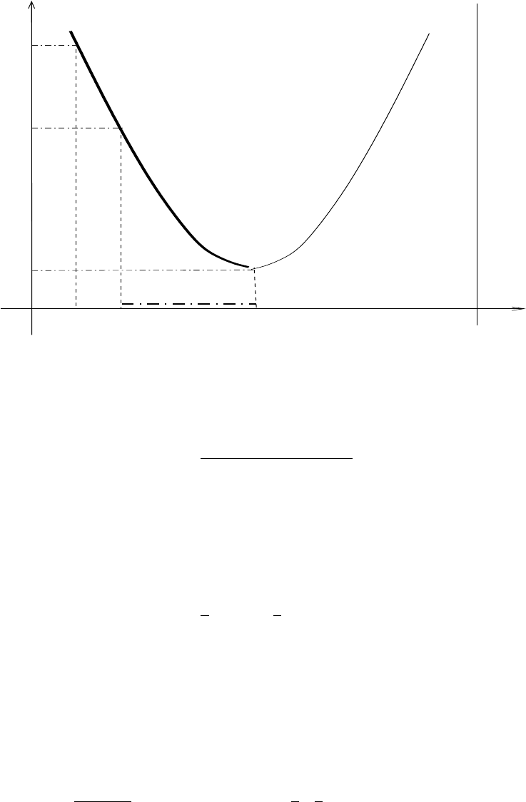
ε
01
1/2ε1
d min
d max
ε0
δ(ε)
Gamma Conversion in the Electron Field The electron cloud gives an
additional contribution to pair creation, proportional to Z(instead of Z2).
This is taken into account through the expression
ξ(Z) = ln(1440/Z2/3)
ln(183/Z1/3)−fc(Z).(5.28)
Factorization of the Cross Section ǫis sampled using the techniques of
’composition+rejection’, as treated in [3, 4, 5]. First, two auxiliary screening
functions should be introduced:
F1(δ) = 3Φ1(δ)−Φ2(δ)−F(Z)
F2(δ) = 3
2Φ1(δ)−1
2Φ2(δ)−F(Z) (5.29)
It can be seen that F1(δ) and F2(δ) are decreasing functions of δ,∀δ∈
[δmin, δmax]. They reach their maximum for δmin =δ(ǫ= 1/2) :
F10 = max F1(δ) = F1(δmin)
F20 = max F2(δ) = F2(δmin).(5.30)
After some algebraic manipulations the formula 5.17 can be written :
dσ(Z, ǫ)
dǫ =αr2
eZ[Z+ξ(Z)]2
91
2−ǫmin
×[N1f1(ǫ)g1(ǫ) + N2f2(ǫ)g2(ǫ)] ,(5.31)
33

where
N1=1
2−ǫmin2
F10 f1(ǫ) = 3
[1
2−ǫmin]31
2−ǫ2g1(ǫ) = F1(ǫ)
F10
N2=3
2F20 f2(ǫ) = const = 1
[1
2−ǫmin]g2(ǫ) = F2(ǫ)
F20
.
f1(ǫ) and f2(ǫ) are probability density functions on the interval ǫ∈[ǫmin,1/2]
such that
Z1/2
ǫmin
fi(ǫ)dǫ = 1
, and g1(ǫ) and g2(ǫ) are valid rejection functions: 0 < gi(ǫ)≤1 .
5.4.2 Final State
The differential cross section depends on the atomic number Zof the material
in which the interaction occurs. In a compound material the element iin
which the interaction occurs is chosen randomly according to the probability
P rob(Zi, Eγ) = natiσ(Zi, Eγ)
Pi[nati ·σi(Eγ)].(5.32)
Sampling the Energy Given a triplet of uniformly distributed random
numbers (ra, rb, rc) :
1. use rato choose which decomposition term in 5.31 to use:
if ra< N1/(N1+N2)→f1(ǫ)g1(ǫ) otherwise →f2(ǫ)g2(ǫ) (5.33)
2. sample ǫfrom f1(ǫ) or f2(ǫ) with rb:
ǫ=1
2−1
2−ǫminr1/3
bor ǫ=ǫmin +1
2−ǫminrb(5.34)
3. reject ǫif g1(ǫ)or g2(ǫ)< rc
note : below Eγ= 2 MeV it is enough to sample ǫuniformly on [ǫ0,1/2],
without rejection.
Charge The charge of each particle of the pair is fixed randomly.
34

Polar Angle of the Electron or Positron
The polar angle of the electron (or positron) is defined with respect to the
direction of the parent photon. The energy-angle distribution given by Tsai
[6] is quite complicated to sample and can be approximated by a density
function suggested by Urban [7] :
∀u∈[0,∞[f(u) = 9a2
9 + d[uexp(−au) + d u exp(−3au)] (5.35)
with
a=5
8d= 27 and θ±=mc2
E±
u. (5.36)
A sampling of the distribution 5.35 requires a triplet of random numbers such
that
if r1<9
9 + d→u=−ln(r2r3)
aotherwise u=−ln(r2r3)
3a.(5.37)
The azimuthal angle φis generated isotropically. The e+and e−momenta are
assumed to be coplanar with the parent photon. This information, together
with energy conservation, is used to calculate the momentum vectors of the
(e+, e−) pair and to rotate them to the global reference system.
5.4.3 Ultra-Relativistic Model
It is implemented in the class G4PairProductionRelModel and is configured
above 80GeV in all reference Physics lists. The cross section is computed
using direct integration of differential cross section [6] and not its parameter-
isation described in 5.4.1. LPM effect is taken into account in the same way
as for bremsstrahlung 8.2.2. Secondary generation algorithm is the same as
in the standard Bethe-Haitler model.
Bibliography
[1] J.H.Hubbell, H.A.Gimm, I.Overbo Jou. Phys. Chem. Ref. Data 9:1023
(1980)
[2] W. Heitler The Quantum Theory of Radiation, Oxford University Press
(1957)
[3] R. Ford and W. Nelson. SLAC-210, UC-32 (1978)
35
[4] J.C. Butcher and H. Messel. Nucl. Phys. 20 15 (1960)
[5] H. Messel and D. Crawford. Electron-Photon shower distribution, Perg-
amon Press (1970)
[6] Y. S. Tsai, Rev. Mod. Phys. 46 815 (1974), Y. S. Tsai, Rev. Mod. Phys.
49 421 (1977)
[7] L.Urban in Geant3 writeup, section PHYS-211. Cern Program Library
(1993)
36
5.5 Gamma Conversion into µ+µ−Pair
The class G4GammaConversionToMuons simulates the process of gamma
conversion into muon pairs. Given the photon energy and Zand Aof the
material in which the photon converts, the probability for the conversions
to take place is calculated according to a parameterized total cross section.
Next, the sharing of the photon energy between the µ+and µ−is deter-
mined. Finally, the directions of the muons are generated. Details of the
implementation are given below and can be also found in [1].
5.5.1 Cross Section and Energy Sharing
Muon pair production on atomic electrons, γ+e→e+µ++µ−, has a
threshold of 2mµ(mµ+me)/me≈43.9 GeV . Up to several hundred GeV
this process has a much lower cross section than the corresponding process
on the nucleus. At higher energies, the cross section on atomic electrons
represents a correction of ∼1/Z to the total cross section.
For the approximately elastic scattering considered here, momentum, but
no energy, is transferred to the nucleon. The photon energy is fully shared
by the two muons according to
Eγ=E+
µ+E−
µ(5.38)
or in terms of energy fractions
x+=E+
µ
Eγ
, x−=E−
µ
Eγ
, x++x−= 1 .
The differential cross section for electromagnetic pair creation of muons in
terms of the energy fractions of the muons is
dσ
dx+
= 4 α Z2r2
c1−4
3x+x−log(W),(5.39)
where Zis the charge of the nucleus, rcis the classical radius of the particles
which are pair produced (here muons) and
W=W∞
1 + (Dn√e−2) δ /mµ
1 + B Z−1/3√e δ /me
(5.40)
where
W∞=B Z−1/3
Dn
mµ
me
δ=m2
µ
2Eγx+x−
√e= 1.6487 . . . .
37

For hydrogen B= 202.4Dn= 1.49
and for all other nuclei B= 183 Dn= 1.54 A0.27.(5.41)
These formulae are obtained from the differential cross section for muon
bremsstrahlung [2] by means of crossing relations. The formulae take into
account the screening of the field of the nucleus by the atomic electrons in
the Thomas-Fermi model, as well as the finite size of the nucleus, which is
essential for the problem under consideration. The above parameterization
gives good results for Eγ≫mµ. The fact that it is approximate close
to threshold is of little practical importance. Close to threshold, the cross
section is small and the few low energy muons produced will not travel very
far. The cross section calculated from Eq. (5.39) is positive for Eγ>4mµ
and
xmin ≤x≤xmax with xmin =1
2−s1
4−mµ
Eγ
xmax =1
2+s1
4−mµ
Eγ
,
(5.42)
except for very asymmetric pair-production, close to threshold, which can
easily be taken care of by explicitly setting σ= 0 whenever σ < 0.
Note that the differential cross section is symmetric in x+and x−and
that
x+x−=x−x2
where xstands for either x+or x−. By defining a constant
σ0= 4 α Z2r2
clog(W∞) (5.43)
the differential cross section Eq. (5.39) can be rewritten as a normalized and
symmetric as function of x:
1
σ0
dσ
dx =1−4
3(x−x2)log W
log W∞
.(5.44)
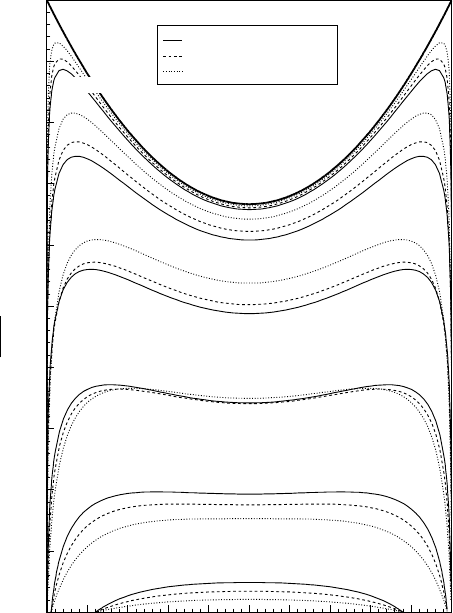
This is shown in Fig. 5.1 for several elements and a wide range of photon
energies. The asymptotic differential cross section for Eγ→ ∞
1
σ0
dσ∞
dx = 1 −4
3(x−x2)
is also shown.
38
0
0.1
0.2
0.3
0.4
0.5
0.6
0.7
0.8
0.9
1
0 0.1 0.2 0.3 0.4 0.5 0.6 0.7 0.8 0.9 1
H
Be
Pb
Eγ = 1 GeV
10 GeV
100 GeV
1 TeV
10 TeV
100 TeV
Eγ → ∞
x
dσ
σ0 dx
Z=1 A=1.00794
Z=4 A=9.01218
Z=82 A=207.2
Figure 5.1: Normalized differential cross section for pair production as a
function of x, the energy fraction of the photon energy carried by one of
the leptons in the pair. The function is shown for three different elements,
hydrogen, beryllium and lead, and for a wide range of photon energies.
39

5.5.2 Parameterization of the Total Cross Section
The total cross section is obtained by integration of the differential cross
section Eq. (5.39), that is
σtot(Eγ) = Zxmax
xmin
dσ
dx+
dx+= 4 α Z2r2
cZxmax
xmin 1−4
3x+x−log(W)dx+.
(5.45)
Wis a function of (x+, Eγ) and (Z, A) of the element (see Eq. (5.40)). Nu-
merical values of Ware given in Table 5.2.
Table 5.2: Numerical values of Wfor x+= 0.5 for different elements.
EγW for H W for Be W for Cu W for Pb
GeV
1 2.11 1.594 1.3505 5.212
10 19.4 10.85 6.803 43.53
100 191.5 102.3 60.10 332.7
1000 1803 919.3 493.3 1476.1
10000 11427 4671 1824 1028.1
∞28087 8549 2607 1339.8
Values of the total cross section obtained by numerical integration are
listed in Table 5.3 for four different elements. Units are in µbarn , where
1µbarn = 10−34 m2.
Table 5.3: Numerical values for the total cross section
Eγσtot, H σtot, Be σtot, Cu σtot, Pb
GeV µbarn µbarn µbarn µbarn
1 0.01559 0.1515 5.047 30.22
10 0.09720 1.209 49.56 334.6
100 0.1921 2.660 121.7 886.4
1000 0.2873 4.155 197.6 1476
10000 0.3715 5.392 253.7 1880
∞0.4319 6.108 279.0 2042
Well above threshold, the total cross section rises about linearly in log(Eγ)
with the slope
WM=1
4Dn√e mµ
(5.46)
40
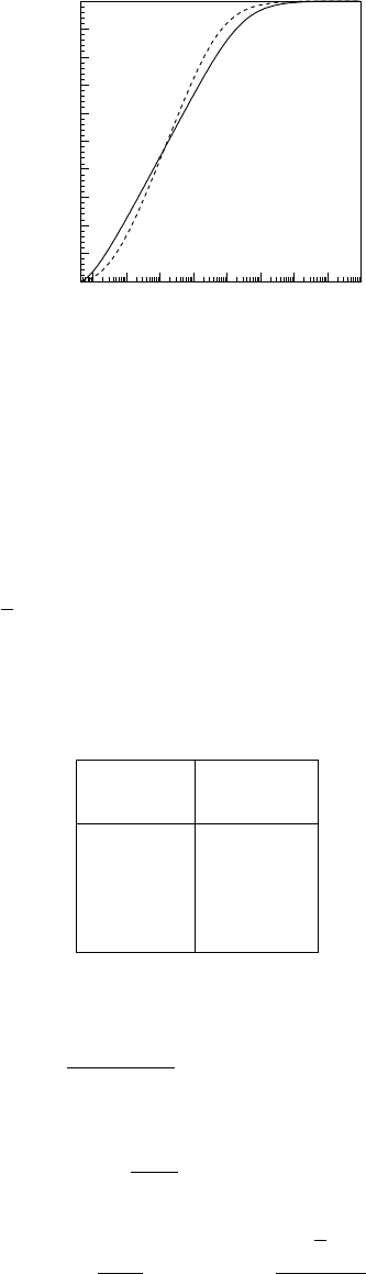
0
0.1
0.2
0.3
0.4
0.5
0.6
0.7
0.8
0.9
1
1 10 10 10 10 10 10 10 10
2 3 4 5 6 7 8
Eγ in GeV
H Pb
σ / σ∞
Figure 5.2: Total cross section for the Bethe-Heitler process γ→µ+µ−as a
function of the photon energy Eγin hydrogen and lead, normalized to the
asymptotic cross section σ∞.
until it saturates due to screening at σ∞. Fig. 5.2 shows the normalized cross
section where
σ∞=7
9σ0and σ0= 4 α Z2r2
clog(W∞).(5.47)
Numerical values of WMare listed in Table 5.4.
Table 5.4: Numerical values of WM.
Element WM
1/GeV
H 0.963169
Be 0.514712
Cu 0.303763
Pb 0.220771
The total cross section can be parameterized as
σpar =28 α Z2r2
c
9log(1 + WMCfEg),(5.48)
with
Eg=1−4mµ
Eγt
Ws
sat +Es
γ1/s .(5.49)
and
Wsat =W∞
WM
=B Z−1/34√e m2
µ
me
.
41
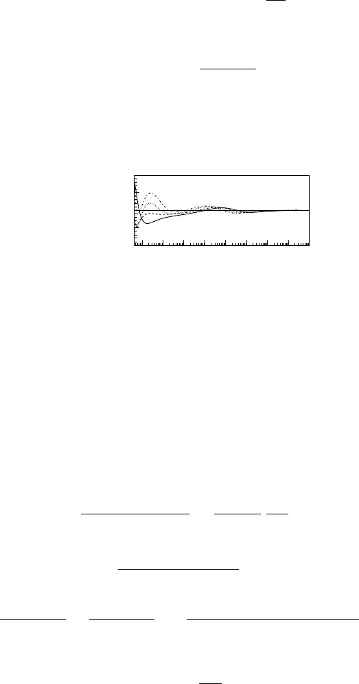
The threshold behavior in the cross section was found to be well approxi-
mated by t= 1.479 + 0.00799Dnand the saturation by s=−0.88. The
agreement at lower energies is improved using an empirical correction factor,
applied to the slope WM, of the form
Cf=1 + 0.04 log 1 + Ec
Eγ ,
where
Ec=−18.+4347.
B Z−1/3GeV .
A comparison of the parameterized cross section with the numerical integra-
tion of the exact cross section shows that the accuracy of the parametrization
is better than 2%, as seen in Fig. 5.3.
0.98
0.99
1
1.01
1.02
1 10 10 10 10 10 10 10 10
2 3 4 5 6 7 8
H
Be
Cu
Pb
Eγ in GeV
σ / σpar
Figure 5.3: Ratio of numerically integrated and parametrized total cross
sections as a function of Eγfor hydrogen, beryllium, copper and lead.
5.5.3 Multi-differential Cross Section and Angular Vari-
ables
The angular distributions are based on the multi-differential cross section for
lepton pair production in the field of the Coulomb center
dσ
dx+du+du−dϕ =4Z2α3
π
m2
µ
q4u+u−
u2
++u2
−
(1 + u2
+) (1 + u2
−)−2x+x−
u2
+
(1 + u2
+)2+u2
−
(1 + u2
−)2−2u+u−(1 −2x+x−) cos ϕ
(1 + u2
+) (1 + u2
−).(5.50)
Here
u±=γ±θ±, γ±=E±
µ
mµ
, q2=q2
k+q2
⊥,(5.51)
42

where
q2
k=q2
min (1 + x−u2
++x+u2
−)2,
q2
⊥=m2
µ(u+−u−)2+ 2 u+u−(1 −cos ϕ).(5.52)
q2is the square of the momentum qtransferred to the target and q2
kand q2
⊥
are the squares of the components of the vector q, which are parallel and
perpendicular to the initial photon momentum, respectively. The minimum
momentum transfer is qmin =m2
µ/(2Eγx+x−).
The muon vectors have the components
p+=p+( sin θ+cos(ϕ0+ϕ/2) ,sin θ+sin(ϕ0+ϕ/2) ,cos θ+),
p−=p−(−sin θ−cos(ϕ0−ϕ/2) ,−sin θ−sin(ϕ0−ϕ/2) ,cos θ−),
(5.53)
where p±=qE2
±−m2
µ. The initial photon direction is taken as the z-axis.
The cross section of Eq. (5.50) does not depend on ϕ0. Because of azimuthal
symmetry, ϕ0can simply be sampled at random in the interval (0,2π).
Eq. (5.50) is too complicated for efficient Monte Carlo generation. To
simplify, the cross section is rewritten to be symmetric in u+,u−using a
new variable uand small parameters ξ, β, where u±=u±ξ/2 and β=u ϕ.
When higher powers in small parameters are dropped, the differential cross
section in terms of u, ξ, β becomes
dσ
dx+dξ dβ udu =4Z2α3
π
m2
µ
q2
k+m2
µ(ξ2+β2)2(5.54)
ξ21
(1 + u2)2−2x+x−
(1 −u2)2
(1 + u2)4+β2(1 −2x+x−)
(1 + u2)2,
where, in this approximation,
q2
k=q2
min (1 + u2)2.
For Monte Carlo generation, it is convenient to replace (ξ, β) by the polar
coordinates (ρ, ψ) with ξ=ρcos ψand β=ρsin ψ. Integrating Eq. 5.54
over ψand using symbolically du2where du2= 2u du yields
dσ
dx+dρ du2=4Z2α3
m2
µ
ρ3
(q2
k/m2
µ+ρ2)21−x+x−
(1 + u2)2−x+x−(1 −u2)2
(1 + u2)4.
(5.55)
43

Integration with logarithmic accuracy over ρgives
Zρ3dρ
(q2
k/m2
µ+ρ2)2≈
1
Z
qk/mµ
dρ
ρ= log mµ
qk.(5.56)
Within the logarithmic accuracy, log(mµ/qk) can be replaced by log(mµ/qmin),
so that
dσ
dx+du2=4Z2α3
m2
µ1−x+x−
(1 + u2)2−x+x−(1 −u2)2
(1 + u2)4log mµ
qmin .(5.57)
Making the substitution u2= 1/t −1, du2=−dt /t2gives
dσ
dx+dt =4Z2α3
m2
µ
[1 −2x+x−+ 4 x+x−t(1 −t)] log mµ
qmin .(5.58)
Atomic screening and the finite nuclear radius may be taken into account by
multiplying the differential cross section determined by Eq. (5.55) with the
factor
(Fa(q)−Fn(q) )2,(5.59)
where Faand Fnare atomic and nuclear form factors. Please note that after
integrating Eq. 5.55 over ρ, the q-dependence is lost.
5.5.4 Procedure for the Generation of µ+µ−Pairs
Given the photon energy Eγand Zand Aof the material in which the γ
converts, the probability for the conversions to take place is calculated ac-
cording to the parametrized total cross section Eq. (5.48). The next step,
determining how the photon energy is shared between the µ+and µ−, is
done by generating x+according to Eq. (5.39). The directions of the muons
are then generated via the auxilliary variables t, ρ, ψ. In more detail, the
final state is generated by the following five steps, in which R1,2,3,4,... are ran-
dom numbers with a flat distribution in the interval [0,1]. The generation
proceeds as follows.
1) Sampling of the positive muon energy E+
µ=x+Eγ.
This is done using the rejection technique. x+is first sampled from a flat
distribution within kinematic limits using
x+=xmin +R1(xmax −xmin)
44

and then brought to the shape of Eq. (5.39) by keeping all x+which satisfy
1−4
3x+x−log(W)
log(Wmax)< R2.
Here Wmax =W(x+= 1/2) is the maximum value of W, obtained for sym-
metric pair production at x+= 1/2. About 60% of the events are kept in this
step. Results of a Monte Carlo generation of x+are illustrated in Fig. 5.4.
The shape of the histograms agrees with the differential cross section illus-
trated in Fig. 5.1.
0
5000
10000
15000
20000
25000
30000
0 0.1 0.2 0.3 0.4 0.5 0.6 0.7 0.8 0.9 1
x+
1000 GeV
100 GeV
10 GeV
Eγ
Figure 5.4: Histogram of generated x+distributions for beryllium at three
different photon energies. The total number of entries at each energy is 106.
2) Generate t(= 1
γ2θ2+1 ) .
The distribution in tis obtained from Eq.(5.58) as
f1(t)dt =1−2x+x−+ 4 x+x−t(1 −t)
1 + C1/t2dt , 0< t ≤1.(5.60)
with form factors taken into account by
C1=(0.35 A0.27)2
x+x−Eγ/mµ
.(5.61)
In the interval considered, the function f1(t) will always be bounded from
above by
max[f1(t)] = 1−x+x−
1 + C1
.
For small x+and large Eγ,f1(t) approaches unity, as shown in Fig. 5.5.
45
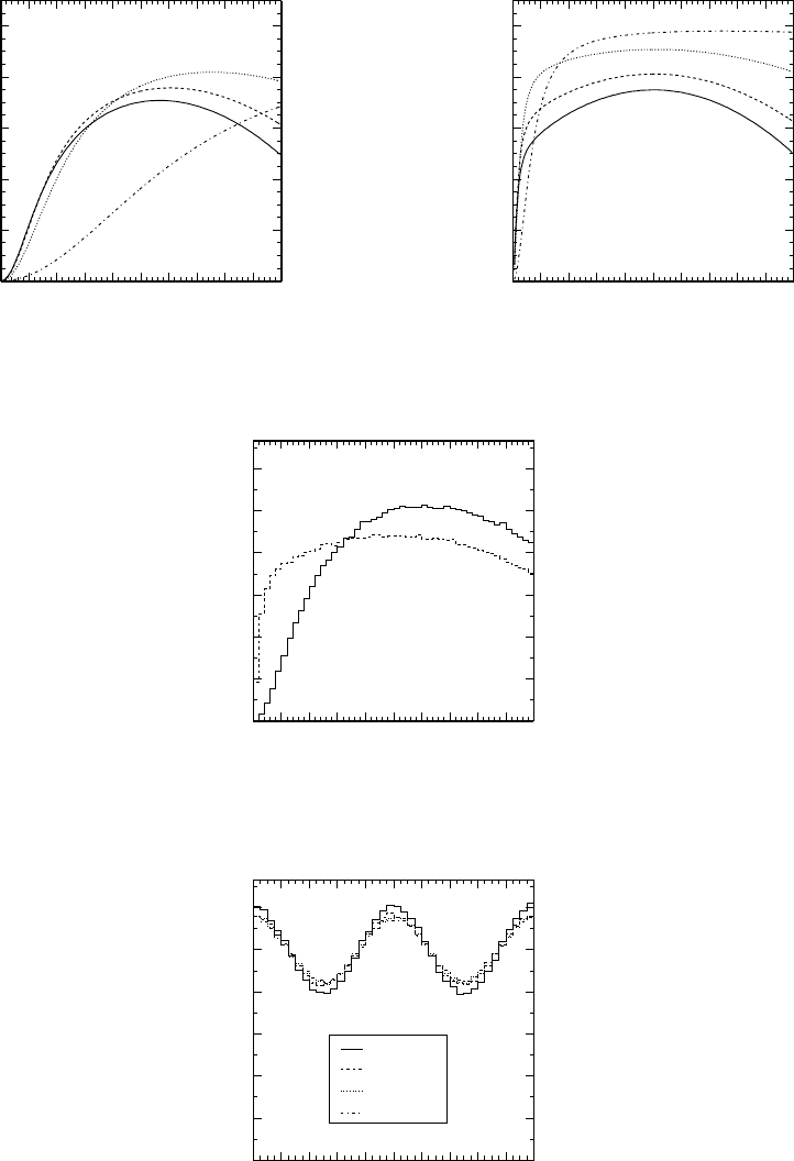
0
0.2
0.4
0.6
0.8
1
0 0.1 0.2 0.3 0.4 0.5 0.6 0.7 0.8 0.9 1
f1(t)
t
0.5
0.25
0.1
0.01
x+
Eγ = 10 GeV
0
0.2
0.4
0.6
0.8
1
0 0.1 0.2 0.3 0.4 0.5 0.6 0.7 0.8 0.9 1
0.5
0.25
0.1
0.01
x+
f1(t)
t
Eγ = 1 TeV
Figure 5.5: The function f1(t) at Eγ= 10 GeV (left) and Eγ= 1 TeV (right)
in beryllium for different values of x+.
0
5000
10000
15000
20000
25000
30000
0 0.1 0.2 0.3 0.4 0.5 0.6 0.7 0.8 0.9 1
t
Eγ = 10 GeV
Eγ = 1 TeV
Figure 5.6: Histograms of generated tdistributions for Eγ= 10 GeV (solid
line) and Eγ= 100 GeV (dashed line) with 106events each.
0
5000
10000
15000
20000
25000
30000
0 0.2 0.4 0.6 0.8 1 1.2 1.4 1.6 1.8 2
ψ/π
1 GeV
10 GeV
100 GeV
1000 GeV
Figure 5.7: Histograms of generated ψdistributions for beryllium at four
different photon energies.
46

The Monte Carlo generation is done using the rejection technique. About
70% of the generated numbers are kept in this step. Generated t-distributions
are shown in Fig. 5.6.
3) Generate ψby the rejection technique using tgenerated in the previous
step for the frequency distribution
f2(ψ) = h1−2x+x−+4 x+x−t(1−t) (1+cos(2ψ))i,0≤ψ≤2π . (5.62)
The maximum of f2(ψ) is
max[f2(ψ)] = 1 −2x+x−[1 −4t(1 −t)] .(5.63)
Generated distributions in ψare shown in Fig. 5.7.
4) Generate ρ.
The distribution in ρhas the form
f3(ρ)dρ =ρ3dρ
ρ4+C2
,0≤ρ≤ρmax ,(5.64)
where
ρ2
max =1.9
A0.27 1
t−1,(5.65)
and
C2=4
√x+x−"mµ
2Eγx+x−t2
+me
183 Z−1/3mµ2#2
.(5.66)
The ρdistribution is obtained by a direct transformation applied to uniform
random numbers Riaccording to
ρ= [C2(exp(β Ri)−1)]1/4,(5.67)
where
β= log C2+ρ4
max
C2.(5.68)
Generated distributions of ρare shown in Fig. 5.8
5) Calculate θ+, θ−and ϕfrom t, ρ, ψ with
γ±=E±
µ
mµ
and u=r1
t−1.(5.69)
47
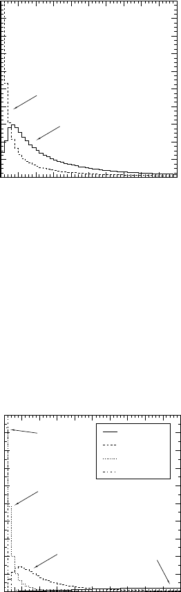
0
200
400
600
800
1000
1200
1400
1600
1800
2000
x 100
0 0.1 0.2 0.3 0.4 0.5 0.6 0.7 0.8 0.9 1
ρ
Eγ = 10 GeV
1 TeV
Figure 5.8: Histograms of generated ρdistributions for beryllium at two
different photon energies. The total number of entries at each energy is 106.
0
500
1000
1500
2000
2500
3000
3500
4000
4500
5000
x 100
0 .01 .02 .03 .04 .05 .06 .07 .08 .09 0.1
θ+
1 GeV
10 GeV
100 GeV
1000 GeV
10 GeV
100 GeV
1 GeV
1TeV
Figure 5.9: Histograms of generated θ+distributions at different photon
energies.
48
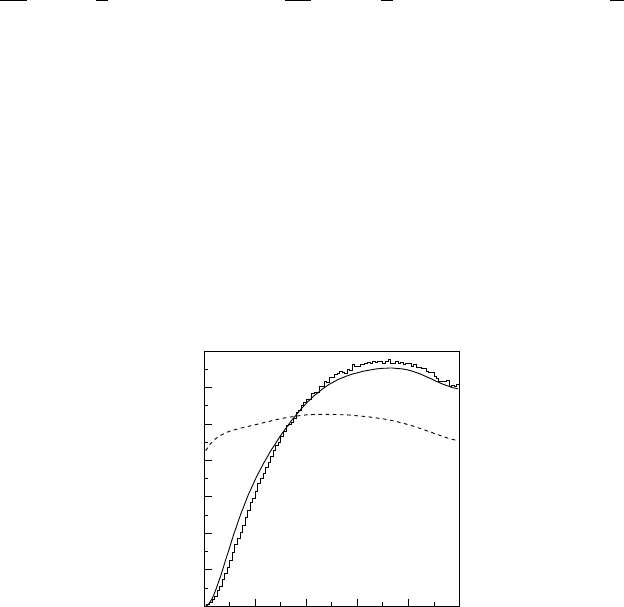
according to
θ+=1
γ+u+ρ
2cos ψ, θ−=1
γ−u−ρ
2cos ψand ϕ=ρ
usin ψ .
(5.70)
The muon vectors can now be constructed from Eq. (5.53), where ϕ0is chosen
randomly between 0 and 2π. Fig. 5.9 shows distributions of θ+at different
photon energies (in beryllium). The spectra peak around 1/γ as expected.
The most probable values are θ+∼mµ/E+
µ= 1/γ+. In the small angle
approximation used here, the values of θ+and θ−can in principle be any
positive value from 0 to ∞. In the simulation, this may lead (with a very
small probability, of the order of mµ/Eγ) to unphysical events in which θ+or
θ−is greater than π. To avoid this, a limiting angle θcut =πis introduced,
and the angular sampling repeated, whenever max(θ+, θ−)> θcut .
0.0
0.2
0.4
0.6
0.8
1.0
1.2
1.4
0 0.2 0.4 0.6 0.8 1
Coulomb centre
exact
simulated
1 / ( 1 + θ+ γ+ )
22
Figure 5.10: Angular distribution of positive (or negative) muons. The solid
curve represents the results of the exact calculations. The histogram is the
simulated distribution. The angular distribution for pairs created in the field
of the Coulomb centre (point-like target) is shown by the dashed curve for
comparison.
Figs. 5.10,5.11 and 5.12 show distributions of the simulated angular char-
acteristics of muon pairs in comparison with results of exact calculations.
The latter were obtained by means of numerical integration of the squared
matrix elements with respective nuclear and atomic form factors. All these
calculations were made for iron, with Eγ= 10 GeV and x+= 0.3. As seen
from Fig. 5.10, wide angle pairs (at low values of the argument in the fig-
ure) are suppressed in comparison with the Coulomb center approximation.
This is due to the influence of the finite nuclear size which is comparable
to the inverse mass of the muon. Typical angles of particle emission are of
49
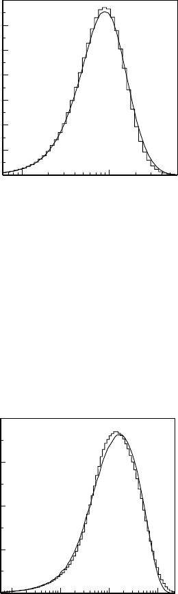
0
1
2
3
4
5
6
7
10 -1 1
θ+ γ+
Figure 5.11: Angular distribution in logarithmic scale. The curve corre-
sponds to the exact calculations and the histogram is the simulated distri-
bution.
0
1
2
3
4
10-3 10-2 10-1 1
| θ+ γ+ - θ- γ- |
Figure 5.12: Distribution of the difference of transverse momenta of positive
and negative muons (with logarithmic x-scale).
50
the order of 1/γ±=mµ/E±
µ(Fig. 5.11). Fig. 5.12 illustrates the influence of
the momentum transferred to the target on the angular characteristics of the
produced pair. In the frame of the often used model which neglects target
recoil, the pair particles would be symmetric in transverse momenta, and
coplanar with the initial photon.
Bibliography
[1] H. Burkhardt, S. Kelner, and R. Kokoulin, Monte Carlo Generator for
Muon Pair Production. CERN-SL-2002-016 (AP) and CLIC Note 511,
May 2002.
[2] S.R. Kelner, R.P. Kokoulin, and A.A. Petrukhin, About cross section
for high energy muon bremsstrahlung. Moscow Phys. Eng. Inst. 024-95,
1995. 31pp.
51
Chapter 6
Elastic scattering
52
6.1 Multiple Scattering
Elastic scattering of electrons and other charged particles is an important
component of any transport code. Elastic cross section is huge when particle
energy decreases, so multiple scattering (MSC) approach should be intro-
duced in order to have acceptable CPU performance of the simulation. A
universal interface G4VMultipleScattering is used by all Geant4 MSC pro-
cesses [1]:
•G4eMultipleScattering;
•G4hMultipleScattering;
•G4MuMultipleScattering.
For concrete simulation the G4VMscModel interface is used, which is an
extension of the base G4VEmModel interface. The following models are
available:
•G4UrbanMscModel - since Geant4 10.0 only one Urban model is avail-
able and it is applicable to all types of particles;
•G4GoudsmitSaundersonModel - for electrons and positrons [2];
•G4LowEWentzelVIModel - for all particles with low-energy limit 10 eV;
•G4WentzelVIModel - for muons and hadrons, for muons should be in-
cluded in Physics List together with G4CoulombScattering process, for
hadrons large angle scattering is simulated by hadron elastic process.
The discussion on Geant4 MSC models is available in Ref.[3]. Below we will
describe models developed by L. Urban [4], because these models are used
in many Geant4 applications and have general components reused by other
models.
6.1.1 Introduction
MSC simulation algorithms can be classified as either detailed or condensed.
In the detailed algorithms, all the collisions/interactions experienced by the
particle are simulated. This simulation can be considered as exact, it gives
the same results as the solution of the transport equation. However, it can
be used only if the number of collisions is not too large, a condition fulfilled
only for special geometries (such as thin foils, or low density gas). In solid
53
or liquid media the average number of collisions is very large and the de-
tailed simulation becomes very inefficient. High energy simulation codes use
condensed simulation algorithms, in which the global effects of the collisions
are simulated at the end of a track segment. The global effects generally
computed in these codes are the net energy loss, displacement, and change
of direction of the charged particle. The last two quantities are computed
from MSC theories used in the codes and the accuracy of the condensed
simulations is limited by accuracy of MSC approximation.
Most particle physics simulation codes use the multiple scattering theo-
ries of Moli`ere [5], Goudsmit and Saunderson [6] and Lewis [7]. The theories
of Moli`ere and Goudsmit-Saunderson give only the angular distribution after
a step, while the Lewis theory computes the moments of the spatial distribu-
tion as well. None of these MSC theories gives the probability distribution
of the spatial displacement. Each of the MSC simulation codes incorporates
its own algorithm to determine the angular deflection, true path length cor-
rection, and spatial displacement of the charged particle after a given step.
These algorithms are not exact, of course, and are responsible for most of
the uncertainties of the transport codes. Also due to inaccuracy of MSC the
simulation results can depend on the value of the step length and generally
user has to select the value of the step length carefully.
A new class of MSC simulation, the mixed simulation algorithms (see
e.g.[8]), appeared in the literature recently. The mixed algorithm simulates
the hard collisions one by one and uses a MSC theory to treat the effects of
the soft collisions at the end of a given step. Such algorithms can prevent
the number of steps from becoming too large and also reduce the dependence
on the step length. Geant4 original implementation of a similar approach is
realized in G4WentzelVIModel [3].
The Urban MSC models used in Geant4 belongs to the class of condensed
simulations. Urban uses model functions to determine the angular and spatial
distributions after a step. The functions have been chosen in such a way as
to give the same moments of the (angular and spatial) distributions as are
given by the Lewis theory [7].
6.1.2 Definition of Terms
In simulation, a particle is transported by steps through the detector ge-
ometry. The shortest distance between the endpoints of a step is called
the geometrical path length,z. In the absence of a magnetic field, this is a
straight line. For non-zero fields, zis the length along a curved trajectory.
Constraints on zare imposed when particle tracks cross volume boundaries.
The path length of an actual particle, however, is usually longer than the ge-
54

ometrical path length, due to multiple scattering. This distance is called the
true path length,t. Constraints on tare imposed by the physical processes
acting on the particle.
The properties of the MSC process are determined by the transport mean
free paths,λk, which are functions of the energy in a given material. The
k-th transport mean free path is defined as
1
λk
= 2πnaZ1
−1
[1 −Pk(cosχ)] dσ(χ)
dΩd(cosχ) (6.1)
where dσ(χ)/dΩ is the differential cross section of the scattering, Pk(cosχ)
is the k-th Legendre polynomial, and nais the number of atoms per volume.
Most of the mean properties of MSC computed in the simulation codes
depend only on the first and second transport mean free paths. The mean
value of the geometrical path length (first moment) corresponding to a given
true path length tis given by
hzi=λ11−exp −t
λ1 (6.2)
Eq. 6.2 is an exact result for the mean value of zif the differential cross
section has axial symmetry and the energy loss can be neglected. The trans-
formation between true and geometrical path lengths is called the path length
correction. This formula and other expressions for the first moments of the
spatial distribution were taken from either [8] or [9], but were originally cal-
culated by Goudsmit and Saunderson [6] and Lewis [7].
At the end of the true step length, t, the scattering angle is θ. The mean
value of cosθ is
hcosθi= exp −t
λ1(6.3)
The variance of cosθ can be written as
σ2=hcos2θi − hcosθi2=1 + 2e−2κτ
3−e−2τ(6.4)
where τ=t/λ1and κ=λ1/λ2. The mean lateral displacement is given
by a more complicated formula [8], but this quantity can also be calculated
relatively easily and accurately. The square of the mean lateral displacement
is
hx2+y2i=4λ2
1
3τ−κ+ 1
κ+κ
κ−1e−τ−1
κ(κ−1)e−κτ (6.5)
55

Here it is assumed that the initial particle direction is parallel to the the z
axis. The lateral correlation is determined by the equation
hxvx+yvyi=2λ1
31−κ
κ−1e−τ+1
κ−1e−κτ (6.6)
where vxand vyare the x and y components of the direction unit vector. This
equation gives the correlation strength between the final lateral position and
final direction.
The transport mean free path values have been calculated in Refs.[10],[11]
for electrons and positrons in the kinetic energy range 100 eV - 20 MeV in
15 materials. The Urban MSC model in Geant4 uses these values for kinetic
energies below 10 MeV. For high energy particles (above 10 MeV) the trans-
port mean free path values have been taken from a paper of R. Mayol and
F. Salvat [12]. When necessary, the model linearly interpolates or extrap-
olates the transport cross section, σ1= 1/λ1, in atomic number Zand in
the square of the particle velocity, β2. The ratio κis a very slowly varying
function of the energy: κ > 2 for T > a few keV, and κ→3 for very high
energies (see [9]). Hence, a constant value of 2.5 is used in the model.
Nuclear size effects are negligible for low energy particles and they are
accounted for in the Born approximation in [12], so there is no need for extra
corrections of this kind in the Urban model.
6.1.3 Path Length Correction
As mentioned above, the path length correction refers to the transformation
t−→ gand its inverse. The t−→ gtransformation is given by Eq. 6.2 if the
step is small and the energy loss can be neglected. If the step is not small
the energy dependence makes the transformation more complicated. For this
case Eqs. 6.3,6.2 should be modified as
hcosθi= exp −Zt
0
du
λ1(u)(6.7)
hzi=Zt
0hcosθiudu (6.8)
where θis the scattering angle, tand zare the true and geometrical path
lengths, and λ1is the transport mean free path.
In order to compute Eqs. 6.7,6.8 the tdependence of the transport mean
free path must be known. λ1depends on the kinetic energy of the particle
56

which decreases along the step. All computations in the model use a linear
approximation for this tdependence:
λ1(t) = λ10(1 −αt) (6.9)
Here λ10 denotes the value of λ1at the start of the step, and αis a constant.
It is worth noting that Eq. 6.9 is not a crude approximation. It is rather
good at low (<1 MeV) energy. At higher energies the step is generally much
smaller than the range of the particle, so the change in energy is small and
so is the change in λ1. Using Eqs. 6.7 - 6.9 the explicit formula for hcosθi
and hziare:
hcosθi= (1 −αt)1
αλ10 (6.10)
hzi=1
α(1 + 1
αλ10 )h1−(1 −αt)1+ 1
αλ10 i(6.11)
The value of the constant αcan be expressed using λ10 and λ11 where λ11 is
the value of the transport mean free path at the end of the step
α=λ10 −λ11
tλ10
(6.12)
At low energies ( Tkin < M , M - particle mass) αhas a simpler form:
α=1
r0
(6.13)
where r0denotes the range of the particle at the start of the step. It can
easily be seen that for a small step (i.e. for a step with small relative energy
loss) the formula of hziis
hzi=λ10 1−exp −t
λ10 (6.14)
Eq. 6.11 or 6.14 gives the mean value of the geometrical step length for a
given true step length. The actual geometrical path length is sampled in
the model according to the simple probability density function defined for
v=z/t ∈[0,1] :
f(v) = (k+ 1)(k+ 2)vk(1 −v) (6.15)
The value of the exponent kis computed from the requirement that f(v)
must give the same mean value for z=vt as Eq. 6.11 or 6.14. Hence
k=3hzi − t
t− hzi(6.16)
57

The value of z=vt is sampled using f(v) if k > 0, otherwise z=hziis
used. The g−→ ttransformation is performed using the mean values. The
transformation can be written as
t(z) = hti=−λ1log 1−z
λ1(6.17)
if the geometrical step is small and
t(z) = 1
αh1−(1 −αwz)1
wi(6.18)
where
w= 1 + 1
αλ10
if the step is not small, i.e. the energy loss should be taken into account.
6.1.4 Angular Distribution
The quantity u=cosθ is sampled according to a model function g(u). The
shape of this function has been chosen such that Eqs. 6.3 and 6.4 are satisfied.
The functional form of gis
g(u) = q[pg1(u) + (1 −p)g2(u)] + (1 −q)g3(u) (6.19)
where 0 ≤p, q ≤1, and the giare simple functions of u=cosθ, normalized
over the range u∈[−1,1]. The functions gihave been chosen as
g1(u) = C1e−a(1−u)−1≤u0≤u≤1 (6.20)
g2(u) = C2
1
(b−u)d−1≤u≤u0≤1 (6.21)
g3(u) = C3−1≤u≤1 (6.22)
where a > 0, b > 0, d > 0 and u0are model parameters, and the Ciare
normalization constants. It is worth noting that for small scattering angles,
θ,g1(u) is nearly Gaussian (exp(−θ2/2θ2
0)) if θ2
0≈1/a, while g2(u) has a
Rutherford-like tail for large θ, if b≈1 and dis not far from 2 .
6.1.5 Determination of the Model Parameters
The parameters a,b,d,u0and p,qare not independent. The requirement
that the angular distribution function g(u) and its first derivative be contin-
uous at u=u0imposes two constraints on the parameters:
p g1(u0) = (1 −p)g2(u0) (6.23)
58

p a g1(u0) = (1 −p)d
b−u0
g2(u0) (6.24)
A third constraint comes from Eq. 6.7 : g(u) must give the same mean value
for uas the theory. It follows from Eqs. 6.10 and 6.19 that
q{phui1+ (1 −p)hui2}= [1 −α t]1
αλ10 (6.25)
where huiidenotes the mean value of ucomputed from the distribution gi(u).
The parameter awas chosen according to a modified Highland-Lynch-Dahl
formula for the width of the angular distribution [13], [14].
a=0.5
1−cos(θ0)(6.26)
where θ0is
θ0=13.6MeV
βcp zchrt
X01 + hcln t
X0 (6.27)
when the original Highland-Lynch-Dahl formula is used. Here θ0=θrms
plane
is the width of the approximate Gaussian projected angle distribution, p,
βc and zch are the momentum, velocity and charge number of the incident
particle, and t/X0is the true path length in radiation length unit. The
correction term hc= 0.038 in the formula. This value of θ0is from a fit to
the Moli`ere distribution for singly charged particles with β= 1 for all Z,
and is accurate to 11 % or better for 10−3≤t/X0≤100 (see e.g. Rev. of
Particle Properties, section 23.3).
The model uses a slightly modified Highland-Lynch-Dahl formula to com-
pute θ0. For electrons/positrons the modified θ0formula is
θ0=13.6MeV
βcp zch√yc (6.28)
where
y= ln t
X0(6.29)
The correction term cand coeffitients ciare
c=c0˙
(c1+c2y),(6.30)
c0= 0.990395 −0.168386Z1/6+ 0.093286Z1/3,(6.31)
c1= 1 −0.08778
Z,(6.32)
59

c2= 0.04078 + 0.00017315Z. (6.33)
This formula gives a much smaller step dependence in the angular dis-
tribution than the Highland form. The value of the parameter u0has been
chosen as
u0= 1 −ξ
a(6.34)
where
ξ=d1+d2v+d3v2+d4v3(6.35)
with
v= ln t
λ1(6.36)
The parameters di-s have the form
di=di0+di1Z1
3+di2Z2
3(6.37)
The numerical values of the dij constants can be found in the code.
The tail parameter dis the same as the parameter ξ.
This (empirical) expression is obtained comparing the simulation results
to the data of the MuScat experiment [16]. The remaining three parame-
ters can be computed from Eqs. 6.23 - 6.25. The numerical value of the
parameters can be found in the code.
In the case of heavy charged particles (µ,π,p, etc.) the mean transport
free path is calculated from the electron or positron λ1values with a ’scaling’
applied. This is possible because the transport mean free path λ1depends
only on the variable P βc, where Pis the momentum, and βc is the velocity
of the particle.
In its present form the model samples the path length correction and an-
gular distribution from model functions, while for the lateral displacement
and the lateral correlation only the mean values are used and all the other
correlations are neglected. However, the model is general enough to incorpo-
rate other random quantities and correlations in the future.
6.1.6 Step Limitation Algorithm
In Geant4 the boundary crossing is treated by the transportation process.
The transportation ensures that the particle does not penetrate in a new
volume without stopping at the boundary, it restricts the step size when the
particle leaves a volume. However, this step restriction can be rather weak
in big volumes and this fact can result a not very good angular distribution
after the volume. At the same time, there is no similar step limitation when
60

a particle enters a volume and this fact does not allow a good backscattering
simulation for low energy particles. Low energy particles penetrate too deeply
into the volume in the first step and then - because of energy loss - they are
not able to reach again the boundary in backward direction.
MSC step limitation algorithm has been developed [4] in order to achieve
optimal balance between simulation precision and CPU performance of sim-
ulation for different applications. At the start of a track or after entering in
a new volume, the algorithm restricts the step size to a value
fr·max{r, λ1}(6.38)
where ris the range of the particle, fris a parameter ∈[0,1], taking the max
of rand λ1is an empirical choice.The value of fris constant for low energy
particles while for particles with λ1> λlim an effective value is used given by
the scaling equation
fref f =fr·1−sc +sc ∗λ1
λlim (6.39)
( The numerical values sc = 0.25 and λlim = 1 mm are used in the equation.)
In order not to use very small - unphysical - step sizes a lower limit is given
for the step size as
tlimitmin =max λ1
nstepmax, λelastic(6.40)
with nstepmax = 25 and λelastic is the elastic mean free path of the particle
(see later).
It can be easily seen that this kind of step limitation poses a real constraint
only for low energy particles. In order to prevent a particle from crossing a
volume in just one step, an additional limitation is imposed: after entering
a volume the step size cannot be bigger than
dgeom
fg
(6.41)
where dgeom is the distance to the next boundary (in the direction of the
particle) and fgis a constant parameter. A similar restriction at the start of
a track is 2dgeom
fg
(6.42)
At this point the program also checks whether the particle has entered a
new volume. If it has, the particle steps cannot be bigger than tlim =
61

frmax(r, λ). This step limitation is governed by the physics, because tlim
depends on the particle energy and the material.
The choice of the parameters frand fgis also related to performance.
By default fr= 0.02 and fg= 2.5 are used, but these may be set to any
other value in a simple way. One can get an approximate simulation of
the backscattering with the default value, while if a better backscattering
simulation is needed it is possible to get it using a smaller value for fr.
However, this model is very simple and it can only approximately reproduce
the backscattering data.
6.1.7 Boundary Crossing Algorithm
A special stepping algorithm has been implemented in order to improve the
simulation around interfaces. This algorithm does not allow ’big’ last steps
in a volume and ’big’ first steps in the next volume. The step length of these
steps around a boundary crossing can not be bigger than the mean free path
of the elastic scattering of the particle in the given volume (material). After
these small steps the particle scattered according to a single scattering law
(i.e. there is no multiple scattering very close to the boundary or at the
boundary).
The key parameter of the algorithm is the variable called skin. The
algorithm is not active for skin ≤0, while for skin > 0 it is active in
layers of thickness skin ·λelastic before boundary crossing and of thickness
(skin−1)·λelastic after boundary crossing (for skin = 1 there is only one small
step just before the boundary). In this active area the particle performs steps
of length λelastic (or smaller if the particle reaches the boundary traversing a
smaller distance than this value).
The scattering at the end of a small step is single or plural and for these
small steps there are no path length correction and lateral displacement com-
putation. In other words the program works in this thin layer in ’microscopic
mode’. The elastic mean free path can be estimated as
λelastic =λ1·rat (Tkin) (6.43)
where rat(Tkin) a simple empirical function computed from the elastic and
first transport cross section values of Mayol and Salvat [12]
rat (Tkin) = 0.001(MeV )2
Tkin (Tkin + 10MeV )(6.44)
Tkin is the kinetic energy of the particle.
At the end of a small step the number of scatterings is sampled according
to the Poisson’s distribution with a mean value t/λelastic and in the case of
62

plural scattering the final scattering angle is computed by summing the con-
tributions of the individual scatterings. The single scattering is determined
by the distribution
g(u) = C1
(2a+ 1 −u)2(6.45)
where u= cos(θ) , ais the screening parameter, Cis a normalization con-
stant. The form of the screening parameter is the same as in the single
scattering (see there).
6.1.8 Implementation Details
The step length of a particles is determined by the physics processes or the
geometry of the detectors. The tracking/stepping algorithm checks all the
step lengths demanded by the (continuous or discrete) physics processes and
determines the minimum of these step lengths (see 3.1). The MSC model
should be called to compute step limit after all processes except the trans-
portation process. The following sequence of computations are performed to
make the step:
•the minimum of all processes true step length limit tincluding one of
the MSC process is selected;
•The conversion t−→ g(geometrical step limit) is performed;
•the minimum of obtained value gand the transportation step limit is
selected;
•The final conversion g−→ tis performed.
The reason for this ordering is that the physics processes ’feel’ the true path
length ttraveled by the particle, while the transportation process (geometry)
uses the zstep length.
A new optional mechanis was recently introduced allowing sample dis-
placemnt in vicinity of geometry boundary. If it is enabled and the trans-
portation limit the step due to geometry boundary then after initial sampling
of the displacenet an additional ’push’ of track is applied forcing end point be
at the boundary. Corresponding correction to the true step length is applied
according to the value of the ’push’.
After the actual step of the particle is done, the MSC model is responsible
for sampling of scattering angle and relocation of the end-point of the step.
The scattering angle θof the particle after the step of length ’t’ is sampled
according to the model function given in Eq. 6.19 . The azimuthal angle φ
is generated uniformly in the range [0,2π].
63

After the simulation of the scattering angle, the lateral displacement is
computed using Eq. 6.5. Then the correlation given by Eq. 6.6 is used to
determine the direction of the lateral displacement. Before ’moving’ the
particle according to the displacement a check is performed to ensure that
the relocation of the particle with the lateral displacement does not take the
particle beyond the volume boundary.
Default MSC parameter values optimized per particle type are shown in
Table 6.1. Note, that there is three types of step limitation by multiple
scattering process:
•Minimal - only frparameter and range are used;
•UseSafety -frparameter, range and geometrical safety are used;
•UseSafetyPlus -frparameter, range and geometrical safety are used;
•UseDistanceToBoundary - uses particle range, geometrical safety and
linear distance to geometrical boundary.
particle e+,e−muons, hadrons ions
StepLimitType fUseSafety fMinimal fMinimal
skin 0 0 0
fr0.04 0.2 0.2
fg2.5 0.1 0.1
LateralDisplacement true true false
Table 6.1: The default values of parameters for different particle type.
The parameters of the model can be changed via public functions of the base
class G4VMultipleSacttering. They can be changed for all multiple scattering
processes simultaneously via G4EmParameters class, G4EmProcessOptions
class, or via Geant4 UI commands. The following commands are available:
/process/msc/StepLimit UseDistanceToBoundary
/process/msc/LateralDisplacement false
/process/msc/MuHadLateralDisplacement false
/process/msc/DisplacementBeyondSafety true
/process/msc/RangeFactor 0.02
/process/msc/GeomFactor 2.5
/process/msc/Skin 2
64
Bibliography
[1] J. Apostolakis et al., Geometry and physics of the Geant4 toolkit for high
and medium energy applications. Rad. Phys. Chem. 78 (2009) 859.
[2] O. Kadri, V. Ivanchenko, F. Gharbi, A. Trabelsi, Incorporation of the
Goudsmit-Saunderson electron transport theory in the Geant4 Monte
Carlo code, Nucl. Instrum. and Meth. B 267 (2009) 3624.
[3] V.N. Ivanchenko et al., Geant4 models for simulation of multiple scat-
tering, J. Phys.: Conf. Ser. 219 (2010) 032045.
[4] L. Urban, A multiple scattering model, CERN-OPEN-2006-077, Dec
2006. 18 pp.
[5] G.Z. Moli`ere Z. Naturforsch. 3a (1948) 78.
[6] S. Goudsmit and J.L. Saunderson. Phys. Rev. 57 (1940) 24.
[7] H.W. Lewis. Phys. Rev. 78 (1950) 526.
[8] J.M. Fernandez-Varea et al. NIM B73 (1993) 447.
[9] I. Kawrakow and A.F. Bielajew NIM B 142 (1998) 253.
[10] D. Liljequist and M. Ismail. J.Appl.Phys. 62 (1987) 342.
[11] D. Liljequist et al. J.Appl.Phys. 68 (1990) 3061.
[12] R. Mayol and F. Salvat At.Data and Nucl.Data Tables 65 (1997) 55..
[13] V.L. Highland NIM 129 (1975) 497.
[14] G.R. Lynch and O.I. Dahl NIM B58 (1991) 6.
[15] G. Shen et al. Phys. Rev. D 20 (1979) 1584.
[16] D. Attwood et al. NIM B 251 (2006) 41.
65
6.2 Discrete Processes for Charged Particles
Some processes for charged particles following the same interface G4V EmP rocess
as gamma processes described in section 5.1:
•G4CoulombScattering;
•G4eplusAnnihilation (with additional AtRest methods);
•G4eplusPolarizedAnnihilation (with additional AtRest methods);
•G4eeToHadrons;
•G4NuclearStopping;
•G4MicroElecElastic;
•G4MicroElecInelastic.
Corresponding model classes follow the G4V EmModel interface:
•G4DummyModel (zero cross section, no secondaries);
•G4eCoulombScatteringModel;
•G4eSingleCoulombScatteringModel;
•G4IonCoulombScatteringModel;
•G4eeToHadronsModel;
•G4PenelopeAnnihilationModel;
•G4PolarizedAnnihilationModel;
•G4ICRU49NuclearStoppingModel;
•G4MicroElecElasticModel;
•G4MicroElecInelasticModel.
Some processes from do not follow described EM interfaces but provide direct
implementations of the basic G4V DiscreteP rocess process:
•G4AnnihiToMuPair;
•G4ScreenedNuclearRecoil;
66
•G4Cerenkov;
•G4Scintillation;
•G4SynchrotronRadiation;
67

6.3 Single Scattering
Single elastic scattering process is an alternative to the multiple scattering
process. The advantage of the single scattering process is in possibility of
usage of theory based cross sections, in contrary to the Geant4 multiple scat-
tering model [1], which uses a number of phenomenological approximations
on top of Lewis theory. The process G4CoulombScattering was created for
simulation of single scattering of muons, it also applicable with some physical
limitations to electrons, muons and ions. Because each of elastic collisions are
simulated the number of steps of charged particles significantly increasing in
comparison with the multiple scattering approach, correspondingly its CPU
performance is pure. However, in low-density media (vacuum, low-density
gas) multiple scattering may provide wrong results and single scattering pro-
cesses is more adequate.
6.3.1 Coulomb Scattering
The single scattering model of Wentzel [2] is used in many of multiple scat-
tering models including Penelope code [4]. The Wentzel for describing elastic
scattering of particles with charge ze (z=−1 for electron) by atomic nucleus
with atomic number Zbased on simplified scattering potential
V(r) = zZe2
rexp(−r/R),(6.46)
where the exponential factor tries to reproduce the effect of screening. The
parameter Ris a screening radius [3]
R= 0.885Z−1/3rB,(6.47)
where rBis the Bohr radius. In the first Born approximation the elastic
scattering cross section σ(W) can be obtained as
dσ(W)(θ)
dΩ=(ze2)2
(pβc)2
Z(Z+ 1)
(2A+ 1 −cosθ)2,(6.48)
where pis the momentum and βis the velocity of the projectile particle. The
screening parameter Aaccording to Moliere and Bethe [3]
A=ℏ
2pR2
(1.13 + 3.76(αZ/β)2),(6.49)
where αis a fine structure constant and the factor in brackets is used to take
into account second order corrections to the first Born approximation.
68
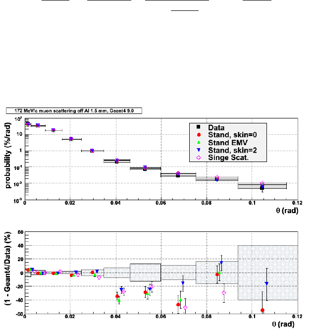
The total elastic cross section σcan be expressed via Wentzel cross section
(6.48)
dσ(θ)
dΩ=dσ(W)(θ)
dΩ Z
(1 + (qRN)2
12 )2+ 1!1
Z+ 1,(6.50)
where qis momentum transfer to the nucleus, RNis nuclear radius. This
term takes into account nuclear size effect [5], the second term takes into
account scattering off electrons. The results of simulation with the single
scattering model (Fig.6.1) are competitive with the results of the multiple
scattering.
Figure 6.1: Scattering of muons off 1.5 mm aluminum foil: data [6] - black
squares; simulation - colored markers corresponding different options of mul-
tiple scattering and single scattering model; in the bottom plot - relative
difference between the simulation and the data in percents; hashed area
demonstrates one standard deviation of the data.
6.3.2 Implementation Details
The total cross section of the process is obtained as a result of integration
of the differential cross section (6.50). The first term of this cross section
is integrated in the interval (0, π). The second term in the smaller interval
(0, θm), where θmis the maximum scattering angle off electrons, which is
determined using the cut value for the delta electron production. Before
69
sampling of angular distribution the random choice is performed between
scattering off the nucleus and off electrons.
Bibliography
[1] L. Urban, A multiple scattering model, CERN-OPEN-2006-077, Dec
2006. 18 pp.
[2] G. Wentzel, Z. Phys. 40 (1927) 590.
[3] H.A. Bethe, Phys. Rev. 89 (1953) 1256.
[4] J.M. Fernandez-Varea et al. NIM B 73 (1993) 447.
[5] A.V. Butkevich et al., NIM A 488 (2002) 282.
[6] D. Attwood et al. NIM B 251 (2006) 41.
70

6.4 Ion Scattering
The necessity of accurately computing the characteristics of interatomic scat-
tering arises in many disciplines in which energetic ions pass through mate-
rials. Traditionally, solutions to this problem not involving hadronic inter-
actions have been dominated by the multiple scattering, which is reasonably
successful, but not very flexible. In particular, it is relatively difficult to in-
troduce into such a system a particular screening function which has been
measured for a specific atomic pair, rather than the universal functions which
are applied. In many problems of current interest, such as the behavior of
semiconductor device physics in a space environment, nuclear reactions, par-
ticle showers, and other effects are critically important in modeling the full
details of ion transport. The process G4ScreenedNuclearRecoil provides sim-
ulation of ion elastic scattering [1]. This process is available with extended
electromagnetic example TestEm7.
6.4.1 Method
The method used in this computation is a variant of a subset of the method
described in Ref.[2]. A very short recap of the basic material is included here.
The scattering of two atoms from each other is assumed to be a completely
classical process, subject to an interatomic potential described by a potential
function
V(r) = Z1Z2e2
rφr
a(6.51)
where Z1and Z2are the nuclear proton numbers, e2is the electromagnetic
coupling constant (q2
e/4πǫ0in SI units), ris the inter-nuclear separation, φ
is the screening function describing the effect of electronic screening of the
bare nuclear charges, and ais a characteristic length scale for this screening.
In most cases, φis a universal function used for all ion pairs, and the value of
ais an appropriately adjusted length to give reasonably accurate scattering
behavior. In the method described here, there is no particular need for
a universal function φ, since the method is capable of directly solving the
problem for most physically plausible screening functions. It is still useful
to define a typical screening length ain the calculation described below, to
keep the equations in a form directly comparable with our previous work even
though, in the end, the actual value is irrelevant as long as the final function
φ(r) is correct. From this potential V(r) one can then compute the classical
scattering angle from the reduced center-of-mass energy ε≡Eca/Z1Z2e2
(where Ecis the kinetic energy in the center-of-mass frame) and reduced
71

impact parameter β≡b/a
θc=π−2βZ∞
x0
f(z)dz/z2(6.52)
where
f(z) = 1−φ(z)
z ε −β2
z2−1/2
(6.53)
and x0is the reduced classical turning radius for the given εand β.
The problem, then, is reduced to the efficient computation of this scat-
tering integral. In our previous work, a great deal of analytical effort was
included to proceed from the scattering integral to a full differential cross
section calculation, but for application in a Monte-Carlo code, the scattering
integral θc(Z1, Z2, Ec, b) and an estimated total cross section σ0(Z1, Z2, Ec)
are all that is needed. Thus, we can skip algorithmically forward in the orig-
inal paper to equations 15-18 and the surrounding discussion to compute the
reduced distance of closest approach x0. This computation follows that in
the previous work exactly, and will not be reintroduced here.
For the sake of ultimate accuracy in this algorithm, and due to the rela-
tively low computational cost of so doing, we compute the actual scattering
integral (as described in equations 19-21 of [2]) using a Lobatto quadrature
of order 6, instead of the 4th order method previously described. This re-
sults in the integration accuracy exceeding that of any available interatomic
potentials in the range of energies above those at which molecular structure
effects dominate, and should allow for future improvements in that area. The
integral αthen becomes (following the notation of the previous paper)
α≈1 + λ0
30 +
4
X
i=1
w′
ifx0
qi(6.54)
where
λ0=1
2+β2
2x2
0−φ′(x0)
2ε−1/2
(6.55)
w′
i∈[0.03472124, 0.1476903, 0.23485003, 0.1860249]
qi∈[0.9830235, 0.8465224, 0.5323531, 0.18347974]
Then
θc=π−πβα
x0
(6.56)
The other quantity required to implement a scattering process is the total
scattering cross section σ0for a given incident ion and a material through
72

which the ion is propagating. This value requires special consideration for a
process such as screened scattering. In the limiting case that the screening
function is unity, which corresponds to Rutherford scattering, the total cross
section is infinite. For various screening functions, the total cross section
may or may not be finite. However, one must ask what the intent of defining
a total cross section is, and determine from that how to define it.
In Geant4, the total cross section is used to determine a mean-free-path
lµwhich is used in turn to generate random transport distances between
discrete scattering events for a particle. In reality, where an ion is propagating
through, for example, a solid material, scattering is not a discrete process
but is continuous. However, it is a useful, and highly accurate, simplification
to reduce such scattering to a series of discrete events, by defining some
minimum energy transfer of interest, and setting the mean free path to be
the path over which statistically one such minimal transfer has occurred. This
approach is identical to the approach developed for the original TRIM code
[3]. As long as the minimal interesting energy transfer is set small enough
that the cumulative effect of all transfers smaller than that is negligible,
the approximation is valid. As long as the impact parameter selection is
adjusted to be consistent with the selected value of lµ, the physical result
isn’t particularly sensitive to the value chosen.
Noting, then, that the actual physical result isn’t very sensitive to the
selection of lµ,one can be relatively free about defining the cross section σ0
from which lµis computed. The choice used for this implementation is fairly
simple. Define a physical cutoff energy Emin which is the smallest energy
transfer to be included in the calculation. Then, for a given incident particle
with atomic number Z1, mass m1, and lab energy Einc, and a target atom
with atomic number Z2and mass m2, compute the scattering angle θcwhich
will transfer this much energy to the target from the solution of
Emin =Einc
4m1m2
(m1+m2)2sin2θc
2(6.57)
. Then, noting that αfrom eq. 6.54 is a number very close to unity, one
can solve for an approximate impact parameter bwith a single root-finding
operation to find the classical turning point. Then, define the total cross
section to be σ0=πb2, the area of the disk inside of which the passage of an
ion will cause at least the minimum interesting energy transfer. Because this
process is relatively expensive, and the result is needed extremely frequently,
the values of σ0(Einc) are precomputed for each pairing of incident ion and
target atom, and the results cached in a cubic-spline interpolation table.
However, since the actual result isn’t very critical, the cached results can be
stored in a very coarsely sampled table without degrading the calculation at
73

all, as long as the values of the lµused in the impact parameter selection are
rigorously consistent with this table.
The final necessary piece of the scattering integral calculation is the sta-
tistical selection of the impact parameter bto be used in each scattering
event. This selection is done following the original algorithm from TRIM,
where the cumulative probability distribution for impact parameters is
P(b) = 1 −exp −π b2
σ0(6.58)
where N σ0≡1/lµwhere Nis the total number density of scattering centers
in the target material and lµis the mean free path computed in the conven-
tional way. To produce this distribution from a uniform random variate ron
(0,1], the necessary function is
b=s−log r
π N lµ
(6.59)
This choice of sampling function does have the one peculiarity that it can
produce values of the impact parameter which are larger than the impact
parameter which results in the cutoff energy transfer, as discussed above
in the section on the total cross section, with probability 1/e. When this
occurs, the scattering event is not processed further, since the energy transfer
is below threshold. For this reason, impact parameter selection is carried out
very early in the algorithm, so the effort spent on uninteresting events is
minimized.
The above choice of impact sampling is modified when the mean-free-path
is very short. If σ0> π l
22where lis the approximate lattice constant of
the material, as defined by l=N−1/3, the sampling is replaced by uniform
sampling on a disk of radius l/2, so that
b=l
2√r(6.60)
This takes into account that impact parameters larger than half the lattice
spacing do not occur, since then one is closer to the adjacent atom. This also
derives from TRIM.
One extra feature is included in our model, to accelerate the produc-
tion of relatively rare events such as high-angle scattering. This feature is a
cross-section scaling algorithm, which allows the user access to an unphys-
ical control of the algorithm which arbitrarily scales the cross-sections for
a selected fraction of interactions. This is implemented as a two-parameter
74

adjustment to the central algorithm. The first parameter is a selection fre-
quency fhwhich sets what fraction of the interactions will be modified. The
second parameter is the scaling factor for the cross-section. This is imple-
mented by, for a fraction fhof interactions, scaling the impact parameter by
b′=b/√scale. This feature, if used with care so that it does not provide
excess multiple-scattering, can provide between 10 and 100-fold improve-
ments to event rates. If used without checking the validity by comparing to
un-adjusted scattering computations, it can also provide utter nonsense.
6.4.2 Implementation Details
The coefficients for the summation to approximate the integral for αin
eq.(6.54) are derived from the values in Abramowitz & Stegun [4], altered to
make the change-of-variable used for this integral. There are two basic steps
to the transformation. First, since the provided abscissas xiand weights wi
are for integration on [-1,1], with only one half of the values provided, and
in this work the integration is being carried out on [0,1], the abscissas are
transformed as:
yi∈1∓xi
2(6.61)
Then, the primary change-of-variable is applied resulting in:
qi= cos π yi
2(6.62)
w′
i=wi
2sin π yi
2(6.63)
except for the first coefficient w′
1where the sin() part of the weight is taken
into the limit of λ0as described in eq.(6.55). This value is just w′
1=w1/2.
Bibliography
[1] M.H. Mendenhall, R.A. Weller, An algorithm for computing screened
Coulomb scattering in Geant4, Nucl. Instr. Meth. B 227 (2005) 420.
[2] M.H. Mendenhall, R.A. Weller, Algorithms for the rapid computation
of classical cross sections for screened coulomb collisions, Nucl. Instr.
Meth. in Physics Res. B58 (1991) 11.
[3] J.P. Biersack, L.G. Haggmark, A Monte Carlo computer program for
the transport of energetic ions in amorphous targets, Nucl. Instr. Meth.
in Physics Res. 174 (1980) 257.
75
[4] M. Abramowitz, I. Stegun (Eds.), Handbook of Mathematical Functions,
Dover, New York, 1965, pp. 888, 920.
76
6.5 Single Scattering, Screened Coulomb Po-
tential and NIEL
Alternative model of Coulomb scattering of ions have been developed based
on [1] and references therein. The advantage of this model is the wide appli-
cability range in energy from 50 keV to 100 T eV per nucleon.
6.5.1 Nucleus–Nucleus Interactions
As discussed in Ref. [1], at small distances from the nucleus, the potential
energy is a Coulomb potential, while - at distances larger than the Bohr
radius - the nuclear field is screened by the fields of atomic electrons. The
interaction between two nuclei is usually described in terms of an interatomic
Coulomb potential (e.g., see Section 2.1.4.1 of Ref. [2] and Section 4.1 of
Ref. [3]), which is a function of the radial distance rbetween the two nuclei
V(r) = zZe2
rΨI(rr),(6.64)
where ez (projectile) and eZ (target) are the charges of the bare nuclei and
ΨIis the interatomic screening function and rris given by
rr=r
aI
,(6.65)
with aIthe so-called screening length (also termed screening radius). In the
framework of the Thomas–Fermi model of the atom (e.g., see Ref. [1] and
references therein) - thus, following the approach of ICRU Report 49 (1993)
-, a commonly used screening length for z= 1 incoming particles is that from
Thomas–Fermi
aTF =CTF a0
Z1/3,(6.66)
and - for incoming particles with z≥2 - that introduced by Ziegler, Biersack
and Littmark (1985) (and termed universal screening length):
aU=CTF a0
z0.23 +Z0.23 ,(6.67)
where
a0=~2
me2
is the Bohr radius, mis the electron rest mass and
CTF =1
23π
42/3
≃0.88534
77

is a constant introduced in the Thomas–Fermi model.
The simple scattering model due to Wentzel [5] - with a single exponen-
tial screening-function ΨI(rr){e.g., see Ref. [1] and references therein}- was
repeatedly employed in treating single and multiple Coulomb-scattering with
screened potentials. The resulting elastic differential cross section differs from
the Rutherford differential cross section by an additional term - the so-called
screening parameter - which prevents the divergence of the cross section when
the angle θof scattered particles approaches 0◦. The screening parameter As
[e.g., see Equation (21) of Bethe (1953)] - as derived by Moli`ere (1947, 1948)
for the single Coulomb scattering using a Thomas–Fermi potential - is ex-
pressed as
As=~
2p aI2"1.13 + 3.76 ×αzZ
β2#(6.68)
where aIis the screening length - from Eqs. (6.66, 6.67) for particles with
z= 1 and z≥2, respectively; αis the fine-structure constant; p(βc) is
the momentum (velocity) of the incoming particle undergoing the scattering
onto a target supposed to be initially at rest; cand ~are the speed of light
and the reduced Planck constant, respectively. When the (relativistic) mass
- with corresponding rest mass m- of the incoming particle is much lower
than the rest mass (M) of the target nucleus, the differential cross section -
obtained from the Wentzel–Moli`ere treatment of the single scattering - is:
dσWM(θ)
dΩ=zZe2
2p βc21
As+ sin2(θ/2)2.(6.69)
Equation (6.69) differs from Rutherford’s formula - as already mentioned -
for the additional term Asto sin2(θ/2). As discussed in Ref. [1], for β≃1
(i.e., at very large p) and with As≪1, one finds that the cross section
approaches a constant:
σWM
c≃2zZe2aI
~c2π
1.13 + 3.76 ×(αzZ)2.(6.70)
As discussed in Ref. [1] and references therein, for a scattering under the
action of a central potential (for instance that due to a screened Coulomb
field), when the rest mass of the target particle is no longer much larger than
the relativistic mass of the incoming particle, the expression of the differential
cross section must properly be re-written - in the center of mass system - in
terms of an “effective particle” with momentum equal to that of the incoming
particle (p′
in) and rest mass equal to the relativistic reduced mass
µrel =mM
M1,2
,(6.71)
78

where M1,2is the invariant mass; mand Mare the rest masses of the incoming
and target particles, respectively. The “effective particle” velocity is given by:
βrc=cv
u
u
t"1 + µrelc
p′
in 2#−1
.
Thus, one finds (e.g, see Ref. [1]):
dσWM(θ′)
dΩ′=zZe2
2p′
in βrc21
As+ sin2(θ′/2)2,(6.72)
with
As=~
2p′
in aI2"1.13 + 3.76 ×αzZ
βr2#(6.73)
and θ′the scattering angle in the center of mass system.
The energy Ttransferred to the recoil target is related to the scattering
angle as T=Tmax sin2(θ′/2) - where Tmax is the maximum energy which
can be transferred in the scattering (e.g., see Section 1.5 of Ref. [2]) -, thus,
assuming an isotropic azimuthal distribution one can re-write Eq. (6.72) in
terms of the kinetic recoil energy Tof the target
dσWM(T)
dT =πzZe2
p′
in βrc2Tmax
[Tmax As+T]2.(6.74)
Furthermore, one can demonstrates that Eq. (6.74) can be re-written as
(e.g, see Ref. [1]);
dσWM(T)
dT = 2 πzZe22E2
p2Mc4
1
[Tmax As+T]2(6.75)
with pand Ethe momentum and total energy of the incoming particle in the
laboratory. Equation (6.75) expresses - as already mentioned - the differential
cross section as a function of the (kinetic) energy Tachieved by the recoil
target.
6.5.2 Nuclear Stopping Power
Using Eq. (6.75) the nuclear stopping power - in MeV cm−1- is obtained as
−dE
dx nucl
= 2 nAπzZe22E2
p2Mc4As
As+ 1 −1 + ln As+ 1
As (6.76)
79
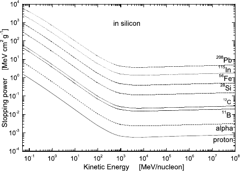
Figure 6.2: Nuclear stopping power from Ref. [1] - in MeV cm2g−1- calcu-
lated using Eq. (6.76) in silicon is shown as a function of the kinetic energy per
nucleon - from 50 keV/nucleon up 100 TeV/nucleon - for protons, α-particle
and 11B-, 12C-, 28Si-, 56Fe-, 115In-, 208Pb-nuclei.
with nAthe number of nuclei (atoms) per unit of volume and, finally, the
negative sign indicates that the energy is lost by the incoming particle (thus,
achieved by recoil targets). As discussed in Ref. [1], a slight increase of the
nuclear stopping power with energy is expected because of the decrease of
the screening parameter with energy.
For instance, in Fig. 6.2 the nuclear stopping power in silicon - in MeV cm2g−1
- is shown as a function of the kinetic energy per nucleon - from 50 keV/nucleon
up 100 TeV/nucleon - for protons, α-particles and 11B-, 12C-, 28Si-, 56Fe-,
115In-, 208Pb-nuclei.
A comparison of the present treatment with that obtained from Ziegler,
Biersack and Littmark (1985) - available in SRIM (2008) [8] - using the so-
called universal screening potential (see also Ref. [9]) is discussed in Ref. [1]:
a good agreement is achieved down to about 150 keV/nucleon. At large en-
ergies, the non-relativistic approach due to Ziegler, Biersack and Littmark
(1985) becomes less appropriate and deviations from stopping powers cal-
culated by means of the universal screening potential are expected and ob-
served.
The non-relativistic approach - based on the universal screening potential
- of Ziegler, Biersack and Littmark (1985) was also used by ICRU (1993) to
calculate nuclear stopping powers due to protons and α-particles in materi-
als. ICRU (1993) used as screening lengths those from Eqs. (6.66, 6.67) for
protons and α-particles, respectively. As discussed in Ref. [1], the stopping
powers for protons (α-particles) from Eq. (6.76) are less than ≈5% larger
80
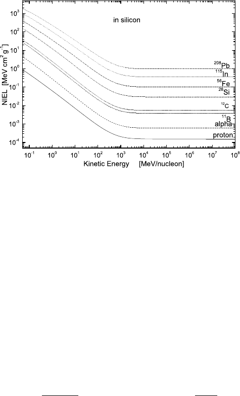
Figure 6.3: Non-ionizing stopping power from Ref. [1] - in MeV cm2g−1-
calculated using Eq. (6.79) in silicon is shown as a function of the kinetic
energy per nucleon - from 50 keV/nucleon up 100 TeV/nucleon - for protons,
α-particles and 11B-, 12C-, 28Si-, 56Fe-, 115In-, 208Pb-nuclei. The threshold
energy for displacement is 21 eV in silicon.
than those reported by ICRU (1993) from 50 keV/nucleon up to ≈8 MeV
(19 MeV/nucleon). At larger energies the stopping powers from Eq. (6.76)
differ from those from ICRU - as expected - due to the complete relativistic
treatment of the present approach (see Ref. [1]).
The simple screening parameter used so far [Eq. (6.73)] - derived by
Moli`ere (1947) - can be modified by means of a practical correction, i.e.,
A′
s=~
2p′
in aI2"1.13 + 3.76 ×CαzZ
βr2#,(6.77)
to achieve a better agreement with low energy calculations of Ziegler, Biersack
and Littmark (1985). For instance - as discussed in Ref. [1] -, for α-particles
and heavier ions, with
C= (10πzZα)0.12 (6.78)
the stopping powers obtained from Eq. (6.76) - in which A′
sreplaces As- differ
from the values of SRIM (2008) by less than ≈4.7 (3.6) % for α-particles (lead
ions) in silicon down to about 50 keV/nucleon. With respect to the tabulated
values of ICRU (1993), the agreement for α-particles is usually better than
4% at low energy down to 50 keV/nucleon - a 5% agreement is achieved at
about 50 keV/nucleon in case of a lead medium. At very high energy, the
stopping power is slightly affected when A′
sreplaces As(a further disvussion
is found in Ref. [1]).
81

6.5.3 Non-Ionizing Energy Loss due to Coulomb Scat-
tering
A relevant process - which causes permanent damage to the silicon bulk struc-
ture - is the so-called displacement damage (e.g., see Chapter 4 of Ref. [2],
Ref. [10] and references therein). Displacement damage may be inflicted when
aprimary knocked-on atom (PKA) is generated. The interstitial atom and
relative vacancy are termed Frenkel-pair (FP). In turn, the displaced atom
may have sufficient energy to migrate inside the lattice and - by further col-
lisions - can displace other atoms as in a collision cascade. This displacement
process modifies the bulk characteristics of the device and causes its degra-
dation. The total number of FPs can be estimated calculating the energy
density deposited from displacement processes. In turn, this energy density
is related to the Non-Ionizing Energy Loss (NIEL), i.e., the energy per unit
path lost by the incident particle due to displacement processes.
In case of Coulomb scattering on nuclei, the non-ionizing energy-loss can
be calculated using the Wentzel–Moli`ere differential cross section [Eq. (6.75)]
discussed in Sect. 6.5.1, i.e.,
−dE
dx NIEL
nucl
=nAZTmax
Td
T L(T)dσWM(T)
dT dT , (6.79)
where Eis the kinetic energy of the incoming particle, Tis the kinetic energy
transferred to the target atom, L(T) is the fraction of Tdeposited by means
of displacement processes. The expression of L(T) - the so-called Lindhard
partition function - can be found, for instance, in Equations (4.94, 4.96) of
Section 4.2.1.1 in Ref. [2] (see also references therein). Tde =T L(T) is the
so-called damage energy, i.e., the energy deposited by a recoil nucleus with
kinetic energy Tvia displacement damages inside the medium. The integral in
Eq. (6.79) is computed from the minimum energy Td- the so-called threshold
energy for displacement, i.e., that energy necessary to displace the atom from
its lattice position - up to the maximum energy Tmax that can be transferred
during a single collision process. Tdis about 21 eV in silicon. For instance, in
Fig. 6.3 the non-ionizing energy loss - in MeV cm2g−1- in silicon is shown
as a function of the kinetic energy per nucleon - from 50 keV/nucleon up
100 TeV/nucleon - for protons, α-particles and 11B-, 12C-, 28Si-, 56Fe-, 115In-,
208Pb-nuclei.
A further discussion on the agreement with the results obtained by Jun
and collaborators (2003) - using a relativistic treatment of Coulomb scat-
tering of protons with kinetic energies above 50 MeV and up to 1 GeV upon
silicon - can be found in Ref. [1].
82

6.5.4 G4IonCoulombScatteringModel
As discussed sofar, high energetic particles may inflict permanent damage to
the electronic devices employed in a radiation environment. In particular the
nuclear energy loss is important for the formation of defects in semiconductor
devices. Nuclear energy loss is also responsible for the displacement damage
which is the typical cause of degradation for silicon devices. The electromag-
netic model G4IonCoulombScatteringModel was created in order to simulate
the single scattering of protons, alpha particles and all heavier nuclei inci-
dent on all target materials in the energy range from 50–100 keV/nucleon to
10 TeV.
6.5.5 The Method
The differential cross section previously described is calculated by means
of the class G4IonCoulombCrossSection where a modified version of the
Wentzel’s cross section is used. To solve the scattering problem of heavy
ions it is necessary to introduce an effective particle whose mass is equal to
the relativistic reduced mass of the system defined as
µr≡m1m2c2
Ecm
.(6.80)
where m1and m2are incident and target rest masses respectively and Ecm
(in Eq. (6.71) M1,2=Ecm/c2) is the total center of mass energy of the
two particles system. The effective particle interacts with a fixed scattering
center with interacting potential expressed by Eq. (6.64) . The momentum
of the effective particle is equal to the momentum of the incoming particle
calculated in the center of mass system (pr≡p1cm). Since the target particle
is inside the material it can be considered at rest in the laboratory as a
consequence the magnitude of pris calculated as
pr≡p1cm =p1lab
m2c2
Ecm
,(6.81)
with Ecm given by
Ecm =p(m1c2)2+ (m2c2)2+ 2E1labm2c2,(6.82)
where p1lab and E1lab are the momentum and the total energy of the incom-
ing particle in the laboratory system respectively. The velocity (βr) of the
effective particle is obtained by the relation
1
β2
r
= 1 + µrc2
prc!2
.(6.83)
83

The modified Wentzel’s cross section is then equal to:
dσ(θr)
dΩ=Z1Z2e2
prc βr21
(2As+ 1 −cos θr)2(6.84)
(in Eq. (6.72) p′
in ≡pr) where Z1and Z2are the nuclear proton numbers
of projectile and of target respectively; Asis the screening coefficient [see
Eq. (6.73)] and θris the scattering angle of the effective particle which is
equal the one in the center of mass system (θr≡θ1cm). Knowing the scat-
tering angle the recoil kinetic energy of the target particle after scattering is
calculated by
T=m2c2 p1labc
Ecm !2
(1 −cos θr).(6.85)
The momentum and the total energy of the incident particle after scattering
in the laboratory system are obtained by the usual Lorentz’s transformations.
6.5.6 Implementation Details
In the G4IonCoulombScatteringModel the scattering off electrons is not con-
sidered: only scattering off nuclei is simulated. Secondary particles are gen-
erated when T[Eq. (6.85)] is greater then a given threshold for displacement
Td; it is not cut in range. The user can set this energy threshold Tdby the
method SetRecoilThreshold(G4double Td). The default screening coefficient
Asis given by Eq. (6.73). If the user wants to use the one given by Eq. (6.77)
the condition SetHeavyIonCorr(1) must be set. When Z1= 1 the Thomas-
Fermi screening length [aT F see Eq. (6.66)] is used in the calculation of As.
For Z1≥2 the screening length is the universal one [aUsee Eq. (6.67)].
In the G4IonCoulombCrossSection the total differential cross section is ob-
tained by the method NuclearCrossSection() where the Eq. (6.84) is inte-
grated in the interval (0, π):
σ=πZ1Z2e2
prc βr21
As(As+ 1) (6.86)
The cosine of the scattering angle is chosen randomly in the interval (-1, 1)
according to the distribution of the total cross section and it is given by the
method SampleCosineTheta() which returns (1 −cos θr).
Bibliography
[1] M. Boschini et al., Nuclear and Non-Ionizing Energy-Loss for Coulomb
Scattered Particles from Low Energy up to Relativistic Regime in
84
Space Radiation Environment, Proc. of the ICATPP Conference on
Cosmic Rays for Particle and Astroparticle Physics, October 7–8
2010, Villa Olmo, Como, Italy, World Scientific, Singapore (2011);
arXiv:1011.4822v3 [physics.space-ph], available at the web site:
http://arxiv.org/abs/1011.4822
[2] C. Leroy and P.G. Rancoita, Principles of Radiation Interaction in Mat-
ter and Detection, 2nd Edition, World Scientific (Singapore) 2009.
[3] ICRU, Stopping Powers and Ranges for Protons and Alpha Particles.
ICRU Report 49, 1993.
[4] J.F. Ziegler, J.P. Biersack, U. Littmark, The Stopping Range of Ions in
Solids, Vol. 1, Pergamon Press (New York) 1985.
[5] G. Wentzel, Z. Phys. 40 (1926), 590–593.
[6] von G. Moli`ere, Z. Naturforsh. A2 (1947), 133–145; A3 (1948), 78.
[7] H.A. Bethe, Phys. Rev. 98 (1953), 1256–1266.
[8] J.F. Ziegler, M.D. Ziegler, J.P. Biersack, The Stopping and Range
of Ions in Matter, SRIM version 2008.03 (2008), available at:
http://www.srim.org/
[9] J.F. Ziegler, M.D. Ziegler, J.P. Biersack, The Stopping and Range of
Ions in Matter, SRIM Co. (Chester.) 2008.
[10] C. Leroy and P.G. Rancoita, Reports on Progress in Physics 70, 4 (2007)
493–625.
[11] S.R. Messenger et al., IEEE Trans. on Nucl. Sci. 50 (2003), 1919–1923.
[12] I. Jun et al., IEEE Trans. on Nucl. Sci. 50 (2003) 1924–1928.
85
6.6 Electron Screened Single Scattering and
NIEL
The present treatment[1] of electron–nucleus interaction is based on numer-
ical and analytical approximations of the Mott differential cross section. It
accounts for effects due to screened Coulomb potentials, finite sizes and finite
rest masses of nuclei for electron with kinetic energies above 200 keV and up
to ultra high. This treatment allows one to determine both the total and
differential cross sections, thus, to calculate the resulting nuclear and non-
ionizing stopping powers (NIEL). Above a few hundreds of MeV, neglecting
the effects of finite sizes and rest masses of recoil nuclei the stopping power
and NIEL result to be largely underestimated, while, above a few tens of
MeV prevents a further large increase, thus, resulting in approaching almost
constant values at high energies.
The non-ionizing energy-loss (NIEL) is the energy lost from a particle
traversing a unit length of a medium through physical process resulting in
permanent displacement damages (e.g. see Ref.[2]). The nuclear stopping
power and NIEL deposition - due to elastic Coulomb scatterings - from pro-
tons, light- and heavy-ions traversing an absorber were previously dealt[3]
and is available in Geant4 (6.5) (see also Sections 1.6, 1.6.1, 2.1.4–2.1.4.2,
4.2.1.6 of Ref.[4]). In the present model included in GEANT4, the nuclear
stopping power and NIEL deposition due to elastic Coulomb scatterings of
electrons are treated up to ultra relativistic energies.
6.6.1 Scattering Cross Section of Electrons on Nuclei
The scattering of electrons by unscreened atomic nuclei was treated by Mott
extending a method - dealing with incident and scattered waves on point-like
nuclei - of Wentzel and including effects related to the spin of electrons. The
differential cross section (DCS) - the so-called Mott differential cross section
(MDCS) - was expressed by Mott as two conditionally convergent infinite
series in terms of Legendre expansions. In Mott–Wentzel treatment, the
scattering occurs on a field of force generating a radially dependent Coulomb
- unscreened (screened) in Mott (Wentzel) - potential. Furthermore, the
MDCS was derived in the laboratory reference system for infinitely heavy
nuclei initially at rest with negligible spin effects and must be numerically
evaluated for any specific nuclear target. Effects related to the recoil and
finite rest mass of the target nucleus (M) were neglected. Thus, in this
framework the total energy of electrons has to be smaller or much smaller
than Mc2.
86

The MDCS is usually expressed as:
dσMott(θ)
dΩ=dσRut
dΩRMott,(6.87)
where RMott is the ratio between the MDCS and Rutherford’s formula [RDCS,
see Equation (1) of Ref.[1]]. For electrons with kinetic energies from several
keV up to 900 MeV and target nuclei with 1 6Z690, Lijian, Quing and
Zhengming[5] provided a practical interpolated expression [Eq. (6.99)] for
RMott with an average error less than 1%; in the present treatment, that ex-
pression - discussed in Sect. 6.6.1 - is the one assumed for RMott in Eq. (6.87)
hereafter. The analytical expression derived by McKinley and Feshbach[6]
for the ratio with respect to Rutherford’s formula [Equation (7) of Ref.[6]] is
given by:
RMcF = 1 −β2sin2(θ/2) + Z αβπ sin(θ/2) [1 −sin(θ/2)] (6.88)
with the corresponding differential cross section (McFDCS)
dσMcF
dΩ=dσRut
dΩRMcF.(6.89)
Furthermore, for Mc2much larger than the total energy of incoming electron
energies the distinction between laboratory (i.e., the system in which the tar-
get particle is initially at rest) and center-of-mass (CoM) systems disappears
(e.g., see discussion in Section 1.6.1 of Ref.[4]). Furthermore, in the CoM of
the reaction the energy transferred from an electron to a nucleus initially at
rest in the laboratory system (i.e., its recoil kinetic energy T) is related with
the maximum energy transferable Tmax as
T=Tmax sin2(θ′/2) (6.90)
[e.g., see Equations (1.27, 1.95) at page 11 and 31, respectively, of Ref.[4]],
where θ′is the scattering angle in the CoM system. In addition, one obtains
dT =Tmax
4πdΩ′.(6.91)
Since for Mc2much larger than the electron energy θis ≈θ′, one finds that
Eq. (6.90) can be approximated as
T≃Tmax sin2(θ/2) ,(6.92)
=⇒sin2(θ/2) = T
Tmax
(6.93)
87

and
dT ≃Tmax
4πdΩ.(6.94)
Using Eqs. (6.88, 6.93, 6.94), Rutherford’s formula and Eq. (6.89) can be
respectively rewritten as:
=⇒dσRut
dT =Ze2
pβc2πTmax
T2,(6.95)
=⇒dσMcF
T=Ze2
pβc2πTmax
T2"1−βT
Tmax
(β+Zαπ)+Zαβπ
rT
Tmax #
(6.96)
=Ze2
pβc2πTmax
T2RMcF(T)
with
RMcF(T) = "1−βT
Tmax
(β+Zαπ)+Zαβπ
rT
Tmax #.(6.97)
Finally, in a similar way the MDCS [Eq. (6.87)] is
dσMott(T)
dT =dσRut
dT RMott(T)
=Ze2
pβc2πTmax
T2RMott(T) (6.98)
with RMott(T) from Eq. (6.101).
Interpolated Expression for RMott
Recently, Lijian, Quing and Zhengming[5] provided a practical interpolated
expression [Eq. (6.99)] which is a function of both θand βfor electron energies
from several keV up to 900 MeV, i.e.,
RMott =
4
X
j=0
aj(Z, β)(1 −cos θ)j/2,(6.99)
where
aj(Z, β) =
6
X
k=1
bk,j(Z)(β−β)k−1,(6.100)
and β c = 0.7181287 cis the mean velocity of electrons within the above men-
tioned energy range. The coefficients bk,j(Z) are listed in Table 1 of Ref.[5]
88
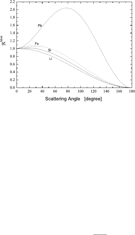
Figure 6.4: RMott obtained from Eq. (6.99) at 100 MeV for Li, Si, Fe and Pb
nuclei as a function of scattering angle.
for 1 6Z690. M.Boschini et al. (2013) [7] provided an extended numerical
solution for the Mott differential cross section on nuclei up to Z= 118 for
both electrons and positrons. RMott obtained from Eq. (6.99) at 100 MeV is
shown in Fig. 6.4 for Li, Si, Fe and Pb nuclei as a function of scattering an-
gle. Furthermore, it has to be remarked that the energy dependence of RMott
from Eq. (6.99) was studied and observed to be negligible above ≈10 MeV
[for instance, see Eq. (6.100)].
Finally, from Eqs.(6.90, 6.99) [e.g., see also Equation (1.93) at page 31
of Ref.[4]], one finds that RMott can be expressed in terms of the transferred
energy Tas
RMott(T) =
4
X
j=0
aj(Z, β)2T
Tmax j/2
.(6.101)
Screened Coulomb Potentials
The simple scattering model due to Wentzel - with a single exponential
screening function [e.g., see Equation (2.71) at page 95 of Ref.[4]] - was re-
peatedly employed in treating single and multiple Coulomb scattering with
screened potentials. Neglecting effects like those related to spin and finite
size of nuclei, for proton and nucleus interactions on nuclei it was shown
that the resulting elastic differential cross section of a projectile with bare
nuclear-charge ez on a target with bare nuclear-charge eZ differs from the
Rutherford differential cross section (RDCS) by an additional term - the
so-called screening parameter - which prevents the divergence of the cross
89

section when the angle θof scattered particles approaches 0◦[e.g., see Sec-
tion 1.6.1 of Ref.[4]]. For z= 1 particles the screening parameter As,Mis
expressed as
As,M=~
2p aTF 2"1.13 + 3.76 ×αZ
β2#(6.102)
where α,cand ~are the fine-structure constant, speed of light and reduced
Planck constant, respectively; p(βc) is the momentum (velocity) of the in-
coming particle undergoing the scattering onto a target supposed to be ini-
tially at rest - i.e., in the laboratory system -; aTF is the screening length
suggested by Thomas–Fermi
aTF =CTF a0
Z1/3(6.103)
with
a0=~2
me2
the Bohr radius, mthe electron rest mass and
CTF =1
23π
42/3
≃0.88534
a constant introduced in the Thomas–Fermi model [e.g., see Ref.[3] , Equa-
tions (2.73, 2,82) - at page 95 and 99, respectively - of Ref.[4], see also
references therein]. The modified Rutherford’s formula [dσWM(θ)/dΩ], i.e.,
the differential cross section -obtained from the Wentzel–Moli`ere treatment
of the single scattering on screened nuclear potential - is given by [e.g., see
Equation (2.84) of Ref.[4] and Ref.[3], see also references therein]:
dσWM(θ)
dΩ=zZe2
2p βc21
As,M+ sin2(θ/2)2(6.104)
=dσRut
dΩF2(θ).(6.105)
with
F(θ) = sin2(θ/2)
As,M+ sin2(θ/2).(6.106)
F(θ) - the so-called screening factor - depends on the scattering angle θand
the screening parameter As,M. As discussed in Sect. 6.6.1, the term As,M
(the screening parameter) cannot be neglected in the DCS [Eq. (6.105)] for
90

scattering angles (θ) within a forward (with respect to the electron direction)
angular region narrowing with increasing energy from several degrees (for
high-Zmaterial) at 200 keV down to less than or much less than a mrad
above 200 MeV.
An approximated description of elastic interactions of electrons with screened
Coulomb fields of nuclei can be obtained by the factorization of the MDCS,
i.e., involving Rutherford’s formula [dσRut/dΩ] for particle with z= 1, the
screening factor [F(θ)] and the ratio RMott between the RDCS and MDCS:
dσMott
sc (θ)
dΩ≃dσRut
dΩF2(θ)RMott.(6.107)
Thus, the corresponding screened differential cross section derived using the
analytical expression from McKinley and Feshbach[6] can be approximated
with dσMcF
sc (θ)
dΩ≃dσRut
dΩF2(θ)RMcF.(6.108)
Zeitler and Olsen[8] suggested that for electron energies above 200 keV the
overlap of spin and screening effects is small for all elements and for all
energies; for lower energies the overlapping of the spin and screening effects
may be appreciable for heavy elements and large angles.
Finite Nuclear Size
The ratio between the actual measured and that expected from the point-
like differential cross section expresses the square of nuclear form factor (|F|)
which, in turn, depends on the momentum transfer q, i.e., that acquired by
the target initially at rest:
q=pT(T+ 2Mc2)
c,(6.109)
with Tfrom Eq. (6.90) or for Mc2larger or much larger than the electron
energy from its approximate expression Eq. (6.92).
The approximated (factorized) differential cross section for elastic inter-
actions of electrons with screened Coulomb fields of nuclei [Eq. (6.107)] ac-
counting for the effects due to the finite nuclear size is given by:
dσMott
sc,F (θ)
dΩ≃dσRut
dΩF2(θ)RMott |F(q)|2.(6.110)
Thus, using the analytical expression derived by McKinley and Feshbach[6]
[Eq. (6.88)] one obtains that the corresponding screened differential cross
91

section [Eq. (6.108)] accounting for the finite nuclear size effects
dσMcF
sc,F (θ)
dΩ≃dσRut
dΩF2(θ)RMcF |F(q)|2(6.111)
=dσRut
dΩF2(θ)|F(q)|2
×1−β2sin2(θ/2) + Z αβπ sin(θ/2) [1 −sin(θ/2)].(6.112)
In terms of kinetic energy, one can respectively rewrite Eqs. (6.110, 6.111) as
dσMott
sc,F (T)
dT =dσRut
dT F2(T)RMott(T)|F(q)|2(6.113)
dσMcF
sc,F (T)
dT ≃dσRut(T)
dT F2(T)RMcF(T)|F(q)|2(6.114)
with dσRut/dT from Eq. (6.95), RMott(T) from Eq. (6.101), RMcF(T) from
Eq. (6.97) and, using Eqs. (6.90, 6.92, 6.106),
F(T) = T
TmaxAs,M+T.
For instance, the form factor Fexp is
Fexp(q) = 1 + 1
12 qrn
~2−2
,(6.115)
where rnis the nuclear radius, rncan be parameterized by
rn= 1.27A0.27 fm (6.116)
with Athe atomic weight. Equation (6.116) provides values of rnin agreement
up to heavy nuclei (like Pb and U) with those available, for instance, in
Table 1 of Ref.[9] .
Finite Rest Mass of Target Nucleus
The DCS treated in Sects. 6.6.1–6.6.1 is based on the extension of MDCS to
include effects due to interactions on screened Coulomb potentials of nuclei
and their finite size. However, the electron energies were considered small (or
much smaller) with respect to that (Mc2) corresponding to rest mass (M)
target nuclei.
The Rutherford scattering on screened Coulomb fields - i.e., under the
action of a central forces - by massive charged particles at energies large or
92

much larger than Mc2was treated by Boschini et al.[3] in the CoM system
(e.g., see also Sections 1.6, 1.6.1, 2.1.4.2 of Ref.[4] and references therein).
It was shown that the differential cross section [dσWM(θ′)/dΩ′with θ′the
scattering angle in the CoM system] is that one derived for describing the in-
teraction on a fixed scattering center of a particle with i) momentum p′
requal
to the momentum of the incoming particle (i.e., the electron in the present
treatment) in the CoM system and ii) rest mass equal to the relativistic re-
duced mass µrel [e.g., see Equations (1.80, 1.81) at page 28 of Ref.[4]]. µrel is
given by
µrel =mM
M1,2
(6.117)
=mMc
qm2c2+M2c2+ 2 Mpm2c4+p2c2
,(6.118)
where pis the momentum of the incoming particle (the electron in the present
treatment) in the laboratory system: mis the rest mass of the incoming
particle (i.e., the electron rest mass); finally, M1,2is the invariant mass - e.g.,
Section 1.3.2 of Ref.[4] - of the two-particle system. Thus, the velocity of the
interacting particle is [e.g., see Equation (1.82) at page 29 of Ref.[4]]
β′
rc=cv
u
u
t"1 + µrelc
p′
r2#−1
.(6.119)
For an incoming particle with z= 1, dσWM(θ′)/dΩ′is given by
dσWM′(θ′)
dΩ′=Ze2
2p′
rβ′
rc21
As+ sin2(θ′/2)2,(6.120)
with
As=~
2p′
raTF 2"1.13 + 3.76 ×αZ
β′
r2#(6.121)
the screening factor [e.g., see Equations (2.87, 2.88) at page 103 of Ref.[4]].
Equation (6.120) can be rewritten as
dσWM′(θ′)
dΩ′=dσRut′(θ′)
dΩ′F2
CoM(θ′) (6.122)
with
dσRut′(θ′)
dΩ′=Ze2
2p′
rβ′
rc21
sin4(θ′/2) (6.123)
93

the corresponding RDCS for the reaction in the CoM system [e.g., see Equa-
tion (1.79) at page 28 of Ref.[4]] and
FCoM(θ′) = sin2(θ′/2)
As+ sin2(θ′/2) (6.124)
the screening factor. Using, Eqs. (6.90, 6.91), one can respectively rewrite
Eqs. (6.123, 6.124, 6.122, 6.120) as
dσRut′
dT =πZe2
p′
rβ′
rc2Tmax
T2(6.125)
FCoM(T) = T
TmaxAs+T(6.126)
dσWM′(T)
dT =dσRut′
dT FCoM(T) (6.127)
dσWM′(T)
dT =πZe2
p′
rβ′
rc2Tmax
(TmaxAs+T)2.(6.128)
[e.g., see Equation (2.90) at page 103 of Ref.[4] or Equation (13) of Ref.[3]].
To account for the finite rest mass of target nucleus the factorized MDCS
[Eq. (6.110)] has to be re-expressed in the CoM system using as:
dσMott
sc,F,CoM(θ′)
dΩ′≃dσRut′(θ′)
dΩ′F2
CoM(θ′)RMott
CoM(θ′)|F(q)|2,(6.129)
where F(q) is the nuclear form factor (Sect. 6.6.1) with qthe momentum
transfer to the recoil nucleus [Eq. (6.109)]; finally, as discussed in Sect. 6.6.1,
RMott exhibits almost no dependence on electron energy above ≈10 MeV,
thus, since at low energies θ⋍θ′and β⋍β′
r,RMott
CoM(θ′) is obtained replacing
θand β′
rwith θ′and β′
r, respectively, in Eq. (6.99).
Using the analytical expression derived by McKinley and Feshbach[6] , one
finds that the corresponding screened differential cross section accounting for
the finite nuclear size effects [Eqs. (6.111, 6.112)] can be re-expressed as
dσMcF
sc,F,CoM(θ′)
dΩ′≃dσRut′(θ′)
dΩ′F2
CoM(θ′)RMcF
CoM(θ′)|F(q)|2(6.130)
with
RMcF
CoM(θ′) = 1−β2
rsin2(θ′/2)+Z αβ′
rπsin(θ′/2) [1−sin(θ′/2)]
.(6.131)
94
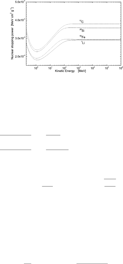
Figure 6.5: In MeV cm2/g, nuclear stopping powers in 7Li, 12C, 28Si and 56Fe
- calculated from Eq. (6.136) - and divided by the density of the material as
a function of the kinetic energy of electrons from 200 keV up to 1 TeV.
In terms of kinetic energy T, from Eqs. (6.90, 6.91) one can respectively
rewrite Eqs. (6.129, 6.130) as
dσMott
sc,F,CoM(T)
dT =dσRut′
dT F2
CoM(T)RMott
CoM(T)|F(q)|2(6.132)
dσMcF
sc,F,CoM(T)
dT ≃dσRut′(T)
dT F2
CoM(T)RMcF
CoM(T)|F(q)|2(6.133)
with dσRut′/dT from Eq. (6.125), FCoM(T) from Eq. (6.126) and RMcF
CoM(T)
replacing βwith β′
rin Eq. (6.97), i.e.,
RMcF
CoM(T) = "1−β′
r
T
Tmax
(β′
r+Zαπ)+Zαβ′
rπ
rT
Tmax #.(6.134)
Finally, as discussed in Sect. 6.6.1, RMott(T) exhibits almost no dependence
on electron energy above ≈10 MeV, thus, since at low energies θ⋍θ′and
β⋍β′
r,RMott
CoM(T) is obtained replacing βwith β′
rin Eq. (6.101).
6.6.2 Nuclear Stopping Power of Electrons
Using Eq. (6.132), the nuclear stopping power - in MeV cm−1- of Coulomb
electron–nucleus interaction can be obtained as
−dE
dx Mott
nucl
=nAZTmax
0
dσMott
sc,F,CoM(T)
dT T dT (6.135)
with nAthe number of nuclei (atoms) per unit of volume [e.g., see Equa-
tion (1.71) of Ref.[4]] and, finally, the negative sign indicates that the energy
95

is lost by the electron (thus, achieved by recoil targets). Using the analytical
approximation derived by McKinley and Feshbach[6], i.e., Eq. (6.133), for
the nuclear stopping power one finds
−dE
dx McF
nucl
=nAZTmax
0
dσMcF
sc,F,CoM(T)
dT T dT. (6.136)
As already mentioned in Sect. 6.6.1, the large momentum transfers -
corresponding to large scattering angles - are disfavored by effects due to
the finite nuclear size accounted for by means of the nuclear form factor
(Sect.6.6.1). For instance, the ratios of nuclear stopping powers of electrons
in silicon are shown in Ref.[1] as a function of the kinetic energies of electrons
from 200 keV up to 1 TeV. These ratios are the nuclear stopping powers
calculated neglecting i) nuclear size effects (i.e., for |Fexp|2= 1) and ii) effects
due to the finite rest mass of the target nucleus [i.e., in Eq. (6.136) replacing
dσMcF
sc,F,CoM(T)/dT with dσMcF
sc,F (T)/dT from Eq. (6.114)] both divided by that
one obtained using Eq. (6.136). Above a few tens of MeV, a larger stopping
power is found assuming |Fexp|2= 1 and, in addition, above a few hundreds
of MeV the stopping power largely decreases when the effects of nuclear rest
mass are not accounted for.
In Fig. 6.5 , the nuclear stopping powers in 7Li, 12C, 28Si and 56Fe are
shown as a function of the kinetic energy of electrons from 200 keV up to
1 TeV. These nuclear stopping powers in MeV cm2/g are calculated from
Eq. (6.136) and divided by the density of the medium.
6.6.3 Non-Ionizing Energy-Loss of Electrons
In case of Coulomb scattering of electrons on nuclei, the non-ionizing energy-
loss can be calculated using (as discussed in Sect. 6.6.1–6.6.2) the MDCRS or
its approximate expression McFDCS [e.g., Eqs. (6.132, 6.133), respectively],
once the screened Coulomb fields, finite sizes and rest masses of nuclei are
accounted for, i.e., in Mev/cm
−dE
dx NIEL
n,Mott
=nAZTmax
Td
T L(T)dσMott
sc,F,CoM(T)
dT dT (6.137)
or
−dE
dx NIEL
n,McF
=nAZTmax
Td
T L(T)dσMcF
sc,F,CoM(T)
dT dT (6.138)
[e.g., see Equation (4.113) at page 402 and, in addition, Sections 4.2.1–4.2.1.2
of Ref.[4]], where Tis the kinetic energy transferred to the target nucleus,
96
L(T) is the fraction of Tdeposited by means of displacement processes. The
Lindhard partition function,L(T), can be approximated using the so-called
Norgett–Robintson–Torrens expression [e.g., see Equations (4.121, 4.123) at
pages 404 and 405, respectively, of Ref.[4] (see also references therein)]. Tde =
T L(T) is the so-called damage energy, i.e., the energy deposited by a recoil
nucleus with kinetic energy Tvia displacement damages inside the medium. In
Eqs. (6.137, 6.138) the integral is computed from the minimum energy Td-
the so-called threshold energy for displacement, i.e., that energy necessary
to displace the atom from its lattice position - up to the maximum energy
Tmax that can be transferred during a single collision process. For instance,
Tdis about 21 eV in silicon requiring electrons with kinetic energies above
≈220 kev.
As already discussed with respect to nuclear stopping powers in Sect. 6.6.2,
the large momentum transfers (corresponding to large scattering angles) are
disfavored by effects due to the finite nuclear size accounted for by the nu-
clear form factor. For instance, the ratios of NIELs for electrons in silicon are
shown in Ref.[1] as a function of the kinetic energy of electrons from 220 keV
up to 1 TeV. These ratios are the NIELs calculated neglecting i) nuclear size
effects (i.e., for |Fexp|2= 1) and ii) effects due to the finite rest mass of the tar-
get nucleus [i.e., in Eq. (6.138) replacing dσMcF
sc,F,CoM(T)/dT with dσMcF
sc,F (T)/dT
from Eq. (6.114)] both divided by that one obtained using Eq. (6.138). Above
≈10 MeV, the NIEL is ≈20% larger assuming |Fexp|2= 1 and, in addition,
above (100–200) MeV the calculated NIEL largely decreases when the effects
of nuclear rest mass are not accounted for.
6.7 G4eSingleScatteringModel
The G4eSingleScatteringModel performs the single scattering interaction of
electrons on nuclei. The differential cross section (DCS) for the energy trans-
ferred is define in the G4ScreeningMottCrossSection class. In this class the
M.Boschini’s et al. [7] Mott differential cross Section approximation is im-
plemented. This CDS is modified by the introduction of the Moliere’s [10]
screening coefficient. In addition the exponential charge distribution Nuclear
Form Factor is applied [11]. This treatment is fully performed in the center of
mass system and the usual Lorentz transformations are applied to obtained
the energy and momentum quantities in the laboratory system after scat-
tering. This model well simulates the interacting process for low scattering
angles and it is suitable for high energy electrons (from 200 keV) incident on
medium light target nuclei. The nuclear energy loss (i.e. nuclear stopping
power) is calculated for every single interaction. In addition the production
97

of secondary scattered nuclei is simulated from a threshold kinetic energy
which can be decided by the user (threshold energy for displacement).
6.7.1 The method
In the G4eSingleScatteringModel the method ComputeCrossSectionPerAtom()
performs the total cross section computation. The SetupParticle() and the
DefineMaterial() methods are called to defined the incident and target par-
ticles. Before the total cross section computation, the SetupKinematic()
method of the G4ScreeningMottCrossSection class calculates all the physi-
cal quantities in the center of mass system (CM). The scattering in the CM
system is equivalent to the one of an effective particle which interacts with
a fixed scattering center. The effective particle rest mass is equal to the
relativistic reduced mass of the system µwhose expression is calculated by:
µ=mMc2
Ecm
(6.139)
where mand Mare rest masses of the electron and of the target nuclei
respectively. Ecm is the total center of mass energy and, since the target is
at rest before scattering, its expression is calculated by:
Ecm =p(mc2)2+ (Mc2)2+ 2E′Mc2(6.140)
where E=γ′mc2is the total energy of the electron before scattering in the
laboratory system. The momentum and the scattering angle of the effective
particle are equal to the corresponding quantities calculated in the center of
mass system (p≡pcm,θ≡θcm) of the incident electron:
pc =p′cMc2
Ecm
(6.141)
where p′is the momentum of the incident electron calculated in the labora-
tory system. The velocity of the effective particle is related with its momen-
tum by the following expression:
1
β2= 1 + µc2
pc 2(6.142)
The integration of the DCS is performed by the NuclearCrossSection() method
of the G4ScreeningMottCrossSection:
σtot = 2πZθmax
θmin
dσ(θ)
dΩsin θdθ (6.143)
98

The integration is performed in the scattering range [0 ;π] but the user can
decide to vary the minimum (θmin) and the maximum (θmax) scattering an-
gles. The DCS is then given by:
dσ(θ)
dΩ= Ze2
µc2β2γ!2RMcF |FN(q)|2
2As+ 2 sin2(θ/2)2(6.144)
where Zis the atomic number of the nucleus, Asis the screening coefficient
whose expression has been given by Moliere[10] :
As=~
2p aT F 21.13 + 3.76αZ
β2(6.145)
where aT F is the Thomas-Fermi screening length given by:
aT F =0.88534 a0
Z1/3(6.146)
and a0is the Bhor radius. RMcF is the ratio of the Mott to the Rutherfor
DCS given by McKinley and Feshbach approximation [6]:
RMcF =1−β2sin2(θ/2) + Zαβπ sin(θ/2)1−sin(θ/2)(6.147)
The nuclear form factor for the exponential charge distribution is given by
[11]:
FN(q) = "1 + (qRN)2
12~2#−2
(6.148)
where RNis the nuclear radius that is parameterized by:
RN= 1.27A0.27 fm.(6.149)
qis the momentum transferred to the nucleus and it is calculated as:
qc =pT(T+ 2Mc2) (6.150)
where Tis the kinetic energy transferred to the nucleus. This kinetic energy
is calculated in the GetNewDirection() method as:
T=2Mc2(p′c)2
E2
cm
sin2θ/2.(6.151)
The scattering angle θcalculation is performed in the GetScatteringAngle()
method of G4ScreeningMottCrossSection class. By means of AngleDistribu-
tion() function the scattering angle is chosen randomly according to the total
99

cross section distribution (p.d.f. probability density function) by means of
the inverse transform method.
In the SampleSecondary() method of G4eSingleScatteringModel the ki-
netic energy of the incident particle after scattering is then calculated as
E′
new =E′−Twhere E′is the electron incident kinetic energy (in lab.); in
addition the new particle direction and momentum are obtained from the
scattering angle information.
6.7.2 Implementation Details
The scattering angle probability density function f(θ) (p.d.f.) is performed
by the AngleDistribution() of G4ScreeningMottCrossSection class where the
inverse transform method is applied. The normalized cumulative function of
the cross section is calculated as a function of the scattering angle in this
way:
σn(θ)≡Zf(θ)dθ =2π
σtot Zθ
0
dσ(t)
dΩsin tdt (6.152)
The normalized cumulative function σn(θ) depends on the DCS and its val-
ues range in the interval [0;1]. After this calculation a random number r,
uniformly distributed in the same interval [0;1], is chosen in order to fix the
cumulative function value (i.e. r≡σn(θ)). This number is the probability
to find the scattering angle in the interval [θ;θ+dθ]. The scattering angle
θis then given by the inverse function of σn(θ).
The threshold energy for displacement Th can by set by the user in her/his
own Physic class by adding the electromagnetic model:
G4eSingleCoulombScatteringModel* mod=
new G4eSingleCoulombScatteringModel();
mod->SetRecoilThreshold(Th);
If the energy lost by the incident particle is grater then this threshold value
a new secondary particle is created for transportation processes. The energy
lost is added to ProposeNonIonizingEnergyDeposit().
NIEL calculation is available in test58.
Bibliography
[1] M. Boschini et al., Nuclear and Non-Ionizing Energy-Loss of Electrons
with Low and Relativistic Energies in Materials and Space Environ-
100
ment,Proc. of the ICATPP Conference on Cosmic Rays for Particle and
Astroparticle Physics, October 3–7 (2011), Villa Olmo, Como, Italy, S.
Giani, C. Leroy, L. Price, P.G. Rancoita and R. Ruchri, Editors, World
Scientific, Singapore (2012); arXiv 1111.4042.
[2] C. Leroy and P.G. Rancoita, Particle Interaction and Displacement
Damage in Silicon Devices operated in Radiation Environments,
Rep. Prog. in Phys. 70 (no. 4)(2007), 403–625, doi: 10.1088/0034-
4885/70/4/R01.
[3] M. Boschini et al., Nuclear and Non-Ionizing Energy-Loss for Coulomb
Scattered Particles from Low Energy up to Relativistic Regime in Space
Radiation Environment, Proc. of the ICATPP Conference on Cos-
mic Rays for Particle and Astroparticle Physics, October 7–8 (2010),
Villa Olmo, Como, Italy, S. Giani, C. Leroy and P.G. Rancoita, Edi-
tors, World Scientific, Singapore (2011), 9–23, IBSN: 978-981-4329-02-6;
arXiv 1011.4822.
[4] C. Leroy and P.G. Rancoita, Principles of Radiation Interaction in Mat-
ter and Detection, 3rd Edition, World Scientific (Singapore) 2011.
[5] T. Lijian, H. Quing and L. Zhengming, Radiat. Phys. Chem. 45 (1995),
235–245.
[6] A.J. McKinley and H. Feshbach, Phys. Rev. 74 (1948), 1759–1763.
[7] M. Boschini et al., Rad. Phys. Chem. 90 (2013), 39–66.
[8] E. Zeitler and A. Olsen, Phys. Rev. 136 (1956), A1546-A1552.
[9] H. De Vries, C.W. De Jager, and C. De Vries, Atomic Data and Nuclear
Data Tables 36 (1987), 495.
[10] von G. Moliere, Z. Naturforsh A2 (1947), 133-145; A3 (1948), 78.
[11] A.V. Butkevich et al. Nucl. Instr. and Meth. in Phys. Res. A 488 (2002),
282–294.
101
Chapter 7
Energy loss of Charged
Particles
102

7.1 Mean Energy Loss
Energy loss processes are very similar for e+/e−,µ+/µ−and charged
hadrons, so a common description for them was a natural choice in Geant4
[1], [2]. Any energy loss process must calculate the continuous and discrete
energy loss in a material. Below a given energy threshold the energy loss is
continuous and above it the energy loss is simulated by the explicit produc-
tion of secondary particles - gammas, electrons, and positrons.
7.1.1 Method
Let dσ(Z, E, T )
dT
be the differential cross-section per atom (atomic number Z) for the ejection
of a secondary particle with kinetic energy Tby an incident particle of total
energy Emoving in a material of density ρ. The value of the kinetic energy
cut-off or production threshold is denoted by Tcut. Below this threshold the
soft secondaries ejected are simulated as continuous energy loss by the inci-
dent particle, and above it they are explicitly generated. The mean rate of
energy loss is given by:
dEsoft(E, Tcut)
dx =nat ·ZTcut
0
dσ(Z, E, T )
dT T dT (7.1)
where nat is the number of atoms per volume in the material. The total cross
section per atom for the ejection of a secondary of energy
T > Tcut is
σ(Z, E, Tcut) = ZTmax
Tcut
dσ(Z, E, T )
dT dT (7.2)
where Tmax is the maximum energy transferable to the secondary particle.
If there are several processes providing energy loss for a given particle, then
the total continuous part of the energy loss is the sum:
dEtot
soft(E, Tcut)
dx =X
i
dEsoft,i(E, Tcut)
dx .(7.3)
These values are pre-calculated during the initialization phase of Geant4
and stored in the dE/dx table. Using this table the ranges of the particle
in given materials are calculated and stored in the Range table. The Range
table is then inverted to provide the InverseRange table. At run time, values
of the particle’s continuous energy loss and range are obtained using these
103
tables. Concrete processes contributing to the energy loss are not involved in
the calculation at that moment. In contrast, the production of secondaries
with kinetic energies above the production threshold is sampled by each
concrete energy loss process.
The default energy interval for these tables extends from 100eV to 10T eV
and the default number of bins is 77. For muons and for heavy particles en-
ergy loss processes models are valid for higher energies and can be extended.
For muons uppper limit may be set to 1000P eV .
7.1.2 General Interfaces
There are a number of similar functions for discrete electromagnetic pro-
cesses and for electromagnetic (EM) packages an additional base classes were
designed to provide common computations [2]. Common calculations for dis-
crete EM processes are performed in the class G4V EnergyLossP rocess. De-
rived classes (7.1) are concrete processes providing initialisation. The physics
models are implemented using the G4V EmModel interface. Each process
may have one or many models defined to be active over a given energy range
and set of G4Regions. Models are implementing computation of energy loss,
cross section and sampling of final state. The list of EM processes and models
for gamma incident is shown in Table 7.1.
7.1.3 Step-size Limit
Continuous energy loss imposes a limit on the step-size because of the energy
dependence of the cross sections. It is generally assumed in MC programs
(for example, Geant3) that the cross sections are approximately constant
along a step, i.e. the step size should be small enough, so that the change
in cross section along the step is also small. In principle one must use very
small steps in order to insure an accurate simulation, however the computing
time increases as the step-size decreases.
For EM processes the exact solution is available (see 7.3) but is is not
implemented yet for all physics processes including hadronics. A good com-
promise is to limit the step-size by not allowing the stopping range of the
particle to decrease by more than ∼20 % during the step. This condition
works well for particles with kinetic energies >1 MeV, but for lower energies
it gives too short step-sizes, so must be relaxed. To solve this problem a
lower limit on the step-size was introduced. A smooth StepFunction, with
2 parameters, controls the step size. At high energy the maximum step
size is defined by Step/Range ∼αR(parameter dRoverRange). By default
αR= 0.2. As the particle travels the maximum step size decreases gradually
104

Table 7.1: List of process and model classes for charged particles.
EM process EM model Ref.
G4eIonisation G4MollerBhabhaModel 8.1
G4LivermoreIonisationModel 9.9
G4PenelopeIonisationModel 10.1.7
G4PAIModel 7.5
G4PAIPhotModel 7.5
G4ePolarizedIonisation G4PolarizedMollerBhabhaModel 17.1
G4MuIonisation G4MuBetheBlochModel 13.1
G4PAIModel 7.5
G4PAIPhotModel 7.5
G4hIonisation G4BetheBlochModel 12.1
G4BraggModel 12.1
G4ICRU73QOModel 12.2.1
G4PAIModel 7.5
G4PAIPhotModel 7.5
G4ionIonisation G4BetheBlochModel 12.1
G4BetheBlochIonGasModel 12.1
G4BraggIonModel 12.1
G4BraggIonGasModel 12.1
G4IonParametrisedLossModel 12.2.4
G4NuclearStopping G4ICRU49NuclearStoppingModel 12.1.3
G4mplIonisation G4mplIonisationWithDeltaModel
G4eBremsstrahlung G4SeltzerBergerModel 8.2.1
G4eBremsstrahlungRelModel 8.2.2
G4LivermoreBremsstrahlungModel 9.10
G4PenelopeBremsstrahlungModel 10.1.6
G4ePolarizedBremsstrahlung G4PolarizedBremsstrahlungModel 17.1
G4MuBremsstrahlung G4MuBremsstrahlungModel 13.2
G4hBremsstrahlung G4hBremsstrahlungModel
G4ePairProduction G4MuPairProductionModel 13.3
G4MuPairProduction G4MuPairProductionModel 13.3
G4hPairProduction G4hPairProductionModel
105
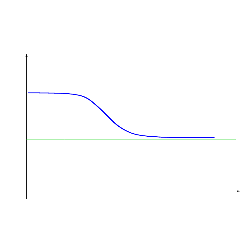
until the range becomes lower than ρR(parameter finalRange). Default final-
Range ρR= 1mm. For the case of a particle range R > ρRthe StepFunction
provides limit for the step size ∆Slim by the following formula:
∆Slim =αRR+ρR(1 −αR)2−ρR
R.(7.4)
In the opposite case of a small range ∆Slim =R. The figure below shows the
ratio step/range as a function of range if step limitation is determined only
by the expression (7.4).
step
−−−−−−
range
range
finalRange
1
dRoverRange
The parameters of StepFunction can be overwritten using an UI command:
/process/eLoss/StepFunction 0.2 1 mm
To provide more accurate simulation of particle ranges in physics constructors
G4EmStandardPhysics option3 and G4EmStandardPhysics option4 more strict
step limitation is chosen for different particle types.
7.1.4 Run Time Energy Loss Computation
The computation of the mean energy loss after a given step is done by using
the dE/dx,Range, and InverseRange tables. The dE/dx table is used if
the energy deposition (∆T) is less than allowed limit ∆T < ξT0, where ξis
106

linearLossLimit parameter (by default ξ= 0.01), T0is the kinetic energy
of the particle. In that case
∆T=dE
dx ∆s, (7.5)
where ∆Tis the energy loss, ∆sis the true step length. When a larger
percentage of energy is lost, the mean loss can be written as
∆T=T0−fT(r0−∆s) (7.6)
where r0the range at the beginning of the step, the function fT(r) is the
inverse of the Range table (i.e. it gives the kinetic energy of the particle for
a range value of r). By default spline approximation is used to retrieve a
value from dE/dx,Range, and InverseRange tables. The spline flag can be
changed using an UI command:
/process/em/spline false
After the mean energy loss has been calculated, the process computes the
actual energy loss, i.e. the loss with fluctuations. The fluctuation models are
described in Section 7.2.
If deexcitation module (see 14.1) is enabled then simulation of atomic de-
excitation is performed using information on step length and ionisation cross
section. Fluorescence gamma and Auger electrons are produced above the
same threshold energy as δ-electrons and bremsstrahlung gammas. Following
UI commands can be used to enable atomic relaxation:
/process/em/deexcitation myregion true true true
/process/em/fluo true
/process/em/auger true
/process/em/pixe true
/process/em/deexcitationIgnoreCut true
The last command means that production threshold for electrons and gam-
mas are not checked, so full atomic de-excitation decay chain is simulated.
After the step a kinetic energy of a charged particle is compered with
the lowestEnergy. In the case if final kinetic energy is below the particle is
stooped and remaining kinetic energy is assigned to the local energy deposit.
The default value of the limit is 1keV . It may be changed separately for
electron/positron and muon/hadron using UI commands:
/process/em/lowestElectronEnergy 100 eV
/process/em/lowestMuHadEnergy 50 eV
These values may be also can be set to zero.
107

7.1.5 Energy Loss by Heavy Charged Particles
To save memory in the case of positively charged hadrons and ions energy
loss, dE/dx,Range and InverseRange tables are constructed only for pro-
ton, antiproton, muons, pions, kaons, and Generic Ion. The energy loss for
other particles is computed from these tables at the scaled kinetic energy
Tscaled :
Tscaled =TMbase
Mparticle
,(7.7)
where Tis the kinetic energy of the particle, Mbase and Mparticle are the masses
of the base particle (proton or kaon) and particle. For positively changed
hadrons with non-zero spin proton is used as a based particle, for negatively
charged hadrons with non-zero spin - antiproton, for charged particles with
zero spin - K+or K−correspondingly. The virtual particle Generic Ion is
used as a base particle for for all ions with Z > 2. It has mass, change and
other quantum numbers of the proton. The energy loss can be defined via
scaling relation:
dE
dx (T) = q2
eff (F1(T)dE
dx base(Tscaled) + F2(T, qef f )),(7.8)
where qeff is particle effective change in units of positron charge, F1and
F2are correction function taking into account Birks effect, Block correction,
low-energy corrections based on data from evaluated data bases [5]. For a
hadron qeff is equal to the hadron charge, for a slow ion effective charge is
different from the charge of the ion’s nucleus, because of electron exchange
between transporting ion and the media. The effective charge approach is
used to describe this effect [3]. The scaling relation (7.7) is valid for any
combination of two heavy charged particles with accuracy corresponding to
high order mass, charge and spin corrections [4].
Bibliography
[1] S. Agostinelli et al., Geant4 – a simulation toolkit Nucl. Instr. Meth.
A506 (2003) 250.
[2] J. Apostolakis et al., Geometry and physics of the Geant4 toolkit for high
and medium energy applications. Rad. Phys. Chem. 78 (2009) 859.
[3] J.F. Ziegler and J.M. Manoyan, Nucl. Instr. and Meth. B35 (1988) 215.
[4] ICRU (A. Allisy et al), Stopping Powers and Ranges for Protons and
Alpha Particles, ICRU Report 49, 1993.
108
[5] ICRU (R. Bimbot et al), Stopping of Ions Heavier than Helium, Journal
of the ICRU Vol5 No1 (2005) Report 73.
109
7.2 Energy Loss Fluctuations
The total continuous energy loss of charged particles is a stochastic quan-
tity with a distribution described in terms of a straggling function. The
straggling is partially taken into account in the simulation of energy loss
by the production of δ-electrons with energy T > Tcut (Eq.7.2). However,
continuous energy loss (Eq.7.1) also has fluctuations. Hence in the current
GEANT4 implementation different models of fluctuations implementing the
G4V EmF luctuationM odel interface:
•G4BohrFluctuations;
•G4IonFluctuations;
•G4PAIModel;
•G4PAIPhotModel;
•G4UniversalFluctuation.
The last model is the default one used in main Physics List and will be de-
scribed below. Other models have limited applicability and will be described
in chapters for ion ionisation and PAI models.
7.2.1 Fluctuations in Thick Absorbers
The total continuous energy loss of charged particles is a stochastic quantity
with a distribution described in terms of a straggling function. The strag-
gling is partially taken into account in the simulation of energy loss by the
production of δ-electrons with energy T > Tc. However, continuous energy
loss also has fluctuations. Hence in the current GEANT4 implementation
two different models of fluctuations are applied depending on the value of
the parameter κwhich is the lower limit of the number of interactions of the
particle in a step. The default value chosen is κ= 10. In the case of a high
range cut (i.e. energy loss without delta ray production) for thick absorbers
the following condition should be fulfilled:
∆E > κ Tmax (7.9)
where ∆Eis the mean continuous energy loss in a track segment of length s,
and Tmax is the maximum kinetic energy that can be transferred to the atomic
electron. If this condition holds the fluctuation of the total (unrestricted)
energy loss follows a Gaussian distribution. It is worth noting that this
110

condition can be true only for heavy particles, because for electrons, Tmax =
T/2, and for positrons, Tmax =T, where Tis the kinetic energy of the
particle. In order to simulate the fluctuation of the continuous (restricted)
energy loss, the condition should be modified. After a study, the following
conditions have been chosen:
∆E > κ Tc(7.10)
Tmax <= 2 Tc(7.11)
where Tcis the cut kinetic energy of δ-electrons. For thick absorbers the
straggling function approaches the Gaussian distribution with Bohr’s vari-
ance [4]:
Ω2= 2πr2
emec2Nel
Z2
h
β2Tcs1−β2
2,(7.12)
where reis the classical electron radius, Nel is the electron density of the
medium, Zhis the charge of the incident particle in units of positron charge,
and βis the relativistic velocity.
7.2.2 Fluctuations in Thin Absorbers
If the conditions 7.10 and 7.11 are not satisfied the model of energy fluctua-
tions in thin absorbers is applied. The formulas used to compute the energy
loss fluctuation (straggling) are based on a very simple physics model of the
atom. It is assumed that the atoms have only two energy levels with binding
energies E1and E2. The particle-atom interaction can be an excitation with
energy loss E1or E2, or ionisation with energy loss distributed according to
a function g(E)∼1/E2:
ZTup
E0
g(E)dE = 1 =⇒g(E) = E0Tup
Tup −E0
1
E2.(7.13)
The macroscopic cross section for excitation (i= 1,2) is
Σi=Cfi
Ei
ln[2mc2(βγ)2/Ei]−β2
ln[2mc2(βγ)2/I]−β2(1 −r) (7.14)
and the ionisation cross section is
Σ3=CTup −E0
E0Tup ln(Tup
E0)r(7.15)
where E0denotes the ionisation energy of the atom, Iis the mean ionisation
energy, Tup is the production threshold for delta ray production (or the max-
imum energy transfer if this value smaller than the production threshold),
111

Eiand fiare the energy levels and corresponding oscillator strengths of the
atom, and Cand rare model parameters.
The oscillator strengths fiand energy levels Eishould satisfy the con-
straints
f1+f2= 1 (7.16)
f1·lnE1+f2·lnE2=lnI. (7.17)
The cross section formulas 7.14,7.15 and the sum rule equations 7.16,7.17
can be found e.g. in Ref. [1]. The model parameter Ccan be defined in the
following way. The numbers of collisions (ni,i= 1,2 for excitation and 3 for
ionisation) follow the Poisson distribution with a mean value hnii. In a step
of length ∆xthe mean number of collisions is given by
hnii= ∆xΣi(7.18)
The mean energy loss in a step is the sum of the excitation and ionisation
contributions and can be written as
dE
dx ·∆x=Σ1E1+ Σ2E2+ZTup
E0
Eg(E)dE∆x. (7.19)
From this, using Eq. 7.14 - 7.17, one can see that
C=dE/dx. (7.20)
The other parameters in the fluctuation model have been chosen in the follow-
ing way. Z·f1and Z·f2represent in the model the number of loosely/tightly
bound electrons
f2= 0 for Z = 1 (7.21)
f2= 2/Z for Z ≥2 (7.22)
E2= 10 eV Z2(7.23)
E0= 10 eV .(7.24)
Using these parameter values, E2corresponds approximately to the K-shell
energy of the atoms ( and Zf2= 2 is the number of K-shell electrons).
The parameters f1and E1can be obtained from Eqs. 7.16 and 7.17. The
parameter ris the only variable in the model which can be tuned. This
parameter determines the relative contribution of ionisation and excitation to
the energy loss. Based on comparisons of simulated energy loss distributions
to experimental data, its value has been fixed as
r= 0.55 (7.25)
112
7.2.3 Width Correction Algorithm
This simple parametrization and sampling in the model give good values for
the most probable energy loss in thin layers. The width of the energy loss
distribution (Full Width at Half Maximum, FWHM) in most of the cases
is too small. In order to get good FWHM values a relatively simple width
correction algorithm has been applied. This algorithm rescales the energy
levels E1,E2and the number of excitations n1,n2in such a way that the
mean energy loss remains the same. Using this width correction scheme the
model gives not only good most probable energy loss, but good FWHM value
too.
Width correction algorithm is in the model since version 9.2. The updated
version in the model (in version 9.4) causes an important change in the
behaviour of the model: the results become much more stable, i.e. the results
do not change practically when the cuts and/or the stepsizes are changing.
Another important change: the (unphysical) second peak or shoulder in the
energy loss distribution which can be seen in some cases (energy loss in thin
gas layers) in older versions of the model disappeared. Limit of validity
of the model for thin targets: the model gives good (reliable) energy loss
distribution if the mean energy loss in the target is ≥(few times)∗Iexc,
where Iexc is the mean excitation energy of the target material.
This simple model of energy loss fluctuations is rather fast and can be
used for any thickness of material. This has been verified by performing
many simulations and comparing the results with experimental data, such as
those in Ref.[2]. As the limit of validity of Landau’s theory is approached,
the loss distribution approaches the Landau form smoothly.
7.2.4 Sampling of Energy Loss
If the mean energy loss and step are in the range of validity of the Gaussian
approximation of the fluctuation (7.10 and 7.11), the Gaussian sampling is
used to compute the actual energy loss (7.12). For smaller steps the energy
loss is computed in the model under the assumption that the step length (or
relative energy loss) is small and, in consequence, the cross section can be
considered constant along the step. The loss due to the excitation is
∆Eexc =n1E1+n2E2(7.26)
where n1and n2are sampled from a Poisson distribution. The energy loss
due to ionisation can be generated from the distribution g(E) by the inverse
113

transformation method :
u=F(E) = ZE
E0
g(x)dx (7.27)
E=F−1(u) = E0
1−uTup−E0
Tup
(7.28)
where uis a uniformly distributed random number ∈[0,1]. The contribution
coming from the ionisation will then be
∆Eion =
n3
X
j=1
E0
1−ujTup−E0
Tup
(7.29)
where n3is the number of ionisations sampled from the Poisson distribution.
The total energy loss in a step will be ∆E= ∆Eexc + ∆Eion and the energy
loss fluctuation comes from fluctuations in the number of collisions niand
from the sampling of the ionisation loss.
Bibliography
[1] H. Bichsel Rev.Mod.Phys. 60 (1988) 663.
[2] K. Lassila-Perini, L. Urb´an Nucl.Inst.Meth. A362(1995) 416.
[3] geant3 manual Cern Program Library Long Writeup W5013 (1994)
[4] ICRU (A. Allisy et al), Stopping Powers and Ranges for Protons and
Alpha Particles, ICRU Report 49 (1993).
114
7.3 Correcting the Cross Section for Energy
Variation
As described in Sections 7.1 and 3.1.2 the step size limitation is provided
by energy loss processes in order to insure the precise calculation of the
probability of particle interaction. It is generally assumed in Monte Carlo
programs that the particle cross sections are approximately constant during a
step, hence the reaction probability pat the end of the step can be expressed
as
p= 1 −exp (−nsσ(Ei)) ,(7.30)
where nis the density of atoms in the medium, sis the step length, Eiis the
energy of the incident particle at the beginning of the step, and σ(Ei) is the
reaction cross section at the beginning of the step.
However, it is possible to sample the reaction probability from the exact
expression
p= 1 −exp −ZEf
Ei
nσ(E)ds,(7.31)
where Efis the energy of the incident particle at the end of the step, by using
the integral approach to particle transport. This approach is available for pro-
cesses implemented via the G4V EnergyLossP rocess and G4V EmP rocess
interfaces.
The Monte Carlo method of integration is used for sampling the reaction
probability [1]. It is assumed that during the step the reaction cross section
smaller, than some value σ(E)< σm. The mean free path for the given step
is computed using σm. If the process is chosen as the process happens at the
step, the sampling of the final state is performed only with the probability p=
σ(Ef)/σm, alternatively no interaction happen and tracking of the particle
is continued. To estimate the maximum value σmfor the given tracking step
at Geant4 initialisation the energy Emof absoluted maximum σmax of the
cross section for given material is determined and stored. If at the tracking
time particle energy E < Em, then σm=σ(E). For higher initial energies
if ξE > Emthen σm=max(σ(E), σ(ξE)), in the opposit case, σm=σmax.
Here ξis a parameter of the algorithm. Its optimal value is connected with
the value of the dRoverRange parameter (see sub-chapter 7.1), by default
ξ= 1 −αR= 0.8. Note, that described method is precise if the cross section
has only one maximum, which is a typical case for electromagnetic processes.
The integral variant of step limitation is the default for the G4eIonisation,
G4eBremsstrahlung and some otehr process but is not automatically acti-
vated for others. To do so the boolean UI command can be used:
115
/process/eLoss/integral true
The integral variant of the energy loss sampling process is less dependent
on values of the production cuts [2] and allows to have less step limitation,
however it should be applied on a case-by-case basis because may require
extra CPU.
Bibliography
[1] V.N.Ivanchenko et al., Proc. of Int. Conf. MC91: Detector and event
simulation in high energy physics, Amsterdam 1991, pp. 79-85. (HEP
INDEX 30 (1992) No. 3237).
[2] J. Apostolakis et al., Geometry and physics of the Geant4 toolkit for high
and medium energy applications. Rad. Phys. Chem. 78 (2009) 859.
116

7.4 Conversion from Cut in Range to Energy
Threshold
In Geant4 charged particles are tracked to the end of their range. The dif-
ferential cross section of δ-electron productions and bremsstrahlung grow
rapidly when secondary energy decrease. If all secondary particles will be
tracked the CPU performance of any Monte Carlo code will be pure. The
traditional solution is to use cuts. The specific of Geant4 [1] is that user
provides value of cut in term of cut in range, which is unique for defined
G4Region or for the complete geometry [2].
Range is used, rather than energy, as a more natural concept for designing
a coherent policy for different particles and materials. Definition of the cer-
tain value of the cut in range means the requirement for precision of spatial
radioactive dose deposition. This conception is more strict for a simulation
code and provides less handles for user to modify final results. At the same
time, it ensures that simulation validated in one geometry is valid also for
the other geometries.
The value of cut is defined for electrons, positrons, gamma and protons.
At the beginning of initialization of Geant4 physics the conversion is per-
formed from unique cut in range to cuts (production thresholds) in kinetic
energy for each G4MaterialCutsCouple [2]. At that moment no energy loss
or range table is created, so computation should be performed using original
formulas. For electrons and positrons ionization above 10keV a simplified
Berger-Seltzer energy loss formula (8.2) is used, in which the density correc-
tion term is omitted. The contribution of the bremsstrahlung is added using
empirical parameterized formula. For T < 10keV the linear dependence of
ionization losses on electron velocity is assumed, bremsstrahlung contribution
is neglected. The stopping range is defined as
R(T) = ZT
0
1
(dE/dx)dE. (7.32)
The integration has been done analytically for the low energy part and numer-
ically above an energy limit 1 keV . For each cut in range the corresponding
kinetic energy can be found out. If obtained production threshold in kinetic
energy cannot be below the parameter lowlimit (default 1 keV ) and above
highlimit (default 10 GeV ). If in specific application lower threshold is re-
quired, then the allowed energy cut needs to be extended:
G4ProductionCutsTable::GetProductionCutsTable()→SetEnergyRange(lowlimit,highlimit);
or via UI commands
117
/cuts/setMinCutEnergy 100 eV
/cuts/setMaxCutEnergy 100 T eV
In contrary to electrons, gammas has no range, so some approximation should
be used for range to energy conversion. An approximate empirical formula is
used to compute the absorption cross section of a photon in an element σabs.
Here, the absorption cross section means the sum of the cross sections of
the gamma conversion, Compton scattering and photoelectric effect. These
processes are the “destructive” processes for photons: they destroy the pho-
ton or decrease its energy. The coherent or Rayleigh scattering changes the
direction of the gamma only; its cross section is not included in the absorp-
tion cross section. The AbsorptionLength Labs vector is calculated for every
material as
Labs = 5/σabs.(7.33)
The factor 5 comes from the requirement that the probability of having no
’destructive’ interaction should be small, hence
exp(−Labsσabs) = exp(−5) = 6.7×10⁻³.(7.34)
The photon cross section for a material has a minimum at a certain energy
Emin. Correspondingly Labs has a maximum at E=Emin, the value of the
maximal Labs is the biggest ”meaningful” cut in absorption length. If the cut
given by the user is bigger than this maximum, a warning is printed and the
cut in kinetic energy is set to the highlimit.
The cut for proton is introduced with Geant4 v9.3. The main goal of
this cut is to limit production of all recoil ions including protons in elastic
scattering processes. A simple linear conversion formula is used to compute
energy threshold from the value of cut in range, in particular, the cut in
range 1 mm corresponds to the production threshold 100keV .
The conversion from range to energy can be studied using G4EmCalculator
class. This class allows access or recalculation of energy loss, ranges and other
values. It can be instantiated and at any place of user code and can be used
after initialisation of Physics Lists:
G4EmCalculator calc;
calc.ComputeEnergyCutFromRangeCut(range, particle, material);
here particle and material may be string names or corresponding const point-
ers to G4ParticleDefinition and G4Material.
118
Bibliography
[1] Geant4 Collaboration (S. Agostinelli et al.), Nucl. Instr. Meth. A506
(2003) 250.
[2] J. Allison et al., IEEE Trans. Nucl. Sci., 53 (2006) 270.
119

7.5 Photoabsorption Ionization Model
7.5.1 Cross Section for Ionizing Collisions
The Photoabsorption Ionization (PAI) model describes the ionization energy
loss of a relativistic charged particle in matter. For such a particle, the
differential cross section dσi/dω for ionizing collisions with energy transfer ω
can be expressed most generally by the following equations [1]:
dσi
dω =2πZe4
mv2f(ω)
ω|ε(ω)|2ln 2mv2
ω|1−β2ε|−
−ε1−β2|ε|2
ε2
arg(1 −β2ε∗)#+˜
F(ω)
ω2),(7.35)
˜
F(ω) = Zω
0
f(ω′)
|ε(ω′)|2dω′,
f(ω) = mωε2(ω)
2π2ZN~2.
Here mand eare the electron mass and charge, ~is Planck’s constant,
β=v/c is the ratio of the particle’s velocity vto the speed of light c,Z
is the effective atomic number, Nis the number of atoms (or molecules)
per unit volume, and ε=ε1+iε2is the complex dielectric constant of the
medium. In an isotropic non-magnetic medium the dielectric constant can
be expressed in terms of a complex index of refraction, n(ω) = n1+in2,
ε(ω) = n2(ω). In the energy range above the first ionization potential I1
for all cases of practical interest, and in particular for all gases, n1∼1.
Therefore the imaginary part of the dielectric constant can be expressed in
terms of the photoabsorption cross section σγ(ω):
ε2(ω) = 2n1n2∼2n2=N~c
ωσγ(ω).
The real part of the dielectric constant is calculated in turn from the disper-
sion relation
ε1(ω)−1 = 2N~c
πV.p. Z∞
0
σγ(ω′)
ω′2−ω2dω′,
where the integral of the pole expression is considered in terms of the princi-
pal value. In practice it is convenient to calculate the contribution from the
continuous part of the spectrum only. In this case the normalized photoab-
sorption cross section
120

˜σγ(ω) = 2π2~e2Z
mc σγ(ω)Zωmax
I1
σγ(ω′)dω′−1
, ωmax ∼100 keV
is used, which satisfies the quantum mechanical sum rule [2]:
Zωmax
I1
˜σγ(ω′)dω′=2π2~e2Z
mc .
The differential cross section for ionizing collisions is expressed by the pho-
toabsorption cross section in the continuous spectrum region:
dσi
dω =α
πβ2˜σγ(ω)
ω|ε(ω)|2ln 2mv2
ω|1−β2ε|−
−ε1−β2|ε|2
ε2
arg(1 −β2ε∗)#+1
ω2Zω
I1
˜σγ(ω′)
|ε(ω′)|2dω′),(7.36)
ε2(ω) = N~c
ω˜σγ(ω),
ε1(ω)−1 = 2N~c
πV.p. Zωmax
I1
˜σγ(ω′)
ω′2−ω2dω′.
For practical calculations using Eq. 7.35 it is convenient to represent the
photoabsorption cross section as a polynomial in ω−1as was proposed in [3]:
σγ(ω) =
4
X
k=1
a(i)
kω−k,
where the coefficients, a(i)
kresult from a separate least-squares fit to experi-
mental data in each energy interval i. As a rule the interval borders are equal
to the corresponding photoabsorption edges. The dielectric constant can now
be calculated analytically with elementary functions for all ω, except near
the photoabsorption edges where there are breaks in the photoabsorption
cross section and the integral for the real part is not defined in the sense of
the principal value.
The third term in Eq. (7.35), which can only be integrated numerically,
results in a complex calculation of dσi/dω. However, this term is dominant
121

for energy transfers ω > 10 keV , where the function |ε(ω)|2∼1. This is clear
from physical reasons, because the third term represents the Rutherford cross
section on atomic electrons which can be considered as quasifree for a given
energy transfer [4]. In addition, for high energy transfers, ε(ω) = 1−ω2
p/ω2∼
1, where ωpis the plasma energy of the material. Therefore the factor |ε(ω)|−2
can be removed from under the integral and the differential cross section of
ionizing collisions can be expressed as:
dσi
dω =α
πβ2|ε(ω)|2˜σγ(ω)
ωln 2mv2
ω|1−β2ε|−
−ε1−β2|ε|2
ε2
arg(1 −β2ε∗)#+1
ω2Zω
I1
˜σγ(ω′)dω′).(7.37)
This is especially simple in gases when |ε(ω)|−2∼1 for all ω > I1[4].
7.5.2 Energy Loss Simulation
For a given track length the number of ionizing collisions is simulated by a
Poisson distribution whose mean is proportional to the total cross section of
ionizing collisions:
σi=Zωmax
I1
dσ(ω′)
dω′dω′.
The energy transfer in each collision is simulated according to a distribution
proportional to
σi(> ω) = Zωmax
ω
dσ(ω′)
dω′dω′.
The sum of the energy transfers is equal to the energy loss. PAI ionisation is
implemented according to the model approach (class G4PAIModel) allowing
a user to select specific models in different regions. Here is an example physics
list:
const G4RegionStore* theRegionStore = G4RegionStore::GetInstance();
G4Region* gas = theRegionStore->GetRegion("VertexDetector");
...
if (particleName == "e-")
{
...
G4eIonisation* eion = new G4eIonisation();
122
G4PAIModel* pai = new G4PAIModel(particle,"PAIModel");
// here 0 is the highest priority in region ’gas’
eion->AddEmModel(0,pai,pai,gas);
...
}
...
It shows how to select the G4PAIModel to be the preferred ionisation model
for electrons in a G4Region named VertexDetector. The first argument in
AddEmModel is 0 which means highest priority.
The class G4PAIPhotonModel generates both δ-electrons and photons as
secondaries and can be used for more detailed descriptions of ionisation space
distribution around the particle trajectory.
7.5.3 Photoabsorption Cross Section at Low Energies
The photoabsorption cross section, σγ(ω), where ωis the photon energy, is
used in Geant4 for the description of the photo-electric effect, X-ray trans-
portation and ionization effects in very thin absorbers. As mentioned in the
discussion of photoabsorption ionization (see section 7.5), it is convenient to
represent the cross section as a polynomial in ω−1[5] :
σγ(ω) =
4
X
k=1
a(i)
kω−k.(7.38)
Using cross sections from the original Sandia data tables, calculations of pri-
mary ionization and energy loss distributions produced by relativistic charged
particles in gaseous detectors show clear disagreement with experimental
data, especially for gas mixtures which include xenon.
Therefore a special investigation was performed [6] by fitting the coefficients
a(i)
kto modern data from synchrotron radiation experiments in the energy
range of 10 −50 eV . The fits were performed for elements typically used
in detector gas mixtures: hydrogen, fluorine, carbon, nitrogen and oxygen.
Parameters for these elements were extracted from data on molecular gases
such as N2,O2,CO2,CH4, and CF4[7, 8]. Parameters for the noble gases
were found using data given in the tables [9, 10].
123
7.5.4 Status of this document
01.12.05 expanded discussion by V. Grichine
08.05.02 re-written by D.H. Wright
16.11.98 created by V. Grichine
20.11.12 updated by V. Ivanchenko
Bibliography
[1] Asoskov V.S., Chechin V.A., Grichine V.M. at el, Lebedev Institute
annual report, v. 140, p. 3 (1982)
[2] Fano U., and Cooper J.W. Rev.Mod.Phys., v. 40, p. 441 (1968)
[3] Biggs F., and Lighthill R., Preprint Sandia Laboratory, SAND 87-0070
(1990)
[4] Allison W.W.M., and Cobb J. Ann.Rev.Nucl.Part.Sci., v.30,p.253 (1980)
[5] Biggs F., and Lighthill R., Preprint Sandia Laboratory, SAND 87-0070
(1990)
[6] Grichine V.M., Kostin A.P., Kotelnikov S.K. et al., Bulletin of the Lebe-
dev Institute no. 2-3, 34 (1994).
[7] Lee L.C. et al., J.Q.S.R.T., v. 13, p. 1023 (1973).
[8] Lee L.C. et al., Journ. of Chem. Phys., v. 67, p. 1237 (1977).
[9] G.V. Marr and J.B. West, Atom. Data Nucl. Data Tabl., v. 18, p. 497
(1976).
[10] J.B. West and J. Morton, Atom. Data Nucl. Data Tabl., v. 30, p. 253
(1980).
124
Chapter 8
Electron and Positron Incident
125

8.1 Ionization
8.1.1 Method
The G4eIonisation class provides the continuous and discrete energy losses
of electrons and positrons due to ionization in a material according to the
approach described in Section 7.1. The value of the maximum energy trans-
ferable to a free electron Tmax is given by the following relation:
Tmax =E−mc2for e+
(E−mc2)/2for e−(8.1)
where mc2is the electron mass. Above a given threshold energy the energy
loss is simulated by the explicit production of delta rays by M¨oller scattering
(e−e−), or Bhabha scattering (e+e−). Below the threshold the soft electrons
ejected are simulated as continuous energy loss by the incident e±.
8.1.2 Continuous Energy Loss
The integration of 7.1 leads to the Berger-Seltzer formula [1]:
dE
dx T <Tcut
= 2πr2
emc2nel
1
β2ln 2(γ+ 1)
(I/mc2)2+F±(τ, τup)−δ(8.2)
with reclassical electron radius: e2/(4πǫ0mc2)
mc2mass energy of the electron
nel electron density in the material
Imean excitation energy in the material
γ E/mc2
β21−(1/γ2)
τ γ −1
Tcut minimum energy cut for δ-ray production
τcTcut/mc2
τmax maximum energy transfer: τfor e+,τ/2 for e−
τup min(τc, τmax)
δdensity effect function.
In an elemental material the electron density is
nel =Z nat =ZNavρ
A.
126

Nav is Avogadro’s number, ρis the material density, and Ais the mass of a
mole. In a compound material
nel =X
i
Zinati =X
i
ZiNavwiρ
Ai
,
where wiis the proportion by mass of the ith element, with molar mass Ai.
The mean excitation energies Ifor all elements are taken from [2].
The functions F±are given by :
F+(τ, τup) = ln(ττup) (8.3)
−τ2
up
ττ+ 2τup −3τ2
upy
2−τup −τ3
up
3y2−τ2
up
2−ττ3
up
3+τ4
up
4y3
F−(τ, τup) = −1−β2(8.4)
+ ln [(τ−τup)τup] + τ
τ−τup
+1
γ2τ2
up
2+ (2τ+ 1) ln 1−τup
τ
where y= 1/(γ+ 1).
The density effect correction is calculated according to the formalism of
Sternheimer [3]:
xis a kinetic variable of the particle : x= log10(γβ) = ln(γ2β2)/4.606,
and δ(x) is defined by
for x < x0:δ(x) = 0
for x∈[x0, x1] : δ(x) = 4.606x−C+a(x1−x)m
for x > x1:δ(x) = 4.606x−C
(8.5)
where the matter-dependent constants are calculated as follows:
hνp= plasma energy of the medium = p4πnelr3
emc2/α =√4πnelre~c
C= 1 + 2 ln(I/hνp)
xa=C/4.606
a= 4.606(xa−x0)/(x1−x0)m
m= 3.
(8.6)
For condensed media
I < 100 eV for C≤3.681 x0= 0.2x1= 2
for C > 3.681 x0= 0.326C−1.0x1= 2
I≥100 eV for C≤5.215 x0= 0.2x1= 3
for C > 5.215 x0= 0.326C−1.5x1= 3
127

and for gaseous media
for C < 10. x0= 1.6x1= 4
for C∈[10.0,10.5[ x0= 1.7x1= 4
for C∈[10.5,11.0[ x0= 1.8x1= 4
for C∈[11.0,11.5[ x0= 1.9x1= 4
for C∈[11.5,12.25[ x0= 2. x1= 4
for C∈[12.25,13.804[ x0= 2. x1= 5
for C≥13.804 x0= 0.326C−2.5x1= 5.
8.1.3 Total Cross Section per Atom and Mean Free
Path
The total cross section per atom for M¨oller scattering (e−e−) and Bhabha
scattering (e+e−) is obtained by integrating Eq. 7.2. In Geant4 Tcut is
always 1 keV or larger. For delta ray energies much larger than the excitation
energy of the material (T≫I), the total cross section becomes [1] for M¨oller
scattering,
σ(Z, E, Tcut) = 2πr2
eZ
β2(γ−1) ×(8.7)
(γ−1)2
γ21
2−x+1
x−1
1−x−2γ−1
γ2ln 1−x
x,
and for Bhabha scattering (e+e−),
σ(Z, E, Tcut) = 2πr2
eZ
(γ−1) ×(8.8)
1
β21
x−1+B1ln x+B2(1 −x)−B3
2(1 −x2) + B4
3(1 −x3).
Here γ=E/mc2B1= 2 −y2
β2= 1 −(1/γ2)B2= (1 −2y)(3 + y2)
x=Tcut/(E−mc2)B3= (1 −2y)2+ (1 −2y)3
y= 1/(γ+ 1) B4= (1 −2y)3.
The above formulas give the total cross section for scattering above the
threshold energies
Tthr
Moller = 2Tcut and Tthr
Bhabha =Tcut.(8.9)
In a given material the mean free path is then
λ= (nat ·σ)−1or λ = (Pinati ·σi)−1.(8.10)
128

8.1.4 Simulation of Delta-ray Production
Differential Cross Section
For T≫Ithe differential cross section per atom becomes [1] for M¨oller
scattering,
dσ
dǫ =2πr2
eZ
β2(γ−1) ×(8.11)
(γ−1)2
γ2+1
ǫ1
ǫ−2γ−1
γ2+1
1−ǫ1
1−ǫ−2γ−1
γ2
and for Bhabha scattering,
dσ
dǫ =2πr2
eZ
(γ−1) 1
β2ǫ2−B1
ǫ+B2−B3ǫ+B4ǫ2.(8.12)
Here ǫ=T/(E−mc2). The kinematical limits of ǫare
ǫ0=Tcut
E−mc2≤ǫ≤1
2for e−e−ǫ0=Tcut
E−mc2≤ǫ≤1 for e+e−.
Sampling
The delta ray energy is sampled according to methods discussed in Chapter
2. Apart from normalization, the cross section can be factorized as
dσ
dǫ =f(ǫ)g(ǫ).(8.13)
For e−e−scattering
f(ǫ) = 1
ǫ2
ǫ0
1−2ǫ0
(8.14)
g(ǫ) = 4
9γ2−10γ+ 5 (γ−1)2ǫ2−(2γ2+ 2γ−1) ǫ
1−ǫ+γ2
(1 −ǫ)2
(8.15)
and for e+e−scattering
f(ǫ) = 1
ǫ2
ǫ0
1−ǫ0
(8.16)
g(ǫ) = B0−B1ǫ+B2ǫ2−B3ǫ3+B4ǫ4
B0−B1ǫ0+B2ǫ2
0−B3ǫ3
0+B4ǫ4
0
.(8.17)
Here B0=γ2/(γ2−1) and all other quantities have been defined above.
To choose ǫ, and hence the delta ray energy,
129
1. ǫis sampled from f(ǫ)
2. the rejection function g(ǫ) is calculated using the sampled value of ǫ
3. ǫis accepted with probability g(ǫ).
After the successful sampling of ǫ, the direction of the ejected electron is
generated with respect to the direction of the incident particle. The az-
imuthal angle φis generated isotropically and the polar angle θis calculated
from energy-momentum conservation. This information is used to calculate
the energy and momentum of both the scattered incident particle and the
ejected electron, and to transform them to the global coordinate system.
Bibliography
[1] H. Messel and D.F. Crawford, Pergamon Press, Oxford (1970).
[2] ICRU (A. Allisy et al), Stopping Powers for Electrons and Positrons,
ICRU Report No.37 (1984).
[3] R.M. Sternheimer. Phys.Rev. B3 (1971) 3681.
130

8.2 Bremsstrahlung
The class G4eBremsstrahlung provides the energy loss of electrons and
positrons due to the radiation of photons in the field of a nucleus accord-
ing to the approach described in Section 7.1. Above a given threshold energy
the energy loss is simulated by the explicit production of photons. Below the
threshold the emission of soft photons is treated as a continuous energy loss.
Below electron/positron energies of 1 GeV, the cross section evaluation
is based on a dedicated parameterization, above this limit an analytic cross
section is used. In GEANT4 the Landau-Pomeranchuk-Migdal effect has also
been implemented.
8.2.1 Seltzer-Berger bremsstrahlung model
In order to iprove accuracy of the model described above a new model
G4SeltzerBergerModel have been design which implementing cross section
based on interpolation of published tables [5, 15]. Single-differential cross
section can be written as a sum of a contribution of bremsstrahlung produced
in the field of the screened atomic nucleus dσn/dk, and the part Z dσe/dk
corresponding to bremsstrahlung produced in the field of the Z atomic elec-
trons, dσ
dk =dσn
dk +Zdσe
dk .(8.18)
The differential cross section depends on the energy kof the emitted photon,
the kinetic energy T1of the incident electron and the atomic number Zof
the target atom.
Seltzer and Berger have published extensive tables for the differential
cross section dσn/dk and dσe/dk [5, 15], covering electron energies from 1 keV
up to 10 GeV, substantially extending previous publications [16]. The results
are in good agreement with experimental data, and provided also the basis of
bremsstrahlung implementations in many Monte Carlo programs (e.g. Pene-
lope, EGS). The estimated uncertainties for dσ/dk are:
•3% to 5% in the high energy region (T1≥50 MeV),
•5% to 10% in the intermediate energy region (2 ≥T1≤50 MeV),
•and 10% at low energies region compared with Pratt results. (T1≤
2 MeV).
The restricted cross section (7.2) and the energy loss (7.3) are obtained
by numerical integration performed at initialisation stage of Geant4. This
131
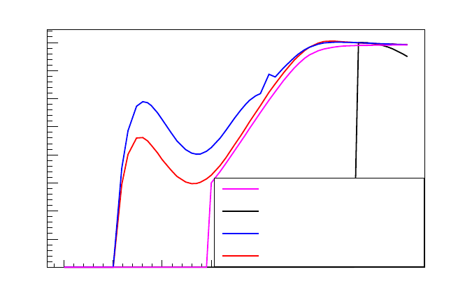
(E/MeV)
10
log
-3 -2 -1 0 1 2 3 4
[mb]
tot
σ
0
0.1
0.2
0.3
0.4
0.5
0.6
0.7
0.8
Parametrized Model
Relativistic Model
Bremsstrahlung Model
SB Model
Figure 8.1: Total cross section comparison between models for Z= 29:
Parametrized Bremsstrahlung Model, Relativistic Model, Bremsstrahlung
Model (Geant4 9.4) and Seltzer-Berger Model. The discontinuities in the
Parametized Model and the Relativistic Model at 1 Mev and 1 GeV, respec-
tively, mark the validity range of these models.
method guarantees consistent description independent of the energy cutoff.
The current version uses an interpolation in tables for 52 available electron
energy points versus 31 photon energy points, and for atomic number Z
ranging from 1 to 99. It is the default bremsstrahlung model in Geant4 since
version 9.5. Figure 8.1 shows a comparison of the total bremsstrahlung cross
sections with the previous implementation, and with the relativistic model.
After the successful sampling of ǫ, the polar angles of the radiated photon are
generated with respect to the parent electron’s momentum. It is difficult to
find simple formulae for this angle in the literature. For example the double
132

differential cross section reported by Tsai [12, 13] is
dσ
dkdΩ=2α2e2
πkm4 2ǫ−2
(1 + u2)2+12u2(1 −ǫ)
(1 + u2)4Z(Z+ 1)
+2−2ǫ−ǫ2
(1 + u2)2−4u2(1 −ǫ)
(1 + u2)4X−2Z2fc((αZ)2)
u=Eθ
m
X=Zm2(1+u2)2
tmin Gel
Z(t) + Gin
Z(t)t−tmin
t2dt
Gel,in
Z(t) atomic form factors
tmin =km2(1 + u2)
2E(E−k)2
=ǫm2(1 + u2)
2E(1 −ǫ)2
.
The sampling of this distribution is complicated. It is also only an approxi-
mation to within a few percent, due at least to the presence of the atomic form
factors. The angular dependence is contained in the variable u=Eθm−1.
For a given value of uthe dependence of the shape of the function on Z,E
and ǫ=k/E is very weak. Thus, the distribution can be approximated by a
function
f(u) = Cue−au +due−3au(8.19)
where
C=9a2
9 + da= 0.625 d= 27
where Eis in GeV. While this approximation is good at high energies, it be-
comes less accurate around a few MeV. However in that region the ionization
losses dominate over the radiative losses.
The sampling of the function f(u) can be done with three random numbers
ri, uniformly distributed on the interval [0,1]:
1. choose between ue−au and due−3au:
b=aif r1<9/(9 + d)
3aif r1≥9/(9 + d)
2. sample ue−bu:
u=−log(r2r3)
b
133

P=Z∞
umax
f(u)du
E (MeV) P(%)
0.511 3.4
0.6 2.2
0.8 1.2
1.0 0.7
2.0 <0.1
Table 8.1: Angular sampling efficiency
3. check that:
u≤umax =Eπ
m
otherwise go back to 1.
The probability of failing the last test is reported in table 8.1.
The function f(u) can also be used to describe the angular distribution of
the photon in µbremsstrahlung and to describe the angular distribution in
photon pair production.
The azimuthal angle φis generated isotropically. Along with θ, this infor-
mation is used to calculate the momentum vectors of the radiated photon
and parent recoiled electron, and to transform them to the global coordinate
system. The momentum transfer to the atomic nucleus is neglected.
8.2.2 Bremsstrahlung of high-energy electrons
Above an electron energy of 1 GeV an analytic differential cross section
representation is used [17], which was modified to account for the density
effect and the Landau-Pomeranchuk-Migdal (LPM) effect [18, 19].
Relativistic Bremsstrahlung cross section
The basis of the implementation is the well known high energy limit of the
Bremsstrahlung process [17],
dσ
dk =4αr2
e
3k{y2+ 2[1 + (1 −y)2]}[Z2(Fel −f) + ZFinel]
+ (1 −y)Z2+Z
3(8.20)
134

The elastic from factor Fel and inelastic form factor Finel, describe the scat-
tering on the nucleus and on the shell electrons, respectively, and for Z > 4
are given by [14]
Fel = log184.15
Z1
3and Finel = log1194.
Z2
3.
This corresponds to the complete screening approximation. The Coulomb
correction is defined as [14]
f=α2Z2∞
X
n=1
1
n(n2+α2Z2)
This approach provides an analytic differential cross section for an efficient
evaluation in a Monte Carlo computer code. Note that in this approximation
the differential cross section dσ/dk is independent of the energy of the initial
electron and is also valid for positrons.
The total integrated cross section Rdσ/dk dk is divergent, but the energy
loss integral Rkdσ/dk dk is finite. This allows the usual separation into
continuous enery loss, and discrete photon production according to Eqs. (7.3)
and (7.2).
Landau Pomeranchuk Migdal (LPM) effect
At higher energies matter effects become more and more important. In
GEANT4 the two leading matter effects, the LPM effect and the dielec-
tric suppresion (or Ter-Mikaelian effect), are considered. The analytic cross
section representation, eq. (8.20), provides the basis for the incorporation of
these matter effects.
The LPM effect (see for example [3, 4, 20] ) is the suppression of photon
production due to the multiple scattering of the electron. If an electron un-
dergoes multiple scattering while traversing the so called “formation zone”,
the bremsstrahlung amplitudes from before and after the scattering can inter-
fere, reducing the probability of bremsstrahlung photon emission (a similar
suppression occurs for pair production). The suppression becomes significant
for photon energies below a certain value, given by
k
E<E
ELP M
,(8.21)
where
kphoton energy
Eelectron energy
ELP M characteristic energy for LPM effect (depend on the medium).
135

The value of the LPM characteristic energy can be written as
ELP M =αm2X0
4hc ,(8.22)
where αfine structure constant
melectron mass
X0radiation length in the material
hPlanck constant
cvelocity of light in vacuum.
At high energies (approximately above 1 GeV) the differential cross section
including the Landau-Pomeranchuk-Migdal effect, can be expressed using an
evaluation based on [8, 19, 18]
dσ
dk =4αr2
e
3kξ(s){y2G(s) + 2[1 + (1 −y)2]φ(s)}
×[Z2(Fel −f) + ZFinel] + (1 −y)Z2+Z
3(8.23)
where LPM suppression functions are defined by [8]
G(s) = 24s2π
2−Z∞
0
e−st sin(st)
sinh( t
2)dt(8.24)
and
φ(s) = 12s2 −π
2+Z∞
0
e−st sin(st) sinht
2dt!(8.25)
They can be piecewise approximated with simple analytic functions, see e.g.
[19]. The suppression function ξ(s) is recursively defined via
s=sk ELPM
8E(E−k)ξ(s)
but can be well approximated using an algorithm introduced by [19]. The
material dependent characteristic energy ELPM is defined in Eq. (8.22) ac-
cording to [4]. Note that this definition differs from other definition (e.g.
[18]) by a factor 1
2.
An additional multiplicative factor governs the dielectric suppression ef-
fect (Ter-Mikaelian effect) [21].
S(k) = k2
k2+k2
p
136

The characteristic photon energy scale kpis given by the plasma frequency
of the media, defined as
kp=~ωp
Ee
mec2=~Ee
mec2·snee2
ǫ0me
.
Both suppression effects, dielectric suppresion and LPM effect, reduce the
effective formation length of the photon, so the suppressions do not simply
multiply.
A consistent treatment of the overlap region, where both suppression
mechanism, was suggested by [22]. The algorithm garanties that the LPM
suppression is turned off as the density effect becomes important. This is
achieved by defining a modified suppression variable ˆsvia
ˆs=s·1 + k2
p
k2
and using ˆsin the LPM suppression functions G(s) and φ(s) instead of sin
Eq. (8.23).
Bibliography
[1] S.T.Perkins, D.E.Cullen, S.M.Seltzer, UCRL-50400 Vol.31
[2] GEANT3 manual ,CERN Program Library Long Writeup W5013 (Oc-
tober 1994).
[3] V.M. Galitsky and I.I. Gurevich, Nuovo Cimento 32 (1964) 1820.
[4] P.L. Anthony et al., Phys. Rev. D 56 (1997) 1373, SLAC-PUB-
7413/LBNL-40054 (February 1997).
[5] S.M.Seltzer and M.J.Berger, Nucl. Inst. Meth. B12 (1985) 95.
[6] W.R. Nelson et al.:The EGS4 Code System. SLAC-Report-265 , Decem-
ber 1985
[7] H.Messel and D.F.Crawford. Pergamon Press,Oxford,1970.
[8] A.B. Migdal, Phys. Rev. 103 (1956) 1811.
[9] L. Kim et al., Phys. Rev. A33 (1986) 3002.
137
[10] R.W. Williams, Fundamental Formulas of Physics, vol.2., Dover Pubs.
(1960).
[11] J.C. Butcher and H. Messel., Nucl. Phys. 20 (1960) 15.
[12] Y-S. Tsai, Rev. Mod. Phys 46 (1974) 815.
[13] Y-S. Tsai, Rev. Mod. Phys 49 (1977) 421.
[14] C. Amsler et al., Phys. Lett. B67 (2008) 1.
[15] S.M. Seltzer and M.J. Berger, Atomic Data and Nuclear Data 35 (1986)
345.
[16] R.H. Pratt et al, Atomic Data and Nuclear Data Tables 20 (1977) 175.
[17] M.L. Perl, in Procede Les Rencontres de physique de la Valle D’Aoste,
SLAC-PUB-6514.
[18] S. Klein, Rev. Mod. Phys. 71 (1999) 1501-1538.
[19] T. Stanev et.al., Phys. Rev. D25 (1982) 1291.
[20] H.D. Hansen et al., Phys. Rev. D 69 (2004) 032001.
[21] M.L. Ter-Mikaelian, Dokl. Akad. Nauk SSSR 94 (1954) 1033.
[22] M.L. Ter-Mikaelian, High-energy Electromagnetic Processes in Con-
densed Media, Wiley, (1972).
138

8.3 Positron - Electron Annihilation
8.3.1 Introduction
The process G4eplusAnnihilation simulates the in-flight annihilation of a
positron with an atomic electron. As is usually done in shower programs [1],
it is assumed here that the atomic electron is initially free and at rest. Also,
annihilation processes producing one, or three or more, photons are ignored
because these processes are negligible compared to the annihilation into two
photons [1, 2].
8.3.2 Cross Section
The annihilation in flight of a positron and electron is described by the cross
section formula of Heitler [3, 1]:
σ(Z, E) = Zπr2
e
γ+ 1 "γ2+ 4γ+ 1
γ2−1ln γ+pγ2−1−γ+ 3
pγ2−1#(8.26)
where
E= total energy of the incident positron
γ=E/mc2
re= classical electron radius
8.3.3 Sampling the final state
The final state of the e+e−annihilation process
e+e−→γaγb
is simulated by first determining the kinematic limits of the photon energy
and then sampling the photon energy within those limits using the differential
cross section. Conservation of energy-momentum is then used to determine
the directions of the final state photons.
If the incident e+has a kinetic energy T, then the total energy is Ee=
T+mc2and the momentum is P c =pT(T+ 2mc2). The total available
energy is Etot =Ee+mc2=Ea+Eband momentum conservation requires
~
P=~
Pγa+~
Pγb. The fraction of the total energy transferred to one photon
(say γa) is
ǫ=Ea
Etot ≡Ea
T+ 2mc2.(8.27)
139

The energy transfered to γais largest when γais emitted in the direction of
the incident e+. In that case Eamax = (Etot +P c)/2 . The energy transfered
to γais smallest when γais emitted in the opposite direction of the incident
e+. Then Eamin = (Etot −P c)/2 . Hence,
ǫmax =Eamax
Etot
=1
21 + rγ−1
γ+ 1(8.28)
ǫmin =Eamin
Etot
=1
21−rγ−1
γ+ 1(8.29)
where γ= (T+mc2)/mc2. Therefore the range of ǫis [ǫmin ;ǫmax]
(≡[ǫmin ; 1 −ǫmin]).
8.3.4 Sampling the Gamma Energy
A short overview of the sampling method is given in Chapter 2. The differ-
ential cross section of the two-photon positron-electron annihilation can be
written as [3, 1]:
dσ(Z, ǫ)
dǫ =Zπr2
e
γ−1
1
ǫ1 + 2γ
(γ+ 1)2−ǫ−1
(γ+ 1)2
1
ǫ(8.30)
where Zis the atomic number of the material, rethe classical electron radius,
and ǫ∈[ǫmin ;ǫmax] . The differential cross section can be decomposed as
dσ(Z, ǫ)
dǫ =Zπr2
e
γ−1αf(ǫ)g(ǫ) (8.31)
where
α= ln(ǫmax/ǫmin)
f(ǫ) = 1
αǫ (8.32)
g(ǫ) = 1 + 2γ
(γ+ 1)2−ǫ−1
(γ+ 1)2
1
ǫ≡1−ǫ+2γǫ −1
ǫ(γ+ 1)2(8.33)
Given two random numbers r, r′∈[0,1], the photon energies are chosen as
follows:
1. sample ǫfrom f(ǫ) : ǫ=ǫmin ǫmax
ǫmin r
2. test the rejection function: if g(ǫ)≥r′accept ǫ, otherwise return to
step 1.
Then the photon energies are Ea=ǫEtot Eb= (1 −ǫ)Etot.
140

Computing the Final State Kinematics
If θis the angle between the incident e+and γa, then from energy-momentum
conservation,
cos θ=1
P c T+mc22ǫ−1
ǫ=ǫ(γ+ 1) −1
ǫpγ2−1.(8.34)
The azimuthal angle, φ, is generated isotropically and the photon momentum
vectors, ~
Pγaand ~
Pγb, are computed from energy-momentum conservation and
transformed into the lab coordinate system.
Annihilation at Rest
The method AtRestDoIt treats the special case when a positron comes to
rest before annihilating. It generates two photons, each with energy k=mc2
and an isotropic angular distribution.
Bibliography
[1] R. Ford and W. Nelson. SLAC-265, UC-32 (1985)
[2] H. Messel and D. Crawford. Electron-Photon shower distribution, Perg-
amon Press (1970)
[3] W. Heitler. The Quantum Theory of Radiation, Clarendon Press, Oxford
(1954)
141

8.4 Positron Annihilation into µ+µ−Pair in
Media
The class G4AnnihiToMuPair simulates the electromagnetic production of
muon pairs by the annihilation of high-energy positrons with atomic electrons
[1]. Details of the implementation are given below and can also be found in
Ref.[2].
8.4.1 Total Cross Section
The annihilation of positrons and target electrons producing muon pairs in
the final state (e+e−→µ+µ−) may give an appreciable contribution to the
total number of muons produced in high-energy electromagnetic cascades.
The threshold positron energy in the laboratory system for this process with
the target electron at rest is
Eth = 2m2
µ/me−me≈43.69 GeV ,(8.35)
where mµand meare the muon and electron masses, respectively. The total
cross section for the process on the electron is
σ=π r2
µ
3ξ1 + ξ
2p1−ξ , (8.36)
where rµ=reme/mµis the classical muon radius, ξ=Eth/E, and Eis the
total positron energy in the laboratory frame. In Eq. 8.36, approximations
are made that utilize the inequality m2
e≪m2
µ.
The cross section as a function of the positron energy Eis shown in Fig.8.2.
It has a maximum at E= 1.396 Eth and the value at the maximum is σmax =
0.5426 r2
µ= 1.008 µb.
8.4.2 Sampling of Energies and Angles
It is convenient to simulate the muon kinematic parameters in the center-of-
mass (c.m.) system, and then to convert into the laboratory frame.
The energies of all particles are the same in the c.m. frame and equal to
Ecm =r1
2me(E+me).(8.37)
The muon momenta in the c.m. frame are Pcm =pE2
cm −m2
µ. In what
follows, let the cosine of the angle between the c.m. momenta of the µ+and
e+be denoted as x= cos θcm .
142
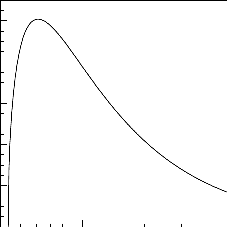
0
0.2
0.4
0.6
0.8
1
50 60 70 80 100 200 300 400 500
E in GeV
σ
in
µ
b
Figure 8.2: Total cross section for the process e+e−→µ+µ−as a function of
the positron energy Ein the laboratory system.
143
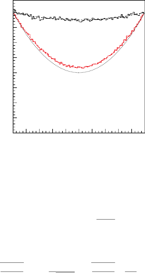
From the differential cross section it is easy to derive that, apart from
normalization, the distribution in xis described by
f(x)dx = (1 + ξ+x2(1 −ξ)) dx , −1≤x≤1.(8.38)
The value of this function is contained in the interval (1 + ξ)≤f(x)≤2 and
the generation of xis straightforward using the rejection technique. Fig. 8.3
shows both generated and analytic distributions.
0
0.25
0.5
0.75
1
1.25
1.5
1.75
2
-1 -0.8 -0.6 -0.4 -0.2 0 0.2 0.4 0.6 0.8 1
E= 500 GeV, ξ = .0874
E = 50 GeV, ξ =.874
1 + cos θcm
2
cos θcm
Entries per bin
Figure 8.3: Generated histograms with 106entries each and the expected
cos θcm distributions (dashed lines) at E= 50 and 500 GeV positron energy
in the lab frame. The asymptotic 1 + cos θ2
cm distribution valid for E→ ∞
is shown as dotted line.
The transverse momenta of the µ+and µ−particles are the same, both
in the c.m. and the lab frame, and their absolute values are equal to
P⊥=Pcm sin θcm =Pcm √1−x2.(8.39)
The energies and longitudinal components of the muon momenta in the lab
system may be obtained by means of a Lorentz transformation. The velocity
and Lorentz factor of the center-of-mass in the lab frame may be written as
β=rE−me
E+me
, γ ≡1
p1−β2=rE+me
2me
=Ecm
me
.(8.40)
144

The laboratory energies and longitudinal components of the momenta of the
positive and negative muons may then be obtained:
E+=γ(Ecm +x β Pcm), P+k=γ(βEcm +x Pcm),(8.41)
E−=γ(Ecm −x β Pcm), P−k=γ(βEcm −x Pcm).(8.42)
Finally, for the vectors of the muon momenta one obtains:
P+= (+P⊥cos ϕ, +P⊥sin ϕ, P+k),(8.43)
P−= (−P⊥cos ϕ, −P⊥sin ϕ, P−k),(8.44)
where ϕis a random azimuthal angle chosen between 0 and 2 π. The z-axis
is directed along the momentum of the initial positron in the lab frame.
The maximum and minimum energies of the muons are given by
Emax ≈1
2E1 + p1−ξ,(8.45)
Emin ≈1
2E1−p1−ξ=Eth
21 + p1−ξ.(8.46)
The fly-out polar angles of the muons are approximately
θ+≈P⊥/P+k, θ−≈P⊥/P−k; (8.47)
the maximal angle θmax ≈me
mµp1−ξis always small compared to 1.
Validity
The process described is assumed to be purely electromagnetic. It is based
on virtual γexchange, and the Z-boson exchange and γ−Zinterference
processes are neglected. The Z-pole corresponds to a positron energy of
E=M2
Z/2me= 8136 TeV. The validity of the current implementation is
therefore restricted to initial positron energies of less than about 1000 TeV.
Bibliography
[1] A.G. Bogdanov et al., Geant4 simulation of production and interaction
of muons, IEEE Trans. Nucl. Sci. 53 (2006) 513.
[2] H. Burkhardt, S. Kelner, and R. Kokoulin, “Production of muon pairs
in annihilation of high-energy positrons with resting electrons,” CERN-
AB-2003-002 (ABP) and CLIC Note 554, January 2003.
145
8.5 Positron Annihilation into Hadrons in Me-
dia
8.5.1 Introduction
The process G4eeToHadrons simulates the in-flight annihilation of a positron
with an atomic electron into hadrons [1]. It is assumed here that the atomic
electron is initially free and at rest. Currently accurate cross section is avail-
able with a validity range up to 1 TeV.
8.5.2 Cross Section
The annihilation of positrons and target electrons producing pion pairs in the
final state (e+e−→π+π−) may give an appreciable contribution to electron-
jet conversion at the LHC, and for the increasing total number of muons
produced in the beam pipe of the linear collider [1]. The threshold positron
energy in the laboratory system for this process with the target electron at
rest is
Eth = 2m2
π/me−me≈70.35 GeV ,(8.48)
where mπand meare the pion and electron masses, respectively. The total
cross section is dominated by the reaction
e+e−→ργ →π+π−γ, (8.49)
where γis a radiative photon and ρ(770) is a well known vector meson. This
radiative correction is essential, because it significantly modifies the shape of
the resonance. Details of the theory are described in [2], in which the main
term and the leading α2corrections are taken into account.
Additional contribution to the hadron production cross section come from
ω(783) and φ(1020) resonanses with π+π−π0,K+K−,KLKS,ηγ, and π0γ
final states.
8.5.3 Sampling the final state
The final state of the e+e−annihilation process is simulated by first sampling
of radiative gamma using a sum of all hadronic cross sections in the center of
mass system. Photon energy is used to define new differential cross section.
After that, hadronic channel is randomly selected according to it partial
cross section. Final state is sampled and final particles transformed to the
laboratory system.
146
Bibliography
[1] A.G. Bogdanov et al., Geant4 simulation of production and interaction
of muons, IEEE Trans. Nucl. Sci. 53 (2006) 513.
[2] M. Benayoun et al., Mod. Phys. Lett. A14, 2605 (1999).
147
Chapter 9
Low Energy Livermore
148
9.1 Introduction
Additional electromagnetic physics processes for photons, electrons, hadrons
and ions have been implemented in Geant4 in order to extend the validity
range of particle interactions to lower energies than those available in the
standard Geant4 electromagnetic processes [1] Because atomic shell structure
is more important in most cases at low energies than it is at higher energies,
the low energy processes make direct use of shell cross section data. The
standard processes, which are optimized for high energy physics applications,
rely on parameterizations of these data.
The low energy processes include the photo-electric effect, Compton scat-
tering, Rayleigh scattering, gamma conversion, bremsstrahlung and ioniza-
tion. Fluorescence and Auger electron emission of excited atoms is also
considered.
Some features common to all low energy processes currently implemented
in Geant4 are summarized in this section. Subsequent sections provide more
detailed information for each process.
9.1.1 Physics
The low energy processes of Geant4 represent electromagnetic interactions
at lower energies than those covered by the equivalent Geant4 standard elec-
tromagnetic processes.
The current implementation of low energy processes is valid for energies
down to 10eV and can be used up to approximately 100GeV for gamma
processes. For electron processes upper limit is significantly below. It covers
elements with atomic number between 1 and 99.
All processes involve two distinct phases:
•the calculation and use of total cross sections, and
•the generation of the final state.
Both phases are based on the theoretical models and on exploitation of eval-
uated data.
9.1.2 Data Sources
The data used for the determination of cross-sections and for sampling of
the final state are extracted from a set of publicly distributed evaluated data
libraries:
•EPDL97 (Evaluated Photons Data Library) [2];
149
•EEDL (Evaluated Electrons Data Library) [3];
•EADL (Evaluated Atomic Data Library) [4];
•binding energy values based on data of Scofield [5].
Evaluated data sets are produced through the process of critical compar-
ison, selection, renormalization and averaging of the available experimental
data, normally complemented by model calculations. These libraries provide
the following data relevant for the simulation of Geant4 low energy processes:
•total cross-sections for photoelectric effect, Compton scattering, Rayleigh
scattering, pair production and bremsstrahlung;
•subshell integrated cross sections for photo-electric effect and ioniza-
tion;
•energy spectra of the secondaries for electron processes;
•scattering functions for the Compton effect;
•binding energies for electrons for all subshells;
•transition probabilities between subshells for fluorescence and the Auger
effect.
The energy range covered by the data libraries extends from 100 GeV
down to 1 eV for Rayleigh and Compton effects, down to the lowest binding
energy for each element for photo-electric effect and ionization, and down to
10 eV for bremsstrahlung.
9.1.3 Distribution of the Data Sets
The author of EPDL97 [2], who is also responsible for the EEDL [3] and
EADL [4] data libraries, Dr. Red Cullen, has kindly permitted the libraries
and their related documentation to be distributed with the Geant4 toolkit.
The data are reformatted for Geant4 input. They can be downloaded from
the source code section of the Geant4 page: http://cern.ch/geant4/geant4.html.
The EADL, EEDL and EPDL97 data-sets are also available from sev-
eral public distribution centres in a format different from the one used by
Geant4 [6].
150

9.1.4 Calculation of Total Cross Sections
The energy dependence of the total cross section is derived for each process
from the evaluated data libraries. For ionisation, bremsstrahlung and Comp-
ton scattering the total cross is obtained by interpolation according to the
formula [7]:
log(σ(E)) = log(σ1)log(E2/E) + log(σ2)log(E/E1)
log(E2/E1)(9.1)
where Eis actial energy, E1and E2are respectively the closest lower and
higher energy points for which data (σ1and σ2) are available. For other
processes interpolation method is chosen depending on cross section shape.
Bibliography
[1] “Geant4 Low Energy Electromagnetic Models for Electrons and Pho-
tons”, J.Apostolakis et al., CERN-OPEN-99-034(1999), INFN/AE-
99/18(1999)
[2] “EPDL97: the Evaluated Photon Data Library, ’97 version”, D.Cullen,
J.H.Hubbell, L.Kissel, UCRL–50400, Vol.6, Rev.5
[3] “Tables and Graphs of Electron-Interaction Cross-Sections from 10 eV
to 100 GeV Derived from the LLNL Evaluated Electron Data Library
(EEDL), Z=1-100” S.T.Perkins, D.E.Cullen, S.M.Seltzer, UCRL-50400
Vol.31
[4] “Tables and Graphs of Atomic Subshell and Relaxation Data De-
rived from the LLNL Evaluated Atomic Data Library (EADL), Z=1-
100” S.T.Perkins, D.E.Cullen, M.H.Chen, J.H.Hubbell, J.Rathkopf,
J.Scofield, UCRL-50400 Vol.30
[5] J.H. Scofield, “Radiative Transitions”, in “Atomic Inner-Shell Pro-
cesses”, B.Crasemann ed. (Academic Press, New York, 1975),pp.265-
292.
[6] http://www.nea.fr/html/dbdata/nds evaluated.htm
[7] “New Photon, Positron and Electron Interaction Data for Geant in En-
ergy Range from 1 eV to 10 TeV”, J. Stepanek, Draft to be submitted
for publication
151

9.2 Compton Scattering
9.2.1 Total Cross Section
The total cross section for the Compton scattering process is determined
from the data as described in section 9.1.4. To avoid sampling problems in
the Compton process the cross section is set to zero at low-energy limit of
cross section table, which is 100eV in majority of EM Phyiscs Lists.
9.2.2 Sampling of the Final State
For low energy incident photons, the simulation of the Compton scattering
process is performed according to the same procedure used for the “standard”
Compton scattering simulation, with the addition that Hubbel’s atomic form
factor [1] or scattering function, SF , is taken into account. The angular and
energy distribution of the incoherently scattered photon is then given by
the product of the Klein-Nishina formula Φ(ǫ) and the scattering function,
SF (q) [2]
P(ǫ, q) = Φ(ǫ)×SF (q).(9.2)
ǫis the ratio of the scattered photon energy E′, and the incident photon
energy E. The momentum transfer is given by q=E×sin2(θ/2), where θis
the polar angle of the scattered photon with respect to the direction of the
parent photon. Φ(ǫ) is given by
Φ(ǫ)∼
=[1
ǫ+ǫ][1 −ǫ
1 + ǫ2sin2θ].(9.3)
The effect of the scattering function becomes significant at low energies,
especially in suppressing forward scattering [2].
The sampling method of the final state is based on composition and re-
jection Monte Carlo methods [3, 4, 5], with the SF function included in the
rejection function
g(ǫ) = 1−ǫ
1 + ǫ2sin2θ×SF (q),(9.4)
with 0 < g(ǫ)< Z. Values of the scattering functions at each momentum
transfer, q, are obtained by interpolating the evaluated data for the corre-
sponding atomic number, Z.
The polar angle θis deduced from the sampled ǫvalue. In the azimuthal
direction, the angular distributions of both the scattered photon and the
recoil electron are considered to be isotropic [6].
152
Since the incoherent scattering occurs mainly on the outermost electronic
subshells, the binding energies can be neglected, as stated in reference [6].
The momentum vector of the scattered photon, −→
P′
γ, is transformed into the
World coordinate system. The kinetic energy and momentum of the recoil
electron are then
Tel =E−E′
−→
Pel =−→
Pγ−−→
P′
γ.
Bibliography
[1] “Summary of Existing Information on the Incoherent Scattering of Pho-
tons particularly on the Validity of the Use of the Incoherent Scattering
Function”, Radiat. Phys. Chem. Vol. 50, No 1, pp 113-124 (1997)
[2] “A simple model of photon transport”, D.E. Cullen, Nucl. Instr. Meth.
in Phys. Res. B 101(1995)499-510
[3] J.C. Butcher and H. Messel. Nucl. Phys. 20 15 (1960)
[4] H. Messel and D. Crawford. Electron-Photon shower distribution, Perg-
amon Press (1970)
[5] R. Ford and W. Nelson. SLAC-265, UC-32 (1985)
[6] “New Photon, Positron and Electron Interaction Data for Geant in En-
ergy Range from 1 eV to 10 TeV”, J. Stepanek, Draft to be submitted
for publication
153

9.3 Compton Scattering by Linearly Polar-
ized Gamma Rays
9.3.1 The Cross Section
The quantum mechanical Klein - Nishina differential cross section for polar-
ized photons is [1]:
dσ
dΩ=1
2r2
0
hν2
hν2
ohνo
hν +hν
hνo−sin2Θ
where Θ is the angle between the two polarization vectors. In terms of the
polar and azimuthal angles (θ, φ) this cross section can be written as
dσ
dΩ=1
2r2
0
hν2
hν2
ohνo
hν +hν
hνo−2cos2φsin2θ
.
9.3.2 Angular Distribution
The integration of this cross section over the azimuthal angle produces the
standard cross section. The angular and energy distribution are then ob-
tained in the same way as for the standard process. Using these values for
the polar angle and the energy, the azimuthal angle is sampled from the
following distribution[2]:
P(φ) = 1 −2a
bcos2φ
where a=sin2θand b=ǫ+ 1/ǫ.ǫis the ratio between the scattered photon
energy and the incident photon energy.
9.3.3 Polarization Vector
The components of the vector polarization of the scattered photon are cal-
culated from ( [2]):
~
ǫ′
⊥=1
Nˆ
jcosθ −ˆ
ksinθsinφsinβ
~
ǫ′
k=Nˆ
i−1
Nˆ
jsin2θsinφcosφ −1
Nˆ
ksinθcosθcosφcosβ
where
N=p1−sin2θcos2φ.
154
cosβ is calculated from cosΘ = Ncosβ, while cosΘ is sampled from the Klein
- Nishina distribution.
The binding effects and the Compton profile are neglected. The kinetic
energy and momentum of the recoil electron are then
Tel =E−E′
~
Pel =~
Pγ−~
P′
γ.
The momentum vector of the scattered photon ~
Pγand its polarization
vector are transformed into the World coordinate system. The polarization
and the direction of the scattered gamma in the final state are calculated in
the reference frame in which the incoming photon is along the z-axis and has
its polarization vector along the x-axis. The transformation to the World
coordinate system performs a linear combination of the initial direction, the
initial poalrization and the cross product between them, using the projections
of the calculated quantities along these axes.
9.3.4 Unpolarized Photons
A special treatment is devoted to unpolarized photons. In this case a random
polarization in the plane perpendicular to the incident photon is selected.
Bibliography
[1] W. Heitler The Quantum Theory of Radiation, Oxford Clarendom Press
(1954)
[2] G.O.Depaola New Monte Carlo method for Compton and Rayleigh scat-
tering by polarized gamma rays, Nuclear Instruments and Methods A
512, (2003) 619
155
9.4 Rayleigh Scattering
9.4.1 Total Cross Section
The total cross section for the Rayleigh scattering process is determined from
the data as described in section 9.1.4.
9.4.2 Sampling of the Final State
The coherent scattered photon angle θis sampled according to the distribu-
tion obtained from the product of the Rayleigh formula (1 + cos2θ) sin θand
the square of Hubbel’s form factor F F 2(q) [1] [2]
Φ(E, θ) = [1 + cos2θ] sin θ×F F 2(q),(9.5)
where q= 2Esin(θ/2) is the momentum transfer.
Form factors introduce a dependency on the initial energy Eof the photon
that is not taken into account in the Rayleigh formula. At low energies,
form factors are isotropic and do not affect angular distribution, while at
high energies they are forward peaked. For effective sampling of final state a
method proposed by D.E. Cullen [2] has been implemented: form factor data
were fitted and fitted parameters included in the G4LivermoreRayleighModel.
The sampling procedure is following:
1. atom is selected randomly according to cross section;
2. cosθ is sampled as proposed in [2];
3. azimuthal angle is sampled uniformly.
Bibliography
[1] ”Relativistic Atom Form Factors and Photon Coherent Scattering Cross
Sections”, J.H. Hubbell et al., J.Phys.Chem.Ref.Data, 8(1979) 69.
[2] ”A simple model of photon transport”, D.E. Cullen, Nucl. Instr. Meth.
in Phys. Res. B101 (1995) 499-510.
156

9.5 Gamma Conversion
9.5.1 Total cross-section
The total cross-section of the Gamma Conversion process is determined from
the data as described in section 9.1.4.
9.5.2 Sampling of the final state
For low energy incident photons, the simulation of the Gamma Conversion
final state is performed according to [1].
The secondary e±energies are sampled using the Bethe-Heitler cross-
sections with Coulomb correction.
The Bethe-Heitler differential cross-section with the Coulomb correction
for a photon of energy Eto produce a pair with one of the particles having
energy ǫE (ǫis the fraction of the photon energy carried by one particle of
the pair) is given by [2]:
dσ(Z, E, ǫ)
dǫ =r2
0αZ(Z+ξ(Z))
E2(ǫ2+ (1 −ǫ)2)Φ1(δ)−F(Z)
2+
+2
3ǫ(1 −ǫ)Φ2(δ)−F(Z)
2
where Φi(δ) are the screening functions depending on the screening vari-
able δ[1].
The value of ǫis sampled using composition and rejection Monte Carlo
methods [1, 3, 4].
After the successful sampling of ǫ, the process generates the polar angles of
the electron with respect to an axis defined along the direction of the parent
photon. The electron and the positron are assumed to have a symmetric
angular distribution. The energy-angle distribution is given by[5]:
dσ
dpdΩ=2α2e2
πkm4" 2x(1 −x)
(1 + l)
2
−12lx(1 −x)
(1 + l)4!(Z2+Z)+
+2x2−2x+ 1
(1 + l)2+4lx(1 −x)
(1 + l)4(X−2Z2f((αZ)2))
where kis the photon energy, pthe momentum and Ethe energy of the
electron of the e±pair x=E/k and l=E2θ2/m2. The sampling of this
cross-section is obtained according to [1].
157
The azimuthal angle φis generated isotropically.
This information together with the momentum conservation is used to
calculate the momentum vectors of both decay products and to transform
them to the GEANT coordinate system. The choice of which particle in the
pair is the electron/positron is made randomly.
Bibliography
[1] Urban L., in Brun R. et al. (1993), Geant. Detector Description and
Simulation Tool, CERN Program Library, section Phys/211
[2] R. Ford and W. Nelson., SLAC-210, UC-32 (1978)
[3] J.C. Butcher and H. Messel. Nucl. Phys. 20 15 (1960)
[4] H. Messel and D. Crawford. Electron-Photon shower distribution, Perg-
amon Press (1970)
[5] Y. S. Tsai, Rev. Mod. Phys. 46 815 (1974), Y. S. Tsai, Rev. Mod. Phys.
49 421 (1977)
158
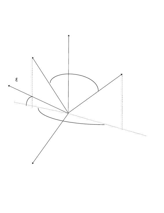
9.6 Pair production by Linearly Polarized Gamma
Rays
A method to study the pair production interaction of linearly polarized
gamma rays at energies >50 MeV was discussed in [1]. The study of the
differential cross section for pair production shows that the polarization in-
formation is coded in the azimuthal distribution of the electron - positron
pair created by polarized photons (Fig.9.1).
z
y
x
k
p-
p+
Ψ
φ
θ-
θ+
Figure 9.1: Angles occurring in the pair creation
9.6.1 Relativistic cross section for linearly polarized
gamma ray
The cross section for pair production by linearly polarized gamma rays in
the high energy limit using natural units with h/2π=c= 1 is
159

dσ =−2αZ2r0m2
(2π)2ω3dEdΩ+dΩ−
E(ω−E)
|~q|4(4Esin θ−cos Ψ
1−cos θ−
+ (ω−E)sin θ+cos (Ψ + φ)
1−cos θ+2
−|~q|2sin θ−cos Ψ
1−cos θ−−sin θ+cos (Ψ + φ)
1−cos θ+2
−ω2sin θ−sin θ+
(1 −cos θ−)(1 −cos θ+)Esin θ+
(ωE) sin θ−
+(ω−E) sin θ−
Esin θ+
+ 2 cos φ ,(9.6)
with
|~q|2=−2 [E(ω−E)(1 −sin θ+sin θ−cos φ−cos θ+cos θ−)
+ωE(cos θ+−1) + ω(ω−E)(cosθ−−1) + m2.(9.7)
Eis the positron energy and we have assumed that the polarization di-
rection is along the xaxis (see Fig.9.1).
9.6.2 Spatial azimuthal distribution
Integrating this cross section over energy and polar angles yields the spa-
tial azimuthal distribution, that was calculated in [1] using a Monte Carlo
procedure.
Fig. 9.2 shows an example of this distribution for 100 MeV gamma - ray.
In this figure the range of the φaxis is restricted between 3.0 and πsince it
gives the most interesting part of the distribution. For angles smaller than
3.0 this distribution monotonically decreases to zero.
In Geant4 the azimuthal distribution surface is parametrized in terms of
smooth functions of (φ, ψ) .
f(φ, ψ) = fπ/2(φ) sin2ψ+f0(φ) cos2ψ . (9.8)
Since both f0(φ) and fπ/2(φ) are functions that rapidly vary when φ
approaches π, it was necessary to adjust the functions in two ranges of φ:
(I) 0 ≤φ≤3.05 rad. (II) 3.06 rad ≤φ≤π, whereas in the small range
3.05 ≤φ≤3.06 we extrapolate the two fitting functions until the intersection
point is reached.
In region II we used Lorentzian functions of the form
f(φ) = y0+2Aω
π[ω2+ 4(φ−xc)2],(9.9)
160
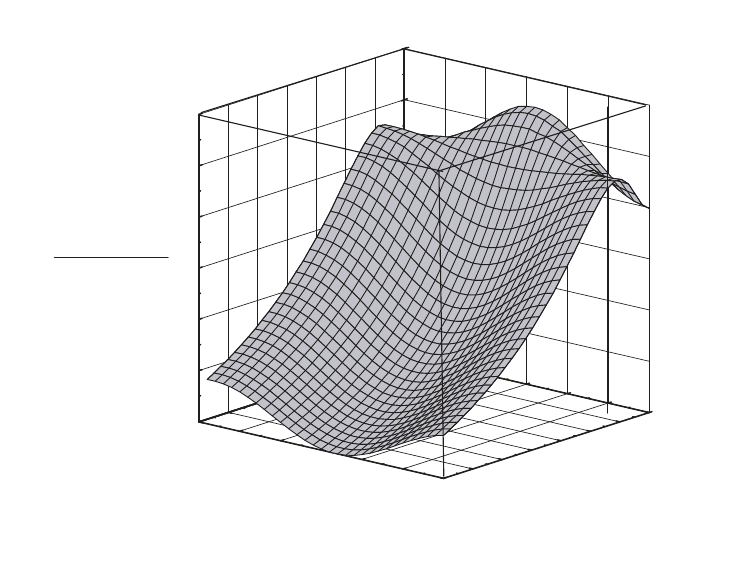
0.00
0.52
1.05
1.57
2.09
2.62
3.14
3.00
3.02
3.04
3.06
3.08
3.10
3.12
3.14
4
6
8
10
12
14
16
1 d
σ
α
(Zr
0
)
2
d
φ
d
ψ
φ
[rad]
ψ
[rad]
Figure 9.2: Spatial azimuthal distribution of a pair created by 100 MeV
photon
whereas for region I the best fitting function was found to adopt the form:
f(φ) = a+dtan (bφ +c).(9.10)
The paper [1] reports the coefficients obtained in different energy regions
to fit the angular distribution and their function form as function of gamma-
ray as energy reported in the tables9.1 and 9.2 below.
9.6.3 Unpolarized Photons
A special treatment is devoted to unpolarized photons. In this case a random
polarization in the plane perpendicular to the incident photon is selected.
Bibliography
[1] G.O.Depaola, C.N.Kozameh and M.H.Tiglio A method to determine the
polarization of high energy gamma rays, Astroparticle Physics 10 (1999)
175
161

Table 9.1: Fit for the parameter of f0(φ) function.
Parameter Function a b c
y0aln E−b2.98 ±0.06 7.7±0.4 -
A a ln E−b1.41 ±0.08 5.6±0.5 -
ω a +b/E +c/E30.015 ±0.001 9.5±0.6 (−2.2±0.1)104
xca+b/E +c/E33.143 ±0.001 −2.7±0.2 (2 ±1)103
Table 9.2: Fit for the parameter of fπ/2(φ) function.
Parameter Function a b c
y0aln E−b1.85 ±0.07 5.1±0.4 -
A a ln E−b1.3±0.1 (6.6±0.2)10−3-
ω a +b/E +c/E30.008 ±0.002 12.1±0.9 (−2.8±0.8)104
xc3.149 - - -
162

9.7 Triple Gamma Conversion
The class G4BoldyshevTripletModel was developed to simulate the pair pro-
duction by linearly polarized gamma rays on electrons For the angular distri-
bution of electron recoil we used the cross section by Vinokurov and Kuraev
[1] using the Borsellino diagrams in the high energy For energy distribution
for the pair, we used Boldyshev [2] formula that differs only in the normaliza-
tion from Wheeler-Lamb. The cross sections include a cut off for momentum
detections[3].
9.7.1 Method
The first step is sample the probability to have an electron recoil with mo-
mentum greater than a threshold define by the user (by default, this value is
p0= 1 in units of mc). This probability is
σ(p≥p0) = αr2
082
27 −14
9lnX0+4
15X0−0.0348X2
0+ 0.008X3
0−...
(9.11)
X0= 2 qp2
0+−1.(9.12)
Since that total cross section is σ=αr2
028
4ln2Eγ−218
27 , if a random number
is ξ≥σ(p≥p0)/σ we create the electron recoil, otherwise we deposited the
energy in the local point.
9.7.2 Azimuthal Distribution for Electron Recoil
The expression for the differential cross section is composed of two terms
which express the azimuthal dependence as follows:
dσ =dσ(t)−P dσ(l)cos(2ϕ) (9.13)
Where, both dσ(t)and dσ(l), are independent of the azimuthal angle, ϕ,
referred to an origin chosen in the direction of the polarization vector ~
Pof
the incoming photons.
9.7.3 Monte Carlo Simulation of the Asymptotic Ex-
pression
In this section we present an algorithm for Monte Carlo simulation of the
asymptotic expressions calculate by Vinokurov et.al. [1].
163

We must generate random values of θand ϕdistributed with probability
proportional to the following function f(θ, ϕ), for θrestricted inside of its
allowed interval value [2] (0, or θmax(p0)):
f(θ, ϕ) = sin θ
cos3θ(F1(θ)−P cos (2ϕ)FP(θ)) (9.14)
F1(θ) = 1 −1−5 cos2θ
cos θln (cot (θ/2)) (9.15)
FP(θ) = 1 −sin2θ
cos θln (cot (θ/2)) (9.16)
As we will see, for θ < π/2, F1is several times greater than FP, and since
both are positive, it follows that fis positive for any possible value of P
(0 ≤P≤1).
Since F1is the dominant term in expression , it is more convenient to
begin developing the algorithm of this term, belonging to the unpolarized
radiation.
9.7.4 Algorithm for Non Polarized Radiation
The algorithm was described in Ref.[4]. We must generate random values of
θbetween 0 and θmax =arccos E1−mc2
p0+mc2E1+mc2
Eγp0,E1=pp2
0+ (mc2)2
distributed with probability proportional to the following function f1(θ):
f1(θ) = sin(θ)
cos3(θ)1−1−5 cos2(θ)
cos(θ)ln(cot(θ/2))
=sin(θ)
cos3(θ)×F1(θ)(9.17)
By substitution cos(θ/2) = q1+cosθ
2and sin(θ/2) = q1−cosθ
2, We can
write:
ln (cot (θ/2)) = 1
2ln 1 + cos θ
1−cos θ(9.18)
In order to simulate the f1function, it may be decomposed in two factors:
the first, sin(θ)/cos3(θ), easy to integrate, and the other, F1(θ), which may
constitute a reject function, on despite of its θ= 0 divergence. This is
possible because they have very low probability. On other hand, θvalues
near to zero are not useful to measure polarization because for those angles
it is very difficult to determine the azimuthal distribution (due to multiple
scattering).
164

Then, it is possible to choose some value of θ0, small enough that it is not
important that the sample is fitted rigorously for θ < θ0, and at the same
time F1(θ0) is not too big.
Modifying F1so that it is constant for θ≤θ0, we may obtain an adequate
reject function. Doing this, we introduce only a very few missed points, all
of which lie totally outside of the interesting region.
Expanding F1for great values of θ, we see it is proportional to cos2θ:
F1(θ)→14
3cos2θ1 + 33
35 cos2θ+...,if θ→π/2
Thus, it is evident that F1divided by cos2(θ) will be a better reject function,
because it tends softly to a some constant value (14/3 = 4,6666...) for large
θs, whereas its behavior is not affected in the region of small θs, where
cos(θ)→1.
It seems adequate to choose θ0near 50, and, after some manipulation
looking for round numbers we obtain:
F1(4.470)
cos2(4.470)∼
=14.00
Finally we define a reject function:
r(θ) = 1
14
F1(θ)
cos2(θ)=1
14 cos2(θ)
1−1−5 cos2(θ)
2 cos(θ)ln 1+cos θ
1−cos θ; for θ≥4.470
r(θ) = 1 ; forθ≤4.470
(9.19)
Now we have a probability distribution function (PDF) for θ,p(θ) = Cf1(θ),
expressed as a product of another PDF, π(θ), by the reject function:
p(θ) = Cf1(θ)∼
=C′π(θ)r(θ) (9.20)
where Cis the normalization constant belonging to the function p(θ).
One must note that the equality between C∼f1(θ) and C′π(θ)r(θ) is
not exact for small values of θ, where we have truncated the infinity of F1(θ);
but this can not affect appreciably the distribution because f1→0 there.
Now the PDF π(θ) is:
π(θ) = Cπ
14sin(θ)
cos(θ)(9.21)
From the normalization, the constant Cπresults:
165

Cπ=1
14 Rθmax
0
sin(θ)
cos(θ)dθ =−1
14 ln (cos(θmax)) =1
7ln ω
4m(9.22)
And the relation with Cis given by:
C=1
Rθmax
0f1(θ)dθ ∼
=C′Cπ(9.23)
Then we obtain the cumulative probability by integrating the PDF π(θ):
Pπ=Zθ
0
π(θ′)dθ′=−14 ln(cos(θ))
7 ln ω
4m=2 ln(cos(θ))
ln (4m/ω)(9.24)
Finally for the Monte Carlo method we sample a random number ξ1(between
0 and 1), which is defined as equal to Pπ, and obtain the corresponding θ
value:
ξ1=2 ln(cos θ)
ln (4m/ω)=ln(cos θ)
ln (cos(θmax))
Then,
θ= arccos 4m
ωξ1
2!(9.25)
Another random number ξ2is sampled for the reject process: the θvalue is
accepted if ξ2≤r(θ), and reject in the contrary.
For θ≤4,470all values are accepted. It happens automatically without
any modification in the algorithm previously defined (it is not necessary to
define the truncated reject function for θ < θ0).
9.7.5 Algorithm for Polarized Radiation
The algorithm was also described in Ref.[4]. As we have seen, the azimuthal
dependence of the differential cross section is given by the expressions and :
f(θ, ϕ) = sin θ
cos3θ(F1(θ)−P cos (2ϕ)FP(θ)) (9.26)
FP(θ) = 1 −sin2θ
cos θln (cot (θ/2)) (9.27)
166
We see that FPtends to 1 at θ= 0, decreases monotonically to 0 as θgoes
to π/2.
Furthermore, the expansion of FPfor θnear π/2 shows that it is propor-
tional to cos2(θ), in virtue of which FP/cos2(θ) tends to a non null value,
2/3. This value is exactly 7 times the value of F1/cos2(θ).
This suggests applying the combination method, rearranging the whole
function as follows:
f(θ, ϕ) = tan(θ)F1(θ)
cos2(θ)1−cos(2ϕ)PFP(θ)
F1(θ)(9.28)
and the normalized PDF p(θ, ϕ):
p(θ, ϕ) = Cf(θ, ϕ) (9.29)
where is Cthe normalization constant
1
C=Zθmax
0Z2π
0
f(θ, ϕ)dϕdθ (9.30)
Taking account that R2π
0cos(2ϕ)dϕ = 0, then:
1
C= 2πZθmax
0
tan(θ)F1(θ)
cos2(θ)dθ (9.31)
On the other hand the integration over the azimuthal angle is straightforward
and gives:
q(θ) = Z2π
0
p(θ, ϕ)dϕ = 2πC tan(θ)F1(θ)
cos2(θ)(9.32)
and p(ϕ/θ) is the conditional probability of ϕgiven θ:
p(ϕ/θ) = p(θ,ϕ)
q(θ)=1
2πC tan(θ)F1(θ)
cos2(θ)
Csin(θ)
cos3(θ)F1(θ)1−cos(2ϕ)PFP(θ)
F1(θ)
=1
2π1−cos(2ϕ)PFP(θ)
F1(θ)(9.33)
Now the procedure consists of sampling θaccording the PDF q(θ); then, for
each value of θwe must sample ϕaccording to the conditional PDF p(ϕ/θ).
Knowing that F1is several times greater than FP, we can see that P
F1/FP<< 1, and thus p(ϕ/θ) maintains a nearly constant value slightly
diminished in some regions of ϕ. Consequently the ϕsample can be done
directly by the rejecting method with high efficiency.
On the other hand, q(θ) is the same function p(θ) given by , that is the
PDF for unpolarized radiation, q(θ)∼
=C′π(θ)r(θ), so we can sample θwith
167

exactly the same procedure, specified as follows:
1.- We begin sampling a random number ξ1and obtain θfrom :
θ= arccos 4m
ωξ1
2!
2.- Then we sample a second random number ξ2 and accept the values
of θif ξ2≤r(θ), where r(θ) is the same expression defined before:
r (θ) = 1
14 cos2θ1−1−5cos2θ
2 cos θln 1 + cos θ
1−cos θ
For θ≥4,470and for θ≤4,470all values are accepted.
3.- Now we sample ϕ. According to the reject method, we sample a
third random number ξ3(which is defined as ϕ/2π) and evaluate the reject
function (which is essentially):
rθ(ξ3) = 1
2π1−cos (4πξ3)PFP(θ)
F1(θ)(9.34)
=1
2π 1−cos(4πξ3)Pcos θ−sin2θln cot θ
2
cosθ −(1 −5cos2θ) ln cot θ
2!(9.35)
4.- Finally, with a fourth random number ξ4, we accept the values of
ϕ= 2πξ4if ξ4≤rθ(ξ3).
9.7.6 Sampling of Energy
For the electron recoil we calculate the energy from the maximum momentum
that can take according with the θangle
Er=mc2(S+ (mc2)2)
D2(9.36)
Where S=mc2(2Egamma +mc2)
D2 = 4Smc2+ (S−(mc2)2)2sin2(θ)
The remnant energy is distributed to the pair according to the Boldyshev
formula [2](xis the fraction of the positron energy):
2πd2σ
dxdφ = 2αr2
0{[1 −2x(1 −x)] J1(p0) + 2x(1 −x) [1 −Pcos(φ)] J2(p0)}
(9.37)
168

J1(p0) = 2 tcosh(t)
sinh(t)−ln(2 sinh(t))
J2(p0) = −2
3ln(2 sinh(t))+tcosh(t)
sinh(t)+sinh(t)−tcosh3(t)
3 sinh3(t),sinh(2t) = p0
This distribution can by write like a PDF for x:
P(x) = N(1 −Jx(1 −x)) (9.38)
where Nis a normalization constant and J= (J1−J2)/J1.
Solving for x(ξis a random number):
x=c1/3
1
2J+J−4
2c1/3
1
+1
2(9.39)
c1= (−6 + 12rn+J+ 2a)J2
a=16−3J−36rn+36Jr2
n+6rnJ2
J
rn=ξ1−J
6
Bibliography
[1] E.A. Vinokurov and E.A. Kuraev, Zh. Eksp. Teor. Fiz. 63 (1972) 1142,
in Russian; Sov. Phys. JETP 36, 602 (1973).
[2] V.F. Boldyshev, E.A. Vinokurov, N.P. Merenkov, Yu.P. Peresunko,
Phys. Part. Nucl. 25 (1994) 292.
[3] M.L. Iparraguirre, G.O. Depaola, The European Physical Journal C 71
(2011) 1778.
[4] G.O. Depaola, M.L. Iparraguirre, Nucl. Instr. Meth. A611 (2009) 84.
169

9.8 Photoelectric effect
Three model classes are available G4LivermorePhotoElectricModel
G4LivermorePolarizedPhotoElectricModel, and G4LivermorePolarizedPhotelectricGDModel.
9.8.1 Cross sections
The total photoelectric and single shell cross-sections are tabulated from
threshold to 600keV . Above 600keV EPDL97 cross sections [1] are parame-
terized as following:
σ(E) = a1
E+a2
E2+a3
E3+a4
E4+a5
E5.(9.40)
The accuracy of such parameterisation is better than 1%. To avoid tracking
problems for very low-energy gamma the photoelectric cross section is not
zero below first ionisation potential but stay constant, so all types of media
are not transparant for gamma.
9.8.2 Sampling of the final state
The incident photon is absorbed and an electron is emitted.
The electron kinetic energy is the difference between the incident photon
energy and the binding energy of the electron before the interaction. The
sub-shell, from which the electron is emitted, is randomly selected according
to the relative cross-sections of all subshells, determined at the given energy.
The interaction leaves the atom in an excited state. The deexcitation of the
atom is simulated as described in section 14.1.
9.8.3 Angular distribution of the emitted photoelec-
tron
For sampling of the direction of the emitted photoelectron by default the an-
gular generator G4SauterGavrilaAngularDistribution is used. The algorithm
is described in 5.2.
For polarized models alternative angular generators are applied.
G4LivermorePolarizedPhotoElectricModel uses the
G4PhotoElectricAngularGeneratorPolarized angular generator.
This model models the double differential cross section (for angles θand
φ) and thus it is capable of account for polarization of the incident photon.
The developed generator was based in the research of Sauter in 1931[2]. The
Sauter’s formula was recalculated by Gavrila in 1959 for the K-shell [3] and
170

in 1961 for the L-shells [4]. These new double differential formulas have some
limitations, αZ<<1 and have a range between 0.1< β <0.99 c.
The double differential photoeffect for K–shell can be written as [3]:
dσ
dω (θ, φ) = 4
m2α6Z5β3(1 −β2)3
[1 −(1 −β2)1/2]F1−παZ
β+παZG(9.41)
where
F=sin2θcos2φ
(1 −βcos θ)4−1−(1 −β2)1/2
2(1 −β2)
sin2θcos2φ
(1 −βcos θ)3
+1−(1 −β2)1/22
4(1 −β2)3/2
sin2θ
(1 −βcos θ)3
G=[1 −(1 −β2)1/2]1/2
27/2β2(1 −βcos θ)5/24β2
(1 −β2)1/2
sin2θcos2φ
1−βcos θ+4β
1−β2cos θcos2φ−
−41−(1 −β2)1/2
1−β2(1 −cos2φ)−β21−(1 −β2)1/2
1−β2
sin2θ
1−βcos θ−
+ 4β21−(1 −β2)1/2
(1 −β2)3/2−4β1−(1 −β2)1/22
(1 −β2)3/2#
+1−(1 −β2)1/2
4β2(1 −βcos θ)2β
1−β2−2
1−β2cos θcos2φ+1−(1 −β2)1/2
(1 −β2)3/2cos θ
−β1−(1 −β2)1/2
(1 −β2)3/2
where βis the electron velocity, αis the fine–structure constant, Zis the
atomic number of the material and θ,φare the emission angles with respect
to the electron initial direction.
The double differential photoeffect distribution for L1–shell is the same
as for K–shell despising a constant [4]:
B=ξ1
8(9.42)
where ξis equal to 1 when working with unscreened Coulomb wave functions
as it is done in this development.
Since the polarized Gavrila cross–section is a 2–dimensional non–factorized
distribution an acceptance–rejection technique was the adopted [5]. For the
Gravrila distribution, two functions were defined g1(φ) and g2(θ):
g1(φ) = a(9.43)
g2(θ) = θ
1 + cθ2(9.44)
171

such that:
Ag1(φ)g2(θ)≥d2σ
dφdθ (9.45)
where A is a global constant. The method used to calculate the distribution
is the same as the one used in Low Energy 2BN Bremsstrahlung Generator,
being the difference g1(φ) = a.
G4LivermorePolarizedPhotoElectricGDModel uses its own methods to pro-
duce the angular distribution of the photoelectron. The method to sample
the azimuthal angle φis described in [6].
Bibliography
[1] “EPDL97: the Evaluated Photon Data Library, ’97 version”, D.Cullen,
J.H.Hubbell, L.Kissel, UCRL–50400, Vol.6, Rev.5
[2] “K–Shell Photoelectric Cross Sections from 200 keV to 2 MeV”, R H
Pratt, R D Levee, R L Pexton and W Aron, Phys. Rev. 134 (1964) 4A
[3] “Relativistic K–Shell Photoeffect”, M. Gavrila, Phys. Rev. 113 (1959) 2
[4] “Relativistic L–Shell Photoeffect”, M. Gavrila, Phys. Rev. 124 (1961) 4
[5] “Monte Carlo Generation of 2BNBremsstrahlung Distribution”, L. Per-
alta, P. Rodrigues, A. Trindade CERN EXT–2004–039 (July, 2003)
[6] “Measuring polarization in the X-ray range: New simulation method for
gaseous detectors”, G.O. Depaola and F. Longo, NIMA 566 (2006) 590
172

9.9 Electron ionisation
The class G4LivermoreIonisationModel calculates the continuous energy loss
due to electron ionisation and simulates δ-ray production by electrons. The
delta-electron production threshold for a given material, Tc, is used to sep-
arate the continuous and the discrete parts of the process. The energy loss
of an electron with the incident energy, T, is expressed via the sum over all
atomic shells, s, and the integral over the energy, t, of delta-electrons:
dE
dx =X
s σs(T)RTc
0.1eV tdσ
dt dt
RTmax
0.1eV
dσ
dt dt !,(9.46)
where Tmax = 0.5Tis the maximum energy transfered to a δ-electron, σs(T)
is the total cross-section for the shell, s, at a given incident kinetic energy,
T, and 0.1eV is the low energy limit of the EEDL data. The δ-electron
production cross-section is a complimentary function:
σ(T) = X
s σs(T)RTmax
Tc
dσ
dt dt
RTmax
0.1eV
dσ
dt dt!.(9.47)
The partial sub-shell cross-sections, σs, are obtained from an interpolation
of the evaluated cross-section data in the EEDL library [1], according to the
formula (9.1) in Section 9.1.4.
The probability of emission of a δ-electron with kinetic energy, t, from
a sub-shell, s, of binding energy, Bs, as the result of the interaction of an
incoming electron with kinetic energy, T, is described by:
dσ
dt =P(x)
x2,withx=t+Bs
T+Bs
,(9.48)
where the parameter xis varied from xmin = (0.1eV +Bs)/(T+Bs) to 0.5.
The function, P(x), is parametrised differently in 3 regions of x: from xmin
to x1the linear interpolation with linear scale of 4 points is used; from x1to
x2the linear interpolation with logarithmic scale of 16 points is used; from
x2to 0.5 the following interpolation is applied:
P(x) = 1 −gx + (1 −g)x2+x2
1−x(1
1−x−g) + A∗(0.5−x)/x, (9.49)
where Ais a fit coefficient, gis expressed via the gamma factor of the in-
coming electron:
g= (2γ−1)/γ2.(9.50)
173
For the high energy case (x >> 1) the formula (9.49) is transformed to the
M¨oller electron-electron scattering formula [2, 3].
The value of the coefficient, A, for each element is obtained as a result
of the fit on the spectrum from the EEDL data for those energies which
are available in the database. The values of x1and x2are chosen for each
atomic shell according to the spectrum of δ-electrons in this shell. Note that
x1corresponds to the maximum of the spectrum, if the maximum does not
coincide with xmin. The dependence of all 24 parameters on the incident
energy, T, is evaluated from a logarithmic interpolation (9.1).
The sampling of the final state proceeds in three steps. First a shell is
randomly selected, then the energy of the delta-electron is sampled, finally
the angle of emission of the scattered electron and of the δ-ray is determined
by energy-momentum conservation taken into account electron motion on
the atomic orbit.
The interaction leaves the atom in an excited state. The deexcitation of
the atom is simulated as described in section 14.1. Sampling of the excitations
is carried out for both the continuous and the discrete parts of the process.
Bibliography
[1] “Tables and Graphs of Electron-Interaction Cross-Sections from 10 eV
to 100 GeV Derived from the LLNL Evaluated Electron Data Library
(EEDL), Z=1-100” S.T.Perkins, D.E.Cullen, S.M.Seltzer, UCRL-50400
Vol.31
[2] Geant3 manual ,CERN Program Library Long Writeup W5013 (Octo-
ber 1994).
[3] H.Messel and D.F.Crawford. Pergamon Press,Oxford,1970.
174

9.10 Bremsstrahlung
The class G4LivermoreBremsstrahlungModel calculates the continuous en-
ergy loss due to low energy gamma emission and simulates the gamma pro-
duction by electrons. The gamma production threshold for a given material
ωcis used to separate the continuous and the discrete parts of the process.
The energy loss of an electron with the incident energy Tare expressed via
the integrand over energy of the gammas:
dE
dx =σ(T)Rωc
0.1eV tdσ
dω dω
RT
0.1eV
dσ
dω dω ,(9.51)
where σ(T) is the total cross-section at a given incident kinetic energy, T,
0.1eV is the low energy limit of the EEDL data. The production cross-section
is a complimentary function:
σ=σ(T)RT
ωc
dσ
dω dω
RT
0.1eV
dσ
dω dω .(9.52)
The total cross-section, σs, is obtained from an interpolation of the eval-
uated cross-section data in the EEDL library [1], according to the formula
(9.1) in Section 9.1.4.
The EEDL data [1] of total cross-sections are parametrised [2] according
to (9.1). The probability of the emission of a photon with energy, ω, consid-
ering an electron of incident kinetic energy, T, is generated according to the
formula:
dσ
dω =F(x)
x,withx=ω
T.(9.53)
The function, F(x), describing energy spectra of the outcoming photons
is taken from the EEDL library. For each element 15 points in xfrom 0.01
to 1 are used for the linear interpolation of this function. The function F
is normalised by the condition F(0.01) = 1. The energy distributions of the
emitted photons available in the EEDL library are for only a few incident
electron energies (about 10 energy points between 10 eV and 100 GeV). For
other energies a logarithmic interpolation formula (9.1) is used to obtain
values for the function, F(x). For high energies, the spectral function is very
close to:
F(x) = 1 −x+ 0.75x2.(9.54)
175

9.10.1 Bremsstrahlung angular distributions
The angular distribution of the emitted photons with respect to the inci-
dent electron can be sampled according to three alternative generators de-
scribed below. The direction of the outcoming electron is determined from
the energy-momentum balance. This generators are currently implemented
in G4ModifiedTsai, G4Generator2BS and G4Generator2BN classes.
G4ModifiedTsai
The angular distribution of the emitted photons is obtained from a simplified
[3] formula based on the Tsai cross-section [4], which is expected to become
isotropic in the low energy limit.
G4Generator2BS
In G4Generator2BS generator, the angular distribution of the emitted pho-
tons is obtained from the 2BS Koch and Motz bremsstrahlung double differ-
ential cross-section [5]:
dσk,θ=4Z2r2
0
137
dk
kydy 16y2E
(y2+ 1)4E0−
(E0+E)2
(y2+ 1)2E2
0
+E2
0+E2
(y2+ 1)2E2
0−4y2E
(y2+ 1)4E0lnM(y)
where kthe photon energy, θthe emission angle, E0and Eare the initial
and final electron energy in units of mec2,r0is the classical electron radius
and Zthe atomic number of the material. yand M(y) are defined as:
y=E0θ
1
M(y)=k
2E0E2
+Z1/3
111(y2+ 1)2
The adopted sampling algorithm is based on the sampling scheme devel-
oped by A. F. Bielajew et al. [6], and latter implemented in EGS4. In this
sampling algorithm only the angular part of 2BS is used, with the emitted
photon energy, k, determined by GEANT4 dσ
dk differential cross-section.
G4Generator2BN
The angular distribution of the emitted photons is obtained from the 2BN
Koch and Motz bremsstrahlung double differential cross-section [5] that can
be written as:
176

dσk,θ=Z2r2
0
8π137
dk
k
p
p0
dΩk8 sin2θ(2E2
0+ 1)
p2
0∆4
0−
2(5E2
0+ 2EE0+ 3)
p2
0∆2
0−2(p2
0−k2)
Q2∆0
+4E
p2
2∆0
+L
pp0
4E0sin2θ(3k−p2
0E)
p2
0∆4+4E2
0(E2
0+E2)
p2
0∆2
0
+
2−2(7E2
0−3EE0+E2)
p2
0∆2
0
+2k(E2
0+EE0−1)
p2
0∆0
−4ǫ
p∆0+ǫQ
pQ 4
∆2
0−6k
∆0−2k(p2
0−k2)
Q2∆0
in which:
L= ln EE0−1 + pp0
EE0−1−pp0
∆0=E0−p0cos θ
Q2=p2
0+k2−2p0kcos θ
ǫ= ln E+p
E−pǫQ= ln Q+p
Q−p
where kis the photon energy, θthe emission angle and (E0, p0) and (E, p) are
the total (energy, momentum) of the electron before and after the radiative
emission, all in units of mec2.
Since the 2BN cross–section is a 2-dimensional non-factorized distribution an
acceptance-rejection technique was the adopted. For the 2BN distribution,
two functions g1(k) and g2(θ) were defined:
g1(k) = k−bg2(θ) = θ
1 + cθ2(9.55)
such that:
Ag1(k)g2(θ)≥dσ
dkdθ (9.56)
where A is a global constant to be completed. Both functions have an analyt-
ical integral Gand an analytical inverse G−1. The bparameter of g1(k) was
empirically tuned and set to 1.2. For positive θvalues, g2(θ) has a maximum
at 1
√(c).cparameter controls the function global shape and it was used to
tune g2(θ) according to the electron kinetic energy.
177

To generate photon energy kaccording to g1and θaccording to g2the inverse-
transform method was used. The integration of these functions gives
G1=C1Zkmax
kmin
k′−bdk′=C1
k1−b−k1−b
min
1−b(9.57)
G2=C2Zθ
0
θ′
1 + cθ′2dθ′=C2
log(1 + cθ2)
2c(9.58)
where C1and C2are two global constants chosen to normalize the integral
in the overall range to the unit. The photon momentum kwill range from
a minimum cut value kmin (required to avoid infrared divergence) to a max-
imum value equal to the electron kinetic energy Ek, while the polar angle
ranges from 0 to π, resulting for C1and C2:
C1=1−b
E1−b
k
C2=2c
log(1 + cπ2)(9.59)
kand θare then sampled according to:
k=1−b
C1
ξ1+k1−b
minθ=v
u
u
texp 2cξ2
C1
2c(9.60)
where ξ1and ξ2are uniformly sampled in the interval (0,1). The event is
accepted if:
uAg1(k)g2(θ)≤dσ
dkdθ (9.61)
where uis a random number with uniform distribution in (0,1). The Aand
cparameters were computed in a logarithmic grid, ranging from 1 keV to 1.5
MeV with 100 points per decade. Since the g2(θ) function has a maximum
at θ=1
√c, the cparameter was computed using the relation c=1
θmax . At the
point (kmin, θmax) where kmin is the kcut value, the double differential cross-
section has its maximum value, since it is monotonically decreasing in kand
thus the global normalization parameter Ais estimated from the relation:
Ag1(kmin)g2(θmax) = d2σ
dkdθ max
(9.62)
where g1(kmin)g2(θmax) = k−b
min
2√c. Since Aand ccan only be retrieved for
a fixed number of electron kinetic energies there exists the possibility that
Ag1(kmin)g2(θmax)≤d2σ
dkdθ max for a given Ek. This is a small violation that
178
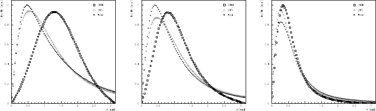
can be corrected introducing an additional multiplicative factor to the Apa-
rameter, which was empirically determined to be 1.04 for the entire energy
range.
Comparisons between Tsai, 2BS and 2BN generators
The currently available generators can be used according to the user required
precision and timing requirements. Regarding the energy range, validation
results indicate that for lower energies (≤100 keV) there is a significant
deviation on the most probable emission angle between Tsai/2BS generators
and the 2BN generator - Figure 9.3. The 2BN generator maintains however
a good agreement with Kissel data [7], derived from the work of Tseng and
co-workers [8], and it should be used for energies between 1 keV and 100 keV
[9]. As the electron kinetic energy increases, the different distributions tend
to overlap and all generators present a good agreement with Kissel data.
Figure 9.3: Comparison of polar angle distribution of bremsstrahlung pho-
tons (k/T = 0.5) for 10 keV (left) and 100 keV (middle) and 500 keV (right)
electrons in silver, obtained with Tsai, 2BS and 2BN generator
In figure 9.4 the sampling efficiency for the different generators are presented.
The sampling generation efficiency was defined as the ratio between the num-
ber of generated events and the total number of trials. As energies increases
the sampling efficiency of the 2BN algorithm decreases from 0.65 at 1 keV
electron kinetic energy down to almost 0.35 at 1 MeV. For energies up to
10 keV the 2BN sampling efficiency is superior or equivalent to the one of
the 2BS generator. These results are an indication that precision simula-
tion of low energy bremsstrahlung can be obtained with little performance
degradation. For energies above 500 keV, Tsai generator can be used, retain-
179
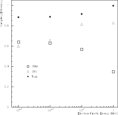
ing a good physics accuracy and a sampling efficiency superior to the 2BS
generator.
Figure 9.4: Sampling efficiency for Tsai generator, 2BS and 2BN Koch and
Motz generators.
Bibliography
[1] “Geant4 Low Energy Electromagnetic Models for Electrons and Pho-
tons”, J.Apostolakis et al., CERN-OPEN-99-034(1999), INFN/AE-
99/18(1999)
[2] “Tables and Graphs of Electron-Interaction Cross-Sections from 10 eV
to 100 GeV Derived from the LLNL Evaluated Electron Data Library
(EEDL), Z=1-100” S.T.Perkins, D.E.Cullen, S.M.Seltzer, UCRL-50400
Vol.31
[3] “GEANT, Detector Description and Simulation Tool”, CERN Applica-
tion Software Group, CERN Program Library Long Writeup W5013
[4] “Pair production and bremsstrahlung of charged leptons”, Y. Tsai, Rev.
Mod. Phys., Vol.46, 815(1974), Vol.49, 421(1977)
180
[5] “Bremsstrahlung Cross-Section Formulas and Related Data”, H. W.
Koch and J. W. Motz, Rev. Mod. Phys., Vol.31, 920(1959)
[6] “Improved bremsstrahlung photon angular sampling in the EGS4
code system”, A. F. Bielajew, R. Mohan and C.-S. Chui, Report
NRCC/PIRS-0203 (1989)
[7] “Bremsstrahlung from electron collisions with neutral atoms”, L. Kissel,
C. A. Quarls and R. H. Pratt, At. Data Nucl. Data Tables, Vol. 28,
382(1983)
[8] “Electron bremsstrahlung angular distributions in the 1-500 keV energy
range”, H. K. Tseng, R. H. Pratt and C. M. Lee , Phys. Rev. A, Vol.
19, 187(1979)
[9] “GEANT4 Applications and Developments for Medical Physics Exper-
iments”, P. Rodrigues et al. IEEE 2003 NSS/MIC Conference Record
181
Chapter 10
Low Energy Penelope
182
10.1 Penelope physics
10.1.1 Introduction
A new set of physics processes for photons, electrons and positrons is im-
plemented in Geant4: it includes Compton scattering, photoelectric effect,
Rayleigh scattering, gamma conversion, bremsstrahlung, ionization (to be
released) and positron annihilation (to be released). These processes are the
Geant4 implementation of the physics models developed for the PENELOPE
code (PENetration and Energy LOss of Positrons and Electrons), version
2001, that are described in detail in Ref. [1]. The Penelope models have
been specifically developed for Monte Carlo simulation and great care was
given to the low energy description (i.e. atomic effects, etc.). Hence, these
implementations provide reliable results for energies down to a few hundred
eV and can be used up to ∼1 GeV [1, 2]. For this reason, they may be
used in Geant4 as an alternative to the Low Energy processes. For the same
physics processes, the user now has more alternative descriptions from which
to choose, including the cross section calculation and the final state sampling.
10.1.2 Compton scattering
Total cross section
The total cross section of the Compton scattering process is determined from
an analytical parameterization. For γenergy Egreater than 5 MeV, the usual
Klein-Nishina formula is used for σ(E). For E < 5 MeV a more accurate
parameterization is used, which takes into account atomic binding effects
and Doppler broadening [3]:
σ(E) = 2πZ1
−1
r2
e
2
E2
C
E2(EC
E+E
EC−sin2θ)·
X
shells
fiΘ(E−Ui)ni(pmax
z)d(cos θ) (10.1)
where:
re= classical radius of the electron;
me= mass of the electron;
θ= scattering angle;
EC= Compton energy
=E
1 + E
mec2(1 −cos θ)
183

fi= number of electrons in the i-th atomic shell;
Ui= ionisation energy of the i-th atomic shell;
Θ = Heaviside step function;
pmax
z= highest possible value of pz(projection of the initial momentum of
the electron in the direction of the scattering angle)
=E(E−Ui)(1 −cos θ)−mec2Ui
cp2E(E−Ui)(1 −cos θ) + U2
i
.
Finally,
ni(x) =
1
2e[1
2−(1
2−√2Ji0x)2]if x < 0
1−1
2e[1
2−(1
2+√2Ji0x)2]if x > 0
(10.2)
where Ji0is the value of the pz-distribution profile Ji(pz) for the i-th atomic
shell calculated in pz= 0. The values of Ji0for the different shells of the
different elements are tabulated from the Hartree-Fock atomic orbitals of
Ref. [4].
The integration of Eq.(10.1) is performed numerically using the 20-point
Gaussian method. For this reason, the initialization of the Penelope Compton
process is somewhat slower than the Low Energy process.
Sampling of the final state
The polar deflection cos θis sampled from the probability density function
P(cos θ) = r2
e
2
E2
C
E2EC
E+E
EC−sin2θX
shells
fiΘ(E−Ui)ni(pmax
z) (10.3)
(see Ref. [1] for details on the sampling algorithm). Once the direction of
the emerging photon has been set, the active electron shell iis selected with
relative probability equal to ZiΘ(E−Ui)ni[pmax
z(E, θ)]. A random value of
pzis generated from the analytical Compton profile [4]. The energy of the
emerging photon is
E′=Eτ
1−τt h(1 −τt cos θ) + pz
|pz|p(1 −τt cos θ)2−(1 −tτ2)(1 −t)i,
(10.4)
where
t=pz
mec2and τ=EC
E.(10.5)
The azimuthal scattering angle φof the photon is sampled uniformly in
the interval (0,2π). It is assumed that the Compton electron is emitted with
184

energy Ee=E−E′−Ui, with polar angle θeand azimuthal angle φe=φ+π,
relative to the direction of the incident photon. In this case cos θeis given by
cos θe=E−E′cos θ
√E2+E′2−2EE′cos θ.(10.6)
Since the active electron shell is known, characteristic x-rays and electrons
emitted in the de-excitation of the ionized atom can also be followed. The de-
excitation is simulated as described in section 14.1. For further details see [1].
10.1.3 Rayleigh scattering
Total cross section
The total cross section of the Rayleigh scattering process is determined from
an analytical parameterization. The atomic cross section for coherent scat-
tering is given approximately by [5]
σ(E) = πr2
eZ1
−1
1 + cos2θ
2[F(q, Z)]2dcos θ, (10.7)
where F(q, Z) is the atomic form factor, Zis the atomic number and qis the
magnitude of the momentum transfer, i.e.
q= 2 E
csin θ
2.(10.8)
In the numerical calculation the following analytical approximations are used
for the form factor:
F(q, Z) = f(x, Z) =
Z1+a1x2+a2x3+a3x4
(1+a4x2+a5x4)2or
max[f(x, Z), FK(x, Z)] if Z > 10 and f(x, Z)<2
(10.9)
where
FK(x, Z) = sin(2barctan Q)
bQ(1 + Q2)b,(10.10)
with
x= 20.6074 q
mec, Q =q
2meca, b =√1−a2, a =αZ−5
16,(10.11)
where αis the fine-structure constant. The function FK(x, Z) is the contri-
bution to the atomic form factor due to the two K-shell electrons (see [6]).
185

The parameters of expression f(x, Z) have been determined in Ref. [6] for
Z=1 to 92 by numerically fitting the atomic form factors tabulated in Ref.
[7]. The integration of Eq.(10.7) is performed numerically using the 20-point
Gaussian method. For this reason the initialization of the Penelope Rayleigh
process is somewhat slower than the Low Energy process.
Sampling of the final state
The angular deflection cos θof the scattered photon is sampled from the
probability distribution function
P(cos θ) = 1 + cos2θ
2[F(q, Z)]2.(10.12)
For details on the sampling algorithm (which is quite heavy from the com-
putational point of view) see Ref. [1]. The azimuthal scattering angle φof
the photon is sampled uniformly in the interval (0,2π).
10.1.4 Gamma conversion
Total cross section
The total cross section of the γconversion process is determined from the
data [8], as described in section 9.1.4.
Sampling of the final state
The energies E−and E+of the secondary electron and positron are sampled
using the Bethe-Heitler cross section with the Coulomb correction, using the
semiempirical model of Ref. [6]. If
ǫ=E−+mec2
E(10.13)
is the fraction of the γenergy Ewhich is taken away from the electron,
κ=E
mec2and a=αZ, (10.14)
the differential cross section, which includes a low-energy correction and a
high-energy radiative correction, is
dσ
dǫ =r2
ea(Z+η)Cr
2
3h21
2−ǫ2φ1(ǫ) + φ2(ǫ)i,(10.15)
186

where:
φ1(ǫ) = 7
3−2 ln(1 + b2)−6barctan(b−1)
−b2[4 −4barctan(b−1)−3 ln(1 + b−2)]
+4 ln(Rmec/~)−4fC(Z) + F0(κ, Z) (10.16)
and
φ2(ǫ) = 11
6−2 ln(1 + b2)−3barctan(b−1)
+1
2b2[4 −4barctan(b−1)−3 ln(1 + b−2)]
+4 ln(Rmec/~)−4fC(Z) + F0(κ, Z),(10.17)
with
b=Rmec
~
1
2κ
1
ǫ(1 −ǫ).(10.18)
In this case Ris the screening radius for the atom Z(tabulated in [10] for
Z=1 to 92) and ηis the contribution of pair production in the electron field
(rather than in the nuclear field). The parameter ηis approximated as
η=η∞(1 −e−v),(10.19)
where
v= (0.2840 −0.1909a) ln(4/κ) + (0.1095 + 0.2206a) ln2(4/κ)
+(0.02888 −0.04269a) ln3(4/κ)
+(0.002527 + 0.002623) ln4(4/κ) (10.20)
and η∞is the contribution for the atom Zin the high-energy limit and is
tabulated for Z=1 to 92 in Ref. [10]. In the Eq.(10.15), the function fC(Z)
is the high-energy Coulomb correction of Ref. [9], given by
fC(Z) = a2[(1 + a2)−1+ 0.202059 −0.03693a2+ 0.00835a4
−0.00201a6+ 0.00049a8−0.00012a10 + 0.00003a12]; (10.21)
Cr= 1.0093 is the high-energy limit of Mork and Olsen’s radiative correction
(see Ref. [10]); F0(κ, Z) is a Coulomb-like correction function, which has been
analytically approximated as [1]
F0(κ, Z) = (−0.1774 −12.10a+ 11.18a2)(2/κ)1/2
+(8.523 + 73.26a−44.41a2)(2/κ)
−(13.52 + 121.1a−96.41a2)(2/κ)3/2
+(8.946 + 62.05a−63.41a2)(2/κ)2.(10.22)
187

The kinetic energy E+of the secondary positron is obtained as
E+=E−E−−2mec2.(10.23)
The polar angles θ−and θ+of the directions of movement of the electron and
the positron, relative to the direction of the incident photon, are sampled
from the leading term of the expression obtained from high-energy theory
(see Ref. [11])
p(cos θ±) = a(1 −β±cos θ±)−2,(10.24)
where ais the a normalization constant and β±is the particle velocity in
units of the speed of light. As the directions of the produced particles and
of the incident photon are not necessarily coplanar, the azimuthal angles φ−
and φ+of the electron and of the positron are sampled independently and
uniformly in the interval (0,2π).
10.1.5 Photoelectric effect
Total cross section
The total photoelectric cross section at a given photon energy Eis calculated
from the data [12], as described in section 9.1.4.
Sampling of the final state
The incident photon is absorbed and one electron is emitted. The direction of
the electron is sampled according to the Sauter distribution [13]. Introducing
the variable ν= 1 −cos θe, the angular distribution can be expressed as
p(ν) = (2 −ν)h1
A+ν+1
2βγ(γ−1)(γ−2)iν
(A+ν)3,(10.25)
where
γ= 1 + Ee
mec2, A =1
β−1,(10.26)
Eeis the electron energy, meits rest mass and βits velocity in units of the
speed of light c. Though the Sauter distribution, strictly speaking, is ad-
equate only for ionisation of the K-shell by high-energy photons, in many
practical simulations it does not introduce appreciable errors in the descrip-
tion of any photoionisation event, irrespective of the atomic shell or of the
photon energy.
The subshell from which the electron is emitted is randomly selected accord-
ing to the relative cross sections of subshells, determined at the energy E
188

by interpolation of the data of Ref. [11]. The electron kinetic energy is the
difference between the incident photon energy and the binding energy of the
electron before the interaction in the sampled shell. The interaction leaves
the atom in an excited state; the subsequent de-excitation is simulated as
described in section 14.1.
10.1.6 Bremsstrahlung
Introduction
The class G4PenelopeBremsstrahlung calculates the continuous energy loss
due to soft γemission and simulates the photon production by electrons and
positrons. As usual, the gamma production threshold Tcfor a given material
is used to separate the continuous and the discrete parts of the process.
Electrons
The total cross sections are calculated from the data [15], as described in
sections 9.1.4 and 9.10.
The energy distribution dσ
dW (E), i.e. the probability of the emission of a
photon with energy Wgiven an incident electron of kinetic energy E, is
generated according to the formula
dσ
dW (E) = F(κ)
κ, κ =W
E.(10.27)
The functions F(κ) describing the energy spectra of the outgoing photons are
taken from Ref. [14]. For each element Zfrom 1 to 92, 32 points in κ, ranging
from 10−12 to 1, are used for the linear interpolation of this function. F(κ)
is normalized using the condition F(10−12) = 1. The energy distribution
of the emitted photons is available in the library [14] for 57 energies of the
incident electron between 1 keV and 100 GeV. For other primary energies,
logarithmic interpolation is used to obtain the values of the function F(κ).
The direction of the emitted bremsstrahlung photon is determined by the
polar angle θand the azimuthal angle φ. For isotropic media, with randomly
oriented atoms, the bremsstrahlung differential cross section is independent
of φand can be expressed as
d2σ
dW d cos θ=dσ
dW p(Z, E, κ; cos θ).(10.28)
Numerical values of the “shape function” p(Z, E, κ; cos θ), calculated by
partial-wave methods, have been published in Ref. [16] for the following
189

benchmark cases: Z= 2, 8, 13, 47, 79 and 92; E= 1, 5, 10, 50, 100 and 500
keV; κ= 0, 0.6, 0.8 and 0.95. It was found in Ref. [1] that the benchmark
partial-wave shape function of Ref. [16] can be closely approximated by the
analytical form (obtained in the Lorentz-dipole approximation)
p(cos θ) = A3
8h1 + cos θ−β′
1−β′cos θ2i1−β′2
(1 −β′cos θ)2
+(1 −A)3
4h1−cos θ−β′
1−β′cos θm2i1−β′2
(1 −β′cos θ)2,(10.29)
with β′=β(1 + B), if one considers Aand Bas adjustable parameters. The
parameters Aand Bhave been determined, by least squares fitting, for the
144 combinations of atomic numbers, electron energies and reduced photon
energies corresponding to the benchmark shape functions tabulated in [16].
The quantities ln(AZβ) and Bβ vary smoothly with Z, βand κand can
be obtained by cubic spline interpolation of their values for the benchmark
cases. This permits the fast evaluation of the shape function p(Z, E, κ; cos θ)
for any combination of Z,βand κ.
The stopping power dE
dx due to soft bremsstrahlung is calculated by interpo-
lating in Eand κthe numerical data of scaled cross sections of Ref. [17]. The
energy and the direction of the outgoing electron are determined by using
energy-momentum balance.
Positrons
The radiative differential cross section dσ+
dW (E) for positrons reduces to that
for electrons in the high-energy limit, but is smaller for intermediate and low
energies. Owing to the lack of more accurate calculations, the differential
cross section for positrons is obtained by multiplying the electron differential
cross section dσ−
dW (E) by a κ−indendent factor, i.e.
dσ+
dW =Fp(Z, E)dσ−
dW .(10.30)
The factor Fp(Z, E) is set equal to the ratio of the radiative stopping powers
for positrons and electrons, which has been calculated in Ref. [18]. For the
actual calculation, the following analytical approximation is used:
Fp(Z, E) = 1 −exp(−1.2359 ·10−1t+ 6.1274 ·10−2t2−3.1516 ·10−2t3
+7.7446 ·10−3t4−1.0595 ·10−3t5+ 7.0568 ·10−5t6
−1.8080 ·10−6t7),(10.31)
190

where
t= ln 1 + 106
Z2
E
mec2.(10.32)
Because the factor Fp(Z, E) is independent on κ, the energy distribution of
the secondary γ’s has the same shape as electron bremsstrahlung. Similarly,
owing to the lack of numerical data for positrons, it is assumed that the shape
of the angular distribution p(Z, E, κ; cos θ) of the bremsstrahlung photons for
positrons is the same as for the electrons.
The energy and direction of the outgoing positron are determined from
energy-momentum balance.
10.1.7 Ionisation
The G4PenelopeIonisation class calculates the continuous energy loss due
to electron and positron ionisation and simulates the δ-ray production by
electrons and positrons. The electron production threshold Tcfor a given
material is used to separate the continuous and the discrete parts of the
process.
The simulation of inelastic collisions of electrons and positrons is performed
on the basis of a Generalized Oscillation Strength (GOS) model (see Ref. [1]
for a complete description). It is assumed that GOS splits into contributions
from the different atomic electron shells.
Electrons
The total cross section σ−(E) for the inelastic collision of electrons of energy
Eis calculated analytically. It can be split into contributions from distant
longitudinal, distant transverse and close interactions,
σ−(E) = σdis,l +σdis,t +σ−
clo.(10.33)
The contributions from distant longitudinal and transverse interactions are
σdis,l =2πe4
mev2X
shells
fk
1
Wk
ln Wk
Qmin
k
Qmin
k+ 2mec2
Wk+ 2mec2Θ(E−Wk) (10.34)
and
σdis,t =2πe4
mev2X
shells
fk
1
Wkhln 1
1−β2−β2−δFiΘ(E−Wk) (10.35)
respectively, where:
me= mass of the electron;
191

v= velocity of the electron;
β= velocity of the electron in units of c;
fk= number of electrons in the k-th atomic shell;
Θ = Heaviside step function;
Wk= resonance energy of the k-th atomic shell oscillator;
Qmin
k= minimum kinematically allowed recoil energy for energy transfer Wk
=rhpE(E+ 2mec2)−p(E−Wk)(E−Wk+ 2mec2)i2+m2
ec4−mec2;
δF= Fermi density effect correction, computed as described in Ref. [19].
The value of Wkis calculated from the ionisation energy Ukof the k-th
shell as Wk= 1.65 Uk. This relation is derived from the hydrogenic model,
which is valid for the innermost shells. In this model, the shell ionisation
cross sections are only roughly approximated; nevertheless the ionisation of
inner shells is a low-probability process and the approximation has a weak
effect on the global transport properties1.
The integrated cross section for close collisions is the Møller cross section
σ−
clo =2πe4
mev2X
shells
fkZE
2
Wk
1
W2F−(E, W )dW, (10.36)
where
F−(E, W ) = 1 + W
E−W2−W
E−W+E
E+mec22W
E−W+W2
E2.
(10.37)
The integral of Eq.(10.36) can be evaluated analytically. In the final state
there are two indistinguishable free electrons and the fastest one is considered
as the “primary”; accordingly, the maximum allowed energy transfer in close
collisions is E
2.
The GOS model also allows evaluation of the spectrum dσ−
dW of the energy
Wlost by the primary electron as the sum of distant longitudinal, distant
transverse and close interaction contributions,
dσ−
dW =dσ−
clo
dW +dσdis,l
dW +dσdis,t
dW .(10.38)
1In cases where inner-shell ionisation is directly observed, a more accurate description
of the process should be used.
192

In particular,
dσdis,l
dW =2πe4
mev2X
shells
fk
1
Wk
ln Wk
Q−
Q−+ 2mec2
Wk+ 2mec2δ(W−Wk)Θ(E−Wk),
(10.39)
where
Q−=rhpE(E+ 2mec2)−p(E−W)(E−W+ 2mec2)i2+m2
ec4−mec2,
(10.40)
dσdis,t
dW =2πe4
mev2X
shells
fk
1
Wkhln 1
1−β2−β2−δFi
Θ(E−Wk)δ(W−Wk) (10.41)
and dσ−
clo
dW =2πe4
mev2X
shells
fk
1
W2F−(E, W )Θ(W−Wk).(10.42)
Eqs. (10.34), (10.35) and (10.36) derive respectively from the integration
in dW of Eqs. (10.39), (10.41) and (10.42) in the interval [0,Wmax], where
Wmax =Efor distant interactions and Wmax =E
2for close. The analytical
GOS model provides an accurate average description of inelastic collisions.
However, the continuous energy loss spectrum associated with single distant
excitations of a given atomic shell is approximated as a single resonance (a
δdistribution). As a consequence, the simulated energy loss spectra show
unphysical narrow peaks at energy losses that are multiples of the resonance
energies. These spurious peaks are automatically smoothed out after multiple
inelastic collisions.
The explicit expression of dσ−
dW , Eq. (10.38), allows the analytic calculation
of the partial cross sections for soft and hard ionisation events, i.e.
σ−
soft =ZTc
0
dσ−
dW dW and σ−
hard =ZWmax
Tc
dσ−
dW dW. (10.43)
The first stage of the simulation is the selection of the active oscillator k
and the oscillator branch (distant or close).
In distant interactions with the k-th oscillator, the energy loss Wof the
primary electron corresponds to the excitation energy Wk, i.e. W=Wk. If the
interaction is transverse, the angular deflection of the projectile is neglected,
i.e. cos θ=1. For longitudinal collisions, the distribution of the recoil energy
193

Qis given by
Pk(Q) =
1
Q[1+Q/(2mec2)] if Q−< Q < Wmax
0 otherwise (10.44)
Once the energy loss Wand the recoil energy Qhave been sampled, the
polar scattering angle is determined as
cos θ=E(E+ 2mec2) + (E−W)(E−W+ 2mec2)−Q(Q+ 2mec2)
2pE(E+ 2mec2)(E−W)(E−W+ 2mec2).
(10.45)
The azimuthal scattering angle φis sampled uniformly in the interval (0,2π).
For close interactions, the distributions for the reduced energy loss κ≡W/E
for electrons are
P−
k(κ) = h1
κ2+1
(1 −κ)2−1
κ(1 −κ)+E
E+mec221 + 1
κ(1 −κ)i
Θ(κ−κc)Θ(1
2−κ)(10.46)
with κc= max(Wk, Tc)/E. The maximum allowed value of κis 1/2, consis-
tent with the indistinguishability of the electrons in the final state. After the
sampling of the energy loss W=κE, the polar scattering angle θis obtained
as
cos2θ=E−W
E
E+ 2mec2
E−W+ 2mec2.(10.47)
The azimuthal scattering angle φis sampled uniformly in the interval (0,2π).
According to the GOS model, each oscillator Wkcorresponds to an atomic
shell with fkelectrons and ionisation energy Uk. In the case of ionisation
of an inner shell i(K or L), a secondary electron (δ-ray) is emitted with
energy Es=W−Uiand the residual ion is left with a vacancy in the shell
(which is then filled with the emission of fluorescence x-rays and/or Auger
electrons). In the case of ionisation of outer shells, the simulated δ-ray is
emitted with kinetic energy Es=Wand the target atom is assumed to
remain in its ground state. The polar angle of emission of the secondary
electron is calculated as
cos2θs=W2/β2
Q(Q+ 2mec2)h1 + Q(Q+ 2mec2)−W2
2W(E+mec2)i2(10.48)
(for close collisions Q=W), while the azimuthal angle is φs=φ+π. In
this model, the Doppler effects on the angular distribution of the δrays are
194

neglected.
The stopping power due to soft interactions of electrons, which is used for the
computation of the continuous part of the process, is analytically calculated
as
S−
in =NZTc
0
Wdσ−
dW dW (10.49)
from the expression (10.38), where Nis the number of scattering centers
(atoms or molecules) per unit volume.
Positrons
The total cross section σ+(E) for the inelastic collision of positrons of energy
Eis calculated analytically. As in the case of electrons, it can be split into
contributions from distant longitudinal, distant transverse and close interac-
tions,
σ+(E) = σdis,l +σdis,t +σ+
clo.(10.50)
The contributions from distant longitudinal and transverse interactions are
the same as for electrons, Eq. (10.34) and (10.35), while the integrated cross
section for close collisions is the Bhabha cross section
σ+
clo =2πe4
mev2X
shells
fkZE
Wk
1
W2F+(E, W )dW, (10.51)
where
F+(E, W ) = 1 −b1
W
E+b2
W2
E2−b3
W3
E3+b4
W4
E4; (10.52)
the Bhabha factors are
b1=γ−1
γ22(γ+ 1)2−1
γ2−1b2=γ−1
γ23(γ+ 1)2+ 1
(γ+ 1)2,
b3=γ−1
γ22(γ−1)γ
(γ+ 1)2, b4=γ−1
γ2(γ−1)2
(γ+ 1)2,(10.53)
(10.54)
and γis the Lorentz factor of the positron. The integral of Eq. (10.51) can
be evaluated analytically. The particles in the final state are not undistin-
guishable so the maximum energy transfer Wmax in close collisions is E.
As for electrons, the GOS model allows the evaluation of the spectrum dσ+
dW of
195

the energy Wlost by the primary positron as the sum of distant longitudinal,
distant transverse and close interaction contributions,
dσ+
dW =dσ+
clo
dW +dσdis,l
dW +dσdis,t
dW ,(10.55)
where the distant terms dσdis,l
dW and dσdis,t
dW are those from Eqs. (10.39) and
(10.41), while the close contribution is
dσ+
clo
dW =2πe4
mev2X
shells
fk
1
W2F+(E, W )Θ(W−Wk).(10.56)
Also in this case, the explicit expression of dσ+
dW , Eq. (10.55), allows an
analytic calculation of the partial cross sections for soft and hard ionisation
events, i.e.
σ+
soft =ZTc
0
dσ+
dW dW and σ+
hard =ZE
Tc
dσ+
dW dW. (10.57)
The sampling of the final state in the case of distant interactions (transverse
or longitudinal) is performed in the same way as for primary electrons, see
section 10.1.7. For close positron interactions with the k-th oscillator, the
distribution for the reduced energy loss κ≡W/E is
P+
k(κ) = h1
κ2−b1
κ+b2−b3κ+b4κ2iΘ(κ−κc)Θ(1 −κ) (10.58)
with κc= max(Wk, Tc)/E. In this case, the maximum allowed reduced
energy loss κis 1. After sampling the energy loss W=κE, the polar angle
θand the azimuthal angle φare obtained using the equations introduced for
electrons in section 10.1.7. Similarly, the generation of δrays is performed
in the same way as for electrons.
Finally, the stopping power due to soft interactions of positrons, which is
used for the computation of the continuous part of the process, is analytically
calculated as
S+
in =NZTc
0
Wdσ+
dW dW (10.59)
from the expression (10.55), where Nis the number of scattering centers per
unit volume.
196

10.1.8 Positron Annihilation
Total Cross Section
The total cross section (per target electron) for the annihilation of a positron
of energy Einto two photons is evaluated from the analytical formula [20, 21]
σ(E) = πr2
e
(γ+ 1)(γ2−1) ×
n(γ2+ 4γ+ 1) ln hγ+pγ2−1i−(3 + γ)pγ2−1o.(10.60)
where
re= classical radius of the electron, and
γ= Lorentz factor of the positron.
Sampling of the Final State
The target electrons are assumed to be free and at rest: binding effects, that
enable one-photon annihilation [20], are neglected. When the annihilation
occurs in flight, the two photons may have different energies, say E−and
E+(the photon with lower energy is denoted by the superscript “−”), whose
sum is E+ 2mec2. Each annihilation event is completely characterized by
the quantity
ζ=E−
E+ 2mec2,(10.61)
which is in the interval ζmin ≤ζ≤1
2, with
ζmin =1
γ+ 1 + pγ2−1.(10.62)
The parameter ζis sampled from the differential distribution
P(ζ) = πr2
e
(γ+ 1)(γ2−1)[S(ζ) + S(1 −ζ)],(10.63)
where γis the Lorentz factor and
S(ζ) = −(γ+ 1)2+ (γ2+ 4γ+ 1)1
ζ−1
ζ2.(10.64)
From conservation of energy and momentum, it follows that the two photons
are emitted in directions with polar angles
cos θ−=1
pγ2−1γ+ 1 −1
ζ(10.65)
197

and
cos θ+=1
pγ2−1γ+ 1 −1
1−ζ(10.66)
that are completely determined by ζ; in particuar, when ζ=ζmin, cos θ−=
−1. The azimuthal angles are φ−and φ+=φ−+π; owing to the axial
symmetry of the process, the angle φ−is uniformly distributed in (0,2π).
Bibliography
[1] Penelope - A Code System for Monte Carlo Simulation of Electron and
Photon Transport, Workshop Proceedings Issy-les-Moulineaux, France,
5−7 November 2001, AEN-NEA;
[2] J.Sempau et al.,Experimental benchmarks of the Monte Carlo code
PENELOPE, submitted to NIM B (2002);
[3] D.Brusa et al.,Fast sampling algorithm for the simulation of photon
Compton scattering, NIM A379,167 (1996);
[4] F.Biggs et al.,Hartree-Fock Compton profiles for the elements, At.Data
Nucl.Data Tables 16,201 (1975);
[5] M.Born, Atomic physics, Ed. Blackie and Sons (1969);
[6] J.Bar´o et al.,Analytical cross sections for Monte Carlo simulation of
photon transport, Radiat.Phys.Chem. 44,531 (1994);
[7] J.H.Hubbel et al.,Atomic form factors, incoherent scattering func-
tions and photon scattering cross sections, J. Phys.Chem.Ref.Data 4,471
(1975). Erratum: ibid. 6,615 (1977);
[8] M.J.Berger and J.H.Hubbel, XCOM: photom cross sections on a per-
sonal computer, Report NBSIR 87-3597 (National Bureau of Standards)
(1987);
[9] H.Davies et al.,Theory of bremsstrahlung and pair production. II.Integral
cross section for pair production, Phys.Rev. 93,788 (1954);
[10] J.H.Hubbel et al.,Pair, triplet and total atomic cross sections (and mass
attenuation coefficients) for 1 MeV −100 GeV photons in element Z=1
to 100, J.Phys.Chem.Ref.Data 9,1023 (1980);
[11] J.W.Motz et al.,Pair production by photons, Rev.Mod.Phys 41,581
(1969);
198
[12] D.E.Cullen et al.,Tables and graphs of photon-interaction cross sec-
tions from 10 eV to 100 GeV derived from the LLNL evaluated photon
data library (EPDL), Report UCRL-50400 (Lawrence Livermore Na-
tional Laboratory) (1989);
[13] , F. Sauter, Ann. Phys. 11 (1931) 454
[14] S.M.Seltzer and M.J.Berger, Bremsstrahlung energy spectra from elec-
trons with kinetic energy 1 keV - 100 GeV incident on screened nuclei
and orbital electrons of neutral atoms with Z=1-100, At.Data Nucl.Data
Tables 35,345 (1986);
[15] D.E.Cullen et al.,Tables and graphs of electron-interaction cross sec-
tions from 10 eV to 100 GeV derived from the LLNL evaluated photon
data library (EEDL), Report UCRL-50400 (Lawrence Livermore Na-
tional Laboratory) (1989);
[16] L.Kissel et al.,Shape functions for atomic-field bremsstrahlung from elec-
tron of kinetic energy 1−500 keV on selected neutral atoms 1≤Z≤92,
At.Data Nucl.Data.Tab. 28,381 (1983);
[17] M.J.Berger and S.M.Seltzer, Stopping power of electrons and positrons,
Report NBSIR 82-2550 (National Bureau of Standards) (1982);
[18] L.Kim et al.,Ratio of positron to electron bremsstrahlung energy loss:
an approximate scaling law, Phys.Rev.A 33,3002 (1986);
[19] U.Fano, Penetration of protons, alpha particles and mesons,
Ann.Rev.Nucl.Sci. 13,1 (1963);
[20] W.Heitler, The quantum theory of radiation, Oxford University Press,
London (1954);
[21] W.R.Nelson et al.,The EGS4 code system, Report SLAC-265 (1985).
199
Chapter 11
Monash University low energy
photon processes
200

11.1 Monash Low Energy Photon Processes
11.1.1 Introduction
The Monash Compton Scattering models, for polarised (G4LowEPPolarizedComptonModel)
and non-polarised (G4LowEPComptonModel) photons, are an alternative set
of Compton scattering models to those of Livermore and Penelope that were
constructed using Ribberfors’ theoretical framework [1, 2, 3]. The limitation
of the Livermore and Penelope models is that only the components of the
pre-collision momentum of the target electron contained within the photon
plane, two-dimensional plane defined by the incident and scattered photon, is
incorporated into their scattering frameworks [4]. Both models are forced to
constrain the ejected direction of the Compton electron into the photon plane
as a result. The Monash Compton scattering models avoid this limitation
through the use of a two-body fully relativistic three-dimensional scatter-
ing framework to ensure the conservation of energy and momentum in the
Relativistic Impulse Approximation (RIA) [5, 6].
11.1.2 Physics and Simulation
Total Cross Section
The Monash Compton scattering models were built using the Livermore and
Polarised Livermore Compton scattering models as templates. As a result
the total cross section for the Compton scattering process and handling of
polarisation effects mimic those outlined in Section 9.
Sampling of the Final State
The scattering diagram seen in Figure 11.1 outlines the basic principles of
Compton scattering with an electron of non-zero pre-collision momentum in
the RIA.
The process of sampling the target atom, atomic shell and target electron
pre-collision momentum mimic that outlined in Section 9. After the sampling
of these parameters the following four equations are utilised to model the
scattered photon energy E′, recoil electron energy Tel and recoil electron
polar and azimuthal angles (φand ψ) with respect to the incident photon
direction and out-going plane of polarisation:
E′=γmc (c−ucos α)
1−cos θ+γmc(c−ucos θcos α−usin θsin αcos β)
E
,(11.1)
201
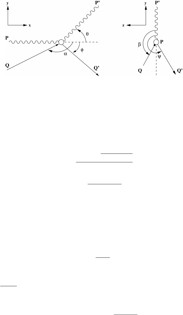
Figure 11.1: Scattering diagram of atomic bound electron Compton scat-
tering. Pis the incident photon momentum, Qthe electron pre-collision
momentum, P′the scattered photon momentum and Q′the recoil electron
momentum.
Tel =E−E′−EB,(11.2)
cos φ=−Y±√Y2−4W Z
2W,(11.3)
cos ψ=C−Bcos φ
Asin φ,(11.4)
where:
A=E′u′sin θ, (11.5)
B=E′u′cos θ−Eu′,(11.6)
C=c(E′−E)−EE′
γ′mc (1 −cos θ),(11.7)
D=γmE′
c(c−ucos θcos α−usin θcos βsin α) + m2c2(γγ′−1) −γ′mE′,
(11.8)
F= (γγ′m2uu′cos βsin α−γ′mE′u′
csin θ),(11.9)
G=γγ′m2uu′sin βsin α, (11.10)
202

H= (γγ′m2uu′cos α−γ′mE′
cu′cos θ),(11.11)
W= (F B −HA)2+G2A2+G2B2,(11.12)
Y= 2 (AD −F C) (F B −HA)−G2BC,(11.13)
Z= (AD −F C)2+G2C2−A2,(11.14)
and cis the speed of light, mis the rest mass of an electron, uis the speed of
the target electron, u′is the speed of the recoil electron, γ= (1 −(u2/c2))−1/2
and γ′= (1 −(u′2/c2))−1/2. Further information regarding the Monash
Compton scattering models can be found in [6].
Bibliography
[1] Ribberfors R., Phys. Rev. B. 12 2067-2074, 1975.
[2] Brusa D. et al., Nucl. Instrum. Methods Phys. Res. A 379 167-175, 1996.
[3] Kippen, R. M., New Astro. Reviews 48, 221-225, 2004.
[4] Salvat F. et al., PENELOPE, A Code System for Monte Carlo Sim-
ulation of Electron and Photon Transport, Proceedings of a Work-
shop/Training Course, OECD/NEA 5-7 November 2001.
[5] Du Mond J. W. M., Phys. Rev. 33 643-658, 1929.
[6] Brown J. M. C. et al., Nucl. Instrum. Methods Phys. Res. B 338, 77-88,
2014.
203
Chapter 12
Charged Hadron Incident
204

12.1 Hadron and Ion Ionization
12.1.1 Method
The class G4hIonisation provides the continuous energy loss due to ionization
and simulates the ’discrete’ part of the ionization, that is, delta rays produced
by charged hadrons. The class G4ionIonisation is intended for the simulation
of energy loss by positive ions with change greater than unit. Inside these
classes the following models are used:
•G4BetherBlochModel (valid for protons with T > 2MeV )
•G4BraggModel (valid for protons with T < 2MeV )
•G4BraggIonModel (valid for protons with T < 2MeV )
•G4ICRU73QOModel (valid for anti-protons with T < 2MeV )
The scaling relation (7.7) is a basic conception for the description of ionization
of heavy charged particles. It is used both in energy loss calculation and in
determination of the validity range of models. Namely the Tp= 2MeV limit
for protons is scaled for a particle with mass Miby the ratio of the particle
mass to the proton mass Ti=TpMp/Mi.
For all ionization models the value of the maximum energy transferable
to a free electron Tmax is given by the following relation [1]:
Tmax =2mec2(γ2−1)
1 + 2γ(me/M) + (me/M)2,(12.1)
where meis the electron mass and Mis the mass of the incident particle.
The method of calculation of the continuous energy loss and the total cross-
section are explained below.
12.1.2 Continuous Energy Loss
The integration of 7.1 leads to the Bethe-Bloch restricted energy loss (T <
Tcut formula [1], which is modified taken into account various corrections [2]:
dE
dx = 2πr2
emc2nel
z2
β2ln 2mc2β2γ2Tup
I2−β21 + Tup
Tmax −δ−2Ce
Z+F
(12.2)
205

where
reclassical electron radius: e2/(4πǫ0mc2)
mc2mass-energy of the electron
nel electrons density in the material
Imean excitation energy in the material
Zatomic number of the material
z charge of the hadron in units of the electron change
γ E/mc2
β21−(1/γ2)
Tup min(Tcut, Tmax)
δdensity effect function
Ceshell correction function
Fhigh order corrections
In a single element the electron density is
nel =Z nat =ZNavρ
A
(Nav: Avogadro number, ρ: density of the material, A: mass of a mole). In
a compound material
nel =X
i
Zinati =X
i
ZiNavwiρ
Ai
.
wiis the proportion by mass of the ith element, with molar mass Ai.
The mean excitation energy Ifor all elements is tabulated according to
the ICRU recommended values [3].
Shell Correction
2Ce/Z is the so-called shell correction term which accounts for the fact of
interaction of atomic electrons with atomic nucleus. This term more visible
at low energies and for heavy atoms. The classical expression for the term
[4] is used
C=XCν(θν, ην), ν =K, L, M, ..., θ =Jν
ǫν
, ην=β2
α2Z2
ν
,(12.3)
where αis the fine structure constant, βis the hadron velocity, Jνis the
ionisation energy of the shell ν,ǫνis Bohr ionisation energy of the shell
ν,Zνis the effective charge of the shell ν. First terms CKand CLcan
206
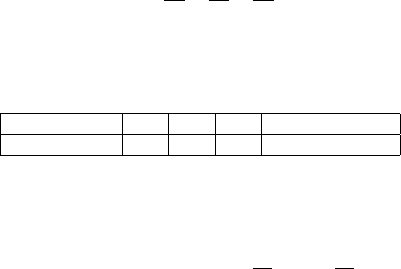
be analytically computed in using an assumption non-relativistic hydrogenic
wave functions [5, 6]. The results [7] of tabulation of these computations in
the interval of parameters ην= 0.005 ÷10 and θν= 0.25 ÷0.95 are used
directly. For higher values of ηνthe parameterization [7] is applied:
Cν=K1
η+K2
η2+K3
η3,(12.4)
where coefficients Kiprovide smooth shape of the function. The effective nu-
clear charge for the L-shell can be reproduced as ZL=Z−d,dis a parameter
shown in Table 12.24. For outer shells the calculations are not available, so
Z3 4 5 6 7 8 9 >9
d1.72 2.09 2.48 2.82 3.16 3.53 3.84 4.15
Table 12.1: Effective nuclear charge for the L-shell [4].
L-shell parameterization is used and the following scaling relation [4, 8] is
applied:
Cν=VνCL(θL, HνηL), Vν=nν
nL
, Hν=Jν
JL
,(12.5)
where Vνis a vertical scaling factor proportional to number of electrons at
the shell nν. The contribution of the shell correction term is about 10% for
protons at T= 2MeV .
Density Correction
δis a correction term which takes into account the reduction in energy loss
due to the so-called density effect. This becomes important at high energies
because media have a tendency to become polarized as the incident particle
velocity increases. As a consequence, the atoms in a medium can no longer
be considered as isolated. To correct for this effect the formulation of Stern-
heimer [9] is used:
xis a kinetic variable of the particle : x= log10(γβ) = ln(γ2β2)/4.606,
and δ(x) is defined by
for x < x0:δ(x) = 0
for x∈[x0, x1] : δ(x) = 4.606x−C+a(x1−x)m
for x > x1:δ(x) = 4.606x−C
(12.6)
207

where the matter-dependent constants are calculated as follows:
hνp= plasma energy of the medium = p4πnelr3
emc2/α =√4πnelre~c
C= 1 + 2 ln(I/hνp)
xa=C/4.606
a= 4.606(xa−x0)/(x1−x0)m
m= 3.
(12.7)
For condensed media
I < 100 eV for C≤3.681 x0= 0.2x1= 2
for C > 3.681 x0= 0.326C−1.0x1= 2
I≥100 eV for C≤5.215 x0= 0.2x1= 3
for C > 5.215 x0= 0.326C−1.5x1= 3
and for gaseous media
for C < 10. x0= 1.6x1= 4
for C∈[10.0,10.5[ x0= 1.7x1= 4
for C∈[10.5,11.0[ x0= 1.8x1= 4
for C∈[11.0,11.5[ x0= 1.9x1= 4
for C∈[11.5,12.25[ x0= 2. x1= 4
for C∈[12.25,13.804[ x0= 2. x1= 5
for C≥13.804 x0= 0.326C−2.5x1= 5.
High Order Corrections
High order corrections term to Bethe-Bloch formula (12.2) can be expressed
as
F=G−S+ 2(zL1+z2L2),(12.8)
where G is the Mott correction term, S is the finite size correction term,
L1is the Barkas correction, L2is the Bloch correction. The Mott term [2]
describes the close-collision corrections tend to become more important at
large velocities and higher charge of projectile. The Fermi result is used:
G=παzβ. (12.9)
The Barkas correction term describes distant collisions. The parameteriza-
tion of Ref. is expressed in the form:
L1=1.29FA(b/x1/2)
Z1/2x3/2, x =β2
Zα2,(12.10)
208

Z1 (H2gas) 1 2 3 - 10 11 - 17 18 19 - 25 26 - 50 >50
d0.6 1.8 0.6 1.8 1.4 1.8 1.4 1.35 1.3
Table 12.2: Scaled minimum impact parameter b [4].
where FAis tabulated function [10], b is scaled minimum impact parame-
ter shown in Table 12.2. This and other corrections depending on atomic
properties are assumed to be additive for mixtures and compounds. For the
Bloch correction term the classical expression [4] is following:
z2L2=−y2∞
X
n=1
1
n(n2+y2), y =zα
β.(12.11)
The finite size correction term takes into account the space distribution of
charge of the projectile particle. For muon it is zero, for hadrons this term
become visible at energies above few hundred GeV and the following param-
eterization [2] is used:
S=ln(1 + q), q =2meTmax
ε2,(12.12)
where Tmax is given in relation (12.1), εis proportional to the inverse ef-
fective radius of the projectile (Table 12.3). All these terms break scaling
mesons, spin = 0 (π±,K±) 0.736 GeV
baryons, spin = 1/2 0.843 GeV
ions 0.843 A1/3GeV
Table 12.3: The values of the εparameter for different particle types.
relation (7.7) if the projectile particle charge differs from ±1. To take this
circumstance into account in G4ionIonisation process at initialisation time
the term Fis ignored for the computation of the dE/dx table. At run time
this term is taken into account by adding to the mean energy loss a value
∆T′= 2πr2
emc2nel
z2
β2F∆s, (12.13)
where ∆sis the true step length and Fis the high order correction term
(12.8).
Parameterizations at Low Energies
For scaled energies below Tlim = 2 MeV shell correction becomes very large
and precision of the Bethe-Bloch formula degrades, so parameterisation of
209

evaluated data for stopping powers at low energies is required. These pa-
rameterisations for all atoms is available from ICRU’49 report [4]. The
proton parametrisation is used in G4BraggModel, which is included by de-
fault in the process G4hIonisation. The alpha particle parameterisation is
used in the G4BraggIonModel, which is included by default in the process
G4ionIonisation. To provide a smooth transition between low-energy and
high-energy models the modified energy loss expression is used for high en-
ergy
S(T) = SH(T) + (SL(Tlim)−SH(Tlim))Tlim
T, T > Tlim,(12.14)
where Sis smoothed stopping power, SHis stopping power from formula
(12.2) and SLis the low-energy parameterisation.
The precision of Bethe-Bloch formula for T > 10MeV is within 2%, below
the precision degrades and at 1keV only 20% may be garanteed. In the energy
interval 1 −10MeV the quality of description of the stopping power varied
from atom to atom. To provide more stable and precise parameterisation
the data from the NIST databases are included inside the standard package.
These data are provided for 74 materials of the NIST material database [11].
The data from the PSTAR database are included into G4BraggModel. The
data from the ASTAR database are included into G4BraggIonModel. So, if
Geant4 material is defined as a NIST material, than NIST data are used for
low-energy parameterisation of stopping power. If material is not from the
NIST database, then the ICRU’49 parameterisation is used.
12.1.3 Nuclear Stopping
Nuclear stopping due to elastic ion-ion scattering since Geant4 v9.3 can be
simulated with the continuous process G4NuclearStopping. By default this
correction is active and the ICRU’49 parameterisation [4] is used, which is
implemented in the model class G4ICRU49NuclearStoppingModel.
12.1.4 Total Cross Section per Atom
For T≫Ithe differential cross section can be written as
dσ
dT = 2πr2
emc2Zz2
p
β2
1
T21−β2T
Tmax
+T2
2E2(12.15)
210

[1]. In Geant4 Tcut ≥1 keV. Integrating from Tcut to Tmax gives the total
cross section per atom :
σ(Z, E, Tcut) = 2πr2
eZz2
p
β2mc2×(12.16)
1
Tcut −1
Tmax −β2
Tmax
ln Tmax
Tcut
+Tmax −Tcut
2E2
The last term is for spin 1/2 only. In a given material the mean free path is:
λ= (nat ·σ)−1or λ = (Pinati ·σi)−1(12.17)
The mean free path is tabulated during initialization as a function of the
material and of the energy for all kinds of charged particles.
12.1.5 Simulating Delta-ray Production
A short overview of the sampling method is given in Chapter 2. Apart from
the normalization, the cross section 12.15 can be factorized :
dσ
dT =f(T)g(T)with T ∈[Tcut, Tmax] (12.18)
where
f(T) = 1
Tcut −1
Tmax 1
T2(12.19)
g(T) = 1 −β2T
Tmax
+T2
2E2.(12.20)
The last term in g(T) is for spin 1/2 only. The energy Tis chosen by
1. sampling Tfrom f(T)
2. calculating the rejection function g(T) and accepting the sampled T
with a probability of g(T).
After the successful sampling of the energy, the direction of the scattered elec-
tron is generated with respect to the direction of the incident particle. The
azimuthal angle φis generated isotropically. The polar angle θis calculated
from energy-momentum conservation. This information is used to calculate
the energy and momentum of both scattered particles and to transform them
into the global coordinate system.
211

12.1.6 Ion Effective Charge
As ions penetrate matter they exchange electrons with the medium. In the
implementation of G4ionIonisation the effective charge approach is used [12].
A state of equilibrium between the ion and the medium is assumed, so that
the ion’s effective charge can be calculated as a function of its kinetic energy
in a given material. Before and after each step the dynamic charge of the ion
is recalculated and saved in G4DynamicP article, where it can be used not
only for energy loss calculations but also for the sampling of transportation
in an electromagnetic field.
The ion effective charge is expressed via the ion charge ziand the frac-
tional effective charge of ion γi:
zeff =γizi.(12.21)
For helium ions fractional effective charge is parameterized for all elements
(γHe)2= 1−exp "−
5
X
j=0
CjQj#!1 + 7 + 0.05Z
1000 exp(−(7.6−Q)2)2
,
Q= max(0,ln T),(12.22)
where the coefficients Cjare the same for all elements, and the helium ion
kinetic energy Tis in keV/amu.
The following expression is used for heavy ions [13]:
γi= q+1−q
2v0
vF2
ln 1 + Λ2!1 + (0.18 + 0.0015Z) exp(−(7.6−Q)2)
Z2
i,
(12.23)
where qis the fractional average charge of the ion, v0is the Bohr velocity,
vFis the Fermi velocity of the electrons in the target medium, and Λ is the
term taking into account the screening effect:
Λ = 10vF
v0
(1 −q)2/3
Z1/3
i(6 + q).(12.24)
The Fermi velocity of the medium is of the same order as the Bohr veloc-
ity, and its exact value depends on the detailed electronic structure of the
medium. The expression for the fractional average charge of the ion is the
following:
q= [1 −exp(0.803y0.3−1.3167y0.6−0.38157y−0.008983y2)],(12.25)
212

where yis a parameter that depends on the ion velocity vi
y=vi
v0Z2/31 + v2
F
5v2
i.(12.26)
The parametrisation of the effective charge of the ion applied if the kinetic
energy is below limit value
T < 10zi
Mi
Mp
MeV, (12.27)
where Miis the ion mass and Mpis the proton mass.
Bibliography
[1] W.-M. Yao et al., Jour. of Phys. G33 (2006) 1.
[2] S.P. Ahlen, Rev. Mod. Phys. 52 (1980) 121.
[3] ICRU (A. Allisy et al), Stopping Powers for Electrons and Positrons,
ICRU Report 37, 1984.
[4] ICRU (A. Allisy et al), Stopping Powers and Ranges for Protons and
Alpha Particles, ICRU Report 49, 1993.
[5] M.C. Walske, Phys. Rev. 88 (1952) 1283.
[6] M.C. Walske, Phys. Rev. 181 (1956) 940.
[7] G.S. Khandelwal, Nucl. Phys. A116 (1968) 97.
[8] H. Bichsel, Phys. Rev. A46 (1992) 5761.
[9] R.M. Sternheimer. Phys.Rev. B3 (1971) 3681.
[10] J.C. Ashley, R.H. Ritchie and W. Brandt, Phys. Rev. A8 (1973) 2402.
[11] http://physics.nist.gov/PhysRevData/contents-radi.html
[12] J.F. Ziegler, J.P. Biersack, U. Littmark, The Stopping and Ranges of
Ions in Solids. Vol.1, Pergamon Press, 1985.
[13] W. Brandt and M. Kitagawa, Phys. Rev. B25 (1982) 5631.
213

12.2 Low energy extentions
12.2.1 Energy losses of slow negative particles
At low energies, e.g. below a few MeV for protons/antiprotons, the Bethe-
Bloch formula is no longer accurate in describing the energy loss of charged
hadrons and higher Zterms should be taken in account. Odd terms in Z
lead to a significant difference between energy loss of positively and nega-
tively charged particles. The energy loss of negative hadrons is scaled from
that of antiprotons. The antiproton energy loss is calculated according to
the quantum harmonic oscillator model is used, as described in [1] and ref-
erences therein. The lower limit of applicability of the model is chosen for
all materials at 10 keV . Below this value stopping power is set to constant
equal to the dE/dx at 10 keV .
12.2.2 Energy losses of hadrons in compounds
To obtain energy losses in a mixture or compound, the absorber can be
thought of as made up of thin layers of pure elements with weights propor-
tional to the electron density of the element in the absorber (Bragg’s rule):
dE
dx =X
idE
dx i
,(12.28)
where the sum is taken over all elements of the absorber, iis the number of
the element, (dE
dx )iis energy loss in the pure i-th element.
Bragg’s rule is very accurate for relativistic particles when the interaction
of electrons with a nucleus is negligible. But at low energies the accuracy of
Bragg’s rule is limited because the energy loss to the electrons in any material
depends on the detailed orbital and excitation structure of the material. In
the description of Geant4 materials there is a special attribute: the chemical
formula. It is used in the following way:
•if the data on the stopping power for a compound as a function of
the proton kinetic energy is available (Table 12.4), then the direct
parametrisation of the data for this material is performed;
•if the data on the stopping power for a compound is available for only
one incident energy (Table 12.5), then the computation is performed
based on Bragg’s rule and the chemical factor for the compound is
taken into account;
214
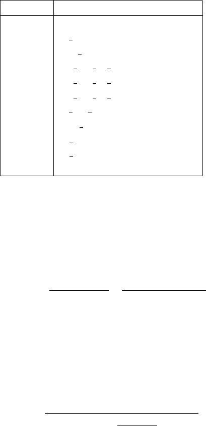
Table 12.4: The list of chemical formulae of compounds for which parametri-
sation of stopping power as a function of kinetic energy is in Ref.[3].
Number Chemical formula
1. AlO
2. C 2O
3. CH 4
4. (C 2H 4) N-Polyethylene
5. (C 2H 4) N-Polypropylene
6. (C 8H 8) N
7. C 3H 8
8. SiO 2
9. H 2O
10. H 2O-Gas
11. Graphite
•if there are no data for the compound, the computation is performed
based on Bragg’s rule.
In the review [2] the parametrisation stopping power data are presented as
Se(Tp) = SBragg(Tp)1 + f(Tp)
f(125 keV )Sexp(125 keV )
SBragg(125 keV )−1,(12.29)
where Sexp(125 keV ) is the experimental value of the energy loss for the
compound for 125 keV protons or the reduced experimental value for He
ions, SBragg(Tp) is a value of energy loss calculated according to Bragg’s
rule, and f(Tp) is a universal function, which describes the disappearance of
deviations from Bragg’s rule for higher kinetic energies according to:
f(Tp) = 1
1 + exp h1.48( β(Tp)
β(25 keV )−7.0)i,(12.30)
where β(Tp) is the relative velocity of the proton with kinetic energy Tp.
12.2.3 Fluctuations of energy losses of hadrons
The total continuous energy loss of charged particles is a stochastic quantity
with a distribution described in terms of a straggling function. The strag-
gling is partially taken into account by the simulation of energy loss by the
215
Table 12.5: The list of chemical formulae of compounds for which the chem-
ical factor is calculated from the data of Ref.[2].
Number Chemical formula Number Chemical formula
1. H 2O 28. C 2H 6
2. C 2H 4O 29. C 2F 6
3. C 3H 6O 30. C 2H 6O
4. C 2H 2 31. C 3H 6O
5. C H 3OH 32. C 4H 10O
6. C 2H 5OH 33. C 2H 4
7. C 3H 7OH 34. C 2H 4O
8. C 3H 4 35. C 2H 4S
9. NH 3 36. SH 2
10. C 14H 10 37. CH 4
11. C 6H 6 38. CCLF 3
12. C 4H 10 39. CCl 2F 2
13. C 4H 6 40. CHCl 2F
14. C 4H 8O 41. (CH 3) 2S
15. CCl 4 42. N 2O
16. CF 4 43. C 5H 10O
17. C 6H 8 44. C 8H 6
18. C 6H 12 45. (CH 2) N
19. C 6H 10O 46. (C 3H 6) N
20. C 6H 10 47. (C 8H 8) N
21. C 8H 16 48. C 3H 8
22. C 5H 10 49. C 3H 6-Propylene
23. C 5H 8 50. C 3H 6O
24. C 3H 6-Cyclopropane 51. C 3H 6S
25. C 2H 4F 2 52. C 4H 4S
26. C 2H 2F 2 53. C 7H 8
27. C 4H 8O 2
216

production of δ-electrons with energy T > Tc. However, continuous energy
loss also has fluctuations. Hence in the current GEANT4 implementation
two different models of fluctuations are applied depending on the value of
the parameter κwhich is the lower limit of the number of interactions of the
particle in the step. The default value chosen is κ= 10. To select a model
for thick absorbers the following boundary conditions are used:
∆E > Tcκ)or Tc< Iκ, (12.31)
where ∆Eis the mean continuous energy loss in a track segment of length
s,Tcis the cut kinetic energy of δ-electrons, and Iis the average ionisation
potential of the atom.
For long path lengths the straggling function approaches the Gaussian
distribution with Bohr’s variance [3]:
Ω2=KNel
Z2
h
β2Tcsf 1−β2
2,(12.32)
where fis a screening factor, which is equal to unity for fast particles, whereas
for slow positively charged ions with β2<3Z(v0/c)2f=a+b/Z2
eff , where
parameters aand bare parametrised for all atoms [4, 5].
For short path lengths, when the condition 12.31 is not satisfied, the
model described in the charter 7.2 is applied.
12.2.4 ICRU 73-based energy loss model
The ICRU 73 [1] report contains stopping power tables for ions with atomic
numbers 3–18 and 26, covering a range of different elemental and compound
target materials. The stopping powers derive from calculations with the
PASS code [6], which implements the binary stopping theory described in
[6, 7]. Tables in ICRU 73 extend over an energy range up to 1 GeV/nucleon.
All stopping powers were incorporated into Geant4 and are available through
a parameterisation model (G4IonParametrisedLossModel). For a few mate-
rials revised stopping powers were included (water, water vapor, nylon type
6 and 6/6 from P. Sigmund et al [8] and copper from P. Sigmund [9]), which
replace the corresponding tables of the original ICRU 73 report.
To account for secondary electron production above Tc, the continuous
energy loss per unit path length is calculated according to
dE
dx T <TC
=dE
dx ICRU 73 −dE
dx δ
(12.33)
217

where (dE/dx)ICRU73 refers to stopping powers obtained by interpolating
ICRU 73 tables and (dE/dx)δis the mean energy transferred to δ-electrons
per path length given by
dE
dx δ
=X
i
nat,i ZTmax
Tc
dσi(T)
dT T dT (12.34)
where the index iruns over all elements composing the material, nat,i is
the number of atoms of the element iper volume, Tmax is the maximum
energy transferable to an electron according to formula and dσi/dT specifies
the differential cross section per atom for producing an δ-electron following
equation
For compound targets not considered in the ICRU 73 report, the first
term on the rightern side in equation (12.33) is computed by applying Bragg’s
additivity rule [3] if tables for all elemental components are available in ICRU
73.
Bibliography
[1] Stopping of Ions Heavier Than Helium, ICRU Report 73, Oxford Uni-
versity Press (2005).
[2] J.F. Ziegler and J.M. Manoyan, Nucl. Instr. and Meth. B35 (1988) 215.
[3] ICRU (A. Allisy et al), Stopping Powers and Ranges for Protons and
Alpha Particles, ICRU Report 49, 1993.
[4] Q. Yang, D.J. O’Connor, Z. Wang, Nucl. Instr. and Meth. B61 (1991)
149.
[5] W.K. Chu, in: Ion Beam Handbook for Material Analysis, edt.
J.W. Mayer and E. Rimini, Academic Press, NY, 1977.
[6] P. Sigmund and A. Schinner, Nucl. Instr. Meth. in Phys. Res. B 195
(2002) 64.
[7] P. Sigmund and A. Schinner, Eur. Phys. J. D 12 (2000) 425.
[8] P. Sigmund, A. Schinner and H. Paul, Errata and Addenda for ICRU
Report 73, Stopping of Ions Heavier than Helium (2009).
[9] Personal communication with P. Sigmund (2009).
218
Chapter 13
Muon Incident
219

13.1 Muon Ionization
The class G4MuIonisation provides the continuous energy loss due to ion-
ization and simulates the ’discrete’ part of the ionization, that is, delta rays
produced by muons. Inside this class the following models are used:
•G4BraggModel (valid for protons with T < 0.2MeV )
•G4BetherBlochModel (valid for protons with 0.2MeV < T < 1GeV )
•G4MuBetherBlochModel (valid for protons with T > 1GeV )
The limit energy 0.2MeV is equivalent to the proton limit energy 2MeV
because of scaling relation (7.7), which allows simulation for muons with
energy below 1 GeV in the same way as for point-like hadrons with spin 1/2
described in the section 7.1.
For higher energies the G4MuBetherBlochModel is applied, in which lead-
ing radiative corrections are taken into account [1]. Simple analytical formula
for the cross section, derived with the logarithmic are used. Calculation re-
sults appreciably differ from usual elastic µ−escattering in the region of
high energy transfers me<< T < Tmax and give non-negligible correction to
the total average energy loss of high-energy muons. The total cross section
is written as following:
σ(E, ǫ) = σBB(E, ǫ)1 + α
2πln 1 + 2ǫ
meln 4meE(E−ǫ)
m2
µ(2ǫ+me),(13.1)
here σ(E, ǫ) is the differential cross sections, σ(E, ǫ)BB is the Bethe-Bloch
cross section (12.15), meis the electron mass, mµis the muon mass, Eis the
muon energy, ǫis the energy transfer, ǫ=ω+T, where T is the electron
kinetic energy and ωis the energy of radiative gamma.
For computation of the truncated mean energy loss (7.1) the partial in-
tegration of the expression (13.1) is performed
S(E, ǫup) = SBB(E, ǫup) + SRC (E, ǫup), ǫup =min(ǫmax, ǫcut),(13.2)
where term SBB is the Bethe-Bloch truncated energy loss (12.2) for the inter-
val of energy transfer (0 −ǫup) and term SRC is a correction due to radiative
effects. The function become smooth after log-substitution and is computed
by numerical integration
SRC (E, ǫup) = Zln ǫup
ln ǫ1
ǫ2(σ(E, ǫ)−σBB(E, ǫ))d(ln ǫ),(13.3)
220
where lower limit ǫ1does not effect result of integration in first order and in
the class G4MuBetheBlochModel the default value ǫ1= 100keV is used.
For computation of the discrete cross section (7.2) another substitution
is used in order to perform numerical integration of a smooth function
σ(E) = Z1/ǫup
1/ǫmax
ǫ2σ(E, ǫ)d(1/ǫ).(13.4)
The sampling of energy transfer is performed between 1/ǫup and 1/ǫmax using
rejection constant for the function ǫ2σ(E, ǫ). After the successful sampling
of the energy transfer, the direction of the scattered electron is generated
with respect to the direction of the incident particle. The energy of radiative
gamma is neglected. The azimuthal electron angle φis generated isotropi-
cally. The polar angle θis calculated from energy-momentum conservation.
This information is used to calculate the energy and momentum of both
scattered particles and to transform them into the global coordinate system.
Bibliography
[1] S.R. Kelner, R.P. Kokoulin, A.A. Petrukhin, Phys. Atomic Nuclei 60
(1997) 576.
221

13.2 Bremsstrahlung
Bremsstrahlung dominates other muon interaction processes in the region
of catastrophic collisions (v≥0.1 ), that is at ”moderate” muon energies
above the kinematic limit for knock–on electron production. At high energies
(E≥1 TeV) this process contributes about 40% of the average muon energy
loss.
13.2.1 Differential Cross Section
The differential cross section for muon bremsstrahlung (in units of cm2/(g GeV))
can be written as
dσ(E, ǫ, Z, A)
dǫ =16
3αNA(m
µre)21
ǫAZ(ZΦn+ Φe)(1 −v+3
4v2)
= 0 if ǫ≥ǫmax =E−µ, (13.5)
where µand mare the muon and electron masses, Zand Aare the atomic
number and atomic weight of the material, and NAis Avogadro’s number.
If Eand Tare the initial total and kinetic energy of the muon, and ǫis
the emitted photon energy, then ǫ=E−E′and the relative energy transfer
v=ǫ/E.
Φnrepresents the contribution of the nucleus and can be expressed as
Φn= ln BZ−1/3(µ+δ(D′
n√e−2))
D′
n(m+δ√eBZ−1/3);
= 0 if negative.
Φerepresents the contribution of the electrons and can be expressed as
Φe= ln B′Z−2/3µ
1 + δµ
m2√e(m+δ√eB′Z−2/3)
;
= 0 if ǫ≥ǫ′
max =E/(1 + µ2/2mE);
= 0 if negative.
In Φnand Φe, for all nuclei except hydrogen,
δ=µ2ǫ/2EE′=µ2v/2(E−ǫ);
D′
n=D(1−1/Z)
n, Dn= 1.54A0.27;
B= 183, B′= 1429,√e= 1.648(721271).
222

For hydrogen (Z=1) B= 202.4, B′= 446, D′
n=Dn.
These formulae are taken mostly from Refs. [1] and [2]. They include
improved nuclear size corrections in comparison with Ref. [3] in the region
v∼1 and low Z. Bremsstrahlung on atomic electrons (taking into account
target recoil and atomic binding) is introduced instead of a rough substitution
Z(Z+ 1). A correction for processes with nucleus excitation is also included
[4].
Applicability and Restrictions of the Method
The above formulae assume that:
1. E≫µ, hence the ultrarelativistic approximation is used;
2. E≤1020 eV; above this energy, LPM suppression can be expected;
3. v≥10−6; below 10−6Ter-Mikaelyan suppression takes place. However, in
the latter region the cross section of muon bremsstrahlung is several orders
of magnitude less than that of other processes.
The Coulomb correction (for high Z) is not included. However, existing
calculations [5] show that for muon bremsstrahlung this correction is small.
13.2.2 Continuous Energy Loss
The restricted energy loss for muon bremsstrahlung (dE/dx)rest with relative
transfers v=ǫ/(T+µ)≤vcut can be calculated as follows :
dE
dx rest
=Zǫcut
0
ǫ σ(E, ǫ)dǫ = (T+µ)Zvcut
0
ǫ σ(E, ǫ)dv .
If the user cut vcut ≥vmax =T/(T+µ), the total average energy loss is
calculated. Integration is done using Gaussian quadratures, and binning
provides an accuracy better than about 0.03% for T= 1 GeV, Z= 1. This
rapidly improves with increasing Tand Z.
13.2.3 Total Cross Section
The integration of the differential cross section over dǫ gives the total cross
section for muon bremsstrahlung:
σtot(E, ǫcut) = Zǫmax
ǫcut
σ(E, ǫ)dǫ =Zln vmax
ln vcut
ǫσ(E, ǫ)d(ln v),(13.6)
where vmax =T/(T+µ). If vcut ≥vmax ,σtot = 0.
223
13.2.4 Sampling
The photon energy ǫpis found by numerically solving the equation :
P=Zǫmax
ǫp
σ(E, ǫ, Z, A)dǫ Zǫmax
ǫcut
σ(E, ǫ, Z, A)dǫ .
Here Pis the random uniform probability, ǫmax =T, and ǫcut = (T+µ)·
vcut.vmin.cut = 10−5is the minimal relative energy transfer adopted in the
algorithm.
For fast sampling, the solution of the above equation is tabulated at
initialization time for selected Z,Tand P. During simulation, this table is
interpolated in order to find the value of ǫpcorresponding to the probability
P.
The tabulation routine uses accurate functions for the differential cross
section. The table contains values of
xp= ln(vp/vmax)/ln(vmax/vcut),(13.7)
where vp=ǫp/(T+µ) and vmax =T/(T+µ). Tabulation is performed
in the range 1 ≤Z≤128, 1 ≤T≤1000 PeV, 10−5≤P≤1 with con-
stant logarithmic steps. Atomic weight (which is a required parameter in the
cross section) is estimated here with an iterative solution of the approximate
relation:
A=Z(2 + 0.015 A2/3).
For Z= 1, A= 1 is used.
To find xp(and thus ǫp) corresponding to a given probability P, the
sampling method performs a linear interpolation in ln Zand ln T, and a
cubic, 4 point Lagrangian interpolation in ln P. For P≤Pmin, a linear
interpolation in (P, x) coordinates is used, with x= 0 at P= 0. Then the
energy ǫpis obtained from the inverse transformation of 13.7 :
ǫp= (T+µ)vmax(vmax/vcut)xp
The algorithm with the parameters described above has been tested for var-
ious Zand T. It reproduces the differential cross section to within 0.2 –
0.7 % for T≥10 GeV. The average total energy loss is accurate to within
0.5%. While accuracy improves with increasing T, satisfactory results are
also obtained for 1 ≤T≤10 GeV.
It is important to note that this sampling scheme allows the generation
of ǫpfor different user cuts on vwhich are above vmin.cut. To perform such a
simulation, it is sufficient to define a new probability variable
P′=P σtot (vuser.cut)/σtot(vmin.cut)
224

and use it in the sampling method. Time consuming re-calculation of the
3-dimensional table is therefore not required because only the tabulation of
σtot(vuser.cut) is needed.
The small-angle, ultrarelativistic approximation is used for the simulation
(with about 20% accuracy at θ≤θ∗≈1) of the angular distribution of the
final state muon and photon. Since the target recoil is small, the muon
and photon are directed symmetrically (with equal transverse momenta and
coplanar with the initial muon):
p⊥µ=p⊥γ,where p⊥µ=E′θµ, p⊥γ=ǫθγ.(13.8)
θµand θγare muon and photon emission angles. The distribution in the
variable r=Eθγ/µ is given by
f(r)dr ∼rdr/(1 + r2)2.(13.9)
Random angles are sampled as follows:
θγ=µ
Er θµ=ǫ
E′θγ,(13.10)
where
r=ra
1−a, a =ξr2
max
1 + r2
max
, rmax = min(1, E′/ǫ)·E θ∗/µ ,
and ξis a random number uniformly distributed between 0 and 1.
Bibliography
[1] S.R.Kelner, R.P.Kokoulin, A.A.Petrukhin. Preprint MEPhI 024-95,
Moscow, 1995; CERN SCAN-9510048.
[2] S.R.Kelner, R.P.Kokoulin, A.A.Petrukhin. Phys. Atomic Nuclei, 60
(1997) 576.
[3] A.A.Petrukhin, V.V.Shestakov. Canad.J.Phys., 46 (1968) S377.
[4] Yu.M.Andreyev, L.B.Bezrukov, E.V.Bugaev. Phys. Atomic Nuclei, 57
(1994) 2066.
[5] Yu.M.Andreev, E.V.Bugaev, Phys. Rev. D, 55 (1997) 1233.
225
13.3 Positron - Electron Pair Production by
Muons
Direct electron pair production is one of the most important muon inter-
action processes. At TeV muon energies, the pair production cross section
exceeds those of other muon interaction processes over a range of energy
transfers between 100 MeV and 0.1Eµ. The average energy loss for pair
production increases linearly with muon energy, and in the TeV region this
process contributes more than half the total energy loss rate.
To adequately describe the number of pairs produced, the average energy
loss and the stochastic energy loss distribution, the differential cross section
behavior over an energy transfer range of 5 MeV ≤ǫ≤0.1 ·Eµmust be
accurately reproduced. This is is because the main contribution to the total
cross section is given by transferred energies 5 MeV ≤ǫ≤0.01 ·Eµ, and be-
cause the contribution to the average muon energy loss is determined mostly
in the region 0.001 ·Eµ≤ǫ≤0.1 ·Eµ.
For a theoretical description of the cross section, the formulae of Ref. [1]
are used, along with a correction for finite nuclear size [2]. To take into
account electron pair production in the field of atomic electrons, the inelastic
atomic form factor contribution of Ref. [3] is also applied.
13.3.1 Differential Cross Section
Definitions and Applicability
In the following discussion, these definitions are used:
•mand µare the electron and muon masses, respectively
•E≡Eµis the total muon energy, E=T+µ
•Zand Aare the atomic number and weight of the material
•ǫis the total pair energy or, approximately, the muon energy loss (E−
E′)
•v=ǫ/E
•e= 2.718 ...
•A⋆= 183.
The formula for the differential cross section applies when:
226

•Eµ≫µ(E≥2 – 5 GeV) and Eµ≤1015 – 1017 eV. If muon energies
exceed this limit, the LPM (Landau Pomeranchuk Migdal) effect may
become important, depending on the material
•the muon energy transfer ǫlies between ǫmin = 4 mand ǫmax =Eµ−
3√e
4µ Z1/3, although the formal lower limit is ǫ≫2m, and the formal
upper limit requires E′
µ≫µ.
•Z≤40 – 50. For higher Z, the Coulomb correction is important but
has not been sufficiently studied theoretically.
Formulae
The differential cross section for electron pair production by muons σ(Z, A, E, ǫ)
can be written as :
σ(Z, A, E, ǫ) = 4
3π
Z(Z+ζ)
ANA(αr0)21−v
ǫZρmax
0
G(Z, E, v, ρ)dρ,
(13.11)
where
G(Z, E, v, ρ) = Φe+ (m/µ)2Φµ,
Φe,µ =Be,µL′
e,µ
and
Φe,µ = 0 whenever Φe,µ <0.
Beand Bµdo not depend on Z, A, and are given by
Be= [(2 + ρ2)(1 + β) + ξ(3 + ρ2)] ln 1 + 1
ξ+1−ρ2−β
1 + ξ−(3 + ρ2);
Be≈1
2ξ[(3 −ρ2) + 2β(1 + ρ2)] for ξ≥103;
Bµ=(1 + ρ2)1 + 3β
2−1
ξ(1 + 2β)(1 −ρ2)ln(1 + ξ)
+ξ(1 −ρ2−β)
1 + ξ+ (1 + 2β)(1 −ρ2);
Bµ≈ξ
2[(5 −ρ2) + β(3 + ρ2)] for ξ≤10−3;
Also,
227

ξ=µ2v2
4m2
(1 −ρ2)
(1 −v);β=v2
2(1 −v);
L′
e= ln A∗Z−1/3p(1 + ξ)(1 + Ye)
1 + 2m√eA∗Z−1/3(1 + ξ)(1 + Ye)
Ev(1 −ρ2)
−1
2ln "1 + 3mZ1/3
2µ2
(1 + ξ)(1 + Ye)#;
L′
µ= ln (µ/m)A∗Z−1/3p(1 + 1/ξ)(1 + Yµ)
1 + 2m√eA∗Z−1/3(1 + ξ)(1 + Yµ)
Ev(1 −ρ2)
−ln 3
2Z1/3q(1 + 1/ξ)(1 + Yµ).
For faster computing, the expressions for L′
e,µ are further algebraically trans-
formed. The functions L′
e,µ include the nuclear size correction [2] in compar-
ison with parameterization [1] :
Ye=5−ρ2+ 4 β(1 + ρ2)
2(1 + 3β) ln(3 + 1/ξ)−ρ2−2β(2 −ρ2);
Yµ=4 + ρ2+ 3 β(1 + ρ2)
(1 + ρ2)(3
2+ 2β) ln(3 + ξ) + 1 −3
2ρ2;
ρmax = [1 −6µ2/E2(1 −v)]p1−4m/Ev.
Comment on the Calculation of the Integral Rdρ in Eq. 13.11
The integral
ρmax
R
0
G(Z, E, v, ρ)dρ is computed with the substitutions:
t= ln(1 −ρ),
1−ρ= exp(t),
1 + ρ= 2 −exp(t),
1−ρ2=et(2 −et).
After that,
Zρmax
0
G(Z, E, v, ρ)dρ =Z0
tmin
G(Z, E, v, ρ)etdt, (13.12)
228

where
tmin = ln
4m
ǫ+12µ2
EE′1−4m
ǫ
1 + 1−6µ2
EE′r1−4m
ǫ
.
To compute the integral of Eq. 13.12 with an accuracy better than 0.5%,
Gaussian quadrature with N= 8 points is sufficient.
The function ζ(E, Z) in Eq. 13.11 serves to take into account the process
on atomic electrons (inelastic atomic form factor contribution). To treat
the energy loss balance correctly, the following approximation, which is an
algebraic transformation of the expression in Ref. [3], is used:
ζ(E, Z) =
0.073 ln E/µ
1 + γ1Z2/3E/µ −0.26
0.058 ln E/µ
1 + γ2Z1/3E/µ −0.14
;
ζ(E, Z) = 0 if the numerator is negative.
For E ≤35 µ, ζ(E, Z) = 0. Also γ1= 1.95 ·10−5and γ2= 5.30 ·10−5.
The above formulae make use of the Thomas-Fermi model which is not
good enough for light elements. For hydrogen (Z= 1) the following param-
eters must be changed:
A∗= 183 ⇒202.4;
γ1= 1.95 ·10−5⇒4.4·10−5;
γ2= 5.30 ·10−5⇒4.8·10−5.
13.3.2 Total Cross Section and Restricted Energy Loss
If the user’s cut for the energy transfer ǫcut is greater than ǫmin, the process is
represented by continuous restricted energy loss for interactions with ǫ≤ǫcut,
and discrete collisions with ǫ > ǫcut. Respective values of the total cross
section and restricted energy loss rate are defined as:
σtot =Zǫmax
ǫcut
σ(E, ǫ)dǫ; (dE/dx)restr =Zǫcut
ǫmin
ǫ σ(E, ǫ)dǫ.
For faster computing, ln ǫsubstitution and Gaussian quadratures are used.
229
13.3.3 Sampling of Positron - Electron Pair Produc-
tion
The e+e−pair energy ǫP, is found numerically by solving the equation
P=Zǫmax
ǫP
σ(Z, A, T, ǫ)dǫ / Zǫmax
cut
σ(Z, A, T, ǫ)dǫ (13.13)
or
1−P=ZǫP
cut
σ(Z, A, T, ǫ)dǫ / Zǫmax
cut
σ(Z, A, T, ǫ)dǫ (13.14)
To reach high sampling speed, solutions of Eqs. 13.13, 13.14 are tabulated
at initialization time. Two 3-dimensional tables (referred to here as A and
B) of ǫP(P, T, Z) are created, and then interpolation is used to sample ǫP.
The number and spacing of entries in the table are chosen as follows:
•a constant increment in ln Tis chosen such that there are four points
per decade in the range Tmin −Tmax. The default range of muon kinetic
energies in Geant4 is T= 1 GeV −1000 PeV.
•a constant increment in ln Zis chosen. The shape of the sampling dis-
tribution does depend on Z, but very weakly, so that eight points in the
range 1 ≤Z≤128 are sufficient. There is practically no dependence
on the atomic weight A.
•for probabilities P≤0.5, Eq. 13.13 is used and Table A is computed
with a constant increment in ln Pin the range 10−7≤P≤0.5. The
number of points in ln Pfor Table A is about 100.
•for P≥0.5, Eq. 13.14 is used and Table B is computed with a constant
increment in ln(1 −P) in the range 10−5≤(1 −P)≤0.5. In this case
50 points are sufficient.
The values of ln(ǫP−cut) are stored in both Table A and Table B.
To create the “probability tables” for each (T, Z) pair, the following pro-
cedure is used:
•a temporary table of ∼2000 values of ǫ·σ(Z, A, T, ǫ) is constructed
with a constant increment (∼0.02) in ln ǫin the range (cut, ǫmax). ǫis
taken in the middle of the corresponding bin in ln ǫ.
•the accumulated cross sections
σ1=Zln ǫmax
ln ǫ
ǫ σ(Z, A, T, ǫ)d(ln ǫ)
230
and
σ2=Zln ǫ
ln(cut)
ǫ σ(Z, A, T, ǫ)d(ln ǫ)
are calculated by summing the temporary table over the values above
ln ǫ(for σ1) and below ln ǫ(for σ2) and then normalizing to obtain the
accumulated probability functions.
•finally, values of ln(ǫP−cut) for corresponding values of ln Pand
ln(1 −P) are calculated by linear interpolation of the above accumu-
lated probabilities to form Tables A and B. The monotonic behavior of
the accumulated cross sections is very useful in speeding up the inter-
polation procedure.
The random transferred energy corresponding to a probability P, is then
found by linear interpolation in ln Zand ln T, and a cubic interpolation in
ln Pfor Table A or in ln(1−P) for Table B. For P≤10−7and (1−P)≤10−5,
linear extrapolation using the entries at the edges of the tables may be safely
used. Electron pair energy is related to the auxiliary variable x= ln(ǫP−cut)
found by the trivial interpolation ǫP=ex+cut.
Similar to muon bremsstrahlung (section 13.2), this sampling algorithm
does not re-initialize the tables for user cuts greater than cutmin. Instead,
the probability variable is redefined as
P′=P σtot(cutuser)/σtot(cutmin),
and P′is used for sampling.
In the simulation of the final state, the muon deflection angle (which is
of the order of m/E) is neglected. The procedure for sampling the energy
partition between e+and e−and their emission angles is similar to that used
for the γ→e+e−conversion.
Bibliography
[1] R.P.Kokoulin and A.A.Petrukhin, Proc. 11th Intern. Conf. on Cosmic
Rays, Budapest, 1969 [Acta Phys. Acad. Sci. Hung.,29, Suppl.4, p.277,
1970].
[2] R.P.Kokoulin and A.A.Petrukhin, Proc. 12th Int. Conf. on Cosmic Rays,
Hobart, 1971, vol.6, p.2436.
[3] S.R.Kelner, Phys. Atomic Nuclei, 61 (1998) 448.
231

13.4 Muon Photonuclear Interaction
The inelastic interaction of muons with nuclei is important at high muon en-
ergies (E≥10 GeV), and at relatively high energy transfers ν(ν/E ≥10−2).
It is especially important for light materials and for the study of detector re-
sponse to high energy muons, muon propagation and muon-induced hadronic
background. The average energy loss for this process increases almost lineary
with energy, and at TeV muon energies constitutes about 10% of the energy
loss rate.
The main contribution to the cross section σ(E, ν) and energy loss comes
from the low Q2–region ( Q2≪1 GeV2). In this domain, many simplifi-
cations can be made in the theoretical consideration of the process in order
to obtain convenient and simple formulae for the cross section. Most widely
used are the expressions given by Borog and Petrukhin [1], and Bezrukov and
Bugaev [2]. Results from these authors agree within 10% for the differential
cross section and within about 5% for the average energy loss, provided the
same photonuclear cross section, σγN , is used in the calculations.
13.4.1 Differential Cross Section
The Borog and Petrukhin formula for the cross section is based on:
•Hand’s formalism [3] for inelastic muon scattering,
•a semi-phenomenological inelastic form factor, which is a Vector Dom-
inance Model with parameters estimated from experimental data, and
•nuclear shadowing effects with a reasonable theoretical parameteriza-
tion [4].
For E≥10 GeV, the Borog and Petrukhin cross section (cm2/g GeV), dif-
ferential in transferred energy, is
σ(E, ν) = Ψ(ν)Φ(E, v),(13.15)
Ψ(ν) = α
π
Aeff NAV
AσγN (ν)1
ν,(13.16)
Φ(E, v) = v−1 + 1−v+v2
21 + 2µ2
Λ2ln
E2(1 −v)
µ21 + µ2v2
Λ2(1 −v)
1 + Ev
Λ1 + Λ
2M+Ev
Λ,
(13.17)
232

where νis the energy lost by the muon, v=ν/E, and µand Mare
the muon and nucleon (proton) masses, respectively. Λ is a Vector Dom-
inance Model parameter in the inelastic form factor which is estimated to be
Λ2= 0.4 GeV2.
For Aeff , which includes the effect of nuclear shadowing, the parameterization
[4]
Aeff = 0.22A+ 0.78A0.89 (13.18)
is chosen.
A reasonable choice for the photonuclear cross section, σγN , is the parame-
terization obtained by Caldwell et al. [5] based on the experimental data on
photoproduction by real photons:
σγN = (49.2 + 11.1 ln K+ 151.8/√K)·10−30cm2Kin GeV.(13.19)
The upper limit of the transferred energy is taken to be νmax =E−M/2. The
choice of the lower limit νmin is less certain since the formula 13.15, 13.16,
13.17 is not valid in this domain. Fortunately, νmin influences the total cross
section only logarithmically and has no practical effect on the average energy
loss for high energy muons. Hence, a reasonable choice for νmin is 0.2 GeV.
In Eq. 13.16, Aeff and σγN appear as factors. A more rigorous theoretical
approach may lead to some dependence of the shadowing effect on νand E;
therefore in the differential cross section and in the sampling procedure, this
possibility is forseen and the atomic weight Aof the element is kept as an
explicit parameter.
The total cross section is obtained by integration of Eq. 13.15 between νmin
and νmax; to facilitate the computation, a ln(ν)–substitution is used.
13.4.2 Sampling
Sampling the Transferred Energy
The muon photonuclear interaction is always treated as a discrete process
with its mean free path determined by the total cross section. The total
cross section is obtained by the numerical integration of Eq. 13.15 within the
limits νmin and νmax. The process is considered for muon energies 1GeV ≤
T≤1000PeV, though it should be noted that above 100 TeV the extrapola-
tion (Eq. 13.19) of σγN may be too crude.
233

The random transferred energy, νp, is found from the numerical solution of
the equation :
P=Zνmax
νp
σ(E, ν)dν Zνmax
νmin
σ(E, ν)dν . (13.20)
Here Pis the random uniform probability, with νmax =E−M/2 and
νmin = 0.2 GeV.
For fast sampling, the solution of Eq. 13.20 is tabulated at initialization time.
During simulation, the sampling method returns a value of νpcorresponding
to the probability P, by interpolating the table. The tabulation routine uses
Eq. 13.15 for the differential cross section. The table contains values of
xp= ln(νp/νmax)/ln(νmax/νmin),(13.21)
calculated at each point on a three-dimensional grid with constant spacings in
ln(T), ln(A) and ln(P) . The sampling uses linear interpolations in ln(T) and
ln(A), and a cubic interpolation in ln(P). Then the transferred energy is cal-
culated from the inverse transformation of Eq. 13.21, νp=νmax(νmax/νmin)xp.
Tabulated parameters reproduce the theoretical dependence to better than
2% for T > 1 GeV and better than 1% for T > 10 GeV.
Sampling the Muon Scattering Angle
According to Refs. [1, 6], in the region where the four-momentum transfer is
not very large (Q2≤3GeV2), the t– dependence of the cross section may
be described as:
dσ
dt ∼(1 −t/tmax)
t(1 + t/ν2)(1 + t/m2
0)[(1 −y)(1 −tmin/t) + y2/2],(13.22)
where tis the square of the four-momentum transfer, Q2= 2(EE′−P P ′cos θ−
µ2). Also, tmin = (µy)2/(1 −y), y=ν/E and tmax = 2Mν.ν=E−E′is
the energy lost by the muon and Eis the total initial muon energy. Mis
the nucleon (proton) mass and m2
0≡Λ2≃0.4 GeV2is a phenomenological
parameter determing the behavior of the inelastic form factor. Factors which
depend weakly, or not at all, on tare omitted.
To simulate random tand hence the random muon deflection angle, it is
convenient to represent Eq. 13.22 in the form :
σ(t)∼f(t)g(t),(13.23)
234

where
f(t) = 1
t(1 + t/t1),(13.24)
g(t) = 1−t/tmax
1 + t/t2·(1 −y)(1 −tmin/t) + y2/2
(1 −y) + y2/2,
and
t1= min(ν2, m2
0)t2= max(ν2, m2
0).(13.25)
tPis found analytically from Eq. 13.24 :
tP=tmaxt1
(tmax +t1)tmax(tmin +t1)
tmin(tmax +t1)P
−tmax
,
where Pis a random uniform number between 0 and 1, which is accepted
with probability g(t). The conditions of Eq. 13.25 make use of the symmetry
between ν2and m2
0in Eq. 13.22 and allow increased selection efficiency, which
is typically ≥0.7. The polar muon deflection angle θcan easily be found
from 1
sin2(θ/2) = tP−tmin
4 (EE′−µ2)−2tmin
.
The hadronic vertex is generated by the hadronic processes taking into ac-
count the four-momentum transfer.
Bibliography
[1] V.V.Borog and A.A.Petrukhin, Proc. 14th Int.Conf. on Cosmic Rays,
Munich,1975, vol.6, p.1949.
[2] L.B.Bezrukov and E.V.Bugaev, Sov. J. Nucl. Phys., 33, 1981, p.635.
[3] L.N.Hand. Phys. Rev., 129, 1834 (1963).
[4] S.J.Brodsky, F.E.Close and J.F.Gunion, Phys. Rev. D6, 177 (1972).
[5] D.O. Caldwell et al., Phys. Rev. Lett., 42, 553 (1979).
[6] V.V.Borog, V.G.Kirillov-Ugryumov, A.A.Petrukhin, Sov. J. Nucl.
Phys., 25, 1977, p.46.
1This convenient formula has been shown to the authors by D.A. Timashkov.
235
Chapter 14
Atomic Relaxation
236
14.1 Atomic relaxation
Atomic relaxation processes can be induced by any ionisation process that
leaves the interested atom in an excited state (i.e. with a vacancy in its
electronic structure). Processes inducing atomic relaxation in Geant4 are
photoelectric effect, Compton and ionization (both Standard and Lowen-
ergy).
Geant4 uses the Livermore Evaluation Atomic Data Library EADL [1],
that contains data to describe the relaxation of atoms back to neutrality after
they are ionised.
It is assumed that the binding energy of all subshells (from now on shells
are the same for neutral ground state atoms as for ionised atoms [1]).
Data in EADL includes the radiative and non-radiative transition prob-
abilities for each sub-shell of each element, for Z=1 to 100. The atom has
been ionised by a process that has caused an electron to be ejected from an
atom, leaving a vacancy or “hole” in a given subshell. The EADL data are
then used to calculate the complete radiative and non-radiative spectrum of
X-rays and electrons emitted as the atom relaxes back to neutrality.
Non-radiative de-excitation can occur via the Auger effect (the initial and
secondary vacancies are in different shells) or Coster-Kronig effect (transi-
tions within the same shell).
14.1.1 Fluorescence
The simulation procedure for the fluorescence process is the following:
1. If the vacancy shell is not included in the data, energy equal to the
binding energy of the shell is deposited locally
2. If the vacancy subshell is included in the data, an outer subshell is ran-
domly selected taking into account the relative transition probabilities
for all possible outer subshells.
3. In the case where the energy corresponding to the selected transition is
larger than a user defined cut value (equal to zero by default), a photon
particle is created and emitted in a random direction in 4π, with an
energy equal to the transition energy, provided by EADL.
4. the procedure is repeated from step 1, for the new vacancy subshell.
The final local energy deposit is the difference between the binding energy
of the initial vacancy subshell and the sum of all transition energies which
237
were taken by fluorescence photons. The atom is assumed to be initially
ionised with an electric charge of +1e.
Sub-shell data are provided in the EADL data bank [1] for Z=1 through
100. However, transition probabilities are only explicitly included for Z=6
through 100, from the subshells of the K, L, M, N shells and some O sub-
shells. For subshells O,P,Q: transition probabilities are negligible (of the
order of 0.1%) and smaller than the precision with which they are known.
Therefore, for the time being, for Z=1 through 5, only a local energy deposit
corresponding to the binding energy B of an electron in the ionised subshell
is simulated. For subshells of the O, P, and Q shells, a photon is emitted
with that energy B.
14.1.2 Auger process
The Auger effect is complimentary to fluorescence, hence the simulation pro-
cess is the same as for the fluorescence, with the exception that two random
shells are selected, one for the transition electron that fills the original va-
cancy, and the other for selecting the shell generating the Auger electron.
Subshell data are provided in the EADL data bank [1] for Z= 6 through
100. Since in EADL no data for elements with Z < 5 are provided, Auger
effects are only considered for 5 < Z < 100 and always due to the EADL data
tables, only for those transitions which have a probabiliy to occur >0.1% of
the total non-radiative transition probability. EADL probability data used
are, however, normalized to one for Fluorescence + Auger.
14.1.3 PIXE
PIXE (Particle Induced X-Ray Emission) can be simulated for ionisation
continuous processes perfomed by ions. Ionised shells are selected randomly
according the ionisation cross section of each shell once known the (continu-
ous) energy loss along the step 7.1.
Different shell ionisation cross sections models are available in different
energy ranges:
•ECPSSR[2],[3] internal Geant4 calculation for K and L shells.
•ECPSSR calculations from Factor Form according to Reis[4] for K and
L shells from 0.1 to 100 MeV and for M shells from 0.1 to 10 MeV.
•empirical “reference” K-shell values from Paul for protons[5] and for
for alphas[6]. Energies ranges are 0.1 - 10 MeV/amu circa, depending
on the atomic number that varies between 4 and 32.
238
•empirical Li-shell values from Orlic[7]. Energy Range 0.1-10 MeV for
Z between 41 and 92.
Otside Z and energy of limited shell ionisation cross sections, the ECPSSR
internal calculation method is applied.
Please refer to ref.[8] and original papers to have detailed information of
every model.
Bibliography
[1] ”Tables and Graphs of Atomic Subshell and Relaxation Data De-
rived from the LLNL Evaluated Atomic Data Library (EADL), Z=1-
100” S.T.Perkins, D.E.Cullen, M.H.Chen, J.H.Hubbell, J.Rathkopf,
J.Scofield, UCRL-50400 Vol.30
[2] W.Brandt and G.Lapicki, Phys.Rev.A23(1981)
[3] W. Brandt and G. Lapicki, Phys.Rev.A20 N2 (1979)
[4] A. Taborda et al., X-Ray Spec. 40 (2011) 127-134
[5] H. Paul, J.Sacher, Atom.Dat. and Nucl. Dat. Tabl. Volume 42, Issue 1,
May 1989, Pages 105-156
[6] H. Paul, O. Bolik, Atom. Dat. and Nucl. Dat. Tabl. Volume 54, Issue 1,
May 1993, Pages 75-131
[7] I. Orlic et al., International Journal of PIXE.Vol.4(1994) 217-230
[8] A. Mantero et al., X-Ray Spec. 40 (2011) 135-140
239
Chapter 15
Geant4-DNA
240
15.1 Geant4-DNA processes and models
The Geant4-DNA processes and models (theoretical, semi-empirical) are
adapted for track structure simulations in liquid water down to the eV scale.
They are described on a dedicated web site: http://geant4-dna.org, which
includes a full list of publications.
Any report or published results obtained using the Geant4-DNA software
shall cite the following publication : Comparison of Geant4 very low energy
cross section models with experimental data in water, S. Incerti et al., Med.
Phys. 37 (2010) 4692-4708
241
Chapter 16
Microelectronics
242

16.1 The MicroElec1extension for microelec-
tronics applications
The Geant4-MicroElec extension [1], developed by CEA, aims at modeling
the effect of ionizing radiation in highly integrated microelectronic compo-
nents. It describes the transport and generation of very low energy electrons
by incident electrons, protons and heavy ions in silicon.
All Geant4-MicroElec physics processes and models simulate step-by-step
interactions of particles in silicon down to the eV scale; they are pure discrete
processes. Table 16.1 summarizes the list of physical interactions per particle
type that can be modeled using the Geant4-MicroElec extension, along with
the corresponding process classes, model classes, low energy limit applica-
bility of models, high energy applicability of models and energy threshold
below which the incident particle is killed (stopped and the kinetic energy is
locally deposited). All models are interpolated. For now, they are valid for
silicon only (use the G4 Si Geant4-NIST material).
Particle Interaction Process, Model, Range Kill
Electron Elastic scattering G4MicroElastic 16.7 eV (*)
G4MicroElecElasticModel
5 eV < E < 100 MeV
Electron Ionisation G4MicroElecInelastic —
G4MicroElecInelasticModel
16.7 eV < E < 100 MeV
Protons, ions Ionisation G4MicroElecInelastic —
G4MicroElecInelasticModel
50 keV/u < E < 23 MeV/u
(*) because of the low energy limit applicability of the inelastic model.
Table 16.1: List of G4MicroElec physical interactions
All details regarding the physics and formula used for these processes
and models and available in [2] for incident electrons and in [3] for incident
protons and heavy ions.
1Previously called MuElec.
243
Bibliography
[1] Geant4-MicroElec online available at: https://twiki.cern.ch/twiki/bin/-
view/Geant4LoweMuElec
[2] A. Valentin, M. Raine, J.-E. Sauvestre, M. Gaillardin and P. Paillet,
“Geant4 physics processes for microdosimetry simulation: very low en-
ergy electromagnetic models for electrons in silicon”, Nuclear Instru-
ments and Methods in Physics Research B, vol. 288, pp. 66 - 73, 2012.
[3] A. Valentin, M. Raine, M. Gaillardin and P. Paillet, “Geant4 physics
processes for microdosimetry simulation: very low energy electromag-
netic models for protons and heavy ions in silicon”, Nuclear Instruments
and Methods in Physics Research B, vol. 287, pp. 124 - 129, 2012.
244
Chapter 17
Polarized
Electron/Positron/Gamma
Incident
245
17.1 Introduction
With the EM polarization extension it is possible to track polarized par-
ticles (leptons and photons). Special emphasis will be put in the proper
treatment of polarized matter and its interaction with longitudinal polarized
electrons/positrons or circularly polarized photons, which is for instance es-
sential for the simulation of positron polarimetry. The implementation is
base on Stokes vectors [1]. Further details can be found in [2].
In its current state, the following polarization dependent processes are
considered
•Bhabha/Møller scattering,
•Positron Annihilation,
•Compton scattering,
•Pair creation,
•Bremsstrahlung.
Several simulation packages for the realistic description of the develop-
ment of electromagnetic showers in matter have been developed. A prominent
example of such codes is EGS (Electron Gamma Shower)[3]. For this simu-
lation framework extensions with the treatment of polarized particles exist
[4, 5, 6]; the most complete has been developed by K. Fl¨ottmann [4]. It is
based on the matrix formalism [1], which enables a very general treatment of
polarization. However, the Fl¨ottmann extension concentrates on evaluation
of polarization transfer, i.e. the effects of polarization induced asymmetries
are neglected, and interactions with polarized media are not considered.
Another important simulation tool for detector studies is Geant3 [7].
Here also some effort has been made to include polarization [8, 9], but these
extensions are not publicly available.
In general the implementation of polarization in this EM polarization
library follows very closely the approach by K. Fl¨ottmann [4]. The basic
principle is to associate a Stokes vector to each particle and track the mean
polarization from one interaction to another. The basics for this approach is
the matrix formalism as introduced in [1].
17.1.1 Stokes vector
The Stokes vector [10, 1] is a rather simple object (in comparison to e.g. the
spin density matrix), three real numbers are sufficient for the characterization
246

of the polarization state of any single electron, positron or photon. Using
Stokes vectors all possible polarization states can be described, i.e. circular
and linear polarized photons can be handled with the same formalism as
longitudinal and transverse polarized electron/positrons.
The Stokes vector can be used also for beams, in the sense that it defines
a mean polarization.
In the EM polarization library the Stokes vector is defined as follows:
Photons Electrons
ξ1linear polarization polarization in x direction
ξ2linear polarization but π/4 to right polarization in y direction
ξ3circular polarization polarization in z direction
This definition is assumed in the particle reference frame, i.e. with the mo-
mentum of the particle pointing to the z direction, cf. also next section about
coordinate transformations. Correspondingly a 100% longitudinally polar-
ized electron or positron is characterized by
ξ=
0
0
±1
,(17.1)
where ±1 corresponds to spin parallel (anti parallel) to particle’s momentum.
Note that this definition is similar, but not identical to the definition used
in McMaster [1].
Many scattering cross sections of polarized processes using Stokes vectors
for the characterization of initial and final states are available in [1]. In
general a differential cross section has the form
dσ(ζ(1),ζ(2),ξ(1),ξ(2))
dΩ,(17.2)
i.e. it is a function of the polarization states of the initial particles ζ(1) and
ζ(2), as well as of the polarization states of the final state particles ξ(1) and
ξ(2) (in addition to the kinematic variables E,θ, and φ).
Consequently, in a simulation we have to account for
•Asymmetries:
Polarization of beam (ζ(1)) and target (ζ(2)) can induce azimuthal and
polar asymmetries, and may also influence on the total cross section
(Geant4: GetMeanFreePath()).
247

•Polarization transfer / depolarization effects
The dependence on the final state polarizations defines a possible trans-
fer from initial polarization to final state particles.
17.1.2 Transfer matrix
Using the formalism of McMaster, differential cross section and polarization
transfer from the initial state (ζ(1)) to one final state particle (ξ(1)) are com-
bined in an interaction matrix T:
O
ξ(1) =TI
ζ(1) ,(17.3)
where Iand Oare the incoming and outgoing currents, respectively. In
general the 4 ×4 matrix Tdepends on the target polarization ζ(2) (and of
course on the kinematic variables E,θ,φ). Similarly one can define a matrix
defining the polarization transfer to second final state particle like
O
ξ(2) =T′I
ζ(1) .(17.4)
In this framework the transfer matrix Tis of the form
T=
S A1A2A3
P1M11 M21 M31
P2M12 M22 M32
P3M13 M23 M33
.(17.5)
The matrix elements Tij can be identified as (unpolarized) differential cross
section (S), polarized differential cross section (Aj), polarization transfer
(Mij), and (de)polarization (Pi). In the Fl¨ottmann extension the elements
Ajand Pihave been neglected, thus concentrating on polarization transfer
only. Using the full matrix takes now all polarization effects into account.
The transformation matrix, i.e. the dependence of the mean polarization
of final state particles, can be derived from the asymmetry of the differential
cross section w.r.t. this particular polarization. Where the asymmetry is
defined as usual by
A=σ(+1) −σ(−1)
σ(+1) + σ(−1) .(17.6)
The mean final state polarizations can be determined coefficient by coeffi-
cient.
248

In general, the differential cross section is a linear function of the polar-
izations, i.e.
dσ(ζ(1),ζ(2),ξ(1),ξ(2))
dΩ= Φ(ζ(1),ζ(2))+A(ζ(1),ζ(2))·ξ(1) +B(ζ(1),ζ(2))·ξ(2)
+ξ(1)TM(ζ(1),ζ(2))ξ(2) (17.7)
In this form, the mean polarization of the final state can be read off easily,
and one obtains
hξ(1)i=1
Φ(ζ(1),ζ(2))
A(ζ(1),ζ(2))and (17.8)
hξ(2)i=1
Φ(ζ(1),ζ(2))
B(ζ(1),ζ(2)).(17.9)
Note, that the mean polarization states do not depend on the correlation
matrix M(ζ(1),ζ(2)). In order to account for correlation one has to generate
single particle Stokes vector explicitly, i.e. on an event by event basis. How-
ever, this implementation generates mean polarization states, and neglects
correlation effects.
17.1.3 Coordinate transformations
Three different coordinate systems are used in the evaluation of polarization
states:
•World frame
The geometry of the target, and the momenta of all particles in Geant4
are noted in the world frame X,Y,Z(the global reference frame, GRF).
It is the basis of the calculation of any other coordinate system.
•Particle frame
Each particle is carrying its own coordinate system. In this system
the direction of motion coincides with the z-direction. Geant4 provides
a transformation from any particle frame to the World frame by the
method G4ThreeMomemtum::rotateUz(). Thus, the y-axis of the par-
ticle reference frame (PRF) lies in the X-Y-plane of the world frame.
The Stokes vector of any moving particle is defined w.r.t. the corre-
sponding particle frame. Particles at rest (e.g. electrons of a media)
use the world frame as particle frame.
249
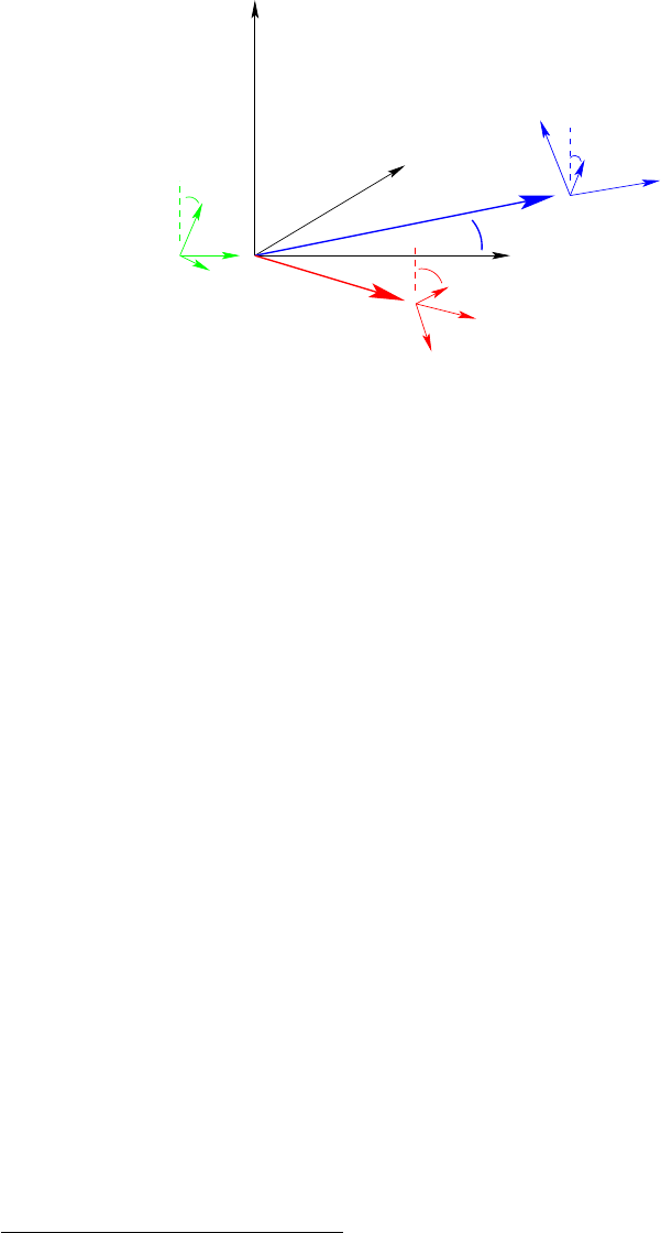
X
Y
z
x
y
z
photon
electron
photon
z
y
y
x
Z
x
Figure 17.1: The interaction frame and the particle frames for the exam-
ple of Compton scattering. The momenta of all participating particle lie in
the x-z-plane, the scattering plane. The incoming photon gives the zdirec-
tion. The outgoing photon is defined as particle 1 and gives the x-direction,
perpendicular to the z-axis. The y-axis is then perpendicular to the scatter-
ing plane and completes the definition of a right handed coordinate system
called interaction frame. The particle frame is defined by the Geant4 routine
G4ThreeMomemtum::rotateUz().
•Interaction frame
For the evaluation of the polarization transfer another coordinate sys-
tem is used, defined by the scattering plane, cf. fig. 17.1. There the
z-axis is defined by the direction of motion of the incoming particle.
The scattering plane is spanned by the z-axis and the x-axis, in a way,
that the direction of particle 1 has a positive xcomponent. The def-
inition of particle 1 depends on the process, for instance in Compton
scattering, the outgoing photon is referred as particle 11.
All frames are right handed.
17.1.4 Polarized beam and material
Polarization of beam particles is well established. It can be used for simulat-
ing low-energy Compton scattering of linear polarized photons. The inter-
pretation as Stokes vector allows now the usage in a more general framework.
The polarization state of a (initial) beam particle can be fixed using standard
1Note, for an incoming particle travelling on the Z-axis (of GRF), the y-axis of the
PRF of both outgoing particles is parallel to the y-axis of the interaction frame.
250
the ParticleGunMessenger class. For example, the class G4ParticleGun pro-
vides the method SetParticlePolarization(), which is usually accessable
via
/gun/polarization <Sx> <Sy> <Sz>
in a macro file.
In addition for the simulation of polarized media, a possibility to assign
Stokes vectors to physical volumes is provided by a new class, the so-called
G4PolarizationManager. The procedure to assign a polarization vector to a
media, is done during the detector construction. There the logical volumes
with certain polarization are made known to polarization manager. One
example DetectorConstruction might look like follows:
G4double Targetthickness = .010*mm;
G4double Targetradius = 2.5*mm;
G4Tubs *solidTarget =
new G4Tubs("solidTarget",
0.0,
Targetradius,
Targetthickness/2,
0.0*deg,
360.0*deg );
G4LogicalVolume * logicalTarget =
new G4LogicalVolume(solidTarget,
iron,
"logicalTarget",
0,0,0);
G4VPhysicalVolume * physicalTarget =
new G4PVPlacement(0,G4ThreeVector(0.*mm, 0.*mm, 0.*mm),
logicalTarget,
"physicalTarget",
worldLogical,
false,
0);
G4PolarizationManager * polMgr = G4PolarizationManager::GetInstance();
polMgr->SetVolumePolarization(logicalTarget,G4ThreeVector(0.,0.,0.08));
251
Once a logical volume is known to the G4PolarizationManager, its polariza-
tion vector can be accessed from a macro file by its name, e.g. the polarization
of the logical volume called “logicalTarget” can be changed via
/polarization/volume/set logicalTarget 0. 0. -0.08
Note, the polarization of a material is stated in the world frame.
Bibliography
[1] W. H. McMaster, Rev. Mod. Phys. 33 (1961) 8; and references therein.
[2] K. Laihem, PhD thesis, Measurement of the positron polarization at
an helical undulator based positron source for the International Linear
Collider ILC, Humboldt University Berlin, Germany, (2008).
[3] W. R. Nelson, H. Hirayama, D. W. O. Rogers, SLAC-R-0265.
[4] K. Fl¨ottmann, PhD thesis, DESY Hamburg (1993); DESY-93-161.
[5] Y. Namito, S. Ban, H. Hirayama, Nucl. Instrum. Meth. A 332 (1993)
277.
[6] J. C. Liu, T. Kotseroglou, W. R. Nelson, D. C. Schultz, SLAC-PUB-
8477.
[7] R. Brun, M. Caillat, M. Maire, G. N. Patrick, L. Urban, CERN-
DD/85/1.
[8] G. Alexander et al., SLAC-TN-04-018, SLAC-PROPOSAL-E-166.
[9] J. Hoogduin, PhD thesis, Rijksuniversiteit Groningen (1997).
[10] G. Stokes, Trans. Cambridge Phil. Soc. 9(1852) 399.
252

17.2 Ionization
17.2.1 Method
The class G4ePolarizedIonization provides continuous and discrete energy
losses of polarized electrons and positrons in a material. It evaluates po-
larization transfer and – if the material is polarized – asymmetries in the
explicit delta rays production. The implementation baseline follows the ap-
proach derived for the class G4eIonization described in sections 7.1 and 8.1.
For continuous energy losses the effects of a polarized beam or target are
negligible provided the separation cut Tcut is small, and are therefore not
considered separately. On the other hand, in the explicit production of delta
rays by Møller or Bhabha scattering, the effects of polarization on total cross
section and mean free path, on distribution of final state particles and the
average polarization of final state particles are taken into account.
17.2.2 Total cross section and mean free path
Kinematics of Bhabha and Møller scattering is fixed by initial energy
γ=Ek1
mc2(17.10)
and variable
ǫ=Ep2−mc2
Ek1−mc2,(17.11)
which is the part of kinetic energy of initial particle carried out by scatter.
Lower kinematic limit for ǫis 0, but in order to avoid divergencies in both
total and differential cross sections one sets
ǫmin =x=Tmin
Ek1−mc2,(17.12)
where Tmin has meaning of minimal kinetic energy of secondary electron.
And, ǫmax = 1(1/2) for Bhabha(Møller) scatterings.
Total Møller cross section
The total cross section of the polarized Møller scattering can be expressed
as follows
σM
pol =2πγ2r2
e
(γ−1)2(γ+ 1) hσM
0+ζ(1)
3ζ(2)
3σM
L+ζ(1)
1ζ(2)
1+ζ(1)
2ζ(2)
2σM
Ti,
(17.13)
253

where the reis classical electron radius, and
σM
0=−1
1−x+1
x−(γ−1)2
γ21
2−x+2−4γ
2γ2ln 1−x
x
σM
L=(−3 + 2 γ+γ2) (1 −2x)
2γ2+2γ(−1 + 2 γ)
2γ2ln 1−x
x
σM
T=2 (γ−1) (2 x−1)
2γ2+(1 −3γ)
2γ2ln 1−x
x(17.14)
Total Bhabha cross section
The total cross section of the polarized Bhabha scattering can be expressed
as follows
σB
pol =2πr2
e
γ−1hσB
0+ζ(1)
3ζ(2)
3σB
L+ζ(1)
1ζ(2)
1+ζ(1)
2ζ(2)
2σB
Ti,(17.15)
where
σB
0=1−x
2 (γ−1) x+2 (−1 + 3 x−6x2+ 4 x3)
3 (1 + γ)3
+−1−5x+ 12 x2−10 x3+ 4 x4
2 (1 + γ)x+−3−x+ 8 x2−4x3−ln(x)
(1 + γ)2
+3 + 4 x−9x2+ 3 x3−x4+ 6 xln(x)
3x
σB
L=2 (1 −3x+ 6 x2−4x3)
3 (1 + γ)3+−14 + 15 x−3x2+ 2 x3−9 ln(x)
3 (1 + γ)
+5 + 3 x−12 x2+ 4 x3+ 3 ln(x)
3 (1 + γ)2+7−9x+ 3 x2−x3+ 6 ln(x)
3
σB
T=2 (−1 + 3 x−6x2+ 4 x3)
3 (1 + γ)3+−7−3x+ 18 x2−8x3−3 ln(x)
3 (1 + γ)2
+5 + 3 x−12 x2+ 4 x3+ 9 ln(x)
6 (1 + γ)(17.16)
Mean free path
With the help of the total polarized Møller cross section one can define a
longitudinal asymmetry AM
Land the transverse asymmetry AM
T, by
AM
L=σM
L
σM
0
and AM
T=σM
T
σM
0
.
254

Similarly, using the polarized Bhabha cross section one can introduce a
longitudinal asymmetry AB
Land the transverse asymmetry AB
Tvia
AB
L=σB
L
σB
0
and AB
T=σB
T
σB
0
.
These asymmetries are depicted in figures 17.2 and 17.3 respectively.
If both beam and target are polarized the mean free path as defined
in section 8.1 has to be modified. In the class G4ePolarizedIonization the
polarized mean free path λpol is derived from the unpolarized mean free path
λunpol via
λpol =λunpol
1 + ζ(1)
3ζ(2)
3AL+ζ(1)
1ζ(2)
1+ζ(1)
2ζ(2)
2AT
(17.17)
17.2.3 Sampling the final state
Differential cross section
The polarized differential cross section is rather complicated, the full result
can be found in [1, 2, 3]. In G4PolarizedMollerCrossSection the complete
result is available taking all mass effects into account, only binding effects
are neglected. Here we state only the ultra-relativistic approximation (URA),
to show the general dependencies.
dσM
URA
dǫdϕ =rǫ2
γ+ 1 ×
"(1 −ǫ+ǫ2)2
4 (ǫ−1)2ǫ2+ζ(1)
3ζ(2)
3
2−ǫ+ǫ2
−4ǫ(1 −ǫ)+ζ(1)
2ζ(2)
2−ζ(1)
1ζ(2)
11
4
+ξ(1)
3ζ(1)
3−ξ(2)
3ζ(2)
31−ǫ+ 2 ǫ2
4 (1 −ǫ)ǫ2+ξ(2)
3ζ(1)
3−ξ(1)
3ζ(2)
32−3ǫ+ 2 ǫ2
4 (1 −ǫ)2ǫ#
(17.18)
The corresponding cross section for Bhabha cross section is implemented in
G4PolarizedBhabhaCrossSection. In the ultra-relativistic approximation it
255
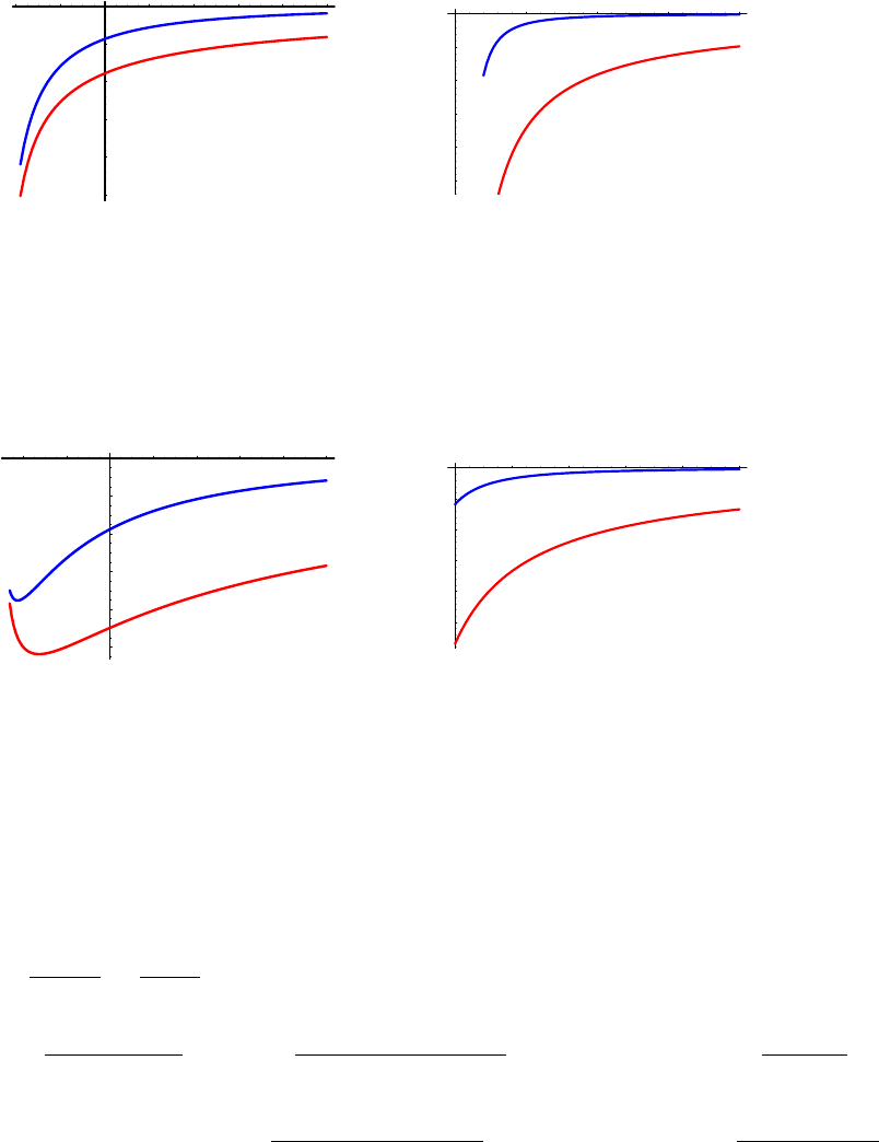
0.6 0.8 1.2 1.4 1.6 1.8 2
Ein,MeV
-5
-4
-3
-2
-1
AL,T,% (a)
5 10 15 20
Ein,MeV
-0.5
-0.4
-0.3
-0.2
-0.1
AL,T,% (b)
Figure 17.2: Møller total cross section asymmetries depending on the total
energy of the incoming electron, with a cut-off Tcut = 1keV. Transverse
asymmetry is plotted in blue, longitudinal asymmetry in red. Left part,
between 0.5 MeV and 2 MeV, right part up to 10 MeV.
0.6 0.8 1.2 1.4 1.6 1.8 2
Ein,MeV
-1
-0.8
-0.6
-0.4
-0.2
AL,T,% (a)
4 6 8 10 12
Ein,MeV
-0.5
-0.4
-0.3
-0.2
-0.1
AL,T,% (b)
Figure 17.3: Bhabha total cross section asymmetries depending on the total
energy of the incoming positron, with a cut-off Tcut = 1keV. Transverse
asymmetry is plotted in blue, longitudinal asymmetry in red. Left part,
between 0.5 MeV and 2 MeV, right part up to 10 MeV.
reads
dσB
URA
dǫdϕ =rǫ2
γ−1×
"(1 −ǫ+ǫ2)2
4ǫ2+ζ(1)
3ζ(2)
3
(ǫ−1) (2 −ǫ+ǫ2)
4ǫ+ζ(1)
2ζ(2)
2−ζ(1)
1ζ(2)
1(1 −ǫ)2
4
+ξ(1)
3ζ(1)
3−ξ(2)
3ζ(2)
31−2ǫ+ 3 ǫ2−2ǫ3
4ǫ2+ξ(2)
3ζ(1)
3−ξ(1)
3ζ(2)
32−3ǫ+ 2 ǫ2
4ǫ#
(17.19)
256

where re= classical electron radius
γ=Ek1/mec2
ǫ= (Ep1−mec2)/(Ek1−mec2)
Ek1= energy of the incident electron/positron
Ep1= energy of the scattered electron/positron
mec2= electron mass
ζ(1) = Stokes vector of the incoming electron/positron
ζ(2) = Stokes vector of the target electron
ξ(1) = Stokes vector of the outgoing electron/positron
ξ(2) = Stokes vector of the outgoing (2nd) electron .
Sampling
The delta ray is sampled according to methods discussed in Chapter 2. After
exploitation of the symmetry in the Møller cross section under exchanging ǫ
versus (1 −ǫ), the differential cross section can be approximated by a simple
function fM(ǫ):
fM(ǫ) = 1
ǫ2
ǫ0
1−2ǫ0
(17.20)
with the kinematic limits given by
ǫ0=Tcut
Ek1−mec2≤ǫ≤1
2(17.21)
A similar function fB(ǫ) can be found for Bhabha scattering:
fB(ǫ) = 1
ǫ2
ǫ0
1−ǫ0
(17.22)
with the kinematic limits given by
ǫ0=Tcut
Ek1−mec2≤ǫ≤1 (17.23)
The kinematic of the delta ray production is constructed by the following
steps:
1. ǫis sampled from f(ǫ)
2. calculate the differential cross section, depending on the initial polar-
izations ζ(1) and ζ(2).
3. ǫis accepted with the probability defined by ratio of the differential
cross section over the approximation function.
257
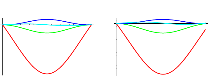
4. The ϕis diced uniformly.
5. ϕis determined from the differential cross section, depending on the
initial polarizations ζ(1) and ζ(2)
Note, for initial states without transverse polarization components, the ϕ
distribution is always uniform. In figure 17.4 the asymmetries indicate the
influence of polarization. In general the effect is largest around ǫ=1
2.
0.2 0.4 0.6 0.8 1
Ε
-80
-60
-40
-20
A,% Moller asymmetries
0.2 0.4 0.6 0.8 1
Ε
-80
-60
-40
-20
A,% Bhabha asymmetries
Figure 17.4: Differential cross section asymmetries in% for Møller (left) and
Bhabha (right) scattering ( red - AZZ (ǫ), green - AXX (ǫ), blue - AY Y (ǫ),
lightblue - AZX (ǫ))
After both φand ǫare known, the kinematic can be constructed fully.
Using momentum conservation the momenta of the scattered incident particle
and the ejected electron are constructed in global coordinate system.
Polarization transfer
After the kinematics is fixed the polarization properties of the outgoing par-
ticles are determined. Using the dependence of the differential cross section
on the final state polarization a mean polarization is calculated according to
method described in section 17.1.
The resulting polarization transfer functions ξ(1,2)
3(ǫ) are depicted in fig-
ures 17.5 and 17.6.
Bibliography
[1] P. Starovoitov et.al., in preparation.
[2] G. W. Ford, C. J. Mullin, Phys. Rev. 108 (1957) 477.
[3] P. Stehle, Phys. Rev. 110 (1958) 1458.
258
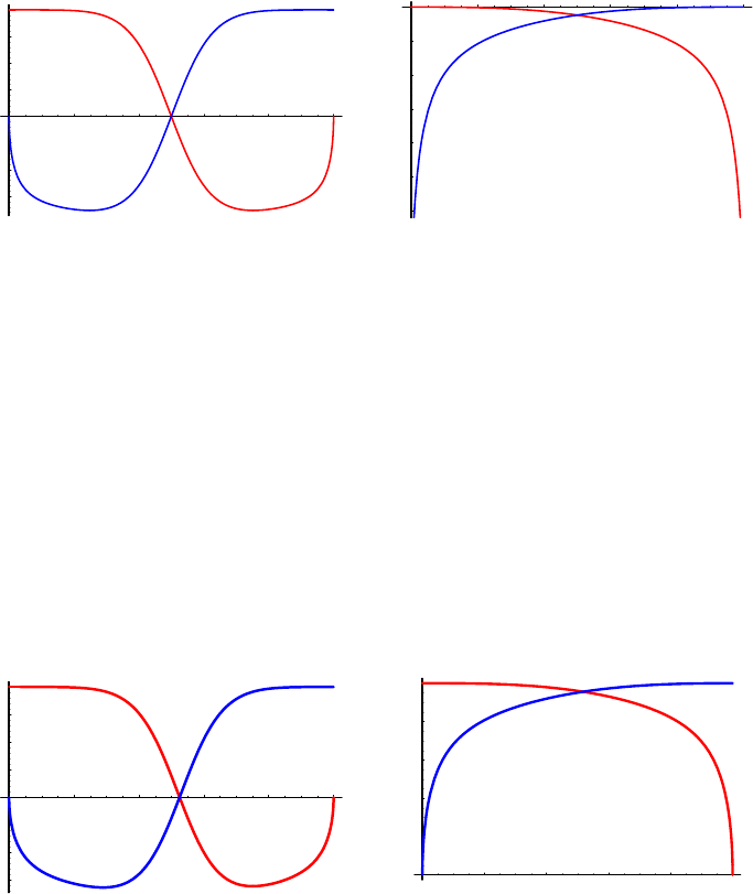
0.2 0.4 0.6 0.8 1
Ε
-0.75
-0.5
-0.25
0.25
0.5
0.75
1
TBeam P=1 <> Target P=1
0.2 0.4 0.6 0.8 1
Ε
0.4
0.5
0.6
0.7
0.8
0.9
TBeam P=1 <> Target P=-1
Figure 17.5: Polarization transfer functions in Møller scattering. Longitu-
dinal polarization ξ(2)
3of electron with energy Ep2in blue; longitudinal po-
larization ξ(1)
3of second electron in red. Kinetic energy of incoming electron
Tk1= 10MeV
.
0.2 0.4 0.6 0.8 1
Ε
-0.75
-0.5
-0.25
0.25
0.5
0.75
1
TBeam P = 1 <> Target P = 1
0.2 0.4 0.6 0.8 1
Ε
0.2
0.4
0.6
0.8
1
TBeam P = 1 <> Target P = -1
Figure 17.6: Polarization Transfer in Bhabha scattering. Longitudinal po-
larization ξ(2)
3of electron with energy Ep2in blue; longitudinal polarization
ξ(1)
3of scattered positron. Kinetic energy of incoming positron Tk1= 10MeV
.
259
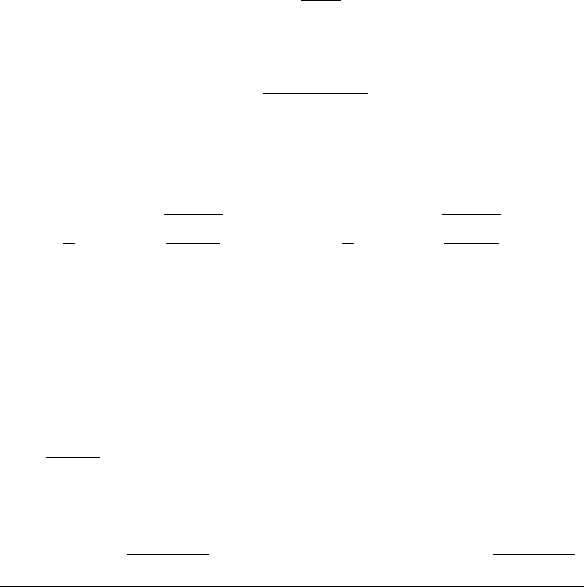
17.3 Positron - Electron Annihilation
17.3.1 Method
The class G4eplusPolarizedAnnihilation simulates annihilation of polarized
positrons with electrons in a material. The implementation baseline follows
the approach derived for the class G4eplusAnnihilation described in section
8.3. It evaluates polarization transfer and – if the material is polarized –
asymmetries in the produced photons. Thus, it takes the effects of polar-
ization on total cross section and mean free path, on distribution of final
state photons into account. And calculates the average polarization of these
generated photons. The material electrons are assumed to be free and at
rest.
17.3.2 Total cross section and mean free path
Kinematics of annihilation process is fixed by initial energy
γ=Ek1
mc2(17.24)
and variable
ǫ=Ep1
Ek1+mc2,(17.25)
which is the part of total energy available in initial state carried out by first
photon. This variable has the following kinematical limits
1
21−rγ−1
γ+ 1< ǫ < 1
21 + rγ−1
γ+ 1.(17.26)
Total Cross Section
The total cross section of the annihilation of a polarized e+e−pair into two
photons could be expressed as follows
σA
pol =πr2
e
γ+ 1 hσA
0+ζ(1)
3ζ(2)
3σA
L+ζ(1)
1ζ(2)
1+ζ(1)
2ζ(2)
2σA
Ti,(17.27)
where
σA
0=−(3 + γ)p−1 + γ2+ (1 + γ(4 + γ)) ln(γ+p−1 + γ2)
4 (γ2−1) (17.28)
260
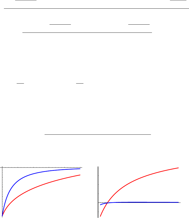
σA
L=−p−1 + γ2(5 + γ(4 + 3 γ)) + (3 + γ(7 + γ+γ2)) ln(γ+pγ2−1)
4 (γ−1)2(1 + γ)
(17.29)
σA
T=(5 + γ)p−1 + γ2−(1 + 5 γ) ln(γ+p−1 + γ2)
4 (−1 + γ)2(1 + γ)(17.30)
Mean free path
With the help of the total polarized annihilation cross section one can define
a longitudinal asymmetry AA
Land the transverse asymmetry AA
T, by
AA
L=σA
L
σA
0
and AA
T=σA
T
σA
0
.
These asymmetries are depicted in figure 17.7.
If both incident positron and target electron are polarized the mean free
path as defined in section 8.3 has to be modified. The polarized mean free
path λpol is derived from the unpolarized mean free path λunpol via
λpol =λunpol
1 + ζ(1)
3ζ(2)
3AL+ζ(1)
1ζ(2)
1+ζ(1)
2ζ(2)
2AT
(17.31)
2 3 4 5 6
Γ
-100
-80
-60
-40
-20
AL,T,% (a)
10 15 20 25 30 35 40
Γ
-10
10
20
30
AL,T,% (b)
Figure 17.7: Annihilation total cross section asymmetries depending on the
total energy of the incoming positron Ek1. The transverse asymmetry is
shown in blue, the longitudinal asymmetry in red.
261

17.3.3 Sampling the final state
Differential Cross Section
The fully polarized differential cross section is implemented in the class
G4PolarizedAnnihilationCrossSection, which takes all mass effects into ac-
count, but binding effects are neglected [1, 2]. In the ultra-relativistic ap-
proximation (URA) and concentrating on longitudinal polarization states
only the cross section is rather simple:
dσA
URA
dǫdϕ =re2
γ−1× 1−2ǫ+ 2 ǫ2
8ǫ−8ǫ21 + ζ(1)
3ζ(2)
3
+
(1 −2ǫ)ζ(1)
3+ζ(2)
3ξ(1)
3−ξ(2)
3
8 (ǫ−1) ǫ!(17.32)
where re= classical electron radius
γ=Ek1/mec2
Ek1= energy of the incident positron
mec2= electron mass
ζ(1) = Stokes vector of the incoming positron
ζ(2) = Stokes vector of the target electron
ξ(1) = Stokes vector of the 1st photon
ξ(2) = Stokes vector of the 2nd photon .
Sampling
The photon energy is sampled according to methods discussed in Chapter 2.
After exploitation of the symmetry in the Annihilation cross section under
exchanging ǫversus (1−ǫ), the differential cross section can be approximated
by a simple function f(ǫ):
f(ǫ) = 1
ǫln−1ǫmax
ǫmin (17.33)
with the kinematic limits given by
ǫmin =1
21−rγ−1
γ+ 1,
ǫmax =1
21 + rγ−1
γ+ 1.(17.34)
The kinematic of the two photon final state is constructed by the following
steps:
262
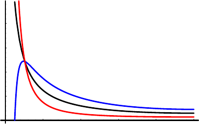
0.1 0.2 0.3 0.4 0.5
Ε
1
2
3
4
d2 Σ A
dΕdΦAnnihilation cross section
Figure 17.8: Annihilation differential cross section in arbitrary units. Black
line corresponds to unpolarized cross section; red line – to the antiparallel
spins of initial particles, and blue line – to the parallel spins. Kinetic energy
of the incoming positron Tk1= 10MeV.
1. ǫis sampled from f(ǫ)
2. calculate the differential cross section, depending on the initial polar-
izations ζ(1) and ζ(2).
3. ǫis accepted with the probability defined by the ratio of the differential
cross section over the approximation function f(ǫ).
4. The ϕis diced uniformly.
5. ϕis determined from the differential cross section, depending on the
initial polarizations ζ(1) and ζ(2).
A short overview over the sampling method is given in Chapter 2. In figure
17.9 the asymmetries indicate the influence of polarization for an 10MeV
incoming positron. The actual behavior is very sensitive to the energy of the
incoming positron.
Polarization transfer
After the kinematics is fixed the polarization of the outgoing photon is de-
termined. Using the dependence of the differential cross section on the final
state polarizations a mean polarization is calculated for each photon accord-
ing to method described in section 17.1.
263
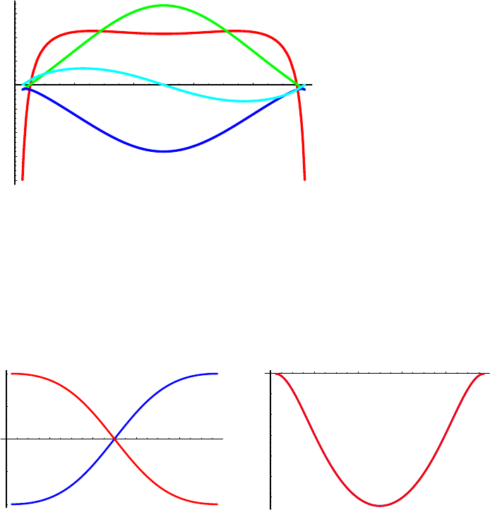
0.2 0.4 0.6 0.8
Ε
-100
-75
-50
-25
25
50
75
A,% Annihilation asymmetries
Figure 17.9: Annihilation differential cross section asymmetries in%. Red
line corrsponds to AZZ (ǫ), green line – AXX (ǫ), blue line – AY Y (ǫ), lightblue
line – AZX (ǫ)). Kinetic energy of the incoming positron Tk1= 10MeV.
The resulting polarization transfer functions ξ(1,2)(ǫ) are depicted in figure
17.10.
0.2 0.4 0.6 0.8
Ε
-1
-0.5
0.5
1
TBeam P = 1 <> Target P = 1
0.2 0.4 0.6 0.8
Ε
0.7
0.75
0.8
0.85
0.9
0.95
TBeam P = 1 <> Target P = -1
Figure 17.10: Polarization Transfer in annihilation process. Blue line corre-
sponds to the circular polarization ξ(1)
3of the photon with energy m(γ+ 1)ǫ;
red line – circular polarization ξ(2)
3of the photon photon with energy
m(γ+ 1)(1 −ǫ).
17.3.4 Annihilation at Rest
The method AtRestDoIt treats the special case where a positron comes to
rest before annihilating. It generates two photons, each with energy Ep1/2=
mc2and an isotropic angular distribution. Starting with the differential cross
section for annihilation with positron and electron spins opposed and parallel,
264

respectively,[2]
dσ1=∼(1 −β2) + β2(1 −β2)(1 −cos2θ)2
(1 −β2cos2θ)2dcos θ(17.35)
dσ2=∼β2(1 −cos4θ)
(1 −β2cos2θ)2dcos θ(17.36)
In the limit β→0 the cross section dσ1becomes one, and the cross section
dσ2vanishes. For the opposed spin state, the total angular momentum is
zero and we have a uniform photon distribution. For the parallel case the
total angular momentum is 1. Here the two photon final state is forbidden
by angular momentum conservation, and it can be assumed that higher order
processes (e.g. three photon final state) play a dominant role. However, in
reality 100% polarized electron targets do not exist, consequently there are
always electrons with opposite spin, where the positron can annihilate with.
Final state polarization does not play a role for the decay products of a spin
zero state, and can be safely neglected. (Is set to zero)
Bibliography
[1] P. Starovoitov et.al., in preparation.
[2] L. A. Page, Phys. Rev. 106 (1957) 394-398.
265

17.4 Polarized Compton scattering
17.4.1 Method
The class G4PolarizedCompton simulates Compton scattering of polarized
photons with (possibly polarized) electrons in a material. The implementa-
tion follows the approach described for the class G4ComptonScattering in-
troduced in section 5.3. Here the explicit production of a Compton scattered
photon and the ejected electron is considered taking the effects of polariza-
tion on total cross section and mean free path as well as on the distribution
of final state particles into account. Further the average polarizations of
the scattered photon and electron are calculated. The material electrons are
assumed to be free and at rest.
17.4.2 Total cross section and mean free path
Kinematics of the Compton process is fixed by the initial energy
X=Ek1
mc2(17.37)
and the variable
ǫ=Ep1
Ek1
,(17.38)
which is the part of total energy avaible in initial state carried out by scat-
tered photon, and the scattering angle
cos θ= 1 −1
X1
ǫ−1(17.39)
The variable ǫhas the following limits:
1
1 + 2X< ǫ < 1 (17.40)
Total Cross Section
The total cross section of Compton scattering reads
σC
pol =π re2
X2(1 + 2 X)2hσC
0+ζ(1)
3ζ(2)
3σC
Li(17.41)
where
σC
0=2X(2 + X(1 + X) (8 + X)) −(1 + 2 X)2(2 + (2 −X)X) ln(1 + 2 X)
X(17.42)
266
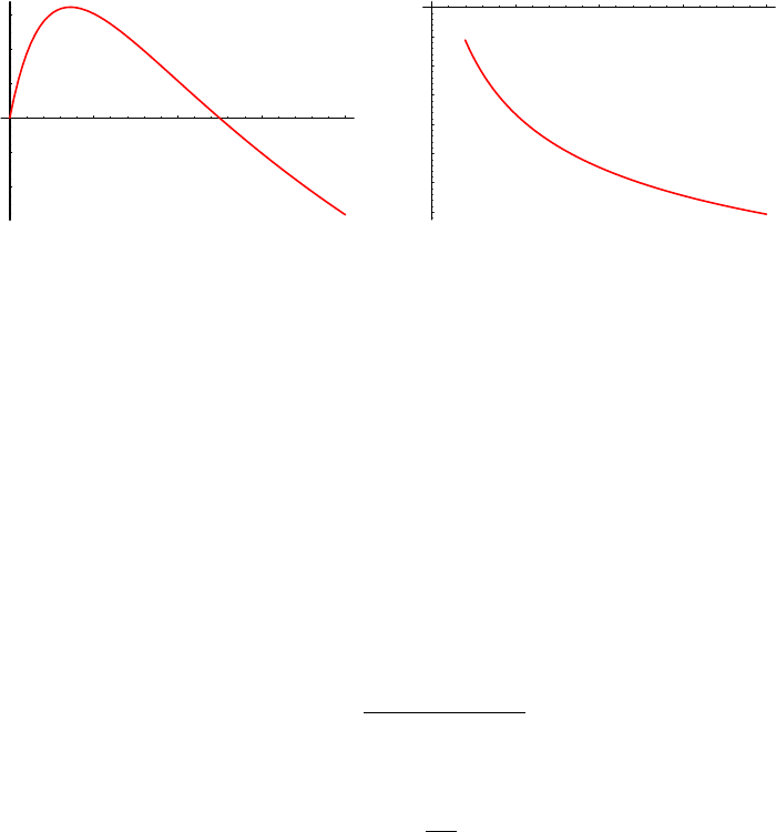
and
σC
L= 2 X(1 + X(4 + 5 X)) −(1 + X) (1 + 2 X)2ln(1 + 2 X) (17.43)
0.5 1 1.5 2
X
-4
-2
2
4
6
AC, % (a)
5 10 15 20
X
-35
-30
-25
-20
-15
-10
-5
AC, % (b)
Figure 17.11: Compton total cross section asymmetry depending on the en-
ergy of incoming photon. Left part, between 0 and ∼1 MeV, right part –
up to 10MeV.
Mean free path
When simulating the Compton scattering of a photon with an atomic elec-
tron, an empirical cross section formula is used, which reproduces the cross
section data down to 10 keV (see section 5.3). If both, beam and target, are
polarized this mean free path has to be corrected.
In the class G4ComptonScattering the polarized mean free path λpol is
defined on the basis of the the unpolarized mean free path λunpol via
λpol =λunpol
1 + ζ(1)
3ζ(2)
3AC
L
(17.44)
where
AC
L=σA
L
σA
0
(17.45)
is the expected asymmetry from the the total polarized Compton cross sec-
tion given above. This asymmetry is depicted in figure 17.11.
17.4.3 Sampling the final state
Differential Compton Cross Section
In the ultra-relativistic approximation the dependence of the differential cross
section on the longitudinal/circular degree of polarization is very simple. It
267
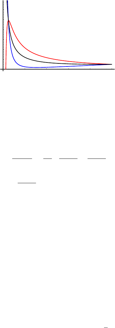
0.2 0.4 0.6 0.8 1
Ε
2
4
6
8
10
12
d2 Σ C
dΕdΦCompton cross section
Figure 17.12: Compton scattering differential cross section in arbitrary units.
Black line corresponds to the unpolarized cross section; red line – to the
antiparallel spins of initial particles, and blue line – to the parallel spins.
Energy of the incoming photon Ek1= 10MeV.
reads
dσC
URA
dedϕ =re2
X ǫ2+ 1
2ǫ+ǫ2−1
2ǫζ(1)
3ζ(2)
3+ζ(2)
3ξ(1)
3−ζ(1)
3ξ(2)
3
+ǫ2+ 1
2ǫζ(1)
3ξ(1)
3−ζ(2)
3ξ(2)
3!(17.46)
where re= classical electron radius
X=Ek1/mec2
Ek1= energy of the incident photon
mec2= electron mass
The fully polarized differential cross section is available in the class G4PolarizedComptonCrossSe
It takes all mass effects into account, but binding effects are neglected [1, 2].
The cross section dependence on ǫfor right handed circularly polarized pho-
tons and longitudinally polarized electrons is plotted in figure 17.12
Sampling
The photon energy is sampled according to methods discussed in Chapter 2.
The differential cross section can be approximated by a simple function Φ(ǫ):
Φ(ǫ) = 1
ǫ+ǫ(17.47)
268
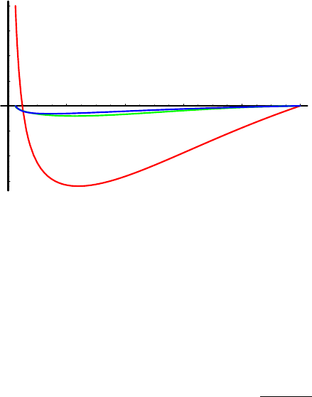
0.2 0.4 0.6 0.8 1
Ε
-75
-50
-25
25
50
75
100
A, % Compton asymmetries
Figure 17.13: Compton scattering differential cross section asymmetries in%.
Red line corresponds to the asymmetry due to circular photon and longitudi-
nal electron initial state polarization, green line – due to circular photon and
transverse electron initial state polarization, blue line – due to linear photon
and transverse electron initial state polarization.
with the kinematic limits given by
ǫmin =1
1 + 2X(17.48)
ǫmax = 1 (17.49)
The kinematic of the scattered photon is constructed by the following
steps:
1. ǫis sampled from Φ(ǫ)
2. calculate the differential cross section, depending on the initial polar-
izations ζ(1) and ζ(2), which the correct normalization.
3. ǫis accepted with the probability defined by ratio of the differential
cross section over the approximation function.
4. The ϕis diced uniformly.
5. ϕis determined from the differential cross section, depending on the
initial polarizations ζ(1) and ζ(2).
In figure 17.13 the asymmetries indicate the influence of polarization for an
10MeV incoming positron. The actual behavior is very sensitive to energy of
the incoming positron.
269
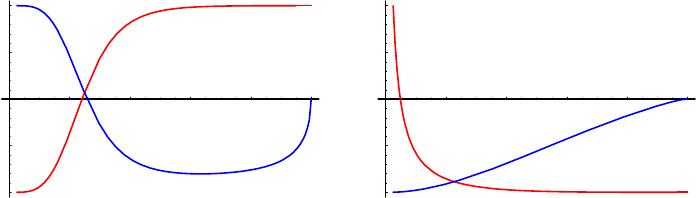
Polarization transfer
After the kinematics is fixed the polarization of the outgoing photon is de-
termined. Using the dependence of the differential cross section on the final
state polarizations a mean polarization is calculated for each photon accord-
ing to the method described in section 17.1.
The resulting polarization transfer functions ξ(1,2)(ǫ) are depicted in figure
17.14.
0.2 0.4 0.6 0.8 1
Ε
-1
-0.5
0.5
1
Γ: Circ=1, e-: POL=1
0.2 0.4 0.6 0.8 1
Ε
-1
-0.5
0.5
1
Γ: Circ=-1, e-: POL=0
Figure 17.14: Polarization Transfer in Compton scattering. Blue line corre-
sponds to the longitudinal polarization ξ(2)
3of the electron, red line – circular
polarization ξ(1)
3of the photon.
Bibliography
[1] P. Starovoitov et.al., in preparation.
[2] F.W. Lipps, H.A. Tolhoek, Physica 20 (1954) 85; F.W. Lipps, H.A. Tol-
hoek, Physica 20 (1954) 395.
270
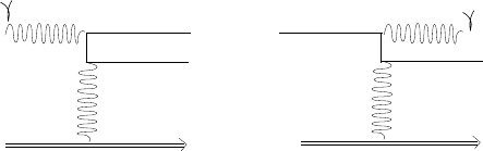
17.5 Polarized Bremsstrahlung for electron
and positron
17.5.1 Method
The polarized version of Bremsstrahlung is based on the unpolarized cross
section. Energy loss, mean free path, and distribution of explicitly generated
final state particles are treated by the unpolarized version G4eBremsstrahlung.
For details consult section 8.2.
The remaining task is to attribute polarization vectors to the generated
final state particles, which is discussed in the following.
17.5.2 Polarization in gamma conversion and brems-
strahlung
Gamma conversion and bremsstrahlung are cross-symmetric processes (i.e.
the Feynman diagram for electron bremsstrahlung can be obtained from the
gamma conversion diagram by flipping the incoming photon and outgoing
positron lines) and their cross sections closely related. For both processes,
the interaction occurs in the field of the nucleus and the total and differential
cross section are polarization independent. Therefore, only the polarization
transfer from the polarized incoming particle to the outgoing particles is
taken into account.
e−
N1 N2
q
k
e− P−
P’−
N1 N2
k
q
P+
P−
e+
e−
Gamma conversion Bremsstrahlung
Figure 17.15: Feynman diagrams of Gamma conversion and bremsstrahlung
processes.
For both processes, the scattering can be formulated by:
K1(k1,ζ(1)) + N1(kN1,ζ(N1))−→ P1(p1,ξ(1)) + P2(p2,ξ(2)) + N2(pN2,ξ(N2))
(17.50)
Where N1(kN1,ζ(N1)) and N2(pN2,ξ(N2)) are the initial and final state of
the field of the nucleus respectively assumed to be unchanged, at rest and
unpolarized. This leads to kN1=kN2= 0 and ζ(N1)=ξ(N2)= 0
271
In the case of gamma conversion process:
K1(k1,ζ(1)) is the incoming photon initial state with momentum k1and po-
larization state ζ(1).
P1(p1,ξ(1)) and P2(p2,ξ(2)) are the two photons final states with momenta
p1and p2and polarization states ξ(1) and ξ(2).
In the case of bremsstrahlung process:
K1(k1,ζ(1)) is the incoming lepton e−(e+) initial state with momentum k1
and polarization state ζ(1).
P1(p1,ξ(1)) is the lepton e−(e+) final state with momentum p1and polariza-
tion state ξ(1).
P2(p2,ξ(2)) is the bremsstrahlung photon in final state with momentum p2
and polarization state ξ(2).
17.5.3 Polarization transfer from the lepton e−(e+)to
a photon
The polarization transfer from an electron (positron) to a photon in a brems-
strahlung process was first calculated by Olsen and Maximon [1] taking into
account both Coulomb and screening effects. In the Stokes vector formalism,
the e−(e+) polarization state can be transformed to a photon polarization
finale state by means of interaction matrix Tb
γ. It defined via
O
ξ(2) =Tb
γ1
ζ(1) ,(17.51)
and
Tb
γ≈
1 0 0 0
D0 0 0
0 0 0 0
0T0L
,(17.52)
where
I= (ǫ2
1+ǫ2
2)(3 + 2Γ) −2ǫ1ǫ2(1 + 4u2ˆ
ξ2Γ) (17.53)
D=n8ǫ1ǫ2u2ˆ
ξ2Γo/I (17.54)
T=n−4kǫ2ˆ
ξ(1 −2ˆ
ξ)uΓo/I (17.55)
L=k{(ǫ1+ǫ2)(3 + 2Γ) −2ǫ2(1 + 4u2ˆ
ξ2Γ)}/I (17.56)
and
272

ǫ1Total energy of the incoming lepton e+(e−) in units mc2
ǫ2Total energy of the outgoing lepton e+(e−) in units mc2
k= (ǫ1−ǫ2), the energy of the bremsstrahlung photon in units of mc2
pElectron (positron) initial momentum in units mc
kBremsstrahlung photon momentum in units mc
uComponent of pperpendicular to kin units mc and u=|u|
ˆ
ξ= 1/(1 + u2)
Coulomb and screening effects are contained in Γ, defined as follows
Γ = ln 1
δ−2−f(Z) + F ˆ
ξ
δ!for ∆ ≤120 (17.57)
Γ = ln 111
ˆ
ξZ 1
3−2−f(z) for ∆ ≥120 (17.58)
with
∆ = 12Z1
3ǫ1ǫ2ˆ
ξ
121kwith Zthe atomic number and δ=k
2ǫ1ǫ2(17.59)
f(Z) is the coulomb correction term derived by Davies, Bethe and Maxi-
mon [6]. F(ˆ
ξ/δ) contains the screening effects and is zero for ∆ ≤0.5 (No
screening effects). For 0.5≤∆≤120 (intermediate screening) it is a slowly
decreasing function. The F(ˆ
ξ/δ) values versus ∆ are given in table 17.1 and
used with a linear interpolation in between.
The polarization vector of the incoming e−(e+) must be rotated into the
frame defined by the scattering plane (x-z-plane) and the direction of the out-
going photon (z-axis). The resulting polarization vector of the bremsstrahlung
photon is also given in this frame. Using Eq. (17.51) and the transfer matrix
given by Eq. (17.52) the bremsstrahlung photon polarization state in the
Stokes formalism [2, 3] is given by
ξ(2) =
ξ(2)
1
ξ(2)
2
ξ(2)
3
≈
D
0
ζ(1)
1L+ζ(1)
2T
(17.60)
17.5.4 Remaining polarization of the lepton after emit-
ting a bremsstrahlung photon
The e−(e+) polarization final state after emitting a bremsstrahlung photon
can be calculated using the interaction matrix Tb
lwhich describes the lepton
273

Table 17.1: F(ˆ
ξ/δ) for intermediate values of the screening factor [7].
∆−F ˆ
ξ/δ∆−F ˆ
ξ/δ
0.5 0.0145 40.0 2.00
1.0 0.0490 45.0 2.114
2.0 0.1400 50.0 2.216
4.0 0.3312 60.0 2.393
8.0 0.6758 70.0 2.545
15.0 1.126 80.0 2.676
20.0 1.367 90.0 2.793
25.0 1.564 100.0 2.897
30.0 1.731 120.0 3.078
35.0 1.875
depolarization. The polarization vector for the outgoing e−(e+) is not given
by Olsen and Maximon. However, their results can be used to calculate the
following transfer matrix [4, 5].
O
ξ(1) =Tb
l1
ζ(1) (17.61)
Tb
l≈
1 0 0 0
D M 0E
0 0 M0
0F0M+P
(17.62)
where
I= (ǫ2
1+ǫ2
2)(3 + 2Γ) −2ǫ1ǫ2(1 + 4u2ˆ
ξ2Γ) (17.63)
F=ǫ2n4kˆ
ξu(1 −2ˆ
ξ)Γo/I (17.64)
E=ǫ1n4kˆ
ξu(2ˆ
ξ−1)Γo/I (17.65)
M=n4kǫ1ǫ2(1 + Γ −2u2ˆ
ξ2Γ)o/I (17.66)
P=nk2(1 + 8Γ(ˆ
ξ−0.5)2o/I (17.67)
and
274
ǫ1Total energy of the incoming e+/e−in units mc2
ǫ2Total energy of the outgoing e+/e−in units mc2
k= (ǫ1−ǫ2), energy of the photon in units of mc2
pElectron (positron) initial momentum in units mc
kPhoton momentum in units mc
uComponent of pperpendicular to kin units mc and u=|u|
Using Eq. (17.61) and the transfer matrix given by Eq. (17.62) the e−(e+)
polarization state after emitting a bremsstrahlung photon is given in the
Stokes formalism by
ξ(1) =
ξ(1)
1
ξ(1)
2
ξ(1)
3
≈
ζ(1)
1M+ζ(1)
3E
ζ(1)
2M
ζ(1)
3(M+P) + ζ(1)
1F
.(17.68)
Bibliography
[1] H. Olsen and L.C. Maximon. Photon and electron polarization in high-
energy bremsstrahlung and pair production with screening. Physical Re-
view, 114:887-904, 1959.
[2] W.H. McMaster. Polarization and the Stokes parameters. American Jour-
nal of Physics, 22(6):351-362, 1954.
[3] W.H. McMaster. Matrix representation of polarization. Reviews of Mod-
ern Physics, 33(1):8-29, 1961.
[4] K. Fl¨ottmann. Investigations toward the development of polarized and
unpolarized high intensity positron sources for linear colliders. PhD the-
sis, Universitat Hamburg, 1993.
[5] Hoogduin, Johannes Marinus, Electron, positron and photon polarimetry.
PhD thesis, Rijksuniversiteit Groningen 1997.
[6] H. Davies, H.A. Bethe and L.C. Maximon, Theory of Bremsstrahlung and
Pair Production. II. Integral Cross Section for Pair Production, Physical
Review, 93(4):788-795, 1954.
[7] H.W. Koch and J.W. Motz, Bremsstrahlung cross-section formulas and
related data. Review Mod. Phys., 31(4):920-955, 1959.
[8] K. Laihem, PhD thesis, Measurement of the positron polarization at an
helical undulator based positron source for the International Linear Col-
lider ILC, Humboldt University Berlin, Germany, (2008).
275
17.6 Polarized Gamma conversion into an electron–
positron pair
17.6.1 Method
The polarized version of gamma conversion is based on the EM standard pro-
cess G4GammaConversion. Mean free path and the distribution of explicitly
generated final state particles are treated by this version. For details consult
section 5.4.
The remaining task is to attribute polarization vectors to the generated
final state leptons, which is discussed in the following.
17.6.2 Polarization transfer from the photon to the
two leptons
Gamma conversion process is essentially the inverse process of Bremsstrahlung
and the interaction matrix is obtained by inverting the rows and columns of
the bremsstrahlung matrix and changing the sign of ǫ2, cf. section 17.5. It
follows from the work by Olsen and Maximon [1] that the polarization state
ξ(1) of an electron or positron after pair production is obtained by
O
ξ(1) =Tp
l1
ζ(1) (17.69)
and
Tp
l≈
1D0 0
000T
0 0 0 0
000L
,(17.70)
where
I= (ǫ2
1+ǫ2
2)(3 + 2Γ) + 2ǫ1ǫ2(1 + 4u2ˆ
ξ2Γ) (17.71)
D=n−8ǫ1ǫ2u2ˆ
ξ2Γo/I (17.72)
T=n−4kǫ2ˆ
ξ(1 −2ˆ
ξ)uΓo/I (17.73)
L=k{(ǫ1−ǫ2)(3 + 2Γ) + 2ǫ2(1 + 4u2ˆ
ξ2Γ)}/I (17.74)
and
276
ǫ1total energy of the first lepton e+(e−) in units mc2
ǫ2total energy of the second lepton e−(e+) in units mc2
k= (ǫ1+ǫ2) energy of the incoming photon in units of mc2
pelectron=positron initial momentum in units mc
kphoton momentum in units mc
uelectron/positron initial momentum in units mc
u=|u|
Coulomb and screening effects are contained in Γ, defined in section 17.5.
Using Eq. (17.69) and the transfer matrix given by Eq. (17.70) the polar-
ization state of the produced e−(e+) is given in the Stokes formalism by:
ξ(1) =
ξ(1)
1
ξ(1)
2
ξ(1)
3
≈
ζ(1)
3T
0
ζ(1)
3L
(17.75)
Bibliography
[1] H. Olsen and L.C. Maximon. Photon and electron polarization in high-
energy bremsstrahlung and pair production with screening. Physical Re-
view, 114:887-904, 1959.
[2] K. Laihem, PhD thesis, Measurement of the positron polarization at an
helical undulator based positron source for the International Linear Col-
lider ILC, Humboldt University Berlin, Germany, (2008).
277
17.7 Polarized Photoelectric Effect
17.7.1 Method
This section describes the basic formulas of polarization transfer in the pho-
toelectric effect class (G4PolarizedPhotoElectricEffect). The photoelectric
effect is the emission of electrons from matter upon the absorption of elec-
tromagnetic radiation, such as ultraviolet radiation or x-rays. The energy
of the photon is completely absorbed by the electron and, if sufficient, the
electron can escape from the material with a finite kinetic energy. A single
photon can only eject a single electron, as the energy of one photon is only
absorbed by one electron. The electrons that are emitted are often called
photoelectrons. If the photon energy is higher than the binding energy the
remaining energy is transferred to the electron as a kinetic energy
Ee−
kin =k−Bshell (17.76)
In Geant4 the photoelectric effect process is taken into account if:
k > Bshell (17.77)
Where kis the incoming photon energy and Bshell the electron binding energy
provided by the class G4AtomicShells.
The polarized version of the photoelectric effect is based on the EM stan-
dard process G4PhotoElectricEffect. Mean free path and the distribution
of explicitly generated final state particles are treated by this version. For
details consult section 5.2.
The remaining task is to attribute polarization vectors to the generated
final state electron, which is discussed in the following.
17.7.2 Polarization transfer
The polarization state of an incoming polarized photon is described by the
Stokes vector ~
ζ(1). The polarization transfer to the photoelectron can be de-
scribed in the Stokes formalism using the same approach as for the Bremsstrahlung
and gamma conversion processes, cf. 17.5 and 17.6. The relation between the
photoelectron’s Stokes parameters and the incoming photon’s Stokes param-
eters is described by the interaction matrix Tp
lderived from H. Olsen [1] and
reviewed by H.W McMaster [2]:
I′
~
ξ(1) =Tp
lI0
~
ζ(1) (17.78)
278
In general, for the photoelectric effect as a two-body scattering, the cross
section should be correlated with the spin states of the incoming photon
and the target electron. In our implementation the target electron is not
polarized and only the polarization transfer from the photon to the pho-
toelectron is taken into account. In this case the cross section of the pro-
cess remains polarization independent. To compute the matrix elements we
take advantage of the available kinematic variables provided by the generic
G4PhotoelectricEffect class. To compute the photoelectron spin state (Stokes
parameters), four main parameters are needed:
•The incoming photon Stokes vector ~
ζ(1)
•The incoming photon’s energy k.
•the photoelectron’s kinetic energy Ee−
kin or the Lorentz factors βand γ.
•The photoelectron’s polar angle θor cos θ.
The interaction matrix derived by H. Olsen [1] is given by:
TP
l=
1 + D−D0 0
0 0 0 B
0 0 0 0
0 0 0 A
(17.79)
Where
D=1
k2
kǫ(1 −βcos θ)−1(17.80)
A=ǫ
ǫ+ 1 2
kǫ +βcos θ+2
kǫ2(1 −βcos θ)(17.81)
B=ǫ
ǫ+ 1βsin θ2
kǫ(1 −βcos θ)−1(17.82)
Using Eq. (17.78) and the transfer matrix given by Eq. (17.79) the polar-
ization state of the produced e−is given in the Stokes formalism by:
~
ξ(1) =
ξ(1)
1
ξ(1)
2
ξ(1)
3
=
ζ(1)
3B
0
ζ(1)
3A
(17.83)
From equation (17.83) one can see that a longitudinally (transversally)
polarized photoelectron can only be produced if the incoming photon is cir-
cularly polarized.
279
Bibliography
[1] H. Olsen, Kgl. N. Videnskab. Selskabs Forh. 31, Nos 11, 11a (1958).
[2] W.H. McMaster. Matrix representation of polarization. Reviews of Mod-
ern Physics, 33(1):8-29, 1961.
[3] K. Laihem, PhD thesis, Measurement of the positron polarization at an
helical undulator based positron source for the International Linear Col-
lider ILC, Humboldt University Berlin, Germany, (2008).
280
Chapter 18
X-Ray Production
281

18.1 Transition radiation
18.1.1 The Relationship of Transition Radiation to X-
ray Cherenkov Radiation
X-ray transition radiation (XTR ) occurs when a relativistic charged particle
passes from one medium to another of a different dielectric permittivity. In
order to describe this process it is useful to begin with an explanation of
X-ray Cherenkov radiation, which is closely related.
The mean number of X-ray Cherenkov radiation (XCR) photons of fre-
quency ωemitted into an angle θper unit distance along a particle trajectory
is [1]
d3¯
Nxcr
~dω dx dθ2=α
π~c
ω
cθ2Im {Z}.(18.1)
Here the quantity Zis introduced as the complex formation zone of XCR in
the medium:
Z=L
1−iL
l
, L =c
ωγ−2+ω2
p
ω2+θ2−1
, γ−2= 1 −β2.(18.2)
with land ωpthe photon absorption length and the plasma frequency, re-
spectively, in the medium. For the case of a transparent medium, l→ ∞
and the complex formation zone reduces to the coherence length Lof XCR.
The coherence length roughly corresponds to that part of the trajectory in
which an XCR photon can be created.
Introducing a complex quantity Zwith its imaginary part proportional
to the absorption cross-section (∼l−1) is required in order to account for
absorption in the medium. Usually, ω2
p/ω2≫c/ωl. Then it can be seen from
Eqs. 18.1 and 18.2 that the number of emitted XCR photons is considerably
suppressed and disappears in the limit of a transparent medium. This is
caused by the destructive interference between the photons emitted from
different parts of the particle trajectory.
The destructive interference of X-ray Cherenkov radiation is removed if
the particle crosses a boundary between two media with different dielectric
permittivities, ǫ, where
ǫ= 1 −ω2
p
ω2+ic
ωl .(18.3)
Here the standard high-frequency approximation for the dielectric permittiv-
ity has been used. This is valid for energy transfers larger than the K-shell
excitation potential.
282
If layers of media are alternated with spacings of order L, the X-ray
radiation yield from a trajectory of unit length can be increased by roughly
l/L times. The radiation produced in this case is called X-ray transition
radiation (XTR).
18.1.2 Calculating the X-ray Transition Radiation Yield
Using the methods developed in Ref. [2] one can derive the relation describing
the mean number of XTR photons generated per unit photon frequency and
θ2inside the radiator for a general XTR radiator consisting of ndifferent
absorbing media with fluctuating thicknesses:
d2¯
Nin
~dω dθ2=α
π~c2ωθ2Re (n−1
X
i=1
(Zi−Zi+1)2+ (18.4)
+ 2
n−1
X
k=1
k−1
X
i=1
(Zi−Zi+1)"k
Y
j=i+1
Fj#(Zk−Zk+1)), Fj= exp −tj
2Zj.
In the case of gamma distributed gap thicknesses (foam or fiber radiators)
the values Fj, (j= 1,2) can be estimated as:
Fj=Z∞
0
dtjνj
¯
tjνjtνj−1
j
Γ(νj)exp −νjtj
¯
tj−itj
2Zj=1 + i¯
tj
2Zjνj−νj
,
(18.5)
where Zjis the complex formation zone of XTR (similar to relation 18.2
for XCR) in the j-th medium [2, 6]. Γ is the Euler gamma function, ¯
tjis
the mean thickness of the j-th medium in the radiator and νj>0 is the
parameter roughly describing the relative fluctuations of tj. In fact, the
relative fluctuation is δtj/¯
tj∼1/√νj.
In the particular case of nfoils of the first medium (Z1, F1) interspersed
with gas gaps of the second medium (Z2, F2), one obtains:
d2¯
Nin
~dω dθ2=2α
π~c2ωθ2Re hR(n)i, F =F1F2,(18.6)
hR(n)i= (Z1−Z2)2n(1 −F1)(1 −F2)
1−F+(1 −F1)2F2[1 −Fn]
(1 −F)2.(18.7)
Here hR(n)iis the stack factor reflecting the radiator geometry. The integra-
tion of (18.6) with respect to θ2can be simplified for the case of a regular
radiator (ν1,2→ ∞), transparent in terms of XTR generation media, and
283

n≫1 [3]. The frequency spectrum of emitted XTR photons is given by:
d¯
Nin
~dω =Z∼10γ−2
0
dθ2d2¯
Nin
~dω dθ2=4αn
π~ω(C1+C2)2
·
kmax
X
k=kmin
(k−Cmin)
(k−C1)2(k+C2)2sin2πt1
t1+t2
(k+C2),
(18.8)
C1,2=t1,2(ω2
1−ω2
2)
4πcω , Cmin =1
4πc ω(t1+t2)
γ2+t1ω2
1+t2ω2
2
ω.
The sum in (18.8) is defined by terms with k≥kmin corresponding to the
region of θ≥0. Therefore kmin should be the nearest to Cmin integer kmin ≥
Cmin. The value of kmax is defined by the maximum emission angle θ2
max ∼
10γ−2. It can be evaluated as the integer part of
Cmax =Cmin +ω(t1+t2)
4πc
10
γ2, kmax −kmin ∼102÷103≫1.
Numerically, however, only a few tens of terms contribute substantially to the
sum, that is, one can choose kmax ∼kmin + 20. Equation (18.8) corresponds
to the spectrum of the total number of photons emitted inside a regular
transparent radiator. Therefore the mean interaction length, λXT R, of the
XTR process in this kind of radiator can be introduced as:
λXT R =n(t1+t2)Z~ωmax
~ωmin
~dω d¯
Nin
~dω −1
,
where ~ωmin ∼1 keV, and ~ωmax ∼100 keV for the majority of high energy
physics experiments. Its value is constant along the particle trajectory in
the approximation of a transparent regular radiator. The spectrum of the
total number of XTR photons after regular transparent radiator is defined
by (18.8) with:
n→neff =
n−1
X
k=0
exp[−k(σ1t1+σ2t2)] = 1−exp[−n(σ1t1+σ2t2)]
1−exp[−(σ1t1+σ2t2)] ,
where σ1and σ2are the photo-absorption cross-sections corresponding to the
photon frequency ωin the first and the second medium, respectively. With
this correction taken into account the XTR absorption in the radiator (18.8)
corresponds to the results of [4]. In the more general case of the flux of XTR
284

photons after a radiator, the XTR absorption can be taken into account with
a calculation based on the stack factor derived in [5]:
hR(n)
fluxi= (L1−L2)21−Qn
1−Q
(1 + Q1)(1 + F)−2F1−2Q1F2
2(1 −F)
+(1 −F1)(Q1−F1)F2(Qn−Fn)
(1 −F)(Q−F),(18.9)
Q=Q1·Q2, Qj= exp [−tj/lj] = exp [−σjtj], j = 1,2.
Both XTR energy loss (18.7) and flux (18.9) models can be implemented as
a discrete electromagnetic process (see below).
18.1.3 Simulating X-ray Transition Radiation Produc-
tion
A typical XTR radiator consits of many (∼100) boundaries between different
materials. To improve the tracking performance in such a volume one can
introduce an artificial material [6], which is the geometrical mixture of foil
and gas contents. Here is an example:
// In DetectorConstruction of an application
// Preparation of mixed radiator material
foilGasRatio = fRadThickness/(fRadThickness+fGasGap);
foilDensity = 1.39*g/cm3; // Mylar
gasDensity = 1.2928*mg/cm3 ; // Air
totDensity = foilDensity*foilGasRatio +
gasDensity*(1.0-foilGasRatio);
fractionFoil = foilDensity*foilGasRatio/totDensity;
fractionGas = gasDensity*(1.0-foilGasRatio)/totDensity;
G4Material* radiatorMat = new G4Material("radiatorMat",
totDensity,
ncomponents = 2 );
radiatorMat->AddMaterial( Mylar, fractionFoil );
radiatorMat->AddMaterial( Air, fractionGas );
G4cout << *(G4Material::GetMaterialTable()) << G4endl;
// materials of the TR radiator
fRadiatorMat = radiatorMat; // artificial for geometry
fFoilMat = Mylar;
fGasMat = Air;
This artificial material will be assigned to the logical volume in which
XTR will be generated:
285

solidRadiator = new G4Box("Radiator",
1.1*AbsorberRadius ,
1.1*AbsorberRadius,
0.5*radThick );
logicRadiator = new G4LogicalVolume( solidRadiator,
fRadiatorMat, // !!!
"Radiator");
physiRadiator = new G4PVPlacement(0,
G4ThreeVector(0,0,zRad),
"Radiator", logicRadiator,
physiWorld, false, 0 );
XTR photons generated by a relativistic charged particle intersecting a
radiator with 2ninterfaces between different media can be simulated by using
the following algorithm. First the total number of XTR photons is estimated
using a Poisson distribution about the mean number of photons given by the
following expression:
¯
N(n)=Zω2
ω1
dω Zθ2
max
0
dθ2d2¯
N(n)
dω dθ2=2α
πc2Zω2
ω1
ωdω Zθ2
max
0
θ2dθ2Re hR(n)i.
Here θ2
max ∼10γ−2,~ω1∼1 keV, ~ω2∼100 keV, and hR(n)icorrespond to
the geometry of the experiment. For events in which the number of XTR
photons is not equal to zero, the energy and angle of each XTR quantum is
sampled from the integral distributions obtained by the numerical integration
of expression (18.6). For example, the integral energy spectrum of emitted
XTR photons, ¯
N(n)
>ω , is defined from the following integral distribution:
¯
N(n)
>ω =2α
πc2Zω2
ω
ωdω Zθ2
max
0
θ2dθ2Re hR(n)i.
In Geant4 XTR generation inside or after radiators is described as a dis-
crete electromagnetic process. It is convenient for the description of tracks in
magnetic fields and can be used for the cases when the radiating charge ex-
periences a scattering inside the radiator. The base class G4VXTRenergyLoss
is responsible for the creation of tables with integral energy and angular
distributions of XTR photons. It also contains the PostDoIt function pro-
viding XTR photon generation and motion (if fExitFlux=true) through a
XTR radiator to its boundary. Particular models like G4RegularXTRadiator
implement the pure virtual function GetStackFactor, which calculates the
response of the XTR radiator reflecting its geometry. Included below are
some comments for the declaration of XTR in a user application.
286
In the physics list one should pass to the XTR process additional details
of the XTR radiator involved:
// In PhysicsList of an application
else if (particleName == "e-") // Construct processes for electron with XTR
{
pmanager->AddProcess(new G4MultipleScattering, -1, 1,1 );
pmanager->AddProcess(new G4eBremsstrahlung(), -1,-1,1 );
pmanager->AddProcess(new Em10StepCut(), -1,-1,1 );
// in regular radiators:
pmanager->AddDiscreteProcess(
new G4RegularXTRadiator // XTR dEdx in general regular radiator
// new G4XTRRegularRadModel - XTR flux after general regular radiator
// new G4TransparentRegXTRadiator - XTR dEdx in transparent
// regular radiator
// new G4XTRTransparentRegRadModel - XTR flux after transparent
// regular radiator
(pDet->GetLogicalRadiator(), // XTR radiator
pDet->GetFoilMaterial(), // real foil
pDet->GetGasMaterial(), // real gas
pDet->GetFoilThick(), // real geometry
pDet->GetGasThick(),
pDet->GetFoilNumber(),
"RegularXTRadiator"));
// or for foam/fiber radiators:
pmanager->AddDiscreteProcess(
new G4GammaXTRadiator - XTR dEdx in general foam/fiber radiator
// new G4XTRGammaRadModel - XTR flux after general foam/fiber radiator
( pDet->GetLogicalRadiator(),
1000.,
100.,
pDet->GetFoilMaterial(),
pDet->GetGasMaterial(),
pDet->GetFoilThick(),
pDet->GetGasThick(),
pDet->GetFoilNumber(),
"GammaXTRadiator"));
}
Here for the foam/fiber radiators the values 1000 and 100 are the νparame-
ters (which can be varied) of the Gamma distribution for the foil and gas gaps,
287
respectively. Classes G4TransparentRegXTRadiator and G4XTRTransparentRegRadModel
correspond (18.8) to nand nef f , respectively.
Bibliography
[1] V.M. Grichine, Nucl. Instr. and Meth.,A482 (2002) 629.
[2] V.M. Grichine, Physics Letters,B525 (2002) 225-239
[3] G.M. Garibyan, Sov. Phys. JETP 32 (1971) 23.
[4] C.W. Fabian and W. Struczinski Physics Letters,B57 (1975) 483.
[5] G.M. Garibian, L.A. Gevorgian, and C. Yang, Sov. Phys.- JETP, 39
(1975) 265.
[6] J. Apostolakis, S. Giani, V. Grichine et al., Comput. Phys. Commun.
132 (2000) 241.
288
18.2 Scintillation
Every scintillating material has a characteristic light yield, Y(photons/MeV ),
and an intrinsic resolution which generally broadens the statistical distribu-
tion, σi/σs>1, due to impurities which are typical for doped crystals like
NaI(Tl) and CsI(Tl). The average yield can have a non-linear dependence
on the local energy deposition. Scintillators also have a time distribution
spectrum with one or more exponential decay time constants, τi, with each
decay component having its intrinsic photon emission spectrum. These are
empirical parameters typical for each material.
The generation of scintillation light can be simulated by sampling the number
of photons from a Poisson distribution. This distribution is based on the
energy lost during a step in a material and on the scintillation properties of
that material. The frequency of each photon is sampled from the empirical
spectra. The photons are generated evenly along the track segment and are
emitted uniformly into 4πwith a random linear polarization.
289

18.3 ˇ
Cerenkov Effect
The radiation of ˇ
Cerenkov light occurs when a charged particle moves through
a dispersive medium faster than the speed of light in that medium. A dis-
persive medium is one whose index of refraction is an increasing function of
photon energy. Two things happen when such a particle slows down:
1. a cone of ˇ
Cerenkov photons is emitted, with the cone angle (measured
with respect to the particle momentum) decreasing as the particle loses
energy;
2. the momentum of the photons produced increases, while the number
of photons produced decreases.
When the particle velocity drops below the local speed of light, photons are
no longer emitted. At that point, the ˇ
Cerenkov cone collapses to zero.
In order to simulate ˇ
Cerenkov radiation the number of photons per track
length must be calculated. The formulae used for this calculation can be
found below and in [1, 2]. Let nbe the refractive index of the dielectric
material acting as a radiator. Here n=c/c′where c′is the group velocity of
light in the material, hence 1 ≤n. In a dispersive material nis an increasing
function of the photon energy ǫ(dn/dǫ ≥0). A particle traveling with speed
β=v/c will emit photons at an angle θwith respect to its direction, where
θis given by
cos θ=1
βn.
From this follows the limitation for the momentum of the emitted photons:
n(ǫmin) = 1
β.
Photons emitted with an energy beyond a certain value are immediately
re-absorbed by the material; this is the window of transparency of the radi-
ator. As a consequence, all photons are contained in a cone of opening angle
cos θmax = 1/(βn(ǫmax)).
The average number of photons produced is given by the relations :
dN =αz2
~csin2θdǫdx =αz2
~c(1 −1
n2β2)dǫdx
≈370z2photons
eV cm (1 −1
n2β2)dǫdx
290

and the number of photons generated per track length is
dN
dx ≈370z2Zǫmax
ǫmin
dǫ 1−1
n2β2= 370z2ǫmax −ǫmin −1
β2Zǫmax
ǫmin
dǫ
n2(ǫ)
.
The number of photons produced is calculated from a Poisson distribution
with a mean of hni= StepLength dN/dx. The energy distribution of the
photon is then sampled from the density function
f(ǫ) = 1−1
n2(ǫ)β2
.
Bibliography
[1] J.D.Jackson, Classical Electrodynamics, John Wiley and Sons (1998)
[2] D.E. Groom et al. Particle Data Group . Rev. of Particle Properties.
Eur. Phys. J. C15,1 (2000) http://pdg.lbl.gov/
291

18.4 Synchrotron Radiation
18.4.1 Photon spectrum
Synchrotron radiation photons are emitted by relativistic charged particles
traveling in magnetic fields. The properties of synchrotron radiation are well
understood and described in textbooks [1, 2, 3].
In the simplest case, we have an electron of momentum pmoving perpen-
dicular to a homogeneous magnetic field B. The magnetic field will keep the
particle on a circular path, with radius
ρ=p
e B =mγβc
e B .Numerically we have ρ[m] = p[GeV/c] 3.336 m
B[T] .
(18.10)
In general, there will be an arbitrary angle θbetween the local magnetic
field Band momentum vector pof the particle. The motion has a circular
component in the plane perpendicular to the magnetic field, and in addition a
constant momentum component parallel to the magnetic field. For a constant
homogeneous field, the resulting trajectory is a helix.
The critical energy of the synchrotron radiation can be calculated using
the radius ρof Eq.18.10 and angle θor the magnetic field perpendicular to
the particle direction B⊥=Bsin θaccording to
Ec=3
2~cγ3sin θ
ρ=3~
2mγ2eB⊥.(18.11)
Half of the synchrotron radiation power is radiated by photons above the
critical energy.
With xwe denote the photon energy Eγ, expressed in units of the critical
energy Ec
x=Eγ
Ec
.(18.12)
The photon spectrum (number of photons emitted per path length sand
relative energy x) can be written as
d2N
ds dx =√3α
2π
eB⊥
mc Z∞
x
K5/3(ξ)dξ (18.13)
where α=e2/4πǫ0~cis the dimensionless electromagnetic coupling (or fine
structure) constant and K5/3is the modified Bessel function of the third kind.
The number of photons emitted per unit length and the mean free path
λbetween two photon emissions is obtained by integration over all photon
292
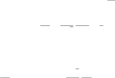
energies. Using Z∞
0
dx Z∞
x
K5/3(ξ)dξ =5π
3(18.14)
we find that dN
ds =5α
2√3
eB⊥
mβc =1
λ.(18.15)
Here we are only interested in ultra-relativistic (β≈1) particles, for
which λonly depends on the field Band not on the particle energy. We
define a constant λBsuch that
λ=λB
B⊥
where λB=2√3
5
m c
α e = 0.16183 Tm .(18.16)
As an example, consider a 10 GeV electron, travelling perpendicular to
a 1 T field. It moves along a circular path of radius ρ= 33.356 m. For the
Lorentz factor we have γ= 19569.5 and β= 1−1.4×10⁻⁹. The critical energy
is Ec= 66.5 keV and the mean free path between two photon emissions is
λ= 0.16183 m.
18.4.2 Validity
The spectrum given in Eq. 18.13 can generally be expected to provide a very
accurate description for the synchrotron radiation spectrum generated by
GeV electrons in magnetic fields.
Here we discuss some known limitations and possible extensions.
For particles traveling on a circular path, the spectrum observed in one
location will in fact not be a continuous spectrum, but a discrete spectrum,
consisting only of harmonics or modes nof the revolution frequency. In
practice, the mode numbers will generally be too high to make this a visible
effect. The critical mode number corresponding to the critical energy is
nc= 3/2γ3. 10 GeV electrons for example have nc≈1013.
Synchrotron radiation can be neglected for slower particles and only be-
comes relevant for ultra-relativistic particles with γ > 103. Using β= 1
introduces an uncertainty of about 1/2γ2or less than 5 ×10⁻⁷.
It is rather straightforward to extend the formulas presented here to par-
ticles other than electrons, with arbitrary charge qand mass m, see [4]. The
number of photons and the power scales with the square of the charge.
The standard synchrotron spectrum of Eq. 18.13 is only valid as long as
the photon energy remains small compared to the particle energy [5, 6]. This
is a very safe assumption for GeV electrons and standard magnets with fields
of order of Tesla.
293
An extension of synchrotron radiation to fields exceeding several hundred
Tesla, such as those present in the beam-beam interaction in linear-colliders,
is also known as beamstrahlung. For an introduction see [7].
The standard photon spectrum applies to homogeneous fields and re-
mains a good approximation for magnetic fields which remain approximately
constant over a the length ρ/γ, also known as the formation length for syn-
chrotron radiation. Short magnets and edge fields will result instead in more
energetic photons than predicted by the standard spectrum.
We also note that short bunches of many particles will start to radiate
coherently like a single particle of the equivalent charge at wavelengths which
are longer than the bunch dimensions.
Low energy, long-wavelength synchrotron radiation may destructively in-
terfere with conducting surfaces [8].
The soft part of the synchrotron radiation spectrum emitted by charged
particles travelling through a medium will be modified for frequencies close
to and lower than the plasma frequency [9].
18.4.3 Direct inversion and generation of the photon
energy spectrum
The task is to find an algorithm that effectively transforms the flat distri-
bution given by standard pseudo-random generators into the desired distri-
bution proportional to the expressions given in Eqs. 18.13, 18.17. The trans-
formation is obtained from the inverse F−1of the cumulative distribution
function F(x) = Rx
0f(t)dt.
Leaving aside constant factors, the probability density function relevant
for the photon energy spectrum is
SynRad(x) = Z∞
x
K5/3(t)dt . (18.17)
Numerical methods to evaluate K5/3are discussed in [10]. An efficient al-
gorithm to evaluate the integral SynRad using Chebyshev polynomials is
described in [11]. This has been used in an earlier version of the Monte Carlo
generator for synchrotron radiation using approximate transformations and
the rejection method [12].
The cumulative distribution function is the integral of the probability
density function. Here we have
SynRadInt(z) = Z∞
z
SynRad(x)dx , (18.18)
294
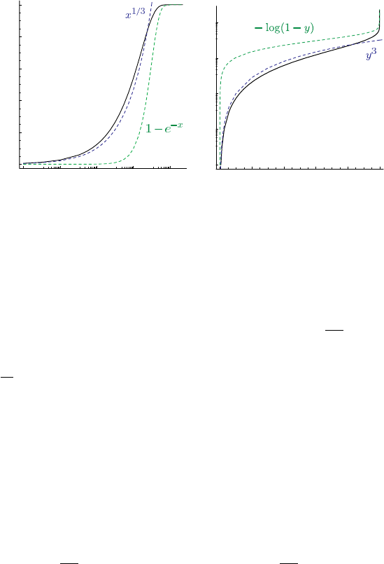
10-70.00001 0.001 0.1 10.
0.
0.2
0.4
0.6
0.8
1.
x
y
0. 0.2 0.4 0.6 0.8 1.
10-7
10-5
0.001
0.1
10.
x
y
Figure 18.1: SynFracInt (left) and its inverse InvSynFracInt (right), on a
log xscale. The functions x1/3,y3and 1 −e−x,−log(1 −y) are shown as
dashed lines.
with normalization
SynRadInt(0) = Z∞
0
SynRad(x)dx =5π
3,(18.19)
such that 3
5πSynRadInt(x) gives the fraction of photons above x.
It is possible to directly obtain the desired distribution with a fast and
accurate algorithm using an analytical description based on simple transfor-
mations and Chebyshev polynomials. This approach is used here.
We now describe in some detail how the analytical description was ob-
tained. For more details see [13].
It turned out to be convenient to start from the normalized complement
rather then Eq. 18.18 directly, that is
SynFracInt(x) = 3
5πZx
0Z∞
x
K5/3(t)dt dx = 1 −3
5πSynRadInt(x),(18.20)
which gives the fraction of photons below x.
Figure 18.1 shows on the left hand side y= SynFracInt(x) and on the
right hand side the inverse x= InvSynFracInt(y) together with simple ap-
proximate functions. We can see, that SynFracInt can be approximated by
x1/3for small arguments, and by 1 −e−xfor large x. Consequently, we have
for the inverse, InvSynFracInt(y), which can be approximated for small yby
y3and for large yby −log(1 −y).
Good convergence for InvSynFracInt(y) was obtained using Chebyshev
polynomials combined with the approximate expressions for small and large
arguments. For intermediate values, a Chebyshev polynomial can be used
directly. Table 18.1 summarizes the expressions used in the different intervals.
295
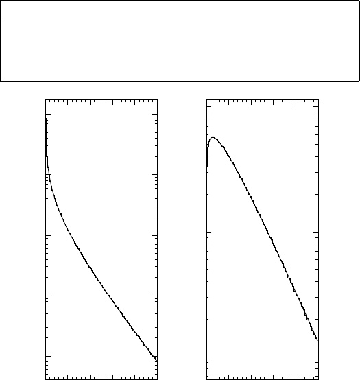
Table 18.1: InvSynFracInt.
y x = InvSynFracInt(y)
y < 0.7y3PCh(y)
0.7≤y≤0.9999 PCh(y)
y > 0.9999 −log(1 −y)PCh(−log(1 −y))
10 3
10 4
10 5
10 6
10 7
012345
x = Eγ / Ec
photon spectrum dN/dx
10 4
10 5
10 6
012345
x = Eγ / Ec
power spectrum x dN/dx
Figure 18.2: Comparison of the exact (smooth curve) and generated (his-
togram) spectra for 2 ×10⁷events. The photon spectrum is shown on the
left and the power spectrum on the right side.
The procedure for Monte Carlo simulation is to generate yat random uni-
formly distributed between 0 at 1, as provided by standard random gen-
erators, and then to calculate the energy xin units of the critical energy
according to x= InvSynFracInt(y).
The numerical accuracy of the energy spectrum presented here is about 14
decimal places, close to the machine precision. Fig. 18.2 shows a comparison
of generated and expected spectra. A Geant4 display of an electron moving
in a magnetic field radiating synchrotron photons is presented in Fig. 18.3
296
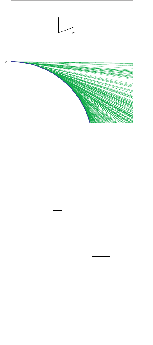
e+
-250 250
250
x [m]
y [m]
-250
x
y
z
B
Synchrotron radiation photons
Figure 18.3: Geant4 display. 10 GeV e+moving initially in x-direction, bends
downwards on a circular path by a 0.1 T magnetic field in z-direction.
18.4.4 Properties of the Power Spectra
The normalised probability function describing the photon energy spectrum
is
nγ(x) = 3
5πZ∞
x
K5/3(t)dt . (18.21)
nγ(x) gives the fraction of photons in the interval xto x+dx, where xis
the photon energy in units of the critical energy. The first moment or mean
value is
µ=Z∞
0
x nγ(x)dx =8
15 √3.(18.22)
implying that the mean photon energy is 8
15 √3= 0.30792 of the critical en-
ergy.
The second moment about the mean, or variance, is
σ2=Z∞
0
(x−µ)2nγ(x)dx =211
675 ,(18.23)
and the r.m.s. value of the photon energy spectrum is σ=q211
675 = 0.5591.
297

The normalised power spectrum is
Pγ(x) = 9√3
8πxZ∞
x
K5/3(t)dt . (18.24)
Pγ(x) gives the fraction of the power which is radiated in the interval xto
x+dx.
Half of the power is radiated below the critical energy
Z1
0
Pγ(x)dx = 0.5000 (18.25)
The mean value of the power spectrum is
µ=Z∞
0
x Pγ(x)dx =55
24 √3= 1.32309 .(18.26)
The variance is
σ2=Z∞
0
(x−µ)2Pγ(x)dx =2351
1728 ,(18.27)
and the r.m.s. width is σ=q2351
1728 = 1.16642.
Bibliography
[1] A.A.Sokolov and I.M.Ternov, Radiation from Relativistic Electrons,
Amer. Inst of Physics, 1986.
[2] J. Jackson, Classical Electrodynamics. John Wiley & Sons, third ed.,
1998.
[3] A. Hofmann, The Physics of Synchrotron Radiation. Cambridge Uni-
versity Press, 2004.
[4] H. Burkhardt, “Reminder of the Edge Effect in Synchrotron Radiation”,
LHC Project Note 172, CERN Geneva 1998.
[5] F. Herlach, R. McBroom, T. Erber, J. .Murray, and R. Gearhart, “Ex-
periments with Megagauss targets at SLAC”, IEEE Trans Nucl Sci, NS
18, 3 (1971) 809-814.
[6] T. Erber, G. B. Baumgartner, D. White, and H. G. Latal, “Megagauss
Bremsstrahlung and Radiation Reaction”, in *Batavia 1983, proceed-
ings, High Energy Accelerators*, 372-374.
298
[7] P. Chen, “An Introduction to Beamstrahlung and Disruption”, in Fron-
tiers of Particle Beams, M. Month and S. Turner, eds., Lecture Notes
in Physics 296, pp. 481–494. Springer-Verlag, 1986.
[8] J. B. Murphy, S. Krinsky, and R. L. Gluckstern, “Longitudinal wakefield
for an electron moving on a circular orbit”, Part. Acc. 57 (1997) 9.
[9] V. M. Grichine, “Radiation of accelerated charge in absorbing medium”,
CERN-OPEN-2002-056.
[10] Y. Luke, “The special functions and their approximations”, New York,
NY: Academic Press, 1975.- 585 p.
[11] H.H.Umst¨atter. CERN/PS/SM/81-13, CERN Geneva 1981.
[12] H. Burkhardt, “Monte Carlo Generator for Synchrotron Radiation”,
LEP Note 632, CERN, December, 1990.
[13] H. Burkhardt, “Monte Carlo Generation of the Energy Spectrum of
Synchrotron Radiation”, to be published as CERN-AB and EuroTeV
report.
299
Chapter 19
Optical Photons
300
19.1 Interactions of optical photons
Optical photons are produced when a charged particle traverses:
1. a dielectric material with velocity above the ˇ
Cerenkov threshold;
2. a scintillating material.
19.1.1 Physics processes for optical photons
A photon is called optical when its wavelength is much greater than the
typical atomic spacing, for instance when λ≥10nm which corresponds to
an energy E≤100eV . Production of an optical photon in a HEP detector
is primarily due to:
1. ˇ
Cerenkov effect;
2. Scintillation.
Optical photons undergo three kinds of interactions:
1. Elastic (Rayleigh) scattering;
2. Absorption;
3. Medium boundary interactions.
Rayleigh scattering
For optical photons Rayleigh scattering is usually unimportant. For λ=
.2µm we have σRayleigh ≈.2bfor N2or O2which gives a mean free path of
≈1.7km in air and ≈1min quartz. Two important exceptions are aerogel,
which is used as a ˇ
Cerenkov radiator for some special applications and large
water ˇ
Cerenkov detectors for neutrino detection.
The differential cross section in Rayleigh scattering, dσ/dΩ, is propor-
tional to 1 + cos2θ, where θis the polar angle of the new polarization with
respect to the old polarization.
Absorption
Absorption is important for optical photons because it determines the lower
λlimit in the window of transparency of the radiator. Absorption competes
with photo-ionization in producing the signal in the detector, so it must be
treated properly in the tracking of optical photons.
301
Medium boundary effects
When a photon arrives at the boundary of a dielectric medium, its behaviour
depends on the nature of the two materials which join at that boundary:
•Case dielectric →dielectric.
The photon can be transmitted (refracted ray) or reflected (reflected
ray). In case where the photon can only be reflected, total internal
reflection takes place.
•Case dielectric →metal.
The photon can be absorbed by the metal or reflected back into the
dielectric. If the photon is absorbed it can be detected according to
the photoelectron efficiency of the metal.
•Case dielectric →black material.
A black material is a tracking medium for which the user has not defined
any optical property. In this case the photon is immediately absorbed
undetected.
19.1.2 Photon polarization
The photon polarization is defined as a two component vector normal to the
direction of the photon:
a1eiΦ1
a2eiΦ2=eΦoa1eiΦc
a2e−iΦc
where Φc= (Φ1−Φ2)/2 is called circularity and Φo= (Φ1+Φ2)/2 is called
overall phase. Circularity gives the left- or right-polarization characteristic
of the photon. RICH materials usually do not distinguish between the two
polarizations and photons produced by the ˇ
Cerenkov effect and scintillation
are linearly polarized, that is Φc= 0.
The overall phase is important in determining interference effects between
coherent waves. These are important only in layers of thickness comparable
with the wavelength, such as interference filters on mirrors. The effects of
such coatings can be accounted for by the empirical reflectivity factor for
the surface, and do not require a microscopic simulation. GEANT4 does not
keep track of the overall phase.
Vector polarization is described by the polarization angle tan Ψ = a2/a1.
Reflection/transmission probabilities are sensitive to the state of linear po-
larization, so this has to be taken into account. One parameter is sufficient to
302

describe vector polarization, but to avoid too many trigonometrical transfor-
mations, a unit vector perpendicular to the direction of the photon is used in
GEANT4. The polarization vector is a data member of G4DynamicParticle.
19.1.3 Tracking of the photons
Optical photons are subject to in flight absorption, Rayleigh scattering and
boundary action. As explained above, the status of the photon is defined by
two vectors, the photon momentum (~p =~~
k) and photon polarization (~e).
By convention the direction of the polarization vector is that of the electric
field. Let also ~u be the normal to the material boundary at the point of
intersection, pointing out of the material which the photon is leaving and
toward the one which the photon is entering. The behaviour of a photon at
the surface boundary is determined by three quantities:
1. refraction or reflection angle, this represents the kinematics of the effect;
2. amplitude of the reflected and refracted waves, this is the dynamics of
the effect;
3. probability of the photon to be refracted or reflected, this is the quan-
tum mechanical effect which we have to take into account if we want
to describe the photon as a particle and not as a wave.
As said above, we distinguish three kinds of boundary action, dielectric
→black material, dielectric →metal, dielectric →dielectric. The first case
is trivial, in the sense that the photon is immediately absorbed and it goes
undetected.
To determine the behaviour of the photon at the boundary, we will at
first treat it as an homogeneous monochromatic plane wave:
~
E=~
E0ei~
k·~x−iωt
~
B=√µǫ~
k×~
E
k
Case dielectric →dielectric
In the classical description the incoming wave splits into a reflected wave
(quantities with a double prime) and a refracted wave (quantities with a
single prime). Our problem is solved if we find the following quantities:
~
E′=~
E′
0ei~
k′·~x−iωt
303

~
E′′ =~
E′′
0ei~
k′′·~x−iωt
For the wave numbers the following relations hold:
|~
k|=|~
k′′|=k=ω
c√µǫ
|~
k′|=k′=ω
cpµ′ǫ′
Where the speed of the wave in the medium is v=c/√µǫ and the quantity
n=c/v =√µǫ is called refractive index of the medium. The condition that
the three waves, refracted, reflected and incident have the same phase at the
surface of the medium, gives us the well known Fresnel law:
(~
k·~x)surf = (~
k′·~x)surf = (~
k′′ ·~x)surf
ksin i=k′sin r=k′′ sin r′
where i, r, r′are, respectively, the angle of the incident, refracted and
reflected ray with the normal to the surface. From this formula the well
known condition emerges:
i=r′
sin i
sin r=sµ′ǫ′
µǫ =n′
n
The dynamic properties of the wave at the boundary are derived from
Maxwell’s equations which impose the continuity of the normal components
of ~
Dand ~
Band of the tangential components of ~
Eand ~
Hat the surface
boundary. The resulting ratios between the amplitudes of the the generated
waves with respect to the incoming one are expressed in the two following
cases:
1. a plane wave with the electric field (polarization vector) perpendicular
to the plane defined by the photon direction and the normal to the
boundary:
E′
0
E0
=2ncos i
ncos i=µ
µ′n′cos r=2ncos i
ncos i+n′cos r
E′′
0
E0
=ncos i−µ
µ′n′cos r
ncos i+µ
µ′n′cos r=ncos i−n′cos r
ncos i+n′cos r
where we suppose, as it is legitimate for visible or near-visible light,
that µ/µ′≈1;
304

2. a plane wave with the electric field parallel to the above surface:
E′
0
E0
=2ncos i
µ
µ′n′cos i+ncos r=2ncos i
n′cos i+ncos r
E′′
0
E0
=
µ
µ′n′cos i−ncos r
µ
µ′n′cos i+ncos r=n′cos i−ncos r
n′cos i+ncos r
with the same approximation as above.
We note that in case of photon perpendicular to the surface, the following
relations hold:
E′
0
E0
=2n
n′+n
E′′
0
E0
=n′−n
n′+n
where the sign convention for the parallel field has been adopted. This
means that if n′> n there is a phase inversion for the reflected wave.
Any incoming wave can be separated into one piece polarized parallel to
the plane and one polarized perpendicular, and the two components treated
accordingly.
To maintain the particle description of the photon, the probability to
have a refracted or reflected photon must be calculated. The constraint is
that the number of photons be conserved, and this can be imposed via the
conservation of the energy flux at the boundary, as the number of photons is
proportional to the energy. The energy current is given by the expression:
~
S=1
2
c
4π√µǫ ~
E×~
H=c
8πrǫ
µE2
0ˆ
k
and the energy balance on a unit area of the boundary requires that:
~
S·~u =~
S′·~u −~
S′′ ·~u
Scos i=S′cosr +S′′cosi
c
8π
1
µnE2
0cos i=c
8π
1
µ′n′E′2
0cos r+c
8π
1
µnE′′2
0cos i
If we set again µ/µ′≈1, then the transmission probability for the photon
will be:
T= (E′
0
E0
)2n′cos r
ncos i
and the corresponding probability to be reflected will be R= 1 −T.
305

In case of reflection, the relation between the incoming photon (~
k, ~e), the
refracted one (~
k′, ~e′) and the reflected one (~
k′′, ~e′′) is given by the following
relations:
~q =~
k×~u
~e⊥= (~e ·~q
|~q|)~q
|~q|
~ek=~e −~e⊥
e′
k=ek
2ncos i
n′cos i+ncos r
e′
⊥| =e⊥
2ncos i
ncos i+n′cos r
e′′
k=n′
ne′
k−ek
e′′
⊥=e′
⊥−e⊥
After transmission or reflection of the photon, the polarization vector
is re-normalized to 1. In the case where sin r=nsin i/n′>1 then there
cannot be a refracted wave, and in this case we have a total internal reflection
according to the following formulas:
~
k′′ =~
k−2(~
k·~u)~u
~e′′ =−~e + 2(~e ·~u)~u
Case dielectric →metal
In this case the photon cannot be transmitted. So the probability for the
photon to be absorbed by the metal is estimated according to the table
provided by the user. If the photon is not absorbed, it is reflected.
19.1.4 Mie Scattering in Henyey-Greensterin Approx-
imation
(Author: X. Qian, 2010-07-04)
Mie Scattering (or Mie solution) is an analytical solution of Maxwell’s
equations for the scattering of optical photon by spherical particles. The
general introduction of Mie scattering can be found in Ref. [2]. The ana-
lytical express of Mie Scattering are very complicated since they are a series
306

sum of Bessel functions [3]. Therefore, the exact expression of Mie scattering
is not suitable to be included in the Monte Carlo simulation.
One common approximation made is called “Henyey-Greensterin” [5].
It has been used by Vlasios Vasileiou in GEANT4 simulation of Milagro
experiment [6]. In the HG approximation,
dσ
dΩ∼1−g2
(1 + g2−2gcos(θ))3/2(19.1)
where
dΩ = dcos(θ)dφ (19.2)
and g=<cos(θ)>can be viewed as a free constant labeling the angular
distribution.
Therefore, the normalized density function of HG approximation can be
expressed as:
P(cos(θ0)) = Rcos(θ0)
−1
dσ
dΩdcos(θ)
R1
−1
dσ
dΩdcos(θ)=1−g2
2g(1
(1 + g2−2gcos(θ0)) −1
1 + g)(19.3)
Therefore,
cos(θ) = 1
2g·(1+g2−(1−g2
1−g+ 2g·p)2) = 2p(1 + g)2(1 −g+gp)
(1 −g+ 2gp)2−1 (19.4)
where pis a uniform random number between 0 and 1.
Similarly, the backward angle where θb=π−θfcan also be simulated by
replacing θfto θb. Therefore the final differential cross section can be viewed
as: dσ
dΩ=rdσ
dΩ(θf, gf) + (1 −r)dσ
dΩ(θb, gb) (19.5)
This is the exact approach used in Ref. [4]. Here ris the ratio factor between
the forward angle and backward angle.
In implementing the above MC method into GEANT4, the treatment of
polarization and momentum are similar to that of Rayleigh scattering. We
require the final polarization direction to be perpendicular to the momentum
direction. We also require the final momentum, initial polarization and final
polarization to be in the same plane.
Bibliography
[1] J.D. Jackson, Classical Electrodynamics, J. Wiley & Sons Inc., New
York, 1975.
307

[2] http://en.wikipedia.org/wiki/Mie theory
[3] http://farside.ph.utexas.edu/teaching/jk1/lectures/node103.html
[4] Vlasios Vasileiou private communication.
[5] G. Zhao and X. Sun Prog. in Elec. Res. Sym. Proc. Xi’an, China, 1449,
(March 22nd 2010).
[6] http://umdgrb.umd.edu/cosmic/milagro.html
308
Chapter 20
Phonon-Lattice Interactions
309

20.1 Introduction
Phonons are quantized vibrations in solid-state lattices or amorphous solids,
of interest to the low-temperature physics community. Phonons are typically
produced when a heat source excites lattice vibrations, or when energy from
radiation is deposited through elastic interactions with nuclei of lattice atoms.
Below 1 K, thermal phonons are highly suppressed; this leaves only acoustic
and optical phonons to propagate.
There is significant interest from the condensed-matter community and
direct dark-matter searches to integrate phonon production and propaga-
tion with the excellent nuclear and electromagnetic simulations available in
Geant4. An effort in this area began in 2011 by the SuperCDMS Collaboration[1]
and is continuing; initial developments in phonon propagation have been in-
corporated into the Geant4 toolkit for Release 10.0.
As quasiparticles, phonons at low temparatures may be treated in the
Geant4 particle-tracking framework, carrying well defined momenta, and
propagating in specific directions until they interact[1]. The present imple-
mentation handles ballistic transport, scattering with mode-mixing, and an-
harmonic downcoversion[2][3][4] of acoustic phonons. Optical phonon trans-
port and interactions between propagating phonons and thermal background
phonons are not treated.
Production of phonons from charged particle energy loss or by photon-
lattice interactions are in development, but are not yet included in the Geant4
toolkit.
20.2 Phonon Propagation
The propagation of phonons is governed by the three-dimensional wave equation[5]:
ρω2ei=Cijlmkjkmel(20.1)
where ρis the crystal mass density and Cijml is the elasticity tensor; the
phonon is described by its wave vector ~
k, frequency ωand polarization ~e.
For a given wave vector ~
k, Eq. 20.1 has three eigenvalues ωand three
polarization eigenvectors ~e. The three polarization states are labelled Fast
Transverse (FT),Slow Transverse (ST) and Longitudinal (L). The direction
and speed of propagation of the phonon are given by the group velocity ~vg=
dω/dk, which may be computed from Eq. 20.1:
~vg=dω(~
k)
d~
k=∇kω(~
k).(20.2)
310
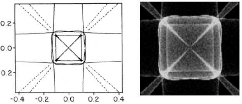
Figure 20.1: Left: outline of phonon caustics in germanium as predicted
by Nothrop and Wolfe [6]. Right: Phonon caustics as simulated using the
Geant4 phonon transport code.
Since the lattice tensor Cijml is anisotropic in general, the phonon group
velocity ~vgis not parallel to the momentum vector ~~
k. This anisotropic
transport leads to a focussing effect, where phonons are driven to directions
which correspond to the highest density of eigenvectors ~
k. Experimentally,
this is seen[6] as caustics in the energy distribution resulting from a point-like
phonon source isotropic in ~
k-space, as shown in Figure 20.1.
20.3 Lattice Parameters
20.4 Scattering and Mode Mixing
In a pure crystal, isotope scattering occurs when a phonon interacts with an
isotopic substitution site in the lattice. We treat it as an elastic scattering
process, where the phonon momentum direction (wave vector) and polariza-
tion are both randomized. The scattering rate for a phonon of frequency ν
(ω/2π) is given by[3]
Γscatter =Bν4(20.3)
where Γscatter is the number of scattering events per unit time, and Bis a
constant of proportionality derived from the elasticity tensor (see Eq. 11 and
Table 1 in [4]). For germanium, B= 3.67 ×10−41 s3. [4]
At each scattering event, the phonon polarziation may change between
311
any of the three states L,ST ,F T . The branching ratios for the polarizations
are determined by the relative density of allowed states in the lattice. This
process is often referred to as mode mixing.
20.5 Anharmonic Downconversion
An energetic phonon may interact in the crystal to produce two phonons of
reduced energy. This anharmonic downconversion conserves energy (~
k=~
k′+
~
k′′), but not momentum, since momentum is exchanged with the bulk lattice.
In principle, all three polarization states may decay through downconversion.
In practice, however, the rate for L-phonons completely dominates the energy
evolution of the system, with downconversion events from other polarization
states being negligigible[3].
The total downconversion rate Γanh for an L-phonon of frequency νis
given by[3]
Γanh =Aν5(20.4)
where (as in Eq. 20.3) Ais a constant of proportionality derived from the
elasticity tensor (see Eq. 11 and Table 1 in [4]). For germanium, A= 6.43 ×
10−55 s4. [4]
Downconversion may produce either two transversely polarized phonons,
or one transverse and one longitudinal. The relative rates are determined by
dynamical constants derived from the elasticity tensor Cijkl.
As can be seen from Eqs. 20.3 and 20.4, phonon interactions depend
strongly on energy ~ν. High energy phonons (ν∼THz) start out in a
diffusive regime with high isotope scattering and downconversion rates and
mean free paths of order microns. After several such interactions, mean free
paths increase to several centimeters or more. This transition from a diffuse
to a ballistic transport mode is commonly referred to as “quasi-diffuse” and
it controls the time evolution of phonon heat pulses.
Simulation of heat pulse propagation using our Geant4 transport code has
been described previously[1] and shows good agreement with experiment.
20.6 References
Bibliography
[1] D. Brandt et al., Journal of Low Temperature Physics 167, 485–490,
(2012)
312
[2] S. Tamura, J. Lo. T. Phys. 93, 433, (1993)
[3] S. Tamura, Phys. Rev. B. 48, 13502, (1993)
[4] S. Tamura, Phys. Rev. B. 31, (1985)
[5] J.P. Wolfe, Imaging Phonons, Chapter 2,42, Cambridge University
Press, United Kingdom (1998)
[6] G.A. Nothrop and J.P. Wolfe, Phys. Rev. Lett. 19, 1424, (1979)
313
Chapter 21
Precision multi-scale modeling
314
21.1 Overview
The physics simulation tools grouped in this domain reflect ongoing research
in key issues of particle transport:
•multi-scale simulation and its implications on condensed and discrete
transport schemes [1], [2], [3], [4], [5],
•epistemic uncertainties in physics models and parameters [6],
•innovative software design techniques [7], [9], [8], [10], [11] in support
of physics modeling,
•the assessment of the accuracy of data libraries used by Monte Carlo
simulation codes [12], [13], [14], [15], [16], [17],
•precision models of particle interactions with matter, quantitatively
assessed through comparison with experimental measurements of the
model constituents [1], [16], [17].
The main features of the simulation tools developed in this research con-
text, which are so far released in Geant4, are summarized below. They
concern impact ionisation by protons and αparticles, and the following par-
ticle induced X-ray emission (PIXE), which are encompassed in the Geant4
”electromagnetic/pii” package.
21.2 Impact ionisation by hadrons and PIXE
Despite the simplicity of its nature as a physical effect, PIXE represents a
conceptual challenge for general-purpose Monte Carlo codes, since it involves
an intrinsically discrete effect (the atomic relaxation) intertwined with a pro-
cess (ionisation) affected by infrared divergence, therefore usually treated in
Monte Carlo codes by means of con The largely incomplete knowledge of
ionisation cross sections by hadron impact, limited to the innermost atomic
shells both as theoretical calculations and experimental measurements, fur-
ther complicates the achievement of a conceptually consistent description of
this process.
Early developments of proton and αparticle impact ionisation cross sec-
tions in Geant4 are reviewed in a detailed paper devoted to PIXE simulation
with Geant4 [1]. This article also presents new, extensive developments for
PIXE simulation, their validation with respect to experimental data and the
first Geant4-based simulation involving PIXE in a concrete experimental use
315
case: the optimization of the graded shielding of the X-ray detectors of the
eROSITA [18] mission. The new developments described in [1] are released
in Geant4 in the pii package (in source/processes/electromagnetic/pii).
The developments for PIXE simulation described in [1] provide a variety
of proton and αparticle cross sections for the ionisation of K, L and M shells:
•theoretical calculations based on the ECPSSR [19] model and its vari-
ants (with Hartree-Slater corrections [20], with the united atom ap-
proximation [21] and specialized for high energies [22]),
•theoretical calculations based on plane wave Born approximation (PWBA),
•empirical models based on fits to experimental data collected by Paul
and Sacher [23] (for protons, K shell), Paul and Bolik [24] (for α, K
shell), Kahoul et al. [25]) (for protons, K, shell), Miyagawa et al. [26],
Orlic et al. [27] and Sow et al. [28] for L shell.
The cross section models available in Geant4 are listed in Table 21.1.
The calculation of cross sections in the course of the simulation is based
on the interpolation of tabulated values, which are collected in a data li-
brary. The tabulations corresponding to theoretical calculations span the
energy range between 10 keV and 10 GeV; empirical models are tabulated
consistently with the energy range of validity documented by their authors,
that corresponds to the range of the data used in the empirical fits and varies
along with the atomic number and sub-shell.
ECPSSR tabulations have been produced using the ISICS software [29,
30], 2006 version; an extended version, kindly provided by ISICS author S.
Cipolla [31], has been exploited to produce tabulations associated with recent
high energy modelling developments [22].
An example of the characteristics of different cross section models is il-
lustrated in Fig. 21.1. Fig. 21.2 shows various cross section models for
the ionisation of carbon K shell by proton, compared to experimental data
reported in [23].
The implemented cross section models have been subject to rigorous sta-
tistical analysis to evaluate their compatibility with experimental measure-
ments reported in [23], [32], [33] and to compare the relative accuracy of the
various modelling options.
The validation process involved two stages: first goodness-of-fit analysis
based on the χ2test to evaluate the hypothesis of compatibility with ex-
perimental data, then categorical analysis exploiting contingency tables to
determine whether the various modelling options differ significantly in accu-
racy. Contingency tables were analyzed with the χ2test and with Fishers
exact test.
316

Table 21.1: Ionisation cross section models available for PIXE simulation
with Geant4 Protons, K shell
Model Z range
ECPSSR 6-92
ECPSSR High Energy 6-92
ECPSSR Hartree-Slater 6-92
ECPSSR United Atom 6-92
ECPSSR reference [23] 6-92
PWBA 6-92
Paul and Sacher 6-92
Kahoul et al. 6-92
Protons, L shell
Model Z range
ECPSSR 6-92
ECPSSR United Atom 6-92
PWBA 6-92
Miyagawa et al. 40-92
Orlic et al. 43-92
Sow et al. 43-92
Protons, M shell
Model Z range
ECPSSR 6-92
PWBA 6-92
α, K shell
Model Z range
ECPSSR 6-92
ECPSSR Hartree-Slater 6-92
ECPSSR reference [24] 6-92
PWBA 6-92
Paul and Bolik 6-92
α, L and M shell
Model Z range
ECPSSR 6-92
PWBA 6-92
317

400
600
800
1000
1200
Cross section (barn)
0
200
400
600
800
1000
1200
0.1 1 10 100 1000 10000
Cross section (barn)
Energy (MeV)
ECPSSR ECPSSR-HS ECPSSR-UA ECPSSR-HE
PWBA Paul and Sacher Kahoul et al.
Figure 21.1: Cross section for the ionisation of copper K shell by proton
impact according to the various implemented modeling options: ECPSSR
model, ECPSSR model with “united atom” (UA) approximation, Hartree-
Slater (HS) corrections and specialized for high energies (HE); plane wave
Born approximation (PWBA); empirical models by Paul and Sacher and
Kahoul et al. The curves reproducing some of the model implementations
can be hardly distinguished in the plot due to their similarity.
The complete set of validation results is documented in [1]. Only the
main ones are summarized here; Geant4 users interested in detailed results,
like the accuracy of different cross section models for specific target elements,
should should refer to [1] for detailed information.
Regarding the K shell, the statistical analysis identified the ECPSSR
model with Hartree-Slater correction as the most accurate in the energy
range up to approximately 10 MeV; at higher energies the ECPSSR model
in its plain formulation or the empirical Paul and Sacher one (within its range
of applicability) exhibit the best performance. The scarceness of high energy
data prevents a definitive appraisal of the ECPSSR specialization for high
energies.
318
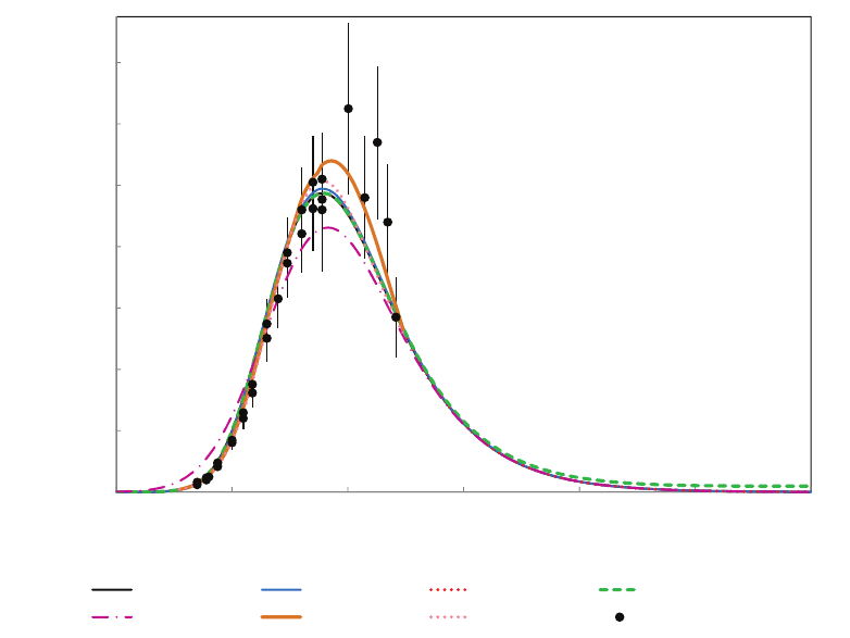
4.E+05
6.E+05
8.E+05
1.E+06
1.E+06
1.E+06
Cross section (barn)
0.E+00
2.E+05
4.E+05
6.E+05
8.E+05
1.E+06
1.E+06
1.E+06
0.01 0.1 1 10 100 1000 10000
Cross section (barn)
Energy (MeV)
ECPSSR ECPSSR-HS ECPSSR-UA ECPSSR-HE
PWBA Paul and Sacher Kahoul et al. experiment
Figure 21.2: Cross section for the ionisation of carbon K shell by proton im-
pact according to the various implemented modeling options, and comparison
with experimental data [23]: ECPSSR model, ECPSSR model with “united
atom” (UA) approximation, Hartree-Slater (HS) corrections and specialized
for high energies (HE); plane wave Born approximation (PWBA); empirical
models by Paul and Sacher and Kahoul et al. The curves reproducing some
of the model implementations can be hardly distinguished in the plot due to
their similarity.
Regarding the L shell, the ECPSSR model with “united atom” approx-
imation exhibits the best accuracy among the various implemented models;
its compatibility with experimental measurements at 95% confidence level
ranges from approximately 90% of the test cases for the L3sub-shell to
approximately 65% for the L1sub-shell. According to the results of the
categorical analysis, the ECPSSR model in its original formulation can be
considered an equivalently accurate alternative. The Orlic et al. model ex-
hibits the worst accuracy with respect to experimental data; its accuracy is
significantly different from the one of the ECPSSR model in the united atom
variant.
319
In the current Geant4 release the implementation of the hadron im-
pact ionisation process (G4ImpactIonisation) is largely based on the orig-
inal G4hLowEnergyIonisation process [34],[35], [36]. Thanks to the adopted
component-based software design, the simulation of PIXE currently exploits
the existing Geant4 atomic relaxation [37] component to produce secondary
X-rays resulting from impact ionisation.
Bibliography
[1] M. G. Pia, G. Weidenspointner, M. Augelli, L. Quintieri, P. Saracco,
M. Sudhakar, and A. Zoglauer, “PIXE simulation with Geant4”, IEEE
Trans. Nucl. Sci., vol. 56, no. 6, pp. 3614-3649, 2009.
[2] M. G. Pia et al., “R&D for co-working condensed and discrete transport
methods in Geant4 kernel”, in Proc. Int. Conf. on Mathematics, Com-
putational Methods & Reactor Physics (M&C 2009), New York, 2009.
[3] M. Augelli et al., “Geant4-related R&D for new particle transport meth-
ods”, in Proc. IEEE Nucl. Sci. Symp., 2009.
[4] M. Augelli et al., “Environmental Adaptability and Mutants: Explor-
ing New Concepts in Particle Transport for Multi-Scale Simulation”, in
Proc. IEEE Nucl. Sci. Symp., 2010.
[5] M. Augelli et al., “Environmental adaptability and mutants: explor-
ing new concepts in particle transport for multi-scale simulation”, in
Proc. Int. Conf. on Supercomp. in Nucl. Appl. and Monte Carlo (SNA
+ MC2010), 2010.
[6] M. G. Pia, M. Begalli, A. Lechner, L. Quintieri, and P. Saracco,
“Physics-related epistemic uncertainties of proton depth dose simula-
tion”, IEEE Trans. Nucl. Sci., vol. 57, no. 5, pp. , 2010.
[7] M. G. Pia et al., “Design and performance evaluations of generic pro-
gramming techniques in a R&D prototype of Geant4 physics”, J. Phys.:
Conf. Ser., vol. 219, pp. 042019, 2009.
[8] M. Augelli et al., “Research in Geant4 electromagnetic physics design,
and its effects on computational performance and quality assurance”, in
Proc. IEEE Nucl. Sci. Symp., 2009.
[9] M. G. Pia et al., “New techniques in Monte Carlo simulation: experience
with a prototype of generic programming application to Geant4 physics
320
processes”, in Proc. Int. Conf. on Supercomp. in Nucl. Appl. and Monte
Carlo (SNA + MC2010), 2010.
[10] M. Han, C. H. Kim, L. Moneta, M. G. Pia, and H. Seo, “Physics data
management tools: computational evolutions and benchmarks”, in Proc.
Int. Conf. on Supercomp. in Nucl. Appl. and Monte Carlo (SNA +
MC2010), 2010.
[11] M. Han, C. H. Kim, L. Moneta, M. G. Pia, and H. Seo, “Physics Data
Management Tools for Monte Carlo Transport: Computational Evolu-
tions and Benchmarks”, in Proc. IEEE Nucl. Sci. Symp., 2010.
[12] M. G. Pia, P. Saracco, M. Sudhakar, “Validation of radiative transition
probability calculations”, IEEE Trans. Nucl. Sci., vol. 56, no. 6, pp.
3650-3661, 2009.
[13] H. Seo, M. G. Pia, M. Begalli, L. Quintieri, P. Saracco and C. H. Kim,
“Atomic Parameters for Monte Carlo Transport Simulation: Survey,
Validation and Induced Systematic Effects”, in Proc. IEEE Nucl. Sci.
Symp., 2010.
[14] M. Augelli et al., “New Physics Data Libraries for Monte Carlo Trans-
port”, in Proc. IEEE Nucl. Sci. Symp., 2010.
[15] M. Augelli et al., “Data libraries as a collaborative tool across Monte
Carlo codes”, in Proc. Int. Conf. on Supercomp. in Nucl. Appl. and
Monte Carlo (SNA + MC2010), 2010.
[16] H. Seo, M. G. Pia, P. Saracco and C. H. Kim, “Design, development
and validation of electron ionisation models for nano-scale simulation”,
in Proc. Int. Conf. on Supercomp. in Nucl. Appl. and Monte Carlo (SNA
+ MC2010), 2010.
[17] H. Seo, M. G. Pia, P. Saracco and C. H. Kim, “Ionisation Models for
Nano-Scale Simulation”, in Proc. IEEE Nucl. Sci. Symp., 2010.
[18] P. Predehl et al., “eROSITA”, in Proc. of the SPIE, vol. 6686, pp.
668617-668617-9, 2007.
[19] W. Brandt and G. Lapicki, “Energy-loss effect in inner-shell Coulomb
ionization by heavy charged particles”, Phys. Rev.A, vol. 23, pp. 1717-
1729, 1981.
[20] G. Lapicki, “The status of theoretical K-shell ionization cross sections
by protons”, X-Ray Spectrom., vol. 34, pp. 269-278, 2005.
321
[21] S. J. Cipolla, “The united atom approximation option in the ISICS
program to calculate K-, L-, and M-shell cross sections from PWBA
and ECPSSR theory”, Nucl. Instrum. Meth. B, vol. 261, pp. 142-144,
2007.
[22] G. Lapicki, “Scaling of analytical cross sections for K-shell ionization
by nonrelativistic protons to cross sections by protons at relativistic
velocities”, J. Phys. B, vol. 41, pp. 115201 (13pp), 2008.
[23] H. Paul and J. Sacher, “Fitted empirical reference cross sections for
K-shell ionization by protons”, At. Data Nucl. Data Tab., vol. 42, pp.
105-156, 1989.
[24] H. Paul and O. Bolik, “Fitted Empirical Reference Cross Sections for
K-Shell Ionization by Alpha Particles”, At. Data Nucl. Data Tab., vol.
54, pp. 75-131, 1993.
[25] A. Kahoul, M. Nekkab, and B. Deghfel, “Empirical K-shell ionization
cross-sections of elements from 4Be to 92U by proton impact”, Nucl.
Instrum. Meth. B, vol. 266, pp. 4969-4975, 2008.
[26] Y. Miyagawa, S. Nakamura and S. Miyagawa, “Analytical Formulas
for Ionization Cross Sections and Coster-Kronig Corrected Fluorescence
Yields of the Ll, L2, and L3 Subshells”, Nucl. Instrum. Meth. B, vol.
30, pp. 115-122, 1988.
[27] I. Orlic, C. H. Sow, and S. M. Tang, “Semiempirical Formulas for Cal-
culation of L Subshell Ionization Cross Sections”, Int. J. PIXE, vol. 4,
no. 4, pp. 217-230, 1994.
[28] C. H. Sow, I. Orlic, K. K. Lob and S. M. Tang, “New parameters for
the calculation of L subshell ionization cross sections”, Nucl. Instrum.
Meth. B, vol. 75, pp. 58-62, 1993.
[29] Z. Liu and S. J. Cipolla, “ISICS: A program for calculating K-, L-, and
M-shell cross sections from ECPSSR theory using a personal computer”,
Comp. Phys. Comm., vol. 97, pp. 315-330, 1996.
[30] S. J. Cipolla, “An improved version of ISICS: a program for calculating
K-, L-, and M-shell cross sections from PWBA and ECPSSR theory
using a personal computer”, Comp. Phys. Comm., vol. 176, pp. 157-
159, 2007.
322
[31] S. Cipolla, ISICS, 2008 version. Private communication: S Cipolla,
Creighton Univ., Omaha NE 68178.
[32] I. Orlic, J. Sow, and S. M. Tang, “Experimental L-shell X-ray production
and ionization cross sections for proton impact”, At. Data Nucl. Data
Tab., vol. 56, pp. 159-210, 1994.
[33] R. S. Sokhi and D. Crumpton, “Experimental L-Shell X-Ray Production
and Ionization Cross Sections for Proton Impact”, At. Data Nucl. Data
Tab., vol. 30, pp. 49-124, 1984.
[34] S. Chauvie et al., “Geant4 Low Energy Electromagnetic Physics”, in
Proc. Computing in High Energy and Nuclear Physics, Beijing, China,
pp. 337-340, 2001.
[35] S. Chauvie et al., “Geant4 Low Energy Electromagnetic Physics”, in
Conf. Rec. IEEE Nucl. Sci. Symp., N33-165, 2004.
[36] S. Chauvie, P. Nieminen, M. G. Pia, “Geant4 model for the stopping
power of low energy negatively charged hadrons”, IEEE Trans. Nucl.
Sci., vol. 54, no. 3, pp. 578-584, 2007.
[37] S. Guatelli et al., “Geant4 Atomic Relaxation”, IEEE Trans. Nucl. Sci.,
vol. 54, no. 3, pp. 585-593, 2007.
323
Chapter 22
Shower Parameterizations
324

22.1 Gflash Shower Parameterizations
The computing time needed for the simulation of high energy electromag-
netic showers can become very large, since it increases approximately linearly
with the energy absorbed in the detector. Using parameterizations instead
of individual particle tracking for electromagnetic (sub)showers can speed
up the simulations considerably without sacrificing much precision. The
Gflash package allows the parameterization of electron and positron show-
ers in homogeneous (for the time being) calorimeters and is based on the
parameterization described in Ref. [1] .
22.1.1 Parameterization Ansatz
The spatial energy distribution of electromagnetic showers is given by three
probability density functions (pdf),
dE(~r) = E f(t)dt f(r)dr f(φ)dφ, (22.1)
describing the longitudinal, radial, and azimuthal energy distributions. Here
tdenotes the longitudinal shower depth in units of radiation length, rmea-
sures the radial distance from the shower axis in Moli`ere units, and φis the
azimuthal angle. The start of the shower is defined by the space point where
the electron or positron enters the calorimeter, which is different from the
original Gflash. A gamma distribution is used for the parameterization of the
longitudinal shower profile, f(t). The radial distribution f(r), is described
by a two-component ansatz. In φ, it is assumed that the energy is distributed
uniformly: f(φ) = 1/2π.
22.1.2 Longitudinal Shower Profiles
The average longitudinal shower profiles can be described by a gamma dis-
tribution [2]:
1
E
dE(t)
dt =f(t) = (βt)α−1βexp(−βt)
Γ(α).(22.2)
The center of gravity, hti, and the depth of the maximum, T, are calcu-
lated from the shape parameter αand the scaling parameter βaccording to:
hti=α
β(22.3)
T=α−1
β.(22.4)
325

In the parameterization all lengths are measured in units of radiation
length (X0), and energies in units of the critical energy (Ec= 2.66 X0Z
A1.1).
This allows material independence, since the longitudinal shower moments
are equal in different materials, according to Ref. [3]. The following equations
are used for the energy dependence of Thom and (αhom), with y=E/Ecand
t=x/X0, x being the longitudinal shower depth:
Thom = ln y+t1(22.5)
αhom =a1+ (a2+a3/Z) ln y. (22.6)
The y-dependence of the fluctuations can be described by:
σ= (s1+s2ln y)−1.(22.7)
The correlation between ln Thom and ln αhom is given by:
ρ(ln Thom,ln αhom)≡ρ=r1+r2ln y. (22.8)
From these formulae, correlated and varying parameters αiand βiare gen-
erated according to
ln Ti
ln αi=hln Ti
hln αi+Cz1
z2(22.9)
with
C=σ(ln T) 0
0σ(ln α)
q1+ρ
2q1−ρ
2
q1+ρ
2−q1−ρ
2
σ(ln α) and σ(ln T) are the fluctuations of Thom and (αhom. The values of the
coefficients can be found in Ref. [1].
22.1.3 Radial Shower Profiles
For the description of average radial energy profiles,
f(r) = 1
dE(t)
dE(t, r)
dr ,(22.10)
a variety of different functions can be found in the literature. In Gflash the
following two-component ansatz, an extension of that in Ref.[4], was used:
f(r) = pfC(r) + (1 −p)fT(r) (22.11)
=p2rR2
C
(r2+R2
C)2+ (1 −p)2rR2
T
(r2+R2
T)2
326

with
0≤p≤1.
Here RC(RT) is the median of the core (tail) component and pis a probabil-
ity giving the relative weight of the core component. The variable τ=t/T ,
which measures the shower depth in units of the depth of the shower max-
imum, is used in order to generalize the radial profiles. This makes the
parameterization more convenient and separates the energy and material de-
pendence of various parameters. The median of the core distribution, RC,
increases linearly with τ. The weight of the core, p, is maximal around the
shower maximum, and the width of the tail, RT, is minimal at τ≈1.
The following formulae are used to parameterize the radial energy density
distribution for a given energy and material:
RC,hom(τ) = z1+z2τ(22.12)
RT,hom(τ) = k1{exp(k3(τ−k2)) + exp(k4(τ−k2))}(22.13)
phom(τ) = p1exp p2−τ
p3−exp p2−τ
p3 (22.14)
The parameters z1···p3are either constant or simple functions of ln Eor Z.
Radial shape fluctuations are also taken into account. A detailed expla-
nation of this procedure, as well as a list of all the parameters used in Gflash,
can be found in Ref. [1].
22.1.4 Gflash Performance
The parameters used in this Gflash implementation were extracted from full
simulation studies with Geant 3. They also give good results inside the
Geant4 fast shower framework when compared with the full electromagnetic
shower simulation. However, if more precision or higher particle energies are
required, retuning may be necessary. For the longitudinal profiles the dif-
ference between full simulation and Gflash parameterization is at the level
of a few percent. Because the radial profiles are slightly broader in Geant3
than in Geant4, the differences may reach >10%. The gain in speed, on the
other hand, is impressive. The simulation of a 1 TeV electron in a P bW O4
cube is 160 times faster with Gflash. Gflash can also be used to parameter-
ize electromagnetic showers in sampling calorimeters. So far, however, only
homogeneous materials are supported.
327
Bibliography
[1] G. Grindhammer, S. Peters, The Parameterized Simulation of Electro-
magnetic Showers in Homogeneous and Sampling Calorimeters, hep-
ex/0001020 (1993).
[2] E. Longo and I. Sestili,Nucl. Instrum. Meth. 128, 283 (1975).
[3] Rossi rentice Hall, New York (1952).
[4] G. Grindhammer, M. Rudowicz, and S. Peters, Nucl. In-
strum. Meth. A290, 469 (1990).
328
Part IV
Hadronic Interactions
329
Chapter 23
Total Reaction Cross Section in
Nucleus-nucleus Reactions
The transportation of heavy ions in matter is a subject of much interest in
several fields of science. An important input for simulations of this process
is the total reaction cross section, which is defined as the total (σT) minus
the elastic (σel) cross section for nucleus-nucleus reactions:
σR=σT−σel.
The total reaction cross section has been studied both theoretically and ex-
perimentally and several empirical parameterizations of it have been devel-
oped. In Geant4 the total reaction cross sections are calculated using four
such parameterizations: the Sihver[1], Kox[2], Shen[3] and Tripathi[4] formu-
lae. Each of these is discussed in order below.
23.1 Sihver Formula
Of the four parameterizations, the Sihver formula has the simplest form:
σR=πr2
0[A1/3
p+A1/3
t−b0[A−1/3
p+A−1/3
t]]2(23.1)
where Apand Atare the mass numbers of the projectile and target nuclei,
and
b0= 1.581 −0.876(A−1/3
p+A−1/3
t),
r0= 1.36fm.
330

It consists of a nuclear geometrical term (A1/3
p+A1/3
t) and an overlap or
transparency parameter (b0) for nucleons in the nucleus. The cross section
is independent of energy and can be used for incident energies greater than
100 MeV/nucleon.
23.2 Kox and Shen Formulae
Both the Kox and Shen formulae are based on the strong absorption model.
They express the total reaction cross section in terms of the interaction radius
R, the nucleus-nucleus interaction barrier B, and the center-of-mass energy
of the colliding system ECM :
σR=πR2[1 −B
ECM
].(23.2)
Kox formula: Here Bis the Coulomb barrier (Bc) of the projectile-target
system and is given by
Bc=ZtZpe2
rC(A1/3
t+A1/3
p),
where rC= 1.3 fm, eis the electron charge and Zt,Zpare the atomic numbers
of the target and projectile nuclei. Ris the interaction radius Rint which in
the Kox formula is divided into volume and surface terms:
Rint =Rvol +Rsurf .
Rvol and Rsurf correspond to the energy-independent and energy-dependent
components of the reactions, respectively. Collisions which have relatively
small impact parameters are independent of both energy and mass number.
These core collisions are parameterized by Rvol. Therefore Rvol can depend
only on the volume of the projectile and target nuclei:
Rvol =r0(A1/3
t+A1/3
p).
The second term of the interaction radius is a nuclear surface contribution
and is parameterized by
Rsurf =r0[aA1/3
tA1/3
p
A1/3
t+A1/3
p−c] + D.
The first term in brackets is the mass asymmetry which is related to
the volume overlap of the projectile and target. The second term cis
331

an energy-dependent parameter which takes into account increasing surface
transparency as the projectile energy increases. Dis the neutron-excess
which becomes important in collisions of heavy or neutron-rich targets. It is
given by
D=5(At−Zt)Zp
ApAr
.
The surface component (Rsurf ) of the interaction radius is actually not part
of the simple framework of the strong absorption model, but a better repro-
duction of experimental results is possible when it is used.
The parameters r0,aand care obtained using a χ2minimizing procedure
with the experimental data. In this procedure the parameters r0and awere
fixed while cwas allowed to vary only with the beam energy per nucleon. The
best χ2fit is provided by r0= 1.1 fm and a= 1.85 with the corresponding
values of clisted in Table III and shown in Fig. 12 of Ref. [2] as a function
of beam energy per nucleon. This reference presents the values of conly in
chart and figure form, which is not suitable for Monte Carlo calculations.
Therefore a simple analytical function is used to calculate cin Geant4. The
function is:
c=−10
x5+ 2.0 for x ≥1.5
c= (−10
1.55+ 2.0) ×(x
1.5)3for x <1.5,
x=log(KE),
where KE is the projectile kinetic energy in units of MeV/nucleon in the
laboratory system.
Shen formula: as mentioned earlier, this formula is also based on the strong
absorption model, therefore it has a structure similar to the Kox formula:
σR= 10πR2[1 −B
ECM
].(23.3)
However, different parameterized forms for Rand Bare applied. The inter-
action radius Ris given by
R=r0[A1/3
t+A1/3
p+ 1.85 A1/3
tA1/3
p
A1/3
t+A1/3
p−C′(KE)]
+α5(At−Zt)Zp
ApAr
+βE−1/3
CM
A1/3
tA1/3
p
A1/3
t+A1/3
p
332

where α,βand r0are
α= 1fm
β= 0.176MeV 1/3·fm
r0= 1.1fm
In Ref. [3] as well, no functional form for C′(KE) is given. Hence the same
simple analytical function is used by Geant4 to derive cvalues.
The second term Bis called the nuclear-nuclear interaction barrier in the
Shen formula and is given by
B=1.44ZtZp
r−bRtRp
Rt+Rp
(MeV )
where r,b,Rtand Rpare given by
r=Rt+Rp+ 3.2fm
b= 1MeV ·fm−1
Ri= 1.12A1/3
i−0.94A−1/3
i(i=t, p)
The difference between the Kox and Shen formulae appears at energies below
30 MeV/nucleon. In this region the Shen formula shows better agreement
with the experimental data in most cases.
23.3 Tripathi formula
Because the Tripathi formula is also based on the strong absorption model
its form is similar to the Kox and Shen formulae:
σR=πr2
0(A1/3
p+A1/3
t+δE)2[1 −B
ECM
],(23.4)
where r0= 1.1 fm. In the Tripathi formula Band Rare given by
B=1.44ZtZp
R
333

R=rp+rt+1.2(A1/3
p+A1/3
t)
E1/3
CM
where riis the equivalent sphere radius and is related to the rrms,i radius by
ri= 1.29rrms,i (i=p, t).
δErepresents the energy-dependent term of the reaction cross section
which is due mainly to transparency and Pauli blocking effects. It is given
by
δE= 1.85S+ (0.16S/E1/3
CM )−CKE + [0.91(At−2Zt)Zp/(ApAt)],
where Sis the mass asymmetry term given by
S=A1/3
pA1/3
t
A1/3
p+A1/3
t
.
This is related to the volume overlap of the colliding system. The last term
accounts for the isotope dependence of the reaction cross section and corre-
sponds to the Dterm in the Kox formula and the second term of Rin the
Shen formula.
The term CKE corresponds to cin Kox and C′(KE) in Shen and is given
by
CE=DP auli[1 −exp(−KE/40)] −0.292 exp(−KE/792) ×cos(0.229KE0.453).
Here DP auli is related to the density dependence of the colliding system,
scaled with respect to the density of the 12C+12C colliding system:
DP auli = 1.75 ρAp+ρAt
ρAC+ρAC
.
The nuclear density is calculated in the hard sphere model. DP auli simulates
the modifications of the reaction cross sections caused by Pauli blocking and
is being introduced to the Tripathi formula for the first time. The modifica-
tion of the reaction cross section due to Pauli blocking plays an important
role at energies above 100 MeV/nucleon. Different forms of DP auli are used
in the Tripathi formula for alpha-nucleus and lithium-nucleus collisions. For
alpha-nucleus collisions,
DP auli = 2.77 −(8.0×10⁻³At) + (1.8×10⁻⁵A2
t)
−0.8/{1 + exp[(250 −KE)/75]}
334

For lithium-nucleus collisions,
DP auli =DP auli/3.
Note that the Tripathi formula is not fully implemented in Geant4 and can
only be used for projectile energies less than 1 GeV/nucleon.
23.4 Representative Cross Sections
Representative cross section results from the Sihver, Kox, Shen and Tripathi
formulae in Geant4 are displayed in Table I and compared to the experimental
measurements of Ref. [2].
23.5 Tripathi Formula for ”light” Systems
For nuclear-nuclear interactions in which the projectile and/or target are
light, Tripathi et al [6] propose an alternative algorithm for determining the
interaction cross section (implemented in the new class G4TripathiLightCrossSection).
For such systems, Eq.23.4 becomes:
σR=πr2
0[A1/3
p+A1/3
t+δE]2(1 −RC
B
ECM
)Xm(23.5)
RCis a Coulomb multiplier, which is added since for light systems Eq. 23.4
overestimates the interaction distance, causing B(in Eq. 23.4) to be under-
estimated. Values for RCare given in Table 23.2.
Xm= 1 −X1exp −E
X1SL(23.6)
where:
X1= 2.83 −3.1×10⁻²AT+1.7×10⁻⁴A2
T(23.7)
except for neutron interactions with 4He, for which X1is better approximated
to 5.2, and the function SLis given by:
SL= 1.2 + 1.61−exp −E
15 (23.8)
For light nuclear-nuclear collisions, a slightly more general expression for CE
is used:
335

CE=D1−exp −E
T1−0.292 exp −E
792·cos 0.229E0.453(23.9)
Dand T1are dependent on the interaction, and are defined in table 23.3.
Bibliography
[1] L. Sihver et al., Phys. Rev. C47, 1225 (1993).
[2] Kox et al. Phys. Rev. C35, 1678 (1987).
[3] Shen et al. Nucl. Phys. A491, 130 (1989).
[4] Tripathi et al, NASA Technical Paper 3621 (1997).
[5] Jaros et al, Phys. Rev. C 18 2273 (1978).
[6] R K Tripathi, F A Cucinotta, and J W Wilson, ”Universal parameter-
ization of absorption cross-sections - Light systems,” NASA Technical
Paper TP-1999-209726, 1999.
336

Table 23.1: Representative total reaction cross sections
Proj. Target Elab Exp. Results Sihver Kox Shen Tripathi
[MeV/n] [mb]
12C12C30 1316±40 — 1295.04 1316.07 1269.24
83 965±30 — 957.183 969.107 989.96
200 864±45 868.571 885.502 893.854 864.56
300 858±60 868.571 871.088 878.293 857.414
8701939±50 868.571 852.649 857.683 939.41
21001888±49 868.571 846.337 850.186 936.205
27Al 30 1748±85 — 1801.4 1777.75 1701.03
83 1397±40 — 1407.64 1386.82 1405.61
200 1270±70 1224.95 1323.46 1301.54 1264.26
300 1220±85 1224.95 1306.54 1283.95 1257.62
89Y30 2724±300 — 2898.61 2725.23 2567.68
83 2124±140 — 2478.61 2344.26 2346.54
200 1885±120 2156.47 2391.26 2263.77 2206.01
300 1885±150 2156.47 2374.17 2247.55 2207.01
16O27Al 30 1724±80 — 1965.85 1935.2 1872.23
89Y30 2707±330 — 3148.27 2957.06 2802.48
20Ne 27Al 30 2113±100 — 2097.86 2059.4 2016.32
100 1446±120 1473.87 1684.01 1658.31 1667.17
300 1328±120 1473.87 1611.88 1586.17 1559.16
108Ag 300 2407±20022730.69 3095.18 2939.86 2893.12
1. Data measured by Jaros et al. [5]
2. Natural silver was used in this measurement.
337

Table 23.2: Coulomb multiplier for light systems [6].
System RC
p + d 13.5
p + 3He 21
p + 4He 27
p + Li 2.2
d + d 13.5
d + 4He 13.5
d + C 6.0
4He + Ta 0.6
4He + Au 0.6
338

Table 23.3: Parameters D and T1 for light systems [6].
System T1 [MeV] D G [MeV]
(4He + X only)
p + X 23 1.85 + 0.16
1+exp(500−E
200 )(Not applicable)
n + X 18 1.85 + 0.16
1+exp(500−E
200 )(Not applicable)
d + X 23 1.65 + 0.1
1+exp(500−E
200 )(Not applicable)
3He + X 40 1.55 (Not applicable)
4He + 4He 40
D= 2.77 −8.0×10⁻³AT
+1.8×10⁻⁵A2
T
−0.8
1+exp(250−E
G)
300
4He + Be 25 (as for 4He + 4He) 300
4He + N 40 (as for 4He + 4He) 500
4He + Al 25 (as for 4He + 4He) 300
4He + Fe 40 (as for 4He + 4He) 300
4He + X (general) 40 (as for 4He + 4He) 75
339
Chapter 24
Coherent elastic scattering
24.1 Nucleon-Nucleon elastic Scattering
The classes G4LEpp and G4LEnp provide data-driven models for proton-
proton (or neutron-neutron) and neutron-proton elastic scattering over the
range 10-1200 MeV. Final states (primary and recoil particle) are derived by
sampling from tables of the cumulative distribution function of the centre-
of-mass scattering angle, tabulated for a discrete set of lab kinetic energies
from 10 MeV to 1200 MeV. The CDF’s are tabulated at 1 degree intervals
and sampling is done using bi-linear interpolation in energy and CDF values.
The data are derived from differential cross sections obtained from the SAID
database, R. Arndt, 1998.
In class G4LEpp there are two data sets: one including Coulomb ef-
fects (for p-p scattering) and one with no Coulomb effects (for n-n scat-
tering or p-p scattering with Coulomb effects suppressed). The method
G4LEpp::SetCoulombEffects can be used to select the desired data set:
•SetCoulombEffects(0): No Coulomb effects (the default)
•SetCoulombEffects(1): Include Coulomb effects
The recoil particle will be generated as a new secondary particle. In class
G4LEnp, the possiblity of a charge-exchange reaction is included, in which
case the incident track will be stopped and both the primary and recoil
particles will be generated as secondaries.
340

Chapter 25
Hadron-nucleus Elastic
Scattering at Medium and High
Energy
25.1 Method of Calculation
The Glauber model [1] is used as an alternative method of calculating dif-
ferential cross sections for elastic and quasi-elastic hadron-nucleus scattering
at high and intermediate energies.
For high energies this includes corrections for inelastic screening and for
quasi-elastic scattering the exitation of a discrete level or a state in the con-
tinuum is considered.
The usual expression for the Glauber model amplitude for multiple scat-
tering was used
F(q) = ik
2πZd2be~
q·~
bM(~
b).(25.1)
Here M(~
b) is the hadron-nucleus amplitude in the impact parameter repre-
sentation
M(~
b) = 1 −[1 −e−ARd3rΓ(~
b−~
s)ρ(~r)]A,(25.2)
kis the incident particle momentum, ~q =~
k′−~
kis the momentum transfer,
and ~
k′is the scattered particle momentum. Note that |~q|2=−t- invari-
ant momentum transfer squared in the center of mass system. Γ(~
b) is the
hadron-nucleon amplitude of elastic scattering in the impact-parameter rep-
resentation
341

Γ(~
b) = 1
2πikhN Zd~qe−~
q·~
bf(~q).(25.3)
The exponential parameterization of the hadron-nucleon amplitude is
usually used:
f(~q) = ikhN σhN
2πe−0.5q2B.(25.4)
Here σhN =σhN
tot (1 −iα), σhN
tot is the total cross section of a hadron-nucleon
scattering, Bis the slope of the diffraction cone and αis the ratio of the real
to imaginary parts of the amplitude at q= 0. The value khN is the hadron
momentum in the hadron-nucleon coordinate system.
The important difference of these calculations from the usual ones is that
the two-gaussian form of the nuclear density was used
ρ(r) = C(e−(r/R1)2−pe−(r/R2)2),(25.5)
where R1,R2and pare the fitting parameters and Cis a normalization
constant.
This density representation allows the expressions for amplitude and dif-
ferential cross section to be put into analytical form. It was earlier used for
light [2, 3] and medium [4] nuclei. Described below is an extension of this
method to heavy nuclei. The form 25.5 is not physical for a heavy nucleus,
but nevertheless works rather well (see figures below). The reason is that
the nucleus absorbs the hadrons very strongly, especially at small impact
parameters where the absorption is full. As a result only the peripherial part
of the nucleus participates in elastic scattering. Eq. 25.5 therefore describes
only the edge of a heavy nucleus.
Substituting Eqs. 25.5 and 25.4 into Eqs. 25.1, 25.2 and 25.3 yields the
following formula
F(q) = ikπ
2
A
X
k=1
(−1)kA
k[σhN
2π(R3
1−pR3
2)]k
k
X
m=0
(−1)mk
m R3
1
R2
1+ 2Bk−m
×pR3
2
R2
2+ 2Bmm
R2
2+ 2B+k−m
R2
1+ 2B−1
×exp "−−q2
4m
R2
2+ 2B+k−m
R2
1+ 2B−1#.(25.6)
342

An analogous procedure can be used to get the inelastic screening cor-
rections to the hadron-nucleus amplitude ∆M(~
b) [5]. In this case an inter-
mediate inelastic diffractive state is created which rescatters on the nucleons
of the nucleus and then returns into the initial hadron. Hence it is ness-
esary to integrate the production cross section over the mass distribution of
the exited system dσdif f
dtdM2
x. The expressions for the corresponding amplitude
are quite long and so are not presented here. The corrections for the total
cross-sections can be found in [5].
The full amplitude is the sum M(~
b) + ∆M(~
b).
The differential cross section is connected with the amplitude in the fol-
lowing way
dσ
dΩCM
=|F(q)|2,dσ
|dt|=dσ
dq2
CM
=π
k2
CM |F(q)|2.(25.7)
The main energy dependence of the hadron-nucleus elastic scattering
cross section comes from the energy dependence of the parameters of hadron-
nucleon scattering (σhN
tot α,Band dσdif f
dtdM2
x). At interesting energies these param-
eters were fixed at their well-known values. The fitting of the nuclear density
parameters was performed over a wide range of atomic numbers (A= 4−208)
using experimental data on proton-nuclei elastic scattering at a kinetic energy
of Tp= 1GeV .
The fitting was perfomed both for individual nuclei and for the entire set
of nuclei at once.
It is necessary to note that for every nucleus an optimal set of density
parameters exists and it differs slightly from the one derived for the full set
of nuclei.
A comparision of the phenomenological cross sections [6] with experiment
is presented in Figs. 25.1 - 25.9
In this comparison, the individual nuclei parameters were used. The
experimental data were obtained in Gatchina (Russia) and in Saclay (France)
[6]. The horizontal axis is the scattering angle in the center of mass system
ΘCM and the vertical axis is dσ
dΩCM in mb
Ster .
Comparisions were also made for p4He elastic scatering at T=1GeV [7],
45GeV and 301GeV [3]. The resulting cross sections dσ
d|t|are shown in the
Figs. 25.10 - 25.12.
In order to generate events the distribution function Fof a corresponding
process must be known. The differential cross section is proportional to the
density distribution. Therefore to get the distribution function it is sufficient
to integrate the differential cross section and normalize it:
343
F(q2) =
q2
Z
0
d(q2)dσ
d(q2)
q2
max
Z
0
d(q2)dσ
d(q2).
(25.8)
Expressions 25.6 and 25.7 allow analytic integration in Eq. 25.8 but the
result is too long to be given here.
For light and medium nuclei the analytic expression is more convenient
for calculations than the numerical integration of Eq. 25.8, but for heavy
nuclei the latter is preferred due to the large number of terms in the analytic
expression.
Bibliography
[1] R.J. Glauber, in ”High Energy Physics and Nuclear Structure”, edited
by S. Devons (Plenum Press, NY 1970).
[2] R. H. Bassel, W. Wilkin, Phys. Rev., 174, p. 1179, 1968;
T. T. Chou, Phys. Rev., 168, 1594, 1968;
M. A. Nasser, M. M. Gazzaly, J. V. Geaga et al., Nucl. Phys., A312,
pp. 209-216, 1978.
[3] Bujak, P. Devensky, A. Kuznetsov et al., Phys. Rev., D23, N 9, pp.
1895-1910, 1981.
[4] V. L. Korotkikh, N. I. Starkov, Sov. Journ. of Nucl. Phys., v. 37, N 4,
pp. 610-613, 1983;
N. T. Ermekov, V. L. Korotkikh, N. I. Starkov, Sov. Journ. of Nucl.
Phys., 33, N 6, pp. 775-777, 1981.
[5] R.A. Nam, S. I. Nikol’skii, N. I. Starkov et al., Sov. Journ. of Nucl.
Phys., v. 26, N 5, pp. 550-555, 1977.
[6] G.D. Alkhazov et al., Phys. Rep., 1978, C42, N 2, pp. 89-144;
[7] J. V. Geaga, M. M. Gazzaly, G. J. Jgo et al., Phys. Rev. Lett. 38, N
22, pp. 1265-1268;
S. J. Wallace. Y. Alexander, Phys. Rev. Lett. 38, N 22, pp. 1269-1272.
344
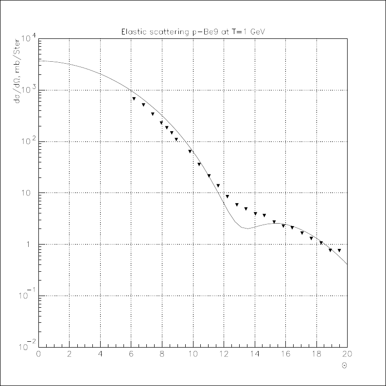
Figure 25.1: Elastic proton scattering on 9Be at 1 GeV
345
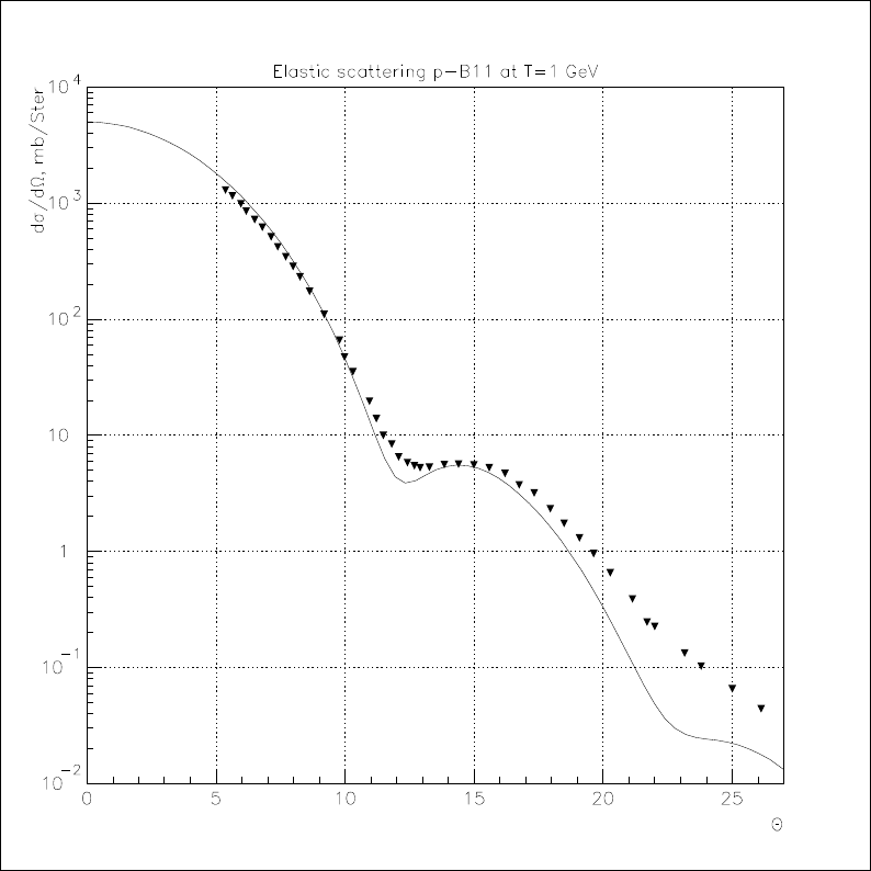
Figure 25.2: Elastic proton scattering on 11B at 1 GeV
346
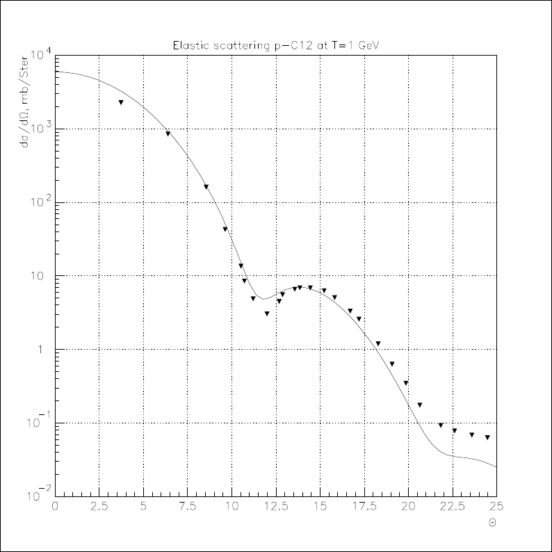
Figure 25.3: Elastic proton scattering on 12C at 1 GeV
347

Figure 25.4: Elastic proton scattering on 16O at 1 GeV
348
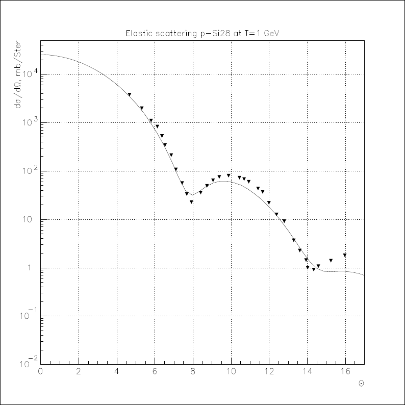
Figure 25.5: Elastic proton scattering on 28Si at 1 GeV
349
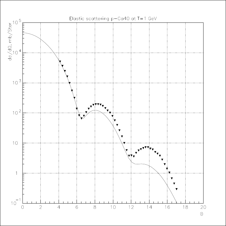
Figure 25.6: Elastic proton scattering on 40Ca at 1 GeV
350
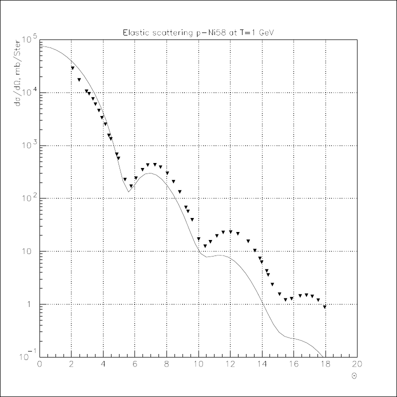
Figure 25.7: Elastic proton scattering on 58Ni at 1 GeV
351
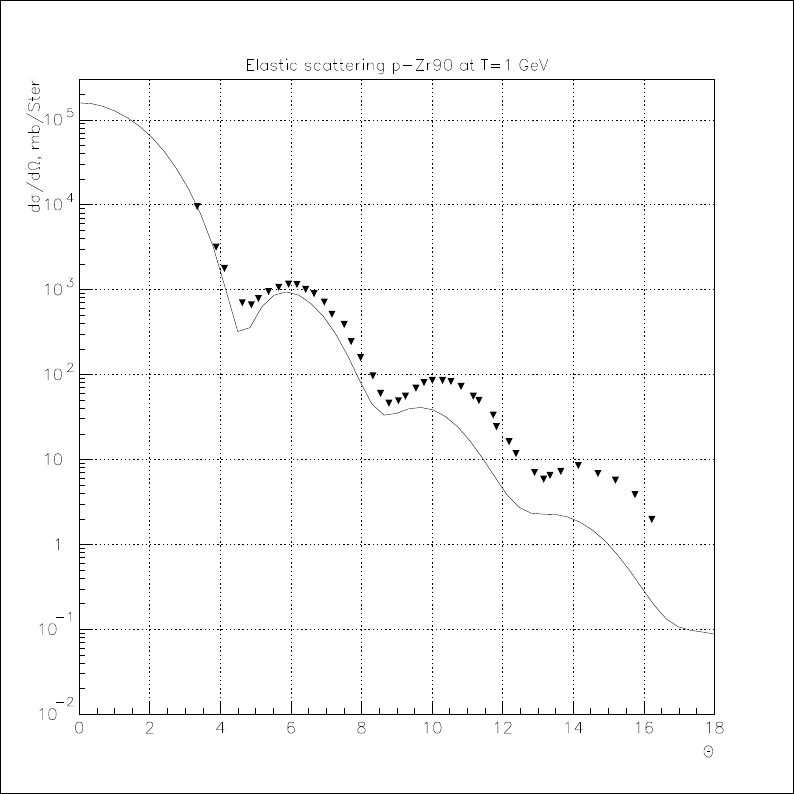
Figure 25.8: Elastic proton scattering on 90Zr at 1 GeV
352
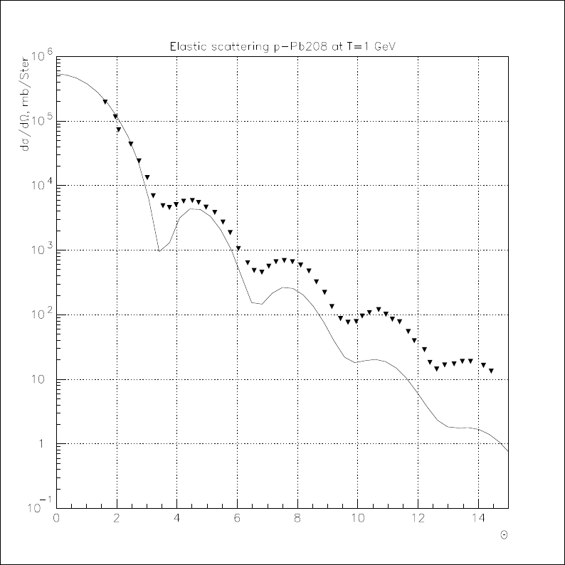
Figure 25.9: Elastic proton scattering on 208Pb at 1 GeV
353
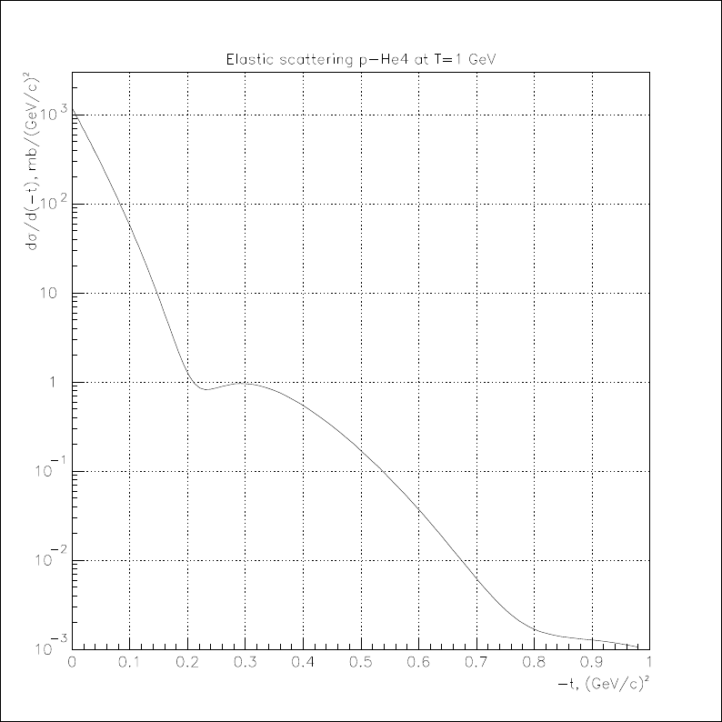
Figure 25.10: Elastic proton scattering on 4He at 1 GeV
354
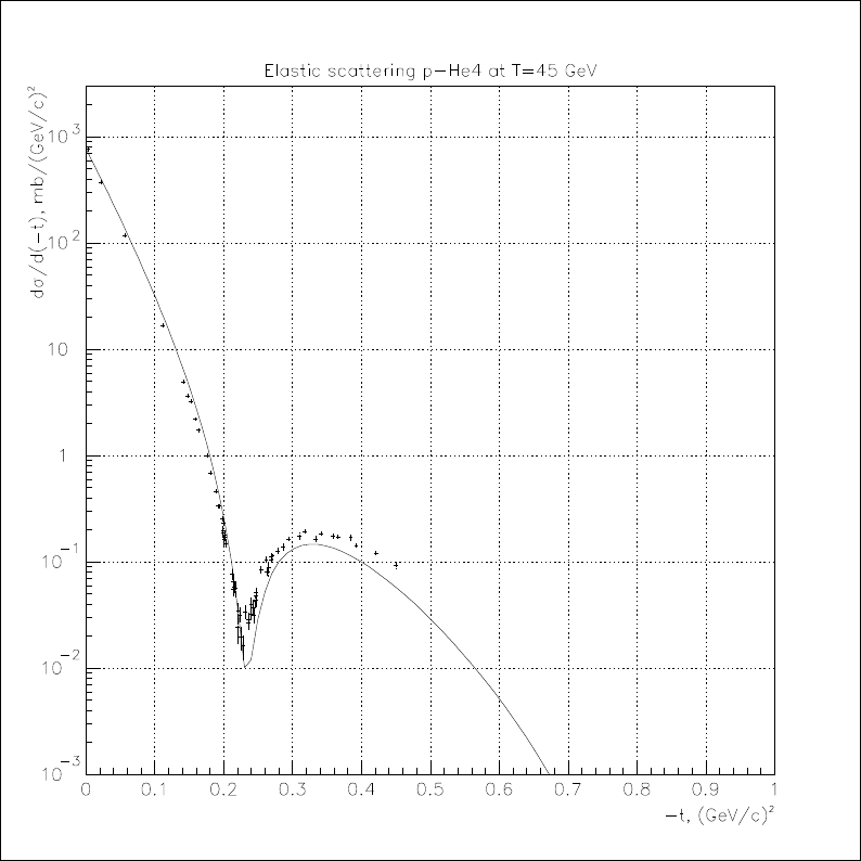
Figure 25.11: Elastic proton scattering on 4He at 45 GeV
355
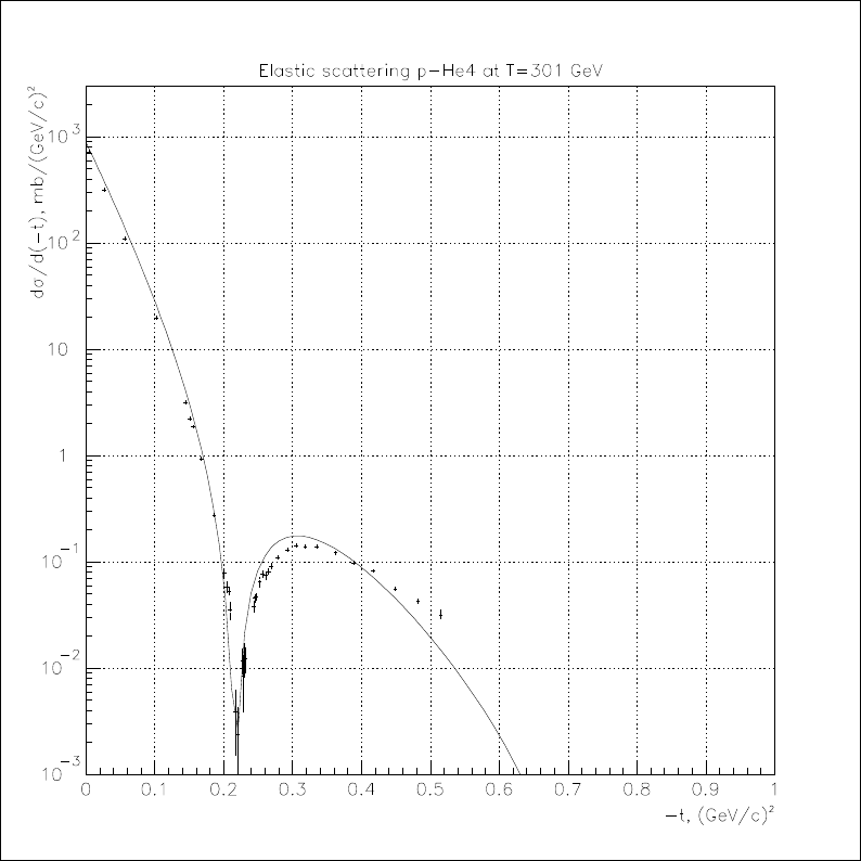
Figure 25.12: Elastic proton scattering on 4He at 301 GeV
356
Chapter 26
Interactions of Stopping
Particles
26.1 Complementary parameterised and the-
oretical treatment
Absorption of negative pions and kaons at rest from a nucleus is described
in literature [1], [2], [3], [4] as consisting of two main components:
•a primary absorption process, involving the interaction of the incident
stopped hadron with one or more nucleons of the target nucleus;
•the deexcitation of the remnant nucleus, left in an excitated state as a
result of the occurrence of the primary absorption process.
This interpretation is supported by several experiments [5], [6], [7], [8], [9],
[10], [11], that have measured various features characterizing these processes.
In many cases the experimental measurements are capable to distinguish the
final products originating from the primary absorption process and those
resulting from the nuclear deexcitation component.
A set of stopped particle absorption processes is implemented in GEANT4,
based on this two-component model (PiMinusAbsorptionAtRest and Kaon-
MinusAbsorptionAtRest classes, for π−and K−respectively. Both imple-
mentations adopt the same approach: the primary absorption component
of the process is parameterised, based on available experimental data; the
nuclear deexcitation component is handled through the theoretical models
described elsewhere in this Manual.
357
26.1.1 Pion absorption at rest
The absorption of stopped negative pions in nuclei is interpreted [1], [2],
[3], [4] as starting with the absorption of the pion by two or more correlated
nucleons; the total energy of the pion is transferred to the absorbing nucleons,
which then may leave the nucleus directly, or undergo final-state interactions
with the residual nucleus. The remaining nucleus de-excites by evaporation
of low energetic particles.
G4PiMinusAbsorptionAtRest generates the primary absorption compo-
nent of the process through the parameterisation of existing experimental
data; the primary absorption component is handled by class G4PiMinusStopAbsorption.
In the current implementation only absorption on a nucleon pair is consid-
ered, while contributions from absorption on nucleon clusters are neglected;
this approximation is supported by experimental results [1], [13] showing that
it is the dominating contribution.
Several features of stopped pion absorption are known from experimental
measurements on various materials [5], [6], [7], [8], [9], [10], [11], [12]:
•the average number of nucleons emitted, as resulting from the primary
absorption process;
•the ratio of nn vs np as nucleon pairs involved in the absorption process;
•the energy spectrum of the resulting nucleons emitted and their opening
angle distribution.
The corresponding final state products and related distributions are gener-
ated according to a parameterisation of the available experimental measure-
ments listed above. The dependence on the material is handled by a strategy
pattern: the features pertaining to material for which experimental data are
available are treated in G4PiMinusStopX classes (where X represents an el-
ement), inheriting from G4StopMaterial base class. In case of absorption on
an element for which experimental data are not available, the experimental
distributions for the elements closest in Z are used.
The excitation energy of the residual nucleus is calculated by difference
between the initial energy and the energy of the final state products of the
primary absorption process.
Another strategy handles the nucleus deexcitation; the current default
implementation consists in handling the deexcitatoin component of the pro-
cess through the evaporation model described elsewhere in this Manual.
358
Bibliography
[1] E. Gadioli and E. Gadioli Erba Phys. Rev. C 36 741 (1987)
[2] H.C. Chiang and J. Hufner Nucl. Phys. A352 442 (1981)
[3] D. Ashery and J. P. Schiffer Ann. Rev. Nucl. Part. Sci. 36 207 (1986)
[4] H. J. Weyer Phys. Rep. 195 295 (1990)
[5] R. Hartmann et al., Nucl. Phys. A300 345 (1978)
[6] R. Madley et al., Phys. Rev. C 25 3050 (1982)
[7] F. W. Schleputz et al., Phys. Rev. C 19 135 (1979)
[8] C.J. Orth et al., Phys. Rev. C 21 2524 (1980)
[9] H.S. Pruys et al., Nucl. Phys. A316 365 (1979)
[10] P. Heusi et al., Nucl. Phys. A407 429 (1983)
[11] H.P. Isaak et al., Nucl. Phys. A392 368 (1983)
[12] H.P. Isaak et al., Helvetica Physica Acta 55 477 (1982)
[13] H. Machner Nucl. Phys. A395 457 (1983)
359

Chapter 27
Parton string model.
27.1 Reaction initial state simulation.
27.1.1 Allowed projectiles and bombarding energy range
for interaction with nucleon and nuclear targets
The GEANT4 parton string models are capable to predict final states (pro-
duced hadrons which belong to the scalar and vector meson nonets and the
baryon (antibaryon) octet and decuplet) of reactions on nucleon and nuclear
targets with nucleon, pion and kaon projectiles. The allowed bombarding
energy √s > 5 GeV is recommended. Two approaches, based on diffractive
excitation or soft scattering with diffractive admixture according to cross-
section, are considered. Hadron-nucleus collisions in the both approaches
(diffractive and parton exchange) are considered as a set of the independent
hadron-nucleon collisions. However, the string excitation procedures in these
approaches are rather different.
27.1.2 MC initialization procedure for nucleus.
The initialization of each nucleus, consisting from Anucleons and Zpro-
tons with coordinates riand momenta pi, where i= 1,2, ..., A is performed.
We use the standard initialization Monte Carlo procedure, which is realized
in the most of the high energy nuclear interaction models:
•Nucleon radii riare selected randomly in the rest of nucleus according
to proton or neutron density ρ(ri). For heavy nuclei with A > 16 [1]
nucleon density is
ρ(ri) = ρ0
1 + exp [(ri−R)/a](27.1)
360

where
ρ0≈3
4πR3(1 + a2π2
R2)−1.(27.2)
Here R=r0A1/3fm and r0= 1.16(1 −1.16A−2/3) fm and a≈0.545
fm. For light nuclei with A < 17 nucleon density is given by a harmonic
oscillator shell model [2], e. g.
ρ(ri) = (πR2)−3/2exp (−r2
i/R2),(27.3)
where R2= 2/3< r2>= 0.8133A2/3fm2. To take into account
nucleon repulsive core it is assumed that internucleon distance d > 0.8
fm;
•The initial momenta of the nucleons are randomly choosen between
0 and pmax
F, where the maximal momenta of nucleons (in the local
Thomas-Fermi approximation [3]) depends from the proton or neutron
density ρaccording to
pmax
F=~c(3π2ρ)1/3(27.4)
with ~c= 0.197327 GeV fm;
•To obtain coordinate and momentum components, it is assumed that
nucleons are distributed isotropicaly in configuration and momentum
spaces;
•Then perform shifts of nucleon coordinates r′
j=rj−1/A Piriand
momenta p′
j=pj−1/A Pipiof nucleon momenta. The nucleus must
be centered in configuration space around 0,i. e. Piri=0and the
nucleus must be at rest, i. e. Pipi=0;
•We compute energy per nucleon e=E/A =mN+B(A, Z)/A, where
mNis nucleon mass and the nucleus binding energy B(A, Z) is given
by the Bethe-Weizs¨acker formula[4]:
B(A, Z) =
=−0.01587A+ 0.01834A2/3+ 0.09286(Z−A
2)2+ 0.00071Z2/A1/3,
(27.5)
and find the effective mass of each nucleon meff
i=p(E/A)2−p2′
i.
361

27.1.3 Random choice of the impact parameter.
The impact parameter 0 ≤b≤Rtis randomly selected according to the
probability:
P(b)db=bdb,(27.6)
where Rtis the target radius, respectively. In the case of nuclear projectile
or target the nuclear radius is determined from condition:
ρ(R)
ρ(0) = 0.01.(27.7)
27.2 Sample of collision participants in nu-
clear collisions.
27.2.1 MC procedure to define collision participants.
The inelastic hadron–nucleus interactions at ultra–relativistic energies are
considered as independent hadron–nucleon collisions. It was shown long time
ago [5] for the hadron–nucleus collision that such a picture can be obtained
starting from the Regge–Gribov approach [6], when one assumes that the
hadron-nucleus elastic scattering amplitude is a result of reggeon exchanges
between the initial hadron and nucleons from target–nucleus. This result
leads to simple and efficient MC procedure [7] to define the interaction cross
sections and the number of the nucleons participating in the inelastic hadron–
nucleus collision:
•We should randomly distribute Bnucleons from the target-nucleus on
the impact parameter plane according to the weight function T([~
bB
j]).
This function represents probability density to find sets of the nucleon
impact parameters [~
bB
j], where j= 1,2, ..., B.
•For each pair of projectile hadron iand target nucleon jwith choosen
impact parameters ~
biand ~
bB
jwe should check whether they interact
inelastically or not using the probability pij(~
bi−~
bB
j, s), where sij =
(pi+pj)2is the squared total c.m. energy of the given pair with the
4–momenta piand pj, respectively.
In the Regge–Gribov approach[6] the probability for an inelastic collision
of pair of iand jas a function at the squared impact parameter difference
b2
ij = (~
bi−~
bB
j)2and sis given by
pij(~
bi−~
bB
j, s) = c−1[1 −exp {−2u(b2
ij, s)}] = ∞
X
n=1
p(n)
ij (~
bi−~
bB
j, s),(27.8)
362

where
p(n)
ij (~
bi−~
bB
j, s) = c−1exp {−2u(b2
ij, s)}[2u(b2
ij, s)]n
n!.(27.9)
is the probability to find the ncut Pomerons or the probability for 2nstrings
produced in an inelastic hadron-nucleon collision. These probabilities are de-
fined in terms of the (eikonal) amplitude of hadron–nucleon elastic scattering
with Pomeron exchange:
u(b2
ij, s) = z(s)
2exp(−b2
ij/4λ(s)).(27.10)
The quantities z(s) and λ(s) are expressed through the parameters of the
Pomeron trajectory, α′
P= 0.25 GeV −2and αP(0) = 1.0808, and the param-
eters of the Pomeron-hadron vertex RPand γP:
z(s) = 2cγP
λ(s)(s/s0)αP(0)−1(27.11)
λ(s) = R2
P+α′
Pln(s/s0),(27.12)
respectively, where s0is a dimensional parameter.
In Eqs. (27.8,27.9) the so–called shower enhancement coefficient cis intro-
duced to determine the contribution of diffractive dissociation[6]. Thus, the
probability for diffractive dissociation of a pair of nucleons can be computed
as
pd
ij(~
bi−~
bB
j, s) = c−1
c[ptot
ij (~
bi−~
bB
j, s)−pij(~
bi−~
bB
j, s)],(27.13)
where
ptot
ij (~
bi−~
bB
j, s) = (2/c)[1 −exp{−u(b2
ij, s)}].(27.14)
The Pomeron parameters are found from a global fit of the total, elas-
tic, differential elastic and diffractive cross sections of the hadron–nucleon
interaction at different energies.
For the nucleon-nucleon, pion-nucleon and kaon-nucleon collisions the
Pomeron vertex parameters and shower enhancement coefficients are found:
R2N
P= 3.56 GeV −2,γN
P= 3.96 GeV −2,sN
0= 3.0GeV 2,cN= 1.4 and
R2π
P= 2.36 GeV −2,γπ
P= 2.17 GeV −2, and R2K
P= 1.96 GeV −2,γK
P= 1.92
GeV −2,sK
0= 2.3GeV 2,cπ= 1.8.
27.2.2 Separation of hadron diffraction excitation.
For each pair of target hadron iand projectile nucleon jwith choosen im-
pact parameters ~
biand ~
bB
jwe should check whether they interact inelastically
or not using the probability
pin
ij (~
bi−~
bB
j, s) = pij(~
bi−~
bB
j, s) + pd
ij(~
bA
i−~
bB
j, s).(27.15)
363

If interaction will be realized, then we have to consider it to be diffractive or
nondiffractive with probabilities
pd
ij(~
bi−~
bB
j, s)
pin
ij (~
bA
i−~
bB
j, s)(27.16)
and
pij(~
bi−~
bB
j, s)
pin
ij (~
bA
i−~
bB
j, s).(27.17)
27.3 Longitudinal string excitation
27.3.1 Hadron–nucleon inelastic collision
Let us consider collision of two hadrons with their c. m. momenta P1=
{E+
1, m2
1/E+
1,0}and P2={E−
2, m2
2/E−
2,0}, where the light-cone variables
E±
1,2=E1,2±Pz1,2are defined through hadron energies E1,2=qm2
1,2+P2
z1,2,
hadron longitudinal momenta Pz1,2and hadron masses m1,2, respectively.
Two hadrons collide by two partons with momenta p1={x+E+
1,0,0}and
p2={0, x−E−
2,0}, respectively.
27.3.2 The diffractive string excitation
In the diffractive string excitation (the Fritiof approach [9]) only momentum
can be transferred: P′
1=P1+q
P′
2=P2−q, (27.18)
where
q={−q2
t/(x−E−
2), q2
t/(x+E+
1),qt}(27.19)
is parton momentum transferred and qtis its transverse component. We use
the Fritiof approach to simulate the diffractive excitation of particles.
27.3.3 The string excitation by parton exchange
For this case the parton exchange (rearrangement) and the momentum
exchange are allowed [10],[11],[7]:
P′
1=P1−p1+p2+q
P′
2=P2+p1−p2−q, (27.20)
where q={0,0,qt}is parton momentum transferred, i. e. only its transverse
components qt= 0 is taken into account.
364

27.3.4 Transverse momentum sampling
The transverse component of the parton momentum transferred is gener-
ated according to probability
P(qt)dqt=ra
πexp (−aq2
t)dqt,(27.21)
where parameter a= 0.6 GeV−2.
27.3.5 Sampling x-plus and x-minus
Light cone parton quantities x+and x−are generated independently and
according to distribution:
u(x)∼xα(1 −x)β,(27.22)
where x=x+or x=x−. Parameters α=−1 and β= 0 are chosen for
the FRITIOF approach [9]. In the case of the QGSM approach [7] α=−0.5
and β= 1.5 or β= 2.5. Masses of the excited strings should satisfy the
kinematical constraints:
P′+
1P′−
1≥m2
h1+q2
t(27.23)
and
P′+
2P′−
2≥m2
h2+q2
t,(27.24)
where hadronic masses mh1and mh2(model parameters) are defined by string
quark contents. Thus, the random selection of the values x+and x−is limited
by above constraints.
27.3.6 The diffractive string excitation
In the diffractive string excitation (the FRITIOF approach [9]) for each
inelastic hadron–nucleon collision we have to select randomly the transverse
momentum transferred qt(in accordance with the probability given by Eq.
(27.21)) and select randomly the values of x±(in accordance with distribution
defined by Eq. (27.22)). Then we have to calculate the parton momentum
transferred qusing Eq. (27.19) and update scattered hadron and nucleon
or scatterred nucleon and nucleon momenta using Eq. (27.20). For each
collision we have to check the constraints (27.23) and (27.24), which can be
written more explicitly:
[E+
1−q2
t
x−E−
2
][ m2
1
E+
1
+q2
t
x+E+
1
]≥m2
h1+q2
t(27.25)
365

and
[E−
2+q2
t
x−E−
2
][ m2
2
E−
2−q2
t
x+E+
1
]≥m2
h1+q2
t.(27.26)
27.3.7 The string excitation by parton rearrangement
In this approach [7] strings (as result of parton rearrangement) should
be spanned not only between valence quarks of colliding hadrons, but also
between valence and sea quarks and between sea quarks. The each par-
ticipant hadron or nucleon should be splitted into set of partons: valence
quark and antiquark for meson or valence quark (antiquark) and diquark
(antidiquark) for baryon (antibaryon) and additionaly the (n−1) sea quark-
antiquark pairs (their flavours are selected according to probability ratios
u:d:s= 1 : 1 : 0.35), if hadron or nucleon is participating in the ninelastic
collisions. Thus for each participant hadron or nucleon we have to generate
a set of light cone variables x2n, where x2n=x+
2nor x2n=x−
2naccording to
distribution:
fh(x1, x2, ..., x2n) = f0
2n
Y
i=1
uh
qi(xi)δ(1 −
2n
X
i=1
xi),(27.27)
where f0is the normalization constant. Here, the quark structure functions
uh
qi(xi) for valence quark (antiquark) qv, sea quark and antiquark qsand
valence diquark (antidiquark) qq are:
uh
qv(xv) = xαv
v, uh
qs(xs) = xαs
s, uh
qq(xqq) = xβqq
qq ,(27.28)
where αv=−0.5 and αs=−0.5 [10] for the non-strange quarks (antiquarks)
and αv= 0 and αs= 0 for strange quarks (antiquarks), βuu = 1.5 and
βud = 2.5 for proton (antiproton) and βdd = 1.5 and βud = 2.5 for neutron
(antineutron). Usualy xiare selected between xmin
i≤xi≤1, where model
parameter xmin is a function of initial energy, to prevent from production
of strings with low masses (less than hadron masses), when whole selection
procedure should be repeated. Then the transverse momenta of partons
qit are generated according to the Gaussian probability Eq. (27.21) with
a= 1/4Λ(s) and under the constraint: P2n
i=1 qit = 0. The partons are
considered as the off-shell partons, i. e. m2
i6= 0.
366
27.4 Longitudinal string decay.
27.4.1 Hadron production by string fragmentation.
A string is stretched between flying away constituents: quark and anti-
quark or quark and diquark or diquark and antidiquark or antiquark and
antidiquark. From knowledge of the constituents longitudinal p3i=pzi and
transversal p1i=pxi,p2i=pyi momenta as well as their energies p0i=Ei,
where i= 1,2, we can calculate string mass squared:
M2
S=pµpµ=p2
0−p2
1−p2
2−p2
3,(27.29)
where pµ=pµ1+pµ2is the string four momentum and µ= 0,1,2,3.
The fragmentation of a string follows an iterative scheme:
string ⇒hadron +new string, (27.30)
i. e. a quark-antiquark (or diquark-antidiquark) pair is created and placed
between leading quark-antiquark (or diquark-quark or diquark-antidiquark
or antiquark-antidiquark) pair.
The values of the strangeness suppression and diquark suppression factors
are
u:d:s:qq = 1 : 1 : 0.35 : 0.1.(27.31)
A hadron is formed randomly on one of the end-points of the string. The
quark content of the hadrons determines its species and charge. In the chosen
fragmentation scheme we can produce not only the groundstates of baryons
and mesons, but also their lowest excited states. If for baryons the quark-
content does not determine whether the state belongs to the lowest octet
or to the lowest decuplet, then octet or decuplet are choosen with equal
probabilities. In the case of mesons the multiplet must also be determined
before a type of hadron can be assigned. The probability of choosing a certain
multiplet depends on the spin of the multiplet.
The zero transverse momentum of created quark-antiquark (or diquark-
antidiquark) pair is defined by the sum of an equal and opposite directed
transverse momenta of quark and antiquark.
The transverse momentum of created quark is randomly sampled accord-
ing to probability (27.21) with the parameter a= 0.25 GeV−2. Then a
hadron transverse momentum ptis determined by the sum of the transverse
momenta of its constituents.
The fragmentation function fh(z, pt) represents the probability distribu-
tion for hadrons with the transverse momenta ptto aquire the light cone
momentum fraction z=z±= (Eh±ph
z/(Eq±pq
z), where Ehand Eq
367

are the hadron and fragmented quark energies, respectively and ph
zand pq
z
are hadron and fragmented quark longitudinal momenta, respectively, and
z±
min ≤z±≤z±
max, from the fragmenting string. The values of z±
min,max are
determined by hadron mhand constituent transverse masses and the avail-
able string mass. One of the most common fragmentation function is used
in the LUND model [12]:
fh(z, pt)∼1
z(1 −z)aexp [−b(m2
h+p2
t)
z].(27.32)
One can use this fragmentation function for the decay of the excited string.
One can use also the fragmentation functions are derived in [13]:
fh
q(z, pt) = [1 + αh
q(< pt>)](1 −z)αh
q(<pt>).(27.33)
The advantage of these functions as compared to the LUND fragmentation
function is that they have correct three–reggeon behaviour at z→1 [13].
27.4.2 The hadron formation time and coordinate.
To calculate produced hadron formation times and longitudinal coordi-
nates we consider the (1 + 1)-string with mass MSand string tension κ,
which decays into hadrons at string rest frame. The i-th produced hadron
has energy Eiand its longitudinal momentum pzi, respectively. Introduc-
ing light cone variables p±
i=Ei±piz and numbering string breaking points
consecutively from right to left we obtain p+
0=MS,p+
i=κ(z+
i−1−z+
i) and
p−
i=κx−
i.
We can identify the hadron formation point coordinate and time as the
point in space-time, where the quark lines of the quark-antiquark pair forming
the hadron meet for the first time (the so-called ’yo-yo’ formation point [12]):
ti=1
2κ[MS−2
i−1
X
j=1
pzj +Ei−pzi] (27.34)
and coordinate
zi=1
2κ[MS−2
i−1
X
j=1
Ej+pzi −Ei].(27.35)
Bibliography
[1] Grypeos M. E., Lalazissis G. A., Massen S. E., Panos C. P., J. Phys.
G17 1093 (1991).
368
[2] Elton L. R. B., Nuclear Sizes, Oxford University Press, Oxford, 1961.
[3] DeShalit A., Feshbach H., Theoretical Nuclear Physics, Vol. 1: Nuclear
Structure, Wyley, 1974.
[4] Bohr A., Mottelson B. R., Nuclear Structure, W. A. Benjamin, New
York, Vol. 1, 1969.
[5] Capella A. and Krzywicki A., Phys. Rev. D18 (1978) 4120.
[6] Baker M. and Ter–Martirosyan K. A., Phys. Rep. 28C (1976) 1.
[7] Amelin N. S., Gudima K. K., Toneev V. D., Sov. J. Nucl. Phys. 51
(1990) 327; Amelin N. S., JINR Report P2-86-56 (1986).
[8] Abramovskii V. A., Gribov V. N., Kancheli O. V., Sov. J. Nucl. Phys.
18 (1974) 308.
[9] Andersson B., Gustafson G., Nielsson-Almquist, Nucl. Phys. 281 289
(1987).
[10] Kaidalov A. B., Ter-Martirosyan K. A., Phys. Lett. B117 247 (1982).
[11] Capella A., Sukhatme U., Tan C. I., Tran Thanh Van. J., Phys. Rep.
236 225 (1994).
[12] Andersson B., Gustafson G., Ingelman G., Sj¨ostrand T., Phys. Rep.
97 31 (1983).
[13] Kaidalov A. B., Sov. J. Nucl. Phys. 45 1452 (1987).
369
Chapter 28
Fritiof (FTF) Model
The Fritiof model, or FTF for short, is used in Geant4 for simulation of
the following interactions: hadron-nucleus at Plab >3–4 GeV/c, nucleus-
nucleus at Plab >2–3 GeV/c/nucleon, antibaryon-nucleus at all energies,
and antinucleus-nucleus. Because the model does not include multi-jet pro-
duction in hadron-nucleon interactions, the upper limit of its validity range
is estimated to be 1000 GeV/c per hadron or nucleon.
The model assumes that one or two unstable objects (quark-gluon strings)
are produced in elementary interactions. If only one object is created, the
process is called diffraction dissociation. It is assumed also that the objects
can interact with other nucleons in hadron-nucleus and nucleus-nucleus col-
lisions, and can produce other objects. The number of produced objects in
these non-diffractive interactions is proportional to the number of participat-
ing nucleons. Thus, multiplicities in the hadron-nucleus and nucleus-nucleus
interactions are larger than those in elementary ones.
The modeling of hadron-nucleon interactions in the FTF model includes
simulations of elastic scattering, binary reactions like NN →N∆, πN →
π∆, single diffractive and non-diffractive events, and annihilation in antibaryon-
nucleon interactions. It is assumed that the unstable objects created in
hadron-nucleus and nucleus-nucleus collisions can have analogous reactions.
Parameterizations of the CHIPS Geant4 model are used for calculations of
elastic and inelastic hadron-nucleon cross sections. Data-driven parameteri-
zations of the binary reaction cross sections and the diffraction dissociation
cross sections in the elementary interactions are implemented in the FTF
model. It is assumed in the model that the unstable object cross sections are
equal to the cross sections of stable objects having the same quark content.
The LUND string fragmentation model is used for the simulation of un-
stable object decays. The formation time of hadrons is considered also. Pa-
rameters of the fragmentation model were tuned to experimental data. A
370
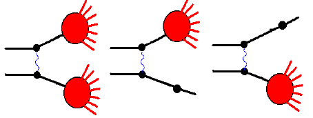
restriction of the available phase space is taken into account in low mass
string fragmentation.
A simplified Glauber model is used for sampling the multiplicity of intra-
nuclear collisions. Gribov inelastic screening is not considered. For medium
and heavy nuclei a Saxon-Woods parameterization of the one-particle nuclear
density is used, while for light nuclei a harmonic oscillator shape is used.
Center-of-mass correlations and short range nucleon-nucleon correlations are
taken into account.
The reggeon theory inspired model (RTIM) of nuclear destruction is ap-
plied for a description of secondary particle intra-nuclear cascading. A new
algorithm to simulate ”Fermi motion” in nuclear reactions is used.
Excitation energies of residual nuclei are estimated in the wounded nu-
cleon approximation. This allows for a direct coupling of the FTF model to
the Precompound model of Geant4 and hence with the GEM nuclear frag-
mentation model. The determination of the particle formation time allows
one to couple the FTF model with the Binary cascade model of Geant4.
28.1 Main assumptions of the FTF model
The Fritiof model[1, 2] assumes that all hadron-hadron interactions are bi-
nary reactions, h1+h2→h′
1+h′
2, where h′
1and h′
2are excited states of the
hadrons with discrete or continuous mass spectra (see Fig. 28.1). If one of
the final hadrons is in its ground state (h1+h2→h1+h′
2) the reaction is
called ”single diffraction dissociation”, and if neither hadron is in its ground
state it is called a ”non-diffractive” interaction. (Notice that, in spite of
its name, this definition of ”non-diffractive” interaction includes the double
diffraction dissociation as well.)
Figure 28.1: Non-diffractive and diffractive
interactions considered in the Fritiof model.
The excited hadrons are considered as QCD-strings, and the correspond-
ing LUND-string fragmentation model is applied in order to simulate their
371
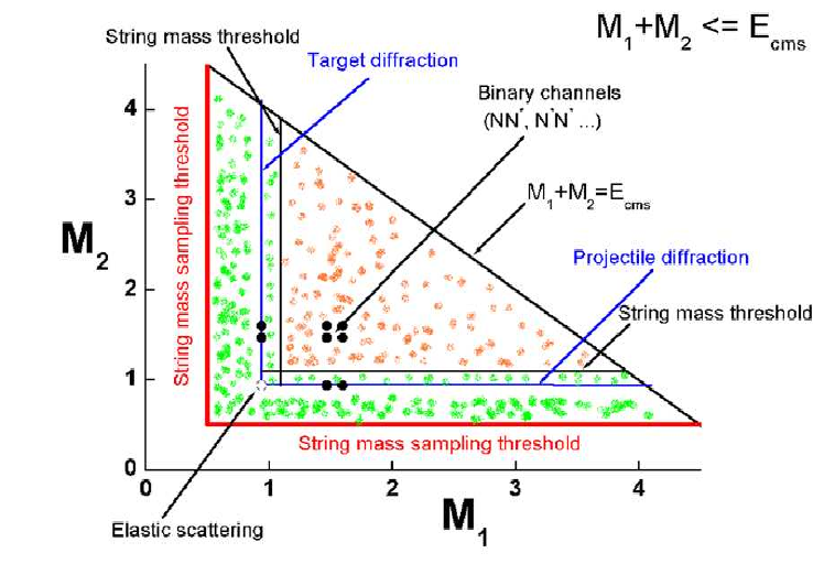
decays.
The key ingredient of the Fritiof model is the sampling of the string
masses. In general, the set of final state of interactions can be represented
by Fig. 28.2, where samples of possible string masses are shown. There is
a point corresponding to elastic scattering, a group of points which repre-
sents final states of binary hadron-hadron interactions, lines corresponding
to the diffractive interactions, and various intermediate regions. The region
populated with the red points is responsible for the non-diffractive interac-
tions. In the model, the mass sampling threshold is set equal to the ground
state hadron masses, but in principle the threshold can be lower than these
masses. The string masses are sampled in the triangular region restricted by
the diagonal line corresponding to the kinematical limit M1+M2=Ecms
where M1and M2are the masses of the h′
1and h′
2hadrons, and also of the
threshold lines. If a point is below the string mass threshold, it is shifted to
the nearest diffraction line.
Figure 28.2: Diagram of the final states of hadron-hadron interactions.
Unlike the original Fritiof model, the final state diagram of the current
model is complicated, which leads to a mass sampling algorithm that is not
simple. This will be considered below. The original model had no points
corresponding to elastic scattering or to the binary final states. As it was
372
known at the time, the mass of an object produced by diffraction dissociation,
Mx, for example from the reaction p+p→p+X, is distributed as dMx/Mx∝
dM2
x/M2
x, so it was natural to assume that the object mass distributions in
all inelastic interactions obeyed the same law. This can be re-written using
the light-cone momentum variables, P+or P−,
P+=E+pz, P −=E−pz(28.1)
where Eis an energy of a particle, and pzis its longitudinal momentum along
the collision axis. At large energy and positive pz,P−≃(M2+P2
T)/2pz.
At negative pz,P+≃(M2+P2
T)/2|pz|. Usually, the transferred transverse
momentum, PT, is small and can be neglected. Thus, it was assumed that
P−and P+of a projectile, or target associated hadron, respectively, are
distributed as
dP −/P −, dP +/P +(28.2)
A gaussian distribution was used to sample PT.
In the case of hadron-nucleus or nucleus-nucleus interactions it was as-
sumed that the created objects can interact further with other nuclear nu-
cleons and create new objects. Assuming equal masses of the objects, the
multiplicity of particles produced in these interactions will be proportional
to the number of participating nuclear nucleons, or to the multiplicity of
intra-nuclear collisions. Due to this, the multiplicity of particles produced in
hadron-nucleus or nucleus-nucleus interactions is larger than that in hadron-
hadron ones. The probabilities of multiple intra-nuclear collisions were sam-
pled with the help of a simplified Glauber model. Cascading of secondary
particles was not considered.
Because the Fermi motion of nuclear nucleons was simulated in a simple
manner, the original Fritiof model could not work at Plab <10–20 GeV/c.
It was assumed in the model that the created objects are quark-gluon
strings with constituent quarks at their ends originating from the primary
colliding hadrons. Thus, the LUND-string fragmentation model was applied
for a simulation of the object decays. It was assumed also that the strings
with sufficiently large masses have ”kinks” – additional radiated gluons. This
was very important for a correct reproduction of particle multiplicities in the
interactions.
All of the above assumptions were reconsidered in the implementation
of the Geant4 Fritiof model, and new features were added. These will be
presented below.
373
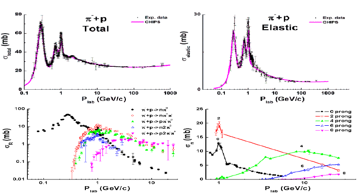
28.2 General properties of hadron–nucleon in-
teractions
Before going into details of the FTF model implementation it would be better
to consider briefly the general properties of hadron-nucleon interactions in
order to understand what needs to be simulated. These properties include
total and elastic cross sections, and cross sections of various other reactions.
There is so much data on inclusive spectra that not all of it can be addressed
in this work. It is hoped that the remaining data will be the subject of
a future paper. Inclusive data present kinematical properties of produced
particles. Their description requires additional methods and parameters,
which will be considered later.
28.2.1 π−p– interactions
Figure 28.3: General properties of π−p-interactions. Points are experi-
mental data: data on total and elastic cross sections from PDG data-base
[3], other data from [4].
Total, elastic and reaction cross sections of π−p-interactions are presented
in Fig. 28.3. As seen, there are peaks in the total cross section connected with
∆-isobar production (∆(1232), ∆(1600), ∆(1700) and so on) in the s-channel,
π−+p→∆0. The main channel of a ∆0-isobar decay is ∆0→π−+p. These
resonances are reflected in the elastic cross section. The other important de-
374
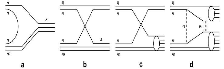
cay channel is ∆0→π0+n, which is the main inelastic reaction channel at
Plab <700 MeV/c. At higher energy two-meson production channels start to
dominate, and at Plab >3 GeV/c there is practically no structure in the cross
sections. Cross sections of final states with defined charged particle multi-
plicity, so-called prong cross sections according to the old terminology, are
presented in the last figure. As seen, real multi-particle production processes
(n≥4) dominate at Plab >5–7 GeV/c.
In the constituent quark model of hadrons, the creation of s-channel ∆-
isobars is explained by quark–antiquark annihilation (see Fig. 28.4a). The
production of two mesons may result from quark exchange (see Fig. 28.4b,
28.4c). A quark–diquark (q–qq) system created in the process can be in
a resonance state (28.4b), or in a state with a continuous mass spectrum
(28.4c). In the latter case, multi-meson production is possible. Amplitudes
of these two channels are connected by crossing symmetry to annihilation
in the t-channel, and with non-vacuum exchanges in the elastic scattering
according to the reggeon phenomenology. According to that phenomenology,
pomeron exchange must dominate in elastic scattering at high energies. In a
simple approach, this corresponds to two-gluon exchange between colliding
hadrons. It reflects also one or many non-perturbative gluon exchanges in the
inelastic reaction. Due to these exchanges, a state with subdivided colors is
created (see Fig. 28.4d). The state can decay into two colorless objects. The
quark content of the objects coincides with the quark content of the primary
hadrons, according to the FTF model, or it is a mixture of the primary
hadron’s quarks, according to the Quark-Gluon-String model (QGSM).
Figure 28.4: Quark flow diagrams of πN-interactions.
The original Fritiof model contains only the pomeron exchange process
shown in Fig. 28.4d. It would be useful to extend the model by adding the
exchange processes shown in Figs. 28.4b and 28.4c, and the annihilation pro-
cess of Fig. 28.4a . This could probably be done by introducing a restricted
375
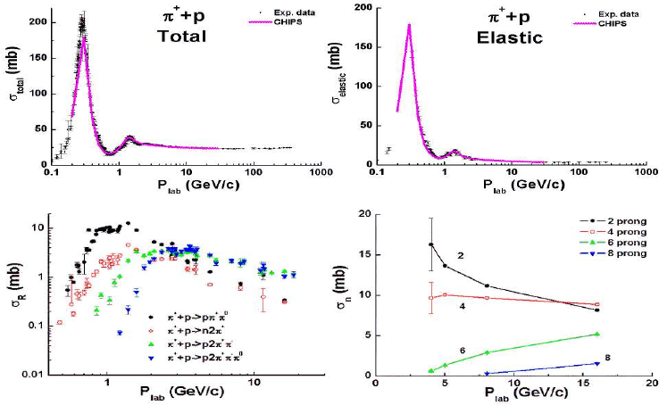
set of mesonic and baryonic resonances and a corresponding set of parame-
ters. This procedure was employed in the binary cascade model of Geant4
(BIC) [5] and in the Ultra-Relativistic-Quantum-Molecular-Dynamic model
(UrQMD) [6]. However, it is complicated to use this solution for a simulation
of hadron-nucleus and nucleus-nucleus interactions. The problem is that one
has to consider resonance propagation in the nuclear medium and take into
account their possible decays which enormously increases computing time.
Thus, in the current version of the FTF model only quark exchange processes
have been added to account for meson and baryon interactions with nucleons,
without considering resonance propagation and decay. This is a reasonable
hypothesis at sufficiently high energies.
28.2.2 π+p– interactions
Figure 28.5: General properties of π+p-interactions. Points are experi-
mental data: data on total and elastic cross sections from PDG data-base
[3], other data from [4].
Total, elastic and reaction cross sections of π+p-interactions are presented
in Fig. 28.5. As seen, there are fewer peaks in the total cross section than in
π−p-collisions. The creation of ∆++-isobars in the s-channel (π++p→∆++)
is mainly seen in the elastic cross section because the main channel of ∆++-
isobar decay is ∆++ →π++p. This process is due to quark–antiquark
376
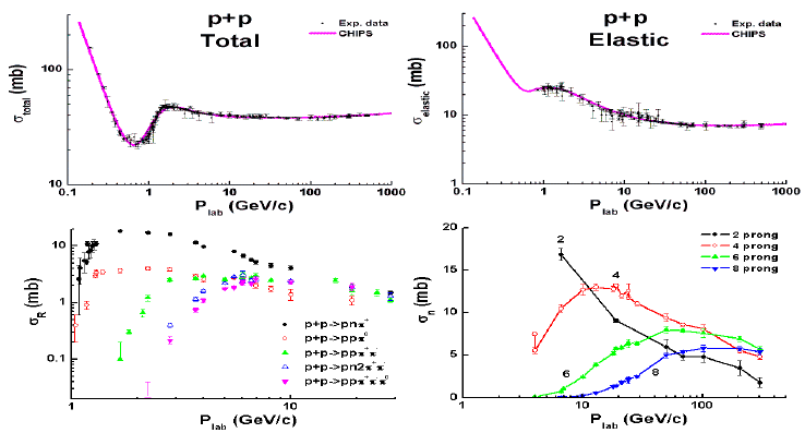
annihilation. At Plab >400 MeV/c two-meson production channels appear.
They can be connected with quark exchange and with the formation of ∆++
and ∆+isobars at the proton site. The corresponding cross sections of the
reactions – π++p→π0+∆++ →π0+π++p,π++p→π++∆+→π++π0+p,
π++p→π++ ∆+→π++π++nhave structures at Plab ≃1.5 and 2.8
GeV/c. At higher energies there is no structure. The cross sections of other
reactions are rather smooth.
28.2.3 pp – interactions
Figure 28.6: General properties of pp-interactions. Points are experimen-
tal data: data on total and elastic cross sections from PDG data-base.
[3], other data from [7].
Total, elastic and reaction cross sections of pp-interactions are presented
in Fig. 28.6. The total cross section is seen to decrease with energy below
the meson production threshold (Plab ≤800 MeV/c). Above the threshold
the cross section starts to increase and becomes nearly constant. The main
reaction channel below 6–8 GeV/c is p+p→p+n+π+. Because there
cannot be quark–antiquark annihilation in the interaction, the reaction must
be connected to quark exchange. Intermediate states can be p+p→p+ ∆+
and p+p→n+ ∆++. In the first case, quarks of the same flavor in the
projectile and the target are exchanged. In the second case quarks with
different flavors take part in the exchange. Because the cross section of the
377
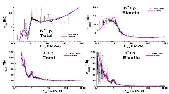
p+p→p+n+π+reaction is larger than the that of p+p→p+p+π0, one has
to assume that the exchange of quarks with the same flavors is suppressed.
All the reactions shown can also be caused by diffraction dissociation.
Although there can be a contribution of the p+p→∆0+ ∆++ reaction
into the cross section of the channel p+p→(p+π−) + (p+π+) at Plab ∼
2–3 GeV/c, one can assume that diffraction plays an essential role in these
interactions, because there are no defined structures in the cross sections.
Summing up the consideration of the interactions, one can conclude that
the probability of quark exchanges can depend on quark flavors, and that
pp-collisions could be a source of information about diffraction.
28.2.4 K+p– and K−p– interactions
For completeness, the properties of K+p- and K−p-interactions are presented.
Total and elastic cross sections are shown in Fig. 28.7. As the s-antiquark in
the K+-mesons cannot annihilate in the K+p-interactions, the structure of
the corresponding cross sections is rather simple, and is very like the structure
of pp cross sections. The u-antiquark in the K−-mesons can annihilate, and
the structure of the cross sections is more complicated. Due to these features,
inelastic reactions are very different even though all of them can be connected
with various quark flow diagrams like that shown in Fig. 28.4
Figure 28.7: Total and elastic cross sections of Kp-interactions.
Points are experimental data from PDG data-base [3].
The reactions K−+p→Σ−+π+and K−+p→Σ0+π0can be explained
by the annihilation of the u-antiquark of the K−and the formation of s-
378

channel resonances. The other reactions – K−+p→Σ++π−and K−+p→
Λ + π0, are connected with quark exchange. As seen, the energy dependence
of the cross sections of the two types of processes are different. The K−+p→
n+K0reaction must be caused by annihilation, but the dependence of its
cross section on energy is closer to that of the quark exchange processes.
The cross section of the reaction has a resonance structure only at Plab <2
GeV/c. Above that energy there is no structure. Because the cross section
of the reaction is sufficiently small at high energies, one can omit its correct
description.
Figure 28.8: Reaction cross sections of Kp-interactions. Points are ex-
perimental data [8].
K−+p→n+K−+π+and K−+p→p+K0+π−reactions are mainly
caused by the diffraction dissociation of a projectile or a target hadron. The
energy dependence of their cross sections are different from those of annihi-
lation and quark exchange.
The same regularities can be seen in K+preactions. The energy depen-
dence of the cross sections of the K++p→p+K0+π+,K++p→p+K++π0
and K++p→n+K++π+reactions are quite different from those of K−+p.
In summary, there are three types of energy dependence in the reaction
cross sections. The rapidly decreasing one is due to annihilation. The cross
sections of the quark exchange processes decrease more slowly. Finally, the
diffraction cross sections grow with energy and reach near-constant values.
379
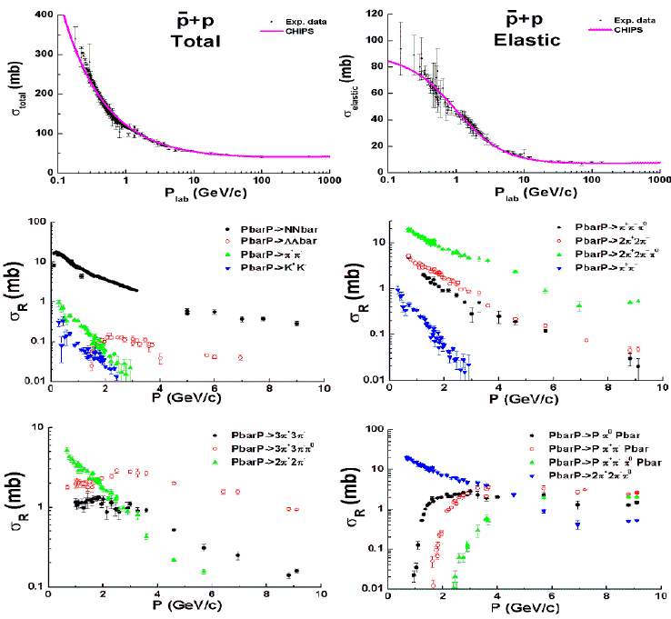
28.2.5 p¯p– interactions
Proton–antiproton interactions provide the beautiful possibility of studying
annihilation processes in detail. The general properties of the interactions
are presented in Fig. 28.9. Almost no structure is seen in the cross sections
and their energy dependence is very different from the previously described
reactions.
Figure 28.9: General properties of ¯pp-interactions. Points are experimen-
tal data: data on total and elastic cross sections from PDG data-base [3],
other data from [7].
Cross sections of the reactions – ¯p+p→π++π−and ¯p+p→K++K−,
decrease faster than other cross sections as a functions of energy. ¯p+p→
π++π−+π0and ¯p+p→2π++2π−cross sections decrease less rapidly, nearly
in the same manner as cross sections of the reactions – ¯p+p→n+ ¯nand
380
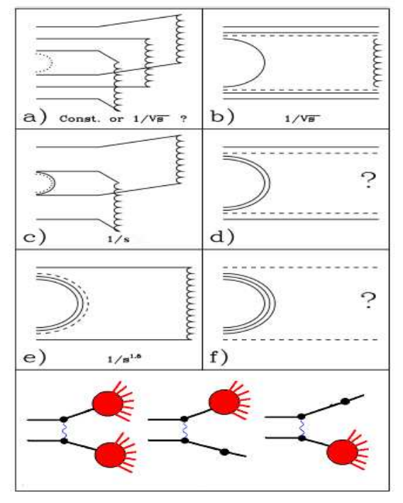
¯p+p→Λ + ¯
Λ. The cross sections of the reaction – ¯p+p→2π++ 2π−+π0,
is a slowly decreasing function. The cross section of the process – ¯p+p→
3π++ 3π−+π0varies only a little over the studied energy range. Cross
sections of other reactions (¯p+p→p+π0+ ¯p, ¯p+p→p+π++π−+ ¯pand
so on) show behaviour typical of diffraction cross sections.
The main channel of ¯pp interactions at Plab <4 GeV/c is ¯p+p→
2π++ 2π−+π0. At higher energies, there is a mixture of various channels.
Such variety in the processes is indicative of complicated quark interactions.
Possible quark flow diagrams are shown in Fig. 28.10.
Figure 28.10: Quark flow diagrams of ¯pp-interactions.
As usual, quarks and antiquarks are shown by solid lines. Dashed lines
present so-called string junctions. It is assumed that the gluon field in
baryons has a non-trivial topology. This heterogeneity is called a ”string
381
junction”. Quark-gluon strings produced in the reaction are shown by wavy
lines.
The diagram of 28.10a represents a process with a string junction anni-
hilation and the creation of three strings. Diagram 28.10b describes quark-
antiquark annihilation and string creation between the diquark and anti-
diquark. Quark-antiquark and string junction annihilation is shown in Fig.
28.10c. Finally, one string is created in the process of 28.10e. Hadrons ap-
pear at the fragmentation of the strings in the same way that they appear
in e+e−-annihilation. One can assume that excited strings with complicated
gluonic field configurations are created in processes 28.10d and 28.10f. If the
collision energy is sufficiently small glueballs can be formed in the process
28.10f. Mesons with constituent gluons or with hidden baryon number can
be created in process 28.10d. Of course the standard FTF processes shown
in the bottom of the figure are also allowed.
In the simplest approach it is assumed that the energy dependence of the
cross sections of these processes vary inversely with a power of sas depicted
in Fig. 28.10 . Here sis center-of-mass energy squared. This is suggested
by the reggeon phenomenology (at the leading order). Calculating the cross
sections of binary reactions (in the reggeon framework, including higher-
order terms) is a rather complicated procedure (see [9]) because there can be
interactions in the initial and final states. Similar complications appear also
in the computation of cross sections of other reactions [10].
28.3 Cross sections of hadron–nucleon pro-
cesses
28.3.1 Total, elastic and inelastic hadron–nucleon cross
sections
Parameterizations of the cross sections implemented in the CHIPS model of
Geant4 (authors: M.V. Kossov and P.V. Degtyarenko) are used in the FTF
model. The general form of the parameterization is:
σ=σLE +σAs (28.3)
where σLE is a low energy parameterization depending on the types of col-
liding particles, and σAs is the asymptotic part of cross sections. The COM-
PLETE Collaboration proposed a hypothesis [11] that σAs of total cross
sections at very high energies does not depend on the types of colliding par-
ticles:
σtot
As =Zh1h2+B(log(s/s0))2(28.4)
382

B= 0.3152, s0= 34.0 [(GeV/c)2] (COM P LET E, 2002) (28.5)
B= 0.308 , s0= 28.9 [(GeV/c)2] (P DG, 2006) (28.6)
B= 0.304 , s0= 33.1 [(GeV/c)2] (M.Ishida, K.Igi, 2009)(28.7)
while the pre-asymptotic part does depend on colliding particles (h1,h2).
The CHIPS model σAs for total and elastic cross sections has the same
form:
σAs =A[ln(Plab)−B]2+C+D/P 0.5
lab +E/Plab +F/P 2
lab/
(1 + G/P 0.5
lab +H/P 3
lab +I/P 4
lab) [mb] (28.8)
where Plab is in [GeV /c], and the parameters A,B, etc. are given in the
tables 28.1 and 28.2.
Table 28.1: CHIPS model parameters for total cross sections
h1h2A B C D E F G H I
π−p0.3 3.5 22.3 12.0 0 0 0 0 0.4
π+p0.3 3.5 22.3 5.0 0 0 0 0 1.0
pp 0.3 3.5 38.2 0 0 0 0 0 0.54
np 0.3 3.5 38.2 0 0 52.7 0 0 2.72
K+p0.3 3.5 19.5 0 0 0 0.46 0 1.6
K−p0.3 3.5 19.5 0 0 0 -0.21 0 0.52
¯pp 0.3 3.5 38.2 0 0 0 0 0 0
Table 28.2: CHIPS model parameters for elastic cross sections
h1h2A B C D E F G H I
π−p0.0557 3.5 2.4 6.0 0 0 0 0 3.0
π+p0.0557 3.5 2.4 7.0 0 0 0 0 0.7
pp 0.0557 3.5 6.72 0 30.0 0 0 0.49 0.
np 0.0557 3.5 6.72 0 32.6 0 0 0 1.0
K+p0.0557 3.5 2.23 0 0 0 -0.7 0 0.1
K−p0.0557 3.5 2.23 0 0 0 -0.7 0 0.075
The low energy parts of the cross sections are very different for various
projectiles, and they are not presented here. These can be found in the
corresponding classes of Geant4.
It is obvious that σin =σtot −σel.
A comparison of the parameterizations with experimental data was pre-
sented in the previous figures.
383

28.3.2 Cross sections of quark exchange processes
Cross sections of quark exchange processes are parameterized as:
σqe =σin A e−B ylab (28.9)
where ylab is a projectile rapidity in a target rest frame. Aand Bare param-
eters given in Tabl. 28.3
Table 28.3: Parameters of quark exchange cross sections
h1h2A B
pp/pn 1.85 0.7
πp/πn 240 2
Kp/Kn 40 2.25
The parameters were determined from a description of reaction channel
cross sections.
28.3.3 Cross sections of antiproton processes
The annihilation cross section is parameterized as:
σann =σa+B Xb+C Xc+D Xd(28.10)
where: Xiare the contributions of the diagrams of Fig. 28.10; all cross
sections are given in [mb];
σa= 25 √s/λ1/2(s, m2
p, m2
N) (28.11)
λ(s, m2
p, m2
N) = s2+m4
p+m4
N−2sm2
p−2sm2
N−2m2
pm2
N(28.12)
Xb= 3.13 + 140 (sth −s)2.5, s < sth (28.13)
Xb= 6.8/√s, s > sth (28.14)
sth = (mp+mN+ 2mπ+δ)2
Xc= 2 √s
λ1/2(s, m2
p, m2
N)
(mp+mN)2
s(28.15)
Xd= 23.3/s (28.16)
The coefficients B,Cand Dare pure combinatorial coefficients calcu-
lated on the assumption that the same conditions apply to all quarks and
antiquarks. For example, in ¯pp interactions there are five possibilities to
annihilate a quark and an antiquark, and six possibilities to annihilate two
quarks and two antiquarks. Thus, B=C= 5 and D= 6.
384

Table 28.4: Coefficients B,Cand D
¯pp ¯pn ¯np ¯nn ¯
Λp¯
Λn¯
Σ−p¯
Σ−n¯
Σ0p¯
Σ0n¯
Σ+p¯
Σ+n
B 5 4 4 5 3 3 2 4 3 3 4 2
C 5 4 4 5 3 3 2 4 3 3 4 2
D 6 4 4 6 3 3 2 2 2 2 2 0
¯
Ξ−p¯
Ξ−n¯
Ξ0p¯
Ξ0n¯
Ω−p¯
Ω−n
B 1 2 2 1 0 0
C 1 2 2 1 0 0
D 0 0 0 0 0 0
Note that final state particles in the process of Fig. 28.10b can coincide
with initial state particles. Thus the true elastic cross section is not given by
the experimental cross section.
At Plab <40 MeV/c antiproton-nucleon cross sections are:
σtot = 1512.9, σel = 473.2, σa= 625.1, σb= 0, σc= 49.99, σd= 6.61
All cross sections are given in [mb]. σb= 0 for ¯pp-interactions because the
process ¯pp →¯nn is impossible at these energies (Plab <40 MeV/c).
28.3.4 Cross sections of diffractive and non-diffractive
processes
As mentioned above, three processes are considered in the FTF model at
high energies: projectile diffraction (pd), target diffraction (td) and non-
diffractive interactions (nd). They are parameterized as:
σpd
pp =σtd
pp = 6 + σin 1.5
s(mb) (28.17)
σpd
¯pp =σtd
¯pp = 6 + σin 1.5
s(mb) (28.18)
σpd
πp = 6.2−e−(√s−7)2
16 , σtd
πp = 2 + 22/s (mb) (28.19)
σpd
Kp = 4.7, σtd
Kp = 1.5 (mb) (28.20)
For the determination of these cross sections, inclusive spectra of particles
in hadronic interactions were used. In Fig. 28.11 an inclusive spectrum of
protons in the reaction p+p→p+Xis shown in comparison with model
predictions.
As it can be seen, all the models have difficulties in describing the data. In
the FTF model this was overcome by tuning the single diffraction dissociation
385
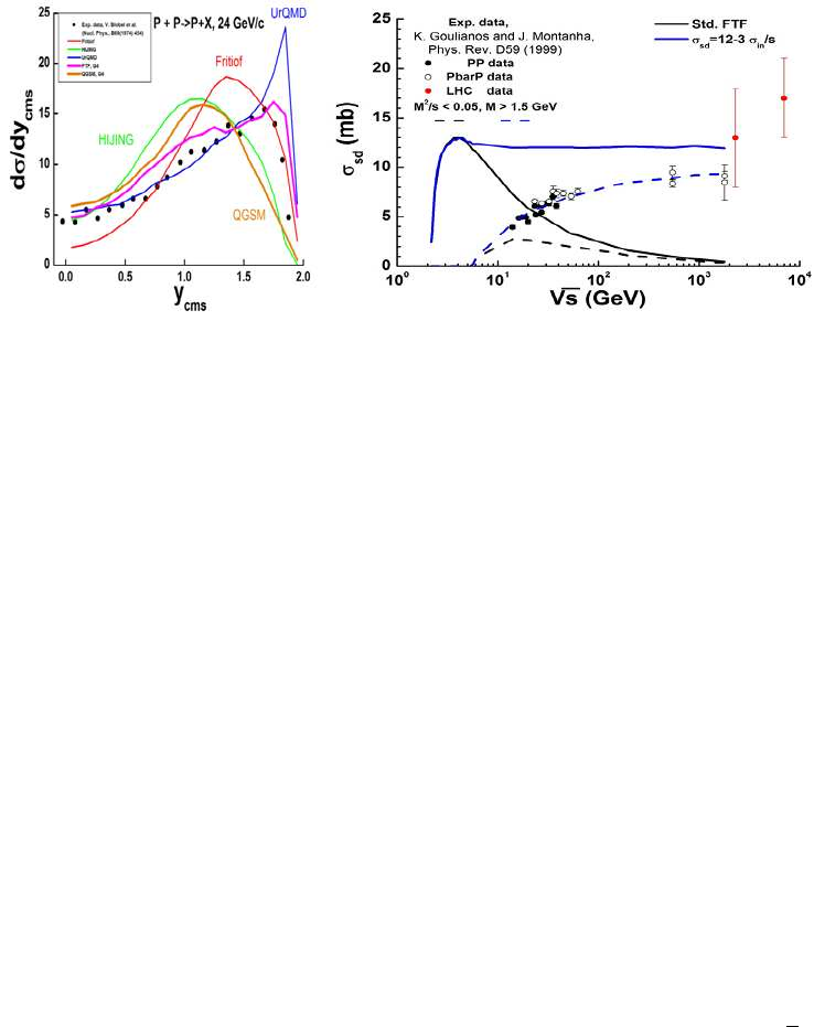
Figure 28.11: Left: inclusive spectrum of proton in pp-interactions at
Plab = 24 GeV/c. Points are experimental data [14], lines are model
calculations. Right: single diffraction dissociation cross section in pp-
interactions. Points are data gathered by K. Goulianos and J. Montanha
[15]. Lines are FTF model calculations.
cross section. Tuning was possible by the fact that the height of the proton
peak at large rapidities depends on this cross section (see left Fig. 28.11).
The 2σpd
pp (the factor of 2 is due to the fact that σpd
pp =σtd
pp) predicted
by the expression (blue solid curve) is shown at the right of Fig. 28.11
in a comparison with experimental data gathered by K. Goulianos and J.
Montanha [15]. The values are larger than experimental data. Though taking
into account the restriction that the mass of a produced system, X, cannot
be very small or very large (M2/s < 0.05 and M > 1.5 GeV) brings the
predictions closer to the data. So, the accounting of this restriction is very
important for a correct reproduction of the data.
A more complicated situation arises with πp- and Kp-interactions. The
set of experimental data on diffraction cross sections is very restricted. Thus,
a refined tuning was used. The FTF processes discussed above contribute
in various regions of particle spectra. The target diffraction dissociation,
π+p→π+X, gives its main contribution at large values of xF= 2pz/√sfor
π-mesons. The projectile diffraction dissociation contribution (π+p→X+p)
has a maximum at xF∼ −1. Thus, using various experimental data and
varying the cross sections of the processes, the points presented in the lower
left corner of Fig. 28.12 were obtained. They were parameterized by the
expressions 28.17–28.20. A correct reproduction of particle spectra in the
central region, xF∼0, was very important for these. As a result, we have a
good description of π-meson spectra in the interactions at various energies.
In Kp-interactions the projectile diffraction cross sections were deter-
386
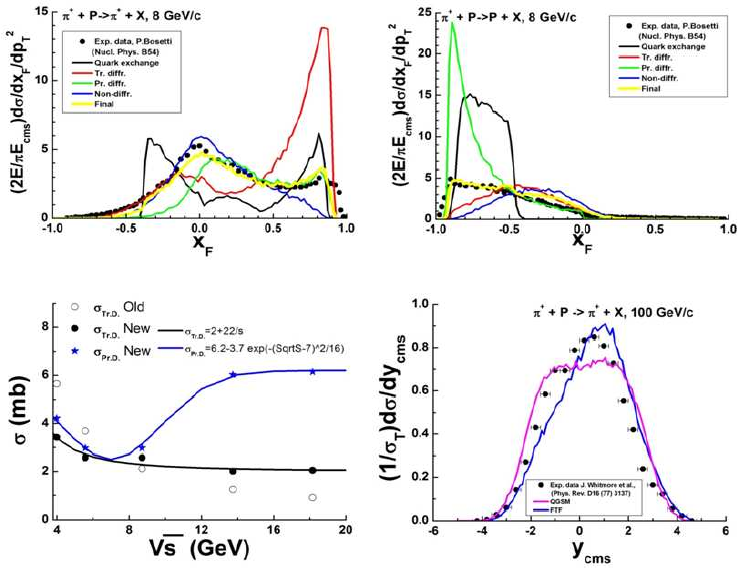
mined by tuning on proton spectra from the reactions K+p→p+X(see
Fig. 28.13). There are no data on leading K-meson spectra in the reac-
tions K+p→K+X. Thus, π−-meson spectra in the central region were
tuned. At a given value of a projectile diffraction cross section, the central
spectrum depends on a target diffraction. This was used to determine the
target diffraction cross sections. The estimated cross sections are shown in
the lower left corner of Fig. 28.13. As a result, a satisfactory description of
meson spectra was obtained.
Figure 28.12: Upper figures: inclusive spectra of protons and π+-mesons
in π+p-interactions. Points are experimental data [16]. Lines represent
the contributions of the various FTF processes calculated by assuming
that the probability of each process is 100 %. Bottom left figure: diffrac-
tion dissociation cross sections obtained by tuning (points), and their
description (lines) by the expression 28.19. Bottom right figure: rapidity
spectrum of π+-mesons in π+p-interactions at plab =100 GeV/c. Points
are experimental data [17].
387
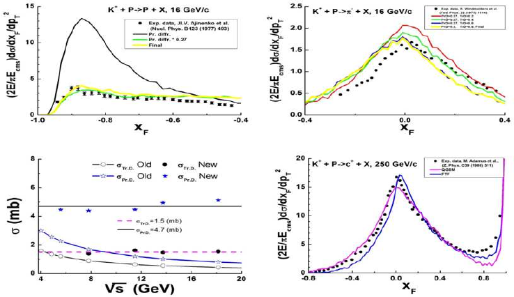
Figure 28.13: Upper figures: inclusive spectra of protons and π−-mesons
in Kp-interactions. Points are experimental data [18]. Lines are FTF
calculations. Bottom left figure: diffraction dissociation cross sections ob-
tained by tuning (points), and their description (lines) by the expression
28.20. Bottom right figure: xFspectrum of positive charged particles in
Kp-interactions at plab =250 GeV/c. Points are experimental data [17],
lines are model calculations.
28.4 Simulation of hadron-nucleon interactions
28.4.1 Simulation of meson–nucleon and nucleon–nucleon
interactions
Colliding hadrons may either be on or off the mass shell when they are bound
in nuclei. When they are off-shell the total mass of the hadrons is checked.
If the sum of the masses is above the center-of-mass energy of the collision,
the simulated event is rejected. If below, the event is accepted. It is assumed
that due to the interaction the hadrons go on-shell, and the center-of-mass
energy of the collision is not changed.
The simulation of an inelastic hadron-nucleon interaction starts with a
choice: should a quark exchange or a diffractive/non-diffractive excitation be
simulated? The probability of a quark exchange is given by Wqe =σqe/σin.
The combined probability of diffractive dissociation and non-diffractive exci-
tation is then 1−Wqe.σqe depends on the energies and flavors of the colliding
388
hadron (see Eq.28.9).
If a quark exchange is sampled, the quark contents of the projectile and
target are determined. After that the possibility of a quark exchange is
checked. A meson consists of a quark and an antiquark. Thus there is no
alternative but to choose a quark. Let it be qM. A baryon has three quarks,
q1,q2and q3. The quark from the meson can be exchanged, in principle, with
any of the baryon quarks, but the above description of the experimental data
indicates that an exchange of quarks with the same flavor must be suppressed.
So, only the exchange of quarks with different flavors is allowed. After the
exchange (qM↔qi), the new contents of the meson and the baryon are
determined. The new meson may be either pseudo-scalar or pseudo-vector
with a 50% probability. The new baryon may be in its ground state, or in
an excited state. The probability of an excited baryon state is assumed (as
common also in other codes) to be 0.5 for both πN-interactions and KN-
interactions. Only ∆(1232)’s are considered as excited states. If all quarks
of a baryon have the same flavor, the ∆(1232) is always created (∆(1232)++
or ∆(1232)−−).
The same procedure is followed for a projectile baryon, but in this case
any quark of the projectile or target may participate in an exchange if they
have different flavors. Only the ground state of the new baryon is considered.
In order to generate a transverse momentum between the two final-state
hadrons, these final-state hadrons undergo to either an additional elastic scat-
tering with probability Wel = 2.256 e−0.6ylab (the parameters have been fit-
ted from experimental data), or a diffractive/non-diffractive excitation with
probability 1 −Wel, where ylab is the rapidity of the projectile in the target
rest frame.
The above procedure is sufficient for a description of hadron-nucleon re-
action cross sections at plab <3 – 5 GeV/c. At higher energies, diffractive
dissociations and non-diffractive excitations must be simulated.
As mentioned above, there can be a projectile diffraction, or a target
diffraction, or a non-diffractive interaction. Probabilities of the correspond-
ing processes at high energies are: σpd/σin,σtd/σin, and (σin −σpd −σtd)/σin.
The processes are sampled randomly.
Having sampled a projectile diffraction or a target diffraction, the cor-
responding light-cone momentum (P−or P+) is chosen according to the
distribution: dP −/P −or dP +/P +. Boundaries for a sampling have to be
determined before.
Let us consider the kinematics of projectile diffraction, P+T→P′+T, for
the definition of these boundaries. It is obvious that a mass of the diffractive
389

produced system, mP′, must satisfy the conditions:
mD≤mP′≤√s−mT(28.21)
where mDis the minimal mass of the system, sis the center-of-mass energy
squared, mTis the mass of the target. If there is not a transverse momentum
transfer, and mP′reaches the lower boundary then
P−
min =qm2
D+p2
z−pz, pz=λ1/2(s, m2
D, m2
T)/2√s(28.22)
(See 28.12 for the definition of λ().)
When mP′reaches the upper boundary, the longitudinal momenta of the
particles are zeros. Thus,
P−
max =√s−mT(28.23)
Having sampled P−, then mP′and P+can be found with the help of the
energy-momentum conservation law written is the center-of-mass system:
EP′+ET=√s
Pz,P ′+Pz,T = 0
P−
P′+P−
T=√s
P+
P′+P+
T=√s
P−
T=√s−P−
P′
P+
T=m2
T/P −
T
m2
P′=P−
P′·(√s−P+
T)
(28.24)
The transferred transverse momentum is sampled according to the distri-
bution:
dW =1
π < P 2
⊥>e−P2
⊥/<P 2
⊥>d2P⊥, < P 2
⊥>= 0.3 (GeV/c)2(28.25)
To account for it, it is enough to replace the masses with the transverse
masses, m⊥=pm2+P2
⊥.
The light-cone momenta transferred to the projectile are:
Q+=P+
T,0−P+
T, Q−=P−
T,0−P−
T(28.26)
where P+
T,0and P−
T,0are the light-cone momenta of the target in the initial
state.
In the case of non-diffractive excitation (P+T→P′+T′), P−
P′is sampled
first of all as it was described above at mT=mT,nd, where mT,nd is the
minimal mass of a target-originated particle produced in the non-diffractive
excitation. After that, P+
T′is independently sampled at mP=mP,nd. The
minimal light-cone momenta, P−
P′and P+
T′, are calculated at mP=mP,nd
and mT=mT,nd. At the last step it is checked that mP′≥mP,nd and
mT′≥mT,nd. In the current version of the FTF model the same values for
minimal masses are used in the diffractive and non-diffractive excitation.
390

Table 28.5: Minimal masses of diffractive produced strings
p/n π K
mD(MeV) 1160 500 600
28.4.2 Simulation of antibaryon–nucleon interactions
At the beginning of the simulation of an annihilation interaction, the cross
sections of the processes (see Fig. 28.10) are calculated (see 28.10). After
that a sampling of the processes takes place.
In the cases of the processes 28.10b and 28.10e quarks for the annihilation
are chosen randomly. In each of the processes only one string is created. Its
mass is equal to the center-of-mass energy of the interaction. After that the
string is fragmented. It is required that in the fragmentation of the process
28.10b there must not be a baryon and an antibaryon in the final state.
At sufficiently high energies the standard FTF processes can be simulated
as it was described above.
In the process 28.10c only 2 strings will be created. If their masses are
given, the kinematical properties of the strings can be determined with the
help of the energy-momentum conservation law. The masses must be related
to the momenta of the quarks and antiquarks.
We assume that in the process all quarks and antiquarks are in the same
conditions, thus, their transverse momenta are sampled independently ac-
cording to the gaussian distribution with < P 2
⊥>= 0.04 (GeV/c)2. To
guarantee that the sum of the transverse momenta is zero, the transverse
momentum of each particle is re-defined as follows: ~
P⊥i→~
P⊥i−1
4P4
j=1 ~
P⊥j.
To find the longitudinal momenta of quarks we use the light-cone mo-
menta: total light-cone momenta of projectile-originated antiquarks and
target-originated quarks,
P+=P+
¯q1+P+
¯q2, P −=P−
q1+P−
q2(28.27)
Let us introduce also the light-cone momentum fractions:
x+
¯q1=P+
¯q1/P +, x+
¯q2= 1 −x+
¯q1(28.28)
x−
q1=P−
q1/P −, x−
q2= 1 −x−
q1(28.29)
Using these variables, the energy-momentum conservation law in the
center-of-mass system can be written as:
P+
2+α
2P++P−
2+β
2P−=√s(28.30)
P+
2−α
2P+−P−
2+β
2P−= 0 (28.31)
391

α=m2
⊥¯q1
x+
¯q1
+m2
⊥¯q2
1−x+
¯q1
(28.32)
β=m2
⊥q1
x−
q1
+m2
⊥q2
1−x−
q1
(28.33)
A solution of the equations at √α+√β≤√sis:
P+=s+α−β+λ1/2(s, α, β)
2√s(28.34)
P−=s−α+β+λ1/2(s, α, β)
2√s(28.35)
(See 28.12 for the definition of λ().)
If √α+√β > √s, the transverse momenta and xs are re-sampled until
the inequality is broken.
Because quarks are in the same conditions, the distribution on xcan have
the form xa(1 −x)a. A recommended value of acan be zero or −0.5. We
chose a=−0.5. We assumed also that the quark masses are zero. Probably,
other values could be used, but we have not yet found experimental data
sensitive to these parameters.
For the simulation of the process 28.10a we follow the same approach, and
introduce light-cone momentum fractions – x+
¯q1, x+
¯q2, x+
¯q3and x−
q1, x−
q2, x−
q3.
The distribution on xs is chosen according to the form:
dW ∝xa
q1xa
q2xa
q3δ(1 −xq1−xq2−xq3)dxq1dxq2dxq3, a =−0.5 (28.36)
It is obvious that in this case:
α=
3
X
i=1
m2
⊥¯qi
x+
¯qi
, β =
3
X
i=1
m2
⊥qi
x−
qi
(28.37)
28.5 Flowchart of the FTF model
The simulation of hadron-nucleus or nucleus-nucleus interaction events starts
with an initialization (done ”on-the-fly” just before simulating the interac-
tion, not at the beginning of the program) of the model variables: calculations
of cross sections, setting up slopes, masses and so on. The next step is the
determination of intra-nuclear collision multiplicity with the help of Glauber
model. If the energy of collisions is sufficiently high, the simulation of sec-
ondary particle cascading within the reggeon theory inspired model (RTIM
[19]) is carried out. After that all involved nuclear nucleons are put on the
392

mass-shell. If the energy is not high enough these steps are skipped. The
reason for this will be explained later.
The main job of the FTF algorithm is done in the loop over intra-nuclear
collisions. At that moment, the time ordering of the collisions has been de-
termined. For each collision, it is sampled what has to be simulated – elastic
scattering, inelastic interaction or annihilation for projectile antibaryons. For
each branch, an adjustment of the participating nuclear nucleon is performed
at low energy, and the corresponding process is simulated. In the case of the
sampling of the inelastic interaction at high energy there is an alternative –
to reject the interaction or to process it.
Figure 28.14: Flowchart of the FTF model.
At the end of the loop, the properties of nuclear residuals (mass number,
charge, excitation energy and 4-momentum) are transferred to a calling pro-
gram. The program initiates the fragmentation of created strings and decays
393
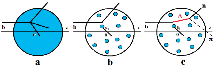
the excited residuals.
Simulations of elastic scattering, inelastic interactions and annihilation
were considered above. Other steps of the FTF model will be presented
below.
28.6 Simulation of nuclear interactions
28.6.1 Sampling of intra-nuclear collisions
Classical cascade-type sampling
As it is known, the intra-nuclear cascade models like the ones implemented in
Geant4 – the Bertini model, the Binary cascade model, the Liege (INCLXX)
model – work well for projectile energies below 5 – 10 GeV. The first step in
these models is the sampling of the impact parameter, b. The next step is
the sampling of a point where the projectile will interact with nuclear matter
(see Fig. 28.15a).
Figure 28.15: Cascade-type sampling.
The following consideration is used here: the probability that the projec-
tile reaches a point zgoing from minus infinity to the point zis
P=e−σtot Rz
−∞ ρA(~
b,z′)dz′(28.38)
where σtot is the total cross section of the projectile-nucleon interaction, ρA
is the density of the nucleus considered as a continuous medium.
The probability that the projectile will have an interaction in the range
z–z+dz is equal to σtotρA(~
b, z)dz. Thus, the total probability is:
P(~
b, z) = σtotρA(~
b, z)e−σtot Rz
−∞ ρA(~
b,z′)dz′dz (28.39)
394

P(~
b) = Z+∞
−∞
P(~
b, z)dz = 1 −e−σtot R∞
−∞ ρA(~
b,z′)dz′(28.40)
Having sampled the interaction point, the choice between an elastic scattering
and an inelastic interaction is then implemented.
In the case of the inelastic interaction, a multi-particle production process
is simulated. After this, for each produced particle new interaction points
are sampled, and so on.
In the case of the elastic scattering, the scattering is simulated, and then
new interaction points for the recoil nucleon and the projectile are sampled.
The prescription is changed a little bit by replacing the continuous medium
with a collection of Anucleons located in the points {~si, zi},i= 1–Awhere
{~si}are coordinates of the nucleons in the impact parameter plane. The
projectile can interact with the nearest nuclear nucleon, whose ~sisatisfies
the condition: |~
b−~si| ≤ pσtot/π (see Fig. 28.15b).
In the first versions of the cascade models, only nucleons and pions were
considered. When it was recognized that most of inelastic reactions at inter-
mediate energies are going through resonance productions, various baryonic
and mesonic resonances were included, and the algorithm changed (see Fig.
28.15c). As energy grows, more and more heavy resonances are produced.
Because the properties of resonance-nucleon collisions were not known, the
interpretation of the Glauber approximation was very useful.
Short review of Glauber approximation
The Glauber approach [20] was proposed in the framework of the potential
theory, before the creation of the intra-nuclear cascade models. Its main as-
sumption is that at sufficiently high energies many partial waves contribute to
a particle elastic scattering amplitude, f(~q). Thus, a summation on angular
momenta can be replaced by an integral:
f(~q) = iP
2πZei~q~
bh1−eiχ(~
b)id2b , dσ
dΩ=|f(~q)|2(28.41)
γ(~
b) = 1
2πiP Ze−i~q~
bf(~q)d2q(28.42)
where Pis the projectile momentum, qis the transferred transverse momen-
tum, ~
bis the impact parameter, χis the phase shift, and γis the scattering
amplitude in the impact parameter representation.
Due to the additivity of potentials, it was natural to assume that the
overall phase shift for the projectile scattered on Acenters located in the
395
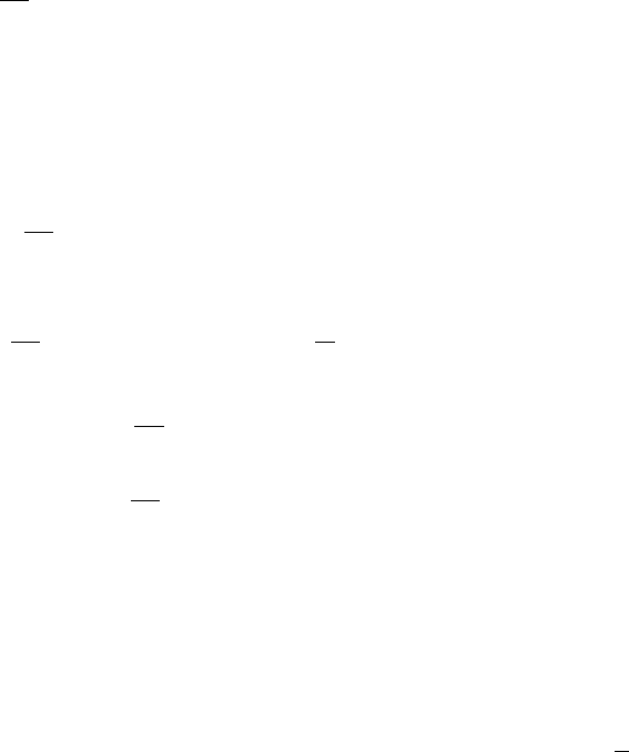
points {~si, zi},i= 1–Ais the sum of the corresponding shifts on each center:
χhA =
A
X
i=1
χ(~
b−~si) (28.43)
γhA(~
b) = 1 −
A
Y
i=1 h1−γ(~
b−~si)i(28.44)
Because the positions of nucleons in nuclei are not fixed, the Eq. 28.44
has to be averaged, and the hadron-nucleus scattering amplitude takes the
form:
FhA
0→f=iP
2πZd2b e−i~q~
b(1−
A
Y
i=1 h1−γ(~
b−~si)i)Ψ0({rA})Ψ∗
f({rA})
A
Y
i=1
d3ri
(28.45)
where Ψ0and Ψfare wave functions of the nucleus in initial and final states,
respectively.
In the case of elastic scattering, Ψ0= Ψf, we have:
FhA
el =iP
2πZd2b e−i~q~
b(1−
A
Y
i=1 1−Zγ(~
b−~si)ρA(~si, z′)d2sidz′)≃
(28.46)
≃iP
2πZd2b e−i~q~
b(1−1−1
AZγ(~
b−~s)TA(~s)d2sA)(28.47)
≃iP
2πZd2b e−i~q~
bn1−e−Rγ(~
b−~s)TA(~s)d2so(28.48)
≃iP
2πZd2b e−i~q~
bn1−e−σtot
hN (1−iα)TA(~
b)/2o(28.49)
Some assumptions and simplifications have been used in the above deriva-
tions. First of all, it was assumed that |Ψ0|2≃QA
i=1 ρ(~si, zi) where ρis the
one-particle nuclear density. Because the nucleon coordinates must obey
the obvious condition: PA
i=1 ~ri= 0, it would be better to use |Ψ0|2≃
δ(PA
i=1 ~ri)QA
i=1 ρ(~si, zi). Considering this δ-function corresponds to take into
account the center-of-mass correlation.
The second assumption is that Ais sufficiently large, thus (1−x
A)A
A→∞ =e−x
(optical limit).
A thickness function of the nucleus was introduced:
T(~
b) = AZ+∞
−∞
ρ(~
b, z)dz (28.50)
396

It was assumed also that the range of the γ-function is much less than the
range of the nuclear density: Rγ(~
b−~s)TA(~s)d2s≃σtot
hN (1−iα)TA(~
b)/2, where
σtot
hN is the hadron-nucleon total cross section, and α=Re f (0)/Im f(0) is
the ratio of real and imaginary parts of hadron-nucleon elastic scattering
amplitude at zero momentum transfer.
There were many applications of the Glauber approach for calculations of
elastic scattering cross sections, cross sections of nuclear excitations, coherent
particle production and so on. We consider here only its application to
inelastic reactions.
If the energy resolution of a scattered projectile is not too high, many
nuclear excited states can contribute to the scattering amplitude: FhA =
PfFhA
0→f. To find the corresponding cross section, it is usually assumed
that a set of final-state wave functions satisfy the completeness relation:
PfΨf({~ri})Ψ∗
f({~r′
j}) = QA
i=1 δ(~ri−~r′
i).
In the Glauber approach, it is possible to show that the cross section of
elastic and quasi-elastic scatterings has the following expression:
σhA
el.+qel. =Zd2bn1−2Re e−σtot
hN (1−iα)TA(~
b)/2+e−σin
hN TA(~
b)o(28.51)
Subtracting from it the cross section of the elastic scattering, we have:
σhA
qel. =Zd2bne−σin
hN TA(~
b)−e−σtot
hN TA(~
b)o=Zd2b e−σtot
hN TA(~
b)neσel
hN TA(~
b)−1o
=Zd2b e−σtot
hN TA(~
b)∞
X
n=1
[σel
hN TA(~
b)]n
n!(28.52)
The last expression shows that the quasi-elastic cross section is a sum of
cross sections with various multiplicities of elastic scatterings. It coincides
with the prescription of the cascade model if only elastic scatterings of the
projectile are considered.
The cross section of multi-particle production processes in the Glauber
approach has the form:
σhA
mpp =σhA
tot −σhA
el.+qel. =Zd2bn1−e−σin
hN TA(~
b)o
=Zd2b e−σin
hN TA(~
b)∞
X
n=1
[σin
hN TA(~
b)]n
n!(28.53)
This expression coincides with the analogous cascade expression in the
case of a projectile particle that can be distinguished from the produced
particles. Of course, it cannot be so in the case of projectile pions.
397

In the FTF model of Geant4 it is assumed that projectile- and target-
originated strings are distinguished. Thus, the cascade-type algorithm of the
sampling of the multiplicities and types of interactions in nuclei is used.
A generalization of the Glauber approach for the case of nucleus-nucleus
interactions was proposed by V. Franco [21]. In this approach, the cross
section of multi-particle production processes is given by the expression:
σAB
mpp =Zd2b(1−
A
Y
i=1
B
Y
j=1 h1−g(~
b+τj−~si)i)·
·|ΨA
0({rA})|2|ΨB
0({tB})|2"A
Y
i=1
d3ri#" B
Y
j=1
d3ti#(28.54)
where g(~
b) = γ(~
b) + γ∗(~
b)− |γ(~
b)|2,Aand Bare mass numbers of colliding
nuclei, {~τj}is a set of impact coordinates of projectile nucleons (~
t= (~τ, z)).
Considering g(~
b) as a probability that two nucleons separated by the im-
pact parameter ~
bwill have an inelastic interaction, a simple interpretation of
the Eq. 28.54 can be given. The expression in the curly brackets of Eq. 28.54
is the probability that there will be at least one or more inelastic nucleon-
nucleon interactions. |ΨA
0({rA})|2|ΨB
0({tB})|2hQA
i=1 d3rii hQB
j=1 d3tiiis
the probability to find nucleons with coordinates {rA}and {tB}. This
interpretation allows a simple implementation in a program code, as de-
scribed in many papers [22], sometimes with the simplifying assumption
that g(~
b) = θ(|~
b| − pσin
NN /π). This is the so-called Glauber Monte Carlo
approach.
Because there is no expression in the Glauber theory that combines elastic
and inelastic nucleon-nucleon collisions in nucleus-nucleus interactions, the
same cascade-type sampling is used in the FTF model also in the case of
these interactions.
Correction of the number of interactions
The Glauber cross section of multi-particle production processes in hadron-
nucleus interactions (Eq. 28.53) was obtained in the reggeon phenomenology
approach [23], applying the asymptotical Abramovski-Gribov-Kancheli cut-
ting rules [24] to the elastic scattering amplitude (Eq. 28.46). Thus, the
summation in Eq. 28.53 is going from one to infinity. But a large number
of intra-nuclear collisions cannot be reached in interactions with extra-heavy
nuclei (like neutron star), or at low energy. To restrict the number of colli-
sions it is needed to introduce finite-energy corrections to the cutting rules.
398

Because there is no well-defined prescriptions for accounting these correc-
tions, let us take a phenomenological approach, starting with the cascade
model.
As it was said above, a simple cascade model considers only pions and
nucleons. Due to this it cannot work when resonance production is a domi-
nating process in hadronic interactions. But if energy is sufficiently low the
resonances can decay before a next possible collision, and the model can be
valid. Let pbe the momentum of a produced resonance (∆). The average
life-time of the resonance in its rest frame is 1/Γ. In the laboratory frame
the time is E∆/Γm∆. During the time, the resonance will fly a distance
¯
l=v E∆/Γm∆=p/Γm∆. If the distance is less than the average distance
between nucleons in nuclei ( ¯
d∼2 fm), the model can be applied. From this
condition, we have:
p≤¯
dΓm∆∼1.5 (GeV/c)
Direct ∆-resonance production takes place in πN interactions at low en-
ergies. Thus the model cannot work quite well for momentum of pions above
2 GeV/c. In nucleon-nucleon interactions, due to the momentum transfer to
a target nucleon, the boundary can be higher.
Returning back to the FTF model, let us assume that the projectile-
originated strings have average life-time 1/Γ, and an average mass m∗. The
strings can interact on average with ¯
l/ ¯
d=p/Γm∗/¯
d=p/p0nucleons. Here
p0is a new parameter. According to our estimations p0has value of about
3–5 GeV/c. Thus, we can assume that at a given energy there is a maximum
number of intra-nuclear collisions in the FTF model, given by: νmax =p/p0.
Let us introduce this number in the Glauber expression for the cross
section of multi-particle production processes.
σhA
mpp =Zd2b(1−1−1
Aσin
hN TA(~
b)A)
=Zd2b(1−"1−1
Aσin
hN TA(~
b)A/νmax #νmax )
=Zd2b
νmax
X
ν=1
νmax!
ν!(νmax −ν)! "1−1−1
Aσin
hN TA(~
b)A/νmax #ν
·
·"1−1
Aσin
hN TA(~
b)A/νmax #νmax−ν
(28.55)
As seen from the expression above, the number of the intra-nuclear colli-
sions is restricted to νmax.
399
The formula looks rather complicated, but a Monte Carlo algorithm for
the rejection of the interaction number is quite simple.
For example, an algorithm implementing it could look like this: at the be-
ginning, a projectile has the ”power”, Pw, to interact inelastically with νmax
nucleons (Pw=νmax; you can think about it as a likelihood, or unnormal-
ized probability), thus the probability of an interaction with the first nucleon,
Pw/νmax, is equal to 1. The power decreases after the first interaction. Thus,
the probability of an inelastic interaction with a second nucleon is equal to
Pw/νmax, where Pw=νmax −1. If the second interaction happens, the power
is decreased once more; else it is left at the same level. This is applied for
each possible interaction.
The same algorithm is applied in the case of nucleus-nucleus interactions,
but the power Pwis ascribed to each of the projectile or target nucleons.
28.6.2 Reggeon cascading
As known, the Glauber approximation used in the Fritiof model and in other
string models does not provide enough amount of intra-nuclear collisions for
a correct description of nuclear destruction. Additional cascading in nuclei
is needed. The usage of a standard cascade for secondary particle interac-
tions leads to a too large multiplicity of produced particles. Usually, it is
assumed that the inclusion of secondary particle’s formation time can help
to solve this problem. Hadrons are not point-like particles: they have fi-
nite space sizes. Thus, the production of a hadron cannot be considered as
a process taking place in a point, but rather in a space region. To imple-
ment this idea in Monte Carlo generators, it is assumed that particles do not
appear in the nominal space-time point of production, but after some time
interval called the formation time, and at some distance called the forma-
tion length. Because these time and length depend on the reference frame,
it is assumed that for them standard relativistic formulae can be applied:
tF=τ0E/m, lF=τ0p/m, where E,pand mare, respectively, energy,
momentum and mass of the particle in the final state; τ0is a parameter. The
problem is now: how can one determine the ”nominal” point of the produc-
tion? There is no a well established and accepted solution to this problem.
Moreover, reggeon theory experts criticized for long time the concept of the
formation time and the ”standard” model of particle cascading in nuclei –
the approaches do not consider the space-time structure of strong interac-
tions. It was also assumed that the cascading could be correctly treated in
the reggeon theory by considering the of so-called enhanced diagrams.
400
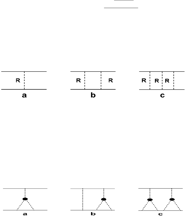
Reggeon phenomenology of nuclear interactions
According to the phenomenology, an elastic hadron-hadron scattering am-
plitude is the sum of contributions connected with various exchanges in the
t-channel. Each contribution has the following form in the impact parameter
representation:
AR
NN (~
b, ξ) = ηRg2
Re∆Rξe−b2
4(R2+α′
Rξ)
(R2
NN +α′
Rξ)(28.56)
Here |~
b|is the impact parameter, ξ=ln(s), sis the squared center-of-mass
energy, ηRis the signature factor: ηR= 1 + i cot(π(1 + ∆R)/2) for a pole
with positive signature, and ηR=−1 + i cot(π(1 + ∆R)/2) for a pole with
negative signature. 1 + ∆Ris the intercept of the reggeon trajectory, α′
Ris
its slope, and the vertex of reggeon-nucleon interaction is parameterized as
g(t) = gRexp(R2
NN t/2), tis the transferred 4-momentum.
Figure 28.16: Nonenhanced diagrams of NN-scattering.
Taking into account the contributions of other diagrams, shown in Fig.
28.16, one can find the NN-scattering amplitude:
γNN (~
b, ξ) = 1 −e−AR
NN (~
b,ξ)(28.57)
The calculation of amplitudes and cross sections for cascade interactions
requires to consider the so-called enhanced diagrams, like those shown in Fig.
28.17.
Figure 28.17: Simplest enhanced diagrams of NN-scattering.
401
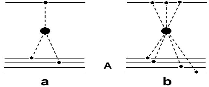
The contribution of the diagram in Fig. 28.17a to the elastic scattering
amplitude is given by the expression:
GEa(~
b, ξ) = −G
ξ−ǫ
Z
ǫ
dξ′Zd2b′AR1
Nπ(~
b−~
b′, ξ −ξ′)AR2
πN (~
b′, ξ′)AR3
πN (~
b′, ξ′) (28.58)
where AπN is the amplitude of meson-nucleon scattering due to one-reggeon
exchange, Gis the three reggeon’s coupling constant, ǫis the cutoff parameter
(ǫ∼1). Here we use the model of multi-reggeon vertices proposed in [25],
where it was assumed that reggeons are coupled to one another via a created
virtual meson (pion) pair.
The simplest enhanced diagrams for hadron-nucleus scattering were eval-
uated in [26, 27]. An effective computational procedure was proposed in
papers [28, 29], but it was not applied to the analysis of experimental data.
The structure of the enhanced diagrams and their analytical properties were
studied in [30].
Figure 28.18: Possible enhanced diagrams of hA-interactions.
In the reggeon approach the interaction of secondary particles with a nu-
cleus is described by cuttings of enhanced diagrams. Here the Abramovski-
Gribov-Kancheli (AGK) cutting rules [24] are frequently applied. The cor-
rections to them were discussed in [30] for the problem of particle cascading
into the nucleus. It was shown there that inelastic rescatterings occur for any
secondary particle, both slow and fast, and the contributions of enhanced di-
agrams lead to the enrichment of the spectrum by slow particles in the target
fragmentation region.
As in [25] we shall assume that the reggeon interaction vertices are small.
Therefore of the full set of enhanced diagrams the only important ones will
402

be those containing vertices where one of the reggeons split into several,
which then interact with different nucleons of the nucleus (figure 28.18a). In
studying interactions with nuclei, however, it is convenient, in the spirit of the
Glauber approach, to deal not with individual reggeons, but with sets of them
interacting with a given nucleon of the nucleus (figure 28.18b). Unfortunately,
the reggeon method of calculating the sum of the contributions of enhanced
diagrams in the case of hA- and AA-interactions is not developed for practical
tasks. Hence we propose a simple model of estimating reggeon cascading in
hA- and AA-interactions.
Let us consider the contribution of the first diagram of Fig. 28.18a:
Y=GZdξ′d2b′FNπ(~
b−~
b′, ξ −ξ′)×FπN (~
b′−~s1, ξ′)FπN (~
b′−~s2, ξ′) (28.59)
where ~
bis the impact parameter of a projectile hadron, ~s1and ~s2are im-
pact coordinates of two nuclear nucleons, ~
b′is the position of the reggeon
interaction vertex in the impact parameter plane, ξ′is its rapidity.
Using a gaussian parameterization for FN π (FπN =exp(−|~
b|2/R2
πN )) and
neglecting its dependence on energy, we have
Y≃G(ξ0−2ǫ)R2
πN
3exp(−(~
b−(~s1+~s2)/2)2/3R2
πN )×exp(−(~s1−~s2)2/2R2
πN )
(28.60)
where RπN is the pion-nucleon interaction radius. According to this expres-
sion, the contribution reaches a maximum when the nucleon coordinates, ~s1
and ~s2, coincide, and decreases very fast with increasing distance between
the nucleons.
Cutting the diagram, one can obtain that the probability, φ, to involve 2
neighboring nucleons is
φ(|~s1−~s2|)∼exp(−|~s1−~s2|2
R2
πN
) (28.61)
Schematically, the hadron-nucleus interaction process in the impact pa-
rameter plane can be represented as in Fig. 28.19, where the position of
the projectile hadron is marked by an open circle, the positions of nuclear
nucleons by closed circles, reggeon exchanges by dashed lines and the small
points are the coordinates of the reggeon interaction vertices.
Let us consider the problem by using the quark-gluon approach. There
were some successful attempts to describe the hadron-nucleon elastic scatter-
ing at low and intermediate energies (below 1 – 2 GeV) within this approach
(see [31]). In particular, in the paper [31] the theoretical calculations of the
403
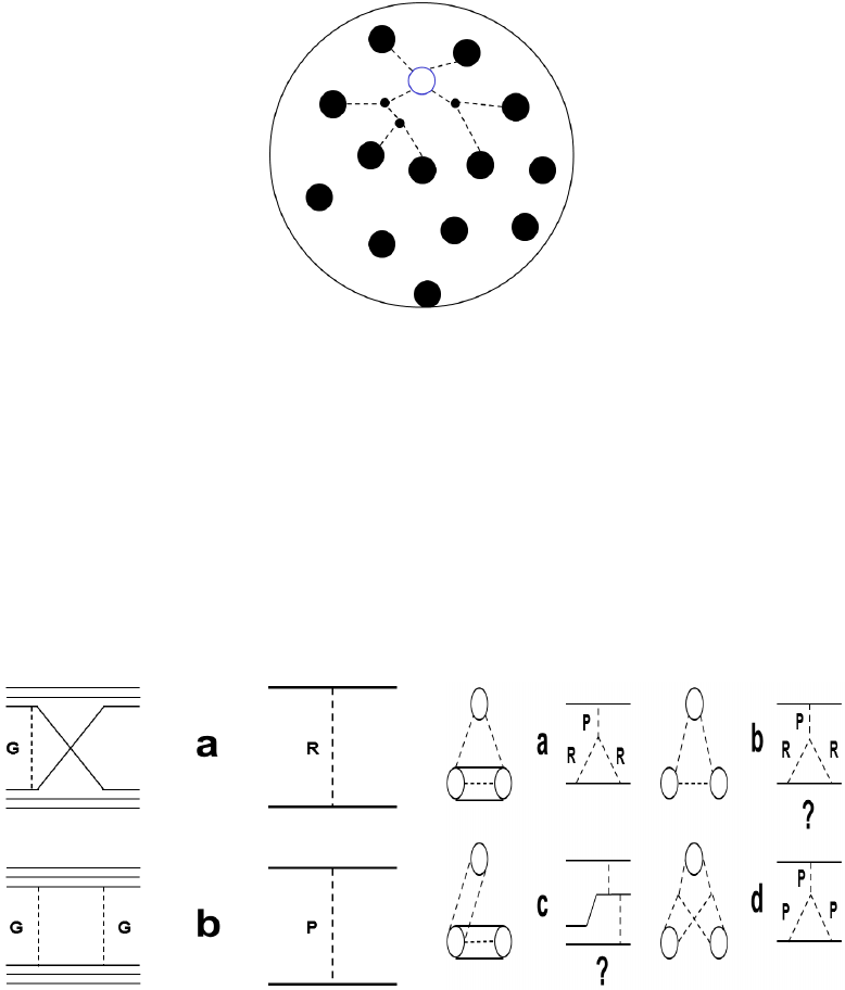
Figure 28.19: Reggeon ”cas-
cade” in hA-scattering.
amplitudes of ππ-, KK- and NN -scatterings were found in agreement with
experimental data, assuming that in the elastic hadron scattering one-gluon
exchange with following quark interchange between hadrons takes place (see
Fig. 28.20a). At high energies, two-gluon exchange approximation (Fig.
28.20b) works quite well (see [32]). What kind of exchanges can dominate in
hadron-nucleus and nucleus-nucleus interactions?
Figure 28.20: Diagrams of quark-
gluon exchanges and corresponding
reggeon diagrams for hadron-hadron
interactions.
Figure 28.21: Diagrams of quark-
gluon exchanges and corresponding
reggeon diagrams for hadron-nucleus
interactions.
The simplest possible diagrams of processes with three nucleons are given
in Fig. 28.21. A calculation of their amplitudes according to [31] is a serious
mathematical problem. It can be simplified if one takes into account an
analogy between quark-gluon diagrams and reggeon diagrams: the quark
404

diagram of Fig. 28.20a corresponds to a one-nonvacuum reggeon exchange;
the diagram of Fig. 28.20b describes the pomeron exchange in the t-channel;
the diagram of Fig. 28.21a is in correspondence with the enhanced reggeon
diagram of the pomeron splitting into two non-vacuum reggeons. The three
pomeron diagram (Fig. 28.21d) represents a more complicated process. It is
rather difficult to find a correspondence between reggeon diagrams and the
diagrams of Fig. 28.21b, 28.21c.
It seems obvious that the processes like one in Fig. 28.21d cannot domi-
nate in the elastic hadron-nucleus scattering because they are accompanied
by a production of high-mass diffractive particles in the intermediate state.
Thus, their contributions are damped by a nuclear form-factor. For the same
reason, the contributions of processes like the ones in Figs. 28.21a, 28.21b
can be small too. If this is not the case, then one can expect large correc-
tions to Glauber cross sections. The practice shows that the corrections to
hadron-nucleus cross sections must be lower than 5 – 7 %.
The diagram 28.21c can give a correction to the Glauber one-scattering
amplitude. Analogous corrections exist for the other terms of Glauber series.
They can re-normalize the nuclear vertex constants. According to [31] the
contribution has the form:
Yc∝exp [−(~
b−~s1)/R2
p] exp [−(~s1−~s2)/R2
c] (28.62)
where Rpis the radius of high-energy nucleon-nucleon interactions, and Rc
is another low-energy radius. Let us note that Ycdoes not depend, as other
reggeon diagram contributions, on the longitudinal coordinates of nucleons
and the multiplicity of produced particles. This is the main difference be-
tween ”reggeon cascading” and usual cascading.
As well known, the intra-nuclear cascade models assume that in a hadron-
nucleus collision secondary particles are produced in the first inelastic inter-
action of the projectile with a nuclear nucleon. The produced particles can
interact with other target nucleons. The distribution of the distance lbe-
tween the first interaction and the second one has the form:
W(l)dl ∝n
< l >exp(−n
< l > l) (28.63)
where < l >= 1/σρA,σis the hadron-nucleon cross section, nis the multi-
plicity of the produced particles, and ρA∼0.15 (fm)−3is the nuclear density.
At the same time, the amplitudes or cross sections of processes like Fig. 28.21
have no dependence on lor n. Thus, one can expect that the ”cascade” in
the quark-gluon approach will be more restricted than in the cascade models.
The difference between these approaches can lead to different predictions for
405
hadron interactions with heavy nuclei due to the large multiplicity of the
produced particles.
Because it is complicated to calculate the contributions of various di-
agrams, and to take into account all possibilities, let us formulate a sim-
pler phenomenological model that keeps the main features of the above ap-
proaches.
The model formulation
1. As it was said above, the ”reggeon” cascade is developed in the im-
pact parameter plane, and has features typical for branching processes.
Thus, for its description it is needed to determine the probability to
involve a nuclear nucleon into the ”cascade”. It is obvious that the
probability depends on the difference of the impact coordinates of the
new and previous involved nucleons. Looking at the contribution of
the diagram 28.21c, the functional form of the probability is chosen as:
P(|~si−~sj|) = Cnd exp[−(~si−~sj)2/R2
c] (28.64)
where ~siand ~sjare the projections of the radii of the ith and jth nucleons
on the impact parameter plane.
2. The ”cascade” is initiated by the primary involved nucleons. These
nucleons are determined with the help of the Glauber approach.
3. All involved nucleons are ejected from the nucleus.
The ”cascade” looks like that: a projectile particle interacts with some
intra-nuclear nucleons. These nucleons are called ”wounded” or ”participat-
ing” nucleons. These nucleons initiate the ”cascade”. A wounded nucleon
can involve a ”spectator” nucleon into the ”cascade” with the probability
(28.64). A spectator nucleon can involve another nucleon, which in turn can
involve a third one and so on. This algorithm is implemented in the FTF
model.
We have tuned Cnd using the HARP-CDP data on proton production in
the p+Cu interactions [33]. According to our estimations,
Cnd =e4 (y−2.1)/[1 + e4 (y−2.1)], R2
c= 1.5 (fm)2(28.65)
where yis the projectile rapidity. The value of the exponent, 2.1, corresponds
to Plab ∼4 GeV/c.
406

28.6.3 ”Fermi motion” of nuclear nucleons
In the ”standard” approach, a nucleus is considered as a potential well where
nucleons are freely moving. A particle falling on the nucleus changes its mo-
mentum on the border of the well. Here a question appears: to whom the
recoil momentum must be ascribed? If the particle is absorbed by the nu-
cleus, probably, one has to imagine in the final state the potential well with
its nucleons moving with a momentum of the particle. If some nucleons
are ejected from the nucleus, what conditions have to satisfy the nucleon
momenta, and how will the ”residual” well be moving to satisfy the energy-
momentum conservation law? In the case of a 3-dimensional potential well,
how will be changed the momentum components of a particle on the well sur-
face? Will only the component transverse to the surface, or the one parallel
to the surface, or both be changed? The list of questions can be extended
by considering nucleus-nucleus interactions.
Two approaches are frequently used in practice.
According to the first one, the nucleus is considered as a continuous
medium, and nucleons appeared only in points of the projectile interactions
with the medium. It seems natural in this approach to sum the momenta of
all ejected particles. Then, subtracting it from the initial momentum, one
can find the momentum of the residual nucleus. It is unclear, however, what
has to be done in the case of nucleus-nucleus interactions.
In the second approach, space coordinates and momenta of the nucleons
are sampled according to some assumptions. In order to satisfy the energy-
momentum conservation law, the projectile momentum does not changed,
and to each nucleon is ascribed a new mass:
m=p(m0−ǫb)2−p2(28.66)
where m0is the nucleon mass in the free state, ǫbis the nuclear binding en-
ergy per nucleon, and pis the momentum of the nucleon.
In this approach, the nucleus is a collection of off-mass-shell particles. Ap-
parently, in the case of nucleus-nucleus interactions one has to consider two
of such collections.
The energy-momentum conservation law is satisfied in this approach if it is
satisfied in each collision of out-of-mass-shell nucleons. However, there is a
problem with the excitation energy of the nuclear residual: in most of the
cases, it is too small.
All these questions are absent in the approach proposed in the paper [34].
Let us consider it starting from a simple example of a hadron interaction
with a bound system of two nucleons, (1,2). In this approach it is assumed
407

that the process has two stages. At the first one, the system is dissociated:
h+ (1,2) →h+ 1 + 2 (28.67)
At the second stage a ”hard” collision of the projectile with the first or
second nucleon takes place. Neglecting transverse momenta let us write the
energy-momentum conservation law in the form:
ph=p′
h+p1+p2
Eh+E(1,2) =E′
h+E1+E2
In the above expressions, there are three variables and two equations. Thus,
only one variable can be chosen as independent. It can be p′
h– hadron
momentum in the final state, or p1or p2– nucleon momentum in the final
state. We choose as the variable the light-cone momentum fraction of one of
the final-state nucleons:
x1= (E1−p1)/(E1+E2−p1−p2) (28.68)
This variable is invariant under the Lorentz transformation along the collision
axis.
Using this variable and the energy-momentum conservation law, one can
find:
W−=E1+E2−p1−p2= [s−m2
h+β2−λ1/2(s, m2
h, β2)]/2W+
0(28.69)
where:
W+
0=Eh+E(1,2) +ph, W −
0=Eh+E(1,2) −ph
s=W+
0W−
0, β2=m2
1
x1
+m2
2
1−x1
(28.70)
(See 28.12 for the definition of λ().)
The other kinematical variables are:
p1=m2
1
2x1W−−x1W−
2, E1=m2
1
2x1W−+x1W−
2
p2=m2
2
2(1 −x1)W−−(1 −x1)W−
2, E2=m2
2
2(1 −x1)W−+(1 −x1)W−
2
p′
h=ph−p1−p2, E′
h=Eh+E(1,2) −E1−E2(28.71)
So, for the simulation of the interactions, one has to determine only one
function: f(x1) – the distribution of x1. Distributions for p1and p2have
408

interesting properties: at ph→ ∞ they become stable (i.e. the distribu-
tions remain nearly unchanged when we vary ph, for large values of ph),
thus reproducing the typical ”limiting fragmentation” (according to an old
terminology) of bound system; at ph→0, Eh+E(1,2) > mh+m1+m2
the distributions p1and p2become narrower and narrower (i.e. similar to a
δ-Dirac distribution).
It is not complicated to introduce transverse momenta – p′
⊥h,p⊥1and
p⊥2, such that p′
⊥h+p⊥1+p⊥2= 0. It is sufficient to replace the masses with
the the transverse ones: mi→m⊥i=pm2
i+p2
⊥i.
In the case of interactions of two composed systems, Aand B, consisting
of Aand Bconstituents respectively (for brevity, we denote with the same
symbol both a composed system and the number of its constituents), let us
describe the ith constituent of Aby the variables:
x+
i= (EAi +piz)/W +
Aand ~pi⊥(28.72)
and the jth constituent of Bby the variables:
y−
j= (EBj −qjz)/W −
Band ~qi⊥(28.73)
Here EAi(EBi) and ~pi(~qi) are energy and momentum of the ith constituent of
the system A(B).
W+
A=
A
X
i=1
(EAi +piz), W −
B=
B
X
i=1
(EBi −qiz) (28.74)
Using these variables, the energy-momentum conservation law takes the
form:
W+
A
2+1
2W+
A
A
X
i=1
m2
i⊥
x+
i
+W−
B
2+1
2W−
B
B
X
i=1
µ2
i⊥
y−
i
=E0
A+E0
B
W+
A
2−1
2W+
A
A
X
i=1
m2
i⊥
x+
i−W−
B
2+1
2W−
B
B
X
i=1
µ2
i⊥
y−
i
=P0
A+P0
B(28.75)
A
X
i=1
~pi⊥+
B
X
i=1
~qi⊥= 0
where m2
i⊥=m2
i+~p2
i⊥, µ2
i⊥=µ2
i+~q2
i⊥, and mi(µi) is the mass of ith
constituent of the system A(B).
409

The system of equations (28.75) allows one to find W+
A, W −
Band all
kinematical properties of the particles at given {x+
i, ~pi⊥},{y−
i, ~qi⊥}.
W+
A= (W−
0W+
0+α−β+√∆)/2W−
0(28.76)
W−
B= (W−
0W+
0−α+β+√∆)/2W+
0(28.77)
W+
0= (E0
A+E0
B) + (P0
Az +P0
Bz) (28.78)
W−
0= (E0
A+E0
B)−(P0
Az +P0
Bz) (28.79)
α=
A
X
i=1
m2
i⊥
x+
i
, β =
B
X
i=1
µ2
i⊥
y−
i
(28.80)
∆ = (W−
0W+
0)2+α2+β2−2W−
0W+
0α−2W−
0W+
0β−2αβ(28.81)
piz = (W+
Ax+
i−m2
i⊥
x+
iW+
A
)/2; qiz =−(W−
By−
i−µ2
i⊥
y−
iW−
B
)/2 (28.82)
Consequently, the problem of accounting for the binding energy and Fermi
motion in the simulation of interacting composed systems comes to the defi-
nition of the distributions for x+
i, y−
i, ~pi⊥, ~qi⊥.
The transverse momentum of an ejected nucleon (~p⊥) is sampled accord-
ing to the distribution:
dW ∝exp(−~p2
⊥/ < p2
⊥>)d2p⊥(28.83)
< p2
⊥>= 0.035 + 0.04 e4 (ylab−2.5)
1 + e4 (ylab−2.5) (GeV/c)2(28.84)
where ylab is the projectile nucleus rapidity in the rest frame of the target
nucleus. The sum of the transverse momenta with minus sign is ascribed to
the residual of the target nucleus.
x+(and similarly for y−) is sampled according to the distribution:
dW ∝exp[−(x+−1/A)2/(d/A)2]dx+, d = 0.3 (28.85)
x+of the nuclear residual is determined as 1 −Px+
i.
28.6.4 Excitation energy of nuclear residuals
According to the approach presented above, the excitation energy of a nuclear
residual has to be determined before the simulation of particle production.
It seems natural to assume that this excitation energy is connected with the
multiplicity of ejected nuclear nucleons, both the participating ones and those
involved in the reggeon cascading. Without the involved nucleons, the exci-
tation energy would be proportional to the multiplicity of the participating
410

nucleons as calculated in the Glauber approach. Such approach was followed
in the paper [35], where proton-nucleus interactions at intermediate energies
were analyzed. There the multiplicity of the nucleons was calculated in the
Glauber approach. It was also assumed that each recoil of the participating
nucleons contributes to the excitation energy with a value sampled from the
following distribution:
dW (E) = 1
hEie−E/hEidE (28.86)
The sum of these contributions determines the residual excitation energy.
The authors of the paper [35] considered both absorptions and ejections of
the nucleons, and took into account the effect of decreasing projectile energy
during the interactions. They obtained a good agreement of their calculations
with experimental data on neutron production as a function of the residual
excitation energy.
Extending this approach, we assume, as a first step, that each partici-
pating or involved nucleon adds 100 MeV to the nuclear residual excitation
energy. The excited residual is then fragmented by using the Generalized
Evaporation Model (GEM) [36].
Bibliography
[1] B.Andersson et al. Nucl. Phys. B281 289 (1987).
[2] B.Nilsson-Almquist, E.Stenlund, Comp. Phys. Comm. 43 387 (1987).
[3] http://pdg.lbl.gov/2012/hadronic-xsections/hadron.html
[4] E. Bracci et al. CERN–HERA 72-1 (1972).
[5] G. Folger, V.N. Ivanchenko, J.P. Wellisch, Eur. Phys. J. A21 407
(2004).
[6] S.A. Bass et al. Prog. Part. Nucl. Phys. 41 225 (1998); M. Bleicher et
al. J. Phys. G25 1859 (1999).
[7] E. Bracci et al. CERN–HERA 73-1 (1973); V. Flaminio et al.CERN–
HERA 84-01 (1984).
[8] V. Flaminio et al. CERN–HERA 79-02 (1979).
[9] A.B. Kaidalov and P.E. Volkovitsky, Zeit. fur Phys. C63 517 (1994).
411
[10] V.V. Uzhinsky and A.S. Galoyan, arXiv: hep-ph/0212369 (2002).
[11] J.R. Cudell et al. (COMPLETE collab.) Phys. Rev. D65 074024
(2002).
[12] W.-M. Yao et al. (PDG), J. Phys. G33 337 (2006).
[13] M. Ishida and K. Igi, Phys. Rev. D79 096003 (2009).
[14] Bonn-Hamburg-Munich Collab. (V. Blobel et al.) Nucl. Phys. B69 454
(1974).
[15] K.A. Goulianos and J. Montanha, Phys. Rev. D59 114017 (1999).
[16] P. Bosettii et al., Nucl. Phys. B54 141 (1973).
[17] J. Whitmore, Phys. Rep. 10 273 (1974).
[18] NA22 Collab. (M. Adamus et al.) Zeit. fur Phys. C32 475 (1986);
BBCMS Collab. (I.V. Azhinenko et al.) Nucl. Phys. B123 493 (1977).
[19] Kh. Abdel-Waged and V.V. Uzhinsky, Phys. Atom. Nucl. 60 828 (1997)
(Yad. Fiz. 60 925 (1997)).
Kh. Abdel-Waged and V.V. Uzhinsky, J. Phys. G24 1723 (1997).
[20] R.J. Glauber, In: ”Lectures in Theoretical Physics”, Ed. W.E.Brittin
et al., v. 1, Interscience Publishers, N.Y., 1959.; R.J. Glauber, Proc. of
the 2nd Int. Conf. on High Energy Physics and Nuclear structure, (Re-
hovoth, 1967) Ed. G.A.Alexander, North-Holland, Amsterdam, 1967.
[21] V. Franco, Phys. Rev. 175 1376 (1968).
[22] S.Yu. Shmakov, V.V. Uzhinski and A.M. Zadorojny, Comp. Phys. Com-
mun. 54 125 (1989);
B. Alver, M. Baker, C. Loizides, and P. Steinberg, arxiv:0805.4411
[nucl-exp] (2005). M.L. Miller, K. Reygers, S.J. Sanders and P. Stein-
berg, Ann. Rev. Nucl. Part. Sci., 57 205 (2007);
W. Broniowski, M. Rybczynski, and P. Bozek, Comp. Phys. Commun.,
180 69 (2009).
[23] Yu.M. Shabelski, Sov. J. Part. Nucl., 12 430 (1981).
[24] V.A. Abramovsky, V.N. Gribov and O.V. Kancheli, Sov. J. Nucl. Phys.
18 308 (1974) (Yad. Fiz. 18 595 (1973)).
412
[25] A.B. Kaidalov, L.A. ponomarev and K.A. Ter-Martirosian, Sov. J.
Nucl. Phys. 44 468 (1986) (Yad. Fiz. 44 722 (1986)).
[26] R. Jengo and D.Treliani, Nucl. Phys. 117B 433 (1976).
[27] R.E. Camboa Saravi, Phys. Rev. 21 2021 (1980).
[28] A. Schwimmer, Nucl. Phys. 94B 445 (1975).
[29] L. Caneschi, A. Schwimmer and R.Jenco, Nucl. Phys. 108B 82 ( 1976).
[30] K.G. Boreskov, A.B. Kaidalov, S.M. Kiselev and N.Ya. Smorodinskaya,
Sov. J. Nucl. Phys. 53 356 (1991) (Yad. Fiz. 53 569 (1991)).
[31] T. Barnes and E.S.Swanson, Phys. Rev. D46 131 (1992);
T.Barnes, E.S.Swanson and J.Weinstein, Phys. Rev. D46 4868 (1992);
T.Barnes, S.Capstick, M.D.Kovarik and E.S. Swanson, Phys. Rev. C48
539 (1993);
T.Barnes and E.S.Swanson, Phys. Rev. C49 1166 (1992).
[32] F. Low, Phys. Rev. D12 163 (1975);
S. Nussinov, Phys. Rev. D14 246 (1976);
J. Gunion and D.Shoper, Phys. Rev. D15 2617 (1977);
E.M. Levin and M.G. Ryskin, Yad. Fiz. 34 619 (1981).
[33] HARP-CDP Collab. (A. Bolshakova et al.) Eur. Phys. J. C64 181
(2009).
[34] EMU-01 Collab. (M.I. Adamovich et al.) Zeit. fur Phys. A358 337
(1997).
[35] A.Y. Abul-Magd, W.A.Friedman and J.Hufner, Phys. Rev. C34 113
(1986).
[36] S. Furihata, NIM B171 251 (2000).
413
Chapter 29
Bertini Intranuclear Cascade
Model in Geant4
29.1 Introduction
This cascade model is a re-engineered version of the INUCL code and includes
the Bertini intra-nuclear cascade model with excitons, a pre-equilibrium
model, a nucleus explosion model, a fission model, and an evaporation model.
It treats nuclear reactions initiated by long-lived hadrons (p, n, π, K, Λ,Σ,Ξ,Ω)
and γs with energies between 0 and 10 GeV. Presented here is an overview of
the models and a review of results achieved from simulations and comparisons
with experimental data.
The intranuclear cascade model (INC) was was first proposed by Ser-
ber in 1947 [19]. He noticed that in particle-nuclear collisions the deBroglie
wavelength of the incident particle is comparable (or shorter) than the aver-
age intra-nucleon distance. Hence, a description of interactions in terms of
particle-particle collisions is justified.
The INC has been used succesfully in Monte Carlo simulations at interme-
diate energies since Goldberger made the first hand-calculations in 1947 [9].
The first computer simulations were done by Metropolis et al. in 1958 [16].
Standard methods in INC implementations were developed when Bertini pub-
lished his results in 1968 [3]. An important addition to INC was the exciton
model introduced by Griffin in 1966 [10].
The current presentation describes the implementation of the Bertini INC
model within the Geant4 hadronic physics framework [8]. This framework
is flexible and allows for the modular implementation of various kinds of
hadronic interactions.
414
29.2 The Geant4 Cascade Model
Inelastic particle-nucleus collisions are characterized by both fast and slow
components. The fast (10−23 −10−22s) intra-nuclear cascade results in a
highly excited nucleus which may decay by fission or pre-equilibrium emis-
sion. The slower (10−18 −10−16s) compound nucleus phase follows with
evaporation. A Boltzmann equation must be solved to treat the collision
process in detail.
The intranuclear cascade (INC) model developed by Bertini [3, 4] solves
the Boltzmann equation on average. This model has been implemented
in several codes such as HETC [1]. Our model, which is based on a re-
engineering of the INUCL code [20], includes the Bertini intranuclear cascade
model with excitons, a pre-equilibrium model, a simple nucleus explosion
model, a fission model, and an evaporation model.
The target nucleus is modeled by up to six concentric shells of constant
density as an approximation to the continuously changing density distribu-
tion of nuclear matter within nuclei. The cascade begins when an incident
particle strikes a nucleon in the target nucleus and produces secondaries. The
secondaries may in turn interact with other nucleons or be absorbed. The
cascade ends when all particles, which are kinematically able to do so, es-
cape the nucleus. At that point energy conservation is checked. Relativistic
kinematics is applied throughout the cascade.
29.2.1 Model Limits
The model is valid for incident p, n, π, K, Λ,Σ,Ξ,Ω and γs with energies
between 0 and 10 GeV. All types of nuclear targets are allowed.
The necessary condition of validity of the INC model is λB/v << τc<<
∆t, where δBis the deBroglie wavelenth of the nucleons, vis the average
relative velocity between two nucleons and ∆tis the time interval between
collisions. At energies below 200MeV , this condition is no longer strictly
valid, and a pre-quilibrium model must be invoked. At energies greater than
≈10 GeV) the INC picture breaks down. This model has been tested against
experimental data at incident kinetic energies between 100 MeV and 10 GeV.
29.2.2 Intranuclear Cascade Model
The basic steps of the INC model are summarized as follows:
1. the space point at which the incident particle enters the nucleus is
selected uniformly over the projected area of the nucleus,
415

2. the total particle-particle cross sections and region-depenent nucleon
densities are used to select a path length for the projectile,
3. the momentum of the struck nucleon, the type of reaction and the
four-momenta of the reaction products are determined, and
4. the exciton model is updated as the cascade proceeds.
5. If the Pauli exclusion principle allows and Eparticle > Ecutoff = 2 MeV,
step (2) is performed to transport the products.
After the intra-nuclear cascade, the residual excitation energy of the re-
sulting nucleus is used as input for non-equilibrium model.
29.2.3 Nuclear Model
Some of the basic features of the nuclear model are:
•the nucleons are assumed to have a Fermi gas momentum distribution.
The Fermi energy is calculated in a local density approximation i.e. the
Fermi energy is made radius-dependent with Fermi momentum pF(r) =
(3π2ρ(r)
2)1
3.
•Nucleon binding energies (BE) are calculated using the mass formula.
A parameterization of the nuclear binding energy uses a combination
of the Kummel mass formula and experimental data. Also, the asymp-
totic high temperature mass formula is used if it is impossible to use
experimental data.
Initialization
The initialization phase fixes the nuclear radius and momentum according to
the Fermi gas model.
If the target is hydrogen (A = 1) a direct particle-particle collision is
performed, and no nuclear modeling is required.
If 1 < A < 4, a nuclear model consisting of one layer with a radius of 8.0
fm is created.
For 4 < A < 11, the nuclear model is composed of three concentric
spheres i={1,2,3}with radius
ri(αi) = rC2
1(1 −1
A) + 6.4p−log(αi)
.
416

Here αi={0.01,0.3,0.7}and C1= 3.3836A1/3.
If A > 11, a nuclear model with three concentric spheres is also used.
The sphere radius is now defined as
ri(αi) = C2log(1 + e−C1
C2
αi−1) + C1,(29.1)
where C2= 1.7234.
The potential energy Vfor nucleon Nis
VN=p2
F
2mN
+BEN(A, Z),(29.2)
where pfis the Fermi momentum and BE is the binding energy.
The momentum distribution in each region follows the Fermi distribution
with zero temperature.
f(p) = cp2(29.3)
where
ZpF
0
f(p)dp =npornn(29.4)
where npand nnare the number of protons or neutrons in the region. Pfis
the momentum corresponding to the Fermi energy
Ef=p2
F
2mN
=~2
2mN
(3π2
v)2
3,(29.5)
which depends on the density n/v of particles, and which is different for each
particle and each region.
Pauli Exclusion Principle
The Pauli exclusion principle forbids interactions where the products would
be in occupied states. Following the assumption of a completely degenerate
Fermi gas, the levels are filled from the lowest level. The minimum energy
allowed for the products of a collision correspond to the lowest unfilled level
of the system, which is the Fermi energy in the region. So in practice, the
Pauli exclusion principle is taken into account by accepting only secondary
nucleons which have EN> Ef.
417
Cross Sections and Kinematics
Path lengths of nucleons in the nucleus are sampled according to the local
density and the free N−Ncross sections. Angles after the collision are sam-
pled from experimental differential cross sections. Tabulated total reaction
cross sections are calculated by Letaw’s formulation [14, 15, 17]. For N−N
cross sections the parameterizations are based on the experimental energy
and isospin dependent data. The parameterization described in [2] is used.
For pions the intra-nuclear cross sections are provided to treat elastic
collisions and the following inelastic channels: π−p→π0n, π0p→π+n, π0n
→π−p, and π+n→π0p. Multiple particle production is also implemented.
The pion absorption channels are π+nn →pn, π+pn →pp, π0nn →nn,
π0pn →pn, π0pp →pp, π−pn →nn , and π−pp →pn.
29.2.4 Pre-equilibrium Model
The Geant4 cascade model implements the exciton model proposed by Grif-
fin [10, 11]. In this model, nucleon states are characterized by the number
of excited particles and holes (the excitons). Intra-nuclear cascade collisions
give rise to a sequence of states characterized by increasing exciton number,
eventually leading to an equilibrated nucleus. For a practical implementation
of the exciton model we use parameters from [18], (level densities) and [13]
(matrix elements).
In the exciton model the possible selection rules for particle-hole configu-
rations in the source of the cascade are: ∆p= 0,±1 ∆h= 0,±1 ∆n= 0,±2,
where pis the number of particles, his number of holes and n=p+his the
number of excitons.
The cascade pre-equilibrium model uses target excitation data and the
exciton configurations for neutrons and protons to produce non-equilibrium
evaporation. The angular distribution is isotropic in the rest frame of the
exciton system.
Parameterizations of the level density are tabulated as functions of Aand
Z, and with high temperature behavior (the nuclear binding energy using the
smooth liquid high energy formula).
29.2.5 Break-up models
Fermi break-up is allowed only in some extreme cases, i.e. for light nuclei
(A < 12 and 3(A−Z)< Z < 6 ) and Eexcitation >3Ebinding. A simple
explosion model decays the nucleus into neutrons and protons and decreases
exotic evaporation processes.
418
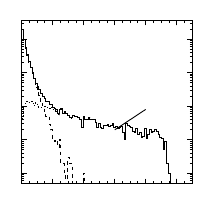
90 MeV
/E
kin
E
0 0.2 0.4 0.6 0.8 1
/dE (mb/MeV)σd
1
10
2
10
3
10
4
10 Secondary neutrons from
Bi (p, X n) 90 MeV
Total
Evaporation
INC with exitons
Figure 29.1: Secondary neutrons generated by Bertini INC with exitons and
evaporation model.
The fission model is phenomenological, using potential minimization. A
binding energy paramerization is used and some features of the fission sta-
tistical model are incorporated [7].
29.2.6 Evaporation Model
A statistical theory for particle emission of the excited nucleus remaining
after the intra-nuclear cascade was originally developed by Weisskopf [21].
This model assumes complete energy equilibration before particle emission,
and re-equilibration of excitation energies between successive evaporations.
As a result the angular distribution of emitted particles is isotropic.
The Geant4 evaporation model for the cascade implementation adapts
the often-used computational method developed by Dostrowski [5, 6]. The
emission of particles is computed until the excitation energy falls below some
specific cutoff. If a light nucleus is highly excited, the Fermi break-up model
is executed. Also, fission is performed if that channel is open. The main
chain of evaporation is followed until Eexcitation falls below Ecutof f = 0.1 MeV.
The evaporation model ends with an emission chain which is followed until
Eexcitation < Eγ
cutoff = 10−15 MeV.
An example of Bertini evaporation model in action is shown in Fig. 29.1.
29.3 Interfacing Bertini implementation
Typically Bertini models are used through physics lists, with ’BERT’ in their
name. User should consult these validated physics model collection to un-
derstand the inclusion mechanisms before using directly the actual Bertini
cascade interfaces:
G4CascadeInterface All the Bertini cascade submodels in integrated fash-
ion, can be used collectively through this interface using method Apply-
419
Yourself. A Geant4 track (G4Track) and a nucleus (G4Nucleus) are
given as parameters.
G4ElasticCascadeInterface provides an access to elastic hadronic scat-
tering. Particle treated are the same as in case for G4CascadeInterface
but only elastic scattering is modeled.
G4PreCompoundCascadeInterface provides an interface to INUCL in-
tra nuclear cascade with exitons. Subsequent evaporation phase is not
modeled.
G4InuclEvaporation provides an interface to INUCL evaporation model.
This interface with method BreakItUp inputs an exited nuclei G4Fragment
to model evaporation phase.
Bibliography
[1] R.G. Alsmiller and F.S. Alsmiller and O.W. Hermann, The high-energy
transport code HETC88 and comparisons with experimental data, Nu-
clear Instruments and Methods in Physics Research A 295, (1990), 337–
343,
[2] V.S. Barashenkov and V.D. Toneev, High Energy interactions of parti-
cles and nuclei with nuclei (In russian), (1972)
[3] M. P. Guthrie, R. G. Alsmiller and H. W. Bertini, Nucl. Instr. Meth,
66, 1968, 29.
[4] H. W. Bertini and P. Guthrie, Results from Medium-Energy
Intranuclear-Cascade Calculation, Nucl. Phys.A169, (1971).
[5] I. Dostrovsky, Z. Zraenkel and G. Friedlander, Monte carlo calculations
of high-energy nuclear interactions. III. Application to low-lnergy calcu-
lations, Physical Review, 1959, 116, 3, 683-702.
[6] I. Dostrovsky and Z. Fraenkel and P. Rabinowitz, Monte Carlo Calcula-
tions of Nuclear Evaporation Processes. V. Emission of Particles Heavier
Than 4He, Physical Review, 1960.
[7] P. Fong, Statistical Theory of Fission, 1969, Gordon and Breach, New
York.
[8] Geant4 collaboration, Geant4 general paper (to be published), Nuclear
Instruments and Methods A, (2003).
420
[9] M. Goldberger, The Interaction of High Energy Neutrons and Hevy
Nuclei, Phys. Rev. 74, (1948), 1269.
[10] J. J. Griffin, Statistical Model of Intermediate Structure, Physical Re-
view Letters 17, (1966), 478-481.
[11] J. J. Griffin, Statistical Model of Intermediate Structure, Physics Letters
24B, 1 (1967), 5-7.
[12] A. S. Iljonov et al., Intermediate-Energy Nuclear Physics, CRC Press
1994.
[13] C. Kalbach, Exciton Number Dependence of the Griffin Model Two-
Body Matrix Element, Z. Physik A 287, (1978), 319-322.
[14] J. R. Letaw et al., The Astrophysical Journal Supplements 51, (1983),
271f.
[15] J. R. Letaw et al., The Astrophysical Journal 414, 1993, 601.
[16] N. Metropolis, R. Bibins, M. Storm, Monte Carlo Calculations on
Intranuclear Cascades. I. Low-Energy Studies, Physical Review 110,
(1958), 185ff.
[17] S. Pearlstein, Medium-energy nuclear data libraries: a case study,
neutron- and proton-induced reactions in 56Fe, The Astrophysical Jour-
nal 346, (1989), 1049-1060.
[18] I. Ribansky et al., Pre-equilibrium decay and the exciton model, Nucl.
Phys. A 205, (1973), 545-560.
[19] R. Serber, Nuclear Reactions at High Energies, Phys. Rev. 72, (1947),
1114.
[20] Experimental and Computer Simulations Study of Radionuclide Pro-
duction in Heavy Materials Irradiated by Intermediate Energy Protons,
Yu. E. Titarenko et al., nucl-ex/9908012, (1999).
[21] V. Weisskopf, Statistics and Nuclear Reactions, Physical Review 52,
(1937), 295–302.
421

Chapter 30
The Geant4 Binary Cascade
30.1 Modeling overview
The Geant4 Binary Cascade is an intranuclear cascade propagating primary
and secondary particles in a nucleus. Interactions are between a primary or
secondary particle and an individual nucleon of the nucleus, leading to the
name Binary Cascade. Cross section data are used to select collisions. Where
available, experimental cross sections are used by the simulation. Propagat-
ing of particles is the nuclear field is done by numerically solving the equa-
tion of motion. The cascade terminates when the average and maximum
energy of secondaries is below threshold. The remaining fragment is treated
by precompound and de-excitation models documented in the corresponding
chapters.
30.1.1 The transport algorithm
For the primary particle an impact parameter is chosen random in a disk
outside the nucleus perpendicular to a vector passing through the center of
the nucleus coordinate system an being parallel to the momentum direction.
Using a straight line trajectory, the distance of closest approach dmin
ito each
target nucleon iand the corresponding time-of-flight td
iis calculated. In
this calculation the momentum of the target nucleons is ignored, i.e. the
target nucleons do not move. The interaction cross section σiwith target
nucleons is calculated using total inclusive cross-sections described below.
For calculation of the cross-section the momenta of the nucleons are taken
into account. The primary particle may interact with those target nucleons
where the distance of closest approach dmin
iis smaller than dmin
i<pσi
π.
These candidate interactions are called collisions, and these collisions are
422

stored ordered by time-of-flight td
i. In the case no collision is found, a new
impact parameter is chosen.
The primary particle is tracked the time-step given by the time to the
first collision. As long a particle is outside the nucleus, that is a radius of the
outermost nucleon plus 3fm, particles travel along straight line trajectories.
Particles entering the nucleus have their energy corrected for Coulomb effects.
Inside the nucleus particles are propagated in the scalar nuclear field. The
equation of motion in the field is solved for a given time-step using a Runge-
Kutta integration method.
At the end of the step, the primary and the nucleon interact suing the
scattering term. The resulting secondaries are checked for the Fermi exclusion
principle. If any of the two particles has a momentum below Fermi momen-
tum, the interaction is suppressed, and the original primary is tracked to
the next collision. In case interaction is allowed, the secondaries are treated
like the primary, that is, all possible collisions are calculated like above, with
the addition that these new primary particles may be short-lived and may
decay. A decay is treated like others collisions, the collision time being the
time until the decay of the particle. All secondaries are tracked until they
leave the nucleus, or the until the cascade stops.
30.1.2 The description of the target nucleus and fermi
motion
The nucleus is constructed from Anucleons and Zprotons with nucleon
coordinates riand momenta pi, with i= 1,2, ..., A. We use a common
initialization Monte Carlo procedure, which is realized in the most of the
high energy nuclear interaction models:
•Nucleon radii riare selected randomly in the nucleus rest frame accord-
ing to nucleon density ρ(ri). For heavy nuclei with A > 16 [2] nucleon
density is
ρ(ri) = ρ0
1 + exp [(ri−R)/a](30.1)
where
ρ0≈3
4πR3(1 + a2π2
R2)−1.(30.2)
Here R=r0A1/3fm and r0= 1.16(1 −1.16A−2/3) fm and a≈0.545
fm. For light nuclei with A < 17 nucleon density is given by a harmonic
oscillator shell model [3], e. g.
ρ(ri) = (πR2)−3/2exp (−r2
i/R2),(30.3)
423

where R2= 2/3< r2>= 0.8133A2/3fm2. To take into account
nucleon repulsive core it is assumed that internucleon distance d > 0.8
fm;
•The nucleus is assumed to be isotropic, i.e. we place each nucleon using
a random direction and the previously determined radius ri.
•The initial momenta of the nucleons piare randomly choosen between
0 and pmax
F(r), where the maximal momenta of nucleons (in the local
Thomas-Fermi approximation [4]) depends from the proton or neutron
density ρaccording to
pmax
F(r) = ~c(3π2ρ(r))1/3(30.4)
•To obtain momentum components, it is assumed that nucleons are
distributed isotropic in momentum space; i.e. the momentum direction
is chosen at random.
•The nucleus must be centered in momentum space around 0,i. e. the
nucleus must be at rest, i. e. Pipi=0; To achieve this, we choose
one nucleon to compensate the sum the remaining nucleon momenta
prest =Pi=A−1
i=1 . If this sum is larger than maximum momentum
pmax
F(r), we change the direction of the momentum of a few nucleons.
If this does not lead to a possible momentum value, than we repeat the
procedure with a different nucleon having a larger maximum momen-
tum pmax
F(r). In the rare case this fails as well, we choose new momenta
for all nucleons.
This procedure gives special for hydrogen 1H, where the proton has
momentum p= 0, and for deuterium 2H, where the momenta of proton
and neutron are equal, and in opposite direction.
•We compute energy per nucleon e=E/A =mN+B(A, Z)/A, where
mNis nucleon mass and the nucleus binding energy B(A, Z) is given
by the tabulation of [5]: and find the effective mass of each nucleon
meff
i=p(E/A)2−p2′
i.
30.1.3 Optical and phenomenological potentials
The effect of collective nuclear elastic interaction upon primary and sec-
ondary particles is approximated by a nuclear potential.
424

For projectile protons and neutrons this scalar potential is given by the
local Fermi momentum pF(r)
V(r) = p2
F(r)
2m(30.5)
where mis the mass of the neutron mnor the mass of proton mp.
For pions the potential is given by the lowest order optical potential [6]
V(r) = −2π(~c)2A
mπ
(1 + mπ
M)b0ρ(r) (30.6)
where Ais the nuclear mass number, mπ,Mare the pion and nucleon mass,
mπis the reduced pion mass mπ= (mπmN)/(mπ+mN), with mNis the mass
of the nucleus, and ρ(r) is the nucleon density distribution. The parameter
b0is the effective s−wave scattering length and is obtained from analysis to
pion atomic data to be about −0.042fm.
30.1.4 Pauli blocking simulation
The cross sections used in this model are cross sections for free particles.
In the nucleus these cross sections are reduced to effective cross sections by
Pauli-blocking due to Fermi statistics.
For nucleons created by a collision, ie. an inelastic scattering or from
decay, we check that all secondary nucleons occupy a state allowed by Fermi
statistics. We assume that the nucleus in its ground state and all states
below Fermi energy are occupied. All secondary nucleons therefore must
have a momentum piabove local Fermi momentum pF(r), i.e.
pi> pmax
F(r).(30.7)
If any of the nucleons of the collision has a momentum below the local
Fermi momentum, then the collision is Pauli blocked. The reaction products
are discarded, and the original particles continue the cascade.
30.1.5 The scattering term
The basis of the description of the reactive part of the scattering amplitude
are two particle binary collisions (hence binary cascade), resonance produc-
tion, and decay. Based on the cross-section described later in this paper,
collisions will occur when the transverse distance dtof any projectile target
pair becomes smaller than the black disk radium corresponding to the total
cross-section σtσt
π> d2
t
425
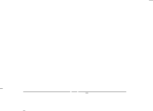
In case of a collision, all particles will be propagated to the estimated time
of the collision, i.e. the time of closest approach, and the collision final state
is produced.
30.1.6 Total inclusive cross-sections
Experimental data are used in the calculation of the total, inelastic and
elastic cross-section wherever available.
hadron-nucleon scattering
For the case of proton-proton(pp) and proton-neutron(pn) collisions, as well
as π=and π−nucleon collisions, experimental data are readily available as
collected by the Particle Data Group (PDG) for both elastic and inelastic
collisions. We use a tabulation based on a sub-set of these data for √S
below 3 GeV. For higher energies, parametrizations from the CERN-HERA
collection are included.
30.1.7 Channel cross-sections
A large fraction of the cross-section in individual channels involving meson
nucleon scattering can be modeled as resonance excitation in the s-channel.
This kind of interactions show a resonance structure in the energy depen-
dency of the cross-section, and can be modeled using the Breit-Wigner func-
tion
σres(√s) = X
F S
2J+ 1
(2S1+ 1)(2S2+ 1)
π
k2
ΓISΓFS
(√s−MR)2+ Γ/4,
Where S1 and S2 are the spins of the two fusing particles, Jis the
spin of the resonance, p(s) the energy in the center of mass system, kthe
momentum of the fusing particles in the center of mass system, ΓISand Γ)F S
the partial width of the resonance for the initial and final state respectively.
MRis the nominal mass of the resonance.
The initial states included in the model are pion and kaon nucleon scatter-
ing. The product resonances taken into account are the Delta resonances with
masses 1232, 1600, 1620, 1700, 1900, 1905, 1910, 1920, 1930, and 1950 MeV,
the excited nucleons with masses of 1440, 1520, 1535, 1650, 1675, 1680, 1700,
1710, 1720, 1900, 1990, 2090, 2190, 2220, and 2250 MeV, the Lambda, and
its excited states at 1520, 1600, 1670, 1690, 1800, 1810, 1820, 1830, 1890,
2100, and 2110 MeV, and the Sigma and its excited states at 1660, 1670,
1750, 1775, 1915, 1940, and 2030 MeV.
426
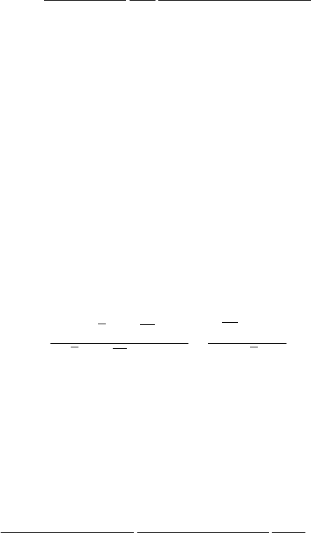
30.1.8 Mass dependent resonance width and partial
width
During the cascading, the resonances produced are assigned reall masses,
with values distributed according to the production cross-section described
above. The concrete (rather than nominal) masses of these resonances may
be small compared to the PDG value, and this implies that some channels
may not be open for decay. In general it means, that the partial and total
width will depend on the concrete mass of the resonance. We are using the
UrQMD[13][14] approach for calculating these actual width,
ΓR→12(M) = (1 + r)ΓR→12(MR)
p(MR)(2l+1)
MR
M
p(M)(2l+1)
1 + r(p(M)/p(MR))2l.(30.8)
Here MRis the nominal mass of the resonance, Mthe actual mass, pis
the momentum in the center of mass system of the particles, Lthe angular
momentum of the final state, and r=0.2.
30.1.9 Resonance production cross-section in the t-
channel
In resonance production in the t-channel, single and double resonance exci-
tation in nucleon-nucleon collisions are taken into account. The resonance
production cross-sections are as much as possible based on parametrizations
of experimental data[15] for proton proton scattering. The basic formula
used is motivated from the form of the exclusive production cross-section of
the ∆1232 in proton proton collisions:
σAB = 2αABβAB
√s−√s0
(√s−√s0)2+β2
AB √s0 + βAB
√s!γAB
The parameters of the description for the various channels are given in
table30.1. For all other channels, the parametrizations were derived from
these by adjusting the threshold behavior.
The reminder of the cross-section are derived from these, applying de-
tailed balance. Iso-spin invariance is assumed. The formalism used to apply
detailed balance is
σ(cd →ab) = X
J,M
hjcmcjdmdkJMi2
hjamajbmbkJMi2
(2Sa+ 1)(2Sb+ 1)
(2Sc+ 1)(2Sd+ 1) hp2
abi
hp2
cdiσ(ab →cd)
(30.9)
427

Reaction α β γ
pp →p∆1232 25 mbarn 0.4 GeV 3
pp →∆1232∆1232 1.5 mbarn 1 GeV 1
pp →pp∗0.55 mbarn 1 GeV 1
pp →p∆∗0.4 mbarn 1 GeV 1
pp →∆1232∆∗0.35 mbarn 1 GeV 1
pp →∆1232N∗0.55 mbarn 1 GeV 1
Table 30.1: Values of the parameters of the cross-section formula for the
individual channels.
30.1.10 Nucleon Nucleon elastic collisions
Angular distributions for elastic scattering of nucleons are taken as closely as
possible from experimental data, i.e. from the result of phase-shift analysis.
They are derived from differential cross sections obtained from the SAID
database, R. Arndt, 1998.
Final states are derived by sampling from tables of the cumulative distri-
bution function of the centre-of-mass scattering angle, tabulated for a discrete
set of lab kinetic energies from 10 MeV to 1200 MeV. The CDF’s are tabu-
lated at 1 degree intervals and sampling is done using bi-linear interpolation
in energy and CDF values. Coulomb effects are taken into consideration for
pp scattering.
30.1.11 Generation of transverse momentum
Angular distributions for final states other than nucleon elastic scattering
are calculated analytically, derived from the collision term of the in-medium
relativistic Boltzmann-Uehling-Uhlenbeck equation, absed on the nucleon nu-
cleon elastic scattering cross-sections:
σNN→NN (s, t) = 1
(2π)2s(D(s, t) + E(s, t) + (invertedt, u))
Here s,t,uare the Mandelstamm variables, D(s, t) is the direct term,
and E(s, t) is the exchange term, with
D(s, t) = (gσ
NN )4(t−4m∗2)2
2(t−m2
σ)2+(gω
NN )4(2s2+2st+t2−8m∗2s+8m∗4)
(t−m2
ω)2+
24(gπ
NN )4m∗2t2
(t−m2
π)2−4(gσ
NN gω
NN )2(2s+t−4m∗2)m∗2
(t−m2
σ)(t−m2
ω),
428

and
E(s, t) = (gσ
NN )4(t(t+s)+4m∗2(s−t))
8(t−m2
σ)(u−m2
σ)+(gω
NN )4(s−2m∗2)(s−6m∗2))
2(t−m2
ω)(u−m2
ω)−
6(gπ
NN )4(4m∗2−s−t)m∗4t
(t−m2
π)(u=mpi2)+3(gσ
NN gπ
NN )2m∗2(4m∗2−s−t)(4m∗2−t)
(t−m2
σ)(u−m2
π)+
3(gσ
NN gπ
NN )2t(t+s)m∗2
2(t−m2
π)(u−m2
σ)+(gσ
NN gω
NN )2t2−4m∗2s−10m∗2t+24m∗4
4(t−m2
σ)(u−m2
ω)+
(gσ
NN gω
NN )2(t+s)2−2m∗2s+2m∗2t
4(t−m2
ω)(u−m2
σ)+3(gω
NN gπ
NN )2(t+s−4m∗2)(t+s−2m∗2)
(t−m2
ω)(u−m2
π)+
3(gω
NN gπ
NN )2m∗2(t2−2m∗2t)
(t−m2
π)(u−m2
ω).(30.10)
(30.11)
Here, in this first release, the in-medium mass was set to the free mass, and
the nucleon nucleon coupling constants used were 1.434 for the π, 7.54 for the
ω, and 6.9 for the σ. This formula was used for elementary hadron-nucleon
differential cross-sections by scaling teh center of mass energy squared ac-
cordingly.
Finite size effects were taken into account at the meson nucleon vertex,
using a phenomenological form factor (cut-off) at each vertex.
30.1.12 Decay
In the simulation of decay of strong resonances, we use the nominal decay
branching ratios from the particle data book. The stochastic mass of a
individual resonance created is sampled at creation time from the Breit-
Wigner form, under the mass constraints posed by center of mass energy of
the scattering, and the mass in the lightest decay channel. The decay width
from the particle data book are then adjusted according to equation 30.8, to
take the stochastic mass value into account.
All decay channels with nominal branching ratios greater than 1% are
simulated.
30.1.13 The escaping particle and coherent effects
When a nucleon other than the incident particle leaves the nucleus, the
ground state of the nucleus changes. The energy of the outgoing particle
cannot be such that the total mass of the new nucleus would be below its
ground state mass. To avoid this, we reduce the energy of an outgoing nu-
cleons by the mass-difference of old and new nucleus.
Furthermore, the momentum of the final exited nucleus derived from
energy momentum balance may be such that its mass is below its ground
429
state mass. In this case, we arbitrarily scale the momenta of all outgoing
particles by a factor derived from the mass of the nucleus and the mass of
the system of outgoing particles.
30.1.14 Light ion reactions
In simulating light ion reactions, the initial state of the cascade is prepared
in the form of two nuclei, as described in the above section on the nuclear
model.
The lighter of the collision partners is selected to be the projectile. The
nucleons in the projectile are then entered, with position and momenta, into
the initial state of the cascade. Note that before the first scattering of an
individual nucleon, a projectile nucleon’s Fermi-momentum is not taken into
account in the tracking inside the target nucleus. The nucleon distribution
inside the projectile nucleus is taken to be a representative distribution of
its nucleons in configuration space, rather than an initial state in the sense
of QMD. The Fermi momentum and the local field are taken into account
in the calculation of the collision probabilities and final states of the binary
collisions.
30.1.15 Transition to pre-compound modeling
Eventually, the cascade assumptions will break down at low energies, and the
state of affairs has to be treated by means of evaporation and pre-equilibrium
decay. This transition is not at present studied in depth, and an interesting
approach which uses the tracking time, as in the Liege cascade code, remains
to be studied in our context.
For this first release, the following algorithm is used to determine when
cascading is stopped, and pre-equilibrium decay is called: As long as there
are still particles above the kinetic energy threshold (75 MeV), cascading will
continue. Otherwise, when the mean kinetic energy of the participants has
dropped below a second threshold (15 MeV), the cascading is stopped.
The residual participants, and the nucleus in its current state are then
used to define the initial state, i.e. excitation energy, number of excitons,
number of holes, and momentum of the exciton system, for pre-equilibrium
decay.
In the case of light ion reactions, the projectile excitation is determined
from the binary collision participants (P) using the statistical approach to-
wards excitation energy calculation in an adiabatic abrasion process, as de-
430
scribed in [12]:
Eex =X
P
(EP
fermi −EP)
Given this excitation energy, the projectile fragment is then treated by
the evaporation models described previously.
30.1.16 Calculation of excitation energies and residu-
als
At the end of the cascade, we form a fragment for further treatment in
precompound and nuclear de-excitation models ([16]).
These models need information about the nuclear fragment created by
the cascade. The fragment is characterized by the number of nucleons in the
fragment, the charge of the fragment, the number of holes, the number of all
excitons, and the number of charged excitons, and the four momentum of
the fragment.
The number of holes is given by the difference of the number of nucleons
in the original nucleus and the number of non-excited nucleons left in the
fragment. An exciton is a nucleon captured in the fragment at the end of the
cascade.
The momentum of the fragment calculated by the difference between the
momentum of the primary and the outgoing secondary particles must be
split in two components. The first is the momentum acquired by coherent
elastic effects, and the second is the momentum of the excitons in the nu-
cleus rest frame. Only the later part is passed to the de-excitation models.
Secondaries arising from de-excitation models, including the final nucleus,
are transformed back the frame of the moving fragment.
30.2 Comparison with experiments
We add here a set of preliminary results produced with this code, focusing on
neutron and pion production. Given that we are still in the process of writing
up the paper, we apologize for the at release time still less then publication
quality plots.
Bibliography
[1] J. Cugnon, C. Volant, S. Vuillier DAPNIA-SPHN-97-01, Dec 1996. 62pp.
Submitted to Nucl.Phys.A,
431
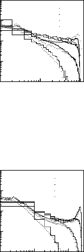
Ekin (MeV)
cross section (mb/sr.MeV)
113 MeV p + Al - 7.5 deg
- 30 deg
- 60 deg
- 150 deg
10 -2
10 -1
1
10
1 10 102
Figure 30.1: Double differential cross-section for neutrons produced in proton
scattering off Aluminum. Proton incident energy was 113 MeV.
Ekin (MeV)
cross section (mb/sr.MeV)
256 MeV p + Al - 7.5 deg
- 30 deg
- 60 deg
- 150 deg
10 -2
10 -1
1
10
1 10 102
Figure 30.2: Double differential cross-section for neutrons produced in proton
scattering off Aluminum. Proton incident energy was 256 MeV. The points
are data, the histogram is Binary Cascade prediction.
432
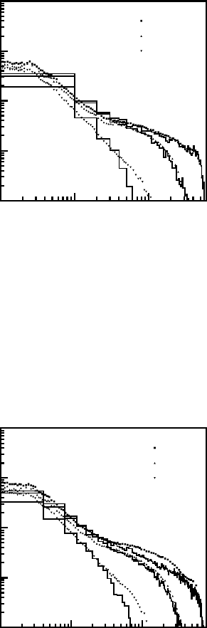
Ekin (MeV)
cross section (mb/sr.MeV)
597 MeV p + Al - 30 deg
- 60 deg
- 150 deg
10 -2
10 -1
1
10
1 10 102
Figure 30.3: Double differential cross-section for neutrons produced in proton
scattering off Aluminum. Proton incident energy was 597 MeV. The points
are data, the histogram is Binary Cascade prediction.
Ekin (MeV)
cross section (mb/sr.MeV)
800 MeV p + Al - 30 deg
- 60 deg
- 150 deg
10 -2
10 -1
1
10
1 10 102
Figure 30.4: Double differential cross-section for neutrons produced in proton
scattering off Aluminum. Proton incident energy was 800 MeV. The points
are data, the histogram is Binary Cascade prediction.
433
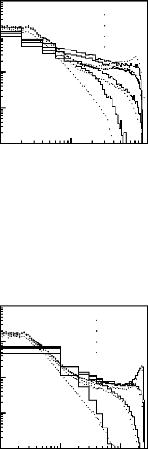
Ekin (MeV)
cross section (mb/sr.MeV)
113 MeV p + Fe - 7.5 deg
- 30 deg
- 60 deg
- 150 deg
10 -2
10 -1
1
10
1 10 102
Figure 30.5: Double differential cross-section for neutrons produced in proton
scattering off Iron. Proton incident energy was 113 MeV. The points are data,
the histogram is Binary Cascade prediction.
Ekin (MeV)
cross section (mb/sr.MeV)
256 MeV p + Fe - 7.5 deg
- 30 deg
- 60 deg
- 150 deg
10 -2
10 -1
1
10
1 10 102
Figure 30.6: Double differential cross-section for neutrons produced in proton
scattering off Iron. Proton incident energy was 256 MeV. The points are data,
the histogram is Binary Cascade prediction.
434
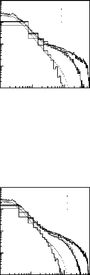
Ekin (MeV)
cross section (mb/sr.MeV)
597 MeV p + Fe - 30 deg
- 60 deg
- 150 deg
10 -2
10 -1
1
10
1 10 102
Figure 30.7: Double differential cross-section for neutrons produced in proton
scattering off Iron. Proton incident energy was 597 MeV. The points are data,
the histogram is Binary Cascade prediction.
Ekin (MeV)
cross section (mb/sr.MeV)
800 MeV p + Fe - 30 deg
- 60 deg
- 150 deg
10 -2
10 -1
1
10
1 10 102
Figure 30.8: Double differential cross-section for neutrons produced in proton
scattering off Iron. Proton incident energy was 800 MeV. The points are data,
the histogram is Binary Cascade prediction.
435

Ekin (MeV)
cross section (mb/sr.MeV)
113 MeV p + Pb - 7.5 deg
- 30 deg
- 60 deg
- 150 deg
10 -2
10 -1
1
10
10 2
10 3
1 10 102
Figure 30.9: Double differential cross-section for neutrons produced in proton
scattering off Lead. Proton incident energy was 113 MeV. The points are
data, the histogram is Binary Cascade prediction.
Ekin (MeV)
cross section (mb/sr.MeV)
256 MeV p + Pb - 7.5 deg
- 30 deg
- 60 deg
- 150 deg
10 -2
10 -1
1
10
10 2
10 3
1 10 102
Figure 30.10: Double differential cross-section for neutrons produced in pro-
ton scattering off Lead. Proton incident energy was 256 MeV. The points
are data, the histogram is Binary Cascade prediction.
436
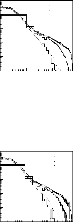
Ekin (MeV)
cross section (mb/sr.MeV)
597 MeV p + Pb - 30 deg
- 60 deg
- 150 deg
10 -2
10 -1
1
10
10 2
10 3
1 10 102
Figure 30.11: Double differential cross-section for neutrons produced in pro-
ton scattering off Lead. Proton incident energy was 597 MeV. The points
are data, the histogram is Binary Cascade prediction.
Ekin (MeV)
cross section (mb/sr.MeV)
800 MeV p + Pb - 30 deg
- 60 deg
- 150 deg
10 -2
10 -1
1
10
10 2
10 3
1 10 102
Figure 30.12: Double differential cross-section for neutrons produced in pro-
ton scattering off Lead. Proton incident energy was 800 MeV. The points
are data, the histogram is Binary Cascade prediction.
437

Ekin (MeV)
cross section (mb/sr.MeV)
p + C 45 degrees
pi+
pi-
Ekin (MeV)
cross section (mb/sr.MeV)
p + Al 45 degrees
pi+
pi-
Ekin (MeV)
cross section (mb/sr.MeV)
p + Ni 45 degrees
pi+
pi-
Ekin (MeV)
cross section (mb/sr.MeV)
p + Pb 45 degrees
pi+
pi-
10 -4
10 -3
10 -2
10 -1
1
0 100 200 300 10 -4
10 -3
10 -2
10 -1
1
0 100 200 300
10 -4
10 -3
10 -2
10 -1
1
0 100 200 300 10 -4
10 -3
10 -2
10 -1
1
0 100 200 300
Figure 30.13: Double differential cross-section for pions produced at 45◦in
proton scattering off various materials. Proton incident energy was 597 MeV
in each case. The points are data, the histogram is Binary Cascade predic-
tion.
G. Peter, D. Behrens, C.C. Noack Phys.Rev. C49, 3253, (1994),
Hai-Qiao Wang, Xu Cai, Yong Liu High Energy Phys.Nucl.Phys. 16, 101,
(1992),
A.S. Ilinov, A.B. Botvina, E.S. Golubeva, I.A. Pshenichnov, Sov. J. Nucl.
Phys. 55, 734, (1992),
and citations therein.
[2] Grypeos M. E., Lalazissis G. A., Massen S. E., Panos C. P., J. Phys. G17
1093 (1991).
[3] Elton L. R. B., Nuclear Sizes, Oxford University Press, Oxford, 1961.
[4] DeShalit A., Feshbach H., Theoretical Nuclear Physics, Vol. 1: Nuclear
Structure, Wyley, 1974.
[5] reference to be completed
[6] K. Stricker, H. McManus, J. A. Carr Nuclear scattering of low energy
pions, Phys. Rev. C 19, 929, (1979)
[7] M. M. Meier et al., Differential neutron production cross sections and
neutron yields from stopping-length targets for 113-MeV protons, Nucl.
Scien. Engin. 102, 310, (1989)
438
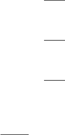
[8] M. M. Meier et al., Differential neutron production cross sections for
256-MeV protons, Nucl. Scien. Engin. 110, 289, (1992)
[9] W. B. Amian et al., Differential neutron production cross sections for
597-MeV protons, Nucl. Scien. Engin. 115, 1, (1993)
[10] W. B. Amian et al., Differential neutron production cross sections for
800-MeV protons, Nucl. Scien. Engin. 112, 78, (1992)
[11] J. F. Crawford et al., Measurement of cross sections and asymmetry
parameters for the production of charged pions from various nuclei by
585-MeV protons, Phys. Rev. C 22, 1184, (1980)
[12] J. J. Gaimard and K. H. Schmidt, “A Reexamination of the abrasion -
ablation model for the description of the nuclear fragmentation reaction,”
Nucl. Phys. A 531 (1991) 709.
[13] reference to be completed.
[14] reference to be completed
[15] reference to be completed
[16] reference to be completed
439
Chapter 31
Quantum Molecular Dynamics
for Heavy Ions
QMD is the quantum extension of the classical molecular dynamics model
and is widely used to analyze various aspects of heavy ion reactions, espe-
cially for many-body processes, and in particular the formation of complex
fragments. In the previous section, we mentioned several similar and dis-
similar points between Binary Cascade and QMD. There are three major
differences between them:
1. The definition of a participant particle,
2. The potential term in the Hamiltonian, and
3. Participant-participant interactions.
At first, we will explain how they are each treated in QMD. The entire
nucleons in the target and projectile nucleus are considered as participant
particles in the QMD model. Therefore each nucleon has its own wave func-
tion, however the total wave function of a system is still assumed as the direct
product of them. The potential terms of the Hamiltonian in QMD are calcu-
lated from the entire relation of particles in the system, in other words, it can
be regarded as self-generating from the system configuration. On the con-
trary to Binary Cascade which tracks the participant particles sequentially,
all particles in the system are tracked simultaneously in QMD. Along with
the time evolution of the system, its potential is also dynamically changed.
As there is no criterion between participant particle and others in QMD,
participant-participant scatterings are naturally included. Therefore QMD
accomplishes more detailed treatments of the above three points, however
with a cost of computing performance.
440

31.1 Equations of Motion
The basic assumption of QMD is that each nucleon state is represented by a
Gaussian wave function of width L,
ϕi(r)≡1
(2πL)3/4exp −(r−ri)2
4L+i
~r·pi(31.1)
where riand pirepresent the center values of position and momentum of the
ith particle. The total wave function is assumed to be a direct product of
them,
Ψ(r1,r2,...,rN)≡Y
i
ϕi(ri).(31.2)
Equations of the motion of particle derived on the basis of the time de-
pendent variation principle as
˙ri=∂H
∂pi
,˙pi=−∂H
∂ri
(31.3)
where His the Hamiltonian which consists particle energy including mass
energy and the energy of the two-body interaction.
However, further details in the prescription of QMD differ from author
to author and JAERI QMD (JQMD)[1] is selected as a basis for our model.
In this model, the Hamiltonian is
H=X
iqm2
i+p2
i+ˆ
V(31.4)
A Skyrme type interaction, a Coulomb interaction, and a symmetry term
are included in the effective Potential ( ˆ
V). The relativistic form of the en-
ergy expression is introduced in the Hamiltonian. The interaction term is a
function of the squared spatial distance:
Rij = (Ri−Rj)2(31.5)
This is not a Lorentz scalar. In Relativistic QMD (RQMD)[2], they are
replaced by the squared transverse four-dimensional distance,
−q2
T ij =−q2
ij +(qij ·pij)2
p2
ij
(31.6)
where qij is the four-dimensional distance and pij is the sum of the four
momentum. In JQMD they change the argument by the squared distance in
center of mass system of the two particles,
441

˜
R=R2
ij +γ2
ij(Rij ·βij )2(31.7)
with
βij =pi+pj
Ei+Ej
, γij =1
p1−βij
(31.8)
As a result of this, the interaction term in (31.4) also depends on momentum.
Recently R-JQMD, the Lorentz covariant version of JQMD, has been
proposed[3]. The covariant version of Hamiltonian (31.4) is
HC=X
iqp2
i+m2
i+ 2miVi(31.9)
where Viis the effective potential felt by the ith particle.
With on-mass-shell constraints and a simple form of the “time fixations”
constraint, the entire particle has the same time coordinate. They justified
the latter assumption with the following argument “In high-energy reactions,
two-body collisions are dominant; the purpose of the Lorentz-covariant for-
malism is only to describe relatively low energy phenomena between particles
in a fast-moving medium”[3].
From this assumption, they get following equation of motion together
with a big improvement in CPU performance.
˙ri=pi
2p0
i
+X
j
2mj
2p0
j
˜
Vj
∂pi
=∂
∂piX
jqp2
j+m2
j+ 2mj˜
V(31.10)
˙pi=−X
j
2mj
2p0
j
˜
Vj
∂ri
=∂
∂riX
jqp2
j+m2
j+ 2mj˜
V(31.11)
The ith particle has an effective mass of
m∗
i=qm2
i+ 2miVi.(31.12)
We follow their prescription and also use the same parameter values, such
as the width of the Gaussian L= 2.0 fm2and so on.
442
31.2 Ion-ion Implementation
For the case of two body collisions and resonance decay, we used the same
codes which the Binary Cascade uses in Geant4. However for the relativistic
covariant kinematic case, the effective mass of ith particle (31.12) depends on
the one-particle effective potential, Vi, which also depends on the momentum
of the entire particle system. Therefore, in R-JQMD, all the effective masses
are calculated iteratively for keeping energy conservation of the whole system.
We track their treatment for this.
As already mentioned, the Binary cascade model creates detailed 3r+ 3p
dimensional nucleus at the beginning of each reaction. However, we could
not use them in our QMD code, because they are not stable enough in time
evolution. Also, a real ground state as an energy minimum state of the nu-
cleus is not available in the framework of QMD, because it does not have
fermionic properties. However, a reasonably stable “ground state” nucleus is
required for the initial phase space distribution of nucleons in the QMD cal-
culation. JQMD succeeded to create such a “ground state” nucleus. We also
follow their prescription of generating the ground state nucleus. And “ground
state” nuclei for target and projectile will be Lorentz-boosted (construct) to
the center-of-mass system between them. By this Lorentz transformation,
additional instabilities are introduced into both nuclei in the case of the
non-covariant version.
The time evolution of the QMD system will be calculated until a certain
time, typically 100 fm/c. The δT of the evolution is 1 fm/c. The user can
modify both values from the Physics List of Geant4. After the termination
of the time evolution, cluster identification is carried out in the phase space
distribution of nucleons in the system. Each identified cluster is considered
as a fragmented nucleus from the reaction and it usually has more energy
than the ground state. Therefore, excitation energy of the nucleus is calcu-
lated and then the nucleus is passed on to other Geant4 models like Binary
Cascade. However, unlike Binary Cascade which passes them to Precom-
pound model and Excitation models by calling them inside of the model, the
QMD model uses Excitation models directly. There are multiple choices of
excitation model and one of them is the GEM model[4] which JQMD and
RJQMD use. The default excitation model is currently this GEM model.
Figure 31.1 shows an example of time evolution of the reaction of 290 MeV/n
56Fe ions bombarding a 208Pb target. Because of the small Lorentz factor
(∼1.3), the Lorentz contractions of both nuclei are not seen clearly.
443
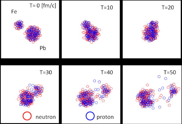
Figure 31.1: Time evolution of reaction of 290 MeV/n Fe on Pb in position
space. Red and Blue circle represents neutron and proton respectively. Full
scale of each panel is 50 fm.
31.3 Cross Sections
Nucleus-Nucleus (NN) cross section is not a fundamental component of ei-
ther QMD or Binary Light Ions Cascade model. However without the cross
section, no meaningful simulation beyond the study of the NN reaction itself
can be done. In other words, Geant4 needs the cross section to decide where
an NN reaction will happen in simulation geometry.
Many cross section formulae for NN collisions are included in Geant4, such
as Tripathi[5] and Tripathi Light System[6], Shen[7], Kox[8] and Sihver[9].
These are empirical and parameterized formulae with theoretical insights and
give total reaction cross section of wide variety of combination of projectile
and target nucleus in fast. These cross sections are also used in the sampling
of impact parameter in the QMD model.
Bibliography
[1] K. Niita et al., “Analysis of the (N, xN’) reaction by quantum molecu-
lar dynamics plus statistical decay model” Phys. Rev. C 52, 2620-2635
(1995); K. Niita et al.,Development of JQMD (Jaeri Quantum Molec-
444
ular Dynamics) Code JAERI-Data/Code 99-042, Japan Atomic Energy
Research Institute (JAERI) (1999).
[2] H. Sorge, H. St¨ocker, W. Greiner, “Poincar´e invariant Hamiltonian dy-
namics: Modelling multi-hadronic interactions in a phase space ap-
proach” Ann. Phys. (N.Y.) 192, 266-306 (1989).
[3] D. Mancusi, K. Niita, T. Maryuyama and L. Sihver, “Stability of nuclei
in peripheral collisions in the JAERI quantum molecular dynamics,”
Phys. Rev. C 52, 014614 (2009).
[4] S. Furihata, “Statistical analysis of light fragment production from
medium energy proton-induced reactions,” Nucl. Instrum. Meth. Phys.
Res. B 171, 251-258 (2000).
[5] R. K. Tripathi, F. A. Cucinotta and J. W. Wilson, Universal Parameter-
ization of Absorption Cross Sections, NASA Technical Paper TP-3621
(1997).
[6] R. K. Tripathi, F. A. Cucinotta and J. W. Wilson, Universal Parameter-
ization of Absorption Cross Sections, NASA Technical Paper TP-209726
(1999).
[7] W.-q. Shen, B. Wang, J. Feng, W.-l. Zhan, Y.-t. Zhu and E.-p. Feng,
“Total reaction cross section for heavy-ion collisions and its relation to
the neutron excess degree of freedom”, Nuclear Physics A 491 130-146
(1989).
[8] S. Kox et al., “Trends of total reaction cross sections for heavy ion
collisions in the intermediate energy range,” Phys. Rev. C 35 1678-1691
(1987).
[9] L. Sihver, C. H. Tsao, R. Silberberg, T. Kanai, and A. F. Barghouty,
“Total reaction and partial cross section calculations in proton-nucleus
(Zt ≤26) and nucleus-nucleus reactions (Zp and Zt ≤26),” Phys. Rev.
C 47 1225-1236 (1993).
445
Chapter 32
Abrasion-ablation Model
32.1 Introduction
The abrasion model is a simplified macroscopic model for nuclear-nuclear
interactions based largely on geometric arguments rather than detailed con-
sideration of nucleon-nucleon collisions. As such the speed of the simulation
is found to be faster than models such as G4BinaryCascade, but at the cost
of accuracy. The version of the model implemented is interpreted from the
so-called abrasion-ablation model described by Wilson et al [1],[2] together
with an algorithm from Cucinotta to approximate the secondary nucleon en-
ergy spectrum [3]. By default, instead of performing an ablation process to
simulate the de-excitation of the nuclear pre-fragments, the Geant4 imple-
mentation of the abrasion model makes use of existing and more detailed nu-
clear de-excitation models within Geant4 (G4Evaporation, G4FermiBreakup,
G4StatMF) to perform this function (see section 32.5). However, in some
cases cross sections for the production of fragments with large ∆A from the
pre-abrasion nucleus are more accurately determined using a Geant4 imple-
mentation of the ablation model (see section 32.6).
The abrasion interaction is the initial fast process in which the overlap region
between the projectile and target nuclei is sheered-off (see figure 32.1) The
spectator nucleons in the projectile are assumed to undergo little change in
momentum, and likewise for the spectators in the target nucleus. Some of
the nucleons in the overlap region do suffer a change in momentum, and
are assumed to be part of the original nucleus which then undergoes de-
excitation.
Less central impacts give rise to an overlap region in which the nucleons can
suffer significant momentum change, and zones in the projectile and target
outside of the overlap where the nucleons are considered as spectators to the
446

initial energetic interaction.
The initial description of the interaction must, however, take into consid-
eration changes in the direction of the projectile and target nuclei due to
Coulomb effects, which can then modify the distance of closest approach
compared with the initial impact parameter. Such effects can be important
for low-energy collisions.
32.2 Initial nuclear dynamics and impact pa-
rameter
For low-energy collisions, we must consider the deflection of the nuclei as a
result of the Coulomb force (see figure 32.2). Since the dynamics are non-
relativistic, the motion is governed by the conservation of energy equation:
Etot =1
2µ˙r2+l2
2µr2+ZPZTe2
r(32.1)
where:
Etot = total energy in the centre of mass frame;
r, ˙r= distance between nuclei, and rate of change of distance;
l= angular momentum;
µ= reduced mass of system i.e. m1m2/(m1+m2);
e= electric charge (units dependent upon the units for Etot and r);
ZP,ZT= charge numbers for the projectile and target nuclei.
The angular momentum is based on the impact parameter between the nuclei
when their separation is large, i.e.
Etot =1
2
l2
µb2⇒l2= 2Etotµb2(32.2)
At the point of closest approach, ˙r=0, therefore:
Etot =Etotb2
r2+ZPZTe2
r
r2=b2+ZPZTe2
Etot r(32.3)
Rearranging this equation results in the expression:
b2=r(r−rm) (32.4)
where:
rm=ZPZTe2
Etot
(32.5)
447

In the implementation of the abrasion process in Geant4, the square of the
far-field impact parameter, b, is sampled uniformly subject to the distance of
closest approach, r, being no greater than rP+rT(the sum of the projectile
and target nuclear radii).
32.3 Abrasion process
In the abrasion process, as implemented by Wilson et al [1] it is assumed
that the nuclear density for the projectile is constant up to the radius of the
projectile (rP) and zero outside. This is also assumed to be the case for the
target nucleus. The amount of nuclear material abraded from the projectile
is given by the expression:
∆abr =F AP1−exp −CT
λ (32.6)
where F is the fraction of the projectile in the interaction zone, λis the
nuclear mean-free-path, assumed to be:
λ=16.6
E0.26 (32.7)
Eis the energy of the projectile in MeV/nucleon and CTis the chord-length
at the position in the target nucleus for which the interaction probability is
maximum. For cases where the radius of the target nucleus is greater than
that of the projectile (i.e. rT> rP):
CT=2pr2
T−x2:x > 0
2pr2
T−r2:x≤0(32.8)
where:
x=r2
P+r2−r2
T
2r(32.9)
In the event that rP> rTthen CTis:
CT=2pr2
T−x2:x > 0
2rT:x≤0(32.10)
where:
x=r2
T+r2−r2
P
2r(32.11)
The projectile and target nuclear radii are given by the expression:
448

rP≈1.29qr2
RMS,P −0.842
rT≈1.29qr2
RMS,T −0.842(32.12)
The excitation energy of the nuclear fragment formed by the spectators in
the projectile is assumed to be determined by the excess surface area, given
by:
∆S= 4πr2
P1 + P−(1 −F)2/
3(32.13)
where the functions Pand Fare given in section 32.7. Wilson et al equate
this surface area to the excitation to:
ES= 0.95∆S(32.14)
if the collision is peripheral and there is no significant distortion of the nu-
cleus, or
ES= 0.95 {1 + 5F+ ΩF3}∆S
Ω =
0 : AP>16
1500 : AP<12
1500 −320 (AP−12) : 12 ≤AP≤16
(32.15)
if the impact separation is such that r << rP+rT.ESis in MeV provided
∆Sis in fm2.
For the abraded region, Wilson et al assume that fragments with a nucleon
number of five are unbounded, 90% of fragments with a nucleon number of
eight are unbound, and 50% of fragments with a nucleon number of nine
are unbound. This was not implemented within the Geant4 version of the
abrasion model, and disintegration of the pre-fragment was only simulated by
the subsequent de-excitation physics models in the G4DeexcitationHandler
(evaporation, etc. or G4WilsonAblationModel) since the yields of lighter
fragments were already underestimated compared with experiment.
In addition to energy as a result of the distortion of the fragment, some energy
is assumed to be gained from transfer of kinetic energy across the boundaries
of the nuclei. This is approximated to the average energy transferred to a
nucleon per unit intersection pathlength (assumed to be 13 MeV/fm) and
the longest chord-length, Cl, and for half of the nucleon-nucleon collisions it
is assumed that the excitation energy is:
E∗
X=13 ·1 + Ct−1.5
3Cl:Ct>1.5fm
13 ·Cl:Ct≤1.5fm (32.16)
449

where:
Cl=2pr2
P+ 2rrT−r2−r2
Tr > rT
2rPr≤rT
(32.17)
Ct= 2sr2
P−(r2
P+r2−r2
T)2
4r2(32.18)
For the remaining events, the projectile energy is assumed to be unchanged.
Wilson et al assume that the energy required to remove a nucleon is 10MeV,
therefore the number of nucleons removed from the projectile by ablation is:
∆abl =ES+EX
10 + ∆spc (32.19)
where ∆spc is the number of loosely-bound spectators in the interaction re-
gion, given by:
∆spc =APFexp −CT
λ(32.20)
Wilson et al appear to assume that for half of the events the excitation
energy is transferred into one of the nuclei (projectile or target), otherwise
the energy is transferred in to the other (target or projectile respectively).
The abrasion process is assumed to occur without preference for the nucleon
type, i.e. the probability of a proton being abraded from the projectile is
proportional to the fraction of protons in the original projectile, therefore:
∆Zabr = ∆abr
ZP
AP
(32.21)
In order to calculate the charge distribution of the final fragment, Wilson et al
assume that the products of the interaction lie near to nuclear stability and
therefore can be sampled according to the Rudstam equation (see section
32.6). The other obvious condition is that the total charge must remain
unchanged.
32.4 Abraded nucleon spectrum
Cucinotta has examined different formulae to represent the secondary protons
spectrum from heavy ion collisions [3]. One of the models (which has been
implemented to define the final state of the abrasion process) represents the
momentum distribution of the secondaries as:
450

ψ(p)∝
3
X
i=1
Ciexp −p2
2p2
i+d0
γp
sinh (γp)(32.22)
where:
ψ(p) = number of secondary protons with momentum pper unit of
momentum phase space [c3/MeV3];
p= magnitude of the proton momentum in the rest frame of the
nucleus from which the particle is projected [MeV/c];
C1, C2, C3 = 1.0, 0.03, and 0.0002;
p1, p2, p3 = q2
5pF,q6
5pF, 500 [MeV/c]
pF= Momentum of nucleons in the nuclei at the Fermi surface [MeV/c]
d0= 0.1
1
γ= 90 [MeV/c];
G4WilsonAbrasionModel approximates the momentum distribution for the
neutrons to that of the protons, and as mentioned above, the nucleon type
sampled is proportional to the fraction of protons or neutrons in the original
nucleus.
The angular distribution of the abraded nucleons is assumed to be isotropic
in the frame of reference of the nucleus, and therefore those particles from the
projectile are Lorentz-boosted according to the initial projectile momentum.
32.5 De-excitation of the projectile and tar-
get nuclear pre-fragments by standard
Geant4 de-excitation physics
Unless specified otherwise, G4WilsonAbrasionModel will instantiate the fol-
lowing de-excitation models to treat subsequent particle emission of the ex-
cited nuclear pre-fragments (from both the projectile and the target):
1 G4Evaporation, which will perform nuclear evaporation of (α-particles,
3He, 3H, 2H, protons and neutrons, in competition with photo-evaporation
and nuclear fission (if the nucleus has sufficiently high A).
2 G4FermiBreakUp, for nuclei with A≤12 and Z≤6.
3 G4StatMF, for multi-fragmentation of the nucleus (minimum energy for
this process set to 5 MeV).
As an alternative to using this de-excitation scheme, the user may provide
to the G4WilsonAbrasionModel a pointer to her own de-excitation handler,
or invoke instantiation of the ablation model (G4WilsonAblationModel).
451

32.6 De-excitation of the projectile and tar-
get nuclear pre-fragments by nuclear ab-
lation
A nuclear ablation model, based largely on the description provided by Wil-
son et al [1], has been developed to provide a better approximation for the
final nuclear fragment from an abrasion interaction. The algorithm imple-
mented in G4WilsonAblationModel uses the same approach for selecting the
final-state nucleus as NUCFRG2 and determining the particles evaporated
from the pre-fragment in order to achieve that state. However, use is also
made of classes in Geant4’s evaporation physics to determine the energies of
the nuclear fragments produced.
The number of nucleons ablated from the nuclear pre-fragment (whether
as nucleons or light nuclear fragments) is determined based on the average
binding energy, assumed by Wilson et al to be 10 MeV, i.e.:
Aabl =Int Ex
10MeV :AP F > Int Ex
10MeV
AP F :otherwise (32.23)
Obviously, the nucleon number of the final fragment, AF, is then determined
by the number of remaining nucleons. The proton number of the final nuclear
fragment (ZF) is sampled stochastically using the Rudstam equation:
σ(AF, ZF)∝exp −RZF−SAF−T A2
F
3/
2(32.24)
Here R=11.8/AF 0.45,S=0.486, and T=3.8·10−4. Once ZFand AFhave been
calculated, the species of the ablated (evaporated) particles are determined
again using Wilson’s algorithm. The number of α-particles is determined
first, on the basis that these have the greatest binding energy:
Nα=Int Zabl
2:Int Zabl
2< Int Aabl
4
Int Aabl
4:Int Zabl
2≥Int Aabl
4(32.25)
Calculation of the other ablated nuclear/nucleon species is determined in
a similar fashion in order of decreasing binding energy per nucleon of the
ablated fragment, and subject to conservation of charge and nucleon number.
Once the ablated particle species are determined, use is made of the Geant4
evaporation classes to sample the order in which the particles are ejected
(from G4AlphaEvaporationProbability, G4He3EvaporationProbability, G4TritonEvaporationProbabilit
G4DeuteronEvaporationProbability, G4ProtonEvaporationProbability and G4NeutronEvaporationProbabilit
452

and the energies and momenta of the evaporated particle and the resid-
ual nucleus at each two-body decay (using G4AlphaEvaporationChannel,
G4He3EvaporationChannel, G4TritonEvaporationChannel, G4DeuteronEvaporationChannel,
G4ProtonEvaporationChannel and G4NeutronEvaporationChannel). If at
any stage the probability for evaporation of any of the particles selected by
the ablation process is zero, the evaporation is forced, but no significant
momentum is imparted to the particle/nucleus. Note, however, that any
particles ejected from the projectile will be Lorentz boosted depending upon
the initial energy per nucleon of the projectile.
32.7 Definition of the functions P and F used
in the abrasion model
In the first instance, the form of the functions Pand Fused in the abrasion
model are dependent upon the relative radii of the projectile and target and
the distance of closest approach of the nuclear centres. Four radius condtions
are treated.
rT> rPand rT−rP≤r≤rT+rP:
P= 0.125√µν 1
µ−21−β
ν2
−0.125 0.5√µν 1
µ−2+ 11−β
ν3
(32.26)
F= 0.75√µν 1−β
ν2
−0.125 [3√µν −1] 1−β
ν3
(32.27)
where:
ν=rP
rP+rT
(32.28)
β=r
rP+rT
(32.29)
µ=rT
rP
(32.30)
rT> rPand r < rT−rP:
P=−1 (32.31)
453

F= 1 (32.32)
rP> rTand rP−rT≤r≤rP+rT:
P= 0.125√µν 1
µ−21−β
ν2
(32.33)
−0.125 (0.5rν
µ1
µ−2−"p1−µ2
ν−1#r2−µ
µ5)1−β
ν3
F= 0.75√µν 1−β
ν2
(32.34)
−0.125
3rν
µ−1−(1 −µ2)3/
2q1−(1 −µ)2
µ3
1−β
ν3
rP> rTand r < rT−rP:
P="p1−µ2
ν−1#s1−β
ν2
(32.35)
F=1−1−µ23/
2s1−β
ν2
(32.36)
Bibliography
[1] J W Wilson, R K Tripathi, F A Cucinotta, J K Shinn, F F Ba-
davi, S Y Chun, J W Norbury, C J Zeitlin, L Heilbronn, and J Miller,
”NUCFRG2: An evaluation of the semiempirical nuclear fragmentation
database,” NASA Technical Paper 3533, 1995.
[2] Lawrence W Townsend, John W Wilson, Ram K Tripathi, John W
Norbury, Francis F Badavi, and Ferdou Khan, ”HZEFRG1, An energy-
dependent semiempirical nuclear fragmentation model,” NASA Technical
Paper 3310, 1993.
[3] Francis A Cucinotta, ”Multiple-scattering model for inclusive proton pro-
duction in heavy ion collisions,” NASA Technical Paper 3470, 1994.
454
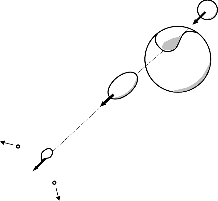
Figure 32.1: In the abrasion process, a fraction of the nucleons in the pro-
jectile and target nucleons interact to form a fireball region with a velocity
between that of the projectile and the target. The remaining spectator nu-
cleons in the projectile and target are not initially affected (although they
do suffer change as a result of longer-term de-excitation).
455
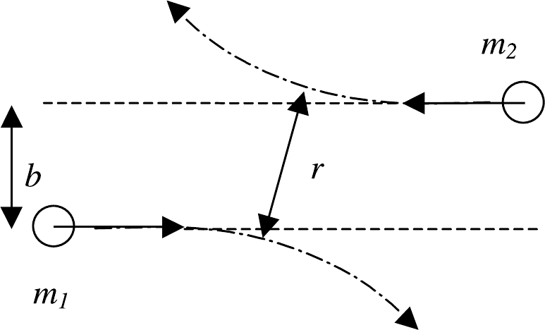
Figure 32.2: Illustration clarifying impact parameter in the far-field (b) and
actual impact parameter (r).
456

Chapter 33
Electromagnetic Dissociation
Model
33.1 The Model
The relative motion of a projectile nucleus travelling at relativistic speeds
with respect to another nucleus can give rise to an increasingly hard spec-
trum of virtual photons. The excitation energy associated with this en-
ergy exchange can result in the liberation of nucleons or heavier nuclei (i.e.
deuterons, α-particles, etc.). The contribution of this source to the total
inelastic cross section can be important, especially where the proton number
of the nucleus is large. The electromagnetic dissociation (ED) model is im-
plemented in the classes G4EMDissociation, G4EMDissociationCrossSection
and G4EMDissociationSpectrum, with the theory taken from Wilson et al
[1], and Bertulani and Baur [2].
The number of virtual photons N(Eγ, b) per unit area and energy interval
experienced by the projectile due to the dipole field of the target is given by
the expression [2]:
N(Eγ, b) = αZ2
T
π2β2b2Eγx2k2
1(x) + x2
γ2k2
0(x)(33.1)
where xis a dimensionless quantity defined as:
x=bEγ
γβ¯
hc (33.2)
and:
α= fine structure constant
β= ratio of the velocity of the projectile in the laboratory frame to
the velocity of light
457

γ= Lorentz factor for the projectile in the laboratory frame
b= impact parameter
c= speed of light
¯
h= quantum constant
Eγ= energy of virtual photon
k0and k1= zeroth and first order modified Bessel functions of the
second kind
ZT= atomic number of the target nucleus
Integrating Eq. 33.1 over the impact parameter from bmin to ∞produces
the virtual photon spectrum for the dipole field of:
NE1(Eγ) = 2αZ2
T
πβ2Eγξk0(ξ)k1(ξ)−ξ2β2
2k2
1(ξ)−k2
0(ξ)(33.3)
where, according to the algorithm implemented by Wilson et al in NUCFRG2
[1]:
ξ=Eγbmin
γβ¯
hc
bmin = (1 + xd)bc+πα0
2γ
α0=ZPZTe2
µβ2c2
bc= 1.34 "A1/
3
P+A1/
3
T−0.75 A−1/
3
P+A−1/
3
T!#
(33.4)
and µis the reduced mass of the projectile/target system, xd= 0.25, and AP
and ATare the projectile and target nucleon numbers. For the last equation,
the units of bcare fm. Wilson et al state that there is an equivalent virtual
photon spectrum as a result of the quadrupole field:
NE2(Eγ) = 2αZ2
T
πβ4Eγ21−β2k2
1(ξ) + ξ2−β22k0(ξ)k1(ξ)−ξ2β4
2k2
1(ξ)−k2
0(ξ)
(33.5)
The cross section for the interaction of the dipole and quadrupole fields is
given by:
σED =ZNE1(Eγ)σE1(Eγ)dEγ+ZNE2(Eγ)σE2(Eγ)dEγ(33.6)
458

Wilson et al assume that σE1(Eγ) and σE2(Eγ) are sharply peaked at the
giant dipole and quadrupole resonance energies:
EGDR =¯
hc hm∗c2R2
0
8J1 + u−1+ε+3u
1+ε+uεi−1
2
EGQR =63
A
1/
3
P
(33.7)
so that the terms for NE1and NE2can be taken out of the integrals in Eq.
33.6 and evaluated at the resonances.
In Eq. 33.7:
u=3J
Q′A−1/
3
P
R0=r0A1/
3
P
(33.8)
ǫ= 0.0768, Q′= 17MeV, J= 36.8MeV, r0= 1.18fm, and m∗is 7/10 of
the nucleon mass (taken as 938.95 MeV/c2). (The dipole and quadrupole
energies are expressed in units of MeV.)
The photonuclear cross sections for the dipole and quadrupole resonances are
assumed to be given by:
ZσE1(Eγ)dEγ= 60NPZP
AP
(33.9)
in units of MeV-mb (NPbeing the number of neutrons in the projectile) and:
ZσE2(Eγ)dEγ
E2
γ
= 0.22fZPA2/
3
P(33.10)
in units of µb/MeV. In the latter expression, fis given by:
f=
0.9AP>100
0.6 40 < AP≤100
0.3 40 ≤AP
(33.11)
The total cross section for electromagnetic dissociation is therefore given by
Eq. 33.6 with the virtual photon spectra for the dipole and quadrupole fields
calculated at the resonances:
459

σED =NE1(EGDR)ZσE1(Eγ)dEγ+NE2(EGQR)E2
GQR ZσE2(Eγ)
E2
γ
dEγ
(33.12)
where the resonance energies are given by Eq. 33.7 and the integrals for the
photonuclear cross sections given by Eq. 33.9 and Eq. 33.10.
The selection of proton or neutron emission is made according to the following
prescription from Wilson et al.
σED,p =σED ×
0.5ZP<6
0.6 6 ≤ZP≤8
0.7 8 < ZP<14
min hZP
AP,1.95 exp(−0.075ZP)iZP≥14
σED,n =σED −σED,p
(33.13)
Note that this implementation of ED interactions only treats the ejection
of single nucleons from the nucleus, and currently does not allow emission of
other light nuclear fragments.
Bibliography
[1] J. W. Wilson, R. K. Tripathi, F. A. Cucinotta, J. K. Shinn, F. F. Badavi,
S. Y. Chun, J. W. Norbury, C. J. Zeitlin, L. Heilbronn, and J. Miller,
”NUCFRG2: An evaluation of the semiempirical nuclear fragmentation
database,” NASA Technical Paper 3533, 1995.
[2] C. A. Bertulani, and G. Baur, Electromagnetic processes in relativistic
heavy ion collisions, Nucl Phys, A458, 725-744, 1986.
460
Chapter 34
Precompound model.
34.1 Reaction initial state.
The GEANT4 precompound model is considered as an extension of the
hadron kinetic model. It gives a possibility to extend the low energy range
of the hadron kinetic model for nucleon-nucleus inelastic collision and it pro-
vides a ”smooth” transition from kinetic stage of reaction described by the
hadron kinetic model to the equilibrium stage of reaction described by the
equilibrium deexcitation models.
The initial information for calculation of pre-compound nuclear stage
consists from the atomic mass number A, charge Zof residual nucleus, its
four momentum P0, excitation energy Uand number of excitons nequals
the sum of number of particles p(from them pZare charged) and number of
holes h.
At the preequilibrium stage of reaction, we following the [1] approach,
take into account all possible nuclear transition the number of excitons n
with ∆n= +2,−2,0 [1], which defined by transition probabilities. Only
emmision of neutrons, protons, deutrons, thritium and helium nuclei are
taken into account.
34.2 Simulation of pre-compound reaction
The precompound stage of nuclear reaction is considered until nuclear
system is not an equilibrium state. Further emission of nuclear fragments or
photons from excited nucleus is simulated using an equilibrium model (see
Chapter 35.6).
461

34.2.1 Statistical equilibrium condition
In the state of statistical equilibrium, which is characterized by an eqilib-
rium number of excitons neq, all three type of transitions are equiprobable.
Thus neq is fixed by ω+2(neq, U) = ω−2(neq, U). From this condition we can
get
neq =p2gU. (34.1)
34.2.2 Level density of excited (n-exciton) states
To obtain Eq. (34.1) it was assumed an equidistant scheme of single-
particle levels with the density g≈0.595aA, where ais the level density
parameter, when we have the level density of the n-exciton state as
ρn(U) = g(gU)n−1
p!h!(n−1)!.(34.2)
34.2.3 Transition probabilities
The partial transition probabilities changing the exciton number by ∆nis
determined by the squared matrix element averaged over allowed transitions
<|M|2>and the density of final states ρ∆n(n, U), which are really accessible
in this transition. It can be defined as following:
ω∆n(n, U) = 2π
h<|M|2> ρ∆n(n, U).(34.3)
The density of final states ρ∆n(n, U) were derived in paper [2] using the Eq.
(34.2) for the level density of the n-exciton state and later corrected for the
Pauli principle and indistinguishability of identical excitons in paper [3]:
ρ∆n=+2(n, U) = 1
2g[gU −F(p+ 1, h + 1)]2
n+ 1 [gU −F(p+ 1, h + 1)
gU −F(p, h)]n−1,
(34.4)
ρ∆n=0(n, U) = 1
2g[gU −F(p, h)]
n[p(p−1) + 4ph +h(h−1)] (34.5)
and
ρ∆n=−2(n, U) = 1
2gph(n−2),(34.6)
where F(p, h) = (p2+h2+p−h)/4−h/2 and it was taken to be equal zero.
To avoid calculation of the averaged squared matrix element <|M|2>it
was assumed [1] that transition probability ω∆n=+2(n, U) is the same as the
462

probability for quasi-free scattering of a nucleon above the Fermi level on a
nucleon of the target nucleus, i. e.
ω∆n=+2(n, U) = < σ(vrel)vrel >
Vint
.(34.7)
In Eq. (34.7) the interaction volume is estimated as Vint =4
3π(2rc+λ/2π)3,
with the De Broglie wave length λ/2πcorresponding to the relative velocity
< vrel >=p2Trel/m, where mis nucleon mass and rc= 0.6 fm.
The averaging in < σ(vrel)vrel >is further simplified by
< σ(vrel)vrel >=< σ(vrel)>< vrel > . (34.8)
For σ(vrel) we take approximation:
σ(vrel) = 0.5[σpp(vrel) + σpn(vrel]P(TF/Trel),(34.9)
where factor P(TF/Trel) was introduced to take into account the Pauli prin-
ciple. It is given by
P(TF/Trel) = 1 −7
5
TF
Trel
(34.10)
for TF
Trel ≤0.5 and
P(TF/Trel) = 1 −7
5
TF
Trel
+2
5
TF
Trel
(2 −Trel
TF
)5/2(34.11)
for TF
Trel >0.5.
The free-particle proton-proton σpp(vrel) and proton-neutron σpn(vrel) in-
teraction cross sections are estimated using the equations [4]:
σpp(vrel) = 10.63
v2
rel −29.93
vrel
+ 42.9 (34.12)
and
σpn(vrel) = 34.10
v2
rel −82.2
vrel
+ 82.2,(34.13)
where cross sections are given in mbarn.
The mean relative kinetic energy Trel is needed to calculate < vrel >
and the factor P(TF/Trel) was computed as Trel =Tp+Tn, where mean
kinetic energies of projectile nucleons Tp=TF+U/n and target nucleons
TN= 3TF/5, respecively.
463

Combining Eqs. (34.3) - (34.7) and assuming that <|M|2>are the same
for transitions with ∆n= 0 and ∆n=±2 we obtain for another transition
probabilities:
ω∆n=0(n, U) =
=<σ(vrel)vrel>
Vint
n+1
n[gU−F(p,h)
gU−F(p+1,h+1) ]n+1 p(p−1)+4ph+h(h−1)
gU−F(p,h)
(34.14)
and ω∆n=−2(n, U) =
=<σ(vrel)vrel>
Vint [gU−F(p,h)
gU−F(p+1,h+1) ]n+1 ph(n+1)(n−2)
[gU−F(p,h)]2.(34.15)
34.2.4 Emission probabilities for nucleons
Emission process probability has been choosen similar as in the classical
equilibrium Weisskopf-Ewing model [5]. Probability to emit nucleon bin the
energy interval (Tb, Tb+dTb) is given
Wb(n, U, Tb) = σb(Tb)(2sb+ 1)µb
π2h3Rb(p, h)ρn−b(E∗)
ρn(U)Tb,(34.16)
where σb(Tb) is the inverse (absorption of nucleon b) reaction cross section,
sband mbare nucleon spin and reduced mass, the factor Rb(p, h) takes into
account the condition for the exciton to be a proton or neutron, ρn−b(E∗)
and ρn(U) are level densities of nucleus after and before nucleon emission are
defined in the evaporation model, respectively and E∗=U−Qb−Tbis the
excitation energy of nucleus after fragment emission.
34.2.5 Emission probabilities for complex fragments
It was assumed [1] that nucleons inside excited nucleus are able to ”con-
dense” forming complex fragment. The ”condensation” probability to create
fragment consisting from Nbnucleons inside nucleus with Anucleons is given
by
γNb=N3
b(Vb/V )Nb−1=N3
b(Nb/A)Nb−1,(34.17)
where Vband Vare fragment band nucleus volumes, respectively. The last
equation was estimated [1] as the overlap integral of (constant inside a vol-
ume) wave function of independent nucleons with that of the fragment.
During the prequilibrium stage a ”condense” fragment can be emitted.
The probability to emit a fragment can be written as [1]
Wb(n, U, Tb) = γNbRb(p, h)ρ(Nb,0, Tb+Qb)
gb(Tb)σb(Tb)(2sb+ 1)µb
π2h3
ρn−b(E∗)
ρn(U)Tb,
(34.18)
464

where
gb(Tb) = Vb(2sb+ 1)(2µb)3/2
4π2h3(Tb+Qb)1/2(34.19)
is the single-particle density for complex fragment b, which is obtained by
assuming that complex fragment moves inside volume Vbin the uniform po-
tential well whose depth is equal to be Qb, and the factor Rb(p, h) garantees
correct isotopic composition of a fragment b.
34.2.6 The total probability
This probability is defined as
Wtot(n, U) = X
∆n=+2,0,−2
ω∆n(n, U) +
6
X
b=1
Wb(n, U),(34.20)
where total emission Wb(n, U) probabilities to emit fragment bcan be ob-
tained from Eqs. (34.16) and (34.18) by integration over Tb:
Wb(n, U) = ZU−Qb
Vb
Wb(n, U, Tb)dTb.(34.21)
34.2.7 Calculation of kinetic energies for emitted par-
ticle
The equations (34.16) and (34.18) are used to sample kinetic energies of
emitted fragment.
34.2.8 Parameters of residual nucleus.
After fragment emission we update parameter of decaying nucleus:
Af=A−Ab;Zf=Z−Zb;Pf=P0−pb;
E∗
f=qE2
f−~
P2
f−M(Af, Zf).(34.22)
Here pbis the evaporated fragment four momentum.
Bibliography
[1] K.K. Gudima, S.G. Mashnik, V.D. Toneev, Nucl. Phys. A401 329
(1983).
465
[2] F. C. Williams, Phys. Lett. B31 180 (1970).
[3] I. Ribansk´y, P. Obloˆzinsk´y, E. B´etaˆ
k, Nucl. Phys. A205 545 (1973).
[4] N. Metropolis et al., Phys. Rev. 100 185 (1958).
[5] V.E. Weisskopf, D.H. Ewing, Phys. Rev. 57 472 (1940).
466
Chapter 35
Evaporation Model
35.1 Introduction
At the end of the pre-equilibrium stage, or a thermalizing process, the
residual nucleus is supposed to be left in an equilibrium state, in which the
excitation energy E∗is shared by a large number of nucleons. Such an equili-
brated compound nucleus is characterized by its mass, charge and excitation
energy with no further memory of the steps which led to its formation. If the
excitation energy is higher than the separation energy, it can still eject nu-
cleons and fragments (d, t, 3He, α, others). These constitute the low energy
and most abundant part of the emitted particles in the rest system of the
residual nucleus. The emission of particles by an excited compound nucleus
has been successfully described by comparing the nucleus with the evapora-
tion of molecules from a fluid [1]. The first statistical theory of compound
nuclear decay is due to Weisskopf and Ewing[2].
35.2 Evaporation model
The Weisskopf treatment is an application of the detailed balance principle
that relates the probabilities to go from a state ito another dand viceversa
through the density of states in the two systems:
Pi→dρ(i) = Pd→iρ(d) (35.1)
where Pd→iis the probability per unit of time of a nucleus dcaptures a particle
jand form a compound nucleus iwhich is proportional to the compound
nucleus cross section σinv. Thus, the probability that a parent nucleus iwith
an excitation energy E∗emits a particle jin its ground state with kinetic
467

energy εis
Pj(ε)dε=gjσinv(ε)ρd(Emax −ε)
ρi(E∗)εdε(35.2)
where ρi(E∗) is the level density of the evaporating nucleus, ρd(Emax −ε) that
of the daugther (residual) nucleus after emission of a fragment jand Emax is
the maximum energy that can be carried by the ejectile. With the spin sjand
the mass mjof the emitted particle, gjis expressed as gj= (2sj+1)mj/π2~2.
This formula must be implemented with a suitable form for the level den-
sity and inverse reaction cross section. We have followed, like many other
implementations, the original work of Dostrovsky et al. [3] (which represents
the first Monte Carlo code for the evaporation process) with slight modifi-
cations. The advantage of the Dostrovsky model is that it leds to a simple
expression for equation 35.2 that can be analytically integrated and used for
Monte Carlo sampling.
35.2.1 Cross sections for inverse reactions
The cross section for inverse reaction is expressed by means of empirical
equation [3]
σinv(ε) = σgα1 + β
ε(35.3)
where σg=πR2is the geometric cross section.
In the case of neutrons, α= 0.76 + 2.2A−1
3and β= (2.12A−2
3−0.050)/α
MeV. This equation gives a good agreement to those calculated from con-
tinuum theory [4] for intermediate nuclei down to ε∼0.05 MeV. For lower
energies σinv,n(ε) tends toward infinity, but this causes no difficulty because
only the product σinv,n(ε)εenters in equation 35.2. It should be noted, that
the inverse cross section needed in 35.2 is that between a neutron of kinetic
energy εand a nucleus in an excited state.
For charged particles (p, d, t, 3He and α), α= (1 + cj) and β=−Vj,
where cjis a set of parameters calculated by Shapiro [5] in order to provide
a good fit to the continuum theory [4] cross sections and Vjis the Coulomb
barrier.
35.2.2 Coulomb barriers
Coulomb repulsion, as calculated from elementary electrostatics are not
directly applicable to the computation of reaction barriers but must be cor-
rected in several ways. The first correction is for the quantum mechanical
468

phenomenoon of barrier penetration. The proper quantum mechanical ex-
pressions for barrier penetration are far too complex to be used if one wishes
to retain equation 35.2 in an integrable form. This can be approximately
taken into account by multiplying the electrostatic Coulomb barrier by a
coefficient kjdesigned to reproduce the barrier penetration approximately
whose values are tabulated [5].
Vj=kj
ZjZde2
Rc
(35.4)
The second correction is for the separation of the centers of the nuclei at
contact, Rc. We have computed this separation as Rc=Rj+Rdwhere
Rj,d =rcA1/3
j,d and rcis given [6] by
rc= 2.1731 + 0.006103ZjZd
1 + 0.009443ZjZd
(35.5)
35.2.3 Level densities
The simplest and most widely used level density based on the Fermi
gas model are those of Weisskopf [7] for a completely degenerate Fermi gas.
We use this approach with the corrections for nucleon pairing proposed by
Hurwitz and Bethe [8] which takes into account the displacements of the
ground state:
ρ(E) = Cexp 2pa(E−δ)(35.6)
where Cis considered as constant and does not need to be specified since
only ratios of level densities enter in equation 35.2. δis the pairing energy
correction of the daughter nucleus evaluated by Cook et al. [9] and Gilbert
and Cameron [10] for those values not evaluated by Cook et al.. The level
density parameter is calculated according to:
a(E, A, Z) = ˜a(A)1 + δ
E[1 −exp(−γE)](35.7)
and the parameters calculated by Iljinov et al. [11] and shell corrections of
Truran, Cameron and Hilf [12].
35.2.4 Maximum energy available for evaporation
The maximum energy avilable for the evaporation process (i.e. the
maximum kinetic energy of the outgoing fragment) is usually computed
like E∗−δ−Qjwhere is the separation energy of the fragment j:Qj=
469

Mi−Md−Mjand Mi,Mdand Mjare the nclear masses of the compound,
residual and evporated nuclei respectively. However, that expression does
not consider the recoil energy of the residual nucleus. In order to take into
account the recoil energy we use the expression
εmax
j=(Mi+E∗−δ)2+M2
j−M2
d
2(Mi+E∗−δ)−Mj(35.8)
35.2.5 Total decay width
The total decay width for evaporation of a fragment jcan be obtained by
integrating equation 35.2 over kinetic energy
Γj=~Zεmax
j
Vj
P(εj)dεj(35.9)
This integration can be performed analiticaly if we use equation 35.6 for level
densities and equation 35.3 for inverse reaction cross section. Thus, the total
width is given by
Γj=gjmjR2
d
2π~2
α
a2
d×
βad−3
2+ad(εmax
j−Vj)exp n−pai(E∗−δi)o+
(2βad−3)qad(εmax
j−Vj) + 2ad(εmax
j−Vj)×
exp n2hqad(εmax
j−Vj)−pai(E∗−δi)io
(35.10)
where ad=a(Ad, Zd, εmax
j) and ai=a(Ai, Zi, E∗).
35.3 GEM model
As an alternative model we have implemented the generalized evaporation
model (GEM) by Furihata [13]. This model considers emission of fragments
heavier than αparticles and uses a more accurate level density function for
total decay width instead of the approximation used by Dostrovsky. We use
the same set of parameters but for heavy ejectiles the parameters determined
by Matsuse et al. [14] are used.
Based on the Fermi gas model, the level density function is expressed as
ρ(E) = (√π
12
e2√a(E−δ)
a1/4(E−δ)5/4for E ≥Ex
1
Te(E−E0)/T for E <Ex
(35.11)
470

where Ex=Ux+δand Ux= 150/Md+ 2.5 (Mdis the mass of the daughter
nucleus). Nuclear temperature Tis given as 1/T =pa/Ux−1.5Ux, and E0
is defined as E0=Ex−T(log T−log a/4−(5/4) log Ux+ 2√aUx).
By substituting equation 35.11 into equation 35.2 and integrating over
kinetic energy can be obtained the following expression
Γj=√πgjπR2
dα
12ρ(E∗)×
{I1(t, t) + (β+V)I0(t)}for εmax
j−Vj<Ex
{I1(t, tx) + I3(s, sx)es+
(β+V)(I0(tx) + I2(s, sx)es)}for εmax
j−Vj≥Ex.
(35.12)
I0(t), I1(t, tx), I2(s, sx), and I3(s, sx) are expressed as:
I0(t) = e−E0/T (et−1) (35.13)
I1(t, tx) = e−E0/T T{(t−tx+ 1)etx−t−1}(35.14)
I2(s, sx) = 2√2s−3/2+ 1.5s−5/2+ 3.75s−7/2−
(s−3/2
x+ 1.5s−5/2
x+ 3.75s−7/2
x)(35.15)
I3(s, sx) = 1
2√2"2s−1/2+ 4s−3/2+ 13.5s−5/2+ 60.0s−7/2+
325.125s−9/2−(s2−s2
x)s−3/2
x+ (1.5s2+ 0.5s2
x)s−5/2
x+
(3.75s2+ 0.25s2
x)s−7/2
x+ (12.875s2+ 0.625s2
x)s−9/2
x+
(59.0625s2+ 0.9375s2
x)s−11/2
x+
(324.8s2+ 3.28s2
x)s−13/2
x+#(35.16)
where t= (εmax
j−Vj)/T ,tx=Ex/T ,s= 2qa(εmax
j−Vj−δj) and sx=
2pa(Ex−δ).
Besides light fragments, 60 nuclides up to 28Mg are considered, not only in
their ground states but also in their exited states, are considered. The excited
state is assumed to survive if its lifetime T1/2is longer than the decay time,
i. e.,T1/2/ln 2 >~/Γ∗
j, where Γ∗
jis the emission width of the resonance
calculated in the same manner as for ground state particle emission. The
total emission width of an ejectile jis summed over its ground state and all
its excited states which satisfy the above condition.
471

35.4 Nuclear fission
The fission decay channel (only for nuclei with A > 65) is taken into
account as a competitor for fragment and photon evaporation channels.
35.4.1 The fission total probability
The fission probability (per unit time) Wfis in the Bohr and Wheeler theory
of fission [15] is proportional to the level density ρfis(T) ( approximation Eq.
(35.6) is used) at the saddle point, i.e.
Wfis =1
2π~ρfis(E∗)RE∗−Bf is
0ρfis(E∗−Bfis −T)dT =
=1+(Cf−1) exp (Cf)
4πafis exp (2√aE∗),(35.17)
where Bfis is the fission barrier height. The value of Cf= 2pafis(E∗−Bfis)
and a,afis are the level density parameters of the compound and of the fission
saddle point nuclei, respectively.
The value of the level density parameter is large at the saddle point, when
excitation energy is given by initial excitation energy minus the fission barrier
height, than in the ground state, i. e. af is > a.af is = 1.08afor Z < 85,
afis = 1.04afor Z≥89 and af=a[1.04 + 0.01(89.−Z)] for 85 ≤Z < 89 is
used.
35.4.2 The fission barrier
The fission barrier is determined as difference between the saddle-point
and ground state masses.
We use simple semiphenomenological approach was suggested by Barashenkov
and Gereghi [16]. In their approach fission barrier Bfis(A, Z) is approximated
by
Bfis =B0
fis + ∆g+ ∆p.(35.18)
The fission barrier height B0
fis(x) varies with the fissility parameter x=
Z2/A.B0
fis(x) is given by
B0
fis(x) = 12.5 + 4.7(33.5−x)0.75 (35.19)
for x≤33.5 and
B0
fis(x) = 12.5−2.7(x−33.5)2/3(35.20)
for x > 33.5. The ∆g= ∆M(N) + ∆M(Z), where ∆M(N) and ∆M(Z) are
shell corrections for Cameron’s liquid drop mass formula [17] and the pairing
energy corrections: ∆p= 1 for odd-odd nuclei, ∆p= 0 for odd-even nuclei,
∆p= 0.5 for even-odd nuclei and ∆p=−0.5 for even-even nuclei.
472

35.5 Photon evaporation
Photon evaporation main be simulated as a continium gamma transition us-
ing dipole approximation and via discrete gamma transition using evaluated
database on nuclear gamma transitions.
35.5.1 Computation of probability
As the first approximation we assume that dipole E1–transitions is the
main source of γ–quanta from highly–excited nuclei [11]. The probability to
evaporate γin the energy interval (ǫγ, ǫγ+dǫγ) per unit of time is given
Wγ(ǫγ) = 1
π2(~c)3σγ(ǫγ)ρ(E∗−ǫγ)
ρ(E∗)ǫ2
γ,(35.21)
where σγ(ǫγ) is the inverse (absorption of γ) reaction cross section, ρis a
nucleus level density is defined by Eq. (35.6).
The photoabsorption reaction cross section is given by the expression
σγ(ǫγ) = σ0ǫ2
γΓ2
R
(ǫ2
γ−E2
GDP )2+ Γ2
Rǫ2
γ
,(35.22)
where σ0= 2.5Amb, ΓR= 0.3EGDP and EGDP = 40.3A−1/5MeV are
empirical parameters of the giant dipole resonance [11]. The total radiation
probability is
Wγ=1
π2(~c)3ZE∗
0
σγ(ǫγ)ρ(E∗−ǫγ)
ρ(E∗)ǫ2
γdǫγ.(35.23)
The integration is performed numericaly. The energy of γ-quantum is sam-
pled according to the Eq. (35.21) distribution.
35.5.2 Discrete photon evaporation
The last step of evaporation cascade consists of evaporation of photons
with discrete energies. The competition between photons and fragments as
well as giant resonance photons is neglected at this step. We consider the
discrete E1, M1 and E2 photon transitions from tabulated isotopes. There
are large number of isotopes [18] with the experimentally measured exited
level energies, spins, parities and relative transitions probabilities. This in-
formation is uploaded for each excited state in run time when corresponding
excited state first created.
The list of isotopes included in the photon evaporation data base has been
extended from A <= 240 to A <= 250. The highest atomic number included
is Z= 98 (this ensures that Americium sources can now be simulated).
473
35.5.3 Internal conversion electron emission
An important conpetitive channel to photon emission is internal con-
version. To take this into account, the photon evaporation data-base was
entended to include internal conversion coeffficients.
The above constitute the first six columns of data in the photon evap-
oration files. The new version of the data base adds eleven new columns
corresponding to:
7. ratio of internal conversion to gamma-ray emmission probability
8. - 17. internal conversion coefficients for shells K, L1, L2, L3, M1, M2,
M3, M4, M5 and N+ respectively. These coefficients are normalised to
1.0
The calculation of the Internal Conversion Coefficients (ICCs) is done by a
cubic spline interpolation of tabulalted data for the corresponding transition
energy. These ICC tables, which we shall label Band [19], R¨osel [20] and
Hager-Seltzer [21], are widely used and were provided in electronic format
by staff at LBNL. The reliability of these tabulated data has been reviewed
in Ref. [22]. From tests carried out on these data we find that the ICCs
calculated from all three tables are comparable within a 10% uncertainty,
which is better than what experimetal measurements are reported to be able
to achive.
The range in atomic number covered by these tables is Band: 1 <=Z <=
80; R¨osel: 30 <=Z <= 104 and Hager-Seltzer: 3,6,10,14 <=Z <= 103.
For simplicity and taking into account the completeness of the tables, we
have used the Band table for Z <= 80 and R¨osel for 81 <=Z <= 98.
The Band table provides a higher resolution of the ICC curves used in the
interpolation and covers ten multipolarities for all elements up to Z= 80,
but it only includes ICCs for shells up to M5. In order to calculate the
ICC of the N+ shell, the ICCs of all available M shells are added together
and the total divided by 3. This is the scheme adopted in the LBNL ICC
calculation code when using the Band table. The R¨osel table includes ICCs
for all shells in every atom and for Z > 80 the N+ shell ICC is calculated
by adding together the ICCs of all shells above M5. In this table only eight
multipolarities have ICCs calculated for.
For the production of an internal conversion electron, the energy of the
transition must be at least the binding energy of the shell the electron is
being released from. The binding energy corresponding to the various shells
in all isotopes used in the ICC calculation has been taken from the Geant4
file G4AtomicShells.hh.
474
The ENSDF data provides information on the multipolarity of the tran-
sition. The ICCs included in the photon evaporation data base refer to the
multipolarity indicated in the ENSDF file for that transition. Only one type
of mixed mulltipolarity is considered (M1+E2) and whenever the mixing ratio
is provided in the ENSDF file, it is used to calculate the ICCs corresponding
to the mixed multipolarity according the the formula:
- fraction in M1 = 1/(1 + δ2)
- fraction in E2 = δ2/(1 + δ2)
where δis the mixing ratio.
35.6 Sampling procedure
The evaporation model algorithm consists from repeating steps on decay
channels. The stack of excited nuclear fragments is created and initial excited
fragent is stored there. For the each fragment from the stack decay chain is
sampled via loop of actions:
1. switch to the next excited fragment in the stack;
2. check if Fermi break-up model 37.1 is applicable and apply this model
if it is the case;
3. sort out decay products between store of excited fragments and the list
of final products;
4. if Fermi break up is not applicable compute probabilities of all evapo-
ration channels;
5. randomly select of a break-up channel and sample final state for the
selected channel;
6. sort out decay products between store of excited fragments and the list
of final products;
7. check if the residual fragment is stable, stop the loop if it is the case
and store residual fragment to the list of final products;
8. if the fragment is not stable check if Fermi break-up is applicable, if yes
then store this residual into the stack of excited fragments, else repeat
from (4).
475
Bibliography
[1] I. Frenkel. Sov. Phys. 9533 (1936).
[2] V. E. Weisskopf and D. H. Ewing. Phys. Rev. 57 472 (1940).
[3] I. Dostrovsky, Z. Fraenkel, G. Friedlander. Phys. Rev. 116 683 (1959).
[4] J. Blatt and V. F. Weisskopf, Theoretical Nuclear Physics (John Wiley
& Sons, Inc., New York, 1952)
[5] M. M. Shapiro. Phys. Rev. 90, 171 (1953).
[6] A. S. Iljinov, M. V. Kazarnovsky and E. Ya. Paryev. Intermediate–
Energy Nuclear Physics (CRC Press, 1994).
[7] V. F. Weisskopf. Phys. Rev. 52, 295 (1937)
[8] H. Hurwitz and H. A. Bethe. Phys. Rev. 81, (1951)
[9] J.L. Cook, H. Ferguson and A. R. L. Musgrove. Aust. J. Phys.,20, 477
(1967)
[10] A. Gilbert and A.G.W. Cameron, Can. J. Phys.,43, 1446 (1965)
[11] A. S. Iljinov, M. V. Mevel et al..Nucl. Phys. A543, 517 (1992).
[12] J. W. Truran, A. G. W. Cameron, and E. Hilf. Proc. Int. Conf. on the
Properties of Nuclei Far From the Beta-Stability Leysin, Switzerland,
August 31 - September 4, 1970, Vol.1, p. 275
[13] S. Furihata. Nucl. Instr. and Meth. in Phys. Res. B171, 251 (2000)
[14] T. Matsuse, A. Arima, and S. M. Lee. Phys. Rev. C 26, 2338 (1982)
[15] Bohr N., Wheeler J. W., Phys. Rev., 56 426 (1939).
[16] Barashenkov V. S., Iljinov A. S., Toneev V. D., Gereghi F. G, Nucl.
Phys. A206 131 (1973).
[17] Cameron A. G. W. Canad. J. Phys., 35 1021 (1957), 36 1040 (1958).
[18] Evaluated Nuclear Structure Data File (ENSDF) - a computer file
of evaluated experimental nuclear structure data maintained by the
National Nuclear Data Center, Brookhaven National Laboratory
(http://www.nndc.bnl.gov/nndc/nudat/).
476
[19] I.M. Band and M.B. Trzhaskovskaya, Tables of the Gamma-ray Internal
Conversion Coefficients for the K, L, M Shells, for 1 <=Z <= 80,
Leningrad: Nuclear Physics Institute (1978).
[20] F. R¨osel, H.M. Fries, K. Alder and H.C. Pauli, At. Data Nucl. Data
Tables 21 (1978).
[21] R.S. Hager and E.C. Seltzer, Nucl. Data A4 (1968).
[22] M. Rysavy and O. Dragoun, On the Reliability of the Theoretical Inter-
nal Conversion Coefficients, J. Phys. G: Nucl. Part. Phys., 2000, v.26,
N. 12, pp 1859-72.
477

Chapter 36
Fission model.
36.1 Reaction initial state.
The GEANT4 fission model is capable to predict final excited fragments
as result of an excited nucleus symmetric or asymmetric fission. The fission
process (only for nuclei with atomic number A≥65) is considered as a com-
petitor for evaporation process, when nucleus transits from an excited state
to the ground state. Here we describe the final state generation. The cal-
culation of the relative probability of fission with respect to the evaporation
channels are described in the chapter concerning evaporation.
The initial information for calculation of fission decay consists from the
atomic mass number A, charge Zof excited nucleus, its four momentum P0
and excitation energy U.
36.2 Fission process simulation.
36.2.1 Atomic number distribution of fission products.
As follows from experimental data [1] mass distribution of fission products
consists of the symmetric and the asymmetric components:
F(Af) = Fsym(Af) + ωFasym(Af),(36.1)
where ω(U, A, Z) defines relative contribution of each component and it de-
pends from excitation energy Uand A, Z of fissioning nucleus. It was found
in [2] that experimental data can be approximated with a good accuracy, if
one take
Fsym(Af) = exp [−(Af−Asym)2
2σ2
sym
] (36.2)
478

and
Fasym(Af) = exp [−(Af−A2)2
2σ2
2] + exp [−Af−(A−A2)2
2σ2
2]+
+Casym{exp [−(Af−A1)2
2σ2
1] + exp [−Af−(A−A1)2
2σ2
2]},(36.3)
where Asym =A/2, A1and A2are the mean values and σ2
sim,σ2
1and σ2
2are
dispertions of the Gaussians respectively. From an analysis of experimental
data [2] the parameter Casym ≈0.5 was defined and the next values for
dispersions:
σ2
sym = exp (0.00553U+ 2.1386),(36.4)
where Uin MeV,
2σ1=σ2= 5.6MeV (36.5)
for A≤235 and
2σ1=σ2= 5.6 + 0.096(A−235) MeV (36.6)
for A > 235 were found.
The weight ω(U, A, Z) was approximated as follows
ω=ωa−Fasym(Asym)
1−ωaFsym((A1+A2)/2).(36.7)
The values of ωafor nuclei with 96 ≥Z≥90 were approximated by
ωa(U) = exp (0.538U−9.9564) (36.8)
for U≤16.25 MeV,
ωa(U) = exp (0.09197U−2.7003) (36.9)
for U > 16.25 MeV and
ωa(U) = exp (0.09197U−1.08808) (36.10)
for z= 89. For nuclei with Z≤88 the authors of [2] constracted the following
approximation:
ωa(U) = exp [0.3(227 −a)] exp {0.09197[U−(Bfis −7.5)] −1.08808},
(36.11)
where for A > 227 and U < Bfis −7.5 the corresponding factors occuring in
exponential functions vanish.
479

36.2.2 Charge distribution of fission products.
At given mass of fragment Afthe experimental data [1] on the charge Zf
distribution of fragments are well approximated by Gaussian with dispertion
σ2
z= 0.36 and the average < Zf>is described by expression:
< Zf>=Af
AZ+ ∆Z, (36.12)
when parameter ∆Z=−0.45 for Af≥134, ∆Z=−0.45(Af−A/2)/(134 −
A/2) for A−134 < Af<134 and ∆Z= 0.45 for A≤A−134.
After sampling of fragment atomic masses numbers and fragment charges,
we have to check that fragment ground state masses do not exceed initial
energy and calculate the maximal fragment kinetic energy
Tmax < U +M(A, Z)−M1(Af1, Zf1)−M2(Af2, Zf2),(36.13)
where Uand M(A, Z) are the excitation energy and mass of initial nucleus,
M1(Af1, Zf1), and M2(Af2, Zf2) are masses of the first and second fragment,
respectively.
36.2.3 Kinetic energy distribution of fission products.
We use the empiricaly defined [3] dependence of the average kinetic energy
< Tkin >(in MeV) of fission fragments on the mass and the charge of a
fissioning nucleus:
< Tkin >= 0.1178Z2/A1/3+ 5.8.(36.14)
This energy is distributed differently in cases of symmetric and asymmetric
modes of fission. It follows from the analysis of data [2] that in the asym-
metric mode, the average kinetic energy of fragments is higher than that in
the symmetric one by approximately 12.5 MeV. To approximate the average
numbers of kinetic energies < T sym
kin and < T asym
kin >for the symmetric and
asymmetric modes of fission the authors of [2] suggested empirical expres-
sions:
< T sym
kin >=< Tkin >−12.5Wasim,(36.15)
< T asym
kin >=< Tkin >+12.5Wsim,(36.16)
where
Wsim =ωZFsim(A)dA/ ZF(A)dA (36.17)
and
Wasim =ZFasim(A)dA/ ZF(A)dA, (36.18)
480

respectively. In the symmetric fission the experimental data for the ratio of
the average kinetic energy of fission fragments < Tkin(Af)>to this maximum
energy < T max
kin >as a function of the mass of a larger fragment Amax can be
approximated by expressions
< Tkin(Af)> / < T max
kin >= 1 −k[(Af−Amax)/A]2(36.19)
for Asim ≤Af≤Amax + 10 and
< Tkin(Af)> / < T max
kin >= 1 −k(10/A)2−2(10/A)k(Af−Amax −10)/A
(36.20)
for Af> Amax + 10, where Amax =Asim and k= 5.32 and Amax = 134 and
k= 23.5 for symmetric and asymmetric fission respectively. For both modes
of fission the distribution over the kinetic energy of fragments Tkin is choosen
Gaussian with their own average values < Tkin(Af)>=< T sym
kin (Af)>or
< Tkin(Af)>=< T asym
kin (Af)>and dispersions σ2
kin equal 82MeV or 102
MeV2for symmetrical and asymmetrical modes, respectively.
36.2.4 Calculation of the excitation energy of fission
products.
The total excitation energy of fragments Ufrag can be defined according to
equation:
Ufrag =U+M(A, Z)−M1(Af1, Zf1)−M2(Af2, Zf2)−Tkin,(36.21)
where Uand M(A, Z) are the excitation energy and mass of initial nucleus,
Tkin is the fragments kinetic energy, M1(Af1, Zf1), and M2(Af2, Zf2) are
masses of the first and second fragment, respectively.
The value of excitation energy of fragment Ufdetermines the fragment
temperature (T=pUf/af, where af∼Afis the parameter of fragment
level density). Assuming that after disintegration fragments have the same
temperature as initial nucleus than the total excitation energy will be dis-
tributed between fragments in proportion to their mass numbers one obtains
Uf=Ufrag
Af
A.(36.22)
36.2.5 Excited fragment momenta.
Assuming that fragment kinetic energy Tf=P2
f/(2(M(Af, Zf+Uf) we
are able to calculate the absolute value of fragment c.m. momentum
Pf=(M1(Af1, Zf1+Uf1)(M2(Af2, Zf2+Uf2)
M1(Af1, Zf1) + Uf1+M2(Af2, Zf2) + Uf2
Tkin.(36.23)
481
and its components, assuming fragment isotropical distribution.
Bibliography
[1] Vandenbosch R., Huizenga J. R., Nuclear Fission, Academic Press,
New York, 1973.
[2] Adeev G. D. et al. Preprint INR 816/93, Moscow, 1993.
[3] Viola V. E., Kwiatkowski K. and Walker M, Phys. Rev. C31 1550
(1985).
482

Chapter 37
Fermi break-up model.
37.1 Fermi break-up simulation for light nu-
clei
For light nuclei the values of excitation energy per nucleon are often
comparable with nucleon binding energy. Thus a light excited nucleus breaks
into two or more fragments with branching given by available phase space.
To describe a process of nuclear disassembling the so-called Fermi break-
up model is formulated [1], [2], [3], [4]. This statistical approach was first
used by Fermi [1] to describe the multiple production in high energy nucleon
collision. The GEANT4 Fermi break-up model is capable to predict final
states as result of an excited nucleus with Z < 9 and A < 17 statistical
break-up.
37.1.1 Allowed channels
The channel will be allowed for decay, if the total kinetic energy Ekin of all
fragments of the given channel at the moment of break-up is positive. This
energy can be calculated according to equation:
Ekin =U+M(A, Z)−ECoulomb −
n
X
b=1
(mb+ǫb),(37.1)
Uis primary fragment excitation, mband ǫbare masses and excitation en-
ergies of fragments, respectively, ECoulomb is the Coulomb barrier for a given
channel. It is approximated by
ECoulomb =3
5
e2
r0
(1 + V
V0
)−1/3(Z2
A1/3−
n
X
b=1
Z2
A1/3
b
),(37.2)
483

where V0is the volume of the system corresponding to the normal nuclear
matter density
V0= 4πR3/3 = 4πr3
0A/3,(37.3)
where r0= 1.3fm is used. Free parameter of the model is the ratio of the
effective volume Vto the normal volume, currently
κ=V
V0
= 6.(37.4)
37.1.2 Break-up probability
The total probability for nucleus to break-up into ncomponets (nucleons,
deutrons, tritons, alphas etc) in the final state is given by
W(E, n) = (V /Ω)n−1ρn(E),(37.5)
where ρn(E) is the density of a number of final states, Ω = (2π~)3is the
normalization volume. The density ρn(E) can be defined as a product of
three factors:
ρn(E) = Mn(E)SnGn.(37.6)
The first one is the phase space factor defined as
Mn=Z+∞
−∞
... Z+∞
−∞
δ(
n
X
b=1
pb)δ(E−
n
X
b=1 qp2+m2
b)
n
Y
b=1
d3pb,(37.7)
where pbis fragment bmomentum. The second one is the spin factor
Sn=
n
Y
b=1
(2sb+ 1),(37.8)
which gives the number of states with different spin orientations. The last
one is the permutation factor
Gn=
k
Y
j=1
1
nj!,(37.9)
which takes into account identity of components in final state. njis a number
of components of j- type particles and kis defined by n=Pk
j=1 nj).
In non-relativistic case (Eq. (37.11) the integration in Eq. (37.7) can be
evaluated analiticaly (see e. g. [6]). The probability for a nucleus with energy
484

Edisassembling into nfragments with masses mb, where b= 1,2,3, ..., n
equals
W(Ekin, n) = SnGn(V
Ω)n−1(1
Pn
b=1 mb
n
Y
b=1
mb)3/2(2π)3(n−1)/2
Γ(3(n−1)/2)E3n/2−5/2
kin ,
(37.10)
where Γ(x) is the gamma function.
37.1.3 Fragment characteristics
We take into account the formation of fragments in their ground and low-
lying excited states, which are stable for nucleon emission. However, several
unstable fragments with large lifetimes: 5He,5Li,8Be,9Betc are also consid-
ered. Fragment characteristics Ab,Zb,sband ǫbare taken from [7]. Recently
nuclear level energies were changed to be identical with nuclear levels in the
gamma evaporation database (see Chapter 35.5.2).
37.1.4 Sampling procedure
The nucleus break-up is described by the Monte Carlo (MC) procedure.
We randomly (according to probability Eq. (37.10) and condition Eq. (37.1))
select decay channel. Then for given channel we calculate kinematical quan-
tities of each fragment according to n-body phase space distribution:
Mn=Z+∞
−∞
... Z+∞
−∞
δ(
n
X
b=1
pb)δ(
n
X
b=1
p2
b
2mb−Ekin)
n
Y
b=1
d3pb.(37.11)
The Kopylov’s sampling procedure [8] is applied. The angular distributions
for emitted fragments are considered to be isotropical.
Bibliography
[1] Fermi E., Prog. Theor. Phys. 51570 (1950).
[2] Kretschmar M. Annual Rev. Nucl. Sci. 11 1 (1961).
[3] Epherre M., Gradsztajn E., J. Physique 18 48 (1967).
[4] Bonorf J. P., Botvina A. S., Iljinov A. S., Mishustin I. N., Sneppen K.,
Phys. Rep. 257 133 (1995).
[5] Cameron A. G. W. Canad. J. Phys., 35 1021 (1957), 36 1040 (1958).
485
[6] Barashenkov V. S., Barbashov B. M., Bubelev E. G. Nuovo Cimento,
7117 (1958).
[7] Ajzenberg-Selone F., Nucl. Phys. 1 360 (1981); A375 (1982); 392
(1983); A413 (1984); A433 (1985).
[8] Kopylov G. I., Principles of resonance kinematics, Moscow, Nauka,
1970 (in Russian).
486

Chapter 38
Multifragmentation model.
38.1 Multifragmentation process simulation.
The GEANT4 multifragmentation model is capable to predict final states
as result of an highly excited nucleus statistical break-up.
The initial information for calculation of multifragmentation stage con-
sists from the atomic mass number A, charge Zof excited nucleus and its
excitation energy U. At high excitation energies U/A > 3 MeV the multi-
fragmentation mechanism, when nuclear system can eventually breaks down
into fragments, becomes the dominant. Later on the excited primary frag-
ments propagate independently in the mutual Coulomb field and undergo
de-excitation. Detailed description of multifragmentation mechanism and
model can be found in review [1].
38.1.1 Multifragmentation probability.
The probability of a breakup channel bis given by the expression (in the
so-called microcanonical approach [1], [2]):
Wb(U, A, Z) = 1
Pbexp[Sb(U, A, Z)] exp[Sb(U, A, Z)],(38.1)
where Sb(U, A, Z) is the entropy of a multifragment state corresponding to the
breakup channel b. The channels {b}can be parametrized by set of fragment
multiplicities NAf,Zffor fragment with atomic number Afand charge Zf.
All partitions {b}should satisfy constraints on the total mass and charge:
X
f
NAf,ZfAf=A(38.2)
487

and X
f
NAf,ZfZf=Z. (38.3)
It is assumed [2] that thermodynamic equilibrium is established in every
channel, which can be characterized by the channel temperature Tb.
The channel temperature Tbis determined by the equation constraining
the average energy Eb(Tb, V ) associated with partition b:
Eb(Tb, V ) = U+Eground =U+M(A, Z),(38.4)
where Vis the system volume, Eground is the ground state (at Tb= 0) energy
of system and M(A, Z) is the mass of nucleus.
According to the conventional thermodynamical formulae the average en-
ergy of a partitition bis expressed through the system free energy Fbas
follows
Eb(Tb, V ) = Fb(Tb, V ) + TbSb(Tb, V ).(38.5)
Thus, if free energy Fbof a partition bis known, we can find the channel
temperature Tbfrom Eqs. (38.4) and (38.5), then the entropy Sb=−dFb/dTb
and hence, decay probability Wbdefined by Eq. (38.1) can be calculated.
Calculation of the free energy is based on the use of the liquid-drop de-
scription of individual fragments [2]. The free energy of a partition bcan be
splitted into several terms:
Fb(Tb, V ) = X
f
Ff(Tb, V ) + EC(V),(38.6)
where Ff(Tb, V ) is the average energy of an individual fragment including
the volume
FV
f= [−E0−T2
b/ǫ(Af)]Af,(38.7)
surface
FSur
f=β0[(T2
c−T2
b)/(T2
c+T2
b)]5/4A2/3
f=β(Tb)A2/3
f,(38.8)
symmetry
FSim
f=γ(Af−2Zf)2/Af,(38.9)
Coulomb
FC
f=3
5
Z2
fe2
r0A1/3
f
[1 −(1 + κC)−1/3] (38.10)
and translational
Ft
f=−Tbln (gfVf/λ3
Tb) + Tbln (NAf,Zf!)/NAf,Zf(38.11)
488

terms and the last term
EC(V) = 3
5
Z2e2
R(38.12)
is the Coulomb energy of the uniformly charged sphere with charge Ze and
the radius R= (3V/4π)1/3=r0A1/3(1 + κC)1/3, where κC= 2 [2].
Parameters E0= 16 MeV, β0= 18 MeV, γ= 25 MeV are the coefficients
of the Bethe-Weizsacker mass formula at Tb= 0. gf= (2Sf+ 1)(2If+ 1)
is a spin Sfand isospin Ifdegeneracy factor for fragment ( fragments with
Af>1 are treated as the Boltzmann particles), λTb= (2πh2/mNTb)1/2is
the thermal wavelength, mNis the nucleon mass, r0= 1.17 fm, Tc= 18
MeV is the critical temperature, which corresponds to the liquid-gas phase
transition. ǫ(Af) = ǫ0[1 + 3/(Af−1)] is the inverse level density of the
mass Affragment and ǫ0= 16 MeV is considered as a variable model
parameter, whose value depends on the fraction of energy transferred to the
internal degrees of freedom of fragments [2]. The free volume Vf=κV =
κ4
3πr4
0Aavailable to the translational motion of fragment, where κ≈1 and
its dependence on the multiplicity of fragments was taken from [2]:
κ= [1 + 1.44
r0A1/3(M1/3−1)]3−1.(38.13)
For M= 1 κ= 0.
The light fragments with Af<4, which have no excited states, are con-
sidered as elementary particles characterized by the empirical masses Mf,
radii Rf, binding energies Bf, spin degeneracy factors gfof ground states.
They contribute to the translation free energy and Coulomb energy.
38.1.2 Direct simulation of the low multiplicity multi-
fragment disintegration
At comparatively low excitation energy (temperature) system will disin-
tegrate into a small number of fragments M≤4 and number of channel is
not huge. For such situation a direct (microcanonical) sorting of all decay
channels can be performed. Then, using Eq. (38.1), the average multiplicity
value < M > can be found. To check that we really have the situation with
the low excitation energy, the obtained value of < M > is examined to obey
the inequality < M >≤M0, where M0= 3.3 and M0= 2.6 for A∼100
and for A∼200, respectively [2]. If the discussed inequality is fulfilled, then
the set of channels under consideration is belived to be able for a correct
description of the break up. Then using calculated according Eq. (38.1)
probabilities we can randomly select a specific channel with given values of
Afand Zf.
489

38.1.3 Fragment multiplicity distribution.
The individual fragment multiplicities NAf,Zfin the so-called macrocanon-
ical ensemble [1] are distributed according to the Poisson distribution:
P(NAf,Zf) = exp (−ωAf,Zf)ωNAf,Zf
Af,Zf
NAf,Zf!(38.14)
with mean value < NAf,Zf>=ωAf,Zfdefined as
< NAf,Zf>=gfA3/2
f
Vf
λ3
Tb
exp [ 1
Tb
(Ff(Tb, V )−Ft
f(Tb, V )−µAf−νZf)],
(38.15)
where µand νare chemical potentials. The chemical potential are found by
substituting Eq. (38.15) into the system of constraints:
X
f
< NAf,Zf> Af=A(38.16)
and X
f
< NAf,Zf> Zf=Z(38.17)
and solving it by iteration.
38.1.4 Atomic number distribution of fragments.
Fragment atomic numbers Af>1 are also distributed according to the
Poisson distribution [1] (see Eq. (38.14)) with mean value < NAf>defined
as
< NAf>=A3/2
f
Vf
λ3
Tb
exp [ 1
Tb
(Ff(Tb, V )−Ft
f(Tf, V )−µAf−ν < Zf>)],
(38.18)
where calculating the internal free energy Ff(Tb, V )−Ft
f(Tb, V ) one has to
substitute Zf→< Zf>. The average charge < Zf>for fragment having
atomic number Afis given by
< Zf(Af)>=(4γ+ν)Af
8γ+ 2[1 −(1 + κ)−1/3]A2/3
f
.(38.19)
490

38.1.5 Charge distribution of fragments.
At given mass of fragment Af>1 the charge Zfdistribution of fragments
are described by Gaussian
P(Zf(Af)) ∼exp [−(Zf(Af)−< Zf(Af)>)2
2(σZf(Af))2] (38.20)
with dispertion
σZf(Af)=sAfTb
8γ+ 2[1 −(1 + κ)−1/3]A2/3
f≈sAfTb
8γ.(38.21)
and the average charge < Zf(Af)>defined by Eq. (38.17).
38.1.6 Kinetic energy distribution of fragments.
It is assumed [2] that at the instant of the nucleus break-up the kinetic
energy of the fragment Tf
kin in the rest of nucleus obeys the Boltzmann dis-
tribution at given temperature Tb:
dP (Tf
kin)
dT f
kin ∼qTf
kin exp (−Tf
kin/Tb).(38.22)
Under assumption of thermodynamic equilibrium the fragment have isotropic
velocities distribution in the rest frame of nucleus. The total kinetic energy
of fragments should be equal 3
2MTb, where Mis fragment multiplicity, and
the total fragment momentum should be equal zero. These conditions are
fullfilled by choosing properly the momenta of two last fragments.
The initial conditions for the divergence of the fragment system are de-
termined by random selection of fragment coordinates distributed with equal
probabilities over the break-up volume Vf=κV . It can be a sphere or pro-
longated ellipsoid. Then Newton’s equations of motion are solved for all
fragments in the self-consistent time-dependent Coulomb field [2]. Thus the
asymptotic energies of fragments determined as result of this procedure differ
from the initial values by the Coulomb repulsion energy.
38.1.7 Calculation of the fragment excitation energies.
The temparature Tbdetermines the average excitation energy of each frag-
ment:
Uf(Tb) = Ef(Tb)−Ef(0) = T2
b
ǫ0
Af+ [β(Tb)−Tb
dβ(Tb)
dTb−β0]A2/3
f,(38.23)
491
where Ef(Tb) is the average fragment energy at given temperature Tband
β(Tb) is defined in Eq. (38.8). There is no excitation for fragment with
Af<4, for 4He excitation energy was taken as U4He = 4T2
b/ǫo.
Bibliography
[1] Bondorf J. P., Botvina A. S., Iljinov A. S., Mishustin I. N., Sneppen
K., Phys. Rep. 257 133 (1995).
[2] Botvina A. S. et al., Nucl. Phys. A475 663 (1987).
492

Chapter 39
INCL++: the Li`ege Intranuclear
Cascade model
39.1 Introduction
There is a renewed interest in the study of spallation reactions. This is largely
due to new technological applications, such as Accelerator-Driven Systems,
consisting of sub-critical nuclear reactor coupled to a particle accelerator.
These applications require optimized targets as spallation sources. This type
of problem typically involves a large number of parameters and thus it cannot
be solved by trial and error. One has to rely on simulations, which implies
that very accurate tools need to be developed and their validity and accuracy
need to be assessed.
Above ∼200 MeV incident energy it is necessary to use reliable mod-
els due to the prohibitive number of open channels. The most appropriate
modeling technique in this energy region is intranuclear cascade (INC) com-
bined with evaporation model. One such pair of models is the Li`ege cascade
model INCL++ [1, 2] coupled with the G4ExcitationHandler statistical de-
excitation model. The strategy adopted by the INCL++ cascade is to improve
the quasi-classical treatment of physics without relying on too many free
parameters.
This chapter introduces the physics provided by INCL++ as implemented
in Geant4. Table 39.1 summarizes the key features and provides references
to detailed descriptions of the physics.
The INCL++ model is available through dedicated physics lists (see Ta-
ble 39.1). The *HP variants of the physics lists use the NeutronHP model
(Chapter 41) for neutron interactions at low energy; the QGSP *and FTFP *
variants respectively use the QGSP and FTFP model at high energy. Figure 39.1
493
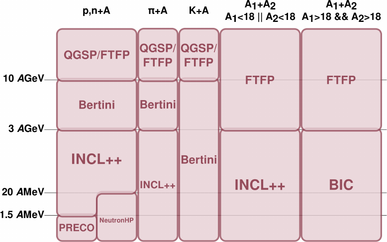
1.5 AMeV
3 AGeV
10 AGeV
20 AMeV
Figure 39.1: Model map for the INCL++-based physics lists. The first two
columns represent nucleon- and pion-induced reactions. The third column
represents nucleus-nucleus reactions where at least one of the partners is
below A= 18. The fourth column represents other nucleus-nucleus reactions.
shows a schematic model map of the INCL++-based physics lists.
Finally, the INCL++ model is directly accessible through its interface
(G4INCLXXInterface).
The reference paper for the INCL++ model is Ref. [2]. Please make sure
you cite it appropriately if you publish any work based on this model.
39.1.1 Suitable application fields
The INCL++-dedicated physics lists are suitable for the simulation of any
system where spallation reactions or light-ion-induced reactions play a dom-
inant role. As examples, we include here a non-exhaustive list of possible
application fields:
•Accelerator-Driven Systems (ADS);
•spallation targets;
•radioprotection close to high-energy accelerators;
494
•radioprotection in space;
•proton or carbon therapy;
•production of beams of exotic nuclei.
39.2 Generalities of the INCL++ cascade
INCL++ is a Monte-Carlo simulation incorporating the aforementioned cas-
cade physics principles. The INCL++ algorithm consists of an initialization
stage and the actual data processing stage.
The INCL++ cascade can be used to simulate the collisions between bullet
particles and nuclei. The supported bullet particles and the interface classes
supporting them are presented in table 39.1.
The momenta and positions of the nucleons inside the nuclei are deter-
mined at the beginning of the simulation run by modeling the nucleus as a
free Fermi gas in a static potential well with a realistic density. The cascade
is modeled by tracking the nucleons and their collisions.
The possible reactions inside the nucleus are
•NN →NN (elastic scattering)
•NN →N∆ and N∆→NN
•∆→πN and πN →∆
•NN →NN xπ (multiple pion production)
•πN →πN (elastic scattering and charge exchange)
•πN →N(x+ 1)π(multiple pion production)
•NN →NNM (M=ηor ω)
•NN →NNM xπ (inclusive production, M=ηor ω)
•πN →MN (M=ηor ω)
•MN →πN, ππN (M=ηor ω)
•MN →MN (M=ηor ω; elastic scattering)
495

39.2.1 Model limits
The INCL++ model has certain limitations with respect to the bullet particle
energy and type, and target-nucleus type. The supported energy range for
incident nucleons and pions is 1 MeV–20 GeV. Any target nucleus from
deuterium (2H) up is in principle acceptable, but not all areas of the nuclide
chart have received equal attention during testing. Heavy nuclei (say above
Fe) close to the stability valley have been more thoroughly studied than light
or unstable nuclei. The model is anyway expected to accept any existing
nucleus as a target.
Light nuclei (from A= 2 to A= 18 included) can also be used as pro-
jectiles. The G4INCLXXInterface class can be used for collisions between
nuclei of any mass, but it will internally rely on the Binary Cascade model
(see chapter 30) if both reaction partners have A > 18. A warning message
will be displayed (once) if this happens.
39.3 Physics ingredients
The philosophy of the INCL++ model is to minimize the number of free pa-
rameters, which guarantees the predictive power of the model. All INCL++
parameters are either taken from known phenomenology (e.g. nuclear radii,
elementary cross sections, nucleon potentials) or fixed once and for all (stop-
ping time, cluster-coalescence parameters).
The nucleons are modeled as a free Fermi gas in a static potential well.
The radius of the well depends on the nucleon momentum, the r-pcorrelation
being determined by the desired spatial density distribution ρr(r) according
to the following equation:
ρp(p)p2dp =−dρr(r)
dr
r3
3dr, (39.1)
where ρp(p) is the momentum-space density (a hard-sphere of radius equal
to the Fermi momentum).
After the initialization a projectile particle, or bullet, is shot towards the
target nucleus. In the following we assume that the projectile is a nucleon
or a pion; the special case of composite projectiles will be described in more
detail in subsection 39.3.4.
The impact parameter, i.e. the distance between the projectile particle
and the center point of the projected nucleus surface is chosen at random.
The value of the impact parameter determines the point where the bullet
particle will enter the calculation volume. After this the algorithm tracks
496
the nucleons by determining the times at which an event will happen. The
possible events are:
•collision
•decay of a delta resonance
•reflection from the nuclear potential well
•transmission through the nuclear potential well
The particles are assumed to propagate along straight-line trajectories.
The algorithm calculates the time at which events will happen and propagates
the particles directly to their positions at that particular point in time. This
means that the length of the time step in simulation is not constant, and that
we do not need to perform expensive numerical integration of the particle
trajectories.
Particles in the model are labeled either as participants (projectile parti-
cles and particles that have undergone a collision with a projectile) or spec-
tators (target particles that have not undergone any collision). Collisions
between spectator particles are neglected.
39.3.1 Emission of composite particles
INCL++ is able to simulate the emission of composite particles (up to A= 8)
during the cascade stage. Clusters are formed by coalescence of nucleons;
when a nucleon (the leading particle) reaches the surface and is about to
leave the system, the coalescence algorithm looks for other nucleons that are
“sufficiently close” in phase space; if any are found, a candidate cluster is
formed. If several clusters are formed, the algorithm selects the least excited
one. Penetration of the Coulomb barrier is tested for the candidate cluster,
which is emitted if the test is successful; otherwise, normal transmission of
the leading nucleon is attempted.
There are at least two peculiarities of INCL++’s cluster-coalescence algo-
rithm. First, it acts in phase space, while many existing algorithms act in
momentum space only. Second, it is dynamical, in the sense that it acts on
the instantaneous phase-space distribution of nucleons in the system, and
not on the distribution of the escaping nucleons.
39.3.2 Cascade stopping time
Stopping time is defined as the point in time when the cascade phase is
finished and the excited remnant is passed to evaporation model. In the
497
INCL++ model the stopping time, tstop, is defined as:
tstop =t0(Atarget/208)0.16.(39.2)
Here Atarget is the target mass number and t0= 70 fm/c. The intranuclear
cascade also stops if no participants are left in the nucleus.
39.3.3 Conservation laws
The INCL++ model generally guarantees energy and momentum conservation
at the keV level, which is compatible with the numerical accuracy of the
code. It uses G4ParticleTable and G4IonTable for the masses of particles
and ions, which means that the energy balance is guaranteed to be consistent
with radiation transport. However, INCL++ can occasionally generate an
event such that conservation laws cannot be exactly fulfilled; these corner
cases typically happen for very light targets.
Baryon number and charge are always conserved.
39.3.4 Initialisation of composite projectiles
In the case of composite projectiles, the projectile nucleons are initialised
off their mass shell, to account for their binding in the projectile. The sum
of the four-momenta of the projectile nucleons is equal to the nominal four-
momentum of the projectile nucleus.
Given a random impact parameter, projectile nucleons are separated in
geometrical spectators (those that do not enter the calculation volume) and
geometrical participants (those that do). Geometrical participant that tra-
verse the nucleus without undergoing any collision are coalesced with any ex-
isting geometrical spectators to form an excited projectile-like pre-fragment.
The excitation energy of the pre-fragment is generated by a simple particle-
hole model. At the end of the cascade stage, the projectile-like pre-fragment
is handed over to G4ExcitationHandler.
39.3.5 ηand ωmesons as new particles
The mesons ηand ωcan be produced and emitted during the intranuclear
cascade phase. The cross sections taken into account are listed in section
39.2. By default in Geant4 the ηmeson emitted is not decayed by INCL++,
while that is the case for the ωmeson (then only the decay products (πand
γ) are given to Geant4).
498
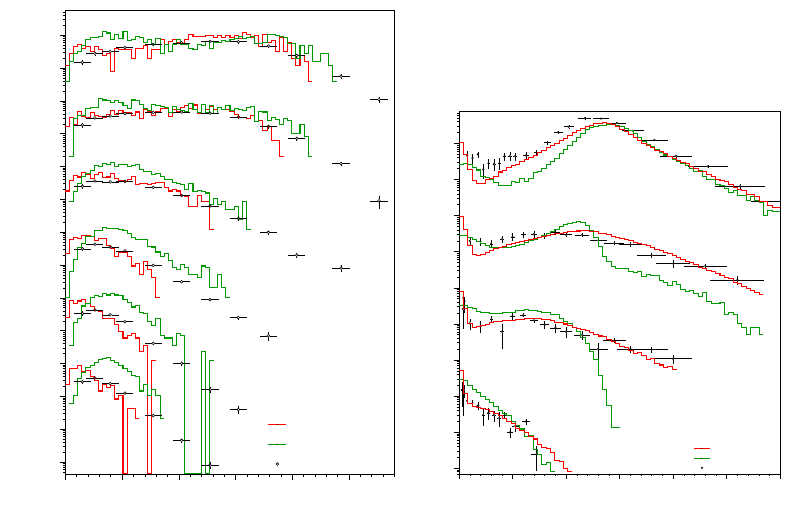
pion energy [MeV]
0 100 200 300 400 500
dE [mb/sr/MeV]Ω/dσ
2
d
-14
10
-13
10
-12
10
-11
10
-10
10
-9
10
-8
10
-7
10
-6
10
-5
10
-4
10
-3
10
-2
10
-1
10
+
π →730-MeV p + Cu
INCL++
BIC
Cochran et al.
°15
)
-2
10× (°30
)
-4
10× (°60
)
-6
10× (°90
)
-8
10× (°120
)
-10
10× (°150
neutron energy [MeV]
0 100 200 300 400 500 600
dE [mb/sr/MeV]Ω/dσ
2
d
-8
10
-7
10
-6
10
-5
10
-4
10
-3
10
-2
10
-1
10
1
10
°5
)
-2
10× (°20
)
-4
10× (°40
)
-6
10× (°80
C
12
C+
12
290 AMeV
INCL++
BIC
Iwata et al.
Figure 39.2: Left: double-differential cross sections for the production of
charged pions in 730-MeV p+Cu. Right: double-differential cross sections
for the production of neutrons in 290-AMeV 12C+12C. Predictions of the
INCL++ and Binary-Cascade models are compared with experimental data
from Refs. [5] and [6].
39.3.6 De-excitation phase
The INCL++ model simulates only the first part of the nuclear reaction; the
de-excitation of the cascade remnant is simulated by default by G4Exci-
tationHandler. As an alternative, the ABLA V3 model (Chapter 40) can
be used instead, by employing the technique described in the Application
Developer Guide, section “hadronic interactions”.
39.4 Physics performance
INCL++ (coupled with G4ExcitationHandler) provides an accurate modeling
tool for spallation studies in the tens of MeV–15 GeV energy range. The
INCL++-ABLA07 [3] model was recognized as one of the best on the market
by the IAEA Benchmark of Spallation Models [4] (note however that the
ABLA07 de-excitation model is presenty not available in Geant4).
499
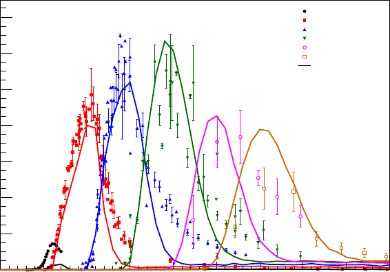
projectile energy [MeV]
10 20 30 40 50 60 70 80 90 100
cross section [mb]
0
200
400
600
800
1000
1200
1400 x=1
x=2
x=3
x=4
x=5
x=6
INCL++/G4EH
At
213-x
He,xn)
4
Bi(
209
Figure 39.3: Excitation functions for (α, xn) cross sections on 209Bi. The
predictions of INCL++-G4ExcitationHandler are represented by the solid
line and are compared to experimental data [7, 8, 9, 10, 11, 12, 13, 14, 15].
As a sample of the quality of the model predictions of INCL++-G4Exci-
tationHandler for nucleon-induced reactions, the left panel of Figure 39.2
presents a comparison of double-differential cross sections for pion production
in 730-MeV p+Cu, compared with the predictions of the Binary-Cascade
model (chapter 30) and with experimental data.
Reactions induced by light-ion projectiles up to A= 18 are also treated by
the model. The right panel of Figure 39.2 shows double-differential cross sec-
tions for neutron production in 290-AMeV 12C+12C. Figure 39.3 shows exci-
tation curves for 209Bi(α, xn) reactions at very low energy. We stress here that
intranuclear-cascade models are supposedly not valid below ∼150 AMeV.
The very good agreement presented in Figure 39.3 is due to the complete-
fusion model that smoothly replaces INCL++ at low energy.
INCL++ is continuously updated and validated against experimental data.
Bibliography
[1] A. Boudard et al., Phys. Rev. C87 (2013) 014606.
[2] D. Mancusi et al., Phys. Rev. C90 (2014) 054602.
500
[3] A. Keli´c, M. V. Ricciardi and K.-H. Schmidt, Joint ICTP-IAEA Ad-
vanced Workshop on Model Codes for Spallation Reactions, Report
INDC(NDC)-0530 (2008) 181.
[4] Benchmark of Spallation Models, organized by the IAEA. Web site:
http://www-nds.iaea.org/spallations.
[5] D. R. F. Cochran et al., Phys. Rev. D6 (1972) 3085.
[6] Y. Iwata et al., Phys. Rev. C6 (2001) 054609.
[7] A. Hermanne et al., Conf. on Nucl. Data for Sci. and Techn., Santa Fe
2004,
[8] A. R. Barnett et al., Phys. Rev. C9 (1974) 2010.
[9] E. L. Kelly and E. Segr´e, Phys. Rev. 75 (1949) 999.
[10] G. Deconninck and M. Longree, Ann. Soc. Sci. Brux. 88 (1974) 341.
[11] H. B. Patel, D. J. Shah and N. L. Singh, Riv. Nuovo Cimento A112
(1999) 1439.
[12] I. A. Rizvi et al., Appl. Radiat. Isotopes 41 (1990) 215.
[13] J. D. Stickler and K. J. Hofstetter, Phys. Rev. C9 (1974) 1064.
[14] N. L. Singh, S. Mukherjee and D. R. S. Somayajulu, Riv. Nuovo Cimento
A107 (1994) 1635.
[15] R. M. Lambrecht and S. Mirzadeh, Appl. Radiat. Isotopes 36 (1985)
443.
501

Table 39.1: INCL++ feature summary.
usage
physics lists QGSP INCLXX
QGSP INCLXX HP
FTFP INCLXX
FTFP INCLXX HP
interfaces
G4INCLXXInterface nucleon-, pion- and nucleus-nucleus
projectile particles proton, neutron
pions (π+,π0,π−)
deuteron, triton
3He, α
light ions (up to A= 18)
energy range 1 MeV - 20 GeV
target nuclei
lightest applicable deuterium, 2H
heaviest no limit, tested up to uranium
features no ad-hoc parameters
realistic nuclear densities
Coulomb barrier
non-uniform time-step
pion and delta production cross sections
delta decay
Pauli blocking
emission of composite particles (A≤8)
complete-fusion model at low energy
conservation laws satisfied at the keV level
typical CPU time 0.5.INCL++/Binary Cascade .2
code size 75 classes, 14k lines
references Ref. [2]
502

Chapter 40
ABLA V3 evaporation/fission
model
The ABLA V3 evaporation model takes excited nucleus parameters, exci-
tation energy, mass number, charge number and nucleus spin, as input. It
calculates the probabilities for emitting proton, neutron or alpha particle
and also probability for fission to occur. The summary of Geant4 ABLA V3
implementation is represented in Table 40.1.
The probabilities for emission of particle type jare calculated using for-
mula:
Wj(N, Z, E) = Γj(N, Z, E)
PkΓk(N, Z, E),(40.1)
where Γjis emission width for particle j,Nis neutron number, Zcharge
number and Eexcitation energy. Possible emitted particles are protons,
neutrons and alphas. Emission widths are calculated using the following
formula:
Γj=1
2πρc(E)
4mjR2
~2T2
jρj(E−Sj−Bj),(40.2)
where ρc(E) and ρj(E−Sj−Bj) are the level densities of the compound
nucleus and the exit channel, respectively. Bjis the height of the Coulomb
barrier, Sjthe separation energy, Ris the radius and Tjthe temperature of
the remnant nucleus after emission and mjthe mass of the emitted particle.
The fission width is calculated from:
Γi=1
2πρc(E)Tfρf(E−Bf),(40.3)
where ρf(E) is the level density of transition states in the fissioning nucleus,
Bfthe height of the fission barrier and Tfthe temperature of the nucleus.
503

Table 40.1: ABLA V3 (located in the Geant4 directory source/processes/-
hadronic/models/abla) feature summary.
Requirements
External data file G4ABLA3.0 available at Geant4 site
Environment variable G4ABLADATA
for external data
Usage
Physics list No default physics list,
see Section 40.4.
Interfaces
G4AblaInterface
Supported input Excited nuclei
Output particles proton, neutron
α
fission products
residual nuclei
Features evaporation of proton, neutron and α
fission
References Key reference: [1], see also [2]
40.1 Level densities
Nuclear level densities are calculated using the following formula:
a= 0.073A[MeV −1] + 0.095BsA2/3[MeV −2],(40.4)
where Athe nucleus mass number and Bsdimensionless surface area of the
nucleus.
40.2 Fission
Fission barrier, used to calculate fission width 40.3, is calculated using a semi-
empirical model fitting to data obtained from nuclear physics experiments.
504
40.3 External data file required
ABLA V3 needs specific data files. These files contain ABLA V3 shell correc-
tions and nuclear masses. To enable this data set, the environment variable
G4ABLADATA needs to be set, and the relevant data should be installed on
your machine. You can download them from the Geant4 web site or you can
have CMake download them for you during installation. For Geant4 10.0 we
use the G4ABLA3.0 data files.
40.4 How to use ABLA V3
None of the stock physics lists use the ABLA V3 model by default. It should
also be understood that ABLA V3 is a nuclear de-excitation model and
must be used as a secondary reaction stage; the first, dynamical reaction
stage must be simulated using some other model, typically an intranuclear-
cascade (INC) model. The coupling of the ABLA V3 to the INCL++ model
(Chapter 39) has been somewhat tested and seems to work, but no extensive
benchmarking has been realized at the time of writing. Coupling to the
Binary-Cascade model (Chapter 30) should in principle be possible, but has
never been tested. The technique to realize the coupling is described in the
Application Developer Guide.
Finally, please note that the ABLA V3 model is in alpha status. The
code may crash and be affected by bugs.
Bibliography
[1] A.R. Junghans et al Nuc. Phys. A629 (1998) 635
[2] J. Benlliure et al Nuc. Phys. A628 (1998) 458
[3] A. Heikkinen et al. J. Phys.: Conf. Series 119 (2008) 032024
505
Chapter 41
Low Energy Neutron
Interactions
41.1 Introduction
The neutron transport class library described here simulates the interactions
of neutrons with kinetic energies from thermal energies up to O(20 MeV).
The upper limit is set by the comprehensive evaluated neutron scattering
data libraries that the simulation is based on. The result is a set of sec-
ondary particles that can be passed on to the tracking sub-system for further
geometric tracking within Geant4.
The interactions of neutrons at low energies are split into four parts in
analogy to the other hadronic processes in Geant4. We consider radiative
capture, elastic scattering, fission, and inelastic scattering as separate models.
These models comply with the interface for use with the Geant4 hadronic
processes which enables their transparent use within the Geant4 tool-kit
together with all other Geant4 compliant hadronic shower models.
41.2 Physics and Verification
41.2.1 Inclusive Cross-sections
All cross-section data are taken from the ENDF/B-VI[1] evaluated data li-
brary.
All inclusive cross-sections are treated as point-wise cross-sections for
reasons of performance. For this purpose, the data from the evaluated data
library have been processed, to explicitly include all neutron nuclear reso-
nances in the form of point-like cross-sections rather than in the form of
506

parametrisations. The resulting data have been transformed into a linearly
interpolable format, such that the error due to linear interpolation between
adjacent data points is smaller than a few percent.
The inclusive cross-sections comply with the cross-sections data set in-
terface of the Geant4 hadronic design. They are, when registered with the
tool-kit at initialisation, used to select the basic process. In the case of fis-
sion and inelastic scattering, point-wise semi-inclusive cross-sections are also
used in order to decide on the active channel for an individual interaction.
As an example, in the case of fission this could be first, second, third, or
forth chance fission.
41.2.2 Elastic Scattering
The final state of elastic scattering is described by sampling the differen-
tial scattering cross-sections dσ
dΩ . Two representations are supported for the
normalised differential cross-section for elastic scattering. The first is a tab-
ulation of the differential cross-section, as a function of the cosine of the
scattering angle θand the kinetic energy Eof the incoming neutron.
dσ
dΩ =dσ
dΩ (cos θ, E)
The tabulations used are normalised by σ/(2π) so the integral of the differ-
ential cross-sections over the scattering angle yields unity.
In the second representation, the normalised cross-section are represented
as a series of legendre polynomials Pl(cos θ), and the legendre coefficients al
are tabulated as a function of the incoming energy of the neutron.
2π
σ(E)
dσ
dΩ (cos θ, E) =
nl
X
l=0
2l+ 1
2al(E)Pl(cos θ)
Describing the details of the sampling procedures is outside the scope of
this paper.
An example of the result we show in figure 41.1 for the elastic scattering
of 15 MeV neutrons off Uranium a comparison of the simulated angular
distribution of the scattered neutrons with evaluated data. The points are
the evaluated data, the histogram is the Monte Carlo prediction.
In order to provide full test-coverage for the algorithms, similar tests
have been performed for 72Ge, 126Sn, 238U, 4He, and 27Al for a set of neutron
kinetic energies. The agreement is very good for all values of scattering angle
and neutron energy investigated.
507
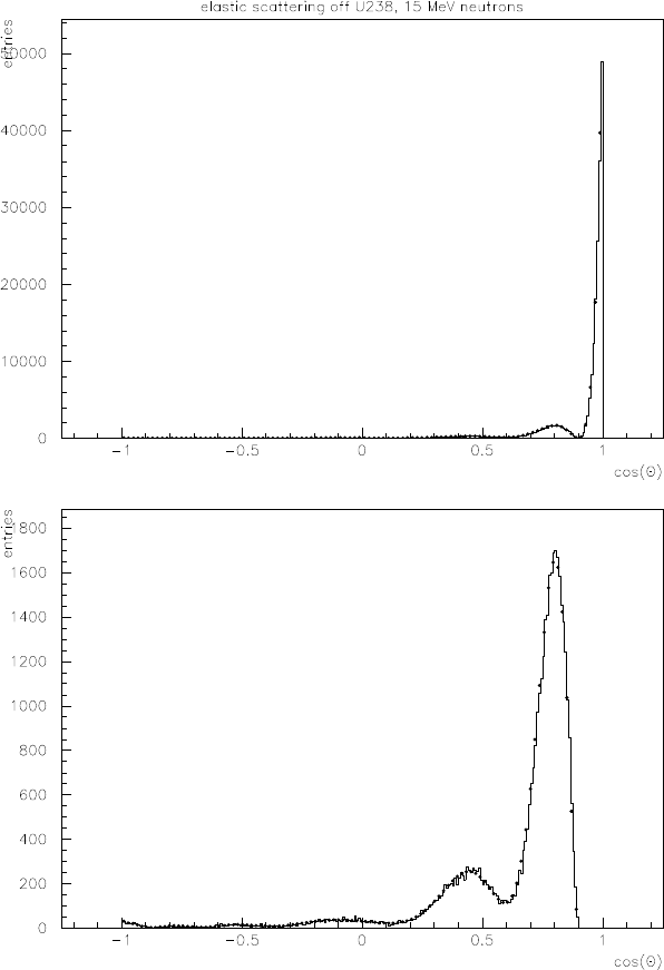
41.2.3 Radiative Capture
The final state of radiative capture is described by either photon multiplic-
ities, or photon production cross-sections, and the discrete and continuous
Figure 41.1: Comparison of data and Monte Carlo for the angular distribu-
tion of 15 MeV neutrons scattered elastically off Uranium (238U). The points
are evaluated data, and the histogram is the Monte Carlo prediction. The
lower plot excludes the forward peak, to better show the Frenel structure of
the angular distribution of the scattered neutron.
508
contributions to the photon energy spectra, along with the angular distribu-
tions of the emitted photons.
For the description of the photon multiplicity there are two supported
data representations. It can either be tabulated as a function of the energy
of the incoming neutron for each discrete photon as well as the eventual
continuum contribution, or the full transition probability array is known, and
used to determine the photon yields. If photon production cross-sections are
used, only a tabulated form is supported.
The photon energies Eγare associated to the multiplicities or the cross-
sections for all discrete photon emissions. For the continuum contribution,
the normalised emission probability fis broken down into a weighted sum
of normalised distributions g.
f(E→Eγ) = X
i
pi(E)gi(E→Eγ)
The weights piare tabulated as a function of the energy Eof the incoming
neutron. For each neutron energy, the distributions gare tabulated as a
function of the photon energy. As in the ENDF/B-VI data formats[1], several
interpolation laws are used to minimise the amount of data, and optimise the
descriptive power. All data are derived from evaluated data libraries.
The techniques used to describe and sample the angular distributions are
identical to the case of elastic scattering, with the difference that there is
either a tabulation or a set of legendre coefficients for each photon energy
and continuum distribution.
As an example of the results is shown in figure41.2 the energy distribution
of the emitted photons for the radiative capture of 15 MeV neutrons on
Uranium (238U). Similar comparisons for photon yields, energy and angular
distributions have been performed for capture on 238U, 235U, 23Na, and 14N
for a set of incoming neutron energies. In all cases investigated the agreement
between evaluated data and Monte Carlo is very good.
41.2.4 Fission
For neutron induced fission, we take first chance, second chance, third chance
and forth chance fission into account.
Neutron yields are tabulated as a function of both the incoming and out-
going neutron energy. The neutron angular distributions are either tabulated,
or represented in terms of an expansion in legendre polynomials, similar to
the angular distributions for neutron elastic scattering. In case no data are
available on the angular distribution, isotropic emission in the centre of mass
system of the collision is assumed.
509
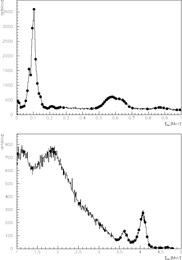
There are six different possibilities implemented to represent the neu-
tron energy distributions. The energy distribution of the fission neutrons
f(E→E′) can be tabulated as a normalised function of the incoming and
outgoing neutron energy, again using the ENDF/B-VI interpolation schemes
to minimise data volume and maximise precision.
Figure 41.2: Comparison of data and Monte Carlo for photon energy distri-
butions for radiative capture of 15 MeV neutrons on Uranium (238U). The
points are evaluated data, the histogram is the Monte Carlo prediction.
510

The energy distribution can also be represented as a general evaporation
spectrum,
f(E→E′) = f(E′/Θ(E)) .
Here Eis the energy of the incoming neutron, E′is the energy of a fission
neutron, and Θ(E) is effective temperature used to characterise the sec-
ondary neutron energy distribution. Both the effective temperature and the
functional behaviour of the energy distribution are taken from tabulations.
Alternatively energy distribution can be represented as a Maxwell spec-
trum,
f(E→E′)∝√E′eE′/Θ(E),
or a evaporation spectrum
f(E→E′)∝E′eE′/Θ(E).
In both these cases, the temperature is tabulated as a function of the incom-
ing neutron energy.
The last two options are the energy dependent Watt spectrum, and the
Madland Nix spectrum. For the energy dependent Watt spectrum, the energy
distribution is represented as
f(E→E′)∝e−E′/a(E)sinh pb(E)E′.
Here both the parameters a, and b are used from tabulation as function of
the incoming neutron energy. In the case of the Madland Nix spectrum, the
energy distribution is described as
f(E→E′) = 1
2[g(E′, < Kl>) + g(E′, < Kh>)] .
Here
g(E′, < K >) = 1
3√< K > Θhu3/2
2E1(u2)−u3/2
1E1(u1) + γ(3/2, u2)−γ(3/2, u1)i,
u1(E′, < K >) = (√E′−√< K >)2
Θ,and
u2(E′, < K >) = (√E′+√< K >)2
Θ.
Here Klis the kinetic energy of light fragments and Khthe kinetic energy of
heavy fragments, E1(x) is the exponential integral, and γ(x) is the incomplete
gamma function. The mean kinetic energies for light and heavy fragments
511
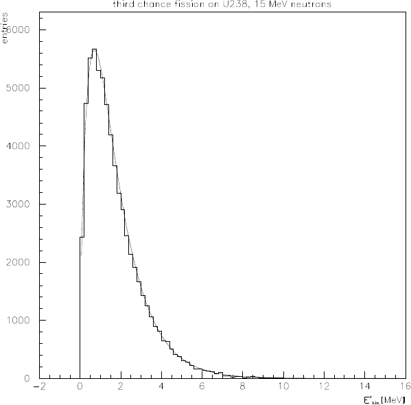
are assumed to be energy independent. The temperature Θ is tabulated as
a function of the kinetic energy of the incoming neutron.
Fission photons are describes in analogy to capture photons, where evalu-
ated data are available. The measured nuclear excitation levels and transition
probabilities are used otherwise, if available.
As an example of the results is shown in figure41.3 the energy distribu-
tion of the fission neutrons in third chance fission of 15 MeV neutrons on
Uranium (238U). This distribution contains two evaporation spectra and one
Watt spectrum. Similar comparisons for neutron yields, energy and angular
distributions, and well as fission photon yields, energy and angular distri-
butions have been performed for 238U, 235U, 234U, and 241Am for a set of
incoming neutron energies. In all cases the agreement between evaluated
data and Monte Carlo is very good.
Figure 41.3: Comparison of data and Monte Carlo for fission neutron energy
distributions for induced fission by 15 MeV neutrons on Uranium (238U).
The curve represents evaluated data and the histogram is the Monte Carlo
prediction.
512
41.2.5 Inelastic Scattering
For inelastic scattering, the currently supported final states are (nA→) nγs
(discrete and continuum), np, nd, nt, n3He, nα, nd2α, nt2α, n2p, n2α, npα,
n3α, 2n, 2np, 2nd, 2nα, 2n2α, nX, 3n, 3np, 3nα, 4n, p, pd, pα, 2p d, dα,
d2α, dt, t, t2α,3He, α, 2α, and 3α.
The photon distributions are again described as in the case of radiative
capture.
The possibility to describe the angular and energy distributions of the fi-
nal state particles as in the case of fission is maintained, except that normally
only the arbitrary tabulation of secondary energies is applicable.
In addition, we support the possibility to describe the energy angular
correlations explicitly, in analogy with the ENDF/B-VI data formats. In
this case, the production cross-section for reaction product n can be written
as
σn(E, E′,cos(θ)) = σ(E)Yn(E)p(E, E′,cos(θ)).
Here Yn(E) is the product multiplicity, σ(E) is the inelastic cross-section,
and p(E, E′,cos(θ)) is the distribution probability. Azimuthal symmetry is
assumed.
The representations for the distribution probability supported are isotro-
pic emission, discrete two-body kinematics, N-body phase-space distribution,
continuum energy-angle distributions, and continuum angle-energy distribu-
tions in the laboratory system.
The description of isotropic emission and discrete two-body kinematics is
possible without further information. In the case of N-body phase-space dis-
tribution, tabulated values for the number of particles being treated by the
law, and the total mass of these particles are used. For the continuum energy-
angle distributions, several options for representing the angular dependence
are available. Apart from the already introduced methods of expansion in
terms of legendre polynomials, and tabulation (here in both the incoming
neutron energy, and the secondary energy), the Kalbach-Mann systematic is
available. In the case of the continuum angle-energy distributions in the lab-
oratory system, only the tabulated form in incoming neutron energy, product
energy, and product angle is implemented.
First comparisons for product yields, energy and angular distributions
have been performed for a set of incoming neutron energies, but full test cov-
erage is still to be achieved. In all cases currently investigated, the agreement
between evaluated data and Monte Carlo is very good.
513

41.3 Neutron Data Library (G4NDL) Format
This document describes the format of G4NDL4.5. The previous version of
G4NDL does not have entries for data library identification and names of
original data libraries, but other formats are same, i.e., the first element of
the old version is equivalent to the 3rd element of a new version.
Since G4NDL4.4, files in the data library are compressed by zlib[6]. In
this section, we will explain the format of G4NDL in its pre-compressed form.
41.3.1 Cross Section
Each file in the cross section directories has the following entries:
•the first entry is identification of library (in this case G4NDL)
•the second entry original data library from which the file came
•the third entry is a dummy entry but the value usually corresponds to
the MT number of reaction in ENDF formats (2:Elastic, 102:Capture,
18:Fission; files in the directory of inelastic cross section usually have
0 for this entry).1
•the fourth entry is also a dummy
•the fifth entry represents the number of (energy, cross section) pairs (in
eV, barn) to follow.
This is an example of cross section file format:
G4NDL (1st entry)
ENDF/B-VII.1 (2nd entry)
2 (3rd entry) \\MT
0 (4th entry)
682 (5th entry) \\number of E-XS pairs
1.000000e-05 2.043634e+01 1.062500e-05 2.043634e+01 ,,,,,
(1st pair of E and XS) (2nd pair of E and XS)
2.000000e+07 4.827462e-01
(682th pair of E and XS)
1MF and MT numbers are used in the ENDF format to indicate the type of data and
the type of reaction or products resulting from the reaction. For example, MF3 represents
cross section data and MF4 symbolizes angular distribution, also, MT2 represents elastic
reaction and MT102 is radiative capture.
514
41.3.2 Final State
Unlike the format of the cross section files, the format of the final state files
is not straightforward and pretty complicated. Even though each of these
files follows the same format rules, the actual length and appearance of each
file will depend on the specific data. The format rules of the final state files
are a subset of the ENDF-6 format and a deep understanding of the format
is required to correctly interpret the content of the files. Because of limited
resources, we do not plan to provide a complete documentation on this part
in the near future.
41.3.3 Thermal Scattering Cross Section
The format of the thermal scattering cross section data is similar to that of
the cross section data described above:
•the 1st and 2nd entries have the same meaning
•the 3rd and 4th entries are also dummies and not used in simulation.
However the 3rd entry has the value of 3 that represents MF number
of ENDF-6 format and the 4th entry has the value of MT numbers of
ENDF-6 format.
•the 5th entry is the temperature (in Kelvin)
•the 6th entry represents the number of (energy, cross section) pairs
given for the temperature in entry 5.
•If there are multiple temperatures listed, which is typical, then for each
temperature there is a corresponding data block which consists of MF,
MT, temperature, number of pairs, and paired E and cross section data.
This is an example of thermal scattering cross section file format:
G4NDL (1st entry)
ENDF/B-VII.1 (2nd entry)
3 (3rd entry) \\MF
223 (4th entry) \\MT
296 (5th entry) \\temperature
2453 (6th entry) \\number of E-XS pairs
1.000000e-5 3.456415e+2 1.125000e-5 3.272908e+2 ,,,,,
(1st pair of E and XS) (2nd pair of E and XS)
4.000040e+0 0.000000e+0 2.000000e+7 0.000000e+0
515
(2452nd pair of E and XS)(2453rd pair of E and XS)
3 (MF)
223 (MT)
350 (temperature)
2789 (Number of E-XS pair)
1.000000e-5 4.457232e+2 1.125000e-5 4.220525e+2 ,,,,,,
(1st pair of E and XS) (2nd pair of E and XS)
41.3.4 Coherent Final State
The final state files have a similar format:
•the 1st and 2nd entries have the same meaning before
•the 3rd and 4th entries are also dummy entries and not used in simu-
lation. However the 3rd entry has the value of 7 that represents MF
number of ENDF-6 format and the 4th entry has the value 2 as MT
number of the ENDF-6 format.
•the 5th entry represents temperature
•the 6th entry shows the number of Bragg edges given. This is followed
by pairs of Bragg edge energies in eV and structure factors.
•If there are multiple temperatures listed, which is typical, then for each
temperature there is a corresponding data block which consists of MF,
MT, temperature, number of Bragg edges, and paired energy of Bragg
edge and structure factors. However the energies of the Bragg edges
only appear in the first data block.
This is an example of thermal scattering coherent final state file:
G4NDL (1st entry)
ENDF/B-VII.1 (2nd entry)
7 (3rd entry) // MF
2 (4th entry) // MT
296 (5th entry) // temperature
248 (6th entry) // number of Bragg edges
4.555489e-4 0.000000e+0 1.822196e-3 1.347465e-2 ,,,,,,
(1st pair of E and S) (2nd pair of E and S)
1.791770e+0 6.259710e-1 5.000000e+0 6.259711e-1
(247th pair of E, S) (248th pair of E, S)
7 (MF)
516
2 (MT)
400 (temperature)
248 (# of Bragg edge structure factors without energies)
0.000000e+0 1.342127e-2 ,,,,,
(1st pair of E and S)
4.994888e-1 4.994889e-1
(247th pair of E and S)
41.3.5 Incoherent Final State
The incoherent final state files have a similar format:
•the 1st and 2nd entry has same meaning before
•the 3rd and 4th entries are dummy entries and not used in simulation.
However the 3rd entry has the value of 6 that represents the MF number
of the ENDF-6 format and the 4th entry is the MT number of the
ENDF-6 format.
•the 5th entry is the temperature of this data block
•the 6th entry is the number of isoAngle data sets, described below.
•If there are multiple temperatures listed, which is typical, then for each
temperature there is a corresponding data block which consists of MF,
MT, temperature, number of isoAngle data sets and the isoAngle data
sets.
The format of the isoAngle data set is following.
•Up to the 8th entry, only 2nd and 5th entry has real meaning in simu-
lation and the 2nd entry has energy of incidence neutron and 5th entry
is the number of equal probability bins (N) in mu.
•9th to (9+N-2)th entries are the boundary values of the equal proba-
bility bins. The lowest and highest boundary of -1 and 1 are obvious
thus they are omitted from entries.
This is an example of isoAngle data set
0.000000e+0 1.000000e-5 0 0 10 10
(1st entry) (2nd entry)(3rd entry)(4th entry)(5th entry)(6th entry)
1.000000e-05 1.000000e+00 -8.749199e-01 -6.247887e-01 ,,,
(7th entry) (8th entry) (2nd boundary) (3rd boundary)
6.252111e-01 8.750801e-01
(9th boundary)(10th boundary)
517
This is an example of thermal scattering incoherent final state file
G4NDL (1st entry)
ENDF/B-VII.1 (2nd entry)
6 (3rd entry) \\MF
224 (4th entry) \\MT
296 (5th entry) \\temperature
2452 (6th entry) \\number of isoAngle data sets
0.000000e+0 1.000000e-5 0 0 10 10
(1st isoAngle data set)
1.000000e-05 1.000000e+00 -8.749199e-01 -6.247887e-01 -3.747014e-01
-1.246577e-01 1.253423e-01 3.752985e-01 6.252111e-01 8.750801e-01
,,,,,,,,,,,,,,,,,,,
0.000000e+0 1.125000e-5 0 0 10 10
(2452st isoAngle data set)
4.000040e+00 1.000000e+00 9.889886e-01 9.939457e-01 9.958167e-01
9.970317e-01 9.979352e-01 9.986553e-01 9.992540e-01 9.997666e-01
6 (MF)
224 (MT)
350 (temperature)
2788 (sumber of isoAngle data sets)
0.000000e+0 1.000000e-5 0 0 10 10
1.000000e-05 1.000000e+00 -8.749076e-01 -6.247565e-01 -3.746559e-01
-1.246055e-01 1.253944e-01 3.753440e-01 6.252433e-01 8.750923e-01
,,,,,,,,,,,,,,,,,,,
41.3.6 Inelastic Final State
As before, the top six entries are similar:
•the 1st and 2nd entries have the same meaning.
•the 3rd and 4th entries are dummy entries and not used in simulation.
However the 3rd entry has the value of 6 that represents the MF number
of ENDF-6 format and the 4th entry corresponding to MT number of
ENDF-6 format.
•the 5th entry is the temperature [K] of this data block
•the 6th entry is number of E-(E-isoAngle) data sets, where E is the
energy of the incident neutron and E is energy of the scattered neutron.
518
•If there are multiple temperatures listed, which is typical, then for
each temperature there is a corresponding data block which consists of
MF, MT, temperature, number of E-(E-isoAngle) data set and E-(E-
isoAngle) data.
The format of E-(E-isoAngle) is following.
•The 1st, 3rd and 4th entries are dummies and not be used in simulation.
•The 2nd entry is the energy of the incident neutron(E)
•the 5th entry is the number of entries to be found after the 6th entry.
•the 6th entry corresponds to the number of entries of each E-isoAngle
data set. The first entry of E-isoAngle data set represents energy of
scattered neutron(E) and 2nd entry is probability of E-¿E scattering.
Following entries correspond to boundaries of iso-probability bins in
mu. The lowest and highest boundaries are also omitted. The first and
last E-isoAng set should always have all 0 values excepting for energy
of scattering neutron.
This is an example of E-(E-isoAngle) data set
0.000000e+0 1.000000e-5 0 0 2080 10
(1st entry) (2nd entry)(3rd entry)(4th entry)(5th entry)(6th entry)
0.000000e+00 0.000000e+00 0.000000e+00 0.000000e+00 0.000000e+00
0.000000e+00 0.000000e+00 0.000000e+00 0.000000e+00 0.000000e+00
(1st E-isoAng data set)
6.103500e-10 3.127586e+00 -8.741139e-01 -6.226646e-01 -3.716976e-01
-1.212145e-01 1.287860e-01 3.783033e-01 6.273366e-01 8.758833e-01
(2nd E-isoAng data set)
,,,,,,,,,,,,,,,,,,,,,,
7.969600e-01 5.411300e-13 -8.750360e-01 -6.254547e-01 -3.755898e-01
-1.257686e-01 1.241790e-01 3.742614e-01 6.242919e-01 8.753607e-01
(207th E-isoAng data set)
8.199830e-01 0.000000e+00 0.000000e+00 0.000000e+00 0.000000e+00
0.000000e+00 0.000000e+00 0.000000e+00 0.000000e+00 0.000000e+00
(208th E-isoAng data set)
This is an example of thermal scattering inelastic final state file
519
G4NDL (1st entry)
ENDF/B-VII.1 (2nd entry)
6 (3rd entry) \\MF
222 (4th entry) \\MT
293.6 (5th entry) \\temperature
107 (6th entry) \\number of E-(E-isoAngle) data sets
0.000000e+0 1.000000e-5 0 0 2080 10
0.000000e+00 0.000000e+00 0.000000e+00 0.000000e+00 0.000000e+00
0.000000e+00 0.000000e+00 0.000000e+00 0.000000e+00 0.000000e+00
6.103500e-10 3.127586e+00 -8.741139e-01 -6.226646e-01 -3.716976e-01
-1.212145e-01 1.287860e-01 3.783033e-01 6.273366e-01 8.758833e-01
1.220700e-09 4.423091e+00 -8.737468e-01 -6.216975e-01 -3.703295e-01
-1.196465e-01 1.303546e-01 3.796722e-01 6.283050e-01 8.762478e-01
41.3.7 Further Information
A detailed description of the file format has been created by reverse engineer-
ing the code by a user, Wesley Ford, who was a masters student at McMaster
University [7] under the supervision of Prof. Adriaan Buijs and has kindly
agreed for its inclusion here:
http://cern.ch/geant4/UserDocumentation/ContributionFromUsers/UsefulNotes/G4NDLFinalStateDecryptionCERNv1.pdf
The link provides a document which describes G4NDL format and as a
consequence readers and expert users may obtain useful information from it.
Especially detailed descriptions of variable names used in the package and
their meanings will be useful to developers who consider extensions of the
package.
41.4 High Precision Models and Low Energy
Parameterized Models
The high precision neutron models discussed in the previous section depend
on an evaluated neutron data library (G4NDL) for cross sections, angular
distributions and final state information. However the library is not complete
because there are no data for several key elements. In order to use the high
precision models, users must develop their detectors using only elements
which exist in the library. In order to avoid this difficulty, alternative models
were developed which use the high precision models when data are found in
the library, but use the low energy parameterized neutron models when data
are missing.
520
The alternative models cover the same types of interaction as the orig-
inals, that is elastic and inelastic scattering, capture and fission. Because
the low energy parameterized part of the models is independent of G4NDL,
results will not be as precise as they would be if the relevant data existed.
41.5 Summary and Important Remark
By the way of abstraction and code reuse we minimised the amount of code
to be written and maintained. The concept of container-sampling lead to
abstraction and encapsulation of data representation and the corresponding
random number generators. The Object Oriented design allows for easy
extension of the cross-section base of the system, and the ENDF-B VI data
evaluations have already been supplemented with evaluated data on nuclear
excitation levels, thus improving the energy spectra of de-excitation photons.
Other established data evaluations have been investigated, and extensions
based on the JENDL[2], CENDL[4], and Brond[5] data libraries are foreseen
for next year.
Followings are important remark of the NeutornHP package. Correlation
between final state particles is not included in tabulated data. The method
described here does not included necessary correlation or phase space con-
strains needed to conserver momentum and energy. Such conservation is not
guarantee either in single event or averaged over many events.
Bibliography
[1] ENDF/B-VI: Cross Section Evaluation Working Group, ENDF/B-
VI Summary Document, Report BNL-NCS-17541 (ENDF-201)
(1991), edited by P.F. Rose, National Nuclear Data Center, Brookhave
National Laboratory, Upton, NY, USA.
[2] JENDL-3: T. Nakagawa, et al., Japanese Evaluated Nuclear Data Li-
brary, Version 3, Revision 2, J. Nucl. Sci. Technol. 32, 1259 (1995).
[3] Jef-2: C. Nordborg, M. Salvatores, Status of the JEF Evaluated Data
Library,Nuclear Data for Science and Technology, edited by J.
K. Dickens (American Nuclear Society, LaGrange, IL, 1994).
[4] CENDL-2: Chinese Nuclear Data Center, CENDL-2, The Chinese
Evaluated Nuclear Data Library for Neutron Reaction Data, Report
IAEA-NDS-61, Rev. 3 (1996), International Atomic Energy Agency,
Vienna, Austria.
521
[5] Brond-2.2: A.I Blokhin et al., Current status of Russian Nuclear Data
Libraries,Nuclear Data for Science and Technology, Volume2,
p.695. edited by J. K. Dickens (American Nuclear Society, LaGrange,
IL, 1994)
[6] http://www.zlib.net.
[7] http://geant4.org.
522
Chapter 42
Low Energy Charged Particle
Interactions
42.1 Introduction
The low energy charged particle transport class library described here simu-
lates the interactions of protons, deuterons, tritons, He-3 and alpha particle
with kinetic energies up to 200 MeV. The upper limit is set by the com-
prehensive evaluated neutron scattering data libraries that the simulation is
based on. It reuses the code of the low energy neutron interactions package,
with some small modifications to take into account the change of incident
particle.
Only the inelastic interactions are included in this model, while the elas-
tic interaction is treated approximately by other Geant4 models, and the
interference between Coulumb and nuclear elastic is neglected.
42.2 Physics and Verification
42.2.1 Inclusive Cross-sections
Cross-section data is taken from the ENDF/B-VII.r1[1] evaluated data li-
brary for those few elements where data exist. As these isotopes are only
a few, most of the isotopes data are taken from the TENDL data library,
which uses the TALYS nuclear model. The format is exactly the same as for
the low energy neutron data libraries. While the energy of the TENDL files
goes up to 200 MeV, in the case of ENDF it only reaches 150 MeV for most
isotopes and for some is even less.
The treatment of this data is done with the same code as for the low
523
energy neutron package. It should be mentioned that for all except a few low
Z isotopes in the ENDF data library, there is no information about individual
decay channels, but only about the total cross section plus particle yields.
Therefore the same remark as for the neutron package holds: there is no
event-by-event conservation of energy, nor of atomic or mass number.
The absence of treatment of the correlation between inelastic and elastic
interactions affects the emission of charged particles, while it does not for
neutron and gamma emission. The effect is expected to increase with incident
energy and modify the secondary particle spectra.
524

Chapter 43
Geant4 Low Energy Nuclear
Data (LEND) Package
43.1 Low Energy Nuclear Data
Geant4 Low Energy Nuclear Data (LEND) Package G4LEND is a set of low
energy nuclear interaction models in Geant4. The LEND package uses Gen-
eralized Nuclear Data (GND) which is a modern format for storing nuclear
data. To use the package, users must download data from
ftp://gdo142.ucllnl.org/pub/GND after2013 and set the environment
variable “G4LENDDATA” to point to the directory where the data is un-
packed. GND v1.3.tar.gz is a tar ball which can be downloaded from the
ftp site and includes GND-formatted nuclear data for incident neutrons and
gammas which are converted from the ENDF/B-VII.r1 library. A total of
421 target nuclides from H to Es are available for the neutron- incident data
and 162 nuclides from H to Pt for the gamma-incident data. The cross sec-
tions and final state products of the interactions are extracted from the data
using the General Interaction Data Interface (GIDI). G4LEND then allow
them to be used in Geant4 hadronic cross section and model. G4LEND is a
data-driven model; therefore the data library quality is crucial for its physics
performance. Energy range of the package is also a function of data library.
In the case of the data which converted from ENDF/B-VII.r1, it can handle
neutrons interaction from below thermal energy up to 20MeV for most target
nuclides. The upper limit of the energy enhances up to 150 MeV for some
target nuclides. One important limitation of the model is that it does not
guarantee conservation laws beyond the 2 body interaction.
525
Chapter 44
Radioactive Decay
44.1 The Radioactive Decay Module
G4RadioactiveDecay and associated classes are used to simulate the decay,
either in-flight or at rest, of radioactive nuclei by α,β+, and β−emission
and by electron capture (EC). The simulation model depends on data taken
from the Evaluated Nuclear Structure Data File (ENSDF) [1] which provides
information on:
•nuclear half-lives,
•nuclear level structure for the parent or daughter nuclide,
•decay branching ratios, and
•the energy of the decay process.
If the daughter of a nuclear decay is an excited isomer, its prompt nuclear
de-excitation is treated using the G4PhotoEvaporation class [2].
44.2 Alpha Decay
The final state of alpha decay consists of an αand a recoil nucleus with
(Z−2, A −4). The two particles are emitted back-to-back in the center of
mass with the energy of the αtaken from the ENSDF data entry for the
decaying isotope.
526

44.3 Beta Decay
Beta decay is modeled by the emission of a β−or β+, an anti-neutrino or
neutrino, and a recoil nucleus of either Z+ 1 or Z−1. The energy of the βis
obtained by sampling either from histogrammed data or from the theoretical
three-body phase space spectral shapes. The latter include allowed, first, sec-
ond and third unique forbidden, and first non-unique forbidden transitions.
The shape of the energy spectrum of the emitted lepton is given by
d2n
dEdpe
= (E0−Ee)2EepeF(Z, Ee)S(Z, E0, Ee) (44.1)
where, in units of electron mass, E0is the endpoint energy of the decay
taken from the ENSDF data, Eeand peare the emitted electron energy and
momentum, Zis the atomic number, Fis the Fermi function and Sis the
shape factor.
The Fermi function Faccounts for the effect of the Coulomb barrier on
the probability of β±emission. Its relativistic form is
F(Z, Ee) = 2(1 + γ)(2peR)2γ−2e±παZEe/pe|Γ(γ+iαZEe/pe)|2
Γ(2γ+ 1)2(44.2)
where Ris the nuclear radius, γ=p1−(αZ)2, and αis the fine structure
constant. The squared modulus of Γ is computed using approximation B of
Wilkinson [3].
The factor Sdetermines whether or not additional corrections are applied
to the decay spectrum. When S= 1 the decay spectrum takes on the so-
called allowed shape which is just the phase space shape modified by the
Fermi function. For this type of transition the emitted lepton carries no
angular momentum and the nuclear spin and parity do not change. When
the emitted lepton carries angular momentum and nuclear size effects are
not negligible, the factor Sis no longer unity and the transitions are called
”forbidden”. Corrections are then made to the spectrum shape which take
into account the energy dependence of the nuclear matrix element. The form
of Sused in the spectrum sampling is that of Konopinski [4].
44.4 Electron Capture
Electron capture from the atomic K, L and M shells is simulated by producing
a recoil nucleus of (Z−1, A) and an electron-neutrino back-to-back in the
center of mass. Since this leaves a vacancy in the electron orbitals, the atomic
527
relaxation model (ARM) is triggered in order to produce the resulting x-rays
and Auger electrons. More information on the ARM can be found in the
Electromagnetic section of this manual.
In the electron capture decay mode, internal conversion is also enabled
so that atomic electrons may be ejected when interacting with the nucleus.
44.5 Recoil Nucleus Correction
Due to the level of imprecision of the rest-mass energy of the nuclei generated
by G4IonTable::GetNucleusMass, the mass of the parent nucleus is modified
to a minor extent just before performing the two- or three-body decay so
that the Qfor the transition process equals that identified in the ENSDF
data.
44.6 Biasing Methods
By default, sampling of the times of radioactive decay and branching ratios is
done according to standard, analogue Monte Carlo modeling. The user may
switch on one or more of the following variance reduction schemes, which can
provide significant improvement in the modelling efficiency:
1. The decays can be biased to occur more frequently at certain times,
for example, corresponding to times when measurements are taken in a real
experiment. The statistical weights of the daughter nuclides are reduced
according to the probability of survival to the time of the event, t, which is
determined from the decay rate. The decay rate of the nth nuclide in a decay
chain is given by the recursive formulae:
Rn(t) =
n−1
X
i=1
An:if(t, τi) + An:nf(t, τn) (44.3)
where:
An:i=τi
τi−τn
An:i∀i < n (44.4)
An:n=−
n−1
X
i=1
τn
τi−τn
An:i−yn(44.5)
f(t, τi) = e−t
τi
τi
t
Z
−inf
F(t′)et′
τidt′.(44.6)
528
The values τiare the mean life-times for the nuclei, yiis the yield of the
ith nucleus, and F(t) is a function identifying the time profile of the source.
The above expression for decay rate is simplified, since it assumes that the
ith nucleus undergoes 100% of the decays to the (i+ 1)th nucleus. Similar
expressions which allow for branching and merging of different decay chains
can be found in Ref. [5].
A consequence of the form of equations 44.4 and 44.6 is that the user may
provide a source time profile so that each decay produced as a result of a
simulated source particle incident at time t= 0 is convolved over the source
time profile to derive the actual decay rate for that source function.
This form of variance reduction is only appropriate if the radionuclei can
be considered to be at rest with respect to the geometry when decay occurs.
2. For a given decay mode (α,β++EC, or β−) the branching ratios to
the daughter nuclide can be sampled with equal probability, so that some
low probability branches which may have a disproportionately greater effect
on the measurement are sampled with increased probability.
3. Each parent nuclide can be split into a user-defined number of nuclides
(of proportionally lower statistical weight) prior to treating decay in order to
increase the sampling of the effects of the daughter products.
Bibliography
[1] J. Tuli, ”Evaluated Nuclear Structure Data File,” BNL-NCS-51655-
Rev87, 1987.
[2] Chapter 25, Geant4 Physics Reference Manual.
[3] D.H. Wilkinson, Nucl. Instr. & Meth. 82, 122 (1970).
[4] E. Konopinski, ”The Theory of Beta Radioactivity”, Oxford Press
(1966).
[5] P.R. Truscott, PhD Thesis, University of London, 1996.
529
Part V
Gamma- and Lepto-Nuclear
Interactions
530
Chapter 45
Introduction
Gamma-nuclear and lepto-nuclear reactions are handled in Geant4 as hybrid
processes which typically require both electromagnetic and hadronic models
for their implementation. While neutrino-induced reactions are not currently
provided, the Geant4 hadronic framework is general enough to include their
future implementation as a hybrid of weak and hadronic models.
The general scheme followed is to factor the full interaction into an elec-
tromagnetic (or weak) vertex, in which a virtual particle is generated, and a
hadronic vertex in which the virtual particle interacts with a target nucleus.
In most cases the hadronic vertex is implemented by an existing Geant4
model which handles the intra-nuclear propagation.
The cross sections for these processes are parameterizations, either di-
rectly of data or of theoretical distributions determined from the integration
of lepton-nucleon cross sections double differential in energy loss and mo-
mentum transfer.
531
Chapter 46
Cross-sections in Photonuclear
and Electronuclear Reactions
46.1 Approximation of Photonuclear Cross Sec-
tions.
The photonuclear cross sections parameterized in the G4PhotoNuclearCrossSection
class cover all incident photon energies from the hadron production threshold
upward. The parameterization is subdivided into five energy regions, each
corresponding to the physical process that dominates it.
•The Giant Dipole Resonance (GDR) region, depending on the nucleus,
extends from 10 Mev up to 30 MeV. It usually consists of one large
peak, though for some nuclei several peaks appear.
•The “quasi-deuteron” region extends from around 30 MeV up to the
pion threshold and is characterized by small cross sections and a broad,
low peak.
•The ∆ region is characterized by the dominant peak in the cross section
which extends from the pion threshold to 450 MeV.
•The Roper resonance region extends from roughly 450 MeV to 1.2 GeV.
The cross section in this region is not strictly identified with the real
Roper resonance because other processes also occur in this region.
•The Reggeon-Pomeron region extends upward from 1.2 GeV.
In the GEANT4 photonuclear data base there are about 50 nuclei for which
the photonuclear absorption cross sections have been measured in the above
532

energy ranges. For low energies this number could be enlarged, because for
heavy nuclei the neutron photoproduction cross section is close to the total
photo-absorption cross section. Currently, however, 14 nuclei are used in the
parameterization: 1H, 2H, 4He, 6Li, 7Li, 9Be, 12C, 16O, 27Al, 40Ca, Cu, Sn,
Pb, and U. The resulting cross section is a function of Aand e=log(Eγ),
where Eγis the energy of the incident photon. This function is the sum of
the components which parameterize each energy region.
The cross section in the GDR region can be described as the sum of two
peaks,
GDR(e) = th(e, b1, s1)·exp(c1−p1·e) + th(e, b2, s2)·exp(c2−p2·e).(46.1)
The exponential parameterizes the falling edge of the resonance which be-
haves like a power law in Eγ. This behavior is expected from the CHIPS
modelling approach ([11]), which includes the nonrelativistic phase space of
nucleons to explain evaporation. The function
th(e, b, s) = 1
1 + exp(b−e
s),(46.2)
describes the rising edge of the resonance. It is the nuclear-barrier-reflection
function and behaves like a threshold, cutting off the exponential. The ex-
ponential powers p1and p2are
p1= 1, p2= 2 for A < 4
p1= 2, p2= 4 for 4 ≤A < 8
p1= 3, p2= 6 for 8 ≤A < 12
p1= 4, p2= 8 for A≥12.
The A-dependent parameters bi,ciand siwere found for each of the 14 nuclei
listed above and interpolated for other nuclei.
The ∆ isobar region was parameterized as
∆(e, d, f, g, r, q) = d·th(e, f, g)
1 + r·(e−q)2,(46.3)
where dis an overall normalization factor. qcan be interpreted as the energy
of the ∆ isobar and rcan be interpreted as the inverse of the ∆ width. Once
again th is the threshold function. The A-dependence of these parameters is
as follows:
533

•d= 0.41 ·A(for 1H it is 0.55, for 2H it is 0.88), which means that the
∆ yield is proportional to A;
•f= 5.13 −.00075 ·A.exp(f) shows how the pion threshold depends on
A. It is clear that the threshold becomes 140 MeV only for uranium;
for lighter nuclei it is higher.
•g= 0.09 for A≥7 and 0.04 for A < 7;
•q= 5.84−.09
1+.003·A2, which means that the “mass” of the ∆ isobar moves
to lower energies;
•r= 11.9−1.24 ·log(A). ris 18.0 for 1H. The inverse width becomes
smaller with A, hence the width increases.
The A-dependence of the f,qand rparameters is due to the ∆+N→N+N
reaction, which can take place in the nuclear medium below the pion thresh-
old.
The quasi-deuteron contribution was parameterized with the same form as
the ∆ contribution but without the threshold function:
QD(e, v, w, u) = v
1 + w·(e−u)2.(46.4)
For 1H and 2H the quasi-deuteron contribution is almost zero. For these
nuclei the third baryonic resonance was used instead, so the parameters for
these two nuclei are quite different, but trivial. The parameter values are
given below.
•v=exp(−1.7+a·0.84)
1+exp(7·(2.38−a)) , where a=log(A). This shows that the A-dependence
in the quasi-deuteron region is stronger than A0.84. It is clear from the
denominator that this contribution is very small for light nuclei (up
to 6Li or 7Li). For 1H it is 0.078 and for 2H it is 0.08, so the delta
contribution does not appear to be growing. Its relative contribution
disappears with A.
•u= 3.7 and w= 0.4. The experimental information is not sufficient
to determine an A-dependence for these parameters. For both 1H and
2Hu= 6.93 and w= 90, which may indicate contributions from the
∆(1600) and ∆(1620).
534

The transition Roper contribution was parameterized using the same form
as the quasi-deuteron contribution:
T r(e, v, w, u) = v
1 + w·(e−u)2.(46.5)
Using a=log(A), the values of the parameters are
•v=exp(−2.+a·0.84). For 1H it is 0.22 and for 2H it is 0.34.
•u= 6.46 + a·0.061 (for 1H and for 2H it is 6.57), so the “mass” of the
Roper moves higher with A.
•w= 0.1 + a·1.65. For 1H it is 20.0 and for 2H it is 15.0).
The Regge-Pomeron contribution was parametrized as follows:
RP (e, h) = h·th(7., 0.2) ·(0.0116 ·exp(e·0.16) + 0.4·exp(−e·0.2)),(46.6)
where h=A·exp(−a·(0.885 + 0.0048 ·a)) and, again, a=log(A). The first
exponential in Eq. 46.6 describes the Pomeron contribution while the second
describes the Regge contribution.
46.2 Electronuclear Cross Sections and Re-
actions
Electronuclear reactions are so closely connected with photonuclear reac-
tions that they are sometimes called “photonuclear” because the one-photon
exchange mechanism dominates in electronuclear reactions. In this sense
electrons can be replaced by a flux of equivalent photons. This is not com-
pletely true, because at high energies the Vector Dominance Model (VDM) or
diffractive mechanisms are possible, but these types of reactions are beyond
the scope of this discussion.
46.3 Common Notation for Different Approaches
to Electronuclear Reactions
The Equivalent Photon Approximation (EPA) was proposed by E. Fermi [1]
and developed by C. Weizsacker and E. Williams [2] and by L. Landau and
E. Lifshitz [3]. The covariant form of the EPA method was developed in Refs.
[4] and [5]. When using this method it is necessary to take into account that
535

real photons are always transversely polarized while virtual photons may
be longitudinally polarized. In general the differential cross section of the
electronuclear interaction can be written as
d2σ
dydQ2=α
πQ2(ST L ·(σT+σL)−SL·σL),(46.7)
where
ST L =y1−y+y2
2+Q2
4E2−m2
e
Q2(y2+Q2
E2)
y2+Q2
E2
,(46.8)
SL=y
2(1 −2m2
e
Q2).(46.9)
The differential cross section of the electronuclear scattering can be rewritten
as
d2σeA
dydQ2=αy
πQ2 (1 −y
2)2
y2+Q2
E2
+1
4−m2
e
Q2!σγ∗A,(46.10)
where σγ∗A=σγA(ν) for small Q2and must be approximated as a function of
ǫ,ν, and Q2for large Q2. Interactions of longitudinal photons are included
in the effective σγ∗Across section through the ǫfactor, but in the present
GEANT4 method, the cross section of virtual photons is considered to be
ǫ-independent. The electronuclear problem, with respect to the interaction
of virtual photons with nuclei, can thus be split in two. At small Q2it is
possible to use the σγ(ν) cross section. In the Q2>> m2
eregion it is neces-
sary to calculate the effective σγ∗(ǫ, ν, Q2) cross section.
Following the EPA notation, the differential cross section of electronuclear
scattering can be related to the number of equivalent photons dn =dσ
σγ∗. For
y << 1 and Q2<4m2
ethe canonical method [6] leads to the simple result
ydn(y)
dy =−2α
πln(y).(46.11)
In [7] the integration over Q2for ν2>> Q2
max ≃m2
eleads to
ydn(y)
dy =−α
π1 + (1 −y)2
2ln(y2
1−y) + (1 −y).(46.12)
In the y << 1 limit this formula converges to Eq.(46.11). But the correspon-
dence with Eq.(46.11) can be made more explicit if the exact integral
ydn(y)
dy =α
π1 + (1 −y)2
2l1−(1 −y)l2−(2 −y)2
4l3,(46.13)
536

where l1=ln Q2
max
Q2
min ,l2= 1 −Q2
max
Q2
min ,l3=ln y2+Q2
max/E2
y2+Q2
min/E2,Q2
min =m2
ey2
1−y, is
calculated for
Q2
max(me)=4m2
e
1−y.(46.14)
The factor (1 −y) is used arbitrarily to keep Q2
max(me)> Q2
min, which can
be considered as a boundary between the low and high Q2regions. The full
transverse photon flux can be calculated as an integral of Eq.(46.13) with
the maximum possible upper limit
Q2
max(max)= 4E2(1 −y).(46.15)
The full transverse photon flux can be approximated by
ydn(y)
dy =−2α
π(2 −y)2+y2
2ln(γ)−1,(46.16)
where γ=E
me. It must be pointed out that neither this approximation nor
Eq.(46.13) works at y≃1; at this point Q2
max(max)becomes smaller than
Q2
min. The formal limit of the method is y < 1−1
2γ.
In Fig. 46.1(a,b) the energy distribution for the equivalent photons is shown.
The low-Q2photon flux with the upper limit defined by Eq.(46.14)) is com-
pared with the full photon flux. The low-Q2photon flux is calculated using
Eq.(46.11) (dashed lines) and using Eq.(46.13) (dotted lines). The full pho-
ton flux is calculated using Eq.(46.16) (the solid lines) and using Eq.(46.13)
with the upper limit defined by Eq.(46.15) (dash-dotted lines, which differ
from the solid lines only at ν≈Ee). The conclusion is that in order to
calculate either the number of low-Q2equivalent photons or the total num-
ber of equivalent photons one can use the simple approximations given by
Eq.(46.11) and Eq.(46.16), respectively, instead of using Eq.(46.13), which
cannot be integrated over yanalytically. Comparing the low-Q2photon flux
and the total photon flux it is possible to show that the low-Q2photon flux is
about half of the the total. From the interaction point of view the decrease of
σγ∗with increasing Q2must be taken into account. The cross section reduc-
tion for the virtual photons with large Q2is governed by two factors. First,
the cross section drops with Q2as the squared dipole nucleonic form-factor
G2
D(Q2)≈1 + Q2
(843 MeV )2−2
.(46.17)
Second, all the thresholds of the γA reactions are shifted to higher νby a
factor Q2
2M, which is the difference between the Kand νvalues. Following the
537
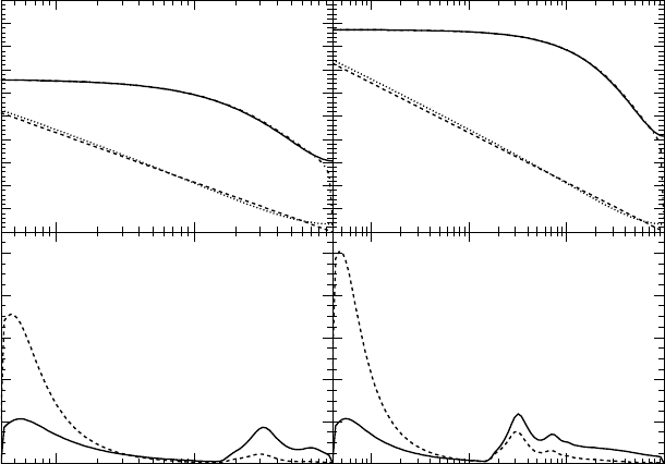
0
0.005
0.01
0.015
0.02
0.025
0.03
0.035
0.04
0.045
0.05
a
n(ν) Ee=1 GeV
b
Ee=10 GeV
0
0.02
0.04
0.06
0.08
0.1
10 102
〈nσγ*〉, mb
c
10 102103
d
ν (MeV)
Figure 46.1: Relative contribution of equivalent photons with small Q2to
the total “photon flux” for (a) 1 GeV electrons and (b) 10 GeV electrons. In
figures (c) and (d) the equivalent photon distribution dn(ν, Q2) is multiplied
by the photonuclear cross section σγ∗(K, Q2) and integrated over Q2in two
regions: the dashed lines are integrals over the low-Q2equivalent photons
(under the dashed line in the first two figures), and the solid lines are integrals
over the high-Q2equivalent photons (above the dashed lines in the first two
figures).
538

method proposed in [8] the σγ∗at large Q2can be approximated as
σγ∗= (1 −x)σγ(K)G2
D(Q2)eb(ǫ,K)·r+c(ǫ,K)·r3,(46.18)
where r=1
2ln(Q2+ν2
K2). The ǫ-dependence of the a(ǫ, K) and b(ǫ, K) functions
is weak, so for simplicity the b(K) and c(K) functions are averaged over ǫ.
They can be approximated as
b(K)≈K
185 MeV 0.85
,(46.19)
and
c(K)≈ −K
1390 MeV 3
.(46.20)
The result of the integration of the photon flux multiplied by the cross sec-
tion approximated by Eq.(46.18) is shown in Fig. 46.1(c,d). The integrated
cross sections are shown separately for the low-Q2region (Q2< Q2
max(me),
dashed lines) and for the high-Q2region (Q2> Q2
max(me), solid lines). These
functions must be integrated over ln(ν), so it is clear that because of the
Giant Dipole Resonance contribution, the low-Q2part covers more than half
the total eA →hadrons cross section. But at ν > 200 MeV , where the
hadron multiplicity increases, the large Q2part dominates. In this sense, for
a better simulation of the production of hadrons by electrons, it is necessary
to simulate the high-Q2part as well as the low-Q2part.
Taking into account the contribution of high-Q2photons it is possible to use
Eq.(46.16) with the over-estimated σγ∗A=σγA(ν) cross section. The slightly
over-estimated electronuclear cross section is
σ∗
eA = (2ln(γ)−1) ·J1−ln(γ)
Ee2J2−J3
Ee.(46.21)
where
J1(Ee) = α
πZEe
σγA(ν)dln(ν) (46.22)
J2(Ee) = α
πZEe
νσγA(ν)dln(ν),(46.23)
and
J3(Ee) = α
πZEe
ν2σγA(ν)dln(ν).(46.24)
539

The equivalent photon energy ν=yE can be obtained for a particular ran-
dom number Rfrom the equation
R=(2ln(γ)−1)J1(ν)−ln(γ)
Ee(2J2(ν)−J3(ν)
Ee)
(2ln(γ)−1)J1(Ee)−ln(γ)
Ee(2J2(Ee)−J3(Ee)
Ee).(46.25)
Eq.(46.13) is too complicated for the randomization of Q2but there is an
easily randomized formula which approximates Eq.(46.13) above the hadronic
threshold (E > 10 MeV ). It reads
π
αD(y)ZQ2
Q2
min
ydn(y, Q2)
dydQ2dQ2=−L(y, Q2)−U(y),(46.26)
where
D(y) = 1 −y+y2
2,(46.27)
L(y, Q2) = ln F(y) + (eP(y)−1 + Q2
Q2
min
)−1,(46.28)
and
U(y) = P(y)·1−Q2
min
Q2
max ,(46.29)
with
F(y) = (2 −y)(2 −2y)
y2·Q2
min
Q2
max
(46.30)
and
P(y) = 1−y
D(y).(46.31)
The Q2value can then be calculated as
Q2
Q2
min
= 1 −eP(y)+eR·L(y,Q2
max)−(1−R)·U(y)−F(y)−1,(46.32)
where Ris a random number. In Fig. 46.2, Eq.(46.13) (solid curve) is com-
pared to Eq.(46.26) (dashed curve). Because the two curves are almost in-
distinguishable in the figure, this can be used as an illustration of the Q2
spectrum of virtual photons, which is the derivative of these curves. An al-
ternative approach is to use Eq.(46.13) for the randomization with a three
dimensional table ydn
dy (Q2, y, Ee).
After the νand Q2values have been found, the value of σγ∗A(ν, Q2) is cal-
culated using Eq.(46.18). If R·σγA(ν)> σγ∗A(ν, Q2), no interaction occurs
and the electron keeps going. This “do nothing” process has low probability
and cannot shadow other processes.
540

0
2
4
6
E=10, y=0.001
πydn/αdy
E=10, y=0.5 E=10, y=0.95
0
2
4
6
8
E=100, y=0.001 E=100, y=0.5 E=100, y=0.95
0
5
10
10 -610 -410 -2 1 10210 4106
E=1000, y=0.001
1 10 10 210310410 5106
E=1000, y=0.5
10 102103104105
E=1000, y=0.95
Q2(MeV2)
Figure 46.2: Integrals of Q2spectra of virtual photons for three energies
10 MeV , 100 MeV , and 1 GeV at y= 0.001, y= 0.5, and y= 0.95.
The solid line corresponds to Eq.(46.13) and the dashed line (which almost
everywhere coincides with the solid line) corresponds to Eq.(46.13).
541
Bibliography
[1] E. Fermi, Z. Physik 29, 315 (1924).
[2] K. F. von Weizsacker, Z. Physik 88, 612 (1934), E. J. Williams, Phys.
Rev. 45, 729 (1934).
[3] L. D. Landau and E. M. Lifshitz, Soc. Phys. 6, 244 (1934).
[4] I. Ya. Pomeranchuk and I. M. Shmushkevich, Nucl. Phys. 23, 1295
(1961).
[5] V. N. Gribov et al., ZhETF 41, 1834 (1961).
[6] L. D. Landau, E. M. Lifshitz, “Course of Theoretical Physics” v.4, part
1, “Relativistic Quantum Theory”, Pergamon Press, p. 351, The method
of equivalent photons.
[7] V. M. Budnev et al., Phys. Rep. 15, 181 (1975).
[8] F. W. Brasse et al., Nucl. Phys. B 110, 413 (1976).
[9] P. V. Degtyarenko, M. V. Kossov, and H.P. Wellisch, Chiral invariant
phase space event generator, I. Nucleon-antinucleon annihilation at rest,
Eur. Phys. J. A 8 (2000) 217.
[10] P. V. Degtyarenko, M. V. Kossov, and H. P. Wellisch, Chiral invariant
phase space event generator, II.Nuclear pion capture at rest, Eur. Phys.
J. A 9 (2000) 411.
[11] P. V. Degtyarenko, M. V. Kossov, and H. P. Wellisch, Chiral invariant
phase space event generator, III Photonuclear reactions below ∆(3,3)
excitation, Eur. Phys. J. A 9, (2000) 421.
542
Chapter 47
Gamma-nuclear Interactions
47.1 Process and Cross Section
Gamma-nuclear reactions in Geant4 are handled by the class G4PhotoNuclearProcess.
The default cross section class for this process is G4PhotoNuclearCrossSection,
which was described in detail in the previous chapter.
47.2 Final State Generation
Final state generation proceeds by two different models, one for incident
gamma energies of a few GeV and below, and one for high energies. For
high energy gammas, the QGSP model is used. Indicent gammas are treated
as QCD strings which collide with nucleons in the nucleus, forming more
strings which later hadronize to produce secondaries. In this particular model
the remnant nucleus is de-excited using the Geant4 precompound and de-
excitation sub-models.
At lower incident energies, there are two models to choose from. The
Bertini-style cascade (G4CascadeInterface interacts the incoming gamma
with nucleons using measured partial cross sections to decide the final state
multiplicity and particle types. Secondaries produced in this initial interac-
tion are then propagated through the nucleus so that they may react with
other nucleons before exiting the nucleus. The remnant nucleus is then de-
excited to produce low energy fragments. Details of this model are provided
in another chapter in this manual.
An alternate handling of low energy gamma interactions is provided by
G4GammaNuclearReaction, which is based upon the Chiral Invariant Phase
Space model (CHIPS [9, 10, 11]). In Geant4 version 9.6 and earlier a sepa-
rate CHIPS model was provided for gamma nuclear interactions. Here the
543
incoming gamma is absorbed into a nucleon or cluster of nucleons within
the target nucleus. This forms an excited bag of partons which later fuse to
form final state hadrons. Parton fusion continues until there are none left,
at which point the final nuclear evaporation stage is invoked to bring the
nucleus to its ground state.
544
Chapter 48
Electro-nuclear Interactions
48.1 Process and Cross Section
Electro-nuclear reactions in Geant4 are handled by the classes G4ElectronNuclearProcess
and G4PositronNuclearProcess. The default cross section class for both these
processes is G4ElectroNuclearCrossSection which was described in detail in
an earlier chapter.
48.2 Final State Generation
Final state generation proceeds in two steps. In the first step the electro-
magnetic vertex of the electron/positron-nucleus reaction is calculated. Here
the virtual photon spectrum is generated by sampling parameterized Q2and
νdistributions. The equivalent photon method is used to get a real photon
from this distribution.
In the second step, the real photon is interacted with the target nucleus
at the hadronic vertex, assuming the photon can be treated as a hadron.
Photons with energies below 10 GeV can be interacted directly with nucleons
in the target nucleus using the measured (γ, p) partial cross sections to decide
the final state multiplicity and particle types. This is currently done by the
Bertini-style cascade (G4CascadeInterface). Photons with energies above
10 GeV are converted to π0s and then allowed to interact with nucleons
using the FTFP model. In this model the hadrons are treated as QCD
strings which collide with nucleons in the nucleus, forming more strings which
later hadronize to produce secondaries. In this particular model the remnant
nucleus is de-excited using the Geant4 precompound and de-excitation sub-
models.
This two-step process is implemented in the G4ElectroVDNuclearModel.
545
An alternative model is the CHIPS-based G4ElectroNuclearReaction [11].
This model also uses the equivalent photon approximation in which the in-
coming electron or positron generates a virtual photon at the electromagnetic
vertex, and the virtual photon is converted to a real photon before it interacts
with the nucleus. The real photon interacts with the hadrons in the target
using the CHIPS model in which quasmons (generalized excited hadrons) are
produced and then decay into final state hadrons. Electrons and positrons
of all energies can be handled by this single model.
546
Chapter 49
Muon-nuclear Interactions
49.1 Process and Cross Section
Muon-nuclear reactions in Geant4 are handled by the class G4MuonNuclearProcess.
The default cross section class for this process is G4KokoulinMuonNuclearXS,
the details of which are discussed in section 13.4.
49.2 Final State Generation
Just as for the electro-nuclear models, the final state generation for the muon-
nuclear reactions proceeds in two steps. In the first step the electromagnetic
vertex of the muon-nucleus reaction is calculated. Here the virtual photon
spectrum is generated by sampling parameterized momentum transfer (Q2)
and energy transfer (ν) distributions. In this case the same equations used
to generate the process cross section are used to sample Q2and ν. The
equivalent photon method is then used to get a real photon.
In the second step, the real photon is interacted with the target nucleus
at the hadronic vertex, assuming the photon can be treated as a hadron.
Photons with energies below 10 GeV can be interacted directly with nucleons
in the target nucleus using the measured (γ, p) partial cross sections to decide
the final state multiplicity and particle types. This is currently done by the
Bertini-style cascade (G4CascadeInterface). Photons with energies above
10 GeV are converted to π0s and then allowed to interact with nucleons
using the FTFP model. In this model the hadrons are treated as QCD
strings which collide with nucleons in the nucleus, forming more strings which
later hadronize to produce secondaries. In this particular model the remnant
nucleus is de-excited using the Geant4 precompound and de-excitation sub-
models.
547
This two-step process is implemented in the G4MuonVDNuclearModel.
548
