Plant Application Guide
User Manual:
Open the PDF directly: View PDF ![]() .
.
Page Count: 97
- Introduction
- Scope
- EnergyPlus Nomenclature
- Generating an EnergyPlus Line Diagram
- Inputting the system into the IDF file
- Example System 1: Chiller and Condenser Loops
- Example System 2: Thermal Energy Storage
- Example System 3: Primary/Secondary Pumping
- References

EnergyPlus™ Version 8.6 Documentation
Plant Application Guide
U.S. Department of Energy
September 30, 2016
COPYRIGHT (c) 1996-2016 THE BOARD OF TRUSTEES OF THE UNIVERSITY OF
ILLINOIS AND THE REGENTS OF THE UNIVERSITY OF CALIFORNIA THROUGH THE
ERNEST ORLANDO LAWRENCE BERKELEY NATIONAL LABORATORY. ALL RIGHTS
RESERVED. NO PART OF THIS MATERIAL MAY BE REPRODUCED OR TRANSMITTED
IN ANY FORM OR BY ANY MEANS WITHOUT THE PRIOR WRITTEN PERMISSION OF
THE UNIVERSITY OF ILLINOIS OR THE ERNEST ORLANDO LAWRENCE BERKELEY
NATIONAL LABORATORY. ENERGYPLUS IS A TRADEMARK OF THE US DEPARTMENT
OF ENERGY.
Contents
1 Introduction 4
1.1 Organization ................................... 4
2 Scope 5
3 EnergyPlus Nomenclature 7
4 Generating an EnergyPlus Line Diagram 9
4.1 Example for EnergyPlus Line Diagram Generation .............. 10
5 Inputting the system into the IDF le 17
6 Example System 1: Chiller and Condenser Loops 19
6.1 Chilled water (CW) loop ............................. 20
6.1.1 Flowcharts for the CW Loop Input Process .............. 20
6.1.2 Flowcharts for CW Loop Controls ................... 24
6.2 Condenser Loop .................................. 28
6.2.1 Flowcharts for the Condenser Loop Input Process ........... 28
6.2.2 Flowcharts for Condenser Loop Controls ................ 33
7 Example System 2: Thermal Energy Storage 38
7.1 Primary Cooling Loop (CoolSysPrimary) - Chiller ............... 41
7.1.1 Flowcharts for the Primary Cooling Loop Input Process ....... 41
7.1.2 Flowcharts for Primary Cooling Loop Controls ............ 43
7.2 Condenser Loop (Condenser Loop) - Cooling Tower .............. 52
7.2.1 Flowcharts for the Condenser Loop Input Process ........... 52
7.2.2 Flowcharts for Condenser Loop Controls ................ 56
7.3 Heating Loop (HeatSys1) - Boiler ........................ 60
7.3.1 Flowcharts for the Heating Loop Input Process ............ 61
7.3.2 Flowcharts for Heating Loop Controls ................. 61
8 Example System 3: Primary/Secondary Pumping 69
8.1 Primary Chilled Water Loop – Chiller(s) and purchased cooling ....... 70
8.1.1 Flowcharts for the Primary Chilled Water Loop Input Process . . . . 72
8.1.2 Flowcharts for Primary Chilled Water Loop Controls ......... 75
8.2 Secondary Chilled Water Loop – Plate Heat Exchanger ............ 77
2
CONTENTS 3
8.2.1 Flowcharts for the Secondary Chilled Water Loop Input Process . . . 79
8.2.2 Flowcharts for secondary chilled water loop Controls ......... 85
8.3 Primary/Secondary Pumping .......................... 87
8.4 Condenser Loop - Cooling Tower ........................ 87
8.4.1 Flowcharts for the Condenser Loop Input Process ........... 89
8.4.2 Flowcharts for Condenser Loop Controls ................ 90
9 References 97
Chapter 1
Introduction
This document provides an in-depth look at plant modeling in EnergyPlus. Plant refers to
the subset of HVAC that involves hydronic equipment for heating, cooling, and service water
heating (or domestic hot water).
This guide serves as an aid to help model plant systems in EnergyPlus simulations. It is
intended to augment the Input Output Reference, which describes the syntax and the details
of individual input objects. This guide will discuss how the dierent objects can be used to
construct a plant loop that can service a building load.
1.1 Organization
This document begins with some general information to introduce users to the syntax used
in EnergyPlus as well as this guide. Then some basic conversion methods needed to take
a real system and format it to simplify the input process are provided. The bulk of this
Application Guide is devoted to modeling example systems. The example systems are in-
tended to demonstrate the input process for various types of plant systems, such as systems
that use thermal energy storage tanks and those that have a primary/secondary pumping
congurations.
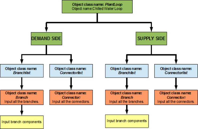
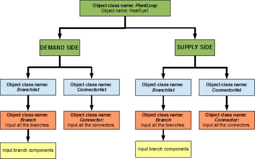
The example systems are dened by breaking the system into its constituent loops. The
loops are then separated into supply and demand sides. These half-loops are then dened
by branches, connectors, and components. The controls for each loop are set after the loop
has been completed. Figures and owcharts are used to display the denition process. The
ow charts should be read from top to bottom and each branched level should be read from
left to right.
The Object Class Names and Object Names used in the ow charts match those used in
the input le provided for the example. One thing that is not specied in the ow charts or
gures is the node names used. The various object class names and object names used in
the examples refer to the entries in the example input les.
4
Chapter 2
Scope
The scope of modeling plant loops in EnergyPlus is limited depending on the application.
For example, there is no provision to model nested loops, and multiple splitter-mixer pairs
in a single loop which are often used in large scale systems. Thus, it has to be realized that
modeling large scale district loops may be challenging in EnergyPlus. One way to model such
systems is to make some assumptions to condense some arrangements of components that
cannot be modeled in EnergyPlus. This approach may not work because the arrangements
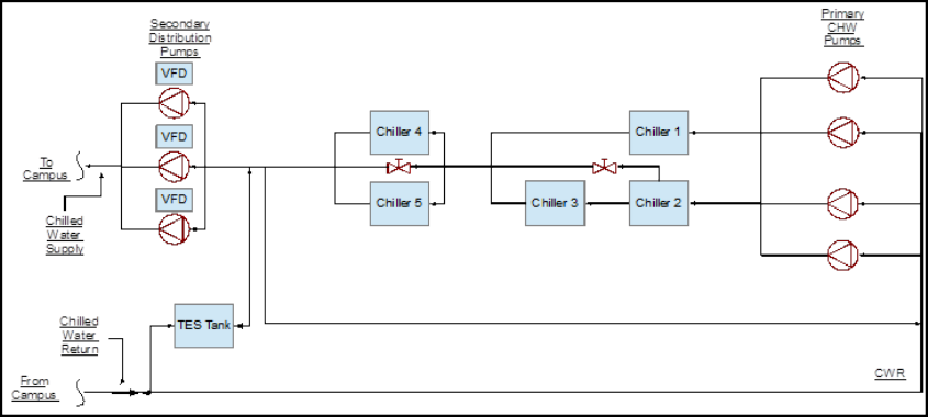
could be very important to the system. Figure 2.1 shows a central plant chilled water system
for the University of California, Riverside (Hyman and Little, 2004). This system contains
a total of eight splitter-mixer pairs, four on the supply side, and four on the demand side.
We could make some assumptions to simplify the system. For example we can use a single
chiller instead of the array of ve chillers, this could work if we size and control the chiller
properly, but the concept of scheduling the dierent chillers to operate at dierent times of
the day to improve eciency will be lost. Hence, it should be noted that while simplications
can provide a general overview of how the system will operate, they may defeat the original
purpose of the complex design. Therefore, this guide will only discuss building plant systems
which are less complicated.
5
6CHAPTER 2. SCOPE
Figure 2.1: Central plant chilled water schematic for the University of California, Riverside
(recreated from Hyman and Little, 2004)
Chapter 3
EnergyPlus Nomenclature
The following is a list of terms that are used in this guide. A simple description of each
of the terms is provided. More detailed descriptions can be obtained from the EnergyPlus
Input Output Reference. Some keywords are provided to assist with the search for these
terms in the Input Output Reference guide.
•Loops – Loops are high-level construction objects in EnergyPlus. Loops are paths
through which the working uid is circulated in order to satisfy a cooling or heating
load. An HVAC system may consist of a zone, plant loop, and a condenser loop. Loops
are constructed by using branches. (Keywords: PlantLoop).Note: Although Energy-
Plus has separate object classes for CondenserLoops and PlantLoops, the dierence
between them is very trivial; therefore all the condenser loops in this guide will be
modeled by a PlantLoop object.
•Supply side half-loop – This is the half loop that contains components (such as
Boilers and chillers) which treat the working uid to supply a working uid state to
the demand components.
•Demand side half-loop – This is the half loop that contains components (such as
cooling coils and heating coils which use the working uid to satisfy a load.
•Branches – Branches are mid-level construction objects in EnergyPlus. Branches are
the segments used to construct the loops. They are constructed by using nodes and
a series of components. Every branch must have at least one component. Branches
will be denoted by using blue colored lines in the EnergyPlus schematics. (Keyword:
Branch).
•Branchlists – Branchlists list all the branches on one side of a loop. (Keyword:
Branchlist).
•Bypass Branch – A bypass branch is used to bypass the core operating components,
it ensures that when the operating components are not required, the working uid can
be circulated through the bypass pipe instead of component. Note: Only one bypass
per half loop is required.
7
8CHAPTER 3. ENERGYPLUS NOMENCLATURE
•Connectors – Connectors are mid-level loop construction objects that are used to
connect the various branches in the loops. There are two kinds of connectors: splitter
which split the ow into two or more branches, and mixers which mix the ow from two
or more branches. A connector pair consists of a splitter and a mixer. A maximum
of one connector pair is allowed on each half loop. Connectors will be denoted by
using green colored lines in the EnergyPlus schematics used in this guide. (Keywords:
Connector:Mixer, Connector:Splitter).
•Connectorlists – Connectorlists list all the connectors on one side of a loop. (Key-
word: Connectorlist).
•Components – Components are the low-level construction objects in EnergyPlus.
Physical objects that are present in the loop are generally called components. Com-
ponents such as a chiller, cooling tower, and a circulation pump can be considered
as the operating/active components. Pipes and ducts can be considered as passive
or supporting components. (Keywords: Chiller:Electric, Pipe:Adiabatic, and many
others).
•Nodes – Nodes dene the starting and ending points of components and branches.
•Nodelists – Nodelists can be used to list a set of nodes in the loop. These nodelists
can then be used for a variety of purposes. For example, a setpoint can be assigned to
multiple nodes by referring to a particular nodelist. (Keyword: Nodelist).
•Set-point – Setpoints are control conditions imposed on node(s) that are monitored
by the SetpointManager to control the system. (Keyword: SetpointManager:Scheduled,
and others).
•Plant equipment operation scheme – This object details the mechanism required
to control the operation of the plant loop, as well as the availability of the plant equip-
ment under various conditions. (Keyword: PlantEquipmentOperation:CoolingLoad,
and others).
•Schedule – Schedules allow the user to inuence the scheduling of many operational
parameters in the loop. For example, a schedule can determine the time period of a
simulation, or instruct the load prole object of a plant to import data from a certain
external le, among other actions. (Keywords: Schedule:Compact, Schedule:le).
•Load Prole – A load prole object is used to simulate a demand prole. This object
can be used when the load prole of a building is already known. (Keyword: LoadPro-
le:Plant). Note: This object does not allow feedback from the plant conditions to the
air system or the zones. However, this object is a great tool for plant-only development
and debugging.
Chapter 4
Generating an EnergyPlus Line
Diagram
The following list of steps will outline the process for converting an engineering line dia-
gram into an EnergyPlus line diagram. Throughout the process, the components in the
systems should be identied and named properly. It is easier to input the system if a list of
components and their names is available.
1. Obtain an engineering line diagram for the system.
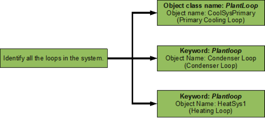
2. Identify all the loops in the system. Some systems may be very complex, but
an eort should be made to separate the system into its constituent plant loops. A system
may have multiple plant loops. Therefore, proper documentation of the loops and their
components should be a priority.
3. Identify the demand side and supply side of the individual loops. Ener-
gyPlus expects the demand side loop and supply side loop to be entered separately. Some
examples of simple plant loops are: a hot water heater (supply component) connected to a
heating coil (demand component), a chiller (supply component) connected to a cooling coil
(demand component) or a cooling tower (supply component) connected to a water cooled
chiller (demand component). These loops may have multiple supply components and mul-
tiple demand components. A chiller may also be a supply or demand component depending
on the loop.
4. Identify the components in the system. All the operating/active components,
such as chillers, pumps, cooling towers, thermal energy storage tanks, heating and cooling
coils, and other components should be identied and named properly. It should be noted that
even though EnergyPlus has objects for modeling valves, they are not often used. Instead
the ow through a component is regulated by using schedules, plant equipment operation
schemes and set points. Passive components such as inlet and outlet pipes for each side of
the loop should also be identied, as they will help in modeling the loop connectors.
5. Identify all the nodes in the system. Nodes are necessary to connect the
dierent components in the system. Nodes dene the starting and ending points of branches
as well as intermediate nodes on multi-component branches. A good method to pin-point
nodes on the line diagram would be to put a node on either side of an active or passive
component. Note: If the outlet of one component does not feed into a splitter or a mixer,
then the outlet node will be the same as the inlet node of the downstream component.
9
10 CHAPTER 4. GENERATING AN ENERGYPLUS LINE DIAGRAM
6. Identify all the branches in the loops. A good way to dene a branch would be to
include at least one of the components in the branch. Branches can accommodate multiple
components in series, but parallel components should be modeled on separate branches.
Operating/active components (except pumps) should be bypassed by adding a bypass branch
parallel to the branch containing the active component. Multiple bypass branches in parallel
can be replaced by a single bypass branch.
7. Identify the position of the connectors in the system. Connectors are an
integral part of the system and are important in constructing the loop. There are two types
of connectors, splitters and mixers. Splitters can distribute the ow from a single branch
into multiple parallel branches. Mixers can combine the ow from multiple branches into
a single branch. As mentioned above, most systems have multiple supply and demand side
components, so splitters and mixers play a crucial role in distributing and recombining the
ow of the working uid through all the components.
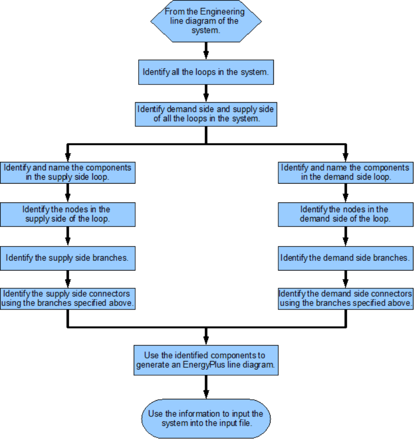
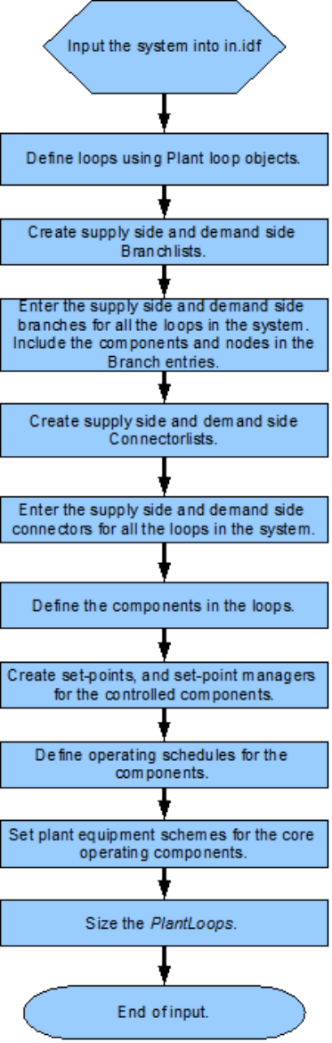
8. Generate an EnergyPlus diagram of the whole system as well as the individual
loops by using the information gathered from the preceding steps.
A owchart for this process is provided in Figure 4.1 .
4.1 Example for EnergyPlus Line Diagram Generation
A series of gures are provided below to detail the process for generating an EnergyPlus line
diagram.
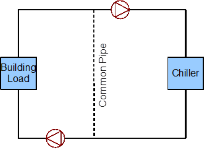
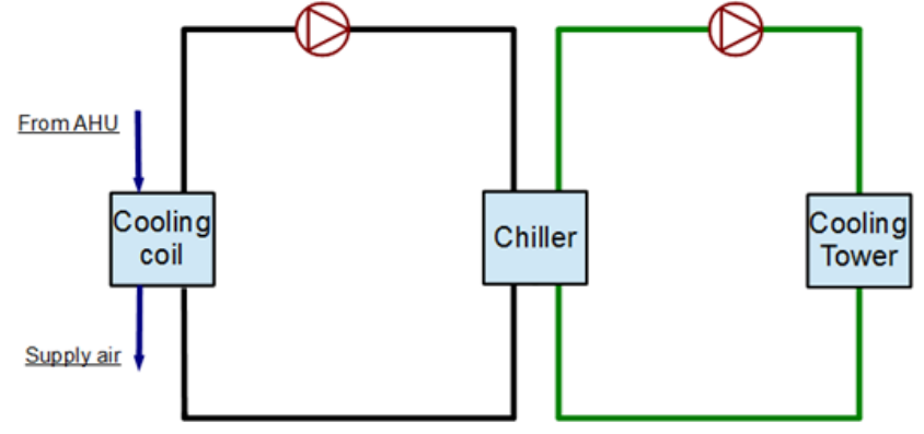
1. Obtain a simple engineering line diagram for the system. This system is
a simple cooling system that employs a primary/secondary pumping setup with a one-way
common pipe to circulate chilled water through a building. Figure 4.2 shows the simple line
diagram for the system.
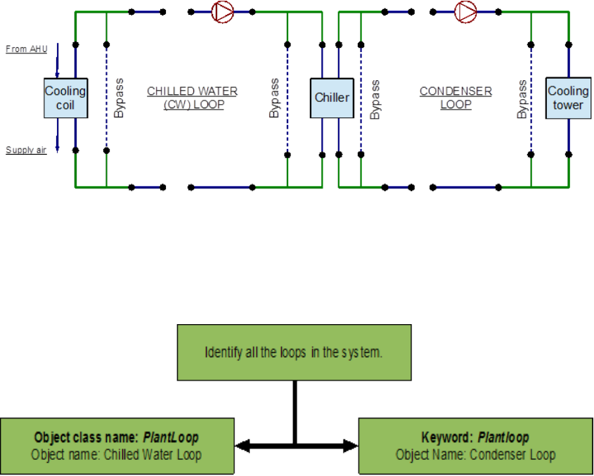
2. Identify all the loops in the system. This system contains only one plant loop.
Loop name: Cooling Loop.
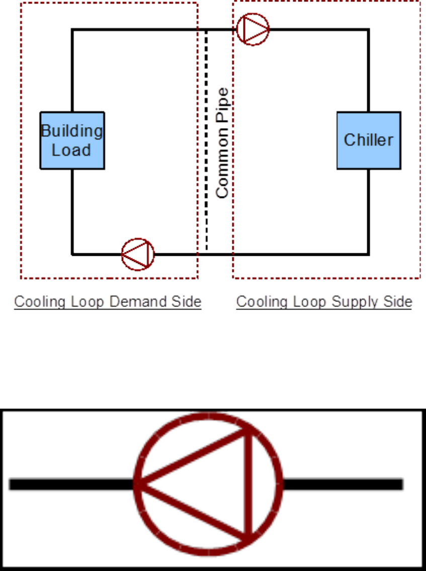
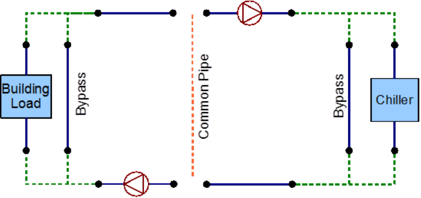
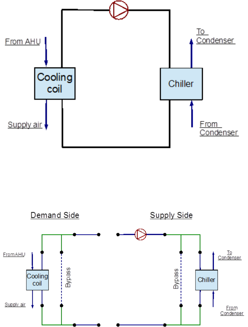
3. Identify the demand side and supply side of the loop. The half loops are
depicted in Figure 4.3.
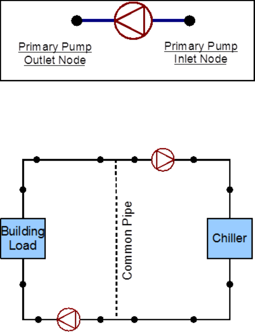
4. Identify the components in the system. While identifying the main components
in the loop, it should be noted that this loop has a primary/secondary pumping setup, and
that there is a common pipe that allows for ow imbalance. (Note: The PlantLoop object
in EnergyPlus has a provision for the input of a common pipe. The user only has to specify
the existence of a common pipe in the loop, and the program calculates its position in the
loop). The primary pump is shown below is shown in Figure 4.4.
5. Identify all the nodes in the system. As mentioned above, placing a node on
each side of a component is a good way to pinpoint all the nodes in the system. This process
should be repeated for every component in the loop. Figure 4.5 shows the placement of all
the nodes on Individual components, while Figure 4.6 shows all the nodes in the system.
Note: No nodes were placed on the common pipe, but its existence should be specied
in the PlantLoop object.
6. Identify all the branches in the system. Remember to add the bypass branches
to the operating components (except the pumps). Branches have to start and end with
4.1. EXAMPLE FOR ENERGYPLUS LINE DIAGRAM GENERATION 11
Figure 4.1: Flowchart for EnergyPlus line diagram generation
12 CHAPTER 4. GENERATING AN ENERGYPLUS LINE DIAGRAM
Figure 4.2: Simple line diagram for the example system, (recreated from Reed and Davis
2007)
4.1. EXAMPLE FOR ENERGYPLUS LINE DIAGRAM GENERATION 13
Figure 4.3: Breakdown of a loop into its constituent half-loops
Figure 4.4: A component in the loop
14 CHAPTER 4. GENERATING AN ENERGYPLUS LINE DIAGRAM
Figure 4.5: Node placement on components
Figure 4.6: Nodes in the system
4.1. EXAMPLE FOR ENERGYPLUS LINE DIAGRAM GENERATION 15
nodes, and should contain at least one component. The branches are denoted by the blue
lines in Figure 4.7.
Figure 4.7: Branch denition
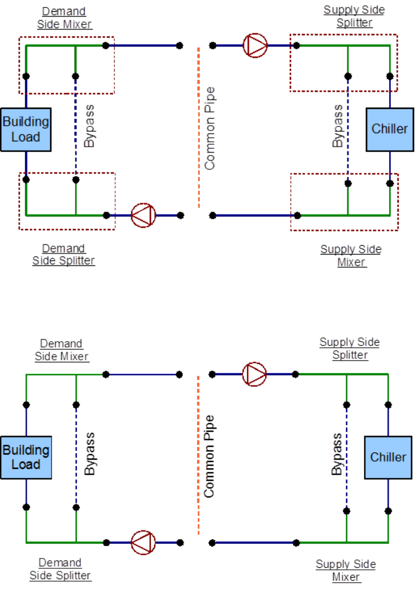
7. Identify the position of the connectors in the system. The PlantLoop accepts
only one splitter-mixer pair per half loop. The connectors are dened by using branches; a
splitter can have one inlet branch and any number of outlet branches whereas a mixer can
have any number of inlet branches and one outlet branch. All the connectors in the loop are
denoted by the green lines in Figure 4.8.
8. An EnergyPlus diagram can be generated by using all the identied components.
The complete schematic is shown in Figure 4.9.
16 CHAPTER 4. GENERATING AN ENERGYPLUS LINE DIAGRAM
Figure 4.8: Splitters and mixers in the loop
Figure 4.9: Complete EnergyPlus line diagram
Chapter 5
Inputting the system into the IDF le
Since, it is not possible to input schematics into the input le, it is important to add de-
scriptive comments to all of the entries to ensure that all the components in the system have
been accounted for. Such documentation will also make debugging easier. It should be noted
that all of the syntax for the inputs is documented in the Input-Output reference guide. A
owchart for the basic input process is provided in Figure 5.1.
17
18 CHAPTER 5. INPUTTING THE SYSTEM INTO THE IDF FILE
Figure 5.1: Flowchart for input process
Chapter 6
Example System 1: Chiller and
Condenser Loops
A simple cooling system will be used as an example to demonstrate the process of inputting
a system into the input le. The input le for this example can be found under the name:
PlantApplicationsGuide_Example1.idf.
This particular system consists of two unique sub-systems/loops. It contains the Plant-
Loop with the chiller and the load prole, and another PlantLoop with the cooling tower.
A schedule containing previously obtained simulation loads is used to simulate the demand
load prole for this loop (Note: In a more general scenario a cooling coil placed in a building
zone would provide the load prole). Flow diagrams along with some keywords from the
input le will be used to record to steps that are required to properly input the system into
EnergyPlus. The simple line diagram for this system is provided in Figure 6.1. The complete
EnergyPlus schematic for the system is provided in Figure 6.2.
Figure 6.1: Simple cooling system line diagram
The cooling system consists of a chilled water loop which is dened by the PlantLoop
object, and a condenser loop which is also dened by the PlantLoop object. Identication of
19
20 CHAPTER 6. EXAMPLE SYSTEM 1: CHILLER AND CONDENSER LOOPS
Figure 6.2: EnergyPlus line diagram for the simple cooling system
these loops in the system is critical for the process of modeling the system in the input le
the owchart for loop identication is provided in Figure 6.3.
Figure 6.3: Flowchart for loop identication
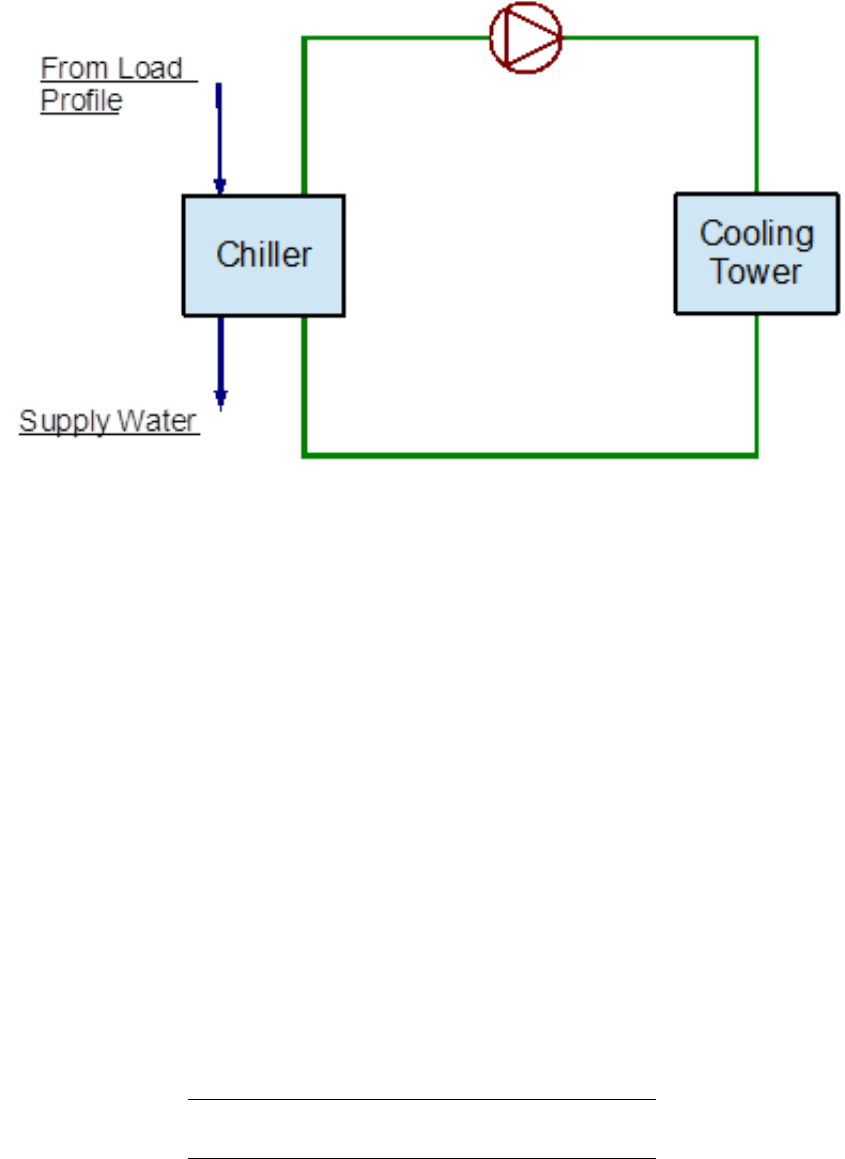
6.1 Chilled water (CW) loop
The chilled water loop is constructed by using a PlantLoop object.This loop uses a water-
cooled electric chiller to supply chilled water to the demand side of this loop. As mentioned
above, the cooling coil is replaced by a load prole object that contains the demand load
prole. The chiller is operated by using set points, plant equipment operation schemes and
schedules. Refer to Figure 6.4 for a simple diagram of the Chilled Water Loop.
6.1.1 Flowcharts for the CW Loop Input Process
This series of ow charts serve as a process guide for identifying and inputting the chilled
water loop and its components into the input le. Refer to Figure 6.5 for an EnergyPlus
schematic of the Chilled Water Loop.
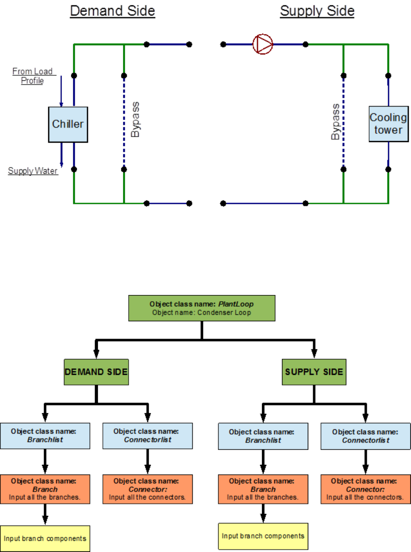
The “PlantLoop” object is entered into the input le, with water as the working uid.
The supply side of the chilled water loop is then input into the system followed by the
demand side. A ow chart for separating the half loops in the loop is provided in Figure 6.6.
6.1. CHILLED WATER (CW) LOOP 21
Figure 6.4: Simple line diagram for the chilled water loop
Figure 6.5: EnergyPlus line diagram for the chilled water loop
22 CHAPTER 6. EXAMPLE SYSTEM 1: CHILLER AND CONDENSER LOOPS
Figure 6.6: Simple owchart for separation of half loops in the chilled water loop
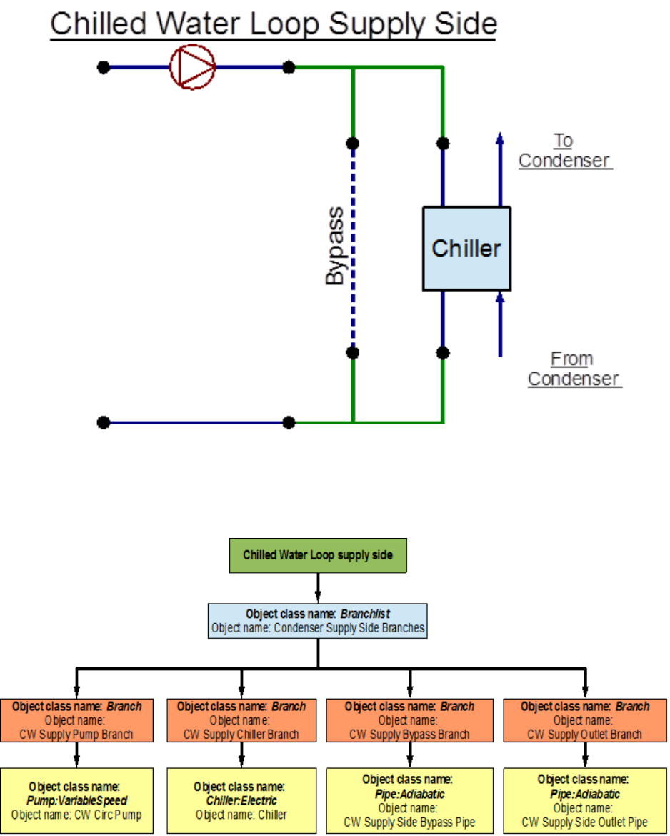
6.1.1.1 CW Loop Supply Side Loop Construction
The main components in the supply side of the chilled water loop are the circulation pump
for the chilled water and the electric chiller that supplies the chilled water. The set-point is
set to the outlet node of this half of the loop; the temperature at this node is controlled to
regulate the operation of the chiller. This side of the loop has eight nodes, four components
and four branches, while it is not required to dene individual node positions in the loop, the
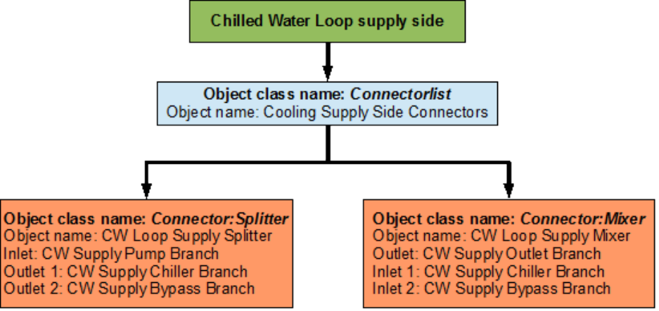
components and branches have to be dened with an inlet and an outlet node. Connectors
are the objects that connect the branches together and complete the loop. Therefore, the
branches and the connectors will set the positions of the nodes in the loop. The EnergyPlus
line diagram for the Chilled Water Loop supply side is provided in Figure 6.7. The owchart
for supply side branches and components is provided in Figure 6.8. The owchart for the
supply side connectors is provided in Figure 6.9.
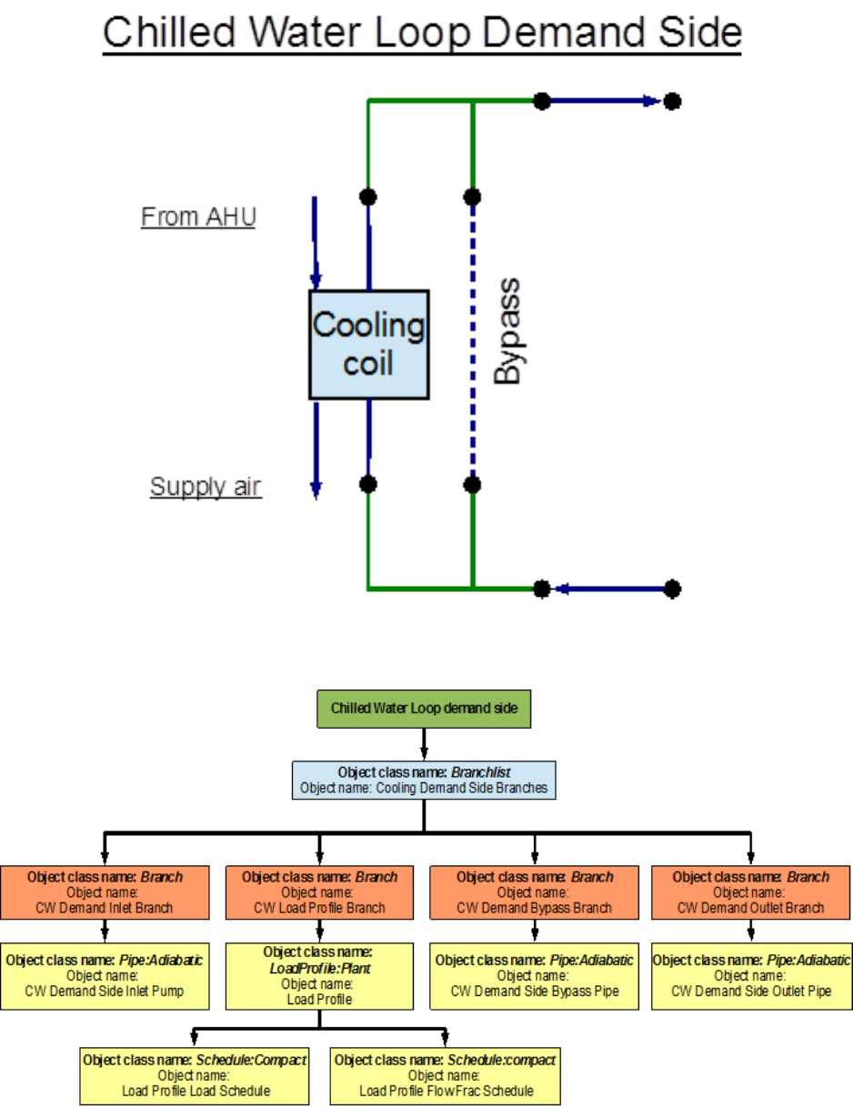
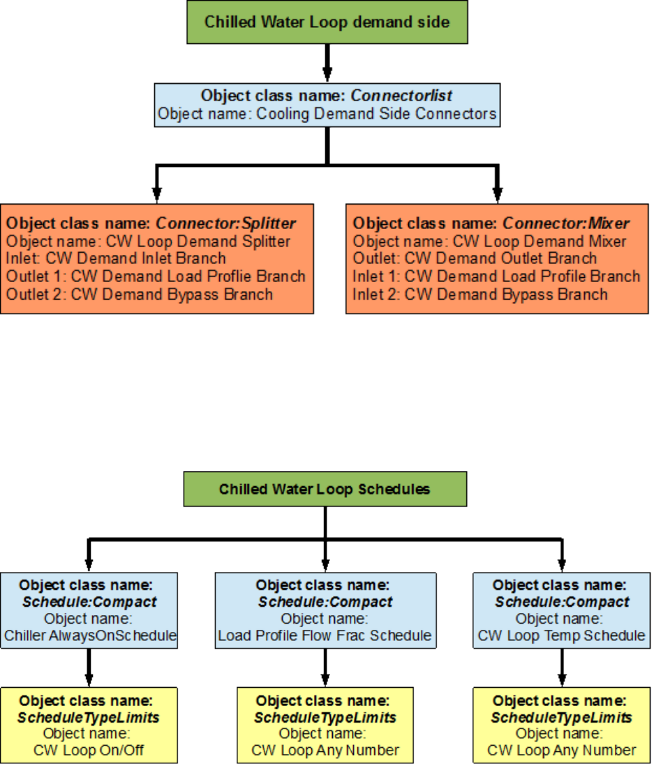
6.1.1.2 CW Loop Demand Side Loop Construction
The demand side of the loop is entered next. The main component in this side of the
loop is the cooling load prole(instead of the cooling coil). This load prole is input by
using a Schedule:Compact object which indicates the hourly cooling loads for the annual run
period. In a more general scenario a cooling coil would take the place of the load prole
and the cooling load will be simulated from the data obtained in the building system energy
simulation. Apart from the load prole, the structure of the loop is very similar to the
structure of the supply side. This side of the loop also has eight nodes, four components,
6.1. CHILLED WATER (CW) LOOP 23
Figure 6.7: EnergyPlus line diagram for the supply side of the chilled water loop
Figure 6.8: Flowchart for chilled water loop supply side branches and components
24 CHAPTER 6. EXAMPLE SYSTEM 1: CHILLER AND CONDENSER LOOPS
Figure 6.9: Flowchart for chilled water loop supply side connectors
and four branches. An EnergyPlus schematic for the demand side is provided in Figure 6.10.
The owchart for demand side branch denition is provided in Figure 6.11. The owchart
for the demand side connectors is provided in Figure 6.12.
As shown in the owchart above, the load prole is attached to the chilled water loop at its
designated position (the LoadProle:Plant object can be used just like any other component)
on the demand side of the loop.
6.1.2 Flowcharts for CW Loop Controls
The chilled water loop is operated by using set-points, plant equipment operation schemes
and schedules.
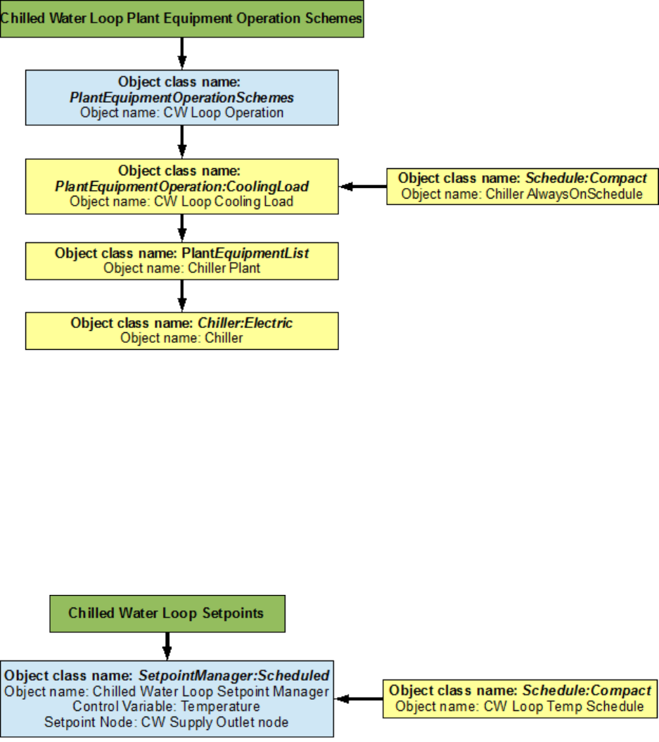
6.1.2.1 Chilled Water Loop Schedules
The chilled water loop uses two dierent schedules to operate properly. The Chiller Al-
waysOnSchedule is a compact schedule that keeps the chiller ON at all times of the day for
a whole year. This compact schedule uses a discrete ScheduleTypeLimit (CW Loop On/O)
which denes that the value of On is 1 and that of O is 0. This plant loop also uses another
compact schedule named CW Loop Temp Schedule to set the temperature at the chilled wa-
ter loop outlet node. This schedule uses a schedule type limit named CW Loop Any Number.
The owchart for chilled water loop schedule denition is provided in Figure 6.13.
6.1.2.2 Chilled Water Loop Plant Equipment Operation Schemes
The PlantEquipmentOperationschemes object uses the Chiller AlwaysOnSchedule and the
CW Loop Cooling Load objects to set the range of the demand load for which the chiller
6.1. CHILLED WATER (CW) LOOP 25
Figure 6.10: EnergyPlus line diagram for the demand side of the chilled water loop
Figure 6.11: Flowchart for chilled water loop demand side branches and components
26 CHAPTER 6. EXAMPLE SYSTEM 1: CHILLER AND CONDENSER LOOPS
Figure 6.12: Flowchart for chilled water loop demand side connectors
Figure 6.13: Flowchart for chilled water loop schedules
6.1. CHILLED WATER (CW) LOOP 27
can be operated during the simulation period. Operation schemes are especially useful and
crucial when using multiple active components. For example, the performance of multiple
chillers can be optimized by carefully managing the load ranges on each of the chillers. A
owchart detailing the chilled water loop plant equipment operation schemes is provided in
Figure 6.14.
Figure 6.14: Flowchart for chilled water loop plant equipment operation schemes
6.1.2.3 Chilled Water Loop Setpoints
The Chilled Water Loop Setpoint Manager uses the CW Loop Temp Schedule to set a tem-
perature control point at the CW Supply Outlet Node. This setpoint allows the program to
control the temperature at the node by operating the components in the chilled water loop.
Since, setpoint managers are high-level control objects, their usefulness is realized in much
more complex systems, where multiple nodes have to be monitored in order to operate the
system properly. A owchart for chilled water loop setpoints is provided in Figure 6.15.
Figure 6.15: Flowchart for chilled water Loop setpoints
28 CHAPTER 6. EXAMPLE SYSTEM 1: CHILLER AND CONDENSER LOOPS
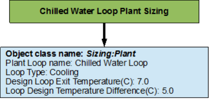
6.1.2.4 Chilled Water Loop Sizing
The chilled water loop is sized such a way that the design loop exit temperature is 7 degrees
Celsius, and the loop design temperature dierence is 5 degrees Celsius. A owchart for
the chilled water loop sizing is provided in Figure 6.16. Note: Since the Load Prole object
does not demand any feedback from the PlantLoop object, the chilled water loop does not
necessarily need to be sized (This object is commented out in the example le). The sizing
shown here is just an example of how the object class can be used in EnergyPlus.
Figure 6.16: Flowchart for chilled water loop sizing
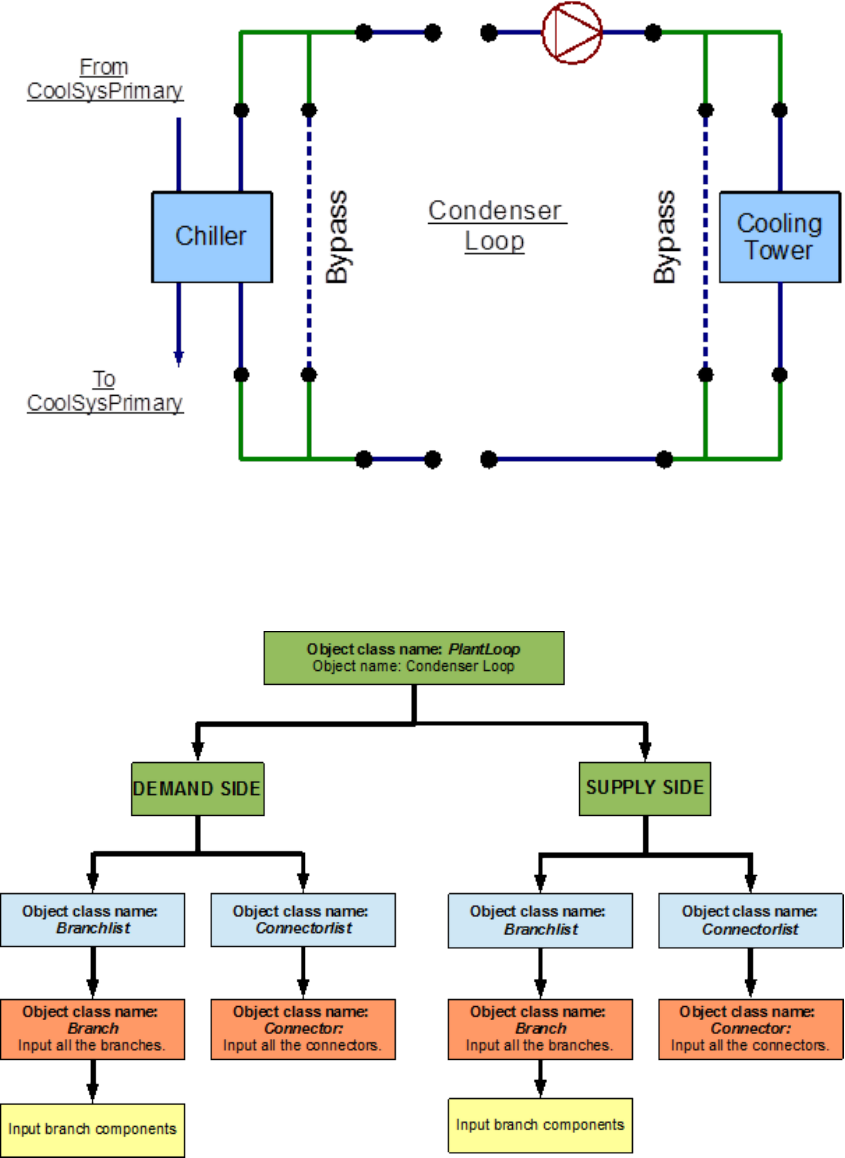
6.2 Condenser Loop
The condenser loop uses a cooling tower to supply cooling water to the water-cooled electric
chiller in the chilled water loop. Hence, the supply side of this loop consists of the cooling
tower and the demand side consists of the electric chiller. The schedules for this loop are
almost identical to the ones applied on the CW loop. They dictate that the cooling tower
also works around the year. The plant equipment schemes specify the cooling capacity/load
of the cooling tower. The operation of the cooling tower is managed by monitoring the
outdoor air wet bulb (air cooled condenser) temperature at the location of the simulation.
The structure of this loop is very similar to that of the chilled water loop, the only dierence
being the main components in the loop. A simple line diagram of the condenser loop is
provided in Figure 6.17.
6.2.1 Flowcharts for the Condenser Loop Input Process
As discussed in Section 1 the supply side and the demand side of the loop are modeled
separately by following the process provided in the ow chart. The ow charts for this loop
are provided below.
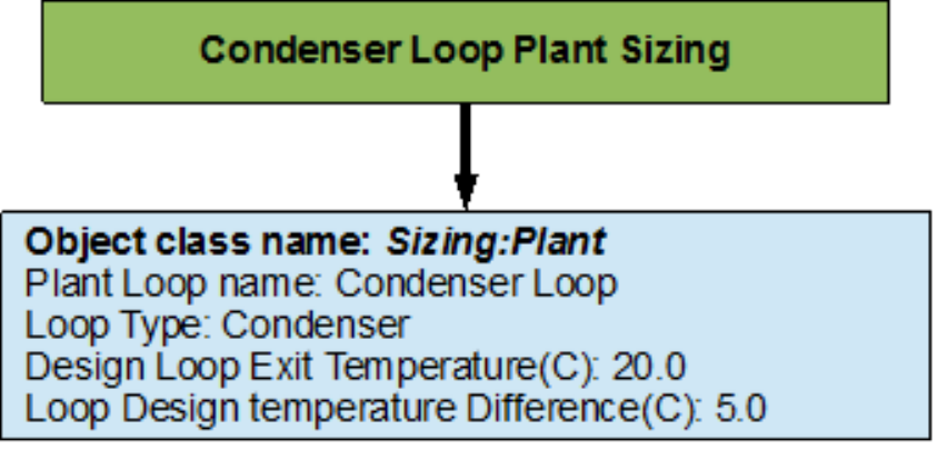
APlantLoop object is used to model the condenser loop with the chiller and the cooling
tower as its main components. The working uid is water. This loop is also sized such
that the loop exit temperature is set to 20 degrees Celsius and the loop design temperature
6.2. CONDENSER LOOP 29
Figure 6.17: Simple line diagram for the condenser loop
dierence is 5 degrees Celsius. The chiller serves as the bridge between the chilled water
loop and the condenser loop. This is achieved by managing the nodal connections on the
chiller, hence the chiller appears on two branches in the system (supply branch of the CW
loop, and the demand branch of the condenser loop). The EnergyPlus line diagram for the
condenser loop is provided in Figure 6.18. A simple ow chart for the separation of the half
loops is provided in Figure 6.19.
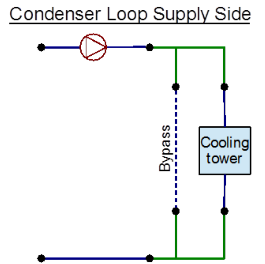
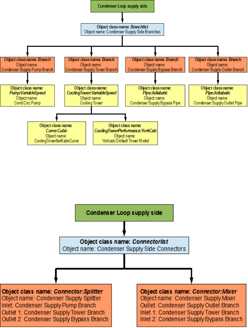
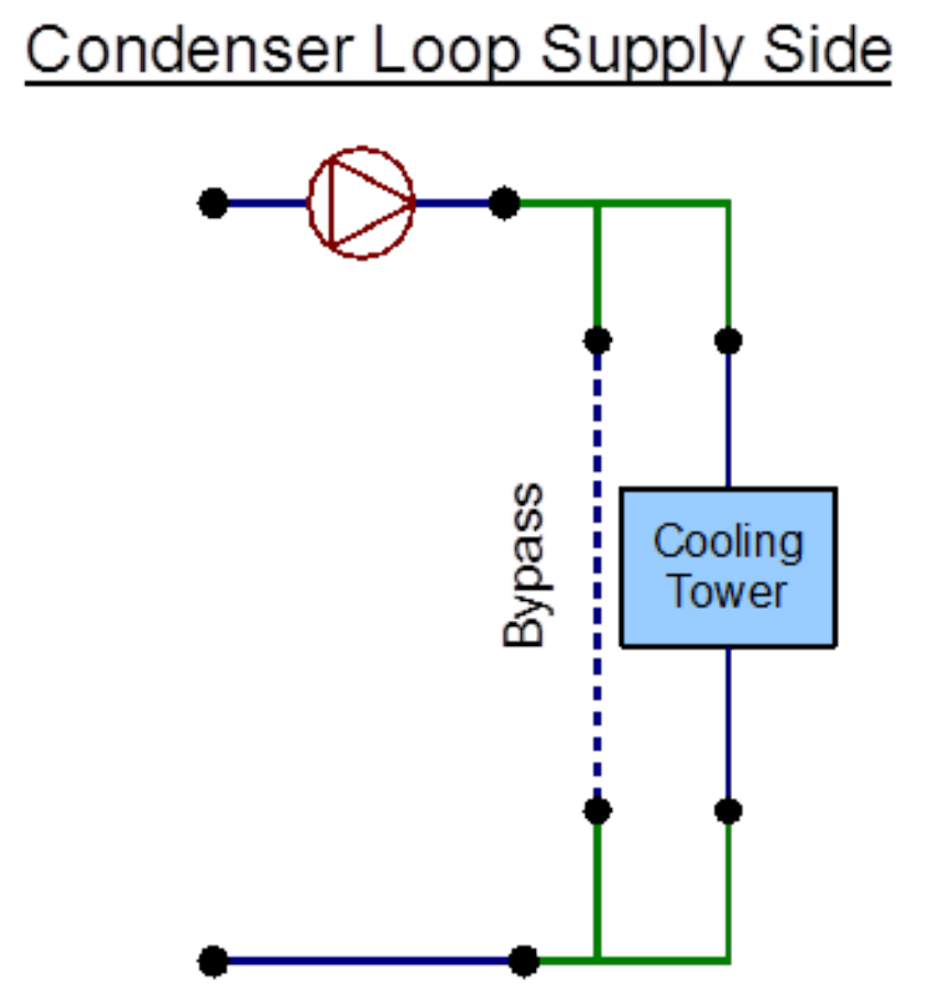
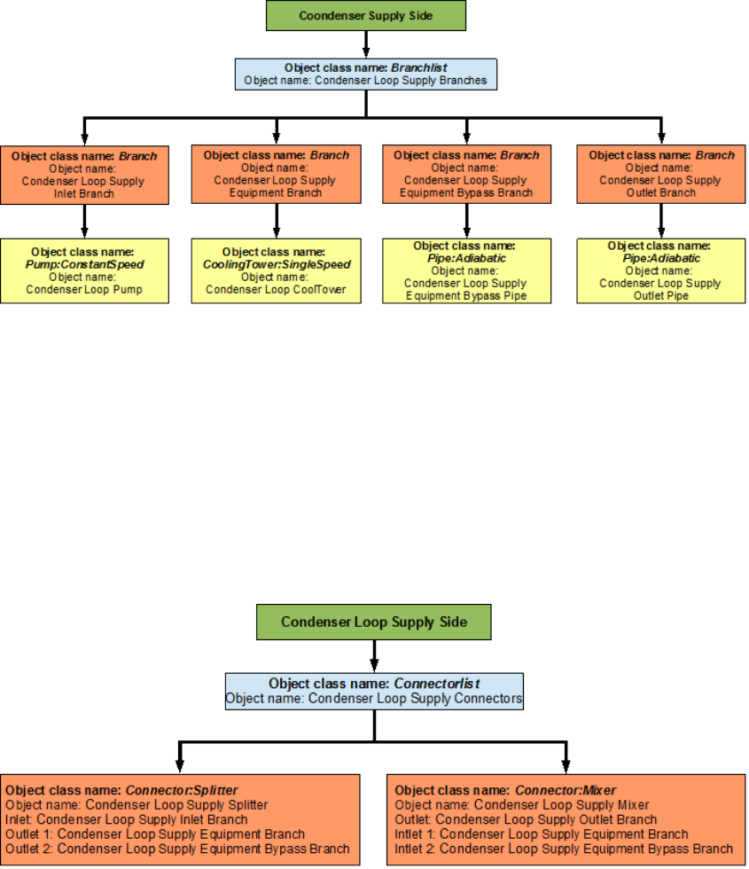
6.2.1.1 Condenser Loop Supply Side Construction
The main components in the supply side of the condenser loop are the condenser circulation
pump and the cooling tower. The temperature set-point is set at the outlet node, where
the outdoor air wet bulb temperature is monitored to regulate the operation of the cooling
tower. The outdoor air conditions are obtained from the weather information le during the
simulation. This side of the loop has eight nodes and four branches. An EnergyPlus diagram
for the condenser loop supply side is provided in Figure 6.20. The owchart for supply side
branch denition is provided in Figure 6.21. The owchart for the supply side connectors is
provided in Figure 6.22.
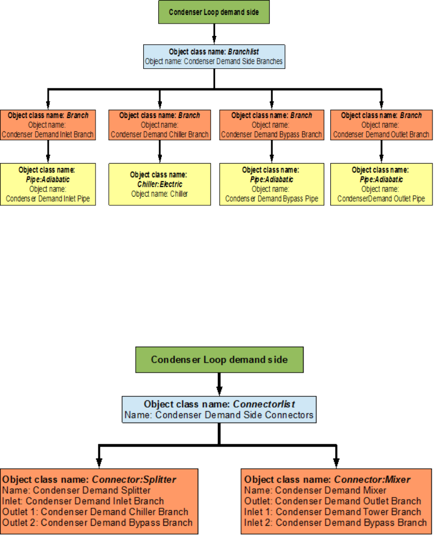
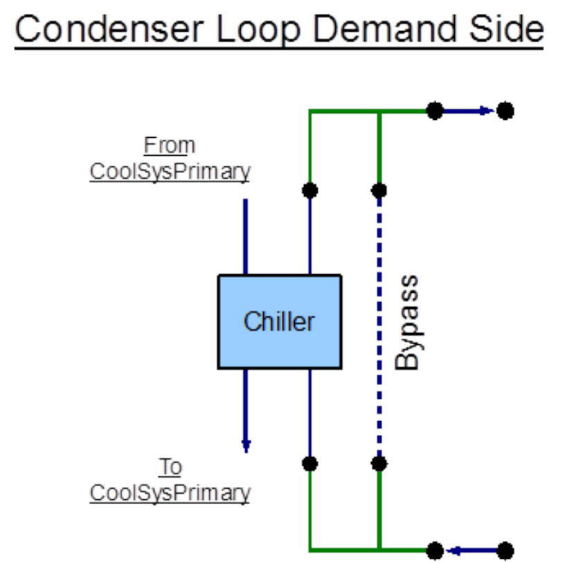
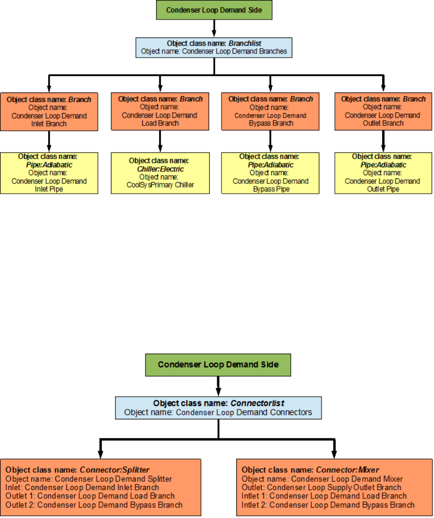
6.2.1.2 Condenser Loop Demand Side Construction
The central component of the demand side is the chiller. The owchart for the construction
of the demand side is also provided below. The schedules for this side do not need to
30 CHAPTER 6. EXAMPLE SYSTEM 1: CHILLER AND CONDENSER LOOPS
Figure 6.18: EnergyPlus line diagram for the condenser loop
Figure 6.19: Simple owchart for separation of half loops in the condenser loop
6.2. CONDENSER LOOP 31
Figure 6.20: EnergyPlus line diagram for the supply side of the condenser loop
32 CHAPTER 6. EXAMPLE SYSTEM 1: CHILLER AND CONDENSER LOOPS
Figure 6.21: Flowchart for condenser supply side branches and components
Figure 6.22: Condenser loop supply side connectors
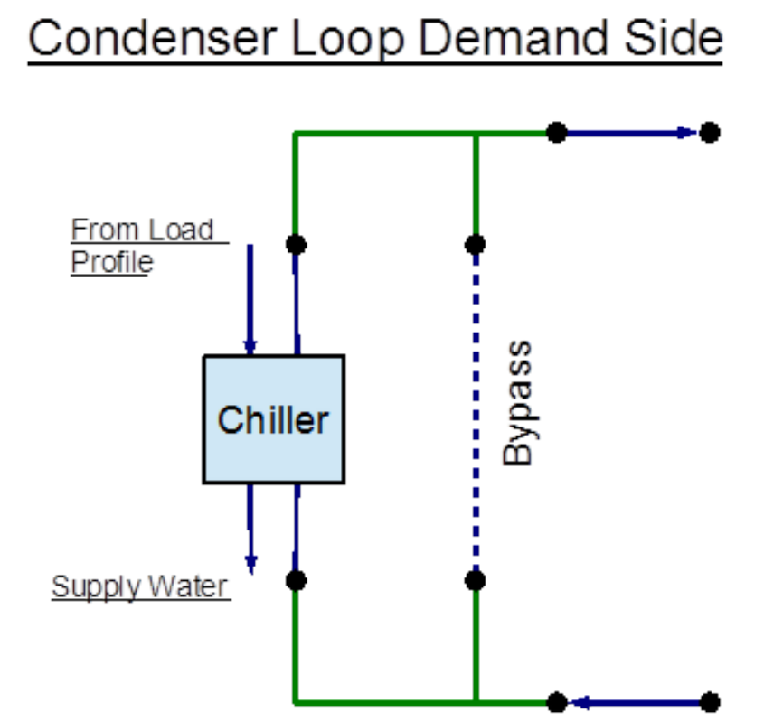
6.2. CONDENSER LOOP 33
be specied, because the schedules that apply to the chiller also apply to this side of the
condenser loop. This side of the loop also contains eight nodes and four branches. An
EnergyPlus schematic for the demand side is provided in Figure 6.23. The owchart for
demand side branch denition is provided in Figure 6.24. The owchart for the demand side
connectors is provided in Figure 6.25.
Figure 6.23: EnergyPlus line diagram for the demand side of the condenser loop
6.2.2 Flowcharts for Condenser Loop Controls
The cooling tower is also scheduled similar to the chiller because both of these units have
to work together in order to satisfy the cooling load. The operation of the cooling tower is
determined by using a set point at the condenser supply exit node. This set point monitors
the temperature at this node as well as the outdoor air wet bulb temperature to operate the
cooling tower. The owchart for the schedules, plant equipment schemes, and the set points
are also provided below.
34 CHAPTER 6. EXAMPLE SYSTEM 1: CHILLER AND CONDENSER LOOPS
Figure 6.24: Condenser loop demand side construction
Figure 6.25: Condenser loop demand side schedules, equipment schemes and setpoints
6.2. CONDENSER LOOP 35
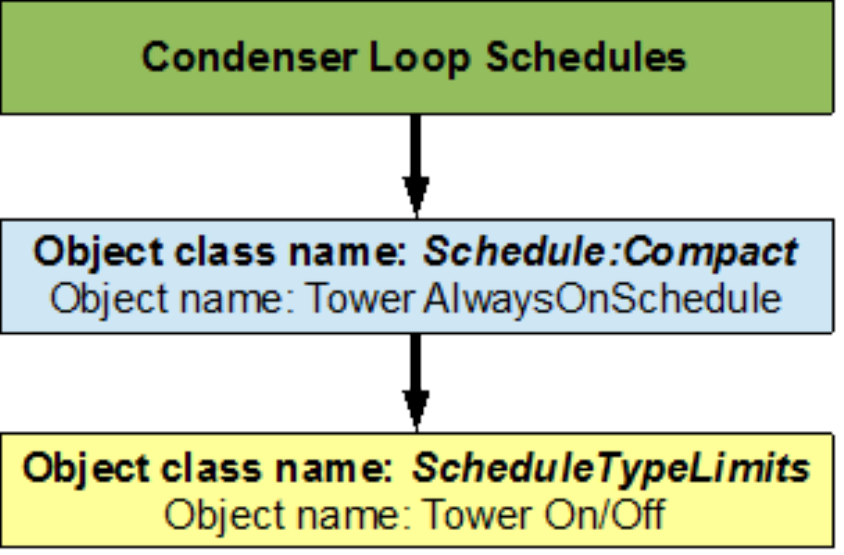
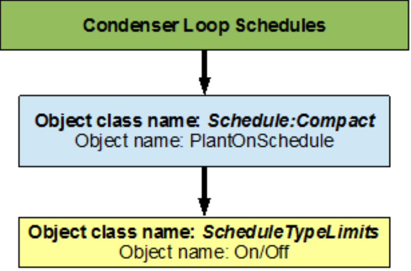
6.2.2.1 Condenser Loop Schedules
The Tower AlwaysOnSchedule is a compact schedule that keeps the tower ON at all times
of the day for a whole year, this compact schedule uses a discrete scheduletypelimit (Tower
On/O) which denes that the value of On is 1 and that of O is 0. A owchart for condenser
loop schedules is provided in Figure 6.26.
Figure 6.26: Condenser loop schedules
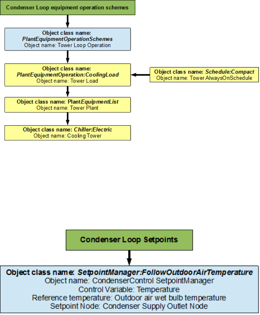
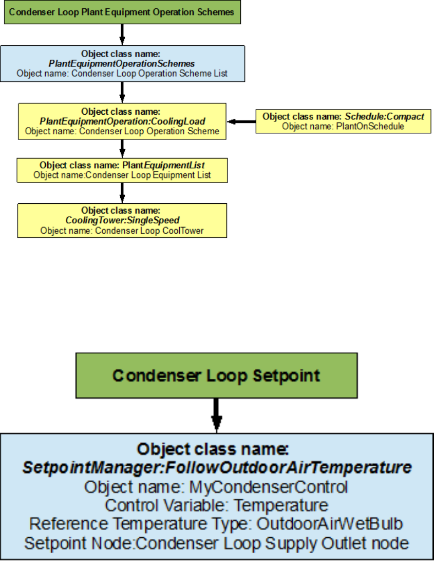
6.2.2.2 Condenser Loop Plant Equipment Operation Schemes
The plant equipment operation schemes for the condenser loop are very similar to those
of the chilled water loop. The PlantEquipmentOperationschemes object uses the Tower
AlwaysOnSchedule and the Tower Load objects to set the range of the demand loads for which
the cooling tower is operated during the simulation period. A owchart for the condenser
loop plant equipment operation schemes is provided in Figure 6.27.
6.2.2.3 Condenser Loop Setpoints
The Condensercontrol setpointmanager places a temperature setpoint at the Condenser Sup-
ply Outlet Node. The temperature at this point is controlled with respect to the outdoor air
wet bulb temperature at that point in the simulation. The outdoor air wet bulb tempera-
ture is obtained from the weather data at the location of the simulation. A owchart for the
condenser loop setpoint is provided in Figure 6.28.
36 CHAPTER 6. EXAMPLE SYSTEM 1: CHILLER AND CONDENSER LOOPS
Figure 6.27: Condenser loop plant equipment operation schemes
Figure 6.28: Condenser loop setpoints
Chapter 7
Example System 2: Thermal Energy
Storage
This system will detail the process required to model a Plant Loop coupled with Thermal
Energy Storage (TES) in EnergyPlus. The input le for this example can be found under
the name: PlantApplicationsGuide_Example2.idf.
The TES tank will be charged by using a chiller loop, which will in turn be cooled by
a condenser loop. The schedules for this system are setup such that the TES tank will be
charged by the chiller during the night and then the stored chilled water is used to satisfy the
building cooling load during the day. The TES tank used in this system is a stratied tank.
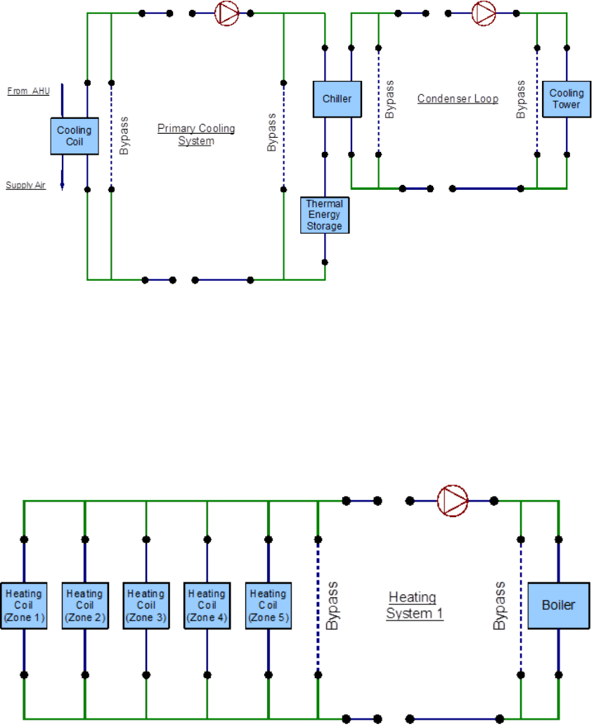
This system also includes one heating loop which satises the heating load. The cooling
and heating system operate in conjunction with an air loop that is spread across a total of
ve zones. The air loop modeling will not be discussed in this guide. This system consists
of a total of three separate plant loops, the cooling side is comprised of two loops and the
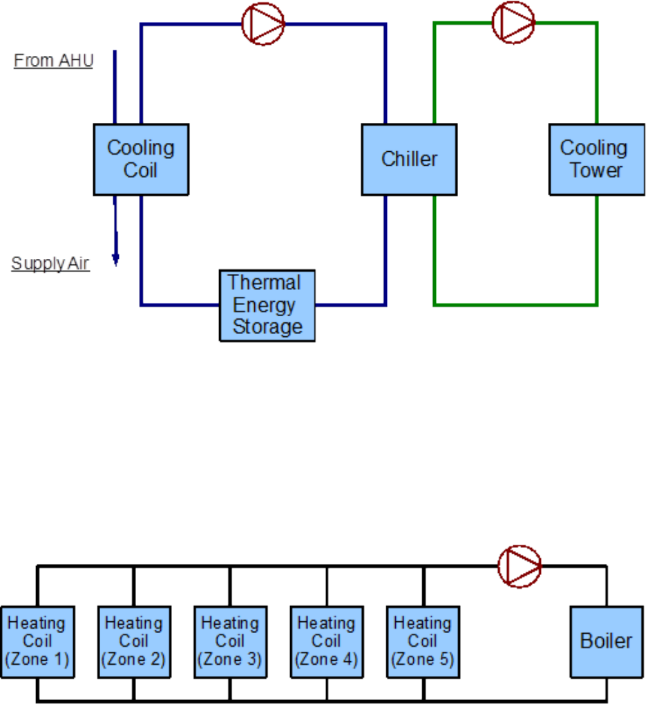
heating side contains one loop. A simple line diagram for the cooling system is provided in
Figure 7.1. The EnergyPlus line diagram for the cooling loop is provided in Figure 7.3. A
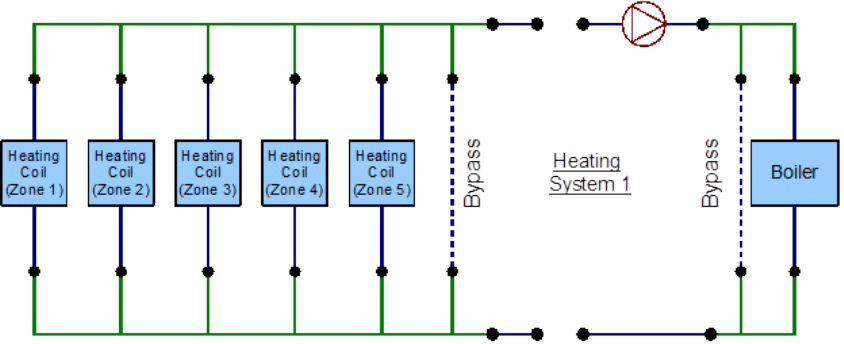
simple line diagram for the heating loop is provided in Figure 7.2, whereas its EnergyPlus
line diagram is provided in Figure 7.4.
SHWSys1
The cooling side of the system will be modeled rst. The primary cooling loop (named
“CoolSysPrimary” in the input le) uses the chiller as the supply side component to charge
the TES tank. The chilled water that is stored in the TES tank is then supplied to the
cooling coil. A cooling tower that operates on the supply side of the condenser loop (named
“Condenser Loop”) supplies the cooling water to the chiller that is used in the primary
cooling loop. These two loops serve as the cooling system for this building. This system
will be modeled rst with emphasis placed on the primary cooling loop. In particular the
schedules used for the charging and discharging the TES tank play a crucial role in the
ecient operation of the system.
The building also has one heating loop. The heating loop (named “HeatSys 1”) uses
a boiler to provide hot water to ve heating coils that are located in the ve zones. This
heating loop also supplies hot water to the reheat coil. A ow chart for loop identication
is provided in Figure 7.5.
38
39
Figure 7.1: Simple line diagram for cooling system
Figure 7.2: Simple line diagram for heating loop
40 CHAPTER 7. EXAMPLE SYSTEM 2: THERMAL ENERGY STORAGE
Figure 7.3: EnergyPlus line diagram for cooling system
Figure 7.4: EnergyPlus line diagram for heating loop
7.1. PRIMARY COOLING LOOP (COOLSYSPRIMARY) - CHILLER 41
Figure 7.5: Flowchart for loop identication
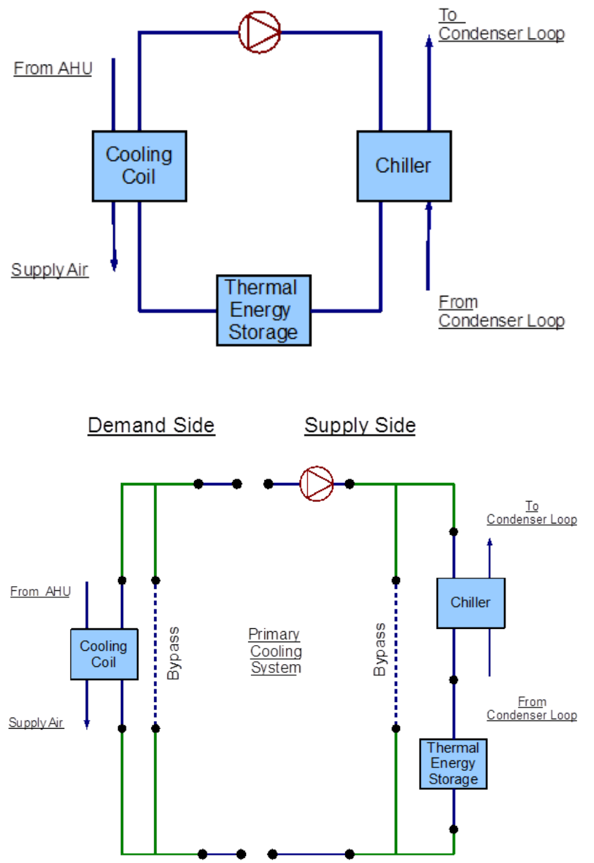
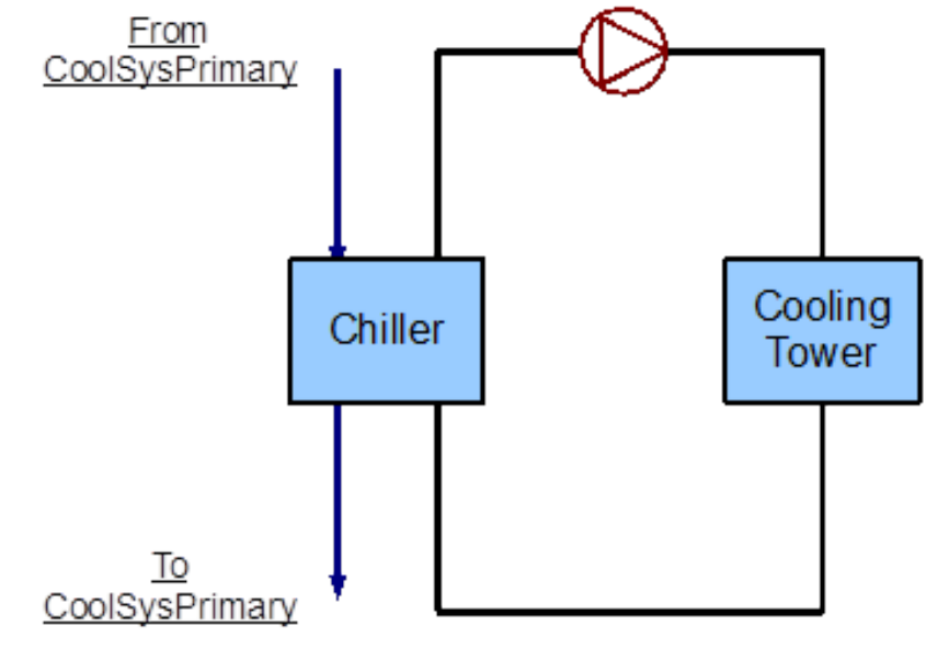
7.1 Primary Cooling Loop (CoolSysPrimary) - Chiller
The primary cooling system is constructed by using a PlantLoop object. It uses an electric
chiller that generates chilled water which is used to charge the TES tank at night. The chilled
water stored in the TES tank is later used during the peak hours to satisfy the demand loads.
Therefore, the supply side of the loop contains the electric chiller and the charge side of the
TES tank. The demand side loop contains the cooling coil. The loop is operated by using
plant equipment operation schemes, and schedules. Refer to Figure 7.6 for a simple diagram
of the Primary Cooling Loop.
7.1.1 Flowcharts for the Primary Cooling Loop Input Process
This series of owcharts serve as a guide for identifying and inputting the CoolSysPrimary
loop and its components into the input le. The working uid in this loop is water. The
important area for this loop is its controls. The EnergyPlus line diagram for this loop is
provided in Figure 7.7. A simple owchart for the separation of the half loops is provided in
Figure 7.8.
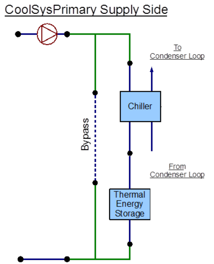
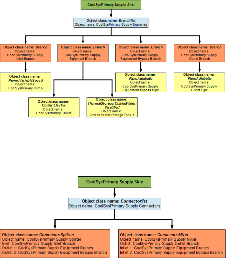
7.1.1.1 CoolSysPrimary Supply Side Loop Construction
The main components on the supply side half loop for the primary cooling system are the
electric chiller that supplies the chilled water, the variable speed pump that circulates the
chilled water through the loop, and the TES tank that stores the supplied chilled water. This
half loop supplies chilled water to the cooling coil which is placed on the demand side half
loop. The supply side half loop contains ve components, four branches, nine nodes, and
one splitter-mixer pair. The EnergyPlus line diagram for the primary cooling loop supply
side is provided in Figure 7.9. The owchart for supply side branches and components is
provided in Figure 7.10. The owchart for supply side connectors is provided in Figure 7.11.
42 CHAPTER 7. EXAMPLE SYSTEM 2: THERMAL ENERGY STORAGE
Figure 7.6: Simple line diagram for the primary cooling system
Figure 7.7: EnergyPlus line diagram for the primary cooling system

7.1. PRIMARY COOLING LOOP (COOLSYSPRIMARY) - CHILLER 43
Figure 7.8: Simple owchart for the separation of half-loops in the primary cooling system
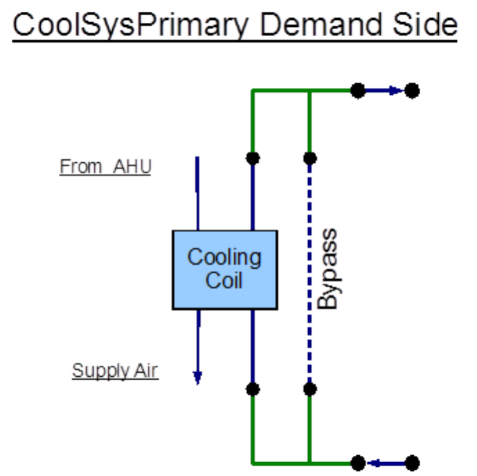
7.1.1.2 CoolSysPrimary Demand Side Loop Construction
The main component on the demand side half loop is the cooling coil which cools the air in
the building by using the chilled water that is supplied by the supply side half loop. This
side of the loop has eight nodes, four components, four branches, and one splitter mixer pair.
An EnergyPlus line diagram for the demand side is provided in Figure 7.12. The owchart
for demand side branch denition is provided in Figure 7.13. The owchart for the demand
side connectors is provided in Figure 7.14.
7.1.2 Flowcharts for Primary Cooling Loop Controls
The Primary Cooling loop is operated by using set-points, plant equipment operation schemes
and schedules. The TES tank charging schedule is one of the most important schedules in
this system.
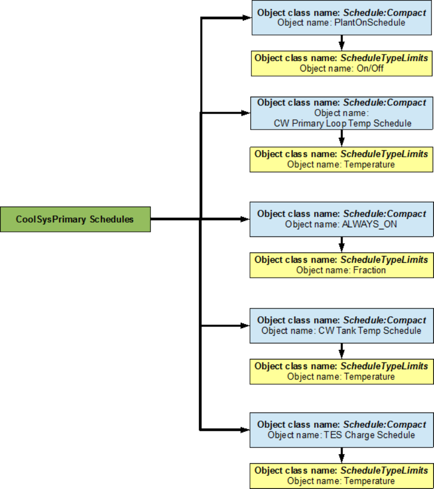
7.1.2.1 CoolSysPrimary Schedules
The owchart for Primary Cooling loop schedule denition is provided in Figure 56. The
Primary Cooling loop uses ve dierent schedules to operate properly. The PlantOnSchedule
is a compact schedule that keeps the chiller and the TES tank ON at all times of the day,
this compact schedule uses a discrete ScheduleTypeLimit (On/O) which denes that the
value of On is 1 and that of O is 0. This plant loop also uses another compact schedule
named CW Primary Loop Temp Schedule declare that the temperature of the chilled water
loop outlet ow is 6.7 degrees Celsius at all times. This schedule is used by the setpoint
44 CHAPTER 7. EXAMPLE SYSTEM 2: THERMAL ENERGY STORAGE
Figure 7.9: EnergyPlus line diagram for the supply side of the primary cooling loop
7.1. PRIMARY COOLING LOOP (COOLSYSPRIMARY) - CHILLER 45
Figure 7.10: Flowchart for primary cooling loop supply side branches and components
Figure 7.11: Flowchart for primary cooling loop supply side connectors
46 CHAPTER 7. EXAMPLE SYSTEM 2: THERMAL ENERGY STORAGE
Figure 7.12: EnergyPlus line diagram for the demand side of the primary cooling loop
7.1. PRIMARY COOLING LOOP (COOLSYSPRIMARY) - CHILLER 47
Figure 7.13: Flowchart for primary cooling loop demand side branches and components
Figure 7.14: Flowchart for primary cooling loop demand side connectors
48 CHAPTER 7. EXAMPLE SYSTEM 2: THERMAL ENERGY STORAGE
manager (CoolSysPrimary Loop Setpoint Manager). This schedule uses a schedule type limit
named Temperature, which denes the upper and lower loop temperature limits
The compact schedule ALWAYS_ON dictates that the use/discharge side of the TES
tank is On at all times of the day. This schedule uses the ScheduleTypeLimit (Fraction)
to set the fractional ow rate of the use side. This schedule is used to dene the use side
availability of the TES tank. The compact schedule CW Tank Temp Schedule is input in the
TES tank object class to dene the limits of the temperature for the chilled water storage
tank outlet. This schedule uses the ScheduleTypeLimit (Temperature) to dene that the
temperature at that outlet should be 7.5 degrees Celsius at all times of the day.
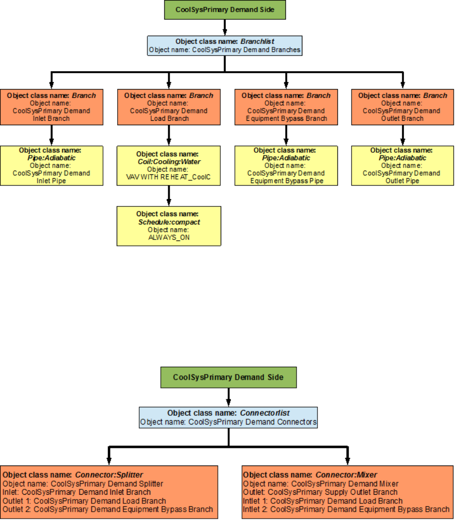
The TES Charge Schedule is a very important schedule for the functioning of the Cool-
SysPrimary Loop the schedule from the input le is provided in Figure 7.15. The schedule
shows that, the on/o ScheduleTypeLimit is used to determine if the TES schedule is On or
o for a certain period of time. A value of 1.0 means On and a value of 0 means O. For
example, it can be observed from the gure that, for the weekdays the TES tank is charged
until 10:00AM, then it is operated during the day from 10:00 AM to 5:00 PM and then it is
charged until midnight. The schedule for the other days is also shown in the gure.
Figure 7.15: TES Charge Schedule
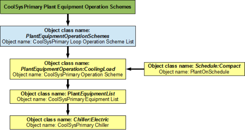
7.1.2.2 CoolSysPrimary Plant Equipment Operation Schemes
This loop has two plant equipment operation schemes, one for the chiller and one for the
TES tank. The PlantEquipmentOperationschemes object uses the PlantOnSchedule and the
CoolSysPrimary Operation Scheme objects to set the range of demand loads for which the
chiller is operated during the simulation period. Operation schemes are especially useful and
crucial when using multiple active components. For example, the performance of multiple
chillers can be optimized by carefully managing the load ranges on each of the chillers. It
should be noted that it is required to enter a plant equipment operation scheme for every
7.1. PRIMARY COOLING LOOP (COOLSYSPRIMARY) - CHILLER 49
Figure 7.16: Flowchart for primary cooling loop schedules
50 CHAPTER 7. EXAMPLE SYSTEM 2: THERMAL ENERGY STORAGE
plant loop in the system. A owchart detailing the chilled water loop plant equipment
operation schemes is provided in Figure 7.17.
Figure 7.17: Flowchart for Chiller plant equipment operation schemes
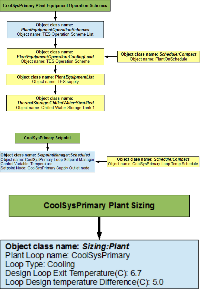
The TES tank operation is modeled here. The PlantEquipmentOperationschemes object
uses the PlantOnSchedule and the TES Operation Scheme objects to set the range of the
demand loads for which the TES tank is operated during the simulation period. A owchart
detailing the Secondary Cooling Loop plant equipment operation schemes is provided in
Figure 7.18.
7.1.2.3 CoolSysPrimary Setpoints
The CoolSysPrimary Loop Setpoint Manager uses the CoolSysPrimary Loop Temp Schedule
to set a temperature control point at the CoolSysPrimary Supply Outlet Node. This setpoint
allows the program to control the temperature at the node by operating the components in
the Primary Cooling loop. A owchart for Secondary Cooling loop setpoints is provided in
Figure 7.19.
7.1.2.4 CoolSysPrimary Sizing
The chilled water loop is sized such a way that the design loop exit temperature is 6.7 degrees
Celsius, and the loop design temperature dierence is 5 degrees Celsius. A owchart for the
Secondary Cooling loop sizing is provided in Figure 7.20.
7.1. PRIMARY COOLING LOOP (COOLSYSPRIMARY) - CHILLER 51
Figure 7.18: Flowchart for Thermal Energy Storage plant equipment operation schemes
Figure 7.19: Flowchart for primary cooling loop setpoints
Figure 7.20: Flowchart for primary cooling loop sizing
52 CHAPTER 7. EXAMPLE SYSTEM 2: THERMAL ENERGY STORAGE
7.2 Condenser Loop (Condenser Loop) - Cooling
Tower
The Condenser Loop is constructed by using a PlantLoop object. It uses a cooling tower
(modeled by using a CoolingTower:SingleSpeed object class) and a constant speed pump
(modeled by using a Pump:ConstantSpeed) to supply cooling water to the electric chiller
(modeled by using a Chiller:Electric object). Therefore, the supply side of the loop contains
the Cooling Tower and the demand side contains the electric chiller. The loop is operated by
using plant equipment operation schemes, and schedules. Refer to Figure 7.21 for a simple
diagram of the Condenser Loop.
Figure 7.21: Simple line diagram for the condenser loop
7.2.1 Flowcharts for the Condenser Loop Input Process
This series of owcharts serve as a guide for identifying and inputting the Condenser Loop and
its components into the input le. The EnergyPlus line diagram for this loop is provided in
Figure 7.22. A simple owchart for the separation of the half loops is provided in Figure 7.23.
7.2.1.1 Condenser Loop Supply Side Construction
The main components on the supply side half loop for the Condenser Loop are the Cooling
Tower that supplies the cooling water and the constant speed pump that circulates the cooling
7.2. CONDENSER LOOP (CONDENSER LOOP) - COOLING TOWER 53
Figure 7.22: EnergyPlus line diagram for the condenser loop
Figure 7.23: Simple ow chart for separation on half loops in the condenser loop
54 CHAPTER 7. EXAMPLE SYSTEM 2: THERMAL ENERGY STORAGE
water through the loop. This half loop supplies cooling water to the electric chiller on the
demand side half loop. The supply side half loop contains four components, four branches,
eight nodes, and one splitter-mixer pair. The EnergyPlus line diagram for the Condenser
loop supply side is provided in Figure 7.24. The owchart for supply side branches and
components is provided in Figure 7.25. The owchart for supply side connectors is provided
in Figure 7.26.
Figure 7.24: EnergyPlus line diagram for the supply side of the condenser loop
7.2.1.2 Condenser Loop Demand Side Construction
The main component on the demand side half loop is the Chiller that uses the cooling
water supplied by the cooling tower. The chiller in turn is used to supply chilled water in
7.2. CONDENSER LOOP (CONDENSER LOOP) - COOLING TOWER 55
Figure 7.25: Flowchart for condenser loop supply side branches and components
Figure 7.26: Flowchart for condenser loop supply side connectors
56 CHAPTER 7. EXAMPLE SYSTEM 2: THERMAL ENERGY STORAGE
the Primary Cooling loop. This side of the loop also has eight nodes, four components,
four branches and one splitter-mixer pair. An EnergyPlus schematic for the demand side
is provided in Figure 7.27. The owchart for demand side branch denition is provided in
Figure 7.28. The owchart for the demand side connectors is provided in Figure 7.29.
Figure 7.27: EnergyPlus line diagram for the demand side of the condenser loop
7.2.2 Flowcharts for Condenser Loop Controls
The Condenser Loop is operated by using set-points, plant equipment operation schemes
and schedules.
7.2.2.1 Condenser Loop Schedules
The owchart for condenser loop schedule denition is provided in Figure 7.30. The Con-
denser loop uses one schedule to operate properly. PlantOnSchedule is a compact schedule
7.2. CONDENSER LOOP (CONDENSER LOOP) - COOLING TOWER 57
Figure 7.28: Flowchart for condenser loop demand side branches and components
Figure 7.29: Flowchart for condenser loop demand side connectors
58 CHAPTER 7. EXAMPLE SYSTEM 2: THERMAL ENERGY STORAGE
that keeps the Cooling Tower On at all times of the day, this compact schedule uses a dis-
crete ScheduleTypeLimit (On/O) which denes that the value of On is 1 and that of O is
0.
Figure 7.30: Flowchart for condenser loop schedules
7.2.2.2 Condenser Loop Plant Equipment Operation Schemes
The PlantEquipmentOperationschemes object uses the PlantOnSchedule and the Condenser
Loop Operation Scheme objects to set the range of demand loads for which the cooling tower
is operated during the simulation period. A owchart detailing the Condenser Loop plant
equipment operation schemes is provided in Figure 7.31.
7.2.2.3 Condenser Loop Setpoints
The MyCondenserControl setpointmanager places a temperature setpoint at the Condenser
Supply Outlet Node. The temperature at this point is controlled with respect to the out-
door air wet bulb temperature at that point in the simulation. The outdoor air wet bulb
temperature is obtained from the weather data at the location of the simulation. The mini-
mum setpoint temperature is 5 degrees Celsius and the maximum setpoint temperature is 80
degrees Celsius. A owchart for Secondary Cooling loop setpoints is provided in Figure 7.32.
7.2. CONDENSER LOOP (CONDENSER LOOP) - COOLING TOWER 59
Figure 7.31: Flowchart for condenser loop plant equipment operation schemes
Figure 7.32: Flowchart for condenser loop setpoints
60 CHAPTER 7. EXAMPLE SYSTEM 2: THERMAL ENERGY STORAGE
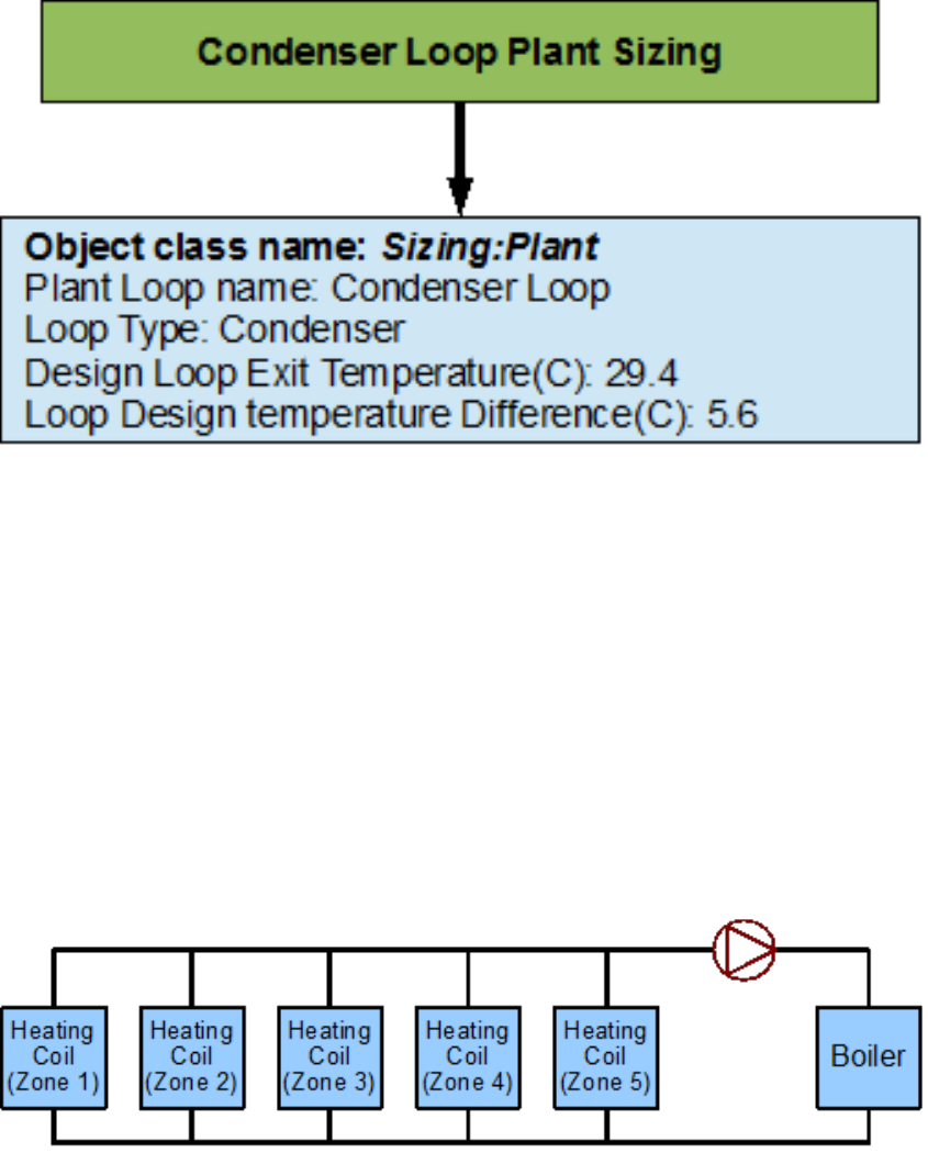
7.2.2.4 Condenser Loop Sizing
The Condenser loop is sized such a way that the design loop exit temperature is 29.4 degrees
Celsius, and the loop design temperature dierence is 5.6 degrees Celsius. A owchart for
the chilled water loop sizing is provided in Figure 7.33.
Figure 7.33: Flowchart for condenser loop sizing
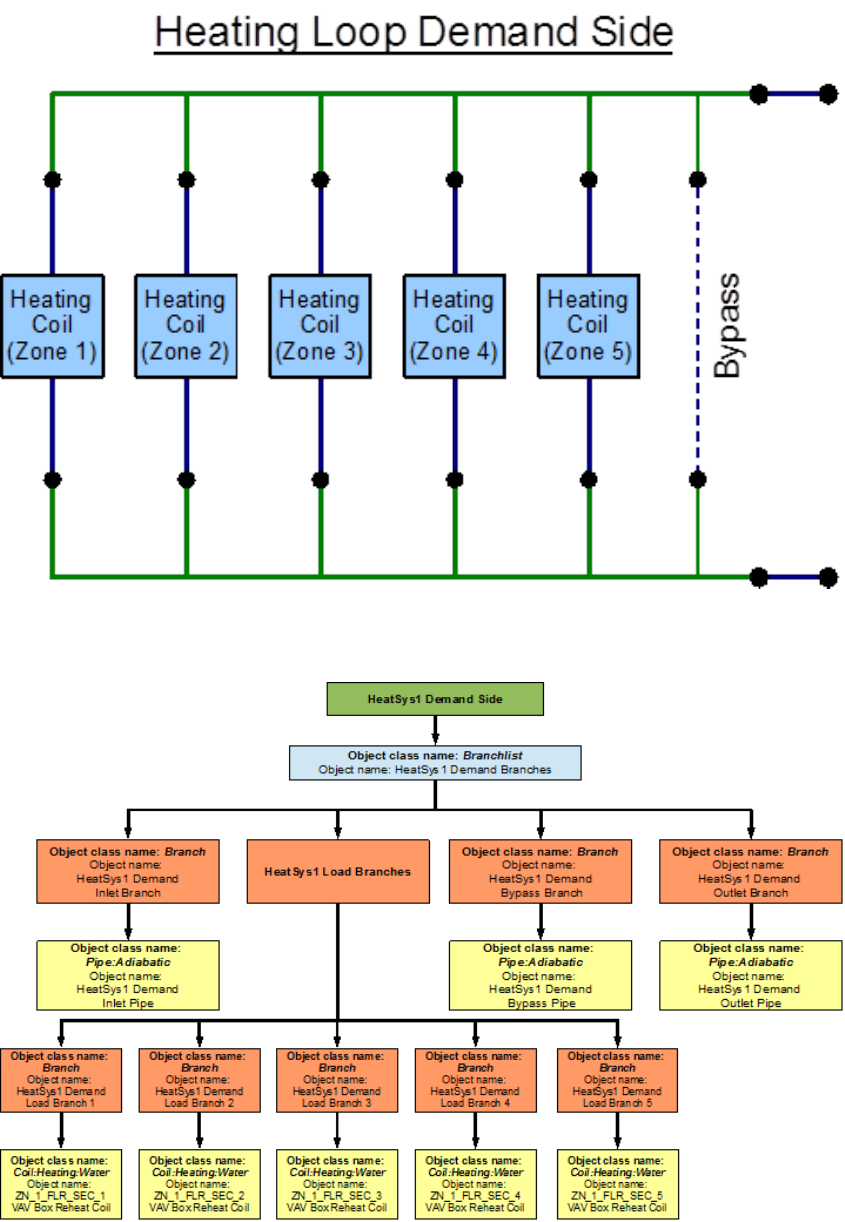
7.3 Heating Loop (HeatSys1) - Boiler
The Heating loop is constructed by using a PlantLoop object. It uses an electric boiler to
(modeled by using a Boiler:HotWater object class) to supply hot water to the ve heating
coils placed in the ve zones of the building (modeled by using a Coil:Heating:Water object
class). Therefore, the supply side of the loop contains the hot water boiler and the demand
side contains a total of six heating coils. The loop is operated by using plant equipment
operation schemes, and schedules. Refer to Figure 7.34 for a simple diagram of the Condenser
Loop.
Figure 7.34: Simple line diagram for the heating loop
7.3. HEATING LOOP (HEATSYS1) - BOILER 61
7.3.1 Flowcharts for the Heating Loop Input Process
This series of owcharts serve as a guide for identifying and inputting the Heating loop and
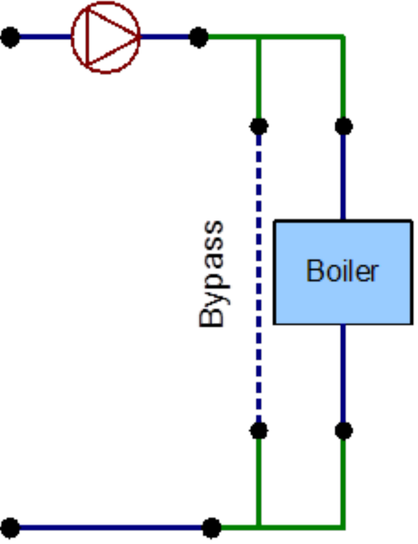
its components into the input le. The EnergyPlus line diagram for this loop is provided in
Figure 7.35. A simple owchart for the separation of the half loops is provided in Figure 7.36.
Figure 7.35: EnergyPlus line diagram for the heating loop
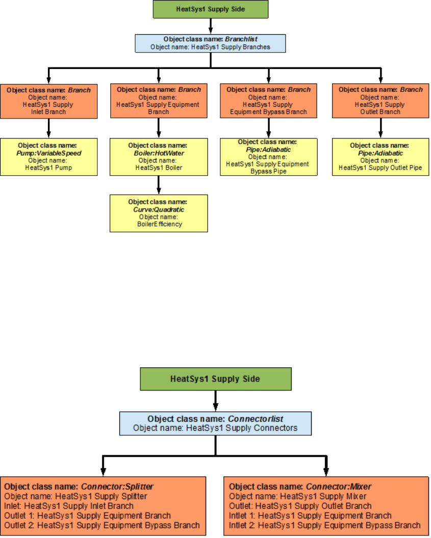
7.3.1.1 Heating Loop Supply Side Construction
The main components on the supply side half loop for the Heating Loop are the hot water
boiler that generates hot water and the variable speed pump that circulates the hot water
through the loop. This half loop supplies hot water to ve heating coils on the demand
side half loop. The supply side half loop contains four components, four branches, eight
nodes, and one splitter-mixer pair. The EnergyPlus line diagram for the Primary Cooling
loop supply side is provided in Figure 7.37. The owchart for supply side branches and
components is provided in Figure 7.38. The owchart for supply side connectors is provided
in Figure 7.39.
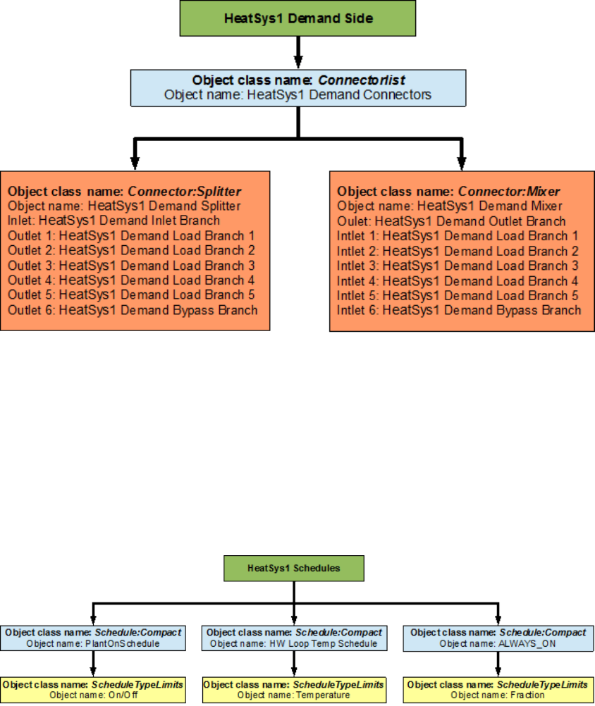
7.3.1.2 Heating Loop Demand Side Construction
The demand side half loop contains ve heating coils that heat the air in the dierent zones
of the building by using the hot water that is supplied by the hot water boiler. This side
of the loop also has sixteen nodes, eight components, eight branches, and one splitter-mixer
pair. An EnergyPlus schematic for the demand side is provided in Figure 7.40. The owchart
for demand side branch denition is provided in Figure 7.41. The owchart for the demand
side connectors is provided in Figure 7.42.
7.3.2 Flowcharts for Heating Loop Controls
The Heating Loop is operated by using set-points, plant equipment operation schemes and
schedules.
62 CHAPTER 7. EXAMPLE SYSTEM 2: THERMAL ENERGY STORAGE
Figure 7.36: Simple ow chart for separation on half loops in the heating loop
7.3.2.1 Heating Loop Schedules
The owchart for Primary Heating loop schedule denition is provided in Figure 7.43. The
Heating Loop uses three dierent schedules to operate properly. PlantOnSchedule is a com-
pact schedule that uses a discrete ScheduleTypeLimit (On/O) which denes that the value
of ON is 1 and that of O is 0. This plant loop also uses another compact schedule named
HW Loop Temp Schedule to declare that the temperature at the heating loop outlet and the
boiler outlet to be 82 degrees Celsius. This schedule uses a schedule type limit named Tem-
perature, which denes the loop upper and lower temperature limits. The compact schedule
ALWAYS_ON dictates that the boiler and the cooling coils are On at all times of the day.
This schedule uses the ScheduleTypeLimit (Fraction) to set the fractional ow rate of the
components to 1.
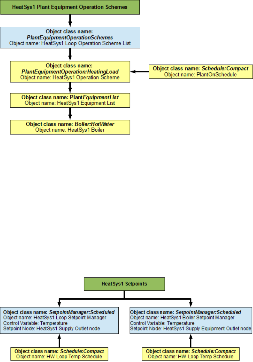
7.3.2.2 Heating Loop Plant Equipment Operation Schemes
The PlantEquipmentOperationschemes object uses the PlantOnSchedule and the HeatSys1
Operation Scheme objects to set the range of the demand loads for which the boiler is
operated during the simulation period. Operation schemes are especially useful and crucial
when using multiple active components but it is required to enter set up a plant equipment
operation scheme for every PlantLoop that is used in a system. A owchart detailing the
heating loop plant equipment operation scheme is provided in Figure 7.44.
7.3. HEATING LOOP (HEATSYS1) - BOILER 63
Figure 7.37: EnergyPlus line diagram for the supply side of the heating loop
64 CHAPTER 7. EXAMPLE SYSTEM 2: THERMAL ENERGY STORAGE
Figure 7.38: Flowchart for heating loop supply side branches and components
Figure 7.39: Flowchart for heating loop supply side connectors
7.3. HEATING LOOP (HEATSYS1) - BOILER 65
Figure 7.40: EnergyPlus line diagram for the demand side of the heating loop
Figure 7.41: Flowchart for heating loop demand side branches and components
66 CHAPTER 7. EXAMPLE SYSTEM 2: THERMAL ENERGY STORAGE
Figure 7.42: Flowchart for heating loop demand side connectors
Figure 7.43: Flowchart for heating loop schedules
7.3. HEATING LOOP (HEATSYS1) - BOILER 67
Figure 7.44: Flowchart for heating loop plant equipment operation schemes
7.3.2.3 Heating Loop Setpoints
The HeatSys1 Loop Setpoint Manager uses the HW Loop Temp Schedule to set a temperature
control point at the HeatSys1 Supply Outlet Node. This setpoint allows the program to
control the temperature (set to 82 degrees Celsius) at the node by operating the components
in the Heating loop. The Heating Loop also uses another schedule (HeatSys1 Boiler Setpoint
Manager) to set the temperature of the boiler outlet to 82 degrees Celsius. If the HeatSys1
Boiler Setpoint Manager is not entered the program assumes the overall loop setpoint for the
boiler outlet node. Since, setpoint managers are high-level control objects, their usefulness
is realized in much more complex systems, where multiple nodes have to be monitored in
order to operate the system properly. A owchart for heating loop setpoints is provided in
Figure 7.45.
Figure 7.45: Flowchart for heating loop setpoints
68 CHAPTER 7. EXAMPLE SYSTEM 2: THERMAL ENERGY STORAGE
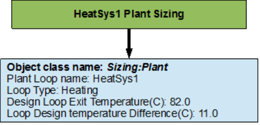
7.3.2.4 Heating Loop Sizing
The Heating Loop is sized such a way that the design loop exit temperature is 82.0 degrees
Celsius, and the loop design temperature dierence is 11.0 degrees Celsius. A owchart for
the chilled water loop sizing is provided in Figure 7.46.
Figure 7.46: Flowchart for heating loop sizing
Chapter 8
Example System 3:
Primary/Secondary Pumping
This example will discuss the basics of primary/secondary pumping systems and some of
the controls that are used in managing such systems. The input le for this example can be
found under the name: PlantApplicationsGuide_Example3.idf.
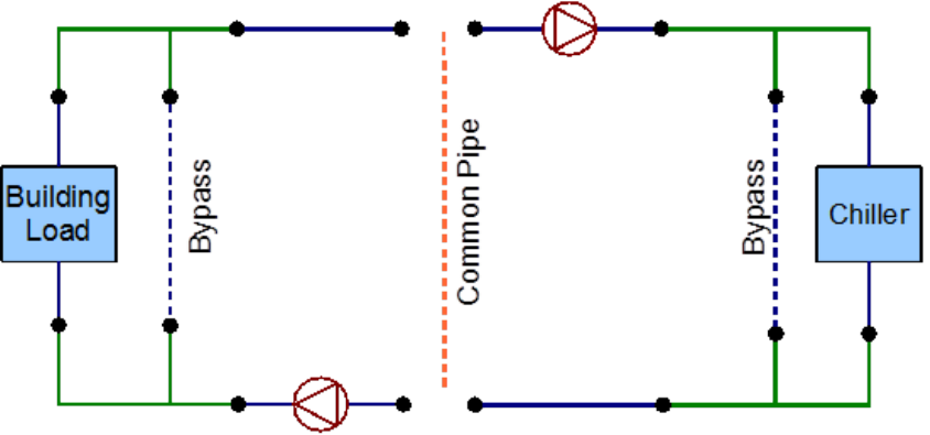
Although it is common for these systems to have a common pipe setup to allow for ow
imbalance as shown in Figure 8.1 and even though there is a provision in EnergyPlus to
model common pipes, this example will not discuss them. In the future, the common pipe
is expected to be obsolesced, and therefore using a heat exchanger and two separate loops
is recommended for future primary/secondary pumping arrangements.
Figure 8.1: Example of a common pipe setup
This system services a three zone building by using, two chillers and purchased cooling
on the primary chilled water loop to satisfy the demand loads. The chilled water from the
supply side of the primary chilled water loop is passes through a plate heat exchanger which
serves as the supply side for the secondary chilled water loop. The cooling coil is placed
on the demand side of the secondary loop. The primary loop uses a constant speed pump
69
70 CHAPTER 8. EXAMPLE SYSTEM 3: PRIMARY/SECONDARY PUMPING
to circulate the working uid (water). The secondary loop uses a variable speed pump to
manipulate the ow of the uid such that the cooling coil demand is satised. The above
mentioned pumps are considered as a primary/secondary pumping pair.
Therefore there are four dierent loops in the system. The cooling loops in the system
will be modeled rst. The primary cooling loop (‘Primary Chilled Water Loop’) which
contains a small chiller, a big chiller and a purchased cooling object on the supply side half
loop for supplying chilled water to a uid to uid plate heat exchanger on the demand side.
The secondary cooling loop (‘Secondary Chilled Water Loop’) contains the uid to uid
plate heat exchanger on the supply side half loop and a cooling coil on the demand side.
The condenser loop (‘Condenser Loop’) which uses a cooling tower to supply cold water to
the chillers on the demand side is modeled next. The heating loop (‘Heating Loop’) uses
purchased heating to serve the demand loads of three reheat coils places in each of the zones
of the buildings, this loop will not be discussed in this application guide because it does not
relate to the primary/secondary pumping setup in any way.
The plant equipment operation scheme for the primary chilled water loop and the pri-
mary/secondary pumping setup are the most important features of this system.
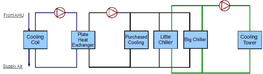
The simple line diagram for the system is shown in Figure 8.3. The EnergyPlus line
diagram is shown in Figure 8.3.
Figure 8.2: Simple line diagram for the cooling system
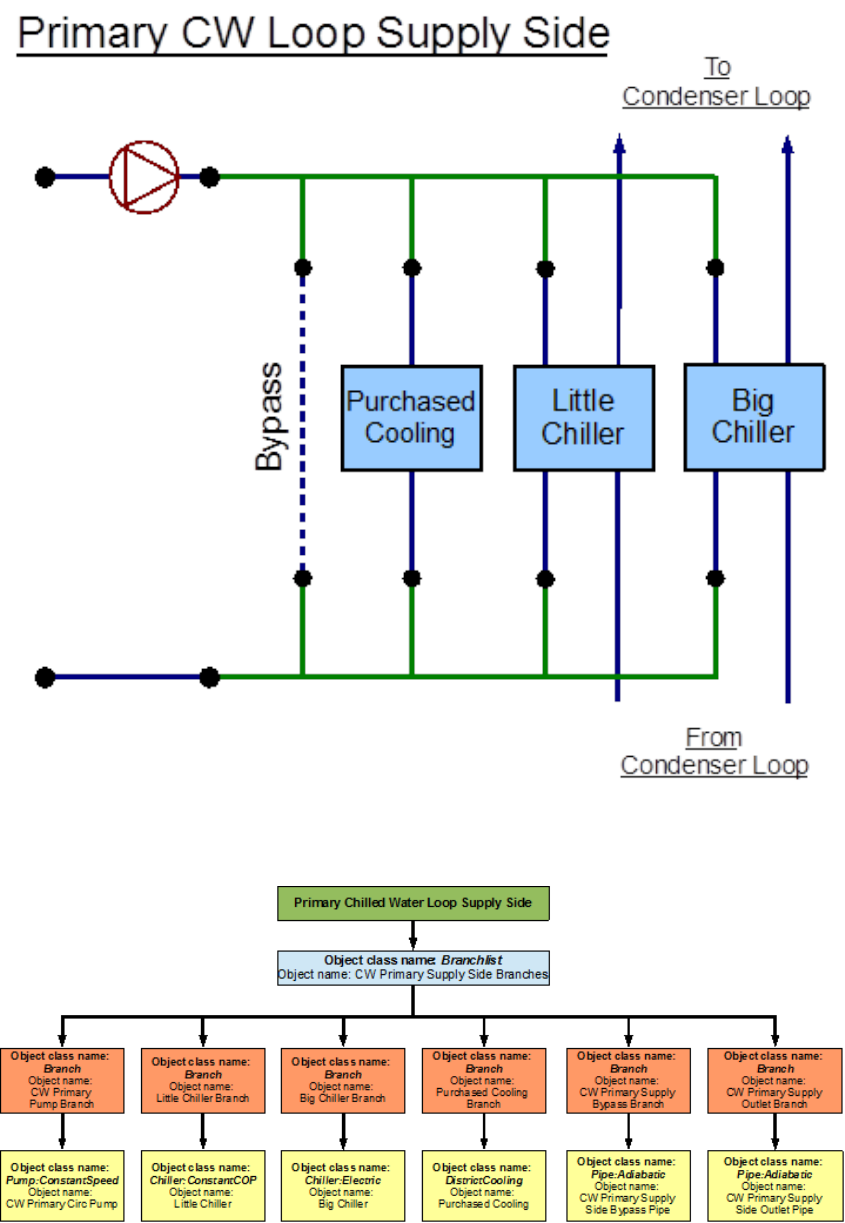
8.1 Primary Chilled Water Loop – Chiller(s) and pur-
chased cooling
The Secondary Cooling system is constructed by using a PlantLoop object. It uses two chillers
(a small constant COP chiller and a bigger electric chiller) and purchased district cooling.
Therefore, the supply side of the loop contains the chillers and the purchased cooling, and
the demand side contains one side of the plate heat exchanger. The loop is operated by using
plant equipment operation schemes and schedules. Refer to Figure 8.4 for a simple diagram
of the Primary Cooling Loop.
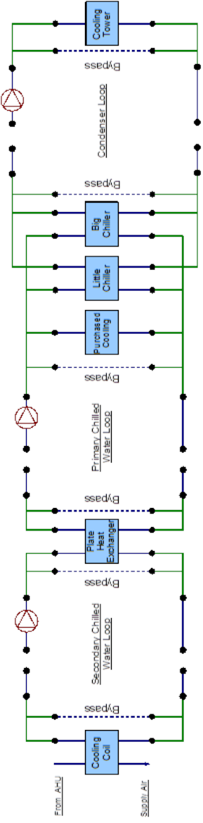
8.1. PRIMARY CHILLED WATER LOOP – CHILLER(S) AND PURCHASED COOLING71
Figure 8.3: EnergyPlus line diagram for the cooling system
72 CHAPTER 8. EXAMPLE SYSTEM 3: PRIMARY/SECONDARY PUMPING
Figure 8.4: Simple line diagram for the primary chilled water loop
8.1.1 Flowcharts for the Primary Chilled Water Loop Input Pro-
cess
This series of owcharts serve as a guide for identifying and inputting the Primary Chilled
Water loop and its components into the input le. The working uid in this loop is water.
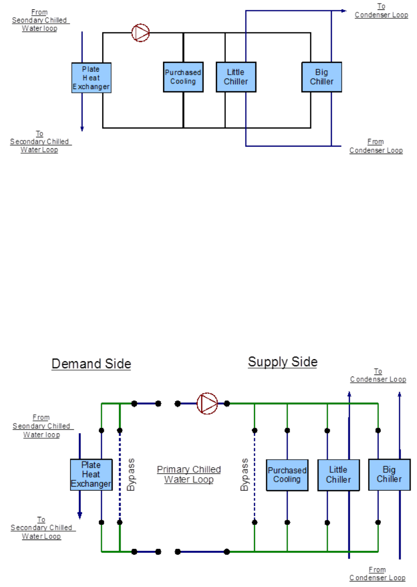
The EnergyPlus line diagram for this loop is provided in Figure 8.5. A simple owchart for
the separation of the half loops is provided in Figure 8.6.
Figure 8.5: EnergyPlus line diagram for the primary chilled water loop

8.1. PRIMARY CHILLED WATER LOOP – CHILLER(S) AND PURCHASED COOLING73
Figure 8.6: Simple owchart for the separation of half-loops in the primary chilled water
loop
8.1.1.1 Primary Cooling System Supply Side Loop Construction
The main components on the supply side half loop for the primary chilled water loop are two
chillers and district cooling object that supply chilled water and the constant speed pump
that circulates the chilled water through the loop. This pump (‘CW Primary Circ Pump’) is
the primary pump in the primary/secondary pumping setup. This half loop supplies chilled
water to the plate heat exchanger which is placed on the demand side half loop. The supply
side half loop contains six components, six branches, twelve nodes, and one splitter-mixer
pair. The EnergyPlus line diagram for the Primary Cooling loop supply side is provided in
Figure 8.7. The owchart for supply side branches and components is provided in Figure 8.8.
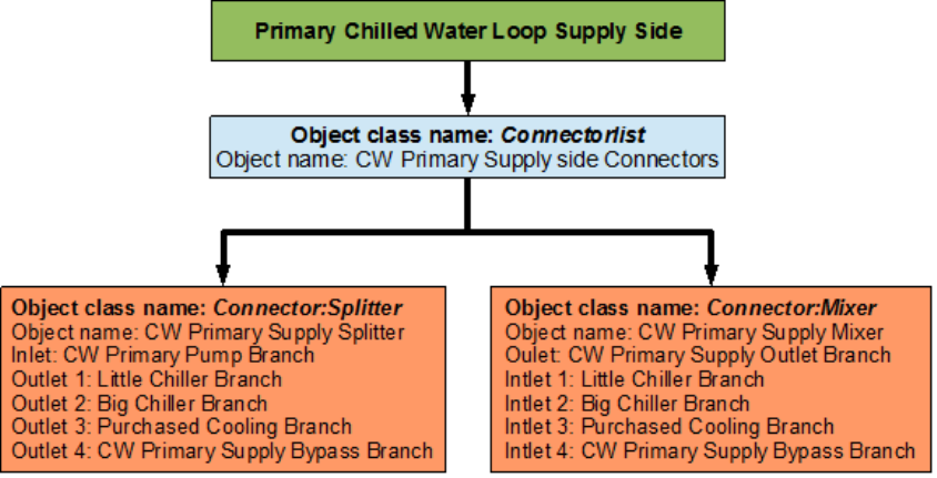
The owchart for supply side connectors is provided in Figure 8.9.
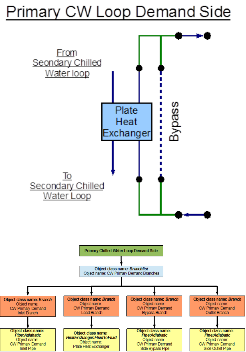
8.1.1.2 Primary Cooling Loop Demand Side Loop Construction
The main component on the demand side half loop is the plate heat exchanger that facilitates
the exchange of heat between the uids of the primary and secondary chilled water loop. The
plate heat exchanger will not be discussed in this loop. Instead the object will be discussed
in the supply side half loop of the secondary chilled water loop. This side of the loop also has
eight nodes, four components, four branches, and one splitter mixer pair. An EnergyPlus
schematic for the demand side is provided in Figure 8.10. The owchart for demand side
branch denition is provided in Figure 8.11. The owchart for the demand side connectors
is provided in Figure 8.12.
74 CHAPTER 8. EXAMPLE SYSTEM 3: PRIMARY/SECONDARY PUMPING
Figure 8.7: EnergyPlus line diagram for the supply side of the primary chilled water loop
Figure 8.8: Flowchart for Primary Cooling Loop supply side branches and components
8.1. PRIMARY CHILLED WATER LOOP – CHILLER(S) AND PURCHASED COOLING75
Figure 8.9: Flowchart for Primary Cooling Loop supply side branches and components
8.1.2 Flowcharts for Primary Chilled Water Loop Controls
The Primary Cooling loop is operated by using set-points, plant equipment operation schemes
and schedules. The plant equipment scheme for the on peak and o peak operation of the
chillers is very important
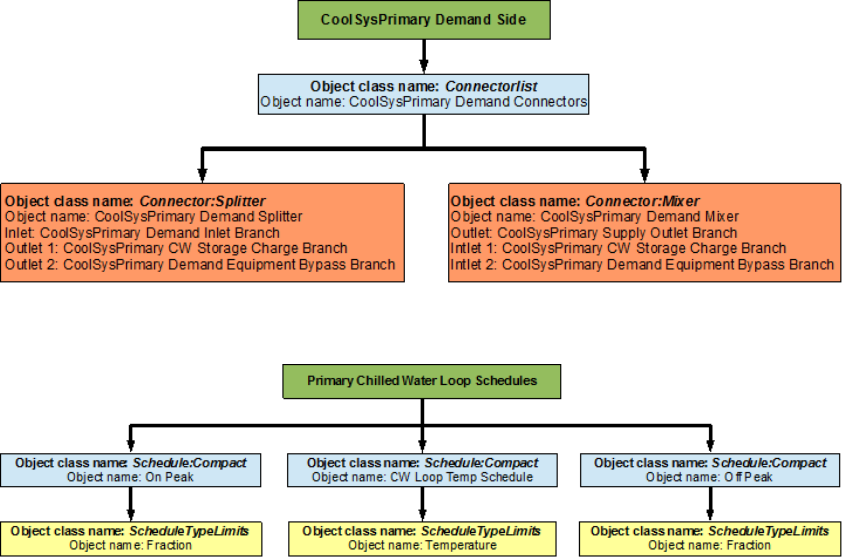
8.1.2.1 Primary Chilled Water Loop Schedules
The Primary Cooling loop uses three dierent schedules to operate properly. On Peak is
a compact schedule that denes the on peak hours (9 AM to 6 PM). The O Peak is a
compact schedule that denes the o peak hours (6 PM to 9 AM). This plant loop also uses
another compact schedule named CW Loop Temp Schedule declare that the temperature of
the chilled water loop outlet ow is 6.7 degrees Celsius at all times. This schedule is used by
the setpoint manager (Primary CW Loop Setpoint Manager). This schedule uses a schedule
type limit named Temperature, which denes the loop upper and lower temperature limits.
The owchart for Primary Cooling loop schedule denition is provided in Figure 8.13.
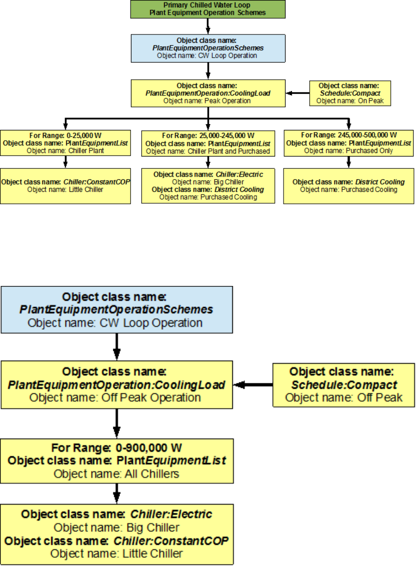
8.1.2.2 Primary Chilled Water Loop Plant Equipment Operation Schemes
There are two important operation schemes in the primary chilled water loop. The CW Loop
Operation plant equipment operation scheme used two schedules (On Peak and o Peak) to
control the supply components in the primary cooling loop. Peak Operation is set up such
that dierent components or combinations of components are operated for dierent values of
cooling load during the peak hours (9AM to 6PM everyday) of the simulation period. Up to
25,000 W of cooling load, the small constant COP chiller is operated, for 25,000-245,000 W
the big electric chiller and purchased cooling are used and for 245,000-500,000 W purchased
cooling is used. This setup serves to increase the eciency of the system. O Peak Operation
is set up such that both the chillers are operated during the o peak hours (6 PM to 9 AM).
76 CHAPTER 8. EXAMPLE SYSTEM 3: PRIMARY/SECONDARY PUMPING
Figure 8.10: EnergyPlus line diagram for the demand side of the primary chilled water loop
Figure 8.11: Flowchart for primary chilled water loop demand side branches and components
8.2. SECONDARY CHILLED WATER LOOP – PLATE HEAT EXCHANGER 77
Figure 8.12: Flowchart for primary chilled water loop demand side connectors
Figure 8.13: Flowchart for primary chilled water loop schedules
Flowcharts detailing the chilled water loop plant equipment operation schemes are provided
in Figure 8.14 and Figure 8.15.
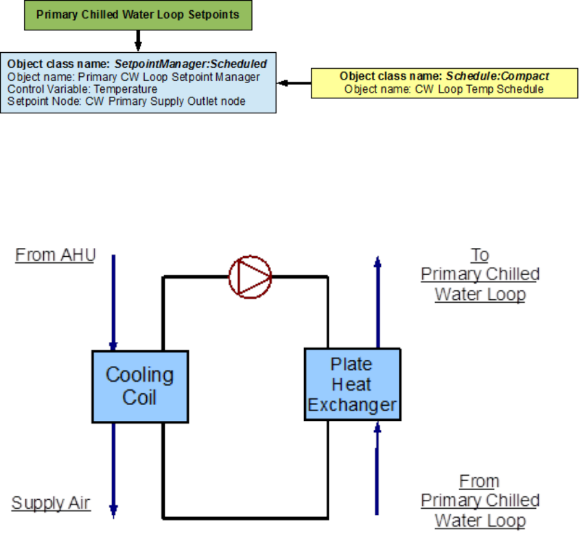
8.1.2.3 Primary Chilled Water Loop Setpoints
The Primary CW Loop Setpoint Manager uses the CW Loop Temp Schedule to set a tem-
perature control point at the CW Primary Supply Outlet Node. This setpoint allows the
program to control the temperature at the node by operating the components in the Pri-
mary Cooling loop. Since, setpoint managers are high-level control objects, their usefulness
is realized in much more complex systems, where multiple nodes have to be monitored in
order to operate the system properly. A owchart for Secondary Cooling loop setpoints is
provided in Figure 8.16.
8.2 Secondary Chilled Water Loop – Plate Heat Ex-
changer
The Secondary Cooling system is constructed by using a PlantLoop object, the working uid
in this loop is water. It uses one side of a plate heat exchanger (modeled using a HeatEx-
changer:FluidToFluid object) to supply chilled water to a cooling coil (modeled by using
aCoil:Cooling:DetailedGeometry object). Therefore, the supply side of the loop contains
the heat exchanger and the demand side contains the cooling coil. The loop is operated by
78 CHAPTER 8. EXAMPLE SYSTEM 3: PRIMARY/SECONDARY PUMPING
Figure 8.14: Flowchart for on peak operation of the primary chilled water loop
Figure 8.15: Flowchart for o peak plant operation of the primary chilled water loop
8.2. SECONDARY CHILLED WATER LOOP – PLATE HEAT EXCHANGER 79
Figure 8.16: Flowchart for Primary Cooling Loop setpoints
using plant equipment operation schemes, and schedules. Refer to Figure 8.17 for a simple
diagram of the secondary chilled water loop.
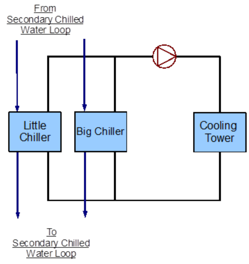
Figure 8.17: Simple line diagram for the secondary chilled water loop
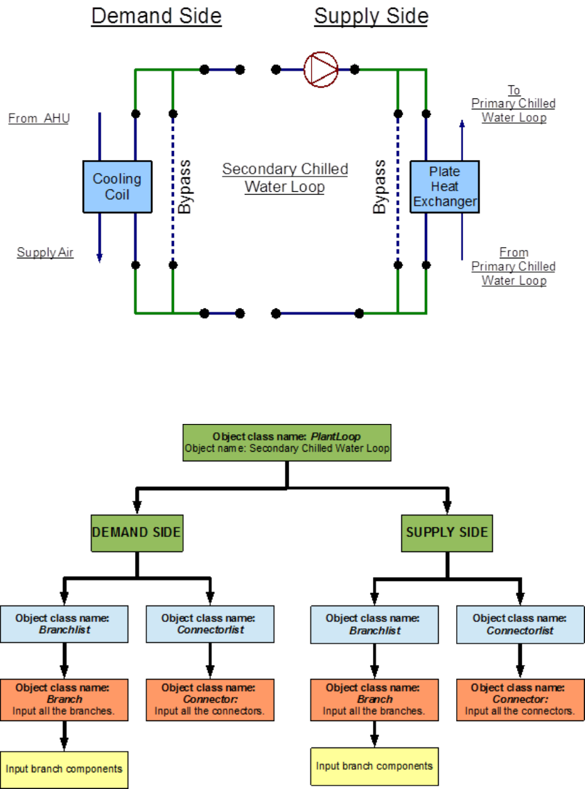
8.2.1 Flowcharts for the Secondary Chilled Water Loop Input Pro-
cess
This series of owcharts serve as a guide for identifying and inputting the secondary chilled
water loop and its components into the input le. The EnergyPlus line diagram for this loop
is provided in Figure 8.18. A simple owchart for the separation of the half loops is provided
in Figure 8.19.
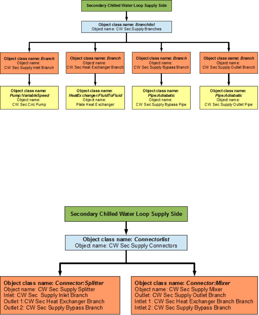
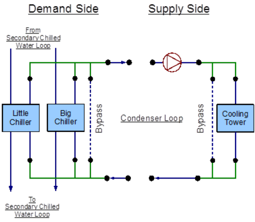
8.2.1.1 Secondary Chilled Water Loop Supply Side Loop Construction
The main components on the supply side half loop for the Secondary Cooling System are
the plate heat exchanger that supplies the chilled water and the variable speed pump that
circulates the chilled water through the loop. The variable speed pump (named ‘CW Sec
Circ Pump’) is the secondary pump in the primary/secondary pumping setup. This half loop
80 CHAPTER 8. EXAMPLE SYSTEM 3: PRIMARY/SECONDARY PUMPING
Figure 8.18: EnergyPlus line diagram for the secondary chilled water loop
Figure 8.19: Simple ow chart for separation on half loops in the secondary chilled water
loop
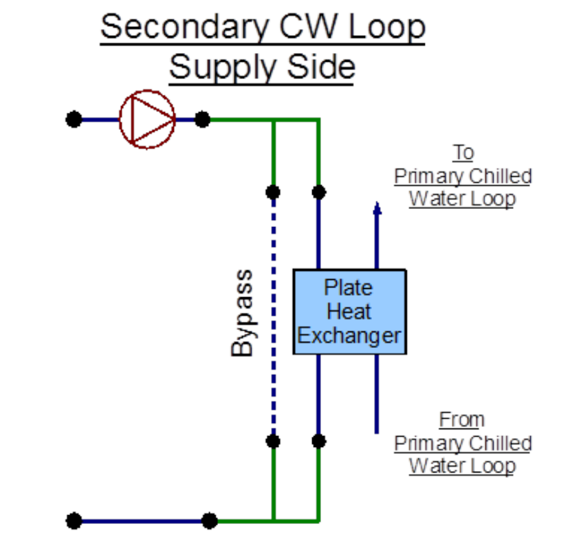
8.2. SECONDARY CHILLED WATER LOOP – PLATE HEAT EXCHANGER 81
supplies chilled water to a cooling coil on the demand side half loop. The supply side half
loop contains four components, four branches, eight nodes, and one splitter-mixer pair. The
EnergyPlus line diagram for the secondary chilled water loop supply side is provided in Fig-
ure 8.20. The owchart for supply side branches and components is provided in Figure 8.21.
The owchart for supply side connectors is provided in Figure 8.22.
Figure 8.20: EnergyPlus line diagram for the supply side of the secondary chilled water loop
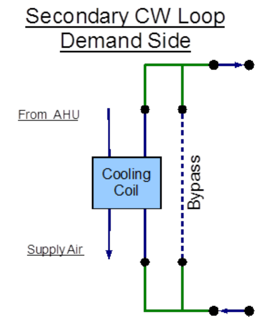
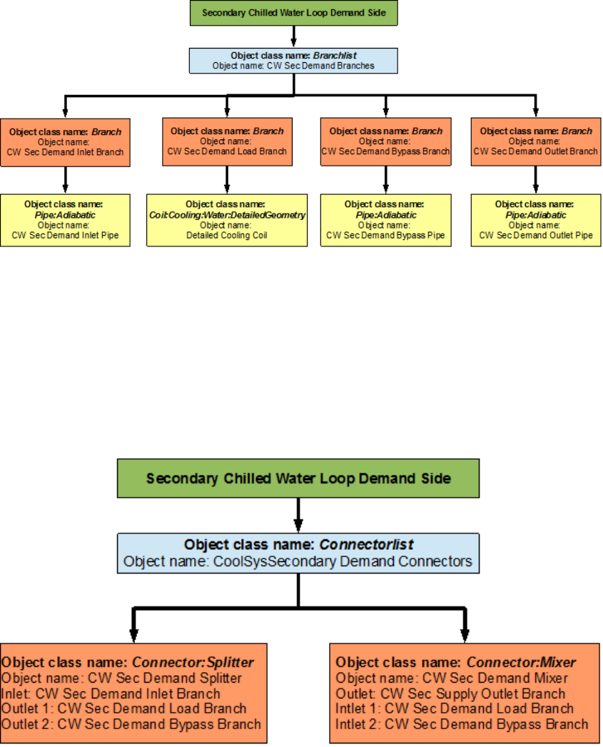
8.2.1.2 Secondary Chilled Water Loop Demand Side Loop Construction
The main component on the demand side half loop is the Cooling Coil that cools the air in
the building by using the chilled water that is supplied by the plate heat exchanger. This
side of the loop also has eight nodes, four components, four branches, and one splitter-mixer
pair. An EnergyPlus schematic for the demand side is provided in Figure 8.23. The owchart
for demand side branch denition is provided in Figure 8.24. The owchart for the demand
side connectors is provided in Figure 8.25.
82 CHAPTER 8. EXAMPLE SYSTEM 3: PRIMARY/SECONDARY PUMPING
Figure 8.21: Flowchart for secondary chilled water loop supply side branches and components
Figure 8.22: Flowchart for secondary chilled water loop supply side connectors
8.2. SECONDARY CHILLED WATER LOOP – PLATE HEAT EXCHANGER 83
Figure 8.23: EnergyPlus line diagram for the demand side of the secondary chilled water
loop
84 CHAPTER 8. EXAMPLE SYSTEM 3: PRIMARY/SECONDARY PUMPING
Figure 8.24: Flowchart for secondary chilled water loop demand side branches and compo-
nents
Figure 8.25: Flowchart for secondary chilled water loop demand side connectors
8.2. SECONDARY CHILLED WATER LOOP – PLATE HEAT EXCHANGER 85
8.2.2 Flowcharts for secondary chilled water loop Controls
The secondary chilled water loop is operated by using set-points, plant equipment operation
schemes and schedules.
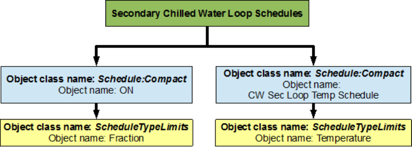
8.2.2.1 Secondary Chilled Water Loop Schedules
The owchart for Primary Cooling loop schedule denition is provided in Figure 8.26. The
Secondary Cooling loop uses two dierent schedules to operate properly. ON is a compact
schedule that keeps the plate heat exchanger running at all times of the day, this compact
schedule uses a continuous ScheduleTypeLimit (Fraction) which denes that the value of On
is 1 and that of O is 0. This plant loop also uses another compact schedule named CW
Sec Loop Temp Schedule declares that the outlet temperature of the Secondary Cooling loop
should be 6.67 degrees Celsius at any time; this schedule is used by the setpoint manager (CW
Sec Loop Setpoint Manager). This schedule uses a schedule type limit named Temperature,
which denes the loop upper and lower temperature limits.
Figure 8.26: Flowchart for secondary chilled water loop schedules
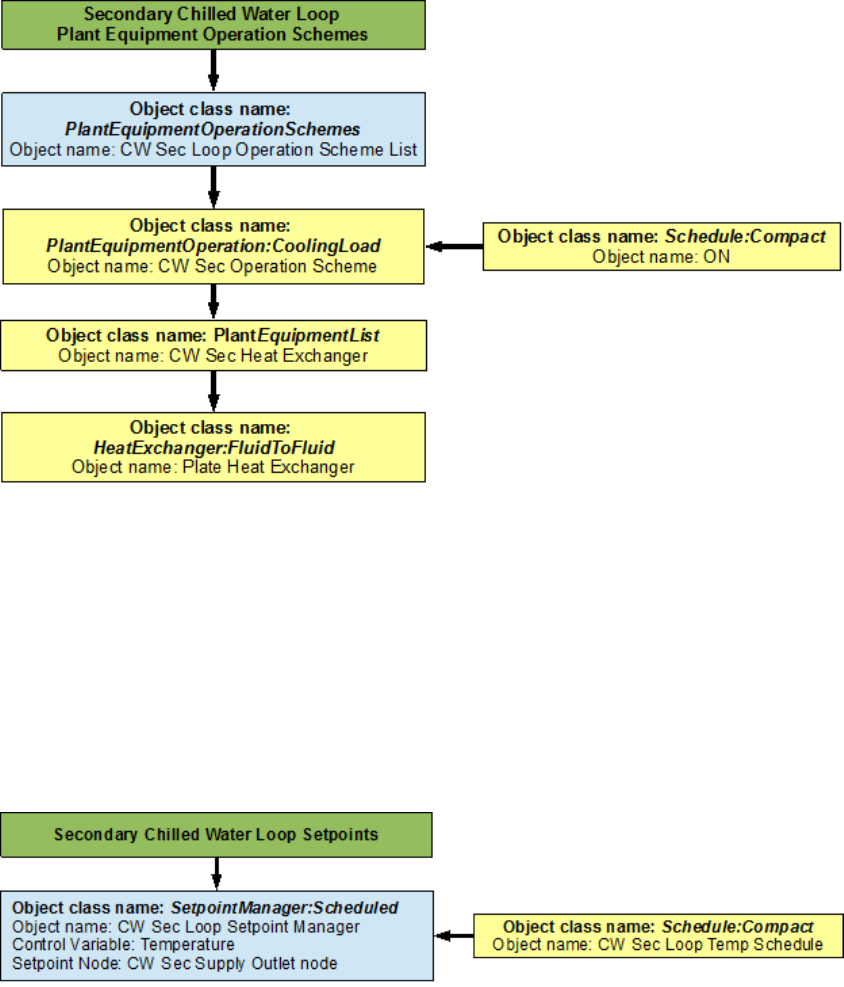
8.2.2.2 Secondary Chilled Water Loop Plant Equipment Operation Schemes
The PlantEquipmentOperationschemes object uses the ON schedule and the CW Sec Op-
eration Scheme objects to set the range of the demand loads for which the heat exchanger
is operated during the simulation period. A owchart detailing the secondary chilled water
loop plant equipment operation schemes is provided in Figure 8.27.
8.2.2.3 Secondary Chilled Water Loop Setpoints
The CW Sec Loop Setpoint Manager uses the CW Sec Loop Temp Schedule to set a temper-
ature control point at the CW Sec Supply Outlet Node. This setpoint allows the program to
control the temperature at the node by operating the components in the Secondary Cooling
loop. A owchart for Secondary Cooling loop setpoints is provided in Figure 8.28.
86 CHAPTER 8. EXAMPLE SYSTEM 3: PRIMARY/SECONDARY PUMPING
Figure 8.27: Flowchart for secondary chilled water loop plant equipment operation schemes
Figure 8.28: Flowchart for secondary chilled water loop setpoints
8.3. PRIMARY/SECONDARY PUMPING 87
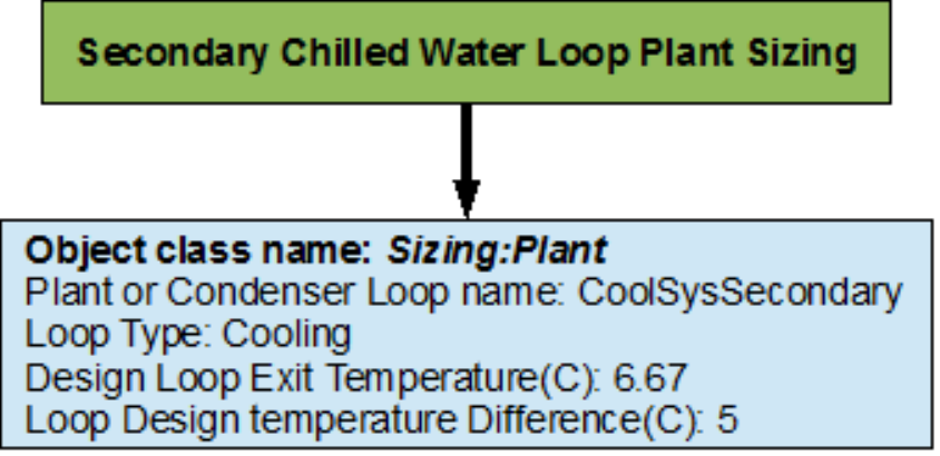
8.2.2.4 Secondary Chilled Water Loop Sizing
The secondary chilled water loop is sized such a way that the design loop exit temperature
is 6.67 degrees Celsius, and the loop design temperature dierence is 5 degrees Celsius. A
owchart for the chilled water loop sizing is provided in Figure 8.29.
Figure 8.29: Flowchart for secondary chilled water loop sizing
8.3 Primary/Secondary Pumping
As mentioned in sections Primary Cooling System Supply Side Loop Construction and Sec-
ondary Chilled Water Loop Supply Side Loop Construction, the CW primary Circ Pump and
the CW Sec Circ Pump function as the primary/secondary (respectively) pumping system.
The primary pump is a constant speed pump that circulates chilled water at a constant
ow rate through one side the plate heat exchanger in the primary chilled water loop. The
secondary pump is a variable speed pump that circulates chilled water at a variable ow rate
through the other side of the plate heat exchanger depending on the demand load.
8.4 Condenser Loop - Cooling Tower
The Condenser Loop is constructed by using a PlantLoop object. It uses a cooling tower
(modeled by using a CoolingTower:SingleSpeed object class) and a variable speed pump
(modeled by using a Pump:VariableSpeed) to supply cooling water to the chillers in the
primary cooling loop. Therefore, the supply side of the loop contains the Cooling Tower
and the demand side contains the chillers. The loop is operated by using plant equipment
operation schemes, and schedules. Refer to Figure 8.30 for a simple diagram of the Condenser
Loop.
88 CHAPTER 8. EXAMPLE SYSTEM 3: PRIMARY/SECONDARY PUMPING
Figure 8.30: Simple line diagram for the condenser loop
8.4. CONDENSER LOOP - COOLING TOWER 89
8.4.1 Flowcharts for the Condenser Loop Input Process
This series of owcharts serve as a guide for identifying and inputting the Condenser Loop and
its components into the input le. The EnergyPlus line diagram for this loop is provided in
Figure 8.31. A simple owchart for the separation of the half loops is provided in Figure 8.32.
Figure 8.31: EnergyPlus line diagram for the condenser loop
8.4.1.1 Condenser Loop Supply Side Construction
The main components on the supply side half loop for the Condenser Loop are the Cooling
Tower that supplies the cooling water and the variable speed pump that circulates the
cooling water through the loop. This half loop supplies cooling water to the chillers on the
demand side half loop. The supply side half loop contains four components, four branches,
eight nodes, and one splitter-mixer pair. The EnergyPlus line diagram for the Condenser
loop supply side is provided in Figure 8.33. The owchart for supply side branches and
components is provided in Figure 8.34. The owchart for supply side connectors is provided
in Figure 8.35.

90 CHAPTER 8. EXAMPLE SYSTEM 3: PRIMARY/SECONDARY PUMPING
Figure 8.32: Simple ow chart for separation on half loops in the condenser loop
8.4.1.2 Condenser Loop Demand Side Construction
The main components on the demand side half loop are the small constant COP chiller and
the bigger electric chiller that use the cooling water supplied by the cooling tower. The
chillers are in turn used to supply chilled water in the Primary Cooling loop. This side
of the loop also has ten nodes, ve components, ve branches and one splitter-mixer pair.
An EnergyPlus schematic for the demand side is provided in Figure 8.36. The owchart for
demand side branch denition is provided in Figure 8.37. The owchart for the demand side
connectors is provided in Figure 8.38.
8.4.2 Flowcharts for Condenser Loop Controls
The Condenser loop is operated by using set-points, plant equipment operation schemes and
schedules.
8.4.2.1 Condenser Loop Schedules
The owchart for condenser loop schedule denition is provided in Figure 8.39. The Con-
denser loop uses one schedule to operate properly. ON is a compact schedule that keeps
the Cooling Tower On at all times of the day, this compact schedule uses a continuous
ScheduleTypeLimit (Fraction) which denes that the value of On is 1 and that of O is 0.
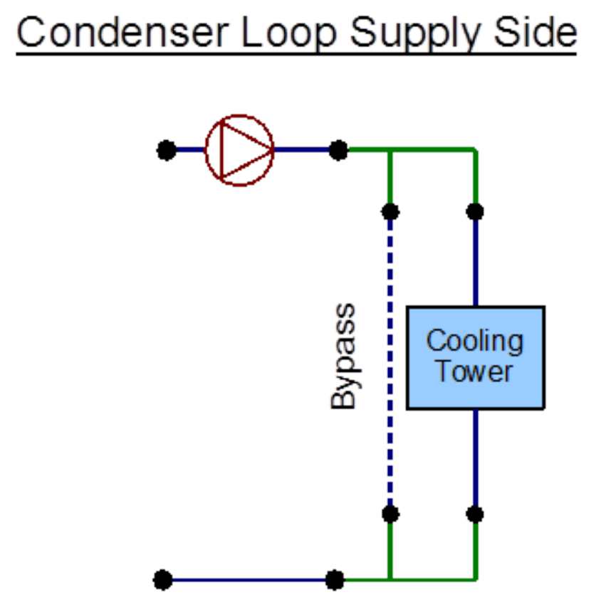
8.4. CONDENSER LOOP - COOLING TOWER 91
Figure 8.33: EnergyPlus line diagram for the supply side of the Condenser Loop
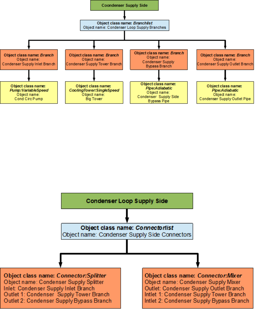
92 CHAPTER 8. EXAMPLE SYSTEM 3: PRIMARY/SECONDARY PUMPING
Figure 8.34: Flowchart for Condenser Loop supply side branches and components
Figure 8.35: Flowchart for Condenser Loop supply side connectors
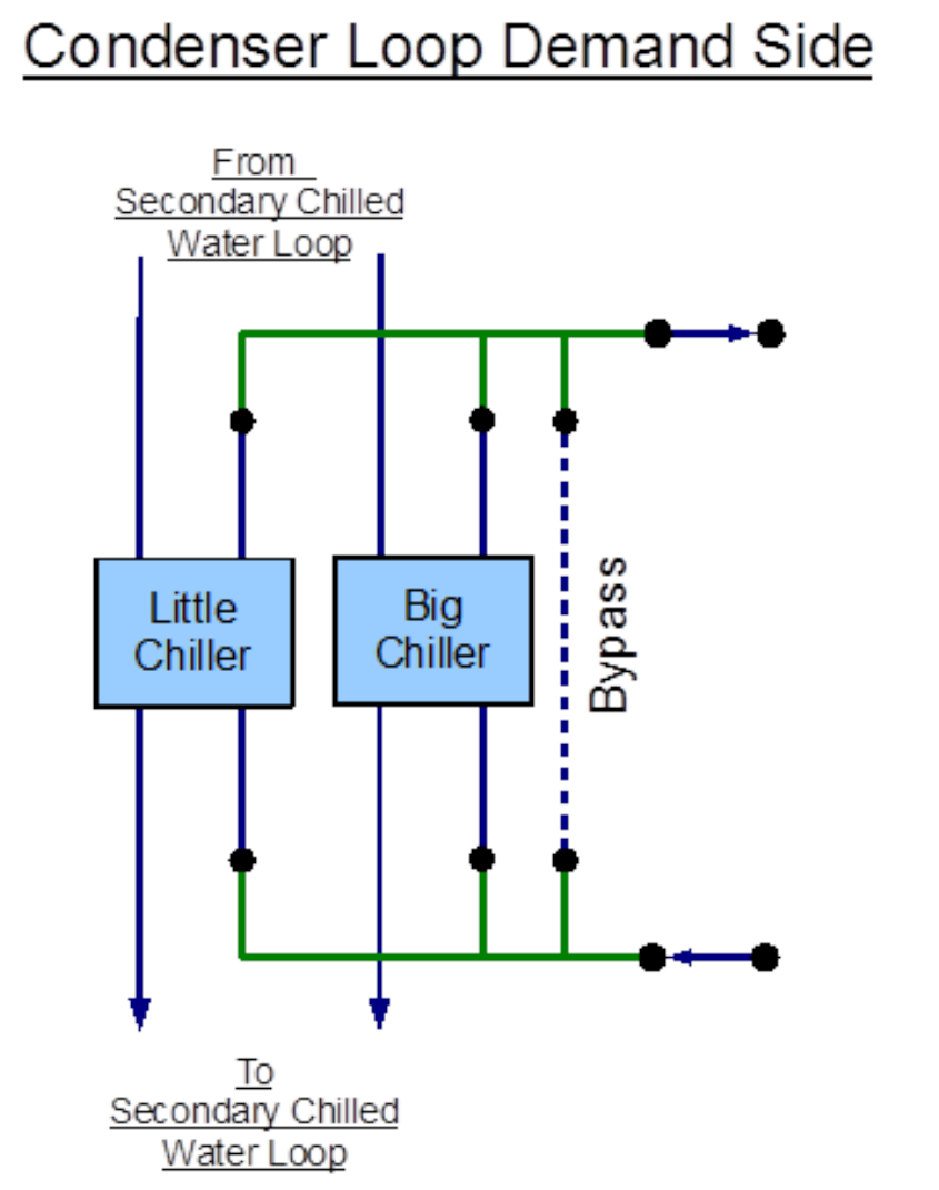
8.4. CONDENSER LOOP - COOLING TOWER 93
Figure 8.36: EnergyPlus line diagram for the demand side of the Condenser Loop
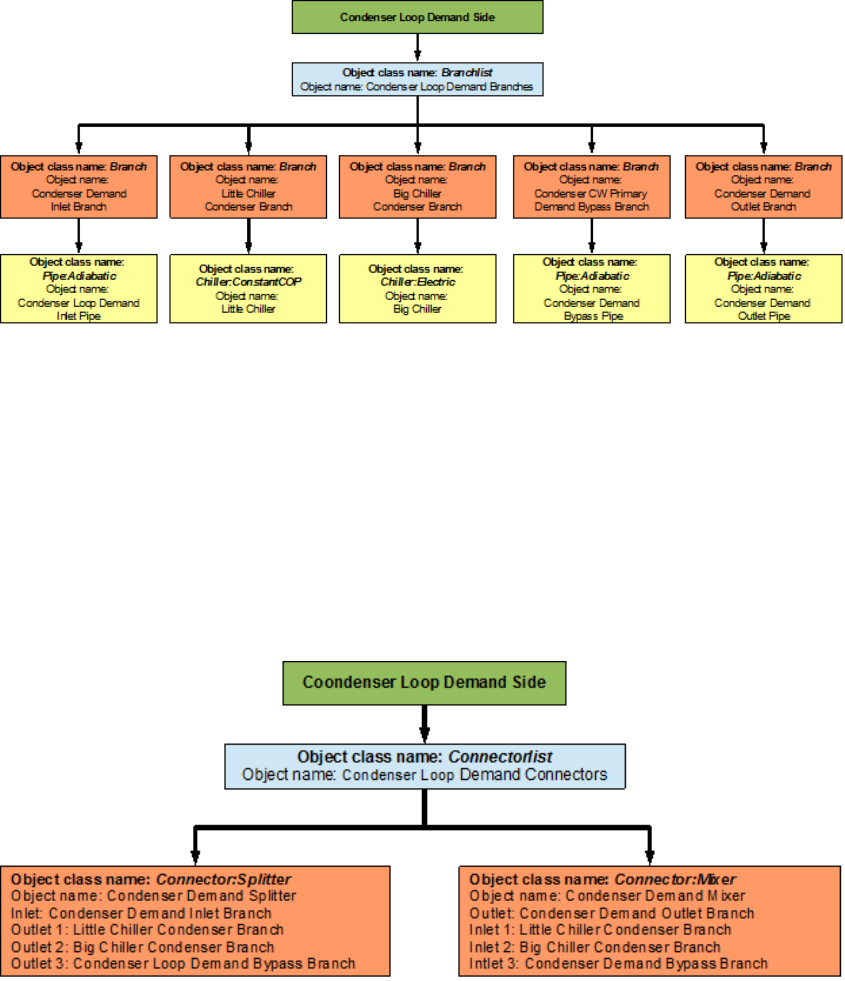
94 CHAPTER 8. EXAMPLE SYSTEM 3: PRIMARY/SECONDARY PUMPING
Figure 8.37: Flowchart for Condenser Loop demand side branches and components
Figure 8.38: Flowchart for Condenser Loop demand side connectors
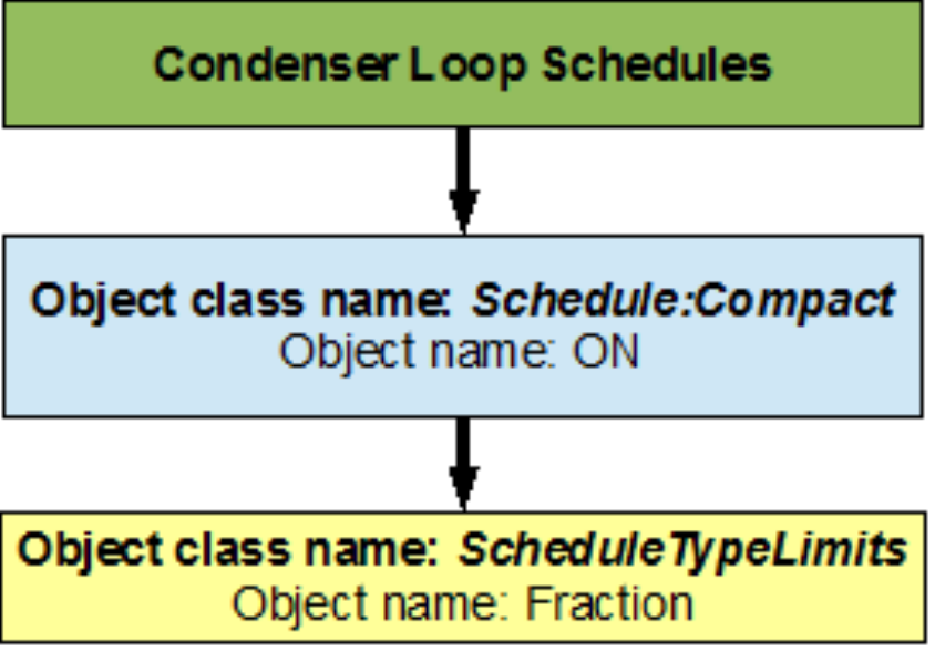
8.4. CONDENSER LOOP - COOLING TOWER 95
Figure 8.39: Flowchart for condenser loop schedules
8.4.2.2 Condenser Loop Plant Equipment Operation Schemes
The PlantEquipmentOperationschemes object uses the ON schedule and the Tower Operation
objects to set the range of demand loads for which the cooling tower is operated during the
simulation period. A owchart detailing the Condenser Loop plant equipment operation
schemes is provided in Figure 8.40.
8.4.2.3 Condenser Loop Setpoints
The MyCondenserControl setpoint manager places a temperature setpoint at the Condenser
Supply Outlet Node. The temperature at this point is controlled with respect to the outdoor
air wet bulb temperature at that point in the simulation. The outdoor air wet bulb temper-
ature is obtained from the weather data at the location of the simulation. A owchart for
Secondary Cooling loop setpoints is provided in Figure 8.41.
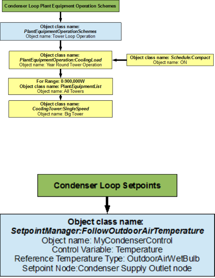
96 CHAPTER 8. EXAMPLE SYSTEM 3: PRIMARY/SECONDARY PUMPING
Figure 8.40: Flowchart for Condenser Loop plant equipment operation schemes
Figure 8.41: Flowchart for Condenser Loop setpoints
Chapter 9
References
Reed, M. A., Davis, C. 2007, “Chilled Water Plant Savings at No Cost.” ASHRAE Journal
49(7), 38-44.
Hyman, L. B., Little, D. 2004, “Overcoming Low Delta T, Negative Delta P At Large
University Campus.” ASHRAE Journal 46(2), 28-34.
97
