Programming In Scala A Comprehensive Step By Guide, Third Edition Martin Odersky
User Manual:
Open the PDF directly: View PDF ![]() .
.
Page Count: 592 [warning: Documents this large are best viewed by clicking the View PDF Link!]
- Praise for the earlier editions of Programming in Scala
- Table of Contents
- Foreword
- Acknowledgments
- Introduction
- A Scalable Language
- First Steps in Scala
- Next Steps in Scala
- STEP 7. PARAMETERIZE ARRAYS WITH TYPES
- STEP 8. USE LISTS
- WHY NOT APPEND TO LISTS?
- STEP 9. USE TUPLES
- ACCESSING THE ELEMENTS OF A TUPLE
- STEP 10. USE SETS AND MAPS
- Listing 3.5 - Creating, initializing, and using an immutable set.
- Figure 3.2 - Class hierarchy for Scala sets.
- Listing 3.6 - Creating, initializing, and using a mutable set.
- Figure 3.3 - Class hierarchy for Scala maps.
- Listing 3.7 - Creating, initializing, and using a mutable map.
- Listing 3.8 - Creating, initializing, and using an immutable map.
- STEP 11. LEARN TO RECOGNIZE THE FUNCTIONAL STYLE
- A BALANCED ATTITUDE FOR SCALA PROGRAMMERS
- STEP 12. READ LINES FROM A FILE
- CONCLUSION
- Chapter 4
- Classes and Objects
- Basic Types and Operations
- 5.1 SOME BASIC TYPES
- 5.2 LITERALS
- FAST TRACK FOR JAVA PROGRAMMERS
- 5.3 STRING INTERPOLATION
- 5.4 OPERATORS ARE METHODS
- ANY METHOD CAN BE AN OPERATOR
- FAST TRACK FOR JAVA PROGRAMMERS
- 5.5 ARITHMETIC OPERATIONS
- 5.6 RELATIONAL AND LOGICAL OPERATIONS
- 5.7 BITWISE OPERATIONS
- 5.8 OBJECT EQUALITY
- HOW SCALA'S == DIFFERS FROM JAVA'S
- 5.9 OPERATOR PRECEDENCE AND ASSOCIATIVITY
- 5.10 RICH WRAPPERS
- 5.11 CONCLUSION
- Chapter 6
- Functional Objects
- 6.1 A SPECIFICATION FOR CLASS RATIONAL
- 6.2 CONSTRUCTING A RATIONAL
- IMMUTABLE OBJECT TRADE-OFFS
- 6.3 REIMPLEMENTING THE TOSTRING METHOD
- 6.4 CHECKING PRECONDITIONS
- 6.5 ADDING FIELDS
- 6.6 SELF REFERENCES
- 6.7 AUXILIARY CONSTRUCTORS
- 6.8 PRIVATE FIELDS AND METHODS
- 6.9 DEFINING OPERATORS
- 6.10 IDENTIFIERS IN SCALA
- 6.11 METHOD OVERLOADING
- 6.12 IMPLICIT CONVERSIONS
- 6.13 A WORD OF CAUTION
- 6.14 CONCLUSION
- Chapter 7
- Built-in Control Structures
- 7.1 IF EXPRESSIONS
- 7.2 WHILE LOOPS
- 7.3 FOR EXPRESSIONS
- 7.4 EXCEPTION HANDLING WITH TRY EXPRESSIONS
- 7.5 MATCH EXPRESSIONS
- 7.6 LIVING WITHOUT BREAK AND CONTINUE
- 7.7 VARIABLE SCOPE
- FAST TRACK FOR JAVA PROGRAMMERS
- 7.8 REFACTORING IMPERATIVE-STYLE CODE
- 7.9 CONCLUSION
- Chapter 8
- Functions and Closures
- Control Abstraction
- Composition and Inheritance
- 10.1 A TWO-DIMENSIONAL LAYOUT LIBRARY
- 10.2 ABSTRACT CLASSES
- 10.3 DEFINING PARAMETERLESS METHODS
- 10.4 EXTENDING CLASSES
- 10.5 OVERRIDING METHODS AND FIELDS
- 10.6 DEFINING PARAMETRIC FIELDS
- 10.7 INVOKING SUPERCLASS CONSTRUCTORS
- 10.8 USING OVERRIDE MODIFIERS
- 10.9 POLYMORPHISM AND DYNAMIC BINDING
- 10.10 DECLARING FINAL MEMBERS
- 10.11 USING COMPOSITION AND INHERITANCE
- 10.12 IMPLEMENTING ABOVE, BESIDE, AND TOSTRING
- 10.13 DEFINING A FACTORY OBJECT
- 10.14 HEIGHTEN AND WIDEN
- 10.15 PUTTING IT ALL TOGETHER
- 10.16 CONCLUSION
- Chapter 11
- Scala's Hierarchy
- Traits
- Packages and Imports
- 13.1 PUTTING CODE IN PACKAGES
- 13.2 CONCISE ACCESS TO RELATED CODE
- 13.3 IMPORTS
- SCALA'S FLEXIBLE IMPORTS
- 13.4 IMPLICIT IMPORTS
- 13.5 ACCESS MODIFIERS
- 13.6 PACKAGE OBJECTS
- 13.7 CONCLUSION
- Chapter 14
- Assertions and Tests
- Case Classes and Pattern Matching
- 15.1 A SIMPLE EXAMPLE
- 15.2 KINDS OF PATTERNS
- 15.3 PATTERN GUARDS
- 15.4 PATTERN OVERLAPS
- 15.5 SEALED CLASSES
- 15.6 THE OPTION TYPE
- 15.7 PATTERNS EVERYWHERE
- 15.8 A LARGER EXAMPLE
- 15.9 CONCLUSION
- Chapter 16
- Working with Lists
- 16.1 LIST LITERALS
- 16.2 THE LIST TYPE
- 16.3 CONSTRUCTING LISTS
- 16.4 BASIC OPERATIONS ON LISTS
- 16.5 LIST PATTERNS
- ABOUT PATTERN MATCHING ON LISTS
- 16.6 FIRST-ORDER METHODS ON CLASS LIST
- Concatenating two lists
- The Divide and Conquer principle
- Taking the length of a list: length
- Accessing the end of a list: init and last
- Reversing lists: reverse
- Prefixes and suffixes: drop, take, and splitAt
- Element selection: apply and indices
- Flattening a list of lists: flatten
- Zipping lists: zip and unzip
- Displaying lists: toString and mkString
- Converting lists: iterator, toArray, copyToArray
- Example: Merge sort
- THE FAST TRACK
- 16.7 HIGHER-ORDER METHODS ON CLASS LIST
- 16.8 METHODS OF THE LIST OBJECT
- 16.9 PROCESSING MULTIPLE LISTS TOGETHER
- THE FAST TRACK
- 16.10 UNDERSTANDING SCALA'S TYPE INFERENCE ALGORITHM
- 16.11 CONCLUSION
- Chapter 17
- Working with Other Collections
- Mutable Objects
- Type Parameterization
- Abstract Members
- 20.1 A QUICK TOUR OF ABSTRACT MEMBERS
- 20.2 TYPE MEMBERS
- 20.3 ABSTRACT VALS
- 20.4 ABSTRACT VARS
- 20.5 INITIALIZING ABSTRACT VALS
- LAZY FUNCTIONAL LANGUAGES
- 20.6 ABSTRACT TYPES
- 20.7 PATH-DEPENDENT TYPES
- 20.8 REFINEMENT TYPES
- 20.9 ENUMERATIONS
- 20.10 CASE STUDY: CURRENCIES
- 20.11 CONCLUSION
- Chapter 21
- Implicit Conversions and Parameters
- Implementing Lists
- For Expressions Revisited
- Collections in Depth
- 24.1 MUTABLE AND IMMUTABLE COLLECTIONS
- 24.2 COLLECTIONS CONSISTENCY
- 24.3 TRAIT TRAVERSABLE
- 24.4 TRAIT ITERABLE
- 24.5 THE SEQUENCE TRAITS SEQ, INDEXEDSEQ, AND LINEARSEQ
- 24.6 SETS
- 24.7 MAPS
- 24.8 CONCRETE IMMUTABLE COLLECTION CLASSES
- 24.9 CONCRETE MUTABLE COLLECTION CLASSES
- 24.10 ARRAYS
- 24.11 STRINGS
- 24.12 PERFORMANCE CHARACTERISTICS
- 24.13 EQUALITY
- 24.14 VIEWS
- 24.15 ITERATORS
- 24.16 CREATING COLLECTIONS FROM SCRATCH
- 24.17 CONVERSIONS BETWEEN JAVA AND SCALA COLLECTIONS
- 24.18 CONCLUSION
- Chapter 25
- The Architecture of Scala Collections
- Extractors
- Working with XML
- Modular Programming Using Objects
- Object Equality
- 30.1 EQUALITY IN SCALA
- 30.2 WRITING AN EQUALITY METHOD
- 30.3 DEFINING EQUALITY FOR PARAMETERIZED TYPES
- 30.4 RECIPES FOR EQUALS AND HASHCODE
- 30.5 CONCLUSION
- Chapter 31
- Combining Scala and Java
- Futures and Concurrency
- 32.1 TROUBLE IN PARADISE
- 32.2 ASYNCHRONOUS EXECUTION AND TRYS
- 32.3 WORKING WITH FUTURES
- Transforming Futures with map
- Transforming Futures with for expressions
- Creating the Future: Future.failed, Future.successful, Future.fromTry, and Promises
- Filtering: filter and collect
- Dealing with failure: failed, fallBackTo, recover, and recoverWith
- Mapping both possibilities: transform
- Combining futures: zip, Future.fold, Future.reduce, Future.sequence, and Future.traverse
- Performing side-effects: foreach, onComplete, and andThen
- Other methods added in 2.12: flatten, zipWith, and transformWith
- 32.4 TESTING WITH FUTURES
- 32.5 CONCLUSION
- Chapter 33
- Combinator Parsing
- 33.1 EXAMPLE: ARITHMETIC EXPRESSIONS
- 33.2 RUNNING YOUR PARSER
- 33.3 BASIC REGULAR EXPRESSION PARSERS
- 33.4 ANOTHER EXAMPLE: JSON
- 33.5 PARSER OUTPUT
- TURNING OFF SEMICOLON INFERENCE
- CHOOSING BETWEEN SYMBOLIC AND ALPHABETIC NAMES
- 33.6 IMPLEMENTING COMBINATOR PARSERS
- 33.7 STRING LITERALS AND REGULAR EXPRESSIONS
- 33.8 LEXING AND PARSING
- 33.9 ERROR REPORTING
- 33.10 BACKTRACKING VERSUS LL(1)
- 33.11 CONCLUSION
- Chapter 34
- GUI Programming
- The SCells Spreadsheet
- Scala Scripts on Unix and Windows
- Glossary
- Bibliography
- About the Authors
Praise for the earlier editions of Programming
in Scala
Programming in Scala is probably one of the best programming books I've ever read. I like the writing
style, the brevity, and the thorough explanations. The book seems to answer every question as it enters
my mind—it's always one step ahead of me. The authors don't just give you some code and take things
for granted. They give you the meat so you really understand what's going on. I really like that.
- Ken Egervari, Chief Software Architect
Programming in Scala is clearly written, thorough, and easy to follow. It has great examples and useful
tips throughout. It has enabled our organization to ramp up on the Scala language quickly and
efficiently. This book is great for any programmer who is trying to wrap their head around the
flexibility and elegance of the Scala language.
- Larry Morroni, Owner, Morroni Technologies, Inc.
The Programming in Scala book serves as an excellent tutorial to the Scala language. Working through
the book, it flows well with each chapter building on concepts and examples described in earlier ones.
The book takes care to explain the language constructs in depth, often providing examples of how the
language differs from Java. As well as the main language, there is also some coverage of libraries such
as containers and actors.
I have found the book really easy to work through, and it is probably one of the better written technical
books I have read recently. I really would recommend this book to any programmer wanting to find out
more about the Scala language.
- Matthew Todd
I am amazed by the effort undertaken by the authors of Programming in Scala. This book is an
invaluable guide to what I like to call Scala the Platform: a vehicle to better coding, a constant
inspiration for scalable software design and implementation. If only I had Scala in its present mature
state and this book on my desk back in 2003, when co-designing and implementing parts of the Athens
2004 Olympic Games Portal infrastructure!
To all readers: No matter what your programming background is, I feel you will find programming in
Scala liberating and this book will be a loyal friend in the journey.
- Christos KK Loverdos, Software Consultant, Researcher
Programming in Scala is a superb in-depth introduction to Scala, and it's also an excellent reference. I'd
say that it occupies a prominent place on my bookshelf, except that I'm still carrying it around with me
nearly everywhere I go.
- Brian Clapper, President, ArdenTex, Inc.
Great book, well written with thoughtful examples. I would recommend it to both seasoned
programmers and newbies.
- Howard Lovatt
The book Programming in Scala is not only about how, but more importantly, why to develop programs
in this new programming language. The book's pragmatic approach in introducing the power of
combining object-oriented and functional programming leaves the reader without any doubts as to what
Scala really is.
- Dr. Ervin Varga, CEO/founder, EXPRO I.T. Consulting
This is a great introduction to functional programming for OO programmers. Learning about FP was
my main goal, but I also got acquainted with some nice Scala surprises like case classes and pattern
matching. Scala is an intriguing language and this book covers it well.
There's always a fine line to walk in a language introduction book between giving too much or not
enough information. I find Programming in Scala to achieve a perfect balance.
- Jeff Heon, Programmer Analyst
I bought an early electronic version of the Programming in Scala book, by Odersky, Spoon, and
Venners, and I was immediately a fan. In addition to the fact that it contains the most comprehensive
information about the language, there are a few key features of the electronic format that impressed me.
I have never seen links used as well in a PDF, not just for bookmarks, but also providing active links
from the table of contents and index. I don't know why more authors don't use this feature, because it's
really a joy for the reader. Another feature which I was impressed with was links to the forums
("Discuss") and a way to send comments ("Suggest") to the authors via email. The comments feature
by itself isn't all that uncommon, but the simple inclusion of a page number in what is generated to
send to the authors is valuable for both the authors and readers. I contributed more comments than I
would have if the process would have been more arduous.
Read Programming in Scala for the content, but if you're reading the electronic version, definitely take
advantage of the digital features that the authors took the care to build in!
- Dianne Marsh, Founder/Software Consultant, SRT Solutions
Lucidity and technical completeness are hallmarks of any well-written book, and I congratulate Martin
Odersky, Lex Spoon, and Bill Venners on a job indeed very well done! The Programming in
Scala book starts by setting a strong foundation with the basic concepts and ramps up the user to an
intermediate level & beyond. This book is certainly a must buy for anyone aspiring to learn Scala.
- Jagan Nambi, Enterprise Architecture, GMAC Financial Services
Programming in Scala is a pleasure to read. This is one of those well-written technical books that
provide deep and comprehensive coverage of the subject in an exceptionally concise and elegant
manner.

The book is organized in a very natural and logical way. It is equally well suited for a curious
technologist who just wants to stay on top of the current trends and a professional seeking deep
understanding of the language core features and its design rationales. I highly recommend it to all
interested in functional programming in general. For Scala developers, this book is unconditionally a
must-read.
- Igor Khlystov, Software Architect/Lead Programmer, Greystone Inc.
The book Programming in Scala outright oozes the huge amount of hard work that has gone into it. I've
never read a tutorial-style book before that accomplishes to be introductory yet comprehensive: in their
(misguided) attempt to be approachable and not "confuse" the reader, most tutorials silently ignore
aspects of a subject that are too advanced for the current discussion. This leaves a very bad taste, as one
can never be sure as to the understanding one has achieved. There is always some residual "magic" that
hasn't been explained and cannot be judged at all by the reader. This book never does that, it never
takes anything for granted: every detail is either sufficiently explained or a reference to a later
explanation is given. Indeed, the text is extensively cross-referenced and indexed, so that forming a
complete picture of a complex topic is relatively easy.
- Gerald Loeffler, Enterprise Java Architect
Programming in Scala by Martin Odersky, Lex Spoon, and Bill Venners: in times where good
programming books are rare, this excellent introduction for intermediate programmers really stands
out. You'll find everything here you need to learn this promising language.
- Christian Neukirchen
Programming in Scala, Third Edition
Programming in Scala, Third Edition
Third Edition
Martin Odersky, Lex Spoon, Bill Venners
Artima Press
Walnut Creek, California
Programming in Scala
Third Edition
Martin Odersky is the creator of the Scala language and a professor at EPFL in Lausanne, Switzerland.
Lex Spoon worked on Scala for two years as a post-doc with Martin Odersky. Bill Venners is president
of Artima, Inc.
Artima Press is an imprint of Artima, Inc.
P.O. Box 305, Walnut Creek, California 94597
Copyright © 2007-2016 Martin Odersky, Lex Spoon, and Bill Venners.
All rights reserved.
First edition published as PrePrint® eBook 2007
First edition published 2008
Second edition published as PrePrint® eBook 2010
Second edition published 2010
Third edition published as PrePrint® eBook 2016
Third edition published 2016
Build date of this impression April 08, 2016
Produced in the United States of America
No part of this publication may be reproduced, modified, distributed, stored in a retrieval system,
republished, displayed, or performed, for commercial or noncommercial purposes or for compensation
of any kind without prior written permission from Artima, Inc.
All information and materials in this book are provided "as is" and without warranty of any kind.
The term "Artima" and the Artima logo are trademarks or registered trademarks of Artima, Inc. All
other company and/or product names may be trademarks or registered trademarks of their owners.
to Nastaran - M.O.
to Fay - L.S.
to Siew - B.V.
Table of Contents
Table of Contents
Foreword
Acknowledgments
Introduction
1. A Scalable Language
2. First Steps in Scala
3. Next Steps in Scala
4. Classes and Objects
5. Basic Types and Operations
6. Functional Objects
7. Built-in Control Structures
8. Functions and Closures
9. Control Abstraction
10. Composition and Inheritance
11. Scala's Hierarchy
12. Traits
13. Packages and Imports
14. Assertions and Tests
15. Case Classes and Pattern Matching
16. Working with Lists
17. Working with Other Collections
18. Mutable Objects
19. Type Parameterization
20. Abstract Members
21. Implicit Conversions and Parameters
22. Implementing Lists
23. For Expressions Revisited
24. Collections in Depth
25. The Architecture of Scala Collections
26. Extractors
27. Annotations
28. Working with XML
29. Modular Programming Using Objects
30. Object Equality
31. Combining Scala and Java
32. Futures and Concurrency
33. Combinator Parsing
34. GUI Programming
35. The SCells Spreadsheet
A. Scala Scripts on Unix and Windows
Glossary
Bibliography
About the Authors
Index
Foreword
You've chosen a great time to pick up this book! Scala adoption keeps accelerating, our community is
thriving, and job ads abound. Whether you're programming for fun or profit (or both), Scala's promise
of joy and productivity is proving hard to resist. To me, the true joy of programming comes from
tackling interesting challenges with simple, sophisticated solutions. Scala's mission is not just to make
this possible, but enjoyable, and this book will show you how.
I first experimented with Scala 2.5, and was immediately drawn to its syntactic and conceptual
regularity. When I ran into the irregularity that type parameters couldn't have type parameters
themselves, I (timidly) walked up to Martin Odersky at a conference in 2006 and proposed an
internship to remove that restriction. My contribution was accepted, bringing support for type
constructor polymorphism to Scala 2.7 and up. Since then, I've worked on most other parts of the
compiler. In 2012 I went from post-doc in Martin's lab to Scala team lead at Typesafe, as Scala, with
version 2.10, graduated from its pragmatic academic roots to a robust language for the enterprise.
Scala 2.10 was a turning point from fast-paced, feature-rich releases based on academic research,
towards a focus on simplification and increased adoption in the enterprise. We shifted our attention to
issues that won't be written up in dissertations, such as binary compatibility between major releases. To
balance stability with our desire to keep evolving and refining the Scala platform, we're working
towards a smaller core library, which we aim to stabilize while evolving the platform as a whole. To
enable this, my first project as Scala tech lead was to begin modularizing the Scala standard library in
2.11.
To reduce the rate of change, Typesafe also decided to alternate changing the library and the compiler.
This edition of Programming in Scala covers Scala 2.12, which will be a compiler release sporting a
new back-end and optimizer to make the most of Java 8's new features. For interoperability with Java
and to enjoy the same benefits from JVM optimizations, Scala compiles functions to the same bytecode
as the Java 8 compiler. Similarly, Scala traits now compile to Java interfaces with default
methods. Both compilation schemes reduce the magic that older Scala compilers had to perform,
aligning us more closely with the Java platform, while improving both compile-time and run-time
performance, with a smoother binary compatibility story to boot!
These improvement to the Java 8 platform are very exciting for Scala, and it's very rewarding to see
Java align with the trend Scala has been setting for over a decade! There's no doubt that Scala provides
a much better functional programming experience, with immutability by default, a uniform treatment of
expressions (there's hardly a return statement in sight in this book), pattern matching, definition-site
variance (Java's use-site variance make function subtyping quite awkward), and so on! To be blunt,
there's more to functional programming than nice syntax for lambdas.
As stewards of the language, our goal is to develop the core language as much as to foster the
ecosystem. Scala is successful because of the many excellent libraries, outstanding IDEs and tools, and
the friendly and ever helpful members of our community. I've thoroughly enjoyed my first decade of
Scala—as an implementer of the language, it's such a thrill and inspiration to meet programmers having
fun with Scala across so many domains.
I love programming in Scala, and I hope you will too. On behalf of the Scala community, welcome!
Adriaan Moors
San Francisco, CA
January 14, 2016
Acknowledgments
Many people have contributed to this book and to the material it covers. We are grateful to all of them.
Scala itself has been a collective effort of many people. The design and the implementation of version
1.0 was helped by Philippe Altherr, Vincent Cremet, Gilles Dubochet, Burak Emir, Stéphane
Micheloud, Nikolay Mihaylov, Michel Schinz, Erik Stenman, and Matthias Zenger. Phil Bagwell,
Antonio Cunei, Iulian Dragos, Gilles Dubochet, Miguel Garcia, Philipp Haller, Sean McDirmid, Ingo
Maier, Donna Malayeri, Adriaan Moors, Hubert Plociniczak, Paul Phillips, Aleksandar Prokopec, Tiark
Rompf, Lukas Rytz, and Geoffrey Washburn joined in the effort to develop the second and current
version of the language and tools.
Gilad Bracha, Nathan Bronson, Caoyuan, Aemon Cannon, Craig Chambers, Chris Conrad, Erik Ernst,
Matthias Felleisen, Mark Harrah, Shriram Krishnamurti, Gary Leavens, David MacIver, Sebastian
Maneth, Rickard Nilsson, Erik Meijer, Lalit Pant, David Pollak, Jon Pretty, Klaus Ostermann, Jorge
Ortiz, Didier Rémy, Miles Sabin, Vijay Saraswat, Daniel Spiewak, James Strachan, Don Syme, Erik
Torreborre, Mads Torgersen, Philip Wadler, Jamie Webb, John Williams, Kevin Wright, and Jason
Zaugg have shaped the design of the language by graciously sharing their ideas with us in lively and
inspiring discussions, by contributing important pieces of code to the open source effort, as well as
through comments on previous versions of this document. The contributors to the Scala mailing list
have also given very useful feedback that helped us improve the language and its tools.
George Berger has worked tremendously to make the build process and the web presence for the book
work smoothly. As a result this project has been delightfully free of technical snafus.
Many people gave us valuable feedback on early versions of the text. Thanks goes to Eric Armstrong,
George Berger, Alex Blewitt, Gilad Bracha, William Cook, Bruce Eckel, Stéphane Micheloud, Todd
Millstein, David Pollak, Frank Sommers, Philip Wadler, and Matthias Zenger. Thanks also to the
Silicon Valley Patterns group for their very helpful review: Dave Astels, Tracy Bialik, John Brewer,
Andrew Chase, Bradford Cross, Raoul Duke, John P. Eurich, Steven Ganz, Phil Goodwin, Ralph
Jocham, Yan-Fa Li, Tao Ma, Jeffery Miller, Suresh Pai, Russ Rufer, Dave W. Smith, Scott Turnquest,
Walter Vannini, Darlene Wallach, and Jonathan Andrew Wolter. And we'd like to thank Dewayne
Johnson and Kim Leedy for their help with the cover art, and Frank Sommers for his work on the
index.
We'd also like to extend a special thanks to all of our readers who contributed comments. Your
comments were very helpful to us in shaping this into an even better book. We couldn't print the names
of everyone who contributed comments, but here are the names of readers who submitted at least five
comments during the eBook PrePrint® stage by clicking on the Suggest link, sorted first by the highest
total number of comments submitted, then alphabetically. Thanks goes to: David Biesack, Donn
Stephan, Mats Henricson, Rob Dickens, Blair Zajac, Tony Sloane, Nigel Harrison, Javier Diaz Soto,
William Heelan, Justin Forder, Gregor Purdy, Colin Perkins, Bjarte S. Karlsen, Ervin Varga, Eric
Willigers, Mark Hayes, Martin Elwin, Calum MacLean, Jonathan Wolter, Les Pruszynski, Seth Tisue,
Andrei Formiga, Dmitry Grigoriev, George Berger, Howard Lovatt, John P. Eurich, Marius Scurtescu,
Jeff Ervin, Jamie Webb, Kurt Zoglmann, Dean Wampler, Nikolaj Lindberg, Peter McLain, Arkadiusz
Stryjski, Shanky Surana, Craig Bordelon, Alexandre Patry, Filip Moens, Fred Janon, Jeff Heon, Boris
Lorbeer, Jim Menard, Tim Azzopardi, Thomas Jung, Walter Chang, Jeroen Dijkmeijer, Casey Bowman,
Martin Smith, Richard Dallaway, Antony Stubbs, Lars Westergren, Maarten Hazewinkel, Matt Russell,
Remigiusz Michalowski, Andrew Tolopko, Curtis Stanford, Joshua Cough, Zemian Deng, Christopher
Rodrigues Macias, Juan Miguel Garcia Lopez, Michel Schinz, Peter Moore, Randolph Kahle, Vladimir
Kelman, Daniel Gronau, Dirk Detering, Hiroaki Nakamura, Ole Hougaard, Bhaskar Maddala, David
Bernard, Derek Mahar, George Kollias, Kristian Nordal, Normen Mueller, Rafael Ferreira, Binil
Thomas, John Nilsson, Jorge Ortiz, Marcus Schulte, Vadim Gerassimov, Cameron Taggart, Jon-Anders
Teigen, Silvestre Zabala, Will McQueen, and Sam Owen.
We would also like to thank those who submitted comments and errata after the first two editions were
published, including Felix Siegrist, Lothar Meyer-Lerbs, Diethard Michaelis, Roshan Dawrani, Donn
Stephan, William Uther, Francisco Reverbel, Jim Balter, and Freek de Bruijn, Ambrose Laing, Sekhar
Prabhala, Levon Saldamli, Andrew Bursavich, Hjalmar Peters, Thomas Fehr, Alain O'Dea, Rob
Dickens, Tim Taylor, Christian Sternagel, Michel Parisien, Joel Neely, Brian McKeon, Thomas Fehr,
Joseph Elliott, Gabriel da Silva Ribeiro, Thomas Fehr, Pablo Ripolles, Douglas Gaylor, Kevin Squire,
Harry-Anton Talvik, Christopher Simpkins, Martin Witmann-Funk, Jim Balter, Peter Foster, Craig
Bordelon, Heinz-Peter Gumm, Peter Chapin, Kevin Wright, Ananthan Srinivasan, Omar Kilani, Donn
Stephan, Guenther Waffler.
Lex would like to thank Aaron Abrams, Jason Adams, Henry and Emily Crutcher, Joey Gibson, Gunnar
Hillert, Matthew Link, Toby Reyelts, Jason Snape, John and Melinda Weathers, and all of the Atlanta
Scala Enthusiasts for many helpful discussions about the language design, its mathematical
underpinnings, and how to present Scala to working engineers.
A special thanks to Dave Briccetti and Adriaan Moors for reviewing the third edition, and to Marconi
Lanna for not only reviewing, but providing motivation for the third edition by giving a talk entitled
"What's new since Programming in Scala."
Bill would like to thank Gary Cornell, Greg Doench, Andy Hunt, Mike Leonard, Tyler Ortman, Bill
Pollock, Dave Thomas, and Adam Wright for providing insight and advice on book publishing. Bill
would also like to thank Dick Wall for collaborating on Escalate'sStairway to Scala course, which is in
great part based on this book. Our many years of experience teaching Stairway to Scala has helped
make this book better. Lastly, Bill would like to thank Darlene Gruendl and Samantha Woolf for their
help in getting the third edition completed.
Introduction
This book is a tutorial for the Scala programming language, written by people directly involved in the
development of Scala. Our goal is that by reading this book, you can learn everything you need to be a
productive Scala programmer. All examples in this book compile with Scala version 2.11.7, except for
those marked 2.12, which compile with 2.12.0-M3.
WHO SHOULD READ THIS BOOK
The main target audience for this book is programmers who want to learn to program in Scala. If you
want to do your next software project in Scala, then this is the book for you. In addition, the book
should be interesting to programmers wishing to expand their horizons by learning new concepts. If
you're a Java programmer, for example, reading this book will expose you to many concepts from
functional programming as well as advanced object-oriented ideas. We believe learning about Scala,
and the ideas behind it, can help you become a better programmer in general.
General programming knowledge is assumed. While Scala is a fine first programming language, this is
not the book to use to learn programming.
On the other hand, no specific knowledge of programming languages is required. Even though most
people use Scala on the Java platform, this book does not presume you know anything about Java.
However, we expect many readers to be familiar with Java, and so we sometimes compare Scala to
Java to help such readers understand the differences.
HOW TO USE THIS BOOK
Because the main purpose of this book is to serve as a tutorial, the recommended way to read this book
is in chapter order, from front to back. We have tried hard to introduce one topic at a time, and explain
new topics only in terms of topics we've already introduced. Thus, if you skip to the back to get an
early peek at something, you may find it explained in terms of concepts you don't quite understand. To
the extent you read the chapters in order, we think you'll find it quite straightforward to gain
competency in Scala, one step at a time.
If you see a term you do not know, be sure to check the glossary and the index. Many readers will skim
parts of the book, and that is just fine. The glossary and index can help you backtrack whenever you
skim over something too quickly.
After you have read the book once, it should also serve as a language reference. There is a formal
specification of the Scala language, but the language specification tries for precision at the expense of
readability. Although this book doesn't cover every detail of Scala, it is quite comprehensive and should
serve as an approachable language reference as you become more adept at programming in Scala.
HOW TO LEARN SCALA
You will learn a lot about Scala simply by reading this book from cover to cover. You can learn Scala
faster and more thoroughly, though, if you do a few extra things.
First of all, you can take advantage of the many program examples included in the book. Typing them
in yourself is a way to force your mind through each line of code. Trying variations is a way to make
them more fun and to make sure you really understand how they work.
Second, keep in touch with the numerous online forums. That way, you and other Scala enthusiasts can
help each other. There are numerous mailing lists, discussion forums, a chat room, a wiki, and multiple
Scala-specific article feeds. Take some time to find ones that fit your information needs. You will spend
a lot less time stuck on little problems, so you can spend your time on deeper, more important
questions.
Finally, once you have read enough, take on a programming project of your own. Work on a small
program from scratch or develop an add-in to a larger program. You can only go so far by reading.
EBOOK FEATURES
This book is available in both paper and PDF eBook form. The eBook is not simply an electronic copy
of the paper version of the book. While the content is the same as in the paper version, the eBook has
been carefully designed and optimized for reading on a computer screen.
The first thing to notice is that most references within the eBook are hyperlinked. If you select a
reference to a chapter, figure, or glossary entry, your PDF viewer should take you immediately to the
selected item so that you do not have to flip around to find it.
Additionally, at the bottom of each page in the eBook are a number of navigation links. The Cover,
Overview, and Contents links take you to the front matter of the book. The Glossary and Index links
take you to reference parts of the book. Finally, the Discuss link takes you to an online forum where
you discuss questions with other readers, the authors, and the larger Scala community. If you find a
typo, or something you think could be explained better, please click on the Suggest link, which will
take you to an online web application where you can give the authors feedback.
Although the same pages appear in the eBook as in the printed book, blank pages are removed and the
remaining pages renumbered. The pages are numbered differently so that it is easier for you to
determine PDF page numbers when printing only a portion of the eBook. The pages in the eBook are,
therefore, numbered exactly as your PDF viewer will number them.
TYPOGRAPHIC CONVENTIONS
The first time a term is used, it is italicized. Small code examples, such as x + 1, are written inline with
a mono-spaced font. Larger code examples are put into mono-spaced quotation blocks like this:
def hello() = {
println("Hello, world!")
}
When interactive shells are shown, responses from the shell are shown in a lighter font:
scala> 3 + 4
res0: Int = 7
CONTENT OVERVIEW
•Chapter 1 "A Scalable Language," gives an overview of Scala's design as well as the reasoning,
and history, behind it.
•Chapter 2 "First Steps in Scala," shows you how to do a number of basic programming tasks in
Scala, without going into great detail about how they work. The goal of this chapter is to get
your fingers started typing and running Scala code.
•Chapter 3 "Next Steps in Scala," shows you several more basic programming tasks that will
help you get up to speed quickly in Scala. After completing this chapter, you should be able to
start using Scala for simple scripting tasks.
•Chapter 4 "Classes and Objects," starts the in-depth coverage of Scala with a description of its
basic object-oriented building blocks and instructions on how to compile and run a Scala
application.
•Chapter 5 "Basic Types and Operations," covers Scala's basic types, their literals, the operations
you can perform on them, how precedence and associativity works, and what rich wrappers are.
•Chapter 6 "Functional Objects," dives more deeply into the object-oriented features of Scala,
using functional (i.e., immutable) rational numbers as an example.
•Chapter 7 "Built-in Control Structures," shows you how to use Scala's built-in control
structures: if, while, for, try, and match.
•Chapter 8 "Functions and Closures," provides in-depth coverage of functions, the basic building
block of functional languages.
•Chapter 9 "Control Abstraction," shows how to augment Scala's basic control structures by
defining your own control abstractions.
•Chapter 10 "Composition and Inheritance," discusses more of Scala's support for object-
oriented programming. The topics are not as fundamental as those in Chapter 4, but they
frequently arise in practice.
•Chapter 11 "Scala's Hierarchy," explains Scala's inheritance hierarchy and discusses its
universal methods and bottom types.
•Chapter 12 "Traits," covers Scala's mechanism for mixin composition. The chapter shows how
traits work, describes common uses, and explains how traits improve on traditional multiple
inheritance.
•Chapter 13 "Packages and Imports," discusses issues with programming in the large, including
top-level packages, import statements, and access control modifiers likeprotected and private.
•Chapter 14 "Assertions and Tests," shows Scala's assertion mechanism and gives a tour of
several tools available for writing tests in Scala, focusing on ScalaTest in particular.
•Chapter 15 "Case Classes and Pattern Matching," introduces twin constructs that support you
when writing regular, non-encapsulated data structures. Case classes and pattern matching are
particularly helpful for tree-like recursive data.
•Chapter 16 "Working with Lists," explains in detail lists, which are probably the most
commonly used data structure in Scala programs.
•Chapter 17 "Working with Other Collections," shows you how to use the basic Scala
collections, such as lists, arrays, tuples, sets, and maps.
•Chapter 18 "Mutable Objects," explains mutable objects and the syntax Scala provides to
express them. The chapter concludes with a case study on discrete event simulation, which
shows some mutable objects in action.
•Chapter 19 "Type Parameterization," explains some of the techniques for information hiding
introduced in Chapter 13 by means of a concrete example: the design of a class for purely
functional queues. The chapter builds up to a description of variance of type parameters and
how it interacts with information hiding.
•Chapter 20 "Abstract Members," describes all kinds of abstract members that Scala supports;
not only methods, but also fields and types, can be declared abstract.
•Chapter 21 "Implicit Conversions and Parameters," covers two constructs that can help you
omit tedious details from source code, letting the compiler supply them instead.
•Chapter 22 "Implementing Lists," describes the implementation of class List. It is important to
understand how lists work in Scala, and furthermore the implementation demonstrates the use of
several of Scala's features.
•Chapter 23 "For Expressions Revisited," shows how for expressions are translated to
invocations of map, flatMap, filter, and foreach.
•Chapter 24 "Collections in Depth," gives a detailed tour of the collections library.
•Chapter 25 "The Architecture of Scala Collections," shows how the collection library is built
and how you can implement your own collections.
•Chapter 26 "Extractors," shows how to pattern match against arbitrary classes, not just case
classes.
•Chapter 27 "Annotations," shows how to work with language extension via annotation. The
chapter describes several standard annotations and shows you how to make your own.

•Chapter 28 "Working with XML," explains how to process XML in Scala. The chapter shows
you idioms for generating XML, parsing it, and processing it once it is parsed.
•Chapter 29 "Modular Programming Using Objects," shows how you can use Scala's objects as a
modules system.
•Chapter 30 "Object Equality," points out several issues to consider when writing
an equalsmethod. There are several pitfalls to avoid.
•Chapter 31 "Combining Scala and Java," discusses issues that arise when combining Scala and
Java together in the same project, and suggests ways to deal with them.
•Chapter 32 "Futures and Concurrency," shows you how to use Scala's Future. Although you can
use the Java platform's concurrency primitives and libraries for Scala programs, futures can help
you avoid the deadlocks and race conditions that plague the traditional "threads and locks"
approach to concurrency.
•Chapter 33 "Combinator Parsing," shows how to build parsers using Scala's library of parser
combinators.
•Chapter 34 "GUI Programming," gives a quick tour of a Scala library that simplifies GUI
programming with Swing.
•Chapter 35 "The SCells Spreadsheet," ties everything together by showing a complete
spreadsheet application written in Scala.
RESOURCES
At http://www.scala-lang.org, the main website for Scala, you'll find the latest Scala release and links to
documentation and community resources. For a more condensed page of links to Scala resources, visit
this book's website:http://booksites.artima.com/programming_in_scala_3ed. To interact with other
readers of this book, check out the Programming in Scala Forum,
at:http://www.artima.com/forums/forum.jsp?forum=282.
SOURCE CODE
You can download a ZIP file containing the source code of this book, which is released under the
Apache 2.0 open source license, from the book's
website:http://booksites.artima.com/programming_in_scala_3ed.
ERRATA
Although this book has been heavily reviewed and checked, errors will inevitably slip through. For a
(hopefully short) list of errata for this book, visit
http://booksites.artima.com/programming_in_scala_3ed/errata.
If you find an error, please report it at the above URL, so that we can fix it in a future printing or
edition of this book.
Programming in Scala, Third Edition
Third Edition
println("Hello, reader!")
Chapter 1
A Scalable Language
The name Scala stands for "scalable language." The language is so named because it was designed to
grow with the demands of its users. You can apply Scala to a wide range of programming tasks, from
writing small scripts to building large systems.[1]
Scala is easy to get into. It runs on the standard Java platform and interoperates seamlessly with all
Java libraries. It's quite a good language for writing scripts that pull together Java components. But it
can apply its strengths even more when used for building large systems and frameworks of reusable
components.
Technically, Scala is a blend of object-oriented and functional programming concepts in a statically
typed language. The fusion of object-oriented and functional programming shows up in many different
aspects of Scala; it is probably more pervasive than in any other widely used language. The two
programming styles have complementary strengths when it comes to scalability. Scala's functional
programming constructs make it easy to build interesting things quickly from simple parts. Its object-
oriented constructs make it easy to structure larger systems and adapt them to new demands. The
combination of both styles in Scala makes it possible to express new kinds of programming patterns
and component abstractions. It also leads to a legible and concise programming style. And because it is
so malleable, programming in Scala can be a lot of fun.
This initial chapter answers the question, "Why Scala?" It gives a high-level view of Scala's design and
the reasoning behind it. After reading the chapter you should have a basic feel for what Scala is and
what kinds of tasks it might help you accomplish. Although this book is a Scala tutorial, this chapter
isn't really part of the tutorial. If you're eager to start writing some Scala code, you should jump ahead
to Chapter 2.
1.1 A LANGUAGE THAT GROWS ON YOU
Programs of different sizes tend to require different programming constructs. Consider, for example,
the following small Scala program:
var capital = Map("US" -> "Washington", "France" -> "Paris")
capital += ("Japan" -> "Tokyo")
println(capital("France"))
This program sets up a map from countries to their capitals, modifies the map by adding a new
binding ("Japan" -> "Tokyo"), and prints the capital associated with the country France.[2]The notation
in this example is high level, to the point, and not cluttered with extraneous semicolons or type
annotations. Indeed, the feel is that of a modern "scripting" language like Perl, Python, or Ruby. One
common characteristic of these languages, which is relevant for the example above, is that they each
support an "associative map" construct in the syntax of the language.
Associative maps are very useful because they help keep programs legible and concise, but sometimes
you might not agree with their "one size fits all" philosophy because you need to control the properties
of the maps you use in your program in a more fine-grained way. Scala gives you this fine-grained
control if you need it, because maps in Scala are not language syntax. They are library abstractions that
you can extend and adapt.
In the above program, you'll get a default Map implementation, but you can easily change that. You
could for example specify a particular implementation, such as a HashMap or a TreeMap, or invoke
the par method to obtain a ParMap that executes operations in parallel. You could specify a default
value for the map, or you could override any other method of the map you create. In each case, you can
use the same easy access syntax for maps as in the example above.
This example shows that Scala can give you both convenience and flexibility. Scala has a set of
convenient constructs that help you get started quickly and let you program in a pleasantly concise
style. At the same time, you have the assurance that you will not outgrow the language. You can always
tailor the program to your requirements, because everything is based on library modules that you can
select and adapt as needed.
Growing new types
Eric Raymond introduced the cathedral and bazaar as two metaphors of software development.[3] The
cathedral is a near-perfect building that takes a long time to build. Once built, it stays unchanged for a
long time. The bazaar, by contrast, is adapted and extended each day by the people working in it. In
Raymond's work the bazaar is a metaphor for open-source software development. Guy Steele noted in a
talk on "growing a language" that the same distinction can be applied to language design.[4] Scala is
much more like a bazaar than a cathedral, in the sense that it is designed to be extended and adapted by
the people programming in it. Instead of providing all constructs you might ever need in one "perfectly
complete" language, Scala puts the tools for building such constructs into your hands.
Here's an example. Many applications need a type of integer that can become arbitrarily large without
overflow or "wrap-around" of arithmetic operations. Scala defines such a type in library
class scala.BigInt. Here is the definition of a method using that type, which calculates the factorial of a
passed integer value:[5]
def factorial(x: BigInt): BigInt =
if (x == 0) 1 else x * factorial(x - 1)
Now, if you call factorial(30) you would get:
265252859812191058636308480000000
BigInt looks like a built-in type because you can use integer literals and operators such as *and - with
values of that type. Yet it is just a class that happens to be defined in Scala's standard library.[6] If the
class were missing, it would be straightforward for any Scala programmer to write an implementation,
for instance, by wrapping Java's classjava.math.BigInteger (in fact that's how Scala's BigInt class is
implemented).
Of course, you could also use Java's class directly. But the result is not nearly as pleasant, because
although Java allows you to create new types, those types don't feel much like native language support:
import java.math.BigInteger
def factorial(x: BigInteger): BigInteger =
if (x == BigInteger.ZERO)
BigInteger.ONE
else
x.multiply(factorial(x.subtract(BigInteger.ONE)))
BigInt is representative of many other number-like types—big decimals, complex numbers, rational
numbers, confidence intervals, polynomials—the list goes on. Some programming languages
implement some of these types natively. For instance, Lisp, Haskell, and Pythonimplement big
integers; Fortran and Python implement complex numbers. But any language that attempted to
implement all of these abstractions at the same time would simply become too big to be manageable.
What's more, even if such a language were to exist, some applications would surely benefit from other
number-like types that were not supplied. So the approach of attempting to provide everything in one
language doesn't scale very well. Instead, Scala allows users to grow and adapt the language in the
directions they need by defining easy-to-use libraries that feel like native language support.
Growing new control constructs
The previous example demonstrates that Scala lets you add new types that can be used as conveniently
as built-in types. The same extension principle also applies to control structures. This kind of
extensibility is illustrated by Akka, a Scala API for "actor-based" concurrent programming.
As multicore processors continue to proliferate in the coming years, achieving acceptable performance
may increasingly require that you exploit more parallelism in your applications. Often, this will mean
rewriting your code so that computations are distributed over several concurrent threads. Unfortunately,
creating dependable multi-threaded applications has proven challenging in practice. Java's threading
model is built around shared memory and locking, a model that is often difficult to reason about,
especially as systems scale up in size and complexity. It is hard to be sure you don't have a race
condition or deadlock lurking—something that didn't show up during testing, but might just show up in
production. An arguably safer alternative is a message passing architecture, such as the "actors"
approach used by the Erlang programming language.
Java comes with a rich, thread-based concurrency library. Scala programs can use it like any other Java
API. However, Akka is an additional Scala library that implements an actor model similar to Erlang's.
Actors are concurrency abstractions that can be implemented on top of threads. They communicate by
sending messages to each other. An actor can perform two basic operations, message send and receive.
The send operation, denoted by an exclamation point (!), sends a message to an actor. Here's an
example in which the actor is named recipient:
recipient ! msg
A send is asynchronous; that is, the sending actor can proceed immediately, without waiting for the
message to be received and processed. Every actor has a mailbox in which incoming messages are
queued. An actor handles messages that have arrived in its mailbox via a receiveblock:
def receive = {
case Msg1 => ... // handle Msg1
case Msg2 => ... // handle Msg2
// ...
}
A receive block consists of a number of cases that each query the mailbox with a message pattern. The
first message in the mailbox that matches any of the cases is selected, and the corresponding action is
performed on it. Once the mailbox does not contain any messages, the actor suspends and waits for
further incoming messages.
As an example, here is a simple Akka actor implementing a checksum calculator service:
class ChecksumActor extends Actor {
var sum = 0
def receive = {
case Data(byte) => sum += byte
case GetChecksum(requester) =>
val checksum = ~(sum & 0xFF) + 1
requester ! checksum
}
}
This actor first defines a local variable named sum with initial value zero. It defines a receiveblock that
will handle messages. If it receives a Data message, it adds the contained byte to thesum variable. If it
receives a GetChecksum message, it calculates a checksum from the current value of sum and sends the
result back to the requester using the message send requester ! sum. The requester field is embedded in
the GetChecksum message; it usually refers to the actor that made the request.
We don't expect you to fully understand the actor example at this point. Rather, what's significant about
this example for the topic of scalability is that neither the receive block nor message send (!) are built-
in operations in Scala. Even though the receive block may look and act very much like a built-in
control construct, it is in fact a method defined in Akka's actors library. Likewise, even though `!' looks
like a built-in operator, it too is just a method defined in the Akka actors library. Both of these
constructs are completely independent of the Scala programming language.
The receive block and send (!) syntax look in Scala much like they look in Erlang, but in Erlang, these
constructs are built into the language. Akka also implements most of Erlang's other concurrent
programming constructs, such as monitoring failed actors and time-outs. All in all, the actor model has
turned out to be a very pleasant means for expressing concurrent and distributed computations. Even
though they must be defined in a library, actors can feel like an integral part of the Scala language.
This example illustrates that you can "grow" the Scala language in new directions even as specialized
as concurrent programming. To be sure, you need good architects and programmers to do this. But the
crucial thing is that it is feasible—you can design and implement abstractions in Scala that address
radically new application domains, yet still feel like native language support when used.
1.2 WHAT MAKES SCALA SCALABLE?
Scalability is influenced by many factors, ranging from syntax details to component abstraction
constructs. If we were forced to name just one aspect of Scala that helps scalability, though, we'd pick
its combination of object-oriented and functional programming (well, we cheated, that's really two
aspects, but they are intertwined).
Scala goes further than all other well-known languages in fusing object-oriented and functional
programming into a uniform language design. For instance, where other languages might have objects
and functions as two different concepts, in Scala a function value is an object. Function types are
classes that can be inherited by subclasses. This might seem nothing more than an academic nicety, but
it has deep consequences for scalability. In fact the actor concept shown previously could not have been
implemented without this unification of functions and objects. This section gives an overview of
Scala's way of blending object-oriented and functional concepts.
Scala is object-oriented
Object-oriented programming has been immensely successful. Starting from Simula in the mid-60s and
Smalltalk in the 70s, it is now available in more languages than not. In some domains, objects have
taken over completely. While there is not a precise definition of what object-oriented means, there is
clearly something about objects that appeals to programmers.
In principle, the motivation for object-oriented programming is very simple: all but the most trivial
programs need some sort of structure. The most straightforward way to do this is to put data and
operations into some form of containers. The great idea of object-oriented programming is to make
these containers fully general, so that they can contain operations as well as data, and that they are
themselves values that can be stored in other containers, or passed as parameters to operations. Such
containers are called objects. Alan Kay, the inventor of Smalltalk, remarked that in this way the
simplest object has the same construction principle as a full computer: it combines data with operations
under a formalized interface.[7] So objects have a lot to do with language scalability: the same
techniques apply to the construction of small as well as large programs.
Even though object-oriented programming has been mainstream for a long time, there are relatively
few languages that have followed Smalltalk in pushing this construction principle to its logical
conclusion. For instance, many languages admit values that are not objects, such as the primitive values
in Java. Or they allow static fields and methods that are not members of any object. These deviations
from the pure idea of object-oriented programming look quite harmless at first, but they have an
annoying tendency to complicate things and limit scalability.
By contrast, Scala is an object-oriented language in pure form: every value is an object and every
operation is a method call. For example, when you say 1 + 2 in Scala, you are actually invoking a
method named + defined in class Int. You can define methods with operator-like names that clients of
your API can then use in operator notation. This is how the designer of Akka's actors API enabled you
to use expressions such as requester ! sum shown in the previous example: `!' is a method of
the Actor class.
Scala is more advanced than most other languages when it comes to composing objects. An example is
Scala's traits. Traits are like interfaces in Java, but they can also have method implementations and
even fields.[8] Objects are constructed by mixin composition, which takes the members of a class and
adds the members of a number of traits to them. In this way, different aspects of classes can be
encapsulated in different traits. This looks a bit like multiple inheritance, but differs when it comes to
the details. Unlike a class, a trait can add some new functionality to an unspecified superclass. This
makes traits more "pluggable" than classes. In particular, it avoids the classical "diamond inheritance"
problems of multiple inheritance, which arise when the same class is inherited via several different
paths.
Scala is functional
In addition to being a pure object-oriented language, Scala is also a full-blown functional language.
The ideas of functional programming are older than (electronic) computers. Their foundation was laid
in Alonzo Church's lambda calculus, which he developed in the 1930s. The first functional
programming language was Lisp, which dates from the late 50s. Other popular functional languages are
Scheme, SML, Erlang, Haskell, OCaml, and F#. For a long time, functional programming has been a
bit on the sidelines—popular in academia, but not that widely used in industry. However, in recent
years, there has been an increased interest in functional programming languages and techniques.
Functional programming is guided by two main ideas. The first idea is that functions are first-class
values. In a functional language, a function is a value of the same status as, say, an integer or a string.
You can pass functions as arguments to other functions, return them as results from functions, or store
them in variables. You can also define a function inside another function, just as you can define an
integer value inside a function. And you can define functions without giving them a name, sprinkling
your code with function literals as easily as you might write integer literals like 42.
Functions that are first-class values provide a convenient means for abstracting over operations and
creating new control structures. This generalization of functions provides great expressiveness, which
often leads to very legible and concise programs. It also plays an important role for scalability. As an
example, the ScalaTest testing library offers an eventuallyconstruct that takes a function as an
argument. It is used like this:
val xs = 1 to 3
val it = xs.iterator
eventually { it.next() shouldBe 3 }
The code inside eventually—the assertion, it.next() shouldBe 3—is wrapped in a function that is passed
unexecuted to the eventually method. For a configured amount of time, eventually will repeatedly
execute the function until the assertion succeeds.
In most traditional languages, by contrast, functions are not values. Languages that do have function
values often relegate them to second-class status. For example, the function pointers of C and C++ do
not have the same status as non-functional values in those languages: Function pointers can only refer
to global functions, they do not allow you to define first-class nested functions that refer to some values
in their environment. Nor do they allow you to define unnamed function literals.
The second main idea of functional programming is that the operations of a program should map input
values to output values rather than change data in place. To see the difference, consider the
implementation of strings in Ruby and Java. In Ruby, a string is an array of characters. Characters in a
string can be changed individually. For instance you can change a semicolon character in a string to a
period inside the same string object. In Java and Scala, on the other hand, a string is a sequence of
characters in the mathematical sense. Replacing a character in a string using an expression
like s.replace(';', '.') yields a new string object, which is different from s. Another way of expressing this
is that strings are immutable in Java whereas they are mutable in Ruby. So looking at just strings, Java
is a functional language, whereas Ruby is not. Immutable data structures are one of the cornerstones of
functional programming. The Scala libraries define many more immutable data types on top of those
found in the Java APIs. For instance, Scala has immutable lists, tuples, maps, and sets.
Another way of stating this second idea of functional programming is that methods should not have
any side effects. They should communicate with their environment only by taking arguments and
returning results. For instance, the replace method in Java's String class fits this description. It takes a
string and two characters and yields a new string where all occurrences of one character are replaced by
the other. There is no other effect of callingreplace. Methods like replace are called referentially
transparent, which means that for any given input the method call could be replaced by its result
without affecting the program's semantics.
Functional languages encourage immutable data structures and referentially transparent methods. Some
functional languages even require them. Scala gives you a choice. When you want to, you can write in
an imperative style, which is what programming with mutable data and side effects is called. But Scala
generally makes it easy to avoid imperative constructs when you want because good functional
alternatives exist.
1.3 WHY SCALA?
Is Scala for you? You will have to see and decide for yourself. We have found that there are actually
many reasons besides scalability to like programming in Scala. Four of the most important aspects will
be discussed in this section: compatibility, brevity, high-level abstractions, and advanced static typing.
Scala is compatible
Scala doesn't require you to leap backwards off the Java platform to step forward from the Java
language. It allows you to add value to existing code—to build on what you already have—because it
was designed for seamless interoperability with Java.[9] Scala programs compile to JVM bytecodes.
Their run-time performance is usually on par with Java programs. Scala code can call Java methods,
access Java fields, inherit from Java classes, and implement Java interfaces. None of this requires
special syntax, explicit interface descriptions, or glue code. In fact, almost all Scala code makes heavy
use of Java libraries, often without programmers being aware of this fact.
Another aspect of full interoperability is that Scala heavily re-uses Java types. Scala's Ints are
represented as Java primitive integers of type int, Floats are represented as floats, Booleans asbooleans,
and so on. Scala arrays are mapped to Java arrays. Scala also re-uses many of the standard Java library
types. For instance, the type of a string literal "abc" in Scala isjava.lang.String, and a thrown exception
must be a subclass of java.lang.Throwable.
Scala not only re-uses Java's types, but also "dresses them up" to make them nicer. For instance, Scala's
strings support methods like toInt or toFloat, which convert the string to an integer or floating-point
number. So you can write str.toInt instead of Integer.parseInt(str). How can this be achieved without
breaking interoperability? Java's String class certainly has no toInt method! In fact, Scala has a very
general solution to solve this tension between advanced library design and interoperability. Scala lets
you define implicit conversions,which are always applied when types would not normally match up, or
when non-existing members are selected. In the case above, when looking for a toInt method on a
string, the Scala compiler will find no such member of class String, but it will find an implicit
conversion that converts a Java String to an instance of the Scala class StringOps, which does define
such a member. The conversion will then be applied implicitly before performing the toIntoperation.
Scala code can also be invoked from Java code. This is sometimes a bit more subtle, because Scala is a
richer language than Java, so some of Scala's more advanced features need to be encoded before they
can be mapped to Java. Chapter 31 explains the details.
Scala is concise
Scala programs tend to be short. Scala programmers have reported reductions in number of lines of up
to a factor of ten compared to Java. These might be extreme cases. A more conservative estimate would
be that a typical Scala program should have about half the number of lines of the same program written
in Java. Fewer lines of code mean not only less typing, but also less effort at reading and understanding
programs and fewer possibilities of defects. There are several factors that contribute to this reduction in
lines of code.
First, Scala's syntax avoids some of the boilerplate that burdens Java programs. For instance,
semicolons are optional in Scala and are usually left out. There are also several other areas where
Scala's syntax is less noisy. As an example, compare how you write classes and constructors in Java
and Scala. In Java, a class with a constructor often looks like this:
// this is Java
class MyClass {
private int index;
private String name;
public MyClass(int index, String name) {
this.index = index;
this.name = name;
}
}
In Scala, you would likely write this instead:
class MyClass(index: Int, name: String)
Given this code, the Scala compiler will produce a class that has two private instance variables,
an Int named index and a String named name, and a constructor that takes initial values for those
variables as parameters. The code of this constructor will initialize the two instance variables with the
values passed as parameters. In short, you get essentially the same functionality as the more verbose
Java version.[10] The Scala class is quicker to write, easier to read, and most importantly, less error
prone than the Java class.
Scala's type inference is another factor that contributes to its conciseness. Repetitive type information
can be left out, so programs become less cluttered and more readable.
But probably the most important key to compact code is code you don't have to write because it is done
in a library for you. Scala gives you many tools to define powerful libraries that let you capture and
factor out common behavior. For instance, different aspects of library classes can be separated out into
traits, which can then be mixed together in flexible ways. Or, library methods can be parameterized
with operations, which lets you define constructs that are, in effect, your own control structures.
Together, these constructs allow the definition of libraries that are both high-level and flexible to use.
Scala is high-level
Programmers are constantly grappling with complexity. To program productively, you must understand
the code on which you are working. Overly complex code has been the downfall of many a software
project. Unfortunately, important software usually has complex requirements. Such complexity can't be
avoided; it must instead be managed.
Scala helps you manage complexity by letting you raise the level of abstraction in the interfaces you
design and use. As an example, imagine you have a String variable name, and you want to find out
whether or not that String contains an upper case character. Prior to Java 8, you might have written a
loop, like this:
boolean nameHasUpperCase = false; // this is Java
for (int i = 0; i < name.length(); ++i) {
if (Character.isUpperCase(name.charAt(i))) {
nameHasUpperCase = true;
break;
}
}
Whereas in Scala, you could write this:
val nameHasUpperCase = name.exists(_.isUpper)
The Java code treats strings as low-level entities that are stepped through character by character in a
loop. The Scala code treats the same strings as higher-level sequences of characters that can be queried
with predicates. Clearly the Scala code is much shorter and—for trained eyes—easier to understand
than the Java code. So the Scala code weighs less heavily on the total complexity budget. It also gives
you less opportunity to make mistakes.
The predicate _.isUpper is an example of a function literal in Scala.[11] It describes a function that
takes a character argument (represented by the underscore character) and tests whether it is an upper
case letter.[12]
Java 8 introduced support for lambdas and streams, which enable you to perform a similar operation in
Java. Here's what it might look like:
boolean nameHasUpperCase = // This is Java 8
name.chars().anyMatch(
(int ch) -> Character.isUpperCase((char) ch)
);
Although a great improvement over earlier versions of Java, the Java 8 code is still more verbose than
the equivalent Scala code. This extra "heaviness" of Java code, as well as Java's long tradition of loops,
may encourage many Java programmers in need of new methods likeexists to just write out loops and
live with the increased complexity in their code.
On the other hand, function literals in Scala are really lightweight, so they are used frequently. As you
get to know Scala better you'll find more and more opportunities to define and use your own control
abstractions. You'll find that this helps avoid code duplication and thus keeps your programs shorter
and clearer.
Scala's functional programming style also offers high-level reasoning principles for programming. The
key idea is that functions are referentially transparent—a function application is characterized only by
its result. You can, therefore, freely exchange a function application with the function's right hand side
(i.e., its body, which follows the equals sign) without worrying about any hidden side effects. This
principle gives many useful laws that you can employ to better understand or to refactor your code. As
an example, take once more the exists method described above. This method should satisfy the
following law: for every sequence s and for every pair of predicates p and q it should hold that
s.exists(p) || s.exists(q) == s.exists(x => p(x) || q(x))
That is, querying the same sequence with two predicates p and q and or-ing the results is the same as
querying with a single predicate that tests at the same time for p or for q. A law like this is clearly
useful for writing and refactoring programs. However, if exists had side effects, it would in general not
be correct to assume such a law because the left hand side executesexists twice for each sequence
element whereas the right hand side executes it only once per element. So this is an example where
purely functional code leads to more laws that are useful for understanding and refactoring your code.
The functional programming style also eliminates aliasing problems encountered in imperative
programming. Aliasing happens when multiple variables refer to the same object. It gives rise to some
thorny questions and complications. For instance, does changing a fieldr.x also affect s.x? It does
if r and s refer to the same object. In practice it is often very difficult to trace such aliases. Immutable
data, on the other hand, can be shared freely, because a copy is indistinguishable from a shared
reference. This advantage is particularly crucial when writing concurrent code. (This is why Java has
immutable strings.)
Scala is statically typed
A static type system classifies variables and expressions according to the kinds of values they hold and
compute. Scala stands out as a language with a very advanced static type system. Starting from a
system of nested class types much like Java's, it allows you to parameterize types with generics, to
combine types using intersections, and to hide details of types usingabstract types.[13] These give a
strong foundation for building and composing your own types, so that you can design interfaces that
are at the same time safe and flexible to use.
If you like dynamic languages, such as Perl, Python, Ruby, or Groovy, you might find it a bit strange
that Scala's static type system is listed as one of its strong points. After all, the absence of a static type
system has been cited by some as a major advantage of dynamic languages. The most common
arguments against static types are that they make programs too verbose, prevent programmers from
expressing themselves as they wish, and make impossible certain patterns of dynamic modifications of
software systems. However, often these arguments do not go against the idea of static types in general,
but against specific type systems, which are perceived to be too verbose or too inflexible. For instance,
Alan Kay, the inventor of the Smalltalk language, once remarked: "I'm not against types, but I don't
know of any type systems that aren't a complete pain, so I still like dynamic typing."[14]
We hope to convince you in this book that Scala's type system is far from being a "complete pain." In
fact, it addresses nicely two of the usual concerns about static typing: Verbosity is avoided through type
inference, and flexibility is gained through pattern matching and several new ways to write and
compose types. With these impediments out of the way, the classical benefits of static type systems can
be better appreciated. Among the most important of these benefits are verifiable properties of program
abstractions, safe refactorings, and better documentation.
Verifiable properties. Static type systems can prove the absence of certain run-time errors. For
instance, they can prove properties like: Booleans are never added to integers; private variables are not
accessed from outside their class; functions are applied to the right number of arguments; only strings
are ever added to a set of strings.
Other kinds of errors are not detected by today's static type systems. For instance, they will usually not
detect non-terminating functions, array bounds violations, or divisions by zero. They will also not
detect that your program does not conform to its specification (assuming there is a spec, that is!). Static
type systems have therefore been dismissed by some as not being very useful. The argument goes that
since such type systems can only detect simple errors, whereas unit tests provide more extensive
coverage, why bother with static types at all? We believe that these arguments miss the point. Although
a static type system certainly cannot replace unit testing, it can reduce the number of unit tests needed
by taking care of some properties that would otherwise need to be tested. Likewise, unit testing cannot
replace static typing. After all, as Edsger Dijkstra said, testing can only prove the presence of errors,
never their absence.[15] So the guarantees that static typing gives may be simple, but they are real
guarantees of a form no amount of testing can deliver.
Safe refactorings. A static type system provides a safety net that lets you make changes to a codebase
with a high degree of confidence. Consider for instance a refactoring that adds an additional parameter
to a method. In a statically typed language you can do the change, re-compile your system, and simply
fix all lines that cause a type error. Once you have finished with this, you are sure to have found all
places that need to be changed. The same holds for many other simple refactorings, like changing a
method name or moving methods from one class to another. In all cases a static type check will provide
enough assurance that the new system works just like the old.
Documentation. Static types are program documentation that is checked by the compiler for
correctness. Unlike a normal comment, a type annotation can never be out of date (at least not if the
source file that contains it has recently passed a compiler). Furthermore, compilers and integrated
development environments (IDEs) can make use of type annotations to provide better context help. For
instance, an IDE can display all the members available for a selection by determining the static type of
the expression on which the selection is made and looking up all members of that type.
Even though static types are generally useful for program documentation, they can sometimes be
annoying when they clutter the program. Typically, useful documentation is what readers of a program
cannot easily derive by themselves. In a method definition like:
def f(x: String) = ...
it's useful to know that f's argument should be a String. On the other hand, at least one of the two
annotations in the following example is annoying:
val x: HashMap[Int, String] = new HashMap[Int, String]()
Clearly, it should be enough to say just once that x is a HashMap with Ints as keys and Strings as
values; there's no need to repeat the same phrase twice.
Scala has a very sophisticated type inference system that lets you omit almost all type information
that's usually considered annoying. In the previous example, the following two less annoying
alternatives would work just as well:
val x = new HashMap[Int, String]()
val x: Map[Int, String] = new HashMap()
Type inference in Scala can go quite far. In fact, it's not uncommon for user code to have no explicit
types at all. Therefore, Scala programs often look a bit like programs written in a dynamically
typed scripting language. This holds particularly for client application code, which glues together pre-
written library components. It's less true for the library components themselves, because these often
employ fairly sophisticated types to allow flexible usage patterns. This is only natural. After all, the
type signatures of the members that make up the interface of a reusable component should be explicitly
given, because they constitute an essential part of the contract between the component and its clients.
1.4 SCALA'S ROOTS
Scala's design has been influenced by many programming languages and ideas in programming
language research. In fact, only a few features of Scala are genuinely new; most have been already
applied in some form in other languages. Scala's innovations come primarily from how its constructs
are put together. In this section, we list the main influences on Scala's design. The list cannot be
exhaustive—there are simply too many smart ideas around in programming language design to
enumerate them all here.
At the surface level, Scala adopts a large part of the syntax of Java and C#, which in turn borrowed
most of their syntactic conventions from C and C++. Expressions, statements, and blocks are mostly as
in Java, as is the syntax of classes, packages and imports.[16] Besides syntax, Scala adopts other
elements of Java, such as its basic types, its class libraries, and its execution model.
Scala also owes much to other languages. Its uniform object model was pioneered by Smalltalk and
taken up subsequently by Ruby. Its idea of universal nesting (almost every construct in Scala can be
nested inside any other construct) is also present in Algol, Simula, and, more recently, in Beta and
gbeta. Its uniform access principle for method invocation and field selection comes from Eiffel. Its
approach to functional programming is quite similar in spirit to the ML family of languages, which has
SML, OCaml, and F# as prominent members. Many higher-order functions in Scala's standard library
are also present in ML or Haskell. Scala's implicit parameters were motivated by Haskell's type classes;
they achieve analogous results in a more classical object-oriented setting. Scala's main actor-based
concurrency library, Akka, was heavily inspired by Erlang.
Scala is not the first language to emphasize scalability and extensibility. The historic root of extensible
languages that can span different application areas is Peter Landin's 1966 paper,"The Next 700
Programming Languages."[17] (The language described in this paper, Iswim, stands beside Lisp as one
of the pioneering functional languages.) The specific idea of treating an infix operator as a function can
be traced back to Iswim and Smalltalk. Another important idea is to permit a function literal (or block)
as a parameter, which enables libraries to define control structures. Again, this goes back to Iswim and
Smalltalk. Smalltalk and Lisp both have a flexible syntax that has been applied extensively for building
internal domain-specific languages. C++ is another scalable language that can be adapted and extended
through operator overloading and its template system; compared to Scala it is built on a lower-level,
more systems-oriented core. Scala is also not the first language to integrate functional and object-
oriented programming, although it probably goes furthest in this direction. Other languages that have

integrated some elements of functional programming into object-oriented programming (OOP) include
Ruby, Smalltalk, and Python. On the Java platform, Pizza, Nice, Multi-Java—and Java 8 itself—have
all extended a Java-like core with functional ideas. There are also primarily functional languages that
have acquired an object system; examples are OCaml, F#, and PLT-Scheme.
Scala has also contributed some innovations to the field of programming languages. For instance, its
abstract types provide a more object-oriented alternative to generic types, its traits allow for flexible
component assembly, and its extractors provide a representation-independent way to do pattern
matching. These innovations have been presented in papers at programming language conferences in
recent years.[18]
1.5 CONCLUSION
In this chapter, we gave you a glimpse of what Scala is and how it might help you in your
programming. To be sure, Scala is not a silver bullet that will magically make you more productive. To
advance, you will need to apply Scala artfully, and that will require some learning and practice. If
you're coming to Scala from Java, the most challenging aspects of learning Scala may involve Scala's
type system (which is richer than Java's) and its support for functional programming. The goal of this
book is to guide you gently up Scala's learning curve, one step at a time. We think you'll find it a
rewarding intellectual experience that will expand your horizons and make you think differently about
program design. Hopefully, you will also gain pleasure and inspiration from programming in Scala.
In the next chapter, we'll get you started writing some Scala code.
Footnotes for Chapter 1:
[1] Scala is pronounced skah-lah.
[2] Please bear with us if you don't understand all the details of this program. They will be explained in
the next two chapters.
[3] Raymond, The Cathedral and the Bazaar. [Ray99]
[4] Steele, "Growing a language." [Ste99]
[5] factorial(x), or x! in mathematical notation, is the result of computing 1 * 2 * ... * x, with 0!defined
to be 1.
[6] Scala comes with a standard library, some of which will be covered in this book. For more
information, you can also consult the library's Scaladoc documentation, which is available in the
distribution and online at http://www.scala-lang.org.
[7] Kay, "The Early History of Smalltalk." [Kay96]
[8] Starting with Java 8, interfaces can have default method implementations, but these do not offer all
the features of Scala's traits.
[9] Originally, there was an implementation of Scala that ran on the .NET platform, but it is no longer
active. More recently, an implementation of Scala that runs on JavaScript, Scala.js,has become
increasingly popular.
[10] The only real difference is that the instance variables produced in the Scala case will be final.
You'll learn how to make them non-final in Section 10.6.
[11] A function literal can be called a predicate if its result type is Boolean.
[12] This use of the underscore as a placeholder for arguments is described in Section 8.5.
[13] Generics are discussed in Chapter 19; intersections (e.g., A with B with C) in Chapter 12; and
abstract types in Chapter 20.
[14] Kay, in an email on the meaning of object-oriented programming. [Kay03]
[15] Dijkstra, "Notes on Structured Programming." [Dij70]
[16] The major deviation from Java concerns the syntax for type annotations: it's "variable: Type"
instead of "Type variable" in Java. Scala's postfix type syntax resembles Pascal, Modula-2, or
Eiffel. The main reason for this deviation has to do with type inference, which often lets you omit the
type of a variable or the return type of a method. Using the "variable: Type" syntax is easy—just leave
out the colon and the type. But in C-style "Type variable" syntax you cannot simply leave off the type;
there would be no marker to start the definition anymore. You'd need some alternative keyword to be a
placeholder for a missing type (C# 3.0, which does some type inference, uses var for this purpose).
Such an alternative keyword feels more ad-hoc and less regular than Scala's approach.
[17] Landin, "The Next 700 Programming Languages." [Lan66]
[18] For more information, see [Ode03], [Ode05], and [Emi07] in the bibliography.

Chapter 2
First Steps in Scala
It's time to write some Scala code. Before we start on the in-depth Scala tutorial, we put in two chapters
that will give you the big picture of Scala, and most importantly, get you writing code. We encourage
you to actually try out all the code examples presented in this chapter and the next as you go. The best
way to start learning Scala is to program in it.
To run the examples in this chapter, you should have a standard Scala installation. To get one, go
to http://www.scala-lang.org/downloads and follow the directions for your platform.You can also use a
Scala plug-in for Eclipse, IntelliJ, or NetBeans. For the steps in this chapter, we'll assume you're using
the Scala distribution from scala-lang.org.[1]
If you are a veteran programmer new to Scala, the next two chapters should give you enough
understanding to enable you to start writing useful programs in Scala. If you are less experienced, some
of the material may seem a bit mysterious to you. But don't worry. To get you up to speed quickly, we
had to leave out some details. Everything will be explained in a less "fire hose" fashion in later
chapters. In addition, we inserted quite a few footnotes in these next two chapters to point you to later
sections of the book where you'll find more detailed explanations.
STEP 1. LEARN TO USE THE SCALA INTERPRETER
The easiest way to get started with Scala is by using the Scala interpreter, an interactive "shell" for
writing Scala expressions and programs. The interpreter, which is called scala, will evaluate
expressions you type and print the resulting value. You use it by typing scala at a command prompt:[2]
$ scala
Welcome to Scala version 2.11.7
Type in expressions to have them evaluated.
Type :help for more information.
scala>
After you type an expression, such as 1 + 2, and hit enter:
scala> 1 + 2
The interpreter will print:
res0: Int = 3
This line includes:
•an automatically generated or user-defined name to refer to the computed value (res0, which
means result 0),
•a colon (:), followed by the type of the expression (Int),
•an equals sign (=),
•the value resulting from evaluating the expression (3).
The type Int names the class Int in the package scala. Packages in Scala are similar to packages in Java:
They partition the global namespace and provide a mechanism for information hiding.[3] Values of
class Int correspond to Java's int values. More generally, all of Java's primitive types have
corresponding classes in the scala package. For example,scala.Boolean corresponds to
Java's boolean. scala.Float corresponds to Java's float. And when you compile your Scala code to Java
bytecodes, the Scala compiler will use Java's primitive types where possible to give you the
performance benefits of the primitive types.
The resX identifier may be used in later lines. For instance, since res0 was set to 3
previously,res0 * 3 will be 9:
scala> res0 * 3
res1: Int = 9
To print the necessary, but not sufficient, Hello, world! greeting, type:
scala> println("Hello, world!")
Hello, world!
The println function prints the passed string to the standard output, similar toSystem.out.println in Java.
STEP 2. DEFINE SOME VARIABLES
Scala has two kinds of variables, vals and vars. A val is similar to a final variable in Java. Once
initialized, a val can never be reassigned. A var, by contrast, is similar to a non-final variable in Java.
A var can be reassigned throughout its lifetime. Here's a val definition:
scala> val msg = "Hello, world!"
msg: String = Hello, world!
This statement introduces msg as a name for the string "Hello, world!". The type
of msg isjava.lang.String, because Scala strings are implemented by Java's String class.
If you're used to declaring variables in Java, you'll notice one striking difference here:
neitherjava.lang.String nor String appear anywhere in the val definition. This example illustrates type
inference, Scala's ability to figure out types you leave off. In this case, because you initializedmsg with
a string literal, Scala inferred the type of msg to be String. When the Scala interpreter (or compiler) can
infer types, it is often best to let it do so rather than fill the code with unnecessary, explicit type
annotations. You can, however, specify a type explicitly if you wish, and sometimes you probably
should. An explicit type annotation can both ensure the Scala compiler infers the type you intend, as
well as serve as useful documentation for future readers of the code. In contrast to Java, where you
specify a variable's type before its name, in Scala you specify a variable's type after its name, separated
by a colon. For example:
scala> val msg2: java.lang.String = "Hello again, world!"
msg2: String = Hello again, world!
Or, since java.lang types are visible with their simple names[4] in Scala programs, simply:
scala> val msg3: String = "Hello yet again, world!"
msg3: String = Hello yet again, world!
Going back to the original msg, now that it is defined, you can use it as you'd expect, for example:
scala> println(msg)
Hello, world!
What you can't do with msg, given that it is a val, not a var, is reassign it.[5] For example, see how the
interpreter complains when you attempt the following:
scala> msg = "Goodbye cruel world!"
<console>:8: error: reassignment to val
msg = "Goodbye cruel world!"
^
If reassignment is what you want, you'll need to use a var, as in:
scala> var greeting = "Hello, world!"
greeting: String = Hello, world!
Since greeting is a var not a val, you can reassign it later. If you are feeling grouchy later, for example,
you could change your greeting to:
scala> greeting = "Leave me alone, world!"
greeting: String = Leave me alone, world!
To enter something into the interpreter that spans multiple lines, just keep typing after the first line. If
the code you typed so far is not complete, the interpreter will respond with a vertical bar on the next
line.
scala> val multiLine =
| "This is the next line."
multiLine: String = This is the next line.
If you realize you have typed something wrong, but the interpreter is still waiting for more input, you
can escape by pressing enter twice:
scala> val oops =
|
|
You typed two blank lines. Starting a new command.
scala>
In the rest of the book, we'll leave out the vertical bars to make the code easier to read (and easier to
copy and paste from the PDF eBook into the interpreter).
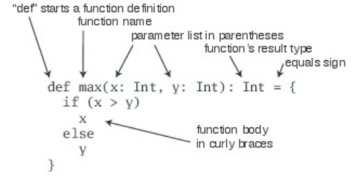
STEP 3. DEFINE SOME FUNCTIONS
Now that you've worked with Scala variables, you'll probably want to write some functions. Here's how
you do that in Scala:
scala> def max(x: Int, y: Int): Int = {
if (x > y) x
else y
}
max: (x: Int, y: Int)Int
Function definitions start with def. The function's name, in this case max, is followed by a comma-
separated list of parameters in parentheses. A type annotation must follow every function parameter,
preceded by a colon, because the Scala compiler (and interpreter, but from now on we'll just say
compiler) does not infer function parameter types. In this example, the function named max takes two
parameters, x and y, both of type Int. After the close parenthesis of max's parameter list you'll find
another ": Int" type annotation. This one defines the result type of the max function itself.[6] Following
the function's result type is an equals sign and pair of curly braces that contain the body of the function.
In this case, the body contains a single if expression, which selects either x or y, whichever is greater,
as the result of the max function. As demonstrated here, Scala's if expression can result in a value,
similar to Java's ternary operator. For example, the Scala expression "if (x > y) x else y" behaves
similarly to "(x > y) ? x : y" in Java. The equals sign that precedes the body of a function hints that in
the functional world view, a function defines an expression that results in a value. The basic structure of
a function is illustrated in Figure 2.1.
Figure 2.1 - The basic form of a function definition in Scala.
Sometimes the Scala compiler will require you to specify the result type of a function. If the function
is recursive,[7] for example, you must explicitly specify the function's result type. In the case of max,
however, you may leave the result type off and the compiler will infer it.[8]Also, if a function consists
of just one statement, you can optionally leave off the curly braces. Thus, you could alternatively write
the max function like this:
scala> def max(x: Int, y: Int) = if (x > y) x else y
max: (x: Int, y: Int)Int
Once you have defined a function, you can call it by name, as in:
scala> max(3, 5)
res4: Int = 5
Here's the definition of a function that takes no parameters and returns no interesting result:
scala> def greet() = println("Hello, world!")
greet: ()Unit
When you define the greet() function, the interpreter will respond with greet: ()Unit. "greet" is, of
course, the name of the function. The empty parentheses indicate the function takes no parameters.
And Unit is greet's result type. A result type of Unit indicates the function returns no interesting value.
Scala's Unit type is similar to Java's void type; in fact, every void-returning method in Java is mapped
to a Unit-returning method in Scala. Methods with the result type of Unit, therefore, are only executed
for their side effects. In the case of greet(), the side effect is a friendly greeting printed to the standard
output.
In the next step, you'll place Scala code in a file and run it as a script. If you wish to exit the interpreter,
you can do so by entering :quit or :q.
scala> :quit
$
STEP 4. WRITE SOME SCALA SCRIPTS
Although Scala is designed to help programmers build very large-scale systems, it also scalesdown
nicely to scripting. A script is just a sequence of statements in a file that will be executed sequentially.
Put this into a file named hello.scala:
println("Hello, world, from a script!")
then run:[9]
$ scala hello.scala
And you should get yet another greeting:
Hello, world, from a script!
Command line arguments to a Scala script are available via a Scala array named args. In Scala, arrays
are zero based, and you access an element by specifying an index in parentheses. So the first element in
a Scala array named steps is steps(0), not steps[0], as in Java. To try this out, type the following into a
new file named helloarg.scala:
// Say hello to the first argument
println("Hello, " + args(0) + "!")
then run:
$ scala helloarg.scala planet
In this command, "planet" is passed as a command line argument, which is accessed in the script
as args(0). Thus, you should see:
Hello, planet!
Note that this script included a comment. The Scala compiler will ignore characters between// and the
next end of line and any characters between /* and */. This example also showsStrings being
concatenated with the + operator. This works as you'd expect. The expression"Hello, " + "world!" will
result in the string "Hello, world!".
STEP 5. LOOP WITH WHILE; DECIDE WITH IF
To try out a while, type the following into a file named printargs.scala:
var i = 0
while (i < args.length) {
println(args(i))
i += 1
}
Note
Although the examples in this section help explain while loops, they do not demonstrate the best Scala
style. In the next section, you'll see better approaches that avoid iterating through arrays with indexes.
This script starts with a variable definition, var i = 0. Type inference gives i the type scala.Int, because
that is the type of its initial value, 0. The while construct on the next line causes theblock (the code
between the curly braces) to be repeatedly executed until the boolean expression i < args.length is
false. args.length gives the length of the args array. The block contains two statements, each indented
two spaces, the recommended indentation style for Scala. The first statement, println(args(i)), prints out
the ith command line argument. The second statement, i += 1, increments i by one. Note that Java's +
+i and i++ don't work in Scala. To increment in Scala, you need to say either i = i + 1 or i += 1. Run
this script with the following command:
$ scala printargs.scala Scala is fun
And you should see:
Scala
is
fun
For even more fun, type the following code into a new file with the name echoargs.scala:
var i = 0
while (i < args.length) {
if (i != 0)
print(" ")
print(args(i))
i += 1
}
println()
In this version, you've replaced the println call with a print call, so that all the arguments will be printed
out on the same line. To make this readable, you've inserted a single space before each argument except
the first via the if (i != 0) construct. Since i != 0 will be false the first time through the while loop, no
space will get printed before the initial argument. Lastly, you've added one more println to the end, to
get a line return after printing out all the arguments. Your output will be very pretty indeed. If you run
this script with the following command:
$ scala echoargs.scala Scala is even more fun
You'll get:
Scala is even more fun
Note that in Scala, as in Java, you must put the boolean expression for a while or an if in parentheses.
(In other words, you can't say in Scala things like if i < 10 as you can in a language such as Ruby. You
must say if (i < 10) in Scala.) Another similarity to Java is that if a block has only one statement, you
can optionally leave off the curly braces, as demonstrated by the if statement in echoargs.scala. And
although you haven't seen any of them, Scala does use semicolons to separate statements as in Java,
except that in Scala the semicolons are very often optional, giving some welcome relief to your right
little finger. If you had been in a more verbose mood, therefore, you could have written
the echoargs.scala script as follows:
var i = 0;
while (i < args.length) {
if (i != 0) {
print(" ");
}
print(args(i));
i += 1;
}
println();
STEP 6. ITERATE WITH FOREACH AND FOR
Although you may not have realized it, when you wrote the while loops in the previous step, you were
programming in an imperative style. In the imperative style, which is the style you normally use with
languages like Java, C++, and C, you give one imperative command at a time, iterate with loops, and
often mutate state shared between different functions. Scala enables you to program imperatively, but
as you get to know Scala better, you'll likely often find yourself programming in a
more functional style. In fact, one of the main aims of this book is to help you become as comfortable
with the functional style as you are with imperative style.
One of the main characteristics of a functional language is that functions are first class constructs, and
that's very true in Scala. For example, another (far more concise) way to print each command line
argument is:
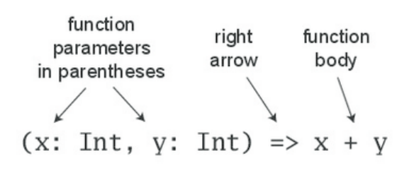
args.foreach(arg => println(arg))
In this code, you call the foreach method on args and pass in a function. In this case, you're passing in
a function literal that takes one parameter named arg. The body of the function isprintln(arg). If you
type the above code into a new file named pa.scala and execute with the command:
$ scala pa.scala Concise is nice
You should see:
Concise
is
nice
In the previous example, the Scala interpreter infers the type of arg to be String, since String is the
element type of the array on which you're calling foreach. If you'd prefer to be more explicit, you can
mention the type name. But when you do, you'll need to wrap the argument portion in parentheses
(which is the normal form of the syntax anyway):
args.foreach((arg: String) => println(arg))
Running this script has the same behavior as the previous one.
If you're in the mood for more conciseness instead of more explicitness, you can take advantage of a
special shorthand in Scala. If a function literal consists of one statement that takes a single argument,
you need not explicitly name and specify the argument.[10] Thus, the following code also works:
args.foreach(println)
To summarize, the syntax for a function literal is a list of named parameters, in parentheses, a right
arrow, and then the body of the function. This syntax is illustrated in Figure 2.2.
Figure 2.2 - The syntax of a function literal in Scala.
Now, by this point you may be wondering what happened to those trusty for loops you have been
accustomed to using in imperative languages, such as Java or C. In an effort to guide you in a
functional direction, only a functional relative of the imperative for (called a forexpression) is available
in Scala. While you won't see their full power and expressiveness until you reach (or peek ahead
to) Section 7.3, we'll give you a glimpse here. In a new file named forargs.scala, type the following:
for (arg <- args)
println(arg)
The parentheses after the "for" contain arg <- args.[11] To the right of the <- symbol is the
familiar args array. To the left of <- is "arg", the name of a val, not a var. (Because it is always aval, you
just write "arg" by itself, not "val arg".) Although arg may seem to be a var, because it will get a new
value on each iteration, it really is a val: arg can't be reassigned inside the body of the for expression.
Instead, for each element of the args array, a new arg val will be created and initialized to the element
value, and the body of the for will be executed.
If you run the forargs.scala script with the command:
$ scala forargs.scala for arg in args
You'll see:
for
arg
in
args
Scala's for expression can do much more than this, but this example is enough to get you started. We'll
show you more about for in Section 7.3 and Chapter 23.
CONCLUSION
In this chapter, you learned some Scala basics and, hopefully, took advantage of the opportunity to
write a bit of Scala code. In the next chapter, we'll continue this introductory overview and get into
more advanced topics.
Footnotes for Chapter 2:
[1] We tested the examples in this book with Scala version 2.11.7.
[2] If you're using Windows, you'll need to type the scala command into the "Command Prompt" DOS
box.
[3] If you're not familiar with Java packages, you can think of them as providing a full name for
classes. Because Int is a member of package scala, "Int" is the class's simple name, and "scala.Int" is its
full name. The details of packages are explained in Chapter 13.
[4] The simple name of java.lang.String is String.
[5] In the interpreter, however, you can define a new val with a name that was already used before. This
mechanism is explained in Section 7.7.
[6] In Java, the type of the value returned from a method is its return type. In Scala, that same concept
is called result type.
[7] A function is recursive if it calls itself.
[8] Nevertheless, it is often a good idea to indicate function result types explicitly, even when the
compiler doesn't require it. Such type annotations can make the code easier to read, because the reader
need not study the function body to figure out the inferred result type.
[9] You can run scripts without typing "scala" on Unix and Windows using a "pound-bang" syntax,
which is shown in Appendix A.
[10] This shorthand, called a partially applied function, is described in Section 8.6.
[11] You can say "in" for the <- symbol. You'd read for (arg <- args), therefore, as "for arg in args."
Chapter 3
Next Steps in Scala
This chapter continues the previous chapter's introduction to Scala. In this chapter, we'll introduce some
more advanced features. When you complete this chapter, you should have enough knowledge to
enable you to start writing useful scripts in Scala. As with the previous chapter, we recommend you try
out these examples as you go. The best way to get a feel for Scala is to start writing Scala code.
STEP 7. PARAMETERIZE ARRAYS WITH TYPES
In Scala, you can instantiate objects, or class instances, using new. When you instantiate an object in
Scala, you can parameterize it with values and types. Parameterization means "configuring" an
instance when you create it. You parameterize an instance with values by passing objects to a
constructor in parentheses. For example, the following Scala code instantiates a
new java.math.BigInteger and parameterizes it with the value "12345":
val big = new java.math.BigInteger("12345")
You parameterize an instance with types by specifying one or more types in square brackets. An
example is shown in Listing 3.1. In this example, greetStrings is a value of type Array[String](an "array
of string") that is initialized to length 3 by parameterizing it with the value 3 in the first line of code. If
you run the code in Listing 3.1 as a script, you'll see yet anotherHello, world! greeting. Note that when
you parameterize an instance with both a type and a value, the type comes first in its square brackets,
followed by the value in parentheses.
val greetStrings = new Array[String](3)
greetStrings(0) = "Hello"
greetStrings(1) = ", "
greetStrings(2) = "world!\n"
for (i <- 0 to 2)
print(greetStrings(i))
Listing 3.1 - Parameterizing an array with a type.
Note
Although the code in Listing 3.1 demonstrates important concepts, it does not show the recommended
way to create and initialize an array in Scala. You'll see a better way in Listing 3.2 here.
Had you been in a more explicit mood, you could have specified the type of greetStringsexplicitly like
this:
val greetStrings: Array[String] = new Array[String](3)
Given Scala's type inference, this line of code is semantically equivalent to the actual first line
of Listing 3.1. But this form demonstrates that while the type parameterization portion (the type names
in square brackets) forms part of the type of the instance, the value parameterization part (the values in
parentheses) does not. The type of greetStrings isArray[String], not Array[String](3).
The next three lines of code in Listing 3.1 initialize each element of the greetStrings array:
greetStrings(0) = "Hello"
greetStrings(1) = ", "
greetStrings(2) = "world!\n"
As mentioned previously, arrays in Scala are accessed by placing the index inside parentheses, not
square brackets as in Java. Thus the zeroth element of the array isgreetStrings(0), not greetStrings[0].
These three lines of code illustrate an important concept to understand about Scala concerning the
meaning of val. When you define a variable with val, the variable can't be reassigned, but the object to
which it refers could potentially still be changed. So in this case, you couldn't reassign greetStrings to a
different array; greetStrings will always point to the same Array[String] instance with which it was
initialized. But you can change the elements of that Array[String] over time, so the array itself is
mutable.
The final two lines in Listing 3.1 contain a for expression that prints out each greetStringsarray element
in turn:
for (i <- 0 to 2)
print(greetStrings(i))
The first line of code in this for expression illustrates another general rule of Scala: if a method takes
only one parameter, you can call it without a dot or parentheses. The to in this example is actually a
method that takes one Int argument. The code 0 to 2 is transformed into the method call (0).to(2).
[1] Note that this syntax only works if you explicitly specify the receiver of the method call. You
cannot write "println 10", but you can write "Console println 10".
Scala doesn't technically have operator overloading, because it doesn't actually have operators in the
traditional sense. Instead, characters such as +, -, *, and / can be used in method names. Thus, when
you typed 1 + 2 into the Scala interpreter in Step 1, you were actually invoking a method named + on
the Int object 1, passing in 2 as a parameter. As illustrated in Figure 3.1, you could alternatively have
written 1 + 2 using traditional method invocation syntax, (1).+(2).
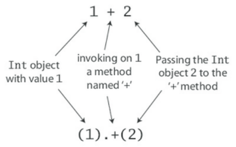
Figure 3.1 - All operations are method calls in Scala.
Another important idea illustrated by this example will give you insight into why arrays are accessed
with parentheses in Scala. Scala has fewer special cases than Java. Arrays are simply instances of
classes like any other class in Scala. When you apply parentheses surrounding one or more values to a
variable, Scala will transform the code into an invocation of a method named apply on that variable.
So greetStrings(i) gets transformed into greetStrings.apply(i). Thus accessing an element of an array in
Scala is simply a method call like any other. This principle is not restricted to arrays: any application of
an object to some arguments in parentheses will be transformed to an apply method call. Of course this
will compile only if that type of object actually defines an apply method. So it's not a special case; it's a
general rule.
Similarly, when an assignment is made to a variable to which parentheses and one or more arguments
have been applied, the compiler will transform that into an invocation of an updatemethod that takes
the arguments in parentheses as well as the object to the right of the equals sign. For example:
greetStrings(0) = "Hello"
will be transformed into:
greetStrings.update(0, "Hello")
Thus, the following is semantically equivalent to the code in Listing 3.1:
val greetStrings = new Array[String](3)
greetStrings.update(0, "Hello")
greetStrings.update(1, ", ")
greetStrings.update(2, "world!\n")
for (i <- 0.to(2))
print(greetStrings.apply(i))
Scala achieves a conceptual simplicity by treating everything, from arrays to expressions, as objects
with methods. You don't have to remember special cases, such as the differences in Java between
primitive and their corresponding wrapper types, or between arrays and regular objects. Moreover, this
uniformity does not incur a significant performance cost. The Scala compiler uses Java arrays,
primitive types, and native arithmetic where possible in the compiled code.
Although the examples you've seen so far in this step compile and run just fine, Scala provides a more
concise way to create and initialize arrays that you would normally use (seeListing 3.2). This code
creates a new array of length three, initialized to the passed strings,"zero", "one", and "two". The
compiler infers the type of the array to be Array[String], because you passed strings to it.
val numNames = Array("zero", "one", "two")
Listing 3.2 - Creating and initializing an array.
What you're actually doing in Listing 3.2 is calling a factory method, named apply, which creates and
returns the new array. This apply method takes a variable number of arguments[2] and is defined on
the Array companion object. You'll learn more about companion objects in Section 4.3. If you're a Java
programmer, you can think of this as calling a static method named apply on class Array. A more
verbose way to call the same applymethod is:
val numNames2 = Array.apply("zero", "one", "two")
STEP 8. USE LISTS
One of the big ideas of the functional style of programming is that methods should not have side
effects. A method's only act should be to compute and return a value. Some benefits gained when you
take this approach are that methods become less entangled, and therefore more reliable and reusable.
Another benefit (in a statically typed language) is that everything that goes into and out of a method is
checked by a type checker, so logic errors are more likely to manifest themselves as type errors.
Applying this functional philosophy to the world of objects means making objects immutable.
As you've seen, a Scala array is a mutable sequence of objects that all share the same type.
AnArray[String] contains only strings, for example. Although you can't change the length of an array
after it is instantiated, you can change its element values. Thus, arrays are mutable objects.
For an immutable sequence of objects that share the same type you can use Scala's List class. As with
arrays, a List[String] contains only strings. Scala's List, scala.List, differs from Java'sjava.util.List type
in that Scala Lists are always immutable (whereas Java Lists can be mutable). More generally,
Scala's List is designed to enable a functional style of programming. Creating a list is easy, and Listing
3.3 shows how:
val oneTwoThree = List(1, 2, 3)
Listing 3.3 - Creating and initializing a list.
The code in Listing 3.3 establishes a new val named oneTwoThree, initialized with a newList[Int] with
the integer elements 1, 2, and 3.[3] Because Lists are immutable, they behave a bit like Java strings:
when you call a method on a list that might seem by its name to imply the list will mutate, it instead
creates and returns a new list with the new value. For example,List has a method named `:::' for list
concatenation. Here's how you use it:
val oneTwo = List(1, 2)
val threeFour = List(3, 4)
val oneTwoThreeFour = oneTwo ::: threeFour
println(oneTwo + " and " + threeFour + " were not mutated.")
println("Thus, " + oneTwoThreeFour + " is a new list.")
If you run this script, you'll see:
List(1, 2) and List(3, 4) were not mutated.
Thus, List(1, 2, 3, 4) is a new list.
Perhaps the most common operator you'll use with lists is `::', which is pronounced "cons."Cons
prepends a new element to the beginning of an existing list and returns the resulting list. For example,
if you run this script:
val twoThree = List(2, 3)
val oneTwoThree = 1 :: twoThree
println(oneTwoThree)
You'll see:
List(1, 2, 3)
Note
In the expression "1 :: twoThree", :: is a method of its right operand, the list,twoThree. You might
suspect there's something amiss with the associativityof the :: method, but it is actually a simple rule to
remember: If a method is used in operator notation, such as a * b, the method is invoked on the left
operand, as in a.*(b)—unless the method name ends in a colon. If the method name ends in a colon, the
method is invoked on the right operand. Therefore, in 1 :: twoThree, the :: method is invoked
on twoThree, passing in1, like this: twoThree.::(1). Operator associativity will be described in more
detail in Section 5.9.
Given that a shorthand way to specify an empty list is Nil, one way to initialize new lists is to string
together elements with the cons operator, with Nil as the last element.[4] For example, the following
script will produce the same output as the previous one, "List(1, 2, 3)":
val oneTwoThree = 1 :: 2 :: 3 :: Nil
println(oneTwoThree)
Scala's List is packed with useful methods, many of which are shown in Table 3.1. The full power of
lists will be revealed in Chapter 16.
WHY NOT APPEND TO LISTS?
Class List does offer an "append" operation—it's written :+ and is explained in Chapter 24—but this
operation is rarely used, because the time it takes to append to a list grows linearly with the size of the
list, whereas prepending with :: takes constant time. If you want to build a list efficiently by appending
elements, you can prepend them and when you're done call reverse. Or you can use a ListBuffer, a
mutable list that does offer an append operation, and when you're done call toList. ListBuffer will be
described inSection 22.2.
Some List methods and usages
What it is What it does
List() or Nil The empty List
List("Cool", "tools", "rule") Creates a new List[String] with the three values"Cool", "tools",
and "rule"
val thrill = "Will" :: "fill" ::
"until" :: Nil Creates a new List[String] with the three values"Will", "fill", and "until"
List("a", "b") ::: List("c", "d"
)
Concatenates two lists (returns a new List[String]with
values "a", "b", "c", and "d")
thrill(2) Returns the element at index 2 (zero based) of thethrill list
(returns "until")
thrill.count(s => s.length ==
4)
Counts the number of string elements in thrill that have length 4 (returns
2)
thrill.drop(2) Returns the thrill list without its first 2 elements (returns List("until"))
thrill.dropRight(2) Returns the thrill list without its rightmost 2 elements
(returns List("Will"))
thrill.exists(s => s == "until"
)
Determines whether a string element exists in thrillthat has the
value "until" (returns true)
thrill.filter(s => s.length ==
4)
Returns a list of all elements, in order, of the thrilllist that have length 4
(returns List("Will", "fill"))
thrill.forall(s =>
s.endsWith("l"))
Indicates whether all elements in the thrill list end with the
letter "l" (returns true)
thrill.foreach(s => print(s)) Executes the print statement on each of the strings in the thrill list
(prints "Willfilluntil")
thrill.foreach(print) Same as the previous, but more concise (also prints"Willfilluntil")
thrill.head Returns the first element in the thrill list (returns"Will")
thrill.init Returns a list of all but the last element in the thrilllist
(returns List("Will", "fill"))
thrill.isEmpty Indicates whether the thrill list is empty (returnsfalse)
thrill.last Returns the last element in the thrill list (returns"until")
thrill.length Returns the number of elements in the thrill list (returns 3)
thrill.map(s => s + "y") Returns a list resulting from adding a "y" to each string element in
the thrill list (returnsList("Willy", "filly", "untily"))
thrill.mkString(", ") Makes a string with the elements of the list (returns"Will, fill, until")
thrill.filterNot(s =>
s.length == 4)
Returns a list of all elements, in order, of the thrilllist except those that
have length 4 (returnsList("until"))
thrill.reverse Returns a list containing all elements of the thrilllist in reverse order
(returnsList("until", "fill", "Will"))
thrill.sort((s, t) =>
s.charAt(0).toLower <
t.charAt(0).toLower)
Returns a list containing all elements of the thrilllist in alphabetical order
of the first character lowercased (returns List("fill", "until", "Will"))
thrill.tail Returns the thrill list minus its first element (returns List("fill", "until"))
STEP 9. USE TUPLES
Another useful container object is the tuple. Like lists, tuples are immutable, but unlike lists, tuples can
contain different types of elements. Whereas a list might be a List[Int] or aList[String], a tuple could
contain both an integer and a string at the same time. Tuples are very useful, for example, if you need
to return multiple objects from a method. Whereas in Java you would often create a JavaBean-like class
to hold the multiple return values, in Scala you can simply return a tuple. And it is simple: To
instantiate a new tuple that holds some objects, just place the objects in parentheses, separated by
commas. Once you have a tuple instantiated, you can access its elements individually with a dot,
underscore, and the one-based index of the element. An example is shown in Listing 3.4:
val pair = (99, "Luftballons")
println(pair._1)
println(pair._2)
Listing 3.4 - Creating and using a tuple.
In the first line of Listing 3.4, you create a new tuple that contains the integer 99, as its first element,
and the string, "Luftballons", as its second element. Scala infers the type of the tuple to
be Tuple2[Int, String], and gives that type to the variable pair as well. In the second line, you access
the _1 field, which will produce the first element, 99. The "." in the second line is the same dot you'd
use to access a field or invoke a method. In this case you are accessing a field named _1. If you run this
script, you'll see:
99
Luftballons
The actual type of a tuple depends on the number of elements it contains and the types of those
elements. Thus, the type of (99, "Luftballons") is Tuple2[Int, String]. The type
of('u', 'r', "the", 1, 4, "me") is Tuple6[Char, Char, String, Int, Int, String].[5]
ACCESSING THE ELEMENTS OF A TUPLE
You may be wondering why you can't access the elements of a tuple like the elements of a list, for
example, with "pair(0)". The reason is that a list's apply method always returns the same type, but each
element of a tuple may be a different type: _1 can have one result type, _2 another, and so on.
These _N numbers are one-based, instead of zero-based, because starting with 1 is a tradition set by
other languages with statically typed tuples, such as Haskell and ML.
STEP 10. USE SETS AND MAPS
Because Scala aims to help you take advantage of both functional and imperative styles, its collections
libraries make a point to differentiate between mutable and immutable collections. For example, arrays
are always mutable; lists are always immutable. Scala also provides mutable and immutable
alternatives for sets and maps, but uses the same simple names for both versions. For sets and
maps, Scala models mutability in the class hierarchy.
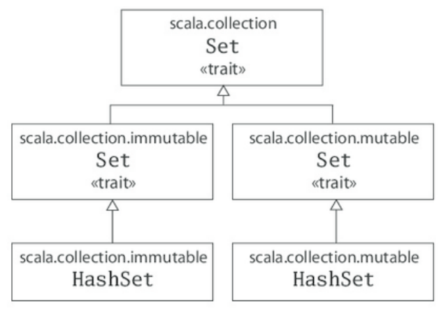
For example, the Scala API contains a base trait for sets, where a trait is similar to a Java interface.
(You'll find out more about traits in Chapter 12.) Scala then provides two subtraits, one for mutable sets
and another for immutable sets.
As you can see in Figure 3.2, these three traits all share the same simple name, Set. Their fully
qualified names differ, however, because each resides in a different package. Concrete set classes in the
Scala API, such as the HashSet classes shown in Figure 3.2, extend either the mutable or
immutable Set trait. (Although in Java you "implement" interfaces, in Scala you "extend" or "mix in"
traits.) Thus, if you want to use a HashSet, you can choose between mutable and immutable varieties
depending upon your needs. The default way to create a set is shown in Listing 3.5:
var jetSet = Set("Boeing", "Airbus")
jetSet += "Lear"
println(jetSet.contains("Cessna"))
Listing 3.5 - Creating, initializing, and using an immutable set.
Figure 3.2 - Class hierarchy for Scala sets.
In the first line of code in Listing 3.5, you define a new var named jetSet and initialize it with an
immutable set containing the two strings, "Boeing" and "Airbus". As this example shows, you can
create sets in Scala similarly to how you create lists and arrays: by invoking a factory method
named apply on a Set companion object. In Listing 3.5, you invoke apply on the companion object
for scala.collection.immutable.Set, which returns an instance of a default, immutable Set. The Scala
compiler infers jetSet's type to be the immutable Set[String].
To add a new element to a set, you call + on the set, passing in the new element. On both mutable and
immutable sets, the + method will create and return a new set with the element added. In Listing 3.5,
you're working with an immutable set. Although mutable sets offer an actual += method, immutable
sets do not.
In this case, the second line of code, "jetSet += "Lear"", is essentially a shorthand for:
jetSet = jetSet + "Lear"
Thus, in the second line of Listing 3.5, you reassign the jetSet var with a new set
containing"Boeing", "Airbus", and "Lear". Finally, the last line of Listing 3.5 prints out whether or not
the set contains the string "Cessna". (As you'd expect, it prints false.)
If you want a mutable set, you'll need to use an import, as shown in Listing 3.6:
import scala.collection.mutable
val movieSet = mutable.Set("Hitch", "Poltergeist")
movieSet += "Shrek"
println(movieSet)
Listing 3.6 - Creating, initializing, and using a mutable set.
In the first line of Listing 3.6 you import the mutable Set. As with Java, an import statement allows you
to use a simple name, such as Set, instead of the longer, fully qualified name. As a result, when you
say Set on the third line, the compiler knows you meanscala.collection.mutable.Set. On that line, you
initialize movieSet with a new mutable set that contains the strings "Hitch" and "Poltergeist". The
subsequent line adds "Shrek" to the mutable set by calling the += method on the set, passing in the
string "Shrek". As mentioned previously,+= is an actual method defined on mutable sets. Had you
wanted to, instead of writingmovieSet += "Shrek", you could have written movieSet.+=("Shrek").[6]
Although the default set implementations produced by the mutable and immutable Setfactory methods
shown thus far will likely be sufficient for most situations, occasionally you may want an explicit set
class. Fortunately, the syntax is similar. Simply import that class you need, and use the factory method
on its companion object. For example, if you need an immutable HashSet, you could do this:
import scala.collection.immutable.HashSet
val hashSet = HashSet("Tomatoes", "Chilies")
println(hashSet + "Coriander")
Another useful collection class in Scala is Map. As with sets, Scala provides mutable andimmutable
versions of Map, using a class hierarchy. As you can see in Figure 3.3, the class hierarchy for maps
looks a lot like the one for sets. There's a base Map trait in packagescala.collection, and two
subtrait Maps: a mutable Map in scala.collection.mutable and an immutable one
in scala.collection.immutable.
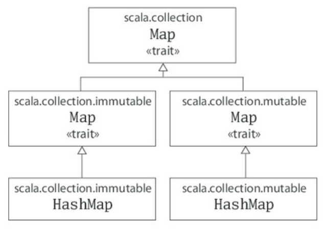
Figure 3.3 - Class hierarchy for Scala maps.
Implementations of Map, such as the HashMaps shown in the class hierarchy in Figure 3.3, extend
either the mutable or immutable trait. You can create and initialize maps using factory methods similar
to those used for arrays, lists, and sets.
import scala.collection.mutable
val treasureMap = mutable.Map[Int, String]()
treasureMap += (1 -> "Go to island.")
treasureMap += (2 -> "Find big X on ground.")
treasureMap += (3 -> "Dig.")
println(treasureMap(2))
Listing 3.7 - Creating, initializing, and using a mutable map.
For example, Listing 3.7 shows a mutable map in action. On the first line of Listing 3.7, you import the
mutable Map. You then define a val named treasureMap, and initialize it with an empty
mutable Map that has integer keys and string values. The map is empty because you pass nothing to the
factory method (the parentheses in "Map[Int, String]()" are empty).[7] On the next three lines you add
key/value pairs to the map using the -> and += methods. As illustrated previously, the Scala compiler
transforms a binary operation expression like 1 -> "Go to island." into (1).->("Go to island."). Thus,
when you say 1 -> "Go to island.", you are actually calling a method named -> on an integer with the
value 1, passing in a string with the value "Go to island." This -> method, which you can invoke on any
object in a Scala program, returns a two-element tuple containing the key and value.[8] You then pass
this tuple to the+= method of the map object to which treasureMap refers. Finally, the last line prints
the value that corresponds to the key 2 in the treasureMap.
If you run this code, it will print:
Find big X on ground.
If you prefer an immutable map, no import is necessary, as immutable is the default map. An example
is shown in Listing 3.8:
val romanNumeral = Map(
1 -> "I", 2 -> "II", 3 -> "III", 4 -> "IV", 5 -> "V"
)
println(romanNumeral(4))
Listing 3.8 - Creating, initializing, and using an immutable map.
Given there are no imports, when you say Map in the first line of Listing 3.8, you'll get the default:
a scala.collection.immutable.Map. You pass five key/value tuples to the map's factory method, which
returns an immutable Map containing the passed key/value pairs. If you run the code in Listing 3.8 it
will print "IV".
STEP 11. LEARN TO RECOGNIZE THE FUNCTIONAL STYLE
As mentioned in Chapter 1, Scala allows you to program in an imperative style, but encourages you to
adopt a more functional style. If you are coming to Scala from an imperative background—for
example, if you are a Java programmer—one of the main challenges you may face when learning Scala
is figuring out how to program in the functional style. We realize this style might be unfamiliar at first,
and in this book we try hard to guide you through the transition. It will require some work on your part,
and we encourage you to make the effort. If you come from an imperative background, we believe that
learning to program in a functional style will not only make you a better Scala programmer, it will
expand your horizons and make you a better programmer in general.
The first step is to recognize the difference between the two styles in code. One telltale sign is that if
code contains any vars, it is probably in an imperative style. If the code contains no vars at all—i.e., it
contains only vals—it is probably in a functional style. One way to move towards a functional style,
therefore, is to try to program without vars.
If you're coming from an imperative background, such as Java, C++, or C#, you may think ofvar as a
regular variable and val as a special kind of variable. On the other hand, if you're coming from a
functional background, such as Haskell, OCaml, or Erlang, you might think ofval as a regular variable
and var as akin to blasphemy. The Scala perspective, however, is thatval and var are just two different
tools in your toolbox, both useful, neither inherently evil. Scala encourages you to lean towards vals,
but ultimately reach for the best tool given the job at hand. Even if you agree with this balanced
philosophy, however, you may still find it challenging at first to figure out how to get rid of vars in
your code.
Consider the following while loop example, adapted from Chapter 2, which uses a var and is therefore
in the imperative style:
def printArgs(args: Array[String]): Unit = {
var i = 0
while (i < args.length) {
println(args(i))
i += 1
}
}
You can transform this bit of code into a more functional style by getting rid of the var, for example,
like this:
def printArgs(args: Array[String]): Unit = {
for (arg <- args)
println(arg)
}
or this:
def printArgs(args: Array[String]): Unit = {
args.foreach(println)
}
This example illustrates one benefit of programming with fewer vars. The refactored (more functional)
code is clearer, more concise, and less error-prone than the original (more imperative) code. The reason
Scala encourages a functional style is that it can help you write more understandable, less error-prone
code.
But you can go even further. The refactored printArgs method is not purely functional because it has
side effects—in this case, its side effect is printing to the standard output stream. The telltale sign of a
function with side effects is that its result type is Unit. If a function isn't returning any interesting value,
which is what a result type of Unit means, the only way that function can make a difference in the
world is through some kind of side effect. A more functional approach would be to define a method that
formats the passed args for printing, but just returns the formatted string, as shown in Listing 3.9:
def formatArgs(args: Array[String]) = args.mkString("\n")
Listing 3.9 - A function without side effects or vars.
Now you're really functional: no side effects or vars in sight. The mkString method, which you can call
on any iterable collection (including arrays, lists, sets, and maps), returns a string consisting of the
result of calling toString on each element, separated by the passed string. Thus if args contains three
elements "zero", "one", and "two", formatArgs will return"zero\none\ntwo". Of course, this function
doesn't actually print anything out like the printArgsmethods did, but you can easily pass its result
to println to accomplish that:
println(formatArgs(args))
Every useful program is likely to have side effects of some form; otherwise, it wouldn't be able to
provide value to the outside world. Preferring methods without side effects encourages you to design
programs where side-effecting code is minimized. One benefit of this approach is that it can help make
your programs easier to test.
For example, to test any of the three printArgs methods shown earlier in this section, you'd need to
redefine println, capture the output passed to it, and make sure it is what you expect. By contrast, you
could test the formatArgs function simply by checking its result:
val res = formatArgs(Array("zero", "one", "two"))
assert(res == "zero\none\ntwo")
Scala's assert method checks the passed Boolean and if it is false, throws AssertionError. If the
passed Boolean is true, assert just returns quietly. You'll learn more about assertions and tests
in Chapter 14.
That said, bear in mind that neither vars nor side effects are inherently evil. Scala is not a pure
functional language that forces you to program everything in the functional style. Scala is a hybrid
imperative/functional language. You may find that in some situations an imperative style is a better fit
for the problem at hand, and in such cases you should not hesitate to use it. To help you learn how to
program without vars, however, we'll show you many specific examples of code with vars and how to
transform those vars to vals in Chapter 7.
A BALANCED ATTITUDE FOR SCALA PROGRAMMERS
Prefer vals, immutable objects, and methods without side effects. Reach for them first. Use vars,
mutable objects, and methods with side effects when you have a specific need and justification for
them.
STEP 12. READ LINES FROM A FILE
Scripts that perform small, everyday tasks often need to process lines in files. In this section, you'll
build a script that reads lines from a file and prints them out prepended with the number of characters
in each line. The first version is shown in Listing 3.10:
import scala.io.Source
if (args.length > 0) {
for (line <- Source.fromFile(args(0)).getLines())
println(line.length + " " + line)
}
else
Console.err.println("Please enter filename")
Listing 3.10 - Reading lines from a file.
This script starts with an import of a class named Source from package scala.io. It then checks to see if
at least one argument was specified on the command line. If so, the first argument is interpreted as a
filename to open and process. The expression Source.fromFile(args(0))attempts to open the specified
file and returns a Source object, on which you call getLines. ThegetLines method returns
an Iterator[String], which provides one line on each iteration, excluding the end-of-line character.
The for expression iterates through these lines and prints for each the length of the line, a space, and the
line itself. If there were no arguments supplied on the command line, the final else clause will print a
message to the standard error stream. If you place this code in a file named countchars1.scala, and run
it on itself with:
$ scala countchars1.scala countchars1.scala
You should see:
22 import scala.io.Source
0
22 if (args.length > 0) {
0
51 for (line <- Source.fromFile(args(0)).getLines())
37 println(line.length + " " + line)
1 }
4 else
46 Console.err.println("Please enter filename")
Although the script in its current form prints out the needed information, you may wish to line up the
numbers, right adjusted, and add a pipe character, so that the output looks instead like:
22 | import scala.io.Source
0 |
22 | if (args.length > 0) {
0 |
51 | for (line <- Source.fromFile(args(0)).getLines())
37 | println(line.length + " " + line)
1 | }
4 | else
46 | Console.err.println("Please enter filename")
To accomplish this, you can iterate through the lines twice. The first time through you'll determine the
maximum width required by any line's character count. The second time through you'll print the output,
using the maximum width calculated previously. Because you'll be iterating through the lines twice,
you may as well assign them to a variable:
val lines = Source.fromFile(args(0)).getLines().toList
The final toList is required because the getLines method returns an iterator. Once you've iterated
through an iterator, it is spent. By transforming it into a list via the toList call, you gain the ability to
iterate as many times as you wish, at the cost of storing all lines from the file in memory at once.
The lines variable, therefore, references a list of strings that contains the contents of the file specified
on the command line. Next, because you'll be calculating the width of each line's character count twice,
once per iteration, you might factor that expression out into a small function, which calculates the
character width of the passed string's length:
def widthOfLength(s: String) = s.length.toString.length
With this function, you could calculate the maximum width like this:
var maxWidth = 0
for (line <- lines)
maxWidth = maxWidth.max(widthOfLength(line))
Here you iterate through each line with a for expression, calculate the character width of that line's
length, and, if it is larger than the current maximum, assign it to maxWidth, a var that was initialized to
0. (The max method, which you can invoke on any Int, returns the greater of the value on which it was
invoked and the value passed to it.) Alternatively, if you prefer to find the maximum without vars, you
could first find the longest line like this:
val longestLine = lines.reduceLeft(
(a, b) => if (a.length > b.length) a else b
)
The reduceLeft method applies the passed function to the first two elements in lines, then applies it to
the result of the first application and the next element in lines, and so on, all the way through the list.
On each such application, the result will be the longest line encountered so far because the passed
function, (a, b) => if (a.length > b.length) a else b, returns the longest of the two passed strings.
"reduceLeft" will return the result of the last application of the function, which in this case will be the
longest string element contained in lines.
Given this result, you can calculate the maximum width by passing the longest line towidthOfLength:
val maxWidth = widthOfLength(longestLine)
All that remains is to print out the lines with proper formatting. You can do that like this:
for (line <- lines) {
val numSpaces = maxWidth - widthOfLength(line)
val padding = " " * numSpaces
println(padding + line.length + " | " + line)
}
In this for expression, you once again iterate through the lines. For each line, you first calculate the
number of spaces required before the line length and assign it to numSpaces. Then you create a string
containing numSpaces spaces with the expression " " * numSpaces. Finally, you print out the
information with the desired formatting. The entire script looks as shown inListing 3.11:
import scala.io.Source
def widthOfLength(s: String) = s.length.toString.length
if (args.length > 0) {
val lines = Source.fromFile(args(0)).getLines().toList
val longestLine = lines.reduceLeft(
(a, b) => if (a.length > b.length) a else b
)
val maxWidth = widthOfLength(longestLine)
for (line <- lines) {
val numSpaces = maxWidth - widthOfLength(line)
val padding = " " * numSpaces
println(padding + line.length + " | " + line)
}
}
else
Console.err.println("Please enter filename")
Listing 3.11 - Printing formatted character counts for the lines of a file.
CONCLUSION
With the knowledge you've gained in this chapter, you should be able to start using Scala for small
tasks, especially scripts. In later chapters, we will dive further into these topics and introduce other
topics that weren't even hinted at here.
Footnotes for Chapter 3:
[1] This to method actually returns not an array but a different kind of sequence, containing the values
0, 1, and 2, which the for expression iterates over. Sequences and other collections will be described
in Chapter 17.
[2] Variable-length argument lists, or repeated parameters, are described in Section 8.8.
[3] You don't need to say new List because "List.apply()" is defined as a factory method on
thescala.List companion object. You'll read more on companion objects in Section 4.3.
[4] The reason you need Nil at the end is that :: is defined on class List. If you try to just say1 :: 2 :: 3, it
won't compile because 3 is an Int, which doesn't have a :: method.
[5] Although conceptually you could create tuples of any length, currently the Scala library only
defines them up to Tuple22.
[6] Because the set in Listing 3.6 is mutable, there is no need to reassign movieSet, which is why it can
be a val. By contrast, using += with the immutable set in Listing 3.5 required reassigning jetSet, which
is why it must be a var.
[7] The explicit type parameterization, "[Int, String]", is required in Listing 3.7 because without any
values passed to the factory method, the compiler is unable to infer the map's type parameters. By
contrast, the compiler can infer the type parameters from the values passed to the map factory shown
in Listing 3.8, thus no explicit type parameters are needed.
[8] The Scala mechanism that allows you to invoke -> on any object, implicit conversion, will be
covered in Chapter 21.
Chapter 4
Classes and Objects
You've now seen the basics of classes and objects in Scala from the previous two chapters. In this
chapter, we'll take you a bit deeper. You'll learn more about classes, fields, and methods, and get an
overview of semicolon inference. We'll discuss singleton objects, including how to use them to write
and run a Scala application. If you are familiar with Java, you'll find that the concepts in Scala are
similar, but not exactly the same. So even if you're a Java guru, it will pay to read on.
4.1 CLASSES, FIELDS, AND METHODS
A class is a blueprint for objects. Once you define a class, you can create objects from the class
blueprint with the keyword new. For example, given the class definition:
class ChecksumAccumulator {
// class definition goes here
}
You can create ChecksumAccumulator objects with:
new ChecksumAccumulator
Inside a class definition, you place fields and methods, which are collectively called members.Fields,
which you define with either val or var, are variables that refer to objects. Methods, which you define
with def, contain executable code. The fields hold the state, or data, of an object, whereas the methods
use that data to do the computational work of the object. When you instantiate a class, the runtime sets
aside some memory to hold the image of that object's state (i.e., the content of its variables). For
example, if you defined a ChecksumAccumulator class and gave it a var field named sum:
class ChecksumAccumulator {
var sum = 0
}
and you instantiated it twice with:
val acc = new ChecksumAccumulator
val csa = new ChecksumAccumulator
The image of the objects in memory might look like this:
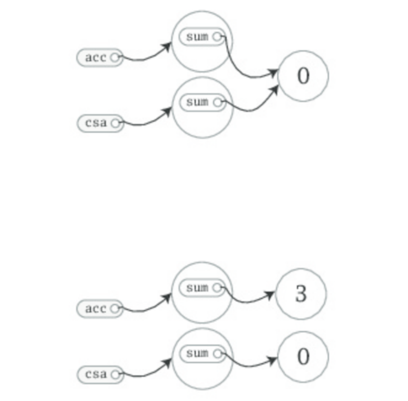
Since sum, a field declared inside class ChecksumAccumulator, is a var, not a val, you can later
reassign to sum a different Int value, like this:
acc.sum = 3
Now the picture would look like this:
One thing to notice about this picture is that there are two sum variables, one in the object referenced
by acc and the other in the object referenced by csa. Fields are also known asinstance
variables, because every instance gets its own set of the variables. Collectively, an object's instance
variables make up the memory image of the object. You see this illustrated here not only in that you see
two sum variables, but also that when you changed one, the other was unaffected.
Another thing to note in this example is that you were able to mutate the object acc referred to, even
though acc is a val. What you can't do with acc (or csa), given that they are vals, notvars, is reassign a
different object to them. For example, the following attempt would fail:
// Won't compile, because acc is a val
acc = new ChecksumAccumulator
What you can count on, therefore, is that acc will always refer to the
same ChecksumAccumulatorobject with which you initialize it, but the fields contained inside that
object might change over time.
One important way to pursue robustness of an object is to ensure that the object's state—the values of
its instance variables—remains valid during its entire lifetime. The first step is to prevent outsiders
from accessing the fields directly by making the fields private. Because private fields can only be
accessed by methods defined in the same class, all the code that can update the state will be localized to
the class. To declare a field private, you place a privateaccess modifier in front of the field, like this:
class ChecksumAccumulator {
private var sum = 0
}
Given this definition of ChecksumAccumulator, any attempt to access sum from the outside of the class
would fail:
val acc = new ChecksumAccumulator
acc.sum = 5 // Won't compile, because sum is private
Note
The way you make members public in Scala is by not explicitly specifying any access modifier. Put
another way, where you'd say "public" in Java, you simply say nothing in Scala. Public is Scala's
default access level.
Now that sum is private, the only code that can access sum is code defined inside the body of the class
itself. Thus, ChecksumAccumulator won't be of much use to anyone unless we define some methods in
it:
class ChecksumAccumulator {
private var sum = 0
def add(b: Byte): Unit = {
sum += b
}
def checksum(): Int = {
return ~(sum & 0xFF) + 1
}
}
The ChecksumAccumulator now has two methods, add and checksum, both of which exhibit the basic
form of a function definition, shown in Figure 2.1 here.
Any parameters to a method can be used inside the method. One important characteristic of method
parameters in Scala is that they are vals, not vars.[1] If you attempt to reassign a parameter inside a
method in Scala, therefore, it won't compile:
def add(b: Byte): Unit = {
b = 1 // This won't compile, because b is a val
sum += b
}
Although add and checksum in this version of ChecksumAccumulator correctly implement the desired
functionality, you can express them using a more concise style. First, the return at the end of
the checksum method is superfluous and can be dropped. In the absence of any explicit return
statement, a Scala method returns the last value computed by the method.
The recommended style for methods is in fact to avoid having explicit, and especially multiple, return
statements. Instead, think of each method as an expression that yields one value, which is returned.
This philosophy will encourage you to make methods quite small, to factor larger methods into
multiple smaller ones. On the other hand, design choices depend on the design context, and Scala
makes it easy to write methods that have multiple, explicitreturns if that's what you desire.
Because all checksum does is calculate a value, it does not need an explicit return. Another shorthand
for methods is that you can leave off the curly braces if a method computes only a single result
expression. If the result expression is short, it can even be placed on the same line as the def itself. For
the utmost in conciseness, you can leave off the result type and Scala will infer it. With these changes,
class ChecksumAccumulator looks like this:
class ChecksumAccumulator {
private var sum = 0
def add(b: Byte) = sum += b
def checksum() = ~(sum & 0xFF) + 1
}
Although the Scala compiler will correctly infer the result types of the add and checksummethods
shown in the previous example, readers of the code will also need to mentally inferthe result types by
studying the bodies of the methods. As a result it is often better to explicitly provide the result types of
public methods declared in a class even when the compiler would infer it for you. Listing 4.1 shows
this style.
// In file ChecksumAccumulator.scala
class ChecksumAccumulator {
private var sum = 0
def add(b: Byte): Unit = { sum += b }
def checksum(): Int = ~(sum & 0xFF) + 1
}
Listing 4.1 - Final version of class ChecksumAccumulator.
Methods with a result type of Unit, such as ChecksumAccumulator's add method, are executed for their
side effects. A side effect is generally defined as mutating state somewhere external to the method or
performing an I/O action. In add's case, the side effect is that sum is reassigned. A method that is
executed only for its side effects is known as a procedure.
4.2 SEMICOLON INFERENCE
In a Scala program, a semicolon at the end of a statement is usually optional. You can type one if you
want but you don't have to if the statement appears by itself on a single line. On the other hand, a
semicolon is required if you write multiple statements on a single line:
val s = "hello"; println(s)
If you want to enter a statement that spans multiple lines, most of the time you can simply enter it and
Scala will separate the statements in the correct place. For example, the following is treated as one
four-line statement:
if (x < 2)
println("too small")
else
println("ok")
Occasionally, however, Scala will split a statement into two parts against your wishes:
x
+ y
This parses as two statements x and +y. If you intend it to parse as one statement x + y, you can always
wrap it in parentheses:
(x
+ y)
Alternatively, you can put the + at the end of a line. For just this reason, whenever you are chaining an
infix operation such as +, it is a common Scala style to put the operators at the end of the line instead of
the beginning:
x +
y +
z
THE RULES OF SEMICOLON INFERENCE
The precise rules for statement separation are surprisingly simple for how well they work. In short, a
line ending is treated as a semicolon unless one of the following conditions is true:
1. The line in question ends in a word that would not be legal as the end of a statement, such as a
period or an infix operator.
2. The next line begins with a word that cannot start a statement.
3. The line ends while inside parentheses (...) or brackets [...], because these cannot contain
multiple statements anyway.
4.3 SINGLETON OBJECTS
As mentioned in Chapter 1, one way in which Scala is more object-oriented than Java is that classes in
Scala cannot have static members. Instead, Scala has singleton objects. A singleton object definition
looks like a class definition, except instead of the keyword class you use the keyword object. Listing
4.2 shows an example.
The singleton object in this figure is named ChecksumAccumulator, the same name as the class in the
previous example. When a singleton object shares the same name with a class, it is called that
class's companion object. You must define both the class and its companion object in the same source
file. The class is called the companion class of the singleton object. A class and its companion object
can access each other's private members.
// In file ChecksumAccumulator.scala
import scala.collection.mutable
object ChecksumAccumulator {
private val cache = mutable.Map.empty[String, Int]
def calculate(s: String): Int =
if (cache.contains(s))
cache(s)
else {
val acc = new ChecksumAccumulator
for (c <- s)
acc.add(c.toByte)
val cs = acc.checksum()
cache += (s -> cs)
cs
}
}
Listing 4.2 - Companion object for class ChecksumAccumulator.
The ChecksumAccumulator singleton object has one method, named calculate, which takes a Stringand
calculates a checksum for the characters in the String. It also has one private field, cache, a mutable
map in which previously calculated checksums are cached.[2] The first line of the method,
"if (cache.contains(s))", checks the cache to see if the passed string is already contained as a key in the
map. If so, it just returns the mapped value, cache(s). Otherwise, it executes the else clause, which
calculates the checksum. The first line of the else clause defines a val named acc and initializes it with
a new ChecksumAccumulator instance.[3] The next line is a for expression, which cycles through each
character in the passed string, converts the character to a Byte by invoking toByte on it, and passes that
to the add method of theChecksumAccumulator instances to which acc refers. After the for expression
completes, the next line of the method invokes checksum on acc, which gets the checksum for the
passed String, and stores it into a val named cs. In the next line, cache += (s -> cs), the passed string
key is mapped to the integer checksum value, and this key-value pair is added to the cache map. The
last expression of the method, cs, ensures the checksum is the result of the method.
If you are a Java programmer, one way to think of singleton objects is as the home for any static
methods you might have written in Java. You can invoke methods on singleton objects using a similar
syntax: the name of the singleton object, a dot, and the name of the method. For example, you can
invoke the calculate method of singleton object ChecksumAccumulator like this:
ChecksumAccumulator.calculate("Every value is an object.")
A singleton object is more than a holder of static methods, however. It is a first-class object. You can
think of a singleton object's name, therefore, as a "name tag" attached to the object:
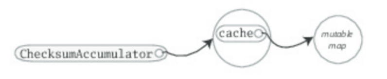
Defining a singleton object doesn't define a type (at the Scala level of abstraction). Given just a
definition of object ChecksumAccumulator, you can't make a variable of type ChecksumAccumulator.
Rather, the type named ChecksumAccumulator is defined by the singleton object's companion class.
However, singleton objects extend a superclass and can mix in traits. Given each singleton object is an
instance of its superclasses and mixed-in traits, you can invoke its methods via these types, refer to it
from variables of these types, and pass it to methods expecting these types. We'll show some examples
of singleton objects inheriting from classes and traits in Chapter 13.
One difference between classes and singleton objects is that singleton objects cannot take parameters,
whereas classes can. Because you can't instantiate a singleton object with the newkeyword, you have
no way to pass parameters to it. Each singleton object is implemented asan instance of a synthetic
class referenced from a static variable, so they have the same initialization semantics as Java statics.
[4] In particular, a singleton object is initialized the first time some code accesses it.
A singleton object that does not share the same name with a companion class is called astandalone
object. You can use standalone objects for many purposes, including collecting related utility methods
together or defining an entry point to a Scala application. This use case is shown in the next section.
4.4 A SCALA APPLICATION
To run a Scala program, you must supply the name of a standalone singleton object with amain method
that takes one parameter, an Array[String], and has a result type of Unit. Any standalone object with
a main method of the proper signature can be used as the entry point into an application. An example is
shown in Listing 4.3:
// In file Summer.scala
import ChecksumAccumulator.calculate
object Summer {
def main(args: Array[String]) = {
for (arg <- args)
println(arg + ": " + calculate(arg))
}
}
Listing 4.3 - The Summer application.
The name of the singleton object in Listing 4.3 is Summer. Its main method has the proper signature, so
you can use it as an application. The first statement in the file is an import of thecalculate method
defined in the ChecksumAccumulator object in the previous example. This import statement allows
you to use the method's simple name in the rest of the file.[5] The body of the main method simply
prints out each argument and the checksum for the argument, separated by a colon.
Note
Scala implicitly imports members of packages java.lang and scala, as well as the members of a
singleton object named Predef, into every Scala source file. Predef, which resides in package scala,
contains many useful methods. For example, when you say println in a Scala source file, you're actually
invoking println on Predef. (Predef.println turns around and invokes Console.println, which does the
real work.) When you say assert, you're invoking Predef.assert.
To run the Summer application, place the code from Listing 4.3 into a file named Summer.scala.
Because Summer uses ChecksumAccumulator, place the code for ChecksumAccumulator, both the
class shown in Listing 4.1 and its companion object shown in Listing 4.2, into a file
namedChecksumAccumulator.scala.
One difference between Scala and Java is that whereas Java requires you to put a public class in a file
named after the class—for example, you'd put class SpeedRacer in file SpeedRacer.java—in Scala, you
can name .scala files anything you want, no matter what Scala classes or code you put in them. In
general in the case of non-scripts, however, it is recommended style to name files after the classes they
contain as is done in Java, so that programmers can more easily locate classes by looking at file names.
This is the approach we've taken with the two files in this
example, Summer.scala and ChecksumAccumulator.scala.
Neither ChecksumAccumulator.scala nor Summer.scala are scripts, because they end in a definition. A
script, by contrast, must end in a result expression. Thus if you try to run Summer.scala as a script, the
Scala interpreter will complain that Summer.scala does not end in a result expression (assuming of
course you didn't add any expression of your own after the Summer object definition). Instead, you'll
need to actually compile these files with the Scala compiler, then run the resulting class files. One way
to do this is to use scalac, which is the basic Scala compiler, like this:
$ scalac ChecksumAccumulator.scala Summer.scala
This compiles your source files, but there may be a perceptible delay before the compilation finishes.
The reason is that every time the compiler starts up, it spends time scanning the contents of jar files and
doing other initial work before it even looks at the fresh source files you submit to it. For this reason,
the Scala distribution also includes a Scala compilerdaemon called fsc (for fast Scala compiler). You
use it like this:
$ fsc ChecksumAccumulator.scala Summer.scala
The first time you run fsc, it will create a local server daemon attached to a port on your computer. It
will then send the list of files to compile to the daemon via the port, and the daemon will compile the
files. The next time you run fsc, the daemon will already be running, so fsc will simply send the file list
to the daemon, which will immediately compile the files. Using fsc, you only need to wait for the Java
runtime to startup the first time. If you ever want to stop the fsc daemon, you can do so with fsc -
shutdown.
Running either of these scalac or fsc commands will produce Java class files that you can then run via
the scala command, the same command you used to invoke the interpreter in previous
examples. However, instead of giving it a filename with a .scala extension containing Scala code to
interpret as you did in every previous example,[6] in this case you'll give it the name of a standalone
object containing a main method of the proper signature. You can run theSummer application,
therefore, by typing:
$ scala Summer of love
You will see checksums printed for the two command line arguments:
of: -213
love: -182
4.5 THE APP TRAIT
Scala provides a trait, scala.App, that can save you some finger typing. Although we haven't yet
covered everything you'll need to understand exactly how this trait works, we figured you'd want to
know about it now anyway. Listing 4.4 shows an example:
import ChecksumAccumulator.calculate
object FallWinterSpringSummer extends App {
for (season <- List("fall", "winter", "spring"))
println(season + ": " + calculate(season))
}
Listing 4.4 - Using the App trait.
To use the trait, you first write "extends App" after the name of your singleton object. Then instead of
writing a main method, you place the code you would have put in the main method directly between
the curly braces of the singleton object. You can access command-line arguments via an array of strings
named args. That's it. You can compile and run this application just like any other.
4.6 CONCLUSION
This chapter has given you the basics of classes and objects in Scala, and shown you how to compile
and run applications. In the next chapter, you'll learn about Scala's basic types and how to use them.
Footnotes for Chapter 4:
[1] The reason parameters are vals is that vals are easier to reason about. You needn't look further to
determine if a val is reassigned, as you must do with a var.
[2] We used a cache here to show a singleton object with a field. A cache such as this is a performance
optimization that trades off memory for computation time. In general, you would likely use such a
cache only if you encountered a performance problem that the cache solves, and might use a weak map,
such as WeakHashMap in scala.collection.jcl, so that entries in the cache could be garbage collected if
memory becomes scarce.
[3] Because the keyword new is only used to instantiate classes, the new object created here is an
instance of the ChecksumAccumulator class, not the singleton object of the same name.
[4] The name of the synthetic class is the object name plus a dollar sign. Thus the synthetic class for the
singleton object named ChecksumAccumulator is ChecksumAccumulator$.
[5] If you're a Java programmer, you can think of this import as similar to the static import feature
introduced in Java 5. One difference in Scala, however, is that you can import members from any
object, not just singleton objects.
[6] The actual mechanism that the scala program uses to "interpret" a Scala source file is that it
compiles the Scala source code to Java bytecodes, loads them immediately via a class loader, and
executes them.
Chapter 5
Basic Types and Operations
Now that you've seen classes and objects in action, it's a good time to look at Scala's basic types and
operations in more depth. If you're familiar with Java, you'll be glad to find that Java's basic types and
operators have the same meaning in Scala. However, there are some interesting differences that will
make this chapter worth reading even if you're an experienced Java developer. Because some aspects of
Scala covered in this chapter are essentially the same as in Java, we've inserted notes indicating what
sections Java developers can safely skip.
In this chapter, you'll get an overview of Scala's basic types, including Strings and the value
types Int, Long, Short, Byte, Float, Double, Char, and Boolean. You'll learn the operations you can
perform on these types, including how operator precedence works in Scala expressions. You'll also
learn how implicit conversions can "enrich" variants of these basic types, giving you additional
operations beyond those supported by Java.
5.1 SOME BASIC TYPES
Several fundamental types of Scala, along with the ranges of values instances of these types may have,
are shown in Table 5.1. Collectively, types Byte, Short, Int, Long, and Char are calledintegral
types. The integral types plus Float and Double are called numeric types.
Table 5.1 - Some basic types
Basic type Range
Byte 8-bit signed two's complement integer (-27 to 27 - 1, inclusive)
Short 16-bit signed two's complement integer (-215 to 215 - 1, inclusive)
Int 32-bit signed two's complement integer (-231 to 231 - 1, inclusive)
Long 64-bit signed two's complement integer (-263 to 263 - 1, inclusive)
Char 16-bit unsigned Unicode character (0 to 216 - 1, inclusive)
String a sequence of Chars
Float 32-bit IEEE 754 single-precision float
Double 64-bit IEEE 754 double-precision float
Boolean true or false
Other than String, which resides in package java.lang, all of the types shown in Table 5.1 are members
of package scala.[1] For example, the full name of Int is scala.Int. However, given that all the members
of package scala and java.lang are automatically imported into every Scala source file, you can just use
the simple names (i.e., names like Boolean, Char, or String) everywhere.
Savvy Java developers will note that Scala's basic types have the exact same ranges as the
corresponding types in Java. This enables the Scala compiler to transform instances of Scalavalue
types, such as Int or Double, down to Java primitive types in the bytecodes it produces.
5.2 LITERALS
All of the basic types listed in Table 5.1 can be written with literals. A literal is a way to write a
constant value directly in code.
FAST TRACK FOR JAVA PROGRAMMERS
The syntax of most literals shown in this section are exactly the same as in Java, so if you're a Java
master, you can safely skip much of this section. Some differences you should read about are Scala's
literals for raw strings and symbols, described starting here, and string interpolation, described
starting here. Also, Scala does not support octal literals; integer literals that start with a 0, such as 031,
do not compile.
Integer literals
Integer literals for the types Int, Long, Short, and Byte come in two forms: decimal and hexadecimal.
The way an integer literal begins indicates the base of the number. If the number begins with
a 0x or 0X, it is hexadecimal (base 16), and may contain 0 through 9 as well as upper or lowercase
digits A through F. Some examples are:
scala> val hex = 0x5
hex: Int = 5
scala> val hex2 = 0x00FF
hex2: Int = 255
scala> val magic = 0xcafebabe
magic: Int = -889275714
Note that the Scala shell always prints integer values in base 10, no matter what literal form you may
have used to initialize it. Thus the interpreter displays the value of the hex2 variable you initialized
with literal 0x00FF as decimal 255. (Of course, you don't need to take our word for it. A good way to
start getting a feel for the language is to try these statements out in the interpreter as you read this
chapter.) If the number begins with a non-zero digit, and is otherwise undecorated, it is decimal (base
10). For example:
scala> val dec1 = 31
dec1: Int = 31
scala> val dec2 = 255
dec2: Int = 255
scala> val dec3 = 20
dec3: Int = 20
If an integer literal ends in an L or l, it is a Long; otherwise it is an Int. Some examples of Longinteger
literals are:
scala> val prog = 0XCAFEBABEL
prog: Long = 3405691582
scala> val tower = 35L
tower: Long = 35
scala> val of = 31l
of: Long = 31
If an Int literal is assigned to a variable of type Short or Byte, the literal is treated as if it were
aShort or Byte type so long as the literal value is within the valid range for that type. For example:
scala> val little: Short = 367
little: Short = 367
scala> val littler: Byte = 38
littler: Byte = 38
Floating point literals
Floating point literals are made up of decimal digits, optionally containing a decimal point, and
optionally followed by an E or e and an exponent. Some examples of floating-point literals are:
scala> val big = 1.2345
big: Double = 1.2345
scala> val bigger = 1.2345e1
bigger: Double = 12.345
scala> val biggerStill = 123E45
biggerStill: Double = 1.23E47
Note that the exponent portion means the power of 10 by which the other portion is multiplied. Thus,
1.2345e1 is 1.2345 times 101, which is 12.345. If a floating-point literal ends in an F or f, it is a Float;
otherwise it is a Double. Optionally, a Double floating-point literal can end in D or d. Some examples
of Float literals are:
scala> val little = 1.2345F
little: Float = 1.2345
scala> val littleBigger = 3e5f
littleBigger: Float = 300000.0
That last value expressed as a Double could take these (and other) forms:
scala> val anotherDouble = 3e5
anotherDouble: Double = 300000.0
scala> val yetAnother = 3e5D
yetAnother: Double = 300000.0
Character literals
Character literals are composed of any Unicode character between single quotes, such as:
scala> val a = 'A'
a: Char = A
In addition to providing an explicit character between the single quotes, you can identify a character
using its Unicode code point. To do so, write \u followed by four hex digits with the code point, like
this:
scala> val d = '\u0041'
d: Char = A
scala> val f = '\u0044'
f: Char = D
In fact, such Unicode characters can appear anywhere in a Scala program. For instance you could also
write an identifier like this:
scala> val B\u0041\u0044 = 1
BAD: Int = 1
This identifier is treated as identical to BAD, the result of expanding the two Unicode characters in the
code above. In general, it is a bad idea to name identifiers like this because it is hard to read. Rather,
this syntax is intended to allow Scala source files that include non-ASCII Unicode characters to be
represented in ASCII.
Finally, there are also a few character literals represented by special escape sequences, shown in Table
5.2. For example:
scala> val backslash = '\\'
backslash: Char = \
Table 5.2 - Special character literal escape sequences
Literal Meaning
\n line feed (\u000A)
\b backspace (\u0008)
\t tab (\u0009)
\f form feed (\u000C)
\r carriage return (\u000D)
\" double quote (\u0022)
\' single quote (\u0027)
\\ backslash (\u005C)
String literals
A string literal is composed of characters surrounded by double quotes:
scala> val hello = "hello"
hello: String = hello
The syntax of the characters within the quotes is the same as with character literals. For example:
scala> val escapes = "\\\"\'"
escapes: String = \"'
Because this syntax is awkward for strings that contain a lot of escape sequences or strings that span
multiple lines, Scala includes a special syntax for raw strings. You start and end a raw string with three
double quotation marks in a row ("""). The interior of a raw string may contain any characters
whatsoever, including newlines, quotation marks, and special characters, except of course three quotes
in a row. For example, the following program prints out a message using a raw string:
println("""Welcome to Ultamix 3000.
Type "HELP" for help.""")
However, running this code does not produce quite what is desired:
Welcome to Ultamix 3000.
Type "HELP" for help.
The issue is that the leading spaces before the second line are included in the string! To help with this
common situation, you can call stripMargin on strings. To use this method, put a pipe character (|) at
the front of each line, and then call stripMargin on the whole string:
println("""|Welcome to Ultamix 3000.
|Type "HELP" for help.""".stripMargin)
Now the code behaves as desired:
Welcome to Ultamix 3000.
Type "HELP" for help.
Symbol literals
A symbol literal is written 'ident, where ident can be any alphanumeric identifier. Such literals are
mapped to instances of the predefined class scala.Symbol. Specifically, the literal'cymbal will be
expanded by the compiler to a factory method invocation: Symbol("cymbal"). Symbol literals are
typically used in situations where you would use just an identifier in a dynamically typed language. For
instance, you might want to define a method that updates a record in a database:
scala> def updateRecordByName(r: Symbol, value: Any) = {
// code goes here
}
updateRecordByName: (Symbol,Any)Unit
The method takes as parameters a symbol indicating the name of a record field and a value with which
the field should be updated in the record. In a dynamically typed language, you could invoke this
operation passing an undeclared field identifier to the method, but in Scala this would not compile:
scala> updateRecordByName(favoriteAlbum, "OK Computer")
<console>:6: error: not found: value favoriteAlbum
updateRecordByName(favoriteAlbum, "OK Computer")
^
Instead, and almost as concisely, you can pass a symbol literal:
scala> updateRecordByName('favoriteAlbum, "OK Computer")
There is not much you can do with a symbol, except find out its name:
scala> val s = 'aSymbol
s: Symbol = 'aSymbol
scala> val nm = s.name
nm: String = aSymbol
Another thing that's noteworthy is that symbols are interned. If you write the same symbol literal twice,
both expressions will refer to the exact same Symbol object.
Boolean literals
The Boolean type has two literals, true and false:
scala> val bool = true
bool: Boolean = true
scala> val fool = false
fool: Boolean = false
That's all there is to it. You are now literally[2] an expert in Scala.
5.3 STRING INTERPOLATION
Scala includes a flexible mechanism for string interpolation, which allows you to embed expressions
within string literals. Its most common use case is to provide a concise and readable alternative to
string concatenation. Here's an example:
val name = "reader"
println(s"Hello, $name!")
The expression, s"Hello, $name!" is a processed string literal. Because the letter s immediately
precedes the open quote, Scala will use the s string interpolator to process the literal. The sinterpolator
will evaluate each embedded expression, invoke toString on each result, and replace the embedded
expressions in the literal with those results. Thus s"Hello, $name!" yields"Hello, reader!", the same
result as "Hello, " + name + "!".
You can place any expression after a dollar sign ($) in a processed string literal. For single-variable
expressions, you can often just place the variable name after the dollar sign. Scala will interpret all
characters up to the first non-identifier character as the expression. If the expression includes non-
identifier characters, you must place it in curly braces, with the open curly brace immediately following
the dollar sign. Here's an example:
scala> s"The answer is ${6 * 7}."
res0: String = The answer is 42.
Scala provides two other string interpolators by default: raw and f. The raw string interpolator behaves
like s, except it does not recognize character literal escape sequences (such as those shown in Table
5.2). For example, the following statement prints four backslashes, not two:
println(raw"No\\\\escape!") // prints: No\\\\escape!
The f string interpolator allows you to attach printf-style formatting instructions to embedded
expressions. You place the instructions after the expression, starting with a percent sign (%), using the
syntax specified by java.util.Formatter. For example, here's how you might format pi:
scala> f"${math.Pi}%.5f"
res1: String = 3.14159
If you provide no formatting instructions for an embedded expression, the f string interpolator will
default to %s, which means the toString value will be substituted, just like thes string interpolator. For
example:
scala> val pi = "Pi"
pi: String = Pi
scala> f"$pi is approximately ${math.Pi}%.8f."
res2: String = Pi is approximately 3.14159265.
In Scala, string interpolation is implemented by rewriting code at compile time. The compiler will treat
any expression consisting of an identifier followed immediately by the open double quote of a string
literal as a string interpolator expression. The s, f, and raw string interpolators are implemented via this
general mechanism. Libraries and users can define other string interpolators for other purposes.
5.4 OPERATORS ARE METHODS
Scala provides a rich set of operators for its basic types. As mentioned in previous chapters, these
operators are actually just a nice syntax for ordinary method calls. For example, 1 + 2really means the
same thing as 1.+(2). In other words, class Int contains a method named +that takes an Int and returns
an Int result. This + method is invoked when you add two Ints:
scala> val sum = 1 + 2 // Scala invokes 1.+(2)
sum: Int = 3
To prove this to yourself, you can write the expression explicitly as a method invocation:
scala> val sumMore = 1.+(2)
sumMore: Int = 3
In fact, Int contains several overloaded + methods that take different parameter types.[3] For
example, Int has another method, also named +, that takes and returns a Long. If you add a Longto
an Int, this alternate + method will be invoked, as in:
scala> val longSum = 1 + 2L // Scala invokes 1.+(2L)
longSum: Long = 3
The + symbol is an operator—an infix operator to be specific. Operator notation is not limited to
methods like + that look like operators in other languages. You can use any method in operator
notation. For example, class String has a method, indexOf, that takes one Charparameter.
The indexOf method searches the string for the first occurrence of the specified character and returns
its index or -1 if it doesn't find the character. You can use indexOf as an operator, like this:
scala> val s = "Hello, world!"
s: String = Hello, world!
scala> s indexOf 'o' // Scala invokes s.indexOf('o')
res0: Int = 4
In addition, String offers an overloaded indexOf method that takes two parameters, the character for
which to search and an index at which to start. (The other indexOf method, shown previously, starts at
index zero, the beginning of the String.) Even though this indexOfmethod takes two arguments, you
can use it in operator notation. But whenever you call a method that takes multiple arguments using
operator notation, you have to place those arguments in parentheses. For example, here's how you use
this other indexOf form as an operator (continuing from the previous example):
scala> s indexOf ('o', 5) // Scala invokes s.indexOf('o', 5)
res1: Int = 8
ANY METHOD CAN BE AN OPERATOR
In Scala operators are not special language syntax; any method can be an operator. What makes a
method an operator is how you use it. When you write "s.indexOf('o')",indexOf is not an operator. But
when you write "s indexOf 'o'", indexOf is an operator, because you're using it in operator notation.
So far, you've seen examples of infix operator notation, which means the method to invoke sits between
the object and the parameter (or parameters) you wish to pass to the method, as in "7 + 2". Scala also
has two other operator notations: prefix and postfix. In prefix notation, you put the method name before
the object on which you are invoking the method (for example, the `-' in -7). In postfix notation, you
put the method after the object (for example, the "toLong" in "7 toLong").
In contrast to the infix operator notation—in which operators take two operands, one to the left and the
other to the right—prefix and postfix operators are unary: they take just one operand. In prefix
notation, the operand is to the right of the operator. Some examples of prefix operators are -2.0, !found,
and ~0xFF. As with the infix operators, these prefix operators are a shorthand way of invoking
methods. In this case, however, the name of the method has "unary_" prepended to the operator
character. For instance, Scala will transform the expression -2.0 into the method invocation
"(2.0).unary_-". You can demonstrate this to yourself by typing the method call both via operator
notation and explicitly:
scala> -2.0 // Scala invokes (2.0).unary_-
res2: Double = -2.0
scala> (2.0).unary_-
res3: Double = -2.0
The only identifiers that can be used as prefix operators are +, -, !, and ~. Thus, if you define a method
named unary_!, you could invoke that method on a value or variable of the appropriate type using
prefix operator notation, such as !p. But if you define a method namedunary_*, you wouldn't be able to
use prefix operator notation because * isn't one of the four identifiers that can be used as prefix
operators. You could invoke the method normally, as inp.unary_*, but if you attempted to invoke it
via *p, Scala will parse it as if you'd written *.p, which is probably not what you had in mind![4]
Postfix operators are methods that take no arguments, when they are invoked without a dot or
parentheses. In Scala, you can leave off empty parentheses on method calls. The convention is that you
include parentheses if the method has side effects, such as println(), but you can leave them off if the
method has no side effects, such as toLowerCase invoked on aString:
scala> val s = "Hello, world!"
s: String = Hello, world!
scala> s.toLowerCase
res4: String = hello, world!
In this latter case of a method that requires no arguments, you can alternatively leave off the dot and
use postfix operator notation:
scala> s toLowerCase
res5: String = hello, world!
In this case, toLowerCase is used as a postfix operator on the operand s.
Therefore, to see what operators you can use with Scala's basic types, all you really need to do is look
at the methods declared in the type's classes in the Scala API documentation. Given that this is a Scala
tutorial, however, we'll give you a quick tour of most of these methods in the next few sections.
FAST TRACK FOR JAVA PROGRAMMERS
Many aspects of Scala described in the remainder of this chapter are the same as in Java. If you're a
Java guru in a rush, you can safely skip to Section 5.8 here, which describes how Scala differs from
Java in the area of object equality.
5.5 ARITHMETIC OPERATIONS
You can invoke arithmetic methods via infix operator notation for addition (+), subtraction (-),
multiplication (*), division (/), and remainder (%) on any numeric type. Here are some examples:
scala> 1.2 + 2.3
res6: Double = 3.5
scala> 3 - 1
res7: Int = 2
scala> 'b' - 'a'
res8: Int = 1
scala> 2L * 3L
res9: Long = 6
scala> 11 / 4
res10: Int = 2
scala> 11 % 4
res11: Int = 3
scala> 11.0f / 4.0f
res12: Float = 2.75
scala> 11.0 % 4.0
res13: Double = 3.0
When both the left and right operands are integral types (Int, Long, Byte, Short, or Char), the /operator
will tell you the whole number portion of the quotient, excluding any remainder. The % operator
indicates the remainder of an implied integer division.
The floating-point remainder you get with % is not the one defined by the IEEE 754 standard. The
IEEE 754 remainder uses rounding division, not truncating division, in calculating the remainder, so it
is quite different from the integer remainder operation. If you really want an IEEE 754 remainder, you
can call IEEEremainder on scala.math, as in:
scala> math.IEEEremainder(11.0, 4.0)
res14: Double = -1.0
The numeric types also offer unary prefix operators + (method unary_+) and - (method unary_-), which
allow you to indicate whether a literal number is positive or negative, as in -3 or +4.0. If you don't
specify a unary + or -, a literal number is interpreted as positive. Unary + exists solely for symmetry
with unary -, but has no effect. The unary - can also be used to negate a variable. Here are some
examples:
scala> val neg = 1 + -3
neg: Int = -2
scala> val y = +3
y: Int = 3
scala> -neg
res15: Int = 2
5.6 RELATIONAL AND LOGICAL OPERATIONS
You can compare numeric types with relational methods greater than (>), less than (<), greater than or
equal to (>=), and less than or equal to (<=), which yield a Boolean result. In addition, you can use the
unary `!' operator (the unary_! method) to invert a Boolean value.Here are a few examples:
scala> 1 > 2
res16: Boolean = false
scala> 1 < 2
res17: Boolean = true
scala> 1.0 <= 1.0
res18: Boolean = true
scala> 3.5f >= 3.6f
res19: Boolean = false
scala> 'a' >= 'A'
res20: Boolean = true
scala> val untrue = !true
untrue: Boolean = false
Logical methods, logical-and (&& and &) and logical-or (|| and |), take Boolean operands in infix
notation and yield a Boolean result. For example:
scala> val toBe = true
toBe: Boolean = true
scala> val question = toBe || !toBe
question: Boolean = true
scala> val paradox = toBe && !toBe
paradox: Boolean = false
The && and || operations short-circuit as in Java: expressions built from these operators are only
evaluated as far as needed to determine the result. In other words, the right-hand side
of&& and || expressions won't be evaluated if the left-hand side determines the result. For example, if
the left-hand side of a && expression evaluates to false, the result of the expression will definitely
be false, so the right-hand side is not evaluated. Likewise, if the left-hand side of a || expression
evaluates to true, the result of the expression will definitely be true, so the right-hand side is not
evaluated.
scala> def salt() = { println("salt"); false }
salt: ()Boolean
scala> def pepper() = { println("pepper"); true }
pepper: ()Boolean
scala> pepper() && salt()
pepper
salt
res21: Boolean = false
scala> salt() && pepper()
salt
res22: Boolean = false
In the first expression, pepper and salt are invoked, but in the second, only salt is invoked.
Given salt returns false, there's no need to call pepper.
If you want to evaluate the right hand side no matter what, use & and | instead. The & method performs
a logical-and operation, and | a logical-or, but don't short-ciruit like && and ||. Here's an example:
scala> salt() & pepper()
salt
pepper
res23: Boolean = false
Note
You may be wondering how short-circuiting can work given operators are just methods. Normally, all
arguments are evaluated before entering a method, so how can a method avoid evaluating its second
argument? The answer is that all Scala methods have a facility for delaying the evaluation of their
arguments, or even declining to evaluate them at all. The facility is called by-name parameters and is
discussed in Section 9.5.
5.7 BITWISE OPERATIONS
Scala enables you to perform operations on individual bits of integer types with several bitwise
methods. The bitwise methods are: bitwise-and (&), bitwise-or (|), and bitwise-xor (^).[5] The unary
bitwise complement operator (~, the method unary_~) inverts each bit in its operand. For example:
scala> 1 & 2
res24: Int = 0
scala> 1 | 2
res25: Int = 3
scala> 1 ^ 3
res26: Int = 2
scala> ~1
res27: Int = -2
The first expression, 1 & 2, bitwise-ands each bit in 1 (0001) and 2 (0010), which yields 0 (0000). The
second expression, 1 | 2, bitwise-ors each bit in the same operands, yielding 3 (0011). The third
expression, 1 ^ 3, bitwise-xors each bit in 1 (0001) and 3 (0011), yielding 2 (0010). The final
expression, ~1, inverts each bit in 1 (0001), yielding -2, which in binary looks like
11111111111111111111111111111110.
Scala integer types also offer three shift methods: shift left (<<), shift right (>>), and unsigned shift
right (>>>). The shift methods, when used in infix operator notation, shift the integer value on the left
of the operator by the amount specified by the integer value on the right. Shift left and unsigned shift
right fill with zeroes as they shift. Shift right fills with the highest bit (the sign bit) of the left-hand
value as it shifts. Here are some examples:
scala> -1 >> 31
res28: Int = -1
scala> -1 >>> 31
res29: Int = 1
scala> 1 << 2
res30: Int = 4
-1 in binary is 11111111111111111111111111111111. In the first example, -1 >> 31, -1 is shifted to the
right 31 bit positions. Since an Int consists of 32 bits, this operation effectively moves the leftmost bit
over until it becomes the rightmost bit.[6] Since the >> method fills with ones as it shifts right, because
the leftmost bit of -1 is 1, the result is identical to the original left operand, 32 one bits, or -1. In the
second example, -1 >>> 31, the leftmost bit is again shifted right until it is in the rightmost position,
but this time filling with zeroes along the way. Thus the result this time is binary
00000000000000000000000000000001, or 1. In the final example, 1 << 2, the left operand, 1, is
shifted left two positions (filling in with zeroes), resulting in binary
00000000000000000000000000000100, or 4.
5.8 OBJECT EQUALITY
If you want to compare two objects for equality, you can use either == or its inverse !=. Here are a few
simple examples:
scala> 1 == 2
res31: Boolean = false
scala> 1 != 2
res32: Boolean = true
scala> 2 == 2
res33: Boolean = true
These operations actually apply to all objects, not just basic types. For example, you can use== to
compare lists:
scala> List(1, 2, 3) == List(1, 2, 3)
res34: Boolean = true
scala> List(1, 2, 3) == List(4, 5, 6)
res35: Boolean = false
Going further, you can compare two objects that have different types:
scala> 1 == 1.0
res36: Boolean = true
scala> List(1, 2, 3) == "hello"
res37: Boolean = false
You can even compare against null, or against things that might be null. No exception will be thrown:
scala> List(1, 2, 3) == null
res38: Boolean = false
scala> null == List(1, 2, 3)
res39: Boolean = false
As you see, == has been carefully crafted so that you get just the equality comparison you want in most
cases. This is accomplished with a very simple rule: First check the left side for null. If it is not null,
call the equals method. Since equals is a method, the precise comparison you get depends on the type
of the left-hand argument. Since there is an automatic null check, you do not have to do the check
yourself.[7]
This kind of comparison will yield true on different objects, so long as their contents are the same and
their equals method is written to be based on contents. For example, here is a comparison between two
strings that happen to have the same five letters in them:
scala> ("he" + "llo") == "hello"
res40: Boolean = true
HOW SCALA'S == DIFFERS FROM JAVA'S
In Java, you can use == to compare both primitive and reference types. On primitive types,
Java's == compares value equality, as in Scala. On reference types, however,
Java's == compares reference equality, which means the two variables point to the same object on the
JVM's heap. Scala provides a facility for comparing reference equality, as well, under the name eq.
However, eq and its opposite, ne, only apply to objects that directly map to Java objects. The full
details about eq and ne are given in Sections 11.1and 11.2. Also, see Chapter 30 on how to write a
good equals method.
5.9 OPERATOR PRECEDENCE AND ASSOCIATIVITY
Operator precedence determines which parts of an expression are evaluated before the other parts. For
example, the expression 2 + 2 * 7 evaluates to 16, not 28, because the * operator has a higher
precedence than the + operator. Thus the multiplication part of the expression is evaluated before the
addition part. You can of course use parentheses in expressions to clarify evaluation order or to override
precedence. For example, if you really wanted the result of the expression above to be 28, you could
write the expression like this:
(2 + 2) * 7
Given that Scala doesn't have operators, per se, just a way to use methods in operator notation, you may
be wondering how operator precedence works. Scala decides precedence based on the first character of
the methods used in operator notation (there's one exception to this rule, which will be discussed in the
following pages). If the method name starts with a*, for example, it will have a higher precedence than
a method that starts with a +. Thus2 + 2 * 7 will be evaluated as 2 + (2 * 7). Similarly, a ++
+ b *** c (in which a, b, and c are variables, and +++ and *** are methods) will be evaluated a ++
+ (b *** c), because the *** method has a higher precedence than the +++ method.
Table 5.3 - Operator precedence
(all other special characters)
* / %
+ -
:
= !
< >
&
^
|
(all letters)
(all assignment operators)
Table 5.3 shows the precedence given to the first character of a method in decreasing order of
precedence, with characters on the same line having the same precedence. The higher a character is in
this table, the higher the precedence of methods that start with that character. Here's an example that
illustrates the influence of precedence:
scala> 2 << 2 + 2
res41: Int = 32
The << method starts with the character <, which appears lower in Table 5.3 than the character +,
which is the first and only character of the + method. Thus << will have lower precedence than +, and
the expression will be evaluated by first invoking the + method, then the << method, as
in 2 << (2 + 2). 2 + 2 is 4, by our math, and 2 << 4 yields 32. If you swap the operators, you'll get a
different result:
scala> 2 + 2 << 2
res42: Int = 16
Since the first characters are the same as in the previous example, the methods will be invoked in the
same order. First the + method will be invoked, then the << method. So 2 + 2 will again yield 4,
and 4 << 2 is 16.
The one exception to the precedence rule, alluded to earlier, concerns assignment operators, which end
in an equals character. If an operator ends in an equals character (=), and the operator is not one of the
comparison operators <=, >=, ==, or !=, then the precedence of the operator is the same as that of
simple assignment (=). That is, it is lower than the precedence of any other operator. For instance:
x *= y + 1
means the same as:
x *= (y + 1)
because *= is classified as an assignment operator whose precedence is lower than +, even though the
operator's first character is *, which would suggest a precedence higher than +.
When multiple operators of the same precedence appear side by side in an expression,
theassociativity of the operators determines the way operators are grouped. The associativity of an
operator in Scala is determined by its last character. As mentioned here of Chapter 3, any method that
ends in a `:' character is invoked on its right operand, passing in the left operand. Methods that end in
any other character are the other way around: They are invoked on their left operand, passing in the
right operand. So a * b yields a.*(b), but a ::: byields b.:::(a).
No matter what associativity an operator has, however, its operands are always evaluated left to right.
So if a is an expression that is not just a simple reference to an immutable value, thena ::: b is more
precisely treated as the following block:
{ val x = a; b.:::(x) }
In this block a is still evaluated before b, and then the result of this evaluation is passed as an operand
to b's ::: method.
This associativity rule also plays a role when multiple operators of the same precedence appear side by
side. If the methods end in `:', they are grouped right to left; otherwise, they are grouped left to right.
For example, a ::: b ::: c is treated as a ::: (b ::: c). But a * b * c, by contrast, is treated as (a * b) * c.
Operator precedence is part of the Scala language. You needn't be afraid to use it. Nevertheless, it is
good style to use parentheses to clarify what operators are operating upon what expressions. Perhaps
the only precedence you can truly count on other programmers knowing without looking up is that
multiplicative operators, *, /, and %, have a higher precedence than the additive ones + and -. Thus
even if a + b << c yields the result you want without parentheses, the extra clarity you get by
writing (a + b) << c may reduce the frequency with which your peers utter your name in operator
notation, for example, by shouting in disgust, "bills !*&^%~ code!".[8]
5.10 RICH WRAPPERS
You can invoke many more methods on Scala's basic types than were described in the previous
sections. A few examples are shown in Table 5.4. These methods are available viaimplicit conversions,
a technique that will be described in detail in Chapter 21. All you need to know for now is that for each
basic type described in this chapter, there is also a "rich wrapper" that provides several additional
methods. To see all the available methods on the basic types, therefore, you should look at the API
documentation on the rich wrapper for each basic type. Those classes are listed in Table 5.5.
Table 5.4 - Some rich operations
Code Result
0 max 5 5
0 min 5 0
-2.7 abs 2.7
-2.7 round -3L
1.5 isInfinity false
(1.0 / 0) isInfinity true
4 to 6 Range(4, 5, 6)
"bob" capitalize "Bob"
"robert" drop 2 "bert"
Table 5.5 - Rich wrapper classes
Basic type Rich wrapper
Byte scala.runtime.RichByte
Short scala.runtime.RichShort
Int scala.runtime.RichInt
Long scala.runtime.RichLong
Char scala.runtime.RichChar
Float scala.runtime.RichFloat
Double scala.runtime.RichDouble
Boolean scala.runtime.RichBoolean
String scala.collection.immutable.StringOps
5.11 CONCLUSION
The main take-aways from this chapter are that operators in Scala are method calls, and that implicit
conversions to rich variants exist for Scala's basic types that add even more useful methods. In the next
chapter, we'll show you what it means to design objects in a functional style that gives new
implementations of some of the operators that you have seen in this chapter.
Footnotes for Chapter 5:
[1] Packages, which were briefly described in Step 1 in Chapter 2, will be covered in depth inChapter
13.
[2] figuratively speaking
[3] Overloaded methods have the same name but different argument types. More on method
overloading in Section 6.11.
[4] All is not necessarily lost, however. There is an extremely slight chance your program with
the *p might compile as C++.
[5] The bitwise-xor method performs an exclusive or on its operands. Identical bits yield a 0. Different
bits yield a 1. Thus 0011 ^ 0101 yields 0110.
[6] The leftmost bit in an integer type is the sign bit. If the leftmost bit is 1, the number is negative. If 0,
the number is positive.
[7] The automatic check does not look at the right-hand side, but any reasonable equalsmethod should
return false if its argument is null.
[8] By now you should be able to figure out that given this code, the Scala compiler would
invoke (bills.!*&^%~(code)).!().
Chapter 6
Functional Objects
With the understanding of Scala basics you've gained from previous chapters, you're ready to design
more full-featured classes in Scala. In this chapter, the emphasis is on classes that define functional
objects, or objects that do not have any mutable state. As a running example, we'll create several
variants of a class that models rational numbers as immutable objects. Along the way, we'll show you
more aspects of object-oriented programming in Scala: class parameters and constructors, methods and
operators, private members, overriding, checking preconditions, overloading, and self references.
6.1 A SPECIFICATION FOR CLASS RATIONAL
A rational number is a number that can be expressed as a ratio n/d, where n and d are integers, except
that d cannot be zero. n is called the numerator and d the denominator. Examples of rational numbers
are 1/2, 2/3, 112/239, and 2/1. Compared to floating-point numbers, rational numbers have the
advantage that fractions are represented exactly, without rounding or approximation.
The class we'll design in this chapter must model the behavior of rational numbers, including allowing
them to be added, subtracted, multiplied, and divided. To add two rationals, you must first obtain a
common denominator, then add the two numerators. For example, to add1/2 + 2/3, you multiply both
parts of the left operand by 3 and both parts of the right operand by 2, which gives you 3/6 + 4/6.
Adding the two numerators yields the result, 7/6. To multiply two rational numbers, you can simply
multiply their numerators and multiply their denominators. Thus, 1/2 * 2/5 gives 2/10, which can be
represented more compactly in its "normalized" form as 1/5. You divide by swapping the numerator
and denominator of the right operand and then multiplying. For instance 1/2 / 3/5 is the same
as 1/2 * 5/3, or 5/6.
One, maybe rather trivial, observation is that in mathematics, rational numbers do not have mutable
state. You can add one rational number to another, but the result will be a new rational number. The
original numbers will not have "changed." The immutable Rational class we'll design in this chapter
will have the same property. Each rational number will be represented by one Rational object. When
you add two Rational objects, you'll create a newRational object to hold the sum.
This chapter will give you a glimpse of some of the ways Scala enables you to write libraries that feel
like native language support. For example, at the end of this chapter you'll be able to do this with
class Rational:
scala> val oneHalf = new Rational(1, 2)
oneHalf: Rational = 1/2
scala> val twoThirds = new Rational(2, 3)
twoThirds: Rational = 2/3
scala> (oneHalf / 7) + (1 - twoThirds)
res0: Rational = 17/42
6.2 CONSTRUCTING A RATIONAL
A good place to start designing class Rational is to consider how client programmers will create a
new Rational object. Given we've decided to make Rational objects immutable, we'll require that
clients provide all data needed by an instance (in this case, a numerator and a denominator) when they
construct the instance. Thus, we will start the design with this:
class Rational(n: Int, d: Int)
One of the first things to note about this line of code is that if a class doesn't have a body, you don't
need to specify empty curly braces (though you could, of course, if you wanted to). The
identifiers n and d in the parentheses after the class name, Rational, are called class parameters. The
Scala compiler will gather up these two class parameters and create aprimary constructor that takes the
same two parameters.
IMMUTABLE OBJECT TRADE-OFFS
Immutable objects offer several advantages over mutable objects, and one potential disadvantage. First,
immutable objects are often easier to reason about than mutable ones, because they do not have
complex state spaces that change over time. Second, you can pass immutable objects around quite
freely, whereas you may need to make defensive copies of mutable objects before passing them to other
code. Third, there is no way for two threads concurrently accessing an immutable to corrupt its state
once it has been properly constructed, because no thread can change the state of an immutable. Fourth,
immutable objects make safe hash table keys. If a mutable object is mutated after it is placed into
a HashSet, for example, that object may not be found the next time you look into the HashSet.
The main disadvantage of immutable objects is that they sometimes require that a large object graph be
copied, whereas an update could be done in its place. In some cases this can be awkward to express and
might also cause a performance bottleneck. As a result, it is not uncommon for libraries to provide
mutable alternatives to immutable classes. For example, class StringBuilder is a mutable alternative to
the immutable String. We'll give you more information on designing mutable objects in Scala
in Chapter 18.
Note
This initial Rational example highlights a difference between Java and Scala. In Java, classes have
constructors, which can take parameters; whereas in Scala, classes can take parameters directly. The
Scala notation is more concise—class parameters can be used directly in the body of the class; there's
no need to define fields and write assignments that copy constructor parameters into fields. This can
yield substantial savings in boilerplate code, especially for small classes.
The Scala compiler will compile any code you place in the class body, which isn't part of a field or a
method definition, into the primary constructor. For example, you could print a debug message like
this:
class Rational(n: Int, d: Int) {
println("Created " + n + "/" + d)
}
Given this code, the Scala compiler would place the call to println into Rational's primary constructor.
The println call will, therefore, print its debug message whenever you create a new Rational instance:
scala> new Rational(1, 2)
Created 1/2
res0: Rational = Rational@2591e0c9
6.3 REIMPLEMENTING THE TOSTRING METHOD
When we created an instance of Rational in the previous example, the interpreter printed
"Rational@90110a". The interpreter obtained this somewhat funny looking string by callingtoString on
the Rational object. By default, class Rational inherits the implementation oftoString defined in
class java.lang.Object, which just prints the class name, an @ sign, and a hexadecimal number. The
result of toString is primarily intended to help programmers by providing information that can be used
in debug print statements, log messages, test failure reports, and interpreter and debugger output. The
result currently provided by toString is not especially helpful because it doesn't give any clue about the
rational number's value. A more useful implementation of toString would print out the values of
the Rational's numerator and denominator. You can override the default implementation by adding a
method toString to class Rational, like this:
class Rational(n: Int, d: Int) {
override def toString = n + "/" + d
}
The override modifier in front of a method definition signals that a previous method definition is
overridden (more on this in Chapter 10). Since Rational numbers will display nicely now, we removed
the debug println statement we put into the body of previous version of classRational. You can test the
new behavior of Rational in the interpreter:
scala> val x = new Rational(1, 3)
x: Rational = 1/3
scala> val y = new Rational(5, 7)
y: Rational = 5/7
6.4 CHECKING PRECONDITIONS
As a next step, we will turn our attention to a problem with the current behavior of the primary
constructor. As mentioned at the beginning of this chapter, rational numbers may not have a zero in the
denominator. Currently, however, the primary constructor accepts a zero passed as d:
scala> new Rational(5, 0)
res1: Rational = 5/0
One of the benefits of object-oriented programming is that it allows you to encapsulate data inside
objects so that you can ensure the data is valid throughout its lifetime. In the case of an immutable
object such as Rational, this means that you should ensure the data is valid when the object is
constructed. Given that a zero denominator is an invalid state for a Rationalnumber, you should not let
a Rational be constructed if a zero is passed in the d parameter.
The best way to approach this problem is to define as a precondition of the primary constructor
that d must be non-zero. A precondition is a constraint on values passed into a method or constructor, a
requirement which callers must fulfill. One way to do that is to userequire,[1] like this:
class Rational(n: Int, d: Int) {
require(d != 0)
override def toString = n + "/" + d
}
The require method takes one boolean parameter. If the passed value is true, require will return
normally. Otherwise, require will prevent the object from being constructed by throwing
an IllegalArgumentException.
6.5 ADDING FIELDS
Now that the primary constructor is properly enforcing its precondition, we will turn our attention to
supporting addition. To do so, we'll define a public add method on class Rationalthat takes
another Rational as a parameter. To keep Rational immutable, the add method must not add the passed
rational number to itself. Rather, it must create and return a new Rationalthat holds the sum. You might
think you could write add this way:
class Rational(n: Int, d: Int) { // This won't compile
require(d != 0)
override def toString = n + "/" + d
def add(that: Rational): Rational =
new Rational(n * that.d + that.n * d, d * that.d)
}
However, given this code the compiler will complain:
<console>:11: error: value d is not a member of Rational
new Rational(n * that.d + that.n * d, d * that.d)
^
<console>:11: error: value d is not a member of Rational
new Rational(n * that.d + that.n * d, d * that.d)
^
Although class parameters n and d are in scope in the code of your add method, you can only access
their value on the object on which add was invoked. Thus, when you say n or d in add's
implementation, the compiler is happy to provide you with the values for these class parameters. But it
won't let you say that.n or that.d because that does not refer to the Rationalobject on which add was
invoked.[2] To access the numerator and denominator on that, you'll need to make them into
fields. Listing 6.1 shows how you could add these fields to classRational.[3]
class Rational(n: Int, d: Int) {
require(d != 0)
val numer: Int = n
val denom: Int = d
override def toString = numer + "/" + denom
def add(that: Rational): Rational =
new Rational(
numer * that.denom + that.numer * denom,
denom * that.denom
)
}
Listing 6.1 - Rational with fields.
In the version of Rational shown in Listing 6.1, we added two fields named numer and denom, and
initialized them with the values of class parameters n and d.[4] We also changed the implementation
of toString and add so that they use the fields, not the class parameters. This version of
class Rational compiles. You can test it by adding some rational numbers:
scala> val oneHalf = new Rational(1, 2)
oneHalf: Rational = 1/2
scala> val twoThirds = new Rational(2, 3)
twoThirds: Rational = 2/3
scala> oneHalf add twoThirds
res2: Rational = 7/6
One other thing you can do now that you couldn't do before is access the numerator and denominator
values from outside the object. Simply access the public numer and denom fields, like this:
scala> val r = new Rational(1, 2)
r: Rational = 1/2
scala> r.numer
res3: Int = 1
scala> r.denom
res4: Int = 2
6.6 SELF REFERENCES
The keyword this refers to the object instance on which the currently executing method was invoked, or
if used in a constructor, the object instance being constructed. As an example, consider adding a
method, lessThan, which tests whether the given Rational is smaller than a parameter:
def lessThan(that: Rational) =
this.numer * that.denom < that.numer * this.denom
Here, this.numer refers to the numerator of the object on which lessThan was invoked. You can also
leave off the this prefix and write just numer; the two notations are equivalent.
As an example of where you can't do without this, consider adding a max method to classRational that
returns the greater of the given rational number and an argument:
def max(that: Rational) =
if (this.lessThan(that)) that else this
Here, the first this is redundant. You could have left it off and written: lessThan(that). But the
second this represents the result of the method in the case where the test returns false; were you to omit
it, there would be nothing left to return!
6.7 AUXILIARY CONSTRUCTORS
Sometimes you need multiple constructors in a class. In Scala, constructors other than the primary
constructor are called auxiliary constructors. For example, a rational number with a denominator of 1
can be written more succinctly as simply the numerator. Instead of 5/1, for example, you can just write
5. It might be nice, therefore, if instead of writingnew Rational(5, 1), client programmers could simply
write new Rational(5). This would require adding an auxiliary constructor to Rational that takes only
one argument, the numerator, with the denominator predefined to be 1. Listing 6.2 shows what that
would look like.
class Rational(n: Int, d: Int) {
require(d != 0)
val numer: Int = n
val denom: Int = d
def this(n: Int) = this(n, 1) // auxiliary constructor
override def toString = numer + "/" + denom
def add(that: Rational): Rational =
new Rational(
numer * that.denom + that.numer * denom,
denom * that.denom
)
}
Listing 6.2 - Rational with an auxiliary constructor.
Auxiliary constructors in Scala start with def this(...). The body of Rational's auxiliary constructor
merely invokes the primary constructor, passing along its lone argument, n, as the numerator and 1 as
the denominator. You can see the auxiliary constructor in action by typing the following into the
interpreter:
scala> val y = new Rational(3)
y: Rational = 3/1
In Scala, every auxiliary constructor must invoke another constructor of the same class as its first
action. In other words, the first statement in every auxiliary constructor in every Scala class will have
the form "this(...)". The invoked constructor is either the primary constructor (as in
the Rational example), or another auxiliary constructor that comes textually before the calling
constructor. The net effect of this rule is that every constructor invocation in Scala will end up
eventually calling the primary constructor of the class. The primary constructor is thus the single point
of entry of a class.
Note
If you're familiar with Java, you may wonder why Scala's rules for constructors are a bit more
restrictive than Java's. In Java, a constructor must either invoke another constructor of the same class,
or directly invoke a constructor of the superclass, as its first action. In a Scala class, only the primary
constructor can invoke a superclass constructor. The increased restriction in Scala is really a design
trade-off that needed to be paid in exchange for the greater conciseness and simplicity of Scala's
constructors compared to Java's. Superclasses and the details of how constructor invocation and
inheritance interact will be explained in Chapter 10.
6.8 PRIVATE FIELDS AND METHODS
In the previous version of Rational, we simply initialized numer with n and denom with d. As a result,
the numerator and denominator of a Rational can be larger than needed. For example, the
fraction 66/42 could be normalized to an equivalent reduced form, 11/7, but Rational's primary
constructor doesn't currently do this:
scala> new Rational(66, 42)
res5: Rational = 66/42
To normalize in this way, you need to divide the numerator and denominator by theirgreatest common
divisor. For example, the greatest common divisor of 66 and 42 is 6. (In other words, 6 is the largest
integer that divides evenly into both 66 and 42.) Dividing both the numerator and denominator
of 66/42 by 6 yields its reduced form, 11/7. Listing 6.3 shows one way to do this:
class Rational(n: Int, d: Int) {
require(d != 0)
private val g = gcd(n.abs, d.abs)
val numer = n / g
val denom = d / g
def this(n: Int) = this(n, 1)
def add(that: Rational): Rational =
new Rational(
numer * that.denom + that.numer * denom,
denom * that.denom
)
override def toString = numer + "/" + denom
private def gcd(a: Int, b: Int): Int =
if (b == 0) a else gcd(b, a % b)
}
Listing 6.3 - Rational with a private field and method.
In this version of Rational, we added a private field, g, and modified the initializers
for numerand denom. (An initializer is the code that initializes a variable; for example, the "n / g" that
initializes numer.) Because g is private, it can be accessed inside the body of the class, but not outside.
We also added a private method, gcd, which calculates the greatest common divisor of two passed Ints.
For example, gcd(12, 8) is 4. As you saw in Section 4.1, to make a field or method private you simply
place the private keyword in front of its definition. The purpose of the private "helper method" gcd is to
factor out code needed by some other part of the class, in this case, the primary constructor. To
ensure g is always positive, we pass the absolute value of n and d, which we obtain by invoking abs on
them, a method you can invoke on any Int to get its absolute value.
The Scala compiler will place the code for the initializers of Rational's three fields into the primary
constructor in the order in which they appear in the source code. Thus, g's initializer,gcd(n.abs, d.abs),
will execute before the other two, because it appears first in the source. Fieldg will be initialized with
the result, the greatest common divisor of the absolute value of the class parameters, n and d. Field g is
then used in the initializers of numer and denom. By dividingn and d by their greatest common
divisor, g, every Rational will be constructed in its normalized form:
scala> new Rational(66, 42)
res6: Rational = 11/7
6.9 DEFINING OPERATORS
The current implementation of Rational addition is OK, but could be made more convenient to use. You
might ask yourself why you can write:
x + y
if x and y are integers or floating-point numbers, but you have to write:
x.add(y)
or at least:
x add y
if they are rational numbers. There's no convincing reason why this should be so. Rational numbers are
numbers just like other numbers. In a mathematical sense they are even more natural than, say,
floating-point numbers.
Why should you not use the natural arithmetic operators on them? In Scala you can do this. In the rest
of this chapter, we'll show you how.
The first step is to replace add by the usual mathematical symbol. This is straightforward, as +is a legal
identifier in Scala. We can simply define a method with + as its name. While we're at it, we may as well
implement a method named * that performs multiplication. The result is shown in Listing 6.4:
class Rational(n: Int, d: Int) {
require(d != 0)
private val g = gcd(n.abs, d.abs)
val numer = n / g
val denom = d / g
def this(n: Int) = this(n, 1)
def + (that: Rational): Rational =
new Rational(
numer * that.denom + that.numer * denom,
denom * that.denom
)
def * (that: Rational): Rational =
new Rational(numer * that.numer, denom * that.denom)
override def toString = numer + "/" + denom
private def gcd(a: Int, b: Int): Int =
if (b == 0) a else gcd(b, a % b)
}
Listing 6.4 - Rational with operator methods.
With class Rational defined in this manner, you can now write:
scala> val x = new Rational(1, 2)
x: Rational = 1/2
scala> val y = new Rational(2, 3)
y: Rational = 2/3
scala> x + y
res7: Rational = 7/6
As always, the operator syntax on the last input line is equivalent to a method call. You could also
write:
scala> x.+(y)
res8: Rational = 7/6
but this is not as readable.
Another thing to note is that given Scala's rules for operator precedence, which were described
in Section 5.9, the * method will bind more tightly than the + method for Rationals. In other words,
expressions involving + and * operations on Rationals will behave as expected.For
example, x + x * y will execute as x + (x * y), not (x + x) * y:
scala> x + x * y
res9: Rational = 5/6
scala> (x + x) * y
res10: Rational = 2/3
scala> x + (x * y)
res11: Rational = 5/6
6.10 IDENTIFIERS IN SCALA
You have now seen the two most important ways to form an identifier in Scala: alphanumeric and
operator. Scala has very flexible rules for forming identifiers. Besides the two forms you have seen
there are also two others. All four forms of identifier formation are described in this section.
An alphanumeric identifier starts with a letter or underscore, which can be followed by further letters,
digits, or underscores. The `$' character also counts as a letter; however, it is reserved for identifiers
generated by the Scala compiler. Identifiers in user programs should not contain `$' characters, even
though it will compile; if they do, this might lead to name clashes with identifiers generated by the
Scala compiler.
Scala follows Java's convention of using camel-case[5] identifiers, such
as toString andHashSet. Although underscores are legal in identifiers, they are not used that often in
Scala programs, in part to be consistent with Java, but also because underscores have many other non-
identifier uses in Scala code. As a result, it is best to avoid identifiers like to_string,__init__, or name_.
Camel-case names of fields, method parameters, local variables, and functions should start with a lower
case letter, for example: length, flatMap, and s. Camel-case names of classes and traits should start with
an upper case letter, for example: BigInt, List, and UnbalancedTreeMap.[6]
Note
One consequence of using a trailing underscore in an identifier is that if you attempt, for example, to
write a declaration like this, "val name_: Int = 1", you'll get a compiler error. The compiler will think
you are trying to declare a val named "name_:". To get this to compile, you would need to insert an
extra space before the colon, as in: "val name_ : Int = 1".
One way in which Scala's conventions depart from Java's involves constant names. In Scala, the
word constant does not just mean val. Even though a val does remain constant after it is initialized, it is
still a variable. For example, method parameters are vals, but each time the method is called those vals
can hold different values. A constant is more permanent. For example, scala.math.Pi is defined to be the
double value closest to the real value of π, the ratio of a circle's circumference to its diameter. This
value is unlikely to change ever; thus, Pi is clearly a constant. You can also use constants to give names
to values that would otherwise bemagic numbers in your code: literal values with no explanation,
which in the worst case appear in multiple places. You may also want to define constants for use in
pattern matching, a use case that will be described in Section 15.2. In Java, the convention is to give
constants names that are all upper case, with underscores separating the words, such
as MAX_VALUE or PI. In Scala, the convention is merely that the first character should be upper case.
Thus, constants named in the Java style, such as X_OFFSET, will work as Scala constants, but the
Scala convention is to use camel case for constants, such as XOffset.
An operator identifier consists of one or more operator characters. Operator characters are printable
ASCII characters such as +, :, ?, ~ or #.[7] Here are some examples of operator identifiers:
+ ++ ::: <?> :->
The Scala compiler will internally "mangle" operator identifiers to turn them into legal Java identifiers
with embedded $ characters. For instance, the identifier :-> would be represented internally
as $colon$minus$greater. If you ever wanted to access this identifier from Java code, you'd need to use
this internal representation.
Because operator identifiers in Scala can become arbitrarily long, there is a small difference between
Java and Scala. In Java, the input x<-y would be parsed as four lexical symbols, so it would be
equivalent to x < - y. In Scala, <- would be parsed as a single identifier, giving x <- y. If you want the
first interpretation, you need to separate the < and the - characters by a space. This is unlikely to be a
problem in practice, as very few people would write x<-y in Java without inserting spaces or
parentheses between the operators.
A mixed identifier consists of an alphanumeric identifier, which is followed by an underscore and an
operator identifier. For example, unary_+ used as a method name defines a unary +operator.
Or, myvar_= used as method name defines an assignment operator. In addition, the mixed identifier
form myvar_= is generated by the Scala compiler to support properties (more on that in Chapter 18).
A literal identifier is an arbitrary string enclosed in back ticks (` ...`). Some examples of literal
identifiers are:
`x` `<clinit>` `yield`
The idea is that you can put any string that's accepted by the runtime as an identifier between back
ticks. The result is always a Scala identifier. This works even if the name contained in the back ticks
would be a Scala reserved word. A typical use case is accessing the static yieldmethod in
Java's Thread class. You cannot write Thread.yield() because yield is a reserved word in Scala.
However, you can still name the method in back ticks, e.g., Thread.`yield`().
6.11 METHOD OVERLOADING
Back to class Rational. With the latest changes, you can now do addition and multiplication operations
in a natural style on rational numbers. But one thing still missing is mixed arithmetic. For instance, you
cannot multiply a rational number by an integer because the operands of * always have to be Rationals.
So for a rational number r you can't write r * 2. You must write r * new Rational(2), which is not as
nice.
To make Rational even more convenient, we'll add new methods to the class that perform mixed
addition and multiplication on rational numbers and integers. While we're at it, we'll add methods for
subtraction and division too. The result is shown in Listing 6.5.
class Rational(n: Int, d: Int) {
require(d != 0)
private val g = gcd(n.abs, d.abs)
val numer = n / g
val denom = d / g
def this(n: Int) = this(n, 1)
def + (that: Rational): Rational =
new Rational(
numer * that.denom + that.numer * denom,
denom * that.denom
)
def + (i: Int): Rational =
new Rational(numer + i * denom, denom)
def - (that: Rational): Rational =
new Rational(
numer * that.denom - that.numer * denom,
denom * that.denom
)
def - (i: Int): Rational =
new Rational(numer - i * denom, denom)
def * (that: Rational): Rational =
new Rational(numer * that.numer, denom * that.denom)
def * (i: Int): Rational =
new Rational(numer * i, denom)
def / (that: Rational): Rational =
new Rational(numer * that.denom, denom * that.numer)
def / (i: Int): Rational =
new Rational(numer, denom * i)
override def toString = numer + "/" + denom
private def gcd(a: Int, b: Int): Int =
if (b == 0) a else gcd(b, a % b)
}
Listing 6.5 - Rational with overloaded methods.
There are now two versions each of the arithmetic methods: one that takes a rational as its argument
and another that takes an integer. In other words, each of these method names isoverloaded because
each name is now being used by multiple methods. For example, the name + is used by one method
that takes a Rational and another that takes an Int. In a method call, the compiler picks the version of an
overloaded method that correctly matches the types of the arguments. For instance, if the
argument y in x.+(y) is a Rational, the compiler will pick the method + that takes a Rational parameter.
But if the argument is an integer, the compiler will pick the method + that takes an Int parameter
instead. If you try this:
scala> val x = new Rational(2, 3)
x: Rational = 2/3
scala> x * x
res12: Rational = 4/9
scala> x * 2
res13: Rational = 4/3
You'll see that the * method invoked is determined in each case by the type of the right operand.
Note
Scala's process of overloaded method resolution is very similar to Java's. In every case, the chosen
overloaded version is the one that best matches the static types of the arguments. Sometimes there is no
unique best matching version; in that case the compiler will give you an "ambiguous reference" error.
6.12 IMPLICIT CONVERSIONS
Now that you can write r * 2, you might also want to swap the operands, as in 2 * r. Unfortunately this
does not work yet:
scala> 2 * r
<console>:10: error: overloaded method value * with
alternatives:
(x: Double)Double <and>
(x: Float)Float <and>
(x: Long)Long <and>
(x: Int)Int <and>
(x: Char)Int <and>
(x: Short)Int <and>
(x: Byte)Int
cannot be applied to (Rational)
2 * r
^
The problem here is that 2 * r is equivalent to 2.*(r), so it is a method call on the number 2, which is an
integer. But the Int class contains no multiplication method that takes a Rationalargument—it couldn't
because class Rational is not a standard class in the Scala library.
However, there is another way to solve this problem in Scala: You can create an implicit conversion
that automatically converts integers to rational numbers when needed. Try adding this line in the
interpreter:
scala> implicit def intToRational(x: Int) = new Rational(x)
This defines a conversion method from Int to Rational. The implicit modifier in front of the method
tells the compiler to apply it automatically in a number of situations. With the conversion defined, you
can now retry the example that failed before:
scala> val r = new Rational(2,3)
r: Rational = 2/3
scala> 2 * r
res15: Rational = 4/3
For an implicit conversion to work, it needs to be in scope. If you place the implicit method definition
inside class Rational, it won't be in scope in the interpreter. For now, you'll need to define it directly in
the interpreter.
As you can glimpse from this example, implicit conversions are a very powerful technique for making
libraries more flexible and more convenient to use. Because they are so powerful, they can also be
easily misused. You'll find out more on implicit conversions, including ways to bring them into scope
where they are needed, in Chapter 21.
6.13 A WORD OF CAUTION
As this chapter has demonstrated, creating methods with operator names and defining implicit
conversions can help you design libraries for which client code is concise and easy to understand. Scala
gives you a great deal of power to design such easy-to-use libraries. But please bear in mind that with
power comes responsibility.
If used unartfully, both operator methods and implicit conversions can give rise to client code that is
hard to read and understand. Because implicit conversions are applied implicitly by the compiler, not
explicitly written down in the source code, it can be non-obvious to client programmers what implicit
conversions are being applied. And although operator methods will usually make client code more
concise, they will only make it more readable to the extent client programmers will be able to recognize
and remember the meaning of each operator.
The goal you should keep in mind as you design libraries is not merely enabling concise client code,
but readable, understandable client code. Conciseness will often be a big part of that readability, but
you can take conciseness too far. By designing libraries that enable tastefully concise and at the same
time understandable client code, you can help those client programmers work productively.
6.14 CONCLUSION
In this chapter, you saw more aspects of classes in Scala. You saw how to add parameters to a class,
define several constructors, define operators as methods, and customize classes so that they are natural
to use. Maybe most importantly, you saw that defining and using immutable objects is a quite natural
way to code in Scala.
Although the final version of Rational shown in this chapter fulfills the requirements set forth at the
beginning of the chapter, it could still be improved. We will in fact return to this example later in the
book. For example, in Chapter 30, you'll learn how to override equals andhashcode to allow Rationals
to behave better when compared with == or placed into hash tables. In Chapter 21, you'll learn how to
place implicit method definitions in a companion object forRational, so they can be more easily placed
into scope when client programmers are working with Rationals.
Footnotes for Chapter 6:
[1] The require method is defined in standalone object, Predef. As mentioned in Section 4.4,Predef's
members are imported automatically into every Scala source file.
[2] Actually, you could add a Rational to itself, in which case that would refer to the object on
which add was invoked. But because you can pass any Rational object to add, the compiler still won't
let you say that.n.
[3] In Section 10.6 you'll find out about parametric fields, which provide a shorthand for writing the
same code.
[4] Even though n and d are used in the body of the class, given they are only used inside constructors,
the Scala compiler will not emit fields for them. Thus, given this code the Scala compiler will generate
a class with two Int fields, one for numer and one for denom.
[5] This style of naming identifiers is called camel case because the identifiersHaveHumps consisting
of the embedded capital letters.
[6] In Section 16.5, you'll see that sometimes you may want to give a special kind of class known as
a case class a name consisting solely of operator characters. For example, the Scala API contains a
class named ::, which facilitates pattern matching on Lists.
[7] More precisely, an operator character belongs to the Unicode set of mathematical symbols(Sm) or
other symbols(So), or to the 7-bit ASCII characters that are not letters, digits, parentheses, square
brackets, curly braces, single or double quote, or an underscore, period, semi-colon, comma, or back
tick character.
Chapter 7
Built-in Control Structures
Scala has only a handful of built-in control structures. The only control structures
are if,while, for, try, match, and function calls. The reason Scala has so few is that it has included
function literals since its inception. Instead of accumulating one higher-level control structure after
another in the base syntax, Scala accumulates them in libraries. (Chapter 9will show precisely how that
is done.) This chapter will show those few control structures that are built in.
One thing you will notice is that almost all of Scala's control structures result in some value. This is the
approach taken by functional languages, where programs are viewed as computing a value, thus the
components of a program should also compute values. You can also view this approach as the logical
conclusion of a trend already present in imperative languages. In imperative languages, function calls
can return a value, even though having the called function update an output variable passed as an
argument would work just as well. In addition, imperative languages often have a ternary operator
(such as the ?: operator of C, C++, and Java), which behaves exactly like if, but results in a value. Scala
adopts this ternary operator model, but calls it if. In other words, Scala's if can result in a value. Scala
then continues this trend by having for, try, and match also result in values.
Programmers can use these result values to simplify their code, just as they use return values of
functions. Without this facility, the programmer must create temporary variables just to hold results that
are calculated inside a control structure. Removing these temporary variables makes the code a little
simpler, and it also prevents many bugs where you set the variable in one branch but forget to set it in
another.
Overall, Scala's basic control structures, minimal as they are, provide all of the essentials from
imperative languages. Further, they allow you to shorten your code by consistently having result
values. To show you how this works, we'll take a closer look at each of Scala's basic control structures.
7.1 IF EXPRESSIONS
Scala's if works just like in many other languages. It tests a condition and then executes one of two
code branches depending on whether the condition holds true. Here is a common example, written in an
imperative style:
var filename = "default.txt"
if (!args.isEmpty)
filename = args(0)
This code declares a variable, filename, and initializes it to a default value. It then uses an ifexpression
to check whether any arguments were supplied to the program. If so, it changes the variable to hold the
value specified in the argument list. If no arguments were supplied, it leaves the variable set to the
default value.
This code can be written more nicely because, as mentioned in Step 3 in Chapter 2, Scala's ifis an
expression that results in a value. Listing 7.1 shows how you can accomplish the same effect as the
previous example, without using any vars:
val filename =
if (!args.isEmpty) args(0)
else "default.txt"
Listing 7.1 - Scala's idiom for conditional initialization.
This time, the if has two branches. If args is not empty, the initial element, args(0), is chosen;
otherwise, the default value is chosen. The if expression results in the chosen value, and
thefilename variable is initialized with that value. This code is slightly shorter, but its real advantage is
that it uses a val instead of a var. Using a val is the functional style, and it helps you in much the same
way as a final variable in Java. It tells readers of the code that the variable will never change, saving
them from scanning all code in the variable's scope to see if it ever changes.
A second advantage to using a val instead of a var is that it better supports equational reasoning. The
introduced variable is equal to the expression that computes it, assuming that expression has no side
effects. Thus, any time you are about to write the variable name, you could instead write the
expression. Instead of println(filename), for example, you could just write this:
println(if (!args.isEmpty) args(0) else "default.txt")
The choice is yours. You can write it either way. Using vals helps you safely make this kind of
refactoring as your code evolves over time.
Look for opportunities to use vals. They can make your code both easier to read and easier to refactor.
7.2 WHILE LOOPS
Scala's while loop behaves as in other languages. It has a condition and a body, and the body is
executed over and over as long as the condition holds true. Listing 7.2 shows an example:
def gcdLoop(x: Long, y: Long): Long = {
var a = x
var b = y
while (a != 0) {
val temp = a
a = b % a
b = temp
}
b
}
Listing 7.2 - Calculating greatest common divisor with a while loop.
Scala also has a do-while loop. This works like the while loop except that it tests the condition after the
loop body instead of before. Listing 7.3 shows a Scala script that uses a do-while to echo lines read
from the standard input, until an empty line is entered:
var line = ""
do {
line = readLine()
println("Read: " + line)
} while (line != "")
Listing 7.3 - Reading from the standard input with do-while.
The while and do-while constructs are called "loops," not expressions, because they don't result in an
interesting value. The type of the result is Unit. It turns out that a value (and in fact, only one value)
exists whose type is Unit. It is called the unit value and is written (). The existence of () is how
Scala's Unit differs from Java's void. Try this in the interpreter:
scala> def greet() = { println("hi") }
greet: ()Unit
scala> () == greet()
hi
res0: Boolean = true
Because no equals sign precedes its body, greet is defined to be a procedure with a result type of Unit.
Therefore, greet returns the unit value, (). This is confirmed in the next line: comparing the greet's
result for equality with the unit value, (), yields true.
One other construct that results in the unit value, which is relevant here, is reassignment tovars. For
example, were you to attempt to read lines in Scala using the following while loop idiom from Java
(and C and C++), you'll run into trouble:
var line = ""
while ((line = readLine()) != "") // This doesn't work!
println("Read: " + line)
When you compile this code, Scala will give you a warning that comparing values of
type Unitand String using != will always yield true. Whereas in Java, assignment results in the value
assigned (in this case a line from the standard input), in Scala assignment always results in the unit
value, (). Thus, the value of the assignment "line = readLine()" will always be () and never be "". As a
result, this while loop's condition will never be false, and the loop will, therefore, never terminate.
Because the while loop results in no value, it is often left out of pure functional languages. Such
languages have expressions, not loops. Scala includes the while loop nonetheless because sometimes an
imperative solution can be more readable, especially to programmers with a predominantly imperative
background. For example, if you want to code an algorithm that repeats a process until some condition
changes, a while loop can express it directly while the functional alternative, which likely uses
recursion, may be less obvious to some readers of the code.
For example, Listing 7.4 shows an alternate way to determine a greatest common divisor of two
numbers.[1] Given the same two values for x and y, the gcd function shown in Listing 7.4will return
the same result as the gcdLoop function, shown in Listing 7.2. The difference between these two
approaches is that gcdLoop is written in an imperative style, using vars and and a while loop,
whereas gcd is written in a more functional style that involves recursion (gcdcalls itself) and requires
no vars.
def gcd(x: Long, y: Long): Long =
if (y == 0) x else gcd(y, x % y)
Listing 7.4 - Calculating greatest common divisor with recursion.
In general, we recommend you challenge while loops in your code in the same way you challenge vars.
In fact, while loops and vars often go hand in hand. Because while loops don't result in a value, to make
any kind of difference to your program, a while loop will usually either need to update vars or perform
I/O. You can see this in action in the gcdLoop example shown previously. As that while loop does its
business, it updates vars a and b. Thus, we suggest you be a bit suspicious of while loops in your code.
If there isn't a good justification for a particular while or do-while loop, try to find a way to do the same
thing without it.
7.3 FOR EXPRESSIONS
Scala's for expression is a Swiss army knife of iteration. It lets you combine a few simple ingredients in
different ways to express a wide variety of iterations. Simple uses enable common tasks such as
iterating through a sequence of integers. More advanced expressions can iterate over multiple
collections of different kinds, filter out elements based on arbitrary conditions, and produce new
collections.
Iteration through collections
The simplest thing you can do with for is to iterate through all the elements of a collection. For
example, Listing 7.5 shows some code that prints out all files in the current directory. The I/O is
performed using the Java API. First, we create a java.io.File on the current directory,".", and call
its listFiles method. This method returns an array of File objects, one per directory and file contained in
the current directory. We store the resulting array in thefilesHere variable.
val filesHere = (new java.io.File(".")).listFiles
for (file <- filesHere)
println(file)
Listing 7.5 - Listing files in a directory with a for expression.
With the "file <- filesHere" syntax, which is called a generator, we iterate through the elements
of filesHere. In each iteration, a new val named file is initialized with an element value. The compiler
infers the type of file to be File, because filesHere is an Array[File]. For each iteration, the body of
the for expression, println(file), will be executed. Because File'stoString method yields the name of the
file or directory, the names of all the files and directories in the current directory will be printed.
The for expression syntax works for any kind of collection, not just arrays.[2] One convenient special
case is the Range type, which you briefly saw in Table 5.4 here. You can create Ranges using syntax
like "1 to 5" and can iterate through them with a for. Here is a simple example:
scala> for (i <- 1 to 4)
println("Iteration " + i)
Iteration 1
Iteration 2
Iteration 3
Iteration 4
If you don't want to include the upper bound of the range in the values that are iterated over,
use until instead of to:
scala> for (i <- 1 until 4)
println("Iteration " + i)
Iteration 1
Iteration 2
Iteration 3
Iterating through integers like this is common in Scala, but not nearly as much as in other languages. In
other languages, you might use this facility to iterate through an array, like this:
// Not common in Scala...
for (i <- 0 to filesHere.length - 1)
println(filesHere(i))
This for expression introduces a variable i, sets it in turn to each integer
between 0 andfilesHere.length - 1, and executes the body of the for expression for each setting of i. For
each setting of i, the i'th element of filesHere is extracted and processed.
The reason this kind of iteration is less common in Scala is that you can just iterate over the collection
directly. When you do, your code becomes shorter and you sidestep many of the off-by-one errors that
can arise when iterating through arrays. Should you start at 0 or 1? Should you add -1, +1, or nothing to
the final index? Such questions are easily answered, but also easily answered wrong. It is safer to avoid
such questions entirely.
Filtering
Sometimes you don't want to iterate through a collection in its entirety; you want to filter it down to
some subset. You can do this with a for expression by adding a filter, an if clause inside the for's
parentheses. For example, the code shown in Listing 7.6 lists only those files in the current directory
whose names end with ".scala":
val filesHere = (new java.io.File(".")).listFiles
for (file <- filesHere if file.getName.endsWith(".scala"))
println(file)
Listing 7.6 - Finding .scala files using a for with a filter.
You could alternatively accomplish the same goal with this code:
for (file <- filesHere)
if (file.getName.endsWith(".scala"))
println(file)
This code yields the same output as the previous code, and likely looks more familiar to programmers
with an imperative background. The imperative form, however, is only an option because this
particular for expression is executed for its printing side-effects and results in the unit value (). As
demonstrated later in this section, the for expression is called an "expression" because it can result in an
interesting value, a collection whose type is determined by the for expression's <- clauses.
You can include more filters if you want. Just keep adding if clauses. For example, to be extra
defensive, the code in Listing 7.7 prints only files and not directories. It does so by adding a filter that
checks the file's isFile method.
for (
file <- filesHere
if file.isFile
if file.getName.endsWith(".scala")
) println(file)
Listing 7.7 - Using multiple filters in a for expression.
Nested iteration
If you add multiple <- clauses, you will get nested "loops." For example, the for expression shown
in Listing 7.8 has two nested loops. The outer loop iterates through filesHere, and the inner loop
iterates through fileLines(file) for any file that ends with .scala.
def fileLines(file: java.io.File) =
scala.io.Source.fromFile(file).getLines().toList
def grep(pattern: String) =
for (
file <- filesHere
if file.getName.endsWith(".scala");
line <- fileLines(file)
if line.trim.matches(pattern)
) println(file + ": " + line.trim)
grep(".*gcd.*")
Listing 7.8 - Using multiple generators in a for expression.
If you prefer, you can use curly braces instead of parentheses to surround the generators and filters.
One advantage to using curly braces is that you can leave off some of the semicolons that are needed
when you use parentheses because, as explained in Section 4.2, the Scala compiler will not infer
semicolons while inside parentheses.
Mid-stream variable bindings
Note that the previous code repeats the expression line.trim. This is a non-trivial computation, so you
might want to only compute it once. You can do this by binding the result to a new variable using an
equals sign (=). The bound variable is introduced and used just like a val, only with the val keyword
left out. Listing 7.9 shows an example.
def grep(pattern: String) =
for {
file <- filesHere
if file.getName.endsWith(".scala")
line <- fileLines(file)
trimmed = line.trim
if trimmed.matches(pattern)
} println(file + ": " + trimmed)
grep(".*gcd.*")
Listing 7.9 - Mid-stream assignment in a for expression.
In Listing 7.9, a variable named trimmed is introduced halfway through the for expression. That
variable is initialized to the result of line.trim. The rest of the for expression then uses the new variable
in two places, once in an if and once in println.
Producing a new collection
While all of the examples so far have operated on the iterated values and then forgotten them, you can
also generate a value to remember for each iteration. To do so, you prefix the body of the for expression
by the keyword yield. For example, here is a function that identifies the.scala files and stores them in
an array:
def scalaFiles =
for {
file <- filesHere
if file.getName.endsWith(".scala")
} yield file
Each time the body of the for expression executes, it produces one value, in this case simplyfile. When
the for expression completes, the result will include all of the yielded values contained in a single
collection. The type of the resulting collection is based on the kind of collections processed in the
iteration clauses. In this case the result is an Array[File], becausefilesHere is an array and the type of
the yielded expression is File.
Be careful, by the way, where you place the yield keyword. The syntax of a for-yield expression is like
this:
for clauses yield body
The yield goes before the entire body. Even if the body is a block surrounded by curly braces, put
the yield before the first curly brace, not before the last expression of the block. Avoid the temptation to
write things like this:
for (file <- filesHere if file.getName.endsWith(".scala")) {
yield file // Syntax error!
}
For example, the for expression shown in Listing 7.10 first transforms the Array[File] namedfilesHere,
which contains all files in the current directory, to one that contains only .scala files. For each of these
it generates an Iterator[String], the result of the fileLines method, whose definition is shown in Listing
7.8. An Iterator offers methods next and hasNext that allow you to iterate over a collection of elements.
This initial iterator is transformed into anotherIterator[String] containing only trimmed lines that
include the substring "for". Finally, for each of these, an integer length is yielded. The result of
this for expression is an Array[Int]containing those lengths.
val forLineLengths =
for {
file <- filesHere
if file.getName.endsWith(".scala")
line <- fileLines(file)
trimmed = line.trim
if trimmed.matches(".*for.*")
} yield trimmed.length
Listing 7.10 - Transforming an Array[File] to Array[Int] with a for.
At this point, you have seen all the major features of Scala's for expression, but we went through them
rather quickly. A more thorough coverage of for expressions is given in Chapter 23.
7.4 EXCEPTION HANDLING WITH TRY EXPRESSIONS
Scala's exceptions behave just like in many other languages. Instead of returning a value in the normal
way, a method can terminate by throwing an exception. The method's caller can either catch and handle
that exception, or it can itself simply terminate, in which case the exception propagates to the caller's
caller. The exception propagates in this way, unwinding the call stack, until a method handles it or there
are no more methods left.
Throwing exceptions
Throwing an exception in Scala looks the same as in Java. You create an exception object and then
throw it with the throw keyword:
throw new IllegalArgumentException
Although it may seem somewhat paradoxical, in Scala, throw is an expression that has a result
type. Here's an example where result type matters:
val half =
if (n % 2 == 0)
n / 2
else
throw new RuntimeException("n must be even")
What happens here is that if n is even, half will be initialized to half of n. If n is not even, an exception
will be thrown before half can be initialized to anything at all. Because of this, it is safe to treat a
thrown exception as any kind of value whatsoever. Any context that tries to use the return from
a throw will never get to do so, and thus no harm will come.
Technically, an exception throw has type Nothing. You can use a throw as an expression even though it
will never actually evaluate to anything. This little bit of technical gymnastics might sound weird, but
is frequently useful in cases like the previous example. One branch of an ifcomputes a value, while the
other throws an exception and computes Nothing. The type of the whole if expression is then the type
of that branch which does compute something. TypeNothing is discussed further in Section 11.3.
Catching exceptions
You catch exceptions using the syntax shown in Listing 7.11 The syntax for catch clauses was chosen
for its consistency with an important part of Scala: pattern matching. Pattern matching, a powerful
feature, is described briefly in this chapter and in more detail inChapter 15.
import java.io.FileReader
import java.io.FileNotFoundException
import java.io.IOException
try {
val f = new FileReader("input.txt")
// Use and close file
} catch {
case ex: FileNotFoundException => // Handle missing file
case ex: IOException => // Handle other I/O error
}
Listing 7.11 - A try-catch clause in Scala.
The behavior of this try-catch expression is the same as in other languages with exceptions. The body is
executed, and if it throws an exception, each catch clause is tried in turn. In this example, if the
exception is of type FileNotFoundException, the first clause will execute. If it is of type IOException,
the second clause will execute. If the exception is of neither type, the try-catchwill terminate and the
exception will propagate further.
Note
One difference you'll quickly notice in Scala is that, unlike Java, Scala does not require you to catch
checked exceptions or declare them in a throws clause. You can declare a throws clause if you wish
with the @throwsannotation, but it is not required. See Section 31.2 for more information on@throws.
The finally clause
You can wrap an expression with a finally clause if you want to cause some code to execute no matter
how the expression terminates. For example, you might want to be sure an open file gets closed even if
a method exits by throwing an exception. Listing 7.12 shows an example.[3]
import java.io.FileReader
val file = new FileReader("input.txt")
try {
// Use the file
} finally {
file.close() // Be sure to close the file
}
Listing 7.12 - A try-finally clause in Scala.
Note
Listing 7.12 shows the idiomatic way to ensure a non-memory resource, such as a file, socket, or
database connection, is closed. First you acquire the resource. Then you start a try block in which you
use the resource. Lastly, you close the resource in a finally block. This idiom is the same in Scala as in
Java; alternatively, in Scala you can employ a technique called the loan pattern to achieve the same
goal more concisely. The loan pattern will be described in Section 9.4.
Yielding a value
As with most other Scala control structures, try-catch-finally results in a value. For example,Listing
7.13 shows how you can try to parse a URL but use a default value if the URL is badly formed. The
result is that of the try clause if no exception is thrown, or the relevant catchclause if an exception is
thrown and caught. If an exception is thrown but not caught, the expression has no result at all. The
value computed in the finally clause, if there is one, is dropped. Usually finally clauses do some kind of
clean up, such as closing a file. Normally, they should not change the value computed in the main body
or a catch clause of the try.
import java.net.URL
import java.net.MalformedURLException
def urlFor(path: String) =
try {
new URL(path)
} catch {
case e: MalformedURLException =>
new URL("http://www.scala-lang.org")
}
Listing 7.13 - A catch clause that yields a value.
If you're familiar with Java, it's worth noting that Scala's behavior differs from Java only because
Java's try-finally does not result in a value. As in Java, if a finally clause includes an explicit return
statement, or throws an exception, that return value or exception will "overrule" any previous one that
originated in the try block or one of its catch clauses. For example, given this, rather contrived,
function definition:
def f(): Int = try return 1 finally return 2
calling f() results in 2. By contrast, given:
def g(): Int = try 1 finally 2
calling g() results in 1. Both of these functions exhibit behavior that could surprise most programmers,
so it's usually best to avoid returning values from finally clauses. The best way to think
of finally clauses is as a way to ensure some side effect happens, such as closing an open file.
7.5 MATCH EXPRESSIONS
Scala's match expression lets you select from a number of alternatives, just like switchstatements in
other languages. In general a match expression lets you select using arbitrarypatterns, which will be
described in Chapter 15. The general form can wait. For now, just consider using match to select
among a number of alternatives.
As an example, the script in Listing 7.14 reads a food name from the argument list and prints a
companion to that food. This match expression examines firstArg, which has been set to the first
argument out of the argument list. If it is the string "salt", it prints "pepper", while if it is the
string "chips", it prints "salsa", and so on. The default case is specified with an underscore (_), a
wildcard symbol frequently used in Scala as a placeholder for a completely unknown value.
val firstArg = if (args.length > 0) args(0) else ""
firstArg match {
case "salt" => println("pepper")
case "chips" => println("salsa")
case "eggs" => println("bacon")
case _ => println("huh?")
}
Listing 7.14 - A match expression with side effects.
There are a few important differences from Java's switch statement. One is that any kind of constant, as
well as other things, can be used in cases in Scala, not just the integer-type, enum, and string constants
of Java's case statements. In Listing 7.14, the alternatives are strings. Another difference is that there
are no breaks at the end of each alternative. Instead the break is implicit, and there is no fall through
from one alternative to the next. The common case—not falling through—becomes shorter, and a
source of errors is avoided because programmers can no longer fall through by accident.
The most significant difference from Java's switch, however, may be that match expressions result in a
value. In the previous example, each alternative in the match expression prints out a value. It would
work just as well to yield the value rather than print it, as shown in Listing 7.15. The value that results
from this match expression is stored in the friend variable. Aside from the code getting shorter (in
number of tokens anyway), the code now disentangles two separate concerns: first it chooses a food
and then prints it.
val firstArg = if (!args.isEmpty) args(0) else ""
val friend =
firstArg match {
case "salt" => "pepper"
case "chips" => "salsa"
case "eggs" => "bacon"
case _ => "huh?"
}
println(friend)
Listing 7.15 - A match expression that yields a value.
7.6 LIVING WITHOUT BREAK AND CONTINUE
You may have noticed that there has been no mention of break or continue. Scala leaves out these
commands because they do not mesh well with function literals, a feature described in the next chapter.
It is clear what continue means inside a while loop, but what would it mean inside a function literal?
While Scala supports both imperative and functional styles of programming, in this case it leans
slightly towards functional programming in exchange for simplifying the language. Do not worry,
though. There are many ways to program withoutbreak and continue, and if you take advantage of
function literals, those alternatives can often be shorter than the original code.
The simplest approach is to replace every continue by an if and every break by a boolean variable. The
boolean variable indicates whether the enclosing while loop should continue. For example, suppose
you are searching through an argument list for a string that ends with ".scala" but does not start with a
hyphen. In Java you could—if you were quite fond of whileloops, break, and continue—write the
following:
int i = 0; // This is Java
boolean foundIt = false;
while (i < args.length) {
if (args[i].startsWith("-")) {
i = i + 1;
continue;
}
if (args[i].endsWith(".scala")) {
foundIt = true;
break;
}
i = i + 1;
}
To transliterate this Java code directly to Scala, instead of doing an if and then a continue, you could
write an if that surrounds the entire remainder of the while loop. To get rid of the break, you would
normally add a boolean variable indicating whether to keep going, but in this case you can
reuse foundIt. Using both of these tricks, the code ends up looking as shown in Listing 7.16.
var i = 0
var foundIt = false
while (i < args.length && !foundIt) {
if (!args(i).startsWith("-")) {
if (args(i).endsWith(".scala"))
foundIt = true
}
i = i + 1
}
Listing 7.16 - Looping without break or continue.
This Scala code in Listing 7.16 is quite similar to the original Java code. All the basic pieces are still
there and in the same order. There are two reassignable variables and a while loop. Inside the loop,
there is a test that i is less than args.length, a check for "-", and a check for".scala".
If you wanted to get rid of the vars in Listing 7.16, one approach you could try is to rewrite the loop as
a recursive function. You could, for example, define a searchFrom function that takes an integer as an
input, searches forward from there, and then returns the index of the desired argument. Using this
technique the code would look as shown in Listing 7.17:
def searchFrom(i: Int): Int =
if (i >= args.length) -1
else if (args(i).startsWith("-")) searchFrom(i + 1)
else if (args(i).endsWith(".scala")) i
else searchFrom(i + 1)
val i = searchFrom(0)
Listing 7.17 - A recursive alternative to looping with vars.
The version in Listing 7.17 gives a human-meaningful name to what the function does, and it uses
recursion to substitute for looping. Each continue is replaced by a recursive call with i + 1as the
argument, effectively skipping to the next integer. Many people find this style of programming easier to
understand, once they get used to the recursion.
Note
The Scala compiler will not actually emit a recursive function for the code shown inListing 7.17.
Because all of the recursive calls are in tail-call position, the compiler will generate code similar to
a while loop. Each recursive call will be implemented as a jump back to the beginning of the function.
Tail-call optimization is discussed inSection 8.9.
If after all this discussion you still feel the need to use break, there's help in Scala's standard library.
Class Breaks in package scala.util.control offers a break method, which can be used to exit an enclosing
block that's marked with breakable. Here is an example how this library-supplied break method could
be applied:
import scala.util.control.Breaks._
import java.io._
val in = new BufferedReader(new InputStreamReader(System.in))
breakable {
while (true) {
println("? ")
if (in.readLine() == "") break
}
}
This will repeatedly read non-empty lines from the standard input. Once the user enters an empty line,
control flow exits from the enclosing breakable, and with it the while loop.
The Breaks class implements break by throwing an exception that is caught by an enclosing application
of the breakable method. Therefore, the call to break does not need to be in the same method as the call
to breakable.
7.7 VARIABLE SCOPE
Now that you've seen Scala's built-in control structures, we'll use them in this section to explain how
scoping works in Scala.
FAST TRACK FOR JAVA PROGRAMMERS
If you're a Java programmer, you'll find that Scala's scoping rules are almost identical to Java's. One
difference between Java and Scala is that Scala allows you to define variables of the same name in
nested scopes. So if you're a Java programmer, you may wish to at least skim this section.
Variable declarations in Scala programs have a scope that defines where you can use the name. The
most common example of scoping is that curly braces generally introduce a newscope, so anything
defined inside curly braces leaves scope after the final closing brace.[4] As an illustration, consider the
function shown in Listing 7.18.
def printMultiTable() = {
var i = 1
// only i in scope here
while (i <= 10) {
var j = 1
// both i and j in scope here
while (j <= 10) {
val prod = (i * j).toString
// i, j, and prod in scope here
var k = prod.length
// i, j, prod, and k in scope here
while (k < 4) {
print(" ")
k += 1
}
print(prod)
j += 1
}
// i and j still in scope; prod and k out of scope
println()
i += 1
}
// i still in scope; j, prod, and k out of scope
}
Listing 7.18 - Variable scoping when printing a multiplication table.
The printMultiTable function shown in Listing 7.18 prints out a multiplication table.[5] The first
statement of this function introduces a variable named i and initializes it to the integer 1. You can then
use the name i for the remainder of the function.
The next statement in printMultiTable is a while loop:
while (i <= 10) {
var j = 1
...
}
You can use i here because it is still in scope. In the first statement inside that while loop, you introduce
another variable, this time named j, and again initialize it to 1. Because the variablej was defined inside
the open curly brace of the while loop, it can be used only within thatwhile loop. If you were to attempt
to do something with j after the closing curly brace of thiswhile loop, after the comment that
says j, prod, and k are out of scope, your program would not compile.
All variables defined in this example—i, j, prod, and k—are local variables. Such variables are "local"
to the function in which they are defined. Each time a function is invoked, a new set of its local
variables is used.
Once a variable is defined, you can't define a new variable with the same name in the same scope. For
example, the following script with two variables named a in the same scope would not compile:
val a = 1
val a = 2 // Does not compile
println(a)
You can, on the other hand, define a variable in an inner scope that has the same name as a variable in
an outer scope. The following script would compile and run:
val a = 1;
{
val a = 2 // Compiles just fine
println(a)
}
println(a)
When executed, the script shown previously would print 2 then 1, because the a defined inside the
curly braces is a different variable, which is in scope only until the closing curly brace.[6] One
difference to note between Scala and Java is that Java will not let you create a variable in an inner
scope that has the same name as a variable in an outer scope. In a Scala program, an inner variable is
said to shadow a like-named outer variable, because the outer variable becomes invisible in the inner
scope.
You might have already noticed something that looks like shadowing in the interpreter:
scala> val a = 1
a: Int = 1
scala> val a = 2
a: Int = 2
scala> println(a)
2
In the interpreter, you can reuse variable names to your heart's content. Among other things, this allows
you to change your mind if you made a mistake when you defined a variable the first time in the
interpreter. You can do this because conceptually the interpreter creates a new nested scope for each
new statement you type in. Thus, you could visualize the previous interpreted code like this:
val a = 1;
{
val a = 2;
{
println(a)
}
}
This code will compile and run as a Scala script, and like the code typed into the interpreter, will print
2. Keep in mind that such code can be very confusing to readers, because variable names adopt new
meanings in nested scopes. It is usually better to choose a new, meaningful variable name rather than to
shadow an outer variable.
7.8 REFACTORING IMPERATIVE-STYLE CODE
To help you gain insight into the functional style, in this section we'll refactor the imperative approach
to printing a multiplication table shown in Listing 7.18. Our functional alternative is shown in Listing
7.19.
// Returns a row as a sequence
def makeRowSeq(row: Int) =
for (col <- 1 to 10) yield {
val prod = (row * col).toString
val padding = " " * (4 - prod.length)
padding + prod
}
// Returns a row as a string
def makeRow(row: Int) = makeRowSeq(row).mkString
// Returns table as a string with one row per line
def multiTable() = {
val tableSeq = // a sequence of row strings
for (row <- 1 to 10)
yield makeRow(row)
tableSeq.mkString("\n")
}
Listing 7.19 - A functional way to create a multiplication table.
The imperative style reveals itself in Listing 7.18 in two ways. First, invoking printMultiTablehas a
side effect: printing a multiplication table to the standard output. In Listing 7.19, we refactored the
function so that it returns the multiplication table as a string. Since the function no longer prints, we
renamed it multiTable. As mentioned previously, one advantage of side-effect-free functions is they are
easier to unit test. To test printMultiTable, you would need to somehow redefine print and println so
you could check the output for correctness. You could test multiTable more easily by checking its string
result.
The other telltale sign of the imperative style in printMultiTable is its while loop and vars. By contrast,
the multiTable function uses vals, for expressions, helper functions, and calls tomkString.
We factored out the two helper functions, makeRow and makeRowSeq, to make the code easier to read.
Function makeRowSeq uses a for expression whose generator iterates through column numbers 1
through 10. The body of this for calculates the product of row and column, determines the padding
needed for the product, and yields the result of concatenating the padding and product strings. The
result of the for expression will be a sequence (some subclass of scala.Seq) containing these yielded
strings as elements. The other helper function,makeRow, simply invokes mkString on the result
returned by makeRowSeq. mkString will concatenate the strings in the sequence and return them as one
string.
The multiTable method first initializes tableSeq with the result of a for expression whose generator
iterates through row numbers 1 to 10, and for each calls makeRow to get the string for that row. This
string is yielded; thus the result of this for expression will be a sequence of row strings. The only
remaining task is to convert the sequence of strings into a single string. The call
to mkString accomplishes this, and because we pass "\n", we get an end of line character inserted
between each string. If you pass the string returned by multiTable to println, you'll see the same output
that's produced by calling printMultiTable.
1 2 3 4 5 6 7 8 9 10
2 4 6 8 10 12 14 16 18 20
3 6 9 12 15 18 21 24 27 30
4 8 12 16 20 24 28 32 36 40
5 10 15 20 25 30 35 40 45 50
6 12 18 24 30 36 42 48 54 60
7 14 21 28 35 42 49 56 63 70
8 16 24 32 40 48 56 64 72 80
9 18 27 36 45 54 63 72 81 90
10 20 30 40 50 60 70 80 90 100
7.9 CONCLUSION
Scala's built-in control structures are minimal, but they do the job. They act much like their imperative
equivalents, but because they tend to result in a value, they support a functional style, too. Just as
important, they are careful in what they omit, thus leaving room for one of Scala's most powerful
features, the function literal, which will be described in the next chapter.
Footnotes for Chapter 7:
[1] The gcd function shown in Listing 7.4 uses the same approach used by the like-named function,
first shown in Listing 6.3, to calculate greatest common divisors for class Rational. The main difference
is that instead of Ints the gcd of Listing 7.4 works with Longs.
[2] To be precise, the expression to the right of the <- symbol in a for expression can be any type that
has certain methods (in this case foreach) with appropriate signatures. Details on how the Scala
compiler processes for expressions are described in Chapter 23.
[3] Although you must always surround the case statements of a catch clause in
parentheses,try and finally do not require parentheses if they contain only one expression. For example,
you could write: try t() catch { case e: Exception => ... } finally f().
[4] There are a few exceptions to this rule because in Scala you can sometimes use curly braces in place
of parentheses. One example of this kind of curly-brace use is the alternativefor expression syntax
described in Section 7.3.
[5] The printMultiTable function shown in Listing 7.18 is written in an imperative style. We'll refactor
it into a functional style in the next section.
[6] By the way, the semicolon is required in this case after the first definition of a because Scala's
semicolon inference mechanism will not place one there.
Chapter 8
Functions and Closures
When programs get larger, you need some way to divide them into smaller, more manageable pieces.
For dividing up control flow, Scala offers an approach familiar to all experienced programmers: divide
the code into functions. In fact, Scala offers several ways to define functions that are not present in
Java. Besides methods, which are functions that are members of some object, there are also functions
nested within functions, function literals, and function values. This chapter takes you on a tour through
all of these flavors of functions in Scala.
8.1 METHODS
The most common way to define a function is as a member of some object; such a function is called
a method. As an example, Listing 8.1 shows two methods that together read a file with a given name
and print out all lines whose length exceeds a given width. Every printed line is prefixed with the name
of the file it appears in.
import scala.io.Source
object LongLines {
def processFile(filename: String, width: Int) = {
val source = Source.fromFile(filename)
for (line <- source.getLines())
processLine(filename, width, line)
}
private def processLine(filename: String,
width: Int, line: String) = {
if (line.length > width)
println(filename + ": " + line.trim)
}
}
Listing 8.1 - LongLines with a private processLine method.
The processFile method takes a filename and width as parameters. It creates a Source object from the
file name and, in the generator of the for expression, calls getLines on the source. As mentioned in Step
12 of Chapter 3, getLines returns an iterator that provides one line from the file on each iteration,
excluding the end-of-line character. The for expression processes each of these lines by calling the
helper method, processLine. The processLine method takes three parameters: a filename, a width, and
a line. It tests whether the length of the line is greater than the given width, and, if so, it prints the
filename, a colon, and the line.
To use LongLines from the command line, we'll create an application that expects the line width as the
first command-line argument, and interprets subsequent arguments as filenames:[1]
object FindLongLines {
def main(args: Array[String]) = {
val width = args(0).toInt
for (arg <- args.drop(1))
LongLines.processFile(arg, width)
}
}
Here's how you'd use this application to find the lines in LongLines.scala that are over 45 characters in
length (there's just one):
$ scala FindLongLines 45 LongLines.scala
LongLines.scala: def processFile(filename: String, width: Int) = {
So far, this is very similar to what you would do in any object-oriented language. However, the concept
of a function in Scala is more general than a method. Scala's other ways to express functions will be
explained in the following sections.
8.2 LOCAL FUNCTIONS
The construction of the processFile method in the previous section demonstrated an important design
principle of the functional programming style: programs should be decomposed into many small
functions that each do a well-defined task. Individual functions are often quite small. The advantage of
this style is that it gives a programmer many building blocks that can be flexibly composed to do more
difficult things. Each building block should be simple enough to be understood individually.
One problem with this approach is that all the helper function names can pollute the program
namespace. In the interpreter this is not so much of a problem, but once functions are packaged in
reusable classes and objects, it's desirable to hide the helper functions from clients of a class. They
often do not make sense individually, and you often want to keep enough flexibility to delete the helper
functions if you later rewrite the class a different way.
In Java, your main tool for this purpose is the private method. This private-method approach works in
Scala as well, as demonstrated in Listing 8.1, but Scala offers an additional approach: you can define
functions inside other functions. Just like local variables, such local functions are visible only in their
enclosing block. Here's an example:
def processFile(filename: String, width: Int) = {
def processLine(filename: String,
width: Int, line: String) = {
if (line.length > width)
println(filename + ": " + line.trim)
}
val source = Source.fromFile(filename)
for (line <- source.getLines()) {
processLine(filename, width, line)
}
}
In this example, we refactored the original LongLines version, shown in Listing 8.1, by transforming
private method, processLine, into a local function of processFile. To do so we removed
the private modifier, which can only be applied (and is only needed) for members, and placed the
definition of processLine inside the definition of processFile. As a local function,processLine is in
scope inside processFile, but inaccessible outside.
Now that processLine is defined inside processFile, however, another improvement becomes possible.
Notice how filename and width are passed unchanged into the helper function? This is not necessary
because local functions can access the parameters of their enclosing function. You can just use the
parameters of the outer processLine function, as shown in Listing 8.2.
import scala.io.Source
object LongLines {
def processFile(filename: String, width: Int) = {
def processLine(line: String) = {
if (line.length > width)
println(filename + ": " + line.trim)
}
val source = Source.fromFile(filename)
for (line <- source.getLines())
processLine(line)
}
}
Listing 8.2 - LongLines with a local processLine function.
Simpler, isn't it? This use of an enclosing function's parameters is a common and useful example of the
general nesting Scala provides. The nesting and scoping described in Section 7.7 applies to all Scala
constructs, including functions. It's a simple principle, but very powerful, especially in a language with
first-class functions.
8.3 FIRST-CLASS FUNCTIONS
Scala has first-class functions. Not only can you define functions and call them, but you can write
down functions as unnamed literals and then pass them around as values. We introduced function
literals in Chapter 2 and showed the basic syntax in Figure 2.2 here.
A function literal is compiled into a class that when instantiated at runtime is a function value.[2] Thus
the distinction between function literals and values is that function literals exist in the source code,
whereas function values exist as objects at runtime. The distinction is much like that between classes
(source code) and objects (runtime).
Here is a simple example of a function literal that adds one to a number:
(x: Int) => x + 1
The => designates that this function converts the thing on the left (any integer x) to the thing on the
right (x + 1). So, this is a function mapping any integer x to x + 1.
Function values are objects, so you can store them in variables if you like. They are functions, too, so
you can invoke them using the usual parentheses function-call notation. Here is an example of both
activities:
scala> var increase = (x: Int) => x + 1
increase: Int => Int = <function1>
scala> increase(10)
res0: Int = 11
Because increase, in this example, is a var, you can assign a different function value to it later on.
scala> increase = (x: Int) => x + 9999
increase: Int => Int = <function1>
scala> increase(10)
res1: Int = 10009
If you want to have more than one statement in the function literal, surround its body by curly braces
and put one statement per line, thus forming a block. Just like a method, when the function value is
invoked, all of the statements will be executed, and the value returned from the function is whatever
results from evaluating the last expression.
scala> increase = (x: Int) => {
println("We")
println("are")
println("here!")
x + 1
}
increase: Int => Int = <function1>
scala> increase(10)
We
are
here!
res2: Int = 11
So now you have seen the nuts and bolts of function literals and function values. Many Scala libraries
give you opportunities to use them. For example, a foreach method is available for all collections.[3] It
takes a function as an argument and invokes that function on each of its elements. Here is how it can be
used to print out all of the elements of a list:
scala> val someNumbers = List(-11, -10, -5, 0, 5, 10)
someNumbers: List[Int] = List(-11, -10, -5, 0, 5, 10)
scala> someNumbers.foreach((x: Int) => println(x))
-11
-10
-5
0
5
10
As another example, collection types also have a filter method. This method selects those elements of a
collection that pass a test the user supplies. That test is supplied using a function. For example, the
function (x: Int) => x > 0 could be used for filtering. This function maps positive integers to true and all
others to false. Here is how to use it with filter:
scala> someNumbers.filter((x: Int) => x > 0)
res4: List[Int] = List(5, 10)
Methods like foreach and filter are described further later in the book. Chapter 16 talks about their use
in class List. Chapter 17 discusses their use with other collection types.
8.4 SHORT FORMS OF FUNCTION LITERALS
Scala provides a number of ways to leave out redundant information and write function literals more
briefly. Keep your eyes open for these opportunities, because they allow you to remove clutter from
your code.
One way to make a function literal more brief is to leave off the parameter types. Thus, the previous
example with filter could be written like this:
scala> someNumbers.filter((x) => x > 0)
res5: List[Int] = List(5, 10)
The Scala compiler knows that x must be an integer, because it sees that you are immediately using the
function to filter a list of integers (referred to by someNumbers). This is called target typing because
the targeted usage of an expression (in this case, an argument tosomeNumbers.filter()) is allowed to
influence the typing of that expression (in this case to determine the type of the x parameter). The
precise details of target typing are not important. You can simply start by writing a function literal
without the argument type, and if the compiler gets confused, add in the type. Over time you'll get a
feel for which situations the compiler can and cannot puzzle out.
A second way to remove useless characters is to leave out parentheses around a parameter whose type
is inferred. In the previous example, the parentheses around x are unnecessary:
scala> someNumbers.filter(x => x > 0)
res6: List[Int] = List(5, 10)
8.5 PLACEHOLDER SYNTAX
To make a function literal even more concise, you can use underscores as placeholders for one or more
parameters, so long as each parameter appears only one time within the function literal. For
example, _ > 0 is very short notation for a function that checks whether a value is greater than zero:
scala> someNumbers.filter(_ > 0)
res7: List[Int] = List(5, 10)
You can think of the underscore as a "blank" in the expression that needs to be "filled in." This blank
will be filled in with an argument to the function each time the function is invoked. For example, given
that someNumbers was initialized here to the valueList(-11, -10, -5, 0, 5, 10), the filter method will
replace the blank in _ > 0 first with -11, as in-11 > 0, then with -10, as in -10 > 0, then with -5, as in -
5 > 0, and so on to the end of the List. The function literal _ > 0, therefore, is equivalent to the slightly
more verbose x => x > 0, as demonstrated here:
scala> someNumbers.filter(x => x > 0)
res8: List[Int] = List(5, 10)
Sometimes when you use underscores as placeholders for parameters, the compiler might not have
enough information to infer missing parameter types. For example, suppose you write_ + _ by itself:
scala> val f = _ + _
<console>:7: error: missing parameter type for expanded
function ((x$1, x$2) => x$1.$plus(x$2))
val f = _ + _
^
In such cases, you can specify the types using a colon, like this:
scala> val f = (_: Int) + (_: Int)
f: (Int, Int) => Int = <function2>
scala> f(5, 10)
res9: Int = 15
Note that _ + _ expands into a literal for a function that takes two parameters. This is why you can use
this short form only if each parameter appears in the function literal exactly once. Multiple underscores
mean multiple parameters, not reuse of a single parameter repeatedly. The first underscore represents
the first parameter, the second underscore the second parameter, the third underscore the third
parameter, and so on.
8.6 PARTIALLY APPLIED FUNCTIONS
Although the previous examples substitute underscores in place of individual parameters, you can also
replace an entire parameter list with an underscore. For example, rather than writing println(_), you
could write println _. Here's an example:
someNumbers.foreach(println _)
Scala treats this short form exactly as if you had written the following:
someNumbers.foreach(x => println(x))
Thus, the underscore in this case is not a placeholder for a single parameter. It is a placeholder for an
entire parameter list. Remember that you need to leave a space between the function name and the
underscore; otherwise, the compiler will think you are referring to a different symbol, such as, for
example, a method named println_, which likely does not exist.
When you use an underscore in this way, you are writing a partially applied function. In Scala, when
you invoke a function, passing in any needed arguments, you apply that functionto the arguments. For
example, given the following function:
scala> def sum(a: Int, b: Int, c: Int) = a + b + c
sum: (a: Int, b: Int, c: Int)Int
You could apply the function sum to the arguments 1, 2, and 3 like this:
scala> sum(1, 2, 3)
res10: Int = 6
A partially applied function is an expression in which you don't supply all of the arguments needed by
the function. Instead, you supply some, or none, of the needed arguments. For example, to create a
partially applied function expression involving sum, in which you supply none of the three required
arguments, you just place an underscore after "sum". The resulting function can then be stored in a
variable. Here's an example:
scala> val a = sum _
a: (Int, Int, Int) => Int = <function3>
Given this code, the Scala compiler instantiates a function value that takes the three integer parameters
missing from the partially applied function expression, sum _, and assigns a reference to that new
function value to the variable a. When you apply three arguments to this new function value, it will turn
around and invoke sum, passing in those same three arguments:
scala> a(1, 2, 3)
res11: Int = 6
Here's what just happened: The variable named a refers to a function value object. This function value
is an instance of a class generated automatically by the Scala compiler from sum _, the partially applied
function expression. The class generated by the compiler has an applymethod that takes three
arguments.[4] The generated class's apply method takes three arguments because three is the number of
arguments missing in the sum _ expression. The Scala compiler translates the expression a(1, 2, 3) into
an invocation of the function value'sapply method, passing in the three arguments 1, 2, and 3.
Thus, a(1, 2, 3) is a short form for:
scala> a.apply(1, 2, 3)
res12: Int = 6
This apply method, defined in the class generated automatically by the Scala compiler from the
expression sum _, simply forwards those three missing parameters to sum, and returns the result. In this
case apply invokes sum(1, 2, 3), and returns what sum returns, which is 6.
Another way to think about this kind of expression, in which an underscore is used to represent an
entire parameter list, is as a way to transform a def into a function value. For example, if you have a
local function, such as sum(a: Int, b: Int, c: Int): Int, you can "wrap" it in a function value
whose apply method has the same parameter list and result types. When you apply this function value
to some arguments, it in turn applies sum to those same arguments and returns the result. Although you
can't assign a method or nested function to a variable, or pass it as an argument to another function, you
can do these things if you wrap the method or nested function in a function value by placing an
underscore after its name.
Now, although sum _ is indeed a partially applied function, it may not be obvious to you why it is
called this. It has this name because you are not applying that function to all of its arguments. In the
case of sum _, you are applying it to none of its arguments. But you can also express a partially applied
function by supplying only some of the required arguments. Here's an example:
scala> val b = sum(1, _: Int, 3)
b: Int => Int = <function1>
In this case, you've supplied the first and last argument to sum, but not the middle argument. Since only
one argument is missing, the Scala compiler generates a new function class whoseapply method takes
one argument. When invoked with that one argument, this generated function's apply method
invokes sum, passing in 1, the argument passed to the function, and 3. Here are some examples:
scala> b(2)
res13: Int = 6
In this case, b.apply invoked sum(1, 2, 3).
scala> b(5)
res14: Int = 9
And in this case, b.apply invoked sum(1, 5, 3).
If you are writing a partially applied function expression in which you leave off all parameters, such
as println _ or sum _, you can express it more concisely by leaving off the underscore if a function is
required at that point in the code. For example, instead of printing out each of the numbers
in someNumbers (defined here) like this:
someNumbers.foreach(println _)
You could just write:
someNumbers.foreach(println)
This last form is allowed only in places where a function is required, such as the invocation
offoreach in this example. The compiler knows a function is required in this case,
becauseforeach requires that a function be passed as an argument. In situations where a function is not
required, attempting to use this form will cause a compilation error. Here's an example:
scala> val c = sum
<console>:8: error: missing arguments for method sum;
follow this method with `_' if you want to treat it as a
partially applied function
val c = sum
^
scala> val d = sum _
d: (Int, Int, Int) => Int = <function3>
scala> d(10, 20, 30)
res14: Int = 60
8.7 CLOSURES
So far in this chapter, all the examples of function literals have referred only to passed parameters. For
example, in (x: Int) => x > 0, the only variable used in the function body, x > 0, is x, which is defined
as a parameter to the function. You can, however, refer to variables defined elsewhere:
(x: Int) => x + more // how much more?
This function adds "more" to its argument, but what is more? From the point of view of this
function, more is a free variable because the function literal does not itself give a meaning to it.
The x variable, by contrast, is a bound variable because it does have a meaning in the context of the
function: it is defined as the function's lone parameter, an Int. If you try using this function literal by
itself, without any more defined in its scope, the compiler will complain:
scala> (x: Int) => x + more
<console>:8: error: not found: value more
(x: Int) => x + more
^
WHY THE TRAILING UNDERSCORE?
Scala's syntax for partially applied functions highlights a difference in the design trade-offs of Scala
and classical functional languages, such as Haskell or ML. In these languages, partially applied
functions are considered the normal case. Furthermore, these languages have a fairly strict static type
system that will usually highlight every error with partial applications that you can make. Scala bears a
much closer relation to imperative languages, such as Java, where a method that's not applied to all its
arguments is considered an error. Furthermore, the object-oriented tradition of subtyping and a
universal root type accepts some programs that would be considered erroneous in classical functional
languages.
For instance, say you mistook the drop(n: Int) method of List for tail(), and therefore forgot you need to
pass a number to drop. You might write, "println(drop)". Had Scala adopted the classical functional
tradition that partially applied functions are OK everywhere, this code would type check. However, you
might be surprised to find out that the output printed by this println statement would always
be <function>! What would have happened is that the expression drop would have been treated as a
function object. Because println takes objects of any type, this would have compiled OK, but it would
have given an unexpected result.
To avoid situations like this, Scala normally requires you to specify function arguments that are left out
explicitly, even if the indication is as simple as a `_'. Scala allows you to leave off even the _ only when
a function type is expected.
On the other hand, the same function literal will work fine so long as there is something available
named more:
scala> var more = 1
more: Int = 1
scala> val addMore = (x: Int) => x + more
addMore: Int => Int = <function1>
scala> addMore(10)
res16: Int = 11
The function value (the object) that's created at runtime from this function literal is called aclosure. The
name arises from the act of "closing" the function literal by "capturing" the bindings of its free
variables. A function literal with no free variables, such as (x: Int) => x + 1, is called a closed term,
where a term is a bit of source code. Thus a function value created at runtime from this function literal
is not a closure in the strictest sense, because (x: Int) => x + 1is already closed as written. But any
function literal with free variables, such as(x: Int) => x + more, is an open term. Therefore, any
function value created at runtime from(x: Int) => x + more will, by definition, require that a binding for
its free variable, more, be captured. The resulting function value, which will contain a reference to the
captured morevariable, is called a closure because the function value is the end product of the act of
closing the open term, (x: Int) => x + more.
This example brings up a question: What happens if more changes after the closure is created? In Scala,
the answer is that the closure sees the change. For example:
scala> more = 9999
more: Int = 9999
scala> addMore(10)
res17: Int = 10009
Intuitively, Scala's closures capture variables themselves, not the value to which variables refer.[5] As
the previous example shows, the closure created for (x: Int) => x + more sees the change to more made
outside the closure. The same is true in the opposite direction. Changes made by a closure to a captured
variable are visible outside the closure. Here's an example:
scala> val someNumbers = List(-11, -10, -5, 0, 5, 10)
someNumbers: List[Int] = List(-11, -10, -5, 0, 5, 10)
scala> var sum = 0
sum: Int = 0
scala> someNumbers.foreach(sum += _)
scala> sum
res19: Int = -11
This example uses a roundabout way to sum the numbers in a List. Variable sum is in a surrounding
scope from the function literal sum += _, which adds numbers to sum. Even though it is the closure
modifying sum at runtime, the resulting total, -11, is still visible outside the closure.
What if a closure accesses some variable that has several different copies as the program runs? For
example, what if a closure uses a local variable of some function, and the function is invoked many
times? Which instance of that variable gets used at each access?
Only one answer is consistent with the rest of the language: the instance used is the one that was active
at the time the closure was created. For example, here is a function that creates and returns "increase"
closures:
def makeIncreaser(more: Int) = (x: Int) => x + more
Each time this function is called it will create a new closure. Each closure will access the morevariable
that was active when the closure was created.
scala> val inc1 = makeIncreaser(1)
inc1: Int => Int = <function1>
scala> val inc9999 = makeIncreaser(9999)
inc9999: Int => Int = <function1>
When you call makeIncreaser(1), a closure is created and returned that captures the value 1 as the
binding for more. Similarly, when you call makeIncreaser(9999), a closure that captures the
value 9999 for more is returned. When you apply these closures to arguments (in this case, there's just
one argument, x, which must be passed in), the result that comes back depends on how more was
defined when the closure was created:
scala> inc1(10)
res20: Int = 11
scala> inc9999(10)
res21: Int = 10009
It makes no difference that the more in this case is a parameter to a method call that has already
returned. The Scala compiler rearranges things in cases like these so that the captured parameter lives
out on the heap, instead of the stack, and thus can outlive themethod call that created it. This
rearrangement is all taken care of automatically, so you don't have to worry about it. Capture any
variable you like: val, var, or parameter.
8.8 SPECIAL FUNCTION CALL FORMS
Most functions and function calls you encounter will be as you have seen so far in this chapter. The
function will have a fixed number of parameters, the call will have an equal number of arguments, and
the arguments will be specified in the same order and number as the parameters.
Since function calls are so central to programming in Scala, however, a few special forms of function
definitions and function calls have been added to the language to address some special needs. Scala
supports repeated parameters, named arguments, and default arguments.
Repeated parameters
Scala allows you to indicate that the last parameter to a function may be repeated. This allows clients to
pass variable length argument lists to the function. To denote a repeated parameter, place an asterisk
after the type of the parameter. For example:
scala> def echo(args: String*) =
for (arg <- args) println(arg)
echo: (args: String*)Unit
Defined this way, echo can be called with zero to many String arguments:
scala> echo()
scala> echo("one")
one
scala> echo("hello", "world!")
hello
world!
Inside the function, the type of the repeated parameter is an Array of the declared type of the parameter.
Thus, the type of args inside the echo function, which is declared as type "String*" is
actually Array[String]. Nevertheless, if you have an array of the appropriate type, and you attempt to
pass it as a repeated parameter, you'll get a compiler error:
scala> val arr = Array("What's", "up", "doc?")
arr: Array[String] = Array(What's, up, doc?)
scala> echo(arr)
<console>:10: error: type mismatch;
found : Array[String]
required: String
echo(arr)
^
To accomplish this, you'll need to append the array argument with a colon and an _* symbol,like this:
scala> echo(arr: _*)
What's
up
doc?
This notation tells the compiler to pass each element of arr as its own argument to echo, rather than all
of it as a single argument.
Named arguments
In a normal function call, the arguments in the call are matched one by one in the order of the
parameters of the called function:
scala> def speed(distance: Float, time: Float): Float =
distance / time
speed: (distance: Float, time: Float)Float
scala> speed(100, 10)
res27: Float = 10.0
In this call, the 100 is matched to distance and the 10 to time. The 100 and 10 are matched in the same
order as the formal parameters are listed.
Named arguments allow you to pass arguments to a function in a different order. The syntax is simply
that each argument is preceded by a parameter name and an equals sign. For example, the following
call to speed is equivalent to speed(100,10):
scala> speed(distance = 100, time = 10)
res28: Float = 10.0
Called with named arguments, the arguments can be reversed without changing the meaning:
scala> speed(time = 10, distance = 100)
res29: Float = 10.0
It is also possible to mix positional and named arguments. In that case, the positional arguments come
first. Named arguments are most frequently used in combination with default parameter values.
Default parameter values
Scala lets you specify default values for function parameters. The argument for such a parameter can
optionally be omitted from a function call, in which case the corresponding argument will be filled in
with the default.
An example is shown in Listing 8.3. Function printTime has one parameter, out, and it has a default
value of Console.out.
def printTime(out: java.io.PrintStream = Console.out) =
out.println("time = " + System.currentTimeMillis())
Listing 8.3 - A parameter with a default value.
If you call the function as printTime(), thus specifying no argument to be used for out, then outwill be
set to its default value of Console.out. You could also call the function with an explicit output stream.
For example, you could send logging to the standard error output by calling the function
as printTime(Console.err).
Default parameters are especially helpful when used in combination with named parameters. In Listing
8.4, function printTime2 has two optional parameters. The out parameter has a default of Console.out,
and the divisor parameter has a default value of 1.
def printTime2(out: java.io.PrintStream = Console.out,
divisor: Int = 1) =
out.println("time = " + System.currentTimeMillis()/divisor)
Listing 8.4 - A function with two parameters that have defaults.
Function printTime2 can be called as printTime2() to have both parameters filled in with their default
values. Using named arguments, however, either one of the parameters can be specified while leaving
the other as the default. To specify the output stream, call it like this:
printTime2(out = Console.err)
To specify the time divisor, call it like this:
printTime2(divisor = 1000)
8.9 TAIL RECURSION
In Section 7.2, we mentioned that to transform a while loop that updates vars into a more functional
style that uses only vals, you may sometimes need to use recursion. Here's an example of a recursive
function that approximates a value by repeatedly improving a guess until it is good enough:
def approximate(guess: Double): Double =
if (isGoodEnough(guess)) guess
else approximate(improve(guess))
A function like this is often used in search problems, with appropriate implementations
forisGoodEnough and improve. If you want the approximate function to run faster, you might be
tempted to write it with a while loop to try and speed it up, like this:
def approximateLoop(initialGuess: Double): Double = {
var guess = initialGuess
while (!isGoodEnough(guess))
guess = improve(guess)
guess
}
Which of the two versions of approximate is preferable? In terms of brevity and var avoidance, the
first, functional one wins. But is the imperative approach perhaps more efficient? In fact, if we measure
execution times, it turns out that they are almost exactly the same!
This might seem surprising because a recursive call looks much more "expansive" than a simple jump
from the end of a loop to its beginning. However, in the case of approximate above, the Scala compiler
is able to apply an important optimization. Note that the recursive call is the last thing that happens in
the evaluation of function approximate's body. Functions likeapproximate, which call themselves as
their last action, are called tail recursive. The Scala compiler detects tail recursion and replaces it with
a jump back to the beginning of the function, after updating the function parameters with the new
values.
The moral is that you should not shy away from using recursive algorithms to solve your problem.
Often, a recursive solution is more elegant and concise than a loop-based one. If the solution is tail
recursive, there won't be any runtime overhead to be paid.
Tracing tail-recursive functions
A tail-recursive function will not build a new stack frame for each call; all calls will execute in a single
frame. This may surprise a programmer inspecting a stack trace of a program that failed. For example,
this function calls itself some number of times then throws an exception:
def boom(x: Int): Int =
if (x == 0) throw new Exception("boom!")
else boom(x - 1) + 1
This function is not tail recursive, because it performs an increment operation after the recursive call.
You'll get what you expect when you run it:
scala> boom(3)
java.lang.Exception: boom!
at .boom(<console>:5)
at .boom(<console>:6)
at .boom(<console>:6)
at .boom(<console>:6)
at .<init>(<console>:6)
...
TAIL CALL OPTIMIZATION
The compiled code for approximate is essentially the same as the compiled code forapproximateLoop.
Both functions compile down to the same thirteen instructions of Java bytecodes. If you look through
the bytecodes generated by the Scala compiler for the tail recursive method, approximate, you'll see
that although both isGoodEnough and improveare invoked in the body of the method, approximate is
not. The Scala compiler optimized away the recursive call:
public double approximate(double);
Code:
0: aload_0
1: astore_3
2: aload_0
3: dload_1
4: invokevirtual #24; //Method isGoodEnough:(D)Z
7: ifeq 12
10: dload_1
11: dreturn
12: aload_0
13: dload_1
14: invokevirtual #27; //Method improve:(D)D
17: dstore_1
18: goto 2
If you now modify boom so that it does become tail recursive:
def bang(x: Int): Int =
if (x == 0) throw new Exception("bang!")
else bang(x - 1)
You'll get:
scala> bang(5)
java.lang.Exception: bang!
at .bang(<console>:5)
at .<init>(<console>:6) ...
This time, you see only a single stack frame for bang. You might think that bang crashed before it
called itself, but this is not the case. If you think you might be confused by tail-call optimizations when
looking at a stack trace, you can turn them off by giving the following argument to the scala shell or to
the scalac compiler:
-g:notailcalls
With that option specified, you will get a longer stack trace:
scala> bang(5)
java.lang.Exception: bang!
at .bang(<console>:5)
at .bang(<console>:5)
at .bang(<console>:5)
at .bang(<console>:5)
at .bang(<console>:5)
at .bang(<console>:5)
at .<init>(<console>:6) ...
Limits of tail recursion
The use of tail recursion in Scala is fairly limited because the JVM instruction set makes implementing
more advanced forms of tail recursion very difficult. Scala only optimizes directly recursive calls back
to the same function making the call. If the recursion is indirect, as in the following example of two
mutually recursive functions, no optimization is possible:
def isEven(x: Int): Boolean =
if (x == 0) true else isOdd(x - 1)
def isOdd(x: Int): Boolean =
if (x == 0) false else isEven(x - 1)
You also won't get a tail-call optimization if the final call goes to a function value. Consider for
instance the following recursive code:
val funValue = nestedFun _
def nestedFun(x: Int) : Unit = {
if (x != 0) { println(x); funValue(x - 1) }
}
The funValue variable refers to a function value that essentially wraps a call to nestedFun. When you
apply the function value to an argument, it turns around and applies nestedFun to that same argument,
and returns the result. Therefore, you might hope the Scala compiler would perform a tail-call
optimization, but in this case it would not. Tail-call optimization is limited to situations where a method
or nested function calls itself directly as its last operation, without going through a function value or
some other intermediary. (If you don't fully understand tail recursion yet, see Section 8.9).
8.10 CONCLUSION
This chapter has given you a grand tour of functions in Scala. In addition to methods, Scala provides
local functions, function literals, and function values. In addition to normal function calls, Scala
provides partially applied functions and functions with repeated parameters. When possible, function
calls are implemented as optimized tail calls, and thus many nice-looking recursive functions run just
as quickly as hand-optimized versions that use whileloops. The next chapter will build on these
foundations and show how Scala's rich support for functions helps you abstract over control.
Footnotes for Chapter 8:
[1] In this book, we usually won't check command-line arguments for validity in example applications,
both to save trees and reduce boilerplate code that can obscure the example's important code. The
trade-off is that instead of producing a helpful error message when given bad input, our example
applications will throw an exception.
[2] Every function value is an instance of some class that extends one of several FunctionNtraits in
package scala, such as Function0 for functions with no parameters, Function1 for functions with one
parameter, and so on. Each FunctionN trait has an apply method used to invoke the function.
[3] A foreach method is defined in trait Traversable, a common supertrait of List, Set, Array, andMap.
See Chapter 17 for the details.
[4] The generated class extends trait Function3, which declares a three-arg apply method.
[5] By contrast, Java's inner classes do not allow you to access modifiable variables in surrounding
scopes at all, so there is no difference between capturing a variable and capturing its currently held
value.
Chapter 9
Control Abstraction
In Chapter 7, we pointed out that Scala doesn't have many built-in control abstractions because it gives
you the ability to create your own. In the previous chapter, you learned about function values. In this
chapter, we'll show you how to apply function values to create new control abstractions. Along the way,
you'll also learn about currying and by-name parameters.
9.1 REDUCING CODE DUPLICATION
All functions are separated into common parts, which are the same in every invocation of the function,
and non-common parts, which may vary from one function invocation to the next. The common parts
are in the body of the function, while the non-common parts must be supplied via arguments. When
you use a function value as an argument, the non-common part of the algorithm is itself some other
algorithm! At each invocation of such a function, you can pass in a different function value as an
argument, and the invoked function will, at times of its choosing, invoke the passed function value.
These higher-order functions—functions that take functions as parameters—give you extra
opportunities to condense and simplify code.
One benefit of higher-order functions is they enable you to create control abstractions that allow you to
reduce code duplication. For example, suppose you are writing a file browser, and you want to provide
an API that allows users to search for files matching some criterion. First, you add a facility to search
for files whose names end in a particular string. This would enable your users to find, for example, all
files with a ".scala" extension. You could provide such an API by defining a public filesEnding method
inside a singleton object like this:
object FileMatcher {
private def filesHere = (new java.io.File(".")).listFiles
def filesEnding(query: String) =
for (file <- filesHere; if file.getName.endsWith(query))
yield file
}
The filesEnding method obtains the list of all files in the current directory using the private helper
method filesHere, then filters them based on whether each file name ends with the user-specified query.
Given filesHere is private, the filesEnding method is the only accessible method defined
in FileMatcher, the API you provide to your users.
So far so good, and there is no repeated code yet. Later on, though, you decide to let people search
based on any part of the file name. This is good for when your users cannot remember if they named a
file phb-important.doc, stupid-phb-report.doc, may2003salesdoc.phb, or something entirely different;
they just know that "phb" appears in the name somewhere. You go back to work and add this function
to your FileMatcher API:
def filesContaining(query: String) =
for (file <- filesHere; if file.getName.contains(query))
yield file
This function works just like filesEnding. It searches filesHere, checks the name, and returns the file if
the name matches. The only difference is that this function uses contains instead ofendsWith.
The months go by, and the program becomes more successful. Eventually, you give in to the requests of
a few power users who want to search based on regular expressions. These sloppy guys have immense
directories with thousands of files, and they would like to do things like find all "pdf" files that have
"oopsla" in the title somewhere. To support them, you write this function:
def filesRegex(query: String) =
for (file <- filesHere; if file.getName.matches(query))
yield file
Experienced programmers will notice all of this repetition and wonder if it can be factored into a
common helper function. Doing it the obvious way does not work, however. You would like to be able
to do the following:
def filesMatching(query: String, null) =
for (file <- filesHere; if file.getName.null(query))
yield file
This approach would work in some dynamic languages, but Scala does not allow pasting together code
at runtime like this. So what do you do?
Function values provide an answer. While you cannot pass around a method name as a value, you can
get the same effect by passing around a function value that calls the method for you. In this case, you
could add a matcher parameter to the method whose sole purpose is to check a file name against a
query:
def filesMatching(query: String,
matcher: (String, String) => Boolean) = {
for (file <- filesHere; if matcher(file.getName, query))
yield file
}
In this version of the method, the if clause now uses matcher to check the file name against the query.
Precisely what this check does depends on what is specified as the matcher. Take a look, now, at the
type of matcher itself. It is a function, and thus has a => in the type. This function takes two string
arguments—the file name and the query—and returns a boolean, so the type of this function
is (String, String) => Boolean.
Given this new filesMatching helper method, you can simplify the three searching methods by having
them call the helper method, passing in an appropriate function:
def filesEnding(query: String) =
filesMatching(query, _.endsWith(_))
def filesContaining(query: String) =
filesMatching(query, _.contains(_))
def filesRegex(query: String) =
filesMatching(query, _.matches(_))
The function literals shown in this example use the placeholder syntax, introduced in the previous
chapter, which may not as yet feel very natural to you. So here's a clarification of how placeholders are
used: The function literal _.endsWith(_), used in the filesEnding method, means the same thing as:
(fileName: String, query: String) => fileName.endsWith(query)
Because filesMatching takes a function that requires two String arguments, you need not specify the
types of the arguments; you could just write(fileName, query) => fileName.endsWith(query). Since the
parameters are each used only once in the body of the function (i.e., the first parameter, fileName, is
used first in the body, and the second parameter, query, is used second), you can use the placeholder
syntax: _.endsWith(_). The first underscore is a placeholder for the first parameter, the file name, and
the second underscore a placeholder for the second parameter, the query string.
This code is already simplified, but it can actually be even shorter. Notice that the query gets passed
to filesMatching, but filesMatching does nothing with the query except to pass it back to the
passed matcher function. This passing back and forth is unnecessary because the caller already knew
the query to begin with! You might as well remove the query parameter
fromfilesMatching and matcher, thus simplifying the code as shown in Listing 9.1.
object FileMatcher {
private def filesHere = (new java.io.File(".")).listFiles
private def filesMatching(matcher: String => Boolean) =
for (file <- filesHere; if matcher(file.getName))
yield file
def filesEnding(query: String) =
filesMatching(_.endsWith(query))
def filesContaining(query: String) =
filesMatching(_.contains(query))
def filesRegex(query: String) =
filesMatching(_.matches(query))
}
Listing 9.1 - Using closures to reduce code duplication.
This example demonstrates the way in which first-class functions can help you eliminate code
duplication where it would be very difficult to do so without them. In Java, for example, you could
create an interface containing a method that takes one String and returns a Boolean, then create and
pass anonymous inner class instances that implement this interface tofilesMatching. Although this
approach would remove the code duplication you are trying to eliminate, it would, at the same time,
add as much or more new code. Thus the benefit is not worth the cost, and you may as well live with
the duplication.
Moreover, this example demonstrates how closures can help you reduce code duplication. The function
literals used in the previous example, such as _.endsWith(_) and _.contains(_), are instantiated at
runtime into function values that are not closures because they don't capture any free variables. Both
variables used in the expression, _.endsWith(_), for example, are represented by underscores, which
means they are taken from arguments to the function. Thus, _.endsWith(_) uses two bound variables,
and no free variables. By contrast, the function literal _.endsWith(query), used in the most recent
example, contains one bound variable, the argument represented by the underscore, and one free
variable named query. It is only because Scala supports closures that you were able to remove
the query parameter fromfilesMatching in the most recent example, thereby simplifying the code even
further.
9.2 SIMPLIFYING CLIENT CODE
The previous example demonstrated that higher-order functions can help reduce code duplication as
you implement an API. Another important use of higher-order functions is to put them in an API itself
to make client code more concise. A good example is provided by the special-purpose looping methods
of Scala's collection types.[1] Many of these are listed inTable 3.1 in Chapter 3, but take a look at just
one example for now to see why these methods are so useful.
Consider exists, a method that determines whether a passed value is contained in a collection. You
could, of course, search for an element by having a var initialized to false, looping through the
collection checking each item, and setting the var to true if you find what you are looking for. Here's a
method that uses this approach to determine whether a passedList contains a negative number:
def containsNeg(nums: List[Int]): Boolean = {
var exists = false
for (num <- nums)
if (num < 0)
exists = true
exists
}
If you define this method in the interpreter, you can call it like this:
scala> containsNeg(List(1, 2, 3, 4))
res0: Boolean = false
scala> containsNeg(List(1, 2, -3, 4))
res1: Boolean = true
A more concise way to define the method, though, is by calling the higher-order functionexists on the
passed List, like this:
def containsNeg(nums: List[Int]) = nums.exists(_ < 0)
This version of containsNeg yields the same results as the previous:
scala> containsNeg(Nil)
res2: Boolean = false
scala> containsNeg(List(0, -1, -2))
res3: Boolean = true
The exists method represents a control abstraction. It is a special-purpose looping construct provided
by the Scala library, rather than built into the Scala language like while or for. In the previous section,
the higher-order function, filesMatching, reduces code duplication in the implementation of
the object FileMatcher. The exists method provides a similar benefit, but because exists is public in
Scala's collections API, the code duplication it reduces is client code of that API. If exists didn't exist,
and you wanted to write a containsOdd method to test whether a list contains odd numbers, you might
write it like this:
def containsOdd(nums: List[Int]): Boolean = {
var exists = false
for (num <- nums)
if (num % 2 == 1)
exists = true
exists
}
If you compare the body of containsNeg with that of containsOdd, you'll find that everything is
repeated except the test condition of an if expression. Using exists, you could write this instead:
def containsOdd(nums: List[Int]) = nums.exists(_ % 2 == 1)
The body of the code in this version is again identical to the body of the
correspondingcontainsNeg method (the version that uses exists), except the condition for which to
search is different. Yet the amount of code duplication is much smaller because all of the looping
infrastructure is factored out into the exists method itself.
There are many other looping methods in Scala's standard library. As with exists, they can often shorten
your code if you recognize opportunities to use them.
9.3 CURRYING
In Chapter 1, we said that Scala allows you to create new control abstractions that "feel like native
language support." Although the examples you've seen so far are indeed control abstractions, it is
unlikely anyone would mistake them for native language support. To understand how to make control
abstractions that feel more like language extensions, you first need to understand the functional
programming technique called currying.
A curried function is applied to multiple argument lists, instead of just one. Listing 9.2 shows a regular,
non-curried function, which adds two Int parameters, x and y.
scala> def plainOldSum(x: Int, y: Int) = x + y
plainOldSum: (x: Int, y: Int)Int
scala> plainOldSum(1, 2)
res4: Int = 3
Listing 9.2 - Defining and invoking a "plain old" function.
By contrast, Listing 9.3 shows a similar function that's curried. Instead of one list of two Intparameters,
you apply this function to two lists of one Int parameter each.
scala> def curriedSum(x: Int)(y: Int) = x + y
curriedSum: (x: Int)(y: Int)Int
scala> curriedSum(1)(2)
res5: Int = 3
Listing 9.3 - Defining and invoking a curried function.
What's happening here is that when you invoke curriedSum, you actually get two traditional function
invocations back to back. The first function invocation takes a single Int parameter named x, and
returns a function value for the second function. This second function takes theInt parameter y. Here's a
function named first that does in spirit what the first traditional function invocation
of curriedSum would do:
scala> def first(x: Int) = (y: Int) => x + y
first: (x: Int)Int => Int
Applying the first function to 1—in other words, invoking the first function and passing in 1—yields
the second function:
scala> val second = first(1)
second: Int => Int = <function1>
Applying the second function to 2 yields the result:
scala> second(2)
res6: Int = 3
These first and second functions are just an illustration of the currying process. They are not directly
connected to the curriedSum function. Nevertheless, there is a way to get an actual reference
to curriedSum's "second" function. You can use the placeholder notation to usecurriedSum in a partially
applied function expression, like this:
scala> val onePlus = curriedSum(1)_
onePlus: Int => Int = <function1>
The underscore in curriedSum(1)_ is a placeholder for the second parameter list.[2] The result is a
reference to a function that, when invoked, adds one to its sole Int argument and returns the result:
scala> onePlus(2)
res7: Int = 3
And here's how you'd get a function that adds two to its sole Int argument:
scala> val twoPlus = curriedSum(2)_
twoPlus: Int => Int = <function1>
scala> twoPlus(2)
res8: Int = 4
9.4 WRITING NEW CONTROL STRUCTURES
In languages with first-class functions, you can effectively make new control structures even though the
syntax of the language is fixed. All you need to do is create methods that take functions as arguments.
For example, here is the "twice" control structure, which repeats an operation two times and returns the
result:
scala> def twice(op: Double => Double, x: Double) = op(op(x))
twice: (op: Double => Double, x: Double)Double
scala> twice(_ + 1, 5)
res9: Double = 7.0
The type of op in this example is Double => Double, which means it is a function that takes
oneDouble as an argument and returns another Double.
Any time you find a control pattern repeated in multiple parts of your code, you should think about
implementing it as a new control structure. Earlier in the chapter you saw filesMatching, a very
specialized control pattern. Consider now a more widely used coding pattern: open a resource, operate
on it, and then close the resource. You can capture this in a control abstraction using a method like the
following:
def withPrintWriter(file: File, op: PrintWriter => Unit) = {
val writer = new PrintWriter(file)
try {
op(writer)
} finally {
writer.close()
}
}
Given such a method, you can use it like this:
withPrintWriter(
new File("date.txt"),
writer => writer.println(new java.util.Date)
)
The advantage of using this method is that it's withPrintWriter, not user code, that assures the file is
closed at the end. So it's impossible to forget to close the file. This technique is called the loan pattern,
because a control-abstraction function, such as withPrintWriter, opens a resource and "loans" it to a
function. For instance, withPrintWriter in the previous example loans a PrintWriter to the function, op.
When the function completes, it signals that it no longer needs the "borrowed" resource. The resource
is then closed in a finally block, to ensure it is indeed closed, regardless of whether the function
completes by returning normally or throwing an exception.
One way in which you can make the client code look a bit more like a built-in control structure is to use
curly braces instead of parentheses to surround the argument list. In any method invocation in Scala in
which you're passing in exactly one argument, you can opt to use curly braces to surround the argument
instead of parentheses.
For example, instead of:
scala> println("Hello, world!")
Hello, world!
You could write:
scala> println { "Hello, world!" }
Hello, world!
In the second example, you used curly braces instead of parentheses to surround the arguments
to println. This curly braces technique will work, however, only if you're passing in one argument.
Here's an attempt at violating that rule:
scala> val g = "Hello, world!"
g: String = Hello, world!
scala> g.substring { 7, 9 }
<console>:1: error: ';' expected but ',' found.
g.substring { 7, 9 }
^
Because you are attempting to pass in two arguments to substring, you get an error when you try to
surround those arguments with curly braces. Instead, you'll need to use parentheses:
scala> g.substring(7, 9)
res12: String = wo
The purpose of this ability to substitute curly braces for parentheses for passing in one argument is to
enable client programmers to write function literals between curly braces. This can make a method call
feel more like a control abstraction. Take the withPrintWritermethod defined previously as an example.
In its most recent form, withPrintWriter takes two arguments, so you can't use curly braces.
Nevertheless, because the function passed towithPrintWriter is the last argument in the list, you can use
currying to pull the first argument, the File, into a separate argument list. This will leave the function as
the lone parameter of the second argument list. Listing 9.4 shows how you'd need to
redefine withPrintWriter.
def withPrintWriter(file: File)(op: PrintWriter => Unit) = {
val writer = new PrintWriter(file)
try {
op(writer)
} finally {
writer.close()
}
}
Listing 9.4 - Using the loan pattern to write to a file.
The new version differs from the old one only in that there are now two parameter lists with one
parameter each instead of one parameter list with two parameters. Look between the two parameters. In
the previous version of withPrintWriter, shown here, you see ...File, op.... But in this version, you
see ...File)(op.... Given the above definition, you can call the method with a more pleasing syntax:
val file = new File("date.txt")
withPrintWriter(file) { writer =>
writer.println(new java.util.Date)
}
In this example, the first argument list, which contains one File argument, is written surrounded by
parentheses. The second argument list, which contains one function argument, is surrounded by curly
braces.
9.5 BY-NAME PARAMETERS
The withPrintWriter method shown in the previous section differs from built-in control structures of the
language, such as if and while, in that the code between the curly braces takes an argument. The
function passed to withPrintWriter requires one argument of typePrintWriter. This argument shows up
as the "writer =>" in:
withPrintWriter(file) { writer =>
writer.println(new java.util.Date)
}
But what if you want to implement something more like if or while, where there is no value to pass into
the code between the curly braces? To help with such situations, Scala provides by-name parameters.
As a concrete example, suppose you want to implement an assertion construct called myAssert.
[3] The myAssert function will take a function value as input and consult a flag to decide what to do. If
the flag is set, myAssert will invoke the passed function and verify that it returns true. If the flag is
turned off, myAssert will quietly do nothing at all.
Without using by-name parameters, you could write myAssert like this:
var assertionsEnabled = true
def myAssert(predicate: () => Boolean) =
if (assertionsEnabled && !predicate())
throw new AssertionError
The definition is fine, but using it is a little bit awkward:
myAssert(() => 5 > 3)
You would really prefer to leave out the empty parameter list and => symbol in the function literal and
write the code like this:
myAssert(5 > 3) // Won't work, because missing () =>
By-name parameters exist precisely so that you can do this. To make a by-name parameter, you give the
parameter a type starting with => instead of () =>. For example, you could
changemyAssert's predicate parameter into a by-name parameter by changing its type, "() => Boolean",
into "=> Boolean". Listing 9.5 shows how that would look:
def byNameAssert(predicate: => Boolean) =
if (assertionsEnabled && !predicate)
throw new AssertionError
Listing 9.5 - Using a by-name parameter.
Now you can leave out the empty parameter in the property you want to assert. The result is that
using byNameAssert looks exactly like using a built-in control structure:
byNameAssert(5 > 3)
A by-name type, in which the empty parameter list, (), is left out, is only allowed for parameters. There
is no such thing as a by-name variable or a by-name field.
Now, you may be wondering why you couldn't simply write myAssert using a plain old Booleanfor the
type of its parameter, like this:
def boolAssert(predicate: Boolean) =
if (assertionsEnabled && !predicate)
throw new AssertionError
This formulation is also legal, of course, and the code using this version of boolAssert would still look
exactly as before:
boolAssert(5 > 3)
Nevertheless, one difference exists between these two approaches that is important to note. Because the
type of boolAssert's parameter is Boolean, the expression inside the parentheses inboolAssert(5 > 3) is
evaluated before the call to boolAssert. The expression 5 > 3 yields true, which is passed to boolAssert.
By contrast, because the type of byNameAssert's predicate parameter is=> Boolean, the expression
inside the parentheses in byNameAssert(5 > 3) is not evaluated before the call to byNameAssert.
Instead a function value will be created whose apply method will evaluate 5 > 3, and this function
value will be passed to byNameAssert.
The difference between the two approaches, therefore, is that if assertions are disabled, you'll see any
side effects that the expression inside the parentheses may have in boolAssert, but not
in byNameAssert. For example, if assertions are disabled, attempting to assert on "x / 0 == 0" will yield
an exception in boolAssert's case:
scala> val x = 5
x: Int = 5
scala> var assertionsEnabled = false
assertionsEnabled: Boolean = false
scala> boolAssert(x / 0 == 0)
java.lang.ArithmeticException: / by zero
... 33 elided
But attempting to assert on the same code in byNameAssert's case will not yield an exception:
scala> byNameAssert(x / 0 == 0)
9.6 CONCLUSION
This chapter has shown you how to build on Scala's rich function support to build control abstractions.
You can use functions within your code to factor out common control patterns, and you can take
advantage of higher-order functions in the Scala library to reuse control patterns that are common
across all programmers' code. We also discussed how to use currying and by-name parameters so that
your own higher-order functions can be used with a concise syntax.
In the previous chapter and this one, you have seen quite a lot of information about functions. The next
few chapters will go back to discussing more object-oriented features of the language.
Footnotes for Chapter 9:
[1] These special-purpose looping methods are defined in trait Traversable, which is extended
by List, Set, and Map. See Chapter 17 for a discussion.
[2] In the previous chapter, when the placeholder notation was used on traditional methods,
like println _, you had to leave a space between the name and the underscore. In this case you don't,
because whereas println_ is a legal identifier in Scala, curriedSum(1)_ is not.
[3] You'll call this myAssert, not assert, because Scala provides an assert of its own, which will be
described in Section 14.1.
Chapter 10
Composition and Inheritance
Chapter 6 introduced some basic object-oriented aspects of Scala. This chapter picks up where Chapter
6 left off and dives into Scala's support for object-oriented programming in much greater detail.
We'll compare two fundamental relationships between classes: composition and inheritance.
Composition means one class holds a reference to another, using the referenced class to help it fulfill its
mission. Inheritance is the superclass/subclass relationship.
In addition to these topics, we'll discuss abstract classes, parameterless methods, extending classes,
overriding methods and fields, parametric fields, invoking superclass constructors, polymorphism and
dynamic binding, final members and classes, and factory objects and methods.
10.1 A TWO-DIMENSIONAL LAYOUT LIBRARY
As a running example in this chapter, we'll create a library for building and rendering two-dimensional
layout elements. Each element will represent a rectangle filled with text. For convenience, the library
will provide factory methods named "elem" that construct new elements from passed data. For
example, you'll be able to create a layout element containing a string using a factory method with the
following signature:
elem(s: String): Element
As you can see, elements will be modeled with a type named Element. You'll be able to
call aboveor beside on an element, passing in a second element, to get a new element that combines the
two. For example, the following expression would construct a larger element consisting of two
columns, each with a height of two:
val column1 = elem("hello") above elem("***")
val column2 = elem("***") above elem("world")
column1 beside column2
Printing the result of this expression would give you:
hello ***
*** world
Layout elements are a good example of a system in which objects can be constructed from simple parts
with the aid of composing operators. In this chapter, we'll define classes that enable element objects to
be constructed from arrays, lines, and rectangles. These basic element objects will be the simple parts.
We'll also define composing operators above andbeside. Such composing operators are also often
called combinators because they combine elements of some domain into new elements.
Thinking in terms of combinators is generally a good way to approach library design: it pays to think
about the fundamental ways to construct objects in an application domain. What are the simple objects?
In what ways can more interesting objects be constructed out of simpler ones? How do combinators
hang together? What are the most general combinations? Do they satisfy any interesting laws? If you
have good answers to these questions, your library design is on track.
10.2 ABSTRACT CLASSES
Our first task is to define type Element, which represents layout elements. Since elements are two
dimensional rectangles of characters, it makes sense to include a member, contents, that refers to the
contents of a layout element. The contents can be represented as an array of strings, where each string
represents a line. Hence, the type of the result returned by contentswill be Array[String]. Listing
10.1 shows what it will look like.
abstract class Element {
def contents: Array[String]
}
Listing 10.1 - Defining an abstract method and class.
In this class, contents is declared as a method that has no implementation. In other words, the method is
an abstract member of class Element. A class with abstract members must itself be declared abstract,
which is done by writing an abstract modifier in front of the class keyword:
abstract class Element ...
The abstract modifier signifies that the class may have abstract members that do not have an
implementation. As a result, you cannot instantiate an abstract class. If you try to do so, you'll get a
compiler error:
scala> new Element
<console>:5: error: class Element is abstract;
cannot be instantiated
new Element
^
Later in this chapter, you'll see how to create subclasses of class Element, which you'll be able to
instantiate because they fill in the missing definition for contents.
Note that the contents method in class Element does not carry an abstract modifier. A method is abstract
if it does not have an implementation (i.e., no equals sign or body). Unlike Java, no abstract modifier is
necessary (or allowed) on method declarations. Methods that have an implementation are
called concrete.
Another bit of terminology distinguishes between declarations and definitions.
Class Elementdeclares the abstract method contents, but currently defines no concrete methods. In the
next section, however, we'll enhance Element by defining some concrete methods.
10.3 DEFINING PARAMETERLESS METHODS
As a next step, we'll add methods to Element that reveal its width and height, as shown inListing
10.2. The height method returns the number of lines in contents. The width method returns the length
of the first line, or if there are no lines in the element, returns zero. (This means you cannot define an
element with a height of zero and a non-zero width.)
abstract class Element {
def contents: Array[String]
def height: Int = contents.length
def width: Int = if (height == 0) 0 else contents(0).length
}
Listing 10.2 - Defining parameterless methods width and height.
Note that none of Element's three methods has a parameter list, not even an empty one. For example,
instead of:
def width(): Int
the method is defined without parentheses:
def width: Int
Such parameterless methods are quite common in Scala. By contrast, methods defined with empty
parentheses, such as def height(): Int, are called empty-paren methods. The recommended convention is
to use a parameterless method whenever there are no parameters and the method accesses mutable state
only by reading fields of the containing object (in particular, it does not change mutable state). This
convention supports the uniform access principle,[1] which says that client code should not be affected
by a decision to implement an attribute as a field or method.
For instance, we could implement width and height as fields, instead of methods, simply by changing
the def in each definition to a val:
abstract class Element {
def contents: Array[String]
val height = contents.length
val width =
if (height == 0) 0 else contents(0).length
}
The two pairs of definitions are completely equivalent from a client's point of view. The only difference
is that field accesses might be slightly faster than method invocations because the field values are pre-
computed when the class is initialized, instead of being computed on each method call. On the other
hand, the fields require extra memory space in each Element object. So it depends on the usage profile
of a class whether an attribute is better represented as a field or method, and that usage profile might
change over time. The point is that clients of theElement class should not be affected when its internal
implementation changes.
In particular, a client of class Element should not need to be rewritten if a field of that class gets
changed into an access function, so long as the access function is pure (i.e., it does not have any side
effects and does not depend on mutable state). The client should not need to care either way.
So far so good. But there's still a slight complication that has to do with the way Java handles things.
The problem is that Java does not implement the uniform access principle. So it'sstring.length() in Java,
not string.length, even though it's array.length, not array.length(). Needless to say, this is very
confusing.
To bridge that gap, Scala is very liberal when it comes to mixing parameterless and empty-paren
methods. In particular, you can override a parameterless method with an empty-paren method, and vice
versa. You can also leave off the empty parentheses on an invocation of any function that takes no
arguments. For instance, the following two lines are both legal in Scala:
Array(1, 2, 3).toString
"abc".length
In principle it's possible to leave out all empty parentheses in Scala function calls. However, it's still
recommended to write the empty parentheses when the invoked method represents more than a
property of its receiver object. For instance, empty parentheses are appropriate if the method performs
I/O, writes reassignable variables (vars), or reads vars other than the receiver's fields, either directly or
indirectly by using mutable objects. That way, the parameter list acts as a visual clue that some
interesting computation is triggered by the call. For instance:
"hello".length // no () because no side-effect
println() // better to not drop the ()
To summarize, it is encouraged in Scala to define methods that take no parameters and have no side
effects as parameterless methods (i.e., leaving off the empty parentheses). On the other hand, you
should never define a method that has side-effects without parentheses, because invocations of that
method would then look like a field selection. So your clients might be surprised to see the side effects.
Similarly, whenever you invoke a function that has side effects, be sure to include the empty
parentheses when you write the invocation. Another way to think about this is if the function you're
calling performs an operation, use the parentheses. But if it merely provides access to a property, leave
the parentheses off.
10.4 EXTENDING CLASSES
We still need to be able to create new element objects. You have already seen that "new Element"
cannot be used for this because class Element is abstract. To instantiate an element, therefore, we will
need to create a subclass that extends Element and implements the abstract contentsmethod. Listing
10.3 shows one possible way to do that:
class ArrayElement(conts: Array[String]) extends Element {
def contents: Array[String] = conts
}
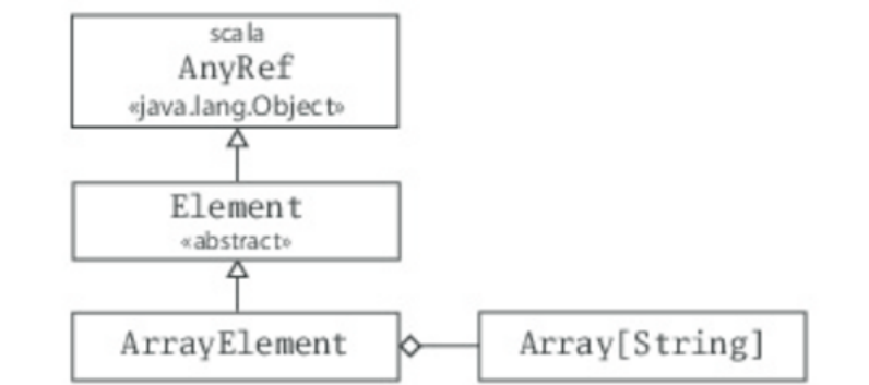
Listing 10.3 - Defining ArrayElement as a subclass of Element.
Class ArrayElement is defined to extend class Element. Just like in Java, you use an extends clause
after the class name to express this:
... extends Element ...
Figure 10.1 - Class diagram for ArrayElement.
Such an extends clause has two effects: It makes class ArrayElement inherit all non-private members
from class Element, and it makes the type ArrayElement a subtype of the type Element.
Given ArrayElement extends Element, class ArrayElement is called a subclass of
class Element.Conversely, Element is a superclass of ArrayElement. If you leave out an extends clause,
the Scala compiler implicitly assumes your class extends from scala.AnyRef, which on the Java
platform is the same as class java.lang.Object. Thus, class Element implicitly extends class AnyRef.
You can see these inheritance relationships in Figure 10.1.
Inheritance means that all members of the superclass are also members of the subclass, with two
exceptions. First, private members of the superclass are not inherited in a subclass. Second, a member
of a superclass is not inherited if a member with the same name and parameters is already implemented
in the subclass. In that case we say the member of the subclass overrides the member of the superclass.
If the member in the subclass is concrete and the member of the superclass is abstract, we also say that
the concrete memberimplements the abstract one.
For example, the contents method in ArrayElement overrides (or alternatively: implements) abstract
method contents in class Element.[2] By contrast, class ArrayElement inherits
the widthand height methods from class Element. For example, given an ArrayElement ae, you can
query its width using ae.width, as if width were defined in class ArrayElement:
scala> val ae = new ArrayElement(Array("hello", "world"))
ae: ArrayElement = ArrayElement@39274bf7
scala> ae.width
res0: Int = 5
Subtyping means that a value of the subclass can be used wherever a value of the superclass is
required. For example:
val e: Element = new ArrayElement(Array("hello"))
Variable e is defined to be of type Element, so its initializing value should also be an Element. In fact,
the initializing value's type is ArrayElement. This is OK, because class ArrayElement extends
class Element, and as a result, the type ArrayElement is compatible with the type Element.[3]
Figure 10.1 also shows the composition relationship that exists
between ArrayElement andArray[String]. This relationship is called composition because
class ArrayElement is "composed" out of class Array[String], in that the Scala compiler will place into
the binary class it generates for ArrayElement a field that holds a reference to the passed conts array.
We'll discuss some design considerations concerning composition and inheritance later in this chapter,
inSection 10.11.
10.5 OVERRIDING METHODS AND FIELDS
The uniform access principle is just one aspect where Scala treats fields and methods more uniformly
than Java. Another difference is that in Scala, fields and methods belong to the same namespace. This
makes it possible for a field to override a parameterless method. For instance, you could change the
implementation of contents in class ArrayElement from a method to a field without having to modify
the abstract method definition of contents in class Element, as shown in Listing 10.4:
class ArrayElement(conts: Array[String]) extends Element {
val contents: Array[String] = conts
}
Listing 10.4 - Overriding a parameterless method with a field.
Field contents (defined with a val) in this version of ArrayElement is a perfectly good implementation
of the parameterless method contents (declared with a def) in class Element. On the other hand, in
Scala it is forbidden to define a field and method with the same name in the same class, whereas this is
allowed in Java.
For example, this Java class would compile just fine:
// This is Java
class CompilesFine {
private int f = 0;
public int f() {
return 1;
}
}
But the corresponding Scala class would not compile:
class WontCompile {
private var f = 0 // Won't compile, because a field
def f = 1 // and method have the same name
}
Generally, Scala has just two namespaces for definitions in place of Java's four. Java's four namespaces
are fields, methods, types, and packages. By contrast, Scala's two namespaces are:
•values (fields, methods, packages, and singleton objects)
•types (class and trait names)
The reason Scala places fields and methods into the same namespace is precisely so you can override a
parameterless method with a val, something you can't do with Java.[4]
10.6 DEFINING PARAMETRIC FIELDS
Consider again the definition of class ArrayElement shown in the previous section. It has
aparameter conts whose sole purpose is to be copied into the contents field. The name conts of the
parameter was chosen just so that it would look similar to the field name contents without actually
clashing with it. This is a "code smell," a sign that there may be some unnecessary redundancy and
repetition in your code.
You can avoid the code smell by combining the parameter and the field in a singleparametric
field definition, as shown in Listing 10.5:
class ArrayElement(
val contents: Array[String]
) extends Element
Listing 10.5 - Defining contents as a parametric field.
Note that now the contents parameter is prefixed by val. This is a shorthand that defines at the same
time a parameter and field with the same name. Specifically, class ArrayElement now has an
(unreassignable) field contents, which can be accessed from outside the class. The field is initialized
with the value of the parameter. It's as if the class had been written as follows, where x123 is an
arbitrary fresh name for the parameter:
class ArrayElement(x123: Array[String]) extends Element {
val contents: Array[String] = x123
}
You can also prefix a class parameter with var, in which case the corresponding field would be
reassignable. Finally, it is possible to add modifiers, such as private, protected,[5] or override to these
parametric fields, just as you can for any other class member. Consider, for instance, the following
class definitions:
class Cat {
val dangerous = false
}
class Tiger(
override val dangerous: Boolean,
private var age: Int
) extends Cat
Tiger's definition is a shorthand for the following alternate class definition with an overriding
member dangerous and a private member age:
class Tiger(param1: Boolean, param2: Int) extends Cat {
override val dangerous = param1
private var age = param2
}
Both members are initialized from the corresponding parameters. We chose the names of those
parameters, param1 and param2, arbitrarily. The important thing was that they not clash with any other
name in scope.
10.7 INVOKING SUPERCLASS CONSTRUCTORS
You now have a complete system consisting of two classes: an abstract class Element, which is
extended by a concrete class ArrayElement. You might also envision other ways to express an
element. For example, clients might want to create a layout element consisting of a single line given by
a string. Object-oriented programming makes it easy to extend a system with new data-variants. You
can simply add subclasses. For example, Listing 10.6 shows a LineElementclass that
extends ArrayElement:
class LineElement(s: String) extends ArrayElement(Array(s)) {
override def width = s.length
override def height = 1
}
Listing 10.6 - Invoking a superclass constructor.
Since LineElement extends ArrayElement, and ArrayElement's constructor takes a parameter
(anArray[String]), LineElement needs to pass an argument to the primary constructor of its superclass.
To invoke a superclass constructor, you simply place the argument or arguments you want to pass in
parentheses following the name of the superclass. For example,
classLineElement passes Array(s) to ArrayElement's primary constructor by placing it in parentheses
after the superclass ArrayElement's name:
... extends ArrayElement(Array(s)) ...
With the new subclass, the inheritance hierarchy for layout elements now looks as shown inFigure
10.2.
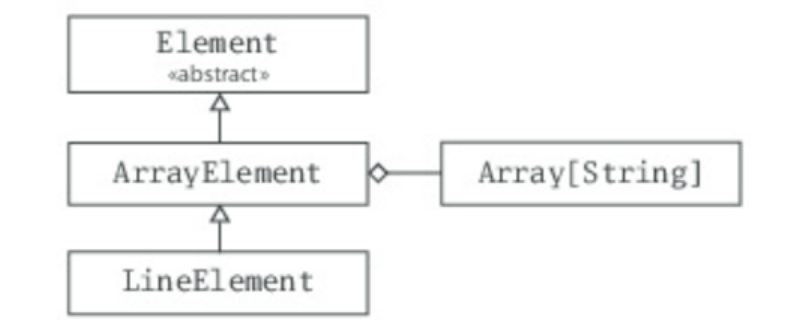
Figure 10.2 - Class diagram for LineElement.
10.8 USING OVERRIDE MODIFIERS
Note that the definitions of width and height in LineElement carry an override modifier. In Section 6.3,
you saw this modifier in the definition of a toString method. Scala requires such a modifier for all
members that override a concrete member in a parent class. The modifier is optional if a member
implements an abstract member with the same name. The modifier is forbidden if a member does not
override or implement some other member in a base class. Since height and width in
class LineElement override concrete definitions in class Element, overrideis required.
This rule provides useful information for the compiler that helps avoid some hard-to-catch errors and
makes system evolution safer. For instance, if you happen to misspell the method or accidentally give it
a different parameter list, the compiler will respond with an error message:
$ scalac LineElement.scala
.../LineElement.scala:50:
error: method hight overrides nothing
override def hight = 1
^
The override convention is even more important when it comes to system evolution. Say you defined a
library of 2D drawing methods. You made it publicly available, and it is widely used. In the next
version of the library you want to add to your base class Shape a new method with this signature:
def hidden(): Boolean
Your new method will be used by various drawing methods to determine whether a shape needs to be
drawn. This could lead to a significant speedup, but you cannot do this without the risk of breaking
client code. After all, a client could have defined a subclass of Shape with a different implementation
of hidden. Perhaps the client's method actually makes the receiver object disappear instead of testing
whether the object is hidden. Because the two versions ofhidden override each other, your drawing
methods would end up making objects disappear, which is certainly not what you want!
These "accidental overrides" are the most common manifestation of what is called the "fragile base
class" problem. The problem is that if you add new members to base classes (which we usually call
superclasses) in a class hierarchy, you risk breaking client code. Scala cannot completely solve the
fragile base class problem, but it improves on the situation compared to Java.[6] If the drawing library
and its clients were written in Scala, then the client's original implementation of hidden could not have
had an override modifier, because at the time there was no other method with that name.
Once you add the hidden method to the second version of your shape class, a recompile of the client
would give an error like the following:
.../Shapes.scala:6: error: error overriding method
hidden in class Shape of type ()Boolean;
method hidden needs `override' modifier
def hidden(): Boolean =
^
That is, instead of wrong behavior your client would get a compile-time error, which is usually much
preferable.
10.9 POLYMORPHISM AND DYNAMIC BINDING
You saw in Section 10.4 that a variable of type Element could refer to an object of typeArrayElement.
The name for this phenomenon is polymorphism, which means "many shapes" or "many forms." In this
case, Element objects can have many forms.[7]
So far, you've seen two such forms: ArrayElement and LineElement. You can create more forms
ofElement by defining new Element subclasses. For example, you could define a new form
ofElement that has a given width and height, and is filled everywhere with a given character:
class UniformElement(
ch: Char,
override val width: Int,
override val height: Int
) extends Element {
private val line = ch.toString * width
def contents = Array.fill(height)(line)
}
The inheritance hierarchy for class Element now looks as shown in Figure 10.3. As a result, Scala will
accept all of the following assignments, because the type of the assigning expression conforms to the
type of the defined variable:
val e1: Element = new ArrayElement(Array("hello", "world"))
val ae: ArrayElement = new LineElement("hello")
val e2: Element = ae
val e3: Element = new UniformElement('x', 2, 3)
If you check the inheritance hierarchy, you'll find that in each of these four val definitions, the type of
the expression to the right of the equals sign is below the type of the val being initialized to the left of
the equals sign.
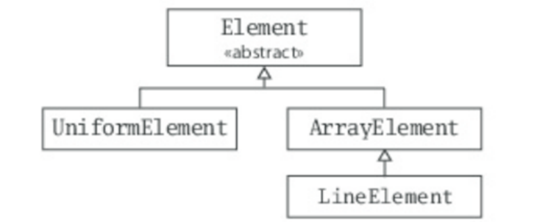
Figure 10.3 - Class hierarchy of layout elements.
The other half of the story, however, is that method invocations on variables and expressions
are dynamically bound. This means that the actual method implementation invoked is determined at run
time based on the class of the object, not the type of the variable or expression. To demonstrate this
behavior, we'll temporarily remove all existing members from our Element classes and add a method
named demo to Element. We'll override demo inArrayElement and LineElement, but not
in UniformElement:
abstract class Element {
def demo() = {
println("Element's implementation invoked")
}
}
class ArrayElement extends Element {
override def demo() = {
println("ArrayElement's implementation invoked")
}
}
class LineElement extends ArrayElement {
override def demo() = {
println("LineElement's implementation invoked")
}
}
// UniformElement inherits Element's demo
class UniformElement extends Element
If you enter this code into the interpreter, you can then define this method that takes anElement and
invokes demo on it:
def invokeDemo(e: Element) = {
e.demo()
}
If you pass an ArrayElement to invokeDemo, you'll see a message indicating ArrayElement's
implementation of demo was invoked, even though the type of the variable, e, on which demowas
invoked is Element:
scala> invokeDemo(new ArrayElement)
ArrayElement's implementation invoked
Similarly, if you pass a LineElement to invokeDemo, you'll see a message that
indicates LineElement'sdemo implementation was invoked:
scala> invokeDemo(new LineElement)
LineElement's implementation invoked
The behavior when passing a UniformElement may at first glance look suspicious, but it is correct:
scala> invokeDemo(new UniformElement)
Element's implementation invoked
Because UniformElement does not override demo, it inherits the implementation of demo from its
superclass, Element. Thus, Element's implementation is the correct implementation of demo to invoke
when the class of the object is UniformElement.
10.10 DECLARING FINAL MEMBERS
Sometimes when designing an inheritance hierarchy, you want to ensure that a member cannot be
overridden by subclasses. In Scala, as in Java, you do this by adding a finalmodifier to the member. As
shown in Listing 10.7, you could place a final modifier onArrayElement's demo method.
class ArrayElement extends Element {
final override def demo() = {
println("ArrayElement's implementation invoked")
}
}
Listing 10.7 - Declaring a final method.
Given this version of ArrayElement, an attempt to override demo in its subclass, LineElement, would
not compile:
elem.scala:18: error: error overriding method demo
in class ArrayElement of type ()Unit;
method demo cannot override final member
override def demo() = {
^
You may also at times want to ensure that an entire class not be subclassed. To do this you simply
declare the entire class final by adding a final modifier to the class declaration. For example, Listing
10.8 shows how you would declare ArrayElement final:
final class ArrayElement extends Element {
override def demo() = {
println("ArrayElement's implementation invoked")
}
}
Listing 10.8 - Declaring a final class.
With this version of ArrayElement, any attempt at defining a subclass would fail to compile:
elem.scala: 18: error: illegal inheritance from final class
ArrayElement
class LineElement extends ArrayElement {
^
We'll now remove the final modifiers and demo methods, and go back to the earlier implementation of
the Element family. We'll focus our attention in the remainder of this chapter to completing a working
version of the layout library.
10.11 USING COMPOSITION AND INHERITANCE
Composition and inheritance are two ways to define a new class in terms of another existing class. If
what you're after is primarily code reuse, you should in general prefer composition to inheritance. Only
inheritance suffers from the fragile base class problem, in which you can inadvertently break subclasses
by changing a superclass.
One question you can ask yourself about an inheritance relationship is whether it models anis-
a relationship.[8] For example, it would be reasonable to say that ArrayElement is-an Element. Another
question you can ask is whether clients will want to use the subclass type as a superclass type.[9] In the
case of ArrayElement, we do indeed expect clients will want to use anArrayElement as an Element.
If you ask these questions about the inheritance relationships shown in Figure 10.3, do any of the
relationships seem suspicious? In particular, does it seem obvious to you that a LineElementis-
an ArrayElement? Do you think clients would ever need to use a LineElement as an ArrayElement?
In fact, we defined LineElement as a subclass of ArrayElement primarily to reuse ArrayElement's
definition of contents. Perhaps it would be better, therefore, to define LineElement as a direct subclass
of Element, like this:
class LineElement(s: String) extends Element {
val contents = Array(s)
override def width = s.length
override def height = 1
}
In the previous version, LineElement had an inheritance relationship with ArrayElement, from which it
inherited contents. It now has a composition relationship with Array: it holds a reference to an array of
strings from its own contents field.[10] Given this implementation ofLineElement, the inheritance
hierarchy for Element now looks as shown in Figure 10.4.
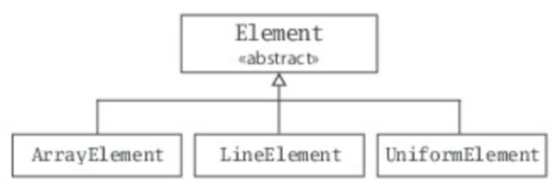
Figure 10.4 - Class hierarchy with revised LineElement.
10.12 IMPLEMENTING ABOVE, BESIDE, AND TOSTRING
As a next step, we'll implement method above in class Element. Putting one element above another
means concatenating the two contents values of the elements. So a first draft of method above could
look like this:
def above(that: Element): Element =
new ArrayElement(this.contents ++ that.contents)
The ++ operation concatenates two arrays. Arrays in Scala are represented as Java arrays, but support
many more methods. Specifically, arrays in Scala can be converted to instances of a class scala.Seq,
which represents sequence-like structures and contains a number of methods for accessing and
transforming sequences. Some other array methods will be explained in this chapter and a more
comprehensive discussion will be given in Chapter 17.
In fact, the code shown previously is not quite sufficient because it does not let you put elements of
different widths on top of each other. To keep things simple in this section, however, we'll leave this as
is and only pass elements of the same length to above. In Section 10.14, we'll make an enhancement
to above so that clients can use it to combine elements of different widths.
The next method to implement is beside. To put two elements beside each other, we'll create a new
element in which every line results from concatenating corresponding lines of the two elements. As
before, to keep things simple, we'll start by assuming the two elements have the same height. This leads
to the following design of method beside:
def beside(that: Element): Element = {
val contents = new Array[String](this.contents.length)
for (i <- 0 until this.contents.length)
contents(i) = this.contents(i) + that.contents(i)
new ArrayElement(contents)
}
The beside method first allocates a new array, contents, and fills it with the concatenation of the
corresponding array elements in this.contents and that.contents. It finally produces a
newArrayElement containing the new contents.
Although this implementation of beside works, it is in an imperative style, the telltale sign of which is
the loop in which we index through arrays. Alternatively, the method could be abbreviated to one
expression:
new ArrayElement(
for (
(line1, line2) <- this.contents zip that.contents
) yield line1 + line2
)
Here, the two arrays, this.contents and that.contents, are transformed into an array of pairs (asTuple2s
are called) using the zip operator. The zip operator picks corresponding elements in its two operands
and forms an array of pairs. For instance, this expression:
Array(1, 2, 3) zip Array("a", "b")
will evaluate to:
Array((1, "a"), (2, "b"))
If one of the two operand arrays is longer than the other, zip will drop the remaining elements. In the
expression above, the third element of the left operand, 3, does not form part of the result, because it
does not have a corresponding element in the right operand.
The zipped array is then iterated over by a for expression. Here, the syntax "for ((line1, line2) <- ...)"
allows you to name both elements of a pair in one pattern (i.e., line1stands now for the first element of
the pair, and line2 stands for the second). Scala's pattern-matching system will be described in detail
in Chapter 15. For now, you can just think of this as a way to define two vals, line1 and line2, for each
step of the iteration.
The for expression has a yield part and therefore yields a result. The result is of the same kind as the
expression iterated over (i.e., it is an array). Each element of the array is the result of concatenating the
corresponding lines, line1 and line2. So the end result of this code is the same as in the first version
of beside, but because it avoids explicit array indexing, the result is obtained in a less error-prone way.
You still need a way to display elements. As usual, this is done by defining a toString method that
returns an element formatted as a string. Here is its definition:
override def toString = contents mkString "\n"
The implementation of toString makes use of mkString, which is defined for all sequences, including
arrays. As you saw in Section 7.8, an expression like "arr mkString sep" returns a string consisting of
all elements of the array arr. Each element is mapped to a string by calling its toString method. A
separator string sep is inserted between consecutive element strings. So the expression,
"contents mkString "\n"" formats the contents array as a string, where each array element appears on a
line by itself.
abstract class Element {
def contents: Array[String]
def width: Int =
if (height == 0) 0 else contents(0).length
def height: Int = contents.length
def above(that: Element): Element =
new ArrayElement(this.contents ++ that.contents)
def beside(that: Element): Element =
new ArrayElement(
for (
(line1, line2) <- this.contents zip that.contents
) yield line1 + line2
)
override def toString = contents mkString "\n"
}
Listing 10.9 - Class Element with above, beside, and toString.
Note that toString does not carry an empty parameter list. This follows the recommendations for the
uniform access principle, because toString is a pure method that does not take any parameters. With the
addition of these three methods, class Element now looks as shown inListing 10.9.
10.13 DEFINING A FACTORY OBJECT
You now have a hierarchy of classes for layout elements. This hierarchy could be presented to your
clients "as is," but you might also choose to hide the hierarchy behind a factory object.
A factory object contains methods that construct other objects. Clients would then use these factory
methods to construct objects, rather than constructing the objects directly with new. An advantage of
this approach is that object creation can be centralized and the details of how objects are represented
with classes can be hidden. This hiding will both make your library simpler for clients to understand,
because less detail is exposed, and provide you with more opportunities to change your library's
implementation later without breaking client code.
The first task in constructing a factory for layout elements is to choose where the factory methods
should be located. Should they be members of a singleton object or of a class? What should the
containing object or class be called? There are many possibilities. A straightforward solution is to
create a companion object of class Element and make this the factory object for layout elements. That
way, you need to expose only the class/object combo of Element to your clients, and you can hide the
three implementation classes ArrayElement,LineElement, and UniformElement.
Listing 10.10 is a design of the Element object that follows this scheme. The Element object contains
three overloaded variants of an elem method and each constructs a different kind of layout object.
object Element {
def elem(contents: Array[String]): Element =
new ArrayElement(contents)
def elem(chr: Char, width: Int, height: Int): Element =
new UniformElement(chr, width, height)
def elem(line: String): Element =
new LineElement(line)
}
Listing 10.10 - A factory object with factory methods.
With the advent of these factory methods, it makes sense to change the implementation of
class Element so that it goes through the elem factory methods rather than creating
newArrayElement instances explicitly. To call the factory methods without qualifying them
withElement, the name of the singleton object, we will import Element.elem at the top of the source
file. In other words, instead of invoking the factory methods with Element.elem inside classElement,
we'll import Element.elem so we can just call the factory methods by their simple name,elem. Listing
10.11 shows what class Element will look like after these changes.
import Element.elem
abstract class Element {
def contents: Array[String]
def width: Int =
if (height == 0) 0 else contents(0).length
def height: Int = contents.length
def above(that: Element): Element =
elem(this.contents ++ that.contents)
def beside(that: Element): Element =
elem(
for (
(line1, line2) <- this.contents zip that.contents
) yield line1 + line2
)
override def toString = contents mkString "\n"
}
Listing 10.11 - Class Element refactored to use factory methods.
In addition, given the factory methods, the subclasses, ArrayElement, LineElement,
andUniformElement, could now be private because they no longer need to be accessed directly by
clients. In Scala, you can define classes and singleton objects inside other classes and singleton
objects. One way to make the Element subclasses private is to place them inside theElement singleton
object and declare them private there. The classes will still be accessible to the three elem factory
methods, where they are needed. Listing 10.12 shows how that will look.
10.14 HEIGHTEN AND WIDEN
We need one last enhancement. The version of Element shown in Listing 10.11 is not quite sufficient
because it does not allow clients to place elements of different widths on top of each other, or place
elements of different heights beside each other.
For example, evaluating the following expression won't work correctly, because the second line in the
combined element is longer than the first:
new ArrayElement(Array("hello")) above
new ArrayElement(Array("world!"))
Similarly, evaluating the following expression would not work properly, because the
firstArrayElement has a height of two and the second a height of only one:
new ArrayElement(Array("one", "two")) beside
new ArrayElement(Array("one"))
Listing 10.13 shows a private helper method, widen, which takes a width and returns an Elementof that
width. The result contains the contents of this Element, centered, padded to the left and right by any
spaces needed to achieve the required width. Listing 10.13 also shows a similar method, heighten,
which performs the same function in the vertical direction. The widenmethod is invoked by above to
ensure that Elements placed above each other have the same width. Similarly, the heighten method is
invoked by beside to ensure that elements placed beside each other have the same height. With these
changes, the layout library is ready for use.
object Element {
private class ArrayElement(
val contents: Array[String]
) extends Element
private class LineElement(s: String) extends Element {
val contents = Array(s)
override def width = s.length
override def height = 1
}
private class UniformElement(
ch: Char,
override val width: Int,
override val height: Int
) extends Element {
private val line = ch.toString * width
def contents = Array.fill(height)(line)
}
def elem(contents: Array[String]): Element =
new ArrayElement(contents)
def elem(chr: Char, width: Int, height: Int): Element =
new UniformElement(chr, width, height)
def elem(line: String): Element =
new LineElement(line)
}
Listing 10.12 - Hiding implementation with private classes.
import Element.elem
abstract class Element {
def contents: Array[String]
def width: Int = contents(0).length
def height: Int = contents.length
def above(that: Element): Element = {
val this1 = this widen that.width
val that1 = that widen this.width
elem(this1.contents ++ that1.contents)
}
def beside(that: Element): Element = {
val this1 = this heighten that.height
val that1 = that heighten this.height
elem(
for ((line1, line2) <- this1.contents zip that1.contents)
yield line1 + line2)
}
def widen(w: Int): Element =
if (w <= width) this
else {
val left = elem(' ', (w - width) / 2, height)
val right = elem(' ', w - width - left.width, height)
left beside this beside right
}
def heighten(h: Int): Element =
if (h <= height) this
else {
val top = elem(' ', width, (h - height) / 2)
val bot = elem(' ', width, h - height - top.height)
top above this above bot
}
override def toString = contents mkString "\n"
}
Listing 10.13 - Element with widen and heighten methods.
10.15 PUTTING IT ALL TOGETHER
A fun way to exercise almost all elements of the layout library is to write a program that draws a spiral
with a given number of edges. This Spiral program, shown in Listing 10.14, will do just that.
import Element.elem
object Spiral {
val space = elem(" ")
val corner = elem("+")
def spiral(nEdges: Int, direction: Int): Element = {
if (nEdges == 1)
elem("+")
else {
val sp = spiral(nEdges - 1, (direction + 3) % 4)
def verticalBar = elem('|', 1, sp.height)
def horizontalBar = elem('-', sp.width, 1)
if (direction == 0)
(corner beside horizontalBar) above (sp beside space)
else if (direction == 1)
(sp above space) beside (corner above verticalBar)
else if (direction == 2)
(space beside sp) above (horizontalBar beside corner)
else
(verticalBar above corner) beside (space above sp)
}
}
def main(args: Array[String]) = {
val nSides = args(0).toInt
println(spiral(nSides, 0))
}
}
Listing 10.14 - The Spiral application.
Because Spiral is a standalone object with a main method with the proper signature, it is a Scala
application. Spiral takes one command-line argument, an integer, and draws a spiral with the specified
number of edges. For example, you could draw a six-edge spiral, as shown on the left, and larger
spirals, as shown on the right.
$ scala Spiral 6 $ scala Spiral 11 $ scala Spiral 17
+----- +---------- +----------------
| | |
| +-+ | +------+ | +------------+
| + | | | | | | |
| | | | +--+ | | | +--------+ |
+---+ | | | | | | | | | |
| | ++ | | | | | +----+ | |
| | | | | | | | | | |
| +----+ | | | | | ++ | | |
| | | | | | | | | |
+--------+ | | | +--+ | | |
| | | | | |
| | +------+ | |
| | | |
| +----------+ |
| |
+--------------+
10.16 CONCLUSION
In this section, you saw more concepts related to object-oriented programming in Scala. Among others,
you encountered abstract classes, inheritance and subtyping, class hierarchies, parametric fields, and
method overriding. You should have developed a feel for constructing a non-trivial class hierarchy in
Scala. We'll work with the layout library again inChapter 14.
Footnotes for Chapter 10:
[1] Meyer, Object-Oriented Software Construction [Mey00]
[2] One flaw with this design is that because the returned array is mutable, clients could change it. For
the book we'll keep things simple, but were ArrayElement part of a real project, you might consider
returning a defensive copy of the array instead. Another problem is we aren't currently ensuring that
every String element of the contents array has the same length. This could be solved by checking the
precondition in the primary constructor and throwing an exception if it is violated.
[3] For more perspective on the difference between subclass and subtype, see the glossary entry
for subtype.
[4] The reason that packages share the same namespace as fields and methods in Scala is to enable you
to import packages (in addition to just the names of types) and the fields and methods of singleton
objects. This is also something you can't do in Java. It will be described in Section 13.3.
[5] The protected modifier, which grants access to subclasses, will be covered in detail inChapter 13.
[6] In Java 1.5, an @Override annotation was introduced that works similarly to
Scala's overridemodifier, but unlike Scala's override, is not required.
[7] This kind of polymorphism is called subtyping polymorphism. Another kind of polymorphism in
Scala called universal polymorphism is discussed in Chapter 19.
[8] Meyers, Effective C++ [Mey91]
[9] Eckel, Thinking in Java [Eck98]
[10] Class ArrayElement also has a composition relationship with Array, because its
parametriccontents field holds a reference to an array of strings. The code for ArrayElement is shown
inListing 10.5 here. Its composition relationship is represented in class diagrams by a diamond, as
shown, for example, in Figure 10.1 here.
Chapter 11
Scala's Hierarchy
Now that you've seen the details of class inheritance in the previous chapter, it is a good time to take a
step back and look at Scala's class hierarchy as a whole. In Scala, every class inherits from a common
superclass named Any. Because every class is a subclass of Any, the methods defined in Any are
"universal" methods: they may be invoked on any object. Scala also defines some interesting classes at
the bottom of the hierarchy, Null and Nothing, which essentially act as common subclasses. For
example, just as Any is a superclass of every other class, Nothing is a subclass of every other class. In
this chapter, we'll give you a tour of Scala's class hierarchy.
11.1 SCALA'S CLASS HIERARCHY
Figure 11.1 shows an outline of Scala's class hierarchy. At the top of the hierarchy is class Any, which
defines methods that include the following:
final def ==(that: Any): Boolean
final def !=(that: Any): Boolean
def equals(that: Any): Boolean
def ##: Int
def hashCode: Int
def toString: String
Because every class inherits from Any, every object in a Scala program can be compared using==, !=,
or equals; hashed using ## or hashCode; and formatted using toString. The equality and inequality
methods, == and !=, are declared final in class Any, so they cannot be overridden in subclasses.
The == method is essentially the same as equals and != is always the negation ofequals.[1] So
individual classes can tailor what == or != means by overriding the equals method. We'll show an
example later in this chapter.
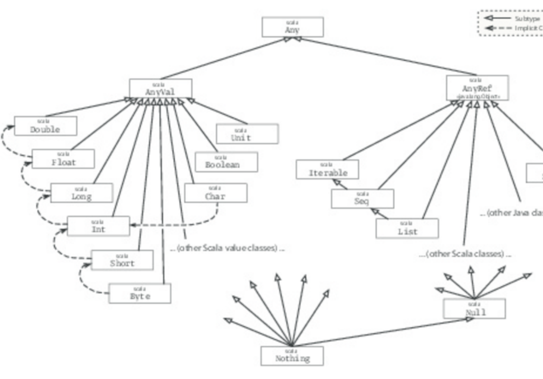
Class hierarchy of Scala.
The root class Any has two subclasses: AnyVal and AnyRef. AnyVal is the parent class of value
classes in Scala. While you can define your own value classes (see Section 11.4), there are nine value
classes built into Scala: Byte, Short, Char, Int, Long, Float, Double, Boolean, and Unit. The first eight
of these correspond to Java's primitive types, and their values are represented at run time as Java's
primitive values. The instances of these classes are all written as literals in Scala. For example, 42 is an
instance of Int, 'x' is an instance of Char, and false an instance ofBoolean. You cannot create instances
of these classes using new. This is enforced by the "trick" that value classes are all defined to be both
abstract and final.
So if you were to write:
scala> new Int
you would get:
<console>:5: error: class Int is abstract; cannot be
instantiated
new Int
^
The other value class, Unit, corresponds roughly to Java's void type; it is used as the result type of a
method that does not otherwise return an interesting result. Unit has a single instance value, which is
written (), as discussed in Section 7.2.
As explained in Chapter 5, the value classes support the usual arithmetic and boolean operators as
methods. For instance, Int has methods named + and *, and Boolean has methods named || and &&.
Value classes also inherit all methods from class Any. You can test this in the interpreter:
scala> 42.toString
res1: String = 42
scala> 42.hashCode
res2: Int = 42
scala> 42 equals 42
res3: Boolean = true
Note that the value class space is flat; all value classes are subtypes of scala.AnyVal, but they do not
subclass each other. Instead there are implicit conversions between different value class types. For
example, an instance of class scala.Int is automatically widened (by an implicit conversion) to an
instance of class scala.Long when required.
As mentioned in Section 5.10, implicit conversions are also used to add more functionality to value
types. For instance, the type Int supports all of the operations below:
scala> 42 max 43
res4: Int = 43
scala> 42 min 43
res5: Int = 42
scala> 1 until 5
res6: scala.collection.immutable.Range = Range(1, 2, 3, 4)
scala> 1 to 5
res7: scala.collection.immutable.Range.Inclusive
= Range(1, 2, 3, 4, 5)
scala> 3.abs
res8: Int = 3
scala> (-3).abs
res9: Int = 3
Here's how this works: The methods min, max, until, to, and abs are all defined in a
classscala.runtime.RichInt, and there is an implicit conversion from class Int to RichInt. The
conversion is applied whenever a method is invoked on an Int that is undefined in Int but defined
in RichInt. Similar "booster classes" and implicit conversions exist for the other value classes. Implicit
conversions will be discussed in detail in Chapter 21.
The other subclass of the root class Any is class AnyRef. This is the base class of all reference
classes in Scala. As mentioned previously, on the Java platform AnyRef is in fact just an alias for
class java.lang.Object. So classes written in Java, as well as classes written in Scala, all inherit
from AnyRef.[2] One way to think of java.lang.Object, therefore, is as the way AnyRef is implemented
on the Java platform. Thus, although you can use Object and AnyRefinterchangeably in Scala programs
on the Java platform, the recommended style is to useAnyRef everywhere.
11.2 HOW PRIMITIVES ARE IMPLEMENTED
How is all this implemented? In fact, Scala stores integers in the same way as Java—as 32-bit words.
This is important for efficiency on the JVM and also for interoperability with Java libraries. Standard
operations like addition or multiplication are implemented as primitive operations. However, Scala uses
the "backup" class java.lang.Integer whenever an integer needs to be seen as a (Java) object. This
happens for instance when invoking the toStringmethod on an integer number or when assigning an
integer to a variable of type Any. Integers of type Int are converted transparently to "boxed integers" of
type java.lang.Integer whenever necessary.
All this sounds a lot like auto-boxing in Java 5 and it is indeed quite similar. There's one crucial
difference though: Boxing in Scala is much less visible than boxing in Java. Try the following in Java:
// This is Java
boolean isEqual(int x, int y) {
return x == y;
}
System.out.println(isEqual(421, 421));
You will surely get true. Now, change the argument types of isEqual to java.lang.Integer (orObject, the
result will be the same):
// This is Java
boolean isEqual(Integer x, Integer y) {
return x == y;
}
System.out.println(isEqual(421, 421));
You will find that you get false! What happens is that the number 421 gets boxed twice, so that the
arguments for x and y are two different objects. Because == means reference equality on reference
types, and Integer is a reference type, the result is false. This is one aspect where it shows that Java is
not a pure object-oriented language. There is a difference between primitive types and reference types
that can be clearly observed.
Now try the same experiment in Scala:
scala> def isEqual(x: Int, y: Int) = x == y
isEqual: (x: Int, y: Int)Boolean
scala> isEqual(421, 421)
res10: Boolean = true
scala> def isEqual(x: Any, y: Any) = x == y
isEqual: (x: Any, y: Any)Boolean
scala> isEqual(421, 421)
res11: Boolean = true
The equality operation == in Scala is designed to be transparent with respect to the type's
representation. For value types, it is the natural (numeric or boolean) equality. For reference types other
than Java's boxed numeric types, == is treated as an alias of the equals method inherited from Object.
That method is originally defined as reference equality, but is overridden by many subclasses to
implement their natural notion of equality. This also means that in Scala you never fall into Java's well-
known trap concerning string comparisons. In Scala, string comparison works as it should:
scala> val x = "abcd".substring(2)
x: String = cd
scala> val y = "abcd".substring(2)
y: String = cd
scala> x == y
res12: Boolean = true
In Java, the result of comparing x with y would be false. The programmer should have usedequals in
this case, but it is easy to forget.
However, there are situations where you need reference equality instead of user-defined equality. For
example, in some situations where efficiency is paramount, you would like tohash cons with some
classes and compare their instances with reference equality.[3] For these cases, class AnyRef defines an
additional eq method, which cannot be overridden and is implemented as reference equality (i.e., it
behaves like == in Java for reference types). There's also the negation of eq, which is called ne. For
example:
scala> val x = new String("abc")
x: String = abc
scala> val y = new String("abc")
y: String = abc
scala> x == y
res13: Boolean = true
scala> x eq y
res14: Boolean = false
scala> x ne y
res15: Boolean = true
Equality in Scala is discussed further in Chapter 30.
11.3 BOTTOM TYPES
At the bottom of the type hierarchy in Figure 11.1 you see the two classes scala.Null andscala.Nothing.
These are special types that handle some "corner cases" of Scala's object-oriented type system in a
uniform way.
Class Null is the type of the null reference; it is a subclass of every reference class (i.e., every class that
itself inherits from AnyRef). Null is not compatible with value types. You cannot, for example, assign
a null value to an integer variable:
scala> val i: Int = null
<console>:7: error: an expression of type Null is ineligible
for implicit conversion
val i: Int = null
^
Type Nothing is at the very bottom of Scala's class hierarchy; it is a subtype of every other type.
However, there exist no values of this type whatsoever. Why does it make sense to have a type without
values? As discussed in Section 7.4, one use of Nothing is that it signals abnormal termination.
For instance there's the error method in the Predef object of Scala's standard library, which is defined
like this:
def error(message: String): Nothing =
throw new RuntimeException(message)
The return type of error is Nothing, which tells users that the method will not return normally (it throws
an exception instead). Because Nothing is a subtype of every other type, you can use methods
like error in very flexible ways. For instance:
def divide(x: Int, y: Int): Int =
if (y != 0) x / y
else error("can't divide by zero")
The "then" branch of the conditional, x / y, has type Int, whereas the else branch, the call toerror, has
type Nothing. Because Nothing is a subtype of Int, the type of the whole conditional isInt, as required.
11.4 DEFINING YOUR OWN VALUE CLASSES
As mentioned in Section 11.1, you can define your own value classes to augment the ones that are built
in. Like the built-in value classes, an instance of your value class will usually compile to Java bytecode
that does not use the wrapper class. In contexts where a wrapper is needed, such as with generic code,
the value will get boxed and unboxed automatically.
Only certain classes can be made into value classes. For a class to be a value class, it must have exactly
one parameter and it must have nothing inside it except defs. Furthermore, no other class can extend a
value class, and a value class cannot redefine equals or hashCode.
To define a value class, make it a subclass of AnyVal, and put val before the one parameter. Here is an
example value class:
class Dollars(val amount: Int) extends AnyVal {
override def toString() = "$" + amount
}
As described in Section 10.6, the val prefix allows the amount parameter to be accessed as a field. For
example, the following code creates an instance of the value class, then retrieves the amount from it:
scala> val money = new Dollars(1000000)
money: Dollars = $1000000
scala> money.amount
res16: Int = 1000000
In this example, money refers to an instance of the value class. It is of type Dollars in Scala source
code, but the compiled Java bytecode will use type Int directly.
This example defines a toString method, and the compiler figures out when to use it. That's why
printing money gives $1000000, with a dollar sign, but printing money.amount gives 1000000. You can
even define multiple value types that are all backed by the same Int value. For example:
class SwissFrancs(val amount: Int) extends AnyVal {
override def toString() = amount + " CHF"
}
Even though both Dollars and SwissFrancs are represented as integers, it works fine to use them in the
same scope:
scala> val dollars = new Dollars(1000)
dollars: Dollars = $1000
scala> val francs = new SwissFrancs(1000)
francs: SwissFrancs = 1000 CHF
Avoiding a types monoculture
To get the most benefit from the Scala class hierarchy, try to define a new class for each domain
concept, even when it would be possible to reuse the same class for different purposes. Even if such a
class is a so-called tiny type with no methods or fields, defining the additional class is a way to help the
compiler be helpful to you.
For example, suppose you are writing some code to generate HTML. In HTML, a style name is
represented as a string. So are anchor identifiers. HTML itself is also a string, so if you wanted, you
could define helper code using strings to represent all of these things, like this:
def title(text: String, anchor: String, style: String): String =
s"<a id='$anchor'><h1 class='$style'>$text</h1></a>"
That type signature has four strings in it! Such stringly typed code is technically strongly typed, but
since everything in sight is of type String, the compiler cannot help you detect the use of one when you
meant to write the other. For example, it won't stop you from this travesty:
scala> title("chap:vcls", "bold", "Value Classes")
res17: String = <a id='bold'><h1 class='Value
Classes'>chap:vcls</h1></a>
This HTML is mangled. The intended display text "Value Classes" is being used as a style class, and
the text being displayed is "chap.vcls," which was supposed to be an anchor. To top it off, the actual
anchor identifier is "bold," which is supposed to be a style class. Despite this comedy of errors, the
compiler utters not a peep.
The compiler can be more helpful if you define a tiny type for each domain concept. For example, you
could define a small class for styles, anchor identifiers, display text, and HTML. Since these classes
have one parameter and no members, they can be defined as value classes:
class Anchor(val value: String) extends AnyVal
class Style(val value: String) extends AnyVal
class Text(val value: String) extends AnyVal
class Html(val value: String) extends AnyVal
Given these classes, it is possible to write a version of title that has a less trivial type signature:
def title(text: Text, anchor: Anchor, style: Style): Html =
new Html(
s"<a id='${anchor.value}'>" +
s"<h1 class='${style.value}'>" +
text.value +
"</h1></a>"
)
If you try to use this version with the arguments in the wrong order, the compiler can now detect the
error. For example:
scala> title(new Anchor("chap:vcls"), new Style("bold"),
new Text("Value Classes"))
<console>:18: error: type mismatch;
found : Anchor
required: Text
new Anchor("chap:vcls"),
^
<console>:19: error: type mismatch;
found : Style
required: Anchor
new Style("bold"),
^
<console>:20: error: type mismatch;
found : Text
required: Style
new Text("Value Classes"))
^
11.5 CONCLUSION
In this chapter we showed you the classes at the top and bottom of Scala's class hierarchy. Now that
you've gotten a good foundation on class inheritance in Scala, you're ready to understand mixin
composition. In the next chapter, you'll learn about traits.
Footnotes for Chapter 11:
[1] The only case where == does not directly call equals is for Java's boxed numeric classes, such
as Integer or Long. In Java, a new Integer(1) does not equal a new Long(1) even though for primitive
values 1 == 1L. Since Scala is a more regular language than Java, it was necessary to correct this
discrepancy by special-casing the == method for these classes. Likewise, the ##method provides a
Scala version of hashing that is the same as Java's hashCode, except for boxed numeric types, where it
works consistently with ==. For instance new Integer(1) andnew Long(1) hash the same with ## even
though their Java hashCodes are different.
[2] The reason AnyRef alias exists, instead of just using the name java.lang.Object, is because Scala
was originally designed to work on both the Java and .NET platforms. On .NET, AnyRefwas an alias
for System.Object.
[3] You hash cons instances of a class by caching all instances you have created in a weak collection.
Then, any time you want a new instance of the class, you first check the cache. If the cache already has
an element equal to the one you are about to create, you can reuse the existing instance. As a result of
this arrangement, any two instances that are equal withequals() are also equal with reference equality.
Chapter 12
Traits
Traits are a fundamental unit of code reuse in Scala. A trait encapsulates method and field definitions,
which can then be reused by mixing them into classes. Unlike class inheritance, in which each class
must inherit from just one superclass, a class can mix in any number of traits. This chapter shows you
how traits work and shows two of the most common ways they are useful: widening thin interfaces to
rich ones, and defining stackable modifications. It also shows how to use the Ordered trait and
compares traits to the multiple inheritance of other languages.
12.1 HOW TRAITS WORK
A trait definition looks just like a class definition except that it uses the keyword trait. An example is
shown in Listing 12.1:
trait Philosophical {
def philosophize() = {
println("I consume memory, therefore I am!")
}
}
Listing 12.1 - The definition of trait Philosophical.
This trait is named Philosophical. It does not declare a superclass, so like a class, it has the default
superclass of AnyRef. It defines one method, named philosophize, which is concrete. It's a simple trait,
just enough to show how traits work.
Once a trait is defined, it can be mixed in to a class using either the extends or with keywords.Scala
programmers "mix in" traits rather than inherit from them, because mixing in a trait has important
differences from the multiple inheritance found in many other languages. This issue is discussed
in Section 12.6. For example, Listing 12.2 shows a class that mixes in thePhilosophical trait
using extends:
class Frog extends Philosophical {
override def toString = "green"
}
Listing 12.2 - Mixing in a trait using extends.
You can use the extends keyword to mix in a trait; in that case you implicitly inherit the trait's
superclass. For instance, in Listing 12.2, class Frog subclasses AnyRef (the superclass ofPhilosophical)
and mixes in Philosophical. Methods inherited from a trait can be used just like methods inherited from
a superclass. Here's an example:
scala> val frog = new Frog
frog: Frog = green
scala> frog.philosophize()
I consume memory, therefore I am!
A trait also defines a type. Here's an example in which Philosophical is used as a type:
scala> val phil: Philosophical = frog
phil: Philosophical = green
scala> phil.philosophize()
I consume memory, therefore I am!
The type of phil is Philosophical, a trait. Thus, variable phil could have been initialized with any object
whose class mixes in Philosophical.
If you wish to mix a trait into a class that explicitly extends a superclass, you use extends to indicate
the superclass and with to mix in the trait. Listing 12.3 shows an example. If you want to mix in
multiple traits, you add more with clauses. For example, given a trait HasLegs, you could mix
both Philosophical and HasLegs into Frog as shown in Listing 12.4.
class Animal
class Frog extends Animal with Philosophical {
override def toString = "green"
}
Listing 12.3 - Mixing in a trait using with.
class Animal
trait HasLegs
class Frog extends Animal with Philosophical with HasLegs {
override def toString = "green"
}
Listing 12.4 - Mixing in multiple traits.
In the examples you've seen so far, class Frog has inherited an implementation of philosophizefrom
trait Philosophical. Alternatively, Frog could override philosophize. The syntax looks the same as
overriding a method declared in a superclass. Here's an example:
class Animal
class Frog extends Animal with Philosophical {
override def toString = "green"
override def philosophize() = {
println("It ain't easy being " + toString + "!")
}
}
Because this new definition of Frog still mixes in trait Philosophical, you can still use it from a variable
of that type. But because Frog overrides Philosophical's implementation of philosophize, you'll get a
new behavior when you call it:
scala> val phrog: Philosophical = new Frog
phrog: Philosophical = green
scala> phrog.philosophize()
It ain't easy being green!
At this point you might philosophize that traits are like Java interfaces with concrete methods, but they
can actually do much more. Traits can, for example, declare fields and maintain state. In fact, you can
do anything in a trait definition that you can do in a class definition, and the syntax looks exactly the
same, with only two exceptions.
First, a trait cannot have any "class" parameters (i.e., parameters passed to the primary constructor of a
class). In other words, although you could define a class like this:
class Point(x: Int, y: Int)
The following attempt to define a trait would not compile:
trait NoPoint(x: Int, y: Int) // Does not compile
You'll find out in Section 20.5 how to work around this restriction.
The other difference between classes and traits is that whereas in classes, super calls are statically
bound, in traits, they are dynamically bound. If you write "super.toString" in a class, you know exactly
which method implementation will be invoked. When you write the same thing in a trait, however, the
method implementation to invoke for the super call is undefined when you define the trait. Rather, the
implementation to invoke will be determined anew each time the trait is mixed into a concrete class.
This curious behavior of super is key to allowing traits to work as stackable modifications, which will
be described in Section 12.5. The rules for resolving super calls will be given in Section 12.6.
12.2 THIN VERSUS RICH INTERFACES
One major use of traits is to automatically add methods to a class in terms of methods the class already
has. That is, traits can enrich a thin interface, making it into a rich interface.
Thin versus rich interfaces represents a commonly faced trade-off in object-oriented design. The trade-
off is between the implementers and the clients of an interface. A rich interface has many methods,
which make it convenient for the caller. Clients can pick a method that exactly matches the
functionality they need. A thin interface, on the other hand, has fewer methods, and thus is easier on the
implementers. Clients calling into a thin interface, however, have to write more code. Given the smaller
selection of methods to call, they may have to choose a less than perfect match for their needs and write
extra code to use it.
Java's interfaces are more often thin than rich. For example, interface CharSequence, which was
introduced in Java 1.4, is a thin interface common to all string-like classes that hold a sequence of
characters. Here's its definition when seen as a Scala trait:
trait CharSequence {
def charAt(index: Int): Char
def length: Int
def subSequence(start: Int, end: Int): CharSequence
def toString(): String
}
Although most of the dozens of methods in class String would apply to any CharSequence,
Java'sCharSequence interface declares only four methods. Had CharSequence instead included the
fullString interface, it would have placed a large burden on implementers of CharSequence. Every
programmer that implemented CharSequence in Java would have had to define dozens more methods.
Because Scala traits can contain concrete methods, they make rich interfaces far more convenient.
Adding a concrete method to a trait tilts the thin-rich trade-off heavily towards rich interfaces. Unlike
in Java, adding a concrete method to a Scala trait is a one-time effort. You only need to implement the
method once, in the trait itself, instead of needing to reimplement it for every class that mixes in the
trait. Thus, rich interfaces are less work to provide in Scala than in a language without traits.
To enrich an interface using traits, simply define a trait with a small number of abstract methods—the
thin part of the trait's interface—and a potentially large number of concrete methods, all implemented
in terms of the abstract methods. Then you can mix the enrichment trait into a class, implement the thin
portion of the interface, and end up with a class that has all of the rich interface available.
12.3 EXAMPLE: RECTANGULAR OBJECTS
Graphics libraries often have many different classes that represent something rectangular. Some
examples are windows, bitmap images, and regions selected with a mouse. To make these rectangular
objects convenient to use, it is nice if the library provides geometric queries, such
as width, height, left, right, topLeft, and so on. However, many such methods exist that would be nice
to have, so it can be a large burden on library writers to provide all of them for all rectangular objects in
a Java library. If such a library were written in Scala, by contrast, the library writer could use traits to
easily supply all of these convenience methods on all the classes they like.
To see how, first imagine what the code would look like without traits. There would be some basic
geometric classes like Point and Rectangle:
class Point(val x: Int, val y: Int)
class Rectangle(val topLeft: Point, val bottomRight: Point) {
def left = topLeft.x
def right = bottomRight.x
def width = right - left
// and many more geometric methods...
}
This Rectangle class takes two points in its primary constructor: the coordinates of the top-left and
bottom-right corners. It then implements many convenience methods, such as left, right, and width, by
performing simple calculations on these two points.
Another class a graphics library might have is a 2-D graphical widget:
abstract class Component {
def topLeft: Point
def bottomRight: Point
def left = topLeft.x
def right = bottomRight.x
def width = right - left
// and many more geometric methods...
}
Notice that the definitions of left, right, and width are exactly the same in the two classes. They will
also be the same, aside from minor variations, in any other classes for rectangular objects.
This repetition can be eliminated with an enrichment trait. The trait will have two abstract methods: one
that returns the top-left coordinate of the object, and another that returns the bottom-right coordinate. It
can then supply concrete implementations of all the other geometric queries. Listing 12.5 shows what it
will look like:
trait Rectangular {
def topLeft: Point
def bottomRight: Point
def left = topLeft.x
def right = bottomRight.x
def width = right - left
// and many more geometric methods...
}
Listing 12.5 - Defining an enrichment trait.
Class Component can mix in this trait to get all the geometric methods provided by Rectangular:
abstract class Component extends Rectangular {
// other methods...
}
Similarly, Rectangle itself can mix in the trait:
class Rectangle(val topLeft: Point, val bottomRight: Point)
extends Rectangular {
// other methods...
}
Given these definitions, you can create a Rectangle and call geometric methods such
as widthand left on it:
scala> val rect = new Rectangle(new Point(1, 1),
new Point(10, 10))
rect: Rectangle = Rectangle@5f5da68c
scala> rect.left
res2: Int = 1
scala> rect.right
res3: Int = 10
scala> rect.width
res4: Int = 9
12.4 THE ORDERED TRAIT
Comparison is another domain where a rich interface is convenient. Whenever you compare two
objects that are ordered, it is convenient if you use a single method call to ask about the precise
comparison you want. If you want "is less than," you would like to call <, and if you want "is less than
or equal," you would like to call <=. With a thin comparison interface, you might just have
the < method, and you would sometimes have to write things like "(x < y) || (x == y)". A rich interface
would provide you with all of the usual comparison operators, thus allowing you to directly write
things like "x <= y".
Before looking at Ordered, imagine what you might do without it. Suppose you took the Rationalclass
from Chapter 6 and added comparison operations to it. You would end up with something like this:[1]
class Rational(n: Int, d: Int) {
// ...
def < (that: Rational) =
this.numer * that.denom < that.numer * this.denom
def > (that: Rational) = that < this
def <= (that: Rational) = (this < that) || (this == that)
def >= (that: Rational) = (this > that) || (this == that)
}
This class defines four comparison operators (<, >, <=, and >=), and it's a classic demonstration of the
costs of defining a rich interface. First, notice that three of the comparison operators are defined in
terms of the first one. For example, > is defined as the reverse of <, and <= is defined as literally "less
than or equal." Next, notice that all three of these methods would be the same for any other class that is
comparable. There is nothing special about rational numbers regarding <=. In a comparison
context, <= is always used to mean "less than or equals." Overall, there is quite a lot of boilerplate code
in this class which would be the same in any other class that implements comparison operations.
This problem is so common that Scala provides a trait to help with it. The trait is calledOrdered. To use
it, you replace all of the individual comparison methods with a
single comparemethod. The Ordered trait then defines <, >, <=, and >= for you in terms of this one
method. Thus, trait Ordered allows you to enrich a class with comparison methods by implementing
only one method, compare.
Here is how it looks if you define comparison operations on Rational by using the Ordered trait:
class Rational(n: Int, d: Int) extends Ordered[Rational] {
// ...
def compare(that: Rational) =
(this.numer * that.denom) - (that.numer * this.denom)
}
There are just two things to do. First, this version of Rational mixes in the Ordered trait. Unlike the
traits you have seen so far, Ordered requires you to specify a type parameter when you mix it in. Type
parameters are not discussed in detail until Chapter 19, but for now all you need to know is that when
you mix in Ordered, you must actually mix in Ordered[C], where C is the class whose elements you
compare. In this case, Rational mixes in Ordered[Rational].
The second thing you need to do is define a compare method for comparing two objects. This method
should compare the receiver, this, with the object passed as an argument to the method. It should return
an integer that is zero if the objects are the same, negative if receiver is less than the argument, and
positive if the receiver is greater than the argument.
In this case, the comparison method of Rational uses a formula based on converting the fractions to a
common denominator and then subtracting the resulting numerators. Given this mixin and the
definition of compare, class Rational now has all four comparison methods:
scala> val half = new Rational(1, 2)
half: Rational = 1/2
scala> val third = new Rational(1, 3)
third: Rational = 1/3
scala> half < third
res5: Boolean = false
scala> half > third
res6: Boolean = true
Any time you implement a class that is ordered by some comparison, you should consider mixing in
the Ordered trait. If you do, you will provide the class's users with a rich set of comparison methods.
Beware that the Ordered trait does not define equals for you, because it is unable to do so. The problem
is that implementing equals in terms of compare requires checking the type of the passed object, and
because of type erasure, Ordered itself cannot do this test. Thus, you need to define equals yourself,
even if you inherit Ordered. You'll find out how to go about this inChapter 30.
The complete Ordered trait, minus comments and compatibility cruft, is as follows:
trait Ordered[T] {
def compare(that: T): Int
def <(that: T): Boolean = (this compare that) < 0
def >(that: T): Boolean = (this compare that) > 0
def <=(that: T): Boolean = (this compare that) <= 0
def >=(that: T): Boolean = (this compare that) >= 0
}
Do not worry much about the T's and [T]'s. T here is a type parameter, as described in detail inChapter
19. For understanding the Ordered trait, just think of it as "the same type as the receiver". You can then
see that this trait defines one abstract method, compare, which is expected to compare the receiver
(this) against another object of the same type as the receiver (that). Given this one method, Ordered can
then provide concrete definitions for <, >, <=, and >=.
12.5 TRAITS AS STACKABLE MODIFICATIONS
You have now seen one major use of traits: turning a thin interface into a rich one. Now we'll turn to a
second major use: providing stackable modifications to classes. Traits let youmodify the methods of a
class, and they do so in a way that allows you to stack those modifications with each other.
As an example, consider stacking modifications to a queue of integers. The queue will have two
operations: put, which places integers in the queue, and get, which takes them back out. Queues are
first-in, first-out, so get should return the integers in the same order they were put in the queue.
Given a class that implements such a queue, you could define traits to perform modifications such as
these:
•Doubling: double all integers that are put in the queue
•Incrementing: increment all integers that are put in the queue
•Filtering: filter out negative integers from a queue
These three traits represent modifications, because they modify the behavior of an underlying queue
class rather than defining a full queue class themselves. The three are alsostackable. You can select any
of the three you like, mix them into a class, and obtain a new class that has all of the modifications you
chose.
An abstract IntQueue class is shown in Listing 12.6. IntQueue has a put method that adds new integers
to the queue, and a get method that removes and returns them. A basic implementation of IntQueue that
uses an ArrayBuffer is shown in Listing 12.7.
abstract class IntQueue {
def get(): Int
def put(x: Int)
}
Listing 12.6 - Abstract class IntQueue.
import scala.collection.mutable.ArrayBuffer
class BasicIntQueue extends IntQueue {
private val buf = new ArrayBuffer[Int]
def get() = buf.remove(0)
def put(x: Int) = { buf += x }
}
Listing 12.7 - A BasicIntQueue implemented with an ArrayBuffer.
Class BasicIntQueue has a private field holding an array buffer. The get method removes an entry from
one end of the buffer, while the put method adds elements to the other end. Here's how this
implementation looks when you use it:
scala> val queue = new BasicIntQueue
queue: BasicIntQueue = BasicIntQueue@23164256
scala> queue.put(10)
scala> queue.put(20)
scala> queue.get()
res9: Int = 10
scala> queue.get()
res10: Int = 20
So far so good. Now take a look at using traits to modify this behavior. Listing 12.8 shows a trait that
doubles integers as they are put in the queue. The Doubling trait has two funny things going on. The
first is that it declares a superclass, IntQueue. This declaration means that the trait can only be mixed
into a class that also extends IntQueue. Thus, you can mix Doubling intoBasicIntQueue, but not
into Rational.
trait Doubling extends IntQueue {
abstract override def put(x: Int) = { super.put(2 * x) }
}
Listing 12.8 - The Doubling stackable modification trait.
The second funny thing is that the trait has a super call on a method declared abstract. Such calls are
illegal for normal classes because they will certainly fail at run time. For a trait, however, such a call
can actually succeed. Since super calls in a trait are dynamically bound, the super call in
trait Doubling will work so long as the trait is mixed in after another trait or class that gives a concrete
definition to the method.
This arrangement is frequently needed with traits that implement stackable modifications. To tell the
compiler you are doing this on purpose, you must mark such methods as abstractoverride. This
combination of modifiers is only allowed for members of traits, not classes, and it means that the trait
must be mixed into some class that has a concrete definition of the method in question.
There is a lot going on with such a simple trait, isn't there! Here's how it looks to use the trait:
scala> class MyQueue extends BasicIntQueue with Doubling
defined class MyQueue
scala> val queue = new MyQueue
queue: MyQueue = MyQueue@44bbf788
scala> queue.put(10)
scala> queue.get()
res12: Int = 20
In the first line in this interpreter session, we define class MyQueue, which extends BasicIntQueueand
mixes in Doubling. We then put a 10 in the queue, but because Doubling has been mixed in, the 10 is
doubled. When we get an integer from the queue, it is a 20.
Note that MyQueue defines no new code. It simply identifies a class and mixes in a trait. In this
situation, you could supply "BasicIntQueue with Doubling" directly to new instead of defining a named
class. It would look as shown in Listing 12.9:
scala> val queue = new BasicIntQueue with Doubling
queue: BasicIntQueue with Doubling = $anon$1@141f05bf
scala> queue.put(10)
scala> queue.get()
res14: Int = 20
Listing 12.9 - Mixing in a trait when instantiating with new.
To see how to stack modifications, we need to define the other two modification
traits,Incrementing and Filtering. Implementations of these traits are shown in Listing 12.10:
trait Incrementing extends IntQueue {
abstract override def put(x: Int) = { super.put(x + 1) }
}
trait Filtering extends IntQueue {
abstract override def put(x: Int) = {
if (x >= 0) super.put(x)
}
}
Listing 12.10 - Stackable modification traits Incrementing and Filtering.
Given these modifications, you can now pick and choose which ones you want for a particular queue.
For example, here is a queue that both filters negative numbers and adds one to all numbers that it
keeps:
scala> val queue = (new BasicIntQueue
with Incrementing with Filtering)
queue: BasicIntQueue with Incrementing with Filtering...
scala> queue.put(-1); queue.put(0); queue.put(1)
scala> queue.get()
res16: Int = 1
scala> queue.get()
res17: Int = 2
The order of mixins is significant.[2] The precise rules are given in the following section, but, roughly
speaking, traits further to the right take effect first. When you call a method on a class with mixins, the
method in the trait furthest to the right is called first. If that method calls super, it invokes the method in
the next trait to its left, and so on. In the previous example, Filtering's put is invoked first, so it removes
integers that were negative to begin with. Incrementing's put is invoked second, so it adds one to those
integers that remain.
If you reverse the order, first integers will be incremented, and then the integers that are still negative
will be discarded:
scala> val queue = (new BasicIntQueue
with Filtering with Incrementing)
queue: BasicIntQueue with Filtering with Incrementing...
scala> queue.put(-1); queue.put(0); queue.put(1)
scala> queue.get()
res19: Int = 0
scala> queue.get()
res20: Int = 1
scala> queue.get()
res21: Int = 2
Overall, code written in this style gives you a great deal of flexibility. You can define sixteen different
classes by mixing in these three traits in different combinations and orders. That's a lot of flexibility for
a small amount of code, so you should keep your eyes open for opportunities to arrange code as
stackable modifications.
12.6 WHY NOT MULTIPLE INHERITANCE?
Traits are a way to inherit from multiple class-like constructs, but they differ in important ways from
the multiple inheritance present in many languages. One difference is especially important: the
interpretation of super. With multiple inheritance, the method called by a supercall can be determined
right where the call appears. With traits, the method called is determined by a linearization of the
classes and traits that are mixed into a class. This is the difference that enables the stacking of
modifications described in the previous section.
Before looking at linearization, take a moment to consider how to stack modifications in a language
with traditional multiple inheritance. Imagine the following code, but this time interpreted as multiple
inheritance instead of trait mixin:
// Multiple inheritance thought experiment
val q = new BasicIntQueue with Incrementing with Doubling
q.put(42) // which put would be called?
The first question is: Which put method would get invoked by this call? Perhaps the rule would be that
the last superclass wins, in which case Doubling would get called. Doubling would double its argument
and call super.put, and that would be it. No incrementing would happen! Likewise, if the rule were that
the first superclass wins, the resulting queue would increment integers but not double them. Thus
neither ordering would work.
You might also entertain the possibility of allowing programmers to identify exactly which superclass
method they want when they say super. For example, imagine the following Scala-like code, in
which super appears to be explicitly invoked on both Incrementing and Doubling:
// Multiple inheritance thought experiment
trait MyQueue extends BasicIntQueue
with Incrementing with Doubling {
def put(x: Int) = {
Incrementing.super.put(x) // (Not real Scala)
Doubling.super.put(x)
}
}
This approach would give us new problems (with the verbosity of this attempt being the least of its
problems). What would happen is that the base class's put method would get calledtwice—once with an
incremented value and once with a doubled value, but neither time with an incremented, doubled value.
There is simply no good solution to this problem using multiple inheritance. You would have to back
up in your design and factor the code differently. By contrast, the traits solution in Scala is
straightforward. You simply mix in Incrementing and Doubling, and Scala's special treatment
of super in traits makes it all work out. Something is clearly different here from traditional multiple
inheritance, but what? As hinted previously, the answer is linearization. When you instantiate a class
with new, Scala takes the class, and all of its inherited classes and traits, and puts them in a
single, linear order. Then, whenever you call super inside one of those classes, the invoked method is
the next one up the chain. If all of the methods but the last call super, the net result is stackable
behavior.
The precise order of the linearization is described in the language specification. It is a little bit
complicated, but the main thing you need to know is that, in any linearization, a class is always
linearized in front of all its superclasses and mixed in traits. Thus, when you write a method that
calls super, that method is definitely modifying the behavior of the superclasses and mixed in traits, not
the other way around.
Note
The remainder of this section describes the details of linearization. You can safely skip the rest of this
section if you are not interested in understanding those details right now.
The main properties of Scala's linearization are illustrated by the following example: Say you have a
class Cat, which inherits from a superclass Animal and two
supertraits Furry andFourLegged. FourLegged extends in turn another trait HasLegs:
class Animal
trait Furry extends Animal
trait HasLegs extends Animal
trait FourLegged extends HasLegs
class Cat extends Animal with Furry with FourLegged
Class Cat's inheritance hierarchy and linearization are shown in Figure 12.1. Inheritance is indicated
using traditional UML notation:[3] arrows with white, triangular arrowheads indicate inheritance, with
the arrowhead pointing to the supertype. The arrows with darkened, non-triangular arrowheads depict
linearization. The darkened arrowheads point in the direction in which super calls will be resolved.
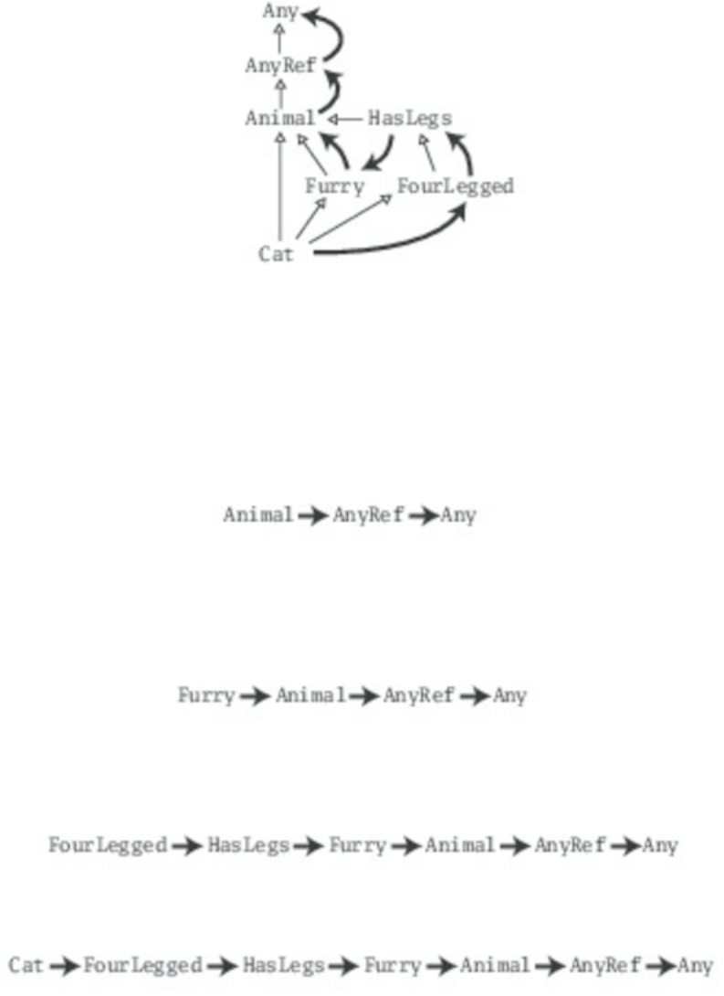
Figure 12.1 - Inheritance hierarchy and linearization of class Cat.
The linearization of Cat is computed from back to front as follows. The last part of the linearization
of Cat is the linearization of its superclass, Animal. This linearization is copied over without any
changes. (The linearization of each of these types is shown in Table 12.1here.) Because Animal doesn't
explicitly extend a superclass or mix in any supertraits, it by default extends AnyRef, which
extends Any. Animal's linearization, therefore, looks like:
The second to last part is the linearization of the first mixin, trait Furry, but all classes that are already
in the linearization of Animal are left out now, so that each class appears only once inCat's
linearization. The result is:
This is preceded by the linearization of FourLegged, where again any classes that have already been
copied in the linearizations of the superclass or the first mixin are left out:
Finally, the first class in the linearization of Cat is Cat itself:
When any of these classes and traits invokes a method via super, the implementation invoked will be
the first implementation to its right in the linearization.
Table 12.1 - Linearization of types in Cat's hierarchy
Type Linearization
Animal Animal, AnyRef, Any
Furry Furry, Animal, AnyRef, Any
FourLegged FourLegged, HasLegs, Animal, AnyRef, Any
HasLegs HasLegs, Animal, AnyRef, Any
Cat Cat, FourLegged, HasLegs, Furry, Animal, AnyRef, Any
12.7 TO TRAIT OR NOT TO TRAIT?
Whenever you implement a reusable collection of behavior, you will have to decide whether you want
to use a trait or an abstract class. There is no firm rule, but this section contains a few guidelines to
consider.
If the behavior will not be reused, then make it a concrete class. It is not reusable behavior after all.
If it might be reused in multiple, unrelated classes, make it a trait. Only traits can be mixed into
different parts of the class hierarchy.
If you want to inherit from it in Java code, use an abstract class. Since traits with code do not have a
close Java analog, it tends to be awkward to inherit from a trait in a Java class. Inheriting from a Scala
class, meanwhile, is exactly like inheriting from a Java class. As one exception, a Scala trait with only
abstract members translates directly to a Java interface, so you should feel free to define such traits
even if you expect Java code to inherit from it. SeeChapter 31 for more information on working with
Java and Scala together.
If you plan to distribute it in compiled form, and you expect outside groups to write classes inheriting
from it, you might lean towards using an abstract class. The issue is that when a trait gains or loses a
member, any classes that inherit from it must be recompiled, even if they have not changed. If outside
clients will only call into the behavior, instead of inheriting from it, then using a trait is fine.
If you still do not know, after considering the above, then start by making it as a trait. You can always
change it later, and in general using a trait keeps more options open.
12.8 CONCLUSION
This chapter has shown you how traits work and how to use them in several common idioms. You saw
that traits are similar to multiple inheritance. But because traits interpret super using linearization, they
both avoid some of the difficulties of traditional multiple inheritance and allow you to stack behaviors.
You also saw the Ordered trait and learned how to write your own enrichment traits.
Now that you have seen all of these facets, it is worth stepping back and taking another look at traits as
a whole. Traits do not merely support the idioms described in this chapter; they are a fundamental unit
of code that is reusable through inheritance. As such, many experienced Scala programmers start with
traits when they are at the early stages of implementation. Each trait can hold less than an entire
concept, a mere fragment of a concept. As the design solidifies, the fragments can be combined into
more complete concepts through trait mixin.
Footnotes for Chapter 12:
[1] This example is based on the Rational class shown in Listing 6.5 here, with equals, hashCode, and
modifications to ensure a positive denom added.
[2] Once a trait is mixed into a class, you can alternatively call it a mixin.
[3] Rumbaugh, et. al., The Unified Modeling Language Reference Manual. [Rum04]
Chapter 13
Packages and Imports
When working on a program, especially a large one, it is important to minimize coupling—the extent to
which the various parts of the program rely on the other parts. Low coupling reduces the risk that a
small, seemingly innocuous change in one part of the program will have devastating consequences in
another part. One way to minimize coupling is to write in a modular style. You divide the program into
a number of smaller modules, each of which has an inside and an outside. When working on the inside
of a module—its implementation—you need only coordinate with other programmers working on that
very same module. Only when you must change the outside of a module—its interface—is it necessary
to coordinate with developers working on other modules.
This chapter shows several constructs that help you program in a modular style. It shows how to place
things in packages, make names visible through imports, and control the visibility of definitions
through access modifiers. The constructs are similar in spirit to constructs in Java, but there are some
differences—usually ways that are more consistent—so it's worth reading this chapter even if you
already know Java.
13.1 PUTTING CODE IN PACKAGES
Scala code resides in the Java platform's global hierarchy of packages. The example code you've seen
so far in this book has been in the unnamed package. You can place code into named packages in Scala
in two ways. First, you can place the contents of an entire file into a package by putting
a package clause at the top of the file, as shown in Listing 13.1.
package bobsrockets.navigation
class Navigator
Listing 13.1 - Placing the contents of an entire file into a package.
The package clause of Listing 13.1 places class Navigator into the package
namedbobsrockets.navigation. Presumably, this is the navigation software developed by Bob's Rockets,
Inc.
Note
Because Scala code is part of the Java ecosystem, it is recommended to follow Java's reverse-domain-
name convention for Scala packages that you release to the public. Thus, a better name for Navigator's
package might becom.bobsrockets.navigation. In this chapter, however, we'll leave off the "com." to
make the examples easier to understand.
The other way you can place code into packages in Scala is more like C# namespaces. You follow a
package clause by a section in curly braces that contains the definitions that go into the package. This
syntax is called a packaging. The packaging shown in Listing 13.2 has the same effect as the code
in Listing 13.1:
package bobsrockets.navigation {
class Navigator
}
Listing 13.2 - Long form of a simple package declaration.
For such simple examples, you might as well use the syntactic sugar shown in Listing 13.1. However,
one use of the more general notation is to have different parts of a file in different packages. For
example, you might include a class's tests in the same file as the original code, but put the tests in a
different package, as shown in Listing 13.3.
package bobsrockets {
package navigation {
// In package bobsrockets.navigation
class Navigator
package tests {
// In package bobsrockets.navigation.tests
class NavigatorSuite
}
}
}
Listing 13.3 - Multiple packages in the same file.
package bobsrockets {
package navigation {
class Navigator {
// No need to say bobsrockets.navigation.StarMap
val map = new StarMap
}
class StarMap
}
class Ship {
// No need to say bobsrockets.navigation.Navigator
val nav = new navigation.Navigator
}
package fleets {
class Fleet {
// No need to say bobsrockets.Ship
def addShip() = { new Ship }
}
}
}
Listing 13.4 - Concise access to classes and packages.
package bobsrockets {
class Ship
}
package bobsrockets.fleets {
class Fleet {
// Doesn't compile! Ship is not in scope.
def addShip() = { new Ship }
}
}
Listing 13.5 - Symbols in enclosing packages not automatically available.
// In file launch.scala
package launch {
class Booster3
}
// In file bobsrockets.scala
package bobsrockets {
package navigation {
package launch {
class Booster1
}
class MissionControl {
val booster1 = new launch.Booster1
val booster2 = new bobsrockets.launch.Booster2
val booster3 = new _root_.launch.Booster3
}
}
package launch {
class Booster2
}
}
Listing 13.6 - Accessing hidden package names.
13.2 CONCISE ACCESS TO RELATED CODE
When code is divided into a package hierarchy, it doesn't just help people browse through the code. It
also tells the compiler that code in the same package is related in some way to each other. Scala takes
advantage of this relatedness by allowing short, unqualified names when accessing code that is in the
same package.
Listing 13.4 gives three simple examples. First, as you would expect, a class can be accessed from
within its own package without needing a prefix. That's why new StarMap compiles. ClassStarMap is
in the same package, bobsrockets.navigation, as the new expression that accesses it, so the package
name doesn't need to be prefixed.
Second, a package itself can be accessed from its containing package without needing a prefix.
In Listing 13.4, look at how class Navigator is instantiated. The new expression appears in
package bobsrockets, which is the containing package of bobsrockets.navigation. Thus, it can access
package bobsrockets.navigation as simply navigation.
Third, when using the curly-braces packaging syntax, all names accessible in scopes outside the
packaging are also available inside it. An example in Listing 13.4 is the way addShip()creates a
new Ship. The method is defined within two packagings: an outer one for bobsrockets, and an inner
one for bobsrockets.fleets. Since Ship is accessible in the outer packaging, it can be referenced from
within addShip().
Note that this kind of access is only available if you explicitly nest the packagings. If you stick to one
package per file, then—like in Java—the only names available will be the ones defined in the current
package. In Listing 13.5, the packaging of bobsrockets.fleets has been moved to the top level. Since it
is no longer enclosed in a packaging for bobsrockets, names frombobsrockets are not immediately in
scope. As a result, new Ship gives a compile error. If nesting packages with braces shifts your code
uncomfortably to the right, you can also use multiple package clauses without the braces.[1] For
instance, the code below also defines class Fleet in two nested packages bobrockets and fleets, just like
you saw it in Listing 13.4:
package bobsrockets
package fleets
class Fleet {
// No need to say bobsrockets.Ship
def addShip() = { new Ship }
}
One final trick is important to know. Sometimes, you end up coding in a heavily crowded scope where
package names are hiding each other. In Listing 13.6, the scope of classMissionControl includes three
separate packages named launch! There's one launch inbobsrockets.navigation, one in bobsrockets, and
one at the top level. How would you reference each of Booster1, Booster2, and Booster3?
Accessing the first one is easiest. A reference to launch by itself will get you to
packagebobsrockets.navigation.launch, because that is the launch package defined in the closest
enclosing scope. Thus, you can refer to the first booster class as simply launch.Booster1. Referring to
the second one also is not tricky. You can write bobrockets.launch.Booster2 and be clear about which
one you are referencing. That leaves the question of the third booster class: How can you
access Booster3, considering that a nested launch package shadows the top-level one?
To help in this situation, Scala provides a package named _root_ that is outside any package a user can
write. Put another way, every top-level package you can write is treated as a member of
package _root_. For example, both launch and bobsrockets of Listing 13.6 are members of
package _root_. As a result, _root_.launch gives you the top-level launch package,
and_root_.launch.Booster3 designates the outermost booster class.
13.3 IMPORTS
In Scala, packages and their members can be imported using import clauses. Imported items can then
be accessed by a simple name like File, as opposed to requiring a qualified name likejava.io.File. For
example, consider the code shown in Listing 13.7.
package bobsdelights
abstract class Fruit(
val name: String,
val color: String
)
object Fruits {
object Apple extends Fruit("apple", "red")
object Orange extends Fruit("orange", "orange")
object Pear extends Fruit("pear", "yellowish")
val menu = List(Apple, Orange, Pear)
}
Listing 13.7 - Bob's delightful fruits, ready for import.
An import clause makes members of a package or object available by their names alone without
needing to prefix them by the package or object name. Here are some simple examples:
// easy access to Fruit
import bobsdelights.Fruit
// easy access to all members of bobsdelights
import bobsdelights._
// easy access to all members of Fruits
import bobsdelights.Fruits._
The first of these corresponds to Java's single type import and the second to Java's on-
demand import. The only difference is that Scala's on-demand imports are written with a trailing
underscore (_) instead of an asterisk (*). (After all, * is a valid identifier in Scala!) The third import
clause above corresponds to Java's import of static class fields.
These three imports give you a taste of what imports can do, but Scala imports are actually much more
general. For one, imports in Scala can appear anywhere, not just at the beginning of a compilation unit.
Also, they can refer to arbitrary values. For instance, the import shown in Listing 13.8 is possible:
def showFruit(fruit: Fruit) = {
import fruit._
println(name + "s are " + color)
}
Listing 13.8 - Importing the members of a regular (not singleton) object.
Method showFruit imports all members of its parameter fruit, which is of type Fruit. The
subsequent println statement can refer to name and color directly. These two references are equivalent
to fruit.name and fruit.color. This syntax is particularly useful when you use objects as modules, which
will be described in Chapter 29.
SCALA'S FLEXIBLE IMPORTS
Scala's import clauses are quite a bit more flexible than Java's. There are three principal differences. In
Scala, imports:
•may appear anywhere
•may refer to objects (singleton or regular) in addition to packages
•let you rename and hide some of the imported members
Another way Scala's imports are flexible is that they can import packages themselves, not just their
non-package members. This is only natural if you think of nested packages being contained in their
surrounding package. For example, in Listing 13.9, the packagejava.util.regex is imported. This
makes regex usable as a simple name. To access the Patternsingleton object from
the java.util.regex package, you can just say, regex.Pattern, as shown inListing 13.9:
import java.util.regex
class AStarB {
// Accesses java.util.regex.Pattern
val pat = regex.Pattern.compile("a*b")
}
Listing 13.9 - Importing a package name.
Imports in Scala can also rename or hide members. This is done with an import selector
clause enclosed in braces, which follows the object from which members are imported. Here are some
examples:
import Fruits.{Apple, Orange}
This imports just members Apple and Orange from object Fruits.
import Fruits.{Apple => McIntosh, Orange}
This imports the two members Apple and Orange from object Fruits. However, the Apple object is
renamed to McIntosh, so this object can be accessed with either Fruits.Apple or McIntosh. A renaming
clause is always of the form "<original-name> => <new-name>".
import java.sql.{Date => SDate}
This imports the SQL date class as SDate, so that you can simultaneously import the normal Java date
class as simply Date.
import java.{sql => S}
This imports the java.sql package as S, so that you can write things like S.Date.
import Fruits.{_}
This imports all members from object Fruits. It means the same thing as import Fruits._.
import Fruits.{Apple => McIntosh, _}
This imports all members from object Fruits but renames Apple to McIntosh.
import Fruits.{Pear => _, _}
This imports all members of Fruits except Pear. A clause of the form "<original-name> => _"
excludes <original-name> from the names that are imported. In a sense, renaming something to `_'
means hiding it altogether. This is useful to avoid ambiguities. Say you have two
packages,Fruits and Notebooks, which both define a class Apple. If you want to get just the notebook
named Apple, and not the fruit, you could still use two imports on demand like this:
import Notebooks._
import Fruits.{Apple => _, _}
This would import all Notebooks and all Fruits, except for Apple.
These examples demonstrate the great flexibility Scala offers when it comes to importing members
selectively and possibly under different names. In summary, an import selector can consist of the
following:
•A simple name x. This includes x in the set of imported names.
•A renaming clause x => y. This makes the member named x visible under the name y.
•A hiding clause x => _. This excludes x from the set of imported names.
•A catch-all `_'. This imports all members except those members mentioned in a preceding
clause. If a catch-all is given, it must come last in the list of import selectors.
The simpler import clauses shown at the beginning of this section can be seen as special abbreviations
of import clauses with a selector clause. For example, "import p._" is equivalent to "import p.{_}" and
"import p.n" is equivalent to "import p.{n}".
13.4 IMPLICIT IMPORTS
Scala adds some imports implicitly to every program. In essence, it is as if the following three import
clauses had been added to the top of every source file with extension ".scala":
import java.lang._ // everything in the java.lang package
import scala._ // everything in the scala package
import Predef._ // everything in the Predef object
The java.lang package contains standard Java classes. It is always implicitly imported in Scala source
files.[2] Because java.lang is imported implicitly, you can write Thread instead ofjava.lang.Thread, for
instance.
As you have no doubt realized by now, the scala package contains the standard Scala library, with
many common classes and objects. Because scala is imported implicitly, you can writeList instead
of scala.List, for instance.
The Predef object contains many definitions of types, methods, and implicit conversions that are
commonly used on Scala programs. For example, because Predef is imported implicitly, you can
write assert instead of Predef.assert.
These three import clauses are treated a bit specially in that later imports overshadow earlier ones. For
instance, the StringBuilder class is defined both in package scala and, from Java version 1.5 on, also in
package java.lang. Because the scala import overshadows the java.langimport, the simple
name StringBuilder will refer to scala.StringBuilder, notjava.lang.StringBuilder.
13.5 ACCESS MODIFIERS
Members of packages, classes, or objects can be labeled with the access modifiers private andprotected.
These modifiers restrict access to the members to certain regions of code. Scala's treatment of access
modifiers roughly follows Java's but there are some important differences which are explained in this
section.
Private members
Private members in Scala are treated similarly to Java. A member labeled private is visible only inside
the class or object that contains the member definition. In Scala, this rule applies also for inner classes.
This treatment is more consistent, but differs from Java. Consider the example shown in Listing 13.10.
class Outer {
class Inner {
private def f() = { println("f") }
class InnerMost {
f() // OK
}
}
(new Inner).f() // error: f is not accessible
}
Listing 13.10 - How private access differs in Scala and Java.
In Scala, the access (new Inner).f() is illegal because f is declared private in Inner and the access is not
from within class Inner. By contrast, the first access to f in class InnerMost is OK, because that access
is contained in the body of class Inner. Java would permit both accesses because it lets an outer class
access private members of its inner classes.
Protected members
Access to protected members in Scala is also a bit more restrictive than in Java. In Scala,
aprotected member is only accessible from subclasses of the class in which the member is defined. In
Java such accesses are also possible from other classes in the same package. In Scala, there is another
way to achieve this effect[3] so protected is free to be left as is. The example shown in Listing
13.11 illustrates protected accesses.
package p {
class Super {
protected def f() = { println("f") }
}
class Sub extends Super {
f()
}
class Other {
(new Super).f() // error: f is not accessible
}
}
Listing 13.11 - How protected access differs in Scala and Java.
In Listing 13.11, the access to f in class Sub is OK because f is declared protected in Super and Subis a
subclass of Super. By contrast the access to f in Other is not permitted, because Other does not inherit
from Super. In Java, the latter access would be still permitted because Other is in the same package
as Sub.
Public members
Scala has no explicit modifier for public members: Any member not labeled private orprotected is
public. Public members can be accessed from anywhere.
package bobsrockets
package navigation {
private[bobsrockets] class Navigator {
protected[navigation] def useStarChart() = {}
class LegOfJourney {
private[Navigator] val distance = 100
}
private[this] var speed = 200
}
}
package launch {
import navigation._
object Vehicle {
private[launch] val guide = new Navigator
}
}
Listing 13.12 - Flexible scope of protection with access qualifiers.
Scope of protection
Access modifiers in Scala can be augmented with qualifiers. A modifier of the
form private[X]or protected[X] means that access is private or protected "up to" X, where X designates
some enclosing package, class or singleton object.
Qualified access modifiers give you very fine-grained control over visibility. In particular they enable
you to express Java's accessibility notions, such as package private, package protected, or private up to
outermost class, which are not directly expressible with simple modifiers in Scala. But they also let you
express accessibility rules that cannot be expressed in Java.
Listing 13.12 presents an example with many access qualifiers being used. In this listing,
classNavigator is labeled private[bobsrockets]. This means that this class is visible in all classes and
objects that are contained in package bobsrockets. In particular, the access to Navigator in
objectVehicle is permitted because Vehicle is contained in package launch, which is contained
inbobsrockets. On the other hand, all code outside the package bobsrockets cannot access
classNavigator.
This technique is quite useful in large projects that span several packages. It allows you to define things
that are visible in several sub-packages of your project but that remain hidden from clients external to
your project. The same technique is not possible in Java. There, once a definition escapes its immediate
package boundary, it is visible to the world at large.
Of course, the qualifier of a private may also be the directly enclosing package. An example is the
access modifier of guide in object Vehicle in Listing 13.12. Such an access modifier is equivalent to
Java's package-private access.
Table 13.1 - Effects of private qualifiers on LegOfJourney.distance
no access modifier public access
private[bobsrockets] access within outer package
private[navigation] same as package visibility in Java
private[Navigator] same as private in Java
private[LegOfJourney] same as private in Scala
private[this] access only from same object
All qualifiers can also be applied to protected, with the same meaning as private. That is, a
modifier protected[X] in a class C allows access to the labeled definition in all subclasses of Cand also
within the enclosing package, class, or object X. For instance, the useStarChart method in Listing
13.12 is accessible in all subclasses of Navigator and also in all code contained in the enclosing
package navigation. It thus corresponds exactly to the meaning of protected in Java.
The qualifiers of private can also refer to an enclosing class or object. For instance the distancevariable
in class LegOfJourney in Listing 13.12 is labeled private[Navigator], so it is visible from everywhere in
class Navigator. This gives the same access capabilities as for private members of inner classes in Java.
A private[C] where C is the outermost enclosing class is the same as just private in Java.
Finally, Scala also has an access modifier that is even more restrictive than private. A definition
labeled private[this] is accessible only from within the same object that contains the definition. Such a
definition is called object-private. For instance, the definition of speedin class Navigator in Listing
13.12 is object-private. This means that any access must not only be within class Navigator, it must also
be made from the very same instance of Navigator. Thus the accesses "speed" and "this.speed" would
be legal from within Navigator.
The following access, though, would not be allowed, even if it appeared inside class Navigator:
val other = new Navigator
other.speed // this line would not compile
Marking a member private[this] is a guarantee that it will not be seen from other objects of the same
class. This can be useful for documentation. It also sometimes lets you write more general variance
annotations (see Section 19.7 for details).
To summarize, Table 13.1 here lists the effects of private qualifiers. Each line shows a qualified private
modifier and what it would mean if such a modifier were attached to the distancevariable declared in
class LegOfJourney in Listing 13.12.
Visibility and companion objects
In Java, static members and instance members belong to the same class, so access modifiers apply
uniformly to them. You have already seen that in Scala there are no static members; instead you can
have a companion object that contains members that exist only once. For instance, in Listing
13.13 object Rocket is a companion of class Rocket.
class Rocket {
import Rocket.fuel
private def canGoHomeAgain = fuel > 20
}
object Rocket {
private def fuel = 10
def chooseStrategy(rocket: Rocket) = {
if (rocket.canGoHomeAgain)
goHome()
else
pickAStar()
}
def goHome() = {}
def pickAStar() = {}
}
Listing 13.13 - Accessing private members of companion classes and objects.
Scala's access rules privilege companion objects and classes when it comes to private or protected
accesses. A class shares all its access rights with its companion object and vice versa. In particular, an
object can access all private members of its companion class, just as a class can access all private
members of its companion object.
For instance, the Rocket class in Listing 13.13 can access method fuel, which is declared privatein
object Rocket. Analogously, the Rocket object can access the private method canGoHomeAgain in
class Rocket.
One exception where the similarity between Scala and Java breaks down
concerns protectedstatic members. A protected static member of a Java class C can be accessed in all
subclasses of C. By contrast, a protected member in a companion object makes no sense, as singleton
objects don't have any subclasses.
13.6 PACKAGE OBJECTS
So far, the only code you have seen added to packages are classes, traits, and standalone objects. These
are by far the most common definitions that are placed at the top level of a package. But Scala doesn't
limit you to just those—Any kind of definition that you can put inside a class can also be at the top
level of a package. If you have some helper method you'd like to be in scope for an entire package, go
ahead and put it right at the top level of the package.
To do so, put the definitions in a package object. Each package is allowed to have one package object.
Any definitions placed in a package object are considered members of the package itself.
An example is shown in Listing 13.14. File package.scala holds a package object for
packagebobsdelights. Syntactically, a package object looks much like one of the curly-braces
packagings shown earlier in the chapter. The only difference is that it includes the objectkeyword. It's a
package object, not a package. The contents of the curly braces can include any definitions you like. In
this case, the package object includes the showFruit utility method from Listing 13.8.
Given that definition, any other code in any package can import the method just like it would import a
class. For example, Listing 13.14 also shows the standalone object PrintMenu, which is located in a
different package. PrintMenu can import the utility method showFruit in the same way it would import
the class Fruit.
// In file bobsdelights/package.scala
package object bobsdelights {
def showFruit(fruit: Fruit) = {
import fruit._
println(name + "s are " + color)
}
}
// In file PrintMenu.scala
package printmenu
import bobsdelights.Fruits
import bobsdelights.showFruit
object PrintMenu {
def main(args: Array[String]) = {
for (fruit <- Fruits.menu) {
showFruit(fruit)
}
}
}
Listing 13.14 - A package object.
Looking ahead, there are other uses of package objects for kinds of definitions you haven't seen yet.
Package objects are frequently used to hold package-wide type aliases (Chapter 20) and implicit
conversions (Chapter 21). The top-level scala package has a package object, and its definitions are
available to all Scala code.
Package objects are compiled to class files named package.class that are the located in the directory of
the package that they augment. It's useful to keep the same convention for source files. So you would
typically put the source file of the package object bobsdelights of Listing 13.14 into a file
named package.scala that resides in the bobsdelights directory.
13.7 CONCLUSION
In this chapter, you saw the basic constructs for dividing a program into packages. This gives you a
simple and useful kind of modularity, so that you can work with very large bodies of code without
different parts of the code trampling on each other. Scala's system is the same in spirit as Java's
packages, but there are some differences where Scala chooses to be more consistent or more general.
Looking ahead, Chapter 29 describes a more flexible module system than division into packages. In
addition to letting you separate code into several namespaces, that approach allows modules to be
parameterized and inherit from each other. In the next chapter, we'll turn our attention to assertions and
unit testing.
Footnotes for Chapter 13:
[1] This style of multiple package clauses without braces is called chained package clauses.
[2] Scala also originally had an implementation on .NET., where namespace System, the .NETanalogue
of package java.lang, was imported instead.
[3] Using qualifiers, described in "Scope of protection" here.
Chapter 14
Assertions and Tests
Assertions and tests are two important ways you can check that the software you write behaves as you
expect. In this chapter, we'll show you several options you have in Scala to write and run them.
14.1 ASSERTIONS
Assertions in Scala are written as calls of a predefined method assert.[1] The
expressionassert(condition) throws an AssertionError if condition does not hold. There's also a two-
argument version of assert: The expression assert(condition, explanation) tests condition and, if it does
not hold, throws an AssertionError that contains the given explanation. The type of explanation is Any,
so you can pass any object as the explanation. The assert method will calltoString on it to get a string
explanation to place inside the AssertionError. For example, in the method named "above" of
class Element, shown in Listing 10.13 here, you might place an assert after the calls to widen to make
sure that the widened elements have equal widths. This is shown in Listing 14.1.
def above(that: Element): Element = {
val this1 = this widen that.width
val that1 = that widen this.width
assert(this1.width == that1.width)
elem(this1.contents ++ that1.contents)
}
Listing 14.1 - Using an assertion.
Another way you might choose to do this is to check the widths at the end of the widenmethod, right
before you return the value. You can accomplish this by storing the result in aval, performing an
assertion on the result, then mentioning the val last so the result is returned if the assertion succeeds.
However, you can do this more concisely with a convenience method in Predef named ensuring, as
shown in Listing 14.2.
The ensuring method can be used with any result type because of an implicit conversion.Although it
looks in this code as if we're invoking ensuring on widen's result, which is typeElement, we're actually
invoking ensuring on a type to which Element is implicitly converted. Theensuring method takes one
argument, a predicate function that takes a result type and returnsBoolean, and passes the result to the
predicate. If the predicate returns true, ensuring will return the result; otherwise, ensuring will throw
an AssertionError.
In this example, the predicate is "w <= _.width". The underscore is a placeholder for the one argument
passed to the predicate, the Element result of the widen method. If the width passed as w to widen is
less than or equal to the width of the result Element, the predicate will result in true, and ensuring will
result in the Element on which it was invoked. Because this is the last expression of
the widen method, widen itself will then result in the Element.
private def widen(w: Int): Element =
if (w <= width)
this
else {
val left = elem(' ', (w - width) / 2, height)
var right = elem(' ', w - width - left.width, height)
left beside this beside right
} ensuring (w <= _.width)
Listing 14.2 - Using ensuring to assert a function's result.
Assertions can be enabled and disabled using the JVM's -ea and -da command-line flags. When
enabled, each assertion serves as a little test that uses the actual data encountered as the software runs.
In the remainder of this chapter, we'll focus on the writing of external tests, which provide their own
test data and run independently from the application.
14.2 TESTING IN SCALA
You have many options for testing in Scala, from established Java tools, such as JUnit and TestNG, to
tools written in Scala, such as ScalaTest, specs2, and ScalaCheck. For the remainder of this chapter,
we'll give you a quick tour of these tools. We'll start with ScalaTest.
ScalaTest is the most flexible Scala test framework: it can be easily customized to solve different
problems. ScalaTest's flexibility means teams can use whatever testing style fits their needs best. For
example, for teams familar with JUnit, the FunSuite style will feel comfortable and familiar. Listing
14.3 shows an example.
import org.scalatest.FunSuite
import Element.elem
class ElementSuite extends FunSuite {
test("elem result should have passed width") {
val ele = elem('x', 2, 3)
assert(ele.width == 2)
}
}
Listing 14.3 - Writing tests with FunSuite.
The central concept in ScalaTest is the suite, a collection of tests. A test can be anything with a name
that can start and either succeed, fail, be pending, or canceled. Trait Suite is the central unit of
composition in ScalaTest. Suite declares "lifecycle" methods defining a default way to run tests, which
can be overridden to customize how tests are written and run.
ScalaTest offers style traits that extend Suite and override lifecycle methods to support different testing
styles. It also provides mixin traits that override lifecycle methods to address particular testing needs.
You define test classes by composing Suite style and mixin traits, and define test suites by
composing Suite instances.
FunSuite, which is extended by the test class shown in Listing 14.3, is an example of a testing style.
The "Fun" in FunSuite stands for function; "test" is a method defined in FunSuite, which is invoked by
the primary constructor of ElementSuite. You specify the name of the test as a string between the
parentheses and the test code itself between curly braces. The test code is a function passed as a by-
name parameter to test, which registers it for later execution.
ScalaTest is integrated into common build tools (such as sbt and Maven) and IDEs (such as IntelliJ
IDEA and Eclipse). You can also run a Suite directly via ScalaTest's Runner application or from the
Scala interpreter simply by invoking execute on it. Here's an example:
scala> (new ElementSuite).execute()
ElementSuite:
- elem result should have passed width
All ScalaTest styles, including FunSuite, are designed to encourage the writing of focused tests with
descriptive names. In addition, all styles generate specification-like output that can facilitate
communication among stakeholders. The style you choose dictates only how the declarations of your
tests will look. Everything else in ScalaTest works consistently the same way no matter what style you
choose.[2]
14.3 INFORMATIVE FAILURE REPORTS
The test in Listing 14.3 attempts to create an element of width 2 and assert that the width of the
resulting element is indeed 2. Were this assertion to fail, the failure report would include the filename
and line number of the offending assertion, and an informative error message:
scala> val width = 3
width: Int = 3
scala> assert(width == 2)
org.scalatest.exceptions.TestFailedException:
3 did not equal 2
To provide descriptive error messages when assertions fail, ScalaTest analyzes the expressions passed
to each assert invocation at compile time. If you prefer to see even more detailed information about
assertion failures, you can use ScalaTest's DiagrammedAssertions, whose error messages display a
diagram of the expression passed to assert:
scala> assert(List(1, 2, 3).contains(4))
org.scalatest.exceptions.TestFailedException:
assert(List(1, 2, 3).contains(4))
| | | | | |
| 1 2 3 false 4
List(1, 2, 3)
ScalaTest's assert methods do not differentiate between the actual and expected result in error
messages. They just indicate that the left operand did not equal the right operand, or show the values in
a diagram. If you wish to emphasize the distinction between actual and expected, you can alternatively
use ScalaTest's assertResult method, like this:
assertResult(2) {
ele.width
}
With this expression you indicate that you expect the code between the curly braces to result in 2. Were
the code between the braces to result in 3, you'd see the message, "Expected 2, but got 3" in the test
failure report.
If you want to check that a method throws an expected exception, you can use
ScalaTest'sassertThrows method, like this:
assertThrows[IllegalArgumentException] {
elem('x', -2, 3)
}
If the code between the curly braces throws a different exception than expected, or throws no
exception, assertThrows will complete abruptly with a TestFailedException. You'll get a helpful error
message in the failure report, such as:
Expected IllegalArgumentException to be thrown,
but NegativeArraySizeException was thrown.
On the other hand, if the code completes abruptly with an instance of the passed exception
class, assertThrows will return normally. If you wish to inspect the expected exception further, you can
use intercept instead of assertThrows. The intercept method works the same asassertThrows, except if
the expected exception is thrown, intercept returns it:
val caught =
intercept[ArithmeticException] {
1 / 0
}
assert(caught.getMessage == "/ by zero")
In short, ScalaTest's assertions work hard to provide useful failure messages that will help you diagnose
and fix problems in your code.
14.4 TESTS AS SPECIFICATIONS
In the behavior-driven development (BDD) testing style, the emphasis is on writing human-readable
specifications of the expected behavior of code and accompanying tests that verify the code has the
specified behavior. ScalaTest includes several traits that facilitate this style of testing. An example
using one such trait, FlatSpec, is shown in Listing 14.4.
import org.scalatest.FlatSpec
import org.scalatest.Matchers
import Element.elem
class ElementSpec extends FlatSpec with Matchers {
"A UniformElement" should
"have a width equal to the passed value" in {
val ele = elem('x', 2, 3)
ele.width should be (2)
}
it should "have a height equal to the passed value" in {
val ele = elem('x', 2, 3)
ele.height should be (3)
}
it should "throw an IAE if passed a negative width" in {
an [IllegalArgumentException] should be thrownBy {
elem('x', -2, 3)
}
}
}
Listing 14.4 - Specifying and testing behavior with a ScalaTest FlatSpec.
In a FlatSpec, you write tests as specifier clauses. You start by writing a name for the subjectunder test
as a string ("A UniformElement" in Listing 14.4), then should (or must or can), then a string that
specifies a bit of behavior required of the subject, then in. In the curly braces following in, you write
code that tests the specified behavior. In subsequent clauses you can write it to refer to the most
recently given subject. When a FlatSpec is executed, it will run each specifier clause as a ScalaTest
test. FlatSpec (and ScalaTest's other specification traits) generate output that reads like a specification
when run. For example, here's what the output will look like if you run ElementSpec from Listing
14.4 in the interpreter:
scala> (new ElementSpec).execute()
A UniformElement
- should have a width equal to the passed value
- should have a height equal to the passed value
- should throw an IAE if passed a negative width
Listing 14.4 also illustrates ScalaTest's matchers domain-specific language (DSL). By mixing in
trait Matchers, you can write assertions that read more like natural language. ScalaTest provides many
matchers in its DSL, and also enables you to define new matchers with custom failure messages. The
matchers shown in Listing 14.4 include the "should be" and "an [...] should be thrownBy { ...} " syntax.
You can alternatively mix in MustMatchers if you prefer must toshould. For example, mixing
in MustMatchers would allow you to write expressions such as:
result must be >= 0
map must contain key 'c'
If the last assertion failed, you'd see an error message similar to:
Map('a' -> 1, 'b' -> 2) did not contain key 'c'
The specs2 testing framework, an open source tool written in Scala by Eric Torreborre, also supports
the BDD style of testing but with a different syntax. For example, you could use specs2 to write the test
shown in Listing 14.5:
import org.specs2._
import Element.elem
object ElementSpecification extends Specification {
"A UniformElement" should {
"have a width equal to the passed value" in {
val ele = elem('x', 2, 3)
ele.width must be_==(2)
}
"have a height equal to the passed value" in {
val ele = elem('x', 2, 3)
ele.height must be_==(3)
}
"throw an IAE if passed a negative width" in {
elem('x', -2, 3) must
throwA[IllegalArgumentException]
}
}
}
Listing 14.5 - Specifying and testing behavior with the specs2 framework.
Like ScalaTest, specs2 provides a matchers DSL. You can see some examples of specs2 matchers in
action in Listing 14.5 in the lines that contain "must be_==" and "must throwA".[3]You can use specs2
standalone, but it is also integrated with ScalaTest and JUnit, so you can run specs2 tests with those
tools as well.
One of the big ideas of BDD is that tests can be used to facilitate communication between the people
who decide what a software system should do, the people who implement the software, and the people
who determine whether the software is finished and working. Although any of ScalaTest's or specs2's
styles can be used in this manner, ScalaTest'sFeatureSpec in particular is designed for it. Listing
14.6 shows an example:
import org.scalatest._
class TVSetSpec extends FeatureSpec with GivenWhenThen {
feature("TV power button") {
scenario("User presses power button when TV is off") {
Given("a TV set that is switched off")
When("the power button is pressed")
Then("the TV should switch on")
pending
}
}
}
Listing 14.6 - Using tests to facilitate communication among stakeholders.
FeatureSpec is designed to guide conversations about software requirements: You must identify
specific features, then specify those features in terms of scenarios. The Given, When, and Thenmethods
(provided by trait GivenWhenThen) can help focus the conversation on the specifics of individual
scenarios. The pending call at the end indicates that neither the test nor the actual behavior has been
implemented—just the specification. Once all the tests and specified behavior have been implemented,
the tests will pass and the requirements can be deemed to have been met.
14.5 PROPERTY-BASED TESTING
Another useful testing tool for Scala is ScalaCheck, an open source framework written by Rickard
Nilsson. ScalaCheck enables you to specify properties that the code under test must obey. For each
property, ScalaCheck will generate data and execute assertions that check whether the property
holds. Listing 14.7 shows an example of using ScalaCheck from a ScalaTest WordSpec that mixes in
trait PropertyChecks.
import org.scalatest.WordSpec
import org.scalatest.prop.PropertyChecks
import org.scalatest.MustMatchers._
import Element.elem
class ElementSpec extends WordSpec with PropertyChecks {
"elem result" must {
"have passed width" in {
forAll { (w: Int) =>
whenever (w > 0) {
elem('x', w, 3).width must equal (w)
}
}
}
}
}
Listing 14.7 - Writing property-based tests with ScalaCheck.
WordSpec is a ScalaTest style class. The PropertyChecks trait provides several forAll methods that
allow you to mix property-based tests with traditional assertion-based or matcher-based tests. In this
example, we check a property that the elem factory should obey. ScalaCheck properties are expressed
as function values that take as parameters the data needed by the property's assertions. This data will be
generated by ScalaCheck. In the property shown inListing 14.7, the data is an integer named w that
represents a width. Inside the body of the function, you see this code:
whenever (w > 0) {
elem('x', w, 3).width must equal (w)
}
The whenever clause indicates that whenever the left hand expression is true, the expression on the
right must hold true. Thus in this case, the expression in the block must hold true whenever w is greater
than 0. The right-hand expression in this case will yield true if the width passed to the elem factory is
the same as the width of the Element returned by the factory.
With this small amount of code, ScalaCheck will generate possibly hundreds of values for wand test
each one, looking for a value for which the property doesn't hold. If the property holds true for every
value ScalaCheck tries, the test will pass. Otherwise, the test will complete abruptly with
a TestFailedException that contains information including the value that caused the failure.
14.6 ORGANIZING AND RUNNING TESTS
Each framework mentioned in this chapter provides some mechanism for organizing and running tests.
In this section, we'll give a quick overview of ScalaTest's approach. To get the full story on any of these
frameworks, however, you'll need to consult their documentation.
In ScalaTest, you organize large test suites by nesting Suites inside Suites. When a Suite is executed, it
will execute its nested Suites as well as its tests. The nested Suites will in turn execute their
nested Suites, and so on. A large test suite, therefore, is represented as a tree ofSuite objects. When you
execute the root Suite in the tree, all Suites in the tree will be executed.
You can nest suites manually or automatically. To nest manually, you either override
thenestedSuites method on your Suites or pass the Suites you want to nest to the constructor of
class Suites, which ScalaTest provides for this purpose. To nest automatically, you provide package
names to ScalaTest's Runner, which will discover Suites automatically, nest them under a root Suite,
and execute the root Suite.
You can invoke ScalaTest's Runner application from the command line or via a build tool, such as sbt,
maven, or ant. The simplest way to invoke Runner on the command line is via
theorg.scalatest.run application. This application expects a fully qualified test class name. For example,
to run the test class shown in Listing 14.6, you must compile it with:
$ scalac -cp scalatest.jar TVSetSpec.scala
Then you can run it with:
$ scala -cp scalatest.jar org.scalatest.run TVSetSpec
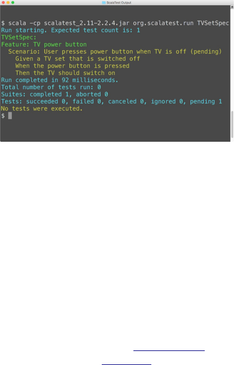
Figure 14.1 - The output of org.scalatest.run.
With -cp you place ScalaTest's JAR file on the class path. (When downloaded, the JAR file name will
include embedded Scala and ScalaTest version numbers.) The next token,org.scalatest.run, is the fully
qualified application name. Scala will run this application and pass the remaining tokens as command
line arguments. The TVSetSpec argument specifies the suite to execute. The result is shown in Figure
14.1.
14.7 CONCLUSION
In this chapter you saw examples of mixing assertions directly in production code, as well as writing
them externally in tests. You saw that as a Scala programmer, you can take advantage of popular testing
tools from the Java community, such as JUnit and TestNG, as well as newer tools designed explicitly
for Scala, such as ScalaTest, ScalaCheck, and specs2. Both in-code assertions and external tests can
help you achieve your software quality goals. We felt that these techniques are important enough to
justify the short detour from the Scala tutorial that this chapter represented. In the next chapter,
however, we'll return to the language tutorial and cover a very useful aspect of Scala: pattern matching.
Footnotes for Chapter 14:
[1] The assert method is defined in the Predef singleton object, whose members are automatically
imported into every Scala source file.
[2] More detail on ScalaTest is available from http://www.scalatest.org/.
[3] You can download specs2 from http://specs2.org/.
Chapter 15
Case Classes and Pattern Matching
This chapter introduces case classes and pattern matching, twin constructs that support you when
writing regular, non-encapsulated data structures. These two constructs are particularly helpful for tree-
like recursive data.
If you have programmed in a functional language before, then you will probably recognize pattern
matching. But case classes will be new to you. Case classes are Scala's way to allow pattern matching
on objects without requiring a large amount of boilerplate. Generally, all you need to do is add a
single case keyword to each class that you want to be pattern matchable.
This chapter starts with a simple example of case classes and pattern matching. It then goes through all
of the kinds of patterns that are supported, talks about the role of sealed classes, discusses
the Option type, and shows some non-obvious places in the language where pattern matching is used.
Finally, a larger, more realistic example of pattern matching is shown.
15.1 A SIMPLE EXAMPLE
Before delving into all the rules and nuances of pattern matching, it is worth looking at a simple
example to get the general idea. Let's say you need to write a library that manipulates arithmetic
expressions, perhaps as part of a domain-specific language you are designing.
A first step to tackling this problem is the definition of the input data. To keep things simple, we'll
concentrate on arithmetic expressions consisting of variables, numbers, and unary and binary
operations. This is expressed by the hierarchy of Scala classes shown in Listing 15.1.
abstract class Expr
case class Var(name: String) extends Expr
case class Number(num: Double) extends Expr
case class UnOp(operator: String, arg: Expr) extends Expr
case class BinOp(operator: String,
left: Expr, right: Expr) extends Expr
Listing 15.1 - Defining case classes.
The hierarchy includes an abstract base class Expr with four subclasses, one for each kind of
expression being considered.[1] The bodies of all five classes are empty. As mentioned previously, in
Scala you can leave out the braces around an empty class body if you wish, soclass C is the same
as class C {}.
Case classes
The other noteworthy thing about the declarations of Listing 15.1 is that each subclass
has acase modifier. Classes with such a modifier are called case classes. Using the modifier makes the
Scala compiler add some syntactic conveniences to your class.
First, it adds a factory method with the name of the class. This means that, for instance, you can
write Var("x") to construct a Var object, instead of the slightly longer new Var("x"):
scala> val v = Var("x")
v: Var = Var(x)
The factory methods are particularly nice when you nest them. Because there are no
noisy newkeywords sprinkled throughout the code, you can take in the expression's structure at a
glance:
scala> val op = BinOp("+", Number(1), v)
op: BinOp = BinOp(+,Number(1.0),Var(x))
The second syntactic convenience is that all arguments in the parameter list of a case class implicitly
get a val prefix, so they are maintained as fields:
scala> v.name
res0: String = x
scala> op.left
res1: Expr = Number(1.0)
Third, the compiler adds "natural" implementations of methods toString, hashCode, and equalsto your
class. They will print, hash, and compare a whole tree consisting of the class and (recursively) all its
arguments. Since == in Scala always delegates to equals, this means that elements of case classes are
always compared structurally:
scala> println(op)
BinOp(+,Number(1.0),Var(x))
scala> op.right == Var("x")
res3: Boolean = true
Finally, the compiler adds a copy method to your class for making modified copies. This method is
useful for making a new instance of the class that is the same as another one except that one or two
attributes are different. The method works by using named and default parameters (see Section 8.8).
You specify the changes you'd like to make by using named parameters. For any parameter you don't
specify, the value from the old object is used. As an example, here is how you can make an operation
just like op except that the operator has changed:
scala> op.copy(operator = "-")
res4: BinOp = BinOp(-,Number(1.0),Var(x))
All these conventions add a lot of convenience—at a small price. You have to write the case modifier,
and your classes and objects become a bit larger. They are larger because additional methods are
generated and an implicit field is added for each constructor parameter. However, the biggest advantage
of case classes is that they support pattern matching.
Pattern matching
Say you want to simplify arithmetic expressions of the kinds just presented. There is a multitude of
possible simplification rules. The following three rules just serve as an illustration:
UnOp("-", UnOp("-", null)) => null // Double negation
BinOp("+", null, Number(0)) => null // Adding zero
BinOp("*", null, Number(1)) => null // Multiplying by one
Using pattern matching, these rules can be taken almost as they are to form the core of a simplification
function in Scala, as shown in Listing 15.2. The function, simplifyTop, can be used like this:
scala> simplifyTop(UnOp("-", UnOp("-", Var("x"))))
res4: Expr = Var(x)
def simplifyTop(expr: Expr): Expr = expr match {
case UnOp("-", UnOp("-", e)) => e // Double negation
case BinOp("+", e, Number(0)) => e // Adding zero
case BinOp("*", e, Number(1)) => e // Multiplying by one
case _ => expr
}
Listing 15.2 - The simplifyTop function, which does a pattern match.
The right-hand side of simplifyTop consists of a match expression. match corresponds to switch in
Java, but it's written after the selector expression. In other words, it's:
selector match { alternatives }
instead of:
switch (selector) { alternatives }
A pattern match includes a sequence of alternatives, each starting with the keyword case. Each
alternative includes a pattern and one or more expressions, which will be evaluated if the pattern
matches. An arrow symbol => separates the pattern from the expressions.
A match expression is evaluated by trying each of the patterns in the order they are written. The first
pattern that matches is selected, and the part following the arrow is selected and executed.
A constant pattern like "+" or 1 matches values that are equal to the constant with respect to==.
A variable pattern like e matches every value. The variable then refers to that value in the right hand
side of the case clause. In this example, note that the first three alternatives evaluate to e, a variable that
is bound within the associated pattern. The wildcard pattern (_) also matches every value, but it does
not introduce a variable name to refer to that value. InListing 15.2, notice how the match ends with a
default case that does nothing to the expression. Instead, it just results in expr, the expression matched
upon.
A constructor pattern looks like UnOp("-", e). This pattern matches all values of type UnOpwhose first
argument matches "-" and whose second argument matches e. Note that the arguments to the
constructor are themselves patterns. This allows you to write deep patterns using a concise notation.
Here's an example:
UnOp("-", UnOp("-", e))
Imagine trying to implement this same functionality using the visitor design pattern![2]Almost as
awkward, imagine implementing it as a long sequence of if statements, type tests, and type casts.
match compared to switch
Match expressions can be seen as a generalization of Java-style switches. A Java-style switchcan be
naturally expressed as a match expression, where each pattern is a constant and the last pattern may be
a wildcard (which represents the default case of the switch).
However, there are three differences to keep in mind: First, match is an expression in Scala (i.e., it
always results in a value). Second, Scala's alternative expressions never "fall through" into the next
case. Third, if none of the patterns match, an exception named MatchError is thrown. This means you
always have to make sure that all cases are covered, even if it means adding a default case where there's
nothing to do.
expr match {
case BinOp(op, left, right) =>
println(expr + " is a binary operation")
case _ =>
}
Listing 15.3 - A pattern match with an empty "default" case.
Listing 15.3 shows an example. The second case is necessary because without it, the matchexpression
would throw a MatchError for every expr argument that is not a BinOp. In this example, no code is
specified for that second case, so if that case runs it does nothing. The result of either case is the unit
value `()', which is also the result of the entire matchexpression.
15.2 KINDS OF PATTERNS
The previous example showed several kinds of patterns in quick succession. Now take a minute to look
at each pattern in detail.
The syntax of patterns is easy, so do not worry about that too much. All patterns look exactly like the
corresponding expression. For instance, given the hierarchy of Listing 15.1, the pattern Var(x) matches
any variable expression, binding x to the name of the variable. Used as an expression, Var(x)—exactly
the same syntax—recreates an equivalent object, assuming x is already bound to the variable's name.
Since the syntax of patterns is so transparent, the main thing to pay attention to is just what kinds of
patterns are possible.
Wildcard patterns
The wildcard pattern (_) matches any object whatsoever. You have already seen it used as a default,
catch-all alternative, like this:
expr match {
case BinOp(op, left, right) =>
println(expr + " is a binary operation")
case _ => // handle the default case
}
Wildcards can also be used to ignore parts of an object that you do not care about. For example, the
previous example does not actually care what the elements of a binary operation are; it just checks
whether or not it is a binary operation. Thus, the code can just as well use the wildcard pattern for the
elements of the BinOp, as shown in Listing 15.4.
expr match {
case BinOp(_, _, _) => println(expr + " is a binary operation")
case _ => println("It's something else")
}
Listing 15.4 - A pattern match with wildcard patterns.
Constant patterns
A constant pattern matches only itself. Any literal may be used as a constant. For example, 5,true,
and "hello" are all constant patterns. Also, any val or singleton object can be used as a constant. For
example, Nil, a singleton object, is a pattern that matches only the empty list.Listing 15.5 shows some
examples of constant patterns:
def describe(x: Any) = x match {
case 5 => "five"
case true => "truth"
case "hello" => "hi!"
case Nil => "the empty list"
case _ => "something else"
}
Listing 15.5 - A pattern match with constant patterns.
Here is how the pattern match shown in Listing 15.5 looks in action:
scala> describe(5)
res6: String = five
scala> describe(true)
res7: String = truth
scala> describe("hello")
res8: String = hi!
scala> describe(Nil)
res9: String = the empty list
scala> describe(List(1,2,3))
res10: String = something else
Variable patterns
A variable pattern matches any object, just like a wildcard. But unlike a wildcard, Scala binds the
variable to whatever the object is. You can then use this variable to act on the object further. For
example, Listing 15.6 shows a pattern match that has a special case for zero, and a default case for all
other values. The default case uses a variable pattern so that it has a name for the value, no matter what
it is.
expr match {
case 0 => "zero"
case somethingElse => "not zero: " + somethingElse
}
Listing 15.6 - A pattern match with a variable pattern.
Variable or constant?
Constant patterns can have symbolic names. You saw this already when we used Nil as a pattern. Here
is a related example, where a pattern match involves the constants E(2.71828...) and Pi (3.14159...):
scala> import math.{E, Pi}
import math.{E, Pi}
scala> E match {
case Pi => "strange math? Pi = " + Pi
case _ => "OK"
}
res11: String = OK
As expected, E does not match Pi, so the "strange math" case is not used.
How does the Scala compiler know that Pi is a constant imported from scala.math, and not a variable
that stands for the selector value itself? Scala uses a simple lexical rule for disambiguation: a simple
name starting with a lowercase letter is taken to be a pattern variable; all other references are taken to
be constants. To see the difference, create a lowercase alias for pi and try with that:
scala> val pi = math.Pi
pi: Double = 3.141592653589793
scala> E match {
case pi => "strange math? Pi = " + pi
}
res12: String = strange math? Pi = 2.718281828459045
Here the compiler will not even let you add a default case at all. Since pi is a variable pattern, it will
match all inputs, and so no cases following it can be reached:
scala> E match {
case pi => "strange math? Pi = " + pi
case _ => "OK"
}
<console>:12: warning: unreachable code
case _ => "OK"
^
You can still use a lowercase name for a pattern constant, if you need to, by using one of two tricks.
First, if the constant is a field of some object, you can prefix it with a qualifier. For instance, pi is a
variable pattern, but this.pi or obj.pi are constants even though they start with lowercase letters. If that
does not work (because pi is a local variable, say), you can alternatively enclose the variable name in
back ticks. For instance, `pi` would again be interpreted as a constant, not as a variable:
scala> E match {
case `pi` => "strange math? Pi = " + pi
case _ => "OK"
}
res14: String = OK
As you can see, the back-tick syntax for identifiers is used for two different purposes in Scala to help
you code your way out of unusual circumstances. Here you see that it can be used to treat a lowercase
identifier as a constant in a pattern match. Earlier on, in Section 6.10, you saw that it can also be used
to treat a keyword as an ordinary identifier, e.g., writingThread.`yield`() treats yield as an identifier
rather than a keyword.
Constructor patterns
Constructors are where pattern matching becomes really powerful. A constructor pattern looks like
"BinOp("+", e, Number(0))". It consists of a name (BinOp) and then a number of patterns within
parentheses: "+", e, and Number(0). Assuming the name designates a case class, such a pattern means
to first check that the object is a member of the named case class, and then to check that the constructor
parameters of the object match the extra patterns supplied.
These extra patterns mean that Scala patterns support deep matches. Such patterns not only check the
top-level object supplied, but also the contents of the object against further patterns. Since the extra
patterns can themselves be constructor patterns, you can use them to check arbitrarily deep into an
object. For example, the pattern shown in Listing 15.7 checks that the top-level object is a BinOp, that
its third constructor parameter is a Number, and that the value field of that number is 0. This pattern is
one line long yet checks three levels deep.
expr match {
case BinOp("+", e, Number(0)) => println("a deep match")
case _ =>
}
Listing 15.7 - A pattern match with a constructor pattern.
Sequence patterns
You can match against sequence types, like List or Array, just like you match against case classes. Use
the same syntax, but now you can specify any number of elements within the pattern. Listing
15.8 shows a pattern that checks for a three-element list starting with zero.
expr match {
case List(0, _, _) => println("found it")
case _ =>
}
Listing 15.8 - A sequence pattern with a fixed length.
If you want to match against a sequence without specifying how long it can be, you can specify _* as
the last element of the pattern. This funny-looking pattern matches any number of elements within a
sequence, including zero elements. Listing 15.9 shows an example that matches any list that starts with
zero, regardless of how long the list is.
expr match {
case List(0, _*) => println("found it")
case _ =>
}
Listing 15.9 - A sequence pattern with an arbitrary length.
Tuple patterns
You can match against tuples too. A pattern like (a, b, c) matches an arbitrary 3-tuple. An example is
shown in Listing 15.10.
def tupleDemo(expr: Any) =
expr match {
case (a, b, c) => println("matched " + a + b + c)
case _ =>
}
Listing 15.10 - A pattern match with a tuple pattern.
If you load the tupleDemo method shown in Listing 15.10 into the interpreter, and pass to it a tuple
with three elements, you'll see:
scala> tupleDemo(("a ", 3, "-tuple"))
matched a 3-tuple
Typed patterns
You can use a typed pattern as a convenient replacement for type tests and type casts. Listing
15.11 shows an example.
def generalSize(x: Any) = x match {
case s: String => s.length
case m: Map[_, _] => m.size
case _ => -1
}
Listing 15.11 - A pattern match with typed patterns.
Here are a few examples of using generalSize in the Scala interpreter:
scala> generalSize("abc")
res16: Int = 3
scala> generalSize(Map(1 -> 'a', 2 -> 'b'))
res17: Int = 2
scala> generalSize(math.Pi)
res18: Int = -1
The generalSize method returns the size or length of objects of various types. Its argument is of
type Any, so it could be any value. If the argument is a String, the method returns the string's length.
The pattern "s: String" is a typed pattern; it matches every (non-null) instance ofString. The pattern
variable s then refers to that string.
Note that even though s and x refer to the same value, the type of x is Any, while the type of s isString.
So you can write s.length in the alternative expression that corresponds to the pattern, but you could not
write x.length, because the type Any does not have a length member. An equivalent but more long-
winded way that achieves the effect of a match against a typed pattern employs a type test followed by
a type cast. Scala uses a different syntax than Java for these. To test whether an expression expr has
type String, say, you write:
expr.isInstanceOf[String]
To cast the same expression to type String, you use:
expr.asInstanceOf[String]
Using a type test and cast, you could rewrite the first case of the previous match expression as shown
in Listing 15.12.
if (x.isInstanceOf[String]) {
val s = x.asInstanceOf[String]
s.length
} else ...
Listing 15.12 - Using isInstanceOf and asInstanceOf (poor style).
The operators isInstanceOf and asInstanceOf are treated as predefined methods of class Any that take a
type parameter in square brackets. In fact, x.asInstanceOf[String] is a special case of a method
invocation with an explicit type parameter String.
As you will have noted by now, writing type tests and casts is rather verbose in Scala. That's intentional
because it is not encouraged practice. You are usually better off using a pattern match with a typed
pattern. That's particularly true if you need to do both a type test and a type cast, because both
operations are then rolled into a single pattern match.
The second case of the match expression in Listing 15.11 contains the typed pattern "m: Map[_, _]".
This pattern matches any value that is a Map of some arbitrary key and value types, and lets m refer to
that value. Therefore, m.size is well typed and returns the size of the map. The underscores in the type
pattern[3] are like wildcards in other patterns. You could have also used (lowercase) type variables
instead.
Type erasure
Can you also test for a map with specific element types? This would be handy, say, for testing whether
a given value is a map from type Int to type Int. Let's try:
scala> def isIntIntMap(x: Any) = x match {
case m: Map[Int, Int] => true
case _ => false
}
<console>:9: warning: non-variable type argument Int in type
pattern scala.collection.immutable.Map[Int,Int] (the
underlying of Map[Int,Int]) is unchecked since it is
eliminated by erasure
case m: Map[Int, Int] => true
^
Scala uses the erasure model of generics, just like Java does. This means that no information about type
arguments is maintained at runtime. Consequently, there is no way to determine at runtime whether a
given Map object has been created with two Int arguments, rather than with arguments of different
types. All the system can do is determine that a value is a Map of some arbitrary type parameters. You
can verify this behavior by applying isIntIntMap to arguments of different instances of class Map:
scala> isIntIntMap(Map(1 -> 1))
res19: Boolean = true
scala> isIntIntMap(Map("abc" -> "abc"))
res20: Boolean = true
The first application returns true, which looks correct, but the second application also returnstrue,
which might be a surprise. To alert you to the possibly non-intuitive runtime behavior, the compiler
emits unchecked warnings like the one shown previously.
The only exception to the erasure rule is arrays, because they are handled specially in Java as well as in
Scala. The element type of an array is stored with the array value, so you can pattern match on it.
Here's an example:
scala> def isStringArray(x: Any) = x match {
case a: Array[String] => "yes"
case _ => "no"
}
isStringArray: (x: Any)String
scala> val as = Array("abc")
as: Array[String] = Array(abc)
scala> isStringArray(as)
res21: String = yes
scala> val ai = Array(1, 2, 3)
ai: Array[Int] = Array(1, 2, 3)
scala> isStringArray(ai)
res22: String = no
Variable binding
In addition to the standalone variable patterns, you can also add a variable to any other pattern. You
simply write the variable name, an at sign (@), and then the pattern. This gives you a variable-binding
pattern, which means the pattern is to perform the pattern match as normal, and if the pattern succeeds,
set the variable to the matched object just as with a simple variable pattern.
As an example, Listing 15.13 shows a pattern match that looks for the absolute value operation being
applied twice in a row. Such an expression can be simplified to only take the absolute value one time.
expr match {
case UnOp("abs", e @ UnOp("abs", _)) => e
case _ =>
}
Listing 15.13 - A pattern with a variable binding (via the @ sign).
The example shown in Listing 15.13 includes a variable-binding pattern with e as the variable
and UnOp("abs", _) as the pattern. If the entire pattern match succeeds, then the portion that matched
the UnOp("abs", _) part is made available as variable e. The result of the case is just e, because e has
the same value as expr but with one less absolute value operation.
15.3 PATTERN GUARDS
Sometimes, syntactic pattern matching is not precise enough. For instance, say you are given the task
of formulating a simplification rule that replaces sum expressions with two identical operands, such
as e + e, by multiplications of two (e.g., e * 2). In the language of Expr trees, an expression like:
BinOp("+", Var("x"), Var("x"))
would be transformed by this rule to:
BinOp("*", Var("x"), Number(2))
You might try to define this rule as follows:
scala> def simplifyAdd(e: Expr) = e match {
case BinOp("+", x, x) => BinOp("*", x, Number(2))
case _ => e
}
<console>:14: error: x is already defined as value x
case BinOp("+", x, x) => BinOp("*", x, Number(2))
^
This fails because Scala restricts patterns to be linear: a pattern variable may only appear once in a
pattern. However, you can re-formulate the match with a pattern guard, as shown in Listing 15.14:
scala> def simplifyAdd(e: Expr) = e match {
case BinOp("+", x, y) if x == y =>
BinOp("*", x, Number(2))
case _ => e
}
simplifyAdd: (e: Expr)Expr
Listing 15.14 - A match expression with a pattern guard.
A pattern guard comes after a pattern and starts with an if. The guard can be an arbitrary boolean
expression, which typically refers to variables in the pattern. If a pattern guard is present, the match
succeeds only if the guard evaluates to true. Hence, the first case above would only match binary
operations with two equal operands.
Some other examples of guarded patterns are:
// match only positive integers
case n: Int if 0 < n => ...
// match only strings starting with the letter `a'
case s: String if s(0) == 'a' => ...
15.4 PATTERN OVERLAPS
Patterns are tried in the order in which they are written. The version of simplify shown inListing
15.15 presents an example where the order of the cases matters.
def simplifyAll(expr: Expr): Expr = expr match {
case UnOp("-", UnOp("-", e)) =>
simplifyAll(e) // `-' is its own inverse
case BinOp("+", e, Number(0)) =>
simplifyAll(e) // `0' is a neutral element for `+'
case BinOp("*", e, Number(1)) =>
simplifyAll(e) // `1' is a neutral element for `*'
case UnOp(op, e) =>
UnOp(op, simplifyAll(e))
case BinOp(op, l, r) =>
BinOp(op, simplifyAll(l), simplifyAll(r))
case _ => expr
}
Listing 15.15 - Match expression in which case order matters.
The version of simplify shown in Listing 15.15 will apply simplification rules everywhere in an
expression, not just at the top, as simplifyTop did. It can be derived from simplifyTop by adding two
more cases for general unary and binary expressions (cases four and five in Listing 15.15).
The fourth case has the pattern UnOp(op, e); i.e., it matches every unary operation. The operator and
operand of the unary operation can be arbitrary. They are bound to the pattern variables op and e,
respectively. The alternative in this case applies simplifyAll recursively to the operand e and then
rebuilds the same unary operation with the (possibly) simplified operand. The fifth case for BinOp is
analogous: it is a "catch-all" case for arbitrary binary operations, which recursively applies the
simplification method to its two operands.
In this example, it is important that the catch-all cases come after the more specific simplification rules.
If you wrote them in the other order, then the catch-all case would be run in favor of the more specific
rules. In many cases, the compiler will even complain if you try. For example, here's
a match expression that won't compile because the first case will match anything that would be
matched by the second case:
scala> def simplifyBad(expr: Expr): Expr = expr match {
case UnOp(op, e) => UnOp(op, simplifyBad(e))
case UnOp("-", UnOp("-", e)) => e
}
<console>:21: warning: unreachable code
case UnOp("-", UnOp("-", e)) => e
^
15.5 SEALED CLASSES
Whenever you write a pattern match, you need to make sure you have covered all of the possible cases.
Sometimes you can do this by adding a default case at the end of the match, but that only applies if
there is a sensible default behavior. What do you do if there is no default? How can you ever feel safe
that you covered all the cases?
You can enlist the help of the Scala compiler in detecting missing combinations of patterns in
a match expression. To do this, the compiler needs to be able to tell which are the possible cases. In
general, this is impossible in Scala because new case classes can be defined at any time and in arbitrary
compilation units. For instance, nothing would prevent you from adding a fifth case class to
the Expr class hierarchy in a different compilation unit from the one where the other four cases are
defined.
The alternative is to make the superclass of your case classes sealed. A sealed class cannot have any
new subclasses added except the ones in the same file. This is very useful for pattern matching because
it means you only need to worry about the subclasses you already know about. What's more, you get
better compiler support as well. If you match against case classes that inherit from a sealed class, the
compiler will flag missing combinations of patterns with a warning message.
If you write a hierarchy of classes intended to be pattern matched, you should consider sealing them.
Simply put the sealed keyword in front of the class at the top of the hierarchy. Programmers using your
class hierarchy will then feel confident in pattern matching against it. The sealed keyword, therefore, is
often a license to pattern match. Listing 15.16 shows an example in which Expr is turned into a sealed
class.
sealed abstract class Expr
case class Var(name: String) extends Expr
case class Number(num: Double) extends Expr
case class UnOp(operator: String, arg: Expr) extends Expr
case class BinOp(operator: String,
left: Expr, right: Expr) extends Expr
Listing 15.16 - A sealed hierarchy of case classes.
Now define a pattern match where some of the possible cases are left out:
def describe(e: Expr): String = e match {
case Number(_) => "a number"
case Var(_) => "a variable"
}
You will get a compiler warning like the following:
warning: match is not exhaustive!
missing combination UnOp
missing combination BinOp
Such a warning tells you that there's a risk your code might produce a MatchError exception because
some possible patterns (UnOp, BinOp) are not handled. The warning points to a potential source of
runtime faults, so it is usually a welcome help in getting your program right.
However, at times you might encounter a situation where the compiler is too picky in emitting the
warning. For instance, you might know from the context that you will only ever apply
the describe method above to expressions that are either Numbers or Vars, so you know that
no MatchError will be produced. To make the warning go away, you could add a third catch-all case to
the method, like this:
def describe(e: Expr): String = e match {
case Number(_) => "a number"
case Var(_) => "a variable"
case _ => throw new RuntimeException // Should not happen
}
That works, but it is not ideal. You will probably not be very happy that you were forced to add code
that will never be executed (or so you think), just to make the compiler shut up.
A more lightweight alternative is to add an @unchecked annotation to the selector expression of the
match. This is done as follows:
def describe(e: Expr): String = (e: @unchecked) match {
case Number(_) => "a number"
case Var(_) => "a variable"
}
Annotations are described in Chapter 27. In general, you can add an annotation to an expression in the
same way you add a type: follow the expression with a colon and the name of the annotation (preceded
by an at sign). For example, in this case you add an @uncheckedannotation to the variable e, with
"e: @unchecked". The @unchecked annotation has a special meaning for pattern matching. If a match's
selector expression carries this annotation, exhaustivity checking for the patterns that follow will be
suppressed.
15.6 THE OPTION TYPE
Scala has a standard type named Option for optional values. Such a value can be of two
forms:Some(x), where x is the actual value, or the None object, which represents a missing value.
Optional values are produced by some of the standard operations on Scala's collections. For instance,
the get method of Scala's Map produces Some(value) if a value corresponding to a given key has been
found, or None if the given key is not defined in the Map. Here's an example:
scala> val capitals =
Map("France" -> "Paris", "Japan" -> "Tokyo")
capitals: scala.collection.immutable.Map[String,String] =
Map(France -> Paris, Japan -> Tokyo)
scala> capitals get "France"
res23: Option[String] = Some(Paris)
scala> capitals get "North Pole"
res24: Option[String] = None
The most common way to take optional values apart is through a pattern match. For instance:
scala> def show(x: Option[String]) = x match {
case Some(s) => s
case None => "?"
}
show: (x: Option[String])String
scala> show(capitals get "Japan")
res25: String = Tokyo
scala> show(capitals get "France")
res26: String = Paris
scala> show(capitals get "North Pole")
res27: String = ?
The Option type is used frequently in Scala programs. Compare this to the dominant idiom in Java of
using null to indicate no value. For example, the get method of java.util.HashMapreturns either a value
stored in the HashMap or null if no value was found. This approach works for Java but is error prone
because it is difficult in practice to keep track of which variables in a program are allowed to be null.
If a variable is allowed to be null, then you must remember to check it for null every time you use it.
When you forget to check, you open the possibility that a NullPointerException may result at runtime.
Because such exceptions may not happen very often, it can be difficult to discover the bug during
testing. For Scala, the approach would not work at all because it is possible to store value types in hash
maps, and null is not a legal element for a value type. For instance, aHashMap[Int, Int] cannot
return null to signify "no element."
By contrast, Scala encourages the use of Option to indicate an optional value. This approach to optional
values has several advantages over Java's. First, it is far more obvious to readers of code that a variable
whose type is Option[String] is an optional String than a variable of typeString, which may sometimes
be null. But most importantly, that programming error described earlier of using a variable that may
be null without first checking it for null becomes a type error in Scala. If a variable is of
type Option[String] and you try to use it as a String, your Scala program will not compile.
15.7 PATTERNS EVERYWHERE
Patterns are allowed in many parts of Scala, not just in standalone match expressions. Take a look at
some other places you can use patterns.
Patterns in variable definitions
Anytime you define a val or a var, you can use a pattern instead of a simple identifier. For example, you
can take apart a tuple and assign each of its parts to its own variable, as shown in Listing 15.17:
scala> val myTuple = (123, "abc")
myTuple: (Int, String) = (123,abc)
scala> val (number, string) = myTuple
number: Int = 123
string: String = abc
Listing 15.17 - Defining multiple variables with one assignment.
This construct is quite useful when working with case classes. If you know the precise case class you
are working with, then you can deconstruct it with a pattern. Here's an example:
scala> val exp = new BinOp("*", Number(5), Number(1))
exp: BinOp = BinOp(*,Number(5.0),Number(1.0))
scala> val BinOp(op, left, right) = exp
op: String = *
left: Expr = Number(5.0)
right: Expr = Number(1.0)
Case sequences as partial functions
A sequence of cases (i.e., alternatives) in curly braces can be used anywhere a function literal can be
used. Essentially, a case sequence is a function literal, only more general. Instead of having a single
entry point and list of parameters, a case sequence has multiple entry points, each with their own list of
parameters. Each case is an entry point to the function, and the parameters are specified with the
pattern. The body of each entry point is the right-hand side of the case.
Here is a simple example:
val withDefault: Option[Int] => Int = {
case Some(x) => x
case None => 0
}
The body of this function has two cases. The first case matches a Some, and returns the number inside
the Some. The second case matches a None, and returns a default value of zero. Here is this function in
use:
scala> withDefault(Some(10))
res28: Int = 10
scala> withDefault(None)
res29: Int = 0
This facility is quite useful for the Akka actors library, because it allows its receive method to be
defined as a series of cases:
var sum = 0
def receive = {
case Data(byte) =>
sum += byte
case GetChecksum(requester) =>
val checksum = ~(sum & 0xFF) + 1
requester ! checksum
}
One other generalization is worth noting: a sequence of cases gives you a partial function. If you apply
such a function on a value it does not support, it will generate a run-time exception. For example, here
is a partial function that returns the second element of a list of integers:
val second: List[Int] => Int = {
case x :: y :: _ => y
}
When you compile this, the compiler will correctly warn that the match is not exhaustive:
<console>:17: warning: match is not exhaustive!
missing combination Nil
This function will succeed if you pass it a three-element list, but not if you pass it an empty list:
scala> second(List(5, 6, 7))
res24: Int = 6
scala> second(List())
scala.MatchError: List()
at $anonfun$1.apply(<console>:17)
at $anonfun$1.apply(<console>:17)
If you want to check whether a partial function is defined, you must first tell the compiler that you
know you are working with partial functions. The type List[Int] => Int includes all functions from lists
of integers to integers, whether or not the functions are partial. The type that only
includes partial functions from lists of integers to integers is writtenPartialFunction[List[Int],Int]. Here
is the second function again, this time written with a partial function type:
val second: PartialFunction[List[Int],Int] = {
case x :: y :: _ => y
}
Partial functions have a method isDefinedAt, which can be used to test whether the function is defined
at a particular value. In this case, the function is defined for any list that has at least two elements:
scala> second.isDefinedAt(List(5,6,7))
res30: Boolean = true
scala> second.isDefinedAt(List())
res31: Boolean = false
The typical example of a partial function is a pattern matching function literal like the one in the
previous example. In fact, such an expression gets translated by the Scala compiler to a partial function
by translating the patterns twice—once for the implementation of the real function, and once to test
whether the function is defined or not.
For instance, the function literal { case x :: y :: _ => y } gets translated to the following partial function
value:
new PartialFunction[List[Int], Int] {
def apply(xs: List[Int]) = xs match {
case x :: y :: _ => y
}
def isDefinedAt(xs: List[Int]) = xs match {
case x :: y :: _ => true
case _ => false
}
}
This translation takes effect whenever the declared type of a function literal is PartialFunction. If the
declared type is just Function1, or is missing, the function literal is instead translated to acomplete
function.
In general, you should try to work with complete functions whenever possible, because using partial
functions allows for runtime errors that the compiler cannot help you with. Sometimes partial functions
are really helpful though. You might be sure that an unhandled value will never be supplied.
Alternatively, you might be using a framework that expects partial functions and so will always
check isDefinedAt before calling the function. An example of the latter is the react example given
above, where the argument is a partially defined function, defined precisely for those messages that the
caller wants to handle.
Patterns in for expressions
You can also use a pattern in a for expression, as shown in Listing 15.18. This for expression retrieves
all key/value pairs from the capitals map. Each pair is matched against the pattern(country, city), which
defines the two variables country and city.
scala> for ((country, city) <- capitals)
println("The capital of " + country + " is " + city)
The capital of France is Paris
The capital of Japan is Tokyo
Listing 15.18 - A for expression with a tuple pattern.
The pair pattern shown in Listing 15.18 was special because the match against it can never fail.
Indeed, capitals yields a sequence of pairs, so you can be sure that every generated pair can be matched
against a pair pattern. But it is equally possible that a pattern might not match a generated
value. Listing 15.19 shows an example where that is the case.
scala> val results = List(Some("apple"), None,
Some("orange"))
results: List[Option[String]] = List(Some(apple), None,
Some(orange))
scala> for (Some(fruit) <- results) println(fruit)
apple
orange
Listing 15.19 - Picking elements of a list that match a pattern.
As you can see from this example, generated values that do not match the pattern are discarded. For
instance, the second element None in the results list does not match the patternSome(fruit); therefore it
does not show up in the output.
15.8 A LARGER EXAMPLE
After having learned the different forms of patterns, you might be interested in seeing them applied in a
larger example. The proposed task is to write an expression formatter class that displays an arithmetic
expression in a two-dimensional layout. Divisions such as "x / (x + 1)" should be printed vertically, by
placing the numerator on top of the denominator, like this:
x
-----
x + 1
As another example, here's the expression ((a / (b * c) + 1 / n) / 3) in two dimensional layout:
a 1
----- + -
b * c n
---------
3
From these examples it looks like the class (we'll call it ExprFormatter) will have to do a fair bit of
layout juggling, so it makes sense to use the layout library developed in Chapter 10. We'll also use
the Expr family of case classes you saw previously in this chapter, and place bothChapter 10's layout
library and this chapter's expression formatter into named packages. The full code for the example will
be shown in Listings 15.20 and 15.21.
A useful first step is to concentrate on horizontal layout. A structured expression like:
BinOp("+",
BinOp("*",
BinOp("+", Var("x"), Var("y")),
Var("z")),
Number(1))
should print (x + y) * z + 1. Note that parentheses are mandatory around x + y, but would be optional
around (x + y) * z. To keep the layout as legible as possible, your goal should be to omit parentheses
wherever they are redundant, while ensuring that all necessary parentheses are present.
To know where to put parentheses, the code needs to know about the relative precedence of each
operator, so it's a good idea to tackle this first. You could express the relative precedence directly as a
map literal of the following form:
Map(
"|" -> 0, "||" -> 0,
"&" -> 1, "&&" -> 1, ...
)
However, this would involve some amount of pre-computation of precedences on your part. A more
convenient approach is to just define groups of operators of increasing precedence and then calculate
the precedence of each operator from that. Listing 15.20 shows the code.
package org.stairwaybook.expr
import org.stairwaybook.layout.Element.elem
sealed abstract class Expr
case class Var(name: String) extends Expr
case class Number(num: Double) extends Expr
case class UnOp(operator: String, arg: Expr) extends Expr
case class BinOp(operator: String,
left: Expr, right: Expr) extends Expr
class ExprFormatter {
// Contains operators in groups of increasing precedence
private val opGroups =
Array(
Set("|", "||"),
Set("&", "&&"),
Set("^"),
Set("==", "!="),
Set("<", "<=", ">", ">="),
Set("+", "-"),
Set("*", "%")
)
// A mapping from operators to their precedence
private val precedence = {
val assocs =
for {
i <- 0 until opGroups.length
op <- opGroups(i)
} yield op -> i
assocs.toMap
}
private val unaryPrecedence = opGroups.length
private val fractionPrecedence = -1
// continued in Listing 15.21...
Listing 15.20 - The top half of the expression formatter.
// ...continued from Listing 15.20
import org.stairwaybook.layout.Element
private def format(e: Expr, enclPrec: Int): Element =
e match {
case Var(name) =>
elem(name)
case Number(num) =>
def stripDot(s: String) =
if (s endsWith ".0") s.substring(0, s.length - 2)
else s
elem(stripDot(num.toString))
case UnOp(op, arg) =>
elem(op) beside format(arg, unaryPrecedence)
case BinOp("/", left, right) =>
val top = format(left, fractionPrecedence)
val bot = format(right, fractionPrecedence)
val line = elem('-', top.width max bot.width, 1)
val frac = top above line above bot
if (enclPrec != fractionPrecedence) frac
else elem(" ") beside frac beside elem(" ")
case BinOp(op, left, right) =>
val opPrec = precedence(op)
val l = format(left, opPrec)
val r = format(right, opPrec + 1)
val oper = l beside elem(" " + op + " ") beside r
if (enclPrec <= opPrec) oper
else elem("(") beside oper beside elem(")")
}
def format(e: Expr): Element = format(e, 0)
}
Listing 15.21 - The bottom half of the expression formatter.
The precedence variable is a map from operators to their precedences, which are integers starting
with 0. It is calculated using a for expression with two generators. The first generator produces every
index i of the opGroups array. The second generator produces every operator opin opGroups(i). For
each such operator the for expression yields an association from the operator op to its index i. Hence,
the relative position of an operator in the array is taken to be its precedence.
Associations are written with an infix arrow, e.g., op -> i. So far you have seen associations only as part
of map constructions, but they are also values in their own right. In fact, the association op -> i is
nothing else but the pair (op, i).
Now that you have fixed the precedence of all binary operators except /, it makes sense to generalize
this concept to also cover unary operators. The precedence of a unary operator is higher than the
precedence of every binary operator. Thus we can set unaryPrecedence (shown in Listing 15.20) to the
length of the opGroups array, which is one more than the precedence of the * and % operators. The
precedence of a fraction is treated differently from the other operators because fractions use vertical
layout. However, it will prove convenient to assign to the division operator the special precedence
value -1, so we'll initialize fractionPrecedence to -1 (shown in Listing 15.20).
After these preparations, you are ready to write the main format method. This method takes two
arguments: an expression e, of type Expr, and the precedence enclPrec of the operator directly
enclosing the expression e. (If there's no enclosing operator, enclPrec should be zero.) The method
yields a layout element that represents a two-dimensional array of characters.
Listing 15.21 shows the remainder of class ExprFormatter, which includes three methods. The first
method, stripDot, is a helper method. The next method, the private format method, does most of the
work to format expressions. The last method, also named format, is the lone public method in the
library, which takes an expression to format. The private format method does its work by performing a
pattern match on the kind of expression. The match expression has five cases. We'll discuss each case
individually.
The first case is:
case Var(name) =>
elem(name)
If the expression is a variable, the result is an element formed from the variable's name.
The second case is:
case Number(num) =>
def stripDot(s: String) =
if (s endsWith ".0") s.substring(0, s.length - 2)
else s
elem(stripDot(num.toString))
If the expression is a number, the result is an element formed from the number's value.
ThestripDot function cleans up the display of a floating-point number by stripping any ".0" suffix from
a string.
The third case is:
case UnOp(op, arg) =>
elem(op) beside format(arg, unaryPrecedence)
If the expression is a unary operation UnOp(op, arg) the result is formed from the operation opand the
result of formatting the argument arg with the highest-possible environment precedence.[4] This means
that if arg is a binary operation (but not a fraction) it will always be displayed in parentheses.
The fourth case is:
case BinOp("/", left, right) =>
val top = format(left, fractionPrecedence)
val bot = format(right, fractionPrecedence)
val line = elem('-', top.width max bot.width, 1)
val frac = top above line above bot
if (enclPrec != fractionPrecedence) frac
else elem(" ") beside frac beside elem(" ")
If the expression is a fraction, an intermediate result frac is formed by placing the formatted
operands left and right on top of each other, separated by an horizontal line element. The width of the
horizontal line is the maximum of the widths of the formatted operands. This intermediate result is also
the final result unless the fraction appears itself as an argument of another fraction. In the latter case, a
space is added on each side of frac. To see the reason why, consider the expression "(a / b) / c".
Without the widening correction, formatting this expression would give:
a
-
b
-
c
The problem with this layout is evident—it's not clear where the top-level fractional bar is. The
expression above could mean either "(a / b) / c" or "a / (b / c)". To disambiguate, a space should be
added on each side to the layout of the nested fraction "a / b". Then the layout becomes unambiguous:
a
-
b
---
c
The fifth and last case is:
case BinOp(op, left, right) =>
val opPrec = precedence(op)
val l = format(left, opPrec)
val r = format(right, opPrec + 1)
val oper = l beside elem(" " + op + " ") beside r
if (enclPrec <= opPrec) oper
else elem("(") beside oper beside elem(")")
This case applies for all other binary operations. Since it comes after the case starting with:
case BinOp("/", left, right) => ...
you know that the operator op in the pattern BinOp(op, left, right) cannot be a division. To format such
a binary operation, one needs to format first its operands left and right. The precedence parameter for
formatting the left operand is the precedence opPrec of the operatorop, while for the right operand it is
one more than that. This scheme ensures that parentheses also reflect the correct associativity.
For instance, the operation:
BinOp("-", Var("a"), BinOp("-", Var("b"), Var("c")))
would be correctly parenthesized as "a - (b - c)". The intermediate result oper is then formed by placing
the formatted left and right operands side-by-side, separated by the operator. If the precedence of the
current operator is smaller than the precedence of the enclosing operator, oper is placed between
parentheses; otherwise, it is returned as is.
import org.stairwaybook.expr._
object Express extends App {
val f = new ExprFormatter
val e1 = BinOp("*", BinOp("/", Number(1), Number(2)),
BinOp("+", Var("x"), Number(1)))
val e2 = BinOp("+", BinOp("/", Var("x"), Number(2)),
BinOp("/", Number(1.5), Var("x")))
val e3 = BinOp("/", e1, e2)
def show(e: Expr) = println(f.format(e)+ "\n\n")
for (e <- Array(e1, e2, e3)) show(e)
}
Listing 15.22 - An application that prints formatted expressions.
This finishes the design of the private format function. The only remaining method is the
public format method, which allows client programmers to format a top-level expression without
passing a precedence argument. Listing 15.22 shows a demo program that exercisesExprFormatter.
Note that, even though this program does not define a main method, it is still a runnable application
because it inherits from the App trait. You can run the Express program with the command:
scala Express
This will give the following output:
1
- * (x + 1)
2
x 1.5
- + ---
2 x
1
- * (x + 1)
2
-----------
x 1.5
- + ---
2 x
15.9 CONCLUSION
In this chapter, you learned about Scala's case classes and pattern matching in detail. By using them,
you can take advantage of several concise idioms not normally available in object-oriented languages.
However, Scala's pattern matching goes further than this chapter describes. If you want to use pattern
matching on one of your classes, but you do not want to open access to your classes the way case
classes do, you can use the extractors described inChapter 26. In the next chapter, we'll turn our
attention to lists.
Footnotes for Chapter 15:
[1] Instead of an abstract class, we could have also chosen to model the root of that class hierarchy as a
trait. Modeling it as an abstract class may be slightly more efficient.
[2] Gamma, et. al., Design Patterns [Gam95]
[3] In the typed pattern, m: Map[_, _], the "Map[_, _]" portion is called a type pattern.
[4] The value of unaryPrecedence is the highest possible precedence, because it was initialized to one
more than the precedence of the * and % operators.
Chapter 16
Working with Lists
Lists are probably the most commonly used data structure in Scala programs. This chapter explains lists
in detail. We will present many common operations that can be performed on lists. We'll also cover
some important design principles for programs working on lists.
16.1 LIST LITERALS
You saw lists already in the preceding chapters, so you know that a list containing the elements 'a', 'b',
and 'c' is written List('a', 'b', 'c'). Here are some other examples:
val fruit = List("apples", "oranges", "pears")
val nums = List(1, 2, 3, 4)
val diag3 =
List(
List(1, 0, 0),
List(0, 1, 0),
List(0, 0, 1)
)
val empty = List()
Lists are quite similar to arrays, but there are two important differences. First, lists are immutable. That
is, elements of a list cannot be changed by assignment. Second, lists have a recursive structure (i.e.,
a linked list),[1] whereas arrays are flat.
16.2 THE LIST TYPE
Like arrays, lists are homogeneous: the elements of a list all have the same type. The type of a list that
has elements of type T is written List[T]. For instance, here are the same four lists with explicit types
added:
val fruit: List[String] = List("apples", "oranges", "pears")
val nums: List[Int] = List(1, 2, 3, 4)
val diag3: List[List[Int]] =
List(
List(1, 0, 0),
List(0, 1, 0),
List(0, 0, 1)
)
val empty: List[Nothing] = List()
The list type in Scala is covariant. This means that for each pair of types S and T, if S is a subtype of T,
then List[S] is a subtype of List[T]. For instance, List[String] is a subtype ofList[Object]. This is
natural because every list of strings can also be seen as a list of objects.[2]
Note that the empty list has type List[Nothing]. You saw in Section 11.3 that Nothing is the bottom
type in Scala's class hierarchy. It is a subtype of every other Scala type. Because lists are covariant, it
follows that List[Nothing] is a subtype of List[T] for any type T. So the empty list object, which has
type List[Nothing], can also be seen as an object of every other list type of the form List[T]. That's why
it is permissible to write code like:
// List() is also of type List[String]!
val xs: List[String] = List()
16.3 CONSTRUCTING LISTS
All lists are built from two fundamental building blocks, Nil and :: (pronounced "cons"). Nilrepresents
the empty list. The infix operator, ::, expresses list extension at the front. That is,x :: xs represents a list
whose first element is x, followed by (the elements of) list xs. Hence, the previous list values could also
have been defined as follows:
val fruit = "apples" :: ("oranges" :: ("pears" :: Nil))
val nums = 1 :: (2 :: (3 :: (4 :: Nil)))
val diag3 = (1 :: (0 :: (0 :: Nil))) ::
(0 :: (1 :: (0 :: Nil))) ::
(0 :: (0 :: (1 :: Nil))) :: Nil
val empty = Nil
In fact the previous definitions of fruit, nums, diag3, and empty in terms of List(...) are just wrappers
that expand to these definitions. For instance, List(1, 2, 3) creates the list1 :: (2 :: (3 :: Nil)).
Because it ends in a colon, the :: operation associates to the right: A :: B :: C is interpreted
asA :: (B :: C). Therefore, you can drop the parentheses in the previous definitions. For instance:
val nums = 1 :: 2 :: 3 :: 4 :: Nil
is equivalent to the previous definition of nums.
16.4 BASIC OPERATIONS ON LISTS
All operations on lists can be expressed in terms of the following three:
head returns the first element of a list
tail returns a list consisting of all elements except the first
isEmpty returns true if the list is empty
These operations are defined as methods of class List. Some examples are shown in Table 16.1.
The head and tail methods are defined only for non-empty lists. When selected from an empty list, they
throw an exception:
scala> Nil.head
java.util.NoSuchElementException: head of empty list
As an example of how lists can be processed, consider sorting the elements of a list of numbers into
ascending order. One simple way to do so is insertion sort, which works as follows: To sort a non-
empty list x :: xs, sort the remainder xs and insert the first element x at the right position in the result.
Sorting an empty list yields the empty list. Expressed as Scala code, the insertion sort algorithm looks
like:
def isort(xs: List[Int]): List[Int] =
if (xs.isEmpty) Nil
else insert(xs.head, isort(xs.tail))
def insert(x: Int, xs: List[Int]): List[Int] =
if (xs.isEmpty || x <= xs.head) x :: xs
else xs.head :: insert(x, xs.tail)
Table 16.1 - Basic list operations
What it is What it does
empty.isEmpty returns true
fruit.isEmpty returns false
fruit.head returns "apples"
fruit.tail.head returns "oranges"
diag3.head returns List(1, 0, 0)
16.5 LIST PATTERNS
Lists can also be taken apart using pattern matching. List patterns correspond one-by-one to list
expressions. You can either match on all elements of a list using a pattern of the formList(...), or you
take lists apart bit by bit using patterns composed from the :: operator and the Nil constant.
Here's an example of the first kind of pattern:
scala> val List(a, b, c) = fruit
a: String = apples
b: String = oranges
c: String = pears
The pattern List(a, b, c) matches lists of length 3, and binds the three elements to the pattern
variables a, b, and c. If you don't know the number of list elements beforehand, it's better to match
with :: instead. For instance, the pattern a :: b :: rest matches lists of length 2 or greater:
ABOUT PATTERN MATCHING ON LISTS
If you review the possible forms of patterns explained in Chapter 15, you might find that
neither List(...) nor :: look like it fits the kinds of patterns defined there. In fact,List(...) is an instance of
a library-defined extractor pattern. Such patterns will be discussed in Chapter 26. The "cons"
pattern x :: xs is a special case of an infix operation pattern. As an expression, an infix operation is
equivalent to a method call. For patterns, the rules are different: As a pattern, an infix operation such
as p op q is equivalent to op(p, q). That is, the infix operator op is treated as a constructor pattern. In
particular, a cons pattern such as x :: xs is treated as ::(x, xs).
This hints that there should be a class named :: that corresponds to the pattern constructor. Indeed, there
is such a class—it is named scala.:: and is exactly the class that builds non-empty lists. So :: exists
twice in Scala, once as a name of a class in package scala and again as a method in class List. The
effect of the method :: is to produce an instance of the class scala.::. You'll find out more details about
how the List class is implemented in Chapter 22.
scala> val a :: b :: rest = fruit
a: String = apples
b: String = oranges
rest: List[String] = List(pears)
Taking lists apart with patterns is an alternative to taking them apart with the basic methodshead, tail,
and isEmpty. For instance, here's insertion sort again, this time written with pattern matching:
def isort(xs: List[Int]): List[Int] = xs match {
case List() => List()
case x :: xs1 => insert(x, isort(xs1))
}
def insert(x: Int, xs: List[Int]): List[Int] = xs match {
case List() => List(x)
case y :: ys => if (x <= y) x :: xs
else y :: insert(x, ys)
}
Often, pattern matching over lists is clearer than decomposing them with methods, so pattern matching
should be a part of your list processing toolbox.
This is all you need to know about lists in Scala to use them correctly. However, there are also a large
number of methods that capture common patterns of operations over lists. These methods make list
processing programs more concise and often clearer. The next two sections present the most important
methods defined in the List class.
16.6 FIRST-ORDER METHODS ON CLASS LIST
This section explains most first-order methods defined in the List class. A method is first-order if it
does not take any functions as arguments. We will also introduce some recommended techniques to
structure programs that operate on lists by using two examples.
Concatenating two lists
An operation similar to :: is list concatenation, written `:::'. Unlike ::, ::: takes two lists as operands. The
result of xs ::: ys is a new list that contains all the elements of xs, followed by all the elements of ys.
Here are some examples:
scala> List(1, 2) ::: List(3, 4, 5)
res0: List[Int] = List(1, 2, 3, 4, 5)
scala> List() ::: List(1, 2, 3)
res1: List[Int] = List(1, 2, 3)
scala> List(1, 2, 3) ::: List(4)
res2: List[Int] = List(1, 2, 3, 4)
Like cons, list concatenation associates to the right. An expression like this:
xs ::: ys ::: zs
is interpreted like this:
xs ::: (ys ::: zs)
The Divide and Conquer principle
Concatenation (:::) is implemented as a method in class List. It would also be possible to implement
concatenation "by hand," using pattern matching on lists. It's instructive to try to do that yourself,
because it shows a common way to implement algorithms using lists. First, we'll settle on a signature
for the concatenation method, which we'll call append. In order not to mix things up too much, assume
that append is defined outside the List class, so it will take the two lists to be concatenated as
parameters. These two lists must agree on their element type, but that element type can be arbitrary.
This can be expressed by giving append a type parameter[3] that represents the element type of the two
input lists:
def append[T](xs: List[T], ys: List[T]): List[T]
To design the implementation of append, it pays to remember the "divide and conquer" design principle
for programs over recursive data structures such as lists. Many algorithms over lists first split an input
list into simpler cases using a pattern match. That's the divide part of the principle. They then construct
a result for each case. If the result is a non-empty list, some of its parts may be constructed by recursive
invocations of the same algorithm. That's theconquer part of the principle.
To apply this principle to the implementation of the append method, the first question to ask is on
which list to match. This is less trivial in the case of append than for many other methods because there
are two choices. However, the subsequent "conquer" phase tells you that you need to construct a list
consisting of all elements of both input lists. Since lists are constructed from the back towards the
front, ys can remain intact, whereas xs will need to be taken apart and prepended to ys. Thus, it makes
sense to concentrate on xs as a source for a pattern match. The most common pattern match over lists
simply distinguishes an empty from a non-empty list. So this gives the following outline of
an append method:
def append[T](xs: List[T], ys: List[T]): List[T] =
xs match {
case List() => ???
case x :: xs1 => ???
}
All that remains is to fill in the two places marked with ???.[4] The first such place is the alternative
where the input list xs is empty. In this case concatenation yields the second list:
case List() => ys
The second place left open is the alternative where the input list xs consists of some head xfollowed by
a tail xs1. In this case the result is also a non-empty list. To construct a non-empty list you need to
know what the head and the tail of that list should be. You know that the first element of the result list
is x. As for the remaining elements, these can be computed by appending the second list, ys, to the rest
of the first list, xs1.
This completes the design and gives:
def append[T](xs: List[T], ys: List[T]): List[T] =
xs match {
case List() => ys
case x :: xs1 => x :: append(xs1, ys)
}
The computation of the second alternative illustrated the "conquer" part of the divide and conquer
principle: Think first what the shape of the desired output should be, then compute the individual parts
of that shape, using recursive invocations of the algorithm where appropriate. Finally, construct the
output from these parts.
Taking the length of a list: length
The length method computes the length of a list.
scala> List(1, 2, 3).length
res3: Int = 3
On lists, unlike arrays, length is a relatively expensive operation. It needs to traverse the whole list to
find its end, and therefore takes time proportional to the number of elements in the list. That's why it's
not a good idea to replace a test such as xs.isEmpty by xs.length == 0. The result of the two tests is
equivalent, but the second one is slower, in particular if the list xs is long.
Accessing the end of a list: init and last
You know already the basic operations head and tail, which respectively take the first element of a list,
and the rest of the list except the first element. They each have a dual operation: lastreturns the last
element of a (non-empty) list, whereas init returns a list consisting of all elements except the last one:
scala> val abcde = List('a', 'b', 'c', 'd', 'e')
abcde: List[Char] = List(a, b, c, d, e)
scala> abcde.last
res4: Char = e
scala> abcde.init
res5: List[Char] = List(a, b, c, d)
Like head and tail, these methods throw an exception when applied to an empty list:
scala> List().init
java.lang.UnsupportedOperationException: Nil.init
at scala.List.init(List.scala:544)
at ...
scala> List().last
java.util.NoSuchElementException: Nil.last
at scala.List.last(List.scala:563)
at ...
Unlike head and tail, which both run in constant time, init and last need to traverse the whole list to
compute their result. As a result, they take time proportional to the length of the list.
It's a good idea to organize your data so that most accesses are at the head of a list, rather than the last
element.
Reversing lists: reverse
If at some point in the computation an algorithm demands frequent accesses to the end of a list, it's
sometimes better to reverse the list first and work with the result instead. Here's how to do the reversal:
scala> abcde.reverse
res6: List[Char] = List(e, d, c, b, a)
Like all other list operations, reverse creates a new list rather than changing the one it operates on.
Since lists are immutable, such a change would not be possible anyway. To verify this, check that the
original value of abcde is unchanged after the reverse operation:
scala> abcde
res7: List[Char] = List(a, b, c, d, e)
The reverse, init, and last operations satisfy some laws that can be used for reasoning about
computations and for simplifying programs.
1. reverse is its own inverse:
xs.reverse.reverse equals xs
2. reverse turns init to tail and last to head, except that the elements are reversed:
xs.reverse.init equals xs.tail.reverse
xs.reverse.tail equals xs.init.reverse
xs.reverse.head equals xs.last
xs.reverse.last equals xs.head
Reverse could be implemented using concatenation (:::), like in the following method, rev:
def rev[T](xs: List[T]): List[T] = xs match {
case List() => xs
case x :: xs1 => rev(xs1) ::: List(x)
}
However, this method is less efficient than one would hope for. To study the complexity ofrev, assume
that the list xs has length n. Notice that there are n recursive calls to rev. Each call except the last
involves a list concatenation. List concatenation xs ::: ys takes time proportional to the length of its first
argument xs. Hence, the total complexity of rev is:
n + (n - 1) + ... + 1 = (1 + n) * n / 2
In other words, rev's complexity is quadratic in the length of its input argument. This is disappointing
when compared to the standard reversal of a mutable, linked list, which has linear complexity.
However, the current implementation of rev is not the best implementation possible. In the example
starting here, you will see how to speed it up.
Prefixes and suffixes: drop, take, and splitAt
The drop and take operations generalize tail and init in that they return arbitrary prefixes or suffixes of
a list. The expression "xs take n" returns the first n elements of the list xs. If n is greater than xs.length,
the whole list xs is returned. The operation "xs drop n" returns all elements of the list xs, except for the
first n ones. If n is greater than xs.length, the empty list is returned.
The splitAt operation splits the list at a given index, returning a pair of two lists.[5] It is defined by the
equality:
xs splitAt n equals (xs take n, xs drop n)
However, splitAt avoids traversing the list xs twice. Here are some examples of these three methods:
scala> abcde take 2
res8: List[Char] = List(a, b)
scala> abcde drop 2
res9: List[Char] = List(c, d, e)
scala> abcde splitAt 2
res10: (List[Char], List[Char]) = (List(a, b),List(c, d, e))
Element selection: apply and indices
Random element selection is supported through the apply method; however it is a less common
operation for lists than it is for arrays.
scala> abcde apply 2 // rare in Scala
res11: Char = c
As for all other types, apply is implicitly inserted when an object appears in the function position in a
method call. So the line above can be shortened to:
scala> abcde(2) // rare in Scala
res12: Char = c
One reason why random element selection is less popular for lists than for arrays is that xs(n)takes time
proportional to the index n. In fact, apply is simply defined by a combination of dropand head:
xs apply n equals (xs drop n).head
This definition also makes clear that list indices range from 0 up to the length of the list minus one, the
same as for arrays. The indices method returns a list consisting of all valid indices of a given list:
scala> abcde.indices
res13: scala.collection.immutable.Range
= Range(0, 1, 2, 3, 4)
Flattening a list of lists: flatten
The flatten method takes a list of lists and flattens it out to a single list:
scala> List(List(1, 2), List(3), List(), List(4, 5)).flatten
res14: List[Int] = List(1, 2, 3, 4, 5)
scala> fruit.map(_.toCharArray).flatten
res15: List[Char] = List(a, p, p, l, e, s, o, r, a, n, g, e,
s, p, e, a, r, s)
It can only be applied to lists whose elements are all lists. Trying to flatten any other list will give a
compilation error:
scala> List(1, 2, 3).flatten
<console>:8: error: No implicit view available from Int =>
scala.collection.GenTraversableOnce[B].
List(1, 2, 3).flatten
^
Zipping lists: zip and unzip
The zip operation takes two lists and forms a list of pairs:
scala> abcde.indices zip abcde
res17: scala.collection.immutable.IndexedSeq[(Int, Char)] =
Vector((0,a), (1,b), (2,c), (3,d), (4,e))
If the two lists are of different length, any unmatched elements are dropped:
scala> val zipped = abcde zip List(1, 2, 3)
zipped: List[(Char, Int)] = List((a,1), (b,2), (c,3))
A useful special case is to zip a list with its index. This is done most efficiently with
thezipWithIndex method, which pairs every element of a list with the position where it appears in the
list.
scala> abcde.zipWithIndex
res18: List[(Char, Int)] = List((a,0), (b,1), (c,2), (d,3),
(e,4))
Any list of tuples can also be changed back to a tuple of lists by using the unzip method:
scala> zipped.unzip
res19: (List[Char], List[Int])
= (List(a, b, c),List(1, 2, 3))
The zip and unzip methods provide one way to operate on multiple lists together. See Section 16.9 for a
more concise way to do this.
Displaying lists: toString and mkString
The toString operation returns the canonical string representation of a list:
scala> abcde.toString
res20: String = List(a, b, c, d, e)
If you want a different representation you can use the mkString method. The
operationxs mkString (pre, sep, post) involves four operands: the list xs to be displayed, a prefix
string preto be displayed in front of all elements, a separator string sep to be displayed between
successive elements, and a postfix string post to be displayed at the end.
The result of the operation is the string:
pre + xs(0) + sep + ...+ sep + xs(xs.length - 1) + post
The mkString method has two overloaded variants that let you drop some or all of its arguments. The
first variant only takes a separator string:
xs mkString sep equals xs mkString ("", sep, "")
The second variant lets you omit all arguments:
xs.mkString equals xs mkString ""
Here are some examples:
scala> abcde mkString ("[", ",", "]")
res21: String = [a,b,c,d,e]
scala> abcde mkString ""
res22: String = abcde
scala> abcde.mkString
res23: String = abcde
scala> abcde mkString ("List(", ", ", ")")
res24: String = List(a, b, c, d, e)
There are also variants of the mkString methods called addString which append the constructed string
to a StringBuilder object,[6] rather than returning them as a result:
scala> val buf = new StringBuilder
buf: StringBuilder =
scala> abcde addString (buf, "(", ";", ")")
res25: StringBuilder = (a;b;c;d;e)
The mkString and addString methods are inherited from List's super trait Traversable, so they are
applicable to all other collections as well.
Converting lists: iterator, toArray, copyToArray
To convert data between the flat world of arrays and the recursive world of lists, you can use
method toArray in class List and toList in class Array:
scala> val arr = abcde.toArray
arr: Array[Char] = Array(a, b, c, d, e)
scala> arr.toList
res26: List[Char] = List(a, b, c, d, e)
There's also a method copyToArray, which copies list elements to successive array positions within
some destination array. The operation:
xs copyToArray (arr, start)
copies all elements of the list xs to the array arr, beginning with position start. You must ensure that the
destination array arr is large enough to hold the list in full. Here's an example:
scala> val arr2 = new Array[Int](10)
arr2: Array[Int] = Array(0, 0, 0, 0, 0, 0, 0, 0, 0, 0)
scala> List(1, 2, 3) copyToArray (arr2, 3)
scala> arr2
res28: Array[Int] = Array(0, 0, 0, 1, 2, 3, 0, 0, 0, 0)
Finally, if you need to access list elements via an iterator, you can use the iterator method:
scala> val it = abcde.iterator
it: Iterator[Char] = non-empty iterator
scala> it.next
res29: Char = a
scala> it.next
res30: Char = b
Example: Merge sort
The insertion sort presented earlier is concise to write, but it is not very efficient. Its average
complexity is proportional to the square of the length of the input list. A more efficient algorithm
is merge sort.
THE FAST TRACK
This example provides another illustration of the divide and conquer principle and currying, as well as
a useful discussion of algorithmic complexity. If you prefer to move a bit faster on your first pass
through this book, however, you can safely skip to Section 16.7.
Merge sort works as follows: First, if the list has zero or one elements, it is already sorted, so the list
can be returned unchanged. Longer lists are split into two sub-lists, each containing about half the
elements of the original list. Each sub-list is sorted by a recursive call to the sort function, and the
resulting two sorted lists are then combined in a merge operation.
For a general implementation of merge sort, you want to leave open the type of list elements to be
sorted and the function to be used for the comparison of elements. You obtain a function of maximal
generality by passing these two items as parameters. This leads to the implementation shown in Listing
16.1.
def msort[T](less: (T, T) => Boolean)
(xs: List[T]): List[T] = {
def merge(xs: List[T], ys: List[T]): List[T] =
(xs, ys) match {
case (Nil, _) => ys
case (_, Nil) => xs
case (x :: xs1, y :: ys1) =>
if (less(x, y)) x :: merge(xs1, ys)
else y :: merge(xs, ys1)
}
val n = xs.length / 2
if (n == 0) xs
else {
val (ys, zs) = xs splitAt n
merge(msort(less)(ys), msort(less)(zs))
}
}
Listing 16.1 - A merge sort function for Lists.
The complexity of msort is order (n log(n)), where n is the length of the input list. To see why, note that
splitting a list in two and merging two sorted lists each take time proportional to the length of the
argument list(s). Each recursive call of msort halves the number of elements in its input, so there are
about log(n) consecutive recursive calls until the base case of lists of length 1 is reached. However, for
longer lists each call spawns off two further calls. Adding everything up, we obtain at each of the log(n)
call levels, every element of the original lists takes part in one split operation and one merge operation.
Hence, every call level has a total cost proportional to n. Since there are log(n) call levels, we obtain an
overall cost proportional to n log(n). That cost does not depend on the initial distribution of elements in
the list, so the worst case cost is the same as the average case cost. This property makes merge sort an
attractive algorithm for sorting lists.
Here is an example of how msort is used:
scala> msort((x: Int, y: Int) => x < y)(List(5, 7, 1, 3))
res31: List[Int] = List(1, 3, 5, 7)
The msort function is a classical example of the currying concept discussed in Section 9.3.
Currying makes it easy to specialize the function for particular comparison functions. Here's an
example:
scala> val intSort = msort((x: Int, y: Int) => x < y) _
intSort: List[Int] => List[Int] = <function1>
The intSort variable refers to a function that takes a list of integers and sorts them in numerical
order. As described in Section 8.6, an underscore stands for a missing argument list. In this case, the
missing argument is the list that should be sorted. As another example, here's how you could define a
function that sorts a list of integers in reverse numerical order:
scala> val reverseIntSort = msort((x: Int, y: Int) => x > y) _
reverseIntSort: (List[Int]) => List[Int] = <function>
Because you provided the comparison function already via currying, you now need only provide the list
to sort when you invoke the intSort or reverseIntSort functions. Here are some examples:
scala> val mixedInts = List(4, 1, 9, 0, 5, 8, 3, 6, 2, 7)
mixedInts: List[Int] = List(4, 1, 9, 0, 5, 8, 3, 6, 2, 7)
scala> intSort(mixedInts)
res0: List[Int] = List(0, 1, 2, 3, 4, 5, 6, 7, 8, 9)
scala> reverseIntSort(mixedInts)
res1: List[Int] = List(9, 8, 7, 6, 5, 4, 3, 2, 1, 0)
16.7 HIGHER-ORDER METHODS ON CLASS LIST
Many operations over lists have a similar structure. Several patterns appear time and time again. Some
examples are: transforming every element of a list in some way, verifying whether a property holds for
all elements of a list, extracting from a list elements satisfying a certain criterion, or combining the
elements of a list using some operator. In Java, such patterns would usually be expressed by idiomatic
combinations of for or while loops. In Scala, they can be expressed more concisely and directly using
higher-order operators,[7] which are implemented as methods in class List. These higher-order
operators are discussed in this section.
Mapping over lists: map, flatMap and foreach
The operation xs map f takes as operands a list xs of type List[T] and a function f of type T => U. It
returns the list that results from applying the function f to each list element in xs. For instance:
scala> List(1, 2, 3) map (_ + 1)
res32: List[Int] = List(2, 3, 4)
scala> val words = List("the", "quick", "brown", "fox")
words: List[String] = List(the, quick, brown, fox)
scala> words map (_.length)
res33: List[Int] = List(3, 5, 5, 3)
scala> words map (_.toList.reverse.mkString)
res34: List[String] = List(eht, kciuq, nworb, xof)
The flatMap operator is similar to map, but it takes a function returning a list of elements as its right
operand. It applies the function to each list element and returns the concatenation of all function results.
The difference between map and flatMap is illustrated in the following example:
scala> words map (_.toList)
res35: List[List[Char]] = List(List(t, h, e), List(q, u, i,
c, k), List(b, r, o, w, n), List(f, o, x))
scala> words flatMap (_.toList)
res36: List[Char] = List(t, h, e, q, u, i, c, k, b, r, o, w,
n, f, o, x)
You see that where map returns a list of lists, flatMap returns a single list in which all element lists are
concatenated.
The differences and interplay between map and flatMap are also demonstrated by the following
expression, which constructs a list of all pairs (i, j) such that 1 ≤ j < i < 5:
scala> List.range(1, 5) flatMap (
i => List.range(1, i) map (j => (i, j))
)
res37: List[(Int, Int)] = List((2,1), (3,1), (3,2), (4,1),
(4,2), (4,3))
List.range is a utility method that creates a list of all integers in some range. It is used twice in this
example: once to generate a list of integers from 1 (including) until 5 (excluding), and a second time to
generate a list of integers from 1 until i, for each value of i taken from the first list. The map in this
expression generates a list of tuples (i, j) where j < i. The outer flatMap in this example generates this
list for each i between 1 and 5, and then concatenates all the results. Alternatively, the same list can be
constructed with a for expression:
for (i <- List.range(1, 5); j <- List.range(1, i)) yield (i, j)
You'll learn more about the interplay of for expressions and list operations in Chapter 23.
The third map-like operation is foreach. Unlike map and flatMap, however, foreach takes a procedure
(a function with result type Unit) as right operand. It simply applies the procedure to each list element.
The result of the operation itself is again Unit; no list of results is assembled. As an example, here is a
concise way of summing up all numbers in a list:
scala> var sum = 0
sum: Int = 0
scala> List(1, 2, 3, 4, 5) foreach (sum += _)
scala> sum
res39: Int = 15
Filtering lists: filter, partition, find, takeWhile, dropWhile, and span
The operation "xs filter p" takes as operands a list xs of type List[T] and a predicate function pof
type T => Boolean. It yields the list of all elements x in xs for which p(x) is true. For instance:
scala> List(1, 2, 3, 4, 5) filter (_ % 2 == 0)
res40: List[Int] = List(2, 4)
scala> words filter (_.length == 3)
res41: List[String] = List(the, fox)
The partition method is like filter but returns a pair of lists. One list contains all elements for which the
predicate is true, while the other contains all elements for which the predicate is false. It is defined by
the equality:
xs partition p equals (xs filter p, xs filter (!p(_)))
Here's an example:
scala> List(1, 2, 3, 4, 5) partition (_ % 2 == 0)
res42: (List[Int], List[Int]) = (List(2, 4),List(1, 3, 5))
The find method is also similar to filter, but it returns the first element satisfying a given predicate,
rather than all such elements. The operation xs find p takes a list xs and a predicatep as operands. It
returns an optional value. If there is an element x in xs for which p(x) is true,Some(x) is returned.
Otherwise, p is false for all elements, and None is returned. Here are some examples:
scala> List(1, 2, 3, 4, 5) find (_ % 2 == 0)
res43: Option[Int] = Some(2)
scala> List(1, 2, 3, 4, 5) find (_ <= 0)
res44: Option[Int] = None
The takeWhile and dropWhile operators also take a predicate as their right operand. The
operation xs takeWhile p takes the longest prefix of list xs such that every element in the prefix
satisfies p. Analogously, the operation xs dropWhile p removes the longest prefix from list xssuch that
every element in the prefix satisfies p. Here are some examples:
scala> List(1, 2, 3, -4, 5) takeWhile (_ > 0)
res45: List[Int] = List(1, 2, 3)
scala> words dropWhile (_ startsWith "t")
res46: List[String] = List(quick, brown, fox)
The span method combines takeWhile and dropWhile in one operation, just
like splitAt combinestake and drop. It returns a pair of two lists, defined by the equality:
xs span p equals (xs takeWhile p, xs dropWhile p)
Like splitAt, span avoids traversing the list xs twice:
scala> List(1, 2, 3, -4, 5) span (_ > 0)
res47: (List[Int], List[Int]) = (List(1, 2, 3),List(-4, 5))
Predicates over lists: forall and exists
The operation xs forall p takes as arguments a list xs and a predicate p. Its result is true if all elements
in the list satisfy p. Conversely, the operation xs exists p returns true if there is an element in xs that
satisfies the predicate p. For instance, to find out whether a matrix represented as a list of lists has a
row with only zeroes as elements:
scala> def hasZeroRow(m: List[List[Int]]) =
m exists (row => row forall (_ == 0))

hasZeroRow: (m: List[List[Int]])Boolean
scala> hasZeroRow(diag3)
res48: Boolean = false
Folding lists: /: and :\
Another common kind of operation combines the elements of a list with some operator. For instance:
sum(List(a, b, c)) equals 0 + a + b + c
This is a special instance of a fold operation:
scala> def sum(xs: List[Int]): Int = (0 /: xs) (_ + _)
sum: (xs: List[Int])Int
Similarly:
product(List(a, b, c)) equals 1 * a * b * c
is a special instance of this fold operation:
scala> def product(xs: List[Int]): Int = (1 /: xs) (_ * _)
product: (xs: List[Int])Int
A fold left operation "(z /: xs) (op)" involves three objects: a start value z, a list xs, and a binary
operation op. The result of the fold is op applied between successive elements of the list prefixed by z.
For instance:
(z /: List(a, b, c)) (op) equals op(op(op(z, a), b), c)
Or, graphically:
Here's another example that illustrates how /: is used. To concatenate all words in a list of strings with
spaces between them and in front, you can write this:
scala> ("" /: words) (_ + " " + _)
res49: String = " the quick brown fox"
This gives an extra space at the beginning. To remove the space, you can use this slight variation:
scala> (words.head /: words.tail) (_ + " " + _)
res50: String = the quick brown fox

The /: operator produces left-leaning operation trees (its syntax with the slash rising forward is intended
to be a reflection of that). The operator has :\ as an analog that produces right-leaning trees. For
instance:
(List(a, b, c) :\ z) (op) equals op(a, op(b, op(c, z)))
Or, graphically:
The :\ operator is pronounced fold right. It involves the same three operands as fold left, but the first
two appear in reversed order: The first operand is the list to fold, the second is the start value.
For associative operations, fold left and fold right are equivalent, but there might be a difference in
efficiency. Consider for instance an operation corresponding to the flattenmethod, which concatenates
all elements in a list of lists. This could be implemented with either fold left or fold right:
def flattenLeft[T](xss: List[List[T]]) =
(List[T]() /: xss) (_ ::: _)
def flattenRight[T](xss: List[List[T]]) =
(xss :~List[T]()) (_ ::: _)
Because list concatenation, xs ::: ys, takes time proportional to its first argument xs, the implementation
in terms of fold right in flattenRight is more efficient than the fold left implementation in flattenLeft.
The problem is that flattenLeft(xss) copies the first element listxss.head n-1 times, where n is the length
of the list xss.
Note that both versions of flatten require a type annotation on the empty list that is the start value of the
fold. This is due to a limitation in Scala's type inferencer, which fails to infer the correct type of the list
automatically. If you try to leave out the annotation, you get the following:
scala> def flattenRight[T](xss: List[List[T]]) =
(xss :~List()) (_ ::: _)
<console>:8: error: type mismatch;
found : List[T]
required: List[Nothing]
(xss :~List()) (_ ::: _)
^
To find out why the type inferencer goes wrong, you'll need to know about the types of the fold
methods and how they are implemented. More on this in Section 16.10. Lastly, although
the /: and :\ operators have the advantage that the direction of the slash resembles the graphical
depiction of their respective left or right-leaning trees, and the associativity of the colon character
places the start value in the same position in the expression as it is in the tree, some may find the
resulting code less than intuitive. If you prefer, you can use the methods
named foldLeft and foldRight instead, which are also defined on class List.
Example: List reversal using fold
Earlier in the chapter you saw an implementation of method reverse, named rev, whose running time
was quadratic in the length of the list to be reversed. Here is a different implementation of reverse that
has linear cost. The idea is to use a fold left operation based on the following scheme:
def reverseLeft[T](xs: List[T]) = (startvalue /: xs)(operation)
What remains is to fill in the startvalue and operation parts. In fact, you can try to deduce these parts
from some simple examples. To deduce the correct value of startvalue, you can start with the smallest
possible list, List(), and calculate as follows:
List()
equals (by the properties of reverseLeft)
reverseLeft(List())
equals (by the template for reverseLeft)
(startvalue /: List())(operation)
equals (by the definition of /:)
startvalue
Hence, startvalue must be List(). To deduce the second operand, you can pick the next smallest list as
an example case. You know already that startvalue is List(), so you can calculate as follows:
List(x)
equals (by the properties of reverseLeft)
reverseLeft(List(x))
equals (by the template for reverseLeft, with startvalue = List())
(List() /: List(x)) (operation)
equals (by the definition of /:)
operation(List(), x)
Hence, operation(List(), x) equals List(x), which can also be written as x :: List(). This suggests taking
as operation the :: operator with its operands exchanged. (This operation is sometimes called "snoc," in
reference to ::, which is called cons.) We arrive then at the following implementation for reverseLeft:
def reverseLeft[T](xs: List[T]) =
(List[T]() /: xs) {(ys, y) => y :: ys}
Again, the type annotation in List[T]() is needed to make the type inferencer work. If you analyze the
complexity of reverseLeft, you'll find that it applies a constant-time operation ("snoc") n times,
where n is the length of the argument list. Thus, the complexity ofreverseLeft is linear.
Sorting lists: sortWith
The operation xs sortWith before, where "xs" is a list and "before" is a function that can be used to
compare two elements, sorts the elements of list xs. The expression x before y should
returntrue if x should come before y in the intended ordering for the sort. For instance:
scala> List(1, -3, 4, 2, 6) sortWith (_ < _)
res51: List[Int] = List(-3, 1, 2, 4, 6)
scala> words sortWith (_.length > _.length)
res52: List[String] = List(quick, brown, the, fox)
Note that sortWith performs a merge sort similar to the msort algorithm shown in the last section.
But sortWith is a method of class List, whereas msort is defined outside lists.
16.8 METHODS OF THE LIST OBJECT
So far, all operations you have seen in this chapter are implemented as methods of class List, so you
invoke them on individual list objects. There are also a number of methods in the globally accessible
object scala.List, which is the companion object of class List. Some of these operations are factory
methods that create lists. Others are operations that work on lists of some specific shape. Both kinds of
methods will be presented in this section.
Creating lists from their elements: List.apply
You've already seen on several occasions list literals such as List(1, 2, 3). There's nothing special about
their syntax. A literal like List(1, 2, 3) is simply the application of the object Listto the elements 1, 2, 3.
That is, it is equivalent to List.apply(1, 2, 3):
scala> List.apply(1, 2, 3)
res53: List[Int] = List(1, 2, 3)
Creating a range of numbers: List.range
The range method, which you saw briefly earlier in the discussion of map and flatmap, creates a list
consisting of a range of numbers. Its simplest form is List.range(from, until), which creates a list of all
numbers starting at from and going up to until minus one. So the end value, until, does not form part of
the range.
There's also a version of range that takes a step value as third parameter. This operation will yield list
elements that are step values apart, starting at from. The step can be positive or negative:
scala> List.range(1, 5)
res54: List[Int] = List(1, 2, 3, 4)
scala> List.range(1, 9, 2)
res55: List[Int] = List(1, 3, 5, 7)
scala> List.range(9, 1, -3)
res56: List[Int] = List(9, 6, 3)
Creating uniform lists: List.fill
The fill method creates a list consisting of zero or more copies of the same element. It takes two
parameters: the length of the list to be created, and the element to be repeated. Each parameter is given
in a separate list:
scala> List.fill(5)('a')
res57: List[Char] = List(a, a, a, a, a)
scala> List.fill(3)("hello")
res58: List[String] = List(hello, hello, hello)
If fill is given more than two arguments, then it will make multi-dimensional lists. That is, it will make
lists of lists, lists of lists of lists, etc. The additional arguments go in the first argument list.
scala> List.fill(2, 3)('b')
res59: List[List[Char]] = List(List(b, b, b), List(b, b, b))
Tabulating a function: List.tabulate
The tabulate method creates a list whose elements are computed according to a supplied function. Its
arguments are just like those of List.fill: the first argument list gives the dimensions of the list to create,
and the second describes the elements of the list. The only difference is that instead of the elements
being fixed, they are computed from a function:
scala> val squares = List.tabulate(5)(n => n * n)
squares: List[Int] = List(0, 1, 4, 9, 16)
scala> val multiplication = List.tabulate(5,5)(_ * _)
multiplication: List[List[Int]] = List(List(0, 0, 0, 0, 0),
List(0, 1, 2, 3, 4), List(0, 2, 4, 6, 8),
List(0, 3, 6, 9, 12), List(0, 4, 8, 12, 16))
Concatenating multiple lists: List.concat
The concat method concatenates a number of element lists. The lists to be concatenated are supplied as
direct arguments to concat:
scala> List.concat(List('a', 'b'), List('c'))
res60: List[Char] = List(a, b, c)
scala> List.concat(List(), List('b'), List('c'))
res61: List[Char] = List(b, c)
scala> List.concat()
res62: List[Nothing] = List()
16.9 PROCESSING MULTIPLE LISTS TOGETHER
The zipped method on tuples generalizes several common operations to work on multiple lists instead
of just one. One such operation is map. The map method for two zipped lists maps pairs of elements
rather than individual elements. One pair is for the first element of each list, another pair is for the
second element of each list, and so on—as many pairs as the lists are long. Here is an example of its
use:
scala> (List(10, 20), List(3, 4, 5)).zipped.map(_ * _)
res63: List[Int] = List(30, 80)
Notice that the third element of the second list is discarded. The zipped method zips up only as many
elements as appear in all the lists together. Any extra elements on the end are discarded.
There are also zipped analogs to exists and forall. They are just like the single-list versions of those
methods except they operate on elements from multiple lists instead of just one:
scala> (List("abc", "de"), List(3, 2)).zipped.
forall(_.length == _)
res64: Boolean = true
scala> (List("abc", "de"), List(3, 2)).zipped.
exists(_.length != _)
res65: Boolean = false
THE FAST TRACK
In the next (and final) section of this chapter, we provide insight into Scala's type inference algorithm.
If you're not interested in such details right now, you can skip the entire section and go straight to the
conclusion here.
16.10 UNDERSTANDING SCALA'S TYPE INFERENCE ALGORITHM
One difference between the previous uses of sortWith and msort concerns the admissible syntactic
forms of the comparison function.
Compare:
scala> msort((x: Char, y: Char) => x > y)(abcde)
res66: List[Char] = List(e, d, c, b, a)
with:
scala> abcde sortWith (_ > _)
res67: List[Char] = List(e, d, c, b, a)
The two expressions are equivalent, but the first uses a longer form of comparison function with named
parameters and explicit types. The second uses the concise form, (_ > _), where named parameters are
replaced by underscores. Of course, you could also use the first, longer form of comparison
with sortWith.
However, the short form cannot be used with msort.
scala> msort(_ > _)(abcde)
<console>:12: error: missing parameter type for expanded
function ((x$1, x$2) => x$1.$greater(x$2))
msort(_ > _)(abcde)
^
To understand why, you need to know some details of Scala's type inference algorithm. Type inference
in Scala is flow based. In a method application m(args), the inferencer first checks whether the
method m has a known type. If it does, that type is used to infer the expected type of the arguments. For
instance, in abcde.sortWith(_ > _), the type of abcde is List[Char]. Hence,sortWith is known to be a
method that takes an argument of type (Char, Char) => Boolean and produces a result of
type List[Char]. Since the parameter types of the function arguments are known, they need not be
written explicitly. With what it knows about sortWith, the inferencer can deduce that (_ > _) should
expand to ((x: Char, y: Char) => x > y) where x and y are some arbitrary fresh names.
Now consider the second case, msort(_ > _)(abcde). The type of msort is a curried, polymorphic
method type that takes an argument of type (T, T) => Boolean to a function
from List[T] toList[T] where T is some as-yet unknown type. The msort method needs to be
instantiated with a type parameter before it can be applied to its arguments.
Because the precise instance type of msort in the application is not yet known, it cannot be used to infer
the type of its first argument. The type inferencer changes its strategy in this case; it first type checks
method arguments to determine the proper instance type of the method. However, when tasked to type
check the short-hand function literal, (_ > _), it fails because it has no information about the types of
the implicit function parameters that are indicated by underscores.
One way to resolve the problem is to pass an explicit type parameter to msort, as in:
scala> msort[Char](_ > _)(abcde)
res68: List[Char] = List(e, d, c, b, a)
Because the correct instance type of msort is now known, it can be used to infer the type of the
arguments. Another possible solution is to rewrite the msort method so that its parameters are swapped:
def msortSwapped[T](xs: List[T])(less:
(T, T) => Boolean): List[T] = {
// same implementation as msort,
// but with arguments swapped
}
Now type inference would succeed:
scala> msortSwapped(abcde)(_ > _)
res69: List[Char] = List(e, d, c, b, a)
What has happened is that the inferencer used the known type of the first parameter abcde to determine
the type parameter of msortSwapped. Once the precise type of msortSwapped was known, it could be
used in turn to infer the type of the second parameter, (_ > _).
Generally, when tasked to infer the type parameters of a polymorphic method, the type inferencer
consults the types of all value arguments in the first parameter list but no arguments beyond that.
Since msortSwapped is a curried method with two parameter lists, the second argument (i.e., the
function value) did not need to be consulted to determine the type parameter of the method.
This inference scheme suggests the following library design principle: When designing a polymorphic
method that takes some non-function arguments and a function argument, place the function argument
last in a curried parameter list on its own. That way, the method's correct instance type can be inferred
from the non-function arguments, and that type can in turn be used to type check the function
argument. The net effect is that users of the method will be able to give less type information and write
function literals in more compact ways.
Now to the more complicated case of a fold operation. Why is there the need for an explicit type
parameter in an expression like the body of the flattenRight method shown here?
(xss :~List[T]()) (_ ::: _)
The type of the fold-right operation is polymorphic in two type variables. Given an expression:
(xs :~z) (op)
The type of xs must be a list of some arbitrary type A, say xs: List[A]. The start value z can be of some
other type B. The operation op must then take two arguments of type A and B, and return a result of
type B, i.e., op: (A, B) => B. Because the type of z is not related to the type of the listxs, type inference
has no context information for z.
Now consider the expression in the erroneous version of flattenRight, also shown here:
(xss :~List()) (_ ::: _) // this won't compile
The start value z in this fold is an empty list, List(), so without additional type information its type is
inferred to be a List[Nothing]. Hence, the inferencer will infer that the B type of the fold
is List[Nothing]. Therefore, the operation (_ ::: _) of the fold is expected to be of the following type:
(List[T], List[Nothing]) => List[Nothing]
This is indeed a possible type for the operation in that fold but it is not a very useful one! It says that
the operation always takes an empty list as second argument and always produces an empty list as
result.
In other words, the type inference settled too early on a type for List(); it should have waited until it
had seen the type of the operation op. So the (otherwise very useful) rule to only consider the first
argument section in a curried method application for determining the method's type is at the root of the
problem here. On the other hand, even if that rule were relaxed, the inferencer still could not come up
with a type for op because its parameter types are not given. Hence, there is a Catch-22 situation that
can only be resolved by an explicit type annotation from the programmer.
This example highlights some limitations of the local, flow-based type inference scheme of Scala. It is
not present in the more global Hindley-Milner style of type inference used in functional languages,
such as ML or Haskell. However, Scala's local type inference deals much more gracefully with object-
oriented subtyping than the Hindley-Milner style does. Fortunately, the limitations show up only in
some corner cases, and are usually easily fixed by adding an explicit type annotation.
Adding type annotations is also a useful debugging technique when you get confused by type error
messages related to polymorphic methods. If you are unsure what caused a particular type error, just
add some type arguments or other type annotations, which you think are correct. Then you should be
able to quickly see where the real problem is.
16.11 CONCLUSION
Now you have seen many ways to work with lists. You have seen the basic operations like headand tail,
the first-order operations like reverse, the higher-order operations like map, and the utility methods in
the List object. Along the way, you learned a bit about how Scala's type inference works.
Lists are a real work horse in Scala, so you will benefit from knowing how to use them. For that reason,
this chapter has delved deeply into how to use lists. Lists are just one kind of collection that Scala
supports, however. The next chapter is broad, rather than deep, and shows you how to use a variety of
Scala's collection types.
Footnotes for Chapter 16:
[1] For a graphical depiction of the structure of a List, see Figure 22.2 here.
[2] Chapter 19 gives more details on covariance and other kinds of variance.
[3] Type parameters will be explained in more detail in Chapter 19.
[4] The ??? method, which throws scala.NotImplementedError and has result type Nothing, can be used
as a temporary implementation during development.
[5] As mentioned in Section 10.12, the term pair is an informal name for Tuple2.
[6] This is class scala.StringBuilder, not java.lang.StringBuilder.
[7] By higher-order operators, we mean higher-order functions used in operator notation. As
mentioned in Section 9.1, a function is "higher-order" if it takes one or more other functions as a
parameters.
Chapter 17
Working with Other Collections
Scala has a rich collection library. This chapter gives you a tour of the most commonly used collection
types and operations, showing just the parts you will use most frequently. Chapter 24 will provide a
more comprehensive tour of what's available, and Chapter 25 will show how Scala's composition
constructs are used to provide such a rich API.
17.1 SEQUENCES
Sequence types let you work with groups of data lined up in order. Because the elements are ordered,
you can ask for the first element, second element, 103rd element, and so on. In this section, we'll give
you a quick tour of the most important sequences.
Lists
Perhaps the most important sequence type to know about is class List, the immutable linked-list
described in detail in the previous chapter. Lists support fast addition and removal of items to the
beginning of the list, but they do not provide fast access to arbitrary indexes because
the implementation must iterate through the list linearly.
This combination of features might sound odd, but they hit a sweet spot that works well for many
algorithms. The fast addition and removal of initial elements means that pattern matching works well,
as described in Chapter 15. The immutability of lists helps you develop correct, efficient algorithms
because you never need to make copies of a list.
Here's a short example showing how to initialize a list, and access its head and tail:
scala> val colors = List("red", "blue", "green")
colors: List[String] = List(red, blue, green)
scala> colors.head
res0: String = red
scala> colors.tail
res1: List[String] = List(blue, green)
For a refresher on lists, see Step 8 in Chapter 3. You can find details on using lists in Chapter 16. Lists
will also be discussed in Chapter 22, which provides insight into how lists are implemented in Scala.
Arrays
Arrays allow you to hold a sequence of elements and efficiently access an element at an arbitrary
position, either to get or update the element, with a zero-based index. Here's how you create an array
whose size you know, but for which you don't yet know the element values:
scala> val fiveInts = new Array[Int](5)
fiveInts: Array[Int] = Array(0, 0, 0, 0, 0)
Here's how you initialize an array when you do know the element values:
scala> val fiveToOne = Array(5, 4, 3, 2, 1)
fiveToOne: Array[Int] = Array(5, 4, 3, 2, 1)
As mentioned previously, arrays are accessed in Scala by placing an index in parentheses, not square
brackets as in Java. Here's an example of both accessing and updating an array element:
scala> fiveInts(0) = fiveToOne(4)
scala> fiveInts
res3: Array[Int] = Array(1, 0, 0, 0, 0)
Scala arrays are represented in the same way as Java arrays. So, you can seamlessly use existing Java
methods that return arrays.[1]
You have seen arrays in action many times in previous chapters. The basics are in Step 7 inChapter 3.
Several examples of iterating through the elements of an array with a forexpression are shown
in Section 7.3. Arrays also figure prominently in the two-dimensional layout library of Chapter 10.
List buffers
Class List provides fast access to the head of the list, but not the end. Thus, when you need to build a
list by appending to the end, consider building the list backwards by prepending elements to the front.
Then when you're done, call reverse to get the elements in the order you need.
Another alternative, which avoids the reverse operation, is to use a ListBuffer. A ListBuffer is a
mutable object (contained in package scala.collection.mutable), which can help you build lists more
efficiently when you need to append. ListBuffer provides constant time append and prepend operations.
You append elements with the += operator, and prepend them with the+=: operator. When you're done
building, you can obtain a List by invoking toList on theListBuffer. Here's an example:
scala> import scala.collection.mutable.ListBuffer
import scala.collection.mutable.ListBuffer
scala> val buf = new ListBuffer[Int]
buf: scala.collection.mutable.ListBuffer[Int] = ListBuffer()
scala> buf += 1
res4: buf.type = ListBuffer(1)
scala> buf += 2
res5: buf.type = ListBuffer(1, 2)
scala> buf
res6: scala.collection.mutable.ListBuffer[Int] =
ListBuffer(1, 2)
scala> 3 +=: buf
res7: buf.type = ListBuffer(3, 1, 2)
scala> buf.toList
res8: List[Int] = List(3, 1, 2)
Another reason to use ListBuffer instead of List is to prevent the potential for stack overflow.If you can
build a list in the desired order by prepending, but the recursive algorithm that would be required is not
tail recursive, you can use a for expression or while loop and aListBuffer instead. You'll
see ListBuffer being used in this way in Section 22.2.
Array buffers
An ArrayBuffer is like an array, except that you can additionally add and remove elements from the
beginning and end of the sequence. All Array operations are available, though they are a little slower
due to a layer of wrapping in the implementation. The new addition and removal operations are
constant time on average, but occasionally require linear time due to the implementation needing to
allocate a new array to hold the buffer's contents.
To use an ArrayBuffer, you must first import it from the mutable collections package:
scala> import scala.collection.mutable.ArrayBuffer
import scala.collection.mutable.ArrayBuffer
When you create an ArrayBuffer, you must specify a type parameter, but you don't need to specify a
length. The ArrayBuffer will adjust the allocated space automatically as needed:
scala> val buf = new ArrayBuffer[Int]()
buf: scala.collection.mutable.ArrayBuffer[Int] =
ArrayBuffer()
You can append to an ArrayBuffer using the += method:
scala> buf += 12
res9: buf.type = ArrayBuffer(12)
scala> buf += 15
res10: buf.type = ArrayBuffer(12, 15)
scala> buf
res11: scala.collection.mutable.ArrayBuffer[Int] =
ArrayBuffer(12, 15)
All the normal array methods are available. For example, you can ask an ArrayBuffer its length or you
can retrieve an element by its index:
scala> buf.length
res12: Int = 2
scala> buf(0)
res13: Int = 12
Strings (via StringOps)
One other sequence to be aware of is StringOps, which implements many sequence methods.
Because Predef has an implicit conversion from String to StringOps, you can treat any string like a
sequence. Here's an example:
scala> def hasUpperCase(s: String) = s.exists(_.isUpper)
hasUpperCase: (s: String)Boolean
scala> hasUpperCase("Robert Frost")
res14: Boolean = true
scala> hasUpperCase("e e cummings")
res15: Boolean = false
In this example, the exists method is invoked on the string named s in the hasUpperCase method body.
Because no method named "exists" is declared in class String itself, the Scala compiler will implicitly
convert s to StringOps, which has the method. The exists method treats the string as a sequence of
characters, and will return true if any of the characters are upper case.[2]
17.2 SETS AND MAPS
You have already seen the basics of sets and maps in previous chapters, starting with Step 10in Chapter
3. In this section, we'll offer more insight into their use and show you a few more examples.
As mentioned previously, the Scala collections library offers both mutable and immutable versions of
sets and maps. The hierarchy for sets is shown in Figure 3.2 here, and the hierarchy for maps is shown
in Figure 3.3 here. As these diagrams show, the simple namesSet and Map are used by three traits each,
residing in different packages.
By default when you write "Set" or "Map" you get an immutable object. If you want the mutable
variant, you need to do an explicit import. Scala gives you easier access to the immutable variants, as a
gentle encouragement to prefer them over their mutable counterparts. The easy access is provided via
the Predef object, which is implicitly imported into every Scala source file. Listing 17.1 shows the
relevant definitions:
object Predef {
type Map[A, +B] = collection.immutable.Map[A, B]
type Set[A] = collection.immutable.Set[A]
val Map = collection.immutable.Map
val Set = collection.immutable.Set
// ...
}
Listing 17.1 - Default map and set definitions in Predef.
The "type" keyword is used in Predef to define Set and Map as aliases for the longer fully qualified
names of the immutable set and map traits.[3] The vals named Set and Map are initialized to refer to
the singleton objects for the immutable Set and Map. So Map is the same asPredef.Map, which is
defined to be the same as scala.collection.immutable.Map. This holds both for the Map type
and Map object.
If you want to use both mutable and immutable sets or maps in the same source file, one approach is to
import the name of the package that contains the mutable variants:
scala> import scala.collection.mutable
import scala.collection.mutable
You can continue to refer to the immutable set as Set, as before, but can now refer to the mutable set
as mutable.Set. Here's an example:
scala> val mutaSet = mutable.Set(1, 2, 3)
mutaSet: scala.collection.mutable.Set[Int] = Set(1, 2, 3)
Using sets
The key characteristic of sets is that they will ensure that at most one of each object, as determined
by ==, will be contained in the set at any one time. As an example, we'll use a set to count the number
of different words in a string.
The split method on String can separate a string into words, if you specify spaces and punctuation as
word separators. The regular expression "[ !,.]+" will suffice: It indicates the string should be split at
each place that one or more space and/or punctuation characters exist.
scala> val text = "See Spot run. Run, Spot. Run!"
text: String = See Spot run. Run, Spot. Run!
scala> val wordsArray = text.split("[ !,.]+")
wordsArray: Array[String]
= Array(See, Spot, run, Run, Spot, Run)
To count the distinct words, you can convert them to the same case and then add them to a set. Because
sets exclude duplicates, each distinct word will appear exactly one time in the set.
First, you can create an empty set using the empty method provided on the Set companion objects:
scala> val words = mutable.Set.empty[String]
words: scala.collection.mutable.Set[String] = Set()
Then, just iterate through the words with a for expression, convert each word to lower case, and add it
to the mutable set with the += operator:
scala> for (word <- wordsArray)
words += word.toLowerCase
scala> words
res17: scala.collection.mutable.Set[String] =
Set(see, run, spot)
Thus, the text contained exactly three distinct words: spot, run, and see. The most commonly used
methods on both mutable and immutable sets are shown in Table 17.1.
Common operations for sets
What it is What it does
val nums = Set(1, 2, 3) Creates an immutable set (nums.toString returnsSet(1, 2, 3))
nums + 5 Adds an element (returns Set(1, 2, 3, 5))
nums - 3 Removes an element (returns Set(1, 2))
nums ++ List(5, 6) Adds multiple elements (returns Set(1, 2, 3, 5, 6))
nums -- List(1, 2) Removes multiple elements (returns Set(3))
nums & Set(1, 3, 5, 7) Takes the intersection of two sets (returns Set(1, 3))
nums.size Returns the size of the set (returns 3)
nums.contains(3) Checks for inclusion (returns true)
import scala.collection.mutable Makes the mutable collections easy to access
val words =
mutable.Set.empty[String] Creates an empty, mutable set (words.toString returnsSet())
words += "the" Adds an element (words.toString returns Set(the))
words -= "the" Removes an element, if it exists (words.toStringreturns Set())
words ++= List("do", "re", "mi") Adds multiple elements (words.toString returnsSet(do, re, mi))
words --= List("do", "re") Removes multiple elements (words.toString returnsSet(mi))
words.clear Removes all elements (words.toString returns Set())
Using maps
Maps let you associate a value with each element of a set. Using a map looks similar to using an array,
except instead of indexing with integers counting from 0, you can use any kind of key. If you import
the mutable package name, you can create an empty mutable map like this:
scala> val map = mutable.Map.empty[String, Int]
map: scala.collection.mutable.Map[String,Int] = Map()
Note that when you create a map, you must specify two types. The first type is for the keys of the map,
the second for the values. In this case, the keys are strings and the values are integers. Setting entries in
a map looks similar to setting entries in an array:
scala> map("hello") = 1
scala> map("there") = 2
scala> map
res20: scala.collection.mutable.Map[String,Int] =
Map(hello -> 1, there -> 2)
Likewise, reading a map is similar to reading an array:
scala> map("hello")
res21: Int = 1
Putting it all together, here is a method that counts the number of times each word occurs in a string:
scala> def countWords(text: String) = {
val counts = mutable.Map.empty[String, Int]
for (rawWord <- text.split("[ ,!.]+")) {
val word = rawWord.toLowerCase
val oldCount =
if (counts.contains(word)) counts(word)
else 0
counts += (word -> (oldCount + 1))
}
counts
}
countWords: (text:
String)scala.collection.mutable.Map[String,Int]
scala> countWords("See Spot run! Run, Spot. Run!")
res22: scala.collection.mutable.Map[String,Int] =
Map(spot -> 2, see -> 1, run -> 3)
Given these counts, you can see that this text talks a lot about running, but not so much about seeing.
The way this code works is that a mutable map, named counts, maps each word to the number of times
it occurs in the text. For each word in the text, the word's old count is looked up, that count is
incremented by one, and the new count is saved back into counts. Note the use ofcontains to check
whether a word has been seen yet or not. If counts.contains(word) is not true, then the word has not yet
been seen and zero is used for the count.
Many of the most commonly used methods on both mutable and immutable maps are shown in Table
17.2.
Common operations for maps
What it is What it does
val nums = Map("i" -> 1, "ii" ->
2)
Creates an immutable map (nums.toString returnsMap(i -> 1, ii -
> 2))
nums + ("vi" -> 6) Adds an entry (returns Map(i -> 1, ii -> 2, vi -> 6))
nums - "ii" Removes an entry (returns Map(i -> 1))
nums ++ List("iii" -> 3, "v" -> 5) Adds multiple entries (returns Map(i -> 1, ii -> 2, iii -> 3, v -> 5))
nums -- List("i", "ii") Removes multiple entries (returns Map())
nums.size Returns the size of the map (returns 2)
nums.contains("ii") Checks for inclusion (returns true)
nums("ii") Retrieves the value at a specified key (returns 2)
nums.keys Returns the keys (returns an Iterable over the strings"i" and "ii")
nums.keySet Returns the keys as a set (returns Set(i, ii))
nums.values Returns the values (returns an Iterable over the integers 1 and 2)
nums.isEmpty Indicates whether the map is empty (returns false)
import scala.collection.mutable Makes the mutable collections easy to access
val words =
mutable.Map.empty[String, Int] Creates an empty, mutable map
words += ("one" -> 1) Adds a map entry from "one" to 1 (words.toStringreturns Map(one -
> 1))
words -= "one" Removes a map entry, if it exists (words.toStringreturns Map())
words ++= List("one" -> 1,
"two" -> 2, "three" -> 3)
Adds multiple map entries (words.toString returnsMap(one -
> 1, two -> 2, three -> 3))
words --= List("one", "two") Removes multiple objects (words.toString returnsMap(three -> 3))
Default sets and maps
For most uses, the implementations of mutable and immutable sets and maps provided
bythe Set(), scala.collection.mutable.Map(), etc., factories will likely be sufficient. The
implementations provided by these factories use a fast lookup algorithm, usually involving a hash table,
so they can quickly decide whether or not an object is in the collection.
The scala.collection.mutable.Set() factory method, for example, returns
ascala.collection.mutable.HashSet, which uses a hash table internally. Similarly,
thescala.collection.mutable.Map() factory returns a scala.collection.mutable.HashMap.
The story for immutable sets and maps is a bit more involved. The class returned by
thescala.collection.immutable.Set() factory method, for example, depends on how many elements you
pass to it, as shown in Table 17.3. For sets with fewer than five elements, a special class devoted
exclusively to sets of each particular size is used to maximize performance. Once you request a set that
has five or more elements in it, however, the factory method will return an implementation that uses
hash tries.
Similarly, the scala.collection.immutable.Map() factory method will return a different class depending
on how many key-value pairs you pass to it, as shown in Table 17.4. As with sets, for immutable maps
with fewer than five elements, a special class devoted exclusively to maps of each particular size is
used to maximize performance. Once a map has five or more key-value pairs in it, however, an
immutable HashMap is used.
The default immutable implementation classes shown in Tables 17.3 and 17.4 work together to give
you maximum performance. For example, if you add an element to an EmptySet, it will return a Set1.
If you add an element to that Set1, it will return a Set2. If you then remove an element from the Set2,
you'll get another Set1.
Table 17.3 - Default immutable set implementations
Number of elements Implementation
0 scala.collection.immutable.EmptySet
1 scala.collection.immutable.Set1
2 scala.collection.immutable.Set2
3 scala.collection.immutable.Set3
4 scala.collection.immutable.Set4
5 or more scala.collection.immutable.HashSet
Table 17.4 - Default immutable map implementations
Number of elements Implementation
0 scala.collection.immutable.EmptyMap
1 scala.collection.immutable.Map1
2 scala.collection.immutable.Map2
3 scala.collection.immutable.Map3
4 scala.collection.immutable.Map4
5 or more scala.collection.immutable.HashMap
Sorted sets and maps
On occasion you may need a set or map whose iterator returns elements in a particular order. For this
purpose, the Scala collections library provides traits SortedSet and SortedMap. These traits are
implemented by classes TreeSet and TreeMap, which use a red-black tree to keep elements (in the case
of TreeSet) or keys (in the case of TreeMap) in order. The order is determined by the Ordered trait,
which the element type of the set, or key type of the map, must either mix in or be implicitly
convertible to. These classes only come in immutable variants. Here are some TreeSet examples:
scala> import scala.collection.immutable.TreeSet
import scala.collection.immutable.TreeSet
scala> val ts = TreeSet(9, 3, 1, 8, 0, 2, 7, 4, 6, 5)
ts: scala.collection.immutable.TreeSet[Int] =
TreeSet(0, 1, 2, 3, 4, 5, 6, 7, 8, 9)
scala> val cs = TreeSet('f', 'u', 'n')
cs: scala.collection.immutable.TreeSet[Char] =
TreeSet(f, n, u)
And here are a few TreeMap examples:
scala> import scala.collection.immutable.TreeMap
import scala.collection.immutable.TreeMap
scala> var tm = TreeMap(3 -> 'x', 1 -> 'x', 4 -> 'x')
tm: scala.collection.immutable.TreeMap[Int,Char] =
Map(1 -> x, 3 -> x, 4 -> x)
scala> tm += (2 -> 'x')
scala> tm
res30: scala.collection.immutable.TreeMap[Int,Char] =
Map(1 -> x, 2 -> x, 3 -> x, 4 -> x)
17.3 SELECTING MUTABLE VERSUS IMMUTABLE COLLECTIONS
For some problems, mutable collections work better, while for others, immutable collections work
better. When in doubt, it is better to start with an immutable collection and change it later, if you need
to, because immutable collections can be easier to reason about than mutable ones.
Also, it can be worthwhile to go the opposite way sometimes. If you find some code that uses mutable
collections becoming complicated and hard to reason about, consider whether it would help to change
some of the collections to immutable alternatives. In particular, if you find yourself worrying about
making copies of mutable collections in just the right places, or thinking a lot about who "owns" or
"contains" a mutable collection, consider switching some of the collections to their immutable
counterparts.
Besides being potentially easier to reason about, immutable collections can usually be stored more
compactly than mutable ones if the number of elements stored in the collection is small. For instance an
empty mutable map in its default representation of HashMap takes up about 80 bytes, and about 16
more are added for each entry that's added to it. An empty immutable Map is a single object that's
shared between all references, so referring to it essentially costs just a single pointer field.
What's more, the Scala collections library currently stores immutable maps and sets with up to four
entries in a single object, which typically takes up between 16 and 40 bytes, depending on the number
of entries stored in the collection.[4] So for small maps and sets, the immutable versions are much
more compact than the mutable ones. Given that many collections are small, switching them to be
immutable can bring important space savings and performance advantages.
To make it easier to switch from immutable to mutable collections, and vice versa, Scala provides some
syntactic sugar. Even though immutable sets and maps do not support a true+= method, Scala gives a
useful alternate interpretation to +=. Whenever you write a += b, and adoes not support a method
named +=, Scala will try interpreting it as a = a + b.
For example, immutable sets do not support a += operator:
scala> val people = Set("Nancy", "Jane")
people: scala.collection.immutable.Set[String] =
Set(Nancy, Jane)
scala> people += "Bob"
<console>:14: error: value += is not a member of
scala.collection.immutable.Set[String]
people += "Bob"
^
However, if you declare people as a var, instead of a val, then the collection can be "updated" with
a += operation, even though it is immutable. First, a new collection will be created, and
then people will be reassigned to refer to the new collection:
scala> var people = Set("Nancy", "Jane")
people: scala.collection.immutable.Set[String] =
Set(Nancy, Jane)
scala> people += "Bob"
scala> people
res34: scala.collection.immutable.Set[String] =
Set(Nancy, Jane, Bob)
After this series of statements, the people variable refers to a new immutable set, which contains the
added string, "Bob". The same idea applies to any method ending in =, not just the+= method. Here's
the same syntax used with the -= operator, which removes an element from a set, and the ++= operator,
which adds a collection of elements to a set:
scala> people -= "Jane"
scala> people ++= List("Tom", "Harry")
scala> people
res37: scala.collection.immutable.Set[String] =
Set(Nancy, Bob, Tom, Harry)
To see how this is useful, consider again the following Map example from Section 1.1:
var capital = Map("US" -> "Washington", "France" -> "Paris")
capital += ("Japan" -> "Tokyo")
println(capital("France"))
This code uses immutable collections. If you want to try using mutable collections instead, all that is
necessary is to import the mutable version of Map, thus overriding the default import of the
immutable Map:
import scala.collection.mutable.Map // only change needed!
var capital = Map("US" -> "Washington", "France" -> "Paris")
capital += ("Japan" -> "Tokyo")
println(capital("France"))
Not all examples are quite that easy to convert, but the special treatment of methods ending in an
equals sign will often reduce the amount of code that needs changing.
By the way, this syntactic treatment works on any kind of value, not just collections. For example, here
it is being used on floating-point numbers:
scala> var roughlyPi = 3.0
roughlyPi: Double = 3.0
scala> roughlyPi += 0.1
scala> roughlyPi += 0.04
scala> roughlyPi
res40: Double = 3.14
The effect of this expansion is similar to Java's assignment operators (+=, -=, *=, etc.), but it is more
general because every operator ending in = can be converted.
17.4 INITIALIZING COLLECTIONS
As you've seen previously, the most common way to create and initialize a collection is to pass the
initial elements to a factory method on the companion object of your chosen collection. You just place
the elements in parentheses after the companion object name, and the Scala compiler will transform
that to an invocation of an apply method on that companion object:
scala> List(1, 2, 3)
res41: List[Int] = List(1, 2, 3)
scala> Set('a', 'b', 'c')
res42: scala.collection.immutable.Set[Char] = Set(a, b, c)
scala> import scala.collection.mutable
import scala.collection.mutable
scala> mutable.Map("hi" -> 2, "there" -> 5)
res43: scala.collection.mutable.Map[String,Int] =
Map(hi -> 2, there -> 5)
scala> Array(1.0, 2.0, 3.0)
res44: Array[Double] = Array(1.0, 2.0, 3.0)
Although most often you can let the Scala compiler infer the element type of a collection from the
elements passed to its factory method, sometimes you may want to create a collection but specify a
different type from the one the compiler would choose. This is especially an issue with mutable
collections. Here's an example:
scala> import scala.collection.mutable
import scala.collection.mutable
scala> val stuff = mutable.Set(42)
stuff: scala.collection.mutable.Set[Int] = Set(42)
scala> stuff += "abracadabra"
<console>:16: error: type mismatch;
found : String("abracadabra")
required: Int
stuff += "abracadabra"
^
The problem here is that stuff was given an element type of Int. If you want it to have an element type
of Any, you need to say so explicitly by putting the element type in square brackets, like this:
scala> val stuff = mutable.Set[Any](42)
stuff: scala.collection.mutable.Set[Any] = Set(42)
Another special situation is if you want to initialize a collection with another collection. For example,
imagine you have a list, but you want a TreeSet containing the elements in the list. Here's the list:
scala> val colors = List("blue", "yellow", "red", "green")
colors: List[String] = List(blue, yellow, red, green)
You cannot pass the colors list to the factory method for TreeSet:
scala> import scala.collection.immutable.TreeSet
import scala.collection.immutable.TreeSet
scala> val treeSet = TreeSet(colors)
<console>:16: error: No implicit Ordering defined for
List[String].
val treeSet = TreeSet(colors)
^
Instead, you'll need to create an empty TreeSet[String] and add to it the elements of the list with
the TreeSet's ++ operator:
scala> val treeSet = TreeSet[String]() ++ colors
treeSet: scala.collection.immutable.TreeSet[String] =
TreeSet(blue, green, red, yellow)
Converting to array or list
If you need to initialize a list or array with another collection, on the other hand, it is quite
straightforward. As you've seen previously, to initialize a new list with another collection, simply
invoke toList on that collection:
scala> treeSet.toList
res50: List[String] = List(blue, green, red, yellow)
Or, if you need an array, invoke toArray:
scala> treeSet.toArray
res51: Array[String] = Array(blue, green, red, yellow)
Note that although the original colors list was not sorted, the elements in the list produced by
invoking toList on the TreeSet are in alphabetical order. When you invoke toList or toArray on a
collection, the order of the elements in the resulting list or array will be the same as the order of
elements produced by an iterator obtained by invoking elements on that collection. Because
a TreeSet[String]'s iterator will produce strings in alphabetical order, those strings will appear in
alphabetical order in the list resulting from invoking toList on that TreeSet.
Keep in mind, however, that conversion to lists or arrays usually requires copying all of the elements of
the collection, and thus may be slow for large collections. Sometimes you need to do it, though, due to
an existing API. Further, many collections only have a few elements anyway, in which case there is
only a small speed penalty.
Converting between mutable and immutable sets and maps
Another situation that arises occasionally is the need to convert a mutable set or map to an immutable
one, or vice versa. To accomplish this, you can use the technique shown on the previous page to
initialize a TreeSet with the elements of a list. Create a collection of the new type using
the empty method and then add the new elements using either ++ or ++=, whichever is appropriate for
the target collection type. Here's how you'd convert the immutable TreeSetfrom the previous example
to a mutable set, and back again to an immutable one:
scala> import scala.collection.mutable
import scala.collection.mutable
scala> treeSet
res52: scala.collection.immutable.TreeSet[String] =
TreeSet(blue, green, red, yellow)
scala> val mutaSet = mutable.Set.empty ++= treeSet
mutaSet: scala.collection.mutable.Set[String] =
Set(red, blue, green, yellow)
scala> val immutaSet = Set.empty ++ mutaSet
immutaSet: scala.collection.immutable.Set[String] =
Set(red, blue, green, yellow)
You can use the same technique to convert between mutable and immutable maps:
scala> val muta = mutable.Map("i" -> 1, "ii" -> 2)
muta: scala.collection.mutable.Map[String,Int] =
Map(ii -> 2,i -> 1)
scala> val immu = Map.empty ++ muta
immu: scala.collection.immutable.Map[String,Int] =
Map(ii -> 2, i -> 1)
17.5 TUPLES
As described in Step 9 in Chapter 3, a tuple combines a fixed number of items together so that they can
be passed around as a whole. Unlike an array or list, a tuple can hold objects with different types. Here
is an example of a tuple holding an integer, a string, and the console:
(1, "hello", Console)
Tuples save you the tedium of defining simplistic data-heavy classes. Even though defining a class is
already easy, it does require a certain minimum effort, which sometimes serves no purpose. Tuples save
you the effort of choosing a name for the class, choosing a scope to define the class in, and choosing
names for the members of the class. If your class simply holds an integer and a string, there is no clarity
added by defining a class namedAnIntegerAndAString.
Because tuples can combine objects of different types, tuples do not inherit from Traversable. If you
find yourself wanting to group exactly one integer and exactly one string, then you want a tuple, not
a List or Array.
A common application of tuples is returning multiple values from a method. For example, here is a
method that finds the longest word in a collection and also returns its index:
def longestWord(words: Array[String]) = {
var word = words(0)
var idx = 0
for (i <- 1 until words.length)
if (words(i).length > word.length) {
word = words(i)
idx = i
}
(word, idx)
}
Here is an example use of the method:
scala> val longest =
longestWord("The quick brown fox".split(" "))
longest: (String, Int) = (quick,1)
The longestWord function here computes two items: word, the longest word in the array, and idx, the
index of that word. To keep things simple, the function assumes there is at least one word in the list,
and it breaks ties by choosing the word that comes earlier in the list. Once the function has chosen
which word and index to return, it returns both of them together using the tuple syntax (word, idx).
To access elements of a tuple, you can use method _1 to access the first element, _2 to access the
second, and so on:
scala> longest._1
res53: String = quick
scala> longest._2
res54: Int = 1
Additionally, you can assign each element of the tuple to its own variable,[5] like this:
scala> val (word, idx) = longest
word: String = quick
idx: Int = 1
scala> word
res55: String = quick
By the way, if you leave off the parentheses you get a different result:
scala> val word, idx = longest
word: (String, Int) = (quick,1)
idx: (String, Int) = (quick,1)
This syntax gives multiple definitions of the same expression. Each variable is initialized with its own
evaluation of the expression on the right-hand side. That the expression evaluates to a tuple in this case
does not matter. Both variables are initialized to the tuple in its entirety. SeeChapter 18 for some
examples where multiple definitions are convenient.
As a note of warning, tuples are almost too easy to use. Tuples are great when you combine data that
has no meaning beyond "an A and a B." However, whenever the combination has some meaning, or
you want to add some methods to the combination, it is better to go ahead and create a class. For
example, do not use a 3-tuple for the combination of a month, a day, and a year. Make a Date class. It
makes your intentions explicit, which both clears up the code for human readers and gives the compiler
and language opportunities to help you catch mistakes.
17.6 CONCLUSION
This chapter has given an overview of the Scala collections library and the most important classes and
traits in it. With this foundation you should be able to work effectively with Scala collections, and
know where to look in Scaladoc when you need more information. For more detailed information about
Scala collections, look ahead to Chapter 24 and Chapter 25. For now, in the next chapter, we'll turn our
attention from the Scala library back to the language and discuss Scala's support for mutable objects.
Footnotes for Chapter 17:
[1] The difference in variance of Scala's and Java's arrays—i.e., whether Array[String] is a subtype
of Array[AnyRef]—will be discussed in Section 19.3.
[2] The code given here of Chapter 1 presents a similar example.
[3] The type keyword will be explained in more detail in Section 20.6.
[4] The "single object" is an instance of Set1 through Set4, or Map1 through Map4, as shown inTables
17.3 and 17.4.
[5] This syntax is actually a special case of pattern matching, as described in detail in Section 15.7.
Chapter 18
Mutable Objects
In previous chapters, we put the spotlight on functional (immutable) objects. We did so because the
idea of objects without any mutable state deserves to be better known. However, it is also perfectly
possible to define objects with mutable state in Scala. Such mutable objects often come up naturally
when you want to model objects in the real world that change over time.
This chapter explains what mutable objects are and what Scala provides in terms of syntax to express
them. We will also introduce a larger case study on discrete event simulation, which involves mutable
objects, as well as building an internal DSL for defining digital circuits to simulate.
18.1 WHAT MAKES AN OBJECT MUTABLE?
You can observe the principal difference between a purely functional object and a mutable one even
without looking at the object's implementation. When you invoke a method or dereference a field on
some purely functional object, you will always get the same result.
For instance, given a list of characters:
val cs = List('a', 'b', 'c')
an application of cs.head will always return 'a'. This is the case even if there is an arbitrary number of
operations on the list cs between the point where it is defined and the point where the access cs.head is
made.
For a mutable object, on the other hand, the result of a method call or field access may depend on what
operations were previously performed on the object. A good example of a mutable object is a bank
account. Listing 18.1 shows a simplified implementation of bank accounts:
class BankAccount {
private var bal: Int = 0
def balance: Int = bal
def deposit(amount: Int) = {
require(amount > 0)
bal += amount
}
def withdraw(amount: Int): Boolean =
if (amount > bal) false
else {
bal -= amount
true
}
}
Listing 18.1 - A mutable bank account class.
The BankAccount class defines a private variable, bal, and three public methods: balance returns the
current balance; deposit adds a given amount to bal; and withdraw tries to subtract a
givenamount from bal while assuring that the remaining balance won't be negative. The return value
of withdraw is a Boolean indicating whether the requested funds were successfully withdrawn.
Even if you know nothing about the inner workings of the BankAccount class, you can still tell
that BankAccounts are mutable objects:
scala> val account = new BankAccount
account: BankAccount = BankAccount@21cf775d
scala> account deposit 100
scala> account withdraw 80
res1: Boolean = true
scala> account withdraw 80
res2: Boolean = false
Note that the two final withdrawals in the previous interaction returned different results. The first
withdraw operation returned true because the bank account contained sufficient funds to allow the
withdrawal. The second operation, although the same as the first one, returnedfalse because the balance
of the account had been reduced so that it no longer covered the requested funds. So, clearly, bank
accounts have mutable state, because the same operation can return different results at different times.
You might think that the mutability of BankAccount is immediately apparent because it contains
a var definition. Mutation and vars usually go hand in hand, but things are not always so clear cut. For
instance, a class might be mutable without defining or inheriting any vars because it forwards method
calls to other objects that have mutable state. The reverse is also possible: A class might contain vars
and still be purely functional. An example would be a class that caches the result of an expensive
operation in a field for optimization purposes. To pick an example, assume the following unoptimized
class Keyed with an expensive operationcomputeKey:
class Keyed {
def computeKey: Int = ... // this will take some time
...
}
Provided that computeKey neither reads nor writes any vars, you can make Keyed more efficient by
adding a cache:
class MemoKeyed extends Keyed {
private var keyCache: Option[Int] = None
override def computeKey: Int = {
if (!keyCache.isDefined) keyCache = Some(super.computeKey)
keyCache.get
}
}
Using MemoKeyed instead of Keyed can speed things up because the second time the result of
thecomputeKey operation is requested, the value stored in the keyCache field can be returned instead of
running computeKey once again. But except for this speed gain, the behavior of
class Keyed andMemoKeyed is exactly the same. Consequently, if Keyed is purely functional, then so
is MemoKeyed, even though it contains a reassignable variable.
18.2 REASSIGNABLE VARIABLES AND PROPERTIES
You can perform two fundamental operations on a reassignable variable: get its value or set it to a new
value. In libraries such as JavaBeans, these operations are often encapsulated in separate getter and
setter methods, which need to be defined explicitly.
In Scala, every var that is a non-private member of some object implicitly defines a getter and a setter
method with it. These getters and setters are named differently from the Java convention, however. The
getter of a var x is just named "x", while its setter is named "x_=".
For example, if it appears in a class, the var definition:
var hour = 12
generates a getter, "hour", and setter, "hour_=", in addition to a reassignable field. The field is always
marked private[this], which means it can be accessed only from the object that contains it. The getter
and setter, on the other hand, get the same visibility as the original var. If the var definition is public, so
are its getter and setter. If it is protected, they are alsoprotected, and so on.
For instance, consider the class Time shown in Listing 18.2, which defines two public vars
named hour and minute:
class Time {
var hour = 12
var minute = 0
}
Listing 18.2 - A class with public vars.
This implementation is exactly equivalent to the class definition shown in Listing 18.3. In the
definitions shown in Listing 18.3, the names of the local fields h and m are arbitrarily chosen so as not
to clash with any names already in use.
class Time {
private[this] var h = 12
private[this] var m = 0
def hour: Int = h
def hour_=(x: Int) = { h = x }
def minute: Int = m
def minute_=(x: Int) = { m = x }
}
Listing 18.3 - How public vars are expanded into getter and setter methods.
An interesting aspect about this expansion of vars into getters and setters is that you can also choose to
define a getter and a setter directly, instead of defining a var. By defining these access methods directly
you can interpret the operations of variable access and variable assignment as you like. For instance,
the variant of class Time shown in Listing 18.4 contains requirements that catch all assignments
to hour and minute with illegal values.
class Time {
private[this] var h = 12
private[this] var m = 0
def hour: Int = h
def hour_= (x: Int) = {
require(0 <= x && x < 24)
h = x
}
def minute = m
def minute_= (x: Int) = {
require(0 <= x && x < 60)
m = x
}
}
Listing 18.4 - Defining getter and setter methods directly.
Some languages have a special syntactic construct for these variable-like quantities that are not plain
variables in that their getter or setter can be redefined. For instance, C# has properties, which fulfill this
role. In effect, Scala's convention of always interpreting a variable as a pair of setter and getter methods
gives you the same capabilities as C# properties without requiring special syntax.
Properties can serve many different purposes. In the example shown in Listing 18.4, the setters
enforced an invariant, thus protecting the variable from being assigned illegal values. You could also
use a property to log all accesses to getters or setters of a variable. Or you could integrate variables
with events, for instance by notifying some subscriber methods each time a variable is modified (you'll
see examples of this in Chapter 35).
It's also possible, and sometimes useful, to define a getter and a setter without an associated field. For
example, Listing 18.5 shows a Thermometer class, which encapsulates a temperature variable that can
be read and updated. Temperatures can be expressed in Celsius or Fahrenheit degrees. This class allows
you to get and set the temperature in either measure.
class Thermometer {
var celsius: Float = _
def fahrenheit = celsius * 9 / 5 + 32
def fahrenheit_= (f: Float) = {
celsius = (f - 32) * 5 / 9
}
override def toString = fahrenheit + "F/" + celsius + "C"
}
Listing 18.5 - Defining a getter and setter without an associated field.
The first line in the body of this class defines a var, celsius, which will contain the temperature in
degrees Celsius. The celsius variable is initially set to a default value by specifying `_' as the
"initializing value" of the variable. More precisely, an initializer "= _" of a field assigns a zero value to
that field. The zero value depends on the field's type. It is 0 for numeric types, falsefor booleans,
and null for reference types. This is the same as if the same variable was defined in Java without an
initializer.
Note that you cannot simply leave off the "= _" initializer in Scala. If you had written:
var celsius: Float
this would declare an abstract variable, not an uninitialized one.[1]
The celsius variable definition is followed by a getter, "fahrenheit", and a setter, "fahrenheit_=", which
access the same temperature, but in degrees Fahrenheit. There is no separate field that contains the
current temperature value in Fahrenheit. Instead the getter and setter methods for Fahrenheit values
automatically convert from and to degrees Celsius, respectively. Here's an example of interacting with
a Thermometer object:
scala> val t = new Thermometer
t: Thermometer = 32.0F/0.0C
scala> t.celsius = 100
t.celsius: Float = 100.0
scala> t
res3: Thermometer = 212.0F/100.0C
scala> t.fahrenheit = -40
t.fahrenheit: Float = -40.0
scala> t
res4: Thermometer = -40.0F/-40.0C
18.3 CASE STUDY: DISCRETE EVENT SIMULATION
The rest of this chapter shows by way of an extended example how mutable objects can be combined
with first-class function values in interesting ways. You'll see the design and implementation of a
simulator for digital circuits. This task is broken down into several subproblems, each of which is
interesting individually.
First, you'll see a little language for digital circuits. The definition of this language will highlight a
general method for embedding domain-specific languages (DSL) in a host language like Scala. Second,
we'll present a simple but general framework for discrete event simulation. Its main task will be to keep
track of actions that are performed in simulated time. Finally, we'll show how discrete simulation
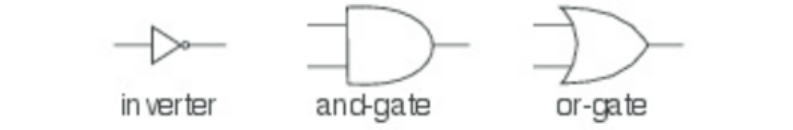
programs can be structured and built. The idea of such simulations is to model physical objects by
simulated objects, and use the simulation framework to model physical time.
The example is taken from the classic textbook Structure and Interpretation of Computer Programs by
Abelson and Sussman [Abe96]. What's different here is that the implementation language is Scala
instead of Scheme, and that the various aspects of the example are structured into four software layers:
one for the simulation framework, another for the basic circuit simulation package, a third for a library
of user-defined circuits, and the last layer for each simulated circuit itself. Each layer is expressed as a
class, and more specific layers inherit from more general ones.
THE FAST TRACK
Understanding the discrete event simulation example presented in this chapter will take some time. If
you feel you want to get on with learning more Scala instead, it's safe to skip ahead to the next chapter.
Figure 18.1 - Basic gates.
18.4 A LANGUAGE FOR DIGITAL CIRCUITS
We'll start with a "little language" to describe digital circuits. A digital circuit is built
fromwires and function boxes. Wires carry signals, which are transformed by function boxes. Signals
are represented by booleans: true for signal-on and false for signal-off.
Figure 18.1 shows three basic function boxes (or gates):
•An inverter, which negates its signal.
•An and-gate, which sets its output to the conjunction of its inputs.
•An or-gate, which sets its output to the disjunction of its inputs.
These gates are sufficient to build all other function boxes. Gates have delays, so an output of a gate
will change only some time after its inputs change.
We'll describe the elements of a digital circuit by the following set of Scala classes and functions. First,
there is a class Wire for wires. We can construct wires like this:
val a = new Wire
val b = new Wire
val c = new Wire
or, equivalent but shorter, like this:
val a, b, c = new Wire
Second, there are three procedures which "make" the basic gates we need:
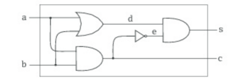
def inverter(input: Wire, output: Wire)
def andGate(a1: Wire, a2: Wire, output: Wire)
def orGate(o1: Wire, o2: Wire, output: Wire)
What's unusual, given the functional emphasis of Scala, is that these procedures construct the gates as a
side effect, instead of returning the constructed gates as a result. For instance, an invocation
of inverter(a, b) places an inverter between the wires a and b. It turns out that this side-effecting
construction makes it easier to construct complicated circuits gradually. Also, although methods most
often have verb names, these have noun names that indicate which gate they are making. This reflects
the declarative nature of the DSL: it should describe a circuit, not the actions of making one.
More complicated function boxes can be built from the basic gates. For instance, the method shown
in Listing 18.6 constructs a half-adder. The halfAdder method takes two inputs, a and b, and produces a
sum, s, defined by "s = (a + b) % 2" and a carry, c, defined by "c = (a + b) / 2". A diagram of the half-
adder is shown in Figure 18.2.
def halfAdder(a: Wire, b: Wire, s: Wire, c: Wire) = {
val d, e = new Wire
orGate(a, b, d)
andGate(a, b, c)
inverter(c, e)
andGate(d, e, s)
}
Listing 18.6 - The halfAdder method.
Figure 18.2 - A half-adder circuit.
Note that halfAdder is a parameterized function box just like the three methods that construct the
primitive gates. You can use the halfAdder method to construct more complicated circuits. For
instance, Listing 18.7 defines a full, one-bit adder, shown in Figure 18.3, which takes two
inputs, a and b, as well as a carry-in, cin, and which produces a sum output defined by
"sum = (a + b + cin) % 2" and a carry-out output defined by "cout = (a + b + cin) / 2".
def fullAdder(a: Wire, b: Wire, cin: Wire,
sum: Wire, cout: Wire) = {
val s, c1, c2 = new Wire
halfAdder(a, cin, s, c1)
halfAdder(b, s, sum, c2)
orGate(c1, c2, cout)
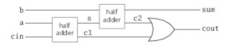
}
Listing 18.7 - The fullAdder method.
Class Wire and functions inverter, andGate, and orGate represent a little language with which users can
define digital circuits. It's a good example of an internal DSL, a domain-specific language defined as a
library in a host language instead of being implemented on its own.
Figure 18.3 - A full-adder circuit.
The implementation of the circuit DSL still needs to be worked out. Since the purpose of defining a
circuit in the DSL is simulating the circuit, it makes sense to base the DSL implementation on a general
API for discrete event simulation. The next two sections will present first the simulation API and then
the implementation of the circuit DSL on top of it.
18.5 THE SIMULATION API
The simulation API is shown in Listing 18.8. It consists of class Simulation in
packageorg.stairwaybook.simulation. Concrete simulation libraries inherit this class and augment it
with domain-specific functionality. The elements of the Simulation class are presented in this section.
abstract class Simulation {
type Action = () => Unit
case class WorkItem(time: Int, action: Action)
private var curtime = 0
def currentTime: Int = curtime
private var agenda: List[WorkItem] = List()
private def insert(ag: List[WorkItem],
item: WorkItem): List[WorkItem] = {
if (ag.isEmpty || item.time < ag.head.time) item :: ag
else ag.head :: insert(ag.tail, item)
}
def afterDelay(delay: Int)(block: => Unit) = {
val item = WorkItem(currentTime + delay, () => block)
agenda = insert(agenda, item)
}
private def next() = {
(agenda: @unchecked) match {
case item :: rest =>
agenda = rest
curtime = item.time
item.action()
}
}
def run() = {
afterDelay(0) {
println("*** simulation started, time = " +
currentTime + " ***")
}
while (!agenda.isEmpty) next()
}
}
Listing 18.8 - The Simulation class.
A discrete event simulation performs user-defined actions at specified times. The actions, which are
defined by concrete simulation subclasses, all share a common type:
type Action = () => Unit
This statement defines Action to be an alias of the type of procedure that takes an empty parameter list
and returns Unit. Action is a type member of class Simulation. You can think of it as a more readable
name for type () => Unit. Type members will be described in detail inSection 20.6.
The time at which an action is performed is simulated time; it has nothing to do with the actual "wall
clock" time. Simulated times are represented simply as integers. The current simulated time is kept in a
private variable:
private var curtime: Int = 0
The variable has a public accessor method, which retrieves the current time:
def currentTime: Int = curtime
This combination of private variable with public accessor is used to make sure that the current time
cannot be modified outside the Simulation class. After all, you don't usually want your simulation
objects to manipulate the current time, except possibly if your simulation models time travel.
An action that needs to be executed at a specified time is called a work item. Work items are
implemented by the following class:
case class WorkItem(time: Int, action: Action)
We made the WorkItem class a case class because of the syntactic conveniences this entails: You can
use the factory method, WorkItem, to create instances of the class, and you get accessors for the
constructor parameters time and action for free. Note also that class WorkItem is nested inside
class Simulation. Nested classes in Scala are treated similarly to Java. Section 20.7 will give more
details.
The Simulation class keeps an agenda of all remaining work items that have not yet been executed. The
work items are sorted by the simulated time at which they have to be run:
private var agenda: List[WorkItem] = List()
The agenda list will be kept in the proper sorted order by the insert method, which updates it. You can
see insert being called from afterDelay, which is the only way to add a work item to the agenda:
def afterDelay(delay: Int)(block: => Unit) = {
val item = WorkItem(currentTime + delay, () => block)
agenda = insert(agenda, item)
}
As the name implies, this method inserts an action (given by block) into the agenda so that it is
scheduled for execution delay time units after the current simulation time. For instance, the following
invocation would create a new work item to be executed at the simulated time,currentTime + delay:
afterDelay(delay) { count += 1 }
The code to be executed is contained in the method's second argument. The formal parameter for this
argument has type "=> Unit" (i.e., it is a computation of type Unit which is passed by name). Recall
that by-name parameters are not evaluated when passed to a method. So in the call above, count would
be incremented only when the simulation framework calls the action stored in the work item. Note
that afterDelay is a curried function. It's a good example of the principle set forward in Section 9.5 that
currying can be used to make method calls look more like built-in syntax. The created work item still
needs to be inserted into the agenda. This is done by the insert method, which maintains the invariant
that the agenda is time-sorted:
private def insert(ag: List[WorkItem],
item: WorkItem): List[WorkItem] = {
if (ag.isEmpty || item.time < ag.head.time) item :: ag
else ag.head :: insert(ag.tail, item)
}
The core of the Simulation class is defined by the run method:
def run() = {
afterDelay(0) {
println("*** simulation started, time = " +
currentTime + " ***")
}
while (!agenda.isEmpty) next()
}
This method repeatedly takes the first item in the agenda, removes it from the agenda and executes it. It
does this until there are no more items left in the agenda to execute. Each step is performed by calling
the next method, which is defined as follows:
private def next() = {
(agenda: @unchecked) match {
case item :: rest =>
agenda = rest
curtime = item.time
item.action()
}
}
The next method decomposes the current agenda with a pattern match into a front item, item, and a
remaining list of work items, rest. It removes the front item from the current agenda, sets the simulated
time curtime to the work item's time, and executes the work item's action.
Note that next can be called only if the agenda is non-empty. There's no case for an empty list, so you
would get a MatchError exception if you tried to run next on an empty agenda.
In fact, the Scala compiler would normally warn you that you missed one of the possible patterns for a
list:
Simulator.scala:19: warning: match is not exhaustive!
missing combination Nil
agenda match {
^
one warning found
In this case, the missing case is not a problem because you know that next is called only on a non-
empty agenda. Therefore, you might want to disable the warning. You saw in Section 15.5 that this can
be done by adding an @unchecked annotation to the selector expression of the pattern match. That's
why the Simulation code uses "(agenda: @unchecked) match", not "agenda match". That's it. This
might look like surprisingly little code for a simulation framework. You might wonder how this
framework could possibly support interesting simulations, if all it does is execute a list of work items?
In fact the power of the simulation framework comes from the fact that actions stored in work items
can themselves install further work items into the agenda when they are executed. That makes it
possible to have long-running simulations evolve from simple beginnings.
18.6 CIRCUIT SIMULATION
The next step is to use the simulation framework to implement the domain-specific language for
circuits shown in Section 18.4. Recall that the circuit DSL consists of a class for wires and methods
that create and-gates, or-gates, and inverters. These are all contained in aBasicCircuitSimulation class,
which extends the simulation framework. This class is shown inListings 18.9 and 18.10.
package org.stairwaybook.simulation
abstract class BasicCircuitSimulation extends Simulation {
def InverterDelay: Int
def AndGateDelay: Int
def OrGateDelay: Int
class Wire {
private var sigVal = false
private var actions: List[Action] = List()
def getSignal = sigVal
def setSignal(s: Boolean) =
if (s != sigVal) {
sigVal = s
actions foreach (_ ())
}
def addAction(a: Action) = {
actions = a :: actions
a()
}
}
def inverter(input: Wire, output: Wire) = {
def invertAction() = {
val inputSig = input.getSignal
afterDelay(InverterDelay) {
output setSignal !inputSig
}
}
input addAction invertAction
}
// continued in Listing 18.10...
Listing 18.9 - The first half of the BasicCircuitSimulation class.
// ...continued from Listing 18.9
def andGate(a1: Wire, a2: Wire, output: Wire) = {
def andAction() = {
val a1Sig = a1.getSignal
val a2Sig = a2.getSignal
afterDelay(AndGateDelay) {
output setSignal (a1Sig & a2Sig)
}
}
a1 addAction andAction
a2 addAction andAction
}
def orGate(o1: Wire, o2: Wire, output: Wire) = {
def orAction() = {
val o1Sig = o1.getSignal
val o2Sig = o2.getSignal
afterDelay(OrGateDelay) {
output setSignal (o1Sig | o2Sig)
}
}
o1 addAction orAction
o2 addAction orAction
}
def probe(name: String, wire: Wire) = {
def probeAction() = {
println(name + " " + currentTime +
" new-value = " + wire.getSignal)
}
wire addAction probeAction
}
}
Listing 18.10 - The second half of the BasicCircuitSimulation class.
Class BasicCircuitSimulation declares three abstract methods that represent the delays of the basic
gates: InverterDelay, AndGateDelay, and OrGateDelay. The actual delays are not known at the level of
this class because they depend on the technology of circuits that are simulated. That's why the delays
are left abstract in class BasicCircuitSimulation, so that their concrete definition is delegated to a
subclass.[2] The implementation of class BasicCircuitSimulation's other members is described next.
The Wire class
A wire needs to support three basic actions:
• getSignal: Boolean: returns the current signal on the wire.
• setSignal(sig: Boolean): sets the wire's signal to sig.
• addAction(p: Action): attaches the specified procedure p to the actions of the wire. The idea is
that all action procedures attached to some wire will be executed every time the signal of the
wire changes. Typically actions are added to a wire by components connected to the wire. An
attached action is executed once at the time it is added to a wire, and after that, every time the
signal of the wire changes.
Here is the implementation of the Wire class:
class Wire {
private var sigVal = false
private var actions: List[Action] = List()
def getSignal = sigVal
def setSignal(s: Boolean) =
if (s != sigVal) {
sigVal = s
actions foreach (_ ())
}
def addAction(a: Action) = {
actions = a :: actions
a()
}
}
Two private variables make up the state of a wire. The variable sigVal represents the current signal, and
the variable actions represents the action procedures currently attached to the wire. The only interesting
method implementation is the one for setSignal: When the signal of a wire changes, the new value is
stored in the variable sigVal. Furthermore, all actions attached to a wire are executed. Note the
shorthand syntax for doing this: "actions foreach (_ ())" applies the function, "_ ()", to each element in
the actions list. As described in Section 8.5, the function "_ ()" is a shorthand for "f => f ()"—i.e., it
takes a function (we'll call it f) and applies it to the empty parameter list.
The inverter method
The only effect of creating an inverter is that an action is installed on its input wire. This action is
invoked once at the time the action is installed, and thereafter every time the signal on the input
changes. The effect of the action is that the value of the inverter's output value is set (via setSignal) to
the inverse of its input value. Since inverter gates have delays, this change should take effect
only InverterDelay units of simulated time after the input value has changed and the action was
executed. This suggests the following implementation:
def inverter(input: Wire, output: Wire) = {
def invertAction() = {
val inputSig = input.getSignal
afterDelay(InverterDelay) {
output setSignal !inputSig
}
}
input addAction invertAction
}
The effect of the inverter method is to add invertAction to the input wire. This action, when invoked,
gets the input signal and installs another action that inverts the output signal into the simulation agenda.
This other action is to be executed after InverterDelay units of simulated time. Note how the method
uses the afterDelay method of the simulation framework to create a new work item that's going to be
executed in the future.
The andGate and orGate methods
The implementation of and-gates is analogous to the implementation of inverters. The purpose of an
and-gate is to output the conjunction of its input signals. This should happen
atAndGateDelay simulated time units after any one of its two inputs changes. Hence, the following
implementation:
def andGate(a1: Wire, a2: Wire, output: Wire) = {
def andAction() = {
val a1Sig = a1.getSignal
val a2Sig = a2.getSignal
afterDelay(AndGateDelay) {
output setSignal (a1Sig & a2Sig)
}
}
a1 addAction andAction
a2 addAction andAction
}
The effect of the andGate method is to add andAction to both of its input wires a1 and a2. This action,
when invoked, gets both input signals and installs another action that sets the outputsignal to the
conjunction of both input signals. This other action is to be executed afterAndGateDelay units of
simulated time. Note that the output has to be recomputed if either of the input wires changes. That's
why the same andAction is installed on each of the two input wiresa1 and a2. The orGate method is
implemented similarly, except it performs a logical-or instead of a logical-and.
Simulation output
To run the simulator, you need a way to inspect changes of signals on wires. To accomplish this, you
can simulate the action of putting a probe on a wire:
def probe(name: String, wire: Wire) = {
def probeAction() = {
println(name + " " + currentTime +
" new-value = " + wire.getSignal)
}
wire addAction probeAction
}
The effect of the probe procedure is to install a probeAction on a given wire. As usual, the installed
action is executed every time the wire's signal changes. In this case it simply prints the name of the
wire (which is passed as first parameter to probe), as well as the current simulated time and the wire's
new value.
Running the simulator
After all these preparations, it's time to see the simulator in action. To define a concrete simulation, you
need to inherit from a simulation framework class. To see something interesting, we'll create an abstract
simulation class that extends BasicCircuitSimulation and contains method definitions for half-adders
and full-adders as they were presented earlier in this chapter in Listings 18.6 and 18.7, respectively.
This class, which we'll callCircuitSimulation, is shown in Listing 18.11.
package org.stairwaybook.simulation
abstract class CircuitSimulation
extends BasicCircuitSimulation {
def halfAdder(a: Wire, b: Wire, s: Wire, c: Wire) = {
val d, e = new Wire
orGate(a, b, d)
andGate(a, b, c)
inverter(c, e)
andGate(d, e, s)
}
def fullAdder(a: Wire, b: Wire, cin: Wire,
sum: Wire, cout: Wire) = {
val s, c1, c2 = new Wire
halfAdder(a, cin, s, c1)
halfAdder(b, s, sum, c2)
orGate(c1, c2, cout)
}
}
Listing 18.11 - The CircuitSimulation class.
A concrete circuit simulation will be an object that inherits from class CircuitSimulation. The object
still needs to fix the gate delays according to the circuit implementation technology that's simulated.
Finally, you will also need to define the concrete circuit that's going to be simulated.
You can do these steps interactively in the Scala interpreter:
scala> import org.stairwaybook.simulation._
import org.stairwaybook.simulation._
First, the gate delays. Define an object (call it MySimulation) that provides some numbers:
scala> object MySimulation extends CircuitSimulation {
def InverterDelay = 1
def AndGateDelay = 3
def OrGateDelay = 5
}
defined module MySimulation
Because you are going to access the members of the MySimulation object repeatedly, an import of the
object keeps the subsequent code shorter:
scala> import MySimulation._
import MySimulation._
Next, the circuit. Define four wires, and place probes on two of them:
scala> val input1, input2, sum, carry = new Wire
input1: MySimulation.Wire =
BasicCircuitSimulation$Wire@111089b
input2: MySimulation.Wire =
BasicCircuitSimulation$Wire@14c352e
sum: MySimulation.Wire =
BasicCircuitSimulation$Wire@37a04c
carry: MySimulation.Wire =
BasicCircuitSimulation$Wire@1fd10fa
scala> probe("sum", sum)
sum 0 new-value = false
scala> probe("carry", carry)
carry 0 new-value = false
Note that the probes immediately print an output. This is because every action installed on a wire is
executed a first time when the action is installed.
Now define a half-adder connecting the wires:
scala> halfAdder(input1, input2, sum, carry)
Finally, set the signals, one after another, on the two input wires to true and run the simulation:
scala> input1 setSignal true
scala> run()
*** simulation started, time = 0 ***
sum 8 new-value = true
scala> input2 setSignal true
scala> run()
*** simulation started, time = 8 ***
carry 11 new-value = true
sum 15 new-value = false
18.7 CONCLUSION
This chapter brought together two techniques that seem disparate at first: mutable state and higher-
order functions. Mutable state was used to simulate physical entities whose state changes over time.
Higher-order functions were used in the simulation framework to execute actions at specified points in
simulated time. They were also used in the circuit simulations astriggers that associate actions with
state changes. Along the way, you saw a simple way to define a domain-specific language as a library.
That's probably enough for one chapter!
If you feel like staying a bit longer, you might want to try more simulation examples. You can combine
half-adders and full-adders to create larger circuits, or design new circuits from the basic gates defined
so far and simulate them. In the next chapter, you'll learn about type parameterization in Scala, and see
another example in which a combination of functional and imperative approaches yields a good
solution.
Footnotes for Chapter 18:
[1] Abstract variables will be explained in Chapter 20.
[2] The names of these "delay" methods start with a capital letter because they represent constants.
They are methods so they can be overridden in subclasses. You'll find out how to do the same thing
with vals in Section 20.3.
Chapter 19
Type Parameterization
In this chapter, we'll explain the details of type parameterization in Scala. Along the way we'll
demonstrate some of the techniques for information hiding introduced in Chapter 13 by using a
concrete example: the design of a class for purely functional queues. We're presenting type
parameterization and information hiding together, because information hiding can be used to obtain
more general type parameterization variance annotations.
Type parameterization allows you to write generic classes and traits. For example, sets are generic and
take a type parameter: they are defined as Set[T]. As a result, any particular set instance might be
a Set[String], a Set[Int], etc., but it must be a set of something. Unlike Java, which allows raw
types, Scala requires that you specify type parameters. Variance defines inheritance relationships of
parameterized types, such as whether a Set[String], for example, is a subtype of Set[AnyRef].
The chapter contains three parts. The first part develops a data structure for purely functional queues.
The second part develops techniques to hide internal representation details of this structure. The final
part explains variance of type parameters and how it interacts with information hiding.
19.1 FUNCTIONAL QUEUES
A functional queue is a data structure with three operations:
head returns the first element of the queue
tail returns a queue without its first element
enqueue returns a new queue with a given element
appended at the end
Unlike a mutable queue, a functional queue does not change its contents when an element is appended.
Instead, a new queue is returned that contains the element. The goal of this chapter will be to create a
class, which we'll name Queue, that works like this:
scala> val q = Queue(1, 2, 3)
q: Queue[Int] = Queue(1, 2, 3)
scala> val q1 = q enqueue 4
q1: Queue[Int] = Queue(1, 2, 3, 4)
scala> q
res0: Queue[Int] = Queue(1, 2, 3)
If Queue were a mutable implementation, the enqueue operation in the second input line above would
affect the contents of q; in fact both the result, q1, and the original queue, q, would contain the
sequence 1, 2, 3, 4 after the operation. But for a functional queue, the appended value shows up only in
the result, q1, not in the queue, q, being operated on.
Purely functional queues also have some similarity with lists. Both are so called fully persistent data
structures, where old versions remain available even after extensions or modifications. Both
support head and tail operations. But where a list is usually extended at the front, using a :: operation, a
queue is extended at the end, using enqueue.
How can this be implemented efficiently? Ideally, a functional (immutable) queue should not have a
fundamentally higher overhead than an imperative (mutable) one. That is, all three
operations, head, tail, and enqueue, should operate in constant time.
One simple approach to implement a functional queue would be to use a list as representation type.
Then head and tail would just translate into the same operations on the list, whereas enqueue would be
concatenation.
This would give the following implementation:
class SlowAppendQueue[T](elems: List[T]) { // Not efficient
def head = elems.head
def tail = new SlowAppendQueue(elems.tail)
def enqueue(x: T) = new SlowAppendQueue(elems ::: List(x))
}
The problem with this implementation is in the enqueue operation. It takes time proportional to the
number of elements stored in the queue. If you want constant time append, you could also try to reverse
the order of the elements in the representation list, so that the last element that's appended comes first
in the list. This would lead to the following implementation:
class SlowHeadQueue[T](smele: List[T]) { // Not efficient
// smele is elems reversed
def head = smele.last
def tail = new SlowHeadQueue(smele.init)
def enqueue(x: T) = new SlowHeadQueue(x :: smele)
}
Now enqueue is constant time, but head and tail are not. They now take time proportional to the
number of elements stored in the queue.
Looking at these two examples, it does not seem easy to come up with an implementation that's
constant time for all three operations. In fact, it looks doubtful that this is even possible! However, by
combining the two operations you can get very close. The idea is to represent a queue by two lists,
called leading and trailing. The leading list contains elements towards the front, whereas the trailing list
contains elements towards the back of the queue in reversed order. The contents of the whole queue are
at each instant equal to "leading ::: trailing.reverse".
Now, to append an element, you just cons it to the trailing list using the :: operator, so enqueueis
constant time. This means that, when an initially empty queue is constructed from
successive enqueue operations, the trailing list will grow whereas the leading list will stay empty. Then,
before the first head or tail operation is performed on an empty leading list, the whole trailing list is
copied to leading, reversing the order of the elements. This is done in an operation
called mirror. Listing 19.1 shows an implementation of queues that uses this approach.
class Queue[T](
private val leading: List[T],
private val trailing: List[T]
) {
private def mirror =
if (leading.isEmpty)
new Queue(trailing.reverse, Nil)
else
this
def head = mirror.leading.head
def tail = {
val q = mirror
new Queue(q.leading.tail, q.trailing)
}
def enqueue(x: T) =
new Queue(leading, x :: trailing)
}
Listing 19.1 - A basic functional queue.
What is the complexity of this implementation of queues? The mirror operation might take time
proportional to the number of queue elements, but only if list leading is empty. It returns directly
if leading is non-empty. Because head and tail call mirror, their complexity might be linear in the size
of the queue, too. However, the longer the queue gets, the less often mirror is called.
Indeed, assume a queue of length n with an empty leading list. Then mirror has to reverse-copy a list of
length n. However, the next time mirror will have to do any work is once the leading list is empty
again, which will be the case after n tail operations. This means you can "charge" each of
these n tail operations with one n'th of the complexity of mirror, which means a constant amount of
work. Assuming that head, tail, and enqueue operations appear with about the same frequency,
the amortized complexity is hence constant for each operation. So functional queues are asymptotically
just as efficient as mutable ones.
Now, there are some caveats that need to be attached to this argument. First, the discussion was only
about asymptotic behavior; the constant factors might well be somewhat different. Second, the
argument rested on the fact that head, tail and enqueue are called with about the same frequency.
If head is called much more often than the other two operations, the argument is not valid, as each call
to head might involve a costly re-organization of the list with mirror. The second caveat can be
avoided; it is possible to design functional queues so that in a sequence of successive head operations
only the first one might require a re-organization. You will find out at the end of this chapter how this is
done.
19.2 INFORMATION HIDING
The implementation of Queue shown in Listing 19.1 is now quite good with regards toefficiency. You
might object, though, that this efficiency is paid for by exposing a needlessly detailed implementation.
The Queue constructor, which is globally accessible, takes two lists as parameters, where one is
reversed—hardly an intuitive representation of a queue. What's needed is a way to hide this constructor
from client code. In this section, we'll show you some ways to accomplish this in Scala.
Private constructors and factory methods
In Java, you can hide a constructor by making it private. In Scala, the primary constructor does not
have an explicit definition; it is defined implicitly by the class parameters and body. Nevertheless, it is
still possible to hide the primary constructor by adding a private modifier in front of the class parameter
list, as shown in Listing 19.2:
class Queue[T] private (
private val leading: List[T],
private val trailing: List[T]
)
Listing 19.2 - Hiding a primary constructor by making it private.
The private modifier between the class name and its parameters indicates that the constructor
of Queue is private: it can be accessed only from within the class itself and its companion object. The
class name Queue is still public, so you can use it as a type, but you cannot call its constructor:
scala> new Queue(List(1, 2), List(3))
<console>:9: error: constructor Queue in class Queue cannot
be accessed in object $iw
new Queue(List(1, 2), List(3))
^
Now that the primary constructor of class Queue can no longer be called from client code, there needs
to be some other way to create new queues. One possibility is to add an auxiliary constructor, like this:
def this() = this(Nil, Nil)
The auxiliary constructor shown in the previous example builds an empty queue. As a refinement, the
auxiliary constructor could take a list of initial queue elements:
def this(elems: T*) = this(elems.toList, Nil)
Recall that T* is the notation for repeated parameters, as described in Section 8.8.
Another possibility is to add a factory method that builds a queue from such a sequence of initial
elements. A neat way to do this is to define an object Queue that has the same name as the class being
defined and contains an apply method, as shown in Listing 19.3:
object Queue {
// constructs a queue with initial elements `xs'
def apply[T](xs: T*) = new Queue[T](xs.toList, Nil)
}
Listing 19.3 - An apply factory method in a companion object.
By placing this object in the same source file as class Queue, you make the object a companion object
of the class. You saw in Section 13.5 that a companion object has the same access rights as its class.
Because of this, the apply method in object Queue can create a new Queue object, even though the
constructor of class Queue is private.
Note that, because the factory method is called apply, clients can create queues with an expression such
as Queue(1, 2, 3). This expression expands to Queue.apply(1, 2, 3) since Queue is an object instead of a
function. As a result, Queue looks to clients as if it was a globally defined factory method. In reality,
Scala has no globally visible methods; every method must be contained in an object or a class.
However, using methods named apply inside global objects, you can support usage patterns that look
like invocations of global methods.
trait Queue[T] {
def head: T
def tail: Queue[T]
def enqueue(x: T): Queue[T]
}
object Queue {
def apply[T](xs: T*): Queue[T] =
new QueueImpl[T](xs.toList, Nil)
private class QueueImpl[T](
private val leading: List[T],
private val trailing: List[T]
) extends Queue[T] {
def mirror =
if (leading.isEmpty)
new QueueImpl(trailing.reverse, Nil)
else
this
def head: T = mirror.leading.head
def tail: QueueImpl[T] = {
val q = mirror
new QueueImpl(q.leading.tail, q.trailing)
}
def enqueue(x: T) =
new QueueImpl(leading, x :: trailing)
}
}
Listing 19.4 - Type abstraction for functional queues.
An alternative: private classes
Private constructors and private members are one way to hide the initialization and representation of a
class. Another more radical way is to hide the class itself and only export a trait that reveals the public
interface of the class. The code in Listing 19.4 implements this design. There's a trait Queue, which
declares the methods head, tail, and enqueue. All three methods are implemented in a
subclass QueueImpl, which is itself a private inner class of objectQueue. This exposes to clients the
same information as before, but using a different technique. Instead of hiding individual constructors
and methods, this version hides the whole implementation class.
19.3 VARIANCE ANNOTATIONS
Queue, as defined in Listing 19.4, is a trait, but not a type. Queue is not a type because it takes a type
parameter.
As a result, you cannot create variables of type Queue:
scala> def doesNotCompile(q: Queue) = {}
<console>:8: error: class Queue takes type parameters
def doesNotCompile(q: Queue) = {}
^
Instead, trait Queue enables you to specify parameterized types, such as Queue[String],Queue[Int],
or Queue[AnyRef]:
scala> def doesCompile(q: Queue[AnyRef]) = {}
doesCompile: (q: Queue[AnyRef])Unit
Thus, Queue is a trait and Queue[String] is a type. Queue is also called a type constructor because you
can construct a type with it by specifying a type parameter. (This is analogous to constructing an object
instance with a plain-old constructor by specifying a value parameter.) The type
constructor Queue "generates" a family of types, which includes Queue[Int],Queue[String],
and Queue[AnyRef].
You can also say that Queue is a generic trait. (Classes and traits that take type parameters are
"generic," but the types they generate are "parameterized," not generic.) The term "generic" means that
you are defining many specific types with one generically written class or trait. For example,
trait Queue in Listing 19.4 defines a generic queue. Queue[Int] and Queue[String],etc., would be the
specific queues.
The combination of type parameters and subtyping poses some interesting questions. For example, are
there any special subtyping relationships between members of the family of types generated
by Queue[T]? More specifically, should a Queue[String] be considered a subtype of Queue[AnyRef]?
Or more generally, if S is a subtype of type T, then should Queue[S] be considered a subtype
of Queue[T]? If so, you could say that trait Queue is covariant (or "flexible") in its type parameter T.
Or, since it just has one type parameter, you could say simply that Queues are covariant.
Covariant Queues would mean, for example, that you could pass a Queue[String] to
the doesCompile method shown previously, which takes a value parameter of type Queue[AnyRef].
Intuitively, all this seems OK, since a queue of Strings looks like a special case of a queue ofAnyRefs.
In Scala, however, generic types have by default nonvariant (or "rigid") subtyping. That is,
with Queue defined as in Listing 19.4, queues with different element types would never be in a subtype
relationship. A Queue[String] would not be usable as a Queue[AnyRef]. However, you can demand
covariant (flexible) subtyping of queues by changing the first line of the definition of class Queue like
this:
trait Queue[+T] { ... }
Prefixing a formal type parameter with a + indicates that subtyping is covariant (flexible) in that
parameter. By adding this single character, you are telling Scala that you wantQueue[String], for
example, to be considered a subtype of Queue[AnyRef]. The compiler will check that Queue is defined
in a way that this subtyping is sound.
Besides +, there is also a prefix -, which indicates contravariant subtyping. If Queue were defined like
this:
trait Queue[-T] { ... }
then if T is a subtype of type S, this would imply that Queue[S] is a subtype of Queue[T] (which in the
case of queues would be rather surprising!). Whether a type parameter is covariant, contravariant, or
nonvariant is called the parameter's variance. The + and - symbols you can place next to type
parameters are called variance annotations.
In a purely functional world, many types are naturally covariant (flexible). However, the situation
changes once you introduce mutable data. To find out why, consider the simple type of one-element
cells that can be read or written, shown in Listing 19.5.
class Cell[T](init: T) {
private[this] var current = init
def get = current
def set(x: T) = { current = x }
}
Listing 19.5 - A nonvariant (rigid) Cell class.
The Cell type of Listing 19.5 is declared nonvariant (rigid). For the sake of argument, assume for a
moment that Cell was declared covariant instead—i.e., it was declared class Cell[+T]—and that this
passed the Scala compiler. (It doesn't, and we'll explain why shortly.) Then you could construct the
following problematic statement sequence:
val c1 = new Cell[String]("abc")
val c2: Cell[Any] = c1
c2.set(1)
val s: String = c1.get
Seen by itself, each of these four lines looks OK. The first line creates a cell of strings and stores it in
a val named c1. The second line defines a new val, c2, of type Cell[Any], which initialized with c1.
This is OK since Cells are assumed to be covariant. The third line sets the value of cell c2 to 1. This is
also OK because the assigned value 1 is an instance of c2's element type Any. Finally, the last line
assigns the element value of c1 into a string. Nothing strange here, as both the sides are of the same
type. But taken together, these four lines end up assigning the integer 1 to the string s. This is clearly a
violation of type soundness.
Which operation is to blame for the runtime fault? It must be the second one, which uses covariant
subtyping. The other statements are too simple and fundamental. Thus, a Cell ofString is not also
a Cell of Any, because there are things you can do with a Cell of Any that you cannot do with
a Cell of String. You cannot use set with an Int argument on a Cell of String, for example.
In fact, were you to pass the covariant version of Cell to the Scala compiler, you would get a compile-
time error:
Cell.scala:7: error: covariant type T occurs in
contravariant position in type T of value x
def set(x: T) = current = x
^
Variance and arrays
It's interesting to compare this behavior with arrays in Java. In principle, arrays are just like cells except
that they can have more than one element. Nevertheless, arrays are treated as covariant in Java.
You can try an example analogous to the cell interaction described here with Java arrays:
// this is Java
String[] a1 = { "abc" };
Object[] a2 = a1;
a2[0] = new Integer(17);
String s = a1[0];
If you try out this example, you will find that it compiles. But executing the program will cause
an ArrayStore exception to be thrown when a2[0] is assigned to an Integer:
Exception in thread "main" java.lang.ArrayStoreException:
java.lang.Integer
at JavaArrays.main(JavaArrays.java:8)
What happens here is that Java stores the element type of the array at runtime. Then, every time an
array element is updated, the new element value is checked against the stored type. If it is not an
instance of that type, an ArrayStore exception is thrown.
You might ask why Java adopted this design, which seems both unsafe and expensive. When asked this
question, James Gosling, the principal inventor of the Java language, answered that they wanted to
have a simple means to treat arrays generically. For instance, they wanted to be able to write a method
to sort all elements of an array, using a signature like the following that takes an array of Object:
void sort(Object[] a, Comparator cmp) { ... }
Covariance of arrays was needed so that arrays of arbitrary reference types could be passed to
this sort method. Of course, with the arrival of Java generics, such a sort method can now be written
with a type parameter, so the covariance of arrays is no longer necessary. For compatibility reasons,
though, it has persisted in Java to this day.
Scala tries to be purer than Java in not treating arrays as covariant. Here's what you get if you translate
the first two lines of the array example to Scala:
scala> val a1 = Array("abc")
a1: Array[String] = Array(abc)
scala> val a2: Array[Any] = a1
<console>:8: error: type mismatch;
found : Array[String]
required: Array[Any]
val a2: Array[Any] = a1
^
What happened here is that Scala treats arrays as nonvariant (rigid), so an Array[String] is not
considered to conform to an Array[Any]. However, sometimes it is necessary to interact with legacy
methods in Java that use an Object array as a means to emulate a generic array. For instance, you might
want to call a sort method like the one described previously with an array of Strings as argument. To
make this possible, Scala lets you cast an array of Ts to an array of any supertype of T:
scala> val a2: Array[Object] =
a1.asInstanceOf[Array[Object]]
a2: Array[Object] = Array(abc)
The cast is always legal at compile-time, and it will always succeed at run-time because the JVM's
underlying run-time model treats arrays as covariant, just as Java the language does. But you might
get ArrayStore exceptions afterwards, again just as you would in Java.
19.4 CHECKING VARIANCE ANNOTATIONS
Now that you have seen some examples where variance is unsound, you may be wondering which kind
of class definitions need to be rejected and which can be accepted. So far, all violations of type
soundness involved some reassignable field or array element. The purely functional implementation of
queues, on the other hand, looks like a good candidate for covariance. However, the following example
shows that you can "engineer" an unsound situation even if there is no reassignable field.
To set up the example, assume that queues as defined in Listing 19.4 are covariant. Then, create a
subclass of queues that specializes the element type to Int and overrides the enqueuemethod:
class StrangeIntQueue extends Queue[Int] {
override def enqueue(x: Int) = {
println(math.sqrt(x))
super.enqueue(x)
}
}
The enqueue method in StrangeIntQueue prints out the square root of its (integer) argument before
doing the append proper.
Now, you can write a counterexample in two lines:
val x: Queue[Any] = new StrangeIntQueue
x.enqueue("abc")
The first of these two lines is valid because StrangeIntQueue is a subclass of Queue[Int] and, assuming
covariance of queues, Queue[Int] is a subtype of Queue[Any]. The second line is valid because you can
append a String to a Queue[Any]. However, taken together, these two lines have the effect of applying
a square root method to a string, which makes no sense.
Clearly it's not just mutable fields that make covariant types unsound. The problem is more general. It
turns out that as soon as a generic parameter type appears as the type of a method parameter, the
containing class or trait may not be covariant in that type parameter.
For queues, the enqueue method violates this condition:
class Queue[+T] {
def enqueue(x: T) =
...
}
Running a modified queue class like the one above through a Scala compiler would yield:
Queues.scala:11: error: covariant type T occurs in
contravariant position in type T of value x
def enqueue(x: T) =
^
Reassignable fields are a special case of the rule that disallows type parameters annotated with + from
being used as method parameter types. As mentioned in Section 18.2, a reassignable field, "var x: T", is
treated in Scala as a getter method, "def x: T", and a setter method, "def x_=(y: T)". As you can see, the
setter method has a parameter of the field's type T. So that type may not be covariant.
THE FAST TRACK
In the rest of this section, we'll describe the mechanism by which the Scala compiler checks variance
annotations. If you're not interested in such detail right now, you can safely skip toSection 19.5. The
most important thing to understand is that the Scala compiler will check any variance annotations you
place on type parameters. For example, if you try to declare a type parameter to be covariant (by adding
a +), but that could lead to potential runtime errors, your program won't compile.
To verify correctness of variance annotations, the Scala compiler classifies all positions in a class or
trait body as positive, negative or neutral. A "position" is any location in the class or trait (but from
now on we'll just write "class") body where a type parameter may be used. For example, every method
value parameter is a position because a method value parameter has a type. Therefore a type parameter
could appear in that position.
The compiler checks each use of each of the class's type parameters. Type parameters annotated
with + may only be used in positive positions, while type parameters annotated with - may only be used
in negative positions. A type parameter with no variance annotation may be used in any position, and is,
therefore, the only kind of type parameter that can be used in neutral positions of the class body.
To classify the positions, the compiler starts from the declaration of a type parameter and then moves
inward through deeper nesting levels. Positions at the top level of the declaring class are classified as
positive. By default, positions at deeper nesting levels are classified the same as that at enclosing
levels, but there are a handful of exceptions where the classification changes. Method value parameter
positions are classified to the flipped classification relative to positions outside the method, where the
flip of a positive classification is negative, the flip of a negative classification is positive, and the flip of
a neutral classification is still neutral.
Besides method value parameter positions, the current classification is also flipped at the type
parameters of methods. A classification is sometimes flipped at the type argument position of a type,
such as the Arg in C[Arg], depending on the variance of the corresponding type parameter. If C's type
parameter is annotated with a + then the classification stays the same. If C's type parameter is annotated
with a -, then the current classification is flipped. IfC's type parameter has no variance annotation then
the current classification is changed to neutral.
As a somewhat contrived example, consider the following class definition, where several positions are
annotated with their classifications, ^+ (for positive) or ^- (for negative):
abstract class Cat[-T, +U] {
def meow[W^-](volume: T^-, listener: Cat[U^+, T^-]^-)
: Cat[Cat[U^+, T^-]^-, U^+]^+
}
The positions of the type parameter, W, and the two value parameters, volume and listener, are all
negative. Looking at the result type of meow, the position of the first Cat[U, T] argument is negative
because Cat's first type parameter, T, is annotated with a -. The type U inside this argument is again in
positive position (two flips), whereas the type T inside that argument is still in negative position.
You see from this discussion that it's quite hard to keep track of variance positions. That's why it's a
welcome relief that the Scala compiler does this job for you.
Once the classifications are computed, the compiler checks that each type parameter is only used in
positions that are classified appropriately. In this case, T is only used in negative positions, and U is
only used in positive positions. So class Cat is type correct.
19.5 LOWER BOUNDS
Back to the Queue class. You saw that the previous definition of Queue[T] shown in Listing 19.4cannot
be made covariant in T because T appears as a type of a parameter of the enqueuemethod, and that's a
negative position.
Fortunately, there's a way to get unstuck: you can generalize enqueue by making it polymorphic (i.e.,
giving the enqueue method itself a type parameter) and using a lower bound for its type
parameter. Listing 19.6 shows a new formulation of Queue that implements this idea.
class Queue[+T] (private val leading: List[T],
private val trailing: List[T] ) {
def enqueue[U >: T](x: U) =
new Queue[U](leading, x :: trailing) // ...
}
Listing 19.6 - A type parameter with a lower bound.
The new definition gives enqueue a type parameter U, and with the syntax, "U >: T", defines T as the
lower bound for U. As a result, U is required to be a supertype of T.[1] The parameter toenqueue is now
of type U instead of type T, and the return value of the method is now Queue[U]instead of Queue[T].
For example, suppose there is a class Fruit with two subclasses, Apple and Orange. With the new
definition of class Queue, it is possible to append an Orange to a Queue[Apple]. The result will be
aQueue[Fruit].
This revised definition of enqueue is type correct. Intuitively, if T is a more specific type than expected
(for example, Apple instead of Fruit), a call to enqueue will still work because U (Fruit) will still be a
supertype of T (Apple).[2]
The new definition of enqueue is arguably better than the old, because it is more general. Unlike the old
version, the new definition allows you to append an arbitrary supertype U of the queue element type T.
The result is then a Queue[U]. Together with queue covariance, this gives the right kind of flexibility
for modeling queues of different element types in a natural way.
This shows that variance annotations and lower bounds play well together. They are a good example
of type-driven design, where the types of an interface guide its detailed design and implementation. In
the case of queues, it's likely you would not have thought of the refined implementation
of enqueue with a lower bound. But you might have decided to make queues covariant, in which case,
the compiler would have pointed out the variance error for enqueue. Correcting the variance error by
adding a lower bound makes enqueue more general and queues as a whole more usable.
This observation is also the main reason that Scala prefers declaration-site variance over use-site
variance as it is found in Java's wildcards. With use-site variance, you are on your own designing a
class. It will be the clients of the class that need to put in the wildcards, and if they get it wrong, some
important instance methods will no longer be applicable. Variance being a tricky business, users usually
get it wrong, and they come away thinking that wildcards and generics are overly complicated. With
definition-side variance, you express your intent to the compiler, and the compiler will double check
that the methods you want available will indeed be available.
19.6 CONTRAVARIANCE
So far in this chapter, all examples you've seen were either covariant or nonvariant. But there are also
cases where contravariance is natural. For instance, consider the trait of output channels shown
in Listing 19.7:
trait OutputChannel[-T] {
def write(x: T)
}
Listing 19.7 - A contravariant output channel.
Here, OutputChannel is defined to be contravariant in T. So an output channel of AnyRefs, say, is a
subtype of an output channel of Strings. Although it may seem non-intuitive, it actually makes sense.
To see why, consider what you can do with an OutputChannel[String]. The only supported operation is
writing a String to it. The same operation can also be done on anOutputChannel[AnyRef]. So it is safe
to substitute an OutputChannel[AnyRef] for anOutputChannel[String]. By contrast, it would not be safe
to substitute an OutputChannel[String]where an OutputChannel[AnyRef] is required. After all, you can
send any object to anOutputChannel[AnyRef], whereas an OutputChannel[String] requires that the
written values are all strings.
This reasoning points to a general principle in type system design: It is safe to assume that a type T is a
subtype of a type U if you can substitute a value of type T wherever a value of type Uis required. This
is called the Liskov Substitution Principle. The principle holds if T supports the same operations as U,
and all of T's operations require less and provide more than the corresponding operations in U. In the
case of output channels, an OutputChannel[AnyRef] can be a subtype of
an OutputChannel[String] because the two support the same write operation, and this operation requires
less in OutputChannel[AnyRef] than in OutputChannel[String]. "Less" means the argument is only
required to be an AnyRef in the first case, whereas it is required to be a Stringin the second case.
Sometimes covariance and contravariance are mixed in the same type. A prominent example is Scala's
function traits. For instance, whenever you write the function type A => B, Scala expands this
to Function1[A, B]. The definition of Function1 in the standard library uses both covariance and
contravariance: the Function1 trait is contravariant in the function argument type S and covariant in the
result type T, as shown in Listing 19.8. This satisfies the Liskov Substitution Principle because
arguments are something that's required, whereas results are something that's provided.
trait Function1[-S, +T] {
def apply(x: S): T
}
Listing 19.8 - Covariance and contravariance of Function1s.
As an example, consider the application shown in Listing 19.9. Here, class Publicationcontains one
parametric field, title, of type String. Class Book extends Publication and forwards its
string title parameter to the constructor of its superclass. The Library singleton object defines a set of
books and a method printBookList, which takes a function, named info, of typeBook => AnyRef. In
other words, the type of the lone parameter to printBookList is a function that takes one Book argument
and returns an AnyRef. The Customer application defines a method,getTitle, which takes
a Publication as its lone parameter and returns a String, the title of the passed Publication.
class Publication(val title: String)
class Book(title: String) extends Publication(title)
object Library {
val books: Set[Book] =
Set(
new Book("Programming in Scala"),
new Book("Walden")
)
def printBookList(info: Book => AnyRef) = {
for (book <- books) println(info(book))
}
}
object Customer extends App {
def getTitle(p: Publication): String = p.title
Library.printBookList(getTitle)
}
Listing 19.9 - Demonstration of function type parameter variance.
Now take a look at the last line in Customer. This line invokes Library's printBookList method and
passes getTitle, wrapped in a function value:
Library.printBookList(getTitle)
This line of code type checks even though String, the function's result type, is a subtype ofAnyRef, the
result type of printBookList's info parameter. This code passes the compiler because function result
types are declared to be covariant (the +T in Listing 19.8). If you look inside the body
of printBookList, you can get a glimpse of why this makes sense.
The printBookList method iterates through its book list and invokes the passed function on each book.
It passes the AnyRef result returned by info to println, which invokes toString on it and prints the
result. This activity will work with String as well as any other subclass of AnyRef, which is what
covariance of function result types means.
Now consider the parameter type of the function being passed to the printBookList method.
Although printBookList's parameter type is declared as Book, the getTitle we're passing in takes
a Publication, a supertype of Book. The reason this works is that since printBookList's parameter type
is Book, the body of the printBookList method will only be allowed to pass a Book into the function.
And because getTitle's parameter type is Publication, the body of that function will only be able to
access on its parameter, p, members that are declared in class Publication. Because any method
declared in Publication is also available on its subclass Book, everything should work, which is what
contravariance of function parameter types means. You can see all this graphically in Figure 19.1.
The code in Listing 19.9 compiles because Publication => String is a subtype of Book => AnyRef, as
shown in the center of the Figure 19.1. Because the result type of a Function1 is defined as covariant,
the inheritance relationship of the two result types, shown at the right of the diagram, is in the same
direction as that of the two functions shown in the center. By contrast, because the parameter type of
a Function1 is defined as contravariant, the inheritance relationship of the two parameter types, shown
at the left of the diagram, is in the opposite direction as that of the two functions.
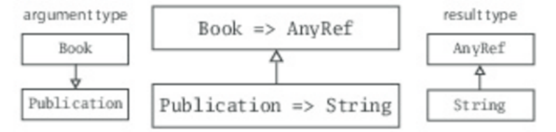
Figure 19.1 - Covariance and contravariance in function type parameters.
class Queue[+T] private (
private[this] var leading: List[T],
private[this] var trailing: List[T]
) {
private def mirror() =
if (leading.isEmpty) {
while (!trailing.isEmpty) {
leading = trailing.head :: leading
trailing = trailing.tail
}
}
def head: T = {
mirror()
leading.head
}
def tail: Queue[T] = {
mirror()
new Queue(leading.tail, trailing)
}
def enqueue[U >: T](x: U) =
new Queue[U](leading, x :: trailing)
}
Listing 19.10 - An optimized functional queue.
19.7 OBJECT PRIVATE DATA
The Queue class seen so far has a problem in that the mirror operation will repeatedly copy
thetrailing into the leading list if head is called several times in a row on a list where leading is empty.
The wasteful copying could be avoided by adding some judicious side effects. Listing 19.10 presents a
new implementation of Queue, which performs at most one trailing to leadingadjustment for any
sequence of head operations.
What's different with respect to the previous version is that now leading and trailing are reassignable
variables, and mirror performs the reverse copy from trailing to leading as a side effect on the current
queue instead of returning a new queue. This side effect is purely internal to the implementation of
the Queue operation; since leading and trailing are private variables, the effect is not visible to clients
of Queue. So by the terminology established inChapter 18, the new version of Queue still defines
purely functional objects, in spite of the fact that they now contain reassignable fields.
You might wonder whether this code passes the Scala type checker. After all, queues now contain two
reassignable fields of the covariant parameter type T. Is this not a violation of the variance rules? It
would be indeed, except for the detail that leading and trailing have aprivate[this] modifier, and are
thus declared to be object private.
As mentioned in Section 13.5, object private members can be accessed only from within the object in
which they are defined. It turns out that accesses to variables from the same object in which they are
defined do not cause problems with variance. The intuitive explanation is that, in order to construct a
case where variance would lead to type errors, you need to have a reference to a containing object that
has a statically weaker type than the type the object was defined with. For accesses to object private
values, however, this is impossible.
Scala's variance checking rules contain a special case for object private definitions. Such definitions are
omitted when it is checked that a type parameter with either a + or -annotation occurs only in positions
that have the same variance classification. Therefore, the code in Listing 19.10 compiles without error.
On the other hand, if you had left out the [this]qualifiers from the two private modifiers, you would see
two type errors:
Queues.scala:1: error: covariant type T occurs in
contravariant position in type List[T] of parameter of
setter leading_=
class Queue[+T] private (private var leading: List[T],
^
Queues.scala:1: error: covariant type T occurs in
contravariant position in type List[T] of parameter of
setter trailing_=
private var trailing: List[T]) {
^
19.8 UPPER BOUNDS
In Listing 16.1 here, we showed a merge sort function for lists that took a comparison function as a first
argument and a list to sort as a second, curried argument. Another way you might want to organize such
a sort function is by requiring the type of the list to mix in theOrdered trait. As mentioned in Section
12.4, by mixing Ordered into a class and implementingOrdered's one abstract method, compare,
you enable clients to compare instances of that class with <, >, <=, and >=. For example, Listing
19.11 shows Ordered being mixed into a Person class.
As a result, you can compare two people like this:
scala> val robert = new Person("Robert", "Jones")
robert: Person = Robert Jones
scala> val sally = new Person("Sally", "Smith")
sally: Person = Sally Smith
scala> robert < sally
res0: Boolean = true
class Person(val firstName: String, val lastName: String)
extends Ordered[Person] {
def compare(that: Person) = {
val lastNameComparison =
lastName.compareToIgnoreCase(that.lastName)
if (lastNameComparison != 0)
lastNameComparison
else
firstName.compareToIgnoreCase(that.firstName)
}
override def toString = firstName + " " + lastName
}
Listing 19.11 - A Person class that mixes in the Ordered trait.
def orderedMergeSort[T <: Ordered[T]](xs: List[T]): List[T] = {
def merge(xs: List[T], ys: List[T]): List[T] =
(xs, ys) match {
case (Nil, _) => ys
case (_, Nil) => xs
case (x :: xs1, y :: ys1) =>
if (x < y) x :: merge(xs1, ys)
else y :: merge(xs, ys1)
}
val n = xs.length / 2
if (n == 0) xs
else {
val (ys, zs) = xs splitAt n
merge(orderedMergeSort(ys), orderedMergeSort(zs))
}
}
Listing 19.12 - A merge sort function with an upper bound.
To require that the type of the list passed to your new sort function mixes in Ordered, you need to use
an upper bound. An upper bound is specified similar to a lower bound, except instead of the >: symbol
used for lower bounds, you use a <: symbol, as shown in Listing 19.12.
With the "T <: Ordered[T]" syntax, you indicate that the type parameter, T, has an upper
bound,Ordered[T]. This means that the element type of the list passed to orderedMergeSort must be a
subtype of Ordered. Thus, you could pass a List[Person] to orderedMergeSort because Person mixes
in Ordered.
For example, consider this list:
scala> val people = List(
new Person("Larry", "Wall"),
new Person("Anders", "Hejlsberg"),
new Person("Guido", "van Rossum"),
new Person("Alan", "Kay"),
new Person("Yukihiro", "Matsumoto")
)
people: List[Person] = List(Larry Wall, Anders Hejlsberg,
Guido van Rossum, Alan Kay, Yukihiro Matsumoto)
Because the element type of this list, Person, mixes in (and is therefore a subtype of)Ordered[People],
you can pass the list to orderedMergeSort:
scala> val sortedPeople = orderedMergeSort(people)
sortedPeople: List[Person] = List(Anders Hejlsberg, Alan Kay,
Yukihiro Matsumoto, Guido van Rossum, Larry Wall)
Now, although the sort function shown in Listing 19.12 serves as a useful illustration of upper bounds,
it isn't actually the most general way in Scala to design a sort function that takes advantage of
the Ordered trait.
For example, you couldn't use the orderedMergeSort function to sort a list of integers, because
class Int is not a subtype of Ordered[Int]:
scala> val wontCompile = orderedMergeSort(List(3, 2, 1))
<console>:5: error: inferred type arguments [Int] do
not conform to method orderedMergeSort's type
parameter bounds [T <: Ordered[T]]
val wontCompile = orderedMergeSort(List(3, 2, 1))
^
In Section 21.6, we'll show you how to use implicit parameters and context bounds to achieve a more
general solution.
19.9 CONCLUSION
In this chapter you saw several techniques for information hiding: private constructors, factory
methods, type abstraction, and object private members. You also learned how to specify data type
variance and what it implies for class implementation. Finally, you saw two techniques which help in
obtaining flexible variance annotations: lower bounds for method type parameters
and private[this] annotations for local fields and methods.
Footnotes for Chapter 19:
[1] Supertype and subtype relationships are reflexive, which means a type is both a supertype and a
subtype of itself. Even though T is a lower bound for U, you could still pass in a T toenqueue.
[2] Technically, what happens is a flip occurs for lower bounds. The type parameter U is in a negative
position (1 flip), while the lower bound (>: T) is in a positive position (2 flips).
Chapter 20
Abstract Members
A member of a class or trait is abstract if the member does not have a complete definition in the
class. Abstract members are intended to be implemented in subclasses of the class in which they are
declared. This idea is found in many object-oriented languages. For instance, Java lets you declare
abstract methods. Scala also lets you declare such methods, as you saw in Section 10.2. But Scala goes
beyond that and implements the idea in its full generality: Besides methods, you can declare abstract
fields and even abstract types as members of classes and traits.
In this chapter we'll describe all four kinds of abstract member: vals, vars, methods, and types. Along
the way we'll discuss pre-initialized fields, lazy vals, path-dependent types, and enumerations.
20.1 A QUICK TOUR OF ABSTRACT MEMBERS
The following trait declares one of each kind of abstract member: an abstract type (T), method
(transform), val (initial), and var (current):
trait Abstract {
type T
def transform(x: T): T
val initial: T
var current: T
}
A concrete implementation of Abstract needs to fill in definitions for each of its abstract members.
Here is an example implementation that provides these definitions:
class Concrete extends Abstract {
type T = String
def transform(x: String) = x + x
val initial = "hi"
var current = initial
}
The implementation gives a concrete meaning to the type name T by defining it as an alias of
type String. The transform operation concatenates a given string with itself, and
the initial andcurrent values are both set to "hi".
This example gives you a rough first idea of what kinds of abstract members exist in Scala. The
remainder of the chapter will present the details and explain what the new forms of abstract members,
as well as type members in general, are good for.
20.2 TYPE MEMBERS
As you can see from the example in the previous section, the term abstract type in Scala means a
type declared (with the "type" keyword) to be a member of a class or trait, without specifying a
definition. Classes themselves may be abstract, and traits are by definition abstract, but neither of these
are what are referred to as abstract types in Scala. An abstract type in Scala is always a member of
some class or trait, such as type T in trait Abstract.
You can think of a non-abstract (or "concrete") type member, such as type T in class Concrete, as a way
to define a new name, or alias, for a type. In class Concrete, for example, the typeString is given the
alias T. As a result, anywhere T appears in the definition of class Concrete, it means String. This
includes the parameter and result types of transform, initial, and current, which mention T when they
are declared in supertrait Abstract. Thus, when class Concreteimplements these methods, those Ts are
interpreted to mean String.
One reason to use a type member is to define a short, descriptive alias for a type whose real name is
more verbose, or less obvious in meaning, than the alias. Such type members can help clarify the code
of a class or trait. The other main use of type members is to declare abstract types that must be defined
in subclasses. This use, which was demonstrated in the previous section, will be described in detail later
in this chapter.
20.3 ABSTRACT VALS
An abstract val declaration has a form like:
val initial: String
It gives a name and type for a val, but not its value. This value has to be provided by a
concrete val definition in a subclass. For instance, class Concrete implemented the val using:
val initial = "hi"
You use an abstract val declaration in a class when you do not know the correct value in the class, but
you do know that the variable will have an unchangeable value in each instance of the class.
An abstract val declaration resembles an abstract parameterless method declaration such as:
def initial: String
Client code would refer to both the val and the method in exactly the same way (i.e.,obj.initial).
However, if initial is an abstract val, the client is guaranteed that obj.initial will yield the same value
every time it is referenced. If initial were an abstract method, that guarantee would not hold because, in
that case, initial could be implemented by a concrete method that returns a different value every time
it's called.
In other words, an abstract val constrains its legal implementation: Any implementation must be
a val definition; it may not be a var or a def. Abstract method declarations, on the other hand, may be
implemented by both concrete method definitions and concrete valdefinitions. Given the abstract
class Fruit shown in Listing 20.1, class Apple would be a legal subclass implementation, but
class BadApple would not.
abstract class Fruit {
val v: String // `v' for value
def m: String // `m' for method
}
abstract class Apple extends Fruit {
val v: String
val m: String // OK to override a `def' with a `val'
}
abstract class BadApple extends Fruit {
def v: String // ERROR: cannot override a `val' with a `def'
def m: String
}
Listing 20.1 - Overriding abstract vals and parameterless methods.
20.4 ABSTRACT VARS
Like an abstract val, an abstract var declares just a name and a type, but not an initial value. For
instance, Listing 20.2 shows a trait AbstractTime, which declares two abstract variables
named hour and minute:
trait AbstractTime {
var hour: Int
var minute: Int
}
Listing 20.2 - Declaring abstract vars.
What is the meaning of abstract vars like hour and minute? You saw in Section 18.2 that vars declared
as members of classes come equipped with getter and setter methods. This holds for abstract vars as
well. If you declare an abstract var named hour, for example, you implicitly declare an abstract getter
method, hour, and an abstract setter method, hour_=. There's no reassignable field to be defined—that
will come in subclasses that define the concrete implementation of the abstract var. For instance, the
definition of AbstractTime shown inListing 20.2 is exactly equivalent to the definition shown in Listing
20.3.
trait AbstractTime {
def hour: Int // getter for `hour'
def hour_=(x: Int) // setter for `hour'
def minute: Int // getter for `minute'
def minute_=(x: Int) // setter for `minute'
}
Listing 20.3 - How abstract vars are expanded into getters and setters.
20.5 INITIALIZING ABSTRACT VALS
Abstract vals sometimes play a role analogous to superclass parameters: they let you provide details in
a subclass that are missing in a superclass. This is particularly important for traits, because traits don't
have a constructor to which you could pass parameters. So the usual notion of parameterizing a trait
works via abstract vals that are implemented in subclasses.
As an example, consider a reformulation of class Rational from Chapter 6, as shown in Listing
6.5 here, as a trait:
trait RationalTrait {
val numerArg: Int
val denomArg: Int
}
The Rational class from Chapter 6 had two parameters: n for the numerator of the rational number,
and d for the denominator. The RationalTrait trait given here defines instead two
abstract vals: numerArg and denomArg. To instantiate a concrete instance of that trait, you need to
implement the abstract val definitions. Here's an example:
new RationalTrait {
val numerArg = 1
val denomArg = 2
}
Here the keyword new appears in front of a trait name, RationalTrait, which is followed by a class body
in curly braces. This expression yields an instance of an anonymous class that mixes in the trait and is
defined by the body. This particular anonymous class instantiation has an effect analogous to the
instance creation new Rational(1, 2).
The analogy is not perfect, however. There's a subtle difference concerning the order in which
expressions are initialized. When you write:
new Rational(expr1, expr2)
the two expressions, expr1 and expr2, are evaluated before class Rational is initialized, so the values
of expr1 and expr2 are available for the initialization of class Rational.
For traits, the situation is the opposite. When you write:
new RationalTrait {
val numerArg = expr1
val denomArg = expr2
}
the expressions, expr1 and expr2, are evaluated as part of the initialization of the anonymous class, but
the anonymous class is initialized after the RationalTrait. So the values of numerArgand denomArg are
not available during the initialization of RationalTrait (more precisely, a selection of either value would
yield the default value for type Int, 0). For the definition ofRationalTrait given previously, this is not a
problem, because the trait's initialization does not make use of values numerArg or denomArg.
However, it becomes a problem in the variant ofRationalTrait shown in Listing 20.4, which defines
normalized numerators and denominators.
trait RationalTrait {
val numerArg: Int
val denomArg: Int
require(denomArg != 0)
private val g = gcd(numerArg, denomArg)
val numer = numerArg / g
val denom = denomArg / g
private def gcd(a: Int, b: Int): Int =
if (b == 0) a else gcd(b, a % b)
override def toString = numer + "/" + denom
}
Listing 20.4 - A trait that uses its abstract vals.
If you try to instantiate this trait with some numerator and denominator expressions that are not simple
literals, you'll get an exception:
scala> val x = 2
x: Int = 2
scala> new RationalTrait {
val numerArg = 1 * x
val denomArg = 2 * x
}
java.lang.IllegalArgumentException: requirement failed
at scala.Predef$.require(Predef.scala:207)
at RationalTrait$class.$init$(<console>:10)
... 28 elided
The exception in this example was thrown because denomArg still had its default value of 0 when
class RationalTrait was initialized, which caused the require invocation to fail.
This example demonstrates that initialization order is not the same for class parameters and abstract
fields. A class parameter argument is evaluated before it is passed to the class constructor (unless the
parameter is by-name). An implementing val definition in a subclass, by contrast, is evaluated
only after the superclass has been initialized.
Now that you understand why abstract vals behave differently from parameters, it would be good to
know what can be done about this. Is it possible to define a RationalTrait that can be initialized
robustly, without fearing errors due to uninitialized fields? In fact, Scala offers two alternative solutions
to this problem, pre-initialized fields and lazy vals. They are presented in the remainder of this section.
Pre-initialized fields
The first solution, pre-initialized fields, lets you initialize a field of a subclass before the superclass is
called. To do this, simply place the field definition in braces before the superclass constructor call. As
an example, Listing 20.5 shows another attempt to create an instance of RationalTrait. As you see from
this example, the initialization section comes before the mention of the supertrait RationalTrait. Both
are separated by a with.
scala> new {
val numerArg = 1 * x
val denomArg = 2 * x
} with RationalTrait
res1: RationalTrait = 1/2
Listing 20.5 - Pre-initialized fields in an anonymous class expression.
Pre-initialized fields are not restricted to anonymous classes; they can also be used in objects or named
subclasses. Two examples are shown in Listings 20.6 and 20.7. As you can see from these examples,
the pre-initialization section comes in each case after the extends keyword of the defined object or
class. Class RationalClass, shown in Listing 20.7, exemplifies a general schema of how class
parameters can be made available for the initialization of a supertrait.
object twoThirds extends {
val numerArg = 2
val denomArg = 3
} with RationalTrait
Listing 20.6 - Pre-initialized fields in an object definition.
class RationalClass(n: Int, d: Int) extends {
val numerArg = n
val denomArg = d
} with RationalTrait {
def + (that: RationalClass) = new RationalClass(
numer * that.denom + that.numer * denom,
denom * that.denom
)
}
Listing 20.7 - Pre-initialized fields in a class definition.
Because pre-initialized fields are initialized before the superclass constructor is called, their initializers
cannot refer to the object that's being constructed. Consequently, if such an initializer refers to this, the
reference goes to the object containing the class or object that's being constructed, not the constructed
object itself.
Here's an example:
scala> new {
val numerArg = 1
val denomArg = this.numerArg * 2
} with RationalTrait
<console>:11: error: value numerArg is not a member of object
$iw
val denomArg = this.numerArg * 2
^
The example did not compile because the reference this.numerArg was looking for a numerArgfield in
the object containing the new (which in this case was the synthetic object named $iw, into which the
interpreter puts user input lines). Once more, pre-initialized fields behave in this respect like class
constructor arguments.
Lazy vals
You can use pre-initialized fields to simulate precisely the initialization behavior of class constructor
arguments. Sometimes, however, you might prefer to let the system itself sort out how things should be
initialized. This can be achieved by making your val definitions lazy. If you prefix a val definition with
a lazy modifier, the initializing expression on the right-hand side will only be evaluated the first time
the val is used.
For an example, define an object Demo with a val as follows:
scala> object Demo {
val x = { println("initializing x"); "done" }
}
defined object Demo
Now, first refer to Demo, then to Demo.x:
scala> Demo
initializing x
res3: Demo.type = Demo$@2129a843
scala> Demo.x
res4: String = done
As you can see, the moment you use Demo, its x field becomes initialized. The initialization of xforms
part of the initialization of Demo. The situation changes, however, if you define the x field to be lazy:
scala> object Demo {
lazy val x = { println("initializing x"); "done" }
}
defined object Demo
scala> Demo
res5: Demo.type = Demo$@5b1769c
scala> Demo.x
initializing x
res6: String = done
Now, initializing Demo does not involve initializing x. The initialization of x will be deferred until the
first time x is used. This is similar to the situation where x is defined as a parameterless method, using
a def. However, unlike a def, a lazy val is never evaluated more than once. In fact, after the first
evaluation of a lazy val the result of the evaluation is stored, to be reused when the same val is used
subsequently.
Looking at this example, it seems that objects like Demo themselves behave like lazy vals, in that they
are also initialized on demand, the first time they are used. This is correct. In fact an object definition
can be seen as a shorthand for the definition of a lazy val with an anonymous class that describes the
object's contents.
Using lazy vals, you could reformulate RationalTrait as shown in Listing 20.8. In the new trait
definition, all concrete fields are defined lazy. Another change with respect to the previous definition
of RationalTrait, shown in Listing 20.4, is that the require clause was moved from the body of the trait
to the initializer of the private field, g, which computes the greatest common divisor
of numerArg and denomArg. With these changes, there's nothing that remains to be done
when LazyRationalTrait is initialized; all initialization code is now part of the right-hand side of a
lazy val. Thus, it is safe to initialize the abstract fields of LazyRationalTrait after the class is defined.
trait LazyRationalTrait {
val numerArg: Int
val denomArg: Int
lazy val numer = numerArg / g
lazy val denom = denomArg / g
override def toString = numer + "/" + denom
private lazy val g = {
require(denomArg != 0)
gcd(numerArg, denomArg)
}
private def gcd(a: Int, b: Int): Int =
if (b == 0) a else gcd(b, a % b)
}
Listing 20.8 - Initializing a trait with lazy vals.
Here's an example:
scala> val x = 2
x: Int = 2
scala> new LazyRationalTrait {
val numerArg = 1 * x
val denomArg = 2 * x
}
res7: LazyRationalTrait = 1/2
No pre-initialization is needed. It's instructive to trace the sequence of initializations that lead to the
string 1/2 to be printed in the code above:
1. A fresh instance of LazyRationalTrait gets created and the initialization code
ofLazyRationalTrait is run. This initialization code is empty; none of the fields
ofLazyRationalTrait is initialized yet.
2. Next, the primary constructor of the anonymous subclass defined by the new expression is
executed. This involves the initialization of numerArg with 2 and denomArg with 4.
3. Next, the toString method is invoked on the constructed object by the interpreter, so that the
resulting value can be printed.
4. Next, the numer field is accessed for the first time by the toString method in
traitLazyRationalTrait, so its initializer is evaluated.
5. The initializer of numer accesses the private field, g, so g is evaluated next. This evaluation
accesses numerArg and denomArg, which were defined in Step 2.
6. Next, the toString method accesses the value of denom, which causes denom's evaluation. The
evaluation of denom accesses the values of denomArg and g. The initializer of the g field is not
re-evaluated, because it was already evaluated in Step 5.
7. Finally, the result string "1/2" is constructed and printed.
Note that the definition of g comes textually after the definitions of numer and denom in
classLazyRationalTrait. Nevertheless, because all three values are lazy, g gets initialized before the
initialization of numer and denom is completed.
This shows an important property of lazy vals: The textual order of their definitions does not matter
because values get initialized on demand. Thus, lazy vals can free you as a programmer from having to
think hard how to arrange val definitions to ensure that everything is defined when it is needed.
However, this advantage holds only as long as the initialization of lazy vals neither produces side
effects nor depends on them. In the presence of side effects, initialization order starts to matter. And
then it can be quite difficult to trace in what order initialization code is run, as the previous example has
demonstrated. So lazy vals are an ideal complement to functional objects, where the order of
initializations does not matter, as long as everything gets initialized eventually. They are less well
suited for code that's predominantly imperative.
LAZY FUNCTIONAL LANGUAGES
Scala is by no means the first language to have exploited the perfect match of lazy definitions and
functional code. In fact, there is a category of "lazy functional programming languages" in
which every value and parameter is initialized lazily. The best known member of this class of languages
is Haskell [SPJ02].
20.6 ABSTRACT TYPES
In the beginning of this chapter, you saw, "type T", an abstract type declaration. The rest of this chapter
discusses what such an abstract type declaration means and what it's good for. Like all other abstract
declarations, an abstract type declaration is a placeholder for something that will be defined concretely
in subclasses. In this case, it is a type that will be defined further down the class hierarchy. So T above
refers to a type that is as yet unknown at the point where it is declared. Different subclasses can provide
different realizations of T.
Here is a well-known example where abstract types show up naturally. Suppose you are given the task
of modeling the eating habits of animals. You might start with a class Food and a classAnimal with
an eat method:
class Food
abstract class Animal {
def eat(food: Food)
}
You might then attempt to specialize these two classes to a class of Cows that eat Grass:
class Grass extends Food
class Cow extends Animal {
override def eat(food: Grass) = {} // This won't compile
}
However, if you tried to compile the new classes, you'd get the following compilation errors:
BuggyAnimals.scala:7: error: class Cow needs to be
abstract, since method eat in class Animal of type
(Food)Unit is not defined
class Cow extends Animal {
^
BuggyAnimals.scala:8: error: method eat overrides nothing
override def eat(food: Grass) = {}
^
What happened is that the eat method in class Cow did not override the eat method in
classAnimal because its parameter type is different: it's Grass in class Cow vs. Food in class Animal.
Some people have argued that the type system is unnecessarily strict in refusing these classes. They
have said that it should be OK to specialize a parameter of a method in a subclass. However, if the
classes were allowed as written, you could get yourself in unsafe situations very quickly.
For instance, the following script would pass the type checker:
class Food
abstract class Animal {
def eat(food: Food)
}
class Grass extends Food
class Cow extends Animal {
override def eat(food: Grass) = {} // This won't compile,
} // but if it did,...
class Fish extends Food
val bessy: Animal = new Cow
bessy eat (new Fish) // ...you could feed fish to cows.
The program would compile if the restriction were eased, because Cows are Animals and Animals do
have an eat method that accepts any kind of Food, including Fish. But surely it would do a cow no
good to eat a fish!
What you need to do instead is apply some more precise modeling. Animals do eat Food, but what kind
of Food each Animal eats depends on the Animal. This can be neatly expressed with an abstract type,
as shown in Listing 20.9:
class Food
abstract class Animal {
type SuitableFood <: Food
def eat(food: SuitableFood)
}
Listing 20.9 - Modeling suitable food with an abstract type.
With the new class definition, an Animal can eat only food that's suitable. What food is suitable cannot
be determined at the level of the Animal class. That's why SuitableFood is modeled as an abstract type.
The type has an upper bound, Food, which is expressed by the "<: Food" clause. This means that any
concrete instantiation of SuitableFood (in a subclass of Animal) must be a subclass of Food. For
example, you would not be able to instantiate SuitableFood with classIOException.
With Animal defined, you can now progress to cows, as shown in Listing 20.10. Class Cow fixes
its SuitableFood to be Grass and also defines a concrete eat method for this kind of food.
class Grass extends Food
class Cow extends Animal {
type SuitableFood = Grass
override def eat(food: Grass) = {}
}
Listing 20.10 - Implementing an abstract type in a subclass.
These new class definitions compile without errors. If you tried to run the "cows-that-eat-fish"
counterexample with the new class definitions, you would get the following compiler error:
scala> class Fish extends Food
defined class Fish
scala> val bessy: Animal = new Cow
bessy: Animal = Cow@1515d8a6
scala> bessy eat (new Fish)
<console>:14: error: type mismatch;
found : Fish
required: bessy.SuitableFood
bessy eat (new Fish)
^
20.7 PATH-DEPENDENT TYPES
Have a look at the last error message again. What's interesting about it is the type required by
the eat method: bessy.SuitableFood. This type consists of an object reference, bessy, followed by a type
field, SuitableFood, of the object. So this shows that objects in Scala can have types as members. The
meaning of bessy.SuitableFood is "the type SuitableFood that is a member of the object referenced
from bessy" or, alternatively, the type of food that's suitable for bessy.
A type like bessy.SuitableFood is called a path-dependent type. The word "path" here means a
reference an object. It could be a single name, such as bessy, or a longer access path, such
asfarm.barn.bessy, where each of farm, barn, and bessy are variables (or singleton object names) that
refer to objects.
As the term "path-dependent type" implies, the type depends on the path; in general, different paths
give rise to different types. For instance, say you defined classes DogFood andDog, like this:
class DogFood extends Food
class Dog extends Animal {
type SuitableFood = DogFood
override def eat(food: DogFood) = {}
}
If you attempted to feed a dog with food fit for a cow, your code would not compile:
scala> val bessy = new Cow
bessy: Cow = Cow@713e7e09
scala> val lassie = new Dog
lassie: Dog = Dog@6eaf2c57
scala> lassie eat (new bessy.SuitableFood)
<console>:16: error: type mismatch;
found : Grass
required: DogFood
lassie eat (new bessy.SuitableFood)
^
The problem here is that the type of the SuitableFood object passed to
the eat method,bessy.SuitableFood, is incompatible with the parameter type of eat, lassie.SuitableFood.
The case would be different for two Dogs. Because Dog's SuitableFood type is defined to be an alias
for class DogFood, the SuitableFood types of two Dogs are in fact the same. As a result,
the Doginstance named lassie could actually eat the suitable food of a different Dog instance (which
we'll name bootsie):
scala> val bootsie = new Dog
bootsie: Dog = Dog@13a7c48c
scala> lassie eat (new bootsie.SuitableFood)
A path-dependent type resembles the syntax for an inner class type in Java, but there is a crucial
difference: a path-dependent type names an outer object, whereas an inner class type names an
outer class. Java-style inner class types can also be expressed in Scala, but they are written differently.
Consider these two classes, Outer and Inner:
class Outer {
class Inner
}
In Scala, the inner class is addressed using the expression Outer#Inner instead of Java'sOuter.Inner. The
`.' syntax is reserved for objects. For example, imagine you instantiate two objects of type Outer, like
this:
val o1 = new Outer
val o2 = new Outer
Here o1.Inner and o2.Inner are two path-dependent types (and they are different types). Both of these
types conform to (are subtypes of) the more general type Outer#Inner, which represents the Inner class
with an arbitrary outer object of type Outer. By contrast, typeo1.Inner refers to the Inner class with
a specific outer object (the one referenced from o1). Likewise, type o2.Inner refers to the Inner class
with a different, specific outer object (the one referenced from o2).
In Scala, as in Java, inner class instances hold a reference to an enclosing outer class instance. This
allows an inner class, for example, to access members of its outer class. Thus you can't instantiate an
inner class without in some way specifying an outer class instance. One way to do this is to instantiate
the inner class inside the body of the outer class. In this case, the current outer class instance
(referenced from this) will be used.
Another way is to use a path-dependent type. For example, because the type, o1.Inner, names a specific
outer object, you can instantiate it:
scala> new o1.Inner
res11: o1.Inner = Outer$Inner@1ae1e03f
The resulting inner object will contain a reference to its outer object, the object referenced from o1. By
contrast, because the type Outer#Inner does not name any specific instance of Outer, you can't create an
instance of it:
scala> new Outer#Inner
<console>:9: error: Outer is not a legal prefix for a
constructor
new Outer#Inner
^
20.8 REFINEMENT TYPES
When a class inherits from another, the first class is said to be a nominal subtype of the other one. It's
a nominal subtype because each type has a name, and the names are explicitly declared to have a
subtyping relationship. Scala additionally supports structural subtyping,where you get a subtyping
relationship simply because two types have compatible members. To get structural subtyping in Scala,
use Scala's refinement types.
Nominal subtyping is usually more convenient, so you should try nominal types first with any new
design. A name is a single short identifier and thus is more concise than an explicit listing of member
types. Further, structural subtyping is often more flexible than you want. A widget can draw(), and a
Western cowboy can draw(), but they aren't really substitutable. You'd typically prefer to get a
compilation error if you tried to substitute a cowboy for a widget.
Nonetheless, structural subtyping has its own advantages. One is that sometimes there really is no more
to a type than its members. For example, suppose you want to define a Pastureclass that can contain
animals that eat grass. One option would be to define a traitAnimalThatEatsGrass and mix it into every
class where it applies. It would be verbose, however. Class Cow has already declared that it's an animal
and that it eats grass, and now it would have to declare that it is also an animal-that-eats-grass.
Instead of defining AnimalThatEatsGrass, you can use a refinement type. Simply write the base
type, Animal, followed by a sequence of members listed in curly braces. The members in the curly
braces further specify—or refine, if you will—the types of members from the base class.
Here is how you write the type, "animal that eats grass":
Animal { type SuitableFood = Grass }
Given this type, you can now write the pasture class like this:
class Pasture {
var animals: List[Animal { type SuitableFood = Grass }] = Nil
// ...
}
20.9 ENUMERATIONS
An interesting application of path-dependent types is found in Scala's support for enumerations. Some
other languages, including Java and C#, have enumerations as a built-in language construct to define
new types. Scala does not need special syntax for enumerations. Instead, there's a class in its standard
library, scala.Enumeration.
To create a new enumeration, you define an object that extends this class, as in the following example,
which defines a new enumeration of Colors:
object Color extends Enumeration {
val Red = Value
val Green = Value
val Blue = Value
}
Scala lets you also shorten several successive val or var definitions with the same right-hand side.
Equivalently to the above you could write:
object Color extends Enumeration {
val Red, Green, Blue = Value
}
This object definition provides three values: Color.Red, Color.Green, and Color.Blue. You could also
import everything in Color with:
import Color._
and then just use Red, Green, and Blue. But what is the type of these values?
Enumeration defines an inner class named Value, and the same-named parameterless Valuemethod
returns a fresh instance of that class. In other words, a value such as Color.Red is of
type Color.Value; Color.Value is the type of all enumeration values defined in object Color. It's a path-
dependent type, with Color being the path and Value being the dependent type. What's significant about
this is that it is a completely new type, different from all other types.
In particular, if you define another enumeration, such as:
object Direction extends Enumeration {
val North, East, South, West = Value
}
then Direction.Value would be different from Color.Value because the path parts of the two types differ.
Scala's Enumeration class also offers many other features found in the enumeration designs of other
languages. You can associate names with enumeration values by using a different overloaded variant of
the Value method:
object Direction extends Enumeration {
val North = Value("North")
val East = Value("East")
val South = Value("South")
val West = Value("West")
}
You can iterate over the values of an enumeration via the set returned by the
enumeration'svalues method:
scala> for (d <- Direction.values) print(d + " ")
North East South West
Values of an enumeration are numbered from 0, and you can find out the number of an enumeration
value by its id method:
scala> Direction.East.id
res14: Int = 1
It's also possible to go the other way, from a non-negative integer number to the value that has this
number as id in an enumeration:
scala> Direction(1)
res15: Direction.Value = East
This should be enough to get you started with enumerations. You can find more information in the
Scaladoc comments of class scala.Enumeration.
20.10 CASE STUDY: CURRENCIES
The rest of this chapter presents a case study that explains how abstract types can be used in Scala. The
task is to design a class Currency. A typical instance of Currency would represent an amount of money
in dollars, euros, yen, or some other currency. It should be possible to do some arithmetic on
currencies. For instance, you should be able to add two amounts of the same currency. Or you should
be able to multiply a currency amount by a factor representing an interest rate.
These thoughts lead to the following first design for a currency class:
// A first (faulty) design of the Currency class
abstract class Currency {
val amount: Long
def designation: String
override def toString = amount + " " + designation
def + (that: Currency): Currency = ...
def * (x: Double): Currency = ...
}
The amount of a currency is the number of currency units it represents. This is a field of typeLong so
that very large amounts of money, such as the market capitalization of Google or Apple, can be
represented. It's left abstract here, waiting to be defined when a subclass talks about concrete amounts
of money. The designation of a currency is a string that identifies it. The toString method of
class Currency indicates an amount and a designation. It would yield results such as:
79 USD
11000 Yen
99 Euro
Finally, there are methods + for adding currencies and * for multiplying a currency with a floating-
point number. You can create a concrete currency value by supplying
concrete amountand designation values, like this:
new Currency {
val amount = 79L
def designation = "USD"
}
This design would be OK if all we wanted to model was a single currency, like only dollars or only
euros. But it fails if we need to deal with several currencies. Assume that you model dollars and euros
as two subclasses of class currency:
abstract class Dollar extends Currency {
def designation = "USD"
}
abstract class Euro extends Currency {
def designation = "Euro"
}
At first glance this looks reasonable. But it would let you add dollars to euros. The result of such an
addition would be of type Currency. But it would be a funny currency that was made up of a mix of
euros and dollars. What you want instead is a more specialized version of the +method. When
implemented in class Dollar, it should take Dollar arguments and yield a Dollarresult; when
implemented in class Euro, it should take Euro arguments and yield a Euro result. So the type of the
addition method would change depending on which class you are in. Nonetheless, you would like to
write the addition method just once, not each time a new currency is defined.
In Scala, there's a simple technique to deal with situations like this. If something is not known at the
point where a class is defined, make it abstract in the class. This applies to both values and types. In the
case of currencies, the exact argument and result type of the addition method are not known, so it is a
good candidate for an abstract type.
This would lead to the following sketch of class AbstractCurrency:
// A second (still imperfect) design of the Currency class
abstract class AbstractCurrency {
type Currency <: AbstractCurrency
val amount: Long
def designation: String
override def toString = amount + " " + designation
def + (that: Currency): Currency = ...
def * (x: Double): Currency = ...
}
The only differences from the previous situation are that the class is now calledAbstractCurrency, and
that it contains an abstract type Currency, which represents the real currency in question. Each concrete
subclass of AbstractCurrency would need to fix the Currencytype to refer to the concrete subclass
itself, thereby "tying the knot."
For instance, here is a new version of class Dollar, which now extends class AbstractCurrency:
abstract class Dollar extends AbstractCurrency {
type Currency = Dollar
def designation = "USD"
}
This design is workable, but it is still not perfect. One problem is hidden by the ellipses that indicate
the missing method definitions of + and * in class AbstractCurrency. In particular, how should addition
be implemented in this class? It's easy enough to calculate the correct amount of the new currency
as this.amount + that.amount, but how would you convert the amount into a currency of the right type?
You might try something like:
def + (that: Currency): Currency = new Currency {
val amount = this.amount + that.amount
}
However, this would not compile:
error: class type required
def + (that: Currency): Currency = new Currency {
^
One of the restrictions of Scala's treatment of abstract types is that you can neither create an instance of
an abstract type nor have an abstract type as a supertype of another class.[1] So the compiler would
refuse the example code here that attempted to instantiate Currency.
However, you can work around this restriction using a factory method. Instead of creating an instance
of an abstract type directly, declare an abstract method that does it. Then, wherever the abstract type is
fixed to be some concrete type, you also need to give a concrete implementation of the factory
method. For class AbstractCurrency, this would look as follows:
abstract class AbstractCurrency {
type Currency <: AbstractCurrency // abstract type
def make(amount: Long): Currency // factory method
... // rest of class
}
A design like this could be made to work, but it looks rather suspicious. Why place the factory
method inside class AbstractCurrency? This looks dubious for at least two reasons. First, if you have
some amount of currency (say, one dollar), you also hold in your hand the ability to make more of the
same currency, using code such as:
myDollar.make(100) // here are a hundred more!
In the age of color copying this might be a tempting scenario, but hopefully not one which you would
be able to do for very long without being caught. The second problem with this code is that you can
make more Currency objects if you already have a reference to a Currencyobject. But how do you get
the first object of a given Currency? You'd need another creation method, which does essentially the
same job as make. So you have a case of code duplication, which is a sure sign of a code smell.
The solution, of course, is to move the abstract type and the factory method outside
classAbstractCurrency. You need to create another class that contains the AbstractCurrency class,
theCurrency type, and the make factory method.
We'll call this a CurrencyZone:
abstract class CurrencyZone {
type Currency <: AbstractCurrency
def make(x: Long): Currency
abstract class AbstractCurrency {
val amount: Long
def designation: String
override def toString = amount + " " + designation
def + (that: Currency): Currency =
make(this.amount + that.amount)
def * (x: Double): Currency =
make((this.amount * x).toLong)
}
}
An example concrete CurrencyZone is the US, which could be defined as:
object US extends CurrencyZone {
abstract class Dollar extends AbstractCurrency {
def designation = "USD"
}
type Currency = Dollar
def make(x: Long) = new Dollar { val amount = x }
}
Here, US is an object that extends CurrencyZone. It defines a class Dollar, which is a subclass
ofAbstractCurrency. So the type of money in this zone is US.Dollar. The US object also fixes the
typeCurrency to be an alias for Dollar, and it gives an implementation of the make factory method to
return a dollar amount.
This is a workable design. There are only a few refinements to be added. The first refinement concerns
subunits. So far, every currency was measured in a single unit: dollars, euros, or yen. However, most
currencies have subunits: For instance, in the US, it's dollars and cents. The most straightforward way
to model cents is to have the amount field in US.Currencyrepresent cents instead of dollars. To convert
back to dollars, it's useful to introduce a fieldCurrencyUnit into class CurrencyZone, which contains
the amount of one standard unit in that currency:
class CurrencyZone {
...
val CurrencyUnit: Currency
}
As shown in Listing 20.11, The US object could define the quantities Cent, Dollar, andCurrencyUnit.
This definition is just like the previous definition of the US object, except that it adds three new fields.
The field Cent represents an amount of 1 US.Currency. It's an object analogous to a one-cent coin. The
field Dollar represents an amount of 100 US.Currency. So theUS object now defines the name Dollar in
two ways. The type Dollar (defined by the abstract inner class named Dollar) represents the generic
name of the Currency valid in the US currency zone. By contrast, the value Dollar (referenced from
the val field named Dollar) represents a single US dollar, analogous to a one-dollar bill. The third field
definition of CurrencyUnitspecifies that the standard currency unit in the US zone is the Dollar (i.e., the
value Dollar, referenced from the field, not the type Dollar).
The toString method in class Currency also needs to be adapted to take subunits into account. For
instance, the sum of ten dollars and twenty three cents should print as a decimal number: 10.23 USD.
To achieve this, you could implement Currency's toString method as follows:
override def toString =
((amount.toDouble / CurrencyUnit.amount.toDouble)
formatted ("%." + decimals(CurrencyUnit.amount) + "f")
+ " " + designation)
Here, formatted is a method that Scala makes available on several classes, including Double.
[2]The formatted method returns the string that results from formatting the original string on
which formatted was invoked according to a format string passed as the formatted method's right-hand
operand. The syntax of format strings passed to formatted is the same as that of
Java's String.format method.
object US extends CurrencyZone {
abstract class Dollar extends AbstractCurrency {
def designation = "USD"
}
type Currency = Dollar
def make(cents: Long) = new Dollar {
val amount = cents
}
val Cent = make(1)
val Dollar = make(100)
val CurrencyUnit = Dollar
}
Listing 20.11 - The US currency zone.
For instance, the format string %.2f formats a number with two decimal digits. The format string used
in the toString shown previously is assembled by calling the decimals method onCurrencyUnit.amount.
This method returns the number of decimal digits of a decimal power minus one. For
instance, decimals(10) is 1, decimals(100) is 2, and so on. The decimals method is implemented by a
simple recursion:
private def decimals(n: Long): Int =
if (n == 1) 0 else 1 + decimals(n / 10)
Listing 20.12 shows some other currency zones. As another refinement, you can add a currency
conversion feature to the model. First, you could write a Converter object that contains applicable
exchange rates between currencies, as shown in Listing 20.13. Then, you could add a conversion
method, from, to class Currency, which converts from a given source currency into the
current Currency object:
def from(other: CurrencyZone#AbstractCurrency): Currency =
make(math.round(
other.amount.toDouble * Converter.exchangeRate
(other.designation)(this.designation)))
The from method takes an arbitrary currency as argument. This is expressed by its formal parameter
type, CurrencyZone#AbstractCurrency, which indicates that the argument passed asother must be
an AbstractCurrency type in some arbitrary and unknown CurrencyZone. It produces its result by
multiplying the amount of the other currency with the exchange rate between the other and the current
currency.[3]
object Europe extends CurrencyZone {
abstract class Euro extends AbstractCurrency {
def designation = "EUR"
}
type Currency = Euro
def make(cents: Long) = new Euro {
val amount = cents
}
val Cent = make(1)
val Euro = make(100)
val CurrencyUnit = Euro
}
object Japan extends CurrencyZone {
abstract class Yen extends AbstractCurrency {
def designation = "JPY"
}
type Currency = Yen
def make(yen: Long) = new Yen {
val amount = yen
}
val Yen = make(1)
val CurrencyUnit = Yen
}
Listing 20.12 - Currency zones for Europe and Japan.
object Converter {
var exchangeRate = Map(
"USD" -> Map("USD" -> 1.0 , "EUR" -> 0.7596,
"JPY" -> 1.211 , "CHF" -> 1.223),
"EUR" -> Map("USD" -> 1.316 , "EUR" -> 1.0 ,
"JPY" -> 1.594 , "CHF" -> 1.623),
"JPY" -> Map("USD" -> 0.8257, "EUR" -> 0.6272,
"JPY" -> 1.0 , "CHF" -> 1.018),
"CHF" -> Map("USD" -> 0.8108, "EUR" -> 0.6160,
"JPY" -> 0.982 , "CHF" -> 1.0 )
)
}
Listing 20.13 - A converter object with an exchange rates map.
abstract class CurrencyZone {
type Currency <: AbstractCurrency
def make(x: Long): Currency
abstract class AbstractCurrency {
val amount: Long
def designation: String
def + (that: Currency): Currency =
make(this.amount + that.amount)
def * (x: Double): Currency =
make((this.amount * x).toLong)
def - (that: Currency): Currency =
make(this.amount - that.amount)
def / (that: Double) =
make((this.amount / that).toLong)
def / (that: Currency) =
this.amount.toDouble / that.amount
def from(other: CurrencyZone#AbstractCurrency): Currency =
make(math.round(
other.amount.toDouble * Converter.exchangeRate
(other.designation)(this.designation)))
private def decimals(n: Long): Int =
if (n == 1) 0 else 1 + decimals(n / 10)
override def toString =
((amount.toDouble / CurrencyUnit.amount.toDouble)
formatted ("%." + decimals(CurrencyUnit.amount) + "f")
+ " " + designation)
}
val CurrencyUnit: Currency
}
Listing 20.14 - The full code of class CurrencyZone.
The final version of the CurrencyZone class is shown in Listing 20.14. You can test the class in the
Scala command shell. We'll assume that the CurrencyZone class and all concrete CurrencyZoneobjects
are defined in a package org.stairwaybook.currencies. The first step is to import
"org.stairwaybook.currencies._" into the command shell. Then you can do some currency conversions:
scala> Japan.Yen from US.Dollar * 100
res16: Japan.Currency = 12110 JPY
scala> Europe.Euro from res16
res17: Europe.Currency = 75.95 EUR
scala> US.Dollar from res17
res18: US.Currency = 99.95 USD
The fact that we obtain almost the same amount after three conversions implies that these are some
pretty good exchange rates! You can also add up values of the same currency:
scala> US.Dollar * 100 + res18
res19: US.Currency = 199.95 USD
On the other hand, you cannot add amounts of different currencies:
scala> US.Dollar + Europe.Euro
<console>:12: error: type mismatch;
found : Europe.Euro
required: US.Currency
(which expands to) US.Dollar
US.Dollar + Europe.Euro
^
By preventing the addition of two values with different units (in this case, currencies), the type
abstraction has done its job. It prevents us from performing calculations that are unsound. Failures to
convert correctly between different units may seem like trivial bugs, but they have caused many serious
systems faults. An example is the crash of the Mars Climate Orbiter spacecraft on September 23, 1999,
which was caused because one engineering team used metric units while another used English units. If
units had been coded in the same way as currencies are coded in this chapter, this error would have
been detected by a simple compilation run. Instead, it caused the crash of the orbiter after a near ten-
month voyage.
20.11 CONCLUSION
Scala offers systematic and very general support for object-oriented abstraction. It enables you to not
only abstract over methods, but also over values, variables, and types. This chapter has shown how to
take advantage of abstract members. They support a simple yet effective principle for systems
structuring: when designing a class, make everything that is not yet known into an abstract member.
The type system will then drive the development of your model, just as you saw with the currency case
study. It does not matter whether the unknown is a type, method, variable or value. In Scala, all of these
can be declared abstract.
Footnotes for Chapter 20:
[1] There's some promising recent research on virtual classes, which would allow this, but virtual
classes are not currently supported in Scala.
[2] Scala uses rich wrappers, described in Section 5.10, to make formatted available.
[3] By the way, in case you think you're getting a bad deal on Japanese yen, the exchange rates convert
currencies based on their CurrencyZone amounts. Thus, 1.211 is the exchange rate between US cents
and Japanese yen.
Chapter 21
Implicit Conversions and Parameters
There's a fundamental difference between your own code and other people's libraries: You can change
or extend your own code as you wish, but if you want to use someone else's libraries, you usually have
to take them as they are. A number of constructs have sprung up in programming languages to alleviate
this problem. Ruby has modules, and Smalltalk lets packages add to each other's classes. These are
very powerful but also dangerous, in that you can modify the behavior of a class for an entire
application, some parts of which you might not know. C# 3.0 has static extension methods, which are
more local but also more restrictive, in that you can only add methods, not fields, to a class, and you
can't make a class implement new interfaces.
Scala's answer is implicit conversions and parameters. These can make existing libraries much more
pleasant to deal with by letting you leave out tedious, obvious details that obscure the interesting parts
of your code. Used tastefully, this results in code that is focused on the interesting, non-trivial parts of
your program. This chapter shows you how implicits work, and it presents some of the most common
ways they are used.
21.1 IMPLICIT CONVERSIONS
Before delving into the details of implicit conversions, take a look at a typical example of their use.
Implicit conversions are often helpful for working with two bodies of software that were developed
without each other in mind. Each library has its own way to encode a concept that is essentially the
same thing. Implicit conversions help by reducing the number of explicit conversions that are needed
from one type to another.
Java includes a library named Swing for implementing cross-platform user interfaces. One of the things
Swing does is process events from the operating system, convert them to platform-independent event
objects, and pass those events to parts of an application called event listeners.
If Swing had been written with Scala in mind, event listeners would probably have been represented by
a function type. Callers could then use the function literal syntax as a lightweight way to specify what
should happen for a certain class of events. Since Java doesn't have function literals, Swing uses the
next best thing, an inner class that implements a one-method interface. In the case of action listeners,
the interface is ActionListener.
Without the use of implicit conversions, a Scala program that uses Swing must use inner classes just
like in Java. Here's an example that creates a button and hooks up an action listener to it. The action
listener is invoked whenever the button is pressed, at which point it prints the string "pressed!":
val button = new JButton
button.addActionListener(
new ActionListener {
def actionPerformed(event: ActionEvent) = {
println("pressed!")
}
}
)
This code has a lot of information-free boilerplate. The fact that this listener is anActionListener, the
fact that the callback method is named actionPerformed, and the fact that the argument is
an ActionEvent are all implied for any argument to addActionListener. The only new information here
is the code to be performed, namely the call to println. This new information is drowned out by the
boilerplate. Someone reading this code will need to have an eagle's eye to pick through the noise and
find the informative part.
A more Scala-friendly version would take a function as an argument, greatly reducing the amount of
boilerplate:
button.addActionListener( // Type mismatch!
(_: ActionEvent) => println("pressed!")
)
As written so far, this code doesn't work.[1] The addActionListener method wants an action listener but
is getting a function. With implicit conversions, however, this code can be made to work.
The first step is to write an implicit conversion between the two types. Here is an implicit conversion
from functions to action listeners:
implicit def function2ActionListener(f: ActionEvent => Unit) =
new ActionListener {
def actionPerformed(event: ActionEvent) = f(event)
}
This is a one-argument method that takes a function and returns an action listener. Like any other one-
argument method, it can be called directly and have its result passed on to another expression:
button.addActionListener(
function2ActionListener(
(_: ActionEvent) => println("pressed!")
)
)
This is already an improvement on the version with the inner class. Note how arbitrary amounts of
boilerplate end up replaced by a function literal and a call to a method. It gets better, though, with
implicit conversions. Because function2ActionListener is marked as implicit, it can be left out and the
compiler will insert it automatically. Here is the result:
// Now this works
button.addActionListener(
(_: ActionEvent) => println("pressed!")
)
The way this code works is that the compiler first tries to compile it as is, but it sees a type error.
Before giving up, it looks for an implicit conversion that can repair the problem. In this case, it
finds function2ActionListener. It tries that conversion method, sees that it works, and moves on. The
compiler works hard here so that the developer can ignore one more fiddly detail. Action listener?
Action event function? Either one will work—use the one that's more convenient.
In this section, we illustrated some some of the power of implicit conversions and how they let you
dress up existing libraries. In the next sections, you'll learn the rules that determine when implicit
conversions are tried and how they are found.
21.2 RULES FOR IMPLICITS
Implicit definitions are those that the compiler is allowed to insert into a program in order to fix any of
its type errors. For example, if x + y does not type check, then the compiler might change it
to convert(x) + y, where convert is some available implicit conversion. If convertchanges x into
something that has a + method, then this change might fix a program so that it type checks and runs
correctly. If convert really is just a simple conversion function, then leaving it out of the source code
can be a clarification.
Implicit conversions are governed by the following general rules:
Marking rule: Only definitions marked implicit are available. The implicit keyword is used to mark
which declarations the compiler may use as implicits. You can use it to mark any variable, function, or
object definition. Here's an example of an implicit function definition:[2]
implicit def intToString(x: Int) = x.toString
The compiler will only change x + y to convert(x) + y if convert is marked as implicit. This way, you
avoid the confusion that would result if the compiler picked random functions that happen to be in
scope and inserted them as "conversions." The compiler will only select among the definitions you
have explicitly marked as implicit.
Scope rule: An inserted implicit conversion must be in scope as a single identifier, or be
associated with the source or target type of the conversion. The Scala compiler will only consider
implicit conversions that are in scope. To make an implicit conversion available, therefore, you must in
some way bring it into scope. Moreover, with one exception, the implicit conversion must be in
scope as a single identifier. The compiler will not insert a conversion of the
form someVariable.convert. For example, it will not expand x + y tosomeVariable.convert(x) + y. If you
want to make someVariable.convert available as an implicit, you would need to import it, which would
make it available as a single identifier. Once imported, the compiler would be free to apply it
as convert(x) + y. In fact, it is common for libraries to include a Preamble object including a number of
useful implicit conversions. Code that uses the library can then do a single "import Preamble._" to
access the library's implicit conversions.
There's one exception to the "single identifier" rule. The compiler will also look for implicit definitions
in the companion object of the source or expected target types of the conversion. For example, if you're
attempting to pass a Dollar object to a method that takes a Euro, the source type is Dollar and the target
type is Euro. You could, therefore, package an implicit conversion from Dollar to Euro in the
companion object of either class, Dollar or Euro.
Here's an example in which the implicit definition is placed in Dollar's companion object:
object Dollar {
implicit def dollarToEuro(x: Dollar): Euro = ...
}
class Dollar { ... }
In this case, the conversion dollarToEuro is said to be associated to the type Dollar. The compiler will
find such an associated conversion every time it needs to convert from an instance of type Dollar.
There's no need to import the conversion separately into your program.
The Scope Rule helps with modular reasoning. When you read code in a file, the only things you need
to consider from other files are those that are either imported or are explicitly referenced through a
fully qualified name. This benefit is at least as important for implicits as for explicitly written code. If
implicits took effect system-wide, then to understand a file you would have to know about every
implicit introduced anywhere in the program!
One-at-a-time rule: Only one implicit is inserted. The compiler will never
rewrite x + yto convert1(convert2(x)) + y. Doing so would cause compile times to increase dramatically
on erroneous code, and it would increase the difference between what the programmer writes and what
the program actually does. For sanity's sake, the compiler does not insert further implicit conversions
when it is already in the middle of trying another implicit. However, it's possible to circumvent this
restriction by having implicits take implicit parameters, which will be described later in this chapter.
Explicits-first rule: Whenever code type checks as it is written, no implicits are attempted. The
compiler will not change code that already works. A corollary of this rule is that you can always replace
implicit identifiers by explicit ones, thus making the code longer but with less apparent ambiguity. You
can trade between these choices on a case-by-case basis. Whenever you see code that seems repetitive
and verbose, implicit conversions can help you decrease the tedium. Whenever code seems terse to the
point of obscurity, you can insert conversions explicitly. The amount of implicits you leave the
compiler to insert is ultimately a matter of style.
Naming an implicit conversion
Implicit conversions can have arbitrary names. The name of an implicit conversion matters only in two
situations: If you want to write it explicitly in a method application and for determining which implicit
conversions are available at any place in the program. To illustrate the second point, say you have an
object with two implicit conversions:
object MyConversions {
implicit def stringWrapper(s: String):
IndexedSeq[Char] = ...
implicit def intToString(x: Int): String = ...
}
In your application, you want to make use of the stringWrapper conversion, but you don't want integers
to be converted automatically to strings by means of the intToString conversion. You can achieve this
by importing only one conversion, but not the other:
import MyConversions.stringWrapper
... // code making use of stringWrapper
In this example, it was important that the implicit conversions had names, because only that way could
you selectively import one and not the other.
Where implicits are tried
There are three places implicits are used in the language: conversions to an expected type, conversions
of the receiver of a selection, and implicit parameters. Implicit conversions to an expected type let you
use one type in a context where a different type is expected. For example, you might have a String and
want to pass it to a method that requires anIndexedSeq[Char]. Conversions of the receiver let you adapt
the receiver of a method call (i.e., the object on which a method is invoked), if the method is not
applicable on the original type. An example is "abc".exists, which is converted
to stringWrapper("abc").exists because the existsmethod is not available on Strings but is available
on IndexedSeqs. Implicit parameters, on the other hand, are usually used to provide more information
to the called function about what the caller wants. Implicit parameters are especially useful with
generic functions, where the called function might otherwise know nothing at all about the type of one
or more arguments. We will examine each of these three kinds of implicits in the next sections.
21.3 IMPLICIT CONVERSION TO AN EXPECTED TYPE
Implicit conversion to an expected type is the first place the compiler will use implicits. The rule is
simple. Whenever the compiler sees an X, but needs a Y, it will look for an implicit function that
converts X to Y. For example, normally a double cannot be used as an integer because it loses
precision:
scala> val i: Int = 3.5
<console>:7: error: type mismatch;
found : Double(3.5)
required: Int
val i: Int = 3.5
^
However, you can define an implicit conversion to smooth this over:
scala> implicit def doubleToInt(x: Double) = x.toInt
doubleToInt: (x: Double)Int
scala> val i: Int = 3.5
i: Int = 3
What happens here is that the compiler sees a Double, specifically 3.5, in a context where it requires
an Int. So far, the compiler is looking at an ordinary type error. Before giving up, though, it searches for
an implicit conversion from Double to Int. In this case, it finds one:doubleToInt,
because doubleToInt is in scope as a single identifier. (Outside the interpreter, you might
bring doubleToInt into scope via an import or possibly through inheritance.) The compiler then inserts
a call to doubleToInt automatically. Behind the scenes, the code becomes:
val i: Int = doubleToInt(3.5)
This is literally an implicit conversion. You did not explicitly ask for conversion. Instead, you
marked doubleToInt as an available implicit conversion by bringing it into scope as a single identifier,
and then the compiler automatically used it when it needed to convert from aDouble to an Int.
Converting Doubles to Ints might raise some eyebrows because, it's a dubious idea to have something
that causes a loss in precision happen invisibly. So this is not really a conversion we recommend. It
makes much more sense to go the other way, from some more constrained type to a more general one.
For instance, an Int can be converted without loss of precision to a Double, so an implicit conversion
from Int to Double makes sense. In fact, that's exactly what happens. The scala.Predef object, which is
implicitly imported into every Scala program, defines implicit conversions that convert "smaller"
numeric types to "larger" ones. For instance, you will find in Predef the following conversion:
implicit def int2double(x: Int): Double = x.toDouble
That's why in Scala Int values can be stored in variables of type Double. There's no special rule in the
type system for this; it's just an implicit conversion that gets applied.[3]
21.4 CONVERTING THE RECEIVER
Implicit conversions also apply to the receiver of a method call, the object on which the method is
invoked. This kind of implicit conversion has two main uses. First, receiver conversions allow
smoother integration of a new class into an existing class hierarchy. And second, they support writing
domain-specific languages (DSLs) within the language.
To see how it works, suppose you write down obj.doIt, and obj does not have a member named doIt.
The compiler will try to insert conversions before giving up. In this case, the conversion needs to apply
to the receiver, obj. The compiler will act as if the expected "type" of obj was "has a member
named doIt." This "has a doIt" type is not a normal Scala type, but it is there conceptually and is why
the compiler will insert an implicit conversion in this case.
Interoperating with new types
As mentioned previously, one major use of receiver conversions is allowing smoother integration of
new types with existing types. In particular, they allow you to enable client programmers to use
instances of existing types as if they were instances of your new type. Take, for example,
class Rational shown in Listing 6.5 here. Here's a snippet of that class again:
class Rational(n: Int, d: Int) {
...
def + (that: Rational): Rational = ...
def + (that: Int): Rational = ...
}
Class Rational has two overloaded variants of the + method, which take Rationals and Ints,
respectively, as arguments. So you can either add two rational numbers or a rational number and an
integer:
scala> val oneHalf = new Rational(1, 2)
oneHalf: Rational = 1/2
scala> oneHalf + oneHalf
res0: Rational = 1/1
scala> oneHalf + 1
res1: Rational = 3/2
What about an expression like 1 + oneHalf? This expression is tricky because the receiver, 1, does not
have a suitable + method. So the following gives an error:
scala> 1 + oneHalf
<console>:6: error: overloaded method value + with
alternatives (Double)Double <and> ... cannot be applied
to (Rational)
1 + oneHalf
^
To allow this kind of mixed arithmetic, you need to define an implicit conversion from Int toRational:
scala> implicit def intToRational(x: Int) =
new Rational(x, 1)
intToRational: (x: Int)Rational
With the conversion in place, converting the receiver does the trick:
scala> 1 + oneHalf
res2: Rational = 3/2
What happens behind the scenes here is that the Scala compiler first tries to type check the
expression 1 + oneHalf as it is. This fails because Int has several + methods, but none that takes
a Rational argument. Next, the compiler searches for an implicit conversion from Int to another type
that has a + method which can be applied to a Rational. It finds your conversion and applies it, which
yields:
intToRational(1) + oneHalf
In this case, the compiler found the implicit conversion function because you entered its definition into
the interpreter, which brought it into scope for the remainder of the interpreter session.
Simulating new syntax
The other major use of implicit conversions is to simulate adding new syntax. Recall that you can make
a Map using syntax like this:
Map(1 -> "one", 2 -> "two", 3 -> "three")
Have you wondered how the -> is supported? It's not syntax! Instead, -> is a method of the
class ArrowAssoc, a class defined inside the standard Scala preamble (scala.Predef). The preamble also
defines an implicit conversion from Any to ArrowAssoc. When you write 1 -> "one", the compiler
inserts a conversion from 1 to ArrowAssoc so that the -> method can be found. Here are the relevant
definitions:
package scala
object Predef {
class ArrowAssoc[A](x: A) {
def -> [B](y: B): Tuple2[A, B] = Tuple2(x, y)
}
implicit def any2ArrowAssoc[A](x: A): ArrowAssoc[A] =
new ArrowAssoc(x)
...
}
This "rich wrappers" pattern is common in libraries that provide syntax-like extensions to the language,
so you should be ready to recognize the pattern when you see it. Whenever you see someone calling
methods that appear not to exist in the receiver class, they are probably using implicits. Similarly, if
you see a class named RichSomething (e.g., RichInt or RichBoolean), that class is likely adding syntax-
like methods to type Something.
You have already seen this rich wrappers pattern for the basic types described in Chapter 5. As you can
now see, these rich wrappers apply more widely, often letting you get by with an internal DSL defined
as a library where programmers in other languages might feel the need to develop an external DSL.
Implicit classes
Implicit classes were added in Scala 2.10 to make it easier to write rich wrapper classes. An implicit
class is a class that is preceded by the implicit keyword. For any such class, the compiler generates an
implicit conversion from the class's constructor parameter to the class itself. Such a conversion is just
what you need if you plan to use the class for the rich wrappers pattern.
For example, suppose you have a class named Rectangle for representing the width and height of a
rectangle on the screen:
case class Rectangle(width: Int, height: Int)
If you use this class very frequently, you might want to use the rich wrappers pattern so you can more
easily construct it. Here's one way to do so.
implicit class RectangleMaker(width: Int) {
def x(height: Int) = Rectangle(width, height)
}
The above definition defines a RectangleMaker class in the usual manner. In addition, it causes the
following conversion to be automatically generated:
// Automatically generated
implicit def RectangleMaker(width: Int) =
new RectangleMaker(width)
As a result, you can create points by putting an x in between two integers:
scala> val myRectangle = 3 x 4
myRectangle: Rectangle = Rectangle(3,4)
This is how it works: Since type Int has no method named x, the compiler will look for an implicit
conversion from Int to something that does. It will find the generated RectangleMakerconversion,
and RectangleMaker does have a method named x. The compiler inserts a call to this conversion, after
which the call to x type checks and does what is desired.
As a warning to the adventurous, it might be tempting to think that any class can haveimplicit put in
front of it. It's not so. An implicit class cannot be a case class, and its constructor must have exactly one
parameter. Also, an implicit class must be located within some other object, class, or trait. In practice,
so long as you use implicit classes as rich wrappers to add a few methods onto an existing class, these
restrictions should not matter.
21.5 IMPLICIT PARAMETERS
The remaining place the compiler inserts implicits is within argument lists. The compiler will
sometimes replace someCall(a) with someCall(a)(b), or new SomeClass(a) with new SomeClass(a)(b),
thereby adding a missing parameter list to complete a function call. It is the entire last curried
parameter list that's supplied, not just the last parameter. For example, if someCall's missing last
parameter list takes three parameters, the compiler might replace someCall(a)with someCall(a)(b, c, d).
For this usage, not only must the inserted identifiers, such as b, c, andd in (b, c, d), be
marked implicit where they are defined, but also the last parameter list insomeCall's or someClass's
definition must be marked implicit.
Here's a simple example. Suppose you have a class PreferredPrompt, which encapsulates a shell
prompt string (such as, say "$ " or "> ") that is preferred by a user:
class PreferredPrompt(val preference: String)
Also, suppose you have a Greeter object with a greet method, which takes two parameter lists. The first
parameter list takes a string user name, and the second parameter list takes aPreferredPrompt:
object Greeter {
def greet(name: String)(implicit prompt: PreferredPrompt) = {
println("Welcome, " + name + ". The system is ready.")
println(prompt.preference)
}
}
The last parameter list is marked implicit, which means it can be supplied implicitly. But you can still
provide the prompt explicitly, like this:
scala> val bobsPrompt = new PreferredPrompt("relax> ")
bobsPrompt: PreferredPrompt = PreferredPrompt@714d36d6
scala> Greeter.greet("Bob")(bobsPrompt)
Welcome, Bob. The system is ready.
relax>
To let the compiler supply the parameter implicitly, you must first define a variable of the expected
type, which in this case is PreferredPrompt. You could do this, for example, in a preferences object:
object JoesPrefs {
implicit val prompt = new PreferredPrompt("Yes, master> ")
}
Note that the val itself is marked implicit. If it wasn't, the compiler would not use it to supply the
missing parameter list. It will also not use it if it isn't in scope as a single identifier, as shown in this
example:
scala> Greeter.greet("Joe")
<console>:13: error: could not find implicit value for
parameter prompt: PreferredPrompt
Greeter.greet("Joe")
^
Once you bring it into scope via an import, however, it will be used to supply the missing parameter
list:
scala> import JoesPrefs._
import JoesPrefs._
scala> Greeter.greet("Joe")
Welcome, Joe. The system is ready.
Yes, master>
Note that the implicit keyword applies to an entire parameter list, not to individual parameters. Listing
21.1 shows an example in which the last parameter list of Greeter's greetmethod, which is again
marked implicit, has two parameters: prompt (of type PreferredPrompt) and drink (of
type PreferredDrink).
Singleton object JoesPrefs declares two implicit vals, prompt of type PreferredPrompt and drink of
type PreferredDrink. As before, however, so long as these are not in scope as single identifiers, they
won't be used to fill in a missing parameter list to greet:
scala> Greeter.greet("Joe")
<console>:19: error: could not find implicit value for
parameter prompt: PreferredPrompt
Greeter.greet("Joe")
^
You can bring both implicit vals into scope with an import:
scala> import JoesPrefs._
import JoesPrefs._
Because both prompt and drink are now in scope as single identifiers, you can use them to supply the
last parameter list explicitly, like this:
scala> Greeter.greet("Joe")(prompt, drink)
Welcome, Joe. The system is ready.
But while you work, why not enjoy a cup of tea?
Yes, master>
And because all the rules for implicit parameters are now met, you can alternatively let the Scala
compiler supply prompt and drink for you by leaving off the last parameter list:
scala> Greeter.greet("Joe")
Welcome, Joe. The system is ready.
But while you work, why not enjoy a cup of tea?
Yes, master>
class PreferredPrompt(val preference: String)
class PreferredDrink(val preference: String)
object Greeter {
def greet(name: String)(implicit prompt: PreferredPrompt,
drink: PreferredDrink) = {
println("Welcome, " + name + ". The system is ready.")
print("But while you work, ")
println("why not enjoy a cup of " + drink.preference + "?")
println(prompt.preference)
}
}
object JoesPrefs {
implicit val prompt = new PreferredPrompt("Yes, master> ")
implicit val drink = new PreferredDrink("tea")
}
Listing 21.1 - An implicit parameter list with multiple parameters.
One thing to note about the previous examples is that we didn't use String as the type
of promptor drink, even though ultimately it was a String that each of them provided through
theirpreference fields. Because the compiler selects implicit parameters by matching types of
parameters against types of values in scope, implicit parameters usually have "rare" or "special" enough
types that accidental matches are unlikely. For example, the
typesPreferredPrompt and PreferredDrink in Listing 21.1 were defined solely to serve as implicit
parameter types. As a result, it is unlikely that implicit variables of these types will be in scope if they
aren't intended to be used as implicit parameters to Greeter.greet.
Another thing to know about implicit parameters is that they are perhaps most often used to provide
information about a type mentioned explicitly in an earlier parameter list, similar to the type classes of
Haskell.
As an example, consider the maxListOrdering function shown in Listing 21.2, which returns the
maximum element of the passed list.
def maxListOrdering[T](elements: List[T])
(ordering: Ordering[T]): T =
elements match {
case List() =>
throw new IllegalArgumentException("empty list!")
case List(x) => x
case x :: rest =>
val maxRest = maxListOrdering(rest)(ordering)
if (ordering.gt(x, maxRest)) x
else maxRest
}
Listing 21.2 - A function with an upper bound.
The signature of maxListOrdering is similar to that of orderedMergeSort, shown in Listing 19.12here:
It takes a List[T] as its argument, and now it takes an additional argument of typeOrdering[T]. This
additional argument specifies which ordering to use when comparing elements of type T. As such, this
version can be used for types that don't have a built-in ordering. Additionally, this version can be used
for types that do have a built-in ordering, but for which you occasionally want to use some other
ordering.
This version is more general, but it's also more cumbersome to use. Now a caller must specify an
explicit ordering even if T is something like String or Int that has an obvious default ordering. To make
the new method more convenient, it helps to make the second argument implicit. This approach is
shown in Listing 21.3.
The ordering parameter in this example is used to describe the ordering of Ts. In the body
ofmaxListImpParm, this ordering is used in two places: a recursive call to maxListImpParm, and
an ifexpression that checks whether the head of the list is larger than the maximum element of the rest
of the list.
def maxListImpParm[T](elements: List[T])
(implicit ordering: Ordering[T]): T =
elements match {
case List() =>
throw new IllegalArgumentException("empty list!")
case List(x) => x
case x :: rest =>
val maxRest = maxListImpParm(rest)(ordering)
if (ordering.gt(x, maxRest)) x
else maxRest
}
Listing 21.3 - A function with an implicit parameter.
The maxListImpParm function is an example of an implicit parameter used to provide more
information about a type mentioned explicitly in an earlier parameter list. To be specific, the implicit
parameter ordering, of type Ordering[T], provides more information about type T—in this case, how to
order Ts. Type T is mentioned in List[T], the type of parameter elements, which appears in the earlier
parameter list. Because elements must always be provided explicitly in any invocation
of maxListImpParm, the compiler will know T at compile time and can therefore determine whether an
implicit definition of type Ordering[T] is available. If so, it can pass in the second parameter
list, ordering, implicitly.
This pattern is so common that the standard Scala library provides implicit "ordering" methods for
many common types. You could therefore use this maxListImpParm method with a variety of types:
scala> maxListImpParm(List(1,5,10,3))
res9: Int = 10
scala> maxListImpParm(List(1.5, 5.2, 10.7, 3.14159))
res10: Double = 10.7
scala> maxListImpParm(List("one", "two", "three"))
res11: String = two
In the first case, the compiler inserted an ordering for Ints; in the second case, for Doubles; in the third
case, for Strings.
A style rule for implicit parameters
As a style rule, it is best to use a custom named type in the types of implicit parameters. For example,
the types of prompt and drink in the previous example was not String,
butPreferredPrompt and PreferredDrink, respectively. As a counterexample, consider that
themaxListImpParm function could just as well have been written with the following type signature:
def maxListPoorStyle[T](elements: List[T])
(implicit orderer: (T, T) => Boolean): T
To use this version of the function, though, the caller would have to supply an ordererparameter of
type (T, T) => Boolean. This is a fairly generic type that includes any function from two Ts to
a Boolean. It does not indicate anything at all about what the type is for; it could be an equality test, a
less-than test, a greater-than test, or something else entirely.
The actual code for maxListImpParm, given in Listing 21.3, shows better style. It uses
an orderingparameter of type Ordering[T]. The word Ordering in this type indicates exactly what the
implicit parameter is used for: it is for ordering elements of T. Because this ordering type is more
explicit, it's no trouble to add implicit providers for this type in the standard library. To contrast,
imagine the chaos that would ensue if you added an implicit of type (T, T) => Booleanin the standard
library, and the compiler started sprinkling it around in people's code. You would end up with code that
compiles and runs, but that does fairly arbitrary tests against pairs of items! Thus the style rule: Use at
least one role-determining name within the type of an implicit parameter.
21.6 CONTEXT BOUNDS
The previous example showed an opportunity to use an implicit but did not. Note that when you
use implicit on a parameter, not only will the compiler try to supply that parameter with an implicit
value, but the compiler will also use that parameter as an available implicit in the body of the method!
Thus, the first use of ordering within the body of the method can be left out.
def maxList[T](elements: List[T])
(implicit ordering: Ordering[T]): T =
elements match {
case List() =>
throw new IllegalArgumentException("empty list!")
case List(x) => x
case x :: rest =>
val maxRest = maxList(rest) // (ordering) is implicit
if (ordering.gt(x, maxRest)) x // this ordering is
else maxRest // still explicit
}
Listing 21.4 - A function that uses an implicit parameter internally.
When the compiler examines the code in Listing 21.4, it will see that the types do not match up. The
expression maxList(rest) only supplies one parameter list, but maxList requires two. Since the second
parameter list is implicit, the compiler does not give up type checking immediately. Instead, it looks for
an implicit parameter of the appropriate type, in this caseOrdering[T]. In this case, it finds one and
rewrites the call to maxList(rest)(ordering), after which the code type checks.
There is also a way to eliminate the second use of ordering. It involves the following method defined in
the standard library:
def implicitly[T](implicit t: T) = t
The effect of calling implicitly[Foo] is that the compiler will look for an implicit definition of type Foo.
It will then call the implicitly method with that object, which in turn returns the object right back. Thus
you can write implicitly[Foo] whenever you want to find an implicit object of type Foo in the current
scope. For example, Listing 21.5 shows a use ofimplicitly[Ordering[T]] to retrieve
the ordering parameter by its type.
Look closely at this last version of maxList. There is not a single mention of the orderingparameter in
the text of the method. The second parameter could just as well be named "comparator":
def maxList[T](elements: List[T])
(implicit comparator: Ordering[T]): T = // same body...
def maxList[T](elements: List[T])
(implicit ordering: Ordering[T]): T =
elements match {
case List() =>
throw new IllegalArgumentException("empty list!")
case List(x) => x
case x :: rest =>
val maxRest = maxList(rest)
if (implicitly[Ordering[T]].gt(x, maxRest)) x
else maxRest
}
Listing 21.5 - A function that uses implicitly.
For that matter, this version works as well:
def maxList[T](elements: List[T])
(implicit iceCream: Ordering[T]): T = // same body...
Because this pattern is common, Scala lets you leave out the name of this parameter and shorten the
method header by using a context bound. Using a context bound, you would write the signature
of maxList as shown in Listing 21.6. The syntax [T : Ordering] is a context bound, and it does two
things. First, it introduces a type parameter T as normal. Second, it adds an implicit parameter of
type Ordering[T]. In previous versions of maxList, that parameter was called ordering, but when using
a context bound you don't know what the parameter will be called. As shown earlier, you often don't
need to know what the parameter is called.
Intuitively, you can think of a context bound as saying something about a type parameter. When you
write [T <: Ordered[T]] you are saying that a T is an Ordered[T]. To contrast, when you
write [T : Ordering] you are not so much saying what T is; rather, you are saying that there is some
form of ordering associated with T. Thus, a context bound is quite flexible. It allows you to use code
that requires orderings—or any other property of a type—without having to change the definition of
that type.
def maxList[T : Ordering](elements: List[T]): T =
elements match {
case List() =>
throw new IllegalArgumentException("empty list!")
case List(x) => x
case x :: rest =>
val maxRest = maxList(rest)
if (implicitly[Ordering[T]].gt(x, maxRest)) x
else maxRest
}
Listing 21.6 - A function with a context bound.
21.7 WHEN MULTIPLE CONVERSIONS APPLY
It can happen that multiple implicit conversions are in scope and each would work. For the most part,
Scala refuses to insert a conversion in such a case. Implicits work well when the conversion left out is
completely obvious and pure boilerplate. If multiple conversions apply, then the choice isn't so obvious
after all.
Here's a simple example. There is a method that takes a sequence, a conversion that turns an integer
into a range, and a conversion that turns an integer into a list of digits:
scala> def printLength(seq: Seq[Int]) = println(seq.length)
printLength: (seq: Seq[Int])Unit
scala> implicit def intToRange(i: Int) = 1 to i
intToRange: (i:
Int)scala.collection.immutable.Range.Inclusive
scala> implicit def intToDigits(i: Int) =
i.toString.toList.map(_.toInt)
intToDigits: (i: Int)List[Int]
scala> printLength(12)
<console>:26: error: type mismatch;
found : Int(12)
required: Seq[Int]
Note that implicit conversions are not applicable because
they are ambiguous:
both method intToRange of type (i:
Int)scala.collection.immutable.Range.Inclusive
and method intToDigits of type (i: Int)List[Int]
are possible conversion functions from Int(12) to Seq[Int]
printLength(12)
^
The ambiguity here is real. Converting an integer to a sequence of digits is completely different from
converting it to a range. In this case, the programmer should specify which one is intended and be
explicit. Up through Scala 2.7, that was the end of the story. Whenever multiple implicit conversions
applied, the compiler refused to choose between them. The situation was just as with method
overloading. If you try to call foo(null) and there are two different foo overloads that accept null, the
compiler will refuse. It will say that the method call's target is ambiguous.
Scala 2.8 loosened this rule. If one of the available conversions is strictly more specific than the others,
then the compiler will choose the more specific one. The idea is that whenever there is a reason to
believe a programmer would always choose one of the conversions over the others, don't require the
programmer to write it explicitly. After all, method overloading has the same relaxation. Continuing the
previous example, if one of the available foo methods takes a String while the other takes an Any, then
choose the String version. It's clearly more specific.
To be more precise, one implicit conversion is more specific than another if one of the following
applies:
•The argument type of the former is a subtype of the latter's.
•Both conversions are methods, and the enclosing class of the former extends the enclosing class
of the latter.
The motivation to revisit this issue and revise the rule was to improve interoperation between Java
collections, Scala collections, and strings.
Here's a simple example:
val cba = "abc".reverse
What is the type inferred for cba? Intuitively, the type should be String. Reversing a string should yield
another string, right? However, in Scala 2.7, what happened was that "abc" was converted to a Scala
collection. Reversing a Scala collection yields a Scala collection, so the type of cba would be a
collection. There's also an implicit conversion back to a string, but that didn't patch up every problem.
For example, in versions prior to Scala 2.8,"abc" == "abc".reverse.reverse was false!
With Scala 2.8, the type of cba is String. The old implicit conversion to a Scala collection (now
named WrappedString) is retained. However, there is a more specific conversion supplied fromString to
a new type called StringOps. StringOps has many methods such as reverse, but instead of returning a
collection, they return a String. The conversion to StringOps is defined directly inPredef, whereas the
conversion to a Scala collection is defined in a new class,LowPriorityImplicits, which is extended
by Predef. Whenever a choice exists between these two conversions, the compiler chooses the
conversion to StringOps, because it's defined in a subclass of the class where the other conversion is
defined.
21.8 DEBUGGING IMPLICITS
Implicits are a powerful feature in Scala, but one that's sometimes difficult to get right. This section
contains a few tips for debugging implicits.
Sometimes you might wonder why the compiler did not find an implicit conversion that you think
should apply. In that case it helps to write the conversion out explicitly. If that also gives an error
message, you then know why the compiler could not apply your implicit.
For instance, assume that you mistakenly took wrapString to be a conversion from Strings toLists,
instead of IndexedSeqs. You would wonder why the following code does not work:
scala> val chars: List[Char] = "xyz"
<console>:24: error: type mismatch;
found : String("xyz")
required: List[Char]
val chars: List[Char] = "xyz"
^
Again, it helps to write the wrapString conversion explicitly to find out what went wrong:
scala> val chars: List[Char] = wrapString("xyz")
<console>:24: error: type mismatch;
found : scala.collection.immutable.WrappedString
required: List[Char]
val chars: List[Char] = wrapString("xyz")
^
With this, you have found the cause of the error: wrapString has the wrong return type. On the other
hand, it's also possible that inserting the conversion explicitly will make the error go away. In that case
you know that one of the other rules (such as the Scope Rule) was preventing the implicit conversion
from being applied.
When you are debugging a program, it can sometimes help to see what implicit conversions the
compiler is inserting. The -Xprint:typer option to the compiler is useful for this. If you runscalac with
this option, the compiler will show you what your code looks like after all implicit conversions have
been added by the type checker. An example is shown in Listing 21.7 andListing 21.8. If you look at
the last statement in each of these listings, you'll see that the second parameter list to enjoy, which was
left off in the code in Listing 21.7, "enjoy("reader")," was inserted by the compiler, as shown in Listing
21.8:
Mocha.this.enjoy("reader")(Mocha.this.pref)
If you are brave, try scala -Xprint:typer to get an interactive shell that prints out the post-typing source
code it uses internally. If you do so, be prepared to see an enormous amount of boilerplate surrounding
the meat of your code.
object Mocha extends App {
class PreferredDrink(val preference: String)
implicit val pref = new PreferredDrink("mocha")
def enjoy(name: String)(implicit drink: PreferredDrink) = {
print("Welcome, " + name)
print(". Enjoy a ")
print(drink.preference)
println("!")
}
enjoy("reader")
}
Listing 21.7 - Sample code that uses an implicit parameter.
$ scalac -Xprint:typer mocha.scala
[[syntax trees at end of typer]]
// Scala source: mocha.scala
package <empty> {
final object Mocha extends java.lang.Object with Application
with ScalaObject {
// ...
private[this] val pref: Mocha.PreferredDrink =
new Mocha.this.PreferredDrink("mocha");
implicit <stable> <accessor>
def pref: Mocha.PreferredDrink = Mocha.this.pref;
def enjoy(name: String)
(implicit drink: Mocha.PreferredDrink): Unit = {
scala.this.Predef.print("Welcome, ".+(name));
scala.this.Predef.print(". Enjoy a ");
scala.this.Predef.print(drink.preference);
scala.this.Predef.println("!")
};
Mocha.this.enjoy("reader")(Mocha.this.pref)
}
}
Listing 21.8 - Sample code after type checking and insertion of implicits.
21.9 CONCLUSION
Implicits are a powerful, code-condensing feature of Scala. This chapter has shown you Scala's rules
about implicits and several common programming situations where you can profit from using implicits.
As a word of warning, implicits can make code confusing if they are used too frequently. Thus, before
adding a new implicit conversion, first ask whether you can achieve a similar effect through other
means, such as inheritance, mixin composition, or method overloading. If all of these fail, however, and
you feel like a lot of your code is still tedious and redundant, then implicits might just be able to help
you out.
Footnotes for Chapter 21:
[1] As will be explained in Section 31.5, it does work in Scala 2.12.
[2] Variables and singleton objects marked implicit can be used as implicit parameters. This use case
will be described later in this chapter.
[3] The Scala compiler backend will treat the conversion specially, however, translating it to a special
"i2d" bytecode. So the compiled image is the same as in Java.
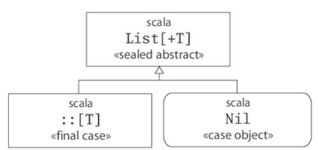
Chapter 22
Implementing Lists
Lists have been ubiquitous in this book. Class List is probably the most commonly used structured data
type in Scala. Chapter 16 showed you how to use lists. This chapter "opens up the covers" and explains
a bit about how lists are implemented in Scala.
Knowing the internal workings of the List class is useful for several reasons. You gain a better idea of
the relative efficiency of list operations, which will help you in writing fast and compact code using
lists. You also gain a toolbox of techniques that you can apply in the design of your own libraries.
Finally, the List class is a sophisticated application of Scala's type system in general and its genericity
concepts in particular. So studying class List will deepen your knowledge in these areas.
22.1 THE LIST CLASS IN PRINCIPLE
Lists are not "built-in" as a language construct in Scala; they are defined by an abstract classList in
the scala package, which comes with two subclasses for :: and Nil. In this chapter we will present a
quick tour through class List. This section presents a somewhat simplified account of the class,
compared to its real implementation in the Scala standard library, which is covered in Section 22.3.
package scala
abstract class List[+T] {
List is an abstract class, so you cannot define elements by calling the empty List constructor. For
instance the expression "new List" would be illegal. The class has a type parameter T. The +in front of
this type parameter specifies that lists are covariant, as discussed in Chapter 19.
Figure 22.1 - Class hierarchy for Scala lists.
Because of this property, you can assign a value of type List[Int] to a variable of typeList[Any]:
scala> val xs = List(1, 2, 3)
xs: List[Int] = List(1, 2, 3)
scala> var ys: List[Any] = xs
ys: List[Any] = List(1, 2, 3)
All list operations can be defined in terms of three basic methods:
def isEmpty: Boolean
def head: T
def tail: List[T]
These three methods are all abstract in class List. They are defined in the subobject Nil and the
subclass ::. The hierarchy for List is shown in Figure 22.1.
The Nil object
The Nil object defines an empty list. Its definition is shown in Listing 22.1. The Nil object inherits
from type List[Nothing]. Because of covariance, this means that Nil is compatible with every instance
of the List type.
case object Nil extends List[Nothing] {
override def isEmpty = true
def head: Nothing =
throw new NoSuchElementException("head of empty list")
def tail: List[Nothing] =
throw new NoSuchElementException("tail of empty list")
}
Listing 22.1 - The definition of the Nil singleton object.
The three abstract methods of class List are implemented in the Nil object in a straightforward way:
The isEmpty method returns true, and the head and tail methods both throw an exception. Note that
throwing an exception is not only reasonable, but practically the only possible thing to do for head:
Because Nil is a List of Nothing, the result type of headmust be Nothing. Since there is no value of this
type, this means that head cannot return a normal value. It has to return abnormally by throwing an
exception.[1]
The :: class
Class ::, pronounced "cons" for "construct," represents non-empty lists. It's named that way in order to
support pattern matching with the infix ::. You have seen in Section 16.5 that every infix operation in a
pattern is treated as a constructor application of the infix operator to its arguments. So the
pattern x :: xs is treated as ::(x, xs) where :: is a case class.
Here is the definition of the :: class:
final case class ::[T](hd: T, tl: List[T]) extends List[T] {
def head = hd
def tail = tl
override def isEmpty: Boolean = false
}
The implementation of the :: class is straightforward. It takes two parameters hd and tl, representing the
head and the tail of the list to be constructed. The definitions of the head andtail method simply return
the corresponding parameter. In fact, this pattern can be abbreviated by letting the parameters directly
implement the head and tail methods of the superclass List, as in the following equivalent but shorter
definition of the :: class:
final case class ::[T](head: T, tail: List[T])
extends List[T] {
override def isEmpty: Boolean = false
}
This works because every case class parameter is implicitly also a field of the class (it's like the
parameter declaration was prefixed with val). Recall from Section 20.3 that Scala allows you to
implement an abstract parameterless method such as head or tail with a field. So the code above
directly uses the parameters head and tail as implementations of the abstract methods head and tail that
were inherited from class List.
Some more methods
All other List methods can be written using the basic three. For instance:
def length: Int =
if (isEmpty) 0 else 1 + tail.length
or:
def drop(n: Int): List[T] =
if (isEmpty) Nil
else if (n <= 0) this
else tail.drop(n - 1)
or:
def map[U](f: T => U): List[U] =
if (isEmpty) Nil
else f(head) :: tail.map(f)
List construction
The list construction methods :: and ::: are special. Because they end in a colon, they are bound to their
right operand. That is, an operation such as x :: xs is treated as the method callxs.::(x), not x.::(xs). In
fact, x.::(xs) would not make sense, as x is of the list element type, which can be arbitrary, so we cannot
assume that this type would have a :: method.
For this reason, the :: method should take an element value and yield a new list. What is the required
type of the element value? You might be tempted to say it should be the same as the list's element type,
but in fact this is more restrictive than necessary.
To see why, consider this class hierarchy:
abstract class Fruit
class Apple extends Fruit
class Orange extends Fruit
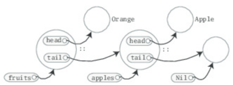
Listing 22.2 shows what happens when you construct lists of fruit:
scala> val apples = new Apple :: Nil
apples: List[Apple] = List(Apple@e885c6a)
scala> val fruits = new Orange :: apples
fruits: List[Fruit] = List(Orange@3f51b349, Apple@e885c6a)
Listing 22.2 - Prepending a supertype element to a subtype list.
The apples value is treated as a List of Apples, as expected. However, the definition of fruitsshows that
it's still possible to add an element of a different type to that list. The element type of the resulting list
is Fruit, which is the most precise common supertype of the original list element type (i.e., Apple) and
the type of the element to be added (i.e., Orange). This flexibility is obtained by defining the :: method
(cons) as shown in Listing 22.3:
def ::[U >: T](x: U): List[U] = new scala.::(x, this)
Listing 22.3 - The definition of method :: (cons) in class List.
Note that the method is itself polymorphic—it takes a type parameter named U. Furthermore,U is
constrained in [U >: T] to be a supertype of the list element type T. The element to be added is required
to be of type U and the result is a List[U].
With the formulation of :: shown in Listing 22.3, you can check how the definition of fruitsshown
in Listing 22.2 works out type-wise: In that definition, the type parameter U of :: is instantiated to Fruit.
The lower-bound constraint of U is satisfied because the list apples has type List[Apple] and Fruit is a
supertype of Apple. The argument to the :: is new Orange, which conforms to type Fruit. Therefore, the
method application is type-correct with result typeList[Fruit]. Figure 22.2 illustrates the structure of the
lists that result from executing the code shown in Listing 22.2.
Figure 22.2 - The structure of the Scala lists shown in Listing 22.2.
In fact, the polymorphic definition of :: with the lower bound T is not only convenient, it is also
necessary to render the definition of class List type-correct. This is because Lists are defined to be
covariant.
Assume for a moment that we had defined :: like this:
// A thought experiment (which wouldn't work)
def ::(x: T): List[T] = new scala.::(x, this)
You saw in Chapter 19 that method parameters count as contravariant positions, so the list element
type T is in contravariant position in the definition above. But then List cannot be declared covariant
in T. The lower bound [U >: T] thus kills two birds with one stone: It removes a typing problem and
leads to a :: method that's more flexible to use. The list concatenation method ::: is defined in a similar
way to ::, as shown in Listing 22.4.
def :::[U >: T](prefix: List[U]): List[U] =
if (prefix.isEmpty) this
else prefix.head :: prefix.tail ::: this
Listing 22.4 - The definition of method ::: in class List.
Like cons, concatenation is polymorphic. The result type is "widened" as necessary to include the types
of all list elements. Note again that the order of the arguments is swapped between an infix operation
and an explicit method call. Because both ::: and :: end in a colon, they both bind to the right and are
both right associative. For instance, the else part of the definition of ::: shown in Listing 22.4 contains
infix operations of both :: and :::.
These infix operations can be expanded to equivalent method calls as follows:
prefix.head :: prefix.tail ::: this
equals (because :: and ::: are right-associative)
prefix.head :: (prefix.tail ::: this)
equals (because :: binds to the right)
(prefix.tail ::: this).::(prefix.head)
equals (because ::: binds to the right)
this.:::(prefix.tail).::(prefix.head)
22.2 THE LISTBUFFER CLASS
The typical access pattern for a list is recursive. For instance, to increment every element of a list
without using map you could write:
def incAll(xs: List[Int]): List[Int] = xs match {
case List() => List()
case x :: xs1 => x + 1 :: incAll(xs1)
}
One shortcoming of this program pattern is that it is not tail recursive. Note that the recursive call
to incAll above occurs inside a :: operation. Therefore each recursive call requires a new stack frame.
On today's virtual machines this means that you cannot apply incAll to lists of much more than about
30,000 to 50,000 elements. This is a pity. How do you write a version of incAllthat can work on lists of
arbitrary size (as much as heap-capacity allows)?
One approach is to use a loop:
for (x <- xs) // ??
But what should go in the loop body? Note that where incAll constructs the list by prepending elements
to the result of the recursive call, the loop needs to append new elements at the end of the result list. A
very inefficient possibility is to use :::, the list append operator:
var result = List[Int]() // a very inefficient approach
for (x <- xs) result = result ::: List(x + 1)
result
This is terribly inefficient. Because ::: takes time proportional to the length of its first operand, the
whole operation takes time proportional to the square of the length of the list. This is clearly
unacceptable.
A better alternative is to use a list buffer. List buffers let you accumulate the elements of a list. To do
this, you use an operation such as "buf += elem", which appends the element elem at the end of the list
buffer buf. Once you are done appending elements, you can turn the buffer into a list using
the toList operation.
ListBuffer is a class in package scala.collection.mutable. To use the simple name only, you can
import ListBuffer from its package:
import scala.collection.mutable.ListBuffer
Using a list buffer, the body of incAll can now be written as follows:
val buf = new ListBuffer[Int]
for (x <- xs) buf += x + 1
buf.toList
This is a very efficient way to build lists. In fact, the list buffer implementation is organized so that
both the append operation (+=) and the toList operation take (very short) constant time.
22.3 THE LIST CLASS IN PRACTICE
The implementations of list methods given in Section 22.1 are concise and clear, but suffer from the
same stack overflow problem as the non-tail recursive implementation of incAll. Therefore, most
methods in the real implementation of class List avoid recursion and use loops with list buffers instead.
For example, Listing 22.5 shows the real implementation of mapin class List:
final override def map[U](f: T => U): List[U] = {
val b = new ListBuffer[U]
var these = this
while (!these.isEmpty) {
b += f(these.head)
these = these.tail
}
b.toList
}
Listing 22.5 - The definition of method map in class List.
This revised implementation traverses the list with a simple loop, which is highly efficient. A tail
recursive implementation would be similarly efficient, but a general recursive implementation would be
slower and less scalable. But what about the operation b.toList at the end? What is its complexity? In
fact, the call to the toList method takes only a small number of cycles, which is independent of the
length of the list.
To understand why, take a second look at class ::, which constructs non-empty lists. In practice, this
class does not quite correspond to its idealized definition given previously inSection 22.1. The real
definition is shown in Listing 22.6. As you can see, there's one peculiarity: the tl argument is a var!
This means that it is possible to modify the tail of a list after the list is constructed. However, because
the variable tl has the modifier private[scala], it can be accessed only from within package scala. Client
code outside this package can neither read nor write tl.
final case class ::[U](hd: U,
private[scala] var tl: List[U]) extends List[U] {
def head = hd
def tail = tl
override def isEmpty: Boolean = false
}
Listing 22.6 - The definition of the :: subclass of List.
Since the ListBuffer class is contained in a subpackage of
package scala,scala.collection.mutable, ListBuffer can access the tl field of a cons cell. In fact the
elements of a list buffer are represented as a list and appending new elements involves a modification
of the tl field of the last :: cell in that list. Here's the start of class ListBuffer:
package scala.collection.immutable
final class ListBuffer[T] extends Buffer[T] {
private var start: List[T] = Nil
private var last0: ::[T] = _
private var exported: Boolean = false
...
You see three private fields that characterize a ListBuffer:
start points to the list of all elements stored in the buffer
last0 points to the last :: cell in that list
exported indicates whether the buffer has been turned into
a list using a toList operation
The toList operation is very simple:
override def toList: List[T] = {
exported = !start.isEmpty
start
}
It returns the list of elements referred to by start and also sets exported to true if that list is nonempty.
So toList is very efficient because it does not copy the list which is stored in aListBuffer. But what
happens if the list is further extended after the toList operation? Of course, once a list is returned
from toList, it must be immutable. However, appending to thelast0 element will modify the list which
is referred to by start.
To maintain the correctness of the list buffer operations, you need to work on a fresh list instead. This is
achieved by the first line in the implementation of the += operation:
override def += (x: T) = {
if (exported) copy()
if (start.isEmpty) {
last0 = new scala.::(x, Nil)
start = last0
} else {
val last1 = last0
last0 = new scala.::(x, Nil)
last1.tl = last0
}
}
You see that += copies the list pointed to by start if exported is true. So, in the end, there is no free
lunch. If you want to go from lists which can be extended at the end to immutable lists, there needs to
be some copying. However, the implementation of ListBuffer is such that copying is necessary only for
list buffers that are further extended after they have been turned into lists. This case is quite rare in
practice. Most use cases of list buffers add elements incrementally and then do one toList operation at
the end. In such cases, no copying is necessary.
22.4 FUNCTIONAL ON THE OUTSIDE
In the previous section, we showed key elements of the implementation of
Scala's List andListBuffer classes. You saw that lists are purely functional on the "outside" but have an
imperative implementation using list buffers on the "inside." This is a typical strategy in Scala
programming—trying to combine purity with efficiency by carefully delimiting the effects of impure
operations.
But you might ask, Why insist on purity? Why not just open up the definition of lists, making
the tail field, and maybe also the head field, mutable? The disadvantage of such an approach is that it
would make programs much more fragile. Note that constructing lists with :: re-uses the tail of the
constructed list.
So when you write:
val ys = 1 :: xs
val zs = 2 :: xs
the tails of lists ys and zs are shared; they point to the same data structure. This is essential for
efficiency; if the list xs was copied every time you added a new element onto it, this would be much
slower. Because sharing is pervasive, changing list elements, if it were possible, would be quite
dangerous. For instance, taking the code above, if you wanted to truncate listys to its first two elements
by writing:
ys.drop(2).tail = Nil // can't do this in Scala!
you would also truncate lists zs and xs as a side effect.
Clearly, it would be quite difficult to keep track of what gets changed. That's why Scala opts for
pervasive sharing and no mutation for lists. The ListBuffer class still allows you to build up lists
imperatively and incrementally, if you wish. But since list buffers are not lists, the types keep mutable
buffers and immutable lists separate.
The design of Scala's List and ListBuffer is quite similar to what's done in Java's pair of
classesString and StringBuffer. This is no coincidence. In both situations the designers wanted to
maintain a pure immutable data structure but also provide an efficient way to construct this structure
incrementally. For Java and Scala strings, StringBuffers (or, in Java 5, StringBuilders) provide a way to
construct a string incrementally. For Scala's lists, you have a choice: You can either construct lists
incrementally by adding elements to the beginning of a list using ::, or you use a list buffer for adding
elements to the end. Which one is preferable depends on the situation. Usually, :: lends itself well to
recursive algorithms in the divide-and-conquer style. List buffers are often used in a more traditional
loop-based style.
22.5 CONCLUSION
In this chapter, you saw how lists are implemented in Scala. List is one of the most heavily used data
structures in Scala, and it has a refined implementation. List's two subclasses, Niland ::, are both case
classes. Instead of recursing through this structure, however, many core list methods are implemented
using a ListBuffer. ListBuffer, in turn, is carefully implemented so that it can efficiently build lists
without allocating extraneous memory. It is functional on the outside, but uses mutation internally to
speed up the common case where a buffer is discarded after toList has been called. After studying all of
this, you now know the list classes inside and out, and you might have learned an implementation trick
or two.
Footnotes for Chapter 22:
[1] To be precise, the types would also permit for head to always go into an infinite loop instead of
throwing an exception, but this is clearly not what's wanted.
Chapter 23
For Expressions Revisited
Chapter 16 demonstrated that higher-order functions, such as map, flatMap, and filter, provide
powerful constructions for dealing with lists. But sometimes the level of abstraction required by these
functions makes a program a bit hard to understand.
Here's an example. Say you are given a list of persons, each defined as an instance of a classPerson.
Class Person has fields indicating the person's name, whether he or she is male, and his or her children.
Here's the class definition:
scala> case class Person(name: String,
isMale: Boolean,
children: Person*)
Here's a list of some sample persons:
val lara = Person("Lara", false)
val bob = Person("Bob", true)
val julie = Person("Julie", false, lara, bob)
val persons = List(lara, bob, julie)
Now, say you want to find out the names of all pairs of mothers and their children in that list.
Using map, flatMap and filter, you can formulate the following query:
scala> persons filter (p => !p.isMale) flatMap (p =>
(p.children map (c => (p.name, c.name))))
res0: List[(String, String)] = List((Julie,Lara),
(Julie,Bob))
You could optimize this example a bit by using a withFilter call instead of filter. This would avoid the
creation of an intermediate data structure for female persons:
scala> persons withFilter (p => !p.isMale) flatMap (p =>
(p.children map (c => (p.name, c.name))))
res1: List[(String, String)] = List((Julie,Lara),
(Julie,Bob))
These queries do their job, but they are not exactly trivial to write or understand. Is there a simpler
way? In fact, there is. Remember the for expressions in Section 7.3? Using a forexpression, the same
example can be written as follows:
scala> for (p <- persons; if !p.isMale; c <- p.children)
yield (p.name, c.name)
res2: List[(String, String)] = List((Julie,Lara),
(Julie,Bob))
The result of this expression is exactly the same as the result of the previous expression. What's more,
most readers of the code would likely find the for expression much clearer than the previous query,
which used the higher-order functions, map, flatMap, and withFilter.
However, the last two queries are not as dissimilar as it might seem. In fact, it turns out that the Scala
compiler will translate the second query into the first one. More generally, all forexpressions
that yield a result are translated by the compiler into combinations of invocations of the higher-order
methods map, flatMap, and withFilter. All for loops without yield are translated into a smaller set of
higher-order functions: just withFilter and foreach.
In this chapter, you'll find out first about the precise rules of writing for expressions. After that, you'll
see how they can make combinatorial problems easier to solve. Finally, you'll learn
how for expressions are translated, and how as a result, for expressions can help you "grow" the Scala
language into new application domains.
23.1 FOR EXPRESSIONS
Generally, a for expression is of the form:
for ( seq ) yield expr
Here, seq is a sequence of generators, definitions, and filters, with semicolons between successive
elements. An example is the for expression:
for (p <- persons; n = p.name; if (n startsWith "To"))
yield n
This for expression contains one generator, one definition, and one filter. As mentioned inSection
7.3 here, you can also enclose the sequence in braces instead of parentheses. Then the semicolons
become optional:
for {
p <- persons // a generator
n = p.name // a definition
if (n startsWith "To") // a filter
} yield n
A generator is of the form:
pat <- expr
The expression expr typically returns a list, even though you will see later that this can be generalized.
The pattern pat gets matched one-by-one against all elements of that list. If the match succeeds, the
variables in the pattern get bound to the corresponding parts of the element, just the way it is described
in Chapter 15. But if the match fails, no MatchError is thrown. Instead, the element is simply discarded
from the iteration.
In the most common case, the pattern pat is just a variable x, as in x <- expr. In that case, the
variable x simply iterates over all elements returned by expr.
A definition is of the form:
pat = expr
This definition binds the pattern pat to the value of expr, so it has the same effect as a valdefinition:
val x = expr
The most common case is again where the pattern is a simple variable x (e.g., x = expr). This
defines x as a name for the value expr.
A filter is of the form:
if expr
Here, expr is an expression of type Boolean. The filter drops from the iteration all elements for
which expr returns false.
Every for expression starts with a generator. If there are several generators in a forexpression, later
generators vary more rapidly than earlier ones. You can verify this easily with the following simple test:
scala> for (x <- List(1, 2); y <- List("one", "two"))
yield (x, y)
res3: List[(Int, String)] =
List((1,one), (1,two), (2,one), (2,two))
23.2 THE N-QUEENS PROBLEM
A particularly suitable application area of for expressions are combinatorial puzzles. An example of
such a puzzle is the 8-queens problem: Given a standard chess-board, place eight queens such that no
queen is in check from any other (a queen can check another piece if they are on the same column, row,
or diagonal). To find a solution to this problem, it's actually simpler to generalize it to chess-boards of
arbitrary size. Hence, the problem is to place Nqueens on a chess-board of N x N squares, where the
size N is arbitrary. We'll start numbering cells at one, so the upper-left cell of an N x N board has
coordinate (1, 1) and the lower-right cell has coordinate (N, N).
To solve the N-queens problem, note that you need to place a queen in each row. So you could place
queens in successive rows, each time checking that a newly placed queen is not in check from any
other queens that have already been placed. In the course of this search, it might happen that a queen
that needs to be placed in row k would be in check in all fields of that row from queens in row 1 to k-1.
In that case, you need to abort that part of the search in order to continue with a different configuration
of queens in columns 1 to k-1.
An imperative solution to this problem would place queens one by one, moving them around on the
board. But it looks difficult to come up with a scheme that really tries all possibilities. A more
functional approach represents a solution directly, as a value. A solution consists of a list of
coordinates, one for each queen placed on the board. Note, however, that a full solution can not be
found in a single step. It needs to be built up gradually, by occupying successive rows with queens.
This suggests a recursive algorithm. Assume you have already generated all solutions of
placing k queens on a board of size N x N, where k is less than N. Each such solution can be presented
by a list of length k of coordinates (row, column), where both row and column numbers range from 1
to N. It's convenient to treat these partial solution lists as stacks, where the coordinates of the queen in
row k come first in the list, followed by the coordinates of the queen in row k-1, and so on. The bottom
of the stack is the coordinate of the queen placed in the first row of the board. All solutions together are
represented as a list of lists, with one element for each solution.
Now, to place the next queen in row k+1, generate all possible extensions of each previous solution by
one more queen. This yields another list of solution lists, this time of length k+1. Continue the process
until you have obtained all solutions of the size of the chess-board N.
This algorithmic idea is embodied in function placeQueens below:
def queens(n: Int): List[List[(Int, Int)]] = {
def placeQueens(k: Int): List[List[(Int, Int)]] =
if (k == 0)
List(List())
else
for {
queens <- placeQueens(k - 1)
column <- 1 to n
queen = (k, column)
if isSafe(queen, queens)
} yield queen :: queens
placeQueens(n)
}
The outer function queens in the program above simply calls placeQueens with the size of the
board n as its argument. The task of the function application placeQueens(k) is to generate all partial
solutions of length k in a list. Every element of the list is one solution, represented by a list of length k.
So placeQueens returns a list of lists.
If the parameter k to placeQueens is 0, this means that it needs to generate all solutions of placing zero
queens on zero rows. There is only one such solution: place no queen at all. This solution is represented
by the empty list. So if k is zero, placeQueens returns List(List()), a list consisting of a single element
that is the empty list. Note that this is quite different from the empty list List().
If placeQueens returns List(), this means no solutions, instead of a single solution consisting of no
placed queens.
In the other case, where k is not zero, all the work of placeQueens is done in a for expression. The first
generator of that for expression iterates through all solutions of placing k - 1 queens on the board. The
second generator iterates through all possible columns on which the k'th queen might be placed. The
third part of the for expression defines the newly considered queenposition to be the pair consisting of
row k and each produced column. The fourth part of the forexpression is a filter which checks
with isSafe whether the new queen is safe from check by all previous queens (the definition
of isSafe will be discussed a bit later).
If the new queen is not in check from any other queens, it can form part of a partial solution,
so placeQueens generates with queen :: queens a new solution. If the new queen is not safe from check,
the filter returns false, so no solution is generated.
The only remaining bit is the isSafe method, which is used to check whether a given queen is in check
from any other element in a list of queens. Here is its definition:
def isSafe(queen: (Int, Int), queens: List[(Int, Int)]) =
queens forall (q => !inCheck(queen, q))
def inCheck(q1: (Int, Int), q2: (Int, Int)) =
q1._1 == q2._1 || // same row
q1._2 == q2._2 || // same column
(q1._1 - q2._1).abs == (q1._2 - q2._2).abs // on diagonal
The isSafe method expresses that a queen is safe with respect to some other queens if it is not in check
from any other queen. The inCheck method expresses that queens q1 and q2 are mutually in check.
It returns true in one of three cases:
1. If the two queens have the same row coordinate,
2. If the two queens have the same column coordinate,
3. If the two queens are on the same diagonal (i.e., the difference between their rows and the
difference between their columns are the same).
The first case—that the two queens have the same row coordinate—cannot happen in the application
because placeQueens already takes care to place each queen in a different row. So you could remove
the test without changing the functionality of the program.
23.3 QUERYING WITH FOR EXPRESSIONS
The for notation is essentially equivalent to common operations of database query languages. For
instance, say you are given a database named books, represented as a list of books, whereBook is
defined as follows:
case class Book(title: String, authors: String*)
Here is a small example database represented as an in-memory list:
val books: List[Book] =
List(
Book(
"Structure and Interpretation of Computer Programs",
"Abelson, Harold", "Sussman, Gerald J."
),
Book(
"Principles of Compiler Design",
"Aho, Alfred", "Ullman, Jeffrey"
),
Book(
"Programming in Modula-2",
"Wirth, Niklaus"
),
Book(
"Elements of ML Programming",
"Ullman, Jeffrey"
),
Book(
"The Java Language Specification", "Gosling, James",
"Joy, Bill", "Steele, Guy", "Bracha, Gilad"
)
)
To find the titles of all books whose author's last name is "Gosling":
scala> for (b <- books; a <- b.authors
if a startsWith "Gosling")
yield b.title
res4: List[String] = List(The Java Language Specification)
Or to find the titles of all books that have the string "Program" in their title:
scala> for (b <- books if (b.title indexOf "Program") >= 0)
yield b.title
res5: List[String] = List(Structure and Interpretation of
Computer Programs, Programming in Modula-2, Elements of ML
Programming)
Or to find the names of all authors who have written at least two books in the database:
scala> for (b1 <- books; b2 <- books if b1 != b2;
a1 <- b1.authors; a2 <- b2.authors if a1 == a2)
yield a1
res6: List[String] = List(Ullman, Jeffrey, Ullman, Jeffrey)
The last solution is still not perfect because authors will appear several times in the list of results. You
still need to remove duplicate authors from result lists. This can be achieved with the following
function:
scala> def removeDuplicates[A](xs: List[A]): List[A] = {
if (xs.isEmpty) xs
else
xs.head :: removeDuplicates(
xs.tail filter (x => x != xs.head)
)
}
removeDuplicates: [A](xs: List[A])List[A]
scala> removeDuplicates(res6)
res7: List[String] = List(Ullman, Jeffrey)
It's worth noting that the last expression in method removeDuplicates can be equivalently expressed
using a for expression:
xs.head :: removeDuplicates(
for (x <- xs.tail if x != xs.head) yield x
)
23.4 TRANSLATION OF FOR EXPRESSIONS
Every for expression can be expressed in terms of the three higher-order functions map,flatMap,
and withFilter. This section describes the translation scheme, which is also used by the Scala compiler.
Translating for expressions with one generator
First, assume you have a simple for expression:
for (null <- expr_1) yield expr_2
where x is a variable. Such an expression is translated to:
expr_1.map(null => expr_2)
Translating for expressions starting with a generator and a filter
Now, consider for expressions that combine a leading generator with some other elements.
Afor expression of the form:
for (null <- expr_1 if expr_2) yield expr_3
is translated to:
for (null <- expr_1 withFilter (null => expr_2)) yield expr_3
This translation gives another for expression that is shorter by one element than the original, because
an if element is transformed into an application of withFilter on the first generator expression. The
translation then continues with this second expression, so in the end you obtain:
expr_1 withFilter (null => expr_2) map (null => expr_3)
The same translation scheme also applies if there are further elements following the filter. Ifseq is an
arbitrary sequence of generators, definitions, and filters, then:
for (null <- expr_1 if expr_2; seq) yield expr_3
is translated to:
for (null <- expr_1 withFilter expr_2; seq) yield expr_3
Then translation continues with the second expression, which is again shorter by one element than the
original one.
Translating for expressions starting with two generators
The next case handles for expressions that start with two generators, as in:
for (null <- expr_1; null <- expr_2; seq) yield expr_3
Again, assume that seq is an arbitrary sequence of generators, definitions, and filters. In fact,seq might
also be empty, and in that case there would not be a semicolon after expr_2. The translation scheme
stays the same in each case. The for expression above is translated to an application of flatMap:
expr_1.flatMap(null => for (null <- expr_2; seq) yield expr_3)
This time, there is another for expression in the function value passed to flatMap. That forexpression
(which is again simpler by one element than the original) is in turn translated with the same rules.
The three translation schemes given so far are sufficient to translate all for expressions that contain just
generators and filters, and where generators bind only simple variables. Take, for instance, the query,
"find all authors who have published at least two books," from Section 23.3:
for (b1 <- books; b2 <- books if b1 != b2;
a1 <- b1.authors; a2 <- b2.authors if a1 == a2)
yield a1
This query translates to the following map/flatMap/filter combination:
books flatMap (b1 =>
books withFilter (b2 => b1 != b2) flatMap (b2 =>
b1.authors flatMap (a1 =>
b2.authors withFilter (a2 => a1 == a2) map (a2 =>
a1))))
The translation scheme presented so far does not yet handle generators that bind whole patterns instead
of simple variables. It also does not yet cover definitions. These two aspects will be explained in the
next two sub-sections.
Translating patterns in generators
The translation scheme becomes more complicated if the left hand side of generator is a pattern, pat,
other than a simple variable. The case where the for expression binds a tuple of variables is still
relatively easy to handle. In that case, almost the same scheme as for single variables applies.
A for expression of the form:
for ((null, ..., null) <- expr_1) yield expr_2
translates to:
expr_1.map { case (null, ..., null) => expr_2 }
Things become a bit more involved if the left hand side of the generator is an arbitrary
pattern pat instead of a single variable or a tuple.
In this case:
for (pat <- expr_1) yield expr_2
translates to:
expr_1 withFilter {
case pat => true
case _ => false
} map {
case pat => expr_2
}
That is, the generated items are first filtered and only those that match pat are mapped. Therefore, it's
guaranteed that a pattern-matching generator will never throw a MatchError.
The scheme here only treated the case where the for expression contains a single pattern-matching
generator. Analogous rules apply if the for expression contains other generators, filters or definitions.
Because these additional rules don't add much new insight, they are omitted from discussion here. If
you are interested, you can look them up in the Scala Language Specification [Ode11].
Translating definitions
The last missing situation is where a for expression contains embedded definitions. Here's a typical
case:
for (null <- expr_1; null = expr_2; seq) yield expr_3
Assume again that seq is a (possibly empty) sequence of generators, definitions, and filters. This
expression is translated to this one:
for ((null, null) <- for (null <- expr_1) yield (null, expr_2); seq)
yield expr_3
So you see that expr_2 is evaluated each time there is a new x value being generated. This re-evaluation
is necessary because expr_2 might refer to x and so needs to be re-evaluated for changing values of x.
For you as a programmer, the conclusion is that it's probably not a good idea to have definitions
embedded in for expressions that do not refer to variables bound by some preceding generator, because
re-evaluating such expressions would be wasteful. For instance, instead of:
for (x <- 1 to 1000; y = expensiveComputationNotInvolvingX)
yield x * y
it's usually better to write:
val y = expensiveComputationNotInvolvingX
for (x <- 1 to 1000) yield x * y
Translating for loops
The previous subsections showed how for expressions that contain a yield are translated.What
about for loops that simply perform a side effect without returning anything? Their translation is
similar, but simpler than for expressions. In principle, wherever the previous translation scheme used
a map or a flatMap in the translation, the translation scheme for forloops uses just a foreach.
For instance, the expression:
for (null <- expr_1) body
translates to:
expr_1 foreach (null => body)
A larger example is the expression:
for (null <- expr_1; if expr_2; null <- expr_3) body
This expression translates to:
expr_1 withFilter (null => expr_2) foreach (null =>
expr_3 foreach (null => body))
For example, the following expression sums up all elements of a matrix represented as a list of lists:
var sum = 0
for (xs <- xss; x <- xs) sum += x
This loop is translated into two nested foreach applications:
var sum = 0
xss foreach (xs =>
xs foreach (x =>
sum += x))
23.5 GOING THE OTHER WAY
The previous section showed that for expressions can be translated into applications of the higher-order
functions map, flatMap, and withFilter. In fact, you could equally go the other way: Every application
of a map, flatMap, or filter can be represented as a for expression.
Here are implementations of the three methods in terms of for expressions. The methods are contained
in an object Demo to distinguish them from the standard operations on Lists. To be concrete, the three
functions all take a List as parameter, but the translation scheme would work just as well with other
collection types:
object Demo {
def map[A, B](xs: List[A], f: A => B): List[B] =
for (x <- xs) yield f(x)
def flatMap[A, B](xs: List[A], f: A => List[B]): List[B] =
for (x <- xs; y <- f(x)) yield y
def filter[A](xs: List[A], p: A => Boolean): List[A] =
for (x <- xs if p(x)) yield x
}
Not surprisingly, the translation of the for expression used in the body of Demo.map will produce a call
to map in class List. Similarly, Demo.flatMap and Demo.filter translate to flatMap andwithFilter in
class List. So this little demonstration shows that for expressions really are equivalent in their
expressiveness to applications of the three functions map, flatMap, andwithFilter.
23.6 GENERALIZING FOR
Because the translation of for expressions only relies on the presence of methods map, flatMap,
and withFilter, it is possible to apply the for notation to a large class of data types.
You have already seen for expressions over lists and arrays. These are supported because lists, as well
as arrays, define operations map, flatMap, and withFilter. Because they define aforeach method as
well, for loops over these data types are also possible.
Besides lists and arrays, there are many other types in the Scala standard library that support the same
four methods and therefore allow for expressions. Examples are ranges, iterators, streams, and all
implementations of sets. It's also perfectly possible for your own data types to support for expressions
by defining the necessary methods. To support the full range of forexpressions and for loops, you need
to define map, flatMap, withFilter, and foreach as methods of your data type. But it's also possible to
define a subset of these methods, and thereby support a subset of all possible for expressions or loops.
Here are the precise rules:
•If your type defines just map, it allows for expressions consisting of a single generator.
•If it defines flatMap as well as map, it allows for expressions consisting of several generators.
•If it defines foreach, it allows for loops (both with single and multiple generators).
•If it defines withFilter, it allows for filter expressions starting with an if in the forexpression.
The translation of for expressions happens before type checking. This allows for maximum flexibility
because the only requirement is that the result of expanding a for expression type checks. Scala defines
no typing rules for the for expressions themselves, and does not require that
methods map, flatMap, withFilter, or foreach have any particular type signatures.
Nevertheless, there is a typical setup that captures the most common intention of the higher order
methods to which for expressions translate. Say you have a parameterized class, C, which typically
would stand for some sort of collection. Then it's quite natural to pick the following type signatures
for map, flatMap, withFilter, and foreach:
abstract class C[A] {
def map[B](f: A => B): C[B]
def flatMap[B](f: A => C[B]): C[B]
def withFilter(p: A => Boolean): C[A]
def foreach(b: A => Unit): Unit
}
That is, the map function takes a function from the collection's element type A to some other type B. It
produces a new collection of the same kind C, but with B as the element type. TheflatMap method
takes a function f from A to some C-collection of Bs and produces a C-collection of Bs.
The withFilter method takes a predicate function from the collection's element type A toBoolean. It
produces a collection of the same type as the one on which it is invoked. Finally, theforeach method
takes a function from A to Unit and produces a Unit result:
In class C above, the withFilter method produces a new collection of the same class. That means that
every invocation of withFilter creates a new C object, just the same as filter would work. Now, in the
translation of for expressions, any calls to withFilter are always followed by calls to one of the other
three methods. Therefore, the object created by withFilter will be taken apart by one of the other
methods immediately afterwards. If objects of class C are large (think long sequences), you might want
to avoid the creation of such an intermediate object. A standard technique is to let withFilter return not
a C object but just a wrapper object that "remembers" that elements need to be filtered before being
processed further.
Concentrating on just the first three functions of class C, the following facts are noteworthy. In
functional programming, there's a general concept called a monad, which can explain a large number of
types with computations, ranging from collections, to computations with state and I/O, backtracking
computations, and transactions, to name a few. You can formulate functions map, flatMap,
and withFilter on a monad, and, if you do, they end up having exactly the types given here.
Furthermore, you can characterize every monad by map, flatMap, and withFilter, plus a "unit"
constructor that produces a monad from an element value. In an object-oriented language, this "unit"
constructor is simply an instance constructor or a factory method. Therefore, map,flatMap,
and withFilter can be seen as an object-oriented version of the functional concept of monad.
Because for expressions are equivalent to applications of these three methods, they can be seen as
syntax for monads.
All this suggests that the concept of for expression is more general than just iteration over a collection,
and indeed it is. For instance, for expressions also play an important role in asynchronous I/O, or as an
alternative notation for optional values. Watch out in the Scala libraries for occurrences
of map, flatMap, and withFilter—when they are present, for expressions suggest themselves as a
concise way of manipulating elements of the type.
23.7 CONCLUSION
In this chapter, you were given a peek under the hood of for expressions and for loops. You learned that
they translate into applications of a standard set of higher-order methods. As a result, you saw
that for expressions are really much more general than mere iterations over collections, and that you
can design your own classes to support them.
Chapter 24
Collections in Depth
Scala includes an elegant and powerful collection library. Even though the collections API is subtle at
first glance, the changes it can provoke in your programming style can be profound. Quite often it's as
if you work on a higher level with the basic building blocks of a program being whole collections
instead of their elements. This new style of programming requires some adaptation. Fortunately, the
adaptation is helped by several nice properties of Scala collections. They are easy to use, concise, safe,
fast, and universal.
•Easy to use: A small vocabulary of twenty to fifty methods is enough to solve most collection
problems in a couple of operations. No need to wrap your head around complicated looping
structures or recursions. Persistent collections and side-effect-free operations mean that you
need not worry about accidentally corrupting existing collections with new data. Interference
between iterators and collection updates is eliminated.
•Concise: You can achieve with a single word what used to take one or several loops. You can
express functional operations with lightweight syntax and combine operations effortlessly, so
that the result feels like a custom algebra.
•Safe: This one has to be experienced to sink in. The statically typed and functional nature of
Scala's collections means that the overwhelming majority of errors you might make are caught
at compile-time. The reason is that (1) the collection operations themselves are heavily used and
therefore well tested. (2) the usages of the collection operation make inputs and output explicit
as function parameters and results. (3) These explicit inputs and outputs are subject to static
type checking. The bottom line is that the large majority of misuses will manifest themselves as
type errors. It's not at all uncommon to have programs of several hundred lines run at first try.
•Fast: Collection operations are tuned and optimized in the libraries. As a result, using
collections is typically quite efficient. You might be able to do a little bit better with carefully
hand-tuned data structures and operations, but you might also do a lot worse by making some
suboptimal implementation decisions along the way. What's more, collections are have been
adapted to parallel execution on multi-cores. Parallel collections support the same operations as
sequential ones, so no new operations need to be learned and no code needs to be rewritten. You
can turn a sequential collection into a parallel one simply by invoking the par method.
•Universal: Collections provide the same operations on any type where it makes sense to do so.
So you can achieve a lot with a fairly small vocabulary of operations. For instance, a string is
conceptually a sequence of characters. Consequently, in Scala collections, strings support all
sequence operations. The same holds for arrays.
This chapter describes in depth the APIs of the Scala collection classes from a user perspective. You've
already seen a quick tour of the collections library, in Chapter 17. This chapter takes you on a more
detailed tour, showing all the collection classes and all the methods they define, so it includes
everything you need to know to use Scala collections. Looking ahead, Chapter 25 will concentrate on
the architecture and extensibility aspects of the library, for people implementing new collection types.
24.1 MUTABLE AND IMMUTABLE COLLECTIONS
As is now familiar to you, Scala collections systematically distinguish between mutable and immutable
collections. A mutable collection can be updated or extended in place. This means you can change, add,
or remove elements of a collection as a side effect. Immutable collections, by contrast, never change.
You still have operations that simulate additions, removals, or updates, but those operations will in each
case return a new collection and leave the old collection unchanged.
All collection classes are found in the package scala.collection or one of its
subpackages:mutable, immutable, and generic. Most collection classes needed by client code exist in
three variants, each of which has different characteristics with respect to mutability. The three variants
are located in packages scala.collection, scala.collection.immutable, andscala.collection.mutable.
A collection in package scala.collection.immutable is guaranteed to be immutable for everyone. Such a
collection will never change after it is created. Therefore, you can rely on the fact that accessing the
same collection value repeatedly at different points in time will always yield a collection with the same
elements.
A collection in package scala.collection.mutable is known to have some operations that change the
collection in place. These operations let you write code to mutate the collection yourself. However, you
must be careful to understand and defend against any updates performed by other parts of the code
base.
A collection in package scala.collection can be either mutable or immutable. For
instance,scala.collection.IndexedSeq[T] is a supertrait of
both scala.collection.immutable.IndexedSeq[T] and its mutable
sibling scala.collection.mutable.IndexedSeq[T]. Generally, the root collections in
package scala.collection define the same interface as the immutable collections. And typically, the
mutable collections in package scala.collection.mutable add some side-effecting modification
operations to this immutable interface.
The difference between root collections and immutable collections is that clients of an immutable
collection have a guarantee that nobody can mutate the collection, whereas clients of a root collection
only know that they can't change the collection themselves. Even though the static type of such a
collection provides no operations for modifying the collection, it might still be possible that the run-
time type is a mutable collection that can be changed by other clients.
By default, Scala always picks immutable collections. For instance, if you just write Setwithout any
prefix or without having imported anything, you get an immutable set, and if you write Iterable you get
an immutable iterable, because these are the default bindings imported from the scala package. To get
the mutable default versions, you need to write explicitlycollection.mutable.Set,
or collection.mutable.Iterable.
The last package in the collection hierarchy is collection.generic. This package contains building blocks
for implementing collections. Typically, collection classes defer the implementations of some of their
operations to classes in generic. Everyday users of the collection framework on the other hand should
need to refer to classes in generic only in exceptional circumstances.
Traversable
Iterable
Seq
IndexedSeq
Vector
ResizableArray
GenericArray
LinearSeq
MutableList
List
Stream
Buffer
ListBuffer
ArrayBuffer
Set
SortedSet
TreeSet
HashSet (mutable)
LinkedHashSet
HashSet (immutable)
BitSet
EmptySet, Set1, Set2, Set3, Set4
Map
SortedMap
TreeMap
HashMap (mutable)
LinkedHashMap (mutable)
HashMap (immutable)
EmptyMap, Map1, Map2, Map3, Map4
Collection hierarchy.
24.2 COLLECTIONS CONSISTENCY
The most important collection classes are shown in Figure 24.1. There is quite a bit of commonality
shared by all these classes. For instance, every kind of collection can be created by the same uniform
syntax, writing the collection class name followed by its elements:
Traversable(1, 2, 3)
Iterable("x", "y", "z")
Map("x" -> 24, "y" -> 25, "z" -> 26)
Set(Color.Red, Color.Green, Color.Blue)
SortedSet("hello", "world")
Buffer(x, y, z)
IndexedSeq(1.0, 2.0)
LinearSeq(a, b, c)
The same principle also applies for specific collection implementations:
List(1, 2, 3)
HashMap("x" -> 24, "y" -> 25, "z" -> 26)
The toString methods for all collections produce output written as above, with a type name followed by
the elements of the collection in parentheses. All collections support the API provided by Traversable,
but their methods all return their own class rather than the root classTraversable. For instance,
the map method on List has a return type of List, whereas the mapmethod on Set has a return type
of Set. Thus the static return type of these methods is fairly precise:
scala> List(1, 2, 3) map (_ + 1)
res0: List[Int] = List(2, 3, 4)
scala> Set(1, 2, 3) map (_ * 2)
res1: scala.collection.immutable.Set[Int] = Set(2, 4, 6)
Equality is also organized uniformly for all collection classes; more on this in Section 24.13.
Most of the classes in Figure 24.1 exist in three variants: root, mutable, and immutable. The only
exception is the Buffer trait, which only exists as a mutable collection.
In the remainder of this chapter, we will review these classes one by one.
24.3 TRAIT TRAVERSABLE
At the top of the collection hierarchy is trait Traversable. Its only abstract operation is foreach:
def foreach[U](f: Elem => U)
Collection classes implementing Traversable just need to define this method; all other methods can be
inherited from Traversable.
The foreach method is meant to traverse all elements of the collection, and apply the given operation, f,
to each element. The type of the operation is Elem => U, where Elem is the type of the collection's
elements and U is an arbitrary result type. The invocation of f is done for its side effect only; in fact any
function result of f is discarded by foreach.
Traversable also defines many concrete methods, which are all listed in Table 24.1 here. These methods
fall into the following categories:
•Addition ++, which appends two traversables together, or appends all elements of an iterator to
a traversable.
•Map operations map, flatMap, and collect, which produce a new collection by applying some
function to collection elements.
•Conversions toIndexedSeq, toIterable, toStream, toArray, toList, toSeq, toSet, and toMap,
which turn a Traversable collection into a more specific collection. All these conversions return
the receiver object if it already matches the demanded collection type. For instance,
applying toList to a list will yield the list itself.
•Copying operations copyToBuffer and copyToArray. As their names imply, these copy
collection elements to a buffer or array, respectively.
•Size operations isEmpty, nonEmpty, size, and hasDefiniteSize. Collections that are traversable
can be finite or infinite. An example of an infinite traversable collection is the stream of natural
numbers Stream.from(0). The method hasDefiniteSize indicates whether a collection is possibly
infinite. If hasDefiniteSize returns true, the collection is certainly finite. If it returns false, the
collection might be infinite, in which case size will emit an error or not return.
•Element retrieval operations head, last, headOption, lastOption, and find. These select the first
or last element of a collection, or else the first element matching a condition. Note, however,
that not all collections have a well-defined meaning of what "first" and "last" means. For
instance, a hash set might store elements according to their hash keys, which might change from
run to run. In that case, the "first" element of a hash set could also be different for different runs
of a program. A collection is ordered if it always yields its elements in the same order. Most
collections are ordered, but some (such as hash sets) are not—dropping the ordering provides a
little bit of extra efficiency. Ordering is often essential to give reproducible tests and help in
debugging. That's why Scala collections provide ordered alternatives for all collection types.
For instance, the ordered alternative for HashSet is LinkedHashSet.
•Subcollection
retrieval operations takeWhile, tail, init, slice, take, drop, filter,dropWhile, filterNot,
and withFilter. These all return some subcollection identified by an index range or a predicate.
•Subdivision operations splitAt, span, partition, and groupBy, which split the elements of this
collection into several subcollections.
•Element tests exists, forall, and count, which test collection elements with a given predicate.
•Folds foldLeft, foldRight, /:, :\, reduceLeft, reduceRight, which apply a binary operation to
successive elements.
•Specific folds sum, product, min, and max, which work on collections of specific types
(numeric or comparable).
•String operations mkString, addString, and stringPrefix, which provide alternative ways of
converting a collection to a string.
•View operations consisting of two overloaded variants of the view method. A view is a
collection that's evaluated lazily. You'll learn more about views in Section 24.14.
Operations in trait Traversable
What it is What it does
Abstract method:
xs foreach f Executes function f for every element of xs.
Addition:
xs ++ ys A collection consisting of the elements of both xs and ys. ysis
a TraversableOnce collection, i.e., either a Traversable or anIterator.
Maps:
xs map f The collection obtained from applying the function f to every element in xs.
xs flatMap f The collection obtained from applying the collection-valued function f to every
element in xs and concatenating the results.
xs collect f The collection obtained from applying the partial functionf to every element
in xs for which it is defined and collecting the results.
Conversions:
xs.toArray Converts the collection to an array.
xs.toList Converts the collection to a list.
xs.toIterable Converts the collection to an iterable.
xs.toSeq Converts the collection to a sequence.
xs.toIndexedSeq Converts the collection to an indexed sequence.
xs.toStream Converts the collection to a stream (a lazily computed sequence).
xs.toSet Converts the collection to a set.
xs.toMap Converts a collection of key/value pairs to a map.
Copying:
xs copyToBuffer buf Copies all elements of the collection to buffer buf.
xs copyToArray(arr, s,
len)
Copies at most len elements of arr, starting at index s. The last two arguments
are optional.
Size info:
xs.isEmpty Tests whether the collection is empty.
xs.nonEmpty Tests whether the collection contains elements.
xs.size The number of elements in the collection.
xs.hasDefiniteSize True if xs is known to have finite size.
Element retrieval:
xs.head The first element of the collection (or, some element, if no order is defined).
xs.headOption The first element of xs in an option value, or None if xs is empty.
xs.last The last element of the collection (or, some element, if no order is defined).
xs.lastOption The last element of xs in an option value, or None if xs is empty.
xs find p An option containing the first element in xs that satisfies p, or None if no
element qualifies.
Subcollections:
xs.tail The rest of the collection except xs.head.
xs.init The rest of the collection except xs.last.
xs slice (from, to) A collection consisting of elements in some index range ofxs (from from, up to
and excluding to).
xs take n A collection consisting of the first n elements of xs (or, some
arbitrary n elements, if no order is defined).
xs drop n The rest of the collection except xs take n.
xs takeWhile p The longest prefix of elements in the collection that all satisfy p.
xs dropWhile p The collection without the longest prefix of elements that all satisfy p.
xs filter p The collection consisting of those elements of xs that satisfy the predicate p.
xs withFilter p A non-strict filter of this collection. All operations on the resulting filter will
only apply to those elements of xs for which the condition p is true.
xs filterNot p The collection consisting of those elements of xs that do not satisfy the
predicate p.
Subdivisions:
xs splitAt n Splits xs at a position, giving the pair of collections(xs take n, xs drop n).
xs span p Splits xs according to a predicate, giving the pair of
collections (xs takeWhile p, xs.dropWhile p).
xs partition p
Splits xs into a pair of collections; one with elements that satisfy the
predicate p, the other with elements that do not, giving the pair of
collections(xs filter p, xs.filterNot p).
xs groupBy f Partitions xs into a map of collections according to a discriminator function f.
Element conditions:
xs forall p A boolean indicating whether the predicate p holds for all elements of xs.
xs exists p A boolean indicating whether the predicate p holds for some element in xs.
xs count p The number of elements in xs that satisfy the predicate p.
Folds:
(z /: xs)(op) Applies binary operation op between successive elements of xs, going left to
right, starting with z.
(xs :\ z)(op) Applies binary operation op between successive elements of xs, going right to
left, starting with z.
xs.foldLeft(z)(op) Same as (z /: xs)(op).
xs.foldRight(z)(op) Same as (xs :\ z)(op).
xs reduceLeft op Applies binary operation op between successive elements of non-empty
collection xs, going left to right.
xs reduceRight op Applies binary operation op between successive elements of non-empty
collection xs, going right to left.
Specific folds:
xs.sum The sum of the numeric element values of collection xs.
xs.product The product of the numeric element values of collectionxs.
xs.min The minimum of the ordered element values of collectionxs.
xs.max The maximum of the ordered element values of collectionxs.
Strings:
xs addString (b, start,
sep, end)
Adds a string to StringBuilder b that shows all elements ofxs between
separators sep enclosed in strings start and end.start, sep, and end are all
optional.
xs mkString (start,
sep, end)
Converts the collection to a string that shows all elements of xs between
separators sep enclosed in strings start andend. start, sep, and end are all
optional.
xs.stringPrefix The collection name at the beginning of the string returned from xs.toString.
Views:
xs.view Produces a view over xs.
xs view (from, to) Produces a view that represents the elements in some index range of xs.
24.4 TRAIT ITERABLE
The next trait from the top in Figure 24.1 is Iterable. All methods in this trait are defined in terms of an
abstract method, iterator, which yields the collection's elements one by one. The
abstract foreach method inherited from trait Traversable is implemented in Iterable in terms ofiterator.
Here is the actual implementation:
def foreach[U](f: Elem => U): Unit = {
val it = iterator
while (it.hasNext) f(it.next())
}
Quite a few subclasses of Iterable override this standard implementation of foreach in Iterable, because
they can provide a more efficient implementation. Remember that foreach is the basis of the
implementation of all operations in Traversable, so its performance matters.
Two more methods exist in Iterable that return iterators: grouped and sliding. These iterators, however,
do not return single elements but whole subsequences of elements of the original collection. The
maximal size of these subsequences is given as an argument to these methods. The grouped method
chunks its elements into increments, whereas sliding yields a sliding window over the elements. The
difference between the two should become clear by looking at the following interpreter interaction:
scala> val xs = List(1, 2, 3, 4, 5)
xs: List[Int] = List(1, 2, 3, 4, 5)
scala> val git = xs grouped 3
git: Iterator[List[Int]] = non-empty iterator
scala> git.next()
res2: List[Int] = List(1, 2, 3)
scala> git.next()
res3: List[Int] = List(4, 5)
scala> val sit = xs sliding 3
sit: Iterator[List[Int]] = non-empty iterator
scala> sit.next()
res4: List[Int] = List(1, 2, 3)
scala> sit.next()
res5: List[Int] = List(2, 3, 4)
scala> sit.next()
res6: List[Int] = List(3, 4, 5)
Trait Iterable also adds some other methods to Traversable that can be implemented efficiently only if
an iterator is available. They are summarized in Table 24.2:
Operations in trait Iterable
What it is What it does
Abstract method:
xs.iterator An iterator that yields every element in xs, in the same order asforeach traverses
elements
Other iterators:
xs grouped size An iterator that yields fixed-sized "chunks" of this collection
xs sliding size An iterator that yields a sliding fixed-sized window of elements in this collection
Subcollections:
xs takeRight n A collection consisting of the last n elements of xs (or, some arbitrary n elements,
if no order is defined)
xs dropRight n The rest of the collection except xs takeRight n
Zippers:
xs zip ys An iterable of pairs of corresponding elements from xs and ys
xs zipAll (ys, x, y) An iterable of pairs of corresponding elements from xs and ys, where the shorter
sequence is extended to match the longer one by appending elements x or y
xs.zipWithIndex An iterable of pairs of elements from xs with their indicies
Comparison:
xs sameElements ys Tests whether xs and ys contain the same elements in the same order
Why have both Traversable and Iterable?
You might wonder why the extra trait Traversable is above Iterable. Can we not do everything with
an iterator? So what's the point of having a more abstract trait that defines its methods in terms
of foreach instead of iterator? One reason for having Traversable is that sometimes it is easier or more
efficient to provide an implementation of foreach than to provide an implementation of iterator. Here's
a simple example. Let's say you want a class hierarchy for binary trees that have integer elements at the
leaves. You might design this hierarchy like this:
sealed abstract class Tree
case class Branch(left: Tree, right: Tree) extends Tree
case class Node(elem: Int) extends Tree
Now assume you want to make trees traversable. To do this, have Tree inherit fromTraversable[Int] and
define a foreach method like this:
sealed abstract class Tree extends Traversable[Int] {
def foreach[U](f: Int => U) = this match {
case Node(elem) => f(elem)
case Branch(l, r) => l foreach f; r foreach f
}
}
That's not too hard, and it is also very efficient—traversing a balanced tree takes time proportional to
the number of elements in the tree. To see this, consider that for a balanced tree with N leaves you will
have N - 1 interior nodes of class Branch. So the total number of steps to traverse the tree is N + N - 1.
Now, compare this with making trees iterable. To do this, have Tree inherit from Iterable[Int]and define
an iterator method like this:
sealed abstract class Tree extends Iterable[Int] {
def iterator: Iterator[Int] = this match {
case Node(elem) => Iterator.single(elem)
case Branch(l, r) => l.iterator ++ r.iterator
}
}
At first glance, this looks no harder than the foreach solution. However, there's an efficiency problem
that has to do with the implementation of the iterator concatenation method, ++. Every time an element
is produced by a concatenated iterator such as l.iterator ++ r.iterator, the computation needs to follow
one indirection to get at the right iterator (either l.iterator, or r.iterator). Overall, that makes \log(N)
indirections to get at a leaf of a balanced tree with Nleaves. So the cost of visiting all elements of a tree
went up from about 2N for the foreachtraversal method to N \log(N) for the traversal with iterator. If
the tree has a million elements that means about two million steps for foreach and about twenty million
steps for iterator. So the foreach solution has a clear advantage.
Subcategories of Iterable
In the inheritance hierarchy below Iterable you find three traits: Seq, Set, and Map. A common aspect
of these three traits is that they all implement the PartialFunction trait[1] with
its applyand isDefinedAt methods. However, the way each trait implements PartialFunction differs.
For sequences, apply is positional indexing, where elements are always numbered from 0. That
is, Seq(1, 2, 3)(1) == 2. For sets, apply is a membership test. For instance, Set('a', 'b', 'c')
('b') == true whereas Set()('a') == false. Finally for maps, apply is a selection. For instance,Map('a' -
> 1, 'b' -> 10, 'c' -> 100)('b') == 10.
In the following three sections, we will explain each of the three kinds of collections in more detail.
24.5 THE SEQUENCE TRAITS SEQ, INDEXEDSEQ, AND LINEARSEQ
The Seq trait represents sequences. A sequence is a kind of iterable that has a length and whose
elements have fixed index positions, starting from 0.
The operations on sequences, summarized in Figure 24.3, fall into the following categories:
•Indexing and length operations apply, isDefinedAt, length, indices, and lengthCompare. For
a Seq, the apply operation means indexing; hence a sequence of type Seq[T] is a partial function
that takes an Int argument (an index) and yields a sequence element of type T. In other
words Seq[T] extends PartialFunction[Int, T]. The elements of a sequence are indexed from
zero up to the length of the sequence minus one. The length method on sequences is an alias of
the size method of general collections. The lengthCompare method allows you to compare the
lengths of two sequences even if one of the sequences has infinite length.
•Index
search operations indexOf, lastIndexOf, indexOfSlice, lastIn- dexOfSlice, indexWhere,lastInde
xWhere, segmentLength, and prefixLength, which return the index of an element equal to a
given value or matching some predicate.
•Addition operations +:, :+, and padTo, which return new sequences obtained by adding
elements at the front or the end of a sequence.
•Update operations updated and patch, which return a new sequence obtained by replacing
some elements of the original sequence.
•Sorting operations sorted, sortWith, and sortBy, which sort sequence elements according to
various criteria.
•Reversal operations reverse, reverseIterator, and reverseMap, which yield or process sequence
elements in reverse order, from last to first.
•Comparison operations startsWith, endsWith, contains, corresponds, and containsSlice, which
relate two sequences or search an element in a sequence.
•Multiset operations intersect, diff, union, and distinct, which perform set-like operations on the
elements of two sequences or remove duplicates.
If a sequence is mutable, it offers in addition a side-effecting update method, which lets sequence
elements be updated. Recall from Chapter 3 that syntax like seq(idx) = elem is just a shorthand
for seq.update(idx, elem). Note the difference between update and updated. The updatemethod changes
a sequence element in place, and is only available for mutable sequences. The updated method is
available for all sequences and always returns a new sequence instead of modifying the original.
Operations in trait Seq
What it is What it does
Indexing and length:
xs(i) (or, written out, xs apply i) The element of xs at index i.
xs isDefinedAt i Tests whether i is contained in xs.indices.
xs.length The length of the sequence (same as size).
xs.lengthCompare ys Returns -1 if xs is shorter than ys, +1 if it is longer, and 0 is they have the
same length. Works even if one of the sequences is infinite.
xs.indices The index range of xs, extending from 0 to xs.length - 1.
Index search:
xs indexOf x The index of the first element in xs equal to x (several variants exist).
xs lastIndexOf x The index of the last element in xs equal to x (several variants exist).
xs indexOfSlice ys The first index of xs such that successive elements starting from that index
form the sequence ys.
xs lastIndexOfSlice ys The last index of xs such that successive elements starting from that index
form the sequence ys.
xs indexWhere p The index of the first element in xs that satisfies p (several variants exist).
xs segmentLength (p, i
)
The length of the longest uninterrupted segment of elements in xs, starting
with xs(i), that all satisfy the predicate p.
xs prefixLength p The length of the longest prefix of elements in xs that all satisfy the
predicate p.
Additions:
x +: xs A new sequence consisting of x prepended to xs.
xs :+ x A new sequence that consists of x append to xs.
xs padTo (len, x) The sequence resulting from appending the value x to xs until length len is
reached.
Updates:
xs patch (i, ys, r) The sequence resulting from replacing r elements of xsstarting with i by the
patch ys.
xs updated (i, x) A copy of xs with the element at index i replaced by x.
xs(i) = x (or, written out, xs.update(i, x), only available for mutable.Seqs) Changes the
element of xs at index i to y.
Sorting:
xs.sorted A new sequence obtained by sorting the elements of xs using the standard
ordering of the element type of xs.
xs sortWith lessThan A new sequence obtained by sorting the elements of xs, usinglessThan as
comparison operation.
xs sortBy f
A new sequence obtained by sorting the elements of xs. Comparison between
two elements proceeds by mapping the function f over both and comparing the
results.
Reversals:
xs.reverse A sequence with the elements of xs in reverse order.
xs.reverseIterator An iterator yielding all the elements of xs in reverse order.
xs reverseMap f A sequence obtained by mapping f over the elements of xs in reverse order.
Comparisons:
xs startsWith ys Tests whether xs starts with sequence ys (several variants exist).
xs endsWith ys Tests whether xs ends with sequence ys (several variants exist).
xs contains x Tests whether xs has an element equal to x.
xs containsSlice ys Tests whether xs has a contiguous subsequence equal to ys.
(xs corresponds ys)(p) Tests whether corresponding elements of xs and ys satisfy the binary
predicate p.
Multiset operations:
xs intersect ys The multi-set intersection of sequences xs and ys that preserves the order of
elements in xs.
xs diff ys The multi-set difference of sequences xs and ys that preserves the order of
elements in xs.
xs union ys Multiset union; same as xs ++ ys.
xs.distinct A subsequence of xs that contains no duplicated element.
Each Seq trait has two subtraits, LinearSeq and IndexedSeq. These do not add any new operations, but
each offers different performance characteristics. A linear sequence has
efficient head and tail operations, whereas an indexed sequence has efficient apply, length, and (if
mutable) update operations. List is a frequently used linear sequence, as is Stream. Two frequently used
indexed sequences are Array and ArrayBuffer. The Vector class provides an interesting compromise
between indexed and linear access. It has both effectively constant time indexing overhead and constant
time linear access overhead. Because of this, vectors are a good foundation for mixed access patterns
where both indexed and linear accesses are used. More on vectors in Section 24.8.
Buffers
An important sub-category of mutable sequences is buffers. Buffers allow not only updates of existing
elements but also element insertions, element removals, and efficient additions of new elements at the
end of the buffer. The principal new methods supported by a buffer are+= and ++=, for element
addition at the end, +=: and ++=: for addition at the front, insert andinsertAll for element insertions, as
well as remove and -= for element removal. These operations are summarized in Table 24.4.
Two Buffer implementations that are commonly used are ListBuffer and ArrayBuffer. As the name
implies, a ListBuffer is backed by a List and supports efficient conversion of its elements to a List,
whereas an ArrayBuffer is backed by an array, and can be quickly converted into one. You saw a
glimpse of the implementation of ListBuffer in Section 22.2.
Operations in trait Buffer
What it is What it does
Additions:
buf += x Appends element x to buffer buf, and returns buf itself as result
buf += (x, y, z) Appends given elements to buffer
buf ++= xs Appends all elements in xs to buffer
x +=: buf Prepends element x to buffer
xs ++=: buf Prepends all elements in xs to buffer
buf insert (i, x) Inserts element x at index i in buffer
buf insertAll (i, xs) Inserts all elements in xs at index i in buffer
Removals:
buf -= x Removes element x from buffer
buf remove i Removes element at index i from buffer
buf remove (i, n) Removes n elements starting at index i from buffer
buf trimStart n Removes first n elements from buffer
buf trimEnd n Removes last n elements from buffer
buf.clear() Removes all elements from buffer
Cloning:
buf.clone A new buffer with the same elements as buf
24.6 SETS
Sets are Iterables that contain no duplicate elements. The operations on sets are summarized in Table
24.5 for general sets and Table 24.6 for mutable sets. They fall into the following categories:
•Tests contains, apply, and subsetOf. The contains method indicates whether a set contains a
given element. The apply method for a set is the same as contains, so set(elem) is the same
as set contains elem. That means sets can also be used as test functions that return true for the
elements they contain. For example:
scala> val fruit = Set("apple", "orange", "peach", "banana")
fruit: scala.collection.immutable.Set[String] =
Set(apple, orange, peach, banana)
scala> fruit("peach")
res7: Boolean = true
scala> fruit("potato")
res8: Boolean = false
•Additions + and ++, which add one or more elements to a set, yielding a new set as a result.
•Removals - and --, which remove one or more elements from a set, yielding a new set.
•Set operations for union, intersection, and set difference. These set operations exist in two
forms: alphabetic and symbolic. The alphabetic versions are intersect, union, and diff, whereas
the symbolic versions are &, |, and &~. The ++ that Set inherits from Traversable can be seen as
yet another alias of union or |, except that ++ takes a Traversable argument
whereas union and | take sets.
Operations in trait Set
What it is What it does
Tests:
xs contains x Tests whether x is an element of xs
xs(x) Same as xs contains x
xs subsetOf ys Tests whether xs is a subset of ys
Additions:
xs + x The set containing all elements of xs as well as x
xs + (x, y, z) The set containing all elements of xs as well as the given additional elements
xs ++ ys The set containing all elements of xs as well as all elements of ys
Removals:
xs - x The set containing all elements of xs except x
xs - (x, y, z) The set containing all elements of xs except the given elements
xs -- ys The set containing all elements of xs except the elements of ys
xs.empty An empty set of the same class as xs
Binary operations:
xs & ys The set intersection of xs and ys
xs intersect ys Same as xs & ys
xs | ys The set union of xs and ys
xs union ys Same as xs | ys
xs &~ ys The set difference of xs and ys
xs diff ys Same as xs &~ ys
Mutable sets have methods that add, remove, or update elements, which are summarized inTable 24.6:
Operations in trait mutable.Set
What it is What it does
Additions:
xs += x Adds element x to set xs as a side effect and returns xs itself
xs += (x, y, z) Adds the given elements to set xs as a side effect and returns xs itself
xs ++= ys Adds all elements in ys to set xs as a side effect and returns xs itself
xs add x Adds element x to xs and returns true if x was not previously contained in the
set, false if it was previously contained
Removals:
xs -= x Removes element x from set xs as a side effect and returns xs itself
xs -= (x, y, z) Removes the given elements from set xs as a side effect and returns xsitself
xs --= ys Removes all elements in ys from set xs as a side effect and returns xsitself
xs remove x Removes element x from xs and returns true if x was previously contained in the
set, false if it was not previously contained
xs retain p Keeps only those elements in xs that satisfy predicate p
xs.clear() Removes all elements from xs
Update:
xs(x) = b (or, written out, xs.update(x, b)) If boolean argument b is true, adds x toxs, otherwise
removes x from xs
Cloning:
xs.clone A new mutable set with the same elements as xs
Just like an immutable set, a mutable set offers the + and ++ operations for element additions and
the - and -- operations for element removals. But these are less often used for mutable sets since they
involve copying the set. As a more efficient alternative, mutable sets offer the update methods += and -
=. The operation s += elem adds elem to the set s as a side effect, and returns the mutated set as a result.
Likewise, s -= elem removes elem from the set, and returns the mutated set as a result. Besides += and -
= there are also the bulk operations ++= and --=, which add or remove all elements of a traversable or
an iterator.
The choice of the method names += and -= means that very similar code can work with either mutable
or immutable sets. Consider first the following interpreter dialogue that uses an immutable set s:
scala> var s = Set(1, 2, 3)
s: scala.collection.immutable.Set[Int] = Set(1, 2, 3)
scala> s += 4; s -= 2
scala> s
res10: scala.collection.immutable.Set[Int] = Set(1, 3, 4)
In this example, we used += and -= on a var of type immutable.Set. As was explained in Step
10 inChapter 3, a statement such as s += 4 is an abbreviation for s = s + 4. So this invokes the addition
method + on the set s and then assigns the result back to the s variable. Consider now an analogous
interaction with a mutable set:
scala> val s = collection.mutable.Set(1, 2, 3)
s: scala.collection.mutable.Set[Int] = Set(1, 2, 3)
scala> s += 4
res11: s.type = Set(1, 2, 3, 4)
scala> s -= 2
res12: s.type = Set(1, 3, 4)
The end effect is very similar to the previous interaction; we start with a Set(1, 2, 3) and end up with
a Set(1, 3, 4). However, even though the statements look the same as before, they do something
different. The s += 4 statement now invokes the += method on the mutable set values, changing the set
in place. Likewise, the s -= 2 statement now invokes the -= method on the same set.
Comparing the two interactions shows an important principle. You often can replace a mutable
collection stored in a val by an immutable collection stored in a var, and vice versa. This works at least
as long as there are no alias references to the collection through which you can observe whether it was
updated in place or a new collection was created.
Mutable sets also provide add and remove as variants of += and -=. The difference is
that add andremove return a boolean result indicating whether the operation had an effect on the set.
The current default implementation of a mutable set uses a hash table to store the set's elements. The
default implementation of an immutable set uses a representation that adapts to the number of elements
of the set. An empty set is represented by just a singleton object. Sets of sizes up to four are represented
by a single object that stores all elements as fields. Beyond that size, immutable sets are implemented
as hash tries.[2]
A consequence of these representation choices is that for sets of small sizes, up to about four,
immutable sets are more compact and more efficient than mutable sets. So if you expect the size of a
set to be small, try to make it immutable.
24.7 MAPS
Maps are Iterables of pairs of keys and values (also named mappings or associations). As explained
in Section 21.4, Scala's Predef class offers an implicit conversion that lets you writekey -> value as an
alternate syntax for the pair (key, value). Therefore, Map("x" -> 24, "y" -> 25, "z" -> 26) means exactly
the same as Map(("x", 24), ("y", 25), ("z", 26)), but reads better.
The fundamental operations on maps, summarized in Table 24.7, are similar to those on sets. Mutable
maps additionally support the operations shown in Table 24.8. Map operations fall into the following
categories:
•Lookups apply, get, getOrElse, contains, and isDefinedAt. These operations turn maps into
partial functions from keys to values. The fundamental lookup method for a map is:
def get(key): Option[Value]
The operation "m get key" tests whether the map contains an association for the given key. If so,
it returns the associated value in a Some. If no key is defined in the map, get returns None.
Maps also define an apply method that returns the value associated with a given key directly,
without wrapping it in an Option. If the key is not defined in the map, an exception is raised.
•Additions and updates +, ++, and updated, which let you add new bindings to a map or change
existing bindings.
•Removals - and --, which remove bindings from a map.
•Subcollection producers keys, keySet, keysIterator, valuesIterator, and values, which return a
map's keys and values separately in various forms.
•Transformations filterKeys and mapValues, which produce a new map by filtering and
transforming bindings of an existing map.
Operations in trait Map
What it is What it does
Lookups:
ms get k The value associated with key k in map ms as an option, or Noneif not found
ms(k) (or, written out, ms apply k) The value associated with key k in map ms, or a
thrown exception if not found
ms getOrElse (k, d) The value associated with key k in map ms, or the default value dif not found
ms contains k Tests whether ms contains a mapping for key k
ms isDefinedAt k Same as contains
Additions and
updates:
ms + (k -> v) The map containing all mappings of ms as well as the mappingk -> v from
key k to value v
ms + (k -> v, l -> w) The map containing all mappings of ms as well as the given key/value pairs
ms ++ kvs The map containing all mappings of ms as well as all key/value pairs of kvs
ms updated (k, v) Same as ms + (k -> v)
Removals:
ms - k The map containing all mappings of ms except for any mapping of key k
ms - (k, l, m) The map containing all mappings of ms except for any mapping with the given
keys
ms -- ks The map containing all mappings of ms except for any mapping with a key
in ks
Subcollections:
ms.keys An iterable containing each key in ms
ms.keySet A set containing each key in ms
ms.keysIterator An iterator yielding each key in ms
ms.values An iterable containing each value associated with a key in ms
ms.valuesIterator An iterator yielding each value associated with a key in ms
Transformation:
ms filterKeys p A map view containing only those mappings in ms where the key satisfies
predicate p
ms mapValues f A map view resulting from applying function f to each value associated with a
key in ms
Operations in trait mutable.Map
What it is What it does
Additions and updates:
ms(k) = v (or, written out, ms.update(k, v)) Adds mapping from key k to value v to
map ms as a side effect, overwriting any previous mapping of k
ms += (k -> v) Adds mapping from key k to value v to map ms as a side effect and
returns ms itself
ms += (k -> v, l -> w) Adds the given mappings to ms as a side effect and returns msitself
ms ++= kvs Adds all mappings in kvs to ms as a side effect and returns msitself
ms put (k, v) Adds mapping from key k to value v to ms and returns any value
previously associated with k as an option
ms getOrElseUpdate (k, d) If key k is defined in map ms, returns its associated value. Otherwise,
updates ms with the mapping k -> d and returns d
Removals:
ms -= k Removes mapping with key k from ms as a side effect and
returns ms itself
ms -= (k, l, m) Removes mappings with the given keys from ms as a side effect and
returns ms itself
ms --= ks Removes all keys in ks from ms as a side effect and returns msitself
ms remove k Removes any mapping with key k from ms and returns any value
previously associated with k as an option
ms retain p Keeps only those mappings in ms that have a key satisfying predicate p.
ms.clear() Removes all mappings from ms
Transformation and
cloning:
ms transform f Transforms all associated values in map ms with function f
ms.clone Returns a new mutable map with the same mappings as ms
The addition and removal operations for maps mirror those for sets. As for sets, mutable maps also
support the non-destructive addition operations +, -, and updated, but they are used less frequently
because they involve a copying of the mutable map. Instead, a mutable map mis usually updated "in
place," using the two variants m(key) = value or m += (key -> value). There is also the
variant m put (key, value), which returns an Option value that contains the value previously associated
with key, or None if the key did not exist in the map before.
The getOrElseUpdate is useful for accessing maps that act as caches. Say you have an expensive
computation triggered by invoking a function f:
scala> def f(x: String) = {
println("taking my time."); Thread.sleep(100)
x.reverse }
f: (x: String)String
Assume further that f has no side-effects, so invoking it again with the same argument will always yield
the same result. In that case you could save time by storing previously computed bindings of argument
and results of f in a map, and only computing the result of f if a result of an argument was not found
there. You could say the map is a cache for the computations of the function f.
scala> val cache = collection.mutable.Map[String, String]()
cache: scala.collection.mutable.Map[String,String] = Map()
You can now create a more efficient caching version of the f function:
scala> def cachedF(s: String) = cache.getOrElseUpdate(s, f(s))
cachedF: (s: String)String
scala> cachedF("abc")
taking my time.
res16: String = cba
scala> cachedF("abc")
res17: String = cba
Note that the second argument to getOrElseUpdate is "by-name," so the computation of f("abc")above
is only performed if getOrElseUpdate requires the value of its second argument, which is precisely if
its first argument is not found in the cache map. You could also have implementedcachedF directly,
using just basic map operations, but it would have have taken more code to do so:
def cachedF(arg: String) = cache get arg match {
case Some(result) => result
case None =>
val result = f(arg)
cache(arg) = result
result
}
24.8 CONCRETE IMMUTABLE COLLECTION CLASSES
Scala provides many concrete immutable collection classes for you to choose from. They differ in the
traits they implement (maps, sets, sequences), whether they can be infinite, and the speed of various
operations. We'll start by reviewing the most common immutable collection types.
Lists
Lists are finite immutable sequences. They provide constant-time access to their first element as well as
the rest of the list, and they have a constant-time cons operation for adding a new element to the front
of the list. Many other operations take linear time. See Chapters 16 and22 for extensive discussions
about lists.
Streams
A stream is like a list except that its elements are computed lazily. Because of this, a stream can be
infinitely long. Only those elements requested will be computed. Otherwise, streams have the same
performance characteristics as lists.
Whereas lists are constructed with the :: operator, streams are constructed with the similar-looking #::.
Here is a simple example of a stream containing the integers 1, 2, and 3:
scala> val str = 1 #:: 2 #:: 3 #:: Stream.empty
str: scala.collection.immutable.Stream[Int] = Stream(1, ?)
The head of this stream is 1, and the tail of it has 2 and 3. The tail is not printed here, though, because it
hasn't been computed yet! Streams are required to compute lazily, and the toStringmethod of a stream
is careful not to force any extra evaluation.
Below is a more complex example. It computes a stream that contains a Fibonacci sequence starting
with the given two numbers. A Fibonacci sequence is one where each element is the sum of the
previous two elements in the series:
scala> def fibFrom(a: Int, b: Int): Stream[Int] =
a #:: fibFrom(b, a + b)
fibFrom: (a: Int, b: Int)Stream[Int]
This function is deceptively simple. The first element of the sequence is clearly a, and the rest of the
sequence is the Fibonacci sequence starting with b followed by a + b. The tricky part is computing this
sequence without causing an infinite recursion. If the function used :: instead of #::, then every call to
the function would result in another call, thus causing an infinite recursion. Since it uses #::, though,
the right-hand side is not evaluated until it is requested.
Here are the first few elements of the Fibonacci sequence starting with two ones:
scala> val fibs = fibFrom(1, 1).take(7)
fibs: scala.collection.immutable.Stream[Int] = Stream(1, ?)
scala> fibs.toList
res23: List[Int] = List(1, 1, 2, 3, 5, 8, 13)
Vectors
Lists are very efficient when the algorithm processing them is careful to only process their heads.
Accessing, adding, and removing the head of a list takes only constant time, whereas accessing or
modifying elements later in the list takes time linear in the depth into the list.
Vectors are a collection type that give efficient access to elements beyond the head. Access to any
elements of a vector take only "effectively constant time," as defined below. It's a larger constant than
for access to the head of a list or for reading an element of an array, but it's a constant nonetheless. As a
result, algorithms using vectors do not have to be careful about accessing just the head of the sequence.
They can access and modify elements at arbitrary locations, and thus they can be much more
convenient to write.
Vectors are built and modified just like any other sequence:
scala> val vec = scala.collection.immutable.Vector.empty
vec: scala.collection.immutable.Vector[Nothing] = Vector()
scala> val vec2 = vec :+ 1 :+ 2
vec2: scala.collection.immutable.Vector[Int] = Vector(1, 2)
scala> val vec3 = 100 +: vec2
vec3: scala.collection.immutable.Vector[Int]
= Vector(100, 1, 2)
scala> vec3(0)
res24: Int = 100
Vectors are represented as broad, shallow trees. Every tree node contains up to 32 elements of the
vector or contains up to 32 other tree nodes. Vectors with up to 32 elements can be represented in a
single node. Vectors with up to 32 * 32 = 1024 elements can be represented with a single indirection.
Two hops from the root of the tree to the final element node are sufficient for vectors with up to
215 elements, three hops for vectors with 220, four hops for vectors with 225 elements and five hops
for vectors with up to 230 elements. So for all vectors of reasonable size, an element selection involves
up to five primitive array selections. This is what we meant when we wrote that element access is
"effectively constant time."
Vectors are immutable, so you cannot change an element of a vector in place. However, with
the updated method you can create a new vector that differs from a given vector only in a single
element:
scala> val vec = Vector(1, 2, 3)
vec: scala.collection.immutable.Vector[Int] = Vector(1, 2, 3)
scala> vec updated (2, 4)
res25: scala.collection.immutable.Vector[Int] = Vector(1, 2, 4)
scala> vec
res26: scala.collection.immutable.Vector[Int] = Vector(1, 2, 3)
As the last line above shows, a call to updated has no effect on the original vector vec. Like selection,
functional vector updates are also "effectively constant time." Updating an element in the middle of a
vector can be done by copying the node that contains the element, and every node that points to it,
starting from the root of the tree. This means that a functional update creates between one and five
nodes that each contain up to 32 elements or subtrees. This is certainly more expensive than an in-place
update in a mutable array, but still a lot cheaper than copying the whole vector.
Because vectors strike a good balance between fast random selections and fast random functional
updates, they are currently the default implementation of immutable indexed sequences:
scala> collection.immutable.IndexedSeq(1, 2, 3)
res27: scala.collection.immutable.IndexedSeq[Int]
= Vector(1, 2, 3)
Immutable stacks
If you need a last-in-first-out sequence, you can use a Stack. You push an element onto a stack
with push, pop an element with pop, and peek at the top of the stack without removing it withtop. All of
these operations are constant time.
Here are some simple operations performed on a stack:
scala> val stack = scala.collection.immutable.Stack.empty
stack: scala.collection.immutable.Stack[Nothing] = Stack()
scala> val hasOne = stack.push(1)
hasOne: scala.collection.immutable.Stack[Int] = Stack(1)
scala> stack
res28: scala.collection.immutable.Stack[Nothing] = Stack()
scala> hasOne.top
res29: Int = 1
scala> hasOne.pop
res30: scala.collection.immutable.Stack[Int] = Stack()
Immutable stacks are used rarely in Scala programs because their functionality is subsumed by lists:
A push on an immutable stack is the same as a :: on a list, and a pop on a stack is the same a tail on a
list.
Immutable queues
A queue is just like a stack except that it is first-in-first-out rather than last-in-first-out. A simplified
implementation of immutable queues was discussed in Chapter 19. Here's how you can create an empty
immutable queue:
scala> val empty = scala.collection.immutable.Queue[Int]()
empty: scala.collection.immutable.Queue[Int] = Queue()
You can append an element to an immutable queue with enqueue:
scala> val has1 = empty.enqueue(1)
has1: scala.collection.immutable.Queue[Int] = Queue(1)
To append multiple elements to a queue, call enqueue with a collection as its argument:
scala> val has123 = has1.enqueue(List(2, 3))
has123: scala.collection.immutable.Queue[Int] = Queue(1, 2,
3)
To remove an element from the head of the queue, use dequeue:
scala> val (element, has23) = has123.dequeue
element: Int = 1
has23: scala.collection.immutable.Queue[Int] = Queue(2, 3)
Note that dequeue returns a pair consisting of the element removed and the rest of the queue.
Ranges
A range is an ordered sequence of integers that are equally spaced apart. For example, "1, 2, 3" is a
range, as is "5, 8, 11, 14." To create a range in Scala, use the predefined methods to andby. Here are
some examples:
scala> 1 to 3
res31: scala.collection.immutable.Range.Inclusive
= Range(1, 2, 3)
scala> 5 to 14 by 3
res32: scala.collection.immutable.Range = Range(5, 8, 11, 14)
If you want to create a range that is exclusive of its upper limit, use the convenience
methoduntil instead of to:
scala> 1 until 3
res33: scala.collection.immutable.Range = Range(1, 2)
Ranges are represented in constant space, because they can be defined by just three numbers: their start,
their end, and the stepping value. Because of this representation, most operations on ranges are
extremely fast.
Hash tries
Hash tries[3] are a standard way to implement immutable sets and maps efficiently. Their
representation is similar to vectors in that they are also trees where every node has 32 elements or 32
subtrees, but selection is done based on a hash code. For instance, to find a given key in a map, you use
the lowest five bits of the hash code of the key to select the first subtree, the next five bits the next
subtree, and so on. Selection stops once all elements stored in a node have hash codes that differ from
each other in the bits that are selected so far. Thus, not all the bits of the hash code are necessarily used.
Hash tries strike a nice balance between reasonably fast lookups and reasonably efficient functional
insertions (+) and deletions (-). That's why they underlie Scala's default implementations of immutable
maps and sets. In fact, Scala has a further optimization for immutable sets and maps that contain less
than five elements. Sets and maps with one to four elements are stored as single objects that just
contain the elements (or key/value pairs in the case of a map) as fields. The empty immutable set and
empty immutable map is in each case a singleton object—there's no need to duplicate storage for those
because an empty immutable set or map will always stay empty.
Red-black trees
Red-black trees are a form of balanced binary trees where some nodes are designated "red" and others
"black." Like any balanced binary tree, operations on them reliably complete in time logarithmic to the
size of the tree.
Scala provides implementations of sets and maps that use a red-black tree internally. You access them
under the names TreeSet and TreeMap:
scala> val set = collection.immutable.TreeSet.empty[Int]
set: scala.collection.immutable.TreeSet[Int] = TreeSet()
scala> set + 1 + 3 + 3
res34: scala.collection.immutable.TreeSet[Int] = TreeSet(1, 3)
Red-black trees are also the standard implementation of SortedSet in Scala, because they provide an
efficient iterator that returns all elements of the set in sorted order.
Immutable bit sets
A bit set represents a collection of small integers as the bits of a larger integer. For example, the bit set
containing 3, 2, and 0 would be represented as the integer 1101 in binary, which is 13 in decimal.
Internally, bit sets use an array of 64-bit Longs. The first Long in the array is for integers 0 through 63,
the second is for 64 through 127, and so on. Thus, bit sets are very compact so long as the largest
integer in the set is less than a few hundred or so.
Operations on bit sets are very fast. Testing for inclusion takes constant time. Adding an item to the set
takes time proportional to the number of Longs in the bit set's array, which is typically a small number.
Here are some simple examples of the use of a bit set:
scala> val bits = scala.collection.immutable.BitSet.empty
bits: scala.collection.immutable.BitSet = BitSet()
scala> val moreBits = bits + 3 + 4 + 4
moreBits: scala.collection.immutable.BitSet = BitSet(3, 4)
scala> moreBits(3)
res35: Boolean = true
scala> moreBits(0)
res36: Boolean = false
List maps
A list map represents a map as a linked list of key-value pairs. In general, operations on a list map
might have to iterate through the entire list. Thus, operations on a list map take time linear in the size of
the map. In fact there is little usage for list maps in Scala because standard immutable maps are almost
always faster. The only possible difference is if the map is for some reason constructed in such a way
that the first elements in the list are selected much more often than the other elements.
scala> val map = collection.immutable.ListMap(
1 -> "one", 2 -> "two")
map: scala.collection.immutable.ListMap[Int,String] = Map(1
-> one, 2 -> two)
scala> map(2)
res37: String = "two"
24.9 CONCRETE MUTABLE COLLECTION CLASSES
Now that you've seen the most commonly used immutable collection classes that Scala provides in its
standard library, take a look at the mutable collection classes.
Array buffers
You've already seen array buffers in Section 17.1. An array buffer holds an array and a size. Most
operations on an array buffer have the same speed as an array, because the operations simply access
and modify the underlying array. Additionally, array buffers can have data efficiently added to the end.
Appending an item to an array buffer takes amortized constant time. Thus, array buffers are useful for
efficiently building up a large collection whenever the new items are always added to the end. Here are
some examples:
scala> val buf = collection.mutable.ArrayBuffer.empty[Int]
buf: scala.collection.mutable.ArrayBuffer[Int]
= ArrayBuffer()
scala> buf += 1
res38: buf.type = ArrayBuffer(1)
scala> buf += 10
res39: buf.type = ArrayBuffer(1, 10)
scala> buf.toArray
res40: Array[Int] = Array(1, 10)
List buffers
You've also already seen list buffers in Section 17.1. A list buffer is like an array buffer except that it
uses a linked list internally instead of an array. If you plan to convert the buffer to a list once it is built
up, use a list buffer instead of an array buffer. Here's an example:[4]
scala> val buf = collection.mutable.ListBuffer.empty[Int]
buf: scala.collection.mutable.ListBuffer[Int]
= ListBuffer()
scala> buf += 1
res41: buf.type = ListBuffer(1)
scala> buf += 10
res42: buf.type = ListBuffer(1, 10)
scala> buf.toList
res43: List[Int] = List(1, 10)
String builders
Just like an array buffer is useful for building arrays, and a list buffer is useful for building lists, a string
builder is useful for building strings. String builders are so commonly used that they are already
imported into the default namespace. Create them with a simplenew StringBuilder, like this:
scala> val buf = new StringBuilder
buf: StringBuilder =
scala> buf += 'a'
res44: buf.type = a
scala> buf ++= "bcdef"
res45: buf.type = abcdef
scala> buf.toString
res46: String = abcdef
Linked lists
Linked lists are mutable sequences that consist of nodes that are linked with next pointers. In most
languages null would be picked as the empty linked list. That does not work for Scala collections,
because even empty sequences must support all sequence methods.LinkedList.empty.isEmpty, in
particular, should return true and not throw a NullPointerException. Empty linked lists are encoded
instead in a special way: Their next field points back to the node itself.
Like their immutable cousins, linked lists are best operated on sequentially. In addition, linked lists
make it easy to insert an element or linked list into another linked list.
Double linked lists
DoubleLinkedLists are like the single linked lists described in the previous subsection, except
besides next, they have another mutable field, prev, that points to the element preceding the current
node. The main benefit of that additional link is that it makes element removal very fast.
Mutable lists
A MutableList consists of a single linked list together with a pointer that refers to the terminal empty
node of that list. This makes list append a constant time operation because it avoids having to traverse
the list in search for its terminal node. MutableList is currently the standard implementation
of mutable.LinearSeq in Scala.
Queues
Scala provides mutable queues in addition to immutable ones. You use a mutable queue similarly to the
way you use an immutable one, but instead of enqueue, you use the += and ++=operators to append.
Also, on a mutable queue, the dequeue method will just remove the head element from the queue and
return it. Here's an example:
scala> val queue = new scala.collection.mutable.Queue[String]
queue: scala.collection.mutable.Queue[String] = Queue()
scala> queue += "a"
res47: queue.type = Queue(a)
scala> queue ++= List("b", "c")
res48: queue.type = Queue(a, b, c)
scala> queue
res49: scala.collection.mutable.Queue[String] = Queue(a, b, c)
scala> queue.dequeue
res50: String = a
scala> queue
res51: scala.collection.mutable.Queue[String] = Queue(b, c)
Array sequences
Array sequences are mutable sequences of fixed size that store their elements internally in
anArray[AnyRef]. They are implemented in Scala by class ArraySeq.
You would typically use an ArraySeq if you want an array for its performance characteristics, but you
also want to create generic instances of the sequence where you do not know the type of the elements
and do not have a ClassTag to provide it at run-time. You will find out about these issues with arrays
shortly, in Section 24.10.
Stacks
You saw immutable stacks earlier. There is also a mutable version. It works exactly the same as the
immutable version except that modifications happen in place. Here's an example:
scala> val stack = new scala.collection.mutable.Stack[Int]
stack: scala.collection.mutable.Stack[Int] = Stack()
scala> stack.push(1)
res52: stack.type = Stack(1)
scala> stack
res53: scala.collection.mutable.Stack[Int] = Stack(1)
scala> stack.push(2)
res54: stack.type = Stack(2, 1)
scala> stack
res55: scala.collection.mutable.Stack[Int] = Stack(2, 1)
scala> stack.top
res56: Int = 2
scala> stack
res57: scala.collection.mutable.Stack[Int] = Stack(2, 1)
scala> stack.pop
res58: Int = 2
scala> stack
res59: scala.collection.mutable.Stack[Int] = Stack(1)
Array stacks
ArrayStack is an alternative implementation of a mutable stack, which is backed by an Arraythat gets
resized as needed. It provides fast indexing and is generally slightly more efficient for most operations
than a normal mutable stack.
Hash tables
A hash table stores its elements in an underlying array, placing each item at a position in the array
determined by the hash code of that item. Adding an element to a hash table takes only constant time,
so long as there isn't already another element in the array that has the same hash code. Hash tables are
thus very fast so long as the objects placed in them have a good distribution of hash codes. As a result,
the default mutable map and set types in Scala are based on hash tables.
Hash sets and maps are used just like any other set or map. Here are some simple examples:
scala> val map = collection.mutable.HashMap.empty[Int,String]
map: scala.collection.mutable.HashMap[Int,String] = Map()
scala> map += (1 -> "make a web site")
res60: map.type = Map(1 -> make a web site)
scala> map += (3 -> "profit!")
res61: map.type = Map(1 -> make a web site, 3 -> profit!)
scala> map(1)
res62: String = make a web site
scala> map contains 2
res63: Boolean = false
Iteration over a hash table is not guaranteed to occur in any particular order. Iteration simply proceeds
through the underlying array in whichever order it happens to be. To get a guaranteed iteration order,
use a linked hash map or set instead of a regular one. A linked hash map or set is just like a regular hash
map or set except that it also includes a linked list of the elements in the order they were added.
Iteration over such a collection is always in the same order that the elements were initially added.
Weak hash maps
A weak hash map is a special kind of hash map in which the garbage collector does not follow links
from the map to the keys stored in it. This means that a key and its associated value will disappear from
the map if there is no other reference to that key. Weak hash maps are useful for tasks such as caching,
where you want to re-use an expensive function's result if the function is called again on the same key.
If keys and function results are stored in a regular hash map, the map could grow without bounds, and
no key would ever become garbage. Using a weak hash map avoids this problem. As soon as a key
object becomes unreachable, it's entry is removed from the weak hash map. Weak hash maps in Scala
are implemented as a wrapper of an underlying Java implementation, java.util.WeakHashMap.
Concurrent Maps
A concurrent map can be accessed by several threads at once. In addition to the usual Mapoperations, it
provides the following atomic operations:
Operations in trait ConcurrentMap
What it is What it does
m putIfAbsent(k, v) Adds key/value binding k -> m unless k is already defined in m
m remove (k, v) Removes entry for k if it is currently mapped to v
m replace (k, old, new) Replaces value associated with key k to new, if it was previously bound to old
m replace (k, v) Replaces value associated with key k to v, if it was previously bound to some
value
ConcurrentMap is a trait in the Scala collections library. Currently, its only implementation is
Java's java.util.concurrent.ConcurrentMap, which can be converted automatically into a Scala map
using the standard Java/Scala collection conversions, which will be described in Section 24.17.
Mutable bit sets
A mutable bit set is just like an immutable one, except that it can be modified in place. Mutable bit sets
are slightly more efficient at updating than immutable ones, because they don't have to copy
around Longs that haven't changed. Here is an example:
scala> val bits = scala.collection.mutable.BitSet.empty
bits: scala.collection.mutable.BitSet = BitSet()
scala> bits += 1
res64: bits.type = BitSet(1)
scala> bits += 3
res65: bits.type = BitSet(1, 3)
scala> bits
res66: scala.collection.mutable.BitSet = BitSet(1, 3)
24.10 ARRAYS
Arrays are a special kind of collection in Scala. One the one hand, Scala arrays correspond one-to-one
to Java arrays. That is, a Scala array Array[Int] is represented as a Java int[], anArray[Double] is
represented as a Java double[] and an Array[String] is represented as a JavaString[]. But at the same
time, Scala arrays offer much more their Java analogues. First, Scala arrays can be generic. That is, you
can have an Array[T], where T is a type parameter or abstract type. Second, Scala arrays are
compatible with Scala sequences—you can pass anArray[T] where a Seq[T] is required. Finally, Scala
arrays also support all sequence operations. Here's an example of this in action:
scala> val a1 = Array(1, 2, 3)
a1: Array[Int] = Array(1, 2, 3)
scala> val a2 = a1 map (_ * 3)
a2: Array[Int] = Array(3, 6, 9)
scala> val a3 = a2 filter (_ % 2 != 0)
a3: Array[Int] = Array(3, 9)
scala> a3.reverse
res1: Array[Int] = Array(9, 3)
Given that Scala arrays are represented just like Java arrays, how can these additional features be
supported in Scala?
The answer lies in systematic use of implicit conversions. An array cannot pretend to be a sequence,
because the data type representation of a native array is not a subtype of Seq. Instead, whenever an
array would be used as a Seq, implicitly wrap it in a subclass of Seq. The name of that subclass
is scala.collection.mutable.WrappedArray. Here you see it in action:
scala> val seq: Seq[Int] = a1
seq: Seq[Int] = WrappedArray(1, 2, 3)
scala> val a4: Array[Int] = seq.toArray
a4: Array[Int] = Array(1, 2, 3)
scala> a1 eq a4
res2: Boolean = true
This interaction demonstrates that arrays are compatible with sequences, because there's an implicit
conversion from Array to WrappedArray. To go the other way, from a WrappedArray to anArray, you
can use the toArray method defined in Traversable. The last interpreter line above shows that wrapping
then unwrapping with toArray gives you back the same array you started with.
There is yet another implicit conversion that gets applied to arrays. This conversion simply "adds" all
sequence methods to arrays but does not turn the array itself into a sequence. "Adding" means that the
array is wrapped in another object of type ArrayOps, which supports all sequence methods. Typically,
this ArrayOps object is short-lived; it will usually be inaccessible after the call to the sequence method
and its storage can be recycled. Modern VMs often avoid creating this object entirely.
The difference between the two implicit conversions on arrays is demonstrated here:
scala> val seq: Seq[Int] = a1
seq: Seq[Int] = WrappedArray(1, 2, 3)
scala> seq.reverse
res2: Seq[Int] = WrappedArray(3, 2, 1)
scala> val ops: collection.mutable.ArrayOps[Int] = a1
ops: scala.collection.mutable.ArrayOps[Int] = [I(1, 2, 3)
scala> ops.reverse
res3: Array[Int] = Array(3, 2, 1)
You see that calling reverse on seq, which is a WrappedArray, will give again a WrappedArray. That's
logical, because wrapped arrays are Seqs, and calling reverse on any Seq will give again a Seq. On the
other hand, calling reverse on the ops value of class ArrayOps will result in an Array, not aSeq.
The ArrayOps example above was quite artificial, intended only to show the difference
toWrappedArray. Normally, you'd never define a value of class ArrayOps. You'd just call a Seq method
on an array:
scala> a1.reverse
res4: Array[Int] = Array(3, 2, 1)
The ArrayOps object gets inserted automatically by the implicit conversion. So the line above is
equivalent to the following line, where intArrayOps was the conversion that was implicitly inserted
previously:
scala> intArrayOps(a1).reverse
res5: Array[Int] = Array(3, 2, 1)
This raises the question how the compiler picked intArrayOps over the other implicit conversion
to WrappedArray in the line above. After all, both conversions map an array to a type that supports
a reverse method, which is what the input specified. The answer to that question is that the two implicit
conversions are prioritized. The ArrayOps conversion has a higher priority than
the WrappedArray conversion. The first is defined in the Predef object whereas the second is defined in
a class scala.LowPriorityImplicits, which is a superclass of Predef. Implicits in subclasses and
subobjects take precedence over implicits in base classes. So if both conversions are applicable, the one
in Predef is chosen. A very similar scheme, which was described in Section 21.7, works for strings.
So now you know how arrays can be compatible with sequences and how they can support all sequence
operations. What about genericity? In Java you cannot write a T[] where T is a type parameter. How
then is Scala's Array[T] represented? In fact a generic array like Array[T] could be at run time any of
Java's eight primitive array types byte[], short[], char[], int[], long[],float[], double[], boolean[], or it
could be an array of objects. The only common run-time type encompassing all of these types
is AnyRef (or, equivalently java.lang.Object), so that's the type to which the Scala compiler
maps Array[T]. At run-time, when an element of an array of typeArray[T] is accessed or updated there
is a sequence of type tests that determine the actual array type, followed by the correct array operation
on the Java array. These type tests slow down array operations somewhat. You can expect accesses to
generic arrays to be three to four times slower than accesses to primitive or object arrays. This means
that if you need maximal performance, you should prefer concrete over generic arrays.
Representing the generic array type is not enough, however, there must also be a way tocreate generic
arrays. This is an even harder problem, which requires a little bit of help from you. To illustrate the
problem, consider the following attempt to write a generic method that creates an array:
// This is wrong!
def evenElems[T](xs: Vector[T]): Array[T] = {
val arr = new Array[T]((xs.length + 1) / 2)
for (i <- 0 until xs.length by 2)
arr(i / 2) = xs(i)
arr
}
The evenElems method returns a new array that consists of all elements of the argument vectorxs that
are at even positions in the vector. The first line of the body of evenElems creates the result array,
which has the same element type as the argument. So depending on the actual type parameter for T, this
could be an Array[Int], or an Array[Boolean], or an array of some of the other primitive types in Java,
or an array of some reference type. But these types all have different runtime representations, so how is
the Scala runtime going to pick the correct one? In fact, it can't do that based on the information it is
given, because the actual type that corresponds to the type parameter T is erased at runtime. That's why
you will get the following error message if you attempt to compile the code above:
error: cannot find class tag for element type T
val arr = new Array[T]((arr.length + 1) / 2)
^
What's required here is that you help the compiler by providing a runtime hint of what the actual type
parameter of evenElems is. This runtime hint takes the form of a class tag of typescala.reflect.ClassTag.
A class tag describes the erased type of a given type, which is all the information needed to construct
an array of that type.
In many cases the compiler can generate a class tag on its own. Such is the case for a concrete type
like Int or String. It's also the case for certain generic types, like List[T], where enough information is
known to predict the erased type; in this example the erased type would beList.
For fully generic cases, the usual idiom is to pass the class tag using a context bound, as discussed
in Section 21.6. Here is how the above definition could be fixed by using a context bound:
// This works
import scala.reflect.ClassTag
def evenElems[T: ClassTag](xs: Vector[T]): Array[T] = {
val arr = new Array[T]((xs.length + 1) / 2)
for (i <- 0 until xs.length by 2)
arr(i / 2) = xs(i)
arr
}
In this new definition, when the Array[T] is created, the compiler looks for a class tag for the type
parameter T, that is, it will look for an implicit value of type ClassTag[T]. If such a value is found, the
class tag is used to construct the right kind of array. Otherwise, you'll see an error message like the one
shown previously.
Here is an interpreter interaction that uses the evenElems method:
scala> evenElems(Vector(1, 2, 3, 4, 5))
res6: Array[Int] = Array(1, 3, 5)
scala> evenElems(Vector("this", "is", "a", "test", "run"))
res7: Array[java.lang.String] = Array(this, a, run)
In both cases, the Scala compiler automatically constructed a class tag for the element type (first Int,
then String) and passed it to the implicit parameter of the evenElems method. The compiler can do that
for all concrete types, but not if the argument is itself another type parameter without its class tag. For
instance, the following fails:
scala> def wrap[U](xs: Vector[U]) = evenElems(xs)
<console>:9: error: No ClassTag available for U
def wrap[U](xs: Vector[U]) = evenElems(xs)
^
What happened here is that the evenElems demands a class tag for the type parameter U, but none was
found. The solution in this case is, of course, to demand another implicit class tag for U. So the
following works:
scala> def wrap[U: ClassTag](xs: Vector[U]) = evenElems(xs)
wrap: [U](xs: Vector[U])(implicit evidence$1:
scala.reflect.ClassTag[U])Array[U]
This example also shows that the context bound in the definition of U is just a shorthand for an implicit
parameter named here evidence$1 of type ClassTag[U].
24.11 STRINGS
Like arrays, strings are not directly sequences, but they can be converted to them, and they also support
all sequence operations. Here are some examples of operations you can invoke on strings:
scala> val str = "hello"
str: java.lang.String = hello
scala> str.reverse
res6: String = olleh
scala> str.map(_.toUpper)
res7: String = HELLO
scala> str drop 3
res8: String = lo
scala> str slice (1, 4)
res9: String = ell
scala> val s: Seq[Char] = str
s: Seq[Char] = WrappedString(h, e, l, l, o)
These operations are supported by two implicit conversions, which were explained in Section 21.7. The
first, low-priority conversion maps a String to a WrappedString, which is a subclass
ofimmutable.IndexedSeq. This conversion was applied in the last line of the previous example in which
a string was converted into a Seq. The other, high-priority conversion maps a string to
aStringOps object, which adds all methods on immutable sequences to strings. This conversion was
implicitly inserted in the method calls of reverse, map, drop, and slice in the previous example.
24.12 PERFORMANCE CHARACTERISTICS
As the previous explanations have shown, different collection types have different performance
characteristics. That's often the primary reason for picking one collection type over another. You can
see the performance characteristics of some common operations on collections summarized in two
tables, Table 24.12 and Table 24.12.
head tail apply update prepend append insert
immutable
List C C L L C L -
Stream C C L L C L -
Vector eC eC eC eC eC eC -
Stack C C L L C L -
Queue aC aC L L L C -
Range C C C - - - -
String C L C L L L -
mutable
ArrayBuffer C L C C L aC L
ListBuffer C L L L C C L
StringBuilder C L C C L aC L
MutableList C L L L C C L
Queue C L L L C C L
ArraySeq C L C C - - -
Stack C L L L C L L
ArrayStack C L C C aC L L
Array C L C C - - -
Performance characteristics of sequence types
lookup add remove min
immutable
HashSet/HashMap eC eC eC L
TreeSet/TreeMap Log Log Log Log
BitSet C L L eC[5]
ListMap L L L L
mutable
HashSet/HashMap eC eC eC L
WeakHashMap eC eC eC L
BitSet C aC C eC^a
Performance characteristics of set and map types
The entries in these two tables are explained as follows:
C The operation takes (fast) constant time.
eC The operation takes effectively constant time, but this might depend on some assumptions such as
the maximum length of a vector or the distribution of hash keys.
aC
The operation takes amortized constant time. Some invocations of the operation might take
longer, but if many operations are performed on average only constant time per operation is
taken.
Log The operation takes time proportional to the logarithm of the collection size.
L The operation is linear, that is it takes time proportional to the collection size.
- The operation is not supported.
Table 24.12 treats sequence types—both immutable and mutable—with the following operations:
head Selecting the first element of the sequence.
tail Producing a new sequence that consists of all elements except the first one.
apply Indexing.
update Functional update (with updated) for immutable sequences, side-effecting update
(with update) for mutable sequences.
prepend Adding an element to the front of the sequence. For immutable sequences, this produces a
new sequence. For mutable sequences it modifies the existing sequence.
append Adding an element at the end of the sequence. For immutable sequences, this produces a new
sequence. For mutable sequences it modifies the existing sequence.
insert Inserting an element at an arbitrary position in the sequence. This is only supported directly
for mutable sequences.
Table 24.12 treats mutable and immutable sets and maps with the following operations:
lookup Testing whether an element is contained in set, or selecting a value associated with a key.
add Adding a new element to a set or a new key/value pair to a map.
remove Removing an element from a set or a key from a map.
min The smallest element of the set, or the smallest key of a map.
24.13 EQUALITY
The collection libraries have a uniform approach to equality and hashing. The idea is, first, to divide
collections into sets, maps, and sequences. Collections in different categories are always unequal. For
instance, Set(1, 2, 3) is unequal to List(1, 2, 3) even though they contain the same elements. On the
other hand, within the same category, collections are equal if and only if they have the same elements
(for sequences: the same elements in the same order). For example, List(1, 2, 3) == Vector(1, 2, 3),
and HashSet(1, 2) == TreeSet(2, 1).
It does not matter for the equality check whether a collection is mutable or immutable. For a mutable
collection, equality simply depends on the current elements at the time the equality test is performed.
This means that a mutable collection might be equal to different collections at different times,
depending what elements are added or removed. This is a potential trap when using a mutable
collection as a key in a hash map. For example:
scala> import collection.mutable.{HashMap, ArrayBuffer}
import collection.mutable.{HashMap, ArrayBuffer}
scala> val buf = ArrayBuffer(1, 2, 3)
buf: scala.collection.mutable.ArrayBuffer[Int] =
ArrayBuffer(1, 2, 3)
scala> val map = HashMap(buf -> 3)
map: scala.collection.mutable.HashMap[scala.collection.
mutable.ArrayBuffer[Int],Int] = Map((ArrayBuffer(1, 2, 3),3))
scala> map(buf)
res13: Int = 3
scala> buf(0) += 1
scala> map(buf)
java.util.NoSuchElementException: key not found:
ArrayBuffer(2, 2, 3)
In this example, the selection in the last line will most likely fail because the hash code of the
array xs has changed in the second-to-last line. Therefore, the hash-code-based lookup will look at a
different place than the one in which xs was stored.
24.14 VIEWS
Collections have quite a few methods that construct new collections. Some examples are map,filter,
and ++. We call such methods transformers because they take at least one collection as their receiver
object and produce another collection in their result.
Transformers can be implemented in two principal ways: strict and non-strict (or lazy). A strict
transformer constructs a new collection with all of its elements. A non-strict, or lazy, transformer
constructs only a proxy for the result collection, and its elements are constructed on demand.
As an example of a non-strict transformer, consider the following implementation of a lazy map
operation:
def lazyMap[T, U](coll: Iterable[T], f: T => U) =
new Iterable[U] {
def iterator = coll.iterator map f
}
Note that lazyMap constructs a new Iterable without stepping through all elements of the given
collection coll. The given function f is instead applied to the elements of the new collection'siterator as
they are demanded.
Scala collections are by default strict in all their transformers, except for Stream, which implements all
its transformer methods lazily. However, there is a systematic way to turn every collection into a lazy
one and vice versa, which is based on collection views. A view is a special kind of collection that
represents some base collection, but implements all of its transformers lazily.
To go from a collection to its view, you can use the view method on the collection. If xs is some
collection, then xs.view is the same collection, but with all transformers implemented lazily. To get
back from a view to a strict collection, you can use the force method.
As an example, say you have a vector of Ints over which you want to map two functions in succession:
scala> val v = Vector(1 to 10: _*)
v: scala.collection.immutable.Vector[Int] =
Vector(1, 2, 3, 4, 5, 6, 7, 8, 9, 10)
scala> v map (_ + 1) map (_ * 2)
res5: scala.collection.immutable.Vector[Int] =
Vector(4, 6, 8, 10, 12, 14, 16, 18, 20, 22)
In the last statement, the expression v map (_ + 1) constructs a new vector that is then transformed into
a third vector by the second call to map (_ * 2). In many situations, constructing the intermediate result
from the first call to map is a bit wasteful. In the pseudo example, it would be faster to do a
single map with the composition of the two functions (_ + 1)and (_ * 2). If you have the two functions
available in the same place you can do this by hand. But quite often, successive transformations of a
data structure are done in different program modules. Fusing those transformations would then
undermine modularity. A more general way to avoid the intermediate results is by turning the vector
first into a view, applying all transformations to the view, and finally forcing the view to a vector:
scala> (v.view map (_ + 1) map (_ * 2)).force
res12: Seq[Int] = Vector(4, 6, 8, 10, 12, 14, 16, 18, 20, 22)
We'll do this sequence of operations again, one by one:
scala> val vv = v.view
vv: scala.collection.SeqView[Int,Vector[Int]] =
SeqView(1, 2, 3, 4, 5, 6, 7, 8, 9, 10)
The application v.view gives you a SeqView, i.e., a lazily evaluated Seq. The type SeqView has two
type parameters. The first, Int, shows the type of the view's elements. The second, Vector[Int], shows
you the type constructor you get back when forcing the view.
Applying the first map to the view gives you:
scala> vv map (_ + 1)
res13: scala.collection.SeqView[Int,Seq[_]] = SeqViewM(...)
The result of the map is a value that prints SeqViewM(...). This is in essence a wrapper that records the
fact that a map with function (_ + 1) needs to be applied on the vector v. It does not apply that map
until the view is forced, however. The "M" after SeqView is an indication that the view encapsulates
a map operation. Other letters indicate other delayed operations. For instance "S" indicates a
delayed slice operation, and "R" indicates a reverse. We'll now apply the second map to the last result.
scala> res13 map (_ * 2)
res14: scala.collection.SeqView[Int,Seq[_]] = SeqViewMM(...)
You now get a SeqView that contains two map operations, so it prints with a double
"M":SeqViewMM(...). Finally, forcing the last result gives:
scala> res14.force
res15: Seq[Int] = Vector(4, 6, 8, 10, 12, 14, 16, 18, 20, 22)
Both stored functions get applied as part of the execution of the force operation and a new vector is
constructed. That way, no intermediate data structure is needed.
One detail to note is that the static type of the final result is a Seq, not a Vector. Tracing the types back
we see that as soon as the first delayed map was applied, the result had static
typeSeqViewM[Int, Seq[_]]. That is, the "knowledge" that the view was applied to the specific
sequence type Vector got lost. The implementation of a view for any particular class requires quite a bit
of code, so the Scala collection libraries provide views mostly only for general collection types, not for
specific implementations.[6]
There are two reasons why you might want to consider using views. The first is performance. You have
seen that by switching a collection to a view the construction of intermediate results can be avoided.
These savings can be quite important. As another example, consider the problem of finding the first
palindrome in a list of words. A palindrome is a word that reads backwards the same as forwards. Here
are the necessary definitions:
def isPalindrome(x: String) = x == x.reverse
def findPalindrome(s: Seq[String]) = s find isPalindrome
Now, assume you have a very long sequence words and you want to find a palindrome in the first
million words of that sequence. Can you re-use the definition of findPalindrome? Of course, you could
write:
findPalindrome(words take 1000000)
This nicely separates the two aspects of taking the first million words of a sequence and finding a
palindrome in it. But the downside is that it always constructs an intermediary sequence consisting of
one million words, even if the first word of that sequence is already a palindrome. So potentially,
999,999 words are copied into the intermediary result without being inspected at all afterwards. Many
programmers would give up here and write their own specialized version of finding palindromes in
some given prefix of an argument sequence. But with views, you don't have to. Simply write:
findPalindrome(words.view take 1000000)
This has the same nice separation of concerns, but instead of a sequence of a million elements it will
only construct a single lightweight view object. This way, you do not need to choose between
performance and modularity.
The second use case applies to views over mutable sequences. Many transformer functions on such
views provide a window into the original sequence that can then be used to update selectively some
elements of that sequence. To see this in an example, suppose you have an array arr:
scala> val arr = (0 to 9).toArray
arr: Array[Int] = Array(0, 1, 2, 3, 4, 5, 6, 7, 8, 9)
You can create a subwindow into that array by creating a slice of a view of the array:
scala> val subarr = arr.view.slice(3, 6)
subarr: scala.collection.mutable.IndexedSeqView[
Int,Array[Int]] = IndexedSeqViewS(...)
This gives a view, subarr, which refers to the elements at positions 3 through 5 of the array arr. The
view does not copy these elements, it just provides a reference to them. Now, assume you have a
method that modifies some elements of a sequence. For instance, the following negatemethod would
negate all elements of the sequence of integers it's given:
scala> def negate(xs: collection.mutable.Seq[Int]) =
for (i <- 0 until xs.length) xs(i) = -xs(i)
negate: (xs: scala.collection.mutable.Seq[Int])Unit
Assume now you want to negate elements at positions three through five of the array arr. Can you
use negate for this? Using a view, this is simple:
scala> negate(subarr)
scala> arr
res4: Array[Int] = Array(0, 1, 2, -3, -4, -5, 6, 7, 8, 9)
What happened here is that negate changed all elements of subarr, which were a slice of the elements
of arr. Again, you see that views help in keeping things modular. The code above nicely separated the
question of what index range to apply a method to from the question what method to apply.
After having seen all these nifty uses of views you might wonder why have strict collections at all? One
reason is that performance comparisons do not always favor lazy over strict collections. For smaller
collection sizes the added overhead of forming and applying closures in views is often greater than the
gain from avoiding the intermediary data structures. A possibly more important reason is that
evaluation in views can be very confusing if the delayed operations have side effects.
Here's an example that bit a few users of versions of Scala before 2.8. In these versions theRange type
was lazy, so it behaved in effect like a view. People were trying to create a number of actors[7] like
this:
val actors = for (i <- 1 to 10) yield actor { ... }
They were surprised that none of the actors were executing afterwards, even though the actormethod
should create and start an actor from the code that's enclosed in the braces following it. To explain why
nothing happened, remember that the for expression above is equivalent to an application of
the map method:
val actors = (1 to 10) map (i => actor { ... })
Since previously the range produced by (1 to 10) behaved like a view, the result of the map was again a
view. That is, no element was computed, and, consequently, no actor was created! Actors would have
been created by forcing the range of the whole expression, but it's far from obvious that this is what
was required to make the actors do their work.
To avoid surprises like this, the Scala collections gained more regular rules in version 2.8. All
collections except streams and views are strict. The only way to go from a strict to a lazy collection is
via the view method. The only way to go back is via force. So the actors definition above would behave
as expected in Scala 2.8 in that it would create and start ten actors. To get back the surprising previous
behavior, you'd have to add an explicit view method call:
val actors = for (i <- (1 to 10).view) yield actor { ... }
In summary, views are a powerful tool to reconcile concerns of efficiency with concerns of modularity.
But in order not to be entangled in aspects of delayed evaluation, you should restrict views to two
scenarios. Either you apply views in purely functional code where collection transformations do not
have side effects. Or you apply them over mutable collections where all modifications are done
explicitly. What's best avoided is a mixture of views and operations that create new collections while
also having side effects.
24.15 ITERATORS
An iterator is not a collection, but rather a way to access the elements of a collection one by one. The
two basic operations on an iterator it are next and hasNext. A call to it.next() will return the next
element of the iterator and advance the state of the iterator. Calling next again on the same iterator will
then yield the element one beyond the one returned previously. If there are no more elements to return,
a call to next will throw a NoSuchElementException. You can find out whether there are more elements
to return using Iterator's hasNext method.
The most straightforward way to "step through" all the elements returned by an iterator is to use
a while loop:
while (it.hasNext)
println(it.next())
Iterators in Scala also provide analogues of most of the methods that you find in
theTraversable, Iterable, and Seq traits. For instance, they provide a foreach method that executes a
given procedure on each element returned by an iterator. Using foreach, the loop above could be
abbreviated to:
it foreach println
As always, for expressions can be used as an alternate syntax for expressions
involvingforeach, map, filter, and flatMap, so yet another way to print all elements returned by an
iterator would be:
for (elem <- it) println(elem)
There's an important difference between the foreach method on iterators and the same method on
traversable collections: When called on an iterator, foreach will leave the iterator at its end when it is
done. So calling next again on the same iterator will fail with aNoSuchElementException. By contrast,
when called on a collection, foreach leaves the number of elements in the collection unchanged (unless
the passed function adds or removes elements, but this is discouraged, because it can easily lead to
surprising results).
The other operations that Iterator has in common with Traversable have the same property of leaving
the iterator at its end when done. For instance, iterators provide a map method, which returns a new
iterator:
scala> val it = Iterator("a", "number", "of", "words")
it: Iterator[java.lang.String] = non-empty iterator
scala> it.map(_.length)
res1: Iterator[Int] = non-empty iterator
scala> res1 foreach println
1
6
2
5
scala> it.next()
java.util.NoSuchElementException: next on empty iterator
As you can see, after the call to map, the it iterator has advanced to its end.
Another example is the dropWhile method, which can be used to find the first element of an iterator
that has a certain property. For instance, to find the first word in the iterator shown previously that has
at least two characters, you could write:
scala> val it = Iterator("a", "number", "of", "words")
it: Iterator[java.lang.String] = non-empty iterator
scala> it dropWhile (_.length < 2)
res4: Iterator[java.lang.String] = non-empty iterator
scala> it.next()
res5: java.lang.String = number
Note again that it has changed by the call to dropWhile: it now points to the second word "number" in
the list. In fact, it and the result res4 returned by dropWhile will return exactly the same sequence of
elements.
There is only one standard operation, duplicate, which allows you to re-use the same iterator:
val (it1, it2) = it.duplicate
The call to duplicate gives you two iterators, which each return exactly the same elements as the
iterator it. The two iterators work independently; advancing one does not affect the other. By contrast
the original iterator, it, is advanced to its end by duplicate and is thus rendered unusable.
In summary, iterators behave like collections if you never access an iterator again after invoking a
method on it. The Scala collection libraries make this explicit with an abstraction
called TraversableOnce, which is a common supertrait of Traversable and Iterator. As the name
implies, TraversableOnce objects can be traversed using foreach, but the state of that object after the
traversal is not specified. If the TraversableOnce object is in fact an Iterator, it will be at its end after
the traversal, but if it is a Traversable, it will still exist as before. A common use case
of TraversableOnce is as an argument type for methods that can take either an iterator or traversable as
argument. An example is the appending method ++ in trait Traversable. It takes
aTraversableOnce parameter, so you can append elements coming from either an iterator or a
traversable collection.
All operations on iterators are summarized in Table 24.12.
Operations in trait Iterator
What it is What it does
Abstract methods:
it.next() Returns the next element in the iterator and advances pastit.
it.hasNext Returns true if it can return another element.
Variations:
it.buffered A buffered iterator returning all elements of it.
it grouped size An iterator that yields the elements returned by it in fixed-sized sequence
"chunks."
xs sliding size An iterator that yields the elements returned by it in sequences representing a
sliding fixed-sized window.
Copying:
it copyToBuffer buf Copies all elements returned by it to buffer buf.
it copyToArray(arr, s, l) Copies at most l elements returned by it to array arrstarting at index s. The last
two arguments are optional.
Duplication:
it.duplicate A pair of iterators that each independently return all elements of it.
Additions:
it ++ jt An iterator returning all elements returned by iterator it, followed by all
elements returned by iterator jt.
it padTo (len, x) The iterator that returns all elements of it followed by copies of x until
length len elements are returned overall.
Maps:
it map f The iterator obtained from applying the function f to every element returned
from it.
it flatMap f The iterator obtained from applying the iterator-valued function f to every
element in it and appending the results.
it collect f The iterator obtained from applying the partial function f to every element
in it for which it is defined and collecting the results.
Conversions:
it.toArray Collects the elements returned by it in an array.
it.toList Collects the elements returned by it in a list.
it.toIterable Collects the elements returned by it in an iterable.
it.toSeq Collects the elements returned by it in a sequence.
it.toIndexedSeq Collects the elements returned by it in an indexed sequence.
it.toStream Collects the elements returned by it in a stream.
it.toSet Collects the elements returned by it in a set.
it.toMap Collects the key/value pairs returned by it in a map.
Size info:
it.isEmpty Tests whether the iterator is empty (opposite of hasNext).
it.nonEmpty Tests whether the collection contains elements (alias ofhasNext).
it.size The number of elements returned by it. Note: it will be at its end after this
operation!
it.length Same as it.size.
it.hasDefiniteSize Returns true if it is known to return finitely many elements (by default the
same as isEmpty).
Element retrieval index
search:
it find p
An option containing the first element returned by it that satisfies p,
or None if no element qualifies. Note: The iterator advances to just after the
element, or, if none is found, to the end.
it indexOf x The index of the first element returned by it that equals x. Note: The iterator
advances past the position of this element.
it indexWhere p The index of the first element returned by it that satisfies p. Note: The iterator
advances past the position of this element.
Subiterators:
it take n An iterator returning of the first n elements of it. Note: itwill advance to the
position after the n'th element, or to its end, if it contains less than n elements.
it drop n The iterator that starts with the (n + 1)'th element of it. Note: it will advance to
the same position.
it slice (m, n) The iterator that returns a slice of the elements returned from it, starting with
the m'th element and ending before then'th element.
it takeWhile p An iterator returning elements from it as long as conditionp is true.
it dropWhile p An iterator skipping elements from it as long as condition pis true, and
returning the remainder.
it filter p An iterator returning all elements from it that satisfy the condition p.
it withFilter p Same as it filter p. Needed so that iterators can be used infor expressions.
it filterNot p An iterator returning all elements from it that do not satisfy the condition p.
Subdivisions:
it partition p Splits it into a pair of two iterators; one returning all elements from it that
satisfy the predicate p, the other returning all elements from it that do not.
Element conditions:
it forall p A boolean indicating whether the predicate p holds for all elements returned
by it.
it exists p A boolean indicating whether the predicate p holds for some element in it.
it count p The number of elements in it that satisfy the predicate p.
Folds:
(z /: it)(op) Applies binary operation op between successive elements returned by it,
going left to right, starting with z.
(it :\ z)(op) Applies binary operation op between successive elements returned by it,
going right to left, starting with z.
it.foldLeft(z)(op) Same as (z /: it)(op).
it.foldRight(z)(op) Same as (it :\ z)(op).
it reduceLeft op Applies binary operation op between successive elements returned by non-
empty iterator it, going left to right.
it reduceRight op Applies binary operation op between successive elements returned by non-
empty iterator it, going right to left.
Specific folds:
it.sum The sum of the numeric element values returned by iteratorit.
it.product The product of the numeric element values returned by iterator it.
it.min The minimum of the ordered element values returned by iterator it.
it.max The maximum of the ordered element values returned by iterator it.
Zippers:
it zip jt An iterator of pairs of corresponding elements returned from iterators it and jt.
it zipAll (jt, x, y)
An iterator of pairs of corresponding elements returned from iterators it and jt,
where the shorter iterator is extended to match the longer one by appending
elements xor y.
it.zipWithIndex An iterator of pairs of elements returned from it with their indicies.
Update:
it patch (i, jt, r) The iterator resulting from it by replacing r elements starting with i by the
patch iterator jt.
Comparison:
it sameElements jt A test whether iterators it and jt return the same elements in the same order.
Note: At least one of it and jt will be at its end after this operation.
Strings:
it addString (b, start,
sep, end)
Adds a string to StringBuilder b that shows all elements returned
by it between separators sep enclosed in stringsstart and end. start,sep,
and end are all optional.
it mkString (start,
sep, end)
Converts the iterator to a string that shows all elements returned by it between
separators sep enclosed in stringsstart and end. start,sep, and end are all
optional.
Buffered iterators
Sometimes you want an iterator that can "look ahead" so that you can inspect the next element to be
returned without advancing past that element. Consider, for instance, the task to skip leading empty
strings from an iterator that returns a sequence of strings. You might be tempted to write something like
the following method:
// This won't work
def skipEmptyWordsNOT(it: Iterator[String]) = {
while (it.next().isEmpty) {}
}
But looking at this code more closely, it's clear that this is wrong: the code will indeed skip leading
empty strings, but it will also advance it past the first non-empty string!
The solution to this problem is to use a buffered iterator, an instance of
trait BufferedIterator.BufferedIterator is a subtrait of Iterator, which provides one extra method, head.
Calling head on a buffered iterator will return its first element, but will not advance the iterator. Using a
buffered iterator, skipping empty words can be written like this:
def skipEmptyWords(it: BufferedIterator[String]) =
while (it.head.isEmpty) { it.next() }
Every iterator can be converted to a buffered iterator by calling its buffered method. Here's an example:
scala> val it = Iterator(1, 2, 3, 4)
it: Iterator[Int] = non-empty iterator
scala> val bit = it.buffered
bit: java.lang.Object with scala.collection.
BufferedIterator[Int] = non-empty iterator
scala> bit.head
res10: Int = 1
scala> bit.next()
res11: Int = 1
scala> bit.next()
res11: Int = 2
Note that calling head on the buffered iterator, bit, did not advance it. Therefore, the subsequent
call, bit.next(), returned again the same value as bit.head.
24.16 CREATING COLLECTIONS FROM SCRATCH
You have already seen syntax like List(1, 2, 3), which creates a list of three integers, andMap('A' -
> 1, 'C' -> 2), which creates a map with two bindings. This is actually a universal feature of Scala
collections. You can take any collection name and follow it by a list of elements in parentheses. The
result will be a new collection with the given elements. Here are some more examples:
Traversable() // An empty traversable object
List() // The empty list
List(1.0, 2.0) // A list with elements 1.0, 2.0
Vector(1.0, 2.0) // A vector with elements 1.0, 2.0
Iterator(1, 2, 3) // An iterator returning three integers.
Set(dog, cat, bird) // A set of three animals
HashSet(dog, cat, bird) // A hash set of the same animals
Map('a' -> 7, 'b' -> 0) // A map from characters to integers
"Under the covers" each of the above lines is a call to the apply method of some object. For instance,
the third line above expands to:
List.apply(1.0, 2.0)
So this is a call to the apply method of the companion object of the List class. That method takes an
arbitrary number of arguments and constructs a list from them. Every collection class in the Scala
library has a companion object with such an apply method. It does not matter whether the collection
class represents a concrete implementation, like List, Stream, orVector, or whether it is an trait such
as Seq, Set, or Traversable. In the latter case, calling applywill produce some default implementation of
the trait. Here are some examples:
scala> List(1, 2, 3)
res17: List[Int] = List(1, 2, 3)
scala> Traversable(1, 2, 3)
res18: Traversable[Int] = List(1, 2, 3)
scala> mutable.Traversable(1, 2, 3)
res19: scala.collection.mutable.Traversable[Int] =
ArrayBuffer(1, 2, 3)
Besides apply, every collection companion object also defines a member empty, which returns an
empty collection. So instead of List() you could write List.empty, instead of Map(), Map.empty, and so
on.
Descendants of Seq traits also provide other factory operations in their companion objects. These are
summarized in Table 24.13. In short, there's:
• concat, which concatenates an arbitrary number of traversables together,
• fill and tabulate, which generate single or multi-dimensional sequences of given dimensions
initialized by some expression or tabulating function,
• range, which generates integer sequences with some constant step length, and
• iterate, which generates the sequence resulting from repeated application of a function to a start
element.
Factory methods for sequences
What it is What it does
S.empty The empty sequence
S(x, y, z) A sequence consisting of elements x, y, and z
S.concat(xs, ys, zs) The sequence obtained by concatenating the elements of xs,ys, and zs
S.fill(n)(e) A sequence of length n where each element is computed by expression e
S.fill(m, n)(e) A sequence of sequences of dimension m x n where each element is computed by
expression e (exists also in higher dimensions)
S.tabulate(n)(f) A sequence of length n where the element at each index i is computed by f(i)
S.tabulate(m, n)(f) A sequence of sequences of dimension m x n where the element at each index (i, j)
is computed by f(i, j) (exists also in higher dimensions)
S.range(start, end) The sequence of integers start ... end - 1
S.range(start, end,
step)
The sequence of integers starting with start and progressing by step increments up
to, and excluding, the endvalue
S.iterate(x, n)(f) The sequence of length n with elements x, f(x), f(f(x)), ...
24.17 CONVERSIONS BETWEEN JAVA AND SCALA COLLECTIONS
Like Scala, Java has a rich collections library. There are many similarities between the two. For
instance, both libraries know iterators, iterables, sets, maps, and sequences. But there are also important
differences. In particular, the Scala libraries put much more emphasis on immutable collections, and
provide many more operations that transform a collection into a new one.
Sometimes you might need to convert from one collection framework to the other. For instance, you
might want to access to an existing Java collection, as if it were a Scala collection. Or you might want
to pass one of Scala's collections to a Java method that expects the Java counterpart. It is quite easy to
do this, because Scala offers implicit conversions between all the major collection types in
the JavaConversions object. In particular, you will find bidirectional conversions between the following
types:
Iterator \null java.util.Iterator
Iterator \null java.util.Enumeration
Iterable \null java.lang.Iterable
Iterable \null java.util.Collection
mutable.Buffer \null java.util.List
mutable.Set \null java.util.Set
mutable.Map \null java.util.Map
To enable these conversions, simply import like this:
scala> import collection.JavaConversions._
import collection.JavaConversions._
You have now automatic conversions between Scala collections and their corresponding Java
collections.
scala> import collection.mutable._
import collection.mutable._
scala> val jul: java.util.List[Int] = ArrayBuffer(1, 2, 3)
jul: java.util.List[Int] = [1, 2, 3]
scala> val buf: Seq[Int] = jul
buf: scala.collection.mutable.Seq[Int] = ArrayBuffer(1, 2, 3)
scala> val m: java.util.Map[String, Int] =
HashMap("abc" -> 1, "hello" -> 2)
m: java.util.Map[String,Int] = {hello=2, abc=1}
Internally, these conversion work by setting up a "wrapper" object that forwards all operations to the
underlying collection object. So collections are never copied when converting between Java and Scala.
An interesting property is that if you do a round-trip conversion from, say, a Java type to its
corresponding Scala type, and back to the same Java type, you end up with the identical collection
object you started with.
Some other common Scala collections exist that can also be converted to Java types, but for which no
corresponding conversion exists in the other direction. These are:
Seq \null java.util.List
mutable.Seq \null java.util.List
Set \null java.util.Set
Map \null java.util.Map
Because Java does not distinguish between mutable and immutable collections in their type, a
conversion from, say, collection.immutable.List will yield a java.util.List, on which all attempted
mutation operations will throw an UnsupportedOperationException. Here's an example:
scala> val jul: java.util.List[Int] = List(1, 2, 3)
jul: java.util.List[Int] = [1, 2, 3]
scala> jul.add(7)
java.lang.UnsupportedOperationException
at java.util.AbstractList.add(AbstractList.java:131)
24.18 CONCLUSION
You've now seen how to use Scala's collection in great detail. Scala's collections take the approach of
giving you powerful building blocks rather than a number of ad hoc utility methods. Putting together
two or three such building blocks allows you to express an enormous number of useful computations.
This style of library is especially effective due to Scala having a light syntax for function literals, and
due to it providing many collection types that are persistent and immutable.
This chapter has shown collections from the point of view of a programmer using the collection library.
The next chapter will show you how the collections are built and how you can add your own collection
types.
Footnotes for Chapter 24:
[1] Partial functions were described in Section 15.7.
[2] Hash tries are described in Section 24.8.
[3] "Trie" comes from the word "retrieval" and is pronounced tree or try.
[4] The "buf.type" that appears in the interpreter responses in this and several other examples in this
section is a singleton type. As will be explained in Section 29.6, buf.type means the variable holds
exactly the object referred to by buf.
[5] Assuming bits are densely packed.
[6] An exception to this is arrays: applying delayed operations on arrays will again give results with
static type Array.
[7] The Scala actors library has been deprecated, but this historical example is still relevant.
Chapter 25
The Architecture of Scala Collections
This chapter describes the architecture of the Scala collections framework in detail. Continuing the
theme of Chapter 24, you will find out more about the internal workings of the framework. You will
also learn how this architecture helps you define your own collections in a few lines of code, while
reusing the overwhelming part of collection functionality from the framework.
Chapter 24 enumerated a large number of collection operations, which exist uniformly on many
different collection implementations. Implementing every collection operation anew for every
collection type would lead to an enormous amount of code, most of which would be copied from
somewhere else. Such code duplication could lead to inconsistencies over time, when an operation is
added or modified in one part of the collection library but not in others. The principal design objective
of the new collections framework was to avoid any duplication, defining every operation in as few
places as possible.[1] The design approach was to implement most operations in collection "templates"
that can be flexibly inherited from individual base classes and implementations. In this chapter, we will
examine these templates, and other classes and traits that constitute the "building blocks" of the
framework, as well as the construction principles they support.
25.1 BUILDERS
Almost all collection operations are implemented in terms of traversals and builders. Traversals are
handled by Traversable's foreach method, and building new collections is handled by instances of
class Builder. Listing 25.1 presents a slightly abbreviated outline of this class.
package scala.collection.generic
class Builder[-Elem, +To] {
def +=(elem: Elem): this.type
def result(): To
def clear()
def mapResult[NewTo](f: To => NewTo): Builder[Elem, NewTo]
= ...
}
Listing 25.1 - An outline of the Builder class.
You can add an element x to a builder b with b += x. There's also syntax to add more than one element
at once: For instance, b += (x, y) and b ++= xs work as for buffers. (In fact, buffers are an enriched
version of builders.) The result() method returns a collection from a builder. The state of the builder is
undefined after taking its result, but it can be reset into a new empty state using clear(). Builders are
generic in both the element type, Elem, and in the type, To, of collections they return.
Often, a builder can refer to some other builder for assembling the elements of a collection, but then
would like to transform the result of the other builder—for example, to give it a different type. This
task is simplified by method mapResult in class Builder. Suppose for instance you have an array
buffer buf. Array buffers are builders for themselves, so taking theresult() of an array buffer will return
the same buffer. If you want to use this buffer to produce a builder that builds arrays, you can
use mapResult:
scala> val buf = new ArrayBuffer[Int]
buf: scala.collection.mutable.ArrayBuffer[Int] = ArrayBuffer()
scala> val bldr = buf mapResult (_.toArray)
bldr: scala.collection.mutable.Builder[Int,Array[Int]]
= ArrayBuffer()
The result value, bldr, is a builder that uses the array buffer, buf, to collect elements. When a result is
demanded from bldr, the result of buf is computed, which yields the array buffer bufitself. This array
buffer is then mapped with _.toArray to an array. So the end result is that bldris a builder for arrays.
25.2 FACTORING OUT COMMON OPERATIONS
The main design objectives of the collection library redesign were to have, at the same time, natural
types and maximal sharing of implementation code. In particular, Scala's collections follow the "same-
result-type" principle: Wherever possible, a transformation method on a collection will yield a
collection of the same type. For instance, the filter operation should yield, on every collection type, an
instance of the same collection type. Applying filter on aList should give a List; applying it on
a Map should give a Map; and so on. In the rest of this section, you will find out how this is achieved.
THE FAST TRACK
The material in this section is a bit more dense than usual and might require some time to absorb. If
you want to move ahead quickly, you could skip the remainder of this section and move on to Section
25.3 here where you will learn from concrete examples how to integrate your own collection classes in
the framework.
The Scala collection library avoids code duplication and achieves the "same-result-type" principle by
using generic builders and traversals over collections in so-calledimplementation traits. These traits are
named with a Like suffix; for instance, IndexedSeqLike is the implementation trait for IndexedSeq, and
similarly, TraversableLike is the implementation trait for Traversable. Collection classes such
as Traversable or IndexedSeq inherit all their concrete method implementations from these traits.
Implementation traits have two type parameters instead of one for normal collections. They
parameterize not only over the collection's element type, but also over the collection's representation
type (i.e., the type of the underlying collection), such as Seq[I] or List[T].
For instance, here is the header of trait TraversableLike:
trait TraversableLike[+Elem, +Repr] { ... }
The type parameter, Elem, stands for the element type of the traversable whereas the type
parameter Repr stands for its representation. There are no constraints on Repr. In particularRepr might
be instantiated to a type that is itself not a subtype of Traversable. That way, classes outside the
collections hierarchy, such as String and Array, can still make use of all operations defined in a
collection implementation trait.
package scala.collection
trait TraversableLike[+Elem, +Repr] {
def newBuilder: Builder[Elem, Repr] // deferred
def foreach[U](f: Elem => U) // deferred
...
def filter(p: Elem => Boolean): Repr = {
val b = newBuilder
foreach { elem => if (p(elem)) b += elem }
b.result
}
}
Listing 25.2 - Implementation of filter in TraversableLike.
Taking filter as an example, this operation is defined once for all collection classes in the
trait TraversableLike. An outline of the relevant code is shown in Listing 25.2. The trait declares two
abstract methods, newBuilder and foreach, which are implemented in concrete collection classes.
The filter operation is implemented in the same way for all collections using these methods. It first
constructs a new builder for the representation type Repr, using newBuilder. It then traverses all
elements of the current collection, using foreach. If an element x satisfies the given predicate p—
i.e., p(x) is true—it is added with the builder. Finally, the elements collected in the builder are returned
as an instance of the Repr collection type by calling the builder'sresult method.
The map operation on collections is a bit more complicated. For instance, if f is a function
fromString to Int, and xs is a List[String], then xs map f should give a List[Int]. Likewise, if ys is
anArray[String], then ys map f should give a Array[Int]. But how do you achieve that without
duplicating the definition of the map method in lists and arrays?
The newBuilder/foreach framework shown in Listing 25.2 is not sufficient for this because it only
allows creation of new instances of the same collection type, whereas map needs an instance of the
same collection type constructor but possibly with a different element type. What's more, even the
result type constructor of a function like map might depend, in non-trivial ways, on the other argument
types. Here is an example:
scala> import collection.immutable.BitSet
import collection.immutable.BitSet
scala> val bits = BitSet(1, 2, 3)
bits: scala.collection.immutable.BitSet = BitSet(1, 2, 3)
scala> bits map (_ * 2)
res13: scala.collection.immutable.BitSet = BitSet(2, 4, 6)
scala> bits map (_.toFloat)
res14: scala.collection.immutable.Set[Float] =
Set(1.0, 2.0, 3.0)
If you map the doubling function _ * 2 over a bit set you obtain another bit set. However, if you map
the function (_.toFloat) over the same bit set, the result is a general Set[Float]. Of course, it can't be a
bit set because bit sets contain Ints, not Floats.
Note that map's result type depends on the type of function that's passed to it. If the result type of that
function argument is again an Int, the result of map is a BitSet. But if the result type of the function
argument is something else, the result of map is just a Set. You'll find out soon how this type-flexibility
is achieved in Scala.
The problem with BitSet is not an isolated case. Here are two more interactions with the interpreter that
both map a function over a map:
scala> Map("a" -> 1, "b" -> 2) map { case (x, y) => (y, x) }
res3: scala.collection.immutable.Map[Int,java.lang.String] =
Map(1 -> a, 2 -> b)
scala> Map("a" -> 1, "b" -> 2) map { case (x, y) => y }
res4: scala.collection.immutable.Iterable[Int] =
List(1, 2)
The first function swaps two arguments of a key/value pair. The result of mapping this function is again
a map, but now going in the other direction. In fact, the first expression yields the inverse of the
original map, provided it is invertible. The second function, however, maps the key/value pair to an
integer, namely its value component. In that case, we cannot form a Map from the results, but we still
can form an Iterable, a supertrait of Map.
You might ask, Why not restrict map so that it can always return the same kind of collection? For
instance, on bit sets map could accept only Int-to-Int functions and on maps it could only accept pair-
to-pair functions. Not only are such restrictions undesirable from an object-oriented modeling point of
view, they are illegal because they would violate the Liskov Substitution Principle:
A Map is an Iterable. So every operation that's legal on an Iterable must also be legal on a Map.
Scala solves this problem instead with overloading: Not the simple form of overloading inherited by
Java (that would not be flexible enough), but the more systematic form of overloading that's provided
by implicit parameters.
def map[B, That](f: Elem => B)
(implicit bf: CanBuildFrom[Repr, B, That]): That = {
val b = bf(this)
for (x <- this) b += f(x)
b.result
}
Listing 25.3 - Implementation of map in TraversableLike.
Listing 25.3 shows trait TraversableLike's implementation of map. It's quite similar to the
implementation of filter shown in Listing 25.2. The principal difference is that where filterused
the newBuilder method, which is abstract in class TraversableLike, map uses a builder factorythat's
passed as an additional implicit parameter of type CanBuildFrom.
package scala.collection.generic
trait CanBuildFrom[-From, -Elem, +To] {
// Creates a new builder
def apply(from: From): Builder[Elem, To]
}
Listing 25.4 - The CanBuildFrom trait.
Listing 25.4 shows the definition of the trait CanBuildFrom, which represents builder factories. It has
three type parameters: Elem indicates the element type of the collection to be built, Toindicates the type
of collection to build, and From indicates the type for which this builder factory applies. By defining
the right implicit definitions of builder factories, you can tailor the right typing behavior as needed.
Take class BitSet as an example. Its companion object would contain a builder factory of
typeCanBuildFrom[BitSet, Int, BitSet]. This means that when operating on a BitSet you can construct
another BitSet, provided the type of the collection to build is Int. If this is not the case, you can always
fall back to a different implicit builder factory, this time implemented inmutable.Set's companion
object. The type of this more general builder factory, where A is a generic type parameter, is:
CanBuildFrom[Set[_], A, Set[A]]
This means that when operating on an arbitrary Set, expressed by the wildcard type Set[_], you can
build a Set again no matter what the element type A is. Given these two implicit instances
of CanBuildFrom, you can then rely on Scala's rules for implicit resolution to pick the one that's
appropriate and maximally specific.
So implicit resolution provides the correct static types for tricky collection operations, such asmap. But
what about the dynamic types? Specifically, say you have a list value that has Iterableas its static type,
and you map some function over that value:
scala> val xs: Iterable[Int] = List(1, 2, 3)
xs: Iterable[Int] = List(1, 2, 3)
scala> val ys = xs map (x => x * x)
ys: Iterable[Int] = List(1, 4, 9)
The static type of ys above is Iterable, as expected. But its dynamic type is (and should be) stillList!
This behavior is achieved by one more indirection. The apply method in CanBuildFrom is passed the
source collection as argument. Most builder factories for generic traversables (in fact all except builder
factories for leaf classes) forward the call to a method genericBuilder of a collection.
The genericBuilder method in turn calls the builder that belongs to the collection in which it is defined.
So Scala uses static implicit resolution to resolve constraints on the types of map, and virtual dispatch
to pick the best dynamic type that corresponds to these constraints.
25.3 INTEGRATING NEW COLLECTIONS
What needs to be done if you want to integrate a new collection class, so that it can profit from all
predefined operations at the right types? In this section we'll show you two examples that do this.
Integrating sequences
Say you want to create a new sequence type for RNA strands, which are sequences of bases A
(adenine), T (thymine), G (guanine), and U (uracil). The definitions for bases are easily set up as shown
in Listing 25.5.
Every base is defined as a case object that inherits from a common abstract class Base. TheBase class
has a companion object that defines two functions that map between bases and the integers 0 to 3. You
can see in the examples two different ways to use collections to implement these functions.
The toInt function is implemented as a Map from Base values to integers. The reverse
function, fromInt, is implemented as an array. This makes use of the fact that both maps and
arrays are functions because they inherit from the Function1 trait.
The next task is to define a class for strands of RNA. Conceptually, a strand of RNA is simply
a Seq[Base]. However, RNA strands can get quite long, so it makes sense to invest some work in a
compact representation. Because there are only four bases, a base can be identified with two bits, and
you can therefore store sixteen bases as two-bit values in an integer. The idea, then, is to construct a
specialized subclass of Seq[Base], which uses this packed representation.
Listing 25.6 presents the first version of this class; it will be refined later. The class RNA1 has a
constructor that takes an array of Ints as its first argument. This array contains the packed RNA data,
with sixteen bases in each element, except for the last array element, which might be partially filled.
The second argument, length, specifies the total number of bases on the array (and in the sequence).
Class RNA1 extends IndexedSeq[Base]. Trait IndexedSeq, which comes from
package scala.collection.immutable, defines two abstract methods, length and apply.
abstract class Base
case object A extends Base
case object T extends Base
case object G extends Base
case object U extends Base
object Base {
val fromInt: Int => Base = Array(A, T, G, U)
val toInt: Base => Int = Map(A -> 0, T -> 1, G -> 2, U -> 3)
}
Listing 25.5 - RNA Bases.
These need to be implemented in concrete subclasses. Class RNA1 implements lengthautomatically by
defining a parametric field (described in Section 10.6) of the same name. It implements the indexing
method apply with the code given in Listing 25.6. Essentially, applyfirst extracts an integer value from
the groups array, then extracts the correct two-bit number from that integer using right shift (>>) and
mask (&). The private constants S, N, and M come from the RNA1 companion object. S specifies the
size of each packet (i.e., two); N specifies the number of two-bit packets per integer; and M is a bit
mask that isolates the lowest S bits in a word.
Note that the constructor of class RNA1 is private. This means that clients cannot
create RNA1sequences by calling new, which makes sense, because it hides the representation
of RNA1sequences in terms of packed arrays from the user. If clients cannot see what the
representation details of RNA sequences are, it becomes possible to change these representation details
at any point in the future without affecting client code.
In other words, this design achieves a good decoupling of the interface of RNA sequences and its
implementation. However, if constructing an RNA sequence with new is impossible, there must be
some other way to create new RNA sequences, or else the whole class would be rather useless. There
are two alternatives for RNA sequence creation, both provided by theRNA1 companion object. The
first way is method fromSeq, which converts a given sequence of bases (i.e., a value of type Seq[Base])
into an instance of class RNA1. The fromSeq method does this by packing all the bases contained in its
argument sequence into an array, then callingRNA1's private constructor with that array and the length
of the original sequence as arguments. This makes use of the fact that a private constructor of a class is
visible in the class's companion object.
import collection.IndexedSeqLike
import collection.mutable.{Builder, ArrayBuffer}
import collection.generic.CanBuildFrom
final class RNA1 private (val groups: Array[Int],
val length: Int) extends IndexedSeq[Base] {
import RNA1._
def apply(idx: Int): Base = {
if (idx < 0 || length <= idx)
throw new IndexOutOfBoundsException
Base.fromInt(groups(idx / N) >> (idx % N * S) & M)
}
}
object RNA1 {
// Number of bits necessary to represent group
private val S = 2
// Number of groups that fit in an Int
private val N = 32 / S
// Bitmask to isolate a group
private val M = (1 << S) - 1
def fromSeq(buf: Seq[Base]): RNA1 = {
val groups = new Array[Int]((buf.length + N - 1) / N)
for (i <- 0 until buf.length)
groups(i / N) |= Base.toInt(buf(i)) << (i % N * S)
new RNA1(groups, buf.length)
}
def apply(bases: Base*) = fromSeq(bases)
}
Listing 25.6 - RNA strands class, first version.
The second way to create an RNA1 value is provided by the apply method in the RNA1 object. It takes
a variable number of Base arguments and simply forwards them as a sequence to fromSeq.
Here are the two creation schemes in action:
scala> val xs = List(A, G, T, A)
xs: List[Product with Base] = List(A, G, T, A)
scala> RNA1.fromSeq(xs)
res1: RNA1 = RNA1(A, G, T, A)
scala> val rna1 = RNA1(A, U, G, G, T)
rna1: RNA1 = RNA1(A, U, G, G, T)
Adapting the result type of RNA methods
Here are some more interactions with the RNA1 abstraction:
scala> rna1.length
res2: Int = 5
scala> rna1.last
res3: Base = T
scala> rna1.take(3)
res4: IndexedSeq[Base] = Vector(A, U, G)
The first two results are as expected, but the last result of taking the first three elements ofrna1 might
not be. In fact, you see an IndexedSeq[Base] as static result type and a Vector as the dynamic type of
the result value. You might have expected to see an RNA1 value instead. But this is not possible
because all that was done in Listing 25.6 was make RNA1 extend IndexedSeq. Class IndexedSeq, on
the other hand, has a take method that returns an IndexedSeq, and that's implemented in terms
of IndexedSeq's default implementation, Vector.
Now that you understand why things are the way they are, the next question should be what needs to be
done to change them? One way to do this would be to override the take method in class RNA1, maybe
like this:
def take(count: Int): RNA1 = RNA1.fromSeq(super.take(count))
This would do the job for take. But what about drop, or filter, or init? In fact there are over fifty
methods on sequences that return again a sequence. For consistency, all of these would have to be
overridden. This looks less and less like an attractive option.
Fortunately, there is a much easier way to achieve the same effect. The RNA class needs to inherit not
only from IndexedSeq, but also from its implementation trait IndexedSeqLike. This is shown in Listing
25.7. The new implementation differs from the previous one in only two aspects. First,
class RNA2 now also extends from IndexedSeqLike[Base, RNA2]. The IndexedSeqLiketrait
implements all concrete methods of IndexedSeq in an extensible way.
For instance, the return type of methods like take, drop, filter or init is the second type parameter
passed to class IndexedSeqLike (i.e., RNA2 in Listing 25.7). To do this, IndexedSeqLikebases itself on
the newBuilder abstraction, which creates a builder of the right kind. Subclasses of
trait IndexedSeqLike have to override newBuilder to return collections of their own kind. In
class RNA2, the newBuilder method returns a builder of type Builder[Base, RNA2]. To construct this
builder, it first creates an ArrayBuffer, which itself is a Builder[Base, ArrayBuffer]. It then transforms
the ArrayBuffer builder by calling its mapResult method to an RNA2 builder. ThemapResult method
expects a transformation function from ArrayBuffer to RNA2 as its parameter. The function given is
simply RNA2.fromSeq, which converts an arbitrary base sequence to an RNA2value (recall that an
array buffer is a kind of sequence, so RNA2.fromSeq can be applied to it).
final class RNA2 private (
val groups: Array[Int],
val length: Int
) extends IndexedSeq[Base] with IndexedSeqLike[Base, RNA2] {
import RNA2._
override def newBuilder: Builder[Base, RNA2] =
new ArrayBuffer[Base] mapResult fromSeq
def apply(idx: Int): Base = // as before
}
Listing 25.7 - RNA strands class, second version.
If you had left out the newBuilder definition, you would have gotten an error message like the
following:
RNA2.scala:5: error: overriding method newBuilder in trait
TraversableLike of type => scala.collection.mutable.Builder[Base,RNA2];
method newBuilder in trait GenericTraversableTemplate of type
=> scala.collection.mutable.Builder[Base,IndexedSeq[Base]] has
incompatible type
class RNA2 private (val groups: Array[Int], val length: Int)
^
one error found
The error message is quite long and complicated, which reflects the intricate way the collection
libraries are put together. It's best to ignore the information about where the methods come from,
because in this case it detracts more than it helps. What remains is that a method newBuilder with result
type Builder[Base, RNA2] needed to be defined, but a methodnewBuilder with result
type Builder[Base,IndexedSeq[Base]] was found. The latter does not override the former.
The first method, whose result type is Builder[Base, RNA2], is an abstract method that got instantiated
at this type in Listing 25.7 by passing the RNA2 type parameter to IndexedSeqLike. The second
method, of result type Builder[Base,IndexedSeq[Base]], is what's provided by the
inherited IndexedSeq class. In other words, the RNA2 class is invalid without a definition
ofnewBuilder with the first result type.
With the refined implementation of the RNA class in Listing 25.7, methods like take, drop,
orfilter work now as expected:
scala> val rna2 = RNA2(A, U, G, G, T)
rna2: RNA2 = RNA2(A, U, G, G, T)
scala> rna2 take 3
res5: RNA2 = RNA2(A, U, G)
scala> rna2 filter (U !=)
res6: RNA2 = RNA2(A, G, G, T)
Dealing with map and friends
There is another class of methods in collections that we haven't dealt with yet. These methods do not
always return the collection type exactly. They might return the same kind of collection, but with a
different element type. The classical example of this is the map method. Ifs is a Seq[Int], and f is a
function from Int to String, then s.map(f) would return a Seq[String]. So the element type changes
between the receiver and the result, but the kind of collection stays the same.
There are a number of other methods that behave like map. For some of them you would expect this
(e.g., flatMap, collect), but for others you might not. For instance, the append method, ++, also might
return a result whose type differs from that of its arguments—appending a list of String to a list
of Int would give a list of Any. How should these methods be adapted to RNA strands? Ideally we'd
expect that mapping bases to bases over an RNA strand would yield again an RNA strand:
scala> val rna = RNA(A, U, G, G, T)
rna: RNA = RNA(A, U, G, G, T)
scala> rna map { case A => T case b => b }
res7: RNA = RNA(T, U, G, G, T)
Likewise, appending two RNA strands with ++ should yield again another RNA strand:
scala> rna ++ rna
res8: RNA = RNA(A, U, G, G, T, A, U, G, G, T)
On the other hand, mapping bases to some other type over an RNA strand cannot yield another RNA
strand because the new elements have the wrong type. It has to yield a sequence instead. In the same
vein appending elements that are not of type Base to an RNA strand can yield a general sequence, but it
cannot yield another RNA strand.
scala> rna map Base.toInt
res2: IndexedSeq[Int] = Vector(0, 3, 2, 2, 1)
scala> rna ++ List("missing", "data")
res3: IndexedSeq[java.lang.Object] =
Vector(A, U, G, G, T, missing, data)
This is what you'd expect in the ideal case. But this is not what the RNA2 class as given inListing
25.7 provides. In fact, if you ran the first two examples above with instances of this class you would
obtain:
scala> val rna2 = RNA2(A, U, G, G, T)
rna2: RNA2 = RNA2(A, U, G, G, T)
scala> rna2 map { case A => T case b => b }
res0: IndexedSeq[Base] = Vector(T, U, G, G, T)
scala> rna2 ++ rna2
res1: IndexedSeq[Base] = Vector(A, U, G, G, T, A, U, G, G, T)
So the result of map and ++ is never an RNA strand, even if the element type of the generated
collection is a Base. To see how to do better, it pays to have a close look at the signature of
themap method (or of ++, which has a similar signature). The map method is originally defined in
class scala.collection.TraversableLike with the following signature:
def map[B, That](f: Elem => B)
(implicit cbf: CanBuildFrom[Repr, B, That]): That
Here Elem is the type of elements of the collection, and Repr is the type of the collection itself; that is,
the second type parameter that gets passed to implementation classes such
asTraversableLike and IndexedSeqLike. The map method takes two more type parameters, B and That.
The B parameter stands for the result type of the mapping function, which is also the element type of
the new collection. The That appears as the result type of map, so it represents the type of the new
collection that gets created.
How is the That type determined? It is linked to the other types by an implicit parameter cbf, of
type CanBuildFrom[Repr, B, That]. These CanBuildFrom implicits are defined by the individual
collection classes. In essence, an implicit value of type CanBuildFrom[From, Elem, To] says: "Here is
a way, given a collection of type From, to build with elements of type Elem a collection of typeTo."
final class RNA private (val groups: Array[Int], val length: Int)
extends IndexedSeq[Base] with IndexedSeqLike[Base, RNA] {
import RNA._
// Mandatory re-implementation of `newBuilder` in `IndexedSeq`
override protected[this] def newBuilder: Builder[Base, RNA] =
RNA.newBuilder
// Mandatory implementation of `apply` in `IndexedSeq`
def apply(idx: Int): Base = {
if (idx < 0 || length <= idx)
throw new IndexOutOfBoundsException
Base.fromInt(groups(idx / N) >> (idx % N * S) & M)
}
// Optional re-implementation of foreach,
// to make it more efficient.
override def foreach[U](f: Base => U): Unit = {
var i = 0
var b = 0
while (i < length) {
b = if (i % N == 0) groups(i / N) else b >>> S
f(Base.fromInt(b & M))
i += 1
}
}
}
Listing 25.8 - RNA strands class, final version.
Now the behavior of map and ++ on RNA2 sequences becomes clearer. There is
no CanBuildFrominstance that creates RNA2 sequences, so the next best available CanBuildFrom was
found in the companion object of the inherited trait IndexedSeq. That implicit creates IndexedSeqs, and
that's what you saw when applying map to rna2.
To address this shortcoming, you need to define an implicit instance of CanBuildFrom in the
companion object of the RNA class. That instance should have typeCanBuildFrom[RNA, Base, RNA].
Hence, this instance states that, given an RNA strand and a new element type Base, you can build
another collection which is again an RNA strand. Listing 25.8 and Listing 25.9 show the details.
object RNA {
private val S = 2 // number of bits in group
private val M = (1 << S) - 1 // bitmask to isolate a group
private val N = 32 / S // number of groups in an Int
def fromSeq(buf: Seq[Base]): RNA = {
val groups = new Array[Int]((buf.length + N - 1) / N)
for (i <- 0 until buf.length)
groups(i / N) |= Base.toInt(buf(i)) << (i % N * S)
new RNA(groups, buf.length)
}
def apply(bases: Base*) = fromSeq(bases)
def newBuilder: Builder[Base, RNA] =
new ArrayBuffer mapResult fromSeq
implicit def canBuildFrom: CanBuildFrom[RNA, Base, RNA] =
new CanBuildFrom[RNA, Base, RNA] {
def apply(): Builder[Base, RNA] = newBuilder
def apply(from: RNA): Builder[Base, RNA] = newBuilder
}
}
Listing 25.9 - RNA companion object—final version.
Compared to class RNA2 there are two important differences. First, the newBuilderimplementation has
moved from the RNA class to its companion object. The newBuildermethod in class RNA simply
forwards to this definition. Second, there is now an implicitCanBuildFrom value in object RNA. To
create such an object you need to define two apply methods in the CanBuildFrom trait. Both create a
new builder for an RNA collection, but they differ in their argument list. The apply() method simply
creates a new builder of the right type. By contrast, the apply(from) method takes the original
collection as argument. This can be useful to adapt the dynamic type of builder's return type to be the
same as the dynamic type of the receiver. In the case of RNA this does not come into play
because RNA is a final class, so any receiver of static type RNA also has RNA as its dynamic type.
That's why apply(from) also simply callsnewBuilder, ignoring its argument.
That is it. The RNA class in Listing 25.8 implements all collection methods at their natural types. Its
implementation requires a little bit of protocol. In essence, you need to know where to put
the newBuilder factories and the canBuildFrom implicits. On the plus side, with relatively little code
you get a large number of methods automatically defined. Also, if you don't intend to do bulk
operations like take, drop, map, or ++ on your collection, you can choose to not go the extra length and
stop at the implementation shown in Listing 25.6.
The discussion so far centered on the minimal amount of definitions needed to define new sequences
with methods that obey certain types. But in practice you might also want to add new functionality to
your sequences or override existing methods for better efficiency. An example of this is the
overridden foreach method in class RNA. foreach is an important method in its own right because it
implements loops over collections. Furthermore, many other collection methods are implemented in
terms of foreach. So it makes sense to invest some effort optimizing the method's implementation.
The standard implementation of foreach in IndexedSeq will simply select every i'th element of the
collection using apply, where i ranges from 0 to the collection's length minus one. So this standard
implementation selects an array element and unpacks a base from it once for every element in an RNA
strand. The overriding foreach in class RNA is smarter than that. For every selected array element it
immediately applies the given function to all bases contained in it. So the effort for array selection and
bit unpacking is much reduced.
Integrating new sets and maps
As a second example you'll learn how to integrate a new kind of map into the collection framework.
The idea is to implement a mutable map with String as the type of keys by a "Patricia trie".[2] The
term Patricia is an abbreviation for "Practical Algorithm to Retrieve Information Coded in
Alphanumeric." The idea is to store a set or a map as a tree where subsequent characters in a search key
determines uniquely a descendant tree.
For instance, a Patricia trie storing the five strings, "abc", "abd", "al", "all", "xy", would look like the
tree given in Figure 25.1. To find the node corresponding to the string "abc" in this trie, simply follow
the subtree labeled "a", proceed from there to the subtree labeled "b" to finally reach its subtree labeled
"c". If the Patricia trie is used as a map, the value that's associated with a key is stored in the nodes that
can be reached by the key. If it is a set, you simply store a marker saying that the node is present in the
set.
import collection._
class PrefixMap[T]
extends mutable.Map[String, T]
with mutable.MapLike[String, T, PrefixMap[T]] {

var suffixes: immutable.Map[Char, PrefixMap[T]] = Map.empty
var value: Option[T] = None
def get(s: String): Option[T] =
if (s.isEmpty) value
else suffixes get (s(0)) flatMap (_.get(s substring 1))
def withPrefix(s: String): PrefixMap[T] =
if (s.isEmpty) this
else {
val leading = s(0)
suffixes get leading match {
case None =>
suffixes = suffixes + (leading -> empty)
case _ =>
}
suffixes(leading) withPrefix (s substring 1)
}
override def update(s: String, elem: T) =
withPrefix(s).value = Some(elem)
override def remove(s: String): Option[T] =
if (s.isEmpty) { val prev = value; value = None; prev }
else suffixes get (s(0)) flatMap (_.remove(s substring 1))
def iterator: Iterator[(String, T)] =
(for (v <- value.iterator) yield ("", v)) ++
(for ((chr, m) <- suffixes.iterator;
(s, v) <- m.iterator) yield (chr +: s, v))
def += (kv: (String, T)): this.type = { update(kv._1, kv._2); this }
def -= (s: String): this.type = { remove(s); this }
override def empty = new PrefixMap[T]
}
Listing 25.10 - An implementation of prefix maps with Patricia tries.
Figure 25.1 - An example Patricia trie.
Patricia tries support very efficient lookups and updates. Another nice feature is that they support
selecting a subcollection by giving a prefix. For instance, in the tree in Figure 25.1you can obtain the
sub-collection of all keys that start with an "a" simply by following the "a" link from the root of the
tree.
Based on these ideas we will now walk you through the implementation of a map that's implemented as
a Patricia trie. We call the map a PrefixMap, which means that it provides a method withPrefix that
selects a submap of all keys starting with a given prefix.
We'll first define a prefix map with the keys shown in Figure 25.1:
scala> val m = PrefixMap("abc" -> 0, "abd" -> 1, "al" -> 2,
"all" -> 3, "xy" -> 4)
m: PrefixMap[Int] = Map((abc,0), (abd,1), (al,2), (all,3),
(xy,4))
Then calling withPrefix on m will yield another prefix map:
scala> m withPrefix "a"
res14: PrefixMap[Int] = Map((bc,0), (bd,1), (l,2), (ll,3))
Listing 25.10 shows the definition of PrefixMap. This class is parameterized with the type of associated
values T, and extends mutable.Map[String, T] andmutable.MapLike[String, T, PrefixMap[T]]. You
have seen this pattern already for sequences in the RNA strand example. Then as now inheriting an
implementation class such as MapLike serves to get the right result type for transformations such
as filter.
A prefix map node has two mutable fields: suffixes and value. The value field contains an optional
value that's associated with the node. It is initialized to None. The suffixes field contains a map from
characters to PrefixMap values. It is initialized to the empty map. You might ask, Why did we pick an
immutable map as the implementation type for suffixes? Would not a mutable map been more standard
since PrefixMap as a whole is also mutable? The answer is that immutable maps that contain only a
few elements are very efficient in both space and execution time.
For instance, maps that contain fewer than 5 elements are represented as a single object. By contrast, as
described in Section 17.2, the standard mutable map is a HashMap, which typically occupies around 80
bytes, even if it is empty. So if small collections are common, it's better to pick immutable over
mutable. In the case of Patricia tries, we'd expect that most nodes, except the ones at the very top of the
tree, would contain only a few successors. So storing these successors in an immutable map is likely to
be more efficient.
Now have a look at the first method that needs to be implemented for a map: get. The algorithm is as
follows: To get the value associated with the empty string in a prefix map, simply select the
optional value stored in the root of the tree. Otherwise, if the key string is not empty, try to select the
submap corresponding to the first character of the string. If that yields a map, follow up by looking up
the remainder of the key string after its first character in that map. If the selection fails, the key is not
stored in the map, so return with None. The combined selection over an option value is elegantly
expressed using flatMap. When applied to an optional value, ov, and a closure, f, which in turn returns
an optional value, ov flatMap f will succeed if both ov and f return a defined value.
Otherwise ov flatMap f will return None.
The next two methods to implement for a mutable map are += and -=. In the implementation of Listing
25.10, these are defined in terms of two other methods: update and remove. The removemethod is very
similar to get, except that before returning any associated value, the field containing that value is set
to None. The update method first calls withPrefix to navigate to the tree node that needs to be updated,
then sets the value field of that node to the given value. The withPrefix method navigates through the
tree, creating sub-maps as necessary if some prefix of characters is not yet contained as a path in the
tree.
The last abstract method to implement for a mutable map is iterator. This method needs to produce an
iterator that yields all key/value pairs stored in the map. For any given prefix map this iterator is
composed of the following parts: First, if the map contains a defined value,Some(x), in the value field
at its root, then ("", x) is the first element returned from the iterator. Furthermore, the iterator needs to
traverse the iterators of all submaps stored in the suffixesfield, but it needs to add a character in front of
every key string returned by those iterators. More precisely, if m is the submap reached from the root
through a character chr, and (s, v) is an element returned from m.iterator, then the root's iterator will
return (chr +: s, v) instead.
This logic is implemented quite concisely as a concatenation of two for expressions in the
implementation of the iterator method in Listing 25.10. The first for expression iterates
overvalue.iterator. This makes use of the fact that Option values define an iterator method that returns
either no element, if the option value is None, or exactly one element x, if the option value is Some(x).
import scala.collection.mutable.{Builder, MapBuilder}
import scala.collection.generic.CanBuildFrom
object PrefixMap {
def empty[T] = new PrefixMap[T]
def apply[T](kvs: (String, T)*): PrefixMap[T] = {
val m: PrefixMap[T] = empty
for (kv <- kvs) m += kv
m
}
def newBuilder[T]: Builder[(String, T), PrefixMap[T]] =
new MapBuilder[String, T, PrefixMap[T]](empty)
implicit def canBuildFrom[T]
: CanBuildFrom[PrefixMap[_], (String, T), PrefixMap[T]] =
new CanBuildFrom[PrefixMap[_], (String, T), PrefixMap[T]] {
def apply(from: PrefixMap[_]) = newBuilder[T]
def apply() = newBuilder[T]
}
}
Listing 25.11 - The companion object for prefix maps.
Note that there is no newBuilder method defined in PrefixMap. There is no need because maps and sets
come with default builders, which are instances of class MapBuilder. For a mutable map the default
builder starts with an empty map and then adds successive elements using the map's += method.
Mutable sets behave the same. The default builders for immutable maps and sets use the non-
destructive element addition method +, instead of method +=. However, in all these cases, to build the
right kind of set or map, you need to start with an empty set or map of this kind. This is provided by
the empty method, which is the last method defined inPrefixMap. In Listing 25.10, this method simply
returns a fresh PrefixMap.
We'll now turn to the companion object PrefixMap, which is shown in Listing 25.11. In fact it is not
strictly necessary to define this companion object, as class PrefixMap can stand well on its own. The
main purpose of object PrefixMap is to define some convenience factory methods. It also defines
a CanBuildFrom implicit to make typing work out better.
The two convenience methods are empty and apply. The same methods are present for all other
collections in Scala's collection framework so it makes sense to define them here too. With the two
methods, you can write PrefixMap literals like you do for any other collection:
scala> PrefixMap("hello" -> 5, "hi" -> 2)
res0: PrefixMap[Int] = Map((hello,5), (hi,2))
scala> PrefixMap.empty[String]
res2: PrefixMap[String] = Map()
The other member in object PrefixMap is an implicit CanBuildFrom instance. It has the same purpose
as the CanBuildFrom definition in the last section: to make methods like map return the best possible
type. For instance, consider mapping a function over the key/value pairs of aPrefixMap. As long as that
function produces pairs of strings and some second type, the result collection will again be
a PrefixMap. Here's an example:
scala> res0 map { case (k, v) => (k + "!", "x" * v) }
res8: PrefixMap[String] = Map((hello!,xxxxx), (hi!,xx))
The given function argument takes the key/value bindings of the prefix map res0 and produces pairs of
strings. The result of the map is a PrefixMap, this time with value type Stringinstead of Int. Without
the canBuildFrom implicit in PrefixMap the result would just have been a general mutable map, not a
prefix map.
Summary
If you want to fully integrate a new collection class into the framework, you need to pay attention to the
following points:
1. Decide whether the collection should be mutable or immutable.
2. Pick the right base traits for the collection.
3. Inherit from the right implementation trait to implement most collection operations.
4. If you want map and similar operations to return instances of your collection type, provide an
implicit CanBuildFrom in your class's companion object.
25.4 CONCLUSION
You have now seen how Scala's collections are built and how you can build new kinds of collections.
Because of Scala's rich support for abstraction, each new collection type can have a large number of
methods without having to reimplement them all over again.
Footnotes for Chapter 25:
[1] Ideally, everything should be defined in one place only, but there are a few exceptions where things
needed to be redefined.
[2] Morrison, "PATRICIA—Practical Algorithm To Retrieve Information Coded in
Alphanumeric" [Mor68]
Chapter 26
Extractors
By now you have probably grown accustomed to the concise way data can be decomposed and
analyzed using pattern matching. This chapter shows you how to generalize this concept further. Until
now, constructor patterns were linked to case classes. For instance, Some(x) is a valid pattern
because Some is a case class. Sometimes you might wish that you could write patterns like this without
creating an associated case class. In fact, you might wish to be able to create your own kinds of
patterns. Extractors give you a way to do so. This chapter explains what extractors are and how you can
use them to define patterns that are decoupled from an object's representation.
26.1 AN EXAMPLE: EXTRACTING EMAIL ADDRESSES
To illustrate the problem extractors solve, imagine that you need to analyze strings that represent email
addresses. Given a string, you want to decide whether it is an email address or not, and, if it is, you
want to access the user and domain parts of the address. The traditional way to do this uses three helper
functions:
def isEMail(s: String): Boolean
def domain(s: String): String
def user(s: String): String
With these functions, you could parse a given string s as follows:
if (isEMail(s)) println(user(s) + " AT " + domain(s))
else println("not an email address")
This works, but is kind of clumsy. What's more, things would become more complicated if you
combined several such tests. For instance you might want to find two successive strings in a list that are
both email addresses with the same user. You can try this yourself with the access functions defined
previously to see what would be involved.
You saw already in Chapter 15 that pattern matching is ideal for attacking problems like this. Let's
assume for the moment that you could match a string with a pattern:
EMail(user, domain)
The pattern would match if the string contained an embedded at sign (@). In that case it would bind
variable user to the part of the string before the @ and variable domain to the part after it. Postulating a
pattern like this, the previous expression could be written more clearly like this:
s match {
case EMail(user, domain) => println(user + " AT " + domain)
case _ => println("not an email address")
}
The more complicated problem of finding two successive email addresses with the same user part
would translate to the following pattern:
ss match {
case EMail(u1, d1) :: EMail(u2, d2) :: _ if (u1 == u2) => ...
...
}
This is much more legible than anything that could be written with access functions. However, the
problem is that strings are not case classes; they do not have a representation that conforms
to EMail(user, domain). This is where Scala's extractors come in: they let you define new patterns for
pre-existing types, where the pattern need not follow the internal representation of the type.
26.2 EXTRACTORS
An extractor in Scala is an object that has a method called unapply as one of its members. The purpose
of that unapply method is to match a value and take it apart. Often, the extractor object also defines a
dual method apply for building values, but this is not required. As an example, Listing 26.1 shows an
extractor object for email addresses:
object EMail {
// The injection method (optional)
def apply(user: String, domain: String) = user + "@" + domain
// The extraction method (mandatory)
def unapply(str: String): Option[(String, String)] = {
val parts = str split "@"
if (parts.length == 2) Some(parts(0), parts(1)) else None
}
}
Listing 26.1 - The EMail string extractor object.
This object defines both apply and unapply methods. The apply method has the same meaning as
always: it turns EMail into an object that can be applied to arguments in parentheses in the same way a
method is applied. So you can write EMail("John", "epfl.ch") to construct the string"John@epfl.ch". To
make this more explicit, you could also let EMail inherit from Scala's function type, like this:
object EMail extends ((String, String) => String) { ... }
Note
The "(String, String) => String" portion of the previous object declaration means the same
as Function2[String, String, String], which declares an abstract apply method that EMail implements.
As a result of this declaration, you could, for example, passEMail to a method expecting
a Function2[String, String, String].
The unapply method is what turns EMail into an extractor. In a sense, it reverses the construction
process of apply. Where apply takes two strings and forms an email address string out of
them, unapply takes an email address and returns potentially two strings: the user and the domain of the
address. But unapply must also handle the case where the given string is not an email address. That's
why unapply returns an Option-type over pairs of strings. Its result is either Some(user, domain) if the
string str is an email address with the given user and domainparts,[1] or None, if str is not an email
address. Here are some examples:
unapply("John@epfl.ch") equals Some("John", "epfl.ch")
unapply("John Doe") equals None
Now, whenever pattern matching encounters a pattern referring to an extractor object, it invokes the
extractor's unapply method on the selector expression. For instance, executing the code:
selectorString match { case EMail(user, domain) => ... }
would lead to the call:
EMail.unapply(selectorString)
As you saw previously, this call to EMail.unapply will return either None or Some(u, d), for some
values u for the user part of the address and d for the domain part. In the None case, the pattern does
not match, and the system tries another pattern or fails with a MatchError exception. In
the Some(u, d) case, the pattern matches and its variables are bound to the elements of the returned
value. In the previous match, user would be bound to u and domain would be bound tod.
In the EMail pattern matching example, the type String of the selector expression,selectorString,
conformed to unapply's argument type (which in the example was also String). This is quite common,
but not necessary. It would also be possible to use the EMail extractor to match selector expressions for
more general types. For instance, to find out whether an arbitrary value x was an email address string,
you could write:
val x: Any = ...
x match { case EMail(user, domain) => ... }
Given this code, the pattern matcher will first check whether the given value x conforms toString, the
parameter type of EMail's unapply method. If it does conform, the value is cast toString and pattern
matching proceeds as before. If it does not conform, the pattern fails immediately.
In object EMail, the apply method is called an injection, because it takes some arguments and yields an
element of a given set (in our case: the set of strings that are email addresses). Theunapply method is
called an extraction, because it takes an element of the same set and extracts some of its parts (in our
case: the user and domain substrings). Injections and extractions are often grouped together in one
object, because then you can use the object's name for both a constructor and a pattern, which simulates
the convention for pattern matching with case classes. However, it is also possible to define an
extraction in an object without a corresponding injection. The object itself is called an extractor,
regardless of whether or not it has an apply method.
If an injection method is included, it should be the dual to the extraction method. For instance, a call of:
EMail.unapply(EMail.apply(user, domain))
should return:
Some(user, domain)
i.e., the same sequence of arguments wrapped in a Some. Going in the other direction means running
first the unapply and then the apply, as shown in the following code:
EMail.unapply(obj) match {
case Some(u, d) => EMail.apply(u, d)
}
In that code, if the match on obj succeeds, you'd expect to get back that same object from theapply.
These two conditions for the duality of apply and unapply are good design principles. They are not
enforced by Scala, but it's recommended to keep to them when designing your extractors.
26.3 PATTERNS WITH ZERO OR ONE VARIABLES
The unapply method of the previous example returned a pair of element values in the success case. This
is easily generalized to patterns of more than two variables. To bind N variables, anunapply would
return an N-element tuple, wrapped in a Some.
The case where a pattern binds just one variable is treated differently, however. There is no one-tuple in
Scala. To return just one pattern element, the unapply method simply wraps the element itself in
a Some. For example, the extractor object shown in Listing 26.2 defines applyand unapply for strings
that consist of the same substring appearing twice in a row:
object Twice {
def apply(s: String): String = s + s
def unapply(s: String): Option[String] = {
val length = s.length / 2
val half = s.substring(0, length)
if (half == s.substring(length)) Some(half) else None
}
}
Listing 26.2 - The Twice string extractor object.
It's also possible that an extractor pattern does not bind any variables. In that case the
corresponding unapply method returns a boolean—true for success and false for failure. For instance,
the extractor object shown in Listing 26.3 characterizes strings consisting of all uppercase characters:
object UpperCase {
def unapply(s: String): Boolean = s.toUpperCase == s
}
Listing 26.3 - The UpperCase string extractor object.
This time, the extractor only defines an unapply, but not an apply. It would make no sense to define
an apply, as there's nothing to construct.
The following userTwiceUpper function applies all previously defined extractors together in its pattern
matching code:
def userTwiceUpper(s: String) = s match {
case EMail(Twice(x @ UpperCase()), domain) =>
"match: " + x + " in domain " + domain
case _ =>
"no match"
}
The first pattern of this function matches strings that are email addresses whose user part consists of
two occurrences of the same string in uppercase letters. For instance:
scala> userTwiceUpper("DIDI@hotmail.com")
res0: String = match: DI in domain hotmail.com
scala> userTwiceUpper("DIDO@hotmail.com")
res1: String = no match
scala> userTwiceUpper("didi@hotmail.com")
res2: String = no match
Note that UpperCase in function userTwiceUpper takes an empty parameter list. This cannot be omitted
as otherwise the match would test for equality with the object UpperCase! Note also that, even
though UpperCase() itself does not bind any variables, it is still possible to associate a variable with the
whole pattern matched by it. To do this, you use the standard scheme of variable binding explained
in Section 15.2: the form x @ UpperCase() associates the variable xwith the pattern matched
by UpperCase(). For instance, in the first userTwiceUpper invocation above, x was bound to "DI",
because that was the value against which the UpperCase() pattern was matched.
26.4 VARIABLE ARGUMENT EXTRACTORS
The previous extraction methods for email addresses all returned a fixed number of element values.
Sometimes, this is not flexible enough. For example, you might want to match on a string representing
a domain name, so that every part of the domain is kept in a different sub-pattern. This would let you
express patterns such as the following:
dom match {
case Domain("org", "acm") => println("acm.org")
case Domain("com", "sun", "java") => println("java.sun.com")
case Domain("net", _*) => println("a .net domain")
}
In this example things were arranged so that domains are expanded in reverse order—from the top-
level domain down to the sub-domains. This was done so that you could better profit from sequence
patterns. You saw in Section 15.2 that a sequence wildcard pattern, _*, at the end of an argument list
matches any remaining elements in a sequence. This feature is more useful if the top-level domain
comes first, because then you can use sequence wildcards to match sub-domains of arbitrary depth.
The question remains how an extractor can support vararg matching as shown in the previous example,
where patterns can have a varying number of sub-patterns. The unapplymethods encountered so far are
not sufficient, because they each return a fixed number of sub-elements in the success case. To handle
this case, Scala lets you define a different extraction method specifically for vararg matching. This
method is called unapplySeq. To see how it is written, have a look at the Domain extractor, shown
in Listing 26.4:
object Domain {
// The injection method (optional)
def apply(parts: String*): String =
parts.reverse.mkString(".")
// The extraction method (mandatory)
def unapplySeq(whole: String): Option[Seq[String]] =
Some(whole.split("\\.").reverse)
}
Listing 26.4 - The Domain string extractor object.
The Domain object defines an unapplySeq method that first splits the string into parts separated by
periods. This is done using Java's split method on strings, which takes a regular expression as its
argument. The result of split is an array of substrings. The result ofunapplySeq is then that array with
all elements reversed and wrapped in a Some.
The result type of an unapplySeq must conform to Option[Seq[T]], where the element type T is
arbitrary. As you saw in Section 17.1, Seq is an important class in Scala's collection hierarchy. It's a
common superclass of several classes describing different kinds of
sequences: Lists,Arrays, WrappedString, and several others.
For symmetry, Domain also has an apply method that builds a domain string from a variable argument
parameter of domain parts starting with the top-level domain. As always, the applymethod is optional.
You can use the Domain extractor to get more detailed information out of email strings. For instance, to
search for an email address named "tom" in some ".com" domain, you could write the following
function:
def isTomInDotCom(s: String): Boolean = s match {
case EMail("tom", Domain("com", _*)) => true
case _ => false
}
This gives the expected results:
scala> isTomInDotCom("tom@sun.com")
res3: Boolean = true
scala> isTomInDotCom("peter@sun.com")
res4: Boolean = false
scala> isTomInDotCom("tom@acm.org")
res5: Boolean = false
It's also possible to return some fixed elements from an unapplySeq together with the variable part.
This is expressed by returning all elements in a tuple, where the variable part comes last, as usual. As
an example, Listing 26.5 shows a new extractor for emails where the domain part is already expanded
into a sequence:
object ExpandedEMail {
def unapplySeq(email: String)
: Option[(String, Seq[String])] = {
val parts = email split "@"
if (parts.length == 2)
Some(parts(0), parts(1).split("\\.").reverse)
else
None
}
}
Listing 26.5 - The ExpandedEMail extractor object.
The unapplySeq method in ExpandedEMail returns an optional value of a pair (a Tuple2). The first
element of the pair is the user part. The second element is a sequence of names representing the
domain. You can match on this as usual:
scala> val s = "tom@support.epfl.ch"
s: String = tom@support.epfl.ch
scala> val ExpandedEMail(name, topdom, subdoms @ _*) = s
name: String = tom
topdom: String = ch
subdoms: Seq[String] = WrappedArray(epfl, support)
26.5 EXTRACTORS AND SEQUENCE PATTERNS
You saw in Section 15.2 that you can access the elements of a list or an array using sequence patterns
such as:
List()
List(x, y, _*)
Array(x, 0, 0, _)
In fact, these sequence patterns are all implemented using extractors in the standard Scala library. For
instance, patterns of the form List(...) are possible because the scala.Listcompanion object is an
extractor that defines an unapplySeq method. Listing 26.6 shows the relevant definitions:
package scala
object List {
def apply[T](elems: T*) = elems.toList
def unapplySeq[T](x: List[T]): Option[Seq[T]] = Some(x)
...
}
Listing 26.6 - An extractor that defines an unapplySeq method.
The List object contains an apply method that takes a variable number of arguments. That's what lets
you write expressions such as:
List()
List(1, 2, 3)
It also contains an unapplySeq method that returns all elements of the list as a sequence. That's what
supports List(...) patterns. Very similar definitions exist in the object scala.Array. These support
analogous injections and extractions for arrays.
26.6 EXTRACTORS VERSUS CASE CLASSES
Even though they are very useful, case classes have one shortcoming: they expose the concrete
representation of data. This means that the name of the class in a constructor pattern corresponds to the
concrete representation type of the selector object. If a match against:
case C(...)
succeeds, you know that the selector expression is an instance of class C.
Extractors break this link between data representations and patterns. You have seen in the examples in
this section that they enable patterns that have nothing to do with the data type of the object that's
selected on. This property is called representation independence. In open systems of large size,
representation independence is very important because it allows you to change an implementation type
used in a set of components without affecting clients of these components.
If your component had defined and exported a set of case classes, you'd be stuck with them because
client code could already contain pattern matches against these case classes. Renaming some case
classes or changing the class hierarchy would affect client code. Extractors do not share this problem,
because they represent a layer of indirection between a data representation and the way it is viewed by
clients. You could still change a concrete representation of a type, as long as you update all your
extractors with it.
Representation independence is an important advantage of extractors over case classes. On the other
hand, case classes also have some advantages of their own over extractors. First, they are much easier
to set up and to define, and they require less code. Second, they usually lead to more efficient pattern
matches than extractors, because the Scala compiler can optimize patterns over case classes much
better than patterns over extractors. This is because the mechanisms of case classes are fixed, whereas
an unapply or unapplySeq method in an extractor could do almost anything. Third, if your case classes
inherit from a sealed base class, the Scala compiler will check your pattern matches for exhaustiveness
and will complain if some combination of possible values is not covered by a pattern. No such
exhaustiveness checks are available for extractors.
So which of the two methods should you prefer for your pattern matches? It depends. If you write code
for a closed application, case classes are usually preferable because of their advantages in conciseness,
speed and static checking. If you decide to change your class hierarchy later, the application needs to be
refactored, but this is usually not a problem. On the other hand, if you need to expose a type to
unknown clients, extractors might be preferable because they maintain representation independence.
Fortunately, you need not decide right away. You could always start with case classes and then, if the
need arises, change to extractors. Because patterns over extractors and patterns over case classes look
exactly the same in Scala, pattern matches in your clients will continue to work.
Of course, there are also situations where it's clear from the start that the structure of your patterns does
not match the representation type of your data. The email addresses discussed in this chapter were one
such example. In that case, extractors are the only possible choice.
26.7 REGULAR EXPRESSIONS
One particularly useful application area of extractors are regular expressions. Like Java, Scala provides
regular expressions through a library, but extractors make it much nicer to interact with them.
Forming regular expressions
Scala inherits its regular expression syntax from Java, which in turn inherits most of the features of
Perl. We assume you know that syntax already; if not, there are many accessible tutorials, starting with
the Javadoc documentation of class java.util.regex.Pattern. Here are just some examples that should be
enough as refreshers:
ab? An `a', possibly followed by a `b'.
[1em] \d+ A number consisting of one or more digits represented by \d.
[a-dA-D]\w*
A word starting with a letter between a and d in lower or upper case, followed by a
sequence of zero or more "word characters" denoted by \w. (A word character is a letter,
digit, or underscore.)
[1em](-)?
(\d+)(\.\d*)?
A number consisting of an optional minus sign, followed by one or more digits,
optionally followed by a period and zero or more digits. The number contains
three groups, i.e., the minus sign, the part before the decimal point, and the fractional
part including the decimal point. Groups are enclosed in parentheses.
Scala's regular expression class resides in package scala.util.matching.
scala> import scala.util.matching.Regex
A new regular expression value is created by passing a string to the Regex constructor. For instance:
scala> val Decimal = new Regex("(-)?(\\d+)(\\.\\d*)?")
Decimal: scala.util.matching.Regex = (-)?(\d+)(\.\d*)?
Note that, compared to the regular expression for decimal numbers given previously, every backslash
appears twice in the string above. This is because in Java and Scala a single backslash is an escape
character in a string literal, not a regular character that shows up in the string. So instead of `\' you need
to write `\\' to get a single backslash in the string.
If a regular expression contains many backslashes this might be a bit painful to write and to read.
Scala's raw strings provide an alternative. As you saw in Section 5.2, a raw string is a sequence of
characters between triple quotes. The difference between a raw and a normal string is that all characters
in a raw string appear exactly as they are typed. This includes backslashes, which are not treated as
escape characters. So you could write equivalently and somewhat more legibly:
scala> val Decimal = new Regex("""(-)?(\d+)(\.\d*)?""")
Decimal: scala.util.matching.Regex = (-)?(\d+)(\.\d*)?
As you can see from the interpreter's output, the generated result value for Decimal is exactly the same
as before.
Another, even shorter way to write a regular expression in Scala is this:
scala> val Decimal = """(-)?(\d+)(\.\d*)?""".r
Decimal: scala.util.matching.Regex = (-)?(\d+)(\.\d*)?
In other words, simply append a .r to a string to obtain a regular expression. This is possible because
there is a method named r in class StringOps, which converts a string to a regular expression. The
method is defined as shown in Listing 26.7:
package scala.runtime
import scala.util.matching.Regex
class StringOps(self: String) ... {
...
def r = new Regex(self)
}
Listing 26.7 - How the r method is defined in StringOps.
Searching for regular expressions
You can search for occurrences of a regular expression in a string using several different operators:
regex findFirstIn str
Finds first occurrence of regular expression regex in string str, returning the result in an Optiontype.
regex findAllIn str
Finds all occurrences of regular expression regex in string str, returning the results in anIterator.
regex findPrefixOf str
Finds an occurrence of regular expression regex at the start of string str, returning the result in
an Option type.
For instance, you could define the input sequence below and then search decimal numbers in it:
scala> val Decimal = """(-)?(\d+)(\.\d*)?""".r
Decimal: scala.util.matching.Regex = (-)?(\d+)(\.\d*)?
scala> val input = "for -1.0 to 99 by 3"
input: String = for -1.0 to 99 by 3
scala> for (s <- Decimal findAllIn input)
println(s)
-1.0
99
3
scala> Decimal findFirstIn input
res7: Option[String] = Some(-1.0)
scala> Decimal findPrefixOf input
res8: Option[String] = None
Extracting with regular expressions
What's more, every regular expression in Scala defines an extractor. The extractor is used to identify
substrings that are matched by the groups of the regular expression. For instance, you could decompose
a decimal number string as follows:
scala> val Decimal(sign, integerpart, decimalpart) = "-1.23"
sign: String = -
integerpart: String = 1
decimalpart: String = .23
In this example, the pattern, Decimal(...), is used in a val definition, as described in Section 15.7. What
happens here is that the Decimal regular expression value defines an unapplySeqmethod. That method
matches every string that corresponds to the regular expression syntax for decimal numbers. If the
string matches, the parts that correspond to the three groups in the regular expression (-)?(\d+)
(\.\d*)? are returned as elements of the pattern and are then matched by the three pattern
variables sign, integerpart, and decimalpart. If a group is missing, the element value is set to null, as
can be seen in the following example:
scala> val Decimal(sign, integerpart, decimalpart) = "1.0"
sign: String = null
integerpart: String = 1
decimalpart: String = .0
It's also possible to mix extractors with regular expression searches in a for expression. For instance,
the following expression decomposes all decimal numbers it finds in the inputstring:
scala> for (Decimal(s, i, d) <- Decimal findAllIn input)
println("sign: " + s + ", integer: " +
i + ", decimal: " + d)
sign: -, integer: 1, decimal: .0
sign: null, integer: 99, decimal: null
sign: null, integer: 3, decimal: null
26.8 CONCLUSION
In this chapter you saw how to generalize pattern matching with extractors. Extractors let you define
your own kinds of patterns, which need not correspond to the type of the expressions you select on.
This gives you more flexibility in the kinds of patterns you can use for matching. In effect it's like
having different possible views on the same data. It also gives you a layer between a type's
representation and the way clients view it. This lets you do pattern matching while maintaining
representation independence, a property which is very useful in large software systems.
Extractors are one more element in your tool box that let you define flexible library abstractions. They
are used heavily in Scala's libraries, for instance, to enable convenient regular expression matching.
Footnotes for Chapter 26:
[1] As demonstrated here, where Some is applied to the tuple, (user, domain), you can leave off one
pair of parentheses when passing a tuple to a function that takes a single argument.
Thus,Some(user, domain) means the same as Some((user, domain)).
Chapter 27
Annotations
27.1 WHY HAVE ANNOTATIONS?
There are many things you can do with a program other than compiling and running it. Some examples
are:
1. Automatic generation of documentation as with Scaladoc.
2. Pretty printing code so that it matches your preferred style.
3. Checking code for common errors such as opening a file but, on some control paths, never
closing it.
4. Experimental type checking, for example to manage side effects or ensure ownership properties.
Such tools are called meta-programming tools, because they are programs that take other programs as
input. Annotations support these tools by letting the programmer sprinkle directives to the tool
throughout their source code. Such directives let the tools be more effective than if they could have no
user input. For example, annotations can improve the previously listed tools as follows:
1. A documentation generator could be instructed to document certain methods as deprecated.
2. A pretty printer could be instructed to skip over parts of the program that have been carefully
hand formatted.
3. A checker for non-closed files could be instructed to ignore a particular file that has been
manually verified to be closed.
4. A side-effects checker could be instructed to verify that a specified method has no side effects.
In all of these cases, it would in theory be possible for the programming language to provide ways to
insert the extra information. In fact, most of these are directly supported in some language or another.
However, there are too many such tools for one language to directly support them all. Further, all of
this information is completely ignored by the compiler, which after all just wants to make the code run.
Scala's philosophy in cases like this is to include the minimum, orthogonal support in the core language
such that a wide variety of meta-programming tools can be written. In this case, that minimum support
is a system of annotations. The compiler understands just one feature, annotations, but it doesn't attach
any meaning to individual annotations. Each meta-programming tool can then define and use its own
specific annotations.
27.2 SYNTAX OF ANNOTATIONS
A typical use of an annotation looks like this:
@deprecated def bigMistake() = //...
The annotation is the @deprecated part, and it applies to the entirety of the bigMistake method (not
shown—it's too embarrassing). In this case, the method is being marked as something the author
of bigMistake wishes you not to use. Maybe bigMistake will be removed entirely from a future version
of the code.
In the previous example, a method is annotated as @deprecated. Annotations are allowed in other
places too. Annotations are allowed on any kind of declaration or definition,
includingvals, vars, defs, classes, objects, traits, and types. The annotation applies to the entirety of the
declaration or definition that follows it:
@deprecated class QuickAndDirty {
//...
}
Annotations can also be applied to an expression, as with the @unchecked annotation for pattern
matching (see Chapter 15). To do so, place a colon (:) after the expression and then write the
annotation. Syntactically, it looks like the annotation is being used as a type:
(e: @unchecked) match {
// non-exhaustive cases...
}
Finally, annotations can be placed on types. Annotated types are described later in this chapter.
So far the annotations shown have been simply an at sign followed by an annotation class. Such simple
annotations are common and useful, but annotations have a richer general form:
@annot(exp_{1}, exp_{2}, ...)
The annot specifies the class of annotation. All annotations must include that much. The expparts are
arguments to the annotation. For annotations like @deprecated that do not need any arguments, you
would normally leave off the parentheses, but you can write @deprecated() if you like. For annotations
that do have arguments, place the arguments in parentheses, for example, @serial(1234).
The precise form of the arguments you may give to an annotation depends on the particular annotation
class. Most annotation processors only let you supply immediate constants such as 123 or "hello". The
compiler itself supports arbitrary expressions, however, so long as they type check. Some annotation
classes can make use of this, for example, to let you refer to other variables that are in scope:
@cool val normal = "Hello"
@coolerThan(normal) val fonzy = "Heeyyy"
Internally, Scala represents an annotation as just a constructor call of an annotation class—replace the
`@' by `new' and you have a valid instance creation expression. This means that named and default
annotation arguments are supported naturally, because Scala already has named and default arguments
for method and constructor calls. One slightly tricky bit concerns annotations that conceptually take
other annotations as arguments, which are required by some frameworks. You cannot write an
annotation directly as an argument to an annotation, because annotations are not valid expressions. In
such cases you must use `new' instead of `@', as illustrated here:
scala> import annotation._
import annotation._
scala> class strategy(arg: Annotation) extends Annotation
defined class strategy
scala> class delayed extends Annotation
defined class delayed
scala> @strategy(@delayed) def f() = {}
<console>:1: error: illegal start of simple expression
@strategy(@delayed) def f() = {}
^
scala> @strategy(new delayed) def f() = {}
f: ()Unit
27.3 STANDARD ANNOTATIONS
Scala includes several standard annotations. They are for features that are used widely enough to merit
putting in the language specification, but that are not fundamental enough to merit their own syntax.
Over time, there should be a trickle of new annotations that are added to the standard in just the same
way.
Deprecation
Sometimes you write a class or method that you later wish you had not. Once it is available, though,
code written by other people might call the method. Thus, you cannot simply delete the method,
because this would cause other people's code to stop compiling.
Deprecation lets you gracefully remove a method or class that turns out to be a mistake. You mark the
method or class as deprecated, and then anyone who calls that method or class will get a deprecation
warning. They had better heed this warning and update their code! The idea is that after a suitable
amount of time has passed, you feel safe in assuming that all reasonable clients will have stopped
accessing the deprecated class or method and thus that you can safely remove it.
You mark a method as deprecated simply by writing @deprecated before it. For example:
@deprecated def bigMistake() = //...
Such an annotation will cause the Scala compiler to emit deprecation warnings whenever Scala code
accesses the method.
If you supply a string as an argument to @deprecated, that string will be emitted along with the error
message. Use this message to explain to developers what they should use instead of the deprecated
method.
@deprecated("use newShinyMethod() instead")
def bigMistake() = //...
Now any callers will get a message like this:
$ scalac -deprecation Deprecation2.scala
Deprecation2.scala:33: warning: method bigMistake in object
Deprecation2 is deprecated: use newShinyMethod() instead
bigMistake()
^
one warning found
Volatile fields
Concurrent programming does not mix well with shared mutable state. For this reason, the focus of
Scala's concurrency support is message passing and a minimum of shared mutable state. See Chapter
32 for the details.
Nonetheless, sometimes programmers want to use mutable state in their concurrent programs.
The @volatile annotation helps in such cases. It informs the compiler that the variable in question will
be used by multiple threads. Such variables are implemented so that reads and writes to the variable are
slower, but accesses from multiple threads behave more predictably.
The @volatile keyword gives different guarantees on different platforms. On the Java platform,
however, you get the same behavior as if you wrote the field in Java code and marked it with the
Java volatile modifier.
Binary serialization
Many languages include a framework for binary serialization. A serialization framework helps you
convert objects into a stream of bytes and vice versa. This is useful if you want to save objects to disk
or send them over the network. XML can help with the same goals (seeChapter 28), but it has different
trade offs regarding speed, space usage, flexibility, and portability.
Scala does not have its own serialization framework. Instead, you should use a framework from your
underlying platform. What Scala does is provide three annotations that are useful for a variety of
frameworks. Also, the Scala compiler for the Java platform interprets these annotations in the Java way
(see Chapter 31).
The first annotation indicates whether a class is serializable at all. Most classes are serializable, but not
all. A handle to a socket or GUI window, for example, cannot be serialized. By default, a class is not
considered serializable. You should add a @serializableannotation to any class you would like to be
serializable.
The second annotation helps deal with serializable classes changing as time goes by. You can attach a
serial number to the current version of a class by adding an annotation like@SerialVersionUID(1234),
where 1234 should be replaced by your serial number of choice. The framework should store this
number in the generated byte stream. When you later reload that byte stream and try to convert it to an
object, the framework can check that the current version of the class has the same version number as
the version in the byte stream. If you want to make a serialization-incompatible change to your class,
then you can change the version number. The framework will then automatically refuse to load old
instances of the class.
Finally, Scala provides a @transient annotation for fields that should not be serialized at all. If you
mark a field as @transient, then the framework should not save the field even when the surrounding
object is serialized. When the object is loaded, the field will be restored to the default value for the type
of the field annotated as @transient.
Automatic get and set methods
Scala code normally does not need explicit get and set methods for fields, because Scala blends the
syntax for field access and method invocation. Some platform-specific frameworks do
expect get and set methods, however. For that purpose, Scala provides
the@scala.reflect.BeanProperty annotation. If you add this annotation to a field, the compiler will
automatically generate get and set methods for you. If you annotate a field named crazy, theget method
will be named getCrazy and the set method will be named setCrazy.
The generated get and set methods are only available after a compilation pass completes. Thus, you
cannot call these get and set methods from code you compile at the same time as the annotated fields.
This should not be a problem in practice, because in Scala code you can access the fields directly. This
feature is intended to support frameworks that expect regularget and set methods, and typically you do
not compile the framework and the code that uses it at the same time.
Tailrec
You would typically add the @tailrec annotation to a method that needs to be tail recursive, for instance
because you expect that it would recurse very deeply otherwise. To make sure that the Scala compiler
does perform the tail-recursion optimization described in Section 8.9on this method, you can
add @tailrec in front of the method definition. If the optimization cannot be performed, you will then
get a warning together with an explanation of the reasons.
Unchecked
The @unchecked annotation is interpreted by the compiler during pattern matches. It tells the compiler
not to worry if the match expression seems to leave out some cases. See Section 15.5for details.
Native methods
The @native annotation informs the compiler that a method's implementation is supplied by the
runtime rather than in Scala code. The compiler will toggle the appropriate flags in the output, and it
will be up to the developer to supply the implementation using a mechanism such as the Java Native
Interface (JNI).
When using the @native annotation, a method body must be supplied, but it will not be emitted into the
output. For example, here is how to declare that method beginCountdown will be supplied by the
runtime:
@native
def beginCountdown() = {}
27.4 CONCLUSION
This chapter described the platform-independent aspects of annotations that you will most commonly
need to know about. First of all it covered the syntax of annotations, because using annotations is far
more common than defining new ones. Second it showed how to use several annotations that are
supported by the standard Scala compiler,
including @deprecated,@volatile, @serializable, @BeanProperty, @tailrec, and @unchecked.
Chapter 31 gives additional, Java-specific information on annotations. It covers annotations only
available when targeting Java, additional meanings of standard annotations when targeting Java, how to
interoperate with Java-based annotations, and how to use Java-based mechanisms to define and process
annotations in Scala.
Annotations are structured information added to program source code. Like comments, they can be
sprinkled throughout a program and attached to any variable, method, expression, or other program
element. Unlike comments, they have structure, thus making them easier to machine process.
This chapter shows how to use annotations in Scala. It shows their general syntax and how to use
several standard annotations.
This chapter does not show how to write new annotation processing tools, because it is beyond the
scope of this book. Chapter 31 shows one technique, but not the only one. Instead, this chapter focuses
on how to use annotations, because it is more common to use annotations than to define new annotation
processors.
Chapter 28
Working with XML
This chapter introduces Scala's support for XML. After discussing semi-structured data in general, it
shows the essential functionality in Scala for manipulating XML: how to make nodes with XML
literals, how to save and load XML to files, and how to take apart XML nodes using query methods and
pattern matching. This chapter is just a brief introduction to what is possible with XML, but it shows
enough to get you started.
28.1 SEMI-STRUCTURED DATA
XML is a form of semi-structured data. It is more structured than plain strings, because it organizes the
contents of the data into a tree. Plain XML is less structured than the objects of a programming
language, though, as it admits free-form text between tags and it lacks a type system.[1]
Semi-structured data is very helpful any time you need to serialize program data for saving in a file or
shipping across a network. Instead of converting structured data all the way down to bytes, you convert
it to and from semi-structured data. You then use pre-existing library routines to convert between semi-
structured data and binary data, saving your time for more important problems.
There are many forms of semi-structured data, but XML is the most widely used on the Internet. There
are XML tools on most operating systems, and most programming languages have XML libraries
available. Its popularity is self-reinforcing. The more tools and libraries are developed in response to
XML's popularity, the more likely software engineers are to choose XML as part of their formats. If
you write software that communicates over the Internet, then sooner or later you will need to interact
with some service that speaks XML.
For all of these reasons, Scala includes special support for processing XML. This chapter shows you
Scala's support for constructing XML, processing it with regular methods, and processing it with
Scala's pattern matching. In addition to these nuts and bolts, the chapter shows along the way several
common idioms for using XML in Scala.
28.2 XML OVERVIEW
XML is built out of two basic elements, text and tags.[2] Text is, as usual, any sequence of characters.
Tags, written like <pod>, consist of a less-than sign, an alphanumeric label, and a greater than sign.
Tags can be start or end tags. An end tag looks just like a start tag except that it has a slash just before
the tag's label, like this: </pod>.
Start and end tags must match each other, just like parentheses. Any start tag must eventually be
followed by an end tag with the same label. Thus the following is illegal:
// Illegal XML
One <pod>, two <pod>, three <pod> zoo
Further, the contents of any two matching tags must itself be valid XML. You cannot have two pairs of
matching tags overlap each other:
// Also illegal
<pod>Three <peas> in the </pod></peas>
You could, however, write it like this:
<pod>Three <peas></peas> in the </pod>
Since tags are required to match in this way, XML is structured as nested elements. Each pair of
matching start and end tags forms an element, and elements may be nested within each other. In the
above example, the entirety of <pod>Three <peas></peas> in the </pod> is an element,
and <peas></peas> is an element nested within it.
Those are the basics. Two other things you should know are, first, there is a shorthand notation for a
start tag followed immediately by its matching end tag. Simply write one tag with a slash put after the
tag's label. Such a tag comprises an empty element. Using an empty element, the previous example
could just as well be written as follows:
<pod>Three <peas/> in the </pod>
Second, start tags can have attributes attached to them. An attribute is a name-value pair written with
an equals sign in the middle. The attribute name itself is plain, unstructured text, and the value is
surrounded by either double quotes ("") or single quotes ("). Attributes look like this:
<pod peas="3" strings="true"/>
28.3 XML LITERALS
Scala lets you type in XML as a literal anywhere that an expression is valid. Simply type a start tag and
then continue writing XML content. The compiler will go into an XML-input mode and will read
content as XML until it sees the end tag matching the start tag you began with:
scala> <a>
This is some XML.
Here is a tag: <atag/>
</a>
res0: scala.xml.Elem =
<a>
This is some XML.
Here is a tag: <atag/>
</a>
The result of this expression is of type Elem, meaning it is an XML element with a label ("a") and
children ("This is some XML...," etc.). Some other important XML classes are:
•Class Node is the abstract superclass of all XML node classes.
•Class Text is a node holding just text. For example, the "stuff" part of <a>stuff</a> is of
classText.
•Class NodeSeq holds a sequence of nodes. Many methods in the XML library processNodeSeqs
in places you might expect them to process individual Nodes. You can still use such methods
with individual nodes, however, since Node extends from NodeSeq. This may sound weird, but
it works out well for XML. You can think of an individual Node as a one-elementNodeSeq.
You are not restricted to writing out the exact XML you want, character for character. You can evaluate
Scala code in the middle of an XML literal by using curly braces ({}) as an escape. Here is a simple
example:
scala> <a> {"hello" + ", world"} </a>
res1: scala.xml.Elem = <a> hello, world </a>
A braces escape can include arbitrary Scala content, including further XML literals. Thus, as the
nesting level increases, your code can switch back and forth between XML and ordinary Scala code.
Here's an example:
scala> val yearMade = 1955
yearMade: Int = 1955
scala> <a> { if (yearMade < 2000) <old>{yearMade}</old>
else xml.NodeSeq.Empty }
</a>
res2: scala.xml.Elem =
<a> <old>1955</old>
</a>
If the code inside the curly braces evaluates to either an XML node or a sequence of XML nodes, those
nodes are inserted directly as is. In the above example, if yearMade is less than 2000, it is wrapped
in <old> tags and added to the <a> element. Otherwise, nothing is added. Note in the above example
that "nothing" as an XML node is denoted with xml.NodeSeq.Empty.
An expression inside a brace escape does not have to evaluate to an XML node. It can evaluate to any
Scala value. In such a case, the result is converted to a string and inserted as a text node:
scala> <a> {3 + 4} </a>
res3: scala.xml.Elem = <a> 7 </a>
Any <, >, and & characters in the text will be escaped if you print the node back out:
scala> <a> {"</a>potential security hole<a>"} </a>
res4: scala.xml.Elem = <a> </a>potential security
hole<a> </a>
To contrast, if you create XML with low-level string operations, you will run into traps such as the
following:
scala> "<a>" + "</a>potential security hole<a>" + "</a>"
res5: String = <a></a>potential security hole<a></a>
What happens here is that a user-supplied string has included XML tags of its own, in this
case </a> and <a>. This behavior can allow some nasty surprises for the original programmer, because
it allows the user to affect the resulting XML tree outside of the space provided for the user inside
the <a> element. You can prevent this entire class of problems by always constructing XML using
XML literals, not string appends.
28.4 SERIALIZATION
You have now seen enough of Scala's XML support to write the first part of a serializer: conversion
from internal data structures to XML. All you need for this are XML literals and their brace escapes.
As an example, suppose you are implementing a database to keep track of your extensive collection of
vintage Coca-Cola thermometers. You might make the following internal class to hold entries in the
catalog:
abstract class CCTherm {
val description: String
val yearMade: Int
val dateObtained: String
val bookPrice: Int // in US cents
val purchasePrice: Int // in US cents
val condition: Int // 1 to 10
override def toString = description
}
This is a straightforward, data-heavy class that holds various pieces of information such as when the
thermometer was made, when you got it, and how much you paid for it.
To convert instances of this class to XML, simply add a toXML method that uses XML literals and
brace escapes, like this:
abstract class CCTherm {
...
def toXML =
<cctherm>
<description>{description}</description>
<yearMade>{yearMade}</yearMade>
<dateObtained>{dateObtained}</dateObtained>
<bookPrice>{bookPrice}</bookPrice>
<purchasePrice>{purchasePrice}</purchasePrice>
<condition>{condition}</condition>
</cctherm>
}
Here is the method in action:
scala> val therm = new CCTherm {
val description = "hot dog #5"
val yearMade = 1952
val dateObtained = "March 14, 2006"
val bookPrice = 2199
val purchasePrice = 500
val condition = 9
}
therm: CCTherm = hot dog #5
scala> therm.toXML
res6: scala.xml.Elem =
<cctherm>
<description>hot dog #5</description>
<yearMade>1952</yearMade>
<dateObtained>March 14, 2006</dateObtained>
<bookPrice>2199</bookPrice>
<purchasePrice>500</purchasePrice>
<condition>9</condition>
</cctherm>
Note
The "new CCTherm" expression in the previous example works even thoughCCTherm is an abstract
class, because this syntax actually instantiates an anonymous subclass of CCTherm. Anonymous
classes were described inSection 20.5.
By the way, if you want to include a curly brace (`{' or `}') as XML text, as opposed to using them to
escape to Scala code, simply write two curly braces in a row:
scala> <a> {{{{brace yourself!}}}} </a>
res7: scala.xml.Elem = <a> {{brace yourself!}} </a>
28.5 TAKING XML APART
Among the many methods available for the XML classes, there are three in particular that you should
be aware of. They allow you to take apart XML without thinking too much about the precise way XML
is represented in Scala. These methods are based on the XPath language for processing XML. As is
common in Scala, you can write them directly in Scala code instead of needing to invoke an external
tool.
Extracting text. By calling the text method on any XML node you retrieve all of the text within that
node, minus any element tags:
scala> <a>Sounds <tag/> good</a>.text
res8: String = Sounds good
Any encoded characters are decoded automatically:
scala> <a> input ---> output </a>.text
res9: String = " input ---> output "
Extracting sub-elements. If you want to find a sub-element by tag name, simply call \with the name of
the tag:
scala> <a><b><c>hello</c></b></a> ~"b"
res10: scala.xml.NodeSeq = NodeSeq(<b><c>hello</c></b>)
You can do a "deep search" and look through sub-sub-elements, etc., by using \\ instead of
the \ operator:
scala> <a><b><c>hello</c></b></a> ~"c"
res11: scala.xml.NodeSeq = NodeSeq()
scala> <a><b><c>hello</c></b></a> \~"c"
res12: scala.xml.NodeSeq = NodeSeq(<c>hello</c>)
scala> <a><b><c>hello</c></b></a> ~"a"
res13: scala.xml.NodeSeq = NodeSeq()
scala> <a><b><c>hello</c></b></a> \~"a"
res14: scala.xml.NodeSeq =
NodeSeq(<a><b><c>hello</c></b></a>)
Note
Scala uses \ and \\ instead of XPath's / and //. The reason is that // starts a comment in Scala! Thus,
some other symbol has to be used, and using the other kind of slashes works well.
Extracting attributes. You can extract tag attributes using the same \ and \\ methods.Simply put an at
sign (@) before the attribute name:
scala> val joe = <employee
name="Joe"
rank="code monkey"
serial="123"/>
joe: scala.xml.Elem = <employee name="Joe" rank="code monkey"
serial="123"/>
scala> joe ~"@name"
res15: scala.xml.NodeSeq = Joe
scala> joe ~"@serial"
res16: scala.xml.NodeSeq = 123
28.6 DESERIALIZATION
Using the previous methods for taking XML apart, you can now write the dual of a serializer, a parser
from XML back into your internal data structures. For example, you can parse back
aCCTherm instance by using the following code:
def fromXML(node: scala.xml.Node): CCTherm =
new CCTherm {
val description = (node ~"description").text
val yearMade = (node ~"yearMade").text.toInt
val dateObtained = (node ~"dateObtained").text
val bookPrice = (node ~"bookPrice").text.toInt
val purchasePrice = (node ~"purchasePrice").text.toInt
val condition = (node ~"condition").text.toInt
}
This code searches through an input XML node, named node, to find each of the six pieces of data
needed to specify a CCTherm. The data that is text is extracted with .text and left as is. Here is this
method in action:
scala> val node = therm.toXML
node: scala.xml.Elem =
<cctherm>
<description>hot dog #5</description>
<yearMade>1952</yearMade>
<dateObtained>March 14, 2006</dateObtained>
<bookPrice>2199</bookPrice>
<purchasePrice>500</purchasePrice>
<condition>9</condition>
</cctherm>
scala> fromXML(node)
res17: CCTherm = hot dog #5
28.7 LOADING AND SAVING
There is one last part needed to write a data serializer: conversion between XML and streams of bytes.
This last part is the easiest, because there are library routines that will do it all for you. You simply have
to call the right routine on the right data.
To convert XML to a string, all you need is toString. The presence of a workable toString is why you
can experiment with XML in the Scala shell. However, it is better to use a library routine and convert
all the way to bytes. That way, the resulting XML can include a directive that specifies which character
encoding was used. If you encode the string to bytes yourself, then the onus is on you to keep track of
the character encoding.
To convert from XML to a file of bytes, you can use the XML.save command. You must specify a file
name and a node to be saved:
scala.xml.XML.save("therm1.xml", node)
After running the above command, the resulting file therm1.xml looks like the following:
<?xml version='1.0' encoding='UTF-8'?>
<cctherm>
<description>hot dog #5</description>
<yearMade>1952</yearMade>
<dateObtained>March 14, 2006</dateObtained>
<bookPrice>2199</bookPrice>
<purchasePrice>500</purchasePrice>
<condition>9</condition>
</cctherm>
Loading is simpler than saving, because the file includes everything the loader needs to know. Simply
call XML.loadFile on a file name:
scala> val loadnode = xml.XML.loadFile("therm1.xml")
loadnode: scala.xml.Elem =
<cctherm>
<description>hot dog #5</description>
<yearMade>1952</yearMade>
<dateObtained>March 14, 2006</dateObtained>
<bookPrice>2199</bookPrice>
<purchasePrice>500</purchasePrice>
<condition>9</condition>
</cctherm>
scala> fromXML(loadnode)
res14: CCTherm = hot dog #5
Those are the basic methods you need. There are many variations on these loading and saving methods,
including methods for reading and writing to various kinds of readers, writers, input and output
streams.
28.8 PATTERN MATCHING ON XML
So far you have seen how to dissect XML using text and the XPath-like methods, \ and \\.These are
good when you know exactly what kind of XML structure you are taking apart. Sometimes, though,
there are a few possible structures the XML could have. Maybe there are multiple kinds of records
within the data, for example because you have extended your thermometer collection to include clocks
and sandwich plates. Maybe you simply want to skip over any white space between tags. Whatever the
reason, you can use the pattern matcher to sift through the possibilities.
An XML pattern looks just like an XML literal. The main difference is that if you insert a {}escape,
then the code inside the {} is not an expression but a pattern. A pattern embedded in{} can use the full
Scala pattern language, including binding new variables, performing type tests, and ignoring content
using the _ and _* patterns. Here is a simple example:
def proc(node: scala.xml.Node): String =
node match {
case <a>{contents}</a> => "It's an a: " + contents
case <b>{contents}</b> => "It's a b: " + contents
case _ => "It's something else."
}
This function has a pattern match with three cases. The first case looks for an <a> element whose
contents consist of a single sub-node. It binds those contents to a variable namedcontents and then
evaluates the code to the right of the associated right arrow (=>). The second case does the same thing
but looks for a <b> instead of an <a>, and the third case matches anything not matched by any other
case. Here is the function in use:
scala> proc(<a>apple</a>)
res18: String = It's an a: apple
scala> proc(<b>banana</b>)
res19: String = It's a b: banana
scala> proc(<c>cherry</c>)
res20: String = It's something else.
Most likely this function is not exactly what you want, because it looks precisely for contents
consisting of a single sub-node within the <a> or <b>. Thus it will fail to match in cases like the
following:
scala> proc(<a>a <em>red</em> apple</a>)
res21: String = It's something else.
scala> proc(<a/>)
res22: String = It's something else.
If you want the function to match in cases like these, you can match against a sequence of nodes
instead of a single one. The pattern for "any sequence" of XML nodes is written `_*'.Visually, this
sequence looks like the wildcard pattern (_) followed by a regex-style Kleene star (*). Here is the
updated function that matches a sequence of sub-elements instead of a single sub-element:
def proc(node: scala.xml.Node): String =
node match {
case <a>{contents @ _*}</a> => "It's an a: " + contents
case <b>{contents @ _*}</b> => "It's a b: " + contents
case _ => "It's something else."
}
Notice that the result of the _* is bound to the contents variable by using the @ pattern described
in Section 15.2. Here is the new version in action:
scala> proc(<a>a <em>red</em> apple</a>)
res23: String = It's an a: ArrayBuffer(a , <em>red</em>,
apple)
scala> proc(<a/>)
res24: String = It's an a: WrappedArray()
As a final tip, be aware that XML patterns work very nicely with for expressions as a way to iterate
through some parts of an XML tree while ignoring other parts. For example, suppose you wish to skip
over the white space between records in the following XML structure:
val catalog =
<catalog>
<cctherm>
<description>hot dog #5</description>
<yearMade>1952</yearMade>
<dateObtained>March 14, 2006</dateObtained>
<bookPrice>2199</bookPrice>
<purchasePrice>500</purchasePrice>
<condition>9</condition>
</cctherm>
<cctherm>
<description>Sprite Boy</description>
<yearMade>1964</yearMade>
<dateObtained>April 28, 2003</dateObtained>
<bookPrice>1695</bookPrice>
<purchasePrice>595</purchasePrice>
<condition>5</condition>
</cctherm>
</catalog>
Visually, it looks like there are two nodes inside the <catalog> element. Actually, though, there are five.
There is white space before, after, and between the two elements! If you do not consider this white
space, you might incorrectly process the thermometer records as follows:
catalog match {
case <catalog>{therms @ _*}</catalog> =>
for (therm <- therms)
println("processing: " +
(therm ~"description").text)
}
processing:
processing: hot dog #5
processing:
processing: Sprite Boy
processing:
Notice all of the lines that try to process white space as if it were a true thermometer record. What you
would really like to do is ignore the white space and process only those sub-nodes that are inside
a <cctherm> element. You can describe this subset using the pattern <cctherm>{_*}</cctherm>, and
you can restrict the for expression to iterating over items that match that pattern:
catalog match {
case <catalog>{therms @ _*}</catalog> =>
for (therm @ <cctherm>{_*}</cctherm> <- therms)
println("processing: " +
(therm ~"description").text)
}
processing: hot dog #5
processing: Sprite Boy
28.9 CONCLUSION
This chapter has only scratched the surface of what you can do with XML. There are many other
extensions, libraries, and tools you could learn about, some customized for Scala, some made for Java
but usable in Scala, and some language-neutral. What you should walk away from this chapter with is
how to use semi-structured data for interchange, and how to access semi-structured data via Scala's
XML support.
Footnotes for Chapter 28:
[1] There are type systems for XML, such as XML Schemas, but they are beyond the scope of this
book.
[2] The full story is more complicated, but this is enough to be effective with XML.
Chapter 29
Modular Programming Using Objects
In Chapter 1, we claimed that one way Scala is a scalable language is that you can use the same
techniques to construct small as well as large programs. So far in this book we've focused primarily
on programming in the small: designing and implementing the smaller program pieces out of which
you can construct a larger program.[1] The other side of the story is programming in the large:
organizing and assembling the smaller pieces into larger programs, applications, or systems. We
touched on this subject when we discussed packages and access modifiers in Chapter 13. In short,
packages and access modifiers enable you toorganize a large program using packages as modules,
where a module is a "smaller program piece" with a well defined interface and a hidden
implementation.
While the division of programs into packages is already quite helpful, it is limited because it provides
no way to abstract. You cannot reconfigure a package two different ways within the same program, and
you cannot inherit between packages. A package always includes one precise list of contents, and that
list is fixed until you change the code.
In this chapter, we'll discuss how you can use Scala's object-oriented features to make a program more
modular. We'll first show how a simple singleton object can be used as a module. Then we'll explain
how you can use traits and classes as abstractions over modules. These abstractions can be reconfigured
into multiple modules, even multiple times within the same program. Finally, we'll show a pragmatic
technique for using traits to divide a module across multiple files.
29.1 THE PROBLEM
As a program grows in size, it becomes increasingly important to organize it in a modular way. First,
being able to compile different modules that make up the system separately helps different teams work
independently. In addition, being able to unplug one implementation of a module and plug in another is
useful, because it allows different configurations of a system to be used in different contexts, such as
unit testing on a developer's desktop, integration testing, staging, and deployment.
For example, you may have an application that uses a database and a message service. As you write
code, you may want to run unit tests on your desktop that use mock versions of both the database and
message service, which simulate these services sufficiently for testing without needing to talk across
the network to a shared resource. During integration testing, you may want to use a mock message
service but a live developer database. During staging and certainly during deployment, your
organization will likely want to use live versions of both the database and message service.
Any technique that aims to facilitate this kind of modularity needs to provide a few essentials. First,
there should be a module construct that provides a good separation of interface and implementation.
Second, there should be a way to replace one module with another that has the same interface without
changing or recompiling the modules that depend on the replaced one. Lastly, there should be a way to
wire modules together. This wiring task can by thought of as configuring the system.
One approach to solving this problem is dependency injection, a technique supported on the Java
platform by frameworks such as Spring and Guice, which are popular in the enterprise Java
community.[2] Spring, for example, essentially allows you to represent the interface of a module as a
Java interface and implementations of the module as Java classes. You can specify dependencies
between modules and "wire" an application together via external XML configuration files. Although
you can use Spring with Scala and thereby use Spring's approach to achieving system-level modularity
of your Scala programs, with Scala you have some alternatives enabled by the language itself. In the
remainder of this chapter, we'll show how to use objects as modules to achieve the desired "in the
large" modularity without using an external framework.
29.2 A RECIPE APPLICATION
Imagine you are building an enterprise web application that will allow users to manage recipes. You
want to partition the software into layers, including a domain layer and anapplication layer. In the
domain layer, you'll define domain objects, which will capture business concepts and rules, as well as
encapsulate state that will be persisted to an external relational database. In the application layer, you'll
provide an API organized in terms of the services the application offers to clients (including the user
interface layer). The application layer will implement these services by coordinating tasks and
delegating the work to the objects of the domain layer.[3]
You want to be able to plug in real or mock versions of certain objects in each of these layers, so that
you can more easily write unit tests for your application. To achieve this goal, you can treat the objects
you want to mock as modules. In Scala, there is no need for objects to be "small" things, no need to use
some other kind of construct for "big" things like modules. One of the ways Scala is a scalable
language is that the same constructs are used for structures both small and large.
For example, since one of the "things" you want to mock in the domain layer is the object that
represents the relational database, you'll make that one of the modules. In the application layer, you'll
treat a "database browser" object as a module. The database will hold all of the recipes that a person
has collected. The browser will help search and browse that database, for example, to find every recipe
that includes an ingredient you have on hand.
The first thing to do is to model foods and recipes. To keep things simple, a food will just have a name,
as shown in Listing 29.1. A recipe will have a name, a list of ingredients, and some instructions, as
shown in Listing 29.2.
package org.stairwaybook.recipe
abstract class Food(val name: String) {
override def toString = name
}
Listing 29.1 - A simple Food entity class.
package org.stairwaybook.recipe
class Recipe(
val name: String,
val ingredients: List[Food],
val instructions: String
) {
override def toString = name
}
Listing 29.2 - Simple Recipe entity class.
The Food and Recipe classes shown in Listings 29.1 and 29.2 represent entities that will be persisted in
the database.[4] Listing 29.3 shows some singleton instances of these classes, which can be used when
writing tests.
package org.stairwaybook.recipe
object Apple extends Food("Apple")
object Orange extends Food("Orange")
object Cream extends Food("Cream")
object Sugar extends Food("Sugar")
object FruitSalad extends Recipe(
"fruit salad",
List(Apple, Orange, Cream, Sugar),
"Stir it all together."
)
Listing 29.3 - Food and Recipe examples for use in tests.
package org.stairwaybook.recipe
object SimpleDatabase {
def allFoods = List(Apple, Orange, Cream, Sugar)
def foodNamed(name: String): Option[Food] =
allFoods.find(_.name == name)
def allRecipes: List[Recipe] = List(FruitSalad)
}
object SimpleBrowser {
def recipesUsing(food: Food) =
SimpleDatabase.allRecipes.filter(recipe =>
recipe.ingredients.contains(food))
}
Listing 29.4 - Mock database and browser modules.
Scala uses objects for modules, so you can start modularizing your program by making two
singleton objects to serve as mock implementations of the database and browser modules during
testing. Because it is a mock, the database module is backed by a simple in-memory list.
Implementations of these objects are shown in Listing 29.4. You can use this database and browser as
follows:
scala> val apple = SimpleDatabase.foodNamed("Apple").get
apple: Food = Apple
scala> SimpleBrowser.recipesUsing(apple)
res0: List[Recipe] = List(fruit salad)
To make things a little more interesting, suppose the database sorts foods into categories. To implement
this, you can add a FoodCategory class and a list of all categories in the database, as shown in Listing
29.5. Notice in this example that the private keyword, so useful for implementing classes, is also useful
for implementing modules. Items marked private are part of the implementation of a module, and thus
are particularly easy to change without affecting other modules.
At this point, many more facilities could be added, but you get the idea. Programs can be divided into
singleton objects, which you can think of as modules. This is not big news, but it becomes very useful
when you consider abstraction (which we'll cover next).
package org.stairwaybook.recipe
object SimpleDatabase {
def allFoods = List(Apple, Orange, Cream, Sugar)
def foodNamed(name: String): Option[Food] =
allFoods.find(_.name == name)
def allRecipes: List[Recipe] = List(FruitSalad)
case class FoodCategory(name: String, foods: List[Food])
private var categories = List(
FoodCategory("fruits", List(Apple, Orange)),
FoodCategory("misc", List(Cream, Sugar)))
def allCategories = categories
}
object SimpleBrowser {
def recipesUsing(food: Food) =
SimpleDatabase.allRecipes.filter(recipe =>
recipe.ingredients.contains(food))
def displayCategory(category: SimpleDatabase.FoodCategory) = {
println(category)
}
}
Listing 29.5 - Database and browser modules with categories added.
29.3 ABSTRACTION
Although the examples shown so far did manage to partition your application into separate database
and browser modules, the design is not yet very "modular." The problem is that there is essentially a
"hard link" from the browser module to the database modules:
SimpleDatabase.allRecipes.filter(recipe => ...
Because the SimpleBrowser module mentions the SimpleDatabase module by name, you won't be able
to plug in a different implementation of the database module without modifying and recompiling the
browser module. In addition, although there's no hard link from theSimpleDatabase module to
the SimpleBrowser module,[5] there's no clear way to enable the user interface layer, for example, to be
configured to use different implementations of the browser module.
When making these modules more pluggable, however, it is important to avoid duplicating code,
because much code can likely be shared by different implementations of the same module. For
example, suppose you want the same code base to support multiple recipe databases, and you want to
be able to create a separate browser for each of these databases. You would like to reuse the browser
code for each of the instances, because the only thing different about the browsers is which database
they refer to. Except for the database implementation, the rest of the code can be reused character for
character. How can the program be arranged to minimize repetitive code? How can the code be made
reconfigurable, so that you can configure it using either database implementation?
The answer is a familiar one: If a module is an object, then a template for a module is a class. Just like
a class describes the common parts of all its instances, a class can describe the parts of a module that
are common to all of its possible configurations.
abstract class Browser {
val database: Database
def recipesUsing(food: Food) =
database.allRecipes.filter(recipe =>
recipe.ingredients.contains(food))
def displayCategory(category: database.FoodCategory) = {
println(category)
}
}
Listing 29.6 - A Browser class with an abstract database val.
The browser definition therefore becomes a class, instead of an object, and the database to use is
specified as an abstract member of the class, as shown in Listing 29.6. The database also becomes a
class, including as much as possible that is common between all databases, and declaring the missing
parts that a database must define. In this case, all database modules must define methods
for allFoods, allRecipes, and allCategories, but since they can use an arbitrary definition, the methods
must be left abstract in the Database class. The foodNamedmethod, by contrast, can be defined in the
abstract Database class, as shown in Listing 29.7.
abstract class Database {
def allFoods: List[Food]
def allRecipes: List[Recipe]
def foodNamed(name: String) =
allFoods.find(f => f.name == name)
case class FoodCategory(name: String, foods: List[Food])
def allCategories: List[FoodCategory]
}
Listing 29.7 - A Database class with abstract methods.
The SimpleDatabase object must be updated to inherit from the abstract Database class, as shown
in Listing 29.8.
object SimpleDatabase extends Database {
def allFoods = List(Apple, Orange, Cream, Sugar)
def allRecipes: List[Recipe] = List(FruitSalad)
private var categories = List(
FoodCategory("fruits", List(Apple, Orange)),
FoodCategory("misc", List(Cream, Sugar)))
def allCategories = categories
}
Listing 29.8 - The SimpleDatabase object as a Database subclass.
Then, a specific browser module is made by instantiating the Browser class and specifying which
database to use, as shown in Listing 29.9.
object SimpleBrowser extends Browser {
val database = SimpleDatabase
}
Listing 29.9 - The SimpleBrowser object as a Browser subclass.
You can use these more pluggable modules the same as before:
scala> val apple = SimpleDatabase.foodNamed("Apple").get
apple: Food = Apple
scala> SimpleBrowser.recipesUsing(apple)
res1: List[Recipe] = List(fruit salad)
Now, however, you can create a second mock database, and use the same browser class with it, as
shown in Listing 29.10:
object StudentDatabase extends Database {
object FrozenFood extends Food("FrozenFood")
object HeatItUp extends Recipe(
"heat it up",
List(FrozenFood),
"Microwave the 'food' for 10 minutes.")
def allFoods = List(FrozenFood)
def allRecipes = List(HeatItUp)
def allCategories = List(
FoodCategory("edible", List(FrozenFood)))
}
object StudentBrowser extends Browser {
val database = StudentDatabase
}
Listing 29.10 - A student database and browser.
29.4 SPLITTING MODULES INTO TRAITS
Often a module is too large to fit comfortably into a single file. When that happens, you can use traits
to split a module into separate files. For example, suppose you wanted to move categorization code out
of the main Database file and into its own. You could create a trait for the code as shown in (Listing
29.11).
trait FoodCategories {
case class FoodCategory(name: String, foods: List[Food])
def allCategories: List[FoodCategory]
}
Listing 29.11 - A trait for food categories.
Now class Database can mix in the FoodCategories trait instead of
defining FoodCategory andallCategories itself, as shown in Listing 29.12:
abstract class Database extends FoodCategories {
def allFoods: List[Food]
def allRecipes: List[Recipe]
def foodNamed(name: String) =
allFoods.find(f => f.name == name)
}
Listing 29.12 - A Database class that mixes in the FoodCategories trait.
You might try and divide SimpleDatabase into two traits, one for foods and one for recipes. This would
allow you to define SimpleDatabase as shown in Listing 29.13:
object SimpleDatabase extends Database
with SimpleFoods with SimpleRecipes
Listing 29.13 - A SimpleDatabase object composed solely of mixins.
The SimpleFoods trait could look as shown in Listing 29.14:
trait SimpleFoods {
object Pear extends Food("Pear")
def allFoods = List(Apple, Pear)
def allCategories = Nil
}
Listing 29.14 - A SimpleFoods trait.
So far so good, but unfortunately, a problem arises if you try to define a SimpleRecipes trait like this:
trait SimpleRecipes { // Does not compile
object FruitSalad extends Recipe(
"fruit salad",
List(Apple, Pear), // Uh oh
"Mix it all together."
)
def allRecipes = List(FruitSalad)
}
The problem is that Pear is located in a different trait from the one that uses it, so it is out of scope. The
compiler has no idea that SimpleRecipes is only ever mixed together with SimpleFoods.
However, there is a way you can tell this to the compiler. Scala provides the self type for precisely this
situation. Technically, a self type is an assumed type for this whenever this is mentioned within the
class. Pragmatically, a self type specifies the requirements on any concrete class the trait is mixed into.
If you have a trait that is only ever used when mixed in with another trait or traits, then you can specify
that those other traits should be assumed. In the present case, it is enough to specify a self type
of SimpleFoods, as shown in Listing 29.15:
trait SimpleRecipes {
this: SimpleFoods =>
object FruitSalad extends Recipe(
"fruit salad",
List(Apple, Pear), // Now Pear is in scope
"Mix it all together."
)
def allRecipes = List(FruitSalad)
}
Listing 29.15 - A SimpleRecipes trait with a self type.
Given the new self type, Pear is now available. Implicitly, the reference to Pear is thought of
asthis.Pear. This is safe, because any concrete class that mixes in SimpleRecipes must also be a subtype
of SimpleFoods, which means that Pear will be a member. Abstract subclasses and traits do not have to
follow this restriction, but since they cannot be instantiated with new, there is no risk that
the this.Pear reference will fail.
29.5 RUNTIME LINKING
Scala modules can be linked together at runtime, and you can decide which modules will link to which
depending on runtime computations. For example, Listing 29.16 shows a small program that chooses a
database at runtime and then prints out all the apple recipes in it:
object GotApples {
def main(args: Array[String]) = {
val db: Database =
if(args(0) == "student")
StudentDatabase
else
SimpleDatabase
object browser extends Browser {
val database = db
}
val apple = SimpleDatabase.foodNamed("Apple").get
for(recipe <- browser.recipesUsing(apple))
println(recipe)
}
}
Listing 29.16 - An app that dynamically selects a module implementation.
Now, if you use the simple database, you will find a recipe for fruit salad. If you use the student
database, you will find no recipes at all using apples:
$ scala GotApples simple
fruit salad
$ scala GotApples student
$
CONFIGURING WITH SCALA CODE
You may wonder if you are not backsliding to the hard links problem of the original examples in this
chapter, because the GotApples object shown in Listing 29.16 contains hard links to
both StudentDatabase and SimpleDatabase. The difference here is that the hard links are localized in
one file that can be replaced.
Every modular application needs some way to specify the actual module implementations to use in a
particular situation. This act of "configuring" the application will by definition involve the naming of
concrete module implementations. For example, in a Spring application, you configure by naming
implementations in an external XML file. In Scala, you can configure via Scala code itself. One
advantage to using Scala source over XML for configuration is that the process of running your
configuration file through the Scala compiler should uncover any misspellings in it prior to its actual
use.
29.6 TRACKING MODULE INSTANCES
Despite using the same code, the different browser and database modules created in the previous
section really are separate modules. This means that each module has its own contents, including any
nested classes. FoodCategory in SimpleDatabase, for example, is a different class
from FoodCategory in StudentDatabase!
scala> val category = StudentDatabase.allCategories.head
category: StudentDatabase.FoodCategory =
FoodCategory(edible,List(FrozenFood))
scala> SimpleBrowser.displayCategory(category)
<console>:21: error: type mismatch;
found : StudentDatabase.FoodCategory
required: SimpleBrowser.database.FoodCategory
SimpleBrowser.displayCategory(category)
^
If instead you prefer all FoodCategorys to be the same, you can accomplish this by moving the
definition of FoodCategory outside of any class or trait. The choice is yours, but as it is written,
each Database gets its own, unique FoodCategory class.
Since the two FoodCategory classes shown in this example really are different, the compiler is correct
to complain. Sometimes, though, you may encounter a case where two types are the same but the
compiler can't verify it. You will see the compiler complaining that two types are not the same, even
though you as the programmer know they are.
In such cases you can often fix the problem using singleton types. For example, in
theGotApples program, the type checker does not know that db and browser.database are the same.
This will cause type errors if you try to pass categories between the two objects:
object GotApples {
// same definitions...
for (category <- db.allCategories)
browser.displayCategory(category)
// ...
}
GotApples2.scala:14: error: type mismatch;
found : db.FoodCategory
required: browser.database.FoodCategory
browser.displayCategory(category)
^
one error found
To avoid this error, you need to inform the type checker that they are the same object. You can do this
by changing the definition of browser.database as shown in Listing 29.17:
object browser extends Browser {
val database: db.type = db
}
Listing 29.17 - Using a singleton type.
This definition is the same as before except that database has the funny-looking type db.type. The
".type" on the end means that this is a singleton type. A singleton type is extremely specific and holds
only one object; in this case, whichever object is referred to by db. Usually such types are too specific
to be useful, which is why the compiler is reluctant to insert them automatically. In this case, though,
the singleton type allows the compiler to know that db andbrowser.database are the same object—
enough information to eliminate the type error.
29.7 CONCLUSION
This chapter has shown how to use Scala's objects as modules. In addition to simple static modules, this
approach gives you a variety of ways to create abstract, reconfigurable modules. There are actually
even more abstraction techniques than shown, since anything that works on a class also works on a
class used to implement a module. As always, how much of this power you use should be a matter of
taste.
Modules are part of programming in the large, and thus are hard to experiment with. You need a large
program before it really makes a difference. Nonetheless, after reading this chapter you know which
Scala features to think about when you want to program in a modular style. Think about these
techniques when you write your own large programs and recognize these coding patterns when you see
them in other people's code.
Footnotes for Chapter 29:
[1] This terminology was introduced in DeRemer, et. al., "Programming-in-the-large versus
programming-in-the-small." [DeR75]
[2] Fowler, "Inversion of control containers and the dependency injection pattern." [Fow04]
[3] The naming of these layers follows that of Evans, Domain-Driven Design. [Eva03]
[4] These entity classes are simplified to keep the example uncluttered with too much real-world detail.
But transforming these classes into entities that could be persisted with Hibernate or the Java
Persistence Architecture, , for example, would require only a few modifications, such as adding a
private Long id field and a no-arg constructor, placingscala.reflect.BeanProperty annotations on the
fields, specifying appropriate mappings via annotations or a separate XML file, and so on.
[5] This is good, because each of these architectural layers should depend only on layers below them.
Chapter 30
Object Equality
Comparing two values for equality is ubiquitous in programming. It is also more tricky than it looks at
first glance. This chapter looks at object equality in detail and gives some recommendations to consider
when you design your own equality tests.
30.1 EQUALITY IN SCALA
As mentioned in Section 11.2, the definition of equality is different in Scala and Java. Java has two
equality comparisons: the == operator, which is the natural equality for value types and object identity
for reference types, and the equals method, which is (user-defined) canonical equality for reference
types. This convention is problematic because the more natural symbol,==, does not always correspond
to the natural notion of equality. When programming in Java, a common pitfall for beginners is to
compare objects with == when they should be compared with equals. For instance, comparing two
strings x and y using "x == y" might yield false in Java, even if x and y have exactly the same
characters in the same order.
Scala also has an equality method signifying object identity, but it is not used much. That kind of
equality, written "x eq y", is true if x and y reference the same object. The == equality is reserved in
Scala for the "natural" equality of each type. For value types, == is value comparison, just like in Java.
For reference types, == is the same as equals in Scala. You can redefine the behavior of == for new
types by overriding the equals method, which is always inherited from class Any. The inherited equals,
which takes effect unless overridden, is object identity, as is the case in Java. So equals (and with
it, ==) is by default the same as eq, but you can change its behavior by overriding the equals method in
the classes you define. It is not possible to override == directly, as it is defined as a final method in
class Any. That is, Scala treats == as if it were defined as follows in class Any:
final def == (that: Any): Boolean =
if (null eq this) {null eq that} else {this equals that}
30.2 WRITING AN EQUALITY METHOD
How should the equals method be defined? It turns out that writing a correct equality method is
surprisingly difficult in object-oriented languages. In fact, after studying a large body of Java code, the
authors of a 2007 paper concluded that almost all implementations of equalsmethods are faulty.[1] This
is problematic because equality is at the basis of many other things. For one, a faulty equality method
for a type C might mean that you cannot reliably put an object of type C in a collection.
For example, you might have two elements, elem1 and elem2, of type C which are equal (i.e.,
"elem1 equals elem2" yields true). Nevertheless, with commonly occurring faulty implementations of
the equals method, you could still see behavior like the following:
var hashSet: Set[C] = new collection.immutable.HashSet
hashSet += elem1
hashSet contains elem2 // returns false!
Here are four common pitfalls[2] that can cause inconsistent behavior when overridingequals:
1. Defining equals with the wrong signature.
2. Changing equals without also changing hashCode.
3. Defining equals in terms of mutable fields.
4. Failing to define equals as an equivalence relation.
These four pitfalls are discussed in the remainder of this section.
Pitfall #1: Defining equals with the wrong signature
Consider adding an equality method to the following class of simple points:
class Point(val x: Int, val y: Int) { ... }
A seemingly obvious but wrong way would be to define it like this:
// An utterly wrong definition of equals
def equals(other: Point): Boolean =
this.x == other.x && this.y == other.y
What's wrong with this method? At first glance, it seems to work OK:
scala> val p1, p2 = new Point(1, 2)
p1: Point = Point@37d7d90f
p2: Point = Point@3beb846d
scala> val q = new Point(2, 3)
q: Point = Point@e0cf182
scala> p1 equals p2
res0: Boolean = true
scala> p1 equals q
res1: Boolean = false
However, trouble starts once you start putting points into a collection:
scala> import scala.collection.mutable
import scala.collection.mutable
scala> val coll = mutable.HashSet(p1)
coll: scala.collection.mutable.HashSet[Point] =
Set(Point@37d7d90f)
scala> coll contains p2
res2: Boolean = false
How to explain that coll does not contain p2, even though p1 was added to it, and p1 and p2 are equal
objects? The reason becomes clear in the following interaction, where the precise type of one of the
compared points is masked. Define p2a as an alias of p2, but with type Any instead of Point:
scala> val p2a: Any = p2
p2a: Any = Point@3beb846d
Now, were you to repeat the first comparison, but with the alias p2a instead of p2, you would get:
scala> p1 equals p2a
res3: Boolean = false
What went wrong? The version of equals given previously does not override the standard
method equals because its type is different. Here is the type of the equals method as it is defined in the
root class Any:[3]
def equals(other: Any): Boolean
Because the equals method in Point takes a Point instead of an Any as an argument, it does not
override equals in Any. Instead, it is just an overloaded alternative. Now, overloading in Scala and in
Java is resolved by the static type of the argument, not the run-time type. So as long as the static type of
the argument is Point, the equals method in Point is called. However, once the static argument is of
type Any, the equals method in Any is called instead. This method has not been overridden, so it is still
implemented by comparing object identity.
That's why the comparison "p1 equals p2a" yields false even though points p1 and p2a have the
same x and y values. That's also why the contains method in HashSet returned false. Since that method
operates on generic sets, it calls the generic equals method in Object instead of the overloaded variant
in Point. Here's a better equals method:
// A better definition, but still not perfect
override def equals(other: Any) = other match {
case that: Point => this.x == that.x && this.y == that.y
case _ => false
}
Now equals has the correct type. It takes a value of type Any as parameter and it yields
a Booleanresult. The implementation of this method uses a pattern match. It first tests whether
theother object is also of type Point. If it is, it compares the coordinates of the two points and returns
the result. Otherwise the result is false.
A related pitfall is to define == with a wrong signature. Normally, if you try to redefine == with the
correct signature, which takes an argument of type Any, the compiler will give you an error because
you try to override a final method of type Any.
Newcomers to Scala sometimes make two errors at once: They try to override == and they give it the
wrong signature. For instance:
def ==(other: Point): Boolean = // Don't do this!
In this case, the user-defined == method is treated as an overloaded variant of the same-named method
class Any and the program compiles. However, the behavior of the program would be just as dubious
as if you had defined equals with the wrong signature.
Pitfall #2: Changing equals without also changing hashCode
We'll continue to use the example from pitfall #1. If you repeat the comparison of p1 and p2awith the
latest definition of Point, you will get true, as expected. However, if you repeat
theHashSet.contains test, you will probably still get false:
scala> val p1, p2 = new Point(1, 2)
p1: Point = Point@122c1533
p2: Point = Point@c23d097
scala> collection.mutable.HashSet(p1) contains p2
res4: Boolean = false
But this outcome is not 100% certain. You might also get true from the experiment. If you do, you can
try with some other points with coordinates 1 and 2. Eventually, you'll get one that is not contained in
the set. What goes wrong here is that Point redefined equals without also redefining hashCode.
Note that the collection in the example here is a HashSet. This means elements of the collection are put
in "hash buckets" determined by their hash code. The contains test first determines a hash bucket to
look in and then compares the given elements with all elements in that bucket. Now, the last version of
class Point did redefine equals, but it did not redefine hashCode at the same time. So hashCode is still
what it was in its version in class AnyRef: some transformation of the address of the allocated object.
The hash codes of p1 and p2 are almost certainly different, even though the fields of both points are the
same. Different hash codes mean, with high probability, different hash buckets in the set.
The contains test will look for a matching element in the bucket which corresponds to p2's hash code.
In most cases, point p1 will be in another bucket, so it will never be found. p1and p2 might also end up
by chance in the same hash bucket. In that case the test would return true. The problem is that the last
implementation of Point violated the contract onhashCode as defined for class Any:[4]
If two objects are equal according to the equals method, then calling the hashCode method on each of
the two objects must produce the same integer result.
In fact, it's well known in Java that hashCode and equals should always be redefined together.
Furthermore, hashCode may only depend on fields that equals depends on. For the Point class, the
following would be a suitable definition of hashCode:
class Point(val x: Int, val y: Int) {
override def hashCode = (x, y).##
override def equals(other: Any) = other match {
case that: Point => this.x == that.x && this.y == that.y
case _ => false
}
}
This is just one of many possible implementations of hashCode. Recall that the ## method is a
shorthand for computing hash codes that works for primitive values, reference types, andnull. When
invoked on a collection or a tuple, it computes a mixed hash that is sensitive to the hash codes of all the
elements in the collection. We'll provide more guidance on writinghashCode later in this chapter.
Adding hashCode fixes the problems of equality when defining classes like Point; however, there are
other trouble spots to watch out for.
Pitfall #3: Defining equals in terms of mutable fields
Consider the following slight variation of class Point:
class Point(var x: Int, var y: Int) { // Problematic
override def hashCode = (x, y).##
override def equals(other: Any) = other match {
case that: Point => this.x == that.x && this.y == that.y
case _ => false
}
}
The only difference is that the fields x and y are now vars instead
of vals. The equals andhashCode methods are now defined in terms of these mutable fields, so their
results change when the fields change. This can have strange effects once you put points in collections:
scala> val p = new Point(1, 2)
p: Point = Point@5428bd62
scala> val coll = collection.mutable.HashSet(p)
coll: scala.collection.mutable.HashSet[Point] =
Set(Point@5428bd62)
scala> coll contains p
res5: Boolean = true
Now, if you change a field in point p, does the collection still contain the point? We'll try it:
scala> p.x += 1
scala> coll contains p
res7: Boolean = false
This looks strange. Where did p go? More strangeness results if you check whether the iterator of the
set contains p:
scala> coll.iterator contains p
res8: Boolean = true
So here's a set that does not contain p, yet p is among the elements of the set! What happened is that
after the change to the x field, the point p ended up in the wrong hash bucket of the setcoll. That is, its
original hash bucket no longer corresponded to the new value of its hash code. In a manner of speaking,
point p "dropped out of sight" in the set coll even though it still belonged to its elements.
The lesson to be drawn from this example is that when equals and hashCode depend on mutable state,
it causes problems for potential users. If you put such objects into collections, you have to be careful to
never modify the depended-on state, and this is tricky. If you need a comparison that takes the current
state of an object into account, you should usually name it something else, not equals.
Considering the last definition of Point, it would have been preferable to omit a redefinition
ofhashCode and name the comparison method equalContents or some other name different
fromequals. Point would then have inherited the default implementation
of equals and hashCode; pwould have stayed locatable in coll even after the modification to its x field.
Pitfall #4: Failing to define equals as an equivalence relation
The contract of the equals method in scala.Any specifies that equals must implement an equivalence
relation on non-null objects:[5]
•It is reflexive: For any non-null value x , the expression x.equals(x) should return true.
•It is symmetric: For any non-null values x and y, x.equals(y) should return true if and only
if y.equals(x) returns true.
•It is transitive: For any non-null values x, y, and z,
if x.equals(y) returns true andy.equals(z) returns true, then x.equals(z) should return true.
•It is consistent: For any non-null values x and y, multiple invocations of x.equals(y)should
consistently return true or consistently return false, provided no information used in equals
comparisons on the objects is modified.
•For any non-null value x, x.equals(null) should return false.
The definition of equals developed for class Point up to now satisfies the contract for equals. However,
things become more complicated once subclasses are considered. Say there is a
subclass ColoredPoint of Point that adds a field color of type Color. Assume Color is defined as an
enumeration, as presented in Section 20.9:
object Color extends Enumeration {
val Red, Orange, Yellow, Green, Blue, Indigo, Violet = Value
}
ColoredPoint overrides equals to take the new color field into account:
class ColoredPoint(x: Int, y: Int, val color: Color.Value)
extends Point(x, y) { // Problem: equals not symmetric
override def equals(other: Any) = other match {
case that: ColoredPoint =>
this.color == that.color && super.equals(that)
case _ => false
}
}
This is what many programmers would likely write. Note that in this case, class ColoredPointneed not
override hashCode. Because the new definition of equals on ColoredPoint is stricter than the
overridden definition in Point (meaning it equates fewer pairs of objects), the contract
forhashCode stays valid. If two colored points are equal, they must have the same coordinates, so their
hash codes are guaranteed to be equal as well.
Taking the class ColoredPoint by itself, its definition of equals looks OK. However, the contract
for equals is broken once points and colored points are mixed. Consider:
scala> val p = new Point(1, 2)
p: Point = Point@5428bd62
scala> val cp = new ColoredPoint(1, 2, Color.Red)
cp: ColoredPoint = ColoredPoint@5428bd62
scala> p equals cp
res9: Boolean = true
scala> cp equals p
res10: Boolean = false
The comparison "p equals cp" invokes p's equals method, which is defined in class Point. This method
only takes into account the coordinates of the two points. Consequently, the comparison yields true. On
the other hand, the comparison "cp equals p" invokes cp's equalsmethod, which is defined in
class ColoredPoint. This method returns false because p is not aColoredPoint. So the relation defined
by equals is not symmetric.
The loss in symmetry can have unexpected consequences for collections. Here's an example:
scala> collection.mutable.HashSet[Point](p) contains cp
res11: Boolean = true
scala> collection.mutable.HashSet[Point](cp) contains p
res12: Boolean = false
Even though p and cp are equal, one contains test succeeds whereas the other one fails:
How can you change the definition of equals so that it becomes symmetric? Essentially there are two
ways. You can either make the relation more general or more strict. Making it more general means that
a pair of two objects, x and y, is taken to be equal if either comparing xwith y or
comparing y with x yields true. Here's code that does this:
class ColoredPoint(x: Int, y: Int, val color: Color.Value)
extends Point(x, y) { // Problem: equals not transitive
override def equals(other: Any) = other match {
case that: ColoredPoint =>
(this.color == that.color) && super.equals(that)
case that: Point =>
that equals this
case _ =>
false
}
}
The new definition of equals in ColoredPoint has one more case than the old one: If the otherobject is
a Point but not a ColoredPoint, the method forwards to the equals method of Point. This has the desired
effect of making equals symmetric. Now, both "cp equals p" and "p equals cp" result in true. However,
the contract for equals is still broken. The problem is that the new relation is no longer transitive!
Here's a sequence of statements that demonstrates this. Define a point and two colored points of
different colors, all at the same position:
scala> val redp = new ColoredPoint(1, 2, Color.Red)
redp: ColoredPoint = ColoredPoint@5428bd62
scala> val bluep = new ColoredPoint(1, 2, Color.Blue)
bluep: ColoredPoint = ColoredPoint@5428bd62
Taken individually, redp is equal to p and p is equal to bluep:
scala> redp == p
res13: Boolean = true
scala> p == bluep
res14: Boolean = true
However, comparing redp and bluep yields false:
scala> redp == bluep
res15: Boolean = false
Hence, the transitivity clause of the equals's contract is violated.
Making the equals relation more general seems to lead to a dead end. We'll try to make it stricter
instead. One way to make equals stricter is to always treat objects of different classes as different. This
could be achieved by modifying the equals methods in classes Point andColoredPoint. In class Point,
you could add an extra comparison that checks whether the run-time class of the other Point is exactly
the same as this Point's class:
// A technically valid, but unsatisfying, equals method
class Point(val x: Int, val y: Int) {
override def hashCode = (x, y).##
override def equals(other: Any) = other match {
case that: Point =>
this.x == that.x && this.y == that.y &&
this.getClass == that.getClass
case _ => false
}
}
You can then revert class ColoredPoint's implementation back to the version that previously had
violated the symmetry requirement:[6]
class ColoredPoint(x: Int, y: Int, val color: Color.Value)
extends Point(x, y) {
override def equals(other: Any) = other match {
case that: ColoredPoint =>
(this.color == that.color) && super.equals(that)
case _ => false
}
}
Here, an instance of class Point is considered to be equal to some other instance of the same class, only
if the objects have the same coordinates and they have the same run-time class, meaning getClass on
either object returns the same value. The new definitions satisfy symmetry and transitivity because now
every comparison between objects of different classes yields false. So a colored point can never be
equal to a point. This convention looks reasonable, but one could argue that the new definition is too
strict.
Consider the following slightly roundabout way to define a point at coordinates (1, 2):
scala> val pAnon = new Point(1, 1) { override val y = 2 }
pAnon: Point = $anon$1@5428bd62
Is pAnon equal to p? The answer is no because the java.lang.Class objects associated
with p andpAnon are different. For p it is Point, whereas for pAnon it is an anonymous subclass
of Point. But clearly, pAnon is just another point at coordinates (1, 2). It does not seem reasonable to
treat it as being different from p.
So it seems we are stuck. Is there a sane way to redefine equality on several levels of the class
hierarchy while keeping its contract? In fact, there is such a way, but it requires one more method to
redefine together with equals and hashCode. The idea is that as soon as a class
redefines equals (and hashCode), it should also explicitly state that objects of this class are never equal
to objects of some superclass that implement a different equality method. This is achieved by adding a
method canEqual to every class that redefines equals. Here's the method's signature:
def canEqual(other: Any): Boolean
The method should return true if the other object is an instance of the class in which canEqual is
(re)defined, false otherwise. It is called from equals to make sure that the objects are comparable both
ways. Listing 30.1 shows a new (and final) implementation of class Pointalong these lines:
class Point(val x: Int, val y: Int) {
override def hashCode = (x, y).##
override def equals(other: Any) = other match {
case that: Point =>
(that canEqual this) &&
(this.x == that.x) && (this.y == that.y)
case _ =>
false
}
def canEqual(other: Any) = other.isInstanceOf[Point]
}
Listing 30.1 - A superclass equals method that calls canEqual.
The equals method in this version of class Point contains the additional requirement that the other
object can equal this one, as determined by the canEqual method. The implementation
ofcanEqual in Point states that all instances of Point can be equal.
Listing 30.2 shows the corresponding implementation of ColoredPoint.
class ColoredPoint(x: Int, y: Int, val color: Color.Value)
extends Point(x, y) {
override def hashCode = (super.hashCode, color).##
override def equals(other: Any) = other match {
case that: ColoredPoint =>
(that canEqual this) &&
super.equals(that) && this.color == that.color
case _ =>
false
}
override def canEqual(other: Any) =
other.isInstanceOf[ColoredPoint]
}
Listing 30.2 - A subclass equals method that calls canEqual.
It can be shown that the new definition of Point and ColoredPoint keeps the contract of equals. Equality
is symmetric and transitive. Comparing a Point to a ColoredPoint always yields false. Indeed, for any
point p and colored point cp, "p equals cp" will return false because "cp canEqual p" will return false.
The reverse comparison, "cp equals p", will also return falsebecause p is not a ColoredPoint, so the first
pattern match in the body of equals in ColoredPointwill fail.
On the other hand, instances of different subclasses of Point can be equal, as long as none of the classes
redefines the equality method. For instance, with the new class definitions, the comparison
of p and pAnon would yield true. Here are some examples:
scala> val p = new Point(1, 2)
p: Point = Point@5428bd62
scala> val cp = new ColoredPoint(1, 2, Color.Indigo)
cp: ColoredPoint = ColoredPoint@e6230d8f
scala> val pAnon = new Point(1, 1) { override val y = 2 }
pAnon: Point = $anon$1@5428bd62
scala> val coll = List(p)
coll: List[Point] = List(Point@5428bd62)
scala> coll contains p
res16: Boolean = true
scala> coll contains cp
res17: Boolean = false
scala> coll contains pAnon
res18: Boolean = true
These examples demonstrate that if a superclass equals implementation defines and callscanEqual, then
programmers who implement subclasses can decide whether or not their subclasses may be equal to
instances of the superclass. Because ColoredPoint overrides canEqual, for example, a colored point
may never be equal to a plain-old point. But because the anonymous subclass referenced
from pAnon does not override canEqual, its instance can be equal to a Point instance.
One potential criticism of the canEqual approach is that it violates the Liskov Substitution Principle.
For example, the technique of implementing equals by comparing run-time classes, which led to the
inability to define a subclass whose instances can equal instances of the superclass, has been described
as a violation of the LSP.[7] The LSP states you should be able to use (substitute) a subclass instance
where a superclass instance is required.
In the previous example, however, "coll contains cp" returned false even though cp's x and yvalues
matched those of the point in the collection. Thus, it may seem like a violation of the LSP because you
can't use a ColoredPoint here where a Point is expected. We believe this is the wrong interpretation,
because the LSP doesn't require that a subclass behaves identically to its superclass, just that it behaves
in a way that fulfills the contract of its superclass.
The problem with writing an equals method that compares run-time classes is not that it violates the
LSP, but that it doesn't give you a way to create a subclass whose instances can equal superclass
instances. For example, had we used the run-time class technique in the previous example,
"coll contains pAnon" would have returned false, and that's not what we wanted. By contrast, we really
did want "coll contains cp" to return false, because by overriding equals in ColoredPoint, we were
basically saying that an indigo-colored point at coordinates (1, 2) is not the same thing as an uncolored
point at (1, 2). Thus, in the previous example we were able to pass two different Point subclass
instances to the collection's containsmethod, and we got back two different answers, both correct.
30.3 DEFINING EQUALITY FOR PARAMETERIZED TYPES
The equals methods in the previous examples all started with a pattern match that tested whether the
type of the operand conformed to the type of the class containing the equalsmethod. When classes are
parameterized, this scheme needs to be adapted a little bit.
As an example, consider binary trees. The class hierarchy shown in Listing 30.3 defines an abstract
class Tree for a binary tree, with two alternative implementations: an EmptyTree object and
a Branch class representing non-empty trees. A non-empty tree is made up of some element elem, and
a left and right child tree. The type of its element is given by a type parameter T.
trait Tree[+T] {
def elem: T
def left: Tree[T]
def right: Tree[T]
}
object EmptyTree extends Tree[Nothing] {
def elem =
throw new NoSuchElementException("EmptyTree.elem")
def left =
throw new NoSuchElementException("EmptyTree.left")
def right =
throw new NoSuchElementException("EmptyTree.right")
}
class Branch[+T](
val elem: T,
val left: Tree[T],
val right: Tree[T]
) extends Tree[T]
Listing 30.3 - Hierarchy for binary trees.
We'll now add equals and hashCode methods to these classes. For class Tree itself there's nothing to do
because we assume that these methods are implemented separately for each implementation of the
abstract class. For object EmptyTree, there's still nothing to do because the default implementations
of equals and hashCode that EmptyTree inherits from AnyRef work just fine. After all, an EmptyTree is
only equal to itself, so equality should be reference equality, which is what's inherited from AnyRef.
But adding equals and hashCode to Branch requires some work. A Branch value should only be equal
to other Branch values, and only if the two values have equal elem, left and right fields. It's natural to
apply the schema for equals that was developed in the previous sections of this chapter. This would
give you:
class Branch[T](
val elem: T,
val left: Tree[T],
val right: Tree[T]
) extends Tree[T] {
override def equals(other: Any) = other match {
case that: Branch[T] => this.elem == that.elem &&
this.left == that.left &&
this.right == that.right
case _ => false
}
}
Compiling this example, however, gives an indication that "unchecked" warnings occurred. Compiling
again with the -unchecked option reveals the following problem:
$ fsc -unchecked Tree.scala
Tree.scala:14: warning: non variable type-argument T in type
pattern is unchecked since it is eliminated by erasure
case that: Branch[T] => this.elem == that.elem &&
^
As the warning says, there is a pattern match against a Branch[T] type, yet the system can only check
that the other reference is (some kind of) Branch; it cannot check that the element type of the tree is T.
You encountered in Chapter 19 the reason for this: Element types of parameterized types are eliminated
by the compiler's erasure phase; they are not available to be inspected at run-time.
So what can you do? Fortunately, it turns out that you need not necessarily check that twoBranches
have the same element types when comparing them. It's quite possible that twoBranches with different
element types are equal, as long as their fields are the same. A simple example of this would be
the Branch that consists of a single Nil element and two empty subtrees. It's plausible to consider any
two such Branches to be equal, no matter what static types they have:
scala> val b1 = new Branch[List[String]](Nil,
EmptyTree, EmptyTree)
b1: Branch[List[String]] = Branch@9d5fa4f
scala> val b2 = new Branch[List[Int]](Nil,
EmptyTree, EmptyTree)
b2: Branch[List[Int]] = Branch@56cdfc29
scala> b1 == b2
res19: Boolean = true
The positive result of the comparison above was obtained with the implementation
of equalson Branch shown previously. This demonstrates that the element type of the Branch was not
checked—if it had been checked, the result would have been false.
We can disagree on which of the two possible outcomes of the comparison would be more natural. In
the end, this depends on the mental model of how classes are represented. In a model where type-
parameters are present only at compile-time, it's natural to consider the two Branch values b1 and b2 to
be equal. In an alternative model where a type parameter forms part of an object's value, it's equally
natural to consider them different. Since Scala adopts the type erasure model, type parameters are not
preserved at run time, so that b1 and b2 are naturally considered to be equal.
There's only a tiny change needed to formulate an equals method that does not produce
anunchecked warning. Instead of an element type T, use a lower case letter, such as t:
case that: Branch[t] => this.elem == that.elem &&
this.left == that.left &&
this.right == that.right
Recall from Section 15.2 that a type parameter in a pattern starting with a lower-case letter represents
an unknown type. Now the pattern match:
case that: Branch[t] =>
will succeed for Branch values of any type. The type parameter t represents the unknown element type
of the Branch. It can also be replaced by an underscore, as in the following case, which is equivalent to
the previous one:
case that: Branch[_] =>
The only thing that remains is to define for class Branch the other two
methods, hashCode andcanEqual, which go with equals. Here's a possible implementation
of hashCode:
override def hashCode: Int = (elem, left, right).##
This is only one of many possible implementations. As shown previously, the principle is to
take hashCode values of all fields and combine them. Here's an implementation of methodcanEqual in
class Branch:
def canEqual(other: Any) = other match {
case that: Branch[_] => true
case _ => false
}
The implementation of the canEqual method used a typed pattern match. It would also be possible to
formulate it with isInstanceOf:
def canEqual(other: Any) = other.isInstanceOf[Branch[_]]
If you feel like nit-picking—and we encourage you to do so!—you might wonder what the occurrence
of the underscore in the type above signifies. After all, Branch[_] is technically a type parameter of a
method, not a type pattern. So how is it possible to leave some parts of it undefined?
The answer to this question is discussed in the next chapter. Branch[_] is shorthand for a so-
called wildcard type, which is, roughly speaking, a type with some unknown parts in it. So even though
technically the underscore stands for two different things in a pattern match and in a type parameter of
a method call, in essence, the meaning is the same: It lets you label something that is unknown. The
final version of Branch is shown in Listing 30.4.
class Branch[T](
val elem: T,
val left: Tree[T],
val right: Tree[T]
) extends Tree[T] {
override def equals(other: Any) = other match {
case that: Branch[_] => (that canEqual this) &&
this.elem == that.elem &&
this.left == that.left &&
this.right == that.right
case _ => false
}
def canEqual(other: Any) = other.isInstanceOf[Branch[_]]
override def hashCode: Int = (elem, left, right).##
}
Listing 30.4 - A parameterized type with equals and hashCode.
30.4 RECIPES FOR EQUALS AND HASHCODE
In this section, we'll provide step-by-step recipes for creating equals and hashCode methods that should
suffice for most situations. As an illustration, we'll use the methods of class Rational, shown in Listing
30.5.
To create this class, we removed the mathematical operator methods from the version of
classRational shown in Listing 6.5 here. We also made a minor enhancement to toString, and modified
the initializers of numer and denom to normalize all fractions to have a positive denominator (i.e., to
transform 1/-2 to -1/2).
Recipe for equals
Here's the recipe for overriding equals:
1. To override equals in a non-final class, create a canEqual method. If the inherited definition
of equals is from AnyRef (that is, equals was not redefined higher up in the class hierarchy), the
definition of canEqual should be new; otherwise, it will override a previous definition of a
method with the same name. The only exception to this requirement is for final classes that
redefine the equals method inherited from AnyRef. For them the subclass anomalies described
in Section 30.2 cannot arise; consequently they need not define canEqual. The type of object
passed to canEqual should be Any:
def canEqual(other: Any): Boolean =
2. The canEqual method should yield true if the argument object is an instance of the current class
(i.e., the class in which canEqual is defined), and false otherwise:
other.isInstanceOf[Rational]
3. In the equals method, make sure you declare the type of the object passed as an Any:
override def equals(other: Any): Boolean =
4. Write the body of the equals method as a single match expression. The selector of
the matchshould be the object passed to equals:
other match {
// ...
}
5. The match expression should have two cases. The first case should declare a typed pattern for
the type of the class on which you're defining the equals method:
case that: Rational =>
6. In the body of this case, write an expression that logical-ands together the individual
expressions that must be true for the objects to be equal. If the equals method you are overriding
is not that of AnyRef, you will most likely want to include an invocation of the
superclass's equals method:
super.equals(that) &&
If you are defining equals for a class that first introduced canEqual, you should
invokecanEqual on the argument to the equality method, passing this as the argument:
(that canEqual this) &&
Overriding redefinitions of equals should also include the canEqual invocation, unless they
contain a call to super.equals. In the latter case, the canEqual test will already be done by the
superclass call. Lastly, for each field relevant to equality, verify that the field in this object is
equal to the corresponding field in the passed object:
numer == that.numer &&
denom == that.denom
7. For the second case, use a wildcard pattern that yields false:
case _ => false
If you adhere to this recipe for equals, equality is guaranteed to be an equivalence relation, as is
required by the equals contract.
class Rational(n: Int, d: Int) {
require(d != 0)
private val g = gcd(n.abs, d.abs)
val numer = (if (d < 0) -n else n) / g
val denom = d.abs / g
private def gcd(a: Int, b: Int): Int =
if (b == 0) a else gcd(b, a % b)
override def equals(other: Any): Boolean =
other match {
case that: Rational =>
(that canEqual this) &&
numer == that.numer &&
denom == that.denom
case _ => false
}
def canEqual(other: Any): Boolean =
other.isInstanceOf[Rational]
override def hashCode: Int = (numer, denom).##
override def toString =
if (denom == 1) numer.toString else numer + "/" + denom
}
Listing 30.5 - Class Rational with equals and hashCode.
Recipe for hashCode
For hashCode, you can usually achieve satisfactory results if you use the following recipe, whichis
similar to a recipe recommended for Java classes in Effective Java.[8] Include in the calculation each
field in your object that is used to determine equality in the equals method (the "relevant" fields). Make
a tuple containing the values of all those fields. Then, invoke ##on the resulting tuple.
For example, to implement the hash code for an object that has five relevant fields named a, b,c, d,
and e, you would write:
override def hashCode: Int = (a, b, c, d, e).##
If the equals method invokes super.equals(that) as part of its calculation, you should start
yourhashCode calculation with an invocation of super.hashCode. For example,
had Rational's equalsmethod invoked super.equals(that), its hashCode would have been:
override def hashCode: Int = (super.hashCode, numer, denom).##
One thing to keep in mind as you write hashCode methods using this approach is that your hash code
will only be as good as the hash codes you build out of it, namely the hash codes you obtain by
calling hashCode on the relevant fields of your object. Sometimes you may need to do something extra
besides just calling hashCode on the field to get a useful hash code for that field. For example, if one of
your fields is a collection, you probably want a hash code for that field that is based on all the elements
contained in the collection. If the field is a Vector, List,Set, Map, or tuple, you can simply include it in
the list of items you are hashing over, becauseequals and hashCode are overridden in those classes to
take into account the contained elements. However the same is not true for Arrays, which do not take
elements into account when calculating a hash code. Thus for an array, you should treat each element of
the array like an individual field of your object, calling ## on each element explicitly or passing the
array to one of the hashCode methods in singleton object java.util.Arrays.
Lastly, if you find that a particular hash code calculation is harming the performance of your program,
consider caching the hash code. If the object is immutable, you can calculate the hash code when the
object is created and store it in a field. You can do this by simply overriding hashCode with
a val instead of a def, like this:
override val hashCode: Int = (numer, denom).##
This approach trades off memory for computation time, because each instance of the immutable class
will have one more field to hold the cached hash code value.
30.5 CONCLUSION
In retrospect, defining a correct implementation of equals has been surprisingly subtle. You must be
careful about the type signature; you must override hashCode; you should avoid dependencies on
mutable state; and you should implement and use a canEqual method if your class is non-final.
Given how difficult it is to implement a correct equality method, you might prefer to define your
classes of comparable objects as case classes. That way, the Scala compiler will
addequals and hashCode methods with the right properties automatically.
Footnotes for Chapter 30:
[1] Vaziri, et. al., "Declarative Object Identity Using Relation Types" [Vaz07]
[2] All but the third pitfall are described in the context of Java in the book, Effective Java Second
Edition, by Joshua Bloch. [Blo08]
[3] If you write a lot of Java, you might expect the argument to this method to be type Objectinstead of
type Any. Don't worry about it; it is the same equals method. The compiler simply makes it appear to
have type Any.
[4] The text of Any's hashCode contract is inspired by the Javadoc documentation of
classjava.lang.Object.
[5] As with hashCode, Any's equals method contract is based on java.lang.Object's equals method
contract.
[6] Given the new implementation of equals in Point, this version of ColoredPoint no longer violates
the symmetry requirement.
[7] Bloch, Effective Java Second Edition, p. 39 [Blo08]
[8] Bloch, Effective Java Second Edition. [Blo08]
Chapter 31
Combining Scala and Java
Scala code is often used in tandem with large Java programs and frameworks. Since Scala is highly
compatible with Java, most of the time you can combine the languages without worrying very much.
For example, standard frameworks, such as Swing, Servlets, and JUnit, are known to work just fine
with Scala. Nonetheless, from time to time, you will run into some issue combining Java and Scala.
This chapter describes two aspects of combining Java and Scala. First, it discusses how Scala is
translated to Java, which is especially important if you call Scala code from Java. Second, it discusses
the use of Java annotations in Scala, an important feature if you want to use Scala with an existing Java
framework.
31.1 USING SCALA FROM JAVA
Most of the time you can think of Scala at the source code level. However, you will have a richer
understanding of how the system works if you know something about its translation. Further, if you call
Scala code from Java, you will need to know what Scala code looks like from a Java point of view.
General rules
Scala is implemented as a translation to standard Java bytecodes. As much as possible, Scala features
map directly onto the equivalent Java features. For example, Scala classes, methods, strings, and
exceptions are all compiled to the same in Java bytecode as their Java counterparts.
To make this happen required an occasional hard choice in the design of Scala. For example, it might
have been nice to resolve overloaded methods at run time, using run-time types, rather than at compile
time. Such a design would break with Java's, however, making it much trickier to mesh Java and Scala.
In this case, Scala stays with Java's overloading resolution, and thus Scala methods and method calls
can map directly to Java methods and method calls.
Scala has its own design for other features. For example, traits have no equivalent in Java. Similarly,
while both Scala and Java have generic types, the details of the two systems clash. For language
features like these, Scala code cannot be mapped directly to a Java construct, so it must be encoded
using some combination of the structures Java does have.
For these features that are mapped indirectly, the encoding is not fixed. There is an ongoing effort to
make the translations as simple as possible so, by the time you read this, some details may be different
than at the time of writing. You can find out what translation your current Scala compiler uses by
examining the ".class" files with tools like javap.
Those are the general rules. Consider now some special cases.
Value types
A value type like Int can be translated in two different ways to Java. Whenever possible, the compiler
translates a Scala Int to a Java int to get better performance. Sometimes this is not possible, though,
because the compiler is not sure whether it is translating an Int or some other data type. For example, a
particular List[Any] might hold only Ints, but the compiler has no way to be sure.
In such cases, where the compiler is unsure whether an object is a value type or not, the compiler uses
objects and relies on wrapper classes. For example, wrapper classes such asjava.lang.Integer allow a
value type to be wrapped inside a Java object and thereby manipulated by code that needs objects.[1]
Singleton objects
Java has no exact equivalent to a singleton object, but it does have static methods. The Scala translation
of singleton objects uses a combination of static and instance methods. For every Scala singleton
object, the compiler will create a Java class for the object with a dollar sign added to the end. For a
singleton object named App, the compiler produces a Java class namedApp$. This class has all the
methods and fields of the Scala singleton object. The Java class also has a single static field
named MODULE$ to hold the one instance of the class that is created at run time.
As a full example, suppose you compile the following singleton object:
object App {
def main(args: Array[String]) = {
println("Hello, world!")
}
}
Scala will generate a Java App$ class with the following fields and methods:
$ javap App$
public final class App$ extends java.lang.Object
implements scala.ScalaObject{
public static final App$ MODULE$;
public static {};
public App$();
public void main(java.lang.String[]);
public int $tag();
}
That's the translation for the general case. An important special case is if you have a "standalone"
singleton object, one which does not come with a class of the same name. For example, you might have
a singleton object named App, and not have any class named App. In that case, the compiler will create
a Java class named App that has a static forwarder method for each method of the Scala singleton
object:
$ javap App
Compiled from "App.scala"
public final class App extends java.lang.Object{
public static final int $tag();
public static final void main(java.lang.String[]);
}
To contrast, if you did have a class named App, Scala would create a corresponding Java Appclass to
hold the members of the App class you defined. In that case it would not add any forwarding methods
for the same-named singleton object, and Java code would have to access the singleton via
the MODULE$ field.
Traits as interfaces
Compiling any trait creates a Java interface of the same name. This interface is usable as a Java type,
and it lets you call methods on Scala objects through variables of that type.
Implementing a trait in Java is another story. In the general case it is not practical; however, one special
case is important. If you make a Scala trait that includes only abstract methods, then that trait will be
translated directly to a Java interface with no other code to worry about. Essentially this means that you
can write a Java interface in Scala syntax if you like.
31.2 ANNOTATIONS
Scala's general annotations system is discussed in Chapter 27. This section discusses Java-specific
aspects of annotations.
Additional effects from standard annotations
Several annotations cause the compiler to emit extra information when targeting the Java platform.
When the compiler sees such an annotation, it first processes it according to the general Scala rules,
and then it does something extra for Java.
Deprecation For any method or class marked @deprecated, the compiler will add Java's own
deprecation annotation to the emitted code. Because of this, Java compilers can issue deprecation
warnings when Java code accesses deprecated Scala methods.
Volatile fields Likewise, any field marked @volatile in Scala is given the Java volatilemodifier in the
emitted code. Thus, volatile fields in Scala behave exactly according to Java's semantics, and accesses
to volatile fields are sequenced precisely according to the rules specified for volatile fields in the Java
memory model.
Serialization
Scala's three standard serialization annotations are all translated to Java equivalents.
A@serializable class has Java's Serializable interface added to it.
A @SerialVersionUID(1234L)annotation is converted to the following Java field definition:
// Java serial version marker
private final static long SerialVersionUID = 1234L
Any variable marked @transient is given the Java transient modifier.
Exceptions thrown
Scala does not check that thrown exceptions are caught. That is, Scala has no equivalent to
Java's throws declarations on methods. All Scala methods are translated to Java methods that declare
no thrown exceptions.[2]
The reason this feature is omitted from Scala is that the Java experience with it has not been purely
positive. Because annotating methods with throws clauses is a heavy burden, too many developers
write code that swallows and drops exceptions, just to get the code to compile without adding all
those throws clauses. They may intend to improve the exception handling later, but experience shows
that all too often time-pressed programmers will never come back and add proper exception handling.
The twisted result is that this well-intentioned feature often ends up making code less reliable. A large
amount of production Java code swallows and hides runtime exceptions, and the reason it does so is to
satisfy the compiler.
Sometimes when interfacing to Java, however, you may need to write Scala code that has Java-friendly
annotations describing which exceptions your methods may throw. For example, each method in an
RMI remote interface is required to mentionjava.io.RemoteException in its throws clause. Thus, if you
wish to write an RMI remote interface as a Scala trait with abstract methods, you would need to
list RemoteException in the throwsclauses for those methods. To accomplish this, all you have to do is
mark your methods with@throws annotations. For example, the Scala class shown in Listing 31.1 has a
method marked as throwing IOException.
import java.io._
class Reader(fname: String) {
private val in =
new BufferedReader(new FileReader(fname))
@throws(classOf[IOException])
def read() = in.read()
}
Listing 31.1 - A Scala method that declares a Java throws clause.
Here is how it looks from Java:
$ javap Reader
Compiled from "Reader.scala"
public class Reader extends java.lang.Object implements
scala.ScalaObject{
public Reader(java.lang.String);
public int read() throws java.io.IOException;
public int $tag();
}
$
Note that the read method indicates with a Java throws clause that it may throw an IOException.
Java annotations
Existing annotations from Java frameworks can be used directly in Scala code. Any Java framework
will see the annotations you write just as if you were writing in Java.
A wide variety of Java packages use annotations. As an example, consider JUnit 4. JUnit is a
framework for writing and running automated tests. The latest version, JUnit 4, uses annotations to
indicate which parts of your code are tests. The idea is that you write a lot of tests for your code, and
then you run those tests whenever you change the source code. That way, if your changes add a new
bug, one of the tests will fail and you will find out immediately.
Writing a test is easy. You simply write a method in a top-level class that exercises your code, and you
use an annotation to mark the method as a test. It looks like this:
import org.junit.Test
import org.junit.Assert.assertEquals
class SetTest {
@Test
def testMultiAdd = {
val set = Set() + 1 + 2 + 3 + 1 + 2 + 3
assertEquals(3, set.size)
}
}
The testMultiAdd method is a test. This test adds multiple items to a set and makes sure that each is
added only once. The assertEquals method, which comes as part of the JUnit API, checks that its two
arguments are equal. If they are different, then the test fails. In this case, the test verifies that repeatedly
adding the same numbers does not increase the size of a set.
The test is marked using the annotation org.junit.Test. Note that this annotation has been imported, so it
can be referred to as simply @Test instead of the more cumbersome@org.junit.Test.
That's all there is to it. The test can be run using any JUnit test runner. Here it is being run with the
command-line test runner:
$ scala -cp junit-4.3.1.jar:. org.junit.runner.JUnitCore SetTest
JUnit version 4.3.1
.
Time: 0.023
OK (1 test)
Writing your own annotations
To make an annotation that is visible to Java reflection, you must use Java notation and compile it
with javac. For this use case, writing the annotation in Scala does not seem helpful, so the standard
compiler does not support it. The reasoning is that the Scala support would inevitably fall short of the
full possibilities of Java annotations, and further, Scala will probably one day have its own reflection,
in which case you would want to access Scala annotations with Scala reflection.
Here is an example annotation:
import java.lang.annotation.*; // This is Java
@Retention(RetentionPolicy.RUNTIME)
@Target(ElementType.METHOD)
public @interface Ignore { }
After compiling the above with javac, you can use the annotation as follows:
object Tests {
@Ignore
def testData = List(0, 1, -1, 5, -5)
def test1 = {
assert(testData == (testData.head :: testData.tail))
}
def test2 = {
assert(testData.contains(testData.head))
}
}
In this example, test1 and test2 are supposed to be test methods, but testData should be ignored even
though its name starts with "test".
To see when these annotations are present, you can use the Java reflection APIs. Here is sample code to
show how it works:
for {
method <- Tests.getClass.getMethods
if method.getName.startsWith("test")
if method.getAnnotation(classOf[Ignore]) == null
} {
println("found a test method: " + method)
}
Here, the reflective methods getClass and getMethods are used to inspect all the fields of the input
object's class. These are normal reflection methods. The annotation-specific part is the use of
method getAnnotation. Many reflection objects have a getAnnotation method for searching for
annotations of a specific type. In this case, the code looks for an annotation of our newIgnore type.
Since this is a Java API, success is indicated by whether the result is null or an actual annotation object.
Here is the code in action:
$ javac Ignore.java
$ scalac Tests.scala
$ scalac FindTests.scala
$ scala FindTests
found a test method: public void Tests$.test2()
found a test method: public void Tests$.test1()
As an aside, notice that the methods are in class Tests$ instead of class Tests when viewed with Java
reflection. As described at the beginning of the chapter, the implementation of a Scala singleton object
is placed in a Java class with a dollar sign added to the end of its name. In this case, the implementation
of Tests is in the Java class Tests$.
Be aware that when you use Java annotations you have to work within their limitations. For example,
you can only use constants, not expressions, in the arguments to annotations. You can
support @serial(1234) but not @serial(x * 2), because x * 2 is not a constant.
31.3 WILDCARD TYPES
All Java types have a Scala equivalent. This is necessary so that Scala code can access any legal Java
class. Most of the time the translation is straightforward. Pattern in Java is Patternin Scala,
and Iterator<Component> in Java is Iterator[Component] in Scala. For some cases, though, the Scala
types you have seen so far are not enough. What can be done with Java wildcard types such
as Iterator<?> or Iterator<? extends Component>? What can be done about raw types like Iterator,
where the type parameter is omitted? For Java wildcard types and raw types, Scala uses an extra kind
of type also called a wildcard type.
Wildcard types are written using placeholder syntax, just like the short-hand function literals described
in Section 8.5. In the short hand for function literals, you can use an underscore (_) in place of an
expression; for example, (_ + 1) is the same as (x => x + 1). Wildcard types use the same idea, only for
types instead of expressions. If you write Iterator[_], then the underscore is replacing a type. Such a
type represents an Iterator where the element type is not known.
You can also insert upper and lower bounds when using this placeholder syntax. Simply add the bound
after the underscore, using the same <: syntax used with type parameters (Section 19.8 and Section
19.5). For example, the type Iterator[_ <: Component] is an iterator where the element type is not
known, but whatever type it is, it must be a subtype of Component.
That's how you write a wildcard type, but how do you use it? In simple cases, you can ignore the
wildcard and call methods on the base type. For example, suppose you had the following Java class:
// This is a Java class with wildcards
public class Wild {
public Collection<?> contents() {
Collection<String> stuff = new Vector<String>();
stuff.add("a");
stuff.add("b");
stuff.add("see");
return stuff;
}
}
If you access this in Scala code you will see that it has a wildcard type:
scala> val contents = (new Wild).contents
contents: java.util.Collection[_] = [a, b, see]
If you want to find out how many elements are in this collection, you can simply ignore the wildcard
part and call the size method as normal:
scala> contents.size()
res0: Int = 3
In more complicated cases, wildcard types can be more awkward. Since the wildcard type has no name,
there is no way to use it in two separate places. For example, suppose you wanted to create a mutable
Scala set and initialize it with the elements of contents:
import scala.collection.mutable
val iter = (new Wild).contents.iterator
val set = mutable.Set.empty[???] // what type goes here?
while (iter.hasMore)
set += iter.next()
A problem occurs on the third line. There is no way to name the type of elements in the Java collection,
so you cannot write down a satisfactory type for set. To work around this kind of problem, here are two
tricks you should consider:
1. When passing a wildcard type into a method, give a parameter to the method for the
placeholder. You now have a name for the type that you can use as many times as you like.
2. Instead of returning wildcard type from a method, return an object that has abstract members for
each of the placeholder types. (See Chapter 20 for information on abstract members.)
Using these two tricks together, the previous code can be written as follows:
import scala.collection.mutable
import java.util.Collection
abstract class SetAndType {
type Elem
val set: mutable.Set[Elem]
}
def javaSet2ScalaSet[T](jset: Collection[T]): SetAndType = {
val sset = mutable.Set.empty[T] // now T can be named!
val iter = jset.iterator
while (iter.hasNext)
sset += iter.next()
return new SetAndType {
type Elem = T
val set = sset
}
}
You can see why Scala code normally does not use wildcard types. To do anything sophisticated with
them, you tend to convert them to use abstract members. So you may as well use abstract members to
begin with.
31.4 COMPILING SCALA AND JAVA TOGETHER
Usually when you compile Scala code that depends on Java code, you first build the Java code to class
files. You then build the Scala code, putting the Java code's class files on the classpath. However, this
approach doesn't work if the Java code has references back into the Scala code. In such a case, no
matter which order you compile the code, one side or the other will have unsatisfied external
references. These situations are not uncommon; all it takes is a mostly Java project where you replace
one Java source file with a Scala source file.
To support such builds, Scala allows compiling against Java source code as well as Java class files. All
you have to do is put the Java source files on the command line as if they were Scala files. The Scala
compiler won't compile those Java files, but it will scan them to see what they contain. To use this
facility, you first compile the Scala code using Java source files, and then compile the Java code using
Scala class files.
Here is a typical sequence of commands:
$ scalac -d bin InventoryAnalysis.scala InventoryItem.java \
Inventory.java
$ javac -cp bin -d bin Inventory.java InventoryItem.java \
InventoryManagement.java
$ scala -cp bin InventoryManagement
Most expensive item = sprocket($4.99)
31.5 JAVA 8 INTEGRATION IN SCALA 2.12
Java 8 added a few improvements to the Java language and bytecodes that Scala takes advantage of in
its 2.12 release.[3] By exploiting new features of Java 8, the Scala 2.12 compiler can generate smaller
class and jar files and improve the binary compatibility of traits.
Lambda expressions and "SAM" types
From the Scala programmer's perspective, the most visible Java 8-related enhancement in Scala 2.12 is
that Scala function literals can be used like Java 8 lambda expressions as a more concise form for
anonymous class instance expressions. To pass behavior into a method prior to Java 8, Java
programmers often defined anonymous inner class instances, like this:
JButton button = new JButton(); // This is Java
button.addActionListener(
new ActionListener() {
public void actionPerformed(ActionEvent event) {
System.out.println("pressed!");
}
}
);
In this example, an anonymous instance of ActionListener is created and passed to
theaddActionListener of a Swing JButton. When a user clicks on the button, Swing will invoke
theactionPerformed method on this instance, which will print "pressed!".
In Java 8, a lambda expression can be used anywhere an instance of a class or interface that contains
just a single abstract method (SAM) is required. ActionListener is such an interface, because it contains
a single abstract method, actionPerformed. Thus a lambda expression can be used to register an action
listener on a Swing button. Here's an example:
JButton button = new JButton(); // This is Java 8
button.addActionListener(
event -> System.out.println("pressed!")
);
In Scala, you could also use an anonymous inner class instance in the same situation, but you might
prefer to use a function literal, like this:
val button = new JButton
button.addActionListener(
_ => println("pressed!")
)
As you have already seen in Section 21.1, you could support such a coding style by defining an implicit
conversion from the ActionEvent => Unit function type to ActionListener.
Scala 2.12 enables a function literal to be used in this case even in the absence of such an implicit
conversion. As with Java 8, Scala 2.12 will allow a function type to be used where an instance of a
class or trait declaring a single abstract method (SAM) is required. This will work with any SAM in
Scala 2.12. For example, you might define a trait, Increaser, with a single abstract method, increase:
scala> trait Increaser {
def increase(i: Int): Int
}
defined trait Increaser
You could then define a method that takes an Increaser:
scala> def increaseOne(increaser: Increaser): Int =
increaser.increase(1)
increaseOne: (increaser: Increaser)Int
To invoke your new method, you could pass in an anonymous instance of trait Increaser, like this:
scala> increaseOne(
new Increaser {
def increase(i: Int): Int = i + 7
}
)
res0: Int = 8
In Scala 2.12, however, you could alternatively just use a function literal, because Increaser is a SAM
type:
scala> increaseOne(i => i + 7) // Scala 2.12
res1: Int = 8
Using Java 8 Streams from Scala 2.12
Java's Stream is a functional data structure that offers a map method taking
ajava.util.function.IntUnaryOperator. From Scala you could invoke Stream.map to increment each
element of an Array, like this:
scala> import java.util.function.IntUnaryOperator
import java.util.function.IntUnaryOperator
scala> import java.util.Arrays
import java.util.Arrays
scala> val stream = Arrays.stream(Array(1, 2, 3))
stream: java.util.stream.IntStream = ...
scala> stream.map(
new IntUnaryOperator {
def applyAsInt(i: Int): Int = i + 1
}
).toArray
res3: Array[Int] = Array(2, 3, 4)
Because IntUnaryOperator is a SAM type, however, you could in Scala 2.12 invoke it more concisely
with a function literal:
scala> val stream = Arrays.stream(Array(1, 2, 3))
stream: java.util.stream.IntStream = ...
scala> stream.map(i => i + 1).toArray // Scala 2.12
res4: Array[Int] = Array(2, 3, 4)
Note that only function literals will be adapted to SAM types, not arbitrary expressions that have a
function type. For example, consider the following val, f, which has type Int => Int:
scala> val f = (i: Int) => i + 1
f: Int => Int = ...
Although f has the same type as the function literal passed to stream.map previously, you can't
use f where an IntUnaryOperator is required:
scala> val stream = Arrays.stream(Array(1, 2, 3))
stream: java.util.stream.IntStream = ...
scala> stream.map(f).toArray
<console>:16: error: type mismatch;
found : Int => Int
required: java.util.function.IntUnaryOperator
stream.map(f).toArray
^
To use f, you can explicitly call it using a function literal, like this:
scala> stream.map(i => f(i)).toArray
res5: Array[Int] = Array(2, 3, 4)
Or, you could annotate f with IntUnaryOperator, the type expected by Stream.map, when you define f:
scala> val f: IntUnaryOperator = i => i + 1
f: java.util.function.IntUnaryOperator = ...
scala> val stream = Arrays.stream(Array(1, 2, 3))
stream: java.util.stream.IntStream = ...
scala> stream.map(f).toArray
res6: Array[Int] = Array(2, 3, 4)
With Scala 2.12 and Java 8, you can also invoke methods compiled with Scala from Java, passing Scala
function types using Java lambda expressions. Although Scala function types are defined as traits that
include concrete methods, Scala 2.12 compiles traits to Java interfaces with default methods, a new
feature of Java 8. As a result, Scala function types appear to Java as SAMs.
31.6 CONCLUSION
Most of the time, you can ignore how Scala is implemented, and simply write and run your code. But
sometimes it is nice to "look under the hood," so this chapter has gone into three aspects of Scala's
implementation on the Java platform: What the translation looks like, how Scala and Java annotations
work together, and how Scala's wildcard types let you access Java wildcard types. It also covered using
Java's concurrency primitives from Scala and compiling combined Scala and Java projects. These
topics are important whenever you use Scala and Java together.
Footnotes for Chapter 31:
[1] The implementation of value types was discussed in detail in Section 11.2.
[2] The reason it all works is that the Java bytecode verifier does not check the declarations anyway!
The Java compiler checks, but not the verifier.
[3] Scala 2.12 requires Java 8 so that it can take advantage of Java 8 features.
Chapter 32
Futures and Concurrency
One consequence of the proliferation of multicore processors has been an increased interest in
concurrency. Java provides concurrency support built around shared memory and locking. Although
this support is sufficient, this approach turns out to be quite difficult to get right in practice. Scala's
standard library offers an alternative that avoids these difficulties by focusing on asynchronous
transformations of immutable state: the Future.
Although Java also offers a Future, it is very different from Scala's. Both represent the result of an
asynchronous computation, but Java's Future requires that you access the result via a
blocking get method. Although you can call isDone to find out if a Java Future has completed before
calling get, thereby avoiding any blocking, you must wait until the Java Future has completed before
proceeding with any computation that uses the result.
By contrast, you can specify transformations on a Scala Future whether it has completed or not. Each
transformation results in a new Future representing the asynchronous result of the
original Future transformed by the function. The thread that performs the computation is determined by
an implicitly provided execution context. This allows you to describe asynchronous computations as a
series of transformations of immutable values, with no need to reason about shared memory and locks.
32.1 TROUBLE IN PARADISE
On the Java platform, each object is associated with a logical monitor, which can be used to control
multi-threaded access to data. To use this model, you decide what data will be shared by multiple
threads and mark as "synchronized" sections of the code that access, or control access to, the shared
data. The Java runtime employs a locking mechanism to ensure that only one thread at a time enters
synchronized sections guarded by the same lock, thereby enabling you to orchestrate multi-threaded
access to the shared data.
For compatibility's sake, Scala provides access to Java's concurrency primitives. The wait,notify,
and notifyAll methods can be called in Scala, and they have the same meaning as in Java. Scala doesn't
technically have a synchronized keyword, but it includes a predefinedsynchronized method that can be
called as follows:
var counter = 0
synchronized {
// One thread in here at a time
counter = counter + 1
}
Unfortunately, programmers have found it very difficult to reliably build robust multi-threaded
applications using the shared data and locks model, especially as applications grow in size and
complexity. The problem is that at each point in the program, you must reason about what data you are
modifying or accessing that might be modified or accessed by other threads, and what locks are being
held. At each method call, you must reason about what locks it will try to hold and convince yourself
that it will not deadlock while trying to obtain them. Compounding the problem, the locks you reason
about are not fixed at compile time, because the program is free to create new locks at run time as it
progresses.
Making things worse, testing is not reliable with multi-threaded code. Since threads are non-
deterministic, you might successfully test a program one thousand times—and the program could still
go wrong the first time it runs on a customer's machine. With shared data and locks, you must get the
program correct through reason alone.
Moreover, you can't solve the problem by over-synchronizing either. It can be just as problematic to
synchronize everything as it is to synchronize nothing. Although new lock operations may remove
possibilities for race conditions, they simultaneously add possibilities for deadlocks. A correct lock-
using program must have neither race conditions nor deadlocks, so you cannot play it safe by
overdoing it in either direction.
The java.util.concurrent library provides higher level abstractions for concurrent programming. Using
the concurrency utilities makes multi-threaded programming far less error prone than rolling your own
abstractions with Java's low-level synchronization primitives. Nevertheless, the concurrent utilities are
also based on the shared data and locks model, and as a result, do not solve the fundamental difficulties
of using that model.
32.2 ASYNCHRONOUS EXECUTION AND TRYS
Although not a silver bullet, Scala's Future offers one way to deal with concurrency that can reduce,
and often eliminate, the need to reason about shared data and locks. When you invoke a Scala method,
it performs a computation "while you wait" and returns a result. If that result is a Future,
the Future represents another computation to be performed asynchronously, often by a completely
different thread. As a result, many operations on Futurerequire an implicit execution context that
provides a strategy for executing functions asynchronously. For example, if you try to create a future
via the Future.apply factory methodwithout providing an implicit execution context, an instance
ofscala.concurrent.ExecutionContext, you'll get a compiler error:
scala> import scala.concurrent.Future
import scala.concurrent.Future
scala> val fut = Future { Thread.sleep(10000); 21 + 21 }
<console>:11: error: Cannot find an implicit ExecutionContext.
You might pass an (implicit ec: ExecutionContext)
parameter to your method or import
scala.concurrent.ExecutionContext.Implicits.global.
val fut = Future { Thread.sleep(10000); 21 + 21 }
^
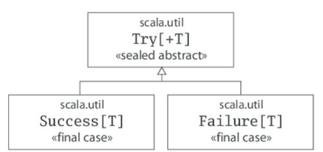
The error message gives you one way to solve the problem: importing a global execution context
provided by Scala itself. On the JVM, the global execution context uses a thread pool.[1] Once you
bring an implicit execution context into scope, you can create a future:
scala> import scala.concurrent.ExecutionContext.Implicits.global
import scala.concurrent.ExecutionContext.Implicits.global
scala> val fut = Future { Thread.sleep(10000); 21 + 21 }
fut: scala.concurrent.Future[Int] = ...
The future created in the previous example asynchronously executes the block of code, using
the global execution context, then completes with the value 42. Once it starts execution, that thread will
sleep for ten seconds. Thus this future will take at least ten seconds to complete.
Two methods on Future allow you to poll: isCompleted and value. When invoked on a future that has
not yet completed, isCompleted will return false and value will return None.
scala> fut.isCompleted
res0: Boolean = false
scala> fut.value
res1: Option[scala.util.Try[Int]] = None
Once the future completes (in this case, after at least ten seconds has gone by), isCompleted will
return true and value will return a Some:
scala> fut.isCompleted
res2: Boolean = true
scala> fut.value
res3: Option[scala.util.Try[Int]] = Some(Success(42))
The option returned by value contains a Try. As shown in Figure 32.1, a Try is either a Success, which
contains a value of type T, or a Failure, which contains an exception (an instance
ofjava.lang.Throwable). The purpose of Try is to provide for asynchronous computations what
thetry expression provides for synchronous computations: It allows you to deal with the possibility that
the computation will complete abruptly with an exception rather than return a result.[2]
Figure 32.1 - Class hierarchy for Try.
For synchronous computations you can use try/catch to ensure that a thread that invokes a method
catches and handles exceptions thrown by the method. For asynchronous computations, however, the
thread that initiates the computation often moves on to other tasks. Later if that asynchronous
computation fails with an exception, the original thread is no longer able to handle the exception in
a catch clause. Thus when working with a Futurerepresenting an asynchronous activity, you use Try to
deal with the possibility that the activity fails to yield a value and instead completes abruptly an
exception. Here's an example that shows what happens when an asynchronous activity fails:
scala> val fut = Future { Thread.sleep(10000); 21 / 0 }
fut: scala.concurrent.Future[Int] = ...
scala> fut.value
res4: Option[scala.util.Try[Int]] = None
Then, after ten seconds:
scala> fut.value
res5: Option[scala.util.Try[Int]] =
Some(Failure(java.lang.ArithmeticException: / by zero))
32.3 WORKING WITH FUTURES
Scala's Future allows you to specify transformations on Future results and obtain a new futurethat
represents the composition of the two asynchronous computations: the original and the transformation.
Transforming Futures with map
The most fundamental such operation is map. Instead of blocking then continuing with another
computation, you can just map the next computation onto the future. The result will be a new future
that represents the original asynchronously computed result transformed asynchronously by the
function passed to map.
For example, the following future will complete after ten seconds:
scala> val fut = Future { Thread.sleep(10000); 21 + 21 }
fut: scala.concurrent.Future[Int] = ...
Mapping this future with a function that increments by one will yield another future. This new future
will represent a computation consisting of the original addition followed by the subsequent increment:
scala> val result = fut.map(x => x + 1)
result: scala.concurrent.Future[Int] = ...
scala> result.value
res5: Option[scala.util.Try[Int]] = None
Once the original future completes and the function has been applied to its result, the future returned
by map will complete:
scala> result.value
res6: Option[scala.util.Try[Int]] = Some(Success(43))
Note that the operations performed in this example—the future creation, the 21 + 21 sum calculation,
and the 42 + 1 increment—may be performed by three different threads.
Transforming Futures with for expressions
Because Scala's future also declares a flatMap method, you can transform futures using
a forexpression. For example, consider the following two futures that will, after ten seconds, produce
42 and 46:
scala> val fut1 = Future { Thread.sleep(10000); 21 + 21 }
fut1: scala.concurrent.Future[Int] = ...
scala> val fut2 = Future { Thread.sleep(10000); 23 + 23 }
fut2: scala.concurrent.Future[Int] = ...
Given these two futures, you can obtain a new future representing the asynchronous sum of their results
like this:
scala> for {
x <- fut1
y <- fut2
} yield x + y
res7: scala.concurrent.Future[Int] = ...
Once the original futures have completed, and the subsequent sum completes, you'll be able to see the
result:
scala> res7.value
res8: Option[scala.util.Try[Int]] = Some(Success(88))
Because for expressions serialize their transformations,[3] if you don't create the futures before
the for expression, they won't run in parallel. For example, although the previous forexpression requires
around ten seconds to complete, the following for expression requires at least twenty seconds:
scala> for {
x <- Future { Thread.sleep(10000); 21 + 21 }
y <- Future { Thread.sleep(10000); 23 + 23 }
} yield x + y
res9: scala.concurrent.Future[Int] = ...
scala> res9.value
res27: Option[scala.util.Try[Int]] = None
scala> // Will need at least 20 seconds to complete
scala> res9.value
res28: Option[scala.util.Try[Int]] = Some(Success(88))
Creating the Future: Future.failed, Future.successful, Future.fromTry, and Promises
Besides the apply method, used in earlier examples to create futures, the Future companion object also
includes three factory methods for creating already-completed futures: successful,failed, and fromTry.
These factory methods do not require an ExecutionContext.
The successful factory method creates a future that has already succeeded:
scala> Future.successful { 21 + 21 }
res2: scala.concurrent.Future[Int] = ...
The failed method creates a future that has already failed:
scala> Future.failed(new Exception("bummer!"))
res3: scala.concurrent.Future[Nothing] = ...
The fromTry method creates an already completed future from a Try:
scala> import scala.util.{Success,Failure}
import scala.util.{Success, Failure}
scala> Future.fromTry(Success { 21 + 21 })
res4: scala.concurrent.Future[Int] = ...
scala> Future.fromTry(Failure(new Exception("bummer!")))
res5: scala.concurrent.Future[Nothing] = ...
The most general way to create a future is to use a Promise. Given a promise you can obtain a future
that is controlled by the promise. The future will complete when you complete the promise. Here's an
example:
scala> val pro = Promise[Int]
pro: scala.concurrent.Promise[Int] = ...
scala> val fut = pro.future
fut: scala.concurrent.Future[Int] = ...
scala> fut.value
res8: Option[scala.util.Try[Int]] = None
You can complete the promise with methods named success, failure, and complete. These methods
on Promise are similar to those described previously for constructing already completed futures. For
example, the success method will complete the future successfully:
scala> pro.success(42)
res9: pro.type = ...
scala> fut.value
res10: Option[scala.util.Try[Int]] = Some(Success(42))
The failure method takes an exception that will cause the future to fail with that exception.
The complete method takes a Try. A completeWith method, which takes a future, also exists; the
promise's future will thereafter mirror the completion status of the future you passed tocompleteWith.
Filtering: filter and collect
Scala's future offers two methods, filter and collect, that allow you to ensure a property holds true about
a future value. The filter method validates the future result, leaving it the same if it is valid. Here's an
example that ensures an Int is positive:
scala> val fut = Future { 42 }
fut: scala.concurrent.Future[Int] = ...
scala> val valid = fut.filter(res => res > 0)
valid: scala.concurrent.Future[Int] = ...
scala> valid.value
res0: Option[scala.util.Try[Int]] = Some(Success(42))
If the future value is not valid, the future returned by filter will fail with aNoSuchElementException:
scala> val invalid = fut.filter(res => res < 0)
invalid: scala.concurrent.Future[Int] = ...
scala> invalid.value
res1: Option[scala.util.Try[Int]] =
Some(Failure(java.util.NoSuchElementException:
Future.filter predicate is not satisfied))
Because Future also offers a withFilter method, you can perform the same operation with forexpression
filters:
scala> val valid = for (res <- fut if res > 0) yield res
valid: scala.concurrent.Future[Int] = ...
scala> valid.value
res2: Option[scala.util.Try[Int]] = Some(Success(42))
scala> val invalid = for (res <- fut if res < 0) yield res
invalid: scala.concurrent.Future[Int] = ...
scala> invalid.value
res3: Option[scala.util.Try[Int]] =
Some(Failure(java.util.NoSuchElementException:
Future.filter predicate is not satisfied))
Future's collect method allows you to validate the future value and transform it in one operation. If the
partial function passed to collect is defined at the future result, the future returned by collect will
succeed with that value transformed by the function:
scala> val valid =
fut collect { case res if res > 0 => res + 46 }
valid: scala.concurrent.Future[Int] = ...
scala> valid.value
res17: Option[scala.util.Try[Int]] = Some(Success(88))
Otherwise, the future will fail with NoSuchElementException:
scala> val invalid =
fut collect { case res if res < 0 => res + 46 }
invalid: scala.concurrent.Future[Int] = ...
scala> invalid.value
res18: Option[scala.util.Try[Int]] =
Some(Failure(java.util.NoSuchElementException:
Future.collect partial function is not defined at: 42))
Dealing with failure: failed, fallBackTo, recover, and recoverWith
Scala's future provides ways to work with futures that fail, including failed, fallBackTo, recover,
and recoverWith. The failed method will transform a failed future of any type into a
successfulFuture[Throwable] that holds onto the exception that caused the failure. Here's an example:
scala> val failure = Future { 42 / 0 }
failure: scala.concurrent.Future[Int] = ...
scala> failure.value
res23: Option[scala.util.Try[Int]] =
Some(Failure(java.lang.ArithmeticException: / by zero))
scala> val expectedFailure = failure.failed
expectedFailure: scala.concurrent.Future[Throwable] = ...
scala> expectedFailure.value
res25: Option[scala.util.Try[Throwable]] =
Some(Success(java.lang.ArithmeticException: / by zero))
If the future on which the failed method is called ultimately succeeds, the future returned byfailed will
itself fail with a NoSuchElementException. The failed method is appropriate, therefore, only when you
expect that the future will fail. Here's an example:
scala> val success = Future { 42 / 1 }
success: scala.concurrent.Future[Int] = ...
scala> success.value
res21: Option[scala.util.Try[Int]] = Some(Success(42))
scala> val unexpectedSuccess = success.failed
unexpectedSuccess: scala.concurrent.Future[Throwable] = ...
scala> unexpectedSuccess.value
res26: Option[scala.util.Try[Throwable]] =
Some(Failure(java.util.NoSuchElementException:
Future.failed not completed with a throwable.))
The fallbackTo method allows you to provide an alternate future to use in case the future on which you
invoke fallbackTo fails. Here's an example in which a failed future falls back to a successful future:
scala> val fallback = failure.fallbackTo(success)
fallback: scala.concurrent.Future[Int] = ...
scala> fallback.value
res27: Option[scala.util.Try[Int]] = Some(Success(42))
If the original future on which fallbackTo is invoked fails, a failure of the future passed tofallbackTo is
essentially ignored. The future returned by fallbackTo will fail with the initial exception. Here's an
example:
scala> val failedFallback = failure.fallbackTo(
Future { val res = 42; require(res < 0); res }
)
failedFallback: scala.concurrent.Future[Int] = ...
scala> failedFallback.value
res28: Option[scala.util.Try[Int]] =
Some(Failure(java.lang.ArithmeticException: / by zero))
The recover method allows you to transform a failed future into a successful one, allowing a successful
future's result to pass through unchanged. For example, on a future that fails withArithmeticException,
you can use the recover method to transform the failure into a success, like this:
scala> val recovered = failedFallback recover {
case ex: ArithmeticException => -1
}
recovered: scala.concurrent.Future[Int] = ...
scala> recovered.value
res32: Option[scala.util.Try[Int]] = Some(Success(-1))
If the original future doesn't fail, the future returned by recover will complete with the same value:
scala> val unrecovered = fallback recover {
case ex: ArithmeticException => -1
}
unrecovered: scala.concurrent.Future[Int] = ...
scala> unrecovered.value
res33: Option[scala.util.Try[Int]] = Some(Success(42))
Similarly, if the partial function passed to recover isn't defined at the exception with which the original
future ultimately fails, that original failure will pass through:
scala> val alsoUnrecovered = failedFallback recover {
case ex: IllegalArgumentException => -2
}
alsoUnrecovered: scala.concurrent.Future[Int] = ...
scala> alsoUnrecovered.value
res34: Option[scala.util.Try[Int]] =
Some(Failure(java.lang.ArithmeticException: / by zero))
The recoverWith method is similar to recover, except instead of recovering to a value like recover,
the recoverWith method allows you to recover to a future value. Here's an example:
scala> val alsoRecovered = failedFallback recoverWith {
case ex: ArithmeticException => Future { 42 + 46 }
}
alsoRecovered: scala.concurrent.Future[Int] = ...
scala> alsoRecovered.value
res35: Option[scala.util.Try[Int]] = Some(Success(88))
As with recover, if either the original future doesn't fail, or the partial function passed
torecoverWith isn't defined at the exception the original future ultimately fails with, the original success
(or failure) will pass through to the future returned by recoverWith.
Mapping both possibilities: transform
Future's transform method accepts two functions with which to transform a future: one to use in case of
success and the other in case of failure:
scala> val first = success.transform(
res => res * -1,
ex => new Exception("see cause", ex)
)
first: scala.concurrent.Future[Int] = ...
If the future succeeds, the first function is used:
scala> first.value
res42: Option[scala.util.Try[Int]] = Some(Success(-42))
If the future fails, the second function is used:
scala> val second = failure.transform(
res => res * -1,
ex => new Exception("see cause", ex)
)
second: scala.concurrent.Future[Int] = ...
scala> second.value
res43: Option[scala.util.Try[Int]] =
Some(Failure(java.lang.Exception: see cause))
Note that with the transform method shown in the previous examples, you can't change a successful
future into a failed one, nor can you change a failed future into a successful one. To make this kind of
transformation easier, Scala 2.12 introduced an alternate overloaded form of transform that takes a
function from Try to Try. Here are some examples:
scala> val firstCase = success.transform { // Scala 2.12
case Success(res) => Success(res * -1)
case Failure(ex) =>
Failure(new Exception("see cause", ex))
}
first: scala.concurrent.Future[Int] = ...
scala> firstCase.value
res6: Option[scala.util.Try[Int]] = Some(Success(-42))
scala> val secondCase = failure.transform {
case Success(res) => Success(res * -1)
case Failure(ex) =>
Failure(new Exception("see cause", ex))
}
secondCase: scala.concurrent.Future[Int] = ...
scala> secondCase.value
res8: Option[scala.util.Try[Int]] =
Some(Failure(java.lang.Exception: see cause))
Here's an example of using the new transform method to transform a failure into a success:
scala> val nonNegative = failure.transform { // Scala 2.12
case Success(res) => Success(res.abs + 1)
case Failure(_) => Success(0)
}
nonNegative: scala.concurrent.Future[Int] = ...
scala> nonNegative.value
res11: Option[scala.util.Try[Int]] = Some(Success(0))
Combining futures: zip, Future.fold, Future.reduce, Future.sequence, and Future.traverse
Future and its companion object offer methods that allow you to combine multiple futures.
The zip method will transform two successful futures into a future tuple of both values. Here's an
example:
scala> val zippedSuccess = success zip recovered
zippedSuccess: scala.concurrent.Future[(Int, Int)] = ...
scala> zippedSuccess.value
res46: Option[scala.util.Try[(Int, Int)]] =
Some(Success((42,-1)))
If either of the futures fail, however, the future returned by zip will also fail with the same exception:
scala> val zippedFailure = success zip failure
zippedFailure: scala.concurrent.Future[(Int, Int)] = ...
scala> zippedFailure.value
res48: Option[scala.util.Try[(Int, Int)]] =
Some(Failure(java.lang.ArithmeticException: / by zero))
If both futures fail, the failed future that results will contain the exception stored in the initial future, the
one on which zip was invoked.
Future's companion object offers a fold method that allows you to accumulate a result across
aTraversableOnce collection of futures, yielding a future result. If all futures in the collection succeed,
the resulting future will succeed with the accumulated result. If any future in the collection fails, the
resulting future will fail. If multiple futures fail, the result will fail with the same exception with which
the first future (earliest in the TraversableOnce collection) fails. Here's an example:
scala> val fortyTwo = Future { 21 + 21 }
fortyTwo: scala.concurrent.Future[Int] = ...
scala> val fortySix = Future { 23 + 23 }
fortySix: scala.concurrent.Future[Int] = ...
scala> val futureNums = List(fortyTwo, fortySix)
futureNums: List[scala.concurrent.Future[Int]] = ...
scala> val folded =
Future.fold(futureNums)(0) { (acc, num) =>
acc + num
}
folded: scala.concurrent.Future[Int] = ...
scala> folded.value
res53: Option[scala.util.Try[Int]] = Some(Success(88))
The Future.reduce method performs a fold without a zero, using the initial future result as the start
value. Here's an example:
scala> val reduced =
Future.reduce(futureNums) { (acc, num) =>
acc + num
}
reduced: scala.concurrent.Future[Int] = ...
scala> reduced.value
res54: Option[scala.util.Try[Int]] = Some(Success(88))
If you pass an empty collection to reduce, the resulting future will fail with aNoSuchElementException.
The Future.sequence method transforms a TraversableOnce collection of futures into a
futureTraversableOnce of values. For instance, in the following example, sequence is used to transform
a List[Future[Int]] to a Future[List[Int]]:
scala> val futureList = Future.sequence(futureNums)
futureList: scala.concurrent.Future[List[Int]] = ...
scala> futureList.value
res55: Option[scala.util.Try[List[Int]]] =
Some(Success(List(42, 46)))
The Future.traverse method will change a TraversableOnce of any element type into
aTraversableOnce of futures and "sequence" that into a future TraversableOnce of values. For example,
here a List[Int] is transformed into a Future[List[Int]] by Future.traverse:
scala> val traversed =
Future.traverse(List(1, 2, 3)) { i => Future(i) }
traversed: scala.concurrent.Future[List[Int]] = ...
scala> traversed.value
res58: Option[scala.util.Try[List[Int]]] =
Some(Success(List(1, 2, 3)))
Performing side-effects: foreach, onComplete, and andThen
Sometimes you may need to perform a side effect after a future completes. Future provides several
methods for this purpose. The most basic method is foreach, which will perform a side effect if a future
completes successfully. For instance, in the following example a println is not executed in the case of a
failed future, just a successful future:
scala> failure.foreach(ex => println(ex))
scala> success.foreach(res => println(res))
42
Since for without yield will rewrite to an invocation of foreach, you can also accomplish the same
effect using for expressions:
scala> for (res <- failure) println(res)
scala> for (res <- success) println(res)
42
Future also offers two methods for registering "callback" functions. The onComplete method will be
executed whether the future ultimately succeeds or fails. The function will be passed a Try—
a Success holding the result if the future succeeded, else a Failure holding the exception that caused the
future to fail. Here's an example:
scala> import scala.util.{Success, Failure}
import scala.util.{Success, Failure}
scala> success onComplete {
case Success(res) => println(res)
case Failure(ex) => println(ex)
}
42
scala> failure onComplete {
case Success(res) => println(res)
case Failure(ex) => println(ex)
}
java.lang.ArithmeticException: / by zero
Future does not guarantee any order of execution for callback functions registered withonComplete. If
you want to enforce an order for callback functions, you must
use andThen instead.The andThen method returns a new future that mirrors (succeeds or fails in the
same way as) the original future on which you invoke andThen, but it does not complete until the
callback function has been fully executed:
scala> val newFuture = success andThen {
case Success(res) => println(res)
case Failure(ex) => println(ex)
}
42
newFuture: scala.concurrent.Future[Int] = ...
scala> newFuture.value
res76: Option[scala.util.Try[Int]] = Some(Success(42))
Note that if a callback function passed to andThen throws an exception when executed, that exception
will not be propagated to subsequent callbacks or reported via the resulting future.
Other methods added in 2.12: flatten, zipWith, and transformWith
The flatten method, added in 2.12, transforms a Future nested inside another Future into aFuture of the
nested type. For example, flatten can transform a Future[Future[Int]] into aFuture[Int]:
scala> val nestedFuture = Future { Future { 42 } }
nestedFuture: Future[Future[Int]] = ...
scala> val flattened = nestedFuture.flatten // Scala 2.12
flattened: scala.concurrent.Future[Int] = Future(Success(42))
The zipWith method, added in 2.12, essentially zips two Futures together, then performs a mapon the
resulting tuple. Here's an example of the two-step process, a zip followed by a map:
scala> val futNum = Future { 21 + 21 }
futNum: scala.concurrent.Future[Int] = ...
scala> val futStr = Future { "ans" + "wer" }
futStr: scala.concurrent.Future[String] = ...
scala> val zipped = futNum zip futStr
zipped: scala.concurrent.Future[(Int, String)] = ...
scala> val mapped = zipped map {
case (num, str) => s"$num is the $str"
}
mapped: scala.concurrent.Future[String] = ...
scala> mapped.value
res2: Option[scala.util.Try[String]] =
Some(Success(42 is the answer))
The zipWith method allows you to perform the same operation in one step:
scala> val fut = futNum.zipWith(futStr) { // Scala 2.12
case (num, str) => s"$num is the $str"
}
zipWithed: scala.concurrent.Future[String] = ...
scala> fut.value
res3: Option[scala.util.Try[String]] =
Some(Success(42 is the answer))
Future also gained a transformWith method in Scala 2.12, which allows you to transform a future using
a function from Try to Future. Here's an example:
scala> val flipped = success.transformWith { // Scala 2.12
case Success(res) =>
Future { throw new Exception(res.toString) }
case Failure(ex) => Future { 21 + 21 }
}
flipped: scala.concurrent.Future[Int] = ...
scala> flipped.value
res5: Option[scala.util.Try[Int]] =
Some(Failure(java.lang.Exception: 42))
The transformWith method is similar to the new, overloaded transform method added in Scala 2.12,
except instead of yielding a Try in your passed function as in transform, transformWithallows you to
yield a future.
32.4 TESTING WITH FUTURES
One advantage of Scala's futures is that they help you avoid blocking. On most JVM implementations,
after creating just a few thousand threads, the cost of context switching between threads will degrade
performance to an unnacceptable level. By avoiding blocking, you can keep the finite number of
threads you decide to work with busy. Nevertheless, Scala does allow you to block on a future result
when you need to. Scala's Await object facilitates blocking to wait for future results. Here's an example:
scala> import scala.concurrent.Await
import scala.concurrent.Await
scala> import scala.concurrent.duration._
import scala.concurrent.duration._
scala> val fut = Future { Thread.sleep(10000); 21 + 21 }
fut: scala.concurrent.Future[Int] = ...
scala> val x = Await.result(fut, 15.seconds) // blocks
x: Int = 42
Await.result takes a Future and a Duration. The Duration indicates how long Await.result should wait
for a Future to complete before timing out. In this example, fifteen seconds was specified for
the Duration. Thus the Await.result method should not time out before the future completes with its
eventual value, 42.
One place where blocking has been generally accepted is in tests of asynchronous code. Now that
the Await.result has returned, you can perform a computation using that result, such as an assertion in a
test:
scala> import org.scalatest.Matchers._
import org.scalatest.Matchers._
scala> x should be (42)
res0: org.scalatest.Assertion = Succeeded
Alternatively, you can use blocking constructs provided by ScalaTest's trait ScalaFutures. For example,
the futureValue method, implicitly added to Future by ScalaFutures, will block until the future
completes. If the future fails, futureValue will throw a TestFailedException describing the problem. If
the future succeeds, futureValue will return the successful result of the future so you can perform
asssertions on that value:
scala> import org.scalatest.concurrent.ScalaFutures._
import org.scalatest.concurrent.ScalaFutures._
scala> val fut = Future { Thread.sleep(10000); 21 + 21 }
fut: scala.concurrent.Future[Int] = ...
scala> fut.futureValue should be (42) // futureValue blocks
res1: org.scalatest.Assertion = Succeeded
While blocking in tests is often fine, ScalaTest 3.0 adds "async" testing styles that allow you to test
futures without blocking. Given a future, instead of blocking and performing assertions on the result,
you can map assertions directly onto that future and return the resultingFuture[Assertion] to ScalaTest.
An example is shown in Listing 32.1. When the future assertion completes, ScalaTest will fire events
(test succeeded, test failed, etc.) to the test reporter asynchronously.
import org.scalatest.AsyncFunSpec
import scala.concurrent.Future
class AddSpec extends AsyncFunSpec {
def addSoon(addends: Int*): Future[Int] =
Future { addends.sum }
describe("addSoon") {
it("will eventually compute a sum of passed Ints") {
val futureSum: Future[Int] = addSoon(1, 2)
// You can map assertions onto a Future, then return
// the resulting Future[Assertion] to ScalaTest:
futureSum map { sum => assert(sum == 3) }
}
}
}
Listing 32.1 - Returning a future assertion to ScalaTest.
The async testing use case illustrates a general principle for working with futures: Once in "future
space," try to stay in future space. Don't block on a future then continue the computation with the
result. Stay asynchronous by performing a series of transformations, each of which returns a new future
to transform. To get results out of future space, register side effects to be performed asynchronously
once futures complete. This approach will help you make maximum use of your threads.
32.5 CONCLUSION
Concurrent programming gives you great power. It lets you simplify your code and take advantage of
multiple processors. It's unfortunate that the most widely used concurrency primitives, threads, locks,
and monitors, are such a minefield of deadlocks and race conditions. Futures provide a way out of that
minefield, letting you write concurrent programs without as great a risk of deadlocks and race
conditions. This chapter has introduced several fundamental constructs for working with futures in
Scala, including how to create futures, how to transform them, and how to test them, among other nuts
and bolts. It then showed you how to use these constructs as part of a general futures style.
Footnotes for Chapter 32:
[1] On Scala.js, the global execution context places tasks on the JavaScript event queue.
[2] Note that the Java Future also has a way to deal with the potential of an exception being thrown by
the asynchronous computation: its get method will throw that exception wrapped in
an ExecutionException.
[3] The for expression shown in this example will be rewritten as a call to fut1.flatMap passing in a
function that calls fut2.map: fut1.flatMap(x => fut2.map(y => x + y)).
Chapter 33
Combinator Parsing
Occasionally, you may need to process a small, special-purpose language. For example, you may need
to read configuration files for your software, and you want to make them easier to modify by hand than
XML. Alternatively, maybe you want to support an input language in your program, such as search
terms with boolean operators (computer, find me a movie "with `space ships' and without `love
stories"'). Whatever the reason, you are going to need aparser. You need a way to convert the input
language into some data structure your software can process.
Essentially, you have only a few choices. One choice is to roll your own parser (and lexical analyzer).
If you are not an expert, this is hard. If you are an expert, it is still time consuming.
An alternative choice is to use a parser generator. There exist quite a few of these generators. Some of
the better known are Yacc and Bison for parsers written in C and ANTLR for parsers written in
Java. You'll probably also need a scanner generator such as Lex, Flex, or JFlex to go with it. This might
be the best solution, except for a couple of inconveniences. You need to learn new tools, including their
—sometimes obscure—error messages. You also need to figure out how to connect the output of these
tools to your program. This might limit the choice of your programming language, and complicate your
tool chain.
This chapter presents a third alternative. Instead of using the standalone domain specific language of a
parser generator, you will use an internal domain specific language, or internal DSL for short. The
internal DSL will consist of a library of parser combinators—functions and operators defined in Scala
that will serve as building blocks for parsers. These building blocks will map one to one to the
constructions of a context-free grammar, to make them easy to understand.
This chapter introduces only one language feature that was not explained before: thisaliasing,
in Section 33.6. The chapter does, however, heavily use several other features that were explained in
previous chapters. Among others, parameterized types, abstract types, functions as objects, operator
overloading, by-name parameters, and implicit conversions all play important roles. The chapter shows
how these language elements can be combined in the design of a very high-level library.
The concepts explained in this chapter tend to be a bit more advanced than previous chapters. If you
have a good grounding in compiler construction, you'll profit from it reading this chapter, because it
will help you put things better in perspective. However, the only prerequisite for understanding this
chapter is that you know about regular and context-free grammars. If you don't, the material in this
chapter can also safely be skipped.
33.1 EXAMPLE: ARITHMETIC EXPRESSIONS
We'll start with an example. Say you want to construct a parser for arithmetic expressions consisting of
floating-point numbers, parentheses, and the binary operators +, -, *, and /. The first step is always to
write down a grammar for the language to be parsed. Here's the grammar for arithmetic expressions:
expr ::= term \{"+" term | "-" term\}.
term ::= factor \{"*" factor | "/" factor\}.
factor ::= floatingPointNumber | "(" expr ")".
Here, | denotes alternative productions, and \{ ... \} denotes repetition (zero or more times). And
although there's no use of it in this example, [ ... ] denotes an optional occurrence.
This context-free grammar defines formally a language of arithmetic expressions. Every expression
(represented by expr) is a term, which can be followed by a sequence of + or -operators and
further terms. A term is a factor, possibly followed by a sequence of * or /operators and further factors.
A factor is either a numeric literal or an expression in parentheses. Note that the grammar already
encodes the relative precedence of operators. For instance, * binds more tightly than +, because
a * operation gives a term, whereas a +operation gives an expr, and exprs can contain terms but
a term can contain an expr only when the latter is enclosed in parentheses.
Now that you have defined the grammar, what's next? If you use Scala's combinator parsers, you are
basically done! You only need to perform some systematic text replacements and wrap the parser in a
class, as shown in Listing 33.1:
import scala.util.parsing.combinator._
class Arith extends JavaTokenParsers {
def expr: Parser[Any] = term~rep("+"~term | "-"~term)
def term: Parser[Any] = factor~rep("*"~factor | "/"~factor)
def factor: Parser[Any] = floatingPointNumber | "("~expr~")"
}
Listing 33.1 - An arithmetic expression parser.
The parsers for arithmetic expressions are contained in a class that inherits from the
traitJavaTokenParsers. This trait provides the basic machinery for writing a parser and also provides
some primitive parsers that recognize some word classes: identifiers, string literals and numbers. In the
example in Listing 33.1 you need only the primitive floatingPointNumberparser, which is inherited
from this trait.
The three definitions in class Arith represent the productions for arithmetic expressions. As you can
see, they follow very closely the productions of the context-free grammar. In fact, you could generate
this part automatically from the context-free grammar, by performing a number of simple text
replacements:
1. Every production becomes a method, so you need to prefix it with def.
2. The result type of each method is Parser[Any], so you need to change the ::= symbol to
": Parser[Any] =". You'll find out later in this chapter what the type Parser[Any] signifies, and
also how to make it more precise.
3. In the grammar, sequential composition was implicit, but in the program it is expressed by an
explicit operator: ~. So you need to insert a ~ between every two consecutive symbols of a
production. In the example in Listing 33.1 we chose not to write any spaces around
the ~ operator. That way, the parser code keeps closely to the visual appearance of the grammar
—it just replaces spaces by ~ characters.
4. Repetition is expressed rep( ... ) instead of \{ ... \}. Analogously (though not shown in the
example), option is expressed opt( ... ) instead of [ ... ].
5. The period (.) at the end of each production is omitted—you can, however, write a semicolon (;)
if you prefer.
That's all there is to it. The resulting class Arith defines three parsers, expr, term and factor, which can
be used to parse arithmetic expressions and their parts.
33.2 RUNNING YOUR PARSER
You can exercise your parser with the following small program:
object ParseExpr extends Arith {
def main(args: Array[String]) = {
println("input : " + args(0))
println(parseAll(expr, args(0)))
}
}
The ParseExpr object defines a main method that parses the first command-line argument passed to it.
It prints the original input argument, and then prints its parsed version. Parsing is done by the
expression:
parseAll(expr, input)
This expression applies the parser, expr, to the given input. It expects that all of the input matches, i.e.,
that there are no characters trailing a parsed expression. There's also a methodparse, which allows you
to parse an input prefix, leaving some remainder unread.
You can run the arithmetic parser with the following command:
$ scala ParseExpr "2 * (3 + 7)"
input: 2 * (3 + 7)
[1.12] parsed: ((2~List((*~(((~((3~List())~List((+
~(7~List())))))~)))))~List())
The output tells you that the parser successfully analyzed the input string up to position [1.12]. That
means the first line and the twelfth column—in other words, the whole input string—was parsed.
Disregard for the moment the result after "parsed:". It is not very useful, and you will find out later how
to get more specific parser results.
You can also try to introduce some input string that is not a legal expression. For instance, you could
write one closing parenthesis too many:
$ scala ParseExpr "2 * (3 + 7))"
input: 2 * (3 + 7))
[1.12] failure: `-' expected but `)' found
2 * (3 + 7))
^
Here, the expr parser parsed everything until the final closing parenthesis, which does not form part of
the arithmetic expression. The parseAll method then issued an error message, which said that it
expected a - operator at the point of the closing parenthesis. You'll find out later in this chapter why it
produced this particular error message, and how you can improve it.
33.3 BASIC REGULAR EXPRESSION PARSERS
The parser for arithmetic expressions made use of another parser, named floatingPointNumber. This
parser, which was inherited from Arith's supertrait, JavaTokenParsers, recognizes a floating point
number in the format of Java. But what do you do if you need to parse numbers in a format that's a bit
different from Java's? In this situation, you can use a regular expression parser.
The idea is that you can use any regular expression as a parser. The regular expression parses all strings
that it can match. Its result is the parsed string. For instance, the regular expression parser shown
in Listing 33.2 describes Java's identifiers:
object MyParsers extends RegexParsers {
val ident: Parser[String] = """[a-zA-Z_]\w*""".r
}
Listing 33.2 - A regular expression parser for Java identifiers.
The MyParsers object of Listing 33.2 inherits from trait RegexParsers, whereas Arith inherited
from JavaTokenParsers. Scala's parsing combinators are arranged in a hierarchy of traits, which are all
contained in package scala.util.parsing.combinator. The top-level trait is Parsers, which defines a very
general parsing framework for all sorts of input. One level below is traitRegexParsers, which requires
that the input is a sequence of characters and provides for regular expression parsing. Even more
specialized is trait JavaTokenParsers, which implements parsers for basic classes of words (or tokens)
as they are defined in Java.
33.4 ANOTHER EXAMPLE: JSON
JSON, the JavaScript Object Notation, is a popular data interchange format. In this section, we'll show
you how to write a parser for it. Here's a grammar that describes the syntax of JSON:
value ::= obj | arr | stringLiteral |
floatingPointNumber |
"null" | "true" | "false".
obj ::= "{" [members] "}".
arr ::= "[" [values] "]".
members ::= member \{"," member\}.
member ::= stringLiteral ":" value.
values ::= value \{"," value\}.
A JSON value is an object, array, string, number, or one of the three reserved words null, true, or false.
A JSON object is a (possibly empty) sequence of members separated by commas and enclosed in
braces. Each member is a string/value pair where the string and the value are separated by a colon.
Finally, a JSON array is a sequence of values separated by commas and enclosed in square brackets. As
an example, Listing 33.3 contains an address-book formatted as a JSON object.
{
"address book": {
"name": "John Smith",
"address": {
"street": "10 Market Street",
"city" : "San Francisco, CA",
"zip" : 94111
},
"phone numbers": [
"408 338-4238",
"408 111-6892"
]
}
}
Listing 33.3 - Data in JSON format.
Parsing such data is straightforward when using Scala's parser combinators. The complete parser is
shown in Listing 33.4. This parser follows the same structure as the arithmetic expression parser. It is
again a straightforward mapping of the productions of the JSON grammar. The productions use one
shortcut that simplifies the grammar: The repsepcombinator parses a (possibly empty) sequence of
terms that are separated by a given separator string. For instance, in the example in Listing
33.4, repsep(member, ",") parses a comma-separated sequence of member terms. Otherwise, the
productions in the parser correspond exactly to the productions in the grammar, as was the case for the
arithmetic expression parsers.
import scala.util.parsing.combinator._
class JSON extends JavaTokenParsers {
def value : Parser[Any] = obj | arr |
stringLiteral |
floatingPointNumber |
"null" | "true" | "false"
def obj : Parser[Any] = "{"~repsep(member, ",")~"}"
def arr : Parser[Any] = "["~repsep(value, ",")~"]"
def member: Parser[Any] = stringLiteral~":"~value
}
Listing 33.4 - A simple JSON parser.
To try out the JSON parsers, we'll change the framework a bit, so that the parser operates on a file
instead of on the command line:
import java.io.FileReader
object ParseJSON extends JSON {
def main(args: Array[String]) = {
val reader = new FileReader(args(0))
println(parseAll(value, reader))
}
}
The main method in this program first creates a FileReader object. It then parses the characters returned
by that reader according to the value production of the JSON grammar. Note
thatparseAll and parse exist in overloaded variants: both can take a character sequence or alternatively
an input reader as second argument.
If you store the "address book" object shown in Listing 33.3 into a file named address-book.jsonand
run the ParseJSON program on it, you should get:
$ scala ParseJSON address-book.json
[13.4] parsed: (({~List((("address book"~:)~(({~List(((
"name"~:)~"John Smith"), (("address"~:)~(({~List(((
"street"~:)~"10 Market Street"), (("city"~:)~"San Francisco
,CA"), (("zip"~:)~94111)))~})), (("phone numbers"~:)~(([~
List("408 338-4238", "408 111-6892"))~]))))~}))))~})
33.5 PARSER OUTPUT
The ParseJSON program successfully parsed the JSON address book. However, the parser output looks
strange. It seems to be a sequence composed of bits and pieces of the input glued together with lists
and ~ combinations. This output is not very useful. It is less readable for humans than the input, but it is
also too disorganized to be easily analyzable by a computer. It's time to do something about this.
To figure out what to do, you need to know first what the individual parsers in the combinator
frameworks return as a result (provided they succeed in parsing the input). Here are the rules:
1. Each parser written as a string (such as: "{" or ":" or "null") returns the parsed string itself.
2. Regular expression parsers such as """[a-zA-Z_]\w*""".r also return the parsed string itself. The
same holds for regular expression parsers such as stringLiteral or floatingPointNumber, which
are inherited from trait JavaTokenParsers.
3. A sequential composition P~Q returns the results of both P and of Q. These results are returned
in an instance of a case class that is also written ~. So if P returns "true" and Qreturns "?", then
the sequential composition P~Q returns ~("true", "?"), which prints as(true~?).
4. An alternative composition P | Q returns the result of either P or Q, whichever one succeeds.
5. A repetition rep(P) or repsep(P, separator) returns a list of the results of all runs of P.
6. An option opt(P) returns an instance of Scala's Option type. It returns Some(R) if P succeeds
with result R and None if P fails.
With these rules you can now deduce why the parser output appeared as it did in the previous
examples. However, the output is still not very convenient. It would be much better to map a JSON
object into an internal Scala representation that represents the meaning of the JSON value. A more
natural representation would be as follows:
•A JSON object is represented as a Scala map of type Map[String, Any]. Every member is
represented as a key/value binding in the map.
•A JSON array is represented as a Scala list of type List[Any].
•A JSON string is represented as a Scala String.
•A JSON numeric literal is represented as a Scala Double.
•The values true, false, and null are represented as the Scala values with the same names.
To produce this representation, you need to make use of one more combination form for parsers: ^^.
The ^^ operator transforms the result of a parser. Expressions using this operator have the
form P ^^ f where P is a parser and f is a function. P ^^ f parses the same sentences as just P.
Whenever P returns with some result R, the result of P ^^ f is f(R).
As an example, here is a parser that parses a floating point number and converts it to a Scala value of
type Double:
floatingPointNumber ^^ (_.toDouble)
And here is a parser that parses the string "true" and returns Scala's boolean true value:
"true" ^^ (x => true)
Now for more advanced transformations. Here's a new version of a parser for JSON objects that returns
a Scala Map:
def obj: Parser[Map[String, Any]] = // Can be improved
"{"~repsep(member, ",")~"}" ^^
{ case "{"~ms~"}" => Map() ++ ms }
Remember that the ~ operator produces as its result an instance of a case class with the same name: ~.
Here's a definition of that class—it's an inner class of trait Parsers:
case class ~[+A, +B](x: A, y: B) {
override def toString = "(" + x + "~" + y + ")"
}
The name of the class is intentionally the same as the name of the sequence combinator method, ~.
That way, you can match parser results with patterns that follow the same structure as the parsers
themselves. For instance, the pattern "{"~ms~"}" matches a result string "{" followed by a result
variable ms, which is followed in turn by a result string "}". This pattern corresponds exactly to what is
returned by the parser on the left of the ^^. In its desugared versions where the ~ operator comes first,
the same pattern reads ~(~("{", ms), "}"), but this is much less legible.
The purpose of the "{"~ms~"}" pattern is to strip off the braces so that you can get at the list of
members resulting from the repsep(member, ",") parser. In cases like these there is also an alternative
that avoids producing unnecessary parser results that are immediately discarded by the pattern match.
The alternative makes use of the ~> and <~ parser combinators. Both express sequential composition
like ~, but ~> keeps only the result of its right operand, whereas <~ keeps only the result of its left
operand. Using these combinators, the JSON object parser can be expressed more succinctly:
def obj: Parser[Map[String, Any]] =
"{"~> repsep(member, ",") <~"}" ^^ (Map() ++ _)
Listing 33.5 shows a full JSON parser that returns meaningful results. If you run this parser on
the address-book.json file, you will get the following result (after adding some newlines and
indentation):
$ scala JSON1Test address-book.json
[14.1] parsed: Map(
address book -> Map(
name -> John Smith,
address -> Map(
street -> 10 Market Street,
city -> San Francisco, CA,
zip -> 94111),
phone numbers -> List(408 338-4238, 408 111-6892)
)
)
This is all you need to know in order to get started writing your own parsers. As an aide to
memory, Table 33.1 lists the parser combinators that were discussed so far.
import scala.util.parsing.combinator._
class JSON1 extends JavaTokenParsers {
def obj: Parser[Map[String, Any]] =
"{"~> repsep(member, ",") <~"}" ^^ (Map() ++ _)
def arr: Parser[List[Any]] =
"["~> repsep(value, ",") <~"]"
def member: Parser[(String, Any)] =
stringLiteral~":"~value ^^
{ case name~":"~value => (name, value) }
def value: Parser[Any] = (
obj
| arr
| stringLiteral
| floatingPointNumber ^^ (_.toDouble)
| "null" ^^ (x => null)
| "true" ^^ (x => true)
| "false" ^^ (x => false)
)
}
Listing 33.5 - A full JSON parser that returns meaningful results.
Table 33.1 - Summary of parser combinators
"..." literal
"...".r regular expression
P~Q sequential composition
P <~ Q, P ~> Q sequential composition; keep left/right only
P | Q alternative
opt(P) option
rep(P) repetition
repsep(P, Q) interleaved repetition
P ^^ f result conversion
TURNING OFF SEMICOLON INFERENCE
Note that the body of the value parser in Listing 33.5 is enclosed in parentheses. This is a little trick to
disable semicolon inference in parser expressions. You saw in Section 4.2 that Scala assumes there's a
semicolon between any two lines that can be separate statements syntactically, unless the first line ends
in an infix operator, or the two lines are enclosed in parentheses or square brackets. Now, you could
have written the |operator at the end of the each alternative instead of at the beginning of the following
one, like this:
def value: Parser[Any] =
obj |
arr |
stringLiteral |
...
In that case, no parentheses around the body of the value parser would have been required. However,
some people prefer to see the | operator at the beginning of the second alternative rather than at the end
of the first. Normally, this would lead to an unwanted semicolon between the two lines, like this:
obj; // semicolon implicitly inserted
| arr
The semicolon changes the structure of the code, causing it to fail compilation. Putting the whole
expression in parentheses avoids the semicolon and makes the code compile correctly.
Symbolic versus alphanumeric names
Many of the parser combinators in Table 33.1 use symbolic names. This has both advantages and
disadvantages. On the minus side, symbolic names take time to learn. Users who are unfamiliar with
Scala's combinator parsing libraries are probably mystified what ~, ~>, or ^^mean. On the plus side,
symbolic names are short, and can be chosen to have the "right" precedences and associativities. For
instance, the parser combinators ~, ^^, and | are chosen intentionally in decreasing order of precedence.
A typical grammar production is composed of alternatives that have a parsing part and a transformation
part. The parsing part usually contains several sequential items separated by ~ operators. With the
chosen precedences of~, ^^, and | you can write such a grammar production without needing any
parentheses.
Furthermore, symbolic operators take less visual real estate than alphabetic ones. That's important for a
parser because it lets you concentrate on the grammar at hand, instead of the combinators themselves.
To see the difference, imagine for a moment that sequential composition (~) was called andThen and
alternative (|) was called orElse. The arithmetic expression parsers in Listing 33.1 here would look as
follows:
class ArithHypothetical extends JavaTokenParsers {
def expr: Parser[Any] =
term andThen rep(("+" andThen term) orElse
("-" andThen term))
def term: Parser[Any] =
factor andThen rep(("*" andThen factor) orElse
("/" andThen factor))
def factor: Parser[Any] =
floatingPointNumber orElse
("(" andThen expr andThen ")")
}
You notice that the code becomes much longer, and that it's hard to "see" the grammar among all those
operators and parentheses. On the other hand, somebody new to combinator parsing could probably
figure out better what the code is supposed to do.
CHOOSING BETWEEN SYMBOLIC AND ALPHABETIC NAMES
As guidelines for choosing between symbolic and alphabetic names we recommend the following:
•Use symbolic names in cases where they already have a universally established meaning. For
instance, nobody would recommend writing add instead of + for numeric addition.
•Otherwise, give preference to alphabetic names if you want your code to be understandable to
casual readers.
•You can still choose symbolic names for domain-specific libraries, if this gives clear advantages
in legibility and you do not expect anyway that a casual reader without a firm grounding in the
domain would be able to understand the code immediately.
In the case of parser combinators we are looking at a highly domain-specific language, which casual
readers may have trouble understanding even with alphabetic names. Furthermore, symbolic names
give clear advantages in legibility for the expert. So we believe their use is warranted in this
application.
33.6 IMPLEMENTING COMBINATOR PARSERS
The previous sections have shown that Scala's combinator parsers provide a convenient means for
constructing your own parsers. Since they are nothing more than a Scala library, they fit seamlessly into
your Scala programs. So it's very easy to combine a parser with some code that processes the results it
delivers, or to rig a parser so that it takes its input from some specific source (say, a file, a string, or a
character array).
How is this achieved? In the rest of this chapter you'll take a look "under the hood" of the combinator
parser library. You'll see what a parser is, and how the primitive parsers and parser combinators
encountered in previous sections are implemented. You can safely skip these parts if all you want to do
is write some simple combinator parsers. On the other hand, reading the rest of this chapter should give
you a deeper understanding of combinator parsers in particular, and of the design principles of a
combinator domain-specific language in general.
The core of Scala's combinator parsing framework is contained in the
traitscala.util.parsing.combinator.Parsers. This trait defines the Parser type as well as all fundamental
combinators. Except where stated explicitly otherwise, the definitions explained in the following two
subsections all reside in this trait. That is, they are assumed to be contained in a trait definition that
starts as follows:
package scala.util.parsing.combinator
trait Parsers {
... // code goes here unless otherwise stated
}
A Parser is in essence just a function from some input type to a parse result. As a first approximation,
the type could be written as follows:
type Parser[T] = Input => ParseResult[T]
Parser input
Sometimes, a parser reads a stream of tokens instead of a raw sequence of characters. A separate lexical
analyzer is then used to convert a stream of raw characters into a stream of tokens. The type of parser
inputs is defined as follows:
type Input = Reader[Elem]
The class Reader comes from the package scala.util.parsing.input. It is similar to a Stream, but also
keeps track of the positions of all the elements it reads. The type Elem represents individual input
elements. It is an abstract type member of the Parsers trait:
type Elem
This means that subclasses and subtraits of Parsers need to instantiate class Elem to the type of input
elements that are being parsed. For instance, RegexParsers and JavaTokenParsers fix Elem to be equal
to Char. But it would also be possible to set Elem to some other type, such as the type of tokens
returned from a separate lexer.
Parser results
A parser might either succeed or fail on some given input. Consequently class ParseResult has two
subclasses for representing success and failure:
sealed abstract class ParseResult[+T]
case class Success[T](result: T, in: Input)
extends ParseResult[T]
case class Failure(msg: String, in: Input)
extends ParseResult[Nothing]
The Success case carries the result returned from the parser in its result parameter. The type of parser
results is arbitrary; that's why ParseResult, Success, and Parser are all parameterized with a type
parameter T. The type parameter represents the kinds of results returned by a given parser. Success also
takes a second parameter, in, which refers to the input immediately following the part that the parser
consumed. This field is needed for chaining parsers, so that one parser can operate after another. Note
that this is a purely functional approach to parsing. Input is not read as a side effect, but it is kept in a
stream. A parser analyzes some part of the input stream, and then returns the remaining part in its
result.
The other subclass of ParseResult is Failure. This class takes as a parameter a message that describes
why the parser failed. Like Success, Failure also takes the remaining input stream as a second
parameter. This is needed not for chaining (the parser won't continue after a failure), but to position the
error message at the correct place in the input stream.
Note that parse results are defined to be covariant in the type parameter T. That is, a parser
returning Strings as result, say, is compatible with a parser returning AnyRefs.
The Parser class
The previous characterization of parsers as functions from inputs to parse results was a bit
oversimplified. The previous examples showed that parsers also implement methods such as~ for
sequential composition of two parsers and | for their alternative composition. So Parseris in reality a
class that inherits from the function type Input => ParseResult[T] and additionally defines these
methods:
abstract class Parser[+T] extends (Input => ParseResult[T])
{ p =>
// An unspecified method that defines
// the behavior of this parser.
def apply(in: Input): ParseResult[T]
def ~ ...
def | ...
...
}
Since parsers are (i.e., inherit from) functions, they need to define an apply method. You see an
abstract apply method in class Parser, but this is just for documentation, as the same method is in any
case inherited from the parent type Input => ParseResult[T] (recall that this type is an abbreviation
for scala.Function1[Input, ParseResult[T]]). The apply method still needs to be implemented in the
individual parsers that inherit from the abstract Parser class. These parsers will be discussed after the
following section on this aliasing.
Aliasing this
The body of the Parser class starts with a curious expression:
abstract class Parser[+T] extends ... { p =>
A clause such as "id =>" immediately after the opening brace of a class template defines the
identifier id as an alias for this in the class. It's as if you had written:
val id = this
in the class body, except that the Scala compiler knows that id is an alias for this. For instance, you
could access an object-private member m of the class using either id.m or this.m; the two are
completely equivalent. The first expression would not compile if id were just defined as
a val with this as its right hand side, because in that case the Scala compiler would treat id as a normal
identifier.
You saw syntax like this in Section 29.4, where it was used to give a self type to a trait. Aliasing can
also be a good abbreviation when you need to access the this of an outer class. Here's an example:
class Outer { outer =>
class Inner {
println(Outer.this eq outer) // prints: true
}
}
The example defines two nested classes, Outer and Inner. Inside Inner the this value of the Outerclass is
referred to twice, using different expressions. The first expression shows the Java way of doing things:
You can prefix the reserved word this with the name of an outer class and a period; such an expression
then refers to the this of the outer class. The second expression shows the alternative that Scala gives
you. By introducing an alias named outer for this in class Outer, you can refer to this alias directly also
in inner classes. The Scala way is more concise, and can also improve clarity, if you choose the name
of the alias well. You'll see examples of this here and here.
Single-token parsers
Trait Parsers defines a generic parser elem that can be used to parse any single token:
def elem(kind: String, p: Elem => Boolean) =
new Parser[Elem] {
def apply(in: Input) =
if (p(in.first)) Success(in.first, in.rest)
else Failure(kind + " expected", in)
}
This parser takes two parameters: a kind string describing what kind of token should be parsed and a
predicate p on Elems, which indicates whether an element fits the class of tokens to be parsed.
When applying the parser elem(kind, p) to some input in, the first element of the input stream is tested
with predicate p. If p returns true, the parser succeeds. Its result is the element itself, and its remaining
input is the input stream starting just after the element that was parsed. On the other hand,
if p returns false, the parser fails with an error message that indicates what kind of token was expected.
Sequential composition
The elem parser only consumes a single element. To parse more interesting phrases, you can string
parsers together with the sequential composition operator ~. As you have seen before,P~Q is a parser
that applies first the P parser to a given input string. Then, if P succeeds, the Qparser is applied to the
input that's left after P has done its job.
The ~ combinator is implemented as a method in class Parser. Its definition is shown inListing 33.6.
The method is a member of the Parser class. Inside this class, p is specified by the "p =>" part as an
alias of this, so p designates the left operand (or: receiver) of ~. Its right operand is represented by
parameter q. Now, if p~q is run on some input in, first p is run on inand the result is analyzed in a
pattern match. If p succeeds, q is run on the remaining inputin1. If q also succeeds, the parser as a
whole succeeds. Its result is a ~ object containing both the result of p (i.e., x) and the result
of q (i.e., y). On the other hand, if either p or q fails the result of p~q is the Failure object returned
by p or q.
abstract class Parser[+T] ... { p =>
...
def ~ [U](q: => Parser[U]) = new Parser[T~U] {
def apply(in: Input) = p(in) match {
case Success(x, in1) =>
q(in1) match {
case Success(y, in2) => Success(new ~(x, y), in2)
case failure => failure
}
case failure => failure
}
}
Listing 33.6 - The ~ combinator method.
The result type of ~ is a parser that returns an instance of the case class ~ with elements of
types T and U. The type expression T~U is just a more legible shorthand for the parameterized
type ~[T, U]. Generally, Scala always interprets a binary type operation such as A op B, as the
parameterized type op[A, B]. This is analogous to the situation for patterns, where a binary
pattern P op Q is also interpreted as an application, i.e., op(P, Q).
The other two sequential composition operators, <~ and ~>, could be defined just like ~, only with
some small adjustment in how the result is computed. A more elegant technique, though, is to define
them in terms of ~ as follows:
def <~ [U](q: => Parser[U]): Parser[T] =
(p~q) ^^ { case x~y => x }
def ~> [U](q: => Parser[U]): Parser[U] =
(p~q) ^^ { case x~y => y }
Alternative composition
An alternative composition P | Q applies either P or Q to a given input. It first tries P. If Psucceeds, the
whole parser succeeds with the result of P. Otherwise, if P fails, then Q is tried on the same input as P.
The result of Q is then the result of the whole parser.
Here is a definition of | as a method of class Parser:
def | (q: => Parser[T]) = new Parser[T] {
def apply(in: Input) = p(in) match {
case s1 @ Success(_, _) => s1
case failure => q(in)
}
}
Note that if P and Q both fail, then the failure message is determined by Q. This subtle choice is
discussed later, in Section 33.9.
Dealing with recursion
Note that the q parameter in methods ~ and | is by-name—its type is preceded by =>. This means that
the actual parser argument will be evaluated only when q is needed, which should only be the case
after p has run. This makes it possible to write recursive parsers like the following one which parses a
number enclosed by arbitrarily many parentheses:
def parens = floatingPointNumber | "("~parens~")"
If | and ~ took by-value parameters, this definition would immediately cause a stack overflow without
reading anything, because the value of parens occurs in the middle of its right-hand side.
Result conversion
The last method of class Parser converts a parser's result. The parser P ^^ f succeeds exactly
when P succeeds. In that case it returns P's result converted using the function f. Here is the
implementation of this method:
def ^^ [U](f: T => U): Parser[U] = new Parser[U] {
def apply(in: Input) = p(in) match {
case Success(x, in1) => Success(f(x), in1)
case failure => failure
}
}
} // end Parser
Parsers that don't read any input
There are also two parsers that do not consume any input: success and failure. The
parsersuccess(result) always succeeds with the given result. The parser failure(msg) always fails with
error message msg. Both are implemented as methods in trait Parsers, the outer trait that also contains
class Parser:
def success[T](v: T) = new Parser[T] {
def apply(in: Input) = Success(v, in)
}
def failure(msg: String) = new Parser[Nothing] {
def apply(in: Input) = Failure(msg, in)
}
Option and repetition
Also defined in trait Parsers are the option and repetition combinators opt, rep, and repsep.They are all
implemented in terms of sequential composition, alternative, and result conversion:
def opt[T](p: => Parser[T]): Parser[Option[T]] = (
p ^^ Some(_)
| success(None)
)
def rep[T](p: => Parser[T]): Parser[List[T]] = (
p~rep(p) ^^ { case x~xs => x :: xs }
| success(List())
)
def repsep[T](p: => Parser[T],
q: => Parser[Any]): Parser[List[T]] = (
p~rep(q~> p) ^^ { case r~rs => r :: rs }
| success(List())
)
} // end Parsers
33.7 STRING LITERALS AND REGULAR EXPRESSIONS
The parsers you saw so far made use of string literals and regular expressions to parse single words.
The support for these comes from RegexParsers, a subtrait of Parsers:
trait RegexParsers extends Parsers {
This trait is more specialized than trait Parsers in that it only works for inputs that are sequences of
characters:
type Elem = Char
It defines two methods, literal and regex, with the following signatures:
implicit def literal(s: String): Parser[String] = ...
implicit def regex(r: Regex): Parser[String] = ...
Note that both methods have an implicit modifier, so they are automatically applied whenever
a String or Regex is given but a Parser is expected. That's why you can write string literals and regular
expressions directly in a grammar, without having to wrap them with one of these methods. For
instance, the parser "("~expr~")" will be automatically expanded toliteral("(")~expr~literal(")").
The RegexParsers trait also takes care of handling white space between symbols. To do this, it calls a
method named handleWhiteSpace before running a literal or regex parser.
ThehandleWhiteSpace method skips the longest input sequence that conforms to the whiteSpaceregular
expression, which is defined by default as follows:
protected val whiteSpace = """\s+""".r
} // end RegexParsers
If you prefer a different treatment of white space, you can override the whiteSpace val. For instance, if
you want white space not to be skipped at all, you can override whiteSpace with the empty regular
expression:
object MyParsers extends RegexParsers {
override val whiteSpace = "".r
...
}
33.8 LEXING AND PARSING
The task of syntax analysis is often split into two phases. The lexer phase recognizes individual words
in the input and classifies them into some token classes. This phase is also called lexical analysis. This
is followed by a syntactical analysis phase that analyzes sequences of tokens. Syntactical analysis is
also sometimes just called parsing, even though this is slightly imprecise, as lexical analysis can also be
regarded as a parsing problem.
The Parsers trait as described in the previous section can be used for either phase, because its input
elements are of the abstract type Elem. For lexical analysis, Elem would be instantiated toChar,
meaning the individual characters that make up a word are being parsed. The syntactical analyzer
would in turn instantiate Elem to the type of token returned by the lexer.
Scala's parsing combinators provide several utility classes for lexical and syntactic analysis. These are
contained in two sub-packages, one for each kind of analysis:
scala.util.parsing.combinator.lexical
scala.util.parsing.combinator.syntactical
If you want to split your parser into a separate lexer and syntactical analyzer, you should consult the
Scaladoc documentation for these packages. But for simple parsers, the regular expression based
approach shown previously in this chapter is usually sufficient.
33.9 ERROR REPORTING
There's one final topic that was not covered yet: how does the parser issue an error message? Error
reporting for parsers is somewhat of a black art. One problem is that when a parser rejects some input,
it generally has encountered many different failures. Each alternative parse must have failed, and
recursively so at each choice point. Which of the usually numerous failures should be emitted as error
message to the user?
Scala's parsing library implements a simple heuristic: among all failures, the one that occurred at the
latest position in the input is chosen. In other words, the parser picks the longest prefix that is still valid
and issues an error message that describes why parsing the prefix could not be continued further. If
there are several failure points at that latest position, the one that was visited last is chosen.
For instance, consider running the JSON parser on a faulty address book which starts with the line:
{ "name": John,
The longest legal prefix of this phrase is "{ "name": ". So the JSON parser will flag the word Johnas an
error. The JSON parser expects a value at this point, but John is an identifier, which does not count as a
value (presumably, the author of the document had forgotten to enclose the name in quotation marks).
The error message issued by the parser for this document is:
[1.13] failure: "false" expected but identifier John found
{ "name": John,
^
The part that "false" was expected comes from the fact that "false" is the last alternative of the
production for value in the JSON grammar. So this was the last failure at this point. Users who know
the JSON grammar in detail can reconstruct the error message, but for non-experts this error message is
probably surprising and can also be quite misleading.
A better error message can be engineered by adding a "catch-all" failure point as last alternative of
a value production:
def value: Parser[Any] =
obj | arr | stringLit | floatingPointNumber | "null" |
"true" | "false" | failure("illegal start of value")
This addition does not change the set of inputs that are accepted as valid documents. What it does is
improve the error messages, because now it will be the explicitly added failure that comes as last
alternative and therefore gets reported:
[1.13] failure: illegal start of value
{ "name": John,
^
The implementation of the "latest possible" scheme of error reporting uses a field namedlastFailure in
trait Parsers to mark the failure that occurred at the latest position in the input:
var lastFailure: Option[Failure] = None
The field is initialized to None. It is updated in the constructor of the Failure class:
case class Failure(msg: String, in: Input)
extends ParseResult[Nothing] {
if (lastFailure.isDefined &&
lastFailure.get.in.pos <= in.pos)
lastFailure = Some(this)
}
The field is read by the phrase method, which emits the final error message if the parser failed. Here is
the implementation of phrase in trait Parsers:
def phrase[T](p: Parser[T]) = new Parser[T] {
lastFailure = None
def apply(in: Input) = p(in) match {
case s @ Success(out, in1) =>
if (in1.atEnd) s
else Failure("end of input expected", in1)
case f : Failure =>
lastFailure
}
}
The phrase method runs its argument parser p. If p succeeds with a completely consumed input, the
success result of p is returned. If p succeeds but the input is not read completely, a failure with message
"end of input expected" is returned. If p fails, the failure or error stored in lastFailure is returned. Note
that the treatment of lastFailure is non-functional; it is updated as a side effect by the constructor
of Failure and by the phrase method itself. A functional version of the same scheme would be possible,
but it would require threading thelastFailure value through every parser result, no matter whether this
result is a Success or aFailure.
33.10 BACKTRACKING VERSUS LL(1)
The parser combinators employ backtracking to choose between different parsers in an alternative. In
an expression P | Q, if P fails, then Q is run on the same input as P. This happens even if P has parsed
some tokens before failing. In this case the same tokens will be parsed again by Q.
Backtracking imposes only a few restrictions on how to formulate a grammar so that it can be parsed.
Essentially, you just need to avoid left-recursive productions. A production such as:
expr ::= expr "+" term | term.
will always fail because expr immediately calls itself and thus never progresses any further.[1]On the
other hand, backtracking is potentially costly because the same input can be parsed several times.
Consider for instance the production:
expr ::= term "+" expr | term.
What happens if the expr parser is applied to an input such as (1 + 2) * 3 which constitutes a legal
term? The first alternative would be tried, and would fail when matching the + sign. Then the second
alternative would be tried on the same term and this would succeed. In the end the term ended up being
parsed twice.
It is often possible to modify the grammar so that backtracking can be avoided. For instance, in the case
of arithmetic expressions, either one of the following productions would work:
expr ::= term ["+" expr].
expr ::= term \{"+" term\}.
Many languages admit so-called "LL(1)" grammars.[2] When a combinator parser is formed from such
a grammar, it will never backtrack, i.e., the input position will never be reset to an earlier value. For
instance, the grammars for arithmetic expressions and JSON terms earlier in this chapter are both
LL(1), so the backtracking capabilities of the parser combinator framework are never exercised for
inputs from these languages.
The combinator parsing framework allows you to express the expectation that a grammar is LL(1)
explicitly, using a new operator ~!. This operator is like sequential composition ~ but it will never
backtrack to "un-read" input elements that have already been parsed. Using this operator, the
productions in the arithmetic expression parser could alternatively be written as follows:
def expr : Parser[Any] =
term ~! rep("+" ~! term | "-" ~! term)
def term : Parser[Any] =
factor ~! rep("*" ~! factor | "/" ~! factor)
def factor: Parser[Any] =
"(" ~! expr ~! ")" | floatingPointNumber
One advantage of an LL(1) parser is that it can use a simpler input technique. Input can be read
sequentially, and input elements can be discarded once they are read. That's another reason why LL(1)
parsers are usually more efficient than backtracking parsers.
33.11 CONCLUSION
You have now seen all the essential elements of Scala's combinator parsing framework. It's surprisingly
little code for something that's genuinely useful. With the framework you can construct parsers for a
large class of context-free grammars. The framework lets you get started quickly, but it is also
customizable to new kinds of grammars and input methods. Being a Scala library, it integrates
seamlessly with the rest of the language. So it's easy to integrate a combinator parser in a larger Scala
program.
One downside of combinator parsers is that they are not very efficient, at least not when compared with
parsers generated from special purpose tools such as Yacc or Bison. There are two reasons for this.
First, the backtracking method used by combinator parsing is itself not very efficient. Depending on the
grammar and the parse input, it might yield an exponential slow-down due to repeated backtracking.
This can be fixed by making the grammar LL(1) and by using the committed sequential composition
operator, ~!.
The second problem affecting the performance of combinator parsers is that they mix parser
construction and input analysis in the same set of operations. In effect, a parser is generated anew for
each input that's parsed.
This problem can be overcome, but it requires a different implementation of the parser combinator
framework. In an optimizing framework, a parser would no longer be represented as a function from
inputs to parse results. Instead, it would be represented as a tree, where every construction step was
represented as a case class. For instance, sequential composition could be represented by a case
class Seq, alternative by Alt, and so on. The "outermost" parser method, phrase, could then take this
symbolic representation of a parser and convert it to highly efficient parsing tables, using standard
parser generator algorithms.
What's nice about all this is that from a user perspective nothing changes compared to plain combinator
parsers. Users still write parsers in terms of ident, floatingPointNumber, ~, |, and so on. They need not
be aware that these methods generate a symbolic representation of a parser instead of a parser function.
Since the phrase combinator converts these representations into real parsers, everything works as
before.
The advantage of this scheme with respect to performance is two-fold. First, you can now factor out
parser construction from input analysis. If you were to write:
val jsonParser = phrase(value)
and then apply jsonParser to several different inputs, the jsonParser would be constructed only once,
not every time an input is read.
Second, the parser generation can use efficient parsing algorithms such as LALR(1).[3] These
algorithms usually lead to much faster parsers than parsers that operate with backtracking.
At present, such an optimizing parser generator has not yet been written for Scala. But it would be
perfectly possible to do so. If someone contributes such a generator, it will be easy to integrate into the
standard Scala library. Even postulating that such a generator will exist at some point in the future,
however, there are reasons for keeping the current parser combinator framework around. It is much
easier to understand and to adapt than a parser generator, and the difference in speed would often not
matter in practice, unless you want to parse very large inputs.
Footnotes for Chapter 33:
[1] There are ways to avoid stack overflows even in the presence of left-recursion, but this requires a
more refined parsing combinator framework, which to date has not been implemented.
[2] Aho, et. al., Compilers: Principles, Techniques, and Tools. [Aho86]
[3] Aho, et. al., Compilers: Principles, Techniques, and Tools. [Aho86]

Chapter 34
GUI Programming
In this chapter you'll learn how to develop in Scala applications that use a graphical user interface
(GUI). The applications we'll develop are based on a Scala library that provides access to Java's Swing
framework of GUI classes. Conceptually, the Scala library resembles the underlying Swing classes, but
hides much of their complexity. You'll find out that developing GUI applications using the framework
is actually quite easy.
Even with Scala's simplifications, a framework like Swing is quite rich, with many different classes and
many methods in each class. To find your way in such a rich library, it helps to use an IDE such as
Scala's Eclipse plugin. The advantage is that the IDE can show you interactively with its command
completion which classes are available in a package and which methods are available for objects you
reference. This speeds up your learning considerably when you first explore an unknown library space.
Figure 34.1 - A simple Swing application: initial (left) and resized (right).
34.1 A FIRST SWING APPLICATION
As a first Swing application, we'll start with a window containing a single button. To program with
Swing, you need to import various classes from Scala's Swing API package:
import scala.swing._
Listing 34.1 shows the code of your first Swing application in Scala. If you compile and run that file,
you should see a window as shown on the left of Figure 34.1. The window can be resized to a larger
size as shown on the right of Figure 34.1.
import scala.swing._
object FirstSwingApp extends SimpleSwingApplication {
def top = new MainFrame {
title = "First Swing App"
contents = new Button {
text = "Click me"
}
}
}
Listing 34.1 - A simple Swing application in Scala.
If you analyze the code in Listing 34.1 line by line, you'll notice the following elements:
object FirstSwingApp extends SimpleSwingApplication {
In the first line after the import, the FirstSwingApp object inherits
fromscala.swing.SimpleSwingApplication. This application differs from traditional command-line
applications, which may inherit from scala.App. The SimpleSwingApplication class already defines
a main method that contains some setup code for Java's Swing framework. The main method then
proceeds to call the top method, which you supply:
def top = new MainFrame {
The next line implements the top method. This method contains the code that defines your top-level
GUI component. This is usually some kind of Frame—i.e., a window that can contain arbitrary data.
In Listing 34.1, we chose a MainFrame as the top-level component. A MainFrame is like a normal
Swing Frame except that closing it will also close the whole GUI application.
title = "First Swing App"
Frames have a number of attributes. Two of the most important are the frame's title, which will be
written in the title bar, and its contents, which will be displayed in the window itself. In Scala's Swing
API, such attributes are modeled as properties. You know from Section 18.2that properties are encoded
in Scala as pairs of getter and setter methods. For instance, thetitle property of a Frame object is
modeled as a getter method:
def title: String
and a setter method:
def title_=(s: String)
It is this setter method that gets invoked by the above assignment to title. The effect of the assignment
is that the chosen title is shown in the header of the window. If you leave it out, the window will have
an empty title.
contents = new Button {
The top frame is the root component of the Swing application. It is a Container, which means that
further components can be defined in it. Every Swing container has a contents property, which allows
you to get and set the components it contains. The getter contents of this property has
type Seq[Component], indicating that a component can in general have several objects as its contents.
Frames, however, always have just a single component as theircontents. This component is set and
potentially changed using the setter contents_=. For example, in Listing 34.1 a single Button constitutes
the contents of the top frame.
text = "Click me"
The button also gets a title, in this case "Click me."

34.2 PANELS AND LAYOUTS
As next step, we'll add some text as a second content element to the top frame of the application. The
left part of Figure 34.2 shows what the application should look like.
Figure 34.2 - A reactive Swing application: initial (left) after clicks (right).
import scala.swing._
object SecondSwingApp extends SimpleSwingApplication {
def top = new MainFrame {
title = "Second Swing App"
val button = new Button {
text = "Click me"
}
val label = new Label {
text = "No button clicks registered"
}
contents = new BoxPanel(Orientation.Vertical) {
contents += button
contents += label
border = Swing.EmptyBorder(30, 30, 10, 30)
}
}
}
Listing 34.2 - Component assembly on a panel.
You saw in the last section that a frame contains exactly one child component. Hence, to make a frame
with both a button and a label, you need to create a different container component that holds both.
That's what panels are used for. A Panel is a container that displays all the components it contains
according to some fixed layout rules. There are a number of different possible layouts that are
implemented by various subclasses of classPanel, ranging from simple to quite intricate. In fact, one of
the hardest parts of a complex GUI application can be getting the layouts right—it's not easy to come
up with something that displays reasonably well on all sorts of devices and for all window sizes.
Listing 34.2 shows a complete implementation. In this class, the two sub-components of thetop frame
are named button and label. The button is defined as before. The label is a displayed text field that can't
be edited:
val label = new Label {
text = "No button clicks registered"
}
The code in Listing 34.2 picks a simple vertical layout where components are stacked on top of each
other in a BoxPanel:
contents = new BoxPanel(Orientation.Vertical) {
The contents property of the BoxPanel is an (initially empty) buffer, to which
the button and labelelements are added with the += operator:
contents += button
contents += label
We also add a border around the two objects by assigning to the border property of the panel:
border = Swing.EmptyBorder(30, 30, 10, 30)
As is the case with other GUI components, borders are represented as objects. EmptyBorder is a factory
method in object Swing that takes four parameters indicating the width of the borders on the top, right,
bottom, and left sides of the objects to be drawn.
Simple as it is, the example has already shown the basic way to structure a GUI application. It is built
from components, which are instances of scala.swing classes such as Frame, Panel, Labelor Button.
Components have properties, which can be customized by the application. Panelcomponents can
contain several other components in their contents property, so that in the end a GUI application
consists of a tree of components.
34.3 HANDLING EVENTS
On the other hand, the application still misses an essential property. If you run the code inListing
34.2 and click on the displayed button, nothing happens. In fact, the application is completely static; it
does not react in any way to user events except for the close button of thetop frame, which terminates
the application. So as a next step, we'll refine the application so that it displays together with the button
a label that indicates how often the button was clicked. The right part of Figure 34.2 contains a
snapshot of what the application should look like after a few button clicks.
To achieve this behavior, you need to connect a user-input event (the button was clicked) with an action
(the displayed label is updated). Java and Scala have fundamentally the same "publish/subscribe"
approach to event handling: Components may be publishers and/or subscribers. A publisher publishes
events. A subscriber subscribes with a publisher to be notified of any published events. Publishers are
also called "event sources," and subscribers are also called "event listeners". For instance a Button is an
event source, which publishes an event, ButtonClicked, indicating that the button was clicked.
In Scala, subscribing to an event source source is done by the call listenTo(source). There's also a way
to unsubscribe from an event source using deafTo(source). In the current example application, the first
thing to do is to get the top frame to listen to its button, so that it gets notified of any events that the
button issues. To do that you need to add the following call to the body of the top frame:
listenTo(button)
Being notified of events is only half the story; the other half is handling them. It is here that the Scala
Swing framework is most different from (and radically simpler than) the Java Swing API's. In Java,
signaling an event means calling a "notify" method in an object that has to implement
some Listener interfaces. Usually, this involves a fair amount of indirection and boiler-plate code,
which makes event-handling applications hard to write and read. By contrast, in Scala, an event is a
real object that gets sent to subscribing components much like messages are sent to actors. For instance,
pressing a button will create an event which is an instance of the following case class:
case class ButtonClicked(source: Button)
The parameter of the case class refers to the button that was clicked. As with all other Scala Swing
events, this event class is contained in a package named scala.swing.event.
To have your component react to incoming events you need to add a handler to a property
called reactions. Here's the code that does this:
var nClicks = 0
reactions += {
case ButtonClicked(b) =>
nClicks += 1
label.text = "Number of button clicks: " + nClicks
}
The first line above defines a variable, nClicks, which holds the number of times a button was clicked.
The remaining lines add the code between braces as a handler to the reactionsproperty of the top frame.
Handlers are functions defined by pattern matching on events, much like Akka actor receive methods
are defined by pattern matching on messages. The handler above matches events of the
form ButtonClicked(b), i.e., any event which is an instance of class ButtonClicked. The pattern
variable b refers to the actual button that was clicked. The action that corresponds to this event in the
code above increments nClicks and updates the text of the label.
Generally, a handler is a PartialFunction that matches on events and performs some actions. It is also
possible to match on more than one kind of event in a single handler by using multiple cases.
import scala.swing._
import scala.swing.event._
object ReactiveSwingApp extends SimpleSwingApplication {
def top = new MainFrame {
title = "Reactive Swing App"
val button = new Button {
text = "Click me"
}
val label = new Label {
text = "No button clicks registered"
}
contents = new BoxPanel(Orientation.Vertical) {
contents += button
contents += label
border = Swing.EmptyBorder(30, 30, 10, 30)
}
listenTo(button)
var nClicks = 0
reactions += {
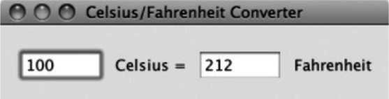
case ButtonClicked(b) =>
nClicks += 1
label.text = "Number of button clicks: " + nClicks
}
}
}
Listing 34.3 - Implementing a reactive Swing application.
The reactions property implements a collection, just like the contents property does. Some components
come with predefined reactions. For instance, a Frame has a predefined reaction that it will close if the
user presses the close button on the upper right. If you install your own reactions by adding them
with += to the reactions property, the reactions you define will be considered in addition to the standard
ones. Conceptually, the handlers installed in reactionsform a stack. In the current example, if
the top frame receives an event, the first handler tried will be the one that matches on ButtonClicked,
because it was the last handler installed for the frame. If the received event is of type ButtonClicked,
the code associated with the pattern will be invoked. After that code has completed, the system will
search for further handlers in the event stack that might also be applicable. If the received event is not
of type ButtonClicked, the event is immediately propagated to the rest of the installed handler stack. It's
also possible to remove handlers from the reaction property, using the -= operator.
Listing 34.3 shows the completed application, including reactions. The code illustrates the essential
elements of a GUI application in Scala's Swing framework: The application consists of a tree of
components, starting with the top frame. The components shown in the code
areFrame, BoxPanel, Button, and Label, but there are many other kinds of components defined in the
Swing libraries. Each component is customized by setting attributes. Two important attributes
are contents, which fixes the children of a component in the tree, and reactions, which determines how
the component reacts to events.
Figure 34.3 - A converter between degrees Celsius and Fahrenheit.
import swing._
import event._
object TempConverter extends SimpleSwingApplication {
def top = new MainFrame {
title = "Celsius/Fahrenheit Converter"
object celsius extends TextField { columns = 5 }
object fahrenheit extends TextField { columns = 5 }
contents = new FlowPanel {
contents += celsius
contents += new Label(" Celsius = ")
contents += fahrenheit
contents += new Label(" Fahrenheit")
border = Swing.EmptyBorder(15, 10, 10, 10)
}
listenTo(celsius, fahrenheit)
reactions += {
case EditDone(`fahrenheit`) =>
val f = fahrenheit.text.toInt
val c = (f - 32) * 5 / 9
celsius.text = c.toString
case EditDone(`celsius`) =>
val c = celsius.text.toInt
val f = c * 9 / 5 + 32
fahrenheit.text = f.toString
}
}
}
Listing 34.4 - An implementation of the temperature converter.
34.4 EXAMPLE: CELSIUS/FAHRENHEIT CONVERTER
As another example, we'll write a GUI program that converts between temperature degrees in Celsius
and Fahrenheit. The user interface of the program is shown in Figure 34.3. It consists of two text fields
(shown in white) with a label following each. One text field shows temperatures in degrees Celsius, the
other in degrees Fahrenheit. Each of the two fields can be edited by the user of the application. Once
the user has changed the temperature in either field, the temperature in the other field should
automatically update.
Listing 34.4 shows the complete code that implements this application. The imports at the top of the
code use a short-hand:
import swing._
import event._
This is in fact equivalent to the imports used before:
import scala.swing._
import scala.swing.event._
The reason you can use the shorthand is that packages nest in Scala. Because packagescala.swing is
contained in package scala, and everything in that package imported automatically, you can write
just swing to refer to the package. Likewise, packagescala.swing.event, is contained as
subpackage event in package scala.swing. Because you have imported everything in scala.swing in the
first import, you can refer to the event package with just event thereafter.
The two components celsius and fahrenheit in TempConverter are objects of class TextField.
ATextField in Swing is a component that lets you edit a single line of text. It has a default width, which
is given in the columns property measured in characters (set to 5 for both fields).
The contents of TempConverter are assembled into a panel, which includes the two text fields and two
labels that explain what the fields are. The panel is of class FlowPanel, which means it displays all its
elements one after another, in one or more rows, depending on the width of the frame.
The reactions of TempConverter are defined by a handler that contains two cases. Each case matches
an EditDone event for one of the two text fields. Such an event gets issued when a text field has been
edited by the user. Note the form of the patterns, which include back ticks around the element names:
case EditDone(`celsius`)
As was explained in Section 15.2, the back ticks around celsius ensure that the pattern matches only if
the source of the event was the celsius object. If you had omitted the back ticks and just
written case EditDone(celsius), the pattern would have matched every event of class EditDone. The
changed field would then be stored in the pattern variable celsius. Obviously, this is not what you want.
Alternatively, you could have defined the two TextFieldobjects starting with upper case
characters, i.e., Celsius and Fahrenheit. In that case you could have matched them directly without back
ticks, as in case EditDone(Celsius).
The two actions of the EditDone events convert one quantity to another. Each starts by reading out the
contents of the modified field and converting it to an Int. It then applies the formula for converting one
temperature degree to the other, and stores the result back as a string in the other text field.
34.5 CONCLUSION
This chapter has given you a first taste of GUI programming, using Scala's wrappers for the Swing
framework. It has shown how to assemble GUI components, how to customize their properties, and
how to handle events. For space reasons, we could discuss only a small number of simple components.
There are many more kinds of components. You can find out about them by consulting the Scala
documentation of the package scala.swing. The next section will develop an example of a more
complicated Swing application.
There are also many tutorials on the original Java Swing framework, on which the Scala wrapper is
based.[1] The Scala wrappers resemble the underlying Swing classes, but try to simplify concepts
where possible and make them more uniform. The simplification makes extensive use of the properties
of the Scala language. For instance, Scala's emulation of properties and its operator overloading allow
convenient property definitions using assignments and += operations. Its "everything is an object"
philosophy makes it possible to inherit the main method of a GUI application. The method can thus be
hidden from user applications, including the boilerplate code for setting things up that comes with it.
Finally, and most importantly, Scala's first-class functions and pattern matching make it possible to
formulate event handling as the reactions component property, which greatly simplifies life for the
application developer.
Footnotes for Chapter 34:
[1] See, for instance, The Java Tutorials. [Jav]

Chapter 35
The SCells Spreadsheet
In the previous chapters you saw many different constructs of the Scala programming language. In this
chapter you'll see how these constructs play together in the implementation of a sizable application.
The task is to write a spreadsheet application, which will be namedSCells.
There are several reasons why this task is interesting. First, everybody knows spreadsheets, so it is easy
to understand what the application should do. Second, spreadsheets are programs that exercise a large
range of different computing tasks. There's the visual aspect, where a spreadsheet is seen as a rich GUI
application. There's the symbolic aspect, having to do with formulas and how to parse and interpret
them. There's the calculational aspect, dealing with how to update possibly large tables incrementally.
There's the reactive aspect, where spreadsheets are seen as programs that react in intricate ways to
events. Finally, there's the component aspect where the application is constructed as a set of reusable
components. All these aspects will be treated in depth in this chapter.
Figure 35.1 - A simple spreadsheet table.
35.1 THE VISUAL FRAMEWORK
We'll start by writing the basic visual framework of the application. Figure 35.1 shows the first iteration
of the user interface. You can see that a spreadsheet is a scrollable table. It has rows going
from 0 to 99 and columns going from A to Z. You express this in Swing by defining a spreadsheet as
a ScrollPane containing a Table. Listing 35.1 shows the code.
package org.stairwaybook.scells
import swing._
class Spreadsheet(val height: Int, val width: Int)
extends ScrollPane {
val table = new Table(height, width) {
rowHeight = 25
autoResizeMode = Table.AutoResizeMode.Off
showGrid = true
gridColor = new java.awt.Color(150, 150, 150)
}
val rowHeader =
new ListView((0 until height) map (_.toString)) {
fixedCellWidth = 30
fixedCellHeight = table.rowHeight
}
viewportView = table
rowHeaderView = rowHeader
}
Listing 35.1 - Code for spreadsheet in Figure 35.1.
The spreadsheet component shown in Listing 35.1 is defined in packageorg.stairwaybook.scells, which
will contain all classes, traits, and objects needed for the application. It imports from
package scala.swing essential elements of Scala's Swing wrapper.Spreadsheet itself is a class that
takes height and width (in numbers of cells) as parameters. The class extends ScrollPane, which gives it
the scroll-bars at the bottom and right in Figure 35.1. It contains two sub-components
named table and rowHeader.
The table component is an instance of an anonymous subclass of class scala.swing.Table. The four lines
in its body set some of its attributes: rowHeight for the height of a table row in
points,autoResizeMode to turn auto-sizing the table off, showGrid to show a grid of lines between
cells, and gridColor to set the color of the grid to a dark gray.
The rowHeader component, which contains the row-number headers at the left of the spreadsheet
in Figure 35.1, is a ListView that displays in its elements the strings 0 through 99.The two lines in its
body fix the width of a cell to be 30 points and the height to be the same as the table's rowHeight.
The whole spreadsheet is assembled by setting two fields in ScrollPane. The field viewportView is set
to the table, and the field rowHeaderView is set to the rowHeader list. The difference between the two
views is that a view port of a scroll pane is the area that scrolls with the two bars, whereas the row
header on the left stays fixed when you move the horizontal scroll bar. By some quirk, Swing already
supplies by default a column header at the top of the table, so there's no need to define one explicitly.
package org.stairwaybook.scells
import swing._
object Main extends SimpleSwingApplication {
def top = new MainFrame {
title = "ScalaSheet"
contents = new Spreadsheet(100, 26)
}
}
Listing 35.2 - The main program for the spreadsheet application.
To try out the rudimentary spreadsheet shown in Listing 35.1, you just need to define a main program
that creates the Spreadsheet component. Such a program is shown in Listing 35.2.
Program Main inherits from SimpleSwingApplication, which takes care of all the low-level details that
need to be set up before a Swing application can be run. You only need to define the top-level window
of the application in the top method. In our example, top is a MainFrame that has two elements defined:
its title, set to "ScalaSheet," and its contents, set to an instance of classSpreadsheet with 100 rows
and 26 columns. That's all. If you launch this application withscala org.stairwaybook.scells.Main, you
should see the spreadsheet in Figure 35.1.
35.2 DISCONNECTING DATA ENTRY AND DISPLAY
If you play a bit with the spreadsheet written so far, you'll quickly notice that the output that's displayed
in a cell is always exactly what you entered in the cell. A real spreadsheet does not behave like that. In
a real spreadsheet, you would enter a formula and you'd see its value. So what is entered into a cell is
different from what is displayed.
package org.stairwaybook.scells
import swing._
class Spreadsheet(val height: Int, val width: Int)
extends ScrollPane {
val cellModel = new Model(height, width)
import cellModel._
val table = new Table(height, width) {
// settings as before...
override def rendererComponent(isSelected: Boolean,
hasFocus: Boolean, row: Int, column: Int): Component =
if (hasFocus) new TextField(userData(row, column))
else
new Label(cells(row)(column).toString) {
xAlignment = Alignment.Right
}
def userData(row: Int, column: Int): String = {
val v = this(row, column)
if (v == null) "" else v.toString
}
}
// rest as before...
}
Listing 35.3 - A spreadsheet with a rendererComponent method.
As a first step to a real spreadsheet application, you should concentrate on disentangling data entry and
display. The basic mechanism for display is contained in the rendererComponentmethod of
class Table. By default, rendererComponent always displays what's entered. If you want to change that,
you need to override rendererComponent to do something different. Listing 35.3shows a new version
of Spreadsheet with a rendererComponent method.
The rendererComponent method overrides a default method in class Table. It takes four parameters.
The isSelected and hasFocus parameters are Booleans that indicate whether the cell has been selected
and whether it has focus, meaning that keyboard events will go into the cell. The remaining two
parameters, row and column, give the cell's coordinates.
The new rendererComponent method checks whether the cell has input focus. If hasFocus is true, the
cell is used for editing. In this case you want to display an editable TextField that contains the data the
user has entered so far. This data is returned by the helper method userData, which displays the
contents of the table at a given row and column. The contents are retrieved by the
call this(row, column).[1] The userData method also takes care to display a null element as the empty
string instead of "null."
So far so good. But what should be displayed if the cell does not have focus? In a real spreadsheet this
would be the value of a cell. Thus, there are really two tables at work. The first table,
named table contains what the user entered. A second "shadow" table contains the internal
representation of cells and what should be displayed. In the spreadsheet example, this table is a two-
dimensional array called cells. If a cell at a given row and column does not have editing focus,
the rendererComponent method will display the element cells(row)(column). The element cannot be
edited, so it should be displayed in a Label instead of in an editableTextField.
It remains to define the internal array of cells. You could do this directly in the Spreadsheetclass, but it's
generally preferable to separate the view of a GUI component from its internal model. That's why in the
example above the cells array is defined in a separate class namedModel. The model is integrated into
the Spreadsheet by defining a value cellModel of type Model. The import clause that follows
this val definition makes the members of cellModel available inside Spreadsheet without having to
prefix them. Listing 35.4 shows a first simplified version of a Model class. The class defines an inner
class, Cell, and a two-dimensional array, cells, ofCell elements. Each element is initialized to be a
fresh Cell.
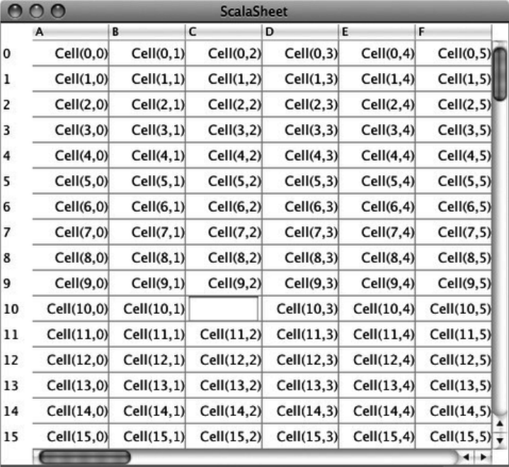
package org.stairwaybook.scells
class Model(val height: Int, val width: Int) {
case class Cell(row: Int, column: Int)
val cells = Array.ofDim[Cell](height, width)
for (i <- 0 until height; j <- 0 until width)
cells(i)(j) = new Cell(i, j)
}
Listing 35.4 - First version of the Model class.
Figure 35.2 - Cells displaying themselves.
That's it. If you compile the modified Spreadsheet class with the Model class and run
the Mainapplication you should see a window as in Figure 35.2.
The objective of this section was to arrive at a design where the displayed value of a cell is different
from the string that was entered into it. This objective has clearly been met, albeit in a very crude way.
In the new spreadsheet you can enter anything you want into a cell, but it will always display just its
coordinates once it loses focus. Clearly, we are not done yet.
35.3 FORMULAS
In reality, a spreadsheet cell holds two things: An actual value and a formula to compute this value.
There are three types of formulas in a spreadsheet:
1. Numeric values such as 1.22, -3, or 0.
2. Textual labels such as Annual sales, Deprecation, or total.
3. Formulas that compute a new value from the contents of cells, such as "=add(A1,B2)", or
"=sum(mul(2, A2), C1:D16)"
A formula that computes a value always starts with an equals sign and is followed by an arithmetic
expression. The SCells spreadsheet has a particularly simple and uniform convention for arithmetic
expressions: every expression is an application of some function to a list of arguments. The function
name is an identifier such as add for binary addition, or sumfor summation of an arbitrary number of
operands. A function argument can be a number, a reference to a cell, a reference to a range of cells
such as C1:D16, or another function application. You'll see later that SCells has an open architecture
that makes it easy to install your own functions via mixin composition.
The first step to handling formulas is writing down the types that represent them. As you might expect,
the different kinds of formulas are represented by case classes. Listing 35.5shows the contents of a file
named Formulas.scala, where these case classes are defined:
package org.stairwaybook.scells
trait Formula
case class Coord(row: Int, column: Int) extends Formula {
override def toString = ('A' + column).toChar.toString + row
}
case class Range(c1: Coord, c2: Coord) extends Formula {
override def toString = c1.toString + ":" + c2.toString
}
case class Number(value: Double) extends Formula {
override def toString = value.toString
}
case class Textual(value: String) extends Formula {
override def toString = value
}
case class Application(function: String,
arguments: List[Formula]) extends Formula {
override def toString =
function + arguments.mkString("(", ",", ")")
}
object Empty extends Textual("")
Listing 35.5 - Classes representing formulas.
Trait Formula, shown in Listing 35.5, has five case classes as children:
Coord for cell coordinates such as A3,
Range for cell ranges such as A3:B17,
Number for floating-point numbers such as 3.1415,
Textual for textual labels such as Deprecation,
Application for function applications such as sum(A1,A2).
Each case class overrides the toString method so that it displays its kind of formula in the standard way
shown above. For convenience there's also an Empty object that represents the contents of an empty
cell. The Empty object is an instance of the Textual class with an empty string argument.
35.4 PARSING FORMULAS
In the previous section you saw the different kinds of formulas and how they display as strings. In this
section you'll see how to reverse the process: to transform a user input string into a Formula tree. The
rest of this section explains one by one the different elements of a classFormulaParsers, which contains
the parsers that do the transformation. The class builds on the combinator framework given in Chapter
33. Specifically, formula parsers are an instance of the RegexParsers class explained in that chapter:
package org.stairwaybook.scells
import scala.util.parsing.combinator._
object FormulaParsers extends RegexParsers {
The first two elements of object FormulaParsers are auxiliary parsers for identifiers and decimal
numbers:
def ident: Parser[String] = """[a-zA-Z_]\w*""".r
def decimal: Parser[String] = """-?\d+(\.\d*)?""".r
As you can see from the first regular expression above, an identifier starts with a letter or
underscore. This is followed by an arbitrary number of "word" characters represented by the regular
expression code \w, which recognizes letters, digits or underscores. The second regular expression
describes decimal numbers, which consist of an optional minus sign, one or more digits that are
represented by regular expression code \d, and an optional decimal part consisting of a period followed
by zero or more digits.
The next element of object FormulaParsers is the cell parser, which recognizes the coordinates of a cell,
such as C11 or B2. It first calls a regular expression parser that determines the form of a coordinate: a
single letter followed by one or more digits. The string returned from that parser is then converted to a
cell coordinate by separating the letter from the numerical part and converting the two parts to indices
for the cell's column and row:
def cell: Parser[Coord] =
"""[A-Za-z]\d+""".r ^^ { s =>
val column = s.charAt(0).toUpper - 'A'
val row = s.substring(1).toInt
Coord(row, column)
}
Note that the cell parser is a bit restrictive in that it allows only column coordinates consisting of a
single letter. Hence the number of spreadsheet columns is in effect restricted to be at most 26, because
further columns cannot be parsed. It's a good idea to generalize the parser so that it accepts cells with
several leading letters. This is left as an exercise to you.
The range parser recognizes a range of cells. Such a range is composed of two cell coordinates with a
colon between them:
def range: Parser[Range] =
cell~":"~cell ^^ {
case c1~":"~c2 => Range(c1, c2)
}
The number parser recognizes a decimal number, which is converted to a Double and wrapped in an
instance of the Number class:
def number: Parser[Number] =
decimal ^^ (d => Number(d.toDouble))
The application parser recognizes a function application. Such an application is composed of an
identifier followed by a list of argument expressions in parentheses:
def application: Parser[Application] =
ident~"("~repsep(expr, ",")~")" ^^ {
case f~"("~ps~")" => Application(f, ps)
}
The expr parser recognizes a formula expression—either a top-level formula following an `=', or an
argument to a function. Such a formula expression is defined to be a cell, a range of cells, a number, or
an application:
def expr: Parser[Formula] =
range | cell | number | application
This definition of the expr parser contains a slight oversimplification because ranges of cells should
only appear as function arguments; they should not be allowed as top-level formulas. You could change
the formula grammar so that the two uses of expressions are separated, and ranges are excluded
syntactically from top-level formulas. In the spreadsheet presented here such an error is instead
detected once an expression is evaluated.
The textual parser recognizes an arbitrary input string, as long as it does not start with an equals sign
(recall that strings that start with `=' are considered to be formulas):
def textual: Parser[Textual] =
"""[^=].*""".r ^^ Textual
The formula parser recognizes all kinds of legal inputs into a cell. A formula is either a number, or
a textual entry, or a formula starting with an equals sign:
def formula: Parser[Formula] =
number | textual | "="~>expr
This concludes the grammar for spreadsheet cells. The final method parse uses this grammar in a
method that converts an input string into a Formula tree:
def parse(input: String): Formula =
parseAll(formula, input) match {
case Success(e, _) => e
case f: NoSuccess => Textual("[" + f.msg + "]")
}
} //end FormulaParsers
The parse method parses all of the input with the formula parser. If that succeeds, the resulting formula
is returned. If it fails, a Textual object with an error message is returned instead.
package org.stairwaybook.scells
import swing._
import event._
class Spreadsheet(val height: Int, val width: Int) ... {
val table = new Table(height, width) {
...
reactions += {
case TableUpdated(table, rows, column) =>
for (row <- rows)
cells(row)(column).formula =
FormulaParsers.parse(userData(row, column))
}
}
}
Listing 35.6 - A spreadsheet that parses formulas.
That's everything there is to parsing formulas. The only thing that remains is to integrate the parser into
the spreadsheet. To do this, you can enrich the Cell class in class Model by a formulafield:
case class Cell(row: Int, column: Int) {
var formula: Formula = Empty
override def toString = formula.toString
}
In the new version of the Cell class, the toString method is defined to display the cell's formula. That
way you can check whether formulas have been correctly parsed.
The last step in this section is to integrate the parser into the spreadsheet. Parsing a formula happens as
a reaction to the user's input into a cell. A completed cell input is modeled in the Swing library by
a TableUpdated event. The TableUpdated class is contained in packagescala.swing.event. The event is
of the form:
TableUpdated(table, rows, column)
It contains the table that was changed, as well as a set of coordinates of affected cells given
byrows and column. The rows parameter is a range value of type Range[Int].[2] The column parameter
is an integer. So in general a TableUpdated event can refer to several affected cells, but they would be
on a consecutive range of rows and share the same column.
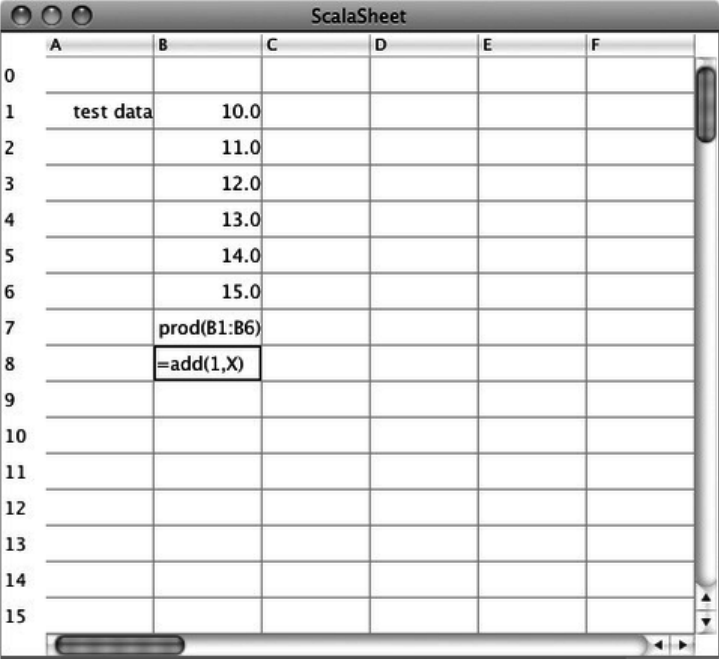
Figure 35.3 - Cells displaying their formulas.
Once a table is changed, the affected cells need to be re-parsed. To react to a TableUpdatedevent, you
add a case to the reactions value of the table component, as is shown in Listing 35.6. Now, whenever
the table is edited the formulas of all affected cells will be updated by parsing the corresponding user
data. When compiling the classes discussed so far and launching the scells.Main application you should
see a spreadsheet application like the one shown in Figure 35.3. You can edit cells by typing into them.
After editing is done, a cell displays the formula it contains. You can also try to type some illegal input
such as the one reading =add(1, X) in the field that has the editing focus in Figure 35.3. Illegal input
will show up as an error message. For instance, once you'd leave the edited field in Figure 35.3 you
should see the error message [`(' expected] in the cell (to see all of the error message you might need to
widen the column by dragging the separation between the column headers to the right).
35.5 EVALUATION
Of course, in the end a spreadsheet should evaluate formulas, not just display them. In this section,
we'll add the necessary components to achieve this.
What's needed is a method, evaluate, which takes a formula and returns the value of that formula in the
current spreadsheet, represented as a Double. We'll place this method in a new trait, Evaluator. The
method needs to access the cells field in class Model to find out about the current values of cells that
are referenced in a formula. On the other hand, the Model class needs to call evaluate. Hence, there's a
mutual dependency between the Model and the Evaluator. A good way to express such mutual
dependencies between classes was shown in Chapter 29: you use inheritance in one direction and self
types in the other.
In the spreadsheet example, class Model inherits from Evaluator and thus gains access to
itsevaluation method. To go the other way, class Evaluator defines its self type to be Model, like this:
package org.stairwaybook.scells
trait Evaluator { this: Model => ...
That way, the this value inside class Evaluator is assumed to be Model and the cells array is accessible
by writing either cells or this.cells.
Now that the wiring is done, we'll concentrate on defining the contents of class Evaluator.Listing
35.7 shows the implementation of the evaluate method. As you might expect, the method contains a
pattern match over the different types of formulas. For a coordinateCoord(row, column), it returns the
value of the cells array at that coordinate. For a numberNumber(v), it returns the value v. For a textual
label Textual(s), it returns zero. Finally, for an application Application(function, arguments), it
computes the values of all arguments, retrieves a function object corresponding to the function name
from an operations table and applies that function to all argument values.
def evaluate(e: Formula): Double = try {
e match {
case Coord(row, column) =>
cells(row)(column).value
case Number(v) =>
v
case Textual(_) =>
0
case Application(function, arguments) =>
val argvals = arguments flatMap evalList
operations(function)(argvals)
}
} catch {
case ex: Exception => Double.NaN
}
Listing 35.7 - The evaluate method of trait Evaluator.
The operations table maps function names to function objects. It is defined as follows:
type Op = List[Double] => Double
val operations = new collection.mutable.HashMap[String, Op]
As you can see from this definition, operations are modeled as functions from lists of values to values.
The Op type introduces a convenient alias for the type of an operation.
The computation in evaluate is wrapped in a try-catch to guard against input errors. There are actually
quite a few things that can go wrong when evaluating a cell formula: coordinates might be out of range;
function names might be undefined; functions might have the wrong number of arguments; arithmetic
operations might be illegal or overflow. The reaction to any of these errors is the same: a "not-a-
number" value is returned. The returned value,Double.NaN, is the IEEE representation for a
computation that does not have a representable floating-point value. This might happen because of an
overflow or a division by zero, for example. The evaluate method of Listing 35.7 chooses to return the
same value also for all other kinds of errors. The advantage of this scheme is that it's simple to
understand and doesn't require much code to implement. Its disadvantage is that all kinds of errors are
lumped together, so a spreadsheet user does not get any detailed feedback on what went wrong. If you
wish you can experiment with more refined ways of representing errors in theSCells application.
The evaluation of arguments is different from the evaluation of top-level formulas. Arguments may be
lists whereas top-level functions may not. For instance, the argument
expression A1:A3 in sum(A1:A3) returns the values of cells A1, A2, A3 in a list. This list is then
passed to the sum operation. It's also possible to mix lists and single values in argument expressions,
for instance the operation sum(A1:A3, 1.0, C7), which would sum up five values. To handle arguments
that might evaluate to lists, there's another evaluation function, calledevalList, which takes a formula
and returns a list of values:
private def evalList(e: Formula): List[Double] = e match {
case Range(_, _) => references(e) map (_.value)
case _ => List(evaluate(e))
}
If the formula argument passed to evalList is a Range, the returned value is a list consisting of the
values of all cells referenced by the range. For every other formula the result is a list consisting of the
single result value of that formula. The cells referenced by a formula are computed by a third
function, references. Here is its definition:
def references(e: Formula): List[Cell] = e match {
case Coord(row, column) =>
List(cells(row)(column))
case Range(Coord(r1, c1), Coord(r2, c2)) =>
for (row <- (r1 to r2).toList; column <- c1 to c2)
yield cells(row)(column)
case Application(function, arguments) =>
arguments flatMap references
case _ =>
List()
}
} // end Evaluator
The references method is actually more general than needed right now in that it computes the list of
cells referenced by any sort of formula, not just a Range formula. It will turn out later that the added
functionality is needed to compute the sets of cells that need updating. The body of the method is a
straightforward pattern match on kinds of formulas. For a coordinateCoord(row, column), it returns a
single-element list containing the cell at that coordinate. For a range expression Range(coord1, coord2),
it returns all cells between the two coordinates, computed by a for expression. For a function
application Application(function, arguments), it returns the cells referenced by each argument
expression, concatenated via flatMap into a single list. For the other two types of
formulas, Textual and Number, it returns an empty list.
35.6 OPERATION LIBRARIES
The class Evaluator itself defines no operations that can be performed on cells: its operationstable is
initially empty. The idea is to define such operations in other traits, which are then mixed into
the Model class. Listing 35.8 shows an example trait that implements common arithmetic operations:
package org.stairwaybook.scells
trait Arithmetic { this: Evaluator =>
operations += (
"add" -> { case List(x, y) => x + y },
"sub" -> { case List(x, y) => x - y },
"div" -> { case List(x, y) => x / y },
"mul" -> { case List(x, y) => x * y },
"mod" -> { case List(x, y) => x % y },
"sum" -> { xs => (0.0 /: xs)(_ + _) },
"prod" -> { xs => (1.0 /: xs)(_ * _) }
)
}
Listing 35.8 - A library for arithmetic operations.
Interestingly, this trait has no exported members. The only thing it does is populate theoperations table
during its initialization. It gets access to that table by using a self typeEvaluator, i.e., by the same
technique the Arithmetic class uses to get access to the model.
Of the seven operations that are defined by the Arithmetic trait, five are binary operations and two take
an arbitrary number of arguments. The binary operations all follow the same schema. For instance, the
addition operation add is defined by the expression:
{ case List(x, y) => x + y }
That is, it expects an argument list consisting of two elements x and y and returns the sum of xand y. If
the argument list contains a number of elements different from two, a MatchError is thrown. This
corresponds to the general "let it crash" philosophy of SCell's evaluation model, where incorrect input
is expected to lead to a runtime exception that then gets caught by the try-catch inside
the evaluation method.
The last two operations, sum and prod, take a list of arguments of arbitrary length and insert a binary
operation between successive elements. So they are instances of the "fold left" schema that's expressed
in class List by the /: operation. For instance, to sum a list of numbersList(x, y, z), the operation
computes 0 + x + y + z. The first operand, 0, is the result if the list is empty.
You can integrate this operation library into the spreadsheet application by mixing theArithmetic trait
into the Model class, like this:
package org.stairwaybook.scells
class Model(val height: Int, val width: Int)
extends Evaluator with Arithmetic {
case class Cell(row: Int, column: Int) {
var formula: Formula = Empty
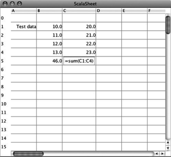
def value = evaluate(formula)
override def toString = formula match {
case Textual(s) => s
case _ => value.toString
}
}
... // rest as before
}
Another change in the Model class concerns the way cells display themselves. In the new version, the
displayed value of a cell depends on its formula. If the formula is a Textual field, the contents of the
field are displayed literally. In all other cases, the formula is evaluated and the result value of that
evaluation is displayed.
Figure 35.4 - Cells that evaluate.
If you compile the changed traits and classes and relaunch the Main program you get something that
starts to resemble a real spreadsheet. Figure 35.4 shows an example. You can enter formulas into cells
and get them to evaluate themselves. For instance, once you close the editing focus on cell C5 in Figure
35.4, you should see 86.0, the result of evaluating the formula sum(C1:C4).
However, there's a crucial element still missing. If you change the value of cell C1 in Figure 35.4 from
20 to 100, the sum in cell C5 will not be automatically updated to 166. You'll have to click
on C5 manually to see a change in its value. What's still missing is a way to have cells recompute their
values automatically after a change.
35.7 CHANGE PROPAGATION
If a cell's value has changed, all cells that depend on that value should have their results recomputed
and redisplayed. The simplest way to achieve this would be to recompute the value of every cell in the
spreadsheet after each change. However such an approach does not scale well as the spreadsheet grows
in size.
A better approach is to recompute the values of only those cells that refer to a changed cell in their
formula. The idea is to use an event-based publish/subscribe framework for change propagation: once a
cell gets assigned a formula, it will subscribe to be notified of all value changes in cells to which the
formula refers. A value change in one of these cells will trigger a re-evaluation of the subscriber cell. If
such a re-evaluation causes a change in the value of the cell, it will in turn notify all cells that depend
on it. The process continues until all cell values have stabilized, i.e., there are no more changes in the
values of any cell.[3]
The publish/subscribe framework is implemented in class Model using the standard event mechanism
of Scala's Swing framework. Here's a new (and final) version of this class:
package org.stairwaybook.scells
import swing._
class Model(val height: Int, val width: Int)
extends Evaluator with Arithmetic {
Compared to the previous version of Model, this version adds a new import of swing._, which makes
Swing's event abstractions directly available.
The main modifications of class Model concern the nested class Cell. Class Cell now inherits
from Publisher, so that it can publish events. The event-handling logic is completely contained in the
setters of two properties: value and formula. Here is Cell's new version:
case class Cell(row: Int, column: Int) extends Publisher {
override def toString = formula match {
case Textual(s) => s
case _ => value.toString
}
To the outside, it looks like value and formula are two variables in class Cell. Their actual
implementation is in terms of two private fields that are equipped with public
getters, valueand formula, and setters, value_= and formula_=. Here are the definitions implementing
the valueproperty:
private var v: Double = 0
def value: Double = v
def value_=(w: Double) = {
if (!(v == w || v.isNaN && w.isNaN)) {
v = w
publish(ValueChanged(this))
}
}
The value_= setter assigns a new value w to the private field v. If the new value is different from the
old one, it also publishes a ValueChanged event with the cell itself as argument. Note that the test
whether the value has changed is a bit tricky because it involves the value NaN. The Java spec says
that NaN is different from every other value, including itself! Therefore, a test whether two values are
the same has to treat NaN specially: two values v, w are the same if they are equal with respect to ==,
or they are both the value NaN, i.e., v.isNaN and w.isNaN both yieldtrue.
Whereas the value_= setter does the publishing in the publish/subscribe framework,
theformula_= setter does the subscribing:
private var f: Formula = Empty
def formula: Formula = f
def formula_=(f: Formula) = {
for (c <- references(formula)) deafTo(c)
this.f = f
for (c <- references(formula)) listenTo(c)
value = evaluate(f)
}
If a cell is assigned a new formula, it first unsubscribes with deafTo from all cells referenced by the
previous formula value. It then stores the new formula in the private variable f and subscribes
with listenTo to all cells referenced by it. Finally, it recomputes its value using the new formula.
The last piece of code in the revised class Cell specifies how to react to a ValueChanged event:
reactions += {
case ValueChanged(_) => value = evaluate(formula)
}
} // end class Cell
The ValueChanged class is also contained in class Model:
case class ValueChanged(cell: Cell) extends event.Event
The rest of class Model is as before:
val cells = Array.ofDim[Cell](height, width)
for (i <- 0 until height; j <- 0 until width)
cells(i)(j) = new Cell(i, j)
} // end class Model
package org.stairwaybook.scells
import swing._, event._
class Spreadsheet(val height: Int, val width: Int)
extends ScrollPane {
val cellModel = new Model(height, width)
import cellModel._
val table = new Table(height, width) {
... // settings as in Listing ???
override def rendererComponent(
isSelected: Boolean, hasFocus: Boolean,
row: Int, column: Int) =
... // as in Listing ???
def userData(row: Int, column: Int): String =
... // as in Listing ???
reactions += {
case TableUpdated(table, rows, column) =>
for (row <- rows)
cells(row)(column).formula =
FormulaParsers.parse(userData(row, column))
case ValueChanged(cell) =>
updateCell(cell.row, cell.column)
}
for (row <- cells; cell <- row) listenTo(cell)
}
val rowHeader = new ListView(0 until height) {
fixedCellWidth = 30
fixedCellHeight = table.rowHeight
}
viewportView = table
rowHeaderView = rowHeader
}
Listing 35.9 - The finished spreadsheet component.
The spreadsheet code is now almost complete. The final piece missing is the re-display of modified
cells. So far, all value propagation concerned the internal Cell values only; the visible table was not
affected. One way to change this would be to add a redraw command to the value_= setter. However,
this would undermine the strict separation between model and view that you have seen so far. A more
modular solution is to notify the table of allValueChanged events and let it do the redrawing
itself. Listing 35.9 shows the final spreadsheet component, which implements this scheme.
Class Spreadsheet of Listing 35.9 has only two new revisions. First, the table component now
subscribes with listenTo to all cells in the model. Second, there's a new case in the table's reactions: if it
is notified of a ValueChanged(cell) event, it demands a redraw of the corresponding cell with a call
of updateCell(cell.row, cell.column).
35.8 CONCLUSION
The spreadsheet developed in this chapter is fully functional, even though at some points it adopts the
simplest solution to implement rather than the most convenient one for the user. That way, it could be
written in just under 200 lines of code. Nevertheless, the architecture of the spreadsheet makes
modifications and extensions easy. In case you would like to experiment with the code a bit further,
here are some suggestions of what you could change or add:
1. You could make the spreadsheet resizable, so that the number of rows and columns can be
changed interactively.
2. You could add new kinds of formulas, for instance binary operations, or other functions.
3. You might think about what to do when cells refer recursively to themselves. For instance, if
cell A1 holds the formula add(B1, 1) and cell B1 holds the formula mul(A1, 2), a re-evaluation
of either cell will trigger a stack-overflow. Clearly, that's not a very good solution. As
alternatives, you could either disallow such a situation, or just compute one iteration each time
one of the cells is touched.
4. You could enhance error handling, giving more detailed messages describing what went wrong.
5. You could add a formula entry field at the top of the spreadsheet, so that long formulas could be
entered more conveniently.
At the beginning of this book we stressed the scalability aspect of Scala. We claimed that the
combination of Scala's object-oriented and functional constructs makes it suitable for programs ranging
from small scripts to very large systems. The spreadsheet presented here is clearly still a small system,
even though it would probably take up much more than 200 lines in most other languages.
Nevertheless, you can see many of the details that make Scala scalable at play in this application.
The spreadsheet uses Scala's classes and traits with their mixin composition to combine its components
in flexible ways. Recursive dependencies between components are expressed using self types. The need
for static state is completely eliminated—the only top-level components that are not classes are formula
trees and formula parsers, and both of these are purely functional. The application also uses higher-
order functions and pattern matching extensively, both for accessing formulas and for event handling.
So it is a good showcase of how functional and object-oriented programming can be combined
smoothly.
One important reason why the spreadsheet application is so concise is that it can base itself on powerful
libraries. The parser combinator library provides in effect an internal domain-specific language for
writing parsers. Without it, parsing formulas would have been much more difficult. The event handling
in Scala's Swing libraries is a good example of the power of control abstractions. If you know Java's
Swing libraries, you probably appreciate the conciseness of Scala's reactions concept, particularly when
compared to the tedium of writing notify methods and implementing listener interfaces in the classical
publish/subscribe design pattern. So the spreadsheet demonstrates the benefits of extensibility, where
high-level libraries can be made to look just like language extensions.
Footnotes for Chapter 35:
[1] Although "this(row, column)" may look similar to a constructor invocation, it is in this case an
invocation of the apply method on the current Table instance.
[2] Range[Int] is also the type of a Scala expression such as "1 to N".
[3] This assumes that there are no cyclic dependencies between cells. We discuss dropping this
assumption at the end of this chapter.
Appendix A
Scala Scripts on Unix and Windows
If you're on some flavor of Unix, you can run a Scala script as a shell script by prepending a "pound
bang" directive at the top of the file. For example, type the following into a file namedhelloarg:
#!/bin/sh
exec scala "$0" "$@"
!#
// Say hello to the first argument
println("Hello, " + args(0) + "!")
The initial #!/bin/sh must be the very first line in the file. Once you set its execute permission:
$ chmod +x helloarg
You can run the Scala script as a shell script by simply saying:
$ ./helloarg globe
If you're on Windows, you can achieve the same effect by naming the file helloarg.bat and placing this
at the top of your script:
::#!
@echo off
call scala %0 %*
goto :eof
::!#
Glossary
algebraic data type A type defined by providing several alternatives, each of which comes with its
own constructor. It usually comes with a way to decompose the type through pattern matching. The
concept is found in specification languages and functional programming languages. Algebraic data
types can be emulated in Scala with case classes.
alternative A branch of a match expression. It has the form "case pattern => expression." Another
name for alternative is case.
annotation An annotation appears in source code and is attached to some part of the syntax.
Annotations are computer processable, so you can use them to effectively add an extension to Scala.
anonymous class An anonymous class is a synthetic subclass generated by the Scala compiler from
a new expression in which the class or trait name is followed by curly braces. The curly braces contains
the body of the anonymous subclass, which may be empty. However, if the name following new refers
to a trait or class that contains abstract members, these must be made concrete inside the curly braces
that define the body of the anonymous subclass.
anonymous function Another name for function literal.
apply You can apply a method, function, or closure to arguments, which means you invoke it on those
arguments.
argument When a function is invoked, an argument is passed for each parameter of that function. The
parameter is the variable that refers to the argument. The argument is the object passed at invocation
time. In addition, applications can take (command line) arguments that show up in
the Array[String] passed to main methods of singleton objects.
assign You can assign an object to a variable. Afterwards, the variable will refer to the object.
auxiliary constructor Extra constructors defined inside the curly braces of the class definition, which
look like method definitions named this, but with no result type.
block One or more expressions and declarations surrounded by curly braces. When the block
evaluates, all of its expressions and declarations are processed in order, and then the block returns the
value of the last expression as its own value. Blocks are commonly used as the bodies of
functions, for expressions, while loops, and any other place where you want to group a number of
statements together. More formally, a block is an encapsulation construct for which you can only see
side effects and a result value. The curly braces in which you define a class or object do not, therefore,
form a block, because fields and methods (which are defined inside those curly braces) are visible from
the outside. Such curly braces form atemplate.
bound variable A bound variable of an expression is a variable that's both used and defined inside the
expression. For instance, in the function literal expression (x: Int) => (x, y), both variables x and y are
used, but only x is bound, because it is defined in the expression as an Int and the sole argument to the
function described by the expression.
by-name parameter A parameter that is marked with a => in front of the parameter
type,e.g., (x: => Int). The argument corresponding to a by-name parameter is evaluated not before the
method is invoked, but each time the parameter is referenced by name inside the method. If a parameter
is not by-name, it is by-value.
by-value parameter A parameter that is not marked with a => in front of the parameter
type, e.g., (x: Int). The argument corresponding to a by-value parameter is evaluated before the method
is invoked. By-value parameters contrast with by-name parameters.
class Defined with the class keyword, a class may either be abstract or concrete, and may be
parameterized with types and values when instantiated. In "new Array[String](2)", the class being
instantiated is Array and the type of the value that results is Array[String]. A class that takes type
parameters is called a type constructor. A type can be said to have a class as well, as in: the class of
type Array[String] is Array.
closure A function object that captures free variables, and is said to be "closed" over the variables
visible at the time it is created.
companion class A class that shares the same name with a singleton object defined in the same source
file. The class is the singleton object's companion class.
companion object A singleton object that shares the same name with a class defined in the same source
file. Companion objects and classes have access to each other's private members. In addition, any
implicit conversions defined in the companion object will be in scope anywhere the class is used.
contravariant A contravariant annotation can be applied to a type parameter of a class or trait by
putting a minus sign (-) before the type parameter. The class or trait then subtypes contravariantly with
—in the opposite direction as—the type annotated parameter. For example, Function1 is contravariant
in its first type parameter, and so Function1[Any, Any] is a subtype of Function1[String, Any].
covariant A covariant annotation can be applied to a type parameter of a class or trait by putting a plus
sign (+) before the type parameter. The class or trait then subtypes covariantly with—in the same
direction as—the type annotated parameter. For example, List is covariant in its type parameter,
so List[String] is a subtype of List[Any].
currying A way to write functions with multiple parameter lists. For instance def f(x: Int)(y: Int) is a
curried function with two parameter lists. A curried function is applied by passing several arguments
lists, as in: f(3)(4). However, it is also possible to write a partial application of a curried function, such
as f(3).
declare You can declare an abstract field, method, or type, which gives an entity a name but not an
implementation. The key difference between declarations and definitions is that definitions establish an
implementation for the named entity, declarations do not.
define To define something in a Scala program is to give it a name and an implementation. You can
define classes, traits, singleton objects, fields, methods, local functions, local variables, etc. Because
definitions always involve some kind of implementation, abstract members are declared not defined.
direct subclass A class is a direct subclass of its direct superclass.
direct superclass The class from which a class or trait is immediately derived, the nearest class above
it in its inheritance hierarchy. If a class Parent is mentioned in a class Child's optional extends clause,
then Parent is the direct superclass of Child. If a trait is mentioned inChild's extends clause, the trait's
direct superclass is the Child's direct superclass. If Child has no extends clause, then AnyRef is the
direct superclass of Child. If a class's direct superclass takes type parameters, for
example class Child extends Parent[String], the direct superclass ofChild is still Parent,
not Parent[String]. On the other hand, Parent[String] would be the directsupertype of Child.
See supertype for more discussion of the distinction between class and type.
equality When used without qualification, equality is the relation between values expressed by `=='.
See also reference equality.
expression Any bit of Scala code that yields a result. You can also say that an expressionevaluates to a
result or results in a value.
filter An if followed by a boolean expression in a for expression. Infor(i <- 1 to 10; if i % 2 == 0), the
filter is "if i % 2 == 0". The value to the right of the if is the filter expression.
filter expression A filter expression is the boolean expression following an if in a forexpression.
In for(i <- 1 to 10; if i % 2 == 0), the filter expression is "i % 2 == 0".
first-class function Scala supports first-class functions, which means you can express functions
in function literal syntax, i.e., (x: Int) => x + 1, and that functions can be represented by objects, which
are called function values.
for comprehension Another name for for expression.
free variable A free variable of an expression is a variable that's used inside the expression but not
defined inside the expression. For instance, in the function literal expression (x: Int) => (x, y), both
variables x and y are used, but only y is a free variable, because it is not defined inside the expression.
function A function can be invoked with a list of arguments to produce a result. A function has a
parameter list, a body, and a result type. Functions that are members of a class, trait, or singleton object
are called methods. Functions defined inside other functions are called local functions. Functions with
the result type of Unit are called procedures. Anonymous functions in source code are called function
literals. At run time, function literals are instantiated into objects called function values.
function literal A function with no name in Scala source code, specified with function literal syntax.
For example, (x: Int, y: Int) => x + y.
function value A function object that can be invoked just like any other function. A function value's
class extends one of the FunctionN traits (e.g., Function0, Function1) from package scala, and is
usually expressed in source code via function literal syntax. A function value is "invoked" when
its apply method is called. A function value that captures free variables is a closure.
functional style The functional style of programming emphasizes functions and evaluation results and
deemphasizes the order in which operations occur. The style is characterized by passing function values
into looping methods, immutable data, methods with no side effects. It is the dominant paradigm of
languages such as Haskell and Erlang, and contrasts with the imperative style.
generator A generator defines a named val and assigns to it a series of values in a forexpression. For
example, in for(i <- 1 to 10), the generator is "i <- 1 to 10". The value to the right of the <- is
the generator expression.
generator expression A generator expression generates a series of values in a forexpression. For
example, in for(i <- 1 to 10), the generator expression is "1 to 10".
generic class A class that takes type parameters. For example, because scala.List takes a type
parameter, scala.List is a generic class.
generic trait A trait that takes type parameters. For example, because traitscala.collection.Set takes a
type parameter, it is a generic trait.
helper function A function whose purpose is to provide a service to one or more other functions
nearby. Helper functions are often implemented as local functions.
helper method A helper function that's a member of a class. Helper methods are often private.
immutable An object is immutable if its value cannot be changed after it is created in any way visible
to clients. Objects may or may not be immutable.
imperative style The imperative style of programming emphasizes careful sequencing of operations so
that their effects happen in the right order. The style is characterized by iteration with loops, mutating
data in place, and methods with side effects. It is the dominant paradigm of languages such as C, C++,
C# and Java, and contrasts with the functional style.
initialize When a variable is defined in Scala source code, you must initialize it with an object.
instance An instance, or class instance, is an object, a concept that exists only at run time.
instantiate To instantiate a class is to make a new object from the class, an action that happens only at
run time.
invariant Invariant is used in two ways. It can mean a property that always holds true when a data
structure is well-formed. For example, it is an invariant of a sorted binary tree that each node is ordered
before its right subnode, if it has a right subnode. Invariant is also sometimes used as a synonym for
nonvariant: "class Array is invariant in its type parameter."
invoke You can invoke a method, function, or closure on arguments, meaning its body will be
executed with the specified arguments.
JVM The JVM is the Java Virtual Machine, or runtime, that hosts a running Scala program.
literal 1, "One", and (x: Int) => x + 1 are examples of literals. A literal is a shorthand way to describe
an object, where the shorthand exactly mirrors the structure of the created object.
local function A local function is a def defined inside a block. To contrast, a def defined as a member
of a class, trait, or singleton object is called a method.
local variable A local variable is a val or var defined inside a block. Although similar to local
variables, parameters to functions are not referred to as local variables, but simply as parameters or
"variables" without the "local."
member A member is any named element of the template of a class, trait, or singleton object. A
member may be accessed with the name of its owner, a dot, and its simple name. For example, top-
level fields and methods defined in a class are members of that class. A trait defined inside a class is a
member of its enclosing class. A type defined with the type keyword in a class is a member of that
class. A class is a member of the package in which is it defined. By contrast, a local variable or local
function is not a member of its surrounding block.
message Actors communicate with each other by sending each other messages. Sending a message
does not interrupt what the receiver is doing. The receiver can wait until it has finished its current
activity and its invariants have been reestablished.
meta-programming Meta-programming software is software whose input is itself software. Compilers
are meta-programs, as are tools like scaladoc. Meta-programming software is required in order to do
anything with an annotation.
method A method is a function that is a member of some class, trait, or singleton object.
mixin Mixin is what a trait is called when it is being used in a mixin composition. In other words, in
"trait Hat," Hat is just a trait, but in "new Cat extends AnyRef with Hat," Hat can be called a mixin.
When used as a verb, "mix in" is two words. For example, you can mix traits into classes or other traits.
mixin composition The process of mixing traits into classes or other traits. Mixin composition differs
from traditional multiple inheritance in that the type of the superreference is not known at the point the
trait is defined, but rather is determined anew each time the trait is mixed into a class or other trait.
modifier A keyword that qualifies a class, trait, field, or method definition in some way. For example,
the private modifier indicates that a class, trait, field, or method being defined is private.
multiple definitions The same expression can be assigned in multiple definitions if you use the
syntax val v1, v2, v3 = exp.
nonvariant A type parameter of a class or trait is by default nonvariant. The class or trait then does not
subtype when that parameter changes. For example, because class Array is nonvariant in its type
parameter, Array[String] is neither a subtype nor a supertype ofArray[Any].
operation In Scala, every operation is a method call. Methods may be invoked in operator notation,
such as b + 2, and when in that notation, + is an operator.
parameter Functions may take zero to many parameters. Each parameter has a name and a type.
The distinction between parameters and arguments is that arguments refer to the actual objects passed
when a function is invoked. Parameters are the variables that refer to those passed arguments.
parameterless function A function that takes no parameters, which is defined without any empty
parentheses. Invocations of parameterless functions may not supply parentheses. This supports
the uniform access principle, which enables the def to be changed into a valwithout requiring a change
to client code.
parameterless method A parameterless method is a parameterless function that is a member of a class,
trait, or singleton object.
parametric field A field defined as a class parameter.
partially applied function A function that's used in an expression and that misses some of its
arguments. For instance, if function f has type Int => Int => Int, then f and f(1) arepartially applied
functions.
path-dependent type A type like swiss.cow.Food. The swiss.cow part is a path that forms a reference
to an object. The meaning of the type is sensitive to the path you use to access it. The
types swiss.cow.Food and fish.Food, for example, are different types.
pattern In a match expression alternative, a pattern follows each case keyword and precedes either
a pattern guard or the => symbol.
pattern guard In a match expression alternative, a pattern guard can follow a pattern. For example, in
"case x if x % 2 == 0 => x + 1", the pattern guard is "if x % 2 == 0". A case with a pattern guard will
only be selected if the pattern matches and the pattern guard yields true.
predicate A predicate is a function with a Boolean result type.
primary constructor The main constructor of a class, which invokes a superclass constructor, if
necessary, initializes fields to passed values, and executes any top-level code defined between the curly
braces of the class. Fields are initialized only for value parameters not passed to the superclass
constructor, except for any that are not used in the body of the class and can therefore be optimized
away.
procedure A procedure is a function with result type of Unit, which is therefore executed solely for its
side effects.
reassignable A variable may or may not be reassignable. A var is reassignable while a val is not.
recursive A function is recursive if it calls itself. If the only place the function calls itself is the last
expression of the function, then the function is tail recursive.
reference A reference is the Java abstraction of a pointer, which uniquely identifies an object that
resides on the JVM's heap. Reference type variables hold references to objects, because reference types
(instances of AnyRef) are implemented as Java objects that reside on the JVM's heap. Value type
variables, by contrast, may sometimes hold a reference (to a boxed wrapper type) and sometimes not
(when the object is being represented as a primitive value). Speaking generally, a Scala
variable refers to an object. The term "refers" is more abstract than "holds a reference." If a variable of
type scala.Int is currently represented as a primitive Java int value, then that variable still refers to
the Int object, but no reference is involved.
reference equality Reference equality means that two references identify the very same Java object.
Reference equality can be determined, for reference types only, by calling eq inAnyRef. (In Java
programs, reference equality can be determined using == on Java reference types.)
reference type A reference type is a subclass of AnyRef. Instances of reference types always reside on
the JVM's heap at run time.
referential transparency A property of functions that are independent of temporal context and have no
side effects. For a particular input, an invocation of a referentially transparent function can be replaced
by its result without changing the program semantics.
refers A variable in a running Scala program always refers to some object. Even if that variable is
assigned to null, it conceptually refers to the Null object. At runtime, an object may be implemented by
a Java object or a value of a primitive type, but Scala allows programmers to think at a higher level of
abstraction about their code as they imagine it running. See alsoreference.
refinement type A type formed by supplying a base type a number of members inside curly braces.
The members in the curly braces refine the types that are present in the base type. For example, the
type of "animal that eats grass" is Animal { type SuitableFood = Grass }.
result An expression in a Scala program yields a result. The result of every expression in Scala is an
object.
result type A method's result type is the type of the value that results from calling the method. (In Java,
this concept is called the return type.)
return A function in a Scala program returns a value. You can call this value the result of the function.
You can also say the function results in the value. The result of every function in Scala is an object.
runtime The Java Virtual Machine, or JVM, that hosts a running Scala program. Runtimeencompasses
both the virtual machine, as defined by the Java Virtual Machine Specification, and the runtime
libraries of the Java API and the standard Scala API. The phrase at run time(with a space
between run and time) means when the program is running, and contrasts with compile time.
runtime type The type of an object at run time. To contrast, a static type is the type of an expression at
compile time. Most runtime types are simply bare classes with no type parameters. For example, the
runtime type of "Hi" is String, and the runtime type of(x: Int) => x + 1 is Function1. Runtime types can
be tested with isInstanceOf.
script A file containing top level definitions and statements, which can be run directly
withscala without explicitly compiling. A script must end in an expression, not a definition.
selector The value being matched on in a match expression. For example, in "s match { case _ => }",
the selector is s.
self type A self type of a trait is the assumed type of this, the receiver, to be used within the trait. Any
concrete class that mixes in the trait must ensure that its type conforms to the trait's self type. The most
common use of self types is for dividing a large class into several traits as described in Chapter 29.
semi-structured data XML data is semi-structured. It is more structured than a flat binary file or text
file, but it does not have the full structure of a programming language's data structures.
serialization You can serialize an object into a byte stream which can then be saved to files or
transmitted over the network. You can later deserialize the byte stream, even on different computer, and
obtain an object that is the same as the original serialized object.
shadow A new declaration of a local variable shadows one of the same name in an enclosing scope.
signature Signature is short for type signature.
singleton object An object defined with the object keyword. Each singleton object has one and only
one instance. A singleton object that shares its name with a class, and is defined in the same source file
as that class, is that class's companion object. The class is its companion class. A singleton object that
doesn't have a companion class is a standalone object.
standalone object A singleton object that has no companion class.
statement An expression, definition, or import, i.e., things that can go into a template or a block in
Scala source code.
static type See type.
subclass A class is a subclass of all of its superclasses and supertraits.
subtrait A trait is a subtrait of all of its supertraits.
subtype The Scala compiler will allow any of a type's subtypes to be used as a substitute wherever that
type is required. For classes and traits that take no type parameters, the subtype relationship mirrors the
subclass relationship. For example, if class Cat is a subclass of abstract class Animal, and neither takes
type parameters, type Cat is a subtype of type Animal. Likewise, if trait Apple is a subtrait of
trait Fruit, and neither takes type parameters, type Appleis a subtype of type Fruit. For classes and traits
that take type parameters, however, variance comes into play. For example, because abstract
class List is declared to be covariant in its lone type parameter (i.e., List is
declared List[+A]), List[Cat] is a subtype of List[Animal], andList[Apple] a subtype of List[Fruit].
These subtype relationships exist even though the class of each of these types is List. By contrast,
because Set is not declared to be covariant in its type parameter (i.e., Set is declared Set[A] with no
plus sign), Set[Cat] is not a subtype of Set[Animal]. A subtype should correctly implement the
contracts of its supertypes, so that the Liskov Substitution Principle applies, but the compiler only
verifies this property at the level of type checking.
superclass A class's superclasses include its direct superclass, its direct superclass's direct superclass,
and so on, all the way up to Any.
supertrait A class's or trait's supertraits, if any, include all traits directly mixed into the class or trait or
any of its superclasses, plus any supertraits of those traits.
supertype A type is a supertype of all of its subtypes.
synthetic class A synthetic class is generated automatically by the compiler rather than being written
by hand by the programmer.
tail recursive A function is tail recursive if the only place the function calls itself is the last operation
of the function.
target typing Target typing is a form of type inference that takes into account the type that's expected.
In nums.filter((x) => x > 0), for example, the Scala compiler infers type of x to be the element type
of nums, because the filter method invokes the function on each element of nums.
template A template is the body of a class, trait, or singleton object definition. It defines the type
signature, behavior, and initial state of the class, trait, or object.
trait A trait, which is defined with the trait keyword, is like an abstract class that cannot take any
value parameters and can be "mixed into" classes or other traits via the process known as mixin
composition. When a trait is being mixed into a class or trait, it is called amixin. A trait may be
parameterized with one or more types. When parameterized with types, the trait constructs a type. For
example, Set is a trait that takes a single type parameter, whereas Set[Int] is a type. Also, Set is said to
be "the trait of" type Set[Int].
type Every variable and expression in a Scala program has a type that is known at compile time. A
type restricts the possible values to which a variable can refer, or an expression can produce, at run
time. A variable or expression's type can also be referred to as a static type if necessary to differentiate
it from an object's runtime type. In other words, "type" by itself means static type. Type is distinct from
class because a class that takes type parameters can construct many types. For example, List is a class,
but not a type. List[T] is a type with a free type parameter. List[Int] and List[String] are also types
(called ground types because they have no free type parameters). A type can have a "class" or "trait."
For example, the class of type List[Int] is List. The trait of type Set[String] is Set.
type constraint Some annotations are type constraints, meaning that they add additional limits, or
constraints, on what values the type includes. For example, @positive could be a type constraint on the
type Int, limiting the type of 32-bit integers down to those that are positive. Type constraints are not
checked by the standard Scala compiler, but must instead be checked by an extra tool or by a compiler
plugin.
type constructor A class or trait that takes type parameters.
type parameter A parameter to a generic class or generic method that must be filled in by a type. For
example, class List is defined as "class List[T] { ...", and method identity, a member of object Predef, is
defined as "def identity[T](x:T) = x". The T in both cases is a type parameter.
type signature A method's type signature comprises its name, the number, order, and types of its
parameters, if any, and its result type. The type signature of a class, trait, or singleton object comprises
its name, the type signatures of all of its members and constructors, and its declared inheritance and
mixin relations.
uniform access principle The uniform access principle states that variables and parameterless
functions should be accessed using the same syntax. Scala supports this principle by not allowing
parentheses to be placed at call sites of parameterless functions. As a result, a parameterless function
definition can be changed to a val, or vice versa, without affecting client code.
unreachable At the Scala level, objects can become unreachable, at which point the memory they
occupy may be reclaimed by the runtime. Unreachable does not necessarily mean unreferenced.
Reference types (instances of AnyRef) are implemented as objects that reside on the JVM's heap. When
an instance of a reference type becomes unreachable, it indeed becomes unreferenced, and is available
for garbage collection. Value types (instances of AnyVal) are implemented as both primitive type
values and as instances of Java wrapper types (such as java.lang.Integer), which reside on the heap.
Value type instances can be boxed (converted from a primitive value to a wrapper object) and unboxed
(converted from a wrapper object to a primitive value) throughout the lifetime of the variables that refer
to them. If a value type instance currently represented as a wrapper object on the JVM's heap becomes
unreachable, it indeed becomes unreferenced, and is available for garbage collection. But if a value
type currently represented as a primitive value becomes unreachable, then it does not become
unreferenced, because it does not exist as an object on the JVM's heap at that point in time. The
runtime may reclaim memory occupied by unreachable objects, but if an Int, for example, is
implemented at run time by a primitive Java int that occupies some memory in the stack frame of an
executing method, then the memory for that object is "reclaimed" when the stack frame is popped as
the method completes. Memory for reference types, such as Strings, may be reclaimed by the JVM's
garbage collector after they become unreachable.
unreferenced See unreachable.
value The result of any computation or expression in Scala is a value, and in Scala, every value is an
object. The term value essentially means the image of an object in memory (on the JVM's heap or
stack).
value type A value type is any subclass of AnyVal, such as Int, Double, or Unit. This term has
meaning at the level of Scala source code. At runtime, instances of value types that correspond to Java
primitive types may be implemented in terms of primitive type values or instances of wrapper types,
such as java.lang.Integer. Over the lifetime of a value type instance, the runtime may transform it back
and forth between primitive and wrapper types (i.e., to box and unbox it).
variable A named entity that refers to an object. A variable is either a val or a var. Both vals and vars
must be initialized when defined, but only vars can be later reassigned to refer to a different object.
variance A type parameter of a class or trait can be marked with a variance annotation,
either covariant (+) or contravariant (-). Such variance annotations indicate how subtyping works for a
generic class or trait. For example, the generic class List is covariant in its type parameter, and
thus List[String] is a subtype of List[Any]. By default, i.e., absent a + or -annotation, type parameters
are nonvariant.
wildcard type A wildcard type includes references to type variables that are unknown. For
example, Array[_] is a wildcard type. It is an array where the element type is completely unknown.
yield An expression can yield a result. The yield keyword designates the result of a forexpression.
Bibliography
[Ray99] Raymond, Eric. The Cathedral & the Bazaar: Musings on Linux and Open Source by an
Accidental Revolutionary. O'Reilly, 1999.
[Blo08] Bloch, Joshua. Effective Java Second Edition. Addison-Wesley, 2008.
[Bay72] Bayer, Rudolf. Symmetric binary B-Trees: Data structure and maintenance algorithms. Acta
Informatica, 1(4):290-306, 1972.
[Mor68] Morrison, Donald R. PATRICIA-Practical Algorithm To Retrieve Information Coded in
Alphanumeric. J. ACM, 15(4):514-534, 1968. ISSN 0004-5411.
http://doi.acm.org/10.1145/321479.321481. [ DOI ]
[DeR75] DeRemer, Frank and Hans Kron. Programming-in-the large versus programming-in-the-
small. In Proceedings of the international conference on Reliable software, pages 114-121.
ACM, New York, NY, USA, 1975. http://doi.acm.org/10.1145/800027.808431. [ DOI ]
[SPJ02] Simon Peyton Jones, et.al. Haskell 98 Language and Libraries, Revised Report. Technical
report, http://www.haskell.org/onlinereport, 2002.
[Vaz07] Vaziri, Mandana, Frank Tip, Stephen Fink, and Julian Dolby. Declarative Object Identity
Using Relation Types. In Proc. ECOOP 2007, pages 54-78. 2007.
[Mey91] Meyers, Scott. Effective C++. Addison-Wesley, 1991.
[Rum04] Rumbaugh, James, Ivar Jacobson, and Grady Booch. The Unified Modeling Language
Reference Manual (2nd Edition). Addison-Wesley, 2004.
[Goe06] Goetz, Brian, Tim Peierls, Joshua Bloch, Joseph Bowbeer, David Homes, and Doug
Lea. Java Concurrency in Practice. Addison Wesley, 2006.
[Mey00] Meyer, Bertrand. Object-Oriented Software Construction. Prentice Hall, 2000.
[Eck98] Eckel, Bruce. Thinking in Java. Prentice Hall, 1998.
[Eva03] Evans, Eric. Domain-Driven Design: Tackling Complexity in the Heart of Software. Addison-
Wesley Professional, 2003.
[Aho86] Aho, Alfred V., Ravi Sethi, and Jeffrey D. Ullman. Compilers: Principles, Techniques, and
Tools. Addison-Wesley Longman Publishing Co., Inc., Boston, MA, USA, 1986. ISBN 0-
201-10088-6.
[Abe96] Abelson, Harold and Gerald Jay Sussman. Structure and Interpretation of Computer
Programs. The MIT Press, second edition, 1996.
[Ode03] Odersky, Martin, Vincent Cremet, Christine Röckl, and Matthias Zenger. A Nominal Theory
of Objects with Dependent Types. In Proc. ECOOP'03, Springer LNCS, pages 201-225. July
2003.
[Ode11] Odersky, Martin. The Scala Language Specification, Version 2.9. EPFL, May 2011. Available
on the web at http://www.scala-lang.org/docu/manuals.html (accessed April 20, 2014).
[Ode05] Odersky, Martin and Matthias Zenger. Scalable Component Abstractions. In Proceedings of
OOPSLA, pages 41-58. October 2005.
[Emi07] Emir, Burak, Martin Odersky, and John Williams. Matching Objects With Patterns. In Proc.
ECOOP, Springer LNCS, pages 273-295. July 2007.
[Ste99] Steele, Jr., Guy L. Growing a Language. Higher-Order and Symbolic Computation, 12:221-
223, 1999. Transcript of a talk given at OOPSLA 1998.
[Kay96] Kay, Alan C. The Early History of Smalltalk. In History of programming languages-II, pages
511-598. ACM, New York, NY, USA, 1996. ISBN 0-201-89502-1.
http://doi.acm.org/10.1145/234286.1057828. [ DOI ]
[Jav] The Java Tutorials: Creating a GUI with JFC/Swing. Available on the web at
http://java.sun.com/docs/books/tutorial/uiswing.
[Lan66] Landin, Peter J. The Next 700 Programming Languages.Communications of the ACM,
9(3):157-166, 1966.
[Fow04] Fowler, Martin. Inversion of Control Containers and the Dependency Injection pattern.
January 2004. Available on the web at http://martinfowler.com/articles/injection.html
(accesssed August 6, 2008).
[Gam95] Gamma, Erich, Richard Helm, Ralph Johnson, and John Vlissides.Design Patterns :
Elements of Reusable Object-Oriented Software. Addison-Wesley, 1995.
[Kay03] Kay, Alan C. An email to Stefan Ram on the meaning of the term “object-oriented
programming”, July 2003. The email is published on the web at
http://www.purl.org/stefan_ram/pub/doc_kay_oop_en (accesssed June 6, 2008).
[Dij70] Dijkstra, Edsger W. Notes on Structured Programming., April 1970. Circulated privately.
Available at http://www.cs.utexas.edu /users/EWD/ewd02xx/EWD249.PDF as EWD249
(accessed June 6, 2008).
About the Authors
Martin Odersky is the creator of the Scala language. He is a professor at EPFL in Lausanne,
Switzerland, and a founder of Typesafe, Inc. He works on programming languages and systems, more
specifically on the topic of how to combine object-oriented and functional programming. Since 2001 he
has concentrated on designing, implementing, and refining Scala. Previously, he has influenced the
development of Java as a co-designer of Java generics and as the original author of the
current javac reference compiler. He is a fellow of the ACM.
Lex Spoon is a software engineer at Semmle, Ltd. He worked on Scala for two years as a post-doc at
EPFL. He has a Ph.D. from Georgia Tech, where he worked on static analysis of dynamic languages. In
addition to Scala, he has helped develop a wide variety of programming languages, including the
dynamic language Smalltalk, the scientific language X10, and the logic language that powers Semmle.
He and his wife live in Atlanta with two cats and a chihuahua.
Bill Venners is president of Artima, Inc., publisher of the Artima Developer website (www.artima.com),
and cofounder of Escalate Software, LLC. He is author of the book, Inside the Java Virtual Machine, a
programmer-oriented survey of the Java platform's architecture and internals. His popular columns in
JavaWorld magazine covered Java internals, object-oriented design, and Jini. Active in the Jini
Community since its inception, Bill led the Jini Community's ServiceUI project, whose ServiceUI API
became the de facto standard way to associate user interfaces to Jini services. Bill is also the lead
developer and designer of ScalaTest, an open source testing tool for Scala and Java developers.
