Proj3 Instructions
Proj3_Instructions
User Manual:
Open the PDF directly: View PDF ![]() .
.
Page Count: 20

Technische Universität München
MIMO Systems Programming Project 3
Instructions
Michael Newinger, M.Sc.
Dr.-Ing. Michael Joham
WS 2018/19
Fakultät für Elektrotechnik und Informationstechnik
Professur für Methoden der Signalverarbeitung
Univ.-Prof. Dr.-Ing. Wolfgang Utschick
©2019 Professur für Methoden der Signalverarbeitung, Technische Universität München
All rights reserved. Personnel and students at universities only may copy the material for their personal use and for
educational purposes with proper referencing. The distribution to and copying by other persons and organizations as
well as any commercial usage is not allowed without the written permission by the publisher.
Professur für Methoden der Signalverarbeitung
Technische Universität München
80290 München
http://www.msv.ei.tum.de
Contents
3 Broadcast Channel 4
3.1 Capacity of the MIMO Broadcast Channel . . . . . . . . . . . . . . . . 4
3.1.1 Dual MIMO Multiple Access Channel . . . . . . . . . . . . . . . 6
3.1.2 Sum-Rate optimization for the MIMO BC . . . . . . . . . . . . . 10
3.1.3 Sato’s Bound . . . . . . . . . . . . . . . . . . . . . . . . . . . 13
3.2 Block Diagonalization Precoding . . . . . . . . . . . . . . . . . . . . . 17
3
Chapter 3
Broadcast Channel
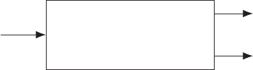
The third project considers the K-user broadcast channel (BC), where one transmitter
sends information to
K
receivers. A BC with input
x
, outputs
y1
,
y2
, ...
yK
, and
the transition probability density function
fy1,...,yK|x(y1,...,yK|x)
is depicted in
Fig. 3.1.
xfy1,...,yK|x(y1,...,yK|x)
yK
.
.
.
y1
Figure 3.1: K-user Broadcast Channel
In the following tasks, the Gaussian MIMO BC is considered, where we analyze the
capacity region, which depends only on the conditional marginals fyk|x(yk|x),∀k.
3.1 Capacity of the MIMO Broadcast Channel
A model of the Gaussian MIMO BC is shown in Fig. 3.2a, where the transmit signal
x∈CNis sent to Kreceivers. The received signals read as
yk=Hkx+nk∈CM, k ∈ {1, . . . , K},
and the transmit power is limited to
E[kxk2
2]≤PTx
. Throughout this project, we
assume white Gaussian noise, i.e.,
nk∼ NC(0,IM).
4

Chapter 3. Broadcast Channel
xxj
y1
yk
yK
n1
nk
nK
H1
Hk
HK
(a) MIMO Broadcast Channel
x1
xk
xK
y
n
HH
1
HH
k
HH
K
(b) Dual Multiple Access Channel
Figure 3.2: Gaussian MIMO Broadcast and Dual Multiple Access Channel
The capacity region of the MIMO BC is achieved via the vector extension of dirty
paper coding. To this end, let the transmitted signal
x
be the superposition of the
K
signals skintended for the respective receiver k, i.e.,
x=
K
X
k=1
sk.
To derive the MIMO BC capacity we will assume that the encoding order corresponds
to the user index for the sake of notational brevity, i.e., user
1
is encoded first, followed
by user
2
, etc. When choosing a codeword for the signal
sk
for user
k
, the transmitter
therefore has knowledge of the
k−1
previously encoded signals and the achievable
rate of receiver kis the same as if sifor i<k would be known to the receiver and
RBC
k≤I(sk;yk|s1,...,sk−1).(3.1)
By the introduction of a one-to-one mapping from user index to encoding order
k7→ π(k)
the following results can be extended to any arbitrary encoding order.
Since the capacity of the Gaussian BC can be achieved with Gaussian signaling, we
furthermore assume
sk∼ NC(0,Sk).(3.2)
QUESTION 1
Calculate the achievable rate
RBC
k
of user
k
in terms of
Si, i ∈ {1, . . . , K}
,
assuming that dirty paper coding is employed and users
i<k
have been encoded
prior to user k.
5

Chapter 3. Broadcast Channel
In the following, we will examine the sum rate optimization for this
K
-user MIMO
Gaussian BC, i.e.,
max
K
X
k=1
RBC
ks.t. E[kxk2
2]≤PTx.(3.3)
The key idea for solving this problem is the transformation to a dual Gaussian MIMO
MAC that inherits the same sum power constraint. The resulting MAC problem is
convex and can be solved with standard convex optimization tools.
3.1.1 Dual MIMO Multiple Access Channel
In the dual MIMO MAC depicted in Fig. 3.2b, the roles of the transmitter and receivers
are reversed compared to the BC (see Fig. 3.2a) with complex-conjugate transpose
channels. The received signal reads as
y=
K
X
k=1
HH
kxk+n∈CN,
with Gaussian noise
n∼ NC(0,I)
. While a successive encoding scheme is used in
the Gaussian MIMO BC, successive decoding is used in the MIMO MAC, where the
MAC decoding order is the reversed BC encoding order, i.e., the achievable rate is
upper bounded by
RMAC
k≤I(xk,y|xk+1,...,xK).(3.4)
Similar to the BC, we assume Gaussian distributed input signals with
xk∼ NC(0,Qk).(3.5)
QUESTION 2
Determine the achievable rate
RMAC
k
of user
k
in terms of
Qi, i ∈ {1, . . . , K}
,
assuming that successive decoding is employed and that users
i>k
have been
decoded prior to user k.
PROGRAMMING TASK 1
Implement a function that calculates the achievable rates of the MAC and BC
for given channels
Hk
and transmit covariance matrices
Qk
,
Sk
and a given BC
encoding order. Note that the MAC decoding order corresponds to the reversed BC
encoding order.
6

Chapter 3. Broadcast Channel
1 Deliverables (Matlab code file): MAC_BC_rates.m
•Function definition:
function [R_BC, R_MAC] = MAC_BC_rates(H,Q,S,order)
2 Input Specification:
•H:K×1cell array with channel Hk∈CM×Nper cell
•Q:K×1cell array with matrix Qk∈CM×Mper cell
•S:K×1cell array with matrix Sk∈CN×Nper cell
•order:1×Kvector in {1, . . . , K}Kwith the BC encoding order
3 Output Specification:
•R_BC:K×1array with achievable rates of the BC: RBC
k
•R_MAC:K×1array with achievable rates of the MAC: RMAC
k
Point-to-Point Duality Principle
The rate duality between the Gaussian MIMO BC and the corresponding MAC is based
on the point-to-point duality principle, i.e., the same rates can be achieved for MIMO
point-to-point systems with the channels
H
and
HH
and additive white Gaussian
noise if the same transmit power is available. To this end, we construct
S0
such
that
log2det IM+HSHH!
= log2det IN+HHQH(3.6)
is satisfied and
tr(S)≤tr(Q)
for given
Q0
, where
H∈CM×N
denotes the
effective channel. Vice versa, a covariance matrix
Q0
could be constructed for
given
S0
with
tr(Q)≤tr(S)
such that
(3.6)
is fulfilled. In the following, we
assume that His full rank, i.e., r=rank(H) = min(M, N ).
Let the reduced singular value decomposition (SVD) of the effective channel be
H=UΣV H,
with the square diagonal matrix
Σ∈Rr×r
+
and the (sub-)unitary matrices
U∈CM×r
and V∈CN×r. Then, the duality requirement in (3.6) can be rewritten as
det IM+ΣV HSV Σ!
= det IN+ΣU HQU Σ
and equality for a given Qholds if
S=V U HQU V H.
7

Chapter 3. Broadcast Channel
For
r=M
, this choice leads to
tr(S) = tr(U U HQ) = tr(Q)
since
U
is unitary
in this case. For r=N, we represent Qas
Q=hU U 0i"Q11 Q12
QH
12 Q22#"UH
U0,H#,
where [U,U0]∈CM×Mis unitary and Q11,Q22 are positive semidefinite.
QUESTION 3
Use above representation to show that tr(S)≤tr(Q).
PROGRAMMING TASK 2
Implement the point-to-point transformation to construct Sfor given Qand H.
1 Deliverables (Matlab code file): ptpTransform.m
•Function definition: function [S] = ptpTransform(Q,Heff)
2 Input Specification:
•Q:M×Mcovariance matrix Q
•Heff: effective channel matrix H
3 Output Specification:
•S:N×Ntransmit covariance matrix S
MAC-BC Transformation Principle
Based on the duality transformation for the point-to-point case, the duality between the
BC and the MAC in Fig. 3.2 can be established. The duality implies that the same rates
are achievable in the BC and the MAC, i.e.,
RBC
k=RMAC
k
, using the same transmit
powers
PK
k=1 tr(Sk) = PK
k=1 tr(Qk)
. In other words, a rate tuple
(R1, . . . , RK)
is
achievable in the MIMO BC if and only if it is achievable in its dual MIMO MAC.
For the transformation, again assume that the MAC decoding order is given by
(K, K −1,...,1)
. We introduce the matrix
Xk=I+Pi<k HH
iQiHi
, and an
invertible Hermitian matrix
Fk
. With these definitions the achievable rate of user
k
in
the MAC can be rewritten to
RMAC
k= log2det I+X−1
2
kHH
kF−1
2
k
| {z }
HH
k,eff
F
1
2
kQkF
H
2
k
| {z }
Qk,eff
F−H
2
kHkX−H
2
k
| {z }
Hk,eff ,(3.7)
8

Chapter 3. Broadcast Channel
with the effective channel and transmit covariance
Hk,eff
and
Qk,eff
, respectively.
From above point-to-point duality we know that the same rate can be achieved if the
channel matrix Hk,eff is flipped, i.e.
RBC
k= log2det I+F−H
2
kHkX−H
2
kSk,eff X−1
2
kHH
kF−1
2
k.(3.8)
We again define the singular value decomposition
Hk,eff =F−H
2
kHkX−H
2
k=UkΣkVH
k.(3.9)
QUESTION 4
Use the point-to-point duality to show that by choosing
Sk=X−H
2
kVkUH
kQk,effUkVH
kX−1
2
k(3.10)
the same rates are achieved in the MAC and BC, i.e.,
RMAC
k=RBC
k
. Give an
expression for Fksuch that RBC
kis equal to your result from Question 1.
As can be seen above, the eigenvalue decomposition depends on
Fk
which itself
is a function of
Si, i > k
. The transmit covariances therefore have to be computed
successively starting with the user that is encoded last.
PROGRAMMING TASK 3
Write a function that calculates the BC transmit covariance matrices
Sk,∀k
for
given matrices Qk,∀kand a given encoding order in the BC.
1 Deliverables (Matlab code file): MACtoBCtransform.m
•Function definition:
function [S] = MACtoBCtransform(Q,H,order)
2 Input Specification:
•Q:K×1cell array with matrix Qk∈CM×Mper cell
•H:K×1cell array with channel Hk∈CM×Nper cell
•order:1×Kvector in {1, . . . , K}Kwith the given BC encoding order
3 Output Specification:
•S:K×1cell array with matrix Sk∈CN×Nper cell
4 Hint(s):
9

Chapter 3. Broadcast Channel
•Use the function ptpTransform.m for the transformation.
•
Use the proper order for calculating
Sk
dependent on the BC encoding
order.
QUESTION 5
Run the
MACtoBCtransform.m
for the exemplary channels and MAC transmit
covariance matrices given in
exampleMIMOBC.mat
and calculate the achieved
rates in the BC and the MAC to test your function for the two encoding orders
(1,2, . . . , K)
and
(K, K −1,...,1)
. Compare the powers of the transmit signals
in the BC and the dual MAC, i.e., tr(Qi)with tr(Si),i∈ {1,...K}.
3.1.2 Sum-Rate optimization for the MIMO BC
Due to the BC-MAC duality, the sum rate maximization problem in
(3.3)
can
alternatively be formulated as a problem in the dual MAC domain, i.e.,
max
K
X
k=1
RMAC
ks.t.
K
X
k=1
E[kxkk2
2]≤PTx.(3.11)
The solution to this problem can then be transformed to the BC domain to obtain the
sum rate maximizing transmit covariance matrices for the BC.
In the dual Gaussian MIMO MAC, the sum-rate is bounded by the mutual
information corresponding to joint decoding, i.e.,
K
X
k=1
RMAC
k≤I(y;x1,...,xk) = log2det IM+
K
X
k=1
HH
kQkHk,(3.12)
and the transmit power is PK
k=1 tr(Qk)≤PTx.
The sum rate maximization in (3.11) can equivalently be written as
max
Qk0log2det IN+
K
X
k=1
HH
kQkHks.t.
K
X
k=1
tr(Qk)≤PTx.(3.13)
The objective of this problem is known to be concave (see Chapter 2). Note, however,
that instead of individual power constraints for each receiver, this optimization problem
is subject to a sum power constraint.
10

Chapter 3. Broadcast Channel
QUESTION 6
Show that the sum-power constraint and the positive semidefiniteness constraints
define a convex constraint set.
Hence,
(3.13)
is a convex problem and can be solved via standard semidefinite
programming such as interior-point methods or a projected gradient method. In this
project we will again use YALMIP with SDPT3. Refer to Project 2 for instructions on
the usage of YALMIP.
PROGRAMMING TASK 4
Implement a function that computes the sum capacity and the optimal transmit
covariances in the dual MAC
Qk
for a joint transmit power constraint with the help
of YALMIP and SDPT3. Use the hints given in Listing 3.1.
1 Deliverables (Matlab code file): DualMACSumRateMaximization.m
•Function definition:
function [Q,Csum] = DualMACSumRateMaximization(H,Ptx)
2 Input Specification:
•H:K×1cell array with channel H∈CM×Nper cell
•Ptx: joint transmit power PTx
3 Output Specification:
•Q:K×1cell array with matrix Q∈CM×Mper cell
•Csum: sum capacity Csum
1% Use c e l l a r r a y s t o d e f i n e m u l t i p l e o p t i m i z a t i o n v a r i a b l e s
2Q = c e l l ( K, 1 ) ;
3f o r k = 1 :K
4Q{ k} = s d p v a r (M,M, ’hermitian ’ ,’ co mplex ’ )
5end
6
7% I t i s p o s s i b l e t o d e f i n e f u n c t i o n s o f o p t i m i z a t i o n
v a r i a b l e s i n l o op s
8Z = zeros (M,M) ;
9f o r k = 1 :K
10 Z = Z + Q{k } ;
11 end
12 % The same i s p o s s i b l e t o d e f i n e c o n s t r a i n t s .
Listing 3.1: Hints for optimization with YALMIP
11

Chapter 3. Broadcast Channel
QUESTION 7
Run
DualMACSumRateMaximization.m
for the exemplary channels given in
exampleMIMOBC.mat and PTx = 10 dB and give the sum capacity Csum.
QUESTION 8
Use the function
MACtoBCtransform.m
to calculate the sum rate maximizing
transmit covariance matrices in the BC, i.e.,
Sk
for the decoding orders
(1,2, . . . , K)
and
(K, K −1,...,1)
. What are the powers allocated to the transmit signals in the
BC, i.e.,
tr(Sk)
for
k= 1, . . . , K
, at the sum capacity for the two possible encoding
orders?
PROVIDED PROGRAM
The provided function
plotSumRateBC.m
runs the function
DualMACSumRateMaximization.m
to calculate the sum capacities
Csum
for given transmit powers PTx in dB and plots these rate values over PTx.
1 Matlab file: plotSumRateBC.m
•Function definition:
function [fig] = plotSumRateBC(H,Ptx,fig)
2 Input Specification:
•H:K×1cell array with channels HM×N
kper cell
•Ptx: vector of PTx values in dB
•fig
(optional): figure handle for plotting the sum rates into a given figure
3 Output Specification:
•fig: returned handle of the plotted figure
QUESTION 9
Run the function
plotSumRateBC.m
to plot the sum capacity
Csum
versus
PTx
in dB for the given exemplary system in
exampleMIMOBCs.mat
with
PTx
from
−15 dB
to
30 dB
(in steps of
5dB
) and save the figure as
CsumBCvsPtx.fig
.
What is the slope of the curve in [bits/channel use] per [dB] power between
25 dB
and 30 dB?
12

Chapter 3. Broadcast Channel
PROGRAMMING TASK 5
Extend the function
plotSumRateBC.m
such that it also calculates and plots
the sum capacity curves and each users’ rate curves that are obtained for the
corresponding BC transmit covariance matrices. To this end, first transform the
MAC transmit covariance matrices into BC transmit covariance matrices and
calculate the corresponding rates. Consider the encoding orders
(1,2, . . . , K)
and
(K, K −1,...,1) for the transformation and the rate calculation.
1 Deliverables (Matlab code file): plotSumRateBC.m
•Function definition:
function [fig] = plotSumRateBC(H,Ptx,fig)
2 Input Specification:
•H:K×1cell array with channels HM×N
kper cell
•Ptx: vector of PTx values in dB
•fig
(optional): figure handle for plotting the sum rates into a given figure
3 Output Specification:
•fig: returned handle of the plotted figure
QUESTION 10
Run the function
plotSumRateBC.m
again to plot the sum capacities
Csum
versus
PTx
in dB for the given exemplary systems in
exampleMIMOBCs.mat
PTx
from
−15 dB
to
30 dB
(in steps of
5dB
) and save the figure as
CsumBCvsEtx_rates.fig
. Qualitatively describe the differences between the ob-
served individual rates for the two encoding orders. Comment on your observation.
3.1.3 Sato’s Bound
In this section, we will numerically illustrate that the result obtained in the previous
section is in fact capacity achieving by evaluating Sato’s upper bound which is given
by
K
X
k=1
Rk≤min
fy1,...,yK|x(y1,...,yK|x)with
marginals fy1|x(y1|x),...,fyK|x(yK|x)
I(y1,...,yK;x),(3.14)
13

Chapter 3. Broadcast Channel
where
I(y1,...,yK;x)
corresponds to the mutual information if both receivers
cooperate and perform joint decoding. Since separate decoding, which is assumed in
the broadcast channel, can never outperform joint decoding, Sato’s upper bound is found
by minimizing
I(y1,y2;x)
with respect to the joint PDF
fy1,...,yK|x(y1,...,yK|x)
under the constraint that the corresponding marginals are given by
fyk|x(yk|x)
,
characterizing the BC.
Since for Sato’s bound, the broadcast channel is interpreted as a Point-to-Point
MIMO Channel, we define the stacked variables
y=
y1
.
.
.
yK
,ˆ
H=
H1
.
.
.
HK
,n=
n1
.
.
.
nK
.(3.15)
Assuming Gaussian signals, the joint distribution
y
unconditioned and given
x
read as
y∼ NC0,ˆ
HC ˆ
HH+Z,y|x∼ NCˆ
Hx,Z,
with
E[xxH] = C
and
E[nnH] = Z
. The joint mutual information from
(3.14)
is
then given by
I(y;x) = log2det(I+Z−1ˆ
HC ˆ
HH).
The Sato bound is now found by minimizing this mutual information with respect to the
joint PDF of
y|x
, while keeping the marginal distributions fixed. As these marginal
distributions are defined by the noise covariances of
n1
and
n2
, which correspond
to the diagonal blocks of
Z
(cf.
(3.15)
), we define the set
Z
of admissible noise
covariance matrices as
Z=Z∈C2M×2M:Z0,SkZST
kI,∀k.(3.16)
The matrices
Sk= [ 0
|{z}
M×(k−1)M
,IM,0
|{z}
M×(K−k)M
](3.17)
are selection matrices that cut out the respective diagonal block of
Z
. Sato’s bound is
then given by
RSato =1
ln(2) min
Z∈Z max
C0
tr(C)≤PTx
ln det(I+Z−1ˆ
HC ˆ
HH).(3.18)
Above problem is difficult to solve in its current form, however, it can be transformed
into an equivalent convex optimization problem via Lagrangian duality. To this end,
we first consider the inner maximization problem only. From the point-to-point duality
14

Chapter 3. Broadcast Channel
in Section 3.1.1 we know that the same rates can be achieved for MIMO point-to-point
systems with the channels
H
and
HH
. The following optimization problems are
therefore equivalent
max
C0
tr(C)≤PTx
ln det(I+Z−1/2ˆ
HC ˆ
HHZ−H/2)
= max
Q0
tr(Q)≤PTx
ln det(I+ˆ
HHZ−H/2QZ−1/2ˆ
H).(3.19)
We rewrite (3.19) by introducing an auxiliary variable X
max
X,Qln det(X)s.t. tr(Q)≤PTx,Q0(3.20)
X=I+ˆ
HHZ−H/2QZ−1/2ˆ
H
QUESTION 11
Determine the Lagrangian function
L(X,Q,K,Λ, µ)
for above optimization
problem, where
K
,
Λ0
, and
µ≥0
correspond to the Lagrangian multipliers
for the equality, non-negative definiteness, and power constraint, respectively.
Since above optimization problem is convex, the KKT conditions must hold at the
optimum. Specifically, the dual feasibility conditions need to hold at the optimum, i.e.,
the derivatives of the Lagrangian function with respect to the optimization variables
are equal to zero.
QUESTION 12
Determine ∂
∂XTL(X,Q,K,Λ, µ)and ∂
∂QTL(X,Q,K,Λ, µ).
Hint: ∂
∂XTdet(X) = det(X)X−1
QUESTION 13
Use the dual feasibility conditions to show that the Lagrangian function can be
written as
L(K, µ) = −ln det(K) + tr(K) + µPTx −tr(IN).
15

Chapter 3. Broadcast Channel
Since
(3.19)
is convex, strong duality holds. The maximization of
(3.19)
is
therefore equivalent to minimizing the Lagrangian dual function with respect to the
dual variables
min
K,Λ,µ max
Q,XL(X,Q,K,Λ, µ)s.t. Λ0, µ ≥0.
Note that, with help of the dual feasibility condition, we have rewritten the Lagrangian
function such that it is independent of
Q
,
X
, and
Λ
, making the maximization w.r.t.
Q
and
X
superfluous. However, for the maximum to exist, we have to make sure that
the dual feasibility conditions hold by adding additional constraints. The resulting
dual problem is then given by
min
K,µ −ln det(K) + tr(K) + µPTx −Ns.t. K0, µ ≥0(3.21)
µZˆ
HK ˆ
HH.
This minimization problem is equivalent to the inner maximization of
(3.18)
. We
substitute this result back into
(3.18)
and introduce the auxiliary variable
ˆ
Z=µZ
,
yielding
RSato =1
ln(2) min
ˆ
Z,K,µ
−ln det(K) + tr(K) + µPTx −N(3.22)
s.t. ˆ
Z0,K0, µ ≥0
ˆ
Zˆ
HK ˆ
HH
Siˆ
ZST
iµI,∀i∈ {1, . . . , K}.
This optimization problem is convex and can be solved with standard optimization
tools.
PROGRAMMING TASK 6
Modify the function
SatoBound.m
to determine
RSato
. Use YALMIP with SDPT3
(cf. Project 2) to solve (3.22).
QUESTION 14
Modify the script
plotSumRateBC.m
to additionally plot the Sato bound for the
given exemplary system in
exampleMIMOBCs.mat
for
PTx
from
−15 dB
to
30 dB
.
Verify that the Sato bound is equal to the sum capacity of the broadcast channel.
16
Chapter 3. Broadcast Channel
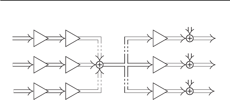
s1
sk
sK
n1
nk
nK
y1
yk
yK
T1
Tk
TK
V1
Vk
VK
H1
Hk
HK
Figure 3.3: Linear Block Diagonalization Precoding
3.2 Block Diagonalization Precoding
Due to the high complexity of dirty paper coding, linear processing is often preferred
in practical systems. In this section, a linear block diagonalization precoder will be
derived and the performance compared to the BC capacity. To this end, consider the
BC depicted in Fig. 3.3 with channels
Hk∈CM×N
and
N≥KM
. The noise is
assumed Gaussian distributed according to
nk∼ NC(0,Cnk)
. The input signals are
given as
sk∼ NC(0,I)∈CM
. All noise and input signals are assumed to be mutually
independent.
The precoding is performed in two steps, where
Vk∈CN×M
ensures that the
signal
sk
is only received at user
k
and does not cause interference at other users.
The transmitted signal intended for user
k
therefore has to lie in the nullspace of the
channels
Hi, i 6=k
. This matrix
Vk
can be obtained via an orthogonal projection
matrix Pk
Pk=I−¯
HH
k(¯
Hk¯
HH
k)−1¯
Hk(3.23)
where
¯
HH
k=hHH
1· · · HH
k−1HH
k+1 · · · HH
Ki.(3.24)
Assuming full rank channel matrices of size
Hk∈CM×N
,
Pk
has rank
M
. With
help of an eigenvalue decomposition, Pkcan therefore be written as
Pk=VkVH
k(3.25)
where
Vk∈CN×M
contains the eigenvectors corresponding to the
M
non-zero
eigenvalues of Pk.
With this choice of the precoder
Vk
, the transmissions from
sk
to
yk
become
independent of the input signals
si, i 6=k
and we can formulate
k
independent
point-to-point channels
yk=HkVkTksk+nk=ˆ
HkTksk+nk.(3.26)
17

Chapter 3. Broadcast Channel
A suboptimal, yet simple choice to now allocate power among the users is to divide
the available transmit power PTx equally among all users.
QUESTION 15
Formulate an optimization problem to maximize the achievable rate of the point-to-
point MIMO system given in
(3.26)
with the assumption that the available transmit
power is divided equally among all users. Give the optimal choice for Tk.
PROGRAMMING TASK 7
Write a function that computes the maximum achievable rate of a MIMO BC with
block diagonalization for given channels
Hk
, noise covariances
Cnk
, assuming
that the available transmit power PTx is divided equally among all users for.
1 Deliverables (Matlab code file): BlockDiagBCEqualPower.m
•Function definition:
function [Rsum] = BlockDiagBCEqualPower(H,C,Ptx)
2 Input Specification:
•H:K×1cell array with channel Hk∈CM×Nper cell
•C:K×1cell array with noise covariance Ck∈CM×Mper cell
•Ptx: Available transmit power PTx
3 Output Specification:
•Rsum: Achievable sum rate with zero forcing precoding.
The achievable rate of this system can still be improved by also optimizing the
transmit power that is allocated to each user. To this end, we now define the composite
matrices
H=
H1
.
.
.
HK
V=hV1. . . VKi(3.27)
as well as the stacked vectors
s=
s1
.
.
.
sK
n=
n1
.
.
.
nK
y=
y1
.
.
.
yK
.(3.28)
18

Chapter 3. Broadcast Channel
With above definitions we can find that the product
HV
as well as the covariance
matrix of nbecome block diagonal, i.e.,
ˆ
H=HV =blockdiag(H1V1,...,HKVK)
C=E[nnH] = blockdiag(Cn1,...,CnK)(3.29)
We can therefore give an equivalent point-to-point channel
y=ˆ
HT s +n,(3.30)
where also
T
is block diagonal with entries
T1,...,TK
. Due to the block diagonal
structure of the equivalent channel as well as the noise covariance, separate decoding
of each block ykis optimal for this system.
QUESTION 16
Formulate an optimization problem to maximize the achievable rate of the point-to-
point MIMO system given in (3.30). What is the optimal choice for T?
PROGRAMMING TASK 8
Write a function that computes the maximum achievable rate of a MIMO BC with
block diagonalization for given channels
Hk
, noise covariances
Cnk
and transmit
power PTx.
1 Deliverables (Matlab code file): BlockDiagBC.m
•Function definition:
function [Rsum] = BlockDiagBC(H,C,Ptx)
2 Input Specification:
•H:K×1cell array with channel Hk∈CM×Nper cell
•C:K×1cell array with noise covariance Ck∈CM×Mper cell
•Ptx: Available transmit power PTx
3 Output Specification:
•Rsum: Achievable sum rate with zero forcing precoding.
Again, assume that the noise at each receiver is given by nk∼ NC(0,I).
19

Chapter 3. Broadcast Channel
PROGRAMMING TASK 9
Write a Matlab script
plotBlogDiagBC.m
to plot the achievable rates obtained with
BlockDiagBCEqualPower.m
,
BlockDiagBC.m
, and the sum capacity of the BC
versus
PTx
for the exemplary channels given in
exampleBlockDiagMIMOBC.mat
.
QUESTION 17
Run the Matlab script
plotBlockDiagBC.m
for the exemplary channels given
in
exampleBlockDiagMIMOBC.m
and
PTx
from
−10 dB
to
40 dB
(in steps of
2dB
) and save the figure as
BlockDiagVSCapacity.fig
. Comment on your
observations.
20
