16_CoverStory_ Pykhtin, Zhu 2007 A Guide To Ling Counterparty Credit Risk
User Manual:
Open the PDF directly: View PDF ![]() .
.
Page Count: 7

Electronic copy available at: http://ssrn.com/abstract=1032522
GLOBAL ASSOCIATION OF RISK PROFESSIONALS
16 JULY/AUGUST 07 ISSUE 3377
C
ounterparty credit risk is the risk that the
counterparty to a financial contract will
default prior to the expiration of the con-
tract and will not make all the payments
required by the contract. Only the con-
tracts privately negotiated between coun-
terparties — over-the-counter (OTC) derivatives and
security financing transactions (SFT) — are subject to
counterparty risk. Exchange-traded derivatives are not
affected by counterparty risk, because the exchange
guarantees the cash flows promised by the derivative to
the counterparties.1
Counterparty risk is similar to other forms of credit
risk in that the cause of economic loss is obligor’s
default. There are, however, two features that set coun-
terparty risk apart from more traditional forms of cred-
it risk: the uncertainty of exposure and bilateral nature
of credit risk. (Canabarro and Duffie [2003] provide an
excellent introduction to the subject.)
In this article, we will focus on two main issues:
modelling credit exposure and pricing counterparty
risk. In the part devoted to credit exposure, we will
define credit exposure at contract and counterparty
levels, introduce netting and margin agreements as risk
management tools for reducing counterparty-level
exposure and present a framework for modelling
credit exposure. In the part devoted to pricing, we will
define credit value adjustment (CVA) as the price of
counterparty credit risk and discuss approaches to its
calculation.
Contract-Level Exposure
If a counterparty in a derivative contract defaults, the
bank must close out its position with the defaulting
counterparty. To determine the loss arising from the
counterparty’s default, it is convenient to assume that
the bank enters into a similar contract with another
counterparty in order to maintain its market posi-
tion.2Since the bank’s market position is unchanged
after replacing the contract, the loss is determined by
the contract’s replacement cost at the time of default.
A Guide to Modelling
Counterparty Credit Risk
What are the steps involved in calculating credit exposure? What are the differences between counterparty
and contract-level exposure? How can margin agreements be used to reduce counterparty credit risk? What
is credit value adjustment and how can it be measured? Michael Pykhtin and Steven Zhu offer a
blueprint for modelling credit exposure and pricing counterparty risk.
Electronic copy available at: http://ssrn.com/abstract=1032522
GLOBAL ASSOCIATION OF RISK PROFESSIONALS
GLOBAL ASSOCIATION OF RISK PROFESSIONALS 17
JULY/AUGUST 07 ISSUE 3377
If the contract value is negative for the bank at the time of
default, the bank
• closes out the position by paying the defaulting coun-
terparty the market value of the contract;
• enters into a similar contract with another counterparty
and receives the market value of the contract; and
• has a net loss of zero.
If the contract value is positive for the bank at the time of
default, the bank
• closes out the position, but receives nothing from the
defaulting counterparty;
• enters into a similar contract with another counterparty
and pays the market value of the contract; and
• has a net loss equal to the contract’s market value.
Thus, the credit exposure of a bank that has a single deriva-
tive contract with a counterparty is the maximum of the con-
tract’s market value and zero. Denoting the value of contract
iat time tas Vi(t), the contract-level exposure is given by
Since the contract value changes unpredictably over time as
the market moves, only the current exposure is known with
certainty, while the future exposure is uncertain. Moreover,
since the derivative contract can be either an asset or a liabili-
ty to the bank, counterparty risk is bilateral between the
bank and its counterparty.
Counterparty-Level Exposure
In general, if there is more than one trade with a defaulted
counterparty and counterparty risk is not mitigated in any
way, the maximum loss for the bank is equal to the sum of
the contract-level credit exposures:
This exposure can be greatly reduced by the means of netting
agreements. A netting agreement is a legally binding contract
between two counterparties that, in the event of default,
allows aggregation of transactions between two counterpar-
ties – i.e., transactions with negative value can be used to off-
set the ones with positive value and only the net positive
value represents credit exposure at the time of default. Thus,
the total credit exposure created by all transactions in a net-
ting set (i.e., those under the jurisdiction of the netting agree-
ment) is reduced to the maximum of the net portfolio value
and zero:
More generally, there can be several netting agreements with
one counterparty. There may also be trades that are not cov-
ered by any netting agreement. Let us denote the k th netting
agreement with a counterparty as NAk. Then, the counter-
party-level exposure is given by
The inner sum in the first term sums values of all trades cov-
ered only by the k th netting agreement (hence, the iNAk
notation), while the outer one sums exposures over all net-
ting agreements. The second term in Equation 4 is simply the
sum of contract-level exposures of all trades that do not
belong to any netting agreement (hence, the i{NA} nota-
tion).
Modelling Credit Exposure
In this section, we describe a general framework for calcu-
lating the potential future exposure on the OTC derivative
products. Such a framework is necessary for banks to com-
pare exposure against limits, to price and hedge counter-
party credit risk and to calculate economic and regulatory
capital.3These calculations may lead to different character-
istics of the exposure distribution — such as expectation,
standard deviation and percentile statistics. The exposure
framework outlined herein is universal because it allows
one to calculate the entire exposure distribution at any
future date. (For more details, see De Prisco and Rosen
[2005] and Pykhtin and Zhu [2006].)
There are three main components in calculating the dis-
tribution of counterparty-level credit exposure:
1. Scenario Generation. Future market scenarios are simu-
lated for a fixed set of simulation dates using evolution
models of the risk factors.
2. Instrument Valuation. For each simulation date and for
each realization of the underlying market risk factors,
instrument valuation is performed for each trade in the
counterparty portfolio.
3. Portfolio Aggregation. For each simulation date and for
each realization of the underlying market risk factors,
counterparty-level exposure is obtained according to
Equation 4 by applying necessary netting rules.
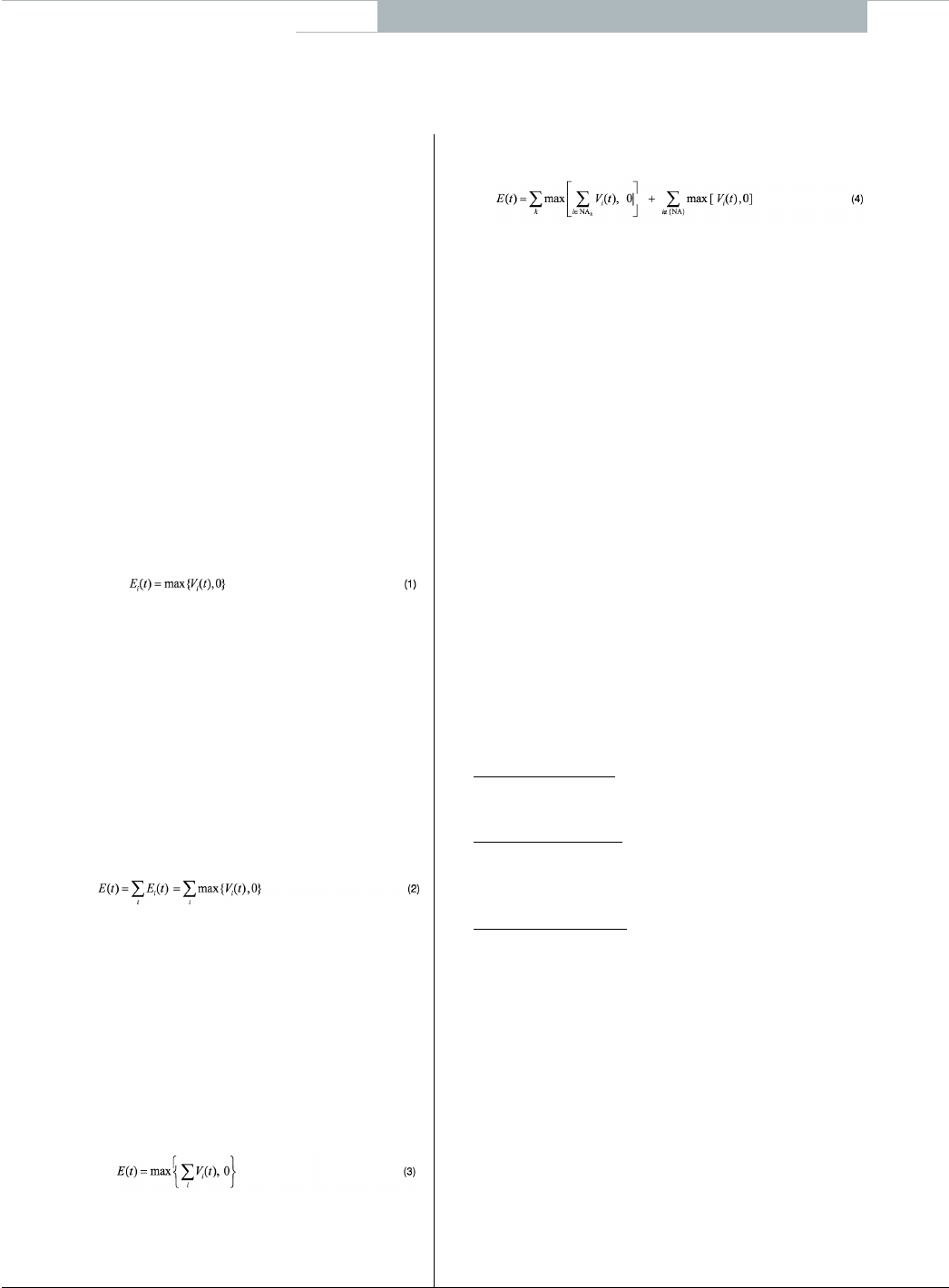
The outcome of this process is a set of realizations of
counterparty-level exposure (each realization corresponds
to one market scenario) at each simulation date, as
schematically illustrated in Figure 1, next page.
Because of the computational intensity required to calcu-
late counterparty exposures — especially for a bank with a
large portfolio — compromises are usually made with
regard to the number of simulation dates and/or the num-
ber of market scenarios. For example, the number of mar-
ket scenarios is limited to a few thousand and the simula-
tion dates (also called “time buckets”) used by most banks
COVER STORY:COUNTERPARTY RISK
GLOBAL ASSOCIATION OF RISK PROFESSIONALS
GLOBAL ASSOCIATION OF RISK PROFESSIONALS
18 JULY/AUGUST 07 ISSUE 3377
COVER STORY:COUNTERPARTY RISK
to calculate credit exposure usually comprise daily or
weekly intervals up to a month, then monthly up to a year
and yearly up to five years, etc.
Figure 1: Simulation Framework for
Credit Exposure
Scenario Generation
The first step in calculating credit exposure is to generate
potential market scenarios at a fixed set of simulation
dates {tk} N
k=1 in the future. Each market scenario is a real-
ization of a set of price factors that affect the values of
the trades in the portfolio. Examples of price factors
include foreign exchange (FX) rates, interest rates, equity
prices, commodity prices and credit spreads.
There are two ways that we can generate possible
future values of the price factors. The first is to generate
a “path” of the market factors through time, so that each
simulation describes a possible trajectory from time t=0
to the longest simulation date, t=T. The other method is
to simulate directly from time t=0 to the relevant simula-
tion date t.
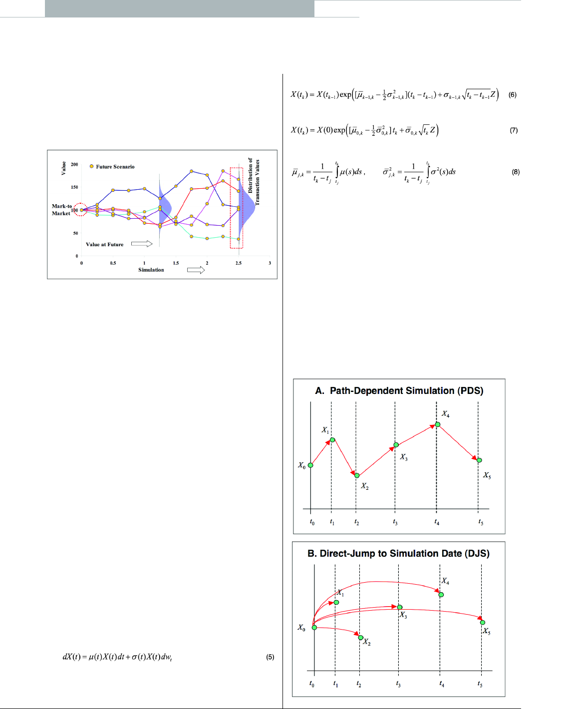
We will refer to the first method as “Path-Dependent
Simulation (PDS)” and to the second method as “Direct
Jump to Simulation Date (DJS).” Figure 2A (across, top)
illustrates a sample path for X(ti), while Figure 2B
(across, bottom) illustrates a direct jump to a simulation
date.
Figure 2 (A and B): Two Ways of
Generating Market Scenarios >>
The scenarios are usually specified via stochastic differential
equations (SDE). Typically, these SDEs describe Markovian
processes and are solvable in closed form. For example, a
popular choice for modelling FX rates and stock indices is
the generalized geometric Brownian motion given by
where (t) is time-dependent drift and (t) is time-dependent
deterministic volatility. From the known solution of this
SDE, we can construct either the PDS model:
or the DJS model:
where is a standard normal variable and
The price factor distribution at a given simulation date
obtained using either PDS or DJS is identical. However, a
PDS method may be more suitable for path-dependent,
American/Bermudan and asset-settled derivatives.
Scenarios can be generated either under the real probabili-
ty measure or under the risk-neutral probability measure.
Under the real measure, both drifts and volatilities are cali-
brated to the historical data of price factors. Under the risk-
neutral measure, drifts must be calibrated to ensure there is
no arbitrage of traded securities on the price factors.
Additionally, volatilities must be calibrated to match market-
implied volatilities of options on the price factors.
For example, the risk-neutral drift of an FX spot rate is
simply given by the interest rate difference between domestic
and foreign currencies, and the volatility should be equal to
GLOBAL ASSOCIATION OF RISK PROFESSIONALS
GLOBAL ASSOCIATION OF RISK PROFESSIONALS 19
JULY/AUGUST 07 ISSUE 3377
the FX option implied volatility. Traditionally, the real mea-
sure has been used in risk management modelling of future
events. However, such applications as pricing counterparty
risk may require modelling scenarios under the risk-neutral
measure.
Instrument Valuation
The second step in credit exposure calculation is to value the
instrument at different future times using the simulated sce-
narios. The valuation models used to calculate exposure
could be very different from the front-office pricing models.
Typically, analytical approximations or simplified valuation
models are used.
While the front office can afford to spend several minutes
or even hours for a trade valuation, valuations in the credit
exposure framework must be done much faster, because each
instrument in the portfolio must be valued at many simula-
tion dates for a few thousand market risk scenarios.
Therefore, valuation models such as those that involve
Monte Carlo simulations or numerical solutions of partial
differential equations do not satisfy the requirements on
computation time.
Path-dependent, American/Bermudan and asset-settled
derivatives present additional difficulty for valuation that
precludes direct application of front-office models. The value
of these instruments may depend on either some event that
happened at an earlier time (e.g., exercising an option) or on
the entire path leading to the valuation date (e.g., barrier or
Asian options). This does not present a problem for front-
office valuation, which is always done at the present time
when the entire path prior to the valuation date is known.
For example, front-office systems always know at the valua-
tion time whether an option has been exercised or a barrier
has been hit.
In contrast, risk management valuation is done at a dis-
crete set of future simulation dates, while the value of an
instrument may depend on the full continuous path prior to
the simulation date or on a discrete set of dates different
from the given set of simulation dates. For example, at a
future simulation date, it is often not known with certainty
whether a barrier option is alive or dead or whether a
Bermudan swaption has been exercised.
This problem presents an even greater challenge for the
DJS approach, where scenarios at previous simulation dates
are completely unrelated to scenarios at the current simula-
tion date. As a solution to this problem, Lomibao and Zhu
(2005) proposed the notion of “conditional valuation,”
which is a probabilistic technique that “adjusts” the mark-
to-market valuation model to account for the events that
could happen between the simulation dates.
Let us assume that we know how to price a derivative when
all information about the past is known. We will denote this
mark-to-market (MTM) value at simulation date tk by VMTM
(tk,{X(t)}tⱕtk), where X(t) is the market price factor that affects
the value of the derivative contract. However, the complete
path of the price factor is not known at tk. Under a PDS
approach, the risk factor is only known at a discrete set of sim-
ulation dates, while under a DJS approach, the risk factor is not
known at all between today (t=0) and the simulation date (t=tk).
The idea behind conditional valuation is to average future
MTM values over all continuous paths of price factors con-
sistent with a given simulation scenario. Mathematically, we
set the value of a derivative contract at a future simulation
date equal to the expectation of the MTM value, conditional
on all the information available between today and the simu-
lation date. Under the PDS approach, the scenario is given by
the set of price factor values xjat all simulation dates tj, such
that jⱕk. The conditional valuation is given by
Under the DJS approach, the scenario is given by a single
price factor value xkat the current simulation date tk. The
conditional valuation is given by
Lomibao and Zhu (2005) have shown that these conditional
expectations can be computed in closed form for such instru-
ments as barrier options, average options and physically set-
tled swaptions. The conditional valuation approach described
by Equations 9 and 10 provides a consistent framework with-
in which the transactions of various types can be aggregated
to recognize the benefits of the netting rule across multiple
price factors.
Exposure Profiles
Uncertain future exposure can be visualized by means of
exposure profiles. These profiles are obtained by calculating
certain statistics of the exposure distribution at each simula-
tion date. For example, the expected exposure profile is
obtained by computing the expectation of exposure at each
simulation date, while a potential future exposure profile
(such profiles are popular for measuring exposure against
credit limits) is obtained by computing a high-level (e.g.,
95%) percentile of exposure at each simulation date.
Though profiles obtained from different exposure measures
have different magnitude, they normally have similar shapes.
There are two main effects that determine the credit
exposure over time for a single transaction or for a portfolio
of transactions with the same counterparty: diffusion and
amortization. As time passes, the “diffusion effect” tends to
increase the exposure, since there is greater variability and,
hence, greater potential for market price factors (such as the
FX or interest rates) to move significantly away from current
levels; the “amortization effect,” in contrast, tends to
COVER STORY:COUNTERPARTY RISK
GLOBAL ASSOCIATION OF RISK PROFESSIONALS
GLOBAL ASSOCIATION OF RISK PROFESSIONALS
20 JULY/AUGUST 07 ISSUE 3377
COVER STORY:COUNTERPARTY RISK
decrease the exposure over time, because it reduces the
remaining cash flows that are exposed to default.
These two effects act in opposite directions — the diffu-
sion effect increases the credit exposure and the amortization
effect decreases it over time. For single cash flow products,
such as FX forwards, the potential exposure peaks at the
maturity of the transaction, because it is driven purely by dif-
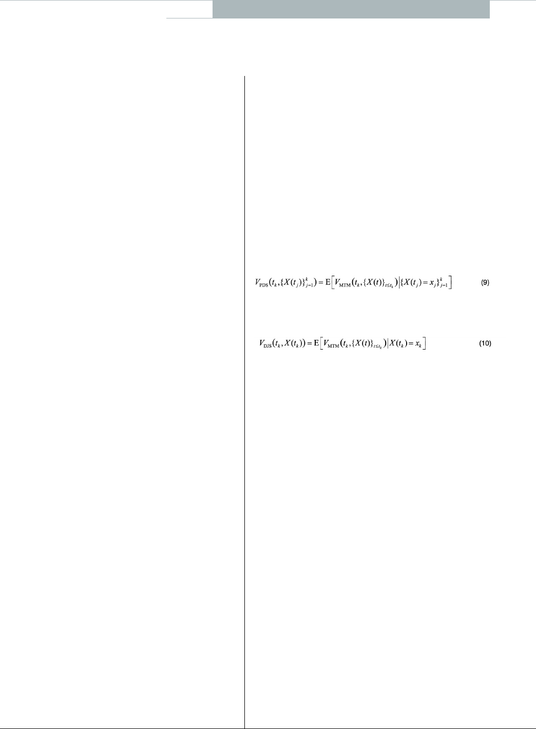
fusion effect.4On the other hand, for products with multiple
cash flows, such as interest-rate swaps, the potential expo-
sure usually peaks at one-third to one-half of the way into
the life of the transaction, as shown in the following exhibit:
Figure 3: Exposure Profile of
Interest-Rate Swap
Different types of instruments can generate very different
credit exposure profiles, and the exposure profile of the
same instruments may also vary under different market
conditions. When the yield curve is upward sloping, the
exposure is greater for a payer swap than the same receiver
swap, because the fixed payments in early periods are
greater than the floating payments, resulting in positive for-
ward values on the payer swap. The opposite is true if the
yield curve is downward sloping.
However, for a humped yield curve, it is not clear which
swap carries more risk, because the forward value on a payer
swap is initially positive and then becomes negative (and vice
versa for a receiver swap). The overall effect implies that
both are almost “equally risky” — i.e., the exposure is
roughly the same between a payer swap and a receiver swap.
Counterparty-level exposure profiles usually have a less intu-
itive shape than simple trade-level profiles. These profiles are
very useful in comparing credit exposure against credit limits
and calculating economic and regulatory capital, as well as
in pricing and hedging counterparty risk.
Collateral Modelling for Margined Portfolios
Banks that are active in OTC derivative markets are increas-
ingly using margin agreements to reduce counterparty credit
risk. A margin agreement is a legally binding contract that
requires one or both counterparties to post collateral when
the uncollateralized exposure exceeds a threshold and to
post additional collateral if this excess grows larger. If this
excess of uncollateralized exposure over the threshold
declines, part of the posted collateral (if there is any) is
returned to bring the difference back to the threshold. To
reduce the frequency of collateral exchanges, a minimum
transfer amount (MTA) is specified; this ensures that no
transfer of collateral occurs unless the required transfer
amount exceeds the MTA.
The following time periods are essential for margin
agreements:
• Call Period. The period that defines the frequency at
which collateral is monitored and called for (typically,
one day).
• Cure Period. The time interval necessary to close out the
counterparty and re-hedge the resulting market risk.
• Margin Period of Risk. The time interval from the last
exchange of collateral until the defaulting counterparty
is closed out and the resulting market risk is re-hedged;
it is usually assumed to be the sum of call period and
cure period.
While margin agreements can reduce the counterparty expo-
sure, they pose a challenge in modelling collateralized expo-
sure. Below, we briefly outline a common procedure that has
been used by many banks to model the effect of margin call
and collateral requirements.
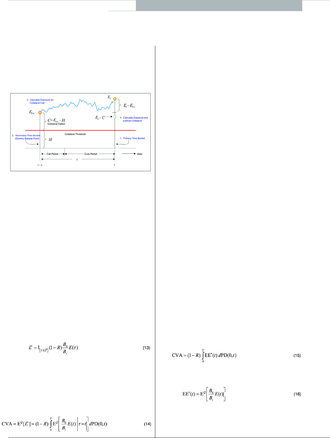
First, the collateral amount C(t) at a given simulation date
tis determined by comparing the uncollateralized exposure
at time t – s against the threshold value H
where sis the margin period of risk, and collateral is set to
zero if it is less than the MTA. Subsequently, the collateralized
exposure at the simulation date tis calculated by subtracting
the collateral C(t) from the uncollateralized exposure
To compute exposure at time t – s, additional simulation
dates (secondary time buckets) are placed prior to the main
simulation dates. Since the margin period of risk can be dif-
ferent for different margin agreements, secondary time
buckets are not fixed. This process is schematically illus-
trated in Figure 4, next page.
Collateral calculation requires the knowledge of exposure
at the secondary time bucket. The obvious approach is calcu-
lating this exposure by the Monte-Carlo simulation. This,
however, would result in doubling the computation time for
margined counterparties. In 2006 (see references), we pro-
posed a simplified approach to modelling the collateral. We
used the concept of the conditional valuation approach of
Lomibao and Zhu (2005) and calculated the exposure value
GLOBAL ASSOCIATION OF RISK PROFESSIONALS
GLOBAL ASSOCIATION OF RISK PROFESSIONALS 21
JULY/AUGUST 07 ISSUE 3377
at the secondary time bucket t – s for each scenario as the
expectation conditional on simulated exposure value at the
primary simulation date(s).
Figure 4: Treatment of Collateral at
Secondary Time Bucket
Credit Value Adjustment
For years, the standard practice in the industry was to mark
derivatives portfolios to market without taking the counter-
party credit quality into account. All cash flows were dis-
counted by the LIBOR curve, and the resulting values were
often referred to as risk-free values.5However, the true port-
folio value must incorporate the possibility of losses due to
counterparty default. Credit value adjustment (CVA) is by
definition the difference between the risk-free portfolio value
and the true portfolio value that takes into account the possi-
bility of a counterparty’s default. In other words, CVA is the
market value of counterparty credit risk.
How do we calculate CVA? Let us assume that a bank has
a portfolio of derivative contracts with a counterparty. We
will denote the bank’s exposure to the counterparty at any
future time tby E(t). This exposure takes into account all
netting and margin agreements between the bank and the
counterparty. If the counterparty defaults, the bank will be
able to recover a constant fraction of exposure that we will
denote by R. Denoting the time of counterparty default by ,
we can write the discounted loss as
where Tis the maturity of the longest transaction in the port-
folio, Btis the future value of one unit of the base currency
invested today at the prevailing interest rate for maturity t.
and 1{.} is the indicator function that takes value one if the
argument is true (and zero otherwise).
Unilateral CVA is given by the risk-neutral expectation of
the discounted loss. The risk-neutral expectation of of
Equation 13 can be written as
where PD(s,t) is the risk neutral probability of counterparty
default between times sand t. These probabilities can be
obtained from the term structure of credit-default swap
(CDS) spreads.
We would like to emphasize that the expectation of the dis-
counted exposure at time tin Equation 14 is conditional on
counterparty default occurring at time t. This conditioning is
material when there is a significant dependence between the
exposure and counterparty credit quality. This dependence is
known as right/wrong-way risk.
The risk is wrong way if exposure tends to increase when
counterparty credit quality worsens. Typical examples of
wrong-way risk include (1) a bank that enters a swap with
an oil producer where the bank receives fixed and pays the
floating crude oil price (lower oil prices simultaneously
worsen credit quality of an oil producer and increase the
value of the swap to the bank); and (2) a bank that buys
credit protection on an underlying reference entity whose
credit quality is positively correlated with that of the coun-
terparty to the trade. As the credit quality of the counterpar-
ty worsens, it is likely that the credit quality of the reference
name will also worsen, which leads to an increase in value of
the credit protection purchased by the bank.
The risk is right way if exposure tends to decrease when
counterparty credit quality worsens. Typical examples of
right-way risk include (1) a bank that enters a swap with an
oil producer where the bank pays fixed and receives the float-
ing crude oil price; and (2) a bank that sells credit protection
on an underlying reference entity whose credit quality is posi-
tively correlated with that of the counterparty to the trade.
While right/wrong-way risk may be important for com-
modity, credit and equity derivatives, it is less significant for
FX and interest rate contracts. Since the bulk of banks’ coun-
terparty credit risk has originated from interest-rate deriva-
tive transactions, most banks are comfortable to assume inde-
pendence between exposure and counterparty credit quality.
Exposure, Independent of Counterparty Default
Assuming independence between exposure and counterpar-
ty’s credit quality greatly simplifies the analysis. Under this
assumption, Equation 14 simplifies to
where EE*(t) is the risk-neutral discounted expected expo-
sure (EE) given by
which is now independent of counterparty default event.
Discounted EE can be computed analytically only at the
contract level for several simple cases. For example, expo-
COVER STORY:COUNTERPARTY RISK
GLOBAL ASSOCIATION OF RISK PROFESSIONALS
GLOBAL ASSOCIATION OF RISK PROFESSIONALS
22 JULY/AUGUST 07 ISSUE 3377
COVER STORY:COUNTERPARTY RISK
sure of a single European option is E(t)=VEO(t), because
European option value VEO(t) is always positive. Since there
are no cash flows between today and option maturity, substi-
tution of this exposure into Equation 16 yields a flat dis-
counted EE profile at the current option value:
EE*EO(t)=VEO(0).
However, calculating discounted EE at the counterparty
level requires simulations. These simulations can be per-
formed according to the exposure modelling framework
described in the previous section. According to this frame-
work, exposure is simulated at a fixed set of simulation dates
{tk} N
k=1. Therefore, the integral in Equation 15 has to be
approximated by the sum:
Since expectation in Equation 16 is risk neutral, scenario
models for all price factors should be arbitrage free. This is
achieved by appropriate calibration of drifts and volatilities
specified in the price-factor evolution model. Drift calibra-
tion depends on the choice of numeraire and probability
measure, while volatilities should be calibrated to the avail-
able prices of options on the price factor.
For PDS scenarios, the same probability measure should be
used across all simulation dates (i.e., the use of spot risk-neu-
tral measure is appropriate). In contrast, the DJS approach
does not require the same probability measure, because sce-
narios at different simulation dates are not directly connected.
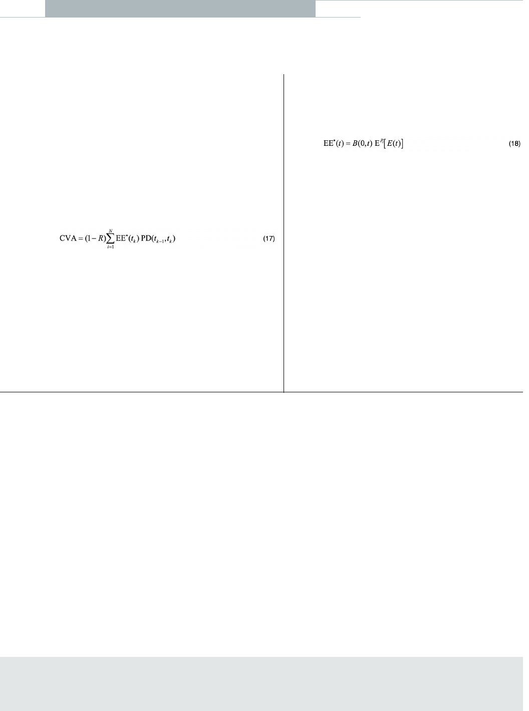
A very convenient choice of measure under the DJS approach
is to model exposure under the forward to simulation date
probability measure Pt, which makes it possible to use today’s
zero coupon bond prices B(0,t) for discounting exposure:
In principle, Equation 18 is equivalent to Equation 16 and,
if properly calibrated, they should generate the same result.
Parting Thoughts
Any firm participating in the OTC derivatives market is
exposed to counterparty credit risk. This risk is especially
important for banks that have large derivatives portfo-
lios. Banks manage counterparty credit risk by setting
credit limits at counterparty level, by pricing and hedging
counterparty risk and by calculating and allocating eco-
nomic capital.
Modelling counterparty risk is more difficult than
modelling lending risk, because of the uncertainty of
future credit exposure. In this article, we have discussed
two modelling issues: modelling credit exposure and cal-
culating CVA. Modelling credit exposure is vital for any
risk management application, while modelling CVA is a
necessary step for pricing and hedging counterparty
credit risk. ■
FOOTNOTES
1. There is a much more remote risk of loss if the exchange itself fails with insufficient collateral in hand to cover all its obligations.
2. In reality, the bank may or may not replace the contract, but the loss can always be determined under the replacement assumption.The loss is, of
course, independent of the strategy the bank chooses after the counterparty’s default.
3. Economic and regulatory capital are out of scope of this article because of space limitation. Economic capital for counterparty risk is covered in
Picoult (2004). For regulatory capital,see Fleck and Schmidt (2005).
4. Currency swaps are also an exception to this amortization effect since most (although not all) of the potential value arises from exchange-rate
movements that affect the value of the final payment.
5. This description is not entirely accurate, because LIBOR rates roughly correspond to AA risk rating and incorporate typical credit risk of large banks.
REFERENCES:
Arvanitis,A. and J. Gregory, 2001. Credit. Risk Books, London.
Canabarro, E. and D. Duffie, 2003. “Measuring and Marking Counterparty Risk. In Asset/Liability Management for Financial Institutions,edited by L.
Tilman. Institutional Investor Books.
De Prisco, B. and D. Rosen, 2005. “Modeling Stochastic Counterparty Credit Exposures for Derivatives Portfolios.” In Counterparty Credit Risk
Modeling, edited by M. Pykhtin, Risk Books, London.
Fleck, M. and A. Schmidt, 2005. “Analysis of Basel II Treatment of Counterparty Credit Risk.” In Counterparty Credit Risk Modeling, edited by M.
Pykhtin, Risk Books, London.
Gibson, M., 2005. “Measuring Counterparty Credit Exposure to a Margined Counterparty.” In Counterparty Credit Risk Modeling, edited by M.
Pykhtin, Risk Books, London.
Lomibao,D. and S. Zhu, 2005. “A Conditional Valuation Approach for Path-Dependent Instruments.” In Counterparty Credit Risk Modeling, edited
by M. Pykhtin, Risk Books, London.
Picout, E., March 2004.“Economic Capital for Counterparty Credit Risk.” RMA Journal.
Pykhtin M. and S. Zhu, 2006.“Measuring Counterparty Credit Risk for Trading Products under Basel II.” In The Basel Handbook (2nd edition), edited
by M. K. Ong, Risk Books, London.
✎MICHAEL PYKHTIN and STEVEN ZHU are responsible for credit risk methodology in the risk architecture group of the global mar-
kets risk management department at Bank of America. Pykhtin can be reached at michael.pykhtin@bankofamerica.com and Zhu can be
reached at steven.zhu@bofasecurities.com.The opinions expressed here are those of the authors and do not necessarily reflect the views or
policies of Bank of America, N.A.
