Python Sso_freeze User Guide Sso Freeze
User Manual:
Open the PDF directly: View PDF ![]() .
.
Page Count: 16
- Python sso_freeze User Guide
- Contents
- Hardwire Locations
- Hardwire Locations
- Using Python sso_freeze
- Section 1): Reading in the Chandra event file
- Section 1): Reading in the Chandra event file
- Section 2): Reading in the orbit empheris file
- Section 3): Reading in the horizons2000 file
- Section 3): Reading in the horizons2000 file
- Section 4): Applying the corrections to the photon position
- Section 4): Applying the corrections to the photon position
- Section 5): Creating the new corrected fits file
- Section 5): Creating the new corrected fits file
- Other comments
- Other comments


2
Contents
•Hardwire Locations
•Using Python sso_freeze:
–Section 1): Reading in the Chandra events file
–Section 2): Reading in the orbit empheris file
–Section 3): Reading in the horizons2000 file
–Section 4): Applying the corrections to the photon position
–Section 5): Creating the new corrected fits file
•Other comments

3
Hardwire Locations
•The code is split into 5 sections (labelled and with
a brief explanation about each within the script).
•Sections 1), 2), 3) and 5) require a file to be
hardwired.
•Section 1) -> evt_location -> input the path of
the event file to be corrected.
•Section 2) -> orb_location -> enter path of the
orbit empheris file of the spacecraft.

4
Hardwire Locations
•Section 3) -> eph_location -> enter path of
chandra_horizons2000 file needed (from
horizons2000 folder).
•Section 5) -> new_evt_location -> enter path of
the new corrected fits file to be written with
corrections.

5
Using Python sso_freeze
•The next few slides will talk about how to use the
code in sections.
•Once the files are hardwired, the code basically
does all the work without any more input required
by the user.
•The code is commented throughout, explaining
what each variable is.
•For new Python users, the very first section
imports all the relevant modules needed to run the
function within the script/Jupyter notebook.
6
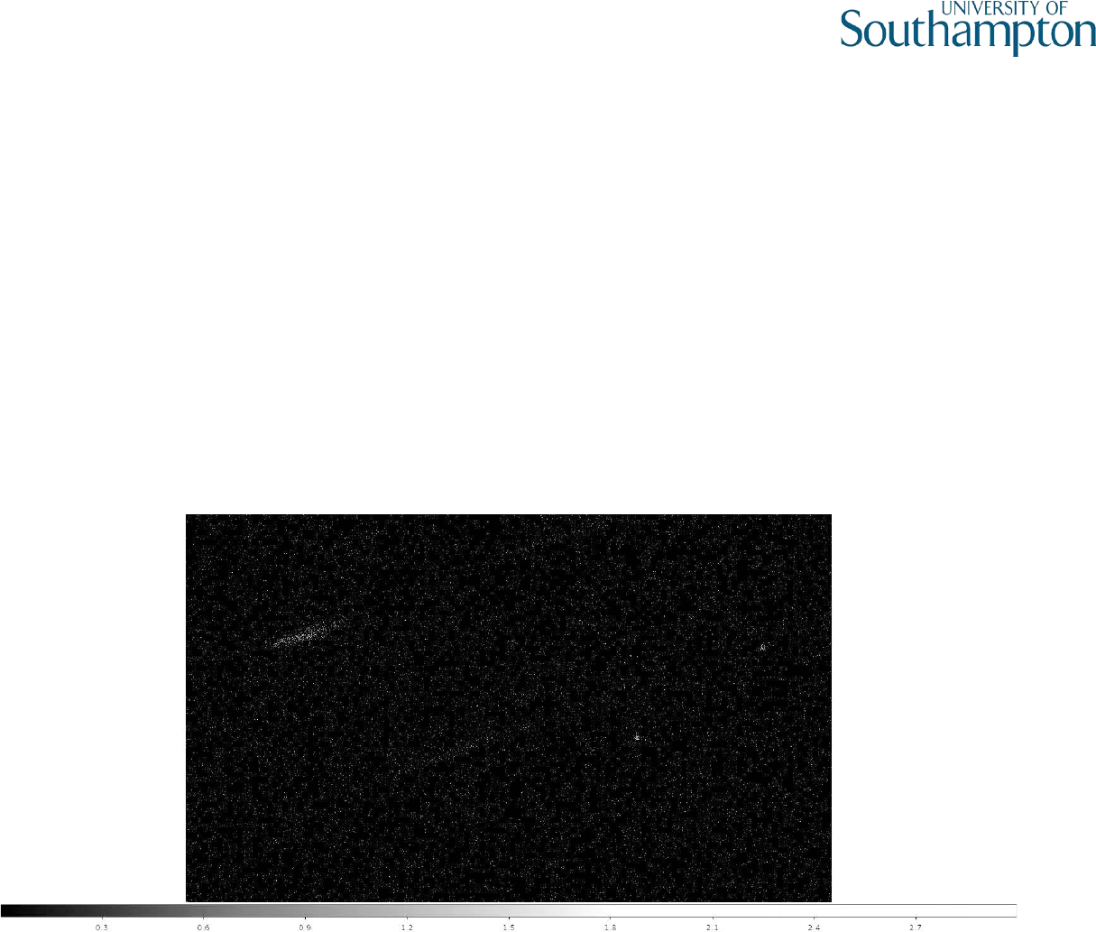
Section 1): Reading in the Chandra event file
•Make sure the event file is hardwired before running the
code! –this is at the beginning of the section.
•The event file pre-correction should look similar the event
file below –distinguishable streaks across the detector (as
Jupiter moves very fast when viewed from Chandra).
ObsID 18608

7
Section 1): Reading in the Chandra event file
•Once the file is read in, the header information and
data needed for analysis is extracted:
–the time of each photon observed,
–start time and date of the observation,
–the x and y position of Jupiter with it’s corresponding
RA and DEC and the start of the observation.
•With the date and time information, the Day of Year
(DOY) when Chandra was making the observations is
calculated – using a defined function at the
beginning of the script, doy_frac.

8
Section 2): Reading in the orbit empheris file
•Make sure the orbit empheris file is hardwired before
running the code! –this is at the beginning of the section.
•When the orbit empheris file is read in, like before, the
relevant header information is extracted:
–Time of observation when the Jovian photons reach the
spacecraft
–Positional coordinates of space craft at the time when the
photons were detected
•The start time of obs is subtracted from the time found in
the orbit empheris file to allow the DOY of the spacecraft to
be calculated.
9
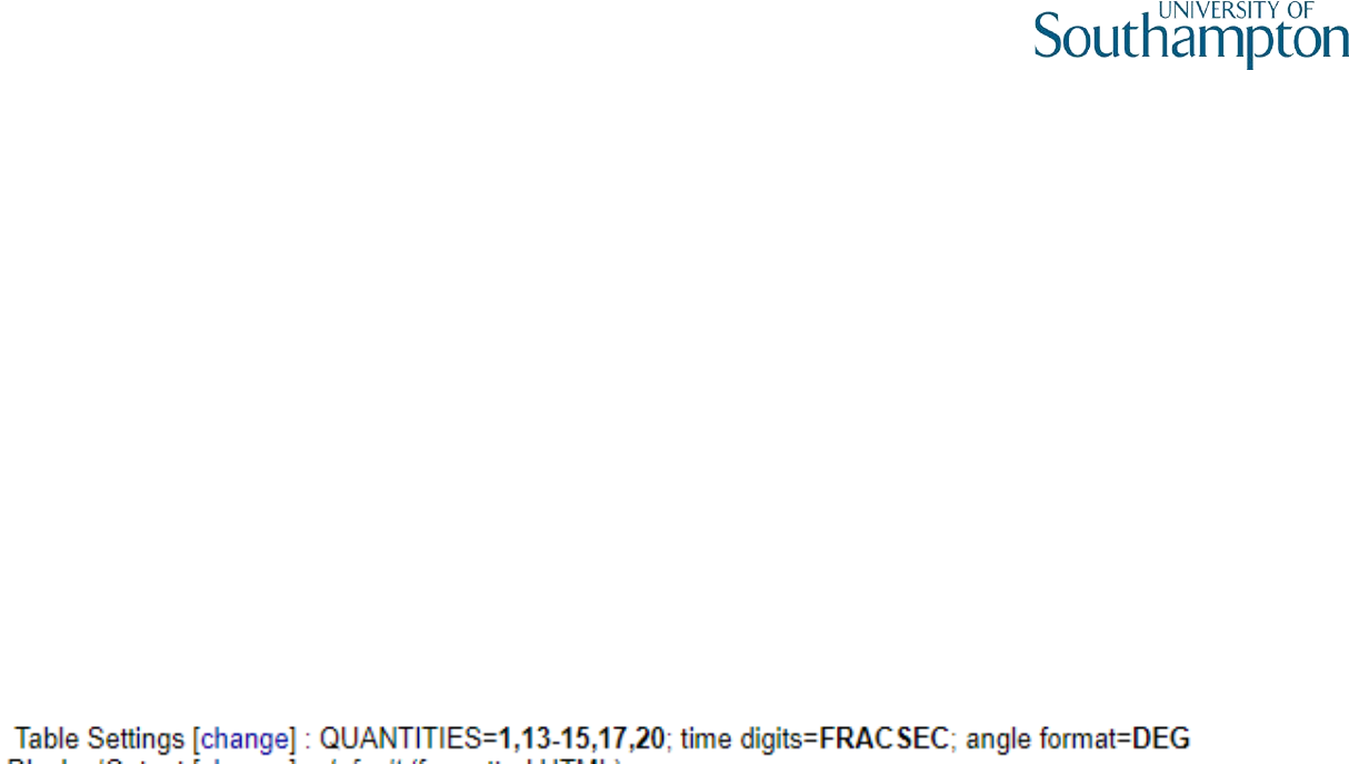
Section 3): Reading in the horizons2000 file
•Make sure the Chandra_horizons2000 file is
hardwired before running the code! –this is at the
beginning of the section –files found from
horizons2000 folder.
•If you are using your own generated file, ensure that
the table settings are of the following form:
•The files do not to be edited to account for the time
to be read into sections –Pythons has in built-in
modules to carry this out!

10
Section 3): Reading in the horizons2000 file
•The code automatically locates the empheris file
data needed and reads in the columns needed –
again, any size horizons2000 file can be read in!
•The date, time, RA and DEC of Jupiter at each
specified interval is read in and the DOY of the
horizons2000 file is calculated.
•If the date lies within a leap year, the DOY is
corrected and this is used instead.

11
Section 4): Applying the corrections to the
photon position
•The code takes the positional coordinates and DOY
from Section 2) and performs a 1D-linear
interpolation to the DOY from the horizons file.
•This produces the new orbital positional coordinates
within this time range.
•This is used to calculate the positional coordinates
of Jupiter during the observation with the
corresponding RA and DEC.
•The offset from Jupiter was also calculated (denoted
as cc in the script/Jupyter notebook).

12
Section 4): Applying the corrections to the
photon position
•An interpolated RA and DEC is calculated from
interpolating the RA/DEC and DOY from Section 3) to
the DOY of Chandra (calculated from Section 1).
•The values are then used to calculate the corrected
position of the photons i.e track them back to
Jupiter’s disk and auroral regions.

13
Section 5): Creating the new corrected fits file
•Make sure the file path of the new fits file is
hardwired before running the code! –this is at the
beginning of the section.
•The code retrieves the data and header information
from the original fits file and changes the x and y
coordinates to the corrected positional coordinates.
•The corrected fits file is then written as a new file –
therefore the original fits file is not overwritten.
14
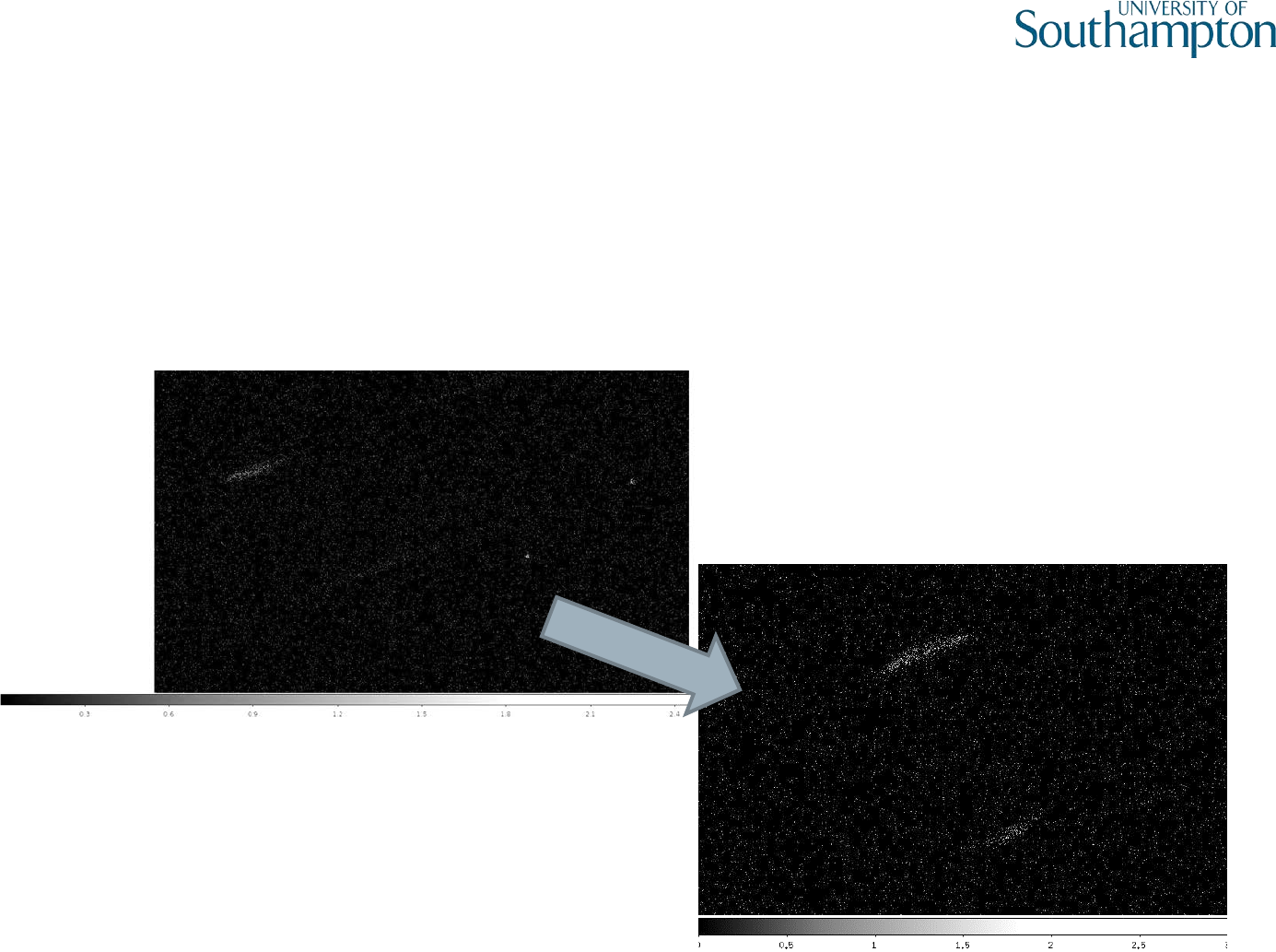
Section 5): Creating the new corrected fits file
•The final result should look something similar to
below –two clear North and South x-ray regions!
ObsID 18608

15
Other comments
•The python code was translated from the stop_hrci
IDL script created by Randy Gladstone.
•The python code produces the same result as the IDL
script without having to overwrite the original file
and making edits the horizons2000 file.
•The plot at the end was used for a sanity check –to
check the data was interpolated correctly.
•The figure can be saved if needed but it is not
essential for the code to run.

16
Other comments
•Future steps:
–To further optimise the code -> no need to hardwire
files and possibly extract the files from a library with
the associated ObsID.
–Translate the other IDL scripts into Python too.
–Will all be on Github and will be made public.
–Github repository with the script(s):
https://github.com/waledeigt/zeno-py.git
