QUESO User's Manual Users

User Manual:

Open the PDF directly: View PDF .
Page Count: 206 [warning: Documents this large are best viewed by clicking the View PDF Link!]

Abstract
Disclaimer
Preface
Introduction
Installation
C++ Classes in the Library
Important Remarks
QUESO Examples
References
Free Software Needs Free Documentation
GNU General Public License
GNU Free Documentation License

The QUESO Library

User’s Manual

Version 0.50.0

Quantiﬁcation of Uncertainty for Estimation,

Simulation, and Optimization (QUESO)

Editors:

Kemelli C. Estacio-Hiroms

Ernesto E. Prudencio

Center for Predictive Engineering and Computational Sciences (PECOS)

Institute for Computational and Engineering Sciences (ICES)

The University of Texas at Austin

Austin, TX 78712, USA

Permission is granted to copy, distribute and/or modify this document under the terms of the

GNU Free Documentation License, Version 1.2 or any later version published by the Free

Software Foundation; with the Invariant Sections being “GNU General Public License” and

“Free Software Needs Free Documentation”, the Front-Cover text being “A GNU Manual”,

and with the Back-Cover text being “You have the freedom to copy and modify this GNU

Manual”. A copy of the license is included in the section entitled “GNU Free Documentation

License”.

iii

Abstract

QUESO stands for Quantiﬁcation of Uncertainty for Estimation, Simulation and Opti-

mization and consists of a collection of algorithms and C++ classes intended for research in

uncertainty quantiﬁcation, including the solution of statistical inverse and statistical forward

problems, the validation of mathematical models under uncertainty, and the prediction of

quantities of interest from such models along with the quantiﬁcation of their uncertainties.

QUESO is designed for ﬂexibility, portability, easy of use and easy of extension. Its software

design follows an object-oriented approach and its code is written on C++ and over MPI. It

can run over uniprocessor or multiprocessor environments.

QUESO contains two forms of documentation: a user’s manual available in PDF format

and a lower-level code documentation available in web based/HTML format.

This is the user’s manual: it gives an overview of the QUESO capabilities, provides pro-

cedures for software execution, and includes example studies.

Disclaimer

This document was prepared by The University of Texas at Austin. Neither the University of

Texas at Austin, nor any of its institutes, departments and employees, make any warranty, ex-

press or implied, or assume any legal liability or responsibility for the accuracy, completeness,

or usefulness of any information, apparatus, product, or process disclosed, or represent that

its use would not infringe privately owned rights. Reference herein to any speciﬁc commercial

product, process, or service by trade name, trademark, manufacturer, or otherwise, does not

necessarily constitute or imply its endorsement, recommendation, or favoring by The Univer-

sity of Texas at Austin or any of its institutes, departments and employees thereof. The views

and opinions expressed herein do not necessarily state or reﬂect those of The University of

Texas at Austin or any institute or department thereof.

QUESO library as well as this material are provided as is, with absolutely no warranty

expressed or implied. Any use is at your own risk.

Contents

Abstract iii

Disclaimer v

Preface x

1 Introduction 1

1.1 Preliminaries .................................... 1

1.2 Key Statistical Concepts .............................. 2

1.3 The Software Stack of an Application Using QUESO .............. 4

1.4 Algorithms for solving Statistical Inverse Problems ............... 5

1.4.1 DRAM Algorithm .............................. 6

1.4.2 Adaptive Multilevel Stochastic Simulation Algorithm .......... 9

1.5 Algorithms for solving the Statistical Forward Problem ............. 15

2 Installation 17

2.1 Getting started ................................... 17

2.1.1 Obtain and Install QUESO Dependencies ................. 18

2.1.2 Prepare your LINUX Environment .................... 19

2.2 Obtaining a Copy of QUESO ........................... 19

2.2.1 Recommended Build Directory Structure ................. 20

2.3 Conﬁgure QUESO Building Environment ..................... 20

2.4 Compile, Check and Install QUESO ........................ 21

2.5 QUESO Developer’s Documentation ....................... 22

2.6 Summary of Installation Steps ........................... 22

2.7 The Build Directory Structure ........................... 23

vii

viii

2.8 The Installed Directory Structure ......................... 24

2.9 Create your Application with the Installed QUESO ............... 25

3 C++ Classes in the Library 27

3.1 Core Classes ..................................... 27

3.1.1 Environment Class (and Options) ..................... 27

3.1.2 Vector .................................... 29

3.1.3 Matrix .................................... 29

3.2 Templated Basic Classes .............................. 33

3.2.1 Vector Set, Subset and Vector Space Classes ............... 33

3.2.2 Scalar Function and Vector Function Classes ............... 33

3.2.3 Scalar Sequence and Vector Sequence Classes .............. 36

3.3 Templated Statistical Classes ........................... 39

3.3.1 Vector Realizer Class ............................ 39

3.3.2 Vector Random Variable Class ....................... 39

3.3.3 Statistical Inverse Problem (and Options) ................ 40

3.3.4 Metropolis-Hastings Solver (and Options) ................ 42

3.3.5 Multilevel Solver (and Options) ...................... 42

3.3.6 Statistical Forward Problem (and Options) ................ 48

3.3.7 Monte Carlo Solver (and Options) ..................... 48

3.4 Miscellaneous Classes and Routines ........................ 50

4 Important Remarks 51

4.1 Revisiting Input Options .............................. 51

4.2 Revisiting Priors .................................. 52

4.3 Running with Multiple Chains or Monte Carlo Sequences ............ 52

4.4 Running with Models that Require Parallel Computing ............. 53

4.5 A Requirement for the DRAM Algorithm ..................... 53

5 QUESO Examples 54

5.1 simpleStatisticalInverseProblem ....................... 55

5.1.1 Running the Example ........................... 56

5.1.2 Example Code ................................ 57

5.1.3 Input File .................................. 60

5.1.4 Create your own Makeﬁle ......................... 61

5.1.5 Data Post-Processing and Visualization .................. 62

5.2 simpleStatisticalForwardProblem ....................... 65

5.2.1 Running the Example ........................... 66

5.2.2 Example Code ................................ 66

5.2.3 Input File .................................. 69

5.2.4 Create your own Makeﬁle ......................... 70

5.2.5 Data Post-Processing and Visualization .................. 71

5.3 gravity ....................................... 73

5.3.1 Statistical Inverse Problem ......................... 73

5.3.2 Statistical Forward Problem ........................ 76

5.3.3 Running the Example ........................... 77

5.3.4 Example Code ................................ 79

5.3.5 Input File .................................. 87

5.3.6 Create your own Makeﬁle ......................... 88

5.3.7 Running the Gravity Example with Several Processors ......... 89

5.3.8 Data Post-Processing and Visualization .................. 90

5.4 validationCycle .................................. 98

5.4.1 Thermogravimetric Experiments and a Simple Model .......... 98

5.4.2 Statistical Inverse Problem ......................... 99

5.4.3 Statistical Forward Problem ........................ 101

5.4.4 Running the Example ........................... 102

5.4.5 TGA Example Code ............................ 102

5.4.6 Input File .................................. 121

5.4.7 Data Post-Processing and Visualization .................. 124

5.5 modal ........................................ 127

5.5.1 One-mode distribution ........................... 127

5.5.2 Two-mode distribution ........................... 128

5.5.3 Example Code ................................ 130

5.5.4 Input File .................................. 135

5.5.5 Create your own Makeﬁle ......................... 136

5.5.6 Data Post-Processing and Visualization .................. 137

5.6 bimodal ....................................... 141

5.6.1 Running the Example ........................... 141

5.6.2 Example Code ................................ 142

5.6.3 Input File .................................. 147

5.6.4 Create your own Makeﬁle ......................... 148

5.6.5 Data Post-Processing and Visualization .................. 149

5.7 hysteretic ..................................... 150

5.7.1 Running the Example ........................... 154

5.7.2 Example Code ................................ 154

5.7.3 Input File .................................. 162

5.7.4 Create your own Makeﬁle ......................... 163

5.7.5 Data Post-Processing and Visualization .................. 164

References 167

A Free Software Needs Free Documentation 171

B GNU General Public License 173

C GNU Free Documentation License 186

Preface

The QUESO project started in 2008 as part of the eﬀorts of the recently established Center

for Predictive Engineering and Computational Sciences (PECOS) at the Institute for Com-

putational and Engineering Sciences (ICES) at The University of Texas at Austin.

The PECOS Center was selected by the National Nuclear Security Administration (NNSA)

as one of its new ﬁve centers of excellence under the Predictive Science Academic Alliance

Program (PSAAP). The goal of the PECOS Center is to advance predictive science and to

develop the next generation of advanced computational methods and tools for the calcula-

tion of reliable predictions on the behavior of complex phenomena and systems (multiscale,

multidisciplinary). This objective demands a systematic, comprehensive treatment of the cal-

ibration and validation of the mathematical models involved, as well as the quantiﬁcation of

the uncertainties inherent in such models. The advancement of predictive science is essential

for the application of Computational Science to the solution of realistic problems of national

interest.

The QUESO library, since its ﬁrst version, has been publicly released as open source

under the GNU General Public License and is available for free download world-wide. See

http://www.gnu.org/licenses/gpl.html for more information on the GPL software use agree-

ment.

Contact Information:

Paul T. Bauman, Kemelli C. Estacio-Hiroms or Damon McDougall,

Institute for Computational and Engineering Sciences

1 University Station C0200

Austin, Texas 78712

email: pecos-dev@ices.utexas.edu

web: http://pecos.ices.utexas.edu

Referencing the QUESO Library

When referencing the QUESO library in a publication, please cite the following:

@incollection{QUESO,

author = "Ernesto Prudencio and Karl W. Schulz",

title = {The Parallel C++ Statistical Library ‘QUESO’:

Quantification of Uncertainty for Estimation,

Simulation and Optimization},

booktitle = {Euro-Par 2011: Parallel Processing Workshops},

series = {Lecture Notes in Computer Science},

publisher = {Springer Berlin / Heidelberg},

isbn = {978-3-642-29736-6},

keyword = {Computer Science},

pages = {398-407},

volume = {7155},

url = {http://dx.doi.org/10.1007/978-3-642-29737-3_44},

year = {2012}

}

@TechReport{queso-user-ref,

Author = {Kemelli C. Estacio-Hiroms and Ernesto E. Prudencio},

Title = {{T}he {QUESO} {L}ibrary, {U}ser’s {M}anual},

Institution = {Center for Predictive Engineering and Computational Sciences

(PECOS), at the Institute for Computational and Engineering

Sciences (ICES), The University of Texas at Austin},

Note = {in preparation},

Year = {2013}

}

@Misc{queso-web-page,

Author = {{QUESO} Development Team},

Title = {{T}he {QUESO} {L}ibrary: {Q}uantification of {U}ncertainty

for {E}stimation, {S}imulation and {O}ptimization},

Note = \url{https://github.com/libqueso/},

Year = {2008-2013}

}

xii

QUESO Development Team

The QUESO development team currently consists of Paul T. Bauman, Sai Hung Cheung,

Kemelli C. Estacio-Hiroms, Nicholas Malaya, Damon McDougall, Kenji Miki, Todd A. Oliver,

Ernesto E. Prudencio, Karl W. Schulz, Chris Simmons, and Rhys Ulerich.

Acknowledgments

This work has been supported by the United States Department of Energy, under the National

Nuclear Security Administration Predictive Science Academic Alliance Program (PSAAP)

award number [DE-FC52-08NA28615], and under the Oﬃce of Science Scientiﬁc Discovery

through Advanced Computing (SciDAC) award number [DE-SC0006656].

We would also like to thank James Martin, Roy Stogner and Lucas Wilcox for interesting

discussions and constructive feedback.

Target Audience

QUESO is a collection of statistical algorithms and programming constructs supporting re-

search into the uncertainty quantiﬁcation (UQ) of models and their predictions. UQ may be a

very complex and time consuming task, involving many steps: decide which physical model(s)

to use; decide which reference or experimental data to use; decide which discrepancy models

to use; decide which quantity(ies) of interest (QoI) to compute; decide which parameters to

calibrate; perform computational runs and collect results; analyze computational results, and

eventually reiterate; predict QoI(s) with uncertainty.

The purpose of this manual is not to teach UQ and its methods, but rather to introduce

QUESO library so it can be used as a tool to assist and facilitate the uncertainty quantiﬁcation

of the user’s application. Thus, the target audience of this manual is researchers who have

solid background in Bayesian methods, are comfortable with UNIX concepts and the command

line, and have knowledge of a programming language, preferably C/C++. Bellow we suggest

some useful literature:

1. Probability, statistics, random variables [11,12,25];

2. Bayes’ formula [5,14,26,37];

3. Markov chain Monte Carlo (MCMC) methods [4,15,18,19,20,28,31,34,35];

4. Monte Carlo methods [38];

5. Kernel density estimation [39];

6. C++ [27,32];

7. Message Passing Interface (MPI) [47,45];

8. UNIX/Linux (installation of packages, compilation, linking);

9. MATLAB/GNU Octave (for dealing with output ﬁles generated by QUESO); and

10. UQ issues in general [10].

CHAPTER 1. INTRODUCTION 1

CHAPTER 1

Introduction

QUESO is a parallel object-oriented statistical library dedicated to the research of statis-

tically robust, scalable, load balanced, and fault-tolerant mathematical algorithms for the

quantiﬁcation of uncertainty (UQ) of mathematical models and their predictions.

The purpose of this chapter is to introduce relevant terminology, mathematical and sta-

tistical concepts, statistical algorithms, together with an overall description of how the user’s

application may be linked with the QUESO library.

1.1 Preliminaries

Statistical inverse theory reformulates inverse problems as problems of statistical inference by

means of Bayesian statistics: all quantities are modeled as random variables, and probability

distribution of the quantities encapsulates the uncertainty observed in their values. The so-

lution to the inverse problem is then the probability distribution of the quantity of interest

when all information available has been incorporated in the model. This (posterior) distri-

bution describes the degree of conﬁdence about the quantity after the measurement has been

performed [28].

Thus, the solution to the statistical inverse problem may be given by Bayes’ formula,

which express the posterior distribution as a function of the prior distribution and the data

represented through the likelihood function.

The likelihood function has an open form and its evaluation is highly computationally

expensive. Moreover, simulation-based posterior inference requires a large number of forward

calculations to be performed, therefore fast and eﬃcient sampling techniques are required for

posterior inference.

Chapter 1: Introduction 2

It is often not straightforward to obtain explicit posterior point estimates of the solution,

since it usually involves the evaluation of a high-dimensional integral with respect to a possibly

non-smooth posterior distribution. In such cases, an alternative integration technique is the

Markov chain Monte Carlo method: posterior means may be estimated using the sample mean

from a series of random draws from the posterior distribution.

QUESO is designed in an abstract way so that it can be used by any computational model,

as long as a likelihood function (in the case of statistical inverse problems) and a quantity of

interest (QoI) function (in the case of statistical forward problems) is provided by the user

application.

QUESO provides tools for both sampling algorithms for statistical inverse problems, fol-

lowing Bayes’ formula, and statistical forward problems. It contains Monte Carlo solvers (for

autocorrelation, kernel density estimation and accuracy assessment), MCMC (e.g. Metropolis

Hastings [34,20]) as well as the DRAM [18] (for sampling from probability distributions); it

also has the capacity to handle many chains or sequences in parallel, each chain or sequence it-

self demanding many computing nodes because of the computational model being statistically

explored [36].

1.2 Key Statistical Concepts

A computational model is a combination of a mathematical model and a discretization that

enables the approximate solution of the mathematical model using computer algorithms and

might be used in two diﬀerent types of problems: forward or inverse.

Any computational model is composed of a vector θof nparameters,state variables u,

and state equations r(θ,u) = 0. Once the solution uis available, the computational model

also includes extra functions for e.g. the calculation of model output data y=y(θ,u), and

the prediction of a vector q=q(θ,u) of mquantities of interest (QoI),

Parameters designate all model variables that are neither state variables nor further quanti-

ties computed by the model, such as: material properties, coeﬃcients, constitutive parameters,

boundary conditions, initial conditions, external forces, parameters for modeling the model

error, characteristics of an experimental apparatus (collection of devices and procedures),

discretization choices and numerical algorithm options.

In the case of a forward problem, the parameters θare given and one then needs to compute

u,yand/or q. In the case of an inverse problem, however, experimental data dis given and

one then needs to estimate the values of the parameters θthat cause yto best ﬁt d.

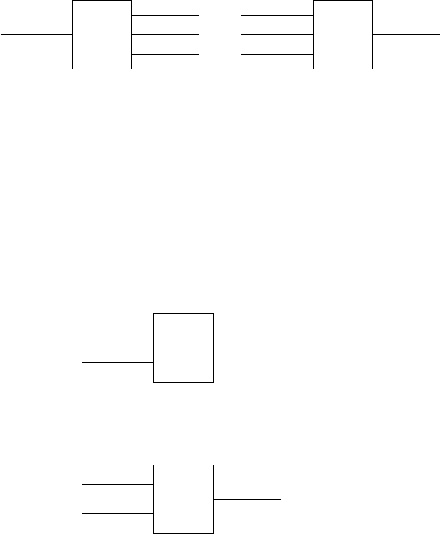
Figure 1.2.1 represents general inverse and forward problems respectively.

There are many possible sources of uncertainty on a computational model. First, dneed

not be equal to the actual values of observables because of errors in the measurement pro-

cess. Second, the values of the input parameters to the phenomenon might not be precisely

known. Third, the appropriate set of equations governing the phenomenon might not be well

understood.

Computational models can be classiﬁed as either deterministic or stochastic – which are

the ones of interest here. In deterministic models, all parameters are assigned numbers, and

Chapter 1: Introduction 3

Forward

Problem

State u=?

Output y=?

Prediction q=?

Input θ

(a)

Inverse

Problem

y(θ,u)

Parameters θ=?r(θ,u) = 0

Experimental d

(b)

Figure 1.2.1: The representation of (a) a generic forward problem and (b) a generic inverse

problem.

no parameter is related to the parametrization of a random variable (RV) or ﬁeld. As a

consequence, a deterministic model assigns a number to each of the components of quantities

u,yand q. In stochastic models, however, at least one parameter is assigned a probability

density function (PDF) or is related to the parametrization of a RV or ﬁeld, causing u,y

and qto become random variables. Note that not all components of θneed to be treated as

random. As long as at least one component is random, θis a random vector, and the problem

is stochastic.

In the case of forward problems, statistical forward problems can be represented very

similarly to deterministic forward problems, as seen in Figure 1.2.2. In the case of inverse

problems, as depicted in Figure 1.2.3, however, the conceptual connection between determin-

istic and statistical problems is not as straightforward.

Statistical

Problem

Forward

q(θ)

Input RV Θ

Output RV Q

Figure 1.2.2: The representation of a statistical forward problem. Θdenotes a random variable

related to parameters, θdenotes a realization of Θand Qdenotes a random variable related

to quantities of interest.

-Posterior RV Θ

Statistical

Problem

Inverse

Prior RV Θ

πlike(d|y,r,Θ)

Figure 1.2.3: The representation of a statistical inverse problem. Θdenotes a random variable

related to parameters, θdenotes a realization of Θand rdenotes model equations, ydenotes

some model output data and ddenotes experimental data.

QUESO adopts a Bayesian analysis [28,37] for statistical inverse problems, interpreting

Chapter 1: Introduction 4

the posterior PDF

πposterior(θ|d) = πprior(θ)πlikelihood(d|θ)

π(d)(1.2.1)

as the solution. Such solutions combine the prior information πprior(θ) of the parameters,

the information π(d) on the data, and the likelihood πlikelihood(d|θ) that the model computes

certain data values with a given set of input parameters.

This semantic interpretation of achieving a posterior knowledge on the parameters (on the

model) after combining some prior model knowledge with experimental information provides

an important mechanism for dealing with uncertainty. Although mathematically simple, is

not computationally trivial.

1.3 The Software Stack of an Application Using QUESO

An application using QUESO falls into three categories: a statistical inverse problem (IP), a

statistical forward problem (FP), or combinations of both. In each problem the user might

deal with up to ﬁve vectors of potentially very diﬀerent sizes: parameters θ, state u, output

y, data dand QoIs q.

Algorithms in the QUESO library require the supply of a likelihood routine πlike :Rn→R+

for statistical inverse problems and of a QoI routine q:Rn→Rmfor statistical forward

problems. These routines exist at the application level and provide the necessary bridge

between the statistical algorithms in QUESO, model knowledge in the model library and

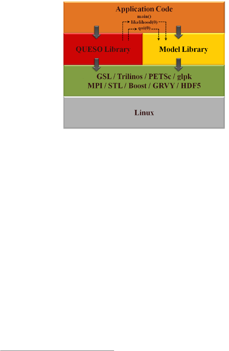
scenario and experimental data in the disk space. Figure 1.3.1 shows the software stack of a

typical application that uses QUESO. In the ﬁgure, the symbol θrepresents a vector of n>1

parameters.

Even though QUESO deals directly with θand qonly, it is usually the case the one of

the other three vectors (u,yand d) will have the biggest number of components and will

therefore dictate the size of the minimum parallel environment to be used in a problem. So,

for example, even though one processor might be suﬃcient for handling θ,y,dand q, eight

processors at least might be necessary to solve for u. QUESO currently only requires that the

amounts nand mcan be handled by the memory available to one processor, which allows the

analysis of problems with thousands of parameters and QoIs, a large amount even for state of

the art UQ algorithms.

QUESO currently supports three modes of parallel execution: an application user may

simultaneously run:

(a) multiple instances of a problem where the physical model requires a single processor, or

(b) multiple instances of a problem where the physical model requires multiple processors, or

For example, suppose an user wants to use the Metropolis-Hastings (MH) algorithm to

solve a statistical IP, and that 1,024 processors are available. If the physical model is simple

Chapter 1: Introduction 5

Figure 1.3.1: An application software stack. QUESO requires the input of a likelihood routine

πlike :Rn→R+for IPs and of a QoI routine q:Rn→Rmfor FPs. These application level

routines provide the bridge between the statistical algorithms in QUESO, physics knowledge

in the model library, and relevant experimental (calibration and validation) data.

enough to be handled eﬃciently by a single processor, then the user can run 1,024 chains

simultaneously, as in case (a). If the model is more complex and requires, say, 16 processors,

then the user can run 64 chains simultaneously, as in case (b), with 16 processors per chain.

QUESO treats this situation by using only 1 of the 16 processors to handle the chain. When

a likelihood evaluation is required, all 16 processors call the likelihood routine simultaneously.

Once the likelihood returns its value, QUESO puts 15 processors into idle state until the

routine is called again or the chain completes. Case (c) is useful, for instance, in the case of a

computational procedure involving two models, where a group of processors can be split into

two groups, each handling one model. Once the two-model analysis end, the combined model

can use the full set of processors.1

1.4 Algorithms for solving Statistical Inverse Problems

The goal of inference is to characterize the posterior PDF, or to evaluate point or interval

estimates based on the posterior [23]. Samples from posterior can be obtained using Markov

chain Monte Carlo (MCMC) which require only pointwise evaluations of the unnormalized

posterior. The resulting samples can then be used to either visually present the posterior

or its marginals, or to construct sample estimates of posterior expectations. Examples of

1The parallel capabilities of QUESO have been exercised on the Ranger system of the TACC [2] with up

to 16k processors.

Chapter 1: Introduction 6

MCMC are: the Metropolis-Hastings (MH) algorithm [34,20], the Delayed Rejection (DR)

algorithm [15,35], and Adaptive Metropolis (AM) [19] which are combined together in the

Delayed Rejection Adaptive Metropolis, DRAM, algorithm [18]. The DRAM is implemented

in QUESO and available for the solution of SIP. MCMC methods are well-established and

documented [4,15,18,19,20,28,31,34,35]; thus only brief description of the DRAM

algorithm is presented in Section 1.4.1.

During model construction, errors arising from imperfect modeling and uncertainties due

to incomplete information about the system and its environment always exist; thus, there has

been a crescent interest in Bayesian model class updating and selection [9,7,8].

Model updating refers to the methodology that determines the most plausible model for a

system, given a prior PDF. One stochastic method that handles model updating successfully is

the multilevel method. Throughout the years, sereveral versions of the same method have been

implemented as improvements of its predecessors [3,9,8]. QUESO hosts the novel Adaptive

Multilevel Stochastic Simulation Algorithm (AMSSA) [8], which is described in Section 1.4.2.

For details about the method, please refer to [8].

1.4.1 DRAM Algorithm

DRAM is a combination of two ideas for improving the eﬃciency of Metropolis-Hastings type

Markov chain Monte Carlo (MCMC) algorithms, Delayed Rejection and Adaptive Metropo-

lis [29].

Random walk Metropolis-Hasting algorithm with Gaussian proposal distribution is useful

in simulating from the posterior distribution in many Bayesian data analysis situations. In

order for the chain to be eﬃcient, the proposal covariance must somehow be tuned to the

shape and size of the target distribution. This is important in highly nonlinear situations,

when there are correlation between the components of the posterior, or when the dimension

of the parameter is high. The problem of adapting the proposal distribution using the chain

simulated so far is that when the accepted values depend on the history of the chain, it is

no longer Markovian and standard convergence results do not apply. One solution is to use

adaptation only for the burn-in period and discard the part of the chain where adaptation

has been used. In that respect, the adaptation can be thought as automatic burn-in. The

idea of diminishing adaptation is that when adaptation works well, its eﬀect gets smaller and

we might be able to prove the ergodicity properties of the chain even when adaptation is

used throughout the whole simulation. This is the ideology behind AM adaptation. On the

other hand, the DR method allows the use of the the current rejected values without losing

the Markovian property and thus allows to adapt locally to the current location of the target

distribution.

In Adaptive Metropolis [19] the covariance matrix of the Gaussian proposal distribution

is adapted on the ﬂy using the past chain. This adaptation destroys the Markovian property

of the chain, however, it can be shown that the ergodicity properties of the generated sample

remain. How well this works on ﬁnite samples and on high dimension is not obvious and must

be veriﬁed by simulations.

Chapter 1: Introduction 7

Starting from initial covariance C(0), the target covariance is updated at given intervals

from the chain generated so far.

C(i)=sdcov(chain1: chaini) + sdεId,

the small number εprevents the sample covariance matrix from becoming singular. For the

scaling factor, the value sd= 2.42/d is standard optimal choice for Gaussian targets, dbeing

the dimension of the target [14]. A standard updating formula for the sample covariance

matrix can be used, so that the whole chain does not need to reside in the computer memory.

With the Delayed rejection method [35], it becomes possible to make use of several tries

after rejecting a value by using diﬀerent proposals while keep the reversibility of the chain.

Delayed rejection method (DR) works in the following way. Upon rejection a proposed can-

didate point, instead of advancing time and retaining the same position, a second stage move

is proposed. The acceptance probability of the second stage candidate is computed so that

reversibility of the Markov chain relative to the distribution of interest is preserved. The

process of delaying rejection can be iterated for a ﬁxed or random number of stages, let’s say

nstages. The higher stage proposals are allowed to depend on the candidates so far proposed

and rejected. Thus DR allows partial local adaptation of the proposal within each time step

of the Markov chain still retaining the Markovian property and reversibility.

The ﬁrst stage acceptance probability in DR is the standard MH acceptance and it can be

written as

α1(a,x(1)) = min 1,π(x(1))

π(a)·q1(x(1),a)

q1(a,x(1)),

Here ais the current point, x(1) is the proposed new value drawn from the distribution

q1(a,·), and πis the target distribution. If x(1) is rejected, a second candidate x(2) is drawn

from q2(a,x(1),·) using the acceptance probability

α2(a,x(1),x(2)) = min 1,π(x(2))q1(x(2),x(1))q2(x(2),x(1),a)[1 −α1(x(2),x(1))]

π(a)q1(a,x(1))q2(a,x(1),x(2))[1 −α1(a,x(1))] 

i.e., it depends not only on the current position of the chain but also on what we have just

proposed and rejected.

As the reversibility property is preserved, this method also leads to the same stationary

distribution πas the standard MH algorithm. The procedure can be iterated further for

higher-stage proposals. The Gaussian proposal at each stage iis deﬁned as:

qi(a,x(1),...,x(i−1)

| {z }

iterms

,z) = e−1

2[z−a]T·[C]−1·[z−a](1.4.1)

where the covariance matrix Cand the scalings for the higher-stage proposal covariances

1 = γ16γ26. . . 6γnstages are given.

If qidenotes the proposal at the i-th stage, the acceptance probability at that stage is:

αi(a,x(1),...,x(i)) = min 1,π(x(i))

π(a)·qfraction ·αfraction.(1.4.2)

Chapter 1: Introduction 8

where the expressions qfraction and αfraction are given by

qfraction =q1(x(i),x(i−1))

q1(a,x(1))

q2(x(i),x(i−1),x(i−2))

q2(a,x(1),x(2)). . . qi(x(i),x(i−1),...,x(1),a)

qi(a,x(1),...,x(i−1),x(i))

and

αfraction =[1 −α1(x(i),x(i−1))]

[1 −α1(a,x(1))]

[1 −α2(x(i),x(i−1),x(i−2))]

[1 −α2(a,x(1),x(2))] . . . [1 −αi−1(x(i),x(i−1),...,x(1))]

[1 −αi−1(a,x(1),...,x(i−1))] .

Since all acceptance probabilities are computed so that reversibility with respect to πis

preserved separately at each stage, the process of delaying rejection can be interrupted at any

stage that is, we can, in advance, decide to try at most, say, 3 times to move away from the

current position, otherwise we let the chain stay where it is. Alternatively, upon each rejection,

we can toss a p-coin (i.e., a coin with head probability equal to p), and if the outcome is head

we move to a higher stage proposal, otherwise we stay put [18].

The smaller overall rejection rate of DR guarantees smaller asymptotic variance of the

estimates based on the chain. The DR chain can be shown to be asymptotically more eﬃcient

that MH chain in the sense of Peskun ordering (Mira, 2001a).

Haario, et al. 2006 [18] combine AM and DR into a method called DRAM, in what they

claim to be a straightforward possibility amongst the possible diﬀerent implementations of

the idea, and which is described in this section.

In order to be able to adapt the proposal, all you need some accepted points to start with.

One “master” proposal is tried ﬁrst – i.e., the proposal at the ﬁrst stage of DR is adapted

just as in AM: the covariance C(1) is computed from the points of the sampled chain, no

matter at which stage these points have been accepted in the sample path. After rejection,

a try with modiﬁed version of the ﬁrst proposal is done according to DR. A second proposal

can be one with a smaller covariance, or with diﬀerent orientation of the principal axes. The

most common choice is to always compute the covariance C(i)of the proposal for the i-th

stage (i= 2, . . . , nstages) simply as a scaled version of the proposal of the ﬁrst stage,

C(i)=γiC(1)

where the scale factors γican be somewhat freely chosen. Then, the master proposal is

adapted using the chain generated so far, and the second stage proposal follows the adaptation

in obvious manner.

The requirements for the DRAM algorithm are:

•Number npos >2 of positions in the chain;

•Initial guess m(0);

•Number of stages for the DR method: nstages >1;

Chapter 1: Introduction 9

•For 1 6i6nstages, functions qi:RN×. . . ×RN

| {z }

(i+1) times →R+, such that qi(a,x(1),...,x(i−1),·)

is a PDF for any (a,x(1),...,x(i−1))∈RN×. . . ×RN

| {z }

itimes

; i.e., choose qias in Equa-

tion (1.4.1);

•Recursively deﬁne αi:Rn×. . . ×Rn

| {z }

(i+1) times →[0,1],16i6nstages according to Equa-

tion (1.4.2).

Recalling that a sample is deﬁned as:

a sample = a+C1/2N(0, I).

a simple, but useful, implementation of DRAM is described in Algorithm 1.

There are six variables in the QUESO input ﬁle used to set available options for the DRAM

algorithm, which are described in 3.3.4. Here, they are presented presented bellow together

with their respective deﬁnition in Algorithm 1.

ip mh dr maxNumExtraStages:deﬁnes how many extra stages should be considered in the

DR loop (nstages);

ip mh dr listOfScalesForExtraStages:deﬁnes the list sof scaling factors that will multi-

ply the covariance matrix (values of γi);

ip mh am adaptInterval:deﬁnes whether or not there will be a period of adaptation;

ip mh am initialNonAdaptInterval:deﬁnes the initial interval where the proposal covari-

ance matrix will not be changed (n0);

ip mh am eta:is a factor used to scale the proposal covariance matrix, usually set to be 2.42/d,

where dis the dimension of the problem [31,18] (sd);

ip mh am epsilon:is the covariance regularization factor (ε).

1.4.2 Adaptive Multilevel Stochastic Simulation Algorithm

In this section we rewrite the Bayesian formula (1.2.1) by making explicit all the implicit

model assumptions. Such explication demands the use of probability logic and the concept of a

stochastic system model class (model class for short); as these concepts enable the comparison

of competing model classes.

Let Mjbe one model class; the choice of θspeciﬁes a particular predictive model in Mj,

and, for brevity, we do not explicitly write θjto indicate that the parameters of diﬀerent

model classes may be diﬀerent, but this should be understood. Based on Mj, one can use

data Dto compute the updated relative plausibility of each predictive model in the set deﬁned

by Mj. This relative plausibility is quantiﬁed by the posterior PDF π(θ|D, Mj).

Chapter 1: Introduction 10

Algorithm 1: DRAM algorithm [31].

Input: Number of positions in the chain npos >2; initial guess m(0); initial ﬁrst stage proposal

covariance C(0);nstages >1; and functions qi:RN×. . . ×RN

| {z }

(i+1) times

→R+

1Select sd;// scaling factor

2Select ε;// covariance regularization factor

3Select n0;// initial non-adaptation period

4for i←1to nstages do // nstages is the number of tries allowed

5Select γi;// scalings for the higher-stage proposal covariances

6end

7repeat

8Set ACCEP T ←false;

9Set i←1;

// After an initial period of simulation, adapt the master proposal (target)

covariance using the chain generated so far:

10 if k>n0then

11 C(1) =sdCov(m(0),...,m(k−1)) + sdεId;

12 end

// nstages-DR loop:

13 repeat

14 Generate candidate c(i)∈RNby sampling qi(m(k),c(1),...,c(i−1),·) ; // qiis the

proposal probability density

15 if c(i)/∈supp(π)then

16 i←i+ 1

17 end

18 if c(i)∈supp(π)then

19 Compute αi(m(k),c(1),...,c(i−1),c(i)) ; // acceptance probability

20 Generate a sample τ∼ U ((0,1])

21 if (αi< τ)then i←i+ 1;

22 if (αi>τ)then ACCEPT←true;

23 end

24 C(i)=γiC(1) ;// Calculate the higher-stage proposal as scaled versions of C(1),

according to the chosen rule

25 until (ACCEPT=false) and (i6nstages);

26 if (ACCEPT=true) then

27 Set m(k+1) ←c(i)

28 end

29 if (ACCEPT=false) then

30 Set m(k+1) ←m(k)

31 end

32 Set k←k+ 1;

33 until (k+ 1 < npos );

Chapter 1: Introduction 11

Bayes theorem allows the update of the probability of each predictive model Mjby com-

bining measured data Dwith the prior PDF into the posterior PDF:

πposterior(θ|D, Mj) = f(D|θ, Mj)·πprior(θ|Mj)

π(D, Mj)

=f(D|θ, Mj)·πprior(θ|Mj)

Rf(D|θ, Mj)·πprior(θ|Mj)dθ

(1.4.3)

where the denominator expresses the probability of getting the data Dbased on Mjand is

called the evidence for Mjprovided by D;πprior(θ|Mj) is the prior PDF of the predictive model

θwithin Mj; and the likelihood function f(D|θ, Mj) expresses the probability of getting D

given the predictive model θwithin Mj– and this allows stochastic models inside a model

class Mjto be compared.

When generating samples of posterior PDF πposterior(θ|D, Mj) in order to forward propa-

gate uncertainty and compute QoI RV’s, it is important to take into account potential multiple

modes in the posterior. One simple idea is to sample increasingly diﬃcult intermediate distri-

butions, accumulating “knowledge” from one intermediate distribution to the next, until the

target posterior distribution is sampled. In [8], an advanced stochastic simulation method,

referred to as Adaptive Multi Level Algorithms, is proposed which can generate posterior

samples from πposterior(θ|D, Mj) and compute the log of the evidence p(D|θ, Mj) at the same

time by adaptively moving samples from the prior to the posterior through an adaptively

selected sequence of intermediate distributions [7].

Speciﬁcally, the intermediate distributions are given by:

π(`)

int(θ|D) = f(θ|D, Mj)τ`·πprior(θ|Mj), ` = 0,1, . . . , L, (1.4.4)

for a given L > 0 and a given sequence 0 = τ0< τ1< . . . < τL= 1 of exponents.

In order to compute the model evidence π(D|Mj) where:

π(D|Mj) = Zf(θ|D, Mj)·πprior(θ|Mj)dθ,(1.4.5)

the use of intermediate distribution is also beneﬁcial. For that, recall that

π(D|Mj) = Zf(θ)π(θ)dθ

=Zf π dθ

=Zf1−τL−1fτL−1−τL−2. . . fτ2−τ1fτ1π dθ

=c1Zf1−τL−1fτL−1−τL−2. . . fτ2−τ1fτ1π

dθ

=c2c1Zf1−τL−1fτL−1−τL−2. . . fτ2−τ1fτ1π

c2c1

dθ

=cLcL−1···c2c1.

(1.4.6)

Chapter 1: Introduction 12

Assuming that the prior PDF is normalized (it integrates to one) and if τ`is small enough,

then Monte Carlo method can be eﬃciently applied to calculate c`in Equation (1.4.6). Due

to numerical (in)stability, it is more appropriate to calculate the estimators:

˜ci= ln ci, i = 1, . . . , L. (1.4.7)

Combining Equations (1.4.6) and (1.4.7), we have:

ln[π(D|Mj)] = ˜cL+ ˜cL−1+. . . + ˜c2+ ˜c1.

Computing the log of the evidence instead of calculating the evidence directly is attractive

because the evidence is often too large or too small relative to the computer precision. The

posterior probability can be calculated readily in terms of the log evidence, allowing overﬂow

and underﬂow errors to be avoided automatically [7].

Now let’s deﬁne some auxiliary variables for k= 1, . . . , n(`)

total:

•k-th sample at the `-th level:

θ(`)[k], ` = 0,1, . . . , L (1.4.8)

•Plausibility weight:

w(`)[k]=f(θ(`)[k]|D, Mj)τ`·πprior(θ(`)[k], Mj)

f(θ(`)[k]|D, Mj)τ`−1·πprior(θ(`)[k], Mj)=f(τ`)(D|θ(`)[k], Mj)

f(τ`−1)(D|θ(`)[k], Mj),

=f(τ`−τ`−1)(D|θ(`)[k], Mj), ` = 0,1, . . . , L

(1.4.9)

•Normalized plausibility weight:

˜w(`)[k]=w(`)[k]

Pn(`)

total

s=1 w(`)[s]

, ` = 0,1, . . . , L (1.4.10)

•Eﬀective sample size:

n(`)

eﬀ =1

Pn(`)

total

s=1 ( ˜w(`)[s])2(1.4.11)

•Estimate for the sample covariance matrix for π(`)

int:

Σ =

n(`−1)

total

m=1

˜wm(θ(`−1)[m]−θ)(θ(`−1)[m]−θ)t,where θ=

n(`−1)

total

m=1

˜wmθ(`−1)[m](1.4.12)

Chapter 1: Introduction 13

so we can deﬁne the discrete distribution:

P(`)(k) = ˜w(`)[k], k = 1,2, . . . , n(`)

total.(1.4.13)

The ML algorithm consists of a series of resampling stages, with each stage doing the

following: given n(`)

total samples from π(`)

int(θ|D), denoted by θ(`)[k], k = 1...n(`)

total obtain samples

from π(`+1)

int (θ|D), denoted by θ(`+1)[k], k = 1...n(`+1)

total .

This is accomplished by: given the samples θ(`)[k], k = 1...n(`)

total, in Equation (1.4.8), from

π(`)

int(θ|D), we compute the plausibility weights w(`)[k]given in Equation (1.4.9) with respect

to π(`+1)

int (θ|D). Then we re-sample the uncertain parameters according to the normalized

weights ˜w(`)[k], given in Equation (1.4.10), through the distribution in Equation (1.4.13). This

is possible due to the fact that for large n(`)

total and n(`+1)

total , then θ(`+1)[k], k = 1...n(`+1)

total will be

distributed as π(`+1)

int (θ|D) [9].

The choice of τ`, ` = 1, . . . , L −1 is essential. It is desirable to increase the τvalues slowly

so that the transition between adjacent PDFs is smooth, but if the increase of the τvalues

is too slow, the required number of intermediate stages (Lvalue) will be too large [9]. More

intermediate stages mean more computational cost. In the ML method proposed by [8] and

implemented in QUESO, τ`is computed through a bissection method so that:

β(`)

min <n(`)

eﬀ

n(`)

total

< β(`)

max (1.4.14)

1.4.2.1 AMSSA Algorithm

Based on the above results, and recalling that the series of intermediate PDFs, π(`)

int(θ|D),

start from the prior PDF and ends with the posterior PDF, Algorithm 2can be applied both

to draw samples from the posterior PDF, πposterior(θ|D, Mj), and to estimate the evidence

π(D, Mj).

Steps 15 and 16 in Algorithm 2are accomplished by sampling the distribution in Equa-

tion (1.4.13) a total of n(`)

total times. The selected indices kdetermine the samples θ(`)[k]to be

used as initial positions, and the number of times an index kis selected determines the size

of the chain beginning at θ(`)[k].

At each level `, many computing nodes can be used to sample the parameter space collec-

tively. Beginning with `= 0, the computing nodes: (a) sample π(`)

int(θ|D, Mj); (b) select some

of the generated samples (“knowledge”) to serve as initial positions of Markov chains for the

next distribution π(`+1)

int (θ|D, Mj); and (c) generate the Markov chains for π(`+1)

int (θ|D, Mj).

The process (a)–(b)–(c) continues until the ﬁnal posterior distribution is sampled. As

`increases, the selection process tends to value samples that are located in the regions of

high probability content, which gradually “appear”as τ`increases. So, as `increases, if the

“good” samples selected from the `-th level to the (`+1)-th level are not redistributed among

computing nodes before the Markov chains for the ( `+1)-th level are generated, the “lucky”

computing nodes (that is, the ones that had, already at the initial levels, samples in the

Chapter 1: Introduction 14

Algorithm 2: Detailed description of the Adaptive Multilevel Stochastic Simulation

Algorithm proposed by [8].

Input: for each `= 0, . . . , L: the total amount of samples to be generated at `-th level (n(`)

total >0) and

the thresholds (0 < β(`)

min < β(`)

max <1) on the eﬀective sample size of the `-th level

Output:θ(m)[k], k = 1, . . . , n(m)

total; which are asymptotically distributed as πposterior(θ|D, Mj)

Output:Q`c`; which is asymptotically unbiased for π(D, Mj)

1Set `= 0;

2Set τ`= 0;

3Sample prior distribution, πprior(θ|Mj), n(0)

total times ; // i.e, obtain θ(0)[k], k = 1, . . . , n(0)

total

4while τ`<1do

/* At the beginning of the `-th level, we have the samples θ(`−1)[k], k = 1...n(`−1)

total

from π(`−1)

int (θ|D), Equation (1.4.4). */

5Set `←`+ 1 ; // begin next level

6Compute plausibility weights w(`)[k]via Equation (1.4.9);

7Compute normalized weights ˜w(`)[k]via Equation (1.4.10);

8Compute n(`)

eﬀ via Equation (1.4.11);

9Compute τ`so that Equation (1.4.14) is satisﬁed;

10 if τ`>1then

11 τ`←1;

12 Recompute w(`)[k]and ˜w(`)[k];

13 end

14 Compute an estimate for the sample covariance matrix for π(`)

int via Equation (1.4.12);

15 Select, from previous level, the initial positions for the Markov chains;

16 Compute sizes of the chains ; // the sum of the sizes =n(`)

total

17 Redistribute chain initial positions among processors;

/* Then the n(`)

total samples θ(`)[k], from π(`)

int(θ)are generated by doing the following

for k= 1, . . . , n(`)

total: */

18 Generate chains: draw a number k0from a discrete distribution P(`)(k) in Equation (1.4.13) via

Metropolis-Hastings ; // i.e., obtain θ(`)[k]=P(l)[k]

19 Compute c`=1

n(`−1)

total Pn(`−1)

total

s=1 ws;// recall that π(D|Mj) = Q`c`, Equation (1.4.5)

20 end

ﬁnal posterior regions of high probability content) will tend to accumulate increasingly more

samples in the next levels. This possible issue is avoided maintaining a balanced computational

load among all computing nodes, which is handled in the ML by the step in Line 17.

Running the step in Line 17 of Algorithm 2is then equivalent of solving the following

problem: given the number of processors Np, the total number of runs ntotal and the number

of runs nj(to be) handled by the j-th processor; distribute Nttasks among the Npprocessors

so that each processor gets its total number njof program runs, j= 1, . . . , Np, the closest

possible to the mean ¯n=ntotal/Np. This parallel implementation of the algorithm is proposed

in [8], and it has been implemented in QUESO by the same authors/researchers.

Chapter 1: Introduction 15

1.5 Algorithms for solving the Statistical Forward Problem

The Monte Carlo method is commonly used for analyzing uncertainty propagation, where the

goal is to determine how random variation, lack of knowledge, or error aﬀects the sensitivity,

performance, or reliability of the system that is being modeled [38].

Monte Carlo works by using random numbers to sample, according to a PDF, the ‘solution

space’ of the problem to be solved. Then, it iteratively evaluates a deterministic model using

such sets of random numbers as inputs.

Suppose we wish to generate random numbers distributed according to a positive deﬁnite

function in one dimension P(x). The function need not be normalized for the algorithm to

work, and the same algorithm works just as easily in a many dimensional space. The random

number sequence xi,i= 0,1,2, . . . is generated by a random walk as follows:

1. Choose a starting point x0

2. Choose a ﬁxed maximum step size δ.

3. Given a xi, generate the next random number as follows:

(a) Choose xtrial uniformly and randomly in the interval [xi−δ, xi+δ].

(b) Compute the ratio w=P(xtrial)

P(xi).

Note that Pneed not be normalized to compute this ratio.

probability.

Accept the step xi+1 =xtrial.

(d) If w < 1 the trial step is in the wrong direction, i.e., towards a region of lower

probability. We should not unconditionally reject this step! So accept the step

conditionally if the decrease in probability is smaller than a random amount:

i. Generate a random number rin the interval [0,1].

ii. If r < w accept the trial step xi+1 =xtrial.

iii. If w≤rreject the step xi+1 =xi. Note that we don’t discard this step! The

two steps have the same value.

There are essentially two important choices to be made. First, the initial point x0must be

chosen carefully. A good choice is close to the maximum of the desired probability distribution.

If this maximum is not known (as is usually the case in multi-dimensional problems), then the

random walker must be allowed to thermalize i.e., to ﬁnd a good starting conﬁguration: the

algorithm is run for some large number of steps which are then discarded. Second, the step

size must be carefully chosen. If it is too small, then most of the trial steps will be accepted,

which will tend to give a uniform distribution that converges very slowly to P(x). If it is

too large the random walker will step right over and may not ‘ ‘see” important peaks in the

Chapter 1: Introduction 16

probability distribution. If the walker is at a peak, too many steps will be rejected. A rough

criterion for choosing the step size is for the

Acceptance ratio = Number of steps accepted

Total number of trial steps

to be around 0.5.

An implementation of Monte Carlo algorithm is described in Algorithm 3.

Algorithm 3: Detailed description of the Monte Carlo Algorithm proposed by [34].

Input: Starting point x0, step size δ, number of trials M, number of steps per trial N, unnormalized

density or probability function P(x) for the target distribution.

Output: Random number sequence xi,i= 0,1,2, . . .

1for i= 0...M do

2for j= 0...N do

3Set xtrial ←xi+ (2 RAND([0,1]) −1)δ;

4Set w=P(xtrial)/P (x);

5Set accepts ←0;

6if w≥1then // uphill

7xi+1 ←xtrial ;// accept the step

8accepts ←accepts+1;

9else // downhill

10 Set r←RAND([0,1]);

11 if r < w then // but not too far

12 xi+1 ←xtrial ;// accept the step

13 accepts ←accepts+1;

14 end

15 end

16 end

17 end

Monte Carlo is implemented in QUESO and it is the chosen algorithm to compute a sample

of the output RV (the QoI) of the SFP for each given sample of the input RV.

CHAPTER 2. INSTALLATION 17

CHAPTER 2

Installation

This chapter covers the basic steps that a user will need follow when beginning to use QUESO:

how to obtain, conﬁgure, compile, build, install, and test the library. It also presents both

QUESO source and installed directory structure, some simple examples and ﬁnally, introduces

the user on how to use QUESO together with the user’s application.

This manual is current at the time of printing; however, QUESO library is under active

development. For the most up-to-date, accurate and complete information, please visit the

online QUESO Home Page1.

2.1 Getting started

In operating systems which have the concept of a superuser, it is generally recommended

that most application work be done using an ordinary account which does not have the

ability to make system-wide changes (and eventually break the system via (ab)use of superuser

privileges).

Thus, suppose you want to install QUESO and its dependencies on the following directory:

$HOME / LIBRARIE S /

so that you will not need superuser access rights. The directory above is referred to as the

QUESO installation directory (tree).

There are two main steps to prepare your LINUX computing system for QUESO library:

obtain and install QUESO dependencies, and deﬁne a number of environmental variables.

1https://github.com/libqueso

Chapter 2: Installation 18

These steps are discussed bellow.

2.1.1 Obtain and Install QUESO Dependencies

QUESO interfaces to a number of high-quality software packages to provide certain function-

alities. While some of them are required for the successful installation of QUESO, other may

be used for enhancing its performance. QUESO dependencies are:

1. C and C++ compilers. Either gcc or icc are recommended [41,44].

2. Autotools: The GNU build system, also known as the Autotools, is a suite of pro-

gramming tools (Automake, Autoconf, Libtool) designed to assist in making source-code

packages portable to many Unix-like systems [42].

3. STL: The Standard Template Library is a C++ library of container classes, algorithms,

and iterators; it provides many of the basic algorithms and data structures of computer

science [24]. The STL usually comes packaged with your compiler.

4. GSL: The GNU Scientiﬁc Library is a numerical library for C and C++ programmers.

It provides a wide range of mathematical routines such as random number generators,

special functions and least-squares ﬁtting [13]. The lowest version of GSL required by

QUESO is GSL 1.10.

5. Boost: Boost provides free peer-reviewed portable C++ source libraries, which can be

used with the C++ Standard Library [40]. QUESO requires Boost 1.35.0 or newer.

6. MPI: The Message Passing Interface is a standard for parallel programming using the

message passing model. E.g. Open MPI [47] or MPICH [45]. QUESO requires MPI

during the compilation step; however, you may run it in serial mode (e.g. in one single

processor) if you wish.

QUESO also works with the following optional libraries:

1. GRVY: The Groovy Toolkit (GRVY) is a library used to house various support func-

tions often required for application development of high-performance, scientiﬁc applica-

tions. The library is written in C++, but provides an API for development in C and

Fortran [43]. QUESO requires GRVY 0.29 or newer.

2. HDF5: The Hierarchical Data Format 5 is a technology suite that makes possible the

management of extremely large and complex data collections [16]. The lowest version

required by QUESO is HDF5 1.8.0.

3. GLPK: The GNU Linear Programming Kit package is is a set of routines written in

ANSI C and organized in the form of a callable library for solving large-scale linear

programming, mixed integer programming, and other related problems [33]. QUESO

works with GLPK versions newer than or equal to GLPK 4.35.

Chapter 2: Installation 19

4. Trilinos: The Trilinos Project is an eﬀort to develop and implement robust algorithms

and enabling technologies using modern object-oriented software design, while still lever-

aging the value of established libraries. It emphasizes abstract interfaces for maximum

ﬂexibility of component interchanging, and provides a full-featured set of concrete classes

that implement all abstract interfaces [22,21]. QUESO requires Trilinos release to be

newer than or equal to 11.0.0. Remark: An additional requirement for QUESO work

with Trilinos is that the latter must have enabled both Epetra and Teuchos libraries.

The majority of QUESO output ﬁles is MATLABr/GNU Octave compatible [17,46].

Thus, for results visualization purposes, it is recommended that the user have available either

one of these tools.

2.1.2 Prepare your LINUX Environment

This section presents the steps to prepared the environment considering the user LINUX

environment runs a BASH-shell. For other types of shell, such as C-shell, some adaptations

may be required.

Before using QUESO, the user must ﬁrst set a number of environmental variables, and

indicate the full path of the QUESO’s dependencies (GSL and Boost) and optional libraries.

For example, supposing the user wants to install QUESO with two additional libraries:

HDF5 and Trilinos. Add the following lines to append the location of QUESO’s dependencies

and optional libraries to the LD_LIBRARY_PATH environment variable:

$export LD_LIB RA RY _P AT H = $LD_LIBRARY_PATH:\

$HOME / LIBRARIE S / gsl -1.15/ lib /:\

$HOME / LIBRARIE S / boost -1.53 .0/ lib /:\

$HOME / LIBRARIE S / hdf5 -1.8.10/ lib /:\

$HOME / LIBRARIE S / trilinos -11.2.4/ lib :

which can be placed in the user’s .bashrc or other startup ﬁle.

In addition, the user must set the following environmental variables:

$export CC = gcc

$export CXX = g ++

$export MPICC = mpicc

$export MPICXX = mpic ++

$export F77 = fort 77

$export FC = g fort ran

2.2 Obtaining a Copy of QUESO

The latest supported public release of QUESO is available in the form of a tarball (tar format

compressed with gzip) from QUESO Home Page: https://github.com/libqueso.

Chapter 2: Installation 20

Suppose you have copied the ﬁle ‘queso-0.47.1.tar.gz’ into $HOME/queso download/.

Then just follow these commands to expand the tarball:

$cd $HOME/queso_download/

$tar x vf queso - 0.4 7.1. tar . gz

$cd queso -0.47.1 #e n t e r t h e d i r e c t o r y

Naturally, for versions of QUESO other than 0.50.0, the ﬁle names in the above commands

must be adjusted.

2.2.1 Recommended Build Directory Structure

Via Autoconf and Automake, QUESO conﬁguration facilities provide a great deal of ﬂexibility

for conﬁguring and building the existing QUESO packages. However, unless a user has prior

experience with Autotools, we strongly recommend the following process to build and maintain

local builds of QUESO (as an example, see note on Section 2.6). To start, we deﬁned three

useful terms:

Source tree - The directory structure where the QUESO source ﬁles are located. A source

tree is is typically the result of expanding an QUESO distribution source code bundle,

such as a tarball.

Build tree - The tree where QUESO is built. It is always related to a speciﬁc source tree,

and it is the directory structure where object and library ﬁles are located. Speciﬁcally,

this is the tree where you invoke configure, make, etc. to build and install QUESO.

Installation tree - The tree where QUESO is installed. It is typically the prefix argument

given to QUESO’s conﬁgure script; it is the directory from which you run installed

QUESO executables.

Although it is possible to run ./configure from the source tree (in the directory where

the conﬁgure ﬁle is located), we recommend separate build trees. The greatest advantage to

having a separate build tree is that multiple builds of the library can be maintained from the

same source tree [22].

2.3 Conﬁgure QUESO Building Environment

QUESO uses the GNU Autoconf system for conﬁguration, which detects various features of

the host system and creates Makeﬁles. The conﬁguration process can be controlled through

environment variables, command-line switches, and host conﬁguration ﬁles. For a complete

list of switches type:

$./ c onfi gure -- help

Chapter 2: Installation 21

from the top level of the source tree (exempliﬁed as $HOME/queso_download/queso-0.47.1

in this report).

This command will also display the help page for QUESO options. Many of the QUESO

conﬁgure options are used to describe the details of the build. For instance, to include HDF5,

a package that is not currently built by default, append --with-hdf5=DIR, where DIR is the

root directory of HDF5 installation, to the conﬁgure invocation line.

QUESO default installation location is ‘/usr/local’, which requires superuser privi-

leges. To use a path other than ‘/usr/local’, specify the path with the ‘--prefix=PATH’

switch. For instance, to follow the suggestion given in Section 2.1, the user should append

‘--prefix=$HOME/LIBRARIES’.

Therefore, the basic steps to conﬁgure QUESO using Boost, GSL (required), HDF5 and

Trilinos (optional) for installation at ‘$HOME/LIBRARIES/QUESO-0.50.0’ are:

$./ c onfi gure -- prefi x = $HOME / LIB RARIES / QUESO -0.50.0 \

--with - boost = $HOME / LIBR ARIES / boost -1.53.0 \

-- with - gsl = $HOME / LIBRAR IES /gsl -1.15 \

-- with - hdf5 = $HOME / LIBRAR IES / hdf5 -1.8.10 \

--with - tri linos = $HOME / LIBRAR IES / trilinos -11. 2.4

Note: the directory ‘$HOME/LIBRARIES/QUESO-0.50.0’ does not need to exist in advance,

since it will be created by the command make install described in Section 2.4.

2.4 Compile, Check and Install QUESO

In order to build, check and install the library, the user must enter the following three com-

mands sequentially:

$make

$make check # o p t i o n a l

$make install

Here, make builds the library, conﬁdence tests, and programs; make check conducts

various test suites in order to check the compiled source; and make install installs QUESO

library, include ﬁles, and support programs.

The ﬁles are installed under the installation tree (refer to Section 2.2.1), e.g. the directory

speciﬁed with ‘--prefix=DIR’ in Section 2.3. The directory, if not existing, will be created

automatically.

By running make check, several printouts appear in the screen and you should see messages

such as:

--------------------------------------------------------------------

( rtest ) : PASSED : Test 1 ( TGA Vali dation Cycle )

--------------------------------------------------------------------

Chapter 2: Installation 22

The tests printed in the screen are tests under your QUESO build tree, i.e., they are

located at the directory $HOME/queso_download/queso-0.47.1/test (see Section 2.7 for the

complete list of the directories under QUESO build tree). These tests are used as part of

the periodic QUESO regression tests, conducted to ensure that more recent program/code

changes have not adversely aﬀected existing features of the library.

2.5 QUESO Developer’s Documentation

QUESO code documentation is written using Doxygen [48], and can be generated by typing

in the build tree:

$make docs

A directory named docs will be created in $HOME/queso_download/queso-0.47.1 (the

build tree; your current path) and you may access the code documentation in two diﬀerent

ways:

1. HyperText Markup Language (HTML) format: docs/html/index.html, and the browser

of your choice can be used to walk through the HTML documentation.

2. Portable Document Format (PDF) format: docs/queso.pdf, which can be accessed

thought any PDF viewer.

2.6 Summary of Installation Steps

Supposing you have downloaded the ﬁle ‘queso-0.47.1.tar.gz’ into $HOME/queso download/.

In a BASH shell, the basic steps to conﬁgure QUESO using GRVY, Boost and GSL for

installation at ‘$HOME/LIBRARIES/QUESO-0.50.0’ are:

$export LD_LIB RA RY _P AT H = $LD_LIBRARY_PATH:\

$HOME / LIBRARIE S / gsl -1.15/ lib /:\

$HOME / LIBRARIE S / boost -1.53 .0/ lib /:\

$HOME / LIBRARIE S / hdf5 -1.8.10/ lib /:\

$HOME / LIBRARIE S / trilinos -11.2.4/ lib :

$export CC = gcc

$export CXX = g ++

$export MPICC = mpicc

$export MPICXX = mpic ++

$export F77 = fort 77

$export FC = g fort ran

$cd $HOME/queso_download/ #e n t e r s o u r c e d i r

$gun zip < queso - 0.47 .1. tar . gz | t ar xf -

$cd $HOME / q ue so_ dow nlo ad / queso -0 .47.1 #e n t e r t h e b u i l d d i r

$./ c onfi gure -- prefi x = $HOME / LIB RARIES / QUESO -0.50.0 \

--with - boost = $HOME / LIBR ARIES / boost -1.53.0 \

Chapter 2: Installation 23

-- with - gsl = $HOME / LIBRAR IES /gsl -1.15 \

-- with - hdf5 = $HOME / LIBRAR IES / hdf5 -1.8.10 \

--with - tri linos = $HOME / LIBRAR IES / trilinos -11. 2.4

$make

$make check

$make install

$make docs

$ls $HOME / LIBRARIES / QUESO -0.50.0 # l i s t i n g QUESO i n s t a l l a t i o n d i r

>> bin i nclude lib examples

2.7 The Build Directory Structure

The QUESO build directory contains three main directories, src,examples and test. They

are listed below and more speciﬁc information about them can be obtained with the Devel-

oper’s documentation from Section 2.5 above.

1. src: this directory contains the QUESO library itself, and its main subdirectories are:

(a) basic/: contain classes for dealing with vector sets, subsets and spaces, scalar and

vector functions and scalar and vector sequences

(b) core/: contain classes that handle QUESO environment, and vector/matrix oper-

ations

statistical inverse and forward problems; and the Monte Carlo and the Metropolis-

Hasting solvers

Details of QUESO classes are presented in Chapter 3.

2. examples: examples of diﬀerent applications, with distinct levels of diﬃculty, using

QUESO. The following examples have been thoroughly documented and are included in

Chapter 5:

(a) gravity/: inference of the acceleration of gravity via experiments and a solution

of a SIP; and forward propagation of uncertainty in the calculation of the distance

traveled by a projectile. It is presented in detail in Section 5.3.

(b) simpleStatisticalForwardProblem/: simplest example of how to use QUESO to

solve a SFP, described in detail in Section 5.2.

solve a SIP, thoroughly described in Section 5.1.

(d) validationCycle/: presents a combination of SIP and SFP to solve a thermo-

gravimetric analysis problem; this problem has the majority of its code in *.h ﬁles,

with templated routines. This example is described in Section 5.4.

Chapter 2: Installation 24

(e) validationCycle2/: also presents a combination of SIP and SFP to solve a ther-

mogravimetric analysis problem; but the majority of its code is in *.C ﬁles.

All the examples presented in Chapter 5come with the mathematical formulation, their

translation into code, the options input ﬁle required by QUESO and auxiliary Matlab

(GNU Octave compatible) ﬁles for data visualization.

The build directory contains only the source ﬁles. The executables are available under

the QUESO installation directory, together with example of Makeﬁles that may be used

to re-build the examples without the need of re-building the library.

3. test: a set of tests used as part of the periodic QUESO regression tests, conduct

to ensure that more recent program/code changes have not adversely aﬀected existing

features of the library, as described in Section 2.4.

(a) gsl tests

(b) t01 valid cycle/

(d) t03 sequence/

(e) t04 bimodal/

(f) test Environment/

(g) test GaussianVectorRVClass/

(h) test GslMatrix/

(i) test GslVector/

(j) test uqEnvironmentOptions/

These tests can optionally be called during QUESO installation steps by entering the

instruction: make check.

2.8 The Installed Directory Structure

After having successfully executed steps described in Sections 2.1–2.4, the QUESO installed

directory will contain four subdirectories:

1. bin: contains the executable queso_version, which provides information about the

installed library. The code bellow presents a sample output:

ke mel li @ma rga rid a :~/ L IBR ARIE S / QUESO - 0.50 .0/ bin$./ queso_version

---------------------------------------------------------------

QUESO Library : V ersion = 0.47.1 (47.1)

Devel opment Build

Chapter 2: Installation 25

Build Date = 2013 -07 -12 12:36

Build Host = margarid a

Build User = kemelli

Build Arch = i686 - pc - linux - gnu

Build Rev = 40392

C ++ C onf ig = m pi c + + - g - O2 - Wall

Tri linos DIR = / home / ke melli / LIB RARIES / trilinos -11. 2. 4

GSL Libs = -L/ home / kemelli / LIBR ARIES / gsl -1.15/ lib - lgsl - lgslcb las

-lm

GRVY DIR =

GLPK DIR =

HDF5 DIR =

---------------------------------------------------------------

ke mel li @ma rga rid a :~/ L IBR ARIE S / QUESO - 0.50 .0/ bin$

2. lib: contains the static and dynamic versions of the library. The full to path to

this directory, e.g., $HOME/LIBRARIES/QUESO-0.50.0/lib should be added to the user’s

LD_LIBRARY_PATH environmental variable in order to use QUESO library with his/her

application code:

$export LD_LIB RA RY _P AT H = $LD_LIBRARY_PATH:\

$HOME / LIBRARIE S / QUESO -0.50 .0/ lib

Note that due to QUESO being compiled/built with other libraries (GSL, Boost, Trilinos

and HDF5), LD_LIBRARY_PATH had already some values set in Section 2.1.2.

3. include: contains the library .h ﬁles.

4. examples: contains the same examples of QUESO build directory, and listed in Sec-

tion 2.7, together with their executables and Matlab ﬁles that may be used for visual-

ization purposes. A selection of examples are described in details in Chapter 5; the user

is invited understand their formulation, to run them and understand their purpose.

2.9 Create your Application with the Installed QUESO

Prepare your environment by either running or saving the following command in your .bashrc

(supposing you have a BASH-shell):

$export LD_LIB RA RY _P AT H = $LD_LIBRARY_PATH:\

$HOME / LIBRARIE S / QUESO -0.50 .0/ lib

Chapter 2: Installation 26

Suppose your application code consists of the ﬁles: example_main.C,example_qoi.C,

example_likelihood.C, example_compute.C and respective .h ﬁles. Your application code

may be linked with QUESO library through a Makeﬁle such as the one displayed as follows:

QUE SO_DIR = $HOME / LI BRARI ES / QUESO -0.50.0/

BOO ST_DIR = $HOME / LI BRARI ES / boost -1.53.0/

GSL_DIR = $HOME / LI BRARIES / gsl -1.15/

GRVY_DIR = $HOME / LI BRARI ES / grvy -0.32.0

TRILINOS_DIR = $HOME / LIBRARI ES / trilinos -11.2.4/

INC _PATHS = \

-I. \

-I$( QUESO _DIR )/ incl ude \

-I$( BO OST_DIR ) / include / boost -1.53.0 \

-I$(GSL_DIR)/include \

-I$( GRVY_DIR ) / in clude \

-I$( TR IL INOS_DIR ) / incl ude \

LIBS = \

-L$( QUESO _DIR )/ lib - lqueso \

-L$( BOOST _DIR )/ lib - lb oo st_pr og ram_opt io ns \

-L$( GSL_DIR )/ lib - lgsl \

-L$( GRVY_DIR ) /lib - lgrvy \

-L$(TRILINOS_DIR)/lib -lteuchoscore -lteuchoscomm -lteuchosnumerics \

- l teu ch osp ar ame ter li st - l te uch os rem ain der - lepet ra

CXX = mpic ++

CXXFLAGS += -O3 -Wall -c

default : all

. SUFFIXES : . o . C

all : ex_ gs l

clean :

rm -f *~

rm -f *. o

% rm -f examp le_gsl

ex_gsl : example _mai n .o ex ampl e_likel ihoo d .o ex ample_q oi .o exa mp le _c ompu te .o

$( CXX ) e xamp le_ mai n .o e xam ple _li kel iho od . o e xamp le_ qoi . o \

exampl e_co mp ut e .o -o e xample_ gsl $( LIBS )

%. o: %. C

$( CXX ) $( INC _PATHS ) $( CXXFLAGS ) $<

CHAPTER 3. C++ CLASSES IN THE LIBRARY 27

CHAPTER 3

C++ Classes in the Library

QUESO is is a parallel object-oriented statistical library dedicated to the research of sta-

tistically robust, scalable, load balanced, and fault-tolerant mathematical algorithms for the

quantiﬁcation of uncertainty in realistic computational models and predictions related to nat-

ural and engineering systems.

Classes in QUESO can be divided in four main groups: core, templated basic, templated

statistical and miscellaneous. The classed that handle environment (and options), vector and

matrix classes are considered core classes. Classes implementing vector sets and subsets,

vector spaces, scalar functions, vector functions, scalar sequences and vector sequences are

templated basic classes; they are necessary for the deﬁnition and description of other entities,

such as RVs, Bayesian solutions of IPs, sampling algorithms and chains. Vector realizer, vector

RV, statistical IP (and options), MH solver (and options), statistical FP (and options), MC

solver (and options) and sequence statistical options are part of templated statistical classes.

And ﬁnally, the miscellaneous classes consist of C and FORTRAN interfaces.

3.1 Core Classes

QUESO core classes are the classes responsible for handling the environment (and options),

vector and matrix operations. They are described in the following sections.

3.1.1 Environment Class (and Options)

The Environment class sets up the environment underlying the use of the QUESO library by an

executable. This class is virtual. It is inherited by EmptyEnvironment and FullEnvironment.

Chapter 3: C++ Classes in the Library 28

The QUESO environment class is instantiated at the application level, right after

MPI_Init(&argc,&argv). The QUESO environment is required by reference by many con-

structors in the QUESO library, and is available by reference from many classes as well.

The constructor of the environment class requires a communicator, the name of an options

input ﬁle, and the eventual preﬁx of the environment in order for the proper options to be

read (multiple environments can coexist, as explained further below).

The environment class has four primary tasks:

1. Assigns rank numbers, other than the world rank, to nodes participating in a parallel

job,

2. Provides MPI communicators for generating a sequence of vectors in a distributed way,

3. Provides functionality to read options from the options input ﬁle (whose name is passed

in the constructor of this environment class), and

4. Opens output ﬁles for messages that would otherwise be written to the screen (one

output ﬁle per allowed rank is opened and allowed ranks can be speciﬁed through the

options input ﬁle).

Let S>1 be the number of problems a QUESO environment will be handling at the same

time, in parallel. Shas default value of 1 and is an option read by QUESO from the input ﬁle

provided by the user. The QUESO environment class manages ﬁve types of communicators,

referred to as:

1. world: MPI WORLD COMM;

2. full: communicator passed to the environment constructor, of size Fand usually equal

to the world communicator;

3. sub: communicator of size F/S that contains the number of MPI nodes necessary to

solve a statistical IP or a statistical FP;

4. self: MPI SELF COMM, of size 1; and

5. inter0: communicator of size Sformed by all MPI nodes that have subrank 0 in their

respective subcommunicators.

Asubenvironment in QUESO is the smallest collection of processors necessary for the

proper run of the model code. An environment in QUESO is the collection of all subenviron-

ments, if there is more than one subenvironment.

Each subenvironment is able to generate a statistical inverse problem and/or a statistical

forward problem; that is, each subenvironment is able to handle a “sub” Markov chain (a

sequence) of vectors and/or a “sub” Monte Carlo sequence of output vectors. The “sub”

sequences can be seen as forming a “uniﬁed” sequence in a distributed way. Indeed, the

virtual class VectorSequence provides “sub” and “uniﬁed” statistical operations.

Chapter 3: C++ Classes in the Library 29

Thus, if the model code requires 16 processors to run and the user decides to run 64

Markov chains in parallel, then the environment will consist of a total of F= 1024 processors

and S= 64 subenvironments, each subenvironment with F/S = 16 processors. Any given

computing node in a QUESO run has potentially ﬁve diﬀerent ranks. Each subenvironment

is assigned a subid varying from 0 (zero) to S−1, and is able to handle a statistical IP

and/or a statistical FP. That is, each subenvironment is able to handle a sub Markov chain

(a sequence) of vectors and/or a sub MC sequence of output vectors. The sub sequences form

an uniﬁed sequence in a distributed way. QUESO takes care of the uniﬁcation of results for

the application programming and for output ﬁles. Of course, if the user is solving just one

statistical problem with just one MPI node, then all ranks are equal to zero.

A QUESO subenvironment eventually prints messages to its own output ﬁle. In order for

that to happen, the requirements are:

1. option m_subDisplayFileName, a string, must be diﬀerent than the default value ".";

2. option m_subDisplayAllowedSet, a set of sub ids, must contain the id of the sub envi-

ronment wanting to write a message to the output ﬁle;

3. the previous requirement is automatically satisﬁed if the option m_subDisplayAllowAll,

a boolean, is set to 1 (the default value is 0);

4. the processor wanting to write a message to the output ﬁle must have sub rank 0 (zero).

If all requirements are satisﬁed, then QUESO will generate a ﬁle with name

<m_subDisplayFileName>_sub.txt. For instance, if m_subDisplayFileName is

‘pROblem_775_’ then a node of sub rank 0 in sub environment 17 will write a message to

the ﬁle ‘pROblem_775_sub17.txt’. The class responsible for reading options one can pass to

a QUESO environment through an input ﬁle is the EnvironmentOptions class.

Figure 3.1.1 depicts class diagram for the environment class and Figure 3.1.2 display its

collaboration graph; and Figure 3.1.3 displays environment options class. Finally, the input

ﬁle options for a QUESO environment, i.e., the options the user may set in his/her input ﬁle

when using QUESO together with the application of interest, is presented in Table 3.1.1.

3.1.2 Vector

The Vector class handles all the vector operations carried out in QUESO, and currently has

two derived classes: GslVector and TeuchosVector.GslVector is based on the GSL vector

structure; whereas TeuchosVector is based on Trilinos Teuchos vector structure [22], and

therefore, it is only available if QUESO was compiled with Trilinos.

A class diagram for Vector class is presented in Figure 3.1.4.

3.1.3 Matrix

The Matrix class handles all the matrix operations carried out in QUESO. Analogously to

the vector class case described in the previous section, matrix class currently has two derived

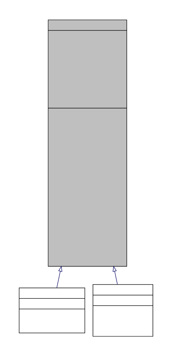
Chapter 3: C++ Classes in the Library 30

QUESO::BaseEnvironment

# m_fullEnvIsReady

# m_worldRank

# m_fullComm

# m_fullRank

# m_fullCommSize

# m_fullGroup

# m_optionsInputFileName

# m_optionsInputFileAccessState

# m_allOptionsDesc

# m_allOptionsMap

and 17 more...

+ BaseEnvironment()

+ ~BaseEnvironment()

+ operator=()

+ fullEnvIsReady()

+ worldRank()

+ fullRank()

+ fullComm()

+ subGroup()

+ subRank()

+ subComm()

+ selfComm()

+ inter0Rank()

+ inter0Comm()

and 21 more...

+ openOutputFile()

+ openUniﬁedOutputFile()

+ openInputFile()

+ openUniﬁedInputFile()

+ closeFile()

+ setExceptionalCircumstance()

+ exceptionalCircumstance()

+ print()

QUESO::EmptyEnvironment

+ print()

+ EmptyEnvironment()

+ ~EmptyEnvironment()

QUESO::FullEnvironment

+ FullEnvironment()

+ ~FullEnvironment()

+ print()

- readOptionsInputFile()

Figure 3.1.1: The class diagram for the Environment class described in Section 3.1.1.

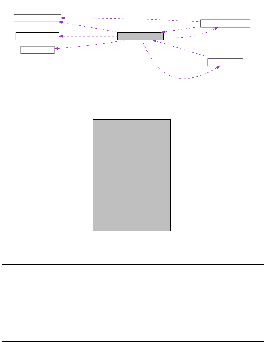
Chapter 3: C++ Classes in the Library 31

QUESO::BaseEnvironment

QUESO::EnvironmentOptions

m_env

QUESO::MpiComm

m_env

QUESO::BasicPdfsBase m_basicPdfs

QUESO::RngBase

m_rngObject

m_optionsObj

QUESO::EnvOptionsValues m_alternativeOptionsValues

m_ov

m_inter0Comm

m_selfComm

m_subComm

m_fullComm

Figure 3.1.2: Collaboration graph for the environment class described in Section 3.1.1.

QUESO::EnvironmentOptions

+ m_ov

- m_env

- m_preﬁx

- m_optionsDesc

- m_option_help

- m_option_numSubEnvironments

- m_option_subDisplayFileName

- m_option_subDisplayAllowAll

- m_option_subDisplayAllowInter0

- m_option_subDisplayAllowedSet

- m_option_displayVerbosity

and 5 more...

+ EnvironmentOptions()

+ ~EnvironmentOptions()

+ scanOptionsValues()

+ print()

- deﬁneMyOptions()

- getMyOptionValues()

Figure 3.1.3: The environment options class with its attributes and methods.

Table 3.1.1: Input ﬁle options for a QUESO environment.

Option name Default value Description

〈PREFIX〉env help Produces help message for environment class

〈PREFIX〉env numSubEnvironments 1Number of subenvironments

〈PREFIX〉env subDisplayFileName "." Output ﬁlename for sub-screen writing

〈PREFIX〉env subDisplayAllowAll 0Allows all subenvironments to write to output

ﬁle

〈PREFIX〉env subDisplayAllowedSet "" Subenvironments that will write to output ﬁle

〈PREFIX〉env displayVerbosity 0Sets verbosity

〈PREFIX〉env syncVerbosity 0Sets syncronized verbosity

〈PREFIX〉env seed 0Set seed

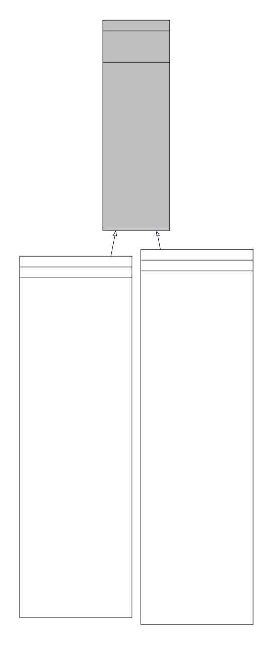
Chapter 3: C++ Classes in the Library 32

QUESO::Vector

# m_env

# m_map

# m_printHorizontally

# m_printScientiﬁc

+ Vector()

+ ~Vector()

+ operator=()

+ operator*=()

+ operator/=()

+ operator+=()

+ operator-=()

+ env()

+ map()

+ numOfProcsForStorage()

+ sizeLocal()

+ sizeGlobal()

+ cwSet()

+ cwSetGaussian()

+ cwInvert()

+ sort()

+ print()

+ setPrintHorizontally()

+ getPrintHorizontally()

+ setPrintScientiﬁc()

+ getPrintScientiﬁc()

# copy()

QUESO::GslVector

- m_vec

+ sort()

+ matlabDiﬀ()

+ matlabLinearInterpExtrap()

+ mpiBcast()

+ mpiAllReduce()

+ mpiAllQuantile()

+ subWriteContents()

+ subReadContents()

+ data()

+ GslVector()

+ ~GslVector()

+ operator=()

+ operator*=()

+ operator/=()

+ operator*=()

+ operator/=()

+ operator+=()

+ operator-=()

+ cwSet()

+ cwSetGaussian()

and 9 more...

+ operator[]()

+ sizeLocal()

+ sizeGlobal()

+ getMaxValue()

+ getMinValue()

+ getMaxValueIndex()

+ getMinValueIndex()

+ getMaxValueAndIndex()

+ getMinValueAndIndex()

+ abs()

+ norm2Sq()

+ norm2()

+ norm1()

+ normInf()

+ sumOfComponents()

+ print()

+ atLeastOneComponentSmallerT han()

+ atLeastOneComponentBiggerThan()

+ atLeastOneComponentSmallerOrEqualThan()

+ atLeastOneComponentBiggerOrEqualT han()

- copy()

QUESO::TeuchosVector

- m_vec

+ TeuchosVector()

+ ~TeuchosVector()

+ operator=()

+ operator*=()

+ operator/=()

+ operator*=()

+ operator/=()

+ operator+=()

+ operator-=()

+ cwSet()

and 9 more...

+ operator[]()

+ sizeLocal()

+ sizeGlobal()

+ values()

+ getMaxValue()

+ getMinValue()

+ getMaxValueIndex()

+ getMinValueIndex()

+ getMaxValueAndIndex()

+ getMinValueAndIndex()

+ norm2Sq()

+ norm2()

+ norm1()

+ normInf()

+ atLeastOneComponentSmallerT han()

+ atLeastOneComponentBiggerThan()

+ atLeastOneComponentSmallerOrEqualThan()

+ atLeastOneComponentBiggerOrEqualT han()

+ abs()

+ copy_to_std_vector()

+ copy_from_std_vector()

+ sort()

+ sumOfComponents()

+ mpiBcast()

+ mpiAllReduce()

+ mpiAllQuantile()

+ matlabLinearInterpExtrap()

+ matlabDiﬀ()

+ print()

+ subReadContents()

+ subWriteContents()

- copy()

Figure 3.1.4: The class diagram for the vector class described in Section 3.1.2.

Chapter 3: C++ Classes in the Library 33

classes: GslMatrix and TeuchosMatrix.GslMatrix is based on the GSL matrix structure;

whereas TeuchosMatrix is based on Trilinos Epetra matrix structure.

A class diagram for Matrix is presented in Figure 3.1.5; it displays its protected attributes

together with its member functions. Again, the diagram displays in some detail the inherited

classes GslMatrix and TeuchosMatrix.

3.2 Templated Basic Classes

The classes in this group are: vector sets, subsets and spaces (Section 3.2.1), scalar and vector

function classes (Section 3.2.2), and scalar and vector sequences (Section 3.2.3).

These classes constitute the core entities necessary for the formal mathematical deﬁnition

and description of other entities, such as random variables, Bayesian solutions of inverse

problems, sampling algorithms and chains.

3.2.1 Vector Set, Subset and Vector Space Classes

The vector set class is fundamental for the proper handling of many mathematical entities.

Indeed, the deﬁnition of a scalar function such as π:B⊂Rn→Rrequires the speciﬁcation

of the domain B, which is a subset of the vector space Rn, which is itself a set. Additionally,

SIPs need a likelihood routine πlike :Rn→R+, and SFPs need a QoI routine q:Rn→Rm;

the sets Rn,Rm, etc., are vector spaces.

The relationship amongst QUESO classes for handling sets, namely VectorSet; subsets,

namely VectorSubset; and vector spaces, namely VectorSpace is sketched in Figure 3.2.1.

An attribute of the subset class is the vector space which it belongs to, and in fact a reference

to a vector space is required by the constructor of the subset class. An example of this case

is the deﬁnition of a scalar function such as π:B⊂Rn→Rabove.

The power of an object-oriented design is clearly featured here. The intersection subset

derived class IntersectionSubset is useful for handling a posterior PDF on Equation (1.2.1),

since its domain is the intersection of the domain of the prior PDF with the domain of the

likelihood function.

3.2.2 Scalar Function and Vector Function Classes

Joint PDF, marginal PDF, and CDF are all examples of scalar functions present in statistical

problems. QUESO currently supports basic PDFs such as uniform and Gaussian and also more

complex PDFs, such as the ones coming from a Bayesian analysis. They are implemented in

the classes UniformJointPdf,GaussianJointPdf, and BayesianJointPdf, respectively. The

posterior PDF may be represented within QUESO by GenericJointPdf. See Diagram 3.2.2

for the scalar function class.

The handling of vector functions within QUESO is also quite straightforward. Indeed,

the deﬁnition of a vector function q:B⊂Rn→Rmrequires only the extra speciﬁ-

Chapter 3: C++ Classes in the Library 34

QUESO::Matrix

# m_env

# m_map

# m_printHorizontally

# m_inDebugMode

+ Matrix() (3)

+ ~Matrix()

+ operator=()

+ operator*=()

+ operator+=()

+ operator-=()

+ env()

+ map()

+ numOfProcsForStorage()

+ numRowsLocal()

+ numRowsGlobal()

+ numCols()

+ chol()

+ zeroLower()

+ zeroUpper()

+ print()

+ setPrintHorizontally()

+ getPrintHorizontally()

+ setInDebugMode()

+ getInDebugMode()

# copy()

QUESO::GslMatrix

- m_mat

- m_LU

- m_inverse

- m_svdColMap

- m_svdUmat

- m_svdSvec

- m_svdVmat

- m_svdVTmat

- m_determinant

- m_lnDeterminant

- m_permutation

- m_signum

- m_isSingular

+ GslMatrix() (6)

+ ~GslMatrix()

+ operator=()

+ operator*=()

+ operator/=()

+ operator+=()

+ operator-=()

+ operator()(v)

+ operator()()

+ numRowsLocal()

+ numRowsGlobal()

+ numCols()

+ max()

+ rank()

+ transpose()

+ inverse()

+ determinant()

+ lnDeterminant()

+ normFrob()

+ normMax()

+ chol()

+ svd()

+ svdMatU()

+ svdMatV()

+ svdSolve() (2)

+ multiply()

+ invertMultiply() (3)

and 11 more...

+ cwSet() (2)

+ cwExtract()

+ zeroLower()

+ zeroUpper()

+ ﬁlterSmallValues()

+ ﬁlterLargeValues()

+ ﬁllWithTranspose()

+ ﬁllWithBlocksDiagonally()

and 5 more...

+ data()

+ mpiSum()

+ matlabLinearInterpExtrap()

+ print()

+ subWriteContents()

+ subReadContents()

- copy()

- resetLU()

- multiply()

- internalSvd()

QUESO::TeuchosMatrix

- m_mat

- m_LU

- m_inverse

- m_svdColMap

- m_svdUmat

- m_svdSvec

- m_svdVmat

- m_svdVTmat

- m_determinant

- m_lnDeterminant

- m_permutation

- v_pivoting

- m_signum

- m_isSingular

+ TeuchosMatrix() (6)

+ ~TeuchosMatrix()

+ operator=()

+ operator*=()

+ operator/=()

+ operator+=()

+ operator-=()

+ operator()()

+ numRowsLocal()

+ numRowsGlobal()

+ numCols()

+ values()

+ stride()

+ max()

+ rank()

+ transpose()

+ inverse()

+ determinant()

+ lnDeterminant()

+ normFrob()

+ normMax()

+ chol()

+ svd()

+ svdMatU()

+ svdMatV()

+ svdSolve() (2)

+ multiply()

+ invertMultiply() (3)

and 5 more...

+ cwSet() (2)

+ getColumn() (2)

+ setColumn()

+ getRow() (2)

setRow()

+ zeroLower()

+ zeroUpper()

and 10 more...

+ mpiSum()

+ matlabLinearInterpExtrap()

+ print()

+ subReadContents()

+ subWriteContents()

- copy()

- resetLU()

- multiply()

- internalSvd()

Figure 3.1.5: The class diagram for the matrix class.

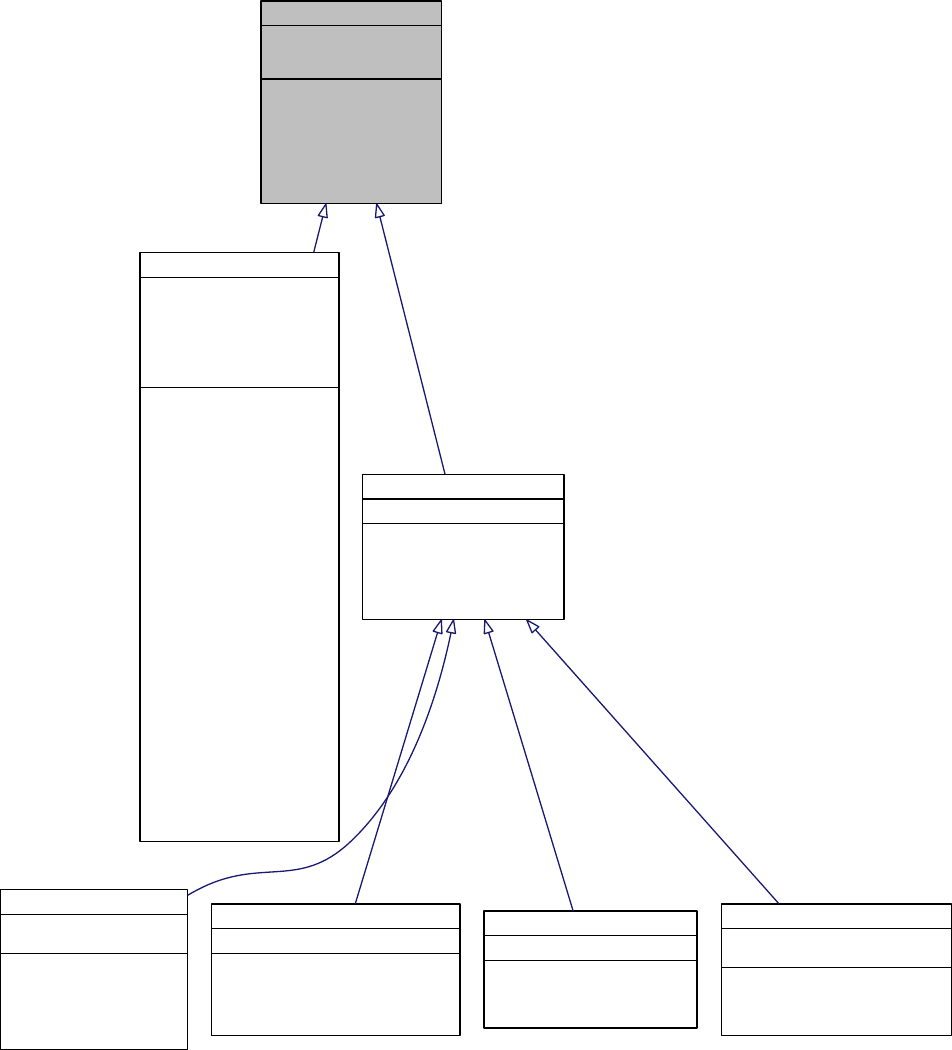
Chapter 3: C++ Classes in the Library 35

QUESO::VectorSet< V, M >

# m_env

# m_preﬁx

# m_volume

+ VectorSet()

+ ~VectorSet()

+ env()

+ preﬁx()

+ volume()

+ vectorSpace()

+ contains()

QUESO::VectorSpace< V, M >

# m_dimGlobal

# m_map

# m_dimLocal

# m_componentsNamesArray

# m_componentsNamesVec

# m_emptyComponentName

# m_zeroVector

+ newVector()

+ newMatrix()

+ newDiagMatrix()

+ VectorSpace()

+ ~VectorSpace()

+ env()

+ map()

+ numOfProcsForStorage()

+ dimLocal()

+ dimGlobal()

+ globalIdOfFirstComponent()

+ zeroVector()

+ newVector()

+ newMatrix()

+ newDiagMatrix()

+ newProposalMatrix()

+ vectorSpace()

+ contains()

+ componentsNamesArray()

+ componentsNamesVec()

+ localComponentName()

+ printComponentsNames()

+ print()

# newMap()

QUESO::VectorSubset< V, M >

# m_vectorSpace

+ VectorSubset()

+ ~VectorSubset()

+ vectorSpace()

+ contains()

+ print()

QUESO::BoxSubset< V, M >

# m_minValues

# m_maxValues

+ print()

+ BoxSubset()

+ ~BoxSubset()

+ contains()

+ minValues()

+ maxValues()

QUESO::ConcatenationSubset< V, M >

# m_sets

+ ConcatenationSubset()

+ ~ConcatenationSubset()

+ contains()

+ print()

QUESO::DiscreteSubset< V, M >

# m_elements

+ DiscreteSubset()

+ ~DiscreteSubset()

+ contains()

+ print()

QUESO::IntersectionSubset< V, M >

# m_set1

# m_set2

+ IntersectionSubset()

+ ~IntersectionSubset()

+ contains()

+ print()

Figure 3.2.1: The class diagram for vector set, vector subset and vector space classes, described

in Section 3.2.1.

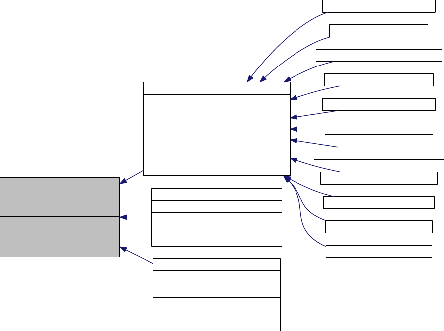
Chapter 3: C++ Classes in the Library 36

cation of the image vector space Rm. The classes representing the vector function class

GenericVectorFunction and ConstantVectorFunction are derived from BaseVectorFunction

and are presented in Diagram 3.2.3

QUESO::BaseScalarFunction< V, M >

# m_env

# m_preﬁx

# m_domainSet

+ BaseScalarFunction()

+ ~BaseScalarFunction()

+ domainSet()

+ actualValue()

+ lnValue()

QUESO::BaseJointPdf< V, M >

# m_normalizationStyle

# m_logOfNormalizationFactor

+ BaseJointPdf()

+ ~BaseJointPdf()

+ actualValue()

+ lnValue()

+ setNormalizationStyle()

+ setLogOfNormalizationFactor()

+ computeLogOfNormalizationFactor()

# commonComputeLogOfNormalizationFactor()

QUESO::ConstantScalarFunction< V, M >

# m_constantValue

+ ConstantScalarFunction()

+ ~ConstantScalarFunction()

+ actualValue()

+ lnValue()

QUESO::GenericScalarFunction< V, M >

# m_valueRoutinePtr

# m_routinesDataPtr

# m_routineIsForLn

+ GenericScalarFunction()

+ ~GenericScalarFunction()

+ actualValue()

+ lnValue()

QUESO::BayesianJointPdf< V, M >

QUESO::BetaJointPdf< V, M >

QUESO::ConcatenatedJointPdf< V, M >

QUESO::GammaJointPdf< V, M >

QUESO::GaussianJointPdf< V, M >

QUESO::GenericJointPdf< V, M >

QUESO::InverseGammaJointPdf< V, M >

QUESO::LogNormalJointPdf< V, M >

QUESO::PoweredJointPdf< V, M >

QUESO::UniformJointPdf< V, M >

QUESO::WignerJointPdf< V, M >

Figure 3.2.2: The class diagram for the scalar function class.

3.2.3 Scalar Sequence and Vector Sequence Classes

The scalar sequence class contemplates scalar samples generated by an algorithm, as well as

operations that can be done over them, e.g., calculation of means, variances, and convergence

indices. Similarly, the vector sequence class contemplates vector samples and operations such

as means, correlation matrices and covariance matrices.

Figures 3.2.4 and 3.2.5 display the class diagram for the scalar sequence and vector sequence

classes, respectively.

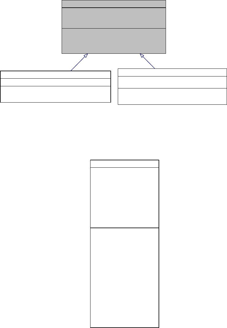
Chapter 3: C++ Classes in the Library 37

QUESO::BaseVectorFunction< P_V, P_M, Q_V, Q_M >

# m_env

# m_preﬁx

# m_domainSet

# m_imageSet

+ BaseVectorFunction()

+ ~BaseVectorFunction()

+ domainSet()

+ imageSet()

+ compute()

QUESO::ConstantVectorFunction< P_V, P_M, Q_V, Q_M >

# m_constantImageVector

+ ConstantVectorFunction()

+ ~ConstantVectorFunction()

+ compute()

QUESO::GenericVectorFunction< P_V, P_M, Q_V, Q_M >

# m_routinePtr

# m_routineDataPtr

+ GenericVectorFunction()

+ ~GenericVectorFunction()

+ compute()

Figure 3.2.3: The class diagram for the vector function class described in Section 3.2.2.

QUESO::ScalarSequence< T >

- m_env

- m_name

- m_seq

- m_subMinPlain

- m_uniﬁedMinPlain

- m_subMaxPlain

- m_uniﬁedMaxPlain

- m_subMeanPlain

- m_uniﬁedMeanPlain

- m_subMedianPlain

- m_uniﬁedMedianPlain

- m_subSampleVariancePlain

- m_uniﬁedSampleVariancePlain

+ ScalarSequence()

+ ~ScalarSequence()

+ operator=()

+ operator[]()

+ env()

+ name()

+ setName()

+ clear()

+ subSequenceSize()

+ uniﬁedSequenceSize()

+ resizeSequence()

+ resetValues()

+ erasePositions()

+ getUniﬁedContentsAtProc0Only()

and 55 more...- copy()

- extractScalarSeq()

- extractRawData()

- rawData()

- subSort()

- parallelMerge()

and 55 more...

Figure 3.2.4: The class diagram for the scalar sequence class.

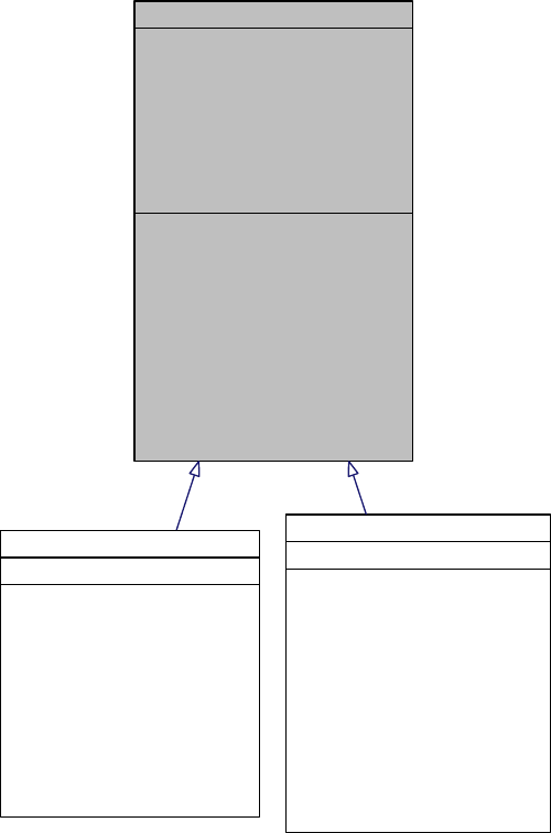
Chapter 3: C++ Classes in the Library 38

QUESO::BaseVectorSequence< V, M >

# m_env

# m_vectorSpace

# m_name

# m_ﬀtObj

# m_subMinPlain

# m_uniﬁedMinPlain

# m_subMaxPlain

# m_uniﬁedMaxPlain

# m_subMeanPlain

# m_uniﬁedMeanPlain

and 5 more...

+ BaseVectorSequence()

+ ~BaseVectorSequence()

+ subSequenceSize()

+ uniﬁedSequenceSize()

+ vectorSizeLocal()

+ vectorSizeGlobal()

+ vectorSpace()

+ name()

+ setName()

+ clear()

+ subMinPlain()

+ uniﬁedMinPlain()

and 51 more...

# copy()

# extractRawData()

QUESO::ArrayOfSequences< V, M >

- m_scalarSequences

+ ArrayOfSequences()

+ ~ArrayOfSequences()

+ subSequenceSize()

+ resizeSequence()

+ resetValues()

+ erasePositions()

+ getPositionValues()

+ setPositionValues()

+ setGaussian()

+ setUniform()

+ mean()

+ uniﬁedMean()

and 19 more...

- extractRawData()

QUESO::SequenceOfVectors< V, M >

- m_seq

+ SequenceOfVectors()

+ ~SequenceOfVectors()

+ operator=()

+ subSequenceSize()

+ resizeSequence()

+ resetValues()

+ erasePositions()

+ getPositionValues()

+ setPositionValues()

+ subUniformlySampledCdf()

+ uniﬁedUniformlySampledCdf()

+ subMeanExtra()

+ uniﬁedMeanExtra()

and 30 more...

- copy()

- extractRawData()

Figure 3.2.5: The class diagram for the vector sequence class.

Chapter 3: C++ Classes in the Library 39

3.3 Templated Statistical Classes

The classes in this group are: vector realizer, vector random variable, statistical inverse prob-

lem (and options), Metropolis-Hastings solver (and options), statistical forward problem (and

options), Monte Carlo solver (and options), and Sequence statistical options.

For QUESO, a SIP has two input entities, a prior RV and a likelihood routine, and one

output entity, the posterior RV, as shown in Chapter 1, Figure 1.2.3. Similarly, a SFP has

two input entities, a input RV and a QoI routine, and one output entity, the output RV, as

shown in Figure 1.2.2.

3.3.1 Vector Realizer Class

Arealizer is an object that, simply put, contains a realization() operation that returns a

sample of a vector RV. QUESO currently supports several realizers:

•uniform, implemented in UniformVectorRealizer,

•Gaussian, implemented in GaussianVectorRealizer,

•Log Normal, implemented in LogNormalVectorRealizer,

•Gamma, implemented in GammaVectorRealizer,

•Inverse Gamma, implemented in InverseGammaVectorRealizer, and

•Beta, , implemented in BetaVectorRealizer,

which are all derived from the base class BaseVectorRealizer.

QUESO conveniently provides the class ConcatenatedVectorRealizer, which allows two

distinct realizers to be concatenated. It also contains a sequence realizer class for storing

samples of a MH algorithm.

3.3.2 Vector Random Variable Class

Vector RVs are expected to have two basic functionalities: compute the value of its PDF

at a point, and generate realizations following such PDF. The joint PDF (BaseJointPdf

and derived classes, see Section 3.2.2) and vector realizer (BaseVectorRealizer and derived

classes, see Section 3.3.1) classes allow a straightforward deﬁnition and manipulation of vector

RVs. Similarly to the vector realizer class above, QUESO also allows users to form new RVs

through the concatenation of existing RVs (class ConcatenatedVectorRV).

QUESO currently supports a few vector RVs such as uniform, Gaussian, Gamma and Beta,

as depicted in Diagram 3.3.1. A derived class called generic vector RV allows QUESO to store

the solution of an statistical IP: a Bayesian joint PDF becomes the PDF of the posterior RV,

while a sequence vector realizer becomes the realizer of the same posterior RV.

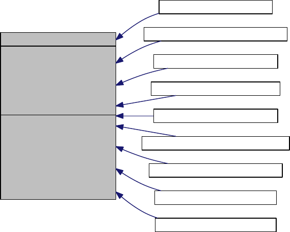
Chapter 3: C++ Classes in the Library 40

QUESO::BaseVectorRV< V, M >

# m_env

# m_preﬁx

# m_imageSet

# m_pdf

# m_realizer

# m_subCdf

# m_uniﬁedCdf

# m_mdf

+ BaseVectorRV()

+ ~BaseVectorRV()

+ env()

+ imageSet()

+ pdf()

+ realizer()

+ subCdf()

+ uniﬁedCdf()

+ mdf()

+ print()

QUESO::BetaVectorRV< V, M >

QUESO::ConcatenatedVectorRV< V, M >

QUESO::GammaVectorRV< V, M >

QUESO::GaussianVectorRV< V, M >

QUESO::GenericVectorRV< V, M >

QUESO::InverseGammaVectorRV< V, M >

QUESO::LogNormalVectorRV< V, M >

QUESO::UniformVectorRV< V, M >

QUESO::WignerVectorRV< V, M >

Figure 3.3.1: The class diagram for the vector random variable class.

3.3.3 Statistical Inverse Problem (and Options)

Similarly to its mathematical concepts, a SIP in QUESO also expects two input entities, a prior

RV and a likelihood routine, and one output entity, the posterior RV. The SIP is represented

in QUESO through the templated class StatisticalInverseProblem<P_V,P_M>, which is

illustrated in Figure 3.3.2a. One important characteristic of the QUESO design is that it

separates ‘what the problem is’ from ‘how the problem is solved’. The prior and the posterior

RV are instances of the BaseVectorRv<V,M> class, while the likelihood function is an instance

of the BaseScalarFunction<V,M> class.

The solution of a SIP is computed by calling either solveWithBayesMetropolisHastings()

or solveWithBayesMLSampling(), which are member functions of the class

StatisticalInverseProblem<P_V,P_M> class. Upon return from a solution operation, the

posterior RV is available through the postRv() member function. More details are provided

about solveWithBayesMetropolisHastings() and solveWithBayesMLSampling() in Sec-

tions 3.3.4 and 3.3.5, respectively.

Figure 3.3.2b displays the StatisticalInverseProblemOptions class, i.e. that class that

handles a variety of options for solving the SIP. Such options may be provided to QUESO by

the user’s input ﬁle; and they are listed in Table 3.3.1.

Chapter 3: C++ Classes in the Library 41

QUESO::StatisticalInverseProblem< P_V, P_M >

- m_env

- m_priorRv

- m_likelihoodFunction

- m_postRv

- m_solutionDomain

- m_solutionPdf

- m_subSolutionMdf

- m_subSolutionCdf

- m_solutionRealizer

- m_mhSeqGenerator

and 5 more...

+ StatisticalInverseProblem()

+ ~StatisticalInverseProblem()

+ computeSolutionFlag()

+ solveWithBayesMetropolisHastings()

+ solveWithBayesMLSampling()

+ priorRv()

+ postRv()

+ logEvidence()

+ meanLogLikelihood()

+ eig()

+ print()

(a) StatisticalInverseProblem

QUESO::StatisticalInverseProblemOptions

+ m_ov

+ m_preﬁx

- m_env

- m_optionsDesc

- m_option_help

- m_option_computeSolution

- m_option_dataOutputFileName

- m_option_dataOutputAllowedSet

+ StatisticalInverseProblemOptions()

+ ~StatisticalInverseProblemOptions()

+ scanOptionsValues()

+ print()

- deﬁneMyOptions()

- getMyOptionValues()

(b) StatisticalInverseProblemOptions

Figure 3.3.2: The statistical inverse problem class, which implements the representation in

Figure 1.2.3, and statistical inverse problem options class.

Table 3.3.1: Input ﬁle options for a QUESO statistical inverse problem.

Option name Default Value Description

〈PREFIX〉ip help Produces help message for statistical inverse

problem

〈PREFIX〉ip computeSolution 1 Computes solution process

〈PREFIX〉ip dataOutputFileName "." Name of data output ﬁle

〈PREFIX〉ip dataOutputAllowedSet "" Subenvironments that will write to data out-

put ﬁle

Chapter 3: C++ Classes in the Library 42

3.3.4 Metropolis-Hastings Solver (and Options)

The templated class that represents a Metropolis-Hastings generator of samples in QUESO

is MetropolisHastingsSG<P_V,P_M>, where SG stands for ’Sequence Generator’. This class

implements the DRAM algorithm of Haario, Laine, Mira and Saksman [18] together with an

operation named generateSequence() based on the core routine at the MCMC toolbox for

MATLAB [30].

The Metropolis-Hastings sequence generator class is depicted in Figure 3.3.3a; the Metropolis-

Hastings sequence generator options class is depicted in Figure 3.3.3b. A collaboration graph

for the Metropolis-Hastings class is presented in Figure 3.3.4; and the options are presented

in Table 3.3.2.

QUESO::MetropolisHastingsSG< P_V, P_M >

- m_env

- m_vectorSpace

- m_targetPdf

- m_initialPosition

- m_initialProposalCovMatrix

- m_nullInputProposalCovMatrix

- m_targetPdfSynchronizer

- m_tk

- m_positionIdForDebugging

- m_stageIdForDebugging

and 9 more...

+ MetropolisHastingsSG()

+ ~MetropolisHastingsSG()

+ generateSequence()

+ getRawChainInfo()

+ print()

- commonConstructor()

- generateFullChain()

- readFullChain()

- updateAdaptedCovMatrix()

- alpha()

- acceptAlpha()

- writeInfo()

(a) MetropolisHastingsSG

QUESO::MetropolisHastingsSGOptions

+ m_ov

+ m_preﬁx

- m_env

- m_optionsDesc

- m_option_help

- m_option_dataOutputFileName

- m_option_dataOutputAllowAll

- m_option_dataOutputAllowedSet

- m_option_totallyMute

- m_option_initialPosition_dataInputFileName

- m_option_initialPosition_dataInputFileT ype

- m_option_initialProposalCovMatrix_dataInputFileName

and 37 more...

+ MetropolisHastingsSGOptions()

+ ~MetropolisHastingsSGOptions()

+ scanOptionsValues()

+ print()

- deﬁneMyOptions()

- getMyOptionValues()

(b) MetropolisHastingsSGOptions

Figure 3.3.3: The Metropolis-Hastings sequence generator class and the Metropolis-Hastings

sequence generator options class.

3.3.5 Multilevel Solver (and Options)

The templated class that represents a Multilevel generator of samples in QUESO is

MLSampling<P_V,P_M>. This class implements the Adaptive Multilevel Stochastic Simulation

Algorithm of Cheung and Prudencio [8]. The Multilevel sequence generator class is assisted

by two extra classes, MLSamplingOptions and MLSamplingLevelOptions, for handling the

options to be used.

The Multilevel class, the Multilevel options and level options classes are depicted in Fig-

ure 3.3.5. A collaboration graph for the Multilevel class is presented in Figure 3.3.6; whereas

its associated options are presented in Table 3.3.3.

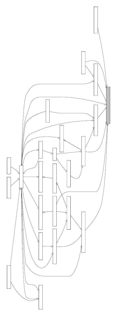
Chapter 3: C++ Classes in the Library 43

QUESO::MetropolisHastingsSG< P_V, P_M >

QUESO::BaseEnvironment

m_env

QUESO::EnvironmentOptions

m_env

QUESO::MpiComm

m_env

QUESO::ScalarFunctionSynchronizer< P_V, P_M >

m_env QUESO::BaseScalarFunction< P_V, P_M >

m_env QUESO::VectorSet< P_V, P_M >

m_env

QUESO::BaseScalarFunction< V, M >

m_env

QUESO::BaseScalarFunction< P_V,P_M >

m_env

QUESO::BaseTKGroup< P_V, P_M >

m_env

QUESO::EmptyEnvironment

QUESO::VectorSet< P_V,P_M >

m_env

QUESO::MetropolisHastingsSGOptions

m_env

QUESO::BasicPdfsBase

m_basicPdfs

QUESO::RngBase

m_rngObject

m_optionsObj

QUESO::EnvOptionsValues

m_alternativeOptionsValues

m_ov

m_inter0Comm

m_selfComm

m_subComm

m_fullComm

QUESO::Map

m_MpiComm

m_targetPdfSynchronizer

m_scalarFunction QUESO::BayesianJointPdf< P_V, P_M >

m_likelihoodFunction

m_domainSet

m_bayesianJointPdfPtr

QUESO::BaseJointPdf< P_V,P_M >QUESO::BaseJointPdf< P_V, P_M >

m_targetPdf

m_priorDensity

QUESO::MhOptionsValues

m_alternativeOptionsValues

m_ov

m_tk

m_emptyEnv

QUESO::VectorSpace< P_V, P_M >

m_vectorSpace

QUESO::DistArray< std::string >

m_componentsNamesVec

m_componentsNamesArray

m_map

m_Map

QUESO::MHRawChainInfoStruct

m_rawChainInfo m_optionsObj

Figure 3.3.4: Collaboration graph of the Metropolis-Hastings sequence generator class.

Chapter 3: C++ Classes in the Library 44

Table 3.3.2: Input ﬁle options for a QUESO Metropolis-Hastings solver.

Option Name Default Value

〈PREFIX〉mh dataOutputFileName "."

〈PREFIX〉mh dataOutputAllowAll 0

〈PREFIX〉mh initialPositionDataInputFileName "."

〈PREFIX〉mh initialPositionDataInputFileType "m"

〈PREFIX〉mh initialProposalCovMatrixDataInputFileName "."

〈PREFIX〉mh initialProposalCovMatrixDataInputFileType "m"

〈PREFIX〉mh rawChainDataInputFileName "."

〈PREFIX〉mh rawChainDataInputFileType "m"

〈PREFIX〉mh rawChainSize 100

〈PREFIX〉mh rawChainGenerateExtra 0

〈PREFIX〉mh rawChainDisplayPeriod 500

〈PREFIX〉mh rawChainMeasureRunTimes 1

〈PREFIX〉mh rawChainDataOutputPeriod 0

〈PREFIX〉mh rawChainDataOutputFileName "."

〈PREFIX〉mh rawChainDataOutputFileType "m"

〈PREFIX〉mh rawChainDataOutputAllowAll 0

〈PREFIX〉mh filteredChainGenerate 0

〈PREFIX〉mh filteredChainDiscardedPortion 0.

〈PREFIX〉mh filteredChainLag 1

〈PREFIX〉mh filteredChainDataOutputFileName "."

〈PREFIX〉mh filteredChainDataOutputFileType "m"

〈PREFIX〉mh filteredChainDataOutputAllowAll 0

〈PREFIX〉mh displayCandidates 0

〈PREFIX〉mh putOutOfBoundsInChain 1

〈PREFIX〉mh tkUseLocalHessian 0

〈PREFIX〉mh tkUseNewtonComponent 1

〈PREFIX〉mh drMaxNumExtraStages 0

〈PREFIX〉mh drDuringAmNonAdaptiveInt 1

〈PREFIX〉mh amKeepInitialMatrix 0

〈PREFIX〉mh amInitialNonAdaptInterval 0

〈PREFIX〉mh amAdaptInterval 0

〈PREFIX〉mh amAdaptedMatricesDataOutputPeriod 0

〈PREFIX〉mh amAdaptedMatricesDataOutputFileName "."

〈PREFIX〉mh amAdaptedMatricesDataOutputFileType "m"

〈PREFIX〉mh amAdaptedMatricesDataOutputAllowAll 0

〈PREFIX〉mh amEta 1.

〈PREFIX〉mh amEpsilon 1×10−5

〈PREFIX〉mh enableBrooksGelmanConvMonitor 0

〈PREFIX〉mh BrooksGelmanLag 100

Chapter 3: C++ Classes in the Library 45

QUESO::MLSampling< P_V, P_M >

- m_env

- m_priorRv

- m_likelihoodFunction

- m_vectorSpace

- m_targetDomain

- m_options

- m_currLevel

- m_currStep

- m_debugExponent

- m_logEvidenceFactors

- m_logEvidence

- m_meanLogLikelihood

- m_eig

+ MLSampling()

+ ~MLSampling()

+ generateSequence()

+ logEvidence()

+ meanLogLikelihood()

+ eig()

+ print()

- checkpointML()

- restartML()

- generateSequence_Level0_all()

- generateSequence_Step01_inter0()

- generateSequence_Step02_inter0()

- generateSequence_Step03_inter0()

- generateSequence_Step04_inter0()

- generateSequence_Step05_inter0()

- generateSequence_Step06_all()

- generateSequence_Step07_inter0()

and 11 more...

(a) MLSampling

QUESO::MLSamplingOptions

+ m_preﬁx

+ m_restartInputFileName

+ m_restartInputFileT ype

+ m_restartChainSize

+ m_dataOutputFileName

+ m_dataOutputAllowAll

+ m_dataOutputAllowedSet

- m_env

- m_optionsDesc

- m_option_help

- m_option_restartInputFileName

- m_option_restartInputFileType

- m_option_restartChainSize

- m_option_dataOutputFileName

- m_option_dataOutputAllowAll

- m_option_dataOutputAllowedSet

+ MLSamplingOptions()

+ ~MLSamplingOptions()

+ scanOptionsValues()

+ print()

- deﬁneMyOptions()

- getMyOptionValues()

(b) MLSamplingOptions

QUESO::MLSamplingLevelOptions

+ m_preﬁx

+ m_checkpointOutputFileName

+ m_stopAtEnd

+ m_dataOutputFileName

+ m_dataOutputAllowAll

+ m_dataOutputAllowedSet

+ m_str1

+ m_loadBalanceAlgorithmId

+ m_loadBalanceTreshold

+ m_minEﬀectiveSizeRatio

and 49 more...

- m_env

- m_optionsDesc

- m_option_help

- m_option_checkpointOutputFileName

- m_option_stopAtEnd

- m_option_dataOutputFileName

- m_option_dataOutputAllowAll

- m_option_dataOutputAllowedSet

- m_option_loadBalanceAlgorithmId

- m_option_loadBalanceTreshold

and 46 more...

+ MLSamplingLevelOptions()

+ ~MLSamplingLevelOptions()

+ env()

+ scanOptionsValues()

+ print()

- copyOptionsValues()

- deﬁneMyOptions()

- getMyOptionValues()

Figure 3.3.5: The Multilevel sequence generator options class (3.3.5a) and its associated classes

for handling options.

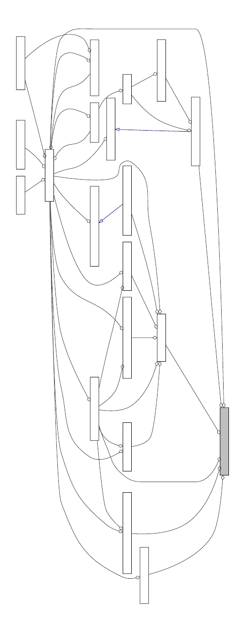
Chapter 3: C++ Classes in the Library 46

QUESO::MLSampling< P_V, P_M >

QUESO::BaseEnvironment

m_env

QUESO::EnvironmentOptions

m_env

QUESO::MpiComm

m_env

QUESO::BaseScalarFunction< P_V, P_M >

m_env QUESO::VectorSet< P_V, P_M >

m_env

QUESO::MLSamplingOptions

m_env

QUESO::BaseVectorRV

m_env

QUESO::BaseVectorCdf

m_env

QUESO::BaseVectorRealizer< P_V, P_M >

m_env

QUESO::BaseVectorMdf

m_env QUESO::BaseScalarFunction< P_V,P_M >

m_env

QUESO::VectorSet< P_V,P_M >

m_env

QUESO::BasicPdfsBase

m_basicPdfs

QUESO::RngBase

m_rngObject

m_optionsObj

QUESO::EnvOptionsValues

m_alternativeOptionsValues

m_ov

m_inter0Comm

m_selfComm

m_subComm

m_fullComm

QUESO::Map

m_MpiComm

m_likelihoodFunction

m_targetDomain

m_domainSet

m_imageSet

m_pdfSupport m_uniﬁedImageSet m_domainSet

m_options

m_priorRv

m_uniﬁedCdf

m_subCdf m_realizer m_mdf

QUESO::BaseJointPdf< P_V, P_M >

m_pdf

QUESO::VectorSpace< P_V, P_M >

m_vectorSpace

QUESO::DistArray< std::string >

m_componentsNamesVec

m_componentsNamesArray

m_map

m_Map

Figure 3.3.6: Collaboration graph of the Multilevel sampling class.

Chapter 3: C++ Classes in the Library 47

Table 3.3.3: Input ﬁle options for a QUESO Multilevel solver (to be continued).

Option Name Default Value

〈PREFIX〉ml restartOutput levelPeriod 0

〈PREFIX〉ml restartOutput baseNameForFiles "."

〈PREFIX〉ml restartOutput fileType "m"

〈PREFIX〉ml restartInput baseNameForFiles "."

〈PREFIX〉ml restartInput fileType "m"

〈PREFIX〉ml stopAtEnd 0

〈PREFIX〉ml dataOutputFileName "."

〈PREFIX〉ml dataOutputAllowAll 0

〈PREFIX〉ml loadBalanceAlgorithmId 2

〈PREFIX〉ml loadBalanceTreshold 1.0

〈PREFIX〉ml minEffectiveSizeRatio 0.85

〈PREFIX〉ml maxEffectiveSizeRatio 0.91

〈PREFIX〉ml scaleCovMatrix 1

〈PREFIX〉ml minRejectionRate 0.50

〈PREFIX〉ml maxRejectionRate 0.75

〈PREFIX〉ml covRejectionRate 0.25

〈PREFIX〉ml minAcceptableEta 0.

〈PREFIX〉ml totallyMute 1

〈PREFIX〉ml initialPositionDataInputFileName "."

〈PREFIX〉ml initialPositionDataInputFileType "m"

〈PREFIX〉ml initialProposalCovMatrixDataInputFileName "."

〈PREFIX〉ml initialProposalCovMatrixDataInputFileType "m"

〈PREFIX〉ml rawChainDataInputFileName "."

〈PREFIX〉ml rawChainDataInputFileType "m"

〈PREFIX〉ml rawChainSize 100

〈PREFIX〉ml rawChainGenerateExtra 0

〈PREFIX〉ml rawChainDisplayPeriod 500

〈PREFIX〉ml rawChainMeasureRunTimes 1

〈PREFIX〉ml rawChainDataOutputPeriod 0

〈PREFIX〉ml rawChainDataOutputFileName "."

〈PREFIX〉ml rawChainDataOutputFileType "m"

〈PREFIX〉ml rawChainDataOutputAllowAll 0

〈PREFIX〉ml filteredChainGenerate 0

〈PREFIX〉ml filteredChainDiscardedPortion 0.

〈PREFIX〉ml filteredChainLag 1

〈PREFIX〉ml filteredChainDataOutputFileName "."

〈PREFIX〉ml filteredChainDataOutputFileType "m"

〈PREFIX〉ml filteredChainDataOutputAllowAll 0

〈PREFIX〉ml displayCandidates 0

〈PREFIX〉ml putOutOfBoundsInChain 1

〈PREFIX〉ml tkUseLocalHessian 0

〈PREFIX〉ml tkUseNewtonComponent 1

〈PREFIX〉ml drMaxNumExtraStages 0

〈PREFIX〉ml drScalesForExtraStages 0

〈PREFIX〉ml drDuringAmNonAdaptiveInt 1

〈PREFIX〉ml amKeepInitialMatrix 0

〈PREFIX〉ml amInitialNonAdaptInterval 0

〈PREFIX〉ml amAdaptInterval 0

〈PREFIX〉ml amAdaptedMatricesDataOutputPeriod 0

〈PREFIX〉ml amAdaptedMatricesDataOutputFileName "."

〈PREFIX〉ml amAdaptedMatricesDataOutputFileType "m"

〈PREFIX〉ml amAdaptedMatricesDataOutputAllowAll 0

〈PREFIX〉ml amEta 1.

〈PREFIX〉ml amEpsilon 1.e-5

Chapter 3: C++ Classes in the Library 48

3.3.6 Statistical Forward Problem (and Options)

A SFP in QUESO also has two input entities, the input (parameter) RV and a QoI func-

tion, and one output entity, the QoI RV. The SIP is represented through the templated

class StatisticalForwardProblem<P_V,P_M,Q_V,Q_M >, which diagram is presented in Fig-

ure 3.3.7a. Again, the types P_V and Q_V of vectors and types P_M and Q_M of matrices, where

P_ stands for ’parameter’ and Q_ stands for ’quantities of interest’.

The input RV and the output QoI RV are instances of the BaseVectorRv<P_V,P_M> class,

while the QoI function is an instance of BaseVectorFunction<P_V,P_M,Q_V,Q_M>. In the

template parameters, the preﬁx P_ refers to the parameters, whereas the preﬁx Q_ refers to

the QoIs.

In order to ﬁnd the solution of a SFP, one must call the solveWithMonteCarlo() member

function of the StatisticalForwardProblem<P_V,P_M> class. Upon return from a solution

operation, the QoI RV is available through the qoiRv() member function. Such QoI RV is able

to provide: a vector realizer through the operation ’qoiRv().realizer()’, which returns an

instance of the class ’uqBaseVectorRealizer<Q_V,Q_M>’.

Figure 3.3.7b displays the statistical forward problem options class, i.e. that class that

handles a variety of options for solving the SFP. Such options may be provided to QUESO at

the user’s input ﬁle; and they are listed in Table 3.3.4. In the table, p-q stands for parameter–

quantity of interest.

Table 3.3.4: Input ﬁle options for a QUESO statistical forward problem.

Option Name Default Value Description

〈PREFIX〉fp computeSolution 1 Computes the solution process

〈PREFIX〉fp computeCovariances 1 Compute p-q covariances

〈PREFIX〉fp computeCorrelations 1 Compute p-q correlations

〈PREFIX〉fp dataOutputFileName "." Name of data output ﬁle

〈PREFIX〉fp dataOutputAllowedSet "" Subenvironments that will write to data

output ﬁle

3.3.7 Monte Carlo Solver (and Options)

The templated class that implements a Monte Carlo generator of samples within QUESO

is MonteCarloSG<P_V,P_M,Q_V,Q_M>, as illustrated in Figure 3.3.8a. This class has the re-

quirement that the image set of the vector random variable and the domain set of the QoI

function belong to vector spaces of equal dimensions. If the requirements are satisﬁed, the class

constructor reads input options that begin with the string ‘<PREFIX>_mc_’ (See Table 3.3.5).

Options reading is handled by class MonteCarloOptions, which is illustrated in Figure 3.3.8b.

Chapter 3: C++ Classes in the Library 49

QUESO::StatisticalForwardProblem< P_V, P_M, Q_V, Q_M >

- m_env

- m_paramRv

- m_qoiFunction

- m_qoiRv

- m_paramChain

- m_qoiChain

- m_mcSeqGenerator

- m_solutionRealizer

- m_solutionPdf

- m_alternativeOptionsValues

- m_optionsObj

+ StatisticalForwardProblem()

+ ~StatisticalForwardProblem()

+ computeSolutionFlag()

+ solveWithMonteCarlo()

+ qoiRv()

+ getParamChain()

+ print()

- commonConstructor()

(a) StatisticalForwardProblem

QUESO::StatisticalForwardProblemOptions

+ m_ov

+ m_preﬁx

- m_env

- m_optionsDesc

- m_option_help

- m_option_computeSolution

- m_option_computeCovariances

- m_option_computeCorrelations

- m_option_dataOutputFileName

- m_option_dataOutputAllowedSet

+ StatisticalForwardProblemOptions()

+ ~StatisticalForwardProblemOptions()

+ scanOptionsValues()

+ print()

- deﬁneMyOptions()

- getMyOptionValues()

(b) StatisticalForwardProblemOptions

Figure 3.3.7: The statistical forward problem class, which implements the representation in

Figure 1.2.2, and the statistical forward problem options class.

QUESO::MonteCarloSG< P_V, P_M, Q_V, Q_M >

- m_env

- m_paramRv

- m_qoiFunction

- m_paramSpace

- m_qoiSpace

- m_qoiFunctionSynchronizer

- m_numPsNotSubWritten

- m_numQsNotSubWritten

- m_alternativeOptionsValues

- m_optionsObj

+ MonteCarloSG()

+ ~MonteCarloSG()

+ generateSequence()

+ print()

- internGenerateSequence()

- actualGenerateSequence()

- actualReadSequence()

(a) MonteCarloSG

QUESO::MonteCarloSGOptions

+ m_ov

+ m_preﬁx

- m_env

- m_optionsDesc

- m_option_help

- m_option_dataOutputFileName

- m_option_dataOutputAllowedSet

- m_option_pseq_dataOutputPeriod

- m_option_pseq_dataOutputFileName

- m_option_pseq_dataOutputFileT ype

- m_option_pseq_dataOutputAllowedSet

- m_option_qseq_dataInputFileName

and 7 more...

+ MonteCarloSGOptions()

+ ~MonteCarloSGOptions()

+ scanOptionsValues()

+ print()

- deﬁneMyOptions()

- getMyOptionValues()

(b) MonteCarloSGOptions

Figure 3.3.8: The Monte Carlo sequence generator class and the Monte Carlo sequence gen-

erator options class.

Chapter 3: C++ Classes in the Library 50

Table 3.3.5: Input ﬁle options for a QUESO statistical forward problem solved via Monte

Carlo algorithm.

Option Name Default Value

〈PREFIX〉mc dataOutputFileName "."

〈PREFIX〉mc dataOutputAllowedSet

〈PREFIX〉mc pseq dataOutputFileName "."

〈PREFIX〉mc pseq dataOutputAllowedSet

〈PREFIX〉mc qseq dataInputFileName "."

〈PREFIX〉mc qseq size 100

〈PREFIX〉mc qseq displayPeriod 500

〈PREFIX〉mc qseq measureRunTimes 0

〈PREFIX〉mc qseq dataOutputFileName "."

〈PREFIX〉mc qseq dataOutputAllowedSet

3.4 Miscellaneous Classes and Routines

As the name suggests, QUESO miscellaneous classes and routines have a variety of routines.

For instance, the function MiscReadDoublesFromString is used for reading the options in-

put ﬁles and assigning the values to the respective variables, in uqMonteCarloSGOptions::

getMyOptionValues and in MetropolisHastingsSGOptions::getMyOptionValues.

QUESO class BaseOneDGrid generates grids necessary for calculating the CDF of a RV; it is

required by class ArrayOfOneDGrids, which, in turn, is used in both classes:

StatisticalForwardProblem and StatisticalInverseProblem.

CHAPTER 4

Important Remarks

At this point, the user may feel comfortable and ready to start his/her validation and cali-

bration exercises using QUESO. There are, however, a few quite important remarks that will

make the linkage of the QUESO Library with the user application code possible. They are

addressed in the following sections.

4.1 Revisiting Input Options

Input options are read from the QUESO input ﬁle, whose name is required by the constructor

of the QUESO environment class. Herein, suppose that no preﬁx is deﬁned, i.e., nothing

will precede the input variables names (PREFIX = "" in Tables 3.1.1 –3.3.5). An example

of the use of preﬁxes may be found in the input ﬁle tgaCycle.inp under the subdirectory

/examples/validationCycle/ of QUESO installation tree.

The ﬁrst part of a input ﬁle commonly handles the environment options. he variable as-

signment env_numSubEnvironments = 1 indicates to QUESO that only one subenvironment

should be used. The variable assignment env subDisplayFileName = outputData/ display

create both the subdirectory outputData/ and a ﬁle named display_sub0.txt that contains

all the options listed in the input ﬁle together with more speciﬁc information, such as the

chain run time and the number of delayed rejections. The existence of ﬁle display_sub0.txt

allows, for instance, the user in verifying the actual parameters read by QUESO.

For an SIP, the user may set up variables related to the DRAM algorithm. Six impor-

tant variables are: ip mh dr maxNumExtraStages deﬁnes how many extra candidates will be

generated; ip mh dr listOfScalesForExtraStages deﬁnes the list sof scaling factors that

will multiply the covariance matrix. The variable ip mh am initialNonAdaptInterval de-

CHAPTER 4. IMPORTANT REMARKS 52

ﬁnes the initial interval in which the proposal covariance matrix will not be changed; whereas

ip mh am adaptInterval deﬁnes the size of the interval in which each adapted proposal co-

variance matrix will be used. ip mh am eta is a factor used to scale the proposal covariance

matrix, usually set to be 2.42/d, where dis the dimension of the problem [31,18]. Finally,

ip mh am epsilon is the covariance regularization factor used in the DRAM algorithm.

For a SFP, the variable assignment fp_computeSolution = 1 tells QUESO to compute the

solution process; the assignment fp_computeCovariances = 1, instructs QUESO to compute

parameter–QoI covariances, and analogously, fp_computeCorrelations = 1 inform QUESO

to compute parameter–QoI correlations. The name of the data output ﬁle can be set with

variable fp_dataOutputFileName arg; and fp_dataOutputAllowedSet deﬁnes which suben-

vironments will write to data output ﬁle.

An example a complete input ﬁle used by QUESO to solve a SIP–SFP is presented in

Section 5.3.5; however every application example included in QUESO build and installation

directories examples has an options input ﬁle and the user is invited to familiarize him/herself

with them.

4.2 Revisiting Priors

QUESO oﬀers a variety of prior distributions: uniform, Gaussian, Beta, Gamma, Inverse

Gamma, and Log Normal. Also, QUESO presents the option of concatenating any of those

priors, through the Concatenated prior.

Concatenated priors are employed in problems with multiple random parameters. They

allow one random parameter to have a diﬀerent prior distribution then other; i.e., one variable

may have a uniform prior distribution whereas other may have a Gaussian prior distribution.

It is important to notice that, in order to set a Gaussian prior, besides providing the mean,

the user must also supply the variance, not the standard deviation.

4.3 Running with Multiple Chains or Monte Carlo Se-

quences

As presented in the previous section, the variable env_numSubEnvironments determines how

many subenvironments QUESO will work with. Thus, if env_numSubEnvironments=1, then

only one subenvironment will be used, and QUESO will use only one set on Monte Carlo

chains of size deﬁned by ones of the variables ip_mh_rawChain_size or fp_mc_qseq_size,

depending either the user is solving a SIP or a SFP.

If the user wants to run QUESO with multiple chains or Monte Carlo sequences, then two

variables have to be set in QUESO input ﬁle: env_numSubEnvironments = Ns, with Ns>1

is the number of chains and/or Monte Carlo sequences of samples; and env_seed = −z, with

z>1, so that each processor sets the seed to value MPI RANK+z. It is crucial that env_seed

takes a negative value, otherwise all chain samples are going to be the same.

CHAPTER 4. IMPORTANT REMARKS 53

Also, the total number Npof processors in the full communicator, usually named

MPI COMM WORLD, needs to be a multiple of Ns.

4.4 Running with Models that Require Parallel Computing

It is possible to run QUESO with models that require parallel computing as long as total

number of processors Npis multiple of the number of subenvironments Ns. QUESO will

internally create Nssubcommunicators, each of size Np/Ns, and make sure that the likelihood

and QoI routines are called for all processors in these subcommunicators – the likelihood/QoI

routine will have available a communicator of size Np/Ns. For instance, if Np= 2048 and

Ns= 16, then each likelihood/QoI will have available a communicator of size 128. s Each

subcommunicator is accessible through env.subComm(). At the end of the simulation, there

will be a total of Nschains.

The user, however, must keep in mind the possible occurrence of race condition, especially

in the case where the application is a black box and ﬁles are being accessed constantly (e.g.

data is being written and read).

4.5 A Requirement for the DRAM Algorithm

Besides setting up the variables related to the DRAM algorithm in the input ﬁle, as described

in Section 4.1 above, the user must also provide an initialized covariance matrix before calling

the DRAM solver, solveWithBayesMetropolisHastings(...), in his/her application code.

It is worth to note that this is rather a DRAM requirement [31], not a QUESO limitation.

An example of the instantiation and initialization of a proposal covariance matrix and its

subsequent use is presented in lines 145-147 of Listings 5.27, Section 5.3.4.

CHAPTER 5

QUESO Examples

This chapter assumes that the user has successfully installed QUESO and its dependencies.

It presents a variety of examples of how to use QUESO in order to develop applications.

There are examples that solve a statistical inverse problem (Sections 5.1,5.5,5.6 and 5.7),

a statistical forward problem (Section 5.2) or a combination of both, where the solution of

the former serves as input to the later (Sections 5.3 and 5.4). Three of the ﬁrst four examples

(Sections 5.1,5.3 –5.4) use the DRAM algorithm for solving the SIP, and the last three

examples use the Multilevel algorithm. Each section presents:

•the mathematical models for the SIP and/or the SFP;

•the application codes that translate the mathematical language into C++ using the

QUESO classes and algorithms;

•the input ﬁle that contains a list of options for either the Markov chain Monte Carlo

algorithm or the Multilevel algorithm (in case of SIPs) and the Monte Carlo algorithm

(in case of SFPs) which will be used by QUESO classes and algorithms;

•examples of Makeﬁles which may be used to link the code with QUESO library;

•how to plot ﬁgures using Matlab/GNU Octave and the output data generated by each

application.

All the examples presented in this chapter may be found under the directory examples in

both QUESO installation and build directories and are compatible with QUESO 0.50.0.

Note: Even though the Multilevel method is a methodology very useful for stochastic system

model class comparison (model updating, model selection, model validation) [6], such tasks

are not discussed in this manual. Thus the explicit dependency of the statistical variables on

the predictive model in the set Mjas presented in Section 1.4.2 are omitted herein.

CHAPTER 5. QUESO EXAMPLES 55

5.1 simpleStatisticalInverseProblem

According to the Bayesian paradigm, the unobservable parameters in a statistical model are

treated as random. When no data is available, a prior distribution is used to quantify our

knowledge about the parameter. When data are available, we can update our prior knowledge

using the conditional distribution of parameters, given the data. The transition from the prior

to the posterior is possible via the Bayes theorem:

πposterior(θ|d) = πprior(θ)πlikelihood(d|θ)

π(d)

In this example, suppose a random variable of interest with two parameters θ∈R2has

a uniform prior distribution, and suppose that a suitable likelihood has normal distribution

with mean µand covariance matrix C, given by:

µ=−1

2and C=4 0

0 1 .(5.1.1)

Therefore, we have:

πprior(θ)∝1

and

πlike(θ)∝exp −1

2(θ−µ)T[C−1](θ−µ),

where

θ=θ1

θ2∈R2.

Therefore, posterior PDF is given by:

πpost(θ)∝e−1

2{(θ−µ)T[C−1](θ−µ)}.(5.1.2)

In this example, we can replace the values for the mean and covariance matrix given in

Equation (5.1.1) into Equation (5.1.2), in order to analytically compute both the posterior

PDF:

πpost(θ) = 1

4πexp −1

2(θ−µ)T[C−1](θ−µ)

4πexp −1

8(θ1+ 1)2−1

2(θ2−2)2,

and the marginal results for θ1and θ2:

πpost(θ1) = 1

2√2πexp −1

8(θ1+ 1)2,

πpost(θ1) = 1

√2πexp −1

2(θ2−2)2.

(5.1.3)

CHAPTER 5. QUESO EXAMPLES 56

Recall that the posterior PDF given in Equation (5.1.2) can be sampled through the

expression:

µ+C1/2N(0, I),(5.1.4)

where N(0, I) designates a Gaussian joint PDF of zero mean and unit covariance matrix, and

C1/2is given by:

C1/2=2 0

0 1 .

Thus, in this simple statistical inverse problem, we use QUESO implementation of the

Markov chain algorithm to sample the posterior (5.1.2) via Expression (5.1.4) and compare

the calculated marginal results for θ1and θ2against the analytical formulas given in Equa-

tion (5.1.3).

Note: Due to the possibility to compare QUESO sampling algorithms to analytical expres-

sions, this example is also used in the veriﬁcation procedures and regression tests within

QUESO, and it is reproduced in the directory tests/t02_sip_sfp.

5.1.1 Running the Example

To run the executable provided (available after QUESO installation), enter the following

commands:

$cd $H OM E / L IB RA RI ES / QU ESO - 0. 50 .0/

$cd examples/simpleStatisticalInverseProblem

$rm output D ata /*

$./ e xSimpleStat i st icalInverseProble m _g sl e xa mp le . in p

$matlab

$simple_ip_plots # i n s i d e ma t l ab

$exit # i n s i d e m a t lab

$ls -l o u tputDa ta /*. png

s im ple_ip_aut o co rrelation_ra w _f ilt . png s im ple_ip _hist_f ilt . png

simple_ ip_cdf _filt . pn g simple_ ip_his t_raw . pn g

simple_ ip_cd f_raw . pn g simple_ ip_kde _filt . pn g

s im ple_ ip_chain_ p os _fil t . png simple_ ip_kd e_raw . pn g

As a result, the user should have created several of PNG ﬁgures containing marginal pos-

terior PDF, chain positions, histograms, cumulative density distributions and autocorrelation

of both parameters. The name of the ﬁgure ﬁles have been chosen to be informative, as shown

in the Listing above.

It is worth noting presence of an argument passed to the executable in the example, namely

‘example.inp’. The argument is a input ﬁle to be provided to QUESO with options for the

solution of the SIP and/or SFP; and it is always required. Each option in the input ﬁle is

related to one (or more) of the QUESO classes, and is presented throughout Chapter 3.

CHAPTER 5. QUESO EXAMPLES 57

5.1.2 Example Code

The source code for the example is composed of 5 ﬁles: example main.C (Listing 5.1),

example likelihood.h and example likelihood.C (Listings 5.2 and 5.3), example compute.h

and example compute.C (Listings 5.4 and 5.5).

#i n c l u d e <example compute .h>

int mai n (int argc , c har * argv [])

{

// Initia l ize e n vironm e nt

MPI _I ni t (& argc ,& a rgv );

UQ_FATAL_TEST_MACRO(argc != 2,

QUESO::UQ_UNAVAILABLE_RANK ,

" m ai n () " ,

" input file must be spe cifie d in comm and line as argv [1] , just after

exec uta ble arg v [0 ] ") ;

QUESO :: F ul lE nvironme nt * env = ne w Q UE SO :: F ullE n vi r on m en t ( M PI _C OM M _W OR LD , a rg v [1 ] , " " , NULL ) ;

// Compute

compute(*en v );

// Final ize e n vironm e nt

delete env;

MPI_Finalize();

return 0;

}

Listing 5.1: File example main.C.

#i f n d e f EX LIKELIHOOD H

#d e f i n e EX LIKELIHOOD H

#i n c l u d e <q u es o / G s l M a t r i x . h>

struct

likelihoodRoutine_DataType

{

const QUE SO :: GslVec tor * m ea nVecto r ;

const QUE SO :: GslMat rix * covM atrix ;

};

double l i kelihoodRo ut in e (

const QUE SO :: GslVec tor & paramValues ,

const QUE SO :: GslVec tor * p aramD irect ion ,

con st v oid * fun ct io nD ataPt r ,

QUESO :: GslVe ctor * grad Vec tor ,

QUESO :: GslMa trix * h essianMat rix ,

QUESO :: GslVe ctor * he ss ianEffe ct ) ;

#e n d i f

Listing 5.2: File example likelihood.h.

CHAPTER 5. QUESO EXAMPLES 58

#i n c l u d e <example likelihood .h>

double l i kelihoodRo ut in e (

const QUE SO :: GslVec tor & paramValues ,

const QUE SO :: GslVec tor * p aramD irect ion ,

con st v oid * fun ct io nD ataPt r ,

QUESO :: GslVe ctor * grad Vec tor ,

QUESO :: GslMa trix * h essianMat rix ,

QUESO :: GslVe ctor * he ss ianEffe ct )

{

// Logic jus t to avoi d war nings from INTEL c ompil er

const QUE SO :: GslVec tor * aux 1 = p ar amDirecti on ;

if ( aux 1 ) {};

au x1 = grad Ve ctor ;

au x1 = hessia nE ffect ;

QUESO :: GslMat rix * aux2 = hessian M atrix ;

if ( aux 2 ) {};

// Just che cking : the user , at the a pplicat i on level , expe cts

// v ec to r ’ par am Va lu es ’ to h ave siz e 2.

UQ_FATA L_ TE ST _M ACRO ( param Va lues . siz eGlobal () != 2 ,

QUESO::UQ_UNAVAILABLE_RANK ,

"likelihoodRoutine()",

" paramV a lues vect or does not have size 2" ) ;

// Actu al code

// This code e x emplif i es m ultip le Metropolis - Hasti ngs solvers , each c allin g this likel i hood

// r outi ne . In t his simple example , only nod e 0 in each subenv i r onment does the job even

// though there might be more than one node per sub - environ ment . In a more r ealis tic

// situation , if the user is as king for mul t iple nod es per s ubenv iron ment , then the model

// code in the like l ihood routi nes m igh t re ally demand more than one node . Here we use

// ’ e nv . subR an k () ’ onl y . A r ea li st ic a pp li ca ti on mig ht want to use eit her ’ env.subComm()’

// or ’env . s ub Com m () . C om m () ’.

double result = 0.;

const QUE SO :: B aseEnvir on ment & env = paramValues.env () ;

if (env . subRa nk () == 0) {

const QUESO :: GslVe c tor & mean V ector =

*(( l ik elih oodRoutin e_DataTyp e *) functi onD ataP tr ) -> m ean Ve ct or ;

const QUE SO :: GslMat rix & c ovMatri x =

*(( l ik elih oodRoutin e_DataTyp e *) functi onD ataP tr ) -> c ov Ma tr ix ;

QUESO :: G slVecto r dif fVec ( pa ra mValues - meanV ector );

result = scalar Pr oduct ( diffVec , covM atrix . in ve r tMultipl y ( diffVec ));

}

else {

// Do n othin g ;

}

#i f d e f QUESO EXPECTS LN LIKELIHOOD INSTEAD OF MINUS 2 LN

return -.5* resu lt ;

#else

return result;

#e n d i f

}

Listing 5.3: File example likelihood.C.

CHAPTER 5. QUESO EXAMPLES 59

#i f n d e f EX COMPUTE H

#d e f i n e EX COMPUTE H

#i n c l u d e <queso/Environment .h>

vo id c ompute ( c onst QUE SO :: F ul lE nv ir onm en t & env ) ;

#e n d i f

Listing 5.4: File example compute.h.

#i n c l u d e <example compute .h>

#i n c l u d e <example likelihood .h>

3#i n c l u d e <queso/GenericScalarFunction .h>

#i n c l u d e <q u es o / G s l M a t r i x . h>

#i n c l u d e <q ueso / U niformVectorRV . h>

#i n c l u d e <q ue s o / S t a t i s t i c a l I n v e r s e P r o b l e m . h>

8vo id c ompute ( c onst QUE SO :: F ul lE nv ir onm en t & env ) {

// Step 1 of 5: Inst a ntiate the p aramet er sp ace

QUESO :: Vec torSpac e < QUESO :: GslVector , QUESO :: GslMatrix >

p ar a mS p ac e ( env ," param_ " , 2, NUL L );

13 // Step 2 of 5: Inst a ntiate the p aramet er domain

QUESO :: G slVecto r para mMins ( par amSpace . z eroVect or () );

para mM in s . cwSe t (- INF IN IT Y );

QUESO :: G slVecto r para mMaxs ( par amSpace . z eroVect or () );

para mM ax s . cwSe t ( INF IN ITY ) ;

18 QUESO :: BoxSubset < QUESO :: GslVector , QUESO :: GslMatrix >

para mD omain ("param_", p ar am Sp ac e , p ar am Mi ns , p a ra mM axs ) ;

// Step 3 of 5: Inst a ntiate the l i keliho od func tion object

QUESO :: G slVecto r meanV ector ( par amSpace . z eroVect or () );

23 mean V ector [0] = -1;

mean V ector [1] = 2;

QUESO :: G slMatri x covM atrix ( par amSpace . z eroVect or () );

covM atrix (0 ,0) = 4.; c ovMat rix (0 ,1) = 0.;

28 covM atrix (1 ,0) = 0.; c ovMat rix (1 ,1) = 1.;

likelihoodRoutine_DataType likelihoodRoutine_Data;

likelihoo dR ou ti ne _D at a . me anVecto r = & meanVe ctor ;

likelihoo dR ou ti ne _D at a . co vMatrix = & covMa trix ;

QUESO :: Generi cScalar F unctio n < QUESO :: GslVector , QUESO :: GslMatrix >

likelihoodFunctionObj(" lik e_ " ,

paramDomain ,

likelihoodRoutine ,

38 ( vo id *) & likel ih ood Ro uti ne _D ata ,

true) ; // r out in e c o mp ut es [ ln ( f unctio n )]

// Step 4 of 5: Inst a ntiate the i nver se problem

QUESO :: Unif ormVe ctorR V < QU ESO :: Gs lVector , QUE SO :: Gsl Matrix >

43 priorRv("prior_", para mD omain );

QUESO :: Gene ricVe ctorR V < QU ESO :: Gs lVector , QUE SO :: Gsl Matrix >

postRv(" p os t_ " , param Space );

QUESO :: Statist icalInve r s eProble m < QUE SO :: Gsl Vector , QUESO :: GslMatrix >

ip ( " " , NULL , priorRv , l ik el ihoodFu nc ti onObj , post Rv ) ;

// Step 5 of 5: S olve the i nvers e pro blem

QUESO :: G slVecto r paramIn it ials ( para mSpace . ze roVecto r () );

param I n itials [0] = 0.1;

CHAPTER 5. QUESO EXAMPLES 60

param I n itials [1] = -1.4;

QUESO :: G slMatri x proposalC ov Ma tr ix ( p aramSp ace . zeroV ector () );

proposa lC ov Matrix (0 ,0) = 8.; p ro p osalCovMat ri x (0 ,1) = 4.;

proposa lC ov Matrix (1 ,0) = 4.; p ro p osalCovMat ri x (1 ,1) = 16 .;

58 ip . s ol v eWith B ayesMetr o polisHast i ngs ( NULL , p ar amI ni tia ls , & p ro p os a lC o vM a tr i x ) ;

return;

}

Listing 5.5: File example compute.C.

5.1.3 Input File

QUESO reads an input ﬁle for solving statistical problems. In the case of a SIP, it expects

a list of options for MCMC (or Multilevel), together with options for QUESO environment;

such as the amount of processors to be used and the seed for its random algorithms. Note

that the names of the variables have been designed to be informative:

env:refers to QUESO environment;

ip:refers to inverse problem;

mh:refers to Metropolis-Hastings;

dr:refers to delayed rejection;

am:refers to adaptive Metropolis;

rawChain:refers to the raw, entire chain;

filteredChain:refers to a ﬁltered chain (related to a speciﬁed lag);

The options used for solving this simple SIP are displayed in Listing 5.6.

###############################################

# UQ Environment

###############################################

#e n v h e l p = a n y t h i n g

env_numSu b E n v i r onments = 1

env_subDi spl ayF ileN ame = o ut putData / d ispla y

env_subDi s p l a y A llowAll = 0

env_subDisplayAllowedSet = 0

env_displayVerbosity = 2

env_syncVerbosity = 0

env _ seed = 0

###############################################

# S t a t i s t i c a l i n v e r s e pr o ble m ( i p )

###############################################

#i p h e l p = a n y t h i n g

ip_computeSolution = 1

ip_dataO ut put Fi le Nam e = output Data / sipO utput

ip_dataOutputAllowedSet = 0

###############################################

# ’ i p ’ : i n f o r m a t i o n f o r M et r o p o l i s −H a s t i n g s a l g o r i t h m

###############################################

#i p m h h e l p = a n y t h i n g

ip_mh_data Out put Fil eNa me = output Data / sipO utput

CHAPTER 5. QUESO EXAMPLES 61

ip_mh_dataOutputAllowedSet = 0 1

ip_mh_rawChain_dataInputFileName = .

ip_mh_rawChain_size = 32768

ip_mh_rawChain _ g e n e r a t e E xtra = 0

ip_mh_rawChain _ d i s p l a y P e riod = 50000

ip_mh_rawChain_measureRunTimes = 1

ip_mh_rawChain_dataOutputFileName = outputData/ip_raw_chain

ip_mh_rawChain_dataOutputAllowedSet = 0 1

ip_mh_rawChain_computeStats = 1

ip_mh_displayCandidates = 0

ip_mh_putOutOfBoundsInChain = 1

ip_mh_tk_useLocalHessian = 0

ip_mh_tk_useNewtonComponent = 1

ip_mh_dr_maxNumExtraStages = 1

ip_mh_dr_listOfScalesForExtraStages = 5.

ip_mh_am_initialNonAdaptInterval = 0

ip_mh_am_ a d a p t I nterval = 100

ip_mh_am_eta = 1.92

ip_mh_am_epsilon = 1.e-5

ip_mh_filtered C h a i n _ g e n e rate = 1

ip_mh_filteredChain_discardedPortion = 0.

ip_mh_filteredChain_lag = 16

ip_mh_filteredChain_dataOutput FileName = o utputDa ta / i p_filt_ch ai n

ip_mh_filteredChain_dataOutputAllowedSet = 0 1

Listing 5.6: Options for QUESO library used in application code (Listings 5.1-5.5).

5.1.4 Create your own Makeﬁle

Makeﬁles are special format ﬁles that together with the make utility will help one to compile

and automatically build and manage projects (programs). Listing 5.7 presents a Makeﬁle,

named ‘Makefile sip example margarida’, that may be used to compile the code and create

the executable simple_sip_example. Naturally, it must be adapted to the user’s settings,

i.e., it has to have the correct paths for the user’s libraries that have actually been used to

compile and install QUESO (see Sections 2.1–2.4).

##########################################################

# U si ng i n s t a l l e d QUESO 0 . 5 0 . 0 , from e x t e r n a l r e l e a s e i n ’ m a r g ar i da ’

##########################################################

QUES O_ DI R = / h ome / ke me ll i / LIB RA RI ES / QUESO -0.5 0. 0

BOOS T_ DI R = / h ome / ke me ll i / LIB RA RI ES / boost -1.5 3. 0

GSL _D IR = / home / k em elli / LIBR AR IE S / gsl -1. 15

HDF 5_ DI R = / ho me / keme ll i / LIB RA RI ES / hdf5 - 1.8.1 0

INC_ PATHS = \

-I. \

-I$( QUESO_ DIR )/ include \

-I$( BOOST_ DIR )/ include \

-I$(GSL_DIR)/include \

-I$( HDF5_ DIR )/ incl ude

LI BS = \

-L$( QUESO_ DIR )/ lib - lqueso \

CHAPTER 5. QUESO EXAMPLES 62

-L$( BOOST_ DIR )/ lib - lboost_progr am _o pti on s \

-L$( GSL_D IR ) /lib - lgsl \

-L$( HDF5_ DIR )/ lib - lhdf5

CXX = mpic ++

C XX FL A GS + = - g - W al l - c

default: all

. SUF FIXES : .o . C

al l : ex am ple _si p

clean :

rm -f *~

rm -f * . o

rm -f simple_sip_ e x a mple

exam p le_sip : e x ample_m a in . o e x a mple_likel i h o o d . o e x a mple_com p u t e . o

$(CXX) example_main.o \

example_likelihood.o \

exampl e_ compute .o \

-o si m p l e _sip_exampl e $( L IBS )

%. o : %. C

$( CX X ) $( IN C_PATHS ) $( CXXF LAGS ) $<

Listing 5.7: Makeﬁle for the application code in Listings 5.1-5.5

Thus, to compile, build and execute the code, the user just needs to run the following

commands in the same directory where the ﬁles are:

$cd $HOME / LIBR ARIES / QUESO -0.50. 0/ examp les / simpleStat is ti ca l I n v erseProblem /

$export LD_LIB RA RY_PATH = $LD_LIBRARY_PATH:\

$H OM E / L IB R AR I ES / gsl - 1. 15 / l ib / :\

$HOM E / L IB RA RIE S / boos t - 1. 53 .0 / l ib / :\

$HOM E / L I BR AR IES / hdf5 - 1 .8 .1 0/ l ib : \

$HOM E / L IB RA RIE S / QUES O - 0. 50 .0 / l ib

$make -f Makefile_example_margarida

$./ s im ple_si p _e xa mple e xa mp le . in p

The ‘export’ instruction above is only necessary if the user has not saved it in his/her

.bashrc ﬁle.

5.1.5 Data Post-Processing and Visualization

There are a few Matlab-ready commands that are very helpful tools for post-processing the

data generated by QUESO when solving statistical inverse problems. This section discusses

the results computed by QUESO with the code of Section 5.1.2, and shows how to use Matlab

for the post-processing of such results. Only the essential Matlab commands are presented;

for the complete/detailed codes, please refer to ﬁle ’simple_ip_plots.m’.

According to the speciﬁcations of the input ﬁle in Listing 5.6, a folder named ‘outputData’

containing the following ﬁles should be created: display_sub0.txt, ip_filt_chain_sub0.m,

ip_raw_chain_sub0.m, sipOutput_sub0.m, ip_filt_chain.m, ip_raw_chain.m

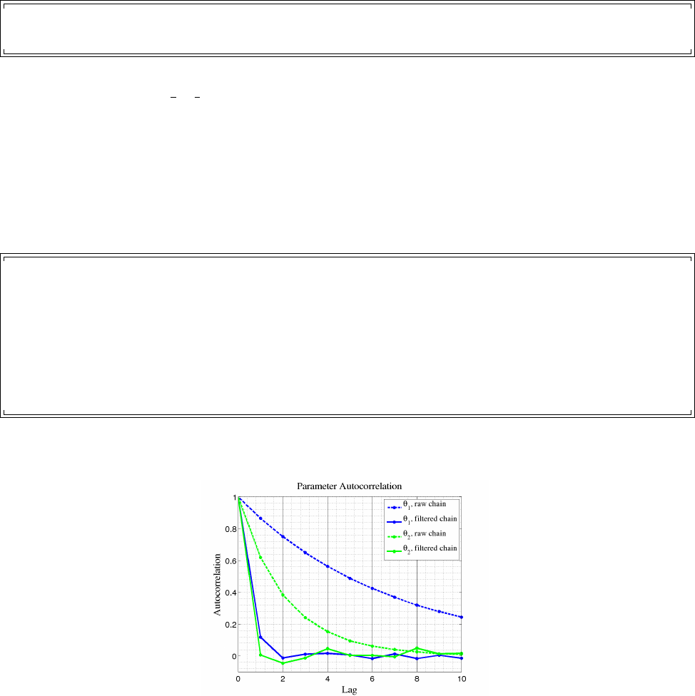
CHAPTER 5. QUESO EXAMPLES 63

The code bellow shows how to load the data provided by QUESO during the solution

process of the SIP described, in the form of chains of positions.

% inside Matlab

>> c lear all

>> s i m p le_ip_pl o t s

Listing 5.8: Matlab code for loading the data in both raw and ﬁltered chains of the SIP, by

calling the ﬁle simple ip plots.m.

5.1.5.1 Autocorrelation Plots

The code presented in Listing 5.9 uses Matlab function autocorr to generate Figure 5.1.1

which presents the autocorrelation of the parameters θ1and θ2in both cases: raw and ﬁltered

chain.

% inside Matlab

% theta_1

>> nlags =10;

>> [ A CF_r aw , l ag s ] = a ut oc orr ( i p_mh _ raw C hai n _un i fie d (: ,1) , nlags , 0) ;

>> [ ACF_f ilt , lag s ] = a ut ocorr ( i p_ mh_ filtCh ain_unif ied (: ,1) , nlags , 0) ;

>> [ A CF _raw 2 , l ag s2 ] = a ut oc orr ( i p _mh _ raw C hai n _un i fied (: , 2) , nlag s , 0) ;

>> [ AC F_filt2 , lags3 ] = auto corr ( ip_mh_filtCha in_ uni fie d (: ,2) , nlags , 0) ;

>> p lot ( la gs , A CF_r aw , ’ b - -* ’ , la gs , A CF _f il t , ’ b* -’ , l ags 2 , A CF _r aw 2 , ’ g - -* ’ , l ags 2 , A CF _f il t2 , ’ g* - ’ , ’

lin ew id th ’ ,3) ;

>> h = l eg en d ( ’\ th et a_ 1 , r aw ch ain ’ , ’\ t he ta _1 , f il te r ed c hai n ’ , ’\ th et a_ 2 , r aw chai n ’ , ’\ t he ta _2 ,

f il te red chain ’ , ’ loc at ion ’ , ’ n or thea st ’) ;

Listing 5.9: Matlab code for the autocorrelation plots depicted in Figure 5.1.1.

Figure 5.1.1: Autocorrelation plots obtained with QUESO for the SIP.

5.1.5.2 KDE Plots

Matlab function [f,xi] = ksdensity(x) (kernel smoothing density estimate) computes a

probability density estimate of the sample in the vector x.fis the vector of density values

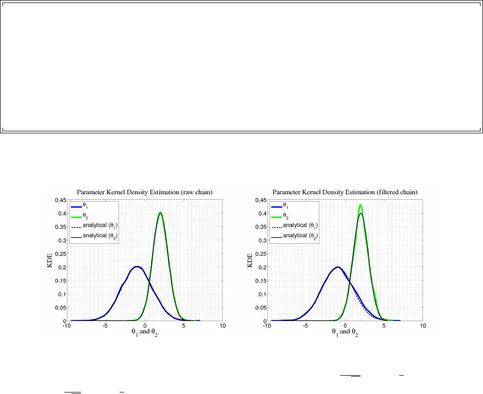
CHAPTER 5. QUESO EXAMPLES 64

evaluated at the points in xi. The estimate is based on a normal kernel function, using a

window parameter (‘width’) that is a function of the number of points in x. The density is

evaluated at 100 equally spaced points that cover the range of the data in x. In order to

estimate the KDE of the parameters, it is used together with the option ‘pdf’.

% Inside Matlab

% Raw chain

>> [ f ,x ] = k sd e ns it y ( i p_ m h_ r awC h ain _ uni f ied (: ,1 ) , ’ function ’, ’ pd f ’ ) ;

>> [ f2 , x2 ] = k s de ns i ty ( i p_ m h_ r awC h ain _ uni f ied (: ,2 ) , ’ function ’, ’ pd f ’ ) ;

>> x_p1 = so rt ( i p_m h_rawC hain_un ified (: ,1) ); % a na ly ti ca l

>> f_p1 =( exp (-( x_p1 +1) .*( x_p1 +1) /8) )/2/ sqrt (2* pi ) ;

>> x_p2 = so rt ( i p_m h_rawC hain_un ified (: ,1) );

>> f_p2 =( exp ( -( x_p2 -2) .*( x_p2 -2) /2) )/ sqrt (2* pi);

>> plo t (x , f , ’b ’ , x2 , f2 , ’ g ’, ’ l in ew id th ’ , 4) ;

>> hold;

>> plo t ( x_p 1 , f _p1 , ’ - -k ’ , x_p 2 , f _p2 , ’ -k ’ , ’ lin ew id th ’ , 2) ;

>> h= leg end ( ’\ theta_1 ’ , ’\ theta_2 ’ , ’ analyt ical (\ theta _1 ) ’, ’ ana ly tical (\ thet a_2 ) ’, ’

lo ca ti on ’ , ’ n orth we st ’) ;

Listing 5.10: Matlab code for the KDE plots displayed in the left of Figure 5.1.2.

(a) Raw chain (b) Filtered chain

Figure 5.1.2: Kernel Density Estimation. QUESO results for estimation of the KDE of θ1

and θ2are plotted against the analytical expressions πpost(θ1) = 1

2√2πexp −1

8(θ1+ 1)2and

πpost(θ2) = 1

√2πexp −1

2(θ2−2)2, respectively.

5.1.5.3 Covariance and Correlation Matrices

Matlab function cov calculates the covariance matrix for a data matrix (where each column

represents a separate quantity), and corr calculates the correlation matrix.

Listing 5.39 presents the Matlab steps for calculating the covariance and correlation ma-

trices for the parameters θ1and θ2.

CHAPTER 5. QUESO EXAMPLES 65

% inside Matlab

>> cov_matrix_theta1_theta2 = cov(ip_mh_rawChain_unified)

cov_matrix_theta1_theta2 =

3.8729 0.0259

0.0259 1.0050

>> corr_matrix_theta1_theta2 = corr(ip_mh_rawChain_unified)

corr_matrix_theta1_theta2 =

1.0000 0.0132

0.0132 1.0000

Listing 5.11: Matlab code for ﬁnding covariance and correlation matrices.

5.2 simpleStatisticalForwardProblem

In this simple statistical forward problem (SFP), suppose that the quantity of interest qis a

function of a random variable θof two parameters, namely q:R2→Rsuch as:

q(θ) = θ1+θ2,∀θ= (θ1, θ2)∈R2.(5.2.1)

Suppose also that the parameters in θhave Gaussian distribution with mean µand co-

variance matrix Cgiven by:

µ=−1

2and C=4 0

0 1 .(5.2.2)

Notice that since the solution Qof this SFP is the sum of two random variables Θ1and

Θ2, and since these two random variables independent Gaussian by assumption, should have:

E[Q] = E[Θ1] + E[Θ2] = −1 + 2 = 1 and V[Q] = V[Θ1] + V[Θ2] = 4 + 1 = 5 (5.2.3)

where Eand Vindicate expectation and variance, respectively. Thus the analytical expression

for the solution Qis this SFP is the one-dimensional Gaussian distribution of mean 1 and

variance 5:

Q(x) = 1

√10πexp −1

10(x−1)2(5.2.4)

In this example, we use QUESO Monte Carlo algorithm to sample from the QoI given

in Equation (5.2.1) and analyze it. Since the parameters have known independent Gaussian

distributions, the results obtained by QUESO via sampling the QoI, in Equation (5.2.1),

should match the Gaussian distribution given in Equation (5.2.4).

Note: Due to the possibility to compare QUESO sampling algorithms to an analytical ex-

pression, this example is also used in the veriﬁcation procedures and regression tests within

QUESO. In fact it is the second part of the test tests/t02_sip_sfp.

CHAPTER 5. QUESO EXAMPLES 66

5.2.1 Running the Example

To run the executable provided (available after QUESO installation), enter the following

commands:

$cd $H OM E / L IB RA RI ES / QU ESO - 0. 50 .0/

$cd examples/simpleStatisticalForwardProblem

$rm output D ata /*

$./ e xSimpleStat i st icalForwardProble m _g sl e xa mp le . in p

$matlab

$simple_fp_plots # i n s i d e ma t l ab

$exit # i n s i d e m a t lab

$ls -l o u tputDa ta /*. png

s im ple_fp_ a ut ocorrelat i on _qoi . png s imp l e_ fp_ch a in _pos_p a ra m . png

s im pl e_fp_hi st_qoi . png s im ple_f p_cdf_ qoi . png

s im ple _ fp _ch ain_pos_q oi . png simple_ fp_kd e_qoi . pn g

As a result, the user should have created several of PNG ﬁgures containing marginal pos-

terior PDF, chain positions of the parameters and the QoI, histogram, cumulative density

distribution and autocorrelation. The name of the ﬁgure ﬁles have been chosen to be infor-

mative, as shown in the Listing above.

5.2.2 Example Code

The source code for the SFP example is composed of 5 ﬁles: simple sfp example main.C

(Listing 5.12), simple sfp example qoi.h and simple sfp example qoi.C (Listings 5.13

and 5.14), simple sfp example compute.h and simple sfp example compute.C (Listings

5.15 and 5.16).

#i n c l u d e <simple sfp example compute .h>

int mai n (int argc , c har * argv [])

{

// Initia l ize e n vironm e nt

MPI _I ni t (& argc ,& a rgv );

UQ_FATA L_TES T_MAC RO ( argc != 2 , QUE SO :: U Q_ UN AV AI LA BL E_ RA NK , " m ai n () " ,

" input file must be spe cifie d in comm and line as argv [1] , just after

exec uta ble arg v [0 ] ") ;

QUESO :: F ul lE nvironme nt * env =

ne w Q UE SO :: F u ll E nv i ro n me n t ( M PI_ COM M_W OR L D , a rg v [1] , " " , NU LL ) ;

// Compute

compute(*en v );

// Final ize e n vironm e nt

delete env;

MPI_Finalize();

return 0;

}

Listing 5.12: File simple sfp example main.C.

CHAPTER 5. QUESO EXAMPLES 67

#i f n d e f EX Q O I H

#d e f i n e EX Q O I H

#i n c l u d e <q u es o / G s l M a t r i x . h>

#i n c l u d e <q ue so / D i s t A r r a y . h>

struct

qoiRoutine_DataType

{

dou ble coef 1 ;

dou ble coef 2 ;

};

void

qoiR outine (

const QUE SO :: GslVec tor & paramV alue s ,

const QUE SO :: GslVec tor * par amDir ectio n ,

con st v oid * fun ct io nD ataPt r ,

QUESO :: GslVe ctor & qoiValues ,

QUESO :: DistArray < QUESO :: Gsl Vector * >* gradVe ctors ,

QUESO :: DistArray < QUESO :: Gsl Matrix * >* hess ianMa tric es ,

QUESO :: DistArray < QUESO :: Gsl Vector * >* hessian Ef fects );

#e n d i f

Listing 5.13: File simple sfp example qoi.h.

#i n c l u d e <s i m p l e s f p e x a m p l e q o i . h>

void

qoiR outine (

const QUE SO :: GslVec tor & paramV alue s ,

const QUE SO :: GslVec tor * par amDir ectio n ,

con st v oid * fun ct io nD ataPt r ,

QUESO :: GslVe ctor & qoiValues ,

QUESO :: DistArray < QUESO :: Gsl Vector * >* gradVe ctors ,

QUESO :: DistArray < QUESO :: Gsl Matrix * >* hess ianMa tric es ,

QUESO :: DistArray < QUESO :: Gsl Vector * >* hessian Ef fects )

{

// Logic jus t to avoi d war nings from INTEL c ompil er

const QUE SO :: GslVec tor * aux 1 = p ar amDirecti on ;

if ( aux 1 ) {};

QUESO :: DistArray < QUESO :: Gsl Vector * >* aux2 = grad Vectors ;

if ( aux 2 ) {};

aux2 = hessianEffects;

QUESO :: DistArray < QUESO :: Gsl Matrix * >* aux3 = hessia nM atrices ;

if ( aux 3 ) {};

// Just che cking : the user , at the a pplicat i on level , expe cts

// v ec to r ’ par am Va lu es ’ to h ave siz e 2 an d

// v ec tor ’ q oi Va lu es ’ to h av e s iz e 1.

UQ_FATA L_ TE ST _M ACRO ( param Va lues . siz eGlobal () != 2 ,

QUESO::UQ_UNAVAILABLE_RANK ,

" q o iR ou t in e () " ,

" paramV a lues vect or does not have size 2" ) ;

UQ_FATA L_ TE ST _M AC RO ( qoiVa lues . size Gl obal () != 1 ,

QUESO::UQ_UNAVAILABLE_RANK ,

" q o iR ou t in e () " ,

" qoiVa lues vector does not have si ze 1" ) ;

// Actu al code

CHAPTER 5. QUESO EXAMPLES 68

// This code e x emplif i es m ultip le Monte Ca rlo solvers , each call ing this qoi routi ne .

// In this si mple example , only nod e 0 in each sub - environ m ent does the job ev en though

// the re mig ht be more than one node per sub - enviro n ment .

// In a more r ealis t ic s ituation , if the user is asking for mult iple nodes per sub -

// environment , then the mo del code in the qoi rou tine might real ly dem and more than one

// node . He re we use ’ e nv . subR an k () ’ onl y . A r ea li st ic applic at io n m ight wa nt to use

// either ’en v . s ub C om m ( ) ’ or ’ env . s ub Com m () . Co mm () ’.

const QUE SO :: B aseEnvir on ment & env = paramValues.env () ;

if (env . subRa nk () == 0) {

dou bl e coe f1 = (( q oiRo u ti ne_ D at aTy p e *) f un ct ionDa taPtr ) - > coef 1 ;

dou bl e coe f2 = (( q oiRo u ti ne_ D at aTy p e *) f un ct ionDa taPtr ) - > coef 2 ;

qoiV al ue s [0] = ( c oef1 * param Va lu es [0] + c oef2 * param Va lu es [1 ]) ;

}

else {

qoiV alues [0] = 0.;

}

return;

}

Listing 5.14: File simple sfp example qoi.C.

#i f n d e f EX COMPUTE H

#d e f i n e EX COMPUTE H

#i n c l u d e <queso/Environment .h>

vo id c ompute ( c onst QUE SO :: F ul lE nv ir onm en t & env ) ;

#e n d i f

Listing 5.15: File simple sfp example compute.h.

#i n c l u d e <simple sfp example compute .h>

#i n c l u d e <s i m p l e s f p e x a m p l e q o i . h>

3#i n c l u d e <q u es o / G s l M a t r i x . h>

#i n c l u d e <q ueso / S t a t i s t i c a l F o r w a r d P r o b l e m . h>

#i n c l u d e <queso/GenericVectorFunction .h>

#i n c l u d e <q ueso / G a ussi a nVec t orRV . h>

8vo id c ompute ( c onst QUE SO :: F ul lE nv ir onm en t & env ) {

// Step 1 of 6: Inst a ntiate the p aramet er sp ace

QUESO :: Vec torSpac e < QUESO :: GslVector , QUESO :: GslMatrix >

p ar a mS p ac e ( env ," param_ " , 2, NUL L );

// Step 2 of 6: Inst a ntiate the p aramet er domain

QUESO :: G slVecto r para mMins ( par amSpace . z eroVect or () );

para mM in s . cwSe t (- INF IN IT Y );

QUESO :: G slVecto r para mMaxs ( par amSpace . z eroVect or () );

18 para mM ax s . cwSe t ( INF IN ITY ) ;

QUESO :: BoxSubset < QUESO :: GslVector , QUESO :: GslMatrix >

para mD omain ("param_", p ar am Sp ac e , p ar am Mi ns , p a ra mM axs ) ;

// Step 3 of 6: I nstant i ate the qoi space

23 QUESO :: Vec torSpac e < QUESO :: GslVector , QUESO :: GslMatrix >

q oi S pa ce ( env ," qoi_ " , 1 , NUL L );

CHAPTER 5. QUESO EXAMPLES 69

// Step 4 of 6: Inst a ntiate the qoi f u nctio n object

qoiRout in e_ D ataType qoiRo ut ine_Data ;

28 qoiRou tin e_ Dat a . coef1 = 1.;

qoiRou tin e_ Dat a . coef2 = 1.;

QUESO :: Generi cVector F unctio n < QUESO :: GslVector , QUESO :: GslMatrix ,

QUESO :: GslVector , QUESO :: GslMatrix >

qoiFunctionObj(" qoi_ " ,

33 paramDomain ,

qoiSpace ,

qoiRoutine ,

( vo id *) & q oi Ro ut ine _Dat a ) ;

38 // Step 5 of 6: Inst a ntiate the f orwa rd problem

// Paramet ers are G aussi an RV

QUESO :: G slVecto r meanV ector ( p aramSp ace . zeroV ector () ) ;

mean V ector [0] = -1;

mean V ector [1] = 2;

QUESO :: GslMa trix c ovMatri x = QUESO :: GslM atrix ( pa ra mSpace . z eroVect or () );

covM atrix (0 ,0) = 4.;

covM atrix (0 ,1) = 0.;

covM atrix (1 ,0) = 0.;

48 covM atrix (1 ,1) = 1.;

QUESO :: Gauss ianVe ctorR V < QU ESO :: GslVe ctor , QUE SO :: Gsl Mat rix >

paramRv("param_", pa ra mD om ai n , m ea nV ec to r , c ovM atr ix ) ;

53 QUESO :: Gene ricVe ctorR V < QU ESO :: Gs lVector , QUE SO :: Gsl Matrix >

qoiRv (" qoi_ ", qoiS pace );

QUESO :: Statist icalForw a r dProble m < QUE SO :: Gsl Vector , QUESO :: GslMatrix ,

QUESO :: GslVector , QUESO :: GslMatr ix >

58 fp ( " " , NULL , paramRv , q oiFun ctionO bj , q oiRv ) ;

// Step 6 of 6: S olve the f orwar d pro blem

fp.solveWithMonteCarlo(NULL);

63 return;

}

Listing 5.16: File simple sfp example compute.C.

5.2.3 Input File

In the case of a SFP, QUESO expects a list of options for Monte Carlo algorithm, together

with options for QUESO environment; such as the name of the output ﬁles and which sub-

environments will write to to them. Note that the names of the variables have been designed

to be informative:

env:refers to QUESO environment;

fp:refers to forward problem;

mc:refers to Monte Carlo;

pseq:refers to the parameter sequence; and

qseq:refers to the quantity of interest sequence.

The options used for solving this simple SFP are displayed in Listing 5.17.

CHAPTER 5. QUESO EXAMPLES 70

###############################################

# UQ Environment

###############################################

env_numSu b E n v i r onments = 1

env_subDi spl ayF ileN ame = o ut putData / d ispla y

env_subDi s p l a y A llowAll = 0

env_subDisplayAllowedSet = 0

env_displayVerbosity = 2

env_syncVerbosity = 0

env _ seed = 0

###############################################

# S t a t i s t i c a l f o r w a r d p r oble m ( f p )

###############################################

fp_computeSolution = 1

fp_computeCovariances = 1

fp_comput e C o r r e lations = 1

fp_dataO ut put Fi le Nam e = output Data / sfpO utput

fp_dataOutputAllowedSet = 0 1

###############################################

# ’ f p ’ : i n f o r m a t i o n f o r Monte C a rl o a l g o r i t h m

###############################################

fp_mc_data Out put Fil eNa me = output Data / sfpO utput

fp_mc_dataOutputAllowedSet = 0 1

fp_mc_pseq_data Out putFi leNam e = output Da ta / fp_p _seq

fp_mc_pseq_dataOutputAllowedSet = 0 1

fp_mc_ q s eq_size = 200 00

fp_mc_qseq_displayPeriod = 2000

fp_mc_qseq_measureRunTimes = 1

fp_mc_qseq_data Out putFi leNam e = output Da ta / fp_q _seq

fp_mc_qseq_dataOutputAllowedSet = 0 1

Listing 5.17: File name simple sfp example.inp with options for QUESO library used in

application code (Listings 5.12–5.16).

5.2.4 Create your own Makeﬁle

Listing 5.33 presents a Makeﬁle, named ‘Makefile sfp example margarida’, that may be

used to compile the code and create the executable simple_sfp_example. Naturally, it must

be adapted to the user’s settings, i.e., it has to have the correct paths for the user’s libraries

that have actually been used to compile and install QUESO.

##########################################################

# U si ng i n s t a l l e d QUESO 0 . 5 0 . 0 , from e x t e r n a l r e l e a s e i n ’ m a r g ar i da ’

##########################################################

QUES O_ DI R = / h ome / ke me ll i / LIB RA RI ES / QUESO -0.5 0. 0

BOOS T_ DI R = / h ome / ke me ll i / LIB RA RI ES / boost -1.5 3. 0

GSL _D IR = / home / k em elli / LIBR AR IE S / gsl -1. 15

HDF 5_ DI R = / ho me / keme ll i / LIB RA RI ES / hdf5 - 1.8.1 0

INC_ PATHS = \

-I. \

-I$( QUESO_ DIR )/ include \

CHAPTER 5. QUESO EXAMPLES 71

-I$( BOOST_ DIR )/ include \

-I$(GSL_DIR)/include \

-I$( HDF5_ DIR )/ incl ude

LI BS = \

-L$( QUESO_ DIR )/ lib - lqueso \

-L$( BOOST_ DIR )/ lib - lboost_progr am _o pti on s \

-L$( GSL_D IR ) /lib - lgsl \

-L$( HDF5_ DIR )/ lib - lhdf5

CXX = mpic ++

C XX FL A GS + = - g - W al l - c

default: all

. SUF FIXES : .o . C

al l : ex am ple _sf p

clean :

rm -f *~

rm -f * . o

rm -f simple_sfp_ e x a mple

example_sfp: simple_sfp_example_main.o simple_sfp_example_qoi.o simple_sfp_example_compute.o

$(CXX) simple_sfp_example_main.o \

simple_sfp_example_qoi.o \

simple_sfp_example_compute.o \

-o si m p l e _sfp_exampl e $( L IBS )

%. o : %. C

$( CX X ) $( IN C_PATHS ) $( CXXF LAGS ) $<

Listing 5.18: Makeﬁle for the application code in Listings 5.12–5.16

Thus, to compile, build and execute the code, the user just needs to run the following

commands in the same directory where the ﬁles are:

$cd HOME / LIBR ARIES / QUESO -0.5 0.0/ examp les / simpleStatisticalForward Prob lem

$export LD_LIB RA RY_PATH = $LD_LIBRARY_PATH:\

$H OM E / L IB R AR I ES / gsl - 1. 15 / l ib / :\

$HOM E / L IB RA RIE S / boos t - 1. 53 .0 / l ib / :\

$HOM E / L I BR AR IES / hdf5 - 1 .8 .1 0/ l ib : \

$HOM E / L IB RA RIE S / QUES O - 0. 50 .0 / l ib

$make -f Makefile_sfp_example_margarida

$./ s im ple_sf p_exam ple simpl e_sfp _exampl e . inp

The ‘export’ instruction above is only necessary if the user has not saved it in his/her

.bashrc ﬁle.

5.2.5 Data Post-Processing and Visualization

This section discusses the results computed by QUESO with the code of Section 5.2.2, and

shows how to use Matlab for the post-processing of the data generated by QUESO when

solving SFPs. Only the essential Matlab commands are presented; for the complete/detailed

codes, please refer to ﬁle ’simple_fp_plots.m’.

CHAPTER 5. QUESO EXAMPLES 72

According to the speciﬁcations of the input ﬁle in Listing 5.17, a folder named ‘outputData’

containing the following ﬁles should be created: display_sub0.txt, fp_p_seq.m,

fp_p_seq_sub0.m, fp_q_seq.m, fp_q_seq_sub0.m, and sfpOutput_sub0.m.

The code below shows how to load the data provided by QUESO during the solution

process of the SFP described, in the form of chains of positions.

% inside Matlab

>> c lear all

>> fp_p_ seq .m

>> fp_q_ seq .m

Listing 5.19: Matlab code for loading the data in both parameter and QoI chains of the SFP.

Alternatively, the user may call the ﬁle simple fp plots.m, which contains the above

commands, together with a variety of others, for data visualization:

% inside Matlab

>> c lear all

>> s i m p le_fp_pl o t s

Listing 5.20: Matlab code for loading the data in both parameter and QoI chains of the SFP,

by calling the ﬁle simple fp plots.m.

5.2.5.1 Histogram Plots

In order to plot a histogram of the QoI, you may use the pre-deﬁned Matlab function hist.

The Matlab code presented in Listing 5.21 below shows how to create the Figure 5.2.1.

% inside Matlab

>> f p_ q_s eq % if comm ands of List ings 3.19/ 3.20 have not been cal led

>> nbins =20;

>> hist ( fp_m c_ Qo iS eq _unifie d , nbins );

>> tit le ( ’ Qo I H is togr am ’ , ’ fo ntsi ze ’ ,20) ;

>> xlabel (’ QoI =\ the ta_1 +\ theta_2 ’ , ’ fontname ’ , ’ Times ’ , ’ fontsize ’ ,20)

>> y la be l (’ Fr eq ue ncy ’ ,’ fo ntsi ze ’ ,20) ;

Listing 5.21: Matlab code for the QoI histogram plot.

5.2.5.2 KDE Plot

Matlab function ksdensity (Kernel smoothing density estimate) together with the option

‘pdf’ may be used to estimate the KDE of the QoI.

% inside Matlab

>> f p_ q_s eq % if comm ands of Lis ting 5.19 have not been ca lled

>> [ fi , xi ] = k sde n si ty ( f p _m c_ Q oi Se q _u nif i ed , ’ function ’ , ’ pdf ’) ;

>> x=sort(fp_mc_QoiSeq_unified);

>> mu =1;

>> sigma2 =5;

>> f =( e xp ( -( x - mu ) . *( x - mu ) / s ig ma 2 / 2) ) / s qrt ( 2* pi * s ig ma 2 ) ;

CHAPTER 5. QUESO EXAMPLES 73

>> plot (xi , fi ,’ -m ’ , ’ li ne wi dth ’ , 4) ;

>> hold;

>> plo t (x , f , ’- - k ’, ’ l in ew id th ’ ,2) ;

>> h= leg end (’ QoI = \ t heta_ 1 +\ theta_2 ’,’ analyt ical ’ ,’ loc ation ’ ,’ northwest ’);

Listing 5.22: Matlab code for the KDE displayed in Figure 5.2.2

5.2.5.3 CDF Plot

Matlab function ksdensity with ’cdf’ option may also be used for plotting the Cumulative

Distribution Function of the QoI.

% inside Matlab

>> f p_ q_s eq % if comm ands of Lis ting 5.19 have not been ca lled

>> [ f ,xi ] = k sd e ns it y ( f p _m c_Q o iS eq _ un ifi e d , ’ function ’ , ’ cdf ’ ) ;

>> plo t ( xi , f ,’ - m ’, ’ l in ew id th ’ , 3)

Listing 5.23: Matlab code for the QoI CDF plot displayed in Figure 5.2.3.

5.3 gravity

This section presents an example of how to use QUESO in order to develop an application

that solves a statistical inverse problem and a statistical forward problem, where the solution

of the former serves as input to the later. During the SIP, the acceleration due to gravity for

an object in free fall near the surface of the Earth is inferred. During the SFP, the distance

traveled by a projectile launched at a given angle and altitude is calculated using the calibrated

magnitude of the acceleration of gravity.

In this section we describe a statistical forward problem of predicting the described in

Section 5.3.1.

5.3.1 Statistical Inverse Problem

A possible deterministic mathematical model for the vertical motion of an object in free fall

near the surface of the Earth is given by

h(t) = −1

2gt2+v0t+h0.(5.3.1)

where v0[m/s] is the initial velocity, h0[m] is the initial altitude, h(t) [m] is the altitude with

respect to time, t[s] is the elapsed time, and g[m/s2] is the magnitude of the acceleration

due to gravity (the parameter which cannot be directly measured and will be statistically

inferred).

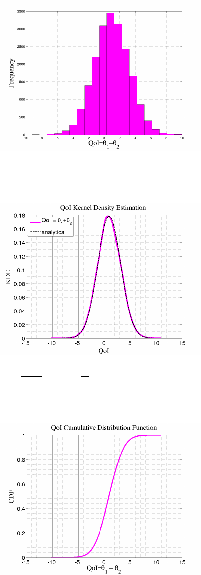
CHAPTER 5. QUESO EXAMPLES 74

Figure 5.2.1: QoI histogram.

Figure 5.2.2: Kernel Density Estimation. QUESO results are plotted against the PDF of a

Gaussian distribution Q(x) = 1

√10πexp −1

10 (x−1)2, where µ= 1 and σ2= 5.

Figure 5.2.3: Cumulative Distribution Function.

CHAPTER 5. QUESO EXAMPLES 75

5.3.1.1 Experimental Data

We assume that the experiment of allowing an object to fall from diﬀerent altitudes with zero

initial velocity has been repeatedly conducted (See Figure 5.3.1). The data collected, e.g.

d, is displayed in Table 5.3.1; the standard deviations, σ’s, refer to the uncertainties in the

measured times during the experiment execution [1].

v0= 0

h(t) = −1

2g t2+h0

Figure 5.3.1: An object falls from altitude h0with zero initial velocity (v0= 0).

Table 5.3.1: Measurement data dof size nd= 14. The object falls from altitude h0in t

seconds, with standard deviation of σseconds in the time measurement [1].

altitude [m] time [s] Std. Dev. σ[s]

10 1.41 0.02

20 2.14 0.12

30 2.49 0.02

40 2.87 0.01

50 3.22 0.03

60 3.49 0.01

70 3.81 0.03

80 4.07 0.03

90 4.32 0.03

100 4.47 0.05

110 4.75 0.01

120 4.99 0.04

130 5.16 0.01

140 5.26 0.09

5.3.1.2 The Prior RV, Likelihood and Posterior RV

In a straightforward classical interpretation of Bayesian inference, the prior signiﬁes the mod-

eler’s honest opinion about the unknown. For the gravity inference problem, let’s assume

CHAPTER 5. QUESO EXAMPLES 76

that gravity varies uniformly in the interval [8,11], or, in other words, we chose uniform prior

distribution in that interval:

πprior =U(8,11).(5.3.2)

We choose the usual likelihood function:

πlike(d|θ)∝exp −1

2[y(θ)−d]T[C(θ)]−1[y(θ)−d],(5.3.3)

where C(θ) is a given covariance matrix, ddenotes experimental data, y(θ) is the model

output data.

Recalling the deterministic model for the acceleration of gravity (5.3.1) with zero initial

velocity, the information provided in Table 5.3.1, and Equation (5.3.3); and, additionally,

invoking the nomenclature used in Section 1.2, we have:

θdef.

=g, y(θ) =







r2h1

r2h2

r2hnd







,d=





tnd







,C(θ) = 





σ2

10··· 0

0σ2

2··· 0

....0

0 0 ··· σ2







,(5.3.4)

where nd= 14 is the number of data points in Table 5.3.1.

Now we are ready to evoke Bayes’ formula in order to obtain the posterior PDF πpost(θ):

πpost(θ|d)∝πlike(d|θ)πprior(θ).(5.3.5)

5.3.2 Statistical Forward Problem

Projectile motion refers to the motion of an object projected into the air at an angle, e.g. a

soccer ball being kicked, a baseball being thrown, or an athlete long jumping. Supposing the

object does not have a propulsion system and neglecting air resistance, then the only force

acting on the object is a constant gravitational acceleration g.

A possible deterministic two-dimensional mathematical model for the vertical motion of

an object projected from near the surface of the Earth is given by

vx=v0x(5.3.6)

vy=v0y−gt (5.3.7)

x=v0xt(5.3.8)

h=h0+v0yt−1

2gt2(5.3.9)

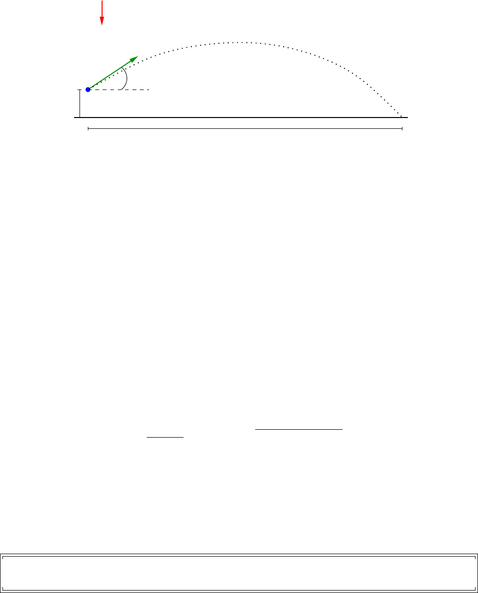
CHAPTER 5. QUESO EXAMPLES 77

Figure 5.3.2: Object traveling with projectile motion.

where h0is the initial height, x=x(t) is the distance traveled by the object, v0= (v0x, v0y)

is the initial velocity, v0x=v0cos(α), v0y=v0sin(α), and v0=kv0k2. Figure 5.3.2 displays

the projectile motion of an object in these conditions.

For this example, we assume that h0= 0 m, α=π/4 radians, v0= 5 m/s, all deterministic

variables; and gis the solution of the SIP described in Section 5.3.1.

Since a PDF is assigned to parameter g; thus, the output of the mathematical model

(5.3.6) becomes a random variable, thus we have a statistical forward problem.

5.3.2.1 The Input RV, QoI Function and Output RV

The input random variable for the statistical forward problem is the acceleration of gravity

g, which is also the solution (posterior PDF) of the inverse problem described in Section

5.3.1. The output random variable for this example is the distance xtraveled by an object

in projectile motion. Note that, since there is uncertainty in the parameter g(gis given as a

PDF), one can expect that this uncertainty will be propagated to x, which will also be given

as a PDF.

Combining the expressions in Equation 5.3.6 and rearranging them, we have that QoI

function for xis:

x=v0cos α

gv0sin α+p(v0sin α)2+ 2g y0.(5.3.10)

where yis the distance traveled and our quantity of interest (QoI).

5.3.3 Running the Example

To run the executable provided (available after QUESO installation), enter the following

commands:

$cd $H OM E / L IB RA RI ES / QU ESO - 0. 50 .0/ e xa mp le s / g ra vi ty

$rm output D ata /*

$./ g ra vi ty_ gsl g ravi ty_in v_fw d . inp

CHAPTER 5. QUESO EXAMPLES 78

The console output of the program is:

kemell i@ vi ol et a :~/ LIBRAR IES / QUESO - 0.50.0 / examp les / gra vity$./ grav ity_ gsl g rav ity_i nv_fw d . inp

---------------------------------------------------------------------

QUESO L ibra ry : Vers ion = 0. 47.1 (47.1)

Deve l opment Build

Build Date = 2013 -04 -29 17 :05

Build Host = v iolet a

Build User = k emell i

Bui ld A rc h = x8 6_64 - u nkn own - linux - g nu

Build Rev = 3899 8 M

C ++ Con fig = mpic ++ -g -O2 - Wall

Tri l inos DIR =

GSL Lib s = -L/ home / kem el li / LIBR AR IE S / gsl -1. 15/ lib - lgs l - lgs lc bl as -lm

GR VY DIR =

GL PK DIR =

HD F5 DIR = / h ome / kem el li / L IB RA RI ES / hdf5 -1.8 .1 0

--------------------------------------------------------------------------------------------------------------

Begi nning run at Mon Apr 29 17:27 :32 2013

MPI node of w o rldRa n k 0 has fu l lRank 0 , belo ngs to subEnvi r o n ment of id 0 , and has s ubRank 0

MPI node of w orldR ank 0 belo ngs to sub c o mmunica t or with full rank s 0

MPI node of w orldRa nk 0 a lso bel ongs to inter0 c o m munica t o r with full ra nks 0 , and has

inte r 0Rank 0

Begi nning run of ’ Gra vity + Pr ojecti l e motion ’ example at Mon Apr 29 1 7:27: 32 2013

my f ullRa nk = 0

my subEnvironmentId = 0

my subRank = 0

my i nterRa nk = 0

Begi nning ’SIP -> Gr avity estima tio n ’ at Mon Apr 29 1 7:27: 32 2013

Sol ving the SIP with Metrop o lis Has tings

Begi nning ’SFP -> Pro j ectile motion ’ at Mon Apr 29 1 7:27:3 3 2013

Sol ving the SFP with Mon te Carlo

Ending run of ’ Gra vity + Pr ojecti le motion ’ example at Mon Apr 29 1 7:27: 33 2013

Ending run at Mon Apr 29 17:27 :33 2013

Total run time = 1 seco nds

kemell i@ vi ol et a :~/ LIBRAR IES / QUESO - 0.50.0 / examp les / gra vity$

Listing 5.24: Console output of program gravity gsl

In order to generate chain plots, histograms, KDEs, etc., the user may use Matlab/GNU

Octave and call the following command lines:

$matlab

$gravity_plots_ip # i n s i d e m a t lab

$gravity_plots_fp # i n s i d e m a t lab

$exit # i n s i d e m a t lab

$ls -l o u tputDa ta /*. png

CHAPTER 5. QUESO EXAMPLES 79

s fp _gravi t y_ autocor r el ation . png s fp _gr avity _cdf . pn g

s fp _gr a vi ty_ c ha in_p os . png sfp_gr avity _hist . pn g

sfp_gr avit y_kde . png s ip _gravity_autoco r re lation_raw_filt . png

sip_gravity_cdf_filt.png sip_gravity_cdf_raw.png

sip_gravity_chain_pos_filt.png sip_gravity_chain_pos_raw.png

sip_gravity_hist_filt.png sip_gravity_hist_raw.png

sip_gravity_kde_filt.png sip_gravity_kde_raw.png

As a result, the user should have created several of PNG ﬁgures containing marginal pos-

terior PDF, chain positions of the parameters and the QoI, histogram, cumulative density

distribution and autocorrelation. The name of the ﬁgure ﬁles have been chosen to be infor-

mative, as shown in the Listing above.

5.3.4 Example Code

The source code for the SIP and the SFP is composed of 7 ﬁles. Three of them are common for

both problems: gravity main.C, gravity compute.h and gravity compute.C; they com-

bine both problems and use the solution of the SIP (the posterior PDF for the gravity) as

an input for the SFP and are presented, respectively, in Listings 5.25,5.26 and 5.27. Two of

ﬁles speciﬁcally handle the SIP: gravity likelihood.h, and gravity likelihood.C, and are

displayed in Listings 5.28 and 5.29. Finally, the ﬁles speciﬁc for the SFP are gravity qoi.h

and gravity qoi.C, and they are presented in Listings 5.30 and 5.31.

/*------------------------------------------------------------------

* B rief d es cr ip ti on of this fil e :

* This is an examp le of how to use QUESO cl asses and a lgorit hms in or der to defi ne and so lve

* a s ta ti sti cal i nv er se pro bl em ( SIP ) a nd / or a s ta ti st ica l f or wa rd p ro bl em ( SF P ).

* The S IP c on sis ts o n c a li br a ti ng the m a gn it u de ’ g ’ of acc e le r at ion g ra vit y u si ng

* me a suremen t s of the time that it takes for an object in free fall to r eac h the ground from

* a given h eight and zero initial v e locit y . The s oluti on of the SIP is the pos terior

* prob a bility densi ty fun ction ( P DF ) of ’g ’.

* The SFP cons ists of c alcula t ing the max imum dista nce t r avele d by an object in proj ectile

* motion . The poste r ior PDF of ’g ’ from the SIP might be us ed as input to the SFP .

* The code con si sts of 7 files :

* - ’ g r av ity_ m ai n . C ’ ( t his fil e )

* - ’ gravity_ c o mpute .C ’ ( the d rivi ng appl i cation code )

* - ’ g r av i ty _ co m pu te . h ’

* - ’ gravity_li k e l i hood .C ’ ( n ecessa ry for t he SIP )

* - ’ g r av i ty _ li k el i ho o d . h ’

* - ’ gravit y _qoi .C’ ( neces sary for the SFP )

* - ’ g r av i ty _q o i . h ’

*-----------------------------------------------------------------*/

#i n c l u d e <g r a v i t y c o m p u t e . h>

int mai n (int argc , c har * argv [])

{

// Initia l ize QUESO e nvironm e nt

MPI _I ni t (& argc ,& a rgv );

QUESO :: F ul lE nvironme nt * env =

ne w Q UE SO :: F u ll E nv i ro n me n t ( M PI_ COM M_W OR L D , a rg v [1] , " " , NU LL ) ;

// Call app l ication

computeGravityAndTraveledDistance(*env );

CHAPTER 5. QUESO EXAMPLES 80

// Final ize QUESO e nvironm e nt

delete env;

MPI_Finalize();

return 0;

}

Listing 5.25: File gravity main.C.

#i f n d e f EX COMPUTE H

#d e f i n e EX COMPUTE H

#i n c l u d e <queso/Environment .h>

vo id computeGravityA ndTraveledDi stance ( con st Q UESO :: F ul lEn vir onm ent & env) ;

#e n d i f

Listing 5.26: File gravity compute.h.

1/*------------------------------------------------------------------

* This file is d ivid ed in two parts :

* - the f irst one handl es the statist i cal inver se probl em ( SIP ) for e stimat ing the magn itude

* ’g ’ of g rav ity a cc e le r at ion ; a nd

* - t he s econd pa rt ha nd le s th e s tat isti cal f or wa rd pro bl em ( SFP ) for p r edicti ng the maximum

6* d istan ce trav eled by a projec tile .

* The SIP defi n ition re quire s a user def ined li k elihoo d funct ion ; refer to files

* ’ gr av it y_likelihoo d .h ’ and ’ gravity _l ik elihood .C ’. The SFP defi nition requir es a user

* def ined qoi f unctio n ; refe r to f iles ’ gravi t y_qoi .h’ and ’ gravit y _qoi .C ’.

11 *-----------------------------------------------------------------*/

#i n c l u d e <g r a v i t y c o m p u t e . h>

#i n c l u d e <gravity likelihood .h>

#i n c l u d e <g r a v i t y q o i . h>

16 #i n c l u d e <q u es o / G s l M a t r i x . h>

#i n c l u d e <queso/GenericScalarFunction .h>

#i n c l u d e <queso/GenericVectorFunction .h>

#i n c l u d e <q ueso / G a ussi a nVec t orRV . h>

#i n c l u d e <q ueso / U niformVectorRV . h>

21 #i n c l u d e <q ueso / G ene r icV ect o rRV . h>

#i n c l u d e <q ue s o / S t a t i s t i c a l I n v e r s e P r o b l e m . h>

#i n c l u d e <q ueso / S t a t i s t i c a l F o r w a r d P r o b l e m . h>

#i n c l u d e <s y s / t im e . h>

#i n c l u d e <cmath>

//================================================================

// If PRIO R _ I S _GAUSSIAN is defined , then:

// --> Gau ssian pri or for gravity.

// O therwis e :

31 // --> Uni form pri or for gravity.

//================================================================

//#d e f i n e PRIOR IS GAUSSIAN

36 vo id computeGravityA ndTraveledDi stance ( con st Q UESO :: F ul lEn vir onm ent & env) {

struct time val tim evalNow ;

getti me ofd ay (& timeval Now , N ULL );

CHAPTER 5. QUESO EXAMPLES 81

if (env . f ullRa nk () == 0) {

41 std :: cout << " \ n B eginni ng run of ’ Grav ity + Pr o jectil e motion ’ examp le at "

<< cti me (& timev al No w . tv_se c )

<< " \n my f ullRa nk = " << env. full Rank ()

<< "\n my subEnvironmentId = " << env . subId ()

<< " \n my s ubRa nk = " << e nv .subRank()

46 << " \n my i nterRa nk = " << env . inter 0R ank ()

<< std :: endl << std :: endl ;

}

// Just examp les of possi ble cal ls

51 if (( env.subDisplayFile() ) &&

(en v .displayVerbosity() >= 2)) {

*en v .subDisplayFile() << " B eg inn ing ru n of ’ G ra vi ty + P ro je cti le motion ’ e xa mp le at "

<< cti me (& timev al No w . tv_se c )

<< s td :: endl ;

56 }

en v . ful l Co mm () . B ar ri er ( ) ;

en v . sub Co mm ( ) . Bar rie r ( ) ; // J ust an e xam ple of a pos s ib le cal l

//================================================================

61 // S tat isti cal i nv er se pro bl em ( SIP ) : fin d p ost er ior PD F for ’g ’

//================================================================

getti me ofd ay (& timeval Now , N ULL );

if (env . f ullRa nk () == 0) {

std :: cout << " Beginn ing ’ SIP -> Gravi ty e sti mation ’ at "

66 << cti me (& timev al No w . tv_se c )

<< s td :: endl ;

}

//------------------------------------------------------

71 // SIP Step 1 of 6: I n stanti a te the para meter spa ce

//------------------------------------------------------

QUESO :: Vec torSpac e < QUESO :: GslVector , QUESO :: GslMatrix > p a ramSpa ce ( env ,"param_", 1, NULL );

//------------------------------------------------------

76 // SIP Step 2 of 6: I n stanti a te the para meter doma in

//------------------------------------------------------

QUESO :: G slVecto r paramMi nV al ues ( param Space . zer oVector ());

QUESO :: G slVecto r paramMa xV al ues ( param Space . zer oVector ());

81 paramMinValues[0] = 8.;

param M a xValues [0] = 11.;

QUESO :: BoxSubset < QUESO :: GslVector , QUESO :: GslMatrix >

para mD omain ("param_",

86 paramSpace ,

paramMinValues ,

paramMaxValues);

//------------------------------------------------------

91 // SIP Step 3 of 6: I n stanti a te the like l ihood funct i on

// object to be used by Q UESO .

//------------------------------------------------------

likelihoodRoutine_Data likelihoodRoutine_Data(env) ;

QUESO :: Generi cScalar F unctio n < QUESO :: GslVector , QUESO :: GslMatrix >

96 likelihoodFunctionObj(" lik e_ " ,

paramDomain ,

likelihoodRoutine ,

( vo id *) & likel ih ood Ro uti ne _D ata ,

true) ; // the r out ine c om put es [ ln ( f unctio n )]

101

//------------------------------------------------------

// SIP Step 4 of 6: Defi ne the prior RV

//------------------------------------------------------

CHAPTER 5. QUESO EXAMPLES 82

106 #i f d e f PRIOR IS GAUSSIAN

QUESO :: G slVecto r meanV ector ( p aramSp ace . zeroV ector () ) ;

mean V ector [0] = 9;

QUESO :: GslMa trix c ovMatri x = QUESO :: GslM atrix ( pa ra mSpace . z eroVect or () );

111 covM atrix (0 ,0) = 1.;

// Create a Gaus s ian p rior RV

QUESO :: Gauss ianVe ctorR V < QU ESO :: GslVe ctor , QUE SO :: Gsl Mat rix > pri orRv (" p rior _ ",paramDomain ,

meanVector , cov Matrix );

116 #else

// Crea te an u niform prior RV

QUESO :: Unif ormVe ctorR V < QU ESO :: Gs lVector , QUE SO :: Gsl Matrix > pri orRv ("prior_", para mDo mai n ) ;

#e n d i f

121

//------------------------------------------------------

// SIP Step 5 of 6: I n stanti a te the i nvers e pro blem

//------------------------------------------------------

QUESO :: Gene ricVe ctorR V < QU ESO :: Gs lVector , QUE SO :: Gsl Matrix >

126 postRv(" p os t_ " , // Extra p refi x before the d efau lt " rv_ " prefix

para mSpace );

QUESO :: Statist icalInve r s eProble m < QUE SO :: Gsl Vector , QUESO :: GslMatrix >

ip ( " " , // No e xtr a prefix before the def ault " ip_ " prefix

131 NULL ,

priorRv ,

likelihoodFunctionObj ,

postRv);

136 //------------------------------------------------------

// SIP Step 6 of 6: S olve the inverse problem , that is ,

// set the ’ pdf ’ and the ’realizer ’ of the poster ior RV

//------------------------------------------------------

std :: cout << " Solvi ng the SIP with Metrop ol is Hast ings "

141 << std :: endl << std :: endl ;

QUESO :: G slVecto r paramIn it ials ( para mSpace . ze roVecto r () );

pri orRv . realiz er () . realiz at ion ( param In itials );

146 QUESO :: G slMatri x proposalC ov Ma tr ix ( p aramSp ace . zeroV ector () );

proposa lC ov Ma trix (0 ,0) = std :: pow( fabs ( paramIn it ials [ 0]) /20. , 2. ) ;

ip . s ol v eWith B ayesMetr o polisHast i ngs ( NULL , p ara mI nit ia ls , & p ro p os a lC o vM a tr i x ) ;

151 //================================================================

// S tat isti cal f or wa rd pro bl em ( SFP ) : fin d the max dis ta nc e

// t ravel ed by an object in p roject ile mo tion ; i nput pdf for ’g ’

// is the solu tion of the SIP ab ove .

//================================================================

156 getti me ofd ay (& timeval Now , N ULL );

std :: cout << " B eginn i ng ’ SFP -> Proje c tile motion ’ at "

<< cti me (& timev al No w . tv_se c )

<< s td :: endl ;

161 //------------------------------------------------------

// SFP S tep 1 of 6: Ins tan tia te the p ara me ter * and * q oi s pa ces .

// SFP inpu t RV = FIP poste r ior RV , so SFP par a meter spa ce

// has been already defi ned .

//------------------------------------------------------

166 QUESO :: Vec torSpac e < QUESO :: GslVector , QUESO :: GslMatrix > q oiSpa ce (env ," q oi_ " , 1 , NU LL ) ;

//------------------------------------------------------

CHAPTER 5. QUESO EXAMPLES 83

// SFP Step 2 of 6: I n stanti a te the para meter doma in

//------------------------------------------------------

171

// Not nec essary because i nput RV of the SFP = output RV of SIP .

// Thus , the param eter do main has been alrea dy defined .

//------------------------------------------------------

176 // SFP Step 3 of 6: I n stanti a te the qoi fun ction object

// to be used by QUESO .

//------------------------------------------------------

qoiRoutine_Data qoiRoutine_Data;

qoiRou ti ne _D at a . m_ angle = M_P I /4.0; //45 degre es ( rad ians )

181 qoiRou ti ne_Data . m_i ni ti alVelocity = 5.; // i nitial sp eed ( m/ s)

qoiRou ti n e_Data . m_in it ialHeight = 0.; // i niti al he ight ( m)

QUESO :: Generi c Vector F unctio n < QUESO :: GslVector , QUESO :: GslMatrix , QUESO :: GslVector , QUESO ::

GslMatrix >

qoiFunctionObj(" qoi_ " ,

186 paramDomain ,

qoiSpace ,

qoiRoutine ,

( vo id *) & q oi Ro ut ine _Dat a ) ;

191 //------------------------------------------------------

// SFP Step 4 of 6: Defi ne the input RV

//------------------------------------------------------

// Not nec essary because i nput RV of SFP = outpu t RV of SIP

196 // ( post Rv ) .

//------------------------------------------------------

// SFP Step 5 of 6: I n stanti a te the f orwar d pro blem

//------------------------------------------------------

201 QUESO :: Gene ricVe ctorR V < QU ESO :: Gs lVector , QUE SO :: Gsl Matrix > q oiR v (" qo i_ " , qoiS pace );

QUESO :: Statist icalForw a r dProble m < QUE SO :: Gsl Vector , QUESO :: GslMatrix , QUESO :: GslVector , QUESO ::

GslMatrix >

fp ( " " ,

NULL ,

206 postRv ,

qoiFunctionObj ,

qoiRv );

//------------------------------------------------------

211 // SFP Step 6 of 6: Solve the fo rward prob lem

//------------------------------------------------------

std :: cout << " Solvi ng the SFP with Mont e Carlo "

<< std :: endl << std :: endl ;

fp.solveWithMonteCarlo(NULL);

216

//------------------------------------------------------

getti me ofd ay (& timeval Now , N ULL );

if (( env.subDisplayFile() ) &&

(en v .displayVerbosity() >= 2)) {

221 *en v .subDisplayFile() << " End ing run of ’ Grav ity + Pr o jecti l e motion ’ examp le at "

<< cti me (& timev al No w . tv_se c )

<< s td :: endl ;

}

if (env . f ullRa nk () == 0) {

226 std :: cout << " Endi ng run of ’ Grav ity + Proj e ctile motion ’ e xampl e at "

<< cti me (& timev al No w . tv_se c )

<< s td :: endl ;

}

231 return;

CHAPTER 5. QUESO EXAMPLES 84

}

Listing 5.27: File gravity compute.C. The ﬁrst part of the code (lines 60–150) handles the

statistical forward problem, whereas the second part of the code (lines 151–216) handles the

statistical forward problem.

#i f n d e f GRAVITY LIKELIHOOD H

#d e f i n e GRAVITY LIKELIHOOD H

#i n c l u d e <q u es o / G s l M a t r i x . h>

struct l i k e lihoodRoutine_ D a t a // user d efin ed class

{

likelihoo dRout ine_D ata ( co nst QUESO :: B as eE nv ir onm en t & env ) ;

~ l i kel i hood R out i ne_ D ata ( ) ;

st d :: v ect or < do uble > m _he ig ht s ; // he ig ht s

st d :: v ect or < do uble > m _t im es ; // times

st d :: v ect or < do uble > m _st dD ev s ; // ac co un t for uncertainties in

// time mea su rement : sigm as

const QUE SO :: B as eE nvi ro nme nt * m _env ;

};

double l i kelihoodRo ut in e ( // user defi ned routi ne

const QUE SO :: GslVec tor & paramValues ,

const QUE SO :: GslVec tor * p aramD irect ion ,

con st v oid * fun ct io nD ataPt r ,

QUESO :: GslVe ctor * grad Vec tor ,

QUESO :: GslMa trix * h essianMat rix ,

QUESO :: GslVe ctor * he ss ianEffe ct ) ;

#e n d i f

Listing 5.28: File gravity likelihood.h.

#i n c l u d e <gravity likelihood .h>

#i n c l u d e <cmath>

#i n c l u d e <s t d i o . h>

#i n c l u d e <fstream>

// Constr u tor

likelihoo dRout ine_D ata :: l ikel ihood Routi ne_Da ta ( const QUE SO :: B as eE nv iro nme nt & env )

m_he ights (0) ,

m_times (0),

m_st dDevs (0) ,

m_env (& e nv )

{

// Dat a a va ilable in / i nputDa ta / d ata02 . dat

double con st h eigh ts [] = {10 ,20 ,30 ,40 ,50 ,60 ,70 ,80 ,90 ,100 ,110 ,120 ,130 ,140};

double const time s [] = {1.41 ,2.14 ,2.4 9 ,2. 87 ,3 .22 , 3.4 9 ,3. 81 ,4 .07 , 4.3 2 ,4.47 ,

4.75,4.99,5.16,5.26};

double con st s tdDe vs [] = { 0.020 ,0. 120 ,0.02 0 ,0.010 ,0 .030 ,0.0 10 ,0.030 , 0.030 ,

0.030,0.050,0.010 ,0.040,0.010,0.09};

std :: size_t const n = sizeof ( height s )/ s izeo f (* h eight s );

m_he ights . a ssig n ( heights , h eight s + n) ;

CHAPTER 5. QUESO EXAMPLES 85

m_t im es . a ss ig n ( times ,times + n) ;

m_st dDevs . a ssig n ( stdDevs , s tdDev s + n) ;

}

// Destru c tor

likelihoodRoutine_Data::~likelihoodRoutine_Data()

{

}

//------------------------------------------------------

// The user de fine d likeli h ood rou tine

//------------------------------------------------------

double l i kelihoodRo ut in e (

const QUE SO :: GslVec tor & paramValues ,

const QUE SO :: GslVec tor * p aramD irect ion ,

con st v oid * fun ct io nD ataPt r ,

QUESO :: GslVe ctor * grad Vec tor ,

QUESO :: GslMa trix * h essianMat rix ,

QUESO :: GslVe ctor * he ss ianEffe ct )

{

const QUE SO :: B aseEnvir on ment & env = *( (( l i ke liho o dR outin e _D ata *) f un cti onDat aPtr ) -> m_ en v );

if ( p a r amDirect i o n && f u n c tionDataP t r && gr a dVect o r && h e s sianMat r i x && h e s sianEffe c t )

{

// Just to eli minate INT EL c ompil er war nings

}

en v .subComm().Barrier();

// The user , at the a pplicat i on level , sho uld have set

// the v ecto r ’ paramValue s ’ to have size 1.

UQ_FATA L_ TE ST _M ACRO ( param Va lues . siz eGlobal () != 1 ,

en v . fu llRank () ,

"likelihoodRoutine()",

" paramV a lues vect or does not have size 1" ) ;

// Compu te l ikelih o od

double g = p aramVa l ues [0 ];

con st std :: vector < double >& h ei gh ts =(( l ik elihoo dRouti ne_Data *) f un ct ion Dat aPtr ) -> m_ he ig ht s ;

con st std :: v ect or < do ubl e >& t imes =(( l ikelih oodRouti ne_Data *) f un ct ionDa taPt r ) -> m_t im es ;

con st std :: vector < double >& s td De vs =(( l ik elihoo dRouti ne_Data *) f un ct ion Dat aPtr ) -> m_ st dD ev s ;

double misfitV a lue = 0.;

for ( u nsi gne d i nt i = 0 ; i < h ei gh ts . s iz e () ; + + i) {

dou bl e m o de lT ime = sqr t ( 2. 0 * h ei ght s [ i ]/ g ) ;

double rat io = ( mode lTime - times [ i ]) / s td De vs [ i ];

misf it Va lu e += r atio * r atio ;

}

return ( -0.5* misfitV alue );

}

Listing 5.29: File gravity likelihood.C.

#i f n d e f GRAVITY QOI H

#d e f i n e GRAVITY QOI H

#i n c l u d e <q u es o / G s l M a t r i x . h>

#i n c l u d e <q ue so / D i s t A r r a y . h>

struct

qoiRoutine_Data

{

CHAPTER 5. QUESO EXAMPLES 86

dou ble m _angl e ;

double m _ initialVel oc it y ;

double m _initialH ei g ht ;

};

void

qoiR outine (

const QUE SO :: GslVec tor & paramV alue s ,

const QUE SO :: GslVec tor * par amDir ectio n ,

con st v oid * fun ct io nD ataPt r ,

QUESO :: GslVe ctor & qoiValues ,

QUESO :: DistArray < QUESO :: Gsl Vector * >* gra dVector s ,

QUESO :: DistArray < QUESO :: Gsl Matrix * >* hess ianMa trice s ,

QUESO :: DistArray < QUESO :: Gsl Vector * >* hessianE ffects );

#e n d i f

Listing 5.30: File gravity qoi.h.

#i n c l u d e <g r a v i t y q o i . h>

#i n c l u d e <cmath>

//------------------------------------------------------

/// The actual ( user - d efine d ) qoi rou tine

//------------------------------------------------------

void

qoiR outine (

const QUE SO :: GslVec tor & paramV alue s ,

const QUE SO :: GslVec tor * par amDir ectio n ,

con st v oid * fun ct io nD ataPt r ,

QUESO :: GslVe ctor & qoiValues ,

QUESO :: DistArray < QUESO :: Gsl Vector * >* gradVe ctors ,

QUESO :: DistArray < QUESO :: Gsl Matrix * >* hess ianMa tric es ,

QUESO :: DistArray < QUESO :: Gsl Vector * >* hessian Ef fects )

{

const QUE SO :: B aseEnvir on ment & env = paramValues.env () ;

if (paramDirection &&

grad V ectors &&

hessianEffects &&

hessia nM atrices ) {

// Logic jus t to avoi d war nings from INTEL c ompil er

}

// The user , at the a pplicat i on level , sho uld have set

// the vector ’pa ramValues ’ to have size 1 and

// t he v ec to r ’ qoi Va lu es ’ t o h ave si ze 1 .

UQ_FATA L_ TE ST _M ACRO ( param Va lues . siz eGlobal () != 1 ,

en v . fu llRank () ,

" q o iR ou t in e () " ,

" paramV a lues vect or does not have size 1" ) ;

UQ_FATA L_ TE ST _M AC RO ( qoiVa lues . size Gl obal () != 1 ,

en v . fu llRank () ,

" q o iR ou t in e () " ,

" qoiVa lues vector does not have si ze 1" ) ;

// C om pu te qoi ( s)

double g = para mValues [0]; // S ampl e of the RV ’ g ravi ty ac cele ration ’

double distanceTraveled = 0.;

if (env . subRa nk () == 0) {

double veloc ity = (( qoiRout in e_Data *) functi on DataPtr ) -> m_in it ia lVelocity ;

CHAPTER 5. QUESO EXAMPLES 87

double heig hts = (( q oiRoutin e_ Data *) functi on Da taPtr ) -> m_init ia lHeight ;

double al pha = (( qoiRoutin e _ Data *) f unctionDa t a Ptr ) -> m _ang le ;

dou ble aux = velo ci ty * sin ( alp ha );

distan c e T raveled = ( v eloci ty * cos ( alpha ) / g) * ( aux + sqrt ( pow( aux ,2) + 2.* g* heights )

);

}

qoiV alues [0] = distanceT ra ve led ;

return;

}

Listing 5.31: File gravity qoi.C.

5.3.5 Input File

QUESO reads an input ﬁle for solving statistical problems. In the case of a SIP, it expects a

list of options for MCMC, while in case of SFP it expects a list of options for Monte Carlo.

The input ﬁle ‘gravity inv fwd.inp used in this example is presented in Listing 5.32.

###############################################

# UQ Environment

###############################################

env_numSu b E n v i r onments = 1

env_subDi sp la yF il eN am e = outpu tData / dis pl ay_env

env_subDi s p l a y A llowAll = 0

env_subDisplayAllowedSet = 0 1 2 3 4 5 6 7

env_displayVerbosity = 2

env _ seed = -1

###############################################

# S t a t i s t i c a l i n v e r s e pr o ble m ( i p )

###############################################

ip_computeSolution = 1

ip_dataO ut pu tF il eN am e = outpu tData / sip _g ravity

ip_dataOutputAllowedSet = 0 1

###############################################

# I n f o r m a t i o n f o r M e t r o p o l i s −H a s t in g s a l g o r i t h m

###############################################

ip_mh_data Ou tp ut Fi le Na me = o utputDa ta / s ip_gra vi ty

ip_mh_dataOutputAllowedSet = 0 1

ip_mh_rawChain_dataInputFileName = .

ip_mh_rawChain_size = 20000

ip_mh_rawChain _ g e n e r a t e E xtra = 0

ip_mh_rawChain _ d i s p l a y P e riod = 20 00

ip_mh_rawChain_measureRunTimes = 1

ip_mh_rawChain_dataO utpu tFile Name = output Data / sip_gravity _r aw _c ha in

ip_mh_rawChain_dataOutputAllowedSet = 0 1 2 3 4 5 6 7

ip_mh_displayCandidates = 0

ip_mh_putOutOfBoundsInChain = 0

ip_mh_dr_maxNumExtraStages = 3

ip_mh_dr_listOfScalesForExtraStages = 5. 10. 20.

ip_mh_am_initialNonAdaptInterval = 0

ip_mh_am_ a d a p t I nterval = 100

ip_mh_am_eta = 1.98 #( 2 . 4 ˆ 2 ) /d , d i s t h e d i m e n s i o n o f t h e p r obl em

CHAPTER 5. QUESO EXAMPLES 88

ip_mh_am_epsilon = 1.e-5

ip_mh_filtered C h a i n _ g e n e rate = 1

ip_mh_filteredChain_discardedPortion = 0.

ip_mh_filteredChain_lag = 20

ip_mh_filteredChain_dataOutput FileName = o utputDa ta / s ip _g ra vi ty _f il te re d_ cha in

ip_mh_filteredChain_dataOutputAllowedSet = 0 1

###############################################

# S t a t i s t i c a l f o r w a r d p r oble m ( f p )

###############################################

fp_ help = any thing

fp_computeSolution = 1

fp_computeCovariances = 1

fp_comput e C o r r e lations = 1

fp_dataO ut pu tF il eN am e = outpu tData / sfp _g ravity

fp_dataOutputAllowedSet = 0 1

###############################################

# ’ f p ’ : i n f o r m a t i o n f o r Monte C a rl o a l g o r i t h m

###############################################

fp_m c _help = anyt hing

fp_mc_data Ou tp ut Fi le Na me = o utputDa ta / s fp_gra vi ty

fp_mc_dataOutputAllowedSet = 0 1

fp_mc_pseq_data Ou tpu tFi leN ame = o utputDa ta / s fp _g ravity_p_s eq

fp_mc_pseq_dataOutputAllowedSet = 0 1

fp_mc_qseq_dat a I n p u t F i l e Name = .

fp_mc_ q s eq_size = 163 84

fp_mc_qseq_displayPeriod = 20000

fp_mc_qseq_measureRunTimes = 1

fp_mc_qseq_data Ou tpu tFi leN ame = o utputDa ta / s fp _g ra vity_qoi_se q

fp_mc_qseq_dataOutputAllowedSet = 0 1

Listing 5.32: Some options for QUESO library used in application code (Listings 5.25-5.29).

Moreover, for the gravity inverse problem, one may notice that QUESO will use the

Metropolis-Hastings algorithm to sample the posterior PDF (indicated by the preﬁx mh in

the variable names) without adaptive steps (indicated by the zero value assigned to the variable

ip mh am initialNonAdaptInterval, which can also be achieved by setting zero to

ip_mh_am_adaptInterval) and with delayed rejection (indicated by the one-value assigned

to the variable ip mh dr maxNumExtraStages).

5.3.6 Create your own Makeﬁle

Listing 5.33 presents a Makeﬁle, named Makefile example violeta, that may be used to

compile the code and create the executable gravity_gsl. Naturally, it must be adapted to

the user’s settings, i.e., it has to have the correct paths for the user’s libraries that were

actually used to compile and install QUESO (see Sections 2.1–2.4).

##########################################################

# U sing i n s t a l l e d QUESO 0 . 5 0 . 0 , from e x t e r n a l r e l e a s e , i n ’ v i o l e t a ’

##########################################################

QUES O_ DI R = / h ome / ke me ll i / LIB RA RI ES / QUESO -0.5 0. 0

CHAPTER 5. QUESO EXAMPLES 89

BOOS T_ DI R = / h ome / ke me ll i / LIB RA RI ES / boost -1.5 3. 0

GSL _D IR = / home / k em elli / LIBR AR IE S / gsl -1. 15

HDF 5_ DI R = / ho me / keme ll i / LIB RA RI ES / hdf5 - 1.8.1 0

INC_ PATHS = \

-I. \

-I$( QUESO_ DIR )/ include \

-I$( BOOST_ DIR )/ include \

-I$(GSL_DIR)/include \

-I$( HDF5_ DIR )/ incl ude

LI BS = \

-L$( QUESO_ DIR )/ lib - lqueso \

-L$( BOOST_ DIR )/ lib - lboost_progr am _o pti on s \

-L$( GSL_D IR ) /lib - lgsl \

-L$( HDF5_ DIR )/ lib - lhdf5

CXX = mpic ++

C XX FL A GS + = - g - W al l - c

default: all

. SUF FIXES : .o . C

all: example_gravity_gsl

clean :

rm -f *~

rm -f * . o

rm -f gravit y _gsl

example _g ra v ity_gsl : g ravity_m ain .o gravity_l ik el i hood .o gravit y_ c ompute .o g ravity _qoi .o

$(CXX) gravity_main.o \

gravity_likelihood.o \

gravit y_ compute .o \

grav it y_qoi .o \

-o gr a vity_g s l $( LIB S )

%. o : %. C

$( CX X ) $( IN C_PATHS ) $( CXXF LAGS ) $<

Listing 5.33: Makeﬁle for the application code in Listings 5.25-5.29

5.3.7 Running the Gravity Example with Several Processors

Even though the application described in Section 5.3.4 is a serial code, it is possible to run it

using more than one processor, i.e., in parallel mode. Supposing the user’s workstation has

Np= 8 processors, then, the user my choose to have Ns= 8, 4 or 2 subenvironments. This

complies with the requirement that the total number of processors in the environment must

be a multiple of the speciﬁed number of subenvironments.

Thus, to build and run the application code with Np= 8, and Ns= 8 subenvironments,

the must set the variable env numSubEnvironments = 8 in the input ﬁle (Listing 5.32) and

enter the following command lines:

cd $HOME / L IBRARI ES / QUESO - 0.50.0 / examp les / grav ity /

mpirun - np 8 ./ gravi t y_gsl g r a vity_inv_ f w d . inp

CHAPTER 5. QUESO EXAMPLES 90

The steps above will create a total number of 8 raw chains, of size deﬁned by the vari-

able ip mh rawChain size. QUESO internally combines these 8 chains into a single chain

of size 8 ×ip mh rawChain size and saves it in a ﬁle named according to the variable

ip mh rawChain dataOutputFileName. QUESO also provides the user with the option of

writing each chain – handled by its corresponding processor – in a separate ﬁle, which is accom-

plished by setting the variable ip mh rawChain dataOutputAllowedSet = 0 1 ... Ns-1.

Note: Although the discussion in the previous paragraph refers to the raw chain of a SIP,

the analogous is true for the ﬁltered chains (SIP), and for the samples employed in the SFP

(ip mh filteredChain size,fp mc qseq size and fp mc qseq size, respectively).

5.3.8 Data Post-Processing and Visualization

According to the speciﬁcations of the input ﬁle in Listing 5.32, both a folder named outputData

and a the following ﬁles should be generated:

sfp_gravity_sub0.m, sip_gravity_sub0.m,

sfp_gravity_p_seq.m, sip_gravity_filtered_chain.m,,

sfp_gravity_p_seq_sub0.m sip_gravity_filtered_chain_sub0.m,

sfp_gravity_qoi_seq.m, sip_gravity_raw_chain.m,

sfp_gravity_qoi_seq_sub0.m sip_gravity_raw_chain_sub0.m,

display_env_sub0.txt

In this section, a convenient capability of QUESO of internally handling possible con-

ﬂicts in chain size is presented. Recalling the input ﬁle gravity_inv_fwd.inp presented in

Listing 5.32, one may notice that the raw chain size for the SIP is chosen to have 20000

positions (ip_mh_rawChain_size = 20000); the lag of the ﬁltered chain is chosen to be

20 (ip_mh_filteredChain_lag = 20) and the chain size for the SFP has 16384 positions

(fp_mc_qseq_size = 16384). Because the solution of the SIP, ie, the posterior PDF, is used

as input PDF for the SFP, QUESO internally sets fp_mc_qseq_size = 20000, as can be seen

in the ﬁle display_env_sub0.txt. The ﬁle display_env_sub0.txt contains information

from the subenvironment ‘0’ that was generated during the run of the application code.

5.3.8.1 Statistical Inverse Problem

There are a few Matlab-ready commands that are very helpful tools for post-processing the

data generated by QUESO when solving statistical inverse problems. This section discusses

the results computed by QUESO with the code of Section 5.3.4, and shows how to use Matlab

for the post-processing of such results.

5.3.8.1.1 Chain Plots

It is quite simple to plot, using Matlab, the chain of positions used in the DRAM algorithm

implemented within QUESO. The sequence of Matlab commands presented in Listing 5.34

generates the graphic depicted in Figure 5.3.3a. Figure 5.3.3b is obtained analogously.

CHAPTER 5. QUESO EXAMPLES 91

% inside Matlab

>> sip_gravity_raw_chain

>> plot ( ip _m h _ rawChain_unifi ed )

>> y la be l ( ’\ t he ta = g ’ ,’ f on tsiz e ’ , 20) ;

>> xlabel (’ Number of pos itions ’,’ fontsize ’ ,20) ;

>> tit le ( ’ DRAM C hain P os it io ns ( raw ) ’ ,’ f ontsiz e ’ , 20) ;

Listing 5.34: Matlab code for the chain plot.

5.3.8.1.2 Histogram Plots

In order to plot histograms of the parameter using either the raw chain or the ﬁltered

chain, you simply have to use the pre-deﬁned Matlab function hist.

% inside Matlab

>> sip_gravity_raw_chain

>> nbins =1 00;

>> hist ( ip_mh_ ra wC hai n_ un ifi ed , nbi ns )

>> tit le ( ’ P ar ame ter H is tog ram ( r aw c hain ) ’ ,’ f on tsize ’ ,2 0) ;

>> x la be l (’ Grav it y ( m/s ^2 ) ’ ,’ f onts ize ’ , 20) ;

>> y la be l (’ Fr eq ue ncy ’ ,’ fo ntsi ze ’ ,20) ;

>> gri d on ;

Listing 5.35: Matlab code for the histogram plot.

5.3.8.1.3 KDE Plots

Matlab function ksdensity (Kernel smoothing density estimate) together with the option

’pdf’ may be used for plotting the KDE of the parameter.

% inside Matlab

>> sip_gravity_raw_chain

>> [ f ,xi ] = k sd e ns it y ( i p_ mh_ r aw Cha i n_ uni f ie d , ’ function ’ , ’ pdf ’) ;

>> plo t ( xi , f ,’ - b ’, ’ l in ew id th ’ , 3)

>> tit le ( ’ P ar ame ter K er ne l Den si ty E stim at io n ’ , ’ fo ntsi ze ’ , 20) ;

>> x la be l (’ Grav it y ( m/s ^2 ) ’ ,’ f onts ize ’ , 20) ;

> > y la b el ( ’ KDE ’ , ’ f on ts iz e ’ , 20) ;

>> gri d on ;

Listing 5.36: Matlab code for the KDE plot.

5.3.8.1.4 CDF Plots

Matlab function ksdensity (Kernel smoothing density estimate) with ’cdf’ option may

also be used for plotting the Cumulative Distribution Function of the parameter.

% inside Matlab

>> sip_gravity_raw_chain

>> [ f ,xi ] = k sd e ns it y ( i p_ mh_ r aw Cha i n_ uni f ie d , ’ function ’ , ’ cdf ’) ;

>> plo t ( xi , f ,’ - b ’, ’ l in ew id th ’ , 3)

>> tit le ( ’ P ar ame ter C um ula tive D ist ribu tion Fun ctio n ’ , ’ fo ntsi ze ’ ,20) ;

>> x la be l (’ Grav it y ( m/s ^2 ) ’ ,’ f onts ize ’ , 20) ;

> > y la b el ( ’ CDF ’ , ’ f on ts iz e ’ , 20) ;

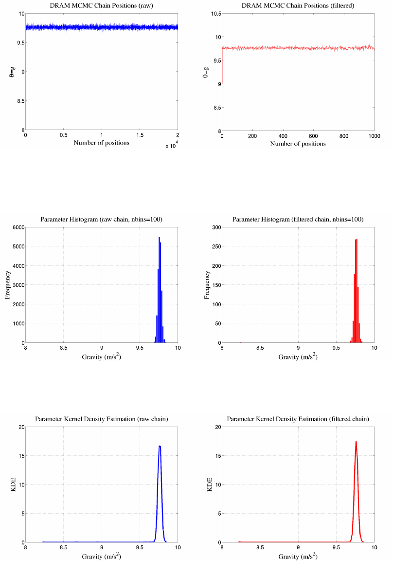
CHAPTER 5. QUESO EXAMPLES 92

(a) Raw chain (b) Filtered chain

Figure 5.3.3: MCMC raw chain with 20000 positions and a ﬁltered chain with lag of 20

positions.

(a) Raw chain (b) Filtered chain

Figure 5.3.4: Histograms of parameter θ=g.

(a) Raw chain (b) Filtered chain

Figure 5.3.5: Kernel Density Estimation.

CHAPTER 5. QUESO EXAMPLES 93

>> gri d on ;

Listing 5.37: Matlab code for the CDF plot.

5.3.8.1.5 Autocorrelation Plots

The code presented in Listing 5.38 uses matlab function autocorr to generate Figure 5.3.7

which presents the autocorrelation of the parameter gin both cases: raw and ﬁltered chain.

% inside Matlab

>> sip_gravity_raw_chain

>> sip_gravity_filtered_chain

>> nlags =10;

>> [ A CF_r aw , la gs , b oun ds ]= aut oco rr ( i p_m h _r awC h ai n_u n if ied , nl ags , 0) ;

>> [ A CF _fil t , l ags , b oun ds ]= a uto cor r ( i p _m h_f i lt Cha i n_ u ni fi e d , n lag s , 0) ;

>> plo t ( lag s , A CF_r aw , ’ bo - ’ , lags , A CF _f ilt , ’r*- ’, ’ l in ew id th ’ ,3) ;

>> ylabel (’ Autocor re la ti on for \ t he ta = g ’ ,’ f on tsiz e ’ , 20) ;

> > x la b el ( ’ Lag ’ , ’ f on ts iz e ’ , 20) ;

>> tit le ( ’ P ar ame ter A ut oc or rel at io n ’ , ’ fo ntsi ze ’ , 20) ;

>> gri d on ;

>> h= leg end (’ raw chain ’ ,’ f il tered chain ’ ,’ location ’ ,’ northeast ’);

>> s et ( h ,’ fon tsiz e ’ , 16) ;

Listing 5.38: Matlab code for the autocorrelation plots.

5.3.8.1.6 Covariance and Correlation Matrices

Matlab function cov calculates the covariance matrix for a data matrix (where each col-

umn represents a separate quantity), and corr calculates the correlation matrix. Since our

statistical inverse problem has only one parameter (the acceleration gdue to gravity), both

covariance and correlation matrices have dimension 1 ×1, i.e., they are scalars.

% inside Matlab

>> s i p _gravity_raw_ ch a i n ;

>> cov_mat ri x_g = cov ( ip_ mh _r aw C hain_unified )

cov_matrix_g =

6.8 70 9 e -04

>> corr_mat ri x_g = corr ( ip_m h_ ra w C hain_unified )

corr_matrix_g =

Listing 5.39: Matlab code for ﬁnding the covariance matrix.

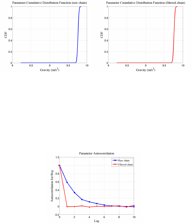
CHAPTER 5. QUESO EXAMPLES 94

(a) Raw chain (b) Filtered chain

Figure 5.3.6: Cumulative Distribution Function.

Figure 5.3.7: Autocorrelation plots.

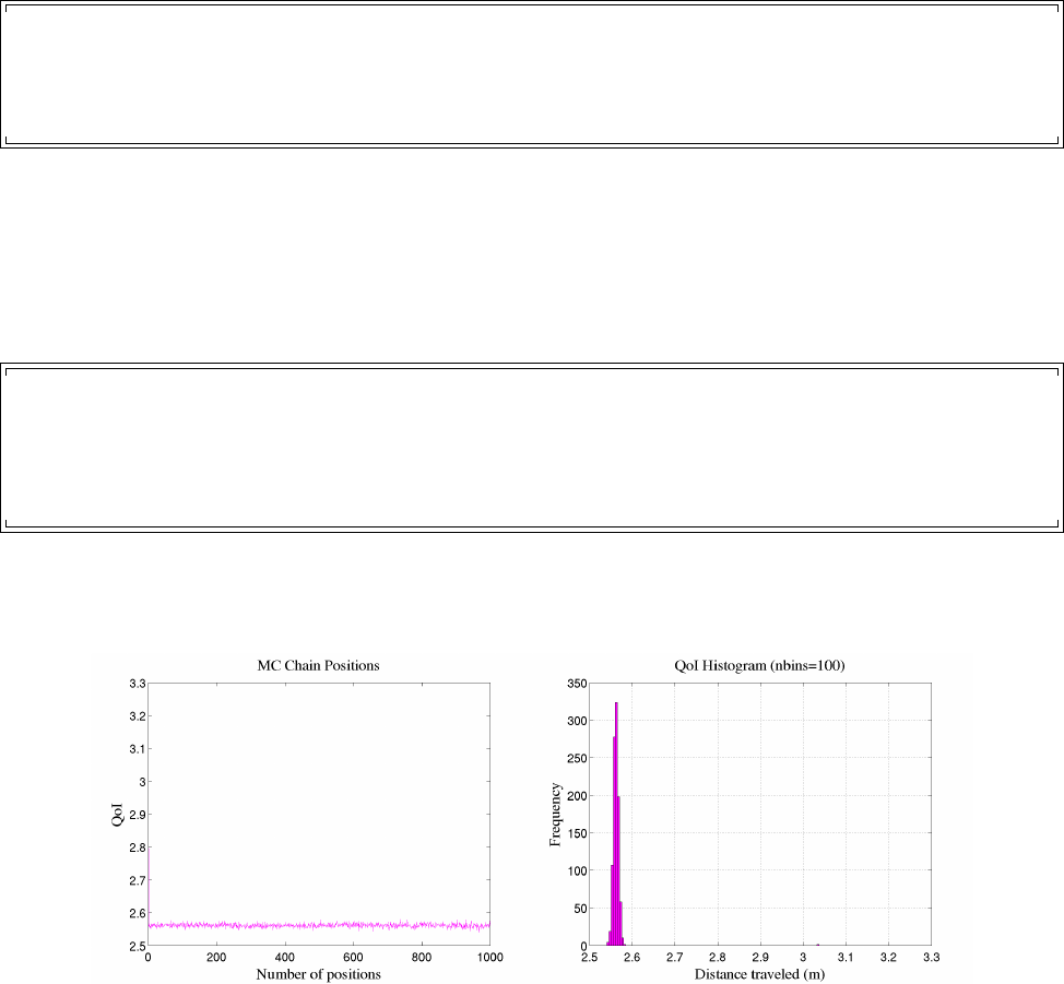
CHAPTER 5. QUESO EXAMPLES 95

5.3.8.2 Statistical Forward Problem

5.3.8.2.1 Chain Plots

It is quite simple to plot, using Matlab, the chain of positions generated by the Monte

Carlo algorithm implemented within QUESO and called during the solution of the statistical

forward problem. The sequence of Matlab commands presented bellow generates the graphic

depicted in Figure 5.3.8a.

% inside Matlab

>> sfp_gravity_qoi_seq.m

>> plot(fp_mc_QoiSeq_unified);

> > y la b el ( ’ QoI ’ , ’ f on ts iz e ’ , 20) ;

>> xlabel (’ Number of pos itions ’,’ fontsize ’ ,20) ;

>> t it le ( ’ MC C ha in Pos it io ns ’ , ’ fo nt si ze ’ , 20) ;

Listing 5.40: Matlab code for the chain plot.

5.3.8.2.2 Histogram Plots

In order to plot a histogram of the QoI, you may use the pre-deﬁned Matlab function hist.

The Matlab code presented in below shows how to create the Figure 5.3.8b.

>> sfp_gravity_qoi_seq.m

>> nbins =1 00;

>> hist(fp_mc_QoiSeq_unified);

>> tit le ( ’ Qo I H is togr am ’ , ’ fo ntsi ze ’ ,20) ;

>> xlabel (’ Dis ta nce tra veled ( m) ’ ,’ fontsiz e ’ ,20) ;

>> y la be l (’ Fr eq ue ncy ’ ,’ fo ntsi ze ’ ,20) ;

>> gri d on ;

Listing 5.41: Matlab code for the QoI histogram plot.

(a) Chain positions (b) Hystogram

Figure 5.3.8: MC chain positions and histogram of QoI = d.

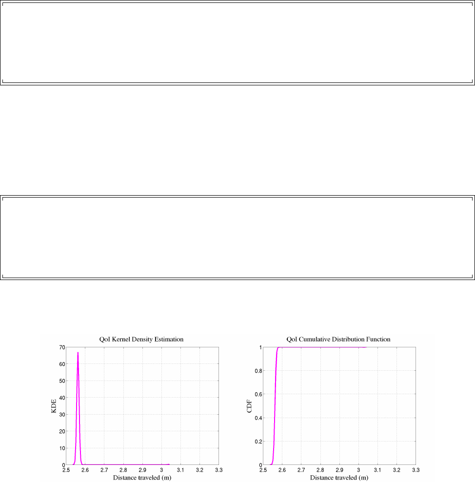
CHAPTER 5. QUESO EXAMPLES 96

5.3.8.2.3 KDE Plots

Matlab function ksdensity (Kernel smoothing density estimate) together with the option

’pdf’ may be used for plotting the KDE of the he QoI, displayed in Figure 5.3.9a.

% inside Matlab

>> sfp_gravity_qoi_seq.m

>> [ f ,xi ] = k sd e ns it y ( f p _m c_Q o iS eq _ un ifi e d , ’ function ’ , ’ pdf ’ ) ;

>> plo t ( xi , f ,’ - b ’, ’ l in ew id th ’ , 3)

>> tit le ( ’ Qo I K er ne l D en si ty E st ima tio n ’ ,’ f on tsiz e ’ , 20) ;

>> xlabel (’ Dis ta nce tra veled ( m) ’ ,’ fontsiz e ’ ,20) ;

> > y la b el ( ’ KDE ’ , ’ f on ts iz e ’ , 20) ;

>> gri d on ;

Listing 5.42: Matlab code for the QoI KDE plot.

5.3.8.2.4 CDF Plots

Matlab function ksdensity (Kernel smoothing density estimate) with ’cdf’ option may

also be used for plotting the Cumulative Distribution Function of the QoI, displayed in Fig-

ure 5.3.9b.

% inside Matlab

>> sfp_gravity_qoi_seq.m

>> [ f ,xi ] = k sd e ns it y ( f p _m c_Q o iS eq _ un ifi e d , ’ function ’ , ’ cdf ’ ) ;

>> plo t ( xi , f ,’ - b ’, ’ l in ew id th ’ , 3)

>> tit le ( ’ Qo I C umul ati ve D istr ibut ion F un cti on ’ ,’ fon tsiz e ’ , 20) ;

>> xlabel (’ Dis ta nce tra veled ( m) ’ ,’ fontsiz e ’ ,20) ;

> > y la b el ( ’ CDF ’ , ’ f on ts iz e ’ , 20) ;

>> gri d on ;

Listing 5.43: Matlab code for the QoI CDF plot.

(a) KDE (b) CDF

Figure 5.3.9: Kernel Density Estimation and Cumulative Distribution Function of QoI.

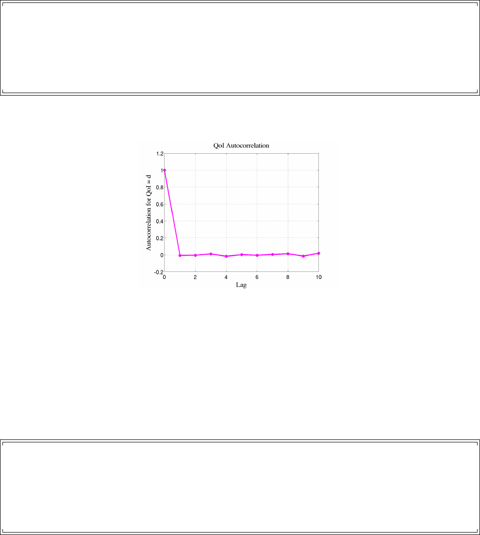
CHAPTER 5. QUESO EXAMPLES 97

5.3.8.2.5 Autocorrelation Plots

The code presented in Listing 5.44 uses Matlab function autocorr to generate Figure 5.3.10,

which presents the autocorrelation of the QoI d.

% inside Matlab

>> sfp_gravity_qoi_seq.m

>> nlags =10;

>> [ ACF , lags , bounds ] = a u tocor r ( f p _mc_Qo iSeq_u n ified , nlags , 0) ;

>> plo t ( lag s , ACF , ’ bo - ’ , ’ li ne wi dt h ’ , 3) ;

>> ylabel (’ Autocor re la ti on for QoI = d ’ , ’ fo nt si ze ’ ,20) ;

> > x la b el ( ’ Lag ’ , ’ f on ts iz e ’ , 20) ;

>> tit le ( ’ Qo I A uto co rr ela ti on ’ , ’ font size ’ ,2 0) ;

>> gri d on ;

Listing 5.44: Matlab code for the QoI autocorrelation plot.

Figure 5.3.10: Autocorrelation plot.

5.3.8.2.6 Covariance and Correlation Matrices

For a matrix input X, where each row is an observation, and each column is a variable, the

Matlab function cov(X) may be used to calculate the covariance matrix.

Thus, in order to calculated the covariance matrix between the parameter and the quantity

of interest sequences generated by Monte Carlo sampler with QUESO, one may simply deﬁne

X=[fp_mc_ParamSeq_unified fp_mc_QoiSeq_unified]. The code presented in Listing 5.45

shows the usage of Matlab commands for ﬁnding such the matrix.

% inside Matlab

>> sfp_gravity_qoi_seq;

>> sfp_gravity_p_seq;

>> X =[ fp_mc_ P a r a m Seq_unified fp_mc _ Q o i S eq_unified ];

>> c ov _p _Q oI = co v (X )

cov_ p_QoI =

[ 2 .8 26 e - 03 -8 .55 5 e -0 4 ]

[ -8.555 e -04 2.599 e -04 ]

Listing 5.45: Matlab code for the matrix of covariance between parameter gand QoI d.

CHAPTER 5. QUESO EXAMPLES 98

Analogously, the Matlab function corrcoef(X) returns a matrix of correlation coeﬃcients

calculated from an input matrix Xwhose rows are observations and whose columns are vari-

ables. In order to calculated the correlation matrix between the parameter and the QoI

sequences, one may simply deﬁne X=[fp_mc_ParamSeq_unified fp_mc_QoiSeq_unified].

% inside Matlab

>> sfp_gravity_qoi_seq;

>> sfp_gravity_p_seq;

>> X =[ fp_mc_ P a r a m Seq_unified fp_mc _ Q o i S eq_unified ];

>> corr_p _Q oI = c orrcoe f (X )

corr _ p_QoI =

[ 1 .000 e + 00 -9.981 e -01 ]

[ - 9. 98 1 e - 01 1 . 00 0 e + 00 ]

Listing 5.46: Matlab code for the matrix of correlation between parameter gand quantity of

interest d.

5.4 validationCycle

This is the last and more complex of all QUESO examples. In this example, we numerically

solve a statistical inverse problem related to a thermogravimetric experiment, where a material

sample has its mass measured while loosing it through a controlled heating process.

Given a simple mass evolution model that has a temperature proﬁle and material properties

as input parameters, and given thermogravimetric measurements with prescribed variances,

the statistical inverse problems ask for the speciﬁcation of the random variables that represent

the unknown material properties. We compute probability density functions with the Bayesian

approach and compute sets of realizations through the Metropolis-Hastings algorithm with

delayed rejection.

We qualitatively analyze the sensitivity of the solutions with respect to problem charac-

teristics, namely “amount” of data and “quality” of data, and also with respect to algorithm

options, namely chain initial position, number of delayed rejections and chain size.

5.4.1 Thermogravimetric Experiments and a Simple Model

Suppose a given material sample of initial mass m0and at initial temperature T0is heated with

constant heating rate β(K/min). Heating is maintained until the sample fully ablates (decom-

poses). The sample mass m(T) is measured at temperatures T > T0. Let w(T) = m(T)/m0

denote the mass fraction.

It is convenient to transform the kinetic equation to a per unit temperature form by dividing

through by β. Thus, a simple approach to the simulation of a thermogravimetric phenomenon

consists on modeling the sample as a homogeneous material of scalar properties A > 0 and

E > 0 whose relative mass wobeys the following initial value ordinal diﬀerential equation

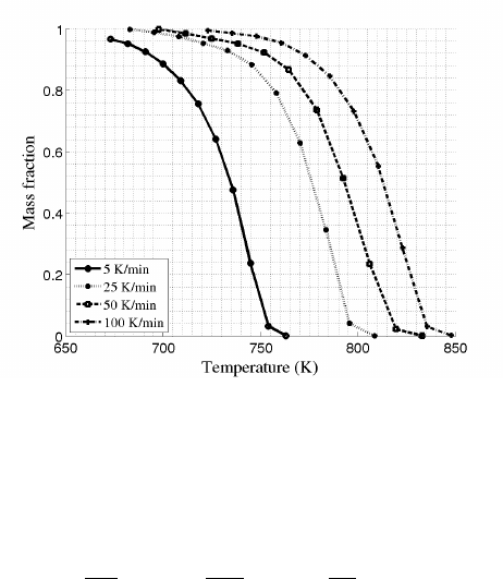
CHAPTER 5. QUESO EXAMPLES 99

Figure 5.4.1: Mass fraction decay over temperature given diﬀerent heating rates. Data from

J. A. Conesa, R. F. Marcilla and J. A. Caballero, “Thermogravimetric studies on the thermal

decomposition of polyethylene”, J. Anal. Appl. Pyrolysis, 36(1):1-15, 1996

problem: 









dt =−Aw

βexp −E

RT , t >0,

w(0) = 1,

(5.4.1)

where the kinetic parameters Aand Eare referred to, respectively, as pre-exponential factor

(min−1) and activation energy (J/mol).

In this combined SIP–SFP, we calibrate both model parameters Aand Egiven the mathe-

matical model in Equation (5.4.1) and experimental data (Section 5.4.2.3). Then the inferred

values for Aand Eare then used for uncertainty propagation on the remaining mass fraction

at time t= 3.9 s when β= 250 K/min, i.e., our quantity of interest is w(t= 3.9).

5.4.2 Statistical Inverse Problem

Let m= (A, E) be the vector of model parameters and M=R2

+be the space of model

parameters. Let VTdenote the space of functions f:R+→R+that are weakly diﬀerentiable.

VTwill be the space of temperature proﬁles. Finally, let Vwdenote the space of functions

f:R+→[0,1] that are weakly diﬀerentiable. Vwwill be the space of relative mass evolutions.

We will denote by

w(m, T )∈Vw

the solution of Equation (5.4.1) for given m∈Mand T∈VT.

5.4.2.1 Misﬁt Functions F(m)

Let VSdenote the space of all functions f:R+→R+that are square-Lebesgue-integrable

over any ﬁnite interval. VSwill be the space of misﬁt weight functions. Let Vσdenote the

CHAPTER 5. QUESO EXAMPLES 100

space of all functions f:R+→R∗

+such that 1/f is square-Lebesgue-integrable over any ﬁnite

interval. Vσwill be the space of variance functions.

Given a reference relative mass evolution function d∈Vw, a temperature proﬁle T∈VT,

and some tF>0, let F:M→Rbe the functional deﬁned by

F(m) = ZtF

0{[w(m, T )](t)−d(t)}2·S(t)dt,

or simply

F(m) = ZtF

(w−d)2·S dt. (5.4.2)

The functional (5.4.2) is general enough for our studies, since it can properly describe not

only the case where one has continuous measurements d, but also the case of a ﬁnite set of

Nmeas discrete measurements 0 6dj61, 1 6i6Nmeas at instants 0 6t1< t2< . . . < tNmeas .

In the case of continuous measurements, for instance, one can set

F1(m) = ZtF

0{[w(m, T )](t)−d(t)}2·1

σ2(t)dt,

for some given variance function σ2∈VSsatisfying σ(t)>0 for all t>0.

On the other hand, when measurements are discrete and a corresponding ﬁnite set of

variances σ2

j>0, j = 1,2, . . . , Nmeas is given, one can set

F2(m) = ZtF

0{[w(m, T )](t)−ˆ

d(t)}2·"Nmeas

j=1

δ(t−tj)

ˆσ2(t)#dt,

where ˆ

d∈Vwand ˆσ∈Vσare any functions satisfying ˆ

d(tj) = djand ˆσ(tj) = σj,j=

1,2, . . . , Nmeas, in which case the functional simply becomes

F2(m) =

Nmeas

j=1

{[w(m, T )](tj)−dj}2

σ2

assuming, without loss of generality, that tF>tNmeas .

5.4.2.2 Bayesian Approach: Prior RV, Likelihood and Posterior RV

In deterministic inverse problems treat the unknown parameters as scalars or vectors and the

goal is the calculation of their best values according to a given criteria, usually least squares,

e.g. solving the unconstrained optimization problem

min

m∈MF(m).(5.4.3)

In statistical inverse problems, the unknown parameters are treated as random variables

(RVs) and the goal is the speciﬁcation of their probability density functions (PDFs) [28].

CHAPTER 5. QUESO EXAMPLES 101

Applying the Bayesian approach

πposterior(m)∝πprior(m)·πlikelihood(m)

we have that for the TGA SIP, the prior distribution and the likelihood are, respectively:

πprior(m)∝e−1

2V(m)and πlikelihood(m)∝e−1

2F(m).

Thus, we chose parameters (A, E) to have joint uniform prior PDF over the open square

domain, i.e.:

πprior =U((1.0×1010,5.0×1011)×(4.0×105,6.0×105)).

5.4.2.3 Data from experiments

Table 5.4.1 presents the data collected in the TGA experiment.

Observation Temperature Relative mass Variance

index “i”Ti(K) m∗

obs,i (%) Vi

1 673.034 96.5855 0.1

2 682.003 95.1549 0.1

3 690.985 92.5048 0.1

4 699.979 88.6353 0.1

5 708.989 83.0585 0.1

6 718.02 75.5306 0.1

7 727.089 64.1003 0.1

8 735.96 47.5474 0.1

9 744.904 23.6777 0.1

10 754.062 03.2234 0.1

11 763.049 00.0855448 0.1

Table 5.4.1: Experimental data.

5.4.3 Statistical Forward Problem

In spacecraft design, ablation is used to both cool and protect mechanical parts and/or pay-

loads that would otherwise be damaged by extremely high temperatures. Two principal

applications are heat shields for spacecraft entering a planetary atmosphere from space and

cooling of rocket engine nozzles [49].

Suppose that an object about to re-enter the Earth atmosphere has a thermal protection

layer (shield) of composition of the same sample material described in Section 5.4.2. Also, as

the object re-enters the atmosphere, its shield loses mass according to Equation (5.4.1). The

initial sample temperature is T0= 0.1 K and it is then heated with constant rate β= 5 K/m.

CHAPTER 5. QUESO EXAMPLES 102

We are interested in answering the following question: at scenario β= 250 K/min, what

is the remaining mass fraction at time t= 3.9 s? In other words, the quantity of interest is

w(t= 3.9s).

5.4.3.1 The Input RV, QoI Function and Output RV

The input random variables for this SFP are the inferred parameters Aand Ewhich are

the solution (posterior PDF) of the inverse problem described in Section 5.4.2. The output

random variable for this example is the remaining mass fraction at 3.9 s, i.e. w(t= 3.9).

Note that, since there is uncertainty in the parameters Aand E(both given as PDFs), one

can expect that this uncertainty will be propagated to w(t= 3.9), which will also be given

as a PDF. Finally, the QoI function for wis the solution of the Equation (5.4.1) evaluated

when t= 3.9 s, which is calculated using numerical integration with adjustable and acceptable

time-stepping using GSL function gsl_odeiv_evolve_apply1.

5.4.4 Running the Example

To run the executable provided (available after QUESO installation), and generate ﬁgures for

the chains, PDFs, CDFs, etc., enter the following commands:

$cd $H OM E / L IB RA RI ES / QU ESO - 0. 50 .0/ e xa mp le s / v alid ation C yc le

$rm output D ata /*

$./exTgaValidationCycle_gsl tagCycle.inp

$matlab

$tga_cycle_plot.m # i n s i d e m atla b

$exit # i n s i d e m a t lab

$ls -l o u tputDa ta /*. png

cal_parameter1_prior.png cal_parameter2_prior.png

c al _va l_parame ter1_PDF . png cal_val_p arameter 2_PDF . png

c al _va l_parame ter1_CDF . png cal_val_p arameter 2_CDF . png

cal_val_param et er 1 _ a utocorr . png cal_val_param et er 2 _ a utocorr . png

cal_va l_Qo I_CDF . png cal_va l_Qo I_PDF . png

c al _val_Q o I_ autocor r el ation . png

As a result, the user should have created several of PNG ﬁgures containing marginal pos-

terior PDF, chain positions of the parameters and the QoI, histogram, cumulative density

distribution and autocorrelation. The name of the ﬁgure ﬁles have been chosen to be infor-

mative, as shown in the Listing above.

5.4.5 TGA Example Code

The program example given in this paper is compatible with version 0.47.1 of QUESO. The

source code for the example is composed of 5 ﬁles: exTgaValidationCycle gsl.C (Listing

5.47), exTgaValidationCycle appl.h (Listing 5.48), exTgaValidationCycle likelihood.h

(Listing 5.49) and exTgaValidationCycle qoi.C (Listing 5.50).

1http://www.gnu.org/software/gsl/manual/html_node/Evolution.html#index-gsl_005fodeiv2_

005fevolve_005fapply

CHAPTER 5. QUESO EXAMPLES 103

/* T his is an e xampl e of how to d efin e and run a PE COS valida t ion c ycl e for a

* t hermog ravim etric a na ly si s ( TGA ) mod el

* using QUES O classes and a lgorit hms . The code itself is in the t e mplat e d

* r ou tin e ’ u qA pp l ( * env) ’. This routine is calle d right after the in i t ializati o n

* of the MPI e n vironm e nt and of the QUES O envi r onment and is ava ilable in

* file ’exTgaValidationCycle_gsl.C’.

* It is easier to und e rstand this exam ple after und e rtandin g t hree oth er sim pler

* e xample s :

* (1) e xam pl es / s impleStatistica l In verseProble m / s rc / e xa mple _ma in . C

* (2) e xam pl es / s impleStatistica l Fo rwardProble m / s rc / s imple_ s fp _exam ple_main . C

* (3) e xam pl es / g ra vi ty / s rc / g ra vit y_m ain . C

* E x am pl e ( 1) f o cu s es o n th e t em p la t ed c la ss S t at i st i ca l I nv e rs e P ro b le m < P_V , P_M >.

* E x am pl e ( 2) f o cu s es o n th e t em p la t ed c la ss S t at i st i ca l F or w ar d P ro b le m < P_V , P_M , Q _V , Q_M > .

* Examp le (3) focu ses on both classes , since it uses the solu tion of the i nverse p robl em

* as input to the f orward pro blem .

* This exam ple with TGA uses both sta t istical problem templ ated classes , twice each in

* fact , but it a lso :

* - us es th e t em p la t ed c la ss V al i da ti o nC y cl e < P_ V , P_ M , Q_V , Q_ M > ,

* - reads e xperim e n tal data from fi les in order to comp ute the l ikelih ood fun ction

* at c andid a te p a ramet er vec tors gene r ated by the Metro polis - H astin gs algorithm , and

* - comp ares the qoi cdfs comp uted from the two stat i stical forwa rd p roble ms at

* the pre di ction s cenari o .

*--------------------------------------------------------------------------

*-------------------------------------------------------------------------- */

#i n c l u d e <e x T g a V a l i d a t i o n C y c l e a p p l . h>

#i n c l u d e <q u es o / G s l M a t r i x . h>

#i n c l u d e <queso/EnvironmentOptions .h>

int mai n (int argc , c har * argv [])

{

//************************************************

// Initia l ize e n vironm e nt

//************************************************

MPI _I ni t (& argc ,& a rgv );

QUESO::EnvOptionsValues* envOptionsValues = NULL;

#i f d e f UQ EXAMPLES USES QUESO INPUT FILE

UQ_FATAL_TEST_MACRO(argc != 2,

QUESO::UQ_UNAVAILABLE_RANK ,

" m ai n () " ,

" input file must be spe cifie d in comm and line as argv [1] , just after

exec uta ble arg v [0 ] ") ;

QUESO :: F ul lE nvironme nt * env = n ew Q UE SO : : F ullE n vi r on m en t ( M PI_ COM M_ WOR LD , a rg v [1 ] , " " ,

envOptionsValues);

#else

envOptionsValues = new QUESO::EnvOptionsValues();

env Option sValu es -> m_subDisp la y F ileName = " o utputDa ta / displ ay " ;

env Option sValu es -> m_subDispl ay Al l o wedSet . insert (0) ;

env Option sValu es -> m_subDispl ay Al l o wedSet . insert (1) ;

env Option sValu es -> m_displa yV er bosity = 2;

env Op tionsV alues - > m_see d = 0;

QUESO :: F ul lE nvironme nt * env = new Q UESO :: F ul lE nv ir on me nt ( M PI_CO MM_WO RLD ," " ,"" ,

envOptionsValues);

#e n d i f

//************************************************

// Run appl i cation

//************************************************

CHAPTER 5. QUESO EXAMPLES 104

uqAppl < QU ESO :: GslVe ctor , // t ype for p aramet er vect ors

QUESO :: GslMatrix , // type for p arame t er matr ices

QUESO :: GslVector , // type for qoi vectors

QUESO :: GslMa trix // type for qoi ma trice s

>(* env ) ;

//************************************************

// Final ize e n vironm e nt

//************************************************

delete env;

delete envOptionsValues;

MPI_Finalize();

return 0;

}

Listing 5.47: File exTgaValidationCycle gsl.C.

#i f n d e f EX TGA VALIDATION CYCLE APPL H

#d e f i n e EX TGA VALIDATION CYCLE APPL H

#d e f i n e UQ EXAMPLES USES QUESO INPUT FILE

#i n c l u d e <e x T g a V a l i d a t i o n C y c l e l i k e l i h o o d . h>

#i n c l u d e <e x T g a V a l i d a t i o n C y c l e q o i . h>

#i n c l u d e <q ueso / V a l i d a t i o n C y c l e . h>

#i n c l u d e <queso/VectorSubset .h>

#i n c l u d e <q ueso / U niformVectorRV . h>

#i n c l u d e <queso/GenericScalarFunction .h>

#i n c l u d e <g s l / g s l e r r n o . h>

#i n c l u d e <g s l / g s l o d e i v . h>

// Just decl aration : act ual code is belo w

te mplate < cla ss P_V , c lass P_M , class Q_V , c lass Q_M >

void

u q Ap p l _L o c al C o m pa r i so n S ta g e ( Q UE SO :: V a li da t io n Cy c le < P_V , P _M , Q _V , Q _M >& c yc l e ) ;

te mplate < cla ss P_V , c lass P_M , class Q_V , c lass Q_M >

void

u q Ap p l _U n i fi e d C om p a ri s o n St a g e ( Q UE SO :: V a li d at io n Cy c le < P_V , P_M , Q _V , Q_ M >& c yc l e ) ;

//********************************************************

// The driving routine " u qAp pl () " : called by main ()

// Ther e are 5 main t asks :

// 1) initili z a tion

// 2) the ’ calibra t ion stage ’

// 3) the ’ valida t ion stage ’

// 4) the ’ compar i son stage ’

// 5) mem ory r eleas e

// Task s 2 , 3 and 4 c on st itute the a ctual valida ti on cyc le .

//********************************************************

te mplate < cla ss P_V , c lass P_M , class Q_V , c lass Q_M >

void

uqA ppl ( const QUE SO :: B as eE nv iro nm ent & env )

{

if (env . f ullRa nk () == 0) {

std :: cout << " B egi nni ng run of ’ u qT ga Ex am pl e ’ e xa mpl e \ n"

<< s td :: endl ;

}

in t iRC ;

struct time val tim evalRef ;

struct time val tim evalNow ;

CHAPTER 5. QUESO EXAMPLES 105

//******************************************************

// Task 1 of 5: i nstanti a t ion of bas ic clas ses

//******************************************************

// Instant i ate the param e ter space

std :: vector < std :: string > p aramNam es (2, "");

para m Names [0] = "A_param";

para m Names [1] = "E_param";

Q UE SO : : V e ct or Sp a ce < P_V , P _M > p a ra m Sp a ce ( env ,"param_", param Names . size () ,& p aramNam es ) ;

// Instant i ate the param e ter doma in

P_V p ar amMinVal ue s ( paramSp ace . zeroV ec tor () );

param MinV alu es [0] = 2.4 0 e +11;

param MinV alu es [1] = 1.8 0 e +05;

P_V p ar amMaxVal ue s ( paramSp ace . zeroV ec tor () );

param MaxV alu es [0] = 2.8 0 e +11;

param MaxV alu es [1] = 2.2 0 e +05;

Q UE SO : : B ox Su b se t p a ra m D om a in ( "param_",

paramSpace ,

paramMinValues ,

paramMaxValues);

// Instant i ate the qoi space

std :: vector < std :: string > q oiNam es (1 , "" ) ;

qoi N ames [0] = " TimeFor25Perc en tO f Mass ";

Q UE SO : : V e ct or Sp a ce < Q_V , Q _M > q oi S pa c e ( env ," qoi_ " , qoiNa mes . size () ,& q oiNam es ) ;

// Instant i ate the valida t ion cycle

Q UE SO : : V al i da t io nC y cl e c y cl e ( env ,

" " , // No extra pr efix

paramSpace ,

qoi Space );

//********************************************************

// Task 2 of 5: cali b ration stage

//********************************************************

iRC = gettim eof da y (& tim eval Ref , NULL );

if ( iRC ) { }; // j ust to rem ov e comp il er w ar ni ng

if (env . f ullRa nk () == 0) {

std :: cout << " B eginni ng ’ calibr a tion stage ’ at " << ctime (& timeva lR ef . tv_sec )

<< s td :: endl ;

}

// I nvers e prob lem : i ns tantiat e the prior rv

Q UE SO : : U ni f or m Ve ct o rR V c a lP r io r Rv (

" c a l_ pr i or _ " , // Extra prefix befo re the default " rv_ " prefix

para mD omain );

// I nvers e prob lem : i ns tantiat e the l ik elihoo d function o bject ( dat a + rout in e )

l ik e li h o od R ou t in e _D a ta c a l Li k e li h o o dR o u ti n e _D a t a ( env ,

"scenario_5_K_min.dat",

" s cen ario_2 5_K_m in . dat " ,

" s cen ario_5 0_K_m in . dat " );

QUESO :: Generi cScalar Functio n < P_V , P_M > c a l L i k e l i hoodFunctionObj (" cal_l ike_ " ,

paramDomain ,

likelihoodRoutine <P_V,P_M>,

( vo id *) &

calLikelihoodRoutine_Data

true); // the r outin e

c om pu tes [ ln ( func tion )]

CHAPTER 5. QUESO EXAMPLES 106

// I nvers e prob lem : i ns tantiat e it ( p os terior rv is i ns ta nt iated int er nally )

QUESO :: S i pOptionsV a l u es * c a lIpOptions V a l u es = NULL ;

#i f d e f UQ EXAMPLES USES QUESO INPUT FILE

#else

c al I pO p ti o ns V al u es = n ew Q UE SO :: S i pO p ti o ns V al ues ( ) ;

calI pOptio nsVal ues -> m_compute So l ution = true;

calI pOptio nsVal ues -> m_dataOutp ut Fi l eName = " o utputD ata / tgaCal Ou tput ";

calI pO pti on sVa lu es - > m _d ataOutpu tAllowed Set . i ns er t (0) ;

calI pO pti on sVa lu es - > m _d ataOutpu tAllowed Set . i ns er t (1) ;

#e n d i f

cycle . in st antiateCa lI P ( calIp Option sValue s ,

calPriorRv ,

calLikelihoodFunctionObj);

// I nvers e pro blem : solve it , that is , set ’ pdf ’ and ’realizer ’ of the poste r ior rv

P_V p ar am In itialValues ( param Space . zer oVector () ) ;

if (env . n u m S u bEnvironmen t s () == 1) {

// For reg r ession test purp oses

paramIn itia lValu es [ 0] = 2 .41 e + 11;

paramIn itia lValu es [ 1] = 2 .19 e + 05;

}

else {

calP riorRv . realize r () . realiz at ion ( paramIn it ia lV a lues );

}

QUESO :: M hOptionsV a l ues * c alIpMhOptions V a l u es = NULL ;

P_ M * c a lP r op o sa l Co v Ma t ri x = c yc le . c al IP () . p ost Rv () . i ma ge Set () . v ec t or Spa c e () .

n ew P ro p os a lM a tr i x ( NULL ,& p a ra m In i ti a lV a lu e s ) ;

#i f d e f UQ EXAMPLES USES QUESO INPUT FILE

#else

QUESO::SsOptionsValues ssOptionsValues1;

QUESO::SsOptionsValues ssOptionsValues2;

ssOpti on s Values1 . m_in it ia l D i s cardedPortions . resiz e (9) ;

ssOpti on s Values1 . m_ini ti al Di sc a r dedPortions [0] = 0.;

ssOpti on s Values1 . m_ini ti al Di sc a r dedPortions [1] = 0.05;

ssOpti on s Values1 . m_ini ti al Di sc a r dedPortions [2] = 0.10;

ssOpti on s Values1 . m_ini ti al Di sc a r dedPortions [3] = 0.15;

ssOpti on s Values1 . m_ini ti al Di sc a r dedPortions [4] = 0.20;

ssOpti on s Values1 . m_ini ti al Di sc a r dedPortions [5] = 0.25;

ssOpti on s Values1 . m_ini ti al Di sc a r dedPortions [6] = 0.30;

ssOpti on s Values1 . m_ini ti al Di sc a r dedPortions [7] = 0.35;

ssOpti on s Values1 . m_ini ti al Di sc a r dedPortions [8] = 0.40;

ssOpti on s Values1 . m_au to Co rr C omputeViaDef = false ;

ssOpti on s Values1 . m_au to Co rr C omputeViaFft = true;

ssOpti on s Values1 . m_a ut oC o rrSecondLag = 2;

ssOpti on s Values1 . m_a ut oC o rrLagSpacing = 2;

ssOptionsValues1.m_autoCorrNumLags = 15;

ssOptionsValues1.m_autoCorrDisplay = true;

ssOptionsValues1.m_autoCorrWrite = true;

ssOpti on sV a lues1 . m_kd eC ompute = f alse ;

ssOptionsValues1.m_covMatrixCompute = true;

ssOpti on s Values1 . m_c or rM a trixCompute = true;

ssOpti on s Values2 . m_in it ia l D i s cardedPortions . resiz e (1) ;

ssOpti on s Values2 . m_ini ti al Di sc a r dedPortions [0] = 0.;

ssOpti on s Values2 . m_au to Co rr C omputeViaDef = false ;

ssOpti on s Values2 . m_au to Co rr C omputeViaFft = true;

ssOpti on s Values2 . m_a ut oC o rrSecondLag = 2;

ssOpti on s Values2 . m_a ut oC o rrLagSpacing = 2;

ssOptionsValues2.m_autoCorrNumLags = 15;

ssOptionsValues2.m_autoCorrDisplay = true;

ssOptionsValues2.m_autoCorrWrite = true;

ssOpti on sV a lues2 . m_kd eC ompute = true;

ssOpti on s Values2 . m_kd eN um E valPositions = 250;

CHAPTER 5. QUESO EXAMPLES 107

ssOptionsValues2.m_covMatrixCompute = true;

ssOpti on s Values2 . m_c or rM a trixCompute = true;

calIpMhO p t i o n sValues = new QUESO :: MhOption s V alues (& ssOp tions Value s1 ,& ssOp t i o nsValues2 ) ;

calI pMhOpti onsVal ues -> m_dataOutpu tF il e Name = " o utputD ata / tgaCal Ou tput ";

calI pMhOpt ionsVal ues -> m_dataOutput Al lo w edSet . in sert (0) ;

calI pMhOpt ionsVal ues -> m_dataOutput Al lo w edSet . in sert (1) ;

calI p MhOpti onsVal ues -> m_rawChainDataInp ut Fi l e N a me = ".";

calI pMhOpti onsValu es - > m_rawChai nS ize = 1 048576 ;

calI pMhOpt ionsVal ues -> m_rawChainGen er at e E xtra = fals e ;

calI pMhOpt ionsVal ues -> m_rawChainDis pl ay P e riod = 20000;

calI pMhOpt ionsVal ues -> m_rawChainMeasu re Ru n T i mes = true;

calI p MhOpti onsVal ues -> m_rawChainDataOutp ut Fi l e N a m e = " outpu tData / fil e_ c al_ip_ra w ";

calI p MhOpti onsVal ues -> m_rawChainDataOutputAl lo we d S e t . ins ert (0) ;

calI p MhOpti onsVal ues -> m_rawChainDataOutputAl lo we d S e t . ins ert (1) ;

calI pMhOpt ionsVal ues -> m_rawChainCo mp ut e Stats = true;

calI pMhOpti onsVal ues -> m_displayC an di d ates = false ;

calI pMhOpt ionsVal ues -> m_putOutOfBou nd sI n C hain = true;

calI pMhOpti onsVal ues -> m_tkUseLoc al He s sian = false ;

calI pMhOpt ionsVal ues -> m_tkUseNewto nC om p onent = true;

calI pMhOpt ionsVal ues -> m_drMaxNumE xt ra S tages = 1;

calI pMhOpt ionsVal ues -> m_drScalesForE xt ra S t ages . resize (1) ;

calI pMhOpt ionsVal ues -> m_drScalesForE xt ra S t ages [0] = 5.;

calI p MhOpti onsVal ues -> m_amInitialNonAda pt In t e r v al = 0;

calI pMhOpti onsValu es - > m_amAdaptI nt er val = 100;

calI pM hOption sV alues - > m_ amEta = 1.92;

calI pMhOpti onsValu es - > m_ amEpsi lo n = 1. e -5;

calI pMhOpt ionsVal ues -> m_filteredCha in Ge n e rate = true;

calI p MhOpti onsVal ues -> m_filteredChainDiscarde dP or ti o n = 0.;

calI pMhOpti onsVal ues -> m_filtered Ch a inLag = 20;

calIpMhOptionsValues ->m_filteredChainDataOutputFileName = ".";

calI pMh Opt io nsV alu es - > m _filtered C ha inDataOutputA l lo wedSet . i ns er t (0) ;

calI pMh Opt io nsV alu es - > m _filtered C ha inDataOutputA l lo wedSet . i ns er t (1) ;

calI p MhOpti onsVal ues -> m_filteredChainCo mp ut e S t a ts = true;

#e n d i f

cycle .cal IP () . solveW it hB ay e s M e t ropolisHastings ( cal IpMhOp tionsVa lues ,

paramInitialValues ,

calProposalCovMatrix);

delete calProposalCovMatrix;

delete calIpMhOptionsValues;

// F orwar d prob lem : i ns tantiat e it ( p ar ameter rv = poste rior rv of inv erse problem ; qoi rv

is i ns tantiate d intern al ly )

double b eta_predi c t ion = 250.;

double criticalMass_prediction = 0.;

double c r i t icalTime_predic t i o n = 3.9;

q oi R ou ti n e_ D at a < P_ V , P_ M , Q_ V , Q_M > c a l Qo i R ou t i ne _ D at a ;

calQoiR ou tin e_D at a . m_beta = beta_pre di ct io n ;

calQoiR ou ti ne_Data . m_cr it icalMass = c ri ti c a lMass_predictio n ;

calQoiR ou ti ne_Data . m_cr it icalTime = c ri ti c a lTime_predictio n ;

QUESO :: S f pOptionsV a l u es * c a lFpOptions V a l u es = NULL ;

#i f d e f UQ EXAMPLES USES QUESO INPUT FILE

#else

c al F pO p ti o ns V al u es = n ew Q UE SO :: S f pO p ti o ns V al ues ( ) ;

calF pOptio nsVal ues -> m_compute So l ution = true;

calF pOptio nsVal ues -> m_computeC ov ar i ances = true;

calF pOptio nsVal ues -> m_computeCo rr el a t ions = true;

calF pOptio nsVal ues -> m_dataOutp ut Fi l eName = " o utputD ata / tgaCal Ou tput ";

calF pO pti on sVa lu es - > m _d ataOutpu tAllowed Set . i ns er t (0) ;

calF pO pti on sVa lu es - > m _d ataOutpu tAllowed Set . i ns er t (1) ;

CHAPTER 5. QUESO EXAMPLES 108

#e n d i f

cycle . in st antiateCa lF P ( calFp Option sValue s ,

q oi Ro ut in e < P_ V , P_ M , Q_V , Q_M > ,

( void *) & c al Q oiRoutine_D at a );

// F orwar d pro blem : solve it , that is , set ’ realizer ’ and ’cdf ’ of the qoi rv

QUESO :: M cOptionsV a l ues * c alFpMcOptions V a l u es = NULL ;

#i f d e f UQ EXAMPLES USES QUESO INPUT FILE

#else

QUESO::SsOptionsValues ssOptionsValues3;

QUESO::SsOptionsValues ssOptionsValues4;

ssOpti on s Values3 . m_in it ia l D i s cardedPortions . resiz e (1) ;

ssOpti on s Values3 . m_ini ti al Di sc a r dedPortions [0] = 0.;

ssOpti on sV a lues3 . m_kd eC ompute = true;

ssOpti on s Values3 . m_kd eN um E valPositions = 250;

ssOptionsValues3.m_covMatrixCompute = true;

ssOpti on s Values3 . m_c or rM a trixCompute = true;

ssOpti on s Values4 . m_in it ia l D i s cardedPortions . resiz e (1) ;

ssOpti on s Values4 . m_ini ti al Di sc a r dedPortions [0] = 0.;

ssOpti on s Values4 . m_au to Co rr C omputeViaDef = false ;

ssOpti on s Values4 . m_au to Co rr C omputeViaFft = true;

ssOpti on s Values4 . m_a ut oC o rrSecondLag = 2;

ssOpti on s Values4 . m_a ut oC o rrLagSpacing = 1;

ssOptionsValues4.m_autoCorrNumLags = 15;

ssOptionsValues4.m_autoCorrDisplay = true;

ssOptionsValues4.m_autoCorrWrite = true;

ssOpti on sV a lues4 . m_kd eC ompute = true;

ssOpti on s Values4 . m_kd eN um E valPositions = 250;

ssOptionsValues4.m_covMatrixCompute = true;

ssOpti on s Values4 . m_c or rM a trixCompute = true;

calFpMcO p t i o n sValues = new QUESO :: McOption s V alues (& ssOp tions Value s3 ,& ssOp t i o nsValues4 ) ;

calF pMcOpti onsVal ues -> m_dataOutpu tF il e Name = " o utputD ata / tgaCal Ou tput ";

calF pMcOpt ionsVal ues -> m_dataOutput Al lo w edSet . in sert (0) ;

calF pMcOpt ionsVal ues -> m_dataOutput Al lo w edSet . in sert (1) ;

calF pMcOpt ionsVal ues -> m_pseqDataOutp ut Fi l e Name = ".";

calF pMc Opt io nsV alu es - > m _pse q Da taOu t pu tAllo wedSet . i ns er t (0) ;

calF pMc Opt io nsV alu es - > m _pse q Da taOu t pu tAllo wedSet . i ns er t (1) ;

calF pMcOpti onsVal ues -> m_pseqComp ut e Stats = true;

calF pMcOpt ionsVal ues -> m_qseqDataInp ut Fi l e Name = ".";

calF pMcOpti onsValu es - > m_ qseqS iz e = 1 04857 6;

calF pMcOpti onsVal ues -> m_qseqDisp la yP e riod = 2000 0;

calF pMcOpt ionsVal ues -> m_qseqMeasu re Ru n Times = true;

calF pMcOpt ionsVal ues -> m_qseqDataOutp ut Fi l e Name = "outputData/file_cal_fp_qoi2";

calF pMc Opt io nsV alu es - > m _qse q Da taOu t pu tAllo wedSet . i ns er t (0) ;

calF pMc Opt io nsV alu es - > m _qse q Da taOu t pu tAllo wedSet . i ns er t (1) ;

calF pMcOpti onsVal ues -> m_qseqComp ut e Stats = true;

#e n d i f

cycle . cal FP () . solve Wi th MonteCarlo ( cal Fp Mc O ptionsValues ) ; // no extra user enti ties need ed

for Monte Carlo algor ithm

delete calFpMcOptionsValues;

iRC = gettim eof da y (& tim eval Now , NULL );

if (env . f ullRa nk () == 0) {

std :: cout << " E nd in g ’ c al ibr atio n stage ’ at " << c time (& t im evalNow . t v_sec )

<< " Tot al ’ c al ibr ati on stage ’ ru n tim e = " << t imevalN ow . tv_sec - timev al Ref .

tv_sec

<< " s econd s \n "

CHAPTER 5. QUESO EXAMPLES 109

<< s td :: endl ;

}

//********************************************************

// Task 3 of 5: val i dation sta ge

//********************************************************

iRC = gettim eof da y (& tim eval Ref , NULL );

if (env . f ullRa nk () == 0) {

std :: cout << " B eg inn ing ’ val id ati on st age ’ at " << ctime (& t imevalR ef . t v_sec )

<< s td :: endl ;

}

// I nver se pro blem : no need to instan t iate the prior rv (= p osteri or rv of c a librat i on

inverse problem)

// I nvers e prob lem : i ns tantiat e the l ik elihoo d function o bject ( dat a + rout in e )

l ik e li h o od R ou t in e _D a ta v a l Li k e li h o o dR o u ti n e _D a t a ( env ,

" s cena rio_1 00_K_mi n . dat " ,

NULL ,

NU LL ) ;

QUESO :: Generi cScalar Functio n < P_V , P_M > v a l L i k e l i hoodFunctionObj (" val_l ike_ " ,

paramDomain ,

likelihoodRoutine <P_V,P_M>,

( vo id *) &

valLikelihoodRoutine_Data

true); // the r outin e

c om pu tes [ ln ( func tion )]

// I nvers e prob lem : i ns tantiat e it ( p os terior rv is i ns ta nt iated int er nally )

QUESO :: S i pOptionsV a l u es * v a lIpOptions V a l u es = NULL ;

#i f d e f UQ EXAMPLES USES QUESO INPUT FILE

#else

v al I pO p ti o ns V al u es = n ew Q UE SO :: S i pO p ti o ns V al ues ( ) ;

valI pOptio nsVal ues -> m_compute So l ution = true;

valI pOptio nsVal ues -> m_dataOutp ut Fi l eName = " o utputD ata / tgaVal Ou tput ";

valI pO pti on sVa lu es - > m _d ataOutpu tAllowed Set . i ns er t (0) ;

valI pO pti on sVa lu es - > m _d ataOutpu tAllowed Set . i ns er t (1) ;

#e n d i f

cycle . in st antiateVa lI P ( valIp Option sValue s ,

valLikelihoodFunctionObj);

// I nvers e pro blem : solve it , that is , set ’ pdf ’ and ’realizer ’ of the poste r ior rv

QUESO :: M hOptionsV a l ues * v alIpMhOptions V a l u es = NULL ;

c on st QU E SO : : S e qu e nt i a lV e ct o rR e a li z er < P_V , P _M >*

t mp R ea l i ze r = d yn am i c_ ca s t < c on s t Q U ES O : : S e qu e n ti a lV e ct o r Re a li z er < P_V , P_ M >* >( &( c y cl e .

cal IP () . p os tR v () . r ea li z er () ) ) ;

// Use ’ real izer () ’ beca use the post . rv was c omput ed with Metr . Hast .

P_ M * v a lP r op o sa l Co v Ma t ri x = c yc le . c al IP () . p ost Rv () . i ma ge Set () . v ec t or Spa c e () .

newProposalMatrix(

& tmp Real izer - > uni fied Sampl eVarV ector () ,

& tmpRea lizer -> unifiedSampleE x p V e c t or () ); // Use these va lues as the initi al v alue s

#i f d e f UQ EXAMPLES USES QUESO INPUT FILE

#else

QUESO::SsOptionsValues ssOptionsValues5;

QUESO::SsOptionsValues ssOptionsValues6;

ssOpti on s Values5 . m_in it ia l D i s cardedPortions . resiz e (9) ;

ssOpti on s Values5 . m_ini ti al Di sc a r dedPortions [0] = 0.;

ssOpti on s Values5 . m_ini ti al Di sc a r dedPortions [1] = 0.05;

CHAPTER 5. QUESO EXAMPLES 110

ssOpti on s Values5 . m_ini ti al Di sc a r dedPortions [2] = 0.10;

ssOpti on s Values5 . m_ini ti al Di sc a r dedPortions [3] = 0.15;

ssOpti on s Values5 . m_ini ti al Di sc a r dedPortions [4] = 0.20;

ssOpti on s Values5 . m_ini ti al Di sc a r dedPortions [5] = 0.25;

ssOpti on s Values5 . m_ini ti al Di sc a r dedPortions [6] = 0.30;

ssOpti on s Values5 . m_ini ti al Di sc a r dedPortions [7] = 0.35;

ssOpti on s Values5 . m_ini ti al Di sc a r dedPortions [8] = 0.40;

ssOpti on s Values5 . m_au to Co rr C omputeViaDef = false ;

ssOpti on s Values5 . m_au to Co rr C omputeViaFft = true;

ssOpti on s Values5 . m_a ut oC o rrSecondLag = 2;

ssOpti on s Values5 . m_a ut oC o rrLagSpacing = 2;

ssOptionsValues5.m_autoCorrNumLags = 15;

ssOptionsValues5.m_autoCorrDisplay = true;

ssOptionsValues5.m_autoCorrWrite = true;

ssOpti on sV a lues5 . m_kd eC ompute = f alse ;

ssOptionsValues5.m_covMatrixCompute = true;

ssOpti on s Values5 . m_c or rM a trixCompute = true;

ssOpti on s Values6 . m_in it ia l D i s cardedPortions . resiz e (1) ;

ssOpti on s Values6 . m_ini ti al Di sc a r dedPortions [0] = 0.;

ssOpti on s Values6 . m_au to Co rr C omputeViaDef = false ;

ssOpti on s Values6 . m_au to Co rr C omputeViaFft = true;

ssOpti on s Values6 . m_a ut oC o rrSecondLag = 2;

ssOpti on s Values6 . m_a ut oC o rrLagSpacing = 2;

ssOptionsValues6.m_autoCorrNumLags = 15;

ssOptionsValues6.m_autoCorrDisplay = true;

ssOptionsValues6.m_autoCorrWrite = true;

ssOpti on sV a lues6 . m_kd eC ompute = true;

ssOpti on s Values6 . m_kd eN um E valPositions = 250;

ssOptionsValues6.m_covMatrixCompute = true;

ssOpti on s Values6 . m_c or rM a trixCompute = true;

valIpMhO p t i o n sValues = new QUESO :: MhOption s V alues (& ssOp tions Value s5 ,& ssOp t i o nsValues6 ) ;

valI pMhOpti onsVal ues -> m_dataOutpu tF il e Name = " o utputD ata / tgaVal Ou tput ";

valI pMhOpt ionsVal ues -> m_dataOutput Al lo w edSet . in sert (0) ;

valI pMhOpt ionsVal ues -> m_dataOutput Al lo w edSet . in sert (1) ;

valI p MhOpti onsVal ues -> m_rawChainDataInp ut Fi l e N a me = ".";

valI pMhOpti onsValu es - > m_rawChai nS ize = 1 04857 6;

valI pMhOpt ionsVal ues -> m_rawChainGen er at e E xtra = false ;

valI pMhOpt ionsVal ues -> m_rawChainDis pl ay P e riod = 2000 0;

valI pMhOpt ionsVal ues -> m_rawChainMeasu re Ru n T i mes = true;

valI p MhOpti onsVal ues -> m_rawChainDataOutp ut Fi l e N a m e = " outp utData / file _v al _i p_raw ";

valI p MhOpti onsVal ues -> m_rawChainDataOutputAl lo we d S e t . ins ert (0) ;

valI p MhOpti onsVal ues -> m_rawChainDataOutputAl lo we d S e t . ins ert (1) ;

valI pMhOpt ionsVal ues -> m_rawChainCo mp ut e Stats = true;

valI pMhOpti onsVal ues -> m_displayC an di d ates = false ;

valI pMhOpt ionsVal ues -> m_putOutOfBou nd sI n C hain = true;

valI pMhOpti onsVal ues -> m_tkUseLoc al He s sian = false ;

valI pMhOpt ionsVal ues -> m_tkUseNewto nC om p onent = true;

valI pMhOpt ionsVal ues -> m_drMaxNumE xt ra S tages = 1;

valI pMhOpt ionsVal ues -> m_drScalesForE xt ra S t ages . resize (1) ;

valI pMhOpt ionsVal ues -> m_drScalesForE xt ra S t ages [0] = 5.;

valI p MhOpti onsVal ues -> m_amInitialNonAda pt In t e r v al = 0;

valI pMhOpti onsValu es - > m_amAdaptI nt er val = 100;

valI pM hOption sV alues - > m_ amEta = 1.92;

valI pMhOpti onsValu es - > m_ amEpsi lo n = 1. e -5;

valI pMhOpt ionsVal ues -> m_filteredCha in Ge n e rate = true;

valI p MhOpti onsVal ues -> m_filteredChainDiscarde dP or ti o n = 0.;

valI pMhOpti onsVal ues -> m_filtered Ch a inLag = 20;

valIpMhOptionsValues ->m_filteredChainDataOutputFileName = ".";

valI pMh Opt io nsV alu es - > m _filtered C ha inDataOutputA l lo wedSet . i ns er t (0) ;

valI pMh Opt io nsV alu es - > m _filtered C ha inDataOutputA l lo wedSet . i ns er t (1) ;

CHAPTER 5. QUESO EXAMPLES 111

valI p MhOpti onsVal ues -> m_filteredChainCo mp ut e S t a ts = true;

#e n d i f

cycle .val IP () . solveW it hB ay e s M e t ropolisHastings ( val IpMhOp tionsVa lues ,

tmp Real izer - > un ified Sampl eExpV ecto r () ,

valProposalCovMatrix);

delete valProposalCovMatrix;

delete valIpMhOptionsValues;

// F orwar d prob lem : i ns tantiat e it ( p ar ameter rv = poste rior rv of inv erse problem ;

// qoi rv is instan t i ated int ernall y )

q oi R ou ti n e_ D at a < P_ V , P_ M , Q_ V , Q_M > v a l Qo i R ou t i ne _ D at a ;

valQoiR ou tin e_D at a . m_beta = beta_pre di ct io n ;

valQoiR ou ti ne_Data . m_cr it icalMass = c ri ti c a lMass_predictio n ;

valQoiR ou ti ne_Data . m_cr it icalTime = c ri ti c a lTime_predictio n ;

QUESO :: S f pOptionsV a l u es * v a lFpOptions V a l u es = NULL ;

#i f d e f UQ EXAMPLES USES QUESO INPUT FILE

#else

v al F pO p ti o ns V al u es = n ew Q UE SO :: S f pO p ti o ns V al ues ( ) ;

valF pOptio nsVal ues -> m_compute So l ution = true;

valF pOptio nsVal ues -> m_computeC ov ar i ances = true;

valF pOptio nsVal ues -> m_computeCo rr el a t ions = true;

valF pOptio nsVal ues -> m_dataOutp ut Fi l eName = " o utputD ata / tgaVal Ou tput ";

valF pO pti on sVa lu es - > m _d ataOutpu tAllowed Set . i ns er t (0) ;

valF pO pti on sVa lu es - > m _d ataOutpu tAllowed Set . i ns er t (1) ;

#e n d i f

cycle . in st antiateVa lF P ( valFp Option sValue s ,

q oi Ro ut in e < P_ V , P_ M , Q_V , Q_M > ,

( void *) & v al Q oiRoutine_D at a );

// F orwar d pro blem : solve it , that is , set ’ realizer ’ and ’cdf ’ of the qoi rv

QUESO :: M cOptionsV a l ues * v alFpMcOptions V a l u es = NULL ;

#i f d e f UQ EXAMPLES USES QUESO INPUT FILE

#else

QUESO::SsOptionsValues ssOptionsValues7;

QUESO::SsOptionsValues ssOptionsValues8;

ssOpti on s Values7 . m_in it ia l D i s cardedPortions . resiz e (1) ;

ssOpti on s Values7 . m_ini ti al Di sc a r dedPortions [0] = 0.;

ssOpti on sV a lues7 . m_kd eC ompute = true;

ssOpti on s Values7 . m_kd eN um E valPositions = 250;

ssOptionsValues7.m_covMatrixCompute = true;

ssOpti on s Values7 . m_c or rM a trixCompute = true;

ssOpti on s Values8 . m_in it ia l D i s cardedPortions . resiz e (1) ;

ssOpti on s Values8 . m_ini ti al Di sc a r dedPortions [0] = 0.;

ssOpti on s Values8 . m_au to Co rr C omputeViaDef = false ;

ssOpti on s Values8 . m_au to Co rr C omputeViaFft = true;

ssOpti on s Values8 . m_a ut oC o rrSecondLag = 2;

ssOpti on s Values8 . m_a ut oC o rrLagSpacing = 1;

ssOptionsValues8.m_autoCorrNumLags = 15;

ssOptionsValues8.m_autoCorrDisplay = true;

ssOptionsValues8.m_autoCorrWrite = true;

ssOpti on sV a lues8 . m_kd eC ompute = true;

ssOpti on s Values8 . m_kd eN um E valPositions = 250;

ssOptionsValues8.m_covMatrixCompute = true;

ssOpti on s Values8 . m_c or rM a trixCompute = true;

valFpMcO p t i o n sValues = new QUESO :: McOption s V alues (& ssOp tions Value s7 ,& ssOp t i o nsValues8 ) ;

valF pMcOpti onsVal ues -> m_dataOutpu tF il e Name = " o utputD ata / tgaVal Ou tput ";

valF pMcOpt ionsVal ues -> m_dataOutput Al lo w edSet . in sert (0) ;

valF pMcOpt ionsVal ues -> m_dataOutput Al lo w edSet . in sert (1) ;

valF pMcOpt ionsVal ues -> m_pseqDataOutp ut Fi l e Name = ".";

valF pMc Opt io nsV alu es - > m _pse q Da taOu t pu tAllo wedSet . i ns er t (0) ;

CHAPTER 5. QUESO EXAMPLES 112

valF pMc Opt io nsV alu es - > m _pse q Da taOu t pu tAllo wedSet . i ns er t (1) ;

valF pMcOpti onsVal ues -> m_pseqComp ut e Stats = true;

valF pMcOpt ionsVal ues -> m_qseqDataInp ut Fi l e Name = ".";

valF pMcOpti onsValu es - > m_ qseqS iz e = 1 04857 6;

valF pMcOpti onsVal ues -> m_qseqDisp la yP e riod = 2000 0;

valF pMcOpt ionsVal ues -> m_qseqMeasu re Ru n Times = true;

valF pMcOpt ionsVal ues -> m_qseqDataOutp ut Fi l e Name = "outputData/file_val_fp_qoi2";

valF pMc Opt io nsV alu es - > m _qse q Da taOu t pu tAllo wedSet . i ns er t (0) ;

valF pMc Opt io nsV alu es - > m _qse q Da taOu t pu tAllo wedSet . i ns er t (1) ;

valF pMcOpti onsVal ues -> m_qseqComp ut e Stats = true;

#e n d i f

cycle . val FP () . solve Wi th MonteCarlo ( val Fp Mc O ptionsValues ) ; // no extra user enti ties need ed

for Monte Carlo algor ithm

delete valFpMcOptionsValues;

delete v a lFpOptionsV al ue s ;

delete v a lIpOptionsV al ue s ;

delete c a lFpOptionsV al ue s ;

delete c a lIpOptionsV al ue s ;

iRC = gettim eof da y (& tim eval Now , NULL );

if (env . f ullRa nk () == 0) {

std :: cout << " Endi ng ’ vali d ation stage ’ at " << cti me (& timev al No w . tv_se c )

<< " Tot al ’ v al id ati on stage ’ r un tim e = " << t imevalN ow . tv_sec - timev alRef .

tv_sec

<< " s econd s \n "

<< s td :: endl ;

}

//********************************************************

// Task 4 of 5: com p arison sta ge

//********************************************************

iRC = gettim eof da y (& tim eval Ref , NULL );

if (env . f ullRa nk () == 0) {

std :: cout << " B eg inn ing ’ com pa ris on st age ’ at " << ctime (& t imevalR ef . t v_sec )

<< s td :: endl ;

}

uqAppl_LocalC omparis onStage ( cycle );

if (env . n umSubEnviro nm en ts () > 1) {

uqAppl_UnifiedComparisonStage(cycle);

}

iRC = gettim eof da y (& tim eval Now , NULL );

if (env . f ullRa nk () == 0) {

std :: cout << " Endi ng ’ comp a rison stage ’ at " << cti me (& timev al No w . tv_se c )

<< " Tot al ’ c om pa ris on stage ’ r un tim e = " << t imevalN ow . tv_sec - timev alRef .

tv_sec

<< " s econd s \n "

<< s td :: endl ;

}

//******************************************************

// Task 5 of 5: rel ease memo ry be fore leav ing ro utine .

//******************************************************

if (env . f ullRa nk () == 0) {

std :: cout << " F ini shi ng run of ’ u qT ga Ex am pl e ’ e xa mpl e "

<< s td :: endl ;

}

return;

}

CHAPTER 5. QUESO EXAMPLES 113

//********************************************************

// The ’ local c ompari s on stage ’ of the d rivi ng routine " u qA ppl () "

//********************************************************

te mplate < cla ss P_V , c lass P_M , class Q_V , c lass Q_M >

void

u q Ap p l _L o c al C o m pa r i so n S ta g e ( Q UE SO :: V a li da t io n Cy c le < P_V , P _M , Q _V , Q _M >& c yc l e )

{

if ( cycle . cal FP () . co mpu teSo luti onFl ag () &&

cyc le . v al FP () . c om p ut e So l ut i on F la g () ) {

}

return;

}

//********************************************************

// The ’ unified c o mparis on stage ’ of the d rivin g rou tine " u qAp pl () "

//********************************************************

te mplate < cla ss P_V , c lass P_M , class Q_V , c lass Q_M >

void

u q Ap p l _U n i fi e d C om p a ri s o n St a g e ( Q UE SO :: V a li d at io n Cy c le < P_V , P_M , Q _V , Q_ M >& c yc l e )

{

if ( cycle . cal FP () . co mpu teSo luti onFl ag () &&

cyc le . v al FP () . c om p ut e So l ut i on F la g () ) {

}

return;

}

#e n d i f // EX TGA VALIDATION CYCLE APPL H

Listing 5.48: File exTgaValidationCycle appl.h.

#i f n d e f EX TGA VALIDATION CYCLE LIKELIHOOD H

#d e f i n e EX TGA VALIDATION CYCLE LIKELIHOOD H

#i n c l u d e <queso/Environment .h>

#i n c l u d e <q ues o / D e f i n e s . h>

#i n c l u d e <g s l / g s l e r r n o . h>

#i n c l u d e <g s l / g s l o d e i v . h>

#i n c l u d e <cmath>

#d e f i n e R CONSTANT 8 . 314 4 72

//********************************************************

// The ODE ( s ta te d ot ) funct i on

//********************************************************

int fun c ( doubl e t , c onst dou bl e M ass [] , d ouble f [] , voi d * i nfo )

{

double* params = (double *)info;

double A = params[0];

double E = params[1];

double beta = par ams [2];

f [0] = -A* Ma ss [0 ]* std :: exp ( -E /( R _C ON ST AN T *t)) / bet a ;

return GSL_ SU CCESS ;

}

//********************************************************

// The ( user def ined ) data class tha t carries the data

// n eeded by the ( user d efine d ) l ik el ih oo d r outin e

//********************************************************

CHAPTER 5. QUESO EXAMPLES 114

te mplate < cl ass P_V , class P_M >

struct

likelihoodRoutine_Data

{

likelihoo dRout ine_D ata ( co nst QUESO :: B as eE nv ir onm en t & env ,

con st c har * inp Name1 ,

con st c har * inp Name2 ,

con st c har * i np Na me 3 );

~ l i kel i hood R out i ne_ D ata ( ) ;

dou ble m _beta 1 ;

double m _varian ce1 ;

st d :: v ect or < do uble > m _Te1 ; // t empe rat ure s

st d :: v ect or < do uble > m _Me1 ; // r el at iv e m as se s

dou ble m _beta 2 ;

double m _varian ce2 ;

st d :: v ect or < do uble > m _Te2 ; // t empe rat ure s

st d :: v ect or < do uble > m _Me2 ; // r el at iv e m as se s

dou ble m _beta 3 ;

double m _varian ce3 ;

st d :: v ect or < do uble > m _Te3 ; // t empe rat ure s

st d :: v ect or < do uble > m _Me3 ; // r el at iv e m as se s

const QUE SO :: B as eE nvi ro nme nt * m _env ;

};

te mplate < cl ass P_V , class P_M >

l ik e li h o od R ou t in e _D a ta :: l i ke l i ho o d R ou t i ne _ D at a (

const QUE SO :: B aseEnvir on ment & env ,

con st c har * inp Name1 ,

con st c har * inp Name2 ,

con st c har * i np Na me 3 )

m_b eta1 (0.) ,

m_va riance1 (0.) ,

m_Te1 (0) ,

m_Me1 (0) ,

m_b eta2 (0.) ,

m_va riance2 (0.) ,

m_Te2 (0) ,

m_Me2 (0) ,

m_b eta3 (0.) ,

m_va riance3 (0.) ,

m_Te3 (0) ,

m_Me3 (0) ,

m_env (& env )

{

// Read ex p eriment a l data

if ( inpNa me1 ) {

m_T e1 . r esize ( 11 , 0.) ;

m_M e1 . r esize ( 11 , 0.) ;

// Open i npu t file on experim e ntal data

FI LE * i np ;

inp = f open ( inpN ame1 , "r");

// Read ki netic param e ters and co nvert heat ing rate to K/s

in t a ux 1 = f sc an f ( i np , " % lf % lf " ,& m_bet a1 ,& m _va ria nce 1 ) ;

m_b eta1 /= 60.;

if ( aux 1 ) {}; // jus t to eli mi na te w arnin gs

uns i gned int n u m Observat i o n s = 0;

CHAPTER 5. QUESO EXAMPLES 115

dou ble tmpT e ;

dou ble tmpM e ;

while ( f sc a nf ( in p , " % lf % lf " ,& tm pTe ,& tmp Me ) ! = E OF ) {

U Q_ F AT A L_ T ES T _M A CR O (( n umOb s er v at i on s >= m _T e1 . s iz e () ) ,

en v . fu llRank () ,

" u qA pp l () , in u qTg a Ex 4 . h" ,

" input file 1 has too ma ny o bs er va ti on s ");

m_Te1 [ numOb ser vat io ns ] = t mpTe ;

m_Me1 [ numOb ser vat io ns ] = t mpMe ;

numObs e r vations ++;

}

U Q_ F AT A L_ T ES T _M A CR O (( n umOb s er v at i on s != m _T e1 . s iz e () ) ,

en v . fu llRank () ,

" u qA pp l () , in u qTg a Ex 4 . h" ,

" input file 1 has a small er nu mber of o b s ervatio n s than expec ted ");

// Close i nput file on experim e ntal data

fcl os e ( inp );

}

// Read ex p eriment a l data

if ( inpNa me2 ) {

m_T e2 . r esize ( 11 , 0.) ;

m_M e2 . r esize ( 11 , 0.) ;

// Open i npu t file on experim e ntal data

FI LE * i np ;

inp = f open ( inpN ame2 , "r");

// Read ki netic param e ters and co nvert heat ing rate to K/s

in t a ux 2 = f sc an f ( i np , " % lf % lf " ,& m_bet a2 ,& m _va ria nce 2 ) ;

m_b eta2 /= 60.;

if ( aux 2 ) {}; // jus t to eli mi na te w arnin gs

uns i gned int n u m Observat i o n s = 0;

dou ble tmpT e ;

dou ble tmpM e ;

while ( f sc a nf ( in p , " % lf % lf " ,& tm pTe ,& tmp Me ) ! = E OF ) {

U Q_ F AT A L_ T ES T _M A CR O (( n umOb s er v at i on s >= m _T e2 . s iz e () ) ,

en v . fu llRank () ,

" u qA pp l () , in u qTg a Ex 4 . h" ,

" input file 2 has too ma ny o bs er va ti on s ");

m_Te2 [ numOb ser vat io ns ] = t mpTe ;

m_Me2 [ numOb ser vat io ns ] = t mpMe ;

numObs e r vations ++;

}

U Q_ F AT A L_ T ES T _M A CR O (( n umOb s er v at i on s != m _T e2 . s iz e () ) ,

en v . fu llRank () ,

" u qA pp l () , in u qTg a Ex 4 . h" ,

" input file 2 has a small er nu mber of o b s ervatio n s than expec ted ");

// Close i nput file on experim e ntal data

fcl os e ( inp );

}

// Read ex p eriment a l data

if ( inpNa me3 ) {

m_T e3 . r esize ( 11 , 0.) ;

m_M e3 . r esize ( 11 , 0.) ;

// Open i npu t file on experim e ntal data

FI LE * i np ;

inp = f open ( inpN ame3 , "r");

CHAPTER 5. QUESO EXAMPLES 116

// Read ki netic param e ters and co nvert heat ing rate to K/s

in t a ux 3 = f sc an f ( i np , " % lf % lf " ,& m_bet a3 ,& m _va ria nce 3 ) ;

m_b eta3 /= 60.;

if ( aux 3 ) {}; // jus t to eli mi na te w arnin gs

uns i gned int n u m Observat i o n s = 0;

dou ble tmpT e ;

dou ble tmpM e ;

while ( f sc a nf ( in p , " % lf % lf " ,& tm pTe ,& tmp Me ) ! = E OF ) {

U Q_ F AT A L_ T ES T _M A CR O (( n umOb s er v at i on s >= m _T e3 . s iz e () ) ,

en v . fu llRank () ,

" u qA pp l () , in u qTg a Ex 4 . h" ,

" input file 3 has too ma ny o bs er va ti on s ");

m_Te3 [ numOb ser vat io ns ] = t mpTe ;

m_Me3 [ numOb ser vat io ns ] = t mpMe ;

numObs e r vations ++;

}

U Q_ F AT A L_ T ES T _M A CR O (( n umOb s er v at i on s != m _T e3 . s iz e () ) ,

en v . fu llRank () ,

" u qA pp l () , in u qTg a Ex 4 . h" ,

" input file 3 has a small er nu mber of o b s ervatio n s than expec ted ");

// Close i nput file on experim e ntal data

fcl os e ( inp );

}

te mplate < cl ass P_V , class P_M >

l ik e li h o od R ou t in e _D a ta :: ~ l i ke l i ho o d Ro u t in e _ Da t a ( )

{

}

//********************************************************

// The ac tual ( user d efine d ) likeli h ood ro utine

//********************************************************

te mplate < cla ss P_V , c lass P_M >

double

likelihoodRoutine(

con st P_V & p aram Va lu es ,

con st P_V * p ar am Di re ct io n ,

con st v oid * f un ct ionDa ta Pt r ,

P_ V * gr ad Vect or ,

P_M* hessianMatrix ,

P_ V * hessi anE ffec t )

{

double resultV a lue = 0.;

const QUE SO :: B aseEnvir on ment & env = *( (( l ik e li h o od R ou t in e _D a ta < P_V , P _M > * ) f u n ct i on D a ta P tr )

-> m _e nv ) ;

en v .subComm().Barrier();

// env.syncPrintDebugMsg(" E nt er ing l i ke l ih oodR o ut i ne ( ) " ,1 , env. f ul lC omm () );

// Compu te l ikelih o od for s cenar io 1

d ou bl e b e ta T es t = ( ( l i ke l i ho o dR o ut i ne _ Da t a * ) f u n ct i on D a ta P t r ) - > m _b e ta 1 ;

if ( betaT est ) {

double A = p a ramValu e s [0];

double E = p a ramValu e s [1];

d ou bl e b et a = (( l i ke l ih o o dR o ut i ne _ Da t a * ) f u nc t i on D a ta P tr ) - >

m_beta1;

d ou bl e v a ri a nc e = (( l i ke l ih o od R o ut i ne _ Da t a < P_V , P _M > * ) f u n ct i o nD a t aP t r ) - >

m_va ri ance1 ;

CHAPTER 5. QUESO EXAMPLES 117

c on st s td : : v ect or < d ou bl e > & Te = ( ( l i ke l ih o od R ou t in e _ Da t a < P_ V , P_M > *) f un c ti o n Da t a Pt r ) - >

m_Te1 ;

c on st s td : : v ect or < d ou bl e > & Me = ( ( l i ke l ih o od R ou t in e _ Da t a < P_ V , P_M > *) f un c ti o n Da t a Pt r ) - >

m_Me1 ;

st d :: ve ctor < d ouble > M t ( Me . s ize () ,0.) ;

dou bl e p ar am s [] ={ A , E , be ta };

// integra t ion

const g s l _odeiv_step _t y pe *T = g sl _ odeiv_step_r kf 4 5 ; // r kf45 ; // gear1 ;

gsl_o deiv _step * s = g sl_o deiv_st ep_alloc (T ,1) ;

gsl_ode iv_c ontro l * c = g sl_odei v_contro l_y_new (1e -6 ,0.0) ;

gsl_od eiv_e volve * e = g sl _odeiv_ evolve_al loc (1 ) ;

gsl_od e i v _system sys = { func , NULL , 1 , ( void *) para ms };

dou ble t = 0.1 , t _f inal = 190 0.;

double h = 1e -3;

double Mass [1];

Ma ss [0]=1.;

uns i gned int i = 0;

double t _old = 0.;

double M_o ld [1];

M_old [0 ]=1.;

double misfit=0.;

// unsi gned int loo pSize = 0;

while (( t < t _f in al ) && ( i < M e . si ze ( ) )) {

in t s tat us = g sl_od e iv_ e vol v e_ap p ly ( e , c , s , & sys , & t , t _fin al , & h , Mas s ) ;

U Q_ F AT A L_ T ES T _M A CR O (( s ta tu s ! = G SL _ SU CCES S ) ,

para mVa lues . env () . f ull Ran k ( ) ,

"likelihoodRoutine()",

" gsl_odeiv_evo lve_ appl y () f aile d ") ;

//printf(" t = %6.1 lf , mass = %10.4 lf \n" ,t , Mass [0]) ;

// loopS ize ++;

while ( ( i < Me . s iz e () ) & & ( t _o ld <= Te [i ]) && ( Te [ i] <= t ) ) {

Mt [ i ] = ( Te [ i ] - t_ ol d ) *( M ass [0] - M_o ld [ 0] ) /( t - t _o ld ) + M _o ld [ 0] ;

mis fi t += ( Me [ i] - Mt [ i ]) *( Me [ i ]- Mt [ i ]) ;

//printf(" % i % lf % lf % l f % lf \ n " ,i , Te [ i ] , Me [ i] , Mt [ i ], m is fi t ) ;

i ++ ;

}

t_old =t;

M_old [0]= Mass [0];

}

resu lt Va lu e += m isfit / v arianc e ;

//printf(" l oo p Si ze = % d \ n" , l oop Si ze ) ;

if (( p ar amV alu es . env () . displ ay Ve rb osity () >= 10) && ( p aramVa lu es . env() . f u ll Ra nk ( ) == 0) )

{

printf(" In l i k e lihoodRout i n e () , A = %g, E = %g, beta = %.3 lf : m isfi t = %lf , likeli hood

= % lf .\ n " ,A , E , beta , m isfit , r es ult V al ue ) ;

}

gsl_odei v _ e v o l ve_free (e);

gsl_odeiv _c on t rol_free (c);

gsl_odeiv_step_free (s);

}

// Compu te l ikelih o od for s cenar io 2

b et a Te s t = (( l i ke l ih o od R o ut i ne _ Da t a < P_V , P_M > * ) f u n ct i o nD a t aP t r ) - > m _b e ta 2 ;

if ( betaT est > 0.) {

double A = p a ramValu e s [0];

double E = p a ramValu e s [1];

CHAPTER 5. QUESO EXAMPLES 118

d ou bl e b et a = (( l i ke l ih o o dR o ut i ne _ Da t a * ) f u nc t i on D a ta P tr ) - >

m_beta2;

d ou bl e v a ri a nc e = (( l i ke l ih o od R o ut i ne _ Da t a < P_V , P _M > * ) f u n ct i o nD a t aP t r ) - >

m_va ri ance2 ;

c on st s td : : v ect or < d ou bl e > & Te = ( ( l i ke l ih o od R ou t in e _ Da t a < P_ V , P_M > *) f un c ti o n Da t a Pt r ) - >

m_Te2 ;

c on st s td : : v ect or < d ou bl e > & Me = ( ( l i ke l ih o od R ou t in e _ Da t a < P_ V , P_M > *) f un c ti o n Da t a Pt r ) - >

m_Me2 ;

st d :: ve ctor < d ouble > M t ( Me . s ize () ,0.) ;

dou bl e p ar am s [] ={ A , E , be ta };

// integra t ion

const g s l _odeiv_step _t y pe *T = g sl _ odeiv_step_r kf 4 5 ; // r kf45 ; // gear1 ;

gsl_o deiv _step * s = g sl_o deiv_st ep_alloc (T ,1) ;

gsl_ode iv_c ontro l * c = g sl_odei v_contro l_y_new (1e -6 ,0.0) ;

gsl_od eiv_e volve * e = g sl _odeiv_ evolve_al loc (1 ) ;

gsl_od e i v _system sys = { func , NULL , 1 , ( void *) para ms };

dou ble t = 0.1 , t _f inal = 190 0.;

double h = 1e -3;

double Mass [1];

Ma ss [0]=1.;

uns i gned int i = 0;

double t _old = 0.;

double M_o ld [1];

M_old [0 ]=1.;

double misfit=0.;

// unsi gned int loo pSize = 0;

while (( t < t _f in al ) && ( i < M e . si ze ( ) )) {

in t s tat us = g sl_od e iv_ e vol v e_ap p ly ( e , c , s , & sys , & t , t _fin al , & h , Mas s ) ;

U Q_ F AT A L_ T ES T _M A CR O (( s ta tu s ! = G SL _ SU CCES S ) ,

para mVa lues . env () . f ull Ran k ( ) ,

"likelihoodRoutine()",

" gsl_odeiv_evo lve_ appl y () f aile d ") ;

//printf(" t = %6.1 lf , mass = %10.4 lf \n" ,t , Mass [0]) ;

// loopS ize ++;

while ( ( i < Me . s iz e () ) & & ( t _o ld <= Te [i ]) && ( Te [ i] <= t ) ) {

Mt [ i ] = ( Te [ i ] - t_ ol d ) *( M ass [0] - M_o ld [ 0] ) /( t - t _o ld ) + M _o ld [ 0] ;

mis fi t += ( Me [ i] - Mt [ i ]) *( Me [ i ]- Mt [ i ]) ;

//printf(" % i % lf % lf % l f % lf \ n " ,i , Te [ i ] , Me [ i] , Mt [ i ], m is fi t ) ;

i ++ ;

}

t_old =t;

M_old [0]= Mass [0];

}

resu lt Va lu e += m isfit / v arianc e ;

//printf(" l oo p Si ze = % d \ n" , l oop Si ze ) ;

if (( p ar amV alu es . env () . displ ay Ve rb osity () >= 10) && ( p aramVa lu es . env() . f u ll Ra nk ( ) == 0) )

{

printf(" In l i k e lihoodRout i n e () , A = %g, E = %g, beta = %.3 lf : m isfi t = %lf , likeli hood

= % lf .\ n " ,A , E , beta , m isfit , r es ult V al ue ) ;

}

gsl_odei v _ e v o l ve_free (e);

gsl_odeiv _c on t rol_free (c);

gsl_odeiv_step_free (s);

}

// Compu te l ikelih o od for s cenar io 3

CHAPTER 5. QUESO EXAMPLES 119

b et a Te s t = (( l i ke l ih o od R o ut i ne _ Da t a < P_V , P_M > * ) f u n ct i o nD a t aP t r ) - > m _b e ta 3 ;

if ( betaT est > 0.) {

double A = p a ramValu e s [0];

double E = p a ramValu e s [1];

d ou bl e b et a = (( l i ke l ih o o dR o ut i ne _ Da t a * ) f u nc t i on D a ta P tr ) - >

m_beta3;

d ou bl e v a ri a nc e = (( l i ke l ih o od R o ut i ne _ Da t a < P_V , P _M > * ) f u n ct i o nD a t aP t r ) - >

m_va ri ance3 ;

c on st s td : : v ect or < d ou bl e > & Te = ( ( l i ke l ih o od R ou t in e _ Da t a < P_ V , P_M > *) f un c ti o n Da t a Pt r ) - >

m_Te3 ;

c on st s td : : v ect or < d ou bl e > & Me = ( ( l i ke l ih o od R ou t in e _ Da t a < P_ V , P_M > *) f un c ti o n Da t a Pt r ) - >

m_Me3 ;

st d :: ve ctor < d ouble > M t ( Me . s ize () ,0.) ;

dou bl e p ar am s [] ={ A , E , be ta };

// integra t ion

const g s l _odeiv_step _t y pe *T = g sl _ odeiv_step_r kf 4 5 ; // r kf45 ; // gear1 ;

gsl_o deiv _step * s = g sl_o deiv_st ep_alloc (T ,1) ;

gsl_ode iv_c ontro l * c = g sl_odei v_contro l_y_new (1e -6 ,0.0) ;

gsl_od eiv_e volve * e = g sl _odeiv_ evolve_al loc (1 ) ;

gsl_od e i v _system sys = { func , NULL , 1 , ( void *) para ms };

dou ble t = 0.1 , t _f inal = 190 0.;

double h = 1e -3;

double Mass [1];

Ma ss [0]=1.;

uns i gned int i = 0;

double t _old = 0.;

double M_o ld [1];

M_old [0 ]=1.;

double misfit=0.;

// unsi gned int loo pSize = 0;

while (( t < t _f in al ) && ( i < M e . si ze ( ) )) {

in t s tat us = g sl_od e iv_ e vol v e_ap p ly ( e , c , s , & sys , & t , t _fin al , & h , Mas s ) ;

U Q_ F AT A L_ T ES T _M A CR O (( s ta tu s ! = G SL _ SU CCES S ) ,

para mVa lues . env () . f ull Ran k ( ) ,

"likelihoodRoutine()",

" gsl_odeiv_evo lve_ appl y () f aile d ") ;

//printf(" t = %6.1 lf , mass = %10.4 lf \n" ,t , Mass [0]) ;

// loopS ize ++;

while ( ( i < Me . s iz e () ) & & ( t _o ld <= Te [i ]) && ( Te [ i] <= t ) ) {

Mt [ i ] = ( Te [ i ] - t_ ol d ) *( M ass [0] - M_o ld [ 0] ) /( t - t _o ld ) + M _o ld [ 0] ;

mis fi t += ( Me [ i] - Mt [ i ]) *( Me [ i ]- Mt [ i ]) ;

//printf(" % i % lf % lf % l f % lf \ n " ,i , Te [ i ] , Me [ i] , Mt [ i ], m is fi t ) ;

i ++ ;

}

t_old =t;

M_old [0]= Mass [0];

}

resu lt Va lu e += m isfit / v arianc e ;

//printf(" l oo p Si ze = % d \ n" , l oop Si ze ) ;

if (( p ar amV alu es . env () . displ ay Ve rb osity () >= 10) && ( p aramVa lu es . env() . f u ll Ra nk ( ) == 0) )

{

printf(" In l i k e lihoodRout i n e () , A = %g, E = %g, beta = %.3 lf : m isfi t = %lf , likeli hood

= % lf .\ n " ,A , E , beta , m isfit , r es ult V al ue ) ;

}

gsl_odei v _ e v o l ve_free (e);

gsl_odeiv _c on t rol_free (c);

CHAPTER 5. QUESO EXAMPLES 120

gsl_odeiv_step_free (s);

}

en v .subComm().Barrier();

// env.syncPrintDebugMsg(" L eav ing l i ke l ih oodR o ut i ne ( ) " ,1 , env. f ul lC omm () );

#i f d e f QUESO EXPECTS LN LIKELIHOOD INSTEAD OF MINUS 2 LN

return -.5* r esultV al ue ;

#else

return resu lt Value ;

#e n d i f

}

#e n d i f // EX TGA VALIDATION CYCLE LIKELIHOOD H

Listing 5.49: File exTgaValidationCycle likelihood.h.

#i f n d e f EX TGA VALIDATION CYCLE QOI H

#d e f i n e EX TGA VALIDATION CYCLE QOI H

#i n c l u d e <q ues o / D e f i n e s . h>

#i n c l u d e <q ue so / D i s t A r r a y . h>

#i n c l u d e <g s l / g s l o d e i v . h>

//********************************************************

// The ( user def ined ) data class tha t carries the data

// n eeded by the ( user d efine d ) qo i r ou tine

//********************************************************

te mplate < cl ass P_V , class P_M , class Q_V , class Q_M >

struct

qoiRoutine_Data

{

double m_beta;

double m_criticalMass;

double m_criticalTime;

};

// The a ct ual ( use r def in ed ) qoi r outin e

te mplate < cla ss P_V , c lass P_M , class Q_V , c lass Q_M >

vo id qoi Rou tin e ( c onst P_V & pa ra mV alue s ,

con st P_V * p ar am Di re ct io n ,

con st v oid * f un ct ionDa ta Pt r ,

Q_V& qoiValues ,

QUE SO :: Dis tArr ay < P_ V * >* gra dV ec to rs ,

QUE SO :: Dis tArr ay < P_ M * >* h es si an Ma tri ce s ,

QUE SO :: Dis tArr ay < P_ V * >* h es s ia nEf fects )

{

double A = p a ramVal u es [0];

double E = p a ramVal u es [1];

d ou bl e b et a = ( ( q o iR o ut in e _D a ta < P_V , P_M , Q _V , Q_ M > * ) f u nc t i on D a ta P tr ) - > m _b e ta ;

d ou bl e c r i ti c al M as s = ( ( q o iR ou t in e _D at a < P_V , P _M , Q _V , Q_ M > * ) f u nc t i on D a ta P tr ) - >

m_criticalMass;

d ou bl e c r i ti c al T im e = ( ( q o iR ou t in e _D at a < P_V , P _M , Q _V , Q_ M > * ) f u nc t i on D a ta P tr ) - >

m_criticalTime;

dou bl e p ar am s [] ={ A , E , be ta };

// integration

const g s l _odeiv_step _t y pe *T = g sl _ odeiv_step_r kf 4 5 ; // r kf45 ; // gear1 ;

gsl_o deiv _step * s = g sl_o deiv_st ep_alloc (T ,1) ;

gsl_ode iv_c ontro l * c = g sl_odei v_contro l_y_new (1e -6 ,0.0) ;

gsl_od eiv_e volve * e = g sl _odeiv_ evolve_al loc (1 ) ;

CHAPTER 5. QUESO EXAMPLES 121

gsl_od e i v _system sys = { func , NULL , 1 , ( void *) para ms };

double tempera t ure = 0.1;

double h = 1e -3;

double Mass [1];

Ma ss [0]=1.;

double t emperatur e _ old = 0.;

double M_o ld [1];

M_old [0 ]=1.;

double crossingTemperature = 0.;

// unsig ned int loo pSize = 0;

while (( temp era tu re < c ri ti ca lT im e * beta ) &&

( Ma ss [0] > c ri ti ca lMa ss ) ) {

in t s tat us = g sl_od e iv_ e vol v e_ap p ly ( e , c , s , & sys , & t em pe ra tur e , c ri t ic alT i me * b eta , & h ,

Ma ss ) ;

U Q_ F AT A L_ T ES T _M A CR O (( s ta tu s ! = G SL _ SU CCES S ) ,

para mVa lues . env () . f u ll Ra nk ( ) ,

" q o iR ou t in e () " ,

" gsl_odeiv_evo lve_ appl y () f aile d ") ;

//printf(" t = %6.1 lf , mass = %10.4 lf \n" ,t , Mass [0]) ;

// loopS ize ++;

if ( Mas s [0 ] <= c rit ic alM ass ) {

crossin gTem pera ture = t em pe rat ure _ol d + ( tempe ra tu re - tempera tur e_o ld ) * ( M_o ld [0] -

c ri tic a lM a ss ) / ( M _o ld [ 0] - M as s [ 0] ) ;

}

temper at ur e_old = temp er ature ;

M_old[0]=Mass[0];

}

if ( c rit ica lM ass > 0.) qoiV al ue s [0] = c rossi ngTem perat ure / beta ; // QoI = tim e to ac hi ev e

cri t ical mass

if ( critica lT ime > 0.) qoi Value s [0] = Mass [0]; // QoI = mass fr action

rema ining at cri tical time

//printf(" l oo p Si ze = % d \ n" , l oop Si ze ) ;

if (( p ar amV alu es . env () . displ ay Ve rb osity () >= 3) && ( paramVa lues . env () . f u ll Ra nk ( ) == 0) ) {

printf(" In q oiRout i ne () , A = %g, E = %g, beta = %.3 lf , crit i c alTime = %.3 lf , critic a l Mass

= %.3 lf : q oi = % lf . \ n" , A ,E , beta , c rit ic al Tim e , c ri ti ca lMa ss , q oiV alu e s [ 0] ) ;

}

gsl_odei v _ e v o l ve_free (e);

gsl_odeiv _c on t rol_free (c);

gsl_odeiv_step_free (s);

return;

}

#e n d i f // EX TGA VALIDATION CYCLE QOI H

Listing 5.50: File exTgaValidationCycle qoi.h.

5.4.6 Input File

The input ﬁle used with this TGA SIP–SFP QUESO provides QUESO with options for its en-

vironments, and for both MCMC and Monte-Carlo algorithms. It is displayed in Listing 5.51.

CHAPTER 5. QUESO EXAMPLES 122

###############################################

# UQ Environment

###############################################

#e n v h e l p = a n y t h i n g

env_numSu b E n v i r onments = 1

env_subDi spl ayF ileN ame = o ut putData / d ispla y

env_subDi s p l a y A llowAll = 0

env_subDisplayAllowedSet = 0 1

env_displayVerbosity = 2

env_syncVerbosity = 0

env _ seed = 0

###############################################

# C a l i b r a t i o n ( c a l ) s t a g e : s t a t i s t i c a l i n v e r s e pr o b lem ( i p )

###############################################

cycle_c a l _ ip_help = anyth ing

cycle_cal_ip_c o m p u t e S o l u tion = 1

cycle_cal_ip_dat aOutp utFi leNa me = output Da ta / tgaCal Ou tput

cycle_cal_ip_dataOutputAllowedSet = 0 1

###############################################

# ’ c a l i p ’ : i n f o r m a t i o n f o r M e tr o po l is −H a s t i n g s a l g o r i t h m

# ’ s i z e ’ e xa mp le s 16K 128K 1M 2M 16M

# 16384 131072 1048576 2097152 16777216

###############################################

cycle_cal_ip_mh_help = anything

cycle_cal_ip_mh_dataOu tpu tFile Name = output Data / tgaCa lO utput

cycle_cal_ip_mh_dataOutputAllowedSet = 0 1

cycle_cal_ip_mh_initialPosition_dataInputFileName = . # i n p u t D a t a / i n i t P o s

cycle_cal_ip_mh_initialPosition_dataInputFileType = m

cycle_cal_ip_mh_initialProposalCovMatrix_dataInputFileName = . # inputData/

adaptedMatrix am910000

cycle_cal_ip_mh_initialProposalCovMatrix_dataInputFileType = m

cycle_cal_ip_mh_rawChain_dataInputFileName = . # ou tpu t Dat a / f i l e c a l i p r a w i n p u t

cycle_cal_ip_mh_rawChain_size = 1048576

cycle_cal_ip_mh_rawChain_gener a t e E x t r a = 0

cycle_cal_ip_mh_rawChain_displ a y P e r i o d = 20000

cycle_cal_ip_mh_rawChain_measureRunTimes = 1

cycle_cal_ip_mh_rawChain_dataOutputFileName = o utputD ata / file_ca l_ ip _r aw

cycle_cal_ip_mh_rawChain_dataOutputAllowedSet = 0 1

cycle_cal_ip_mh_displayCandidates = 0

cycle_cal_ip_mh_putOutOfBoundsInChain = 1

cycle_cal_ip_mh_tk_useLocalHessian = 0

cycle_cal_ip_mh_tk_useNewtonComponent = 1

cycle_cal_ip_mh_dr_maxNumExtraStages = 1

cycle_cal_ip_mh_dr_listOfScalesForExtraStages = 5. 4. 3.

cycle_cal_ip_mh_am_initialNonAdaptInterval = 0 # 10000

cycle_cal_ip_mh_am_adaptInterval = 100 # 10000

cycle_cal_ip_mh_am_adaptedMatrices_dataOutputPeriod = 60000

cycle_cal_ip_mh_am_adaptedMatrices_dataOutputFileName = . # o u tpu tD at a / a d a p t e d M a t r i x

cycle_cal_ip_mh_am_adaptedMatrices_dataOutputFileType = m

cycle_cal _ i p _ m h _am_eta = 1.92

cycle_cal_ip_mh_am_epsilon = 1.e-5

cycle_cal_ip_mh_filteredChain_ g e n e r a t e = 1

cycle_cal_ip_mh_filteredChain_discardedPortion = 0.

cycle_cal_ip_mh_filteredChain_lag = 20

cycle_cal_ip_mh_filteredChain_dataOutputFileName = .

cycle_cal_ip_mh_filteredChain_dataOutputAllowedSet = 0 1

###############################################

CHAPTER 5. QUESO EXAMPLES 123

# C a l i b r a t i o n ( c a l ) s t a g e : s t a t i s t i c a l fo r w a r d pro b lem ( f p )

###############################################

cycle_c a l _ fp_help = anyth ing

cycle_cal_fp_c o m p u t e S o l u tion = 1

cycle_cal_fp_computeCovariances = 1

cycle_cal_fp_computeCorrelations = 1

cycle_cal_fp_dat aOutp utFi leNa me = output Da ta / tgaCal Ou tput

cycle_cal_fp_dataOutputAllowedSet = 0 1

###############################################

# ’ c a l f p ’ : i n f o r m a t i o n f o r Monte C a r l o a l g o r i t hm

# ’ s i z e ’ e xa mp le s 16K 128K 1M 2M 16M

# 16384 131072 1048576 2097152 16777216

###############################################

cycle_cal_fp_mc_help = anything

cycle_cal_fp_mc_dataOu tpu tFile Name = output Data / tgaCa lO utput

cycle_cal_fp_mc_dataOutputAllowedSet = 0 1

cycle_cal_fp_mc_pseq_dataOutputFileName = .

cycle_cal_fp_mc_pseq_dataOutputAllowedSet = 0 1

cycle_cal_fp_mc_qseq_dataInput F i l e N a m e = . # o u tpu t Da t a / f i l e c a l f p q o i 1

cycle_cal_fp_mc_qseq_size = 1048576

cycle_cal_fp_mc_qseq_displayPeriod = 20000

cycle_cal_fp_mc_qseq_measureRunTimes = 1

cycle_cal_fp_mc_qseq_dataOutputFil eName = output Da ta / file_cal _f p_ qo i2

cycle_cal_fp_mc_qseq_dataOutputAllowedSet = 0 1

###############################################

# V a l i d a t i o n ( v a l ) s t a g e : s t a t i s t i c a l i n v e r s e pro b lem ( i p )

###############################################

cycle_v a l _ ip_help = anyth ing

cycle_val_ip_c o m p u t e S o l u tion = 1

cycle_val_ip_dat aOutp utFi leNa me = output Da ta / tgaVal Ou tput

cycle_val_ip_dataOutputAllowedSet = 0 1

###############################################

# ’ v a l i p ’ : i n f o r m a t i o n f o r M e t ro p ol i s −H a s t i ng s a l g o r i t h m

# ’ s i z e ’ e xa mp le s 16K 128K 1M 2M 16M

# 16384 131072 1048576 2097152 16777216

###############################################

cycle_val_ip_mh_help = anything

cycle_val_ip_mh_dataOu tpu tFile Name = output Data / tgaVa lO utput

cycle_val_ip_mh_dataOutputAllowedSet = 0 1

cycle_val_ip_mh_rawChain_dataInputFileName = . # ou tpu t Dat a / f i l e v a l i p r a w i n p u t

cycle_val_ip_mh_rawChain_size = 1048576

cycle_val_ip_mh_rawChain_gener a t e E x t r a = 0

cycle_val_ip_mh_rawChain_displ a y P e r i o d = 20000

cycle_val_ip_mh_rawChain_measureRunTimes = 1

cycle_val_ip_mh_rawChain_dataOutputFileName = o utputD ata / file_va l_ ip _r aw

cycle_val_ip_mh_rawChain_dataOutputAllowedSet = 0 1

cycle_val_ip_mh_displayCandidates = 0

cycle_val_ip_mh_putOutOfBoundsInChain = 1

cycle_val_ip_mh_tk_useLocalHessian = 0

cycle_val_ip_mh_tk_useNewtonComponent = 1

cycle_val_ip_mh_dr_maxNumExtraStages = 1

cycle_val_ip_mh_dr_listOfScalesForExtraStages = 5. 4. 3.

cycle_val_ip_mh_am_initialNonAdaptInterval = 0

cycle_val_ip_mh_am_adaptInterval = 100

cycle_val _ i p _ m h _am_eta = 1.92

cycle_val_ip_mh_am_epsilon = 1.e-5

CHAPTER 5. QUESO EXAMPLES 124

cycle_val_ip_mh_filteredChain_ g e n e r a t e = 1

cycle_val_ip_mh_filteredChain_discardedPortion = 0.

cycle_val_ip_mh_filteredChain_lag = 20

cycle_val_ip_mh_filteredChain_dataOutputFileName = .

cycle_val_ip_mh_filteredChain_dataOutputAllowedSet = 0 1

###############################################

# V a l i d a t i o n ( v a l ) s t a g e : s t a t i s t i c a l fo r w a r d pro b lem ( f p )

###############################################

cycle_v a l _ fp_help = anyth ing

cycle_val_fp_c o m p u t e S o l u tion = 1

cycle_val_fp_computeCovariances = 1

cycle_val_fp_computeCorrelations = 1

cycle_val_fp_dat aOutp utFi leNa me = output Da ta / tgaVal Ou tput

cycle_val_fp_dataOutputAllowedSet = 0 1

###############################################

# ’ v a l f p ’ : i n f o r m a t i o n f o r Monte C a rl o a l g o r i t h m

# ’ s i z e ’ e xa mp le s 16K 128K 1M 2M 16M

# 16384 131072 1048576 2097152 16777216

###############################################

cycle_val_fp_mc_help = anything

cycle_val_fp_mc_dataOu tpu tFile Name = output Data / tgaVa lO utput

cycle_val_fp_mc_dataOutputAllowedSet = 0 1

cycle_val_fp_mc_pseq_dataOutputFileName = .

cycle_val_fp_mc_pseq_dataOutputAllowedSet = 0 1

cycle_val_fp_mc_qseq_dataInput F i l e N a m e = . # o u tpu t Da t a / f i l e v a l f p q o i 1

cycle_val_fp_mc_qseq_size = 1048576

cycle_val_fp_mc_qseq_displayPeriod = 20000

cycle_val_fp_mc_qseq_measureRunTimes = 1

cycle_val_fp_mc_qseq_dataOutputFil eName = output Da ta / file_val _f p_ qo i2

cycle_val_fp_mc_qseq_dataOutputAllowedSet = 0 1

Listing 5.51: File name tgaCycle.inp with options for QUESO library used in application

code (Listings 5.47-5.49).

5.4.7 Data Post-Processing and Visualization

According to the speciﬁcations of the input ﬁle in Listing 5.51, both a folder named outputData

and a the following ﬁles should be generated:

file_cal_ip_raw.m file_val_ip_raw.m

file_cal_ip_raw_sub0.m file_val_ip_raw_sub0.m

file_cal_fp_qoi2.m file_val_fp_qoi2.m

file_cal_fp_qoi2_sub0.m file_val_fp_qoi2_sub0.m

tgaCalOutput_sub0.m tgaValOutput_sub0.m

display_sub0.txt

The sequence of Matlab commands is identical to the ones presented in Sections 5.1.5,

5.2.5 and 5.3.8; therefore, are omitted here. The reader is invited to explore the Matlab ﬁle

tga cycle plot.m for details of how the ﬁgures have been generated.

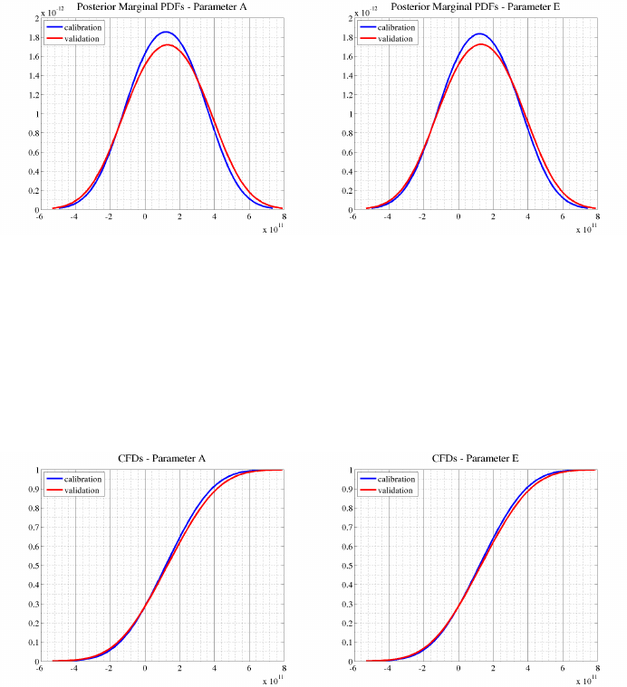
CHAPTER 5. QUESO EXAMPLES 125

5.4.7.1 KDE Plots of Parameters

Matlab function ksdensity (Kernel smoothing density estimate) together with the option

‘pdf’ may be used to estimate the KDE of the parameters, as illustrated in Figure 5.4.2.

Figure 5.4.2: Posterior distributions of parameters Aand E.

5.4.7.2 CDF Plots of Parameters

Matlab function ksdensity with ’cdf’ option may also be used for plotting the Cumulative

Distribution Function of each one of the parameters, as illustrated in Figure 5.4.3.

Figure 5.4.3: Cumulative density functions of parameters Aand E.

5.4.7.3 Autocorrelation Plots of Parameters

Figure 5.4.4 presents the autocorrelation of the parameters Aand Ein both cases: calibration

and validation stages.

5.4.7.4 KDE, CDF and Autocorrelation Plots of QoI

Figures 5.4.5a and 5.4.5b present PDF and CDF of QoI, respectively and Figure 5.4.6 presents

its autocorrelation.

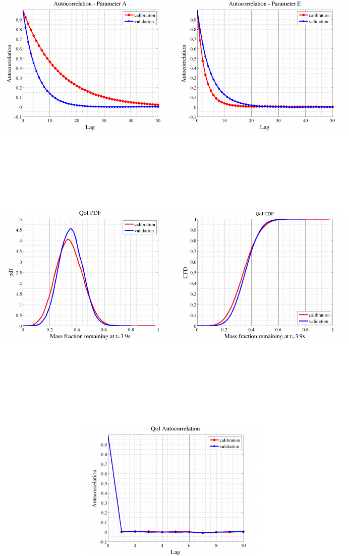
CHAPTER 5. QUESO EXAMPLES 126

Figure 5.4.4: Autocorrelation of parameters Aand E(ﬁltered chain).

(a) QoI PDF (b) QoI CDF

Figure 5.4.5: QoI PDF and CDF, during calibration and validation stages.

Figure 5.4.6: QoI autocorrelation.

CHAPTER 5. QUESO EXAMPLES 127

5.5 modal

This example presents a combination of two statistical inverse problems in one. It presents

the capability of the Multilevel method in sampling from a target distribution that has either

one or two modes (distinct peaks). The random variable of interest has three parameters, i.e.,

θ= (θ1, θ2, σ2)∈R3, where the third parameter may be seen as variation.

The example also it gives the user the opportunity to chose either one single type of prior

distribution, uniform, for the three components of the random variable, or two diﬀerent priors:

a uniform and a beta distribution.

Choosing between a one-mode or a two-mode target distribution is done at execution level,

as presented in the following code line:

$cd $H OM E / L IB RA RI ES / QU ESO - 0. 50 .0/

$cd e xampl es / m odal

$rm output D ata /*

$./ m od al_ gsl e xa mp le . inp < n um _o f_ no de s >

where <num_of_nodes> is either 1 or 2.

5.5.1 One-mode distribution

In this case, the target distribution is assumed to have only one mode. Suppose also that the

random variable θcan either have a uniform prior distribution for all its components, i.e.:

πprior =U([0,3]) × U([0,3]) × U([0,0.3]).

or, the prior distribution is deﬁned as a combination of uniform prior for θ1and θ2, with a

beta prior for σ2:

πprior =U([0,3]) × U([0,3]) × B(α, β),with α= 3 and β= 0.09709133373799.

The likelihood function is deﬁned as follows:

f(D|θ) = −5

2log 2πσ2−1

2σ2" 10r10θ1+ 20θ2+ 10qθ2

1+ 4θ2

2−72.0470!2

+ 10r10θ1+ 20θ2+ 10qθ2

1+ 4θ2

2−71.8995!2

+ 10r10θ1+ 20θ2+ 10qθ2

1+ 4θ2

2−72.2801!2

+ 10r10θ1+ 20θ2+ 10qθ2

1+ 4θ2

2−71.9421!2

+ 10r10θ1+ 20θ2+ 10qθ2

1+ 4θ2

2−72.3578!2#.

(5.5.1)

CHAPTER 5. QUESO EXAMPLES 128

5.5.1.1 Running the One-Mode Example

To run the executable provided considering a one-mode distribution, enter the following com-

mands:

$cd $H OM E / L IB RA RI ES / QU ESO - 0. 50 .0/

$cd e xampl es / m odal

$rm output D ata /*

$./ m od al _g sl e xa mp le . i np 1 #one mode !

$matlab

$plot_modal_all_levels_1mode # i n s i d e m a t lab

$exit # i n s i d e m a t lab

$ls -l o u tputDa ta /*. png

m od al_ 1 _m ode _kde_targ et . png m odal _1_mode _level_ 1 . png m odal_ 1_mode_ level_5 . png

m od al_ 1 _m ode _kde_thet a1 . png m odal _1_mode _level_ 2 . png m odal_ 1_mode_ level_6 . png

m od al_ 1 _m ode _kde_thet a2 . png m odal _1_mode _level_ 3 . png m odal_ 1_mode_ level_7 . png

m od al_ 1 _m ode _kde_thet a3 . png m odal _1_mode _level_ 4 . png

Listing 5.52: Running the example with a one-mode distribution.

As a result, the user should have created several of PNG ﬁgures scatter plots of each one of

the levels and the kernel density estimation of the parameters, for each level in the Multilevel

method. The name of the ﬁgure ﬁles have been chosen to be informative, as shown in the

Listing above.

5.5.2 Two-mode distribution

In this case, the target distribution is assumed to have two modes. Suppose that θhas a

either uniform distribution for all its components, i.e.:

πprior =U([0,3]) × U([0,3]) × U([0,0.3]).

or, the prior distribution is deﬁned as a combination of uniform prior for the θ1, with a beta

prior for θ2:

πprior =U([0,3]) × U([0,3]) × B(α, β),with α= 3 and β= 0.08335837191688.

CHAPTER 5. QUESO EXAMPLES 129

The likelihood function is deﬁned as follows:

f(D|θ) = −5 log 2πσ2−1

2σ2" 10r10θ1+ 20θ2+ 10qθ2

1+ 4θ2

2−72.0470!2

+ 10r10θ1+ 20θ2+ 10qθ2

1+ 4θ2

2−71.8995!2

+ 10r10θ1+ 20θ2+ 10qθ2

1+ 4θ2

2−72.2801!2

+ 10r10θ1+ 20θ2+ 10qθ2

1+ 4θ2

2−71.9421!2

+ 10r10θ1+ 20θ2+ 10qθ2

1+ 4θ2

2−72.3578!2

+ 10r10θ1+ 20θ2−10qθ2

1+ 4θ2

2−28.0292!2

+ 10r10θ1+ 20θ2−10qθ2

1+ 4θ2

2−27.3726!2

+ 10r10θ1+ 20θ2−10qθ2

1+ 4θ2

2−27.5388!2

+ 10r10θ1+ 20θ2−10qθ2

1+ 4θ2

2−27.0357!2

+ 10r10θ1+ 20θ2−10qθ2

1+ 4θ2

2−27.1588!2#.

(5.5.2)

5.5.2.1 Running the Two-Mode Example

To run the executable provided considering a two-modes distribution, enter the following

commands:

$cd $H OM E / L IB RA RI ES / QU ESO - 0. 50 .0/

$cd e xampl es / m odal

$rm output D ata /*

$./ m od al _g sl e xa mp le . i np 2 # two modes !

$matlab

$plot_modal_all_levels_2modes # i n s i d e mat l a b

$exit # i n s i d e m a t lab

$ls -l o u tputDa ta /*. png

modal_2_mo de s_ k d e _target . png m od al _ 2_modes_leve l_ 1 .png modal_2_m od es _ level_5 . png

modal_2_mo de s_ k d e _theta1 . png m od al _ 2_modes_leve l_ 2 .png modal_2_m od es _ level_6 . png

CHAPTER 5. QUESO EXAMPLES 130

modal_2_mo de s_ k d e _theta2 . png m od al _ 2_modes_leve l_ 3 .png modal_2_m od es _ level_7 . png

modal_2_mo de s_ k d e _theta3 . png m od al _ 2_modes_leve l_ 4 .png modal_2_m od es _ level_8 . png

Listing 5.53: Running the example with a two-mode distribution.

As a result, the user should have created several of PNG ﬁgures scatter plots of each one of

the levels and the kernel density estimation of the parameters, for each level in the Multilevel

method. The name of the ﬁgure ﬁles have been chosen to be informative, as shown in the

Listing above.

5.5.3 Example Code

The source code for the example is composed of 5 ﬁles: example main.C (Listing 5.54),

example likelihood.h and example likelihood.C (Listings 5.55 and 5.56), example compute.h

and example compute.C (Listings 5.57 and 5.58).

#i n c l u d e <example compute .h>

int mai n (int argc , c har * argv [])

{

// Initia l ize e n vironm e nt

MPI _I ni t (& argc ,& a rgv );

UQ_FATAL_TEST_MACRO(argc != 3,

QUESO::UQ_UNAVAILABLE_RANK ,

" m ai n () " ,

" after execu t able argv [0] , input fi le must be spe cified in co mmand line

as argv [1] , then n umMod es (1 or 2) must be speci fied as argv [2] ");

QUESO :: F ul lE nvironme nt * env =

ne w Q UE SO :: F u ll E nv i ro n me n t ( M PI_ COM M_W OR L D , a rg v [1] , " " , NU LL ) ;

// Compute

uns ig ne d int n um Mo des = ( u ns ig ned int ) a toi ( argv [2] ) ;

compute(*env , numM odes );

// Final ize e n vironm e nt

delete env;

MPI_Finalize();

std :: cout << std :: endl << " FI M !" << std :: endl << std :: endl ;

return 0;

}

Listing 5.54: File example main.C.

#i f n d e f EX LIKELIHOOD H

#d e f i n e EX LIKELIHOOD H

#i n c l u d e <q u es o / G s l M a t r i x . h>

struct

likelihoodRoutine_DataType

CHAPTER 5. QUESO EXAMPLES 131

{

uns i gned int nu mMode s ;

};

double l i kelihoodRo ut in e (

const QUE SO :: GslVec tor & paramValues ,

const QUE SO :: GslVec tor * p aramD irect ion ,

con st v oid * fun ct io nD ataPt r ,

QUESO :: GslVe ctor * grad Vec tor ,

QUESO :: GslMa trix * h essianMat rix ,

QUESO :: GslVe ctor * he ss ianEffe ct ) ;

#e n d i f

Listing 5.55: File example likelihood.h.

#i n c l u d e <example likelihood .h>

double l i kelihoodRo ut in e (

const QUE SO :: GslVec tor & paramValues ,

const QUE SO :: GslVec tor * p aramD irect ion ,

con st v oid * fun ct io nD ataPt r ,

QUESO :: GslVe ctor * grad Vec tor ,

QUESO :: GslMa trix * h essianMat rix ,

QUESO :: GslVe ctor * he ss ianEffe ct )

{

double theta1 = p aramVa l ues [0];

double theta2 = p aramVa l ues [1];

double sigm aSq = paramVa l ues [2];

uns i gned int nu mMode s = (( l i k e l i h oodRoutine_DataTyp e *) func t i onDataPtr ) -> numMo des ;

double aux1 = theta1 + 2.*theta2;

dou ble aux 2 = sq rt ( theta1 * theta 1 +4.* the ta2 * the ta2 );

dou ble w1 = 10.* s qrt ( 10 .*( a ux1 + aux2 ) );

dou ble w2 = 10.* s qrt ( 10 .*( aux1 - aux2 ));

double sum1 = 0.;

double sum2 = 0.;

dou bl e aux = ( w1 - 7 2. 047 0 ) ;

su m1 += a ux * au x ;

au x = ( w1 - 7 1. 8 99 5) ;

su m1 += a ux * au x ;

au x = ( w1 - 7 2. 2 80 1) ;

su m1 += a ux * au x ;

au x = ( w1 - 7 1. 9 42 1) ;

su m1 += a ux * au x ;

au x = ( w1 - 7 2. 3 57 8) ;

su m1 += a ux * au x ;

if ( numMo des == 1) {

// Ok , do nothing

}

el se if ( num Modes == 2) {

au x = ( w2 - 2 8. 0 29 2) ;

su m2 += a ux * au x ;

au x = ( w2 - 2 7. 3 72 6) ;

su m2 += a ux * au x ;

au x = ( w2 - 2 7. 5 38 8) ;

su m2 += a ux * au x ;

CHAPTER 5. QUESO EXAMPLES 132

au x = ( w2 - 2 7. 0 35 7) ;

su m2 += a ux * au x ;

au x = ( w2 - 2 7. 1 58 8) ;

su m2 += a ux * au x ;

}

else {

UQ_FATAL_TEST_MACRO(true ,

para mVa lues . env () . f u ll Ra nk ( ) ,

" e x amp l e_ l ike l ih o od () " ,

" i n va li d ’ n umM od es ’ " );

}

dou ble r es ult = -0 .5*(( d ouble ) n um Mo des ) *5. * log ( 2.* M_P I * si gm aSq ) - 0.5 *( sum 1 + sum2 ) / si gm aS q ;

#i f d e f QUESO EXPECTS LN LIKELIHOOD INSTEAD OF MINUS 2 LN

return result;

#else

return -2.* resu lt ;

#e n d i f

}

Listing 5.56: File example likelihood.C.

#i f n d e f EX COMPUTE H

#d e f i n e EX COMPUTE H

#i n c l u d e <queso/Environment .h>

vo id c ompute ( c onst QUE SO :: F ul lE nv ir onm en t & env , unsig ned int numM odes ) ;

#e n d i f

Listing 5.57: File example compute.h.

Note that in line 12 of Listings 5.58 the #define directive creates the macro

APPLS_MODAL_USES_CONCATENATION. Such macro, together with the directives #ifdef,#else,

and #endif, tells the compiler that the application will use concatenated priors, by controlling

compilation of portions of ﬁle example compute.C. Commenting line 12 of Listings 5.58 will

make the application to use uniform priors only:

1#i n c l u d e <example compute .h>

#i n c l u d e <example likelihood .h>

#i n c l u d e <q u es o / G s l M a t r i x . h>

#i n c l u d e <q ue s o / S t a t i s t i c a l I n v e r s e P r o b l e m . h>

#i n c l u d e <queso/GenericScalarFunction .h>

6#i n c l u d e <q ueso / G ene r icV ect o rRV . h>

#i n c l u d e <q ueso / U niformVectorRV . h>

#i n c l u d e <q ueso / Co n ca tenate d Ve ctorRV . h>

#i n c l u d e <q ue so / Inv erseGammaV ectorRV . h>

#i n c l u d e <q u eso / C o n c a t e n a t i o n S u b s e t . h>

#d e f i n e APPLS MODAL USES CONCATENATION

vo id c ompute ( c onst QUE SO :: F ul lE nv ir onm en t & env , unsig ned int numM odes ) {

////////////////////////////////////////////////////////

16 // Step 1 of 5: Inst a ntiate the p aramet er sp ace

////////////////////////////////////////////////////////

CHAPTER 5. QUESO EXAMPLES 133

#i f d e f APPLS MODAL USES CONCATENATION

21 QUESO :: Vec torSpac e < QUESO :: GslVector , QUE SO :: GslMat rix >

p ar a mS p a ce A ( env ,"paramA_", 2 , NULL );

QUESO :: Vec torSpac e < QUESO :: GslVector , QUE SO :: GslMat rix >

p ar a mS p a ce B ( env ,"paramB_", 1 , NULL );

#e n d i f

26 QUESO :: Vec torSpac e < QUESO :: GslVector , QUE SO :: GslMat rix >

p ar a mS p ac e ( env ," param_ " , 3, NUL L );

////////////////////////////////////////////////////////

// Step 2 of 5: Inst a ntiate the p aramet er domain

31 ////////////////////////////////////////////////////////

#i f d e f APPLS MODAL USES CONCATENATION

QUESO :: G slVecto r param MinsA ( par am SpaceA . z er oVecto r () );

para m MinsA [0] = 0.;

para m MinsA [1] = 0.;

36 QUESO :: G slVecto r param MaxsA ( par am SpaceA . z er oVecto r () );

para m MaxsA [0] = 3.;

para m MaxsA [1] = 3.;

QUESO :: BoxSubset < QUESO :: GslVector , QUESO :: GslMatrix >

41 paramDomainA("paramA_", pa ra mS pa ce A , p ar am Mi ns A , p ar am M ax sA ) ;

QUESO :: G slVecto r param MinsB ( par am SpaceB . z er oVecto r () );

para m MinsB [0] = 0.;

QUESO :: G slVecto r param MaxsB ( par am SpaceB . z er oVecto r () );

46 para mM axsB [0] = I NFINIT Y ;

QUESO :: BoxSubset < QUESO :: GslVector , QUESO :: GslMatrix >

paramDomainB("paramB_", pa ra mS pa ce B , p ar am Mi ns B , p ar am M ax sB ) ;

QUESO :: Conca t enatio nSubse t < QUESO :: GslVector , QUESO :: GslMatrix >

51 para mD omain (" " ,pa ram Space , para mDom ainA , paramDo ma inB );

#else

QUESO :: G slVecto r para mMins ( par amSpace . z eroVect or () );

para mMins [0] = 0.;

para mMins [1] = 0.;

56 para mMins [2] = 0.;

QUESO :: G slVecto r para mMaxs ( par amSpace . z eroVect or () );

para mMaxs [0] = 3.;

para mMaxs [1] = 3.;

para mMaxs [2] = .3;

61 QUESO :: BoxSubset < QUESO :: GslVector , QUESO :: GslMatrix >

para mD omain ("param_", p ar am Sp ac e , p ar am Mi ns , p a ra mM axs ) ;

#e n d i f

////////////////////////////////////////////////////////

66 // Step 3 of 5: Inst a ntiate the l i keliho od func tion object

////////////////////////////////////////////////////////

likelihoodRoutine_DataType likelihoodRoutine_Data;

likelihoo d R o u t i ne_Data . numMo des = num Modes ;

71 QUESO :: Generi cScalar F unctio n < QUESO :: GslVector , QUESO :: GslMatrix >

likelihoodFunctionObj(" lik e_ " ,

paramDomain ,

likelihoodRoutine ,

( vo id *) & likel ih ood Ro uti ne _D ata ,

76 true); // r outin e comp utes [ -2.* ln ( functi on ) ]

////////////////////////////////////////////////////////

// Step 4 of 5: Inst a ntiate the i nver se problem

////////////////////////////////////////////////////////

81 #i f d e f APPLS MODAL USES CONCATENATION

QUESO :: Unif ormVe ctorR V < QU ESO :: Gs lVector , QUE SO :: Gsl Matrix >

pri orRvA ("priorA_", paramDomainA);

CHAPTER 5. QUESO EXAMPLES 134

QUESO :: G slVecto r alpha ( pa ramSpac eB . z eroVec tor ()) ;

86 alpha [0] = 3.;

QUESO :: G slVect or beta ( pa ramSpa ce B . zeroV ector () );

if ( numMo des == 1) {

be ta [0] = 0.09709 1 3 3 373799;

}

91 else {

be ta [0] = 0.08335 8 3 7 191688;

}

QUESO :: Invers eGamma V ectorR V < QUESO :: GslVector , QUESO :: GslMatrix >

pri orRvB ("priorB_", p aramD omain B , alpha , bet a );

QUESO :: Concat enated V ectorR V < QUESO :: GslVector , QUESO :: GslMatrix >

priorRv("prior_", priorRvA , priorRvB , paramD o main );

#else

QUESO :: Unif ormVe ctorR V < QU ESO :: Gs lVector , QUE SO :: Gsl Matrix >

101 priorRv("prior_", para mD omain );

#e n d i f

QUESO :: Gene ricVe ctorR V < QU ESO :: Gs lVector , QUE SO :: Gsl Matrix >

postRv(" p os t_ " , param Space );

106

QUESO :: Statist icalInve r s eProble m < QUE SO :: Gsl Vector , QUESO :: GslMatrix >

ip ( " " , NULL , priorRv , l ik el ihoodFu nc ti onObj , post Rv ) ;

////////////////////////////////////////////////////////

111 // Step 5 of 5: S olve the i nvers e pro blem

////////////////////////////////////////////////////////

ip.solveWithBayesMLSampling();

////////////////////////////////////////////////////////

116 // Print som e sta t istics

////////////////////////////////////////////////////////

u ns ig ned in t n um Pos T ot al = pos tR v . r eal ize r () . s ub Per i od () ;

if (env .subDisplayFile()) {

*en v .subDisplayFile() << " numPo sTotal = " << numPosTotal

121 << s td :: endl ;

}

QUESO :: G slVecto r aux Vec ( pa ramSpa ce . z eroVec tor ()) ;

uns i gned int n u m P o s T h e t a 1SmallerThan1dot5 = 0;

126 for ( unsi gned int i = 0; i < numP o sTotal ; ++ i ) {

pos tRv . rea li zer () . re al ization ( aux Vec );

if ( auxV ec [0] < 1.5) n umPos Theta1 Smaller Than1do t5 ++;

}

131 if (env .subDisplayFile()) {

*en v .subDisplayFile() << " numPosTheta1Sma ll er T h a n 1dot5 = " <<

numPosTheta1SmallerThan1dot5

<< " , rat io = " << (( d ouble ) n u mP osThe t a1 Smalle r Th an1dot 5 ) / (( d ou bl e

) n um PosTot al )

<< s td :: endl ;

}

136

return;

}

Listing 5.58: File example compute.C.

CHAPTER 5. QUESO EXAMPLES 135

5.5.4 Input File

QUESO reads an input ﬁle for solving statistical problems, which provides options for the

Multilevel or MCMC method. In this example, the Multilevel method is chosen to sample

from the distribution. Many variables are common to both MCMC and Multilevel method,

especially because the Multilevel method also has the option of delaying the rejection of a

candidate. The names of the variables have been designed to be informative in this case as

well:

env:refers to QUESO environment;

ip:refers to inverse problem;

ml:refers to Multilevel;

dr:refers to delayed rejection;

rawChain:refers to the raw, entire chain;

filteredChain:refers to a ﬁltered chain (related to a speciﬁed lag);

last:refers to instructions speciﬁc for the last level of the Multilevel algorithm.

The user may select options for a speciﬁc level by naming its number, i.e., in case the user

wants to write the raw chain of the level 3 in a separate ﬁle, say ’rawChain_ml_level3.m’,

he/she may include the line:

ip_ml_3_rawChain_dataOu tputF ileNa me = outpu tD ata / rawChai n_ ml _l ev el 3

in the input ﬁle.

The options used for solving this example are displayed in Listing 5.59.

###############################################

# UQ Environment

###############################################

#e n v h e l p = a n y t h i n g

env_numSu b E n v i r onments = 1

env_subDi spl ayF ileN ame = o ut putData / d ispla y

env_subDi s p l a y A llowAll = 0

env_subDisplayAllowedSet = 0

env_displayVerbosity = 0

env_syncVerbosity = 0

env _ seed = 0

###############################################

# S t a t i s t i c a l i n v e r s e pr o ble m ( i p )

###############################################

#i p h e l p = a n y t h i n g

ip_computeSolution = 1

ip_dataO ut put Fi le Nam e = output Data / sipO utput

ip_dataOutputAllowedSet = 0

###############################################

# ’ i p ’ : i n f o r m a t i o n f o r M u l t i l e v e l a l g o ri t h m

###############################################

#i p m l h e l p = a n y t h i n g

ip_ml_data Ou tp ut Fi le Na me = o utputDa ta / s ipOutpu t_ ml

ip_ml_dataOutputAllowedSet = 0

CHAPTER 5. QUESO EXAMPLES 136

###############################################

# A l l l e v e l s , u n l e s s o t h e r w i s e s p e c i f i e d

###############################################

ip_ml_default_minEffectiveSizeRatio = 0.49

ip_ml_default_maxEffectiveSizeRatio = 0.51

ip_ml_default _ r a w C h a i n _size = 10000

ip_ml_default_rawChain_dataOutputFileName = outpu tD ata / rawC hain_ml

ip_ml_default_ s c a l e C o v M a trix = 1

ip_ml_default_dr_maxNumExtraStages = 2

ip_ml_default_dr_listOfScalesForExtraStages = 10. 25.

###############################################

# L a s t l e v e l ( l e v e l 7 o r 8 f o r ’ e x a m p l e g s l ’ e x e c u t a b l e )

###############################################

ip_ml_last_data Ou tpu tFi leN ame = o utputDa ta / sipOutp ut _ml

ip_ml_last_dataOutputAllowedSet = 0 1

ip_ml_last_rawChain_size = 10000

ip_ml_last_rawChain_computeStats = 1

ip_ml_last_rawChain_dataOutput FileName = output Da ta / rawCh ai n_ml

Listing 5.59: Options for QUESO library used in application code (Listings 5.54-5.58).

5.5.5 Create your own Makeﬁle

Makeﬁles are special format ﬁles that together with the make utility will help one to compile

and automatically build and manage projects (programs). Listing 5.60 presents a Makeﬁle,

named ‘Makefile modal example margarida’, that may be used to compile the code and

create the executable modal_gsl. Naturally, it must be adapted to the user’s settings, i.e., it

has to have the correct paths for the user’s libraries that have actually been used to compile

and install QUESO (see Sections 2.1–2.4).

##########################################################

# U sing i n s t a l l e d QUESO 0 . 4 7 . 1 , from t a r b a l l , i n ’ v i o l e t a ’

##########################################################

QUES O_ DI R = / h ome / ke me ll i / LIB RA RI ES / QUESO -0.5 0. 0

BOOS T_ DI R = / h ome / ke me ll i / LIB RA RI ES / boost -1.5 3. 0

GSL _D IR = / home / k em elli / LIBR AR IE S / gsl -1. 15

HDF 5_ DI R = / ho me / keme ll i / LIB RA RI ES / hdf5 - 1.8.1 0

INC_ PATHS = \

-I. \

-I$( QUESO_ DIR )/ include \

-I$( BOOST_ DIR )/ include \

-I$(GSL_DIR)/include \

-I$( HDF5_ DIR )/ incl ude

LI BS = \

-L$( QUESO_ DIR )/ lib - lqueso \

-L$( BOOST_ DIR )/ lib - lboost_progr am _o pti on s \

-L$( GSL_D IR ) /lib - lgsl \

-L$( HDF5_ DIR )/ lib - lhdf5

CXX = mpic ++

C XX FL A GS + = - g - W al l - c

default: all

CHAPTER 5. QUESO EXAMPLES 137

. SUF FIXES : .o . C

all: modal_example_gsl

clean :

rm -f *~

rm -f * . o

rm -f modal _gsl

modal_e xa m ple_gsl : e xample_ main .o example_ li ke lihood .o e xa m ple_comp ut e .o

$(CXX) example_main.o \

example_likelihood.o \

exampl e_ compute .o \

-o mo dal_gs l $( LIB S )

%. o : %. C

$( CX X ) $( IN C_PATHS ) $( CXXF LAGS ) $<

Listing 5.60: Makeﬁle for the application code in Listings 5.54-5.58

Thus, to compile, build and execute the code, the user just needs to run the following

commands in the same directory where the ﬁles are:

$cd $HOME / L IB RA RI ES / QUESO -0. 50 .0 / e xample s / modal /

$export LD_LIB RA RY_PATH = $LD_LIBRARY_PATH:\

$H OM E / L IB R AR I ES / gsl - 1. 15 / l ib / :\

$HOM E / L IB RA RIE S / boos t - 1. 53 .0 / l ib / :\

$HOM E / L I BR AR IES / hdf5 - 1 .8 .1 0/ l ib : \

$HOM E / L IB RA RIE S / QUES O - 0. 50 .0 / l ib

$ma ke -f M a k e f i le_modal_viole t a

$./ m od a l_ gs l ex a mp le . i np < n um _m od es >

The ‘export’ instruction above is only necessary if the user has not saved it in his/her

.bashrc ﬁle.

5.5.6 Data Post-Processing and Visualization

According to the speciﬁcations of the input ﬁle in Listing 5.59, both a folder named outputData

and a the following ﬁles should be generated:

rawChain_ml.m

display_sub0.txt

The sequence of Matlab commands is identical to the ones presented in Sections 5.1.5,

5.2.5,5.3.8 and 5.4.7; therefore, are omitted here. The reader is invited to explore the Matlab

ﬁles plot modal all levels 1mode.m and/or plot modal all levels 2modes.m for details

of how the ﬁgures have been generated.

5.5.6.1 Scatter Plots

The code presented in Listing 5.61 uses Matlab function plotmatrix to generate Figures 5.5.1

and 5.5.2 which presents the scatter plots and histograms of the parameters θ1and θ2, based

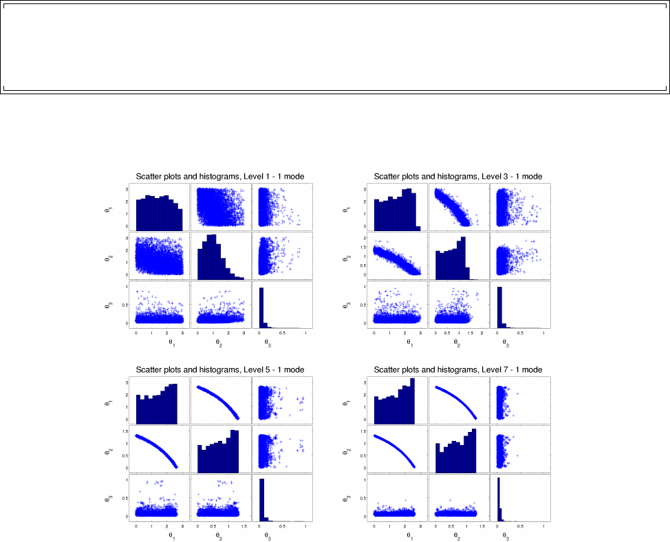
CHAPTER 5. QUESO EXAMPLES 138

on the generated raw chains.

fpr intf (1, ’ Scatter plots and h istogr ams of raw c hain s - Level 1 < press any key >\n ’);

plotmatrix(ip_ml_1_rawChain_unified , ’+b’)

se t ( gca , ’ f on ts iz e ’ , 20) ;

xla be l ( ’\ t he ta _1 \ t he ta _2 \ thet a_3 ’ , ’ fo nt size ’ , 16) ;

yla be l ( ’\ t he ta _3 \ t he ta _2 \ thet a_1 ’ , ’ fo nt size ’ , 16) ;

title ( ’ Sca tter plots and hi sto grams , Leve l 1 - 1 mode ’)

Listing 5.61: Matlab code for the scatter plots depicted in Figures 5.5.1 and 5.5.2.

Figure 5.5.1: Scatter plots for θ1,θ2and θ3=σ2, levels 1, 3, 5 and 7 (last). One mode

distribution.

5.5.6.2 KDE Plots

Figures 5.5.3 and 5.5.4 present the KDE plots of the parameters θ1,θ2,θ3and target PDF in

both cases: one-mode and two-modes distribution.

5.5.6.3 Autocorrelation Plots

Figures 5.5.5 and 5.5.6 present the autocorrelation of the parameters θ1,θ2and θ3in both

cases: one-mode and two-modes distribution.

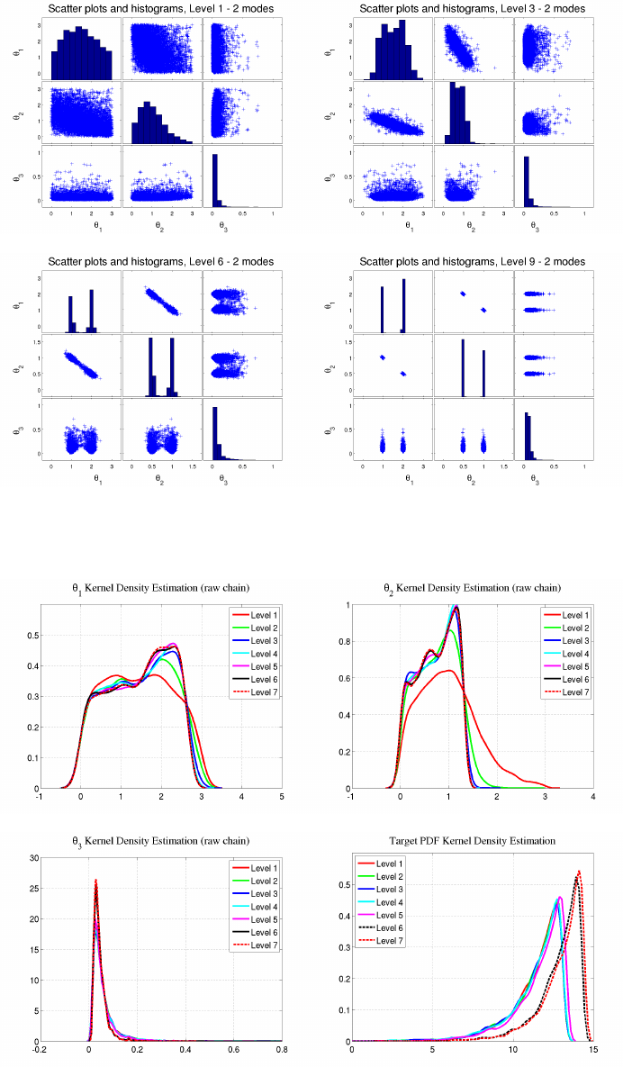
CHAPTER 5. QUESO EXAMPLES 139

Figure 5.5.2: Scatter plots for θ1,θ2and θ3=σ2, levels 1, 3, 6 and 9 (last). Two-mode

distribution.

Figure 5.5.3: KDE plots for θ1,θ2,θ3=σ2, and the target PDF. One mode distribution.

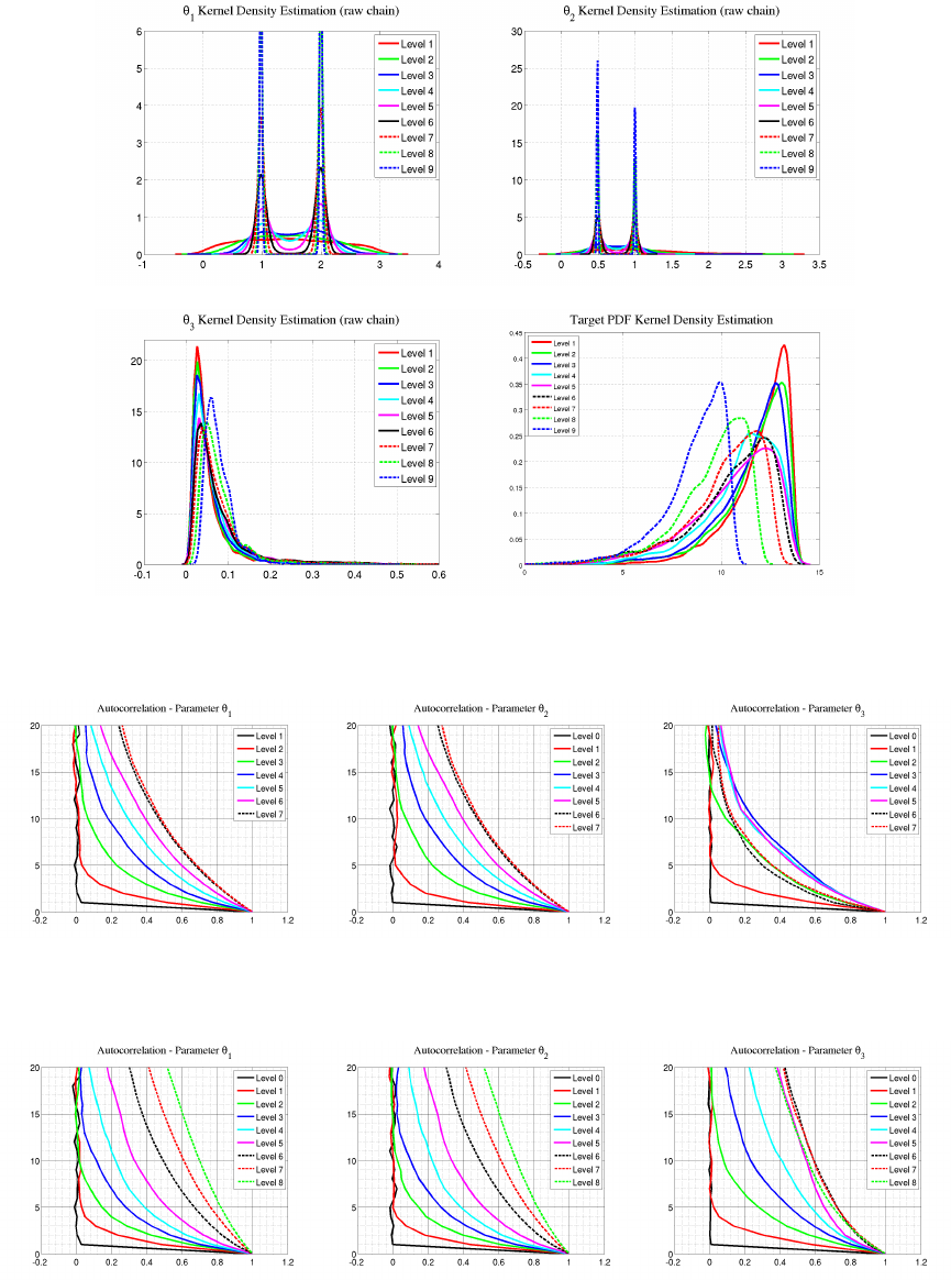
CHAPTER 5. QUESO EXAMPLES 140

Figure 5.5.4: KDE plots for θ1,θ2,θ3=σ2, and the target PDF. Two-mode distribution.

Figure 5.5.5: Autocorrelation plots for θ1,θ2and θ3=σ2. One-mode distribution.

Figure 5.5.6: Autocorrelation plots for θ1,θ2and θ3=σ2. Two-mode distribution.

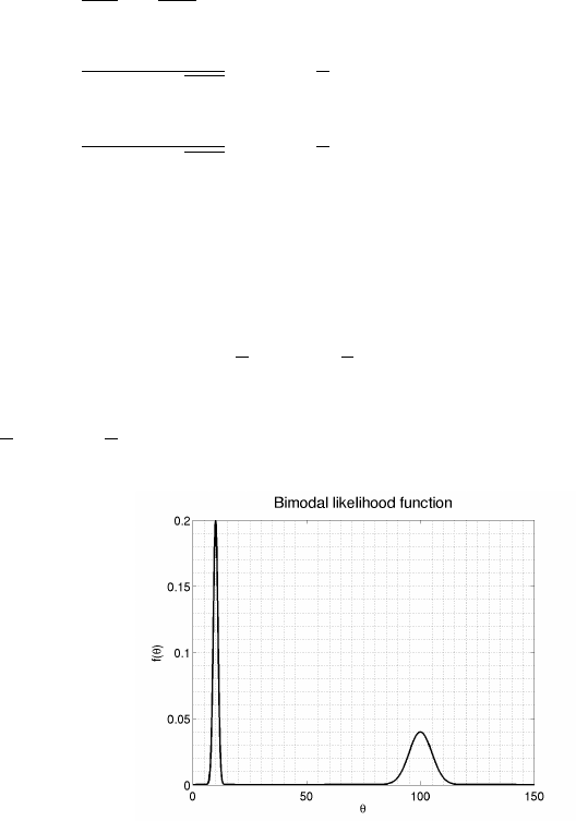
CHAPTER 5. QUESO EXAMPLES 141

5.6 bimodal

This example replicates the problem in “Section 4.1 A 1D Problem” of [8]: it presents how to

use QUESO and the Multilevel method for sampling from a posterior PDF composed of the

sum of two Gaussian distributions.

Let’s deﬁne D= [−250,250] and the three distributions πprior :D→R+,f1:R→R+

and f2:R→R+by:

πprior =1

|D|=1

500,∀θ∈D

f1(θ) = 1

(2π)1/2p|V1|exp −1

2(θ−µ1)TV−1

1(θ−µ1),∀θ∈R

f2(θ) = 1

(2π)1/2p|V2|exp −1

2(θ−µ2)TV−1

2(θ−µ2),∀θ∈R,

(5.6.1)

where

µ1= 10, V1= 12, µ2= 100, V2= 52.

In this example, we want to sample the posterior PDF given by:

πposterior(θ)∝1

2f1(θ) + 1

2f2(θ)·πprior =f(θ)·πprior (5.6.2)

where f(θ) = 1

2f1(θ) + 1

2f2(θ) is the likelihood function, which is depicted in Figure 5.6.1.

Figure 5.6.1: Likelihood function given by f=f1/2 + f2/2, where f1and f2are deﬁned in

Equation (5.6.1).

5.6.1 Running the Example

To run the executable provided (available after QUESO installation), and generate ﬁgures for

the chains, PDFs, CDFs, etc., enter the following commands:

CHAPTER 5. QUESO EXAMPLES 142

$cd $H OM E / L IB RA RI ES / QU ESO - 0. 50 .0/ e xa mp le s / b im od al

$rm output D ata /*

$./ b im od al_ gsl b imo dal_1 chai n . inp

$matlab

$plo t_all .m # i n s i d e m a t lab

$plot_likelihood_normalized_taus.m # i n s i d e m a t lab

$plot_likelihood_unnormalized_taus.m # i n s i d e m a tlab

$exit # i n s i d e m a t lab

$ls -l o u tputDa ta /*. png

bimodal_autocorrelation_rawchain.png bimodal_likelihood.png

b im oda l_cdf_r a wc hai n . p ng bi m od al_likelih o od _taus_normaliz e d . pn g

bimodal_ kde_raw chain . png bimo d al _li k el iho od_taus . png

As a result, the user should have created several of PNG ﬁgures containing marginal

posterior PDF, cumulative density distribution and autocorrelation. The name of the ﬁgure

ﬁles have been chosen to be informative, as shown in the Listing above.

5.6.2 Example Code

The source code for the example is composed of 5 ﬁles: bimodal main.C (Listing 5.62),

bimodal likelihood.h and bimodal likelihood.C (Listings 5.63 and 5.64), bimodal compute.h

and bimodal compute.C (Listings 5.65 and 5.66).

#i n c l u d e <bimodal compute .h>

int mai n (int argc , c har * argv [])

{

// Initia l ize e n vironm e nt

MPI _I ni t (& argc ,& a rgv );

QUESO :: F ul lE nvironme nt * env = n ew Q UE SO : : F ullE n vi r on m en t ( M PI_ COM M_ WOR LD , a rg v [1 ] , " " , NU LL ) ;

// Compute

compute(*en v );

// Final ize e n vironm e nt

delete env;

MPI_Finalize();

return 0;

}

Listing 5.62: File bimodal main.C.

#i f n d e f EX LIKELIHOOD H

#d e f i n e EX LIKELIHOOD H

#i n c l u d e <q u es o / G s l M a t r i x . h>

struct

likelihoodRoutine_DataType

{

const QUE SO :: GslVec tor * m ea nVecto r ;

const QUE SO :: GslMat rix * covM atrix ;

};

double l i kelihoodRo ut in e (

const QUE SO :: GslVec tor & paramValues ,

CHAPTER 5. QUESO EXAMPLES 143

const QUE SO :: GslVec tor * p aramD irect ion ,

con st v oid * fun ct io nD ataPt r ,

QUESO :: GslVe ctor * grad Vec tor ,

QUESO :: GslMa trix * h essianMat rix ,

QUESO :: GslVe ctor * he ss ianEffe ct ) ;

#e n d i f

Listing 5.63: File bimodal likelihood.h.

#i n c l u d e <bimodal likelihood .h>

#i n c l u d e <cmath>

static unsig ned int likeli h o o dCounter = 0;

double l i kelihoodRo ut in e (

const QUE SO :: GslVec tor & paramValues ,

const QUE SO :: GslVec tor * p aramD irect ion ,

con st v oid * fun ct io nD ataPt r ,

QUESO :: GslVe ctor * grad Vec tor ,

QUESO :: GslMa trix * h essianMat rix ,

QUESO :: GslVe ctor * he ss ianEffe ct )

{

likelihoodCounter++;

if (paramDirection ||

functi o n DataPtr ||

grad V ector ||

hessianMatrix ||

hessi a n Effect ) {}; // just to rem ove compi ler w arnin g

double returnV a lue = 0.;

double x = p aramVa l ues [0 ];

double mean 1 = 10.;

double sigma1 = 1.;

dou bl e y1 = (x - m ea n1 ) *( x - me an 1 ) / (2 .* s ig ma1 * s ig ma1 ) ;

dou bl e z1 = (1. / s ig ma1 / s qr t ( 2* M _P I ) )* e xp ( - y1 ) ;

double mean2 = 100.;

double sigma2 = 5.;

dou bl e y2 = (x - m ea n2 ) *( x - me an 2 ) / (2 .* s ig ma2 * s ig ma2 ) ;

dou bl e z2 = (1. / s ig ma2 / s qr t ( 2* M _P I ) )* e xp ( - y2 ) ;

dou ble res ul tVa lu e = -2* log (( z1 +2.* z2) /3.) ;

if ( r esultVa lu e == I NFINIT Y ) {

// std :: cerr << " WAR NING In like li ho od Rou ti ne "

// << " , f ull Ran k " << p ar am Val ues . env () . f ull R an k ()

// << ", subEnvironment " < < p ara mVa lue s . env () . s ub Id ()

// << " , s ubR an k " << p ar am Val ues . env () . s ubR ank ()

// << " , i n te r0 R an k " << p ar am Val ues . env() . i nt e r0 Ra n k ()

// << ": x = " << x

// << ", z1 = " << z1

// << ", z2 = " << z2

// << " , r e su ltV a lu e = " << resultValue

// << std :: end l ;

resu l tValue = 10 40.;

}

#i f d e f QUESO EXPECTS LN LIKELIHOOD INSTEAD OF MINUS 2 LN

retu rn Value = -.5* r esultVal ue ;

#else

CHAPTER 5. QUESO EXAMPLES 144

returnValue = resultValue;

#e n d i f

if (paramValues.env ().exceptionalCircumstance()) {

if (( p ar amV alu es . env ().subDisplayFile() ) &&

( p ar amV alu es . env( ) . d is p la y Ve r bo sity ( ) >= 0 ) ) { / / d et ail e d out pu t d eb ug

* p ar amV alu es . env().subDisplayFile() << " Lea ving l ikeliho od funct ion "

<< " : para m Values = " << paramValues

<< " , r et u rn Val u e = " << returnValue

<< s td :: endl ;

}

return retu rn Value ;

}

Listing 5.64: File bimodal likelihood.C.

#i f n d e f EX COMPUTE H

#d e f i n e EX COMPUTE H

#i n c l u d e <queso/Environment .h>

vo id c ompute ( c onst QUE SO :: F ul lE nv ir onm en t & env ) ;

#e n d i f

Listing 5.65: File bimodal compute.h.

Note that in line 57 of Listings 5.66 the ‘#if 0’ directive tells the compiler that the

application will not use DRAM algorithm, but rather the Multilevel solver (line 65). Naturally,

the user may chose to use the DRAM algorithm by changing the directive in line 57 to ‘#if 1’.

#i n c l u d e <bimodal compute .h>

#i n c l u d e <bimodal likelihood .h>

3#i n c l u d e <q u es o / G s l M a t r i x . h>

#i n c l u d e <q ue s o / S t a t i s t i c a l I n v e r s e P r o b l e m . h>

#i n c l u d e <q ueso /1 D1DFunction . h>

#i n c l u d e <queso/GenericScalarFunction .h>

#i n c l u d e <q ueso / G ene r icV ect o rRV . h>

8#i n c l u d e <q ueso / U niformVectorRV . h>

vo id c ompute ( c onst QUE SO :: F ul lE nv ir onm en t & env ) {

//------------------------------------------------------

// Step 1 of 5: Inst a ntiate the p aramet er sp ace

13 //------------------------------------------------------

QUESO :: Vec torSpac e < QUESO :: GslVector , QUESO :: GslMatrix >

p ar a mS p ac e ( env ," param_ " , 1, NUL L );

//------------------------------------------------------

18 // Step 2 of 5: Inst a ntiate the p aramet er domain

//------------------------------------------------------

QUESO :: G slVecto r para mMins ( par amSpace . z eroVect or () );

para mM in s . cwS et ( -2 50.) ;

QUESO :: G slVecto r para mMaxs ( par amSpace . z eroVect or () );

23 para mM ax s . cwSe t ( 2 50.) ;

QUESO :: BoxSubset < QUESO :: GslVector , QUESO :: GslMatrix >

para mD omain ("param_", p ar am Sp ac e , p ar am Mi ns , p a ra mM axs ) ;

CHAPTER 5. QUESO EXAMPLES 145

//------------------------------------------------------

28 // Step 3 of 5: Inst a ntiate the l i keliho od func tion object

//------------------------------------------------------

QUESO :: G slVecto r meanV ector ( par amSpace . z eroVect or () );

mean V ector [0] = 10.;

QUESO :: GslMa trix * c ovMat rix = p aramSpa ce . n ewMat rix () ;

33 (* c ov Ma tri x ) (0 ,0 ) = 1 .;

likelihoodRoutine_DataType likelihoodRoutine_Data;

likelihoo dR ou ti ne _D at a . me anVecto r = & meanVe ctor ;

likelihoo dR ou ti ne _D at a . co vMatrix = covMat rix ;

QUESO :: Generi cScalar F unctio n < QUESO :: GslVector , QUESO :: GslMatrix >

38 likelihoodFunctionObj(" lik e_ " ,

paramDomain ,

likelihoodRoutine ,

( vo id *) & likel ih ood Ro uti ne _D ata ,

true); // r outin e comp utes [ -2.* ln ( functi on ) ]

//------------------------------------------------------

// Step 4 of 5: Inst a ntiate the i nver se problem

//------------------------------------------------------

QUESO :: Unif ormVe ctorR V < QU ESO :: Gs lVector , QUE SO :: Gsl Matrix >

48 priorRv("prior_", para mD omain );

QUESO :: Gene ricVe ctorR V < QU ESO :: Gs lVector , QUE SO :: Gsl Matrix >

postRv(" p os t_ " , param Space );

QUESO :: Statist icalInve r s eProble m < QUE SO :: Gsl Vector , QUESO :: GslMatrix >

ip ( " " , NULL , priorRv , l ik el ihoodFu nc ti onObj , post Rv ) ;

//------------------------------------------------------

// Step 5 of 5: S olve the i nvers e pro blem

//------------------------------------------------------

#i f 0

58 uqGs lV ector p ar amInitia ls ( p aramSpa ce . zeroVe ctor ());

param I n itials [0] = 45.;

uqGs lM atrix * p roposalCov Ma tr ix = paramS pace . new Matrix () ;

(* p rop o sa lCo v Ma trix ) (0 ,0 ) = 160 0. ;

ip . s ol v eWith B ayesMetr o polisHast i ngs ( NULL , p ara mI nit ia ls , p rop o sa l Co v Ma t ri x ) ;

63 delete p r oposalCovM at ri x ;

#else

ip.solveWithBayesMLSampling();

#e n d i f

68 //------------------------------------------------------

// P ri n t s om e s t at i st i cs in th e f il e ’ d i sp l a y_ s ub 0 . tx t ’

// They will be in the last part of the file .

//------------------------------------------------------

u ns ig ned in t n um Pos T ot al = pos tR v . r eal ize r () . s ub Per i od () ;

73 if (env .subDisplayFile()) {

*en v .subDisplayFile() << " numPo sTotal = " << numPosTotal

<< s td :: endl ;

}

78 QUESO :: G slVecto r aux Vec ( pa ramSpa ce . z eroVec tor ()) ;

uns i gned int n u m P osSmallerTha n 4 0 = 0;

for ( unsi gned int i = 0; i < numP o sTotal ; ++ i ) {

pos tRv . rea li zer () . re al ization ( aux Vec );

if ( auxV ec [0] < 40.) n um Pos Smal ler Tha n40 ++;

83 }

if (env .subDisplayFile()) {

*en v .subDisplayFile() << "numPosSmallerThan40 = " << numPosSmallerThan40

<< " , rat io = " << (( d ouble ) n umPosS mallerT han40 ) /( ( d ouble )

numP os Total )

<< s td :: endl ;

88 }

Q UE SO : : S c al a rS eq u en c e < d oub le > s eq 1 ( env ,numPosSmallerThan40 ,"");

CHAPTER 5. QUESO EXAMPLES 146

Q UE SO : : S c al a rS eq u en c e < d oub le > s eq 2 ( env , num Po sTotal - numPo sSmalle rThan4 0 , "" ) ;

Q UE SO :: S ca l ar S eq ue n ce < d ou bl e > s e qA ll ( env ,numPosTotal ," " ) ;

93 uns i gned int i1 = 0;

uns i gned int i2 = 0;

for ( unsi gned int i = 0; i < numP o sTotal ; ++ i ) {

pos tRv . rea li zer () . re al ization ( aux Vec );

if ( a ux Ve c [ 0] < 40 .) se q1 [ i 1 ++ ] = a ux Ve c [ 0] ;

98 else se q2 [ i 2 ++ ] = a ux Ve c [ 0] ;

seq All [i] = aux Vec [0];

}

dou ble m ean1 = s eq1 . subMe anE xt ra (0 , seq 1 . subS equ ence Siz e () );

103 if (env .subDisplayFile()) {

*en v .subDisplayFile() << " seq1 . si ze () = " << s eq1 . subSeq uenc eSi ze ()

<< " \n seq 1 . mean () = " << mean1

<< " \ n s eq1 . std () = " << s qrt ( seq1 . s ub Sa mpleVa rianceE xtra (0 , s eq1 .

s ub S eq u en ceS i ze ( ) , me an 1 ) )

<< s td :: endl ;

108 }

dou ble m ean2 = s eq2 . subMe anE xt ra (0 , seq 2 . subS equ ence Siz e () );

if (env .subDisplayFile()) {

*en v .subDisplayFile() << " seq2 . si ze () = " << s eq2 . subSeq uenc eSi ze ()

113 << " \n seq 2 . mean () = " << mean2

<< " \ n s eq2 . std () = " << s qrt ( seq2 . s ub Sa mpleVa rianceE xtra (0 , s eq2 .

s ub S eq u en ceS i ze ( ) , me an 2 ) )

<< s td :: endl ;

}

118 dou bl e m ean Al l = s eq Al l . s ubM e an Ext r a (0 , s eq Al l . s u bS eque n ce S iz e ( ) );

if (env .subDisplayFile()) {

*en v .subDisplayFile() << " seqA ll . siz e () = " < < seqA ll . s ub Se qu en ce Si ze ()

<< " \n s eqAll . m ean () = " << meanAll

<< " \ n seq Al l . std () = " << sqr t ( seq Al l . s ubSamp l eV a ri a nc e Ex tra (0 ,

seq Al l . s u bS equ e nc eSi z e () , mea nA ll ) )

123 << s td :: endl ;

}

//------------------------------------------------------

// Test if l i kelih o od is n ormali z ed

128 //------------------------------------------------------

uns i gned int num G r idPoint s = 1 00000 1;

double xMin = paramD omain . min Values () [0];

double xMax = paramD omain . max Values () [0];

dou bl e i n te r va lS i ze = ( xMax - x Mi n ) /( ( d ou ble ) n umGr i dP o in ts - 1) ;

133 double integ ral = 0.;

for ( unsi gned int i = 0; i < n u m GridPoi n t s ; ++ i ) {

auxVec [0] = xMin + i * in tervalSi ze ;

i nt eg ral += l i ke l ih o od F un c tio n Obj . a ctu a lV alu e ( a uxV ec , NU LL , NULL , NULL , N UL L ) ;

}

138 int egral *= interv al Size ;

if (env .subDisplayFile()) {

*en v .subDisplayFile() << " inte gral = " << int egral

<< s td :: endl ;

}

143

// Return

delete covMat rix ;

return;

148 }

Listing 5.66: File bimodal compute.C.

CHAPTER 5. QUESO EXAMPLES 147

5.6.3 Input File

QUESO reads an input ﬁle for solving statistical problems, which provides options for the

Multilevel or MCMC method. In this example, the Multilevel method is chosen to sample

from the distribution. Many variables are common to both MCMC and Multilevel method,

especially because the Multilevel method also has the option of delaying the rejection of a

candidate. The names of the variables have been designed to be informative in this case as

well:

env:refers to QUESO environment;

ip:refers to inverse problem;

ml:refers to Multilevel;

dr:refers to delayed rejection;

rawChain:refers to the raw, entire chain;

filteredChain:refers to a ﬁltered chain (related to a speciﬁed lag);

last:refers to instructions speciﬁc for the last level of the Multilevel algorithm.

The user may select options for a speciﬁc level by naming its number, i.e., in case the

user wants to deﬁne a diﬀerent number of extra stages together with the scales for each stage

(in the DRAM part of the ML algorithm) for the level 3, he/she may include the following

instructions:

ip_ml_3_dr_max N u m E x t r a S t ages = 1

ip_ml_3_dr_listOfScalesForEx t r a S t a g e s = 3.33 3

in the input ﬁle.

The options used for solving this example are displayed in Listing 5.67.

###############################################

# UQ Environment

###############################################

env_numSu b E n v i r onments = 1

env_subDi spl ayF ileN ame = o ut putData / d ispla y

env_subDi s p l a y A llowAll = 0

env_subDisplayAllowedSet = 0 1

env_displayVerbosity = 2

env_syncVerbosity = 0

env _ seed = -1

###############################################

# S t a t i s t i c a l i n v e r s e pr o ble m ( i p )

###############################################

ip_computeSolution = 1

ip_dataO ut put Fi le Nam e = output Data / sipO utput

ip_dataOutputAllowedSet = 0

###############################################

# ’ i p ’ : i n f o r m a t i o n f o r M u l t i l e v e l a l g o ri t h m

###############################################

ip_ml_data Ou tp ut Fi le Na me = o utputDa ta / s ipOutpu t_ ml

ip_ml_dataOutputAllowedSet = 0 1

###############################################

CHAPTER 5. QUESO EXAMPLES 148

# A l l l e v e l s , u n l e s s o t h e r w i s e s p e c i f i e d

###############################################

#ip ml default loadBalance = 0

ip_ml_default _ r a w C h a i n _size = 10000

ip_ml_default_rawChain_dataOutputFileName = outpu tD ata / rawC hain_ml #d a t a from a l l l e v e l s w i l l

be w r i t t e n

ip_ml_default_minEffectiveSizeRatio = 0.49

ip_ml_default_maxEffectiveSizeRatio = 0.51

ip_ml_default_minRejectionRate = 0.24

ip_ml_default_maxRejectionRate = 0.4

ip_ml_default_putOutOfBoundsInChain = 0

###############################################

# L e v e l 3

###############################################

#ip ml 3 dr maxNumExtraStages = 1

#i p m l 3 d r l i s t O f S c a l e s F o r E x t r a S t a g e s = 3. 3 3 3

###############################################

# L a st l e v e l ( l e v e l 4 f o r ’ b i m o d a l g s l ’ e x e c u t a b l e )

###############################################

ip_ml_last_data Ou tpu tFi leN ame = o utputDa ta / sipOutp ut _ml

ip_ml_last_dataOutputAllowedSet = 0 1

#i p m l l a s t l o a d B a l a n c e = 0

ip_ml_last_rawChain_size = 10000

ip_ml_last_rawChain_dataOutput FileName = output Da ta / rawCh ai n_ml

ip_ml_last_rawChain_dataOutputAllowedSet = 0

ip_ml_last_rawChain_computeStats = 1

ip_ml_last_rawChain_stats_kde_compute = 1

ip_ml_last_rawChain_stats_kde_numEvalPositions = 200

ip_ml_last_rawChain_stats_covMatrix_compute = 1

ip_ml_last_rawChain_stats_corrMatrix_compute = 1

ip_ml_last_filteredChain_generate = 1

ip_ml_last_fil t e r e d C h a i n _lag = 2

ip_ml_last_filteredChain_dataOutputFileName = outputData/filtChain_ml

ip_ml_last_filteredChain_dataOutputAllowedSet = 0

ip_ml_last_filteredChain_computeStats = 1

ip_ml_last_filteredChain_stats_kde_compute = 1

ip_ml_last_filteredChain_stats_kde_numEvalPositions = 200

ip_ml_last_filteredChain_stats_covMatrix_compute = 1

ip_ml_last_filteredChain_stats_corrMatrix_compute = 1

ip_ml_last_dr_maxNumExtraStages = 1

ip_ml_last_dr_listOfScalesForExtraStages = 5.

ip_ml_last_minEffectiveSizeRatio = 0.49

ip_ml_last_maxEffectiveSizeRatio = 0.51

ip_ml_last_mi n R e j e c t i o nRate = 0.24

ip_ml_last_ma x R e j e c t i o nRate = 0.4

ip_ml_last_putOutOfBoundsInChain = 0

Listing 5.67: Options for QUESO library used in application code (Listings 5.62-5.66).

5.6.4 Create your own Makeﬁle

Similarly to the other examples presented in this user’s manual and also available with QUESO

distribution, a user-created makeﬁle is available: ‘Makefile bimodal violeta’. When adapted

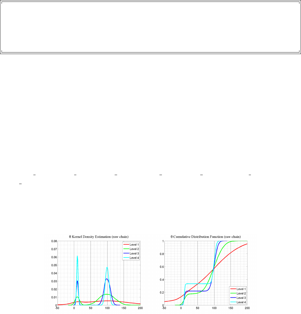
CHAPTER 5. QUESO EXAMPLES 149

to the user’s settings, namely paths for QUESO required libraries, it may be used to compile

the code and create the executable bimodal_gsl.

Thus, to compile, build and execute the code, the user just needs to run the following

commands in the same directory where the ﬁles are:

$cd $HOME / L IBRARI ES / QUESO - 0.50.0 / examp les / bimo dal /

$export LD_LIB RA RY_PATH = $LD_LIBRARY_PATH:\

$H OM E / L IB R AR I ES / gsl - 1. 15 / l ib / :\

$HOM E / L IB RA RIE S / boos t - 1. 53 .0 / l ib / :\

$HOM E / L I BR AR IES / hdf5 - 1 .8 .1 0/ l ib : \

$HOM E / L IB RA RIE S / QUES O - 0. 50 .0 / l ib

$make -f Makefile_bimodal_violeta

$./ b im od al_ gsl e xa mp le . i np

Again, the ‘export’ instruction above is only necessary if the user has not saved it in

his/her .bashrc ﬁle.

5.6.5 Data Post-Processing and Visualization

According to the speciﬁcations of the input ﬁle in Listing 5.67, both a folder named outputData

and a the following ﬁles should be generated:

rawChain_ml.m

display_sub0.txt

The sequence of Matlab commands is identical to the ones presented in Sections 5.1.5,

5.2.5,5.3.8 and 5.4.7; therefore, are omitted here. The reader is invited to explore the Matlab

ﬁles plot likelihood normalized taus.m,plot likelihood unnormalized taus.m and/or

plot all.m, for details of how the ﬁgures have been generated.

5.6.5.1 KDE and CDF Plots

Figure 5.6.2 presents the KDE and CDF plots of the parameter θ.

(a) KDE (b) CDF

Figure 5.6.2: KDE and CDF plots of parameter θ, for all fours levels.

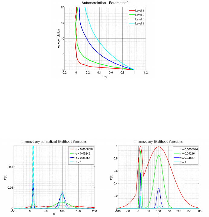
CHAPTER 5. QUESO EXAMPLES 150

5.6.5.2 Autocorrelation Plots

Figure 5.6.3 presents the autocorrelation of the parameter θ, in each one of the intermediate

levels.

Figure 5.6.3: Autocorrelation plots for θ, all four levels.

5.6.5.3 Intermediary Likelihood Plots

(a) normalized (b) unnormalized

Figure 5.6.4: Intermediary likelihood functions f(θ)τ, where τiis the exponent computed at

the i-th level of Multilevel algorithm. In this simple problem, only four levels are needed, i.e.

i= 1 . . . 4. The cyan-colored curve (exponent τ= 1) is the same curve as in Figure 5.6.1.

5.7 hysteretic

This example replicates the problem in “Section 4.3 A Hysteretic Model Class ” of [8], and

which is also discussed in [6]. In this example we consider the nonlinear seismic response

of a four-story building. This response is modeled with an inelastic shear building model

with some linear viscous damping and hysteretic bilinear interstory restoring forces [6]. More

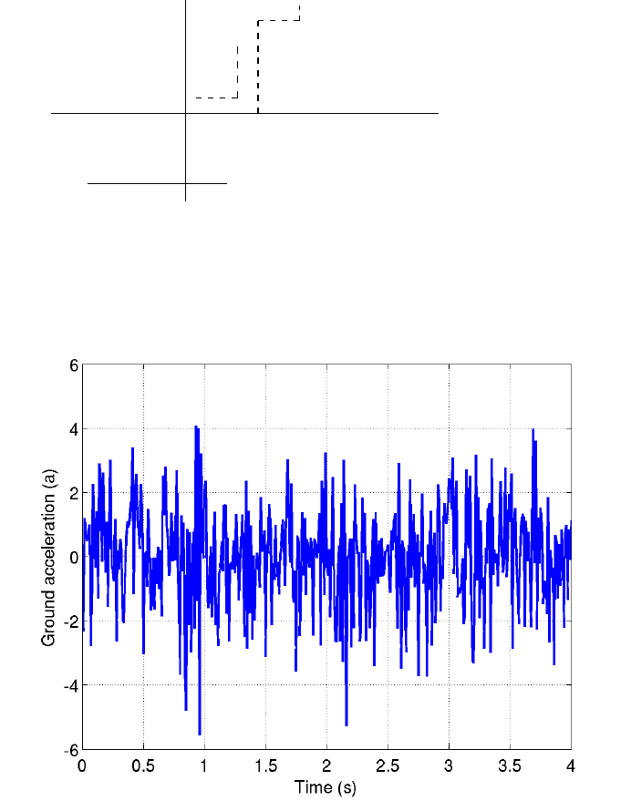
CHAPTER 5. QUESO EXAMPLES 151

speciﬁcally, let t≥0 denote time, let ag(t) be a given total acceleration at the base (Fig. 13),

and for the i-th ﬂoor [degree of freedom (dof)], 1 ≤i≤No≡4, let us denote:

mi= lumped mass,

qi(t) = horizontal displacement,

Fi(t) = hysteretic restoring force

(5.7.1)

The hysteretic restoring force is illustrated in Figure 5.7.1 and the horizontal base (ground)

acceleration (input data) used in [8] is illustrated in 5.7.2.

-

7

1









i-th ﬂoor

interstory

riki

Figure 5.7.1: Illustration of the hysteretic restoring force [see Eq. (5.7.2)] used in our hysteretic

test problem. The terms ri,ki, and uidenote model parameters.

Figure 5.7.2: Horizontal base acceleration (input data) used in the hysteretic test problem [8].

CHAPTER 5. QUESO EXAMPLES 152

We also deﬁne the mass matrix Mand the stiﬀness matrix K:

M=





m1000

0m20 0

0 0 m30

000m4





and K=





k1+k2−k20 0

−k2k2+k3−k30

0−k3k3+k4−k4

0 0 −k4k4







and the Rayleigh damping matrix

C=ρM+γK

for given positive scalar parameters ρand γ. The response q(t)≡[q1(t), q2(t), q3(t), q4(t)] is

modeled as satisfying the equation of motion:

M¨

q(t) + C˙

q(t) + F(t) = −M·









4×1

·ag(t),(5.7.2)

where F(t)≡[F1(t), F2(t), F3(t), F4(t)]. In this model, the hysteretic restoring force F(t)

depends on the whole time history [q(t),˙

q(t)] of responses from the initial instant until time t.

The (noisy) measured data y= (y1, y2, y3, y4) available for model calibration consists of 4

s of accelerometer data at each ﬂoor (refer to Fig. 5.7.3), with a sample interval ∆t= 0.01

s. The simulated dynamic data was obtained by adding Gaussian white noise to the output

simulation of the hysteretic model with the following input values:

m1=m2=m3=m4= 2 ×104kg,

k1= 2.2×107Nm−1,

k2= 2.0×107Nm−1,

k3= 1.7×107Nm−1,

k4= 1.45 ×107Nm−1,

r1=r2=r3=r4= 0.1,

u1=u2= 8 ×10−3m,

u3=u4= 7 ×10−3m,

ρ= 7.959 ×10−1,

γ= 2.5×10−3,

σ2= 0.62,

where for i= 1,2,3,4, kiis the initial stiﬀness, riis the post-yield stiﬀness reduction factor,

and uiis yield displacement.

According to Cheung and Prudencio [8], these input values were chosen deliberately so

that the excitation agdid not cause some of the upper ﬂoors to enter the nonlinear regime;

that is, so that our test inverse problem did not become globally identiﬁable.

In this section, 400 time-steps are used, as the data is available at instants

tn= (n−1) ×∆t, 1≤n≤NT≡401,∆t= 0.01

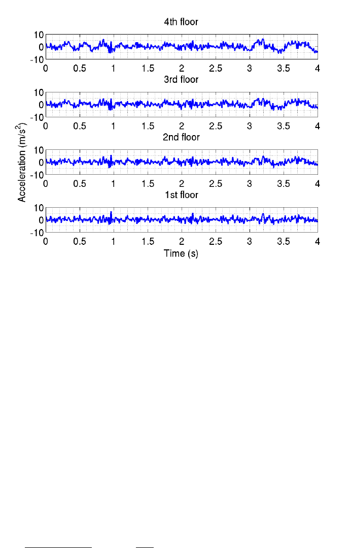
CHAPTER 5. QUESO EXAMPLES 153

Figure 5.7.3: Horizontal acceleration of each of the four ﬂoors (measured data aimed for

calibration) used in our hysteretic test problem.

however, Cheung and Prudencio used only 250 time steps [8].

An additive noise is assumed to be present in the measurements; i.e.,

yi(n) = qi(n) + εi(n),1≤i≤No,1≤n≤NT≡401,

where qi(n;θ2, ..., θ15) denotes the output at time tn=n∆t(∆t= 0.01s) at the i-th observed

degree of freedom predicted by the proposed structural model, and yi(n) denotes the corre-

sponding measured output.

They considered a total of 15 unknown parameters θ= (θ1, ..., θ15) and modeled the

variables εias independently and identically distributed Gaussian variables with mean zero

and some unknown prediction-error variance σ2. The variance σ2is assumed to be the same

for all No= 4 ﬂoors. The ﬁrst component θ1is equal to the prediction error variance σ2and

the other 14 parameters are related to the four triples (ki, ri, ui),1≤i≤No(see Fig. 5.7.1),

to ρ, and to γ. The likelihood function is given by:

f(y|θ) = 1

(2πσ2)NoNT/2exp −1

2σ2

i=1

n=1

[yi(tn)−qi(tn;θ2, . . . , θ15)]2!.(5.7.3)

An inverse gamma prior was used for θ1=σ2, and a 14-dimensional Gaussian prior was used

for θ2, ..., θ15 with zero mean and diagonal covariance matrix equal to a scaled identity matrix.

CHAPTER 5. QUESO EXAMPLES 154

5.7.1 Running the Example

To run the executable provided (available after QUESO installation), and generate ﬁgures for

the chains, KDEs, CDFs, autocorrelation and scatter plots, enter the following commands:

$cd $H OM E / L IB RA RI ES / QU ESO - 0. 50 .0/ e xa mp le s / e xa mp le

$rm output D ata /*

$./ e xa mp le_ gsl e xam ple_1 chai n . inp

$matlab

$plo t_all .m # i n s i d e m a t lab

$ls -l o u tputDa ta /*. png

h ys teret ic_autocorr _ th etas . png h ys teretic_ kde_thet a8 . png

hysteret ic_cdf_t hetas . png h yster etic_kde _theta9 . pn g

hysteret ic_kde_t heta1 . png h ystere tic_kde_ theta10 . pn g

hysteret ic_kde_t heta2 . png h ystere tic_kde_ theta11 . pn g

hysteret ic_kde_t heta3 . png h ystere tic_kde_ theta12 . pn g

hysteret ic_kde_t heta4 . png h ystere tic_kde_ theta13 . pn g

hysteret ic_kde_t heta5 . png h ystere tic_kde_ theta14 . pn g

hysteret ic_kde_t heta6 . png h ystere tic_kde_ theta15 . pn g

hysteretic_kde_theta7.png hysteretic_scatter_thetas.png

As a result, the user should have created several of PNG ﬁgures containing kernel density

estimate of the 15 parameters, cumulative density distribution, autocorrelation and scatter

plots. The name of the ﬁgure ﬁles have been chosen to be informative, as shown in the Listing

above.

Additional ﬁgures may be generated if the user allows the procedure debug hyst( be called

by the compiler in Line 11 of ﬁle example main.C; in that case, call the function cpp gen.m

inside Matlab/Octave.

5.7.2 Example Code

The source code for the example is composed of 5 ﬁles: example main.C (Listing 5.68),

example likelihood.h and example likelihood.C (Listings 5.69 and 5.70), example compute.h

and example compute.C (Listings 5.71 and 5.72), and ﬁnally example hyst.h and example hyst.C,

which contain the Hysteretic model properly said.

Note that in line 11 of Listings 5.68 the ‘#if 1’ directive tells the compiler that the

application will call compute(), which internally uses QUESO and the Multilevel algorithm.

On the contrary, the user may calculate the hysteretic force without uncertainty by changing

the directive to ‘#if 0’, which can assist the analysis of the resulting data.

#i n c l u d e <example compute .h>

int mai n (int argc , c har * argv [])

{

5// Initia l ize e n vironm e nt

MPI _I ni t (& argc ,& a rgv );

QUESO :: F ul lE nvironme nt * env =

ne w Q UE SO :: F u ll E nv i ro n me n t ( M PI_ COM M_W OR L D , a rg v [1] , " " , NU LL ) ;

10 // Compute

#i f 1

compute(*en v );

CHAPTER 5. QUESO EXAMPLES 155

#else

debu g_hyst (* env ) ;

15 #e n d i f

// Final ize e n vironm e nt

delete env;

MPI_Finalize();

return 0;

}

Listing 5.68: File example main.C.

#i f n d e f EX LIKELIHOOD H

#d e f i n e EX LIKELIHOOD H

#i n c l u d e <q u es o / G s l M a t r i x . h>

struct

likelihoodRoutine_DataType

{

st d :: v ect or < st d :: vec tor < d oub le >* > flo or ;

st d :: v ect or < do uble > acc el ;

};

double l i kelihoodRo ut in e (

const QUE SO :: GslVec tor & paramValues ,

const QUE SO :: GslVec tor * p aramD irect ion ,

con st v oid * fun ct io nD ataPt r ,

QUESO :: GslVe ctor * grad Vec tor ,

QUESO :: GslMa trix * h essianMat rix ,

QUESO :: GslVe ctor * he ss ianEffe ct ) ;

#e n d i f

Listing 5.69: File example likelihood.h.

#i n c l u d e <example likelihood .h>

#i n c l u d e <example hyst .h>

double l i kelihoodRo ut in e (

const QUE SO :: GslVec tor & paramValues ,

const QUE SO :: GslVec tor * p aramD irect ion ,

con st v oid * fun ct io nD ataPt r ,

QUESO :: GslVe ctor * grad Vec tor ,

QUESO :: GslMa trix * h essianMat rix ,

QUESO :: GslVe ctor * he ss ianEffe ct )

{

const QUE SO :: B aseEnvir on ment & env = paramValues.env () ;

UQ_FATA L_ TE ST _M ACRO ( param Va lues . siz eLoca l () != 15 ,

en v . fu llRank () ,

" e x amp l e_ l ike l iho o d () " ,

" inva li d param et er size ");

const std :: vector < std :: vector < double >* >&

flo or = (( l ikel i ho odRoutin e _D ataType *) func tionD ataPt r ) - > fl oor ;

con st std :: v ect or < do ubl e >&

acc el = (( l ikel i ho odRoutin e _D ataType *) func tionD ataPt r ) - > ac cel ;

u ns ig ned in t n um Fl oor s = flo or . s iz e () ;

CHAPTER 5. QUESO EXAMPLES 156

u ns ig ned in t n um Tim e St e ps = a cc el . s iz e () ;

UQ_FATA L_TE ST_MA CRO (( n um Fl oors != 4) ,

en v . fu llRank () ,

" e x amp l e_ l ike l iho o d () " ,

" i nva lid ’ n um Fl oo rs ’ " );

UQ_FATA L_ TE ST_MACRO (( n umTimeS teps != 401) ,

en v . fu llRank () ,

" e x amp l e_ l ike l iho o d () " ,

" i nv ali d ’ n umT im eS te ps ’ " );

for ( unsi gned int i = 0; i < n umFloo rs ; ++i) {

UQ_FATA L_TES T_MAC RO ( flo or [ i]-> si ze () != n um TimeS teps ,

en v . fu llRank () ,

" e x amp l e_ l ike l ih o od () " ,

" inva lid n umber of ste ps " );

}

QUESO :: Vec torSpac e < QUESO :: GslVector , QUE SO :: GslMat rix > floor Space (env ,"floor_", numFloors ,

NU LL ) ;

double sigm aSq = paramVa l ues [0];

QUESO :: G slVecto r kVec ( floor Space . zer oVector ()) ;

kV ec [0] = 2 .20 e +7 * ex p( paramV al ue s [1 ]) ;

kV ec [1] = 2 .00 e +7 * ex p( paramV al ue s [2 ]) ;

kV ec [2] = 1 .70 e +7 * ex p( paramV al ue s [3 ]) ;

kV ec [3] = 1 .45 e +7 * ex p( paramV al ue s [4 ]) ;

QUESO :: G slVecto r rVec ( floor Space . zer oVector ()) ;

rV ec [0] = 1.0 e -1 * exp ( p a ramVal u es [5] ) ;

rV ec [1] = 1.0 e -1 * exp ( p a ramVal u es [6] ) ;

rV ec [2] = 1.0 e -1 * exp ( p a ramVal u es [7] ) ;

rV ec [3] = 1.0 e -1 * exp ( p a ramVal u es [8] ) ;

QUESO :: G slVecto r uVec ( floor Space . zer oVector ()) ;

uV ec [0] = 8.0 e -3 * exp ( p a ramVal u es [9] ) ;

uV ec [1] = 8.0 e -3 * exp ( p a ramVal u es [10]) ;

uV ec [2] = 7.0 e -3 * exp ( p a ramVal u es [11]) ;

uV ec [3] = 7.0 e -3 * exp ( p a ramVal u es [12]) ;

dou ble rho = 7.959 e -1 * exp ( paramV al ue s [ 13]) ;

dou bl e g am ma = 2 .5 00 e - 3 * e xp ( p a ra mVa l ue s [ 14 ]) ;

st d :: v ect or < do uble > t ( num Ti me St eps ,0. ) ;

QUESO :: Seque nc eO fVecto rs < QUESO :: GslVector , QU ESO :: GslMat rix > u ( f loor Spac e , n umTim eStep s ,

""); // a bsolut e displ a c ement

QUESO :: Seque nc eO fVecto rs < QUESO :: GslVector , QU ESO :: GslMat rix > ud ( floorSpace , numT imeSt eps ,

""); // v elocit y

QUESO :: S equenc eO fVecto rs < Q UESO :: Gsl Vector , QUE SO :: GslMatrix > udd ( f loor Spac e , num TimeS teps ,

""); // acceleration

QUESO :: Seque nc eO fVecto rs < QUESO :: GslVector , QU ESO :: GslMat rix > r esfor ( f loor Spac e , num TimeS teps ,

""); // r e stori n g force

QUESO :: Seque nc eO fVecto rs < QUESO :: GslVector , QU ESO :: GslMat rix > ru ( floorSpace , numT imeSt eps ,

""); // r elativ e displ a c ement

QUESO :: G slVecto r mas sVec ( fl oorSpac e . ze roVec to r () );

mas sV ec . c wS et (2. 0 e +4) ;

h ys t e re t i cM o de l ( env ,

massVec ,

kVec ,

rVec ,

CHAPTER 5. QUESO EXAMPLES 157

uVec ,

rho ,

gamma ,

accel ,

t , // o ut put

u ,

ud ,

udd ,

resfor ,

ru ) ;

QUESO :: G slVecto r aux Vec ( fl oorSpa ce . z eroVec tor ()) ;

double sum = 0.;

for ( unsi gned int i = 0; i < n umFloo rs ; ++i) {

for ( unsi gned int j = 0; j < n u mTimeSt e p s ; ++j ) {

ud d . g e tP o si t io n Va lues ( j , aux Ve c ) ;

su m += ( (* f lo or [ i ]) [ j ] - au xVe c [ i ]- a cc el [ j ]) *(( * f lo or [ i ]) [ j ] - au xVe c [ i ]- a cc el [ j ]) ;

}

dou bl e res ul t = - 0.5 *(( d ou bl e ) n um Fl oo rs ) *( ( d ouble ) n umT imeS tep s ) * log ( 2.* M _PI * sig ma Sq ) -

0. 5* sum / sigm aSq ;

return result;

}

Listing 5.70: File example likelihood.C.

#i f n d e f EX COMPUTE H

#d e f i n e EX COMPUTE H

#i n c l u d e <queso/Environment .h>

vo id compute ( const QUE SO :: F u l lEnvironm e n t & env);

vo id de bu g_ hy st ( const QUE SO :: F ul lEn vir onm ent & env ) ;

#e n d i f

Listing 5.71: File example compute.h.

#i n c l u d e <example compute .h>

#i n c l u d e <example likelihood .h>

#i n c l u d e <q u es o / G s l M a t r i x . h>

#i n c l u d e <q ue s o / S t a t i s t i c a l I n v e r s e P r o b l e m . h>

#i n c l u d e <q u eso / C o n c a t e n a t i o n S u b s e t . h>

#i n c l u d e <q ueso / Co n ca tenate d Ve ctorRV . h>

#i n c l u d e <queso/GenericScalarFunction .h>

#i n c l u d e <q ueso / U niformVectorRV . h>

#i n c l u d e <s y s / t im e . h>

#i n c l u d e <example hyst .h>

vo id c ompute ( c onst QUE SO :: F ul lE nv ir onm en t & env ) {

struct time val tim evalNow ;

getti me ofd ay (& timeval Now , N ULL );

std :: cout << std :: endl << " B e gi nn i ng r un of ’ H ys te re ti c ’ e xa mpl e at "

<< cti me (& timev al No w . tv_se c );

//------------------------------------------------------

// Step 1 of 5: Inst a ntiate the p aramet er sp ace

CHAPTER 5. QUESO EXAMPLES 158

//------------------------------------------------------

QUESO :: Vec torSpac e < QUESO :: GslVector , QUE SO :: GslMat rix >

p ar a mS p a ce A ( env ,"paramA_", 1 , NULL );

QUESO :: Vec torSpac e < QUESO :: GslVector , QUE SO :: GslMat rix >

p ar a mS p a ce B ( env ,"paramB_", 14 , NUL L );

QUESO :: Vec torSpac e < QUESO :: GslVector , QUE SO :: GslMat rix >

p ar a mS p ac e ( env ,"param_", 15 , NUL L );

//------------------------------------------------------

// Step 2 of 5: Inst a ntiate the p aramet er domain

//------------------------------------------------------

QUESO :: G slVecto r param MinsA ( par am SpaceA . z er oVecto r () );

para mMi nsA . cwS et (0) ;

QUESO :: G slVecto r param MaxsA ( par am SpaceA . z er oVecto r () );

para mMa xsA . cwS et (5) ;

QUESO :: BoxSubset < QUESO :: GslVector , QUESO :: GslMatrix >

paramDomainA("paramA_", pa ra mS pa ce A , p ar am Mi ns A , p ar am M ax sA ) ;

QUESO :: G slVecto r param MinsB ( par am SpaceB . z er oVecto r () );

para mM in sB . c wSet (- IN FI NI TY ) ;

QUESO :: G slVecto r param MaxsB ( par am SpaceB . z er oVecto r () );

para mM ax sB . c wSet ( INFI NI TY ) ;

QUESO :: BoxSubset < QUESO :: GslVector , QUESO :: GslMatrix >

paramDomainB("paramB_", pa ra mS pa ce B , p ar am Mi ns B , p ar am M ax sB ) ;

QUESO :: Conca t enatio nSubse t < QUESO :: GslVector , QUESO :: GslMatrix >

para mD omain (" " ,pa ram Space , para mDom ainA , paramDo ma inB );

//------------------------------------------------------

// Step 3 of 5: Inst a ntiate the l i keliho od func tion object

//------------------------------------------------------

std :: cout << " \ t I n stantiat i n g the Likeli h ood ; callin g i nterna l ly the hyste r etic model "

<< s td :: endl ;

likelihoodRoutine_DataType likelihoodRoutine_Data;

likelihoo dR ou t ine_Data . floor . resize (4 , NULL );

uns i gned int numT i meSteps = 401;

for ( unsi gned int i = 0; i < 4; ++i ) {

l ik eli hoodRout ine_Data . f loor [ i ] = ne w std :: vector < d oub le >( n umTim eS teps ,0.) ;

}

likelihoo dRou tine _Dat a . ac cel . re size ( nu mTimeSte ps ,0 .) ;

FI LE * i np ;

inp = f open (" an . txt " ,"r") ;

uns i gned int n u m Observat i o n s = 0;

dou ble t mpA ;

while ( f sc a nf ( in p , " % lf " ,& t mpA ) != EOF ) {

likelihoo dR ou ti n e_Data . accel [ n umObserv at ions ] = tmpA ;

numObs e r vations ++;

}

numObs e r vations =0;

FI LE * inp1 _1 ;

inp 1_1 = fopen ("measured_data1_1.txt","r");

while ( fsc an f ( inp1_1 , " % lf " ,& tmp A ) != EOF ) {

(* l ik eliho odRouti ne_Dat a . floor [0]) [ n um Ob se rvat ion s ]= tmpA ;

numObs e r vations ++;

}

numObs e r vations =0;

FI LE * inp1 _2 ;

inp 1_2 = fopen ("measured_data1_2.txt","r");

while ( fsc an f ( inp1_2 , " % lf " ,& tmp A ) != EOF ) {

(* l ik eliho odRouti ne_Dat a . floor [1]) [ n um Ob se rvat ion s ]= tmpA ;

numObs e r vations ++;

}

CHAPTER 5. QUESO EXAMPLES 159

numObs e r vations =0;

FI LE * inp1 _3 ;

inp 1_3 = fopen ("measured_data1_3.txt","r");

while ( fsc an f ( inp1_3 , " % lf " ,& tmp A ) != EOF ) {

(* l ik eliho odRouti ne_Dat a . floor [2]) [ n um Ob se rvat ion s ]= tmpA ;

numObs e r vations ++;

}

numObs e r vations =0;

FI LE * inp1 _4 ;

inp 1_4 = fopen ("measured_data1_4.txt","r");

while ( fsc an f ( inp1_4 , " % lf " ,& tmp A ) != EOF ) {

(* l ik eliho odRouti ne_Dat a . floor [3]) [ n um Ob se rvat ion s ]= tmpA ;

numObs e r vations ++;

}

QUESO :: Generi cScalar F unctio n < QUESO :: GslVector , QUESO :: GslMatrix >

likelihoodFunctionObj(" lik e_ " ,

paramDomain ,

likelihoodRoutine ,

( vo id *) & likel ih ood Ro uti ne _D ata ,

true) ; // r out in e c o mp ut es [ ln ( f unctio n )]

//------------------------------------------------------

// Step 4 of 5: Inst a ntiate the i nver se problem

//------------------------------------------------------

std :: cout << " \ t In sta ntia ting the SIP " < < std :: endl ;

QUESO :: Unif ormVe ctorR V < QU ESO :: Gs lVector , QUE SO :: Gsl Matrix >

pri orRvA ("priorA_", paramDomainA);

QUE SO :: G sl V ec to r m ean Vec ( p ar amS p ac eB . z ero V ec tor () ) ;

QUE SO :: G sl V ec to r d iag Vec ( p ar amS p ac eB . z ero V ec tor () ) ;

dia gV ec . cwSet (0.6* 0. 6) ;

QUESO :: GslMa trix cov Matrix ( di agVec ) ;

QUESO :: Gauss ianVe ctorR V < QU ESO :: GslVe ctor , QUE SO :: Gsl Mat rix >

pri orRvB ("priorB_", p ar amDom ainB , meanV ec , c ov Ma tr ix ) ;

QUESO :: Concat enated V ectorR V < QUESO :: GslVector , QUESO :: GslMatrix >

priorRv("prior_", priorRvA , priorRvB , paramD o main );

QUESO :: Gene ricVe ctorR V < QU ESO :: Gs lVector , QUE SO :: Gsl Matrix >

postRv(" p os t_ " , param Space );

QUESO :: Statist icalInve r s eProble m < QUE SO :: Gsl Vector , QUESO :: GslMatrix >

ip ( " " , NULL , priorRv , l ik el ihoodFu nc ti onObj , post Rv ) ;

//------------------------------------------------------

// Step 5 of 5: S olve the i nvers e pro blem

//------------------------------------------------------

std :: cout << " \ tS olving the SIP with Mul ti level m ethod " << std :: end l ;

ip.solveWithBayesMLSampling();

getti me ofd ay (& timeval Now , N ULL );

std :: cout << " E nd in g run of ’ H ys te re ti c ’ e xa mpl e at "

<< cti me (& timev al No w . tv_se c ) << std :: endl ;

return;

}

//------------------------------------------------------

CHAPTER 5. QUESO EXAMPLES 160

//------------------------------------------------------

vo id de bu g_ hy st ( const QUE SO :: F ul lEn vir onm ent & env ) {

uns i gned int numF loors = 4;

uns i gned int numT i meSteps = 401;

st d :: v ect or < do uble > a ccel ( num Ti me Steps ,0. ) ;

FI LE * i np ;

inp = f open (" an . txt " ,"r") ;

uns i gned int n u m Observat i o n s = 0;

dou ble t mpA ;

while ( f sc a nf ( in p , " % lf " ,& t mpA ) != EOF ) {

U Q_ F AT A L_ T ES T _M A CR O (( n umOb s er v at i on s >= a cc el . s iz e () ) ,

en v . fu llRank () ,

" d e bu g_ h ys t () " ,

" input file has too many li nes ");

acc el [ n um Obse rva tion s ] = tmpA ;

numObs e r vations ++;

}

U Q_ F AT A L_ T ES T _M A CR O (( n umOb s er v at i on s != a cc el . s iz e () ) ,

en v . fu llRank () ,

" d e bu g_ h ys t () " ,

" input file has a smaller number of ob servati o ns than exp ected ");

QUESO :: Vec torSpac e < QUESO :: GslVector , QUE SO :: GslMat rix > floor Space (env ,"floor_", numFloors ,

NU LL ) ;

QUESO :: G slVecto r kVec ( floor Space . zer oVector ()) ;

kV ec [0 ] = 2.20 e +7 ;

kV ec [1 ] = 2.00 e +7 ;

kV ec [2 ] = 1.70 e +7 ;

kV ec [3 ] = 1.45 e +7 ;

QUESO :: G slVecto r rVec ( floor Space . zer oVector ()) ;

rV ec [0] = 0.1;

rV ec [1] = 0.1;

rV ec [2] = 0.1;

rV ec [3] = 0.1;

QUESO :: G slVecto r uVec ( floor Space . zer oVector ()) ;

uV ec [0] = 0 .008;

uV ec [1] = 0 .008;

uV ec [2] = 0 .007;

uV ec [3] = 0 .007;

dou bl e rho = 7 .9 59 e - 1 ; //0 . 19 76 ;

dou bl e g am ma = 2 .5 00 e - 3 ; / /0 .00 3 8;

st d :: v ect or < do uble > t ( num Ti me St eps ,0. ) ;

QUESO :: Seque nc eO fVecto rs < QUESO :: GslVector , QU ESO :: GslMat rix > u ( f loor Spac e , n umTim eStep s ,

""); // a bsolut e displ a c ement

QUESO :: Seque nc eO fVecto rs < QUESO :: GslVector , QU ESO :: GslMat rix > ud ( floorSpace , numT imeSt eps ,

""); // v elocit y

QUESO :: S equenc eO fVecto rs < Q UESO :: Gsl Vector , QUE SO :: GslMatrix > udd ( f loor Spac e , num TimeS teps ,

""); // acceleration

QUESO :: Seque nc eO fVecto rs < QUESO :: GslVector , QU ESO :: GslMat rix > r esfor ( f loor Spac e , num TimeS teps ,

""); // r e stori n g force

QUESO :: Seque nc eO fVecto rs < QUESO :: GslVector , QU ESO :: GslMat rix > ru ( floorSpace , numT imeSt eps ,

""); // r elativ e displ a c ement

u . s etP o si t io n Va l ue s (0 , f loo r Sp ace . z e ro Ve c to r () );

ud . s e tP o si t io n Va l ue s ( 0 , f lo o rS pa c e . z ero V ec tor () );

ud d . s e tP o si t io n Va lues (0 , f lo o rS pa c e . z e ro Ve c to r ( ) );

resfor . se tP os it i onValues (0 , flo or Space . ze roVecto r () );

ru . s e tP o si t io n Va l ue s ( 0 , f lo o rS pa c e . z ero V ec tor () );

CHAPTER 5. QUESO EXAMPLES 161

QUESO :: G slVecto r mas sVec ( fl oorSpac e . ze roVec to r () );

mas sV ec . c wS et (2. 0 e +4) ;

h ys t e re t i cM o de l ( env ,

massVec ,

kVec ,

rVec ,

uVec ,

rho ,

gamma ,

accel ,

t , // o ut put

u ,

ud ,

udd ,

resfor ,

ru ) ;

std :: set < uns igned int > auxSet ;

auxSet.insert(0);

// W riti ng some data to the file ’ outpu tData / cpp _output .m ’

std :: ofstr ea m myF ile ;

myF ile . open ( " ou tputDat a / cpp_out put . m " );

// Write ’ t_cpp ’

myFile << " t_ cpp = z eros ( " << 1 << " ," << numTimeSteps << ") ; \ n"

<< " t _cpp = [";

for ( unsi gned int j = 0; j < n u mTimeSt e p s ; ++j ) {

myFile << t[j] << " ";

}

myFile << " ]; " < < st d :: end l ;

// Write ’ a_cpp ’

myFile << " a_ cpp = z eros ( " << 1 << " ," << numTimeSteps << ") ; \ n"

<< " a _cpp = [";

for ( unsi gned int j = 0; j < n u mTimeSt e p s ; ++j ) {

myF ile << acc el [ j] << " ";

}

myFile << " ]; " < < st d :: end l ;

QUESO :: G slVecto r aux Vec ( fl oorSpa ce . z eroVec tor ()) ;

// Write ’ u_cpp ’

myFile << " u_ cpp = z eros ( " << numFl oors << " ," << numTimeSteps << " ) ;\ n "

<< " u _cpp = [";

for ( unsi gned int i = 0; i < n umFloo rs ; ++i) {

for ( unsi gned int j = 0; j < n u mTimeSt e p s ; ++j ) {

u . g etPo s it i onV a lu e s ( j , a ux Ve c ) ;

myFile << auxVec[i] << " ";

}

myF ile < < st d :: end l ;

}

myFile << " ]; " < < st d :: end l ;

// Write ’ ud_cpp ’

myFile << " ud _cpp = z eros ( " << numF l oors << " ," << numTimeSteps << ") ; \ n"

<< " u d_cpp = [";

for ( unsi gned int i = 0; i < n umFloo rs ; ++i) {

for ( unsi gned int j = 0; j < n u mTimeSt e p s ; ++j ) {

ud . g e tP o si t io n Va l ue s ( j , a ux Ve c ) ;

myFile << auxVec[i] << " ";

}

myF ile < < st d :: end l ;

CHAPTER 5. QUESO EXAMPLES 162

}

myFile << " ]; " < < st d :: end l ;

// Write ’ udd_cpp ’

myFile << " udd _cpp = zeros (" << n umFloo rs << " , " << numTimeSteps << " ) ;\ n "

<< "udd_cpp = [";

for ( unsi gned int i = 0; i < n umFloo rs ; ++i) {

for ( unsi gned int j = 0; j < n u mTimeSt e p s ; ++j ) {

ud d . g e tP o si t io n Va lues ( j , aux Ve c ) ;

myFile << auxVec[i] << " ";

}

myF ile < < st d :: end l ;

}

myFile << " ]; " < < st d :: end l ;

// Write ’ resf or_ cpp ’

myFile << " resf or _c pp = zeros (" << n u mFloo r s << " , " << numTimeSteps << " ) ;\ n "

<< " r es for_cp p = [ ";

for ( unsi gned int i = 0; i < n umFloo rs ; ++i) {

for ( unsi gned int j = 0; j < n u mTimeSt e p s ; ++j ) {

res for . getPosit io nVa lue s (j , auxVec );

myFile << auxVec[i] << " ";

}

myF ile < < st d :: end l ;

}

myFile << " ]; " < < st d :: end l ;

// Write ’ ru_cpp ’

myFile << " ru _cpp = z eros ( " << numF l oors << " ," << numTimeSteps << ") ; \ n"

<< " r u_cpp = [";

for ( unsi gned int i = 0; i < n umFloo rs ; ++i) {

for ( unsi gned int j = 0; j < n u mTimeSt e p s ; ++j ) {

ru . g e tP o si t io n Va l ue s ( j , a ux Ve c ) ;

myFile << auxVec[i] << " ";

}

myF ile < < st d :: end l ;

}

myFile << " ]; " < < st d :: end l ;

myF il e . c lo se () ;

return;

}

Listing 5.72: File example compute.C.

5.7.3 Input File

The options used for solving this example are displayed in Listing 5.73.

###############################################

# UQ Environment

###############################################

#e n v h e l p = a n y t h i n g

env_numSu b E n v i r onments = 1

env_subDi spl ayF ileN ame = o ut putData / d ispla y

env_subDi s p l a y A llowAll = 0

env_subDisplayAllowedSet = 0

env_displayVerbosity = 0

env_syncVerbosity = 0

CHAPTER 5. QUESO EXAMPLES 163

env _ seed = 0

###############################################

# S t a t i s t i c a l i n v e r s e pr o ble m ( i p )

###############################################

#i p h e l p = a n y t h i n g

ip_computeSolution = 1

ip_dataO ut put Fi le Nam e = output Data / sipO utput

ip_dataOutputAllowedSet = 0

###############################################

# ’ i p ’ : i n f o r m a t i o n f o r M u l t i l e v e l a l g o ri t h m

###############################################

#i p m l h e l p = a n y t h i n g

ip_ml_data Ou tp ut Fi le Na me = o utputDa ta / s ipOutpu t_ ml

ip_ml_dataOutputAllowedSet = 0 1

###############################################

# A l l l e v e l s , u n l e s s o t h e r w i s e s p e c i f i e d

###############################################

ip_ml_default_minEffectiveSizeRatio = 0.49

ip_ml_default_maxEffectiveSizeRatio = 0.51

ip_ml_default _ r a w C h a i n _size = 1000

#ip ml default rawChain dataOutputFileName = outputData/rawChain ml

#i p m l 0 r a w C h a i n d a t a O u t p u t F i l e N a m e = o utp utD ata / r a wC hai n m l

#ip ml default scaleCovMatrix = 0

#i p m l d e f a u l t d r m a x N u m E x t r a S t a g e s = 2

#ip ml default dr listOfScalesForExtraStages = 10. 25.

###############################################

# L a s t l e v e l ( l e v e l 4 f o r ’ e x a m p l e g s l ’ e x e c u t a b l e )

###############################################

ip_ml_last_data Ou tpu tFi leN ame = o utputDa ta / sipOutp ut _ml

ip_ml_last_dataOutputAllowedSet = 0 1

ip_ml_last_rawChain_size = 5000

ip_ml_last_rawChain_computeStats = 1

ip_ml_last_rawChain_dataOutput FileName = output Da ta / rawCh ai n_ml

#i p m l l a s t s c a l e C o v M a t r i x = 0

#ip ml last dr maxNumExtraStages = 2

#ip ml last dr listOfScalesForExtraStages = 10. 25.

ip_ml_last_rawChain_stats_kde_compute = 1

ip_ml_last_rawChain_stats_kde_numEvalPositions = 250

ip_ml_last_rawChain_stats_covMatrix_compute = 1

ip_ml_last_rawChain_stats_corrMatrix_compute = 1

Listing 5.73: Options for QUESO library used in application code (Listings 5.68-5.72).

5.7.4 Create your own Makeﬁle

Similarly to the other examples presented in this user’s manual and also available with QUESO

distribution, a user-created makeﬁle is available: ‘Makefile hysteretic violeta’ which may

personalized to each user’s computer settings and used to compile the code and create the

executable hysteretic_gsl.

Thus to compile, build and execute the code, commands similar to the following should

be entered:

CHAPTER 5. QUESO EXAMPLES 164

$cd $HOME / LIBRA RIES / QUESO -0.50 .0/ exampl es / hyst er etic /

$export LD_LIB RA RY_PATH = $LD_LIBRARY_PATH:\

$H OM E / L IB R AR I ES / gsl - 1. 15 / l ib / :\

$HOM E / L IB RA RIE S / boos t - 1. 53 .0 / l ib / :\

$HOM E / L I BR AR IES / hdf5 - 1 .8 .1 0/ l ib : \

$HOM E / L IB RA RIE S / QUES O - 0. 50 .0 / l ib

$ma ke -f M a k e f i l e _ hysteretic_violeta

$./ h ys ter etic_ gsl e xa mp le . i np

Again, the ‘export’ instruction above is only necessary if the user has not saved the path

for the libraries used during QUESO installation in his/her .bashrc ﬁle.

5.7.5 Data Post-Processing and Visualization

According to the speciﬁcations of the input ﬁle in Listing 5.73, both a folder named outputData

and a the following ﬁles should be generated:

rawChain_ml.m

display_sub0.txt

Note that in this hysteretic problem a total of 13 levels are required for the Multilevel

method (e.g. see the contents of ﬁle rawChain ml.m).

The sequence of Matlab commands is identical to the ones presented in Sections 5.1.5,

5.2.5,5.3.8 and 5.4.7; therefore, are omitted here. The reader is invited to explore the Matlab

ﬁles plot all.m and/or cpp gen.m, for details of how the ﬁgures have been generated.

5.7.5.1 KDE Plots

Figure 5.7.4 presents the KDE plots of each parameter θi, i = 1,...,15. The Multilevel

method also provides data about the logarithm of the likelihood function as well as of the

target PDF. Figure 5.7.5 presents the KDE plots of both the likelihood function and of its

logarithm.

5.7.5.2 Autocorrelation and CDF Plots

Figure 5.7.6a combines the CDF of all parameters θi, i = 1,...,15 into a single plot. Fig-

ure 5.7.6b presents their autocorrelations.

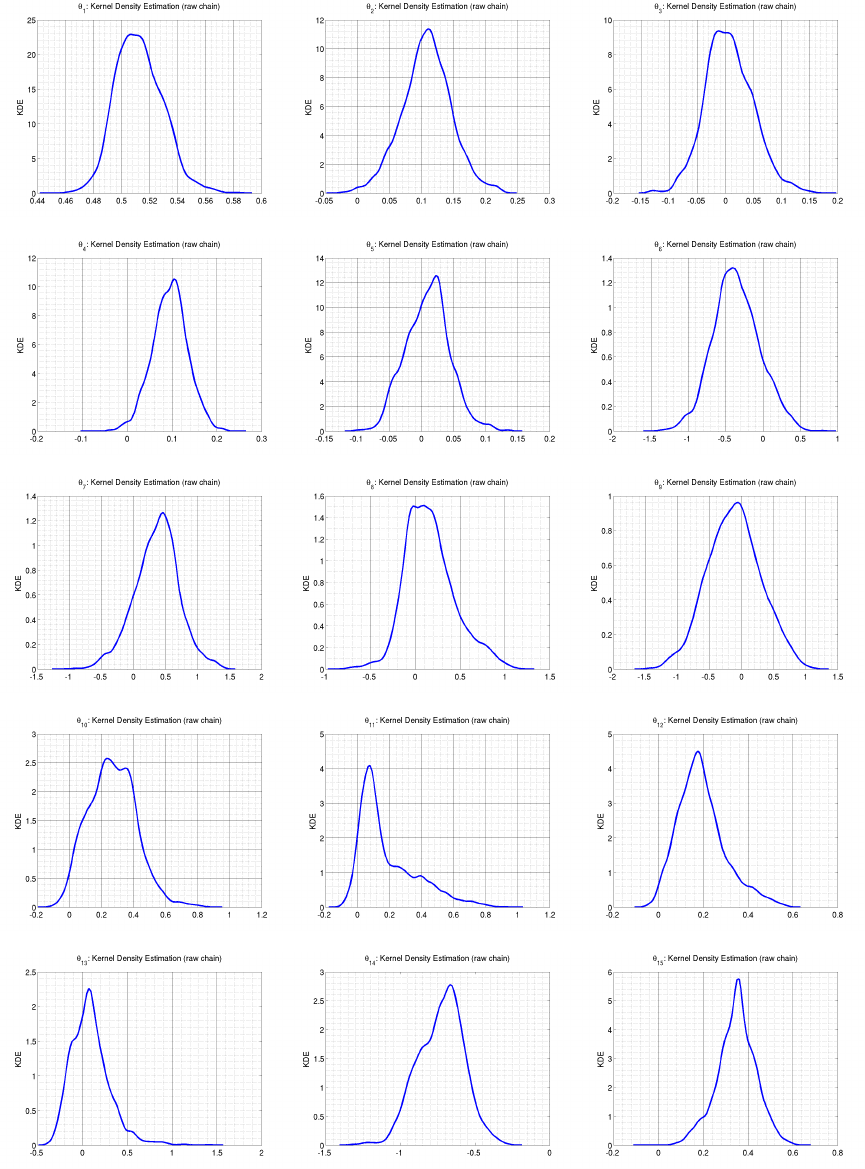
CHAPTER 5. QUESO EXAMPLES 165

Figure 5.7.4: KDE plots of parameter θat the last level.

CHAPTER 5. QUESO EXAMPLES 166

(a) log(f(y|θ)) (b) f(y|θ)

Figure 5.7.5: KDE plots of the likelihood function, given by Eq. (5.7.3), and of its logarithm,

at the last level.

(a) CDF (b) Autocorrelation

Figure 5.7.6: CDF and autocorrelation plots of parameter θat the last level.

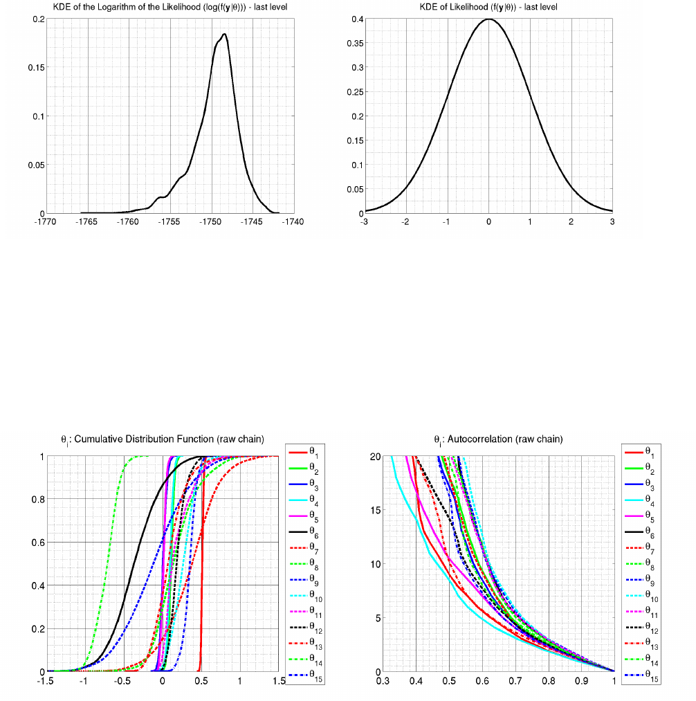
Bibliography

[1] Diagrams for Interactive Learning. http://interactagram.com/. Accessed on August

12th, 2012.

[2] TACC: Texas Advanced Computing Center. http://www.tacc.utexas.edu/, 2001-2013.

[3] J. L. Beck and S.-K. Au. Bayesian updating of structural models and reliability using

Markov Chain Monte Carlo simulation. Journal Of Engineering Mechanics, 128:380–391,

2002.

[4] D. Calvetti and E. Somersalo. Introduction to Bayesian Scientiﬁc Computing, volume 2

of Surveys and Tutorials in the Applied Mathematical Sciences. Springer, 2007.

[5] B. P. Carlin and T. A. Louis. Bayesian Methods for Data Analysis. Texts in Statistical

Science. CRS Press, 3rd edition, 2006.

[6] S. H. Cheung. Stochastic analysis, model and reliability updating of complex systems

with applications to structural dynamics. PhD thesis. Jan 2009, California Institute of

Technology., 2009.

[7] S. H. Cheung, Todd A. Oliver, E. E. Prudencio, Serge Prudhomme, and Robert D.

Moser. Bayesian uncertainty analysis with applications to turbulence modeling. Reliability

Engineering & System Safety, 96(9, SI):1137–1149, 2011.

[8] S. H. Cheung and E. E. Prudencio. Parallel adaptive multilevel sampling algorithms for

the Bayesian analysis of mathematical models. International Journal for Uncertainty

Quantiﬁcation, 2(3):215237, 2012.

[9] J. Ching and Y. Chen. Transitional Markov Chain Monte Carlo method for Bayesian

model updating, model class selection, and model averaging. Journal Of Engineering

Mechanics, 133(7):816832, 2007.

167

BIBLIOGRAPHY 168

[10] Committee on Mathematical Foundations of Veriﬁcation, Validation, and Uncertainty

Quantiﬁcation; Board on Mathematical Sciences and Their Applications, Division on

Engineering and Physical Sciences, National Research Council. Assessing the Reliability

of Complex Models: Mathematical and Statistical Foundations of Veriﬁcation, Validation,

and Uncertainty Quantiﬁcation. The National Academies Press, 2012. http://www.nap.

edu/openbook.php?record_id=13395.

[11] A. DasGupta. Asymptotic Theory of Statistics and Probability. Springer Texts in Statis-

tics. Springer, 2008.

[12] R. Durret. Probability: Theory and Examples. Duxbury Advanced Series. Thomson

Brooks/Cole, 3rd edition, 2005.

[13] Mark Galassi, James Theiler, Brian Gough, Gerard Jungman, and many others. GNU

Scientiﬁc Library. http://www.gnu.org/software/gsl/, 1996-2011.

[14] A. Gelman, J. B. Carlin, H. S. Stern, and D. B. Rubin. Bayesian Data Analysis. Texts

in Statistical Science. Chapman & Hall/CRC, 2nd edition, 2004.

[15] P. J. Green and A. Mira. Delayed rejection in reversible jump Metropolis-Hastings.

BIOMETRIKA, 88(4):1035–1053, 2001.

[16] The HDF Group. HDF5 (Hierarchical Data Format 5). http://www.hdfgroup.org/

HDF5/, 2000–2012.

[17] The MathWorks Group. MATLABr.http://www.mathworks.com/products/matlab/,

2013.

[18] H. Haario, M. Laine, A. Mira, and E. Saksman. DRAM: Eﬃcient adaptive MCMC. Stat.

Comput., 16:339–354, 2006.

[19] H. Haario, E. Saksman, and J. Tamminen. An adaptive Metropolis algorithm. Bernoulli,

7(2):223–242, 2001.

[20] W. K. Hastings. Monte Carlo sampling methods using Markov chains and their applica-

tions. BIOMETRIKA, 57(1):97–109, 1970.

[21] Michael Heroux. Trilinos. http://trilinos.sandia.gov/, 2013.

[22] Michael A. Heroux, Roscoe A. Bartlett, Vicki E. Howle, Robert J. Hoekstra, Jonathan J.

Hu, Tamara G. Kolda, Richard B. Lehoucq, Kevin R. Long, Roger P. Pawlowski, Eric T.

Phipps, Andrew G. Salinger, Heidi K. Thornquist, Ray S. Tuminaro, James M. Willen-

bring, Alan Williams, and Kendall S. Stanley. An overview of the Trilinos project. ACM

Trans. Math. Softw., 31(3):397–423, 2005.

[23] X. Huan and Y. Marzouk. Optimal Bayesian experimental design for combustion kinet-

ics. In 49th AIAA Aerospace Sciences Meeting including the New Horizons Forum and

Aerospace Exposition, number AIAA 2011-513, Orlando, Florida, 2011.

BIBLIOGRAPHY 169

[24] Silicon Graphics International. STL: Standard Template Library. http://www.sgi.com/

tech/stl/, 2000-2011.

[25] J. Jacod and P. Protter. Probability Essentials. Springer, 2nd edition, 2004.

[26] E. T. Jaynes. Probability Theory: The Logic of Science. Cambridge University Press,

2003.

[27] N. M. Josuttis. The C++ Standard Library, A Tutorial and Reference. Addison Wesley,

1st edition, 1999.

[28] J. Kaipio and E. Somersalo. Statistical and Computational Inverse Problems, volume 160

of Applied Mathematical Sciences. Springer, 2005.

[29] M. Laine. DRAM - Delayed Rejection Adaptive Metropolis. http://helios.fmi.fi/

~lainema/dram/, 2006-2008. Accessed on October 8th, 2013.

[30] M. Laine. MCMC Toolbox for Matlab. helios.fmi.fi/~lainema/mcmc/, 2006-2008.

Accessed on March 28th, 2013.

[31] M. Laine. Adaptive MCMC methods with applications in environmental and geophysical

models. PhD thesis, Lappeenranta University of Technology, Lappeenranta, Finland,

2008.

[32] S. B. Lippman, J. Lajoie, and B. E. Moo. C++ Primer. Addison Wesley, 4th edition,

2005.

[33] Andrew Makhorin and GLKP Development Team. GLPK (GNU Linear Programming

Kit). http://www.gnu.org/software/glpk/, 2000-2012.

[34] N. Metropolis, A. W. Rosenbluth, M. N. Rosenbluth, A. H. Teller, and E. Teller. Equa-

tions of state calculations by fast computing machines. Journal of Chemical Physics,

21(6):1087–1092, 1953.

[35] A. Mira. On Metropolis-Hastings algorithms with delayed rejection. Metron - Interna-

tional Journal of Statistics, 59(3-4):231–241, 2001.

[36] E. E. Prudencio and K. W. Schulz. The Parallel C++ Statistical Library ‘QUESO’:

Quantiﬁcation of Uncertainty for Estimation, Simulation and Optimization. In Euro-Par

2011: Parallel Processing Workshops, volume 7155 of Lecture Notes in Computer Science,

pages 398–407. Springer Berlin / Heidelberg, 2012.

[37] C. P. Robert. The Bayesian Choice. Springer Verlag, 2nd edition, 2004.

[38] C. P. Robert and G. Casella. Monte Carlo Statistical Methods. Springer Verlag, 2nd

edition, 2005.

BIBLIOGRAPHY 170

[39] B. W. Silverman. Density Estimation for Statistics and Data Analysis. Number 26 in

Monographs on Statistics & Applied Probability. Chapman & Hall/CRC, 1986.

[40] Boost Development Team. Boost C++ Libraries. http://www.boost.org/, 1998-2013.

[41] GCC Team. GCC, the GNU compiler collection. http://gcc.gnu.org/, 1987-2013.

[42] GNU Development Team. GNU build system (autotools). http://www.gnu.org/

software/software.html, ?–2013. Retrieved August 4th, 2013.

[43] GRVY Development Team. The groovy toolkit (GRVY). https://red.ices.utexas.

edu/projects/software/wiki/GRVY, 1996-2009.

[44] IntelrTeam. Intel c++ compiler. http://software.intel.com/en-us/c-compilers,

1987-2013. Retrieved August 4th, 2013.

[45] MPICH Development Team. MPICH: High-Performance Portable MPI. http://www.

mpich.org/, 2001-2013.

[46] Octave Development Team. GNU Octave. http://www.gnu.org/software/octave/,

1988–2013.

[47] Open MPI Development Team. Open MPI: Open source high performance computing.

http://www.open-mpi.org/, 2008-2012.

[48] Dimitri van Heesch. Doxygen. http://www.doxygen.org/, 2009-2013.

[49] http://en.wikipedia.org/wiki/Ablation. Accessed on August 12th, 2012.

APPENDIX A

Free Software Needs Free Documentation

The following article was written by Richard Stallman, founder of the GNU Project.

The biggest deﬁciency in the free software community today is not in the software−it is

the lack of good free documentation that we can include with the free software. Many of

our most important programs do not come with free reference manuals and free introductory

texts. Documentation is an essential part of any software package; when an important free

software package does not come with a free manual and a free tutorial, that is a major gap.

We have many such gaps today.

Consider Perl, for instance. The tutorial manuals that people normally use are non-

free. How did this come about? Because the authors of those manuals published them with

restrictive terms−no copying, no modiﬁcation, source ﬁles not available−which exclude them

from the free software world.

That wasn’t the ﬁrst time this sort of thing happened, and it was far from the last. Many

times we have heard a GNU user eagerly describe a manual that he is writing, his intended

contribution to the community, only to learn that he had ruined everything by signing a

publication contract to make it non-free.

Free documentation, like free software, is a matter of freedom, not price. The problem

with the non-free manual is not that publishers charge a price for printed copies−that in itself

is ﬁne. (The Free Software Foundation sells printed copies of manuals, too.) The problem is

the restrictions on the use of the manual. Free manuals are available in source code form, and

give you permission to copy and modify. Non-free manuals do not allow this.

The criteria of freedom for a free manual are roughly the same as for free software. Re-

distribution (including the normal kinds of commercial redistribution) must be permitted, so

that the manual can accompany every copy of the program, both on-line and on paper.

171

APPENDIX A. FREE SOFTWARE NEEDS FREE DOCUMENTATION 172

Permission for modiﬁcation of the technical content is crucial too. When people modify the

software, adding or changing features, if they are conscientious they will change the manual

too−so they can provide accurate and clear documentation for the modiﬁed program. A

manual that leaves you no choice but to write a new manual to document a changed version

of the program is not really available to our community.

Some kinds of limits on the way modiﬁcation is handled are acceptable. For example,

requirements to preserve the original author’s copyright notice, the distribution terms, or the

list of authors, are ok. It is also no problem to require modiﬁed versions to include notice that

they were modiﬁed. Even entire sections that may not be deleted or changed are acceptable,

as long as they deal with nontechnical topics (like this one). These kinds of restrictions are

acceptable because they don’t obstruct the community’s normal use of the manual.

However, it must be possible to modify all the technical content of the manual, and then

distribute the result in all the usual media, through all the usual channels. Otherwise, the

restrictions obstruct the use of the manual, it is not free, and we need another manual to

replace it.

Please spread the word about this issue. Our community continues to lose manuals to

proprietary publishing. If we spread the word that free software needs free reference manuals

and free tutorials, perhaps the next person who wants to contribute by writing documenta-

tion will realize, before it is too late, that only free manuals contribute to the free software

community.

If you are writing documentation, please insist on publishing it under the GNU Free

Documentation License or another free documentation license. Remember that this decision

requires your approval−you don’t have to let the publisher decide. Some commercial publish-

ers will use a free license if you insist, but they will not propose the option; it is up to you

to raise the issue and say ﬁrmly that this is what you want. If the publisher you are dealing

with refuses, please try other publishers. If you’re not sure whether a proposed license is free,

write to lice

APPENDIX B

GNU General Public License

Everyone is permitted to copy and distribute verbatim copies of this license document,

but changing it is not allowed.

Preamble

The GNU General Public License is a free, copyleft license for software and other kinds of

works.

The licenses for most software and other practical works are designed to take away your

freedom to share and change the works. By contrast, the GNU General Public License is

intended to guarantee your freedom to share and change all versions of a program–to make

sure it remains free software for all its users. We, the Free Software Foundation, use the GNU

General Public License for most of our software; it applies also to any other work released this

way by its authors. You can apply it to your programs, too.

When we speak of free software, we are referring to freedom, not price. Our General

Public Licenses are designed to make sure that you have the freedom to distribute copies of

free software (and charge for them if you wish), that you receive source code or can get it if

you want it, that you can change the software or use pieces of it in new free programs, and

that you know you can do these things.

To protect your rights, we need to prevent others from denying you these rights or asking

you to surrender the rights. Therefore, you have certain responsibilities if you distribute copies

of the software, or if you modify it: responsibilities to respect the freedom of others.

173

APPENDIX B. GNU GENERAL PUBLIC LICENSE 174

For example, if you distribute copies of such a program, whether gratis or for a fee, you

must pass on to the recipients the same freedoms that you received. You must make sure that

they, too, receive or can get the source code. And you must show them these terms so they

know their rights.

Developers that use the GNU GPL protect your rights with two steps: (1) assert copyright

on the software, and (2) oﬀer you this License giving you legal permission to copy, distribute

and/or modify it.

For the developers’ and authors’ protection, the GPL clearly explains that there is no war-

ranty for this free software. For both users’ and authors’ sake, the GPL requires that modiﬁed

versions be marked as changed, so that their problems will not be attributed erroneously to

authors of previous versions.

Some devices are designed to deny users access to install or run modiﬁed versions of the

software inside them, although the manufacturer can do so. This is fundamentally incompati-

ble with the aim of protecting users’ freedom to change the software. The systematic pattern

of such abuse occurs in the area of products for individuals to use, which is precisely where

it is most unacceptable. Therefore, we have designed this version of the GPL to prohibit the

practice for those products. If such problems arise substantially in other domains, we stand

ready to extend this provision to those domains in future versions of the GPL, as needed to

protect the freedom of users.

Finally, every program is threatened constantly by software patents. States should not

allow patents to restrict development and use of software on general-purpose computers, but

in those that do, we wish to avoid the special danger that patents applied to a free program

could make it eﬀectively proprietary. To prevent this, the GPL assures that patents cannot

be used to render the program non-free.

The precise terms and conditions for copying, distribution and modiﬁcation follow.

Terms and Conditions

0. Deﬁnitions

“This License” refers to version 3 of the GNU General Public License.

“Copyright” also means copyright-like laws that apply to other kinds of works, such as

semiconductor masks.

“The Program” refers to any copyrightable work licensed under this License. Each licensee

is addressed as “you”. “Licensees” and “recipients” may be individuals or organizations.

To “modify” a work means to copy from or adapt all or part of the work in a fashion

requiring copyright permission, other than the making of an exact copy. The resulting work

is called a “modiﬁed version” of the earlier work or a work “based on” the earlier work.

A “covered work” means either the unmodiﬁed Program or a work based on the Program.

To “propagate” a work means to do anything with it that, without permission, would

make you directly or secondarily liable for infringement under applicable copyright law, ex-

cept executing it on a computer or modifying a private copy. Propagation includes copying,

APPENDIX B. GNU GENERAL PUBLIC LICENSE 175

distribution (with or without modiﬁcation), making available to the public, and in some coun-

tries other activities as well.

To “convey” a work means any kind of propagation that enables other parties to make or

receive copies. Mere interaction with a user through a computer network, with no transfer of

a copy, is not conveying.

An interactive user interface displays “Appropriate Legal Notices” to the extent that it in-

cludes a convenient and prominently visible feature that (1) displays an appropriate copyright

notice, and (2) tells the user that there is no warranty for the work (except to the extent that

warranties are provided), that licensees may convey the work under this License, and how to

view a copy of this License. If the interface presents a list of user commands or options, such

as a menu, a prominent item in the list meets this criterion.

1. Source Code

The “source code” for a work means the preferred form of the work for making modiﬁcations

to it. “Object code” means any non-source form of a work.

A “Standard Interface” means an interface that either is an oﬃcial standard deﬁned by a

recognized standards body, or, in the case of interfaces speciﬁed for a particular programming

language, one that is widely used among developers working in that language.

The “System Libraries” of an executable work include anything, other than the work as a

whole, that (a) is included in the normal form of packaging a Major Component, but which

is not part of that Major Component, and (b) serves only to enable use of the work with

that Major Component, or to implement a Standard Interface for which an implementation

is available to the public in source code form. A “Major Component”, in this context, means

a major essential component (kernel, window system, and so on) of the speciﬁc operating

system (if any) on which the executable work runs, or a compiler used to produce the work,

or an object code interpreter used to run it.

The “Corresponding Source” for a work in object code form means all the source code

needed to generate, install, and (for an executable work) run the object code and to modify

the work, including scripts to control those activities. However, it does not include the work’s

System Libraries, or general-purpose tools or generally available free programs which are used

unmodiﬁed in performing those activities but which are not part of the work. For example,

Corresponding Source includes interface deﬁnition ﬁles associated with source ﬁles for the

work, and the source code for shared libraries and dynamically linked subprograms that the

work is speciﬁcally designed to require, such as by intimate data communication or control

ﬂow between those subprograms and other parts of the work.

The Corresponding Source need not include anything that users can regenerate automat-

ically from other parts of the Corresponding Source.

The Corresponding Source for a work in source code form is that same work.

APPENDIX B. GNU GENERAL PUBLIC LICENSE 176

2. Basic Permissions

All rights granted under this License are granted for the term of copyright on the Program, and

are irrevocable provided the stated conditions are met. This License explicitly aﬃrms your

unlimited permission to run the unmodiﬁed Program. The output from running a covered

work is covered by this License only if the output, given its content, constitutes a covered

work. This License acknowledges your rights of fair use or other equivalent, as provided by

You may make, run and propagate covered works that you do not convey, without con-

ditions so long as your license otherwise remains in force. You may convey covered works to

others for the sole purpose of having them make modiﬁcations exclusively for you, or provide

you with facilities for running those works, provided that you comply with the terms of this

License in conveying all material for which you do not control copyright. Those thus making

or running the covered works for you must do so exclusively on your behalf, under your di-

rection and control, on terms that prohibit them from making any copies of your copyrighted

material outside their relationship with you.

Conveying under any other circumstances is permitted solely under the conditions stated

below. Sublicensing is not allowed; section 10 makes it unnecessary.

3. Protecting Users’ Legal Rights From Anti-Circumvention Law

No covered work shall be deemed part of an eﬀective technological measure under any appli-

cable law fulﬁlling obligations under article 11 of the WIPO copyright treaty adopted on 20

December 1996, or similar laws prohibiting or restricting circumvention of such measures.

When you convey a covered work, you waive any legal power to forbid circumvention of

technological measures to the extent such circumvention is eﬀected by exercising rights under

this License with respect to the covered work, and you disclaim any intention to limit operation

or modiﬁcation of the work as a means of enforcing, against the work’s users, your or third

parties’ legal rights to forbid circumvention of technological measures.

4. Conveying Verbatim Copies

You may convey verbatim copies of the Program’s source code as you receive it, in any medium,

provided that you conspicuously and appropriately publish on each copy an appropriate copy-

right notice; keep intact all notices stating that this License and any non-permissive terms

added in accord with section 7 apply to the code; keep intact all notices of the absence of any

warranty; and give all recipients a copy of this License along with the Program.

You may charge any price or no price for each copy that you convey, and you may oﬀer

support or warranty protection for a fee.

APPENDIX B. GNU GENERAL PUBLIC LICENSE 177

5. Conveying Modiﬁed Source Versions

You may convey a work based on the Program, or the modiﬁcations to produce it from the

Program, in the form of source code under the terms of section 4, provided that you also meet

all of these conditions:

(a) The work must carry prominent notices stating that you modiﬁed it, and giving a relevant

date.

(b) The work must carry prominent notices stating that it is released under this License

and any conditions added under section 7. This requirement modiﬁes the requirement in

section 4 to “keep intact all notices”.

possession of a copy. This License will therefore apply, along with any applicable section

7 additional terms, to the whole of the work, and all its parts, regardless of how they are

packaged. This License gives no permission to license the work in any other way, but it

does not invalidate such permission if you have separately received it.

(d) If the work has interactive user interfaces, each must display Appropriate Legal Notices;

however, if the Program has interactive interfaces that do not display Appropriate Legal

Notices, your work need not make them do so.

A compilation of a covered work with other separate and independent works, which are not

by their nature extensions of the covered work, and which are not combined with it such as

to form a larger program, in or on a volume of a storage or distribution medium, is called an

“aggregate” if the compilation and its resulting copyright are not used to limit the access or

legal rights of the compilation’s users beyond what the individual works permit. Inclusion of

a covered work in an aggregate does not cause this License to apply to the other parts of the

aggregate.

6. Conveying Non-Source Forms

You may convey a covered work in object code form under the terms of sections 4 and 5,

provided that you also convey the machine-readable Corresponding Source under the terms

of this License, in one of these ways:

(a) Convey the object code in, or embodied in, a physical product (including a physical dis-

tribution medium), accompanied by the Corresponding Source ﬁxed on a durable physical

medium customarily used for software interchange.

(b) Convey the object code in, or embodied in, a physical product (including a physical

distribution medium), accompanied by a written oﬀer, valid for at least three years and

valid for as long as you oﬀer spare parts or customer support for that product model,

to give anyone who possesses the object code either (1) a copy of the Corresponding

APPENDIX B. GNU GENERAL PUBLIC LICENSE 178

Source for all the software in the product that is covered by this License, on a durable

physical medium customarily used for software interchange, for a price no more than your

reasonable cost of physically performing this conveying of source, or (2) access to copy

the Corresponding Source from a network server at no charge.

Corresponding Source. This alternative is allowed only occasionally and noncommercially,

and only if you received the object code with such an oﬀer, in accord with subsection 6b.

(d) Convey the object code by oﬀering access from a designated place (gratis or for a charge),

and oﬀer equivalent access to the Corresponding Source in the same way through the same

place at no further charge. You need not require recipients to copy the Corresponding

Source along with the object code. If the place to copy the object code is a network server,

the Corresponding Source may be on a diﬀerent server (operated by you or a third party)

that supports equivalent copying facilities, provided you maintain clear directions next to

the object code saying where to ﬁnd the Corresponding Source. Regardless of what server

hosts the Corresponding Source, you remain obligated to ensure that it is available for as

long as needed to satisfy these requirements.

(e) Convey the object code using peer-to-peer transmission, provided you inform other peers

where the object code and Corresponding Source of the work are being oﬀered to the

general public at no charge under subsection 6d.

A separable portion of the object code, whose source code is excluded from the Corre-

sponding Source as a System Library, need not be included in conveying the object code

work.

A “User Product” is either (1) a “consumer product”, which means any tangible personal

property which is normally used for personal, family, or household purposes, or (2) anything

designed or sold for incorporation into a dwelling. In determining whether a product is a

consumer product, doubtful cases shall be resolved in favor of coverage. For a particular

product received by a particular user, “normally used” refers to a typical or common use of

that class of product, regardless of the status of the particular user or of the way in which the

particular user actually uses, or expects or is expected to use, the product. A product is a

consumer product regardless of whether the product has substantial commercial, industrial or

non-consumer uses, unless such uses represent the only signiﬁcant mode of use of the product.

“Installation Information” for a User Product means any methods, procedures, authoriza-

tion keys, or other information required to install and execute modiﬁed versions of a covered

work in that User Product from a modiﬁed version of its Corresponding Source. The infor-

mation must suﬃce to ensure that the continued functioning of the modiﬁed object code is in

no case prevented or interfered with solely because modiﬁcation has been made.

If you convey an object code work under this section in, or with, or speciﬁcally for use

in, a User Product, and the conveying occurs as part of a transaction in which the right of

possession and use of the User Product is transferred to the recipient in perpetuity or for

a ﬁxed term (regardless of how the transaction is characterized), the Corresponding Source

APPENDIX B. GNU GENERAL PUBLIC LICENSE 179

conveyed under this section must be accompanied by the Installation Information. But this

requirement does not apply if neither you nor any third party retains the ability to install

modiﬁed object code on the User Product (for example, the work has been installed in ROM).

The requirement to provide Installation Information does not include a requirement to

continue to provide support service, warranty, or updates for a work that has been modiﬁed

or installed by the recipient, or for the User Product in which it has been modiﬁed or installed.

Access to a network may be denied when the modiﬁcation itself materially and adversely aﬀects

the operation of the network or violates the rules and protocols for communication across the

network.

Corresponding Source conveyed, and Installation Information provided, in accord with

this section must be in a format that is publicly documented (and with an implementation

available to the public in source code form), and must require no special password or key for

unpacking, reading or copying.

7. Additional Terms

“Additional permissions” are terms that supplement the terms of this License by making

exceptions from one or more of its conditions. Additional permissions that are applicable to

the entire Program shall be treated as though they were included in this License, to the extent

that they are valid under applicable law. If additional permissions apply only to part of the

Program, that part may be used separately under those permissions, but the entire Program

remains governed by this License without regard to the additional permissions.

When you convey a copy of a covered work, you may at your option remove any additional

permissions from that copy, or from any part of it. (Additional permissions may be written

to require their own removal in certain cases when you modify the work.) You may place

additional permissions on material, added by you to a covered work, for which you have or

can give appropriate copyright permission.

Notwithstanding any other provision of this License, for material you add to a covered

work, you may (if authorized by the copyright holders of that material) supplement the terms

of this License with terms:

(a) Disclaiming warranty or limiting liability diﬀerently from the terms of sections 15 and 16

of this License; or

(b) Requiring preservation of speciﬁed reasonable legal notices or author attributions in that

material or in the Appropriate Legal Notices displayed by works containing it; or

versions of such material be marked in reasonable ways as diﬀerent from the original

version; or

(d) Limiting the use for publicity purposes of names of licensors or authors of the material;

APPENDIX B. GNU GENERAL PUBLIC LICENSE 180

(e) Declining to grant rights under trademark law for use of some trade names, trademarks,

or service marks; or

(f) Requiring indemniﬁcation of licensors and authors of that material by anyone who conveys

the material (or modiﬁed versions of it) with contractual assumptions of liability to the

recipient, for any liability that these contractual assumptions directly impose on those

licensors and authors.

All other non-permissive additional terms are considered “further restrictions” within the

meaning of section 10. If the Program as you received it, or any part of it, contains a notice

stating that it is governed by this License along with a term that is a further restriction,

you may remove that term. If a license document contains a further restriction but permits

relicensing or conveying under this License, you may add to a covered work material governed

by the terms of that license document, provided that the further restriction does not survive

such relicensing or conveying.

If you add terms to a covered work in accord with this section, you must place, in the

relevant source ﬁles, a statement of the additional terms that apply to those ﬁles, or a notice

indicating where to ﬁnd the applicable terms.

Additional terms, permissive or non-permissive, may be stated in the form of a separately

written license, or stated as exceptions; the above requirements apply either way.

8. Termination

You may not propagate or modify a covered work except as expressly provided under this

License. Any attempt otherwise to propagate or modify it is void, and will automatically

terminate your rights under this License (including any patent licenses granted under the

third paragraph of section 11).

However, if you cease all violation of this License, then your license from a particular

and ﬁnally terminates your license, and (b) permanently, if the copyright holder fails to notify

you of the violation by some reasonable means prior to 60 days after the cessation.

Moreover, your license from a particular copyright holder is reinstated permanently if the

you have received notice of violation of this License (for any work) from that copyright holder,

and you cure the violation prior to 30 days after your receipt of the notice.

Termination of your rights under this section does not terminate the licenses of parties

who have received copies or rights from you under this License. If your rights have been

terminated and not permanently reinstated, you do not qualify to receive new licenses for the

same material under section 10.

APPENDIX B. GNU GENERAL PUBLIC LICENSE 181

9. Acceptance Not Required for Having Copies

You are not required to accept this License in order to receive or run a copy of the Program.

Ancillary propagation of a covered work occurring solely as a consequence of using peer-to-

peer transmission to receive a copy likewise does not require acceptance. However, nothing

other than this License grants you permission to propagate or modify any covered work.

These actions infringe copyright if you do not accept this License. Therefore, by modifying or

propagating a covered work, you indicate your acceptance of this License to do so.

10. Automatic Licensing of Downstream Recipients

Each time you convey a covered work, the recipient automatically receives a license from the

original licensors, to run, modify and propagate that work, subject to this License. You are

not responsible for enforcing compliance by third parties with this License.

An “entity transaction” is a transaction transferring control of an organization, or substan-

tially all assets of one, or subdividing an organization, or merging organizations. If propagation

of a covered work results from an entity transaction, each party to that transaction who re-

ceives a copy of the work also receives whatever licenses to the work the party’s predecessor

in interest had or could give under the previous paragraph, plus a right to possession of the

Corresponding Source of the work from the predecessor in interest, if the predecessor has it

or can get it with reasonable eﬀorts.

You may not impose any further restrictions on the exercise of the rights granted or aﬃrmed

under this License. For example, you may not impose a license fee, royalty, or other charge for

exercise of rights granted under this License, and you may not initiate litigation (including a

cross-claim or counterclaim in a lawsuit) alleging that any patent claim is infringed by making,

using, selling, oﬀering for sale, or importing the Program or any portion of it.

11. Patents

A “contributor” is a copyright holder who authorizes use under this License of the Program

or a work on which the Program is based. The work thus licensed is called the contributor’s

“contributor version”.

A contributor’s “essential patent claims” are all patent claims owned or controlled by the

contributor, whether already acquired or hereafter acquired, that would be infringed by some

manner, permitted by this License, of making, using, or selling its contributor version, but do

not include claims that would be infringed only as a consequence of further modiﬁcation of

the contributor version. For purposes of this deﬁnition, “control” includes the right to grant

patent sublicenses in a manner consistent with the requirements of this License.

Each contributor grants you a non-exclusive, worldwide, royalty-free patent license under

the contributor’s essential patent claims, to make, use, sell, oﬀer for sale, import and otherwise

run, modify and propagate the contents of its contributor version.

APPENDIX B. GNU GENERAL PUBLIC LICENSE 182

In the following three paragraphs, a “patent license” is any express agreement or com-

mitment, however denominated, not to enforce a patent (such as an express permission to

practice a patent or covenant not to sue for patent infringement). To “grant” such a patent

license to a party means to make such an agreement or commitment not to enforce a patent

against the party.

If you convey a covered work, knowingly relying on a patent license, and the Corresponding

Source of the work is not available for anyone to copy, free of charge and under the terms of

this License, through a publicly available network server or other readily accessible means,

then you must either (1) cause the Corresponding Source to be so available, or (2) arrange to

deprive yourself of the beneﬁt of the patent license for this particular work, or (3) arrange,

in a manner consistent with the requirements of this License, to extend the patent license to

downstream recipients. “Knowingly relying” means you have actual knowledge that, but for

the patent license, your conveying the covered work in a country, or your recipient’s use of

the covered work in a country, would infringe one or more identiﬁable patents in that country

that you have reason to believe are valid.

If, pursuant to or in connection with a single transaction or arrangement, you convey, or

propagate by procuring conveyance of, a covered work, and grant a patent license to some of

the parties receiving the covered work authorizing them to use, propagate, modify or convey a

speciﬁc copy of the covered work, then the patent license you grant is automatically extended

to all recipients of the covered work and works based on it.

A patent license is “discriminatory” if it does not include within the scope of its coverage,

prohibits the exercise of, or is conditioned on the non-exercise of one or more of the rights that

are speciﬁcally granted under this License. You may not convey a covered work if you are a

party to an arrangement with a third party that is in the business of distributing software,

under which you make payment to the third party based on the extent of your activity of

conveying the work, and under which the third party grants, to any of the parties who would

receive the covered work from you, a discriminatory patent license (a) in connection with copies

of the covered work conveyed by you (or copies made from those copies), or (b) primarily for

and in connection with speciﬁc products or compilations that contain the covered work, unless

you entered into that arrangement, or that patent license was granted, prior to 28 March 2007.

Nothing in this License shall be construed as excluding or limiting any implied license or

other defenses to infringement that may otherwise be available to you under applicable patent

law.

12. No Surrender of Others’ Freedom

If conditions are imposed on you (whether by court order, agreement or otherwise) that

contradict the conditions of this License, they do not excuse you from the conditions of this

License. If you cannot convey a covered work so as to satisfy simultaneously your obligations

under this License and any other pertinent obligations, then as a consequence you may not

convey it at all. For example, if you agree to terms that obligate you to collect a royalty for

further conveying from those to whom you convey the Program, the only way you could satisfy

APPENDIX B. GNU GENERAL PUBLIC LICENSE 183

both those terms and this License would be to refrain entirely from conveying the Program.

13. Use with the GNU Aﬀero General Public License

Notwithstanding any other provision of this License, you have permission to link or combine

any covered work with a work licensed under version 3 of the GNU Aﬀero General Public

License into a single combined work, and to convey the resulting work. The terms of this

License will continue to apply to the part which is the covered work, but the special require-

ments of the GNU Aﬀero General Public License, section 13, concerning interaction through

a network will apply to the combination as such.

14. Revised Versions of this License

The Free Software Foundation may publish revised and/or new versions of the GNU General

Public License from time to time. Such new versions will be similar in spirit to the present

version, but may diﬀer in detail to address new problems or concerns.

Each version is given a distinguishing version number. If the Program speciﬁes that a

certain numbered version of the GNU General Public License “or any later version” applies to

it, you have the option of following the terms and conditions either of that numbered version

or of any later version published by the Free Software Foundation. If the Program does not

specify a version number of the GNU General Public License, you may choose any version

ever published by the Free Software Foundation.

If the Program speciﬁes that a proxy can decide which future versions of the GNU Gen-

eral Public License can be used, that proxy’s public statement of acceptance of a version

permanently authorizes you to choose that version for the Program.

Later license versions may give you additional or diﬀerent permissions. However, no addi-

tional obligations are imposed on any author or copyright holder as a result of your choosing

to follow a later version.

15. Disclaimer of Warranty

THERE IS NO WARRANTY FOR THE PROGRAM, TO THE EXTENT PERMITTED BY

APPLICABLE LAW. EXCEPT WHEN OTHERWISE STATED IN WRITING THE COPY-

RIGHT HOLDERS AND/OR OTHER PARTIES PROVIDE THE PROGRAM “AS IS”

WITHOUT WARRANTY OF ANY KIND, EITHER EXPRESSED OR IMPLIED, INCLUD-

ING, BUT NOT LIMITED TO, THE IMPLIED WARRANTIES OF MERCHANTABIL-

ITY AND FITNESS FOR A PARTICULAR PURPOSE. THE ENTIRE RISK AS TO THE

QUALITY AND PERFORMANCE OF THE PROGRAM IS WITH YOU. SHOULD THE

PROGRAM PROVE DEFECTIVE, YOU ASSUME THE COST OF ALL NECESSARY

SERVICING, REPAIR OR CORRECTION.

APPENDIX B. GNU GENERAL PUBLIC LICENSE 184

16. Limitation of Liability

IN NO EVENT UNLESS REQUIRED BY APPLICABLE LAW OR AGREED TO IN WRIT-

ING WILL ANY COPYRIGHT HOLDER, OR ANY OTHER PARTY WHO MODIFIES

AND/OR CONVEYS THE PROGRAM AS PERMITTED ABOVE, BE LIABLE TO YOU

FOR DAMAGES, INCLUDING ANY GENERAL, SPECIAL, INCIDENTAL OR CONSE-

QUENTIAL DAMAGES ARISING OUT OF THE USE OR INABILITY TO USE THE

PROGRAM (INCLUDING BUT NOT LIMITED TO LOSS OF DATA OR DATA BEING

RENDERED INACCURATE OR LOSSES SUSTAINED BY YOU OR THIRD PARTIES

OR A FAILURE OF THE PROGRAM TO OPERATE WITH ANY OTHER PROGRAMS),

EVEN IF SUCH HOLDER OR OTHER PARTY HAS BEEN ADVISED OF THE POSSI-

BILITY OF SUCH DAMAGES.

17. Interpretation of Sections 15 and 16

If the disclaimer of warranty and limitation of liability provided above cannot be given local

legal eﬀect according to their terms, reviewing courts shall apply local law that most closely

approximates an absolute waiver of all civil liability in connection with the Program, unless

a warranty or assumption of liability accompanies a copy of the Program in return for a fee.

End of Terms and Conditions

How to Apply These Terms to Your New Programs

If you develop a new program, and you want it to be of the greatest possible use to the public,

the best way to achieve this is to make it free software which everyone can redistribute and

change under these terms.

To do so, attach the following notices to the program. It is safest to attach them to the

start of each source ﬁle to most eﬀectively state the exclusion of warranty; and each ﬁle should

have at least the “copyright” line and a pointer to where the full notice is found.

This program is free software: you can redistribute it and/or modify

it under the terms of the GNU General Public License as published by

the Free Software Foundation, either version 3 of the License, or

(at your option) any later version.

This program is distributed in the hope that it will be useful,

but WITHOUT ANY WARRANTY; without even the implied warranty of

MERCHANTABILITY or FITNESS FOR A PARTICULAR PURPOSE. See the

GNU General Public License for more details.

APPENDIX B. GNU GENERAL PUBLIC LICENSE 185

You should have received a copy of the GNU General Public License

along with this program. If not, see <http://www.gnu.org/licenses/>.

Also add information on how to contact you by electronic and paper mail.

If the program does terminal interaction, make it output a short notice like this when it

starts in an interactive mode:

<program> Copyright (C) <year> <name of author>

This program comes with ABSOLUTELY NO WARRANTY; for details type ‘show w’.

This is free software, and you are welcome to redistribute it

under certain conditions; type ‘show c’ for details.

The hypothetical commands show w and show c should show the appropriate parts of the

General Public License. Of course, your program’s commands might be diﬀerent; for a GUI

interface, you would use an “about box”.

You should also get your employer (if you work as a programmer) or school, if any, to sign

a “copyright disclaimer” for the program, if necessary. For more information on this, and how

to apply and follow the GNU GPL, see http://www.gnu.org/licenses/.

The GNU General Public License does not permit incorporating your program into pro-

prietary programs. If your program is a subroutine library, you may consider it more useful

to permit linking proprietary applications with the library. If this is what you want to do,

use the GNU Lesser General Public License instead of this License. But ﬁrst, please read

http://www.gnu.org/philosophy/why-not-lgpl.html.

APPENDIX C

GNU Free Documentation License

Version 1.3, 3 November 2008

Everyone is permitted to copy and distribute verbatim copies of this license document,

but changing it is not allowed.

0. Preamble

The purpose of this License is to make a manual, textbook, or other functional and useful

document “free” in the sense of freedom: to assure everyone the eﬀective freedom to copy

and redistribute it, with or without modifying it, either commercially or noncommercially.

Secondarily, this License preserves for the author and publisher a way to get credit for their

work, while not being considered responsible for modiﬁcations made by others.

This License is a kind of “copyleft”, which means that derivative works of the document

must themselves be free in the same sense. It complements the GNU General Public License,

which is a copyleft license designed for free software.

We have designed this License in order to use it for manuals for free software, because free

software needs free documentation: a free program should come with manuals providing the

same freedoms that the software does. But this License is not limited to software manuals; it

can be used for any textual work, regardless of subject matter or whether it is published as a

printed book. We recommend this License principally for works whose purpose is instruction

or reference.

186

APPENDIX C. GNU FREE DOCUMENTATION LICENSE 187

1. Applicability and Deﬁnitions

This License applies to any manual or other work, in any medium, that contains a notice

placed by the copyright holder saying it can be distributed under the terms of this License.

Such a notice grants a world-wide, royalty-free license, unlimited in duration, to use that

work under the conditions stated herein. The “Document”, below, refers to any such manual

or work. Any member of the public is a licensee, and is addressed as “you”. You accept

the license if you copy, modify or distribute the work in a way requiring permission under

A “Modiﬁed Version” of the Document means any work containing the Document or a

portion of it, either copied verbatim, or with modiﬁcations and/or translated into another

language.

A “Secondary Section” is a named appendix or a front-matter section of the Document

that deals exclusively with the relationship of the publishers or authors of the Document

to the Document’s overall subject (or to related matters) and contains nothing that could

fall directly within that overall subject. (Thus, if the Document is in part a textbook of

mathematics, a Secondary Section may not explain any mathematics.) The relationship could

be a matter of historical connection with the subject or with related matters, or of legal,

commercial, philosophical, ethical or political position regarding them.

The “Invariant Sections” are certain Secondary Sections whose titles are designated, as

being those of Invariant Sections, in the notice that says that the Document is released under

this License. If a section does not ﬁt the above deﬁnition of Secondary then it is not allowed

to be designated as Invariant. The Document may contain zero Invariant Sections. If the

Document does not identify any Invariant Sections then there are none.

The “Cover Texts” are certain short passages of text that are listed, as Front-Cover Texts

or Back-Cover Texts, in the notice that says that the Document is released under this License.

A Front-Cover Text may be at most 5 words, and a Back-Cover Text may be at most 25 words.

A “Transparent” copy of the Document means a machine-readable copy, represented in

a format whose speciﬁcation is available to the general public, that is suitable for revising

the document straightforwardly with generic text editors or (for images composed of pixels)

generic paint programs or (for drawings) some widely available drawing editor, and that is

suitable for input to text formatters or for automatic translation to a variety of formats

suitable for input to text formatters. A copy made in an otherwise Transparent ﬁle format

whose markup, or absence of markup, has been arranged to thwart or discourage subsequent

modiﬁcation by readers is not Transparent. An image format is not Transparent if used for

any substantial amount of text. A copy that is not “Transparent” is called “Opaque”.

Examples of suitable formats for Transparent copies include plain ASCII without markup,

Texinfo input format, LaTeX input format, SGML or XML using a publicly available DTD,

and standard-conforming simple HTML, PostScript or PDF designed for human modiﬁcation.

Examples of transparent image formats include PNG, XCF and JPG. Opaque formats include

proprietary formats that can be read and edited only by proprietary word processors, SGML

or XML for which the DTD and/or processing tools are not generally available, and the

APPENDIX C. GNU FREE DOCUMENTATION LICENSE 188

machine-generated HTML, PostScript or PDF produced by some word processors for output

purposes only.

The “Title Page” means, for a printed book, the title page itself, plus such following pages

as are needed to hold, legibly, the material this License requires to appear in the title page.

For works in formats which do not have any title page as such, “Title Page” means the text

near the most prominent appearance of the work’s title, preceding the beginning of the body

of the text.

The “publisher” means any person or entity that distributes copies of the Document to

the public.

A section “Entitled XYZ” means a named subunit of the Document whose title either is

precisely XYZ or contains XYZ in parentheses following text that translates XYZ in another

language. (Here XYZ stands for a speciﬁc section name mentioned below, such as “Acknowl-

edgements”, “Dedications”, “Endorsements”, or “History”.) To “Preserve the Title” of such

a section when you modify the Document means that it remains a section “Entitled XYZ”

according to this deﬁnition.

The Document may include Warranty Disclaimers next to the notice which states that this

License applies to the Document. These Warranty Disclaimers are considered to be included

by reference in this License, but only as regards disclaiming warranties: any other implication

that these Warranty Disclaimers may have is void and has no eﬀect on the meaning of this

License.

2. Verbatim Copying

You may copy and distribute the Document in any medium, either commercially or noncom-

mercially, provided that this License, the copyright notices, and the license notice saying this

License applies to the Document are reproduced in all copies, and that you add no other con-

ditions whatsoever to those of this License. You may not use technical measures to obstruct

or control the reading or further copying of the copies you make or distribute. However, you

may accept compensation in exchange for copies. If you distribute a large enough number of

copies you must also follow the conditions in section 3.

You may also lend copies, under the same conditions stated above, and you may publicly

display copies.

3. Copying in Quantity

If you publish printed copies (or copies in media that commonly have printed covers) of the

Document, numbering more than 100, and the Document’s license notice requires Cover Texts,

you must enclose the copies in covers that carry, clearly and legibly, all these Cover Texts:

Front-Cover Texts on the front cover, and Back-Cover Texts on the back cover. Both covers

must also clearly and legibly identify you as the publisher of these copies. The front cover

must present the full title with all words of the title equally prominent and visible. You may

APPENDIX C. GNU FREE DOCUMENTATION LICENSE 189

add other material on the covers in addition. Copying with changes limited to the covers, as

long as they preserve the title of the Document and satisfy these conditions, can be treated

as verbatim copying in other respects.

If the required texts for either cover are too voluminous to ﬁt legibly, you should put the

ﬁrst ones listed (as many as ﬁt reasonably) on the actual cover, and continue the rest onto

adjacent pages.

If you publish or distribute Opaque copies of the Document numbering more than 100,

you must either include a machine-readable Transparent copy along with each Opaque copy,

or state in or with each Opaque copy a computer-network location from which the general

network-using public has access to download using public-standard network protocols a com-

plete Transparent copy of the Document, free of added material. If you use the latter option,

you must take reasonably prudent steps, when you begin distribution of Opaque copies in

quantity, to ensure that this Transparent copy will remain thus accessible at the stated lo-

cation until at least one year after the last time you distribute an Opaque copy (directly or

through your agents or retailers) of that edition to the public.

It is requested, but not required, that you contact the authors of the Document well

before redistributing any large number of copies, to give them a chance to provide you with

an updated version of the Document.

4. Modiﬁcations

You may copy and distribute a Modiﬁed Version of the Document under the conditions of

sections 2 and 3 above, provided that you release the Modiﬁed Version under precisely this

License, with the Modiﬁed Version ﬁlling the role of the Document, thus licensing distribution

and modiﬁcation of the Modiﬁed Version to whoever possesses a copy of it. In addition, you

must do these things in the Modiﬁed Version:

A. Use in the Title Page (and on the covers, if any) a title distinct from that of the Document,

and from those of previous versions (which should, if there were any, be listed in the History

section of the Document). You may use the same title as a previous version if the original

publisher of that version gives permission.

B. List on the Title Page, as authors, one or more persons or entities responsible for authorship

of the modiﬁcations in the Modiﬁed Version, together with at least ﬁve of the principal

authors of the Document (all of its principal authors, if it has fewer than ﬁve), unless they

release you from this requirement.

C. State on the Title page the name of the publisher of the Modiﬁed Version, as the publisher.

D. Preserve all the copyright notices of the Document.

E. Add an appropriate copyright notice for your modiﬁcations adjacent to the other copyright

notices.

APPENDIX C. GNU FREE DOCUMENTATION LICENSE 190

F. Include, immediately after the copyright notices, a license notice giving the public permis-

sion to use the Modiﬁed Version under the terms of this License, in the form shown in the

Addendum below.

G. Preserve in that license notice the full lists of Invariant Sections and required Cover Texts

given in the Document’s license notice.

H. Include an unaltered copy of this License.

I. Preserve the section Entitled “History”, Preserve its Title, and add to it an item stating

at least the title, year, new authors, and publisher of the Modiﬁed Version as given on the

Title Page. If there is no section Entitled “History” in the Document, create one stating

the title, year, authors, and publisher of the Document as given on its Title Page, then

add an item describing the Modiﬁed Version as stated in the previous sentence.

J. Preserve the network location, if any, given in the Document for public access to a Trans-

parent copy of the Document, and likewise the network locations given in the Document

for previous versions it was based on. These may be placed in the “History” section. You

may omit a network location for a work that was published at least four years before the

Document itself, or if the original publisher of the version it refers to gives permission.

K. For any section Entitled “Acknowledgements” or “Dedications”, Preserve the Title of the

section, and preserve in the section all the substance and tone of each of the contributor

acknowledgements and/or dedications given therein.

L. Preserve all the Invariant Sections of the Document, unaltered in their text and in their

titles. Section numbers or the equivalent are not considered part of the section titles.

M. Delete any section Entitled “Endorsements”. Such a section may not be included in the

Modiﬁed Version.

N. Do not retitle any existing section to be Entitled “Endorsements” or to conﬂict in title

with any Invariant Section.

O. Preserve any Warranty Disclaimers.

If the Modiﬁed Version includes new front-matter sections or appendices that qualify as Sec-

ondary Sections and contain no material copied from the Document, you may at your option

designate some or all of these sections as invariant. To do this, add their titles to the list of

Invariant Sections in the Modiﬁed Version’s license notice. These titles must be distinct from

any other section titles.

You may add a section Entitled “Endorsements”, provided it contains nothing but endorse-

ments of your Modiﬁed Version by various parties–for example, statements of peer review or

that the text has been approved by an organization as the authoritative deﬁnition of a stan-

dard.

APPENDIX C. GNU FREE DOCUMENTATION LICENSE 191

You may add a passage of up to ﬁve words as a Front-Cover Text, and a passage of up

to 25 words as a Back-Cover Text, to the end of the list of Cover Texts in the Modiﬁed

Version. Only one passage of Front-Cover Text and one of Back-Cover Text may be added by

(or through arrangements made by) any one entity. If the Document already includes a cover

text for the same cover, previously added by you or by arrangement made by the same entity

you are acting on behalf of, you may not add another; but you may replace the old one, on

explicit permission from the previous publisher that added the old one.

The author(s) and publisher(s) of the Document do not by this License give permission to

use their names for publicity for or to assert or imply endorsement of any Modiﬁed Version.

5. Combining Documents

You may combine the Document with other documents released under this License, under

the terms deﬁned in section 4 above for modiﬁed versions, provided that you include in the

combination all of the Invariant Sections of all of the original documents, unmodiﬁed, and

list them all as Invariant Sections of your combined work in its license notice, and that you

preserve all their Warranty Disclaimers.

The combined work need only contain one copy of this License, and multiple identical

Invariant Sections may be replaced with a single copy. If there are multiple Invariant Sections

with the same name but diﬀerent contents, make the title of each such section unique by

adding at the end of it, in parentheses, the name of the original author or publisher of that

section if known, or else a unique number. Make the same adjustment to the section titles in

the list of Invariant Sections in the license notice of the combined work.

In the combination, you must combine any sections Entitled “History” in the various

original documents, forming one section Entitled “History”; likewise combine any sections

Entitled “Acknowledgements”, and any sections Entitled “Dedications”. You must delete all

sections Entitled “Endorsements”.

6. Collections of Documents

You may make a collection consisting of the Document and other documents released under

this License, and replace the individual copies of this License in the various documents with a

single copy that is included in the collection, provided that you follow the rules of this License

for verbatim copying of each of the documents in all other respects.

You may extract a single document from such a collection, and distribute it individually

under this License, provided you insert a copy of this License into the extracted document,

and follow this License in all other respects regarding verbatim copying of that document.

APPENDIX C. GNU FREE DOCUMENTATION LICENSE 192

7. Aggregation with Independent Works

A compilation of the Document or its derivatives with other separate and independent docu-

ments or works, in or on a volume of a storage or distribution medium, is called an “aggregate”

if the copyright resulting from the compilation is not used to limit the legal rights of the com-

pilation’s users beyond what the individual works permit. When the Document is included in

an aggregate, this License does not apply to the other works in the aggregate which are not

themselves derivative works of the Document.

If the Cover Text requirement of section 3 is applicable to these copies of the Document,

then if the Document is less than one half of the entire aggregate, the Document’s Cover Texts

may be placed on covers that bracket the Document within the aggregate, or the electronic

equivalent of covers if the Document is in electronic form. Otherwise they must appear on

printed covers that bracket the whole aggregate.

8. Translation

Translation is considered a kind of modiﬁcation, so you may distribute translations of the

Document under the terms of section 4. Replacing Invariant Sections with translations requires

special permission from their copyright holders, but you may include translations of some or

all Invariant Sections in addition to the original versions of these Invariant Sections. You

may include a translation of this License, and all the license notices in the Document, and

any Warranty Disclaimers, provided that you also include the original English version of this

License and the original versions of those notices and disclaimers. In case of a disagreement

between the translation and the original version of this License or a notice or disclaimer, the

original version will prevail.

If a section in the Document is Entitled “Acknowledgements”, “Dedications”, or “History”,

the requirement (section 4) to Preserve its Title (section 1) will typically require changing the

actual title.

9. Termination

You may not copy, modify, sublicense, or distribute the Document except as expressly provided

under this License. Any attempt otherwise to copy, modify, sublicense, or distribute it is void,

and will automatically terminate your rights under this License.

However, if you cease all violation of this License, then your license from a particular

and ﬁnally terminates your license, and (b) permanently, if the copyright holder fails to notify

you of the violation by some reasonable means prior to 60 days after the cessation.

Moreover, your license from a particular copyright holder is reinstated permanently if the

APPENDIX C. GNU FREE DOCUMENTATION LICENSE 193

you have received notice of violation of this License (for any work) from that copyright holder,

and you cure the violation prior to 30 days after your receipt of the notice.

Termination of your rights under this section does not terminate the licenses of parties who

have received copies or rights from you under this License. If your rights have been terminated

and not permanently reinstated, receipt of a copy of some or all of the same material does not

give you any rights to use it.

10. Future Revisions of This License

The Free Software Foundation may publish new, revised versions of the GNU Free Docu-

mentation License from time to time. Such new versions will be similar in spirit to the

present version, but may diﬀer in detail to address new problems or concerns. See http:

//www.gnu.org/copyleft/.

Each version of the License is given a distinguishing version number. If the Document

speciﬁes that a particular numbered version of this License “or any later version” applies to

it, you have the option of following the terms and conditions either of that speciﬁed version or

of any later version that has been published (not as a draft) by the Free Software Foundation.

If the Document does not specify a version number of this License, you may choose any version

ever published (not as a draft) by the Free Software Foundation. If the Document speciﬁes

that a proxy can decide which future versions of this License can be used, that proxy’s public

statement of acceptance of a version permanently authorizes you to choose that version for

the Document.

11. Relicensing

“Massive Multiauthor Collaboration Site” (or “MMC Site”) means any World Wide Web

server that publishes copyrightable works and also provides prominent facilities for anybody

to edit those works. A public wiki that anybody can edit is an example of such a server.

A “Massive Multiauthor Collaboration” (or “MMC”) contained in the site means any set of

copyrightable works thus published on the MMC site.

“CC-BY-SA” means the Creative Commons Attribution-Share Alike 3.0 license published

by Creative Commons Corporation, a not-for-proﬁt corporation with a principal place of busi-

ness in San Francisco, California, as well as future copyleft versions of that license published

by that same organization.

“Incorporate” means to publish or republish a Document, in whole or in part, as part of

another Document.

An MMC is “eligible for relicensing” if it is licensed under this License, and if all works that

were ﬁrst published under this License somewhere other than this MMC, and subsequently

incorporated in whole or in part into the MMC, (1) had no cover texts or invariant sections,

and (2) were thus incorporated prior to November 1, 2008.

APPENDIX C. GNU FREE DOCUMENTATION LICENSE 194

The operator of an MMC Site may republish an MMC contained in the site under CC-

BY-SA on the same site at any time before August 1, 2009, provided the MMC is eligible for

relicensing.

ADDENDUM: How to use this License for your documents

To use this License in a document you have written, include a copy of the License in the

document and put the following copyright and license notices just after the title page:

Permission is granted to copy, distribute and/or modify this document

under the terms of the GNU Free Documentation License, Version 1.3

or any later version published by the Free Software Foundation;

with no Invariant Sections, no Front-Cover Texts, and no Back-Cover Texts.

A copy of the license is included in the section entitled ‘‘GNU

Free Documentation License’’.

If you have Invariant Sections, Front-Cover Texts and Back-Cover Texts, replace the “with

... Texts.” line with this:

with the Invariant Sections being LIST THEIR TITLES, with the

Front-Cover Texts being LIST, and with the Back-Cover Texts being LIST.

If you have Invariant Sections without Cover Texts, or some other combination of the

three, merge those two alternatives to suit the situation.

If your document contains nontrivial examples of program code, we recommend releasing

these examples in parallel under your choice of free software license, such as the GNU General

Public License, to permit their use in free software.

QUESO User's Manual Users

Navigation menu

Versions of this User Manual:

Views

Navigation