RNSIT MACHINE LEARNING LAB MANUAL 2018
RNSIT%20MACHINE%20LEARNING%20LAB%20MANUAL%202018%20
User Manual:
Open the PDF directly: View PDF ![]() .
.
Page Count: 86

VISVESVARAYA TECHNOLOGICAL UNIVERSITY
JNANA SANGAMA, BELAGAVI-590018
3-Day FDP on Machine Learning July 19-21, 2018
Jointly Organized by
DEPARTMENTS OF CSE & ISE
RNS INSTITUTE OF TECHNOLOGY
Channasandra, Dr Vishnuvardana Road, Bengaluru-560 098
Laboratory Manual of Machine Learning [15CSL76]
For VII Sem CSE/ISE

MACHINE LEARNING LABORATORY-15CSL76
Department of CSE and ISE, RNSIT Page 1
MACHINE LEARNING LABORATORY
[As per Choice Based Credit System (CBCS) scheme]
SEMESTER – VII Subject Code 15CSL76
Course objectives:
This course will enable students to
1. Make use of Data sets in implementing the machine learning algorithms
2. Implement the machine learning concepts and algorithms in any suitable language of choice
Description (If any):
1. The programs can be implemented in either JAVA or Python.
2. For Problems 1 to 6 and 10, programs are to be developed without using the built-in classes or APIs
of Java/Python.
3. Data sets can be taken from standard repositories (https://archive.ics.uci.edu/ml/datasets.html) or
constructed by the students.
Lab Experiments:
1. Implement and demonstrate the FIND-S algorithm for finding the most specific hypothesis based
on a given set of training data samples. Read the training data from a .CSV file.
2. For a given set of training data examples stored in a .CSV file, implement and demonstrate the
Candidate-Elimination algorithm to output a description of the set of all hypotheses consistent
with the training examples.
3. Write a program to demonstrate the working of the decision tree based ID3 algorithm. Use an
appropriate data set for building the decision tree and apply this knowledge to classify a new
sample.
4. Build an Artificial Neural Network by implementing the Back propagation algorithm and test the
same using appropriate data sets.
5. Write a program to implement the naïve Bayesian classifier for a sample training data set stored as
a .CSV file. Compute the accuracy of the classifier, considering few test data sets.
6. Assuming a set of documents that need to be classified, use the naïve Bayesian Classifier model to
perform this task. Built-in Java classes/API can be used to write the program. Calculate the
accuracy, precision, and recall for your data set.

MACHINE LEARNING LABORATORY-15CSL76
Department of CSE and ISE, RNSIT Page 2
7. Write a program to construct a Bayesian network considering medical data. Use this model to
demonstrate the diagnosis of heart patients using standard Heart Disease Data Set. You can use
Java/Python ML library classes/API.
8. Apply EM algorithm to cluster a set of data stored in a .CSV file. Use the same data set for
clustering using k-Means algorithm. Compare the results of these two algorithms and comment on
the quality of clustering. You can add Java/Python ML library classes/API in the program.
9. Write a program to implement k-Nearest Neighbour algorithm to classify the iris data set. Print
both correct and wrong predictions. Java/Python ML library classes can be used for this problem.
10. Implement the non-parametric Locally Weighted Regression algorithm in order to fit data points.
Select appropriate data set for your experiment and draw graphs.
Course outcomes:
The students should be able to:
1. Understand the implementation procedures for the machine learning algorithms.
2. Design Java/Python programs for various Learning algorithms.
3. Apply appropriate data sets to the Machine Learning algorithms.
4. Identify and apply Machine Learning algorithms to solve real world problems.
Conduction of Practical Examination:
All laboratory experiments are to be included for practical examination.
Students are allowed to pick one experiment from the lot.
Strictly follow the instructions as printed on the cover page of answer script
Marks distribution: Procedure + Conduction + Viva:20 + 50 +10 (80)
MACHINE LEARNING LABORATORY-15CSL76
Department of CSE and ISE, RNSIT Page 3
Program 1
Implement and demonstrate the FIND-S algorithm for finding the most specific hypothesis
based on a given set of training data samples. Read the training data from a .CSV file.
Task: Find-S algorithm is used to find a maximally specific hypothesis.
Positive and negative training examples for the target concept EnjoySport.
Example
Sky
AirTemp
Humidity
Wind
Water
Forecast
EnjoySport
1
Sunny
Warm
Normal
Strong
Warm
Same
Yes
2
Sunny
Warm
High
Strong
Warm
Same
Yes
3
Rainy
Cold
High
Strong
Warm
Change
No
4
Sunny
Warm
High
Strong
Cool
Change
Yes
Given:
Instances X: Possible days, each described by the attributes
Sky (with possible values Sunny, Cloudy, and Rainy),
AirTemp (with values Warm and Cold),
Humidity (with values Normal and High),
Wind (with values Strong and Weak),
Water (with values Warm and Cool), and
Forecast (with values Same and Change).
Hypotheses H: Each hypothesis is described by a conjunction of constraints on the attributes
Sky, AirTemp, Humidity, Wind, Water, and Forecast. The constraints may be "?" (any value is
acceptable), "0 (no value is acceptable), or a specific value.
Target concept c: EnjoySport : X (0,l)
Training examples D: Positive and negative examples of the target function
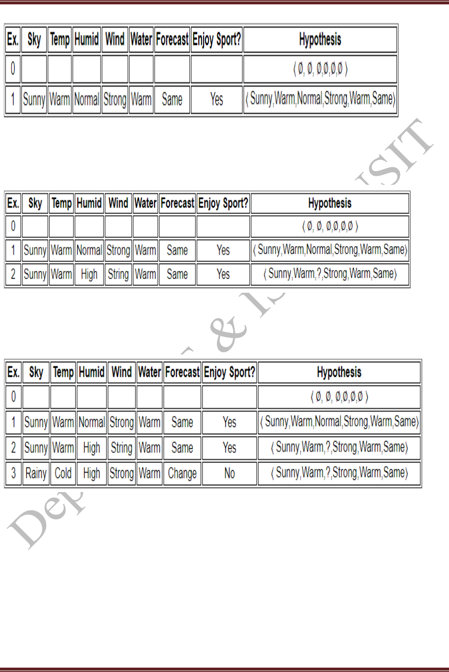
The steps of FINDS are given below:
Step1: The first step of FIND-S is to initialize h to the most specific hypothesis in H
h0 {ɸ, ɸ, ɸ, ɸ, ɸ, ɸ }
Step 2: Positive training example x1= <Sunny, Warm, Normal, Strong, Warm, Same>
h1 <Sunny, Warm, Normal, Strong, Warm, Same>
MACHINE LEARNING LABORATORY-15CSL76
Department of CSE and ISE, RNSIT Page 4
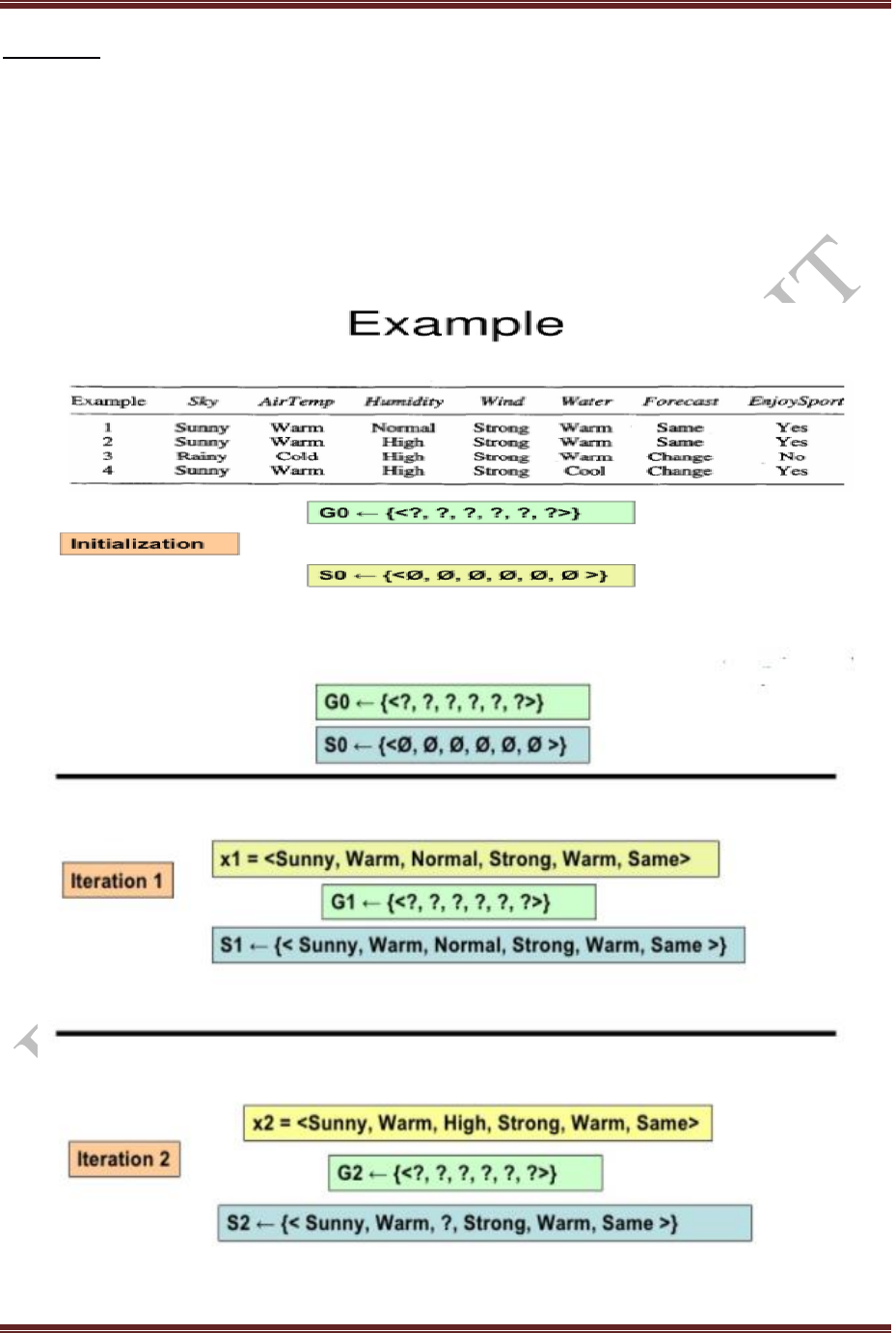
Step 3: Positive training instance x2= <Sunny, Warm, High, Strong, Warm, Same>
h2 <Sunny, Warm,?, Strong, Warm, Same>
Step 4: Negative training example x3= <Rainy, Cold, High, Strong, Warm, Change>
h3 <Sunny, Warm,? , Strong, Warm, Same>
Step 5: Positive training example x4= <Sunny,Warm, High, Strong, Cool, change>
h4 <Sunny, Warm,? , Strong, ?, ?>

MACHINE LEARNING LABORATORY-15CSL76
Department of CSE and ISE, RNSIT Page 5
Find-s Algorithm:
Step 1: Initialize h to the most specific hypothesis in H.
Step 2: For each positive training instance x.
For each attribute constraint ai in h
If the constraint ai is satisfied by x
Then do nothing
Else replace ai in h by the next more general constraint that is satisfied
by x.
Step 3: Output hypothesis h.
Find-s in Python:
import csv
#!usr/bin/python
#list creatin
hypo=['%','%','%','%','%','%'];
with open('Training_examples.csv') as csv_file:
readcsv = csv.reader(csv_file, delimiter=',')
print(readcsv)
data = []
print("\nThe given training examples are:")
for row in readcsv:
print(row)
if row[len(row)-1].upper() == "YES":
data.append(row)
print("\nThe positive examples are:");
for x in data:
print(x);
print("\n");

MACHINE LEARNING LABORATORY-15CSL76
Department of CSE and ISE, RNSIT Page 6
TotalExamples = len(data);
i=0;
j=0;
k=0;
print("The steps of the Find-s algorithm are\n",hypo);
list = [];
p=0;
d=len(data[p])-1;
for j in range(d):
list.append(data[i][j]);
hypo=list;
i=1;
for i in range(TotalExamples):
for k in range(d):
if hypo[k]!=data[i][k]:
hypo[k]='?';
k=k+1;
else:
hypo[k];
print(hypo);
i=i+1;
print("\nThe maximally specific Find-s hypothesis for the given training examples is");
list=[];
for i in range(d):
list.append(hypo[i]);
print(list);
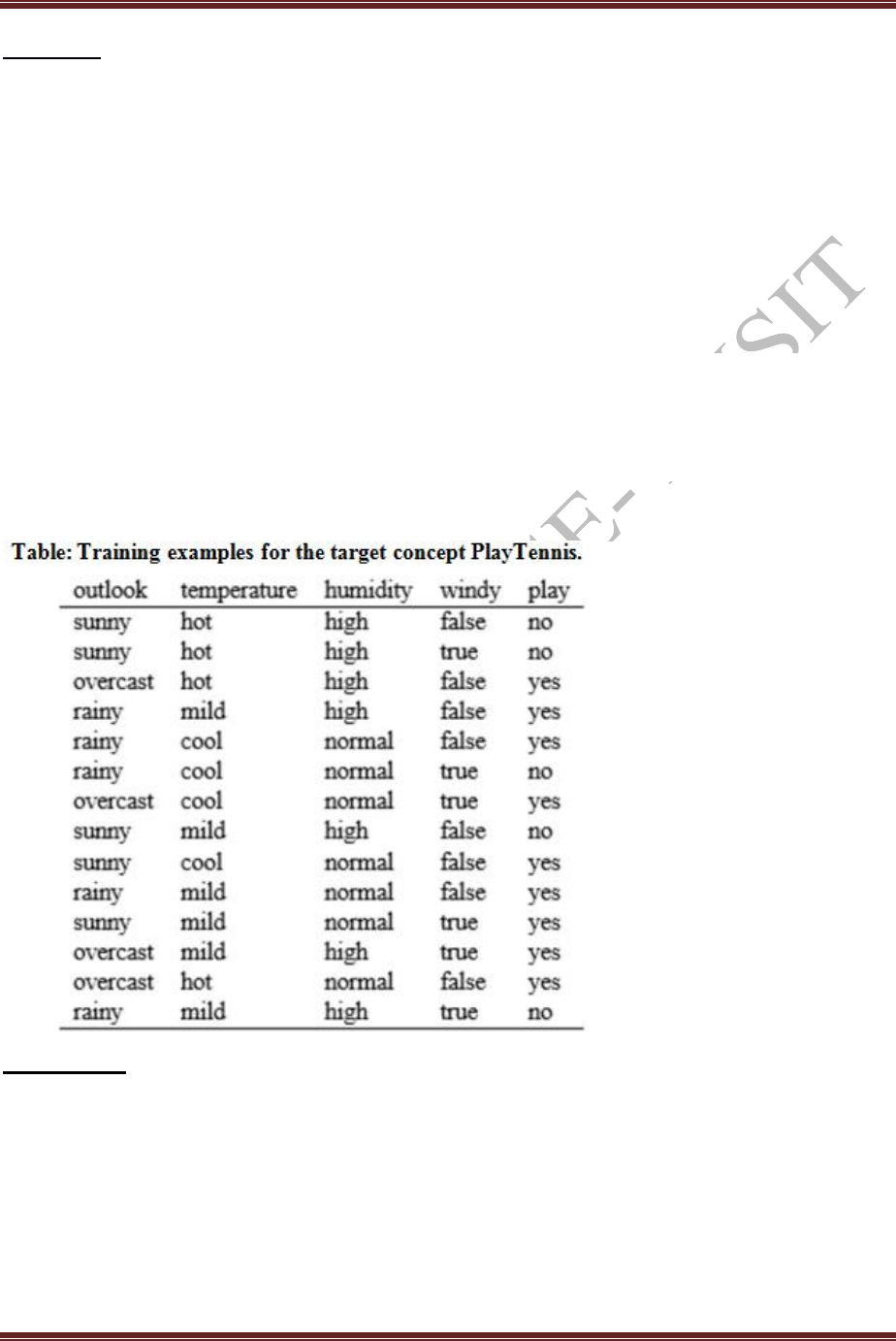
Input csv file:
Training_examples.csv
Output:
The given training examples are:
['Sunny', 'Warm', 'Normal', 'Strong', 'Warm', 'Same', 'Yes']
['Sunny', 'Warm', 'High', 'Strong', 'Warm', 'Same', 'Yes']
['Rainy', 'Cold', 'High', 'Strong', 'Warm', 'Change', 'No']
['Sunny', 'Warm', 'High', 'Strong', 'Cool', 'Change', 'Yes']
The positive examples are:
['Sunny', 'Warm', 'Normal', 'Strong', 'Warm', 'Same', 'Yes']
['Sunny', 'Warm', 'High', 'Strong', 'Warm', 'Same', 'Yes']
['Sunny', 'Warm', 'High', 'Strong', 'Cool', 'Change', 'Yes']

MACHINE LEARNING LABORATORY-15CSL76
Department of CSE and ISE, RNSIT Page 7
The steps of the Find-s algorithm are
['%', '%', '%', '%', '%', '%']
['Sunny', 'Warm', 'Normal', 'Strong', 'Warm', 'Same']
['Sunny', 'Warm', '?', 'Strong', 'Warm', 'Same']
['Sunny', 'Warm', '?', 'Strong', '?', '?']
The maximally specific Find-s hypothesis for the given training examples is
['Sunny', 'Warm', '?', 'Strong', '?', '?']
MACHINE LEARNING LABORATORY-15CSL76
Department of CSE and ISE, RNSIT Page 8
Program 2
For a given set of training data examples stored in a .CSV file, implement and demonstrate the
Candidate-Elimination algorithm to output a description of the set of all hypotheses consistent
with the training examples.
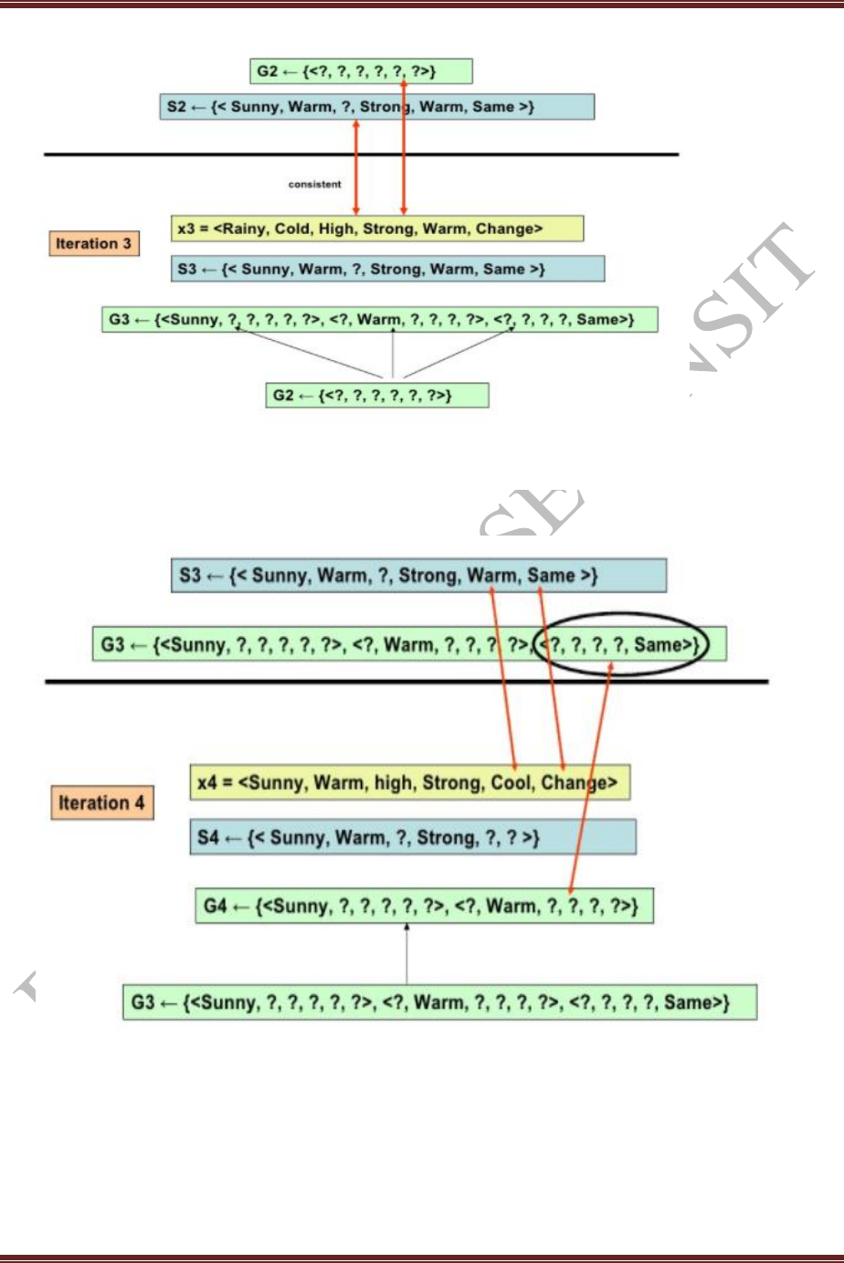
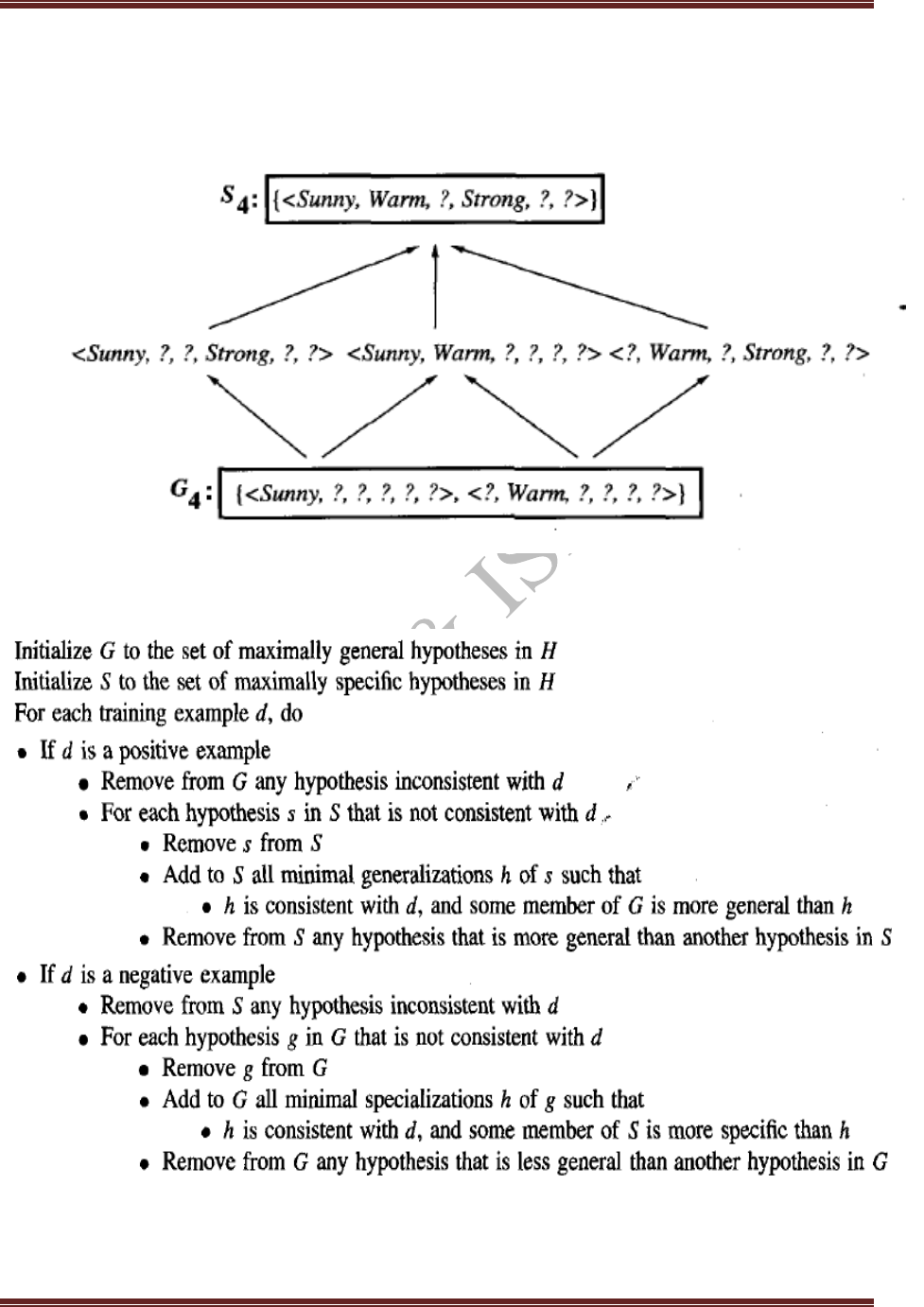
Task: The CANDIDATE-ELIMINATION algorithm computes the version space containing all
hypotheses from H that are consistent with an observed sequence of training examples.
Dataset: EnjoySport training examples
MACHINE LEARNING LABORATORY-15CSL76
Department of CSE and ISE, RNSIT Page 9
MACHINE LEARNING LABORATORY-15CSL76
Department of CSE and ISE, RNSIT Page 10
Candidate-Elimination Algorithm:
Final version space

MACHINE LEARNING LABORATORY-15CSL76
Department of CSE and ISE, RNSIT Page 11
Candidate-Elimiation in Python:
class Holder:
factors={} #Initialize an empty dictionary
attributes = () #declaration of dictionaries parameters with an arbitrary length
'''
Constructor of class Holder holding two parameters,
self refers to the instance of the class
'''
def __init__(self,attr): #
self.attributes = attr
for i in attr:
self.factors[i]=[]
def add_values(self,factor,values):
self.factors[factor]=values
class CandidateElimination:
Positive={} #Initialize positive empty dictionary
Negative={} #Initialize negative empty dictionary
def __init__(self,data,fact):
self.num_factors = len(data[0][0])
self.factors = fact.factors
self.attr = fact.attributes
self.dataset = data
#print self.attr

MACHINE LEARNING LABORATORY-15CSL76
Department of CSE and ISE, RNSIT Page 12
def run_algorithm(self):
# print self.dataset
'''
Initialize the specific and general boundaries, and loop the dataset against the algorithm
'''
G = self.initializeG()
S = self.initializeS()
print("initialize General",G)
print("initialize Specific",S)
'''
Programmatically populate list in the iterating variable trial_set
'''
#count=0
for trial_set in self.dataset:
if self.is_positive(trial_set): #if trial set/example consists of positive examples
G = self.remove_inconsistent_G(G,trial_set[0]) #remove inconsitent data from the general
boundary
S_new = S[:] #initialize the dictionary with no key-value pair
print(S_new)
for s in S:
if not self.consistent(s,trial_set[0]):
S_new.remove(s)
generalization = self.generalize_inconsistent_S(s,trial_set[0])
generalization = self.get_general(generalization,G)
if generalization:
S_new.append(generalization)

MACHINE LEARNING LABORATORY-15CSL76
Department of CSE and ISE, RNSIT Page 13
S = S_new[:]
S = self.remove_more_general(S)
print(S)
else:#if it is negative
S = self.remove_inconsistent_S(S,trial_set[0]) #remove inconsitent data from the specific
boundary
G_new = G[:] #initialize the dictionary with no key-value pair (dataset can take any value)
print(G_new)
for g in G:
if self.consistent(g,trial_set[0]):
G_new.remove(g)
specializations = self.specialize_inconsistent_G(g,trial_set[0])
specializationss = self.get_specific(specializations,S)
if specializations != []:
G_new += specializations
G = G_new[:]
print(G)
G = self.remove_more_specific(G)
print(S)
print(G)
def initializeS(self):
''' Initialize the specific boundary '''
S = tuple(['-' for factor in range(self.num_factors)]) #6 constraints in the vector
return [S]
def initializeG(self):
''' Initialize the general boundary '''

MACHINE LEARNING LABORATORY-15CSL76
Department of CSE and ISE, RNSIT Page 14
G = tuple(['?' for factor in range(self.num_factors)]) # 6 constraints in the vector
return [G]
def is_positive(self,trial_set):
''' Check if a given training trial_set is positive '''
if trial_set[1] == 'Y':
return True
elif trial_set[1] == 'N':
return False
else:
raise TypeError("invalid target value")
def is_negative(self,trial_set):
''' Check if a given training trial_set is negative '''
if trial_set[1] == 'N':
return False
elif trial_set[1] == 'Y':
return True
else:
raise TypeError("invalid target value")
def match_factor(self,value1,value2):
''' Check for the factors values match,
necessary while checking the consistency of
training trial_set with the hypothesis '''
if value1 == '?' or value2 == '?':
return True

MACHINE LEARNING LABORATORY-15CSL76
Department of CSE and ISE, RNSIT Page 15
elif value1 == value2 :
return True
return False
def consistent(self,hypothesis,instance):
''' Check whether the instance is part of the hypothesis '''
for i,factor in enumerate(hypothesis):
if not self.match_factor(factor,instance[i]):
return False
return True
def remove_inconsistent_G(self,hypotheses,instance):
''' For a positive trial_set, the hypotheses in G
inconsistent with it should be removed '''
G_new = hypotheses[:]
for g in hypotheses:
if not self.consistent(g,instance):
G_new.remove(g)
return G_new
def remove_inconsistent_S(self,hypotheses,instance):
''' For a negative trial_set, the hypotheses in S
inconsistent with it should be removed '''
S_new = hypotheses[:]
for s in hypotheses:
if self.consistent(s,instance):
S_new.remove(s)

MACHINE LEARNING LABORATORY-15CSL76
Department of CSE and ISE, RNSIT Page 16
return S_new
def remove_more_general(self,hypotheses):
''' After generalizing S for a positive trial_set, the hypothesis in S
general than others in S should be removed '''
S_new = hypotheses[:]
for old in hypotheses:
for new in S_new:
if old!=new and self.more_general(new,old):
S_new.remove[new]
return S_new
def remove_more_specific(self,hypotheses):
''' After specializing G for a negative trial_set, the hypothesis in G
specific than others in G should be removed '''
G_new = hypotheses[:]
for old in hypotheses:
for new in G_new:
if old!=new and self.more_specific(new,old):
G_new.remove[new]
return G_new
def generalize_inconsistent_S(self,hypothesis,instance):
''' When a inconsistent hypothesis for positive trial_set is seen in the specific boundary S,
it should be generalized to be consistent with the trial_set ... we will get one hypothesis'''
hypo = list(hypothesis) # convert tuple to list for mutability

MACHINE LEARNING LABORATORY-15CSL76
Department of CSE and ISE, RNSIT Page 17
for i,factor in enumerate(hypo):
if factor == '-':
hypo[i] = instance[i]
elif not self.match_factor(factor,instance[i]):
hypo[i] = '?'
generalization = tuple(hypo) # convert list back to tuple for immutability
return generalization
def specialize_inconsistent_G(self,hypothesis,instance):
''' When a inconsistent hypothesis for negative trial_set is seen in the general boundary G
should be specialized to be consistent with the trial_set.. we will get a set of hypotheses '''
specializations = []
hypo = list(hypothesis) # convert tuple to list for mutability
for i,factor in enumerate(hypo):
if factor == '?':
values = self.factors[self.attr[i]]
for j in values:
if instance[i] != j:
hyp=hypo[:]
hyp[i]=j
hyp=tuple(hyp) # convert list back to tuple for immutability
specializations.append(hyp)
return specializations
def get_general(self,generalization,G):
''' Checks if there is more general hypothesis in G

MACHINE LEARNING LABORATORY-15CSL76
Department of CSE and ISE, RNSIT Page 18
for a generalization of inconsistent hypothesis in S
in case of positive trial_set and returns valid generalization '''
for g in G:
if self.more_general(g,generalization):
return generalization
return None
def get_specific(self,specializations,S):
''' Checks if there is more specific hypothesis in S
for each of hypothesis in specializations of an
inconsistent hypothesis in G in case of negative trial_set
and return the valid specializations'''
valid_specializations = []
for hypo in specializations:
for s in S:
if self.more_specific(s,hypo) or s==self.initializeS()[0]:
valid_specializations.append(hypo)
return valid_specializations
def exists_general(self,hypothesis,G):
'''Used to check if there exists a more general hypothesis in
general boundary for version space'''
for g in G:
if self.more_general(g,hypothesis):

MACHINE LEARNING LABORATORY-15CSL76
Department of CSE and ISE, RNSIT Page 19
return True
return False
def exists_specific(self,hypothesis,S):
'''Used to check if there exists a more specific hypothesis in
general boundary for version space'''
for s in S:
if self.more_specific(s,hypothesis):
return True
return False
def get_version_space(self,specific,general):
''' Given the specific and the general boundary of the
version space, evaluate the version space in between '''
while get_order(VS):
for hypothesis in VS[:]:
hypo = list(hypothesis) # convert tuple to list for mutability
for i,factor in enumerate(hypo):
if factor != '?':
hyp=hypo[:]
hyp[i]='?'
if self.exists_general(hyp,general)and self.exists_specific(hyp,specific):
VS.append(tuple(hyp))
return VS

MACHINE LEARNING LABORATORY-15CSL76
Department of CSE and ISE, RNSIT Page 20
def get_order(self,hypothesis):
pass
def more_general(self,hyp1,hyp2):
''' Check whether hyp1 is more general than hyp2 '''
hyp = list(zip(hyp1,hyp2))
for i,j in hyp:
if i == '?':
continue
elif j == '?':
if i != '?':
return False
elif i != j:
return False
else:
continue
return True
def more_specific(self,hyp1,hyp2):
''' hyp1 more specific than hyp2 is
equivalent to hyp2 being more general than hyp1 '''
return self.more_general(hyp2,hyp1)
dataset=[(('sunny','warm','normal','strong','warm','same'),'Y'),(('sunny','warm','high','strong','warm','same'
),'Y'),(('rainy','cold','high','strong','warm','change'),'N'),(('sunny','warm','high','strong','cool','change'),'Y')]

MACHINE LEARNING LABORATORY-15CSL76
Department of CSE and ISE, RNSIT Page 21
#print((dataset[0][1]))
attributes =('Sky','Temp','Humidity','Wind','Water','Forecast')
f = Holder(attributes)
f.add_values('Sky',('sunny','rainy','cloudy')) #sky can be sunny rainy or cloudy
f.add_values('Temp',('cold','warm')) #Temp can be sunny cold or warm
f.add_values('Humidity',('normal','high')) #Humidity can be normal or high
f.add_values('Wind',('weak','strong')) #wind can be weak or strong
f.add_values('Water',('warm','cold')) #water can be warm or cold
f.add_values('Forecast',('same','change')) #Forecast can be same or change
a = CandidateElimination(dataset,f)
#pass the dataset to the algorithm class and call the run algoritm method
a.run_algorithm()
Output
['Sunny' 'Warm' 'Normal' 'Strong' 'Warm' 'Same']
[['?', '?', '?', '?', '?', '?'], ['?', '?', '?', '?', '?', '?'], ['?', '?', '?', '?', '?', '?'], ['?', '?', '?', '?', '?', '?'], ['?', '?', '?', '?', '?',
'?'], ['?', '?', '?', '?', '?', '?']]
0
['Sunny' 'Warm' 'Normal' 'Strong' 'Warm' 'Same']
[['?', '?', '?', '?', '?', '?'], ['?', '?', '?', '?', '?', '?'], ['?', '?', '?', '?', '?', '?'], ['?', '?', '?', '?', '?', '?'], ['?', '?', '?', '?', '?',
'?'], ['?', '?', '?', '?', '?', '?']]
1
['Sunny' 'Warm' '?' 'Strong' 'Warm' 'Same']
[['?', '?', '?', '?', '?', '?'], ['?', '?', '?', '?', '?', '?'], ['?', '?', '?', '?', '?', '?'], ['?', '?', '?', '?', '?', '?'], ['?', '?', '?', '?', '?',
'?'], ['?', '?', '?', '?', '?', '?']]
2
['Sunny' 'Warm' '?' 'Strong' 'Warm' 'Same']

MACHINE LEARNING LABORATORY-15CSL76
Department of CSE and ISE, RNSIT Page 22
[['Sunny', '?', '?', '?', '?', '?'], ['?', 'Warm', '?', '?', '?', '?'], ['?', '?', '?', '?', '?', '?'], ['?', '?', '?', '?', '?', '?'], ['?', '?',
'?', '?', '?', '?'], ['?', '?', '?', '?', '?', 'Same']]
3
['Sunny' 'Warm' '?' 'Strong' '?' '?']
[['Sunny', '?', '?', '?', '?', '?'], ['?', 'Warm', '?', '?', '?', '?'], ['?', '?', '?', '?', '?', '?'], ['?', '?', '?', '?', '?', '?'], ['?', '?',
'?', '?', '?', '?'], ['?', '?', '?', '?', '?', '?']]
Final S:
['Sunny' 'Warm' '?' 'Strong' '?' '?']
Final G:
[['Sunny', '?', '?', '?', '?', '?'], ['?', 'Warm', '?', '?', '?', '?']]
Process finished with exit code 0
MACHINE LEARNING LABORATORY-15CSL76
Department of CSE and ISE, RNSIT Page 23
Program 3
Write a program to demonstrate the working of the decision tree based ID3 algorithm. Use an
appropriate data set for building the decision tree and apply this knowledge to classify a new
sample.
Task: ID3 determines the information gain for each candidate attribute (i.e., Outlook,
Temperature, Humidity, and Wind), then selects the one with highest information gain as the
root node of the tree. The information gain values for all four attributes are calculated using the
following formula:
Entropy(S)=∑- P(I).log2P(I)
Gain(S,A)=Entropy(S)-∑ [ P(S/A).Entropy(S/A) ]
Dataset:
Calculation:
Decision/play column consists of 14 instances and includes two labels: yes and no.
There are 9 decisions labeled yes and 5 decisions labeled no.
Entropy[Decision] = -P(yes).log2P(yes) – P(no).log2P(no)
= - (9/14).log2(9/14) – (5/14).log2(5/14)

MACHINE LEARNING LABORATORY-15CSL76
Department of CSE and ISE, RNSIT Page 24
= 0.940
Now, we need to find out the most dominant factor for decision.
1) Wind factor on decision:
Gain(Decision,wind)= Entropy(Decision) - ∑ [ P(Decision/Wind]. Entropy(Decision/Wind) ]
Wind attribute has two labels : Weak and Strong
Gain(Decision,Wind)= Entropy(Decision) – [P(Decision/Wind=Weak).
Entropy(Decision/Wind=Weak)] - [[P(Decision/Wind=strong).
Entropy(Decision/Wind=strong)]
There are 8 instances for weak. In that decision of 2 items are no and 6 items are yes.
Entropy[Decision/Wind= Weak] = -P[no].log2P(no) – p(yes).log2P(yes)
= -[2/8].log2(2/8) – [6/8].log2(6/8)
= 0.811
Entropy[Decision/Wind= Strong] = -P[no].log2P(no) – p(yes).log2P(yes)
= -[3/6].log2(3/6) – [3/6].log2(3/6)
= 1
Note: There are 6 instances for strong. In that decisionof 3 items are yes and 3 items
are no.
Gain(Decision,Wind) = 0.940 – [(8/14).0.811] – [(6/14).1]
= 0.048
Similarly calculate gain for other factors:
2) Outlook factor on decision:
1 ) Gain(Decision,outlook) = Entropy (decision) - ∑ [ P ( Decision /Outlook).
Entropy(Decision/Outlook)]
outlook has three parameters : Sunny, Overcast, and rain
Gain(Decision,outlook) = Entropy(decision)-
[P(Decision/Outlook=Sunny).Entropy(Decision/Outlook=Sunny)]-[
P(Decision/Outlook=overcast).Entropy(Decision/Outlook=overcast)]-
[P(P(Decision/Outlook=Rain).Entropy(Decision/Outlook=Rain)]

MACHINE LEARNING LABORATORY-15CSL76
Department of CSE and ISE, RNSIT Page 25
Sunny Overcast: Rain:
Instances: 5 Instances:4 Instances:5
yes:2 yes:4 yes:3
No:3 No: - No: 2
1) Entropy[Decision/Outlook= Sunny] = -P[no].log2P(no) – p(yes).log2P(yes)
=0.97094
2) Entropy[Decision/Outlook= Overcast] = -P[no].log2P(no) – p(yes).log2P(yes)
= 0
3) Entropy[Decision/Wind= Rain] = -P[no].log2P(no) – p(yes).log2P(yes)
=0.9708
Gain(Decision,Outlook)= 0.940-(5/14)(0.9709)-(4/14)(0)-(5/14)(0.9708)
=0.2473
3) Temperature factor on decision:
Gain(Decision,Temperature) = Entropy(decision)-
∑[P(Decision/Temperature).Entropy(Decision/Temperature)]
Temperature has 3 parameters: hot, mild, cool
Gain(Decision,Temp) = Entropy(decision)-
[P(Decision/Temp=hot).Entropy(Decision/Temp=hot)]-[
P(Decision/Temp=mild).Entropy(Decision/Temp=mild)]-
[P(P(Decision/Temp=cool).Entropy( Decision/Temp=cool)]
Hot Mild: cool:
Instances:4 Instances:6 Instances:4
Yes:2 Yes: Yes:3
No:2 No: 2 No:1
Entropy[Decision/Temp= hot] = -P[no].log2P(no) – p(yes).log2P(yes)
= 1
Entropy[Decision/Temp= mild] = -P[no].log2P(no) – p(yes).log2P(yes)
=0.9182
Entropy[Decision/Temp= cool] = -P[no].log2P(no) – p(yes).log2P(yes)

MACHINE LEARNING LABORATORY-15CSL76
Department of CSE and ISE, RNSIT Page 26
=0.8112
Gain(Decision,Temp) = 0.940 - (4/14)(1) - (6/14)(0.9182) - (4/14)(0.8112)
= 0.0291
4) Humidity factor on decision:
Gain(Decision,Humidity) = Entropy(decision)-
∑[P(Decision/Humidity).Entropy(Decision/Humidity)]
Humidity has 2 factors: high and normal
Gain(Decision,humidity) = Entropy(decision)-
[P(Decision/humidity=high).Entropy(Decision/humidity=high]-[
P(Decision/humidity=normal).Entropy(Decision/humidity=normal)]
High Normal:
Instances:7 Instances:7
Yes:3 Yes:6
No:4 No: 1
Entropy[Decision/ humidity= high] = -P[no].log2P(no) – p(yes).log2P(yes)
= 0.9851
Entropy[Decision/humidity= normal] = -P[no].log2P(no) – p(yes).log2P(yes)
= 0.5916
Gain(Decision, Humidity)= 0.940 - (7/14)(0.9851) - (7/14)(0.5916)
= 0.1517
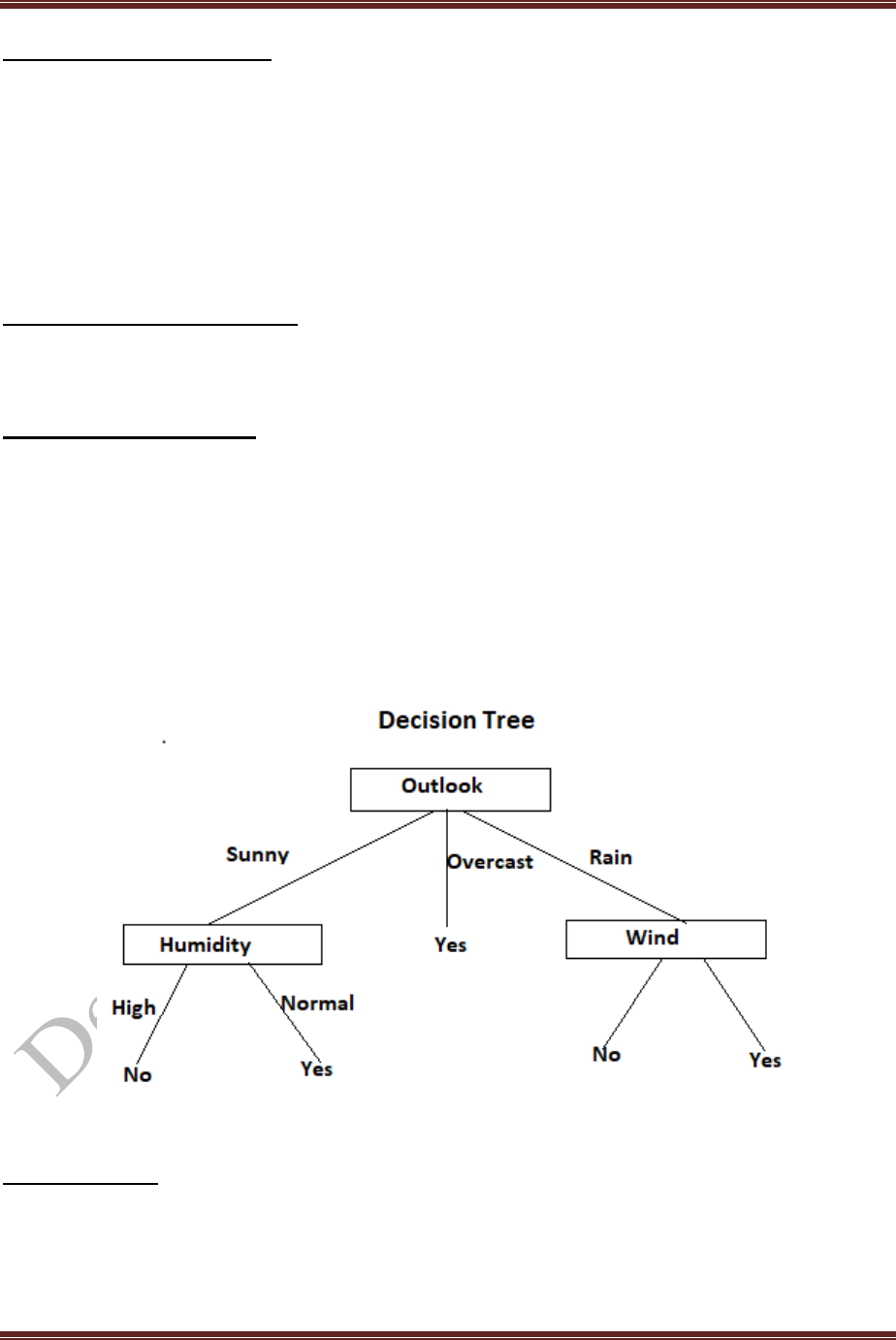
Thus the outlook factor on decision produces the highest score. That’s why outlook decision
will appear in the root node of the tree. Since Outlook has three possible values, the root node
has three branches (sunny, overcast, rain). The next question is "what attribute should be tested
at the Sunny branch node?" Since we have used Outlook at the root, we only decide on the
remaining three attributes: Humidity, Temperature, or Wind.
Now calculate sunny outlook on decision, overcast outlook on decision, and rain outlook
on decision to generate the decision tree.
MACHINE LEARNING LABORATORY-15CSL76
Department of CSE and ISE, RNSIT Page 27
Sunny outlook on decision:
5 instances of sunny : In that 3 instances are NO and 2 instances are YES
Gain( Outlook = Sunny/Temp)= 0.570
Gain ( Outlook = Sunny/Humidity) = 0.970
Gain ( Outlook = Sunny/ Wind) = 0.019
Since humidity produces the highest score, if outlook were Sunny.
Overcast outlook on decision:
Decision will always be yes, if outlook were overcast.
Rain outlook on decision:
5 instances of rain : In that 3 instances are YES and 2 instances are NO.
Gain( Outlook= Rain/Temp)
Gain( Outlook= Rain/Humidity)
Gain( Outlook= Rain/Wind)
Here, wind produces the highest score . And wind has two attributes namely strong and weak.
ID3 Algorithm:
ID3(Examples, Target_attribute, Attributes)

MACHINE LEARNING LABORATORY-15CSL76
Department of CSE and ISE, RNSIT Page 28
Examples are the training examples. Target_attribute is the
attribute whose value is to be predicted by the tree. Attributes is
a list of other attributes that may be tested by the learned
decision tree. Returns a decision tree that correctly classifies the
given Examples.
o Create a Root node for the tree
o If all Examples are positive, Return the single-node tree Root, with label = +
o If all Examples are negative, Return the single-node tree Root, with label = -
o If Attributes is empty, Return the single-node tree Root, with label = most
common value of Target_attribute in Examples
o Otherwise Begin
A ← the attribute from Attributes that best* classifies Examples
The decision attribute for Root ←A
For each possible value, υi, of A,
Add a new tree branch below Root, corresponding to the test A = υi
Let Examplesυi ,be the subset of Examples that have value υi for A
If Examplesυi, is empty
Then below this new branch add a leaf node with label=most common value
of Target_attribute in Examples
Else below this new branch add the subtree
ID3(Examplesυi,Target_attribute, Attributes–{A}))
End
Return Root
ID3 in Python:
import ast
import csv
import sys
import math
import os
def load_csv_to_header_data(filename):
path = os.path.normpath(os.getcwd() + filename)
fs = csv.reader(open(path))

MACHINE LEARNING LABORATORY-15CSL76
Department of CSE and ISE, RNSIT Page 29
all_row = []
for r in fs:
all_row.append(r)
headers = all_row[0]
idx_to_name, name_to_idx = get_header_name_to_idx_maps(headers)
data = {
'header': headers,
'rows': all_row[1:],
'name_to_idx': name_to_idx,
'idx_to_name': idx_to_name
}
return data
def get_header_name_to_idx_maps(headers):
name_to_idx = {}
idx_to_name = {}
for i in range(0, len(headers)):
name_to_idx[headers[i]] = i
idx_to_name[i] = headers[i]
return idx_to_name, name_to_idx
def project_columns(data, columns_to_project):
data_h = list(data['header'])
data_r = list(data['rows'])
all_cols = list(range(0, len(data_h)))
columns_to_project_ix = [data['name_to_idx'][name] for name in
columns_to_project]
columns_to_remove = [cidx for cidx in all_cols if cidx not in
columns_to_project_ix]
for delc in sorted(columns_to_remove, reverse=True):
del data_h[delc]
for r in data_r:
del r[delc]

MACHINE LEARNING LABORATORY-15CSL76
Department of CSE and ISE, RNSIT Page 30
idx_to_name, name_to_idx = get_header_name_to_idx_maps(data_h)
return {'header': data_h, 'rows': data_r,
'name_to_idx': name_to_idx,
'idx_to_name': idx_to_name}
def get_uniq_values(data):
idx_to_name = data['idx_to_name']
idxs = idx_to_name.keys()
val_map = {}
for idx in iter(idxs):
val_map[idx_to_name[idx]] = set()
for data_row in data['rows']:
for idx in idx_to_name.keys():
att_name = idx_to_name[idx]
val = data_row[idx]
if val not in val_map.keys():
val_map[att_name].add(val)
return val_map
def get_class_labels(data, target_attribute):
rows = data['rows']
col_idx = data['name_to_idx'][target_attribute]
labels = {}
for r in rows:
val = r[col_idx]
if val in labels:
labels[val] = labels[val] + 1
else:
labels[val] = 1
return labels
def entropy(n, labels):
ent = 0
for label in labels.keys():
p_x = labels[label] / n

MACHINE LEARNING LABORATORY-15CSL76
Department of CSE and ISE, RNSIT Page 31
ent += - p_x * math.log(p_x, 2)
return ent
def partition_data(data, group_att):
partitions = {}
data_rows = data['rows']
partition_att_idx = data['name_to_idx'][group_att]
for row in data_rows:
row_val = row[partition_att_idx]
if row_val not in partitions.keys():
partitions[row_val] = {
'name_to_idx': data['name_to_idx'],
'idx_to_name': data['idx_to_name'],
'rows': list()
}
partitions[row_val]['rows'].append(row)
return partitions
def avg_entropy_w_partitions(data, splitting_att, target_attribute):
# find uniq values of splitting att
data_rows = data['rows']
n = len(data_rows)
partitions = partition_data(data, splitting_att)
avg_ent = 0
for partition_key in partitions.keys():
partitioned_data = partitions[partition_key]
partition_n = len(partitioned_data['rows'])
partition_labels = get_class_labels(partitioned_data, target_attribute)
partition_entropy = entropy(partition_n, partition_labels)
avg_ent += partition_n / n * partition_entropy
return avg_ent, partitions
def most_common_label(labels):
mcl = max(labels, key=lambda k: labels[k])
return mcl

MACHINE LEARNING LABORATORY-15CSL76
Department of CSE and ISE, RNSIT Page 32
def id3(data, uniqs, remaining_atts, target_attribute):
labels = get_class_labels(data, target_attribute)
node = {}
if len(labels.keys()) == 1:
node['label'] = next(iter(labels.keys()))
return node
if len(remaining_atts) == 0:
node['label'] = most_common_label(labels)
return node
n = len(data['rows'])
ent = entropy(n, labels)
max_info_gain = None
max_info_gain_att = None
max_info_gain_partitions = None
for remaining_att in remaining_atts:
avg_ent, partitions = avg_entropy_w_partitions(data, remaining_att,
target_attribute)
info_gain = ent - avg_ent
if max_info_gain is None or info_gain > max_info_gain:
max_info_gain = info_gain
max_info_gain_att = remaining_att
max_info_gain_partitions = partitions
if max_info_gain is None:
node['label'] = most_common_label(labels)
return node
node['attribute'] = max_info_gain_att
node['nodes'] = {}
remaining_atts_for_subtrees = set(remaining_atts)
remaining_atts_for_subtrees.discard(max_info_gain_att)
uniq_att_values = uniqs[max_info_gain_att]

MACHINE LEARNING LABORATORY-15CSL76
Department of CSE and ISE, RNSIT Page 33
for att_value in uniq_att_values:
if att_value not in max_info_gain_partitions.keys():
node['nodes'][att_value] = {'label': most_common_label(labels)}
continue
partition = max_info_gain_partitions[att_value]
node['nodes'][att_value] = id3(partition, uniqs, remaining_atts_for_subtrees,
target_attribute)
return node
def load_config(config_file):
with open(config_file, 'r') as myfile:
data = myfile.read().replace('\n', '')
return ast.literal_eval(data)
def pretty_print_tree(root):
stack = []
rules = set()
def traverse(node, stack, rules):
if 'label' in node:
stack.append(' THEN ' + node['label'])
rules.add(''.join(stack))
stack.pop()
elif 'attribute' in node:
ifnd = 'IF ' if not stack else ' AND '
stack.append(ifnd + node['attribute'] + ' EQUALS ')
for subnode_key in node['nodes']:
stack.append(subnode_key)
traverse(node['nodes'][subnode_key], stack, rules)
stack.pop()
stack.pop()
traverse(root, stack, rules)
print(os.linesep.join(rules))
def main():
argv ='tennis.cfg'
MACHINE LEARNING LABORATORY-15CSL76
Department of CSE and ISE, RNSIT Page 34
print("Command line args are {}: ".format(argv))
config = load_config(argv)
data = load_csv_to_header_data(config['data_file'])
data = project_columns(data, config['data_project_columns'])
target_attribute = config['target_attribute']
remaining_attributes = set(data['header'])
remaining_attributes.remove(target_attribute)
uniqs = get_uniq_values(data)
root = id3(data, uniqs, remaining_attributes, target_attribute)
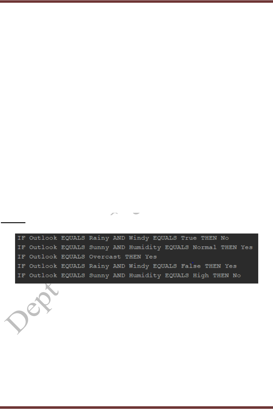
pretty_print_tree(root)
if __name__ == "__main__": main()
Output:

MACHINE LEARNING LABORATORY-15CSL76
Department of CSE and ISE, RNSIT Page 35
Program 4:
Build an Artificial Neural Network by implementing the Back propagation algorithm and
test the same using appropriate data set
Back propagation Algorithm
The Backpropagation algorithm is a supervised learning method for multilayer feed-forward
networks from the field of Artificial Neural Networks, the backpropagation algorithm is a method
for training the weights in a multilayer feed-forward neural network. As such, it requires a network
structure to be defined of one or more layers where one layer is fully connected to the next layer.
A standard network structure is one input layer, one hidden layer, and one output layer.
Backpropagation can be used for both classification and regression problems.
Wheat Seeds Dataset
The seeds dataset involves the prediction of species given measurements seeds from different
varieties of wheat. There are 201 records and 7 numerical input variables. It is a classification
problem with 3 output classes. The scale for each numeric input value vary, so some data
normalization may be required for use with algorithms that weight inputs like the backpropagation
algorithm.
Below is a sample of the first 5 rows of the dataset
1
2
3
4
5
15.26,14.84,0.871,5.763,3.312,2.221,5.22,1
14.88,14.57,0.8811,5.554,3.333,1.018,4.956,1
14.29,14.09,0.905,5.291,3.337,2.699,4.825,1
13.84,13.94,0.8955,5.324,3.379,2.259,4.805,1
16.14,14.99,0.9034,5.658,3.562,1.355,5.175,1
You can download the seeds dataset from the UCI Machine Learning Repository.
Download the seeds dataset and place it into your current working directory with the filename
seeds_dataset.csv.
The dataset is in tab-separated format, so you must convert it to CSV using a text editor or a
spreadsheet program.
Working of algorithm:
1. Initialize Network.
2. Forward Propagate.
3. Back Propagate Error.
4. Train the network
1. Initialize Network
Initialize the network weights to small random numbers in the range of 0 to 1. Below is a function
named initialize_network() that creates a new neural network ready for training. It accepts three
parameters, the number of inputs, the number of neurons to have in the hidden layer and the number of
outputs.

MACHINE LEARNING LABORATORY-15CSL76
Department of CSE and ISE, RNSIT Page 36
The hidden layer we create n_hidden neurons and each neuron in the hidden layer has n_inputs + 1
weights, one for each input column in a dataset and an additional one for the bias. The output layer that
connects to the hidden layer has n_outputs neurons, each with n_hidden + 1 weights. This means that
each neuron in the output layer connects to (has a weight for) each neuron in the hidden layer.
Let’s test out this function. Below is a complete example that creates a small network.
1
2
3
4
5
6
7
8
9
10
11
12
13
14
15
16
from random import seed
from random import random
# Initialize a network
def initialize_network(n_inputs, n_hidden, n_outputs):
network = list()
hidden_layer = [{'weights':[random() for i in range(n_inputs + 1)]} for i in
range(n_hidden)]
network.append(hidden_layer)
output_layer = [{'weights':[random() for i in range(n_hidden + 1)]} for i in
range(n_outputs)]
network.append(output_layer)
return network
seed(1)
network = initialize_network(2, 1, 2)
for layer in network:
print(layer)
Running the example, you can see that the code prints out each layer one by one. You can see the
hidden layer has one neuron with 2 input weights plus the bias. The output layer has 2 neurons, each
with 1 weight plus the bias.
1
2
[{'weights': [0.13436424411240122, 0.8474337369372327, 0.763774618976614]}]
[{'weights': [0.2550690257394217, 0.49543508709194095]}, {'weights':
[0.4494910647887381, 0.651592972722763]}]
Forward Propagate
We can calculate an output from a neural network by propagating an input signal through each layer
until the output layer outputs its values. We call this forward-propagation.
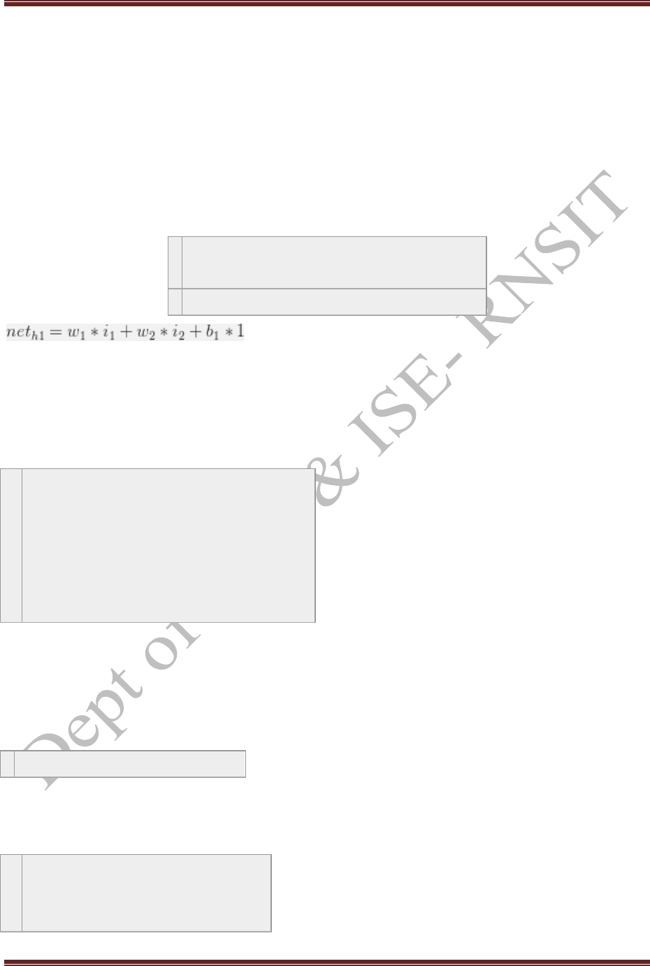
MACHINE LEARNING LABORATORY-15CSL76
Department of CSE and ISE, RNSIT Page 37
We can break forward propagation down into three parts:
Neuron Activation.
Neuron Transfer.
Forward Propagation.
Neuron Activation
The first step is to calculate the activation of one neuron given an input.
The input could be a row from our training dataset, as in the case of the hidden layer. It may also be the
outputs from each neuron in the hidden layer, in the case of the output layer. Neuron activation is
calculated as the weighted sum of the inputs. Much like linear regression.
activation = sum(weight_i * input_i) + bias
Where weight is a network weight, input is an input, i is the index of a weight or an input and bias is a
special weight that has no input to multiply with (or you can think of the input as always being 1.0).
Below is an implementation of this in a function named activate(). You can see that the function
assumes that the bias is the last weight in the list of weights. This helps here and later to make the code
easier to read.
1
2
3
4
5
6
# Calculate neuron activation for an input
def activate(weights, inputs):
activation = weights[-1]
for i in range(len(weights)-1):
activation += weights[i] * inputs[i]
return activation
Neuron Transfer
Once a neuron is activated, we need to transfer the activation to see what the neuron output actually is.
Different transfer functions can be used. It is traditional to use the sigmoid activation function. It is also
a function of which we can easily calculate the derivative (slope) that we will need later when
backpropagating error. We can transfer an activation function using the sigmoid function as follows:
output = 1 / (1 + e^(-activation))
Where e is the base of the natural logarithms (Euler’s number).
Below is a function named transfer() that implements the sigmoid equation.
1
2
3
# Transfer neuron activation
def transfer(activation):
return 1.0 / (1.0 + exp(-activation))

MACHINE LEARNING LABORATORY-15CSL76
Department of CSE and ISE, RNSIT Page 38
Forward Propagation
Forward propagating an input is straightforward. All of the outputs from one layer become inputs to the
neurons on the next layer. Below is a function named forward_propagate() that implements the
forward propagation for a row of data from our dataset with our neural network.
The function returns the outputs from the last layer also called the output layer.
1
2
3
4
5
6
7
8
9
10
11
# Forward propagate input to a network output
def forward_propagate(network, row):
inputs = row
for layer in network:
new_inputs = []
for neuron in layer:
activation = activate(neuron['weights'], inputs)
neuron['output'] = transfer(activation)
new_inputs.append(neuron['output'])
inputs = new_inputs
return inputs
Running the example propagates the input pattern [1, 0] and produces an output value that is printed.
Because the output layer has two neurons, we get a list of two numbers as output.
[0.6629970129852887, 0.7253160725279748]
Back Propagate Error
The backpropagation algorithm is named for the way in which weights are trained. Error is calculated
between the expected outputs and the outputs forward propagated from the network. These errors are
then propagated backward through the network from the output layer to the hidden layer, assigning
blame for the error and updating weights as they go. The math for backpropagating error is rooted in
calculus, but we will remain high level in this section and focus on what is calculated and how rather
than why the calculations take this particular form.
This part is broken down into two sections.
Transfer Derivative.
Error Backpropagation.
Transfer Derivative
Given an output value from a neuron, we need to calculate it’s slope. We are using the sigmoid transfer
function, the derivative of which can be calculated as follows:
1
derivative = output * (1.0 - output)
Below is a function named transfer_derivative() that implements this equation.
1
2
3
# Calculate the derivative of an neuron output
def transfer_derivative(output):
return output * (1.0 - output)

MACHINE LEARNING LABORATORY-15CSL76
Department of CSE and ISE, RNSIT Page 39
Now, let’s see how this can be used.
Error Backpropagation
The first step is to calculate the error for each output neuron, this will give us our error signal (input) to
propagate backwards through the network.
The error for a given neuron can be calculated as follows:
error = (expected - output) * transfer_derivative(output)
Where expected is the expected output value for the neuron, output is the output value for the neuron
and transfer_derivative() calculates the slope of the neuron’s output value, as shown above.
The error signal for a neuron in the hidden layer is calculated as the weighted error of each neuron in
the output layer. Think of the error traveling back along the weights of the output layer to the neurons in
the hidden layer.
The back-propagated error signal is accumulated and then used to determine the error for the neuron in
the hidden layer, as follows:
error = (weight_k * error_j) * transfer_derivative(output)
Where error_j is the error signal from the jth neuron in the output layer, weight_k is the weight that
connects the kth neuron to the current neuron and output is the output for the current neuron.
Below is a function named backward_propagate_error() that implements this procedure. You can see
that the error signal calculated for each neuron is stored with the name ‘delta’. You can see that the
layers of the network are iterated in reverse order, starting at the output and working backwards. This
ensures that the neurons in the output layer have ‘delta’ values calculated first that neurons in the
hidden layer can use in the subsequent iteration. I chose the name ‘delta’ to reflect the change the error
implies on the neuron (e.g. the weight delta). You can see that the error signal for neurons in the hidden
layer is accumulated from neurons in the output layer where the hidden neuron number j is also the
index of the neuron’s weight in the output layer neuron[‘weights’][j].
1
2
3
4
5
6
7
8
9
10
11
12
13
14
15
16
# Backpropagate error and store in neurons
def backward_propagate_error(network, expected):
for i in reversed(range(len(network))):
layer = network[i]
errors = list()
if i != len(network)-1:
for j in range(len(layer)):
error = 0.0
for neuron in network[i + 1]:
error += (neuron['weights'][j] * neuron['delta'])
errors.append(error)
else:
for j in range(len(layer)):
neuron = layer[j]
errors.append(expected[j] - neuron['output'])
for j in range(len(layer)):

MACHINE LEARNING LABORATORY-15CSL76
Department of CSE and ISE, RNSIT Page 40
17
18
neuron = layer[j]
neuron['delta'] = errors[j] * transfer_derivative(neuron['output'])
Running the example prints the network after the backpropagation of error is complete. You can see
that error values are calculated and stored in the neurons for the output layer and the hidden layer.
1
2
[{'output': 0.7105668883115941, 'weights': [0.13436424411240122, 0.8474337369372327,
0.763774618976614], 'delta': -0.0005348048046610517}]
[{'output': 0.6213859615555266, 'weights': [0.2550690257394217, 0.49543508709194095],
'delta': -0.14619064683582808}, {'output': 0.6573693455986976, 'weights':
[0.4494910647887381, 0.651592972722763], 'delta': 0.0771723774346327}]
Now let’s use the backpropagation of error to train the network.
Train Network
The network is trained using stochastic gradient descent. This involves multiple iterations of exposing a
training dataset to the network and for each row of data forward propagating the inputs,
backpropagating the error and updating the network weights.
This part is broken down into two sections:
Update Weights.
Train Network.
Update Weights
Once errors are calculated for each neuron in the network via the back propagation method above, they
can be used to update weights. Network weights are updated as follows:
weight = weight + learning_rate * error * input
Where weight is a given weight, learning_rate is a parameter that you must specify, error is the error
calculated by the backpropagation procedure for the neuron and input is the input value that caused the
error.
Learning rate controls how much to change the weight to correct for the error. Below is a function
named update_weights() that updates the weights for a network given an input row of data, a learning
rate and assume that a forward and backward propagation have already been performed. Remember that
the input for the output layer is a collection of outputs from the hidden layer.
1
2
3
4
5
6
7
8
9
# Update network weights with error
def update_weights(network, row, l_rate):
for i in range(len(network)):
inputs = row[:-1]
if i != 0:
inputs = [neuron['output'] for neuron in network[i - 1]]
for neuron in network[i]:
for j in range(len(inputs)):
neuron['weights'][j] += l_rate * neuron['delta'] * inputs[j]

MACHINE LEARNING LABORATORY-15CSL76
Department of CSE and ISE, RNSIT Page 41
10
neuron['weights'][-1] += l_rate * neuron['delta']
Now we know how to update network weights, let’s see how we can do it repeatedly.
Train Network
As mentioned, the network is updated using stochastic gradient descent. This involves first looping for
a fixed number of epochs and within each epoch updating the network for each row in the training
dataset. Below is a function that implements the training of an already initialized neural network with a
given training dataset, learning rate, fixed number of epochs and an expected number of output values.
The sum squared error between the expected output and the network output is accumulated each epoch
and printed.
1
2
3
4
5
6
7
8
9
10
11
12
# Train a network for a fixed number of epochs
def train_network(network, train, l_rate, n_epoch, n_outputs):
for epoch in range(n_epoch):
sum_error = 0
for row in train:
outputs = forward_propagate(network, row)
expected = [0 for i in range(n_outputs)]
expected[row[-1]] = 1
sum_error += sum([(expected[i]-outputs[i])**2 for i in range(len(expected))])
backward_propagate_error(network, expected)
update_weights(network, row, l_rate)
print('>epoch=%d, lrate=%.3f, error=%.3f' % (epoch, l_rate, sum_error))
ANN in python:
from math import exp
from random import seed
from random import random
# Initialize a network
def initialize_network(n_inputs, n_hidden, n_outputs):
network = list()
hidden_layer = [{'weights':[random() for i in range(n_inputs + 1)]} for i in range(n_hidden)]
network.append(hidden_layer)
output_layer = [{'weights':[random() for i in range(n_hidden + 1)]} for i in range(n_outputs)]

MACHINE LEARNING LABORATORY-15CSL76
Department of CSE and ISE, RNSIT Page 42
network.append(output_layer)
return network
# Calculate neuron activation for an input
def activate(weights, inputs):
activation = weights[-1]
for i in range(len(weights)-1):
activation += weights[i] * inputs[i]
return activation
# Transfer neuron activation
def transfer(activation):
return 1.0 / (1.0 + exp(-activation))
# Forward propagate input to a network output
def forward_propagate(network, row):
inputs = row
for layer in network:
new_inputs = []
for neuron in layer:
activation = activate(neuron['weights'], inputs)
neuron['output'] = transfer(activation)
new_inputs.append(neuron['output'])
inputs = new_inputs
return inputs
# Calculate the derivative of an neuron output
def transfer_derivative(output):
return output * (1.0 - output)
# Backpropagate error and store in neurons
def backward_propagate_error(network, expected):
for i in reversed(range(len(network))):
layer = network[i]
errors = list()
if i != len(network)-1:
for j in range(len(layer)):
error = 0.0
for neuron in network[i + 1]:
error += (neuron['weights'][j] * neuron['delta'])
errors.append(error)
else:
for j in range(len(layer)):
neuron = layer[j]

MACHINE LEARNING LABORATORY-15CSL76
Department of CSE and ISE, RNSIT Page 43
errors.append(expected[j] - neuron['output'])
for j in range(len(layer)):
neuron = layer[j]
neuron['delta'] = errors[j] * transfer_derivative(neuron['output'])
# Update network weights with error
def update_weights(network, row, l_rate):
for i in range(len(network)):
inputs = row[:-1]
if i != 0:
inputs = [neuron['output'] for neuron in network[i - 1]]
for neuron in network[i]:
for j in range(len(inputs)):
neuron['weights'][j] += l_rate * neuron['delta'] * inputs[j]
neuron['weights'][-1] += l_rate * neuron['delta']
# Train a network for a fixed number of epochs
def train_network(network, train, l_rate, n_epoch, n_outputs):
for epoch in range(n_epoch):
sum_error = 0
for row in train:
outputs = forward_propagate(network, row)
expected = [0 for i in range(n_outputs)]
expected[row[-1]] = 1
sum_error += sum([(expected[i]-outputs[i])**2 for i in
range(len(expected))])
backward_propagate_error(network, expected)
update_weights(network, row, l_rate)
print('>epoch=%d, lrate=%.3f, error=%.3f' % (epoch, l_rate, sum_error))
# Test training backprop algorithm
seed(1)
dataset = [[2.7810836,2.550537003,0],
[1.465489372,2.362125076,0],
[3.396561688,4.400293529,0],
[1.38807019,1.850220317,0],
[3.06407232,3.005305973,0],
[7.627531214,2.759262235,1],
[5.332441248,2.088626775,1],
[6.922596716,1.77106367,1],
[8.675418651,-0.242068655,1],
[7.673756466,3.508563011,1]]
n_inputs = len(dataset[0]) - 1
n_outputs = len(set([row[-1] for row in dataset]))

MACHINE LEARNING LABORATORY-15CSL76
Department of CSE and ISE, RNSIT Page 44
network = initialize_network(n_inputs, 2, n_outputs)
train_network(network, dataset, 0.5, 20, n_outputs)
for layer in network:
print(layer)
Output
>epoch=0, lrate=0.500, error=6.350
>epoch=1, lrate=0.500, error=5.531
>epoch=2, lrate=0.500, error=5.22147
>epoch=3, lrate=0.500, error=4.951
>epoch=4, lrate=0.500, error=4.519
>epoch=5, lrate=0.500, error=4.173
>epoch=6, lrate=0.500, error=3.835
>epoch=7, lrate=0.500, error=3.506
>epoch=8, lrate=0.500, error=3.192
>epoch=9, lrate=0.500, error=2.898
>epoch=10, lrate=0.500, error=2.626
>epoch=11, lrate=0.500, error=2.377
>epoch=12, lrate=0.500, error=2.153
>epoch=13, lrate=0.500, error=1.953
>epoch=14, lrate=0.500, error=1.774
>epoch=15, lrate=0.500, error=1.614
>epoch=16, lrate=0.500, error=1.472
>epoch=17, lrate=0.500, error=1.346
>epoch=18, lrate=0.500, error=1.233
>epoch=19, lrate=0.500, error=1.132
[{'weights': [-1.4688375095432327, 1.850887325439514, 1.0858178629550297], 'output':
0.029980305604426185, 'delta': -0.0059546604162323625}, {'weights': [0.37711098142462157, -

MACHINE LEARNING LABORATORY-15CSL76
Department of CSE and ISE, RNSIT Page 45
0.0625909894552989, 0.2765123702642716], 'output': 0.9456229000211323, 'delta':
0.0026279652850863837}]
[{'weights': [2.515394649397849, -0.3391927502445985, -0.9671565426390275], 'output':
0.23648794202357587, 'delta': -0.04270059278364587}, {'weights': [-2.5584149848484263,
1.0036422106209202, 0.42383086467582715], 'output': 0.7790535202438367, 'delta':
0.03803132596437354}]
>>>
MACHINE LEARNING LABORATORY-15CSL76
Department of CSE and ISE, RNSIT Page 46
Program 5
Write a program to implement the naïve Bayesian classifier for a sample training data set stored
as a .CSV file. Compute the accuracy of the classifier, considering few test data sets.
Task: It is a classification technique based on Bayes’ Theorem with an assumption of independence
among predictors. In simple terms, a Naive Bayes classifier assumes that the presence of a particular
feature in a class is unrelated to the presence of any other feature. For example, a fruit may be
considered to be an apple if it is red, round, and about 3 inches in diameter. Even if these features
depend on each other or upon the existence of the other features, all of these properties independently
contribute to the probability that this fruit is an apple and that is why it is known as ‘Naive’.
Data Set : PlayTennis example
Day
Outlook
Temperature
Humidity
Wind
PlayTennis
D1
Sunny
Hot
High
Weak
No
D2
Sunny
Hot
High
Strong
No
D3
Overcast
Hot
High
Weak
Yes
D4
Rain
Mild
High
Weak
Yes
D5
Rain
Cool
Normal
Weak
Yes
D6
Rain
Cool
Normal
Strong
No
D7
Overcast
Cool
Normal
Strong
Yes
D8
Sunny
Mild
High
Weak
No
D9
Sunny
Cool
Normal
Weak
Yes
D10
Rain
Mild
Normal
Weak
Yes
D11
Sunny
Mild
Normal
Strong
Yes
D12
Overcast
Mild
High
Strong
Yes
D13
Overcast
Hot
Normal
Weak
Yes
D14
Rain
Mild
High
Strong
No
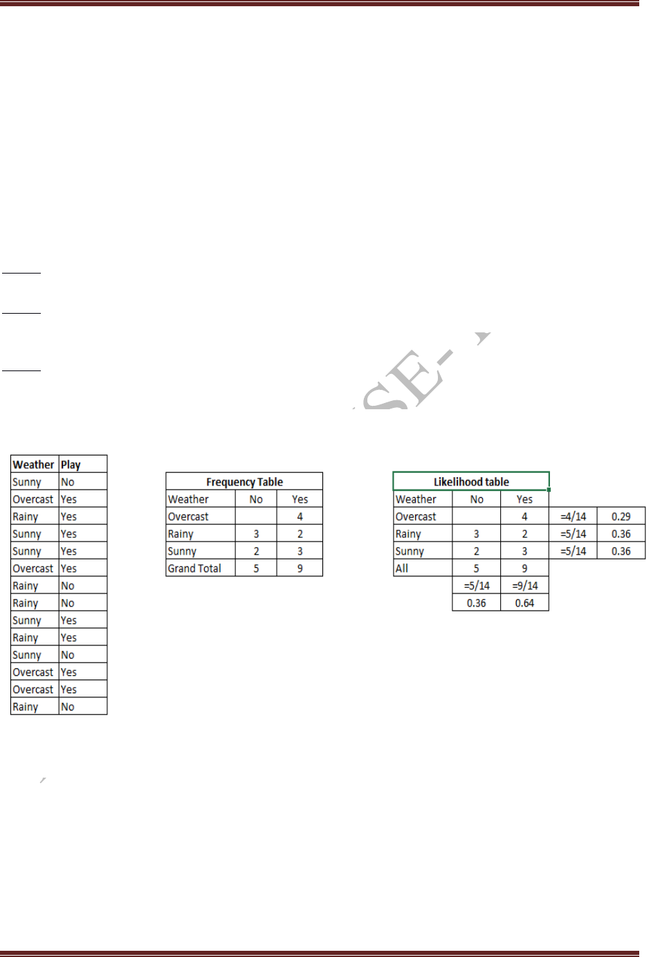
Bayes theorem provides a way of calculating posterior probability P(c|x) from P(c), P(x) and P(x|c).

MACHINE LEARNING LABORATORY-15CSL76
Department of CSE and ISE, RNSIT Page 47
Above,
P(c|x) is the posterior probability of class (c, target) given predictor (x, attributes).
P(c) is the prior probability of class.
P(x|c) is the likelihood which is the probability of predictor given class.
P(x) is the prior probability of predictor.
So here we have 4 attributes. What we need to do is to create “look-up tables” for each of these
attributes, and write in the probability that a game of tennis will be played based on this attribute. In
these tables we have to note that there are 5 cases of not being able to play a game, and 9 cases of being
able to play a game.
We also must note the following probabilities for P(C):
P(Play=Yes) = 9/14
P(Play=No) = 5/14
OUTLOOK
Play = Yes
Play = No
Total
Sunny
2/9
3/5
5/14
Overcast
4/9
0/5
4/14
Rain
3/9
2/5
5/14
TEMPERATURE
Play = Yes
Play = No
Total
Hot
2/9
2/5
4/14
Mild
4/9
2/5
6/14
Cool
3/9
1/5
4/14
HUMIDITY
Play = Yes
Play = No
Total
High
3/9
4/5
7/14
Normal
6/9
1/5
7/14
WIND
Play = Yes
Play = No
Total

MACHINE LEARNING LABORATORY-15CSL76
Department of CSE and ISE, RNSIT Page 48
Strong
3/9
3/5
6/14
Weak
6/9
2/5
8/14
Testing
For this, say we were given a new instance, and we want to know if we can play a game or not, then we
need to lookup the results from the tables above. So, this new instance is:
X = (Outlook=Sunny, Temperature=Cool, Humidity=High, Wind=Strong)
Firstly we look at the probability that we can play the game, so we use the lookup tables to get:
P(Outlook=Sunny | Play=Yes) = 2/9
P(Temperature=Cool | Play=Yes) = 3/9
P(Humidity=High | Play=Yes) = 3/9
P(Wind=Strong | Play=Yes) = 3/9
P(Play=Yes) = 9/14
Next we consider the fact that we cannot play a game:
P(Outlook=Sunny | Play=No) = 3/5
P(Temperature=Cool | Play=No) = 1/5
P(Humidity=High | Play=No) = 4/5
P(Wind=Strong | Play=No) = 3/5
P(Play=No) = 5/14
Then, using those results, you have to multiple the whole lot together. So you multiple all the
probabilities for Play=Yes such as:
P(X|Play=Yes)P(Play=Yes) = (2/9) * (3/9) * (3/9) * (3/9) * (9/14) = 0.0053
And this gives us a value that represents ‘P(X|C)P(C)’, or in this case ‘P(X|Play=Yes)P(Play=Yes)’.
We also have to do the same thing for Play=No:
P(X|Play=No)P(Play=No) = (3/5) * (1/5) * (4/5) * (3/5) * (5/14) = 0.0206
Finally, we have to divide both results by the evidence, or ‘P(X)’. The evidence for both equations
is the same, and we can find the values we need within the ‘Total’ columns of the look-up tables.
Therefore:
P(X) = P(Outlook=Sunny) * P(Temperature=Cool) * P(Humidity=High) * P(Wind=Strong)
P(X) = (5/14) * (4/14) * (7/14) * (6/14)
P(X) = 0.02186
Then, dividing the results by this value:
P(Play=Yes | X) = 0.0053/0.02186 = 0.2424
P(Play=No | X) = 0.0206/0.02186 = 0.9421
MACHINE LEARNING LABORATORY-15CSL76
Department of CSE and ISE, RNSIT Page 49
So, given the probabilities, can we play a game or not? To do this, we look at both probabilities and see
which once has the highest value, and that is our answer. Therefore:
P(Play=Yes | X) = 0.2424
P(Play=No | X) = 0.9421
Since 0.9421 is greater than 0.2424 then the answer is ‘no’, we cannot play a game of tennis today.
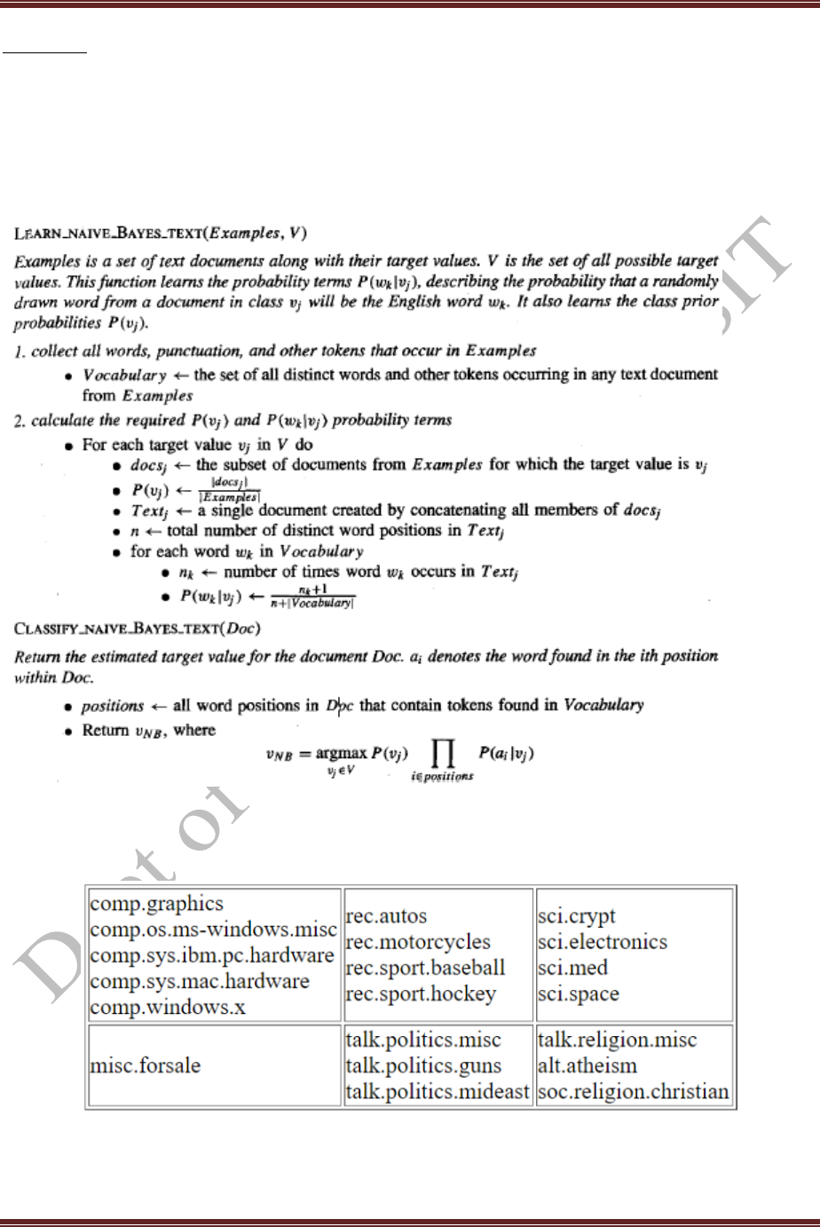
Let’s understand it using an example. Below I have a training data set of weather and corresponding
target variable ‘Play’ (suggesting possibilities of playing). Now, we need to classify whether players
will play or not based on weather condition. Let’s follow the below steps to perform it.
Step 1: Convert the data set into a frequency table
Step 2: Create Likelihood table by finding the probabilities like Overcast probability = 0.29 and
probability of playing is 0.64.
Step 3: Now, use Naive Bayesian equation to calculate the posterior probability for each class. The
class with the highest posterior probability is the outcome of prediction.
Naïve Bayes for PlayTennis dataset in python:
print("\nNaive Bayes Classifier for concept learning problem")
import csv
import random
import math
import operator
def safe_div(x,y):
if y == 0:

MACHINE LEARNING LABORATORY-15CSL76
Department of CSE and ISE, RNSIT Page 50
return 0
return x / y
def loadCsv(filename):
lines = csv.reader(open(filename))
dataset = list(lines)
for i in range(len(dataset)):
dataset[i] = [float(x) for x in dataset[i]]
return dataset
def splitDataset(dataset, splitRatio):
trainSize = int(len(dataset) * splitRatio)
trainSet = []
copy = list(dataset)
i=0
while len(trainSet) < trainSize:
#index = random.randrange(len(copy))
trainSet.append(copy.pop(i))
return [trainSet, copy]
def separateByClass(dataset):
separated = {}
for i in range(len(dataset)):
vector = dataset[i]
if (vector[-1] not in separated):
separated[vector[-1]] = []
separated[vector[-1]].append(vector)
return separated
def mean(numbers):
return safe_div(sum(numbers),float(len(numbers)))
def stdev(numbers):
avg = mean(numbers)
variance = safe_div(sum([pow(x-avg,2) for x in numbers]),float(len(numbers)-1))
return math.sqrt(variance)
def summarize(dataset):
summaries = [(mean(attribute), stdev(attribute)) for attribute in zip(*dataset)]
del summaries[-1]
return summaries
def summarizeByClass(dataset):

MACHINE LEARNING LABORATORY-15CSL76
Department of CSE and ISE, RNSIT Page 51
separated = separateByClass(dataset)
summaries = {}
for classValue, instances in separated.items():
summaries[classValue] = summarize(instances)
return summaries
def calculateProbability(x, mean, stdev):
exponent = math.exp(-safe_div(math.pow(x-mean,2),(2*math.pow(stdev,2))))
final = safe_div(1 , (math.sqrt(2*math.pi) * stdev)) * exponent
return final
def calculateClassProbabilities(summaries, inputVector):
probabilities = {}
for classValue, classSummaries in summaries.items():
probabilities[classValue] = 1
for i in range(len(classSummaries)):
mean, stdev = classSummaries[i]
x = inputVector[i]
probabilities[classValue] *= calculateProbability(x, mean, stdev)
return probabilities
def predict(summaries, inputVector):
probabilities = calculateClassProbabilities(summaries, inputVector)
bestLabel, bestProb = None, -1
for classValue, probability in probabilities.items():
if bestLabel is None or probability > bestProb:
bestProb = probability
bestLabel = classValue
return bestLabel
def getPredictions(summaries, testSet):
predictions = []
for i in range(len(testSet)):
result = predict(summaries, testSet[i])
predictions.append(result)
return predictions
def getAccuracy(testSet, predictions):
correct = 0
for i in range(len(testSet)):
if testSet[i][-1] == predictions[i]:
correct += 1
accuracy = safe_div(correct,float(len(testSet))) * 100.0
return accuracy

MACHINE LEARNING LABORATORY-15CSL76
Department of CSE and ISE, RNSIT Page 52
def main():
filename = 'ConceptLearning.csv'
splitRatio = 0.9
dataset = loadCsv(filename)
trainingSet, testSet = splitDataset(dataset, splitRatio)
print('Split {0} rows into'.format(len(dataset)))
print('Number of Training data: ' + (repr(len(trainingSet))))
print('Number of Test Data: ' + (repr(len(testSet))))
print("\nThe values assumed for the concept learning attributes are\n")
print("OUTLOOK=> Sunny=1 Overcast=2 Rain=3\nTEMPERATURE=> Hot=1 Mild=2
Cool=3\nHUMIDITY=> High=1 Normal=2\nWIND=> Weak=1 Strong=2")
print("TARGET CONCEPT:PLAY TENNIS=> Yes=10 No=5")
print("\nThe Training set are:")
for x in trainingSet:
print(x)
print("\nThe Test data set are:")
for x in testSet:
print(x)
print("\n")
# prepare model
summaries = summarizeByClass(trainingSet)
# test model
predictions = getPredictions(summaries, testSet)
actual = []
for i in range(len(testSet)):
vector = testSet[i]
actual.append(vector[-1])
# Since there are five attribute values, each attribute constitutes to 20% accuracy. So if all attributes
#match with predictions then 100% accuracy
print('Actual values: {0}%'.format(actual))
print('Predictions: {0}%'.format(predictions))
accuracy = getAccuracy(testSet, predictions)
print('Accuracy: {0}%'.format(accuracy))
main()
The input CSV file is as below

MACHINE LEARNING LABORATORY-15CSL76
Department of CSE and ISE, RNSIT Page 53
Output:
Naive Bayes Classifier for concept learning problem
Split 16 rows into
Number of Training data: 14
Number of Test Data: 2
The values assumed for the concept learning attributes are
OUTLOOK=> Sunny=1 Overcast=2 Rain=3
TEMPERATURE=> Hot=1 Mild=2 Cool=3
HUMIDITY=> High=1 Normal=2
WIND=> Weak=1 Strong=2
TARGET CONCEPT:PLAY TENNIS=> Yes=10 No=5
The Training set are:
[1.0, 1.0, 1.0, 1.0, 5.0]
[1.0, 1.0, 1.0, 2.0, 5.0]
[2.0, 1.0, 1.0, 2.0, 10.0]
[3.0, 2.0, 1.0, 1.0, 10.0]
[3.0, 3.0, 2.0, 1.0, 10.0]
[3.0, 3.0, 2.0, 2.0, 5.0]
[2.0, 3.0, 2.0, 2.0, 10.0]
[1.0, 2.0, 1.0, 1.0, 5.0]
[1.0, 3.0, 2.0, 1.0, 10.0]
[3.0, 2.0, 2.0, 2.0, 10.0]
[1.0, 2.0, 2.0, 2.0, 10.0]
[2.0, 2.0, 1.0, 2.0, 10.0]

MACHINE LEARNING LABORATORY-15CSL76
Department of CSE and ISE, RNSIT Page 54
[2.0, 1.0, 2.0, 1.0, 10.0]
[3.0, 2.0, 1.0, 2.0, 5.0]
The Test data set are:
[1.0, 2.0, 1.0, 2.0, 5.0]
[1.0, 2.0, 1.0, 2.0, 5.0]
Actual values: [5.0, 5.0]%
Predictions: [5.0, 5.0]%
Accuracy: 100.0%
MACHINE LEARNING LABORATORY-15CSL76
Department of CSE and ISE, RNSIT Page 55
Program 6
Assuming a set of documents that need to be classified, use the naïve Bayesian Classifier model to
perform this task. Built-in Java classes/API can be used to write the program. Calculate the
accuracy, precision, and recall for your data set.
Multinomial Naïve Bayes Classifier
The 20newsgroups dataset
The data set contained two primary folders named as ‘train’ and ‘test.' Each folder further
contained 20 folders, one for each category of documents. Inside these folders were the actual

MACHINE LEARNING LABORATORY-15CSL76
Department of CSE and ISE, RNSIT Page 56
documents. Each category contained around 600 train documents and around 400 test
documents.
Python Code
from sklearn.datasets import fetch_20newsgroups
from sklearn.metrics import confusion_matrix
from sklearn.metrics import classification_report
import numpy as np
categories = ['alt.atheism', 'soc.religion.christian','comp.graphics', 'sci.med']
twenty_train = fetch_20newsgroups(subset='train',categories=categories,shuffle=True)
twenty_test = fetch_20newsgroups(subset='test',categories=categories,shuffle=True)
print(len(twenty_train.data))
print(len(twenty_test.data))
print(twenty_train.target_names)
print("\n".join(twenty_train.data[0].split("\n")))
print(twenty_train.target[0])
from sklearn.feature_extraction.text import CountVectorizer
count_vect = CountVectorizer()
X_train_tf = count_vect.fit_transform(twenty_train.data)
from sklearn.feature_extraction.text import TfidfTransformer
tfidf_transformer = TfidfTransformer()
X_train_tfidf = tfidf_transformer.fit_transform(X_train_tf)
X_train_tfidf.shape
from sklearn.naive_bayes import MultinomialNB
from sklearn.metrics import accuracy_score
from sklearn import metrics
mod = MultinomialNB()
mod.fit(X_train_tfidf, twenty_train.target)
X_test_tf = count_vect.transform(twenty_test.data)
X_test_tfidf = tfidf_transformer.transform(X_test_tf)
predicted = mod.predict(X_test_tfidf)
print("Accuracy:", accuracy_score(twenty_test.target, predicted))
print(classification_report(twenty_test.target,predicted,target_names=twenty_test.target_names))
print("confusion matrix is \n",metrics.confusion_matrix(twenty_test.target, predicted))

MACHINE LEARNING LABORATORY-15CSL76
Department of CSE and ISE, RNSIT Page 57
Output
2257
1502
['alt.atheism', 'comp.graphics', 'sci.med', 'soc.religion.christian']
From: sd345@city.ac.uk (Michael Collier)
Subject: Converting images to HP LaserJet III?
Nntp-Posting-Host: hampton
Organization: The City University
Lines: 14
Does anyone know of a good way (standard PC application/PD utility) to
convert tif/img/tga files into LaserJet III format. We would also like to
do the same, converting to HPGL (HP plotter) files.
Please email any response.
Is this the correct group?
Thanks in advance. Michael.
--
Michael Collier (Programmer) The Computer Unit,
Email: M.P.Collier@uk.ac.city The City University,
Tel: 071 477-8000 x3769 London,
Fax: 071 477-8565 EC1V 0HB.
1
Accuracy: 0.8348868175765646
precision recall f1-score support
alt.atheism 0.97 0.60 0.74 319
comp.graphics 0.96 0.89 0.92 389
sci.med 0.97 0.81 0.88 396
soc.religion.christian 0.65 0.99 0.78 398
avg / total 0.88 0.83 0.84 1502
confusion matrix is
[[192 2 6 119]
[ 2 347 4 36]
[ 2 11 322 61]
[ 2 2 1 393]]
>>>
MACHINE LEARNING LABORATORY-15CSL76
Department of CSE and ISE, RNSIT Page 58
Testing and Evaluation: The effectiveness of the model is judged by employing the metrics described
below. All the metrics obtained range from 0 to 1 where 1 being the ideal and 0 being the worst.
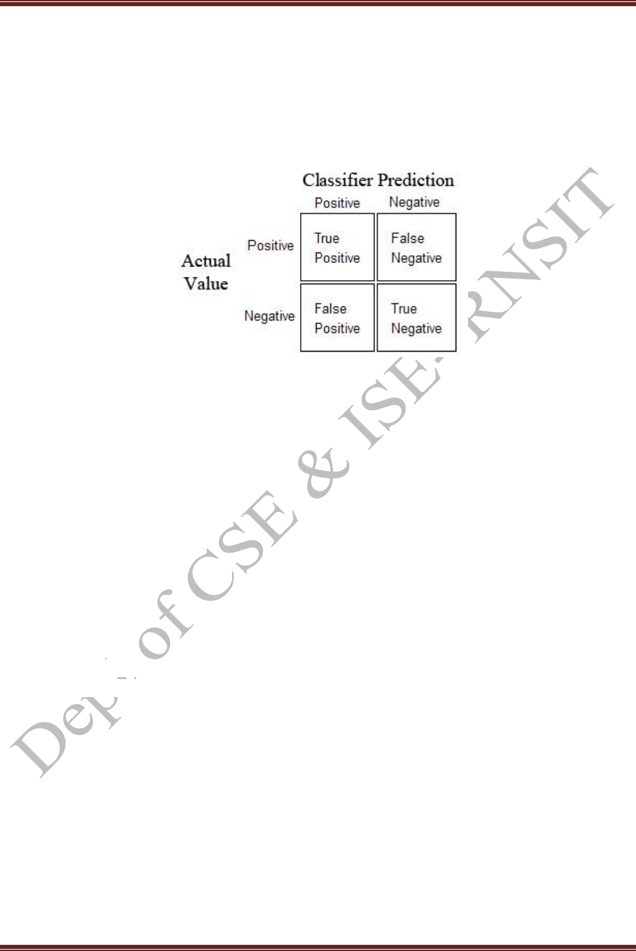
Confusion Matrix: A confusion matrix is a technique for summarizing the performance of a
classification algorithm. Positive (P) the number of real positive cases in the data. Negative (N) the
number of real negative cases in the data
The classification Accuracy is defined as:
Accuracy=TP+TN / (TP+FP+TN+FN)
Precision (P) can be defined as the number of True positives (Tp) over the number of False positives
(Fp) plus the number of True positives (Tp).
Precision = TP/(TP + FP)
Recall (R) is defined as the number of True Positives (Tp) over the number of False Negatives (Fp)
plus the number of True Positives (Tp).
Recall = TP/(TP+FN)
The F1 score is the harmonic average of the precision and recall, where an F1 score reaches its best
value at 1 (perfect precision and recall) and worst at 0.
F1 = 2 x (precision x recall)/(precision + recall)
Consider alt.atheism newsgroup using confusion matrix calculate
Accuracy=192+1117/192+127+6+11170
Precision=192/192+6=0.97
Recall=192/192+127=0.60
F1score=2* [(0.97*0.60)/(0.97+0.60)]=0.74
MACHINE LEARNING LABORATORY-15CSL76
Department of CSE and ISE, RNSIT Page 59
Program 7
Write a program to construct a Bayesian network considering medical data. Use this model to
demonstrate the diagnosis of heart patients using standard Heart Disease Data Set. You can use
Java/Python ML library classes/API.
A Bayesian belief network describes the probability distribution over a set of variables.
Probability
P(A) is used to denote the probability of A. For example if A is discrete with states {True, False} then
P(A) might equal [0.2, 0.8]. I.e. 20% chance of being True, 80% chance of being False.
Joint probability
A joint probability refers to the probability of more than one variable occurring together, such as the
probability of A and B, denoted P(A,B).
Conditional probability
Conditional probability is the probability of a variable (or set of variables) given another variable (or set
of variables), denoted P(A|B).For example, the probability of Windy being True, given that Raining is
True might equal 50%.This would be denoted P(Windy = True | Raining = True) = 50%.
Once the structure has been defined (i.e. nodes and links), a Bayesian network requires a probability
distribution to be assigned to each node.Each node X in a Bayesian network requires a probability
distribution P(X | pa(X)).Note that if a node X has no parents pa(X) is empty, and the required
distribution is just P(X) sometimes referred to as the prior.This is the probability of itself given its
parent nodes.
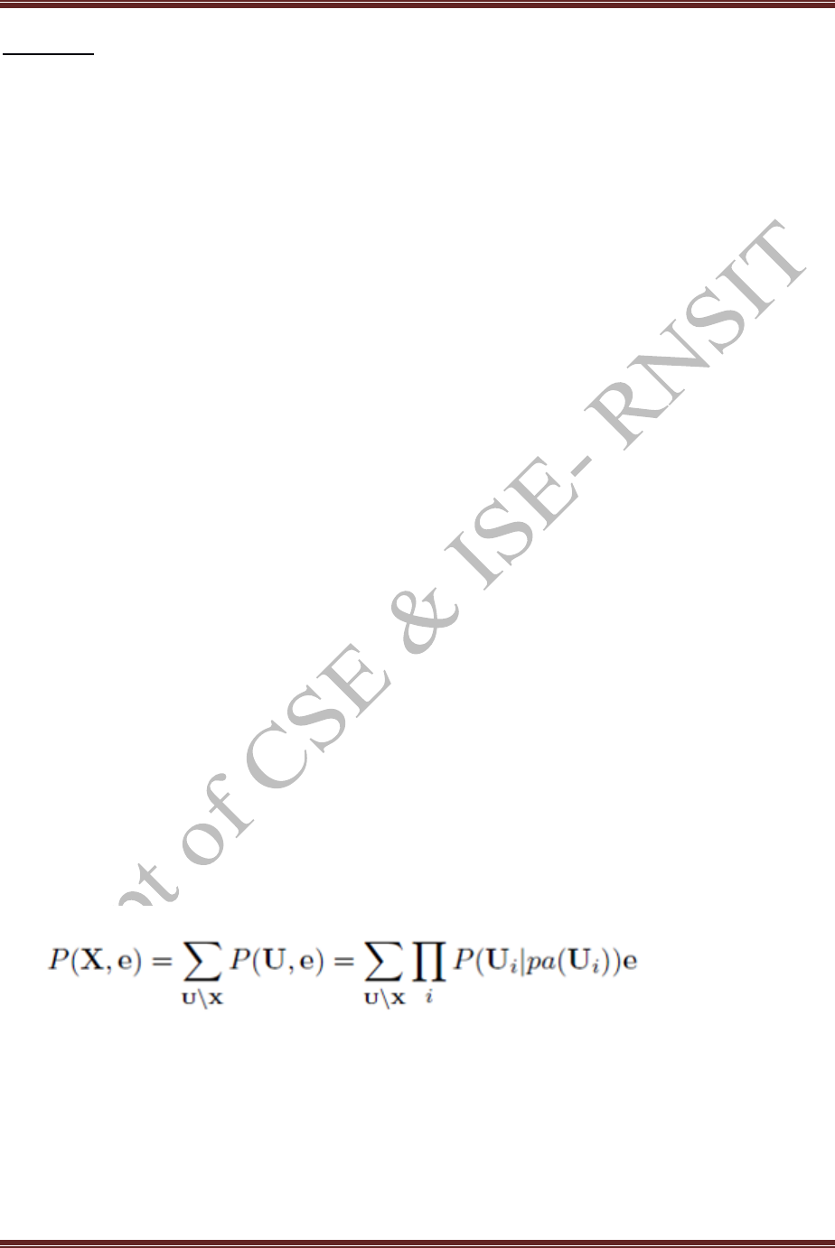
If U = {A1,...,An} is the universe of variables (all the variables) in a Bayesian network, and pa(Ai) are
the parents of Ai then the joint probability distribution P(U) is the simply the product of all the
probability distributions (prior and conditional) in the network, as shown in the equation below.This
equation is known as the chain rule.
From the joint distribution over U we can in turn calculate any query we are interested in (with or
without evidence set).
Suppose that there are two events which could cause grass to be wet: either the sprinkler is on or it's
raining. Also, suppose that the rain has a direct effect on the use of the sprinkler (namely that when it
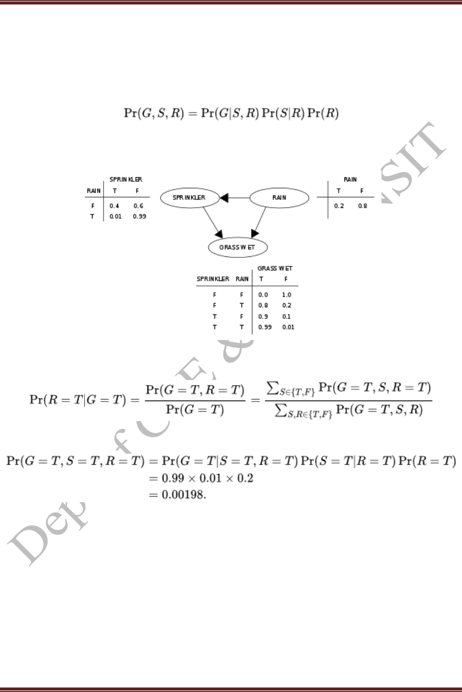
MACHINE LEARNING LABORATORY-15CSL76
Department of CSE and ISE, RNSIT Page 60
rains, the sprinkler is usually not turned on). Then the situation can be modeled with a Bayesian
network (shown to the right). All three variables have two possible values, T (for true) and F (for false).
The joint probability function is:
The model can answer questions like "What is the probability that it is raining, given the grass is wet?"
by using the
conditional
probability
formula and
summing over all
nuisance
variables:
BBn in python:
import bayespy as bp
import numpy as np
import csv
from colorama import init
from colorama import Fore, Back, Style
init()
# Define Parameter Enum values

MACHINE LEARNING LABORATORY-15CSL76
Department of CSE and ISE, RNSIT Page 61
#Age
ageEnum = {'SuperSeniorCitizen':0, 'SeniorCitizen':1, 'MiddleAged':2, 'Youth':3, 'Teen':4}
# Gender
genderEnum = {'Male':0, 'Female':1}
# FamilyHistory
familyHistoryEnum = {'Yes':0, 'No':1}
# Diet(Calorie Intake)
dietEnum = {'High':0, 'Medium':1, 'Low':2}
# LifeStyle
lifeStyleEnum = {'Athlete':0, 'Active':1, 'Moderate':2, 'Sedetary':3}
# Cholesterol
cholesterolEnum = {'High':0, 'BorderLine':1, 'Normal':2}
# HeartDisease
heartDiseaseEnum = {'Yes':0, 'No':1}
#heart_disease_data.csv
with open('heart_disease_data.csv') as csvfile:
lines = csv.reader(csvfile)
dataset = list(lines)
data = []
for x in dataset:
data.append([ageEnum[x[0]],genderEnum[x[1]],familyHistoryEnum[x[2]],dietEnum[x[3]],lifeStyl
eEnum[x[4]],cholesterolEnum[x[5]],heartDiseaseEnum[x[6]]])
# Training data for machine learning todo: should import from csv
data = np.array(data)
N = len(data)
# Input data column assignment
p_age = bp.nodes.Dirichlet(1.0*np.ones(5))
age = bp.nodes.Categorical(p_age, plates=(N,))
age.observe(data[:,0])
p_gender = bp.nodes.Dirichlet(1.0*np.ones(2))
gender = bp.nodes.Categorical(p_gender, plates=(N,))
gender.observe(data[:,1])
p_familyhistory = bp.nodes.Dirichlet(1.0*np.ones(2))
familyhistory = bp.nodes.Categorical(p_familyhistory, plates=(N,))
familyhistory.observe(data[:,2])
p_diet = bp.nodes.Dirichlet(1.0*np.ones(3))
diet = bp.nodes.Categorical(p_diet, plates=(N,))
diet.observe(data[:,3])

MACHINE LEARNING LABORATORY-15CSL76
Department of CSE and ISE, RNSIT Page 62
p_lifestyle = bp.nodes.Dirichlet(1.0*np.ones(4))
lifestyle = bp.nodes.Categorical(p_lifestyle, plates=(N,))
lifestyle.observe(data[:,4])
p_cholesterol = bp.nodes.Dirichlet(1.0*np.ones(3))
cholesterol = bp.nodes.Categorical(p_cholesterol, plates=(N,))
cholesterol.observe(data[:,5])
# Prepare nodes and establish edges
# np.ones(2) -> HeartDisease has 2 options Yes/No
# plates(5, 2, 2, 3, 4, 3) -> corresponds to options present for domain values
p_heartdisease = bp.nodes.Dirichlet(np.ones(2), plates=(5, 2, 2, 3, 4, 3))
heartdisease = bp.nodes.MultiMixture([age, gender, familyhistory, diet, lifestyle, cholesterol],
bp.nodes.Categorical, p_heartdisease)
heartdisease.observe(data[:,6])
p_heartdisease.update()
# Sample Test with hardcoded values
#print("Sample Probability")
#print("Probability(HeartDisease|Age=SuperSeniorCitizen, Gender=Female, FamilyHistory=Yes,
DietIntake=Medium, LifeStyle=Sedetary, Cholesterol=High)")
#print(bp.nodes.MultiMixture([ageEnum['SuperSeniorCitizen'], genderEnum['Female'],
familyHistoryEnum['Yes'], dietEnum['Medium'], lifeStyleEnum['Sedetary'],
cholesterolEnum['High']], bp.nodes.Categorical,
p_heartdisease).get_moments()[0][heartDiseaseEnum['Yes']])
# Interactive Test
m = 0
while m == 0:
print("\n")
res = bp.nodes.MultiMixture([int(input('Enter Age: ' + str(ageEnum))), int(input('Enter Gender: '
+ str(genderEnum))), int(input('Enter FamilyHistory: ' + str(familyHistoryEnum))),
int(input('Enter dietEnum: ' + str(dietEnum))), int(input('Enter LifeStyle: ' + str(lifeStyleEnum))),
int(input('Enter Cholesterol: ' + str(cholesterolEnum)))], bp.nodes.Categorical,
p_heartdisease).get_moments()[0][heartDiseaseEnum['Yes']]
print("Probability(HeartDisease) = " + str(res))
#print(Style.RESET_ALL)
m = int(input("Enter for Continue:0, Exit :1 "))
Output:
Enter Age: {'SuperSeniorCitizen': 0, 'SeniorCitizen': 1, 'MiddleAged': 2, 'Youth': 3, 'Teen':
4}1
Enter Gender: {'Male': 0, 'Female': 1}1

MACHINE LEARNING LABORATORY-15CSL76
Department of CSE and ISE, RNSIT Page 63
Enter FamilyHistory: {'Yes': 0, 'No': 1}1
Enter dietEnum: {'High': 0, 'Medium': 1, 'Low': 2}2
Enter LifeStyle: {'Athlete': 0, 'Active': 1, 'Moderate': 2, 'Sedetary': 3}2
Enter Cholesterol: {'High': 0, 'BorderLine': 1, 'Normal': 2}1
Probability(HeartDisease) = 0.5
Enter for Continue:0, Exit :1 0
Enter Age: {'SuperSeniorCitizen': 0, 'SeniorCitizen': 1, 'MiddleAged': 2, 'Youth': 3, 'Teen':
4}0
Enter Gender: {'Male': 0, 'Female': 1}0
Enter FamilyHistory: {'Yes': 0, 'No': 1}0
Enter dietEnum: {'High': 0, 'Medium': 1, 'Low': 2}0
Enter LifeStyle: {'Athlete': 0, 'Active': 1, 'Moderate': 2, 'Sedetary': 3}3
Enter Cholesterol: {'High': 0, 'BorderLine': 1, 'Normal': 2}0
Probability(HeartDisease) = 0.5
Enter for Continue:0, Exit :1

MACHINE LEARNING LABORATORY-15CSL76
Department of CSE and ISE, RNSIT Page 64
Program 8
Apply EM algorithm to cluster a set of data stored in a .CSV file. Use the same data set for
clustering using k-Means algorithm. Compare the results of these two algorithms and comment
on the quality of clustering. You can add Java/Python ML library classes/API in the program.
Introduction to Expectation-Maximization (EM)
The EM algorithm tends to get stuck less than K-means algorithm. The idea is to assign data
points partially to different clusters instead of assigning to only one cluster. To do this partial
assignment, we model each cluster using a probabilistic distribution So a data point associates
with a cluster with certain probability and it belongs to the cluster with the highest probability
in the final assignment.
Expectation-Maximization (EM) algorithm
Step 1: An initial guess is made for the model’s parameters and a probability
distribution is created. This is sometimes called the “E-Step” for the “Expected”
distribution.
Step 2: Newly observed data is fed into the model.
Step 3: The probability distribution from the E-step is drawn to include the new data.
This is sometimes called the “M-step.”
Step 4: Steps 2 through 4 are repeated until stability.
Data set:
1
1
3
3
5
5
8
8
2
2
11
11
14
14
18
18
Expectation-Maximization in Python:
import csv
import math
import copy
k=2

MACHINE LEARNING LABORATORY-15CSL76
Department of CSE and ISE, RNSIT Page 65
class cluster:
def __init__(self,cluster_head_data):
self.head=cluster_head_data
self.l=[]
self.mean=cluster_head_data[0]
self.variance=1.0
def display_head(self):
print("m=",self.mean)
print("v=",self.variance)
def add_ele_cluster(self,data):
self.l.append(data)
print(self.l)
def display_ele(self):
print('list contains',self.l)
def find_insert_individual_cluster(cluster,element,n):
ele=float(element[0])
prob=[]
for i in range(len(cluster)):
pxb= 1/math.sqrt(2*3.142*cluster[i].variance)* math.exp(-1* ( ele - float(cluster[i].mean)
)**2 / (2*float(cluster[i].variance)))
print('pxb exact==',pxb)
prob.append(pxb)
print('prob elem',prob)
bi_den=0
for i in range(len(prob)):
bi_den=bi_den+prob[i]*1/n
print('bi den', bi_den)
#insert ele in to the cluster-- ele+pxb+bi
for i in range(len(cluster)):
clust_data=[]
clust_data.append(ele)
bi=(prob[i]*1/n)/bi_den
clust_data.append(bi)
#add the contents on to the cluster
cluster[i].add_ele_cluster(clust_data)
def recalculate_cluster_mean_variance(cluster):
l1=cluster.l

MACHINE LEARNING LABORATORY-15CSL76
Department of CSE and ISE, RNSIT Page 66
print('list enteries',l1)
#recalculating mean
mean_num=0.0
mean_den=0.0
var_num=0.0
var_den=0.0
for i in range(len(l1)):
mean_num=mean_num+l1[i][0]*l1[i][1]
mean_den=mean_den+l1[i][1]
mean=mean_num/mean_den
cluster.mean=mean
#recalculating varaiance
for i in range(len(l1)):
var_num=var_num+l1[i][1]*(l1[i][0]-mean)**2
var_den=var_den+l1[i][1]
variance=var_num/var_den
cluster.variance=mean
def find_nearest(cluster,ele):
ele=float(ele[0])
prob=[]
nearest_prob=None
index=1
for i in range(len(cluster)):
pxb= 1/math.sqrt(2*3.142*cluster[i].variance)* math.exp(-1* ( ele - float(cluster[i].mean)
)**2 / (2*float(cluster[i].variance)))
print('pxb for cluster i',i,'=',pxb)
if nearest_prob is None:
nearest_prob=pxb
index=i
else:
if nearest_prob < pxb:
nearest_prob=pxb
index=i
print('index',index,'nearest_prob=',nearest_prob)
cluster[index].l.append(ele)
#read the contents of CSV file
with open('cluster.csv') as csvfile:
spamreader = csv.reader(csvfile, delimiter=',')
#inserting elelments in to the list

MACHINE LEARNING LABORATORY-15CSL76
Department of CSE and ISE, RNSIT Page 67
db=[]
for row in spamreader:
db.append(row)
#creating individual cluster heads
#displaying elelments of the list
print('Db entries')
print(db)
#intialize the cluster
c=[]
#intialize the cluster heads
for i in range(k):
new_clust=cluster(db[i])
c.append(new_clust)
print('initial cluster Mean Variance')
#print cluster mean and variance
for i in range(k):
print('----cluster',i,'------')
c[i].display_head()
error_ratio=1
# Iteration and including elelments in the cluster
while error_ratio>0:
error_ratio=0
prevc=copy.deepcopy(c)
#estimation
for i in range(len(db)):
find_insert_individual_cluster(c,db[i],len(db))
#recalculate cluster mean and variance
for i in range(len(c)):
recalculate_cluster_mean_variance(c[i])
#display recalculated mean and varaiance of cluster
for i in range(k):
print('----cluster',i,'------')
c[i].display_head()
#clear all the values of the cluster list for the next iteration
for i in range(k):
c[i].l=[]
#calculate the error
error_ratio=0

MACHINE LEARNING LABORATORY-15CSL76
Department of CSE and ISE, RNSIT Page 68
for i in range(len(c)):
if abs(c[i].variance - prevc[i].variance)>0.1:
error_ratio=error_ratio+1
#display the cluster elements
#clear all the values of the cluster list for the next iteration
for i in range(k):
c[i].l=[]
#claculate the nearest prob for each elelment and include it in the resultant cluster
for i in range(len(db)):
find_nearest(c,db[i])
#display cluster elelments
for i in range(len(c)):
print(c[i].l)
Output
----cluster 0 ------
m= 2.7213340517024402
v= 2.7213340517024402
----cluster 1 ------
m= 12.504957731742246
v= 12.504957731742246
pxb for cluster i 0 = 0.14030103544739295
pxb for cluster i 1 = 0.0005673529507970876
index 0 nearest_prob= 0.14030103544739295
pxb for cluster i 0 = 0.23839358908896524
pxb for cluster i 1 = 0.003044550243209151
index 0 nearest_prob= 0.23839358908896524
pxb for cluster i 0 = 0.09314788538736465
pxb for cluster i 1 = 0.01186516649339238
index 0 nearest_prob= 0.09314788538736465
pxb for cluster i 0 = 0.0014456877959066348
pxb for cluster i 1 = 0.05011024116755676
index 1 nearest_prob= 0.05011024116755676
pxb for cluster i 0 = 0.2197718847381247
pxb for cluster i 1 = 0.0013678961391086488
index 0 nearest_prob= 0.2197718847381247
pxb for cluster i 0 = 8.216307351891605e-07
pxb for cluster i 1 = 0.10304124381579008
index 1 nearest_prob= 0.10304124381579008

MACHINE LEARNING LABORATORY-15CSL76
Department of CSE and ISE, RNSIT Page 69
pxb for cluster i 0 = 1.709934543851912e-11
pxb for cluster i 1 = 0.10316387232255203
index 1 nearest_prob= 0.10316387232255203
pxb for cluster i 0 = 5.707857566318809e-20
pxb for cluster i 1 = 0.033728682873350235
index 1 nearest_prob= 0.033728682873350235
[1.0, 3.0, 5.0, 2.0]
[8.0, 11.0, 14.0, 18.0]
>>>
K-Means in Python:
import csv
import math
import copy
k=3
class cluster:
def __init__(self,cluster_head_data):
self.head=cluster_head_data
self.l=[]
def display_head(self):
print(self.head)
def add_ele_cluster(self,data):
self.l.append(data)
def display_ele(self):
print('list contains',self.l)
def compare_the_values(first,secound):
x=float(first[0])
y=float(first[1])
x1=float(secound[0])
x2=float(secound[1])
val=math.sqrt( math.pow(math.fabs(x-x1),2)+math.pow(math.fabs(x-x1),2) )
return val
def compare_the_nearest_cluster(cluster,data):
#intialize the nearest cluster to 0
dist_measure=None
nearest=0
for i in range(len(cluster)):
dist=compare_the_values(cluster[i].head,data)
if dist_measure is None:

MACHINE LEARNING LABORATORY-15CSL76
Department of CSE and ISE, RNSIT Page 70
dist_measure=dist
nearest=i
if dist<dist_measure:
dist_measure=dist
nearest=i
return nearest
def recal_head(cluster):
for i in range(len(cluster)):
l1=cluster[i].l
xval=0.0
yval=0.0
for j in l1:
xval=xval+float(j[0])
yval=yval+float(j[1])
xavg=xval/len(l1)
yavg=yval/len(l1)
avgl=[]
avgl.append(xavg)
avgl.append(yavg)
cluster[i].head=avgl
#read the contents of CSV file
with open('cluster.csv') as csvfile:
spamreader = csv.reader(csvfile, delimiter=',')
#inserting elelments in to the list
db=[]
for row in spamreader:
db.append(row)
#creating individual cluster heads
#displaying elelments of the list
print('Db entries')
print(db)
#intialize the cluster
c=[]
#intialize the cluster heads
for i in range(k):
new_clust=cluster(db[i])

MACHINE LEARNING LABORATORY-15CSL76
Department of CSE and ISE, RNSIT Page 71
c.append(new_clust)
print('initial cluster head values')
#print display heads
for i in range(k):
print('----cluster',i,'------')
c[i].display_head()
error_ratio=1
# Iteration and including elelments in the cluster
while error_ratio>0:
prevc=copy.deepcopy(c)
for ele in db:
r=compare_the_nearest_cluster(c,ele)
c[r].add_ele_cluster(ele)
# display all the elements
for clust in c:
clust.display_ele()
#recalculate the avg value
recal_head(c)
for i in range(k):
print('----cluster',i,'------')
c[i].display_head()
#remove the ele of cluter head for the next iter
for i in range(k):
c[i].l=[]
#calculate the error
error_ratio=0
for i in range(k):
if c[i].head != prevc[i].head:
error_ratio=error_ratio+1
#final cluster ele
Output
Db entries
[['1', '1'], ['3', '3'], ['5', '5'], ['8', '8'], ['2', '2'], ['11', '11'], ['14', '14'], ['18', '18']]
initial cluster head values
----cluster 0 ------
['1', '1']
----cluster 1 ------

MACHINE LEARNING LABORATORY-15CSL76
Department of CSE and ISE, RNSIT Page 72
['3', '3']
----cluster 2 ------
['5', '5']
list contains [['1', '1'], ['2', '2']]
list contains [['3', '3']]
list contains [['5', '5'], ['8', '8'], ['11', '11'], ['14', '14'], ['18', '18']]
----cluster 0 ------
[1.5, 1.5]
----cluster 1 ------
[3.0, 3.0]
----cluster 2 ------
[11.2, 11.2]
list contains [['1', '1'], ['2', '2']]
list contains [['3', '3'], ['5', '5']]
list contains [['8', '8'], ['11', '11'], ['14', '14'], ['18', '18']]
----cluster 0 ------
[1.5, 1.5]
----cluster 1 ------
[4.0, 4.0]
----cluster 2 ------
[12.75, 12.75]
list contains [['1', '1'], ['2', '2']]
list contains [['3', '3'], ['5', '5'], ['8', '8']]
list contains [['11', '11'], ['14', '14'], ['18', '18']]
----cluster 0 ------
[1.5, 1.5]
----cluster 1 ------
[5.333333333333333, 5.333333333333333]
----cluster 2 ------
[14.333333333333334, 14.333333333333334]
list contains [['1', '1'], ['3', '3'], ['2', '2']]
list contains [['5', '5'], ['8', '8']]
list contains [['11', '11'], ['14', '14'], ['18', '18']]
----cluster 0 ------
[2.0, 2.0]
----cluster 1 ------
[6.5, 6.5]
----cluster 2 ------
[14.333333333333334, 14.333333333333334]
list contains [['1', '1'], ['3', '3'], ['2', '2']]
list contains [['5', '5'], ['8', '8']]

MACHINE LEARNING LABORATORY-15CSL76
Department of CSE and ISE, RNSIT Page 73
list contains [['11', '11'], ['14', '14'], ['18', '18']]
----cluster 0 ------
[2.0, 2.0]
----cluster 1 ------
[6.5, 6.5]
----cluster 2 ------
[14.333333333333334, 14.333333333333334]
>>>
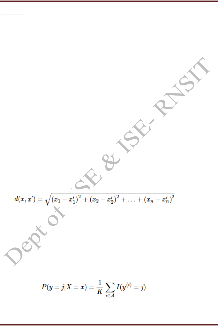
MACHINE LEARNING LABORATORY-15CSL76
Department of CSE and ISE, RNSIT Page 74
Program 9
Write a program to implement k-Nearest Neighbour algorithm to classify the iris data set. Print
both correct and wrong predictions. Java/Python ML library classes can be used for this
problem.
TASK: The task of this program is to classify the IRIS data set examples by using the k-Nearest
Neighbour algorithm. The new instance has to be classified based on its k nearest neighbors.
KNN falls in the supervised learning family of algorithms. Informally, this means that we are given a
labeled dataset consisting of training observations (x,y) and would like to capture the relationship
between x and y. More formally, our goal is to learn a function h:X→Y so that given an unseen
observation x, h(x) can confidently predict the corresponding output y.
The KNN classifier is also a non parametric and instance-based learning algorithm.
Non-parametric means it makes no explicit assumptions about the functional form of h,
avoiding the dangers of mismodeling the underlying distribution of the data. For example,
suppose our data is highly non-Gaussian but the learning model we choose assumes a
Gaussian form. In that case, our algorithm would make extremely poor predictions.
Instance-based learning means that our algorithm doesn’t explicitly learn a model. Instead, it
chooses to memorize the training instances which are subsequently used as “knowledge” for
the prediction phase. Concretely, this means that only when a query to our database is made
(i.e. when we ask it to predict a label given an input), will the algorithm use the training
instances to spit out an answer.
In the classification setting, the K-nearest neighbor algorithm essentially boils down to forming a
majority vote between the K most similar instances to a given “unseen” observation. Similarity is
defined according to a distance metric between two data points. A popular choice is the Euclidean
distance given by
but other measures can be more suitable for a given setting and include the Manhattan, Chebyshev and
Hamming distance.
More formally, given a positive integer K, an unseen observation x and a similarity metric d, KNN
classifier performs the following two steps:
It runs through the whole dataset computing d between x and each training observation. The K
points in the training data that are closest to x are called the set A. Note that K is usually odd
to prevent tie situations.
It then estimates the conditional probability for each class, that is, the fraction of points
in A with that given class label. (Note I(x) is the indicator function which evaluates to 1 when
the argument x is true and 0 otherwise)
Finally, the input x gets assigned to the class with the largest probability.
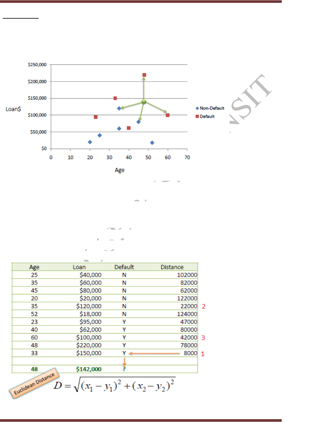
MACHINE LEARNING LABORATORY-15CSL76
Department of CSE and ISE, RNSIT Page 75
EXAMPLE:
Consider the following data concerning credit default. Age and Loan are two numerical
variables (predictors) and Default is the target.
We can now use the training set to classify an unknown case (Age=48 and Loan=$142,000)
using Euclidean distance. If K=1 then the nearest neighbor is the last case in the
training set with Default=Y.
D = Sqrt[(48-33)^2 + (142000-150000)^2] = 8000.01 >> Default=Y

MACHINE LEARNING LABORATORY-15CSL76
Department of CSE and ISE, RNSIT Page 76
With K=3, there are two Default=Y and one Default=N out of three closest neighbors.
The prediction for the unknown case is again Default=Y.
ALGORITHM:
Let m be the number of training data samples. Let p be an unknown point.
1. Store the training samples in an array of data points arr[]. This means each element of this array
represents a tuple (x, y).
2. for i=0 to m:
Calculate Euclidean distance d(arr[i], p).
3. Make set S of K smallest distances obtained. Each of these distances correspond to an already
classified data point.
4. Return the majority label among S.
KNN in Python:
import csv
import random
import math
import operator
def loadDataset(filename, split, trainingSet=[], testSet=[]):
with open(filename) as csvfile:
lines = csv.reader(csvfile)
dataset = list(lines)
for x in range(len(dataset)-1):
for y in range(4):
dataset[x][y] = float(dataset[x][y])
if random.random() < split:
trainingSet.append(dataset[x])
else:
testSet.append(dataset[x])
def euclideanDistance(instance1, instance2, length):
distance = 0
for x in range(length):
distance += pow((instance1[x] - instance2[x]), 2)
return math.sqrt(distance)
def getNeighbors(trainingSet, testInstance, k):
distances = []
length = len(testInstance)-1
for x in range(len(trainingSet)):
dist = euclideanDistance(testInstance, trainingSet[x], length)
distances.append((trainingSet[x], dist))
distances.sort(key=operator.itemgetter(1))

MACHINE LEARNING LABORATORY-15CSL76
Department of CSE and ISE, RNSIT Page 77
neighbors = []
for x in range(k):
neighbors.append(distances[x][0])
return neighbors
def getResponse(neighbors):
classVotes = {}
for x in range(len(neighbors)):
response = neighbors[x][-1]
if response in classVotes:
classVotes[response] += 1
else:
classVotes[response] = 1
sortedVotes = sorted(classVotes.items(), key=operator.itemgetter(1), reverse=True)
return sortedVotes[0][0]
def getAccuracy(testSet, predictions):
correct = 0
for x in range(len(testSet)):
if testSet[x][-1] == predictions[x]:
correct += 1
return (correct/float(len(testSet))) * 100.0
def main():
# prepare data
trainingSet=[]
testSet=[]
split = 0.67
loadDataset('iris_data.csv', split, trainingSet, testSet)
print ('\n Number of Training data: ' + (repr(len(trainingSet))))
print (' Number of Test Data: ' + (repr(len(testSet))))
# generate predictions
predictions=[]
k = 3
print('\n The predictions are: ')
for x in range(len(testSet)):
neighbors = getNeighbors(trainingSet, testSet[x], k)
result = getResponse(neighbors)
predictions.append(result)
print(' predicted=' + repr(result) + ', actual=' + repr(testSet[x][-1]))
accuracy = getAccuracy(testSet, predictions)
print('\n The Accuracy is: ' + repr(accuracy) + '%')
main()

MACHINE LEARNING LABORATORY-15CSL76
Department of CSE and ISE, RNSIT Page 78
Output:
Number of Training data: 106
Number of Test Data: 43
The predictions are:
predicted='Iris-setosa', actual='Iris-setosa'
predicted='Iris-setosa', actual='Iris-setosa'
predicted='Iris-setosa', actual='Iris-setosa'
predicted='Iris-setosa', actual='Iris-setosa'
predicted='Iris-setosa', actual='Iris-setosa'
predicted='Iris-setosa', actual='Iris-setosa'
predicted='Iris-setosa', actual='Iris-setosa'
predicted='Iris-setosa', actual='Iris-setosa'
predicted='Iris-setosa', actual='Iris-setosa'
predicted='Iris-setosa', actual='Iris-setosa'
predicted='Iris-setosa', actual='Iris-setosa'
predicted='Iris-setosa', actual='Iris-setosa'
predicted='Iris-setosa', actual='Iris-setosa'
predicted='Iris-setosa', actual='Iris-setosa'
predicted='Iris-setosa', actual='Iris-setosa'
predicted='Iris-setosa', actual='Iris-setosa'
predicted='Iris-setosa', actual='Iris-setosa'
predicted='Iris-setosa', actual='Iris-setosa'
predicted='Iris-setosa', actual='Iris-setosa'
predicted='Iris-setosa', actual='Iris-setosa'
predicted='Iris-versicolor', actual='Iris-versicolor'
predicted='Iris-versicolor', actual='Iris-versicolor'
predicted='Iris-versicolor', actual='Iris-versicolor'
predicted='Iris-versicolor', actual='Iris-versicolor'
predicted='Iris-versicolor', actual='Iris-versicolor'
predicted='Iris-versicolor', actual='Iris-versicolor'
predicted='Iris-versicolor', actual='Iris-versicolor'
predicted='Iris-versicolor', actual='Iris-versicolor'
predicted='Iris-versicolor', actual='Iris-versicolor'
predicted='Iris-virginica', actual='Iris-virginica'
predicted='Iris-virginica', actual='Iris-virginica'
predicted='Iris-virginica', actual='Iris-virginica'
predicted='Iris-virginica', actual='Iris-virginica'
predicted='Iris-virginica', actual='Iris-virginica'
predicted='Iris-virginica', actual='Iris-virginica'
predicted='Iris-virginica', actual='Iris-virginica'
predicted='Iris-virginica', actual='Iris-virginica'
predicted='Iris-virginica', actual='Iris-virginica'
predicted='Iris-virginica', actual='Iris-virginica'

MACHINE LEARNING LABORATORY-15CSL76
Department of CSE and ISE, RNSIT Page 79
predicted='Iris-virginica', actual='Iris-virginica'
predicted='Iris-virginica', actual='Iris-virginica'
predicted='Iris-virginica', actual='Iris-virginica'
predicted='Iris-virginica', actual='Iris-virginica'
The Accuracy is: 100.0%

MACHINE LEARNING LABORATORY-15CSL76
Department of CSE and ISE, RNSIT Page 80
Program 10
Implement the non-parametric Locally Weighted Regression algorithm in order to fit data
points. Select appropriate data set for your experiment and draw graphs.
Nonparametric regression: is a category of regression analysis in which the predictor does not take a
predetermined form but is constructed according to information derived from the data. Nonparametric
regression requires larger sample sizes than regression based on parametric models because the data
must supply the model structure as well as the model estimates.
Nonparametric regression is used for prediction and is reliable even if hypotheses of linear regression
are not verified.
Locally weighted Learning also known as memory-based learning, instance-based learning, lazy-
learning, and closely related to kernel density estimation, similarity searching and case-based reasoning.
LOWESS (Locally Weighted Scatterplot Smoothing), sometimes called LOESS (locally weighted
smoothing), is a popular tool used in regression analysis that creates a smooth line through
a timeplot or scatter plot to help you to see relationship between variables and foresee trends.
Locally weighted regression is a very powerful non-parametric model used in statistical learning.
Introduction :
Scatter-diagram smoothing (e.g. using the lowess() or loess() functions) involves drawing a smooth
curve on a scatter diagram to summarize a relationship, in a fashion that makes few assumptions
initially about the form or strength of the relationship. It is related to (and is a special case
of) nonparametric regression, in which the objective is to represent the relationship between a response
variable and one or more predictor variables, again in way that makes few assumptions about the form
of the relationship. In other words, in contrast to “standard” linear regression analysis, no assumption is
made that the relationship is represented by a straight line (although one could certainly think of a
straight line as a special case of nonparametric regression).
If the basic decomposition-of-the-data model is:
data = predictable component + noise,
then for the standard bivariate or multiple (linear) regression, the model is
data = straight-line, polynomial or linearizable function + noise,
while for nonparametric regression, the model is
data = smooth function determined by data + noise.
Another way of looking at scatter diagram smoothing is as a way of depicting the “local” relationship
between a response variable and a predictor variable over parts of their ranges, which may differ from a
“global” relationship determined using the whole data set. Nonparametric regression can be thought of
as generalizing the scatter plot smoothing idea to the multiple-regression context.
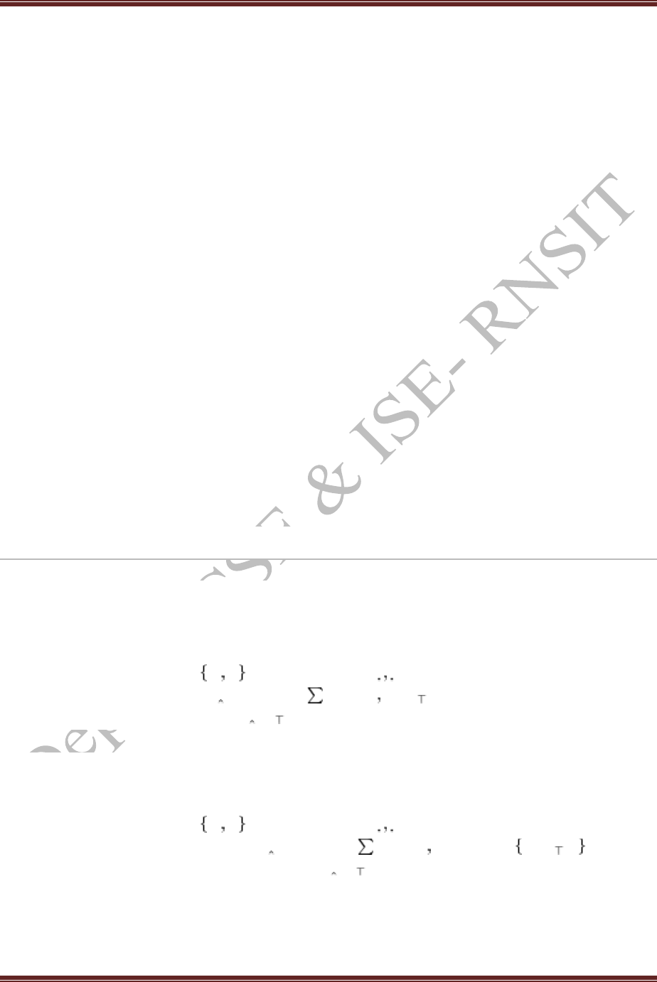
MACHINE LEARNING LABORATORY-15CSL76
Department of CSE and ISE, RNSIT Page 81
Locally Weighted Learning is a class of function approximation techniques, where a prediction is done
by using an approximated local model around the current point of interest.
The goal of function approximation and regression is to find the underlying relationship between input
and output. In a supervised learning problem training data, where each input is associated to one output,
is used to create a model that predicts values which come close to the true function. All of these models
use complete training data to derive global function.
Locally weighted regression
Local means using nearby points (i.e. a nearest neighbors approach)
Weighted means we value points based upon how far away they are.
Regression means approximating a function
This is an instance-based learning method
The idea: whenever you want to classify a sample:
Build a local model of the function (using a linear function, quadratic, neural network, etc.)
Use the model to predict the output value
Throw the model away.
Locally Weighted Regression
Our final method combines advantages of parametric methods with non-parametric. The idea is to fit a
regression model locally, weighting examples by the kernel K.
Locally Weighted Regression Algorithm
1. Given training data D=xiyi , Kernel function K( ) and input x
2. Fit weighted regression w(x)=argminw ni=1K(x xi)(w xi−yi)2
3. Return regression prediction w(x)x.
Note that we can do the same for classification, fitting a locally weighted logistic regression:
Locally Weighted Logistic Regression Algorithm
1. Given training data D=xiyi , Kernel function K( ) and input x
2. Fit weighted logistic regression w(x)=argminw ni=1K(x xi)log(1+exp −yiw xi)
3. Return logistic regression prediction sign(w(x)x).
The difference between regular linear regression and locally weighted linear regression can be
visualized as follows:
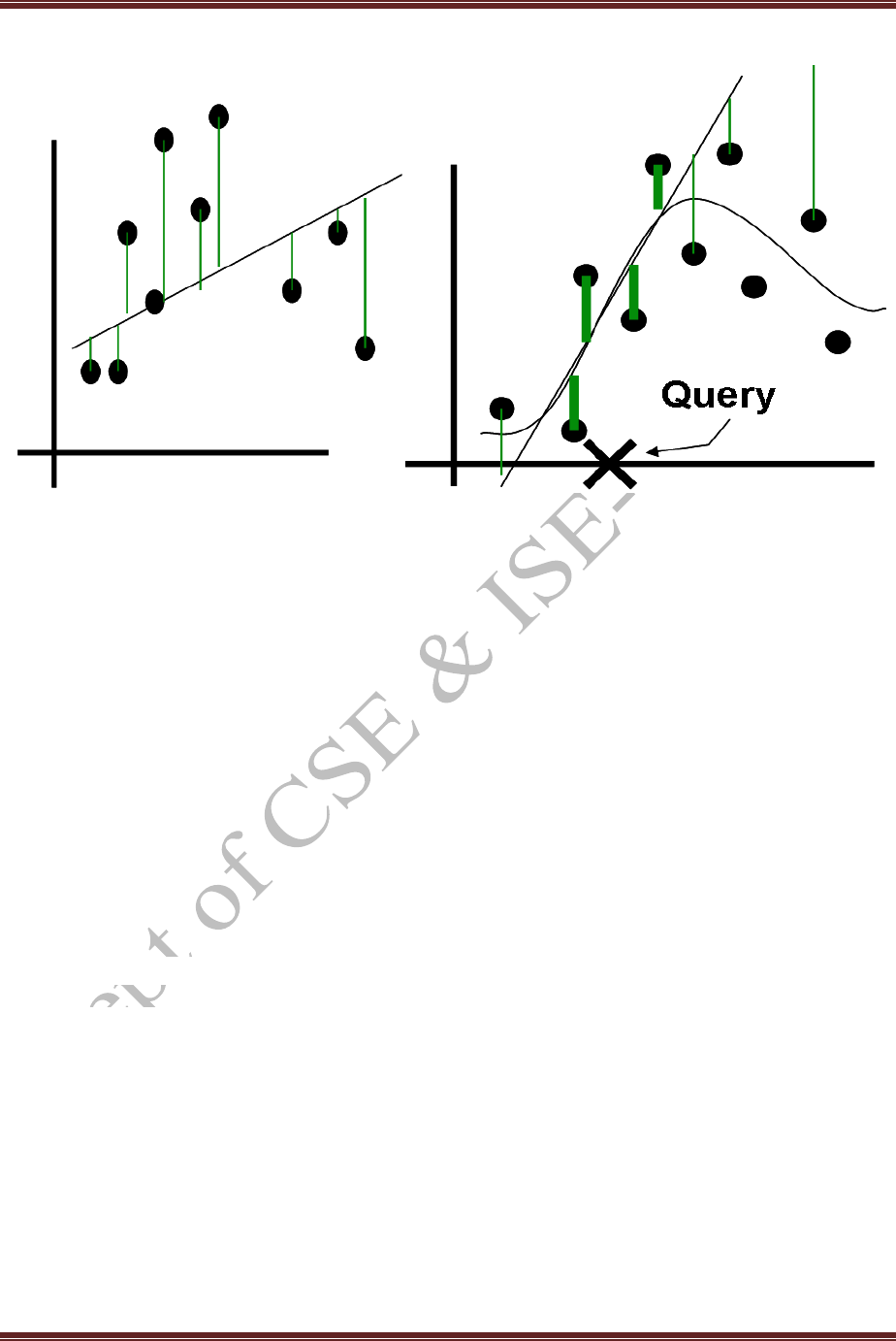
MACHINE LEARNING LABORATORY-15CSL76
Department of CSE and ISE, RNSIT Page 82
x ---- is an instance,
D ---- is the set of possible instances
ai(x)---- is the value of the i th attribute
wi ----The weights form our hypothesis
f ----is the target function
f ˆ ----is our approximation to the target function
In this case, we use a linear model to do the local approximation f ˆ :
fˆ(x) = w0 + w1a1(x) + · · · + wnan(x)
LOWESS is typically used for:
Fitting a line to a scatter plot or time plot where noisy data values, sparse data points or weak
interrelationships interfere with your ability to see a line of best fit.
Linear regression where least squares fitting doesn’t create a line of good fit or is too labor-
intensive to use.
Data exploration and analysis in the social sciences, particularly in elections and voting behavior.
Parametric and Non-Parametric Fitting
LOWESS, and least squares fitting in general, are non-parametric strategies for fitting a smooth curve
to data points. “Parametric” means that the researcher or analyst assumes in advance that the data fits

MACHINE LEARNING LABORATORY-15CSL76
Department of CSE and ISE, RNSIT Page 83
some type of distribution (i.e. the normal distribution). Because some type of distribution is assumed in
advance, parametric fitting can lead to fitting a smooth curve that misrepresents the data. In those cases,
non-parametric smoothers may be a better choice. Non-parametric smoothers like LOESS try to find a
curve of best fit without assuming the data must fit some distribution shape. In general, both types of
smoothers are used for the same set of data to offset the advantages and disadvantages of each type of
smoother.
Benefits of Non-Parametric Smoothing
Provides a flexible approach to representing data.
Ease of use.
Computations are relatively easy.
Disadvantages of Non-Parametric Smoothing
Can’t be used to obtain a simple equation for a set of data.
Less well understood than parametric smoothers.
Requires the analyst to use a little guesswork to obtain a result.
Locally Weighted Regrassion in Python:
from math import ceil
import numpy as np
from scipy import linalg
def lowess(x, y, f=2./3., iter=3):
n = len(x)
r = int(ceil(f*n))
h = [np.sort(np.abs(x - x[i]))[r] for i in range(n)]
w = np.clip(np.abs((x[:,None] - x[None,:]) / h), 0.0, 1.0)
w = (1 - w**3)**3
yest = np.zeros(n)
delta = np.ones(n)
for iteration in range(iter):
for i in range(n):
weights = delta * w[:,i]
b = np.array([np.sum(weights*y), np.sum(weights*y*x)])
A = np.array([[np.sum(weights), np.sum(weights*x)],
[np.sum(weights*x), np.sum(weights*x*x)]])
beta = linalg.solve(A, b)
yest[i] = beta[0] + beta[1]*x[i]
residuals = y - yest
s = np.median(np.abs(residuals))
delta = np.clip(residuals / (6.0 * s), -1, 1)
delta = (1 - delta**2)**2
return yest

MACHINE LEARNING LABORATORY-15CSL76
Department of CSE and ISE, RNSIT Page 84
if __name__ == '__main__':
import math
n = 100
x = np.linspace(0, 2 * math.pi, n)
print("==========================values of x=====================")
print(x)
y = np.sin(x) + 0.3*np.random.randn(n)
print("================================Values of y===================")
print(y)
f = 0.25
yest = lowess(x, y, f=f, iter=3)
import pylab as pl
pl.clf()
pl.plot(x, y, label='y noisy')
pl.plot(x, yest, label='y pred')
pl.legend()
pl.show()
Output
==========================values of x=====================
[0. 0.06346652 0.12693304 0.19039955 0.25386607 0.31733259
0.38079911 0.44426563 0.50773215 0.57119866 0.63466518 0.6981317
0.76159822 0.82506474 0.88853126 0.95199777 1.01546429 1.07893081
1.14239733 1.20586385 1.26933037 1.33279688 1.3962634 1.45972992
1.52319644 1.58666296 1.65012947 1.71359599 1.77706251 1.84052903
1.90399555 1.96746207 2.03092858 2.0943951 2.15786162 2.22132814
2.28479466 2.34826118 2.41172769 2.47519421 2.53866073 2.60212725
2.66559377 2.72906028 2.7925268 2.85599332 2.91945984 2.98292636
3.04639288 3.10985939 3.17332591 3.23679243 3.30025895 3.36372547
3.42719199 3.4906585 3.55412502 3.61759154 3.68105806 3.74452458
3.8079911 3.87145761 3.93492413 3.99839065 4.06185717 4.12532369
4.1887902 4.25225672 4.31572324 4.37918976 4.44265628 4.5061228
4.56958931 4.63305583 4.69652235 4.75998887 4.82345539 4.88692191
4.95038842 5.01385494 5.07732146 5.14078798 5.2042545 5.26772102
5.33118753 5.39465405 5.45812057 5.52158709 5.58505361 5.64852012
5.71198664 5.77545316 5.83891968 5.9023862 5.96585272 6.02931923
6.09278575 6.15625227 6.21971879 6.28318531]
================================Values of y===================
[-0.12131282 0.00704817 0.16084684 0.48415764 0.5790074 0.53758041
0.41471799 0.31435684 0.42541349 0.56873662 0.64857746 0.56416606
0.66906299 0.62626102 0.78385793 0.52007101 0.57661707 0.50246257
0.59223656 1.19576243 0.9781296 0.76416587 0.85825567 0.68360755
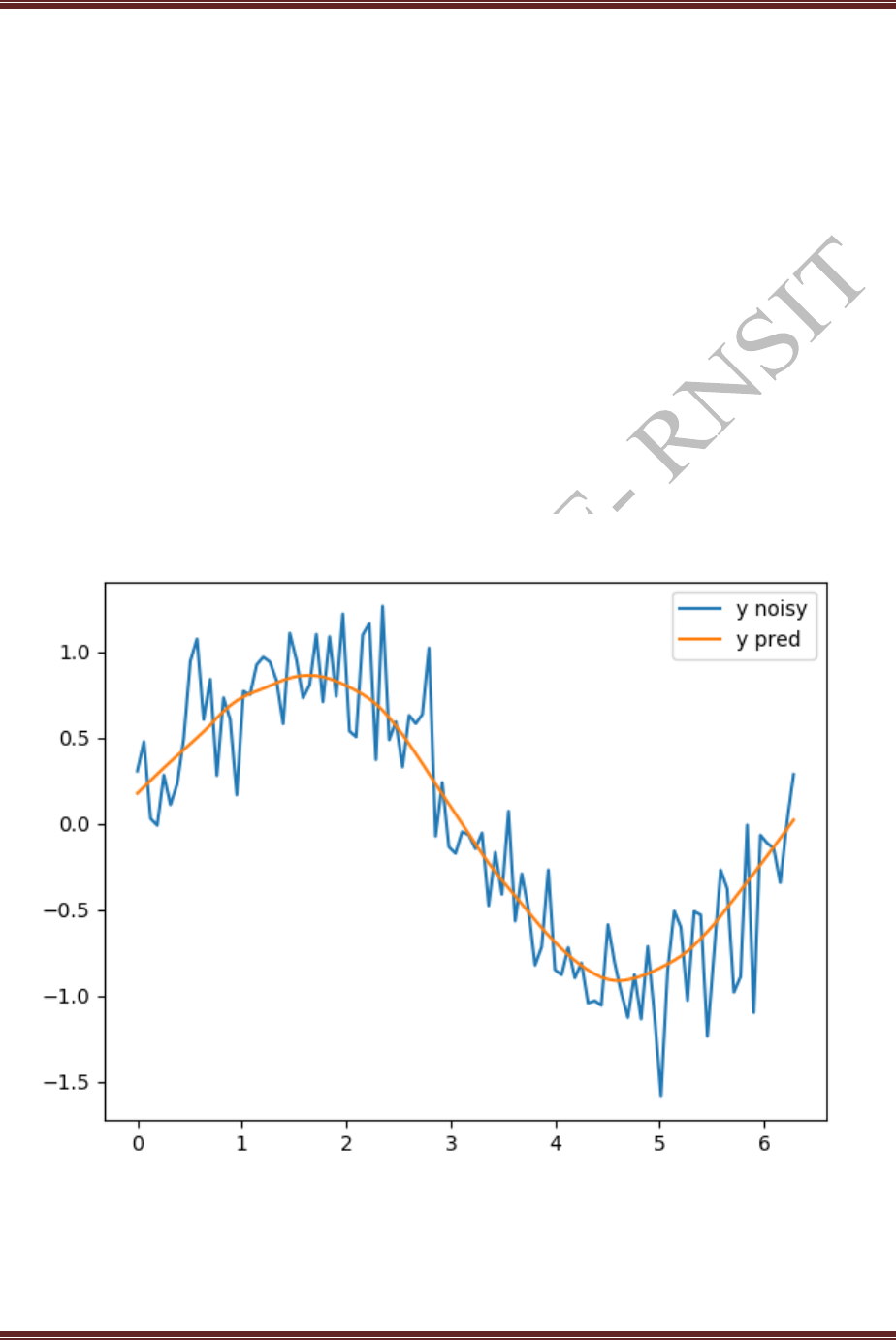
MACHINE LEARNING LABORATORY-15CSL76
Department of CSE and ISE, RNSIT Page 85
0.88965032 0.63976862 0.90159422 0.87464446 1.60256473 1.26886601
0.4200674 1.43656644 0.48378272 1.20891979 1.02955476 0.85766616
0.96519144 0.58303717 0.74996692 0.36357818 0.38481967 0.87027853
0.11686969 0.15356422 0.30403899 0.28014845 -0.15378752 0.56020242
0.20123909 -0.68626527 -0.19912738 -0.20357156 -0.1440503 -0.26493741
-0.32157543 -0.22139059 -0.42434559 -0.11447119 -0.67075934 -0.62973277
-1.18204429 -0.43386851 -1.12424791 -0.80806532 -0.85818104 -1.14149911
-0.23009694 -0.95399329 -0.62350893 -0.29176666 -0.55523556 -0.87957338
-1.78651723 -0.55784149 -1.1570492 -0.91445927 -0.99808369 -1.05836202
-0.55710891 -0.57815623 -0.60534368 -1.23588355 -1.34863514 -1.22421771
-1.01493553 -1.22922209 -0.48436674 -0.25055899 -0.61074483 -0.69197299
-0.52765904 -0.31451055 -0.55313683 -0.03399613 -0.53184918 0.33832978
-0.28385608 0.03227412 -0.38242201 0.1601836 ]
>>>