ROOT Manual For GATE Users
User Manual:
Open the PDF directly: View PDF ![]() .
.
Page Count: 21

ROOT manual for GATE users
Olga KOCHEBINA
kochebina@gmail.com
Version 1.1
October 1, 2018
2
Contents
1 Obtain your ROOT file 4
2 Painless ROOT file opening 4
3 Checking statistics of a TTree 6
4 Smart plotting of your histograms (without TBrowser and python scripts) 7
4.1 Colors,markers,lines............................... 9
4.1.1 Color.................................... 9
4.1.2 Size .................................... 10
4.1.3 Style.................................... 10
4.2 How to apply a simple selection . . . . . . . . . . . . . . . . . . . . . . . . . 13
4.3 Howtorebinahistogram ............................ 13
4.4 Superposition of two distributions . . . . . . . . . . . . . . . . . . . . . . . . 14
4.5 Superposition of two distributions from different ROOT files . . . . . . . . . 16
4.6 Simplefitting ................................... 16
5 Scan option for a printout 17
6 Simplest script to draw with ROOT 18
7 Example of a script to make nice plots 18
8 Adding a new variable to a TTree* 20
Abstract
This manual is for GATE users who want to become familiar with ROOT output
files. This documents contains simple actions with ROOT files. Though, despite their
apparent simplicity, they are very useful and sometimes not easy to figure out. In
some sense it is the manual of ”Getting started” with ROOT. Some of the used files
and scripts you can find on my github, link is here. Please, do not hesitate to contact
the author at kochebina@gmail.com if you have any questions and comments. And of
course, I strongly invite you to visit and use the ROOT web site, https://root.cern.ch/.
This manual is a brief introduction. Hopefully, it will help you in your first steps and
save you some time.
Have fun!
The author would like to thank Benoit VIAUD who taught me almost everything
that you will find in this manual.
3
1 Obtain your ROOT file
The standard way to get ROOT output is to add in your GATE macro:
/gate/output/root/enable
/gate/output/root/setFileName YourOutputFile
This command creates a file YourOutputFile.root, which contains usually several ROOT
TTree objects, like Hits, Singles, Coincidences. TTree is a ROOT object consisting of a
list of independent branches (TBranch). Each of them corresponds to saved variables from
obtained in GATE simulation. It can be energies, hit positions, process IDs etc. for each
generated event.
One can choose the standard TTree with commands:
/gate/output/root/setRootHitFlag 1
/gate/output/root/setRootSinglesFlag 1
In this case the .root file will contain default trees of Singles and Hits.
It is possible to add a TTree, for example, with an energy selection. To do so one should
add in digitizer something like:
/gate/digitizer/name peak171
/gate/digitizer/insert singleChain
/gate/digitizer/peak171/setInputName Singles
/gate/digitizer/peak171/insert thresholder
/gate/digitizer/peak171/thresholder/setThreshold 153.9 keV
/gate/digitizer/peak171/insert upholder
/gate/digitizer/peak171/upholder/setUphold 188.1 keV
This will add to the .root file a TTree with a name peak171 which will contain Singles events
with energies [153.9,188.1] keV. The more details could be found on GATE wiki page.
2 Painless ROOT file opening
The simplest way to open your ROOT file is to type in terminal:
> root -l YourOutputFile.root
Option -l removes the ROOT start image.
There are two ways to check the content of your file:
1. use a TBrowser, which is not very powerful and gives an access to visualize the structure
of your ROOT file but is very limited for selection application or histogram superposi-
tion
2. Recommend way is to use command in terminal:
root[0] .ls
4
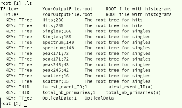
This command will display the list of all ROOT objects contained in your file or that you
created in the current ROOT session (see Figure 1). The first column corresponds to
the type of objects (TFile, TTree, root histogram TH1D, etc). The second is the name
followed by the third column which is a short description of the element. Sometimes
the TTrees are repeated twice, this should not bother you.
Figure 1: Output of .ls command
5
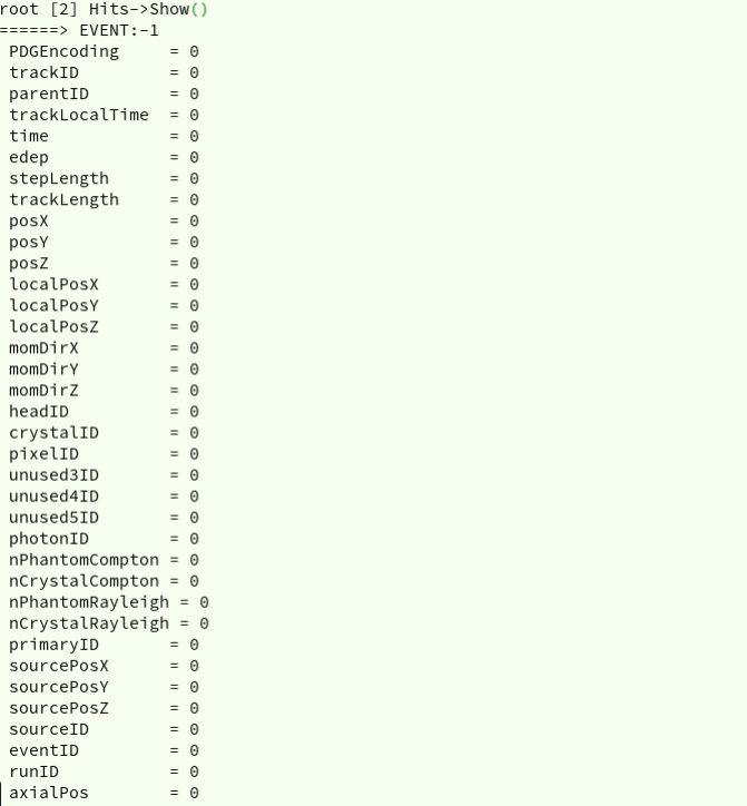
In order to get the content of a TTree, i.e. list of saved histograms or ”branches”, for
example for Hits TTree, one can do:
root[1] Hits->Show()
This method is used to get one entry of a tree, i.e. if one does Hits->Show(10), the
output will be given for the 10th entry. Thus, if the argument is empty, as in the example
above the output will is for the 0 entry (Figure 2).
Figure 2: Output of Show() command
3 Checking statistics of a TTree
To check how many events there are in a TTree without plotting histograms, one can open
ROOT file in a terminal window and do:
root[1] Hits->GetEntries()
The output will be like:
(Long64_t) 235868
6
which means that in the example Hits tree there are 235868 saved events.
4 Smart plotting of your histograms (without TBrowser
and python scripts)
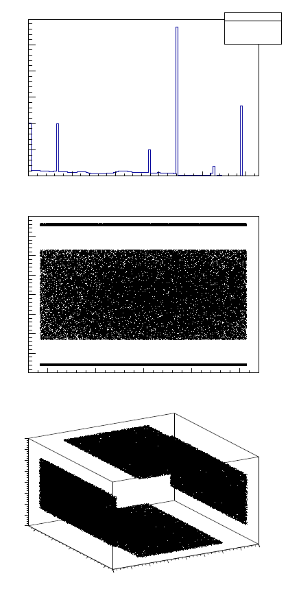
To plot a histogram one should use option TTree -> Draw("name_of_the_branch"). For
example, if you want to plot 1D, 2D or 3D histograms of energy and positions you could do
root[1] Hits->Draw("edep") for 1D (Figure 3, top)
root[2] Hits->Draw("posX:posY") for 2D, where the first argument, posX is ordinate
axis and posY is abscissa axis (Figure 3, middle)
root[3] Hits->Draw("posX:posY:posZ") for 3D (Figure 3, bottom)
7
htemp
Entries 235868
Mean 0.1181
Std Dev 0.07894
edep
0 0.05 0.1 0.15 0.2 0.25
0
10000
20000
30000
40000
50000
htemp
Entries 235868
Mean 0.1181
Std Dev 0.07894
edep
posY
100−50−0 50 100
posX
200−
150−
100−
50−
0
50
100
150
200
posX:posY
posZ
200−150−100−50−050 100 150 200
posY
100−
50−
0
50
100
posX
200−
150−
100−
50−
0
50
100
150
200
posX:posY:posZ
Figure 3: Output of Draw commands
8
4.1 Colors, markers, lines
4.1.1 Color
It is possible to change the colors, line and marker styles and size. To change the color one
can use TTree ->SetMarkerColor(n_of_color) or TTree ->SetLineColor(n_of_color).
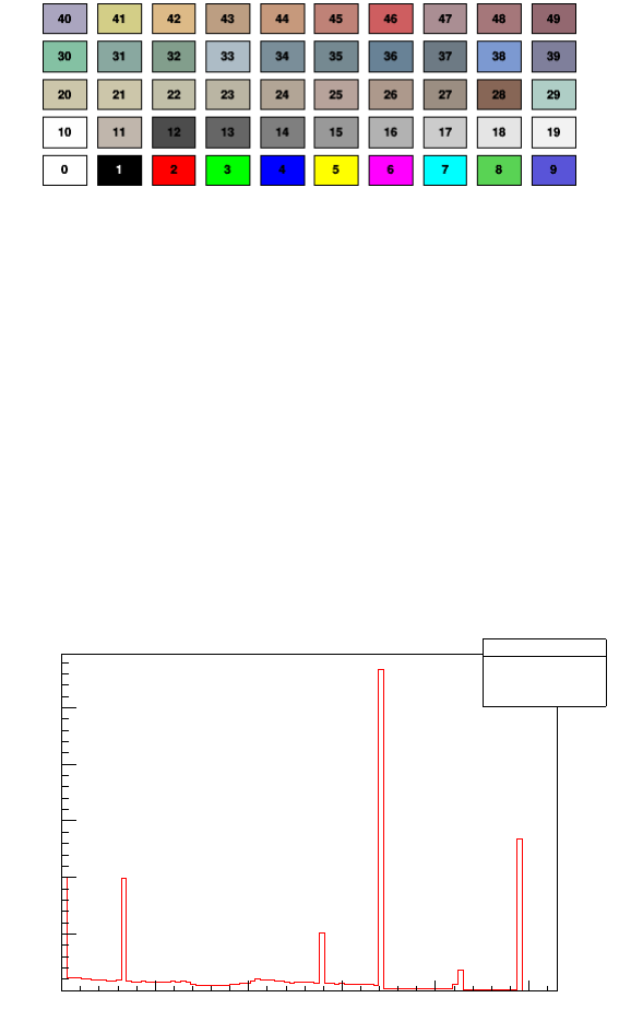
The n_of_color can be chosen from table in Figure 4, for more information check
https://root.cern.ch/doc/v606/classTColor.html
Figure 4: Basic ROOT colors used as a Draw() option. For more information check:
https://root.cern.ch/doc/v606/classTColor.html
The example of usage is in the following command and in Figure 5:
root[4] Hits->SetLineColor(2)
root[5] Hits->Draw("edep")
or to change marker color one can do:
root[4] Hits->SetMarkerColor(2)
root[5] Hits->Draw("edep")
htemp
Entries 235868
Mean 0.1181
Std Dev 0.07894
edep
0 0.05 0.1 0.15 0.2 0.25
0
10000
20000
30000
40000
50000
htemp
Entries 235868
Mean 0.1181
Std Dev 0.07894
edep
Figure 5: Drawing of the 1D histogram with a color option
9
4.1.2 Size
It is also possible to change size of lines with TTree ->SetLineWidth(size) (Figure 6):
root[4] Hits->SetLineWidth(3)
root[5] Hits->Draw("edep")
htemp
Entries 235868
Mean 0.1181
Std Dev 0.07894
edep
0 0.05 0.1 0.15 0.2 0.25
0
10000
20000
30000
40000
50000
htemp
Entries 235868
Mean 0.1181
Std Dev 0.07894
edep
Figure 6: Drawing of the 1D histogram with a LineWidth option
4.1.3 Style
It is also possible to change style of lines and markers with TTree ->SetLineStyle(n_of_style)
and TTree ->SetLineStyle(n_of_style). The n_of_style can be chosen from table in
Figure 7 and in Figure 8, for more information check
https://root.cern.ch/doc/v606/classTAttLine.html and
https://root.cern.ch/root/html534/TAttMarker.html
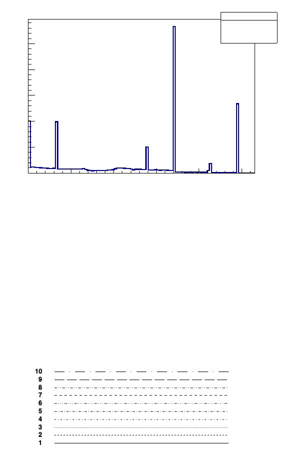
Figure 7: Basic ROOT line styles options. For more information check:
https://root.cern.ch/doc/v606/classTAttLine.html
An example how to use these options is in the following and the results are illustrated in
Figure 9 and in Figure 10:
10
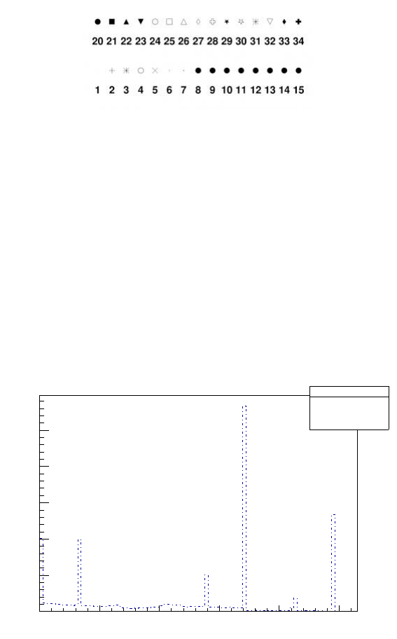
Figure 8: Basic ROOT marker styles options. For more information check:
https://root.cern.ch/root/html534/TAttMarker.html
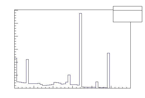
root[4] Hits->SetLineStyle(4)
root[5] Hits->Draw("edep")
and
root[4] Hits->SetMarkerStyle(4)
root[5] Hits->Draw("time:trackLength")
htemp
Entries 235868
Mean 0.1181
Std Dev 0.07894
edep
0 0.05 0.1 0.15 0.2 0.25
0
10000
20000
30000
40000
50000
htemp
Entries 235868
Mean 0.1181
Std Dev 0.07894
edep
Figure 9: Drawing of the 1D histogram with a LineStyle option
11
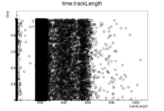
Figure 10: Drawing of the 2D histogram with a MarkerStyle option
12
4.2 How to apply a simple selection
It is also possible to apply a selection and after plot your variable. To do so one should use sec-
ond option of the Draw() function: TTree ->Draw("name_of_the_branch","selection").
The several examples of cuts are presented here and plot the effect of them on edep variable:
root[4] Hits->Draw("edep","trackID==1")
root[5] Hits->Draw("edep","posX>0.5")
root[6] Hits->Draw("edep","localPosX>=0.5")
root[7] Hits->Draw("edep","processName==\"phot\"") (variable is a string)
Or even more complicated selections like:
root[8] Hits->Draw("edep","trackID==1 && posX>0.5")
root[9] Hits->Draw("edep","trackID==1 || posX>0.5")
4.3 How to rebin a histogram
The default binning of a histogram in ROOT is 100 bins per axis (at least for 1D and 2D
histograms). It is possible to change it and the simplest way is the following:
One has to define a histogram with needed parameters:
root[1] TH1F* h = new TH1F("h","h",50,0,0.3)
Here we have a histogram with 50 bins in a range from 0 to 0.3.
Next step is to plot your histogram using the defined histogram ”h” (Figure 11):
root[2] Hits->Draw("edep>>h","","")
h
Entries 235868
Mean 0.1181
Std Dev 0.07894
0 0.05 0.1 0.15 0.2 0.25 0.3
0
10000
20000
30000
40000
50000
60000 h
Entries 235868
Mean 0.1181
Std Dev 0.07894
h
Figure 11: Drawing of rebinned 1D histogram
13
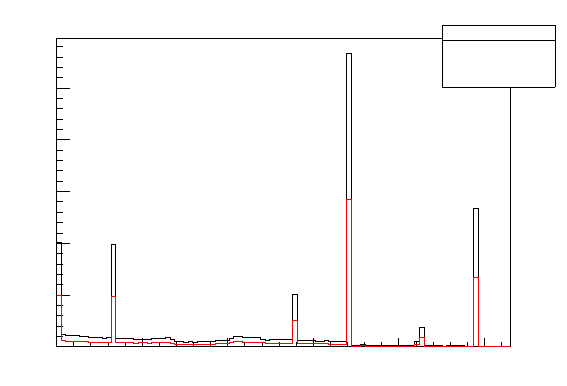
4.4 Superposition of two distributions
To superimpose two or more histograms one should write word ”same” in the third option of
the Draw() function: TTree ->Draw("name_of_the_branch","selection","same"). For
example, to obtain a histogram like in Figure 12 one can do:
root[4] Hits->Draw("edep","")
root[5] Hits->SetLineColor(2)
root[6] Hits->Draw("edep","processName==\"phot\"","same")
htemp
Entries 235868
Mean 0.1181
Std Dev 0.07894
edep
0 0.05 0.1 0.15 0.2 0.25
0
10000
20000
30000
40000
50000
htemp
Entries 235868
Mean 0.1181
Std Dev 0.07894
edep
Figure 12: Drawing of two superposed the 1D histogram: one without any selection (black)
and with a cut (red)
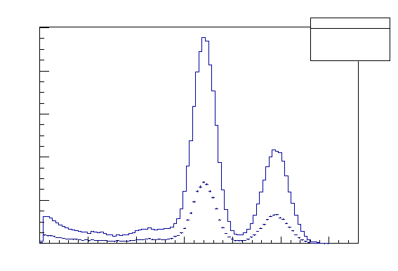
There is also a possibility to use "esame" option for the fast comparison of two histograms.
Actually, this option plot error bars ("e" stands for that) but I would not recommend to
rely on it and calculate and plot your own error bars. However, for a fast and easy
superposition of two histograms without changing of line color it works perfectly (Figure 13):
root[4] Singles->Draw("energy")
root[5] Singles->Draw("energy","time<0.3","esame")
14
htemp
Entries 159958
Mean 0.1741
Std Dev 0.06201
energy
0 0.05 0.1 0.15 0.2 0.25 0.3
0
2000
4000
6000
8000
10000 htemp
Entries 159958
Mean 0.1741
Std Dev 0.06201
energy
Figure 13: Drawing of two superposed the 1D histogram with ”esame” option
15
4.5 Superposition of two distributions from different ROOT files
Sometimes it is useful to plot a superposition of two histograms from different ROOT files.
In this case on start by opening the ROOT file 1:
> root -l YourOutputFile.root
or by an equivalent command directly in ROOT:
root[0] TFile *_file0 = TFile::Open("YourOutputFile.root");
and draw a histogram:
root[2] Singles->Draw("energy")
The next step is to open the second file by:
root[3] TFile *_file1 = TFile::Open("YourOutputFile1.root");
and draw the new histogram with ”same” or ”esame” option:
root[4] Singles->Draw("energy","","esame")
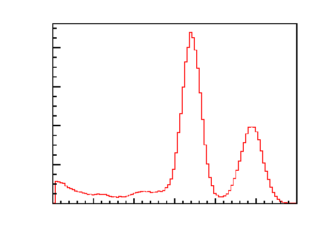
4.6 Simple fitting
It is possible to do a simple fit of your distribution. For this after drawing your histogram
you need to go to the canvas window and select Tools --> Fit Panel . You will have new
window with a Fit Panel as presented in Figure 14. There you can choose your fitting func-
tion, fitting method, fitting range etc. In the following example, the fit is done by Gaussian
function in the range [0.13;0.21] MeV. The parameters of the fit are printed in the terminal
window where you started ROOT and look like following:
FCN=1259.74 FROM MIGRAD STATUS=CONVERGED 75 CALLS 76 TOTAL
EDM=1.82902e-12 STRATEGY= 1 ERROR MATRIX ACCURATE
EXT PARAMETER STEP FIRST
NO. NAME VALUE ERROR SIZE DERIVATIVE
1 Constant 9.05059e+03 4.05523e+01 5.29487e-01 -2.23836e-09
2 Mean 1.70049e-01 4.42797e-05 7.60710e-07 -4.18082e-02
3 Sigma 1.28126e-02 3.88904e-05 1.30065e-05 -8.44577e-04
More about the fitting options can be found on ROOT web page.
16

Figure 14: Fit panel and an example of fitted histogram
5 Scan option for a printout
Sometimes it is useful to printout the content of a branch, for example, in case when you
want to study some anomalies. For this purpose one can use Scan() function. It is similar
to Draw(), i.e. you also can apply cuts and plot several variables. For example, if one does:
root[4] Hits->Scan("edep:posX","time<0.1&&posY>0")
the output will be something like this:
************************************
* Row * edep * posX *
************************************
* 4 * 0.0198734 * 25.182537 *
* 5 * 0 * 25.227350 *
* 11 * 0 * -180.9978 *
* 14 * 0.2450000 * 104.99372 *
* 15 * 0.1710000 * -91.10610 *
* 18 * 0.2199750 * 58.401462 *
* 21 * 0.2450000 * -181.6459 *
* ...
* 60 * 0.1710000 * -47.08741 *
Type <CR> to continue or q to quit ==>
There are only first 25 lines in the output, one can press either ”Enter” to continue or ”q”
to exit.
17
6 Simplest script to draw with ROOT
Sometimes it is useful to group the previous commands in a small script. Let’s call it
my_script.C, in order to run it one can do:
> root -l my_script.C
The my_script.C should contain something like this:
{
TFile *_file0 = TFile::Open("YourOutputFile.root");
Singles->Draw("energy");
Singles->Draw("energy","time<0.3","esame");
},
where you open file at the beginning and after you can copy your plotting commands. NB:
The plotting commands are done for the last opened file. If you want to plot
two histograms from different files, you have to open each time the needed file
before plotting.
7 Example of a script to make nice plots
I hear all the time a lot of complains that the ROOT plots are not beautiful. Thus, in this
section I propose you a template to start for your plots. To run the script one should do:
> root -l my_script.C
The name of the main function in my_script.C must be the same as the name of your
script file containing the following:
void my_script() {
//remove the stat from upper right corner
gStyle->SetOptStat(0);
//remove the title
gStyle->SetOptTitle(0);
//define fonts sizes
gStyle->SetTextSize(0.06);
gStyle->SetLabelSize(0.06,"x");
gStyle->SetLabelSize(0.06,"y");
gStyle->SetLabelSize(0.06,"z");
gStyle->SetTitleSize(0.06,"x");
gStyle->SetTitleSize(0.05,"y");
gStyle->SetTitleSize(0.06,"z");
//define number of divisions on any axis, here is done only for "Y"
gStyle->SetNdivisions(505,"y");
gStyle->SetLineWidth(3);
//define your ROOT file name
TString filename = "YourOutputFile.root";
18
// open the file
TFile *f = TFile::Open(filename);
// get the TTree
TTree *Tree = (TTree*)f->Get("Singles");
// define the variable(s) of interest, type of variable must be respected
Float_t energy;
// define the branch(s) of interest
TBranch *benergy;
// Set branch address
Tree->SetBranchAddress( "energy", &energy, &benergy);
// Get number of events in the TTree
const int n=(const int)Tree->GetEntries();
// Define a histogram with 100 bins, on x from 0 to 0.3
TH1F* h = new TH1F("h","h",100,0,0.3);
// Loop over events
for(int i=0;i<n;i++)
{
//get event i
Tree->GetEntry(i);
benergy->GetEntry(i);
//print out the values
cout<<i<<" "<<energy<<endl;
//fill histogram
h->Fill(energy);
}
//Define canvas
TCanvas *can = new TCanvas("can","can",600,800);
//Define paramters of the canvas
can->SetFillColor(0);
can->SetBorderMode(0);
can->SetBorderSize(3);
can->SetBottomMargin(0.14);
can->SetLeftMargin(0.16);
can->SetFrameBorderMode(0);
can->SetFrameLineWidth(3);
can->SetFrameBorderMode(0);
19
//Define parameters of the histogram
h->SetLineWidth(2);
h->SetLineColor(2);
h->GetXaxis()->SetTitle("Energy, MeV");
h->GetYaxis()->SetTitleOffset(1.6);
h->GetYaxis()->SetTitle("Arbitrary units");
//Draw histogram
h->Draw();
//Save cancas as .pdf
can->SaveAs("energy.pdf");
}
This script could also be found here.
The output result is shown in Figure 15.
Energy, MeV
0 0.05 0.1 0.15 0.2 0.25 0.3
Arbitrary units
0
2000
4000
6000
8000
Figure 15: The output of the example of script making beautiful plots.
8 Adding a new variable to a TTree*
In this section I will just add a link to the script that indicates how to add a new variable.
It is a script that adds a shift on energy which is different for each of four detection heads.
One can find it here: AddShiftedEnergy.C.
20
