The Data Warehouse Toolkit, 3rd Edition Ralph Kimball, Margy Ross Toolkit Definitive Guide To Dimensional Ing Wil
User Manual:
Open the PDF directly: View PDF ![]() .
.
Page Count: 601 [warning: Documents this large are best viewed by clicking the View PDF Link!]
- Cover������������
- Title Page�����������������
- Copyright����������������
- Contents���������������
- 1 Data Warehousing, Business Intelligence, and Dimensional Modeling Primer���������������������������������������������������������������������������������
- Different Worlds of Data Capture and Data Analysis���������������������������������������������������������
- Goals of Data Warehousing and Business Intelligence����������������������������������������������������������
- Dimensional Modeling Introduction����������������������������������������
- Star Schemas Versus OLAP Cubes�������������������������������������
- Fact Tables for Measurements�����������������������������������
- Dimension Tables for Descriptive Context�����������������������������������������������
- Facts and Dimensions Joined in a Star Schema���������������������������������������������������
- Kimball’s DW/BI Architecture�����������������������������������
- Operational Source Systems���������������������������������
- Extract, Transformation, and Load System�����������������������������������������������
- Presentation Area to Support Business Intelligence���������������������������������������������������������
- Business Intelligence Applications�����������������������������������������
- Restaurant Metaphor for the Kimball Architecture�������������������������������������������������������
- Alternative DW/BI Architectures��������������������������������������
- Independent Data Mart Architecture�����������������������������������������
- Hub-and-Spoke Corporate Information Factory Inmon Architecture���������������������������������������������������������������������
- Hybrid Hub-and-Spoke and Kimball Architecture����������������������������������������������������
- Dimensional Modeling Myths���������������������������������
- Myth 1: Dimensional Models are Only for Summary Data�����������������������������������������������������������
- Myth 2: Dimensional Models are Departmental, Not Enterprise������������������������������������������������������������������
- Myth 3: Dimensional Models are Not Scalable��������������������������������������������������
- Myth 4: Dimensional Models are Only for Predictable Usage����������������������������������������������������������������
- Myth 5: Dimensional Models Can’t Be Integrated�����������������������������������������������������
- More Reasons to Think Dimensionally������������������������������������������
- Agile Considerations���������������������������
- Summary��������������
- 2 Kimball Dimensional Modeling Techniques Overview���������������������������������������������������������
- Fundamental Concepts���������������������������
- Gather Business Requirements and Data Realities������������������������������������������������������
- Collaborative Dimensional Modeling Workshops���������������������������������������������������
- Four-Step Dimensional Design Process�������������������������������������������
- Business Processes�������������������������
- Grain������������
- Dimensions for Descriptive Context�����������������������������������������
- Facts for Measurements�����������������������������
- Star Schemas and OLAP Cubes����������������������������������
- Graceful Extensions to Dimensional Models������������������������������������������������
- Basic Fact Table Techniques����������������������������������
- Fact Table Structure���������������������������
- Additive, Semi-Additive, Non-Additive Facts��������������������������������������������������
- Nulls in Fact Tables���������������������������
- Conformed Facts����������������������
- Transaction Fact Tables������������������������������
- Periodic Snapshot Fact Tables������������������������������������
- Accumulating Snapshot Fact Tables����������������������������������������
- Factless Fact Tables���������������������������
- Aggregate Fact Tables or OLAP Cubes������������������������������������������
- Consolidated Fact Tables�������������������������������
- Basic Dimension Table Techniques���������������������������������������
- Dimension Table Structure��������������������������������
- Dimension Surrogate Keys�������������������������������
- Natural, Durable, and Supernatural Keys����������������������������������������������
- Drilling Down��������������������
- Degenerate Dimensions����������������������������
- Denormalized Flattened Dimensions����������������������������������������
- Multiple Hierarchies in Dimensions�����������������������������������������
- Flags and Indicators as Textual Attributes�������������������������������������������������
- Null Attributes in Dimensions������������������������������������
- Calendar Date Dimensions�������������������������������
- Role-Playing Dimensions������������������������������
- Junk Dimensions����������������������
- Snowflaked Dimensions����������������������������
- Outrigger Dimensions���������������������������
- Integration via Conformed Dimensions�������������������������������������������
- Conformed Dimensions���������������������������
- Shrunken Dimensions��������������������������
- Drilling Across����������������������
- Value Chain������������������
- Enterprise Data Warehouse Bus Architecture�������������������������������������������������
- Enterprise Data Warehouse Bus Matrix�������������������������������������������
- Detailed Implementation Bus Matrix�����������������������������������������
- Opportunity/Stakeholder Matrix�������������������������������������
- Dealing with Slowly Changing Dimension Attributes��������������������������������������������������������
- Type 0: Retain Original������������������������������
- Type 1: Overwrite������������������������
- Type 2: Add New Row��������������������������
- Type 3: Add New Attribute��������������������������������
- Type 4: Add Mini-Dimension���������������������������������
- Type 5: Add Mini-Dimension and Type 1 Outrigger������������������������������������������������������
- Type 6: Add Type 1 Attributes to Type 2 Dimension��������������������������������������������������������
- Type 7: Dual Type 1 and Type 2 Dimensions������������������������������������������������
- Dealing with Dimension Hierarchies�����������������������������������������
- Fixed Depth Positional Hierarchies�����������������������������������������
- Slightly Ragged/Variable Depth Hierarchies�������������������������������������������������
- Ragged/Variable Depth Hierarchies with Hierarchy Bridge Tables���������������������������������������������������������������������
- Ragged/Variable Depth Hierarchies with Pathstring Attributes�������������������������������������������������������������������
- Advanced Fact Table Techniques�������������������������������������
- Fact Table Surrogate Keys��������������������������������
- Centipede Fact Tables����������������������������
- Numeric Values as Attributes or Facts��������������������������������������������
- Lag/Duration Facts�������������������������
- Header/Line Fact Tables������������������������������
- Allocated Facts����������������������
- Profit and Loss Fact Tables Using Allocations����������������������������������������������������
- Multiple Currency Facts������������������������������
- Multiple Units of Measure Facts��������������������������������������
- Year-to-Date Facts�������������������������
- Multipass SQL to Avoid Fact-to-Fact Table Joins������������������������������������������������������
- Timespan Tracking in Fact Tables���������������������������������������
- Late Arriving Facts��������������������������
- Advanced Dimension Techniques������������������������������������
- Dimension-to-Dimension Table Joins�����������������������������������������
- Multivalued Dimensions and Bridge Tables�����������������������������������������������
- Time Varying Multivalued Bridge Tables���������������������������������������������
- Behavior Tag Time Series�������������������������������
- Behavior Study Groups����������������������������
- Aggregated Facts as Dimension Attributes�����������������������������������������������
- Dynamic Value Bands��������������������������
- Text Comments Dimension������������������������������
- Multiple Time Zones��������������������������
- Measure Type Dimensions������������������������������
- Step Dimensions����������������������
- Hot Swappable Dimensions�������������������������������
- Abstract Generic Dimensions����������������������������������
- Audit Dimensions�����������������������
- Late Arriving Dimensions�������������������������������
- Special Purpose Schemas������������������������������
- Fundamental Concepts���������������������������
- 3 Retail Sales���������������������
- Four-Step Dimensional Design Process�������������������������������������������
- Retail Case Study������������������������
- Dimension Table Details������������������������������
- Date Dimension���������������������
- Product Dimension������������������������
- Store Dimension����������������������
- Promotion Dimension��������������������������
- Other Retail Sales Dimensions������������������������������������
- Degenerate Dimensions for Transaction Numbers����������������������������������������������������
- Retail Schema in Action������������������������������
- Retail Schema Extensibility����������������������������������
- Factless Fact Tables���������������������������
- Dimension and Fact Table Keys������������������������������������
- Dimension Table Surrogate Keys�������������������������������������
- Dimension Natural and Durable Supernatural Keys������������������������������������������������������
- Degenerate Dimension Surrogate Keys������������������������������������������
- Date Dimension Smart Keys��������������������������������
- Fact Table Surrogate Keys��������������������������������
- Resisting Normalization Urges������������������������������������
- Summary��������������
- 4 Inventory������������������
- Value Chain Introduction�������������������������������
- Inventory Models�����������������������
- Fact Table Types�����������������������
- Value Chain Integration������������������������������
- Enterprise Data Warehouse Bus Architecture�������������������������������������������������
- Conformed Dimensions���������������������������
- Drilling Across Fact Tables����������������������������������
- Identical Conformed Dimensions�������������������������������������
- Shrunken Rollup Conformed Dimension with Attribute Subset����������������������������������������������������������������
- Shrunken Conformed Dimension with Row Subset���������������������������������������������������
- Shrunken Conformed Dimensions on the Bus Matrix������������������������������������������������������
- Limited Conformity�������������������������
- Importance of Data Governance and Stewardship����������������������������������������������������
- Conformed Dimensions and the Agile Movement��������������������������������������������������
- Conformed Facts����������������������
- Summary��������������
- 5 Procurement��������������������
- Procurement Case Study�����������������������������
- Procurement Transactions and Bus Matrix����������������������������������������������
- Slowly Changing Dimension Basics���������������������������������������
- Hybrid Slowly Changing Dimension Techniques��������������������������������������������������
- Slowly Changing Dimension Recap��������������������������������������
- Summary��������������
- 6 Order Management�������������������������
- Order Management Bus Matrix����������������������������������
- Order Transactions�������������������������
- Fact Normalization�������������������������
- Dimension Role Playing�����������������������������
- Product Dimension Revisited����������������������������������
- Customer Dimension�������������������������
- Deal Dimension���������������������
- Degenerate Dimension for Order Number��������������������������������������������
- Junk Dimensions����������������������
- Header/Line Pattern to Avoid�����������������������������������
- Multiple Currencies��������������������������
- Transaction Facts at Different Granularity�������������������������������������������������
- Another Header/Line Pattern to Avoid�������������������������������������������
- Invoice Transactions���������������������������
- Accumulating Snapshot for Order Fulfillment Pipeline�����������������������������������������������������������
- Summary��������������
- 7 Accounting�������������������
- Accounting Case Study and Bus Matrix�������������������������������������������
- General Ledger Data��������������������������
- General Ledger Periodic Snapshot���������������������������������������
- Chart of Accounts������������������������
- Period Close�������������������
- Year-to-Date Facts�������������������������
- Multiple Currencies Revisited������������������������������������
- General Ledger Journal Transactions������������������������������������������
- Multiple Fiscal Accounting Calendars�������������������������������������������
- Drilling Down Through a Multilevel Hierarchy���������������������������������������������������
- Financial Statements���������������������������
- Budgeting Process������������������������
- Dimension Attribute Hierarchies��������������������������������������
- Fixed Depth Positional Hierarchies�����������������������������������������
- Slightly Ragged Variable Depth Hierarchies�������������������������������������������������
- Ragged Variable Depth Hierarchies����������������������������������������
- Shared Ownership in a Ragged Hierarchy���������������������������������������������
- Time Varying Ragged Hierarchies��������������������������������������
- Modifying Ragged Hierarchies�����������������������������������
- Alternative Ragged Hierarchy Modeling Approaches�������������������������������������������������������
- Advantages of the Bridge Table Approach for Ragged Hierarchies���������������������������������������������������������������������
- Consolidated Fact Tables�������������������������������
- Role of OLAP and Packaged Analytic Solutions���������������������������������������������������
- Summary��������������
- 8 Customer Relationship Management�����������������������������������������
- CRM Overview�������������������
- Customer Dimension Attributes������������������������������������
- Name and Address Parsing�������������������������������
- International Name and Address Considerations����������������������������������������������������
- Customer-Centric Dates�����������������������������
- Aggregated Facts as Dimension Attributes�����������������������������������������������
- Segmentation Attributes and Scores�����������������������������������������
- Counts with Type 2 Dimension Changes�������������������������������������������
- Outrigger for Low Cardinality Attribute Set��������������������������������������������������
- Customer Hierarchy Considerations����������������������������������������
- Bridge Tables for Multivalued Dimensions�����������������������������������������������
- Complex Customer Behavior��������������������������������
- Behavior Study Groups for Cohorts����������������������������������������
- Step Dimension for Sequential Behavior���������������������������������������������
- Timespan Fact Tables���������������������������
- Tagging Fact Tables with Satisfaction Indicators�������������������������������������������������������
- Tagging Fact Tables with Abnormal Scenario Indicators������������������������������������������������������������
- Customer Data Integration Approaches�������������������������������������������
- Master Data Management Creating a Single Customer Dimension������������������������������������������������������������������
- Partial Conformity of Multiple Customer Dimensions���������������������������������������������������������
- Avoiding Fact-to-Fact Table Joins����������������������������������������
- Low Latency Reality Check��������������������������������
- Summary��������������
- 9 Human Resources Management�����������������������������������
- Employee Profile Tracking��������������������������������
- Headcount Periodic Snapshot����������������������������������
- Bus Matrix for HR Processes����������������������������������
- Packaged Analytic Solutions and Data Models��������������������������������������������������
- Recursive Employee Hierarchies�������������������������������������
- Multivalued Skill Keyword Attributes�������������������������������������������
- Survey Questionnaire Data��������������������������������
- Summary��������������
- 10 Financial Services����������������������������
- Banking Case Study and Bus Matrix����������������������������������������
- Dimension Triage to Avoid Too Few Dimensions���������������������������������������������������
- Household Dimension��������������������������
- Multivalued Dimensions and Weighting Factors���������������������������������������������������
- Mini-Dimensions Revisited��������������������������������
- Adding a Mini-Dimension to a Bridge Table������������������������������������������������
- Dynamic Value Banding of Facts�������������������������������������
- Supertype and Subtype Schemas for Heterogeneous Products���������������������������������������������������������������
- Hot Swappable Dimensions�������������������������������
- Summary��������������
- 11 Telecommunications����������������������������
- Telecommunications Case Study and Bus Matrix���������������������������������������������������
- General Design Review Considerations�������������������������������������������
- Balance Business Requirements and Source Realities���������������������������������������������������������
- Focus on Business Processes����������������������������������
- Granularity������������������
- Single Granularity for Facts�����������������������������������
- Dimension Granularity and Hierarchies��������������������������������������������
- Date Dimension���������������������
- Degenerate Dimensions����������������������������
- Surrogate Keys���������������������
- Dimension Decodes and Descriptions�����������������������������������������
- Conformity Commitment����������������������������
- Design Review Guidelines�������������������������������
- Draft Design Exercise Discussion���������������������������������������
- Remodeling Existing Data Structures������������������������������������������
- Geographic Location Dimension������������������������������������
- Summary��������������
- 12 Transportation������������������������
- Airline Case Study and Bus Matrix����������������������������������������
- Extensions to Other Industries�������������������������������������
- Combining Correlated Dimensions��������������������������������������
- More Date and Time Considerations����������������������������������������
- Localization Recap�������������������������
- Summary��������������
- 13 Education�������������������
- University Case Study and Bus Matrix�������������������������������������������
- Accumulating Snapshot Fact Tables����������������������������������������
- Factless Fact Tables���������������������������
- More Educational Analytic Opportunities����������������������������������������������
- Summary��������������
- 14 Healthcare��������������������
- Healthcare Case Study and Bus Matrix�������������������������������������������
- Claims Billing and Payments����������������������������������
- Electronic Medical Records���������������������������������
- Facility/Equipment Inventory Utilization�����������������������������������������������
- Dealing with Retroactive Changes���������������������������������������
- Summary��������������
- 15 Electronic Commerce�����������������������������
- Clickstream Source Data������������������������������
- Clickstream Dimensional Models�������������������������������������
- Page Dimension���������������������
- Event Dimension����������������������
- Session Dimension������������������������
- Referral Dimension�������������������������
- Clickstream Session Fact Table�������������������������������������
- Clickstream Page Event Fact Table����������������������������������������
- Step Dimension���������������������
- Aggregate Clickstream Fact Tables����������������������������������������
- Google Analytics�����������������������
- Integrating Clickstream into Web Retailer’s Bus Matrix�������������������������������������������������������������
- Profitability Across Channels Including Web��������������������������������������������������
- Summary��������������
- 16 Insurance�������������������
- Insurance Case Study���������������������������
- Policy Transactions��������������������������
- Dimension Role Playing�����������������������������
- Slowly Changing Dimensions���������������������������������
- Mini-Dimensions for Large or Rapidly Changing Dimensions���������������������������������������������������������������
- Multivalued Dimension Attributes���������������������������������������
- Numeric Attributes as Facts or Dimensions������������������������������������������������
- Degenerate Dimension���������������������������
- Low Cardinality Dimension Tables���������������������������������������
- Audit Dimension����������������������
- Policy Transaction Fact Table������������������������������������
- Heterogeneous Supertype and Subtype Products���������������������������������������������������
- Complementary Policy Accumulating Snapshot�������������������������������������������������
- Premium Periodic Snapshot��������������������������������
- Conformed Dimensions���������������������������
- Conformed Facts����������������������
- Pay-in-Advance Facts���������������������������
- Heterogeneous Supertypes and Subtypes Revisited������������������������������������������������������
- Multivalued Dimensions Revisited���������������������������������������
- More Insurance Case Study Background�������������������������������������������
- Claim Transactions�������������������������
- Claim Accumulating Snapshot����������������������������������
- Policy/Claim Consolidated Periodic Snapshot��������������������������������������������������
- Factless Accident Events�������������������������������
- Common Dimensional Modeling Mistakes to Avoid����������������������������������������������������
- Mistake 10: Place Text Attributes in a Fact Table��������������������������������������������������������
- Mistake 9: Limit Verbose Descriptors to Save Space���������������������������������������������������������
- Mistake 8: Split Hierarchies into Multiple Dimensions������������������������������������������������������������
- Mistake 7: Ignore the Need to Track Dimension Changes������������������������������������������������������������
- Mistake 6: Solve All Performance Problems with More Hardware�������������������������������������������������������������������
- Mistake 5: Use Operational Keys to Join Dimensions and Facts�������������������������������������������������������������������
- Mistake 4: Neglect to Declare and Comply with the Fact Grain�������������������������������������������������������������������
- Mistake 3: Use a Report to Design the Dimensional Model��������������������������������������������������������������
- Mistake 2: Expect Users to Query Normalized Atomic Data��������������������������������������������������������������
- Mistake 1: Fail to Conform Facts and Dimensions������������������������������������������������������
- Summary��������������
- 17 Kimball DW/BI Lifecycle Overview������������������������������������������
- Lifecycle Roadmap������������������������
- Lifecycle Launch Activities����������������������������������
- Lifecycle Technology Track���������������������������������
- Lifecycle Data Track���������������������������
- Lifecycle BI Applications Track��������������������������������������
- Lifecycle Wrap-up Activities�����������������������������������
- Common Pitfalls to Avoid�������������������������������
- Summary��������������
- 18 Dimensional Modeling Process and Tasks������������������������������������������������
- Modeling Process Overview��������������������������������
- Get Organized��������������������
- Identify Participants, Especially Business Representatives�����������������������������������������������������������������
- Review the Business Requirements���������������������������������������
- Leverage a Modeling Tool�������������������������������
- Leverage a Data Profiling Tool�������������������������������������
- Leverage or Establish Naming Conventions�����������������������������������������������
- Coordinate Calendars and Facilities������������������������������������������
- Design the Dimensional Model�����������������������������������
- Reach Consensus on High-Level Bubble Chart�������������������������������������������������
- Develop the Detailed Dimensional Model���������������������������������������������
- Review and Validate the Model������������������������������������
- Finalize the Design Documentation����������������������������������������
- Summary��������������
- 19 ETL Subsystems and Techniques���������������������������������������
- Round Up the Requirements��������������������������������
- Business Needs���������������������
- Compliance�����������������
- Data Quality�������������������
- Security���������������
- Data Integration�����������������������
- Data Latency�������������������
- Archiving and Lineage����������������������������
- BI Delivery Interfaces�����������������������������
- Available Skills�����������������������
- Legacy Licenses����������������������
- The 34 Subsystems of ETL�������������������������������
- Extracting: Getting Data into the Data Warehouse�������������������������������������������������������
- Cleaning and Conforming Data�����������������������������������
- Improving Data Quality Culture and Processes���������������������������������������������������
- Subsystem 4: Data Cleansing System�����������������������������������������
- Subsystem 5: Error Event Schema��������������������������������������
- Subsystem 6: Audit Dimension Assembler���������������������������������������������
- Subsystem 7: Deduplication System����������������������������������������
- Subsystem 8: Conforming System�������������������������������������
- Delivering: Prepare for Presentation�������������������������������������������
- Subsystem 9: Slowly Changing Dimension Manager�����������������������������������������������������
- Subsystem 10: Surrogate Key Generator��������������������������������������������
- Subsystem 11: Hierarchy Manager��������������������������������������
- Subsystem 12: Special Dimensions Manager�����������������������������������������������
- Subsystem 13: Fact Table Builders����������������������������������������
- Subsystem 14: Surrogate Key Pipeline�������������������������������������������
- Subsystem 15: Multivalued Dimension Bridge Table Builder���������������������������������������������������������������
- Subsystem 16: Late Arriving Data Handler�����������������������������������������������
- Subsystem 17: Dimension Manager System���������������������������������������������
- Subsystem 18: Fact Provider System�����������������������������������������
- Subsystem 19: Aggregate Builder��������������������������������������
- Subsystem 20: OLAP Cube Builder��������������������������������������
- Subsystem 21: Data Propagation Manager���������������������������������������������
- Managing the ETL Environment�����������������������������������
- Subsystem 22: Job Scheduler����������������������������������
- Subsystem 23: Backup System����������������������������������
- Subsystem 24: Recovery and Restart System������������������������������������������������
- Subsystem 25: Version Control System�������������������������������������������
- Subsystem 26: Version Migration System���������������������������������������������
- Subsystem 27: Workflow Monitor�������������������������������������
- Subsystem 28: Sorting System�����������������������������������
- Subsystem 29: Lineage and Dependency Analyzer����������������������������������������������������
- Subsystem 30: Problem Escalation System����������������������������������������������
- Subsystem 31: Parallelizing/Pipelining System����������������������������������������������������
- Subsystem 32: Security System������������������������������������
- Subsystem 33: Compliance Manager���������������������������������������
- Subsystem 34: Metadata Repository Manager������������������������������������������������
- Summary��������������
- Round Up the Requirements��������������������������������
- 20 ETL System Design and Development Process and Tasks�������������������������������������������������������������
- ETL Process Overview���������������������������
- Develop the ETL Plan���������������������������
- Step 1: Draw the High-Level Plan���������������������������������������
- Step 2: Choose an ETL Tool���������������������������������
- Step 3: Develop Default Strategies�����������������������������������������
- Step 4: Drill Down by Target Table�����������������������������������������
- Develop the ETL Specification Document���������������������������������������������
- Develop One-Time Historic Load Processing������������������������������������������������
- Develop Incremental ETL Processing�����������������������������������������
- Step 7: Dimension Table Incremental Processing�����������������������������������������������������
- Step 8: Fact Table Incremental Processing������������������������������������������������
- Step 9: Aggregate Table and OLAP Loads���������������������������������������������
- Step 10: ETL System Operation and Automation���������������������������������������������������
- Real-Time Implications�����������������������������
- Summary��������������
- 21 Big Data Analytics����������������������������
- Big Data Overview������������������������
- Recommended Best Practices for Big Data����������������������������������������������
- Management Best Practices for Big Data���������������������������������������������
- Architecture Best Practices for Big Data�����������������������������������������������
- Data Modeling Best Practices for Big Data������������������������������������������������
- Data Governance Best Practices for Big Data��������������������������������������������������
- Summary��������������
- Index������������
- Advertisement

The Data
Warehouse
Toolkit

The Data
Warehouse
Toolkit
Third Edition
Ralph Kimball
Margy Ross
The De nitive Guide to
Dimensional Modeling
The Data Warehouse Toolkit: The Defi nitive Guide to Dimensional Modeling, Third Edition
Published by
John Wiley & Sons, Inc.
10475 Crosspoint Boulevard
Indianapolis, IN 46256
www.wiley.com
Copyright © 2013 by Ralph Kimball and Margy Ross
Published by John Wiley & Sons, Inc., Indianapolis, Indiana
Published simultaneously in Canada
ISBN: 978-1-118-53080-1
ISBN: 978-1-118-53077-1 (ebk)
ISBN: 978-1-118-73228-1 (ebk)
ISBN: 978-1-118-73219-9 (ebk)
Manufactured in the United States of America
10 9 8 7 6 5 4 3 2 1
No part of this publication may be reproduced, stored in a retrieval system or transmitted in any form or
by any means, electronic, mechanical, photocopying, recording, scanning or otherwise, except as permit-
ted under Sections 107 or 108 of the 1976 United States Copyright Act, without either the prior written
permission of the Publisher, or authorization through payment of the appropriate per-copy fee to the
Copyright Clearance Center, 222 Rosewood Drive, Danvers, MA 01923, (978) 750-8400, fax (978) 646-
8600. Requests to the Publisher for permission should be addressed to the Permissions Department, John
Wiley & Sons, Inc., 111 River Street, Hoboken, NJ 07030, (201) 748-6011, fax (201) 748-6008, or online
at http://www.wiley.com/go/permissions.
Limit of Liability/Disclaimer of Warranty: The publisher and the author make no representations or war-
ranties with respect to the accuracy or completeness of the contents of this work and specifi cally disclaim all
warranties, including without limitation warranties of fi tness for a particular purpose. No warranty may be
created or extended by sales or promotional materials. The advice and strategies contained herein may not
be suitable for every situation. This work is sold with the understanding that the publisher is not engaged in
rendering legal, accounting, or other professional services. If professional assistance is required, the services
of a competent professional person should be sought. Neither the publisher nor the author shall be liable for
damages arising herefrom. The fact that an organization or Web site is referred to in this work as a citation
and/or a potential source of further information does not mean that the author or the publisher endorses
the information the organization or website may provide or recommendations it may make. Further, readers
should be aware that Internet websites listed in this work may have changed or disappeared between when
this work was written and when it is read.
For general information on our other products and services please contact our Customer Care
Department within the United States at (877) 762-2974, outside the United States at (317) 572-3993 or fax
(317) 572-4002.
Wiley publishes in a variety of print and electronic formats and by print-on-demand. Some material
included with standard print versions of this book may not be included in e-books or in print-on-
demand. If this book refers to media such as a CD or DVD that is not included in the version you
purchased, you may download this material at http://booksupport.wiley.com. For more informa-
tion about Wiley products, visit www.wiley.com.
Library of Congress Control Number: 2013936841
Trademarks: Wiley and the Wiley logo are trademarks or registered trademarks of John Wiley & Sons,
Inc. and/or its a liates, in the United States and other countries, and may not be used without written per-
mission. All other trademarks are the property of their respective owners. John Wiley & Sons, Inc. is not
associated with any product or vendor mentioned in this book.
Ralph Kimball founded the Kimball Group. Since the mid-1980s, he has been the
data warehouse and business intelligence industry’s thought leader on the dimen-
sional approach. He has educated tens of thousands of IT professionals. The Toolkit
books written by Ralph and his colleagues have been the industry’s best sellers
since 1996. Prior to working at Metaphor and founding Red Brick Systems, Ralph
coinvented the Star workstation, the fi rst commercial product with windows, icons,
and a mouse, at Xerox’s Palo Alto Research Center (PARC). Ralph has a PhD in
electrical engineering from Stanford University.
Margy Ross is president of the Kimball Group. She has focused exclusively on data
warehousing and business intelligence since 1982 with an emphasis on business
requirements and dimensional modeling. Like Ralph, Margy has taught the dimen-
sional best practices to thousands of students; she also coauthored fi ve Toolkit books
with Ralph. Margy previously worked at Metaphor and cofounded DecisionWorks
Consulting. She graduated with a BS in industrial engineering from Northwestern
University.
About the Authors
Executive Editor
Robert Elliott
Project Editor
Maureen Spears
Senior Production Editor
Kathleen Wisor
Copy Editor
Apostrophe Editing Services
Editorial Manager
Mary Beth Wakefi eld
Freelancer Editorial Manager
Rosemarie Graham
Associate Director of Marketing
David Mayhew
Marketing Manager
Ashley Zurcher
Business Manager
Amy Knies
Production Manager
Tim Tate
Vice President and Executive Group
Publisher
Richard Swadley
Vice President and Executive Publisher
Neil Edde
Associate Publisher
Jim Minatel
Project Coordinator, Cover
Katie Crocker
Proofreader
Word One, New York
Indexer
Johnna VanHoose Dinse
Cover Image
iStockphoto.com / teekid
Cover Designer
Ryan Sneed
Credits
First, thanks to the hundreds of thousands who have read our Toolkit books,
attended our courses, and engaged us in consulting projects. We have learned as
much from you as we have taught. Collectively, you have had a profoundly positive
impact on the data warehousing and business intelligence industry. Congratulations!
Our Kimball Group colleagues, Bob Becker, Joy Mundy, and Warren Thornthwaite,
have worked with us to apply the techniques described in this book literally thou-
sands of times, over nearly 30 years of working together. Every technique in this
book has been thoroughly vetted by practice in the real world. We appreciate their
input and feedback on this book—and more important, the years we have shared
as business partners, along with Julie Kimball.
Bob Elliott, our executive editor at John Wiley & Sons, project editor Maureen
Spears, and the rest of the Wiley team have supported this project with skill and
enthusiasm. As always, it has been a pleasure to work with them.
To our families, thank you for your unconditional support throughout our
careers. Spouses Julie Kimball and Scott Ross and children Sara Hayden Smith,
Brian Kimball, and Katie Ross all contributed in countless ways to this book.
Acknowledgments
Contents
Introduction.......................................xxvii
1 Data Warehousing, Business Intelligence, and Dimensional
Modeling Primer.....................................1
Different Worlds of Data Capture and Data Analysis ................... 2
Goals of Data Warehousing and Business Intelligence .................. 3
Publishing Metaphor for DW/BI Managers ....................... 5
Dimensional Modeling Introduction ...............................7
Star Schemas Versus OLAP Cubes .............................8
Fact Tables for Measurements ............................... 10
Dimension Tables for Descriptive Context...................... 13
Facts and Dimensions Joined in a Star Schema ................... 16
Kimball’s DW/BI Architecture................................... 18
Operational Source Systems ................................. 18
Extract, Transformation, and Load System ...................... 19
Presentation Area to Support Business Intelligence................21
Business Intelligence Applications ............................22
Restaurant Metaphor for the Kimball Architecture ................ 23
Alternative DW/BI Architectures................................. 26
Independent Data Mart Architecture .......................... 26
Hub-and-Spoke Corporate Information Factory Inmon Architecture ..28
Hybrid Hub-and-Spoke and Kimball Architecture .................29
Dimensional Modeling Myths...................................30
Myth 1: Dimensional Models are Only for Summary Data.......... 30
Myth 2: Dimensional Models are Departmental, Not Enterprise ..... 31
Myth 3: Dimensional Models are Not Scalable ................... 31
Myth 4: Dimensional Models are Only for Predictable Usage ........ 31
Myth 5: Dimensional Models Can’t Be Integrated ................ 32
More Reasons to Think Dimensionally ............................32
Agile Considerations ..........................................34
Summary.................................................. 35

Contents
x
2 Kimball Dimensional Modeling Techniques Overview .........37
Fundamental Concepts ........................................ 37
Gather Business Requirements and Data Realities ................. 37
Collaborative Dimensional Modeling Workshops .................38
Four-Step Dimensional Design Process .........................38
Business Processes........................................ 39
Grain .................................................. 39
Dimensions for Descriptive Context ........................... 40
Facts for Measurements ....................................40
Star Schemas and OLAP Cubes ..............................40
Graceful Extensions to Dimensional Models ..................... 41
Basic Fact Table Techniques .................................... 41
Fact Table Structure ....................................... 41
Additive, Semi-Additive, Non-Additive Facts .................... 42
Nulls in Fact Tables ....................................... 42
Conformed Facts ......................................... 42
Transaction Fact Tables .................................... 43
Periodic Snapshot Fact Tables ............................... 43
Accumulating Snapshot Fact Tables...........................44
Factless Fact Tables .......................................44
Aggregate Fact Tables or OLAP Cubes ......................... 45
Consolidated Fact Tables................................... 45
Basic Dimension Table Techniques...............................46
Dimension Table Structure ..................................46
Dimension Surrogate Keys ..................................46
Natural, Durable, and Supernatural Keys.......................46
Drilling Down ........................................... 47
Degenerate Dimensions .................................... 47
Denormalized Flattened Dimensions.......................... 47
Multiple Hierarchies in Dimensions ........................... 48
Flags and Indicators as Textual Attributes .......................48
Null Attributes in Dimensions ...............................48
Calendar Date Dimensions ..................................48
Role-Playing Dimensions ................................... 49
Junk Dimensions .........................................49

Contents xi
Snowfl aked Dimensions ....................................50
Outrigger Dimensions.....................................50
Integration via Conformed Dimensions ...........................50
Conformed Dimensions .................................... 51
Shrunken Dimensions ..................................... 51
Drilling Across........................................... 51
Value Chain ............................................. 52
Enterprise Data Warehouse Bus Architecture .................... 52
Enterprise Data Warehouse Bus Matrix ......................... 52
Detailed Implementation Bus Matrix.......................... 53
Opportunity/Stakeholder Matrix ............................. 53
Dealing with Slowly Changing Dimension Attributes................. 53
Type 0: Retain Original ....................................54
Type 1: Overwrite ........................................54
Type 2: Add New Row .....................................54
Type 3: Add New Attribute ................................. 55
Type 4: Add Mini-Dimension ................................ 55
Type 5: Add Mini-Dimension and Type 1 Outrigger ............... 55
Type 6: Add Type 1 Attributes to Type 2 Dimension............... 56
Type 7: Dual Type 1 and Type 2 Dimensions .................... 56
Dealing with Dimension Hierarchies ..............................56
Fixed Depth Positional Hierarchies ............................ 56
Slightly Ragged/Variable Depth Hierarchies ..................... 57
Ragged/Variable Depth Hierarchies with Hierarchy Bridge Tables .... 57
Ragged/Variable Depth Hierarchies with Pathstring Attributes ....... 57
Advanced Fact Table Techniques ................................ 58
Fact Table Surrogate Keys...................................58
Centipede Fact Tables ..................................... 58
Numeric Values as Attributes or Facts ......................... 59
Lag/Duration Facts........................................ 59
Header/Line Fact Tables .................................... 59
Allocated Facts ...........................................60
Profi t and Loss Fact Tables Using Allocations ....................60
Multiple Currency Facts ....................................60
Multiple Units of Measure Facts .............................. 61

Contents
xii
Year-to-Date Facts........................................ 61
Multipass SQL to Avoid Fact-to-Fact Table Joins ..................61
Timespan Tracking in Fact Tables .............................62
Late Arriving Facts ........................................ 62
Advanced Dimension Techniques ................................62
Dimension-to-Dimension Table Joins ..........................62
Multivalued Dimensions and Bridge Tables ..................... 63
Time Varying Multivalued Bridge Tables ....................... 63
Behavior Tag Time Series ................................... 63
Behavior Study Groups ....................................64
Aggregated Facts as Dimension Attributes ......................64
Dynamic Value Bands .....................................64
Text Comments Dimension.................................65
Multiple Time Zones ......................................65
Measure Type Dimensions ..................................65
Step Dimensions ......................................... 65
Hot Swappable Dimensions .................................66
Abstract Generic Dimensions ................................66
Audit Dimensions .........................................66
Late Arriving Dimensions ................................... 67
Special Purpose Schemas...................................... 67
Supertype and Subtype Schemas for Heterogeneous Products ...... 67
Real-Time Fact Tables ......................................68
Error Event Schemas ......................................68
3 Retail Sales .........................................69
Four-Step Dimensional Design Process............................ 70
Step 1: Select the Business Process ............................70
Step 2: Declare the Grain ................................... 71
Step 3: Identify the Dimensions ..............................72
Step 4: Identify the Facts ...................................72
Retail Case Study ............................................ 72
Step 1: Select the Business Process ............................ 74
Step 2: Declare the Grain ................................... 74
Step 3: Identify the Dimensions .............................. 76

Contents xiii
Step 4: Identify the Facts ................................... 76
Dimension Table Details ....................................... 79
Date Dimension .......................................... 79
Product Dimension ....................................... 83
Store Dimension ......................................... 87
Promotion Dimension .....................................89
Other Retail Sales Dimensions............................... 92
Degenerate Dimensions for Transaction Numbers ................ 93
Retail Schema in Action ....................................... 94
Retail Schema Extensibility ....................................95
Factless Fact Tables ........................................... 97
Dimension and Fact Table Keys .................................. 98
Dimension Table Surrogate Keys .............................98
Dimension Natural and Durable Supernatural Keys.............. 100
Degenerate Dimension Surrogate Keys ....................... 101
Date Dimension Smart Keys ................................ 101
Fact Table Surrogate Keys.................................. 102
Resisting Normalization Urges ................................. 104
Snowfl ake Schemas with Normalized Dimensions............... 104
Outriggers ............................................. 106
Centipede Fact Tables with Too Many Dimensions ............... 108
Summary................................................. 109
4 Inventory ......................................... 111
Value Chain Introduction.....................................111
Inventory Models ...........................................112
Inventory Periodic Snapshot ................................113
Inventory Transactions ....................................116
Inventory Accumulating Snapshot........................... 118
Fact Table Types ............................................119
Transaction Fact Tables ................................... 120
Periodic Snapshot Fact Tables .............................. 120
Accumulating Snapshot Fact Tables.......................... 121
Complementary Fact Table Types ........................... 122

Contents
xiv
Value Chain Integration ...................................... 122
Enterprise Data Warehouse Bus Architecture ....................... 123
Understanding the Bus Architecture ......................... 124
Enterprise Data Warehouse Bus Matrix ........................ 125
Conformed Dimensions...................................... 130
Drilling Across Fact Tables ................................. 130
Identical Conformed Dimensions ............................ 131
Shrunken Rollup Conformed Dimension with Attribute Subset ..... 132
Shrunken Conformed Dimension with Row Subset .............. 132
Shrunken Conformed Dimensions on the Bus Matrix ............. 134
Limited Conformity...................................... 135
Importance of Data Governance and Stewardship ............... 135
Conformed Dimensions and the Agile Movement............... 137
Conformed Facts ........................................... 138
Summary................................................. 139
5 Procurement...................................... 141
Procurement Case Study ..................................... 141
Procurement Transactions and Bus Matrix ........................ 142
Single Versus Multiple Transaction Fact Tables .................. 143
Complementary Procurement Snapshot....................... 147
Slowly Changing Dimension Basics ............................. 147
Type 0: Retain Original ................................... 148
Type 1: Overwrite ....................................... 149
Type 2: Add New Row .................................... 150
Type 3: Add New Attribute ................................ 154
Type 4: Add Mini-Dimension ............................... 156
Hybrid Slowly Changing Dimension Techniques .................... 159
Type 5: Mini-Dimension and Type 1 Outrigger ................. 160
Type 6: Add Type 1 Attributes to Type 2 Dimension.............. 160
Type 7: Dual Type 1 and Type 2 Dimensions ................... 162
Slowly Changing Dimension Recap ............................. 164
Summary................................................. 165

Contents xv
6 Order Management ................................. 167
Order Management Bus Matrix ................................ 168
Order Transactions .......................................... 168
Fact Normalization ....................................... 169
Dimension Role Playing................................... 170
Product Dimension Revisited............................... 172
Customer Dimension .....................................174
Deal Dimension ......................................... 177
Degenerate Dimension for Order Number ..................... 178
Junk Dimensions ........................................ 179
Header/Line Pattern to Avoid ............................... 181
Multiple Currencies...................................... 182
Transaction Facts at Different Granularity ..................... 184
Another Header/Line Pattern to Avoid........................ 186
Invoice Transactions ......................................... 187
Service Level Performance as Facts, Dimensions, or Both .......... 188
Profi t and Loss Facts ...................................... 189
Audit Dimension........................................ 192
Accumulating Snapshot for Order Fulfi llment Pipeline ............... 194
Lag Calculations ......................................... 196
Multiple Units of Measure................................. 197
Beyond the Rearview Mirror ............................... 198
Summary................................................. 199
7 Accounting .......................................201
Accounting Case Study and Bus Matrix .......................... 202
General Ledger Data ........................................ 203
General Ledger Periodic Snapshot........................... 203
Chart of Accounts ....................................... 203
Period Close ............................................204
Year-to-Date Facts.......................................206
Multiple Currencies Revisited ...............................206
General Ledger Journal Transactions ......................... 206

Contents
xvi
Multiple Fiscal Accounting Calendars .........................208
Drilling Down Through a Multilevel Hierarchy ..................209
Financial Statements ..................................... 209
Budgeting Process .......................................... 210
Dimension Attribute Hierarchies ................................ 214
Fixed Depth Positional Hierarchies ........................... 214
Slightly Ragged Variable Depth Hierarchies.................... 214
Ragged Variable Depth Hierarchies .......................... 215
Shared Ownership in a Ragged Hierarchy ..................... 219
Time Varying Ragged Hierarchies ...........................220
Modifying Ragged Hierarchies .............................. 220
Alternative Ragged Hierarchy Modeling Approaches............. 221
Advantages of the Bridge Table Approach for Ragged Hierarchies ... 223
Consolidated Fact Tables ..................................... 224
Role of OLAP and Packaged Analytic Solutions ..................... 226
Summary................................................. 227
8 Customer Relationship Management....................229
CRM Overview ............................................. 230
Operational and Analytic CRM .............................. 231
Customer Dimension Attributes................................ 233
Name and Address Parsing ................................ 233
International Name and Address Considerations ................ 236
Customer-Centric Dates ................................... 238
Aggregated Facts as Dimension Attributes ..................... 239
Segmentation Attributes and Scores ......................... 240
Counts with Type 2 Dimension Changes...................... 243
Outrigger for Low Cardinality Attribute Set.................... 243
Customer Hierarchy Considerations ..........................244
Bridge Tables for Multivalued Dimensions ........................ 245
Bridge Table for Sparse Attributes ........................... 247
Bridge Table for Multiple Customer Contacts ................... 248
Complex Customer Behavior.................................. 249
Behavior Study Groups for Cohorts.......................... 249

Contents xvii
Step Dimension for Sequential Behavior ....................... 251
Timespan Fact Tables ..................................... 252
Tagging Fact Tables with Satisfaction Indicators .................254
Tagging Fact Tables with Abnormal Scenario Indicators ........... 255
Customer Data Integration Approaches..........................256
Master Data Management Creating a Single Customer Dimension .. 256
Partial Conformity of Multiple Customer Dimensions .............258
Avoiding Fact-to-Fact Table Joins............................ 259
Low Latency Reality Check ................................... 260
Summary................................................. 261
9 Human Resources Management ........................ 263
Employee Profi le Tracking ..................................... 263
Precise Effective and Expiration Timespans .................... 265
Dimension Change Reason Tracking ......................... 266
Profi le Changes as Type 2 Attributes or Fact Events.............. 267
Headcount Periodic Snapshot .................................. 267
Bus Matrix for HR Processes................................... 268
Packaged Analytic Solutions and Data Models..................... 270
Recursive Employee Hierarchies ................................ 271
Change Tracking on Embedded Manager Key .................. 272
Drilling Up and Down Management Hierarchies ................ 273
Multivalued Skill Keyword Attributes ............................ 274
Skill Keyword Bridge ..................................... 275
Skill Keyword Text String .................................. 276
Survey Questionnaire Data .................................... 277
Text Comments ......................................... 278
Summary................................................. 279
10 Financial Services ...................................281
Banking Case Study and Bus Matrix............................. 282
Dimension Triage to Avoid Too Few Dimensions .................... 283
Household Dimension....................................286
Multivalued Dimensions and Weighting Factors ................. 287

Contents
xviii
Mini-Dimensions Revisited ................................. 289
Adding a Mini-Dimension to a Bridge Table .................... 290
Dynamic Value Banding of Facts ............................ 291
Supertype and Subtype Schemas for Heterogeneous Products ......... 293
Supertype and Subtype Products with Common Facts ........... 295
Hot Swappable Dimensions................................... 296
Summary................................................. 296
11 Telecommunications ................................297
Telecommunications Case Study and Bus Matrix ................... 297
General Design Review Considerations ........................... 299
Balance Business Requirements and Source Realities .............300
Focus on Business Processes ................................300
Granularity ............................................300
Single Granularity for Facts ................................ 301
Dimension Granularity and Hierarchies ....................... 301
Date Dimension ......................................... 302
Degenerate Dimensions ................................... 303
Surrogate Keys .......................................... 303
Dimension Decodes and Descriptions ........................ 303
Conformity Commitment .................................304
Design Review Guidelines .....................................30 4
Draft Design Exercise Discussion ...............................306
Remodeling Existing Data Structures ............................309
Geographic Location Dimension ............................... 310
Summary................................................. 310
12 Transportation ..................................... 311
Airline Case Study and Bus Matrix .............................. 311
Multiple Fact Table Granularities ............................ 312
Linking Segments into Trips ................................ 315
Related Fact Tables ....................................... 316
Extensions to Other Industries................................. 317
Cargo Shipper .......................................... 317
Travel Services .......................................... 317

Contents xix
Combining Correlated Dimensions .............................. 318
Class of Service ......................................... 319
Origin and Destination ................................... 320
More Date and Time Considerations ............................ 321
Country-Specifi c Calendars as Outriggers ..................... 321
Date and Time in Multiple Time Zones ....................... 323
Localization Recap.......................................... 324
Summary................................................. 324
13 Education ........................................325
University Case Study and Bus Matrix ............................325
Accumulating Snapshot Fact Tables ............................. 326
Applicant Pipeline ....................................... 326
Research Grant Proposal Pipeline ............................ 329
Factless Fact Tables .......................................... 329
Admissions Events....................................... 330
Course Registrations ..................................... 330
Facility Utilization ........................................ 334
Student Attendance ...................................... 335
More Educational Analytic Opportunities ......................... 336
Summary................................................. 336
14 Healthcare ........................................ 339
Healthcare Case Study and Bus Matrix ........................... 339
Claims Billing and Payments ................................... 342
Date Dimension Role Playing ............................... 345
Multivalued Diagnoses .................................... 345
Supertypes and Subtypes for Charges........................ 347
Electronic Medical Records ....................................348
Measure Type Dimension for Sparse Facts.....................349
Freeform Text Comments ................................. 350
Images ................................................ 350
Facility/Equipment Inventory Utilization.......................... 351
Dealing with Retroactive Changes .............................. 351
Summary................................................. 352

Contents
xx
15 Electronic Commerce ................................ 353
Clickstream Source Data ...................................... 353
Clickstream Data Challenges............................... 354
Clickstream Dimensional Models............................... 357
Page Dimension ......................................... 358
Event Dimension........................................ 359
Session Dimension ....................................... 359
Referral Dimension .......................................360
Clickstream Session Fact Table .............................. 361
Clickstream Page Event Fact Table........................... 363
Step Dimension ......................................... 366
Aggregate Clickstream Fact Tables ........................... 366
Google Analytics........................................ 367
Integrating Clickstream into Web Retailer’s Bus Matrix ............... 368
Profi tability Across Channels Including Web ....................... 370
Summary................................................. 373
16 Insurance ......................................... 375
Insurance Case Study........................................ 376
Insurance Value Chain.................................... 377
Draft Bus Matrix ........................................ 378
Policy Transactions .......................................... 379
Dimension Role Playing...................................380
Slowly Changing Dimensions ............................... 380
Mini-Dimensions for Large or Rapidly Changing Dimensions ....... 381
Multivalued Dimension Attributes........................... 382
Numeric Attributes as Facts or Dimensions .................... 382
Degenerate Dimension ................................... 383
Low Cardinality Dimension Tables........................... 383
Audit Dimension........................................ 383
Policy Transaction Fact Table............................... 383
Heterogeneous Supertype and Subtype Products ...............384
Complementary Policy Accumulating Snapshot .................384
Premium Periodic Snapshot................................... 385
Conformed Dimensions ...................................386
Conformed Facts ........................................386

Contents xxi
Pay-in-Advance Facts .....................................386
Heterogeneous Supertypes and Subtypes Revisited .............. 387
Multivalued Dimensions Revisited ...........................388
More Insurance Case Study Background ..........................388
Updated Insurance Bus Matrix .............................. 389
Detailed Implementation Bus Matrix.........................390
Claim Transactions .......................................... 390
Transaction Versus Profi le Junk Dimensions .................... 392
Claim Accumulating Snapshot................................. 392
Accumulating Snapshot for Complex Workfl ows................ 393
Timespan Accumulating Snapshot ........................... 394
Periodic Instead of Accumulating Snapshot .................... 395
Policy/Claim Consolidated Periodic Snapshot...................... 395
Factless Accident Events ...................................... 396
Common Dimensional Modeling Mistakes to Avoid ................. 397
Mistake 10: Place Text Attributes in a Fact Table ................. 397
Mistake 9: Limit Verbose Descriptors to Save Space .............. 398
Mistake 8: Split Hierarchies into Multiple Dimensions ............ 398
Mistake 7: Ignore the Need to Track Dimension Changes ......... 398
Mistake 6: Solve All Performance Problems with More Hardware ....399
Mistake 5: Use Operational Keys to Join Dimensions and Facts ...... 399
Mistake 4: Neglect to Declare and Comply with the Fact Grain ..... 399
Mistake 3: Use a Report to Design the Dimensional Model ........400
Mistake 2: Expect Users to Query Normalized Atomic Data ........400
Mistake 1: Fail to Conform Facts and Dimensions ...............400
Summary................................................. 401
17 Kimball DW/BI Lifecycle Overview......................403
Lifecycle Roadmap..........................................404
Roadmap Mile Markers ................................... 405
Lifecycle Launch Activities ....................................406
Program/Project Planning and Management ...................406
Business Requirements Defi nition ........................... 410
Lifecycle Technology Track .................................... 416
Technical Architecture Design.............................. 416
Product Selection and Installation........................... 418

Contents
xxii
Lifecycle Data Track......................................... 420
Dimensional Modeling .................................... 420
Physical Design ......................................... 420
ETL Design and Development.............................. 422
Lifecycle BI Applications Track ................................. 422
BI Application Specifi cation................................ 423
BI Application Development ............................... 423
Lifecycle Wrap-up Activities................................... 424
Deployment ............................................ 424
Maintenance and Growth ................................. 425
Common Pitfalls to Avoid ..................................... 426
Summary................................................. 427
18 Dimensional Modeling Process and Tasks .................429
Modeling Process Overview ................................... 429
Get Organized............................................. 431
Identify Participants, Especially Business Representatives .......... 431
Review the Business Requirements ........................... 432
Leverage a Modeling Tool................................. 432
Leverage a Data Profi ling Tool.............................. 433
Leverage or Establish Naming Conventions.................... 433
Coordinate Calendars and Facilities.......................... 433
Design the Dimensional Model ................................ 434
Reach Consensus on High-Level Bubble Chart .................. 435
Develop the Detailed Dimensional Model..................... 436
Review and Validate the Model ............................. 439
Finalize the Design Documentation.......................... 441
Summary................................................. 441
19 ETL Subsystems and Techniques .......................443
Round Up the Requirements...................................444
Business Needs .........................................444
Compliance ............................................445
Data Quality ........................................... 445
Security ...............................................446
Data Integration ........................................446

Contents xxiii
Data Latency........................................... 447
Archiving and Lineage .................................... 447
BI Delivery Interfaces .....................................448
Available Skills..........................................448
Legacy Licenses .........................................449
The 34 Subsystems of ETL ....................................449
Extracting: Getting Data into the Data Warehouse .................. 450
Subsystem 1: Data Profi ling................................ 450
Subsystem 2: Change Data Capture System .................... 451
Subsystem 3: Extract System............................... 453
Cleaning and Conforming Data................................ 455
Improving Data Quality Culture and Processes .................. 455
Subsystem 4: Data Cleansing System ......................... 456
Subsystem 5: Error Event Schema ...........................458
Subsystem 6: Audit Dimension Assembler.....................460
Subsystem 7: Deduplication System ..........................460
Subsystem 8: Conforming System........................... 461
Delivering: Prepare for Presentation............................. 463
Subsystem 9: Slowly Changing Dimension Manager.............464
Subsystem 10: Surrogate Key Generator ...................... 469
Subsystem 11: Hierarchy Manager ........................... 470
Subsystem 12: Special Dimensions Manager ................... 470
Subsystem 13: Fact Table Builders ........................... 473
Subsystem 14: Surrogate Key Pipeline ........................ 475
Subsystem 15: Multivalued Dimension Bridge Table Builder ........ 477
Subsystem 16: Late Arriving Data Handler ..................... 478
Subsystem 17: Dimension Manager System .................... 479
Subsystem 18: Fact Provider System ..........................480
Subsystem 19: Aggregate Builder ............................ 481
Subsystem 20: OLAP Cube Builder ........................... 481
Subsystem 21: Data Propagation Manager .....................482
Managing the ETL Environment ................................ 483
Subsystem 22: Job Scheduler ............................... 483
Subsystem 23: Backup System .............................. 485
Subsystem 24: Recovery and Restart System ...................486

Contents
xxiv
Subsystem 25: Version Control System .......................488
Subsystem 26: Version Migration System ......................488
Subsystem 27: Workfl ow Monitor ........................... 489
Subsystem 28: Sorting System ..............................490
Subsystem 29: Lineage and Dependency Analyzer ............... 490
Subsystem 30: Problem Escalation System ..................... 491
Subsystem 31: Parallelizing/Pipelining System .................. 492
Subsystem 32: Security System ............................. 492
Subsystem 33: Compliance Manager ......................... 493
Subsystem 34: Metadata Repository Manager ................. 495
Summary................................................. 496
20 ETL System Design and Development Process and Tasks .....497
ETL Process Overview ........................................ 497
Develop the ETL Plan........................................ 498
Step 1: Draw the High-Level Plan ............................ 498
Step 2: Choose an ETL Tool................................ 499
Step 3: Develop Default Strategies ...........................500
Step 4: Drill Down by Target Table ...........................500
Develop the ETL Specifi cation Document ..................... 502
Develop One-Time Historic Load Processing ....................... 503
Step 5: Populate Dimension Tables with Historic Data............ 503
Step 6: Perform the Fact Table Historic Load ...................508
Develop Incremental ETL Processing............................. 512
Step 7: Dimension Table Incremental Processing................ 512
Step 8: Fact Table Incremental Processing ..................... 515
Step 9: Aggregate Table and OLAP Loads ..................... 519
Step 10: ETL System Operation and Automation................ 519
Real-Time Implications....................................... 520
Real-Time Triage ........................................ 521
Real-Time Architecture Trade-Offs........................... 522
Real-Time Partitions in the Presentation Server.................. 524
Summary................................................. 526

Contents xxv
21 Big Data Analytics..................................527
Big Data Overview .......................................... 527
Extended RDBMS Architecture .............................. 529
MapReduce/Hadoop Architecture........................... 530
Comparison of Big Data Architectures........................ 530
Recommended Best Practices for Big Data........................ 531
Management Best Practices for Big Data...................... 531
Architecture Best Practices for Big Data....................... 533
Data Modeling Best Practices for Big Data ..................... 538
Data Governance Best Practices for Big Data................... 541
Summary................................................. 542
Index ............................................543
The data warehousing and business intelligence (DW/BI) industry certainly has
matured since Ralph Kimball published the fi rst edition of The Data Warehouse
Toolkit (Wiley) in 1996. Although large corporate early adopters paved the way, DW/
BI has since been embraced by organizations of all sizes. The industry has built
thousands of DW/BI systems. The volume of data continues to grow as warehouses
are populated with increasingly atomic data and updated with greater frequency.
Over the course of our careers, we have seen databases grow from megabytes to
gigabytes to terabytes to petabytes, yet the basic challenge of DW/BI systems has
remained remarkably constant. Our job is to marshal an organization’s data and
bring it to business users for their decision making. Collectively, you’ve delivered
on this objective; business professionals everywhere are making better decisions
and generating payback on their DW/BI investments.
Since the fi rst edition of The Data Warehouse Toolkit was published, dimensional
modeling has been broadly accepted as the dominant technique for DW/BI presenta-
tion. Practitioners and pundits alike have recognized that the presentation of data
must be grounded in simplicity if it is to stand any chance of success. Simplicity is
the fundamental key that allows users to easily understand databases and software
to e ciently navigate databases. In many ways, dimensional modeling amounts
to holding the fort against assaults on simplicity. By consistently returning to a
business-driven perspective and by refusing to compromise on the goals of user
understandability and query performance, you establish a coherent design that
serves the organization’s analytic needs. This dimensionally modeled framework
becomes the platform for BI. Based on our experience and the overwhelming feed-
back from numerous practitioners from companies like your own, we believe that
dimensional modeling is absolutely critical to a successful DW/BI initiative.
Dimensional modeling also has emerged as the leading architecture for building
integrated DW/BI systems. When you use the conformed dimensions and con-
formed facts of a set of dimensional models, you have a practical and predictable
framework for incrementally building complex DW/BI systems that are inherently
distributed.
For all that has changed in our industry, the core dimensional modeling tech-
niques that Ralph Kimball published 17 years ago have withstood the test of time.
Concepts such as conformed dimensions, slowly changing dimensions, heteroge-
neous products, factless fact tables, and the enterprise data warehouse bus matrix
Introduction

Introduction
xxviii
continue to be discussed in design workshops around the globe. The original con-
cepts have been embellished and enhanced by new and complementary techniques.
We decided to publish this third edition of Kimball’s seminal work because we felt
that it would be useful to summarize our collective dimensional modeling experi-
ence under a single cover. We have each focused exclusively on decision support,
data warehousing, and business intelligence for more than three decades. We want
to share the dimensional modeling patterns that have emerged repeatedly during
the course of our careers. This book is loaded with specifi c, practical design recom-
mendations based on real-world scenarios.
The goal of this book is to provide a one-stop shop for dimensional modeling
techniques. True to its title, it is a toolkit of dimensional design principles and
techniques. We address the needs of those just starting in dimensional DW/BI and
we describe advanced concepts for those of you who have been at this a while. We
believe that this book stands alone in its depth of coverage on the topic of dimen-
sional modeling. It’s the defi nitive guide.
Intended Audience
This book is intended for data warehouse and business intelligence designers, imple-
menters, and managers. In addition, business analysts and data stewards who are
active participants in a DW/BI initiative will fi nd the content useful.
Even if you’re not directly responsible for the dimensional model, we believe it
is important for all members of a project team to be comfortable with dimensional
modeling concepts. The dimensional model has an impact on most aspects of a
DW/BI implementation, beginning with the translation of business requirements,
through the extract, transformation and load (ETL) processes, and fi nally, to the
unveiling of a data warehouse through business intelligence applications. Due to the
broad implications, you need to be conversant in dimensional modeling regardless
of whether you are responsible primarily for project management, business analysis,
data architecture, database design, ETL, BI applications, or education and support.
We’ve written this book so it is accessible to a broad audience.
For those of you who have read the earlier editions of this book, some of the
familiar case studies will reappear in this edition; however, they have been updated
signifi cantly and fl eshed out with richer content, including sample enterprise data
warehouse bus matrices for nearly every case study. We have developed vignettes
for new subject areas, including big data analytics.
The content in this book is somewhat technical. We primarily discuss dimen-
sional modeling in the context of a relational database with nuances for online

Introduction xxix
analytical processing (OLAP) cubes noted where appropriate. We presume you
have basic knowledge of relational database concepts such as tables, rows, keys,
and joins. Given we will be discussing dimensional models in a nondenominational
manner, we won’t dive into specifi c physical design and tuning guidance for any
given database management systems.
Chapter Preview
The book is organized around a series of business vignettes or case studies. We
believe developing the design techniques by example is an extremely e ective
approach because it allows us to share very tangible guidance and the benefi ts of
real world experience. Although not intended to be full-scale application or indus-
try solutions, these examples serve as a framework to discuss the patterns that
emerge in dimensional modeling. In our experience, it is often easier to grasp the
main elements of a design technique by stepping away from the all-too-familiar
complexities of one’s own business. Readers of the earlier editions have responded
very favorably to this approach.
Be forewarned that we deviate from the case study approach in Chapter 2: Kimball
Dimensional Modeling Techniques Overview. Given the broad industry acceptance
of the dimensional modeling techniques invented by the Kimball Group, we have
consolidated the o cial listing of our techniques, along with concise descriptions
and pointers to more detailed coverage and illustrations of these techniques in
subsequent chapters. Although not intended to be read from start to fi nish like the
other chapters, we feel this technique-centric chapter is a useful reference and can
even serve as a professional checklist for DW/BI designers.
With the exception of Chapter 2, the other chapters of this book build on one
another. We start with basic concepts and introduce more advanced content as the
book unfolds. The chapters should be read in order by every reader. For example, it
might be di cult to comprehend Chapter 16: Insurance, unless you have read the
preceding chapters on retailing, procurement, order management, and customer
relationship management.
Those of you who have read the last edition may be tempted to skip the fi rst
few chapters. Although some of the early fact and dimension grounding may be
familiar turf, we don’t want you to sprint too far ahead. You’ll miss out on updates
to fundamental concepts if you skip ahead too quickly.
NOTE This book is laced with tips (like this note), key concept listings, and
chapter pointers to make it more useful and easily referenced in the future.

Introduction
xxx
Chapter 1: Data Warehousing, Business Intelligence,
and Dimensional Modeling Primer
The book begins with a primer on data warehousing, business intelligence, and
dimensional modeling. We explore the components of the overall DW/BI archi-
tecture and establish the core vocabulary used during the remainder of the book.
Some of the myths and misconceptions about dimensional modeling are dispelled.
Chapter 2: Kimball Dimensional Modeling
Techniques Over view
This chapter describes more than 75 dimensional modeling techniques and pat-
terns. This o cial listing of the Kimball techniques includes forward pointers to
subsequent chapters where the techniques are brought to life in case study vignettes.
Chapter 3: Retail Sales
Retailing is the classic example used to illustrate dimensional modeling. We start
with the classic because it is one that we all understand. Hopefully, you won’t need
to think very hard about the industry because we want you to focus on core dimen-
sional modeling concepts instead. We begin by discussing the four-step process for
designing dimensional models. We explore dimension tables in depth, including
the date dimension that will be reused repeatedly throughout the book. We also
discuss degenerate dimensions, snowfl aking, and surrogate keys. Even if you’re not
a retailer, this chapter is required reading because it is chock full of fundamentals.
Chapter 4: Inventory
We remain within the retail industry for the second case study but turn your atten-
tion to another business process. This chapter introduces the enterprise data ware-
house bus architecture and the bus matrix with conformed dimensions. These
concepts are critical to anyone looking to construct a DW/BI architecture that is
integrated and extensible. We also compare the three fundamental types of fact
tables: transaction, periodic snapshot, and accumulating snapshot.
Chapter 5: Procurement
This chapter reinforces the importance of looking at your organization’s value chain
as you plot your DW/BI environment. We also explore a series of basic and advanced
techniques for handling slowly changing dimension attributes; we’ve built on the
long-standing foundation of type 1 (overwrite), type 2 (add a row), and type 3 (add
a column) as we introduce readers to type 0 and types 4 through 7.

Introduction xxxi
Chapter 6: Order Management
In this case study, we look at the business processes that are often the fi rst to be
implemented in DW/BI systems as they supply core business performance met-
rics—what are we selling to which customers at what price? We discuss dimensions
that play multiple roles within a schema. We also explore the common challenges
modelers face when dealing with order management information, such as header/
line item considerations, multiple currencies or units of measure, and junk dimen-
sions with miscellaneous transaction indicators.
Chapter 7: Accounting
We discuss the modeling of general ledger information for the data warehouse in
this chapter. We describe the appropriate handling of year-to-date facts and multiple
fi scal calendars, as well as consolidated fact tables that combine data from mul-
tiple business processes. We also provide detailed guidance on dimension attribute
hierarchies, from simple denormalized fi xed depth hierarchies to bridge tables for
navigating more complex ragged, variable depth hierarchies.
Chapter 8: Customer Relationship Management
Numerous DW/BI systems have been built on the premise that you need to better
understand and service your customers. This chapter discusses the customer dimen-
sion, including address standardization and bridge tables for multivalued dimension
attributes. We also describe complex customer behavior modeling patterns, as well
as the consolidation of customer data from multiple sources.
Chapter 9: Human Resources Management
This chapter explores several unique aspects of human resources dimensional
models, including the situation in which a dimension table begins to behave like a
fact table. We discuss packaged analytic solutions, the handling of recursive man-
agement hierarchies, and survey questionnaires. Several techniques for handling
multivalued skill keyword attributes are compared.
Chapter 10: Financial Services
The banking case study explores the concept of supertype and subtype schemas
for heterogeneous products in which each line of business has unique descriptive
attributes and performance metrics. Obviously, the need to handle heterogeneous
products is not unique to fi nancial services. We also discuss the complicated rela-
tionships among accounts, customers, and households.

Introduction
xxxii
Chapter 11: Telecommunications
This chapter is structured somewhat di erently to encourage you to think critically
when performing a dimensional model design review. We start with a dimensional
design that looks plausible at fi rst glance. Can you fi nd the problems? In addition,
we explore the idiosyncrasies of geographic location dimensions.
Chapter 12: Transportation
In this case study we look at related fact tables at di erent levels of granularity
while pointing out the unique characteristics of fact tables describing segments in
a journey or network. We take a closer look at date and time dimensions, covering
country-specifi c calendars and synchronization across multiple time zones.
Chapter 13: Education
We look at several factless fact tables in this chapter. In addition, we explore accu-
mulating snapshot fact tables to handle the student application and research grant
proposal pipelines. This chapter gives you an appreciation for the diversity of busi-
ness processes in an educational institution.
Chapter 14: Healthcare
Some of the most complex models that we have ever worked with are from the
healthcare industry. This chapter illustrates the handling of such complexities,
including the use of a bridge table to model the multiple diagnoses and providers
associated with patient treatment events.
Chapter 15: Electronic Commerce
This chapter focuses on the nuances of clickstream web data, including its unique
dimensionality. We also introduce the step dimension that’s used to better under-
stand any process that consists of sequential steps.
Chapter 16: Insurance
The fi nal case study reinforces many of the patterns we discussed earlier in the book
in a single set of interrelated schemas. It can be viewed as a pulling-it-all-together
chapter because the modeling techniques are layered on top of one another.

Introduction xxxiii
Chapter 17: Kimball Lifecycle Overview
Now that you are comfortable designing dimensional models, we provide a high-
level overview of the activities encountered during the life of a typical DW/BI proj-
ect. This chapter is a lightning tour of The Data Warehouse Lifecycle Toolkit, Second
Edition (Wiley, 2008) that we coauthored with Bob Becker, Joy Mundy, and Warren
Thornthwaite.
Chapter 18: Dimensional Modeling Process and Tasks
This chapter outlines specifi c recommendations for tackling the dimensional mod-
eling tasks within the Kimball Lifecycle. The fi rst 16 chapters of this book cover
dimensional modeling techniques and design patterns; this chapter describes
responsibilities, how-tos, and deliverables for the dimensional modeling design
activity.
Chapter 19: ETL Subsystems and Techniques
The extract, transformation, and load system consumes a disproportionate share
of the time and e ort required to build a DW/BI environment. Careful consider-
ation of best practices has revealed 34 subsystems found in almost every dimen-
sional data warehouse back room. This chapter starts with the requirements and
constraints that must be considered before designing the ETL system and then
describes the 34 extraction, cleaning, conforming, delivery, and management
subsystems.
Chapter 20: ETL System Design and Development
Process and Tasks
This chapter delves into specifi c, tactical dos and don’ts surrounding the ETL
design and development activities. It is required reading for anyone tasked with
ETL responsibilities.
Chapter 21: Big Data Analytics
We focus on the popular topic of big data in the fi nal chapter. Our perspective
is that big data is a natural extension of your DW/BI responsibilities. We begin
with an overview of several architectural alternatives, including MapReduce and

Introduction
xxxiv
Hadoop, and describe how these alternatives can coexist with your current DW/BI
architecture. We then explore the management, architecture, data modeling, and
data governance best practices for big data.
Website Resources
The Kimball Group’s website is loaded with complementary dimensional modeling
content and resources:
■ Register for Kimball Design Tips to receive practical guidance about dimen-
sional modeling and DW/BI topics.
■ Access the archive of more than 300 Design Tips and articles.
■ Learn about public and onsite Kimball University classes for quality, vendor-
independent education consistent with our experiences and writings.
■ Learn about the Kimball Group’s consulting services to leverage our decades
of DW/BI expertise.
■ Pose questions to other dimensionally aware participants on the Kimball
Forum.
Summary
The goal of this book is to communicate the o cial dimensional design and devel-
opment techniques based on the authors’ more than 60 years of experience and
hard won lessons in real business environments. DW/BI systems must be driven
from the needs of business users, and therefore are designed and presented from a
simple dimensional perspective. We are confi dent you will be one giant step closer
to DW/BI success if you buy into this premise.
Now that you know where you are headed, it is time to dive into the details. We’ll
begin with a primer on DW/BI and dimensional modeling in Chapter 1 to ensure that
everyone is on the same page regarding key terminology and architectural concepts.

Data Warehousing,
Business Intelligence,
and Dimensional
Modeling Primer
This first chapter lays the groundwork for the following chapters. We begin by
considering data warehousing and business intelligence (DW/BI) systems from
a high-level perspective. You may be disappointed to learn that we don’t start with
technology and tools—first and foremost, the DW/BI system must consider the
needs of the business. With the business needs firmly in hand, we work backwards
through the logical and then physical designs, along with decisions about technol-
ogy and tools.
We drive stakes in the ground regarding the goals of data warehousing and busi-
ness intelligence in this chapter, while observing the uncanny similarities between
the responsibilities of a DW/BI manager and those of a publisher.
With this big picture perspective, we explore dimensional modeling core concepts
and establish fundamental vocabulary. From there, this chapter discusses the major
components of the Kimball DW/BI architecture, along with a comparison of alterna-
tive architectural approaches; fortunately, there’s a role for dimensional modeling
regardless of your architectural persuasion. Finally, we review common dimensional
modeling myths. By the end of this chapter, you’ll have an appreciation for the need
to be one-half DBA (database administrator) and one-half MBA (business analyst)
as you tackle your DW/BI project.
Chapter 1 discusses the following concepts:
■ Business-driven goals of data warehousing and business intelligence
■ Publishing metaphor for DW/BI systems
■ Dimensional modeling core concepts and vocabulary, including fact and
dimension tables
■ Kimball DW/BI architecture’s components and tenets
■ Comparison of alternative DW/BI architectures, and the role of dimensional
modeling within each
■ Misunderstandings about dimensional modeling
1

Chapter 1
2
Different Worlds of Data Capture and
Data Analysis
One of the most important assets of any organization is its information. This asset
is almost always used for two purposes: operational record keeping and analytical
decision making. Simply speaking, the operational systems are where you put the
data in, and the DW/BI system is where you get the data out.
Users of an operational system turn the wheels of the organization. They take
orders, sign up new customers, monitor the status of operational activities, and log
complaints. The operational systems are optimized to process transactions quickly.
These systems almost always deal with one transaction record at a time. They predict-
ably perform the same operational tasks over and over, executing the organization’s
business processes. Given this execution focus, operational systems typically do not
maintain history, but rather update data to refl ect the most current state.
Users of a DW/BI system, on the other hand, watch the wheels of the organiza-
tion turn to evaluate performance. They count the new orders and compare them
with last week’s orders, and ask why the new customers signed up, and what the
customers complained about. They worry about whether operational processes are
working correctly. Although they need detailed data to support their constantly
changing questions, DW/BI users almost never deal with one transaction at a time.
These systems are optimized for high-performance queries as users’ questions often
require that hundreds or hundreds of thousands of transactions be searched and
compressed into an answer set. To further complicate matters, users of a DW/BI
system typically demand that historical context be preserved to accurately evaluate
the organization’s performance over time.
In the fi rst edition of The Data Warehouse Toolkit (Wiley, 1996), Ralph Kimball
devoted an entire chapter to describe the dichotomy between the worlds of opera-
tional processing and data warehousing. At this time, it is widely recognized that
the DW/BI system has profoundly di erent needs, clients, structures, and rhythms
than the operational systems of record. Unfortunately, we still encounter supposed
DW/BI systems that are mere copies of the operational systems of record stored on
a separate hardware platform. Although these environments may address the need
to isolate the operational and analytical environments for performance reasons,
they do nothing to address the other inherent di erences between the two types
of systems. Business users are underwhelmed by the usability and performance
provided by these pseudo data warehouses; these imposters do a disservice to DW/
BI because they don’t acknowledge their users have drastically di erent needs than
operational system users.

Data Warehousing, Business Intelligence, and Dimensional Modeling Primer 3
Goals of Data Warehousing and
Business Intelligence
Before we delve into the details of dimensional modeling, it is helpful to focus on
the fundamental goals of data warehousing and business intelligence. The goals can
be readily developed by walking through the halls of any organization and listening
to business management. These recurring themes have existed for more than three
decades:
■ “We collect tons of data, but we can’t access it.”
■ “We need to slice and dice the data every which way.”
■ “Business people need to get at the data easily.”
■ “Just show me what is important.”
■ “We spend entire meetings arguing about who has the right numbers rather
than making decisions.”
■ “We want people to use information to support more fact-based decision
making.”
Based on our experience, these concerns are still so universal that they drive the
bedrock requirements for the DW/BI system. Now turn these business management
quotations into requirements.
■ The DW/BI system must make information easily accessible. The contents
of the DW/BI system must be understandable. The data must be intuitive and
obvious to the business user, not merely the developer. The data’s structures
and labels should mimic the business users’ thought processes and vocabu-
lary. Business users want to separate and combine analytic data in endless
combinations. The business intelligence tools and applications that access
the data must be simple and easy to use. They also must return query results
to the user with minimal wait times. We can summarize this requirement by
simply saying simple and fast.
■ The DW/BI system must present information consistently. The data in the
DW/BI system must be credible. Data must be carefully assembled from a
variety of sources, cleansed, quality assured, and released only when it is fi t
for user consumption. Consistency also implies common labels and defi ni-
tions for the DW/BI system’s contents are used across data sources. If two
performance measures have the same name, they must mean the same thing.
Conversely, if two measures don’t mean the same thing, they should be labeled
di erently.

Chapter 1
4
■ The DW/BI system must adapt to change. User needs, business conditions,
data, and technology are all subject to change. The DW/BI system must be
designed to handle this inevitable change gracefully so that it doesn’t invali-
date existing data or applications. Existing data and applications should not
be changed or disrupted when the business community asks new questions
or new data is added to the warehouse. Finally, if descriptive data in the DW/
BI system must be modifi ed, you must appropriately account for the changes
and make these changes transparent to the users.
■ The DW/BI system must present information in a timely way. As the DW/
BI system is used more intensively for operational decisions, raw data may
need to be converted into actionable information within hours, minutes,
or even seconds. The DW/BI team and business users need to have realistic
expectations for what it means to deliver data when there is little time to
clean or validate it.
■ The DW/BI system must be a secure bastion that protects the information
assets. An organization’s informational crown jewels are stored in the data
warehouse. At a minimum, the warehouse likely contains information about
what you’re selling to whom at what price—potentially harmful details in the
hands of the wrong people. The DW/BI system must e ectively control access
to the organization’s confi dential information.
■ The DW/BI system must serve as the authoritative and trustworthy foun-
dation for improved decision making. The data warehouse must have the
right data to support decision making. The most important outputs from a
DW/BI system are the decisions that are made based on the analytic evidence
presented; these decisions deliver the business impact and value attributable
to the DW/BI system. The original label that predates DW/BI is still the best
description of what you are designing: a decision support system.
■ The business community must accept the DW/BI system to deem it successful.
It doesn’t matter that you built an elegant solution using best-of-breed products
and platforms. If the business community does not embrace the DW/BI environ-
ment and actively use it, you have failed the acceptance test. Unlike an opera-
tional system implementation where business users have no choice but to use
the new system, DW/BI usage is sometimes optional. Business users will embrace
the DW/BI system if it is the “simple and fast” source for actionable information.
Although each requirement on this list is important, the fi nal two are the most
critical, and unfortunately, often the most overlooked. Successful data warehousing
and business intelligence demands more than being a stellar architect, technician,
modeler, or database administrator. With a DW/BI initiative, you have one foot
in your information technology (IT) comfort zone while your other foot is on the

Data Warehousing, Business Intelligence, and Dimensional Modeling Primer 5
unfamiliar turf of business users. You must straddle the two, modifying some tried-
and-true skills to adapt to the unique demands of DW/BI. Clearly, you need to bring
a spectrum of skills to the party to behave like you’re a hybrid DBA/MBA.
Publishing Metaphor for DW/BI Managers
With the goals of DW/BI as a backdrop, let’s compare the responsibilities of DW/BI
managers with those of a publishing editor-in-chief. As the editor of a high-quality
magazine, you would have broad latitude to manage the magazine’s content, style,
and delivery. Anyone with this job title would likely tackle the following activities:
■ Understand the readers:
■ Identify their demographic characteristics.
■ Find out what readers want in this kind of magazine.
■ Identify the “best” readers who will renew their subscriptions and buy
products from the magazine’s advertisers.
■ Find potential new readers and make them aware of the magazine.
■ Ensure the magazine appeals to the readers:
■ Choose interesting and compelling magazine content.
■ Make layout and rendering decisions that maximize the readers’
pleasure.
■ Uphold high-quality writing and editing standards while adopting a
consistent presentation style.
■ Continuously monitor the accuracy of the articles and advertisers’
claims.
■ Adapt to changing reader profiles and the availability of new input
from a network of writers and contributors.
■ Sustain the publication:
■ Attract advertisers and run the magazine profitably.
■ Publish the magazine on a regular basis.
■ Maintain the readers’ trust.
■ Keep the business owners happy.
You also can identify items that should be non-goals for the magazine’s editor-
in-chief, such as building the magazine around a particular printing technology
or exclusively putting management’s energy into operational e ciencies, such as
imposing a technical writing style that readers don’t easily understand, or creating
an intricate and crowded layout that is di cult to read.
By building the publishing business on a foundation of serving the readers e ec-
tively, the magazine is likely to be successful. Conversely, go through the list and
imagine what happens if you omit any single item; ultimately, the magazine would
have serious problems.

Chapter 1
6
There are strong parallels that can be drawn between being a conventional pub-
lisher and being a DW/BI manager. Driven by the needs of the business, DW/BI
managers must publish data that has been collected from a variety of sources and
edited for quality and consistency. The main responsibility is to serve the readers,
otherwise known as business users. The publishing metaphor underscores the need
to focus outward on your customers rather than merely focusing inward on prod-
ucts and processes. Although you use technology to deliver the DW/BI system, the
technology is at best a means to an end. As such, the technology and techniques
used to build the system should not appear directly in your top job responsibilities.
Now recast the magazine publisher’s responsibilities as DW/BI manager
responsibilities:
■ Understand the business users:
■ Understand their job responsibilities, goals, and objectives.
■ Determine the decisions that the business users want to make with the
help of the DW/BI system.
■ Identify the “best” users who make effective, high-impact decisions.
■ Find potential new users and make them aware of the DW/BI system’s
capabilities.
■ Deliver high-quality, relevant, and accessible information and analytics to
the business users:
■ Choose the most robust, actionable data to present in the DW/BI sys-
tem, carefully selected from the vast universe of possible data sources
in your organization.
■ Make the user interfaces and applications simple and template-driven,
explicitly matched to the users’ cognitive processing profiles.
■ Make sure the data is accurate and can be trusted, labeling it consis-
tently across the enterprise.
■ Continuously monitor the accuracy of the data and analyses.
■ Adapt to changing user profiles, requirements, and business priorities,
along with the availability of new data sources.
■ Sustain the DW/BI environment:
■ Take a portion of the credit for the business decisions made using the
DW/BI system, and use these successes to justify staffing and ongoing
expenditures.
■ Update the DW/BI system on a regular basis.
■ Maintain the business users’ trust.
■ Keep the business users, executive sponsors, and IT management
happy.

Data Warehousing, Business Intelligence, and Dimensional Modeling Primer 7
If you do a good job with all these responsibilities, you will be a great DW/BI
manager! Conversely, go through the list and imagine what happens if you omit
any single item. Ultimately, the environment would have serious problems. Now
contrast this view of a DW/BI manager’s job with your own job description. Chances
are the preceding list is more oriented toward user and business issues and may not
even sound like a job in IT. In our opinion, this is what makes data warehousing
and business intelligence interesting.
Dimensional Modeling Introduction
Now that you understand the DW/BI system’s goals, let’s consider the basics of dimen-
sional modeling. Dimensional modeling is widely accepted as the preferred technique
for presenting analytic data because it addresses two simultaneous requirements:
■ Deliver data that’s understandable to the business users.
■ Deliver fast query performance.
Dimensional modeling is a longstanding technique for making databases simple.
In case after case, for more than fi ve decades, IT organizations, consultants, and
business users have naturally gravitated to a simple dimensional structure to match
the fundamental human need for simplicity. Simplicity is critical because it ensures
that users can easily understand the data, as well as allows software to navigate and
deliver results quickly and e ciently.
Imagine an executive who describes her business as, “We sell products in various
markets and measure our performance over time.” Dimensional designers listen
carefully to the emphasis on product, market, and time. Most people fi nd it intui-
tive to think of such a business as a cube of data, with the edges labeled product,
market, and time. Imagine slicing and dicing along each of these dimensions. Points
inside the cube are where the measurements, such as sales volume or profi t, for
that combination of product, market, and time are stored. The ability to visualize
something as abstract as a set of data in a concrete and tangible way is the secret
of understandability. If this perspective seems too simple, good! A data model that
starts simple has a chance of remaining simple at the end of the design. A model
that starts complicated surely will be overly complicated at the end, resulting in
slow query performance and business user rejection. Albert Einstein captured the
basic philosophy driving dimensional design when he said, “Make everything as
simple as possible, but not simpler.”
Although dimensional models are often instantiated in relational database man-
agement systems, they are quite di erent from third normal form (3NF) models which

Chapter 1
8
seek to remove data redundancies. Normalized 3NF structures divide data into
many discrete entities, each of which becomes a relational table. A database of sales
orders might start with a record for each order line but turn into a complex spider
web diagram as a 3NF model, perhaps consisting of hundreds of normalized tables.
The industry sometimes refers to 3NF models as entity-relationship (ER)
models. Entity-relationship diagrams (ER diagrams or ERDs) are drawings that com-
municate the relationships between tables. Both 3NF and dimensional models can
be represented in ERDs because both consist of joined relational tables; the key
di erence between 3NF and dimensional models is the degree of normalization.
Because both model types can be presented as ERDs, we refrain from referring to
3NF models as ER models; instead, we call them normalized models to minimize
confusion.
Normalized 3NF structures are immensely useful in operational processing
because an update or insert transaction touches the database in only one place.
Normalized models, however, are too complicated for BI queries. Users can’t under-
stand, navigate, or remember normalized models that resemble a map of the Los
Angeles freeway system. Likewise, most relational database management systems
can’t e ciently query a normalized model; the complexity of users’ unpredictable
queries overwhelms the database optimizers, resulting in disastrous query perfor-
mance. The use of normalized modeling in the DW/BI presentation area defeats the
intuitive and high-performance retrieval of data. Fortunately, dimensional modeling
addresses the problem of overly complex schemas in the presentation area.
NOTE A dimensional model contains the same information as a normalized
model, but packages the data in a format that delivers user understandability, query
performance, and resilience to change.
Star Schemas Versus OLAP Cubes
Dimensional models implemented in relational database management systems are
referred to as star schemas because of their resemblance to a star-like structure.
Dimensional models implemented in multidimensional database environments are
referred to as online analytical processing (OLAP) cubes, as illustrated in Figure 1-1.
If your DW/BI environment includes either star schemas or OLAP cubes, it lever-
ages dimensional concepts. Both stars and cubes have a common logical design with
recognizable dimensions; however, the physical implementation di ers.
When data is loaded into an OLAP cube, it is stored and indexed using formats
and techniques that are designed for dimensional data. Performance aggregations
or precalculated summary tables are often created and managed by the OLAP cube
engine. Consequently, cubes deliver superior query performance because of the
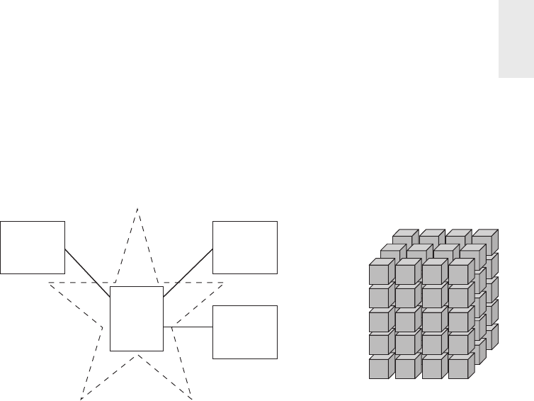
Data Warehousing, Business Intelligence, and Dimensional Modeling Primer 9
precalculations, indexing strategies, and other optimizations. Business users can
drill down or up by adding or removing attributes from their analyses with excellent
performance without issuing new queries. OLAP cubes also provide more analyti-
cally robust functions that exceed those available with SQL. The downside is that you
pay a load performance price for these capabilities, especially with large data sets.
Date
Dimension
Market
Dimension
Product
Dimension
Market
Product
Date
Sales
Facts
Figure 1-1: Star schema versus OLAP cube.
Fortunately, most of the recommendations in this book pertain regardless of the
relational versus multidimensional database platform. Although the capabilities
of OLAP technology are continuously improving, we generally recommend that
detailed, atomic information be loaded into a star schema; optional OLAP cubes are
then populated from the star schema. For this reason, most dimensional modeling
techniques in this book are couched in terms of a relational star schema.
OLAP Deployment Considerations
Here are some things to keep in mind if you deploy data into OLAP cubes:
■ A star schema hosted in a relational database is a good physical foundation
for building an OLAP cube, and is generally regarded as a more stable basis
for backup and recovery.
■ OLAP cubes have traditionally been noted for extreme performance advan-
tages over RDBMSs, but that distinction has become less important with
advances in computer hardware, such as appliances and in-memory databases,
and RDBMS software, such as columnar databases.
■ OLAP cube data structures are more variable across di erent vendors than
relational DBMSs, thus the fi nal deployment details often depend on which
OLAP vendor is chosen. It is typically more di cult to port BI applications
between di erent OLAP tools than to port BI applications across di erent
relational databases.

Chapter 1
10
■ OLAP cubes typically o er more sophisticated security options than RDBMSs,
such as limiting access to detailed data but providing more open access to
summary data.
■ OLAP cubes o er signifi cantly richer analysis capabilities than RDBMSs,
which are saddled by the constraints of SQL. This may be the main justifi ca-
tion for using an OLAP product.
■ OLAP cubes gracefully support slowly changing dimension type 2 changes
(which are discussed in Chapter 5: Procurement), but cubes often need to be
reprocessed partially or totally whenever data is overwritten using alternative
slowly changing dimension techniques.
■ OLAP cubes gracefully support transaction and periodic snapshot fact tables,
but do not handle accumulating snapshot fact tables because of the limitations
on overwriting data described in the previous point.
■ OLAP cubes typically support complex ragged hierarchies of indeterminate
depth, such as organization charts or bills of material, using native query
syntax that is superior to the approaches required for RDBMSs.
■ OLAP cubes may impose detailed constraints on the structure of dimension
keys that implement drill-down hierarchies compared to relational databases.
■ Some OLAP products do not enable dimensional roles or aliases, thus requir-
ing separate physical dimensions to be defi ned.
We’ll return to the world of dimensional modeling in a relational platform as we
consider the two key components of a star schema.
Fact Tables for Measurements
The fact table in a dimensional model stores the performance measurements result-
ing from an organization’s business process events. You should strive to store the
low-level measurement data resulting from a business process in a single dimen-
sional model. Because measurement data is overwhelmingly the largest set of data,
it should not be replicated in multiple places for multiple organizational functions
around the enterprise. Allowing business users from multiple organizations to access
a single centralized repository for each set of measurement data ensures the use of
consistent data throughout the enterprise.
The term fact represents a business measure. Imagine standing in the marketplace
watching products being sold and writing down the unit quantity and dollar sales
amount for each product in each sales transaction. These measurements are captured
as products are scanned at the register, as illustrated in Figure 1-2.
Each row in a fact table corresponds to a measurement event. The data on each
row is at a specifi c level of detail, referred to as the grain, such as one row per product
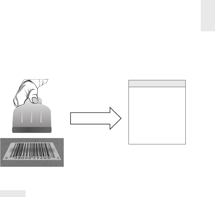
Data Warehousing, Business Intelligence, and Dimensional Modeling Primer 11
sold on a sales transaction. One of the core tenets of dimensional modeling is that
all the measurement rows in a fact table must be at the same grain. Having the dis-
cipline to create fact tables with a single level of detail ensures that measurements
aren’t inappropriately double-counted.
Translates into
Retail Sales Facts
Date Key (FK)
Product Key (FK)
Store Key (FK)
Promotion Key (FK)
Customer Key (FK)
Clerk Key (FK)
Transaction #
Sales Dollars
Sales Units
Figure 1-2: Business process measurement events translate into fact tables.
NOTE The idea that a measurement event in the physical world has a one-to-one
relationship to a single row in the corresponding fact table is a bedrock principle
for dimensional modeling. Everything else builds from this foundation.
The most useful facts are numeric and additive, such as dollar sales amount.
Throughout this book we will use dollars as the standard currency to make the
case study examples more tangible—you can substitute your own local currency
if it isn’t dollars.
Additivity is crucial because BI applications rarely retrieve a single fact table
row. Rather, they bring back hundreds, thousands, or even millions of fact rows at
a time, and the most useful thing to do with so many rows is to add them up. No
matter how the user slices the data in Figure 1-2, the sales units and dollars sum
to a valid total. You will see that facts are sometimes semi-additive or even non-
additive. Semi-additive facts, such as account balances, cannot be summed across
the time dimension. Non-additive facts, such as unit prices, can never be added. You
are forced to use counts and averages or are reduced to printing out the fact rows
one at a time—an impractical exercise with a billion-row fact table.
Facts are often described as continuously valued to help sort out what is a fact
versus a dimension attribute. The dollar sales amount fact is continuously valued in
this example because it can take on virtually any value within a broad range. As an

Chapter 1
12
observer, you must stand out in the marketplace and wait for the measurement before
you have any idea what the value will be.
It is theoretically possible for a measured fact to be textual; however, the condition
rarely arises. In most cases, a textual measurement is a description of something
and is drawn from a discrete list of values. The designer should make every e ort to
put textual data into dimensions where they can be correlated more e ectively with
the other textual dimension attributes and consume much less space. You should
not store redundant textual information in fact tables. Unless the text is unique
for every row in the fact table, it belongs in the dimension table. A true text fact is
rare because the unpredictable content of a text fact, like a freeform text comment,
makes it nearly impossible to analyze.
Referring to the sample fact table in Figure 1-2, if there is no sales activity for a
given product, you don’t put any rows in the table. It is important that you do not
try to fi ll the fact table with zeros representing no activity because these zeros would
overwhelm most fact tables. By including only true activity, fact tables tend to be
quite sparse. Despite their sparsity, fact tables usually make up 90 percent or more
of the total space consumed by a dimensional model. Fact tables tend to be deep in
terms of the number of rows, but narrow in terms of the number of columns. Given
their size, you should be judicious about fact table space utilization.
As examples are developed throughout this book, you will see that all fact table
grains fall into one of three categories: transaction, periodic snapshot, and accu-
mulating snapshot. Transaction grain fact tables are the most common. We will
introduce transaction fact tables in Chapter 3: Retail Sales, and both periodic and
accumulating snapshots in Chapter 4: Inventory.
All fact tables have two or more foreign keys (refer to the FK notation in Figure 1-2)
that connect to the dimension tables’ primary keys. For example, the product key in
the fact table always matches a specifi c product key in the product dimension table.
When all the keys in the fact table correctly match their respective primary keys in
the corresponding dimension tables, the tables satisfy referential integrity. You access
the fact table via the dimension tables joined to it.
The fact table generally has its own primary key composed of a subset of the for-
eign keys. This key is often called a composite key. Every table that has a composite
key is a fact table. Fact tables express many-to-many relationships. All others are
dimension tables.
There are usually a handful of dimensions that together uniquely identify each
fact table row. After this subset of the overall dimension list has been identifi ed, the
rest of the dimensions take on a single value in the context of the fact table row’s
primary key. In other words, they go along for the ride.

Data Warehousing, Business Intelligence, and Dimensional Modeling Primer 13
Dimension Tables for Descriptive Context
Dimension tables are integral companions to a fact table. The dimension tables con-
tain the textual context associated with a business process measurement event. They
describe the “who, what, where, when, how, and why” associated with the event.
As illustrated in Figure 1-3, dimension tables often have many columns or
attributes. It is not uncommon for a dimension table to have 50 to 100 attributes;
although, some dimension tables naturally have only a handful of attributes.
Dimension tables tend to have fewer rows than fact tables, but can be wide with
many large text columns. Each dimension is defi ned by a single primary key (refer
to the PK notation in Figure 1-3), which serves as the basis for referential integrity
with any given fact table to which it is joined.
Product Key (PK)
SKU Number (Natural Key)
Product Description
Brand Name
Category Name
Department Name
Package Type
Package Size
Abrasive Indicator
Weight
Weight Unit of Measure
Storage Type
Shelf Life Type
Shelf Width
Shelf Height
Shelf Depth
...
Product Dimension
Figure 1-3: Dimension tables contain descriptive characteristics of business
process nouns.
Dimension attributes serve as the primary source of query constraints, group-
ings, and report labels. In a query or report request, attributes are identifi ed as the
by words. For example, when a user wants to see dollar sales by brand, brand must
be available as a dimension attribute.
Dimension table attributes play a vital role in the DW/BI system. Because they
are the source of virtually all constraints and report labels, dimension attributes are
critical to making the DW/BI system usable and understandable. Attributes should
consist of real words rather than cryptic abbreviations. You should strive to mini-
mize the use of codes in dimension tables by replacing them with more verbose

Chapter 1
14
textual attributes. You may have already trained the business users to memorize
operational codes, but going forward, minimize their reliance on miniature notes
attached to their monitor for code translations. You should make standard decodes
for the operational codes available as dimension attributes to provide consistent
labeling on queries, reports, and BI applications. The decode values should never be
buried in the reporting applications where inconsistency is inevitable.
Sometimes operational codes or identifi ers have legitimate business signifi cance
to users or are required to communicate back to the operational world. In these
cases, the codes should appear as explicit dimension attributes, in addition to the
corresponding user-friendly textual descriptors. Operational codes sometimes have
intelligence embedded in them. For example, the fi rst two digits may identify the
line of business, whereas the next two digits may identify the global region. Rather
than forcing users to interrogate or fi lter on substrings within the operational codes,
pull out the embedded meanings and present them to users as separate dimension
attributes that can easily be fi ltered, grouped, or reported.
In many ways, the data warehouse is only as good as the dimension attributes; the
analytic power of the DW/BI environment is directly proportional to the quality and
depth of the dimension attributes. The more time spent providing attributes with
verbose business terminology, the better. The more time spent populating the domain
values in an attribute column, the better. The more time spent ensuring the quality
of the values in an attribute column, the better. Robust dimension attributes deliver
robust analytic slicing-and-dicing capabilities.
NOTE Dimensions provide the entry points to the data, and the fi nal labels and
groupings on all DW/BI analyses.
When triaging operational source data, it is sometimes unclear whether a
numeric data element is a fact or dimension attribute. You often make the decision
by asking whether the column is a measurement that takes on lots of values and
participates in calculations (making it a fact) or is a discretely valued description
that is more or less constant and participates in constraints and row labels (making
it a dimensional attribute). For example, the standard cost for a product seems like
a constant attribute of the product but may be changed so often that you decide it
is more like a measured fact. Occasionally, you can’t be certain of the classifi cation;
it is possible to model the data element either way (or both ways) as a matter of the
designer’s prerogative.
NOTE The designer’s dilemma of whether a numeric quantity is a fact or a
dimension attribute is rarely a di cult decision. Continuously valued numeric

Data Warehousing, Business Intelligence, and Dimensional Modeling Primer 15
observations are almost always facts; discrete numeric observations drawn from a
small list are almost always dimension attributes.
Figure 1-4 shows that dimension tables often represent hierarchical relation-
ships. For example, products roll up into brands and then into categories. For each
row in the product dimension, you should store the associated brand and category
description. The hierarchical descriptive information is stored redundantly in the
spirit of ease of use and query performance. You should resist the perhaps habitual
urge to normalize data by storing only the brand code in the product dimension and
creating a separate brand lookup table, and likewise for the category description in a
separate category lookup table. This normalization is called snowfl aking. Instead of
third normal form, dimension tables typically are highly denormalized with fl attened
many-to-one relationships within a single dimension table. Because dimension tables
typically are geometrically smaller than fact tables, improving storage e ciency by
normalizing or snowfl aking has virtually no impact on the overall database size. You
should almost always trade o dimension table space for simplicity and accessibility.
1
2
3
4
5
6
7
8
9
10
11
Product Key
PowerAll 20 oz
PowerAll 32 oz
PowerAll 48 oz
PowerAll 64 oz
ZipAll 20 oz
ZipAll 32 oz
ZipAll 48 oz
Shiny 20 oz
Shiny 32 oz
ZipGlass 20 oz
ZipGlass 32 oz
PowerClean
PowerClean
PowerClean
PowerClean
Zippy
Zippy
Zippy
Clean Fast
Clean Fast
Zippy
Zippy
All Purpose Cleaner
All Purpose Cleaner
All Purpose Cleaner
All Purpose Cleaner
All Purpose Cleaner
All Purpose Cleaner
All Purpose Cleaner
Glass Cleaner
Glass Cleaner
Glass Cleaner
Glass Cleaner
Product Description Brand Name Category Name
Figure 1-4: Sample rows from a dimension table with denormalized hierarchies.
Contrary to popular folklore, Ralph Kimball didn’t invent the terms fact and
dimension. As best as can be determined, the dimension and fact terminology
originated from a joint research project conducted by General Mills and Dartmouth
University in the 1960s. In the 1970s, both AC Nielsen and IRI used the terms con-
sistently to describe their syndicated data o erings and gravitated to dimensional
models for simplifying the presentation of their analytic information. They under-
stood that their data wouldn’t be used unless it was packaged simply. It is probably
accurate to say that no single person invented the dimensional approach. It is an
irresistible force in designing databases that always results when the designer places
understandability and performance as the highest goals.

Chapter 1
16
Facts and Dimensions Joined in a Star Schema
Now that you understand fact and dimension tables, it’s time to bring the building blocks
together in a dimensional model, as shown in Figure 1-5. Each business process is repre-
sented by a dimensional model that consists of a fact table containing the event’s numeric
measurements surrounded by a halo of dimension tables that contain the textual context
that was true at the moment the event occurred. This characteristic star-like structure
is often called a star join, a term dating back to the earliest days of relational databases.
Retail Sales Fact
Date Key (FK)
Product Key (FK)
Store Key (FK)
Promotion Key (FK)
Customer Key (FK)
Clerk Key (FK)
Transaction #
Sales Dollars
Sales Units
Date Dimension
Product Dimension
Promotion Dimension
Clerk Dimension
Store Dimension
Customer Dimension
Figure 1-5: Fact and dimension tables in a dimensional model.
The fi rst thing to notice about the dimensional schema is its simplicity and
symmetry. Obviously, business users benefi t from the simplicity because the data
is easier to understand and navigate. The charm of the design in Figure 1-5 is that
it is highly recognizable to business users. We have observed literally hundreds of
instances in which users immediately agree that the dimensional model is their
business. Furthermore, the reduced number of tables and use of meaningful busi-
ness descriptors make it easy to navigate and less likely that mistakes will occur.
The simplicity of a dimensional model also has performance benefi ts. Database
optimizers process these simple schemas with fewer joins more e ciently. A data-
base engine can make strong assumptions about fi rst constraining the heavily
indexed dimension tables, and then attacking the fact table all at once with the
Cartesian product of the dimension table keys satisfying the user’s constraints.
Amazingly, using this approach, the optimizer can evaluate arbitrary n-way joins
to a fact table in a single pass through the fact table’s index.
Finally, dimensional models are gracefully extensible to accommodate change.
The predictable framework of a dimensional model withstands unexpected changes
in user behavior. Every dimension is equivalent; all dimensions are symmetrically-
equal entry points into the fact table. The dimensional model has no built-in bias
regarding expected query patterns. There are no preferences for the business ques-
tions asked this month versus the questions asked next month. You certainly don’t
want to adjust schemas if business users suggest new ways to analyze their business.
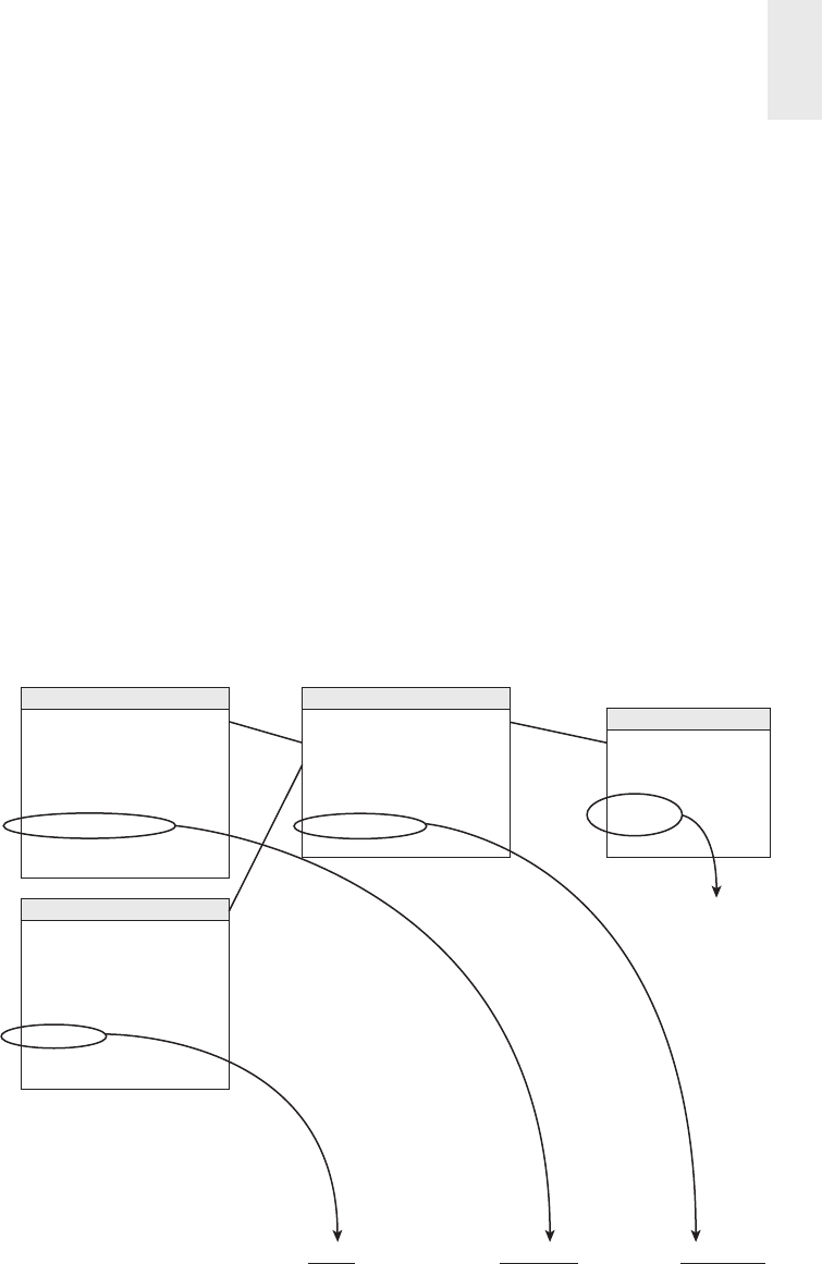
Data Warehousing, Business Intelligence, and Dimensional Modeling Primer 17
This book illustrates repeatedly that the most granular or atomic data has the
most dimensionality. Atomic data that has not been aggregated is the most expres-
sive data; this atomic data should be the foundation for every fact table design to
withstand business users’ ad hoc attacks in which they pose unexpected queries.
With dimensional models, you can add completely new dimensions to the schema
as long as a single value of that dimension is defi ned for each existing fact row.
Likewise, you can add new facts to the fact table, assuming that the level of detail
is consistent with the existing fact table. You can supplement preexisting dimen-
sion tables with new, unanticipated attributes. In each case, existing tables can be
changed in place either by simply adding new data rows in the table or by executing
an SQL ALTER TABLE command. Data would not need to be reloaded, and existing BI
applications would continue to run without yielding di erent results. We examine
this graceful extensibility of dimensional models more fully in Chapter 3.
Another way to think about the complementary nature of fact and dimension
tables is to see them translated into a report. As illustrated in Figure 1-6, dimension
attributes supply the report fi lters and labeling, whereas the fact tables supply the
report’s numeric values.
Product Dimension
Date Dimension
Store Dimension
Sales Fact
Product Key (PK)
SKU Number (Natural Key)
Product Description
Package Type
Package Size
Brand Name
Category Name
... and more
Date Key (FK)
Product Key (FK)
Store Key (FK)
...
Transaction #
Sales Dollars
Sales Units
Store Key (PK)
Store Number
Store Name
Store State
Store ZIP
District
Region
... and more
Date Key (PK)
Date
Day of Week
Month
Year
...and more
Filter
SumGroup byGroup by
Sales Activity for June 2013
District
Atherton
Atherton
Belmont
Belmont
Brand Name
PowerClean
Zippy
Clean Fast
Zippy
Sales Dollars
2,035
707
2,330
527
Figure 1-6: Dimensional attributes and facts form a simple report.

Chapter 1
18
You can easily envision the SQL that’s written (or more likely generated by a BI
tool) to create this report:
SELECT
store.district_name,
product.brand,
sum(sales_facts.sales_dollars) AS "Sales Dollars"
FROM
store,
product,
date,
sales_facts
WHERE
date.month_name="January" AND
date.year=2013 AND
store.store_key = sales_facts.store_key AND
product.product_key = sales_facts.product_key AND
date.date_key = sales_facts.date_key
GROUP BY
store.district_name,
product.brand
If you study this code snippet line-by-line, the fi rst two lines under the SELECT
statement identify the dimension attributes in the report, followed by the aggre-
gated metric from the fact table. The FROM clause identifi es all the tables involved
in the query. The fi rst two lines in the WHERE clause declare the report’s fi lter, and
the remainder declare the joins between the dimension and fact tables. Finally, the
GROUP BY clause establishes the aggregation within the report.
Kimball’s DW/BI Architecture
Let’s build on your understanding of DW/BI systems and dimensional modeling
fundamentals by investigating the components of a DW/BI environment based on
the Kimball architecture. You need to learn the strategic signifi cance of each com-
ponent to avoid confusing their role and function.
As illustrated in Figure 1-7, there are four separate and distinct components to
consider in the DW/BI environment: operational source systems, ETL system, data
presentation area, and business intelligence applications.
Operational Source Systems
These are the operational systems of record that capture the business’s transactions.
Think of the source systems as outside the data warehouse because presumably you
have little or no control over the content and format of the data in these operational
systems. The main priorities of the source systems are processing performance and avail-
ability. Operational queries against source systems are narrow, one-record-at-a-time
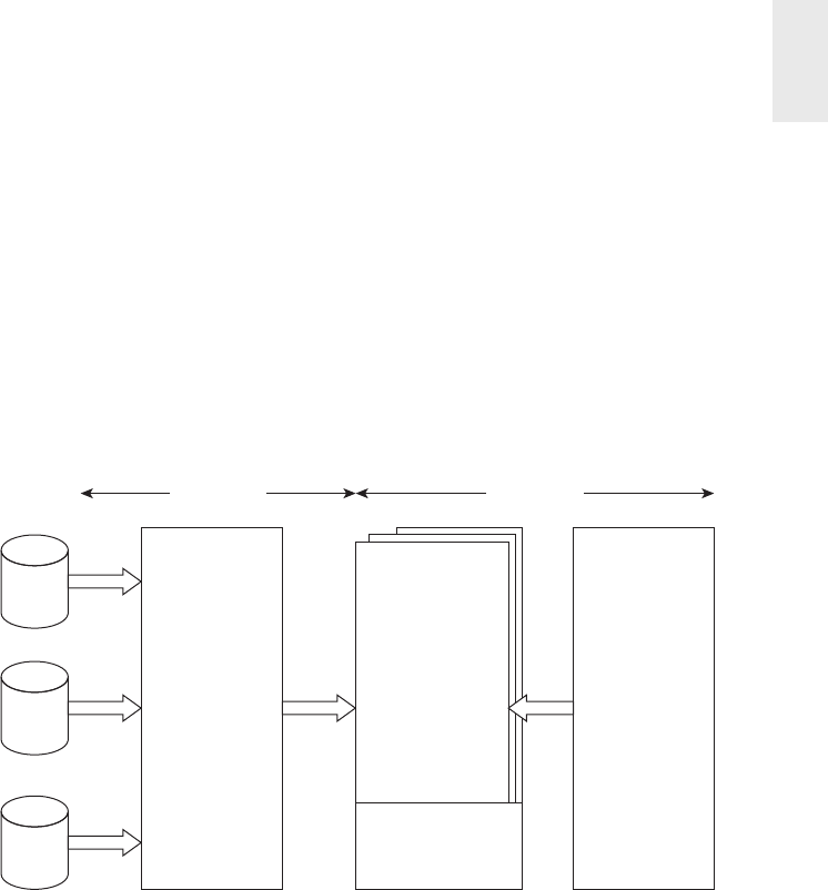
Data Warehousing, Business Intelligence, and Dimensional Modeling Primer 19
queries that are part of the normal transaction fl ow and severely restricted in their
demands on the operational system. It is safe to assume that source systems are not
queried in the broad and unexpected ways that DW/BI systems typically are queried.
Source systems maintain little historical data; a good data warehouse can relieve
the source systems of much of the responsibility for representing the past. In many
cases, the source systems are special purpose applications without any commitment
to sharing common data such as product, customer, geography, or calendar with other
operational systems in the organization. Of course, a broadly adopted cross-application
enterprise resource planning (ERP) system or operational master data management
system could help address these shortcomings.
Source
Transactions
Back Room
ETL System:
• Transform from
source-to-target
• Conform
dimensions
• Normalization
optional
• No user query
support
Design Goals:
• Throughput
• Integrity and
consistency
Presentation Area:
• Dimensional (star
schema or OLAP
cube)
• Atomic and
summary data
• Organized by
business process
• Uses conformed
dimensions
Design Goals:
• Ease-of-use
• Query performance
BI Applications:
• Ad hoc queries
• Standard reports
• Analytic apps
• Data mining and
models
Enterprise DW Bus
Architecture
Front Room
Figure 1-7: Core elements of the Kimball DW/BI architecture.
Extract, Transformation, and Load System
The extract, transformation, and load (ETL) system of the DW/BI environment consists
of a work area, instantiated data structures, and a set of processes. The ETL system
is everything between the operational source systems and the DW/BI presentation
area. We elaborate on the architecture of ETL systems and associated techniques
in Chapter 19: ETL Subsystems and Techniques, but we want to introduce this
fundamental piece of the overall DW/BI system puzzle.
Extraction is the fi rst step in the process of getting data into the data warehouse
environment. Extracting means reading and understanding the source data and
copying the data needed into the ETL system for further manipulation. At this
point, the data belongs to the data warehouse.
After the data is extracted to the ETL system, there are numerous potential trans-
formations, such as cleansing the data (correcting misspellings, resolving domain

Chapter 1
20
confl icts, dealing with missing elements, or parsing into standard formats), com-
bining data from multiple sources, and de-duplicating data. The ETL system adds
value to the data with these cleansing and conforming tasks by changing the data
and enhancing it. In addition, these activities can be architected to create diagnos-
tic metadata, eventually leading to business process reengineering to improve data
quality in the source systems over time.
The fi nal step of the ETL process is the physical structuring and loading of data
into the presentation area’s target dimensional models. Because the primary mis-
sion of the ETL system is to hand o the dimension and fact tables in the delivery
step, these subsystems are critical. Many of these defi ned subsystems focus on
dimension table processing, such as surrogate key assignments, code lookups to
provide appropriate descriptions, splitting, or combining columns to present the
appropriate data values, or joining underlying third normal form table structures
into fl attened denormalized dimensions. In contrast, fact tables are typically large
and time consuming to load, but preparing them for the presentation area is typically
straightforward. When the dimension and fact tables in a dimensional model have
been updated, indexed, supplied with appropriate aggregates, and further quality
assured, the business community is notifi ed that the new data has been published.
There remains industry consternation about whether the data in the ETL system
should be repurposed into physical normalized structures prior to loading into the
presentation area’s dimensional structures for querying and reporting. The ETL
system is typically dominated by the simple activities of sorting and sequential
processing. In many cases, the ETL system is not based on relational technology but
instead may rely on a system of fl at fi les. After validating the data for conformance
with the defi ned one-to-one and many-to-one business rules, it may be pointless to
take the fi nal step of building a 3NF physical database, just before transforming the
data once again into denormalized structures for the BI presentation area.
However, there are cases in which the data arrives at the doorstep of the ETL
system in a 3NF relational format. In these situations, the ETL system develop-
ers may be more comfortable performing the cleansing and transformation tasks
using normalized structures. Although a normalized database for ETL processing
is acceptable, we have some reservations about this approach. The creation of both
normalized structures for the ETL and dimensional structures for presentation
means that the data is potentially extracted, transformed, and loaded twice—once
into the normalized database and then again when you load the dimensional model.
Obviously, this two-step process requires more time and investment for the develop-
ment, more time for the periodic loading or updating of data, and more capacity to
store the multiple copies of the data. At the bottom line, this typically translates into
the need for larger development, ongoing support, and hardware platform budgets.

Data Warehousing, Business Intelligence, and Dimensional Modeling Primer 21
Unfortunately, some DW/BI initiatives have failed miserably because they focused
all their energy and resources on constructing the normalized structures rather
than allocating time to developing a dimensional presentation area that supports
improved business decision making. Although enterprise-wide data consistency is a
fundamental goal of the DW/BI environment, there may be e ective and less costly
approaches than physically creating normalized tables in the ETL system, if these
structures don’t already exist.
NOTE It is acceptable to create a normalized database to support the ETL
processes; however, this is not the end goal. The normalized structures must be
o -limits to user queries because they defeat the twin goals of understandability
and performance.
Presentation Area to Support Business Intelligence
The DW/BI presentation area is where data is organized, stored, and made available
for direct querying by users, report writers, and other analytical BI applications.
Because the back room ETL system is o -limits, the presentation area is the DW/BI
environment as far as the business community is concerned; it is all the business
sees and touches via their access tools and BI applications. The original pre-release
working title for the fi rst edition of The Data Warehouse Toolkit was Getting the Data
Out. This is what the presentation area with its dimensional models is all about.
We have several strong opinions about the presentation area. First of all, we insist
that the data be presented, stored, and accessed in dimensional schemas, either
relational star schemas or OLAP cubes. Fortunately, the industry has matured to the
point where we’re no longer debating this approach; it has concluded that dimen-
sional modeling is the most viable technique for delivering data to DW/BI users.
Our second stake in the ground about the presentation area is that it must
contain detailed, atomic data. Atomic data is required to withstand assaults from
unpredictable ad hoc user queries. Although the presentation area also may contain
performance-enhancing aggregated data, it is not su cient to deliver these sum-
maries without the underlying granular data in a dimensional form. In other words,
it is completely unacceptable to store only summary data in dimensional models
while the atomic data is locked up in normalized models. It is impractical to expect
a user to drill down through dimensional data almost to the most granular level and
then lose the benefi ts of a dimensional presentation at the fi nal step. Although DW/
BI users and applications may look infrequently at a single line item on an order,
they may be very interested in last week’s orders for products of a given size (or
fl avor, package type, or manufacturer) for customers who fi rst purchased within

Chapter 1
22
the last 6 months (or reside in a given state or have certain credit terms). The most
fi nely grained data must be available in the presentation area so that users can ask
the most precise questions possible. Because users’ requirements are unpredictable
and constantly changing, you must provide access to the exquisite details so they
can roll up to address the questions of the moment.
The presentation data area should be structured around business process mea-
surement events. This approach naturally aligns with the operational source data
capture systems. Dimensional models should correspond to physical data capture
events; they should not be designed to deliver the report-of-the-day. An enterprise’s
business processes cross the boundaries of organizational departments and func-
tions. In other words, you should construct a single fact table for atomic sales metrics
rather than populating separate similar, but slightly di erent, databases containing
sales metrics for the sales, marketing, logistics, and fi nance teams.
All the dimensional structures must be built using common, conformed dimen-
sions. This is the basis of the enterprise data warehouse bus architecture described
in Chapter 4. Adherence to the bus architecture is the fi nal stake in the ground
for the presentation area. Without shared, conformed dimensions, a dimensional
model becomes a standalone application. Isolated stovepipe data sets that cannot be
tied together are the bane of the DW/BI movement as they perpetuate incompatible
views of the enterprise. If you have any hope of building a robust and integrated
DW/BI environment, you must commit to the enterprise bus architecture. When
dimensional models have been designed with conformed dimensions, they can be
readily combined and used together. The presentation area in a large enterprise
DW/BI solution ultimately consists of dozens of dimensional models with many of
the associated dimension tables shared across fact tables.
Using the bus architecture is the secret to building distributed DW/BI systems.
When the bus architecture is used as a framework, you can develop the enterprise
data warehouse in an agile, decentralized, realistically scoped, iterative manner.
NOTE Data in the queryable presentation area of the DW/BI system must be
dimensional, atomic (complemented by performance-enhancing aggregates), busi-
ness process-centric, and adhere to the enterprise data warehouse bus architecture.
The data must not be structured according to individual departments’ interpreta-
tion of the data.
Business Intelligence Applications
The fi nal major component of the Kimball DW/BI architecture is the business intelligence
(BI) application. The term BI application loosely refers to the range of capabilities pro-
vided to business users to leverage the presentation area for analytic decision making.

Data Warehousing, Business Intelligence, and Dimensional Modeling Primer 23
By definition, all BI applications query the data in the DW/BI presentation area.
Querying, obviously, is the whole point of using data for improved decision making.
A BI application can be as simple as an ad hoc query tool or as complex as a sophis-
ticated data mining or modeling application. Ad hoc query tools, as powerful as they
are, can be understood and used e ectively by only a small percentage of the potential
DW/BI business user population. Most business users will likely access the data via
prebuilt parameter-driven applications and templates that do not require users to con-
struct queries directly. Some of the more sophisticated applications, such as modeling
or forecasting tools, may upload results back into the operational source systems, ETL
system, or presentation area.
Restaurant Metaphor for the Kimball Architecture
One of our favorite metaphors reinforces the importance of separating the overall
DW/BI environment into distinct components. In this case, we’ll consider the simi-
larities between a restaurant and the DW/BI environment.
ETL in the Back Room Kitchen
The ETL system is analogous to the kitchen of a restaurant. The restaurant’s kitchen
is a world unto itself. Talented chefs take raw materials and transform them into
appetizing, delicious meals for the restaurant’s diners. But long before a commercial
kitchen swings into operation, a signifi cant amount of planning goes into designing
the workspace layout and components.
The kitchen is organized with several design goals in mind. First, the layout must
be highly e cient. Restaurant managers want high kitchen throughput. When the
restaurant is packed and everyone is hungry, there is no time for wasted movement.
Delivering consistent quality from the restaurant’s kitchen is the second important
goal. The establishment is doomed if the plates coming out of the kitchen repeat-
edly fail to meet expectations. To achieve consistency, chefs create their special
sauces once in the kitchen, rather than sending ingredients out to the table where
variations will inevitably occur. Finally, the kitchen’s output, the meals delivered
to restaurant customers, must also be of high integrity. You wouldn’t want someone
to get food poisoning from dining at your restaurant. Consequently, kitchens are
designed with integrity in mind; salad preparation doesn’t happen on the same
surfaces where raw chicken is handled.
Just as quality, consistency, and integrity are major considerations when designing
the restaurant’s kitchen, they are also ongoing concerns for everyday management
of the restaurant. Chefs strive to obtain the best raw materials possible. Procured
products must meet quality standards and are rejected if they don’t meet minimum
standards. Most fi ne restaurants modify their menus based on the availability of
quality ingredients.

Chapter 1
24
The restaurant sta s its kitchen with skilled professionals wielding the tools of
their trade. Cooks manipulate razor-sharp knives with incredible confi dence and
ease. They operate powerful equipment and work around extremely hot surfaces
without incident.
Given the dangerous surroundings, the back room kitchen is o limits to res-
taurant patrons. Things happen in the kitchen that customers just shouldn’t see. It
simply isn’t safe. Professional cooks handling sharp knives shouldn’t be distracted
by diners’ inquiries. You also wouldn’t want patrons entering the kitchen to dip their
fi ngers into a sauce to see whether they want to order an entree. To prevent these
intrusions, most restaurants have a closed door that separates the kitchen from the
area where diners are served. Even restaurants that boast an open kitchen format
typically have a barrier, such as a partial wall of glass, separating the two environ-
ments. Diners are invited to watch but can’t wander into the kitchen. Although part
of the kitchen may be visible, there are always out-of-view back rooms where the
less visually desirable preparation occurs.
The data warehouse’s ETL system resembles the restaurant’s kitchen. Source data
is magically transformed into meaningful, presentable information. The back room
ETL system must be laid out and architected long before any data is extracted from
the source. Like the kitchen, the ETL system is designed to ensure throughput.
It must transform raw source data into the target model e ciently, minimizing
unnecessary movement.
Obviously, the ETL system is also highly concerned about data quality, integrity, and
consistency. Incoming data is checked for reasonable quality as it enters. Conditions
are continually monitored to ensure ETL outputs are of high integrity. Business rules
to consistently derive value-add metrics and attributes are applied once by skilled
professionals in the ETL system rather than relying on each patron to develop them
independently. Yes, that puts extra burden on the ETL team, but it’s done to deliver a
better, more consistent product to the DW/BI patrons.
NOTE A properly designed DW/BI environment trades o work in the front
room BI applications in favor of work in the back room ETL system. Front room
work must be done over and over by business users, whereas back room work is
done once by the ETL sta .
Finally, ETL system should be o limits to the business users and BI application
developers. Just as you don’t want restaurant patrons wandering into the kitchen
and potentially consuming semi-cooked food, you don’t want busy ETL profession-
als distracted by unpredictable inquiries from BI users. The consequences might
be highly unpleasant if users dip their fi ngers into interim staging pots while data
preparation is still in process. As with the restaurant kitchen, activities occur in

Data Warehousing, Business Intelligence, and Dimensional Modeling Primer 25
the ETL system that the DW/BI patrons shouldn’t see. When the data is ready and
quality checked for user consumption, it’s brought through the doorway into the
DW/BI presentation area.
Data Presentation and BI in the Front Dining Room
Now turn your attention to the restaurant’s dining room. What are the key fac-
tors that di erentiate restaurants? According to the popular restaurant ratings and
reviews, restaurants are typically scored on four distinct qualities:
■ Food (quality, taste, and presentation)
■ Decor (appealing, comfortable surroundings for the patrons)
■ Service (prompt food delivery, attentive support sta , and food received
as ordered)
■ Cost
Most patrons focus initially on the food score when they’re evaluating dining
options. First and foremost, does the restaurant serve good food? That’s the res-
taurant’s primary deliverable. However, the decor, service, and cost factors also
a ect the patrons’ overall dining experience and are considerations when evaluating
whether to eat at a restaurant.
Of course, the primary deliverable from the DW/BI kitchen is the data in
the presentation area. What data is available? Like the restaurant, the DW/BI
system provides “menus” to describe what’s available via metadata, published
reports, and parameterized analytic applications. The DW/BI patrons expect con-
sistency and high quality. The presentation area’s data must be properly prepared
and safe to consume.
The presentation area’s decor should be organized for the patrons’ comfort. It
must be designed based on the preferences of the BI diners, not the development
sta . Service is also critical in the DW/BI system. Data must be delivered, as ordered,
promptly in a form that is appealing to the business user or BI application developer.
Finally, cost is a factor for the DW/BI system. The kitchen sta may be dream-
ing up elaborate, expensive meals, but if there’s no market at that price point, the
restaurant won’t survive.
If restaurant patrons like their dining experience, then everything is rosy for
the restaurant manager. The dining room is always busy; sometimes there’s even
a waiting list. The restaurant manager’s performance metrics are all promising:
high numbers of diners, table turnovers, and nightly revenue and profi t, while sta
turnover is low. Things look so good that the restaurant’s owner is considering an
expansion site to handle the tra c. On the other hand, if the restaurant’s diners
aren’t happy, things go downhill in a hurry. With a limited number of patrons,
the restaurant isn’t making enough money to cover its expenses, and the sta isn’t
making any tips. In a relatively short time, the restaurant closes.

Chapter 1
26
Restaurant managers often proactively check on their diners’ satisfaction with
the food and dining experience. If a patron is unhappy, they take immediate action
to rectify the situation. Similarly, DW/BI managers should proactively monitor sat-
isfaction. You can’t a ord to wait to hear complaints. Often, people will abandon
a restaurant without even voicing their concerns. Over time, managers notice that
diner counts have dropped but may not even know why.
Inevitably, the prior DW/BI patrons will locate another “restaurant” that bet-
ter suits their needs and preferences, wasting the millions of dollars invested to
design, build, and sta the DW/BI system. Of course, you can prevent this unhappy
ending by managing the restaurant proactively; make sure the kitchen is properly
organized and utilized to deliver as needed to the presentation area’s food, decor,
service, and cost.
Alternative DW/BI Architectures
Having just described the Kimball architecture, let’s discuss several other DW/BI
architectural approaches. We’ll quickly review the two dominant alternatives to the
Kimball architecture, highlighting the similarities and di erences. We’ll then close
this section by focusing on a hybrid approach that combines alternatives.
Fortunately, over the past few decades, the di erences between the Kimball
architecture and the alternatives have softened. Even more fortunate, there’s a role
for dimensional modeling regardless of your architectural predisposition.
We acknowledge that organizations have successfully constructed DW/BI systems
based on the approaches advocated by others. We strongly believe that rather than
encouraging more consternation over our philosophical di erences, the industry
would be far better o devoting energy to ensure that our DW/BI deliverables are
broadly accepted by the business to make better, more informed decisions. The
architecture should merely be a means to this objective.
Independent Data Mart Architecture
With this approach, analytic data is deployed on a departmental basis without con-
cern to sharing and integrating information across the enterprise, as illustrated in
Figure 1-8. Typically, a single department identifi es requirements for data from an
operational source system. The department works with IT sta or outside consul-
tants to construct a database that satisfi es their departmental needs, refl ecting their
business rules and preferred labeling. Working in isolation, this departmental data
mart addresses the department’s analytic requirements.
Meanwhile, another department is interested in the same source data. It’s extremely
common for multiple departments to be interested in the same performance met-
rics resulting from an organization’s core business process events. But because this
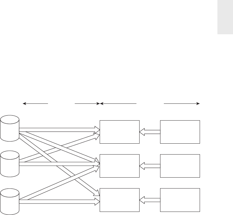
Data Warehousing, Business Intelligence, and Dimensional Modeling Primer 27
department doesn’t have access to the data mart initially constructed by the other
department, it proceeds down a similar path on its own, obtaining resources and
building a departmental solution that contains similar, but slightly di erent data.
When business users from these two departments discuss organizational perfor-
mance based on reports from their respective repositories, not surprisingly, none of
the numbers match because of the di erences in business rules and labeling.
Source
Transactions
Back Room
BI Applications for
Department #1
Data Mart for
Department #1
Data Mart for
Department #2
Data Mart for
Department #3
BI Applications for
Department #2
BI Applications for
Department #3
Front Room
ETL
ETL
ETL
ETL
ETL
Figure 1-8: Simplifi ed illustration of the independent data mart “architecture.”
These standalone analytic silos represent a DW/BI “architecture” that’s essen-
tially un-architected. Although no industry leaders advocate these independent
data marts, this approach is prevalent, especially in large organizations. It mirrors
the way many organizations fund IT projects, plus it requires zero cross-organi-
zational data governance and coordination. It’s the path of least resistance for fast
development at relatively low cost, at least in the short run. Of course, multiple
uncoordinated extracts from the same operational sources and redundant storage
of analytic data are ine cient and wasteful in the long run. Without any enterprise
perspective, this independent approach results in myriad standalone point solutions
that perpetuate incompatible views of the organization’s performance, resulting in
unnecessary organizational debate and reconciliation.
We strongly discourage the independent data mart approach. However, often
these independent data marts have embraced dimensional modeling because they’re
interested in delivering data that’s easy for the business to understand and highly
responsive to queries. So our concepts of dimensional modeling are often applied
in this architecture, despite the complete disregard for some of our core tenets, such
as focusing on atomic details, building by business process instead of department,
and leveraging conformed dimensions for enterprise consistency and integration.
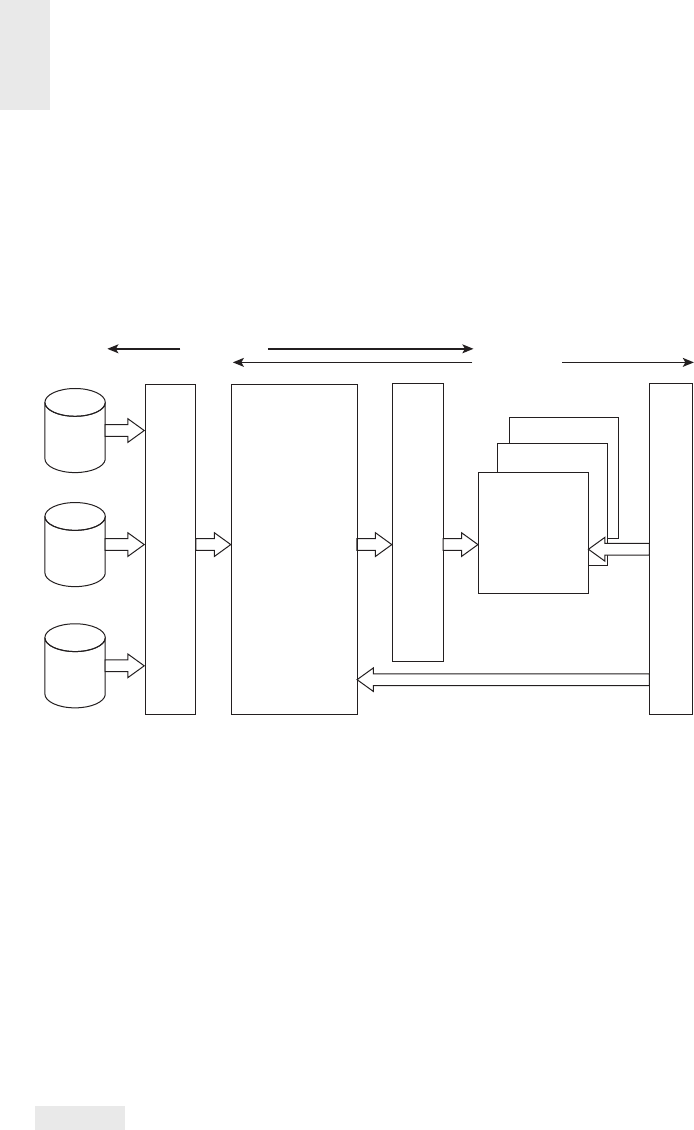
Chapter 1
28
Hub-and-Spoke Corporate Information Factory
Inmon Architecture
The hub-and-spoke Corporate Information Factory (CIF) approach is advocated
by Bill Inmon and others in the industry. Figure 1-9 illustrates a simplifi ed version
of the CIF, focusing on the core elements and concepts that warrant discussion.
Source
Transactions
Back Room
Enterprise Data
Warehouse (EDW)
• Normalized
tables (3NF)
• Atomic data
• User queryable
Front Room
D
a
t
a
A
c
q
u
i
s
i
t
i
o
n
D
a
t
a
D
e
l
i
v
e
r
y
B
I
A
p
p
l
i
c
a
t
i
o
n
s
Data Marts:
• Dimensional
• Often
summarized
• Often
departmental
Figure 1-9: Simplifi ed illustration of the hub-and-spoke Corporate Information Factory
architecture.
With the CIF, data is extracted from the operational source systems and processed
through an ETL system sometimes referred to as data acquisition. The atomic data
that results from this processing lands in a 3NF database; this normalized, atomic
repository is referred to as the Enterprise Data Warehouse (EDW) within the CIF
architecture. Although the Kimball architecture enables optional normalization to
support ETL processing, the normalized EDW is a mandatory construct in the CIF.
Like the Kimball approach, the CIF advocates enterprise data coordination and inte-
gration. The CIF says the normalized EDW fi lls this role, whereas the Kimball archi-
tecture stresses the importance of an enterprise bus with conformed dimensions.
NOTE The process of normalization does not technically speak to integration.
Normalization simply creates physical tables that implement many-to-one rela-
tionships. Integration, on the other hand, requires that inconsistencies arising
from separate sources be resolved. Separate incompatible database sources can be
normalized to the hilt without addressing integration. The Kimball architecture

Data Warehousing, Business Intelligence, and Dimensional Modeling Primer 29
based on conformed dimensions reverses this logic and focuses on resolving data
inconsistencies without explicitly requiring normalization.
Organizations who have adopted the CIF approach often have business users
accessing the EDW repository due to its level of detail or data availability timeli-
ness. However, subsequent ETL data delivery processes also populate downstream
reporting and analytic environments to support business users. Although often
dimensionally structured, the resultant analytic databases typically di er from
structures in the Kimball architecture’s presentation area in that they’re frequently
departmentally-centric (rather than organized around business processes) and popu-
lated with aggregated data (rather than atomic details). If the data delivery ETL
processes apply business rules beyond basic summarization, such as departmental
renaming of columns or alternative calculations, it may be di cult to tie these
analytic databases to the EDW’s atomic repository.
NOTE The most extreme form of a pure CIF architecture is unworkable as a data
warehouse, in our opinion. Such an architecture locks the atomic data in di cult-
to-query normalized structures, while delivering departmentally incompatible data
marts to di erent groups of business users. But before being too depressed by this
view, stay tuned for the next section.
Hybrid Hub-and-Spoke and Kimball Architecture
The fi nal architecture warranting discussion is the marriage of the Kimball and
Inmon CIF architectures. As illustrated in Figure 1-10, this architecture populates
a CIF-centric EDW that is completely o -limits to business users for analysis and
reporting. It’s merely the source to populate a Kimball-esque presentation area
in which the data is dimensional, atomic (complemented by aggregates), process-
centric, and conforms to the enterprise data warehouse bus architecture.
Some proponents of this blended approach claim it’s the best of both worlds. Yes, it
blends the two enterprise-oriented approaches. It may leverage a preexisting invest-
ment in an integrated repository, while addressing the performance and usability
issues associated with the 3NF EDW by o oading queries to the dimensional presen-
tation area. And because the end deliverable to the business users and BI applications
is constructed based on Kimball tenets, who can argue with the approach?
If you’ve already invested in the creation of a 3NF EDW, but it’s not delivering
on the users’ expectations of fast and fl exible reporting and analysis, this hybrid
approach might be appropriate for your organization. If you’re starting with a blank
sheet of paper, the hybrid approach will likely cost more time and money, both dur-
ing development and ongoing operation, given the multiple movements of data and
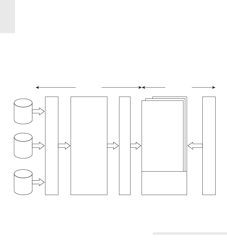
Chapter 1
30
redundant storage of atomic details. If you have the appetite, the perceived need, and
perhaps most important, the budget and organizational patience to fully normalize
and instantiate your data before loading it into dimensional structures that are well
designed according to the Kimball methods, go for it.
Source
Transactions
Back Room
ETL ETL
Presentation Area:
• Dimensional (star
schema or OLAP
cube)
• Atomic and
summary data
• Organized by
business process
• Uses conformed
dimensions
Enterprise DW Bus
Architecture
Front Room
Enterprise Data
Warehouse (EDW)
• Normalized
tables (3NF)
• Atomic data
B
I
A
p
p
l
i
c
a
t
i
o
n
s
Figure 1-10: Hybrid architecture with 3NF structures and dimensional Kimball
presentation area.
Dimensional Modeling Myths
Despite the widespread acceptance of dimensional modeling, some misperceptions
persist in the industry. These false assertions are a distraction, especially when you
want to align your team around common best practices. If folks in your organiza-
tion continually lob criticisms about dimensional modeling, this section should
be on their recommended reading list; their perceptions may be clouded by these
common misunderstandings.
Myth 1: Dimensional Models are Only
for Summary Data
This fi rst myth is frequently the root cause of ill-designed dimensional models.
Because you can’t possibly predict all the questions asked by business users, you
need to provide them with queryable access to the most detailed data so they can
roll it up based on the business question. Data at the lowest level of detail is practi-
cally impervious to surprises or changes. Summary data should complement the

Data Warehousing, Business Intelligence, and Dimensional Modeling Primer 31
granular detail solely to provide improved performance for common queries, but
not replace the details.
A related corollary to this fi rst myth is that only a limited amount of historical
data should be stored in dimensional structures. Nothing about a dimensional model
prohibits storing substantial history. The amount of history available in dimensional
models must only be driven by the business’s requirements.
Myth 2: Dimensional Models are Departmental,
Not Enterprise
Rather than drawing boundaries based on organizational departments, dimensional
models should be organized around business processes, such as orders, invoices, and
service calls. Multiple business functions often want to analyze the same metrics
resulting from a single business process. Multiple extracts of the same source data
that create multiple, inconsistent analytic databases should be avoided.
Myth 3: Dimensional Models are Not Scalable
Dimensional models are extremely scalable. Fact tables frequently have billions of
rows; fact tables containing 2 trillion rows have been reported. The database ven-
dors have wholeheartedly embraced DW/BI and continue to incorporate capabilities
into their products to optimize dimensional models’ scalability and performance.
Both normalized and dimensional models contain the same information and data
relationships; the logical content is identical. Every data relationship expressed in
one model can be accurately expressed in the other. Both normalized and dimen-
sional models can answer exactly the same questions, albeit with varying di culty.
Myth 4: Dimensional Models are Only
for Predictable Usage
Dimensional models should not be designed by focusing on predefi ned reports
or analyses; the design should center on measurement processes. Obviously, it’s
important to consider the BI application’s fi ltering and labeling requirements. But
you shouldn’t design for a top ten list of reports in a vacuum because this list is
bound to change, making the dimensional model a moving target. The key is to
focus on the organization’s measurement events that are typically stable, unlike
analyses that are constantly evolving.
A related corollary is that dimensional models aren’t responsive to changing busi-
ness needs. On the contrary, because of their symmetry, dimensional structures are
extremely fl exible and adaptive to change. The secret to query fl exibility is building

Chapter 1
32
fact tables at the most granular level. Dimensional models that deliver only summary
data are bound to be problematic; users run into analytic brick walls when they try
to drill down into details not available in the summary tables. Developers also run
into brick walls because they can’t easily accommodate new dimensions, attributes,
or facts with these prematurely summarized tables. The correct starting point for
your dimensional models is to express data at the lowest detail possible for maxi-
mum fl exibility and extensibility. Remember, when you pre-suppose the business
question, you’ll likely pre-summarize the data, which can be fatal in the long run.
As the architect Mies van der Rohe is credited with saying, “God is in the details.”
Delivering dimensional models populated with the most detailed data possible ensures
maximum fl exibility and extensibility. Delivering anything less in your dimensional
models undermines the foundation necessary for robust business intelligence.
Myth 5: Dimensional Models Can’t Be Integrated
Dimensional models most certainly can be integrated if they conform to the enterprise
data warehouse bus architecture. Conformed dimensions are built and maintained
as centralized, persistent master data in the ETL system and then reused across
dimensional models to enable data integration and ensure semantic consistency. Data
integration depends on standardized labels, values, and defi nitions. It is hard work
to reach organizational consensus and then implement the corresponding ETL rules,
but you can’t dodge the e ort, regardless of whether you’re populating normalized
or dimensional models.
Presentation area databases that don’t adhere to the bus architecture
with shared conformed dimensions lead to standalone solutions. You can’t hold
dimensional modeling responsible for organizations’ failure to embrace one of its
fundamental tenets.
More Reasons to Think Dimensionally
The majority of this book focuses on dimensional modeling for designing databases
in the DW/BI presentation area. But dimensional modeling concepts go beyond the
design of simple and fast data structures. You should think dimensionally at other
critical junctures of a DW/BI project.
When gathering requirements for a DW/BI initiative, you need to listen for and
then synthesize the fi ndings around business processes. Sometimes teams get lulled
into focusing on a set of required reports or dashboard gauges. Instead you should
constantly ask yourself about the business process measurement events producing
the report or dashboard metrics. When specifying the project’s scope, you must stand

Data Warehousing, Business Intelligence, and Dimensional Modeling Primer 33
fi rm to focus on a single business process per project and not sign up to deploy a
dashboard that covers a handful of them in a single iteration.
Although it’s critical that the DW/BI team concentrates on business processes, it’s
equally important to get IT and business management on the same wavelength. Due
to historical IT funding policies, the business may be more familiar with depart-
mental data deployments. You need to shift their mindset about the DW/BI rollout
to a process perspective. When prioritizing opportunities and developing the DW/
BI roadmap, business processes are the unit of work. Fortunately, business man-
agement typically embraces this approach because it mirrors their thinking about
key performance indicators. Plus, they’ve lived with the inconsistencies, incessant
debates, and never ending reconciliations caused by the departmental approach, so
they’re ready for a fresh tactic. Working with business leadership partners, rank each
business process on business value and feasibility, then tackle processes with the
highest impact and feasibility scores fi rst. Although prioritization is a joint activity
with the business, your underlying understanding of the organization’s business
processes is essential to its e ectiveness and subsequent actionability.
If tasked with drafting the DW/BI system’s data architecture, you need to wrap
your head around the organization’s processes, along with the associated master
descriptive dimension data. The prime deliverable for this activity, the enterprise
data warehouse bus matrix, will be fully vetted in Chapter 4. The matrix also serves
as a useful tool for touting the potential benefi ts of a more rigorous master data
management platform.
Data stewardship or governance programs should focus fi rst on the major dimen-
sions. Depending on the industry, the list might include date, customer, product,
employee, facility, provider, student, faculty, account, and so on. Thinking about
the central nouns used to describe the business translates into a list of data gov-
ernance e orts to be led by subject matter experts from the business community.
Establishing data governance responsibilities for these nouns is the key to eventually
deploying dimensions that deliver consistency and address the business’s needs for
analytic fi ltering, grouping, and labeling. Robust dimensions translate into robust
DW/BI systems.
As you can see, the fundamental motivation for dimensional modeling is front and
center long before you design star schemas or OLAP cubes. Likewise, the dimen-
sional model will remain in the forefront during the subsequent ETL system and BI
application designs. Dimensional modeling concepts link the business and technical
communities together as they jointly design the DW/BI deliverables. We’ll elaborate
on these ideas in Chapter 17: Kimball DW/BI Lifecycle Overview and Chapter 18:
Dimensional Modeling Process and Tasks, but wanted to plant the seeds early so
they have time to germinate.

Chapter 1
34
Agile Considerations
Currently, there’s signifi cant interest within the DW/BI industry on agile development
practices. At the risk of oversimplifi cation, agile methodologies focus on manage-
ably sized increments of work that can be completed within reasonable timeframes
measured in weeks, rather than tackling a much larger scoped (and hence riskier)
project with deliverables promised in months or years. Sounds good, doesn’t it?
Many of the core tenets of agile methodologies align with Kimball best practices,
including
■ Focus on delivering business value. This has been the Kimball mantra for
decades.
■ Value collaboration between the development team and business stakehold-
ers. Like the agile camp, we strongly encourage a close partnership with the
business.
■ Stress ongoing face-to-face communication, feedback, and prioritization with
the business stakeholders.
■ Adapt quickly to inevitably evolving requirements.
■ Tackle development in an iterative, incremental manner.
Although this list is compelling, a common criticism of the agile approaches is the
lack of planning and architecture, coupled with ongoing governance challenges. The
enterprise data warehouse bus matrix is a powerful tool to address these shortcom-
ings. The bus matrix provides a framework and master plan for agile development,
plus identifi es the reusable common descriptive dimensions that provide both data
consistency and reduced time-to-market delivery. With the right collaborative mix
of business and IT stakeholders in a room, the enterprise data warehouse bus matrix
can be produced in relatively short order. Incremental development work can produce
components of the framework until su cient functionality is available and then
released to the business community.
Some clients and students lament that although they want to deliver consistently
defi ned conformed dimensions in their DW/BI environments, it’s “just not feasible.”
They explain that they would if they could, but with the focus on agile development
techniques, it’s “impossible” to take the time to get organizational agreement on
conformed dimensions. We argue that conformed dimensions enable agile DW/BI
development, along with agile decision making. As you fl esh out the portfolio of mas-
ter conformed dimensions, the development crank starts turning faster and faster.
The time-to-market for a new business process data source shrinks as developers
reuse existing conformed dimensions. Ultimately, new ETL development focuses
almost exclusively on delivering more fact tables because the associated dimension
tables are already sitting on the shelf ready to go.

Data Warehousing, Business Intelligence, and Dimensional Modeling Primer 35
Without a framework like the enterprise data warehouse bus matrix, some DW/
BI teams have fallen into the trap of using agile techniques to create analytic or
reporting solutions in a vacuum. In most situations, the team worked with a small
set of users to extract a limited set of source data and make it available to solve
their unique problems. The outcome is often a standalone data stovepipe that others
can’t leverage, or worse yet, delivers data that doesn’t tie to the organization’s other
analytic information. We encourage agility, when appropriate, however building
isolated data sets should be avoided. As with most things in life, moderation and
balance between extremes is almost always prudent.
Summary
In this chapter we discussed the overriding goals for DW/BI systems and the fun-
damental concepts of dimensional modeling. The Kimball DW/BI architecture and
several alternatives were compared. We closed out the chapter by identifying com-
mon misunderstandings that some still hold about dimensional modeling, despite
its widespread acceptance across the industry, and challenged you to think dimen-
sionally beyond data modeling. In the next chapter, you get a turbocharged tour
of dimensional modeling patterns and techniques, and then begin putting these
concepts into action in your fi rst case study in Chapter 3.

Kimball Dimensional
Modeling
Techniques
Overview
Starting with the first edition of The Data Warehouse Toolkit (Wiley, 1996), the
Kimball Group has defined the complete set of techniques for modeling data
in a dimensional way. In the first two editions of this book, we felt the techniques
needed to be introduced through familiar use cases drawn from various industries.
Although we still feel business use cases are an essential pedagogical approach, the
techniques have become so standardized that some dimensional modelers reverse
the logic by starting with the technique and then proceeding to the use case for
context. All of this is good news!
The Kimball techniques have been accepted as industry best practices.
As evidence, some former Kimball University students have published their own
dimensional modeling books. These books usually explain the Kimball techniques
accurately, but it is a sign of our techniques’ resilience that alternative books have
not extended the library of techniques in signifi cant ways or o ered confl icting
guidance.
This chapter is the “o cial” list of Kimball Dimensional Modeling Techniques
from the inventors of these design patterns. We don’t expect you to read this chapter
from beginning to end at fi rst. But we intend the chapter to be a reference for our
techniques. With each technique, we’ve included pointers to subsequent chapters
for further explanation and illustrations based on the motivating use cases.
Fundamental Concepts
The techniques in this section must be considered during every dimensional
design. Nearly every chapter in the book references or illustrates the concepts in
this section.
Gather Business Requirements and Data Realities
Before launching a dimensional modeling e ort, the team needs to understand the
needs of the business, as well as the realities of the underlying source data. You
2

Chapter 2
38
uncover the requirements via sessions with business representatives to understand
their objectives based on key performance indicators, compelling business issues,
decision-making processes, and supporting analytic needs. At the same time, data
realities are uncovered by meeting with source system experts and doing high-level
data profi ling to assess data feasibilities.
Chapter 1 DW/BI and Dimensional Modeling Primer , p 5
Chapter 3 Retail Sales , p 70
Chapter 11 Telecommunications , p 297
Chapter 17 Lifecycle Overview , p 412
Chapter 18 Dimensional Modeling Process and Tasks , p 431
Chapter 19 ETL Subsystems and Techniques ,p 444
Collaborative Dimensional Modeling Workshops
Dimensional models should be designed in collaboration with subject matter experts
and data governance representatives from the business. The data modeler is in
charge, but the model should unfold via a series of highly interactive workshops
with business representatives. These workshops provide another opportunity to
fl esh out the requirements with the business. Dimensional models should not be
designed in isolation by folks who don’t fully understand the business and their
needs; collaboration is critical!
Chapter 3 Retail Sales , p 70
Chapter 4 Inventory , p 135
Chapter 18 Dimensional Modeling Process and Tasks , p 429
Four-Step Dimensional Design Process
The four key decisions made during the design of a dimensional model include:
1. Select the business process.
2. Declare the grain.
3. Identify the dimensions.
4. Identify the facts.
The answers to these questions are determined by considering the needs of the
business along with the realities of the underlying source data during the collab-
orative modeling sessions. Following the business process, grain, dimension, and
fact declarations, the design team determines the table and column names, sample
domain values, and business rules. Business data governance representatives must
participate in this detailed design activity to ensure business buy-in.

Kimball Dimensional Modeling Techniques Overview 39
Chapter 3 Retail Sales , p 70
Chapter 11 Telecommunications , p 300
Chapter 18 Dimensional Modeling Process and Tasks , p 434
Business Processes
Business processes are the operational activities performed by your organization,
such as taking an order, processing an insurance claim, registering students for a
class, or snapshotting every account each month. Business process events generate
or capture performance metrics that translate into facts in a fact table. Most fact
tables focus on the results of a single business process. Choosing the process is
important because it defi nes a specifi c design target and allows the grain, dimen-
sions, and facts to be declared. Each business process corresponds to a row in the
enterprise data warehouse bus matrix.
Chapter 1 DW/BI and Dimensional Modeling Primer , p 10
Chapter 3 Retail Sales , p 70
Chapter 17 Lifecycle Overview , p 414
Chapter 18 Dimensional Modeling Process and Tasks , p 435
Grain
Declaring the grain is the pivotal step in a dimensional design. The grain establishes
exactly what a single fact table row represents. The grain declaration becomes a bind-
ing contract on the design. The grain must be declared before choosing dimensions
or facts because every candidate dimension or fact must be consistent with the grain.
This consistency enforces a uniformity on all dimensional designs that is critical to
BI application performance and ease of use. Atomic grain refers to the lowest level at
which data is captured by a given business process. We strongly encourage you to start
by focusing on atomic-grained data because it withstands the assault of unpredictable
user queries; rolled-up summary grains are important for performance tuning, but they
pre-suppose the business’s common questions. Each proposed fact table grain results
in a separate physical table; di erent grains must not be mixed in the same fact table.
Chapter 1 DW/BI and Dimensional Modeling Primer, p 30
Chapter 3 Retail Sales , p 71
Chapter 4 Inventory , p 112
Chapter 6 Order Management, p 184
Chapter 11 Telecommunications , p 300
Chapter 12 Transportation , p 312
Chapter 18 Dimensional Modeling Process and Tasks , p 435

Chapter 2
40
Dimensions for Descriptive Context
Dimensions provide the “who, what, where, when, why, and how” context surround-
ing a business process event. Dimension tables contain the descriptive attributes
used by BI applications for fi ltering and grouping the facts. With the grain of a fact
table fi rmly in mind, all the possible dimensions can be identifi ed. Whenever pos-
sible, a dimension should be single valued when associated with a given fact row.
Dimension tables are sometimes called the “soul” of the data warehouse because
they contain the entry points and descriptive labels that enable the DW/BI system
to be leveraged for business analysis. A disproportionate amount of e ort is put
into the data governance and development of dimension tables because they are
the drivers of the user’s BI experience.
Chapter 1 DW/BI and Dimensional Modeling Primer , p 13
Chapter 3 Retail Sales , p 72
Chapter 11 Telecommunications , p 301
Chapter 18 Dimensional Modeling Process and Tasks , p 437
Chapter 19 ETL Subsystems and Techniques , p 463
Facts for Measurements
Facts are the measurements that result from a business process event and are almost
always numeric. A single fact table row has a one-to-one relationship to a measurement
event as described by the fact table’s grain. Thus a fact table corresponds to a physi-
cal observable event, and not to the demands of a particular report. Within a fact
table, only facts consistent with the declared grain are allowed. For example, in a
retail sales transaction, the quantity of a product sold and its extended price are
good facts, whereas the store manager’s salary is disallowed.
Chapter 1 DW/BI and Dimensional Modeling Primer , p 10
Chapter 3 Retail Sales , p 72
Chapter 4 Inventory , p 112
Chapter 18 Dimensional Modeling Process and Tasks , p 437
Star Schemas and OLAP Cubes
Star schemas are dimensional structures deployed in a relational database management
system (RDBMS). They characteristically consist of fact tables linked to associated
dimension tables via primary/foreign key relationships. An online analytical processing
(OLAP) cube is a dimensional structure implemented in a multidimensional database;
it can be equivalent in content to, or more often derived from, a relational star schema.
An OLAP cube contains dimensional attributes and facts, but it is accessed through
languages with more analytic capabilities than SQL, such as XMLA and MDX. OLAP

Kimball Dimensional Modeling Techniques Overview 41
cubes are included in this list of basic techniques because an OLAP cube is often
the fi nal step in the deployment of a dimensional DW/BI system, or may exist as an
aggregate structure based on a more atomic relational star schema.
Chapter 1 DW/BI and Dimensional Modeling Primer , p 8
Chapter 3 Retail Sales , p 94
Chapter 5 Procurement , p 149
Chapter 6 Order Management , p 170
Chapter 7 Accounting , p 226
Chapter 9 Human Resources Management , p 273
Chapter 13 Education , p 335
Chapter 19 ETL Subsystems and Techniques , p 481
Chapter 20 ETL System Process and Tasks , p 519
Graceful Extensions to Dimensional Models
Dimensional models are resilient when data relationships change. All the following
changes can be implemented without altering any existing BI query or application,
and without any change in query results.
■ Facts consistent with the grain of an existing fact table can be added by creat-
ing new columns.
■ Dimensions can be added to an existing fact table by creating new foreign key
columns, presuming they don’t alter the fact table’s grain.
■ Attributes can be added to an existing dimension table by creating new
columns.
■ The grain of a fact table can be made more atomic by adding attributes to an exist-
ing dimension table, and then restating the fact table at the lower grain, being
careful to preserve the existing column names in the fact and dimension tables.
Chapter 3 Retail Sales , p 95
Basic Fact Table Techniques
The techniques in this section apply to all fact tables. There are illustrations of fact
tables in nearly every chapter.
Fact Table Structure
A fact table contains the numeric measures produced by an operational measure-
ment event in the real world. At the lowest grain, a fact table row corresponds to a
measurement event and vice versa. Thus the fundamental design of a fact table is
entirely based on a physical activity and is not infl uenced by the eventual reports

Chapter 2
42
that may be produced. In addition to numeric measures, a fact table always contains
foreign keys for each of its associated dimensions, as well as optional degenerate
dimension keys and date/time stamps. Fact tables are the primary target of compu-
tations and dynamic aggregations arising from queries.
Chapter 1 DW/BI and Dimensional Modeling Primer , p 10
Chapter 3 Retail Sales , p 76
Chapter 5 Procurement, p 143
Chapter 6 Order Management, p 169
Additive, Semi-Additive, Non-Additive Facts
The numeric measures in a fact table fall into three categories. The most fl exible and
useful facts are fully additive; additive measures can be summed across any of the
dimensions associated with the fact table. Semi-additive measures can be summed
across some dimensions, but not all; balance amounts are common semi-additive facts
because they are additive across all dimensions except time. Finally, some measures
are completely non-additive, such as ratios. A good approach for non-additive facts is,
where possible, to store the fully additive components of the non-additive measure
and sum these components into the fi nal answer set before calculating the fi nal
non-additive fact. This fi nal calculation is often done in the BI layer or OLAP cube.
Chapter 1 DW/BI and Dimensional Modeling Primer , p 10
Chapter 3 Retail Sales , p 76
Chapter 4 Inventory , p 114
Chapter 7 Accounting , p 204
Nulls in Fact Tables
Null-valued measurements behave gracefully in fact tables. The aggregate functions
(SUM, COUNT, MIN, MAX, and AVG) all do the “right thing” with null facts. However,
nulls must be avoided in the fact table’s foreign keys because these nulls would
automatically cause a referential integrity violation. Rather than a null foreign key,
the associated dimension table must have a default row (and surrogate key) repre-
senting the unknown or not applicable condition.
Chapter 3 Retail Sales , p 92
Chapter 20 ETL System Process and Tasks , p 509
Conformed Facts
If the same measurement appears in separate fact tables, care must be taken to make
sure the technical defi nitions of the facts are identical if they are to be compared

Kimball Dimensional Modeling Techniques Overview 43
or computed together. If the separate fact defi nitions are consistent, the conformed
facts should be identically named; but if they are incompatible, they should be dif-
ferently named to alert the business users and BI applications.
Chapter 4 Inventory , p 138
Chapter 16 Insurance , p 386
Transaction Fact Tables
A row in a transaction fact table corresponds to a measurement event at a point in
space and time. Atomic transaction grain fact tables are the most dimensional and
expressive fact tables; this robust dimensionality enables the maximum slicing
and dicing of transaction data. Transaction fact tables may be dense or sparse
because rows exist only if measurements take place. These fact tables always con-
tain a foreign key for each associated dimension, and optionally contain precise
time stamps and degenerate dimension keys. The measured numeric facts must be
consistent with the transaction grain.
Chapter 3 Retail Sales , p 79
Chapter 4 Inventory , p 116
Chapter 5 Procurement , p 142
Chapter 6 Order Management , p 168
Chapter 7 Accounting , p 206
Chapter 11 Telecommunications , p 306
Chapter 12 Transportation , p 312
Chapter 14 Healthcare , p 351
Chapter 15 Electronic Commerce , p 363
Chapter 16 Insurance , p 379
Chapter 19 ETL Subsystems and Techniques , p 473
Periodic Snapshot Fact Tables
A row in a periodic snapshot fact table summarizes many measurement events occur-
ring over a standard period, such as a day, a week, or a month. The grain is the
period, not the individual transaction. Periodic snapshot fact tables often contain
many facts because any measurement event consistent with the fact table grain is
permissible. These fact tables are uniformly dense in their foreign keys because
even if no activity takes place during the period, a row is typically inserted in the
fact table containing a zero or null for each fact.

Chapter 2
44
Chapter 4 Inventory , p 113
Chapter 7 Accounting , p 204
Chapter 9 Human Resources Management , p 267
Chapter 10 Financial Services , p 283
Chapter 13 Education , p 333
Chapter 14 Healthcare, p 351
Chapter 16 Insurance , p 385
Chapter 19 ETL Subsystems and Techniques , p 474
Accumulating Snapshot Fact Tables
A row in an accumulating snapshot fact table summarizes the measurement events
occurring at predictable steps between the beginning and the end of a process.
Pipeline or workfl ow processes, such as order fulfi llment or claim processing, that
have a defi ned start point, standard intermediate steps, and defi ned end point can be
modeled with this type of fact table. There is a date foreign key in the fact table for
each critical milestone in the process. An individual row in an accumulating snap-
shot fact table, corresponding for instance to a line on an order, is initially inserted
when the order line is created. As pipeline progress occurs, the accumulating fact
table row is revisited and updated. This consistent updating of accumulating snap-
shot fact rows is unique among the three types of fact tables. In addition to the date
foreign keys associated with each critical process step, accumulating snapshot fact
tables contain foreign keys for other dimensions and optionally contain degener-
ate dimensions. They often include numeric lag measurements consistent with the
grain, along with milestone completion counters.
Chapter 4 Inventory , p 118
Chapter 5 Procurement , p 147
Chapter 6 Order Management , p 194
Chapter 13 Education , p 326
Chapter 14 Healthcare , p 342
Chapter 16 Insurance , p 392
Chapter 19 ETL Subsystems and Techniques , p 475
Factless Fact Tables
Although most measurement events capture numerical results, it is possible that
the event merely records a set of dimensional entities coming together at a moment
in time. For example, an event of a student attending a class on a given day may
not have a recorded numeric fact, but a fact row with foreign keys for calendar day,
student, teacher, location, and class is well-defi ned. Likewise, customer communi-
cations are events, but there may be no associated metrics. Factless fact tables can

Kimball Dimensional Modeling Techniques Overview 45
also be used to analyze what didn’t happen. These queries always have two parts: a
factless coverage table that contains all the possibilities of events that might happen
and an activity table that contains the events that did happen. When the activity
is subtracted from the coverage, the result is the set of events that did not happen.
Chapter 3 Retail Sales , p 97
Chapter 6 Order Management , p 176
Chapter 13 Education , p 329
Chapter 16 Insurance , p 396
Aggregate Fact Tables or OLAP Cubes
Aggregate fact tables are simple numeric rollups of atomic fact table data built solely
to accelerate query performance. These aggregate fact tables should be available to
the BI layer at the same time as the atomic fact tables so that BI tools smoothly
choose the appropriate aggregate level at query time. This process, known as
aggregate navigation, must be open so that every report writer, query tool, and BI
application harvests the same performance benefi ts. A properly designed set of
aggregates should behave like database indexes, which accelerate query perfor-
mance but are not encountered directly by the BI applications or business users.
Aggregate fact tables contain foreign keys to shrunken conformed dimensions, as
well as aggregated facts created by summing measures from more atomic fact tables.
Finally, aggregate OLAP cubes with summarized measures are frequently built in
the same way as relational aggregates, but the OLAP cubes are meant to be accessed
directly by the business users.
Chapter 15 Electronic Commerce , p 366
Chapter 19 ETL Subsystems and Techniques , p 481
Chapter 20 ETL System Process and Tasks , p 519
Consolidated Fact Tables
It is often convenient to combine facts from multiple processes together into a single
consolidated fact table if they can be expressed at the same grain. For example, sales
actuals can be consolidated with sales forecasts in a single fact table to make the task
of analyzing actuals versus forecasts simple and fast, as compared to assembling a
drill-across application using separate fact tables. Consolidated fact tables add bur-
den to the ETL processing, but ease the analytic burden on the BI applications. They
should be considered for cross-process metrics that are frequently analyzed together.
Chapter 7 Accounting , p 224
Chapter 16 Insurance , p 395

Chapter 2
46
Basic Dimension Table Techniques
The techniques in this section apply to all dimension tables. Dimension tables are
discussed and illustrated in every chapter.
Dimension Table Structure
Every dimension table has a single primary key column. This primary key is embedded
as a foreign key in any associated fact table where the dimension row’s descriptive
context is exactly correct for that fact table row. Dimension tables are usually wide, fl at
denormalized tables with many low-cardinality text attributes. While operational codes
and indicators can be treated as attributes, the most powerful dimension attributes
are populated with verbose descriptions. Dimension table attributes are the primary
target of constraints and grouping specifi cations from queries and BI applications. The
descriptive labels on reports are typically dimension attribute domain values.
Chapter 1 DW/BI and Dimensional Modeling Primer , p 13
Chapter 3 Retail Sales , p 79
Chapter 11 Telecommunications , p 301
Dimension Surrogate Keys
A dimension table is designed with one column serving as a unique primary key.
This primary key cannot be the operational system’s natural key because there will
be multiple dimension rows for that natural key when changes are tracked over time.
In addition, natural keys for a dimension may be created by more than one source
system, and these natural keys may be incompatible or poorly administered. The
DW/BI system needs to claim control of the primary keys of all dimensions; rather
than using explicit natural keys or natural keys with appended dates, you should
create anonymous integer primary keys for every dimension. These dimension sur-
rogate keys are simple integers, assigned in sequence, starting with the value 1,
every time a new key is needed. The date dimension is exempt from the surrogate
key rule; this highly predictable and stable dimension can use a more meaningful
primary key. See the section “Calendar Date Dimensions.”
Chapter 3 Retail Sales , p 98
Chapter 19 ETL Subsystems and Techniques , p 469
Chapter 20 ETL System Process and Tasks , p 506
Natural, Durable, and Supernatural Keys
Natural keys created by operational source systems are subject to business rules outside
the control of the DW/BI system. For instance, an employee number (natural key) may

Kimball Dimensional Modeling Techniques Overview 47
be changed if the employee resigns and then is rehired. When the data warehouse
wants to have a single key for that employee, a new durable key must be created that is
persistent and does not change in this situation. This key is sometimes referred to as
a durable supernatural key. The best durable keys have a format that is independent of
the original business process and thus should be simple integers assigned in sequence
beginning with 1. While multiple surrogate keys may be associated with an employee
over time as their profi le changes, the durable key never changes.
Chapter 3 Retail Sales , p 100
Chapter 20 ETL System Process and Tasks , p 510
Chapter 21 Big Data Analytics, p 539
Drilling Down
Drilling down is the most fundamental way data is analyzed by business users. Drilling
down simply means adding a row header to an existing query; the new row header
is a dimension attribute appended to the GROUP BY expression in an SQL query. The
attribute can come from any dimension attached to the fact table in the query. Drilling
down does not require the defi nition of predetermined hierarchies or drill-down paths.
See the section “Drilling Across.”
Chapter 3 Retail Sales , p 86
Degenerate Dimensions
Sometimes a dimension is defi ned that has no content except for its primary key.
For example, when an invoice has multiple line items, the line item fact rows inherit
all the descriptive dimension foreign keys of the invoice, and the invoice is left with
no unique content. But the invoice number remains a valid dimension key for fact
tables at the line item level. This degenerate dimension is placed in the fact table with
the explicit acknowledgment that there is no associated dimension table. Degenerate
dimensions are most common with transaction and accumulating snapshot fact tables.
Chapter 3 Retail Sales , p 93
Chapter 6 Order Management , p 178
Chapter 11 Telecommunications , p 303
Chapter 16 Insurance , p 383
Denormalized Flattened Dimensions
In general, dimensional designers must resist the normalization urges caused by years
of operational database designs and instead denormalize the many-to-one fi xed depth

Chapter 2
48
hierarchies into separate attributes on a fl attened dimension row. Dimension denor-
malization supports dimensional modeling’s twin objectives of simplicity and speed.
Chapter 1 DW/BI and Dimensional Modeling Primer , p 13
Chapter 3 Retail Sales , p 84
Multiple Hierarchies in Dimensions
Many dimensions contain more than one natural hierarchy. For example, calendar
date dimensions may have a day to week to fi scal period hierarchy, as well as a
day to month to year hierarchy. Location intensive dimensions may have multiple
geographic hierarchies. In all of these cases, the separate hierarchies can gracefully
coexist in the same dimension table.
Chapter 3 Retail Sales , p 88
Chapter 19 ETL Subsystems and Techniques , p 470
Flags and Indicators as Textual Attributes
Cryptic abbreviations, true/false fl ags, and operational indicators should be sup-
plemented in dimension tables with full text words that have meaning when
independently viewed. Operational codes with embedded meaning within the
code value should be broken down with each part of the code expanded into its
own separate descriptive dimension attribute.
Chapter 3 Retail Sales , p 82
Chapter 11 Telecommunications, p 301
Chapter 16 Insurance , p 383
Null Attributes in Dimensions
Null-valued dimension attributes result when a given dimension row has not been
fully populated, or when there are attributes that are not applicable to all the dimen-
sion’s rows. In both cases, we recommend substituting a descriptive string, such as
Unknown or Not Applicable in place of the null value. Nulls in dimension attributes
should be avoided because di erent databases handle grouping and constraining
on nulls inconsistently.
Chapter 3 Retail Sales , p 92
Calendar Date Dimensions
Calendar date dimensions are attached to virtually every fact table to allow navigation
of the fact table through familiar dates, months, fi scal periods, and special days on

Kimball Dimensional Modeling Techniques Overview 49
the calendar. You would never want to compute Easter in SQL, but rather want to
look it up in the calendar date dimension. The calendar date dimension typically
has many attributes describing characteristics such as week number, month name,
fi scal period, and national holiday indicator. To facilitate partitioning, the primary
key of a date dimension can be more meaningful, such as an integer representing
YYYYMMDD, instead of a sequentially-assigned surrogate key. However, the date
dimension table needs a special row to represent unknown or to-be-determined
dates. When further precision is needed, a separate date/time stamp can be added
to the fact table. The date/time stamp is not a foreign key to a dimension table, but
rather is a standalone column. If business users constrain or group on time-of-day
attributes, such as day part grouping or shift number, then you would add a separate
time-of-day dimension foreign key to the fact table.
Chapter 3 Retail Sales , p 79
Chapter 7 Accounting , p 208
Chapter 8 Customer Relationship Management , p 238
Chapter 12 Transportation , p 321
Chapter 19 ETL Subsystems and Techniques , p 470
Role-Playing Dimensions
A single physical dimension can be referenced multiple times in a fact table, with
each reference linking to a logically distinct role for the dimension. For instance, a
fact table can have several dates, each of which is represented by a foreign key to the
date dimension. It is essential that each foreign key refers to a separate view of
the date dimension so that the references are independent. These separate dimen-
sion views (with unique attribute column names) are called roles.
Chapter 6 Order Management , p 170
Chapter 12 Transportation , p 312
Chapter 14 Healthcare , p 345
Chapter 16 Insurance , p 380
Junk Dimensions
Transactional business processes typically produce a number of miscellaneous, low-
cardinality fl ags and indicators. Rather than making separate dimensions for each
fl ag and attribute, you can create a single junk dimension combining them together.
This dimension, frequently labeled as a transaction profi le dimension in a schema,
does not need to be the Cartesian product of all the attributes’ possible values, but
should only contain the combination of values that actually occur in the source data.

Chapter 2
50
Chapter 6 Order Management , p 179
Chapter 12 Transportation , p 318
Chapter 16 Insurance , p 392
Chapter 19 ETL Subsystems and Techniques , p 470
Snowfl aked Dimensions
When a hierarchical relationship in a dimension table is normalized, low-cardinal-
ity attributes appear as secondary tables connected to the base dimension table by
an attribute key. When this process is repeated with all the dimension table’s hier-
archies, a characteristic multilevel structure is created that is called a snowfl ake.
Although the snowfl ake represents hierarchical data accurately, you should avoid
snowfl akes because it is di cult for business users to understand and navigate
snowfl akes. They can also negatively impact query performance. A fl attened denor-
malized dimension table contains exactly the same information as a snowfl aked
dimension.
Chapter 3 Retail Sales , p 104
Chapter 11 Telecommunications , p 301
Chapter 20 ETL System Process and Tasks , p 504
Outrigger Dimensions
A dimension can contain a reference to another dimension table. For instance, a
bank account dimension can reference a separate dimension representing the date
the account was opened. These secondary dimension references are called outrigger
dimensions. Outrigger dimensions are permissible, but should be used sparingly. In
most cases, the correlations between dimensions should be demoted to a fact table,
where both dimensions are represented as separate foreign keys.
Chapter 3 Retail Sales , p 106
Chapter 5 Procurement , p 160
Chapter 8 Customer Relationship Management , p 243
Chapter 12 Transportation , p 321
Integration via Conformed Dimensions
One of the marquee successes of the dimensional modeling approach has been to
defi ne a simple but powerful recipe for integrating data from di erent business
processes.

Kimball Dimensional Modeling Techniques Overview 51
Conformed Dimensions
Dimension tables conform when attributes in separate dimension tables have the
same column names and domain contents. Information from separate fact tables
can be combined in a single report by using conformed dimension attributes that
are associated with each fact table. When a conformed attribute is used as the
row header (that is, the grouping column in the SQL query), the results from the
separate fact tables can be aligned on the same rows in a drill-across report. This
is the essence of integration in an enterprise DW/BI system. Conformed dimen-
sions, defi ned once in collaboration with the business’s data governance represen-
tatives, are reused across fact tables; they deliver both analytic consistency and
reduced future development costs because the wheel is not repeatedly re-created.
Chapter 4 Inventory , p 130
Chapter 8 Customer Relationship Management , p 256
Chapter 11 Telecommunications , p 304
Chapter 16 Insurance , p 386
Chapter 18 Dimensional Modeling Process and Tasks , p 431
Chapter 19 ETL Subsystems and Techniques , p 461
Shrunken Dimensions
Shrunken dimensions are conformed dimensions that are a subset of rows and/or
columns of a base dimension. Shrunken rollup dimensions are required when con-
structing aggregate fact tables. They are also necessary for business processes that
naturally capture data at a higher level of granularity, such as a forecast by month
and brand (instead of the more atomic date and product associated with sales data).
Another case of conformed dimension subsetting occurs when two dimensions are
at the same level of detail, but one represents only a subset of rows.
Chapter 4 Inventory , p 132
Chapter 19 ETL Subsystems and Techniques , p 472
Chapter 20 ETL System Process and Tasks , p 504
Drilling Across
Drilling across simply means making separate queries against two or more fact tables
where the row headers of each query consist of identical conformed attributes. The
answer sets from the two queries are aligned by performing a sort-merge opera-
tion on the common dimension attribute row headers. BI tool vendors refer to this
functionality by various names, including stitch and multipass query.
Chapter 4 Inventory , p 130

Chapter 2
52
Value Chain
A value chain identifi es the natural fl ow of an organization’s primary business
processes. For example, a retailer’s value chain may consist of purchasing to ware-
housing to retail sales. A general ledger value chain may consist of budgeting to
commitments to payments. Operational source systems typically produce transac-
tions or snapshots at each step of the value chain. Because each process produces
unique metrics at unique time intervals with unique granularity and dimensionality,
each process typically spawns at least one atomic fact table.
Chapter 4 Inventory , p 111
Chapter 7 Accounting , p 210
Chapter 16 Insurance , p 377
Enterprise Data Warehouse Bus Architecture
The enterprise data warehouse bus architecture provides an incremental approach
to building the enterprise DW/BI system. This architecture decomposes the DW/
BI planning process into manageable pieces by focusing on business processes,
while delivering integration via standardized conformed dimensions that are reused
across processes. It provides an architectural framework, while also decomposing
the program to encourage manageable agile implementations corresponding to the
rows on the enterprise data warehouse bus matrix. The bus architecture is tech-
nology and database platform independent; both relational and OLAP dimensional
structures can participate.
Chapter 1 DW/BI and Dimensional Modeling Primer , p 21
Chapter 4 Inventory , p 123
Enterprise Data Warehouse Bus Matrix
The enterprise data warehouse bus matrix is the essential tool for designing and com-
municating the enterprise data warehouse bus architecture. The rows of the matrix
are business processes and the columns are dimensions. The shaded cells of the
matrix indicate whether a dimension is associated with a given business process. The
design team scans each row to test whether a candidate dimension is well-defi ned for
the business process and also scans each column to see where a dimension should be
conformed across multiple business processes. Besides the technical design consid-
erations, the bus matrix is used as input to prioritize DW/BI projects with business
management as teams should implement one row of the matrix at a time.

Kimball Dimensional Modeling Techniques Overview 53
Chapter 4 Inventory , p 125
Chapter 5 Procurement , p 143
Chapter 6 Order Management , p 168
Chapter 7 Accounting, p 202
Chapter 9 Human Resources Management , p 268
Chapter 10 Financial Services , p 282
Chapter 11 Telecommunications , p 297
Chapter 12 Transportation , p 311
Chapter 13 Education , p 325
Chapter 14 Healthcare , p 339
Chapter 15 Electronic Commerce , p 368
Chapter 16 Insurance , p 389
Detailed Implementation Bus Matrix
The detailed implementation bus matrix is a more granular bus matrix where each
business process row has been expanded to show specifi c fact tables or OLAP cubes.
At this level of detail, the precise grain statement and list of facts can be documented.
Chapter 5 Procurement , p 143
Chapter 16 Insurance , p 390
Opportunity/Stakeholder Matrix
After the enterprise data warehouse bus matrix rows have been identifi ed, you can
draft a di erent matrix by replacing the dimension columns with business func-
tions, such as marketing, sales, and fi nance, and then shading the matrix cells to
indicate which business functions are interested in which business process rows.
The opportunity/stakeholder matrix helps identify which business groups should be
invited to the collaborative design sessions for each process-centric row.
Chapter 4 Inventory , p 127
Dealing with Slowly Changing Dimension Attributes
The following section describes the fundamental approaches for dealing with slowly
changing dimension (SCD) attributes. It is quite common to have attributes in the
same dimension table that are handled with di erent change tracking techniques.

Chapter 2
54
Type 0: Retain Original
With type 0, the dimension attribute value never changes, so facts are always grouped
by this original value. Type 0 is appropriate for any attribute labeled “original,” such
as a customer’s original credit score or a durable identifi er. It also applies to most
attributes in a date dimension.
Chapter 5 Procurement , p 148
Type 1: Overwrite
With type 1, the old attribute value in the dimension row is overwritten with the new
value; type 1 attributes always refl ects the most recent assignment, and therefore
this technique destroys history. Although this approach is easy to implement and
does not create additional dimension rows, you must be careful that aggregate fact
tables and OLAP cubes a ected by this change are recomputed.
Chapter 5 Procurement , p 149
Chapter 16 Insurance , p 380
Chapter 19 ETL Subsystems and Techniques , p 465
Type 2: Add New Row
Type 2 changes add a new row in the dimension with the updated attribute values.
This requires generalizing the primary key of the dimension beyond the natural or
durable key because there will potentially be multiple rows describing each member.
When a new row is created for a dimension member, a new primary surrogate key is
assigned and used as a foreign key in all fact tables from the moment of the update
until a subsequent change creates a new dimension key and updated dimension row.
A minimum of three additional columns should be added to the dimension row
with type 2 changes: 1) row e ective date or date/time stamp; 2) row expiration
date or date/time stamp; and 3) current row indicator.
Chapter 5 Procurement , p 150
Chapter 8 Customer Relationship Management , p 243
Chapter 9 Human Resources Management , p 263
Chapter 16 Insurance , p 380
Chapter 19 ETL Subsystems and Techniques , p 465
Chapter 20 ETL System Process and Tasks , p 507

Kimball Dimensional Modeling Techniques Overview 55
Type 3: Add New Attribute
Type 3 changes add a new attribute in the dimension to preserve the old attribute
value; the new value overwrites the main attribute as in a type 1 change. This kind of
type 3 change is sometimes called an alternate reality. A business user can group and
fi lter fact data by either the current value or alternate reality. This slowly changing
dimension technique is used relatively infrequently.
Chapter 5 Procurement , p 154
Chapter 16 Insurance , p 380
Chapter 19 ETL Subsystems and Techniques , p 467
Type 4: Add Mini-Dimension
The type 4 technique is used when a group of attributes in a dimension rapidly
changes and is split o to a mini-dimension. This situation is sometimes called a
rapidly changing monster dimension. Frequently used attributes in multimillion-row
dimension tables are mini-dimension design candidates, even if they don’t fre-
quently change. The type 4 mini-dimension requires its own unique primary key;
the primary keys of both the base dimension and mini-dimension are captured in
the associated fact tables.
Chapter 5 Procurement , p 156
Chapter 10 Financial Services , p 289
Chapter 16 Insurance , p 381
Chapter 19 ETL Subsystems and Techniques , p 467
Type 5: Add Mini-Dimension and Type 1 Outrigger
The type 5 technique is used to accurately preserve historical attribute values,
plus report historical facts according to current attribute values. Type 5 builds on
the type 4 mini-dimension by also embedding a current type 1 reference to the
mini-dimension in the base dimension. This enables the currently-assigned mini-
dimension attributes to be accessed along with the others in the base dimension
without linking through a fact table. Logically, you’d represent the base dimension
and mini-dimension outrigger as a single table in the presentation area. The ETL
team must overwrite this type 1 mini-dimension reference whenever the current
mini-dimension assignment changes.
Chapter 5 Procurement , p 160
Chapter 19 ETL Subsystems and Techniques , p 468

Chapter 2
56
Type 6: Add Type 1 Attributes to Type 2 Dimension
Like type 5, type 6 also delivers both historical and current dimension attribute
values. Type 6 builds on the type 2 technique by also embedding current type
1 versions of the same attributes in the dimension row so that fact rows can be
fi ltered or grouped by either the type 2 attribute value in e ect when the measure-
ment occurred or the attribute’s current value. In this case, the type 1 attribute is
systematically overwritten on all rows associated with a particular durable key
whenever the attribute is updated.
Chapter 5 Procurement , p 160
Chapter 19 ETL Subsystems and Techniques , p 468
Type 7: Dual Type 1 and Type 2 Dimensions
Type 7 is the fi nal hybrid technique used to support both as-was and as-is report-
ing. A fact table can be accessed through a dimension modeled both as a type 1
dimension showing only the most current attribute values, or as a type 2 dimen-
sion showing correct contemporary historical profi les. The same dimension table
enables both perspectives. Both the durable key and primary surrogate key of the
dimension are placed in the fact table. For the type 1 perspective, the current fl ag
in the dimension is constrained to be current, and the fact table is joined via the
durable key. For the type 2 perspective, the current fl ag is not constrained, and the
fact table is joined via the surrogate primary key. These two perspectives would be
deployed as separate views to the BI applications.
Chapter 5 Procurement , p 162
Chapter 19 ETL Subsystems and Techniques , p 468
Dealing with Dimension Hierarchies
Dimensional hierarchies are commonplace. This section describes approaches for
dealing with hierarchies, starting with the most basic.
Fixed Depth Positional Hierarchies
A fi xed depth hierarchy is a series of many-to-one relationships, such as product
to brand to category to department. When a fi xed depth hierarchy is defi ned and
the hierarchy levels have agreed upon names, the hierarchy levels should appear
as separate positional attributes in a dimension table. A fi xed depth hierarchy is
by far the easiest to understand and navigate as long as the above criteria are met.
It also delivers predictable and fast query performance. When the hierarchy is not
a series of many-to-one relationships or the number of levels varies such that the

Kimball Dimensional Modeling Techniques Overview 57
levels do not have agreed upon names, a ragged hierarchy technique, described
below, must be used.
Chapter 3 Retail Sales , p 84
Chapter 7 Accounting , p 214
Chapter 19 ETL Subsystems and Techniques , p 470
Chapter 20 ETL System Process and Tasks , p 501
Slightly Ragged/Variable Depth Hierarchies
Slightly ragged hierarchies don’t have a fi xed number of levels, but the range in depth
is small. Geographic hierarchies often range in depth from perhaps three levels to
six levels. Rather than using the complex machinery for unpredictably variable
hierarchies, you can force-fi t slightly ragged hierarchies into a fi xed depth positional
design with separate dimension attributes for the maximum number of levels, and
then populate the attribute value based on rules from the business.
Chapter 7 Accounting , p 214
Ragged/Variable Depth Hierarchies with Hierarchy Bridge Tables
Ragged hierarchies of indeterminate depth are di cult to model and query in a
relational database. Although SQL extensions and OLAP access languages provide
some support for recursive parent/child relationships, these approaches have limita-
tions. With SQL extensions, alternative ragged hierarchies cannot be substituted at
query time, shared ownership structures are not supported, and time varying ragged
hierarchies are not supported. All these objections can be overcome in relational
databases by modeling a ragged hierarchy with a specially constructed bridge table.
This bridge table contains a row for every possible path in the ragged hierarchy
and enables all forms of hierarchy traversal to be accomplished with standard SQL
rather than using special language extensions.
Chapter 7 Accounting , p 215
Chapter 9 Human Resources Management , p 273
Ragged/Variable Depth Hierarchies with Pathstring Attributes
The use of a bridge table for ragged variable depth hierarchies can be avoided by
implementing a pathstring attribute in the dimension. For each row in the dimen-
sion, the pathstring attribute contains a specially encoded text string containing
the complete path description from the supreme node of a hierarchy down to the
node described by the particular dimension row. Many of the standard hierarchy

Chapter 2
58
analysis requests can then be handled by standard SQL, without resorting to SQL
language extensions. However, the pathstring approach does not enable rapid sub-
stitution of alternative hierarchies or shared ownership hierarchies. The pathstring
approach may also be vulnerable to structure changes in the ragged hierarchy that
could force the entire hierarchy to be relabeled.
Chapter 7 Accounting , p 221
Advanced Fact Table Techniques
The techniques in this section refer to less common fact table patterns.
Fact Table Surrogate Keys
Surrogate keys are used to implement the primary keys of almost all dimension
tables. In addition, single column surrogate fact keys can be useful, albeit not
required. Fact table surrogate keys, which are not associated with any dimension,
are assigned sequentially during the ETL load process and are used 1) as the single
column primary key of the fact table; 2) to serve as an immediate identifi er of a fact
table row without navigating multiple dimensions for ETL purposes; 3) to allow an
interrupted load process to either back out or resume; 4) to allow fact table update
operations to be decomposed into less risky inserts plus deletes.
Chapter 3 Retail Sales , p 102
Chapter 19 ETL Subsystems and Techniques , p 486
Chapter 20 ETL System Process and Tasks , p 520
Centipede Fact Tables
Some designers create separate normalized dimensions for each level of a many-to-
one hierarchy, such as a date dimension, month dimension, quarter dimension, and
year dimension, and then include all these foreign keys in a fact table. This results
in a centipede fact table with dozens of hierarchically related dimensions. Centipede
fact tables should be avoided. All these fi xed depth, many-to-one hierarchically
related dimensions should be collapsed back to their unique lowest grains, such as
the date for the example mentioned. Centipede fact tables also result when design-
ers embed numerous foreign keys to individual low-cardinality dimension tables
rather than creating a junk dimension.
Chapter 3 Retail Sales , p 108

Kimball Dimensional Modeling Techniques Overview 59
Numeric Values as Attributes or Facts
Designers sometimes encounter numeric values that don’t clearly fall into either
the fact or dimension attribute categories. A classic example is a product’s standard
list price. If the numeric value is used primarily for calculation purposes, it likely
belongs in the fact table. If a stable numeric value is used predominantly for fi ltering
and grouping, it should be treated as a dimension attribute; the discrete numeric
values can be supplemented with value band attributes (such as $0-50). In some
cases, it is useful to model the numeric value as both a fact and dimension attribute,
such as a quantitative on-time delivery metric and qualitative textual descriptor.
Chapter 3 Retail Sales , p 85
Chapter 6 Order Management , p 188
Chapter 8 Customer Relationship Management , p 254
Chapter 16 Insurance , p 382
Lag/Duration Facts
Accumulating snapshot fact tables capture multiple process milestones, each with a
date foreign key and possibly a date/time stamp. Business users often want to analyze
the lags or durations between these milestones; sometimes these lags are just the
di erences between dates, but other times the lags are based on more complicated
business rules. If there are dozens of steps in a pipeline, there could be hundreds
of possible lags. Rather than forcing the user’s query to calculate each possible lag
from the date/time stamps or date dimension foreign keys, just one time lag can be
stored for each step measured against the process’s start point. Then every possible
lag between two steps can be calculated as a simple subtraction between the two
lags stored in the fact table.
Chapter 6 Order Management , p 196
Chapter 16 Insurance , p 393
Header/Line Fact Tables
Operational transaction systems often consist of a transaction header row that’s
associated with multiple transaction lines. With header/line schemas (also known
as parent/child schemas), all the header-level dimension foreign keys and degenerate
dimensions should be included on the line-level fact table.
Chapter 6 Order Management , p 181
Chapter 12 Transportation , p 315
Chapter 15 Electronic Commerce , p 363

Chapter 2
60
Allocated Facts
It is quite common in header/line transaction data to encounter facts of di er-
ing granularity, such as a header freight charge. You should strive to allocate
the header facts down to the line level based on rules provided by the business, so the
allocated facts can be sliced and rolled up by all the dimensions. In many cases, you
can avoid creating a header-level fact table, unless this aggregation delivers query
performance advantages.
Chapter 6 Order Management , p 184
Profi t and Loss Fact Tables Using Allocations
Fact tables that expose the full equation of profi t are among the most powerful deliv-
erables of an enterprise DW/BI system. The equation of profi t is (revenue) – (costs) =
(profi t). Fact tables ideally implement the profi t equation at the grain of the atomic
revenue transaction and contain many components of cost. Because these tables are
at the atomic grain, numerous rollups are possible, including customer profi tabil-
ity, product profi tability, promotion profi tability, channel profi tability, and others.
However, these fact tables are di cult to build because the cost components must
be allocated from their original sources to the fact table’s grain. This allocation step
is often a major ETL subsystem and is a politically charged step that requires high-
level executive support. For these reasons, profi t and loss fact tables are typically
not tackled during the early implementation phases of a DW/BI program.
Chapter 6 Order Management , p 189
Chapter 15 Electronic Commerce , p 370
Multiple Currency Facts
Fact tables that record fi nancial transactions in multiple currencies should contain
a pair of columns for every fi nancial fact in the row. One column contains the fact
expressed in the true currency of the transaction, and the other contains the same
fact expressed in a single standard currency that is used throughout the fact table.
The standard currency value is created in an ETL process according to an approved
business rule for currency conversion. This fact table also must have a currency
dimension to identify the transaction’s true currency.
Chapter 6 Order Management , p 182
Chapter 7 Accounting , p 206

Kimball Dimensional Modeling Techniques Overview 61
Multiple Units of Measure Facts
Some business processes require facts to be stated simultaneously in several units
of measure. For example, depending on the perspective of the business user, a
supply chain may need to report the same facts as pallets, ship cases, retail cases,
or individual scan units. If the fact table contains a large number of facts, each of
which must be expressed in all units of measure, a convenient technique is to store
the facts once in the table at an agreed standard unit of measure, but also simulta-
neously store conversion factors between the standard measure and all the others.
This fact table could be deployed through views to each user constituency, using
an appropriate selected conversion factor. The conversion factors must reside in the
underlying fact table row to ensure the view calculation is simple and correct, while
minimizing query complexity.
Chapter 6 Order Management , p 197
Year-to-Date Facts
Business users often request year-to-date (YTD) values in a fact table. It is hard to
argue against a single request, but YTD requests can easily morph into “YTD at the
close of the fi scal period” or “fi scal period to date.” A more reliable, extensible way
to handle these assorted requests is to calculate the YTD metrics in the BI applica-
tions or OLAP cube rather than storing YTD facts in the fact table.
Chapter 7 Accounting , p 206
Multipass SQL to Avoid Fact-to-Fact Table Joins
A BI application must never issue SQL that joins two fact tables together across the
fact table’s foreign keys. It is impossible to control the cardinality of the answer set
of such a join in a relational database, and incorrect results will be returned to the
BI tool. For instance, if two fact tables contain customer’s product shipments and
returns, these two fact tables must not be joined directly across the customer
and product foreign keys. Instead, the technique of drilling across two fact tables
should be used, where the answer sets from shipments and returns are separately
created, and the results sort-merged on the common row header attribute values to
produce the correct result.
Chapter 4 Inventory , p 130
Chapter 8 Customer Relationship Management , p 259

Chapter 2
62
Timespan Tracking in Fact Tables
There are three basic fact table grains: transaction, periodic snapshot, and accu-
mulating snapshot. In isolated cases, it is useful to add a row e ective date, row
expiration date, and current row indicator to the fact table, much like you do with
type 2 slowly changing dimensions, to capture a timespan when the fact row was
e ective. Although an unusual pattern, this pattern addresses scenarios such as
slowly changing inventory balances where a frequent periodic snapshot would load
identical rows with each snapshot.
Chapter 8 Customer Relationship Management , p 252
Chapter 16 Insurance , p 394
Late Arriving Facts
A fact row is late arriving if the most current dimensional context for new fact rows
does not match the incoming row. This happens when the fact row is delayed. In
this case, the relevant dimensions must be searched to fi nd the dimension keys that
were e ective when the late arriving measurement event occurred.
Chapter 14 Healthcare , p 351
Chapter 19 ETL Subsystems and Techniques , p 478
Advanced Dimension Techniques
The techniques in this section refer to more advanced dimension table patterns.
Dimension-to-Dimension Table Joins
Dimensions can contain references to other dimensions. Although these relation-
ships can be modeled with outrigger dimensions, in some cases, the existence of a
foreign key to the outrigger dimension in the base dimension can result in explosive
growth of the base dimension because type 2 changes in the outrigger force cor-
responding type 2 processing in the base dimension. This explosive growth can
often be avoided if you demote the correlation between dimensions by placing the
foreign key of the outrigger in the fact table rather than in the base dimension. This
means the correlation between the dimensions can be discovered only by traversing
the fact table, but this may be acceptable, especially if the fact table is a periodic
snapshot where all the keys for all the dimensions are guaranteed to be present for
each reporting period.
Chapter 6 Order Management , p 175

Kimball Dimensional Modeling Techniques Overview 63
Multivalued Dimensions and Bridge Tables
In a classic dimensional schema, each dimension attached to a fact table has a single
value consistent with the fact table’s grain. But there are a number of situations in
which a dimension is legitimately multivalued. For example, a patient receiving a
healthcare treatment may have multiple simultaneous diagnoses. In these cases, the
multivalued dimension must be attached to the fact table through a group dimen-
sion key to a bridge table with one row for each simultaneous diagnosis in a group.
Chapter 8 Customer Relationship Management , p 245
Chapter 9 Human Resources Management , p 275
Chapter 10 Financial Services , p 287
Chapter 13 Education , p 333
Chapter 14 Healthcare , p 345
Chapter 16 Insurance , p 382
Chapter 19 ETL Subsystems and Techniques , p 477
Time Varying Multivalued Bridge Tables
A multivalued bridge table may need to be based on a type 2 slowly changing dimen-
sion. For example, the bridge table that implements the many-to-many relationship
between bank accounts and individual customers usually must be based on type
2 account and customer dimensions. In this case, to prevent incorrect linkages
between accounts and customers, the bridge table must include e ective and expi-
ration date/time stamps, and the requesting application must constrain the bridge
table to a specifi c moment in time to produce a consistent snapshot.
Chapter 7 Accounting , p 220
Chapter 10 Financial Services , p 286
Behavior Tag Time Series
Almost all text in a data warehouse is descriptive text in dimension tables. Data
mining customer cluster analyses typically results in textual behavior tags, often
identifi ed on a periodic basis. In this case, the customers’ behavior measurements
over time become a sequence of these behavior tags; this time series should be
stored as positional attributes in the customer dimension, along with an optional
text string for the complete sequence of tags. The behavior tags are modeled in a
positional design because the behavior tags are the target of complex simultaneous
queries rather than numeric computations.
Chapter 8 Customer Relationship Management , p 240

Chapter 2
64
Behavior Study Groups
Complex customer behavior can sometimes be discovered only by running lengthy
iterative analyses. In these cases, it is impractical to embed the behavior analyses
inside every BI application that wants to constrain all the members of the customer
dimension who exhibit the complex behavior. The results of the complex behavior
analyses, however, can be captured in a simple table, called a study group, consisting
only of the customers’ durable keys. This static table can then be used as a kind of
fi lter on any dimensional schema with a customer dimension by constraining the
study group column to the customer dimension’s durable key in the target schema
at query time. Multiple study groups can be defi ned and derivative study groups
can be created with intersections, unions, and set di erences.
Chapter 8 Customer Relationship Management , p 249
Aggregated Facts as Dimension Attributes
Business users are often interested in constraining the customer dimension based
on aggregated performance metrics, such as fi ltering on all customers who spent
over a certain dollar amount during last year or perhaps over the customer’s lifetime.
Selected aggregated facts can be placed in a dimension as targets for constraining and
as row labels for reporting. The metrics are often presented as banded ranges in the
dimension table. Dimension attributes representing aggregated performance metrics
add burden to the ETL processing, but ease the analytic burden in the BI layer.
Chapter 8 Customer Relationship Management , p 239
Dynamic Value Bands
A dynamic value banding report is organized as a series of report row headers that
defi ne a progressive set of varying-sized ranges of a target numeric fact. For instance,
a common value banding report in a bank has many rows with labels such as
“Balance from 0 to $10,” “Balance from $10.01 to $25,” and so on. This kind of
report is dynamic because the specifi c row headers are defi ned at query time, not
during the ETL processing. The row defi nitions can be implemented in a small value
banding dimension table that is joined via greater-than/less-than joins to the fact
table, or the defi nitions can exist only in an SQL CASE statement. The value band-
ing dimension approach is probably higher performing, especially in a columnar
database, because the CASE statement approach involves an almost unconstrained
relation scan of the fact table.
Chapter 10 Financial Services , p 291

Kimball Dimensional Modeling Techniques Overview 65
Text Comments Dimension
Rather than treating freeform comments as textual metrics in a fact table, they
should be stored outside the fact table in a separate comments dimension (or as
attributes in a dimension with one row per transaction if the comments’ cardinal-
ity matches the number of unique transactions) with a corresponding foreign key
in the fact table.
Chapter 9 Human Resources Management , p 278
Chapter 14 Healthcare , p 350
Multiple Time Zones
To capture both universal standard time, as well as local times in multi-time zone
applications, dual foreign keys should be placed in the a ected fact tables that join
to two role-playing date (and potentially time-of-day) dimension tables.
Chapter 12 Transportation , p 323
Chapter 15 Electronic Commerce , p 361
Measure Type Dimensions
Sometimes when a fact table has a long list of facts that is sparsely populated in any
individual row, it is tempting to create a measure type dimension that collapses the
fact table row down to a single generic fact identifi ed by the measure type dimen-
sion. We generally do not recommend this approach. Although it removes all the
empty fact columns, it multiplies the size of the fact table by the average number
of occupied columns in each row, and it makes intra-column computations much
more di cult. This technique is acceptable when the number of potential facts is
extreme (in the hundreds), but less than a handful would be applicable to any given
fact table row.
Chapter 6 Order Management , p 169
Chapter 14 Healthcare , p 349
Step Dimensions
Sequential processes, such as web page events, normally have a separate row in a
transaction fact table for each step in a process. To tell where the individual step
fi ts into the overall session, a step dimension is used that shows what step number
is represented by the current step and how many more steps were required to com-
plete the session.

Chapter 2
66
Chapter 8 Customer Relationship Management , p 251
Chapter 15 Electronic Commerce , p 366
Hot Swappable Dimensions
Hot swappable dimensions are used when the same fact table is alternatively paired
with di erent copies of the same dimension. For example, a single fact table con-
taining stock ticker quotes could be simultaneously exposed to multiple separate
investors, each of whom has unique and proprietary attributes assigned to di erent
stocks.
Chapter 10 Financial Services , p 296
Abstract Generic Dimensions
Some modelers are attracted to abstract generic dimensions. For example, their
schemas include a single generic location dimension rather than embedded geo-
graphic attributes in the store, warehouse, and customer dimensions. Similarly,
their person dimension includes rows for employees, customers, and vendor
contacts because they are all human beings, regardless that signifi cantly di erent
attributes are collected for each type. Abstract generic dimensions should be avoided
in dimensional models. The attribute sets associated with each type often di er. If
the attributes are common, such as a geographic state, then they should be uniquely
labeled to distinguish a store’s state from a customer’s. Finally, dumping all variet-
ies of locations, people, or products into a single dimension invariably results in
a larger dimension table. Data abstraction may be appropriate in the operational
source system or ETL processing, but it negatively impacts query performance and
legibility in the dimensional model.
Chapter 9 Human Resources Management , p 270
Chapter 11 Telecommunications , p 310
Audit Dimensions
When a fact table row is created in the ETL back room, it is helpful to create
an audit dimension containing the ETL processing metadata known at the time.
A simple audit dimension row could contain one or more basic indicators of data
quality, perhaps derived from examining an error event schema that records
data quality violations encountered while processing the data. Other useful audit
dimension attributes could include environment variables describing the versions
of ETL code used to create the fact rows or the ETL process execution time stamps.

Kimball Dimensional Modeling Techniques Overview 67
These environment variables are especially useful for compliance and auditing
purposes because they enable BI tools to drill down to determine which rows were
created with what versions of the ETL software.
Chapter 6 Order Management , p 192
Chapter 16 Insurance , p 383
Chapter 19 ETL Subsystems and Techniques , p 460
Chapter 20 ETL System Process and Tasks , p 511
Late Arriving Dimensions
Sometimes the facts from an operational business process arrive minutes, hours,
days, or weeks before the associated dimension context. For example, in a real-time
data delivery situation, an inventory depletion row may arrive showing the natural
key of a customer committing to purchase a particular product. In a real-time ETL
system, this row must be posted to the BI layer, even if the identity of the customer
or product cannot be immediately determined. In these cases, special dimension
rows are created with the unresolved natural keys as attributes. Of course, these
dimension rows must contain generic unknown values for most of the descriptive
columns; presumably the proper dimensional context will follow from the source at
a later time. When this dimensional context is eventually supplied, the placeholder
dimension rows are updated with type 1 overwrites. Late arriving dimension data
also occurs when retroactive changes are made to type 2 dimension attributes.
In this case, a new row needs to be inserted in the dimension table, and then the
associated fact rows must be restated.
Chapter 14 Healthcare , p 351
Chapter 19 ETL Subsystems and Techniques , p 478
Chapter 20 ETL System Process and Tasks , p 523
Special Purpose Schemas
The following design patterns are needed for specifi c use cases.
Supertype and Subtype Schemas for Heterogeneous Products
Financial services and other businesses frequently o er a wide variety of products
in disparate lines of business. For example, a retail bank may o er dozens of types
of accounts ranging from checking accounts to mortgages to business loans, but all
are examples of an account. Attempts to build a single, consolidated fact table with
the union of all possible facts, linked to dimension tables with all possible attributes

Chapter 2
68
of these divergent products, will fail because there can be hundreds of incompatible
facts and attributes. The solution is to build a single supertype fact table that has the
intersection of the facts from all the account types (along with a supertype dimen-
sion table containing the common attributes), and then systematically build separate
fact tables (and associated dimension tables) for each of the subtypes. Supertype and
subtype fact tables are also called core and custom fact tables.
Chapter 10 Financial Services , p 293
Chapter 14 Healthcare , p 347
Chapter 16 Insurance , p 384
Real-Time Fact Tables
Real-time fact tables need to be updated more frequently than the more traditional
nightly batch process. There are many techniques for supporting this requirement,
depending on the capabilities of the DBMS or OLAP cube used for fi nal deployment
to the BI reporting layer. For example, a “hot partition” can be defi ned on a fact table
that is pinned in physical memory. Aggregations and indexes are deliberately not
built on this partition. Other DBMSs or OLAP cubes may support deferred updat-
ing that allows existing queries to run to completion but then perform the updates.
Chapter 8 Customer Relationship Management, p 260
Chapter 20 ETL System Process and Tasks , p 520
Error Event Schemas
Managing data quality in a data warehouse requires a comprehensive system of
data quality screens or fi lters that test the data as it fl ows from the source sys-
tems to the BI platform. When a data quality screen detects an error, this event
is recorded in a special dimensional schema that is available only in the ETL
back room. This schema consists of an error event fact table whose grain is the
individual error event and an associated error event detail fact table whose grain
is each column in each table that participates in an error event.
Chapter 19 ETL Subsystems and Techniques , p 458

Retail Sales
The best way to understand the principles of dimensional modeling is to work
through a series of tangible examples. By visualizing real cases, you hold the
particular design challenges and solutions in your mind more effectively than if they
are presented abstractly. This book uses case studies from a range of businesses to
help move past the idiosyncrasies of your own environment and reinforce dimen-
sional modeling best practices.
To learn dimensional modeling, please read all the chapters in this book, even
if you don’t manage a retail store or work for a telecommunications company. The
chapters are not intended to be full-scale solutions for a given industry or business
function. Each chapter covers a set of dimensional modeling patterns that comes
up in nearly every kind of business. Universities, insurance companies, banks, and
airlines alike surely need the techniques developed in this retail chapter. Besides,
thinking about someone else’s business is refreshing. It is too easy to let historical
complexities derail you when dealing with data from your company. By stepping out-
side your organization and then returning with a well-understood design principle
(or two), it is easier to remember the spirit of the design principles as you descend
into the intricate details of your business.
Chapter 3 discusses the following concepts:
■ Four-step process for designing dimensional models
■ Fact table granularity
■ Transaction fact tables
■ Additive, non-additive, and derived facts
■ Dimension attributes, including indicators, numeric descriptors, and multiple
hierarchies
■ Calendar date dimensions, plus time-of-day
■ Causal dimensions, such as promotion
■ Degenerate dimensions, such as the transaction receipt number
3

Chapter 3
70
■ Nulls in a dimensional model
■ Extensibility of dimension models
■ Factless fact tables
■ Surrogate, natural, and durable keys
■ Snowfl aked dimension attributes
■ Centipede fact tables with “too many dimensions”
Four-Step Dimensional Design Process
Throughout this book, we will approach the design of a dimensional model by
consistently considering four steps, as the following sections discuss in more detail.
Step 1: Select the Business Process
A business process is a low-level activity performed by an organization, such as taking
orders, invoicing, receiving payments, handling service calls, registering students,
performing a medical procedure, or processing claims. To identify your organiza-
tion’s business processes, it’s helpful to understand several common characteristics:
■ Business processes are frequently expressed as action verbs because they repre-
sent activities that the business performs. The companion dimensions describe
descriptive context associated with each business process event.
■ Business processes are typically supported by an operational system, such as
the billing or purchasing system.
■ Business processes generate or capture key performance metrics. Sometimes
the metrics are a direct result of the business process; the measurements are
derivations at other times. Analysts invariably want to scrutinize and evaluate
these metrics by a seemingly limitless combination of fi lters and constraints.
■ Business processes are usually triggered by an input and result in output
metrics. In many organizations, there’s a series of processes in which the
outputs from one process become the inputs to the next. In the parlance of a
dimensional modeler, this series of processes results in a series of fact tables.
You need to listen carefully to the business to identify the organization’s business
processes because business users can’t readily answer the question, “What busi-
ness process are you interested in?” The performance measurements users want to
analyze in the DW/BI system result from business process events.
Sometimes business users talk about strategic business initiatives instead of busi-
ness processes. These initiatives are typically broad enterprise plans championed
by executive leadership to deliver competitive advantage. In order to tie a business
initiative to a business process representing a project-sized unit of work for the

Retail Sales 71
DW/BI team, you need to decompose the business initiative into the underlying
processes. This means digging a bit deeper to understand the data and operational
systems that support the initiative’s analytic requirements.
It’s also worth noting what a business process is not. Organizational business
departments or functions do not equate to business processes. By focusing on pro-
cesses, rather than on functional departments, consistent information is delivered
more economically throughout the organization. If you design departmentally bound
dimensional models, you inevitably duplicate data with di erent labels and data
values. The best way to ensure consistency is to publish the data once.
Step 2: Declare the Grain
Declaring the grain means specifying exactly what an individual fact table row
represents. The grain conveys the level of detail associated with the fact table
measurements. It provides the answer to the question, “How do you describe a
single row in the fact table?” The grain is determined by the physical realities of
the operational system that captures the business process’s events.
Example grain declarations include:
■ One row per scan of an individual product on a customer’s sales transaction
■ One row per line item on a bill from a doctor
■ One row per individual boarding pass scanned at an airport gate
■ One row per daily snapshot of the inventory levels for each item in a warehouse
■ One row per bank account each month
These grain declarations are expressed in business terms. Perhaps you were
expecting the grain to be a traditional declaration of the fact table’s primary key.
Although the grain ultimately is equivalent to the primary key, it’s a mistake to list
a set of dimensions and then assume this list is the grain declaration. Whenever
possible, you should express the grain in business terms.
Dimensional modelers sometimes try to bypass this seemingly unnecessary step
of the four-step design process. Please don’t! Declaring the grain is a critical step that
can’t be taken lightly. In debugging thousands of dimensional designs over the years,
the most frequent error is not declaring the grain of the fact table at the beginning
of the design process. If the grain isn’t clearly defi ned, the whole design rests on
quicksand; discussions about candidate dimensions go around in circles, and rogue
facts sneak into the design. An inappropriate grain haunts a DW/BI implementation!
It is extremely important that everyone on the design team reaches agreement on
the fact table’s granularity. Having said this, you may discover in steps 3 or 4 of the
design process that the grain statement is wrong. This is okay, but then you must
return to step 2, restate the grain correctly, and revisit steps 3 and 4 again.

Chapter 3
72
Step 3: Identify the Dimensions
Dimensions fall out of the question, “How do business people describe the data
resulting from the business process measurement events?” You need to decorate
fact tables with a robust set of dimensions representing all possible descriptions
that take on single values in the context of each measurement. If you are clear about
the grain, the dimensions typically can easily be identifi ed as they represent the
“who, what, where, when, why, and how” associated with the event. Examples of
common dimensions include date, product, customer, employee, and facility. With
the choice of each dimension, you then list all the discrete, text-like attributes that
fl esh out each dimension table.
Step 4: Identify the Facts
Facts are determined by answering the question, “What is the process measuring?”
Business users are keenly interested in analyzing these performance metrics. All
candidate facts in a design must be true to the grain defi ned in step 2. Facts that
clearly belong to a di erent grain must be in a separate fact table. Typical facts are
numeric additive fi gures, such as quantity ordered or dollar cost amount.
You need to consider both your business users’ requirements and the realities
of your source data in tandem to make decisions regarding the four steps, as illus-
trated in Figure 3-1. We strongly encourage you to resist the temptation to model
the data by looking at source data alone. It may be less intimidating to dive into the
data rather than interview a business person; however, the data is no substitute for
business user input. Unfortunately, many organizations have attempted this path-
of-least-resistance data-driven approach but without much success.
Dimensional Model
Business Process
Grain
Dimensions
Facts
Data
Realities
Business
Requirements
Figure 3-1: Key input to the four-step dimensional design process.
Retail Case Study
Let’s start with a brief description of the retail business used in this case study. We
begin with this industry simply because it is one we are all familiar with. But the
patterns discussed in the context of this case study are relevant to virtually every
dimensional model regardless of the industry.

Retail Sales 73
Imagine you work in the headquarters of a large grocery chain. The business has
100 grocery stores spread across fi ve states. Each store has a full complement of
departments, including grocery, frozen foods, dairy, meat, produce, bakery, fl oral,
and health/beauty aids. Each store has approximately 60,000 individual products,
called stock keeping units (SKUs), on its shelves.
Data is collected at several interesting places in a grocery store. Some of the most
useful data is collected at the cash registers as customers purchase products. The point-
of-sale (POS) system scans product barcodes at the cash register, measuring consumer
takeaway at the front door of the grocery store, as illustrated in Figure 3-2’s cash register
receipt. Other data is captured at the store’s back door where vendors make deliveries.
Allstar Grocery
123 Loon Street
Green Prairie, MN 55555
(952) 555-1212
Store: 0022
Cashier: 00245409/Alan
2.50
4.99
1.99
3.19
12.67
12.67
4/15/2013 10:56 AM
4
0030503347 Baked Well Multigrain Muffins
2840201912 SoySoy Milk Quart
TOTAL
AMOUNT TENDERED
CASH
Transaction: 649
0064900220415201300245409
Thank you for shopping at Allstar
ITEM COUNT:
2120201195 Diet Cola 12-pack
Saved $.50 off $5.49
0070806048 Sparkly Toothpaste
Coupon $.30 off $2.29
Figure 3-2: Sample cash register receipt.
At the grocery store, management is concerned with the logistics of ordering,
stocking, and selling products while maximizing profi t. The profi t ultimately comes

Chapter 3
74
from charging as much as possible for each product, lowering costs for product
acquisition and overhead, and at the same time attracting as many customers as
possible in a highly competitive environment. Some of the most signifi cant manage-
ment decisions have to do with pricing and promotions. Both store management
and headquarters marketing spend a great deal of time tinkering with pricing and
promotions. Promotions in a grocery store include temporary price reductions, ads
in newspapers and newspaper inserts, displays in the grocery store, and coupons.
The most direct and e ective way to create a surge in the volume of product sold
is to lower the price dramatically. A 50-cent reduction in the price of paper towels,
especially when coupled with an ad and display, can cause the sale of the paper
towels to jump by a factor of 10. Unfortunately, such a big price reduction usually
is not sustainable because the towels probably are being sold at a loss. As a result of
these issues, the visibility of all forms of promotion is an important part of analyz-
ing the operations of a grocery store.
Now that we have described our business case study, we’ll begin to design the
dimensional model.
Step 1: Select the Business Process
The fi rst step in the design is to decide what business process to model by combin-
ing an understanding of the business requirements with an understanding of the
available source data.
NOTE The fi rst DW/BI project should focus on the business process that is
both the most critical to the business users, as well as the most feasible. Feasibility
covers a range of considerations, including data availability and quality, as well as
organizational readiness.
In our retail case study, management wants to better understand customer pur-
chases as captured by the POS system. Thus the business process you’re modeling
is POS retail sales transactions. This data enables the business users to analyze
which products are selling in which stores on which days under what promotional
conditions in which transactions.
Step 2: Declare the Grain
After the business process has been identifi ed, the design team faces a serious deci-
sion about the granularity. What level of data detail should be made available in
the dimensional model?
Tackling data at its lowest atomic grain makes sense for many reasons. Atomic
data is highly dimensional. The more detailed and atomic the fact measurement,

Retail Sales 75
the more things you know for sure. All those things you know for sure translate
into dimensions. In this regard, atomic data is a perfect match for the dimensional
approach.
Atomic data provides maximum analytic fl exibility because it can be con-
strained and rolled up in every way possible. Detailed data in a dimensional model
is poised and ready for the ad hoc attack by business users.
NOTE You should develop dimensional models representing the most detailed,
atomic information captured by a business process.
Of course, you could declare a more summarized granularity representing an
aggregation of the atomic data. However, as soon as you select a higher level grain,
you limit yourself to fewer and/or potentially less detailed dimensions. The less
granular model is immediately vulnerable to unexpected user requests to drill down
into the details. Users inevitably run into an analytic wall when not given access to
the atomic data. Although aggregated data plays an important role for performance
tuning, it is not a substitute for giving users access to the lowest level details; users
can easily summarize atomic data, but it’s impossible to create details from sum-
mary data. Unfortunately, some industry pundits remain confused about this point.
They claim dimensional models are only appropriate for summarized data and then
criticize the dimensional modeling approach for its supposed need to anticipate the
business question. This misunderstanding goes away when detailed, atomic data is
made available in a dimensional model.
In our case study, the most granular data is an individual product on a POS transac-
tion, assuming the POS system rolls up all sales for a given product within a shopping
cart into a single line item. Although users probably are not interested in analyzing
single items associated with a specifi c POS transaction, you can’t predict all the ways
they’ll want to cull through that data. For example, they may want to understand the
di erence in sales on Monday versus Sunday. Or they may want to assess whether it’s
worthwhile to stock so many individual sizes of certain brands. Or they may want
to understand how many shoppers took advantage of the 50-cents-o promotion on
shampoo. Or they may want to determine the impact of decreased sales when a com-
petitive diet soda product was promoted heavily. Although none of these queries calls
for data from one specifi c transaction, they are broad questions that require detailed
data sliced in precise ways. None of them could have been answered if you elected to
provide access only to summarized data.
NOTE A DW/BI system almost always demands data expressed at the lowest
possible grain, not because queries want to see individual rows but because queries
need to cut through the details in very precise ways.

Chapter 3
76
Step 3: Identify the Dimensions
After the grain of the fact table has been chosen, the choice of dimensions is straight-
forward. The product and transaction fall out immediately. Within the framework
of the primary dimensions, you can ask whether other dimensions can be attributed
to the POS measurements, such as the date of the sale, the store where the sale
occurred, the promotion under which the product is sold, the cashier who handled
the sale, and potentially the method of payment. We express this as another design
principle.
NOTE A careful grain statement determines the primary dimensionality of the
fact table. You then add more dimensions to the fact table if these additional dimen-
sions naturally take on only one value under each combination of the primary
dimensions. If the additional dimension violates the grain by causing additional
fact rows to be generated, the dimension needs to be disqualifi ed or the grain state-
ment needs to be revisited.
The following descriptive dimensions apply to the case: date, product, store,
promotion, cashier, and method of payment. In addition, the POS transaction ticket
number is included as a special dimension, as described in the section “Degenerate
Dimensions for Transaction Numbers” later in this chapter.
Before fl eshing out the dimension tables with descriptive attributes, let’s complete
the fi nal step of the four-step process. You don’t want to lose sight of the forest for
the trees at this stage of the design.
Step 4: Identify the Facts
The fourth and fi nal step in the design is to make a careful determination of which
facts will appear in the fact table. Again, the grain declaration helps anchor your
thinking. Simply put, the facts must be true to the grain: the individual product
line item on the POS transaction in this case. When considering potential facts,
you may again discover adjustments need to be made to either your earlier grain
assumptions or choice of dimensions.
The facts collected by the POS system include the sales quantity (for example,
the number of cans of chicken noodle soup), per unit regular, discount, and net
paid prices, and extended discount and sales dollar amounts. The extended sales
dollar amount equals the sales quantity multiplied by the net unit price. Likewise,
the extended discount dollar amount is the sales quantity multiplied by the unit
discount amount. Some sophisticated POS systems also provide a standard dollar
cost for the product as delivered to the store by the vendor. Presuming this cost
fact is readily available and doesn’t require a heroic activity-based costing initiative,

Retail Sales 77
you can include the extended cost amount in the fact table. The fact table begins
to take shape in Figure 3-3.
Retail Sales Fact
Date Key (FK)
Product Key (FK)
Store Key (FK)
Promotion Key (FK)
Cashier Key (FK)
Payment Method Key (FK)
POS Transaction # (DD)
Sales Quantity
Regular Unit Price
Discount Unit Price
Net Unit Price
Extended Discount Dollar Amount
Extended Sales Dollar Amount
Extended Cost Dollar Amount
Extended Gross Profit Dollar Amount
Date Dimension
Product Dimension
Promotion Dimension
Payment Method Dimension
Store Dimension
Cashier Dimension
Figure 3-3: Measured facts in retail sales schema.
Four of the facts, sales quantity and the extended discount, sales, and cost dollar
amounts, are beautifully additive across all the dimensions. You can slice and dice
the fact table by the dimension attributes with impunity, and every sum of these
four facts is valid and correct.
Derived Facts
You can compute the gross profi t by subtracting the extended cost dollar amount
from the extended sales dollar amount, or revenue. Although computed, gross profi t
is also perfectly additive across all the dimensions; you can calculate the gross
profi t of any combination of products sold in any set of stores on any set of days.
Dimensional modelers sometimes question whether a calculated derived fact should
be stored in the database. We generally recommend it be stored physically. In this
case study, the gross profi t calculation is straightforward, but storing it means it’s
computed consistently in the ETL process, eliminating the possibility of user cal-
culation errors. The cost of a user incorrectly representing gross profi t overwhelms
the minor incremental storage cost. Storing it also ensures all users and BI reporting
applications refer to gross profi t consistently. Because gross profi t can be calculated
from adjacent data within a single fact table row, some would argue that you should
perform the calculation in a view that is indistinguishable from the table. This is
a reasonable approach if all users access the data via the view and no users with
ad hoc query tools can sneak around the view to get at the physical table. Views
are a reasonable way to minimize user error while saving on storage, but the DBA

Chapter 3
78
must allow no exceptions to accessing the data through the view. Likewise, some
organizations want to perform the calculation in the BI tool. Again, this works if all
users access the data using a common tool, which is seldom the case in our expe-
rience. However, sometimes non-additive metrics on a report such as percentages
or ratios must be computed in the BI application because the calculation cannot
be precalculated and stored in a fact table. OLAP cubes excel in these situations.
Non-Additive Facts
Gross margin can be calculated by dividing the gross profi t by the extended sales
dollar revenue. Gross margin is a non-additive fact because it can’t be summarized
along any dimension. You can calculate the gross margin of any set of products,
stores, or days by remembering to sum the revenues and costs respectively before
dividing.
NOTE Percentages and ratios, such as gross margin, are non-additive. The
numerator and denominator should be stored in the fact table. The ratio can then
be calculated in a BI tool for any slice of the fact table by remembering to calculate
the ratio of the sums, not the sum of the ratios.
Unit price is another non-additive fact. Unlike the extended amounts in the fact
table, summing unit price across any of the dimensions results in a meaningless,
nonsensical number. Consider this simple example: You sold one widget at a unit
price of $1.00 and four widgets at a unit price of 50 cents each. You could sum
the sales quantity to determine that fi ve widgets were sold. Likewise, you could
sum the sales dollar amounts ($1.00 and $2.00) to arrive at a total sales amount
of $3.00. However, you can’t sum the unit prices ($1.00 and 50 cents) and declare
that the total unit price is $1.50. Similarly, you shouldn’t announce that the average
unit price is 75 cents. The properly weighted average unit price should be calcu-
lated by taking the total sales amount ($3.00) and dividing by the total quantity
(fi ve widgets) to arrive at a 60 cent average unit price. You’d never arrive at this
conclusion by looking at the unit price for each transaction line in isolation. To
analyze the average price, you must add up the sales dollars and sales quantities
before dividing the total dollars by the total quantity sold. Fortunately, many BI
tools perform this function correctly. Some question whether non-additive facts
should be physically stored in a fact table. This is a legitimate question given
their limited analytic value, aside from printing individual values on a report or
applying a fi lter directly on the fact, which are both atypical. In some situations,
a fundamentally non-additive fact such as a temperature is supplied by the source
system. These non-additive facts may be averaged carefully over many records, if
the business analysts agree that this makes sense.

Retail Sales 79
Transaction Fact Tables
Transactional business processes are the most common. The fact tables representing
these processes share several characteristics:
■ The grain of atomic transaction fact tables can be succinctly expressed in the
context of the transaction, such as one row per transaction or one row per
transaction line.
■ Because these fact tables record a transactional event, they are often sparsely
populated. In our case study, we certainly wouldn’t sell every product in
every shopping cart.
■ Even though transaction fact tables are unpredictably and sparsely populated,
they can be truly enormous. Most billion and trillion row tables in a data
warehouse are transaction fact tables.
■ Transaction fact tables tend to be highly dimensional.
■ The metrics resulting from transactional events are typically additive as long
as they have been extended by the quantity amount, rather than capturing
per unit metrics.
At this early stage of the design, it is often helpful to estimate the number of rows
in your largest table, the fact table. In this case study, it simply may be a matter of
talking with a source system expert to understand how many POS transaction line
items are generated on a periodic basis. Retail tra c fl uctuates signifi cantly from
day to day, so you need to understand the transaction activity over a reasonable
period of time. Alternatively, you could estimate the number of rows added to the
fact table annually by dividing the chain’s annual gross revenue by the average item
selling price. Assuming that gross revenues are $4 billion per year and that the aver-
age price of an item on a customer ticket is $2.00, you can calculate that there are
approximately 2 billion transaction line items per year. This is a typical engineer’s
estimate that gets you surprisingly close to sizing a design directly from your arm-
chair. As designers, you always should be triangulating to determine whether your
calculations are reasonable.
Dimension Table Details
Now that we’ve walked through the four-step process, let’s return to the dimension
tables and focus on populating them with robust attributes.
Date Dimension
The date dimension is a special dimension because it is the one dimension nearly
guaranteed to be in every dimensional model since virtually every business process

Chapter 3
80
captures a time series of performance metrics. In fact, date is usually the fi rst dimen-
sion in the underlying partitioning scheme of the database so that the successive
time interval data loads are placed into virgin territory on the disk.
For readers of the fi rst edition of The Data Warehouse Toolkit (Wiley, 1996), this
dimension was referred to as the time dimension. However, for more than a decade,
we’ve used the “date dimension” to mean a daily grained dimension table. This helps
distinguish between date and time-of-day dimensions.
Unlike most of the other dimensions, you can build the date dimension table in
advance. You may put 10 or 20 years of rows representing individual days in the table,
so you can cover the history you have stored, as well as several years in the future.
Even 20 years’ worth of days is only approximately 7,300 rows, which is a relatively
small dimension table. For a daily date dimension table in a retail environment, we
recommend the partial list of columns shown in Figure 3-4.
Date Dimension
Date Key (PK)
Date
Full Date Description
Day of Week
Day Number in Calendar Month
Day Number in Calendar Year
Day Number in Fiscal Month
Day Number in Fiscal Year
Last Day in Month Indicator
Calendar Week Ending Date
Calendar Week Number in Year
Calendar Month Name
Calendar Month Number in Year
Calendar Year-Month (YYYY-MM)
Calendar Quarter
Calendar Year-Quarter
Calendar Year
Fiscal Week
Fiscal Week Number in Year
Fiscal Month
Fiscal Month Number in Year
Fiscal Year-Month
Fiscal Quarter
Fiscal Year-Quarter
Fiscal Half Year
Fiscal Year
Holiday Indicator
Weekday Indicator
SQL Date Stamp
...
Figure 3-4: Date dimension table.

Retail Sales 81
Each column in the date dimension table is defi ned by the particular day that the
row represents. The day-of-week column contains the day’s name, such as Monday.
This column would be used to create reports comparing Monday business with
Sunday business. The day number in calendar month column starts with 1 at the
beginning of each month and runs to 28, 29, 30, or 31 depending on the month.
This column is useful for comparing the same day each month. Similarly, you could
have a month number in year (1, . . ., 12). All these integers support simple date
arithmetic across year and month boundaries.
For reporting, you should include both long and abbreviated labels. For exam-
ple, you would want a month name attribute with values such as January. In
addition, a year-month (YYYY-MM) column is useful as a report column header.
You likely also want a quarter number (Q1, . . ., Q4), as well as a year-quarter,
such as 2013-Q1. You would include similar columns for the fi scal periods if
they di er from calendar periods. Sample rows containing several date dimen-
sion columns are illustrated in Figure 3-5.
January 1, 2013
January 2, 2013
January 3, 2013
January 4, 2013
January 5, 2013
January 6, 2013
January 7, 2013
January 8, 2013
January
January
January
January
January
January
January
January
Q1
Q1
Q1
Q1
Q1
Q1
Q1
Q1
2013
2013
2013
2013
2013
2013
2013
2013
F2013-01
F2013-01
F2013-01
F2013-01
F2013-01
F2013-01
F2013-01
F2013-01
Holiday
Non-Holiday
Non-Holiday
Non-Holiday
Non-Holiday
Non-Holiday
Non-Holiday
Non-Holiday
Weekday
Weekday
Weekday
Weekday
Weekday
Weekday
Weekday
Weekday
Tuesday
Wednesday
Thursday
Friday
Saturday
Sunday
Monday
Tuesday
20130101
20130102
20130103
20130104
20130105
20130106
20130107
20130108
01/01/2013
01/02/2013
01/03/2013
01/04/2013
01/05/2013
01/06/2013
01/07/2013
01/08/2013
Date Key Date
Full Date
Description
Day of
Week
Calendar
Month
Calendar
Quarter
Calendar
Year
Fiscal Year-
Month
Holiday
Indicator
Weekday
Indicator
Figure 3-5: Date dimension sample rows.
NOTE A sample date dimension is available at www.kimballgroup.com under
the Tools and Utilities tab for this book title.
Some designers pause at this point to ask why an explicit date dimension table is
needed. They reason that if the date key in the fact table is a date type column, then
any SQL query can directly constrain on the fact table date key and use natural SQL
date semantics to fi lter on month or year while avoiding a supposedly expensive
join. This reasoning falls apart for several reasons. First, if your relational database
can’t handle an e cient join to the date dimension table, you’re in deep trouble.
Most database optimizers are quite e cient at resolving dimensional queries; it is
not necessary to avoid joins like the plague.
Since the average business user is not versed in SQL date semantics, he would
be unable to request typical calendar groupings. SQL date functions do not support

Chapter 3
82
fi ltering by attributes such as weekdays versus weekends, holidays, fi scal periods,
or seasons. Presuming the business needs to slice data by these nonstandard date
attributes, then an explicit date dimension table is essential. Calendar logic belongs
in a dimension table, not in the application code.
NOTE Dimensional models always need an explicit date dimension table. There
are many date attributes not supported by the SQL date function, including week
numbers, fi scal periods, seasons, holidays, and weekends. Rather than attempting
to determine these nonstandard calendar calculations in a query, you should look
them up in a date dimension table.
Flags and Indicators as Textual Attributes
Like many operational fl ags and indicators, the date dimension’s holiday indicator
is a simple indicator with two potential values. Because dimension table attributes
serve as report labels and values in pull-down query fi lter lists, this indicator should
be populated with meaningful values such as Holiday or Non-holiday instead of
the cryptic Y/N, 1/0, or True/False. As illustrated in Figure 3-6, imagine a report
comparing holiday versus non-holiday sales for a product. More meaningful domain
values for this indicator translate into a more meaningful, self-explanatory report.
Rather than decoding fl ags into understandable labels in the BI application, we prefer
that decoded values be stored in the database so they’re consistently available to all
users regardless of their BI reporting environment or tools.
Monthly Sales
Extended Sales
Dollar Amount
Holiday
Indicator
Holiday
Indicator
OR
Period:
Product
June 2013
Baked Well Sourdough
N
Y
1,009
6,298
Monthly Sales
Extended Sales
Dollar Amount
Period:
Product
June 2013
Baked Well Sourdough
Holiday
Non-holiday
6,298
1,009
Figure 3-6: Sample reports with cryptic versus textual indicators.
A similar argument holds true for the weekday indicator that would have a value
of Weekday or Weekend. Saturdays and Sundays obviously would be assigned the
weekend value. Of course, multiple date table attributes can be jointly constrained,
so you can easily compare weekday holidays with weekend holidays.
Current and Relative Date Attributes
Most date dimension attributes are not subject to updates. June 1, 2013 will always
roll up to June, Calendar Q2, and 2013. However, there are attributes you can add

Retail Sales 83
to the basic date dimension that will change over time, including IsCurrentDay,
IsCurrentMonth, IsPrior60Days, and so on. IsCurrentDay obviously must be updated
each day; the attribute is useful for generating reports that always run for today. A
nuance to consider is the day that IsCurrentDay refers to. Most data warehouses
load data daily, so IsCurrentDay would refer to yesterday (or more accurately, the
mostrecent day loaded). You might also add attributes to the date dimension that
are unique to your corporate calendar, such as IsFiscalMonthEnd.
Some date dimensions include updated lag attributes. The lag day column would
take the value 0 for today, –1 for yesterday, +1 for tomorrow, and so on. This attribute
could easily be a computed column rather than physically stored. It might be useful
to set up similar structures for month, quarter, and year. Many BI tools include func-
tionality to do prior period calculations, so these lag columns may be unnecessary.
Time-of-Day as a Dimension or Fact
Although date and time are comingled in an operational date/time stamp, time-of-
day is typically separated from the date dimension to avoid a row count explosion
in the date dimension. As noted earlier, a date dimension with 20 years of history
contains approximately 7,300 rows. If you changed the grain of this dimension to
one row per minute in a day, you’d end up with over 10 million rows to accommodate
the 1,440 minutes per day. If you tracked time to the second, you’d have more than
31 million rows per year! Because the date dimension is likely the most frequently
constrained dimension in a schema, it should be kept as small and manageable as
possible.
If you want to fi lter or roll up time periods based on summarized day part group-
ings, such as activity during 15-minute intervals, hours, shifts, lunch hour, or prime
time, time-of-day would be treated as a full-fl edged dimension table with one row per
discrete time period, such as one row per minute within a 24-hour period resulting
in a dimension with 1,440 rows.
If there’s no need to roll up or fi lter on time-of-day groupings, time-of-day should
be handled as a simple date/time fact in the fact table. By the way, business users
are often more interested in time lags, such as the transaction’s duration, rather
than discreet start and stop times. Time lags can easily be computed by taking the
di erence between date/time stamps. These date/time stamps also allow an applica-
tion to determine the time gap between two transactions of interest, even if these
transactions exist in di erent days, months, or years.
Product Dimension
The product dimension describes every SKU in the grocery store. Although a typi-
cal store may stock 60,000 SKUs, when you account for di erent merchandising
schemes and historical products that are no longer available, the product dimension

Chapter 3
84
may have 300,000 or more rows. The product dimension is almost always sourced
from the operational product master fi le. Most retailers administer their product
master fi le at headquarters and download a subset to each store’s POS system at
frequent intervals. It is headquarters’ responsibility to defi ne the appropriate product
master record (and unique SKU number) for each new product.
Flatten Many-to-One Hierarchies
The product dimension represents the many descriptive attributes of each SKU. The
merchandise hierarchy is an important group of attributes. Typically, individual
SKUs roll up to brands, brands roll up to categories, and categories roll up to depart-
ments. Each of these is a many-to-one relationship. This merchandise hierarchy and
additional attributes are shown for a subset of products in Figure 3-7.
Baked Well
Fluffy
Fluffy
Light
Coldpack
Freshlike
Frigid
Icy
Icy
Bread
Bread
Bread
Sweeten Bread
Frozen Desserts
Frozen Desserts
Frozen Desserts
Frozen Desserts
Frozen Desserts
Bakery
Bakery
Bakery
Bakery
Frozen Foods
Frozen Foods
Frozen Foods
Frozen Foods
Frozen Foods
Reduced Fat
Regular Fat
Reduced Fat
Non-Fat
Non-Fat
Reduced Fat
Regular Fat
Regular Fat
Regular Fat
Fresh
Pre-Packaged
Pre-Packaged
Pre-Packaged
Ice Cream
Ice Cream
Ice Cream
Ice Cream
Novelties
1
2
3
4
5
6
7
8
9
Baked Well Light Sourdough Fresh Bread
Fluffy Sliced Whole Wheat
Fluffy Light Sliced Whole Wheat
Light Mini Cinnamon Rolls
Diet Lovers Vanilla 2 Gallon
Light and Creamy Butter Pecan 1 Pint
Chocolate Lovers 1/2 Gallon
Strawberry Ice Creamy 1 Pint
Icy Ice Cream Sandwiches
Product
Key Product Description
Brand
Description
Subcategory
Description
Category
Description
Department
Description Fat Content
Figure 3-7: Product dimension sample rows.
For each SKU, all levels of the merchandise hierarchy are well defi ned. Some
attributes, such as the SKU description, are unique. In this case, there are 300,000
di erent values in the SKU description column. At the other extreme, there are only
perhaps 50 distinct values of the department attribute. Thus, on average, there are
6,000 repetitions of each unique value in the department attribute. This is perfectly
acceptable! You do not need to separate these repeated values into a second nor-
malized table to save space. Remember dimension table space requirements pale in
comparison with fact table space considerations.
NOTE Keeping the repeated low cardinality values in the primary dimension
table is a fundamental dimensional modeling technique. Normalizing these values
into separate tables defeats the primary goals of simplicity and performance, as
discussed in “Resisting Normalization Urges” later in this chapter.
Many of the attributes in the product dimension table are not part of the mer-
chandise hierarchy. The package type attribute might have values such as Bottle,
Bag, Box, or Can. Any SKU in any department could have one of these values.

Retail Sales 85
It often makes sense to combine a constraint on this attribute with a constraint
on a merchandise hierarchy attribute. For example, you could look at all the SKUs
in the Cereal category packaged in Bags. Put another way, you can browse among
dimension attributes regardless of whether they belong to the merchandise hier-
archy. Product dimension tables typically have more than one explicit hierarchy.
A recommended partial product dimension for a retail grocery dimensional model
is shown in Figure 3-8.
Product Key (PK)
SKU Number (NK)
Product Description
Brand Description
Subcategory Description
Category Description
Department Number
Department Description
Package Type Description
Package Size
Fat Content
Diet Type
Weight
Weight Unit of Measure
Storage Type
Shelf Life Type
Shelf Width
Shelf Height
Shelf Depth
...
Product Dimension
Figure 3-8: Product dimension table.
Attributes with Embedded Meaning
Often operational product codes, identifi ed in the dimension table by the NK notation
for natural key, have embedded meaning with di erent parts of the code representing
signifi cant characteristics of the product. In this case, the multipart attribute should
be both preserved in its entirety within the dimension table, as well as broken down
into its component parts, which are handled as separate attributes. For example, if
the fi fth through ninth characters in the operational code identify the manufacturer,
the manufacturer’s name should also be included as a dimension table attribute.
Numeric Values as Attributes or Facts
You will sometimes encounter numeric values that don’t clearly fall into either the
fact or dimension attribute categories. A classic example is the standard list price

Chapter 3
86
for a product. It’s defi nitely a numeric value, so the initial instinct is to place it in
the fact table. But typically the standard price changes infrequently, unlike most
facts that are often di erently valued on every measurement event.
If the numeric value is used primarily for calculation purposes, it likely belongs
in the fact table. Because standard price is non-additive, you might multiply it by
the quantity for an extended amount which would be additive. Alternatively, if the
standard price is used primarily for price variance analysis, perhaps the variance
metric should be stored in the fact table instead. If the stable numeric value is used
predominantly for fi ltering and grouping, it should be treated as a product dimen-
sion attribute.
Sometimes numeric values serve both calculation and fi ltering/grouping func-
tions. In these cases, you should store the value in both the fact and dimension
tables. Perhaps the standard price in the fact table represents the valuation at the
time of the sales transaction, whereas the dimension attribute is labeled to indicate
it’s the current standard price.
NOTE Data elements that are used both for fact calculations and dimension
constraining, grouping, and labeling should be stored in both locations, even
though a clever programmer could write applications that access these data
elements from a single location. It is important that dimensional models be as
consistent as possible and application development be predictably simple. Data
involved in calculations should be in fact tables and data involved in constraints,
groups and labels should be in dimension tables.
Drilling Down on Dimension Attributes
A reasonable product dimension table can have 50 or more descriptive attributes.
Each attribute is a rich source for constraining and constructing row header labels.
Drilling down is nothing more than asking for a row header from a dimension that
provides more information.
Let’s say you have a simple report summarizing the sales dollar amount by depart-
ment. As illustrated in Figure 3-9, if you want to drill down, you can drag any
other attribute, such as brand, from the product dimension into the report next to
department, and you can automatically drill down to this next level of detail. You
could drill down by the fat content attribute, even though it isn’t in the merchandise
hierarchy rollup.
NOTE Drilling down in a dimensional model is nothing more than adding row
header attributes from the dimension tables. Drilling up is removing row headers.
You can drill down or up on attributes from more than one explicit hierarchy and
with attributes that are part of no hierarchy.

Retail Sales 87
Department
Name
Sales Dollar
Amount
Bakery
Frozen Foods
12,331
31,776
Drill down by brand name:
Bakery
Bakery
Bakery
Frozen Foods
Frozen Foods
Frozen Foods
Frozen Foods
Frozen Foods
Baked Well
Fluffy
Light
Coldpack
Freshlike
Frigid
Icy
QuickFreeze
3,009
3,024
6,298
5,321
10,476
7,328
2,184
6,467
Department
Name
Brand
Name
Sales Dollar
Amount
Or drill down by fat content:
Bakery
Bakery
Bakery
Frozen Foods
Frozen Foods
Frozen Foods
Nonfat
Reduced fat
Regular fat
Nonfat
Reduced fat
Regular fat
6,298
5,027
1,006
5,321
10,476
15,979
Department
Name
Fat
Content
Sales Dollar
Amount
Figure 3-9: Drilling down on dimension attributes.
The product dimension is a common dimension in many dimensional models.
Great care should be taken to fi ll this dimension with as many descriptive attributes
as possible. A robust and complete set of dimension attributes translates into robust
and complete analysis capabilities for the business users. We’ll further explore the
product dimension in Chapter 5: Procurement where we’ll also discuss the handling
of product attribute changes.
Store Dimension
The store dimension describes every store in the grocery chain. Unlike the product
master fi le that is almost guaranteed to be available in every large grocery business,
there may not be a comprehensive store master fi le. POS systems may simply sup-
ply a store number on the transaction records. In these cases, project teams must
assemble the necessary components of the store dimension from multiple opera-
tional sources. Often there will be a store real estate department at headquarters
who will help defi ne a detailed store master fi le.

Chapter 3
88
Multiple Hierarchies in Dimension Tables
The store dimension is the case study’s primary geographic dimension. Each store
can be thought of as a location. You can roll stores up to any geographic attribute,
such as ZIP code, county, and state in the United States. Contrary to popular
belief, cities and states within the United States are not a hierarchy. Since many
states have identically named cities, you’ll want to include a City-State attribute
in the store dimension.
Stores likely also roll up an internal organization hierarchy consisting of store
districts and regions. These two di erent store hierarchies are both easily repre-
sented in the dimension because both the geographic and organizational hierarchies
are well defi ned for a single store row.
NOTE It is not uncommon to represent multiple hierarchies in a dimension
table. The attribute names and values should be unique across the multiple
hierarchies.
A recommended retail store dimension table is shown in Figure 3-10.
Store Key (PK)
Store Number (NK)
Store Name
Store Street Address
Store City
Store County
Store City-State
Store State
Store Zip Code
Store Manager
Store District
Store Region
Floor Plan Type
Photo Processing Type
Financial Service Type
Selling Square Footage
Total Square Footage
First Open Date
Last Remodel Date
...
Store Dimension
Figure 3-10: Store dimension table.
The fl oor plan type, photo processing type, and fi nance services type are all short
text descriptors that describe the particular store. These should not be one-character
codes but rather should be 10- to 20-character descriptors that make sense when
viewed in a pull-down fi lter list or used as a report label.

Retail Sales 89
The column describing selling square footage is numeric and theoretically addi-
tive across stores. You might be tempted to place it in the fact table. However, it is
clearly a constant attribute of a store and is used as a constraint or label more often
than it is used as an additive element in a summation. For these reasons, selling
square footage belongs in the store dimension table.
Dates Within Dimension Tables
The fi rst open date and last remodel date in the store dimension could be date type
columns. However, if users want to group and constrain on nonstandard calendar
attributes (like the open date’s fi scal period), then they are typically join keys to
copies of the date dimension table. These date dimension copies are declared in SQL
by the view construct and are semantically distinct from the primary date dimen-
sion. The view declaration would look like the following:
create view first_open_date (first_open_day_number, first_open_month,
...)
as select day_number, month, ...
from date
Now the system acts as if there is another physical copy of the date dimension
table called FIRST_OPEN_DATE. Constraints on this new date table have nothing to
do with constraints on the primary date dimension joined to the fact table. The fi rst
open date view is a permissible outrigger to the store dimension; outriggers will be
described in more detail later in this chapter. Notice we have carefully relabeled all
the columns in the view so they cannot be confused with columns from the primary
date dimension. These distinct logical views on a single physical date dimension are
an example of dimension role playing, which we’ll discuss more fully in Chapter 6:
Order Management.
Promotion Dimension
The promotion dimension is potentially the most interesting dimension in the
retail sales schema. The promotion dimension describes the promotion condi-
tions under which a product is sold. Promotion conditions include temporary
price reductions, end aisle displays, newspaper ads, and coupons. This dimension
is often called a causal dimension because it describes factors thought to cause a
change in product sales.
Business analysts at both headquarters and the stores are interested in determin-
ing whether a promotion is e ective. Promotions are judged on one or more of the
following factors:
■ Whether the products under promotion experienced a gain in sales, called
lift, during the promotional period. The lift can be measured only if the store
can agree on what the baseline sales of the promoted products would have

Chapter 3
90
been without the promotion. Baseline values can be estimated from prior sales
history and, in some cases, with the help of sophisticated models.
■ Whether the products under promotion showed a drop in sales just prior to
or after the promotion, canceling the gain in sales during the promotion (time
shifting). In other words, did you transfer sales from regularly priced products
to temporarily reduced priced products?
■ Whether the products under promotion showed a gain in sales but other
products nearby on the shelf showed a corresponding sales decrease
(cannibalization).
■ Whether all the products in the promoted category of products experienced a
net overall gain in sales taking into account the time periods before, during,
and after the promotion (market growth).
■ Whether the promotion was profi table. Usually the profi t of a promotion is
taken to be the incremental gain in profi t of the promoted category over the
baseline sales taking into account time shifting and cannibalization, as well
as the costs of the promotion.
The causal conditions potentially a ecting a sale are not necessarily tracked
directly by the POS system. The transaction system keeps track of price reduc-
tions and markdowns. The presence of coupons also typically is captured with
the transaction because the customer either presents coupons at the time of sale
or does not. Ads and in-store display conditions may need to be linked from other
sources.
The various possible causal conditions are highly correlated. A temporary price
reduction usually is associated with an ad and perhaps an end aisle display. For
this reason, it makes sense to create one row in the promotion dimension for each
combination of promotion conditions that occurs. Over the course of a year, there
may be 1,000 ads, 5,000 temporary price reductions, and 1,000 end aisle displays,
but there may be only 10,000 combinations of these three conditions a ecting any
particular product. For example, in a given promotion, most of the stores would run
all three promotion mechanisms simultaneously, but a few of the stores may not
deploy the end aisle displays. In this case, two separate promotion condition rows
would be needed, one for the normal price reduction plus ad plus display and one
for the price reduction plus ad only. A recommended promotion dimension table
is shown in Figure 3-11.
From a purely logical point of view, you could record similar information about
the promotions by separating the four causal mechanisms (price reductions, ads,
displays, and coupons) into separate dimensions rather than combining them into
one dimension. Ultimately, this choice is the designer’s prerogative. The trade-o s
in favor of keeping the four dimensions together include the following:

Retail Sales 91
■ If the four causal mechanisms are highly correlated, the combined single
dimension is not much larger than any one of the separated dimensions
would be.
■ The combined single dimension can be browsed e ciently to see how the vari-
ous price reductions, ads, displays, and coupons are used together. However,
this browsing only shows the possible promotion combinations. Browsing in
the dimension table does not reveal which stores or products were a ected
by the promotion; this information is found in the fact table.
Promotion Key (PK)
Promotion Code
Promotion Name
Price Reduction Type
Promotion Media Type
Ad Type
Display Type
Coupon Type
Ad Media Name
Display Provider
Promotion Cost
Promotion Begin Date
Promotion End Date
...
Promotion Dimension
Figure 3-11: Promotion dimension table.
The trade-o s in favor of separating the causal mechanisms into four distinct
dimension tables include the following:
■ The separated dimensions may be more understandable to the business com-
munity if users think of these mechanisms separately. This would be revealed
during the business requirement interviews.
■ Administration of the separate dimensions may be more straightforward than
administering a combined dimension.
Keep in mind there is no di erence in the content between these two choices.
NOTE The inclusion of promotion cost attribute in the promotion dimension
should be done with careful thought. This attribute can be used for constraining
and grouping. However, this cost should not appear in the POS transaction fact
table representing individual product sales because it is at the wrong grain; this
cost would have to reside in a fact table whose grain is the overall promotion.

Chapter 3
92
Null Foreign Keys, Attributes, and Facts
Ty pically, many sales transactions include products that are not being promoted.
Hopefully, consumers aren’t just fi lling their shopping cart with promoted products;
you want them paying full price for some products in their cart! The promotion
dimension must include a row, with a unique key such as 0 or –1, to identify this
no promotion condition and avoid a null promotion key in the fact table. Referential
integrity is violated if you put a null in a fact table column declared as a foreign key
to a dimension table. In addition to the referential integrity alarms, null keys are
the source of great confusion to users because they can’t join on null keys.
WAR NI NG You must avoid null keys in the fact table. A proper design includes
a row in the corresponding dimension table to identify that the dimension is not
applicable to the measurement.
We sometimes encounter nulls as dimension attribute values. These usually result
when a given dimension row has not been fully populated, or when there are attri-
butes that are not applicable to all the dimension’s rows. In either case, we recom-
mend substituting a descriptive string, such as Unknown or Not Applicable, in place
of the null value. Null values essentially disappear in pull-down menus of possible
attribute values or in report groupings; special syntax is required to identify them.
If users sum up facts by grouping on a fully populated dimension attribute, and then
alternatively, sum by grouping on a dimension attribute with null values, they’ll get
di erent query results. And you’ll get a phone call because the data doesn’t appear to
be consistent. Rather than leaving the attribute null, or substituting a blank space or
a period, it’s best to label the condition; users can then purposely decide to exclude
the Unknown or Not Applicable from their query. It’s worth noting that some OLAP
products prohibit null attribute values, so this is one more reason to avoid them.
Finally, we can also encounter nulls as metrics in the fact table. We generally
leave these null so that they’re properly handled in aggregate functions such as SUM,
MIN, MAX, COUNT, and AVG which do the “right thing” with nulls. Substituting a zero
instead would improperly skew these aggregatedcalculations.
Data mining tools may use di erent techniques for tracking nulls. You may need
to do some additional transformation work beyond the above recommendations if
creating an observation set for data mining.
Other Retail Sales Dimensions
Any descriptive attribute that takes on a single value in the presence of a fact table
measurement event is a good candidate to be added to an existing dimension or

Retail Sales 93
be its own dimension. The decision whether a dimension should be associated
with a fact table should be a binary yes/no based on the fact table’s declared
grain. For example, there’s probably a cashier identifi ed for each transaction. The
corresponding cashier dimension would likely contain a small subset of non-
private employee attributes. Like the promotion dimension, the cashier dimension
will likely have a No Cashier row for transactions that are processed through
self-service registers.
A trickier situation unfolds for the payment method. Perhaps the store has rigid
rules and only accepts one payment method per transaction. This would make
your life as a dimensional modeler easier because you’d attach a simple payment
method dimension to the sales schema that would likely include a payment method
description, along with perhaps a grouping of payment methods into either cash
equivalent or credit payment types.
In real life, payment methods often present a more complicated scenario. If
multiple payment methods are accepted on a single POS transaction, the payment
method does not take on a single value at the declared grain. Rather than altering
the declared grain to be something unnatural such as one row per payment method
per product on a POS transaction, you would likely capture the payment method in
a separate fact table with a granularity of either one row per transaction (then the
various payment method options would appear as separate facts) or one row per
payment method per transaction (which would require a separate payment method
dimension to associate with each row).
Degenerate Dimensions for Transaction Numbers
The retail sales fact table includes the POS transaction number on every line item
row. In an operational parent/child database, the POS transaction number would
be the key to the transaction header record, containing all the information valid
for the transaction as a whole, such as the transaction date and store identifi er.
However, in the dimensional model, you have already extracted this interesting
header information into other dimensions. The POS transaction number is still
useful because it serves as the grouping key for pulling together all the products
purchased in a single market basket transaction. It also potentially enables you to
link back to the operational system.
Although the POS transaction number looks like a dimension key in the fact
table, the descriptive items that might otherwise fall in a POS transaction dimension
have been stripped o . Because the resulting dimension is empty, we refer to the
POS transaction number as a degenerate dimension (identifi ed by the DD notation

Chapter 3
94
in this book’s fi gures). The natural operational ticket number, such as the POS
transaction number, sits by itself in the fact table without joining to a dimension
table. Degenerate dimensions are very common when the grain of a fact table rep-
resents a single transaction or transaction line because the degenerate dimension
represents the unique identifi er of the parent. Order numbers, invoice numbers,
and bill-of-lading numbers almost always appear as degenerate dimensions in a
dimensional model.
Degenerate dimensions often play an integral role in the fact table’s primary
key. In our case study, the primary key of the retail sales fact table consists of the
degenerate POS transaction number and product key, assuming scans of identical
products in the market basket are grouped together as a single line item.
NOTE Operational transaction control numbers such as order numbers, invoice
numbers, and bill-of-lading numbers usually give rise to empty dimensions and are
represented as degenerate dimensions in transaction fact tables. The degenerate
dimension is a dimension key without a corresponding dimension table.
If, for some reason, one or more attributes are legitimately left over after all the
other dimensions have been created and seem to belong to this header entity, you
would simply create a normal dimension row with a normal join. However, you would
no longer have a degenerate dimension.
Retail Schema in Action
With our retail POS schema designed, let’s illustrate how it would be put to use in
a query environment. A business user might be interested in better understanding
weekly sales dollar volume by promotion for the snacks category during January
2013 for stores in the Boston district. As illustrated in Figure 3-12, you would place
query constraints on month and year in the date dimension, district in the store
dimension, and category in the product dimension.
If the query tool summed the sales dollar amount grouped by week ending
date and promotion, the SQL query results would look similar to those below in
Figure 3-13. You can plainly see the relationship between the dimensional model
and the associated query. High-quality dimension attributes are crucial because they
are the source of query constraints and report labels. If you use a BI tool with more
functionality, the results would likely appear as a cross-tabular “pivoted” report,
which may be more appealing to business users than the columnar data resulting
from an SQL statement.

Retail Sales 95
Date Key (PK)
Date
Day of Week
Calendar Month
Calendar Quarter
Calendar Year
...
Date Key (FK)
Product Key (FK)
Store Key (FK)
Promotion Key (FK)
Cashier Key (FK)
Payment Method Key (FK)
POS Transaction # (DD)
Sales Quantity
Regular Unit Price
Discount Unit Price
Net Unit Price
Extended Discount Dollar Amount
Extended Sales Dollar Amount
Extended Cost Dollar Amount
Extended Gross Profit Dollar Amount
Product Key (PK)
SKU Number (NK)
Product Description
Brand Description
Category Description
...
Promotion Key (PK)
Promotion Code (NK)
Promotion Name
Promotion Media Type
Promotion Begin Date
...
Snacks
January
2013
Boston
Payment Method Key (PK)
Payment Method Description
Payment Method Group
Store Key (PK)
Store Number (NK)
Store Name
Store District
Store Region
...
Cashier Key (PK)
Cashier Employee ID (NK)
Cashier Name
...
Date Dimension Retail Sales Facts
Product Dimension
Promotion Dimension
Payment Method Dimension
Store Dimension
Cashier Dimension
Figure 3-12: Querying the retail sales schema.
Calendar Week
Ending Date
January 6, 2013
January 13, 2013
January 20, 2013
January 27, 2013
No Promotion
No Promotion
Super Bowl Promotion
Super Bowl Promotion
2,647
4,851
7,248
13,798
Extended Sales
Dollar Amount
Promotion Name
Department
Name
No Promotion
Extended Sales
Dollar Amount
Super Bowl Promotion
Extended Sales
Dollar Amount
January 6, 2013
January 13, 2013
January 20, 2013
January 27, 2013
2,647
4,851
0
0
0
0
7,248
13,798
Figure 3-13: Query results and cross-tabular report.
Retail Schema Extensibility
Let’s turn our attention to extending the initial dimensional design. Several years
after the rollout of the retail sales schema, the retailer implements a frequent shop-
per program. Rather than knowing an unidentifi ed shopper purchased 26 items on

Chapter 3
96
a cash register receipt, you can now identify the specifi c shopper. Just imagine the
business users’ interest in analyzing shopping patterns by a multitude of geographic,
demographic, behavioral, and other di erentiating shopper characteristics.
The handling of this new frequent shopper information is relatively straightfor-
ward. You’d create a frequent shopper dimension table and add another foreign key
in the fact table. Because you can’t ask shoppers to bring in all their old cash register
receipts to tag their historical sales transactions with their new frequent shopper
number, you’d substitute a default shopper dimension surrogate key, corresponding
to a Prior to Frequent Shopper Program dimension row, on the historical fact table
rows. Likewise, not everyone who shops at the grocery store will have a frequent
shopper card, so you’d also want to include a Frequent Shopper Not Identifi ed row
in the shopper dimension. As we discussed earlier with the promotion dimension,
you can’t have a null frequent shopper key in the fact table.
Our original schema gracefully extends to accommodate this new dimension
largely because the POS transaction data was initially modeled at its most granular
level. The addition of dimensions applicable at that granularity did not alter the
existing dimension keys or facts; all existing BI applications continue to run without
any changes. If the grain was originally declared as daily retail sales (transactions
summarized by day, store, product, and promotion) rather than the transaction line
detail, you would not have been able to incorporate the frequent shopper dimen-
sion. Premature summarization or aggregation inherently limits your ability to add
supplemental dimensions because the additional dimensions often don’t apply at
the higher grain.
The predictable symmetry of dimensional models enable them to absorb some
rather signifi cant changes in source data and/or modeling assumptions without
invalidating existing BI applications, including:
■ New dimension attributes. If you discover new textual descriptors of a dimen-
sion, you can add these attributes as new columns. All existing applications
will be oblivious to the new attributes and continue to function. If the new
attributes are available only after a specifi c point in time, then Not Available
or its equivalent should be populated in the old dimension rows. Be fore-
warned that this scenario is more complicated if the business users want to
track historical changes to this newly identifi ed attribute. If this is the case,
pay close attention to the slowly changing dimension coverage in Chapter 5.
■ New dimensions. As we just discussed, you can add a dimension to an exist-
ing fact table by adding a new foreign key column and populating it correctly
with values of the primary key from the new dimension.

Retail Sales 97
■ New measured facts. If new measured facts become available, you can add
them gracefully to the fact table. The simplest case is when the new facts are
available in the same measurement event and at the same grain as the existing
facts. In this case, the fact table is altered to add the new columns, and the
values are populated into the table. If the new facts are only available from
a point in time forward, null values need to be placed in the older fact rows.
A more complex situation arises when new measured facts occur naturally
at a di erent grain. If the new facts cannot be allocated or assigned to the
original grain of the fact table, the new facts belong in their own fact table
because it’s a mistake to mix grains in the same fact table.
Factless Fact Tables
There is one important question that cannot be answered by the previous retail sales
schema: What products were on promotion but did not sell? The sales fact table
records only the SKUs actually sold. There are no fact table rows with zero facts
for SKUs that didn’t sell because doing so would enlarge the fact table enormously.
In the relational world, a promotion coverage or event fact table is needed to
answer the question concerning what didn’t happen. The promotion coverage fact
table keys would be date, product, store, and promotion in this case study. This
obviously looks similar to the sales fact table you just designed; however, the grain
would be signifi cantly di erent. In the case of the promotion coverage fact table,
you’d load one row for each product on promotion in a store each day (or week, if
retail promotions are a week in duration) regardless of whether the product sold.
This fact table enables you to see the relationship between the keys as defi ned by a
promotion, independent of other events, such as actual product sales. We refer to it
as a factless fact table because it has no measurement metrics; it merely captures the
relationship between the involved keys, as illustrated in Figure 3-14. To facilitate
counting, you can include a dummy fact, such as promotion count in this example,
which always contains the constant value of 1; this is a cosmetic enhancement that
enables the BI application to avoid counting one of the foreign keys.
To determine what products were on promotion but didn’t sell requires a two-
step process. First, you’d query the promotion factless fact table to determine the
universe of products that were on promotion on a given day. You’d then determine
what products sold from the POS sales fact table. The answer to our original ques-
tion is the set di erence between these two lists of products. If you work with data
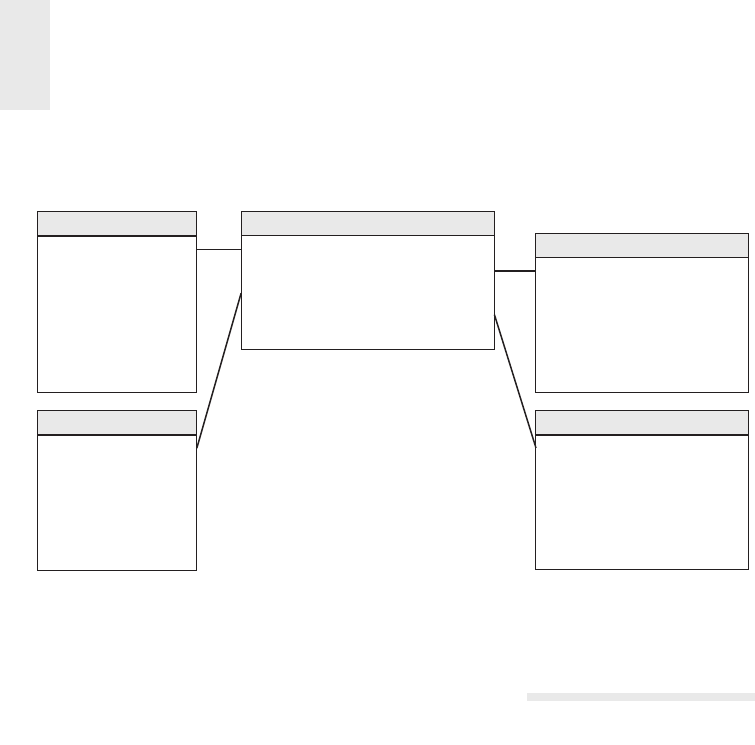
Chapter 3
98
in an OLAP cube, it is often easier to answer the “what didn’t happen” question
because the cube typically contains explicit cells for nonbehavior.
Date Key (PK)
Date
Day of Week
Calendar Month
Calendar Quarter
Calendar Year
...
Store Key (PK)
Store Number (NK)
Store Name
Store District
Store Region
...
Date Key (FK)
Product Key (FK)
Store Key (FK)
Promotion Key (FK)
Promotion Count (=1)
Product Key (PK)
SKU Number (NK)
Product Description
Brand Description
Category Description
...
Promotion Key (PK)
Promotion Code (NK)
Promotion Name
Promotion Media Type
Promotion Begin Date
...
Date Dimension
Store Dimension
Promotion Coverage Facts
Product Dimension
Promotion Dimension
Figure 3-14: Promotion coverage factless fact table.
Dimension and Fact Table Keys
Now that the schemas have been designed, we’ll focus on the dimension and fact
tables’ primary keys, along with other row identifi ers.
Dimension Table Surrogate Keys
The unique primary key of a dimension table should be a surrogate key rather than
relying on the operational system identifi er, known as the natural key. Surrogate keys
go by many other aliases: meaningless keys, integer keys, non-natural keys, artifi -
cial keys, and synthetic keys. Surrogate keys are simply integers that are assigned
sequentially as needed to populate a dimension. The fi rst product row is assigned a
product surrogate key with the value of 1; the next product row is assigned product
key 2; and so forth. The actual surrogate key value has no business signifi cance. The
surrogate keys merely serve to join the dimension tables to the fact table. Throughout
this book, column names with a Key su x, identifi ed as a primary key (PK) or
foreign key (FK), imply a surrogate.
Modelers sometimes are reluctant to relinquish the natural keys because they
want to navigate the fact table based on the operational code while avoiding a join
to the dimension table. They also don’t want to lose the embedded intelligence
that’s often part of a natural multipart key. However, you should avoid relying on

Retail Sales 99
intelligent dimension keys because any assumptions you make eventually may be
invalidated. Likewise, queries and data access applications should not have any
built-in dependency on the keys because the logic also would be vulnerable to
invalidation. Even if the natural keys appear to be stable and devoid of meaning,
don’t be tempted to use them as the dimension table’s primary key.
NOTE Every join between dimension and fact tables in the data warehouse
should be based on meaningless integer surrogate keys. You should avoid using a
natural key as the dimension table’s primary key.
Initially, it may be faster to implement a dimensional model using operational
natural keys, but surrogate keys pay o in the long run. We sometimes think of
them as being similar to a fl u shot for the data warehouse—like an immunization,
there’s a small amount of pain to initiate and administer surrogate keys, but the long
run benefi ts are substantial, especially considering the reduced risk of substantial
rework. Here are several advantages:
■ Bu er the data warehouse from operational changes. Surrogate keys enable
the warehouse team to maintain control of the DW/BI environment rather
than being whipsawed by operational rules for generating, updating, deleting,
recycling, and reusing production codes. In many organizations, historical
operational codes, such as inactive account numbers or obsolete product
codes, get reassigned after a period of dormancy. If account numbers get
recycled following 12 months of inactivity, the operational systems don’t miss
a beat because their business rules prohibit data from hanging around for that
long. But the DW/BI system may retain data for years. Surrogate keys provide
the warehouse with a mechanism to di erentiate these two separate instances
of the same operational account number. If you rely solely on operational
codes, you might also be vulnerable to key overlaps in the case of an acquisi-
tion or consolidation of data.
■ Integrate multiple source systems. Surrogate keys enable the data warehouse
team to integrate data from multiple operational source systems, even if they
lack consistent source keys by using a back room cross-reference mapping
table to link the multiple natural keys to a common surrogate.
■ Improve performance. The surrogate key is as small an integer as possible
while ensuring it will comfortably accommodate the future anticipated car-
dinality (number of rows in the dimension). Often the operational code is a
bulky alphanumeric character string or even a group of fi elds. The smaller
surrogate key translates into smaller fact tables, smaller fact table indexes,
and more fact table rows per block input-output operation. Typically, a 4-byte

Chapter 3
100
integer is su cient to handle most dimensions. A 4-byte integer is a single
integer, not four decimal digits. It has 32 bits and therefore can handle approx-
imately 2 billion positive values (232) or 4 billion total positive and negative
values (–232 to +232). This is more than enough for just about any dimension.
Remember, if you have a large fact table with 1 billion rows of data, every byte
in each fact table row translates into another gigabyte of storage.
■ Handle null or unknown conditions. As mentioned earlier, special surrogate
key values are used to record dimension conditions that may not have an
operational code, such as the No Promotion condition or the anonymous
customer. You can assign a surrogate key to identify these despite the lack of
operational coding. Similarly, fact tables sometimes have dates that are yet
to be determined. There is no SQL date type value for Date to Be Determined
or Date Not Applicable.
■ Support dimension attribute change tracking. One of the primary techniques
for handling changes to dimension attributes relies on surrogate keys to handle
the multiple profi les for a single natural key. This is actually one of the most
important reasons to use surrogate keys, which we’ll describe in Chapter 5.
A pseudo surrogate key created by simply gluing together the natural key
with a time stamp is perilous. You need to avoid multiple joins between the
dimension and fact tables, sometimes referred to as double-barreled joins, due
to their adverse impact on performance and ease of use.
Of course, some e ort is required to assign and administer surrogate keys, but
it’s not nearly as intimidating as many people imagine. You need to establish and
maintain a cross-reference table in the ETL system that will be used to substitute the
appropriate surrogate key on each fact and dimension table row. We lay out a process
for administering surrogate keys in Chapter 19: ETL Subsystems and Techniques.
Dimension Natural and Durable Supernatural Keys
Like surrogate keys, the natural keys assigned and used by operational source sys-
tems go by other names, such as business keys, production keys, and operational
keys. They are identifi ed with the NK notation in the book’s fi gures. The natural
key is often modeled as an attribute in the dimension table. If the natural key comes
from multiple sources, you might use a character data type that prepends a source
code, such as SAP|43251 or CRM|6539152. If the same entity is represented in both
operational source systems, then you’d likely have two natural key attributes in
the dimension corresponding to both sources. Operational natural keys are often
composed of meaningful constituent parts, such as the product’s line of business
or country of origin; these components should be split apart and made available as
separate attributes.

Retail Sales 101
In a dimension table with attribute change tracking, it’s important to have an iden-
tifi er that uniquely and reliably identifi es the dimension entity across its attribute
changes. Although the operational natural key may seem to fi t this bill, sometimes
the natural key changes due to unexpected business rules (like an organizational
merger) or to handle either duplicate entries or data integration from multiple
sources. If the dimension’s natural keys are not absolutely protected and preserved
over time, the ETL system needs to assign permanent durable identifi ers, also known
as supernatural keys. A persistent durable supernatural key is controlled by the DW/
BI system and remains immutable for the life of the system. Like the dimension
surrogate key, it’s a simple integer sequentially assigned. And like the natural keys
discussed earlier, the durable supernatural key is handled as a dimension attribute;
it’s not a replacement for the dimension table’s surrogate primary key. Chapter 19
also discusses the ETL system’s responsibility for these durable identifi ers.
Degenerate Dimension Surrogate Keys
Although surrogate keys aren’t typically assigned to degenerate dimensions, each
situation needs to be evaluated to determine if one is required. A surrogate key is
necessary if the transaction control numbers are not unique across locations or get
reused. For example, the retailer’s POS system may not assign unique transaction
numbers across stores. The system may wrap back to zero and reuse previous con-
trol numbers when its maximum has been reached. Also, the transaction control
number may be a bulky 24-byte alphanumeric column. Finally, depending on the
capabilities of the BI tool, you may need to assign a surrogate key (and create an
associated dimension table) to drill across on the transaction number. Obviously,
control number dimensions modeled in this way with corresponding dimension
tables are no longer degenerate.
Date Dimension Smart Keys
As we’ve noted, the date dimension has unique characteristics and requirements.
Calendar dates are fi xed and predetermined; you never need to worry about deleting
dates or handling new, unexpected dates on the calendar. Because of its predict-
ability, you can use a more intelligent key for the date dimension.
If a sequential integer serves as the primary key of the date dimension, it should
be chronologically assigned. In other words, January 1 of the fi rst year would
be assigned surrogate key value 1, January 2 would be assigned surrogate key 2,
February 1 would be assigned surrogate key 32, a nd so on.
More commonly, the primary key of the date dimension is a meaningful integer
formatted as yyyymmdd. The yyyymmdd key is not intended to provide business
users and their BI applications with an intelligent key so they can bypass the date
dimension and directly query the fact table. Filtering on the fact table’s yyyymmdd

Chapter 3
102
key would have a detrimental impact on usability and performance. Filtering and
grouping on calendar attributes should occur in a dimension table, not in the BI
application’s code.
However, the yyyymmdd key is useful for partitioning fact tables. Partitioning
enables a table to be segmented into smaller tables under the covers. Partitioning
a large fact table on the basis of date is e ective because it allows old data to be
removed gracefully and new data to be loaded and indexed in the current parti-
tion without disturbing the rest of the fact table. It reduces the time required for
loads, backups, archiving, and query response. Programmatically updating and
maintaining partitions is straightforward if the date key is an ordered integer: year
increments by 1 up to the number of years wanted, month increments by 1 up to
12, and so on. Using a smart yyyymmdd key provides the benefi ts of a surrogate,
plus the advantages of easier partition management.
Although the yyyymmdd integer is the most common approach for date dimen-
sion keys, some relational database optimizers prefer a true date type column for
partitioning. In these cases, the optimizer knows there are 31 values between
March 1 and April 1, as opposed to the apparent 100 values between 20130301 and
20130401. Likewise, it understands there are 31 values between December 1 and
January 1, as opposed to the 8,900 integer values between 20121201 and 20130101.
This intelligence can impact the query strategy chosen by the optimizer and further
reduce query times. If the optimizer incorporates date type intelligence, it should
be considered for the date key. If the only rationale for a date type key is simplifi ed
administration for the DBA, then you can feel less compelled.
With more intelligent date keys, whether chronologically assigned or a more
meaningful yyyymmdd integer or date type column, you need to reserve a special
date key value for the situation in which the date is unknown when the fact row is
initially loaded.
Fact Table Surrogate Keys
Although we’re adamant about using surrogate keys for dimension tables, we’re less
demanding about a surrogate key for fact tables. Fact table surrogate keys typically
only make sense for back room ETL processing. As we mentioned, the primary
key of a fact table typically consists of a subset of the table’s foreign keys and/or
degenerate dimension. However, single column surrogate keys for fact tables have
some interesting back room benefi ts.
Like its dimensional counterpart, a fact table surrogate key is a simple integer,
devoid of any business content, that is assigned in sequence as fact table rows are
generated. Although the fact table surrogate key is unlikely to deliver query perfor-
mance advantages, it does have the following benefi ts:

Retail Sales 103
■ Immediate unique identifi cation. A single fact table row is immediately iden-
tifi ed by the key. During ETL processing, a specifi c row can be identifi ed
without navigating multiple dimensions.
■ Backing out or resuming a bulk load. If a large number of rows are being
loaded with sequentially assigned surrogate keys, and the process halts before
completion, the DBA can determine exactly where the process stopped by
fi nding the maximum key in the table. The DBA could back out the complete
load by specifying the range of keys just loaded or perhaps could resume the
load from exactly the correct point.
■ Replacing updates with inserts plus deletes. The fact table surrogate key
becomes the true physical key of the fact table. No longer is the key of the
fact table determined by a set of dimensional foreign keys, at least as far as
the RDBMS is concerned. Thus it becomes possible to replace a fact table
update operation with an insert followed by a delete. The fi rst step is to
place the new row into the database with all the same business foreign keys
as the row it is to replace. This is now possible because the key enforce-
ment depends only on the surrogate key, and the replacement row has a
new surrogate key. Then the second step deletes the original row, thereby
accomplishing the update. For a large set of updates, this sequence is more
e cient than a set of true update operations. The insertions can be pro-
cessed with the ability to back out or resume the insertions as described in
the previous bullet. These insertions do not need to be protected with full
transaction machinery. Then the fi nal deletion step can be performed safely
because the insertions have run to completion.
■ Using the fact table surrogate key as a parent in a parent/child schema. In
those cases in which one fact table contains rows that are parents of those in
a lower grain fact table, the fact table surrogate key in the parent table is also
exposed in the child table. The argument of using the fact table surrogate
key in this case rather than a natural parent key is similar to the argument
for using surrogate keys in dimension tables. Natural keys are messy and
unpredictable, whereas surrogate keys are clean integers and are assigned by
the ETL system, not the source system. Of course, in addition to including
the parent fact table’s surrogate key, the lower grained fact table should also
include the parent’s dimension foreign keys so the child facts can be sliced
and diced without traversing the parent fact table’s surrogate key. And as we’ll
discuss in Chapter 4: Inventory, you should never join fact tables directly to
other fact tables.

Chapter 3
104
Resisting Normalization Urges
In this section, let’s directly confront several of the natural urges that tempt model-
ers coming from a more normalized background. We’ve been consciously breaking
some traditional modeling rules because we’re focused on delivering value through
ease of use and performance, not on transaction processing e ciencies.
Snowfl ake Schemas with Normalized Dimensions
The fl attened, denormalized dimension tables with repeating textual values make
data modelers from the operational world uncomfortable. Let’s revisit the case study
product dimension table. The 300,000 products roll up into 50 distinct depart-
ments. Rather than redundantly storing the 20-byte department description in the
product dimension table, modelers with a normalized upbringing want to store a
2-byte department code and then create a new department dimension for the depart-
ment decodes. In fact, they would feel more comfortable if all the descriptors in the
original design were normalized into separate dimension tables. They argue this
design saves space because the 300,000-row dimension table only contains codes,
not lengthy descriptors.
In addition, some modelers contend that more normalized dimension tables are
easier to maintain. If a department description changes, they’d need to update only
the one occurrence in the department dimension rather than the 6,000 repetitions
in the original product dimension. Maintenance often is addressed by normaliza-
tion disciplines, but all this happens back in the ETL system long before the data
is loaded into a presentation area’s dimensional schema.
Dimension table normalization is referred to as snowfl aking. Redundant attributes
are removed from the fl at, denormalized dimension table and placed in separate
normalized dimension tables. Figure 3-15 illustrates the partial snowfl aking of the
product dimension into third normal form. The contrast between Figure 3-15 and
Figure 3-8 is startling. The plethora of snowfl aked tables (even in our simplistic
example) is overwhelming. Imagine the impact on Figure 3-12 if all the schema’s
hierarchies were normalized.
Snowfl aking is a legal extension of the dimensional model, however, we encour-
age you to resist the urge to snowfl ake given the two primary design drivers: ease
of use and performance.

Retail Sales 105
Product Key (PK)
SKU Number (Natural Key)
Product Description
Brand Key (FK)
Package Type Key (FK)
Fat Content
Weight
Weight Unit of Measure
Storage Type Key (FK)
Shelf Width
Shelf Height
Shelf Depth
...
Brand Key (PK)
Brand Description
Category Key (FK)
Category Key (PK)
Category Description
Department Key (FK)
Department Key (PK)
Department Number
Department Description
Shelf Life Type Key (PK)
Shelf Life Type Description
Package Type Key (PK)
Package Type Description
Storage Type Key (PK)
Storage Type Description
Shelf Life Type Key (FK)
Product Dimension
Brand Dimension Category Dimension
Shelf Life Type Dimension
Department Dimension
Package Type Dimension
Storage Type Dimension
Figure 3-15: Snowfl aked product dimension.
■ The multitude of snowfl aked tables makes for a much more complex presen-
tation. Business users inevitably will struggle with the complexity; simplicity
is one of the primary objectives of a dimensional model.
■ Most database optimizers also struggle with the snowfl aked schema’s complex-
ity. Numerous tables and joins usually translate into slower query performance.
The complexities of the resulting join specifi cations increase the chances that
the optimizer will get sidetracked and choose a poor strategy.
■ The minor disk space savings associated with snowfl aked dimension tables
are insignifi cant. If you replace the 20-byte department description in the
300,000 row product dimension table with a 2-byte code, you’d save a whop-
ping 5.4 MB (300,000 x 18 bytes); meanwhile, you may have a 10 GB fact
table! Dimension tables are almost always geometrically smaller than fact
tables. E orts to normalize dimension tables to save disk space are usually
a waste of time.
■ Snowfl aking negatively impacts the users’ ability to browse within a dimen-
sion. Browsing often involves constraining one or more dimension attributes
and looking at the distinct values of another attribute in the presence of these
constraints. Browsing allows users to understand the relationship between
dimension attribute values.

Chapter 3
106
■ Obviously, a snowfl aked product dimension table responds well if you just
want a list of the category descriptions. However, if you want to see all the
brands within a category, you need to traverse the brand and category dimen-
sions. If you want to also list the package types for each brand in a category,
you’d be traversing even more tables. The SQL needed to perform these seem-
ingly simple queries is complex, and you haven’t touched the other dimensions
or fact table.
■ Finally, snowfl aking defeats the use of bitmap indexes. Bitmap indexes are
useful when indexing low-cardinality columns, such as the category and
department attributes in the product dimension table. They greatly speed
the performance of a query or constraint on the single column in question.
Snowfl aking inevitably would interfere with your ability to leverage this per-
formance tuning technique.
NOTE Fixed depth hierarchies should be flattened in dimension tables.
Normalized, snowfl aked dimension tables penalize cross-attribute browsing and
prohibit the use of bitmapped indexes. Disk space savings gained by normalizing
the dimension tables typically are less than 1 percent of the total disk space needed
for the overall schema. You should knowingly sacrifi ce this dimension table space
in the spirit of performance and ease of use advantages.
Some database vendors argue their platform has the horsepower to query a fully
normalized dimensional model without performance penalties. If you can achieve
satisfactory performance without physically denormalizing the dimension tables,
that’s fi ne. However, you’ll still want to implement a logical dimensional model with
denormalized dimensions to present an easily understood schema to the business
users and their BI applications.
In the past, some BI tools indicated a preference for snowfl ake schemas; snowfl ak-
ing to address the idiosyncratic requirements of a BI tool is acceptable. Likewise, if
all the data is delivered to business users via an OLAP cube (where the snowfl aked
dimensions are used to populate the cube but are never visible to the users), then
snowfl aking is acceptable. However, in these situations, you need to consider the
impact on users of alternative BI tools and the fl exibility to migrate to alternatives
in the future.
Outriggers
Although we generally do not recommend snowfl aking, there are situations in which
it is permissible to build an outrigger dimension that attaches to a dimension within

Retail Sales 107
the fact table’s immediate halo, as illustrated in Figure 3-16. In this example, the
“once removed” outrigger is a date dimension snowfl aked o a primary dimension.
The outrigger date attributes are descriptively and uniquely labeled to distinguish
them from the other dates associated with the business process. It only makes
sense to outrigger a primary dimension table’s date attribute if the business wants
to fi lter and group this date by nonstandard calendar attributes, such as the fi scal
period, business day indicator, or holiday period. Otherwise, you could just treat
the date attribute as a standard date type column in the product dimension. If a date
outrigger is used, be careful that the outrigger dates fall within the range stored in
the standard date dimension table.
Product Key (PK)
SKU Number (NK)
Product Description
Brand Description
Subcategory Description
Category Description
Department Number
Department Description
Package Type Description
Package Size
Product Introduction Date Key (FK)
...
Product Dimension
Product Introduction Date Key (PK)
Product Introduction Date
Product Introduction Calendar Month
Product Introduction Calendar Year
Product Introduction Fiscal Month
Product Introduction Fiscal Quarter
Product Introduction Fiscal Year
Product Introduction Holiday Period Indicator
...
Product Introduction Date Dimension
Figure 3-16: Example of a permissible outrigger.
You’ll encounter more outrigger examples later in the book, such as the han-
dling of customers’ county-level demographic attributes in Chapter 8: Customer
Relationship Management.
Although outriggers may save space and ensure the same attributes are referenced
consistently, there are downsides. Outriggers introduce more joins, which can nega-
tively impact performance. More important, outriggers can negatively impact the
legibility for business users and hamper their ability to browse among attributes
within a single dimension.
WAR NI NG Though outriggers are permissible, a dimensional model should
not be littered with outriggers given the potentially negative impact. Outriggers
should be the exception rather than the rule.

Chapter 3
108
Centipede Fact Tables with Too Many Dimensions
The fact table in a dimensional schema is naturally highly normalized and compact.
There is no way to further normalize the extremely complex many-to-many relation-
ships among the keys in the fact table because the dimensions are not correlated
with each other. Every store is open every day. Sooner or later, almost every product
is sold on promotion in most or all of our stores.
Interestingly, while uncomfortable with denormalized dimension tables, some
modelers are tempted to denormalize the fact table. They have an uncontrollable
urge to normalize dimension hierarchies but know snowfl aking is highly discour-
aged, so the normalized tables end up joined to the fact table instead. Rather than
having a single product foreign key on the fact table, they include foreign keys for
the frequently analyzed elements on the product hierarchy, such as brand, category,
and department. Likewise, the date key suddenly turns into a series of keys joining
to separate week, month, quarter, and year dimension tables. Before you know it,
your compact fact table has turned into an unruly monster that joins to literally
dozens of dimension tables. We a ectionately refer to these designs as centipede
fact tables because they appear to have nearly 100 legs, as shown in Figure 3-17.
POS Retail Sales Transaction Fact
Date Key (FK)
Week Key (FK)
Month Key (FK)
Quarter Key (FK)
Year Key (FK)
Fiscal Year Key (FK)
Fiscal Month Key (FK)
Product Key (FK)
Brand Key (FK)
Category Key (FK)
Department Key (FK)
Package Type Key (FK)
Store Key (FK)
Store County Key (FK)
Store State Key (FK)
Store District Key (FK)
Store Region Key (FK)
Store Floor Plan Key (FK)
Promotion Key (FK)
Promotion Reduction Type Key (FK)
Promotion Media Type Key (FK)
POS Transaction Number (DD)
Sales Quantity
Extended Discount Dollar Amount
Extended Sales Dollar Amount
Extended Cost Dollar Amount
Date Dimension
Brand Dimension
Category Dimension
Department Dimension
Package Type Dimension
Promotion Dimension
Promotion Reduction Type Dimension
Promotion Media Type Dimension
Week Dimension
Month Dimension
Quarter Dimension
Year Dimension
Fiscal Year Dimension
Fiscal Month Dimension
Store Dimension
Store County Dimension
Store State Dimension
Store District Dimension
Store Region Dimension
Store Floor Plan Dimension
Product Dimension
Figure 3-17: Centipede fact table with too many normalized dimensions.

Retail Sales 109
Even with its tight format, the fact table is the behemoth in a dimensional model.
Designing a fact table with too many dimensions leads to signifi cantly increased fact
table disk space requirements. Although denormalized dimension tables consume
extra space, fact table space consumption is a concern because it is your largest
table by orders of magnitude. There is no way to index the enormous multipart
key e ectively in the centipede example. The numerous joins are an issue for both
usability and query performance.
Most business processes can be represented with less than 20 dimensions in the
fact table. If a design has 25 or more dimensions, you should look for ways to com-
bine correlated dimensions into a single dimension. Perfectly correlated attributes,
such as the levels of a hierarchy, as well as attributes with a reasonable statistical
correlation, should be part of the same dimension. It’s a good decision to combine
dimensions when the resulting new single dimension is noticeably smaller than the
Cartesian product of the separate dimensions.
NOTE A very large number of dimensions typically are a sign that several
dimensions are not completely independent and should be combined into a
single dimension. It is a dimensional modeling mistake to represent elements of
a single hierarchy as separate dimensions in the fact table.
Developments with columnar databases may reduce the query and storage penal-
ties associated with wide centipede fact table designs. Rather than storing each table
row, a columnar database stores each table column as a contiguous object that is
heavily indexed for access. Even though the underlying physical storage is colum-
nar, at the query level, the table appears to be made up of familiar rows. But when
queried, only the named columns are actually retrieved from the disk, rather than
the entire row in a more conventional row-oriented relational database. Columnar
databases are much more tolerant of the centipede fact tables just described; how-
ever, the ability to browse across hierarchically related dimension attributes may
be compromised.
Summary
This chapter was your fi rst exposure to designing a dimensional model. Regardless
of the industry, we strongly encourage the four-step process for tackling dimensional
model designs. Remember it is especially important to clearly state the grain associ-
ated with a dimensional schema. Loading the fact table with atomic data provides
the greatest fl exibility because the data can be summarized “every which way.” As

Chapter 3
110
soon as the fact table is restricted to more aggregated information, you run into
walls when the summarization assumptions prove to be invalid. Also it is vitally
important to populate your dimension tables with verbose, robust descriptive attri-
butes for analytic fi ltering and labeling.
In the next chapter we’ll remain within the retail industry to discuss techniques
for tackling a second business process within the organization, ensuring your earlier
e orts are leveraged while avoiding stovepipes.

Inventory
In Chapter 3: Retail Sales, we developed a dimensional model for the sales transac-
tions in a large grocery chain. We remain within the same industry in this chapter
but move up the value chain to tackle the inventory process. The designs developed
in this chapter apply to a broad set of inventory pipelines both inside and outside
the retail industry.
More important, this chapter provides a thorough discussion of the enterprise
data warehouse bus architecture. The bus architecture is essential to creating an
integrated DW/BI system. It provides a framework for planning the overall environ-
ment, even though it will be built incrementally. We will underscore the importance
of using common conformed dimensions and facts across dimensional models, and
will close by encouraging the adoption of an enterprise data governance program.
Chapter 4 discusses the following concepts:
■ Representing organizational value chains via a series of dimensional models
■ Semi-additive facts
■ Three fact table types: periodic snapshots, transaction, and accumulating
snapshots
■ Enterprise data warehouse bus architecture and bus matrix
■ Opportunity/stakeholder matrix
■ Conformed dimensions and facts, and their impact on agile methods
■ Importance of data governance
Value Chain Introduction
Most organizations have an underlying value chain of key business processes. The
value chain identifi es the natural, logical fl ow of an organization’s primary activi-
ties. For example, a retailer issues purchase orders to product manufacturers. The
products are delivered to the retailer’s warehouse, where they are held in inven-
tory. A delivery is then made to an individual store, where again the products sit in
4

Chapter 4
112
inventory until a consumer makes a purchase. Figure 4-1 illustrates this subset of a
retailer’s value chain. Obviously, products sourced from manufacturers that deliver
directly to the retail store would bypass the warehousing processes.
Issue Purchase
Order to
Manufacturer
Receive
Warehouse
Deliveries
Warehouse
Product
Inventory
Receive
Store
Deliveries
Store
Product
Inventory
Retail
Sales
Figure 4-1: Subset of a retailer’s value chain.
Operational source systems typically produce transactions or snapshots at each
step of the value chain. The primary objective of most analytic DW/BI systems is
to monitor the performance results of these key processes. Because each process
produces unique metrics at unique time intervals with unique granularity and
dimensionality, each process typically spawns one or more fact tables. To this end,
the value chain provides high-level insight into the overall data architecture for an
enterprise DW/BI environment. We’ll devote more time to this topic in the “Value
Chain Integration” section later in this chapter.
Inventory Models
In the meantime, we’ll discuss several complementary inventory models. The fi rst
is the inventory periodic snapshot where product inventory levels are measured at
regular intervals and placed as separate rows in a fact table. These periodic snapshot
rows appear over time as a series of data layers in the dimensional model, much like
geologic layers represent the accumulation of sediment over long periods of time.
We’ll then discuss a second inventory model where every transaction that impacts

Inventory 113
inventory levels as products move through the warehouse is recorded. Finally, in the
third model, we’ll describe the inventory accumulating snapshot where a fact table
row is inserted for each product delivery and then the row is updated as the product
moves through the warehouse. Each model tells a di erent story. For some analytic
requirements, two or even all three models may be appropriate simultaneously.
Inventory Periodic Snapshot
Let’s return to our retail case study. Optimized inventory levels in the stores can have
a major impact on chain profi tability. Making sure the right product is in the right
store at the right time minimizes out-of-stocks (where the product isn’t available
on the shelf to be sold) and reduces overall inventory carrying costs. The retailer
wants to analyze daily quantity-on-hand inventory levels by product and store.
It is time to put the four-step dimensional design process to work again. The
business process we’re interested in analyzing is the periodic snapshotting of retail
store inventory. The most atomic level of detail provided by the operational inven-
tory system is a daily inventory for each product in each store. The dimensions
immediately fall out of this grain declaration: date, product, and store. This often
happens with periodic snapshot fact tables where you cannot express the granular-
ity in the context of a transaction, so a list of dimensions is needed instead. In this
case study, there are no additional descriptive dimensions at this granularity. For
example, promotion dimensions are typically associated with product movement,
such as when the product is ordered, received, or sold, but not with inventory.
The simplest view of inventory involves only a single fact: quantity on hand.
This leads to an exceptionally clean dimensional design, as shown in Figure 4-2.
Date Dimension Store Inventory Snapshot Fact
Date Key (PK)
...
Date Key (FK)
Product Key (FK)
Store Key (FK)
Quantity on Hand
Product Key (PK)
Storage Requirement Type
...
Store Key (PK)
...
Product Dimension
Store Dimension
Figure 4-2: Store inventory periodic snapshot schema.
The date dimension table in this case study is identical to the table developed
in Chapter 3 for retail store sales. The product and store dimensions may be deco-
rated with additional attributes that would be useful for inventory analysis. For
example, the product dimension could be enhanced with columns such as the
minimum reorder quantity or the storage requirement, assuming they are constant
and discrete descriptors of each product. If the minimum reorder quantity varies for

Chapter 4
114
a product by store, it couldn’t be included as a product dimension attribute. In the
store dimension, you might include attributes to identify the frozen and refrigerated
storage square footages.
Even a schema as simple as Figure 4-2 can be very useful. Numerous insights can
be derived if inventory levels are measured frequently for many products in many
locations. However, this periodic snapshot fact table faces a serious challenge that
Chapter 3’s sales transaction fact table did not. The sales fact table was reasonably
sparse because you don’t sell every product in every shopping cart. Inventory, on
the other hand, generates dense snapshot tables. Because the retailer strives to
avoid out-of-stock situations in which the product is not available, there may be
a row in the fact table for every product in every store every day. In that case you
would include the zero out-of-stock measurements as explicit rows. For the grocery
retailer with 60,000 products stocked in 100 stores, approximately 6 million rows
(60,000 products x 100 stores) would be inserted with each nightly fact table load.
However, because the row width is just 14 bytes, the fact table would grow by only
84 MB with each load.
Although the data volumes in this case are manageable, the denseness of some
periodic snapshots may mandate compromises. Perhaps the most obvious is to
reduce the snapshot frequencies over time. It may be acceptable to keep the last 60
days of inventory at the daily level and then revert to less granular weekly snap-
shots for historical data. In this way, instead of retaining 1,095 snapshots during
a 3-year period, the number could be reduced to 208 total snapshots; the 60 daily
and 148 weekly snapshots should be stored in two separate fact tables given their
unique periodicity.
Semi-Additive Facts
We stressed the importance of fact additivity in Chapter 3. In the inventory snap-
shot schema, the quantity on hand can be summarized across products or stores
and result in a valid total. Inventory levels, however, are not additive across dates
because they represent snapshots of a level or balance at one point in time. Because
inventory levels (and all forms of fi nancial account balances) are additive across
some dimensions but not all, we refer to them as semi-additive facts.
The semi-additive nature of inventory balance facts is even more understand-
able if you think about your checking account balances. On Monday, presume
that you have $50 in your account. On Tuesday, the balance remains unchanged.
On Wednesday, you deposit another $50 so the balance is now $100. The account
has no further activity through the end of the week. On Friday, you can’t merely
add up the daily balances during the week and declare that the ending balance is
$400 (based on $50 + $50 + $100 + $100 + $100). The most useful way to combine

Inventory 115
account balances and inventory levels across dates is to average them (resulting in
an $80 average balance in the checking example). You are probably familiar with
your bank referring to the average daily balance on a monthly account summary.
NOTE All measures that record a static level (inventory levels, fi nancial account
balances, and measures of intensity such as room temperatures) are inherently
non-additive across the date dimension and possibly other dimensions. In these
cases, the measure may be aggregated across dates by averaging over the number
of time periods.
Unfortunately, you cannot use the SQL AVG function to calculate the average
over time. This function averages over all the rows received by the query, not just
the number of dates. For example, if a query requested the average inventory for
a cluster of three products in four stores across seven dates (e.g., the average daily
inventory of a brand in a geographic region during a week), the SQL AVG function
would divide the summed inventory value by 84 (3 products × 4 stores × 7 dates).
Obviously, the correct answer is to divide the summed inventory value by 7, which
is the number of daily time periods.
OLAP products provide the capability to defi ne aggregation rules within the
cube, so semi-additive measures like balances are less problematic if the data is
deployed via OLAP cubes.
Enhanced Inventory Facts
The simplistic view in the periodic inventory snapshot fact table enables you to see
a time series of inventory levels. For most inventory analysis, quantity on hand isn’t
enough. Quantity on hand needs to be used in conjunction with additional facts to
measure the velocity of inventory movement and develop other interesting metrics
such as the number of turns and number of days’ supply.
If quantity sold (or equivalently, quantity shipped for a warehouse location) was
added to each fact row, you could calculate the number of turns and days’ supply.
For daily inventory snapshots, the number of turns measured each day is calculated
as the quantity sold divided by the quantity on hand. For an extended time span,
such as a year, the number of turns is the total quantity sold divided by the daily
average quantity on hand. The number of days’ supply is a similar calculation. Over
a time span, the number of days’ supply is the fi nal quantity on hand divided by
the average quantity sold.
In addition to the quantity sold, inventory analysts are also interested in the
extended value of the inventory at cost, as well as the value at the latest selling price.
The initial periodic snapshot is embellished in Figure 4-3.

Chapter 4
116
Date Dimension Store Inventory Snapshot Fact
Date Key (PK)
...
Date Key (FK)
Product Key (FK)
Store Key (FK)
Quantity on Hand
Quantity Sold
Inventory Dollar Value at Cost
Inventory Dollar Value at Latest Selling Price
Product Key (PK)
...
Store Key (PK)
...
Product Dimension
Store Dimension
Figure 4-3: Enhanced inventory periodic snapshot.
Notice that quantity on hand is semi-additive, but the other measures in the
enhanced periodic snapshot are all fully additive. The quantity sold amount has been
rolled up to the snapshot’s daily granularity. The valuation columns are extended,
additive amounts. In some periodic snapshot inventory schemas, it is useful to
store the beginning balance, the inventory change or delta, along with the ending
balance. In this scenario, the balances are again semi-additive, whereas the deltas
are fully additive across all the dimensions.
The periodic snapshot is the most common inventory schema. We’ll briefl y dis-
cuss two alternative perspectives that complement the inventory snapshot just
designed. For a change of pace, rather than describing these models in the context
of the retail store inventory, we’ll move up the value chain to discuss the inventory
located in the warehouses.
Inventory Transactions
A second way to model an inventory business process is to record every transac-
tion that a ects inventory. Inventory transactions at the warehouse might include
the following:
■ Receive product.
■ Place product into inspection hold.
■ Release product from inspection hold.
■ Return product to vendor due to inspection failure.
■ Place product in bin.
■ Pick product from bin.
■ Package product for shipment.
■ Ship product to customer.
■ Receive product from customer.
■ Return product to inventory from customer return.
■ Remove product from inventory.
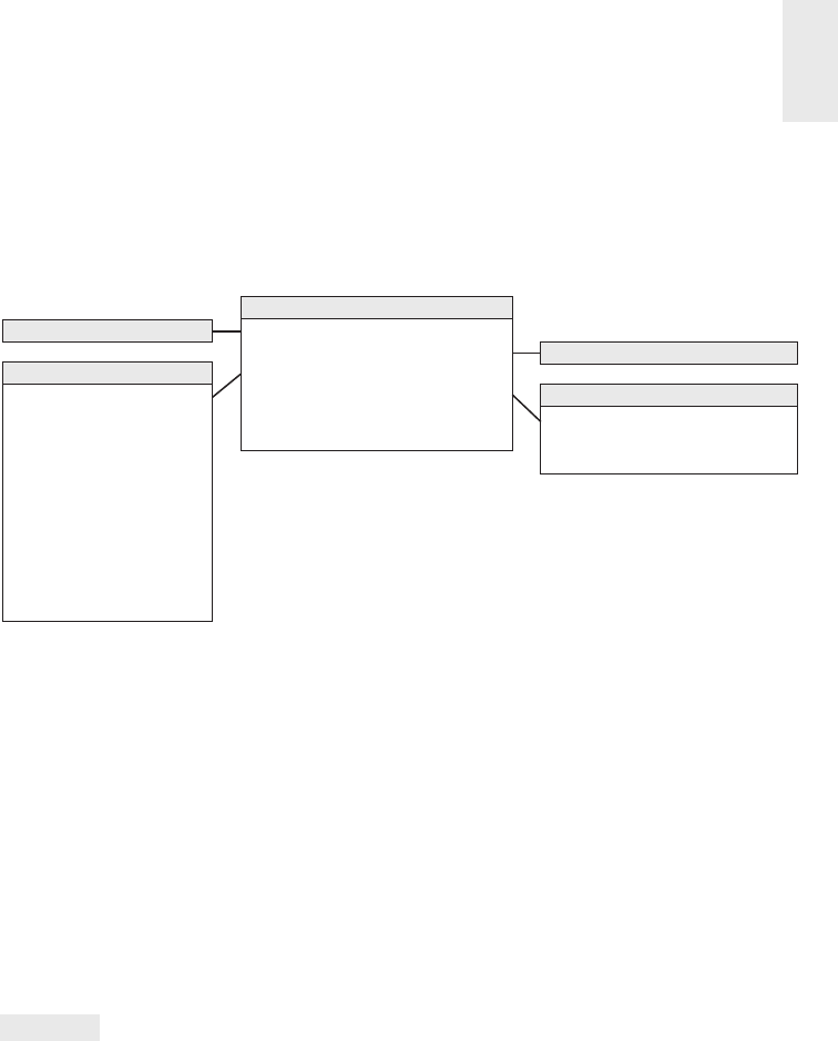
Inventory 117
Each inventory transaction identifi es the date, product, warehouse, vendor, trans-
action type, and in most cases, a single amount representing the inventory quantity
impact caused by the transaction. Assuming the granularity of the fact table is one
row per inventory transaction, the resulting schema is illustrated in Figure 4-4.
Date Dimension
Warehouse Inventory Transaction Fact
Date Key (FK)
Product Key (FK)
Warehouse Key (FK)
Inventory Transaction Type Key (FK)
Inventory Transaction Number (DD)
Inventory Transaction Dollar Amount
Inventory Transaction Type Key (PK)
Inventory Transaction Type Description
Inventory Transaction Type Group
Warehouse Key (PK)
Warehouse Number (NK)
Warehouse Name
Warehouse Address
Warehouse City
Warehouse City-State
Warehouse State
Warehouse ZIP
Warehouse Zone
Warehouse Total Square Footage
...
Product Dimension
Inventory Transaction Type Dimension
Warehouse Dimension
Figure 4-4: Warehouse inventory transaction model.
Even though the transaction fact table is simple, it contains detailed information
that mirrors individual inventory manipulations. The transaction fact table is use-
ful for measuring the frequency and timing of specifi c transaction types to answer
questions that couldn’t be answered by the less granular periodic snapshot.
Even so, it is impractical to use the transaction fact table as the sole basis for ana-
lyzing inventory performance. Although it is theoretically possible to reconstruct the
exact inventory position at any moment in time by rolling all possible transactions
forward from a known inventory position, it is too cumbersome and impractical
for broad analytic questions that span dates, products, warehouses, or vendors.
NOTE Remember there’s more to life than transactions alone. Some form of a
snapshot table to give a more cumulative view of a process often complements
a transaction fact table.
Before leaving the transaction fact table, our example presumes each type of
transaction impacting inventory levels positively or negatively has consistent dimen-
sionality: date, product, warehouse, vendor, and transaction type. We recognize
some transaction types may have varied dimensionality in the real world. For
example, a shipper may be associated with the warehouse receipts and shipments;
customer information is likely associated with shipments and customer returns. If the

Chapter 4
118
transactions’ dimensionality varies by event, then a series of related fact tables should
be designed rather than capturing all inventory transactions in a single fact table.
NOTE If performance measurements have different natural granularity or
dimensionality, they likely result from separate processes that should be modeled
as separate fact tables.
Inventory Accumulating Snapshot
The fi nal inventory model is the accumulating snapshot. Accumulating snapshot
fact tables are used for processes that have a defi nite beginning, defi nite end, and
identifi able milestones in between. In this inventory model, one row is placed in the
fact table when a particular product is received at the warehouse. The disposition
of the product is tracked on this single fact row until it leaves the warehouse. In
this example, the accumulating snapshot model is only possible if you can reliably
distinguish products received in one shipment from those received at a later time;
it is also appropriate if you track product movement by product serial number or
lot number.
Now assume that inventory levels for a product lot captured a series of well-
defi ned events or milestones as it moves through the warehouse, such as receiving,
inspection, bin placement, and shipping. As illustrated in Figure 4-5, the inventory
accumulating snapshot fact table with its multitude of dates and facts looks quite
di erent from the transaction or periodic snapshot schemas.
Inventory Receipt Accumulating Fact
Product Lot Receipt Number (DD)
Date Received Key (FK)
Date Inspected Key (FK)
Date Bin Placement Key (FK)
Date Initial Shipment Key (FK)
Date Last Shipment Key (FK)
Product Key (FK)
Warehouse Key (FK)
Vendor Key (FK)
Quantity Received
Quantity Inspected
Quantity Returned to Vendor
Quantity Placed in Bin
Quantity Shipped to Customer
Quantity Returned by Customer
Quantity Returned to Inventory
Quantity Damaged
Receipt to Inspected Lag
Receipt to Bin Placement Lag
Receipt to Initial Shipment Lag
Initial to Last Shipment Lag
Date Received Dimension
Product Dimension
Warehouse Dimension
Vendor Dimension
Date Inspected Dimension
Date Bin Placement Dimension
Date Initial Shipment Dimension
Date Last Shipment Dimension
Figure 4-5: Warehouse inventory accumulating snapshot.

Inventory 119
The accumulating snapshot fact table provides an updated status of the lot as it
moves through standard milestones represented by multiple date-valued foreign
keys. Each accumulating snapshot fact table row is updated repeatedly until the
products received in a lot are completely depleted from the warehouse, as shown
in Figure 4-6.
Date Inspected
Key
Receipt to
Inspected Lag
Receipt to Bin
Placement Lag
Date Bin
Placement Key
Product
Key
Quantity
Received
Lot Receipt
Number
Date Received
Key
101 20130101 0 0 1 100
Fact row inserted when lot received:
Date Inspected
Key
Receipt to
Inspected Lag
Receipt to Bin
Placement Lag
Date Bin
Placement Key
Product
Key
Quantity
Received
Lot Receipt
Number
Date Received
Key
101 20130101 20130103 0 1 100 2
Fact row updated when lot inspected:
Date Inspected
Key
Receipt to
Inspected Lag
Receipt to Bin
Placement Lag
Date Bin
Placement Key
Product
Key
Quantity
Received
Lot Receipt
Number
Date Received
Key
101 20130101 20130103 20130104 1 100 2 3
Fact row updated when lot placed in bin:
Figure 4-6: Evolution of an accumulating snapshot fact row.
Fact Table Types
There are just three fundamental types of fact tables: transaction, periodic snapshot,
and accumulating snapshot. Amazingly, this simple pattern holds true regardless
of the industry. All three types serve a useful purpose; you often need two comple-
mentary fact tables to get a complete picture of the business, yet the administration
and rhythm of the three fact tables are quite di erent. Figure 4-7 compares and
contrasts the variations.
Transaction
Discrete transaction point
in time
Recurring snapshots at
regular, predictable intervals
1 row per transaction or
transaction line
1 row per snapshot period
plus other dimensions
Snapshot date
Cumulative performance
for time interval
Predictably dense
Transaction date
Transaction performance
Sparse or dense, depending
on activity
No updates, unless error
correction
No updates, unless error
correction
Indeterminate time span for
evolving pipeline/workflow
1 row per pipeline
occurrence
Multiple dates for pipeline’s
key milestones
Performance for pipeline
occurrence
Sparse or dense, depending
on pipeline occurrence
Updated whenever pipeline
activity occurs
Periodicity
Grain
Date dimension(s)
Facts
Fact table sparsity
Fact table updates
Periodic Snapshot Accumulating Snapshot
Figure 4-7: Fact table type comparisons.

Chapter 4
120
Transaction Fact Tables
The most fundamental view of the business’s operations is at the individual transac-
tion or transaction line level. These fact tables represent an event that occurred at
an instantaneous point in time. A row exists in the fact table for a given customer
or product only if a transaction event occurred. Conversely, a given customer or
product likely is linked to multiple rows in the fact table because hopefully the
customer or product is involved in more than one transaction.
Transaction data fi ts easily into a dimensional framework. Atomic transaction
data is the most naturally dimensional data, enabling you to analyze behavior in
extreme detail. After a transaction has been posted in the fact table, you typically
don’t revisit it.
Having made a solid case for the charm of transaction detail, you may be think-
ing that all you need is a big, fast server to handle the gory transaction minutiae,
and your job is over. Unfortunately, even with transaction level data, there are busi-
ness questions that are impractical to answer using only these details. As indicated
earlier, you cannot survive on transactions alone.
Periodic Snapshot Fact Tables
Periodic snapshots are needed to see the cumulative performance of the business
at regular, predictable time intervals. Unlike the transaction fact table where a row
is loaded for each event occurrence, with the periodic snapshot, you take a picture
(hence the snapshot terminology) of the activity at the end of a day, week, or month,
then another picture at the end of the next period, and so on. The periodic snap-
shots are stacked consecutively into the fact table. The periodic snapshot fact table
often is the only place to easily retrieve a regular, predictable view of longitudinal
performance trends.
When transactions equate to little pieces of revenue, you can move easily from
individual transactions to a daily snapshot merely by adding up the transactions.
In this situation, the periodic snapshot represents an aggregation of the transac-
tional activity that occurred during a time period; you would build the snapshot
only if needed for performance reasons. The design of the snapshot table is closely
related to the design of its companion transaction table in this case. The fact tables
share many dimension tables; the snapshot usually has fewer dimensions overall.
Conversely, there are usually more facts in a summarized periodic snapshot table
than in a transactional table because any activity that happens during the period
is fair game for a metric in a periodic snapshot.
In many businesses, however, transaction details are not easily summarized to
present management performance metrics. As you saw in this inventory case study,

Inventory 121
crawling through the transactions would be extremely time-consuming, plus the
logic required to interpret the e ect of di erent kinds of transactions on inventory
levels could be horrendously complicated, presuming you even have access to the
required historical data. The periodic snapshot again comes to the rescue to provide
management with a quick, fl exible view of inventory levels. Hopefully, the data for
this snapshot schema is sourced directly from an operational system that handles
these complex calculations. If not, the ETL system must also implement this com-
plex logic to correctly interpret the impact of each transaction type.
Accumulating Snapshot Fact Tables
Last, but not least, the third type of fact table is the accumulating snapshot. Although
perhaps not as common as the other two fact table types, accumulating snapshots
can be very insightful. Accumulating snapshots represent processes that have a
defi nite beginning and defi nite end together with a standard set of intermediate
process steps. Accumulating snapshots are most appropriate when business users
want to perform workfl ow or pipeline analysis.
Accumulating snapshots always have multiple date foreign keys, representing the
predictable major events or process milestones; sometimes there’s an additional date
column that indicates when the snapshot row was last updated. As we’ll discuss in
Chapter 6: Order Management, these dates are each handled by a role-playing date
dimension. Because most of these dates are not known when the fact row is fi rst
loaded, a default surrogate date key is used for the undefi ned dates.
Lags Between Milestones and Milestone Counts
Because accumulating snapshots often represent the e ciency and elapsed time of
a workfl ow or pipeline, the fact table typically contains metrics representing the
durations or lags between key milestones. It would be di cult to answer duration
questions using a transaction fact table because you would need to correlate rows
to calculate time lapses. Sometimes the lag metrics are simply the raw di erence
between the milestone dates or date/time stamps. In other situations, the lag calcula-
tion is made more complicated by taking workdays and holidays into consideration.
Accumulating snapshot fact tables sometimes include milestone completion coun-
ters, valued as either 0 or 1. Finally, accumulating snapshots often have a foreign
key to a status dimension, which is updated to refl ect the pipeline’s latest status.
Accumulating Snapshot Updates and OLAP Cubes
In sharp contrast to the other fact table types, you purposely revisit accumulating
snapshot fact table rows to update them. Unlike the periodic snapshot where the
prior snapshots are preserved, the accumulating snapshot merely refl ects the most

Chapter 4
122
current status and metrics. Accumulating snapshots do not attempt to accommodate
complex scenarios that occur infrequently. The analysis of these outliers can always
be done with the transaction fact table.
It is worth noting that accumulating snapshots are typically problematic for
OLAP cubes. Because updates to an accumulating snapshot force both facts and
dimension foreign keys to change, much of the cube would need to be reprocessed
with updates to these snapshots, unless the fact row is only loaded once the pipeline
occurrence is complete.
Complementary Fact Table Types
Sometimes accumulating and periodic snapshots work in conjunction with one
another, such as when you incrementally build the monthly snapshot by adding the
e ect of each day’s transactions to a rolling accumulating snapshot while also storing
36 months of historical data in a periodic snapshot. Ideally, when the last day of the
month has been reached, the accumulating snapshot simply becomes the new regular
month in the time series, and a new accumulating snapshot is started the next day.
Transactions and snapshots are the yin and yang of dimensional designs. Used
together, companion transaction and snapshot fact tables provide a complete view
of the business. Both are needed because there is often no simple way to combine
these two contrasting perspectives in a single fact table. Although there is some
theoretical data redundancy between transaction and snapshot tables, you don’t
object to such redundancy because as DW/BI publishers, your mission is to publish
data so that the organization can e ectively analyze it. These separate types of fact
tables each provide di erent vantage points on the same story. Amazingly, these
three types of fact tables turn out to be all the fact table types needed for the use
cases described in this book.
Value Chain Integration
Now that we’ve completed the design of three inventory models, let’s revisit our ear-
lier discussion about the retailer’s value chain. Both business and IT organizations
are typically interested in value chain integration. Business management needs to
look across the business’s processes to better evaluate performance. For example,
numerous DW/BI projects have focused on better understanding customer behavior
from an end-to-end perspective. Obviously, this requires the ability to consistently
look at customer information across processes, such as quotes, orders, invoicing,
payments, and customer service. Similarly, organizations want to analyze their
products across processes, or their employees, students, vendors, and so on.

Inventory 123
IT managers recognize integration is needed to deliver on the promises of data
warehousing and business intelligence. Many consider it their fi duciary respon-
sibility to manage the organization’s information assets. They know they’re not
fulfi lling their responsibilities if they allow standalone, nonintegrated databases
to proliferate. In addition to addressing the business’s needs, IT also benefi ts from
integration because it allows the organization to better leverage scarce resources
and gain e ciencies through the use of reusable components.
Fortunately, the senior managers who typically are most interested in integration
also have the necessary organizational infl uence and economic willpower to make
it happen. If they don’t place a high value on integration, you face a much more
serious organizational challenge, or put more bluntly, your integration project will
probably fail. It shouldn’t be the sole responsibility of the DW/BI manager to garner
organizational consensus for integration across the value chain. The political sup-
port of senior management is important; it takes the DW/BI manager o the hook
and places the burden on senior leadership’s shoulders where it belongs.
In Chapters 3 and 4, we modeled data from several processes of the retailer’s value
chain. Although separate fact tables in separate dimensional schemas represent the
data from each process, the models share several common business dimensions:
date, product, and store. We’ve logically represented this dimension sharing in
Figure 4-8. Using shared, common dimensions is absolutely critical to designing
dimensional models that can be integrated.
Store Dimension
Date Dimension
Retail Sales
Transaction Facts
Retail Inventory
Snapshot Facts
Warehouse Inventory
Transaction Facts
Promotion Dimension
Product Dimension
Warehouse Dimension
Figure 4-8: Sharing dimensions among business processes.
Enterprise Data Warehouse Bus Architecture
Obviously, building the enterprise’s DW/BI system in one galactic e ort is too daunt-
ing, yet building it as isolated pieces defeats the overriding goal of consistency. For
long-term DW/BI success, you need to use an architected, incremental approach to
build the enterprise’s warehouse. The approach we advocate is the enterprise data
warehouse bus architecture.

Chapter 4
124
Understanding the Bus Architecture
Contrary to popular belief, the word bus is not shorthand for business; it’s an old
term from the electrical power industry that is now used in the computer industry.
A bus is a common structure to which everything connects and from which every-
thing derives power. The bus in a computer is a standard interface specifi cation
that enables you to plug in a disk drive, DVD, or any number of other specialized
cards or devices. Because of the computer’s bus standard, these peripheral devices
work together and usefully coexist, even though they were manufactured at di er-
ent times by di erent vendors.
NOTE By defi ning a standard bus interface for the DW/BI environment, separate
dimensional models can be implemented by di erent groups at di erent times.
The separate business process subject areas plug together and usefully coexist if
they adhere to the standard.
If you refer back to the value chain diagram in Figure 4-1, you can envision many
business processes plugging into the enterprise data warehouse bus, as illustrated
in Figure 4-9. Ultimately, all the processes of an organization’s value chain create
a family of dimensional models that share a comprehensive set of common, con-
formed dimensions.
Store Sales
Store Inventory
Purchase Orders
Date Product Store Promotion Warehouse Vendor Shipper
Figure 4-9: Enterprise data warehouse bus with shared dimensions.
The enterprise data warehouse bus architecture provides a rational approach to
decomposing the enterprise DW/BI planning task. The master suite of standard-
ized dimensions and facts has a uniform interpretation across the enterprise. This
establishes the data architecture framework. You can then tackle the implementation
of separate process-centric dimensional models, with each implementation closely

Inventory 125
adhering to the architecture. As the separate dimensional models become available,
they fi t together like the pieces of a puzzle. At some point, enough dimensional models
exist to make good on the promise of an integrated enterprise DW/BI environment.
The bus architecture enables DW/BI managers to get the best of both worlds.
They have an architectural framework guiding the overall design, but the problem
has been divided into bite-sized business process chunks that can be implemented
in realistic time frames. Separate development teams follow the architecture while
working fairly independently and asynchronously.
The bus architecture is independent of technology and database platforms. All
fl avors of relational and OLAP-based dimensional models can be full participants
in the enterprise data warehouse bus if they are designed around conformed dimen-
sions and facts. DW/BI systems inevitably consist of separate machines with di erent
operating systems and database management systems. Designed coherently, they
share a common architecture of conformed dimensions and facts, allowing them
to be fused into an integrated whole.
Enterprise Data Warehouse Bus Matrix
We recommend using an enterprise data warehouse bus matrix to document and com-
municate the bus architecture, as illustrated in Figure 4-10. Others have renamed the
bus matrix, such as the conformance or event matrix, but these are merely synonyms
for this fundamental Kimball concept fi rst introduced in the 1990s.
Issue Purchase Orders
Receive Warehouse Deliveries
Warehouse Inventory
Receive Store Deliveries
Store Inventory
Retail Sales
X
X
X
X
X
X
X
X
X
X
X
X
X
X
X
X
X
XX
X
XX
Retail Sales Forecast X X
Retail Promotion Tracking X
X
X
X
X
Customer Returns X
Returns to Vendor X
X
X
X
X
XFrequent Shopper Sign-Ups
BUSINESS PROCESSES
COMMON DIMENSIONS
Promotion
Store
X
X
X
X
X X
X
X
X
Employee
Customer
Warehouse
Product
Date
Figure 4-10: Sample enterprise data warehouse bus matrix for a retailer.

Chapter 4
126
Working in a tabular fashion, the organization’s business processes are repre-
sented as matrix rows. It is important to remember you are identifying business
processes, not the organization’s business departments. The matrix rows translate
into dimensional models representing the organization’s primary activities and
events, which are often recognizable by their operational source. When it’s time to
tackle a DW/BI development project, start with a single business process matrix row
because that minimizes the risk of signing up for an overly ambitious implementa-
tion. Most implementation risk comes from biting o too much ETL system design
and development. Focusing on the results of a single process, often captured by a
single underlying source system, reduces the ETL development risk.
After individual business processes are enumerated, you sometimes identify more
complex consolidated processes. Although dimensional models that cross processes
can be immensely benefi cial in terms of both query performance and ease of use,
they are typically more di cult to implement because the ETL e ort grows with
each additional major source integrated into a single dimensional model. It is pru-
dent to focus on the individual processes as building blocks before tackling the task
of consolidating. Profi tability is a classic example of a consolidated process in which
separate revenue and cost factors are combined from di erent processes to provide a
complete view of profi tability. Although a granular profi tability dimensional model
is exciting, it is defi nitely not the fi rst dimensional model you should attempt to
implement; you could easily drown while trying to wrangle all the revenue and
cost components.
The columns of the bus matrix represent the common dimensions used across
the enterprise. It is often helpful to create a list of core dimensions before fi lling
in the matrix to assess whether a given dimension should be associated with a busi-
ness process. The number of bus matrix rows and columns varies by organization.
For many, the matrix is surprisingly square with approximately 25 to 50 rows and
a comparable number of columns. In other industries, like insurance, there tend to
be more columns than rows.
After the core processes and dimensions are identifi ed, you shade or “X” the
matrix cells to indicate which columns are related to each row. Presto! You can
immediately see the logical relationships and interplay between the organization’s
conformed dimensions and key business processes.
Multiple Matrix Uses
Creating the enterprise data warehouse bus matrix is one of the most important
DW/BI implementation deliverables. It is a hybrid resource that serves multiple
purposes, including architecture planning, database design, data governance
coordination, project estimating, and organizational communication.

Inventory 127
Although it is relatively straightforward to lay out the rows and columns, the
enterprise bus matrix defi nes the overall data architecture for the DW/BI system.
The matrix delivers the big picture perspective, regardless of database or technol-
ogy preferences.
The matrix’s columns address the demands of master data management and
data integration head-on. As core dimensions participating in multiple dimensional
models are defi ned by folks with data governance responsibilities and built by the
DW/BI team, you can envision their use across processes rather than designing in
a vacuum based on the needs of a single process, or even worse, a single depart-
ment. Shared dimensions supply potent integration glue, allowing the business to
drill across processes.
Each business process-centric implementation project incrementally builds out
the overall architecture. Multiple development teams can work on components
of the matrix independently and asynchronously, with confi dence they’ll fi t together.
Project managers can look across the process rows to see the dimensionality of
each dimensional model at a glance. This vantage point is useful as they’re gauging
the magnitude of the project’s e ort. A project focused on a business process with
fewer dimensions usually requires less e ort, especially if the politically charged
dimensions are already sitting on the shelf.
The matrix enables you to communicate effectively within and across data
governance and DW/BI teams. Even more important, you can use the matrix to
communicate upward and outward throughout the organization. The matrix is a
succinct deliverable that visually conveys the master plan. IT management needs
to understand this perspective to coordinate across project teams and resist the
organizational urge to deploy more departmental solutions quickly. IT management
must also ensure that distributed DW/BI development teams are committed to the
bus architecture. Business management needs to also appreciate the holistic plan;
you want them to understand the staging of the DW/BI rollout by business process.
In addition, the matrix illustrates the importance of identifying experts from the
business to serve as data governance leaders for the common dimensions. It is a
tribute to its simplicity that the matrix can be used e ectively to communicate
with developers, architects, modelers, and project managers, as well as senior IT
and business management.
Opportunity/Stakeholder Matrix
You can draft a di erent matrix that leverages the same business process rows,
but replaces the dimension columns with business functions, such as merchandis-
ing, marketing, store operations, and fi nance. Based on each function’s requirements,
the matrix cells are shaded to indicate which business functions are interested in

Chapter 4
128
which business processes (and projects), as illustrated in Figure 4-11’s opportunity/
stakeholder matrix variation. It also identifi es which groups need to be invited to
the detailed requirements, dimensional modeling, and BI application specifi cation
parties after a process-centric row is queued up as a project.
Issue Purchase Orders
Receive Warehouse Deliveries
Warehouse Inventory
Receive Store Deliveries
Store Inventory
Retail Sales
X
X
X
X
X
X
XX
X
X
X
X
X
X
X
X
X
X
X
X
XX
X
X
X
X
X
X
Retail Sales Forecast X X X X
Retail Promotion Tracking X
X
XX
X
X
Customer Returns X X
Returns to Vendor X X X X
Frequent Shopper Sign-Ups X X X
BUSINESS PROCESSES
STAKEHOLDERS
Finance
Logistics
Store Operations
Marketing
Merchandising
Figure 4-11: Opportunity/stakeholder matrix.
Common Bus Matrix Mistakes
When drafting a bus matrix, people sometimes struggle with the level of detail
expressed by each row, resulting in the following missteps:
■ Departmental or overly encompassing rows. The matrix rows shouldn’t cor-
respond to the boxes on a corporate organization chart representing functional
groups. Some departments may be responsible or acutely interested in a single
business process, but the matrix rows shouldn’t look like a list of the CEO’s
direct reports.
■ Report-centric or too narrowly defi ned rows. At the opposite extreme, the
bus matrix shouldn’t resemble a laundry list of requested reports. A single
business process supports numerous analyses; the matrix row should refer-
ence the business process, not the derivative reports or analytics.
When defi ning the matrix columns, architects naturally fall into the similar traps
of defi ning columns that are either too broad or too narrow:

Inventory 129
■ Overly generalized columns. A “person” column on the bus matrix may refer
to a wide variety of people, from internal employees to external suppliers
and customer contacts. Because there’s virtually zero overlap between these
populations, it adds confusion to lump them into a single, generic dimension.
Similarly, it’s not benefi cial to put internal and external addresses referring
to corporate facilities, employee addresses, and customer sites into a generic
location column in the matrix.
■ Separate columns for each level of a hierarchy. The columns of the bus
matrix should refer to dimensions at their most granular level. Some
business process rows may require an aggregated version of the detailed
dimension, such as inventory snapshot metrics at the weekly level. Rather
than creating separate matrix columns for each level of the calendar hierarchy,
use a single column for dates. To express levels of detail above a daily grain,
you can denote the granularity within the matrix cell; alternatively, you can
subdivide the date column to indicate the hierarchical level associated with
each business process row. It’s important to retain the overarching identifi ca-
tion of common dimensions deployed at di erent levels of granularity. Some
industry pundits advocate matrices that treat every dimension table attribute
as a separate, independent column; this defeats the concept of dimensions
and results in a completely unruly matrix.
Retrofi tting Existing Models to a Bus Matrix
It is unacceptable to build separate dimensional models that ignore a framework
tying them together. Isolated, independent dimensional models are worse than
simply a lost opportunity for analysis. They deliver access to irreconcilable views
of the organization and further enshrine the reports that cannot be compared with
one another. Independent dimensional models become legacy implementations
in their own right; by their existence, they block the development of a coherent
DW/BI environment.
So what happens if you’re not starting with a blank slate? Perhaps several dimen-
sional models have been constructed without regard to an architecture using
conformed dimensions. Can you rescue your stovepipes and convert them to the
bus architecture? To answer this question, you should start fi rst with an honest
appraisal of your existing non-integrated dimensional structures. This typically
entails meetings with the separate teams (including the clandestine pseudo IT
teams within business organizations) to determine the gap between the current
environment and the organization’s architected goal. When the gap is understood,
you need to develop an incremental plan to convert the standalone dimensional
models to the enterprise architecture. The plan needs to be internally sold. Senior
IT and business management must understand the current state of data chaos, the

Chapter 4
130
risks of doing nothing, and the benefi ts of moving forward according to your game
plan. Management also needs to appreciate that the conversion will require a sig-
nifi cant commitment of support, resources, and funding.
If an existing dimensional model is based on a sound dimensional design, per-
haps you can map an existing dimension to a standardized version. The original
dimension table would be rebuilt using a cross-reference map. Likewise, the fact
table would need to be reprocessed to replace the original dimension keys with the
conformed dimension keys. Of course, if the original and conformed dimension
tables contain di erent attributes, rework of the preexisting BI applications and
queries is inevitable.
More typically, existing dimensional models are riddled with dimensional model-
ing errors beyond the lack of adherence to standardized dimensions. In some cases,
the stovepipe dimensional model has outlived its useful life. Isolated dimensional
models often are built for a specifi c functional area. When others try to leverage
the data, they typically discover that the dimensional model was implemented at
an inappropriate level of granularity and is missing key dimensionality. The e ort
required to retrofi t these dimensional models into the enterprise DW/BI architec-
ture may exceed the e ort to start over from scratch. As di cult as it is to admit,
stovepipe dimensional models often have to be shut down and rebuilt in the proper
bus architecture framework.
Conformed Dimensions
Now that you understand the importance of the enterprise bus architecture, let’s fur-
ther explore the standardized conformed dimensions that serve as the cornerstone
of the bus because they’re shared across business process fact tables. Conformed
dimensions go by many other aliases: common dimensions, master dimensions, ref-
erence dimensions, and shared dimensions. Conformed dimensions should be built
once in the ETL system and then replicated either logically or physically throughout
the enterprise DW/BI environment. When built, it’s extremely important that the
DW/BI development teams take the pledge to use these dimensions. It’s a policy
decision that is critical to making the enterprise DW/BI system function; their usage
should be mandated by the organization’s CIO.
Drilling Across Fact Tables
In addition to consistency and reusability, conformed dimensions enable you to com-
bine performance measurements from di erent business processes in a single report,
as illustrated in Figure 4-12. You can use multipass SQL to query each dimensional

Inventory 131
model separately and then outer-join the query results based on a common dimen-
sion attribute, such as Figure 4-12’s product name. The full outer-join ensures all
rows are included in the combined report, even if they only appear in one set of
query results. This linkage, often referred to as drill across, is straightforward if the
dimension table attribute values are identical.
Product Description
Baked Well Sourdough
Fluffy Light Sliced White
Fluffy Sliced Whole Wheat
1,201
1,472
846
935
801
513
1,042
922
368
Open Orders Qty Inventory Qty Sales Qty
Figure 4-12: Drilling across fact tables with conformed dimension attributes.
Drilling across is supported by many BI products and platforms. Their implemen-
tations di er on whether the results are joined in temporary tables, the application
server, or the report. The vendors also use di erent terms to describe this technique,
including multipass, multi-select, multi-fact, or stitch queries. Because metrics from
di erent fact tables are brought together with a drill-across query, often any cross-
fact calculations must be done in the BI application after the separate conformed
results have been returned.
Conformed dimensions come in several di erent fl avors, as described in the
following sections.
Identical Conformed Dimensions
At the most basic level, conformed dimensions mean the same thing with every pos-
sible fact table to which they are joined. The date dimension table connected to the
sales facts is identical to the date dimension table connected to the inventory facts.
Identical conformed dimensions have consistent dimension keys, attribute column
names, attribute defi nitions, and attribute values (which translate into consistent
report labels and groupings). Dimension attributes don’t conform if they’re called
Month in one dimension and Month Name in another; likewise, they don’t conform
if the attribute value is “July” in one dimension and “JULY” in another. Identical
conformed dimensions in two dimensional models may be the same physical table
within the database. However, given the typical complexity of the DW/BI system’s
technical environment with multiple database platforms, it is more likely that the
dimension is built once in the ETL system and then duplicated synchronously out-
ward to each dimensional model. In either case, the conformed date dimensions in
both dimensional models have the same number of rows, same key values, same
attribute labels, same attribute data defi nitions, and same attribute values. Attribute
column names should be uniquely labeled across dimensions.

Chapter 4
132
Most conformed dimensions are defi ned naturally at the most granular level
possible. The product dimension’s grain will be the individual product; the date
dimension’s grain will be the individual day. However, sometimes dimensions at the
same level of granularity do not fully conform. For example, there might be product
and store attributes needed for inventory analysis, but they aren’t appropriate for
analyzing retail sales data. The dimension tables still conform if the keys and com-
mon columns are identical, but the supplemental attributes used by the inventory
schema are not conformed. It is physically impossible to drill across processes using
these add-on attributes.
Shrunken Rollup Conformed Dimension
with Attribute Subset
Dimensions also conform when they contain a subset of attributes from a more
granular dimension. Shrunken rollup dimensions are required when a fact table
captures performance metrics at a higher level of granularity than the atomic
base dimension. This would be the case if you had a weekly inventory snapshot in
addition to the daily snapshot. In other situations, facts are generated by another
business process at a higher level of granularity. For example, the retail sales pro-
cess captures data at the atomic product level, whereas forecasting generates data
at the brand level. You couldn’t share a single product dimension table across the
two business process schemas because the granularity is di erent. The product
and brand dimensions still conform if the brand table attributes are a strict subset
of the atomic product table’s attributes. Attributes that are common to both the
detailed and rolled-up dimension tables, such as the brand and category descrip-
tions, should be labeled, defi ned, and identically valued in both tables, as illustrated
in Figure 4-13. However, the primary keys of the detailed and rollup dimension
tables are separate.
NOTE Shrunken rollup dimensions conform to the base atomic dimension if
the attributes are a strict subset of the atomic dimension’s attributes.
Shrunken Conformed Dimension with Row Subset
Another case of conformed dimension subsetting occurs when two dimensions are
at the same level of detail, but one represents only a subset of rows. For example, a
corporate product dimension contains rows for the full portfolio of products across
multiple disparate lines of business, as illustrated in Figure 4-14. Analysts in the
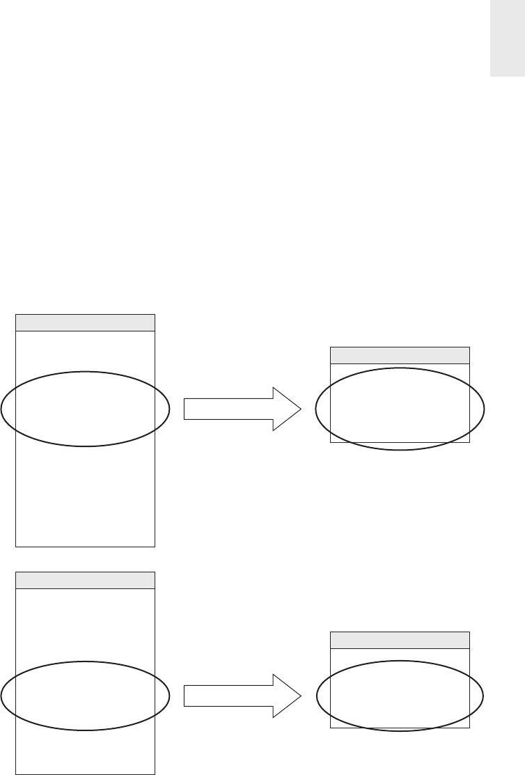
Inventory 133
separate businesses may want to view only their subset of the corporate dimension,
restricted to the product rows for their business. By using a subset of rows, they
aren’t encumbered with the corporation’s entire product set. Of course, the fact table
joined to this subsetted dimension must be limited to the same subset of products.
If a user attempts to use a shrunken subset dimension while accessing a fact table
consisting of the complete product set, they may encounter unexpected query results
because referential integrity would be violated. You need to be cognizant of the
potential opportunity for user confusion or error with dimension row subsetting.
We will further elaborate on dimension subsets when we discuss supertype and
subtype dimensions in Chapter 10: Financial Services.
Product Key (PK)
Product Description
SKU Number (Natural Key)
Brand Description
Subcategory Description
Category Description
Department Description
Package Type Description
Package Size
Fat Content Description
Diet Type Description
Weight
Weight Units of Measure
...
Brand Key (PK)
Brand Description
Subcategory Description
Category Description
Department Description
Month Key (PK)
Calendar Month Name
Calendar Month Number
Calendar YYYY-MM
Calendar Year
Date Key (PK)
Date
Full Date Description
Day of Week
Day Number in Month
Calendar Month Name
Calendar Month Number
Calendar YYYY-MM
Calendar Year
Fiscal Week
Fiscal Month
...
Product Dimension
Date Dimension
Brand Dimension
Month Dimension
Conforms
Conforms
Figure 4-13: Conforming shrunken rollup dimensions.

Chapter 4
134
Appliance
Products
Apparel
Products
Corporate
Product Dimension
Drilling across requires common conformed attributes.
Figure 4-14: Conforming dimension subsets at the same granularity.
Conformed date and month dimensions are a unique example of both row
and column dimension subsetting. Obviously, you can’t simply use the same date
dimension table for daily and monthly fact tables because of the di erence in rollup
granularity. However, the month dimension may consist of the month-end daily
date table rows with the exclusion of all columns that don’t apply at the monthly
granularity, such as the weekday/weekend indicator, week ending date, holiday
indicator, day number within year, and others. Sometimes a month-end indicator on
the daily date dimension is used to facilitate creation of this month dimension table.
Shrunken Conformed Dimensions on the Bus Matrix
The bus matrix identifi es the reuse of common dimensions across business processes.
Typically, the shaded cells of the matrix indicate that the atomic dimension is
associated with a given process. When shrunken rollup or subset dimensions are
involved, you want to reinforce their conformance with the atomic dimensions.
Therefore, you don’t want to create a new, unrelated column on the bus matrix.
Instead, there are two viable approaches to represent the shrunken dimensions within
the matrix, as illustrated in Figure 4-15:
■ Mark the cell for the atomic dimension, but then textually document the
rollup or row subset granularity within the cell.
■ Subdivide the dimension column to indicate the common rollup or subset
granularities, such as day and month if processes collect data at both of these
grains.

Inventory 135
Date
OR
Date
Day Month
Issue Purchase Orders
Receive Deliveries
Inventory
Retail Sales
X
X
X
X
X
X
X
X
X
X
Month
Retail Sales Forecast
Figure 4-15: Alternatives for identifying shrunken dimensions on the bus matrix.
Limited Conformity
Now that we’ve preached about the importance of conformed dimensions, we’ll
discuss the situation in which it may not be realistic or necessary to establish con-
formed dimensions for the organization. If a conglomerate has subsidiaries spanning
widely varied industries, there may be little point in trying to integrate. If each line
of business has unique customers and unique products and there’s no interest in
cross-selling across lines, it may not make sense to attempt an enterprise archi-
tecture because there likely isn’t much perceived business value. The willingness
to seek a common defi nition for product, customer, or other core dimensions is a
major litmus test for an organization theoretically intent on building an enterprise
DW/BI system. If the organization is unwilling to agree on common defi nitions, the
organization shouldn’t attempt to build an enterprise DW/BI environment. It would
be better to build separate, self-contained data warehouses for each subsidiary. But
then don’t complain when someone asks for “enterprise performance” without going
through this logic.
Although organizations may fi nd it di cult to combine data across disparate lines
of business, some degree of integration is typically an ultimate goal. Rather than
throwing your hands in the air and declaring it can’t possibly be done, you should
start down the path toward conformity. Perhaps there are a handful of attributes that
can be conformed across lines of business. Even if it is merely a product description,
category, and line of business attribute that is common to all businesses, this least-
common-denominator approach is still a step in the right direction. You don’t need
to get everyone to agree on everything related to a dimension before proceeding.
Importance of Data Governance and Stewardship
We’ve touted the importance of conformed dimensions, but we also need to acknowl-
edge a key challenge: reaching enterprise consensus on dimension attribute names

Chapter 4
136
and contents (and the handling of content changes which we’ll discuss in Chapter 5:
Procurement). In many organizations, business rules and data defi nitions have
traditionally been established departmentally. The consequences of this commonly
encountered lack of data governance and control are the ubiquitous departmental
data silos that perpetuate similar but slightly di erent versions of the truth. Business
and IT management need to recognize the importance of addressing this shortfall
if you stand any chance of bringing order to the chaos; if management is reluctant
to drive change, the project will never achieve its goals.
Once the data governance issues and opportunities are acknowledged by senior
leadership, resources need to be identifi ed to spearhead the e ort. IT is often tempted
to try leading the charge. They are frustrated by the isolated projects re-creating
data around the organization, consuming countless IT and outside resources while
delivering inconsistent solutions that ultimately just increase the complexity of
the organization’s data architecture at signifi cant cost. Although IT can facilitate
the defi nition of conformed dimensions, it is seldom successful as the sole driver,
even if it’s a temporary assignment. IT simply lacks the organizational authority to
make things happen.
Business-Driven Governance
To boost the likelihood of business acceptance, subject matter experts from the
business need to lead the initiative. Leading a cross-organizational governance
program is not for the faint of heart. The governance resources identifi ed by busi-
ness leadership should have the following characteristics:
■ Respect from the organization
■ Broad knowledge of the enterprise’s operations
■ Ability to balance organizational needs against departmental requirements
■ Gravitas and authority to challenge the status quo and enforce policies
■ Strong communication skills
■ Politically savvy negotiation and consensus building skills
Clearly, not everyone is cut out for the job! Typically those tapped to spearhead
the governance program are highly valued and in demand. It takes the right skills,
experience, and confi dence to rationalize diverse business perspectives and drive
the design of common reference data, together with the necessary organizational
compromises. Over the years, some have criticized conformed dimensions as being
too hard. Yes, it’s di cult to get people in di erent corners of the business to agree
on common attribute names, defi nitions, and values, but that’s the crux of unifi ed,
integrated data. If everyone demands their own labels and business rules, there’s
no chance of delivering on the promises made to establish a single version of the

Inventory 137
truth. The data governance program is critical in facilitating a culture shift away
from the typical siloed environment in which each department retains control of
their data and analytics to one where information is shared and leveraged across
the organization.
Governance Objectives
One of the key objectives of the data governance function is to reach agreement on
data defi nitions, labels, and domain values so that everyone is speaking the same
language. Otherwise, the same words may describe di erent things; di erent words
may describe the same thing; and the same value may have di erent meaning.
Establishing common master data is often a politically charged issue; the chal-
lenges are cultural and geopolitical rather than technical. Defi ning a foundation of
master descriptive conformed dimensions requires e ort. But after it’s agreed upon,
subsequent DW/BI e orts can leverage the work, both ensuring consistency and
reducing the implementation’s delivery cycle time.
In addition to tackling data defi nitions and contents, the data governance func-
tion also establishes policies and responsibilities for data quality and accuracy, as
well as data security and access controls.
Historically, DW/BI teams created the “recipes” for conformed dimensions and
managed the data cleansing and integration mapping in the ETL system; the opera-
tional systems focused on accurately capturing performance metrics, but there was
often little e ort to ensure consistent common reference data. Enterprise resource
planning (ERP) systems promised to fi ll the void, but many organizations still
rely on separate best-of-breed point solutions for niche requirements. Recently,
operational master data management (MDM) solutions have addressed the need
for centralized master data at the source where the transactions are captured.
Although technology can encourage data integration, it doesn’t fi x the problem.
A strong data governance function is a necessary prerequisite for conforming infor-
mation regardless of technical approach.
Conformed Dimensions and the Agile Movement
Some lament that although they want to deliver and share consistently defi ned
master conformed dimensions in their DW/BI environments, it’s “just not feasible.”
They explain they would if they could, but with senior management focused on
using agile development techniques, it’s “impossible” to take the time to get organi-
zational agreement on conformed dimensions. You can turn this argument upside
down by challenging that conformed dimensions enable agile DW/BI development,
along with agile decision making.

Chapter 4
138
Conformed dimensions allow a dimension table to be built and maintained once
rather than re-creating slightly di erent versions during each development cycle.
Reusing conformed dimensions across projects is where you get the leverage for
more agile DW/BI development. As you fl esh out the portfolio of master conformed
dimensions, the development crank starts turning faster and faster. The time-to-
market for a new business process data source shrinks as developers reuse existing
conformed dimensions. Ultimately, new ETL development focuses almost exclusively
on delivering more fact tables because the associated dimension tables are already
sitting on the shelf ready to go.
Defi ning a conformed dimension requires organizational consensus and com-
mitment to data stewardship. But you don’t need to get everyone to agree on every
attribute in every dimension table. At a minimum, you should identify a subset
of attributes that have signifi cance across the enterprise. These commonly referenced
descriptive characteristics become the starter set of conformed attributes, enabling
drill-across integration. Even just a single attribute, such as enterprise product
category, is a viable starting point for the integration e ort. Over time, you can
iteratively expand from this minimalist starting point by adding attributes. These
dimensions could be tackled during architectural agile sprints. When a series of
sprint deliverables combine to deliver su cient value, they constitute a release to
the business users.
If you fail to focus on conformed dimensions because you’re under pressure to
deliver something yesterday, the departmental analytic data silos will likely have
inconsistent categorizations and labels. Even more troubling, data sets may look
like they can be compared and integrated due to similar labels, but the underlying
business rules may be slightly di erent. Business users waste inordinate amounts
of time trying to reconcile and resolve these data inconsistencies, which negatively
impact their ability to be agile decision makers.
The senior IT managers who are demanding agile systems development practices
should be exerting even greater organizational pressure, in conjunction with their
peers in the business, on the development of consistent conformed dimensions if
they’re interested in both long-term development e ciencies and long-term decision-
making e ectiveness across the enterprise.
Conformed Facts
Thus far we have considered the central task of setting up conformed dimensions to
tie dimensional models together. This is 95 percent or more of the data architecture
e ort. The remaining 5 percent of the e ort goes into establishing conformed fact
defi nitions.

Inventory 139
Revenue, profi t, standard prices and costs, measures of quality and customer
satisfaction, and other key performance indicators (KPIs) are facts that must also
conform. If facts live in more than one dimensional model, the underlying defi ni-
tions and equations for these facts must be the same if they are to be called the
same thing. If they are labeled identically, they need to be defi ned in the same
dimensional context and with the same units of measure from dimensional model
to dimensional model. For example, if several business processes report revenue,
then these separate revenue metrics can be added and compared only if they have
the same fi nancial defi nitions. If there are defi nitional di erences, then it is essential
that the revenue facts be labeled uniquely.
NOTE You must be disciplined in your data naming practices. If it is impos-
sible to conform a fact exactly, you should give di erent names to the di erent
interpretations so that business users do not combine these incompatible facts in
calculations.
Sometimes a fact has a natural unit of measure in one fact table and another natu-
ral unit of measure in another fact table. For example, the fl ow of product down the
retail value chain may best be measured in shipping cases at the warehouse but in
scanned units at the store. Even if all the dimensional considerations have been cor-
rectly taken into account, it would be di cult to use these two incompatible units of
measure in one drill-across report. The usual solution to this kind of problem is to
refer the user to a conversion factor buried in the product dimension table and hope
that the user can fi nd the conversion factor and correctly use it. This is unacceptable
for both overhead and vulnerability to error. The correct solution is to carry the fact
in both units of measure, so a report can easily glide down the value chain, picking
o comparable facts. Chapter 6: Order Management talks more about multiple units
of measure.
Summary
In this chapter we developed dimensional models for the three complementary
views of inventory. The periodic snapshot is a good choice for long-running, con-
tinuously replenished inventory scenarios. The accumulating snapshot is a good
choice for fi nite inventory pipeline situations with a defi nite beginning and end.
Finally, most inventory analysis will require a transactional schema to augment
these snapshot models.
We introduced key concepts surrounding the enterprise data warehouse bus
architecture and matrix. Each business process of the value chain, supported by a

Chapter 4
140
primary source system, translates into a row in the bus matrix, and eventually, a
dimensional model. The matrix rows share a surprising number of standardized,
conformed dimensions. Developing and adhering to the enterprise bus architecture
is an absolute must if you intend to build a DW/BI system compose d of an integrated
set of dimensional models.

Procurement
We explore procurement processes in this chapter. This subject area has
obvious cross-industry appeal because it is applicable to any organization
that acquires products or services for either use or resale.
In addition to developing several purchasing models, this chapter provides
in-depth coverage of the techniques for handling dimension table attribute value
changes. Although descriptive attributes in dimension tables are relatively static,
they are subject to change over time. Product lines are restructured, causing product
hierarchies to change. Customers move, causing their geographic information to
change. We’ll describe several approaches to deal with these inevitable dimension
table changes. Followers of the Kimball methods will recognize the type 1, 2, and
3 techniques. Continuing in this tradition, we’ve expanded the slowly changing
dimension technique line-up with types 0, 4, 5, 6, and 7.
Chapter 5 discusses the following concepts:
■ Bus matrix snippet for procurement processes
■ Blended versus separate transaction schemas
■ Slowly changing dimension technique types 0 through 7, covering both basic
and advanced hybrid scenarios
Procurement Case Study
Thus far we have studied downstream sales and inventory processes in the retailer’s
value chain. We explained the importance of mapping out the enterprise data ware-
house bus architecture where conformed dimensions are used across process-centric
fact tables. In this chapter we’ll extend these concepts as we work our way further
up the value chain to the procurement processes.
5

Chapter 5
142
For many companies, procurement is a critical business activity. E ective pro-
curement of products at the right price for resale is obviously important to retail-
ers and distributors. Procurement also has strong bottom line implications for any
organization that buys products as raw materials for manufacturing. Signifi cant
cost savings opportunities are associated with reducing the number of suppliers
and negotiating agreements with preferred suppliers.
Demand planning drives e cient materials management. After demand is fore-
casted, procurement’s goal is to source the appropriate materials or products in
the most economical manner. Procurement involves a wide range of activities from
negotiating contracts to issuing purchase requisitions and purchase orders (POs)
to tracking receipts and authorizing payments. The following list gives you a better
sense of a procurement organization’s common analytic requirements:
■ Which materials or products are most frequently purchased? How many ven-
dors supply these products? At what prices? Looking at demand across the
enterprise (rather than at a single physical location), are there opportunities
to negotiate favorable pricing by consolidating suppliers, single sourcing, or
making guaranteed buys?
■ Are your employees purchasing from the preferred vendors or skirting the
negotiated vendor agreements with maverick spending?
■ Are you receiving the negotiated pricing from your vendors or is there vendor
contract purchase price variance?
■ How are your vendors performing? What is the vendor’s fi ll rate? On-time
delivery performance? Late deliveries outstanding? Percent back ordered?
Rejection rate based on receipt inspection?
Procurement Transactions and Bus Matrix
As you begin working through the four-step dimensional design process, you deter-
mine that procurement is the business process to be modeled. In studying the
process, you observe a fl urry of procurement transactions, such as purchase requisi-
tions, purchase orders, shipping notifi cations, receipts, and payments. Similar to the
approach taken in Chapter 4: Inventory, you could initially design a fact table with
the grain of one row per procurement transaction with transaction date, product,
vendor, contract terms, and procurement transaction type as key dimensions. The
procurement transaction quantity and dollar amount are the facts. The resulting
design is shown in Figure 5-1.
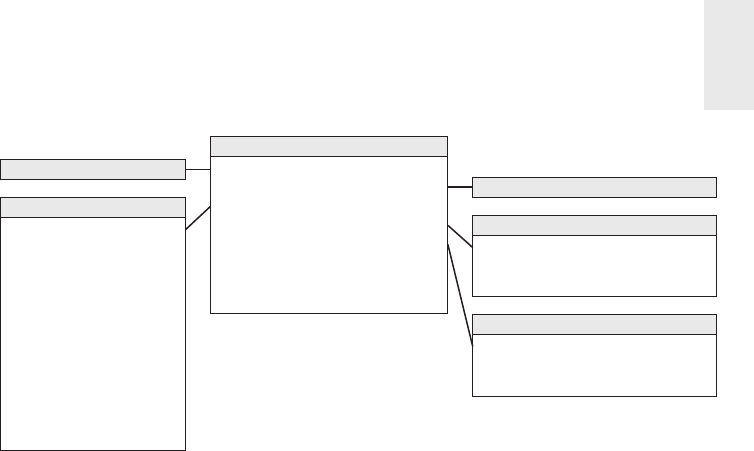
Procurement 143
Date Dimension
Procurement Transaction Fact
Product Dimension
Contract Terms Dimension
Procurement Transaction Type Dimension
Vendor Dimension
Vendor Key (PK)
Vendor Name
Vendor Street Address
Vendor City
Vendor City-State
Vendor ZIP-Postal Code
Vendor State-Province
Vendor Country
Vendor Status
Vendor Minority Ownership Flag
Vendor Corporate Parent
...
Procurement Transaction Date Key (FK)
Product Key (FK)
Vendor Key (FK)
Contract Terms Key (FK)
Procurement Transaction Type Key (FK)
Contract Number (DD)
Procurement Transaction Quantity
Procurement Transaction Dollar Amount
Contract Terms Key (PK)
Contract Terms Description
Contract Terms Type
Procurement Transaction Type Key (PK)
Procurement Transaction Type Description
Procurement Transaction Type Category
Figure 5-1: Procurement fact table with multiple transaction types.
If you work for the same grocery retailer from the earlier case studies, the trans-
action date and product dimensions are the same conformed dimensions developed
originally in Chapter 3: Retail Sales. If you work with manufacturing procurement,
the raw materials products likely are located in a separate raw materials dimen-
sion table rather than included in the product dimension for salable products. The
vendor, contract terms, and procurement transaction type dimensions are new
to this schema. The vendor dimension contains one row for each vendor, along
with interesting descriptive attributes to support a variety of vendor analyses. The
contract terms dimension contains one row for each generalized set of negotiated
terms, similar to the promotion dimension in Chapter 3. The procurement trans-
action type dimension enables grouping or fi ltering on transaction types, such as
purchase orders. The contract number is a degenerate dimension; it could be used
to determine the volume of business conducted under each negotiated contract.
Single Versus Multiple Transaction Fact Tables
As you review the initial procurement schema design with business users, you learn
several new details. First, the business users describe the various procurement trans-
actions di erently. To the business, purchase orders, shipping notices, warehouse
receipts, and vendor payments are all viewed as separate and unique processes.
Several of the procurement transactions come from di erent source systems.
There is a purchasing system that provides purchase requisitions and purchase
orders, a warehousing system that provides shipping notices and warehouse receipts,
and an accounts payable system that deals with vendor payments.

Chapter 5
144
You further discover that several transaction types have di erent dimensionality.
For example, discounts taken are applicable to vendor payments but not to the other
transaction types. Similarly, the name of the employee who received the goods at
the warehouse applies to receipts but doesn’t make sense elsewhere.
There are also a variety of interesting control numbers, such as purchase order
and payment check numbers, created at various steps in the procurement pipeline.
These control numbers are perfect candidates for degenerate dimensions. For certain
transaction types, more than one control number may apply.
As you sort through these new details, you are faced with a design decision.
Should you build a blended transaction fact table with a transaction type dimension
to view all procurement transactions together, or do you build separate fact tables
for each transaction type? This is a common design quandary that surfaces in many
transactional situations, not just procurement.
As dimensional modelers, you need to make design decisions based on a thor-
ough understanding of the business requirements weighed against the realities of
the underlying source data. There is no simple formula to make the defi nite deter-
mination of whether to use a single fact table or multiple fact tables. A single fact
table may be the most appropriate solution in some situations, whereas multiple
fact tables are most appropriate in others. When faced with this design decision,
the following considerations help sort out the options:
■ What are the users’ analytic requirements? The goal is to reduce complexity
by presenting the data in the most e ective form for business users. How will
the business users most commonly analyze this data? Which approach most
naturally aligns with their business-centric perspective?
■ Are there really multiple unique business processes? In the procurement
example, it seems buying products (purchase orders) is distinctly di erent
from receiving products (receipts). The existence of separate control num-
bers for each step in the process is a clue that you are dealing with separate
processes. Given this situation, you would lean toward separate fact tables. By
contrast, in Chapter 4’s inventory example, the varied inventory transactions
were part of a single inventory process resulting in a single fact table design.
■ Are multiple source systems capturing metrics with unique granularities?
There are three separate source systems in this case study: purchasing, ware-
housing, and accounts payable. This would suggest separate fact tables.
■ What is the dimensionality of the facts? In this procurement example, several
dimensions are applicable to some transaction types but not to others. This
would again lead you to separate fact tables.

Procurement 145
A simple way to consider these trade-o s is to draft a bus matrix. As illustrated in
Figure 5-2, you can include two additional columns identifying the atomic granular-
ity and metrics for each row. These matrix embellishments cause it to more closely
resemble the detailed implementation bus matrix, which we’ll more thoroughly
discuss in Chapter 16: Insurance.
Business Processes Atomic Granularity Metrics
Purchase Requisitions X
X
X
X
X
X
X
X
X
X
X
X
X
X
X
X
X
X
X
X
X
X
X
X
X
X
X
X
X
X
X
X
X
X
X
Date
Product
Vendor
Contract Terms
Employee
Warehouse
Carrier
Purchase Orders
Shipping Notifications
Warehouse Receipts
Vendor Invoices
Vendor Payments
1 row per requisition line
1 row per PO line
1 row per shipping notice line
1 row per receipt line
1 row per invoice line
1 row per payment
Requisition Quantity & Dollars
PO Quantity & Dollars
Shipped Quantity
Received Quantity
Invoice Quantity & Dollars
Invoice, Discount & Net
Payment Dollars
Figure 5-2: Sample bus matrix rows for procurement processes.
Based on the bus matrix for this hypothetical case study, multiple transaction
fact tables would be implemented, as illustrated in Figure 5-3. In this example, there
are separate fact tables for purchase requisitions, purchase orders, shipping notices,
warehouse receipts, and vendor payments. This decision was reached because users
view these activities as separate and distinct business processes, the data comes
from di erent source systems, and there is unique dimensionality for the various
transaction types. Multiple fact tables enable richer, more descriptive dimensions
and attributes. The single fact table approach would have required generalized
labeling for some dimensions. For example, purchase order date and receipt date
would likely have been generalized to simply transaction date. Likewise, purchasing
agent and receiving clerk would become employee. This generalization reduces the
legibility of the resulting dimensional model. Also, with separate fact tables as you
progress from purchase requisitions to payments, the fact tables inherit dimensions
from the previous steps.
Multiple fact tables may require more time to manage and administer because
there are more tables to load, index, and aggregate. Some would argue this approach
increases the complexity of the ETL processes. Actually, it may simplify the ETL
activities. Loading the operational data from separate source systems into separate
fact tables likely requires less complex ETL processing than attempting to integrate
data from the multiple sources into a single fact table.

Chapter 5
146
Date Dimension
Vendor Dimension
Employee Dimension
Carrier Dimension
Product Dimension
Contract Terms Dimension
Warehouse Dimension
Purchase Requisition Date Key (FK)
Product Key (FK)
Vendor Key (FK)
Contract Terms Key (FK)
Employee Requested By Key (FK)
Contract Number (DD)
Purchase Requisition Number (DD)
Purchase Requisition Quantity
Purchase Requisition Dollar Amount
Purchase Order Date Key (FK)
Requested By Date Key (FK)
Product Key (FK)
Vendor Key (FK)
Contract Terms Key (FK)
Warehouse Key (FK)
Carrier Key (FK)
Employee Ordered By Key (FK)
Employee Purchase Agent Key (FK)
Contract Number (DD)
Purchase Requisition Number (DD)
Purchase Order Number (DD)
Purchase Order Quantity
Purchase Order Dollar Amount
Purchase Order Fact
Purchase Requisition Fact
Shipping Notification Date Key (FK)
Estimated Arrival Date Key (FK)
Requested By Date Key (FK)
Product Key (FK)
Vendor Key (FK)
Warehouse Key (FK)
Carrier Key (FK)
Employee Ordered By Key (FK)
Purchase Order Number (DD)
Shipping Notification Number (DD)
Shipped Quantity
Shipping Notices Fact
Warehouse Receipt Date Key (FK)
Requested By Date Key (FK)
Product Key (FK)
Vendor Key (FK)
Warehouse Key (FK)
Carrier Key (FK)
Employee Ordered By Key (FK)
Employee Received By Key (FK)
Purchase Order Number (DD)
Shipping Notification Number (DD)
Warehouse Receipt Number (DD)
Received Quantity
Warehouse Receipts Fact
Vendor Payment Date Key (FK)
Product Key (FK)
Vendor Key (FK)
Warehouse Key (FK)
Contract Terms Key (FK)
Contract Number (DD)
Payment Check Number (DD)
Vendor Invoice Dollar Amount
Vendor Discount Dollar Amount
Vendor Net Payment Dollar Amount
Vendor Payment Fact
Figure 5-3: Multiple fact tables for procurement processes.

Procurement 147
Complementary Procurement Snapshot
Apart from the decision regarding multiple procurement transaction fact tables,
you may also need to develop a snapshot fact table to fully address the business’s
needs. As suggested in Chapter 4, an accumulating snapshot such as Figure 5-4 that
crosses processes would be extremely useful if the business is interested in monitor-
ing product movement as it proceeds through the procurement pipeline (including
the duration of each stage). Remember that an accumulating snapshot is meant to
model processes with well-defi ned milestones. If the process is a continuous fl ow
that never really ends, it is not a good candidate for an accumulating snapshot.
Purchase Order Date Key (FK)
Requested By Date Key (FK)
Warehouse Receipt Date Key (FK)
Vendor Invoice Date Key (FK)
Vendor Payment Date Key (FK)
Product Key (FK)
Vendor Key (FK)
Contract Terms Key (FK)
Employee Ordered By Key (FK)
Warehouse Key (FK)
Carrier Key (FK)
Contract Number (DD)
Purchase Order Number (DD)
Warehouse Receipt Number (DD)
Vendor Invoice Number (DD)
Payment Check Number (DD)
Purchase Order Quantity
Purchase Order Dollar Amount
Shipped Quantity
Received Quantity
Vendor Invoice Dollar Amount
Vendor Discount Dollar Amount
Vendor Net Payment Dollar Amount
PO to Requested By Date Lag
PO to Receipt Date Lag
Requested By to Receipt Date Lag
Receipt to Payment Date Lag
Invoice to Payment Date Lag
Procurement Pipeline Fact
Requested By Date Dimension
Vendor Invoice Date Dimension
Product Dimension
Contract Terms Dimension
Warehouse Dimension
Purchase Order Date Dimension
Warehouse Receipt Date Dimension
Vendor Payment Date Dimension
Vendor Dimension
Employee Dimension
Carrier Dimension
Figure 5-4: Procurement pipeline accumulating snapshot schema.
Slowly Changing Dimension Basics
To this point, we have pretended dimensions are independent of time. Unfortunately,
this is not the case in the real world. Although dimension table attributes are relatively
static, they aren’t fi xed forever; attribute values change, albeit rather slowly, over time.

Chapter 5
148
Dimensional designers must proactively work with the business’s data governance
representatives to determine the appropriate change-handling strategy. You shouldn’t
simply jump to the conclusion that the business doesn’t care about dimension changes
just because they weren’t mentioned during the requirements gathering. Although
IT may assume accurate change tracking is unnecessary, business users may assume
the DW/BI system will allow them to see the impact of every attribute value change.
It is obviously better to get on the same page sooner rather than later.
NOTE The business’s data governance and stewardship representatives must be
actively involved in decisions regarding the handling of slowly changing dimension
attributes; IT shouldn’t make determinations on its own.
When change tracking is needed, it might be tempting to put every changing
attribute into the fact table on the assumption that dimension tables are static. This
is unacceptable and unrealistic. Instead you need strategies to deal with slowly
changing attributes within dimension tables. Since Ralph Kimball fi rst introduced
the notion of slowly changing dimensions in 1995, some IT professionals in a never-
ending quest to speak in acronym-ese termed them SCDs. The acronym stuck.
For each dimension table attribute, you must specify a strategy to handle change.
In other words, when an attribute value changes in the operational world, how will
you respond to the change in the dimensional model? In the following sections, we
describe several basic techniques for dealing with attribute changes, followed by
more advanced options. You may need to employ a combination of these techniques
within a single dimension table.
Kimball method followers are likely already familiar with SCD types 1, 2, and 3.
Because legibility is part of our mantra, we sometimes wish we had given these tech-
niques more descriptive names in the fi rst place, such as “overwrite.” But after nearly
two decades, the “type numbers” are squarely part of the DW/BI vernacular. As you’ll
see in the following sections, we’ve decided to expand the theme by assigning new
SCD type numbers to techniques that have been described, but less precisely labeled,
in the past; our hope is that assigning specifi c numbers facilitates clearer communica-
tion among team members.
Type 0: Retain Original
This technique hasn’t been given a type number in the past, but it’s been around
since the beginning of SCDs. With type 0, the dimension attribute value never
changes, so facts are always grouped by this original value. Type 0 is appropriate
for any attribute labeled “original,” such as customer original credit score. It also
applies to most attributes in a date dimension.

Procurement 149
As we staunchly advocated in Chapter 3, the dimension table’s primary key is
a surrogate key rather than relying on the natural operational key. Although we
demoted the natural key to being an ordinary dimension attribute, it still has special
signifi cance. Presuming it’s durable, it would remain inviolate. Persistent durable
keys are always type 0 attributes. Unless otherwise noted, throughout this chapter’s
SCD discussion, the durable supernatural key is assumed to remain constant, as
described in Chapter 3.
Type 1: Overwrite
With the slowly changing dimension type 1 response, you overwrite the old attri-
bute value in the dimension row, replacing it with the current value; the attribute
always refl ects the most recent assignment.
Assume you work for an electronics retailer where products roll up into the retail
store’s departments. One of the products is IntelliKidz software. The existing row in
the product dimension table for IntelliKidz looks like the top half of Figure 5-5. Of
course, there would be additional descriptive attributes in the product dimension,
but we’ve abbreviated the attribute listing for clarity.
IntelliKidz Education12345 ABC922-Z
Product
Key SKU (NK)
Product
Description
Department
Name
IntelliKidz Strategy12345 ABC922-Z
Updated row in Product dimension:
Original row in Product dimension:
Product
Key SKU (NK)
Product
Description
Department
Name
Figure 5-5: SCD type 1 sample rows.
Suppose a new merchandising person decides IntelliKidz software should be
moved from the Education department to the Strategy department on February 1,
2013 to boost sales. With a type 1 response, you’d simply update the existing row
in the dimension table with the new department description, as illustrated in the
updated row of Figure 5-5.
In this case, no dimension or fact table keys were modifi ed when IntelliKidz’s
department changed. The fact table rows still reference product key 12345, regardless
of IntelliKidz’s departmental location. When sales take o following the move to the
Strategy department, you have no information to explain the performance improve-
ment because the historical and more recent facts both appear as if IntelliKidz
always rolled up into Strategy.

Chapter 5
150
The type 1 response is the simplest approach for dimension attribute changes. In
the dimension table, you merely overwrite the preexisting value with the current
assignment. The fact table is untouched. The problem with a type 1 response is that
you lose all history of attribute changes. Because overwriting obliterates historical
attribute values, you’re left solely with the attribute values as they exist today. A type
1 response is appropriate if the attribute change is an insignifi cant correction. It also
may be appropriate if there is no value in keeping the old description. However, too
often DW/BI teams use a type 1 response as the default for dealing with slowly chang-
ing dimensions and end up totally missing the mark if the business needs to track
historical changes accurately. After you implement a type 1, it’s di cult to change
course in the future.
NOTE The type 1 response is easy to implement, but it does not maintain any
history of prior attribute values.
Before we leave the topic of type 1 changes, be forewarned that the same BI
applications can produce di erent results before versus after the type 1 attribute
change. When the dimension attribute’s type 1 overwrite occurs, the fact rows are
associated with the new descriptive context. Business users who rolled up sales by
department on January 31 will get di erent department totals when they run the
same report on February 1 following the type 1 overwrite.
There’s another easily overlooked catch to be aware of. With a type 1 response
to deal with the relocation of IntelliKidz, any preexisting aggregations based on the
department value need to be rebuilt. The aggregated summary data must continue
to tie to the detailed atomic data, where it now appears that IntelliKidz has always
rolled up into the Strategy department.
Finally, if a dimensional model is deployed via an OLAP cube and the type 1
attribute is a hierarchical rollup attribute, like the product’s department in our
example, the cube likely needs to be reprocessed when the type 1 attribute changes.
At a minimum, similar to the relational environment, the cube’s performance aggre-
gations need to be recalculated.
WAR NI NG Even though type 1 changes appear the easiest to implement,
remember they invalidate relational tables and OLAP cubes that have aggregated
data over the a ected attribute.
Type 2: Add New Row
In Chapter 1: Data Warehousing, Business Intelligence, and Dimensional Modeling
Primer, we stated one of the DW/BI system’s goals was to correctly represent history.

Procurement 151
A type 2 response is the predominant technique for supporting this requirement
when it comes to slowly changing dimension attributes.
Using the type 2 approach, when IntelliKidz’s department changed on February
1, 2013, a new product dimension row for IntelliKidz is inserted to refl ect the new
department attribute value. There are two product dimension rows for IntelliKidz,
as illustrated in Figure 5-6. Each row contains a version of IntelliKidz’s attribute
profi le that was true for a span of time.
Original row in Product dimension:
Product
Key SKU (NK)
Product
Description
Department
Name …
Row
Effective
Date
Row
Expiration
Date
Current Row
Indicator
12345 ABC922-Z IntelliKidz Education … 2012-01-01 9999-12-31 Current
Rows in Product dimension following department reassignment:
Product
Key SKU (NK)
Product
Description
Department
Name ...
Row
Effective
Date
Row
Expiration
Date
Current Row
Indicator
12345
25984
ABC922-Z
ABC922-Z
IntelliKidz
IntelliKidz
Education
Strategy
...
...
2012-01-01
2013-02-01
2013-01-31
9999-12-31
Expired
Current
Figure 5-6: SCD type 2 sample rows.
With type 2 changes, the fact table is again untouched; you don’t go back to
the historical fact table rows to modify the product key. In the fact table, rows for
IntelliKidz prior to February 1, 2013, would reference product key 12345 when the
product rolled up to the Education department. After February 1, new IntelliKidz
fact rows would have product key 25984 to refl ect the move to the Strategy depart-
ment. This is why we say type 2 responses perfectly partition or segment history to
account for the change. Reports summarizing pre-February 1 facts look identical
whether the report is generated before or after the type 2 change.
We want to reinforce that reported results may di er depending on whether
attribute changes are handled as a type 1 or type 2. Let’s presume the electronic
retailer sells $500 of IntelliKidz software during January 2013, followed by a $100
sale in February 2013. If the department attribute is a type 1, the results from a
query reporting January and February sales would indicate $600 under Strategy.
Conversely, if the department name attribute is a type 2, the sales would be reported
as $500 for the Education department and $100 for the Strategy department.
Unlike the type 1 approach, there is no need to revisit preexisting aggregation
tables when using the type 2 technique. Likewise, OLAP cubes do not need to be
reprocessed if hierarchical attributes are handled as type 2.
If you constrain on the department attribute, the two product profi les are di er-
entiated. If you constrain on the product description, the query automatically fetches
both IntelliKidz product dimension rows and automatically joins to the fact table for

Chapter 5
152
the complete product history. If you need to count the number of products correctly,
then you would just use the SKU natural key attribute as the basis of the distinct
count rather than the surrogate key; the natural key column becomes the glue that
holds the separate type 2 rows for a single product together.
NOTE The type 2 response is the primary workhorse technique for accurately
tracking slowly changing dimension attributes. It is extremely powerful because
the new dimension row automatically partitions history in the fact table.
Type 2 is the safest response if the business is not absolutely certain about the
SCD business rules for an attribute. As we’ll discuss in the “Type 6: Add Type 1
Attributes to Type 2 Dimension” and “Type 7: Dual Type 1 and Type 2 Dimensions”
sections later in the chapter, you can provide the illusion of a type 1 overwrite when
an attribute has been handled with the type 2 response. The converse is not true. If
you treat an attribute as type 1, reverting to type 2 retroactively requires signifi cant
e ort to create new dimension rows and then appropriately rekey the fact table.
Type 2 Effective and Expiration Dates
When a dimension table includes type 2 attributes, you should include several
administrative columns on each row, as shown in Figure 5-6. The e ective and
expiration dates refer to the moment when the row’s attribute values become valid
or invalid. E ective and expiration dates or date/time stamps are necessary in the
ETL system because it needs to know which surrogate key is valid when loading
historical fact rows. The e ective and expiration dates support precise time slic-
ing of the dimension; however, there is no need to constrain on these dates in the
dimension table to get the right answer from the fact table. The row e ective date
is the fi rst date the descriptive profi le is valid. When a new product is fi rst loaded
in the dimension table, the expiration date is set to December 31, 9999. By avoiding
a null in the expiration date, you can reliably use a BETWEEN command to fi nd the
dimension rows that were in e ect on a certain date.
When a new profi le row is added to the dimension to capture a type 2 attribute
change, the previous row is expired. We typically suggest the end date on the
old row should be just prior to the e ective date of the new row leaving no gaps
between these e ective and expiration dates. The defi nition of “just prior” depends
on the grain of the changes being tracked. Typically, the e ective and expiration
dates represent changes that occur during a day; if you’re tracking more granular
changes, you’d use a date/time stamp instead. In this case, you may elect to apply
di erent business rules, such as setting the row expiration date exactly equal to the

Procurement 153
e ective date of the next row. This would require logic such as “>= e ective date
and < expiration date” constraints, invalidating the use of BETWEEN.
Some argue that a single e ective date is adequate, but this makes for more
complicated searches to locate the dimension row with the latest e ective date
that is less than or equal to a date fi lter. Storing an explicit second date simpli-
fi es the query processing. Likewise, a current row indicator is another useful
administrative dimension attribute to quickly constrain queries to only the cur-
rent profi les.
The type 2 response to slowly changing dimensions requires the use of surrogate
keys, but you’re already using them anyhow, right? You certainly can’t use the opera-
tional natural key because there are multiple profi le versions for the same natural key.
It is not su cient to use the natural key with two or three version digits because you’d
be vulnerable to the entire list of potential operational issues discussed in Chapter 3.
Likewise, it is inadvisable to append an e ective date to the otherwise primary key
of the dimension table to uniquely identify each version. With the type 2 response,
you create a new dimension row with a new single-column primary key to uniquely
identify the new product profi le. This single-column primary key establishes the link-
age between the fact and dimension tables for a given set of product characteristics.
There’s no need to create a confusing secondary join based on the dimension row’s
e ective or expiration dates.
We recognize some of you may be concerned about the administration of surro-
gate keys to support type 2 changes. In Chapter 19: ETL Subsystems and Techniques
and Chapter 20: ETL System Design and Development Process and Tasks, we’ll dis-
cuss a workfl ow for managing surrogate keys and accommodating type 2 changes
in more detail.
Type 1 Attributes in Type 2 Dimensions
It is not uncommon to mix multiple slowly changing dimension techniques within
the same dimension. When type 1 and type 2 are both used in a dimension, some-
times a type 1 attribute change necessitates updating multiple dimension rows. Let’s
presume the dimension table includes a product introduction date. If this attribute
is corrected using type 1 logic after a type 2 change to another attribute occurs,
the introduction date should probably be updated on both versions of IntelliKidz’s
profi le, as illustrated in Figure 5-7.
The data stewards need to be involved in defi ning the ETL business rules in
scenarios like this. Although the DW/BI team can facilitate discussion regarding
proper update handling, the business’s data stewards should make the fi nal deter-
mination, not the DW/BI team.

Chapter 5
154
Original row in Product dimension:
Product
Key SKU (NK)
Product
Description
Department
Name
Introduction
Date
Introduction
Date
…
Row
Effective
Date
Row
Expiration
Date
Current Row
Indicator
12345 ABC922-Z IntelliKidz Education 2012-12-15 … 2012-01-01 9999-12-31 Current
Rows in Product dimension following type 2 change to Department Name and type 1 change to Introduction Date:
Product
Key SKU (NK)
Product
Description
Department
Name ...
Row
Effective
Date
Row
Expiration
Date
Current Row
Indicator
12345
25984
ABC922-Z
ABC922-Z
IntelliKidz
IntelliKidz
Education
Strategy
2012-01-01
2012-01-01
...
...
2012-01-01
2013-02-01
2013-01-31
9999-12-31
Expired
Current
Figure 5-7: Type 1 updates in a dimension with type 2 attributes sample rows.
Type 3: Add New Attribute
Although the type 2 response partitions history, it does not enable you to associ-
ate the new attribute value with old fact history or vice versa. With the type 2
response, when you constrain the department attribute to Strategy, you see only
IntelliKidz facts from after February 1, 2013. In most cases, this is exactly what
you want.
However, sometimes you want to see fact data as if the change never occurred.
This happens most frequently with sales force reorganizations. District boundaries
may be redrawn, but some users still want the ability to roll up recent sales for the
prior districts just to see how they would have done under the old organizational
structure. For a few transitional months, there may be a need to track history for
the new districts and conversely to track new fact data in terms of old district
boundaries. A type 2 response won’t support this requirement, but type 3 comes
to the rescue.
In our software example, let’s assume there is a legitimate business need to
track both the new and prior values of the department attribute for a period of
time around the February 1 change. With a type 3 response, you do not issue a
new dimension row, but rather add a new column to capture the attribute change,
as illustrated in Figure 5-8. You would alter the product dimension table to add
a prior department attribute, and populate this new column with the existing
department value (Education). The original department attribute is treated as a
type 1 where you overwrite to refl ect the current value (Strategy). All existing
reports and queries immediately switch over to the new department description,
but you can still report on the old department value by querying on the prior
department attribute.

Procurement 155
IntelliKidz Education12345 ABC922-Z
Product
Key SKU (NK)
Product
Description
Department
Name
IntelliKidz Strategy Education12345 ABC922-Z
Updated row in Product dimension:
Original row in Product dimension:
Product
Key SKU (NK)
Product
Description
Department
Name
Prior
Department
Name
Figure 5-8: SCD type 3 sample rows.
Don’t be fooled into thinking the higher type number associated with type 3
indicates it is the preferred approach; the techniques have not been presented in
good, better, and best practice sequence. Frankly, type 3 is infrequently used. It is
appropriate when there’s a strong need to support two views of the world simulta-
neously. Type 3 is distinguished from type 2 because the pair of current and prior
attribute values are regarded as true at the same time.
NOTE The type 3 slowly changing dimension technique enables you to see
new and historical fact data by either the new or prior attribute values, sometimes
called alternate realities.
Type 3 is not useful for attributes that change unpredictably, such as a customer’s
home state. There would be no benefi t in reporting facts based on a prior home state
attribute that refl ects a change from 10 days ago for some customers or 10 years
ago for others. These unpredictable changes are typically handled best with type
2 instead.
Type 3 is most appropriate when there’s a signifi cant change impacting many
rows in the dimension table, such as a product line or sales force reorganization.
These en masse changes are prime candidates because business users often want
the ability to analyze performance metrics using either the pre- or post-hierarchy
reorganization for a period of time. With type 3 changes, the prior column is labeled
to distinctly represent the prechanged grouping, such as 2012 department or pre-
merger department. These column names provide clarity, but there may be unwanted
ripples in the BI layer.
Finally, if the type 3 attribute represents a hierarchical rollup level within the
dimension, then as discussed with type 1, the type 3 update and additional column
would likely cause OLAP cubes to be reprocessed.

Chapter 5
156
Multiple Type 3 Attributes
If a dimension attribute changes with a predictable rhythm, sometimes the business
wants to summarize performance metrics based on any of the historic attribute
values. Imagine the product line is recategorized at the start of every year and the
business wants to look at multiple years of historic facts based on the department
assignment for the current year or any prior year.
In this case, we take advantage of the regular, predictable nature of these changes
by generalizing the type 3 approach to a series of type 3 dimension attributes, as
illustrated in Figure 5-9. On every dimension row, there is a current department
attribute that is overwritten, plus attributes for each annual designation, such as
2012 department. Business users can roll up the facts with any of the department
assignments. If a product were introduced in 2013, the department attributes for
2012 and 2011 would contain Not Applicable values.
IntelliKidz Strategy Education Not Applicable12345 ABC922-Z
Updated row in Product dimension:
Product
Key SKU (NK)
Product
Description
Current
Department
Name
2012
Department
Name
2011
Department
Name
Figure 5-9: Dimension table with multiple SCD type 3 attributes.
The most recent assignment column should be identifi ed as the current depart-
ment. This attribute will be used most frequently; you don’t want to modify existing
queries and reports to accommodate next year’s change. When the departments are
reassigned in January 2014, you’d alter the table to add a 2013 department attribute,
populate this column with the current department values, and then overwrite the
current attribute with the 2014 department assignment.
Type 4: Add Mini-Dimension
Thus far we’ve focused on slow evolutionary changes to dimension tables. What
happens when the rate of change speeds up, especially within a large multimillion-
row dimension table? Large dimensions present two challenges that warrant special
treatment. The size of these dimensions can negatively impact browsing and query
fi ltering performance. Plus our tried-and-true type 2 technique for change tracking
is unappealing because we don’t want to add more rows to a dimension that already
has millions of rows, particularly if changes happen frequently.
Fortunately, a single technique comes to the rescue to address both the browsing
performance and change tracking challenges. The solution is to break o frequently
analyzed or frequently changing attributes into a separate dimension, referred to
as a mini-dimension. For example, you could create a mini-dimension for a group

Procurement 157
of more volatile customer demographic attributes, such as age, purchase frequency
score, and income level, presuming these columns are used extensively and changes
to these attributes are important to the business. There would be one row in the
mini-dimension for each unique combination of age, purchase frequency score,
and income level encountered in the data, not one row per customer. With this
approach, the mini-dimension becomes a set of demographic profi les. Although the
number of rows in the customer dimension may be in the millions, the number of
mini-dimension rows should be a signifi cantly smaller. You leave behind the more
constant attributes in the original multimillion-row customer table.
Sample rows for a demographic mini-dimension are illustrated in Figure 5-10.
When creating the mini-dimension, continuously variable attributes, such as income,
are converted to banded ranges. In other words, the attributes in the mini-dimension
are typically forced to take on a relatively small number of discrete values. Although
this restricts use to a set of predefi ned bands, it drastically reduces the number of
combinations in the mini-dimension. If you stored income at a specifi c dollar and
cents value in the mini-dimension, when combined with the other demographic
attributes, you could end up with as many rows in the mini-dimension as in the
customer dimension itself. The use of band ranges is probably the most signifi cant
compromise associated with the mini-dimension technique. Although grouping
facts from multiple band values is viable, changing to more discreet bands (such
as $30,000-34,999) at a later time is di cult. If users insist on access to a specifi c
raw data value, such as a credit bureau score that is updated monthly, it should be
included in the fact table, in addition to being value banded in the demographic
mini-dimension. In Chapter 10: Financial Services, we’ll discuss dynamic value
banding of facts; however, such queries are much less e cient than constraining
the value band in a mini-dimension table.
Low
Medium
High
Low
Medium
High
...
Low
Medium
High
...
<$30,000
<$30,000
<$30,000
$30,000-39,999
$30,000-39,999
$30,000-39,999
...
<$30,000
<$30,000
<$30,000
...
1
2
3
4
5
6
...
142
143
144
...
21-25
21-25
21-25
21-25
21-25
21-25
...
26-30
26-30
26-30
...
Demographics
Key Age Band Income Level
Purchase
Frequency
Score
Figure 5-10: SCD type 4 mini-dimension sample rows.

Chapter 5
158
Every time a fact table row is built, two foreign keys related to the customer would
be included: the customer dimension key and the mini-dimension demographics
key in e ect at the time of the event, as shown in Figure 5-11. The mini-dimension
delivers performance benefi ts by providing a smaller point of entry to the facts.
Queries can avoid the huge customer dimension table unless attributes from that
table are constrained or used as report labels.
Customer Dimension
Customer Key (PK)
Customer ID (NK)
Customer Name
Customer Address
Customer City-State
Customer State
Customer ZIP-Postal Code
Customer Date of Birth
Demographics Dimension
Demographics Key (PK)
Age Band
Purchase Frequency Score
Income Level
Fact Table
Date Key (FK)
Customer Key (FK)
Demographics Key (FK)
More FKs...
Facts...
Figure 5-11: Type 4 mini-dimension with customer dimension.
When the mini-dimension key participates as a foreign key in the fact table, another
benefi t is that the fact table captures the demographic profi le changes. Let’s presume
we are loading data into a periodic snapshot fact table on a monthly basis. Referring
back to our sample demographic mini-dimension sample rows in Figure 5-10, if one
of our customers, John Smith, were 25 years old with a low purchase frequency score
and an income of $25,000, you’d begin by assigning demographics key 1 when loading
the fact table. If John has a birthday several weeks later and turns 26 years old, you’d
assign demographics key 142 when the fact table was next loaded; the demographics
key on John’s earlier fact table rows would not be changed. In this manner, the fact
table tracks the age change. You’d continue to assign demographics key 142 when
the fact table is loaded until there’s another change in John’s demographic profi le. If
John receives a raise to $32,000 several months later, a new demographics key would
be refl ected in the next fact table load. Again, the earlier rows would be unchanged.
OLAP cubes also readily accommodate type 4 mini-dimensions.
Customer dimensions are somewhat unique in that customer attributes frequently
are queried independently from the fact table. For example, users may want to know
how many customers live in Dade County by age bracket for segmentation and profi l-
ing. Rather than forcing any analysis that combines customer and demographic data
to link through the fact table, the most recent value of the demographics key also
can exist as a foreign key on the customer dimension table. We’ll further describe
this customer demographic outrigger as an SCD type 5 in the next section.

Procurement 159
The demographic dimension cannot be allowed to grow too large. If you have
fi ve demographic attributes, each with 10 possible values, then the demographics
dimension could have 100,000 (105) rows. This is a reasonable upper limit for the
number of rows in a mini-dimension if you build out all the possible combina-
tions in advance. An alternate ETL approach is to build only the mini-dimension
rows that actually occur in the data. However, there are certainly cases where even
this approach doesn’t help and you need to support more than fi ve demographic
attributes with 10 values each. We’ll discuss the use of multiple mini-dimensions
associated with a single fact table in Chapter 10.
Demographic profi le changes sometimes occur outside a business event, such
as when a customer’s profi le is updated in the absence of a sales transaction. If the
business requires accurate point-in-time profi ling, a supplemental factless fact table
with e ective and expiration dates can capture every relationship change between
the customer and demographics dimensions.
Hybrid Slowly Changing Dimension
Techniques
In this fi nal section, we’ll discuss hybrid approaches that combine the basic SCD
techniques. Designers sometimes become enamored with these hybrids because they
seem to provide the best of all worlds. However, the price paid for greater analytic
fl exibility is often greater complexity. Although IT professionals may be impressed
by elegant fl exibility, business users may be just as easily turned o by complexity.
You should not pursue these options unless the business agrees they are needed to
address their requirements.
These fi nal approaches are most relevant if you’ve been asked to preserve the
historically accurate dimension attribute associated with a fact event, while sup-
porting the option to report historical facts according to the current attribute values.
The basic slowly changing dimension techniques do not enable this requirement
easily on their own.
We’ll start by considering a technique that combines type 4 with a type 1 outrig-
ger; because 4 + 1 = 5, we’re calling this type 5. Next, we’ll describe type 6, which
combines types 1 through 3 for a single dimension attribute; it’s aptly named type
6 because 2 + 3 + 1 or 2 × 3 × 1 both equal 6. Finally, we’ll fi nish up with type 7,
which just happens to be the next available sequence number; there is no underly-
ing mathematical signifi cance to this label.

Chapter 5
160
Type 5: Mini-Dimension and Type 1 Outrigger
Let’s return to the type 4 mini-dimension. An embellishment to this technique is to
add a current mini-dimension key as an attribute in the primary dimension. This
mini-dimension key reference is a type 1 attribute, overwritten with every profi le
change. You wouldn’t want to track this attribute as a type 2 because then you’d be
capturing volatile changes within the large multimillion-row dimension and avoid-
ing this explosive growth was one of the original motivations for type 4.
The type 5 technique is useful if you want a current profi le count in the absence
of fact table metrics or want to roll up historical facts based on the customer’s cur-
rent profi le. You’d logically represent the primary dimension and mini-dimension
outrigger as a single table in the presentation area, as shown in Figure 5-12. To
minimize user confusion and potential error, the current attributes in this role-
playing dimension should have distinct column names distinguishing them, such
as current age band. Even with unique labeling, be aware that presenting users with
two avenues for accessing demographic data, through either the mini-dimension
or outrigger, can deliver more functionality and complexity than some can handle.
Current Demographics Dimension
Current Demographics Key (PK)
Current Age Band
Current Purchase Frequency Score
Current Income Level
Logical representation to the BI tools:
View of Demographics Dimension
Fact Table
Date Key (FK)
Customer Key (FK)
Demographics Key (FK)
More FKs...
Facts
Customer Dimension
Customer Key (PK)
Customer ID (NK)
Customer Name
...
Current Demographics Key (FK)
Demographics Dimension
Demographics Key (PK)
Age Band
Purchase Frequency Score
Income Level
Fact Table
Date Key (FK)
Customer Key (FK)
Demographics Key (FK)
More FKs...
Facts
Customer Dimension
Customer Key (PK)
Customer ID (NK)
Customer Name
...
Current Age Band
Current Purchase Frequency Score
Current Income Level
Demographics Dimension
Demographics Key (PK)
Age Band
Purchase Frequency Score
Income Level
Figure 5-12: Type 4 mini-dimension with type 1 outrigger in customer dimension.
NOTE The type 4 mini-dimension terminology refers to when the demograph-
ics key is part of the fact table composite key. If the demographics key is a foreign
key in the customer dimension, it is referred to as an outrigger.
Type 6: Add Type 1 Attributes to Type 2 Dimension
Let’s return to the electronics retailer’s product dimension. With type 6, you would
have two department attributes on each row. The current department column

Procurement 161
represents the current assignment; the historic department column is a type 2
attribute representing the historically accurate department value.
When IntelliKidz software is introduced, the product dimension row would look
like the fi rst scenario in Figure 5-13.
Original row in Product dimension:
Product
Key SKU (NK)
Product
Description
Historic
Department
Name
Current
Department
Name …
Row
Effective
Date
Row
Expiration
Date
Current Row
Indicator
12345 ABC922-Z IntelliKidz Education Education … 2012-01-01 9999-12-31 Current
Rows in Product dimension following first department reassignment:
Product
Key SKU (NK)
Product
Description
Historic
Department
Name
Current
Department
Name ...
Row
Effective
Date
Row
Expiration
Date
Current Row
Indicator
12345
25984
ABC922-Z
ABC922-Z
IntelliKidz
IntelliKidz
Education
Strategy
Strategy
Strategy
...
...
2012-01-01
2013-02-01
2013-01-31
9999-12-31
Expired
Current
Rows in Product dimension following second department reassignment:
Product
Key SKU (NK)
Product
Description
Historic
Department
Name
Current
Department
Name ...
Row
Effective
Date
Row
Expiration
Date
Current Row
Indicator
12345
25984
31726
ABC922-Z
ABC922-Z
ABC922-Z
IntelliKidz
IntelliKidz
IntelliKidz
Education
Strategy
Critical Thinking
Critical Thinking
Critical Thinking
Critical Thinking
...
...
...
2012-01-01
2013-02-01
2013-07-01
2013-01-31
2013-06-30
9999-12-31
Expired
Expired
Current
Figure 5-13: SCD type 6 sample rows.
When the departments are restructured and IntelliKidz is moved to the Strategy
department, you’d use a type 2 response to capture the attribute change by issu-
ing a new row. In this new IntelliKidz dimension row, the current department will
be identical to the historical department. For all previous instances of IntelliKidz
dimension rows, the current department attribute will be overwritten to refl ect the
current structure. Both IntelliKidz rows would identify the Strategy department as
the current department (refer to the second scenario in Figure 5-13).
In this manner you can use the historic attribute to group facts based on the attribute
value that was in e ect when the facts occurred. Meanwhile, the current attri-
bute rolls up all the historical fact data for both product keys 12345 and 25984 into
the current department assignment. If IntelliKidz were then moved into the Critical
Thinking software department, the product table would look like Figure 5-13’s fi nal
set of rows. The current column groups all facts by the current assignment, while
the historic column preserves the historic assignments accurately and segments the
facts accordingly.
With this hybrid approach, you issue a new row to capture the change (type 2)
and add a new column to track the current assignment (type 3), where subsequent
changes are handled as a type 1 response. An engineer at a technology company

Chapter 5
162
suggested we refer to this combo approach as type 6 because both the sum and
product of 1, 2, and 3 equals 6.
Again, although this technique may be naturally appealing to some, it is impor-
tant to always consider the business users’ perspective as you strive to arrive at a
reasonable balance between fl exibility and complexity. You may want to limit which
columns are exposed to some users so they’re not overwhelmed by choices.
Type 7: Dual Type 1 and Type 2 Dimensions
When we fi rst described type 6, someone asked if the technique would be appropri-
ate for supporting both current and historic perspectives for 150 attributes in a large
dimension table. That question sent us back to the drawing board.
In this fi nal hybrid technique, the dimension natural key (assuming it’s durable)
is included as a fact table foreign key, in addition to the surrogate key for type 2
tracking, as illustrated in Figure 5-14. If the natural key is unwieldy or ever reas-
signed, you should use a separate durable supernatural key instead. The type 2
dimension contains historically accurate attributes for fi ltering and grouping based
on the e ective values when the fact event occurred. The durable key joins to a
dimension with just the current type 1 values. Again, the column labels in this table
should be prefaced with “current” to reduce the risk of user confusion. You can use
these dimension attributes to summarize or fi lter facts based on the current profi le,
regardless of the attribute values in e ect when the fact event occurred.
Fact Table
Date Key (FK)
Product Key (FK)
Durable Product Key (FK)
More FKs...
Facts
Product Dimension
Product Key (PK)
Durable Product Key (DK)
Product Description
Department Name
...
Row Effective Date
Row Expiration Date
Current Row Indicator
Current Product Dimension
Durable Product Key (PK)
Current Product Description
Current Department Name
...
View of Product Dimension
(where Current Row Indicator=Current)
Figure 5-14: Type 7 with dual foreign keys for dual type 1 and type 2 dimension tables.
This approach delivers the same functionality as type 6. Although the type 6
response spawns more attribute columns in a single dimension table, this approach
relies on two foreign keys in the fact table. Type 7 invariably requires less ETL e ort
because the current type 1 attribute table could easily be delivered via a view of
the type 2 dimension table, limited to the most current rows. The incremental cost
of this fi nal technique is the additional column carried in the fact table; however,

Procurement 163
queries based on current attribute values would be fi ltering on a smaller dimension
table than previously described with type 6.
Of course, you could avoid storing the durable key in the fact table by joining the
type 1 view containing current attributes to the durable key in the type 2 dimension
table itself. In this case, however, queries that are only interested in current rollups
would need to traverse from the type 1 outrigger through the more voluminous
type 2 dimension before fi nally reaching the facts, which would likely negatively
impact query performance for current reporting.
A variation of this dual type 1 and type 2 dimension table approach again relies
on a view to deliver current type 1 attributes. However, in this case, the view associ-
ates the current attribute values with all the durable key’s type 2 rows, as illustrated
in Figure 5-15.
Fact Table
Date Key (FK)
Product Key (FK)
More FKs...
Facts
Product Dimension
Product Key (PK)
Durable Product Key
Product Description
Department Name
...
Row Effective Date
Row Expiration Date
Current Row Indicator
Current Product Dimension
Product Key (PK)
Durable Product Key
Current Product Description
Current Department Name
...
View of Product Dimension
Figure 5-15: Type 7 variation with single surrogate key for dual type 1 and type 2
dimension tables.
Both dimension tables in Figure 5-15 have the same number of rows, but the
contents of the tables are di erent, as shown in Figure 5-16.
Rows in Product dimension:
Product
Key SKU (NK)
Durable
Product
Key
Product
Description
Department
Name ...
Row Effective
Date
Row
Expiration
Date
Current Row
Indicator
12345
25984
31726
ABC922-Z
ABC922-Z
ABC922-Z
12345
12345
12345
IntelliKidz
IntelliKidz
IntelliKidz
Education
Strategy
Critical Thinking
...
...
...
2012-01-01
2013-02-01
2013-07-01
2013-01-31
2013-06-30
9999-12-31
Expired
Expired
Current
Rows in Product dimension’s current view:
Product
Key SKU (NK)
Durable
Product
Key
Current
Product
Description
Current
Department
Name ...
12345
25984
31726
ABC922-Z
ABC922-Z
ABC922-Z
12345
12345
12345
IntelliKidz
IntelliKidz
IntelliKidz
Critical Thinking
Critical Thinking
Critical Thinking
...
...
...
Figure 5-16: SCD type 7 variation sample rows.

Chapter 5
164
Type 7 for Random “As Of” Reporting
Finally, although it’s uncommon, you might be asked to roll up historical facts
based on any specifi c point-in-time profi le, in addition to reporting by the attribute
values in e ect when the fact event occurred or by the attribute’s current values.
For example, perhaps the business wants to report three years of historical metrics
based on the hierarchy in e ect on December 1 of last year. In this case, you can
use the dual dimension keys in the fact table to your advantage. First fi lter on the
type 2 dimension row e ective and expiration dates to locate the rows in e ect on
December 1 of last year. With this constraint, a single row for each durable key
in the type 2 dimension is identifi ed. Then join this fi ltered set to the durable key in
the fact table to roll up any facts based on the point-in-time attribute values. It’s as
if you’re defi ning the meaning of “current” on-the-fl y. Obviously, you must fi lter
on the row e ective and expiration dates, or you’ll have multiple type 2 rows for
each durable key. Finally, only unveil this capability to a limited, highly analytic
audience; this embellishment is not for the timid.
Slowly Changing Dimension Recap
We’ve summarized the techniques for tracking dimension attribute changes in
Figure 5-17. This chart highlights the implications of each slowly changing dimen-
sion technique on the analysis of performance metrics in the fact table.
SCD Type Dimension Table Action Impact on Fact Analysis
Type 0 No change to attribute value. Facts associated with attribute’s original value.
Type 1 Overwrite attribute value. Facts associated with attribute’s current value.
Type 2
Type 3
Type 4
Type 5
Type 6
Add new dimension row for profile
with new attribute value.
Add new column to preserve attribute’s
current and prior values.
Add mini-dimension table containing
rapidly changing attributes.
Add type 4 mini-dimension, along with
overwritten type 1 mini-dimension key
in base dimension.
Add type 1 overwritten attributes to
type 2 dimension row, and overwrite
all prior dimension rows.
Facts associated with attribute value in effect when
fact occured.
Facts associated with both current and prior attribute
alternative values.
Facts associated with rapidly changing attributes in
effect when fact occured.
Facts associated with rapidly changing attributes in
effect when fact occurred, plus current rapidly changing
attribute values.
Facts associated with attribute value in effect when fact
occurred, plus current values.
Facts associated with attribute value in effect when fact
occurred, plus current values.
Type 7
Add type 2 dimension row with new
attribute value, plus view limited to
current rows and/or attribute values.
Figure 5-17: Slowly changing dimension techniques summary.

Procurement 165
Summary
In this chapter we discussed several approaches to handling procurement data.
E ectively managing procurement performance can have a major impact on an
organization’s bottom line.
We also introduced techniques to deal with changes to dimension attribute
values. The slowly changing responses range from doing nothing (type 0) to
overwriting the value (type 1) to complicated hybrid approaches (such as types 5
through 7) which combine techniques to support requirements for both historic
attribute preservation and current attribute reporting. You’ll undoubtedly need to
re-read this section as you consider slowly changing dimension attribute strategies
for your DW/BI system.

Order Management
Order management consists of several critical business processes, including
order, shipment, and invoice processing. These processes spawn metrics,
such as sales volume and invoice revenue, that are key performance indicators for
any organization that sells products or services to others. In fact, these foundation
metrics are so crucial that DW/BI teams frequently tackle one of the order manage-
ment processes for their initial implementation. Clearly, the topics in this case study
transcend industry boundaries.
In this chapter we’ll explore several di erent order management transactions,
including the common characteristics and complications encountered when
dimensionally modeling these transactions. We’ll further develop the concept of
an accumulating snapshot to analyze the order fulfi llment pipeline from initial
order to invoicing.
Chapter 6 discusses the following concepts:
■ Bus matrix snippet for order management processes
■ Orders transaction schema
■ Fact table normalization considerations
■ Role-playing dimensions
■ Ship-to/bill-to customer dimension considerations
■ Factors to determine if single or multiple dimensions
■ Junk dimensions for miscellaneous fl ags and indicators versus alternative
designs
■ More on degenerate dimensions
■ Multiple currencies and units of measure
■ Handling of facts with di erent granularity
■ Patterns to avoid with header and line item transactions
■ Invoicing transaction schema with profi t and loss facts
■ Audit dimension
6

Chapter 6
168
■ Quantitative measures and qualitative descriptors of service level performance
■ Order fulfi llment pipeline as accumulating snapshot schema
■ Lag calculations
Order Management Bus Matrix
The order management function is composed of a series of business processes. In
its most simplistic form, you can envision a subset of the enterprise data warehouse
bus matrix that resembles Figure 6-1.
Quoting
Ordering
Shipping to Customer
Shipment Invoicing
Receiving Payments
Customer Returns
X
X
X
X
X
X
X
X
X
X
X
X
X
X
X
X
X
X
X
X
X
X
X
X
X
X
X
X
X
X
X
X
X
X
Date
Customer
Product
Sales Rep
Deal
Warehouse
Shipper
Figure 6-1: Bus matrix rows for order management processes.
As described in earlier chapters, the bus matrix closely corresponds to the orga-
nization’s value chain. In this chapter we’ll focus on the order and invoice rows
of the matrix. We’ll also describe an accumulating snapshot fact table to evaluate
performance across multiple stages of the overall order fulfi llment process.
Order Transactions
The natural granularity for an order transaction fact table is one row for each line
item on an order. The dimensions associated with the orders business process are
order date, requested ship date, product, customer, sales rep, and deal. The facts
include the order quantity and extended order line gross, discount, and net (equal
to the gross amount less discount) dollar amounts. The resulting schema would
look similar to Figure 6-2.
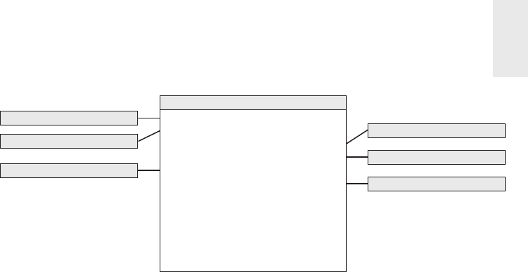
Order Management 169
Order Date Key (FK)
Requested Ship Date Key (FK)
Customer Key (FK)
Product Key (FK)
Sales Rep Key (FK)
Deal Key (FK)
Order Number (DD)
Order Line Number (DD)
Order Line Quantity
Extended Order Line Gross Dollar Amount
Extended Order Line Discount Dollar Amount
Extended Order Line Net Dollar Amount
Customer Dimension
Product Dimension
Deal Dimension
Order Date Dimension
Order Line Transaction Fact
Requested Ship Date Dimension
Sales Rep Dimension
Figure 6-2: Order transaction fact table.
Fact Normalization
Rather than storing the list of facts in Figure 6-2, some designers want to further nor-
malize the fact table so there’s a single, generic fact amount along with a dimension
that identifi es the type of measurement. In this scenario, the fact table granularity is
one row per measurement per order line, instead of the more natural one row per order
line event. The measurement type dimension would indicate whether the fact is the
gross order amount, order discount amount, or some other measure. This technique
may make sense when the set of facts is extremely lengthy, but sparsely populated
for a given fact row, and no computations are made between facts. You could use this
technique to deal with manufacturing quality test data where the facts vary widely
depending on the test conducted.
However, you should generally resist the urge to normalize the fact table in this
way. Facts usually are not sparsely populated within a row. In the order transaction
schema, if you were to normalize the facts, you’d be multiplying the number of rows
in the fact table by the number of fact types. For example, assume you started with
10 million order line fact table rows, each with six keys and four facts. If the fact
rows were normalized, you’d end up with 40 million fact rows, each with seven
keys and one fact. In addition, if any arithmetic function is performed between
the facts (such as discount amount as a percentage of gross order amount), it is
far easier if the facts are in the same row in a relational star schema because SQL
makes it di cult to perform a ratio or di erence between facts in di erent rows.
In Chapter 14: Healthcare, we’ll explore a situation where a measurement type
dimension makes more sense. This pattern is also more appropriate if the primary
platform supporting BI applications is an OLAP cube; the cube enables computations
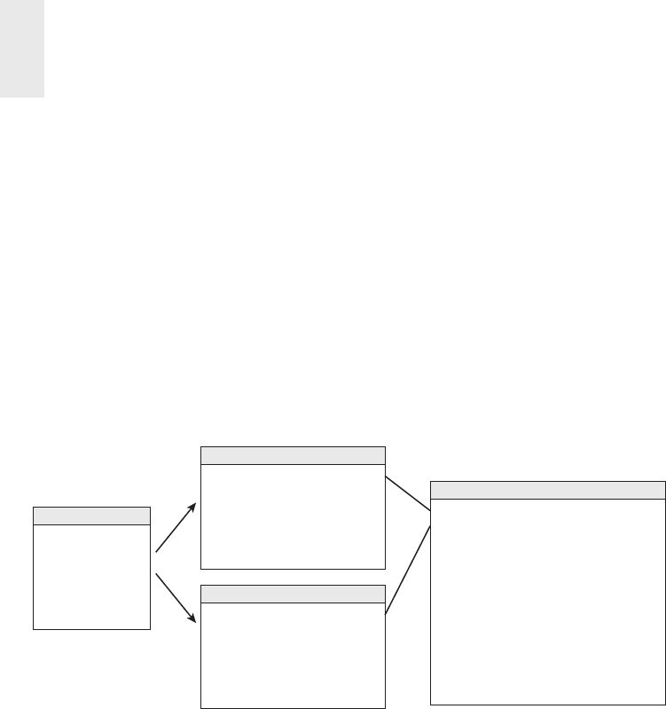
Chapter 6
170
that cut the cube along any dimension, regardless if it’s a date, product, customer,
or measurement type.
Dimension Role Playing
By now you know to expect a date dimension in every fact table because you’re
always looking at performance over time. In a transaction fact table, the primary date
column is the transaction date, such as the order date. Sometimes you discover other
dates associated with each transaction, such as the requested ship date for the order.
Each of the dates should be a foreign key in the fact table, as shown in Figure 6-3.
However, you cannot simply join these two foreign keys to the same date dimension
table. SQL would interpret this two-way simultaneous join as requiring both the
dates to be identical, which isn’t very likely.
Logical views or aliases of the
single physical date dimension
Order Date Key (FK)
Requested Ship Date Key (FK)
Customer Key (FK)
Product Key (FK)
Sales Rep Key (FK)
Deal Key (FK)
Order Number (DD)
Order Line Number (DD)
Order Quantity
Extended Order Line Gross Dollar Amount
Extended Order Line Discount Dollar Amount
Extended Order Line Net Dollar Amount
Order Line Transaction Fact
Date Key
Date
Day of Week
Month
Quarter
...
Date Dimension
Order Date Key
Order Date
Order Day of Week
Order Month
Order Quarter
...
Requested Ship Date Key
Requested Ship Date
Requested Ship Day of Week
Requested Ship Month
Requested Ship Quarter
...
Order Date Dimension
Requested Ship Date Dimension
Figure 6-3: Role-playing date dimensions.
Even though you cannot literally join to a single date dimension table, you can
build and administer a single physical date dimension table. You then create the
illusion of two independent date dimensions by using views or aliases. Be careful to
uniquely label the columns in each of the views or aliases. For example, the order
month attribute should be uniquely labeled to distinguish it from the requested
ship month. If you don’t establish unique column names, you wouldn’t be able to
tell the columns apart when both are dragged into a report.
As we briefl y described in Chapter 3: Retail Sales, we would defi ne the order date
and requested order date views as follows:
create view order_date
(order_date_key, order_day_of_week, order_month, ...)
as select date_key, day_of_week, month, ... from date

Order Management 171
and
create view req_ship_date
(req_ship_date_key, req_ship_day_of_week, req_ship_month, ...)
as select date_key, day_of_week, month, ... from date
Alternatively, SQL supports the concept of aliasing. Many BI tools also enable
aliasing within their semantic layer. However, we caution against this approach
if multiple BI tools, along with direct SQL-based access, are used within the
organization.
Regardless of the implementation approach, you now have two unique logical date
dimensions that can be used as if they were independent with completely unrelated
constraints. This is referred to as role playing because the date dimension simultane-
ously serves di erent roles in a single fact table. You’ll see additional examples of
dimension role playing sprinkled throughout this book.
NOTE Role playing in a dimensional model occurs when a single dimension
simultaneously appears several times in the same fact table. The underlying dimen-
sion may exist as a single physical table, but each of the roles should be presented
to the BI tools as a separately labeled view.
It’s worth noting that some OLAP products do not support multiple roles of the
same dimension; in this scenario, you’d need to create two separate dimensions for
the two roles. In addition, some OLAP products that enable multiple roles do not
enable attribute renaming for each role. In the end, OLAP environments may be
littered with a plethora of separate dimensions, which are treated simply as roles
in the relational star schema.
To handle the multiple dates, some designers are tempted to create a single date
table with a key for each unique order date and requested ship date combination.
This approach falls apart on several fronts. First, the clean and simple daily date
table with approximately 365 rows per year would balloon in size if it needed to
handle all the date combinations. Second, a combination date table would no longer
conform to the other frequently used daily, weekly, and monthly date dimensions.
Role Playing and the Bus Matrix
The most common technique to document role playing on the bus matrix is to
indicate the multiple roles within a single cell, as illustrated in Figure 6-4. We used
a similar approach in Chapter 4: Inventory for documenting shrunken conformed
dimensions. This method is especially appropriate for the date dimension on the
bus matrix given its numerous logical roles. Alternatively, if the number of roles is
limited and frequently reused across processes, you can create subcolumns within
a single conformed dimension column on the matrix.

Chapter 6
172
Quoting
Ordering
Shipping to Customer
Shipment Invoicing
Receiving Payments
Customer Returns
Quote Date
Order Date
Requested Ship Date
Shipment Date
Invoice Date
Payment Receipt Date
Return Date
Date
Figure 6-4: Communicating role-playing dimensions on the bus matrix.
Product Dimension Revisited
Each of the case study vignettes presented so far has included a product dimen-
sion. The product dimension is one of the most common and most important
dimension tables. It describes the complete portfolio of products sold by a com-
pany. In many cases, the number of products in the portfolio turns out to be sur-
prisingly large, at least from an outsider’s perspective. For example, a prominent
U.S. manufacturer of dog and cat food tracks more than 25,000 manufacturing
variations of its products, including retail products everyone (or every dog and
cat) is familiar with, as well as numerous specialized products sold through com-
mercial and veterinary channels. Some durable goods manufacturers, such as
window companies, sell millions of unique product confi gurations.
Most product dimension tables share the following characteristics:
■ Numerous verbose, descriptive columns. For manufacturers, it’s not unusual
to maintain 100 or more descriptors about the products they sell. Dimension
table attributes naturally describe the dimension row, do not vary because
of the infl uence of another dimension, and are virtually constant over time,
although some attributes do change slowly over time.
■ One or more attribute hierarchies, plus non-hierarchical attributes. Products
typically roll up according to multiple defi ned hierarchies. The many-to-one
fi xed depth hierarchical data should be presented in a single fl attened, denor-
malized product dimension table. You should resist creating normalized snow-
fl aked sub-tables; the costs of a more complicated presentation and slower
intra-dimension browsing performance outweigh the minimal storage savings
benefi ts. Product dimension tables can have thousands of entries. With so many

Order Management 173
rows, it is not too useful to request a pull-down list of the product descriptions.
It is essential to have the ability to constrain on one attribute, such as fl avor,
and then another attribute, such as package type, before attempting to display
the product descriptions. Any attributes, regardless of whether they belong to
a single hierarchy, should be used freely for browsing and drilling up or down.
Many product dimension attributes are standalone low-cardinality attributes,
not part of explicit hierarchies.
The existence of an operational product master helps create and maintain the
product dimension, but a number of transformations and administrative steps must
occur to convert the operational master fi le into the dimension table, including the
following:
■ Remap the operational product code to a surrogate key. As we discussed in
Chapter 3, this meaningless surrogate primary key is needed to avoid havoc
caused by duplicate use of an operational product code over time. It also
might be necessary to integrate product information sourced from di erent
operational systems. Finally, as you just learned in Chapter 5: Procurement,
the surrogate key is needed to track type 2 product attribute changes.
■ Add descriptive attribute values to augment or replace operational codes.
You shouldn’t accept the excuse that the business users are familiar with the
operational codes. The only reason business users are familiar with codes is that
they have been forced to use them! The columns in a product dimension are
the sole source of query constraints and report labels, so the contents must be
legible. Cryptic abbreviations are as bad as outright numeric codes; they also
should be augmented or replaced with readable text. Multiple abbreviated codes
in a single column should be expanded and separated into distinct attributes.
■ Quality check the attribute values to ensure no misspellings, impossible
values, or multiple variations. BI applications and reports rely on the precise
contents of the dimension attributes. SQL will produce another line in a report
if the attribute value varies in any way based on trivial punctuation or spell-
ing di erences. You should ensure that the attribute values are completely
populated because missing values easily cause misinterpretations. Incomplete
or poorly administered textual dimension attributes lead to incomplete or
poorly produced reports.
■ Document the attribute defi nitions, interpretations, and origins in the
metadata. Remember that the metadata is analogous to the DW/BI encyclo-
pedia. You must be vigilant about populating and maintaining the metadata
repository.

Chapter 6
174
Customer Dimension
The customer dimension contains one row for each discrete location to which you
ship a product. Customer dimension tables can range from moderately sized (thou-
sands of rows) to extremely large (millions of rows) depending on the nature of the
business. A typical customer dimension is shown in Figure 6-5.
Customer Key (PK)
Customer ID (Natural Key)
Customer Name
Customer Ship To Address
Customer Ship To City
Customer Ship To County
Customer Ship To City-State
Customer Ship To State
Customer Ship To ZIP
Customer Ship To ZIP Region
Customer Ship To ZIP Sectional Center
Customer Bill To Name
Customer Bill To Address
Customer Organization Name
Customer Corporate Parent Name
Customer Credit Rating
Customer Dimension
Figure 6-5: Sample customer dimension.
Several independent hierarchies typically coexist in a customer dimension. The natu-
ral geographic hierarchy is clearly defi ned by the ship-to location. Because the ship-to
location is a point in space, any number of geographic hierarchies may be defi ned by
nesting more expansive geographic entities around the point. In the United States,
the usual geographic hierarchy is city, county, and state. It is often useful to include a
city-state attribute because the same city name exists in multiple states. The ZIP code
identifi es a secondary geographic breakdown. The fi rst digit of the ZIP code identifi es
a geographic region of the United States (for example, 0 for the Northeast and 9 for
certain western states), whereas the fi rst three digits of the ZIP code identify a mailing
sectional center.
Although these geographic characteristics may be captured and managed in a
single master data management system, you should embed the attributes within
the respective dimensions rather than relying on an abstract, generic geography/
location dimension that includes one row for every point in space independent of
the dimensions. We’ll talk more about this in Chapter 11: Telecommunications.
Another common hierarchy is the customer’s organizational hierarchy, assuming
the customer is a corporate entity. For each customer ship-to address, you might
have a customer bill-to and customer parent corporation. For every row in the

Order Management 175
customer dimension, both the physical geographies and organizational a liation
are well defi ned, even though the hierarchies roll up di erently.
NOTE It is natural and common, especially for customer-oriented dimensions,
for a dimension to simultaneously support multiple independent hierarchies. The
hierarchies may have di erent numbers of levels. Drilling up and drilling down
within each of these hierarchies must be supported in a dimensional model.
The alert reader may have a concern with the implied assumption that multiple
ship-tos roll up to a single bill-to in a many-to-one relationship. The real world may
not be quite this clean and simple. There are always a few exceptions involving
ship-to addresses that are associated with more than one bill-to. Obviously, this
breaks the simple hierarchical relationship assumed in Figure 6-5. If this is a rare
occurrence, it would be reasonable to generalize the customer dimension so that the
grain of the dimension is each unique ship-to/bill-to combination. In this scenario,
if there are two sets of bill-to information associated with a given ship-to location,
then there would be two rows in the dimension, one for each combination. On the
other hand, if many of the ship-tos are associated with many bill-tos in a robust
many-to-many relationship, then the ship-to and bill-to customers probably need to
be handled as separate dimensions that are linked together by the fact table. With
either approach, exactly the same information is preserved. We’ll spend more time
on organizational hierarchies, including the handling of variable depth recursive
relationships, in Chapter 7: Accounting.
Single Versus Multiple Dimension Tables
Another potential hierarchy in the customer dimension might be the manufacturer’s
sales organization. Designers sometimes question whether sales organization attri-
butes should be modeled as a separate dimension or added to the customer dimension.
If sales reps are highly correlated with customers in a one-to-one or many-to-one rela-
tionship, combining the sales organization attributes with the customer attributes in
a single dimension is a viable approach. The resulting dimension is only as big as the
larger of the two dimensions. The relationships between sales teams and customers
can be browsed e ciently in the single dimension without traversing the fact table.
However, sometimes the relationship between sales organization and customer
is more complicated. The following factors must be taken into consideration:
■ Is the one-to-one or many-to-one relationship actually a many-to-many?
As we discussed earlier, if the many-to-many relationship is an exceptional
condition, then you may still be tempted to combine the sales rep attributes
into the customer dimension, knowing multiple surrogate keys are needed to
handle these rare many-to-many occurrences. However, if the many-to-many

Chapter 6
176
relationship is the norm, you should handle the sales rep and customer as
separate dimensions.
■ Does the sales rep and customer relationship vary over time or under the
infl uence of another dimension? If so, you’d likely create separate dimensions
for the rep and customer.
■ Is the customer dimension extremely large? If there are millions of customer
rows, you’d be more likely to treat the sales rep as a separate dimension rather
than forcing all sales rep analysis through a voluminous customer dimension.
■ Do the sales rep and customer dimensions participate independently in
other fact tables? Again, you’d likely keep the dimensions separate. Creating a
single customer dimension with sales rep attributes exclusively around order
data may cause users to be confused when they’re analyzing other processes
involving sales reps.
■ Does the business think about the sales rep and customer as separate
things? This factor may be tough to discern and impossible to quantify. But
there’s no sense forcing two critical dimensions into a single blended dimen-
sion if this runs counter to the business’s perspectives.
When entities have a fi xed, time-invariant, strongly correlated relationship, they
should be modeled as a single dimension. In most other cases, the design likely will
be simpler and more manageable when the entities are separated into two dimen-
sions (while remembering the general guidelines concerning too many dimensions).
If you’ve already identifi ed 25 dimensions in your schema, you should consider
combining dimensions, if possible.
When the dimensions are separate, some designers want to create a little table
with just the two dimension keys to show the correlation without using the order
fact table. In many scenarios, this two-dimension table is unnecessary. There is no
reason to avoid the fact table to respond to this relationship inquiry. Fact tables are
incredibly e cient because they contain only dimension keys and measurements,
along with the occasional degenerate dimension. The fact table is created specifi cally
to represent the correlations and many-to-many relationships between dimensions.
As we discussed in Chapter 5, you could capture the customer’s currently assigned
sales rep by including the relevant descriptors as type 1 attributes. Alternatively, you
could use the slowly changing dimension (SCD) type 5 technique by embedding a
type 1 foreign key to a sales rep dimension outrigger within the customer dimen-
sion; the current values could be presented as if they’re included on the customer
dimension via a view declaration.
Factless Fact Table for Customer/Rep Assignments
Before we leave the topic of sales rep assignments to customers, users sometimes
want the ability to analyze the complex assignment of sales reps to customers over

Order Management 177
time, even if no order activity has occurred. In this case, you could construct a
factless fact table, as illustrated in Figure 6-6, to capture the sales rep coverage.
The coverage table would provide a complete map of the historical assignments of
sales reps to customers, even if some of the assignments never resulted in a sale.
This factless fact table contains dual date keys for the e ective and expiration dates
of each assignment. The expiration date on the current rep assignment row would
reference a special date dimension row that identifi es a future, undetermined date.
Assignment Effective Date Key (FK)
Assignment Expiration Date Key (FK)
Sales Rep Key (FK)
Customer Key (FK)
Customer Assignment Counter (=1)
Sales Rep-Customer Assignment Fact
Date Dimension (views for 2 roles)
Sales Rep Dimension
Customer Dimension
Figure 6-6: Factless fact table for sales rep assignments to customers.
You may want to compare the assignments fact table with the order transactions
fact table to identify rep assignments that have not yet resulted in order activity. You
would do so by leveraging SQL’s capabilities to perform set operations (for example,
selecting all the reps in the coverage table and subtracting all the reps in the orders
table) or by writing a correlated subquery.
Deal Dimension
The deal dimension is similar to the promotion dimension from Chapter 3. The deal
dimension describes the incentives o ered to customers that theoretically a ect the
customers’ desire to purchase products. This dimension is also sometimes referred
to as the contract. As shown in Figure 6-7, the deal dimension describes the full
combination of terms, allowances, and incentives that pertain to the particular
order line item.
Deal Key (PK)
Deal ID (NK)
Deal Description
Deal Terms Description
Deal Terms Type Description
Allowance Description
Allowance Type Description
Special Incentive Description
Special Incentive Type Description
Local Budget Indicator
Deal Dimension
Figure 6-7: Sample deal dimension.

Chapter 6
178
The same issues you faced in the retail promotion dimension also arise with this
deal dimension. If the terms, allowances, and incentives are usefully correlated, it
makes sense to package them into a single deal dimension. If the terms, allowances,
and incentives are quite uncorrelated and you end up generating the Cartesian
product of these factors in the dimension, it probably makes sense to split the deal
dimension into its separate components. Again, this is not an issue of gaining or
losing information because the schema contains the same information in both cases.
The issues of user convenience and administrative complexity determine whether
to represent these deal factors as multiple dimensions. In a very large fact table,
with hundreds of millions or billions of rows, the desire to reduce the number of
keys in the fact table composite key favors treating the deal attributes as a single
dimension, assuming this meshes with the business users’ perspectives. Certainly
any deal dimension smaller than 100,000 rows would be tractable in this design.
Degenerate Dimension for Order Number
Each line item row in the order fact table includes the order number as a degenerate
dimension. Unlike an operational header/line or parent/child database, the order
number in a dimensional model is typically not tied to an order header table. You
can triage all the interesting details from the order header into separate dimensions
such as the order date and customer ship-to. The order number is still useful for
several reasons. It enables you to group the separate line items on the order and
answer questions such as “What is the average number of line items on an order?”
The order number is occasionally used to link the data warehouse back to the
operational world. It may also play a role in the fact table’s primary key. Because
the order number sits in the fact table without joining to a dimension table, it is a
degenerate dimension.
NOTE Degenerate dimensions typically are reserved for operational transaction
identifi ers. They should not be used as an excuse to stick cryptic codes in the fact
table without joining to dimension tables for descriptive decodes.
Although there is likely no analytic purpose for the order transaction line num-
ber, it may be included in the fact table as a second degenerate dimension given its
potential role in the primary key, along with the linkage to the operational system
of record. In this case, the primary key for the line item grain fact table would be
the order number and line number.
Sometimes data elements belong to the order itself and do not naturally fall into
other dimension tables. In this situation, the order number is no longer a degenerate
dimension but is a standard dimension with its own surrogate key and attributes.

Order Management 179
However, designers with a strong operational background should resist the urge to
simply dump the traditional order header information into an order dimension. In
almost all cases, the header information belongs in other analytic dimensions that
can be associated with the line item grain fact table rather than merely being cast
o into a dimension that closely resembles the operational order header record.
Junk Dimensions
When modeling complex transactional source data, you often encounter a number
of miscellaneous indicators and fl ags that are populated with a small range of dis-
crete values. You have several rather unappealing options for handling these low
cardinality fl ags and indicators, including:
■ Ignore the fl ags and indicators. You can ask the obligatory question about
eliminating these miscellaneous fl ags because they seem rather insignifi cant,
but this notion is often vetoed quickly because someone occasionally needs
them. If the indicators are incomprehensible or inconsistently populated,
perhaps they should be left out.
■ Leave the fl ags and indicators unchanged on the fact row. You don’t want
to store illegible cryptic indicators in the fact table. Likewise, you don’t
want to store bulky descriptors on the fact row, which would cause the
table to swell alarmingly. It would be a shame to leave a handful of textual
indicators on the row.
■ Make each fl ag and indicator into its own dimension. Adding separate foreign
keys to the fact table is acceptable if the resulting number of foreign keys is
still reasonable (no more than 20 or so). However, if the list of foreign keys
is already lengthy, you should avoid adding more clutter to the fact table.
■ Store the fl ags and indicators in an order header dimension. Rather than
treating the order number as a degenerate dimension, you could make it a
regular dimension with the low cardinality fl ags and indicators as attributes.
Although this approach accurately represents the data relationships, it is ill-
advised, as described below.
An appropriate alternative approach for tackling these fl ags and indicators is to
study them carefully and then pack them into one or more junk dimensions. A junk
dimension is akin to the junk drawer in your kitchen. The kitchen junk drawer is a
dumping ground for miscellaneous household items, such as rubber bands, paper
clips, batteries, and tape. Although it may be easier to locate the rubber bands if
a separate kitchen drawer is dedicated to them, you don’t have adequate storage
capacity to do so. Besides, you don’t have enough stray rubber bands, nor do you
need them frequently, to warrant the allocation of a single-purpose storage space.

Chapter 6
180
The junk drawer provides you with satisfactory access while still retaining storage
space for the more critical and frequently accessed dishes and silverware. In the
dimensional modeling world, the junk dimension nomenclature is reserved for DW/
BI professionals. We typically refer to the junk dimension as a transaction indicator
or transaction profi le dimension when talking with the business users.
NOTE A junk dimension is a grouping of low-cardinality fl ags and indicators.
By creating a junk dimension, you remove the fl ags from the fact table and place
them into a useful dimensional framework.
If a single junk dimension has 10 two-value indicators, such as cash versus credit
payment type, there would be a maximum of 1,024 (210) rows. It probably isn’t
interesting to browse among these fl ags within the dimension because every fl ag
may occur with every other fl ag. However, the junk dimension is a useful holding
place for constraining or reporting on these fl ags. The fact table would have a single,
small surrogate key for the junk dimension.
On the other hand, if you have highly uncorrelated attributes that take on more
numerous values, it may not make sense to lump them together into a single junk
dimension. Unfortunately, the decision is not entirely formulaic. If you have fi ve
indicators that each take on only three values, a single junk dimension is the best
route for these attributes because the dimension has only 243 (35) possible rows.
However, if the fi ve uncorrelated indicators each have 100 possible values, we’d
suggest creating separate dimensions because there are now 100 million (1005)
possible combinations.
Figure 6-8 illustrates sample rows from an order indicator dimension. A subtle
issue regarding junk dimensions is whether you should create rows for the full
Cartesian product of all the combinations beforehand or create junk dimension
rows for the combinations as you encounter them in the data. The answer depends
on how many possible combinations you expect and what the maximum number
could be. Generally, when the number of theoretical combinations is high and you
don’t expect to encounter them all, you build a junk dimension row at extract time
whenever you encounter a new combination of fl ags or indicators.
Now that junk dimensions have been explained, contrast them to the handling
of the fl ags and indicators as attributes in an order header dimension. If you want
to analyze order facts where the order type is Inbound (refer to Figure 6-8’s junk
dimension rows), the fact table would be constrained to order indicator key equals
1, 2, 5, 6, 9, 10, and probably a few others. On the other hand, if these attributes
were stored in an order header dimension, the constraint on the fact table would be
an enormous list of all order numbers with an inbound order type.

Order Management 181
1
2
3
4
5
6
7
8
9
10
12
11
Cash
Cash
Cash
Cash
Visa
Visa
Visa
Visa
MasterCard
MasterCard
MasterCard
MasterCard
Cash
Cash
Cash
Cash
Credit
Credit
Credit
Credit
Credit
Credit
Credit
Credit
Inbound
Inbound
Outbound
Outbound
Inbound
Inbound
Outbound
Outbound
Inbound
Inbound
Outbound
Outbound
Commissionable
Non-Commissionable
Commissionable
Non-Commissionable
Commissionable
Non-Commissionable
Commissionable
Non-Commissionable
Commissionable
Non-Commissionable
Commissionable
Non-Commissionable
Order
Indicator Key
Payment Type
Description
Payment Type
Group Order Type
Commission Credit
Indicator
Figure 6-8: Sample rows of order indicator junk dimension.
Header/Line Pattern to Avoid
There are two common design mistakes to avoid when you model header/line data
dimensionally. Unfortunately, both of these patterns still accurately represent the
data relationships, so they don’t stick out like a sore thumb. Perhaps equally unfor-
tunate is that both patterns often feel more comfortable to data modelers and ETL
team members with signifi cant transaction processing experience than the patterns
we advocate. We’ll discuss the fi rst common mistake here; the other is covered in
the section “Another Header/Line Pattern to Avoid.”
Figure 6-9 illustrates a header/line modeling pattern we frequently observe when
conducting design reviews. In this example, the operational order header is virtually
replicated in the dimensional model as a dimension. The header dimension contains
all the data from its operational equivalent. The natural key for this dimension is
the order number. The grain of the fact table is one row per order line item, but
there’s not much dimensionality associated with it because most descriptive context
is embedded in the order header dimension.
Although this design accurately represents the header/line relationship, there are
obvious fl aws. The order header dimension is likely very large, especially relative to
the fact table itself. If there are typically fi ve line items per order, the dimension is
20 percent as large as the fact table; there should be orders of magnitude di erences
between the size of a fact table and its associated dimensions. Also, dimension tables
don’t normally grow at nearly the same rate as the fact table. With this design, you
would add one row to the dimension table and an average of fi ve rows to the fact
table for every new order. Any analysis of the order’s interesting characteristics,
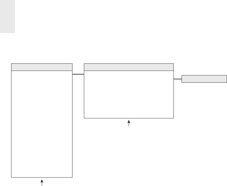
Chapter 6
182
such as the customer, sales rep, or deal involved, would need to traverse this large
dimension table.
Order Number (PK)
Order Date
Order Month
...
Requested Ship Date
Requested Ship Month
...
Customer ID
Customer Name
...
Sales Rep Number
Sales Rep Name
...
Deal ID
Deal Description
...
Order Number (FK)
Product Key (FK)
Order Line Number (DD)
Order Line Quantity
Extended Order Line Gross Dollar Amount
Extended Order Line Discount Dollar Amount
Extended Order Line Net Dollar Amount
1 row per Order Header
Order Line Transaction Fact
Product Dimension
Order Header Dimension
1 row per Order Line
Figure 6-9: Pattern to avoid: treating transaction header as a dimension.
Multiple Currencies
Suppose you track the orders of a large multinational U.S.-based company with sales
o ces around the world. You may be capturing order transactions in more than
15 di erent currencies. You certainly wouldn’t want to include columns in the fact
table for each currency.
The most common analytic requirement is that order transactions be expressed
in both the local transaction currency and the standardized corporate currency,
such as U.S. dollars in this example. To satisfy this need, each order fact would be
replaced with a pair of facts, one for the applicable local currency and another for
the equivalent standard corporate currency, as illustrated in Figure 6-10. The con-
version rate used to construct each fact row with the dual metrics would depend
on the business’s requirements. It might be the rate at the moment the order was
captured, an end of day rate, or some other rate based on defi ned business rules. This
technique would preserve the transactional metrics, plus allow all transactions to
easily roll up to the corporate currency without complicated reporting application
coding. The metrics in standard currency would be fully additive. The local currency
metrics would be additive only for a single specifi ed currency; otherwise, you’d be
trying to sum Japanese yen, Thai bhat, and British pounds. You’d also supplement

Order Management 183
the fact table with a currency dimension to identify the currency type associated
with the local currency facts; a currency dimension is needed even if the location
of the transaction is otherwise known because the location does not necessarily
guarantee which currency was used.
Order Date Key (FK)
Requested Ship Date Key (FK)
Customer Key (FK)
Product Key (FK)
Sales Rep Key (FK)
Deal Key (FK)
Local Currency Dimension Key (FK)
Order Number (DD)
Order Line Number (DD)
Order Line Quantity
Extended Order Line Gross USD Amount
Extended Order Line Discount USD Amount
Extended Order Line Net USD Amount
Extended Order Line Gross Local Currency Amount
Extended Order Line Discount Local Currency Amount
Extended Order Line Net Local Currency Amount
Local Currency Key (PK)
Local Currency Name
Local Currency Abbreviation
Local Currency Dimension
Order Line Transaction Fact
Figure 6-10: Metrics in multiple currencies within the fact table.
This technique can be expanded to support other relatively common examples.
If the business’s sales o ces roll up into a handful of regional centers, you could
supplement the fact table with a third set of metrics representing the transactional
amounts converted into the appropriate regional currency. Likewise, the fact table
columns could represent currencies for the customer ship-to and customer bill-to,
or the currencies as quoted and shipped.
In each of the scenarios, the fact table could physically contain a full set of metrics
in one currency, along with the appropriate currency conversion rate(s) for that row.
Rather than burdening the business users with appropriately multiplying or divid-
ing by the stored rate, the intra-row extrapolation should be done in a view behind
the scenes; all reporting applications would access the facts via this logical layer.
Sometimes the multi-currency support requirements are more complicated than
just described. You may need to allow a manager in any country to see order volume
in any currency. In this case, you can embellish the initial design with an additional
currency conversion fact table, as shown in Figure 6-11. The dimensions in this
fact table represent currencies, not countries, because the relationship between
currencies and countries is not one-to-one. The more common needs of the local
sales rep and sales management in headquarters would be met simply by querying
the orders fact table, but those with less predictable requirements would use the

Chapter 6
184
currency conversion table in a specially crafted query. Navigating the currency
conversion table is obviously more complicated than using the converted metrics
on the orders fact table.
Currency Conversion Fact
Conversion Date Key (FK)
Source Currency Key (FK)
Destination Currency Key (FK)
Source-Destination Exchange Rate
Destination-Source Exchange Rate
Figure 6-11: Tracking multiple currencies with daily currency exchange fact table.
Within each currency conversion fact table row, the amount expressed in local
currency is absolutely accurate because the sale occurred in that currency on that
day. The equivalent U.S. dollar value would be based on a conversion rate to U.S.
dollars for that day. The conversion rate table contains the combinations of rel-
evant currency exchange rates going in both directions because the symmetric
rates between two currencies are not equal. It is unlikely this conversion fact table
needs to include the full Cartesian product of all possible currency combinations.
Although there are approximately 100 unique currencies globally, there wouldn’t
need to be 10,000 daily rows in this currency fact table as there’s not a meaningful
market for every possible pair; likewise, all theoretical combinations are probably
overkill for the business users.
The use of a currency conversion table may also be required to support the busi-
ness’s need for multiple rates, such as an end of month or end of quarter close rate,
which may not be defi ned until long after the transactions have been loaded into
the orders fact table.
Transaction Facts at Different Granularity
It is quite common in header/line operational data to encounter facts of di ering
granularity. On an order, there may be a shipping charge that applies to the entire
order. The designer’s fi rst response should be to try to force all the facts down to
the lowest level, as illustrated in Figure 6-12. This procedure is broadly referred
to as allocating. Allocating the parent order facts to the child line item level is
critical if you want the ability to slice and dice and roll up all order facts by all
dimensions, including product.
Unfortunately, allocating header-level facts down to the line item level may entail
a political wrestling match. It is wonderful if the entire allocation issue is handled by
the fi nance department, not by the DW/BI team. Getting organizational agreement
on allocation rules is often a controversial and complicated process. The DW/BI team
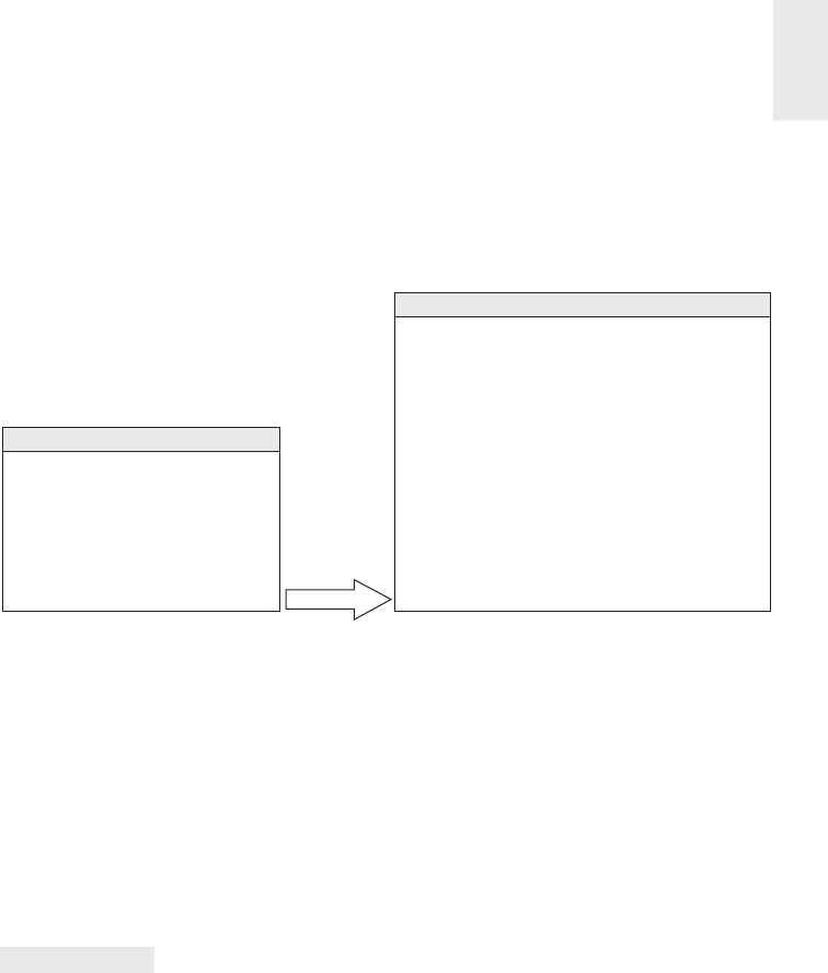
Order Management 185
shouldn’t be distracted and delayed by the inevitable organizational negotiation.
Fortunately, in many companies, the need to rationally allocate costs has already
been recognized. A task force, independent of the DW/BI project, already may have
established activity-based costing measures. This is just another name for allocating.
Allocated
Order Header Transaction Fact
Order Date Key (FK)
Requested Ship Date Key (FK)
Customer Key (FK)
Sales Rep Key (FK)
Deal Key (FK)
Order Number (PK)
Order Shipping Charges Dollar Amount
Order Line Transaction Fact
Order Date Key (FK)
Requested Ship Date Key (FK)
Customer Key (FK)
Product Key (FK)
Sales Rep Key (FK)
Deal Key (FK)
Order Number (DD)
Order Line Number (DD)
Order Line Quantity
Extended Order Line Gross Dollar Amount
Extended Order Line Discount Dollar Amount
Extended Order Line Net Dollar Amount
Allocated Order Line Shipping Charges Dollar Amount
Figure 6-12: Allocating header facts to line items.
If the shipping charges and other header-level facts cannot be successfully allo-
cated, they must be presented in an aggregate table for the overall order. We clearly
prefer the allocation approach, if possible, because the separate higher-level fact
table has some inherent usability issues. Without allocations, you cannot explore
header facts by product because the product isn’t identifi ed in a header-grain fact
table. If you are successful in allocating facts down to the lowest level, the problem
goes away.
WAR NI NG You shouldn’t mix fact granularities such as order header and order
line facts within a single fact table. Instead, either allocate the higher-level facts
to a more detailed level or create two separate fact tables to handle the di erently
grained facts. Allocation is the preferred approach.
Optimally, the business data stewards obtain enterprise consensus on the allocation
rules. But sometimes organizations refuse to agree. For example, the fi nance depart-
ment may want to allocate the header freight charged based on the extended gross
order amount on each line; meanwhile, the logistics group wants the freight charge
to be allocated based on the weight of the line’s products. In this case, you would
have two allocated freight charges on every order line fact table row; the uniquely
calculated metrics would also be uniquely labeled. Obviously, agreeing on a single,
standard allocation scheme is preferable.

Chapter 6
186
Design teams sometimes attempt to devise alternative techniques for handling
header/line facts at di erent granularity, including the following:
■ Repeat the unallocated header fact on every line. This approach is fraught
with peril given the risk of overstating the header amount when it’s summed
on every line.
■ Store the unallocated amount on the transaction’s fi rst or last line. This tac-
tic eliminates the risk of overcounting, but if the fi rst or last lines are excluded
from the query results due to a fi lter constraint on the product dimension, it
appears there were no header facts associated with this transaction.
■ Set up a special product key for the header fact. Teams who adopt this
approach sometimes recycle an existing line fact column. For example, if
product key = 99999, then the gross order metric is a header fact, like the
freight charge. Dimensional models should be straightforward and legible. You
don’t want to embed complexities requiring a business user to wear a special
decoder ring to navigate the dimensional model successfully.
Another Header/Line Pattern to Avoid
The second header/line pattern to avoid is illustrated in Figure 6-13. In this example,
the order header is no longer treated as a monolithic dimension but as a fact table
instead. The header’s associated descriptive information is grouped into dimen-
sions surrounding the order fact. The line item fact table (identical in structure and
granularity as the fi rst diagram) joins to the header fact based on the order number.
Order Date Dimension
Requested Ship Date Dimension
Deal Dimension
Order Header Transaction Fact
Customer Dimension
Sales Rep Dimension
Product Dimension
Order Date Key (FK)
Requested Ship Date Key (FK)
Customer Key (FK)
Sales Rep Key (FK)
Deal Key (FK)
Order Number (PK)
Extended Order Total Gross Dollar Amount
Extended Order Total Discount Dollar Amount
Extended Order Total Net Dollar Amount
Order Total Shipping Charges Dollar Amount
Order Line Transaction Fact
Order Number (FK)
Order Line Number (DD)
Product Key (FK)
Order Line Quantity
Extended Order Line Gross Dollar Amount
Extended Order Line Discount Dollar Amount
Extended Order Line Net Dollar Amount
Figure 6-13: Pattern to avoid: not inheriting header dimensionality in line facts.

Order Management 187
Again, this design accurately represents the parent/child relationship of the order
header and line items, but there are still fl aws. Every time the user wants to slice
and dice the line facts by any of the header attributes, a large header fact table needs
to be associated with an even larger line fact table.
Invoice Transactions
In a manufacturing company, invoicing typically occurs when products are shipped
from your facility to the customer. Visualize shipments at the loading dock as boxes
of product are placed into a truck destined for a particular customer address. The
invoice associated with the shipment is created at this time. The invoice has mul-
tiple line items, each corresponding to a particular product being shipped. Various
prices, discounts, and allowances are associated with each line item. The extended
net amount for each line item is also available.
Although you don’t show it on the invoice to the customer, a number of other
interesting facts are potentially known about each product at the time of shipment.
You certainly know list prices; manufacturing and distribution costs may be avail-
able as well. Thus you know a lot about the state of your business at the moment
of customer invoicing.
In the invoice fact table, you can see all the company’s products, customers,
contracts and deals, o -invoice discounts and allowances, revenue generated by
customers, variable and fi xed costs associated with manufacturing and delivering
products (if available), money left over after delivery of product (profi t contribution),
and customer satisfaction metrics such as on-time shipment.
NOTE For any company that ships products to customers or bills customers
for services rendered, the optimal place to start a DW/BI project typically is with
invoices. We often refer to invoicing as the most powerful data because it combines
the company’s customers, products, and components of profi tability.
You should choose the grain of the invoice fact table to be the individual invoice
line item. A sample invoice fact table associated with manufacturer shipments is
illustrated in Figure 6-14.
As expected, the invoice fact table contains a number of dimensions from earlier
in this chapter. The conformed date dimension table again would play multiple
roles in the fact table. The customer, product, and deal dimensions also would
conform, so you can drill across fact tables using common attributes. If a single
order number is associated with each invoice line item, it would be included as a
second degenerate dimension.

Chapter 6
188
Date Dimension (views for 3 roles)
Product Dimension
Deal Dimension
Shipper Dimension
Shipment Invoice Line Transaction Fact
Customer Dimension
Sales Rep Dimension
Warehouse Dimension
Service Level Dimension
Invoice Date Key (FK)
Requested Ship Date Key (FK)
Actual Ship Date Key (FK)
Customer Key (FK)
Product Key (FK)
Sales Rep Key (FK)
Deal Key (FK)
Warehouse Key (FK)
Shipper Key (FK)
Service Level Key (FK)
Invoice Number (DD)
Invoice Line Number (DD)
Invoice Line Quantity
Extended Invoice Line Gross Dollar Amount
Extended Invoice Line Allowance Dollar Amount
Extended Invoice Line Discount Dollar Amount
Extended Invoice Line Net Dollar Amount
Extended Invoice Line Fixed Mfg Cost Dollar Amount
Extended Invoice Line Variable Mfg Cost Dollar Amount
Extended Invoice Line Storage Cost Dollar Amount
Extended Invoice Line Distribution Cost Dollar Amount
Extended Invoice Line Contribution Dollar Amount
Shipment On-Time Counter
Requested to Actual Ship Lag
Figure 6-14: Shipment invoice fact table.
The shipment invoice fact table also contains some interesting new dimensions.
The warehouse dimension contains one row for each manufacturer warehouse loca-
tion. This is a relatively simple dimension with name, address, contact person, and
storage facility type. The attributes are somewhat reminiscent of the store dimension
from Chapter 3. The shipper dimension describes the method and carrier by which
the product was shipped from the manufacturer to the customer.
Service Level Performance as Facts,
Dimensions, or Both
The fact table in Figure 6-14 includes several critical dates intended to capture
shipment service levels. All these dates are known when the operational invoicing
process occurs. Delivering the multiple event dates in the invoicing fact table with
corresponding role-playing date dimensions allows business users to fi lter, group,
and trend on any of these dates. But sometimes the business requirements are more
demanding.
You could include an additional on-time counter in the fact table that’s set to an
additive zero or one depending on whether the line shipped on time. Likewise, you
could include lag metrics representing the number of days, positive or negative,
between the requested and actual ship dates. As described later in this chapter, the
lag calculation may be more sophisticated than the simple di erence between dates.

Order Management 189
In addition to the quantitative service metrics, you could also include a qualita-
tive assessment of performance by adding either a new dimension or adding more
columns to the junk dimension. Either way, the attribute values might look similar
to those shown in Figure 6-15.
On-time
Early
Early
Early
Too early
Late
Late
Late
Too late
1
2
3
4
5
6
7
8
9
On-time
1 day early
2 days early
3 days early
> 3 days early
1 day late
2 days late
3 days late
> 3 days late
Service Level
Key
Service Level
Description
Service Level
Group
Figure 6-15: Sample qualitative service level descriptors.
If service level performance at the invoice line is closely watched by business
users, you may embrace all the patterns just described, since quantitative metrics
with qualitative text provide di erent perspectives on the same performance.
Profi t and Loss Facts
If your organization has tackled activity-based costing or implemented a robust
enterprise resource planning (ERP) system, you might be in a position to identify
many of the incremental revenues and costs associated with shipping fi nished prod-
ucts to the customer. It is traditional to arrange these revenues and costs in sequence
from the top line, which represents the undiscounted value of the products shipped
to the customer, down to the bottom line, which represents the money left over after
discounts, allowances, and costs. This list of revenues and costs is referred to as a
profi t and loss (P&L) statement. You typically don’t attempt to carry it all the way
to a complete view of company profi t including general and administrative costs.
For this reason, the bottom line in the P&L statement is referred to as contribution.
Keeping in mind that each row in the invoice fact table represents a single line
item on the invoice, the elements of the P&L statement shown in Figure 6-14 have
the following interpretations:
■ Quantity shipped: Number of cases of the particular line item’s product.
The use of multiple equivalent quantities with di erent units of measure is
discussed in the section “Multiple Units of Measure.”
■ Extended gross amount: Also known as extended list price because it is the
quantity shipped multiplied by the list unit price. This and all subsequent

Chapter 6
190
dollar values are extended amounts or, in other words, unit rates multiplied by
the quantity shipped. This insistence on additive values simplifi es most access
and reporting applications. It is relatively rare for a business user to ask for
the unit price from a single fact table row. When the user wants an average
price drawn from many rows, the extended prices are fi rst added, and then
the result is divided by the sum of the quantities.
■ Extended allowance amount: Amount subtracted from the invoice line gross
amount for deal-related allowances. The allowances are described in the
adjoined deal dimension. The allowance amount is often called an o -invoice
allowance. The actual invoice may have several allowances for a given line
item; the allowances are combined together in this simplifi ed example. If
the allowances need to be tracked separately and there are potentially many
simultaneous allowances on a given line item, an allowance detail fact table
could augment the invoice line fact table, serving as a drill-down for details
on the allowance total in the invoice line fact table.
■ Extended discount amount: Amount subtracted for volume or payment term
discounts. The discount descriptions are found in the deal dimension. As
discussed earlier regarding the deal dimension, the decision to describe the
allowances and discount types together is the designer’s prerogative. It makes
sense to do this if allowances and discounts are correlated and business users
want to browse within the deal dimension to study the relationships between
allowances and discounts.
All allowances and discounts in this fact table are represented at the line
item level. As discussed earlier, some allowances and discounts may be cal-
culated operationally at the invoice level, not at the line item level. An effort
should be made to allocate them down to the line item. An invoice P&L state-
ment that does not include the product dimension poses a serious limitation
on your ability to present meaningful contribution slices of the business.
■ Extended net amount: Amount the customer is expected to pay for this line
item before tax. It is equal to the gross invoice amount less the allowances
and discounts.
The facts described so far likely would be displayed to the customer on the invoice
document. The following cost amounts, leading to a bottom line contribution, are
for internal consumption only.
■ Extended fi xed manufacturing cost: Amount identifi ed by manufacturing as
the pro rata fi xed manufacturing cost of the invoice line’s product.
■ Extended variable manufacturing cost: Amount identifi ed by manufacturing
as the variable manufacturing cost of the product on the invoice line. This
amount may be more or less activity-based, refl ecting the actual location and

Order Management 191
time of the manufacturing run that produced the product being shipped to
the customer. Conversely, this number may be a standard value set by a com-
mittee. If the manufacturing costs or any of the other storage and distribution
costs are averages of averages, the detailed P&Ls may become meaningless.
The DW/BI system may illuminate this problem and accelerate the adoption
of activity-based costing methods.
■ Extended storage cost: Cost charged to the invoice line for storage prior to
being shipped to the customer.
■ Extended distribution cost: Cost charged to the invoice line for transportation
from the point of manufacture to the point of shipment. This cost is notori-
ous for not being activity-based. The distribution cost possibly can include
freight to the customer if the company pays the freight, or the freight cost
can be presented as a separate line item in the P&L.
■ Contribution amount: Extended net invoice less all the costs just discussed. This
is not the true bottom line of the overall company because general and admin-
istrative expenses and other fi nancial adjustments have not been made, but it is
important nonetheless. This column sometimes has alternative labels, such as
margin, depending on the company culture.
You should step back and admire the robust dimensional model you just built.
You constructed a detailed P&L view of your business, showing all the activity-based
elements of revenue and costs. You have a full equation of profi tability. However,
what makes this design so compelling is that the P&L view sits inside a rich dimen-
sional framework of dates, customers, products, and causal factors. Do you want
to see customer profi tability? Just constrain and group on the customer dimension
and bring the components of the P&L into the report. Do you want to see product
profi tability? Do you want to see deal profi tability? All these analyses are equally
easy and take the same analytic form in the BI applications. Somewhat tongue in
cheek, we recommend you not deliver this dimensional model too early in your
career because you will get promoted and won’t be able to work directly on any
more DW/BI systems!
Profi tability Words of Warning
We must balance the last paragraph with a more sober note and pass along some
cautionary words of warning. It goes without saying that most of the business users
probably are very interested in granular P&L data that can be rolled up to analyze
customer and product profi tability. The reality is that delivering these detailed
P&L statements often is easier said than done. The problems arise with the cost
facts. Even with advanced ERP implementations, it is fairly common to be unable
to capture the cost facts at this atomic level of granularity. You will face a complex
process of mapping or allocating the original cost data down to the invoice line

Chapter 6
192
level. Furthermore, each type of cost may require a separate extraction from a
source system. Ten cost facts may mean 10 di erent extract and transformation
programs. Before signing up for mission impossible, be certain to perform a detailed
assessment of what is available and feasible from the source systems. You certainly
don’t want the DW/BI team saddled with driving the organization to consensus on
activity-based costing as a side project, on top of managing a number of parallel
extract implementations. If time and organization patience permits, profi tability is
often tackled as a consolidated dimensional model after the components of revenue
and cost have been sourced and delivered separately to business users in the DW/
BI environment.
Audit Dimension
As mentioned, Figure 6-14’s invoice line item design is one of the most powerful
because it provides a detailed look at customers, products, revenues, costs, and
bottom line profi t in one schema. During the building of rows for this fact table,
a wealth of interesting back room metadata is generated, including data quality
indicators, unusual processing requirements, and environment version numbers
that identify how the data was processed during the ETL. Although this metadata is
frequently of interest to ETL developers and IT management, there are times when
it can be interesting to the business users, too. For instance, business users might
want to ask the following:
■ What is my confi dence in these reported numbers?
■ Were there any anomalous values encountered while processing this source
data?
■ What version of the cost allocation logic was used when calculating the costs?
■ What version of the foreign currency conversion rules was used when calcu-
lating the revenues?
These kinds of questions are often hard to answer because the metadata required
is not readily available. However, if you anticipate these kinds of questions, you can
include an audit dimension with any fact table to expose the metadata context that
was true when the fact table rows were built. Figure 6-16 illustrates an example
audit dimension.
The audit dimension is added to the fact table by including an audit dimension
foreign key. The audit dimension itself contains the metadata conditions encountered
when processing fact table rows. It is best to start with a modest audit dimension
design, such as shown in Figure 6-16, both to keep the ETL processing from getting
too complicated and to limit the number of possible audit dimension rows. The fi rst
three attributes (quality indicator, out of bounds indicator, and amount adjusted fl ag)
are all sourced from a special ETL processing table called the error event table, which

Order Management 193
is discussed in Chapter 19: ETL Subsystems and Techniques. The cost allocation and
foreign currency versions are environmental variables that should be available in an
ETL back room status table.
Date Dimension (views for 3 roles)
Product Dimension
Deal Dimension
Shipper Dimension
Shipment Invoice Line Transaction Fact
Customer Dimension
Sales Rep Dimension
Warehouse Dimension
Service Level Dimension
Invoice Date Key (FK)
Requested Ship Date Key (FK)
Actual Ship Date Key (FK)
Customer Key (FK)
Product Key (FK)
Sales Rep Key (FK)
Deal Key (FK)
Warehouse Key (FK)
Shipper Key (FK)
Service Level Key (FK)
Audit Key (FK)
Invoice Number (DD)
Invoice Line Number (DD)
Invoice Line Quantity
Extended Invoice Line Gross Dollar Amount
...
Audit Dimension
Audit Key (PK)
Quality Indicator
Out of Bounds Indicator
Amount Adjusted Flag
Cost Allocation Version
Foreign Currency Version
Figure 6-16: Sample audit dimension included on invoice fact table.
Armed with the audit dimension, some powerful queries can be performed. You
might want to take this morning’s invoice report and ask if any of the reported
numbers were based on out-of-bounds measures. Because the audit dimension is
now just an ordinary dimension, you can just add the out-of-bounds indicator to
your standard report. In the resulting “instrumented” report shown in Figure 6-17,
you see multiple rows showing normal and abnormal out-of-bounds results.
Standard Report:
Axon
Axon
East
West
1,438
2,249
235,000
480,000
Product Warehouse
Invoice Line
Quantity
Extended Invoice Line
Gross Amount
Instrumented Reported (with Out of Bounds Indicator added):
Axon
Axon
Axon
Axon
East
East
West
West
Abnormal
Normal
Abnormal
Normal
14
1,424
675
1,574
Product Warehouse
Out of Bounds
Indicator
Invoice Line
Quantity
2,350
232,650
144,000
336,000
Extended Invoice Line
Gross Amount
Figure 6-17: Audit dimension attribute included on standard report.

Chapter 6
194
Accumulating Snapshot for Order
Fulfi llment Pipeline
The order management process can be thought of as a pipeline, especially in a
build-to-order manufacturing business, as illustrated in Figure 6-18. Customers
place an order that goes into the backlog until it is released to manufacturing to be
built. The manufactured products are placed in fi nished goods inventory and then
shipped to the customers and invoiced. Unique transactions are generated at each
spigot of the pipeline. Thus far we’ve considered each of these pipeline activities as
a separate transaction fact table. Doing so allows you to decorate the detailed facts
generated by each process with the greatest number of detailed dimensions. It also
allows you to isolate analysis to the performance of a single business process, which
is often precisely what the business users want.
Orders Backlog Shipment Invoicing
Release to
Manufacturing
Finished
Goods
Inventory
Figure 6-18: Order fulfi llment pipeline diagram.
However, there are times when business users want to analyze the entire order
fulfi llment pipeline. They want to better understand product velocity, or how quickly
products move through the pipeline. The accumulating snapshot fact table provides
this perspective of the business, as illustrated in Figure 6-19. It enables you to see
an updated status and ultimately the fi nal disposition of each order.
The accumulating snapshot complements alternative schemas’ perspectives of
the pipeline. If you’re interested in understanding the amount of product fl owing
through the pipeline, such as the quantity ordered, produced, or shipped, transac-
tion schemas monitor each of the pipeline’s major events. Periodic snapshots would
provide insight into the amount of product sitting in the pipeline, such as the
backorder or fi nished goods inventories, or the amount of product fl owing through
a pipeline spigot during a predefi ned interval. The accumulating snapshot helps
you better understand the current state of an order, as well as product movement
velocities to identify pipeline bottlenecks and ine ciencies. If you only captured
performance in transaction event fact tables, it would be wildly di cult to calculate
the average number of days to move between milestones.
The accumulating snapshot looks different from the transaction fact tables
designed thus far in this chapter. The reuse of conformed dimensions is to be
expected, but the number of date and fact columns is larger. Each date represents
a major milestone of the fulfi llment pipeline. The dates are handled as dimension

Order Management 195
roles by creating either physically distinct tables or logically distinct views. The date
dimension needs to have a row for Unknown or To Be Determined because many of
these fact table dates are unknown when a pipeline row is initially loaded. Obviously,
you don’t need to declare all the date columns in the fact table’s primary key.
Order Date Key (FK)
Backlog Date Key (FK)
Release to Manufacturing Date Key (FK)
Finished Inventory Placement Date Key (FK)
Requested Ship Date Key (FK)
Scheduled Ship Date Key (FK)
Actual Ship Date Key (FK)
Arrival Date Key (FK)
Invoice Date Key (FK)
Product Key (FK)
Customer Key (FK)
Sales Rep Key (FK)
Deal Key (FK)
Manufacturing Facility Key (FK)
Warehouse Key (FK)
Shipper Key (FK)
Order Number (DD)
Order Line Number (DD)
Invoice Number (DD)
Order Quantity
Extended Order Line Dollar Amount
Release to Manufacturing Quantity
Manufacturing Pass Inspection Quantity
Manufacturing Fail Inspection Quantity
Finished Goods Inventory Quantity
Authorized to Sell Quantity
Shipment Quantity
Shipment Damage Quantity
Customer Return Quantity
Invoice Quantity
Extended Invoice Dollar Amount
Order to Manufacturing Release Lag
Manufacturing Release to Inventory Lag
Inventory to Shipment Lag
Order to Shipment Lag
Customer Dimension
Shipper Dimension
Manufacturing Facility Dimension
Product Dimension
Deal Dimension
Warehouse Dimension
Order Fulfillment Accumulating Fact
Sales Rep Dimension
Date Dimension (views for 9 roles)
Figure 6-19: Order fulfi llment accumulating snapshot fact table.
The fundamental di erence between accumulating snapshots and other fact tables
is that you can revisit and update existing fact table rows as more information becomes
available. The grain of an accumulating snapshot fact table in Figure 6-19 is one row
per order line item. However, unlike the order transaction fact table illustrated in
Figure 6-2 with the same granularity, accumulating snapshot fact rows are modifi ed
while the order moves through the pipeline as more information is collected from
every stage of the cycle.

Chapter 6
196
NOTE Accumulating snapshot fact tables typically have multiple dates repre-
senting the major milestones of the process. However, just because a fact table
has several dates doesn’t dictate that it is an accumulating snapshot. The primary
di erentiator of an accumulating snapshot is that you revisit the fact rows as
activity occurs.
The accumulating snapshot technique is especially useful when the product mov-
ing through the pipeline is uniquely identifi ed, such as an automobile with a vehicle
identifi cation number, electronics equipment with a serial number, lab specimens
with an identifi cation number, or process manufacturing batches with a lot num-
ber. The accumulating snapshot helps you understand throughput and yield. If the
granularity of an accumulating snapshot is at the serial or lot number, you can see
the disposition of a discrete product as it moves through the manufacturing and test
pipeline. The accumulating snapshot fi ts most naturally with short-lived processes
with a defi nite beginning and end. Long-lived processes, such as bank accounts,
are typically better modeled with periodic snapshot fact tables.
Accumulating Snapshots and Type 2 Dimensions
Accumulating snapshots present the latest state of a workfl ow or pipeline. If the
dimensions associated with an accumulating snapshot contain type 2 attributes,
the fact table should be updated to reference the most current surrogate dimension
key for active pipelines. When a single fact table pipeline row is complete, the row
is typically not revisited to refl ect future type 2 changes.
Lag Calculations
The lengthy list of date columns captures the spans of time over which the order is
processed through the fulfi llment pipeline. The numerical di erence between any
two of these dates is a number that can be usefully averaged over all the dimensions.
These date lag calculations represent basic measures of fulfi llment e ciency. You
could build a view on this fact table that calculated a large number of these date
di erences and presented them as if they were stored in the underlying table. These
view columns could include metrics such as orders to manufacturing release lag,
manufacturing release to fi nished goods lag, and order to shipment lag, depending
on the date spans monitored by the organization.
Rather than calculating a simple di erence between two dates via a view, the
ETL system may calculate elapsed times that incorporate more intelligence, such
as workday lags that account for weekends and holidays rather than just the raw
number of days between milestone dates. The lag metrics may also be calculated
by the ETL system at a lower level of granularity (such as the number of hours or

Order Management 197
minutes between milestone events based on operational timestamps) for short-lived
and closely monitored processes.
Multiple Units of Measure
Sometimes, di erent functional organizations within the business want to see the
same performance metrics expressed in di erent units of measure. For instance,
manufacturing managers may want to see the product fl ow in terms of pallets or
shipping cases. Sales and marketing managers, on the other hand, may want to see
the quantities in retail cases, scan units (sales packs), or equivalized consumer units
(such as individual cans of soda).
Designers are tempted to bury the unit-of-measure conversion factors, such as
ship case factor, in the product dimension. Business users are then required to
appropriately multiply (or was it divide?) the order quantity by the conversion factor.
Obviously, this approach places a burden on users, in addition to being susceptible
to calculation errors. The situation is further complicated because the conversion
factors may change over time, so users would also need to determine which factor
is applicable at a specifi c point in time.
Rather than risk miscalculating the equivalent quantities by placing conversion
factors in a dimension table, they should be stored in the fact table instead. In the
orders pipeline fact table, assume you have 10 basic fundamental quantity facts, in
addition to fi ve units of measure. If you physically store all the facts expressed in
the di erent units of measure, you end up with 50 (10 × 5) facts in each fact row.
Instead, you can compromise by building an underlying physical row with 10 quan-
tity facts and 4 unit-of-measure conversion factors. You need only four conversion
factors rather than fi ve because the base facts are already expressed in one of the
units of measure. The physical design now has 14 quantity-related facts (10 + 4), as
shown in Figure 6-20. With this design, you can see performance across the value
chain based on di erent units of measure.
Of course, you would deliver this fact table to the business users through one
or more views. The extra computation involved in multiplying quantities by con-
version factors is negligible; intra-row computations are very e cient. The most
comprehensive view could show all 50 facts expressed in every unit of measure,
but the view could be simplifi ed to deliver only a subset of the quantities in units
of measure relevant to a user. Obviously, each unit of measures’ metrics should be
uniquely labeled.
NOTE Packaging all the facts and conversion factors together in the same fact
table row provides the safest guarantee that these factors will be used correctly.
The converted facts are presented in a view(s) to the users.

Chapter 6
198
Date Keys (FKs)
Product Key (FK)
More FKs...
Order Quantity Shipping Cases
Release to Manufacturing Quantity Shipping Cases
Manufacturing Pass Inspection Quantity Shipping Cases
Manufacturing Fail Inspection Quantity Shipping Cases
Finished Goods Inventory Quantity Shipping Cases
Authorized to Sell Quantity Shipping Cases
Shipment Quantity Shipping Cases
Shipment Damage Quantity Shipping Cases
Customer Return Quantity Shipping Cases
Invoice Quantity Shipping Cases
Pallet Conversion Factor
Retail Cases Conversion Factor
Scan Units Conversion Factor
Equivalized Consumer Units Conversion Factor
Order Fulfillment Accumulating Fact
Figure 6-20: Physical fact table supporting multiple units of measure with conversion
factors.
Finally, another side benefi t of storing these factors in the fact table is it reduces
the pressure on the product dimension table to issue new product rows to refl ect
minor conversion factor modifi cations. These factors, especially if they evolve rou-
tinely over time, behave more like facts than dimension attributes.
Beyond the Rearview Mirror
Much of what we’ve discussed in this chapter focuses on e ective ways to analyze
historical product movement performance. People sometimes refer to these as rear-
view mirror metrics because they enable you to look backward and see where you’ve
been. As the brokerage industry reminds people, past performance is no guarantee of
future results. Many organizations want to supplement these historical performance
metrics with facts from other processes to help project what lies ahead. For example,
rather than focusing on the pipeline at the time an order is received, organizations
are analyzing the key drivers impacting the creation of an order. In a sales organiza-
tion, drivers such as prospecting or quoting activity can be extrapolated to provide
visibility to the expected order activity volume. Many organizations do a better job
collecting the rearview mirror information than they do the early indicators. As these
front window leading indicators are captured, they can be added gracefully to the
DW/BI environment. They’re just more rows on the enterprise data warehouse bus
matrix sharing common dimensions.

Order Management 199
Summary
This chapter covered a lengthy laundry list of topics in the context of the order
management process. Multiples were discussed on several fronts: multiple references
to the same dimension in a fact table (role-playing dimensions), multiple equivalent
units of measure, and multiple currencies. We explored several of the common chal-
lenges encountered when modeling header/line transaction data, including facts at
di erent levels of granularity and junk dimensions, plus design patterns to avoid.
We also explored the rich set of facts associated with invoice transactions. Finally,
the order fulfi llment pipeline illustrated the power of accumulating snapshot fact
tables where you can see the updated status of a specifi c product or order as it moves
through a fi nite pi peline.

Accounting
Financial analysis spans a variety of accounting applications, including the gen-
eral ledger, as well as detailed subledgers for purchasing and accounts payable,
invoicing and accounts receivable, and fixed assets. Because we’ve already touched
upon purchase orders and invoices earlier in this book, we’ll focus on the general
ledger in this chapter. Given the need for accurate handling of a company’s financial
records, general ledgers were one of the first applications to be computerized decades
ago. Perhaps some of you are still running your business on a 20-year-old ledger
system. In this chapter, we’ll discuss the data collected by the general ledger, both
in terms of journal entry transactions and snapshots at the close of an accounting
period. We’ll also talk about the budgeting process.
Chapter 7 discusses the following concepts:
■ Bus matrix snippet for accounting processes
■ General ledger periodic snapshots and journal transactions
■ Chart of accounts
■ Period close
■ Year-to-date facts
■ Multiple fi scal accounting calendars
■ Drilling down through a multi-ledger hierarchy
■ Budgeting chain and associated processes
■ Fixed depth position hierarchies
■ Slightly ragged, variable depth hierarchies
■ Totally ragged hierarchies of indeterminate depth using a bridge table and
alternative modeling techniques
■ Shared ownership in a ragged hierarchy
■ Time varying ragged hierarchies
■ Consolidated fact tables that combine metrics from multiple business processes
■ Role of OLAP and packaged analytic fi nancial solutions
7

Chapter 7
202
Accounting Case Study and Bus Matrix
Because fi nance was an early adopter of technology, it comes as no surprise that
early decision support solutions focused on the analysis of fi nancial data. Financial
analysts are some of the most data-literate and spreadsheet-savvy individuals. Often
their analysis is disseminated or leveraged by many others in the organization.
Managers at all levels need timely access to key fi nancial metrics. In addition to
receiving standard reports, they need the ability to analyze performance trends, vari-
ances, and anomalies with relative speed and minimal e ort. Like many operational
source systems, the data in the general ledger is likely scattered among hundreds of
tables. Gaining access to fi nancial data and/or creating ad hoc reports may require
a decoder ring to navigate through the maze of screens. This runs counter to many
organizations’ objective to push fi scal responsibility and accountability to the line
managers.
The DW/BI system can provide a single source of usable, understandable fi nan-
cial information, ensuring everyone is working o the same data with common
defi nitions and common tools. The audience for fi nancial data is quite diverse in
many organizations, ranging from analysts to operational managers to executives.
For each group, you need to determine which subset of corporate fi nancial data is
needed, in which format, and with what frequency. Analysts and managers want to
view information at a high level and then drill to the journal entries for more detail.
For executives, fi nancial data from the DW/BI system often feeds their dashboard or
scorecard of key performance indicators. Armed with direct access to information,
managers can obtain answers to questions more readily than when forced to work
through a middleman. Meanwhile, fi nance can turn their attention to information
dissemination and value-added analysis, rather than focusing on report creation.
Improved access to accounting data allows you to focus on opportunities to better
manage risk, streamline operations, and identify potential cost savings. Although it
has cross-organization impact, many businesses focus their initial DW/BI implemen-
tation on strategic, revenue-generating opportunities. Consequently, accounting data
is often not the fi rst subject area tackled by the DW/BI team. Given its profi ciency
with technology, the fi nance department has often already performed magic with
spreadsheets and desktop databases to create workaround analytic solutions, per-
haps to its short-term detriment, as these imperfect interim fi xes are likely stressed
to their limits.
Figure 7-1 illustrates an accounting-focused excerpt from an organization’s bus
matrix. The dimensions associated with accounting processes, such as the general
ledger account or organizational cost center, are frequently used solely by these
processes, unlike the core customer, product, and employee dimensions which are
used repeatedly across many diverse business processes.
Accounting 203
General Ledger Transactions
General Ledger Snapshot
Budget
Commitment
Payments
Actual-Budget Variance
X
X
X
X
X
X
X
X
X
X
XX
X
X
X
X
X
X
X
X
X
X
XXXX
X
X
XX
Date
Ledger
Account
Organization
Budget Line
Commitment
Profile
Payment
Profile
Figure 7-1: Bus matrix rows for accounting processes.
General Ledger Data
The general ledger (G/L) is a core foundation fi nancial system that ties together the
detailed information collected by subledgers or separate systems for purchasing,
payables (what you owe to others), and receivables (what others owe you). As we
work through a basic design for G/L data, you’ll discover the need for two comple-
mentary schemas with periodic snapshot and transaction fact tables.
General Ledger Periodic Snapshot
We’ll begin by delving into a snapshot of the general ledger accounts at the end of
each fi scal period (or month if the fi scal accounting periods align with calendar
months). Referring back to our four-step process for designing dimensional models
(see Chapter 3: Retail Sales), the business process is the general ledger. The grain
of this periodic snapshot is one row per accounting period for the most granular
level in the general ledger’s chart of accounts.
Chart of Accounts
The cornerstone of the general ledger is the chart of accounts. The ledger’s chart of
accounts is the epitome of an intelligent key because it usually consists of a series of
identifi ers. For example, the fi rst set of digits may identify the account, account type
(for example, asset, liability, equity, income, or expense), and other account rollups.
Sometimes intelligence is embedded in the account numbering scheme. For example,
account numbers from 1,000 through 1,999 might be asset accounts, whereas account
numbers ranging from 2,000 to 2,999 may identify liabilities. Obviously, in the data

Chapter 7
204
warehouse, you’d include the account type as a dimension attribute rather than forc-
ing users to fi lter on the fi rst digit of the account number.
The chart of accounts likely associates the organization cost center with the
account. Typically, the organization attributes provide a complete rollup from cost
center to department to division, for example. If the corporate general ledger com-
bines data across multiple business units, the chart of accounts would also indicate
the business unit or subsidiary company.
Obviously, charts of accounts vary from organization to organization. They’re
often extremely complicated, with hundreds or even thousands of cost centers in
large organizations. In this case study vignette, the chart of accounts naturally
decomposes into two dimensions. One dimension represents accounts in the general
ledger, whereas the other represents the organization rollup.
The organization rollup may be a fi xed depth hierarchy, which would be handled
as separate hierarchical attributes in the cost center dimension. If the organization
hierarchy is ragged with an unbalanced rollup structure, you need the more power-
ful variable depth hierarchy techniques described in the section “Ragged Variable
Depth Hierarchies.”
If you are tasked with building a comprehensive general ledger spanning multiple
organizations in the DW/BI system, you should try to conform the chart of accounts
so the account types mean the same thing across organizations. At the data level,
this means the master conformed account dimension contains carefully defi ned
account names. Capital Expenditures and O ce Supplies need to have the same
fi nancial meaning across organizations. Of course, this kind of conformed dimen-
sion has an old and familiar name in fi nancial circles: the uniform chart of accounts.
The G/L sometimes tracks fi nancial results for multiple sets of books or sub-
ledgers to support di erent requirements, such as taxation or regulatory agency
reporting. You can treat this as a separate dimension because it’s such a fundamen-
tal fi lter, but we alert you to carefully read the cautionary note in the next section.
Period Close
At the end of each accounting period, the fi nance organization is responsible for
fi nalizing the fi nancial results so that they can be o cially reported internally
and externally. It typically takes several days at the end of each period to recon-
cile and balance the books before they can be closed with fi nance’s o cial stamp
of approval. From there, fi nance’s focus turns to reporting and interpreting the
results. It often produces countless reports and responds to countless variations
on the same questions each month.
Financial analysts are constantly looking to streamline the processes for period-
end closing, reconciliation, and reporting of general ledger results. Although
Accounting 205
operational general ledger systems often support these requisite capabilities, they
may be cumbersome, especially if you’re not dealing with a modern G/L. This chap-
ter focuses on easily analyzing the closed fi nancial results, rather than facilitating
the close. However, in many organizations, general ledger trial balances are loaded
into the DW/BI system leveraging the capabilities of the DW/BI presentation area
to fi nd the needles in the general ledger haystack, and then making the appropriate
operational adjustments before the period ends.
The sample schema in Figure 7-2 shows general ledger account balances at the
end of each accounting period which would be very useful for many kinds of fi nan-
cial analyses, such as account rankings, trending patterns, and period-to-period
comparisons.
Accounting Period Key (FK)
Ledger Key (FK)
Account Key (FK)
Organization Key (FK)
Period End Balance Amount
Period Debit Amount
Period Credit Amount
Period Net Change Amount
Account Key (PK)
Account Name
Account Category
Account Type
Accounting Period Key (PK)
Accounting Period Number
Accounting Period Description
Accounting Period Fiscal Year
Ledger Key (PK)
Ledger Book Name
Organization Key (PK)
Cost Center Name
Cost Center Number
Department Name
Department Number
Division Name
Business Unit Name
Company Name
Accounting Period Dimension General Ledger Snapshot Fact Ledger Dimension
Organization Dimension
Account Dimension
Figure 7-2: General ledger periodic snapshot.
For the moment, we’re just representing actual ledger facts in the Figure 7-2
schema; we’ll expand our view to cover budget data in the section “Budgeting
Process.” In this table, the balance amount is a semi-additive fact. Although the
balance doesn’t represent G/L activity, we include the fact in the design because
it is so useful. Otherwise, you would need to go back to the beginning of time to
calculate an accurate end-of-period balance.
WAR NI NG The ledger dimension is a convenient and intuitive dimension
that enables multiple ledgers to be stored in the same fact table. However, every
query that accesses this fact table must constrain the ledger dimension to a single
value (for example, Final Approved Domestic Ledger) or the queries will double
count values from the various ledgers in this table. The best way to deploy this
schema is to release separate views to the business users with the ledger dimension
pre-constrained to a single value.

Chapter 7
206
The two most important dimensions in the proposed general ledger design are
account and organization. The account dimension is carefully derived from the
uniform chart of accounts in the enterprise. The organization dimension describes
the fi nancial reporting entities in the enterprise. Unfortunately, these two crucial
dimensions almost never conform to operational dimensions such as customer,
product, service, or facility. This leads to a characteristic but unavoidable business
user frustration that the “GL doesn’t tie to my operational reports.” It is best to gently
explain this to the business users in the interview process, rather than promising
to fi x it because this is a deep seated issue in the underlying data.
Year-to-Date Facts
Designers are often tempted to store “to-date” columns in fact tables. They think
it would be helpful to store quarter-to-date or year-to-date additive totals on each
fact row so they don’t need to calculate them. Remember that numeric facts must
be consistent with the grain. To-date facts are not true to the grain and are fraught
with peril. When fact rows are queried and summarized in arbitrary ways, these
untrue-to-the-grain facts produce nonsensical, overstated results. They should be
left out of the relational schema design and calculated in the BI reporting application
instead. It’s worth noting that OLAP cubes handle to-date metrics more gracefully.
NOTE In general, “to-date” totals should be calculated, not stored in the
fact table.
Multiple Currencies Revisited
If the general ledger consolidates data that has been captured in multiple curren-
cies, you would handle it much as we discussed in Chapter 6: Order Management.
With fi nancial data, you typically want to represent the facts both in terms of the
local currency, as well as a standardized corporate currency. In this case, each
fact table row would represent one set of fact amounts expressed in local currency
and a separate set of fact amounts on the same row expressed in the equivalent
corporate currency. Doing so allows you to easily summarize the facts in a com-
mon corporate currency without jumping through hoops in the BI applications.
Of course, you’d also add a currency dimension as a foreign key in the fact table
to identify the local currency type.
General Ledger Journal Transactions
While the end-of-period snapshot addresses a multitude of fi nancial analyses, many
users need to dive into the underlying details. If an anomaly is identifi ed at the

Accounting 207
summary level, analysts want to look at the detailed transactions to sort through
the issue. Others need access to the details because the summarized monthly bal-
ances may obscure large disparities at the granular transaction level. Again, you
can complement the periodic snapshot with a detailed journal entry transaction
schema. Of course, the accounts payable and receivable subledgers may contain
transactions at progressively lower levels of detail, which would be captured in
separate fact tables with additional dimensionality.
The grain of the fact table is now one row for every general ledger journal entry
transaction. The journal entry transaction identifi es the G/L account and the appli-
cable debit or credit amount. As illustrated in Figure 7-3, several dimensions from
the last schema are reused, including the account and organization. If the ledger
tracks multiple sets of books, you’d also include the ledger/book dimension. You
would normally capture journal entry transactions by transaction posting date,
so use a daily-grained date table in this schema. Depending on the business rules
associated with the source data, you may need a second role-playing date dimension
to distinguish the posting date from the e ective accounting date.
Post Date Key (FK)
Journal Entry Effective Date/Time
Ledger Key (FK)
Account Key (FK)
Organization Key (FK)
Debit-Credit Indicator Key (FK)
Journal Entry Number (DD)
Journal Entry Amount
Debit-Credit Indicator Key (PK)
Debit-Credit Indicator Description
General Ledger Journal Entry Fact
Ledger Dimension
Organization Dimension
Post Date Dimension
Account Dimension
Debit-Credit Indicator Dimension
Figure 7-3: General ledger journal entry transactions.
The journal entry number is likely a degenerate dimension with no linkage to
an associated dimension table. If the journal entry numbers from the source are
ordered, then this degenerate dimension can be used to order the journal entries
because the calendar date dimension on this fact table is too coarse to provide this
sorting. If the journal entry numbers do not easily support the sort, then an e ective
date/time stamp must be added to the fact table. Depending on the source data, you
may have a journal entry transaction type and even a description. In this situation,
you would create a separate journal entry transaction profi le dimension (not shown).
Assuming the descriptions are not just freeform text, this dimension would have
signifi cantly fewer rows than the fact table, which would have one row per journal
entry line. The specifi c journal entry number would still be treated as degenerate.
Each row in the journal entry fact table is identifi ed as either a credit or a debit.
The debit/credit indicator takes on two, and only two, values.

Chapter 7
208
Multiple Fiscal Accounting Calendars
In Figure 7-3, the data is captured by posting date, but users may also want to
summarize the data by fi scal account period. Unfortunately, fi scal accounting peri-
ods often do not align with standard Gregorian calendar months. For example, a
company may have 13 4-week accounting periods in a fi scal year that begins on
September 1 rather than 12 monthly periods beginning on January 1. If you deal
with a single fi scal calendar, then each day in a year corresponds to a single calendar
month, as well as a single accounting period. Given these relationships, the calendar
and accounting periods are merely hierarchical attributes on the daily date dimen-
sion. The daily date dimension table would simultaneously conform to a calendar
month dimension table, as well as to a fi scal accounting period dimension table.
In other situations, you may deal with multiple fi scal accounting calendars that
vary by subsidiary or line of business. If the number of unique fi scal calendars is a
fi xed, low number, then you can include each set of uniquely labeled fi scal calendar
attributes on a single date dimension. A given row in the daily date dimension would
be identifi ed as belonging to accounting period 1 for subsidiary A but accounting
period 7 for subsidiary B.
In a more complex situation with a large number of di erent fi scal calendars,
you could identify the o cial corporate fi scal calendar in the date dimension. You
then have several options to address the subsidiary-specifi c fi scal calendars. The
most common approach is to create a date dimension outrigger with a multipart key
consisting of the date and subsidiary keys. There would be one row in this table for
each day for each subsidiary. The attributes in this outrigger would consist of fi s-
cal groupings (such as fi scal week end date and fi scal period end date). You would
need a mechanism for fi ltering on a specifi c subsidiary in the outrigger. Doing so
through a view would then allow the outrigger to be presented as if it were logically
part of the date dimension table.
A second approach for tackling the subsidiary-specifi c calendars would be to
create separate physical date dimensions for each subsidiary calendar, using a
common set of surrogate date keys. This option would likely be used if the fact
data were decentralized by subsidiary. Depending on the BI tool’s capabilities, it
may be easier to either fi lter on the subsidiary outrigger as described in option
1 or ensure usage of the appropriate subsidiary-specifi c physical date dimension
table (option 2). Finally, you could allocate another foreign key in the fact table to
a subsidiary fi scal period dimension table. The number of rows in this table would
be the number of fi scal periods (approximately 36 for 3 years) times the number of
unique calendars. This approach simplifi es user access but puts additional strain
on the ETL system because it must insert the appropriate fi scal period key during
the transformation process.

Accounting 209
Drilling Down Through a Multilevel Hierarchy
Very large enterprises or government agencies may have multiple ledgers arranged
in an ascending hierarchy, perhaps by enterprise, division, and department. At the
lowest level, department ledger entries may be consolidated to roll up to a single
division ledger entry. Then the division ledger entries may be consolidated to the
enterprise level. This would be particularly common for the periodic snapshot grain
of these ledgers. One way to model this hierarchy is by introducing the parent snap-
shot’s fact table surrogate key in the fact table, as shown in Figure 7-4. In this case,
because you defi ne a parent/child relationship between rows, you add an explicit
fact table surrogate key, a single column numeric identifi er incremented as you add
rows to the fact table.
Fact Table Surrogate Key (PK)
Accounting Period Key (FK)
Ledger Key (FK)
Account Key (FK)
Organization Key (FK)
Parent Snapshot Key (FK)
Period End Balance Amount
Period Debit Amount
Period Credit Amount
Period Net Change Amount
General Ledger Snapshot Fact
Ledger Dimension
Organization Dimension
Accounting Period Dimension
Account Dimension
Figure 7-4: Design for drilling down through multiple ledgers.
You can use the parent snapshot surrogate key to drill down in your multilayer
general ledger. Suppose that you detect a large travel amount at the top level of the
ledger. You grab the surrogate key for that high-level entry and then fetch all the entries
whose parent snapshot key equals that key. This exposes the entries at the next lower
level that contribute to the original high-level record of interest. The SQL would look
something like this:
Select * from GL_Fact where Parent_Snapshot_key =
(select fact_table_surrogate_key from GL_Fact f, Account a
where <joins> and a.Account = 'Travel' and f.Amount > 1000)
Financial Statements
One of the primary functions of a general ledger system is to produce the organiza-
tion’s o cial fi nancial reports, such as the balance sheet and income statement. The
operational system typically handles the production of these reports. You wouldn’t
want the DW/BI system to attempt to replace the reports published by the opera-
tional fi nancial systems.

Chapter 7
210
However, DW/BI teams sometimes create complementary aggregated data that
provides simplifi ed access to report information that can be more widely dissemi-
nated throughout the organization. Dimensions in the fi nancial statement schema
would include the accounting period and cost center. Rather than looking at general
ledger account level data, the fact data would be aggregated and tagged with the
appropriate fi nancial statement line number and label. In this manner, managers
could easily look at performance trends for a given line in the fi nancial statement
over time for their organization. Similarly, key performance indicators and fi nancial
ratios may be made available at the same level of detail.
Budgeting Process
Most modern general ledger systems include the capability to integrate budget data
into the general ledger. However, if the G/L either lacks this capability or it has not
been implemented, you need to provide an alternative mechanism for supporting
the budgeting process and variance comparisons.
Within most organizations, the budgeting process can be viewed as a series of
events. Prior to the start of a fi scal year, each cost center manager typically creates a
budget, broken down by budget line items, which is then approved. In reality, bud-
geting is seldom simply a once-per-year event. Budgets are becoming more dynamic
because there are budget adjustments as the year progresses, refl ecting changes in
business conditions or the realities of actual spending versus the original budget.
Managers want to see the current budget’s status, as well as how the budget has
been altered since the fi rst approved version. As the year unfolds, commitments to
spend the budgeted monies are made. Finally, payments are processed.
As a dimensional modeler, you can view the budgeting chain as a series of fact
tables, as shown in Figure 7-5. This chain consists of a budget fact table, commit-
ments fact table, and payments fact table, where there is a logical fl ow that starts
with a budget being established for each organization and each account. Then dur-
ing the operational period, commitments are made against the budgets, and fi nally
payments are made against those commitments.
We’ll begin with the budget fact table. For an expense budget line item, each row
identifi es what an organization in the company is allowed to spend for what purpose
during a given time frame. Similarly, if the line item refl ects an income forecast,
which is just another variation of a budget, it would identify what an organization
intends to earn from what source during a time frame.
You could further identify the grain to be a snapshot of the current status of
each line item in each budget each month. Although this grain has a familiar ring
to it (because it feels like a management report), it is a poor choice as the fact table
Accounting 211
grain. The facts in such a “status report” are all semi-additive balances, rather than
fully additive facts. Also, this grain makes it di cult to determine how much has
changed since the previous month or quarter because you must obtain the rows
from several time periods and then subtract them from each other. Finally, this grain
choice would require the fact table to contain many duplicated rows when nothing
changes in successive months for a given line item.
Month Key (FK)
Organization Key (FK)
Account Key (FK)
Budget Key (FK)
Budget Amount
Month Key (FK)
Organization Key (FK)
Account Key (FK)
Budget Key (FK)
Commitment Key (FK)
Commitment Amount
Month Key (FK)
Organization Key (FK)
Account Key (FK)
Budget Key (FK)
Commitment Key (FK)
Payment Key (FK)
Payment Amount
Budget Key (PK)
Budget Name
Budget Version
Budget Approval Date
Commitment Key (PK)
Commitment Description
Commitment Party
Payment Key (PK)
Payment Description
Payment Party
Organization Dimension
Budget Dimension
Organization Dimension
Budget Dimension
Organization Dimension
Budget Dimension
Payment Dimension
Payment Fact
Account Dimension
Month Dimension
Account Dimension
Commitment Dimension
Month Dimension
Account Dimension
Commitment Dimension
Month Dimension
Budget Fact
Commitment Fact
Figure 7-5: Chain of budget processes.
Instead, the grain you’re interested in is the net change of the budget line item
in an organizational cost center that occurred during the month. Although this
su ces for budget reporting purposes, the accountants eventually need to tie the
budget line item back to a specifi c general ledger account that’s a ected, so you’ll
also go down to the G/L account level.

Chapter 7
212
Given the grain, the associated budget dimensions would include e ective
month, organization cost center, budget line item, and G/L account, as illustrated
in Figure 7-6. The organization is identical to the dimension used earlier with the
general ledger data. The account dimension is also a reused dimension. The only
complication regarding the account dimension is that sometimes a single budget
line item impacts more than one G/L account. In that case, you would need to
allocate the budget line to the individual G/L accounts. Because the grain of the
budget fact table is by G/L account, a single budget line for a cost center may be
represented as several rows in the fact table.
Effective Date Dimension
Account Dimension
Organization Dimension
Budget Line Item Dimension
Budget Effective Date Key (PK)
Budget Effective Date Month
Budget Effective Date Year
...
Budget Effective Date Key (FK)
Budget Line Item Key (FK)
Account Key (FK)
Organization Key (FK)
Budget Amount
Budget Line Item Key (PK)
Budget Name
Budget Version
Budget Line Description
Budget Year
Budget Line Subcategory Description
Budget Line Category Description
Budget Fact
Figure 7-6: Budget schema.
The budget line item identifi es the purpose of the proposed spending, such as
employee wages or o ce supplies. There are typically several levels of summariza-
tion categories associated with a budget line item. All the budget line items may not
have the same number of levels in their summarization hierarchy, such as when some
only have a category rollup, but not a subcategory. In this case, you may populate the
dimension attributes by replicating the category name in the subcategory column to
avoid having line items roll up to a Not Applicable subcategory bucket. The budget
line item dimension would also identify the budget year and/or budget version.
The e ective month is the month during which the budget changes are posted.
The fi rst entries for a given budget year would show the e ective month when the
budget is fi rst approved. If the budget is updated or modifi ed as the budget year
gets underway, the e ective months would occur during the budget year. If you
don’t adjust a budget throughout the year, then the only entries would be the fi rst
ones when the budget is initially approved. This is what is meant when the grain
is specifi ed to be the net change. It’s critical that you understand this point, or you
won’t understand what is in this budget fact table or how it’s used.
Sometimes budgets are created as annual spending plans; other times, they’re
broken down by month or quarter. Figure 7-6 assumes the budget is an annual
amount, with the budget year identifi ed in the budget line item dimension. If you
need to express the budget data by spending month, you would need to include a
second month dimension table that plays the role of spending month.

Accounting 213
The budget fact table has a single budget amount fact that is fully additive. If you
budget for a multinational organization, the budget amount may be tagged with the
expected currency conversion factor for planning purposes. If the budget amount
for a given budget line and account is modifi ed during the year, an additional row
is added to the budget fact table representing the net change. For example, if the
original budget were $200,000, you might have another row in June for a $40,000
increase and then another in October for a negative $25,000 as you tighten your
belt going into year-end.
When the budget year begins, managers make commitments to spend the budget
through purchase orders, work orders, or other forms of contracts. Managers are
keenly interested in monitoring their commitments and comparing them to the
annual budget to manage their spending. We can envision a second fact table for
the commitments (refer to Figure 7-5) that shares the same dimensions, in addi-
tion to dimensions identifying the specifi c commitment document (purchase order,
work order, or contract) and commitment party. In this case, the fact would be the
committed amount.
Finally, payments are made as monies are transferred to the party named in the
commitment. From a practical point of view, the money is no longer available in
the budget when the commitment is made. But the fi nance department is interested
in the relationship between commitments and payments because it manages the
company’s cash. The dimensions associated with the payments fact table would
include the commitment fact table dimensions, plus a payment dimension to identify
the type of payment, as well as the payee to whom the payment was actually made.
Referring the budgeting chain shown in Figure 7-5, the list of dimensions expands
as you move from the budget to commitments to payments.
With this design, you can create a number of interesting analyses. To look at
the current budgeted amount by department and line item, you can constrain
on all dates up to the present, adding the amounts by department and line item.
Because the grain is the net change of the line items, adding up all the entries
over time does exactly the right thing. You end up with the current approved
budget amount, and you get exactly those line items in the given departments
that have a budget.
To ask for all the changes to the budget for various line items, simply constrain
on a single month. You’ll report only those line items that experienced a change
during the month.
To compare current commitments to the current budget, separately sum the
commitment amounts and budget amounts from the beginning of time to the cur-
rent date (or any date of interest). Then combine the two answer sets on the row
headers. This is a standard drill-across application using multipass SQL. Similarly,
you could drill across commitments and payments.

Chapter 7
214
Dimension Attribute Hierarchies
Although the budget chain use case described in this chapter is reasonably simple,
it contains a number of hierarchies, along with a number of choices for the designer.
Remember a hierarchy is defi ned by a series of many-to-one relationships. You likely
have at least four hierarchies: calendar levels, account levels, geographic levels, and
organization levels.
Fixed Depth Positional Hierarchies
In the budget chain, the calendar levels are familiar fi xed depth position hierarchies.
As the name suggests, a fi xed position hierarchy has a fi xed set of levels, all with
meaningful labels. Think of these levels as rollups. One calendar hierarchy may
be day ➪ fi scal period ➪ year. Another could be day ➪ month ➪ year. These two
hierarchies may be di erent if there is no simple relationship between fi scal periods
and months. For example, some organizations have 5-4-4 fi scal periods, consisting
of a 5-week span followed by two 4-week spans. A single calendar date dimension
can comfortably represent these two hierarches at the same time in sets of parallel
attributes since the grain of the date dimension is the individual day.
The account dimension may also have a fi xed many-to-one hierarchy such as
executive level, director level, and manager level accounts. The grain of the dimen-
sion is the manager level account, but the detailed accounts at the lowest grain roll
up to the director and executive levels.
In a fi xed position hierarchy, it is important that each level have a specifi c name.
That way the business user knows how to constrain and interpret each level.
WAR NI NG Avoid fi xed position hierarchies with abstract names such as Level-1,
Level-2, and so on. This is a cheap way to avoid correctly modeling a ragged hierar-
chy. When the levels have abstract names, the business user has no way of knowing
where to place a constraint, or what the attribute values in a level mean in a report.
If a ragged hierarchy attempts to hide within a fi xed position hierarchy with abstract
names, the individual levels are essentially meaningless.
Slightly Ragged Variable Depth Hierarchies
Geographic hierarchies present an interesting challenge. Figure 7-7 shows three
possibilities. The simple location has four levels: address, city, state, and country.
The medium complex location adds a zone level, and the complex location adds
both district and zone levels. If you need to represent all three types of locations

Accounting 215
in a single geographic hierarchy, you have a slightly variable hierarchy. You can
combine all three types if you are willing to make a compromise. For the medium
location that has no concept of district, you can propagate the city name down into
the district attribute. For the simple location that has no concept of either district or
zone, you can propagate the city name down into both these attributes. The business
data governance representatives may instead decide to propagate labels upward or
even populate the empty levels with Not Applicable. The business representatives
need to visualize the appropriate row label values on a report if the attribute is
grouped on. Regardless of the business rules applied, you have the advantage of a
clean positional design with attribute names that make reasonable sense across all
three geographies. The key to this compromise is the narrow range of geographic
hierarchies, ranging from four levels to only six levels. If the data ranged from
four levels to eight or ten or even more, this design compromise would not work.
Remember the attribute names need to make sense.
Simple Loc
Loc Key (PK)
Address+
City
City
City
State
Country
...
Medium Loc
Loc Key (PK)
Address+
City
City
Zone
State
Country
...
Complex Loc
Loc Key (PK)
Address+
City
District
Zone
State
Country
...
Figure 7-7: Sample data values exist simultaneously in a single location dimension
containing simple, intermediate, and complex hierarchies.
Ragged Variable Depth Hierarchies
In the budget use case, the organization structure is an excellent example of a ragged
hierarchy of indeterminate depth. In this chapter, we often refer to the hierarchical struc-
ture as a “tree” and the individual organizations in that tree as “nodes.” Imagine your
enterprise consists of 13 organizations with the rollup structure shown in Figure 7-8.
Each of these organizations has its own budget, commitments, and payments.
For a single organization, you can request a specifi c budget for an account with a
simple join from the organization dimension to the fact table, as shown in Figure 7-9.
But you also want to roll up the budget across portions of the tree or even all the tree.
Figure 7-9 contains no information about the organizational rollup.
Chapter 7
216
1
2
34
56 10 13
11 12
89
7
Figure 7-8: Organization rollup structure.
Organization Dimension
Posting Date Key (FK)
Organization Key (FK)
Account Key (FK)
Transaction Key (FK)
Ledger Key (FK)
Transaction ID (DD)
Amount
Balance
Organization Key (PK)
Organization Name
...
General Ledger Fact
Figure 7-9: Organization dimension joined to fact table.
The classic way to represent a parent/child tree structure is by placing recur-
sive pointers in the organization dimension from each row to its parent, as shown
in Figure 7-10. The original defi nition of SQL did not provide a way to evaluate
these recursive pointers. Oracle implemented a CONNECT BY function that traversed
these pointers in a downward fashion starting at a high-level parent in the tree
and progressively enumerated all the child nodes in lower levels until the tree
was exhausted. But the problem with Oracle CONNECT BY and other more general
approaches, such as SQL Server’s recursive common table expressions, is that the
representation of the tree is entangled with the organization dimension because
these approaches depend on the recursive pointer embedded in the data. It is imprac-
tical to switch from one rollup structure to another because many of the recursive
pointers would have to be destructively modifi ed. It is also impractical to maintain
organizations as type 2 slowly changing dimension attributes because changing the
key for a high-level node would ripple key changes down to the bottom of the tree.
The solution to the problem of representing arbitrary rollup structures is to build
a special kind of bridge table that is independent from the primary dimension table
and contains all the information about the rollup. The grain of this bridge table is

Accounting 217
each path in the tree from a parent to all the children below that parent, as shown
in Figure 7-11. The fi rst column in the map table is the primary key of the parent,
and the second column is the primary key of the child. A row must be constructed
from each possible parent to each possible child, including a row that connects the
parent to itself.
Organization Dimension
Organization Key (PK)
Organization Name
...
Organization Parent Key (FK)
Recursive
Pointer
Figure 7-10: Classic parent/child recursive design.
The example tree depicted in Figure 7-8 results in 43 rows in Figure 7-11. There
are 13 paths from node number 1, 5 paths from node number 2, one path from node
number 3 to itself, as so on.
The highest parent fl ag in the map table means the particular path comes from
the highest parent in the tree. The lowest child fl ag means the particular path ends
in a “leaf node” of the tree.
If you constrain the organization dimension table to a single row, you can join
the dimension table to the map table to the fact table, as shown in Figure 7-12. For
example, if you constrain the organization table to node number 1 and simply fetch
an additive fact from the fact table, you get 13 hits on the fact table, which traverses
the entire tree in a single query. If you perform the same query except constrain the
map table lowest child fl ag to true, then you fetch only the additive fact from the six
leaf nodes, numbers 3, 5, 6, 8, 10, and 11. Again, this answer was computed without
traversing the tree at query time!
NOTE The article “Building Hierarchy Bridge Tables” (available at www
.kimballgroup.com under the Tools and Utilities tab for this book title) provides
a code example for building the hierarchy bridge table described in this section.
You must be careful when using the map bridge table to constrain the organization
dimension to a single row, or else you risk overcounting the children and grandchil-
dren in the tree. For example, if instead of a constraint such as “Node Organization
Number = 1” you constrain on “Node Organization Location = California”, you
would have this problem. In this case you need to craft a custom query, rather than
a simple join, with the following constraint:
GLfact.orgkey in (select distinct bridge.childkey
from innerorgdim, bridge
where innerorgdim.state = 'California' and
innerorgdim.orgkey = bridge.parentkey)

Chapter 7
218
1
1
1
1
1
1
1
1
1
1
1
1
1
2
2
2
2
2
3
4
4
4
5
6
7
7
8
7
7
7
7
7
9
9
9
9
9
10
10
10
11
12
13
Parent
Organization
Key
Depth from
Parent
Highest
Parent
Flag
Lowest
Child
Flag
Child
Organization
Key
1
2
3
4
5
6
7
8
9
10
11
12
13
2
3
4
5
6
3
4
5
6
5
6
7
8
8
9
10
11
12
13
9
10
11
12
13
10
11
12
11
12
13
0
1
2
2
3
3
1
2
2
3
4
4
3
0
1
1
2
2
0
0
1
1
0
0
0
1
0
1
2
3
3
2
0
1
2
2
1
0
1
1
0
0
0
TRUE
TRUE
TRUE
TRUE
TRUE
TRUE
TRUE
TRUE
TRUE
TRUE
TRUE
TRUE
TRUE
FALSE
FALSE
FALSE
FALSE
FALSE
FALSE
FALSE
FALSE
FALSE
FALSE
FALSE
FALSE
FALSE
FALSE
FALSE
FALSE
FALSE
FALSE
FALSE
FALSE
FALSE
FALSE
FALSE
FALSE
FALSE
FALSE
FALSE
FALSE
FALSE
FALSE
FALSE
FALSE
TRUE
FALSE
TRUE
TRUE
FALSE
TRUE
FALSE
FALSE
TRUE
TRUE
TRUE
FALSE
TRUE
FALSE
TRUE
TRUE
TRUE
FALSE
TRUE
TRUE
TRUE
TRUE
FALSE
TRUE
TRUE
FALSE
FALSE
TRUE
TRUE
TRUE
FALSE
FALSE
TRUE
TRUE
TRUE
FALSE
TRUE
TRUE
TRUE
TRUE
TRUE
Organization Map Bridge
Parent Organization Key (FK)
Child Organization Key (FK)
Depth from Parent
Highest Parent Flag
Lowest Child Flag
Sample Organization Map bridge table rows for Figure 7-8:
Figure 7-11: Organization map bridge table sample rows.

Accounting 219
Organization Map Bridge
Parent Organization Key (FK)
Child Organization Key (FK)
Depth from Parent
Highest Parent Flag
Lowest Child Flag
Organization Dimension
Organization Key (PK)
Organization Name
...
Posting Date Key (FK)
Organization Key (FK)
Account Key (FK)
Transaction Profile Key (FK)
Ledger Version Key (FK)
Transaction ID (DD)
Amount
Balance
General Ledger Fact
FIGURE 7-12: Joining organization map bridge table to fact table.
Shared Ownership in a Ragged Hierarchy
The map table can represent partial or shared ownership, as shown in Figure 7-13.
For instance, suppose node 10 is 50 percent owned by node 6 and 50 percent
owned by node 11. In this case, any budget or commitment or payment attributed
to node 10 fl ows upward through node 6 with a 50 percent weighting and also
upward through node 11 with a 50 percent weighting. You now need to add extra
path rows to the original 43 rows to accommodate the connection of node 10 up
to node 6 and its parents. All the relevant path rows ending in node 10 now need
a 50 percent weighting in the ownership percentage column in the map table.
Other path rows not ending in node 10 do not have their ownership percentage
column changed.
Organization Map Bridge
Parent Organization Key (FK)
Child Organization Key (FK)
Depth from Parent
Highest Parent Flag
Lowest Child Flag
Percent Ownership
Organization Dimension
Organization Key (PK)
Organization Name
...
Posting Date Key (FK)
Organization Key (FK)
Account Key (FK)
Transaction Profile Key (FK)
Ledger Version Key (FK)
Transaction ID (DD)
Amount
Balance
General Ledger Fact
FIGURE 7-13: Bridge table for ragged hierarchy with shared ownership.

Chapter 7
220
Time Varying Ragged Hierarchies
The ragged hierarchy bridge table can accommodate slowly changing hierarchies
with the addition of two date/time stamps, as shown in Figure 7-14. When a given
node no longer is a child of another node, the end e ective date/time of the old
relationship must be set to the date/time of the change, and new path rows inserted
into the bridge table with the correct begin e ective date/time.
Organization Map Bridge
Parent Organization Key (FK)
Child Organization Key (FK)
Depth from Parent
Highest Parent Flag
Lowest Child Flag
Begin Effective Date/Time
End Effective Date/Time
Organization Dimension
Organization Key (PK)
Organization Name
...
Posting Date Key (FK)
Organization Key (FK)
Account Key (FK)
Transaction Profile Key (FK)
Ledger Version Key (FK)
Transaction ID (DD)
Amount
Balance
General Ledger Fact
Figure 7-14: Bridge table for time varying ragged hierarchies.
WAR NI NG When using the bridge table in Figure 7-14, the query must always
constrain to a single date/time to “freeze” the bridge table to a single consistent
view of the hierarchy. Failing to constrain in this way otherwise would result in
multiple paths being fetched that could not exist at the same time.
Modifying Ragged Hierarchies
The organization map bridge table can easily be modifi ed. Suppose you want to
move nodes 4, 5, and 6 from their original location reporting up to node 2 to a new
location reporting up to node 9, as shown in Figure 7-15.
In the static case in which the bridge table only refl ects the current rollup struc-
ture, you merely delete the higher level paths in the tree pointing into the group
of nodes 4, 5, and 6. Then you attach nodes 4, 5, and 6 into the parents 1, 7, and 9.
Here is the static SQL:
Delete from Org_Map where child_org in (4, 5,6) and
parent_org not in (4,5,6)
Insert into Org_Map (parent_org, child_org)
select parent_org, 4 from Org_Map where parent_org in (1, 7, 9)
Insert into Org_Map (parent_org, child_org)
select parent_org, 5 from Org_Map where parent_org in (1, 7, 9)
Insert into Org_Map (parent_org, child_org)
select parent_org, 6 from Org_Map where parent_org in (1, 7, 9)
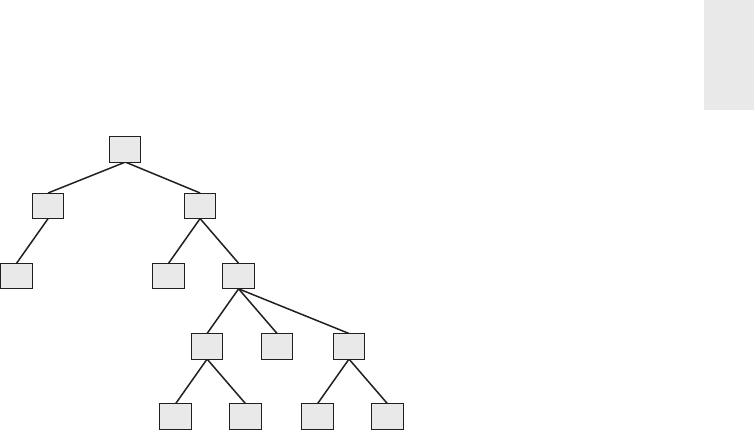
Accounting 221
11 12 56
10 13 4
389
27
1
Figure 7-15: Changes to Figure 7-8’s organization structure.
In the time varying case in which the bridge table has the pair of date/time
stamps, the logic is similar. You can fi nd the higher level paths in the tree point-
ing into the group of nodes 4, 5, and 6 and set their end e ective date/times to the
moment of the change. Then you attach nodes 4, 5, and 6 into the parents 1, 7, and
9 with the appropriate date/times. Here is the time varying SQL:
Update Org_Map set end_eff_date = #December 31, 2012#
where child_org in (4, 5,6) and parent_org not in (4,5,6)
and #Jan 1, 2013# between begin_eff_date and end_eff_date
Insert into Org_Map
(parent_org, child_org, begin_eff_date, end_eff_date)
values (1, 4, #Jan 1, 2013#, #Dec 31, 9999#)
Insert into Org_Map
(parent_org, child_org, begin_eff_date, end_eff_date)
values (7, 4, #Jan 1, 2013#, #Dec 31, 9999#)
Insert into Org_Map
(parent_org, child_org, begin_eff_date, end_eff_date)
values (9, 4, #Jan 1, 2013#, #Dec 31, 9999#)
Identical insert statements for nodes 5 and 6 …
This simple recipe for changing the bridge table avoids nightmarish scenarios
when changing other types of hierarchical models. In the bridge table, only the
paths directly involved in the change are a ected. All other paths are untouched.
In most other schemes with clever node labels, a change in the tree structure can
a ect many or even all the nodes in the tree, as shown in the next section.
Alternative Ragged Hierarchy Modeling Approaches
In addition to using recursive pointers in the organization dimension, there are at
least two other ways to model a ragged hierarchy, both involving clever columns
placed in the organization dimension. There are two disadvantages to these schemes

Chapter 7
222
compared to the bridge table approach. First, the defi nition of the hierarchy is locked
into the dimension and cannot easily be replaced. Second, both of these schemes are
vulnerable to a relabeling disaster in which a large part of the tree must be relabeled
due to a single small change. Textbooks (like this one!) usually show a tiny example,
but you need to tread cautiously if there are thousands of nodes in your tree.
One scheme adds a pathstring attribute to the organization dimension table,
as shown in Figure 7-16. The values of the pathstring attribute are shown within
each node. In this scenario, there is no bridge table. At each level, the pathstring
starts with the full pathstring of the parent and then adds the letters A, B, C, and
so on, from left to right under that parent. The fi nal character is a “+” if the node
has children and is a period if the node has no children. The tree can be navigated
by using wild cards in constraints against the pathstring, for example,
■ A* retrieves the whole tree where the asterisk is a variable length wild card.
■ *. retrieves only the leaf nodes.
■ ?+ retrieves the topmost node where the question mark is a single character
wild card.
AA+
AAA. AAB+
AABA. AABB. ABBA+ABBB.
ABBAA. ABBAB.
ABA. ABB+
AB+
A+
Figure 7-16: Alternate ragged hierarchy design using pathstring attribute.
The pathstring approach is fairly sensitive to relabeling ripples caused by orga-
nization changes; if a new node is inserted somewhere in the tree, all the nodes to
the right of that node under the same parent must be relabeled.
Another similar scheme, known to computer scientists as the modifi ed preordered
tree traversal approach, numbers the tree as shown in Figure 7-17. Every node has a
pair of numbers that identifi es all the nodes below that point. The whole tree can be
enumerated by using the node numbers in the topmost node. If the values in each node
have the names Left and Right, then all the nodes in the example tree can be found with
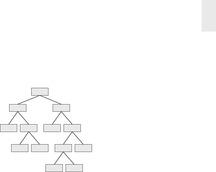
Accounting 223
the constraint “Left between 1 and 26.” Leaf nodes can be found where Left and Right
di er by 1, meaning there aren’t any children. This approach is even more vulnerable
to the relabeling disaster than the pathstring approach because the entire tree must
be carefully numbered in sequence, top to bottom and left to right. Any change to the
tree causes the entire rest of the tree to the right to be relabeled.
2,11
3,4 5,10
6,7 8,9 16,21 22,23
17,18 19,20
13,14 15,24
12,25
1,26
Figure 7-17: Alternative ragged hierarchy design using the modifi ed preordered tree
traversal approach.
Advantages of the Bridge Table Approach for Ragged
Hierarchies
Although the bridge table requires more ETL work to set up and more work when
querying, it o ers exceptional fl exibility for analyzing ragged hierarches of inde-
terminate depth. In particular, the bridge table allows
■ Alternative rollup structures to be selected at query time
■ Shared ownership rollups
■ Time varying ragged hierarchies
■ Limited impact when nodes undergo slowly changing dimension (SCD)
type 2 changes
■ Limited impact when the tree structure is changed
You can use the organization hierarchy bridge table to fetch a fact across all three
fact tables in the budget chain. Figure 7-18 shows how an organization map table
can connect to the three budget chain fact tables. This would allow a drill-across
report such as fi nding all the travel budgets, commitments, and payments made by
all the lowest leaf nodes in a complex organizational structure.
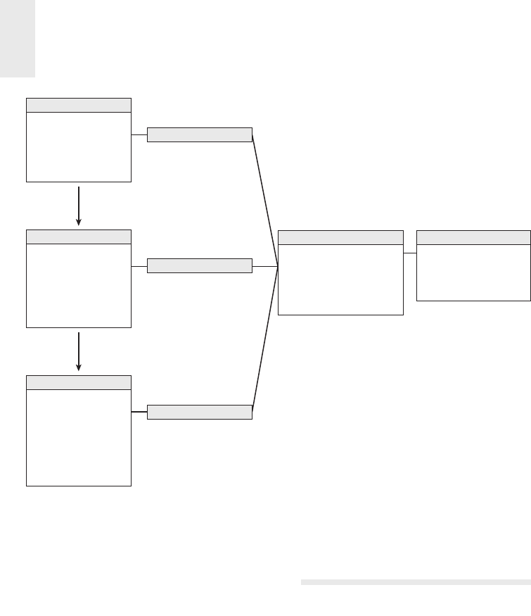
Chapter 7
224
Organization Map
Parent Organization Key (FK)
Child Organization Key (FK)
Depth from Parent
Highest Parent Flag
Lowest Child Flag
Organization Dimension
Organization Key
Cost Center Number
Cost Center Name
...
Month Key (FK)
Organization Key (FK)
Account Key (FK)
Budget Key (FK)
Budget Amount
Month Key (FK)
Organization Key (FK)
Account Key (FK)
Budget Key (FK)
Commitment Key (FK)
Commitment Amount
Month Key (FK)
Organization Key (FK)
Account Key (FK)
Budget Key (FK)
Commitment Key (FK)
Payment Key (FK)
Payment Amount
Payment Fact
Budget Fact
Commitment Fact
Organization Dimension
Organization Dimension
Organization Dimension
Figure 7-18: Drilling across and rolling up the budget chain.
Consolidated Fact Tables
In the last section, we discussed comparing metrics generated by separate business
processes by drilling across fact tables, such as budget and commitments. If this
type of drill-across analysis is extremely common in the user community, it likely
makes sense to create a single fact table that combines the metrics once rather than
relying on business users or their BI reporting applications to stitch together result
sets, especially given the inherent issues of complexity, accuracy, tool capabilities,
and performance.
Most typically, business managers are interested in comparing actual to budget
variances. At this point, you can presume the annual budgets and/or forecasts have
been broken down by accounting period. Figure 7-19 shows the actual and budget
amounts, as well as the variance (which is a calculated di erence) by the common
dimensions.

Accounting 225
Accounting Period Key (FK)
Account Key (FK)
Organization Key (FK)
Accounting Period Actual Amount
Accounting Period Budget Amount
Accounting Period Budget Variance
Budget Variance Fact
Organization Dimension
Accounting Period Dimension
Account Dimension
Figure 7-19: Actual versus budget consolidated fact table.
Again, in a multinational organization, you would likely see the actual amounts
in both local and the equivalent standard currency, based on the e ective conversion
rate. In addition, you may convert the actual results based on the planned currency
conversion factor. Given the unpredictable nature of currency fl uctuations, it is
useful to monitor performance based on both the e ective and planned conversion
rates. In this manner, remote managers aren’t penalized for currency rate changes
outside their control. Likewise, fi nance can better understand the big picture impact
of unexpected currency conversion fl uctuations on the organization’s annual plan.
Fact tables that combine metrics from multiple business processes at a com-
mon granularity are referred to as consolidated fact tables. Although consolidated
fact tables can be useful, both in terms of performance and usability, they often
represent a dimensionality compromise as they consolidate facts at the “least
common denominator” of dimensionality. One potential risk associated with
consolidated fact tables is that project teams sometimes base designs solely on
the granularity of the consolidated table, while failing to meet user requirements
that demand the ability to dive into more granular data. These schemas run into
serious problems if project teams attempt to force a one-to-one correspondence
to combine data with di erent granularity or dimensionality.
NOTE When facts from multiple business processes are combined in a consoli-
dated fact table, they must live at the same level of granularity and dimensionality.
Because the separate facts seldom naturally live at a common grain, you are forced
to eliminate or aggregate some dimensions to support the one-to-one correspon-
dence, while retaining the atomic data in separate fact tables. Project teams should
not create artifi cial facts or dimensions in an attempt to force-fi t the consolidation
of di erently grained fact data.

Chapter 7
226
Role of OLAP and Packaged Analytic
Solutions
While discussing fi nancial dimensional models in the context of relational data-
bases, it is worth noting that multidimensional OLAP vendors have long played a
role in this arena. OLAP products have been used extensively for fi nancial reporting,
budgeting, and consolidation applications. Relational dimensional models often feed
fi nancial OLAP cubes. OLAP cubes can deliver fast query performance that is critical
for executive usage. The data volumes, especially for general ledger balances or fi nan-
cial statement aggregates, do not typically overwhelm the practical size constraints
of a multidimensional product. OLAP is well suited to handle complicated organiza-
tional rollups, as well as complex calculations, including inter-row manipulations.
Most OLAP vendors provide fi nance-specifi c capabilities, such as fi nancial functions
(for example, net present value or compound growth), the appropriate handling of
fi nancial statement data (in the expected sequential order such as income before
expenses), and the proper treatment of debits and credits depending on the account
type, as well as more advanced functions such as fi nancial consolidation. OLAP
cubes often also readily support complex security models, such as limiting access
to detailed data while providing more open access to summary metrics.
Given the standard nature of general ledger processing, purchasing a general
ledger package rather than attempting to build one from scratch has been a popu-
lar route for years. Nearly all the operational packages also o er a complementary
analytic solution, sometimes in partnership with an OLAP vendor. In many cases,
precanned solutions based on the vendor’s cumulative experience are a sound way
to jump start a fi nancial DW/BI implementation with potentially reduced cost and
risk. The analytic solutions often have tools to assist with the extraction and staging
of the operational data, as well as tools to assist with analysis and interpretation.
However, when leveraging packaged solutions, you need to be cautious in order to
avoid stovepipe applications. You could easily end up with separate fi nancial, CRM,
human resources, and ERP packaged analytic solutions from as many di erent
vendors, none of which integrate with other internal data. You need to conform
dimensions across the entire DW/BI environment, regardless of whether you build
a solution or implement packages. Packaged analytic solutions can turbocharge a
DW/BI implementation; however, they do not alleviate the need for conformance.
Most organizations inevitably rely on a combination of building, buying, and inte-
grating for a complete solution.

Accounting 227
Summary
In this chapter, we focused primarily on fi nancial data in the general ledger, both in
terms of periodic snapshots as well as journal entry transactions. We discussed the
handling of common G/L data challenges, including multiple currencies, multiple
fi scal years, unbalanced organizational trees, and the urge to create to-date totals.
We used the familiar organization rollup structure to show how to model complex
ragged hierarchies of indeterminate depth. We introduced a special bridge table for
these hierarchies, and compared this approach to others.
We explored the series of events in a budgeting process chain. We described the
use of “net change” granularity in this situation rather than creating snapshots of
the budget data totals. We also discussed the concept of consolidated fact tables
that combine the results of separate business processes when they are frequently
analyzed together.
Finally, we discussed the natural fi t of OLAP products for fi nancial analysis. We
also stressed the importance of integrating analytic packages into the overall DW/
BI environment through the use of conformed dimensions .

Customer
Relationship
Management
Long before the customer relationship management (CRM) buzzword existed,
organizations were designing and developing customer-centric dimensional
models to better understand their customers’ behavior. For decades, these models
were used to respond to management’s inquiries about which customers were solic-
ited, who responded, and what was the magnitude of their response. The business
value of understanding the full spectrum of customers’ interactions and transactions
has propelled CRM to the top of the charts. CRM not only includes familiar resi-
dential and commercial customers, but also citizens, patients, students, and many
other categories of people and organizations whose behavior and preferences are
important. CRM is a mission-critical business strategy that many view as essential
to an organization’s survival.
In this chapter we start with a CRM overview, including its operational and ana-
lytic roles. We then introduce the basic design of the customer dimension, including
common attributes such as dates, segmentation attributes, repeated contact roles,
and aggregated facts. We discuss customer name and address parsing, along with
international considerations. We remind you of the challenges of modeling complex
hierarchies when we describe various kinds of customer hierarchies.
Chapter 8 discusses the following concepts:
■ CRM overview
■ Customer name and address parsing, including international considerations
■ Handling of dates, aggregated facts, and segmentation behavior attributes and
scores in a customer dimension
■ Outriggers for low cardinality attributes
■ Bridge tables for sparse attributes, along with trade-o s of bridge tables versus
a positional design
■ Bridge tables for multiple customer contacts
■ Behavior study groups to capture customer cohort groups
8

Chapter 8
230
■ Step dimensions to analyze sequential customer behavior
■ Timespan fact tables with e ective and expiration dates
■ Embellishing fact tables with dimensions for satisfaction or abnormal scenarios
■ Integrating customer data via master data management or partial conformity
during the downstream ETL processing
■ Warnings about fact-to-fact table joins
■ Reality check on real time, low latency requirements
Because this chapter’s customer-centric modeling issues and patterns are relevant
across industries and functional areas, we have not included a bus matrix.
CRM Overview
Regardless of the industry, organizations have fl ocked to the concept of CRM.
They’ve jumped on the bandwagon in an attempt to migrate from a product-centric
orientation to one that is driven by customer needs. Although all-encompassing
terms such as customer relationship management sometimes seem ambiguous and/
or overly ambitious, the premise behind CRM is far from rocket science. It’s based
on the simple notion that the better you know your customers, the better you can
maintain long-lasting, valuable relationships with them. The goal of CRM is to
maximize relationships with your customers over their lifetime. It entails focus-
ing all aspects of the business, from marketing, sales, operations, and service, on
establishing and sustaining mutually benefi cial customer relations. To do so, the
organization must develop a single, integrated view of each customer.
CRM promises signifi cant returns for organizations that embrace it, both for
increased revenue and operational e ciencies. Switching to a customer-driven
perspective can lead to increased sales e ectiveness and closure rates, revenue
growth, enhanced sales productivity at reduced cost, improved customer profi t-
ability margins, higher customer satisfaction, and increased customer retention.
Ultimately, every organization wants more loyal, more profi table customers. As it
often requires a sizeable investment to attract new customers, you can’t a ord to
have the profi table ones leave.
In many organizations, the view of the customer varies depending on the product
line business unit, business function, and/or geographic location. Each group may
use di erent customer data in di erent ways with di erent results. The evolution
from the existing silos to a more integrated perspective obviously requires organi-
zational commitment. CRM is like a stick of dynamite that knocks down the silo
walls. It requires the right integration of business processes, people resources, and
application technology to be e ective.
Over the past decade, the explosive growth of social media, location tracking tech-
nology, network usage monitoring, multimedia applications, and sensor networks

Customer Relationship Management 231
has provided an ocean of customer behavioral data that even Main Street enterprises
recognize as providing actionable insights. Although much of this data lies outside
the comfort zone of relational databases, the new “big data” techniques can bring
this data back into the DW/BI fold. Chapter 21: Big Data Analytics discusses the
best practices for bringing this new kind of big data into the DW/BI environment.
But setting aside the purely technological challenges, the real message is the need
for profound integration. You must step up to the challenge of integrating as many
as 100 customer-facing data sources, most of which are external. These data sources
are at di erent grains, have incompatible customer attributes, and are not under
your control. Any questions?
Because it is human nature to resist change, it comes as no surprise that people-
related issues often challenge CRM implementations. CRM involves brand new
ways of interacting with customers and often entails radical changes to the sales
channels. CRM requires new information fl ows based on the complete acquisition
and dissemination of customer “touch point” data. Often organization structures and
incentive systems are dramatically altered.
In Chapter 17: Kimball DW/BI Lifecycle Overview, we’ll stress the importance of
having support from both senior business and IT management for a DW/BI initiative.
This advice also applies to a CRM implementation because of its cross-functional
focus. CRM requires a clear business vision. Without business strategy, buy-in, and
authorization to change, CRM becomes an exercise in futility. Neither IT nor the
business community can successfully implement CRM on its own; CRM demands
a joint commitment of support.
Operational and Analytic CRM
It could be said that CRM su ers from a split personality syndrome because it needs
to address both operational and analytic requirements. E ective CRM relies on the
collection of data at every interaction you have with a customer and then leveraging
that breadth of data through analysis.
On the operational front, CRM calls for the synchronization of customer-facing
processes. Often operational systems must either be updated or supplemented to coor-
dinate across sales, marketing, operations, and service. Think about all the customer
interactions that occur during the purchase and usage of a product or service, from
the initial prospect contact, quote generation, purchase transaction, fulfi llment, pay-
ment transaction, and on-going customer service. Rather than thinking about these
processes as independent silos (or multiple silos varying by product line), the CRM
mindset is to integrate these customer activities. Key customer metrics and charac-
teristics are collected at each touch point and made available to the others.
As data is created on the operational side of the CRM equation, you obviously
need to store and analyze the historical metrics resulting from the customer

Chapter 8
232
interaction and transaction systems. Sounds familiar, doesn’t it? The DW/BI system
sits at the core of CRM. It serves as the repository to collect and integrate the
breadth of customer information found in the operational systems, as well as from
external sources. The data warehouse is the foundation that supports the panoramic
360-degree view of your customers.
Analytic CRM is enabled via accurate, integrated, and accessible customer data
in the DW/BI system. You can measure the e ectiveness of decisions made in the
past to optimize future interactions. Customer data can be leveraged to better iden-
tify up-sell and cross-sell opportunities, pinpoint ine ciencies, generate demand,
and improve retention. In addition, the historical, integrated data can be leveraged
to generate models or scores that close the loop back to the operational world.
Recalling the major components of a DW/BI environment from Chapter 1: Data
Warehousing, Business Intelligence, and Dimensional Modeling Primer, you can
envision the model results pushed back to where the relationship is operationally
managed (such as the rep, call center, or website), as illustrated in Figure 8-1. The
model output can translate into specifi c proactive or reactive tactics recommended
for the next point of customer contact, such as the appropriate next product o er or
anti-attrition response. The model results are also retained in the DW/BI environ-
ment for subsequent analysis.
Integrate
(ETL)
Store
(Data Presentation)
Analyze and
Report
(BI Applications)
Model
(BI Applications)
Collect
(Operational
Source System)
Figure 8-1: Closed loop analytic CRM.

Customer Relationship Management 233
In other situations, information must feed back to the operational website or call
center systems on a more real-time basis. In this case, the closed loop is much tighter
than Figure 8-1 because it’s a matter of collection and storage, and then feedback
to the collection system. Today’s operational processes must combine the current
view with a historical view, so a decision maker can decide, for example, whether
to grant credit to a customer in real time, while considering the customer’s lifetime
history. But generally, the integration requirements for operational CRM are not as
far reaching as for analytic CRM.
Obviously, as the organization becomes more centered on the customer, so must
the DW/BI system. CRM will inevitably drive change in the data warehouse. DW/BI
environments will grow even more rapidly as you collect more and more informa-
tion about your customers. ETL processes will grow more complicated as you match
and integrate data from multiple sources. Most important, the need for a conformed
customer dimension becomes even more paramount.
Customer Dimension Attributes
The conformed customer dimension is a critical element for e ective CRM. A well-
maintained, well-deployed conformed customer dimension is the cornerstone of
sound CRM analysis.
The customer dimension is typically the most challenging dimension for any
DW/BI system. In a large organization, the customer dimension can be extremely
deep (with many millions of rows), extremely wide (with dozens or even hundreds
of attributes), and sometimes subject to rapid change. The biggest retailers, credit
card companies, and government agencies have monster customer dimensions whose
size exceeds 100 million rows. To further complicate matters, the customer dimen-
sion often represents an amalgamation of data from multiple internal and external
source systems.
In this next section, we focus on numerous customer dimension design con-
siderations. We’ll begin with name/address parsing and other common customer
attributes, including coverage of dimension outriggers, and then move on to other
interesting customer attributes. Of course, the list of customer attributes is typically
quite lengthy. The more descriptive information you capture about your customers,
the more robust the customer dimension, and the more interesting the analyses.
Name and Address Parsing
Regardless of whether you deal with individual human beings or commercial enti-
ties, customers’ name and address attributes are typically captured. The operational
handling of name and address information is usually too simplistic to be very useful

Chapter 8
234
in the DW/BI system. Many designers feel a liberal design of general purpose col-
umns for names and addresses, such as Name-1 through Name-3 and Address-1
through Address-6, can handle any situation. Unfortunately, these catchall columns
are virtually worthless when it comes to better understanding and segmenting
the customer base. Designing the name and location columns in a generic way
can actually contribute to data quality problems. Consider the sample design in
Figure 8-2 with general purpose columns.
Ms. R. Jane Smith, Atty
123 Main Rd, North West, Ste 100A
PO Box 2348
Kensington
Ark.
88887-2348
888-555-3333 x776 main, 555-4444 fax
Name
Address 1
Address 2
City
State
ZIP Code
Phone Number
Column Sample Data Value
Figure 8-2: Sample customer name/address data in overly general columns.
In this design, the name column is far too limited. There is no consistent mecha-
nism for handling salutations, titles, or su xes. You can’t identify what the person’s
fi rst name is, or how she should be addressed in a personalized greeting. If you
look at additional sample data from this operational system, you would potentially
fi nd multiple customers listed in a single name attribute. You might also fi nd addi-
tional descriptive information in the name column, such as Confi dential, Trustee,
or UGMA (Uniform Gift to Minors Act).
In the sample address attributes, inconsistent abbreviations are used in various
places. The address columns may contain enough room for any address, but there
is no discipline imposed by the columns that can guarantee conformance with
postal authority regulations or support address matching and latitude/longitude
identifi cation.
Instead of using a few, general purpose columns, the name and location attributes
should be broken down into as many elemental parts as possible. The extract process
needs to perform signifi cant parsing on the original dirty names and addresses. After
the attributes have been parsed, they can be standardized. For example, Rd would
become Road and Ste would become Suite. The attributes can also be verifi ed, such
as verifying the ZIP code and associated state combination is correct. Fortunately,
there are name and address data cleansing and scrubbing tools available in the
market to assist with parsing, standardization, and verifi cation.

Customer Relationship Management 235
A sample set of name and location attributes for individuals in the United States is
shown in Figure 8-3. Every attribute is fi lled in with sample data to make the design
clearer, but no single real instance would look like this. Of course, the business data
governance representatives should be involved in determining the analytic value of
these parsed data elements in the customer dimension.
Ms.
Jane
Ms. Smith
R. Jane
Smith
Jr.
English
Attorney
123
Main
Road
North West
Kensington
Cornwall
Berkeleyshire
Arkansas
South
United States
North America
88887
2348
United States
1
888
5553333
776
1
509
5554444
RJSmith@ABCGenIntl.com
www.ABCGenIntl.com
X.509
Verisign
7346531
Salutation
Informal Greeting Name
Formal Greeting Name
First and Middle Names
Surname
Suffix
Ethnicity
Title
Street Number
Street Name
Street Type
Street Direction
City
District
Second District
State
Region
Country
Continent
Primary Postal Code
Secondary Postal Code
Postal Code Type
Office Telephone Country Code
Office Telephone Area Code
Office Telephone Number
Office Extension
Mobile Telephone Country Code
Mobile Telephone Area Code
Mobile Telephone Number
E-mail
Web Site
Public Key Authentication
Certificate Authority
Unique Individual Identifier
Column Sample Data Value
Figure 8-3: Sample customer name/address data with parsed name and address
elements.

Chapter 8
236
Commercial customers typically have multiple addresses, such as physical and
shipping addresses; each of these addresses would follow much the same logic as
the address structure shown in Figure 8-3.
International Name and Address Considerations
International display and printing typically requires representing foreign characters,
including not just the accented characters from western European alphabets, but
also Cyrillic, Arabic, Japanese, Chinese, and dozens of other less familiar writing
systems. It is important to understand this is not a font problem. This is a character
set problem. A font is simply an artist’s rendering of a set of characters. There are
hundreds of fonts available for standard English, but standard English has a rela-
tively small character set that is enough for anyone’s use unless you are a professional
typographer. This small character set is usually encoded in American Standard Code
for Information Interchange (ASCII), which is an 8-bit encoding that has a maximum
of 255 possible characters. Only approximately 100 of these 255 characters have a
standard interpretation that can be invoked from a normal English keyboard, but
this is usually enough for English speaking computer users. It should be clear that
ASCII is woefully inadequate for representing the thousands of characters needed
for non-English writing systems.
An international body of system architects, the Unicode Consortium, defi ned a
standard known as Unicode for representing characters and alphabets in almost all
the world’s languages and cultures. Their work can be accessed on the web at www.
unicode.org. The Unicode Standard, version 6.2.0 has defi ned specifi c interpreta-
tions for 110,182 possible characters and now covers the principal written languages
of the Americas, Europe, the Middle East, Africa, India, Asia, and Pacifi ca. Unicode
is the foundation you must use for addressing international character sets.
But it is important to understand that implementing Unicode solutions is done in
the foundation layers of your systems. First, the operating system must be Unicode-
compliant. Fortunately, the most current releases of all the major operating systems
are Unicode-compliant.
Above the operating system, all the devices that capture, store, transmit, and
print characters must be Unicode-compliant. Data warehouse back room tools must
be Unicode-compliant, including sort packages, programming languages, and auto-
mated ETL packages. Finally, the DW/BI applications, including database engines,
BI application servers and their report writers and query tools, web servers, and
browsers must all be Unicode-compliant. The DW/BI architect should not only talk
to the vendors of each package in the data pipeline, but also should conduct various
end-to-end tests. Capture some names and addresses with Unicode characters at
the data capture screens of one of the legacy applications, and send them through the
system. Get them to print out of a fi nal report or a fi nal browser window from

Customer Relationship Management 237
the DW/BI system and see if the special characters are still there. That simple
test will cut through a lot of the confusion. Note that even when you do this, the
same character, such as an a-umlaut, sorts di erently in di erent countries such as
Norway and Germany. Even though you can’t solve all the variations in international
collating sequences, at least both the Norwegians and the Germans will agree that
the character is an a-umlaut.
Customer geographic attributes become more complicated if you deal with cus-
tomers from multiple countries. Even if you don’t have international customers, you
may need to contend with international names and addresses somewhere in the
DW/BI system for international suppliers and human resources personnel records.
NOTE Customer dimensions sometimes include a full address block attribute.
This is a specially crafted column that assembles a postally-valid address for the
customer including mail stop, ZIP code, and other attributes needed to satisfy postal
authorities. This attribute is useful for international locations where addresses
have local idiosyncrasies.
International DW/BI Goals
After committing to a Unicode foundation, you need to keep the following goals in
mind, in addition to the name and address parsing requirements discussed earlier:
■ Universal and consistent. As they say, in for a penny, in for a pound. If you
are going to design a system for international use, you want it to work around
the world. You need to think carefully if BI tools are to produce translated ver-
sions of reports in many languages. It may be tempting to provide translated
versions of dimensions for each language, but translated dimensions give rise
to some subtle problems.
■ Sorting sequences will be different, so either the reports will be sorted
differently or all reports except those in the “root” language will appear
to be unsorted.
■ If the attribute cardinalities are not faithfully preserved across lan-
guages, then either group totals will not be the same across reports, or
some groups in various languages will contain duplicated row headers
that look like mistakes. To avoid the worst of these problems, you
should translate dimensions after the report is run; the report first
needs to be produced in a single root language, and then the report
face needs to be translated into the intended target languages.
■ All the BI tool messages and prompts need to be translated for the
benefit of the business user. This process is known as localization and
is further discussed in Chapter 12: Transportation.

Chapter 8
238
■ End-to-end data quality and downstream compatibility. The data warehouse
cannot be the only step in the data pipeline that worries about the integrity
of international names and addresses. A proper design requires support from
the fi rst step of capturing the name and the address, through the data cleaning
and storage steps, to the fi nal steps of performing geographic and demographic
analysis and printing reports.
■ Cultural correctness. In many cases, foreign customers and partners will see
the results from your DW/BI system in some form. If we don’t understand
which name is a fi rst name and which is a last name, and if you don’t under-
stand how to refer to a person, you run the risk of insulting these individuals,
or at the very least, looking stupid. When outputs are punctuated improperly, or
misspelled, your foreign customers and partners will wish they were doing
business with a local company, rather than you.
■ Real-time customer response. DW/BI systems can play an operational role
by supporting real-time customer response systems. A customer service rep-
resentative may answer the telephone and may have 5 seconds or less to wait
for a greeting to appear on the screen that the data warehouse recommends
using with the customer. The greeting may include a proper salutation and
a proper use of the customer’s title and name. This greeting represents an
excellent use of a hot response cache that contains precalculated responses
for each customer.
■ Other kinds of addresses. We are in the midst of a revolution in communication
and networking. If you are designing a system for identifying international
names and addresses, you must anticipate the need to store electronic names,
security tokens, and internet addresses.
Similar to international addresses, telephone numbers must be presented
di erently depending on where the phone call originates. You need to provide
attributes to represent the complete foreign dialing sequence, complete domestic
dialing sequence, and local dialing sequence. Unfortunately, complete foreign dial-
ing sequences vary by origin country.
Customer-Centric Dates
Customer dimensions often contains dates, such as the date of the fi rst purchase,
date of last purchase, and date of birth. Although these dates initially may be SQL
date type columns, if you want to summarize these dates by your unique calen-
dar attributes, such as seasons, quarters, and fi scal periods, the dates should be
changed to foreign key references to the date dimension. You need to be careful
that all such dates fall within the span of the corporate date dimension. These date
dimension roles are declared as semantically distinct views, such as a First Purchase

Customer Relationship Management 239
Date dimension table with unique column labels. The system behaves as if there
is another physical date table. Constraints on any of these tables have nothing to
do with constraints on the primary date dimension table. This design, as shown
in Figure 8-4, is an example of a dimension outrigger, which is discussed in the
section “Outrigger for Low Cardinality Attribute Set.”
Date of 1st Purchase Key (PK)
Date of 1st Purchase
Date of 1st Purchase Month
Date of 1st Purchase Year
Date of 1st Purchase Fiscal Month
Date of 1st Purchase Fiscal Quarter
Date of 1st Purchase Fiscal Year
Date of 1st Purchase Season
…
Date of 1st Purchase Dimension
Customer Key (PK)
Customer ID (Natural Key)
Customer Salutation
Customer First Name
Customer Surname
Customer City
Customer State
…
Date of 1st Purchase Key (FK)
Customer Dimension
Transaction Date Key (FK)
Customer Key (FK)
More FKs …
Facts …
Fact Table
Figure 8-4: Date dimension outrigger.
Aggregated Facts as Dimension Attributes
Business users are often interested in constraining the customer dimension based on
aggregated performance metrics, such as fi ltering on all customers who spent more
than a certain dollar amount during last year. Or to make matters worse, perhaps
they want to constrain based on how much the customer has purchased in a lifetime.
Providing aggregated facts as dimension attributes is sure to be a crowd-pleaser with
the business users. They could issue a query to identify all customers who satisfi ed the
spending criteria and then issue another fact query to analyze the behavior for
that customer dimension subset. But rather than all that, you can instead store
an aggregated fact as a dimension attribute. This allows business users to simply
constrain on the spending attribute just like they might on a geographic attribute.
These attributes are meant to be used for constraining and labeling; they’re not to be
used in numeric calculations. Although there are query usability and performance
advantages of storing these attributes, the main burden falls on the back room ETL
processes to ensure the attributes are accurate, up-to-date, and consistent with the
actual fact rows. These attributes can require signifi cant care and feeding. If you
opt to include some aggregated facts as dimension attributes, be certain to focus on
those that will be frequently used. Also strive to minimize the frequency with which
these attributes need to be updated. For example, an attribute for last year’s spending
would require much less maintenance than one providing year-to-date behavior.
Rather than storing attributes down to the specifi c dollar value, they are sometimes

Chapter 8
240
replaced (or supplemented) with more meaningful descriptive values, such as High
Spender as discussed in the next section. These descriptive values minimize your
vulnerability that the numeric attributes might not tie back to the appropriate fact
tables. In addition, they ensure that all users have a consistent defi nition for high
spenders, for example, rather than resorting to their own individual business rules.
Segmentation Attributes and Scores
Some of the most powerful attributes in a customer dimension are segmentation
classifi cations. These attributes obviously vary greatly by business context. For an
individual customer, they may include:
■ Gender
■ Ethnicity
■ Age or other life stage classifi cations
■ Income or other lifestyle classifi cations
■ Status (such as new, active, inactive, and closed)
■ Referring source
■ Business-specifi c market segment (such as a preferred customer identifi er)
Similarly, many organizations score their customers to characterize them.
Statistical segmentation models typically generate these scores which cluster cus-
tomers in a variety of ways, such as based on their purchase behavior, payment
behavior, propensity to churn, or probability to default. Each customer is tagged
with a resultant score.
Behavior Tag Time Series
One popular approach for scoring and profi ling customers looks at the recency (R),
frequency (F), and intensity (I) of the customer’s behavior. These are known as the
RFI measures; sometimes intensity is replaced with monetary (M), so it’s also known
as RFM. Recency is how many days has it been since the customer last ordered
or visited your site. Frequency is how many times the customer has ordered or
visited, typically in the past year. And intensity is how much money the customer
has spent over the same time period. When dealing with a large customer base,
every customer’s behavior can be modeled as a point in an RFI cube, as depicted
in Figure 8-5. In this fi gure, the scales along each axis are quintiles, from 1 to 5,
which spread the actual values into even groups.
If you have millions of points in the cube, it becomes di cult to see meaning-
ful clusters of these points. This is a good time to ask a data mining professional
where the meaningful clusters are. The data mining professional may come back
with a list of behavior tags like the following, which is drawn from a slightly more
complicated scenario that includes credit behavior and returns:

Customer Relationship Management 241
A: High volume repeat customer, good credit, few product returns
B: High volume repeat customer, good credit, many product returns
C: Recent new customer, no established credit pattern
D: Occasional customer, good credit
E: Occasional customer, poor credit
F: Former good customer, not seen recently
G: Frequent window shopper, mostly unproductive
H: Other
5
Highest
Lowest
HighestLowest
Highest
Lowest
Recency
Frequency
Intensity
4
3
2
1
11
2
3
4
5
2345
Figure 8-5: Recency, frequency, intensity (RFI) cube.
Now you can look at the customers’ time series data and associate each customer
in each reporting period with the nearest cluster. The data miner can help do this.
Thus, the last 10 observations of a customer named John Doe could look like:
John Doe: C C C D D A A A B B
This time series of behavior tags is unusual because although it comes from
a regular periodic measurement process, the observed “values” are textual. The
behavior tags are not numeric and cannot be computed or averaged, but they can
be queried. For example, you may want to fi nd all the customers who were an A
sometime in the fi fth, fourth, or third prior period and were a B in the second or fi rst
prior period. Perhaps you are concerned by progressions like this and fear losing a
valuable customer because of the increasing number of returns.
Behavior tags should not be stored as regular facts. The main use of behavior tags
is formulating complex query patterns like the example in the previous paragraph.
If the behavior tags were stored in separate fact rows, such querying would be
extremely di cult, requiring a cascade of correlated subqueries. The recommended
way to handle behavior tags is to build an explicit time series of attributes in the
customer dimension. This is another example of a positional design. BI interfaces

Chapter 8
242
are simple because the columns are in the same table, and performance is good
because you can build bitmapped indexes on them.
In addition to the separate columns for each behavior tag time period, it would
be a good idea to create a single attribute with all the behavior tags concatenated
together, such as CCCDDAAABB. This column would support wild card searches
for exotic patterns, such as “D followed by a B.”
NOTE In addition to the customer dimension’s time series of behavior tags, it
would be reasonable to include the contemporary behavior tag value in a mini-
dimension to analyze facts by the behavior tag in e ect when the fact row was
loaded.
Relationship Between Data Mining and DW/BI System
The data mining team can be a great client of the data warehouse, and especially
great users of customer behavior data. However, there can be a mismatch between
the velocity that the data warehouse can deliver data and the velocity that the data
miners can consume data. For example, a decision tree tool can process hundreds
of records per second, but a big drill-across report that produces “customer observa-
tions” can never deliver data at such speeds. Consider the following seven-way drill
across a report that might produce millions of customer observations from census,
demographic, external credit, internal credit, purchases, returns, and website data:
SELECT Customer Identifier, Census Tract, City, County, State,
Postal Code, Demographic Cluster, Age, Sex, Marital Status,
Years of Residency, Number of Dependents, Employment Profile,
Education Profile, Sports Magazine Reader Flag,
Personal Computer Owner Flag, Cellular Telephone Owner Flag,
Current Credit Rating, Worst Historical Credit Rating,
Best Historical Credit Rating, Date First Purchase,
Date Last Purchase, Number Purchases Last Year,
Change in Number Purchases vs. Previous Year,
Total Number Purchases Lifetime, Total Value Purchases Lifetime,
Number Returned Purchases Lifetime, Maximum Debt,
Average Age Customer's Debt Lifetime, Number Late Payments,
Number Fully Paid, Times Visited Web Site,
Change in Frequency of Web Site Access,
Number of Pages Visited Per Session,
Average Dwell Time Per Session, Number Web Product Orders,
Value Web Product Orders, Number Web Site Visits to Partner Web
Sites, Change in Partner Web Site Visits
FROM *** WHERE *** ORDER BY *** GROUP BY ***

Customer Relationship Management 243
Data mining teams would love this data! For example a big fi le of millions of these
observations could be analyzed by a decision tree tool where the tool is “aimed”
at the Total Value Purchases Lifetime column, which is highlighted above. In this
analysis, the decision tree tool would determine which of the other columns “predict
the variance” of the target fi eld. Maybe the answer is Best Historical Credit Rating
and Number of Dependents. Armed with this answer, the enterprise now has a
simple way to predict who is going to be a good lifetime customer, without needing
to know all the other data content.
But the data mining team wants to use these observations over and over for
di erent kinds of analyses perhaps with neural networks or case-based reasoning
tools. Rather than producing this answer set on demand as a big, expensive query,
this answer set should be written to a fi le and given to the data mining team to
analyze on its servers.
Counts with Type 2 Dimension Changes
Businesses frequently want to count customers based on their attributes without
joining to a fact table. If you used type 2 to track customer dimension changes,
you need to be careful to avoid overcounting because you may have multiple rows
in the customer dimension for the same individual. Doing a COUNT DISTINCT on a
unique customer identifi er is a possibility, assuming the attribute is indeed unique
and durable. A current row indicator in the customer dimension is also helpful to
do counts based on the most up-to-date descriptive values for a customer.
Things get more complicated if you need to do a customer count at a given histori-
cal point in time using e ective and expiration dates in the customer dimension. For
example, if you need to know the number of customers you had at the beginning of
2013, you could constrain the row e ective date <= ‘1/1/2013’ and row expiration
date >= ‘1/1/2013’ to restrict the result set to only those rows that were valid on
1/1/2013. Note the comparison operators are dependent on the business rules used
to set the row e ective/expiration dates. In this example, the row expiration date on
the no longer valid customer row is 1 day less than the e ective date on the new row.
Outrigger for Low Cardinality Attribute Set
In Chapter 3: Retail Sales, we encouraged designers to avoid snowfl aking where low
cardinality columns in the dimension are removed to separate normalized tables,
which then link back into the original dimension table. Generally, snowfl aking is
not recommended in a DW/BI environment because it almost always makes the
user presentation more complex, in addition to negatively impacting browsing per-
formance. In spite of this prohibition against snowfl aking, there are some special

Chapter 8
244
situations in which it is permissible to build a dimension outrigger that begins to
look like a snowfl aked table.
In Figure 8-6, the dimension outrigger is a set of data from an external data pro-
vider consisting of 150 demographic and socio-economic attributes regarding the
customers’ county of residence. The data for all customers residing in a given county
is identical. Rather than repeating this large block of data for every customer within
a county, opt to model it as an outrigger. There are several reasons for bending the
“no snowfl ake” rule. First, the demographic data is available at a signifi cantly dif-
ferent grain than the primary dimension data and it’s not as analytically valuable.
It is loaded at di erent times than the rest of the data in the customer dimension.
Also, you do save signifi cant space in this case if the underlying customer dimen-
sion is large. If you have a query tool that insists on a classic star schema with no
snowfl akes, the outrigger can be hidden under a view declaration.
Country Demographics Outrigger Dimension
County Demographics Key (PK)
Total Population
Population under 5 Years
% Population under 5 Years
Population under 18 Years
% Population under 18 Years
Population 65 Years and Older
% Population 65 Years and Older
Female Population
% Female Population
Male Population
% Male Population
Number of High School Graduates
Number of College Graduates
Number of Housing Units
Home Ownership Rate
...
Customer Dimension
Customer Key (PK)
Customer ID (Natural Key)
Customer Salutation
Customer First Name
Customer Surname
Customer City
Customer County
County Demographics Key (FK)
Customer State
...
Fact Table
Customer Key (FK)
More FKs ...
Facts ...
Figure 8-6: Dimension outrigger for cluster of low cardinality attributes.
WAR NI NG Dimension outriggers are permissible, but they should be the
exception rather than the rule. A red warning fl ag should go up if your design
is riddled with outriggers; you may have succumbed to the temptation to overly
normalize the design.
Customer Hierarchy Considerations
One of the most challenging aspects of dealing with commercial customers is mod-
eling their internal organizational hierarchy. Commercial customers often have a

Customer Relationship Management 245
nested hierarchy of entities ranging from individual locations or organizations up
through regional o ces, business unit headquarters, and ultimate parent companies.
These hierarchical relationships may change frequently as customers reorganize
themselves internally or are involved in acquisitions and divestitures.
NOTE In Chapter 7: Accounting, we described how to handle fi xed hierar-
chies, slightly variable hierarchies, and ragged hierarchies of indeterminate depth.
Chapter 7 focuses on fi nancial cost center rollups, but the techniques are exactly
transferrable to customer hierarchies. If you skipped Chapter 7, you need to back-
track to read that chapter to make sense of the following recommendations.
Although relatively uncommon, the lucky ones amongst us sometimes are
confronted with a customer hierarchy that has a highly predictable fi xed number
of levels. Suppose you track a maximum of three rollup levels, such as the ultimate
corporate parent, business unit headquarters, and regional headquarters. In this
case, you have three distinct attributes in the customer dimension corresponding
to these three levels. For commercial customers with complicated organizational
hierarchies, you’d populate all three levels to appropriately represent the three di er-
ent entities involved at each rollup level. This is the fi xed depth hierarchy approach
from Chapter 7.
By contrast, if another customer had a mixture of one, two, and three level
organizations, you’d duplicate the lower-level value to populate the higher-level attri-
butes. In this way, all regional headquarters would sum to the sum of all business
unit headquarters, which would sum to the sum of all ultimate corporate parents.
You can report by any level of the hierarchy and see the complete customer base
represented. This is the slightly variable hierarchy approach.
But in many cases, complex commercial customer hierarchies are ragged hier-
archies with an indeterminate depth, so you must use a ragged hierarchy modeling
technique, as described in Chapter 7. For example, if a utility company is devising a
custom rate plan for all the utility consumers that are part of a huge customer with
many levels of o ces, branch locations, manufacturing locations, and sales loca-
tions, you cannot use a fi xed hierarchy. As pointed out in Chapter 7, the worst design
is a set of generic levels named such as Level-1, Level-2, and so on. This makes for
an unusable customer dimension because you don’t know how to constrain against
these levels when you have a ragged hierarchy of indeterminate depth.
Bridge Tables for Multivalued Dimensions
A fundamental tenet of dimensional modeling is to decide on the grain of the fact
table, and then carefully add dimensions and facts to the design that are true to
the grain. For example, if you record customer purchase transactions, the grain of

Chapter 8
246
the individual purchase is natural and physically compelling. You do not want to
change that grain. Thus you normally require any dimension attached to this fact
table to take on a single value because then there’s a clean single foreign key in the
fact table that identifi es a single member of the dimension. Dimensions such as
the customer, location, product or service, and time are always single valued. But
you may have some “problem” dimensions that take on multiple values at the grain
of the individual transaction. Common examples of these multivalued dimensions
include:
■ Demographic descriptors drawn from a multiplicity of sources
■ Contact addresses for a commercial customer
■ Professional skills of a job applicant
■ Hobbies of an individual
■ Diagnoses or symptoms of a patient
■ Optional features for an automobile or truck
■ Joint account holders in a bank account
■ Tenants in a rental property
When faced with a multivalued dimension, there are two basic choices: a posi-
tional design or bridge table design. Positional designs are very attractive because
the multivalued dimension is spread out into named columns that are easy to query.
For example, if modeling the hobbies of an individual as previously mentioned,
you could have a hobby dimension with named columns for all the hobbies gath-
ered from your customers, including stamp collecting, coin collecting, astronomy,
photography, and many others! Immediately you can see the problem. The posi-
tional design approach isn’t very scalable. You can easily run out of columns in
your database, and it is awkward to add new columns. Also if you have a column
for every possible hobby, then any single individual’s hobby dimension row will
contain mostly null values.
The bridge table approach to multivalued dimensions is powerful but comes
with a big compromise. The bridge table removes the scalability and null value
objections because rows in the bridge table exist only if they are actually needed,
and you can add hundreds or even thousands of hobbies in the previous example.
But the resulting table design requires a complex query that must be hidden from
direct view by the business users.
WAR NI NG Be aware that complex queries using bridge tables may require SQL
that is beyond the normal reach of BI tools.

Customer Relationship Management 247
In the next two sections, we illustrate multivalued bridge table designs that
fi t with the customer-centric topics of this chapter. We will revisit multivalued
bridges in Chapter 9: Human Resources Management, Chapter 10: Financial
Services, Chapter 13: Education, Chapter 14: Healthcare, and Chapter 16: Insurance.
We’ll then describe how to build these bridges in Chapter 19: ETL Subsystems and
Techniques.
Bridge Table for Sparse Attributes
Organizations are increasingly collecting demographics and status information
about their customers, but the traditional fi xed column modeling approach for
handling these attributes becomes di cult to scale with hundreds of attributes.
Positional designs have a named column for each attribute. BI tool interfaces are
easy to construct for positional attributes because the named columns are easily
presented in the tool. Because many columns contain low cardinality contents, the
query performance using these attributes can be very good if bitmapped indexes
are placed on each column. Positional designs can be scaled up to perhaps 100 or
so columns before the databases and user interfaces become awkward or hard to
maintain. Columnar databases are well suited to these kinds of designs because
new columns can be easily added with minimal disruption to the internal storage
of the data, and the low-cardinality columns containing only a few discrete values
are dramatically compressed.
When the number of di erent attributes grows beyond your comfort zone, and
if new attributes are added frequently, a bridge table is recommended. Ultimately,
when you have a very large and expanding set of demographics indicators, using
outriggers or mini-dimensions simply does not gracefully scale. For example, you
may collect loan application information as a set of open ended name-value pairs,
as shown in Figure 8-7. Name-value pair data is interesting because the values can
be numeric, textual, a fi le pointer, a URL, or even a recursive reference to enclosed
name-value pair data.
Over a period of time, you could collect hundreds or even thousands of di erent
loan application variables. For a true name-value pair data source, the value fi eld
itself can be stored as a text string to handle the open-ended modality of the val-
ues, which is interpreted by the analysis application. In these situations whenever
the number of variables is open-ended and unpredictable, a bridge table design is
appropriate, as shown in Figure 8-8.

Chapter 8
248
Loan Application Name-Value Pair Data
Photograph: <image>
Primary Income: $72345
Other Taxable Income: $2345
Tax-Free Income: $3456
Long Term Gains: $2367
Garnished Wages: $789
Pending Judgment Potential: $555
Alimony: $666
Jointly Owned Real Estate Appraised Value: $123456
Jointly Owned Real Estate Image: <image>
Jointly Owned Real Estate MLS Listing: <URL>
Percentage Ownership Real Estate: 50
Number Dependents: 4
Pre-existing Medical Disability: Back Injury
Number of Weeks Lost to Disability: 6
Employer Disability Support Statement: <document archive>
Previous Bankruptcy Declaration Type: 11
Years Since Bankruptcy: 8
Spouse Financial Disclosure: <name-value pair>
... 100 more name-value pairs...
Figure 8-7: Loan application name-value pair data.
Loan Application Fact
Application Date Key (FK)
Applicant Key (FK)
Loan Type Key (FK)
Application ID (DD)
Loan Officer Key (FK)
Underwriter Key (FK)
Branch Key (FK)
Status Key (FK)
Application Disclosure Key (FK)
Application Disclosure Dimension
Application Disclosure Key (PK)
Application Disclosure Description
Application Disclosure Bridge
Application Disclosure Key (FK)
Disclosure Item Key (FK)
Disclosure Item Dimension
Disclosure Item Key (PK)
Item Name
Item Value Type
Item Value Text String
Figure 8-8: Bridge table for wide and sparse name-value pair data set.
Bridge Table for Multiple Customer Contacts
Large commercial customers have many points of contact, including decision mak-
ers, purchasing agents, department heads, and user liaisons; each point of contact is
associated with a specifi c role. Because the number of contacts is unpredictable but
possibly large, a bridge table design is a convenient way to handle this situation, as
shown in Figure 8-9. Some care should be taken not to overdo the contact dimen-
sion and make it a dumping ground for every employee or citizen or salesperson or
human being the organization interacts with. Restrict the dimension for this use
case of contacts as part of the customer relationship.

Customer Relationship Management 249
Customer Dimension
Customer Key (PK)
Customer Name
Customer Type
Customer Contact Group (FK)
Date of First Contact
...
Contact Group Dimension
Contact Group Key (PK)
Contact Group Name
Contact Group Bridge
Contact Group Key (FK)
Contact Key (FK)
Contact Role
Contact Dimension
Contact Key (PK)
Contact Name
Contact Street Address
...
Figure 8-9: Bridge table design for multiple contacts.
Complex Customer Behavior
Customer behavior can be very complex. In this section, we’ll discuss the han-
dling of customer cohort groups and capturing sequential behavior. We’ll also cover
precise timespan fact tables and tagging fact events with indicators of customer
satisfaction or abnormal scenarios.
Behavior Study Groups for Cohorts
With customer analysis, simple queries such as how much was sold to custom-
ers in this geographic area in the past year rapidly evolve to much more complex
inquiries, such as how many customers bought more this past month than their
average monthly purchase amount from last year. The latter question is too complex
for business users to express in a single SQL request. Some BI tool vendors allow
embedded subqueries, whereas others have implemented drill-across capabilities
in which complex requests are broken into multiple select statements and then
combined in a subsequent pass.
In other situations, you may want to capture the set of customers from a query or
exception report, such as the top 100 customers from last year, customers who spent
more than $1,000 last month, or customers who received a specifi c test solicitation, and
then use that group of customers, called a behavior study group, for subsequent analyses
without reprocessing to identify the initial condition. To create a behavior study group,
run a query (or series of queries) to identify the set of customers you want to further
analyze, and then capture the customer durable keys of the identifi ed set as an actual
physical table consisting of a single customer key column. By leveraging the custom-
ers’ durable keys, the study group dimension is impervious to type 2 changes to the
customer dimension which may occur after the study group members are identifi ed.
NOTE The secret to building complex behavioral study group queries is to
capture the keys of the customers or products whose behavior you are tracking.
You then use the captured keys to subsequently constrain other fact tables without
having to rerun the original behavior analysis.

Chapter 8
250
You can now use this special behavior study group dimension table of customer
keys whenever you want to constrain any analysis on any table to that set of spe-
cially defi ned customers. The only requirement is that the fact table contains a
customer key reference. The use of the behavior study group dimension is shown
in Figure 8-10.
Customer Behavior Study
Group Dimension
Customer ID (Durable Key)
Customer Dimension
Customer Key (PK)
Customer ID (Durable Key)
...
POS Retail Sales Transaction Fact
Date Key (FK)
Customer Key (FK)
More FKs ...
Sales Quantity
Sales Dollar Amount
Figure 8-10: Behavior study group dimension joined to customer dimension’s
durable key.
The behavior study group dimension is attached with an equijoin to the customer
dimension’s durable key (refer to Customer ID in Figure 8-10). This can even be
done in a view that hides the explicit join to the behavior dimension. In this way,
the resulting dimensional model looks and behaves like an uncomplicated star. If the
special dimension table is hidden under a view, it should be labeled to uniquely
identify it as being associated with the top 100 customers, for example. Virtually
any BI tool can now analyze this specially restricted schema without paying syn-
tax or user-interface penalties for the complex processing that defi ned the original
subset of customers.
NOTE The exceptional simplicity of study group tables allows them to be com-
bined with union, intersection, and set di erence operations. For example, a set of
problem customers this month can be intersected with the set of problem custom-
ers from last month to identify customers who were problems for two consecutive
months.
Study groups can be made even more powerful by including an occurrence date
as a second column correlated with each durable key. For example, a panel study
of consumer purchases can be conducted where consumers enter the study when
they exhibit some behavior such as switching brands of peanut butter. Then fur-
ther purchases can be tracked after the event to see if they switched brands again.
To get this right, these purchase events must be tracked with the right time stamps to
get the behavior in the right sequence.
Like many design decisions, this one represents certain compromises. First,
this approach requires a user interface for capturing, creating, and administering

Customer Relationship Management 251
real physical behavior study group tables in the data warehouse. After a complex
exception report has been defi ned, you need the ability to capture the resulting keys
into an applet to create the special behavior study group dimension. These study
group tables must live in the same space as the primary fact table because they are
going to be joined directly to the customer dimension table. This obviously a ects
the DBA’s responsibilities.
Step Dimension for Sequential Behavior
Most DW/BI systems do not have good examples of sequential processes. Usually
measurements are taken at a particular place watching the stream of customers or
products going by. Sequential measurements, by contrast, need to follow a customer
or a product through a series of steps, often measured by di erent data capture
systems. Perhaps the most familiar example of a sequential process comes from
web events where a session is constructed by collecting individual page events on
multiple web servers tied together via a customer’s cookie. Understanding where
an individual step fi ts in the overall sequence is a major challenge when analyzing
sequential processes.
By introducing a step dimension, you can place an individual step into the context
of an overall session, as shown in Figure 8-11.
Transaction Fact
Transaction Date Key (FK)
Customer Key (FK)
Session Key (FK)
Transaction Number (DD)
Session Step Key (FK)
Purchase Step Key (FK)
Abandon Step Key (FK)
More FKs ...
Facts...
Step Dimension (3 Roles)
Step Key (PK)
Total Number Steps
This Step Number
Steps Until End
Sample Step Dimension Rows:
Step
Key
Total
Number
Steps
This
Step
Number
Steps
Until
End
1
2
3
4
5
6
7
8
9
10
1
2
2
3
3
3
4
4
4
4
1
1
2
1
2
3
1
2
3
4
0
1
0
2
1
0
3
2
1
0
Figure 8-11: Step dimension to capture sequential activities.
The step dimension is an abstract dimension defi ned in advance. The fi rst row in
the dimension is used only for one-step sessions, where the current step is the fi rst
step and there are no more steps remaining. The next two rows in the step dimension
are used for two-step sessions. The fi rst row (Step Key = 2) is for step number 1 where
there is one more step to go, and the next row (Step Key = 3) is for step number2

Chapter 8
252
where there are no more steps. The step dimension can be prebuilt to accommodate
sessions of at least 100 steps. In Figure 8-11 you see the step dimension can be asso-
ciated with a transaction fact table whose grain is the individual page event. In this
example, the step dimension has three roles. The fi rst role is the overall session. The
second role is a successful purchase subsession, where a sequence of page events
leads to a confi rmed purchase. The third role is the abandoned shopping cart, where
the sequence of page events is terminated without a purchase.
Using the step dimension, a specifi c page can immediately be placed into one or
more understandable contexts (overall session, successful purchase, and abandoned
shopping cart). But even more interestingly, a query can constrain exclusively only
to the fi rst page of successful purchases. This is a classic web event query, where
the “attractant” page of successful sessions is identifi ed. Conversely, a query could
constrain exclusively to the last page of abandoned shopping carts, where the cus-
tomer is about to decide to go elsewhere.
Another approach for modeling sequential behavior takes advantage of specifi c
fi xed codes for each possible step. If you track customer product purchases in a
retail environment, and if each product can be encoded, for instance, as a 5 digit
number, then you can create a single wide text column for each customer with the
sequence of product codes. You separate the codes with a unique non-numeric
character. Such a sequence might look like
11254|45882|53340|74934|21399|93636|36217|87952|…etc.
Now using wild cards you can search for specifi c products bought sequentially,
or bought with other products intervening, or situations in which one product was
bought but another was never bought. Modern relational DBMSs can store and
process wide text fi elds of 64,000 characters or more with wild card searches.
Timespan Fact Tables
In more operational applications, you may want to retrieve the exact status of a cus-
tomer at some arbitrary instant in the past. Was the customer on fraud alert when
denied an extension of credit? How long had he been on fraud alert? How many
times in the past two years has he been on fraud alert? How many customers were on
fraud alert at some point in the past two years? All these questions can be addressed
if you carefully manage the transaction fact table containing all customer events. The
key modeling step is to include a pair of date/time stamps, as shown in Figure 8-12.
The fi rst date/time stamp is the precise moment of the transaction, and the second
date/time stamp is the exact moment of the next transaction. If this is done correctly,
then the time history of customer transactions maintains an unbroken sequence
of date/time stamps with no gaps. Each actual transaction enables you to associate

Customer Relationship Management 253
both demographics and status with the customer. Dense transaction fact tables are
interesting because you potentially can change the demographics and especially
the status each time a transaction occurs.
Date Dimension
Demographics Dimension
Customer Dimension
Status Dimension
Customer Transaction Fact
Transaction Date Key (FK)
Customer Key (FK)
Demographics Key (FK)
Status Key (FK)
Transaction Number (DD)
More FKs ...
Begin Effective Date/Time
End Effective Date/Time
Amount
Figure 8-12: Twin date/time stamps in a timespan fact table.
The critical insight is that the pair of date/time stamps on a given transaction
defi nes a span of time in which the demographics and the status are constant.
Queries can take advantage of this “quiet” span of time. Thus if you want to know
what the status of the customer “Jane Smith” was on July 18, 2013 at 6:33 am, you
can issue the following query:
Select Customer.Customer_Name, Status
From Transaction_Fact, Customer_dim, Status_dim
Where Transaction_Fact_Customer_Key = Customer_dim.Customer_key
And Transaction_Fact.Status_key = Status_dim.Status_key
And Customer_dim.Customer_Name = 'Jane Smith'
And #July 18, 2013 6:33:00# >= Transaction_Fact.Begin_Eff_
DateTime
And #July 18, 2013 6:33:00# < Transaction_Fact.End_Eff_DateTime
These date/time stamps can be used to perform tricky queries on your customer
base. If you want to fi nd all the customers who were on fraud alert sometime in the
year 2013, issue the following query:
Select Customer.Customer_Name
From Transaction_Fact, Customer_dim, Status_dim
Where <joins>
And Status_dim Status_Description = 'Fraud Alert'
And Transaction_Fact.Begin_Eff_DateTime <= 12/31/2013:23:59:59
And Transaction_Fact.End_Eff_DateTime >= 1/1/2013:0:0:0
Amazingly, this one query handles all the possible cases of begin and end e ec-
tive date/times straddling the beginning or end of 2013, being entirely contained
with 2013, or completely straddling 2013.

Chapter 8
254
You can even count the number of days each customer was on fraud alert in 2013:
Select Customer.Customer_Name,
sum( least(12/31/2013:23:59:59, Transaction_Fact.End_Eff_
DateTime)
- greatest(1/1/2013:0:0:0, Transaction_Fact.Begin_Eff_
DateTime))
From Transaction_Fact, Customer_dim, Status_dim
Where <joins>
And Status_dim Status_Description = 'Fraud Alert'
And Transaction_Fact.Begin_Eff_DateTime <= 12/31/2013:23:59:59
And Transaction_Fact.End_Eff_DateTime >= 1/1/2013:0:0:0
Group By Customer.Customer_Name
Back Room Administration of Dual Date/Time Stamps
For a given customer, the date/time stamps on the sequence of transactions must
form a perfect unbroken sequence with no gaps. It is tempting to make the end
e ective date/time stamp be one “tick” less than the beginning e ective date/time
stamp of the next transaction, so the query SQL can use the BETWEEN syntax
rather than the uglier constraints shown above. However, in many situations the
little gap defi ned by that tick could be signifi cant if a transaction could fall within
the gap. By making the end e ective date/time exactly equal to the begin date time
of the next transaction, you eliminate this risk.
Using the pair of date/time stamps requires a two-step process whenever a new
transaction row is entered. In the fi rst step, the end e ective date/time stamp of
the most current transaction must be set to a fi ctitious date/time far in the future.
Although it would be semantically correct to insert NULL for this date/time, nulls
become a headache when you encounter them in constraints because they can cause
a database error when you ask if the fi eld is equal to a specifi c value. By using a
fi ctitious date/time far in the future, this problem is avoided.
In the second step, after the new transaction is entered into the database, the ETL
process must retrieve the previous transaction and set its end e ective date/time to
the date/time of the newly entered transaction. Although this two-step process is a
noticeable cost of this twin date/time approach, it is a classic and desirable trade-
o between extra ETL overhead in the back room and reduced query complexity
in the front room.
Tagging Fact Tables with Satisfaction Indicators
Although profi tability might be the most important key performance indicator in
many organizations, customer satisfaction is a close second. And in organizations
without profi t metrics, such as government agencies, satisfaction is (or should be)
number one.

Customer Relationship Management 255
Satisfaction, like profitability, requires integration across many sources.
Virtually every customer facing process is a potential source of satisfaction infor-
mation, whether the source is sales, returns, customer support, billing, website
activity, social media, or even geopositioning data.
Satisfaction data can be either numeric or textual. In the Chapter 6: Order
Management, you saw how classic measures of customer satisfaction could be
modeled both ways simultaneously. The on-time measures could be both additive
numeric facts as well as textual attributes in a service level dimension. Other purely
numeric measures of satisfaction include numbers of product returns, numbers
of lost customers, numbers of support calls, and product attitude metrics from
social media.
Figure 8-13 illustrates a frequent fl yer satisfaction dimension that could be added
to the fl ight activity fact tables described in Chapter 12. Textual satisfaction data is
generally modeled in two ways, depending on the number of satisfaction attributes
and the sparsity of the incoming data. When the list of satisfaction attributes is
bounded and reasonably stable, a positional design is very e ective, as shown in
Figure 8-13.
Satisfaction Dimension
Satisfaction Key (PK)
Delayed Arrival Indicator
Diversion to Other Airport Indicator
Lost Luggage Indicator
Failure to Get Upgrade Indicator
Middle Seat Indicator
Personnel Problem Indicator
Figure 8-13: Positional satisfaction dimension for airline frequent fl yers.
Tagging Fact Tables with Abnormal
Scenario Indicators
Accumulating snapshot fact tables depend on a series of dates that implement the
“standard scenario” for the pipeline process. For order fulfi llment, you may have
the steps of order created, order shipped, order delivered, order paid, and order
returned as standard steps in the order scenario. This kind of design is successful
when 90 percent or more of the orders progress through these steps (hopefully
without the return) without any unusual exceptions.
But if an occasional situation deviates from the standard scenario, you don’t
have a good way to reveal what happened. For example, maybe when the order

Chapter 8
256
was shipped, the delivery truck had a fl at tire. A decision was made to unload the
delivery to another truck, but unfortunately it began to rain and the shipment was
water damaged. Then it was refused by the customer, and ultimately there was a
lawsuit. None of these unusual steps are modeled in the standard scenario in the
accumulating snapshot. Nor should they be!
The way to describe unusual departures from the standard scenario is to add
a delivery status dimension to the accumulating snapshot fact table. For the case
of the weird delivery scenario, you tag this order fulfi llment row with the status
Weird. Then if the analyst wants to see the complete story, the analyst can join to a
companion transaction fact table through the order number and line number that
has every step of the story. The transaction fact table joins to a transaction dimen-
sion, which indeed has Flat Tire, Damaged Shipment, and Lawsuit as transactions.
Even though this transaction dimension will grow over time with unusual entries,
it is well bounded and stable.
Customer Data Integration Approaches
In typical environments with many customer facing processes, you need to choose
between two approaches: a single customer dimension derived from all the versions
of customer source system records or multiple customer dimensions tied together
by conformed attributes.
Master Data Management Creating a Single
Customer Dimension
In some cases, you can build a single customer dimension that is the “best of breed”
choice among a number of available customer data sources. It is likely that such
a conformed customer dimension is a distillation of data from several operational
systems within your organization. But it would be typical for a unique customer to
have multiple identifi ers in multiple touch point systems. To make matters worse,
data entry systems often don’t incorporate adequate validation rules. Obviously, an
operational CRM objective is to create a unique customer identifi er and restrict the
creation of unnecessary identifi ers. In the meantime, the DW/BI team will likely
be responsible for sorting out and integrating the disparate sources of customer
information.
Some organizations are lucky enough to have a centralized master data manage-
ment (MDM) system that takes responsibility for creating and controlling the single
enterprise-wide customer entity. But such centralization is rare in the real world.
More frequently, the data warehouse extracts multiple incompatible customer data
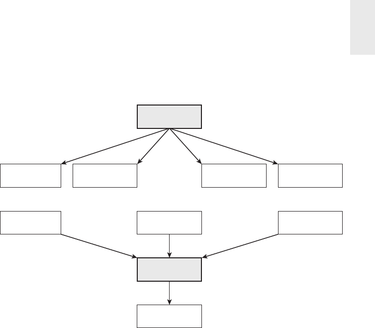
Customer Relationship Management 257
fi les and builds a “downstream” MDM system. These two styles of MDM are illus-
trated in Figure 8-14.
Enterprise
MDM
Downstream
MDM
Operational
App #1
Operational
App #2
Operational
App #3
Operational
App #1
Operational
App #2
Operational
App #3 EDW
EDW
Figure 8-14: Two styles of master data management.
Unfortunately, there’s no secret weapon for tackling this data consolidation. The
attributes in the customer dimension should represent the “best” source available
in the enterprise. A national change of address (NCOA) process should be integrated
to ensure address changes are captured. Much of the heavy lifting associated with
customer data consolidation demands customer matching or deduplicating logic.
Removing duplicates or invalid addresses from large customer lists is critical to
eliminate the costs associated with redundant, misdirected, or undeliverable com-
munication, avoid misleading customer counts, and improve customer satisfaction
through higher quality communication.
The science of customer matching is more sophisticated than it might fi rst appear.
It involves fuzzy logic, address parsing algorithms, and enormous look-up direc-
tories to validate address elements and postal codes, which vary signifi cantly by
country. There are specialized, commercially available software and service o erings
that perform individual customer or commercial entity matching with remarkable
accuracy. Often these products match the address components to standardized
census codes, such as state codes, country codes, census tracts, block groups, metro-
politan statistical areas (MSAs), and latitude/longitude, which facilitate the merging

Chapter 8
258
of external data. As discussed in Chapter 10, there are also householding capabilities
to group or link customers sharing similar name and/or address information. Rather
than merely performing intrafi le matching, some services maintain an enormous
external reference fi le of everyone in the United States to match against. Although
these products and services are expensive and/or complex, it’s worthwhile to make
the investment if customer matching is strategic to the organization. In the end,
e ective consolidation of customer data depends on a balance of capturing the data
as accurately as possible in the source systems, coupled with powerful data cleans-
ing/merging tools in the ETL process.
Partial Conformity of Multiple Customer Dimensions
Enterprises today build customer knowledge stores that collect all the internal and
external customer-facing data sources they can fi nd. A large organization could
have as many as 20 internal data sources and 50 or more external data sources,
all of which relate in some way to the customer. These sources can vary wildly in
granularity and consistency. Of course, there is no guaranteed high-quality customer
key defi ned across all these data sources and no consistent attributes. You don’t have
any control over these sources. It seems like a hopeless mess.
In Chapter 4: Inventory, we laid the groundwork for conformed dimensions,
which are the required glue for achieving integration across separate data sources.
In the ideal case, you examine all the data sources and defi ne a single compre-
hensive dimension which you attach to all the data sources, either simultaneously
within a single tablespace or by replicating across multiple tablespaces. Such a
single comprehensive conformed dimension becomes a wonderful driver for creating
integrated queries, analyses, and reports by making consistent row labels available
for drill-across queries.
But in the extreme integration world with dozens of customer-related dimensions
of di erent granularity and di erent quality, such a single comprehensive customer
dimension is impossible to build. Fortunately, you can implement a lighter weight
kind of conformed customer dimension. Remember the essential requirement for
two dimensions to be conformed is they share one or more specially administered
attributes that have the same column names and data values. Instead of requiring
dozens of customer-related dimensions to be identical, you only require they share
the specially administered conformed attributes.
Not only have you taken the pressure o the data warehouse by relaxing the
requirement that all the customer dimensions in your environment be equal from
top to bottom, but in addition you can proceed in an incremental and agile way
to plant the specially administered conformed attributes in each of the customer-
related dimensions. For example, suppose you start by defi ning a fairly high-level

Customer Relationship Management 259
categorization of customers called customer category. You can proceed methodically
across all the customer-related dimensions, planting this attribute in each dimension
without changing the grain of any target dimension and without invalidating any
existing applications that depend on those dimensions. Over a period of time, you
gradually increase the scope of integration as you add the special attributes to the
separate customer dimensions attached to di erent sources. At any point in time,
you can stop and perform drill-across reports using the dimensions where you have
inserted the customer category attribute.
When the customer category attribute has been inserted into as many of the
customer-related dimensions as possible, you can then defi ne more conformed attri-
butes. Geographic attributes such as city, county, state, and country should be even
easier than the customer category. Over a period of time, the scope and power of the
conformed customer dimensions let you do increasingly sophisticated analyses. This
incremental development with its closely spaced deliverables fi ts an agile approach.
Avoiding Fact-to-Fact Table Joins
DW/BI systems should be built process-by-process, not department-by-department,
on a foundation of conformed dimensions to support integration. You can imagine
querying the sales or support fact tables to better understand a customers’ purchase
or service history.
Because the sales and support tables both contain a customer foreign key, you
can further imagine joining both fact tables to a common customer dimension to
simultaneously summarize sales facts along with support facts for a given customer.
Unfortunately, the many-to-one-to-many join will return the wrong answer in a
relational environment due to the di erences in fact table cardinality, even when
the relational database is working perfectly. There is no combination of inner, outer,
left, or right joins that produces the desired answer when the two fact tables have
incompatible cardinalities.
Consider the case in which you have a fact table of customer solicitations,
and another fact table with the customer responses to solicitations, as shown in
Figure 8-15. There is a one-to-many relationship between customer and solicita-
tion, and another one-to-many relationship between customer and response. The
solicitation and response fact tables have di erent cardinalities; in other words, not
every solicitation results in a response (unfortunately for the marketing department)
and some responses are received for which there is no solicitation. Simultaneously
joining the solicitations fact table to the customer dimension, which is, in turn,
joined to the responses fact table, does not return the correct answer in a relational
DBMS due to the cardinality di erences. Fortunately, this problem is easily avoided.
You simply issue the drill-across technique explained in Chapter 4 to query the

Chapter 8
260
solicitations table and responses table in separate queries and then outer join the two
answer sets. The drill-across approach has additional benefi ts for better controlling
performance parameters, in addition to supporting queries that combine data from
fact tables in di erent physical locations.
Customer Solicitation Fact
Solicitation Date Key (FK)
Customer Key (FK)
More FKs ...
Solicitation Facts ...
Customer Response Fact
Response Date Key (FK)
Customer Key (FK)
More FKs ...
Response Facts ...
Customer Dimension
Customer Key (PK)
Customer ID (Natural Key)
...
Figure 8-15: Many-to-one-to-many joined tables should not be queried with a single
SELECT statement.
WAR NI NG Be very careful when simultaneously joining a single dimension
table to two fact tables of di erent cardinality. In many cases, relational engines
return the “wrong” answer.
If business users are frequently combining data from multiple business pro-
cesses, a fi nal approach is to defi ne an additional fact table that combines the data
once into a consolidated fact table rather than relying on users to consistently
and accurately combine the data on their own, as described in Chapter 7. Merely
using SQL to drill across fact tables to combine the results makes more sense when
the underlying processes are less closely correlated. Of course, when constructing the
consolidated fact table, you still need to establish business rules to deal with
the di ering cardinality. For example, does the consolidated fact table include all the
solicitations and responses or only those where both a solicitation and response
occurred?
Low Latency Reality Check
The behavior of a customer in the last few hours or minutes can be extremely inter-
esting. You may even want to make decisions while dealing with the customer in
real time. But you need to be thoughtful in recognizing the costs and limitations
of low latency data. Generally, data quality su ers as the data is delivered closer
to real time.
Business users may automatically think that the faster the information arrives in
the DW/BI system, the better. But decreasing the latency increases the data quality

Customer Relationship Management 261
problems. Figure 20-6 summarizes the issues that arise as data is delivered faster.
In the conventional batch world, perhaps downloading a batch fi le once each 24
hours, you typically get complete transaction sets. For example, if a commercial
customer places an order, they may have to pass a credit check and verify the fi nal
commitment. The batch download includes orders only where all these steps have
taken place. In addition, because the batch download is processed just once each 24
hours, the ETL team has the time to run the full spectrum of data quality checks,
as we’ll describe in Chapter 19: ETL Subsystems and Techniques.
If the data is extracted many times per day, then the guarantee of complete
transaction sets may have to be relinquished. The customer may have placed the
order but has not passed the credit check. Thus there is the possibility that results
may have to be adjusted after the fact. You also may not run the full spectrum of
data quality checks because you don’t have time for extensive multitable lookups.
Finally, you may have to post data into the data warehouse when all the keys have
not been resolved. In this case, temporary dimensional entries may need to be used
while waiting for additional data feeds.
Finally, if you deliver data instantaneously, you may be getting only transaction
fragments, and you may not have time to perform any data quality checks or other
processing of the data.
Low latency data delivery can be very valuable, but the business users need to
be informed about these trade-o s. An interesting hybrid approach is to provide
low latency intraday delivery but then revert to a batch extract at night, thereby
correcting various data problems that could not be addressed during the day. We
discuss the impact of low latency requirements on the ETL system in Chapter 20:
ETL System Design and Development Process and Tasks.
Summary
In this chapter, we focused exclusively on the customer, beginning with an over-
view of customer relationship management (CRM) basics. We then delved into
design issues surrounding the customer dimension table. We discussed name and
address parsing where operational fi elds are decomposed to their basic elements
so that they can be standardized and validated. We explored several other types
of common customer dimension attributes, such as dates, segmentation attributes,
and aggregated facts. Dimension outriggers that contain a large block of relatively
low-cardinality attributes were described.
This chapter introduced the use of bridge tables to handle unpredictable, sparsely
populated dimension attributes, as well as multivalued dimension attributes.

Chapter 8
262
We also explored several complex customer behavior scenarios, including sequential
activities, timespan fact tables, and tagging fact events with indicators to identify
abnormal situations.
We closed the chapter by discussing alternative approaches for consistently iden-
tifying customers and consolidating a rich set of characteristics from the source
data, either via operational master data management or downstream processing in
the ETL back room with potentially partial conformity. Fi nally, we touched on the
challenges of low latency data requirements.

Human Resources
Management
This chapter, which focuses on human resources (HR) data, is the last in the series
dealing with cross-industry business applications. Similar to the accounting
and finance data described in Chapter 7: Accounting, HR information is dissemi-
nated broadly throughout the organization. Organizations want to better understand
their employees’ demographics, skills, earnings, and performance to maximize their
impact. In this chapter we’ll explore several dimensional modeling techniques in the
context of HR data.
Chapter 9 discusses the following concepts:
■ Dimension tables to track employee profi le changes
■ Periodic headcount snapshots
■ Bus matrix for a snippet of HR-centric processes
■ Pros and cons of packaged DW/BI solutions or data models
■ Recursive employee hierarchies
■ Multivalued skill keyword attributes handled via dimension attributes, out-
riggers, or bridges
■ Survey questionnaire data
■ Text comments
Employee Profi le Tracking
Thus far the dimensional models we have designed closely resemble each other;
the fact tables contain key performance metrics that typically can be added across
all the dimensions. It is easy for dimensional modelers to get lulled into a kind of
additive complacency. In most cases, this is exactly how it is supposed to work.
However, with HR employee data, a robust employee dimension supports numerous
metrics required by the business on its own.
9
Chapter 9
264
To frame the problem with a business vignette, let’s assume you work in the HR
department of a large enterprise. Each employee has a detailed HR profi le with
at least 100 attributes, including hire date, job grade, salary, review dates, review
outcomes, vacation entitlement, organization, education, address, insurance plan,
and many others. Employees are constantly hired, transferred, and promoted, as
well as adjusting their profi les in a variety of ways.
A high-priority business requirement is to accurately track and analyze
employee profi le changes. You might immediately visualize a schema in which
each employee profi le change event is captured in a transaction-grained fact table,
as depicted in Figure 9-1. The granularity of this somewhat generalized fact
table would be one row per employee profi le transaction. Because no numeric
metrics are associated with changes made to employee profi les, such as a new
address or job grade promotion, the fact table is factless.
Employee Key (PK)
Employee ID (NK)
...
Transaction Date Key (FK)
Transaction Date/Time
Employee Key (FK)
Employee Transaction Type Key (FK)
Employee Dimension
Employee Transaction Type Key (PK)
Employee Transaction Type Description
1 row per employee profile transaction
Employee Transaction Type Dimension
Employee Transaction Fact Transaction Date Dimension
Figure 9-1: Initial draft schema for tracking employees’ profi le changes.
In this draft schema, the dimensions include the transaction date, transaction
type, and employee. The transaction type dimension refers to the reason code that
caused the creation of this particular row, such as a promotion or address change.
The employee dimension is extremely wide with many attribute columns.
We envision using the type 2 slowly changing dimension technique for tracking
changed profi le attributes within the employee dimension. Consequently, with every
employee profi le transaction in the Figure 9-1 fact table, you would also create a
new type 2 row in the employee dimension that represents the employee’s profi le as
a result of the profi le change event. This new row continues to accurately describe
the employee until the next employee transaction occurs at some indeterminate
time in the future. The alert reader is quick to point out that the employee profi le
transaction fact table and type 2 employee dimension table have the same number of
rows; plus they are almost always joined to one another. At this point dimensional
modeling alarms should be going o . You certainly don’t want to have as many rows
in a fact table as you do in a related dimension table.
Instead of using the initial schema, you can simplify the design by embellish-
ing the employee dimension table to make it more powerful and thereby doing

Human Resources Management 265
away with the profi le transaction event fact table. As depicted in Figure 9-2, the
employee dimension contains a snapshot of the employee profi le characteristics
following the employee’s profi le change. The transaction type description becomes
a change reason attribute in the employee dimension to track the cause for the pro-
fi le change. In some cases, the a ected characteristics are numeric. If the numeric
attributes are summarized rather than simply constrained upon, they belong in a
fact table instead.
Employee Key (PK)
Employee ID (NK)
Employee Name ...
Employee Address ...
Job Grade ...
Salary ...
Education ...
Original Hire Date (FK)
Last Review Date (FK)
Appraisal Rating ...
Health Insurance Plan ...
Vacation Plan ...
Change Reason Code
Change Reason Description
Row Effective Date/Time
Row Expiration Date/Time
Current Row Indicator
Employee Dimension
Figure 9-2: Employee dimension with profi le characteristics.
As you’d expect, the surrogate employee key is the primary key of the dimen-
sion table; the durable natural employee ID used in the HR operational system to
persistently identify an employee is included as a dimension attribute.
Precise Effective and Expiration Timespans
As discussed in Chapter 5: Procurement with the coverage of slowly changing
dimension techniques, you should include two columns on the employee dimension
to capture when a specifi c row is e ective and then expired. These columns defi ne
a precise timespan during which the employee’s profi le is accurate. Historically,
when daily data latency was the norm, the e ective and expiration columns were
dates. However, if you load data from any business process on a more frequent basis,
the columns should be date/time stamps so that you can associate the appropriate
employee profi le row, which may di er between 9 a.m. and 9 p.m. on the same day,
to operational events.

Chapter 9
266
The expiration attribute for the current row is set to a future date. When the row
needs to be expired because the ETL system has detected a new profi le of attributes,
the expiration attribute is typically set to “just before” the new row’s e ective stamp,
meaning either the prior day, minute, or second.
If the employee’s profi le is accurately changed for a period of time, then the
employee reverts back to an earlier set of characteristics, a new employee dimen-
sion row is inserted. You should resist the urge to simply revisit the earlier profi le
row and modify the expiration date because multiple dimension rows would be
e ective at the same time.
The current row indicator enables the most recent status of any employee to be
retrieved quickly. If a new profi le row occurs for this employee, the indicator in the
former profi le row needs to be updated to indicate it is no longer the current profi le.
On its own, a date/time stamped type 2 employee dimension answers a number
of interesting HR inquiries. You can choose an exact historical point in time and ask
how many employees you have and what their detailed profi les were at that specifi c
moment by constraining the date/time to be equal to or greater than the e ective
date/time and strictly less than the expiration date/time. The query can perform
counts and constraints against all the rows returned from these constraints.
Dimension Change Reason Tracking
When a dimension row contains type 2 attributes, you can embellish it with a change
reason. In this way, some ETL-centric metadata is embedded with the actual data.
The change reason attribute could contain a two-character abbreviation for each
changed attribute on a dimension row. For example, the change reason attribute
value for a last name change could be LN or a more legible value, such as Last
Name, depending on the intended usage and audience. If someone asks how many
peoplechanged ZIP codes last year, the SELECT statement would include a LIKE
operator and wild cards, such as "WHERE ChangeReason LIKE '%ZIP%’".
Because multiple dimension attributes may change concurrently and be repre-
sented by a single new row in the dimension, the change reason would be multi-
valued. As we’ll explore later in the chapter when discussing employee skills, the
multiple reason codes could be handled as a single text string attribute, such as
“|Last Name|ZIP|” or via a multivalued bridge table.
NOTE The e ective and expiration date/time stamps, along with a reason code
description, on each row of a type 2 slowly changing dimension allows very precise
time slicing of the dimension by itself.
Finally, employee profi le changes may be captured in the underlying source
system by a set of micro-transactions corresponding to each individual employee

Human Resources Management 267
attribute change. In the DW/BI system, you may want to encapsulate the series of
micro-transactions from the source system and treat them as a super transaction,
such as an employee promotion because it would be silly to treat these artifi cial
micro-transactions as separate type 2 changes. The new type 2 employee dimen-
sion row would refl ect all the relevant changed attributes in one step. Identifying
these super transactions may be tricky. Obviously the best way to identify them is
to ensure the HR operational application captures the higher level action.
Profi le Changes as Type 2 Attributes or Fact Events
We just described the handling of employee attribute changes as slowly changing
dimension type 2 attributes with profi le e ective and expiration dates within the
employee dimension. Designers sometimes wholeheartedly embrace this pattern
and try to leverage it to capture every employee-centric change. This results in a
dimension table with potentially hundreds of attributes and millions of rows for
a 100,000-employee organization given the attributes’ volatility.
Tracking changes within the employee dimension table enables you to easily
associate the employee’s accurate profi le with multiple business processes. You
simply load these fact tables with the employee key in e ect when the fact event
occurred, and fi lter and group based on the full spectrum of employee attributes.
But the pendulum can swing too far. You probably shouldn’t use the employee
dimension to track every employee review event, every benefi t participation event,
or every professional development event. As illustrated in Figure 9-4’s bus matrix
in the next section, many of these events involve other dimensions, like an event
date, organization, benefi t description, reviewer, approver, exit interviewer, separa-
tion reasons, and the list goes on. Consequently, most of them should be handled
as separate process-centric fact tables. Although many human resources events are
factless, capturing them within a fact table enables business users to easily count
or trend by time periods and all the other associated dimensions.
It’s certainly common to include the outcome of these HR events, like the job
grade resulting from a promotion, as an attribute on the employee dimension. But
designers sometimes err by including lots of foreign keys to outriggers for the
reviewer, benefi t, separation reason and other dimensions within the employee
dimension, resulting in an overloaded dimension that’s di cult to navigate.
Headcount Periodic Snapshot
In addition to profi ling employees in HR, you also want to report statuses of the
employees on a regular basis. Business managers are interested in counts, statistics,
and totals, including number of employees, salary paid, vacation days taken, vaca-
tion days accrued, number of new hires, and number of promotions. They want
Chapter 9
268
to analyze the data by all possible slices, including time and organization, plus
employee characteristics.
As shown in Figure 9-3, the employee headcount periodic snapshot consists of an
ordinary looking fact table with three dimensions: month, employee, and organiza-
tion. The month dimension table contains the usual descriptors for the corporate cal-
endar at the month grain. The employee key corresponds to the employee dimension
row in e ect at the end of the last day of the given reporting month to guarantee the
month-end report is a correct depiction of the employees’ profi les. The organization
dimension contains a description of the organization to which the employee belongs
at the close of the relevant month.
1 row per employee per month
Month Key (FK)
Organization Key (FK)
Employee Key (FK)
Employee Count
New Hire Count
Transfer Count
Promotion Count
Salary Paid
Overtime Paid
Retirement Fund Paid
Retirement Fund Employee Contribution
Vacation Days Accrued
Vacation Days Taken
Vacation Days Balance
Employee Headcount Snapshot Fact
Month Dimension
Employee Dimension
Organization Dimension
Figure 9-3: Employee headcount periodic snapshot.
The facts in this headcount snapshot consist of monthly numeric metrics and
counts that may be di cult to calculate from the employee dimension table alone.
These monthly counts and metrics are additive across all the dimensions or dimen-
sion attributes, except for any facts labeled as balances. These balances, like all
balances, are semi-additive and must be averaged across the month dimension after
adding across the other dimensions.
Bus Matrix for HR Processes
Although an employee dimension with precise type 2 slowly changing dimension
tracking coupled with a monthly periodic snapshot of core HR performance metrics
is a good start, they just scratch the surface when it comes to tracking HR data.

Human Resources Management 269
Figure 9-4 illustrates other processes that HR professionals and functional manag-
ers are likely keen to analyze. We’ve embellished this preliminary bus matrix with
the type of fact table that might be used for each process; however, your source
data realities and business requirements may warrant a di erent or complementary
treatment.
Employee Position Snapshot
Employee Requisition Pipeline
Employee Performance Review Pipeline
Employee Disciplinary Action Pipeline
Employee Separations
Employee Performance Review
Employee Prof Dev Completed Courses
Employee Hiring
Employee “On Board” Pipeline
Employee Benefits Eligibility
Employee Benefits Application
Employee Benefit Participation
Employee Benefit Accruals
Employee Headcount Snapshot
Employee Compensation
X
X
X
X
X
X
XX
X
X
X
X
X
X
X
X
X
X
X
X
Empl
Mgr
Empl
Mgr
Empl
Mgr
Empl
Mgr
Empl
Mgr
Empl
Mgr
Empl
Mgr
Empl
Mgr
X
X
X
X
X
X
X
X
X
X
X
X
X
X
X
X
X
X
X
X
X
X
X
X
X
X
X
X
X
Periodic
Date
Position
Employee
Organization
Benefit
Accumulating
Accumulating
Accumulating
Transaction
Transaction
Transaction
Transaction
Accumulating
Periodic
Accumulating
Periodic
Transaction
Periodic
Transaction
Fact Type
Hiring Processes
Benefits Processes
Employee Management Processes
Figure 9-4: Bus matrix rows for HR processes.
Some of these business processes capture performance metrics, but many result
in factless fact tables, such as benefi t eligibility or participation.

Chapter 9
270
Packaged Analytic Solutions
and Data Models
Many organizations purchase a vendor solution to address their operational HR
application needs. Most of these products o er an add-on DW/BI solution. In addi-
tion, other vendors sell standard data models, potentially with prebuilt data loaders
for the popular HR application products.
Vendors and proponents argue these standard, prebuilt solutions and models
allow for more rapid, less risky implementations by reducing the scope of the data
modeling and ETL development e ort. After all, every HR department hires employ-
ees, signs them up for benefi ts, compensates them, reviews them, and eventually
processes employee separations. Why bother re-creating the wheel by designing
custom data models and solutions to support these common business processes
when you can buy a standard data model or complete solution instead?
Although there are undoubtedly common functions, especially within the HR
space, businesses typically have unique peculiarities. To handle these nuances,
most application software vendors introduce abstractions in their products, which
enable them to be more easily “customized.”
These abstractions, like the party table and associated apparatus to describe each
role or generic attribute column names rather than more meaningful labels, provide
fl exibility to adapt to a variety of business situations. Although implementation
adaptability is a win for vendors who want their products to address a broad range of
potential customers’ business scenarios, the downside is the associated complexity.
HR professionals who live with the vendor’s product 24x7 are often willing to
adjust their vocabulary to accommodate the abstractions. But these abstractions can
feel like a foreign language for less-immersed functional managers. Delivering data
to the business via a packaged DW/BI solution or industry-standard data model may
bypass the necessary translations into the business’s vernacular.
Besides the reliance on the vendor’s terminology instead of incorporating the
business’s vocabulary in the DW/BI solution, another potential sharp corner is
the integration of source data from other domains. Can you readily conform the
dimensions in the vendor solution or industry model with other internally avail-
able master data? If not, the packaged model is destined to become another isolated
stovepipe data set. Clearly, this outcome is unappealing; although it may be less of
an obstacle if all your operational systems are supported by the same ERP vendor,
or you’re a small organization without an IT shop doing independent development.
What can you realistically expect to gain from a packaged model? Prebuilt generic
models can help identify core business processes and associate common dimensions.
That provides some comfort for DW/BI teams feeling initially overwhelmed by the

Human Resources Management 271
design task. After a few days or weeks studying the standard model, most teams
gain enough confi dence to want to customize the schema for their data.
However, is this knowledge worth the price tag associated with the packaged
solution or data model? You could likely gain the same insight by spending a few
weeks with the business users. You’d not only improve your understanding of the
business’s needs, but also begin bonding business users to the DW/BI initiative.
It’s also worth mentioning that just because a packaged model or solution costs
thousands of dollars doesn’t mean it exhibits generally accepted dimensional modeling
best practices. Unfortunately, some standard models embody common dimensional
modeling design fl aws; this isn’t surprising if the model’s designers focused more on
best practices for source system data capture rather than those required for BI report-
ing and analytics. It’s di cult to design a predefi ned generic model, even if the vendor
owns the data capture source code.
Recursive Employee Hierarchies
A common employee characteristic is the name of the employee’s manager. You
could simply embed this attribute along with the other attributes in the employee
dimension. But if the business users want more than the manager’s name, more
complex structures are necessary.
One approach is to include the manager’s employee key as another foreign key in
the fact table, as shown in Figure 9-5. This manager employee key joins to a role-
playing employee dimension where every attribute name refers to “manager” to
di erentiate the manager’s profi le from the employee’s. This approach associates the
employee and their manager whenever a row is inserted into a fact table. BI analyses
can easily fi lter and group by either employee or manager attributes with virtually
identical query performance because both dimensions provide symmetrical access
to the fact table. The downside of this approach is these dual foreign keys must be
embedded in every fact table to support managerial reporting.
Separation Date Key (FK)
Organization Key (FK)
Employee Key (FK)
Manager Key (FK)
Separation Profile Key (FK)
Separation Count
Employee Key (PK)
Employee ID (NK)
...
Employee Dimension
Manager Key (PK)
Manager Employee ID (NK)
...
Manager Dimension Separation Profile Key (PK)
Separation Type Description
Separation Reason Description
Separation Profile Dimension
Employee Separation Fact
Date Dimension
Organization Dimension
Figure 9-5: Dual role-playing employee and manager dimensions.

Chapter 9
272
Another option is to include the manager’s employee key as an attribute on the
employee’s dimension row. The manager key would join to an outrigger consisting of
a role play on the employee dimension where all the attributes reference “manager”
to di erentiate them from the employee’s characteristics, as shown in Figure 9-6.
Separation Date Key (FK)
Organization Key (FK)
Employee Key (FK)
Separation Profile Key (FK)
Separation Count
Employee Key (PK)
Employee ID (NK)
Employee Attributes ...
Manager Key (FK)
Row Effective Date
Row Expiration Date
Current Row Indicator
Employee Dimension
Manager Key (PK)
Manager Employee ID (NK)
Manager Employee Attributes ...
Row Effective Date
Row Expiration Date
Current Row Indicator
Manager Dimension
Employee Separation Fact
Figure 9-6: Manager role-playing dimension as an outrigger.
If the manager’s foreign key in the employee dimension is designated as a type 2
attribute, then new employee rows would be generated with each manager change.
However, we encourage you to think carefully about the underlying ETL business rules.
Change Tracking on Embedded Manager Key
Let’s walk through an example. Abby is Hayden’s manager. With the outrigger
approach just described, Hayden’s employee dimension row would include an
attribute linking to Abby’s row in the manager role-play employee dimension. If
Hayden’s manager changes, and assuming the business wants to track these histori-
cal changes, then treating the manager foreign key as a type 2 and creating a new
row for Hayden to capture his new profi le with a new manager would be appropriate.
However, think about the desired outcome if Abby were still Hayden’s manager,
but her employee profi le changes, perhaps caused by something as innocuous as
a home address change. If the home address is designated as a type 2 attribute,
this move would spawn a new employee dimension row for Abby. If the manager
key is also designated as a type 2 attribute, then Abby’s new employee key would
also spawn a new dimension row for Hayden. Now imagine Abby is the CEO of a
large organization. A type 2 change in her profi le would ripple through the entire
table; you’d end up replicating a new profi le row for every employee due to a single
type 2 attribute change on the CEO’s profi le.
Does the business want to capture these manager profi le changes? If not, perhaps
the manager key on the employee’s row should be the manager’s durable natural key

Human Resources Management 273
linked to a role-playing dimension limited to just the current row for each manager’s
durable natural key in the dimension.
If you designate the manager’s key in the employee dimension to be a type 1
attribute, it would always associate an employee with her current manager. Although
this simplistic approach obliterates history, it may completely satisfy the business
user’s needs.
Drilling Up and Down Management Hierarchies
Adding an attribute, either a textual label or a foreign key to a role-playing dimen-
sion, to an employee dimension row is appropriate for handling the fi xed depth,
many-to-one employee-to-manager relationship. However, more complex approaches
might be required if the business wants to navigate a deeper recursive hierarchy,
such as identifying an employee’s entire management chain or drilling down to
identify the activity for all employees who directly or indirectly work for a given
manager.
If you use an OLAP tool to query employee data, the embedded manager key
on every employee dimension row may su ce. Popular OLAP products contain a
parent/child hierarchy structure that works smoothly with variable depth recursive
hierarchies. In fact, this is one of the strengths of OLAP products.
However, if you want to query the recursive employee/manager relationship in
the relational environment, you must use Oracle’s nonstandard CONNECT BY syntax
or SQL’s recursive common table extension (CTE) syntax. Both approaches are
virtually unworkable for business users armed with a BI reporting tool.
So you’re left with the options described in Chapter 7 for dealing with vari-
able depth customer hierarchies. In Figure 9-7, the employee dimension from
Figure 9-6 relates to the fact table through a bridge table. The bridge table has
one row for each manager and each employee who is directly or indirectly in
their management chain, plus an additional row for the manager to himself. The
bridge joins shown in Figure 9-7 enable you to drill down within a manager’s
chain of command.
Separation Date Key (FK)
Organization Key (FK)
Employee Key (FK)
Separation Profile Key (FK)
Separation Count
Manager Key (FK)
Employee Key (FK)
# Levels from Top
Bottom Flag
Top Flag
Management Hierarchy Bridge
Manager Key (PK)
Manager Employee ID (NK)
Manager Employee Attributes ...
Row Effective Date
Row Expiration Date
Current Row Indicator
Manager Dimension
Employee Separation Fact
Figure 9-7: Bridge table to drill down into a manager’s reporting structure.

Chapter 9
274
As previously described, there are several disadvantages to this approach. The
bridge table is somewhat challenging to build, plus it contains many rows, so query
performance can su er. The BI user experience is complicated for ad hoc queries,
although we’ve seen analysts e ectively use it. Finally, if users want to aggregate
information up rather than down a management chain, the join paths must be
reversed.
Once again, the situation is further complicated if you want to track employee pro-
fi le changes in conjunction with the bridge table. If the manager and employee refl ect
employee profi les with type 2 changes, the bridge table will experience rapid growth,
especially when senior management profi le changes cause new keys to ripple across
the organization.
You could use durable natural keys in the bridge table, instead of the employee
keys which capture type 2 profi le changes. Limiting the relationship to the man-
agement hierarchy’s current profi les is one thing. However, if the business wants
to retain a history of employee/manager rollups, you need to embellish the bridge
table with e ective and expiration dates that capture the e ective timespan for each
employee/manager relationship.
The propagation of new rows in this bridge table using durable keys is substan-
tially reduced compared to the Figure 9-7 bridge because new rows are added when
reporting relationships change, not when any type 2 employee attribute is modifi ed.
A bridge table built on durable keys is easier to manage, but quite challenging to
navigate, especially given the need to associate the relevant organizational structures
with the event dates in the fact table. Given the complexities, the bridge table should
be buried within a canned BI application for all but a small subset of power BI users.
The alternative approaches discussed in Chapter 7 for handling recursive hierar-
chies, like the pathstring attribute, are also relevant to the management hierarchy
conundrum. Unfortunately, there’s no silver bullet solution for handling these com-
plex structures in a simple and fast way.
Multivalued Skill Keyword Attributes
Let’s assume the IT department wants to supplement the employee dimension with
technical skillset profi ciency information. You could consider these technical skills,
such as programming languages, operating systems, or database platforms, to be key-
words describing employees. Each employee is tagged with a number of skill keywords.
You want to search the IT employee population by their descriptive skills.
If the technical skills of interest were a fi nite number, you could include them
as individual attributes in the employee dimension. The advantage of using posi-
tional dimension attributes, such as a Linux attribute with domain values such as

Human Resources Management 275
Linux Skills and No Linux Skills, is they’re easy to query and deliver fast query
performance. This approach works well to a point but falls apart when the number
of potential skills expands.
Skill Keyword Bridge
More realistically, each employee will have a variable, unpredictable number of
skills. In this case, the skill keyword attribute is a prime candidate to be a multi-
valued dimension. Skill keywords, by their nature, are open-ended; new skills are
added regularly as domain values. We’ll show two logically equivalent modeling
schemes for handling open-ended sets of skills.
Figure 9-8 shows a multivalued dimension design for handling the skills as an
outrigger bridge table to the employee dimension table. As you’ll see in Chapter 14:
Healthcare, sometimes the multivalued bridge table is joined directly to a fact table.
Employee Key (FK)
More FKs ...
Headcount Facts ...
Employee Headcount
Snapshot Fact
Employee Key (PK)
...
Employee Skill Group Key (FK)
Employee Dimension
Employee Skill Key (PK)
Employee Skill Description
Employee Skill Category
Skills Dimension
Employee Skill Group Key (FK)
Employee Skill Key (FK)
Employee Skill Group Bridge
Figure 9-8: Skills group keyword bridge table.
The skills group bridge identifi es a given set of skill keywords. IT employees who
are profi cient in Oracle, Unix, and SQL would be assigned the same skills group key.
In the skills group bridge table, there would be three rows for this particular group,
one for each of the associated skill keywords (Oracle, Unix, and SQL).
AND/OR Query Dilemma
Assuming you built the schema shown in Figure 9-8, you are still left with a serious
query problem. Query requests against the skill keywords fall into two categories. The
OR queries (for example, Unix or Linux experience) can be satisfi ed by a simple OR
constraint on the skills description attribute in the skills dimension table. However,
AND queries (for example, Unix and Linux experience) are di cult because the AND
constraint is a constraint across two rows in the skills dimension. SQL is notoriously
poor at handling constraints across rows. The answer is to create SQL code using
unions and intersections, probably in a custom interface that hides the complex logic
from the business user. The SQL code would look like this:
(SELECT employee_ID, employee_name
FROM Employee, SkillBridge, Skills
WHERE Employee.SkillGroupKey = SkillBridge.SkillGroupKey AND
SkillGroup.SkillKey = Skill.SkillKey AND

Chapter 9
276
Skill.Skill = "UNIX")
UNION / INTERSECTION
(SELECT employee_ID, employee_name
FROM Employee, SkillBridge, Skills
WHERE Employee.SkillGroupKey = SkillBridge.SkillGroupKey AND
SkillGroup.SkillKey = Skill.SkillKey AND
Skill.Skill = "LINUX")
Using the UNION lists employees with Unix or Linux experience, whereas using
INTERSECTION identifi es employees with Unix and Linux experience.
Skill Keyword Text String
You can remove the many-to-many bridge and the need for union/intersection SQL
by simplifying the design. One approach would be to add a skills list outrigger to
the employee dimension containing one long text string concatenating all the skill
keywords for that list key. You would need a special delimiter such as a backslash or
vertical bar at the beginning of the skills text string and after each skill in the list.
Thus the skills string containing Unix and C++ would look like |Unix|C++|. This
outrigger approach presumes a number of employees share a common list of skills.
If the lists are not reused frequently, you could collapse the skills list outrigger by
simply including the skills list text string as an employee dimension attribute, as
shown in Figure 9-9.
Employee Key (FK)
More FKs ...
Headcount Facts ...
Employee Headcount Snapshot Fact
Employee Key (PK)
...
Employee Skill Group List
Employee Dimension
Figure 9-9: Delimited skills list string.
Text string searches can be challenging because of the ambiguity caused by
searching on uppercase or lowercase. Is it UNIX or Unix or unix? You can resolve
this by coercing the skills list to upper case with the UCase function in most SQL
environments.
With the design in Figure 9-9, the AND/OR dilemma can be addressed in a single
SELECT statement. The OR constraint looks like this:
UCase(skill_list) like '%|UNIX|% OR UCase(skill_list) like '%|LINUX|%'
Meanwhile, the AND constraint has exactly the same structure:
UCase(skill_list) like '%|UNIX|' AND UCase(skill_list) like '%|LINUX|%'

Human Resources Management 277
The % symbol is a wild card pattern-matching character defi ned in SQL that
matches zero or more characters. The vertical bar delimiter is used explicitly in the
constraints to exactly match the desired keywords and not get erroneous matches.
The keyword list approach shown in Figure 9-9 can work in any relational database
because it is based on standard SQL. Although the text string approach facilitates
AND/OR searching, it doesn’t support queries that count by skill keyword.
Survey Questionnaire Data
HR departments often collect survey data from employees, especially when gather-
ing peer and/or management review data. The department analyzes questionnaire
responses to determine the average rating for a reviewed employee and within a
department.
To handle questionnaire data in a dimensional model, a fact table with one row
for each question on a respondent’s survey is typically created, as illustrated in
Figure 9-10. Two role-playing employee dimensions in the schema correspond to the
responding employee and reviewed employee. The survey dimension has descriptors
about the survey instrument. The question dimension provides the question and
its categorization; presumably, the same question is asked on multiple surveys. The
survey and question dimensions can be useful when searching for specifi c topics in
a broad database of questionnaires. The response dimension contains the responses
and perhaps categories of responses, such as favorable or hostile.
Survey Key (PK)
Survey Title
Survey Type
Survey Objective
Review Year
Question Key (PK)
Question Label
Question Category
Question Objective
Survey Sent Date Key (FK)
Survey Received Date Key (FK)
Survey Key (FK)
Responding Employee Key (FK)
Reviewed Employee Key (FK)
Question Key (FK)
Response Category Key (FK)
Survey Number (DD)
Response
Survey Dimension
Response Category Key (PK)
Response Category Description
Response Category Dimension
Employee Evaluation Survey Fact
Question Dimension
Date Dimension (2 views for roles)
Employee Dimension (2 views for roles)
Figure 9-10: Survey schema.
Creating the simple schema in Figure 9-10 supports robust slicing and dicing
of survey data. Variations of this schema design would be useful for analyzing all
types of survey data, including customer satisfaction and product usage feedback.

Chapter 9
278
Text Comments
Facts are typically thought of as continuously valued numeric measures; dimension
attributes, on the other hand, are drawn from a discrete list of domain values. So
how do you handle textual comments, such as a manager’s remarks on a perfor-
mance review or freeform feedback on a survey question, which seem to defy clean
classifi cation into the fact or dimension category? Although IT professionals may
instinctively want to simply exclude them from a dimensional design, business
users may demand they’re retained to further describe the performance metrics.
After it’s been confi rmed the business is unwilling to relinquish the text com-
ments, you should determine if the comments can be parsed into well-behaved
dimension attributes. Although there are sometimes opportunities to categorize
the text, such as a compliment versus complaint, the full text verbiage is typically
also required.
Because freeform text takes on so many potential values, designers are some-
times tempted to store the text comment within the fact table. Although cognizant
that fact tables are typically limited to foreign keys, degenerate dimensions, and
numeric facts, they contend the text comment is just another degenerate dimension.
Unfortunately, text comments don’t qualify as degenerate dimensions.
Freeform text fi elds shouldn’t be stored in the fact table because they just add
bulky clutter to the table. Depending on the database platform, this relatively low
value bulk may get dragged along on every operation involving the fact table’s much
more valuable performance metrics.
Rather than treating the comments as textual metrics, we recommend retaining
them outside the fact table. The comments should either be captured in a separate
comments dimensions (with a corresponding foreign key in the fact table) or as
an attribute on a transaction-grained dimension table. In some situations, identi-
cal comments are observed multiple times. At a minimum, this typically occurs
with the No Comment comment. If the cardinality of the comments is less than
the number of transactions, the text should be captured in a comments dimension.
Otherwise, if there’s a unique comment for every event, it’s treated as a transaction
dimension attribute. In either case, regardless of whether the comments are handled
in a comment or transaction dimension, the query performance when this sizeable
dimension is joined to the fact table will be slow. However, by the time users are
viewing comments, they’ve likely signifi cantly fi ltered their query as they can real-
istically read only a limited number of comments. Meanwhile, the more common
analyses focusing on the fact table’s performance metrics won’t be burdened by the
extra weight of the textual comments on every fact table query.

Human Resources Management 279
Summary
In this chapter, we discussed several concepts in the context of HR data. First,
we further elaborated on the advantages of embellishing an employee dimension
table. In the world of HR, this single table is used to address a number of ques-
tions regarding the status and profi le of the employee base at any point in time. We
drafted a bus matrix representing multiple processes within the HR arena and high-
lighted a core headcount snapshot fact table, along with the potential advantages
and disadvantages of vendor-designed solutions and data models. The handling of
managerial rollups and multivalued dimension attributes was discussed. Finally,
we provided a brief overview regarding the handling of survey or questionnaire
data, along with text comments.

Financial Services
The financial services industry encompasses a wide variety of businesses, includ-
ing credit card companies, brokerage firms, and mortgage providers. In this
chapter, we’ll primarily focus on the retail bank since most readers have some degree
of personal familiarity with this type of financial institution. A full-service bank offers
a breadth of products, including checking accounts, savings accounts, mortgage
loans, personal loans, credit cards, and safe deposit boxes. This chapter begins with
a very simplistic schema. We then explore several schema extensions, including the
handling of the bank’s broad portfolio of heterogeneous products that vary signifi-
cantly by line of business.
We want to remind you that industry focused chapters like this one are not
intended to provide full-scale industry solutions. Although various dimensional
modeling techniques are discussed in the context of a given industry, the techniques
are certainly applicable to other businesses. If you don’t work in fi nancial services,
you still need to read this chapter. If you do work in fi nancial services, remember
that the schemas in this chapter should not be viewed as complete.
Chapter 10 discusses the following concepts:
■ Bus matrix snippet for a bank
■ Dimension triage to avoid the “too few dimensions” trap
■ Household dimensions
■ Bridge tables to associate multiple customers with an account, along with
weighting factors
■ Multiple mini-dimensions in a single fact table
■ Dynamic value banding of facts for reporting
■ Handling heterogeneous products across lines of business, each with unique
metrics and/or dimension attributes, as supertype and subtype schemas
■ Hot swappable dimensions
10

Chapter 10
282
Banking Case Study and Bus Matrix
The bank’s initial goal is to better analyze the bank’s accounts. Business users want the
ability to slice and dice individual accounts, as well as the residential household groupings
to which they belong. One of the bank’s major objectives is to market more e ectively by
o ering additional products to households that already have one or more accounts with
the bank. Figure 10-1 illustrates a portion of a bank’s bus matrix.
New Business Solicitation
Lead Tracking
Account Application Pipeline
Account Initiation
Account Transactions
Account Monthly Snapshot
Account Servicing Activities
X
X
X
X
X
X
X
X
X
X
X
X
X
X
XX
X
X
X
X
X
X
X
X
X
X
X
X
X
X
X
X
X
X
X
X
X
X
Date
Prospect
Customer
Household
Branch
Account
Product
Figure 10-1: Subset of bus matrix rows for a bank.
After conducting interviews with managers and analysts around the bank, the
following set of requirements were developed:
■ Business users want to see fi ve years of historical monthly snapshot data on
every account.
■ Every account has a primary balance. The business wants to group di erent
types of accounts in the same analyses and compare primary balances.
■ Every type of account (known as products within the bank) has a set of cus-
tom dimension attributes and numeric facts that tend to be quite di erent
from product to product.
■ Every account is deemed to belong to a single household. There is a surprising
amount of volatility in the account/household relationships due to changes
in marital status and other life stage factors.
■ In addition to the household identifi cation, users are interested in demographic
information both as it pertains to individual customers and households. In
addition, the bank captures and stores behavior scores relating to the activity
or characteristics of each account and household.

Financial Services 283
Dimension Triage to Avoid Too Few
Dimensions
Based on the previous business requirements, the grain and dimensionality of the
initial model begin to emerge. You can start with a fact table that records the pri-
mary balances of every account at the end of each month. Clearly, the grain of the
fact table is one row for each account each month. Based on that grain declaration,
you can initially envision a design with only two dimensions: month and account.
These two foreign keys form the fact table primary key, as shown in Figure 10-2.
A data-centric designer might argue that all the other description information, such
as household, branch, and product characteristics should be embedded as descriptive
attributes of the account dimension because each account has only one household,
branch, and product associated with it.
Month Dimension Account Dimension
Month End Date Key (PK)
Month Attributes ...
Month End Date Key (FK)
Account Key (FK)
Primary Month Ending Balance
Account Key (PK)
Account Attributes ...
Primary Customer Attributes ...
Product Attributes ...
Household Attributes ...
Status Attributes ...
Branch Attributes ...
Month Account Snapshot Fact
Figure 10-2: Balance snapshot with too few dimensions.
Although this schema accurately represents the many-to-one and many-to-many
relationships in the snapshot data, it does not adequately refl ect the natural business
dimensions. Rather than collapsing everything into the huge account dimension table,
additional analytic dimensions such as product and branch mirror the instinctive
way users think about their business. These supplemental dimensions provide much
smaller points of entry to the fact table. Thus, they address both the performance and
usability objectives of a dimensional model. Finally, given a big bank may have mil-
lions of accounts, you should worry about type 2 slowly changing dimension e ects
potentially causing this huge dimension to mushroom into something unmanage-
able. The product and branch attributes are convenient groups of attributes to remove
from the account dimension to cut down on the row growth caused by type 2 change
tracking. In the section “Mini-Dimensions Revisited,” the changing demographics
and behavioral attributes will be squeezed out of the account dimension for the same
reasons.
The product and branch dimensions are two separate dimensions as there is
a many-to-many relationship between products and branches. They both change

Chapter 10
284
slowly, but on di erent rhythms. Most important, business users think of them as
distinct dimensions of the banking business.
In general, most dimensional models end up with between fi ve and 20 dimen-
sions. If you are at or below the low end of this range, you should be suspicious
that dimensions may have been inadvertently left out of the design. In this case,
carefully consider whether any of the following kinds of dimensions are appropriate
supplements to your initial dimensional model:
■ Causal dimensions, such as promotion, contract, deal, store condition, or even
weather. These dimensions, as discussed in Chapter 3: Retail Sales, provide
additional insight into the cause of an event.
■ Multiple date dimensions, especially when the fact table is an accumulating
snapshot. Refer to Chapter 4: Inventory for sample fact tables with multiple
date stamps.
■ Degenerate dimensions that identify operational transaction control numbers,
such as an order, an invoice, a bill of lading, or a ticket, as initially illustrated
in Chapter 3.
■ Role-playing dimensions, such as when a single transaction has several busi-
ness entities associated with it, each represented by a separate dimension. In
Chapter 6: Order Management, we described role playing to handle multiple
dates.
■ Status dimensions that identify the current status of a transaction or monthly
snapshot within some larger context, such as an account status.
■ An audit dimension, as discussed in Chapter 6, to track data lineage and
quality.
■ Junk dimensions of correlated indicators and fl ags, as described in Chapter 6.
These dimensions can typically be added gracefully to a design, even after the
DW/BI system has gone into production because they do not change the grain of
the fact table. The addition of these dimensions usually does not alter the existing
dimension keys or measured facts in the fact table. All existing applications should
continue to run without change.
NOTE Any descriptive attribute that is single-valued in the presence of the
measurements in the fact table is a good candidate to be added to an existing
dimension or to be its own dimension.
Based on further study of the bank’s requirements, you can ultimately choose the
following dimensions for the initial schema: month end date, branch, account, pri-
mary customer, product, account status, and household. As illustrated in Figure 10-3,

Financial Services 285
at the intersection of these seven dimensions, you take a monthly snapshot and
record the primary balance and any other metrics that make sense across all prod-
ucts, such as transaction count, interest paid, and fees charged. Remember account
balances are just like inventory balances in that they are not additive across any
measure of time. Instead, you must average the account balances by dividing the
balance sum by the number of time periods.
Month Dimension Account Dimension
Month End Date Key (PK)
Month Attributes ...
Branch Dimension
Branch Key (PK)
Branch Number (NK)
Branch Address Attributes ...
Branch Rollup Attributes ...
Account Key (PK)
Account Number (NK)
Account Address Attributes ...
Account Open Date
...
Household Key (PK)
Household ID (NK)
Household Address Attributes ...
Household Income
Household Homeownership Indicator
Household Presence of Children
...
Primary Customer Key (PK)
Primary Customer Name
Primary Customer Date of Birth
...
Product Dimension
Product Key (PK)
Product Code (NK)
Product Description
...
Account Status Dimension
Account Status Key (PK)
Account Status Description
Account Status Group
Month End Date Key (FK)
Branch Key (FK)
Account Key (FK)
Primary Customer Key (FK)
Product Key (FK)
Account Status Key (FK)
Household Key (FK)
Primary Month Ending Balance
Average Daily Balance
Number of Transactions
Interest Paid
Fees Charged
Primary Customer Dimension
Household Dimension
Monthly Account Snapshot Fact
Figure 10-3: Supertype snapshot fact table for all accounts.
NOTE In this chapter we use the basic object-oriented terms supertype and
subtype to refer respectively to the single fact table covering all possible account
types, as well as the multiple fact tables containing specifi c details of each individual
account type. In past writings these have been called core and custom fact tables,
but it is time to change to the more familiar and accepted terminology.
The product dimension consists of a simple hierarchy that describes all the
bank’s products, including the name of the product, type, and category. The need to
construct a generic product categorization in the bank is the same need that causes
grocery stores to construct a generic merchandise hierarchy. The main di erence
between the bank and grocery store examples is that the bank also develops a large
number of subtype product attributes for each product type. We’ll defer discussion

Chapter 10
286
regarding the handling of these subtype attributes until the “Supertype and Subtype
Schemas for Heterogeneous Products” section at the end of the chapter.
The branch dimension is similar to the facility dimensions we discussed earlier
in this book, such as the retail store or distribution center warehouse.
The account status dimension is a useful dimension to record the condition of
the account at the end of each month. The status records whether the account is
active or inactive, or whether a status change occurred during the month, such as a
new account opening or account closure. Rather than whipsawing the large account
dimension, or merely embedding a cryptic status code or abbreviation directly in
the fact table, we treat status as a full-fl edged dimension with descriptive status
decodes, groupings, and status reason descriptions, as appropriate. In many ways,
you could consider the account status dimension to be another example of a mini-
dimension, as we introduced in Chapter 5: Procurement.
Household Dimension
Rather than focusing solely on the bank’s accounts, business users also want the
ability to analyze the bank’s relationship with an entire economic unit, referred to as
a household. They are interested in understanding the overall profi le of a household,
the magnitude of the existing relationship with the household, and what additional
products should be sold to the household. They also want to capture key demographics
regarding the household, such as household income, whether they own or rent their
home, whether they are retirees, and whether they have children. These demographic
attributes change over time; as you might suspect, the users want to track the changes.
If the bank focuses on accounts for commercial entities, rather than consumers, simi-
lar requirements to identify and link corporate “households” are common.
From the bank’s perspective, a household may be comprised of several accounts
and individual account holders. For example, consider John and Mary Smith as a
single household. John has a checking account, whereas Mary has a savings account.
In addition, they have a joint checking account, credit card, and mortgage with
the bank. All fi ve of these accounts are considered to be a part of the same Smith
household, despite the fact that minor inconsistencies may exist in the operational
name and address information.
The process of relating individual accounts to households (or the commercial
business equivalent) is not to be taken lightly. Householding requires the devel-
opment of business rules and algorithms to assign accounts to households. There
are specialized products and services to do the matching necessary to determine
household assignments. It is very common for a large fi nancial services organization
to invest signifi cant resources in specialized capabilities to support its household-
ing needs.

Financial Services 287
The decision to treat account and household as separate dimensions is somewhat
a matter of the designer’s prerogative. Even though they are intuitively correlated,
you decide to treat them separately because of the size of the account dimension and
the volatility of the account constituents within a household dimension, as men-
tioned earlier. In a large bank, the account dimension is huge, with easily over 10
million rows that group into several million households. The household dimension
provides a somewhat smaller point of entry into the fact table, without traversing
a 10 million-row account dimension table. Also, given the changing nature of the
relationship between accounts and households, you elect to use the fact table to
capture the relationship, rather than merely including the household attributes on
each account dimension row. In this way, you avoid using the type 2 slowly chang-
ing dimension technique with a 10-million row account dimension.
Multivalued Dimensions and Weighting Factors
As you just saw in the John and Mary Smith example, an account can have one, two,
or more individual account holders, or customers, associated with it. Obviously, the
customer cannot be included as an account attribute (beyond the designation of a
primary customer/account holder); doing so violates the granularity of the dimen-
sion table because more than one individual can be associated with an account.
Likewise, you cannot include a customer as an additional dimension in the fact
table; doing so violates the granularity of the fact table (one row per account per
month), again because more than one individual can be associated with any given
account. This is another classic example of a multivalued dimension. To link an
individual customer dimension to an account-grained fact table requires the use of
an account-to-customer bridge table, as shown in Figure 10-4. At a minimum, the
primary key of the bridge table consists of the surrogate account and customer keys.
The time stamping of bridge table rows, as discussed in Chapter 7: Accounting, for
time-variant relationships is also applicable in this scenario.
Account Dimension
Account Key (PK)
Account Number (NK)
Account Address Attributes ...
Account Open Date
...
Account-to-Customer Bridge
Account Key (FK)
Customer Key (FK)
Weighting Factor
Customer Dimension
Customer Key (FK)
Customer Name
Customer Date of Birth
...
Month End Date Key (FK)
Account Key (FK)
More FKs ...
Primary Month Ending Balance
Average Daily Balance
Number of Transactions
Interest Paid
Fees Charged
Monthly Account Snapshot Fact
Figure 10-4: Account-to-customer bridge table with weighting factor.

Chapter 10
288
If an account has two account holders, then the associated bridge table has two
rows. You assign a numerical weighting factor to each account holder such that the
sum of all the weighting factors is exactly 1.00. The weighting factors are used to
allocate any of the numeric additive facts across individual account holders. In this
way you can add up all numeric facts by individual holder, and the grand total will
be the correct grand total amount. This kind of report is a correctly weighted report.
The weighting factors are simply a way to allocate the numeric additive facts
across the account holders. Some would suggest changing the grain of the fact table
to be account snapshot by account holder. In this case you would take the weight-
ing factors and physically multiply them against the original numeric facts. This is
rarely done for three reasons. First, the size of the fact table would be multiplied
by the average number of account holders. Second, some fact tables have more than
one multivalued dimension. The number of rows would get out of hand in this situ-
ation, and you would start to question the physical signifi cance of an individual row.
Finally, you may want to see the unallocated numbers, and it is hard to reconstruct
these if the allocations have been combined physically with the numeric facts.
If you choose not to apply the weighting factors in a given query, you can still
summarize the account snapshots by individual account holder, but in this case you
get what is called an impact report. A question such as, “What is the total balance
of all individuals with a specifi c demographic profi le?” would be an example of an
impact report. Business users understand impact analyses may result in overcount-
ing because the facts are associated with both account holders.
In Figure 10-4, an SQL view could be defi ned combining the fact table and the
account-to-customer bridge table so these two tables, when combined, would appear
to BI tools as a standard fact table with a normal customer foreign key. Two views
could be defi ned, one using the weighting factors and one not using the weighting
factors.
NOTE An open-ended, many-valued attribute can be associated with a dimen-
sion row by using a bridge table to associate the many-valued attributes with the
dimension.
In some fi nancial services companies, the individual customer is identifi ed and
associated with each transaction. For example, credit card companies often issue
unique card numbers to each cardholder. John and Mary Smith may have a joint
credit card account, but the numbers on their respective pieces of plastic are unique.
In this case, there is no need for an account-to-customer bridge table because the
atomic transaction facts are at the discrete customer grain; account and customer
would both be foreign keys in this fact table. However, the bridge table would be

Financial Services 289
required to analyze metrics that are naturally captured at the account level, such
as the credit card billing data.
Mini-Dimensions Revisited
Similar to the discussion of the customer dimension in Chapter 8: Customer
Relationship Management, there are a wide variety of attributes describing the
bank’s accounts, customers, and households, including monthly credit bureau attri-
butes, external demographic data, and calculated scores to identify their behavior,
retention, profi tability, and delinquency characteristics. Financial services organiza-
tions are typically interested in understanding and responding to changes in these
attributes over time.
As discussed earlier, it’s unreasonable to rely on slowly changing dimension tech-
nique type 2 to track changes in the account dimension given the dimension row
count and attribute volatility, such as the monthly update of credit bureau attributes.
Instead, you can break o the browseable and changeable attributes into multiple
mini-dimensions, such as credit bureau and demographics mini-dimensions, whose
keys are included in the fact table, as illustrated in Figure 10-5. The type 4 mini-
dimensions enable you to slice and dice the fact table, while readily tracking attribute
changes over time, even though they may be updated at di erent frequencies. Although
mini-dimensions are extremely powerful, be careful to avoid overusing the technique.
Account-oriented fi nancial services are a good environment for using mini-dimensions
because the primary fact table is a very long-running periodic snapshot. Thus every
month a fact table row is guaranteed to exist for every account, providing a home for
all the associated foreign keys. You can always see the account together with all the
mini-dimensions for any month.
Customer Dimension
Customer Key (PK)
Relatively Constant Attributes ...
Customer Demographics Key (PK)
Customer Age Band
Customer Income Band
Customer Marital Status
Customer Risk Profile Key (PK)
Customer Risk Cluster
Customer Delinquency Cluster
Customer Demographics Dimension
Customer Key (FK)
Customer Demographics Key (FK)
Customer Risk Profile Key (FK)
More FKs ...
Facts ...
Fact Table
Customer Risk Profile Dimension
Figure 10-5: Multiple mini-dimensions associated with a fact table.

Chapter 10
290
NOTE Mini-dimensions should consist of correlated clumps of attributes; each
attribute shouldn’t be its own mini-dimension or you end up with too many dimen-
sions in the fact table.
As described in Chapter 4, one of the compromises associated with mini-dimen-
sions is the need to band attribute values to maintain reasonable mini-dimension row
counts. Rather than storing extremely discrete income amounts, such as $31,257.98,
you store income ranges, such as $30,000 to $34,999 in the mini-dimension.
Similarly, the profi tability scores may range from 1 through 1200, which you band
into fi xed ranges such as less than or equal to 100, 101 to 150, and 151 to 200, in
the mini-dimension.
Most organizations fi nd these banded attribute values support their routine ana-
lytic requirements, however there are two situations in which banded values may
be inadequate. First, data mining analysis often requires discrete values rather than
fi xed bands to be e ective. Secondly, a limited number of power analysts may want
to analyze the discrete values to determine if the bands are appropriate. In this case,
you still maintain the banded value mini-dimension attributes to support consistent
day-to-day analytic reporting but also store the key discrete numeric values as facts
in the fact table. For example, if each account’s profi tability score were recalculated
each month, you would assign the appropriate profi tability range mini-dimension for
that score each month. In addition, you would capture the discrete profi tability score
as a fact in the monthly account snapshot fact table. Finally, if needed, the current
profi tability range or score could be included in the account dimension where any
changes are handled by deliberately overwriting the type 1 attribute. Each of these
data elements should be uniquely labeled so that they are distinguishable. Designers
must always carefully balance the incremental value of including such somewhat
redundant facts and attributes versus the cost in terms of additional complexity for
both the ETL processing and BI presentation.
Adding a Mini-Dimension to a Bridge Table
In the bank account example, the account-to-customer bridge table can get very
large. If you have 20 million accounts and 25 million customers, the bridge table can
grow to hundreds of millions of rows after a few years if both the account dimen-
sion and the customer dimension are slowly changing type 2 dimensions (where
you track history by issuing new rows with new keys).
Now the experienced dimensional modeler asks, “What happens when my cus-
tomer dimension turns out to be a rapidly changing monster dimension?” This could
happen when rapidly changing demographics and status attributes are added to the

Financial Services 291
customer dimension, forcing numerous type 2 additions to the customer dimension.
Now the 25-million row customer dimension threatens to become several hundred
million rows.
The standard response to a rapidly changing monster dimension is to split o the
rapidly changing demographics and status attributes into a type 4 mini-dimension,
often called a demographics dimension. This works great when this dimension attaches
directly to the fact table along with a customer dimension because it stabilizes the
large customer dimension and keeps it from growing every time a demographics or
status attribute changes. But can you get this same advantage when the customer
dimension is attached to a bridge table, as in the bank account example?
The solution is to add a foreign key reference in the bridge table to the demo-
graphics dimension, as shown in Figure 10-6.
Account Dimension
Account Key (PK)
Account Number (NK)
...
Account-to-Customer Bridge
Account Key (FK)
Customer Key (FK)
Demographics Key (FK)
Fact Table
Month Key (FK)
Account Key (FK)
More FKs ...
Facts ...
Customer Dimension
Customer Key (PK)
Customer Name
...
Demographics Key (PK)
Age Band
Income Band
Marital Status
Demographics Dimension
Figure 10-6: Account-to-customer bridge table with an added mini-dimension.
The way to visualize the bridge table is that it links every account to its associ-
ated customers and their demographics. The key for the bridge table now consists
of the account key, customer key, and demographics key.
Depending on how frequently new demographics are assigned to each customer,
the bridge table will perhaps grow signifi cantly. In the above design because the
grain of the root bank account fact table is month by account, the bridge table should
be limited to changes recorded only at month ends. This takes some of the change
tracking pressure o the bridge table.
Dynamic Value Banding of Facts
Suppose business users want the ability to perform value band reporting on a stan-
dard numeric fact, such as the account balance, but are not willing to live with the
predefi ned bands in a dimension table. They may want to create a report based on
the account balance snapshot, as shown in Figure 10-7.

Chapter 10
292
Balance Range
0–1000
1001–2000
2001–5000
5001–10000
10001 and up
Number of Accounts
456,783
367,881
117,754
52,662
8,437
Total of Balances
$229,305,066
$552,189,381
$333,479,328
$397,229,466
$104,888,784
Figure 10-7: Report rows with dynamic value band groups.
Using the schema in Figure 10-3, it is di cult to create this report directly from
the fact table. SQL has no generalization of the GROUP BY clause that clumps additive
values into ranges. To further complicate matters, the ranges are of unequal size and
have textual names, such as “10001 and up.” Also, users typically need the fl exibility
to redefi ne the bands at query time with di erent boundaries or levels of precision.
The schema design shown in Figure 10-8 enables on-the-fl y value band reporting.
The band defi nition table can contain as many sets of di erent reporting bands as
desired. The name of a particular group of bands is stored in the band group column.
The band defi nition table is joined to the balance fact using a pair of less-than and
greater-than joins. The report uses the band range name as the row header and sorts
the report on the sort order attribute.
Band Definition Table
Month End Date Key (FK)
Account Key (FK)
Product Key (FK)
More FKs ...
Primary Month Ending Balance
Band Group Key (PK)
Band Group Sort Order (PK)
Band Group Name
Band Range Name
Band Lower Value
Band Upper Value
Monthly Account Snapshot Fact
Figure 10-8: Dynamic value band reporting.
Controlling the performance of this query can be a challenge. A value band query
is by defi nition very lightly constrained. The example report needed to scan the
balances of more than 1 million accounts. Perhaps only the month dimension was
constrained to the current month. Furthermore the funny joins to the value band-
ing table are not the basis of a nice restricting constraint because they are grouping
the 1 million balances. In this situation, you may need to place an index directly
on the balance fact. The performance of a query that constrains or groups on the
value of a fact-like balance will be improved enormously if the DBMS can e ciently
sort and compress the individual fact. This approach was pioneered by the Sybase
IQ columnar database product in the early 1990s and is now becoming a standard
indexing option on several of the competing columnar DBMSs.

Financial Services 293
Supertype and Subtype Schemas
for Heterogeneous Products
In many fi nancial service businesses, a dilemma arises because of the heteroge-
neous nature of the products or services o ered by the institution. As mentioned
in the introduction, a typical retail bank o ers a myriad of products, from check-
ing accounts to credit cards, to the same customers. Although every account at the
bank has a primary balance and interest amount associated with it, each product
type has many special attributes and measured facts that are not shared by the other
products. For instance, checking accounts have minimum balances, overdraft limits,
service charges, and other measures relating to online banking; time deposits such as
certifi cates of deposit have few attribute overlaps with checking, but have maturity
dates, compounding frequencies, and current interest rate.
Business users typically require two di erent perspectives that are di cult to
present in a single fact table. The fi rst perspective is the global view, including the
ability to slice and dice all accounts simultaneously, regardless of their product
type. This global view is needed to plan appropriate customer relationship manage-
ment cross-sell and up-sell strategies against the aggregate customer/household base
spanning all possible products. In this situation, you need the single supertype fact
table (refer to Figure 10-3) that crosses all the lines of business to provide insight
into the complete account portfolio. Note, however, that the supertype fact table
can present only a limited number of facts that make sense for virtually every line
of business. You cannot accommodate incompatible facts in the supertype fact table
because there may be several hundred of these facts when all the possible account
types are considered. Similarly, the supertype product dimension must be restricted
to the subset of common product attributes.
The second perspective is the line-of-business view that focuses on the in-depth
details of one business, such as checking. There is a long list of special facts and attri-
butes that make sense only for the checking business. These special facts cannot be
included in the supertype fact table; if you did this for each line of business in a retail
bank, you would end up with hundreds of special facts, most of which would have
null values in any specifi c row. Likewise, if you attempt to include line-of-business
attributes in the account or product dimension tables, these tables would have hun-
dreds of special attributes, almost all of which would be empty for any given row. The
resulting tables would resemble Swiss cheese, littered with data holes. The solution
to this dilemma for the checking department in this example is to create a subtype
schema for the checking line of business that is limited to just checking accounts, as
shown in Figure 10-9.

Chapter 10
294
Month Key (FK)
Account Key (FK)
Primary Customer Key (FK)
Branch Key (FK)
Household Key (FK)
Product Key (FK)
Balance
Change in Balance
Total Deposits
Total Withdrawals
Number Transactions
Max Backup Reserve
Number Overdraws
Total Overdraw Penalties
Count Local ATM Transactions
Count Foreign ATM Transactions
Count Online Transactions
Days Below Minimum
+ 10 more facts
Account Key (PK)
Account Number (NK)
Account Address Attributes
Account Open Date
...
Checking Account Fact Checking Account Dimension
Product Key (PK)
Product Code (NK)
Product Description
Premium Flag
Checking Type
Interest Payment Type
Overdraft Policy
+ 12 more attributes
Checking Product Dimension
Figure 10-9: Line-of-business subtype schema for checking products.
Now both the subtype checking fact table and corresponding checking account
dimension are widened to describe all the specifi c facts and attributes that make
sense only for checking products. These subtype schemas must also contain the
supertype facts and attributes to avoid joining tables from the supertype and subtype
schemas for the complete set of facts and attributes. You can also build separate
subtype fact and account tables for the other lines of business to support their in-
depth analysis requirements. Although creating account-specifi c schemas sounds
complex, only the DBA sees all the tables at once. From the business users’ perspec-
tive, either it’s a cross-product analysis that relies on the single supertype fact table
and its attendant supertype account table, or the analysis focuses on a particular
account type and only one of the subtype line of business schemas is utilized. In
general, it makes less sense to combine data from more than one subtype schema,
because by defi nition, the accounts’ facts and attributes are disjointed (or nearly so).
The keys of the subtype account dimensions are the same keys used in the super-
type account dimension, which contains all possible account keys. For example,
if the bank o ers a “$500 minimum balance with no per check charge” checking
account, this account would be identifi ed by the same surrogate key in both the
supertype and subtype checking account dimensions. Each subtype account dimen-
sion is a shrunken conformed dimension with a subset of rows from the supertype

Financial Services 295
account dimension table; each subtype account dimension contains attributes spe-
cifi c to a particular account type.
This supertype/subtype design technique applies to any business that o ers
widely varied products through multiple lines of business. If you work for a technol-
ogy company that sells hardware, software, and services, you can imagine building
supertype sales fact and product dimension tables to deliver the global customer
perspective. The supertype tables would include all facts and dimension attributes
that are common across lines of business. The supertype tables would then be
supplemented with schemas that do a deep dive into subtype facts and attributes that
vary by business. Again, a specifi c product would be assigned the same surrogate
product key in both the supertype and subtype product dimensions.
NOTE A family of supertype and subtype fact tables are needed when a business
has heterogeneous products that have naturally di erent facts and descriptors, but
a single customer base that demands an integrated view.
If the lines of business in your retail bank are physically separated so each has its
own location, the subtype fact and dimension tables will likely not reside in the same
space as the supertype fact and dimension tables. In this case, the data in the super-
type fact table would be duplicated exactly once to implement all the subtype tables.
Remember that the subtype tables provide a disjointed partitioning of the accounts,
so there is no overlap between the subtype schemas.
Supertype and Subtype Products with Common Facts
The supertype and subtype product technique just discussed is appropriate for
fact tables where a single logical row contains many product-specifi c facts. On the
other hand, the metrics captured by some business processes, such as the bank’s
new account solicitations, may not vary by line of business. In this case, you do
not need line-of-business fact tables; one supertype fact table su ces. However,
you still can have a rich set of heterogeneous products with diverse attributes. In
this case, you would generate the complete portfolio of subtype account dimension
tables, and use them as appropriate, depending on the nature of the application.
In a cross product analysis, the supertype account dimension table would be used
because it can span any group of accounts. In a single account type analysis, you
could optionally use the subtype account dimension table instead of the supertype
dimension if you wanted to take advantage of the subtype attributes specifi c to
that account type.

Chapter 10
296
Hot Swappable Dimensions
A brokerage house may have many clients who track the stock market. All of them
access the same fact table of daily high-low-close stock prices. But each client has a
confi dential set of attributes describing each stock. The brokerage house can sup-
port this multi-client situation by having a separate copy of the stock dimension
for each client, which is joined to the single fact table at query time. We call these
hot swappable dimensions. To implement hot swappable dimensions in a relational
environment, referential integrity constraints between the fact table and the various
stock dimension tables probably must be turned o to allow the switches to occur
on an individual query basis.
Summary
We began this chapter by discussing the situation in which a fact table has too few
dimensions and provided suggestions for ferreting out additional dimensions using
a triage process. Approaches for handling the often complex relationship between
accounts, customers, and households were described. We also discussed the use of
multiple mini-dimensions in a single fact table, which is fairly common in fi nancial
services schemas.
We illustrated a technique for clustering numeric facts into arbitrary value bands
for reporting purposes through the use of a separate band table. Finally, we pro-
vided recommendations for any organization that o ers heterogeneous products
to the same set of customers. In this case, we create a supertype fact table that
contains performance metrics that are common across all lines of business. The
companion dimension table contains rows for the complete account portfolio, but
the attributes are limited to those that are applicable across all accounts. Multiple
subtype schemas, one of each line of business, complement the supertype schema
with account-specifi c f acts and attributes.

Telecommunications
This chapter unfolds a bit differently than preceding chapters. We begin with
a case study overview but we won’t be designing a dimensional model from
scratch this time. Instead, we’ll step into a project midstream to conduct a design
review, looking for opportunities to improve the initial draft schema. The bulk of
this chapter focuses on identifying design flaws in dimensional models.
We’ll use a billing vignette drawn from the telecommunications industry as the
basis for the case study; it shares similar characteristics with the billing data gener-
ated by a utilities company. At the end of this chapter we’ll describe the handling
of geographic location information in the data warehouse.
Chapter 11 discusses the following concepts:
■ Bus matrix snippet for telecommunications company
■ Design review exercise
■ Checklist of common design mistakes
■ Recommended tactics when conducting design reviews
■ Retrofi tting existing data structures
■ Abstract geographic location dimensions
Telecommunications Case Study
and Bus Matrix
Given your extensive experience in dimensional modeling (10 chapters so far), you’ve
recently been recruited to a new position as a dimensional modeler on the DW/BI
team for a large wireless telecommunications company. On your fi rst day, after a few
hours of human resources paperwork and orientation, you’re ready to get to work.
The DW/BI team is anxious for you to review its initial dimensional design. So
far it seems the project is o to a good start. The business and IT sponsorship com-
mittee appreciates that the DW/BI program must be business-driven; as such, the
11

Chapter 11
298
committee was fully supportive of the business requirements gathering process.
Based on the requirements initiative, the team drafted an initial data warehouse bus
matrix, illustrated in Figure 11-1. The team identifi ed several core business processes
and a number of common dimensions. Of course, the complete enterprise matrix
would have a much larger number of rows and columns, but you’re comfortable that
the key constituencies’ major data requirements have been captured.
Purchasing
Internal Inventory
Channel Inventory
Service Activation
Product Sales
Promotion Participation
Call Detail Traffic
Date
Product
Customer
Service Line #
Switch
Customer Billing
Customer Support Calls
Repair Work Orders
X
X
X
X
X
X
X
X
X
X
X
X
X
X
X
X
X
X
X
X
X
X
X
X
X
X
X
X
X
X
X
X
X
X
X
X
X
X
X
X
X
X
X
X
X
X
X
X
X
X
X
X
X
X
Employee
Support Call
Profile
Rate Plan
Sales
Organization
Figure 11-1: Sample bus matrix rows for telecommunications company.
The sponsorship committee decided to focus on the customer billing process for the
initial DW/BI project. Business management determined better access to the metrics
resulting from the billing process would have a signifi cant impact on the business.
Management wants the ability to see monthly usage and billing metrics (otherwise
known as revenue) by customer, sales organization, and rate plan to perform sales
channel and rate plan analyses. Fortunately, the IT team felt it was feasible to tackle
this business process during the fi rst warehouse iteration.
Some people in the IT organization thought it would be preferable to tackle
individual call and message detail tra c, such as every call initiated or received by
every phone. Although this level of highly granular data would provide interesting
insights, it was determined by the joint sponsorship committee that the associated
data presents more feasibility challenges while not delivering as much short-term
business value.
Based on the sponsors’ direction, the team looked more closely at the customer
billing data. Each month, the operational billing system generates a bill for each
phone number, also known as a service line. Because the wireless company has
millions of service lines, this represents a signifi cant amount of data. Each service

Telecommunications 299
line is associated with a single customer. However, a customer can have multiple
wireless service lines, which appear as separate line items on the same bill; each
service line has its own set of billing metrics, such as the number of minutes,
number of text messages, amount of data, and monthly service charges. There is a
single rate plan associated with each service line on a given bill, but this plan can
change as customers’ usage habits evolve. Finally, a sales organization and channel
is associated with each service line to evaluate the ongoing billing revenue stream
generated by each channel partner.
Working closely with representatives from the business and other DW/BI team
members, the data modeler designed a fact table with the grain being one row per
bill each month. The team proudly unrolls its draft dimensional modeling master-
piece, as shown in Figure 11-2, and expectantly looks at you.
What do you think? Before moving on, please spend several minutes studying the
design in Figure 11-2. Try to identify the design fl aws and suggest improvements
before reading ahead.
Bill Dimension
Bill #
Service Line Number
Bill Date
Rate Plan Code (PK and NK)
Rate Plan Abbreviation
Plan Minutes Allowed
Plan Messages Allowed
Plan Data MB Allowed
Night-Weekend Minute Ind
Service Line Dimension
Service Line Number (PK)
Service Line Area Code
Service Line Activation Date
Customer ID (PK and NK)
Customer Name
Customer Address
Customer City
Customer State
Customer Zip
Orig Authorization Credit Score
Customer Dimension
Bill # (FK)
Customer ID (FK)
Sales Org Number (FK)
Sales Channel ID (FK)
Rate Plan Code (FK)
Rate Plan Type Code
Call Count
Total Minute Count
Night-Weekend Minute Count
Roam Minute Count
Message Count
Data MB Used
Month Service Charge
Prior Month Service Charge
Year-to-Date Service Charge
Message Charge
Data Charge
Roaming Charge
Taxes
Regulatory Charges
Billing Fact
Sales Org Number (PK and NK)
Sales Channel ID
Sales Org Dimension
Sales Channel ID (PK and NK)
Sales Channel Name
Sales Channel Dimension
Rate Plan Dimension
Figure 11-2: Draft schema prior to design review.
General Design Review Considerations
Before we discuss the specifi c issues and potential recommendations for the Figure
11-2 schema, we’ll outline the design issues commonly encountered when conduct-
ing design reviews. Not to insinuate that the DW/BI team in this case study has
stepped into all these traps, but it may be guilty of violating several. Again, the
design review exercise will be a more e ective learning tool if you take a moment
to jot down your personal ideas regarding Figure 11-2 before proceeding.

Chapter 11
300
Balance Business Requirements and Source Realities
Dimensional models should be designed based on a blended understanding of the
business’s needs, along with the operational source system’s data realities. While
requirements are collected from the business users, the underlying source data
should be profi led. Models driven solely by requirements inevitably include data ele-
ments that can’t be sourced. Meanwhile, models driven solely by source system data
analysis inevitably omit data elements that are critical to the business’s analytics.
Focus on Business Processes
As reinforced for 10 chapters, dimensional models should be designed to mirror an
organization’s primary business process events. Dimensional models should not be
designed solely to deliver specifi c reports or answer specifi c questions. Of course,
business users’ analytic questions are critical input because they help identify which
processes are priorities for the business. But dimensional models designed to pro-
duce a specifi c report or answer a specifi c question are unlikely to withstand the
test of time, especially when the questions and report formats are slightly modifi ed.
Developing dimensional models that more fully describe the underlying business
process are more resilient to change. Process-centric dimensional models also address
the analytic needs from multiple business departments; the same is defi nitely not
true when models are designed to answer a single department’s specifi c need.
After the base processes have been built, it may be useful to design complemen-
tary schemas, such as summary aggregations, accumulating snapshots that look
across a workfl ow of processes, consolidated fact tables that combine facts from
multiple processes to a common granularity, or subset fact tables that provide access
to a limited subset of fact data for security or data distribution purposes. Again, these
are all secondary complements to the core process-centric dimensional models.
Granularity
The fi rst question to always ask during a design review is, “What’s the grain of the
fact table?” Surprisingly, you often get inconsistent answers to this inquiry from a
design team. Declaring a clear and concise defi nition of the grain of the fact table
is critical to a productive modeling e ort. The project team and business liaisons
must share a common understanding of this grain declaration; without this agree-
ment, the design e ort will spin in circles.
Of course, if you’ve read this far, you’re aware we strongly believe fact tables
should be built at the lowest level of granularity possible for maximum fl exibility
and extensibility, especially given the unpredictable fi ltering and grouping required
by business user queries. Users typically don’t need to see a single row at a time,

Telecommunications 301
but you can’t predict the somewhat arbitrary ways they’ll want to screen and roll
up the details. The defi nition of the lowest level of granularity possible depends on
the business process being modeled. In this case, you want to implement the most
granular data available for the selected billing process, not just the most granular
data available in the enterprise.
Single Granularity for Facts
After the fact table granularity has been established, facts should be identifi ed
that are consistent with the grain declaration. To improve performance or reduce
query complexity, aggregated facts such as year-to-date totals sometimes sneak into
the fact row. These totals are dangerous because they are not perfectly additive.
Although a year-to-date total reduces the complexity and run time of a few specifi c
queries, having it in the fact table invites double counting the year-to-date column
(or worse) when more than one date is included in the query results. It is important
that once the grain of a fact table is chosen, all the additive facts are presented at
a uniform grain.
You should prohibit text fi elds, including cryptic indicators and fl ags, from the
fact table. They almost always take up more space in the fact table than a surrogate
key. More important, business users generally want to query, constrain, and report
against these text fi elds. You can provide quicker responses and more fl exible access
by handling these textual values in a dimension table, along with descriptive rollup
attributes associated with the fl ags and indicators.
Dimension Granularity and Hierarchies
Each of the dimensions associated with a fact table should take on a single value
with each row of fact table measurements. Likewise, each of the dimension attri-
butes should take on one value for a given dimension row. If the attributes have a
many-to-one relationship, this hierarchical relationship can be represented within
a single dimension. You should generally look for opportunities to collapse or
denormalize dimension hierarchies whenever possible.
Experienced data modelers often revert to the normalization techniques they’ve
applied countless times in operational entity-relationship models. These modelers
often need to be reminded that normalization is absolutely appropriate to support
transaction processing and ensure referential integrity. But dimensional models
support analytic processing. Normalization in the dimensional model negatively
impacts the model’s twin objectives of understandability and performance. Although
normalization is not forbidden in the extract, transform, and load (ETL) system
where data integrity must be ensured, it does place an additional burden on the
dimension change handling subsystems.

Chapter 11
302
Sometimes designers attempt to deal with dimension hierarchies within the fact
table. For example, rather than having a single foreign key to the product dimension,
they include separate foreign keys for the key elements in the product hierarchy,
such as brand and category. Before you know it, a compact fact table turns into an
unruly centipede fact table joining to dozens of dimension tables. If the fact table
has more than 20 or so foreign keys, you should look for opportunities to combine
or collapse dimensions.
Elsewhere, normalization appears with the snowfl aking of hierarchical relationships
into separate dimension tables linked to one another. We generally also discourage this
practice. Although snowfl aking may reduce the disk space consumed by dimension tables,
the savings are usually insignifi cant when compared with the entire data warehouse
environment and seldom o set the disadvantages in ease of use or query performance.
Throughout this book we have occasionally discussed outriggers as permissible
snowfl akes. Outriggers can play a useful role in dimensional designs, but keep in
mind that the use of outriggers for a cluster of relatively low-cardinality should be
the exception rather than the rule. Be careful to avoid abusing the outrigger tech-
nique by overusing them in schemas.
Finally, we sometimes review dimension tables that contain rows for both atomic and
hierarchical rollups, such as rows for both products and brands in the same dimension
table. These dimensions typically have a telltale “level” attribute to distinguish between
its base and summary rows. This pattern was prevalent and generally accepted decades
ago prior to aggregate navigation capabilities. However, we discourage its continued
use given the strong likelihood of user confusion and the risk of overcounting if the
level indicator in every dimension is not constrained in every query.
Date Dimension
Every fact table should have at least one foreign key to an explicit date dimension.
Design teams sometimes join a generic date dimension to a fact table because they
know it’s the most common dimension but then can’t articulate what the date refers
to, presenting challenges for the ETL team and business users alike. We encourage
a meaningful date dimension table with robust date rollup and fi lter attributes.
Fixed Time Series Buckets Instead of Date Dimension
Designers sometimes avoid a date dimension table altogether by representing a time
series of monthly buckets of facts on a single fact table row. Legacy operational systems
may contain metric sets that are repeated 12 times on a single record to represent
month 1, month 2, and so on. There are several problems with this approach. First,
the hard-coded identity of the time slots is infl exible. When you fi ll up all the buck-
ets, you are left with unpleasant choices. You could alter the table to expand the row.
Otherwise, you could shift everything over by one column, dropping the oldest data,

Telecommunications 303
but this wreaks havoc with existing query applications. The second problem with
this approach is that all the attributes of the date are now the responsibility of the
application, not the database. There is no date dimension in which to place calendar
event descriptions for constraining. Finally, the fi xed slot approach is ine cient if
measurements are taken only in a particular time period, resulting in null columns
in many rows. Instead, these recurring time buckets should be presented as separate
rows in the fact table.
Degenerate Dimensions
Rather than treating operational transaction numbers such as the invoice or order
number as degenerate dimensions, teams sometimes want to create a separate
dimension table for the transaction number. In this case, attributes of the transac-
tion number dimension include elements from the transaction header record, such
as the transaction date and customer.
Remember, transaction numbers are best treated as degenerate dimensions. The
transaction date and customer should be captured as foreign keys on the fact table,
not as attributes in a transaction dimension. Be on the lookout for a dimension
table that has as many (or nearly as many) rows as the fact table; this is a warning
sign that there may be a degenerate dimension lurking within a dimension table.
Surrogate Keys
Instead of relying on operational keys or identifi ers, we recommend the use of sur-
rogate keys as the dimension tables’ primary keys. The only permissible deviation
from this guideline applies to the highly predictable and stable date dimension. If
you are unclear about the reasons for pursuing this strategy, we suggest backtrack-
ing to Chapter 3: Retail Sales to refresh your memory.
Dimension Decodes and Descriptions
All identifi ers and codes in the dimension tables should be accompanied by descrip-
tive decodes. This practice often seems counterintuitive to experienced data modelers
who have historically tried to reduce data redundancies by relying on look-up codes.
In the dimensional model, dimension attributes should be populated with the values
that business users want to see on BI reports and application pull-down menus. You
need to dismiss the misperception that business users prefer to work with codes. To
convince yourself, stroll down to their o ces to see the decode listings fi lling their
bulletin boards or lining their computer monitors. Most users do not memorize the
codes outside of a few favorites. New hires are rendered helpless when assaulted with
a lengthy list of meaningless codes.

Chapter 11
304
The good news is that decodes can usually be sourced from operational systems
with relatively minimal additional e ort or overhead. Occasionally, the descriptions
are not available from an operational system but need to be provided by business
partners. In these cases, it is important to determine an ongoing maintenance strat-
egy to maintain data quality.
Finally, project teams sometimes opt to embed labeling logic in the BI tool’s
semantic layer rather than supporting it via dimension table attributes. Although
some BI tools provide the ability to decode within the query or reporting applica-
tion, we recommend that decodes be stored as data elements instead. Applications
should be data-driven to minimize the impact of decode additions and changes.
Of course, decodes that reside in the database also ensure greater report labeling
consistency because most organizations ultimately utilize multiple BI products.
Conformity Commitment
Last, but certainly not least, design teams must commit to using shared conformed
dimensions across process-centric models. Everyone needs to take this pledge
seriously. Conformed dimensions are absolutely critical to a robust data architec-
ture that ensures consistency and integration. Without conformed dimensions,
you inevitably perpetuate incompatible stovepipe views of performance across the
organization. By the way, dimension tables should conform and be reused whether
you drink the Kimball Kool-Aid or embrace a hub-and-spoke architectural alterna-
tive. Fortunately, operational master data management systems are facilitating the
development and deployment of conformed dimensions.
Design Review Guidelines
Before diving into a review of the draft model in Figure 11-2, let’s review some prac-
tical recommendations for conducting dimensional model design reviews. Proper
advance preparation increases the likelihood of a successful review process. Here
are some suggestions when setting up for a design review:
■ Invite the right players. The modeling team obviously needs to participate,
but you also want representatives from the BI development team to ensure
that proposed changes enhance usability. Perhaps most important, it’s critical
that folks who are very knowledgeable about the business and their needs
are sitting at the table. Although diverse perspectives should participate in a
review, don’t invite 25 people to the party.
■ Designate someone to facilitate the review. Group dynamics, politics, and the
design challenges will drive whether the facilitator should be a neutral resource
or involved party. Regardless, their role is to keep the team on track toward a

Telecommunications 305
common goal. E ective facilitators need the right mix of intelligence, enthu-
siasm, confi dence, empathy, fl exibility, assertiveness (and a sense of humor).
■ Agree on the review’s scope. Ancillary topics will inevitably arise during the
review, but agreeing in advance on the scope makes it easier to stay focused
on the task at hand.
■ Block time on everyone’s calendar. We typically conduct dimensional model
reviews as a focused two day e ort. The entire review team needs to be present
for the full two days. Don’t allow players to fl oat in and out to accommodate
other commitments. Design reviews require undivided attention; it’s disrup-
tive when participants leave intermittently.
■ Reserve the right space. The same conference room should be blocked for
the full two days. Optimally, the room should have a large white board; it’s
especially helpful if the white board drawings can be saved or printed. If a
white board is unavailable, have fl ip charts on hand. Don’t forget markers
and tape; drinks and food also help.
■ Assign homework. For example, ask everyone involved to make a list of their
top fi ve concerns, problem areas, or opportunities for improvement with the
existing design. Encourage participants to use complete sentences when mak-
ing their list so that it’s meaningful to others. These lists should be sent to the
facilitator in advance of the design review for consolidation. Soliciting advance
input gets people engaged and helps avoid “group think” during the review.
After the team gathers to focus on the review, we recommend the following
tactics:
■ Check attitudes at the door. Although it’s easier said than done, don’t be
defensive about prior design decisions. Embark on the review thinking change
is possible; don’t go in resigned to believing nothing can be done to improve
the situation.
■ Ban technology unless needed for the review process. Laptops and smart-
phones should also be checked at the door (at least fi guratively). Allowing
participants to check e-mail during the sessions is no di erent than having
them leave to attend an alternative meeting.
■ Exhibit strong facilitation skills. Review ground rules and ensure everyone is
openly participating and communicating. The facilitator must keep the group
on track and ban side conversations and discussions that are out of scope or
spiral into the death zone.
■ Ensure a common understanding of the current model. Don’t presume every-
one around the table already has a comprehensive perspective. It may be
worthwhile to dedicate the fi rst hour to walking through the current design
and reviewing objectives before delving into potential improvements.

Chapter 11
306
■ Designate someone to act as scribe. He should take copious notes about both
the discussions and decisions being made.
■ Start with the big picture. Just as when you design from a blank slate, begin
with the bus matrix. Focus on a single, high-priority business process, defi ne
its granularity and then move out to the corresponding dimensions. Follow
this same “peeling back the layers of the onion” method with a design review,
starting with the fact table and then tackling dimension-related issues. But
don’t defer the tough stu to the afternoon of the second day.
■ Remind everyone that business acceptance is critical. Business acceptance is
the ultimate measure of DW/BI success. The review should focus on improv-
ing the business users’ experience.
■ Sketch out sample rows with data values. Viewing sample data during the
review sessions helps ensure everyone has a common understanding of
the recommended improvements.
■ Close the meeting with a recap. Don’t let participants leave the room with-
out clear expectations about their assignments and due dates, along with an
established time for the next follow-up.
After the team completes the design review meeting, here are a few recommenda-
tions to wrap up the process:
■ Assign responsibility for any remaining open issues. Commit to wrestling
these issues to the ground following the review, even though this can be chal-
lenging without an authoritative party involved.
■ Don’t let the team’s hard work gather dust. Evaluate the cost/benefi t for the
potential improvements; some changes will be more painless (or painful)
than others. Action plans for implementing the improvements then need to
be developed.
■ Anticipate future reviews. Plan to reevaluate models every 12 to 24 months.
Try to view inevitable changes to the design as signs of success, rather than
failure.
Draft Design Exercise Discussion
Now that you’ve reviewed the common dimensional modeling mistakes frequently
encountered during design reviews, refer to the draft design in Figure 11-2. Several
opportunities for improvement should immediately jump out at you.

Telecommunications 307
The fi rst thing to focus on is the grain of the fact table. The team stated the
grain is one row for each bill each month. However, based on your understanding
from the source system documentation and data profi ling e ort, the lowest level of
billing data would be one row per service line on a bill. When you point this out,
the team initially directs you to the bill dimension, which includes the service line
number. However, when reminded that each service line has its own set of billing
metrics, the team agrees the more appropriate grain declaration would be one row
per service line per bill. The service line key is moved into the fact table as a foreign
key to the service line dimension.
While discussing the granularity, the bill dimension is scrutinized, especially
because the service line key was just moved into the fact table. As the draft model
was originally drawn in Figure 11-2, every time a bill row is loaded into the fact
table, a row also would be loaded into the bill dimension table. It doesn’t take much
to convince the team that something is wrong with this picture. Even with the
modifi ed granularity to include service line, you would still end up with nearly as
many rows in both the fact and bill dimension tables because many customers are
billed for one service line. Instead, the bill number should be treated as a degenerate
dimension. At the same time, you move the bill date into the fact table and join it
to a robust date dimension playing the role of bill date in this schema.
You’ve probably been bothered since fi rst looking at the design by the double
joins on the sales channel dimension table. The sales channel hierarchy has been
unnecessarily snowfl aked. You opt to collapse the hierarchy by including the sales
channel identifi ers (hopefully along with more meaningful descriptors) as additional
attributes in the sales organization dimension table. In addition, you can eliminate
the unneeded sales channel foreign key in the fact table.
The design inappropriately treats the rate plan type code as a textual fact. Textual
facts are seldom a sound design choice. In this case study, the rate plan type code
and its decode can be treated as rollup attributes in the rate plan dimension table.
The team spent some time discussing the relationship between the service line
and the customer, sales organization, and rate plan dimensions. Because there is
a single customer, sales organization, and rate plan associated with a service line
number, the dimensions theoretically could be collapsed and modeled as service
line attributes. However, collapsing the dimensions would result in a schema with
just two dimensions: bill date and service line. The service line dimension already
has millions of rows in it and is rapidly growing. In the end, you opt to treat the
customer, sales organization, and rate plan as separate entities (or mini-dimensions)
of the service line.

Chapter 11
308
Surrogate keys are used inconsistently throughout the design. Many of the draft
dimension tables use operational identifi ers as primary keys. You encourage the
team to implement surrogate keys for all the dimension primary keys and then
reference them as fact table foreign keys.
The original design was riddled with operational codes and identifi ers. Adding
descriptive names makes the data more legible to the business users. If required
by the business, the operational codes can continue to accompany the descriptors
as dimension attributes.
Finally, you notice that there is a year-to-date metric stored in the fact table.
Although the team felt this would enable users to report year-to-date fi gures more
easily, in reality, year-to-date facts can be confusing and prone to error. You opt
to remove the year-to-date fact. Instead, users can calculate year-to-date amounts
on-the-fl y by using a constraint on the year in the date dimension or leveraging the
BI tool’s capabilities.
After two exhausting days, the initial review of the design is complete. Of
course, there’s more ground to cover, including the handling of changes to the
dimension attributes. In the meantime, everyone on the team agrees the revamped
design, illustrated in Figure 11-3, is a vast improvement. You’ve earned your fi rst
week’s pay.
Bill Date Dimension
Rate Plan Key (PK)
Rate Plan Code
Rate Plan Name
Rate Plan Abbreviation
Rate Plan Type Code
Rate Plan Type Description
Plan Minutes Allowed
Plan Messages Allowed
Plan Data MB Allowed
Night-Weekend Minute Ind
Service Line Dimension
Service Line Key (PK)
Service Line Number (NK)
Service Line Area Code
Service Line Activation Date
Customer Key (PK)
Customer ID (NK)
Customer Name
Customer Address
Customer City
Customer State
Customer Zip
Orig Authorization Credit Score
Customer Dimension Bill Date Key (FK)
Customer Key (FK)
Service Line Key (FK)
Sales Organization Key (FK)
Rate Plan Key (FK)
Bill Number (DD)
Call Count
Total Minute Count
Night-Weekend Minute Count
Roam Minute Count
Message Count
Data MB Used
Month Service Charge
Message Charge
Data Charge
Roaming Charge
Taxes
Regulatory Charges
Billing Fact
Sales Organization Key (PK)
Sales Organization Number
Sales Organization Name
Sales Channel ID
Sales Channel Name
Sales Organization Dimension
Rate Plan Dimension
Figure 11-3: Draft schema following design review.

Telecommunications 309
Remodeling Existing Data Structures
It’s one thing to conduct a review and identify opportunities for improvement.
However, implementing the changes might be easier said than done if the design
has already been physically implemented.
For example, adding a new attribute to an existing dimension table feels like a
minor enhancement. It is nearly pain-free if the business data stewards declare it
to be a slowly changing dimension type 1 attribute. Likewise if the attribute is to
be populated starting now with no attempt to backfi ll historically accurate values
beyond a Not Available attribute value; note that while this tactic is relatively easy
to implement, it presents analytic challenges and may be deemed unacceptable. But
if the new attribute is a designated type 2 attribute with the requirement to capture
historical changes, this seemingly simple enhancement just got much more com-
plicated. In this scenario, rows need to be added to the dimension table to capture
the historical changes in the attribute, along with the other dimension attribute
changes. Some fact table rows then need to be recast so the appropriate dimension
table row is associated with the fact table’s event. This most robust approach con-
sumes surprisingly more e ort than you might initially imagine.
Much less surprising is the e ort required to take an existing dimensional model
and convert it into a structure that leverages newly created conformed dimensions.
As discussed in Chapter 4: Inventory, at a minimum, the fact table’s rows must be
completely reprocessed to reference the conformed dimension keys. The task is
obviously more challenging if there are granularity or other major issues.
In addition to thinking about the data-centric challenges of retrofi tting existing
data structures, there are also unwanted ripples in the BI reporting and analytic
applications built on the existing data foundation. Using views to bu er the BI appli-
cations from the physical data structures provides some relief, but it’s typically not
adequate to avoid unpleasant whipsawing in the BI environment.
When considering enhancements to existing data structures, you must evaluate
the costs of tackling the changes alongside the perceived benefi ts. In many cases,
you’ll determine improvements need to be made despite the pain. Similarly, you
may determine the best approach is to decommission the current structures to put
them out of their misery and tackle the subject area with a fresh slate. Finally, in
some situations, the best approach is to simply ignore the suboptimal data structures
because the costs compared to the potential benefi ts don’t justify the remodeling
and schema improvement e ort. Sometimes, the best time to consider a remodeling
e ort is when other changes, such as a source system conversion or migration to a
new BI tool standard, provide a catalyst.

Chapter 11
310
Geographic Location Dimension
Let’s shift gears and presume you work for a phone company with land lines tied to
a specifi c physical location. The telecommunications and utilities industries have a
very well-developed notion of location. Many of their dimensions contain a precise
geographic location as part of the attribute set. The location may be resolved to a
physical street, city, state, ZIP code, latitude, and longitude. Latitude and longitude
geo-coding can be leveraged for geospatial analysis and map-centric visualization.
Some designers imagine a single master location table where address data is stan-
dardized and then the location dimension is attached as an outrigger to the service
line telephone number, equipment inventory, network inventory (including poles
and switch boxes), real estate inventory, service location, dispatch location, right of
way, and customer entities. In this scenario, each row in the master location table
is a specifi c point in space that rolls up to every conceivable geographic grouping.
Standardizing the attributes associated with points in space is valuable. However,
this is a back room ETL task; you don’t need to unveil the single resultant table
containing all the addresses the organization interacts with to the business users.
Geographic information is naturally handled as attributes within multiple dimen-
sions, not as a standalone location dimension or outrigger. There is typically little
overlap between the geographic locations embedded in various dimensions. You
would pay a performance price for consolidating all the disparate addresses into a
single dimension.
Operational systems often embrace data abstraction, but you should typically
avoid generic abstract dimensions, such as a generalized location dimension in the
DW/BI presentation area because they negatively impact the ease-of-use and query
performance objectives. These structures are more acceptable behind the scenes in
the ETL back room.
Summary
This chapter provided the opportunity to conduct a design review using an example
case study. It provided recommendations for conducting e ective design reviews,
along with a laundry list of common design fl aws to scout for when performing a
review. We encourage you to use this laundry list to review your own draft schemas
when searching for potent ial improvements.

Transportation
Voyages occur whenever a person or thing travels from one point to another,
perhaps with stops in the middle. Obviously, voyages are a fundamental
concept for organizations in the travel industry. Shippers and internal logistical
functions also relate to the discussion, as well as package delivery services and car
rental companies. Somewhat unexpected, many of this chapter’s schemas are also
applicable to telecommunications network route analyses; a phone network can
be thought of as a map of possible voyages that a call makes between origin and
destination phone numbers.
In this chapter we’ll draw on an airline case study to explore voyages and routes
because many readers are familiar (perhaps too familiar) with the subject matter.
The case study lends itself to a discussion of multiple fact tables at di erent granu-
larities. We’ll also elaborate on dimension role playing and additional date and time
dimension considerations. As usual, the intended audience for this chapter should
not be limited to the industries previously listed.
Chapter 12 discusses the following concepts:
■ Bus matrix snippet for an airline
■ Fact tables at di erent levels of granularity
■ Combining correlated role-playing dimensions
■ Country-specifi c date dimensions
■ Dates and times in multiple time zones
■ Recap of localization issues
Airline Case Study and Bus Matrix
We’ll begin by exploring a simplifi ed bus matrix, and then dive into the fact tables
associated with fl ight activity.
12

Chapter 12
312
Figure 12-1 shows a snippet of an airline’s bus matrix. This example includes
an additional column to capture the degenerate dimension associated with most of
the bus process events. Like most organizations, airlines are keenly interested in
revenue. In this industry, the sale of a ticket represents unearned revenue; revenue
is earned when a passenger takes a fl ight between origin and destination airports.
Reservations
Issued Tickets
Unearned Revenue & Availability
Flight Activity
Frequent Flyer Account Credits
Customer Care Interactions
Frequent Flyer Communications
Time
Airport
Passenger
Fare Basis
Aircraft
Maintenance Work Orders
Crew Scheduling
X
X
X
X
X
XX
X
X
XXXXXX
X
X
X
X
X
X
X
X
X
X
X
X
X
XX
X
X
X
XX
X
X
X
X
Conf #
Conf #
Ticket #
Conf #
Ticket #
Conf #
Ticket #
Case #
Ticket #
Work
Order #
X
Date
X
X XXXXX
X
X
X
X
X
X
X
Communication
Profile
Booking Channel
Class of Service
Transaction ID #
Figure 12-1: Subset of bus matrix row for an airline.
The business and DW/BI team representatives decide the fi rst deliverable should
focus on fl ight activity. The marketing department wants to analyze what fl ights the
company’s frequent fl yers take, what fare basis they pay, how often they upgrade,
how they earn and redeem their frequent fl yer miles, whether they respond to spe-
cial fare promotions, how long their overnight stays are, and what proportion of
these frequent fl yers have gold, platinum, aluminum, or titanium status. The fi rst
project doesn’t focus on reservation or ticketing activity data that didn’t result in a
passenger boarding a plane. The DW/BI team will contend with those other sources
of data in subsequent phases.
Multiple Fact Table Granularities
When it comes to the grain as you work through the four-step design process, this
case presents multiple potential levels of fact table granularity, each having di er-
ent associated metrics.

Transportation 313
At the most granular level, the airline captures data at the leg level. The leg
represents an aircraft taking o at one airport and landing at another without any
intermediate stops. Capacity planning and fl ight scheduling analysts are interested
in this discrete level of information because they can look at the number of seats
to calculate load factors by leg. Operational aircraft fl ight metrics are captured at
the leg level, such as fl ight duration and the number of minutes late at departure
and arrival. Perhaps there’s even a dimension to easily identify on-time arrivals.
The next level of granularity corresponds to a segment. Segments refer to a
single fl ight number (such as Delta fl ight number 40 or DL0040) fl own by a single
aircraft. Segments may have one or more legs associated with them; in most cases
segments are composed of just one leg with a single take-o and landing. If you
take a fl ight from San Francisco to Minneapolis with a stop in Denver but no air-
craft or fl ight number change, you have fl own one segment (SFO-MSP) but two
legs (SFO-DEN and DEN-MSP). Conversely, if the fl ight fl ew nonstop from San
Francisco to Minneapolis, you would have fl own one segment as well as one leg.
The segment represents the line item on an airline ticket coupon; passenger revenue
and mileage credit is determined at the segment level. So although some airline
departments focus on leg level operations, the marketing and revenue groups focus
on segment-level metrics.
Next, you can analyze fl ight activity by trip. The trip provides an accurate picture
of customer demand. In the prior example, assume the fl ights from San Francisco
to Minneapolis required the fl yer to change aircraft in Denver. In this case, the trip
from San Francisco to Minneapolis would entail two segments corresponding to the
two involved aircraft. In reality, the passenger just asked to go from San Francisco
to Minneapolis; the fact that she needs to stop in Denver is merely a necessary evil.
For this reason, sales and marketing analysts are also interested in trip level data.
Finally, the airline collects data for the itinerary, which is equivalent to the entire
airline ticket or reservation confi rmation number.
The DW/BI team and business representatives decide to begin at the segment-level
grain. This represents the lowest level of data with meaningful revenue metrics.
Alternatively, you could lean on the business for rules to allocate the segment-level
metrics down to the leg, perhaps based on the mileage of each leg within the seg-
ment. The data warehouse inevitably will tackle the more granular leg level data for
the capacity planners and fl ight schedulers at some future point. The conforming
dimensions built during this fi rst iteration will be leveraged at that time.
There will be one row in the fact table for each boarding pass collected from
passengers. The dimensionality associated with this data is quite extensive, as
illustrated in Figure 12-2. The schema extensively uses the role-playing technique.
The multiple date, time, and airport dimensions link to views of a single underly-
ing physical date, time, and airport dimension table, respectively, as we discussed
originally in Chapter 6: Order Management.

Chapter 12
314
Time-of-Day Dimension (views for 2 roles)
Airport Dimension (views for 2 roles)
Date Dimension (views for 2 roles)
Passenger Dimension
Passenger Profile Dimension
Class of Service Flown Dimension
Booking Channel Dimension
Aircraft Dimension
Fare Basis Dimension
Segment-Level Flight Activity Fact
Scheduled Departure Date Key (FK)
Scheduled Departure Time Key (FK)
Actual Departure Date Key (FK)
Actual Departure Time Key (FK)
Passenger Key (FK)
Passenger Profile Key (FK)
Segment Origin Airport Key (FK)
Segment Destination Airport Key (FK)
Aircraft Key (FK)
Class of Service Flown Key (FK)
Fare Basis Key (FK)
Booking Channel Key (FK)
Confirmation Number (DD)
Ticket Number (DD)
Segment Sequence Number (DD)
Flight Number (DD)
Base Fare Revenue
Passenger Facility Charges
Airport Tax
Government Tax
Baggage Charges
Upgrade Fees
Transaction Fees
Segment Miles Flown
Segment Miles Earned
Figure 12-2: Initial segment fl ight activity schema.
The passenger dimension is a garden variety customer dimension with rich attri-
butes captured about the most valuable frequent fl yers. Interestingly, frequent fl yers
are motivated to help maintain this dimension accurately because they want to
ensure they’re receiving appropriate mileage credit. For a large airline, this dimen-
sion has tens to hundreds of millions of rows.
Marketing wants to analyze activity by the frequent fl yer tier, which can change
during the course of a year. In addition, you learned during the requirements pro-
cess that the users are interested in slicing and dicing based on the fl yers’ home
airports, whether they belong to the airline’s airport club at the time of each fl ight,
and their lifetime mileage tier. Given the change tracking requirements, coupled
with the size of the passenger dimension, we opt to create a separate passenger pro-
fi le mini-dimension, as we discussed in Chapter 5: Procurement, with one row for
each unique combination of frequent fl yer elite tier, home airport, club membership
status, and lifetime mileage tier. Sample rows for this mini-dimension are illustrated
in Figure 12-3. You considered treating these attributes as slowly changing type
2 attributes, especially because the attributes don’t rapidly change. But given the
number of passengers, you opt for a type 4 mini-dimension instead. As it turns
out, marketing analysts often leverage this mini-dimension for their analysis and
reporting without touching the millions of passenger dimension rows.

Transportation 315
Passenger Profile
Key
1
2
3
789
790
791
2468
2469
2470
...
...
...
Basic
Basic
Basic
MidTier
MidTier
MidTier
WarriorTier
WarriorTier
WarriorTier
...
...
...
ATL
ATL
BOS
ATL
ATL
BOS
ATL
ATL
BOS
...
...
...
Non-Member
Club Member
Non-Member
Non-Member
Club Member
Non-Member
Club Member
Club Member
Club Member
...
...
...
Under 100,000 miles
Under 100,000 miles
Under 100,000 miles
100,000-499,999 miles
100,000-499,999 miles
100,000-499,999 miles
1,000,000-1,999,999 miles
2,000,000-2,999,999 miles
1,000,000-1,999,999 miles
...
...
...
Frequent Flyer
Tier Home Airport
Club Membership
Status
Lifetime Mileage
Tier
Figure 12-3: Passenger mini-dimension sample rows.
The aircraft dimension contains information about each plane fl own. The origin
and destination airports associated with each fl ight are called out separately to
simplify the user’s view of the data and make access more e cient.
The class of service fl own describes whether the passenger sat in economy, pre-
mium economy, business, or fi rst class. The fare basis dimension describes the terms
surrounding the fare. It would identify whether it’s an unrestricted fare, a 21-day
advance purchase fare with change and cancellation penalties, or a 10 percent o
fare due to a special promotion.
The sales channel dimension identifi es how the ticket was purchased, whether
through a travel agency, directly from the airline’s phone number, city ticket o ce, or
website, or via another internet travel services provider. Although the sales channel
relates to the entire ticket, each segment should inherit ticket-level dimensional-
ity. In addition, several operational numbers are associated with the fl ight activity
data, including the itinerary number, ticket number, fl ight number, and segment
sequence number.
The facts captured at the segment level of granularity include the base fare rev-
enue, passenger facility charges, airport and government taxes, other ancillary
charges and fees, segment miles fl own, and segment miles awarded (in those cases
in which a minimum number of miles are awarded regardless of the fl ight distance).
Linking Segments into Trips
Despite the powerful dimensional framework you just designed, you cannot easily
answer one of the most important questions about your frequent fl yers, namely,
“Where are they going?” The segment grain masks the true nature of the trip. If
you fetch all the segments of a trip and sequence them by segment number, it is still

Chapter 12
316
nearly impossible to discern the trip start and endpoints. Most complete itinerar-
ies start and end at the same airport. If a lengthy stop were used as a criterion for
a meaningful trip destination, it would require extensive and tricky processing at
the BI reporting layer whenever you try to summarize trips.
The answer is to introduce two more airport role-playing dimensions, trip origin
and trip destination, while keeping the grain at the fl ight segment level. These are
determined during data extraction by looking on the ticket for any stop of more
than four hours, which is the airline’s o cial defi nition of a stopover. You need to
exercise some caution when summarizing data by trip in this schema. Some of the
dimensions, such as fare basis or class of service fl own, don’t apply at the trip level.
On the other hand, it may be useful to see how many trips from San Francisco to
Minneapolis included an unrestricted fare on a segment.
In addition to linking segments into trips on the segment fl ight activity schema,
if the business users are constantly looking at information at the trip level, rather
than by segment, you might create an aggregate fact table at the trip grain. Some of
the earlier dimensions discussed, such as class of service and fare basis, obviously
would not be applicable. The facts would include aggregated metrics like trip total
base fare or trip total taxes, plus additional facts that would appear only in this
complementary trip summary table, such as the number of segments in the trip.
However, you would go to the trouble of creating this aggregate table only if there
were obvious performance or usability issues when you use the segment-level table
as the basis for rolling up the same reports. If a typical trip consists of three seg-
ments, you might barely see a three times performance improvement with such an
aggregate table, meaning it may not be worth the bother.
Related Fact Tables
As discussed earlier, you would likely create a leg-grained fl ight activity fact table
to satisfy the more operational needs surrounding the departure and arrival of each
fl ight. Metrics at the leg level might include actual and blocked fl ight durations,
departure and arrival delays, and departure and arrival fuel weights.
In addition to the fl ight activity, there will be fact tables to capture reservations
and issued tickets. Given the focus on maximizing revenue, there might be a rev-
enue and availability snapshot for each fl ight; it could provide snapshots for the
fi nal 90 days leading up to a fl ight departure with cumulative unearned revenue and
remaining availability per class of service for each scheduled fl ight. The snapshot
might include a dimension supporting the concept of “days prior to departure” to
facilitate the comparison of similar fl ights at standard milestones, such as 60 days
prior to scheduled departure.

Transportation 317
Extensions to Other Industries
Using the airline case study to illustrate a voyage schema makes intuitive sense
because most people have boarded a plane at one time or another. We’ll briefl y touch
on several other variations on this theme.
Cargo Shipper
The schema for a cargo shipper looks quite similar to the airline schemas just
developed. Suppose a transoceanic shipping company transports bulk goods in
containers from foreign to domestic ports. The items in the containers are shipped
from an original shipper to a fi nal consignor. The trip can have multiple stops at
intermediate ports. It is possible the containers may be o -loaded from one ship to
another at a port. Likewise, it is possible one or more of the legs may be by truck
rather than ship.
As illustrated in Figure 12-4, the grain of the fact table is the container on a spe-
cifi c bill-of-lading number on a particular leg of its trip. The ship mode dimension
identifi es the type of shipping company and specifi c vessel. The container dimen-
sion describes the size of the container and whether it requires electrical power or
refrigeration. The commodity dimension describes the item in the container. Almost
anything that can be shipped can be described by harmonized commodity codes,
which are a kind of master conformed dimension used by agencies, including U.S.
Customs. The consignor, foreign transporter, foreign consolidator, shipper, domestic
consolidator, domestic transporter, and consignee are all roles played by a master
business entity dimension that contains all the possible business parties associated
with a voyage. The bill-of-lading number is a degenerate dimension. We assume the
fees and tari s are applicable to the individual leg of the voyage.
Travel Ser vices
If you work for a travel services company, you can complement the fl ight activity
schema with fact tables to track associated hotel stays and rental car usage. These
schemas would share several common dimensions, such as the date and customer.
For hotel stays, the grain of the fact table is the entire stay, as illustrated in Figure
12-5. The grain of a similar car rental fact table would be the entire rental episode.
Of course, if constructing a fact table for a hotel chain rather than a travel services
company, the schema would be much more robust because you’d know far more
about the hotel property characteristics, the guest’s use of services, and associated
detailed charges.

Chapter 12
318
Shipping Transport Fact
Voyage Departure Date Key (FK)
Leg Departure Date Key (FK)
Voyage Origin Port Key (FK)
Voyage Destination Port Key (FK)
Leg Origin Port Key (FK)
Leg Destination Port Key (FK)
Ship Mode Key (FK)
Container Key (FK)
Commodity Key (FK)
Consignor Key (FK)
Foreign Transporter Key (FK)
Foreign Consolidator Key (FK)
Shipper Key (FK)
Domestic Consolidator Key (FK)
Domestic Transporter Key (FK)
Consignee Key (FK)
Bill-of-Lading Number (DD)
Leg Fee
Leg Tariffs
Leg Miles
Date Dimension (views for 2 roles)
Port Dimension (views for 4 roles)
Ship Mode Dimension
Container Dimension
Commodity Dimension
Business Entity Dimension (views for 7 roles)
Figure 12-4: Shipper schema.
Travel Services Hotel Stay Fact
Reservation Date Key (FK)
Arrival Date Key (FK)
Departure Date Key (FK)
Customer Key (FK)
Hotel Property Key (FK)
Sales Channel Key (FK)
Confirmation Number (DD)
Ticket Number (DD)
Number of Nights
Extended Room Charge
Tax Charge
Date Dimension (views for 3 roles)
Customer Dimension
Sales Channel Dimension
Hotel Property Dimension
Figure 12-5: Travel services hotel stay schema.
Combining Correlated Dimensions
We stated previously that if a many-to-many relationship exists between two groups
of dimension attributes, they should be modeled as separate dimensions with sepa-
rate foreign keys in the fact table. Sometimes, however, you encounter situations
where these dimensions can be combined into a single dimension rather than treat-
ing them as two separate dimensions with two separate foreign keys in the fact table.

Transportation 319
Class of Service
The Figure 12-2 draft schema includes the class of service flown dimension.
Following a design checkpoint with the business community, you learn the
users also want to analyze the booking class purchased. In addition, the business users
want to easily fi lter and report on activity based on whether an upgrade or down-
grade occurred. Your initial reaction might be to include a second role-playing
dimension and foreign key in the fact table to support both the purchased and
fl own class of service. In addition, you would need a third foreign key for the
upgrade indicator; otherwise, the BI application would need to include logic to
identify numerous scenarios as upgrades, including economy to premium economy,
economy to business, economy to fi rst, premium economy to business, and so on.
In this situation, however, there are only four rows in the class dimension table
to indicate fi rst, business, premium economy, and economy classes. Likewise, the
upgrade indicator dimension also would have just three rows in it, corresponding to
upgrade, downgrade, or no class change. Because the row counts are so small, you
can elect instead to combine the dimensions into a single class of service dimension,
as illustrated in Figure 12-6.
Class of Service
Key Class Purchased Class Flown Purchased-Flown Group
Class Change
Indicator
1
2
3
4
5
6
7
8
9
10
11
12
13
14
15
16
Economy
Economy
Economy
Economy
Prem Economy
Prem Economy
Prem Economy
Prem Economy
Business
Business
Business
Business
First
First
First
First
Economy
Prem Economy
Business
First
Economy
Prem Economy
Business
First
Economy
Prem Economy
Business
First
Economy
Prem Economy
Business
First
Economy-Economy
Economy-Prem Economy
Economy-Business
Economy-First
Prem Economy-Economy
Prem Economy-Prem Economy
Prem Economy-Business
Prem Economy-First
Business-Economy
Business-Prem Economy
Business-Business
Business-First
First-Economy
First-Prem Economy
First-Business
First-First
No Class Change
Upgrade
Upgrade
Upgrade
Downgrade
No Class Change
Upgrade
Upgrade
Downgrade
Downgrade
No Class Change
Upgrade
Downgrade
Downgrade
Downgrade
No Class Change
Figure 12-6: Combined class dimension sample rows.
The Cartesian product of the separate class dimensions results in a 16-row
dimension table (4 class purchased rows times 4 class fl own rows). You also have
the opportunity in this combined dimension to describe the relationship between

Chapter 12
320
the purchased and fl own classes, such as a class change indicator. Think of this
combined class of service dimension as a type of junk dimension, introduced in
Chapter 6. In this case study, the attributes are tightly correlated. Other airline fact
tables, such as inventory availability or ticket purchases, would invariably reference
a conformed class dimension table with just four rows.
NOTE In most cases, role-playing dimensions should be treated as separate logi-
cal dimensions created via views on a single physical table. In isolated situations,
it may make sense to combine the separate dimensions into a single dimension,
notably when the data volumes are extremely small or there is a need for additional
attributes that depend on the combined underlying roles for context and meaning.
Origin and Destination
Likewise, consider the pros and cons of combining the origin and destination airport
dimensions. In this situation the data volumes are more signifi cant, so separate role-
playing origin and destination dimensions seem more practical. However, the busi-
ness users may need additional attributes that depend on the combination of origin
and destination. In addition to accessing the characteristics of each airport, business
users also want to analyze fl ight activity data by the distance between the city-pair
airports, as well as the type of city pair (such as domestic or trans-Atlantic). Even
the seemingly simple question regarding the total activity between San Francisco
(SFO) and Denver (DEN), regardless of whether the fl ights originated in SFO or
DEN, presents some challenges with separate origin and destination dimensions.
SQL experts could surely answer the question programmatically with separate air-
port dimensions, but what about the less empowered? Even if experts can derive
the correct answer, there’s no standard label for the nondirectional city-pair route.
Some reporting applications may label it SFO-DEN, whereas others might opt for
DEN-SFO, San Fran-Denver, Den-SF, and so on. Rather than embedding inconsis-
tent labels in BI reporting application code, the attribute values should be stored
in a dimension table, so common standardized labels can be used throughout the
organization. It would be a shame to go to the bother of creating a data warehouse
and then allowing application code to implement inconsistent reporting labels. The
business sponsors of the DW/BI system won’t tolerate that for long.
To satisfy the need to access additional city-pair route attributes, you have two
options. One is merely to add another dimension to the fact table for the city-pair
route descriptors, including the directional route name, nondirectional route name,
type, and distance, as shown in Figure 12-7. The other alternative is to combine

Transportation 321
the origin and destination airport attributes, plus the supplemental city-pair route
attributes, into a single dimension. Theoretically, the combined dimension could
have as many rows as the Cartesian product of all the origin and destination air-
ports. Fortunately, in real life the number of rows is much smaller than this theo-
retical limit because airlines don’t operate fl ights between every airport where they
have a presence. However, with a couple dozen attributes about the origin airport,
plus a couple dozen identical attributes about the destination airport, along with
attributes about the route, you would probably be more tempted to treat them as
separate dimensions.
City-Pair
Route Key
Directional
Route Name
1
2
3
4
5
6
191
191
3,267
3,267
6,737
6,737
BOS-JFK
JFK-BOS
BOS-LGW
LGW-BOS
BOS-NRT
NRT-BOS
BOS-JFK
BOS-JFK
BOS-LGW
BOS-LGW
BOS-NRT
BOS-NRT
Less than 200 miles
Less than 200 miles
3,000 to 3,500 miles
3,000 to 3,500 miles
More than 6,000 miles
More than 6,000 miles
Domestic
Domestic
International
International
International
International
Non-Oceanic
Non-Oceanic
Transatlantic
Transatlantic
Transpacific
Transpacific
Non-Directional
Route Name
Route Distance
in Miles Route Distance Band Dom-Intl Ind Transocean Ind
Figure 12-7: City-pair route dimension sample rows.
Sometimes designers suggest using a bridge table containing the origin and
destination airport keys to capture the route information. Although the origin
and destination represent a many-to-many relationship, in this case, you can
cleanly represent the relationship within the existing fact table rather than
using a bridge.
More Date and Time Considerations
From the earliest chapters in this book we’ve discussed the importance of having a
verbose date dimension, whether at the individual day, week, or month granular-
ity, that contains descriptive attributes about the date and private labels for fi scal
periods and work holidays. In this fi nal section, we’ll introduce several additional
considerations for dealing with date and time dimensions.
Country-Specifi c Calendars as Outriggers
If the DW/BI system serves multinational needs, you must generalize the standard
date dimension to handle multinational calendars in an open-ended number of coun-
tries. The primary date dimension contains generic calendar attributes about the date,

Chapter 12
322
regardless of the country. If your multinational business spans Gregorian, Hebrew,
Islamic, and Chinese calendars, you would include four sets of days, months, and
years in this primary dimension.
Country-specifi c date dimensions supplement the primary date table. The key to
the supplemental dimension is the primary date key, along with the country code.
The table would include country-specifi c date attributes, such as holiday or season
names, as illustrated in Figure 12-8. This approach is similar to the handling of
multiple fi scal accounting calendars, as described in Chapter 7: Accounting.
Date Dimension
Date Key (FK)
More FKs ...
Facts ...
Date Key (PK)
Date
Day of Week
Day Number in Epoch
Week Number in Epoch
Month Number in Epoch
Day Number in Calendar Month
Day Number in Calendar Year
Day Number in Fiscal Month
Last Day in Fiscal Month Indicator
Calendar Month
Calendar Month Number in Year
Calendar Year-Month (YYYY-MM)
Calendar Quarter
Calendar Year-Quarter
Calendar Year
Fiscal Month
Fiscal Month Number in Year
Fiscal Year-Month
Fiscal Quarter
Fiscal Year-Quarter
Fiscal Year
...
Date Key (FK)
Country Key (FK)
Country Name
Civil Name
Civil Holiday Flag
Civil Holiday Name
Religious Holiday Flag
Religious Holiday Name
Weekday Indicator
Season Name
Country-Specific Date OutriggerFact
Figure 12-8: Country-specifi c calendar outrigger.
You can join this table to the main calendar dimension as an outrigger or directly
to the fact table. If you provide an interface that requires the user to specify a coun-
try name, then the attributes of the country-specifi c supplement can be viewed as
logically appended to the primary date table, allowing them to view the calendar
through the eyes of a single country at a time. Country-specifi c calendars can be

Transportation 323
messy to build in their own right; things get even more complicated if you need to
deal with local holidays that occur on di erent days in di erent parts of a country.
Date and Time in Multiple Time Zones
When operating in multiple countries or even just multiple time zones, you’re faced
with a quandary concerning transaction dates and times. Do you capture the date and
time relative to local midnight in each time zone, or do you express the time period
relative to a standard, such as the corporate headquarters date/time, Greenwich Mean
Time (GMT), or Coordinated Universal Time (UTC), also known as Zulu time in the
aviation world? To fully satisfy users’ requirements, the correct answer is probably
both. The standard time enables you to see the simultaneous nature of transactions
across the business, whereas the local time enables you to understand transaction
timing relative to the time of day.
Contrary to popular belief, there are more than 24 time zones (corresponding
to the 24 hours of the day) in the world. For example, there is a single time zone in
China despite its latitudinal span. Likewise, there is a single time zone in India, o -
set from UTC by 5.5 hours. In Australia, there are three time zones with its Central
time zone o set by one-half hour. Meanwhile, Nepal and some other nations use
one-quarter hour o set. The situation gets even more unpleasant when you account
for switches to and from daylight saving time.
Given the complexities, it’s unreasonable to think that merely providing a UTC
o set in a fact table can support equivalized dates and times. Likewise, the o set
can’t reside in a time or airport dimension table because the o set depends on both
location and date. The recommended approach for expressing dates and times in
multiple time zones is to include separate date and time-of-day dimensions corre-
sponding to the local and equivalized dates, as shown in Figure 12-9. The time-of-day
dimensions, as discussed in Chapter 3: Retail Sales, support time period groupings
such as shift numbers or rush period time block designations.
Flight Activity Fact
Departure Date Key (FK)
GMT Departure Date Key (FK)
Departure Time-of-Day Key (FK)
GMT Departure Time-of-Day Key (FK)
More FKs ...
Degenerate Dimensions ...
Facts ...
Date Dimension
(2 views for roles)
Time-of-Day Dimension
(2 views for roles)
Figure 12-9: Local and equivalized date/time across time zones.

Chapter 12
324
Localization Recap
We have discussed the challenges of international DW/BI system in several chapters
of the book. In addition to the international time zones and calendars discussed in the
previous two sections, we have also talked about multi-currency reporting in Chapter
6 and multi-language support in Chapter 8: Customer Relationship Management.
All these database-centric techniques fall under the general theme of localiza-
tion. Localization in the larger sense also includes the translation of user interface
text embedded in BI tools. BI tool vendors implement this form of localization with text
databases containing all the text prompts and labels needed by the tool, which can
then be confi gured for each local environment. Of course, this can become quite
complicated because text translated from English to most European languages results
in text strings that are longer than their English equivalents, which may force a
redesign of the BI application. Also, Arabic text reads from right to left, and many
Asian languages are completely di erent.
A serious international DW/BI system built to serve business users in many
countries needs to be thoughtfully designed to account for a selected set of these
localization issues. But perhaps it is worth thinking about how airport control tow-
ers and airplane pilots around the world deal with language incompatibilities when
communicating critical messages about fl ight directions and altitudes. They all use
one language (English) and unit of measure (feet).
Summary
In this chapter we turned our attention to airline trips or routes; we briefl y touched
on similar scenarios drawn from the shipping and travel services industries. We
examined the situation in which we have multiple fact tables at multiple granularities
with multiple grain-specifi c facts. We also discussed the possibility of combining
dimensions into a single dimension table for cases in which the row count volumes
are extremely small or when there are additional attributes that depend on the com-
bined dimensions. Again, combining correlated dimensions should be viewed as the
exception rather than the rule.
We wrapped up this chapter by discussing several date and time dimension tech-
niques, including country-specifi c calendar outriggers and the handling of absolute
and relative dates and times.

Education
We step into the world of an educational institution in this chapter, looking first
at the applicant pipeline as an accumulating snapshot. When accumulating
snapshot fact tables were introduced in Chapter 4: Inventory, a product movement
pipeline illustrated the concept; order fulfillment workflows were captured in an
accumulating snapshot in Chapter 6: Order Management. In this chapter, rather than
watching products or orders move through various states, an accumulating snapshot
is used to monitor prospective student applicants as they progress through admis-
sions milestones.
The other primary concept discussed in this chapter is the factless fact table. We’ll
explore several case study illustrations drawn from higher education to further elabo-
rate on these special fact tables and discuss the analysis of events that didn’t occur.
Chapter 13 discusses the following concepts:
■ Example bus matrix snippet for a university or college
■ Applicant tracking and research grant proposals as accumulating snapshot
fact tables
■ Factless fact table for admission events, course registration facilities manage-
ment, and student attendance
■ Handling of nonexistent events
University Case Study and Bus Matrix
In this chapter you’re working for a university, college, or other type of educational
institution. Someone at a higher education client once remarked that running a
university is akin to operating all the businesses needed to support a small vil-
lage. Universities are simultaneously a real estate property management company
(residential student housing), restaurant with multiple outlets (dining halls), retailer
(bookstore), events management and ticketing agency (athletics and speaker events),
13

Chapter 13
326
police department (campus security), professional fundraiser (alumni development),
consumer fi nancial services company (fi nancial aid), investment fi rm (endowment
management), venture capitalist (research and development), job placement fi rm
(career planning), construction company (buildings and facilities maintenance), and
medical services provider (health clinic). In addition to these varied functions, higher
education institutions are obviously also focused on attracting high caliber students
and talented faculty to create a robust educational environment.
The bus matrix snippet in Figure 13-1 covers several core processes within an
educational institution. Traditionally, there has been less focus on revenue and profi t
in higher education, but with ever-escalating costs and competition, universities
and colleges cannot ignore these fi nancial metrics. They want to attract and retain
students who align with their academic and other institutional objectives. There’s
a strong interest in analyzing what students are “buying” in terms of courses each
term and the associated academic outcomes. Colleges and universities want to
understand many aspects of the student’s experience, along with maintaining an
ongoing relationship well beyond graduation.
Accumulating Snapshot Fact Tables
Chapter 4 used an accumulating snapshot fact table to track products identifi ed by
serial or lot numbers as they move through various inventory stages in a warehouse.
Take a moment to recall the distinguishing characteristics of an accumulating snap-
shot fact table:
■ A single row represents the complete history of a workflow or pipeline
instance.
■ Multiple dates represent the standard pipeline milestone events.
■ The accumulating snapshot facts often included metrics corresponding to
each milestone, plus status counts and elapsed durations.
■ Each row is revisited and updated whenever the pipeline instance changes;
both foreign keys and measured facts may be changed during the fact row
updates.
Applicant Pipeline
Now envision these same accumulating snapshot characteristics as applied to the
prospective student admissions pipeline. For those who work in other industries,
there are obvious similarities to tracking job applicants through the hiring process
or sales prospects as they are qualifi ed and become customers.

Education 327
Admission Events
Student Lifecycle Processes
Financial Processes
Applicant Pipeline
Financial Aid Awards
Student Enrollment/Profile Snapshot
Student Residential Housing
Student Course Registration & Outcomes
Student Course Instructor Evaluations
Student Activities
Career Placement Activities
Advancement Contacts
Advancement Pledges & Gifts
Budgeting
Endowment Tracking
GL Transactions
Payroll
Procurement
Employee Management Processes
Employee Headcount Snapshot
Employee Hiring & Separations
Employee Benefits & Compensation
Administrative Processes
Facilities Utilization
Energy Consumption & Waste Management
Work Orders
Staff Performance Management
Faculty Appointment Management
Research Proposal Pipeline
Research Expenditures
Faculty Publications
X
X
X
X
X
X
X
X
X
X
X
X
X
X
X
X
X
X
X
X
X
X
X
X
X
X
X
X
X
X
X
X
X
X
X
X
X
X
X
X
X
X
X
X
X
X
X
X
X
X
X
X
X
X
X
X
X
X
X
X
X
X
X
X
X
X
X
X
X
X
X
X
X
X
X
X
X
X
X
X
X
X
X
X
X
X
X
X
X
X
X
X
X
X
X
X
X
X
X
X
X
X
Date/Term
Applicant-Student-Alum
Employee (Faculty, Staff)
Facility
Account
Course
Department
Figure 13-1: Subset of bus matrix rows for educational institution.

Chapter 13
328
In the case of applicant tracking, prospective students progress through a stan-
dard set of admissions hurdles or milestones. Perhaps you’re interested in tracking
activities around key dates, such as initial inquiry, campus visit, application submit-
ted, application fi le completed, admissions decision notifi cation, and enrolled or
withdrawn. At any point in time, admissions and enrollment management analysts
are interested in how many applicants are at each stage in the pipeline. The process
is much like a funnel, where many inquiries enter the pipeline, but far less prog-
ress through to the fi nal stage. Admission personnel also would like to analyze the
applicant pool by a variety of characteristics.
The grain of the applicant pipeline accumulating snapshot is one row per prospec-
tive student; this granularity represents the lowest level of detail captured when the
prospect enters the pipeline. As more information is collected while the prospective
student progresses toward application, acceptance, and enrollment, you continue
to revisit and update the fact table row, as illustrated in Figure 13-2.
Applicant Dimension
Applicant Key (PK)
Applicant Name
Applicant Address Attributes ...
High School
High School GPA
High School Type
SAT Math Score
SAT Verbal Score
SAT Writing Score
ACT Composite Score
Number of AP Credits
Gender
Date of Birth
Ethnicity
Full time-Part time Indicator
Application Source
Intended Major
...
Date Key (PK)
...
Term
Academic Year-Term
Academic Year
Date Dimension (views for 6 roles)
Application Status Key
Application Status Code
Application Status Description
Application Status Category
Application Status Dimension
Applicant Pipeline Fact
Initial Inquiry Date Key (FK)
Campus Visit Date Key (FK)
Application Submitted Date Key (FK)
Application File Completed Date Key (FK)
Admission Decision Notification Date Key (FK)
Applicant Enroll-Withdraw Date Key (FK)
Applicant Key (FK)
Application Status Key (FK)
Application ID (DD)
Inquiry Count
Campus Visit Count
Application Submitted Count
Application Completed Count
Admit Early Decision Count
Admit Regular Decision Count
Waitlist Count
Defer to Regular Decision Count
Deny Count
Enroll Early Decision Count
Enroll Regular Decision Count
Admit Withdraw Count
Figure 13-2: Student applicant pipeline as an accumulating snapshot.
Like earlier accumulating snapshots, there are multiple dates in the fact table
corresponding to the standard milestone events. You want to analyze the prospect’s
progress by these dates to determine the pace of movement through the pipeline and
spot bottlenecks. This is especially important if you see a signifi cant lag involving
a candidate whom you’re interested in recruiting. Each of these dates is treated as a
role-playing dimension, with a default surrogate key to handle the unknown dates
for new and in-process rows.

Education 329
The applicant dimension contains many interesting attributes about prospective
students. Analysts are interested in slicing and dicing by applicant characteristics
such as geography, incoming credentials (grade point average, college admissions test
scores, advanced placement credits, and high school), gender, date of birth, ethnicity,
preliminary major, application source, and a multitude of others. Analyzing these char-
acteristics at various stages of the pipeline can help admissions personnel adjust their
strategies to encourage more (or fewer) students to proceed to the next mile marker.
The facts in the applicant pipeline fact table include a variety of counts that are
closely monitored by admissions personnel. If available, this table could include esti-
mated probabilities that the prospect will apply and subsequently enroll if accepted
to predict admission yields.
Alternative Applicant Pipeline Schemas
Accumulating snapshots are appropriate for short-lived processes that have a defi ned
beginning and end, with standard intermediate milestones. This type of fact table
enables you to see an updated status and ultimately fi nal disposition of each appli-
cant. However, because accumulating snapshot rows are updated, they do not pre-
serve applicant counts and statuses at critical points in the admissions calendar,
such as the early decision notifi cation date. Given the close scrutiny of these num-
bers, analysts might also want to retain snapshots at several important cut-o dates.
Alternatively, you could build an admission transaction fact table with one row per
transaction per applicant for counting and period-to-period comparisons.
Research Grant Proposal Pipeline
The research proposal pipeline is another education-based example of an accumu-
lating snapshot. Faculty and administration are interested in viewing the lifecycle
of a grant proposal as it progresses through the pipeline from preliminary proposal
to grant approval and award receipt. This would support analysis of the number of
outstanding proposals in each stage of the pipeline by faculty, department, research
topic area, or research funding source. Likewise, you could see success rates by
various attributes. Having this information in a common repository would allow
it to be leveraged by a broader university population.
Factless Fact Tables
So far we’ve largely designed fact tables with very similar structures. Each fact table
typically has 5 to approximately 20 foreign key columns, followed by one to poten-
tially several dozen numeric, continuously valued, preferably additive facts. The
facts can be regarded as measurements taken at the intersection of the dimension

Chapter 13
330
key values. From this perspective, the facts are the justifi cation for the fact table,
and the key values are simply administrative structure to identify the facts.
There are, however, a number of business processes whose fact tables are simi-
lar to those we’ve been designing with one major distinction. There are no mea-
sured facts! We introduced factless fact tables while discussing promotion events
in Chapter 3: Retail Sales, as well as in Chapter 6 to describe sales rep/customer
assignments. There are numerous examples of factless events in higher education.
Admissions Events
You can envision a factless fact table to track each prospective student’s attendance
at an admission event, such as a high school visit, college fair, alumni interview or
campus overnight, as illustrated in Figure 13-3.
Admissions Event Date Key (FK)
Planned Enroll Term Key (FK)
Applicant Key (FK)
Applicant Status Key (FK)
Admissions Officer Key (FK)
Admission Event Key (FK)
Admissions Event Attendance Count (=1)
Admissions Event Attendance Fact
Planned Enroll Term Dimension
Application Status Dimension
Admissions Event Date Dimension
Applicant Dimension
Admissions Officer Dimension
Admission Event Dimension
Figure 13-3: Admission event attendance as a factless fact table.
Course Registrations
Similarly, you can track student course registrations by term using a factless fact
table. The grain would be one row for each registered course by student and term,
as illustrated in Figure 13-4.
Term Dimension
In this fact table, the data is at the term level rather than at the more typical cal-
endar day, week, or month granularity. The term dimension still should conform
to the calendar date dimension. In other words, each date in the daily calendar
dimension should identify the term (for example, Fall), term and academic year
(for example, Fall 2013), and academic year (for example, 2013-2014). The column
labels and values must be identical for the attributes common to both the calendar
date and term dimensions.
Student Dimension and Change Tracking
The student dimension is an expanded version of the applicant dimension discussed
in the fi rst scenario. You still want to retain some information garnered from the
application process (for example, geography, credentials, and intended major) but

Education 331
supplement it with on-campus information, such as part-time or full-time status,
residence, athletic involvement indicator, declared major, and class level status (for
example, sophomore).
Instructor Key (PK)
Instructor Employee ID (NK)
Instructor Name
Instructor Address Attributes...
Instructor Type
Instructor Tenure Indicator
Instructor Original Hire Date
Instructor Years of Service
Student Dimension
Student Key (PK)
Student ID (NK)
...
Term Key (PK)
Term
Academic Year-Term
Academic Year
Term Dimension
Term Key (FK)
Student Key (FK)
Course Key (FK)
Instructor Key (FK)
Course Registration Count (=1)
Course Key (PK)
Course Name
Course Department
Course Format
Course Credit Hours
Course Dimension
Course Registration Event Fact
Instructor Dimension
Figure 13-4: Course registration events as a factless fact table.
As discussed in Chapter 5: Procurement, you could imagine placing some of
these attributes in a type 4 mini-dimension because factions throughout the uni-
versity are interested in tracking changes to them, especially for declared major,
class level, and graduation attainment. People in administration and academia are
keenly interested in academic progress and retention rates by class, school, depart-
ment, and major. Alternatively, if there’s a strong demand to preserve the students’
profi les at the time of course registration, plus fi lter and group by the students’
current characteristics, you should consider handling the student information as
a slowly changing dimension type 7 with dual student dimension keys in the fact
table, as also described in Chapter 5. The surrogate student key would link to a
dimension table with type 2 attributes; the student’s durable identifi er would link
to a view of the complete student dimension containing only the current row for
each student.
Artifi cial Count Metric
A fact table represents the robust set of many-to-many relationships among dimen-
sions; it records the collision of dimensions at a point in time and space. This course
registration fact table could be queried to answer a number of interesting questions
regarding registration for the college’s academic o erings, such as which students
registered for which courses? How many declared engineering majors are taking an
out-of-major fi nance course? How many students have registered for a given faculty
member’s courses during the last three years? How many students have registered

Chapter 13
332
for more than one course from a given faculty member? The only peculiarity in
these examples is that you don’t have a numeric fact tied to this registration data.
As such, analyses of this data will be based largely on counts.
NOTE Events are modeled as fact tables containing a series of keys, each
representing a participating dimension in the event. Event tables sometimes have
no variable measurement facts associated with them and hence are called factless
fact tables.
The SQL for performing counts in this factless fact is asymmetric because of
the absence of any facts. When counting the number of registrations for a faculty
member, any key can be used as the argument to the COUNT function. For example:
select faculty, count(term_key)... group by faculty
This gives the simple count of the number of student registrations by faculty,
subject to any constraints that may exist in the WHERE clause. An oddity of SQL is
that you can count any key and still get the same answer because you are counting
the number of keys that fl y by the query, not their distinct values. You would need
to use a COUNT DISTINCT if you want to count the unique instances of a key rather
than the number of keys encountered.
The inevitable confusion surrounding the SQL statement, although not a serious
semantic problem, causes some designers to create an artifi cial implied fact, perhaps
called course registration count (as opposed to “dummy”), that is always populated
by the value 1. Although this fact does not add any information to the fact table, it
makes the SQL more readable, such as:
select faculty, sum(registration_count)... group by faculty
At this point the table is no longer strictly factless, but the “1” is nothing more
than an artifact. The SQL will be a bit cleaner and more expressive with the regis-
tration count. Some BI query tools have an easier time constructing this query with
a few simple user gestures. More important, if you build a summarized aggregate
table above this fact table, you need a real column to roll up to meaningful aggre-
gate registration counts. And fi nally, if deploying to an OLAP cube, you typically
include an explicit count column (always equal to 1) for complex counts because
the dimension join keys are not explicitly revealed in a cube.
If a measurable fact does surface during the design, it can be added to the schema,
assuming it is consistent with the grain of student course registrations by term. For
example, you could add tuition revenue, earned credit hours, and grade scores to
this fact table, but then it’s no longer a factless fact table.

Education 333
Multiple Course Instructors
If courses are taught by a single instructor, you can associate an instructor key to
the course registration events, as shown in Figure 13-4. However, if some courses
are co-taught, then it is a dimension attribute that takes on multiple values for the
fact table’s declared grain. You have several options:
■ Alter the grain of the fact table to be one row per instructor per course reg-
istration per student per term. Although this would address the multiple
instructors associated with a course, it’s an unnatural granularity that would
be extremely prone to overstated registration count errors.
■ Add a bridge table with an instructor group key in either the fact table or as
an outrigger on the course dimension, as introduced in Chapter 8: Customer
Relationship Management. There would be one row in this table for each instruc-
tor who teaches courses on his own. In addition, there would be two rows for
each instructor team; these rows would associate the same group key with
individual instructor keys. The concatenation of the group key and instructor
key would uniquely identify each bridge table row. As described in Chapter 10:
Financial Services, you could assign a weighting factor to each row in the bridge
if the teaching workload allocation is clearly defi ned. This approach would
be susceptible to the potential overstatement issues surrounding the bridge
table usage described in Chapter 10.
■ Concatenate the instructor names into a single, delimited attribute on the
course dimension, as discussed in Chapter 9: Human Resources Management.
This option enables users to easily label reports with a single dimension attri-
bute, but it would not support analysis of registration events by instructor
characteristics.
■ If one of the instructors is identifi ed as the primary instructor, then her
instructor key could be handled as a single foreign key in the fact table,
joined to a dimension where the attributes were prefaced with “primary” for
di erentiation.
Course Registration Periodic Snapshots
The grain of the fact table illustrated in Figure 13-4 is one row for each regis-
tered course by student and term. Some users at the college or university might be
interested in periodic snapshots of the course registration events at key academic
calendar dates, such as preregistration, start of the term, course drop/add deadline,
and end of the term. In this case, the fact table’s grain would be one row for each
student’s registered courses for a term per snapshot date.
Chapter 13
334
Facility Utilization
The second type of factless fact table deals with coverage, which can be illustrated
with a facilities management scenario. Universities invest a tremendous amount
of capital in their physical plant and facilities. It would be helpful to understand
which facilities were being used for what purpose during every hour of the day
during each term. For example, which facilities were used most heavily? What
was the average occupancy rate of the facilities as a function of time of day?
Does utilization drop o signifi cantly on Fridays when no one wants to attend
(or teach) classes?
Again, the factless fact table comes to the rescue. In this case you’d insert one
row in the fact table for each facility for standard hourly time blocks during each
day of the week during a term regardless of whether the facility is being used.
Figure 13-5 illustrates the schema.
Time-of-Day Hour Dimension
Time-of-Day Hour Key (PK)
Time-of-Day Hour
Day Part Indicator
Term Dimension
Day of Week Dimension
Term Key (FK)
Day of Week Key (FK)
Time-of-Day Hour Key (FK)
Facility Key (FK)
Owner Department Key (FK)
Assigned Department Key (FK)
Utilization Status Key (FK)
Facility Count (=1)
Facility Key (PK)
Facility Building Name - Room
Facility Building Name
Facility Building Address attributes...
Facility Type
Facility Floor
Facility Square Footage
Facility Capacity
Projector Indicator
Vent Indicator
...
Facility Dimension
Facility Utilization Fact
Department Dimension (2 views for roles)
Utilization Status Dimension
Figure 13-5: Facilities utilization as a coverage factless fact table.
The facility dimension would include all types of descriptive attributes about the
facility, such as the building, facility type (for example, classroom, lab, or o ce),
square footage, capacity, and amenities (for example, whiteboard or built-in projec-
tor). The utilization status dimension would include a text descriptor with values
of Available or Utilized. Meanwhile, multiple organizations may be involved in
facilities utilization. For example, one organization might own the facility during
a time block, but the same or a di erent organization might be assigned as the
facility user.

Education 335
Student Attendance
You can visualize a similar schema to track student attendance in a course. In this
case, the grain would be one row for each student who walks through the course’s
classroom door each day. This factless fact table would share a number of the same
dimensions discussed with registration events. The primary di erence would be
the granularity is by calendar date in this schema rather than merely term. This
dimensional model, illustrated in Figure 13-6, allows business users to answer
questions concerning which courses were the most heavily attended. Which courses
su ered the least attendance attrition over the term? Which students attended which
courses? Which faculty member taught the most students?
Date Key (FK)
Student Key (FK)
Course Key (FK)
Instructor Key (FK)
Facility Key (FK)
Attendance Count
Student Attendance Fact
Student Dimension
Instructor Dimension
Date Dimension
Course Dimension
Facility Dimension
Figure 13-6: Student attendance fact table.
Explicit Rows for What Didn’t Happen
Perhaps people are interested in monitoring students who were registered for a
course but didn’t show up. In this example you can envision adding explicit rows to
the fact table for attendance events that didn’t occur. The fact table would no longer
be factless as there is an attendance metric equal to either 1 or 0.
Adding rows is viable in this scenario because the non-attendance events have the
same exact dimensionality as the attendance events. Likewise, the fact table won’t
grow at an alarming rate, presuming (or perhaps hoping) the no-shows are a small
percentage of the total students registered for a course. Although this approach is
reasonable in this scenario, creating rows for events that didn’t happen is ridiculous
in many other situations, such as adding rows to a customer’s sales transaction for
promoted products that weren’t purchased by the customer.
What Didn’t Happen with Multidimensional OLAP
Multidimensional OLAP databases do an excellent job of helping users understand
what didn’t happen. When the cube is constructed, multidimensional databases
handle the sparsity of the transaction data while minimizing the overhead burden
of storing explicit zeroes. As such, at least for fact cubes that are not too sparse, the

Chapter 13
336
event and nonevent data is available for user analysis while reducing some of the
complexities just discussed in the relational star schema world.
More Educational Analytic Opportunities
Many of the business processes described in earlier chapters, such as procurement
and human resources, are obviously applicable to the university environment given
the desire to better monitor and manage costs. Research grants and alumni contri-
butions are key sources of revenue, in addition to the tuition revenue.
Research grant analysis is often a variation of fi nancial analysis, as discussed in
Chapter 7: Accounting, but at a lower level of detail, much like a subledger. The grain
would include additional dimensions to further describe the research grant, such as
the corporate or governmental funding source, research topic, grant duration, and
faculty investigator. There is a strong need to better understand and manage the
budgeted and actual spending associated with each research project. The objective
is to optimize the spending so a surplus or defi cit situation is avoided, and funds
are deployed where they will be most productive. Likewise, understanding research
spending rolled up by various dimensions is necessary to ensure proper institutional
control of such monies.
Better understanding the university’s alumni is much like better understanding
a customer base, as described in Chapter 8. Obviously, there are many interesting
characteristics that would be helpful in maintaining a relationship with your alumni,
such as geographic, demographic, employment, interests, and behavioral information,
in addition to the data you collected about them as students (for example, a liations,
residential housing, school, major, length of time to graduate, and honors designa-
tions). Improved access to a broad range of attributes about the alumni population
would allow the institution to better target messages and allocate resources. In addi-
tion to alumni contributions, alumni relationships can be leveraged for potential
recruiting, job placement, and research opportunities. To this end, a robust CRM
operational system should track all the touch points with alumni to capture mean-
ingful data for the DW/BI analytic platform.
Summary
In this chapter we focused on two primary concepts. First, we looked at the accu-
mulating snapshot fact table to track application or research grant pipelines. Even
though the accumulating snapshot is used much less frequently than the more com-
mon transaction and periodic snapshot fact tables, it is very useful for tracking the
current status of a short-lived process with standard milestones. As we described,

Education 337
accumulating snapshots are often complemented with transactional or periodic
snapshot tables.
Second, we explored several examples of factless fact tables. These fact tables
capture the relationship between dimensions in the case of an event or coverage,
but are unique in that no measurements are collected to serve as actual facts. We
also discussed the handling of situation s in which you want to track events that
didn’t occur.

Healthcare
The healthcare industry is undergoing tremendous change as it seeks to both
improve patient outcomes, while simultaneously improving operational effi-
ciencies. The challenges are plentiful as organizations attempt to integrate their
clinical and administrative information. Healthcare data presents several interesting
dimensional design patterns that we’ll explore in this chapter.
Chapter 14 discusses the following concepts:
■ Example bus matrix snippet for a healthcare organization
■ Accumulating snapshot fact table to handle the claims billing and payment
pipeline
■ Dimension role playing for multiple dates and physicians
■ Multivalued dimensions, such as patient diagnoses
■ Supertype and subtype handling of healthcare charges
■ Treatment of textual comments
■ Measurement type dimension for sparse, heterogeneous measurements
■ Handling of images with dimensional schemas
■ Facility/equipment inventory utilization as transactions and periodic snapshots
Healthcare Case Study and Bus Matrix
In the face of unprecedented consumer focus and governmental policy regulations,
coupled with internal pressures, healthcare organizations need to leverage informa-
tion more e ectively to impact both patient outcomes and operational e ciencies.
Healthcare organizations typically wrestle with many disparate systems to collect
their clinical, fi nancial, and operational performance metrics. This information
needs to be better integrated to deliver more e ective patient care, while concur-
rently managing costs and risks. Healthcare analysts want to better understand
which procedures deliver the best outcomes, while identifying opportunities to
14

Chapter 14
340
impact resource utilization, including labor, facilities, and associated equipment
and supplies. Large healthcare consortiums with networks of physicians, clinics,
hospitals, pharmacies, and laboratories are focused on these requirements, espe-
cially as both the federal government and private payers are encouraging providers
to assume more responsibility for the quality and cost of their healthcare services.
Figure 14-1 illustrates a sample snippet of a healthcare organization’s bus matrix.
Patient Encounter Workflow
Clinical Events
Billing/Revenue Events
Procedures
Physician Orders
Medications
Lab Test Results
Disease/Case Management Participation
Patient Reported Outcomes
Patient Satisfaction Surveys
Inpatient Facility Charges
Outpatient Professional Charges
Claims Billing
Claims Payments
Collections and Write-Offs
Operational Events
Bed Inventory Utilization
Facilities Utilization
Supply Procurement
Supply Utilization
Workforce Scheduling
X
X
X
X
X
X
X
X
X
X
X
X
X
X
X
X
X
X
X
X
X
X
X
X
X
X
X
X
X
X
X
X
X
X
X
X
X
X
X
X
X
X
X
X
X
X
X
X
X
X
X
X
X
X
X
X
X
X
X
X
X
X
X
X
X
X
X
X
X
X
X
X
X
X
X
X
X
X
X
X
X
X
X
X
X
X
X
X
X
X
X
X
X
X
X
X
X
X
X
X
X
X
X
X
Date
Patient
Physician
Diagnosis
Payer
Employee
Facility
Procedure
Figure 14-1: Subset of bus matrix row for a healthcare consortium.
Traditionally, healthcare insurance payers have leveraged claims information to
better understand their risk, improve underwriting policies, and detect potential
fraudulent activity. Payers have historically been more sophisticated than health-
care provider organizations in leveraging data analytically, perhaps in part because
their prime data source, claims, was more reliably captured and structured than

Healthcare 341
providers’ data. However, claims data is both a benefi t and curse for payers’ analytic
e orts because it historically hasn’t provided the robust, granular clinical picture.
Increasingly, healthcare payers are partnering with providers to leverage detailed
patient information to support more predictive analysis. In many ways, the needs
and objectives of the providers and payers are converging, especially with the push
for shared-risk delivery models.
Every patient’s episode of care with a healthcare organization generates mounds
of information. Patient-centric transactional data falls into two prime categories:
administrative and clinical. The claims billing data provides detail on a patient bill
from a physician’s o ce, clinic, hospital, or laboratory. The clinical medical record,
on the other hand, is more comprehensive and includes not only the services result-
ing in charges, but also the laboratory test results, prescriptions, physician’s notes
or orders, and sometimes outcomes.
The issues of conforming common dimensions remain exactly the same for
healthcare as in other industries. Obviously, the most important conformed dimen-
sion is the patient. In Chapter 8: Customer Relationship Management, we described
the need for a 360-degree view of customers. It’s easy to argue that a 360-degree
view of patients is even more critical given the stakes; adoption of patient electronic
medical record (EMR) and electronic health record (EHR) systems clearly focus on
this objective.
Other dimensions that must be conformed include:
■ Date
■ Responsible party
■ Employer
■ Health plan
■ Payer (primary and secondary)
■ Physician
■ Procedure
■ Equipment
■ Lab test
■ Medication
■ Diagnosis
■ Facility (o ce, clinic, outpatient facility, and hospital)
In the healthcare arena, some of these dimensions are hard to conform, whereas
others are easier than they look at fi rst glance. The patient dimension has historically
been challenging, at least in the United States, because of the lack of a reliable national
identity number and/or consistent patient identifi er across facilities and physicians.
To further complicate matters, the Health Insurance Portability and Accountability Act
(HIPAA) includes strict privacy and security requirements to protect the confi dential

Chapter 14
342
nature of patient information. Operational process improvements, like electronic
medical records, are ensuring more consistent master patient identifi cation.
The diagnosis and treatment dimensions are considerably more structured and
predictable than you might expect because the insurance industry and government
have mandated their content. For example, diagnosis and disease classifi cations fol-
low the International Classifi cation of Diseases (ICD) standard for consistent reporting.
Similarly, the Healthcare Common Procedure Coding System (HCPCS) is based on the
American Medical Association’s Current Procedural Terminology (CPT) to describe
medical, surgical, and diagnostic services, along with supplies and devices. Dentists
use the Current Dental Terminology (CDT) code set, which is updated and distributed
by the American Dental Association.
Finally, beyond integrated patient-centric clinical and fi nancial information,
healthcare organizations also want to analyze operational information regarding
the utilization of their workforce, facilities, and supplies. Much of the discussion
from earlier chapters about human resources, inventory management, and procure-
ment processes is also applicable to healthcare organizations.
Claims Billing and Payments
Imagine you work in the healthcare consortium’s billing organization. You receive
the primary charges from the physicians and facilities, prepare bills for the respon-
sible payers, and track the progress of the claims payments received.
The dimensional model for the claims billing process must address a number of
business objectives. You want to analyze the billed dollar amounts by every avail-
able dimension, including patient, physician, facility, diagnosis, procedure, and
date. You want to see how these claims have been paid and what percentage of the
claims have not been collected. You want to see how long it takes to get paid, and
the current status of all unpaid claims.
As we discussed in Chapter 4: Inventory, whenever a source business process is consid-
ered for inclusion in the DW/BI system, there are three essential grain choices. Remember
the fact table’s granularity determines what constitutes a fact table row. In other words,
what is the measurement event being recorded?
The transaction grain is the most fundamental. In the healthcare billing example,
the transaction grain would include every billing transaction from the physicians
and facilities, as well as every claim payment transaction received. We’ll talk more
about these fact tables in a moment.
The periodic snapshot is the grain of choice for long-running time series, such
as bank accounts and insurance policies. However, the periodic snapshot doesn’t

Healthcare 343
do a good job of capturing the behavior of relatively short-lived processes, such as
orders or medical claims billing.
The accumulating snapshot grain is chosen to analyze the claims billing and pay-
ment workfl ow. A single fact table row represents a single line on a medical claim.
Furthermore, the row represents the accumulated history of the line item from the
moment of creation to the current state. When anything about the line changes, the row
is revisited and modifi ed appropriately. From the point of view of the billing organiza-
tion, let’s assume the standard scenario of a claim includes:
■ Treatment date
■ Primary insurance billing date
■ Secondary insurance billing date
■ Responsible party billing date
■ Last primary insurance payment date
■ Last secondary insurance payment date
■ Last responsible party payment date
■ Zero balance date
These dates describe the normal claim workfl ow. An accumulating snapshot
does not attempt to fully describe unusual situations. Business users undoubt-
edly need to see all the details of messy claim payment scenarios because multiple
payments are sometimes received for a single line, or conversely, a single payment
sometimes applies to multiple claims. Companion transaction schemas inevitably
will be needed. In the meantime, the purpose of the accumulating snapshot grain
is to place every claim into a standard framework so that the analytic objectives
described earlier can be satisfi ed easily.
With a clear understanding that an individual fact table row represents the accu-
mulated history of a line item on a claim bill, you can identify the dimensions by
carefully listing everything known to be true in the context of this row. In this
hypothetical scenario, you know the patient, responsible party, physician, physi-
cian organization, procedure, facility, diagnosis, primary insurance organization,
secondary insurance organization, and master patient bill ID number, as shown in
Figure 14-2.
The interesting facts accumulated over the claim line’s history include the billed
amount, primary insurance paid amount, secondary insurance paid amount, respon-
sible party paid amount, total paid amount (calculated), amount sent to collections,
amount written o , amount remaining to be paid (calculated), length of stay, number
of days from billing to initial primary insurance, secondary insurance, and respon-
sible party payments, and fi nally, number of days to zero balance.

Chapter 14
344
Claims Billing and Payment Workflow Fact
Treatment Date Key (FK)
Primary Insurance Billing Date Key (FK)
Secondary Insurance Billing Date Key (FK)
Responsible Party Billing Date Key (FK)
Last Primary Insurance Payment Date Key (FK)
Last Secondary Insurance Payment Date Key (FK)
Last Responsible Party Payment Date Key (FK)
Zero Balance Date Key (FK)
Patient Key (FK)
Physician Key (FK)
Physician Organization Key (FK)
Procedure Key (FK)
Facility Key (FK)
Primary Diagnosis Key (FK)
Primary Insurance Organization Key (FK)
Secondary Insurance Organization Key (FK)
Responsible Party Key (FK)
Employer Key (FK)
Master Bill ID (DD)
Billed Amount
Primary Insurance Paid Amount
Secondary Insurance Paid Amount
Responsible Party Paid Amount
Total Paid Amount
Sent to Collections Amount
Written Off Amount
Unpaid Balance Amount
Length of Stay
Bill to Initial Primary Insurance Payment Lag
Bill to Initial Secondary Insurance Payment Lag
Bill to Initial Responsible Party Payment Lag
Bill to Zero Balance Lag
Patient Dimension
Procedure Dimension
Primary Diagnosis Dimension
Responsible Party Dimension
Physician Dimension
Physician Organization Dimension
Facility Dimension
Insurance Organization Dimension (views for 2 roles)
Employer Dimension
Date Dimension (views for 8 roles)
Figure 14-2: Accumulating snapshot fact table for medical claim billing and payment
workfl ow.
A row is initially created in this fact table when the charge transactions are
received from the physicians or facilities and the initial bills are generated. On a
given bill, perhaps the primary insurance company is billed, but the secondary
insurance and responsible party are not billed, pending a response from the pri-
mary insurance company. For a period of time after the row is fi rst entered into
the fact table, the last seven dates are not applicable. Because the surrogate date
keys in the fact table must not be null, they will point to a date dimension row
reserved for a To Be Determined date.
In the weeks after creation of the row, some payments are received. Bills are then
sent to the secondary insurance company and responsible party. Each time these
events take place, the same fact table row is revisited, and the appropriate keys and
facts are destructively updated. This destructive updating poses some challenges
for the database administrator. If most of the accumulating rows stabilize and stop
changing within a given timeframe, a physical reorganization of the database at
that time can recover disk storage and improve performance. If the fact table is

Healthcare 345
partitioned on the treatment date key, the physical clustering or partitioning prob-
ably will be well preserved throughout these changes because the treatment date
is not revisited and changed.
Date Dimension Role Playing
Accumulating snapshot fact tables always involve multiple date stamps, like the eight
foreign keys pointing to the date dimension in Figure 14-2. The eight date foreign
keys should not join to a single instance of the date dimension table. Instead, create
eight views on the single underlying date dimension table, and join the fact table
separately to these eight views, as if they were eight independent date dimension
tables. The eight view defi nitions should cosmetically relabel the column names to
be distinguishable, so BI tools accessing the views present understandable column
names to the business users.
Although the role-playing behavior of the date dimension is a common charac-
teristic of accumulating snapshot fact tables, other dimensions in Figure 14-2 play
roles in similar ways, such as the payer dimension. In the section “Supertypes and
Subtypes for Charges,” the physician dimension will play multiple roles depending
on whether the physician is the referring physician, attending physician, or working
in a consulting or assisting capacity.
Multivalued Diagnoses
Normally the dimensions surrounding a fact table take on a single value in the
context of the fact event. However, there are situations where multivaluedness is
natural and unavoidable. The diagnosis dimension in healthcare fact tables is a
good example. At the moment of a procedure or lab test, the patient has one or more
diagnoses. Electronic medical record applications facilitate the physician’s selection
of multiple diagnoses well beyond the historical practice of providing the minimal
coding needed for reimbursement; the result is a richer, more complete picture of
the severity of the patient’s medical condition. There is strong analytic incentive to
retain the multivalued diagnoses, along with the other fi nancial performance data,
especially as organizations do more comparative utilization and cost benchmarking.
If there were always a maximum of three diagnoses, for instance, you might be
tempted to create three diagnosis foreign keys in the fact table with correspond-
ing dimensions, almost as if they were roles. However, diagnoses don’t behave like
independent roles. And unfortunately, there are often more than three diagnoses,
especially for hospitalized elderly patients who may present 20 simultaneous diag-
noses! Diagnoses don’t fi t into well-defi ned roles other than potentially the primary
admitting and discharging diagnoses. Finally, a design with multiple diagnosis
Chapter 14
346
foreign keys would make for very ine cient BI applications because the query
doesn’t know which dimensional slot to constrain for a particular diagnosis.
The design shown in Figure 14-3 handles the open-ended nature of multiple diag-
noses. The diagnosis foreign key in the fact table is replaced with a diagnosis group
key. This diagnosis group key is connected by a many-to-many join to a diagnosis
group bridge table, which contains a separate row for each individual diagnosis in
a particular group.
Diagnosis Dimension
Diagnosis Key (PK)
Diagnosis Code (NK)
Diagnosis Description
Diagnosis Section Code
Diagnosis Section Description
Diagnosis Category Code
Diagnosis Category Description
More FKs ...
Diagnosis Group Key (FK)
Master Bill ID (DD)
Facts ...
Diagnosis Group Key (FK)
Diagnosis Key (FK)
Claim Billing Line Item Fact
Diagnosis Group Bridge
Figure 14-3: Bridge table to handle multivalued diagnoses.
If a patient has three diagnoses, he is assigned a diagnosis group with three cor-
responding rows in the bridge table. In Chapter 10: Financial Services, we described
the use of a weighting factor on each bridge table row to allocate the fact table’s
metrics accordingly. However, in the case of multiple patient diagnoses, it’s virtu-
ally impossible to weight their impact on a patient’s treatment or bill, beyond the
potential determination of a primary diagnosis. Without a realistic way of assigning
weighting factors, the analysis of diagnosis codes must largely focus on impact ques-
tions like “What is the total billed amount for procedures involving the diagnosis of
congestive heart failure?” Most healthcare analysts understand impact analysis may
result in over counting as the same metrics are associated with multiple diagnoses.
NOTE Weighting factors in multivalued bridge tables provide an elegant way
to prorate numeric facts to produce correctly weighted reports. However, these
weighting factors are by no means required in a dimensional design. If there is no
agreement or enthusiasm within the business community for the weighting factors,
they should be left out. Also, in a schema with more than one multivalued dimen-
sion, it is not worth trying to decide how multiple weighting factors would interact.
If the many-to-many join in Figure 14-3 causes problems for a modeling tool that
insists on proper foreign-key-to-primary-key relationships, the equivalent design
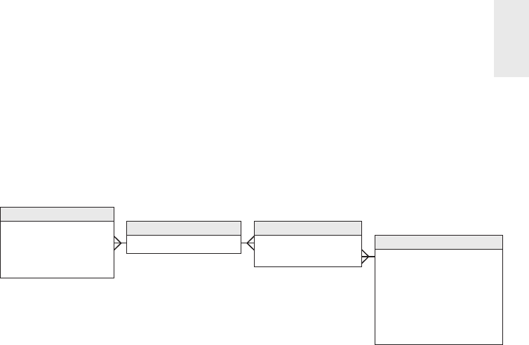
Healthcare 347
of Figure 14-4 can be used. In this case an extra table whose primary key is a diag-
nosis group is inserted between the fact and bridge tables. There is likely no new
information in this extra table, unless there were labels for a cluster of diagnoses,
such as the Kimball Syndrome, but now both the fact table and bridge table have
conventional many-to-one joins in all directions.
Diagnosis Dimension
Diagnosis Key (PK)
Diagnosis Code (NK)
Diagnosis Description
Diagnosis Section Code
Diagnosis Section Description
Diagnosis Category Code
Diagnosis Category Description
Foreign Keys ...
Diagnosis Group Key (FK)
Master Bill ID (DD)
Facts ...
Diagnosis Group Key (FK)
Diagnosis Key (FK)
Claim Billing Line Item Fact
Diagnosis Group Bridge
Diagnosis Group Key (PK)
Diagnosis Group Dimension
Figure 14-4: Diagnosis group dimension to create a primary key relationship.
If a unique diagnosis group is created for every patient encounter, the number
of rows could become astronomical and many of the groups would be identical.
Probably a better approach is to have a portfolio of diagnosis groups that are repeat-
edly used. Each set of diagnoses would be looked up in the master diagnosis group
table during the ETL. If the existing group is found, it is used; if not found, a new
diagnosis group is created. Chapter 19: ETL Subsystems and Techniques provides
guidance for creating and administering bridge tables.
In an inpatient hospital stay scenario, the diagnosis group may be unique to each
patient if it evolves over time during the patient’s stay. In this case you would supple-
ment the bridge table with two date stamps to capture begin and end dates. Although
the twin date stamps complicate updates to the diagnosis group bridge table, they
are useful for change tracking, as described more fully in Chapter 7: Accounting.
Supertypes and Subtypes for Charges
We’ve described a design for billed healthcare treatments to cover both inpatient and
outpatient claims. In reality, healthcare charges resemble the supertype and subtype
pattern described in Chapter 10. Facility charges for inpatient hospital stays di er
from professional charges for outpatient treatments in clinics and doctor o ces.
If you were focused exclusively on hospital stays, it would be reasonable to
tweak the Figure 14-2 dimensional structure to incorporate more hospital-specifi c
information. Figure 14-5 shows a revised set of dimensions specialized for hospital
stays, with the new dimensions bolded.

Chapter 14
348
Treatment Date Key (FK)
Primary Insurance Billing Date Key (FK)
Secondary Insurance Billing Date Key (FK)
Responsible Party Billing Date Key (FK)
Last Primary Insurance Payment Date Key (FK)
Last Secondary Insurance Payment Date Key (FK)
Last Responsible Party Payment Date Key (FK)
Zero Balance Date Key (FK)
Patient Key (FK)
Admitting Physician Key (FK)
Admitting Physician Organization Key (FK)
Attending Physician Key (FK)
Attending Physician Organization Key (FK)
Procedure Key (FK)
Facility Key (FK)
Admitting Diagnosis Group Key (FK)
Discharge Diagnosis Group Key (FK)
Primary Insurance Organization Key (FK)
Secondary Insurance Organization Key (FK)
Responsible Party Key (FK)
Employer Key (FK)
Master Bill ID (DD)
Facts...
Inpatient Hospital Claim Billing and Payment Workflow Fact
Figure 14-5: Accumulating snapshot for hospital stay charges.
Referring to Figure 14-5, you can see two roles for the physician: admitting physi-
cian and attending physician. The fi gure shows physician organizations for both roles
because physicians may represent di erent organizations in a hospital setting. With
more complex surgical events, such as a heart transplant operation, whole teams of
specialists and assistants are assembled. In this case, you could include a key in the
fact table for the primary responsible physician; the other physicians and medical
sta would be linked to the fact row via a group key to a multivalued bridge table.
You also have two multivalued diagnosis dimensions on each fact table row. The
admitting diagnosis group is determined at the beginning of the hospital stay and
should be the same for every treatment row that is part of the same hospital stay.
The discharge diagnosis group is not known until the patient is discharged.
Electronic Medical Records
Many healthcare organizations are moving from paper-based processes to elec-
tronic medical records. In the United States, federally mandated quality goals to
support improved population health management may be achievable only with

Healthcare 349
their adoption. Healthcare providers are aggressively implementing electronic
health record systems; the movement is signifi cantly impacting healthcare DW
/BI initiatives.
Electronic medical records can present challenges for data warehouse environ-
ments because of their extreme variability and potentially extreme volumes. Patients’
medical record data comes in many di erent forms, ranging from numeric data to
freeform text comments entered by a healthcare professional to images and photo-
graphs. We’ll further discuss unstructured data in Chapter 21: Big Data Analytics;
electronic medical and/or health records may become a classic use case for big data.
One thing is certain. The amount and variability of electronic data in the healthcare
industry will continue to grow.
Measure Type Dimension for Sparse Facts
As designers, it is tempting to strive for a more standardized framework that could
be extended to handle data variability. For example, you could potentially handle the
variability of lab test results with a measurement type dimension describing what
the fact row means, or in other words, what the generic fact represents. The unit
of measure for a given numeric entry is found in the associated measurement type
dimension row, along with any additivity restrictions, as shown in Figure 14-6.
Lab Test Measurement Type Dimension
Lab Test Measurement Type Key (PK)
Lab Test Measurement Type Description
Lab Test Measurement Type Unit of Measure
Order Date Key (FK)
Test Date Key (FK)
Patient Key (FK)
Physican Key (FK)
Lab Test Key (FK)
Lab Test Measurement Type Key (FK)
Observed Test Result Value
Lab Test Result Facts
Figure 14-6: Lab test observations with measurement type dimension.
This approach is superbly fl exible; you can add new measurement types simply by
adding new rows in the measurement type dimension, not by altering the structure
of the fact table. This approach also eliminates the nulls in the classic positional fact
table design because a row exists only if the measurement exists. However, there
are trade-o s. Using a measurement type dimension may generate lots of new fact
table rows because the grain is “one row per measurement per event” rather than the
more typical “one row per event.” If a lab test results in 10 numeric measurements,
there are now 10 rows in the fact table rather than a single row in the classic design.
For extremely sparse situations, such as clinical laboratory or manufacturing test
environments, this is a reasonable compromise. However, as the density of the facts

Chapter 14
350
grows, you end up spewing out too many fact rows. At this point you no longer have
sparse facts and should return to the classic fact table design with fi xed columns.
Moreover, this measurement type approach may complicate BI data access appli-
cations. In the relational star schema, combining two numbers that were captured
as part of a single event is more di cult with this approach because now you must
fetch two rows from the fact table. SQL likes to perform arithmetic functions within
a row, not across rows. In addition, you must be careful not to mix incompatible
amounts in a calculation because all the numeric measures reside in a single amount
column. It’s worth noting that multidimensional OLAP cubes are more tolerant of
performing calculations across measurement types.
Freeform Text Comments
Freeform text comments, such as clinical notes, are sometimes associated with fact
table events. Although text comments are not very analytically potent unless they’re
parsed into well-behaved dimension attributes, business users are often unwilling
to part with them given the embedded nuggets of information.
Textual comments should not be stored in a fact table directly because they waste
space and rarely participate in queries. Some designers think it’s permissible to store
textual fi elds in the fact table, as long as they’re referred to as degenerate dimensions.
Degenerate dimensions are most typically used for operational transaction control
numbers and identifi ers; it’s not an acceptable approach or pattern for contending
with bulky text fi elds. Storing freeform comments in the fact table adds clutter that
may negatively impact the performance of analysts’ more typical quantitative queries.
The unbounded text comments should either be stored in a separate comments
dimension or treated as attributes in a transaction event dimension. A key consider-
ation when evaluating these two approaches is the text fi eld’s cardinality. If there’s
nearly a unique comment for every fact table event, storing the textual fi eld in a trans-
action dimension makes the most sense. However, in many cases, No Comment is
associated with numerous fact rows. Because the number of unique text comments in
this scenario is much smaller than the number of unique transactions, it would make
more sense to store the textual data in a comments dimension with an associated
foreign key in the fact table. In either case, queries involving both the text comments
and fact metrics will perform relatively poorly given the need to resolve joins between
two voluminous tables. Often business users want to drill into text comments for
further investigation after highly selective fact table query fi lters have been applied.
Images
Sometimes the data captured in a patient’s electronic medical record is an image,
in addition to either quantitative numbers or qualitative notes. There are trade-o s

Healthcare 351
between capturing a JPEG fi lename in the fact table to refer to an associated image
versus embedding the image as a blob directly in the database. The advantage of
using a JPEG fi lename is that other image creation, viewing, and editing programs
can freely access the image. The disadvantage is that a separate database of graphic
fi les must be maintained in synchrony with the fact table.
Facility/Equipment Inventory Utilization
In addition to fi nancial and clinical data, healthcare organizations are also keenly
interested in more operationally oriented metrics, such as utilization and availability
of their assets, whether referring to patient beds or surgical operating theatres. In
Chapter 4, we discussed product inventory data as transaction events as well as
periodic snapshots. Facility or equipment inventories in a healthcare organization
can be handled similarly.
For example, you can envision a bed utilization periodic snapshot with every bed’s
status at regularly recurring points in time, perhaps at midnight, the start of every
shift, or even more frequently throughout the day. In addition to a snapshot date and
potentially time-of-day, this factless fact table would include foreign keys to identify
the patient, attending physician, and perhaps an assigned nurse on duty.
Conversely, you can imagine treating the bed inventory data as a transaction
fact table with one row per movement into and out of a hospital bed. This may be a
simplistic transaction fact table with transaction date and time dimension foreign
keys, along with dimensions to describe the type of movement, such as fi lled or
vacated. In the case of operating room utilization and availability, you can envision
a lengthier list of statuses, such as pre-operation, post-operation, or downtime,
along with time durations.
If the inventory changes are not terribly volatile, such as the beds in a rehabilita-
tion or eldercare inpatient environment, you should consider a timespan fact table,
as discussed in Chapter 8, with row e ective and expiration dates and times to
represent the various states of a bed over a period of time.
Dealing with Retroactive Changes
As DW/BI practitioners, we have well-developed techniques for accurately capturing
the historical fl ow of data from our enterprise’s source applications. Numeric mea-
surements go into fact tables, which are surrounded with contemporary descriptions
of what you know is true at the time of the measurements, packaged as dimension
tables. The descriptions of patient, physician, facility, and payer evolve as slowly
changing dimensions whenever these entities change their descriptions.

Chapter 14
352
However, in the healthcare industry, especially with legacy operational systems,
you often need to contend with late arriving data that should have been loaded into
the data warehouse weeks or months ago. For example, you might receive data
regarding patient procedures that occurred several weeks ago, or updates to patient
profi les that were back-dated as e ective several months ago. The more delayed the
incoming records are, the more challenging the DW/BI system’s ETL processing
becomes. We’ll discuss these late arriving fact and dimension scenarios in Chapter
19. Unfortunately, these patterns are common in healthcare DW/BI environments;
in fact, they may be the dominant modes of processing rather than specialized
techniques for outlier cases. Eventually, more e ective source data capture systems
should reduce the frequency of these late arriving data anomalies.
Summary
Healthcare provides a wealth of dimensional design examples. In this chapter, the
enterprise data warehouse bus matrix illustrated the critical linkages between a
healthcare organization’s administrative and clinical data. We used an accumulating
snapshot grain fact table with role-playing date dimensions for the healthcare claim
billing and payment pipeline. We also saw role playing used for the physician and
payer dimensions in other fact tables of this chapter.
Healthcare schemas are littered with multivalued dimensions, especially the
diagnosis dimension. Complex surgical events might also use multivalued bridge
tables to represent the teams of involved physicians and other sta members. The
bridge tables used with healthcare data seldom contain weighting factors, as dis-
cussed in earlier chapters, because it is extremely di cult to establish weighting
business rules, beyond the designation of a “primary” relationship.
We discussed medical records and test results, suggesting a measurement type
dimension to organize sparse, heterogeneous measurements into a single, uniform
framework. We also discussed the handling of text comments and linked images.
Transaction and periodic snapshot fact tables were used to represent facility or
equipment inventory utilization and availability. In closing, we touched upon ret-
roactive fact and dimension changes that are often all too common with healthcare
performance data.

Electronic
Commerce
A
web-intensive business’s clickstream data records the gestures of every web
visitor. In its most elemental form, the clickstream is every page event recorded
by each of the company’s web servers. The clickstream contains a number of new
dimensions, such as page, session, and referrer, which are not found in other data
sources. The clickstream is a torrent of data; it can be difficult and exasperating for
DW/BI professionals. Does it connect to the rest of the DW/BI system? Can its dimen-
sions and facts be conformed in the enterprise data warehouse bus architecture?
We start this chapter by describing the raw clickstream data source and designing
its relevant dimensional models. We discuss the impact of Google Analytics, which
can be thought of as an external data warehouse delivering information about your
website. We then integrate clickstream data into a larger matrix of more conven-
tional processes for a web retailer, and argue that the profi tability of the web sales
channel can be measured if you allocate the right costs back to the individual sales.
Chapter 15 discusses the following concepts:
■ Clickstream data and its unique dimensionality
■ Role of external services such as Google Analytics
■ Integrating clickstream data with the other business processes on the bus
matrix
■ Assembling a complete view of profi tability for a web enterprise
Clickstream Source Data
The clickstream is not just another data source that is extracted, cleaned, and
dumped into the DW/BI environment. The clickstream is an evolving collection of
data sources. There are a number of server log fi le formats for capturing clickstream
data. These log fi le formats have optional data components that, if used, can be very
helpful in identifying visitors, sessions, and the true meaning of behavior.
15

Chapter 15
354
Because of the distributed nature of the web, clickstream data often is collected
simultaneously by di erent physical servers, even when the visitor thinks they are
interacting with a single website. Even if the log fi les collected by these separate
servers are compatible, a very interesting problem arises in synchronizing the log
fi les after the fact. Remember that a busy web server may be processing hundreds
of page events per second. It is unlikely the clocks on separate servers will be in
synchrony to one-hundredth of a second.
You also obtain clickstream data from di erent parties. Besides your own log
fi les, you may get clickstream data from referring partners or from internet service
providers (ISPs). Another important form of clickstream data is the search specifi ca-
tion given to a search engine that then directs the visitor to the website.
Finally, if you are an ISP providing web access to directly connected customers,
you have a unique perspective because you see every click of your captive custom-
ers that may allow more powerful and invasive analyses of the customer’s sessions.
The most basic form of clickstream data from a normal website is stateless. That
is, the log shows an isolated page retrieval event but does not provide a clear tie to
other page events elsewhere in the log. Without some kind of contextual help, it is
di cult or impossible to reliably identify a complete visitor session.
The other big frustration with basic clickstream data is the anonymity of the
session. Unless visitors agree to reveal their identity in some way, you often cannot
be sure who they are, or if you have ever seen them before. In certain situations,
you may not distinguish the clicks of two visitors who are simultaneously brows-
ing the website.
Clickstream Data Challenges
Clickstream data contains many ambiguities. Identifying visitor origins, visitor
sessions, and visitor identities is something of an interpretive art. Browser caches
and proxy servers make these identifi cations more challenging.
Identifying the Visitor Origin
If you are very lucky, your site is the default home page for the visitor’s browser.
Every time he opens his browser, your home page is the fi rst thing he sees. This is
pretty unlikely unless you are the webmaster for a portal site or an intranet home
page, but many sites have buttons which, when clicked, prompt visitors to set their
URL as the browser’s home page. Unfortunately there is no easy way to determine
from a log whether your site is set as a browser’s home page.
A visitor may be directed to your site from a search at a portal such as Yahoo! or
Google. Such referrals can come either from the portal’s index, for which you may
have paid a placement fee, or from a word or content search.

Electronic Commerce 355
For some websites, the most common source of visitors is from a browser book-
mark. For this to happen, the visitor must have previously bookmarked your site,
and this can occur only after the site’s interest and trust levels cross the visitor’s
bookmark threshold.
Finally, your site may be reached as a result of a clickthrough—a deliberate click
on a text or graphical link from another site. This may be a paid-for referral via a
banner ad, or a free referral from an individual or cooperating site. In the case of
clickthroughs, the referring site will almost always be identifi able as a fi eld in the
web event record. Capturing this crucial clickstream data is important to verify the
e cacy of marketing programs. It also provides crucial data for auditing invoices
you may receive from clickthrough advertising charges.
Identifying the Session
Most web-centric analyses require every visitor session (visit) to have its own unique
identity tag, similar to a supermarket receipt number. This is the session ID. Records
for every individual visitor action in a session, whether they are derived from the
clickstream or an application interaction, must contain this tag. But keep in mind
the operational application, such as an order entry system generates this session
ID, not the web server.
The basic protocol for the web, Hyper Text Transfer Protocol (HTTP) is stateless;
that is, it lacks the concept of a session. There are no intrinsic login or logout actions
built into the HTTP protocol, so session identity must be established in some other
way. There are several ways to do this:
1. In many cases, the individual hits comprising a session can be consolidated by
collating time-contiguous log entries from the same host (IP address). If the
log contains a number of entries with the same host ID in a short period of
time (for example, one hour), you can reasonably assume the entries are for
the same session. This method breaks down for websites with large numbers
of visitors because dynamically assigned IP addresses may be reused immedi-
ately by di erent visitors over a brief time period. Also, di erent IP addresses
may be used within the same session for the same visitor. This approach also
presents problems when dealing with browsers that are behind some fi rewalls.
Notwithstanding these problems, many commercial log analysis products use
this method of session tracking, and it requires no cookies or special web
server features.
2. Another much more satisfactory method is to let the web browser place a
session-level cookie into the visitor’s web browser. This cookie will last as
long as the browser is open and in general won’t be available in subsequent

Chapter 15
356
browser sessions. The cookie value can serve as a temporary session ID not
only to the browser, but also to any application that requests the session
cookie from the browser. But using a transient cookie has the disadvantage
that you can’t tell when the visitor returns to the site at a later time in a new
session.
3. HTTP’s secure sockets layer (SSL) o ers an opportunity to track a visitor
session because it may include a login action by the visitor and the exchange
of encryption keys. The downside to using this method is that to track the
session, the entire information exchange needs to be in high-overhead SSL,
and the visitor may be put o by security advisories that can pop up using
certain browsers. Also, each host must have its own unique security certifi cate.
4. If page generation is dynamic, you can try to maintain visitor state by plac-
ing a session ID in a hidden fi eld of each page returned to the visitor. This
session ID can be returned to the web server as a query string appended to
a subsequent URL. This method of session tracking requires a great deal of
control over the website’s page generation methods to ensure the thread of
a session ID is not broken. If the visitor clicks links that don’t support this
session ID ping-pong, a single session may appear to be multiple sessions.
This approach also breaks down if multiple vendors supply content in a single
session unless those vendors are closely collaborating.
5. Finally, the website may establish a persistent cookie in the visitor’s machine
that is not deleted by the browser when the session ends. Of course, it’s pos-
sible the visitor will have his browser set to refuse cookies, or may manually
clean out his cookie fi le, so there is no absolute guarantee that even a per-
sistent cookie will survive. Although any given cookie can be read only by
the website that caused it to be created, certain groups of websites can agree
to store a common ID tag that would let these sites combine their separate
notions of a visitor session into a “super session.”
In summary, the most reliable method of session tracking from web server log
records is obtained by setting a persistent cookie in the visitor’s browser. Less reli-
able, but good results can be obtained by setting a session level and a nonpersistent
cookie and by associating time-contiguous log entries from the same host. The latter
method requires a robust algorithm in the log postprocessor to ensure satisfactory
results and to decide when not to take the results seriously.
Identifying the Visitor
Identifying a specifi c visitor who logs into your site presents some of the most
challenging problems facing a site designer, webmaster, or manager of the web
analytics group.

Electronic Commerce 357
■ Web visitors want to be anonymous. They may have no reason to trust you,
the internet, or their computer with personal identifi cation or credit card
information.
■ If you request visitors’ identity, they may not provide accurate information.
■ You can’t be sure which family member is visiting your site. If you obtain
an identity by association, for instance from a persistent cookie left during a
previous visit, the identifi cation is only for the computer, not for the specifi c
visitor. Any family member or company employee may have been using that
particular computer at that moment in time.
■ You can’t assume an individual is always at the same computer. Server-
provided cookies identify a computer, not an individual. If someone accesses
the same website from an o ce computer, home computer, and mobile device,
a di erent website cookie is probably put into each machine.
Clickstream Dimensional Models
Before designing clickstream dimensional models, let’s consider all the dimensions
that may have relevance in a clickstream environment. Any single dimensional
model will not use all the dimensions at once, but it is nice to have a portfolio
of dimensions waiting to be used. The list of dimensions for a web retailer could
include:
■ Date
■ Time of day
■ Part
■ Vendor
■ Status
■ Carrier
■ Facilities location
■ Product
■ Customer
■ Media
■ Promotion
■ Internal organization
■ Employee
■ Page
■ Event
■ Session
■ Referral

Chapter 15
358
All the dimensions in the list, except for the last four shown in bold, are familiar
dimensions, most of which we have already used in earlier chapters of this book.
But the last four are the unique dimensions of the clickstream and warrant some
careful attention.
Page Dimension
The page dimension describes the page context for a web page event, as illustrated
in Figure 15-1. The grain of this dimension is the individual page. The defi nition
of page must be fl exible enough to handle the evolution of web pages from static
page delivery to highly dynamic page delivery in which the exact page the customer
sees is unique at that instant in time. We assume even in the case of the dynamic
page that there is a well-defi ned function that characterizes the page, and we will
use that to describe the page. We will not create a page row for every instance of a
dynamic page because that would yield a dimension with an astronomical number
of rows. These rows also would not di er in interesting ways. You want a row in this
dimension for each interesting distinguishable type of page. Static pages probably get
their own row, but dynamic pages would be grouped by similar function and type.
Page Dimension Attribute
Page Key
Page Source
Page Function
Page Template
Item Type
Graphics Type
Animation Type
Sound Type
Page File Name
Surrogate values (1..N)
Static, Dynamic, Unknown, Corrupted, Inapplicable, ...
Portal, Search, Product description, Corporate information, ...
Sparse, Dense, ...
Product SKU, Book ISBN number, Telco rate type, ...
GIF, JPG, Progressive disclosure, Size pre-declared, ...
Similar to graphics type
Similar to graphics type
Optional application dependent name
Sample Data Values/Definitions
Figure 15-1: Page dimension attributes and sample data values.
When the defi nition of a static page changes because it is altered by the web-
master, the page dimension row can either be type 1 overwritten or treated with
an alternative slowly changing technique. This decision is a matter of policy for
the data warehouse and depends on whether the old and new descriptions of the
page di er materially, and whether the old defi nition should be kept for historical
analysis purposes.
Website designers, data governance representatives from the business, and the
DW/BI architects need to collaborate to assign descriptive codes and attributes to
each page served by the web server, whether the page is dynamic or static. Ideally,
the web page developers supply descriptive codes and attributes with each page

Electronic Commerce 359
they create and embed these codes and attributes into the optional fi elds of the
web log fi les. This crucial step is at the foundation of the implementation of this
page dimension.
Before leaving the page dimension, we want to point out that some internet com-
panies track the more granular individual elements on each page of their web sites,
including graphical elements and links. Each element generates its own row for each
visitor for each page request. A single complex web page can generate hundreds of
rows each time the page is served to a visitor. Obviously, this extreme granularity
generates astronomical amounts of data, often exceeding 10 terabytes per day!
Similarly, gaming companies may generate a row for every gesture made by every
online game player, which again can result in hundreds of millions of rows per day.
In both cases, the most atomic fact table will have extra dimensions describing the
graphical element, link, or game situation.
Event Dimension
The event dimension describes what happened on a particular page at a particular
point in time. The main interesting events are Open Page, Refresh Page, Click Link,
and Enter Data. You want to capture that information in this small event dimension,
as illustrated in Figure 15-2.
Event Dimension Attribute
Event Key
Event Type
Event Content
Surrogate values (1..N)
Open page, Refresh page, Click link, Unknown, Inapplicable
Application-dependent fields eventually driven by XML tags
Sample Data Values/Definitions
Figure 15-2: Event dimension attributes and sample data values.
Session Dimension
The session dimension provides one or more levels of diagnosis for the visitor’s
session as a whole, as shown in Figure 15-3. For example, the local context of the
session might be Requesting Product Information, but the overall session context
might be Ordering a Product. The success status would diagnose whether the mis-
sion was completed. The local context may be decidable from just the identity of
the current page, but the overall session context probably can be judged only by
processing the visitor’s complete session at data extract time. The customer status
attribute is a convenient place to label the customer for periods of time, with labels
that are not clear either from the page or immediate session. These statuses may be
derived from auxiliary business processes in the DW/BI system, but by placing these
labels deep within the clickstream, you can directly study the behavior of certain
types of customers. Do not put these labels in the customer dimension because they

Chapter 15
360
may change over very short periods of time. If there are a large number of these
statuses, consider creating a separate customer status mini-dimension rather than
embedding this information in the session dimension.
Session Dimension Attribute
Session Key
Session Type
Local Context
Session Context
Action Sequence
Success Status
Customer Status
Surrogate values (1..N)
Classified, Unclassified, Corrupted, Inapplicable
Page-derived context like Requesting Product Information
Trajectory-derived context like Ordering a Product
Summary label for overall sequence of actions during session
Identifies whether overall session mission was accomplished
New customer, High value customer, About to cancel, In default
Sample Data Values/Definitions
Figure 15-3: Session dimension attributes and sample data values.
This dimension groups sessions for analysis, such as:
■ How many customers consulted your product information before ordering?
■ How many customers looked at your product information and never ordered?
■ How many customers did not fi nish ordering? Where did they stop?
Referral Dimension
The referral dimension, illustrated in Figure 15-4, describes how the customer
arrived at the current page. The web server logs usually provide this information.
The URL of the previous page is identifi ed, and in some cases additional information
is present. If the referrer was a search engine, usually the search string is specifi ed.
It may not be worthwhile to put the raw search specifi cation into your database
because the search specifi cations are so complicated and idiosyncratic that an ana-
lyst may not be able to query them usefully. You can assume some kind of simplifi ed
and cleaned specifi cation is placed in the specifi cation attribute.
Referral Dimension Attribute
Referral Key
Referral Type
Referring URL
Referring Site
Referring Domain
Search Type
Specification
Target
Surrogate values (1..N)
Intra site, Remote site, Search engine, Corrupted, Inapplicable
www.organization-site.com/linkspage
www.organization-site.com
www.organization-site.com
Simple text match, Complex logical match
Actual spec used (useful if simple text, otherwise questionable)
Meta tags, Body text, Title (where search found its match)
Sample Data Values/Definitions
Figure 15-4: Referral dimension attributes and sample data values.

Electronic Commerce 361
Clickstream Session Fact Table
Now that you have a portfolio of useful clickstream dimensions, you can design
the primary clickstream dimensional models based on the web server log data.
This business process can then be integrated into the family of other web retailing
subject areas.
With an eye toward keeping the fi rst fact table from growing astronomically,
you should choose the grain to be one row for each completed customer session.
This grain is signifi cantly higher than the underlying web server logs which record
each individual page event, including individual pages as well as each graphical
element on each page. While we typically encourage designers to start with the
most granular data available in the source system, this is a purposeful deviation
from our standard practices. Perhaps you have a big site recording more than 100
million page fetches per day, and 1 billion micro page events (graphical elements),
but you want to start with a more manageable number of rows to be loaded each
day. We assume for the sake of argument that the 100 million page fetches boil
down to 20 million complete visitor sessions. This could arise if an average visitor
session touched 5 pages.
The dimensions that are appropriate for this fi rst fact table are calendar date, time
of day, customer, page, session, and referrer. Finally, you can add a set of measured
facts for this session including session seconds, pages visited, orders placed, units
ordered, and order dollars. The completed design is shown in Figure 15-5.
Date Dimension (2 views for roles)
Clickstream Session Fact
Universal Date Key (FK)
Universal Date/Time
Local Date Key (FK)
Local Date/Time
Customer Key (FK)
Entry Page Key (FK)
Session Key (FK)
Referrer Key (FK)
Session ID (DD)
Session Seconds
Pages Visited
Orders Placed
Order Quantity
Order Dollar Amount
Entry Page Dimension
Customer Dimension
Session Dimension
Referrer Dimension
Figure 15-5: Clickstream fact table design for complete sessions.

Chapter 15
362
There are a number of interesting aspects to this design. You may wonder why
there are two connections from the calendar date dimension to the fact table and
two date/time stamps. This is a case in which both the calendar date and the time
of day must play two di erent roles. Because you are interested in measuring the
precise times of sessions, you must meet two confl icting requirements. First, you
want to make sure you can synchronize all session dates and times internationally
across multiple time zones. Perhaps you have other date and time stamps from
other web servers or nonweb systems elsewhere in the DW/BI environment. To
achieve true synchronization of events across multiple servers and processes, you
must record all session dates and times, uniformly, in a single time zone such as
Greenwich Mean Time (GMT) or Coordinated Universal Time (UTC). You should
interpret the session date and time combinations as the beginning of the session.
Because you have the dwell time of the session as a numeric fact, you can tell when
the session ended, if that is of interest.
The other requirement you meet with this design is to record the date and time of
the session relative to the visitor’s wall clock. The best way to represent this informa-
tion is with a second calendar date foreign key and date/time stamp. Theoretically,
you could represent the time zone of the customer in the customer dimension table,
but constraints to determine the correct wall clock time would be horrendously
complicated. The time di erence between two cities (such as London and Sydney)
can change by as much as two hours at di erent times of the year depending on
when these cities go on and o daylight savings time. This is not the business of
the BI reporting application to work out. It is the business of the database to store
this information, so it can be constrained in a simple and direct way.
The two role-playing calendar date dimension tables are views on a single under-
lying table. The column names are massaged in the view defi nition, so they are
slightly di erent when they show up in the user interface pick lists of BI tools.
Note that the use of views makes the two instances of each table semantically
independent.
We modeled the exact instant in time with a full date/time stamp rather than a
time-of-day dimension. Unlike the calendar date dimension, a time-of-day dimen-
sion would contain few if any meaningful attributes. You don’t have labels for each
hour, minute, or second. Such a time-of-day dimension could be ridiculously large
if its grain were the individual second or millisecond. Also, the use of an explicit
date/time stamp allows direct arithmetic between di erent date/time stamps to
calculate precise time gaps between sessions, even those crossing days. Calculating
time gaps using a time-of-day dimension would be awkward.
The inclusion of the page dimension in Figure 15-5 may seem surprising given
the grain of the design is the customer session. However, in a given session, a very

Electronic Commerce 363
interesting page is the entry page. The page dimension in this design is the page the
session started with. In other words, how did the customer hop onto your bus just
now? Coupled with the referrer dimension, you now have an interesting ability to
analyze how and why the customer accessed your website. A more elaborate design
would also add an exit page dimension.
You may be tempted to add the causal dimension to this design, but if the causal
dimension focuses on individual products, it would be inappropriate to add it to
this design. The symptom that the causal dimension does not mesh with this design
is the multivalued nature of the causal factors for a given complete session. If you
run ad campaigns or special deals for several products, how do you represent this
multivalued situation if the customer’s session involves several products? The right
place for a product-oriented causal dimension will be in the more fi ne-grained table
described in the next fact table example. Conversely, a more broadly focused mar-
ket conditions dimension that describes conditions a ecting all products would be
appropriate for a session-grained fact table.
The session seconds fact is the total number of seconds the customer spent on the
site during this session. There will be many cases in which you can’t tell when the
customer left. Perhaps the customer typed in a new URL. This won’t be detected by
conventional web server logs. (If the data is collected by an ISP who can see every
click across sessions, this particular issue goes away.) Or perhaps the customer
got up out of the chair and didn’t return for 1 hour. Or perhaps the customer just
closed the browser without making any more clicks. In all these cases, your extract
software needs to assign a small and nominal number of seconds to this last session
step, so the analysis is not unrealistically distorted.
We purposely designed this fi rst clickstream fact table to focus on complete visitor
sessions while keeping the size under control. The next schema drops down to the
lowest practical granularity you can support in the data warehouse: the individual
page event.
Clickstream Page Event Fact Table
The granularity of the second clickstream fact table is the individual page event in
each customer session; the underlying micro events recording graphical elements
such as JPGs and GIFs are discarded (unless you are Yahoo! or eBay as described
previously). With simple static HTML pages, you can record only one interesting
event per page view, namely the page view. As websites employ dynamically created
XML-based pages, with the ability to establish an on-going dialogue through the
page, the number and type of events will grow.
This fact table could become astronomical in size. You should resist the urge
to aggregate the table up to a coarser granularity because that inevitably involves

Chapter 15
364
dropping dimensions. Actually, the fi rst clickstream fact table represents just such
an aggregation; although it is a worthwhile fact table, analysts cannot ask questions
about visitor behavior or individual pages.
Having chosen the grain, you can choose the appropriate dimensions. The list of
dimensions includes calendar date, time of day, customer, page, event, session, ses-
sion ID, step (three roles), product, referrer, and promotion. The completed design
is shown in Figure 15-6.
Date Dimension (2 views for roles)
Clickstream Page Event Fact
Universal Date Key (FK)
Universal Date/Time
Local Date Key (FK)
Local Date/Time
Customer Key (FK)
Page Key (FK)
Event Key (FK)
Session Key (FK)
Session ID (DD)
Session Step Key (FK)
Purchase Step Key (FK)
Abandonment Step Key (FK)
Product Key (FK)
Referrer Key (FK)
Promotion Key (FK)
Page Seconds
Order Quantity
Order Dollar Amount
Product Key (PK)
Product Attributes ...
Page Dimension Customer Dimension
Event Dimension
Session Dimension
Promotion Dimension
Referrer Dimension
Product Dimension
Step Key (PK)
Step Number
Steps Until End
Step Dimension (3 views for roles)
Figure 15-6: Clickstream fact table design for individual page use.
Figure 15-6 looks similar to the fi rst design, except for the addition of the page,
event, promotion, and step dimensions. This similarity between fact tables is typical
of dimensional models. One of the charms of dimensional modeling is the “boring”
similarity of the designs. But that is where they get their power. When the designs
have a predictable structure, all the software up and down the DW/BI chain, from
extraction, to database querying, to the BI tools, can exploit this similarity to great
advantage.
The two roles played by the calendar date and date/time stamps have the same
interpretation as in the fi rst design. One role is the universal synchronized time,
and the other role is the local wall clock time as measured by the customer. In this
fact table, these dates and times refer to the individual page event.

Electronic Commerce 365
The page dimension refers to the individual page. This is the main di erence in
grain between the two clickstream fact tables. In this fact table you can see all the
pages accessed by the customers.
As described earlier, the session dimension describes the outcome of the session.
A companion column, the session ID, is a degenerate dimension that does not have
a join to a dimension table. This degenerate dimension is a typical dimensional
modeling construct. The session ID is simply a unique identifi er, with no semantic
content, that serves to group together the page events of each customer session
in an unambiguous way. You did not need a session ID degenerate dimension in
the fi rst fact table, but it is included as a “parent key” if you want to easily link to
the individual page event fact table. We recommend the session dimension be at a
higher level of granularity than the session ID; the session dimension is intended
to describe classes and categories of sessions, not the characteristics of each indi-
vidual session.
A product dimension is shown in this design under the assumption this website
belongs to a web retailer. A fi nancial services site probably would have a similar
dimension. A consulting services site would have a service dimension. An auction
site would have a subject or category dimension describing the nature of the items
being auctioned. A news site would have a subject dimension, although with dif-
ferent content than an auction site.
You should accompany the product dimension with a promotion dimension so
you can attach useful causal interpretations to the changes in demand observed
for certain products.
For each page event, you should record the number of seconds that elapse before
the next page event. Call this page seconds to contrast it with session seconds in
the fi rst fact table. This is a simple example of paying attention to conformed facts.
If you call both of these measures simply “seconds,” you risk having these seconds
inappropriately added or combined. Because these seconds are not precisely equiva-
lent, you should name them di erently as a warning. In this particular case, you
would expect the page seconds for a session in this second fact table to add up to
the session seconds in the fi rst fact table.
The fi nal facts are units ordered and order dollars. These columns will be zero
or null for many rows in this fact table if the specifi c page event is not the event
that places the order. Nevertheless, it is highly attractive to provide these columns
because they tie the all-important web revenue directly to behavior. If the units
ordered and order dollars were only available through the production order entry
system elsewhere in the DW/BI environment, it would be ine cient to perform the

Chapter 15
366
revenue-to-behavior analysis across multiple large tables. In many database man-
agement systems, these null facts are handled e ciently and may take up literally
zero space in the fact table.
Step Dimension
Because the fact table grain is the individual page event, you can add the powerful
step dimension described in Chapter 8: Customer Relationship Management. The
step dimension, originally shown in Figure 8-11, provides the position of the specifi c
page event within the overall session.
The step dimension becomes particularly powerful when it is attached to the fact
table in various roles. Figure 15-6 shows three roles: overall session, purchase subses-
sion, and abandonment subsession. A purchase subsession, by defi nition, ends in a
successful purchase. An abandonment subsession is one that fails to complete a pur-
chase transaction for some reason. Using these roles of the step dimension allows some
very interesting queries. For example, if the purchase step dimension is constrained to
step number 1, the query returns nothing but the starting page for successful purchase
experiences. Conversely, if the abandonment step dimension is constrained to zero
steps remaining, the query returns nothing but the last and presumably most unful-
fi lling pages visited in unsuccessful purchase sessions. Although the whole design
shown in Figure 15-6 is aimed at product purchases, the step dimension technique
can be used in the analysis of any sequential process.
Aggregate Clickstream Fact Tables
Both clickstream fact tables designed thus far are pretty large. There are many
business questions that would be forced to summarize millions of rows from these
tables. For example, if you want to track the total visits and revenue from major
demographic groups of customers accessing your website on a month-by-month
basis, you can certainly do that with either fact table. In the session-grained fact
table, you would constrain the calendar date dimension to the appropriate time span
(say January, February, and March of the current year). You would then create row
headers from the demographics type attribute in the customer dimension and the
month attribute in the calendar dimension (to separately label the three months
in the output). Finally, you would sum the Order Dollars and count the number of
sessions. This all works fi ne. But it is likely to be slow without help from an aggre-
gate table. If this kind of query is frequent, the DBA will be encouraged to build an
aggregate table, as shown in Figure 15-7.
You can build this table directly from your fi rst fact table, whose grain is the
individual session. To build this aggregate table, you group by month, demographic
type, entry page, and session outcome. You count the number of sessions, and sum

Electronic Commerce 367
all the other additive facts. This results in a drastically smaller fact table, almost
certainly less than 1% of the original session-grained fact table. This reduction in
size translates directly to a corresponding increase in performance for most queries.
In other words, you can expect queries directed to this aggregate table to run at
least 100 times as fast.
Month Dimension
Session Aggregate Fact
Universal Month Key (FK)
Demographic Key (FK)
Entry Page Key (FK)
Session Outcome Key (FK)
Number of Sessions
Session Seconds
Pages Visited
Orders Placed
Order Quantity
Order Dollar Amount
Entry Page Dimension
Demographic Dimension
Session Outcome Dimension
Figure 15-7: Aggregate clickstream fact table.
Although it may not have been obvious, we followed a careful discipline in build-
ing the aggregate table. This aggregate fact table is connected to a set of shrunken
rollup dimensions directly related to the original dimensions in the more granular
fact tables. The month dimension is a conformed subset of the calendar day dimen-
sion’s attributes. The demographic dimension is a conformed subset of customer
dimension attributes. You should assume the page and session tables are unchanged;
a careful design of the aggregation logic could suggest a conformed shrinking of
these tables as well.
Google Analytics
Google Analytics (GA) is a service provided by Google that is best described as an
external data warehouse that provides many insights about how your website is used.
To use GA, you modify each page of your website to include a GA tracking code
(GATC) embedded in a Java code snippet located in the HTML <head> declaration of
each page to be tracked. When a visitor accesses the page, information is sent to the
Analytics service at Google, as long as the visitor has JavaScript enabled. Virtually
all of the information described in this chapter can be collected through GA, with
the exception of personally identifi able information (PII) which is forbidden by GA’s
terms of service. GA can be combined with Google’s Adword service to track ad
campaigns and conversions (sales). Reportedly, GA is used by more than 50% of the
most popular web sites on the internet.

Chapter 15
368
Data from GA can be viewed in a BI tool dashboard online directly from the under-
lying GA databases, or data can be delivered to you in a wide variety of standard and
custom reports, making it possible to build your own local business process schema
surrounding this data.
Interestingly, GA’s detailed technical explanation of the data elements that can be
collected through the service are described correctly as either dimensions or measures.
Someone at Google has been reading our books…
Integrating Clickstream into Web Retailer’s
Bus Matrix
This section considers the business processes needed by a web-based computer retailer.
The retailer’s enterprise data warehouse bus matrix is illustrated in Figure 15-8. Note
the matrix lists business process subject areas, not individual fact tables. Typically, each
matrix row results in a suite of closely associated fact tables and/or OLAP cubes, which
all represent a particular business process.
The Figure 15-8 matrix has a number of striking characteristics. There are a
lot of check marks. Some of the dimensions, such as date/time, organization, and
employee appear in almost every business process. The product and customer dimen-
sions dominate the middle part of the matrix, where they are attached to business
processes that describe customer-oriented activities. At the top of the matrix, suppli-
ers and parts dominate the processes of acquiring the parts that make up products
and building them to order for the customer. At the bottom of the matrix, you have
classic infrastructure and cost driver business processes that are not directly tied
to customer behavior.
The web visitor clickstream subject area sits squarely among the customer-
oriented processes. It shares the date/time, product, customer, media, causal, and
service policy dimensions with several other business processes nearby. In this
sense it should be obvious that the web visitor clickstream data is well integrated
into the fabric of the overall DW/BI system for this retailer. Applications tying the
web visitor clickstream will be easy to integrate across all the processes sharing
these conformed dimensions because separate queries to each fact table can be
combined across individual rows of the report.
The web visitor clickstream business process contains the four special click-
stream dimensions not found in the others. These dimensions do not pose a problem
for applications. Instead, the ability of the web visitor clickstream data to bridge
between the web world and the brick-and-mortar world is exactly the advantage
you are looking for. You can constrain and group on attributes from the four web

Electronic Commerce 369
dimensions and explore the e ect on the other business processes. For example, you
can see what kinds of web experiences produce customers who purchase certain
kinds of service policies and then invoke certain levels of service demands.
Supplier Purchase Orders
Supply Chain Management
Customer Relationship Management
Supplier Deliveries
Part Inventories
Product Assembly Bill of Materials
Product Assembly to Order
Product Promotions
Advertising
Customer Communications
Customer Inquiries
Web Visitor Clickstream
Product Orders
Service Policy Orders
Product Shipments
Customer Billing
Customer Payments
X
X
X
X
X
X
X
X
X
XXX
XX XX
X
X
X
XX
XXXXX
XXX
XXX
XXX
XX
X
XXX
XXX
XXX
XXX
XXX
XX
X
X
X
X
X
X
X
X
X
X
X
X
X
X
X
X
X
X
X
X
X
X
X
X
X
X
X
X
X
X
X
X
X
X
X
X
X
X
X
X
X
X
X
X
X
X
X
X
X
X
X
X
X
X
XX
X
X
X
X
X
X
X
XX
X
X
XX
X
X
XX XX
Date and Time
Part
Vendor
Carrier
Facility
Product
Customer
Media
Promotion
Service Policy
Internal Organization
Employee
Clickstream (4 dims)
Product Returns
Product Support
Service Policy Responses
Operations
Employee Labor
Human Resources
Facilities Operations
Web Site Operations
Figure 15-8: Bus matrix for web retailer.
Finally, it should be pointed out that the matrix serves as a kind of communica-
tions vehicle for all the business teams and senior management to appreciate the

Chapter 15
370
need to conform dimensions and facts. A given column in the matrix is, in e ect,
an invitation list to the meeting for conforming the dimension!
Profi tability Across Channels Including Web
After the DW/BI team successfully implements the initial clickstream fact tables
and ties them to the sales transaction and customer communication business pro-
cesses, the team may be ready to tackle the most challenging subject area of all:
web profi tability.
You can tackle web profi tability as an extension of the sales transaction process.
Fundamentally, you are allocating all the activity and infrastructure costs down to
each sales transaction. You could, as an alternative, try to build web profi tability
on top of the clickstream, but this would involve an even more controversial allo-
cation process in which you allocate costs down to each session. It would be hard
to assign activity and infrastructure costs to a session that has no obvious product
involvement and leads to no immediate sale.
A big benefi t of extending the sales transaction fact table is that you get a view
of profi tability across all your sales channels, not just the web. In a way, this should
be obvious because you know that you must sort out the costs and assign them to
the various channels.
The grain of the profi t and loss facts is each individual line item sold on a sales
ticket to a customer at a point in time, whether it’s a single sales ticket or single web
purchasing session. This is the same as the grain of the sales transaction business
process and includes all channels, assumed to be store sales, telesales, and web sales.
The dimensions of the profi t and loss facts are also the same as the sales transac-
tion fact table: date, time, customer, channel, product, promotion, and ticket number
(degenerate). The big di erence between the profi tability and sales transaction fact
tables is the breakdown of the costs, as illustrated in Figure 15-9.
Before discussing the allocation of costs, let us examine the format of the profi t
and loss facts. It is organized as a simple profi t and loss (P&L) statement (refer to
Figure 6-14). The fi rst fact is familiar units sold. All the other facts are dollar values
beginning with the value of the sale as if it were sold at the list or catalog price,
referred to as gross revenue. Assuming sales often take place at lower prices, you
would account for any di erence with a manufacturer’s allowance, marketing pro-
motion that is a price reduction, or markdown done to move the inventory. When
these e ects are taken into account, you can calculate the net revenue, which is the
true net price the customer pays times the number of units purchased.
The rest of the P&L consists of a series of subtractions, where you calculate
progressively more far-reaching versions of profi t. You can begin by subtracting
the product manufacturing cost if you manufacture it, or equivalently, the product

Electronic Commerce 371
acquisition cost if it is acquired from a supplier. Then subtract the product storage
cost. At this point, many enterprises call this partial result the gross profi t. You can
divide this gross profi t by the gross revenue to get the gross margin ratio.
Date Dimension (2 views for roles)
Profitability Fact
Universal Date Key (FK)
Universal Time of Day Key (FK)
Local Date Key (FK)
Local Time of Day Key (FK)
Customer Key (FK)
Channel Key (FK)
Product Key (FK)
Promotion Key (FK)
Ticket Number (DD)
Units Sold
Gross Revenue
Manufacturing Allowance
Marketing Promotion
Sales Markdown
Net Revenue
Manufacturing Cost
Storage Cost
Gross Profit
Freight Cost
Special Deal Cost
Other Overhead Cost
Net Profit
Customer Dimension
Time of Day Dimension (2 views for roles)
Channel Dimension
Promotion Dimension
Product Dimension
Figure 15-9: Profi t and loss facts across sales channels, including web sales.
Obviously, the columns called net revenue and gross profi t are calculated directly
from the columns immediately preceding them in the fact table. But should you
explicitly store these columns in the database? The answer depends on whether
you provide access to this fact table through a view or whether users or BI applica-
tions directly access the physical fact table. The structure of the P&L is su ciently
complex that, as the data warehouse provider, you don’t want to risk the impor-
tant measures like net revenue and gross profi t being computed incorrectly. If you
provide all access through views, you can easily provide the computed columns
without physically storing them. But if your users are allowed to access the under-
lying physical table, you should include net revenue, gross profi t, and net profi t as
physical columns.
Below the gross profi t you can continue subtracting various costs. Typically, the
DW/BI team must separately source or estimate each of these costs. Remember the
actual entries in any given fact table row are the fractions of these total costs allo-
cated all the way down to the individual fact row grain. Often there is signifi cant
pressure on the DW/BI team to deliver the profi tability business process. Or to put
it another way, there is tremendous pressure to source all these costs. But how good

Chapter 15
372
are the costs in the various underlying data sets? Sometimes a cost is only available
as a national average, computed for an entire year. Any allocation scheme is going
to assign a kind of pro forma value that has no real texture to it. Other costs will be
broken down a little more granularly, perhaps to calendar quarter and by geographic
region (if relevant). Finally, some costs may be truly activity-based and vary in a
highly dynamic, responsive, and realistic way over time.
Website system costs are an important cost driver in electronic commerce busi-
nesses. Although website costs are classic infrastructure costs, and are therefore
di cult to allocate directly to the product and customer activity, this is a key step
in developing a web-oriented P&L statement. Various allocation schemes are pos-
sible, including allocating the website costs to various product lines by the number
of pages devoted to each product, allocating the costs by pages visited, or allocating
the costs by actual web-based purchases.
The DW/BI team cannot be responsible for implementing activity-based costing
(ABC) in a large organization. When the team is building a profi tability dimensional
model, the team gets the best cost data available at the moment and publishes the
P&L. Perhaps some of the numbers are simple rule-of-thumb ratios. Others may be
highly detailed activity-based costs. Over time, as the sources of cost improve, the
DW/BI team incorporates these new sources and notifi es the users that the business
rules have improved.
Before leaving this design, it is worthwhile putting it in perspective. When a
P&L structure is embedded in a rich dimensional framework, you have immense
power. You can break down all the components of revenue, cost, and profi t for
every conceivable slice and dice provided by the dimensions. You can answer what
is profi table, but also answer “why” because you can see all the components of the
P&L, including:
■ How profi table is each channel (web sales, telesales, and store sales)? Why?
■ How profi table are your customer segments? Why?
■ How profi table is each product line? Why?
■ How profi table are your promotions? Why?
■ When is your business most profi table? Why?
The symmetric dimensional approach enables you to combine constraints from
many dimensions, allowing compound versions of the profi tability analyses like:
■ Who are the profi table customers in each channel? Why?
■ Which promotions work well on the web but do not work well in other
channels? Why?

Electronic Commerce 373
Summary
The web retailer case study used in this chapter is illustrative of any business with
a signifi cant web presence. Besides tackling the clickstream subject area at multiple
levels of granularity, the central challenge is e ectively integrating the clickstream
data into the rest of the business. We discussed ways to address the identifi cation
challenges associated with the web visitor, their origin, and session boundaries,
along with the special dimensions unique to clickstream data, including t he ses-
sion, page, and step dimensions.
In the next chapter, we’ll turn our attention to the primary business processes
in an insurance company as we recap many of the dimensional modeling patterns
presented throughout this book.

Insurance
We bring together concepts from nearly all the previous chapters to build
a DW/BI system for a property and casualty insurance company in this
final case study. If you are from the insurance industry and jumped directly to
this chapter for a quick fix, please accept our apology, but this material depends
heavily on ideas from the earlier chapters. You’ll need to turn back to the beginning
of the book to have this chapter make any sense.
As has been our standard procedure, this chapter launches with background
information for a business case. While the requirements unfold, we’ll draft the enter-
prise data warehouse bus matrix, much like we would in a real-life requirements
analysis e ort. We’ll then design a series of dimensional models by overlaying the
core techniques learned thus far.
Chapter 16 reviews the following concepts:
■ Requirements-driven approach to dimensional design
■ Value chain implications, along with an example bus matrix snippet for an
insurance company
■ Complementary transaction, periodic snapshot, and accumulating snapshot
schemas
■ Dimension role playing
■ Handling of slowly changing dimension attributes
■ Mini-dimensions for dealing with large, rapidly changing dimension attributes
■ Multivalued dimension attributes
■ Degenerate dimensions for operational control numbers
■ Audit dimensions to track data lineage
■ Heterogeneous supertypes and subtypes to handle products with varied attri-
butes and facts
■ Junk dimensions for miscellaneous indicators
16

Chapter 16
376
■ Conformed dimensions and facts
■ Consolidated fact tables combining metrics from separate business processes
■ Factless fact tables
■ Common mistakes to avoid when designing dimensional models
Insurance Case Study
Imagine working for a large property and casualty insurer that o ers automobile,
homeowner, and personal property insurance. You conduct extensive interviews
with business representatives and senior management from the claims, fi eld opera-
tions, underwriting, fi nance, and marketing departments. Based on these interviews,
you learn the industry is in a state of fl ux. Nontraditional players are leveraging
alternative channels. Meanwhile, the industry is consolidating due to globalization,
deregulation, and demutualization challenges. Markets are changing, along with
customer needs. Numerous interviewees tell us information is becoming an even
more important strategic asset. Regardless of the functional area, there is a strong
desire to use information more e ectively to identify opportunities more quickly
and respond most appropriately.
The good news is that internal systems and processes already capture the bulk
of the data required. Most insurance companies generate tons of nitty-gritty opera-
tional data. The bad news is the data is not integrated. Over the years, political and
IT boundaries have encouraged the construction of tall barriers around isolated
islands of data. There are multiple disparate sources for information about the
company’s products, customers, and distribution channels. In the legacy opera-
tional systems, the same policyholder may be identifi ed several times in separate
automobile, home, and personal property applications. Traditionally, this segmented
approach to data was acceptable because the di erent lines of business functioned
largely autonomously; there was little interest in sharing data for cross-selling and
collaboration in the past. Now within our case study, business management is
attempting to better leverage this enormous amount of inconsistent and somewhat
redundant data.
Besides the inherent issues surrounding data integration, business users lack the
ability to access data easily when needed. In an attempt to address this shortcom-
ing, several groups within the case study company rallied their own resources and
hired consultants to solve their individual short-term data needs. In many cases, the
same data was extracted from the same source systems to be accessed by separate
organizations without any strategic overall information delivery strategy.

Insurance 377
It didn’t take long to recognize the negative ramifi cations associated with separate
analytic data repositories because performance results presented at executive meetings
di ered depending on the data source. Management understood this independent
route was not viable as a long-term solution because of the lack of integration, large
volumes of redundant data, and di culty in interpreting and reconciling the results.
Given the importance of information in this brave new insurance world, manage-
ment was motivated to deal with the cost implications surrounding the development,
support, and analytic ine ciencies of these supposed data warehouses that merely
proliferated operational data islands.
Senior management chartered the chief information o cer (CIO) with the respon-
sibility and authority to break down the historical data silos to “achieve information
nirvana.” They charged the CIO with the fi duciary responsibility to manage and
leverage the organization’s information assets more e ectively. The CIO developed
an overall vision that wed an enterprise strategy for dealing with massive amounts
of data with a response to the immediate need to become an information-rich orga-
nization. In the meantime, an enterprise DW/BI team was created to begin designing
and implementing the vision.
Senior management has been preaching about a transformation to a more cus-
tomer-centric focus, instead of the traditional product-centric approach, in an e ort
to gain competitive advantage. The CIO jumped on that bandwagon as a catalyst
for change. The folks in the trenches have pledged intent to share data rather than
squirreling it away for a single purpose. There is a strong desire for everyone to
have a common understanding of the state of the business. They’re clamoring to
get rid of the isolated pockets of data while ensuring they have access to detail and
summary data at both the enterprise and line-of-business levels.
Insurance Value Chain
The primary value chain of an insurance company is seemingly short and simple. The
core processes are to issue policies, collect premium payments, and process claims.
The organization is interested in better understanding the metrics spawned by each
of these events. Users want to analyze detailed transactions relating to the formula-
tion of policies, as well as transactions generated by claims processing. They want
to measure performance over time by coverage, covered item, policyholder, and
sales distribution channel characteristics. Although some users are interested in
the enterprise perspective, others want to analyze the heterogeneous nature of the
insurance company’s individual lines of business.
Obviously, an insurance company is engaged in many other external pro-
cesses, such as the investment of premium payments or compensation of contract

Chapter 16
378
agents, as well as a host of internally focused activities, such as human resources,
fi nance, and purchasing. For now, we will focus on the core business related to
policies and claims.
The insurance value chain begins with a variety of policy transactions. Based
on your current understanding of the requirements and underlying data, you opt
to handle all the transactions impacting a policy as a single business process (and
fact table). If this perspective is too simplistic to accommodate the metrics, dimen-
sionality, or analytics required, you should handle the transaction activities as
separate fact tables, such as quoting, rating, and underwriting. As discussed in
Chapter 5: Procurement, there are trade-o s between creating separate fact tables
for each natural cluster of transaction types versus lumping the transactions into
a single fact table.
There is also a need to better understand the premium revenue associated with
each policy on a monthly basis. This will be key input into the overall profi t picture.
The insurance business is very transaction intensive, but the transactions themselves
do not represent little pieces of revenue, as is the case with retail or manufactur-
ing sales. You cannot merely add up policy transactions to determine the revenue
amount. The picture is further complicated in insurance because customers pay in
advance for services. This same advance-payment model applies to organizations
o ering magazine subscriptions or extended warranty contracts. Premium payments
must be spread across multiple periods because the company earns the revenue over
time as it provides insurance coverage. The complex relationship between policy
transactions and revenue measurements often makes it impossible to answer rev-
enue questions by crawling through the individual transactions. Not only is such
crawling time-consuming, but also the logic required to interpret the e ect of dif-
ferent transaction types on revenue can be horrendously complicated. The natural
confl ict between the detailed transaction view and the snapshot perspective almost
always requires building both kinds of fact tables in the warehouse. In this case,
the premium snapshot is not merely a summarization of the policy transactions; it
is quite a separate thing that comes from a separate source.
Draft Bus Matrix
Based on the interview fi ndings, along with an understanding of the key source
systems, the team begins to draft an enterprise data warehouse bus matrix with the
core policy-centric business processes as rows and core dimensions as columns.
Two rows are defi ned in the matrix, one corresponding to the policy transactions
and another for the monthly premium snapshot.
As illustrated in Figure 16-1, the core dimensions include date, policyholder,
employee, coverage, covered item, and policy. When drafting the matrix, don’t

Insurance 379
attempt to include all the dimensions. Instead, try to focus on the core common
dimensions that are reused in more than one schema.
Policy Transactions
Premium Snapshot
Date
Policyholder
Covered Item
Employee
XXXXXX
X
Month XX
Agent XXX
Policy
Coverage
Figure 16-1: Initial draft bus matrix.
Policy Transactions
Let’s turn our attention to the fi rst row of the matrix by focusing on the transactions
for creating and altering a policy. Assume the policy represents a set of coverages
sold to the policyholder. Coverages can be considered the insurance company’s
products. Homeowner coverages include fi re, fl ood, theft, and personal liability;
automobile coverages include comprehensive, collision damage, uninsured motor-
ist, and personal liability. In a property and casualty insurance company, coverages
apply to a specifi c covered item, such as a particular house or car. Both the coverage
and covered item are carefully identifi ed in the policy. A particular covered item
usually has several coverages listed in the policy.
Agents sell policies to policyholders. Before the policy can be created, a pricing
actuary determines the premium rate that will be charged given the specifi c cover-
ages, covered items, and qualifi cations of the policyholder. An underwriter, who
takes ultimate responsibility for doing business with the policyholder, makes the
fi nal approval.
The operational policy transaction system captures the following types of
transactions:
■ Create policy, alter policy, or cancel policy (with reason)
■ Create coverage on covered item, alter coverage, or cancel coverage (with
reason)
■ Rate coverage or decline to rate coverage (with reason)
■ Underwrite policy or decline to underwrite policy (with reason)

Chapter 16
380
The grain of the policy transaction fact table should be one row for each indi-
vidual policy transaction. Each atomic transaction should be embellished with
as much context as possible to create a complete dimensional description of the
transaction. The dimensions associated with the policy transaction business pro-
cess include the transaction date, e ective date, policyholder, employee, coverage,
covered item, policy number, and policy transaction type. Now let’s further discuss
the dimensions in this schema while taking the opportunity to reinforce concepts
from earlier chapters.
Dimension Role Playing
There are two dates associated with each policy transaction. The policy transac-
tion date is the date when the transaction was entered into the operational system,
whereas the policy transaction e ective date is when the transaction legally takes
e ect. These two foreign keys in the fact table should be uniquely named. The two
independent dimensions associated with these keys are implemented using a single
physical date table. Multiple logically distinct tables are then presented to the user
through views with unique column names, as described originally in Chapter 6:
Order Management.
Slowly Changing Dimensions
Insurance companies typically are very interested in tracking changes to dimensions
over time. You can apply the three basic techniques for handling slowly changing
dimension (SCD) attributes to the policyholder dimension, as introduced in Chapter 5.
With the type 1 technique, you simply overwrite the dimension attribute’s prior
value. This is the simplest approach to dealing with attribute changes because the
attributes always represent the most current descriptors. For example, perhaps the
business agrees to handle changes to the policyholder’s date of birth as a type 1
change based on the assumption that any changes to this attribute are intended as
corrections. In this manner, all fact table history for this policyholder appears to
have always been associated with the updated date of birth.
Because the policyholder’s ZIP code is key input to the insurer’s pricing and risk
algorithms, users are very interested in tracking ZIP code changes, so the type 2
technique is used for this attribute. Type 2 is the most common SCD technique
when there’s a requirement for accurate change tracking over time. In this case, when
the ZIP code changes, you create a new policyholder dimension row with a new
surrogate key and updated geographic attributes. Do not go back and revisit the fact
table. Historical fact table rows, prior to the ZIP code change, still refl ect the old
surrogate key. Going forward, you use the policyholder’s new surrogate key, so new
fact table rows join to the post-change dimension profi le. Although this technique is
extremely graceful and powerful, it places more burdens on ETL processing. Also,

Insurance 381
the number of rows in the dimension table grows with each type 2 SCD change.
Given there might already be more than 1 million rows in your policyholder dimen-
sion table, you may opt to use a mini-dimension for tracking ZIP code changes,
which we will review shortly.
Finally, let’s assume each policyholder is classifi ed as belonging to a particu-
lar segment. Perhaps nonresidential policyholders were historically categorized as
either commercial or government entities. Going forward, the business users want
more detailed classifi cations to di erentiate between large multinational, middle
market, and small business commercial customers, in addition to nonprofi t organi-
zations and governmental agencies. For a period of time, users want the ability to
analyze results by either the historical or new segment classifi cations. In this case
you could use a type 3 approach to track the change for a period of time by adding
a column, labeled Historical for di erentiation, to retain the old classifi cations.
The new classifi cation values would populate the segment attribute that has been
a permanent fi xture on the policyholder dimension. This approach, although not
extremely common, allows you to see performance by either the current or histori-
cal segment maps. This is useful when there’s been an en masse change, such as
the customer classifi cation realignment. Obviously, the type 3 technique becomes
overly complex if you need to track more than one version of the historical map or
before-and-after changes for multiple dimension attributes.
Mini-Dimensions for Large or Rapidly Changing
Dimensions
As mentioned earlier, the policyholder dimension qualifi es as a large dimension with
more than 1 million rows. It is often important to accurately track content values
for a subset of attributes. For example, you need an accurate description of some
policyholder and covered item attributes at the time the policy was created, as well
as at the time of any adjustment or claim. As discussed in Chapter 5, the practical
way to track changing attributes in large dimensions is to split the closely monitored,
more rapidly changing attributes into one or more type 4 mini-dimensions directly
linked to the fact table with a separate surrogate key. The use of mini-dimensions
has an impact on the e ciency of attribute browsing because users typically want
to browse and constrain on these changeable attributes. If all possible combina-
tions of the attribute values in the mini-dimension have been created, handling a
mini-dimension change simply means placing a di erent key in the fact table row
from a certain point in time forward. Nothing else needs to be changed or added
to the database.
The covered item is the house, car, or other specifi c insured item. The cov-
ered item dimension contains one row for each actual covered item. The covered
item dimension is usually somewhat larger than the policyholder dimension, so

Chapter 16
382
it’s another good place to consider deploying a mini-dimension. You do not want
to capture the variable descriptions of the physical covered objects as facts because
most are textual and are not numeric or continuously valued. You should make every
e ort to put textual attributes into dimension tables because they are the target of
textual constraints and the source of report labels.
Multivalued Dimension Attributes
We discussed multivalued dimension attributes when we associated multiple skills
with an employee in Chapter 9: Human Resources Management. In Chapter 10:
Financial Services, we associated multiple customers with an account, and then
in Chapter 14: Healthcare, we modeled a patient’s multiple diagnoses. In this
case study, you’ll look at another multivalued modeling situation: the relationship
between commercial customers and their industry classifi cations.
Each commercial customer may be associated with one or more Standard Industry
Classifi cation (SIC) or North American Industry Classifi cation System (NAICS) codes.
A large, diversifi ed commercial customer could be represented by a dozen or more
classifi cation codes. Much like you did with Chapter 14’s diagnosis group, a bridge
table ties together all the industry classifi cation codes within a group. This indus-
try classifi cation bridge table joins directly to either the fact table or the customer
dimension as an outrigger. It enables you to report fact table metrics by any industry
classifi cation. If the commercial customer’s industry breakdown is proportionally
identifi ed, such as 50 percent agricultural services, 30 percent dairy products, and
20 percent oil and gas drilling, a weighting factor should be included on each
bridge table row. To handle the case in which no valid industry code is associated
with a given customer, you simply create a special bridge table row that represents
Unknown.
Numeric Attributes as Facts or Dimensions
Let’s move on to the coverage dimension. Large insurance companies have dozens
or even hundreds of separate coverage products available to sell for a given type of
covered item. The actual appraised value of a specifi c covered item, like someone’s
house, is a continuously valued numeric quantity that can even vary for a given item
over time, so treat it as a legitimate fact. In the dimension table, you could store a
more descriptive value range, such as $250,000 to $299,999 Appraised Value, for
grouping and fi ltering. The basic coverage limit is likely to be more standardized
and not continuously valued, like Replacement Value or Up to $250,000. In this
case, it would also be treated as a dimension attribute.

Insurance 383
Degenerate Dimension
The policy number will be handled as a degenerate dimension if you have extracted
all the policy header information into other dimensions. You obviously want to avoid
creating a policy transaction fact table with just a small number of keys while embed-
ding all the descriptive details (including the policyholder, dates, and coverages) in
an overloaded policy dimension. In some cases, there may be one or two attributes
that still belong to the policy and not to another dimension. For example, if the
underwriter establishes an overall risk grade for the policy based on the totality of
the coverages and covered items, then this risk grade probably belongs in a policy
dimension. Of course, then the policy number is no longer a degenerate dimension.
Low Cardinality Dimension Tables
The policy transaction type dimension is a small dimension for the transaction types
listed earlier with reason descriptions. A transaction type dimension might contain
less than 50 rows. Even though this table is both narrow in terms of the number
of columns and shallow in terms of the number of rows, the attributes should still
be handled in a dimension table; if the textual characteristics are used for query
fi ltering or report labeling, then they belong in a dimension.
Audit Dimension
You have the option to associate ETL process metadata with transaction fact rows
by including a key that links to an audit dimension row created by the extract
process. As discussed in Chapter 6, each audit dimension row describes the data
lineage of the fact row, including the time of the extract, source table, and extract
software version.
Policy Transaction Fact Table
The policy transaction fact table in Figure 16-2 illustrates several characteristics of
a classic transaction grain fact table. First, the fact table consists almost entirely
of keys. Transaction schemas enable you to analyze behavior in extreme detail. As
you descend to lower granularity with atomic data, the fact table naturally sprouts
more dimensionality. In this case, the fact table has a single numeric fact; interpreta-
tion of the fact depends on the corresponding transaction type dimension. Because
there are di erent kinds of transactions in the same fact table, in this scenario, you
cannot label the fact more specifi cally.

Chapter 16
384
Policy Transaction Date Key (FK)
Policy Effective Date Key (FK)
Policyholder Key (FK)
Employee Key (FK)
Coverage Key (FK)
Covered Item Key (FK)
Policy Transaction Type Key (FK)
Policy Transaction Audit Key (FK)
Policy Number (DD)
Policy Transaction Number (DD)
Policy Transaction Dollar Amount
Policy Transaction Fact
Employee Dimension
Covered Item Dimension
Date Dimension (2 views for roles)
Policyholder Dimension
Coverage Dimension
Policy Transaction Type Dimension
Policy Transaction Audit Dimension
Figure 16-2: Policy transaction schema.
Heterogeneous Supertype and Subtype Products
Although there is strong support for an enterprise-wide perspective at our insur-
ance company, the business users don’t want to lose sight of their line-of-business
specifi cs. Insurance companies typically are involved in multiple, very di erent lines
of business. For example, the detailed parameters of homeowners’ coverages di er
signifi cantly from automobile coverages. And these both di er substantially from
personal property coverage, general liability coverage, and other types of insurance.
Although all coverages can be coded into the generic structures used so far in this
chapter, insurance companies want to track numerous specifi c attributes that make
sense only for a particular coverage and covered item. You can generalize the initial
schema developed in Figure 16-2 by using the supertype and subtype technique
discussed in Chapter 10.
Figure 16-3 shows a schema to handle the specifi c attributes that describe auto-
mobiles and their coverages. For each line of business (or coverage type), subtype
dimension tables for both the covered item and associated coverage are created.
When a BI application needs the specifi c attributes of a single coverage type, it uses
the appropriate subtype dimension tables.
Notice in this schema that you don’t need separate line-of-business fact tables
because the metrics don’t vary by business, but you’d likely put a view on the
supertype fact table to present only rows for a given subtype. The subtype dimen-
sion tables are introduced to handle the special line-of-business attributes. No
new keys need to be generated; logically, all we are doing is extending existing
dimension rows.
Complementary Policy Accumulating Snapshot
Finally, before leaving policy transactions, you should consider the use of an accu-
mulating snapshot to capture the cumulative e ect of the transactions. In this

Insurance 385
scenario, the grain of the fact table likely would be one row for each coverage and
covered item on a policy. You can envision including policy-centric dates, such as
quoted, rated, underwritten, e ective, renewed, and expired. Likewise, multiple
employee roles could be included on the fact table for the agent and underwriter.
Many of the other dimensions discussed would be applicable to this schema, with
the exception of the transaction type dimension. The accumulating snapshot likely
would have an expanded fact set.
Policy Transaction Date Key (FK)
Policy Effective Date Key (FK)
Policyholder Key (FK)
Employee Key (FK)
Coverage Key (FK)
Covered Item Key (FK)
Policy Transaction Type Key (FK)
Policy Transaction Audit Key (FK)
Policy Number (DD)
Policy Transaction Dollar Amount
Coverage Key (PK)
Coverage Description
Line of Business Description
Limit
Deductible
Rental Car Coverage
Windshield Coverage
Policy Transaction Fact
Automobile Coverage Dimension
Covered Item Key (PK)
Covered Item Description
Vehicle Manufacturer
Vehicle Make
Vehicle Year
Vehicle Classification
Vehicle Engine Size
Vehicle Appraised Value Range
Automobile Coverage Item Dimension
Figure 16-3: Policy transaction schema with subtype automobile dimension tables.
As discussed in Chapter 4: Inventory, an accumulating snapshot is e ective for
representing information about a pipeline process’s key milestones. It captures the
cumulative lifespan of a policy, covered items, and coverages; however, it does not
store information about each and every transaction that occurred. Unusual trans-
actional events or unexpected outliers from the standard pipeline would likely be
masked with an accumulating perspective. On the other hand, an accumulating
snapshot, sourced from the transactions, provides a clear picture of the durations
or lag times between key process events.
Premium Periodic Snapshot
The policy transaction schema is useful for answering a wide range of questions.
However, the blizzard of transactions makes it di cult to quickly determine the
status or fi nancial value of an in-force policy at a given point in time. Even if all
the necessary detail lies in the transaction data, a snapshot perspective would
require rolling the transactions forward from the beginning of history taking into
account complicated business rules for when earned revenue is recognized. Not
only is this nearly impractical on a single policy, but it is ridiculous to think about
generating summary top line views of key performance metrics in this manner.

Chapter 16
386
The answer to this dilemma is to create a separate fact table that operates as a
companion to the policy transaction table. In this case, the business process is the
monthly policy premium snapshot. The granularity of the fact table is one row per
coverage and covered item on a policy each month.
Conformed Dimensions
Of course, when designing the premium periodic snapshot table, you should strive to
reuse as many dimensions from the policy transaction table as possible. Hopefully,
you have become a conformed dimension enthusiast by now. As described in Chapter
4, conformed dimensions used in separate fact tables either must be identical or
must represent a shrunken subset of the attributes from the granular dimension.
The policyholder, covered item, and coverage dimensions would be identical.
The daily date dimension would be replaced with a conformed month dimension
table. You don’t need to track all the employees who were involved in policy trans-
actions on a monthly basis; it may be useful to retain the involved agent, especially
because fi eld operations are so focused on ongoing revenue performance analysis.
The transaction type dimension would not be used because it does not apply at the
periodic snapshot granularity. Instead, you introduce a status dimension so users
can quickly discern the current state of a coverage or policy, such as new policies
or cancellations this month and over time.
Conformed Facts
While we’re on the topic of conformity, you also need to use conformed facts. If the
same facts appear in multiple fact tables, such as facts common to this snapshot fact
table as well as the consolidated fact table we’ll discuss later in this chapter, then
they must have consistent defi nitions and labels. If the facts are not identical,
then they need to be given di erent names.
Pay-in-Advance Facts
Business management wants to know how much premium revenue was written (or
sold) each month, as well as how much revenue was earned. Although a policyholder
may contract and pay for coverages on covered items for a period of time, the revenue
is not earned until the service is provided. In the case of the insurance company,
the revenue from a policy is earned month by month as long as the policyholder
doesn’t cancel. The correct calculation of a metric like earned premium would
mean fully replicating all the business rules of the operational revenue recognition
system within the BI application. Typically, the rules for converting a transaction
amount into its monthly revenue impact are complex, especially with mid-month
coverage upgrades and downgrades. Fortunately, these metrics can be sourced from
a separate operational system.

Insurance 387
As illustrated in Figure 16-4, we include two premium revenue metrics in the
periodic snapshot fact table to handle the di erent defi nitions of written versus
earned premium. Simplistically, if an annual policy for a given coverage and cov-
ered item was written on January 1 for a cost of $600, then the written premium
for January would be $600, but the earned premium is $50 ($600 divided by 12
months). In February, the written premium is zero and the earned premium is still
$50. If the policy is canceled on March 31, the earned premium for March is $50,
while the written premium is a negative $450. Obviously, at this point the earned
revenue stream comes to a crashing halt.
Month End Snapshot Date Key (FK)
Policyholder Key (FK)
Agent Key (FK)
Coverage Key (FK)
Covered Item Key (FK)
Policy Status Key (FK)
Policy Number (DD)
Written Premium Revenue Amount
Earned Premium Revenue Amount
Premium Snapshot Fact
Month End Dimension
Agent Dimension
Policyholder Dimension
Coverage Dimension
Policy Status Dimension
Covered Item Dimension
Figure 16-4: Periodic premium snapshot schema.
Pay-in-advance business scenarios typically require the combination of transac-
tion and monthly snapshot fact tables to answer questions of transaction frequency
and timing, as well as questions of earned income in a given month. You can almost
never add enough facts to a snapshot schema to do away with the need for a trans-
action schema, or vice versa.
Heterogeneous Supertypes and Subtypes Revisited
We are again confronted with the need to look at the snapshot data with more spe-
cifi c line-of-business attributes, and grapple with snapshot facts that vary by line of
business. Because the custom facts for each line are incompatible with each other,
most of the fact row would be fi lled with nulls if you include all the line-of-business
facts on every row. In this scenario, the answer is to separate the monthly snap-
shot fact table physically by line of business. You end up with the single supertype
monthly snapshot schema and a series of subtype snapshots, one for each line of
business or coverage type. Each of the subtype snapshot fact tables is a copy of a
segment of the supertype fact table for just those coverage keys and covered item
keys belonging to a particular line of business. We include the supertype facts as
a convenience so analyses within a coverage type can use both the supertype and
custom subtype facts without accessing two large fact tables.

Chapter 16
388
Multivalued Dimensions Revisited
Automobile insurance provides another opportunity to discuss multivalued dimen-
sions. Often multiple insured drivers are associated with a policy. You can construct
a bridge table, as illustrated in Figure 16-5, to capture the relationship between the
insured drivers and policy. In this case the insurance company can assign realistic
weighting factors based on each driver’s share of the total premium cost.
Month End Snapshot Date Key (FK)
Policyholder Key (FK)
More FKs...
Policy Key (FK)
Written Premium Revenue Amount
Earned Premium Revenue Amount
Premium Snapshot Fact
Policy Key (FK)
Insured Driver Key (FK)
Weighting Factor
Policy-Insured Driver Bridge
Insured Driver Key (PK)
Insured Driver Name
Insured Driver Address Attributes...
Insured Driver Date of Birth
Insured Driver Risk Segment
Insured Driver Dimension
Figure 16-5: Bridge table for multiple drivers on a policy.
Because these relationships may change over time, you can add e ective and
expiration dates to the bridge table. Before you know it, you end up with a factless
fact table to capture the evolving relationships between a policy, policy holder,
covered item, and insured driver over time.
More Insurance Case Study Background
Unfortunately, the insurance business has a downside. We learn from the inter-
viewees that there’s more to life than collecting premium revenue payments. The
main costs in this industry result from claim losses. After a policy is in e ect, then
a claim can be made against a specifi c coverage and covered item. A claimant, who
may be the policyholder or a new party not previously known to the insurance
company, makes the claim. When the insurance company opens a new claim, a
reserve is usually established. The reserve is a preliminary estimate of the insurance
company’s eventual liability for the claim. As further information becomes known,
this reserve can be adjusted.
Before the insurance company pays any claim, there is usually an investigative
phase where the insurance company sends out an adjuster to examine the covered
item and interview the claimant, policyholder, or other individuals involved. The
investigative phase produces a stream of task transactions. In complex claims,

Insurance 389
various outside experts may be required to pass judgment on the claim and the
extent of the damage.
In most cases, after the investigative phase, the insurance company issues a
number of payments. Many of these payments go to third parties such as doctors,
lawyers, or automotive body shop operators. Some payments may go directly to
the claimant. It is important to clearly identify the employee responsible for every
payment made against an open claim.
The insurance company may take possession of the covered item after replacing
it for the policyholder or claimant. If the item has any remaining value, salvage pay-
ments received by the insurance company are a credit against the claim accounting.
Eventually, the payments are completed and the claim is closed. If nothing
unusual happens, this is the end of the transaction stream generated by the claim.
However, in some cases, further claim payments or claimant lawsuits may force
a claim to be reopened. An important measure for an insurance company is how
often and under what circumstances claims are reopened.
In addition to analyzing the detailed claims processing transactions, the insur-
ance company also wants to understand what happens over the life of a claim. For
example, the time lag between the claim open date and the fi rst payment date is an
important measure of claims processing e ciency.
Updated Insurance Bus Matrix
With a better understanding of the claims side of the business, the draft matrix from
Figure 16-1 needs to be revisited. Based on the new requirements, you add another
row to the matrix to accommodate claim transactions, as shown in Figure 16-6.
Many of the dimensions identifi ed earlier in the project will be reused; you add new
columns to the matrix for the claim, claimant, and third-party payee.
Policy Transactions
Premium Snapshot
Date
Policyholder
Covered Item
Employee
XXXXXX
X
Month XX
Agent XXX
Policy
Coverage
Claimant
Claim Transactions X X X XXX XXX
3rd Party Payee
Claim
Figure 16-6: Updated insurance bus matrix.

Chapter 16
390
Detailed Implementation Bus Matrix
DW/BI teams sometimes struggle with the level of detail captured in an enterprise
data warehouse bus matrix. In the planning phase of an architected DW/BI project, it
makes sense to stick with rather high-level business processes (or sources). Multiple
fact tables at di erent levels of granularity may result from each of these business
process rows. In the subsequent implementation phase, you can take a subset of
the matrix to a lower level of detail by refl ecting all the fact tables or OLAP cubes
resulting from the process as separate matrix rows. At this point the matrix can
be enhanced by adding columns to refl ect the granularity and metrics associated
with each fact table or cube. Figure 16-7 illustrates a more detailed implementation
bus matrix.
Claim Transactions
The operational claim processing system generates a slew of transactions, including
the following transaction task types:
■ Open claim, reopen claim, close claim
■ Set reserve, reset reserve, close reserve
■ Set salvage estimate, receive salvage payment
■ Adjuster inspection, adjuster interview
■ Open lawsuit, close lawsuit
■ Make payment, receive payment
■ Subrogate claim
When updating the Figure 16-6 bus matrix, you determine that this schema uses
a number of dimensions developed for the policy world. You again have two role-
playing dates associated with the claim transactions. Unique column labels should
distinguish the claim transaction and e ective dates from those associated with
policy transactions. The employee is the employee involved in the transactional
task. As mentioned in the business case, this is particularly interesting for payment
authorization transactions. The claim transaction type dimension would include
the transaction types and groupings just listed.
As shown in Figure 16-8, there are several new dimensions in the claim transac-
tion fact table. The claimant is the party making the claim, typically an individual.
The third-party payee may be either an individual or commercial entity. Both the
claimant and payee dimensions usually are dirty dimensions because of the dif-
fi culty of reliably identifying them across claims. Unscrupulous potential payees
may go out of their way not to identify themselves in a way that would easily tie
them to other claims in the insurance company’s system.

Policy Transactions
Corporate Policy Transactions
stcaFytiralunarGebuC PALO/elbaT tcaF
Auto Policy Transactions
Home Policy Transactions
Claim Transactions
Claim Workflow
Accident Involvements
Policy Premium Snapshot
Corporate Policy Premiums
Auto Policy Premiums
Home Policy Premiums
1 row for every policy
transaction
1 row per auto policy
transaction
1 row per home policy
transaction
1 row for every claim task
transaction
1 row per claim
1 row per loss party and
affiliation on an auto claim
1 row for every policy, covered
item and coverage per month
1 row per auto policy, covered
item and coverage per month
1 row per home policy, covered
item and coverage per month
Claim Events
Policy Transaction Amount
Policy Transaction Amount
Policy Transaction Amount
Claim Transaction Amount
Original Reserve, Estimate, Current
Reserve, Claim Paid, Salvage
Collected, and Subro Collected
Amounts; Loss to Open, Open to
Estimate, Open to 1st Payment,
Open to Subro, and Open to Closed
Lags; # of Transactions
Accident Involvement Count
Written Premium Revenue and
Earned Premium Revenue Amounts
Written Premium Revenue and
Earned Premium Revenue Amounts
Written Premium Revenue and
Earned Premium Revenue Amounts
Trxn
Eff
Trxn
Eff
Trxn
Eff
Trxn
Eff
X
X
X
X
X
X
X
X
X
X
X
X
X
X
X
Auto
Home
X
X
Auto
X
Auto
Home
X
Auto
Home
X
X
Auto
X
Auto
Home
X
X
X
X
Agent
Agent
Agent
Agent
X
X
X
X
X
X
X
X
Auto
X X
X
X
X
X
X
Date
Policyholder
Coverage
Employee
Policy
Covered Item
Claimant
3rd Party Payee
Claim
Figure 16-7: Detailed implementation bus matrix.

Chapter 16
392
Claim Transaction Date Key (FK)
Claim Transaction Effective Date Key (FK)
Policyholder Key (FK)
Claim Transaction Employee Key (FK)
Agent Key (FK)
Coverage Key (FK)
Covered Item Key (FK)
Claimant Key (FK)
3rd Party Payee Key (FK)
Claim Transaction Type Key (FK)
Claim Profile Key (FK)
Claim Key (FK)
Policy Number (DD)
Claim Transaction Number (DD)
Claim Transaction Dollar Amount
Claim Transaction Fact
Employee Dimension (2 views for roles)
Covered Item Dimension
Date Dimension (2 views for roles)
Policyholder Dimension
Coverage Dimension
Claimant Dimension
Claim Transaction Type Dimension
3rd Party Payee Dimension
Claim Profile Dimension
Claim Dimension
Figure 16-8: Claim transaction schema.
Transaction Versus Profi le Junk Dimensions
Beyond the reused dimensions from the policy-centric schemas and the new claim-
centric dimensions just listed, there are a large number of indicators and descriptions
related to a claim. Designers are sometimes tempted to dump all these descriptive
attributes into a claim dimension. This approach makes sense for high-cardinality
descriptors, such as the specifi c address where the loss occurred or a narrative
describing the event. However, in general, you should avoid creating dimensions
with the same number of rows as the fact table.
As we described in Chapter 6, low-cardinality codifi ed data, like the method
used to report the loss or an indicator denoting whether the claim resulted from a
catastrophic event, are better handled in a junk dimension. In this case, the junk
dimension would more appropriately be referred to as the claim profi le dimension
with one row per unique combination of profi le attributes. Grouping or fi ltering on
the profi le attributes would yield faster query responses than if they were alterna-
tively handled as claim dimension attributes.
Claim Accumulating Snapshot
Even with a robust transaction schema, there is a whole class of urgent business
questions that can’t be answered using only transaction detail. It is di cult to
derive claim-to-date performance measures by traversing through every detailed
claim task transaction from the beginning of the claim’s history and appropriately
applying the transactions.

Insurance 393
On a periodic basis, perhaps at the close of each day, you can roll forward all the
transactions to update an accumulating claim snapshot incrementally. The granu-
larity is one row per claim; the row is created once when the claim is opened and
then is updated throughout the life of a claim until it is fi nally closed.
Many of the dimensions are reusable, conformed dimensions, as illustrated in
Figure 16-9. You should include more dates in this fact table to track the key claim
milestones and deliver time lags. These lags may be the raw di erence between
two dates, or they may be calculated in a more sophisticated way by accounting for
only workdays in the calculations. A status dimension is added to quickly identify
all open, closed, or reopened claims, for example. Transaction-specifi c dimensions
such as employee, payee, and claim transaction type are suppressed, whereas the
list of additive, numeric measures has been expanded.
Claim Workflow Fact
Covered Item Dimension
Policyholder Dimension
Coverage Dimension
Claimant Dimension
Claim Status Dimension
Claim Profile Dimension
Claim Dimension
Claim Open Date Key (FK)
Claim Loss Date Key (FK)
Claim Estimate Date Key (FK)
Claim 1st Payment Date Key (FK)
Claim Most Recent Payment Date Key (FK)
Claim Subrogation Date Key (FK)
Claim Close Date Key (FK)
Policyholder Key (FK)
Claim Supervisor Key (FK)
Agent Key (FK)
Coverage Key (FK)
Covered Item Key (FK)
Claimant Key (FK)
Claim Status Key (FK)
Claim Profile Key (FK)
Claim Key (FK)
Policy Number (DD)
Original Reserve Dollar Amount
Estimate Dollar Amount
Current Reserve to Date Dollar Amount
Claim Paid to Date Dollar Amount
Salvage Collected to Date Dollar Amount
Subro Payment Collected to Date Dollar Amount
Claim Loss to Open Lag
Claim Open to Estimate Lag
Claim Open to 1st Payment Lag
Claim Open to Subrogation Lag
Claim Open to Closed Lag
Number of Claim Transactions
Employee Dimension (2 views for roles)
Date Dimension (7 views for roles)
Figure 16-9: Claim accumulating snapshot schema.
Accumulating Snapshot for Complex Workfl ows
Accumulating snapshot fact tables are typically appropriate for predictable workfl ows
with well-established milestones. They usually have fi ve to 10 key milestone dates

Chapter 16
394
representing the pipeline’s start, completion, and key events in between. However,
sometimes workfl ows are less predictable. They still have a defi nite start and end
date, but the milestones in between are numerous and less stable. Some occurrences
may skip over some intermediate milestones, but there’s no reliable pattern.
In this situation, the fi rst task is to identify the key dates that link to role-playing
date dimensions. These dates represent the most important milestones. The start and
end dates for the process would certainly qualify; in addition, you should consider
other commonly occurring critical milestones. These dates (and their associated
dimensions) will be used extensively for BI application fi ltering.
However, if the number of additional milestones is both voluminous and unpre-
dictable, they can’t all be handled as additional date foreign keys in the fact table.
Typically, business users are more interested in the lags between these milestones,
rather than fi ltering or grouping on the dates themselves. If there were a total of
20 potential milestone events, there would be 190 potential lag durations: event
A-to-B, A-to-C, … (19 possible lags from event A), B-to-C, … (18 possible lags from
event B), and so on. Instead of physically storing 190 lag metrics, you can get away
with just storing 19 of them and then calculate the others. Because every pipeline
occurrence starts by passing through milestone A, which is the workfl ow begin
date, you could store all 19 lags from the anchor event A and then calculate the
other variations. For example, if you want to know the lag from B-to-C, take
the A-to-C lag value and subtract the A-to-B lag. If there happens to be a null for one
of the lags involved in a calculation, then the result also needs to be null because
one of the events never occurred. But such a null result is handled gracefully if you
are counting or averaging that lag across a number of claim rows.
Timespan Accumulating Snapshot
An accumulating snapshot does a great job presenting a workfl ow’s current state,
but it obliterates the intermediate states. For example, a claim can move in and out
of various states such as opened, denied, closed, disputed, opened again, and closed
again. The claim transaction fact table will have separate rows for each of these
events, but as discussed earlier, it doesn’t accumulate metrics across transactions;
trying to re-create the evolution of a workfl ow from these transactional events would
be a nightmare. Meanwhile, a classic accumulating snapshot doesn’t allow you to
re-create the claim workfl ow at any arbitrary date in the past.
Alternatively, you could add e ective and expiration dates to the accumulating
snapshot. In this scenario, instead of destructively updating each row as changes
occur, you add a new row that preserves the state of a claim for a span of time.

Insurance 395
Similar to a type 2 slowly changing dimension, the fact row includes the following
additional columns:
■ Snapshot start date
■ Snapshot end date (updated when a new row for a given claim is added)
■ Snapshot current fl ag (updated when a new row is added)
Most users are only interested in the current view provided by a classic accumu-
lating snapshot; you can meet their needs by defi ning a view that fi lters the historical
snapshot rows based on the current fl ag. The minority of users and reports who
need to look at the pipeline as of any arbitrary date in the past can do so by fi ltering
on the snapshot start and end dates.
The timespan accumulating snapshot fact table is more complicated to main-
tain than a standard accumulating snapshot, but the logic is similar. Where the
classic accumulating snapshot updates a row, the timespan snapshot updates
the administrative columns on the row formerly known as current, and inserts
a new row.
Periodic Instead of Accumulating Snapshot
In cases where a claim is not so short-lived, such as with long-term disability or
bodily injury claims that have a multiyear life span, you may represent the snapshot
as a periodic snapshot rather than an accumulating snapshot. The grain of the peri-
odic snapshot would be one row for every active claim at a regular snapshot interval,
such as monthly. The facts would represent numeric, additive facts that occurred
during the period such as amount claimed, amount paid, and change in reserve.
Policy/Claim Consolidated Periodic Snapshot
With the fact tables designed thus far, you can deliver a robust perspective of the pol-
icy and claim transactions, in addition to snapshots from both processes. However,
the business users are also interested in profi t metrics. Although premium revenue
and claim loss fi nancial metrics could be derived by separately querying two fact
tables and then combining the results set, you opt to go the next step in the spirit
of ease of use and performance for this common drill-across requirement.
You can construct another fact table that brings together the premium revenue
and claim loss metrics, as shown in Figure 16-10. This table has a reduced set
of dimensions corresponding to the lowest level of granularity common to both

Chapter 16
396
processes. As discussed in Chapter 7: Accounting, this is a consolidated fact table
because it combines data from multiple business processes. It is best to develop
consolidated fact tables after the base metrics have been delivered in separate atomic
dimensional models.
Consolidated Premium/Loss Fact
Month End Date Dimension
Policyholder Dimension
Coverage Dimension
Policy Status Dimension
Covered Item Dimension
Claim Status Dimension
Agent Dimension
Month End Snapshot Date Key (FK)
Policyholder Key (FK)
Coverage Key (FK)
Covered Item Key (FK)
Agent Key (FK)
Policy Status Key (FK)
Claim Status Key (FK)
Policy Number (DD)
Written Premium Revenue Dollar Amount
Earned Premium Revenue Dollar Amount
Claim Paid Dollar Amount
Claim Collected Dollar Amount
Figure 16-10: Policy/claim consolidated fact table.
Factless Accident Events
We earlier described factless fact tables as the collision of keys at a point in space
and time. In the case of an automobile insurer, you can record literal collisions using
a factless fact table. In this situation, the fact table registers the many-to-many cor-
relations between the loss parties and loss items, or put in laymen’s terms, all the
correlations between the people and vehicles involved in an accident.
Two new dimensions appear in the factless fact table shown in Figure 16-11. The
loss party captures the individuals involved in the accident, whereas the loss party
role identifi es them as passengers, witnesses, legal representation, or some other
capacity. As we did in Chapter 3: Retail Sales, we include a fact that is always valued
at 1 to facilitate counting and aggregation. This factless fact table can represent
complex accidents involving many individuals and vehicles because the number
of involved parties with various roles is open-ended. When there is more than one
claimant or loss party associated with an accident, you can optionally treat these
dimensions as multivalued dimensions using claimant group and loss party group
bridge tables. This has the advantage that the grain of the fact table is preserved
as one record per accident claim. Either schema variation could answer questions
such as, “How many bodily injury claims did you handle where ABC Legal Partners
represented the claimant and EZ-Dent-B-Gone body shop performed the repair?”

Insurance 397
Accident Involvement Fact
Policyholder Dimension
Coverage Dimension
Loss Party Dimension
Covered Item Dimension
Claim Loss Date Dimension
Loss Party Role Dimension
Claim Loss Date Key (FK)
Policyholder Key (FK)
Coverage Key (FK)
Covered Item Key (FK)
Claimant Key (FK)
Loss Party Key (FK)
Loss Party Role Key (FK)
Claim Profile Key (FK)
Claim Number (DD)
Policy Number (DD)
Accident Involvement Count (=1)
Claimant Dimension
Claim Profile Dimension
Figure 16-11: Factless fact table for accident involvements.
Common Dimensional Modeling Mistakes
to Avoid
As we close this fi nal chapter on dimensional modeling techniques, we thought it
would be helpful to establish boundaries beyond which designers should not go.
Thus far in this book, we’ve presented concepts by positively stating dimensional
modeling best practices. Now rather than reiterating the to-dos, we focus on not-
to-dos by elaborating on dimensional modeling techniques that should be avoided.
We’ve listed the not-to-dos in reverse order of importance; be aware, however, that
even the less important mistakes can seriously compromise your DW/BI system.
Mistake 10: Place Text Attributes in a Fact Table
The process of creating a dimensional model is always a kind of triage. The numeric
measurements delivered from an operational business process source belong in the
fact table. The descriptive textual attributes comprising the context of the mea-
surements go in dimension tables. In nearly every case, if an attribute is used for
constraining and grouping, it belongs in a dimension table. Finally, you should make
a fi eld-by-fi eld decision about the leftover codes and pseudo-numeric items, placing
them in the fact table if they are more like measurements and used in calculations
or in a dimension table if they are more like descriptions used for fi ltering and
labeling. Don’t lose your nerve and leave true text, especially comment fi elds, in
the fact table. You need to get these text attributes o the main runway of the data
warehouse and into dimension tables.

Chapter 16
398
Mistake 9: Limit Verbose Descriptors to Save Space
You might think you are being a conservative designer by keeping the size of the
dimensions under control. However, in virtually every data warehouse, the dimen-
sion tables are geometrically smaller than the fact tables. Having a 100 MB product
dimension table is insignifi cant if the fact table is one hundred or thousand times
as large! Our job as designers of easy-to-use dimensional models is to supply as
much verbose descriptive context in each dimension as possible. Make sure every
code is augmented with readable descriptive text. Remember the textual attributes
in the dimension tables provide the browsing, constraining, or fi ltering parameters
in BI applications, as well as the content for the row and column headers in reports.
Mistake 8: Split Hierarchies into Multiple Dimensions
A hierarchy is a cascaded series of many-to-one relationships. For example, many
products roll up to a single brand; many brands roll up to a single category. If a
dimension is expressed at the lowest level of granularity, such as product, then all
the higher levels of the hierarchy can be expressed as unique values in the product
row. Business users understand hierarchies. Your job is to present the hierarchies
in the most natural and e cient manner in the eyes of the users, not in the eyes of
a data modeler who has focused his entire career on designing third normal form
entity-relationship models for transaction processing systems.
A fi xed depth hierarchy belongs together in a single physical fl at dimension
table, unless data volumes or velocity of change dictate otherwise. Resist the urge
to snowfl ake a hierarchy by generating a set of progressively smaller subdimen-
sion tables. Finally, if more than one rollup exists simultaneously for a dimension,
in most cases it’s perfectly reasonable to include multiple hierarchies in the same
dimension as long as the dimension has been defi ned at the lowest possible grain
(and the hierarchies are uniquely labeled).
Mistake 7: Ignore the Need to Track Dimension
Changes
Contrary to popular belief, business users often want to understand the impact of
changes on at least a subset of the dimension tables’ attributes. It is unlikely users
will settle for dimension tables with attributes that always refl ect the current state
of the world. Three basic techniques track slowly moving attribute changes; don’t
rely on type 1 exclusively. Likewise, if a group of attributes changes rapidly, you
can split a dimension to capture the more volatile attributes in a mini-dimension.

Insurance 399
Mistake 6: Solve All Performance Problems with
More Hardware
Aggregates, or derived summary tables, are a cost-e ective way to improve query
performance. Most BI tool vendors have explicit support for the use of aggregates.
Adding expensive hardware should be done as part of a balanced program that
includes building aggregates, partitioning, creating indices, choosing query-e cient
DBMS software, increasing real memory size, increasing CPU speed, and adding
parallelism at the hardware level.
Mistake 5: Use Operational Keys to Join Dimensions
and Facts
Novice designers are sometimes too literal minded when designing the dimension
tables’ primary keys that connect to the fact tables’ foreign keys. It is counterpro-
ductive to declare a suite of dimension attributes as the dimension table key and
then use them all as the basis of the physical join to the fact table. This includes
the unfortunate practice of declaring the dimension key to be the operational key,
along with an e ective date. All types of ugly problems will eventually arise. The
dimension’s operational or intelligent key should be replaced with a simple integer
surrogate key that is sequentially numbered from 1 to N, where N is the total number
of rows in the dimension table. The date dimension is the sole exception to this rule.
Mistake 4: Neglect to Declare and Comply with the
Fact Grain
All dimensional designs should begin by articulating the business process that
generates the numeric performance measurements. Second, the exact granularity
of that data must be specifi ed. Building fact tables at the most atomic, granular level
will gracefully resist the ad hoc attack. Third, surround these measurements with
dimensions that are true to that grain. Staying true to the grain is a crucial step in
the design of a dimensional model. A subtle but serious design error is to add helpful
facts to a fact table, such as rows that describe totals for an extended timespan or a
large geographic area. Although these extra facts are well known at the time of the
individual measurement and would seem to make some BI applications simpler, they
cause havoc because all the automatic summations across dimensions overcount
these higher-level facts, producing incorrect results. Each di erent measurement
grain demands its own fact table.

Chapter 16
400
Mistake 3: Use a Report to Design the Dimensional
Model
A dimensional model has nothing to do with an intended report! Rather, it is a model
of a measurement process. Numeric measurements form the basis of fact tables.
The dimensions appropriate for a given fact table are the context that describes the
circumstances of the measurements. A dimensional model is based solidly on
the physics of a measurement process and is quite independent of how a user chooses
to defi ne a report. A project team once confessed it had built several hundred fact
tables to deliver order management data to its business users. It turned out each
fact table had been constructed to address a specifi c report request; the same data
was extracted many, many times to populate all these slightly di erent fact tables.
Not surprising, the team was struggling to update the databases within the nightly
batch window. Rather than designing a quagmire of report-centric schemas, the
team should have focused on the measurement processes. The users’ requirements
could have been handled with a well-designed schema for the atomic data along
with a handful (not hundreds) of performance-enhancing aggregations.
Mistake 2: Expect Users to Query Normalized
Atomic Data
The lowest level data is always the most dimensional and should be the foundation of
a dimensional design. Data that has been aggregated in any way has been deprived
of some of its dimensions. You can’t build a dimensional model with aggregated data
and expect users and their BI tools to seamlessly drill down to third normal form
(3NF) data for the atomic details. Normalized models may be helpful for preparing
the data in the ETL kitchen, but they should never be used for presenting the data
to business users.
Mistake 1: Fail to Conform Facts and Dimensions
This fi nal not-to-do should be presented as two separate mistakes because they
are both so dangerous to a successful DW/BI design, but we’ve run out of mistake
numbers to assign, so they’re lumped into one.
It would be a shame to get this far and then build isolated data repository stove-
pipes. We refer to this as snatching defeat from the jaws of victory. If you have a
numeric measured fact, such as revenue, in two or more databases sourced from
di erent underlying systems, then you need to take special care to ensure the techni-
cal defi nitions of these facts exactly match. If the defi nitions do not exactly match,
then they shouldn’t both be referred to as revenue. This is conforming the facts.

Insurance 401
Finally, the single most important design technique in the dimensional modeling
arsenal is conforming dimensions. If two or more fact tables are associated with the
same dimension, you must be fanatical about making these dimensions identical or
carefully chosen subsets of each other. When you conform dimensions across fact
tables, you can drill across separate data sources because the constraints and row
headers mean the same thing and match at the data level. Conformed dimensions
are the secret sauce needed for building distributed DW/BI environments, adding
unexpected new data sources to an existing warehouse, and making multiple incom-
patible technologies function together harmoniously. Conformed dimensions also
allow teams to be more agile because they’re not re-creating the wheel repeatedly;
this translates into a faster delivery of value to the business community.
Summary
In this fi nal case study we designed a series of insurance dimensional models rep-
resenting the culmination of many important concepts developed throughout this
book. Hopefully, you now feel comfortable and confi dent using the vocabulary and
tools of a dimensional modeler.
With dimensional modeling mastered, in the next chapter we discuss all the other
activities that occur during the life of a successful DW/BI project. Before you go forth
to be dimensional, it’s useful to have this holistic perspective and understanding,
even if your job focus is limited to modeling.

Kimball DW/BI
Lifecycle Overview
The gears shift rather dramatically in this chapter. Rather than focusing on
Kimball dimensional modeling techniques, we turn your attention to every-
thing else that occurs during the course of a data warehouse/business intelligence
design and implementation project. In this chapter, we’ll cover the life of a DW/BI
project from inception through ongoing maintenance, identifying best practices at
each step, as well as potential vulnerabilities. More comprehensive coverage of the
Kimball Lifecycle is available in The Data Warehouse Lifecycle Toolkit, Second Edition
by Ralph Kimball, Margy Ross, Warren Thornthwaite, Joy Mundy, and Bob Becker
(Wiley, 2008). This chapter is a crash course drawn from the complete text, which
weighs in at a hefty 600+ pages.
You may perceive this chapter’s content is only applicable to DW/BI project
managers, but we feel di erently. Implementing a DW/BI system requires tightly
integrated activities. We believe everyone on the project team, including the ana-
lysts, architects, designers, and developers, needs a high-level understanding of the
complete Lifecycle.
This chapter provides an overview of the entire Kimball Lifecycle approach; spe-
cifi c recommendations regarding dimensional modeling and ETL tasks are deferred
until subsequent chapters. We will dive into the collaborative modeling workshop
process in Chapter 18: Dimensional Modeling Process and Tasks, then make a simi-
lar plunge into ETL activities in Chapter 20: ETL System Design and Development
Process and Tasks.
Chapter 17 covers the following concepts:
■ Kimball Lifecycle orientation
■ DW/BI program/project planning and ongoing management
■ Tactics for collecting business requirements, including prioritization
■ Process for developing the technical architecture and selecting products
17

Chapter 17
404
■ Physical design considerations, including aggregation and indexing
■ BI application design and development activities
■ Recommendations for deployment, ongoing maintenance, and future growth
Lifecycle Roadmap
When driving to a place we’ve never been to before, most of us rely on a roadmap,
albeit displayed via a GPS. Similarly, a roadmap is extremely useful if we’re about
to embark on the unfamiliar journey of data warehousing and business intelligence.
The authors of The Data Warehouse Lifecycle Toolkit drew on decades of experience
to develop the Kimball Lifecycle approach. When we fi rst introduced the Lifecycle
in 1998, we referred to it as the Business Dimensional Lifecycle, a name that rein-
forced our key tenets for data warehouse success: Focus on the business’s needs,
present dimensionally structured data to users, and tackle manageable, iterative
projects. In the 1990s, we were one of the few organizations emphasizing these
core principles, so the moniker di erentiated our methods from others. We are still
very fi rmly wed to these principles, which have since become generally-accepted
industry best practices, but we renamed our approach to be the Kimball Lifecycle
because that’s how most people refer to it.
The overall Kimball Lifecycle approach is encapsulated in Figure 17-1. The dia-
gram illustrates task sequence, dependency, and concurrency. It serves as a roadmap
to help teams do the right thing at the right time. The diagram does not refl ect an
absolute timeline; although the boxes are equally wide, there’s a vast di erence in
the time and e ort required for each major activity.
Program/
Project
Planning
Program/Project Management
Business
Requirements
Definition
Technical
Architecture
Design
Physical
Design
BI
Application
Design
BI
Application
Development
ETL
Design &
Development
Deployment
Maintenance
Dimensional
Modeling
Product
Selection &
Installation
Growth
Figure 17-1: Kimball Lifecycle diagram.

Kimball DW/BI Lifecycle Overview 405
NOTE Given the recent industry focus on agile methodologies, we want to
remind readers about the discussion of the topic in Chapter 1: Data Warehousing,
Business Intelligence, and Dimensional Modeling Primer. The Kimball Lifecycle
approach and agile methodologies share some common doctrines: Focus on busi-
ness value, collaborate with the business, and develop incrementally. However,
we also feel strongly that DW/BI system design and development needs to be built
on a solid data architecture and governance foundation, driven by the bus archi-
tecture. We also believe most situations warrant the bundling of multiple agile
“deliverables” into a more full-function release before being broadly deployed to
the general business community.
Roadmap Mile Markers
Before diving into specifi cs, take a moment to orient yourself to the roadmap. The
Lifecycle begins with program/project planning, as you would expect. This module
assesses the organization’s readiness for a DW/BI initiative, establishes the prelimi-
nary scope and justifi cation, obtains resources, and launches the program/project.
Ongoing project management serves as a foundation to keep the remaining activi-
ties on track.
The second major task in Figure 17-1 focuses on business requirements defi ni-
tion. There’s a two-way arrow between program/project planning and the business
requirements defi nition due to the interplay between these activities. Aligning the
DW/BI initiative with business requirements is absolutely crucial. Best-of-breed
technologies won’t salvage a DW/BI environment that fails to focus on the business.
Business users and their requirements have an impact on almost every design and
implementation decision made during the course of a DW/BI project. In Figure 17-1’s
roadmap, this is refl ected by the three parallel tracks that follow.
The top track of Figure 17-1 deals with technology. Technical architecture design
establishes the overall framework to support the integration of multiple technolo-
gies. Using the capabilities identifi ed in the architecture design as a shopping list,
you then evaluate and select specifi c products. Notice that product selection is not
the fi rst box on the roadmap. One of the most frequent mistakes made by novice
teams is to select products without a clear understanding of what they’re trying to
accomplish. This is akin to grabbing a hammer whether you need to pound a nail
or tighten a screw.
The middle track emanating from business requirements defi nition focuses on
data. It begins by translating the requirements into a dimensional model, as we’ve
been practicing. The dimensional model is then transformed into a physical struc-
ture. The focus is on performance tuning strategies, such as aggregation, indexing,
and partitioning, during the physical design. Last but not least, the ETL system is

Chapter 17
406
designed and developed. As mentioned earlier, the equally sized boxes don’t rep-
resent equally sized e orts; this becomes obvious with the workload di erential
between the physical design and the demanding ETL-centric activities.
The fi nal set of tasks spawned by the business requirements is the design and
development of the BI applications. The DW/BI project isn’t done when you deliver
data. BI applications, in the form of parameter-driven templates and analyses, will
satisfy a large percentage of the business users’ analytic needs.
The technology, data, and BI application tracks, along with a healthy dose of
education and support, converge for a well-orchestrated deployment. From there,
on-going maintenance is needed to ensure the DW/BI system remains healthy.
Finally, you handle future growth by initiating subsequent projects, each return-
ing to the beginning of the Lifecycle all over again.
Now that you have a high-level understanding of the overall roadmap, we’ll
describe each of the boxes in Figure 17-1 in more detail.
Lifecycle Launch Activities
The following sections outline best practices, and pitfalls to avoid, as you launch
a DW/BI project.
Program/Project Planning and Management
Not surprisingly, the DW/BI initiative begins with a series of program and project
planning activities.
Assessing Readiness
Before moving ahead with a DW/BI e ort, it is prudent to take a moment to assess
the organization’s readiness to proceed. Based on our cumulative experience from
hundreds of client engagements, three factors di erentiate projects that were pre-
dominantly smooth sailing versus those that entailed a constant struggle. These
factors are leading indicators of DW/BI success; we’ll describe the characteristics
in rank order of importance.
The most critical readiness factor is to have a strong executive business sponsor.
Business sponsors should have a clear vision for the DW/BI system’s potential impact
on the organization. Optimally, business sponsors have a track record of success
with other internal initiatives. They should be politically astute leaders who can
convince their peers to support the e ort. It’s a much riskier scenario if the chief
information o cer (CIO) is the designated sponsor; we much prefer visible com-
mitment from a business partner-in-crime instead.

Kimball DW/BI Lifecycle Overview 407
The second readiness factor is having a strong, compelling business motivation for
tackling the DW/BI initiative. This factor often goes hand in hand with sponsorship.
The DW/BI project needs to solve critical business problems to garner the resources
required for a successful launch and healthy lifespan. Compelling motivation typi-
cally creates a sense of urgency, whether the motivation is from external sources,
such as competitive factors, or internal sources, such as the inability to analyze
cross-organization performance following acquisitions.
The third factor when assessing readiness is feasibility. There are several aspects
of feasibility, including technical and resource feasibility, but data feasibility is the
most crucial. Are you collecting real data in real operational source systems to sup-
port the business requirements? Data feasibility is a major concern because there
is no short-term fi x if you’re not already collecting reasonably clean source data at
the right granularity.
Scoping and Justifi cation
When you’re comfortable with the organization’s readiness, it’s time to put boundar-
ies around an initial project. Scoping requires the joint input of the IT organization
and business management. The scope of a DW/BI project should be both mean-
ingful to the business organization and manageable for the IT organization. You
should initially tackle projects that focus on data from a single business process;
save the more challenging, cross-process projects for a later phase. Remember to
avoid the Law of Too when scoping—too brief of a timeline for a project with too
many source systems and too many users in too many locations with too diverse
analytic requirements.
Justifi cation requires an estimation of the benefi ts and costs associated with the
DW/BI initiative. Hopefully, the anticipated benefi ts grossly outweigh the costs. IT
usually is responsible for deriving the expenses. DW/BI systems tend to expand
rapidly, so be sure the estimates allow room for short-term growth. Unlike opera-
tional system development where resource requirements tail o after production,
ongoing DW/BI support needs will not decline appreciably over time.
The business community should have prime responsibility for determining the
anticipated fi nancial benefi ts. DW/BI environments typically are justifi ed based on
increased revenue or profi t opportunities rather than merely focusing on expense
reduction. Delivering “a single version of the truth” or “fl exible access to information”
isn’t su cient fi nancial justifi cation. You need to peel back the layers to determine
the quantifi able impact of improved decision making made possible by these sound
bites. If you are struggling with justifi cation, this is likely a symptom that the initia-
tive is focused on the wrong business sponsor or problem.

Chapter 17
408
Staffi ng
DW/BI projects require the integration of a cross-functional team with resources
from both the business and IT communities. It is common for the same person to
fi ll multiple roles on the team; the assignment of named resources to roles depends
on the project’s magnitude and scope, as well as the individual’s availability, capac-
ity, and experience.
From the business side of the house, we’ll need representatives to fi ll the fol-
lowing roles:
■ Business sponsor. The sponsor is the DW/BI system’s ultimate client, as well
as its strongest advocate. Sponsorship sometimes takes the form of an execu-
tive steering committee, especially for cross-enterprise initiatives.
■ Business driver. In a large organization, the sponsor may be too far removed
or inaccessible to the project team. In this case, the sponsor sometimes del-
egates less strategic DW/BI responsibilities to a middle manager in the orga-
nization. This driver should possess the same characteristics as the sponsor.
■ Business lead. The business project lead is a well-respected person who is
highly involved in the project, communicating with the project manager on
a daily basis. Sometimes the business driver fi lls this role.
■ Business users. Optimally, the business users are the enthusiastic fans of the
DW/BI environment. You need to involve them early and often, beginning
with the project scope and business requirements. From there, you must
fi nd creative ways to maintain their interest and involvement throughout the
project. Remember, business user involvement is critical to DW/BI acceptance.
Without business users, the DW/BI system is a technical exercise in futility.
Several positions are sta ed from either the business or IT organizations. These
straddlers can be technical resources who understand the business or business
resources who understand technology:
■ Business analyst. This person is responsible for determining the business
needs and translating them into architectural, data, and BI application
requirements.
■ Data steward. This subject matter expert is often the current go-to resource
for ad hoc analysis. They understand what the data means, how it is used,
and where data inconsistencies are lurking. Given the need for organizational
consensus around core dimensional data, this can be a politically challenging
role, as we described in Chapter 4: Inventory.
■ BI application designer/developer. BI application resources are responsible
for designing and developing the starter set of analytic templates, as well as
providing ongoing BI application support.

Kimball DW/BI Lifecycle Overview 409
The following roles are typically sta ed from the IT organization:
■ Project manager. The project manager is a critical position. This person
should be comfortable with and respected by business executives, as well
as technical resources. The project manager’s communication and project
management skills must be stellar.
■ Technical architect. The architect is responsible for the overall technical
architecture. This person develops the plan that ties together the required
technical functionality and helps evaluate products on the basis of the overall
architecture.
■ Data architect/modeler. This resource likely comes from a transactional
data background with heavy emphasis on normalization. This person should
embrace dimensional modeling concepts and be empathetic to the require-
ments of the business rather than focused strictly on saving space or reducing
the ETL workload.
■ Database administrator. Like the data modeler, the database administrator
must be willing to set aside some traditional database administration truisms,
such as having only one index on a relational table.
■ Metadata coordinator. This person helps establish the metadata repository
strategy and ensures that the appropriate metadata is collected, managed,
and disseminated.
■ ETL architect/designer. This role is responsible for designing the ETL envi-
ronment and processes.
■ ETL developer. Based on direction from the ETL architect/designer, the devel-
oper builds and automates the processes, likely using an ETL tool.
We want to point out again that this is a list of roles, not people. Especially in
smaller shops, talented individuals will fi ll many of these roles simultaneously.
Developing and Maintaining the Plan
The DW/BI project plan identifi es all the necessary Lifecycle tasks. A detailed task
list is available on the Kimball Group website at www.kimballgroup.com; check out
the Tools & Utilities tab under The Data Warehouse Lifecycle Toolkit, Second Edition
book title.
Any good project manager knows key team members should develop estimates
of the e ort required for their tasks; the project manager can’t dictate the amount of
time allowed and expect conformance. The project plan should identify acceptance
checkpoints with business representatives after every major roadmap milestone and
deliverable to ensure the project remains on track.
DW/BI projects demand broad communication. Although project manag-
ers typically excel at intra-team communications, they should also establish

Chapter 17
410
a communication strategy describing the frequency, forum, and key messaging
for other constituencies, including the business sponsors, business community,
and other IT colleagues.
Finally, DW/BI projects are vulnerable to scope creep largely due to a strong
need to satisfy business users’ requirements. You have several options when con-
fronted with changes: Increase the scope (by adding time, resources, or budget),
play the zero-sum game (by retaining the original scope by giving up something
in exchange), or say “no” (without actually saying “no” by handling the change as
an enhancement request). The most important thing about scope decisions is that
they shouldn’t be made in an IT vacuum. The right answer depends on the situa-
tion. Now is the time to leverage the partnership with the business to arrive at an
answer that everyone can live with.
Business Requirements Defi nition
Collaborating with business users to understand their requirements and ensure
their buy-in is absolutely essential to successful data warehousing and business
intelligence. This section focuses on back-to-basics techniques for gathering busi-
ness requirements.
Requirements Preplanning
Before sitting down with business representatives to collect their requirements, we
suggest the following to ensure productive sessions:
Choose the Forum
Business user requirements sessions are typically interwoven with source system
expert data discovery sessions. This dual-pronged approach gives you insight into
the needs of the business with the realities of the data. However, you don’t ask
business representatives about the granularity or dimensionality of their critical
data. You need to talk to them about what they do, why they do it, how they make
decisions, and how they hope to make decisions in the future. Like organizational
therapy, you’re trying to detect the issues and opportunities.
There are two primary techniques for gathering requirements: interviews or facili-
tated sessions. Both have their advantages and disadvantages. Interviews encourage
individual participation and are also easier to schedule. Facilitated sessions may
reduce the elapsed time to gather requirements but require more time commitment
from each participant.
Based on our experience, surveys are not a reasonable tool for gathering require-
ments because they are fl at and two-dimensional. The self-selected respondents
answer only the questions we’ve thought to ask in advance; there’s no option to probe
more deeply. In addition, survey instruments do not help forge the bond between
business users and the DW/BI initiative that we strive for.

Kimball DW/BI Lifecycle Overview 411
We generally use a hybrid approach with interviews to gather the details and then
facilitation to bring the group to consensus. Although we’ll describe this hybrid
approach in more detail, much of the discussion applies to pure facilitation as well.
The requirements gathering forum choice depends on the team’s skills, the organi-
zation’s culture, and what the business users have already been subjected to. One
size defi nitely does not fi t all.
Identify and Prepare the Requirements Team
Regardless of the approach, you need to identify and prepare the involved project
team members. If you’re doing interviews, you need to identify a lead interviewer
whose primary responsibility is to ask great open-ended questions. Meanwhile, the
interview scribe takes copious notes. Although a tape recorder may provide more
complete coverage of each interview, we don’t use one because it changes the meet-
ing dynamics. Our preference is to have a second person in the room with another
brain and a set of eyes and ears rather than relying on technology. We often invite
one or two additional project members (depending on the number of interviewees)
as observers, so they can hear the users’ input directly.
Before sitting down with business users, you need to make sure you’re approach-
ing the sessions with the right mindset. Don’t presume you already know it all;
you will defi nitely learn more about the business during the sessions. On the other
hand, you should do some homework by researching available sources, such as the
annual report, website, and internal organization chart.
Because the key to getting the right answers is asking the right questions, we
recommend drafting questionnaires. The questionnaire should not be viewed as
a script; it is a tool to organize your thoughts and serve as a fallback device in
case your mind goes blank during the session. The questionnaire will be updated
throughout the interview process as the team becomes better versed in the busi-
ness’s subject matter.
Select, Schedule, and Prepare Business Representatives
If this is your fi rst foray into DW/BI, or an e ort to develop a cohesive strategy for
dealing with existing data stovepipes, you should talk to business people represent-
ing a reasonable horizontal spectrum of the organization. This coverage is critical
to formulating the enterprise data warehouse bus matrix blueprint. You need to
understand the common data and vocabulary across core business functions to build
an extensible environment.
Within the target user community, you should cover the organization verti-
cally. DW/BI project teams naturally gravitate toward the business’s power analysts.
Although their insight is valuable, you can’t ignore senior executives and middle
management. Otherwise, you are vulnerable to being overly focused on the tactical
here-and-now and lose sight of the group’s strategic direction.

Chapter 17
412
Scheduling the business representatives can be the most onerous requirements
task; be especially nice to the department’s administrative assistants. We prefer
to meet with executives individually. Meeting with a homogeneous group of two to
three people is appropriate for those lower on the organization chart. Allow 1 hour
for individual meetings and 1½ hours for small groups. The scheduler needs to
allow ½ hour between meetings for debriefi ng and other necessities. Interviewing
is extremely taxing due to the focus required. Consequently, don’t schedule more
than three to four sessions in a day.
When it comes to preparing the interviewees, the business sponsor should
communicate with them, stressing their commitment to the e ort and the impor-
tance of everyone’s participation. The interviewees should be asked to bring copies
of their key reports and analyses to the session. This communication disseminates
a consistent message about the project, plus conveys the business’s ownership of the
initiative. Occasionally interviewees will be reluctant to bring the business’s “crown
jewel” reports to the meeting, especially with an outside consultant. However, almost
always we have found these people will enthusiastically race back to their o ces at
the end of the interview to bring back those same reports.
Collecting Business Requirements
It’s time to sit down face-to-face to gather the business’s requirements. The
process usually fl ows from an introduction through structured questioning to a
fi nal wrap-up.
Launch
Responsibility for introducing the session should be established prior to gathering in
a conference room. The designated kicko person should script the primary talking
points for the fi rst few minutes when the tone of the interview meeting is set. The
introduction should convey a crisp, business-centric message and not ramble with
hardware, software, and other technical jargon.
Interview Flow
The objective of an interview is to get business users to talk about what they do and
why they do it. A simple, nonthreatening place to begin is to ask about job responsi-
bilities and organizational fi t. This is a lob-ball that interviewees can easily respond
to. From there, you typically ask about their key performance metrics. Determining
how they track progress and success translates directly into the dimensional model;
they’re telling you about their key business processes and facts without you asking
those questions directly.
If you meet with a person who has more hands-on data experience, you should
probe to better understand the business’s dimensionality. Questions like “How do
you distinguish between products (or agents, providers, or facilities)?” or “How

Kimball DW/BI Lifecycle Overview 413
do you naturally categorize products?” help identify key dimension attributes and
hierarchies.
If the interviewee is more analytic, ask about the types of analysis currently
generated. Understanding the nature of these analyses and whether they are ad
hoc or standardized provides input into the BI tool requirements, as well as the
BI application design process. Hopefully, the interviewee brought along copies of
key spreadsheets and reports. Rather than stashing them in a folder, it is helpful to
understand how the interviewee uses the analysis today, as well as opportunities for
improvement. Contrary to the advice of some industry pundits, you cannot design
an extensible analytic environment merely by getting users to agree on their top fi ve
reports. The users’ questions are bound to change; consequently, you must resist
the temptation to narrow your design focus to a supposed top fi ve.
If you meet with business executives, don’t dive into these tactical details. Instead,
ask them about their vision for better leveraging information throughout the orga-
nization. Perhaps the project team is envisioning a totally ad hoc environment,
whereas business management is more interested in the delivery of standardized
analyses. You need to ensure the DW/BI deliverable matches the business demand
and expectations.
Ask each interviewee about the impact of improved access to information. You
likely already received preliminary project funding, but it never hurts to capture
more potential, quantifi able benefi ts.
Wrap-Up
As the interview is coming to a conclusion, ask each interviewee about their suc-
cess criteria for the project. Of course, each criterion should be measurable. “Easy
to use” and “fast” mean something di erent to everyone, so the interviewees need to
articulate specifi cs, such as their expectations regarding the amount of training
required to run predefi ned BI reports.
At this point, always make a broad disclaimer. The interviewees must understand
that just because you discussed a capability in the meeting doesn’t guarantee it’ll
be included in the fi rst phase of the project. Thank interviewees for their brilliant
insights, and let them know what’s happening next and what their involvement will be.
Conducting Data-Centric Interviews
While we’re focused on understanding the business’s requirements, it is helpful to
intersperse sessions with the source system data gurus or subject matter experts
to evaluate the feasibility of supporting the business needs. These data-focused
interviews are quite di erent from the ones just described. The goal is to ascer-
tain whether the necessary core data exists before momentum builds behind the
requirements. In these data-centric interviews, you may go so far as to ask for some
initial data profi ling results, such as domain values and counts of a few critical

Chapter 17
414
data fi elds, to be provided subsequently, just to ensure you are not standing on
quicksand. A more complete data audit will occur during the dimensional modeling
process. Try to learn enough at this point to manage the organization’s expectations
appropriately.
Documenting Requirements
Immediately following the interview, the interview team should debrief. You must
ensure everyone is on the same page about what was learned. It is also helpful if
everyone reviews their notes shortly after the session to fi ll in gaps while the inter-
view is still fresh. Abbreviations and partial sentences in the notes become incom-
prehensible after a few days! Likewise, examine the reports gathered to gain further
insight into the dimensionality that must be supported in the data warehouse.
At this point, it is time to document what you’ve heard. Although documentation
is everyone’s least favorite activity, it is critical for both user validation and project
team reference materials. There are two potential levels of documentation resulting
from the requirements process. The fi rst is to write up each individual interview;
this activity is time-consuming because the write-up should not be merely a stream-
of-consciousness transcript but should make sense to someone who wasn’t in the
interview. The more critical documentation is a consolidated fi ndings document.
This document is organized around key business processes. Because you tackle
DW/BI projects on a process-by-process basis, it is appropriate to structure the
business’s requirements into the same buckets that will, in turn, become imple-
mentation e orts.
When writing up the fi ndings document, you should begin with an executive
summary, followed by a project overview covering the process used and participants
involved. The bulk of the document centers on the business processes; for each
process, describe why business users want to analyze the process’s performance met-
rics, what capabilities they want, their current limitations, and potential benefi ts or
impact. Commentary about the feasibility of tackling each process is also important.
As described in Chapter 4 and illustrated in Figure 4-11, the processes are some-
times unveiled in an opportunity/stakeholder matrix to convey the impact across
the organization. In this case, the rows of the opportunity matrix identify business
processes, just like a bus matrix. However, in the opportunity matrix, the columns
identify the organizational groups or functions. Surprisingly, this matrix is usually
quite dense because many groups want access to the same core performance metrics.
Prioritizing Requirements
The consolidated fi ndings document serves as the basis for presentations back to
senior management and other requirements participants. Inevitably you uncov-
ered more than can be tackled in a single iteration, so you need to prioritize. As
discussed with project scope, don’t make this decision in a vacuum; you need to

Kimball DW/BI Lifecycle Overview 415
leverage (or foster) your partnership with the business community to establish
appropriate priorities.
The requirements wrap-up presentation is positioned as a fi ndings review and
prioritization meeting. Participants include senior business representatives (who
optimally participated in the interviews), as well as the DW/BI manager and other
senior IT management. The session begins with an overview of each identifi ed
business process. You want everyone in the room to have a common understanding
of the opportunities. Also review the opportunity/stakeholder matrix, as well as a
simplifi ed bus matrix.
After the fi ndings have been presented, it is time to prioritize using the prioriti-
zation grid, illustrated in Figure 17-2. The grid’s vertical axis refers to the potential
impact or value to the business. The horizontal axis conveys feasibility. Each of the
fi nding’s business process themes is placed on the grid based on the representatives’
composite agreement regarding impact and feasibility. It’s visually obvious where
you should begin; projects that warrant immediate attention are located in the
upper-right corner because they’re high-impact projects, as well as highly feasible.
Projects in the lower-left cell should be avoided like the plague; they’re missions
impossible that do little for the business. Likewise, projects in the lower-right cell
don’t justify short-term attention, although project teams sometimes gravitate here
because these projects are doable but not very crucial. Finally, projects in the upper-
left cell represent meaningful opportunities. These projects have large potential
business payback but are currently infeasible. While the DW/BI project team focuses
on projects in the shaded upper-right corner, other IT teams should address the
current feasibility limitations of those in the upper left.
Med
Feasibility
Potential
Business
Impact
Low High
High
Med
BP3
BP1
BP6
BP4
BP2
BP5
Low
Figure 17-2: Prioritization grid based on business impact and feasibility.

Chapter 17
416
Lifecycle Technology Track
On the Kimball Lifecycle roadmap in Figure 17-1, the business requirements defi -
nition is followed immediately by three concurrent tracks focused on technology,
data, and BI applications, respectively. In the next several sections we’ll zero in on
the technology track.
Technical Architecture Design
Much like a blueprint for a new home, the technical architecture is the blueprint for
the DW/BI environment’s technical services and infrastructure. As the enterprise
data warehouse bus architecture introduced in Chapter 4 supports data integra-
tion, the architecture plan is an organizing framework to support the integration
of technologies and applications.
Like housing blueprints, the technical architecture consists of a series of models
that unveil greater detail regarding each major component. In both situations, the
architecture enables you to catch problems on paper (such as having the dish-
washer too far from the sink) and minimize mid-project surprises. It supports the
coordination of parallel e orts while speeding development through the reuse of
modular components. The architecture identifi es immediately required components
versus those that will be incorporated at a later date (such as the deck and screened
porch). Most important, the architecture serves as a communication tool. Home
construction blueprints enable the architect, general contractor, subcontractors,
and homeowner to communicate from a common document. Likewise, the DW/BI
technical architecture supports communication regarding a consistent set of techni-
cal requirements within the team, upward to management, and outward to vendors.
In Chapter 1, we discussed several major components of the architecture, includ-
ing ETL and BI services. In this section, we focus on the process of creating the
architecture design.
DW/BI teams typically approach the architecture design process from opposite
ends of the spectrum. Some teams simply don’t understand the benefi ts of an archi-
tecture and feel that the topic and tasks are too nebulous. They’re so focused on
delivery that the architecture feels like a distraction and impediment to progress,
so they opt to bypass architecture design. Instead, they piece together the technical
components required for the fi rst iteration with chewing gum and bailing wire, but
the integration and interfaces get taxed as more data, more users, or more func-
tionality are added. Eventually, these teams often end up rebuilding because the
non-architected structure couldn’t withstand the stresses. At the other extreme,
some teams want to invest two years designing the architecture while forgetting
that the primary purpose of a DW/BI environment is to solve business problems,
not address any plausible (and not so plausible) technical challenge.

Kimball DW/BI Lifecycle Overview 417
Neither end of the spectrum is healthy; the most appropriate response lies
somewhere in the middle. We’ve identifi ed the following eight-step process to help
navigate these architectural design waters. Every DW/BI system has a technical
architecture; the question is whether it is planned and explicit or merely implicit.
Establish an Architecture Task Force
It is useful to create a small task force of two to three people focused on architecture
design. Typically, it is the technical architect, along with the ETL architect/designer
and BI application architect/designer who ensure both back room and front room
representation.
Collect Architecture-Related Requirements
As illustrated in Figure 17-1, defi ning the technical architecture is not the fi rst box
in the Lifecycle diagram. The architecture is created to support business needs; it’s
not meant to be an excuse to purchase the latest, greatest products. Consequently,
key input into the design process should come from the business requirements
defi nition. However, you should listen to the business’s requirements with a slightly
di erent fi lter to drive the architecture design. The primary focus is uncovering the
architectural implications associated with the business’s needs. Listen closely for
timing, availability, and performance requirements.
You should also conduct additional interviews within the IT organization. These
are technology-focused sessions to understand current standards, planned techni-
cal directions, and nonnegotiable boundaries. In addition, you should uncover les-
sons learned from prior information delivery projects, as well as the organization’s
willingness to accommodate operational change on behalf of the DW/BI initiative,
such as identifying updated transactions in the source system.
Document Architecture Requirements
After leveraging the business requirements process and conducting supplemental IT
interviews, you need to document your fi ndings. We recommend using a simplistic
tabular format, just listing each business requirement impacting the architecture,
along with a laundry list of architectural implications. For example, if there is a need
to deliver global sales performance data on a nightly basis, the technical implica-
tions might include 24/7 worldwide availability, data mirroring for loads, robust
metadata to support global access, adequate network bandwidth, and su cient ETL
horsepower to handle the complex integration of operational data.
Create the Architecture Model
After the architecture requirements have been documented, you should begin for-
mulating models to support the identifi ed needs. At this point, the architecture
team often sequesters itself in a conference room for several days of heavy thinking.

Chapter 17
418
The architecture requirements are grouped into major components, such as ETL, BI,
metadata, and infrastructure. From there the team drafts and refi nes the high-level
architectural model. This drawing is similar to the front elevation page on housing
blueprints. It illustrates what the architecture will look like from the street, but it
can be dangerously simplistic because signifi cant details are embedded in the pages
that follow.
Determine Architecture Implementation Phases
Like the homeowner’s dream house, you likely can’t implement all aspects of the
technical architecture at once. Some are nonnegotiable mandatory capabilities,
whereas others are nice-to-haves. Again, refer back to the business requirements
to establish architecture priorities because you must minimally provide the archi-
tectural elements needed to deliver the initial project.
Design and Specify the Subsystems
A large percentage of the needed functionality will likely be met by the major tool
vendor’s standard o erings, but there are always a few subsystems that may not
be found in o -the-shelf products. You must defi ne these subsystems in enough
detail, so either someone can build it for you or you can evaluate products against
your needs.
Create the Architecture Plan
The technical architecture needs to be documented, including the planned imple-
mentation phases, for those who were not sequestered in the conference room. The
technical architecture plan document should include adequate detail so skilled
professionals can proceed with construction of the framework, much like carpen-
ters frame a house based on the blueprint. However, it doesn’t typically reference
specifi c products, except those already in-house.
Review and Finalize the Technical Architecture
Eventually we come full circle with the architecture design process. The architecture
task force needs to communicate the architecture plan at varying levels of detail
to the project team, IT colleagues, and business leads. Following the review, docu-
mentation should be updated and put to use immediately in the product selection
process.
Product Selection and Installation
In many ways the architecture plan is similar to a shopping list for selecting products
that fi t into the plan’s framework. The following six tasks associated with DW/BI
product selection are quite similar to any technology selection.

Kimball DW/BI Lifecycle Overview 419
Understand the Corporate Purchasing Process
The fi rst step before selecting new products is to understand the internal hardware
and software purchase processes.
Develop a Product Evaluation Matrix
Using the architecture plan as a starting point, a spreadsheet-based evaluation
matrix should be developed that identifi es the evaluation criteria, along with weight-
ing factors to indicate importance; the more specifi c the criteria, the better. If the
criteria are too vague or generic, every vendor will say they can satisfy your needs.
Conduct Market Research
To become informed buyers when selecting products, you should do market research
to better understand the players and their o erings. A request for proposal (RFP) is
a classic product evaluation tool. Although some organizations have no choice about
their use, you should avoid this technique, if possible. Constructing the RFP and
evaluating responses are tremendously time-consuming for the team. Meanwhile,
vendors are motivated to respond to the questions in the most positive light, so the
response evaluation is often more of a beauty contest. In the end, the value of
the expenditure may not warrant the e ort.
Evaluate a Short List of Options
Despite the plethora of products available in the market, usually only a small number
of vendors can meet both functionality and technical requirements. By comparing
preliminary scores from the evaluation matrix, you can focus on a narrow list of
vendors and disqualify the rest. After dealing with a limited number of vendors, you
can begin the detailed evaluations. Business representatives should be involved in
this process if you’re evaluating BI tools. As evaluators, you should drive the process
rather than allow the vendors to do the driving, sharing relevant information from
the architecture plan, so the sessions focus on your needs rather than on product
bells and whistles. Be sure to talk with vendor references, both those formally pro-
vided and those elicited from your informal network.
If Necessary, Conduct a Prototype
After performing the detailed evaluations, sometimes a clear winner bubbles to the
top, often based on the team’s prior experience or relationships. In other cases,
the leader emerges due to existing corporate commitments such as site licenses or
legacy hardware purchases. In either situation, when a sole candidate emerges as the
winner, you can bypass the prototype step (and the associated investment in both
time and money). If no vendor is the apparent winner, you should conduct a prototype
with no more than two products. Again, take charge of the process by developing a
limited yet realistic business case study.

Chapter 17
420
Select Product, Install on Trial, and Negotiate
It is time to select a product. Rather than immediately signing on the dotted line,
preserve your negotiating power by making a private, not public, commitment to a
single vendor. Instead of informing the vendor that you’re completely sold, embark
on a trial period where you have the opportunity to put the product to real use in
your environment. It takes signifi cant energy to install a product, get trained, and
begin using it, so you should walk down this path only with the vendor you fully
intend to buy from; a trial should not be pursued as another tire-kicking exercise.
As the trial draws to a close, you have the opportunity to negotiate a purchase that’s
benefi cial to all parties involved.
Lifecycle Data Track
In the Figure 17-1 Kimball Lifecycle diagram, the middle track following the busi-
ness requirements defi nition focuses on data. We turn your attention in that direc-
tion throughout the next several sections.
Dimensional Modeling
Given this book’s focus for the fi rst 16 chapters, we won’t spend any time discuss-
ing dimensional modeling techniques here. The next chapter provides detailed
recommendations about the participants, process, and deliverables surrounding our
iterative workshop approach for designing dimensional models in collaboration with
business users. It’s required reading for anyone involved in the modeling activity.
Physical Design
The dimensional models developed and documented via a preliminary source-to-
target mapping need to be translated into a physical database. With dimensional
modeling, the logical and physical designs bear a close resemblance; you don’t
want the database administrator to convert your lovely dimensional schema into a
normalized structure during the physical design process.
Physical database implementation details vary widely by platform and project.
In addition, hardware, software, and tools are evolving rapidly, so the following
physical design activities and considerations merely scratch the surface.
Develop Naming and Database Standards
Table and column names are key elements of the users’ experience, both for navi-
gating the data model and viewing BI applications, so they should be meaningful
to the business. You must also establish standards surrounding key declarations
and the permissibility of nulls.

Kimball DW/BI Lifecycle Overview 421
Develop Physical Database Model
This model should be initially built in the development server where it will be used
by the ETL development team. There are several additional sets of tables that need
to be designed and deployed as part of the DW/BI system, including staging tables to
support the ETL system, auditing tables for ETL processing and data quality, and
structures to support secure access to a subset of the data warehouse.
Develop Initial Index Plan
In addition to understanding how the relational database’s query optimizer
and indexes work, the database administrator also needs to be keenly aware that
DW/BI requirements di er signifi cantly from OLTP requirements. Because dimen-
sion tables have a single column primary key, you’ll have a unique index on that
key. If bitmapped indexes are available, you typically add single column bitmapped
indexes to dimension attributes used commonly for fi ltering and grouping, espe-
cially those attributes that will be jointly constrained; otherwise, you should evalu-
ate the usefulness of B-tree indexes on these attributes. Similarly, the fi rst fact table
index will typically be a B-tree or clustered index on the primary key; placing the
date foreign key in the index’s leading position speeds both data loads and queries
because the date is frequently constrained. If the DBMS supports high-cardinality
bitmapped indexes, these can be a good choice for individual foreign keys in the
fact tables because they are more agnostic than clustered indexes when the user
constrains dimensions in unexpected ways. The determination of other fact table
indexes depends on the index options and optimization strategies within the plat-
form. Although OLAP database engines also use indexes and have a query optimizer,
unlike the relational world, the database administrator has little control in these
environments.
Design Aggregations, Including OLAP Database
Contrary to popular belief, adding more hardware isn’t necessarily the best weapon
in the performance-tuning arsenal; leveraging aggregate tables is a far more cost-
e ective alternative. Whether using OLAP technology or relational aggregation
tables, aggregates need to be designed in the DW/BI environment, as we’ll further
explore in Chapter 19: ETL Subsystems and Techniques, and Chapter 20. When
performance metrics are aggregated, you either eliminate dimensions or associate
the metrics with a shrunken rollup dimension that conforms to the atomic base
dimension. Because you can’t possibly build, store, and administer every theoreti-
cal aggregation, two primary factors need to be evaluated. First, think about the
business users’ access patterns derived from the requirements fi ndings, as well as
from input gained by monitoring actual usage patterns. Second, assess the data’s
statistical distribution to identify aggregation points that deliver bang for the buck.

Chapter 17
422
Finalize Physical Storage Details
This includes the nuts-and-bolts storage structures of blocks, fi les, disks, partitions,
and table spaces or databases. Large fact tables are typically partitioned by activity
date, with data segmented by month into separate partitions while appearing to
users as a single table. Partitioning by date delivers data loading, maintenance, and
query performance advantages.
The aggregation, indexing and other performance tuning strategies will evolve as
actual usage patterns are better understood, so be prepared for the inevitable ongo-
ing modifi cations. However, you must deliver appropriately indexed and aggregated
data with the initial rollout to ensure the DW/BI environment delivers reasonable
query performance from the start.
ETL Design and Development
The Lifecycle’s data track wraps up with the design and development of the ETL
system. Chapter 19 describes the factors, presented as 34 subsystems, which must
be considered during the design. Chapter 20 then provides more granular guidance
about the ETL system design and development process and associated tasks. Stay
tuned for more details regarding ETL.
Lifecycle BI Applications Track
The fi nal set of parallel activities following the business requirements defi nition in
Figure 17-1 is the BI application track where you design and develop the applica-
tions that address a portion of the users’ analytic requirements. As a BI application
developer once said, “Remember, this is the fun part!” You’re fi nally using the
investment in technology and data to help business users make better decisions.
Although some may feel that the data warehouse should be a completely ad hoc,
self-service query environment, delivering parameter-driven BI applications will
satisfy a large percentage of the business community’s needs. For many business
users, “ad hoc” implies the ability to change the parameters on a report to create
their personalized version. There’s no sense making every user start from scratch.
Constructing a set of BI applications establishes a consistent analytic framework for
the organization, rather than allowing each spreadsheet to tell a slightly di erent
story. BI applications also serve to capture the analytic expertise of the organiza-
tion, from monitoring performance to identifying exceptions, determining causal
factors, and modeling alternative responses; this encapsulation provides a jump
start for the less analytically inclined.

Kimball DW/BI Lifecycle Overview 423
BI Application Specifi cation
Following the business requirements defi nition, you need to review the fi ndings
and collected sample reports to identify a starter set of approximately 10 to 15 BI
reports and analytic applications. You want to narrow the initial focus to the most
critical capabilities to manage expectations and ensure on-time delivery. Business
community input will be critical to this prioritization process. Although 15 appli-
cations may not sound like much, numerous analyses can be created from a single
template merely by changing variables.
Before you start designing the initial applications, it’s helpful to establish stan-
dards, such as common pull-down menus and consistent output look and feel.
Using these standards, you specify each application template and capture su cient
information about the layout, input variables, calculations, and breaks, so both the
application developer and business representatives share a common understanding.
During the BI application specifi cation activity, you should also consider the appli-
cations’ organization. You need to identify structured navigational paths to access
the applications, refl ecting the way users think about their business. Leveraging
customizable information portals or dashboards are the dominant strategies for
disseminating access.
BI Application Development
When you move into the development phase for the BI applications, you again
need to focus on standards; naming conventions, calculations, libraries, and cod-
ing standards should be established to minimize future rework. The application
development activity can begin when the database design is complete, the BI tools
and metadata are installed, and a subset of historical data has been loaded. The BI
application template specifi cations should be revisited to account for the inevitable
changes to the model since the specifi cations were completed.
Each BI tool has product-specifi c tricks that can cause it to jump through hoops
backward. Rather than trying to learn the techniques via trial and error, we sug-
gest investing in appropriate tool-specifi c education or supplemental resources for
the development team.
While the BI applications are being developed, several ancillary benefi ts result. BI
application developers, armed with a robust access tool, will quickly fi nd needling
problems in the data haystack despite the quality assurance performed by the ETL
application. This is one reason we prefer to start the BI application development
activity prior to the supposed completion of the ETL system. The developers also
will be the fi rst to realistically test query response times. Now is the time to review
the preliminary performance-tuning strategies.

Chapter 17
424
The BI application quality assurance activities cannot be completed until the data
is stabilized. You must ensure there is adequate time in the schedule beyond the fi nal
ETL cuto to allow for an orderly wrap-up of the BI application development tasks.
Lifecycle Wrap-up Activities
The following sections provide recommendations to ensure your project comes to
an orderly conclusion, while ensuring you’re poised for future expansion.
Deployment
The technology, data, and BI application tracks converge at deployment.
Unfortunately, this convergence does not happen naturally but requires substantial
preplanning. Perhaps more important, successful deployment demands the courage
and willpower to honestly assess the project’s preparedness to deploy. Deployment
is similar to serving a large holiday meal to friends and relatives. It can be di cult
to predict exactly how long it will take to cook the meal’s main entrée. Of course, if
the entrée is not done, the cook is forced to slow down the side dishes to compensate
for the lag before calling everyone to the table.
In the case of DW/BI deployment, the data is the main entrée. “Cooking” the
data in the ETL kitchen is the most unpredictable task. Unfortunately, even if the
data isn’t fully cooked, you often still proceed with the DW/BI deployment because
you told the warehouse guests they’d be served on a specifi c date and time. Because
you’re unwilling to slow down the pace of deployment, you march into their o ces
with undercooked data. No wonder users sometimes refrain from coming back for
a second helping.
Although testing has undoubtedly occurred during the DW/BI development tasks,
you need to perform end-to-end system testing, including data quality assurance,
operations processing, performance, and usability testing. In addition to critically
assessing the readiness of the DW/BI deliverables, you also need to package it with
education and support for deployment. Because the user community must adopt
the DW/BI system for it to be deemed successful, education is critical. The DW/
BI support strategy depends on a combination of management’s expectations and
the realities of the deliverables. Support is often organized into a tiered structure.
The fi rst tier is website and self-service support; the second tier is provided by the
power users residing in the business area; centralized support from the DW/BI team
provides the fi nal line of defense.

Kimball DW/BI Lifecycle Overview 425
Maintenance and Growth
You made it through deployment, so now you’re ready to kick back and relax. Not
so quickly! Your job is far from complete after you deploy. You need to continue
to manage the existing environment by investing resources in the following areas:
■ Support. User support is immediately crucial following the deployment to
ensure the business community gets hooked. You can’t sit back in your cubicle
and assume that no news from the business community is good news. If
you’re not hearing from them, chances are no one is using the DW/BI system.
Relocate (at least temporarily) to the business community so the users have
easy access to support resources. If problems with the data or BI applications
are uncovered, be honest with the business to build credibility while taking
immediate action to correct the problems. If the DW/BI deliverable is not of
high quality, the unanticipated support demands for data reconciliation and
application rework can be overwhelming.
■ Education. You must provide a continuing education program for the DW/
BI system. The curriculum should include formal refresher and advanced
courses, as well as repeat introductory courses. More informal education can
be o ered to the developers and power users to encourage the interchange
of ideas.
■ Technical support. The DW/BI system needs to be treated as a production
environment with service level agreements. Of course, technical support
should proactively monitor performance and system capacity trends. You
don’t want to rely on the business community to tell you that performance
has degraded.
■ Program support. The DW/BI program lives on beyond the implementation
of a single phase. You must closely monitor and then market your success.
Communication with the varied DW/BI constituencies must continue. You
must also ensure that existing implementations continue to address the needs
of the business. Ongoing checkpoint reviews are a key tool to assess and
identify opportunities for improvement.
If you’ve done your job correctly, inevitably there will be demand for growth,
either for new users, new data, new BI applications, or major enhancements to
existing deliverables. Unlike traditional systems development initiatives, DW/BI
change should be viewed as a sign of success, not failure. As we advised earlier when
discussing project scoping, the DW/BI team should not make decisions about these
growth options in a vacuum; the business needs to be involved in the prioritization

Chapter 17
426
process. This is a good time to leverage the prioritization grid illustrated in
Figure 17-2. If you haven’t done so already, an executive business sponsorship com-
mittee should be established to set DW/BI priorities that align with the organization’s
overall objectives. After new priorities have been identifi ed, then you go back to
the beginning of the Lifecycle and do it all again, leveraging and building on the
technical, data, and BI application foundations that have already been established,
while turning your attention to the new requirements.
Common Pitfalls to Avoid
Although we can provide positive recommendations about data warehousing and
business intelligence, some readers better relate to a listing of common pitfalls.
Here is our favorite top 10 list of common errors to avoid while building a DW/
BI system. These are all quite lethal errors—one alone may be su cient to bring
down the initiative:
■ Pitfall 10: Become overly enamored with technology and data rather than
focusing on the business’s requirements and goals.
■ Pitfall 9: Fail to embrace or recruit an infl uential, accessible, and reasonable
senior management visionary as the business sponsor of the DW/BI e ort.
■ Pitfall 8: Tackle a galactic multiyear project rather than pursuing more man-
ageable, although still compelling, iterative development e orts.
■ Pitfall 7: Allocate energy to construct a normalized data structure, yet run
out of budget before building a viable presentation area based on dimensional
models.
■ Pitfall 6: Pay more attention to back room operational performance and ease-
of-development than to front room query performance and ease of use.
■ Pitfall 5: Make the supposedly queryable data in the presentation area overly
complex. Database designers who prefer a more complex presentation should
spend a year supporting business users; they’d develop a much better appre-
ciation for the need to seek simpler solutions.
■ Pitfall 4: Populate dimensional models on a standalone basis without regard
to a data architecture that ties them together using shared, conformed
dimensions.
■ Pitfall 3: Load only summarized data into the presentation area’s dimensional
structures.
■ Pitfall 2: Presume the business, its requirements and analytics, and the under-
lying data and the supporting technology are static.
■ Pitfall 1: Neglect to acknowledge that DW/BI success is tied directly to busi-
ness acceptance. If the users haven’t accepted the DW/BI system as a founda-
tion for improved decision making, your e orts have been exercises in futility.

Kimball DW/BI Lifecycle Overview 427
Summary
This chapter provided a high-speed tour of the Kimball Lifecycle approach for DW/
BI projects. We touched on the key processes and best practices. Although each
project is a bit di erent from the next, they all require attention to the major tasks
discussed to ensure a successful initiative.
The next chapter provides much more detailed coverage of the Kimball Lifec ycle’s
collaborative workshop approach for iteratively designing dimensional models with
business representatives. Chapters 19 and 20 delve into ETL system design consid-
erations and recommended development processes.

Dimensional
Modeling Process
and Tasks
We’ve described countless dimensional modeling patterns in Chapters 1
through 16 of this book. Now it’s time to turn your attention to the tasks
and tactics of the dimensional modeling process.
This chapter, condensed from content in The Data Warehouse Lifecycle Toolkit,
Second Edition (Wiley, 2008), begins with a practical discussion of preliminary
preparation activities, such as identifying the participants (including business
representatives) and arranging logistics. The modeling team develops an initial
high-level model diagram, followed by iterative detailed model development, review,
and validation. Throughout the process, you are reconfi rming your understanding
of the business’s requirements.
Chapter 18 reviews the following concepts:
■ Overview of the dimensional modeling process
■ Tactical recommendations for the modeling tasks
■ Key modeling deliverables
Modeling Process Overview
Before launching into the dimensional modeling design e ort, you must involve
the right players. Most notably, we strongly encourage the participation of business
representatives during the modeling sessions. Their involvement and collaboration
strongly increases the likelihood that the resultant model addresses the business’s
needs. Likewise, the organization’s business data stewards should participate, espe-
cially when you’re discussing the data they’re responsible for governing.
Creating a dimensional model is a highly iterative and dynamic process. After
a few preparation steps, the design e ort begins with an initial graphical model
derived from the bus matrix, identifying the scope of the design and clarifying the
grain of the proposed fact tables and associated dimensions.
18

Chapter 18
430
After completing the high-level model, the design team dives into the dimension
tables with attribute defi nitions, domain values, sources, relationships, data quality
concerns, and transformations. After the dimensions are identifi ed, the fact tables
are modeled. The last phase of the process involves reviewing and validating the
model with interested parties, especially business representatives. The primary
goals are to create a model that meets the business requirements, verify that data
is available to populate the model, and provide the ETL team with a solid starting
source-to-target mapping.
Dimensional models unfold through a series of design sessions with each pass
resulting in a more detailed and robust design that’s been repeatedly tested against the
business needs. The process is complete when the model clearly meets the business’s
requirements. A typical design requires three to four weeks for a single
business process dimensional model, but the time required can vary depending
on the team’s experience, the availability of detailed business requirements, the
involvement of business representatives or data stewards authorized to drive to orga-
nizational consensus, the complexity of the source data, and the ability to leverage
existing conformed dimensions.
Figure 18-1 shows the dimensional modeling process fl ow. The key inputs to the
dimensional modeling process are the preliminary bus matrix and detailed busi-
ness requirements. The key deliverables of the modeling process are the high-level
dimensional model, detailed dimension and fact table designs, and issues log.
Preparation
High Level Dimensional Model
Detailed Dimensional Model Development
Model Review and Validation
Iterate and Test
Final Design Documentation
Figure 18-1: Dimensional modeling process fl ow diagram.
Although the graphic portrays a linear progression, the process is quite iterative.
You will make multiple passes through the dimensional model starting at a high
level and drilling into each table and column, fi lling in the gaps, adding more detail,
and changing the design based on new information.

Dimensional Modeling Process and Tasks 431
If an outside expert is engaged to help guide the dimensional modeling e ort,
insist they facilitate the process with the team rather than disappearing for a few
weeks and returning with a completed design. This ensures the entire team under-
stands the design and associated trade-o s. It also provides a learning opportunity,
so the team can carry the model forward and independently tackle the next model.
Get Organized
Before beginning to model, you must appropriately prepare for the dimensional
modeling process. In addition to involving the right resources, there are also basic
logistical considerations to ensure a productive design e ort.
Identify Participants, Especially Business
Representatives
The best dimensional models result from a collaborative team e ort. No single
individual is likely to have the detailed knowledge of the business requirements and
the idiosyncrasies of the source systems to e ectively create the model themselves.
Although the data modeler facilitates the process and has primary responsibility
for the deliverables, we believe it’s critically important to get subject matter experts
from the business involved to actively collaborate; their insights are invaluable,
especially because they are often the individuals who have historically fi gured
out how to get data out of the source systems and turned it into valuable analytic
information. Although involving more people in the design activities increases the
risk of slowing down the process, the improved richness and completeness of
the design justifi es the additional overhead.
It’s always helpful to have someone with keen knowledge of the source system
realities involved. You might also include some physical DBA and ETL team rep-
resentatives so they can learn from the insights uncovered during the modeling
e ort and resist the temptations to apply third normal form (3NF) concepts or defer
complexities to the BI applications in an e ort to streamline the ETL processing.
Remember the goal is to trade o ETL processing complexity for simplicity and
predictability at the BI presentation layer.
Before jumping into the modeling process, you should take time to consider
the ongoing stewardship of the DW/BI environment. If the organization has
an active data governance and stewardship initiative, it is time to tap into that
function. If there is no preexisting stewardship program, it’s time to initiate
it. An enterprise DW/BI e ort committed to dimensional modeling must also
be committed to a conformed dimension strategy to ensure consistency across
business processes. An active data stewardship program helps the organization

Chapter 18
432
achieve its conformed dimension strategy. Agreeing on conformed dimensions
in a large enterprise can be a challenge; the di culty is usually less a techni-
cal issue and more an organizational communication and consensus building
challenge.
Di erent groups across the enterprise are often committed to their own pro-
prietary business rules and defi nitions. Data stewards must work closely with the
interested groups to develop common business rules and defi nitions, and then
cajole the organization into embracing the common rules and defi nitions to develop
enterprise consensus. Over the years, some have criticized the concept of conformed
dimensions as being “too hard.” Yes, it’s di cult to get people in di erent corners
of the business to agree on common attribute names, defi nitions, and values, but
that’s the crux of unifi ed, integrated data. If everyone demands their own labels and
business rules, then there’s no chance of delivering the single version of the truth
promised by DW/BI systems. And fi nally, one of the reasons the Kimball approach is
sometimes criticized as being hard from people who are looking for quick solutions
is because we have spelled out the detailed steps for actually getting the job done.
In Chapter 19: ETL Subsystems and Techniques, these down-in-the-weeds details
are discussed in the coverage of ETL subsystems 17 and 18.
Review the Business Requirements
Before the modeling begins, the team must familiarize itself with the business
requirements. The fi rst step is to carefully review the requirements documentation,
as we described in Chapter 17: Kimball DW/BI Lifecycle Overview. It’s the modeling
team’s responsibility to translate the business requirements into a fl exible dimen-
sional model that can support a broad range of analysis, not just specifi c reports.
Some designers are tempted to skip the requirements review and move directly into
the design, but the resulting models are typically driven exclusively by the source
data without considering the added value required by the business community.
Having appropriate business representation on the modeling team helps further
avoid this data-driven approach.
Leverage a Modeling Tool
Before jumping into the modeling activities, it’s helpful to have a few tools in place.
Using a spreadsheet as the initial documentation tool is e ective because it enables
you to quickly and easily make changes as you iterate through the modeling process.
After the model begins to fi rm up in the later stages of the process, you can con-
vert to whatever modeling tool is used in your organization. Most modeling tools
are dimensionally aware with functions to support the creation of a dimensional
model. When the detailed design is complete, the modeling tools can help the DBA

Dimensional Modeling Process and Tasks 433
forward engineer the model into the database, including creating the tables, indexes,
partitions, views, and other physical elements of the database.
Leverage a Data Profi ling Tool
Throughout the modeling process, the teams needs to develop an ever-increasing
understanding of the source data’s structure, content, relationships, and derivation
rules. You need to verify the data exists in a usable state, or at least its fl aws can be
managed, and understand what it takes to convert it into the dimensional model.
Data profi ling uses query capabilities to explore the actual content and relation-
ships in the source system rather than relying on perhaps incomplete or outdated
documentation. Data profi ling can be as simple as writing some SQL statements
or as sophisticated as a special purpose tool. The major ETL vendors include data
profi ling capabilities in their products.
Leverage or Establish Naming Conventions
The issue of naming conventions inevitably arises during the creation of the dimen-
sional model. The data model’s labels must be descriptive and consistent from a
business perspective. Table and column names become key elements of the BI appli-
cation’s interface. A column name such as “Description” may be perfectly clear in
the context of a data model but communicates nothing in the context of a report.
Part of the process of designing a dimensional model is agreeing on common defi -
nitions and common labels. Naming is complex because di erent business groups
have di erent meanings for the same name and di erent names with the same
meaning. People are reluctant to give up the familiar and adopt a new vocabulary.
Spending time on naming conventions is one of those tiresome tasks that seem to
have little payback but is worth it in the long run.
Large organizations often have an IT function that owns responsibility for nam-
ing conventions. A common approach is to use a naming standard with three parts:
prime word, qualifi ers (if appropriate), and class word. Leverage the work of this
IT function, understanding that sometimes existing naming conventions need to
be extended to support more business-friendly table and column names. If the
organization doesn’t already have a set of naming conventions, you must establish
them during the dimensional modeling.
Coordinate Calendars and Facilities
Last, but not least, you need to schedule the design sessions on participants’ cal-
endars. Rather than trying to reserve full days, it’s more realistic to schedule
morning and afternoon sessions that are two to three hours in duration for three or
four days each week. This approach recognizes that the team members have other

Chapter 18
434
responsibilities and allows them to try to keep up in the hours before, after, and
between design sessions. The design team can leverage the unscheduled time to
research the source data and confi rm requirements, as well as allow time for the
data modeler to update the design documentation prior to each session.
As we mentioned earlier, the modeling process typically takes three to four weeks
for a single business process, such as sales orders, or a couple of tightly related
business processes such as healthcare facility and professional claim transactions
in a set of distinct but closely aligned fact tables. There are a multitude of factors
impacting the magnitude of the e ort. Ultimately, the availability of previously
existing core dimensions allows the modeling e ort to focus almost exclusively on
the fact table’s performance metrics, which signifi cantly reduces the time required.
Finally, you must reserve appropriate facilities. It is best to set aside a dedicated
conference room for the duration of the design e ort—no easy task in most orga-
nizations where meeting room facilities are always in short supply. Although we’re
dreaming, big fl oor-to-ceiling whiteboards on all four walls would be nice, too! In
addition to a meeting facility, the team needs some basic supplies, such as self-stick
fl ip chart paper. A laptop projector is often useful during the design sessions and
is absolutely required for the design reviews.
Design the Dimensional Model
As outlined in Chapter 3: Retail Sales, there are four key decisions made during the
design of a dimensional model:
■ Identify the business process.
■ Declare the grain of the business process.
■ Identify the dimensions.
■ Identify the facts.
The fi rst step of identifying the business process is typically determined at the
conclusion of the requirements gathering. The prioritization activity described in
Chapter 17 establishes which bus matrix row (and hence business process) will be
modeled. With that grounding, the team can proceed with the design tasks.
The modeling e ort typically works through the following sequence of tasks and
deliverables, as illustrated in Figure 18-1:
■ High-level model defi ning the model’s scope and granularity
■ Detailed design with table-by-table attributes and metrics
■ Review and validation with IT and business representatives
■ Finalization of the design documentation

Dimensional Modeling Process and Tasks 435
As with any data modeling e ort, dimensional modeling is an iterative process.
You will work back and forth between business requirements and source details to
further refi ne the model, changing the model as you learn more.
This section describes each of these major tasks. Depending on the design team’s
experience and exposure to dimensional modeling concepts, you might begin with basic
dimensional modeling education before kicking o the e ort to ensure everyone is on
the same page regarding standard dimensional vocabulary and best practices.
Reach Consensus on High-Level Bubble Chart
The initial task in the design session is to create a high-level dimensional model
diagram for the target business process. Creating the fi rst draft is relatively straight-
forward because you start with the bus matrix. Although an experienced designer
could develop the initial high-level dimensional model and present it to the team
for review, we recommend against this approach because it does not allow the entire
team to participate in the process.
The high-level diagram graphically represents the business process’s dimension
and fact tables. Shown in Figure 18-2, we often refer to this diagram as the bubble
chart for obvious reasons. This entity-level graphical model clearly identifi es the
grain of the fact table and its associated dimensions to a non-technical audience.
Order Date
Sold To
Customer
Currency
Promotion
Channel
Product
Order Profile
Sales
Person
Orders
Grain = 1 row
per order line
Due Date
Ship To
Customer
Bill To
Customer
Figure 18-2: Sample high-level model diagram.

Chapter 18
436
Declaring the grain requires the modeling team to consider what is needed to
meet the business requirements and what is possible based on the data collected
by the source system. The bubble chart must be rooted in the realities of available
physical data sources. A single row of the bus matrix may result in multiple bubble
charts, each corresponding to a unique fact table with unique granularity.
Most of the major dimensions will fall out naturally after you determine the
grain. One of the powerful e ects of a clear fact table grain declaration is you can
precisely visualize the associated dimensionality. Choosing the dimensions may
also cause you to rethink the grain declaration. If a proposed dimension doesn’t
match the grain of the fact table, either the dimension must be left out, the grain
of the fact table changed, or a multivalued design solution needs to be considered.
Figure 18-2’s graphical representation serves several purposes. It facilitates
discussion within the design team before the team dives into the detailed design,
ensuring everyone is on the same page before becoming inundated with minutiae.
It’s also a helpful introduction when the team communicates with interested stake-
holders about the project, its scope, and data contents.
To aid in understanding, it is helpful to retain consistency across the high-level
model diagrams for a given business process. Although each fact table is documented
on a separate page, arranging the associated dimensions in a similar sequence across
the bubble charts is useful.
Develop the Detailed Dimensional Model
After completing the high-level bubble chart designs, it’s time to focus on the details.
The team should meet on a very regular basis to defi ne the detailed dimensional
model, table by table, column by column. The business representatives should
remain engaged during these interactive sessions; you need their feedback on attri-
butes, fi lters, groupings, labels, and metrics.
It’s most e ective to start with the dimension tables and then work on the fact
tables. We suggest launching the detailed design process with a couple of straight-
forward dimensions; the date dimension is always a favorite starting point. This
enables the modeling team to achieve early success, develop an understanding of
the modeling process, and learn to work together as a team.
The detailed modeling identifi es the interesting and useful attributes within each
dimension and appropriate metrics for each fact table. You also want to capture the
sources, defi nitions, and preliminary business rules that specify how these attributes
and metrics are populated. Ongoing analyses of the source system and systematic
data profi ling during the design sessions helps the team better understand the reali-
ties of the underlying source data.

Dimensional Modeling Process and Tasks 437
Identify Dimensions and their Attributes
During the detailed design sessions, key conformed dimensions are defi ned. Because
the DW/BI system is an enterprise resource, these defi nitions must be acceptable
across the enterprise. The data stewards and business analysts are key resources to
achieve organizational consensus on table and attribute naming, descriptions, and
defi nitions. The design team can take the lead in driving the process and leverag-
ing naming conventions, if available. But it is ultimately a business task to agree on
standard business defi nitions and names; the column names must make sense to
the business users. This can take some time, but it is an investment that will deliver
huge returns for the users’ understanding and willingness to accept the dimensional
model. Don’t be surprised if the governance steering committee must get involved
to resolve conformed dimension defi nition and naming issues.
At this point, the modeling team often also wrestles with the potential inclu-
sion of junk dimensions or mini-dimensions in a dimensional model. It may not
be apparent that these more performance-centric patterns are warranted until the
team is deeply immersed in the design.
Identify the Facts
Declaring the grain crystallizes the discussion about the fact table’s metrics because
the facts must all be true to the grain. The data profi ling e ort identifi es the counts
and amounts generated by the measurement event’s source system. However, fact
tables are not limited to just these base facts. There may be additional metrics the
business wants to analyze that are derived from the base facts.
Identify Slowly Changing Dimension Techniques
After the dimension and fact tables from the high-level model diagram have been
initially drafted, you then circle back to the dimension tables. For each dimension
table attribute, you defi ne how source system data changes will be refl ected in the
dimension table. Again, input from the business data stewards is critical to estab-
lishing appropriate rules. It’s also helpful to ask the source system experts if they
can determine whether a data element change is due to a source data correction.
Document the Detailed Table Designs
The key deliverables of the detailed modeling phase are the design work-
sheets, as shown in Figure 18-3; a digital template is available on our website at
www.kimballgroup.com under the Tools and Utilities Tab for The Data Warehouse
Lifecycle Toolkit, Second Edition. The worksheets capture details for communication
to interested stakeholders including other analytical business users, BI applica-
tion developers, and most important, the ETL developers who will be tasked with
populating the design.

OrderProfileKey Surrogate primary key Surrogate keysmallint
varchar
varchar
varchar
8
12
14
1
1
1
OEI
OEI
OEI
OrderHeader
OrderHeader
OrderHeader
Ord_Meth
Ord_Src
Comm_Code
int
char
int
1=Phone, 2=Fax,
3=Internet
R=Reseller, D=Direct
Sales
0=Non-Commission,
1=Commission
1, 2, 3...
Phone, Fax,
Internet
Reseller, Direct
Sales
Commission, Non-
Commission
Derived
OrderMethod Method used to place order
(phone, fax, internet)
OrderSource
CommissionInd
Column Name Description
Source of the order
(reseller, direct sales)
Indicates whether order is
commissionable or not
Datatype Size Example Values
Source
System Source Table
Source Field
Name
Source
Datatype ETL Rules
SCD
Type
Table Name DimOrderProfile
Table Type
ecruoStegraT
Display Name
Description
Used in schemas
Size
Dimension
OrderProfile
Order Profile is the “junk” dimension for miscellaneous information about order transactions
Orders
12 rows
Figure 18-3: Sample detailed dimensional design worksheet.

Dimensional Modeling Process and Tasks 439
Each dimension and fact table should be documented in a separate worksheet. At
a minimum, the supporting information required includes the attribute/fact name,
description, sample values, and a slowly changing dimension type indicator for every
dimension attribute. In addition, the detailed fact table design should identify each
foreign key relationship, appropriate degenerate dimensions, and rules for each fact
to indicate whether it’s additive, semi-additive, or non-additive.
The dimensional design worksheet is the fi rst step toward creating the source-
to-target mapping document. The physical design team will further fl esh out the
mapping with physical table and column names, data types, and key declarations.
Track Model Issues
Any issues, defi nitions, transformation rules, and data quality challenges discovered
during the design process should be captured in an issues tracking log. Someone
should be assigned the task of capturing and tracking issues during the sessions; the
project manager, if they’re participating in the design sessions, often handles this
responsibility because they’re typically adept at keeping the list updated and encour-
aging progress on resolving open issues. The facilitator should reserve adequate
time at the end of every session to review and validate new issue entries and their
assignments. Between design sessions, the design team is typically busy profi ling
data, seeking clarifi cation and agreement on common defi nitions, and meeting with
source system experts to resolve outstanding issues.
Maintain Updated Bus Matrix
During the detailed modeling process, there are often new discoveries about the
business process being modeled. Frequently, these fi ndings result in the intro-
duction of new fact tables to support the business process, new dimensions, or
the splitting or combining of dimensions. You must keep the bus matrix updated
throughout the design process because it is a key communication and planning
tool. As discussed in Chapter 16: Insurance, the detailed bus matrix often captures
additional information about each fact table’s granularity and metrics.
Review and Validate the Model
Once the design team is confi dent about the model, the process moves into the
review and validation phase to get feedback from other interested parties, including:
■ IT resources, such as DW/BI team members not involved in the modeling
e ort, source system experts, and DBAs
■ Analytical or power business users not involved in the modeling e ort
■ Broader business user community

Chapter 18
440
IT Reviews
Ty pically, the fi rst review of the detailed dimensional model is with peers in the
IT organization. This audience is often composed of reviewers who are intimately
familiar with the target business process because they wrote or manage the system
that runs it. They are also at least partly familiar with the target data model because
you’ve already been pestering them with source data questions.
IT reviews can be challenging because the participants often lack an understand-
ing of dimensional modeling. In fact, most of them probably fancy themselves as
profi cient 3NF modelers. Their tendency will be to apply transaction processing-
oriented modeling rules to the dimensional model. Rather than spending the bulk
of your time debating the merits of di erent modeling disciplines, it is best to proac-
tively provide some dimensional modeling education as part of the review process.
When everyone has the basic concepts down, you should begin with a review
of the bus matrix. This gives everyone a sense of the project scope and overall data
architecture, demonstrates the role of conformed dimensions, and shows the relative
business process priorities. Next, illustrate how the selected row on the matrix trans-
lates directly into the high-level dimensional model diagram. This gives everyone the
entity-level map of the model and serves as the guide for the rest of the discussion.
Most of the review session should be spent going through the dimension and fact
table worksheet details. It is also a good idea to review any remaining open issues
for each table as you work through the model.
Changes to the model will likely result from this meeting. Remember to assign
the task of capturing the issues and recommendations to someone on the team.
Core User Review
In many projects, this review is not required because the core business users are
members of the modeling team and are already intimately knowledgeable about the
dimensional model. Otherwise, this review meeting is similar in scope and structure
to the IT review meeting. The core business users are more technical than typical
business users and can handle details about the model. In smaller organizations,
we often combine the IT review and core user review into one session.
Broader Business User Review
This session is as much education as it is design review. You want to educate people
without overwhelming them, while at the same time illustrating how the dimen-
sional model supports their business requirements. You should start with the bus
matrix as the enterprise DW/BI data roadmap, review the high-level model bubble
charts, and fi nally, review the critical dimensions, such as customer and product.
Sometimes the bubble charts are supplemented with diagrams similar to Figure
18-4 to illustrate the hierarchical drill paths within a dimension.
Dimensional Modeling Process and Tasks 441
Department #
Department Name
Category Code
Category Name
SKU #
Product Name
Color Code
Color Name
Brand Code
Brand Name
Package Type ID
Package Type Desc
Figure 18-4: Illustration of hierarchical attribute relationships for business users.
Be sure to allocate time during this education/review to illustrate how the model
can be used to answer a broad range of questions about the business process. We
often pull some examples from the requirements document and walk through how
they would be answered.
Finalize the Design Documentation
After the model is in its fi nal form, the design documentation should be compiled
from the design team’s working papers. This document typically includes:
■ Brief description of the project
■ High-level data model diagram
■ Detailed dimensional design worksheet for each fact and dimension table
■ Open issues
Summary
Dimensional modeling is an iterative design process requiring the cooperative
e ort of people with a diverse set of skills, including business representatives. The
design e ort begins with an initial graphical model pulled from the bus matrix and
presented at the entity level. The detailed modeling process drills down into the
defi nitions, sources, relationships, data quality problems, and required transforma-
tions for each table. The primary goals are to create a model that meets the business
requirements, verify the data is available to populate the model, and provide the
ETL team with a clear direction.

Chapter 18
442
The task of determining column and table names is interwoven into the design
process. The organization as a whole must agree on the names, defi nitions, and
derivations of every column and table in the dimensional model. This is more of a
political process than a technical one, which requires the full attention of the most
diplomatic team member. The resulting column names exposed through the BI tool
must make sense to the business community.
The detailed modeling e ort is followed by several reviews. The end result is
a dimensional model that has been successfully tested against both the business
needs and data realities.

ETL Subsystems and
Techniques
The extract, transformation, and load (ETL) system consumes a disproportionate
share of the time and effort required to build a DW/BI environment. Developing
the ETL system is challenging because so many outside constraints put pressure on its
design: the business requirements, source data realities, budget, processing windows,
and skill sets of the available staff. Yet it can be hard to appreciate just why the ETL
system is so complex and resource-intensive. Everyone understands the three let-
ters: You get the data out of its original source location (E), you do something to it
(T), and then you load it (L) into a final set of tables for the business users to query.
When asked about the best way to design and build the ETL system, many design-
ers say, “Well, that depends.” It depends on the source; it depends on limitations of
the data; it depends on the scripting languages and ETL tools available; it depends
on the sta ’s skills; and it depends on the BI tools. But the “it depends” response
is dangerous because it becomes an excuse to take an unstructured approach to
developing an ETL system, which in the worse-case scenario results in an undif-
ferentiated spaghetti-mess of tables, modules, processes, scripts, triggers, alerts, and
job schedules. This “creative” design approach should not be tolerated. With the
wisdom of hindsight from thousands of successful data warehouses, a set of ETL best
practices have emerged. There is no reason to tolerate an unstructured approach.
Careful consideration of these best practices has revealed 34 subsystems are
required in almost every dimensional data warehouse back room. No wonder the
ETL system takes such a large percentage of the DW/BI development resources!
This chapter is drawn from The Data Warehouse Lifecycle Toolkit, Second Edition
(Wiley, 2008). Throughout the chapter we’ve sprinkled pointers to resources on
the Kimball Group’s website for more in-depth coverage of several ETL techniques.
Chapter 19 reviews the following concepts:
■ Requirements and constraints to be considered before designing the
ETL system
■ Three subsystems focused on extracting data from source systems
19

Chapter 19
444
■ Five subsystems to deal with value-added cleaning and conforming, including
dimensional structures to monitor quality errors
■ Thirteen subsystems to deliver data into now-familiar dimensional structures,
such as a subsystem to implement slowly changing dimension techniques
■ Thirteen subsystems to help manage the production ETL environment
Round Up the Requirements
Establishing the architecture of an ETL system begins with one of the toughest
challenges: rounding up the requirements. By this we mean gathering and under-
standing all the known requirements, realities, and constraints a ecting the ETL
system. The list of requirements can be pretty overwhelming, but it’s essential to
lay them on the table before launching into the development of the ETL system.
The ETL system requirements are mostly constraints you must live with and adapt
your system to. Within the framework of these requirements, there are opportuni-
ties to make your own decisions, exercise judgment, and leverage creativity, but
the requirements dictate the core elements that the ETL system must deliver. The
following ten sections describe the major requirements areas that impact the design
and development of the ETL system.
Before launching the ETL design and development e ort, you should provide a
short response for each of the following ten requirements. We have provided
a sample checklist (as a note) for each to get you started. The point of this exercise
is to ensure you visit each of these topics because any one of them can be a show-
stopper at some point in the project.
Business Needs
From an ETL designer’s view, the business needs are the DW/BI system users’ infor-
mation requirements. We use the term business needs somewhat narrowly here to
mean the information content that business users need to make informed business
decisions. Because the business needs directly drive the choice of data sources and
their subsequent transformation in the ETL system, the ETL team must understand
and carefully examine the business needs.
NOTE You should maintain a list of the key performance indicators (KPIs)
uncovered during the business requirements defi nition that the project intends to
support, as well as the drill-down and drill-across targets required when a business
user needs to investigate “why?” a KPI changed.

ETL Subsystems and Techniques 445
Compliance
Changing legal and reporting requirements have forced many organizations to
seriously tighten their reporting and provide proof that the reported numbers are
accurate, complete, and have not been tampered with. Of course, DW/BI systems in
regulated businesses, such as telecommunications, have complied with regulatory
reporting requirements for years. But certainly the whole tenor of fi nancial report-
ing has become much more rigorous for everyone.
NOTE In consultation with your legal department or chief compliance o cer (if
you have one!) and the BI delivery team, you should list all data and fi nal reports
subject to compliance restrictions. List those data inputs and data transformation
steps for which you must maintain the “chain of custody” showing and proving
that fi nal reports were derived from the original data delivered from your data
sources. List the data that you must provide proof of security for the copies under
your control, both o ine and online. List those data copies you must archive, and
list the expected usable lifetime of those archives. Good luck with all this. This is
why you are paid so well….
Data Quality
Three powerful forces have converged to put data quality concerns near the top of
the list for executives. First, the long-term cultural trend that says, “If only I could
see the data, then I could manage my business better” continues to grow; today’s
knowledge workers believe instinctively that data is a crucial requirement for them
to function in their jobs. Second, most organizations understand their data sources
are profoundly distributed, typically around the world, and that e ectively integrat-
ing a myriad of disparate data sources is required. And third, the sharply increased
demands for compliance mean careless handling of data will not be overlooked or
excused.
NOTE You should list those data elements whose quality is known to be unac-
ceptable, and list whether an agreement has been reached with the source systems
to correct the data before extraction. List those data elements discovered during
data profi ling, which will be continuously monitored and fl agged as part of the
ETL process.

Chapter 19
446
Security
Security awareness has increased signifi cantly in the last few years across IT but
often remains an afterthought and an unwelcome burden to most DW/BI teams.
The basic rhythms of the data warehouse are at odds with the security mentality;
the data warehouse seeks to publish data widely to decision makers, whereas the
security interests assume data should be restricted to those with a need to know.
Additionally, security must be extended to physical backups. If the media can easily
be removed from the backup vault, then security has been compromised as e ec-
tively as if the online passwords were compromised.
During the requirements roundup, the DW/BI team should seek clear guidance
from senior management as to what aspects of the DW/BI system carry extra secu-
rity sensitivity. If these issues have never been examined, it is likely the question
will be tossed back to the team. That is the moment when an experienced security
manager should be invited to join the design team. Compliance requirements are
likely to overlap security requirements; it may be wise to combine these two topics
during the requirements roundup.
NOTE You should expand the compliance checklist to encompass known secu-
rity and privacy requirements.
Data Integration
Data integration is a huge topic for IT because, ultimately, it aims to make all sys-
tems seamlessly work together. The “360 degree view of the enterprise” is a famil-
iar name for data integration. In many cases, serious data integration must take
place among the organization’s primary transaction systems before data arrives at
the data warehouse’s back door. But rarely is that data integration complete, unless the
organization has a comprehensive and centralized master data management (MDM)
system, and even then it’s likely other important operational systems exist outside
the primary MDM system.
Data integration usually takes the form of conforming dimensions and con-
forming facts in the data warehouse. Conforming dimensions means establishing
common dimensional attributes across separated databases, so drill-across reports
can be generated using these attributes. Conforming facts means making agree-
ments on common business metrics such as key performance indicators (KPIs)
across separated databases so these numbers can be compared mathematically by
calculating di erences and ratios.

ETL Subsystems and Techniques 447
NOTE You should use the bus matrix of business processes to generate a priority
list for conforming dimensions (columns of the bus matrix). Annotate each row
of the bus matrix with whether there is a clear executive demand for the busi-
ness process to participate in the integration process, and whether the ETL team
responsible for that business process has agreed.
Data Latency
Data latency describes how quickly source system data must be delivered to the
business users via the DW/BI system. Obviously, data latency requirements have a
huge e ect on the ETL architecture. Clever processing algorithms, parallelization,
and potent hardware can speed up traditional batch-oriented data fl ows. But at
some point, if the data latency requirement is su ciently urgent, the ETL system’s
architecture must convert from batch to microbatch or streaming-oriented. This
switch isn’t a gradual or evolutionary change; it’s a major paradigm shift in which
almost every step of the data delivery pipeline must be re-implemented.
NOTE You should list all legitimate and well-vetted business demands for data
that must be provided on a daily basis, on a many times per day basis, within a few
seconds, or instantaneously. Annotate each demand with whether the business
community understands the data quality trade-o s associated with their particu-
lar choice. Near the end of Chapter 20: ETL System Design and Development
Process and Tasks, we discuss data quality compromises caused by low latency
requirements.
Archiving and Lineage
Archiving and lineage requirements were hinted at in the previous compliance and
security sections. Even without the legal requirements for saving data, every data
warehouse needs various copies of old data, either for comparisons with new
data to generate change capture records or reprocessing. We recommend staging
the data (writing it to disk) after each major activity of the ETL pipeline: after it’s
been extracted, cleaned and conformed, and delivered.
So when does staging turn into archiving where the data is kept indefi nitely on
some form of permanent media? Our simple answer is a conservative answer. All
staged data should be archived unless a conscious decision is made that specifi c
data sets will never be recovered in the future. It’s almost always less problematic
to read the data from permanent media than it is to reprocess the data through
the ETL system at a later time. And, of course, it may be impossible to reprocess

Chapter 19
448
the data according to the old processing algorithms if enough time has passed
or the original extraction cannot be re-created.
And while we are at it, each staged/archived data set should have accompanying
metadata describing the origins and processing steps that produced the data. Again,
the tracking of this lineage is explicitly required by certain compliance requirements
but should be part of every archiving situation.
NOTE You should list the data sources and intermediate data steps that will be
archived, together with retention policies, and compliance, security, and privacy
constraints.
BI Delivery Interfaces
The fi nal step for the ETL system is the hando to the BI applications. We take a
strong and disciplined position on this hando . We believe the ETL team, working
closely with the modeling team, must take responsibility for the content and struc-
ture of the data that makes the BI applications simple and fast. This attitude is more
than a vague motherhood statement. We believe it’s irresponsible to hand o data to
the BI application in such a way as to increase the complexity of the application, slow
down the query or report creation, or make the data seem unnecessarily complex
to the business users. The most elementary and serious error is to hand across a
full-blown, normalized physical model and walk away from the job. This is why we
go to such lengths to build dimensional structures that comprise the fi nal hando .
The ETL team and data modelers need to closely work with the BI application
developers to determine the exact requirements for the data hando . Each BI tool
has certain sensitivities that should be avoided and certain features that can be
exploited if the physical data is in the right format. The same considerations apply
to data prepared for OLAP cubes.
NOTE You should list all fact and dimension tables that will be directly exposed
to your BI tools. This should come directly from the dimensional model specifi -
cation. List all OLAP cubes and special database structures required by BI tools.
List all known indexes and aggregations you have agreed to build to support BI
performance.
Available Skills
Some ETL system design decisions must be made on the basis of available resources
to build and manage the system. You shouldn’t build a system that depends on

ETL Subsystems and Techniques 449
critical C++ processing modules if those programming skills aren’t in-house or can’t
be reasonably acquired. Likewise, you may be much more confi dent in building
the ETL system around a major vendor’s ETL tool if you already have those skills
in-house and know how to manage such a project.
Consider the big decision of whether to hand code the ETL system or use a ven-
dor’s ETL package. Technical issues and license costs aside, don’t go o in a direction
that your employees and managers fi nd unfamiliar without seriously considering
the decision’s long-term implications.
NOTE You should inventory your department’s operating system, ETL tool,
scripting language, programming language, SQL, DBMS, and OLAP skills so you
understand how exposed you are to a shortage or loss of these skills. List those
skills required to support your current systems and your likely future systems.
Legacy Licenses
Finally, in many cases, major design decisions will be made implicitly by senior
management’s insistence that you use existing legacy licenses. In many cases, this
requirement is one you can live with because the environmental advantages are clear
to everyone. But in a few cases, the use of a legacy license for ETL development is
a mistake. This is a di cult position to be in, and if you feel strongly enough, you
may need to bet your job. If you must approach senior management and challenge
the use of an existing legacy license, be well prepared in making the case, and be
willing to accept the fi nal decision or possibly seek employment elsewhere.
NOTE You should list your legacy operating system, ETL tool, scripting lan-
guage, programming language, SQL, DBMS, and OLAP licenses and whether their
exclusive use is mandated or merely recomm ended.
The 34 Subsystems of ETL
With an understanding of the existing requirements, realities, and constraints,
you’re ready to learn about the 34 critical subsystems that form the architec-
ture for every ETL system. This chapter describes all 34 subsystems with equal
emphasis. The next chapter then describes the practical steps of implementing
those subsystems needed for each particular situation. Although we have adopted
the industry vernacular, ETL, to describe these steps, the process really has four
major components:

Chapter 19
450
■ Extracting. Gathering raw data from the source systems and usually writing
it to disk in the ETL environment before any signifi cant restructuring of the
data takes place. Subsystems 1 through 3 support the extracting process.
■ Cleaning and conforming. Sending source data through a series of processing
steps in the ETL system to improve the quality of the data received from the
source, and merging data from two or more sources to create and enforce con-
formed dimensions and conformed metrics. Subsystems 4 through 8 describe
the architecture required to support the cleaning and conforming processes.
■ Delivering. Physically structuring and loading the data into the presentation
server’s target dimensional models. Subsystems 9 through 21 provide the
capabilities for delivering the data to the presentation server.
■ Managing. Managing the related systems and processes of the ETL
environment in a coherent manner. Subsystems 22 through 34 describe the
components needed to support the ongoing management of the ETL system.
Extracting: Getting Data into the Data
Warehouse
To no surprise, the initial subsystems of the ETL architecture address the issues of
understanding your source data, extracting the data, and transferring it to the data
warehouse environment where the ETL system can operate on it independent of
the operational systems. Although the remaining subsystems focus on the trans-
forming, loading, and system management within the ETL environment, the initial
subsystems interface to the source systems for access to the required data.
Subsystem 1: Data Profi ling
Data profi ling is the technical analysis of data to describe its content, consistency,
and structure. In some sense, any time you perform a SELECT DISTINCT investiga-
tive query on a database fi eld, you are doing data profi ling. There are a variety of
tools specifi cally designed to do powerful profi ling. It probably pays to invest in
a tool rather than roll your own because the tools enable many data relationships
to be easily explored with simple user interface gestures. You can be much more
productive in the data profi ling stages of a project using a tool rather than hand
coding all the data content questions.
Data profi ling plays two distinct roles: strategic and tactical. As soon as a can-
didate data source is identifi ed, a light profi ling assessment should be made to
determine its suitability for inclusion in the data warehouse and provide an early
go/no go decision. Ideally, this strategic assessment should occur immediately after

ETL Subsystems and Techniques 451
identifying a candidate data source during the business requirements analysis. Early
disqualifi cation of a data source is a responsible step that can earn you respect from
the rest of the team, even if it is bad news. A late revelation that the data source
doesn’t support the mission can knock the DW/BI initiative o its tracks (and be a
potentially fatal career outcome for you), especially if this revelation occurs months
into a project.
After the basic strategic decision is made to include a data source in the project, a
lengthy tactical data profi ling e ort should occur to squeeze out as many problems
as possible. Usually, this task begins during the data modeling process and extends
into the ETL system design process. Sometimes, the ETL team is expected to include
a source with content that hasn’t been thoroughly evaluated. Systems may support
the needs of the production processes, yet present ETL challenges, because fi elds
that aren’t central to production processing may be unreliable and incomplete for
analysis purposes. Issues that show up in this subsystem result in detailed specifi -
cations that are either 1) sent back to the originator of the data source as requests
for improvement or 2) form requirements for the data quality processing described
in subsystems 4 through 8.
The profi ling step provides the ETL team with guidance as to how much data
cleaning machinery to invoke and protects them from missing major project mile-
stones due to the unexpected diversion of building systems to deal with dirty data.
Do the data profi ling upfront! Use the data profi ling results to set the business
sponsors’ expectations regarding realistic development schedules, limitations in the
source data, and the need to invest in better source data capture practices.
Subsystem 2: Change Data Capture System
During the data warehouse’s initial historic load, capturing source data content
changes is not important because you load all data from a point in time forward.
However, many data warehouse tables are so large that they cannot be refreshed dur-
ing every ETL cycle. You must have a capability to transfer only the relevant changes
to the source data since the last update. Isolating the latest source data is called
change data capture (CDC). The idea behind CDC is simple enough: Just transfer
the data that has changed since the last load. But building a good CDC system is
not as easy as it sounds. The key goals for the change data capture subsystem are:
■ Isolate the changed source data to allow selective processing rather than a
complete refresh.
■ Capture all changes (deletions, edits, and insertions) made to the source data,
including changes made through nonstandard interfaces.
■ Tag changed data with reason codes to distinguish error corrections from
true updates.

Chapter 19
452
■ Support compliance tracking with additional metadata.
■ Perform the CDC step as early as possible, preferably before a bulk data
transfer to the data warehouse.
Capturing data changes is far from a trivial task. You must carefully evaluate
your strategy for each data source. Determining the appropriate strategy to identify
changed data may take some detective work. The data profi ling tasks described
earlier can help the ETL team make this determination. There are several ways to
capture source data changes, each e ective in the appropriate situation, including:
Audit Columns
In some cases, the source system includes audit columns that store the date and time
a record was added or modifi ed. These columns are usually populated via database
triggers that are fi red o automatically as records are inserted or updated. Sometimes,
for performance reasons, the columns are populated by the source application instead
of database triggers. When these fi elds are loaded by any means other than database
triggers, pay special attention to their integrity, analyzing and testing each column
to ensure that it’s a reliable source to indicate change. If you uncover any NULL
values, you must fi nd an alternative approach for detecting change. The most com-
mon situation that prevents the ETL system from using audit columns is when the
fi elds are populated by the source application, but the DBA team allows back-end
scripts to modify data. If this occurs in your environment, you face a high risk of
missing changed data during the incremental loads. Finally, you need to understand
what happens when a record is deleted from the source because querying the audit
column may not capture this event.
Timed Extracts
With a timed extract, you typically select all rows where the create or modifi ed
date fi elds equal SYSDATE-1, meaning all of yesterday’s records. Sounds perfect,
right? Wrong. Loading records based purely on time is a common mistake made by
inexperienced ETL developers. This process is horribly unreliable. Time-based data
selection loads duplicate rows when it is restarted from mid-process failures. This
means manual intervention and data cleanup is required if the process fails for any
reason. Meanwhile, if the nightly load process fails to run and skips a day, there’s a
risk that the missed data will never make it into the data warehouse.
Full Diff Compare
A full di compare keeps a full snapshot of yesterday’s data, and compares it, record
by record, against today’s data to fi nd what changed. The good news is this tech-
nique is thorough: You are guaranteed to fi nd every change. The obvious bad news is
that, in many cases, this technique is very resource-intensive. If a full di compare

ETL Subsystems and Techniques 453
is required, try to do the comparison on the source machine, so you don’t have
to transfer the entire table or database into the ETL environment. Of course, the
source support folks may have an opinion about this. Also, investigate using cyclic
redundancy checksum (CRC) algorithms to quickly tell if a complex record has
changed without examining each individual fi eld.
Database Log Scraping
Log scraping e ectively takes a snapshot of the database redo log at a scheduled
point in time (usually midnight) and scours it for transactions a ecting the tables
of interest for the ETL load. Sni ng involves a polling of the redo log, capturing
transactions on-the-fl y. Scraping the log for transactions is probably the messiest of
all techniques. It’s not uncommon for transaction logs to get full and prevent new
transactions from processing. When this happens in a production transaction envi-
ronment, the knee-jerk reaction from the responsible DBA may be to empty the log
so that business operations can resume, but when a log is emptied, all transactions
within them are lost. If you’ve exhausted all other techniques and fi nd log scraping
is your last resort for fi nding new or changed records, persuade the DBA to create
a special log to meet your specifi c needs.
Message Queue Monitoring
In a message-based transaction system, the queue is monitored for all transactions
against the tables of interest. The contents of the stream are similar to what you get
with log sni ng. One benefi t of this process is relatively low overhead, assuming
the message queue is already in place. However, there may be no replay feature
on the message queue. If the connection to the message queue is lost, you lose data.
Subsystem 3: Extract System
Obviously, extracting data from the source systems is a fundamental component
of the ETL architecture. If you are extremely lucky, all the source data will be in a
single system that can be readily extracted using an ETL tool. In the more common
situation, each source might be in a di erent system, environment, and/or DBMS.
The ETL system might be expected to extract data from a wide variety of systems
involving many di erent types of data and inherent challenges. Organizations need-
ing to extract data from mainframe environments often run into issues involving
COBOL copybooks, EBCDIC to ASCII conversions, packed decimals, redefi nes,
OCCURS fi elds, and multiple and variable record types. Other organizations might
need to extract from sources in relational DBMS, fl at fi les, XML sources, web logs,
or a complex ERP system. Each presents a variety of possible challenges. Some
sources, especially older legacy systems, may require the use of di erent procedural
languages than the ETL tool can support or the team is experienced with. In this

Chapter 19
454
situation, request that the owner of the source system extract the data into a fl at
fi le format.
NOTE Although XML-formatted data has many advantages because it is self-
describing, you may not want it for large, frequent data transfers. The payload
portion of a typical XML formatted fi le can be less than 10 percent of the total
fi le. The exception to this recommendation could be where the XML payload is
a complex deeply hierarchical XML structure, such as an industry standard data
exchange. In these cases, the DW/BI team must decide whether to “shred” the XML
into a large number of destination tables or persist the XML structure within the
data warehouse. Recent advances in RDBMS vendors’ support for XML via XPath
have made this latter option feasible.
There are two primary methods for getting data from a source system: as a fi le
or a stream. If the source is an aging mainframe system, it is often easier to extract
into fi les and then move those fi les to the ETL server.
NOTE If the source data is unstructured, semistructured, or even hyperstruc-
tured “big data,” then rather than loading such data as an un-interpretable RDBMS
“blob,” it is often more e ective to create a MapReduce/Hadoop extract step that
behaves as an ETL fact extractor from the source data, directly delivering loadable
RDBMS data.
If you use an ETL tool and the source data is in a database (not necessarily an
RDBMS), you may set up the extract as a stream where the data fl ows out of the
source system, through the transformation engine, and into the staging database
as a single process. By contrast, an extract to fi le approach consists of three or four
discrete steps: Extract to the fi le, move the fi le to the ETL server, transform the fi le
contents, and load the transformed data into the staging database.
NOTE Although the stream extract is more appealing, extracts to fi le have some
advantages. They are easy to restart at various points. As long as you save the extract
fi le, you can rerun the load without impacting the source system. You can easily
encrypt and compress the data before transferring across the network. Finally, it
is easy to verify that all data has moved correctly by comparing fi le row counts
before and after the transfer. Generally, we recommend a data transfer utility such
as FTP to move the extracted fi le.
Data compression is important if large amounts of data need to be transferred over
a signifi cant distance or through a public network. In this case, the communications

ETL Subsystems and Techniques 455
link is often the bottleneck. If too much time is spent transmitting the data, com-
pression can reduce the transmission time by 30 to 50 percent or more, depending
on the nature of the original data fi le.
Data encryption is important if data is transferred through a public network, or
even internally in some situations. If this is the case, it is best to send everything
through an encrypted link and not worry about what needs to be secure and what
doesn’t. Remember to compress before encrypting because encrypted fi les do not
compress very well.
Cleaning and Conforming Data
Cleaning and conforming data are critical ETL system tasks. These are the steps
where the ETL system adds value to the data. The other activities, extracting and
delivering data, are obviously necessary, but they simply move and load the data.
The cleaning and conforming subsystems actually change data and enhance its
value to the organization. In addition, these subsystems can be architected to create
metadata used to diagnosis what’s wrong with the source systems. Such diagnoses
can eventually lead to business process reengineering initiatives to address the root
causes of dirty data and improve data quality over time.
Improving Data Quality Culture and Processes
It is tempting to blame the original data source for any and all errors that appear
downstream. If only the data entry clerks were more careful! We are only slightly
more forgiving of keyboard-challenged salespeople who enter customer and product
information into their order forms. Perhaps you can fi x data quality problem by
imposing constraints on the data entry user interfaces. This approach provides a
hint about how to think about fi xing data quality because a technical solution often
avoids the real problem. Suppose Social Security number fi elds for customers were
often blank or fi lled with garbage on an input screen. Someone comes up with brilliant
idea to require input in the 999-99-9999 format, and to cleverly disallow nonsensi-
cal entries such as all 9s. What happens? The data entry clerks are forced to supply
valid Social Security numbers to progress to the next screen, so when they don’t have
the customer’s number, they type in an artifi cial number that passes the roadblock.
Michael Hammer, in his revolutionary book Reengineering the Corporation
(Collins, revised 2003), struck the heart of the data quality problem with a bril-
liant observation. Paraphrasing Hammer: “Seemingly small data quality issues are,
in reality, important indications of broken business processes.” Not only does this
insight correctly focus your attention on the source of data quality problems, but it
also shows you the way to the solution.

Chapter 19
456
Technical attempts to address data quality will not prevail unless they are part
of an overall quality culture that must come from the top of an organization. The
famous Japanese car manufacturing quality attitude permeates every level of those
organizations, and quality is embraced enthusiastically by all levels, from the CEO
to the assembly line worker. To cast this in a data context, imagine a company such
as a large drugstore chain, where a team of buyers contracts with thousands of sup-
pliers to provide the inventory. The buyers have assistants, whose job it is to enter
the detailed descriptions of everything purchased by the buyers. These descriptions
contain dozens of attributes. But the problem is the assistants have a deadly job and
are judged on how many items they enter per hour. The assistants have almost no
awareness of who uses their data. Occasionally, the assistants are scolded for obvious
errors. But more insidiously, the data given to the assistants is itself incomplete and
unreliable. For example, there are no formal standards for toxicity ratings, so there
is signifi cant variation over time and over product categories for this attribute. How
does the drugstore improve data quality? Here is a nine-step template, not only for
the drugstore, but for any organization addressing data quality:
■ Declare a high-level commitment to a data quality culture.
■ Drive process reengineering at the executive level.
■ Spend money to improve the data entry environment.
■ Spend money to improve application integration.
■ Spend money to change how processes work.
■ Promote end-to-end team awareness.
■ Promote interdepartmental cooperation.
■ Publicly celebrate data quality excellence.
■ Continuously measure and improve data quality.
At the drugstore, money needs to be spent to improve the data entry system, so
it provides the content and choices needed by the buyers’ assistants. The company’s
executives need to assure the buyers’ assistants that their work is important and
a ects many decision makers in a positive way. Diligent e orts by the assistants
should be publicly praised and rewarded. And end-to-end team awareness and
appreciation of the business value derived from quality data is the fi nal goal.
Subsystem 4: Data Cleansing System
The ETL data cleansing process is often expected to fi x dirty data, yet at the same
time the data warehouse is expected to provide an accurate picture of the data as it
was captured by the organization’s production systems. Striking the proper balance
between these confl icting goals is essential.
One of our goals in describing the cleansing system is to o er a comprehensive
architecture for cleansing data, capturing data quality events, as well as measuring

ETL Subsystems and Techniques 457
and ultimately controlling data quality in the data warehouse. Some organizations
may fi nd this architecture challenging to implement, but we are convinced it is
important for the ETL team to make a serious e ort to incorporate as many of these
capabilities as possible. If you are new to ETL and fi nd this a daunting challenge,
you might well wonder, “What’s the minimum I should focus on?” The answer is
to start by undertaking the best possible data profi ling analysis. The results of that
e ort can help you understand the risks of moving forward with potentially dirty
or unreliable data and help you determine how sophisticated your data cleansing
system needs to be.
The purpose of the cleansing subsystems is to marshal technology to support
data quality. Goals for the subsystem should include:
■ Early diagnosis and triage of data quality issues
■ Requirements for source systems and integration e orts to supply better data
■ Provide specifi c descriptions of data errors expected to be encountered in ETL
■ Framework for capturing all data quality errors and precisely measuring data
quality metrics over time
■ Attachment of quality confi dence metrics to fi nal data
Quality Screens
The heart of the ETL architecture is a set of quality screens that act as diagnostic
fi lters in the data fl ow pipelines. Each quality screen is a test. If the test against the
data is successful, nothing happens and the screen has no side e ects. But if the test
fails, then it must drop an error event row into the error event schema and choose
to either halt the process, send the o ending data into suspension, or merely tag
the data.
Although all quality screens are architecturally similar, it is convenient to divide
them into three types, in ascending order of scope. Jack Olson, in his seminal book
Data Quality: The Accuracy Dimension (Morgan Kaufmann, 2002), classifi ed data
quality screens into three categories: column screens, structure screens, and busi-
ness rule screens.
Column screens test the data within a single column. These are usually simple,
somewhat obvious tests, such as testing whether a column contains unexpected
null values, if a value falls outside of a prescribed range, or if a value fails to adhere
to a required format.
Structure screens test the relationship of data across columns. Two or more
attributes may be tested to verify they implement a hierarchy, such as a series of
many-to-one relationships. Structure screens also test foreign key/primary key rela-
tionships between columns in two tables, and also include testing whole blocks of
columns to verify they implement valid postal addresses.

Chapter 19
458
Business rule screens implement more complex tests that do not fi t the simpler
column or structure screen categories. For example, a customer profi le may be tested
for a complex time-dependent business rule, such as requiring a lifetime platinum
frequent fl yer to have been a member for at least fi ve years and have fl own more
than 2 million miles. Business rule screens also include aggregate threshold data
quality checks, such as checking to see if a statistically improbable number of MRI
examinations have been ordered for minor diagnoses like a sprained elbow. In this
case, the screen throws an error only after a threshold of such MRI exams is reached.
Responding to Quality Events
We have already remarked that each quality screen has to decide what happens
when an error is thrown. The choices are: 1) halting the process; 2) sending the
o ending record(s) to a suspense fi le for later processing; and 3) merely tagging
the data and passing it through to the next step in the pipeline. The third choice is
by far the best choice, whenever possible. Halting the process is obviously a pain
because it requires manual intervention to diagnose the problem, restart or resume
the job, or abort completely. Sending records to a suspense fi le is often a poor solu-
tion because it is not clear when or if these records will be fi xed and re-introduced
to the pipeline. Until the records are restored to the data fl ow, the overall integrity
of the database is questionable because records are missing. We recommend not
using the suspense fi le for minor data transgressions. The third option of tagging
the data with the error condition often works well. Bad fact table data can be tagged
with the audit dimension, as described in subsystem 6. Bad dimension data can
also be tagged using an audit dimension, or in the case of missing or garbage data
can be tagged with unique error values in the attribute itself.
Subsystem 5: Error Event Schema
The error event schema is a centralized dimensional schema whose purpose is to
record every error event thrown by a quality screen anywhere in the ETL pipeline.
Although we focus on data warehouse ETL processing, this approach can be used in
generic data integration (DI) applications where data is being transferred between
legacy applications. The error event schema is shown in Figure 19-1.
The main table is the error event fact table. Its grain is every error thrown (pro-
duced) by a quality screen anywhere in the ETL system. Remember the grain of
a fact table is the physical description of why a fact table row exists. Thus every
quality screen error produces exactly one row in this table, and every row in the
table corresponds to an observed error.
The dimensions of the error event fact table include the calendar date of the
error, the batch job in which the error occurred, and the screen that produced
the error. The calendar date is not a minute and second time stamp of the error,
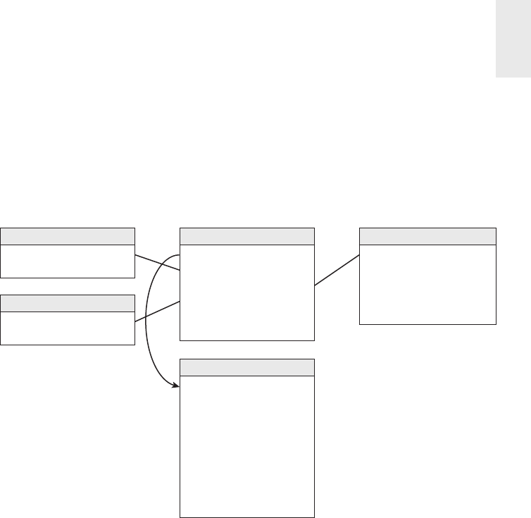
ETL Subsystems and Techniques 459
but rather provides a way to constrain and summarize error events by the usual
attributes of the calendar, such as weekday or last day of a fi scal period. The error
date/time fact is a full relational date/time stamp that specifi es precisely when the
error occurred. This format is useful for calculating the time interval between error
events because you can take the di erence between two date/time stamps to get the
number of seconds separating events.
Date Dimension
Error Event Date Key (PK)
...
Batch Key (PK)
...
Batch Dimension
Error Event Key (PK)
Error Event Date Key (FK)
Screen Key (FK)
Batch Key (FK)
Error Date/Time
Severity Score
Error Event Fact
Screen Key (PK)
Screen Type
ETL Module
Screen Processing Definition
Exception Action
Screen Dimension
Error Event Key (FK)
Error Event Date Key (FK)
Screen Key (FK)
Batch Key (FK)
Error Date/Time
Table Key (FK)
Field Key (FK)
Record Identifier Key (FK)
Error Condition
Error Event Detail Fact
Figure 19-1: Error event schema.
The batch dimension can be generalized to be a processing step in cases in which
data is streamed, rather than batched. The screen dimension identifi es precisely
what the screen criterion is and where the code for the screen resides. It also defi nes
what to do when the screen throws an error. (For example, halt the process, send
the record to a suspense fi le, or tag the data.)
The error event fact table also has a single column primary key, shown as the
error event key. This surrogate key, like dimension table primary keys, is a simple
integer assigned sequentially as rows are added to the fact table. This key column
is necessary in those situations in which an enormous burst of error rows is added
to the error event fact table all at once. Hopefully this won’t happen to you.
The error event schema includes a second error event detail fact table at a lower
grain. Each row in this table identifi es an individual fi eld in a specifi c record that
participated in an error. Thus a complex structure or business rule error that triggers
a single error event row in the higher level error event fact table may generate many
rows in this error event detail fact table. The two tables are tied together by the error
event key, which is a foreign key in this lower grain table. The error event detail

Chapter 19
460
table identifi es the table, record, fi eld, and precise error condition. Thus a complete
description of complex multi-fi eld, multi-record errors is preserved by these tables.
The error event detail table could also contain a precise date/time stamp to
provide a full description of aggregate threshold error events where many records
generate an error condition over a period of time. You should now appreciate that
each quality screen has the responsibility for populating these tables at the time
of an error.
Subsystem 6: Audit Dimension Assembler
The audit dimension is a special dimension that is assembled in the back room
by the ETL system for each fact table, as we discussed in Chapter 6: Order
Management. The audit dimension in Figure 19-2 contains the metadata context at
the moment when a specifi c fact table row is created. You might say we have elevated
metadata to real data! To visualize how audit dimension rows are created, imagine
this shipments fact table is updated once per day from a batch fi le. Suppose today
you have a perfect run with no errors fl agged. In this case, you would generate only
one audit dimension row, and it would be attached to every fact row loaded today.
All the categories, scores, and version numbers would be the same.
Ship Date Key (FK)
Customer Key (FK)
Product Key (FK)
More FKs ...
Audit Key (FK)
Order Number (DD)
Order Line Number (DD)
Facts ...
Audit Key (PK)
Overall Quality Rating
Complete Flag
Validation Flag
Out Of Bounds Flag
Screen Failed Flag
Record Modified Flag
ETL Master Version Number
Allocation Version Number
Shipments Facts Audit Dimension
Figure 19-2: Sample audit dimension attached to a fact table.
Now let’s relax the strong assumption of a perfect run. If you had some fact
rows whose discount dollars triggered an out-of-bounds error, then one more audit
dimension row would be needed to fl ag this condition.
Subsystem 7: Deduplication System
Often dimensions are derived from several sources. This is a common situation
for organizations that have many customer-facing source systems that create and
manage separate customer master tables. Customer information may need to be
merged from several lines of business and outside sources. Sometimes, the data can
be matched through identical values in some key column. However, even when a

ETL Subsystems and Techniques 461
defi nitive match occurs, other columns in the data might contradict one another,
requiring a decision on which data should survive.
Unfortunately, there is seldom a universal column that makes the merge operation
easy. Sometimes, the only clues available are the similarity of several columns. The
di erent sets of data being integrated and the existing dimension table data may need
to be evaluated on di erent fi elds to attempt a match. Sometimes, a match may be
based on fuzzy criteria, such as names and addresses that may nearly match except
for minor spelling di erences.
Survivorship is the process of combining a set of matched records into a unifi ed
image that combines the highest quality columns from the matched records into a
conformed row. Survivorship involves establishing clear business rules that defi ne
the priority sequence for column values from all possible source systems to enable the
creation of a single row with the best-survived attributes. If the dimensional design
is fed from multiple systems, you must maintain separate columns with back refer-
ences, such as natural keys, to all participating source systems used to construct
the row.
There are a variety of data integration and data standardization tools to consider
if you have di cult deduplicating, matching, and survivorship data issues. These
tools are quite mature and in widespread use.
Subsystem 8: Conforming System
Conforming consists of all the steps required to align the content of some or all the
columns in a dimension with columns in similar or identical dimensions in other
parts of the data warehouse. For instance, in a large organization you may have fact
tables capturing invoices and customer service calls that both utilize the customer
dimension. It is highly likely the source systems for invoices and customer service
have separate customer databases. It is likely there will be little guaranteed consis-
tency between the two sources of customer information. The data from these two
customer sources needs to be conformed to make some or all the columns describing
customer share the same domains.
NOTE The process of creating conformed dimensions aligns with an agile
approach. For two dimensions to be conformed, they must share at least one
common attribute with the same name and same contents. You can start with a
single conformed attribute such as Customer Category and systematically add this
column in a nondisruptive way to customer dimensions in each of the customer-
facing processes. As you augment each customer-facing process, you expand the
list of processes that are integrated and can participate in drill-across queries. You
can also incrementally grow the list of conformed attributes, such as city, state, and
country. All this can be staged to align with a more agile implementation approach.
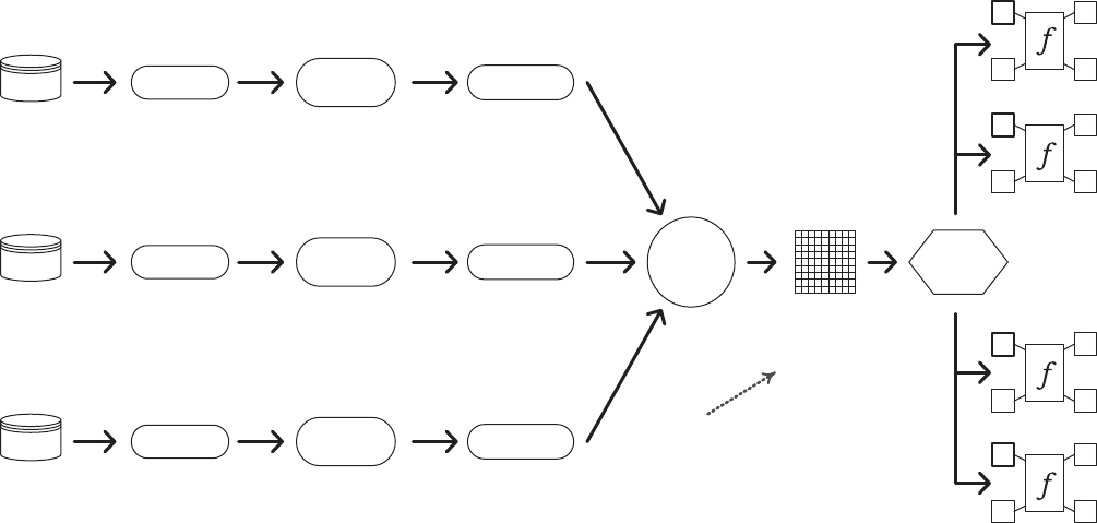
Source 1
Source 2
Source 3
Merged and
globally
Deduped
Extracted
using adapter
Cleaned and
locally
Deduplicated
Conformed and
Survived
Conformed
Dimension ready
for Delivery
Extracted
using adapter
Cleaned and
locally
Deduplicated
Conformed and
Survived
Extracted
using adapter
Cleaned and
locally
Deduplicated
Conformed and
Survived
Replication
Engine
d
d
d
d
d
d
d
d
d
d
d
d
d
d
d
d
Special contents:
1) dimension version number
2) back pointers to all source
natural keys
Figure 19-3: Deduplicating and survivorship processing for conformed dimension process.

ETL Subsystems and Techniques 463
The conforming subsystem is responsible for creating and maintaining the con-
formed dimensions and conformed facts described in Chapter 4: Inventory. To
accomplish this, incoming data from multiple systems needs to be combined and
integrated, so it is structurally identical, deduplicated, fi ltered of invalid data, and
standardized in terms of content rows in a conformed image. A large part of the
conforming process is the deduplicating, matching, and survivorship processes
previously described. The conforming process fl ow combining the deduplicating
and survivorship processing is shown in Figure 19-3.
The process of defining and delivering conformed dimensions and facts is
described later in subsystems 17 (dimension manager) and 18 (fact provider).
Delivering: Prepare for Presentation
The primary mission of the ETL system is the hando of the dimension and fact
tables in the delivery step. For this reason, the delivery subsystems are the most
pivotal subsystems in the ETL architecture. Although there is considerable variation
in source data structures and cleaning and conforming logic, the delivery process-
ing techniques for preparing the dimensional table structures are more defi ned and
disciplined. Use of these techniques is critical to building a successful dimensional
data warehouse that is reliable, scalable, and maintainable.
Many of these subsystems focus on dimension table processing. Dimension tables
are the heart of the data warehouse. They provide the context for the fact tables and
hence for all the measurements. Although dimension tables are usually smaller than
the fact tables, they are critical to the success of the DW/BI system as they provide the
entry points into the fact tables. The delivering process begins with the cleaned and
conformed data resulting from the subsystems just described. For many dimensions,
the basic load plan is relatively simple: You perform basic transformations to the
data to build dimension rows for loading into the target presentation table. This
typically includes surrogate key assignment, code lookups to provide appropriate
descriptions, splitting or combining columns to present the appropriate data val-
ues, or joining underlying third normal form table structures into denormalized
fl at dimensions.
Preparing fact tables is certainly important because fact tables hold the key mea-
surements of the business that the users want to see. Fact tables can be large and
time-consuming to load. However, preparing fact tables for presentation is typically
more straightforward.
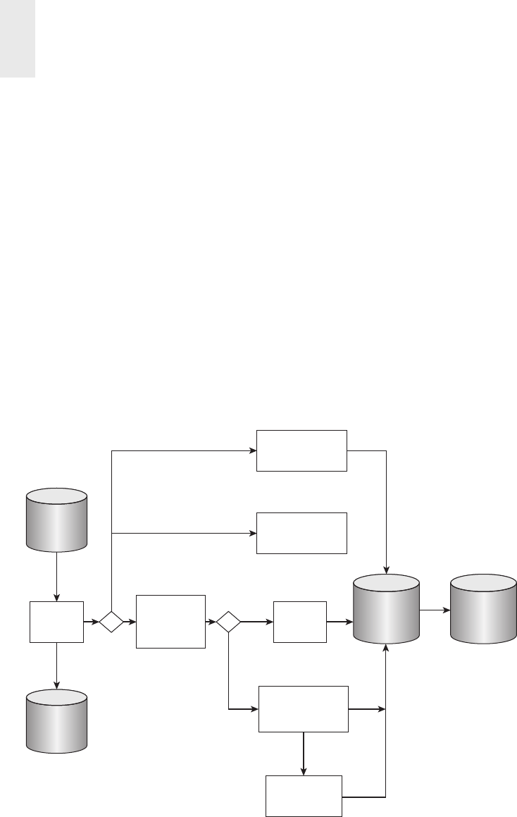
Chapter 19
464
Subsystem 9: Slowly Changing Dimension Manager
One of the more important elements of the ETL architecture is the capability to
implement slowly changing dimension (SCD) logic. The ETL system must determine
how to handle an attribute value that has changed from the value already stored
in the data warehouse. If the revised description is determined to be a legitimate
and reliable update to previous information, the appropriate SCD technique must
be applied.
As described in Chapter 5: Procurement, when the data warehouse receives
notifi cation that an existing row in a dimension has changed, there are three basic
responses: type 1 overwrite, type 2 add a new row, and type 3 add a new column.
The SCD manager should systematically handle the time variance in the dimen-
sions using these three techniques, as well as the other SCD techniques. In addition,
the SCD manager should maintain appropriate housekeeping columns for type 2
changes. Figure 19-4 shows the overall processing fl ow for handling surrogate key
management for processing SCDs.
New record in source
(not in Cross Ref)
insert
update
update
field
type 1 or 3
field is
type 2 insert
update
CRC
options CRCs
different
Most Recent
Surrogate
Key Map
Master
Dimension
Cross Ref
Assign surrogate
keys & set
dates/indicator
Update
dimension
attribute
Update prior
most-recent
row
Find specific
changed
field(s)
Source
Extract
CRC
Compare
Master
Dimension
Cross Ref
CRCs match Ignore
Assign surrogate
keys & set
dates/indicator
Figure 19-4: Processing fl ow for SCD surrogate key management.

ETL Subsystems and Techniques 465
The change data capture process described in subsystem 2 obviously plays an
important role in presenting the changed data to the SCD process. Assuming the
change data capture process has e ectively delivered appropriate changes, the SCD
process can take the appropriate actions.
Type 1: Overwrite
The type 1 technique is a simple overwrite of one or more attributes in an existing
dimension row. You take the revised data from the change data capture system
and overwrite the dimension table contents. Type 1 is appropriate when correcting
data or when there is no business need to keep the history of previous values. For
instance, you may receive a corrected customer address. In this case, overwriting is
the right choice. Note that if the dimension table includes type 2 change tracking,
you should overwrite the a ected column in all existing rows for that particular
customer. Type 1 updates must be propagated forward from the earliest permanently
stored staging tables to all a ected staging tables, so if any of them are used to re-
create the fi nal load tables, the e ect of the overwrite is preserved.
Some ETL tools contain UPDATE else INSERT functionality. This functionality
may be convenient for the developer but can be a performance killer. For maximum
performance, existing row UPDATEs should be segregated from new row INSERTs.
If type 1 updates cause performance problems, consider disabling database logging
or use of the DBMS bulk loader.
Type 1 updates invalidate any aggregates built upon the changed column, so the
dimension manager (subsystem 17) must notify the a ected fact providers (subsys-
tem 18) to drop and rebuild the a ected aggregates.
Type 2: Add New Row
The type 2 SCD is the standard technique for accurately tracking changes in dimen-
sions and associating them correctly with fact rows. Supporting type 2 changes
requires a strong change data capture system to detect changes as soon as they occur.
For type 2 updates, copy the previous version of the dimension row and create a
new dimension row with a new surrogate key. If there is not a previous version of
the dimension row, create a new one from scratch. Then update this row with the
columns that have changed and add any other columns that are needed. This is
the main workhorse technique for handling dimension attribute changes that need
to be tracked over time.
The type 2 ETL process must also update the most recent surrogate key map table,
assuming the ETL tool doesn’t automatically handle this. These little two-column

Chapter 19
466
tables are of immense importance when loading fact table data. Subsystem 14, the
surrogate key pipeline, supports this process.
Refer to Figure 19-4 to see the lookup and key assignment logic for handling a
changed dimension row during the extract process. In this example, the change
data capture process (subsystem 2) uses a CRC compare to determine which
rows have changed in the source data since the last update. If you are lucky, you
already know which dimension records have changed and can omit this CRC
compare step. After you identify rows that have changes in type 2 attributes,
you can generate a new surrogate key from the key sequence and update the
surrogate key map table.
When a new type 2 row is created, you need at least a pair of time stamps, as
well as an optional change description attribute. The pair of time stamps defi nes a
span of time from the beginning e ective time to the ending e ective time when
the complete set of dimension attributes is valid. A more sophisticated treatment
of a type 2 SCD row involves adding fi ve ETL housekeeping columns. Referring to
Figure 19-4, this also requires the type 2 ETL process to fi nd the prior e ective row
and make appropriate updates to these housekeeping columns:
■ Change Date (change date as foreign key to date dimension outrigger)
■ Row E ective Date/Time (exact date/time stamp of change)
■ Row End Date/Time (exact date/time stamp of next change, defaults to
12/31/9999 for most current dimension row)
■ Reason for Change column (optional attribute)
■ Current Flag (current/expired)
NOTE It is possible that back-end scripts are run within the transaction data-
base to modify data without updating the respective metadata fi elds such as the
last_modifi ed_date. Using these fi elds for the dimension time stamps can cause
inconsistent results in the data warehouse. Always use the system or as-of date to
derive the type 2 e ective time stamps.
The type 2 process does not change history as the type 1 process does; thus
type 2 changes don’t require rebuilding a ected aggregate tables as long as the
change was made “today” and not backward in time.
NOTE Kimball Design Tip #80 (available at www.kimballgroup.com under the
Tools and Utilities tab for this book title) provides in-depth guidance on adding a
row change reason code attribute to dimension tables.
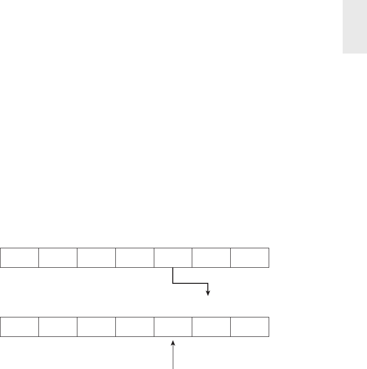
ETL Subsystems and Techniques 467
Type 3: Add New Attribute
The type 3 technique is designed to support attribute “soft” changes that allow a
user to refer either to the old value of the attribute or the new value. For example, if
a sales team is assigned to a newly named sales region, there may be a need to track
the old region assignment, as well as the new one. The type 3 technique requires the
ETL system to alter the dimension table to add a new column to the schema, if this
situation was not anticipated. Of course, the DBA assigned to work with the ETL
team will in all likelihood be responsible for this change. You then need to push
the existing column values into the newly created column and populate the original
column with the new values provided to the ETL system. Figure 19-5 shows how
a type 3 SCD is implemented.
1127648 A 107B Denim
pants 38 Men’s
wear
Prod ID
(NK)
Prod Key
(PK)
Prod
Name Size Category Color
Blue
Add field; Transfer old value
Overwrite
with new
value
...
1127648 A 107B Denim
pants 38 Leisure
wear
Men’s
wear
Prod ID
(NK)
Prod Key
(PK)
Prod
Name Size Category Color
Prior
Category
Blue
Figure 19-5: Type 3 SCD process.
Similar to the type 1 process, type 3 change updates invalidate any aggregates
built upon the changed column; the dimension manager must notify the a ected
fact providers, so they drop and rebuild the a ected aggregates.
Type 4: Add Mini-Dimension
The type 4 technique is used when a group of attributes in a dimension change suf-
fi ciently rapidly so that they are split o to a mini-dimension. This situation is some-
times called a rapidly changing monster dimension. Like type 3, this situation calls
for a schema change, hopefully done at design time. The mini-dimension requires
its own unique primary key, and both the primary key of the main dimension and
the primary key of the mini-dimension must appear in the fact table. Figure 19-6
shows how a type 4 SCD is implemented.
Chapter 19
468
Activity Date Key (FK)
Customer Key (FK)
Demographics Key (FK)
Product Key (FK)
Promotion Key (FK)
Sales Dollars
Sales Units
Customer Key (PK)
Customer Attributes...
Sales Fact Customer Dimension
Demographics Key (PK)
Demographics Attributes...
Demographics Dimension
Figure 19-6: Type 4 SCD process.
Type 5: Add Mini-Dimension and Type 1 Outrigger
The type 5 technique builds on the type 4 mini-dimension by also embedding a type
1 reference to the mini-dimension in the primary dimension. This allows accessing
the current values in the mini-dimension directly from the base dimension without
linking through a fact table. The ETL team must add the type 1 key reference in
the base dimension and must overwrite this key reference in all copies of the base
dimension whenever the current status of the mini-dimension changes over time.
Figure 19-7 shows how a type 5 SCD is implemented.
Activity Date Key (FK)
Customer Key (FK)
Demographics Key (FK)
Product Key (FK)
Promotion Key (FK)
Sales Dollars
Sales Units
Customer Key (PK)
Demographics Key (FK - SCD 1)
Customer Attributes...
Sales Fact Customer Dimension
Demographics Key (PK)
Demographics Attributes...
Demographics Dimension
Figure 19-7: Type 5 SCD process.
Type 6: Add Type 1 Attributes to Type 2 Dimension
The type 6 technique has an embedded attribute that is an alternate value of a
normal type 2 attribute in the base dimension. Usually such an attribute is simply
a type 3 alternative reality, but in this case the attribute is systematically overwrit-
ten whenever the attribute is updated. Figure 19-8 shows how a type 6 SCD is
implemented.
Type 7: Dual Type 1 and Type 2 Dimensions
The type 7 technique is a normal type 2 dimension paired with a specially con-
structed fact table that has both a normal foreign key to the dimension for type 2
historical processing, and also a foreign durable key (FDK in Figure 19-9) that is
ETL Subsystems and Techniques 469
used alternatively for type 1 current processing, connected to the durable key in
the dimension table labeled PDK. The dimension table also contains a current row
indicator that indicates whether the particular row is the one to be used for current
SCD 1 perspective. The ETL team must augment a normally constructed fact table
with this constant value foreign durable key. Figure 19-9 shows how a type 7 SCD
is implemented.
Activity Date Key (FK)
Customer Key (FK)
Demographics Key (FK)
Product Key (FK)
Promotion Key (FK)
Sales Dollars
Sales Units
Customer Key (PK)
Customer Category (SCD 2)
Current Customer Category (SCD 1)
Customer Attributes...
Sales Fact Customer Dimension
Figure 19-8: Type 6 SCD process.
Activity Date Key (FK)
Customer Key (FK)
Customer Durable Key (FDK)
Demographics Key (FK)
Product Key (FK)
Promotion Key (FK)
Sales Dollars
Sales Units
Customer Key (PK)
Customer Durable Key (PDK)
Customer Attributes...
Current Row Indicator
join for SCD 2
Indicator = Current/True for SCD 1
join for SCD 1
Sales Fact
Customer Dimension
Figure 19-9: Type 7 SCD process.
Subsystem 10: Surrogate Key Generator
As you recall from Chapter 3: Retail Sales, we strongly recommend the use of sur-
rogate keys for all dimension tables. This implies you need a robust mechanism for
producing surrogate keys in the ETL system. The surrogate key generator should
independently generate surrogate keys for every dimension; it should be independent
of database instance and able to serve distributed clients. The goal of the surrogate
key generator is to generate a meaningless key, typically an integer, to serve as the
primary key for a dimension row.
Although it may be tempting to create surrogate keys via database triggers,
this technique may create performance bottlenecks. If the DBMS is used to assign
surrogate keys, it is preferable for the ETL process to directly call the database
sequence generator. For improved e ciency, consider having the ETL tool generate

Chapter 19
470
and maintain the surrogate keys. Avoid the temptation of concatenating the opera-
tional key of the source system and a date/time stamp. Although this approach seems
simple, it is fraught with problems and ultimately will not scale.
Subsystem 11: Hierarchy Manager
It is normal for a dimension to have multiple, simultaneous, embedded hierarchi-
cal structures. These multiple hierarchies simply coexist in the same dimension as
dimension attributes. All that is necessary is that every attribute be single valued in
the presence of the dimension’s primary key. Hierarchies are either fi xed or ragged.
A fi xed depth hierarchy has a consistent number of levels and is simply modeled and
populated as separate dimension attributes for each of the levels. Slightly ragged hier-
archies like postal addresses are most often modeled as a fi xed hierarchy. Profoundly
ragged hierarchies are typically found with organization structures that are unbal-
anced and of indeterminate depth. The data model and ETL solution required to
support these needs require the use of a bridge table containing the organization map.
Snowfl akes or normalized data structures are not recommended for the presenta-
tion level. However, the use of a normalized design may be appropriate in the ETL
staging area to assist in the maintenance of the ETL data fl ow for populating and
maintaining the hierarchy attributes. The ETL system is responsible for enforcing
the business rules to assure the hierarchy is populated appropriately in the dimen-
sion table.
Subsystem 12: Special Dimensions Manager
The special dimensions manager is a catch-all subsystem: a placeholder in the ETL
architecture for supporting an organization’s specifi c dimensional design character-
istics. Some organizations’ ETL systems require all the capabilities discussed here,
whereas others will be concerned with few of these design techniques:
Date/Time Dimensions
The date and time dimensions are unique in that they are completely specifi ed
at the beginning of the data warehouse project, and they don’t have a conventional
source. This is okay! Typically, these dimensions are built in an afternoon with a
spreadsheet. But in a global enterprise environment, even this dimension can be
challenging when taking into account multiple fi nancial reporting periods or mul-
tiple cultural calendars.
Junk Dimensions
Junk dimensions are made up from text and miscellaneous fl ags left over in the
fact table after you remove all the critical attributes. There are two approaches for
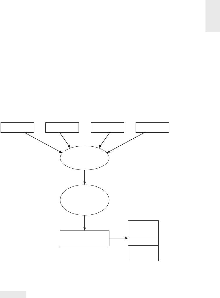
ETL Subsystems and Techniques 471
creating junk dimensions in the ETL system. If the theoretical number of rows in
the dimension is fi xed and known, the junk dimension can be created in advance.
In other cases, it may be necessary to create newly observed junk dimension rows
on-the-fl y while processing fact row input. As illustrated in Figure 19-10, this pro-
cess requires assembling the junk dimension attributes and comparing them to the
existing junk dimension rows to see if the row already exists. If not, a new dimen-
sion row must be assembled, a surrogate key created, and the row loaded into the
junk dimension on-the-fl y during the fact table load process.
code 1 code M
Codes and indicators encountered in daily load:
Combine into
single row
ind 1 ind P
......
Compare to existing
dimension rows; insert
if new
Surrogate key for this
junk dimension row
load
junk key (FK)
fact table
Figure 19-10: Architecture for building junk dimension rows.
NOTE Kimball Design Tip #113 (available at www.kimballgroup.com under the
Tools and Utilities tab for this book title) provides more in-depth guidance on
building and maintaining junk dimension tables.
Mini-Dimensions
As we just discussed in subsystem 9, mini-dimensions are a technique used to
track dimension attribute changes in a large dimension when the type 2 technique
is infeasible, such as a customer dimension. From an ETL perspective, creation of

Chapter 19
472
the mini-dimension is similar to the junk dimension process previously described.
Again, there are two alternatives: building all valid combinations in advance or rec-
ognizing and creating new combinations on-the-fl y. Although junk dimensions are
usually built from the fact table input, mini-dimensions are built from dimension
table inputs. The ETL system is responsible for maintaining a multicolumn surrogate
key lookup table to identify the base dimension member and appropriate mini-
dimension row to support the surrogate pipeline process described in Subsystem 14,
Surrogate Key Pipeline. Keep in mind that very large, complex customer dimensions
often require several mini-dimensions.
NOTE Kimball Design Tip #127 (available at www.kimballgroup.com under the
Tools and Utilities tab for this book title) provides more in-depth guidance on
building and maintaining mini-dimension tables.
Shrunken Subset Dimensions
Shrunken dimensions are conformed dimensions that are a subset of rows and/
or columns of one of your base dimensions. The ETL data fl ow should build
conformed shrunken dimensions from the base dimension, rather than indepen-
dently, to assure conformance. The primary key for the shrunken dimension,
however, must be independently generated; if you attempt to use a key from an
“example” base dimension row, you will get into trouble if this key is retired or
superseded.
NOTE Kimball Design Tip #137 (available at www.kimballgroup.com under the
Tools and Utilities tab for this book title) provides more in-depth guidance on
building shrunken dimension tables.
Small Static Dimensions
A few dimensions are created entirely by the ETL system without a real outside
source. These are usually small lookup dimensions where an operational code is
translated into words. In these cases, there is no real ETL processing. The lookup
dimension is simply created directly by the ETL team as a relational table in its
fi nal form.
User Maintained Dimensions
Often the warehouse requires that totally new “master” dimension tables be created.
These dimensions have no formal system of record; rather they are custom descrip-
tions, groupings, and hierarchies created by the business for reporting and analysis

ETL Subsystems and Techniques 473
purposes. The ETL team often ends up with stewardship responsibility for these
dimensions, but this is typically not successful because the ETL team is not aware of
changes that occur to these custom groupings, so the dimensions fall into disrepair
and become ine ective. The best-case scenario is to have the appropriate business
user department agree to own the maintenance of these attributes. The DW/BI team
needs to provide a user interface for this maintenance. Typically, this takes the form
of a simple application built using the company’s standard visual programming tool.
The ETL system should add default attribute values for new rows, which the user
owner needs to update. If these rows are loaded into the warehouse before they are
changed, they still appear in reports with whatever default description is supplied.
NOTE The ETL process should create a unique default dimension attribute
description that shows someone hasn’t yet done their data stewardship job. We
favor a label that concatenates the phrase Not Yet Assigned with the surrogate
key value: “Not Yet Assigned 157.” That way, multiple unassigned values do not
inadvertently get lumped together in reports and aggregate tables. This also helps
identify the row for later correction.
Subsystem 13: Fact Table Builders
Fact tables hold the measurements of an organization. Dimensional models are
deliberately built around these numerical measurements. The fact table builder
subsystem focuses on the ETL architectural requirements to e ectively build the
three primary types of fact tables: transaction, periodic snapshot, and accumulating
snapshot. An important requirement for loading fact tables is maintaining refer-
ential integrity with the associated dimension tables. The surrogate key pipeline
(subsystem 14) is designed to help support this need.
Transaction Fact Table Loader
The transaction grain represents a measurement event defi ned at a particular instant.
A line item on an invoice is an example of a transaction event. A scanner event at
a cash register is another. In these cases, the time stamp in the fact table is very
simple. It’s either a single daily grain foreign key or a pair consisting of a daily grain
foreign key together with a date/time stamp, depending on what the source system
provides and the analyses require. The facts in this transaction table must be true
to the grain and should describe only what took place in that instant.
Transaction grain fact tables are the largest and most detailed of the three types
of fact tables. The transaction fact table loader receives data from the changed data
capture system and loads it with the proper dimensional foreign keys. The pure

Chapter 19
474
addition of the most current records is the easiest case: simply bulk loading new
rows into the fact table. In most cases, the target fact table should be partitioned by
time to ease the administration and speed the performance of the table. An audit
key, sequential ID, or date/time stamp column should be included to allow backup
or restart of the load job.
The addition of late arriving data is more di cult, requiring additional process-
ing capabilities described in subsystem 16. In the event it is necessary to update
existing rows, this process should be handled in two phases. The fi rst step is to
insert the corrected rows without overwriting or deleting the original rows, and
then delete the old rows in a second step. Using a sequentially assigned single sur-
rogate key for the fact table makes it possible to perform the two steps of insertion
followed by deletion.
Periodic Snapshot Fact Table Loader
The periodic snapshot grain represents a regular repeating measurement or set of
measurements, like a bank account monthly statement. This fact table also has a
single date column, representing the overall period. The facts in this periodic snap-
shot table must be true to the grain and should describe only measures appropriate
to the timespan defi ned by the period. Periodic snapshots are a common fact table
type and are frequently used for account balances, monthly fi nancial reporting,
and inventory balances. The periodicity of a periodic snapshot is typically daily,
weekly, or monthly.
Periodic snapshots have similar loading characteristics to those of transaction
grain fact tables. The same processing applies for inserts and updates. Assuming
data is promptly delivered to the ETL system, all records for each periodic load can
cluster in the most recent time partition. Traditionally, periodic snapshots have
been loaded en masse at the end of the appropriate period.
For example, a credit card company might load a monthly account snapshot table
with the balances in e ect at the end of the month. More frequently, organizations
will populate a hot rolling periodic snapshot. In addition to the rows loaded at the
end of every month, there are special rows loaded with the most current balances
in e ect as of the previous day. As the month progresses, the current month rows
are continually updated with the most current information and continue in this
manner rolling through the month. Note that the hot rolling snapshot can some-
times be di cult to implement if the business rules for calculating the balances
at the period end are complex. Often these complex calculations are dependent
on other periodic processing outside the data warehouse, and there is not enough
information available to the ETL system to perform these complex calculations on
a more frequent basis.

ETL Subsystems and Techniques 475
Accumulating Snapshot Fact Table Loader
The accumulating snapshot grain represents the current evolving status of a process
that has a fi nite beginning and end. Usually, these processes are of short duration
and therefore don’t lend themselves to the periodic snapshot. Order processing is
the classic example of an accumulating snapshot. The order is placed, shipped,
and paid for within one reporting period. The transaction grain provides too much
detail separated into individual fact table rows, and the periodic snapshot just is
the wrong way to report this data.
The design and administration of the accumulating snapshot is quite di erent
from the fi rst two fact table types. All accumulating snapshot fact tables have a
set of dates which describe the typical process workfl ow. For instance, an order
might have an order date, actual ship date, delivery date, fi nal payment date, and
return date. In this example, these fi ve dates appear as fi ve separate date-valued
foreign surrogate keys. When the order row is fi rst created, the fi rst of these dates
is well defi ned, but perhaps none of the others have yet happened. This same
fact row is subsequently revisited as the order winds its way through the order
pipeline. Each time something happens, the accumulating snapshot fact row is
destructively modifi ed. The date foreign keys are overwritten, and various facts
are updated. Often the fi rst date remains inviolate because it describes when
the row was created, but all the other dates may well be overwritten, sometimes
more than once.
Many RDBMSs utilize variable row lengths. Repeated updates to accumulating
snapshot fact rows may cause the rows to grow due to these variable row lengths,
a ecting the residency of disk blocks. It may be worthwhile to occasionally drop
and reload rows after the update activity to improve performance.
An accumulating snapshot fact table is an effective way to represent finite
processes with well-defi ned beginnings and endings. However, the accumulating
snapshot by defi nition is the most recent view. Often it makes sense to utilize all
three fact table types to meet various needs. Periodic history can be captured with
periodic extracts, and all the infi nite details involved in the process can be captured
in an associated transaction grain fact table. The presence of many situations that
violate standard scenarios or involve repeated looping though the process would
prohibit the use of an accumulating snapshot.
Subsystem 14: Surrogate Key Pipeline
Every ETL system must include a step for replacing the operational natural keys
in the incoming fact table row with the appropriate dimension surrogate
keys. Referential integrity (RI) means that for each foreign key in the fact table,
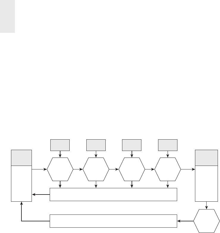
Chapter 19
476
an entry exists in the corresponding dimension table. If there’s a row in a sales
fact table for product surrogate key 323442, you need to have a row in the product
dimension table with the same key, or you won’t know what you’ve sold. You have a
sale for what appears to be a nonexistent product. Even worse, without the product
key in the dimension, a business user can easily construct a query that will omit
this sale without even realizing it.
The key lookup process should result in a match for every incoming natural key
or a default value. In the event there is an unresolved referential integrity failure dur-
ing the lookup process, you need to feed these failures back to the responsible ETL
process for resolution, as shown in Figure 19-11. Likewise, the ETL process needs to
resolve any key collisions that might be encountered during the key lookup process.
Date
Dimension
Replace
date_ID
with surrogate
date_key
Replace
prod_ID
with surrogate
prod_key
Replace
store_ID
with surrogate
store_key
Replace
promo_ID
with surrogate
promo_key
Load fact
table rows
into DBMS
Fact Table
with Natural
Key IDs
date_ID
product_ID
store_ID
promo_ID
dollar_sales
unit_sales
dollar_cost
date_key
product_key
store_key
promo_key
dollar_sales
unit_sales
dollar_cost
Fact Table
with Surrogate
Keys
Product
Dimension
Store
Dimension
Referential Integrity Failures
Key Collisions
Promotion
Dimension
Figure 19-11: Replacing fact record’s operational natural keys with dimension
surrogate keys.
After the fact table data has been processed and just before loading into the pre-
sentation layer, a surrogate key lookup needs to occur to substitute the operational
natural keys in the fact table record with the proper current surrogate key. To pre-
serve referential integrity, always complete the updating of the dimension tables
fi rst. In that way, the dimension tables are always the legitimate source of primary
keys you must replace in the fact table (refer to Figure 19-11).
The most direct approach is to use the actual dimension table as the source for
the most current value of the surrogate key corresponding to each natural key. Each
time you need the current surrogate key, look up all the rows in the dimension with
the natural key equal to the desired value, and then select the surrogate key that
aligns with the historical context of the fact row using the current row indicator or
begin and end e ect dates. Current hardware environments o er nearly unlimited
addressable memory, making this approach practical.

ETL Subsystems and Techniques 477
During processing, each natural key in the incoming fact record is replaced with
the correct current surrogate key. Don’t keep the natural key in the fact row—the
fact table needs to contain only the surrogate key. Do not write the input data to
disk until all fact rows have passed all the processing steps. If possible, all required
dimension tables should be pinned in memory, so they can be randomly accessed
as each incoming record presents its natural keys.
As illustrated at the bottom of Figure 19-11, the surrogate key pipeline needs to
handle key collisions in the event you attempt to load a duplicate row. This is an
example of a data quality problem appropriate for a traditional structure data qual-
ity screen, as discussed in subsystem 4. In the event a key collision is recognized,
the surrogate key pipeline process needs to choose to halt the process, send the
o ending data into suspension, or apply appropriate business rules to determine
if it is possible to correct the problem, load the row, and write an explanatory row
into the error event schema.
Note a slightly di erent process is needed to perform surrogate key lookups if
you need to reload history or if you have a lot of late arriving fact rows because you
don’t want to map the most current value to a historical event. In this case, you need
to create logic to fi nd the surrogate key that applied at the time the fact record was
generated. This means fi nding the surrogate key where the fact transaction date is
between the key’s e ective start date and end date.
When the fact table natural keys have been replaced with surrogate keys, the
fact row is ready to load. The keys in the fact table row have been chosen to be
proper foreign keys, and the fact table is guaranteed to have referential integrity
with respect to the dimension tables.
Subsystem 15: Multivalued Dimension
Bridge Table Builder
Sometimes a fact table must support a dimension that takes on multiple values
at the lowest granularity of the fact table, as described in Chapter 8: Customer
Relationship Management. If the grain of the fact table cannot be changed to directly
support this dimension, then the multivalued dimension must be linked to the fact
table via a bridge table. Bridge tables are common in the healthcare industry, in
sales commission environments, and for supporting variable depth hierarchies, as
discussed in subsystem 11.
The challenge for the ETL team is building and maintaining the bridge table. As
multivalued relationships to the fact row are encountered, the ETL system has the
choice of either making each set of observations a unique group or reusing groups
when an identical set of observations occurs. Unfortunately, there is no simple
answer for the right choice. In the event the multivalued dimension has type 2

Chapter 19
478
attributes, the bridge table must also be time varying, such as a patient’s time vari-
ant set of diagnoses.
One of the bridge table constructs presented in Chapter 10: Financial Services
was the inclusion of a weighting factor to support properly weighted reporting from
the bridge table. In many cases, the weighting factor is a familiar allocation factor,
but in other cases, the identifi cation of the appropriate weighting factor can be prob-
lematic because there may be no rational basis for assigning the weighting factor.
NOTE Kimball Design Tip #142 (available at www.kimballgroup.com under the
Tools and Utilities tab for this book title) provides more in-depth guidance on
building and maintaining bridge tables.
Subsystem 16: Late Arriving Data Handler
Data warehouses are usually built around the ideal assumption that measured activ-
ity (fact records) arrive in the data warehouse at the same time as the context of
the activity (dimension records). When you have both the fact records and the
correct contemporary dimension rows, you have the luxury of fi rst maintaining
the dimension keys and then using these up-to-date keys in the accompanying fact
rows. However, for a variety of reasons, the ETL system may need to process late
arriving fact or dimension data.
In some environments, there may need to be special modifi cations to the stan-
dard processing procedures to deal with late arriving facts, namely fact records
that come into the warehouse very much delayed. This is a messy situation because
you have to search back in history to decide which dimension keys were in e ect
when the activity occurred. In addition, you may need to adjust any semi-additive
balances in subsequent fact rows. In a heavily compliant environment, it is also
necessary to interface with the compliance subsystem because you are about to
change history.
Late arriving dimensions occur when the activity measurement (fact record)
arrives at the data warehouse without its full context. In other words, the statuses of
the dimensions attached to the activity measurement are ambiguous or unknown for
some period of time. If you are living in the conventional batch update cycle of one or
more days’ latency, you can usually just wait for the dimensions to be reported. For
example, the identifi cation of the new customer may come in a separate feed delayed
by several hours; you may just be able to wait until the dependency is resolved.
But in many situations, especially real-time environments, this delay is not
acceptable. You cannot suspend the rows and wait for the dimension updates to
occur; the business requirements demand that you make the fact row visible before

ETL Subsystems and Techniques 479
knowing the dimensional context. The ETL system needs additional capabilities
to support this requirement. Using customer as the problem dimension, the ETL
system needs to support two situations. The fi rst is to support late arriving type 2
dimension updates. In this situation, you need to add the revised customer row to
the dimension with a new surrogate key and then go in and destructively modify
any subsequent fact rows’ foreign key to the customer table. The e ective dates for
the a ected dimension rows also need to be reset. In addition, you need to scan
forward in the dimension to see if there have been any subsequent type 2 rows for
this customer and change this column in any a ected rows.
The second situation occurs when you receive a fact row with what appears to be a
valid customer natural key, but you have not yet loaded this customer in the customer
dimension. It would be possible to load this row pointing to a default row in the
dimension table. This approach has the same unpleasant side e ect discussed earlier
of requiring destructive updates to the fact rows’ foreign keys when the dimension
updates are fi nally processed. Alternatively, if you believe the customer is a valid, but
not yet processed customer, you should assign a new customer surrogate key with
a set of dummy attribute values in a new customer dimension row. You then return
to this dummy dimension row at a later time and make type 1 overwrite changes to
its attributes when you get complete information on the new customer. At least this
step avoids destructively changing any fact table keys.
There is no way to avoid a brief provisional period in which the dimensions
are “not quite right.” But these maintenance steps can minimize the impact of the
unavoidable updates to the keys and other columns.
Subsystem 17: Dimension Manager System
The dimension manager is a centralized authority who prepares and publishes con-
formed dimensions to the data warehouse community. A conformed dimension is
by necessity a centrally managed resource: Each conformed dimension must have a
single, consistent source. It is the dimension manager’s responsibility to administer
and publish the conformed dimension(s) for which he has responsibility. There
may be multiple dimension managers in an organization, each responsible for a
dimension. The dimension manager’s responsibilities include the following ETL
processing:
■ Implement the common descriptive labels agreed to by the data stewards and
stakeholders during the dimension design.
■ Add new rows to the conformed dimension for new source data, generating
new surrogate keys.
■ Add new rows for type 2 changes to existing dimension entries, generating
new surrogate keys.

Chapter 19
480
■ Modify rows in place for type 1 changes and type 3 changes, without chang-
ing the surrogate keys.
■ Update the version number of the dimension if any type 1 or type 3 changes
are made.
■ Replicate the revised dimension simultaneously to all fact table providers.
It is easier to manage conformed dimensions in a single tablespace DBMS on a
single machine because there is only one copy of the dimension table. However,
managing conformed dimensions becomes more di cult in multiple tablespace,
multiple DMBS, or multimachine distributed environments. In these situations, the
dimension manager must carefully manage the simultaneous release of new versions
of the dimension to every fact provider. Each conformed dimension should have a
version number column in each row that is overwritten in every row whenever the
dimension manager releases the dimension. This version number should be utilized
to support any drill-across queries to assure that the same release of the dimension
is being utilized.
Subsystem 18: Fact Provider System
The fact provider is responsible for receiving conformed dimensions from the dimen-
sion managers. The fact provider owns the administration of one or more fact tables
and is responsible for their creation, maintenance, and use. If fact tables are used
in any drill-across applications, then by defi nition the fact provider must be using
conformed dimensions provided by the dimension manager. The fact provider’s
responsibilities are more complex and include:
■ Receive or download replicated dimension from the dimension manager.
■ In an environment in which the dimension cannot simply be replicated but
must be locally updated, the fact provider must process dimension records
marked as new and current to update current key maps in the surrogate key
pipeline and also process any dimension records marked as new but postdated.
■ Add all new rows to fact tables after replacing their natural keys with correct
surrogate keys.
■ Modify rows in all fact tables for error correction, accumulating snapshots,
and late arriving dimension changes.
■ Remove aggregates that have become invalidated.
■ Recalculate a ected aggregates. If the new release of a dimension does not
change the version number, aggregates have to be extended to handle only
newly loaded fact data. If the version number of the dimension has changed,
the entire historical aggregate may have to be recalculated.

ETL Subsystems and Techniques 481
■ Quality ensure all base and aggregate fact tables. Be satisfi ed the aggregate
tables are correctly calculated.
■ Bring updated fact and dimension tables online.
■ Inform users that the database has been updated. Tell them if major changes
have been made, including dimension version changes, postdated records
being added, and changes to historical aggregates.
Subsystem 19: Aggregate Builder
Aggregates are the single most dramatic way to a ect performance in a large data
warehouse environment. Aggregations are like indexes; they are specifi c data struc-
tures created to improve performance. Aggregates can have a signifi cant impact
on performance. The ETL system needs to e ectively build and use aggregates
without causing signifi cant distraction or consuming extraordinary resources and
processing cycles.
You should avoid architectures in which aggregate navigation is built into the
proprietary query tool. From an ETL viewpoint, the aggregation builder needs to
populate and maintain aggregate fact table rows and shrunken dimension tables
where needed by aggregate fact tables. The fastest update strategy is incremental,
but a major change to a dimension attribute may require dropping and rebuild-
ing the aggregate. In some environments, it may be faster to dump data out of the
DBMS and build aggregates with a sort utility rather than building the aggregates
inside the DBMS. Additive numeric facts can be aggregated easily at extract time
by calculating break rows in one of the sort packages. Aggregates must always be
consistent with the atomic base data. The fact provider (subsystem 18) is respon-
sible for taking aggregates o -line when they are not consistent with the base data.
User feedback on the queries that run slowly is critical input to designing aggrega-
tions. Although you can depend on informal feedback to some extent, a log of frequently
attempted slow-running queries should be captured. You should also try to identify the
nonexistent slow-running queries that never made it into the log because they never
run to completion, or aren’t even attempted due to known performance challenges.
Subsystem 20: OLAP Cube Builder
OLAP servers present dimensional data in an intuitive way, enabling a range of
analytic users to slice and dice data. OLAP is a sibling of dimensional star schemas
in the relational database, with intelligence about relationships and calculations
defi ned on the server that enable faster query performance and more interesting
analytics from a broad range of query tools. Don’t think of an OLAP server as a

Chapter 19
482
competitor to a relational data warehouse, but rather an extension. Let the relational
database do what it does best: Provide storage and management.
The relational dimensional schema should be viewed as the foundation for OLAP
cubes if you elect to include them in your architecture. The process of feeding data
from the dimensional schema is an integral part of the ETL system; the relational
schemas are the best and preferred source for OLAP cubes. Because many OLAP
systems do not directly address referential integrity or data cleaning, the pre-
ferred architecture is to load OLAP cubes after the completion of conventional ETL
processes. Note that some OLAP tools are more sensitive to hierarchies than rela-
tional schemas. It is important to strongly enforce the integrity of hierarchies within
dimensions before loading an OLAP cube. Type 2 SCDs fi t an OLAP system well
because a new surrogate key is just treated as a new member. Type 1 SCDs that restate
history do not fi t OLAP well. Overwrites to an attribute value can cause all the cubes
using that dimension to be reprocessed in the background, become corrupted, or be
dropped. Read this last sentence again.
Subsystem 21: Data Propagation Manager
The data propagation manager is responsible for the ETL processes required to
present conformed, integrated enterprise data from the data warehouse presenta-
tion server to other environments for special purposes. Many organizations need
to extract data from the presentation layer to share with business partners, cus-
tomers, and/or vendors for strategic purposes. Similarly, some organizations are
required to submit data to various government organizations for reimbursement
purposes, such as healthcare organizations that participate in the Medicare pro-
gram. Many organizations have acquired package analytic applications. Typically,
these applications cannot be pointed directly against the existing data warehouse
tables, so data needs to be extracted from the presentation layer and loaded into
proprietary data structures required by the analytic applications. Finally, most
data mining tools do not run directly against the presentation server. They need
data extracted from the data warehouse and fed to the data mining tool in a
specifi c format.
All the situations previously described require extraction from the DW/BI
presentation server, possibly some light transformation, and loading into a target
format—in other words ETL. Data propagation should be considered a part of the
ETL system; ETL tools should be leveraged to provide this capability. What is dif-
ferent in this situation is that the requirements of the target are not negotiable; you
must provide the data as specifi ed by the target.

ETL Subsystems and Techniques 483
Managing the ETL Environment
A DW/BI environment can have a great dimensional model, well-deployed BI applica-
tions, and strong management sponsorship. But it cannot be a success until it can be
relied upon as a dependable source for business decision making. One of the goals
for the DW/BI system is to build a reputation for providing timely, consistent, and
reliable data to empower the business. To achieve this goal, the ETL system must
constantly work toward fulfi lling three criteria:
■ Reliability. The ETL processes must consistently run. They must run to
completion to provide data on a timely basis that is trustworthy at any level
of detail.
■ Availability. The data warehouse must meet its service level agreements
(SLAs). The warehouse should be up and available as promised.
■ Manageability. A successful data warehouse is never done. It constantly grows
and changes along with the business. The ETL processes need to gracefully
evolve as well.
The ETL management subsystems are the key components of the architecture
to help achieve the goals of reliability, availability, and manageability. Operating
and maintaining a data warehouse in a professional manner is not much di erent
than any other systems operations: Follow standard best practices, plan for disaster,
and practice. Most of the requisite management subsystems that follow might be
familiar to you.
Subsystem 22: Job Scheduler
Every enterprise data warehouse should have a robust ETL scheduler. The entire ETL
process should be managed, to the extent possible, through a single metadata-driven
job control environment. Major ETL tool vendors package scheduling capabilities
into their environments. If you elect not to use the scheduler included with the ETL
tool, or do not use an ETL tool, you need to utilize existing production scheduling
or perhaps manually code the ETL jobs to execute.
Scheduling is much more than just launching jobs on a schedule. The scheduler
needs to be aware of and control the relationships and dependencies between ETL
jobs. It needs to recognize when a fi le or table is ready to be processed. If the orga-
nization is processing in real time, you need a scheduler that supports your selected
real-time architecture. The job control process must also capture metadata regard-
ing the progress and statistics of the ETL process during its execution. Finally, the

Chapter 19
484
scheduler should support a fully automated process, including notifying the problem
escalation system in the event of any situation that requires resolution.
The infrastructure to manage this can be as basic (and labor-intensive) as a set of
SQL stored procedures, or as sophisticated as an integrated tool designed to manage
and orchestrate multiplatform data extract and loading processes. If you use an ETL
tool, it should provide this capability. In any case, you need to set up an environ-
ment for creating, managing, and monitoring the ETL job stream.
The job control services needed include:
■ Job defi nition. The fi rst step in creating an operations process is to have some
way to defi ne a series of steps as a job and to specify some relationship among
jobs. This is where the execution fl ow of the ETL process is written. In many
cases, if the load of a given table fails, it can impact your ability to load tables
that depend on it. For example, if the customer table is not properly updated,
loading sales facts for new customers that did not make it into the customer
table is risky. In some databases, it is impossible.
■ Job scheduling. At a minimum, the environment needs to provide standard
capabilities, such as time- and event-based scheduling. ETL processes are often
based on some upstream system event, such as the successful completion of
the general ledger close or the successful application of sales adjustments to
yesterday’s sales fi gures. This includes the ability to monitor database fl ags,
check for the existence of fi les, and compare creation dates.
■ Metadata capture. No self-respecting systems person would tolerate a black
box scheduling system. The folks responsible for running the loads will
demand a workfl ow monitoring system (subsystem 27) to understand what
is going on. The job scheduler needs to capture information about what step
the load is on, what time it started, and how long it took. In a handcrafted
ETL system, this can be accomplished by having each step write to a log fi le.
The ETL tool should capture this data every time an ETL process executes.
■ Logging. This means collecting information about the entire ETL process,
not just what is happening at the moment. Log information supports the
recovery and restarting of a process in case of errors during the job execution.
Logging to text fi les is the minimum acceptable level. We prefer a system that
logs to a database because the structure makes it easier to create graphs and
reports. It also makes it possible to create time series studies to help analyze
and optimize the load process.
■ Notifi cation. After the ETL process has been developed and deployed, it
should execute in a hands-o manner. It should run without human inter-
vention, without fail. If a problem does occur, the control system needs to
interface to the problem escalation system (subsystem 30).

ETL Subsystems and Techniques 485
NOTE Somebody needs to know if anything unforeseen happened during the
load, especially if a response is critical to continuing the process.
Subsystem 23: Backup System
The data warehouse is subject to the same risks as any other computer system. Disk
drives will fail, power supplies will go out, and sprinkler systems will accidentally
turn on. In addition to these risks, the warehouse also has a need to keep more
data for longer periods of time than operational systems. Although typically not
managed by the ETL team, the backup and recovery process is often designed as
part of the ETL system. Its goal is to allow the data warehouse to get back to work
after a failure. This includes backing up the intermediate staging data necessary to
restart failed ETL jobs. The archive and retrieval process is designed to enable user
access to older data that has been moved out of the main warehouse onto a less
costly, usually lower-performing media.
Backup
Even if you have a fully redundant system with a universal power supply, fully RAIDed
disks, and parallel processors with failover, some system crisis will eventually visit.
Even with perfect hardware, someone can always drop the wrong table (or database).
At the risk of stating the obvious, it is better to prepare for this than to handle it on-
the-fl y. A full scale backup system needs to provide the following capabilities:
■ High performance. The backup needs to fi t into the allotted timeframe. This
may include online backups that don’t impact performance signifi cantly,
including real-time partitions.
■ Simple administration. The administration interface should provide tools that
easily allow you to identify objects to back up (including tables, tablespaces,
and redo logs), create schedules, and maintain backup verifi cation and logs
for subsequent restore.
■ Automated, lights-out operations. The backup facility must provide storage
management services, automated scheduling, media and device handling,
reporting, and notifi cation.
The backup for the warehouse is usually a physical backup. This is an image
of the database at a certain point in time, including indexes and physical layout
information.
Archive and Retrieval
Deciding what to move out of the warehouse is a cost-benefi t issue. It costs money
to keep the data around—it takes up disk space and slows the load and query

Chapter 19
486
times. On the other hand, the business users just might need this data to do some
critical historical analyses. Likewise an auditor may request archived data as part
of a compliance procedure. The solution is not to throw the data away but to put
it some place that costs less but is still accessible. Archiving is the data security
blanket for the warehouse.
As of this writing, the cost of online disk storage is dropping so rapidly that it
makes sense to plan many of archiving tasks to simply write to disk. Especially if
disk storage is handled by a separate IT resource, the requirement to “migrate and
refresh” is replaced by “refresh.” You need to make sure that you can interpret the
data at various points in the future.
How long it takes the data to get stale depends on the industry, the business, and
the particular data in question. In some cases, it is fairly obvious when older data
has little value. For example, in an industry with rapid evolution of new products
and competitors, history doesn’t necessarily help you understand today or predict
tomorrow.
After a determination has been made to archive certain data, the issue becomes
“what are the long-term implications of archiving data?” Obviously, you need
to leverage existing mechanisms to physically move the data from its current media to
another media and ensure it can be recovered, along with an audit trail that accounts
for the accesses and alterations to the data. But what does it mean to “keep” old data?
Given increasing audit and compliance concerns, you may face archival require-
ments to preserve this data for fi ve, 10, or perhaps even 50 years. What media should
you utilize? Will you be able to read that media in future years? Ultimately, you
may fi nd yourself implementing a library system capable of archiving and regularly
refreshing the data, and then migrating it to more current structures and media.
Finally, if you are archiving data from a system that is no longer going to be used,
you may need to “sunset” the data by extracting it from the system and writing it
in a vanilla format that is independent of the original application. You might need
to do this if the license to use the application will terminate.
Subsystem 24: Recovery and Restart System
After the ETL system is in production, failures can occur for countless reasons
beyond the control of the ETL process. Common causes of ETL production failures
include:
■ Network failure
■ Database failure
■ Disk failure
■ Memory failure
■ Data quality failure
■ Unannounced system upgrade

ETL Subsystems and Techniques 487
To protect yourself from these failures, you need a solid backup system
(subsystem 23) and a companion recovery and restart system. You must plan for
unrecoverable errors during the load because they will happen. The system should
anticipate this and provide crash recovery, stop, and restart capability. First, look
for appropriate tools and design processes to minimize the impact of a crash. For
example, a load process should commit relatively small sets of records at a time and
keep track of what has been committed. The size of the set should be adjustable
because the transaction size has performance implications on di erent DBMSs.
The recovery and restart system is used, of course, for either resuming a job that
has halted or for backing out the whole job and restarting it. This system is signifi -
cantly dependent on the capabilities of the backup system. When a failure occurs,
the initial knee-jerk reaction is to attempt to salvage whatever has processed and
restart the process from that point. This requires an ETL tool with solid and reli-
able checkpoint functionality, so it can perfectly determine what has processed and
what has not to restart the job at exactly the right point. In many cases, it may be
best to back out any rows that have been loaded as part of the process and restart
from the beginning.
We often recommend designing fact tables with a single column primary sur-
rogate key. This surrogate key is a simple integer that is assigned in sequence as
rows are created to be added to the fact table. With the fact table surrogate key,
you can easily resume a load that is halted or back out all the rows in the load by
constraining on a range of surrogate keys.
NOTE Fact table surrogate keys have a number of uses in the ETL back room.
First, as previously described, they can be used as the basis for backing out or
resuming an interrupted load. Second, they provide immediate and unambiguous
identifi cation of a single fact row without needing to constrain multiple dimen-
sions to fetch a unique row. Third, updates to fact table rows can be replaced by
inserts plus deletes because the fact table surrogate key is now the actual key for
the fact table. Thus, a row containing updated columns can be inserted into the
fact table without overwriting the row it is to replace. When all such insertions are
complete, then the underlying old rows can be deleted in a single step. Fourth, the
fact table surrogate key is an ideal parent key to be used in a parent/child design.
The fact table surrogate key appears as a foreign key in the child, along with the
parent’s dimension foreign keys.
The longer an ETL process runs, the more you must be aware of vulnerabilities
due to failure. Designing a modular ETL system made up of e cient processes that
are resilient against crashes and unexpected terminations can reduce the risk of
a failure resulting in a massive recovery e ort. Careful consideration of when to
physically stage data by writing it to disk, along with carefully crafted points of

Chapter 19
488
recovery and load date/time stamps or sequential fact table surrogate keys enable
you to specify appropriate restart logic.
Subsystem 25: Version Control System
The version control system is a “snapshotting” capability for archiving and recover-
ing all the logic and metadata of the ETL pipeline. It controls check-out and check-in
processing for all ETL modules and jobs. It should support source comparisons to
reveal di erences between versions. This system provides a librarian function for
saving and restoring the complete ETL context of a single version. In certain highly
compliant environments, it will be equally important to archive the complete ETL
system context alongside the relevant archived and backup data. Note that master
version numbers need to be assigned for the overall ETL system, just like software
release version numbers.
NOTE You have a master version number for each part of the ETL system as
well as one for the system as a whole, don’t you? And you can restore yesterday’s
complete ETL metadata context if it turns out there is a big mistake in the current
release? Thank you for reassuring us.
Subsystem 26: Version Migration System
After the ETL team gets past the di cult process of designing and developing the ETL
process and completes the creation of the jobs required to load the data warehouse, the
jobs must be bundled and migrated to the next environment—from development to
test and on to production—according to the lifecycle adopted by the organization. The
version migration system needs to interface to the version control system to control
the process and back out a migration if needed. It should provide a single interface
for setting connection information for the entire version.
Most organizations isolate the development, testing, and production environments.
You need to be able to migrate a complete version of the ETL pipeline from devel-
opment, into test, and fi nally into production. Ideally, the test system is identically
confi gured to its corresponding production system. Everything done to the production
system should have been designed in development and the deployment script tested
on the test environment. Every back room operation should go through rigorous
scripting and testing, whether deploying a new schema, adding a column, changing
indexes, changing the aggregate design, modifying a database parameter, backing
up, or restoring. Centrally managed front room operations such as deploying new BI
tools, deploying new corporate reports, and changing security plans should be equally
rigorously tested and scripted if the BI tools allow it.

ETL Subsystems and Techniques 489
Subsystem 27: Workfl ow Monitor
Successful data warehouses are consistently and reliably available, as agreed to with
the business community. To achieve this goal, the ETL system must be constantly
monitored to ensure the ETL processes are operating e ciently and the warehouse
is being loaded on a consistently timely basis. The job scheduler (subsystem 22)
should capture performance data every time an ETL process is initiated. This data
is part of the process metadata captured in the ETL system. The workfl ow monitor
leverages the metadata captured by the job scheduler to provide a dashboard and
reporting system taking many aspects of the ETL system into consideration. You’ll
want to monitor job status for all job runs initiated by the job scheduler including
pending, running, completed and suspended jobs, and capture the historical data
to support trending performance over time. Key performance measures include
the number of records processed, summaries of errors, and actions taken. Most
ETL tools capture the metrics for measuring ETL performance. Be sure to trigger
alerts whenever an ETL job takes signifi cantly more or less time to complete than
indicated by the historical record.
In combination with the job scheduler, the workfl ow monitor should also track
performance and capture measurements of the performance of infrastructure com-
ponents including CPU usage, memory allocation and contention, disk utilization
and contention, bu er pool usage, database performance, and server utilization and
contention. Much of this information is process metadata about the ETL system
and should be considered as part of the overall metadata strategy (subsystem 34).
The workfl ow monitor has a more signifi cant strategic role than you might sus-
pect. It is the starting point for the analysis of performance problems across the
ETL pipeline. ETL performance bottlenecks can occur in many places, and a good
workfl ow monitor shows where the bottlenecks are occurring. Chapter 20, discusses
many ways to improve performance in the ETL pipeline, but this list is more or less
ordered starting with the most important bottlenecks:
■ Poorly indexed queries against a source system or intermediate table
■ SQL syntax causing wrong optimizer choice
■ Insu cient random access memory (RAM) causing thrashing
■ Sorting in the RDBMS
■ Slow transformation steps
■ Excessive I/O
■ Unnecessary writes followed by reads
■ Dropping and rebuilding aggregates from scratch rather than incrementally
■ Filtering (change data capture) applied too late in the pipeline
■ Untapped opportunities for parallelizing and pipelining

Chapter 19
490
■ Unnecessary transaction logging especially if doing updates
■ Network tra c and fi le transfer overhead
Subsystem 28: Sorting System
Certain common ETL processes call for data to be sorted in a particular order,
such as aggregating and joining fl at fi le sources. Because sorting is such a funda-
mental ETL processing capability, it is called out as a separate subsystem to ensure
it receives proper attention as a component of the ETL architecture. There are a
variety of technologies available to provide sorting capabilities. An ETL tool can
undoubtedly provide a sort function, the DBMS can provide sorting via the SQL
SORT clause, and there are a number of sort utilities available.
Sorting simple delimited text fi les with a dedicated sort package is awesomely
fast. These packages typically allow a single read operation to produce up to eight
di erent sorted outputs. Sorting can produce aggregates where each break row of a
given sort is a row for the aggregate table, and sorting plus counting is often a good
way to diagnose data quality issues.
The key is to choose the most e cient sort resource to support the requirements
within your infrastructure. The easy answer for most organizations is to simply
utilize the ETL tool’s sort function. However, in some situations it may be more
e cient to use a dedicated sort package; although ETL and DBMS vendors claim to
have made up much of the performance di erences.
Subsystem 29: Lineage and Dependency Analyzer
Two increasingly important elements being requested of the ETL system are the
ability to track both the lineage and dependencies of data in the DW/BI system:
■ Lineage. Beginning with a specifi c data element in an intermediate table or BI
report, identify the source of that data element, other upstream intermediate
tables containing that data element and its sources, and all transformations
that data element and its sources have undergone.
■ Dependency. Beginning with a specifi c data element in a source table or an
intermediate table, identify all downstream intermediate tables and fi nal BI
reports containing that data element or its derivations and all transformations
applied to that data element and its derivations.
Lineage analysis is often an important component in a highly compliant environ-
ment where you must explain the complete processing fl ow that changed any data
result. This means the ETL system must display the ultimate physical sources and
all subsequent transformations of any selected data element, chosen either from the

ETL Subsystems and Techniques 491
middle of the ETL pipeline or on a fi nal delivered report. Dependency analysis is
important when assessing changes to a source system and the downstream impacts
on the data warehouse and ETL system. This implies the ability to display all a ected
downstream data elements and fi nal report fi elds a ected by a potential change in
any selected data element, chosen either in the middle of the ETL pipeline or an
original source (dependency).
Subsystem 30: Problem Escalation System
Ty pically, the ETL team develops the ETL processes and the quality assurance
team tests them thoroughly before they are turned over to the group responsible
for day-to-day systems operations. To make this work, the ETL architecture needs
to include a proactively designed problem escalation system similar to what is in
place for other production systems.
After the ETL processes have been developed and tested, the fi rst level of oper-
ational support for the ETL system should be a group dedicated to monitoring
production applications. The ETL development team becomes involved only if the
operational support team cannot resolve a production problem.
Ideally, you have developed ETL processes, wrapped them into an automated
scheduler, and have robust workfl ow monitoring capabilities peering into the ETL
processes as they execute. The execution of the ETL system should be a hands-o
operation. It should run like clockwork without human intervention and without
fail. If a problem does occur, the ETL process should automatically notify the
problem escalation system of any situation that needs attention or resolution.
This automatic feed may take the form of simple error logs, operator notifi cation
messages, supervisor notifi cation messages, and system developer messages. The
ETL system may notify an individual or a group depending on the severity of the
situation or the processes involved. ETL tools can support a variety of messag-
ing capabilities including e-mail alerts, operator messages, and notifi cations to
mobile devices.
Each notifi cation event should be written to a database used to understand the
types of problems that arise, their status, and resolution. This data forms part of
the process metadata captured by the ETL system (subsystem 34). You need to
ensure that organizational procedures are in place for proper escalation, so every
problem is resolved appropriately.
In general, the support structure for the ETL system should follow a fairly stan-
dard support structure. First, level support is typically a help desk that is the fi rst
point of contact when a user notices an error. The help desk is responsible for
resolution whenever feasible. If the help desk cannot resolve the issue, the sec-
ond level support is notifi ed. This is typically a systems administrator or DBA on

Chapter 19
492
the production control technical sta capable of supporting general infrastructure
failures. The ETL manager is the third level support and should be knowledgeable
to support most issues that arise in the ETL production process. Finally, when all
else fails, the ETL developer should be called in to analyze the situation and assist
with resolution.
Subsystem 31: Parallelizing/Pipelining System
The goal of the ETL system, in addition to providing high quality data, is to load the
data warehouse within the allocated processing window. In large organizations with
huge data volumes and a large portfolio of dimensions and facts, loading the data
within these constraints can be a challenge. The paralleling/pipelining system pro-
vides capabilities to enable the ETL system to deliver within these time constraints.
The goal of this system is to take advantage of multiple processors or grid computing
resources commonly available. It is highly desirable, and in many cases necessary, that
parallelizing and pipelining be automatically invoked for every ETL process unless
specifi c conditions preclude it from processing in such a manner, such as waiting on
a condition in the middle of the process.
Parallelizing is a powerful performance technique at every stage of the ETL
pipeline. For example, the extraction process can be parallelized by logically parti-
tioning on ranges of an attribute. Verify that the source DBMS handles parallelism
correctly and doesn’t spawn confl icting processes. If possible, choose an ETL tool
that handles parallelizing of intermediate transformation processes automatically.
In some tools it is necessary to hand create parallel processes. This is fi ne until
you add additional processors, and the ETL system then can’t take advantage of the
greater parallelization opportunities unless you modify the ETL modules by hand
to increase the number of parallel fl ows.
Subsystem 32: Security System
Security is an important consideration for the ETL system. A serious security breach
is much more likely to come from within the organization than from someone hack-
ing in from the outside. Although we don’t like to think it, the folks on the ETL
team present as much a potential threat as any group inside the organization. We
recommend administering role-based security on all data and metadata in the ETL
system. To support compliance requirements, you may need to prove that a version
of an ETL module hasn’t been changed or show who made changes to a module.
You should enforce comprehensive authorized access to all ETL data and metadata
by individual and role. In addition, you’ll want to maintain a historical record of
all accesses to ETL data and metadata by individual and role. Another issue to be
careful of is the bulk data movement process. If you move data across the network,

ETL Subsystems and Techniques 493
even if it is within the company fi rewall, it pays to be careful. Make sure to use data
encryption or a fi le transfer utility that uses a secure transfer protocol.
Another back room security issue to consider is administrator access to the
production warehouse server and software. We’ve seen situations where no one on
the team had security privileges; in other cases, everyone had access to everything.
Obviously, many members of the team should have privileged access to the devel-
opment environment, but the production warehouse should be strictly controlled.
On the other hand, someone from the DW/BI team needs to be able to reset the
warehouse machine if something goes wrong. Finally, the backup media should be
guarded. The backup media should have as much security surrounding them as
the online systems.
Subsystem 33: Compliance Manager
In highly compliant environments, supporting compliance requirements is a sig-
nifi cant new requirement for the ETL team. Compliance in the data warehouse
involves “maintaining the chain of custody” of the data. In the same way a police
department must carefully maintain the chain of custody of evidence to argue that
the evidence has not been changed or tampered with, the data warehouse must also
carefully guard the compliance-sensitive data entrusted to it from the moment it
arrives. Furthermore, the data warehouse must always show the exact condition and
content of such data at any point in time that it may have been under the control
of the data warehouse. The data warehouse must also track who had authorized
access to the data. Finally, when the suspicious auditor looks over your shoulder,
you need to link back to an archived and time-stamped version of the data as it
was originally received, which you have stored remotely with a trusted third party.
If the data warehouse is prepared to meet all these compliance requirements, then
the stress of being audited by a hostile government agency or lawyer armed with a
subpoena should be greatly reduced.
The compliance requirements may mean you cannot actually change any data, for
any reason. If data must be altered, then a new version of the altered records must
be inserted into the database. Each row in each table therefore must have begin
and end time stamps that accurately represents the span of time when the record
was the “current truth.” The big impact of these compliance requirements on the
data warehouse can be expressed in simple dimensional modeling terms. Type 1
and type 3 changes are dead. In other words, all changes become inserts. No more
deletes or overwrites.
Figure 19-12 shows how a fact table can be augmented so that overwrite changes
are converted into a fact table equivalent of a type 2 change. The original fact table
consisted of the lower seven columns starting with activity date and ending with

Chapter 19
494
net dollars. The original fact table allowed overwrites. For example, perhaps there
is a business rule that updates the discount and net dollar amounts after the row is
originally created. In the original version of the table, history is lost when the over-
write change takes place, and the chain of custody is broken.
Fact Table Surrogate Key
Begin Version Date/Time
End Version Date/Time
Change Reference Key (FK)
Source Reference Key (FK)
Activity Date Key (FK)
Activity Date/Time
Customer Key (FK)
Service Key (FK)
Gross Dollars
Discount Dollars
Net Dollars
(PK)
(PK)
Original fact table columns
Compliance-Enabled
Transaction Grain Fact
Figure 19-12: Compliance-enabled transaction fact table.
To convert the fact table to be compliance-enabled, fi ve columns are added, as
shown in bold. A fact table surrogate key is created for each original unmodifi ed fact
table row. This surrogate key, like a dimension table surrogate key, is just a unique
integer that is assigned as each original fact table row is created. The begin version
date/time stamp is the exact time of creation of the fact table row. Initially, the end
version date/time is set to a fi ctitious date/time in the future. The change reference
is set to “original,” and the source reference is set to the operational source.
When an overwrite change is needed, a new row is added to the fact table with the
same fact table surrogate key, and the appropriate regular columns changed, such
as discount dollars and net dollars. The begin version date/time column is set to the
exact date/time when the change in the database takes place. The end version date/
time is set to a fi ctitious date/time in the future. The end version date/time of the
original fact row is now set to the exact date/time when the change in the database
takes place. The change reference now provides an explanation for the change, and
the source reference provides the source of the revised columns.
Referring to the design in Figure 19-12, a specifi c moment in time can be selected
and the fact table constrained to show exactly what the rows contained at that
moment. The alterations to a given row can be examined by constraining to a spe-
cifi c fact table surrogate key and sorting by begin version date/time.
The compliance machinery is a signifi cant addition to a normal fact table (refer to
Figure 19-12). If the compliance-enabled table is actually used for only demonstrating

ETL Subsystems and Techniques 495
compliance, then a normal version of the fact table with just the original columns
can remain as the main operational table, with the compliance-enabled table existing
only in the background. The compliance-enabled table doesn’t need to be indexed
for performance because it will not be used in a conventional BI environment.
For heaven’s sake, don’t assume that all data is now subject to draconian compli-
ance restrictions. It is essential you receive fi rm guidelines from the chief compliance
o cer before taking any drastic steps.
The foundation of a compliance system is the interaction of several of the subsys-
tems already described married to a few key technologies and capabilities:
■ Lineage analysis. Show where a fi nal piece of data came from to prove the
original source data plus the transformations including stored procedures
and manual changes. This requires full documentation of all the transforms and
the technical ability to rerun the transforms against the original data.
■ Dependency analysis. Show where an original source data element was ever
used.
■ Version control. It may be necessary to rerun the source data through the
ETL system in e ect at the time, requiring the exact version of the ETL system
for any given data source.
■ Backup and restore. Of course, the requested data may have been archived years
ago and need to be restored for audit purposes. Hopefully, you archived the
proper version of the ETL system alongside the data, so both the data and
the system can be restored. It may be necessary to prove the archived data hasn’t
been altered. During the archival process, the data can be hash-coded and the
hash and data separated. Have the hash codes archived separately by a trusted
third party. Then, when demanded, restore the original data, hash code it again,
and then compare to the hash codes retrieved from the trusted third party to
prove the authenticity of the data.
■ Security. Show who has accessed or modifi ed the data and transforms. Be
prepared to show roles and privileges for users. Guarantee the security log
can’t be altered by using a write once media.
■ Audit dimension. The audit dimension ties runtime metadata context directly
with the data to capture quality events at the time of the load.
Subsystem 34: Metadata Repository Manager
The ETL system is responsible for the use and creation of much of the metadata
involved in the DW/BI environment. Part of the overall metadata strategy should
be to specifi cally capture ETL metadata, including the process metadata, technical
metadata, and business metadata. Develop a balanced strategy between doing noth-
ing and doing too much. Make sure there’s time in the ETL development tasks to

Chapter 19
496
capture and manage metadata. And fi nally, make sure someone on the DW/BI team
is assigned the role of metadata manager and owns the responsibility for creating
and implementing the metadata strategy.
Summary
In this chapter we have introduced the key building blocks of the ETL system. As
you may now better appreciate, building an ETL system is unusually challenging;
the ETL system must address a number of demanding requirements. This chapter
identifi ed and reviewed the 34 subsystems of ETL and gathered these subsystems
into four key areas that represent the ETL process: extracting, cleaning and con-
forming, delivering, and managing. Careful consideration of all the elements of
the ETL architecture is the key to success. You must understand the full breadth
of requirements and then set an appropriate and e ective architecture in place.
ETL is more than simply extract, transform, and load; it’s a host of complex and
important tasks. In the next chapter we will describe the processes and tasks for
building the ETL system.

ETL System Design
and Development
Process and Tasks
Developing the extract, transformation, and load (ETL) system is the hidden
part of the iceberg for most DW/BI projects. So many challenges are buried in
the data sources and systems that developing the ETL application invariably takes
more time than expected. This chapter is structured as a 10-step plan for creating the
data warehouse’s ETL system. The concepts and approach described in this chapter,
based on content from The Data Warehouse Lifecycle Toolkit, Second Edition (Wiley,
2008), apply to systems based on an ETL tool, as well as hand-coded systems.
Chapter 20 discusses the following concepts:
■ ETL system planning and design consideration
■ Recommendations for one-time historic data loads
■ Development tasks for incremental load processing
■ Real-time data warehousing considerations
ETL Process Overview
This chapter follows the fl ow of planning and implementing the ETL system. We
implicitly discuss the 34 ETL subsystems presented in Chapter 19: ETL Subsystems
and Techniques, broadly categorized as extracting data, cleaning and conforming,
delivering for presentation, and managing the ETL environment.
Before beginning the ETL system design for a dimensional model, you should
have completed the logical design, drafted your high-level architecture plan, and
drafted the source-to-target mapping for all data elements.
The ETL system design process is critical. Gather all the relevant information,
including the processing burden the extracts will be allowed to place on the opera-
tional source systems, and test some key alternatives. Does it make sense to host the
transformation process on the source system, target system, or its own platform?
What tools are available on each, and how e ective are they?
20
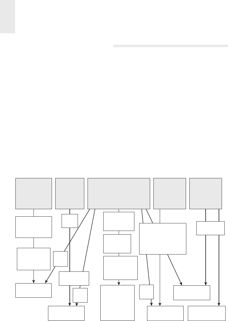
Chapter 20
498
Develop the ETL Plan
ETL development starts out with the high-level plan, which is independent of any
specifi c technology or approach. However, it’s a good idea to decide on an ETL tool
before doing any detailed planning; this can avoid redesign and rework later in the
process.
Step 1: Draw the High-Level Plan
We start the design process with a very simple schematic of the known pieces of the
plan: sources and targets, as shown in Figure 20-1. This schematic is for a fi ctitious
utility company’s data warehouse, which is primarily sourced from a 30-year-old
COBOL system. If most or all the data comes from a modern relational transaction
processing system, the boxes often represent a logical grouping of tables in the
transaction system model.
Sources
Customer
Master
(RDBMS)
Geography
Master
(RDBMS)
DMR system
(COBOL flat file,
2000 fields,
one row per customer)
Meters
(MS Access)
Date
(Spreadsheet)
Slowly changing
on demographics
and account
status
25M customers
–10k new or
changed
customers/day
Customer
Targets
15,000
geogs
check
RI
Labels need
cosmetic work!
Geography
“Unbucketize”
from 13 months
in one row
Process 750k
customers/
day
Missed meter
reads, estimated
bills, restatement
of bills
Electricity
Usage
Old (pre-1972) meter
types are not in the
Meters Group’s system
There are 73 known
meter types
How/by whom
maintained??
check
RI
check
RI
Usage Month
Electric Meter Meter Read Date
Figure 20-1: Example high-level data staging plan schematic.
As you develop the detailed ETL system specifi cation, the high-level view requires
additional details. Figure 20-1 deliberately highlights contemporary questions and
unresolved issues; this plan should be frequently updated and released. You might
sometimes keep two versions of the diagram: a simple one for communicating

ETL System Design and Development Process and Tasks 499
with people outside the team and a detailed version for internal DW/BI team
documentation.
Step 2: Choose an ETL Tool
There are a multitude of ETL tools available in the data warehouse marketplace.
Most of the major database vendors o er an ETL tool, usually at additional licensing
cost. There are also excellent ETL tools available from third-party vendors.
ETL tools read data from a range of sources, including fl at fi les, ODBC, OLE DB,
and native database drivers for most relational databases. The tools contain func-
tionality for defi ning transformations on that data, including lookups and other
kinds of joins. They can write data into a variety of target formats. And they all
contain some functionality for managing the overall logic fl ow in the ETL system.
If the source systems are relational, the transformation requirements are straight-
forward, and good developers are on sta , the value of an ETL tool may not be
immediately obvious. However, there are several reasons that using an ETL tool is
an industry standard best practice:
■ Self-documentation that comes from using a graphical tool. A hand-coded
system is usually an impenetrable mess of staging tables, SQL scripts, stored
procedures, and operating system scripts.
■ Metadata foundation for all steps of the ETL process.
■ Version control for multi-developer environments and for backing out and
restoring consistent versions.
■ Advanced transformation logic, such as fuzzy matching algorithms, inte-
grated access to name and address deduplication routines, and data mining
algorithms.
■ Improved system performance at a lower level of expertise. Relatively few SQL
developers are truly expert on how to use the relational database to manipulate
extremely large data volumes with excellent performance.
■ Sophisticated processing capabilities, including automatically parallel-
izing tasks, and automatic fail-over when a processing resource becomes
unavailable.
■ One-step conversion of virtualized data transformation modules into their
physical equivalents.
Don’t expect to recoup the investment in an ETL tool on the fi rst phase of the
DW/BI project. The learning curve is steep enough that developers sometimes feel
the project could have been implemented faster by coding. The big advantages
come with future phases, and particularly with future modifi cations to existing
systems.

Chapter 20
500
Step 3: Develop Default Strategies
With an overall idea of what needs to happen and what the ETL tool’s infrastructure
requires, you should develop a set of default strategies for the common activities in
the ETL system. These activities include:
■ Extract from each major source system. At this point in the design process,
you can determine the default method for extracting data from each source
system. Will you normally push from the source system to a fl at fi le, extract
in a stream, use a tool to read the database logs, or another method? This
decision can be modifi ed on a table-by-table basis. If using SQL to access
source system data, make sure the native data extractors are used rather than
ODBC, if that’s an option.
■ Archive extracted and staged data. Extracted or staged data, before it’s been
transformed, should be archived for at least a month. Some organizations
permanently archive extracted and staged data.
■ Police data quality for dimensions and particularly facts. Data quality must
be monitored during the ETL process rather than waiting for business users
to fi nd data problems. Chapter 19 describes a comprehensive architecture
for measuring and responding to data quality issues in ETL subsystems 4
through 8.
■ Manage changes to dimension attributes. In Chapter 19, we described the
logic required to manage dimension attribute changes in ETL subsystem 9.
■ Ensure the data warehouse and ETL system meet the system availability
requirements. The fi rst step to meeting availability requirements is to docu-
ment them. You should document when each data source becomes available
and block out high-level job sequencing.
■ Design the data auditing subsystem. Each row in the data warehouse tables
should be tagged with auditing information that describes how the data
entered the system.
■ Organize the ETL staging area. Most ETL systems stage the data at least once
or twice during the ETL process. By staging, we mean the data will be written
to disk for a later ETL step and for system recovery and archiving.
Step 4: Drill Down by Target Table
After overall strategies for common ETL tasks have been developed, you should start
drilling into the detailed transformations needed to populate each target table in the
data warehouse. As you’re fi nalizing the source-to-target mappings, you also perform
more data profi ling to thoroughly understand the necessary data transformations
for each table and column.
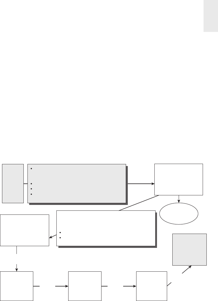
ETL System Design and Development Process and Tasks 501
Ensure Clean Hierarchies
It’s particularly important to investigate whether hierarchical relationships in the
dimension data are perfectly clean. Consider a product dimension that includes
a hierarchical rollup from product stock keeping unit (SKU) to product category.
In our experience, the most reliable hierarchies are well managed in the source
system. The best source systems normalize the hierarchical levels into multiple
tables, with foreign key constraints between the levels. In this case, you can be
confi dent the hierarchies are clean. If the source system is not normalized—espe-
cially if the source for the hierarchies is an Excel spreadsheet on a business user’s
desktop—then you must either clean it up or acknowledge that it is not a hierarchy.
Develop Detailed Table Schematics
Figure 20-2 illustrates the level of detail that’s useful for the table-specifi c drilldown;
it’s for one of the tables in the utility company example previously illustrated.
Detailed
Master
Record
(DMR)
DMR Extract: 80 cols including 13 monthly
buckets for usage. One row per customer meter,
sorted by customer.
EBCDIC file, tab-delimited.
File name: xdmr_yyyymmdd.dat
No transformations on mainframe—need to
minimize mainframe coding and load.
Compress
encrypt ftp xdmr_yyyymmdd.dat
Dimension
processing
Fact_stage1 (only fields
relevant to fact table),
includes customer &
month surrogate keys
Electric_
Usage_Fact
Fact_stage4,
includes
read_date
surrogate key
Fact_stage3,
includes geog
surrogate key
Fact_stage2,
includes meter
surrogate key
Bulk-load into
electric_usage_fact
Sort by
date
lookup
date_key
Sort by
geog
lookup
geog_key
Sort by meter_type,
lookup meter_key
Unbucketize: Usage1 keyed to yyyymm, Usage2
keyed to yyyymm-1,... When
yyyymm<subscribe_date, stop processing row
Will have –13x rows.
Data presorted by cust, so can perform cust_key
lookup on same pass.
Figure 20-2: Example draft detailed load schematic for the fact table.
All the dimension tables must be processed before the key lookup steps for the fact
table. The dimension tables are usually independent from each other, but sometimes
they also have processing dependencies. It’s important to clarify these dependencies,
as they become fi xed points around which the job control fl ows.

Chapter 20
502
Develop the ETL Specifi cation Document
We’ve walked through some general strategies for high-level planning and the physi-
cal design of the ETL system. Now it’s time to pull everything together and develop
a detailed specifi cation for the entire ETL system.
All the documents developed so far—the source-to-target mappings, data profi l-
ing reports, physical design decisions—should be rolled into the fi rst sections of
the ETL specifi cation. Then document all the decisions discussed in this chapter,
including:
■ Default strategy for extracting from each major source system
■ Archiving strategy
■ Data quality tracking and metadata
■ Default strategy for managing changes to dimension attributes
■ System availability requirements and strategy
■ Design of the data auditing subsystem
■ Locations of staging areas
The next section of the ETL specifi cation describes the historic and incremen-
tal load strategies for each table. A good specifi cation includes between two and
10 pages of detail for each table, and documents the following information and
decisions:
■ Table design (column names, data types, keys, and constraints)
■ Historic data load parameters (number of months) and volumes (row counts)
■ Incremental data volumes, measured as new and updated rows per load cycle
■ Handling of late arriving data for facts and dimensions
■ Load frequency
■ Handling of slowly changing dimension (SCD) changes for each dimension
attribute
■ Table partitioning, such as monthly
■ Overview of data sources, including a discussion of any unusual source char-
acteristics, such as an unusually brief access window
■ Detailed source-to-target mapping
■ Source data profi ling, including at least the minimum and maximum values
for each numeric column, count of distinct values in each column, and inci-
dence of NULLs
■ Extract strategy for the source data (for example, source system APIs, direct
query from database, or dump to fl at fi les)
■ Dependencies, including which other tables must be loaded before this table
is processed
■ Document the transformation logic. It’s easiest to write this section as pseudo
code or a diagram, rather than trying to craft complete sentences.

ETL System Design and Development Process and Tasks 503
■ Preconditions to avoid error conditions. For example, the ETL system must
check for fi le or database space before proceeding.
■ Cleanup steps, such as deleting working fi les
■ An estimate of whether this portion of the ETL system will be easy, medium,
or di cult to implement
NOTE Although most people would agree that all the items described in the
ETL system specifi cation document are necessary, it’s a lot of work to pull this
document together, and even more work to keep it current as changes occur.
Realistically, if you pull together the “one-pager” high-level fl ow diagram, data
model and source-to-target maps, and a fi ve-page description of what you plan to
do, you’ll get a better start than most teams.
Develop a Sandbox Source System
During the ETL development process, the source system data needs to be inves-
tigated at great depth. If the source system is heavily loaded, and there isn’t some
kind of reporting instance for operational queries, the DBAs may be willing to set
up a static snapshot of the database for the ETL development team. Early in the
development process, it’s convenient to poke around sandbox versions of the source
systems without worrying about launching a kind of killer query.
It’s easy to build a sandbox source system that simply copies the original; build a
sandbox with a subset of data only if the data volumes are extremely large. On the
plus side, this sandbox could become the basis of training materials and tutorials
after the system is deployed into production.
Develop One-Time Historic Load Processing
After the ETL specifi cation has been created, you typically focus on developing
the ETL process for the one-time load of historic data. Occasionally, the same ETL
code can perform both the initial historic load and ongoing incremental loads, but
more often you build separate ETL processes for the historic and ongoing loads. The
historic and incremental load processes have a lot in common, and depending on
the ETL tool, signifi cant functionality can be reused from one to the other.
Step 5: Populate Dimension Tables with Historic Data
In general, you start building the ETL system with the simplest dimension tables.
After these dimension tables have been successfully built, you tackle the historic
loads for dimensions with one or more columns managed as SCD type 2.

Chapter 20
504
Populate Type 1 Dimension Tables
The easiest type of table to populate is a dimension table for which all attributes
are managed as type 1 overwrites. With a type 1–only dimension, you extract the
current value for each dimension attribute from the source system.
Dimension Transformations
Even the simplest dimension table may require substantial data cleanup and will
certainly require surrogate key assignment.
Simple Data Transformations
The most common, and easiest, form of data transformation is data type conversion.
All ETL tools have rich functions for data type conversion. This task can be tedious,
but it is seldom onerous. We strongly recommend replacing NULL values with
default values within dimension tables; as we have discussed previously, NULLs
can cause problems when they are directly queried.
Combine from Separate Sources
Often dimensions are derived from several sources. Customer information may
need to be merged from several lines of business and from outside sources. There
is seldom a universal key pre-embedded in the various sources that makes this
merge operation easy.
Most consolidation and deduplicating tools and processes work best if names
and addresses are fi rst parsed into their component pieces. Then you can use a
set of passes with fuzzy logic that account for misspellings, typos, and alternative
spellings such as I.B.M., IBM, and International Business Machines. In most orga-
nizations, there is a large one-time project to consolidate existing customers. This
is a tremendously valuable role for master data management systems.
Decode Production Codes
A common merging task in data preparation is looking up text equivalents for pro-
duction codes. In some cases, the text equivalents are sourced informally from a
nonproduction source such as a spreadsheet. The code lookups are usually stored in
a table in the staging database. Make sure the ETL system includes logic for creat-
ing a default decoded text equivalent for the case in which the production code is
missing from the lookup table.
Validate Many-to-One and One-to-One Relationships
The most important dimensions probably have one or more rollup paths, such as
products rolling up to product model, subcategory, and category, as illustrated in
Figure 20-3. These hierarchical rollups need to be perfectly clean.

ETL System Design and Development Process and Tasks 505
Product Dimension
Product Key (PK)
Product SKU
Product Name
Product Description
Product Model
Product Model Description
Subcategory Description
Category Description
Category Manager
Figure 20-3: Product dimension table with a hierarchical relationship.
Many-to-one relationships between attributes, such as a product to product
model, can be verifi ed by sorting on the “many” attribute and verifying that each
value has a unique value on the “one” attribute. For example, this query returns
the products that have more than one product model:
SELECT Product_SKU,
count[*] as Row_Count,
count(distinct Product_Model) as Model_Count
FROM StagingDatabase.Product
GROUP BY Product_SKU
HAVING count(distinct Product_Model) > 1 ;
Database administrators sometimes want to validate many-to-one relationships
by loading data into a normalized snowfl ake version of the dimension table in the
staging database, as illustrated in Figure 20-4. Note that the normalized version
requires individual keys at each of the hierarchy levels. This is not a problem if the
source system supplies the keys, but if you normalize the dimension in the ETL
environment, you need to create them.
The snowfl ake structure has some value in the staging area: It prevents you from
loading data that violates the many-to-one relationship. However, in general, the
relationships should be pre-verifi ed as just described, so that you never attempt to
load bad data into the dimension table. After the data is pre-verifi ed, it’s not tremen-
dously important whether you make the database engine reconfi rm the relationship
at the moment you load the table.
If the source system for a dimensional hierarchy is a normalized database, it’s
usually unnecessary to repeat the normalized structure in the ETL staging area.
However, if the hierarchical information comes from an informal source such as a
spreadsheet managed by the marketing department, you may benefi t from normal-
izing the hierarchy in the ETL system.
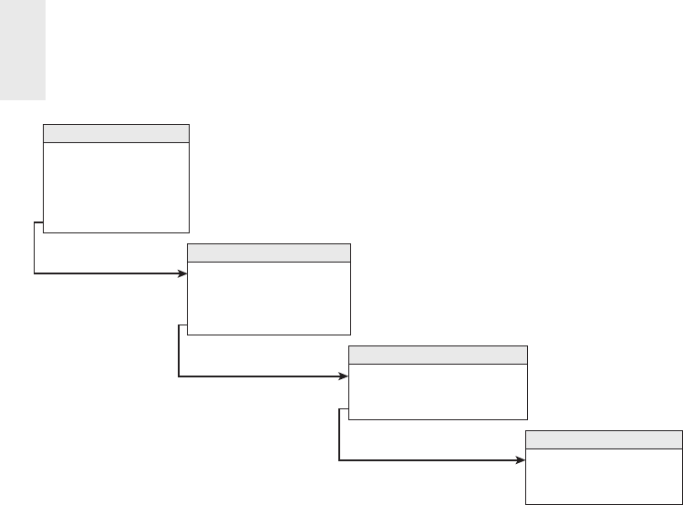
Chapter 20
506
Product Table
Product Key (PK)
Product SKU
Product Name
Product Description
Product Model Key (FK)
Product Model Table
Product Model Key (PK)
Product Model Number
Product Model Description
Product Subcategory Key (FK)
Product Subcategory Table
Product Subcategory Key (PK)
Product Subcategory Description
Product Category Key (FK)
Product Category Key (PK)
Product Category Description
Product Category Manager
Product Category Table
Figure 20-4: Snowfl aked hierarchical relationship in the product dimension.
Dimension Surrogate Key Assignment
After you are confi dent you have dimension tables with one row for each true unique
dimension member, the surrogate keys can be assigned. You maintain a table in the
ETL staging database that matches production keys to surrogate keys; you can use
this key map later during fact table processing.
Surrogate keys are typically assigned as integers, increasing by one for each
new key. If the staging area is in an RDBMS, surrogate key assignment is elegantly
accomplished by creating a sequence. Although syntax varies among the relational
engines, the process is fi rst to create a sequence and then to populate the key map
table.
Here’s the syntax for the one-time creation of the sequence:
create sequence dim1_seq cache=1000; — choose appropriate cache level
And then here’s the syntax to populate the key map table:
insert into dim1_key_map (production_key_id, dim1_key)
select production_key_id, dim1_seq.NEXT
from dim1_extract_table;
Dimension Table Loading
After the dimension data is properly prepared, the load process into the target tables
is fairly straightforward. Even though the fi rst dimension table is usually small, use
the database’s bulk or fast-loading utility or interface. You should use fast-loading

ETL System Design and Development Process and Tasks 507
techniques for most table inserts. Some databases have extended the SQL syntax to
include a BULK INSERT statement. Others have published an API to load data into
the table from a stream.
The bulk load utilities and APIs come with a range of parameters and transforma-
tion capabilities including the following:
■ Turn o logging. Transaction logging adds signifi cant overhead and is not
valuable when loading data warehouse tables. The ETL system should be
designed with one or more recoverability points where you can restart pro-
cessing should something go wrong.
■ Bulk load in fast mode. However, most of the database engines’ bulk load
utilities or APIs require several stringent conditions on the target table to bulk
load in fast mode. If these conditions are not met, the load should not fail; it
simply will not use the “fast” path.
■ Presort the fi le. Sorting the fi le in the order of the primary index signifi cantly
speeds up indexing.
■ Transform with caution. In some cases, the loader supports data conversions,
calculations, and string and date/time manipulation. Use these features care-
fully and test performance. In some cases, these transformations cause the
loader to switch out of high-speed mode into a line-by-line evaluation of the
load fi le. We recommend using the ETL tool to perform most transformations.
■ Truncate table before full refresh. The TRUNCATE TABLE statement is the most
e cient way to delete all the rows in the table. It’s commonly used to clean out
a table from the staging database at the beginning of the day’s ETL processing.
Load Type 2 Dimension Table History
Recall from Chapter 5: Procurement, that dimension attribute changes are typically
managed as type 1 (overwrite) or type 2 (track history by adding new rows to the
dimension table). Most dimension tables contain a mixture of type 1 and type 2
attributes. More advanced SCD techniques are described in Chapter 5.
During the historic load, you need to re-create history for dimension attributes
that are managed as type 2. If business users have identifi ed an attribute as impor-
tant for tracking history, they want that history going back in time, not just from the
date the data warehouse is implemented. It’s usually di cult to re-create dimension
attribute history, and sometimes it’s completely impossible.
This process is not well suited for standard SQL processing. It’s better to use
a database cursor construct or, even better, a procedural language such as Visual
Basic, C, or Java to perform this work. Most ETL tools enable script processing on
the data as it fl ows through the ETL system.

Chapter 20
508
When you’ve completely reconstructed history, make a fi nal pass through the
data to set the row end date column. It’s important to ensure there are no gaps in
the series. We prefer to set the row end date for the older version of the dimension
member to the day before the row e ective date for the new row if these row dates
have a granularity of a full day. If the e ective and end dates are actually precise
date/time stamps accurate to the minute or second, then the end date/time must be
set to exactly the begin date/time of the next row so that no gap exists between rows.
Populate Date and Other Static Dimensions
Every data warehouse database should have a date dimension, usually at the granu-
larity of one row for each day. The date dimension should span the history of the
data, starting with the oldest fact transaction in the data warehouse. It’s easy to set
up the date dimension for the historic data because you know the date range of the
historic fact data being loaded. Most projects build the date dimension by hand,
typically in a spreadsheet.
A handful of other dimensions will be created in a similar way. For example, you
may create a budget scenario dimension that holds the values Actual and Budget.
Business data governance representatives should sign o on all constructed dimen-
sion tables.
Step 6: Perform the Fact Table Historic Load
The one-time historic fact table load di ers fairly signifi cantly from the ongoing
incremental processing. The biggest worry during the historic load is the sheer
volume of data, sometimes thousands of times bigger than the daily incremental
load. On the other hand, you have the luxury of loading into a table that’s not in
production. If it takes several days to load the historic data, that’s usually tolerable.
Historic Fact Table Extracts
As you identify records that fall within the basic parameters of the extract, make
sure these records are useful for the data warehouse. Many transaction systems
keep operational information in the source system that may not be interesting from
a business point of view.
It’s also a good idea to accumulate audit statistics during this step. As the extract
creates the results set, it is often possible to capture various subtotals, totals, and
row counts.
Audit Statistics
During the planning phase for the ETL system, you identifi ed various measures of
data quality. These are usually calculations, such as counts and sums, that you com-
pare between the data warehouse and source systems to cross-check the integrity

ETL System Design and Development Process and Tasks 509
of the data. These numbers should tie backward to operational reports and forward
to the results of the load process in the warehouse. The tie back to the operational
system is important because it is what establishes the credibility of the warehouse.
NOTE There are scenarios in which it’s di cult or impossible for the warehouse
to tie back to the source system perfectly. In many cases, the data warehouse extract
includes business rules that have not been applied to the source systems. Even
more vexing are errors in the source system! Also, di erences in timing make it
even more di cult to cross-check the data. If it’s not possible to tie the data back
exactly, you need to explain the di erences.
Fact Table Transformations
In most projects, the fact data is relatively clean. The ETL system developer spends
a lot of time improving the dimension table content, but the facts usually require
a fairly modest transformation. This makes sense because in most cases the facts
come from transaction systems used to operate the organization.
The most common transformations to fact data include transformation of null
values, pivoting or unpivoting the data, and precomputing derived calculations. All
fact rows then enter the surrogate key pipeline to exchange the natural keys for the
dimension surrogate keys managed in the ETL system.
Null Fact Values
All major database engines explicitly support a null value. In many source systems,
however, the null value is represented by a special value of what should be a legitimate
fact. Perhaps the special value of –1 is understood to represent null. For most fact
table metrics, the “–1” in this scenario should be replaced with a true NULL. A null
value for a numeric measure is reasonable and common in the fact table. Nulls do
the “right thing” in calculations of sums and averages across fact table rows. It’s only
in the dimension tables that you should strive to replace null values with specially
crafted default values. Finally, you should not allow any null values in the fact table
columns that reference the dimension table keys. These foreign key columns should
always be defi ned as NOT NULL.
Improve Fact Table Content
As we have stressed, all the facts in the fi nal fact table row must be expressed in
the same grain. This means there must be no facts representing totals for the year
in a daily fact table or totals for some geography larger than the fact table’s grain.
If the extract includes an interleaving of facts at di erent grains, the transforma-
tion process must eliminate these aggregations, or move them into the appropriate
aggregate tables.

Chapter 20
510
The fact row may contain derived facts; although, in many cases it is more e cient
to calculate derived facts in a view or an online analytical processing (OLAP) cube
rather than in the physical table. For instance, a fact row that contains revenues and
costs may want a fact representing net profi t. It is very important that the net profi t
value be correctly calculated every time a user accesses it. If the data warehouse
forces all users to access the data through a view, it would be fi ne to calculate the
net profi t in that view. If users are allowed to see the physical table, or if they often
fi lter on net profi t and thus you’d want to index it, precomputing it and storing it
physically is preferable.
Similarly, if some facts need to be simultaneously presented with multiple units
of measure, the same logic applies. If business users access the data through a view
or OLAP database, then the various versions of the facts can e ciently be calculated
at access time.
Pipeline the Dimension Surrogate Key Lookup
It is important that referential integrity (RI) is maintained between the fact table
and dimension tables; you must never have a fact row that references a dimension
member that doesn’t exist. Therefore, you should not have a null value for any
foreign key in the fact table nor should any fact row violate referential integrity to
any dimension.
The surrogate key pipeline is the fi nal operation before you load data into the
target fact table. All other data cleaning, transformation, and processing should
be complete. The incoming fact data should look just like the target fact table in
the dimensional model, except it still contains the natural keys from the source
system rather than the warehouse’s surrogate keys. The surrogate key pipeline is
the process that exchanges the natural keys for the surrogate keys and handles any
referential integrity errors.
Dimension table processing must complete before the fact data enters the sur-
rogate key pipeline. Any new dimension members or type 2 changes to existing
dimension members must have already been processed, so their keys are available
to the surrogate key pipeline.
First let’s discuss the referential integrity problem. It’s a simple matter to con-
fi rm that each natural key in the historic fact data is represented in the dimension
tables. This is a manual step. The historic load is paused at this point, so you can
investigate and fi x any referential integrity problems before proceeding. The dimen-
sion table is either fi xed, or the fact table extract is redesigned to fi lter out spurious
rows, as appropriate.
Now that you’re confi dent there will be no referential integrity violations, you can
design the historic surrogate key pipeline, as shown in Figure 19-11 in the previous
chapter. In this scenario, you need to include BETWEEN logic on any dimension

ETL System Design and Development Process and Tasks 511
with type 2 changes to locate the dimension row that was in e ect when the histori-
cal fact measurement occurred.
There are several approaches for designing the historic load’s surrogate key pipe-
line for best performance; the design depends on the features available in your ETL
tool, the data volumes you’re processing, and your dimensional design. In theory,
you could defi ne a query that joins the fact staging table and each dimension table
on the natural keys, returning the facts and surrogate keys from each dimension
table. If the historic data volumes are not huge, this can actually work quite well,
assuming you staged the fact data in the relational database and indexed the dimen-
sion tables to support this big query. This approach has several benefi ts:
■ It leverages the power of the relational database.
■ It performs the surrogate key lookups on all dimensions in parallel.
■ It simplifi es the problem of picking up the correct dimension key for type 2
dimensions. The join to type 2 dimensions must include a clause specifying
that the transaction date falls between the row e ective date and row end date
for that image of the dimension member in the table.
No one would be eager to try this approach if the historic fact data volumes
were large in the hundreds of gigabytes to terabyte range. The complex join to
the type 2 dimension tables create the greatest demands on the system. Many
dimensional designs include a fairly large number of (usually small) dimension
tables that are fully type 1, and a smaller number of dimensions containing type
2 attributes. You could use this relational technique to perform the surrogate key
lookups for all the type 1 dimensions in one pass and then separately handle the
type 2 dimensions. You should ensure the e ective date and end date columns
are properly indexed.
An alternative to the database join technique described is to use the ETL tool’s
lookup operator.
When all the fact source keys have been replaced with surrogate keys, the fact
row is ready to load. The keys in the fact table row have been chosen to be proper
foreign keys to the respective dimension tables, and the fact table is guaranteed to
have referential integrity with respect to the dimension tables.
Assign Audit Dimension Key
Fact tables often include an audit key on each fact row. The audit key points to an
audit dimension that describes the characteristics of the load, including relatively
static environment variables and measures of data quality. The audit dimension can
be quite small. An initial design of the audit dimension might have just two envi-
ronment variables (master ETL version number and profi t allocation logic number),
and only one quality indicator whose values are Quality Checks Passed and Quality
Problems Encountered. Over time, these variables and diagnostic indicators can be

Chapter 20
512
made more detailed and more sophisticated. The audit dimension key is added to the
fact table either immediately after or immediately before the surrogate key pipeline.
Fact Table Loading
The main concern when loading the fact table is load performance. Some database
technologies support fast loading with a specifi ed batch size. Look at the docu-
mentation for the fast-loading technology to see how to set this parameter. You
can experiment to fi nd the ideal batch size for the size of the rows and the server’s
memory confi guration. Most people don’t bother to get so precise and simply choose
a number like 10,000 or 100,000 or 1 million.
Aside from using the bulk loader and a reasonable batch size (if appropriate for
the database engine), the best way to improve the performance of the historic load
is to load into a partitioned table, ideally loading multiple partitions in parallel. The
steps to loading into a partitioned table include:
1. Disable foreign key (referential integrity) constraints between the fact table
and each dimension table before loading data.
2. Drop or disable indexes on the fact table.
3. Load the data using fast-loading techniques.
4. Create or enable fact table indexes.
5. If necessary, perform steps to stitch together the table’s partitions.
6. Confirm each dimension table has a unique index on the surrogate
key column.
7. Enable foreign key constraints between the fact table and dimension tables.
Develop Incremental ETL Processing
One of the biggest challenges with the incremental ETL process is identifying new,
changed, and deleted rows. After you have a stream of inserts, modifi cations, and
deletions, the ETL system can apply transformations following virtually identical
business rules as for the historic data loads.
The historic load for dimensions and facts consisted largely or entirely of inserts.
In incremental processing, you primarily perform inserts, but updates for dimen-
sions and some kinds of fact tables are inevitable. Updates and deletes are expensive
operations in the data warehouse environment, so we’ll describe techniques to
improve the performance of these tasks.
Step 7: Dimension Table Incremental Processing
As you might expect, the incremental ETL system development begins with the
dimension tables. Dimension incremental processing is very similar to the historic
processing previously described.

ETL System Design and Development Process and Tasks 513
Dimension Table Extracts
In many cases, there is a customer master fi le or product master fi le that can serve
as the single source for a dimension. In other cases, the raw source data is a mixture
of dimensional and fact data.
Often it’s easiest to pull the current snapshots of the dimension tables in their
entirety and let the transformation step determine what has changed and how
to handle it. If the dimension tables are large, you may need to use the fact table
technique described in the section “Step 8: Fact Table Incremental Processing” for
identifying the changed record set. It can take a long time to look up each entry in
a large dimension table, even if it hasn’t changed from the existing entry.
If possible, construct the extract to pull only rows that have changed. This is
particularly easy and valuable if the source system maintains an indicator of the
type of change.
Identify New and Changed Dimension Rows
The DW/BI team may not be successful in pushing the responsibility for identify-
ing new, updated, and deleted rows to the source system owners. In this case, the
ETL process needs to perform an expensive comparison operation to identify new
and changed rows.
When the incoming data is clean, it’s easy to fi nd new dimension rows. The raw
data has an operational natural key, which must be matched to the same column in
the current dimension row. Remember, the natural key in the dimension table is an
ordinary dimensional attribute and is not the dimension’s surrogate primary key.
You can fi nd new dimension members by performing a lookup from the incoming
stream to the master dimension, comparing on the natural key. Any rows that fail
the lookup are new dimension members and should be inserted into the dimen-
sion table.
If the dimension contains any type 2 attributes, set the row e ective date column
to the date the dimension member appeared in the system; this is usually yesterday
if you are processing nightly. Set the row end date column to the default value for
current rows. This should be the largest date, very far in the future, supported by
the system. You should avoid using a null value in this second date column because
relational databases may generate an error or return the special value Unknown if
you attempt to compare a specifi c value to a NULL.
The next step is to determine if the incoming dimension row has changed. The
simplest technique is to compare column by column between the incoming data and
the current corresponding member stored in the master dimension table.
If the dimension is large, with more than a million rows, the simple technique
of column-wise comparison may be too slow, especially if there are many columns

Chapter 20
514
in the dimension table. A popular alternative method is to use a hash or checksum
function to speed the comparison process. You can add two new housekeeping
columns to the dimension table: hash type1 and hash type2. You should place
a hash of a concatenation of the type 1 attributes in the hash type1 column and
similarly for hash type2. Hashing algorithms convert a very long string into a
much shorter string that is close to unique. The hashes are computed and stored
in the dimension table. Then compute hashes on the incoming rowset in exactly
the same way, and compare them to the stored values. The comparison on a single,
relatively short string column is far more e cient than the pair-wise comparison
on dozens of separate columns. Alternatively, the relational database engine may
have syntax such as EXCEPT that enables a high-performance query to fi nd the
changed rows.
As a general rule, you do not delete dimension rows that have been deleted in
the source system because these dimension members probably still have fact table
data associated with them in the data warehouse.
Process Changes to Dimension Attributes
The ETL application contains business rules to determine how to handle an attri-
bute value that has changed from the value already stored in the data warehouse.
If the revised description is determined to be a legitimate and reliable update to
previous information, then the techniques of slowly changing dimensions must
be used.
The fi rst step in preparing a dimension row is to decide if you already have
that row. If all the incoming dimensional information matches the correspond-
ing row in the dimension table, no further action is required. If the dimensional
information has changed, then you can apply changes to the dimension, such as
type 1 or type 2.
NOTE You may recall from Chapter 5 that there are three primary methods for
tracking changes in attribute values, as well as a set of advanced hybrid techniques.
Type 3 requires a change in the structure of the dimension table, creating a new
set of columns to hold the “previous” versus “current” versions of the attributes.
This type of structural change is seldom automated in the ETL system; it’s more
likely to be handled as a one-time change in the data model.
The lookup and key assignment logic for handling a changed dimension record
during the extract process is shown in Figure 20-5. In this case, the logic fl ow does
not assume the incoming data stream is limited only to new or changed rows.
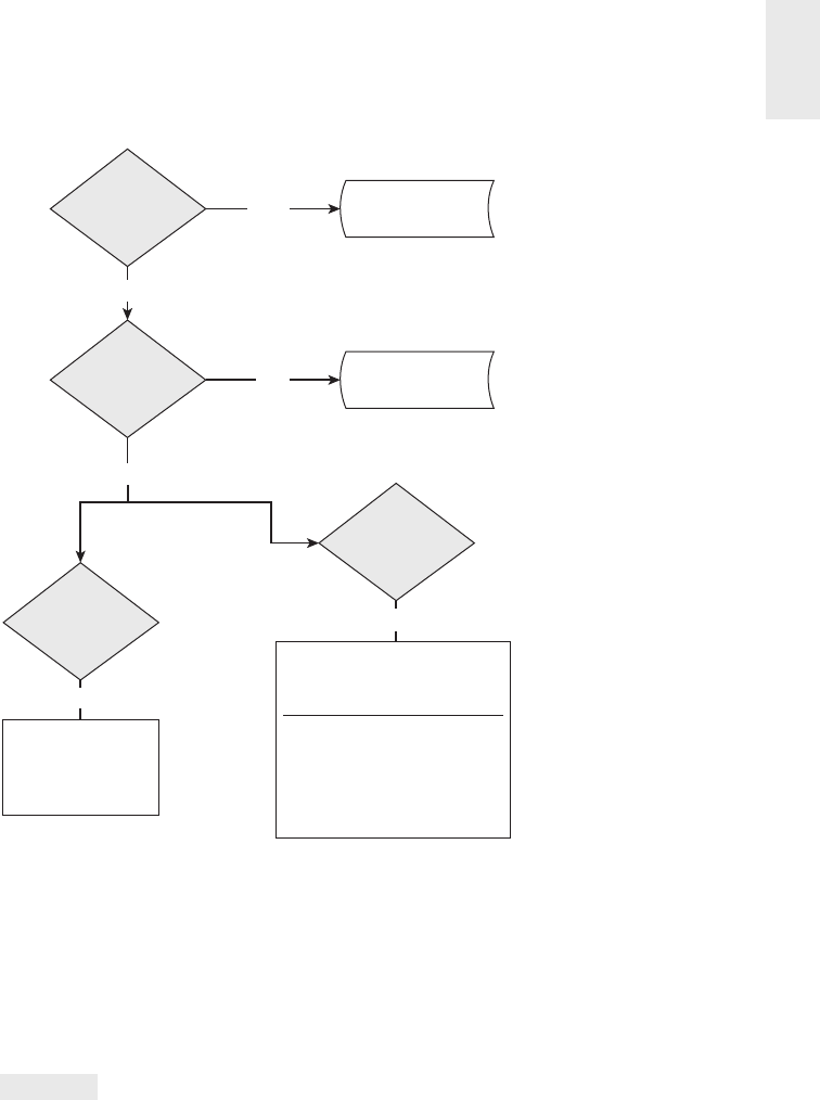
ETL System Design and Development Process and Tasks 515
Add to
dimension
End processing
of row
Row new? YES
YES
YES
YES
NO
NO
Row has Type
2 changes?
Row has Type
1 changes?
Row has any
changes?
Update existing “Current”
row: Set Row_End_Date and
Is_Row_Current
Add new dimension row for
this entity, with a new
surrogate key. Set
Row_Start_Date = yesterday
and Is_Row_Current = True
Update Type 1
attributes–usually
all existing rows
for this entity
Figure 20-5: Logic fl ow for handling dimension updates.
Step 8: Fact Table Incremental Processing
Most data warehouse databases are too large to entirely replace the fact tables in a
single load window. Instead, new and updated fact rows are incrementally processed.
NOTE It is much more e cient to incrementally load only the records that
have been added or updated since the previous load. This is especially true in a
journal-style system where history is never changed and only adjustments in the
current period are allowed.
The ETL process for fact table incremental processing di ers from the historic
load. The historic ETL process doesn’t need to be fully automated; you can stop the

Chapter 20
516
process to examine the data and prepare for the next step. The incremental process-
ing, by contrast, must be fully automated.
Fact Table Extract and Data Quality Checkpoint
As soon as the new and changed fact rows are extracted from the source system, a
copy of the untransformed data should be written to the staging area. At the same
time, measures of data quality on the raw extracted data are computed. The staged
data serves three purposes:
■ Archive for auditability
■ Provide a starting point after data quality verifi cation
■ Provide a starting point for restarting the process
Fact Table Transformations and Surrogate Key Pipeline
The surrogate key pipeline for the incremental fact data is similar to that for the
historic data. The key di erence is that the error handling for referential integrity
violations must be automated. There are several methods for handling referential
integrity violations:
■ Halt the load. This is seldom a useful solution; although, it’s often the default
in many ETL tools.
■ Throw away error rows. There are situations in which a missing dimen-
sion value is a signal that the data is irrelevant to the business requirements
underlying the data warehouse.
■ Write error rows to a fi le or table for later analysis. Design a mechanism
for moving corrected rows into a suspense fi le. This approach is not a good
choice for a fi nancial system, where it is vital that all rows be loaded.
■ Fix error rows by creating a dummy dimension row and returning its sur-
rogate key to the pipeline. The most attractive error handling for referential
integrity violations in the incremental surrogate key pipeline is to create a
dummy dimension row on-the-fl y for the unknown natural key. The natural
key is the only piece of information that you may have about the dimension
member; all the other attributes must be set to default values. This dummy
dimension row will be corrected with type 1 updates when the detailed infor-
mation about that dimension member becomes available.
■ Fix error rows by mapping to a single unknown member in each dimen-
sion. This approach is not recommended. The problem is that all error rows
are mapped to the same dimension member, for any unknown natural key
values in the fact table extract.

ETL System Design and Development Process and Tasks 517
For most systems, you perform the surrogate key lookups against a query, view,
or physical table that subsets the dimension table. The dimension table rows are
fi ltered, so the lookup works against only the current version of each dimension
member.
Late Arriving Facts and the Surrogate Key Pipeline
In most data warehouses, the incremental load process begins soon after midnight
and processes all the transactions that occurred the previous day. However, there
are scenarios in which some facts arrive late. This is most likely to happen when
the data sources are distributed across multiple machines or even worldwide, and
connectivity or latency problems prevent timely data collection.
If all the dimensions are managed completely as type 1 overwrites, late arriving
facts present no special challenges. But most systems have a mixture of type 1 and
type 2 attributes. The late arriving facts must be associated with the version of the
dimension member that was in e ect when the fact occurred. That requires a lookup
in the dimension table using the row begin and end e ective dates.
Incremental Fact Table Load
In the historic fact load, it’s important that data loads use fast-load techniques. In
most data warehouses, these fast-load techniques may not be available for the incre-
mental load. The fast-load technologies often require stringent conditions on the
target table (for example, empty or unindexed). For the incremental load, it’s usually
faster to use non-fast-load techniques than to fully populate or index the table. For
small to medium systems, insert performance is usually adequate.
If your fact table is very large, you should already have partitioned the fact table
for manageability reasons. If incremental data is always loading into an empty
partition, you should use fast-load techniques. With daily loads, you would create
365 new fact table partitions each year. This is probably too many partitions for a
fact table with long history, so consider implementing a process to consolidate daily
partitions into weekly or monthly partitions.
Load Snapshot Fact Tables
The largest fact tables are usually transactional. Transaction fact tables are typically
loaded only through inserts. Periodic snapshot fact tables are usually loaded at
month end. Data for the current month is sometimes updated each day for current-
month-to-date. In this scenario, monthly partitioning of the fact table makes it easy
to reload the current month with excellent performance.
Accumulating snapshot fact tables monitor relatively short-lived processes, such
as fi lling an order. The accumulating snapshot fact table is characterized by many

Chapter 20
518
updates for each fact row over the life of the process. This table is expensive to
maintain; although accumulating snapshots are almost always much smaller than
the other two types of fact tables.
Speed Up the Load Cycle
Processing only data that has been changed is one way to speed up the ETL cycle.
This section lists several additional techniques.
More Frequent Loading
Although it is a huge leap to move from a monthly or weekly process to a nightly one,
it is an e ective way to shorten the load window. Every nightly process involves 1/30
the data volume of a monthly one. Most data warehouses are on a nightly load cycle.
If nightly processing is too expensive, consider performing some preprocessing
on the data throughout the day. During the day, data is moved into a staging database
or operational data store where data cleansing tasks are performed. After midnight,
you can consolidate multiple changes to dimension members, perform fi nal data
quality checks, assign surrogate keys, and move the data into the data warehouse.
Parallel Processing
Another way to shorten the load time is to parallelize the ETL process. This can
happen in two ways: multiple steps running in parallel and a single step running
in parallel.
■ Multiple load steps. The ETL job stream is divided into several independent
jobs submitted together. You need to think carefully about what goes into
each job; the primary goal is to create independent jobs.
■ Parallel execution. The database itself can also identify certain tasks it can
execute in parallel. For example, creating an index can typically be parallel-
ized across as many processors as are available on the machine.
NOTE There are good ways and bad ways to break processing into parallel steps.
One simple way to parallelize is to extract all source data together, then load and
transform the dimensions, and then simultaneously check referential integrity
between the fact table and all dimensions. Unfortunately, this approach is likely
to be no faster—and possibly much slower—than the even simpler sequential
approach because each step launches parallel processes that compete for the same
system resources such as network bandwidth, I/O, and memory. To structure
parallel jobs well, you need to account not just for logically sequential steps but
also for system resources.

ETL System Design and Development Process and Tasks 519
Parallel Structures
You can set up a three-way mirror or clustered confi guration on two servers to
maintain a continuous load data warehouse, with one server managing the loads
and the second handling the queries. The maintenance window is reduced to a
few minutes daily to swap the disks attached to each server. This is a great way to
provide high system availability.
Depending on the requirements and available budget, there are several similar
techniques you can implement for tables, partitions, and databases. For example, you
can load into an o ine partition or table, and swap it into active duty with minimum
downtime. Other systems have two versions of the data warehouse database, one for
loading and one for querying. These are less e ective, but less expensive, versions
of the functionality provided by clustered servers.
Step 9: Aggregate Table and OLAP Loads
An aggregate table is logically easy to build. It’s simply the results of a really big
aggregate query stored as a table. The problem with building aggregate tables from
a query on the fact table, of course, occurs when the fact table is just too big to
process within the load window.
If the aggregate table includes an aggregation along the date dimension, perhaps
to monthly grain, the aggregate maintenance process is more complex. The cur-
rent month of data must be updated, or dropped and re-created, to incorporate the
current day’s data.
A similar problem occurs if the aggregate table is defi ned on a dimension attribute
that is overwritten as a type 1. Any type 1 change in a dimension attribute a ects
all fact table aggregates and OLAP cubes that are defi ned on that attribute. An ETL
process must “back out” the facts from the old aggregate level and move them to
the new one.
It is extremely important that the aggregate management system keep aggrega-
tions in sync with the underlying fact data. You do not want to create a system that
returns a di erent result set if the query is directed to the underlying detail facts
or to a precomputed aggregation.
Step 10: ETL System Operation and Automation
The ideal ETL operation runs the regular load processes in a lights-out manner,
without human intervention. Although this is a di cult outcome to attain, it is
possible to get close.

Chapter 20
520
Schedule Jobs
Scheduling jobs is usually straightforward. The ETL tool should contain function-
ality to schedule a job to kick o at a certain time. Most ETL tools also contain
functionality to conditionally execute a second task if the fi rst task successfully
completed. It’s common to set up an ETL job stream to launch at a certain time, and
then query a database or fi lesystem to see if an event has occurred.
You can also write a script to perform this kind of job control. Every ETL tool
has a way to invoke a job from the operating system command line. Many orga-
nizations are very comfortable using scripting languages, such as Perl, to manage
their job schedules.
Automatically Handle Predictable Exceptions and Errors
Although it’s easy enough to launch jobs, it’s a harder task to make sure they run to
completion, gracefully handling data errors and exceptions. Comprehensive error
handling is something that needs to be built into the ETL jobs from the outset.
Gracefully Handle Unpredictable Errors
Some errors are predictable, such as receiving an early arriving fact or a NULL value
in a column that’s supposed to be populated. For these errors, you can generally
design your ETL system to fi x the data and continue processing. Other errors are
completely unforeseen and range from receiving data that’s garbled to experiencing
a power outage during processing.
We look for ETL tool features and system design practices to help recover from
the unexpected. We generally recommend outfi tting fact tables with a single column
surrogate key that is assigned sequentially to new records that are being loaded. If
a large load job unexpectedly halts, the fact table surrogate key allows the load to
resume from a reliable point, or back out the load by constraining on a contiguous
range of the surrogate keys.
Real-Time Implications
Real-time processing is an increasingly common requirement in data warehousing.
There is a strong possibility that your DW/BI system will have a real-time require-
ment. Some business users expect the data warehouse to be continuously updated
throughout the day and grow impatient with stale data. Building a real-time
DW/BI system requires gathering a very precise understanding of the true business
requirements for real-time data and identifying an appropriate ETL architecture,
incorporating a variety of technologies married with a solid platform.

ETL System Design and Development Process and Tasks 521
Real-Time Triage
Asking business users if they want “real-time” delivery of data is a frustrating
exercise for the DW/BI team. Faced with no constraints, most users will say, “That
sounds good; go for it!” This kind of response is almost worthless.
To avoid this situation, we recommend dividing the real-time design challenge
into three categories, called instantaneous, intra-day, and daily. We use these terms
when we talk to business users about their needs and then design our data delivery
pipelines di erently for each option. Figure 20-6 summarizes the issues that arise
as data is delivered faster.
Daily
Batch processing ETL Micro-batch ETL Streaming EII/ETL
Drive user presentation from
source application
Separate from fact table
Probe with queries or subscribe
to message bus
Daily hot fact table time partition
Provisional Provisional
Individual transactions Transaction fragments
Wait for file ready
Conventional file table time partition
Reconciled
Complete transaction set
Column screens Column screens Column screens
Structure screens Structure screens
--
--
--
Business rule screens
Final results Results updated, corrected nightly Results updated, possibly
repudiated nightly
Intra-Day Instantaneous
Figure 20-6: Data quality trade-offs with low latency delivery.
Instantaneous means the data visible on the screen represents the true state of
the source transaction system at every instant. When the source system status
changes, the screen instantly and synchronously responds. An instantaneous real-
time system is usually implemented as an enterprise information integration (EII)
solution, where the source system itself is responsible for supporting the update of
remote users’ screens and servicing query requests. Obviously, such a system must
limit the complexity of the query requests because all the processing is done on the
source system. EII solutions typically involve no caching of data in the ETL pipeline
because EII solutions by defi nition have no delays between the source systems and
the users’ screens. Some situations are plausible candidates for an instantaneous
real-time solution. Inventory status tracking may be a good example, where the deci-
sion maker has the right to commit available inventory to a customer in real time.
Intra-day means the data visible on the screen is updated many times per day but
is not guaranteed to be the absolute current truth. Most of us are familiar with stock
market quote data that is current to within 15 minutes but is not instantaneous.

Chapter 20
522
The technology for delivering frequent real-time data (as well as the slower daily
data) is distinctly di erent from instantaneous real-time delivery. Frequently deliv-
ered data is usually processed as micro-batches in a conventional ETL architecture.
This means the data undergoes the full gamut of change data capture, extract, stag-
ing to fi le storage in the ETL back room of the data warehouse, cleaning and error
checking, conforming to enterprise data standards, assigning of surrogate keys,
and possibly a host of other transformations to make the data ready to load into the
presentation server. Almost all these steps must be omitted or drastically reduced
in an EII solution. The big di erence between intra-day and daily delivered data is
in the fi rst two steps: change data capture and extract. To capture data many times
per day from the source system, the data warehouse usually must tap into a high
bandwidth communications channel, such as message queue tra c between legacy
applications, an accumulating transaction log fi le, or low level database triggers
coming from the transaction system every time something happens.
Daily means the data visible on the screen is valid as of a batch fi le download or
reconciliation from the source system at the end of the previous working day. There
is a lot to recommend daily data. Quite often processes are run on the source system
at the end of the working day that correct the raw data. When this reconciliation
becomes available, that signals the ETL system to perform a reliable and stable
download of the data. If you have this situation, you should explain to the busi-
ness users what compromises they will experience if they demand instantaneous
or intra-day updated data. Daily updated data usually involves reading a batch fi le
prepared by the source system or performing an extract query when a source system
readiness fl ag is set. This, of course, is the simplest extract scenario because you
wait for the source system to be ready and available.
Real-Time Architecture Trade-Offs
Responding to real-time requirements means you need to change the DW/BI archi-
tecture to get data to the business users’ screens faster. The architectural choices
involve trade-o s that a ect data quality and administration.
You can assume the overall goals for ETL system owners are not changed or com-
promised by moving to real-time delivery. You can remain just as committed to data
quality, integration, security, compliance, backup, recovery, and archiving as you
were before starting to design a real-time system. If you agree with this statement,
then read the following very carefully! The following sections discuss the typical
trade-o s that occur as you implement a more real-time architecture:
Replace Batch Files
Consider replacing a batch fi le extract with reading from a message queue or trans-
action log fi le. A batch fi le delivered from the source system may represent a clean

ETL System Design and Development Process and Tasks 523
and consistent view of the source data. The batch fi le may contain only those records
resulting from completed transactions. Foreign keys in the batch fi les are prob-
ably resolved, such as when the fi le contains an order from a new customer whose
complete identity may be delivered with the batch fi le. Message queue and log fi le
data, on the other hand, is raw instantaneous data that may not be subject to any
corrective process or business rule enforcement in the source system. In the worst
case, this raw data may 1) be incorrect or incomplete because additional transac-
tions may arrive later; 2) contain unresolved foreign keys that the DW/BI system
has not yet processed; and 3) require a parallel batch-oriented ETL data fl ow to cor-
rect or even replace the hot real-time data each 24 hours. And if the source system
subsequently applies complex business rules to the input transactions fi rst seen in
the message queues or the log fi les, then you really don’t want to recapitulate these
business rules in the ETL system!
Limit Data Quality Screens
Consider restricting data quality screening only to column screens and simple
decode lookups. As the time to process data moving through the ETL pipeline is
reduced, it may be necessary to eliminate more costly data quality screening, espe-
cially structure screens and business rule screens. Remember that column screens
involve single fi eld tests and/or simple lookups to replace or expand known values.
Even in the most aggressive real-time applications, most column screens should
survive. But structure screens and business rule screens by defi nition require mul-
tiple fi elds, multiple records, and possibly multiple tables. You may not have time to
pass an address block of fi elds to an address analyzer. You may not check referential
integrity between tables. You may not be able to perform a remote credit check
through a web service. All this may require informing the users of the provisional
and potentially unreliable state of the raw real-time data and may require that you
implement a parallel, batch-oriented ETL pipeline that overwrites the real-time data
periodically with properly checked data.
Post Facts with Dimensions
You should allow early arriving facts to be posted with old copies of dimensions. In
the real-time world, it is common to receive transaction events before the context
(such as the identity of the customer) of those transactions is updated. In other
words, the facts arrive before the dimensions. If the real-time system cannot wait
for the dimensions to be resolved, then old copies of the dimensions must be used if
they are available, or generic empty versions of the dimensions must be used other-
wise. If and when revised versions of the dimensions are received, the data warehouse
may decide to post those into the hot partition or delay updating the dimension until
a batch process takes over, possibly at the end of the day. In any case, the users need

Chapter 20
524
to understand there may be an ephemeral window of time where the dimensions
don’t exactly describe the facts.
Eliminate Data Staging
Some real-time architectures, especially EII systems, stream data directly from the
production source system to the users’ screens without writing the data to perma-
nent storage in the ETL pipeline. If this kind of system is part of the DW/BI team’s
responsibility, then the team should have a serious talk with senior management
about whether backup, recovery, archiving, and compliance responsibilities can be
met, or whether those responsibilities are now the sole concern of the production
source system.
Real-Time Partitions in the Presentation Server
To support real-time requirements, the data warehouse must seamlessly extend its
existing historical time series right up to the current instant. If the customer has
placed an order in the last hour, you need to see this order in the context of the
entire customer relationship. Furthermore, you need to track the hourly status of
this most current order as it changes during the day. Even though the gap between
the production transaction processing systems and the DW/BI system has shrunk
in most cases to 24 hours, the insatiable needs of your business users require the
data warehouse to fi ll this gap with real-time data.
One design solution for responding to this crunch is building a real-time parti-
tion as an extension of the conventional, static data warehouse. To achieve real-time
reporting, a special partition is built that is physically and administratively separated
from the conventional data warehouse tables. Ideally, the real-time partition is a true
database partition where the fact table in question is partitioned by activity date.
In either case, the real-time partition ideally should meet the following tough
set of requirements:
■ Contain all the activity that has occurred since the last update of the static
data warehouse.
■ Link as seamlessly as possible to the grain and content of the static data ware-
house fact tables, ideally as a true physical partition of the fact table.
■ Be indexed so lightly that incoming data can continuously be “dribbled in.”
Ideally, the real-time partition is completely unindexed; however, this may
not be possible in certain RDBMSs where indexes have been built that are not
logically aligned with the partitioning scheme.
■ Support highly responsive queries even in the absence of indexes by pinning
the real-time partition in memory.

ETL System Design and Development Process and Tasks 525
The real-time partition can be used e ectively with both transaction and periodic
snapshot fact tables. We have not found this approach needed with accumulating
snapshot fact tables.
Transaction Real-Time Partition
If the static data warehouse fact table has a transaction grain, it contains exactly
one row for each individual transaction in the source system from the beginning
of “recorded history.” The real-time partition has exactly the same dimensional
structure as its underlying static fact table. It contains only the transactions that
have occurred since midnight when you last loaded the regular fact tables. The real-
time partition may be completely unindexed, both because you need to maintain a
continuously open window for loading and because there is no time series because
only today’s data is kept in this table.
In a relatively large retail environment experiencing 10 million transactions
per day, the static fact table would be pretty big. Assuming each transaction grain
row is 40 bytes wide (seven dimensions plus three facts, all packed into 4-byte col-
umns), you accumulate 400 MB of data each day. Over a year, this would amount to
approximately 150 GB of raw data. Such a fact table would be heavily indexed and
supported by aggregates. But the daily real-time slice of 400 MB should be pinned
in memory. The real-time partition can remain biased toward very fast-loading
performance but at the same time provide speedy query performance.
Periodic Snapshot Real-Time Partition
If the static data warehouse fact table has a periodic grain (say, monthly), then the
real-time partition can be viewed as the current hot rolling month. Suppose you
are a big retail bank with 15 million accounts. The static fact table has the grain of
account by month. A 36-month time series would result in 540 million fact table
rows. Again, this table would be extensively indexed and supported by aggregates
to provide query good performance. The real-time partition, on the other hand, is
just an image of the current developing month, updated continuously as the month
progresses. Semi-additive balances and fully additive facts are adjusted as frequently
as they are reported. In a retail bank, the supertype fact table spanning all account
types is likely to be quite narrow, with perhaps four dimensions and four facts,
resulting in a real-time partition of 480 MB. The real-time partition again can be
pinned in memory.
On the last day of the month, the periodic real-time partition can, with luck,
just be merged onto the less volatile fact table as the most current month, and the
process can start again with an empty real-time partition.

Chapter 20
526
Summary
The previous chapter introduced 34 subsystems that are possible within a compre-
hensive ETL implementation. In this chapter, we provided detailed practical advice
for actually building and deploying the ETL system. Perhaps the most interesting
perspective is to separate the initial historical loads from the ongoing incremental
loads. These processes are quite di erent.
In general we recommend using a commercial ETL tool as opposed to maintaining
a library of scripts, even though the ETL tools can be expensive and have a signifi -
cant learning curve. ETL systems, more than any other part of the DW/BI edifi ce,
are legacy systems that need to be maintainable and scalable over long periods of
time and over changes of personnel.
We concluded this chapter with some design perspectives for real-time (low
latency) deli very of data. Not only are the real-time architectures di erent from
conventional batch processing, but data quality is compromised as the latency is
progressively lowered. Business users need to be thoughtful participants in this
design trade-o .

Big Data Analytics
In this chapter, we introduce big data in all its glory and show how it expands
the mission of the DW/BI system. We conclude with a comprehensive list of big
data best practices.
Chapter 21 discusses the following concepts:
■ Comparison of two architectural approaches for tackling big data analytics
■ Management, architecture, modeling, and governance best practices for deal-
ing with big data
Big Data Overview
What is big data? Its bigness is actually not the most interesting characteristic. Big data
is structured, semistructured, unstructured, and raw data in many di erent formats, in
some cases looking totally di erent than the clean scalar numbers and text you have
stored in your data warehouses for the last 30 years. Much big data cannot be analyzed
with anything that looks like SQL. But most important, big data is a paradigm shift
in how you think about data assets, where you collect them, how you analyze them,
and how you monetize the insights from the analysis.
The big data movement has gathered momentum as a large number of use cases
have been recognized that fall into the category of big data analytics. These use
cases include:
■ Search ranking
■ Ad tracking
■ Location and proximity tracking
■ Causal factor discovery
■ Social CRM
■ Document similarity testing
21

Chapter 21
528
■ Genomics analysis
■ Cohort group discovery
■ In-fl ight aircraft status
■ Smart utility meters
■ Building sensors
■ Satellite image comparison
■ CAT scan comparison
■ Financial account fraud detection and intervention
■ Computer system hacking detection and intervention
■ Online game gesture tracking
■ Big science data analysis
■ Generic name-value pair analysis
■ Loan risk analysis and insurance policy underwriting
■ Customer churn analysis
Given the breadth of potential use cases, this chapter focuses on the architectural
approaches for tackling big data, along with our recommended best practices, but
not specifi c dimensional designs for each use case.
Conventional RDBMSs and SQL simply cannot store or analyze this wide range
of use cases. To fully address big data, a candidate system would have to be capable
of the following:
1. Scaling to easily support petabytes (thousands of terabytes) of data.
2. Being distributed across thousands of processors, potentially geographically
dispersed and potentially heterogeneous.
3. Storing the data in the original captured formats while supporting query and
analysis applications without converting or moving the data.
4. Subsecond response time for highly constrained standard SQL queries.
5. Embedding arbitrarily complex user-defi ned functions (UDFs) within process-
ing requests.
6. Implementing UDFs in a wide variety of industry-standard procedural
languages.
7. Assembling extensive libraries of reusable UDFs crossing most or all the use
cases.
8. Executing UDFs as relation scans over petabyte-sized data sets in a few
minutes.
9. Supporting a wide variety of data types growing to include images, waveforms,
arbitrarily hierarchical data structures, and collections of name-value pairs.
10. Loading data to be ready for analysis, at very high rates, at least gigabytes per
second.

Big Data Analytics 529
11. Integrating data from multiple sources during the load process at very high
rates (GB/sec).
12. Loading data into the database before declaring or discovering its structure.
13. Executing certain streaming analytic queries in real time on incoming load
data.
14. Updating data in place at full load speeds.
15. Joining a billion-row dimension table to a trillion-row fact table without
preclustering the dimension table with the fact table.
16. Scheduling and executing complex multi-hundred node workfl ows.
17. Being confi gured without being subject to a single point of failure.
18. Having failover and process continuation when processing nodes fail.
19. Supporting extreme, mixed workloads including thousands of geographically
dispersed online users and programs executing a variety of requests ranging
from ad hoc queries to strategic analysis, while loading data in batch and
streaming fashion.
In response to these challenges, two architectures have emerged: extended
RDBMSs and MapReduce/Hadoop.
Extended RDBMS Architecture
Existing RDBMS vendors are extending the classic relational data types to include
some of the new data types required by big data, as shown by the arrows in the
Figure 21-1.
- Operational & ODS
- ERP systems
- User desktops
- MDM systems
- External suppliers
- RDBMS
- Flat files & XML docs
- Message queues
- Proprietary formats
- Complex structures
- Unstructured text
- Images, video
- Name-value pairs
- Atomic business process
dimensional models with
aggregate navigation
- Conformed dimensions/
facts driving EDW
integration
- Specially crafted UDFs
embedded in DBMS
inner loop
ETL System
Source Systems
BI Applications
Metadata
Infrastructure and Security
Back Room Front Room
Presentation Server
- Extract
- Clean
- Conform
- Deliver
ETL Management Services
ETL Data Stores
- Queries
- Standard reports
- Analytic applications
- Dashboards
- Operational BI
- Data mining & models
- Genl purpose programs
BI Data Stores
BI Management Services
BI Portal
Figure 21-1: Relational DBMS architecture showing big data extensions.

Chapter 21
530
Existing RDBMSs must open their doors to loading and processing a much
broader range of data types including complex structures such as vectors, matrices,
and custom hyperstructured data. At the other end of the spectrum, the RDBMSs
need to load and process unstructured and semistructured text, as well as images,
video, and collections of name-value pairs, sometimes called data bags.
But it is not su cient for RDBMSs to merely host the new data types as blobs to be
delivered at some later time to a BI application that can interpret the data, although
this alternative has always been possible. To really own big data, RDBMSs must
allow the new data types to be processed within the DBMS inner loop by means of
specially crafted user-defi ned functions (UDFs) written by business user analysts.
Finally, a valuable use case is to process the data twice through the RDBMS,
where in the fi rst pass the RDBMS is used as a fact extractor on the original data,
and then in the second pass, these results are automatically fed back to the RDBMS
input as conventional relational rows, columns, and data types.
MapReduce/Hadoop Architecture
The alternative architecture, MapReduce/Hadoop, is an open source top-level Apache
project with many components. MapReduce is a processing framework originally
developed by Google in the early 2000s for performing web page searches across
thousands of physically separated machines. The MapReduce approach is extremely
general. Complete MapReduce systems can be implemented in a variety of languages;
the most signifi cant implementation is in Java. MapReduce is actually a UDF execu-
tion framework, where the “F” can be extraordinarily complex. The most signifi cant
implementation of MapReduce is Apache Hadoop, known simply as Hadoop. The
Hadoop project has thousands of contributors and a whole industry of diverse appli-
cations. Hadoop runs natively on its own Hadoop distributed fi le system (HDFS) and
can also read and write to Amazon S3 and others. Conventional database vendors
are also implementing interfaces to allow Hadoop jobs to be run over massively
distributed instances of their databases.
NOTE A full discussion of the MapReduce/Hadoop architecture is beyond the
scope of this book. Interested readers are invited to study the in depth big data
resources available on our website at www.kimballgroup.com.
Comparison of Big Data Architectures
The two big data architecture approaches have separate long-term advantages and
are likely to coexist far into the future. At the time of this writing, the characteristics
of the two architectures are summarized in the Figure 21-2.

Big Data Analytics 531
Extended Relational DBMS
Proprietary, mostly Open source
Expensive
Data must be structured
Great for speedy indexed lookups
Deep support for relational semantics
Indirect support for complex data structures
Indirect support for iteration, complex branching
Deep support for transaction processing
Less expensive
Data does not require structuring
Great for massive full data scans
Indirect support for relational semantics, e.g., Hive
Deep support for complex data structures
Deep support for iteration, complex branching
Little or no support for transaction processing
MapReduce/Hadoop
Figure 21-2: Comparison of relational DBMS and MapReduce/Hadoop architectures.
Recommended Best Practices for Big Data
Although the big data marketplace is anything but mature, the industry now has a
decade of accumulated experience. In that time, a number of best practices specifi c
to big data have emerged. This section attempts to capture these best practices,
steering a middle ground between high-level motherhood admonitions versus down-
in-the-weeds technical minutiae specifi c to a single tool.
Having said that, one should recognize that the industry has a well-tested set of
best practices developed over the last 30 years for relationally-based data warehouses
that surely are relevant to big data. We list them briefl y. They are to:
■ Drive the choice of data sources feeding the data warehouse from business
needs.
■ Focus incessantly on user interface simplicity and performance.
■ Think dimensionally: Divide the world into dimensions and facts.
■ Integrate separate data sources with conformed dimensions.
■ Track time variance with slowly changing dimensions (SCDs).
■ Anchor all dimensions with durable surrogate keys.
In the remainder of this section, we divide big data best practices into four cat-
egories: management, architecture, data modeling, and governance.
Management Best Practices for Big Data
The following best practices apply to the overall management of a big data
environment.
Structure Big Data Environments Around Analytics
Consider structuring big data environments around analytics and not ad hoc que-
rying or standard reporting. Every step in the data pathway from original source

Chapter 21
532
to analyst’s screen must support complex analytic routines implemented as user-
defi ned functions (UDFs) or via a metadata-driven development environment that
can be programmed for each type of analysis. This includes loaders, cleansers,
integrators, user interfaces, and fi nally BI tools, as further discussed in the archi-
tectural best practices section.
Delay Building Legacy Environments
It’s not a good idea to attempt building a legacy big data environment at this time.
The big data environment is changing too rapidly to consider building a long-lasting
legacy foundation. Rather, plan for disruptive changes coming from every direc-
tion: new data types, competitive challenges, programming approaches, hardware,
networking technology, and services o ered by literally hundreds of new big data
providers. For the foreseeable future, maintain a balance among several imple-
mentation approaches including Hadoop, traditional grid computing, pushdown
optimization in an RDBMS, on-premise computing, cloud computing, and even
the mainframe. None of these approaches will be the single winner in the long
run. Platform as a service (PaaS) providers o er an attractive option that can help
assemble a compatible set of tools.
Think of Hadoop as a fl exible, general purpose environment for many forms of
ETL processing, where the goal is to add su cient structure and context to big data
so that it can be loaded into an RDBMS. The same data in Hadoop can be accessed
and transformed with Hive, Pig, HBase, and MapReduce code written in a variety
of languages, even simultaneously.
This demands fl exibility. Assume you will reprogram and rehost all your big
data applications within two years. Choose approaches that can be reprogramed
and rehosted. Consider using a metadata-driven codeless development environment
to increase productivity and help insulate from underlying technology changes.
Build From Sandbox Results
Consider embracing sandbox silos and building a practice of productionizing sand-
box results. Allow data scientists to construct their data experiments and prototypes
using their preferred languages and programming environments. Then, after proof
of concept, systematically reprogram these implementations with an IT turnover
team. Here are a couple of examples to illustrate this recommendation:
The production environment for custom analytic programming might be MatLab
within PostgreSQL or SAS within a Teradata RDBMS, but the data scientists might be
building their proofs of concept in a wide variety of their own preferred languages
and architectures. The key insight here: IT must be uncharacteristically tolerant
of the range of technologies the data scientists use and be prepared in many cases
to re-implement the data scientists’ work in a standard set of technologies that can
be supported over the long haul. The sandbox development environment might

Big Data Analytics 533
be custom R code directly accessing Hadoop, but controlled by a metadata-driven
driven ETL tool. Then when the data scientist is ready to hand over the proof of
concept, much of the logic could immediately be redeployed under the ETL tool to
run in a grid computing environment that is scalable, highly available, and secure.
Try Simple Applications First
You can put your toe in the water with a simple big data application, such as backup
and archiving. While starting with a big data program, and searching for valuable
business use cases with limited risk and when assembling the requisite big data
skills, consider using Hadoop as a low-cost, fl exible backup and archiving technol-
ogy. Hadoop can store and retrieve data in the full range of formats from totally
unstructured to highly structured specialized formats. This approach may also
enable you address the sunsetting challenge where original applications may not be
available in the distant future (perhaps because of licensing restrictions); you can
dump data from those applications into your documented format.
Architecture Best Practices for Big Data
The following best practices a ect the overall structure and organization of your
big data environment.
Plan a Data Highway
You should plan for a logical data highway with multiple caches of increasing latency.
Physically implement only those caches appropriate for your environment. The data
highway can have as many as fi ve caches of increasing data latency, each with its
distinct analytic advantages and trade-o s, as shown in Figure 21-3.
Raw Source
(Immediate)
Real Time
Cache
(Seconds)
Business Activity
Cache
(Minutes)
Top Line
Cache
(24 Hours)
DW and
Long Time Series
(Daily, Periodic, Annual)
Figure 21-3: Big data caches of increasing latency and data quality.
Here are potential examples of the fi ve data caches:
■ Raw source applications: Credit card fraud detection, immediate complex
event processing (CEP) including network stability and cyber attack detection.
■ Real time applications: Web page ad selection, personalized price promotions,
on-line games monitoring.
■ Business activity applications: Low-latency KPI dashboards pushed to users,
trouble ticket tracking, process completion tracking, “fused” CEP reporting,
customer service portals and dashboards, and mobile sales apps.

Chapter 21
534
■ Top line applications: Tactical reporting, promotion tracking, midcourse cor-
rections based on social media buzz. Top line refers to the common practice
by senior managers of seeing a quick top line review of what has happened
in the enterprise over the past 24 hours.
■ Data warehouse and long time series applications: All forms of reporting,
ad hoc querying, historical analysis, master data management, large scale
temporal dynamics, and Markov chain analysis.
Each cache that exists in a given environment is physical and distinct from the
other caches. Data moves from the raw source down this highway through ETL
processes. There may be multiple paths from the raw source to intermediate caches.
For instance, data could go to the real-time cache to drive a zero latency-style user
interface, but at the same time be extracted directly into a daily top line cache that
would look like a classic operational data store (ODS). Then the data from this ODS
could feed the data warehouse. Data also fl ows in the reverse direction along the
highway. We’ll discuss implementing backfl ows later in this section.
Much of the data along this highway must remain in nonrelational formats rang-
ing from unstructured text to complex multistructured data, such as images, arrays,
graphs, links, matrices, and sets of name-value pairs.
Build a Fact Extractor from Big Data
It’s a good idea to use big data analytics as a fact extractor to move data to the next
cache. For example, the analysis of unstructured text tweets can produce a whole
set of numerical, trendable sentiment measures including share of voice, audience
engagement, conversation reach, active advocates, advocate infl uence, advocacy
impact, resolution rate, resolution time, satisfaction score, topic trends, sentiment
ratio, and idea impact.
Build Comprehensive Ecosystems
You can use big data integration to build comprehensive ecosystems that integrate
conventional structured RDBMS data, documents, e-mails, and in-house, business-
oriented social networking. One of the potent messages from big data is the ability
to integrate disparate data sources of di erent modalities. You get streams of data
from new data producing channels such as social networks, mobile devices, and
automated alert processes. Imagine a big fi nancial institution handling millions of
accounts, tens of millions of associated paper documents, and thousands of profes-
sionals both within the organization and in the fi eld as partners or customers. Now
set up a secure social network of all the trusted parties to communicate as business
is conducted. Much of this communication is signifi cant and should be saved in a
queryable way. You could capture all this information in Hadoop, dimensionalize
it (as you see in the following modeling best practices), use it in the course of busi-
ness, and then back it up and archive it.

Big Data Analytics 535
Plan for Data Quality
You can plan for data quality to be better further along the data highway. This is
the classic trade-o of latency versus quality. Analysts and business users must
accept the reality that very low latency (that is, immediate) data is unavoidably
dirty because there are limits to how much cleansing and diagnosing can be done
in very short time intervals. Tests and corrections on individual fi eld contents can
be performed at the fastest data transfer rates. Tests and corrections on structural
relationships among fi elds and across data sources are necessarily slower. Tests
and corrections involving complex business rules range from being instantaneous
(such as a set of dates being in a certain order) to taking arbitrarily long times (such
as waiting to see if a threshold of unusual events has been exceeded). And fi nally,
slower ETL processes, such as those feeding the daily top line cache, often are built
on fundamentally more complete data, for example where incomplete transaction
sets and repudiated transactions have been eliminated. In this case, the instanta-
neous data feeds simply do not have the correct information.
Add Value to Data as Soon as Possible
You should apply fi ltering, cleansing, pruning, conforming, matching, joining, and
diagnosing at the earliest touch points possible. This is a corollary of the previous
best practice. Each step on the data highway provides more time to add value to
the data. Filtering, cleansing, and pruning the data reduces the amount transferred
to the next cache and eliminates irrelevant or corrupted data. To be fair, there is
a school of thought that applies cleansing logic only at analysis run time because
cleansing might delete “interesting outliers.” Conforming takes the active step of
placing highly administered enterprise attributes into major entities such as cus-
tomer, product, and date. The existence of these conformed attributes allows high
value joins to be made across separate application domains. A shorter name for this
step is “integration!” Diagnosing allows many interesting attributes to be added to
data, including special confi dence tags and textual identifi ers representing behavior
clusters identifi ed by a data mining professional.
Implement Backfl ow to Earlier Caches
You should implement backfl ows, especially from the data warehouse, to earlier caches
on the data highway. The highly administered dimensions in the data warehouse, such
as customer, product, and date, should be connected back to data in earlier caches.
Ideally, all that is needed are unique durable keys for these entities in all the caches.
The corollary here is that Job One in each ETL step from one cache to the next is to
replace idiosyncratic proprietary keys with the unique durable keys so that analysis
in each cache can take advantage of the rich upstream content with a simple join on
the unique durable key. Can this ETL step be performed even when transferring raw
source data into the real time cache in less than a second? Maybe….

Chapter 21
536
Dimension data is not the only data to be transferred back down the highway
toward the source. Derived data from fact tables, such as historical summaries and
complex data mining fi ndings, can be packaged as simple indicators or grand totals
and then transferred to earlier caches on the data highway.
Implement Streaming Data
You should implement streaming data analytics in selected data fl ows. An interest-
ing angle on low latency data is the need to begin serious analysis on the data as
it streams in, but possibly far before the data transfer process terminates. There is
signifi cant interest in streaming analysis systems, which allow SQL-like queries to
process the data as it fl ows into the system. In some use cases, when the results of
a streaming query surpass a threshold, the analysis can be halted without running
the job to the bitter end. An academic e ort, known as continuous query language
(CQL), has made impressive progress in defi ning the requirements for streaming
data processing including clever semantics for dynamically moving time windows
on the streaming data. Look for CQL language extensions and streaming data query
capabilities in the load programs for both RDBMSs and HDFS deployed data sets.
An ideal implementation would allow streaming data analysis to take place while
the data is loaded at gigabytes per second.
Avoid Boundary Crashes
You should implement far limits on scalability to avoid a boundary crash. In the early
days of computer programming, when machines had pathetically small hard drives
and real memories, boundary crashes were common and were the bane of applica-
tions development. When the application ran out of disk space or real memory, the
developer resorted to elaborate measures, usually requiring signifi cant program-
ming that added nothing to the application’s primary function. Boundary crashes for
normal database applications have more or less been eliminated, but big data raises
this issue again. Hadoop is an architecture that dramatically reduces programming
scalability concerns because you can, for the most part, indefi nitely add commodity
hardware. Of course, even commodity hardware must be provisioned, plugged in,
and have high bandwidth network connections. The lesson is to plan far ahead for
scaling out to huge volumes and throughputs.
Move Prototypes to a Private Cloud
Consider performing big data prototyping on a public cloud and then moving to a
private cloud. The advantage of a public cloud is it can be provisioned and scaled up
instantly. In those cases in which the sensitivity of the data allows quick in-and-out
prototyping, this can be e ective. Just remember not to leave a huge data set online with
the public cloud provider over the weekend when the programmers have gone home!

Big Data Analytics 537
However, keep in mind that in some cases in which you are trying to exploit data locality
with rack-aware MapReduce processes, you may not use a public cloud service because
it may not provide the data storage control needed.
Strive for Performance Improvements
Search for and expect tenfold to hundredfold performance improvements over time,
recognizing the paradigm shift for analysis at high speeds. The openness of the big
data marketplace has encouraged hundreds of special purpose tightly coded solu-
tions for specifi c kinds of analysis. This is a giant blessing and a curse. When free
from being controlled by a big vendor’s RDBMS optimizer and inner loop, smart
developers can implement spot solutions that are truly 100 times as fast as standard
techniques. For instance, some impressive progress has been made on the infamous
“big join” problem in which a billion-row dimension is joined to a trillion-row fact
table. The challenge is these individual spot solutions may not be part of a unifi ed
single architecture.
One very current big data theme is visualization of data sets. “Flying around”
a petabyte of data requires spectacular performance! Visualization of big data is
an exciting new area of development that enables both analysis and discovery of
unexpected features and data profi ling.
Another exciting application that imposes huge performance demands is “seman-
tic zooming without pre-aggregations,” in which the analyst descends from a highly
aggregated level to progressively more detailed levels in unstructured or semistruc-
tured data, analogous to zooming in on a map.
The important lesson behind this best practice is that revolutionary advances
in your power to consume and analyze big data can result from 10x to 100x per-
formance gains, and you have to be prepared to add these developments to your
suite of tools.
Monitor Compute Resources
You should separate big data analytic workloads from the conventional data ware-
house to preserve service level agreements. If your big data is hosted in Hadoop,
it probably doesn’t compete for resources with your conventional RDBMS-based
data warehouse. However, be cautious if your big data analytics run on the data
warehouse machine because big data requirements change rapidly and inevitably
in the direction of requiring more compute resources.
Exploit In-Database Analytics
Remember to exploit the unique capabilities of in-database analytics. The major
RDBMS players all signifi cantly invest in in-database analytics. After you pay the
price of loading data into relational tables, SQL can be combined with analytic

Chapter 21
538
extensions in extremely powerful ways. In particular, PostgreSQL, an open source
database, has extensible syntax for adding powerful user defi ned functions in the
inner loop.
Data Modeling Best Practices for Big Data
The following best practices a ect the logical and physical structures of the data.
Think Dimensionally
By thinking dimensionally, we mean dividing the world into dimensions and facts.
Business users fi nd the concept of dimensions to be natural and obvious. No matter
what the format of the data, the basic associated entities such as customer, product,
service, location, or time can always be found. In the following best practice you
see how, with a little discipline, dimensions can be used to integrate data sources.
But before getting to the integration fi nish line, you must identify the dimensions
in each data source and attach them to every low-level atomic data observation.
This process of dimensionalization is a good application for big data analytics. For
example, a single Twitter tweet “Wow! That is awesome!” may not seem to con-
tain anything worth dimensionalizing, but with some analysis you often can get
customer (or citizen or patient), location, product (or service or contract or event),
marketplace condition, provider, weather, cohort group (or demographic cluster),
session, triggering prior event, fi nal outcome, and the list goes on. Some form of
automated dimensionalizing is required to stay ahead of the high-velocity streams
of data. As we point out in a subsequent best practice, incoming data should be fully
dimensionalized at the earliest extraction step in as close to real time as possible.
Integrate Separate Data Sources with Conformed Dimensions
Conformed dimensions are the glue that holds together separate data sources and
enable them to be combined in a single analysis. Conformed dimensions are perhaps
the most powerful best practice from the conventional DW/BI world that should be
inherited by big data.
The basic idea behind conformed dimensions is the presence of one or more
enterprise attributes (fi elds) in the versions of dimensions associated with separate
data sources. For instance, every customer-facing process in an enterprise will have
some variation of a customer dimension. These variations of the customer dimension
may have di erent keys, di erent fi eld defi nitions, and even di erent granularity.
But even in the worst cases of incompatible data, one or more enterprise attributes
can be defi ned that can be embedded in all the customer dimension variations. For
instance, a customer demographic category is a plausible choice. Such a descriptor
could be attached to nearly every customer dimension, even those at higher levels
of aggregation. After this has been done, analyses on this customer demographic

Big Data Analytics 539
category can cross every participating data source with a simple sort-merge process
after separate queries are run against the di erent data sources. Best of all, the step
of introducing the enterprise attributes into the separate databases can be done in
an incremental, agile, and nondisruptive way as described in Chapter 8: Customer
Relationship Management and Chapter 19: ETL Subsystems and Techniques. All
existing analysis applications will continue to run as the conformed dimension
content is rolled out.
Anchor Dimensions with Durable Surrogate Keys
If there is one lesson we have learned in the data warehouse world, it is not to anchor
major entities such as customer, product, and time with the natural keys defi ned by
a specifi c application. These natural keys turn out to be a snare and a delusion in the
real world. They are incompatible across applications and are poorly administered,
and they are administered by someone else who may not have the interests of the
data warehouse at heart. The fi rst step in every data source is to augment the natural
key coming from a source with an enterprisewide durable surrogate key. Durable
means there is no business rule that can change the key. The durable key belongs
to the DW/BI system, not to the data source. Surrogate means the keys themselves
are simple integers either assigned in sequence or generated by a robust hashing
algorithm that guarantees uniqueness. An isolated surrogate key has no applications
content. It is just an identifi er.
The big data world is fi lled with obvious dimensions that must possess durable
surrogate keys. Earlier in this chapter when we proposed pushing data backward
down the data highway, we relied on the presence of the durable surrogate keys to
make this process work. We also stated that Job One on every data extraction from a
raw source was to embed the durable surrogate keys in the appropriate dimensions.
Expect to Integrate Structured and Unstructured Data
Big data considerably broadens the integration challenge. Much big data will never
end up in a relational database; rather it will stay in Hadoop or a grid. But after you
are armed with conformed dimensions and durable surrogate keys, all forms of data
can be combined in single analyses. For example, a medical study can select a group
of patients with certain demographic and health status attributes and then combine
their conventional DW/BI data with image data (photographs, X-rays, EKGs, and
so on), free form text data (physician’s notes), social media sentiments (opinions of
treatment), and cohort group linkages (patients with similar situations), and doc-
tors with similar patients.
Use Slowly Changing Dimensions
You should track time variance with slowly changing dimensions (SCDs). Tracking
time variance of dimensions is an old and venerable best practice from the data

Chapter 21
540
warehouse world. Chapter 5: Procurement makes a powerful case for using SCD
techniques for handling time variance. This is just as important in the big data
world as it is in the conventional data warehouse world.
Declare Data Structure at Analysis Time
You must get used to not declaring data structures until analysis time. One of the
charms of big data is putting o declaring data structures at the time of loading into
Hadoop or a data grid. This brings many advantages. The data structures may not
be understood at load time. The data may have such variable content that a single
data structure either makes no sense or forces you to modify the data to fi t into
a structure. If you can load data into Hadoop, for instance, without declaring its
structure, you can avoid a resource intensive step. And fi nally, di erent analysts may
legitimately see the same data in di erent ways. Of course, there is a penalty in some
cases because data without a declared structure may be di cult or impossible to
index for rapid access, as in an RDBMS. However, most big data analysis algorithms
process entire data sets without expecting precise fi ltering of subsets of the data.
This best practice confl icts with traditional RDBMS methodologies, which puts a
lot of emphasis on modeling the data carefully before loading. But this does not lead
to a deadly confl ict. For data destined for an RDBMS, the transfer from a Hadoop or
data grid environment and from a name-value pair structure into RDBMS named
columns can be thought of as a valuable ETL step.
Load Data as Simple Name-Value Pairs
Consider building technology around name-value pair data sources. Big data
sources are fi lled with surprises. In many cases, you open the fi re hose and discover
unexpected or undocumented data content, which you must nevertheless load at
gigabytes per second. The escape from this problem is to load this data as simple
name-value pairs. For example, if an applicant were to disclose her fi nancial assets,
as illustrated with Figures 8-7 and 8-8, she might declare something unexpected
such as “rare postage stamp = $10,000.” In a name-value pair data set, this would be
loaded gracefully, even though you had never seen “rare postage stamp” and didn’t
know what to do with it at load time. Of course, this practice meshes nicely with the
previous practice of deferring the declaration of data structures until past load time.
Many MapReduce programming frameworks require data to be presented as
name-value pairs, which makes sense given the complete possible generality of
big data.
Rapidly Prototype Using Data Virtualization
Consider using data virtualization to allow rapid prototyping and schema altera-
tions. Data virtualization is a powerful technique for declaring di erent logical data

Big Data Analytics 541
structures on underlying physical data. Standard view defi nitions in SQL are a good
example of data virtualization. In theory, data virtualization can present a data
source in any format the analyst needs. But data virtualization trades o the cost of
computing at run time with the cost of ETL to build physical tables before run time.
Data virtualization is a powerful way to prototype data structures and make rapid
alterations or provide distinct alternatives. The best data virtualization strategy is
to expect to materialize the virtual schemas when they have been tested and vet-
ted and the analysts want the performance improvements of actual physical tables.
Data Governance Best Practices for Big Data
The following best practices apply to managing big data as a valuable enterprise
asset.
There is No Such Thing as Big Data Governance
Now that we have your attention, the point is that data governance must be a com-
prehensive approach for the entire data ecosystem, not a spot solution for big data
in isolation. Data governance for big data should be an extension of the approach
used to govern all the enterprise data. At a minimum, data governance embraces
privacy, security, compliance, data quality, metadata management, master data
management, and the business glossary that exposes defi nitions and context to
the business community.
Dimensionalize the Data before Applying Governance
Here is an interesting challenge big data introduces: You must apply data gover-
nance principles even when you don’t know what to expect from the content of the
data. You may receive data arriving at gigabytes per minute, often as name-value
pairs with unexpected content. The best chance at classifying data in ways that are
important to your data governance responsibilities is to dimensionalize it as fully
as possible at the earliest stage in the data pipeline. Parse it, match it, and apply
identity resolution on-the-fl y. We made this same point when arguing for the ben-
efi ts of data integration, but here we advocate against even using the data before
this dimensionalizing step.
Privacy is the Most Important Governance Perspective
If you analyze data sets that include identifying information about individuals or
organizations, privacy is the most important governance perspective. Although
every aspect of data governance looms as critically important, in these cases, privacy
carries the most responsibility and business risk. Egregious episodes of compro-
mising the privacy of individuals or groups can damage your reputation, diminish
marketplace trust, expose you to civil lawsuits, and get you in trouble with the

Chapter 21
542
law. At the least, for most forms of analysis, personal details must be masked, and
data aggregated enough to not allow identifi cation of individuals. At the time of
this writing, special attention must be paid when storing sensitive data in Hadoop
because after data is written to Hadoop, Hadoop doesn’t manage updates very well.
Data should either be masked or encrypted on write (persistent data masking) or
data should be masked on read (dynamic data masking).
Don’t Choose Big Data over Governance
Don’t put o data governance completely in the rush to use big data. Even for
exploratory big data prototype projects, maintain a checklist of issues to consider
when going forward. You don’t want an ine ective bureaucracy, but maybe you can
strive to deliver an agile bureaucracy!
Summary
Big data brings a host of changes and opportunities to IT, and it is easy to think that
a whole new set of rules must be created. But with the benefi t of big data experience,
many best practices have emerged. Many of these practices are recognizable exten-
sions from the DW/BI world, and admittedly quite a few are new and novel ways
of thinking about data and the mission of IT. But the recognition that the mission
has expanded is welcome and is in some ways overdue. The current explosion of
data-collecting channels, new data types, and new analytic opportunities mean the
list of best practices will continue to grow in interesting ways.

Index
Symbols
3NF (third normal form) models, 7
ERDs (entity-relationship diagrams), 8
normalized 3NF structures, 8
4-step dimensional design process, 38, 70–72
A
abnormal scenario indicators, 255–256
abstract generic dimensions, 66
geographic location dimension, 310
accessibility goals, 3
accidents (insurance case study), factless fact
tables, 396
accounting case study, 202
budgeting, 210–213
fact tables, consolidated, 224–225
G/L (general ledger), 203
chart of accounts, 203–204
currencies, 206
fi nancial statements, 209–210
fi scal calendar, multiple, 208
hierarchies, 209
journal entries, 206–207
period close, 204–206
periodic snapshot, 203
year-to-date facts, 206
hierarchies
fi xed depth, 214
modifying, ragged, 221
ragged, alternative modeling approaches,
221–223
ragged, bridge table approach, 223
ragged, modifying, 220–221
ragged, shared ownership, 219
ragged, time varying, 220
ragged, variable depth, 215–217
variable depth, 214–215
OLAP and, 226
accumulating grain fact tables, 12
accumulating snapshots, 44, 118–119,
194–196
claims (insurance case study), 393
complex workfl ows, 393–394
timespan accumulating snapshot,
394–395
ETL systems, 475
fact tables, 121, 326–329
complementary fact tables, 122
milestones, 121
OLAP cubes, 121–122
updates, 121–122
healthcare case study, 343
policy (insurance case study), 384–385
type 2 dimensions and, 196
activity-based costing measures, 184
additive facts, 11, 42
add mini dimension and type 1 outrigger
(SCD type 5), 55
add mini-dimension (SCD type 4), 55
multiple, 156–159
add new attribute (SCD type 3), 55, 154–155
multiple, 156
add new row (SCD type 2), 54, 150–152
e ective date, 152–153
expiration date, 152–153
type 1 in same dimension, 153
addresses
ASCII, 236
CRM and, customer dimension, 233–238
Unicode, 236–238
add type 1 attributes to type 2 dimension
(SCD type 6), 56
admissions events (education case study),
330
aggregate builder, ETL system, 481
aggregated facts
as attributes, 64
CRM and, customer dimension, 239–240

Index
544
aggregate fact tables, 45
clickstream data, 366–367
aggregate OLAP cubes, 8, 45
aggregate tables, ETL system development,
519
agile development, 34–35
conformed dimensions and, 137–138
airline case study, 311
bus matrix, 311–315
calendars as outriggers, 321–323
class of service fl own dimension, 319–320
destination airport dimension, 320–321
fact tables, granularity, 312–316
origin dimension, 320–321
passenger dimension, 314
sales channel dimension, 315
segments, linking to trips, 315–316
time zones, multiple, 323
aliasing, 171
allocated facts, 60
allocating, 184–186
allocations, profi t and loss fact tables, 60
ALTER TABLE command, 17
analytics
big data management, 531
GA (Google Analytics), 367
in-database, big data and, 537
analytic solutions, packaged, 270–271
AND queries, skill keywords bridge, 275
architecture
big data best practices
backfl ow, 535–536
boundary crashes, 536
compute resources, 537
data highway planning, 533–534
data quality planning, 535
data value, 535
ecosystems, 534
fact extractor, 534
in-database analytics, 537
performance improvements, 537
prototypes, 536
streaming data, 536
DW/BI alternatives, 26–29
enterprise data warehouse bus architecture,
22, 123–125
hub-and-spoke CIF architecture, 28–29
hybrid hub-and-spoke Kimball architecture,
29
independent data mart architecture, 26–27
MapReduce/Hadoop, 530
RDBMS, extension, 529–530
real-time processing, 522–524
archiving, 447–448, 485–486
artifi cial keys, 98
ASCII (American Standard Code for
Information Interchange), 236
atomic grain data, 17, 74
attributes
aggregated facts as, 64
bridge tables, CRM and, 247
changes, 514
detailed dimension model, 437
expiration, 266
fl ags, 48
indicators, 48
null, 48, 92
numeric values as, 59
pathstring, ragged/variable depth
hierarchies, 57
product dimensions, 132
SCD type 3 (add new attribute), 154–155
multiple, 156
audit columns, CDC (change data capture),
452
audit dimensions, 66, 192–193, 284, 495
assembler, 460
insurance case study, 383
key assignment, 511–512
automation, ETL system development
errors, 520
exceptions, 520
job scheduling, 520
B
backfl ow, big data and, 535–536
backups, 495
backup system, ETL systems, 485
archiving, 485–486
compliance manager, 493–495
dependency, 490–491
high performance, 485
lights-out operations, 485
lineage, 490–491
metadata repository, 495
parallelizing/pipelining system, 492
problem escalation system, 491–492
recovery and restart system, 486–488
retrieval, 485–486
security system, 492–493
simple administration, 485
sorting system, 490
version control system, 488
version migration system, 488
workfl ow monitor, 489–490
banking case study, 282
bus matrix, 282–296
dimensions
household, 286–287

Index 545
mini-dimensions, 289–291
multivalued, weighting, 287–289
too few, 283–286
facts, value banding, 291–292
heterogeneous products, 293–295
hot swappable dimensions, 296
user perspective, 293
behavior
customers, CRM and, 249–251
sequential, step dimension and, 251–252
study groups, 64, 249
behavior tags
facts, 241
time series, 63, 240–242
BI application design/development
(Lifecycle), 408, 423 –424
BI applications, 22
BI (business intelligence) delivery interfaces,
448
big data
architecture best practices
backfl ow, 535–536
boundary crashes, 536
compute resources, 537
data highway planning, 533–534
data quality planning, 535
data value, 535
ecosystems, 534
fact extractor, 534
in-database analytics, 537
performance improvements, 537
prototypes, 536
streaming data, 536
data governance best practices, 541
dimensionalizing and, 541
privacy, 541–542
data modeling best practices
data structure declaration, 540
data virtualization, 540
dimension anchoring, 539
integrating sources and confi ned
dimensions, 538
name-value pairs, 540
SCDs (slowly changing dimensions), 539
structured/unstructured data integration,
539
thinking dimensionally, 538
management best practices
analytics and, 531
legacy environments and, 532
sandbox results and, 532–533
sunsetting and, 533
overview, 527–529
blobs, 530
boundary crashes, big data and, 536
bridge tables
customer contacts, CRM and, 248
mini-dimensions, 290–291
multivalued
CRM and, 245–246
time varying, 63
multivalued dimensions, 63, 477–478
ragged hierarchies and, 223
ragged/variable depth hierarchies, 57
sparse attributes, CRM and, 247
bubble chart, dimension modeling and,
435–436
budget fact table, 210
budgeting process, 210–213
bus architecture, 124–125
enterprise data warehouse bus architecture,
52
business analyst, 408
Business Dimensional Lifecycle, 404
business-driven governance, 136–137
business driver, 408
business initiatives, 70
business lead, 408
business motivation, Lifecycle planning, 407
business processes
characteristics, 70–71
dimensional modeling, 39, 300
retail sales case study, 74
value chain, 111–112
business representatives, dimensional
modeling, 431–432
business requirements
dimensional modeling, 432
Lifecycle, 405, 410
documentation, 414
forum selection, 410–411
interviews, 412–414
launch, 412
prioritization, 414–415
representatives, 411–412
team, 411
business rule screens, 458
business sponsor, 408
Lifecycle planning, 406
business users, 408
perspectives, 293
bus matrix
accounting, 202
airline, 311
banking, 282
detailed implementation bus matrix, 53
dimensional modeling and, 439
enterprise data warehouse bus matrix, 52
healthcare case study, 339–340
HR (human resources), 268–269
insurance, 378–389
detailed implementation, 390

Index
546
inventory, 113–119
opportunity/stakeholder matrix, 127
order management, 168
procurement, 142–147
telecommunications, 297–299
university, 325–326
web retailers, clickstream integration,
368–370
C
calculation lag, 196–197
calendar date dimensions, 48
calendars, country-specifi c as outriggers,
321–323
cannibalization, 90
cargo shipper schema, 317
case studies
accounting, 202
budgeting, 210–213
consolidated fact tables, 224–225
G/L (general ledger), 203–210
hierarchies, 214–223
OLAP and, 226
airline, 311
calendars as outriggers, 321–323
class of service fl own dimension, 319–320
destination airport dimension, 320–321
fact table granularity, 312–316
origin dimension, 320–321
passenger dimension, 314
sales channel dimension, 315
time zones, multiple, 323
CRM (customer relationship management)
analytic, 231–233
bridge tables, 245–248
complex customer behavior, 249–251
customer data integration, 256–260
customer dimension and, 233–245
fact tables, abnormal scenario indicators,
255–256
fact tables, satisfaction indicators,
254–255
fact tables, timespan, 252–254
low latency data, 260–261
operational, 231–233
step dimension, sequential behavior,
251–252
education, 325–326
accumulating snapshot fact table,
326–329
additional uses, 336
admissions events, 330
applicant pipeline, 326–329
attendance, 335
change tracking, 330
course registrations, 330–333
facility use, 334
instructors, multiple, 333
metrics, artifi cial count, 331–332
research grant proposal, 329
student dimensions, 330
term dimensions, 330
electronic commerce
clickstream data, 353–370
profi tability, sales transactions and,
370–372
fi nancial services, 282, 287–295
dimensions, household, 286–287
dimensions, too few, 283–286
healthcare, 339–340
billing, 342–344
claims, 342–344
date dimension, 345
diagnosis dimension, 345–347
EMRs (electronic medical records),
341–348
HCPCS (Healthcare Common Procedure
Coding System), 342
HIPAA (Health Insurance Portability and
Accountability Act), 341
ICD (International Classifi cation of
Diseases), 342
images, 350
inventory, 351
measure type dimension, 349–350
payments, 342–344
retroactive changes, 351–352
subtypes, 347–348
supertypes, 347–348
text comments, 350
HR (Human Resources Management)
bus matrix, 268
employee hierarchies, 271–272
employee profi les, 263–267
hierarchies, 273–274
managers key, 272–273
packaged data models, 270–271
periodic snapshots, 267–268
skill keywords, 274–277
survey questionnaire, 277–278
insurance, 375–377
accident events factless fact table, 396
accumulating snapshot, 384–385
bus matrix, 378, 389–390
claim transactions, 390–396
conformed dimensions, 386
conformed facts, 386
degenerate dimension, 383
dimensions, 380

Index 547
dimensions, audit, 383
dimensions, low cardinality, 383
dimensions, multivalued, 388
junk dimensions, 392
mini-dimensions, 381–382
multivalued dimensions, 382
NAICS (North American Industry
Classifi cation System), 382
numeric attributes, 382
pay-in-advance facts, 386–387
periodic snapshot, 385
policy transaction fact table, 383
policy transactions, 379–380
premiums, periodic snapshot, 386–388
SCDs (slowly changing dimensions),
380–381
SIC (Standard Industry Classifi cation),
382
supertype/subtype products, 384, 387
timespan accumulating snapshot, 394
value chain, 377–378
inventory
accumulating snapshot, 118–119
fact tables, 115–116
periodic snapshot, 112–114
semi-additive facts, 114–115
transactions, 116–118
order management, 167
accumulating snapshots, 194–196
audit dimension, 192–193
customer dimension, 174–175
deal dimension, 177–179
header/line pattern, 186
header/line patterns, 181–182
invoice transactions, 187
junk dimensions, 179–180
lag calculations, 196
multiple currencies, 182–184
product dimension, 172–173
profi t and loss facts, 189–191
transaction granularity, 184–186
transactions, 168–171
units of measure, multiple, 197–198
procurement, 141–142
bus matrix, 142–143
complementary procurement snapshot
fact table, 147
transactions, 142–145
retail sales, 72–73
business process selection, 74
dimensions, selecting, 76
facts, 76–77
facts, derived, 77–78
facts, non-additive, 78
fact tables, 79
frequent shopper program, 96
grain declaration, 74–75
POS schema, 94
retail schema extensibility, 95–97
telecommunications, 297–299
causal dimension, 89–90, 284
CDC (change data capture)
ETL system, 451
audit columns, 452
di compare, 452
log scraping, 453
message queue monitoring, 453
timed extracts, 452
centipede fact tables, 58, 108–109
change reasons, 266–267
change tracking, 147–148
education case study, 330
HR (human resources) case study,
embedded managers key, 272–273
SCDs, 148
chart of accounts (G/L), 203–204
uniform chart of accounts, 204
checkpoints, data quality, 516
CIF (Corporate Information Factory), 28–29
CIO (chief information o cer), 377
claim transactions (insurance case study),
390
claim accumulating snapshot, 393–394
junk dimensions and, 392
periodic snapshot, 395–396
timespan accumulating snapshot, 394–395
class of service fl own dimension (airline case
study), 319–320
cleaning and conforming, ETL systems, 450
audit dimension assembler, 460
conforming system, 461–463
data cleansing system, 456
quality event responses, 458
quality screens, 457–458
data quality improvement, 455–456
deduplication system, 460–461
error event schema, 458–460
clickstream data, 353–354
dimensional models, 357–358
aggregate fact tables, 366–367
customer, 361–362
date, 361–362
event dimension, 359
GA (Google Analytics), 367
page dimension, 358–359
page event fact table, 363–366
referral dimension, 360
session dimension, 359–360
session fact table, 361–363
step dimension, 366
time, 361–362
session IDs, 355–356

Index
548
visitor identifi cation, 356–357
visitor origins, 354–355
web retailer bus matrix integration,
368–370
collaborative design workshops, 38
column screens, 457
comments, survey questionnaire (HR), 278
common dimensions, 130
compliance, ETL system, 445
compliance manager, ETL system, 493–495
composite keys, 12
computer resources, big data and, 537
conformed dimensions, 51, 130, 304
agile movement and, 137–138
drill across, 130–131
grain, 132
identical, 131–132
insurance case study, 386
limited conformity, 135
shrunken on bus matrix, 134
shrunken rollup dimensions, 132
shrunken with row subset, 132–134
conformed facts, 42, 139
insurance case study, 386
inventory case study, 138–139
conforming system, ETL system, 461–463
consistency
adaptability, 4
goals, 3
consolidated fact tables, 45
accounting case study, 224–225
contacts, bridge tables, 248
contribution amount (P&L statement), 191
correctly weighted reports, 288
cost, activity-based costing measures, 184
COUNT DISTINCT, 243
country-specifi c calendars as outriggers,
321–323
course registrations (education case study),
330
CRM (customer relationship management),
229
analytic, 231–233
bridge tables
customer contacts, 248
multivalued, 245–246
sparse attributes, 247
complex customer behavior, 249–251
customer data integration, 256
multiple customer dimension conformity,
258–259
single customer dimension, 256–258
customer dimension and, 233
addresses, 233–236
addresses, international, 236–238
counts with Type 2, 243
dates, 238
facts, aggregated, 239–240
hierarchies, 244–245
names, 233–236
names, international, 236–238
outriggers, low cardinality attribute set
and, 243–244
scores, 240–243
segmentation, 240–243
facts
abnormal scenario indicators, 255–256
satisfaction indicators, 254–255
timespan, 252–254
low latency data, 260–261
operational, 231–233
overview, 230–231
social media and, 230
step dimension, sequential behavior,
251–252
currency, multiple
fact tables, 60
G/L (general ledger), 206
order transactions, 182–184
current date attributes, dimension tables,
82–83
customer contacts, bridge tables, 248
customer dimension, 158, 174–175
clickstream data, 361–362
CRM and, 233
addresses, 233–236
addresses, international, 236–238
counts with Type 2, 243
dates, 238
facts, aggregated, 239–240
hierarchies, 244–245
names, 233–236
names, international, 236–238
outriggers, low cardinality attribute set
and, 243–244
scores, 240–243
segmentation, 240–243
factless fact tables, 176
hierarchies, 174–175
multiple, partial conformity, 258–259
single, 256–258
single versus multiple dimension tables,
175–176
customer matching, 257
customer relationship management. case
study. See CRM, 230
D
data architect/modeler, 409
data bags, 530
database administrator, 409

Index 549
data cleansing system, ETL system, 456
quality event responses, 458
quality screens, 457–458
data compression, ETL system, 454
data governance, 135–136
big data best practices, 541
dimensionalizing, 541
privacy, 541–542
business-driven governance, 136–137
objectives, 137
data handlers, late arriving, 478–479
data highway planning, 533–534
data integration
conformed dimensions, 130–138
CRM and, 256
multiple customer dimension conformity,
258–259
single customer dimension, 256–258
ETL system, 444–446
MDM (master data management), 256
structure/unstructured data, 539
value chain integration, 111–112
data latency, ETL system, 447
data mart, independent data mart
architecture, 26–27
data mining
DW/BI system and, 242–243
null tracking, 92
data modeling, big data best practices
data structure declaration, 540
data virtualization, 540
dimension anchoring, 539
integrating sources and conformed
dimensions, 538
name-value pairs, 540
SCDs (slowly changing dimensions), 539
structured/unstructured data integration,
539
thinking dimensionally, 538
data models, packaged, 270–271
data profi ling
ETL system, 450–451
tools, 433
data propagation, ETL system, 482
data quality
checkpoints, 516
ETL system, 445
improvement, 455–456
planning, big data and, 535
data steward, 408
data structure, analysis time, 540
data value, big data and, 535
data virtualization, big data and, 540
data warehousing versus operational
processing, 2
date dimension, 79–81, 284, 302
calendar date, 48
clickstream data, 361–362
current date attributes, 82–83
fi xed time series buckets and, 302–303
healthcare case study, 345
populating, 508
relative date attributes, 82–83
role playing, 171
smart keys, 101–102
textual attributes, 82
time-of-day, 83
dates
CRM and, customer dimension, 238
dimension tables, 89
timespan fact tables, 252–254
transaction fact table, 170–171
foreign key, 170
role playing, 171
date/time
GMT (Greenwich Mean Time), 323
time zones, multiple, 323
UTC (Coordinated Universal Time, 323
date/time dimensions, 470
date/time stamp dimensions, 284
deal dimensions, 177–178
decision-making goals, 4
decodes, dimensions, 303–304
decoding production codes, 504
deduplication system, 460–461
degenerate dimension, 47, 284, 303
insurance case study, 383
order number, 178–179
retail sales case study, 93–94
surrogate keys, 101
telecommunications case study, 303
transaction numbers, 93–94
demand planning, 142
demographics dimension, 291
size, 159
denormalized fl attened dimensions, 47
dependency analysis, 495
dependency, ETL, 490–491
deployment
Lifecycle, 424
OLAP, 9
derived facts, 77–78
descriptions, dimensions, 303–304
descriptive context, dimensions for, 40
destination airport dimension (airline case
study), 320–321
detailed implementation bus matrix, 53, 390
detailed table design documentation,
437–439
diagnosis dimension (healthcare case study),
345–347

Index
550
di compare, CDC (change data capture),
452
dimensional modeling, 7
3NF (third normal form) models, 7–8
4-step design process
business process, 70–71
dimensions, 72
facts, 72
grain, 71
atomic grain data, 17
benefi ts of thinking dimensionally, 32–33
business processes, 300
business representatives, 431–432
calendar coordination, 433–434
clickstream data, 357–367
data profi ling tools, 433
design
bubble chart, 435–436
detailed model development, 436–439
documentation fi nalization, 441
validation, 440–441
dimension tables, 13
attributes, 13–14
hierarchical relationships, 15
snowfl aking, 15
extensibility, 16
facts
additive facts, 11
composite keys, 12
FK (foreign keys), 12
grains, 10
numeric facts, 11
textual facts, 12
fact tables, 10–12
grain categories, 12
fundamentals
business processes, 39
business requirement gathering, 37–38
collaborative workshops, 38
data realities gathering, 37–38
descriptive context, 40
facts, 40
four-step dimensional design process, 38
grain, 39
model extensions, 41
star schemas, 40
Lifecycle data track, 420
mistakes to avoid, 397–401
myths, 30
departmental versus enterprise, 31
integration, 32
predictable use, 31–32
scalability, 31
summary data, 30
naming conventions, 433
OLAP (online analytical processing) cube, 8
deployment considerations, 9
overview, 429–131
participant identifi cation, 431–432
reports, 17
simplicity in, 16
sources, 300
star schemas, 8
terminology, 15
tools, 432
dimensional thinking, big data and, 538
dimension manager system, 479–480
dimensions
anchoring, big data and, 539
attributes, 514
aggregated facts as, 64
bridge tables, CRM and, 247
changes, 514
detailed dimension model, 437
expiration, 266
fl ags, 48
indicators, 48
null, 48, 92
numeric values as, 59
pathstring, ragged/variable depth
hierarchies, 57
product dimensions, 132
SCD type 3 (add new attribute), 154–156
See also attributes, 48
audit dimension, 66, 192–193, 284
assembler, 460
insurance case study, 383
average number in model, 284
calendar date, 48
causal, 89–90, 284
change reasons, 266–267
class of service fl own (airline case study),
319–320
conformed, 51, 130, 304
agile movement and, 137–138
drill across, 130–131
grain, 132
identical, 131–132
insurance case study, 386
limited conformity, 135
shrunken, bus matrix and, 134
shrunken rollup dimensions, 132
shrunken with row subset, 132–134
customer dimension, 158, 174–175
conformity, 258–259
CRM and, 233–245
factless fact tables, 176
hierarchies, 174–175
single, 256–258
single versus multiple dimension tables,
175–176
data governance, big data and, 541
date dimension, 48, 284, 302

Index 551
fi xed time series buckets and, 302–303
healthcare case study, 345
populating, 508
role playing, 171
date/time stamp, 284
deal dimension, 177–178
decodes, 303–304
degenerate, 47, 284, 303
order number, 178–179
demographic, 291
size, 159
denormalized fl attened, 47
descriptions, 303–304
destination airport (airline case study),
320–321
detailed dimension model, 437
diagnosis (healthcare case study), 345–347
dimensional design models, 72
drilling across, 51
event dimension, clickstream data, 359
generic, abstract, 66
geographic location, 310
granularity, hierarchies and, 301–302
hierarchies
fi xed depth position hierarchies, 56
ragged/variable depth with hierarchy
bridge tables, 57
ragged/variable depth with pathstring
attributes, 57
slightly ragged/variable depth, 57
hot swappable, 66, 296
household, 286–287
insurance case study, 380
degenerate dimension, 383
mini-dimensions, 381–382
multivalued dimensions, 382
numeric attributes, 382
SCDs (slowly changing dimensions),
380–381
junk dimensions, 49, 179–180, 284
keys, natural, 162
late arriving, 67
low cardinality, insurance case study, 383
measure type, 65
healthcare case study, 349–350
mini-dimensions, 289–290
bridge tables, 290–291
insurance case study, 381–382
type 5 SCD and, 160
multivalued
bridge table builder, 477–478
bridge tables and, 63
insurance case study, 382–388
weighting, 287–289
origin (airline case study), 320–321
outrigger, 50
page dimension, clickstream data, 358–359
passenger (airline case study), 314
product dimension
characteristics, 172–173
operational product master, 173
order transactions, 172–173
rapidly changing monster dimension, 55
referral dimension, clickstream data, 360
retail sales case study, 76
role-playing, 284
sales channel, airline case study, 315
service level performance, 188–189
session dimension, clickstream data,
359–360
shrunken, 51
shrunken rollup, 132
special dimensions manager, ETL systems,
470
date/time dimensions, 470
junk dimensions, 470
mini-dimensions, 471
shrunken subset, 472
static, 472
user-maintained, 472–473
static dimension, population, 508
status, 284
step dimension, 65
clickstream data, 366
sequential behavior, 251–252
student (education case study), 330
term (education case study), 330
text comments, 65
too few, 283–286
transaction profi le dimension, 49, 179
transformations
combine from separate sources, 504
decode production codes, 504
relationship validation, 504–505
simple data, 504
surrogate key assignment, 506
value chain, 52
dimension surrogate keys, 46
dimension tables, 13
attributes, 13–14
calendar date dimensions, 48
changed rows, 513–514
date dimension, 79–81
current date attributes, 82–83
smart keys, 101–102
textual attributes, 82
time-of-day, 83
dates, 89
degenerate dimensions, 47
surrogate keys, 101
transaction numbers, 93–94

Index
552
denormalized fl attened dimensions, 47
drilling down, 47
durable keys, 46
extracts, 513
fact tables, centipede, 108–109
fl ags, 48, 82
hierarchical relationships, 15
hierarchies, multiple, 48, 88–89
historic data population, 503–506
holiday indicator, 82
indicators, 48, 82
junk dimensions, 49
loading, 506–507
loading history, 507–508
natural keys, 46, 98–101
new rows, 513–514
null attributes, 48
outrigger dimensions, 50
outriggers, 106–107
product dimension, 83–84
attributes with embedded meaning, 85
drilling down, 86–87
many-to-one hierarchies, 84–85
numeric values, 85–86
promotion dimension, 89–91
null items, 92
role-playing, 49
snowfl aking, 15, 50, 104–106
store dimension, 87–89
structure, 46
supernatural keys, 46, 101
surrogate keys, 46, 98–100
transaction profi le dimensions, 49
weekday indicator, 82
dimension terminology, 15
dimension-to-dimension table joins, 62
documentation
detailed table design, 437–439
dimensional modeling, 441
ETL development, 502–503
sandbox source system, 503
Lifecycle architecture requirements, 417
Lifecycle business requirements, 414
draft design
exercise discussion, 306–308
remodeling existing structures, 309
drill across, 51, 130–131
drill down, 47, 86–87
ETL development, 500
hierarchies, 501
table schematics, 501
G/L (general ledger) hierarchy, 209
management hierarchies, 273–274
dual date/time stamps, 254
dual type 1 and type 2 dimensions
(SCD type 7), 56
duplication, deduplication system, 460–461
durable keys, 46
supernatural keys, 101
DW/BI, 1
alternative architecture, 26–29
data mining and, 242–243
goals, 3
international goals, 237–238
Kimball architecture, 18
BI applications, 22
ETL (extract, transformation, and load)
system, 19–21
hybrid hub-and-spoke Kimball, 29
operational source systems, 18
presentation area, 21–22
restaurant metaphor, 23–26
publishing metaphor for DW/BI managers,
5–7
system users, 2
dynamic value bands, 64, 291
E
ecosystems, big data and, 534
case study, 325–326
education
accumulating snapshot fact table, 326–329
additional uses, 336
admissions events, 330
applicant pipeline, 326–329
attendance, 335
bus matrix, 325–326
change tracking, 330
course registrations, 330–333
facility use, 334
instructors, multiple, 333
metrics, artifi cial count, 331–332
research grant proposal, 329
student dimension, 330–332
term dimension, 330
e ective date, SCD type 2, 152–153
EHR (electronic health record), 341
electronic commerce case study, 353–372
embedded managers key (HR), 272–273
embedding attribute meaning, 85
employee hierarchies, recursive, 271–272
employee profi les, 263–265
dimension change reasons, 266–267
e ective time, 265–266
expiration, 265–266
fact events, 267
type 2 attributes, 267
EMRs (electronic medical records),
healthcare case study, 341, 348

Index 553
enterprise data warehouse bus architecture,
22, 52, 123–125
enterprise data warehouse bus matrix, 52,
125–126
columns, 126
hierarchy levels, 129
common mistakes, 128–129
opportunity/stakeholder matrix, 127
procurement, 142–143
retrofi tting existing models, 129–130
rows
narrowly defi ned, 128
overly encompassing, 128
overly generalized, 129
shrunken conformed dimensions, 134
uses, 126–127
ERDs (entity-relationship diagrams), 8
error event schema, ETL system, 458–460
error event schemas, 68
ETL (extract, transformation, and load)
system, 19–21, 443
archiving, 447–448
BI, delivery, 448
business needs, 444
cleaning and conforming, 450
audit dimension assembler, 460
conforming system, 461–463
data cleansing system, 456–458
data quality, improvement, 455–456
deduplication system, 460–461
error event schema, 458–460
compliance, 445
data integration, 446
data latency, 447
data propagation manager, 482
data quality, 445
delivering, 450, 463
aggregate builder, 481
dimension manager system, 479–480
fact provider system, 480–481
fact table builders, 473–475
hierarchy manager, 470
late arriving data handler, 478–479
multivalued dimension bridge table
builder, 477–478
SCD manager, 464–468
special dimensions manager, 470–473
surrogate key generator, 469–470
surrogate key pipeline, 475–477
design, 443
Lifecycle data track, 422
developer, 409
development, 498
activities, 500
aggregate tables, 519
default strategies, 500
drill down, 500–501
high-level plan, 498
incremental processing, 512–519
OLAP loads, 519
one-time historic load data, 503–512
specifi cation document, 502–503
system operation and automation, 520
tools, 499
ETL architect/designer, 409
extracting, 450
CDC (change data capture), 451–453
data profi ling, 450–451
extract system, 453–455
legacy licenses, 449
lineage, 447–448
managing, 450, 483
backup system, 485–495
job scheduler, 483–484
OLAP cube builder, 481–482
process overview, 497
security, 446
skills, 448
subsystems, 449
event dimension, clickstream data, 359
expiration date, type 2 SCD, 152–153
extended allowance amount (P&L
statement), 190
extended discount amount (P&L statement),
190
extended distribution cost (P&L statement),
191
extended fi xed manufacturing cost (P&L
statement), 190
extended gross amount (P&L statement),
189
extended net amount (P&L statement), 190
extended storage cost (P&L statement), 191
extended variable manufacturing cost (P&L
statement), 190
extensibility in dimensional modeling, 16
extracting, ETL systems, 450
CDC (change data capture), 451
audit columns, 452
di compare, 452
log scraping, 453
message queue monitoring, 453
timed extracts, 452
data profi ling, 450–451
extract system, 453–455
extraction, 19
extract system, ETL system, 453–455
F
fact extractors, 530
big data and, 534

Index
554
factless fact tables, 44, 97–98, 176
accidents (insurance case study), 396
admissions (education case study), 330
attendance (education case study), 335
course registration (education case study),
330–333
facility use (education case study), 334
order management case study, 176
fact provider system
ETL system, 480–481
facts, 10, 12, 72, 79
abnormal scenario indicators, 255–256
accumulating snapshots, 44, 121–122,
326–329
additive facts, 11, 42
aggregate, 45
as attributes, 64
clickstream data, 366–367
CRM and customer dimension, 239–240
allocated facts, 60
allocating, 184–186
behavior tags, 241
budget, 210
builders, ETL systems, 473–475
centipede, 58, 108–109
compliance-enabled, 494
composite keys, 12
conformed, 42, 138–139
consolidated, 45
currency, multiple, 60
derived, 77–78
detailed dimension model, 437
dimensional modeling process and, 40
drill across, 130–131
employee profi les, 267
enhanced, 115–116
FK (foreign keys), 12
grains, 10, 12
granularity, airline bus matrix, 312–315
header/line fact tables, 59
historic, 508
incremental processing, 515, 519
invoice, 187–188
joins, avoiding, 259–260
lag/duration facts, 59
late arriving, 62
loading, 512
mini-dimension demographics key, 158
multiple units of measure, 61
non-additive, 42, 78
normalization, order transactions, 169–170
null, 42, 92
numeric facts, 11
numeric values, 59, 85–86
page event, clickstream data, 363–366
partitioning, smart keys, 102
pay-in-advance, insurance case study,
386–387
periodic snapshots, 43, 120–122
policy transactions (insurance case study),
383
profi tability, 370–372
profi t and loss, 189–192
profi t and loss, allocations and, 60
real-time, 68
referential integrity, 12
reports, 17
retail sales case study, identifying, 76–79
satisfaction indicators, 254–255
semi-additive, 42, 114–115
service level performance, 188–189
session, clickstream data, 361–363
set di erence, 97
shrunken rollup dimensions, 132
single granularity and, 301
snapshot, complementary procurement,
147
structure, 41–42
subtype, 67, 293–295
supertype, 67, 293–295
surrogate keys, 58, 102–103
textual facts, 12
terminology, 15
time-of-day, 83
timespan, 252–254
timespan tracking, 62
transactions, 43, 120
dates, 170–171
single versus multiple, 143–145
transformations, 509–512
value banding, 291–292
year-to-date, 206
YTD (year-to-date), 61
fact-to-fact joins, avoiding with multipass
SQL, 61
feasibility in Lifecycle planning, 407
fi nancial services case study, 281
bus matrix, 282
dimensions
hot-swappable, 296
household, 286–287
mini-dimensions, 289–291
multivalued, weighting, 287–289
too few, 283–286
facts, value banding, 291–292
heterogeneous products, 293–295
OLAP, 226
user perspective, 293
fi nancial statements (G/L), 209–210
fi scal calendar, G/L (general ledger), 208
fi xed depth position hierarchies, 56, 214
fi xed time series buckets, date dimensions
and, 302–303

Index 555
FK (foreign keys). See foreign keys (FK), 12
fl ags
as textual attributes, 48
dimension tables, 82
junk dimensions and, 179–180
fl attened dimensions, denormalized, 47
fl exible access to information, 407
foreign keys (FK)
demographics dimensions, 291
fact tables, 12
managers employee key as, 271–272
mini-dimension keys, 158
null, 92
order transactions, 170
referential integrity, 12
forum, Lifecycle business requirements,
410–411
frequent shopper program, retail sales
schema, 96
FROM clause, 18
G
GA (Google Analytics), 367
general ledger. See G/L (general ledger), 203
generic dimensions, abstract, 66
geographic location dimension, 310
G/L (general ledger), 203
chart of accounts, 203–204
currencies, multiple, 206
fi nancial statements, 209–210
fi scal calendar, multiple, 208
hierarchies, drill down, 209
journal entries, 206–207
period close, 204–206
periodic snapshot, 203
year-to-date facts, 206
GMT (Greenwich Mean Time), 323
goals of DW/BI, 3–4
Google Analytics (GA), 367
governance
business-driven, 136–137
objectives, 137
grain, 39
accumulating snapshots, 44
atomic grain data, 74
budget fact table, 210
conformed dimensions, 132
declaration, 71
retail sales case study, 74–75
dimensions, hierarchies and, 301–302
fact tables, 10
accumulating snapshot, 12
periodic snapshot, 12
transaction, 12
periodic snapshots, 43
single, facts and, 301
transaction fact tables, 43
granularity, 300
GROUP BY clause, 18
growth
Lifecycle, 425–426
market growth, 90
H
Hadoop, MapReduce/Hadoop, 530
HCPCS (Healthcare Common Procedure
Coding System), 342
HDFS (Hadoop distributed fi le system), 530
headcount periodic snapshot, 267–268
header/line fact tables, 59
header/line patterns, 181–182, 186
healthcare case study, 339–340
billing, 342–344
claims, 342–344
date dimension, 345
diagnosis dimension, 345–347
EMRs (electronic medical records), 341,
348
HCPCS (Healthcare Common Procedure
Coding System), 342
HIPAA (Health Insurance Portability and
Accountability Act), 341
ICD (International Classifi cation of
Diseases), 342
images, 350
inventory, 351
measure type dimension, 349–350
payments, 342–344
retroactive changes, 351–352
subtypes, 347–348
supertypes, 347–348
text comments, 350
heterogeneous products, 293–295
hierarchies
accounting case study, 214–223
customer dimension, 174–175, 244–245
dimension granularity, 301–302
dimension tables, multiple, 88–89
drill down, ETL development, 501
employees, 271–272
ETL systems, 470
fi xed-depth positional hierarchies, 56
G/L (general ledger), drill down, 209
management, drilling up/down, 273–274
many-to-one, 84–85
matrix columns, 129
multiple, 48
nodes, 215

Index
556
ragged/variable depth, 57
slightly ragged/variable depth, 57
trees, 215–216
high performance backup, 485
HIPAA (Health Insurance Portability and
Accountability Act), 341
historic fact tables
extracts, 508
statistics audit, 508
historic load data, ETL development,
503–512
dimension table population, 503–506
holiday indicator, 82
hot response cache, 238
hot swappable dimensions, 66, 296
household dimension, 286–287
HR (human resources) case study, 263
bus matrix, 268–269
employee profi les, 263–265
dimension change reasons, 266–267
e ective time, 265–266
expiration, 265–266
fact events, 267
type 2 attributes, 267
hierarchies
management, 273–274
recursive, 271–272
managers key
as foreign key, 271–272
embedded, 272–273
packaged analytic solutions, 270–271
packaged data models, 270–271
periodic snapshots, headcount, 267–268
skill keywords, 274
bridge, 275
text string, 276–277
survey questionnaire, 277
text comments, 278
HTTP (Hyper Text Transfer Protocol),
355–356
hub-and-spoke CIF architecture, 28–29
hub-and-spoke Kimball hybrid architecture,
29
human resources management case study.
See HR (human resources), 263
hybrid hub-and-spoke Kimball architecture,
29
hybrid techniques, SCDs, 159, 164
SCD type 5 (add mini-dimension and type
1 outrigger), 55, 160
SCD type 6 (add type 1 attributes to type 2
dimension), 56, 160–162
SCD type 7 (dual type 1 and type 2
dimension), 56, 162–163
hyperstructured data, 530
I
ICD (International Classifi cation of
Diseases), 342
identical conformed dimensions, 131–132
images, healthcare case study, 350
impact reports, 288
incremental processing, ETL system
development, 512
changed dimension rows, 513–514
dimension attribute changes, 514
dimension table extracts, 513
fact tables, 515–519
new dimension rows, 513–514
in-database analytics, big data and, 537
independent data mart architecture, 26–27
indicators
abnormal, fact tables, 255–256
as textual attributes, 48
dimension tables, 82
junk dimensions and, 179–180
satisfaction, fact tables, 254–255
Inmon, Bill, 28–29
insurance case study, 375–377
accidents, factless fact tables, 396
accumulating snapshot, complementary
policy, 384–385
bus matrix, 378–389
detailed implementation, 390
claim transactions, 390
claim accumulating snapshot, 393–394
junk dimensions and, 392
periodic snapshot, 395–396
timespan accumulating snapshot,
394–395
conformed dimensions, 386
conformed facts, 386
dimensions, 380
audit, 383
degenerate, 383
low cardinality, 383
mini-dimensions, 381–382
multivalued, 382, 388
SCDs (slowly changing dimensions),
380–381
NAICS (North American Industry
Classifi cation System), 382
numeric attributes, 382
pay-in-advance facts, 386–387
periodic snapshot, 385
policy transactions, 379–380, 383
premiums, periodic snapshot, 386–388
SIC (Standard Industry Classifi cation), 382
supertype/subtype products, 384, 387
value chain, 377–378
integer keys, 98
sequential surrogate keys, 101

Index 557
integration
conformed dimensions, 130–138
customer data, 256
customer dimension conformity, 258–259
single customer dimension, 256, 257, 258
dimensional modeling myths, 32
value chain, 122–123
international names/addresses, customer
dimension, 236–238
interviews, Lifecycle business requirements,
412–413
data-centric, 413–414
inventory case study, 112–114
accumulating snapshot, 118–119
fact tables, enhanced, 115–116
periodic snapshot, 112–114
semi-additive facts, 114–115
transactions, 116–118
inventory, healthcare case study, 351
invoice transaction fact table, 187–188
J
job scheduler, ETL systems, 483–484
job scheduling, ETL operation and
automation, 520
joins
dimension-to-dimension table joins, 62
fact tables, avoiding, 259–260
many-to-one-to-many, 259–260
multipass SQL to avoid fact-to-fact joins, 61
journal entries (G/L), 206–207
junk dimensions, 49, 179–180, 284
airline case study, 320
ETL systems, 470
insurance case study, 392
order management case study, 179–180
justifi cation for program/project planning,
407
K
keys
dimension surrogate keys, 46
durable, 46
foreign, 92, 291
managers key (HR), 272–273
natural keys, 46, 98–101, 162
supernatural keys, 101
smart keys, 101–102
subtype tables, 294–295
supernatural, 46
supertype tables, 294–295
surrogate, 58, 98–100, 303
assigning, 506
degenerate dimensions, 101
ETL system, 475–477
fact tables, 102–103
generator, 469–470
lookup pipelining, 510–511
keywords, skill keywords, 274
bridge, 275
text string, 276–277
Kimball Dimensional Modeling Techniques.
See dimensional modeling
Kimball DW/BI architecture, 18
BI applications, 22
ETL (extract, transformation, and load)
system, 19–21
hub-and-spoke hybrid, 29
presentation area, 21–22
restaurant metaphor, 23–26
source systems, operational source systems,
18
Kimball Lifecycle, 404
DW/BI initiative and, 404
KPIs (key performance indicators), 139
L
lag calculations, 196–197
lag/duration facts, 59
late arriving data handler, ETL system,
478–479
late arriving dimensions, 67
late arriving facts, 62
launch, Lifecycle business requirements, 412
Law of Too, 407
legacy environments, big data management,
532
legacy licenses, ETL system, 449
Lifecycle
BI applications, 406
development, 423–424
specifi cation, 423
business requirements, 405, 410
documentation, 414
forum selection, 410–411
interviews, 412–413
interviews, data-centric, 413–414
launch, 412
prioritization, 414–415
representatives, 411–412
team, 411
data, 405
dimensional modeling, 420
ETL design/development, 422
physical design, 420–422
deployment, 424
growth, 425–426
maintenance, 425–426
pitfalls, 426

Index
558
products
evaluation matrix, 419
market research, 419
protoypes, 419
program/project planning, 405–406
business motivation, 407
business sponsor, 406
development, 409–410
feasibility, 407
justifi cation, 407
planning, 409–410
readiness assessment, 406–407
scoping, 407
sta ng, 408–409
technical architecture, 405, 416–417
implementation phases, 418
model creation, 417
plan creation, 418
requirements, 417
requirements collection, 417
subsystems, 418
task force, 417
lift, promotion, 89
lights-out operations, backup, 485
limited conformed dimensions, 135
lineage analysis, 495
lineage, ETL system, 447–448, 490–491
loading fact tables, incremental, 517
localization, 237, 324
location, geographic location dimension, 310
log scraping, CDC (change data capture),
453
low cardinality dimensions, insurance case
study, 383
low latency data, CRM and, 260–261
M
maintenance, Lifecycle, 425–426
management
ETL systems, 450, 483
backup system, 485–495
job scheduler, 483–484
management best practices, big data
analytics, 531
legacy environments, 532
sandbox results, 532–533
sunsetting and, 533
management hierarchies, drilling up/down,
273–274
managers, publishing metaphor, 5–7
many-to-one hierarchies, 84–85
many-to-one relationships, 175–176
many-to-one-to-many joins, 259–260
MapReduce/Hadoop, 530
market growth, 90
master dimensions, 130
MDM (master data management), 137, 256,
446
meaningless keys, 98
measurement, multiple, 61
measure type dimension, 65
healthcare case study, 349–350
message queue monitoring, CDC (change
data capture), 453
metadata coordinator, 409
metadata repository, ETL system, 495
migration, version migration system, ETL,
488
milestones, accumulating snapshots, 121
mini-dimension and type 1 outrigger (SCD
type 5), 160
mini-dimensions, 289–290
bridge tables, 290–291
ETL systems, 471
insurance case study, 381–382
type 4 SCD, 156–159
modeling
benefi ts of thinking dimensionally, 32–33
dimensional, 7–12
atomic grain data, 17
dimension tables, 13–15
extensibility, 16
myths, 30–32
reports, 17
simplicity in, 16
terminology, 15
multipass SQL, avoiding fact-to-fact table
joins, 61
multiple customer dimension, partial
conformity, 258–259
multiple units of measure, 61, 197–198
multivalued bridge tables
CRM and, 245–246
time varying, 63
multivalued dimensions
bridge table builder, 477–478
bridge tables and, 63
CRM and, 245–247
education case study, 325–333
fi nancial services case study, 287–289
healthcare case study, 345–348
HR (human resources) case study, 274–275
insurance case study, 382–388
weighting factors, 287–289
myths about dimensional modeling, 30
departmental versus enterprise, 31
integration, 32
predictable use, 31–32
scalability, 31
summary data, 30

Index 559
N
names
ASCII, 236
CRM and, customer dimension, 233–238
Unicode, 236–238
name-value pairs, 540
naming conventions, 433
natural keys, 46, 98–101, 162
supernatural keys, 101
NCOA (national change of address), 257
nodes (hierarchies), 215
non-additive facts, 42, 78
non-natural keys, 98
normalization, 28, 301
facts
centipede, 108–109
order transactions, 169–170
outriggers, 106–107
snowfl aking, 104–106
normalized 3NF structures, 8
null attributes, 48
null fact values, 509
null values
fact tables, 42
foreign keys, 92
number attributes, insurance case study, 382
numeric facts, 11
numeric values
as attributes, 59, 85–86
as facts, 59, 85–86
O
o -invoice allowance (P&L) statement, 190
OLAP (online analytical processing) cube,
8, 40
accounting case study, 226
accumulating snapshots, 121–122
aggregate, 45
cube builder, ETL system, 481–482
deployment considerations, 9
employee data queries, 273
fi nancial schemas, 226
Lifecycle data physical design, 421
loads, ETL system, 519
what didn’t happen, 335
one-to-one relationships, 175–176
operational processing versus data
warehousing, 2
operational product master, product
dimensions, 173
operational source systems, 18
operational system users, 2
opportunity/stakeholder matrix, 53, 127
order management case study, 167–168
accumulating snapshot, 194–196
type 2 dimensions and, 196
allocating, 184–186
audit dimension, 192–193
bus matrix, 168
currency, multiple, 182–184
customer dimension, 174–175
factless fact tables, 176
single versus multiple dimension tables,
175–176
date, 170–171
foreign keys, 170
role playing, 171
deal dimension, 177–178
degenerate dimension, order number and,
178–179
fact normalization, 169–170
header/line patterns, 181–186
junk dimensions, 179–180
product dimension, 172–173
order number, degenerate dimensions,
178–179
order management case study, role playing,
171
origin dimension (airline case study),
320–321
OR, skill keywords bridge, 275
outrigger dimensions, 50, 89, 106–107
calendars as, 321–323
low cardinality attribute set and, 243–244
type 5 and type 1 SCD, 160
overwrite (type 1 SCD), 54, 149–150
add to type 2 attribute, 160–162
type 2 in same dimension, 153
P
packaged analytic solutions, 270–271
packaged data models, 270–271
page dimension, clickstream data, 358–359
page event fact table, clickstream data,
363–366
parallelizing/pipelining system, 492
parallel processing, fact tables, 518
parallel structures, fact tables, 519
parent/child schemas, 59
parent/child tree structure hierarchy, 216
partitioning
fact tables, smart keys, 102
real-time processing, 524–525
passenger dimension, airline case study, 314
pathstring, ragged/variable depth hierarches,
57
pay-in-advance facts, insurance case study,
386–387
payment method, retail sales, 93

Index
560
performance measurement, fact tables, 10, 12
additive facts, 11
grains, 10–12
numeric facts, 11
textual facts, 12
period close (G/L), 204–206
periodic snapshots, 43, 112–114
education case study, 329, 333
ETL systems, 474
fact tables, 120–121
complementary fact tables, 122
G/L (general ledger), 203
grain fact tables, 12
headcount, 267–268
healthcare case study, 342
insurance case study, 385
claims, 395–396
premiums, 386–387
inventory case study, 112–114
procurement case study, 147
perspectives of business users, 293
physical design, Lifecycle data track, 420
aggregations, 421
database model, 421
database standards, 420
index plan, 421
naming standards, 420–421
OLAP database, 421
storage, 422
pipelining system, 492
planning, demand planning, 142
P&L (profi t and loss) statement
contribution, 189–191
granularity, 191–192
policy transactions (insurance case study),
379–380
fact table, 383
PO (purchase orders), 142
POS (point-of-sale) system, 73
POS schema, retail sales case study, 94
transaction numbers, 93–94
presentation area, 21–22
prioritization, Lifecycle business
requirements, 414–415
privacy, data governance and, 541–542
problem escalation system, 491–492
procurement case study, 141–142
bus matrix, 142–143
snapshot fact table, 147
transactions, 142–145
product dimension, 83–84
attributes with embedded meaning, 85
characteristics, 172–173
drilling down, 86–87
many-to-one hierarchies, 84–85
numeric values, 85–86
operational product master, 173
order transactions, 172–173
operational product master, 173
production codes, decoding, 504
products
heterogeneous, 293–295
Lifecycle
evaluation matrix, 419
market research, 419
prototypes, 419
profi t and loss facts, 189–191, 370–372
allocations and, 60
granularity, 191–192
program/project planning (Lifecycle),
405–406
business motivation, 407
business sponsor, 406
development, 409–410
feasibility, 407
justifi cation, 407
planning, 409–410
readiness assessment, 406–407
scoping, 407
sta ng, 408–409
task list, 409
project manager, 409
promotion dimension, 89–91
null values, 92
promotion lift, 89
prototypes
big data and, 536
Lifecycle, 419
publishing metaphor for DW/BI managers,
5–7
Q
quality events, responses, 458
quality screens, ETL systems, 457–458
questionnaire, HR (human resources), 277
text comments, 278
R
ragged hierarchies
alternative modeling approaches, 221–223
bridge table approach, 223
modifying, 220–221
pathstring attributes, 57
shared ownership, 219
time varying, 220
variable depth, 215–217
rapidly changing monster dimension, 55

Index 561
RDBMS (relational database management
system), 40
architecture extension, 529–530
blobs, 530
fact extractor, 530
hyperstructured data, 530
real-time fact tables, 68
real-time processing, 520–522
architecture, 522–524
partitions, 524–525
rearview mirror metrics, 198
recovery and restart system, ETL system,
486–488
recursive hierarchies, employees, 271–272
reference dimensions, 130
referential integrity, 12
referral dimension, clickstream data, 360
relationships
dimension tables, 15
many-to-one, 175–176
many-to-one-to-many joins, 259–260
one-to-one, 175–176
validation, 504–505
relative date attributes, 82–83
remodeling existing data structures, 309
reports
correctly weighted, 288
dimensional models, 17
dynamic value banding, 64
fact tables, 17
impact, 288
value band reporting, 291–292
requirements for dimensional modeling, 432
restaurant metaphor for Kimball architecture,
23–26
retail sales case study, 72–73, 92
business process selection, 74
dimensions, selecting, 76
facts, 76–77
derived, 77–78
non-additive, 78
fact tables, 79
frequent shopper program, 96
grain declaration, 74–75
payment method, 93
POS (point-of-sale) system, 73
POS schema, 94
retail schema extensibility, 95–97
SKUs, 73
retain original (SCD type 0), 54, 148–149
retrieval, 485–486
retroactive changes, healthcare case study,
351–352
reviewing dimensional model, 440, 441
RFI measures, 240
RFP (request for proposal), 419
role playing, dimensions, 49, 89, 171, 284
airline case study, 313
bus matrix and, 171
healthcare case study, 345
insurance case study, 380
order management case study, 170
S
sales channel dimension, airline case study,
315
sales reps, factless fact tables, 176
sales transactions, web profi tability and,
370–372
sandbox results, big data management,
532–533
sandbox source system, ETL development,
503
satisfaction indicators in fact tables, 254–255
scalability, dimensional modeling myths, 31
SCDs (slowly changing dimensions), 53, 148,
464–465
big data and, 539
detailed dimension model, 437
hybrid techniques, 159–164
insurance case study, 380–381
type 0 (retain original), 54, 148–149
type 1 (overwrite), 54, 149–150
ETL systems, 465
type 2 in same dimension, 153
type 2 (add new row), 54, 150–152
accumulating snapshots, 196
customer counts, 243
e ective date, 152–153
ETL systems, 465–466
expiration date, 152–153
type 1 in same dimension, 153
type 3 (add new attribute), 55, 154–155
ETL systems, 467
multiple, 156
type 4 (add mini-dimension), 55, 156–159
ETL systems, 467
type 5 (add mini-dimension and type 1
outrigger), 55, 160
ETL systems, 468
type 6 (add type 1 attributes to type 2
dimension), 56, 160–162
ETL systems, 468
type 7 (dual type 1 and type 2 dimension),
56, 162–164
ETL systems, 468
scheduling jobs, ETL operation and
automation, 520
scoping for program/project planning, 407

Index
562
scoring, CRM and customer dimension,
240–243
screening
ETL systems
business rule screens, 458
column screens, 457
structure screens, 457
quality screens, 457–458
security, 495
ETL system, 446, 492–493
goals, 4
segmentation, CRM and customer dimension,
240–243
segments, airline bus matrix granularity, 313
linking to trips, 315–316
SELECT statement, 18
semi-additive facts, 42, 114–115
sequential behavior, step dimension, 65,
251–252
sequential integers, surrogate keys, 101
service level performance, 188–189
session dimension, clickstream data, 359–360
session fact table, clickstream data, 361–363
session IDs, clickstream data, 355–356
set di erence, 97
shared dimensions, 130
shipment invoice fact table, 188
shrunken dimensions, 51
conformed
attribute subset, 132
on bus matrix, 134
row subsets and, 132–134
rollup, 132
subsets, ETL systems, 472
simple administration backup, 485
simple data transformation, dimensions, 504
single customer dimension, data integration
and, 256–258
single granularity, facts and, 301
single version of the truth, 407
skill keywords, 274
bridge, 275
AND queries, 275
OR queries, 275
text string, 276–277
skills, ETL system, 448
SKUs (stock keeping units), 73
slightly ragged/variable depth hierarchies, 57
slowly changing dimensions. See SCDs, 148
smart keys
date dimensions, 101–102
fact tables, partitioning, 102
snapshots
accumulating, 44, 118–119, 194–196
claims (insurance case study), 393–395
education case study, 326
ETL systems, 475
fact tables, 121–122, 326–329
fact tables, complementary, 122
healthcare case study, 343
inventory case study, 118–119
order management case study, 194–196
procurement case study, 147
type 2 dimensions and, 196
incremental processing, 517
periodic, 43
education case study, 329
ETL systems, 474
fact tables, 120–121
fact tables, complementary, 122
G/L (general ledger), 203
headcounts, 267–268
insurance case study, 385, 395–396
inventory case study, 112–114
premiums (insurance case study),
386–388
snowfl aking, 15, 50, 104–106, 470
outriggers, 106–107
social media, CRM (customer relationship
management) and, 230
sorting
ETL, 490
international information, 237
source systems, operational, 18
special dimensions manager, ETL systems,
470
date/time dimensions, 470
junk dimensions, 470
mini-dimensions, 471
shrunken subset, 472
static, 472
user-maintained, 472–473
specifi cation document, ETL development,
502–503
sandbox source system, 503
SQL multipass to avoid fact-to-fact table
joins, 61
sta ng for program/project planning,
408–409
star joins, 16
star schemas, 8, 40
static dimensions
ETL systems, 472
population, 508
statistics, historic fact table audit, 508
status dimensions, 284
step dimension, 65
clickstream data, 366
sequential behavior, 251–252
stewardship, 135–136

Index 563
storage, Lifecycle data, 422
store dimension, 87–89
strategic business initiatives, 70
streaming data, big data and, 536
strings, skill keywords, 276–277
structure screens, 457
student dimension (education case study),
330
study groups, behavior, 64
subsets, shrunken subset dimensions, 472
subtypes, 293–294
fact tables
keys, 294–295
supertype common facts, 295
healthcare case study, 347–348
insurance case study, 384, 387
schemas, 67
summary data, dimensional modeling and, 30
sunsetting, big data management, 533
supernatural keys, 46, 101
supertypes
fact tables, 293–294
keys, 294–295
subtype common facts, 295
healthcare case study, 347–348
insurance case study, 384–387
schemas, 67
surrogate keys, 58, 98–100, 303
assignment, 506
degenerate dimensions, 101
dimension tables, 98–100
ETL system, 475–477
generator, 469–470
fact tables, 102–103
fact table transformations, 516
late arriving facts, 517
lookup pipelining, 510–511
survey questionnaire (HR), 277
text comments, 278
synthetic keys, 98
T
tags, behavior, in time series, 63
team building, Lifecycle business
requirements, 411
representatives, 411–412
technical application design/development
(Lifecycle), 406
technical architect, 409
technical architecture (Lifecycle), 405,
416–417
architecture implementation phases, 418
model creation, 417
plan creation, 418
requirements
collection, 417
documentation, 417
requirements collection, 417
subsystems, 418
task force, 417
telecommunications case study, 297–299
term dimension (education case study), 330
text comments
dimensions, 65
healthcare case study, 350
text strings, skill keywords, 276–277
text, survey questionnaire (HR) comments,
278
textual attributes, dimension tables, 82
textual facts, 12
The Data Warehouse Toolkit (Kimball), 2, 80
third normal form (3NF) models, 7
entity-relationship diagrams (ERDs), 8
normalized 3NF structures, 8
time
GMT (Greenwich Mean Time), 323
UTC (Coordinated Universal Time), 323
timed extracts, CDC (change data capture),
452
time dimension, 80
clickstream data, 361–362
timeliness goals, 4
time-of-day
dimension, 83
fact, 83
time series
behavior tags, 63, 240–242
fi xed time series buckets, date dimensions
and, 302–303
time shifting, 90
timespan fact tables, 252–254
dual date/time stamps, 254
timespan tracking in fact tables, 62
time varying multivalued bridge tables, 63
time zones
airline case study, 323
GMT (Greenwich Mean Time), 323
multiple, 65
number of, 323
UTC (Coordinated Universal Time), 323
tools
dimensional modeling, 432
data profi ling tools, 433
ETL development, 499
transactions, 43, 120, 179
claim transactions (insurance case study),
390
claim accumulating snapshot, 393–394
junk dimensions and, 392
periodic snapshot, 395–396
timespan accumulating snapshot,
394–395

Index
564
fact tables, 12, 143–145
healthcare case study, 342
inventory transactions, 116–118
invoice transactions, 187–188
journal entries (G/L), 206–207
numbers, degenerate dimensions, 93–94
order management case study
allocating, 184–186
date, 170–171
deal dimension, 177–178
degenerate dimension, 178–179
header/line patterns, 181–182, 186
junk dimensions, 179–180
product dimension, 172–173
order transactions, 168
audit dimension, 192–193
customer dimension, 174–176
fact normalization, 169–170
multiple currency, 182–184
policies (insurance case study), 379–380
procurement, 142–143
transaction profi le dimension, 49, 179
transportation, 311
airline case study, 311–323
cargo shipper schema, 317
localization and, 324
travel services fl ight schema, 317
travel services fl ight schema, 317
trees (hierarchies), 215
parent/child structure, 216
type 0 (retain original) SCD, 54
retain original, 148–149
type 1 (overwrite) SCD, 54
add to type 2 dimension, 160–162
ETL system, 465
overwrite, 149–150
type 2 in same dimension, 153
type 2 (add new row) SCD, 54, 150–152
accumulating snapshots, 196
customer counts, 243
e ective date, 152–153
employee profi le changes, 267
ETL system, 465–466
expiration date, 152–153
type 1 in same dimension, 153
type 3 (add new attribute) SCD, 55, 154–155
ETL system, 467
multiple, 156
type 4 (add mini-dimension) SCD, 55,
156–159
ETL system, 467
type 5 (add mini-dimension and type 1
outrigger) SCD, 55
type 5 (add mini-dimension and type
outrigger) SCD, 160
ETL system, 468
type 6 (add type 1 attributes to type 2
dimension) SCD, 56, 160–162
ETL system, 468
type 7 (dual type 1 and type 2 dimension)
SCD, 56, 162–163
as of reporting, 164
ETL system, 468
U
Unicode, 236–238
uniform chart of accounts, 204
units of measure, multiple, 197–198
updates, accumulating snapshots, 121–122
user-maintained dimensions, ETL systems,
472–473
UTC (Coordinated Universal Time), 323
V
validating dimension model, 440–441
validation, relationships, 504–505
value band reporting, 291–292
value chain, 52
insurance case study, 377–378
integration, 122–123
inventory case study, 111–112
variable depth hierarchies
pathstring attributes, 57
ragged, 215–217
slightly ragged, 214–215
variable depth/ragged hierarchies with
bridge tables, 57
variable depth/slightly ragged hierarchies,
57
version control, 495
ETL system, 488
version migration system, ETL system, 488
visitor identifi cation, web sites, 356–357
W
weekday indicator, 82
WHERE clause, 18
workfl ow monitor, ETL system, 489–490
workshops, dimensional modeling, 38
X–Y–Z
YTD (year-to-date) facts, 61
G/L (general ledger), 206

www.kimballgroup.com
Learn More. Get More. Do More.
The Kimball Group is the source for dimensional data
warehouse and business intelligence consulting and education.
After all, we wrote the books!
■ Subscribe to Kimball DESIGN TIPS for practical,
reliable guidance
■ Attend KIMBALL UNIVERSITY for courses consistent with
the instructors’ best-selling Toolkit books
■ Work with Kimball CONSULTANTS to leverage our
decades of real-world experience
Visit www.kimballgroup.com for more information.
KIMBALL GROUP
Consulting | Kimball University
