Guide To Business Analysis Risk Analyst
User Manual:
Open the PDF directly: View PDF ![]() .
.
Page Count: 102 [warning: Documents this large are best viewed by clicking the View PDF Link!]
- 1 INTRODUCTION TO SINGLE BORROWER CREDIT ANALYSIS WITH RISKANALYST
- 2 INTERNAL RATING MODEL METHODOLOGY
- 3 FUNDAMENTAL ANALYSIS METHODOLOGY
- 4 SCORECARD METHODOLOGY
- 5 RATIO ASSESSMENT METHODOLOGY
- 6 RATINGS SUMMARY
- 7 LOSS GIVEN DEFAULT ANALYSIS
- 8 LOSS GIVEN DEFAULT CALCULATIONS
- 8.1 CALCULATING EADS
- 8.2 GUARANTEES
- 8.3 COLLATERAL
- 8.4 ALLOCATING CRMS TO FACILITIES
- 8.5 DERIVATION OF THE LGD FOR THE UNSECURED PORTION OF THE FACILITY
- 8.6 DERIVATION OF THE BORROWER PD
- 9 LOSS GIVEN DEFAULT ALGORITHM
- 9.1 INTRODUCTION TO THE LGD ALGORITHM
- 9.2 LGD ALGORITHM OVERVIEW
- 9.3 CALCULATING EAD
- 9.4 CALCULATE ALLOCATIONS
- 9.5 DERIVE CRM ELIGIBILITY PER SE
- 9.6 CRM SORTING
- 9.7 THE LGD CALCULATION
- 9.8 PERFORM CRM ALLOCATION
- 9.9 ELIGIBILITY PER FACILITY
- 9.10 EXPECTED LOSS
- 9.11 CALCULATE EL AND LGD DATA FOR THE FACILITY
- 9.12 CALCULATE EL AND LGD DATA ACROSS ALL FACILITIES
- 10 FACILITY SUMMARY
- 11 ARCHIVE
- 11.1 ARCHIVE OVERVIEW
- Identify staff
- Training
- Review IRT factors
- Review IRT parameters (scores and weights)
- Mapping the score to your Grading System
- Mapping Grades to PDs
- Overrides
- Consider whether multiple variants of the IRT will be used
- Consider Peer Data
- Implementation Issues
- Select Pilot Users
- Train Pilot Users
- Implementation Issues
- Data Capture and Quality Issues
- Assess and Review IRT Performance
- Peer Database Considerations
- Optimize IRT
- Test Optimized IRT
- Calibrate the IRT to your grading system
- If data is available, determine PD values for grades
- Review Overrides
- Data Capture
- Data Quality and Monitoring
- Assess and Review Internal Rating Model Performance
- Re-optimize
- Validate
- Calibrate
- Considerations for multiple versions
- Factor/ Internal Rating Model Review
- Adding Factors to the IRT
- Amending/Specifying Parameters for Factors
- Peer Database
- Financial Conditions
- Internal Rating Model Validation and Calibration
- Versioning and the Internal Rating Model Author/Tuning Console
- Identify staff
- 11.1 ARCHIVE OVERVIEW

AUGUST 2008
GUIDE TO BUSINESS ANALYSIS
RISKANALYST 5.0

© 2008 Moody’s KMV Company. All rights reserved.
Moody’s KMV, RiskAnalyst, Credit Monitor, Risk Advisor, CreditEdge, LossCalc, RiskCalc, Decisions,
Benchmark, Expected Default Frequency, and EDF are trademarks of MIS Quality Management Corp. used
under license.
All other trademarks are the property of their respective owners.
ACKNOWLEDGEMENTS
We would like to thank everyone at Moody’s KMV who contributed to this document.
Published by:
Moody’s KMV Company
405 Howard Street, Suite 300
San Francisco, CA 94105 USA
Phone: +1.415.874.6000
Toll Free: +1.866.321.6568
Fax: +1.415.874.6799
Author: MKMV
Email: docs@mkmv.com
Website: http://www.moodyskmv.com/
To Learn More
Please contact your Moody’s KMV client representative, visit us online at www.moodyskmv.com, contact
Moody’s KMV via e-mail at info@mkmv.com, or call us at:
NORTH AND SOUTH AMERICA, NEW ZEALAND, AND AUSTRALIA CALL:
+1.866.321.MKMV (6568) or +1.415.874.6000
EUROPE, THE MIDDLE EAST, AFRICA, AND INDIA CALL:
+44.20.7280.8300
ASIA-PACIFIC CALL:
+852.3551.3000
FROM JAPAN CALL:
+81.3.5408.4250

TABLE OF CONTENTS
PREFACE ..............................................................................................................................7
P.1.1 About This Guide......................................................................................7
P.1.2 Audience ..................................................................................................7
P.1.3 Typographic Conventions ........................................................................7
1 INTRODUCTION TO SINGLE BORROWER CREDIT ANALYSIS WITH RISKANALYST ....9
1.1 Borrower module and Internal Rating Models...................................................9
1.2 Facilities module and Loss Given Default...........................................................9
1.3 Archive module ..................................................................................................10
2 INTERNAL RATING MODEL METHODOLOGY ............................................................11
2.1 Fundamental Analysis methodology.................................................................11
2.2 Scorecard methodology.....................................................................................11
2.3 Ratio assessment methodology ........................................................................11
3 FUNDAMENTAL ANALYSIS METHODOLOGY ............................................................13
3.1 Assessments......................................................................................................13
3.2 Assessments with Categorized Components ...................................................13
3.3 Uncertainty.........................................................................................................16
3.4 Range .................................................................................................................17
3.5 Assessment algorithm ......................................................................................18
3.6 Calculating the Assessment..............................................................................18
3.6.1 Scoring of Inputs....................................................................................19
3.6.2 Aggregation of input distributions ........................................................20
3.6.3 Transformation of distribution..............................................................21
3.7 Calculating the Means and Standard Deviations of an Assessment ...............22
3.7.1 Real Mean: .............................................................................................22
4 SCORECARD METHODOLOGY...................................................................................25
4.1 Scorecard overview ...........................................................................................25
4.2 Meters ................................................................................................................26
4.3 Factors ...............................................................................................................26
4.4 Calculation of Scores for Numerical Factors ...................................................27
4.4.1 Scoring Factors Using Values ...............................................................27
4.4.2 Scoring Factors by Banding ..................................................................27
4.4.3 Transformation of Numerical Inputs ....................................................27
4.4.4 Special Numeric Factors.......................................................................30
4.5 Calculation of Scores for Categorized Factors.................................................30
4.6 Weighting ...........................................................................................................30
5 RATIO ASSESSMENT METHODOLOGY......................................................................33
5.1 Financial Ratios .................................................................................................33
5.2 Standard Ratio Assessment Algorithm.............................................................34
5.2.1 Algorithm for numeric factors ..............................................................35
5.2.2 Algorithm for categorized factors.........................................................35
5.3 Absolute assessment ........................................................................................36
5.4 Trend assessment .............................................................................................36
5.4.1 Slope ......................................................................................................37
5.4.2 Volatility .................................................................................................37
5.4.3 Peer Trend .............................................................................................38
5.5 Peer ....................................................................................................................39
5.5.1 Standard Ranking Algorithm ................................................................39
5.5.2 Alternative Ranking Algorithm .............................................................40
5.6 Combining Ratio components ...........................................................................41
5.7 Special Conditions .............................................................................................42
5.7.1 Assess Ratio ..........................................................................................42
5.7.2 Ratio Unacceptable ...............................................................................43
5.7.3 Trend Defaults to Good .........................................................................43
5.8 Debt Coverage Ratio Assessments ...................................................................43
5.8.1 Earnings and Cash Flow Coverage Ratios............................................43
5.8.2 The Cash Flow Management Assessments..........................................44
6 RATINGS SUMMARY ................................................................................................47
6.1 Structure of the rating.......................................................................................47
6.2 Ratings Summary screen ..................................................................................48
6.2.1 Customer State......................................................................................48
6.2.2 1-Yr EDF.................................................................................................48
6.2.3 Overrides................................................................................................48
6.2.4 Facilities.................................................................................................48
6.2.5 Constraining ..........................................................................................48
7 LOSS GIVEN DEFAULT ANALYSIS............................................................................49
7.1 Determining LGD and EL Values.......................................................................49
7.2 Facility Status ....................................................................................................51
7.3 Calculating Grades ............................................................................................51
8 LOSS GIVEN DEFAULT CALCULATIONS...................................................................53
8.1 Calculating EADs ...............................................................................................53
8.2 Guarantees.........................................................................................................55
8.2.1 Haircuts Applied to Guarantees............................................................55
8.2.2 Eligibility Criteria for Guarantees .........................................................55
8.3 Collateral ...........................................................................................................56
8.3.1 Mapping RiskAnalyst Collateral Types to Basel II Collateral Types....56
8.3.2 Calculating Haircuts for Financial Collateral.......................................56
8.3.3 Haircuts for Non-Financial Collateral ..................................................57
8.3.4 Prior Liens and Limitations...................................................................58
8.3.5 Eligibility Criteria for Collateral............................................................58
8.3.6 Collateral Minimum LGD% Values .......................................................61
8.4 Allocating CRMs to Facilities.............................................................................63
8.4.1 Automatic Allocation of CRMs using EAD Weighting ...........................63
8.4.2 Manual Allocation of CRMs ...................................................................63
8.5 Derivation of the LGD for the Unsecured portion of the facility.......................64
8.6 Derivation OF the Borrower PD.........................................................................64
GUIDE TO BUSINESS ANALYSIS 5
9 LOSS GIVEN DEFAULT ALGORITHM.........................................................................65
9.1 Introduction to the LGD Algorithm....................................................................65
9.2 LGD Algorithm Overview ...................................................................................66
9.3 Calculating EAD .................................................................................................67
9.4 Calculate Allocations.........................................................................................67
9.5 Derive CRM Eligibility
Per Se
............................................................................68
9.5.1 Deriving CRM Eligibility
Per Se
.............................................................68
9.6 CRM Sorting .......................................................................................................68
9.6.1 Guarantees First....................................................................................69
9.6.2 Guarantees Second ...............................................................................70
9.7 The LGD Calculation ..........................................................................................71
9.7.1 Guarantee First/Second Processing.....................................................71
9.7.2 Guarantee First Processing ..................................................................71
9.7.3 Guarantees Second Processing............................................................71
9.8 Perform CRM Allocation....................................................................................72
9.8.1 Mismatch-Adjusted Eligible Amount ....................................................72
9.8.2 Expected Realization .............................................................................73
9.9 Eligibility
Per Facility
.........................................................................................73
9.9.1 Implementation .....................................................................................73
9.9.2 Determining the Minimum Collateralization Requirement .................75
9.10 Expected Loss ....................................................................................................76
9.11 Calculate EL and LGD Data for the Facility ......................................................76
9.12 Calculate EL and LGD Data Across All Facilities .............................................77
10 FACILITY SUMMARY ................................................................................................79
10.1 Facility Summary ...............................................................................................79
10.1.1 Customer information bar ....................................................................79
10.1.2 Switching between Proposed and Existing Positions ..........................79
10.1.3 Selecting the Evaluation Date ...............................................................79
11 ARCHIVE..................................................................................................................81
11.1 Archive overview ................................................................................................81
A APPENDIX A - INTERNAL RATING TEMPLATES.......................................................83
A.1 The Internal Rating Template Concept .............................................................83
A.2 The Methodology Used to Create Internal Rating Templates..........................84
A.2.1 The Internal Rating Template Creation Process..................................84
A.2.2 Tuning the Internal Rating Template....................................................84
A.2.3 Verification of the Internal Rating Template Performance .................86
A.3 Configuring Internal Rating Templates ............................................................86
A.4 A Typical Internal Rating Template Configuration Life-Cycle .........................87
A.4.1 Model Set-up .........................................................................................89
A.4.2 Pilot Phase.............................................................................................92
A.4.3 Production .............................................................................................94
A.4.4 Some Additional Information on Configuration Tasks .........................95
A.5 Configuration versus Customization.................................................................99
A.6 Making Changes on Your Own...........................................................................99
A.6.1 Configuration Changes..........................................................................99
PREFACE
GUIDE TO BUSINESS ANALYSIS 7
PREFACE
P.1.1 About This Guide
The Guide to Business Analysis is intended for users of the Internal Rating Model Author and
purchasers of internal rating templates. The guide provides detailed information on performing
business analyses using RiskAnalyst. Specifically, it explains the structure and calculations
involved in internal rating models and loss given default. After reading this guide, one should
have a good understanding of how the system arrives at internal rating model grades and loss
given default values.
P.1.2 Audience
This guide is for Moody’s KMV clients and personnel. It assumes a good understanding of
RiskAnalyst.
P.1.3 Typographic Conventions
This guide uses the following typographic conventions—fonts and other stylistic treatments
applied to text—to help you locate and interpret information.
TABLE P.1 Typographic Conventions
Convention Description
Bold Virtual buttons, radio buttons, check boxes, literal key names, menu paths,
and information you type into the system appear in bold type — for
example, “Click Add” or “Press Enter.”
Courier System messages appear in a courier typeface — for example, “The system
displays the following message: Added Amazon.com to your
portfolio.”
Italic Emphasized definitions and words appear in italic type — for example,
“Portfolio Tracker is a portfolio tools page.”
NOTE Information you should note as you work with the system.
WARNING Warning information that prevents you from damaging your system or your
work.
TIP Additional information you can use to improve the performance of the
system.
EXAMPLE Information that illustrates how to use the system.
CHAPTER 1
GUIDE TO BUSINESS ANALYSIS 9
1 INTRODUCTION TO SINGLE BORROWER
CREDIT ANALYSIS WITH RISKANALYST
RiskAnalyst™ optionally includes Borrower, Facilities, and Archive modules. The first two
modules provide the ability to analyze a business and produce risk ratings at both the borrower
and facility level. Once an analysis has been completed, the Archive module is used to create a
record of that analysis.
1.1 BORROWER MODULE AND INTERNAL RATING MODELS
The Borrower module uses internal rating models to analyze industry specific factors and
produce a risk rating grade and PD estimate. Internal rating models can be created or
customized using the RiskAnalyst Internal Rating Model Author (component of RiskAnalyst
Studio). You can also use a Moody’s KMV designed internal rating template (IRT) as a starting
point in producing your own internal rating model.
Internal rating models are assigned to a customer in RiskAnalyst in the Analysis Setup dialog
box. Access the internal rating model using the internal rating model screen.
The methodology behind internal rating models is discussed in detail in Chapters 2-5.
1.2 FACILITIES MODULE AND LOSS GIVEN DEFAULT
When assessing the risk associated with providing credit to borrowers, there are two dimensions
to the risk assessment: the risk that the borrowers will default on their obligations and the risk
associated with any recovery of the obligations from the borrowers if they default. The latter
analysis is often referred to as Loss Given Default (LGD) analysis.
The Facilities module assesses facility risk by calculating LGD and Expected Loss (EL). As
specified by Basel II, LGD and EL are first calculated at the facility level. Each facility's LGD
and EL values are aggregated to provide a total LGD and EL value. Finally, the system produces
a Facility and EL grade based upon the aggregate values.
Access the Facilities module through the Facility Summary screen.
10
Chapters 7, 8, and 9 discuss Facilities and the Loss Given Default calculation in detail.
1.3 ARCHIVE MODULE
The Archive module stores and retrieves records of analyses. When archiving analyses, the
system creates a copy of the customer data contained in the customer database. You can view a
history of the customer’s archives in RiskAnalyst. These archives can later be recovered
individually to support internal audit functions, as well as in batches for model evaluation
purposes.
Access the Archive feature through the Archive dialog box.
Chapter 11 provides an overview of archiving analyses.

CHAPTER 2
GUIDE TO BUSINESS ANALYSIS 11
2 INTERNAL RATING MODEL
METHODOLOGY
RiskAnalyst includes two possible approaches to internal rating models: Fundamental Analysis
and Scorecard. Both approaches support sophisticated analysis of ratios and financial metrics. It
is important to understand that the primary difference between these two approaches is the way
the system calculates and scores the inputs of the model. While the methodologies of these
approaches differ, they are both based on the same technology platform. Additionally, each
internal rating model, no matter the approach used, produces a borrower rating and PD. The
Internal Rating Model Author supports the creation and customization of internal rating
models using both approaches.
This chapter includes a brief description of each of the standard approaches. Subsequent
chapters will explore the methodology behind each approach in detail. Please note that many of
the calculations in both approaches can be overridden by a highly custom designed model. The
following sections and chapters describe the standard calculations and methodologies.
2.1 FUNDAMENTAL ANALYSIS METHODOLOGY
The fundamental analysis approach, like the scorecard approach, supports the analysis of key
financial factors as well as non-financial, subjective factors. Compared to scorecard internal
rating models, however, fundamental analysis internal rating models have a greater degree of
complexity in their scoring mechanism. Assessments are the primary output of the fundamental
analysis approach and the way in which inputs are scored. Assessments are produced by
combining the results of many inputs to produce a number on a scale of 0 to 100. Assessment
results display as this number, called the assessment mean, and also as a graphical meter. The
final assessment in the model is typically mapped to a borrower rating grade and equivalent PD.
Fundamental analysis assessments inherently support uncertainty and can account for missing
information in the model. The methodology behind the fundamental analysis approach, that is,
the way in which inputs are combined to produce assessments, is described in depth in Chapter
3.
2.2 SCORECARD METHODOLOGY
The scorecard approach groups the inputs, or factors, of the internal rating model into sections.
Each factor in a section is scored, and the sum of these scores becomes the total score for that
section. The section scores are summed to produce an overall score, which is then mapped to
the borrower rating grade and equivalent PD. Both the individual factors and the sections can
be weighted. The scoring mechanism is simpler than the fundamental analysis approach since
typically only sums of scores (with any weights) are considered. Inputs are not assessed on a 0 to
100 scale, but rather use the range of possible scores identified when setting up the input.
Because of this, uncertainty and missing information are not supported by scorecard internal
rating models. Scorecard methodology is explored more thoroughly in Chapter 4.
2.3 RATIO ASSESSMENT METHODOLOGY
Ratio assessments are similar to the assessments used in the fundamental analysis approach, but
have unique components and calculations. They can be incorporated in both scorecard and
fundamental analysis internal rating models. Ratio assessments combine a peer, trend, and
absolute assessment to calculate an overall assessment of a ratio or financial metric. The specific
calculations used to produce a ratio assessment can be found in Chapter 5.
CHAPTER 3
GUIDE TO BUSINESS ANALYSIS 13
3 FUNDAMENTAL ANALYSIS METHODOLOGY
3.1 ASSESSMENTS
Assessments are the primary output of fundamental analysis internal rating models. To create
assessments, an internal rating model combines the results of many inputs to produce a number
on a scale of 0 to 100. Assessment results display as this number, called the assessment mean,
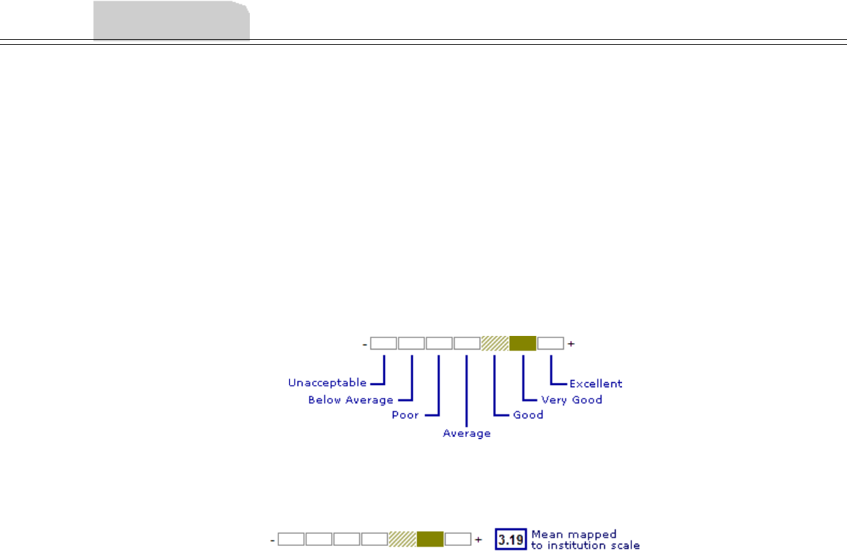
and also as a graphical meter. Meters display the assessment result on a 0 to 100 scale that is
divided into the following seven categories. The certainty of an assessment is also visually
displayed by shaded and solid bands. See section 3.3 for more information about uncertainty.
You can map this scale to your institution's scale using the Configuration Console, Tuning
Console, or the Internal Rating Model Author. If you map this scale, the number on the right
of the meter corresponds to the institution's scale.
The inputs that make up the assessment are called components. For example, an assessment of
Management Character could be made up of two components: one that measures Commitment
and one that measures Integrity. The types of components that make up an assessment
determine how the assessment is calculated:
• Assessments with categorized components (such as subjective factors and aggregated
assessments). The calculation for these assessments is described in the next section.
• Ratio assessments with peer, trend, and absolute components. Ratio assessments are
discussed in Chapter 5.
3.2 ASSESSMENTS WITH CATEGORIZED COMPONENTS
This section discusses how the system produces assessments from components with categorized
inputs. A detailed look at the algorithm behind these calculations can be found in section 3.5.
These components have input values that are predefined categories, such as:
Non-financial factors. Factors with input values that display as drop-down menus and have
categories such as: HIGH, AVERAGE, LOW.
Assessments. Individual assessments have categories (Unacceptable through Excellent) and can
be combined to form an aggregated assessment.

14
To combine categorized inputs into an assessment, the system uses a weight function. The
weight function serves two purposes:
• It allows components with different categories to be combined in the assessment.
• It allows each component category to have more or less importance in the assessment.
The following discussion gives a simplified account of how the system uses weight to create an
assessment. Uncertainty and soft saturation also contribute to the assessment, but to simplify
this discussion they are in a separate section.
Weighting Assessment Components
The weight function assigns a vote to each component category. If the component category
improves the assessment it is assigned a positive vote. If the category worsens the assessment it is
assigned a negative vote. The relative importance of the category is defined by the size of the
vote: the larger the vote, the more influence the component category has on the assessment.
The weight concept in the Tuning Console provides an idea of the importance of individual
components in an assessment (i.e., which components impact the assessment to a greater
degree). It also allows you to adjust, at a very high level, the votes associated with a component
and its categories. It is important to remember that this weight is not explicit in the
fundamental analysis approach; weighting is added to an assessment through the use of votes.
While you can adjust the weights of components in the Tuning Console, what you are really
doing is adjusting the votes.
Each component has a list of possible categories and corresponding votes. When a component
receives its value, for example, through user selection, the system looks up the category to assign
the votes. The sum of the votes for all of the assessment’s components contributes to the
assessment value.
Votes, which center on zero, must be mapped onto the assessment scale of 0–100. To do this,
assessments have an initial distribution which is used as a starting point for the assessment. The
initial distribution generally has a mean of 50 (on a 0-100 scale) and a standard deviation of
seven. The sum of the component votes is added to the initial mean to produce the assessment
mean. This value is then mapped onto the seven assessment meter categories to display the
meter.
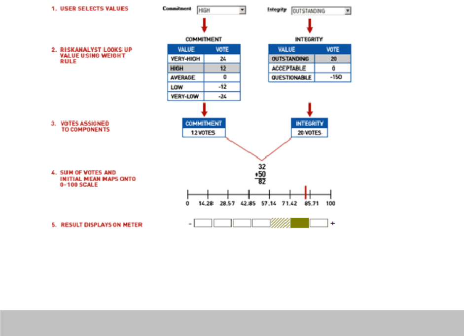
Consider an assessment of Management Character with two components: Commitment and
Integrity. The votes of the Commitment and Integrity components are summed and the result
is added to the initial mean to produce the assessment mean.
The diagram below demonstrates this process. Note that because uncertainty in the assessment
is taken into account, as discussed in section 3.3, the assessment has a shaded band to the left of
the solid band.
GUIDE TO BUSINESS ANALYSIS 15
The same logic applies when aggregating a group of assessments into an overall assessment.
The example below details an assessment with 266 absolute votes to be distributed among five
components. The components have different numbers of categories (some 4 and some 5). The
266 votes used in this example are based on a Range value of 59.
Category Votes for
Component 1
Votes for
Component 2
Votes for
Component 3
Votes for
Component 4
Votes for
Component 5
1 -5 0 12 10 12
2 20 20 8 5 8
3 -10 -10 0 0 0
4 -20 -30 -15 -8 -10
5 N/A N/A -25 -13 -25
Total
Absolute
Vote
55 60 60 36 55
Average
Absolute
Vote
(55/4) 13.75 (60/4) 15 (60/5) 12 (36/5) 7.2 (55/5) 11
The total of the Average Absolute votes is:
13.75 + 15 + 12 + 7.2 + 11 = 58.95
Average Absolute Vote as a percentage of 58.95:
23.3% 25.4% 20.4% 12.2% 18.7%
Total 100%
Adjusting the weight (through the use of votes) of an individual component affects only that
component. It is necessary, therefore, to adjust other weights in order to achieve a total of 100%
weight across all components.
16
Initial Distribution
Each assessment has an initial distribution which is the mean and standard deviation of the
assessment. Generally, the starting mean is set halfway along the meter at 50, with the standard
deviation of seven. Positive voting moves the meter up, and negative voting moves it down. A
meter mean point of 50 adds no bias to the assessment. A meter starting mean point value of
less than 50 will ensure a built-in conservative bias to the assessment, a value of greater than 50
will ensure an optimistic bias.
3.3 UNCERTAINTY
As well as the assessment value, meters display RiskAnalyst’s analysis of the certainty or
uncertainty attached to the assessment. Uncertainty can be introduced as a result of:
• Missing data
• Inherent imprecision of the items under assessment, particularly where these are
subjective analyses
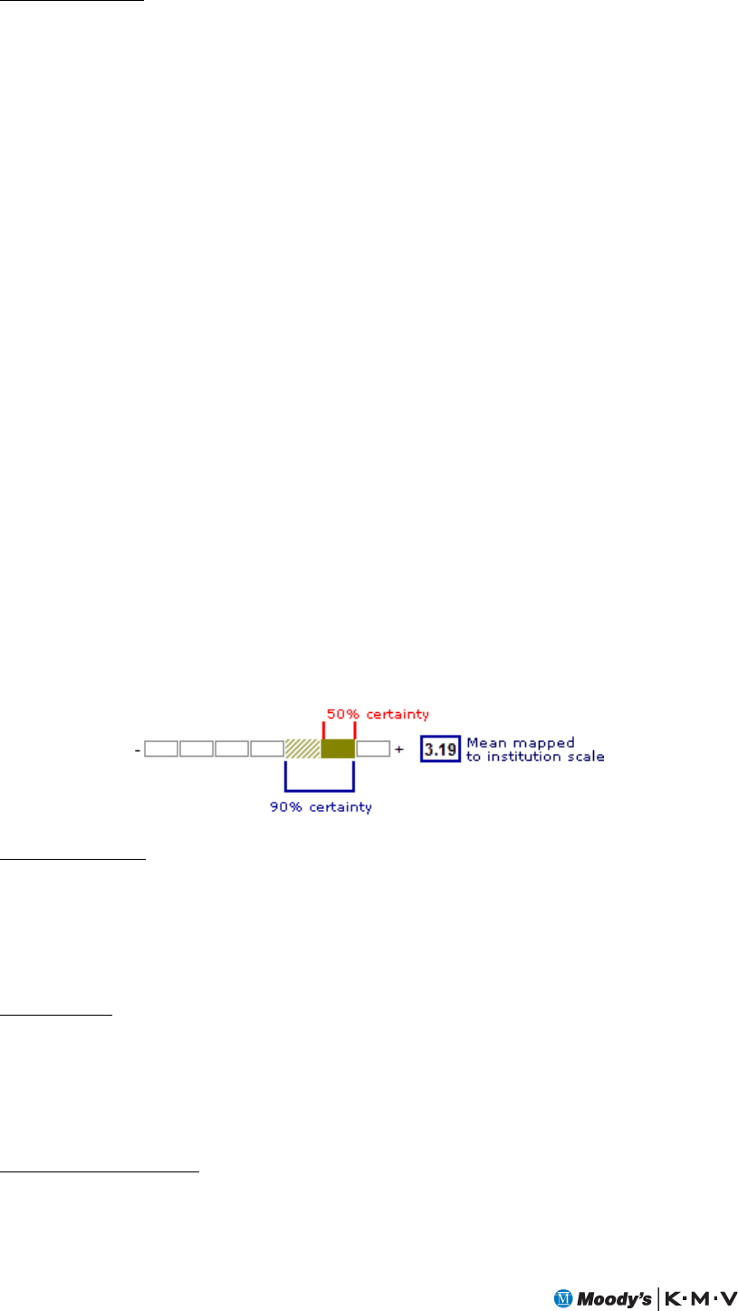
Meters use solid and shaded bands to indicate both the assessment value and the level of
certainty attached to the analysis. A meter displays as either a single, solid green band or a
combination of a solid and shaded green bands. The band or bands denote a range with a 90%
degree of certainty.
The system will color in the smallest number of categories it can to cover 50% of the curve, and
then will shade in the smallest number of categories to the left and right to reach 90% of the
curve.
Where a solid band appears without any shaded bands, the range denoted by the solid band has
a 90% degree of certainty. Where a solid band is accompanied by shaded bands, the range
denoted by the solid and shaded bands has a 90% degree of certainty, but the range denoted by
just the solid band is only 50% certain.
Inbuilt Uncertainty
The inbuilt uncertainty of a component is one of the determinants of the width of the
uncertainty band in the component’s meter. A high uncertainty indicates an inherently
uncertain component, and means that, even when all the inputs are given, the meter displays a
wide shaded band.
Soft Saturation
Although meter values theoretically range from 0 to 100, in practice it is usually impossible to
achieve either extreme. This is due to a type of damping mechanism—soft saturation—that
ensures meters stay within range by applying increasing resistance as the value approaches either
extreme. Values lower than about 3 or higher than about 97 would be rare.
Calculation of Uncertainty
The uncertainty for an assessment is the square root of the sum of:
GUIDE TO BUSINESS ANALYSIS 17
The standard deviation squared
The square of the standard deviation associated with each input applied to its weights.
The latter is derived from the difference between the input's mean value (as derived using the
assessment votes) and the votes for each category in the assessment. The resulting differences are
combined by weighting each difference by the probability that the input could take the value
associated with the weight. The differences are also squared and summed. Then the system takes
the square root of the result to eliminate positive and negative differences canceling out each
other.
The spread of votes you enter for an assessment will affect the uncertainty if the input itself has
some uncertainty. This is due to the use of differences between votes and input mean. Using a
greater spread of votes for meters will affect assessments, especially when questions are
unanswered. Note that if the input to the assessment is a specific answer to a question then the
spread of votes has no impact as its value is certain.
3.4 RANGE
The range is the number that controls the boundaries of an assessment and thus its impact – the
greater the range the greater the potential movement of the meter (14 votes is equal to
approximately one category of the meter). Range sets the maximum number of votes for the
components of an assessment, and changing it changes the votes for each component of the
assessment, resetting them to a straight line and overriding the existing distribution. Similar to
weights in the Tuning Console, changing the range is really just another way to change the
votes of the components of an assessment. The range will be changed if tuning (see ‘Range in
the Tuning Console’) changes the total number of votes within the components.
The highest and lowest possible values for an assessment are determined (indirectly) by a factor
using the range. The actual number of votes is determined using the formula explained below.
This calculation produces votes on a straight line through a midpoint of 0. It must be carried
out for each category in each component using the correct formula (determined by whether a
component has an equal or odd number of categories).
Weight (as a percentage) = p
Number of categories in a component = n
Range = r
Category number (ID) = c
Number of votes = v
For each category (c), the vote (v), is given by the following equations:
For even values of n:
v(c) = 2(npr) * (2c - n - 1) / n2
For odd values of n:
v(c) = 2(npr) * (2c - n - 1) / (n2 - 1)
For example, consider the Operations Skill component category ABOVE AVERAGE. When
Operations Skill has a weight of 24.5%, and the range is 39, the number of votes for the ABOVE
AVERAGE category is calculated as follows:
p = 0.245, n= 5, c = 4

18
v4 = 2(5 x 0.245 x 39) x (8-5-1)/25
= 95.55 x 2/25
= 8
Range in the Tuning Console
In the Internal Rating Model Author, you can use the Tuning Console’s Range slider to adjust
the total number of votes that contribute to the assessment. Changing the range overwrites the
distribution of votes in existing assessments by setting them in a straight line that centers on
zero.
When range is set to a low value, the system allocates fewer votes between all component
categories for the assessment and the resultant meter range is narrower.
Conversely, when you set a high value for range the system allocates more votes, the resultant
meter range is broader, and the extremes of the meter can be reached in the assessment. Since
there is a larger potential movement along the meter between best and worst, the meter has a
greater possible impact. The table below displays how the system allocates votes to components
using three different range settings:
Range
Setting
Votes for
Component
1
(50% weight)
Votes for
Component
2
(30% weight)
Votes for
Component
3
(20% weight)
Assessment
Meter
(Worst/Best)
Potential
Meter
Range
(/100)
20 -15 to +15 -9 to +9 -6 to +6 23.1 / 76.9 53.8
40 -30 to +30 -18 to +18 -12 to +12 8.3 / 91.7 83.4
60 -45 to +45 -27 to +27 -18 to +18 2.7 / 97.3 94.6
3.5 ASSESSMENT ALGORITHM
This section describes the main assessment algorithm of the fundamental analysis approach.
This algorithm is used to derive all the assessments except for those that assess ratio values.
However, even these assessments use the main assessment algorithm as a building block.
In order to derive an assessment, each value that an input can take is associated with a vote as
described above. A vote denotes the “score” of an input for a given value of that input. If the
input takes a numeric value, this value is called a fixed point. If the input takes a category (i.e.,
Excellent, Good, Fair) as a value, this value is called a category. A set of fixed point – vote pairs
or category – vote pairs defines a relative function of “goodness” for the various values of an
input and is defined for all inputs. For categorised inputs a vote is typically defined for each
possible category. For numeric inputs it would clearly not be possible to specify a vote for each
possible value and so a number of votes are specified, each corresponding to one possible value
of the input (the fixed point). If the actual value of the input does not match one of the fixed
points, linear interpolation is used to determine the corresponding vote. If the input value is
greater than the largest fixed point the vote corresponding to this is used. Similarly, if the input
value is less than the smallest fixed point the vote corresponding to this is used.
3.6 CALCULATING THE ASSESSMENT
Assessments are created using the following steps:
1. Scoring of inputs: For each input the system calculates the mean and standard deviation
for a Normal distribution from the set of fixed points or categories associated with this

GUIDE TO BUSINESS ANALYSIS 19
input and the value of this input. The fixed point to vote or category to vote mapping
described above is used to determine the score distribution. Fixed points or categories are
defined during the design and tuning of a model, and can later be adjusted using the
Internal Rating Model Author.
2. Aggregation of input distributions: RiskAnalyst assumes the probability of an assessment is
Normally distributed. The total votes of all inputs are aggregated to calculate the mean and
standard deviation of this distribution.
3. Transformation of distribution: The final stage is to transform the Normal distribution
from the continuous domain on an infinite scale to fit our discrete seven-category
assessment on a 0-100 scale. This is done by calculating areas under the standard Normal
distribution that correspond the range of each of the categories on the infinite scale.
3.6.1 Scoring of Inputs
The methods used to score inputs are slightly different depending on whether they are
categorized or numeric. The following sections provide the algorithms for determining the
scores for each input.
Categorized Inputs
Let categorised input
x
have ncategories where 71
≤
≤
n. Let:
• cix denote the i-th category value of
x
.
• pix denote the probability associated with the i-th category value of
x
.
• vix denote the votes associated with the i-th category value of
x
.
•
μ
xdenote the mean of the Normal distribution associated with
x
, where:
∑
≤
=
ni ix
ixx v
p
.
μ
•
σ
xdenote the standard deviation of the Normal distribution associated with
x
,
where:
(
)
∑−
≤
=
ni ix
xx
ix
v
p
μ
σ
2
.
• If the value of
x
is unknown, i.e.
p
ix is undefined, then:
2
)min()max( vv ixix
x
+
=
μ
(
)
)min()max(.2887.0 vv ixixx −=
σ
i.e. the mean and standard deviation of the uniform distribution is assumed.

20
Numeric inputs
Let numeric input
x
have nfixed-points where 71
≤
≤
n. Let:
• uix denote the i-th fixed-point value of
x
.
• vix denote the votes associated with the i-th fixed point value of
x
.
• wxdenote the value of
x
.
•
μ
xdenote the mean of the Normal distribution associated with
x
, where:
()
⎪
⎪
⎪
⎪
⎩
⎪
⎪
⎪
⎪
⎨
⎧
+=≤≤−
⎟
⎟
⎟
⎠
⎞
⎜
⎜
⎜
⎝
⎛
−
+
≤≤=
≤
≥
=−1for if.
1for if
if
if
11
jk
jxx
nj
uwuvv
uu
uw
v
uwv uwv uwv
kxxjxjxkx
jxkx
jx
jxxjx
xxx
nxxnx
x
μ
This is often referred to as linear interpolation.
Note that typically there is no uncertainty associated with numeric inputs ( 0=
σ
x). The
exception is when the input is the slope where it is possible to measure the standard deviation of
the slope. See section 5.4.1 for details. When there is standard deviation associated with the
input then the standard deviation, denoted by
σ
, is calculated by considering the average
difference of the vote around the mean for the standard deviation:
2
xxxx
x
μμμμ σσ
σ
−+−
=−+
Where
σ
μ
+xis calculated as x
μ
with
σ
μ
σ
+=
+x
x
w. Similarly for
σ
μ
−x.
If
x
is unknown the mean and standard deviation are calculated using the same method for
categorised inputs described above. In RiskAnalyst, this is not used in practice since the ratio
assessment algorithm only assesses defined ratios.
3.6.2 Aggregation of input distributions
Let the assessment being constructed be denoted as
y
. Let
p
w denote an initial distribution
associated with y. Let
σ
μ
pw
pw,denote the mean and standard deviation of this initial
distribution. Given minputs, the mean of the Normal distribution associated with
y
is
calculated as:
∑
≤≤
+=
mx xpwy 1
μ
μ
μ
and the standard deviation as:

GUIDE TO BUSINESS ANALYSIS 21
∑
≤≤
+=
mx xpwy 1
22
σσσ
3.6.3 Transformation of distribution
Let cifor 71 ≤≤ idenote the categories of an assessment, where
EXCELLENT BLE UNACCEPTA 71 == cc L. Let cepi denote the class end point of
the i-th assessment category on a 0 to 100 scale, i.e.,
7
100.i
cepi=
Let iepidenote the interval end point of the i-th assessment category on a ∞− to ∞ scale.
The interval end point is calculated from the class end point using the following inverse sigmoid
function:
⎟
⎟
⎠
⎞
⎜
⎜
⎝
⎛
−
+= cep
cep
iep
i
i
i100
ln.2550
Let
Z
iy denote the Z-score for the i-th category of an assessment.
Z
iy is calculated as:
σ
μ
y
yi
iy
iep
Z−
=
Let )(
Z
iy
F denote the probability that the value of
y
is in one of the j categories up to and
including i ( ij ≤
≤
1). Standard lookup tables can be used to determine )(
Z
iy
F. )(
Z
iy
F
corresponds to the area underneath the standard Normal distribution to the left of
Z
iy . These
areas correspond to the probability that the value of the assessment is contained in any of the
first iintervals. For efficiency reasons RiskAnalyst uses an approximation method for finding
the area under the Standard Normal distribution. It uses linear interpolation with the following
values:
Mean Cumulative Integral
-11 0
-10 0
-3.5 0.0002
-3 0.0013
-2.5 0.0062
-2 0.0228
-1.5 0.0668
-1.2 0.1151
-1 0.1587
-0.8 0.2119
-0.5 0.3085
0 0.5
0.5 0.6915

22
0.8 0.7881
1 0.8413
1.2 0.8849
1.5 0.9332
2 0.9772
2.5 0.9938
3 0.9987
3.5 0.9998
10 1
Finally the probability of the i-th category for
y
,
p
iy , can be calculated from the cumulative
probability )(
Z
iy
F:
⎪
⎩
⎪
⎨
⎧
≤<−
=
=
−72for )()(
1for )(
)1( iFF
iF
ZZ
Z
pyiiy
iy
iy
Note that if 0=
σ
y there is no uncertainty and the mean of the distribution fits entirely into
one of the categories. For 0=
σ
y,
p
iy is calculated as:
⎪
⎩
⎪
⎨
⎧<
=Otherwise0
such that of valuesmallest for the1 iep
piy
iy
i
μ
3.7 CALCULATING THE MEANS AND STANDARD DEVIATIONS
OF AN ASSESSMENT
While the assessment meters provide a powerful way of communicating the evaluation of the
assessment, they are limited in that they are complex to describe and are not particularly precise.
Often it is desirable to have a single figure that describes the assessment. To satisfy this
requirement, we use the assessment mean, or Real Mean. The Real Mean is associated with the
mean of the original continuous Normal distribution, and is defined further in section 3.7.1.
When combining assessments, the fundamental analysis approach uses the full information
from the sub-assessments, and doe not simply combine the real means of the sub-assessments.
3.7.1 Real Mean:
Let r
y
mean denote the Real Mean. This is the mean of the continuous Normal distribution
transformed to the 0-100 scale using the RiskAnalyst saturation function and is calculated as:
(
)
()
25
50
25
50
1
.100
−
−
+
=y
y
e
e
meanr
y
μ
μ

GUIDE TO BUSINESS ANALYSIS 23
Let r
y
sd denote the real standard deviation of an assessment. It is calculated as:
(
)
()
50
25
25
1
.100 −
⎟
⎟
⎟
⎟
⎠
⎞
⎜
⎜
⎜
⎜
⎝
⎛
=
+y
y
e
e
sdr
y
σ
σ
CHAPTER 4
GUIDE TO BUSINESS ANALYSIS 25
4 SCORECARD METHODOLOGY
4.1 SCORECARD OVERVIEW
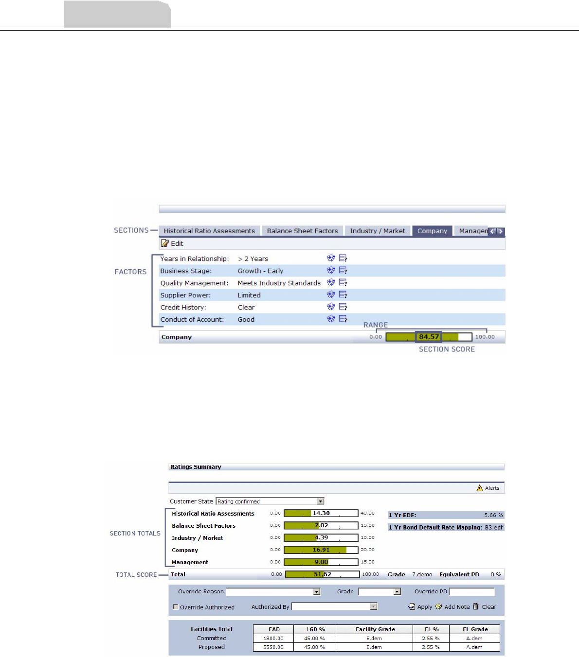
A scorecard internal rating model consists of a set of factors grouped into sections
corresponding to particular areas of analysis. Factors are inputs obtained either from the user or
from values entered in other parts of RiskAnalyst, or from external programs. Each factor within
a section is scored, and the sum of those scores, with any weighting, is the total score for that
section. The sum of each section's total score, with any weighting, is the scorecard's total score.
FIGURE 1.1 Section total
Each factor within a section can be weighted such that it contributes more or less to the section
total than the other factors within that section. Section total scores can also be similarly
weighted to have a greater or lesser influence on the total scorecard score. The Internal Rating
Model screen displays section scores and ranges with factor weighting, but without section
weighting, applied. The Ratings Summary screen shows the section scores and ranges, as well as
the total score, with weighting applied.
FIGURE 1.2 Total score

26
To reiterate, the scoring process is as follows:
• Scorecard factors obtain data from user input or from values entered in other parts of
RiskAnalyst.
• Factors are given a score based on the input value.
• Factor scores are weighted and summed to give a section score.
• The section scores are weighted and summed to give a scorecard total.
• The scorecard total is mapped to a grade and a PD.
4.2 METERS
Once the factors are calculated and the section scores totaled, RiskAnalyst displays a meter to
give a visual representation of the score. The meter includes both the score and the range of
scores possible. The system displays meters for section totals, as well as the total score.
FIGURE 1.3 Scorecard meter
4.3 FACTORS
Scorecard inputs are known as factors and have the following input sources:
• User input. Factors that display in scorecards as drop-down menus or input boxes and
receive their values from user input.
• RiskAnalyst Values. Values entered in other parts of RiskAnalyst. These inputs can be
customer information data, ratios, values, or RiskCalc and Public EDF measures.
• External Program Values. Values obtained from an external program. A module is
necessary to obtain values from an external program and must be configured for use in
the Internal Rating Model Author.
Input values can be:
• Numerical. Values such as ratios or numbers entered by the user.
• Categorized. Predetermined categories, such as drop-down menus, where users select
from a list of possible values.
Each factor is given a score based on its input value. The system calculates numerical factor
scores differently than categorized factor scores. The system can also transform numerical input
values before they are given a score. An explanation of each calculation, and the RiskAnalyst
algorithm for these calculations, follows.
Each factor has a name and belongs to a section. To find out more about the individual factors
associated with a particular section, click the Clarify button on the Internal Rating Model
screen for that section.

GUIDE TO BUSINESS ANALYSIS 27
4.4 CALCULATION OF SCORES FOR NUMERICAL FACTORS
Factors that have numerical inputs, such as ratios and financial statement values, are scored in
one of two ways. Either RiskAnalyst uses the factor’s value as the score, or it calculates the score
using a process called banding.
4.4.1 Scoring Factors Using Values
Using this method, the value of the factor feeds directly into the score. In order to display the
correct score and range for the section on a meter, there must be a minimum and maximum
value for each factor’s input that is scored in this manner. RiskAnalyst uses these values to
determine the lower and upper meter values, and displays the section total on this scale.
4.4.2 Scoring Factors by Banding
Using this method, a number of bands (or numerical ranges) and a score for each of these bands
must be specified:
Band upper point Score
20 0
40 5
60 10
80 20
100 30
RiskAnalyst calculates the factor’s score by determining which band the factor’s input value falls
into. If the value is larger than the highest upper bound, it is scored as if it were within that
band. For example, if the value is 120, a score of 30 is given using the bands shown above. Any
value below 20, including a negative number, is given a score of 0. Band upper points are
inclusive, such that a value of 40 would score 5.
NOTE When banding is set up, it assumes that you are using actual units.
If you are entering currency values, they should be entered in the currency you have
selected for your scorecard.
4.4.3 Transformation of Numerical Inputs
RiskAnalyst can be configured to transform the values of scorecard factors that have numerical
inputs. RiskAnalyst transforms the factor values before calculating their scores.
RiskAnalyst can apply the following three transformation functions to numerical inputs:
• Normalize
• Log (base e)
• LOGIT
Each of these functions is described below.
Normalise
Use Normalise to standardize raw data.
28
To standardize raw data χ, subtract mu μ and divide by sigma σ (the parameters of the normal
distribution), where:
μ is the mean or typical value of χ.
σ is the standard deviation. This is a measure of the spread or volatility of the data, and is equal
to the square root of the arithmetic mean of the squares of the deviations from the arithmetic
mean of the data.
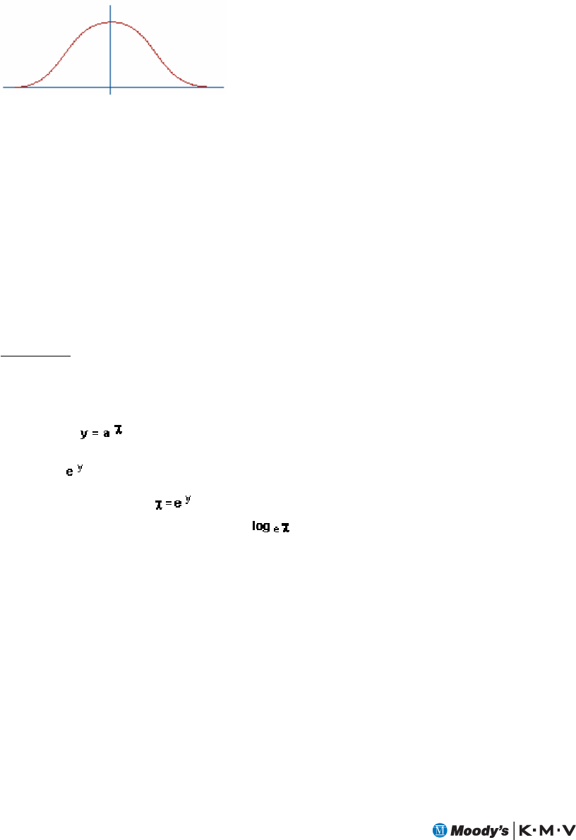
The Normalize function gives the data a bell-shaped distribution that is symmetrical about the
mean (or typical value) of the data, as shown below.
Approximately 95% of the data will be within ± two standard deviations from the mean, and
approximately 99.8% of the data will be within ± three standard deviations from the mean.
Example:
A company has reported a Gross Margin of 45%. If the mean industry Gross Margin is 25%
and the standard deviation is 10, then the standardized value of the company’s Gross Margin
figure is:
((45-25)/10) = 2
This tells us that the company’s Gross Margin is two standard deviations above the mean
industry figure.
Log (base e)
The natural logarithm (log in the base e) gears down the importance of higher data values and
reduces the data’s spread.
In the graph , there is a value a (approximately 2.718282) at which the gradient of the
exponential curve at (0,1) is exactly 1. This is an irrational number symbolized by e. In the
expression , e is called the base and y is called the exponent, power, or logarithm.
Therefore, the expression can also be interpreted as meaning y is the logarithm of the
number χ in the base e. This is written as or ln χ.

GUIDE TO BUSINESS ANALYSIS 29
The graph of is shown above. This graph shows that as the value of data χ increases, the
gradient of the curve decreases. Therefore, the impact of higher numbers is disproportionately
reduced, or geared down.
NOTE You cannot enter negative values into logs.
Example:
Take, for example, an internal rating model that has questions resulting in the following scores:
10
50
90
1000
These results give a data spread of 990, and the highest score is 100 times that of the smallest
figure. Transforming the scores with log in the base e results in the following scores:
2.303
3.912
4.499
6.908
Now the spread of data is just 4.6, and the highest score is just 3 times that of the smallest score.
LOGIT
Use LOGIT to estimate the conditional probability of a positive response or the presence of a
characteristic. For example, is a company likely to honor its loan covenants or not? The
function is based on an “S” shaped curve, with the result of the transformation formula:
This gives the probability of a positive response that falls between zero (no chance of a positive
response) and one (100% chance of a positive response).
You need to define the LOGIT coefficients A and B.
30
4.4.4 Special Numeric Factors
The following are two examples of numeric factors that are calculated differently than other
numeric factors.
Ratios
Ratio assessments are a special type of numeric factor, and are calculated by the RiskAnalyst
Ratio Assessment algorithm. The calculations behind this algorithm are described in Chapter 5.
NOTE It is possible to include a Ratio in a scorecard simply as any other financial value. In
this case, the Ratio Assessment algorithm is not used.
EDF measures
EDF measures are another special instance of a numeric factor. RiskAnalyst gathers EDF values
from Moody's KMV RiskCalcTM and CreditEdge®. Whether or not an EDF value is a factor in
the scorecard, the 1-Yr EDF measure will display on the Ratings Summary screen. See Chapter
6 for more information.
4.5 CALCULATION OF SCORES FOR CATEGORIZED FACTORS
For categorized factors such as drop-down menus, RiskAnalyst calculates factor scores from the
categories. Specify a score for each of the categories in the factor value properties, as shown in
the example below:
Categories Scores
INADEQUATE -10
BELOW AVERAGE 0
AVERAGE 10
ABOVE AVERAGE 20
EXCEPTIONAL 30
RiskAnalyst calculates the score when a category is selected, such as when a user makes a menu
selection.
4.6 WEIGHTING
Weighting can be applied to both factors and sections in scorecards. There are various practical
reasons for using weighting in scorecards. The following is an example that uses weighting to
replicate an averaging approach.

GUIDE TO BUSINESS ANALYSIS 31
Suppose you want the total score for each section to be an average of the factors in the section.
You also want the total score to be the average of the section scores.
Section 1 Value
Factor 1 3
Factor 2 4
Factor 3 5
Factor 6 6
Section total Average of (3, 4, 5, 6) = 4.5
Section 2 Value
Factor 1 5
Factor 2 6
Section total: Average of (5, 6) = 5.5
Scorecard total: Average of (4.5, 5.5) = 5.0
To produce the above result in RiskAnalyst, you would set the following factor and section
weights:
Factor Weights
Section 1 Value * Weight = Weighted Score
Factor 1 3 .25 .75
Factor 2 4 .25 1
Factor 3 5 .25 1.25
Factor 4 6 .25 1.5
Section total: 4.5
Section 2 Value * Weight = Weighted Score
Factor 1 5 .5 2.5
Factor 2 6 .5 3
Section total: 5.5
Section Weights
Scorecard Value * Weight = Weighted Score
Section 1 4.5 .5 2.75
Section 2 5.5 .5 2.25
Scorecard total: 5.0
The weights above correspond to 1 / (number of factors) or 1 / (number of sections). This is a
simple example of using weighting to produce averaging. Using the above example as a starting
point, you could also produce a weighted average, such that a particular section has a greater
impact on the total score (i.e., replace Section 2's weight of .5 in the example above with 1.5 to
make Section 2 three times as important).
CHAPTER 5
GUIDE TO BUSINESS ANALYSIS 33
5 RATIO ASSESSMENT METHODOLOGY
5.1 FINANCIAL RATIOS
Both the fundamental analysis and scorecard approaches make use of ratio assessments.
Financial ratios or metrics are used to form ratio assessments. RiskAnalyst performs different
analyses for each ratio. The different analyses take into account a comparison of each ratio to a
peer benchmark, the direction and volatility in the trend of the ratio, and in several ratios, a
comparison to a policy-based absolute benchmark. These analyses are then combined to
produce an overall ratio assessment.
All the information displayed relating to the ratios comes from financial values in RiskAnalyst.
This information consists of the calculated ratios and the peer benchmarks, and is dependant on
the financial periods and the peer group.
Ratio Assessment Analyses
A ratio assessment is the weighted sum of a calculated peer/trend assessment and an absolute
assessment. The trend assessment also includes a volatility analysis component. The absolute
analysis is performed for certain ratios only.
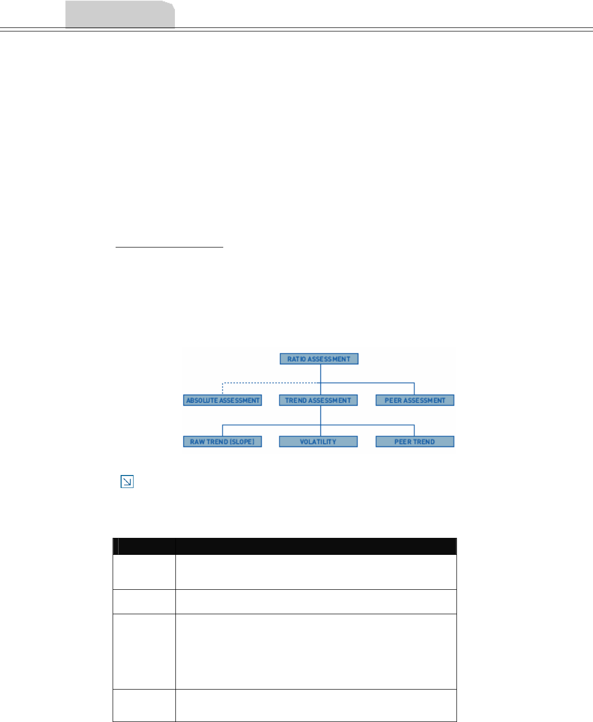
The diagram below gives an overview of the various analysis components that may be involved
in the ratio assessment and how the components are combined together to give the final ratio
assessment.
FIGURE 1.4 Structure of ratio assessment
NOTE The Peer Trend assessment is included in the Internal Rating Model Author as a potential
analysis component of ratio assessments. However, the ratio assessments included with the
RiskAnalyst internal rating templates do not include the Peer Trend assessment.
Each of the sub-components of the analysis is described in more detail below.
Component Description
Peer
Assessment
This is an assessment of the ratio’s performance compared to industry values.
The calculated value of the ratio for the current period is compared to the
industry values to derive the company’s ranking.
Trend
Assessment
The overall trend assessment is itself the weighted combination of the trend
analyses and the volatility assessment of this trend.
Absolute
Assessment
For some of the ratios, there are certain standards common in the lending
community above or below which it can safely be said that the company is
performing well or poorly without regard to the rest of the industry. These
standards of ratio performance are used in the ratio assessment to counter the
effects of making ratio comparisons in a very strong or weak industry. The
absolute values used for this analysis may vary depending on the financial
template used to analyze the company.
Raw Trend
Assessment
This assessment considers the trend of the ratio over the periods analyzed.
Remember that trend analysis will only be performed if sufficient historical
statements are available. Typically, a minimum of three historical values are
34
Component Description
required in order to provide a trend analysis. Comparative analyses, like %
Turnover Growth, require a minimum of four historical statements
Volatility
Analysis
The volatility component is an extension of the trend analysis. Generally, a
ratio trend that is either stable or increasing/decreasing at a consistent rate can
be analyzed with greater certainty than ratios that fluctuate from period to
period. If the historical trend of the ratio shows a pattern of wide fluctuation,
the volatility assessment will be unfavorable. Conversely, if the trend of the
ratio shows stability or a relatively even pattern of change, the volatility
assessment will be favorable. However, even an extremely favorable volatility
assessment will have a relatively small impact on the overall trend assessment.
The main function of the volatility analysis is to worsen the overall trend
assessment.
Peer Trend
Assessment
This assessment compares the average rate of change (slope) of the ratio value
for the company over the past three or four years to the average rate of change
(slope) of the median ratio value for the company's peers. To use this
assessment, the average rate of change (slope) for each peer group needs to be
calculated, and this information must be populated in the PEERINFO
reference table.
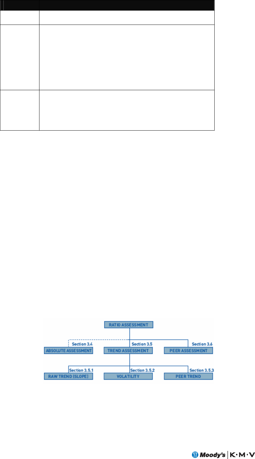
5.2 STANDARD RATIO ASSESSMENT ALGORITHM
This section describes the standard ratio assessment algorithm. It is used for all historical ratio
assessments.
The algorithm has three main components:
1. Absolute: Compares the most recent ratio values to a set of benchmarks.
2. Trend: Looks at how the ratio values for this borrower have changed over time. Derived
from two to three sub-components (see below).
3. Peer: Ranks the ratio values against the borrower’s peer group.
Trend is itself determined from between two and three further sub-components:
• Slope: An assessment of the slope of recent ratio values.
• Volatility: An assessment of the volatility of recent ratio values.
• Peer Trend: Compares the slope of the borrower’s ratio values with those of its peer
group. It is rare for this information to be available and this part of the ratio assessment
is not often used.
FIGURE 1.5 Components of the Standard Ratio Assessment
The three top level ratio assessment components (absolute, trend, and peer) are combined using
a simple weighted sum. This section details each of these components, how they are combined,
and documents a number of special conditions used in the ratio assessment algorithm.

GUIDE TO BUSINESS ANALYSIS 35
By default, RiskAnalyst bases its ratio calculations on statements listed in the Analysis Setup
screen in RiskAnalyst (generally the latest annual, historical statements). Other annual
statements can be selected by hiding statements in the RiskAnalyst grid. Projected statements
can be used in the analysis by selecting the projection to use in the Analysis Setup dialog box.
See the RiskAnalyst Help for more information. For slope and volatility calculations,
RiskAnalyst uses values from prior statements.
The two algorithms below, discussed in 5.2.1 and 5.2.2, are used in the main ratio assessment
algorithm, and will be referenced in the following sections.
5.2.1 Algorithm for numeric factors
Let numeric input
x
have nfixed points where 71
≤
≤
n. Let:
• uix denote the i-th fixed point value of
x
.
• vix denote the votes associated with the i-th fixed point value of
x
.
• wxdenote the value of
x
.
•
μ
xdenote the mean of the Normal distribution associated with
x
, where:
()
⎪
⎪
⎪
⎪
⎩
⎪
⎪
⎪
⎪
⎨
⎧
+=≤≤−
⎟
⎟
⎟
⎠
⎞
⎜
⎜
⎜
⎝
⎛
−
+
≤≤=
≤
≥
=−1for if.
1for if
if
if
11
jk
jxx
nj
uwuvv
uu
uw
v
uwv uwv uwv
kxxjxjxkx
jxkx
jx
jxxjx
xxx
nxxnx
x
μ
This is often referred to as linear interpolation.
Note that typically there is no uncertainty associated with numeric inputs ( 0=
σ
x). The
exception is when the input is the slope where it is possible to measure the standard deviation of
the slope. See section 5.4.1 for details. When there is standard deviation associated with the
input, then the standard deviation, denoted by
σ
, is calculated by considering the average
difference of the vote around the mean for the standard deviation:
2
xxxx
x
μμμμ σσ
σ
−+−
=−+
σ
μ
+xis calculated as x
μ
with
σ
μ
σ
+=
+x
x
w. A similar calculation is used for
σ
μ
−x.
5.2.2 Algorithm for categorized factors
Let categorized input
x
have ncategories where 71
≤
≤
n. Let:
• cix denote the i-th category value of
x
.

36
•
p
ix denote the probability associated with the i-th category value of
x
.
• vix denote the votes associated with the i-th category value of
x
.
•
μ
xdenote the mean of the Normal distribution associated with
x
, where:
∑
≤
=
ni ix
ixx v
p
.
μ
•
σ
xdenote the standard deviation of the Normal distribution associated with
x
,
where:
(
)
∑−
≤
=
ni ix
xx
ix
v
p
μ
σ
2
.
• If the value of
x
is unknown, i.e.
p
ix is undefined, then:
2
)min()max( vv ixix
x
+
=
μ
(
)
)min()max(.2887.0 vv ixixx −=
σ
i.e., the mean and standard deviation of the uniform distribution is assumed.
5.3 ABSOLUTE ASSESSMENT
RiskAnalyst assesses a ratio value against a set of benchmark fixed points. These fixed points are
defined during modelling and are entered in the Internal Rating Model Author. The absolute
assessment is created using the algorithm for numeric factors defined in section 5.2.1. The intial
distribution for the absolute assessment is a mean of 50 and standard deviation of 0.
5.4 TREND ASSESSMENT
RiskAnalyst assesses the trend of the ratio by considering three components. These are
combined using the algorithm for categorized factors described in section 5.2.2. The intial
distribution for the trend assessment is a mean of 50 and standard deviation of 3.
We need to deal with a ratio over a number of data points. For the data points, let idenote an
integer associated with the date of the ratio, where i=1 is the earliest data point. Let t denote a
number specifying the point in time to which the statement date refers. If the statements are all
for twelve month periods, then i=t. For example:
i t Statement date
1 1 12/2000
2 2 12/2001
3 3 12/2002
4 4 12/2003
If statements are for periods other than twelve months, t will be a non-integer for some periods.
For example:

GUIDE TO BUSINESS ANALYSIS 37
i t Statement date
1 1 12/2000
2 2 12/2001
3 2.75 9/2002
4 3.75 9/2003
Let ndenote the number of ratio values and i
xdenotes the ratio value at the i-th data point. For
each ratio, it is possible to choose the maximum and minimum values that n can take.
RiskAnalyst will only consider a maximum of five data points. If the number of data points is
greater than the maximum, only the latest nratio values are used. If the number of data points
is less than the minimum, the trend component is not considered in the assessment of the ratio.
Except where otherwise stated, the summations below all sum over nin
≤
<+
−
)1max_nos( ,
where max_nos is the specified maximum number of periods to be used for the ratio.
5.4.1 Slope
Let ratio
slope denote the fitted slope of the ratio values, where:
()
∑
∑
∑
∑
∑
−
−
=
i
n
t
i
n
slope t
t
x
xt
i
i
i
i
ratio 2
2
As mentioned in the algorithm for numeric factors in section 5.2.1, RiskAnalyst also calculates
the standard deviation of the slope as an input into the slope assessment. This is one-twelfth of
the Residual Standard Deviation calculation. Let slope
ratio
σ
denote the standard deviation of the
slope, where:
()
(
)
()
()
⎟
⎠
⎞
⎜
⎝
⎛∑
−−
∑
−
−
−
⎟
⎠
⎞
⎜
⎝
⎛∑
−
=∑
∑
∑∑∑
∑
i
nn
i
n
t
i
n
i
n
t
t
t
t
x
xt
x
x
i
i
i
i
i
i
slope
ratio 2
2
2
2
2
2
2
)2(
12
1
σ
RiskAnalyst assesses ratio
slope against a set of benchmark fixed points. These fixed points are
defined during modelling and are entered with the tuning tool. The slope assessment is created
using the algorithm for numeric factors defined in section 5.2.1, using both ratio
slope and
slope
ratio
σ
. The intial distribution for the slope assessment is a mean of 50 and standard deviation
of 3.
5.4.2 Volatility
Let i
slope denote the slope between the i-th and i-1 ratio:
nislope tt xx
ii
ii
i≤≤
−
−
=
−
−2,
1
1
Let ratio
ad denote the average difference between consecutive pairs of ratio values, where:

38
(
)
)1(
2
−
=
∑
≤≤
n
slope
ni i
ratio
ad
Let viratio denote the volatility index for a given ratio, where:
n
n
ratio
i
ni i
ni
ratio x
ad
slope
vi ∑
∑−
≤≤
≤≤
−
⎟
⎟
⎠
⎞
⎜
⎜
⎝
⎛⎟
⎠
⎞
⎜
⎝
⎛
=
1
2
2
)1(
RiskAnalyst assesses viratio against a set of benchmark fixed points. There are three fixed points
defined in the system for HIGH, MEDIUM, and LOW volatility groups. The group associated
with a particular ratio is defined during modelling and entered with the Internal Rating Model
Author. The volatility assessment is created using the algorithm for numeric factors defined in
section 5.2.1. The intial distribution for the volatility assessment is a mean of 50 and standard
deviation of 3.
5.4.3 Peer Trend
Let ratio
pt denote the difference between the fitted slope of the ratio values and the peer trend,
where:
peer
ratioratioratio trendslopept −=
peer
ratio
trend is the measured trend of a ratio given a peer group. This value is entered directly into
the RiskAnalyst reference tables. Due to the difficulty in maintaining this data, the peer trend
component has no impact on the trend assessment in the standard models shipped with
RiskAnalyst.
Since there is a standard deviation associated with the slope, this is passed to the peer trend
assessment. It is denoted as pt
ratio
σ
, and it is the same as the standard deviation used in the slope
calculation, i.e.
slope
ratio
pt
ratio
σσ
=
RiskAnalyst assesses ratio
pt against a set of benchmark fixed points. These fixed points are
defined during modelling and are entered with the tuning tool. The slope assessment is created
using the algorithm for numeric factors defined in section 5.2.1. It uses both ratio
pt and
pt
ratio
σ
as inputs. The intial distribution for the peer trend assessment is a mean of 50 and
standard deviation of 3.

GUIDE TO BUSINESS ANALYSIS 39
5.5 PEER
RiskAnalyst estimates the peer rank from a ratio value and three quartile cut-off points. There
are two different peer rank algorithms. The standard algorithm is used to assess the peer rank
under most circumstances. An alternative algorithm is used for gearing/leverage ratios if the
third quartile is negative. RiskAnalyst can also be configured so that the alternative ranking
algorithm can be used by other ratios (possibly new ones).
Let 1Q,2Q, and 3Qdenote the first, second, and third quartile cut-off points for a given ratio
and peer respectively. Note that these correspond to the 75th, 50th, and 25th percentiles.
Depending on the ratio, the 1Q ratio value may be smaller or larger than the 3Qvalue. This
depends on whether the ratio is deemed to be ascending or descending1.
Let rank denote the estimated rank of the ratio against its peer group, where:
⎩
⎨
⎧<
=otherwisestdRank
ratiogearingaisratioandQaltRank
rank 03 if
stdrank and altrank are defined below.
RiskAnalyst assesses rank against a set of benchmark fixed points. These fixed points are
defined during modelling and are entered with the tuning tool. The peer assessment is created
using the assessment algorithm for numeric factors defined in section 5.2.1. The initial
distribution for the peer assessment is a mean of 50 and a variable standard deviation depending
on the sample size of the peer:
Sample size greater than or
equal to:
Initial Distribution
Standard Deviation
100 3
10 5
Default 7
Note that the sample size information must be configured manually in the database tables as
this is not done automatically by the benchmark tool. In RiskAnalyst, this information is added
to the fpRatioPeerSample table.
5.5.1 Standard Ranking Algorithm
Let stdrank denote the standard rank, where:
•
(
)
()
⎪
⎩
⎪
⎨
⎧
−
<<
>>
=
−
−
−
Otherwise21
2 and 13 if2
2 and 13 if2
)1(
)1(
)1(
r
r
r
QxQQ
QxQQ
stdrank
•
x
is the ratio value
•
()
()
()
()
⎪
⎪
⎩
⎪
⎪
⎨
⎧
−
−
>
−
−
=
Otherwise
21,3min
2
2 f
21,3max
2
QQQ
xQ
Qxi
QQQ
xQ
r
1 For an ascending ratio, we deem higher values to be generally better. The inverse applies to descending ratios.
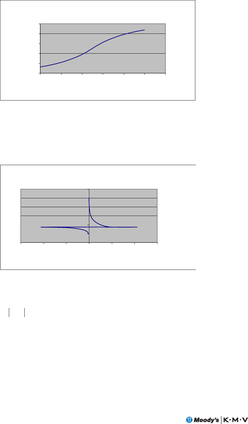
40
This algorithm creates a smooth, S-like mapping from ratio values to peer ranks. For example,
for an ascending ratio that takes values in (0,1) with quartiles at 0.25, 0.5, and 0.75, the
mapping can be described by the following diagram:
0.00%
20.00%
40.00%
60.00%
80.00%
100.00%
0 0.2 0.4 0.6 0.8 1 1.2
Ratio Value
Peer Rank
FIGURE 1.6 The Standard Ranking Algorithm (an Ascending Ratio)
5.5.2 Alternative Ranking Algorithm
The alternate ranking fits a log curve to the peer quartiles. The figure below illustrates the curve
where the quartiles are 1, 10, and -5. Note that for gearing and leverage ratios in RiskAnalyst, if
the ratio is negative, we default the rank to 0. Therefore, the lower section of the curve is flat at
0 for these ratio values.
0.00%
20.00%
40.00%
60.00%
80.00%
100.00%
120.00%
-150 -100 -50 0 50 100 150
Ratio Value
Peer Rank
FIGURE 1.7 The Alternative Ranking Algorithm
The alternate ranking algorithm assumes that the map between ratio and rank can be
approximated by a pair of log linear functions:
cRankmratio += .)ln(
One function is approximated for each side of the discontinuity in the mapping.
Let altrank denote the alternative rank, where:

GUIDE TO BUSINESS ANALYSIS 41
•
()
()
⎪
⎪
⎪
⎪
⎩
⎪
⎪
⎪
⎪
⎨
⎧
<
≥
=
t)RiskAnalys ofion configurat shipped the
with usednot isoption This :(Note Otherwise
100,min
0 if
0 if
0
100
,max
LowRankcrossOver
ratioleverageorgearingifandx
x
HighRankcrossOver
altRank
• gm denotes the gradient multiplier constant of a ratio. This is defined in the
PEER_RANK_MULT table.
• lhCutoff and rhCutoff denote the left- and right-hand cut-off constants respectively.
These are defined in the NEG_RANK_CUTOFF table.
•
(
)()()
522ln1ln QQmh−=
•
()
hh mQc .751ln −=
• gmmm hl .=
•
()
ll mQc .253ln −=
•
(
)
(
)
(
)()
hh mcxHighRank /ln,25max,100min −=
•
(
)
(
)
(
)()
ll mcxLowRank /ln,0max,50min −=
•
(
)
(
)
(
)()
hh mcrhCutoffnkrhCutoffRa /ln,25max,100min −=
•
(
)
(
)
(
)()
ll mclhCutoffnklhCutoffRa /ln,0max,50min −=
•
()
2nkrhCutoffRanklhCutoffRacrossOver
+
=
5.6 COMBINING RATIO COMPONENTS
The absolute, trend, and peer components are combined to give an assessment of the ratio.
A weight is defined for each ratio component. These weights must add up to one, i.e.
1=++ www peertrndabs
The mean of the ratio assessment is calculated as:
www peer
peer
trnd
trnd
abs
absratio ...
μ
μ
μ
μ
++=
The standard deviation is calculated as:
()
(
)
(
)
222 ... www peerpeertrndtrndabsabsratio
σσσσ
++=

42
5.7 SPECIAL CONDITIONS
RiskAnalyst has a number of special conditions that determine the behaviour of ratio
assessments. Many conditions are configurable using the Internal Rating Model Author.
5.7.1 Assess Ratio
A ratio is only assessed if all of the following conditions are true.
• The peer contribution is entered for the ratio. It could be zero.
• At least one of the components of the ratio assessment with a non-zero weight is
defined.
• The ratio has a value for the current statement date.
• The ratio values are not all zero.
• If the ratio is “Gross Margin”
AND the industry division is Services or Transportation (defined in the SPECIAL_INDS
table)
THEN all of the following must be TRUE if the ratio is to be assessed:
• At least one of the “Gross Margin” ratio values considered for analysis is not 100%.
• The quartile values are NOT all 100% OR all 0.
• The ratio value is NOT 100% for both the current and penultimate periods.
• If the ratio is “Creditor Days” OR “Debtor Days” OR “Stock Days” OR “A/P Days”
OR “A/R Days” OR “Inventory Days”
AND the industry division is Services or Transportation (defined in the SPECIAL_INDS
table)
THEN at least one quartile value must be non-zero if the ratio is to be assessed.
• If the ratio is “% NPBT/TNW”
THEN Tangible Net Worth must be positive.

GUIDE TO BUSINESS ANALYSIS 43
5.7.2 Ratio Unacceptable
The ratio value is set to "Unacceptable" if either of the following is true:
• The ratio is “Sales/WC” or “Turnover/WC”
AND the ratio value is negative in the current period
AND the industry is not retail. (The industries are defined in the SPECIAL_INDS table
using the “SWCUnac” key).
• The ratio is one of “OFF BS LEVERAGE”, “OFF BS GEARING”, “ADJ
GEARING”, “ADJ LEVERAGE”, “DEBT/TNW”
AND the ratio is negative for the current period.
5.7.3 Trend Defaults to Good
The ratio value is set to "Good" if the following condition applies:
• This is a gearing ratio (one of “OFF BS LEVERAGE”, “OFF BS GEARING”, “ADJ
GEARING”, “ADJ LEVERAGE”, “DEBT/TNW”)
AND the ratio is either undefined or negative for at least one of the periods which qualify
for trend assessment (except the latest).
5.8 DEBT COVERAGE RATIO ASSESSMENTS
There are a few unique ratios that behave differently from the calculations described above.
These debt coverage ratio assessments are used only in the fundamental analysis approach and
are assessed using the calculations described in the following sections.
5.8.1 Earnings and Cash Flow Coverage Ratios
The Earnings Coverage and Cash Flow Coverage ratios are assessed by determining a weighted
average ratio value and comparing these against a set of benchmarks.
Let xidenote the value of the ratio for period i2 and dsratio denote the weighted average ratio.
∑
∑
≠
≤≤
−
≠
≤≤
−
⎟
⎟
⎠
⎞
⎜
⎜
⎝
⎛
⎟
⎟
⎠
⎞
⎜
⎜
⎝
⎛
=
0
0,1
)(
0
0,1
)(
2
2
1
x
x
i
i
ni
in
ni
in
i
ratio
x
ds
The ratios ( xi) are calculated as either earnings or cash flow over total debt service. If total debt
service is zero for any period then the system substitutes its value (
∞
±
) with a proxy. This
proxy is set as 10 if the earnings or cash flow are positive and –10 if negative. If both the ratio
numerator and denominator are zero, the ratio is not included in the calculation. Note that in
2 The indices are specified in the same way as in section 5.4.

44
this circumstance the index of the other ratios are not altered and the weighting factor for that
ratio is not included in the denominator of dsratio .
RiskAnalyst assesses dsratio against a set of benchmark fixed points. These fixed points are
defined during modelling. The earnings coverage and cash coverage assessments are created
using the algorithm for creating assessments using numeric inputs defined in section 5.2.1.
5.8.2 The Cash Flow Management Assessments
An internal rating model using the fundamental analysis approach determines a cash impact of
management variables assessment for each financial period and then aggregates these
assessments to determine an overall cash flow management assessment. The individual cash
impact of management variables assessments are computed by assessing the cash impact ratio
against a set of benchmark fixed points. The aggregation of the individual assessments is
performed using a weighted sum. Up to four periods of data are considered in the analysis.
The individual cash impact of management variables assessments are determined using the
methodology for assessing numeric assessments described in section 5.2.1. The sole input is the
cash impact ratio. The fixed points are defined during modelling. The mean and standard
deviation are 50 and 3 respectively.
Let r
i
μ
and r
i
σ
be the real mean and standard3 deviation for the cash impact of management
variables assessment for period i, and let r
cfm
μ
and r
cfm
σ
be the real mean and standard
deviation of the aggregate cash impact of management variables assessment. Let n be the
number of periods under consideration. A maximum of four periods’ data can be used.
The real mean of the combined cash impact of management variables assessment is calculated
as:
∑⎟
⎟
⎠
⎞
⎜
⎜
⎝
⎛
∑⎟
⎟
⎠
⎞
⎜
⎜
⎝
⎛
=
−
−
2
2
)(
)(
1in
in
r
i
r
cfm
μ
μ
The standard deviation as:
∑
∑
⎟
⎟
⎠
⎞
⎜
⎜
⎝
⎛
⎟
⎟
⎠
⎞
⎜
⎜
⎝
⎛
=
−
−
2
)(
2
)(
2
2
1in
in
r
i
r
cfm
σ
σ

GUIDE TO BUSINESS ANALYSIS 45
We need to map this distribution onto a meter. This is done in the same way as for ratio
assessments (see section 5.6) using the method described in section 3.6.3. Again, since the input
means are already on the 0-100 scale the Z function uses the class end points rather than the
interval end points in this case, i.e. for this step:
σ
μ
y
yi
iy
cep
Z−
=
except for i=7 where ∞=
Z
y7.

CHAPTER 6
GUIDE TO BUSINESS ANALYSIS 47
6 RATINGS SUMMARY
Each internal rating model produces a borrower rating by combining the inputs of the model
using the methodologies described in earlier chapters. RiskAnalyst displays a summary of the
internal rating model with the overall assessment or score as well as the borrower rating and
probability of default (PD).
6.1 STRUCTURE OF THE RATING
The calculations used on the areas of analysis of an internal rating model vary depending on the
approach used. The figure below displays a typical fundamental analysis internal rating model,
in which the borrower rating is based on a financial and business assessment. The overall
financial assessment is based on several financial inputs assessed in specific analysis areas (i.e.,
Operations, Liquidity, etc.). Similarly the overall business assessment is based on several
subjective inputs assessed in the areas of Company, Management, and Industry. Assessments of
the specific areas of analysis are aggregated according to the methodology described in Chapter
3. The grade and equivalent PD displayed in the Ratings Summary screen are derived from a
mapping of the resulting mean of the overall assessment.
The diagram below shows how the factors in a scorecard internal rating model are summed to
form the section scores, which are then summed to form the scorecard total score. The factor,
section, and overall scores are calculated according to the methodology described in Chapter 4.
The grade and equivalent PD displayed in the Ratings Summary screen are derived from a
mapping of the total score.

48
6.2 RATINGS SUMMARY SCREEN
The Ratings Summary screen displays the overall assessments or scores for the different areas of
analysis in the internal rating model. The areas of analysis are aggregated to form an overall
rating, with a borrower grade and equivalent PD. If constraining is activated for the internal
rating model, the Ratings Summary screen will display the result of constraining on the
borrower grade.
6.2.1 Customer State
The Customer State field lists different key points in the ratings process and is used when
archiving a customer. The items in this drop-down list can be edited by using the Configuration
Console in RiskAnalyst Studio. See Chapter 11 for more information about the role of
archiving in assessing borrower risk.
6.2.2 1-Yr EDF
If you subscribe to RiskCalc and/or Public EDF (CreditEdge) integration for RiskAnalyst, the
Ratings Summary screen will display an EDF value. If using Public EDF, the Ratings Summary
screen will also include the Moody's Rating for the customer. The screen displays the 1-Yr
Bond Default Rate Mapping if using a compatible RiskCalc model. These values can be used as
a gauge for the grade and equivalent PD determined by the borrower rating.
There are some instances when an EDF value will not be displayed, including incorrect
RiskCalc or Public EDF settings, missing Source/Target Currency, and missing Exchange Rate
settings. Ensure your RiskCalc or Public EDF connection and settings are working properly by
running EDF Measures reports.
6.2.3 Overrides
The Override feature allows users with a certain level of security to override the grade and PD
determined by the scorecard total score. A higher security level is required to authorize the
override. See the RiskAnalyst Help and the Configuration Console Help for more information
about overrides.
6.2.4 Facilities
The Facilities Total section provides total EAD, LGD, and EL% values and a total facility grade
and EL grade. Totals are given for both Proposed and Existing Positions.
6.2.5 Constraining
Internal rating models can be designed to include a constraining mechanism. The constraining
mechanism can be any assessment or factor which can realistically be mapped to the internal
grading system configured for the internal rating model. This assessment or factor is then used
to prevent the borrower rating grade from varying too high or too low from the grade attached
to the assessment or factor. A common example of constraining is to use a combined assessment
of the 1-Yr and 5-Yr EDF values to constrain the borrower grade. If constraining is being used,
the Ratings Summary screen displays the initial borrower grade, the grade associated with the
assessment/factor being used to constrain the borrower grade, and the constrained borrower
grade.
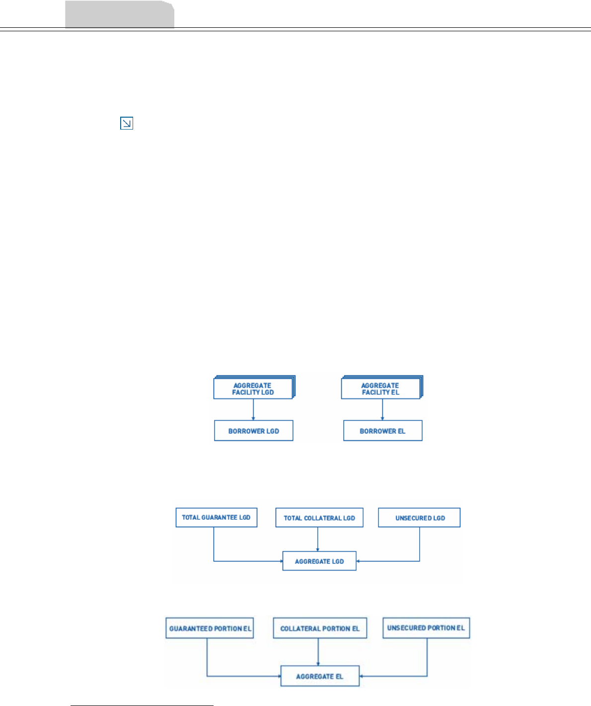
CHAPTER 7
GUIDE TO BUSINESS ANALYSIS 49
7 LOSS GIVEN DEFAULT ANALYSIS
As specified by Basel II, RiskAnalyst’s LGD calculation engine focuses at the level of the
individual facility. To assist management and validation at a customer level, it also aggregates
values up from each facility to create global customer values.
NOTE This is based on Moody's KMV understanding of the provisions of the June 2004
document, International Convergence of Capital Measurement and Capital Standards
as applied to the IRB Foundation Approach
For each facility, RiskAnalyst calculates an Exposure at Default (EAD) value. This is an estimate
of the amount that would be outstanding on the facility if the borrower defaulted.
RiskAnalyst then considers recoveries that could be obtained if the borrower were to default4.
The expected recovery can be improved by using Credit Risk Mitigants (CRMs) to enhance the
quality of the obligation. These commonly take the form of guarantees and collateral. Collateral
typically consists of a charge placed on a borrower's asset by the creditor.
RiskAnalyst also calculates Expected Loss (EL), which is the expected value of losses due to
default. This measure brings together the risk assessments of the borrower and of the borrower’s
facility or facilities.
7.1 DETERMINING LGD AND EL VALUES
RiskAnalyst determines borrower-level LGD and EL simply by summing the LGD and EL
amounts determined for each facility.
To derive the LGD of each facility, RiskAnalyst breaks up the exposure (EAD) into three
possible parts: guaranteed, collateralized, and unsecured. For each of these parts, RiskAnalyst
determines an LGD separately and then sums the LGD amounts to derive the aggregate LGD.
RiskAnalyst calculates EL in a similar way.
4 Recovery can be considered the opposite of LGD. If both are expressed as percentage factors, Recovery = 1 – LGD%.
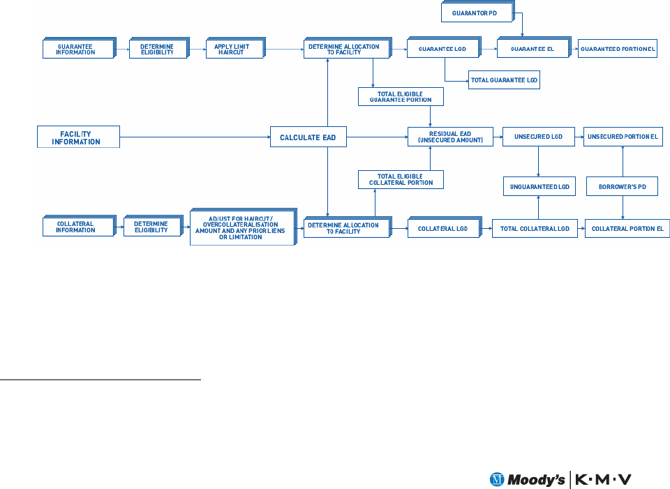
50
The following diagram and description summarizes the process used to determine the LGD
value for each component part of the overall LGD calculation. Please note that Chapter 8
provides further details of the calculations.
A given credit risk mitigant (CRM) may be applied to more than one facility (cross-
collateralization). RiskAnalyst can represent most cross-collateralization scenarios by using a
consistent approach when allocating CRMs to facilities and sharing the risk mitigating effects of
the CRMs between the facilities. By default, RiskAnalyst considers guarantees first (before
collateral), as specified in Basel II.
The system sorts each facility’s guarantees at two levels: first, according to their probability of
default (PD) and second, according to their LGD. There are complex rules governing which
guarantees are eligible to act as credit risk mitigants. Accordingly, RiskAnalyst next considers
eligibility criteria for each guarantee, applying the appropriate5 haircut and, if applicable,
limiting the guarantee’s value according to any limit specified by the user. RiskAnalyst then
determines what proportion of the guarantee to allocate to the facility by considering the size of
the exposure and the available guarantee value. Two factors impact this calculation:
1. Whether the guarantee is shared across other facilities, and how much is already allocated to
these. RiskAnalyst uses a weighting system based on EAD and user input. This is described
in more detail below.
2. How much exposure remains uncovered on this facility. If the remaining exposure is less
than the available guarantee value, the allocation is capped at this value.
Having determined the allocation for an individual guarantee, RiskAnalyst multiplies it by the
guarantor’s LGD to calculate the LGD amount.
The EL is simply the product of the LGD amount and the guarantor’s PD.
The guarantee allocations to the facility can be summed across all the guarantees on the facility
to determine a total eligible guarantee portion.
Having considered the guarantees, RiskAnalyst then considers the collateral allocations. The
process used is very similar to guarantees. One difference is that where guarantee values may
have user-defined limits, collateral items may have prior liens and limitations6.
When the system comes to consider the amount of uncovered exposure, it naturally removes the
amount already covered by guarantees. It is also important to note that when calculating EL for
5 The haircuts for guarantees are all zero in the version of RiskAnalyst delivered out of the box.
6 Almost all collateral items have haircuts. In the cases where Basel II specifies ‘overcollateralization amounts’, these values have
been converted to haircuts. Note that an overcollateralization amount is equal to 1/(1- haircut).

GUIDE TO BUSINESS ANALYSIS 51
each collateral item7, it is the borrower’s PD or expected default frequency (EDF) measure that
is used.
If any of the exposure is still left uncovered after applying all available guarantees and collateral,
RiskAnalyst considers this unsecured and uses the unsecured LGD% to determine an unsecured
LGD amount.
7.2 FACILITY STATUS
Facilities and Credit Risk Mitigants can be assigned to one of three different states.
• Completed (CRMs only)
• Committed (Facilities only)
• Proposed
These different states allow you to add or remove facilities and CRMs from the LGD and EL
calculations without deleting facilities and CRMs from the system.
7.3 CALCULATING GRADES
RiskAnalyst calculates a facility grade for the LGD dimension by mapping the LGD grade from
the LGD% value calculated for the facility. The system displays this as the Facility Grade on the
Facilities Summary screen. Additionally, the system displays an EL grade, which is either a
direct mapping from the EL value or a combined mapping of the borrower grade and facility
grade.
7 As for guarantees, EL is the product of the PD and the LGD amount.

CHAPTER 8
GUIDE TO BUSINESS ANALYSIS 53
8 LOSS GIVEN DEFAULT CALCULATIONS
In the previous section, we presented the structure that RiskAnalyst uses to analyze LGD. In
this section we fill in the detail, specifying how RiskAnalyst performs each of the steps already
outlined. We first consider EAD calculations and then move on to the CRMs. For both
guarantees and collateral, we look at the eligibility criteria and parameters used to determine the
CRM values. In addition, we specify minimum LGD values8 for collateral. Then we move on to
describe the methods used to allocate these CRMs to facilities. The calculation of the unsecured
portion’s LGD is considered next. Finally, we examine the way in which PDs are brought into
the LGD module.
8.1 CALCULATING EADS
Facility-level exposure at default (EAD) is determined using the following process:
• Determine the used and unused parts of the facility.
• The used part is simply the utilization entered by the user.
• The unused part is the commitment (also entered by the user) less the used part.
• Determine the Credit Conversion Factor (CCF) to be utilized for the used and unused
parts of the facility. These will be based on the Facility Type and up to three sub-types.
CCFs are simply numbers used to convert off-balance-sheet items into credit
equivalents by recognizing the inherent risk in various types of items.
• Multiply the used part of the facility by the CCF for the used part and add this to the
product of the unused part of the facility and the unused CCF for the facility.
If the Facility has both utilization and a commitment, then the EAD is the sum of:
• The utilization and CCF for the used part of the facility
• (Commitment minus utilization) multiplied by the CCF for the unused portion
If the Facility only has utilization, then the EAD is the value entered multiplied by the used
portion CCF.
If the Facility only has a commitment, then the EAD is the CCF for the unused portion
multiplied by the value entered.
If there are no CCFs specified for the facility (or any of the components of the MOF), then
EAD is left blank.
In some circumstances the system does not calculate an EAD, for example, derivative
transactions. In this case, the user inputs an EAD value.
8 The LGD% values for guarantees are user input.

54
The following tables document the CCFs that RiskAnalyst uses:
Type CCF – Utilized Portion CCF – Unutilized Portion
Not
Immediately
Cancelable
Immediately
Cancelable
Not
Immediately
Cancelable
Immediately
Cancelable
Short
Term
Long
Term
Short
Term
Long
Term
Short
Term
Long
Term
Short
Term
Long
Term
Revolving Line of Credit 100% 100% 100% 100% 75% 75% 0% 0%
Term Loan 100% 100% 100% 100% 75% 75% 0% 0%
Short Term Loan 100% 100% 100% 100% 75% 75% 0% 0%
Letter of Credit, Trade
Transaction Related
20% 50% 20% 50% 20% 50% 0% 0%
Letter of Credit, Financial
Guarantee
100% 100% 100% 100% 100% 100% 0% 0%
Bonds 50% 50% 50% 50% 50% 50% 0% 0%
Banker’s Acceptance 20% 50% 20% 50% 20% 50% 0% 0%
Indemnities 50% 50% 50% 50% 50% 50% 0% 0%
Bank Guarantee 100% 100% 100% 100% 100% 100% 0% 0%
Forward Currency Contract N/A N/A N/A N/A N/A N/A N/A N/A
Interest Rate Swap N/A N/A N/A N/A N/A N/A N/A N/A
Currency Swap N/A N/A N/A N/A N/A N/A N/A N/A
Other Derivative N/A N/A N/A N/A N/A N/A N/A N/A
Floor Plan Line of Credit 100% 100% 100% 100% 75% 75% 0% 0%
Credit Cards 100% 100% 100% 100% 75% 75% 0% 0%
Negotiations 20% 50% 20% 50% 20% 50% 0% 0%
Overdraft 100% 100% 100% 100% 75% 75% 0% 0%
If using UK English for your language settings, the system uses the following facility types:
Type CCF – Utilised Portion CCF – Unutilised Portion
Not
Immediately
Cancellable
Immediately
Cancellable
Not
Immediately
Cancellable
Immediately
Cancellable
Short
Term
Long
Term
Short
Term
Long
Term
Short
Term
Long
Term
Short
Term
Long
Term
Overdraft 100% 100% 100% 100% 75% 75% 0% 0%
Short Term Loan 100% 100% 100% 100% 75% 75% 0% 0%
Term Loan 100% 100% 100% 100% 75% 75% 0% 0%
Letter of Credit, Trade
Transaction Related
20% 50% 20% 50% 20% 50% 0% 0%
Letter of Credit, Financial
Guarantee
100% 100% 100% 100% 100% 100% 0% 0%
Revolving Credit 100% 100% 100% 100% 75% 75% 0% 0%
Bonds 50% 50% 50% 50% 50% 50% 0% 0%
Banker’s Acceptance 20% 50% 20% 50% 20% 50% 0% 0%
Indemnities 50% 50% 50% 50% 50% 50% 0% 0%
Bank Guarantee 100% 100% 100% 100% 100% 100% 0% 0%
Forward Currency Contract N/A N/A N/A N/A N/A N/A N/A N/A
Interest Rate Swap N/A N/A N/A N/A N/A N/A N/A N/A
Currency Swap N/A N/A N/A N/A N/A N/A N/A N/A

GUIDE TO BUSINESS ANALYSIS 55
Other Derivative N/A N/A N/A N/A N/A N/A N/A N/A
Stocking Loan 100% 100% 100% 100% 75% 75% 0% 0%
Credit Cards 100% 100% 100% 100% 75% 75% 0% 0%
Negotiations 20% 50% 20% 50% 20% 50% 0% 0%
8.2 GUARANTEES
8.2.1 Haircuts Applied to Guarantees
A haircut is normally applied to a CRM in order to account for the risk of a fall in the value of
the CRM held prior to default or during the close-out period. RiskAnalyst is shipped with
haircuts for guarantees with values of zero. The system user is expected to enter the true
expected realization of the guarantee into the ‘Valuation’ field when adding or editing
guarantees in RiskAnalyst.
Type Eligible Personal Min PD Max
Eligible PD
Haircut
Corporate Yes No 0.03% 0.09% 0
Bank Yes No 0.03% N/A 0
Securities Firm Yes No 0.03% N/A 0
Public Sector Entity Yes No 0 N/A 0
Sovereign Yes No 0 N/A 0
Personal No Yes N/A N/A 0
8.2.2 Eligibility Criteria for Guarantees
By default, RiskAnalyst uses the following criteria to determine whether guarantees are eligible:
• The guarantee must be issued by an organization. Personal guarantees are not eligible.
• The guarantee PD must be less than or equal to the borrower’s.
• The guarantee EL (PD × LGD%) must be less than the product of the borrower’s PD
and the LGD% value used for the unsecured portion of the facility.
• If the guarantor is a corporate, the guarantor’s PD must be less than or equal to nine
basis points (0.09%).

56
8.3 COLLATERAL
8.3.1 Mapping RiskAnalyst Collateral Types to Basel II
Collateral Types
The following table provides a mapping from the RiskAnalyst Collateral Types to their Basel II
equivalents:
RiskAnalyst Collateral Type Basel II Collateral Type
Debtors/
Accounts Receivable (Less Than 1 Year)
Receivables
Stock/
Inventory
Other
Plant/Equipment/Furniture/Fixtures Other
Agricultural Charge Other
Land/Property/Real Estate CRE/RRE
Debt Securities Financial Collateral
Cash Financial Collateral
Gold Financial Collateral
UCITS/Mutual Funds Financial Collateral
Life Policies Other
Other Other
8.3.2 Calculating Haircuts for Financial Collateral
RiskAnalyst uses the following table for specifying the base haircuts for financial collateral.
These are taken from Basel II.
Issue rating for debt
securities
Residual Maturity Sovereigns Other Issuers
≤ 1 year 0.5 1
>1 year, ≤ 5 years 2 4
AAA to AA-/A-1
> 5 years 4 8
≤ 1 year 0.5 1 1 2
>1 year, ≤ 5 years 3 6
A+ to BBB-/ A-2/A-3 and
unrated bank securities
per para 116(d)
> 5 years 6 12
BB+ to BB- All 15 N/A
Main index equities and Gold 15
Other equities listed on a recognized exchange 25
UCITS/Mut Fund, Cash only 0
UCITS/Mut Fund, Sovrgn AA-/A-1 Bonds or better 4%
UCITS/Mut Fund, Other AA-/A-1 Bonds or better 8%
UCITS/Mut Fund, Sovrgn BBB-/C-1 Bonds or better 6%
UCITS/Mut Fund, Other BBB-/C-1 Bonds or better 12%
UCITS/Mut Fund, Sovrgn BB- Bonds or better 15%
UCITS/Mut Fund, Main Index Equities or better 15%
UCITS/Mut Fund, Oth Eqties Lstd on Recgnzd
Exchnge or better
25%
UCITS/Mut Fund, Other N/A
Cash in the same currency 0

GUIDE TO BUSINESS ANALYSIS 57
These haircuts are based on the assumption of ‘daily mark to market, daily remargining and a
ten business day holding period’. Basel II also states that, for secured lending, a minimum
holding period of 20 days is appropriate and provides two formulae for transforming the
haircuts.
One formula allows transformation of the holding period under which the asset’s volatility was
determined into the minimum holding period:
HM=HN√(TM/TN)
• HM is the haircut under the minimum holding period.
• HN is the haircut based on a holding period TN
• TM is the minimum holding period for the transaction type (in this case, secured
lending).
• TN is the holding period used by the bank to determine HN
A subsequent formula allows the determination of the appropriate haircut when the frequency
of remargining or revaluation is longer than the minimum.
H = HM √{[NR + (TM – 1)]/TM}
• H is the required haircut.
• NR is the actual number of days between revaluations or remargining.
RiskAnalyst uses the above formulae to transform the supervisory haircuts. It assumes secured
lending and daily revaluation. Therefore, TM is 20, TN is 10, and NR is 1.
8.3.3 Haircuts for Non-Financial Collateral
As mentioned above, the overcollateralization levels specified by Basel II can be transformed
into haircuts using the formula: haircut = 1/(1 – overcollateralization level).
RiskAnalyst uses the following haircuts for eligible non-financial collateral:
Type Haircut
Receivables (≤1yr) – Not Affiliate 20%
Receivables (≤1yr) – Affiliate N/A
Inventory – Physical Inspection Performed 28.57143%
Inventory – No Physical Inspection Performed N/A
Plant/Equipment/Furniture/Fixtures (excl
Leasehold Imprvmnts)
28.57143%
Leasehold Improvements N/A
CRE/RRE – No Dependence btwn Borrower &
Property
28.57143%
CRE/RRE – Dependence btwn Borrower &
Property
N/A
Agricultural Charge 28.57143%
Life Policies – With Surrender Value 28.57143%
Life Policies - Other N/A
Other 28.57143%

58
If using UK English for your language setting, the system uses the following collateral types:
RiskAnalyst Collateral Type Haircut
Debtors (≤1yr) – Not Affiliate 20%
Debtors (≤1yr) – Affiliate N/A
Stock – Physical Inspection Performed 28.57143%
Stock – No Physical Inspection Performed N/A
Plant/Equipment/Furniture/Fixtures 28.57143%
CRE/RRE – No Dependence btwn Borrower &
Property
28.57143%
CRE/RRE – Dependence btwn Borrower &
Property
N/A
Agricultural Charge 28.57143%
Life Policies – With Surrender Value 28.57143%
Life Policies - Other N/A
Other 28.57143%
8.3.4 Prior Liens and Limitations
Users can enter the values of any prior liens and limitations representing the situation where
other creditors have charges issued against a piece of collateral. For each item of collateral,
RiskAnalyst deducts any prior liens and then caps the collateral valuation to the value of the
limitation. This is done after any haircut has been applied to the collateral valuation.
8.3.5 Eligibility Criteria for Collateral
There are a number of eligibility criteria that must be met in order for an item of collateral to be
considered eligible within RiskAnalyst. These are based around the Basel II requirements.
However, it is envisaged that a bank will need to implement its own policy to handle any
additional aspects not addressed as standard. To support this, where appropriate, the help
system describes some of the Basel II requirements.
The following sections describe the criteria encoded within RiskAnalyst.
First Charge Required
Some non-financial collateral types are not eligible if a second or subsequent charge has been
taken. The following table documents this:
Type First Charge Required
Receivables (≤1yr) – Not Affiliate No
Receivables (≤1yr) – Affiliate N/A
Inventory – Physical Inspection Performed Yes
Inventory – No Physical Inspection Performed N/A
Plant/Equipment/Furniture/Fixtures (excl
Leasehold Imprvmnts)
Yes
Leasehold Improvements N/A
CRE/RRE – No Dependence btwn Borrower &
Property
No
CRE/RRE – Dependence btwn Borrower & N/A

GUIDE TO BUSINESS ANALYSIS 59
Property
Agricultural Charge Yes
Life Policies – With Surrender Value Yes
Life Policies - Other N/A
Other Yes
If using UK English for your language setting, the system uses the following collateral types:
RiskAnalyst Collateral Type First Charge Required
Debtors (≤1yr) – Not Affiliate No
Debtors (≤1yr) – Affiliate N/A
Stock – Physical Inspection Performed Yes
Stock – No Physical Inspection Performed N/A
Plant/Equipment/Furniture/Fixtures Yes
CRE/RRE – No Dependence btwn Borrower &
Property
No
CRE/RRE – Dependence btwn Borrower &
Property
N/A
Agricultural Charge Yes
Life Policies – With Surrender Value Yes
Life Policies – Other N/A
Other Yes
Eligibility Criteria based on Seniority
If the facility ‘Seniority’ is set to ‘Subordinated,’ only financial collateral is eligible. The
following table describes RiskAnalyst’s behavior:
(The only differences between MMAS, IFT, and ESM are minor spelling changes).
Type Eligible for Subordinated Facilities
Cash Yes
Gold Yes
Equity, Listed on Main Index Yes
Equity, Listed on Recognized Exchange Yes
Equity, Unquoted N/A
Debt Secrty, Sovrgn, AAA/AA/A-1, ≤1yr Yes
Debt Secrty, Other, AAA/AA/A-1, ≤1yr Yes
Debt Secrty, Sovrgn, AAA/AA/A-1, >1, ≤5yrs Yes
Debt Secrty, Other, AAA/AA/A-1, >1, ≤5yrs Yes
Debt Secrty, Sovrgn, AAA/AA/A-1, >5yrs Yes
Debt Secrty, Other, AAA/AA/A-1, >5yrs Yes
Debt Secrty, Sovrgn, A/BBB/A-2/A-3/P-3, ≤1yr Yes
Debt Secrty, Other, A/BBB/A-2/A-3/P-3, ≤1yr Yes
Debt Secrty, Other Qualifying Bank, •1yr, see Help Yes
Debt Secrty, Sovrgn, A/BBB/A-2/A-3/P-3, >1, ≤5yrs Yes

60
Debt Secrty, Other, A/BBB/A-2/A-3/P-3, >1, ≤5yrs Yes
Debt Secrty, Other Qualifying Bank, >1, ≤5yrs, see Help Yes
Debt Secrty, Sovrgn, A/BBB/A-2/A-3/P-3, >5yrs Yes
Debt Secrty, Other, A/BBB/A-2/A-3/P-3, >5yrs Yes
Debt Secrty, Other Qualifying Bank, >5yrs, see Help Yes
Debt Secrty, Sovrgn, BB Yes
Debt Secrty, Other N/A
UCITS/Mut Fund, Cash only Yes
UCITS/Mut Fund, Sovrgn AA-/A-1 Bonds or better Yes
UCITS/Mut Fund, Other AA-/A-1 Bonds or better Yes
UCITS/Mut Fund, Sovrgn BBB-/C-1 Bonds or better Yes
UCITS/Mut Fund, Other BBB-/C-1 Bonds or better Yes
UCITS/Mut Fund, Sovrgn BB- Bonds or better Yes
UCITS/Mut Fund, Main Index Equities or better Yes
UCITS/Mut Fund, Oth Eqties Lstd on Recgnzd
Exchnge or better
Yes
UCITS/Mut Fund, Other N/A
Minimum Collateralization Level Restrictions
Under Basel II, a minimum collateralization level is specified for certain collateral types9. This
can be summarized as a requirement that, if the collateral is to be eligible, the collateral’s value
must provide significant coverage of the exposure.
The following table provides details of minimum collateralization levels by collateral type10.
Note that all financial collateral has a minimum collateralization level of 0.
Type Minimum Collateralization Level
Receivables (≤1yr) – Not Affiliate 0
Receivables (≤1yr) –Affiliate N/A
Inventory – Physical Inspection Performed 30%
Inventory – No Physical Inspection Performed N/A
Plant/Equipment/Furniture/Fixtures (excl
Leasehold Imprvmnts)
30%
Leasehold Improvements N/A
CRE/RRE – No Dependence btwn Borrower &
Property
30%
CRE/RRE – Dependence btwn Borrower &
Property
N/A
Agricultural Charge 30%
Life Policies – With Surrender Value 30%
Life Policies - Other N/A
Other 30%
9 These types are CRE/RRE and Other Collateral.
10 A minimum collateralization level of zero effectively means that there is no minimum collateralization level applicable to the
collateral type.

GUIDE TO BUSINESS ANALYSIS 61
If using UK English for your language setting, the system uses the following collateral types:
RiskAnalyst Collateral Type Minimum Collateralisation Level
Debtors (≤1yr) – Not Affiliate 0
Debtors (≤1yr) –Affiliate N/A
Stock – Physical Inspection Performed 30%
Stock – No Physical Inspection Performed N/A
Plant/Equipment/Furniture/Fixtures 30%
CRE/RRE – No Dependence btwn Borrower &
Property
30%
CRE/RRE – Dependence btwn Borrower &
Property
N/A
Agricultural Charge 30%
Life Policies – With Surrender Value 30%
Life Policies - Other N/A
Other 30%
The purpose of the Minimum Collateralization Requirement is to ensure that any piece of non-
financial collateral allocated to a facility it is of sufficient value compared to the facility to make
the allocation worthwhile. RiskAnalyst uses the following to determine whether collateral has
met the required Minimum Collateralization level.
• Determine the discounted value for each piece of eligible collateral for which the
minimum collateralization amount is zero.
o The collateral details MIN_COLLAT_AMOUNT specifies the minimum
collateralization amount.
o The discounted value is the valuation times the haircut.
• Determine the amount apportioned to this facility the Allocation Percent.
• Sum the discounted values for zero min-collateralization collateral. Deduct this value
from the EAD.
• If guarantees are taken first, deduct guarantee value from the EAD as well.
• Call the value of the EAD remaining after deducting items with zero min-collateralization
and guarantees EADForNonZeroMinCollat.
• Sum the base values of the remaining eligible collateral items (i.e., non-zero min-
collateralization)
o If a limitation is specified, the base value is the limitation plus any prior liens.
Otherwise it is the valuation value.
• Call the sum of these base values NonZeroMinCollat
• Determine M as follows: NonZeroMinCollat divided by EADForNonZeroMinCollat.
• If M is less than the maximum MIN_COLLAT_AMNT for the piece of collateral, then
the piece of collateral has not passed the Minimum Collateralization test. Otherwise, it
has.
Other Eligibility Criteria
In addition to the above criteria, RiskAnalyst ignores collateral where the collateral LGD% is
greater than the unsecured LGD% for the facility.
8.3.6 Collateral Minimum LGD% Values
The following table specifies the minimum LGD% values for each collateral type. Note that all
financial collateral has a minimum LGD of 0%.

62
RiskAnalyst Collateral Type Minimum LGD Value
Receivables (≤1yr) – Not Affiliate 35%
Receivables (≤1yr) –Affiliate N/A
Inventory – Physical Inspection Performed 40%
Inventory – No Physical Inspection Performed N/A
Plant/Equipment/Furniture/Fixtures (excl
Leasehold Imprvmnts)
40%
Leasehold Improvements N/A
CRE/RRE – No Dependence btwn Borrower &
Property
35%
CRE/RRE – Dependence btwn Borrower &
Property
N/A
Agricultural Charge 40%
Life Policies – With Surrender Value 40%
Life Policies - Other 40%
Other 40%
If using UK English for your language setting, the system uses the following collateral types:
RiskAnalyst Collateral Type Minimum LGD Value
Debtors (≤1yr) – Not Affiliate 35%
Debtors (≤1yr) –Affiliate N/A
Stock – Physical Inspection Performed 40%
Stock – No Physical Inspection Performed N/A
Plant/Equipment/Furniture/Fixtures 40%
CRE/RRE – No Dependence btwn Borrower &
Property
35%
CRE/RRE – Dependence btwn Borrower &
Property
N/A
Agricultural Charge 40%
Life Policies – With Surrender Value 40%
Life Policies - Other 40%
Other 40%
The user can override these values in RiskAnalyst. The system has a configurable restriction on
these overrides and, as shipped, these LGD% values can only be increased by the user.

GUIDE TO BUSINESS ANALYSIS 63
8.4 ALLOCATING CRMS TO FACILITIES
Allocating CRMs to facilities is straightforward in cases where a single CRM is allocated to a
single facility, but in practice it is common for more complex relationships to exist between
facilities and CRMs. To handle this, RiskAnalyst uses both algorithmic and user-specified
approaches. This allows the user to capture any legal nuances while RiskAnalyst does the
number crunching.
Users allocate CRMs to facilities either by auto-allocating or by manually defining a percentage
of the CRM to each facility. Using this method, users model the many-to-many type
relationships that often occur between facilities and CRMs. In addition, fields for prior liens
and limitations allow users to capture details of charges made to other creditors.
If a CRM is shared between two or more facilities, its value needs to be split between these
facilities. RiskAnalyst uses an algorithm based on EAD weighting to apportion the CRMs. The
user is also given the option to control the allocation manually if required.
8.4.1 Automatic Allocation of CRMs using EAD Weighting
RiskAnalyst first allocates all of the guarantees11 to facilities. The following process is used:
• For each guarantee, determine all the facilities to which the guarantee is allocated.
• Find the total EAD of all these facilities.
• Determine a weighting to allocate the guarantee to each individual facility; this is the
facility EAD divided by the total EAD calculated in the previous step.
• For each facility, the guarantee allocation is the guarantee value12 times the weighting
derived in the previous step.
Having allocated guarantees, RiskAnalyst then allocates collateral. The process is similar:
• For each collateral item, determine all the facilities to which the collateral is allocated
and eligible for consideration.
• Determine the residual EAD after deducting the guarantee allocations.
• Find the total EAD of all these facilities.
• Determine a weighting to allocate the collateral to each individual facility; this is the
facility EAD divided by the total EAD calculated in the previous step.
• For each facility, the collateral allocation is the eligible collateral value13 times the
weighting derived in the previous step.
8.4.2 Manual Allocation of CRMs
RiskAnalyst also allows manual allocation of CRMs. This allocation method would be used in
situations where the EAD weighting method is not optimal. Examples include situations where
a particular CRM is tied to a specific facility, while all other CRMs are available to all facilities.
11 The text describes the configuration with which RiskAnalyst is shipped. If RiskAnalyst is configured to consider collateral before
guarantees, the ordering in this section will be reversed.
12 The expected realization after discounting with a haircut, if applied, and limiting with a limit, if present.
13 The valuation after discounting with a haircut and applying any prior liens and limitations.

64
In this situation, it is possible that CRMs could be over-allocated to the first facility while
leaving the other facilities only partially covered.
To use manual allocation, you can specify an allocation portion as a percentage value for each
facility when adding or editing a CRM.
RiskAnalyst multiplies the CRM value by the facility's allocation to determine the portion
allocated to each part of the CRM. Manual allocation and EAD weighting can be used with the
same CRM.
8.5 DERIVATION OF THE LGD FOR THE UNSECURED PORTION
OF THE FACILITY
RiskAnalyst uses the facility ‘seniority’ to determine the LGD% for the unsecured portion of
the facility. This is 45% for senior facilities and 75% for subordinated ones.
8.6 DERIVATION OF THE BORROWER PD
The PD used in the LGD module can come from one of two sources:
• The 1-Yr EDF credit measure supplied by either RiskCalc or CreditEdge.
• The equivalent PD derived from the scorecard total and grade.
The source is configurable within the Facility Configuration application in RiskAnalyst Studio.

CHAPTER 9
GUIDE TO BUSINESS ANALYSIS 65
9 LOSS GIVEN DEFAULT ALGORITHM
9.1 INTRODUCTION TO THE LGD ALGORITHM
The previous chapter provided a detailed overview of the LGD calculations in RiskAnalyst. This
chapter describes the details of the LGD algorithm used in RiskAnalyst. It is designed to enable
you to understand better the LGD functionality of RiskAnalyst.
While it is more technical and programmatic than the previous chapter, it is not a full and
complete technical specification, in that is does not describe functionality at the code level.
The flowchart below shows a simplified version of the LGD algorithm. The following sections
then describe each of the functional blocks referred to in the flowchart.
The block operations are described in two sections:
• A description section, which provides a high level English description of the purpose of
the operation, and
• An implementation section, which provides a detailed technical description of how the
operation is implemented.
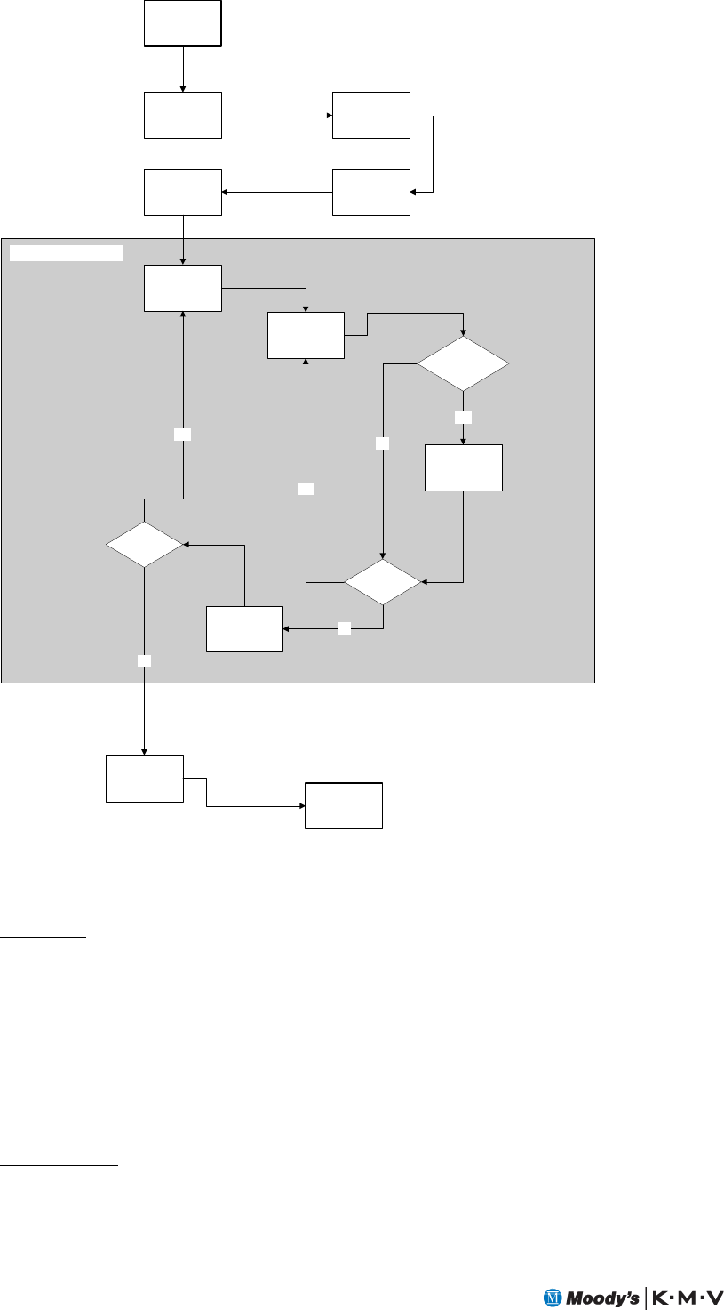
66
Begin
Calculate EAD for
all Facilities
Calculate
Allocations for all
Facilities and
CRMs
Derive Eligibility
Per Se for all
CRMs
Sort CRMs
CRMs
Remaining?
Loop through all
Facilities
Yes
Loop through all
CRMs
CRM eligible for
Facility?
Allocate CRM to
Facility
Yes
No
Calculate
Summary Level
Data
Facilities
Remaining
Yes
Calculate EL and
LGD for Facility No
No
End
LGD Calculation
9.2 LGD ALGORITHM OVERVIEW
Description
The LGD Component operates in three distinct phases:
1. A setup phase, during which data concerning Facilities, CRMs, and allocations is entered
into the engine. Facilities data is passed into the LGD engine from the LGD wrapper
2. A calculation phase, during which the LGD algorithm is run.
3. A results phase, during which results are gathered from the engine and sent to the user.
Implementation
When the calculation phase begins, the order of operation is as follows:

GUIDE TO BUSINESS ANALYSIS 67
1. Calculate EAD for each facility
2. Run the allocation algorithm for each CRM and each facility
3. Identify ineligible CRMs
4. Sort CRMs according to user-specified order
5. Calculate LGD for each facility
6. Calculate Summary Level Data
9.3 CALCULATING EAD
Description
EAD (Exposure at Default) is an estimate of the exposure on the facility at the time of default.
Implementation
EAD is either calculated or user-supplied. If a user-supplied value is entered, and it is larger than
the calculated EAD, the supplied value is the EAD value that is used. Otherwise, EAD is
calculated as follows:
EAD = (Utilized Portion * CCF for utilized Portion) + (Unutilized Portion * CCF For
Unutilized Portion)
where
• Utilized Portion = utilization
• Unutilized portion = commitment – utilization.
• CCF (Credit Conversion Factor) values are read from the LGDRefFacility table for
each facility type. CCF values can differ depending on whether or not the facility is
immediately cancelable, so this is used as another key in the LGDRefFacility table.
9.4 CALCULATE ALLOCATIONS
Description
Determine the percentage of each CRM to allocate to a facility based on the facility’s EAD
relative to the total of all EADs.
Implementation
• It is important the allocation occurs after EAD calculation, as the calculated EAD
values are required in the allocation algorithm.
• The system allocation is stored internally as a double, so 50% is stored as 0.5. When
the value is displayed to the user it is multiplied by 100 to turn it into a percentage.
• Users can supply their own allocation, in which case the user allocation will override
the system allocation.

68
For each CRM
Total EAD = sum (EAD of all facilities linked to this CRM)
For each facility
This EAD = EAD for this facility
System Allocation = This EAD / Total EAD
9.5 DERIVE CRM ELIGIBILITY
PER SE
Description
Not all CRMs can be used to support a given facility. Whether or not a CRM can be used to
support a facility is determined by its eligibility. There are two levels of CRM eligibility:
1. Per Se eligibility, whereby a CRM can be eligible or ineligible of itself, irrespective of any
relation to any facility, and
2. Per Facility eligibility, in which a facility may be eligible per se, but is nonetheless not
eligible for a particular facility. This is derived during the Allocation process.
9.5.1 Deriving CRM Eligibility
Per Se
Personal Guarantees
• In RiskAnalyst, Personal Guarantees are never eligible.
Organizational Guaranatees
An organization guarantee is eligible per se if all the conditions below are true:
• The BIS2_Eligible column in Guarantee Table (Reference Database) is true.
• The PD is less than the value in the MAX_PD column of the Guarantee Table, for this
Guarantee type.
• PD is greater than the minimum PD given in the Guarantee Table.
Collateral
A piece of collateral is eligible per se if:
• For this Credit Risk Mitigant type, the BIS2_ELIGIBLE column in the
Collateral_Details table in the reference database is set to true.
• There are Prior Liens and the REQ_FIRST_CHG column for this collateral type is set
to false.
9.6 CRM SORTING
The order in which CRMs are considered when they are being allocated to facilities makes a
difference to the results that are obtained. Two CRM ordering algorithms are supported.

GUIDE TO BUSINESS ANALYSIS 69
9.6.1 Guarantees First
Description
This algorithm allocates Guarantees, then Financial Collateral, then Non-Financial Collateral.
Implementation
This algorithm lists the guarantees towards the top of the Credit Risk Mitigant list. This is the
Basel preferred option, and the default in RiskAnalyst. The order is:
1. Eligible Guarantees
a. Organizational Guarantees First
b. Lowest EL first
c. Highest Expected Realization First
d. Most time to maturity first
e. Lowest ID first
2. Financial Collateral
a. Low LGD First
b. Where LGDs are the same (quite likely in many cases), then ordered by Minimum
Collateralization Amount (taken from the MIN_COLLAT column of the
LGDRefCollateral table).
c. Where LGD and Min. Collat. Amt. are equal, order by Potential Eligible Amount for
Facility (calculated value), largest first.
d. Most time to maturity first
3. Non-Financial Collateral
a. Low LGD First
b. Where LGDs are the same (quite likely in many cases), then ordered by Minimum
Collateralization Amount (taken from the MIN_COLLAT_AMOUNT column of the
SECURITY_DETAILS table).
c. Where LGD and Min. Collat. Amt. are equal, order by Potential Eligible Amount for
Facility (largest first).
d. Most time to maturity first
4. Ineligible Guarantees (by ID)
5. Ineligible Financial Collateral (by ID)
6. Ineligible Non-Financial Collateral (by ID)

70
9.6.2 Guarantees Second
Description
This algorithm allocates Financial Collateral, then Non-Financial Collateral, and then
Guarantees.
Implementation
This option was requested from customers. The order is:
1. Financial Collateral
a. Low LGD First
b. Where LGDs are the same (quite likely in many cases), then ordered by Minimum
Collateralization Amount (taken from the MIN_COLLAT column of the
LGDRefCollateral table).
c. Where LGD and Min. Collat. Amt. are equal, order by Potential Eligible Amount for
Facility (largest first).
d. Most time to maturity first
2. Non-Financial Collateral
a. Low LGD First
b. Where LGDs are the same (quite likely in many cases), then ordered by Minimum
Collateralization Amount (taken from the MIN_COLLAT_AMOUNT column of the
SECURITY_DETAILS table).
c. Where LGD and Min. Collat. Amt. are equal, order by Potential Eligible Amount for
Facility (largest first).
d. Most time to maturity first
3. Eligible Guarantees
a. Organizational Guarantees First
b. Lowest EL first
c. Highest Expected Realization First
d. Lowest ID first
e. Most time to maturity first
4. Ineligible Financial Collateral (by ID)
5. Ineligible Non-Financial Collateral (by ID)
6. Ineligible Guarantees (by ID)

GUIDE TO BUSINESS ANALYSIS 71
9.7 THE LGD CALCULATION
Description
Once all the data concerning CRMs and Facilities has been entered into the LGD Component,
the LGD Calculations are started by running the LGD Algorithm.
Implementation
The operation of the LGD algorithm is different depending on whether the CRM ordering
method is Guarantees First or Guarantees Second.
If Ordering is Guarantee First
Perform Guarantee First Processing and return EAD remaining after allocation
Otherwise
Perform Guarantee Second Processing and return EAD remaining after allocation
9.7.1 Guarantee First/Second Processing
Description
There are two differences between Guarantee First processing and Guarantee Second
processing:
1. The CRM sorting algorithms are different, and
2. The order in which guarantees, Zero Minimum Collateralization, and Non-Zero Minimum
Collateralization collateral are allocated to facilities is different.
9.7.2 Guarantee First Processing
Description
Guarantee First allocation allocates guarantees before collateral.
Implementation
1. Sort Guarantees
2. Allocate Guarantees
3. Sort Collateral items with zero Minimum Collateralization amounts (ZMC Collateral)
4. Allocate ZMC Collateral
5. Sort Collateral with non-zero Minimum Collateralization amounts (NZMC Collateral)
6. Allocate NZMC Collateral
9.7.3 Guarantees Second Processing
Description
Guarantee Second allocation allocates collateral before guarantees.

72
Implementation
1. Sort ZMC collateral
2. Allocate eligible ZMC collateral
3. Derive eligibility for NZMC collateral, taking minimum collateralization into account
4. Allocate eligible NZMC collateral
5. Sort guarantees
6. Allocate guarantees
9.8 PERFORM CRM ALLOCATION
Description
Allocation is the process of allocating portions of a CRM to a facility. In general, the amount of
a CRM allocated to a facility (called the ‘Eligible Amount’) will be the Mismatch-Discounted
Expected Realization multiplied by the allocation percentage. The Mismatch-Discounted
Expected Realisztion is the Expected Realiation of the CRM, discounted according to the CRM
mismatch formula specified by Basel II. The order that the CRMs are taken in is very
important, as different results will be obtained if a different ordering algorithm is used.
Implementation
The allocation process is almost the same whether we are allocating ZMC collateral, NZMC
collateral, or guarantees. The only slight difference is that when allocating NZMC collateral the
eligibility check has to take Minimum Collateralization into account.
For each CRM
If the CRM is eligible for the facility
If the mismatch-adjusted eligible amount > EAD remaining
Allocate the EAD remaining to the facility
Otherwise
Allocate the mismatch-adjusted eligible amount to the facility
Subtract the allocated amount from the EAD remaining
The LGD Amount for the CRM is (CRM LGD% x allocated amount)
9.8.1 Mismatch-Adjusted Eligible Amount
Description
This is the eligible amount, discounted to take the CRM mismatch into account. It is a
property of the CRM and a particular Facility.
Implementation
The mismatch-adjusted eligible amount is calculated from the eligible amount as follows:

GUIDE TO BUSINESS ANALYSIS 73
The Capped CRM Residual Maturity is Min (Residual Maturity of CRM in years, 5)
The Capped Facility Residual Maturity is Min (Residual Maturity Facility in years,
Capped CRM Residual Maturity)
The Adjustment Factor is (Capped CRM Residual Amount – 0.25) divided by (Capped Facility
Residual Amount – 0.25)
The Adjusted Eligible Amount is (Expected Realisation x Allocation % x Adjustment Factor)
9.8.2 Expected Realization
Description
The Expected Realization is a property of the CRM. It is the valuation of the CRM taking the
haircut, valuation, and any prior liens into account.
Implementation
If a limitation is defined
Min(Max((Valuation x (1 – Haircut)) – Prior Liens),0),Limitation)
Otherwise
Max((Valuation x (1 – Haircut)) – Prior Liens),0)
9.9 ELIGIBILITY
PER FACILITY
Description
This concerns the case in which a facility may be eligible per se, but is nonetheless not eligible
for a particular facility.
9.9.1 Implementation
CRM Mismatches
CRM Mismatches feature heavily when determining the mismatch Eligibility Conditions, as
defined below. This section defines precisely what constitutes a mismatch as far as RiskAnalyst
is concerned.
Data Requirements
When deciding whether there is a CRM mismatch, we need to consider the following data
items. Original maturities are entered in months and reflect the overall lifespan of the CRM or
Facility. Maturity Dates reflect that date when the CRM or Facility Matures. The original
maturity of a Facility is also required to calculate the Facility EAD, and as such is a compulsory
data requirement.
• The original maturity of the CRM
• The original maturity of the Facility
• The maturity date of the CRM

74
• The maturity date of the Facility
Data Conditions
a) If there is no Facility Maturity Date but there is a CRM Maturity Date, the CRM is
not eligible.
b) Otherwise, if any of the mismatch data requirements are missing, there is no
mismatch so the CRM is eligible as far as CRM maturity is concerned.
c) If neither (a) nor (b) applies, then a CRM mismatch is defined as the case where the
residual maturity of the CRM is less than that of the Facility.
Mismatch Eligibility Conditions
These conditions apply to all CRMs. Mismatches are defined as above.
• Any allocation where there is a mismatch and where the residual maturity is less than
3 months is not eligible. The residual maturity is the difference between the maturity
date of the CRM and the evaluation date.
• Any allocation where there is a mismatch and the original maturity of the CRM is
less than 1 year is not eligible.
• Any allocation where the adjusted expected realization is zero is not eligible. The
adjusted expected realization is calculated in the same way as the adjusted eligible
amount, but using an allocation of 100%.
Organizational Guarantees
An organizational guarantee is eligible for a given facility if it is eligible per se, and, for this
facility:
• Either
The Guarantor PD (PD of the guarantee) is less than the Borrower’s PD
(PD of the customer), or
(Guarantor PD x Guarantor LGD%) is less than (Borrower PD x Unsecured
LGD%)
Collateral
A piece of collateral is eligible for a given facility if it is eligible per se and, for this facility:
• If the facility is set as senior or it is set as subordinated and the
INC_SUBORDINATED column of the LGDRefCollateral table is set to true.
• The LGD% of the Credit Risk Mitigant is less than the LGD% of the unsecured
portion.
• Minimum Collateralization has been met (Non-Zero Minimum Collateralization
Collateral only. See below).

GUIDE TO BUSINESS ANALYSIS 75
9.9.2 Determining the Minimum Collateralization
Requirement
Description
The purpose of the Minimum Collateralization Requirement is to ensure that any piece of non-
financial collateral allocated to a facility is of sufficient value compared to the facility to make
the allocation worthwhile.
Implementation
• Note that the minimum collateralization test can only be carried out after:
Guarantees and ZMC items have been allocated (if guarantees taken first),
or
ZMC items have been allocated (if guarantees are taken second).
• In RiskAnalyst, the results of minimum collateralization do not affect the
facility/CRM auto-allocations.
• Determine the discounted value for each piece of eligible collateral for which the
minimum collateralization amount is zero.
The collateral details MIN_COLLAT_AMOUNT specifies the minimum
collateralization amount.
The discounted value is the valuation times the haircut.
• Determine the amount of the discounted value apportioned to this facility using both
the Allocation Percent and the EAD weighting.
• Sum the discounted values for zero min-collateralization collateral. Deduct this value
from the EAD.
• If guarantees are taken first, deduct guarantee value from the EAD as well.
• Call the value of the EAD remaining after deducting items with zero min-
collateralization and guarantees EADForNonZeroMinCollat.
• Sum the base values of the remaining eligible collateral items (i.e., non-zero min-
collateralization)
If a limitation is specified, the base value is the limitation plus any prior
liens. Otherwise, it is the valuation value.
• Call the sum of these base values NonZeroMinCollat
• Determine M as follows: NonZeroMinCollat divided by
EADForNonZeroMinCollat.
• If M is less than the maximum MIN_COLLAT_AMNT for the piece of collateral,
then the piece of collateral has not passed the Minimum Collateralization test.
Otherwise, it has passed the Minimum Collateralization test.

76
9.10 EXPECTED LOSS
Description
If no guarantees are present this is the borrower's PD multiplied by the total LGD amount. If
guarantees are present it is the borrower's PD multiplied by the sum of LGD Amounts for the
Collateralized and Unsecured portions of the facility plus, for each guarantee, the PD for the
guarantee multiplied by its LGD.
Implementation
If (Eligible Amount for Guarantees) is not zero
For each Guarantee associated with the facility
Determine the EL amount (Guarantor PD x Guarantee LGD Amount)
Determine the Total EL Amount for Guarantees
EL Amount for Collateralized Portion = LGD Amount for Collateral x Borrower PD
EL Amount for Unsecured Portion = LGD Amount for Unsecured Portion x Borrower PD
EL Amount = EL Amount for Guarantees +
EL Amount for Collateralized Portion +
EL Amount for Unsecured Portion
Otherwise
EL Amount = Borrower PD x Total LGD Amount
9.11 CALCULATE EL AND LGD DATA FOR THE FACILITY
After calling the main LGD Calculation algorithm, the following values are calculated:
• Unsecured Amount = EAD remaining after allocation
• Unsecured LGD Amount = Unsecured Amount x LGD% for unsecured portion
• UnGuaranteed LGD Amount = Unsecured LGD Amount + LGD Amount for
Collarateral
• UnGuaranteed LGD Percent = UnGuaranteed LGD Amount / Portion of EAD not
covered by guarantees
• UnGuaranteed EL Amount = Borrower PD x UnGuaranteed LG Amount
• EL Percent = EL Amount / EAD

GUIDE TO BUSINESS ANALYSIS 77
9.12 CALCULATE EL AND LGD DATA ACROSS ALL FACILITIES
Description
Once EL and LGD data have been calculated for each facility, we can then produce summary
level data across all the facilities in the system. The values calculated are as follows:
• Total EAD = Sum of all EAD of all Facilities
• Total LGD Amount = Sum of LGD Amounts for all Facilities
• Aggregate LGD Percent = Total LGD Amount / Total EAD
• Aggregate EL Amount = Sum of EL Amounts for all Facilities
• Aggregate EL Percent = Aggregate EL Amount / Total EAD

CHAPTER 10
GUIDE TO BUSINESS ANALYSIS 79
10 FACILITY SUMMARY
10.1 FACILITY SUMMARY
The Facility Summary screen displays the list of facilities, with their status and the calculated
LGD and EL values. It also shows the aggregated values, providing a picture of the overall
facility risk for the customer. The LGD value is mapped to a Facility Grade, and the EL Grade
represents a combination of the borrower grade and facility grade or a direct mapping from the
EL value (This is configurable in Facility Configuration).
10.1.1 Customer information bar
The customer information bar provides useful information about the customer, including the
Borrower Grade and Equivalent PD. These values are taken from the Ratings Summary screen,
and if an override has been authorized, the override values will be the ones displayed. The
system also displays the 1 Yr EDF value as well as the Expected Loss PD. The latter value is the
Equivalent PD or the 1 Yr EDF value divided by 100, depending on how the LGD model you
are using has been configured. Again, if an override has been authorized, and the LGD model is
configured to use the Equivalent PD, the system will use the Override PD in this calculation.
10.1.2 Switching between Proposed and Existing Positions
The Facility Summary, Facility Detail, and CRM Summary screens include radio buttons to
select Proposed or Existing Positions. This allows you to view the impact of proposed facilities
and proposed Credit Risk Mitigants on your overall LGD and EL calculations. In effect, the
toggle lets you choose which facilities and CRMs to include or exclude from the calculations. If
you select Proposed Position, all committed and proposed facilities and CRMs will be taken
into account. Alternatively, selecting Existing Position only includes those facilities and CRMs
that are committed or completed.
The radio buttons may appear grayed-out if you must be in a certain position to perform the
current function. For example, if you try to edit a proposed facility from the Facility Summary
dialog box, the system will display the Facility Detail dialog box locked into the Proposed
Position. Since you must be in Proposed Position to edit a proposed facility, the system will not
allow you to change to the Existing Position.
10.1.3 Selecting the Evaluation Date
RiskAnalyst uses the evaluation date selected on the Facility Summary screen to determine
maturity mismatches. The system uses the date selected in this field as the reference point
against which to compare the maturity dates entered for facilities and CRMs. For example, if
you select April of the current year as your evaluation date, CRMs and facilities with a maturity
date of March of the current year will be considered by the system to have reached maturity.
You can select a distinct evaluation date for the proposed position and for the existing position.
Simply select the position, and then select your evaluation date.

CHAPTER 11
GUIDE TO BUSINESS ANALYSIS 81
11 ARCHIVE
11.1 ARCHIVE OVERVIEW
The Archive module captures all data in the customer database, both financial and rating, and
stores it in an archive database. Archive allows you to capture data at key points in the case’s
lifecycle so that you can record a ratings history of your borrowers. You can archive an
individual customer manually, configure the system to automatically archive a customer based
on its current state, or perform a batch archive on several customers at once.
In addition to the data in the customer database, Archive also stores special archive fields, such
as the reason for the Archive, which can later be queried in the database. While the system
comes with some of these fields predefined, you can customize them and add new ones to allow
for more successful queries. Archive also stores RiskAnalyst, financial template, and internal
rating model version information to ensure the data is restored within the proper analysis
context.
For more information on archiving data, retrieving archived data, and configuring the Archive
module, consult the RiskAnalyst Help, RiskAnalyt Batch Help, and Configuration Console
Help.

APPENDIX A
GUIDE TO BUSINESS ANALYSIS 83
A APPENDIX A - INTERNAL RATING TEMPLATES
A.1 The Internal Rating Template Concept
Moody’s KMV is well known as a leading provider of benchmark rating models. We offer
proprietary models developed to extremely high standards to assess both borrower and portfolio
risk. The borrower models are developed using large data sets specific to regions of the world
and provide very powerful external default predictions.
According to recent proposals under the auspices of Basel II, lending institutions wishing to
follow the ‘Internal Ratings Based Approach’ need to create and own their rating models and
ensure that they meet certain criteria. The models should be tailored to their portfolio of
customers which dovetail into their credit culture.
Typically, the creation of an internal rating system is a major undertaking for an institution. It
requires considerable resources to design and build both model and delivery platform. We
believe that in many cases a vendor solution can provide a more expedient solution than the
undertaking to create such a system from scratch.
We supply tools and services to address this need. The RiskAnalyst platform is designed to assist
institutions in deploying their models. Internal rating templates (IRTs) are designed to form the
basis for the rating models delivered within the rating system.
The aim of the IRTs is to provide pre-constructed borrower rating models that can be used by
institutions as a starting point for their own rating models. In order to achieve this goal, IRTs
(as shipped) have been designed with the following requirements in mind:
• They should have the capability to rank-order borrowers effectively.
• They should provide an internal rating model that can be used by lenders throughout the
world with limited configuration 14.
• The analysis is to be based on a rating methodology that is intuitive to credit analysts.
• The set of factors included should be broad, as it is easier to remove factors than add new
ones.
• The set of factors should span the key attributes that an experienced credit analyst would
consider important to an analysis.
• The factors should be tailored to be as objective as possible, supporting consistent
evaluation by credit analysts.
In order to attain these objectives, Moody’s KMV works with selected partners to create the
IRTs. These partners typically comprise members of the RiskAnalyst Advisory Group
(MRAAG). The MRAAG members are senior risk managers from credit institutions selected
from the key users of Moody’s KMV internal rating solutions. MRAAG provides Moody’s
KMV with strategic direction and expertise that is incorporated within the RiskAnalyst
framework.
14 It is our view that it is not possible to ship an internal rating template that involves a judgmental analysis fully configured to
predict default.

84
The partners’ role involves providing input into the IRT design and its parameters, reviewing
the IRT, and providing data in the form of anonymous customer data together with the grades
assigned to those customers. Approximately 100 customers are provided by each participant.
A.2 The Methodology Used to Create Internal Rating Templates
A.2.1 The Internal Rating Template Creation Process
The following table outlines the approach that Moody’s KMV uses to create the IRTs. More
detail about the participants follows the table.
Phase Purpose/Task Participants
Identify scope Determine which business areas to address (industry, size, regions)
and the implementation framework required (scorecard, multi-layer).
MRAAG, Moody’s KMV
Identify partners Identify the partners who will participate and determine the roles
that they will play.
MRAAG, Moody’s KMV,
Other interested parties
Design Determine main components of IRTs, including preliminary (paper-
based) tuning.
Moody’s KMV
Partner review Review specifications. Partners, Domain Experts,
Moody’s KMV
Build prototype Build a working prototype of the design. Moody’s KMV
Acquire data Partners provide a pre-specified number of cases to support IRT
verification.
Partners, Moody’s KMV
Tune Moody’s KMV and Domain Experts adjust IRT parameter values
using expertise and a sample of the available data.
Moody’s KMV, Domain
Experts
Test performance The IRT is tested against the remaining data and other quality
standards.
Partners, Moody’s KMV,
Domain Experts
Implement The model is implemented as a production quality piece of software
into the RiskAnalyst framework.
Moody’s KMV
Quality assurance Testing is performed to ensure that the implemented IRT and its
documentation meet Moody’s KMV standards. Tests are performed
to ensure the IRT rates companies identically to the completed
prototype
Regression test scripts are created.
Moody’s KMV
Create documentation Creation of documentation to support the model. Moody’s KMV
Domain Experts are experts in the particular area of lending that the IRT addresses. They may
come from within Moody’s KMV or one of the organizations supporting the IRT development.
Domain experts help with the design and tuning of the IRT.
Partners are the organizations that have volunteered to support the verification of the
development. Organizations may be Partners and provide Domain Experts.
A.2.2 Tuning the Internal Rating Template
Tuning is the process of specifying and adjusting the parameters used within the IRT. The
approach used to determine the parameters of the IRTs uses a combination of expert judgment
and data-driven optimization using sample data provided by the development partners. This
approach supports the creation of an IRT with many parameters using limited data sets and
differs considerably to the approach we use for developing our quantitative models15. This is due
to several differences:
15 We provide detailed information on model development methodologies for our quantitative models in the form of white
papers. These can be found at http://www.moodyskmv.com/research/defaultrisk.html.

GUIDE TO BUSINESS ANALYSIS 85
1. Size of sample data sets upon which the IRTs are built. The IRTs evaluate judgmental
inputs in addition to financial ones. It is not normally possible to obtain large numbers
of cases with judgmental data within the timeframe for building the IRTs. This is due
to the cost of acquiring the data; for each test case an experienced and knowledgeable
credit analyst must determine the values for each judgmental attribute.
2. Optimization criteria. The IRT is optimized against the internal ratings assigned to
businesses by experienced lenders. It is generally not possible to obtain large enough
sample data sets that include judgmental factors to optimize against default
information. In addition, it is problematic to determine the values of judgmental
inputs retrospectively; for example, if a credit analyst knows that a customer has
defaulted, this is likely to impact the analyst’s evaluations of the judgmental inputs.
3. Expected use of the IRT. It is envisaged that each purchaser of an IRT will make
changes to ensure that it fits better with the local requirements associated with their
credit culture and portfolio. Therefore, although the performance of the standard IRT
should be good, it does not need to be as optimized as an external model that will be
used without any subsequent changes.
The hybrid IRT tuning approach is outlined below:
Tuning Phase Activities Participants
Initial Tuning Preliminary parameters specified by business experts. These parameters are
estimated independently of the data.
Partners, Moody’s
KMV
Configuration of Ratio
Assessments
The parameters for the sub-components of the ratio assessments (absolute,
peer, slope, volatility) are largely driven from the data with expert review to
determine the final parameters. The weightings to determine the ratio
assessments from the subcomponents are derived in part by expert opinion
and in part by looking at how well each sub-component correlates to the
required ranking.
To determine the parameters for each sub-component, a comparison is made
between the component value for individual cases and the associated ranking
of the case in the sub-portfolio of test-cases.
For example, for the absolute component, the raw ratio value for each case is
plotted against the case’s ranking within the sub-portfolio. This provides a
curve from which parameter values can be inferred. A similar process is
performed for the peer rank, the slope, and the volatility index.
The sub-components are weighted together to determine an overall
assessment. This weighting is determined by a combination of expert review
and consideration of the correlation of each sub-component and the ranking
of case within the sub-portfolio.
For more information on the algorithm used to calculate ratio assessments,
see the Guide to Business Analysis.
Moody’s KMV
Refinement of scores
and weights associated
with factors and sections
The IRT is run against a sub-portfolio of the data provided by the
development partners and a genetic algorithm16 is used to identify potential
improved models. The algorithm is constrained to prevent it suggesting
models that diverge significantly from the original model determined using
the expert’s views.
Candidate models identified by the genetic algorithm are reviewed to
determine potential improvements to the initial model. These improvements
are evaluated based on their impact on model performance, and whether they
make business sense. Improvements satisfying these criteria are incorporated
into the final model.
Moody’s KMV
16 A genetic algorithm is an iterative optimization technique based on evolutionary principles. It uses the following approach:
Many possible models are generated randomly to form an initial generation. Each model within a generation is assessed against a
function chosen to provide a measure of the desirability of that model. A probabilistic function is used to determine whether to
replicate models or kill them off based on the desirability of the model. Remaining models are then combined and mutated to
form the next generation using probabilistic criteria. The process continues iteratively. The function that we use to determine
desirability considers two factors: the ability of the model to rank order the sample data in the way that the partners had, and the
‘closeness’ of the model to that specified by the experts.

86
A.2.3 Verification of the Internal Rating Template
Performance
The applicability and performance of the IRTs are evaluated using a combination of expert
review and testing against customer data rated by experienced credit professionals. To
distinguish this process from the testing performed on Moody’s KMV quantitative models, the
term verification (as opposed to validation) is used.
Verification is designed to achieve the following:
• Determine that the IRT can rank order companies. This rank ordering should be
reasonably robust across portfolios. This ranking should be evaluated against ratings
determined by credit professionals for cases with which they are familiar.
• Ensure that the IRT provides a sufficiently broad starting point for credit providers
who wish to use it as a basis for their internal rating system.
• Ensure that all the factors can be assessed as objectively as possible and that the data
required to enter them is available.
• Ensure that all interim assessments are meaningful.
Verification is conceptually different to validation and calibration. The data sets available for
the verification will be much smaller than those typically used within a validation exercise and
the outputs would not be mapped to a probability of default (PD) estimate. Although
validation and calibration can, and should, be performed on internal rating models, we believe
this can best be performed in the context of the specific institution in which it will be used.
Verification is performed during two of the phases within the model development process
outlined above.
Verification Phase Activities Participants
Partner Review IRT design is reviewed against the following criteria:
• Parameters are meaningful and widely applicable
• Attributes are sufficiently broad to provide a good starting point for a
credit provider’s internal rating system
• Factors can be assessed as objectively as possible and the information
required to enter them is available
• Factor labels and answers are meaningful and intuitive
• Help text is adequate to fully explain how to answer each question
Partners, Domain
Experts, Moody’s
KMV
Performance Testing The IRT is tested against data provided by the development partners. This is
different data to that used for Tuning.
The revised IRT and the revised parameters are reviewed by domain experts.
Partners, Domain
Experts, Moody’s
KMV
A.3 Configuring Internal Rating Templates
The IRTs, when released, are designed to provide a robust starting point for a credit provider’s
internal rating model. Experienced risk personnel have contributed to their design, and data sets
from several portfolios have been used to construct and test the IRTs.
However, Moody’s KMV expects that the performance of IRTs can be improved if adapted to
the local factors of each credit provider’s portfolio and the credit culture they operate with.
Indeed, one of the aims of these products is to provide lenders with IRTs that they can quickly
and easily adapt to their specific requirements without having to build an internal rating model
from scratch. We call the process of adapting IRTs to the local environment localization.
Localization is important for a number of reasons. These include:

GUIDE TO BUSINESS ANALYSIS 87
• The importance of factors differs between portfolios. Those included in the IRT are
designed to be general and therefore are not optimized for your portfolio. Some factors may
be less relevant to your specific portfolio than is generally the case.
• There may be factors that are not included in the model that your organization deems
important or useful to the analysis of its borrowers.
• Factors included in the IRT may prove problematic for your credit analysts and/or
relationship managers. For example, the information required to answer specific factors
may be difficult or costly to accurately obtain.
• Terminology issues: nuances of specific questions or answers may differ in different regions.
• Business norms differ in different regions of the world and this may reflect in the
benchmarks against which the financial factors are assessed.
Therefore, it is important that a review of the IRT is performed. Based on our experience, this
review should occur over a period of time as you learn more about the internal rating model and
the way it behaves in your environment. It is important that you test your internal rating model
using a data set that is representative of the borrowers that you rate.
In addition, as grades assigned to borrowers normally differ between lending institutions and as
Probabilities of Default (PDs) vary between portfolios17, a calibration of grades and PDs will
need to be performed. Normally it is not possible to properly calibrate the internal rating model
before a significant amount of data has been fed through it and experience has been gained of
the borrowers rated through the system. Often institutions perform an initial calibration of
internal rating models to their grading system but avoid calibrating to PDs until this can be
done with a greater level of confidence.
Another important step is internal rating model validation. This task involves determining how
accurately the internal rating model predicts default and the confidence with which that
measure of accuracy can be stated.
This section provides an overview of the process required to configure an IRT. While reading
this section, you should bear in mind that it is our experience that there is no one correct or
normal way of configuring and implementing an IRT. Instead, we find that institutions have
their own unique circumstances and requirements and that the configuration life-cycle varies
depending on these circumstances.
A.4 A Typical Internal Rating Template Configuration Life-Cycle
The following diagram represents a typical set of tasks involved when building an internal rating
model from scratch and implementing it within a credit risk rating system:
17 The IRTs are not shipped with mappings to default probabilities.
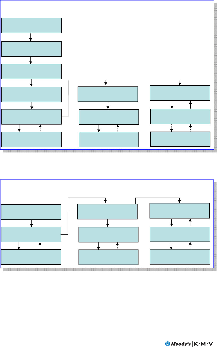
88
A typical internal rating model development life-cycle
With the IRTs, a significant part of this work has already been performed. This is reflected in
the following diagram.
A typical configuration life-cycle for an IRT
As is illustrated in the diagram, the development can be structured into three broad phases.
Model Set-up involves work performed on the IRT prior to use. This may involve some data
gathering, and is likely to require input from your credit officers.
The pilot phase normally involves a limited rollout of the IRT operated in parallel to an existing
rating process. This allows you to test it in a real environment and to capture data necessary for
further model optimization and testing; note that while financial data can often be obtained
retrospectively, it is problematic to do this with judgmental inputs.
Model Set-up Pilot Production
Model Review
Tailor
Pilot
Model Review
Tailor
Production
Val/Cal
Tailor
Tuning
Model Review
Tailor
Pilot
Model Review
Tailor
Production
Val/Cal
Tailor
Model Set-up Pilot Production
Factor Selection
Model Design
Build Model
Tuning

GUIDE TO BUSINESS ANALYSIS 89
In production, the IRT is implemented as an internal rating model. The production phase, or
phases, involve(s) using the internal rating model in a live environment, typically without the
back-up of running another rating system in parallel. The internal rating model will be run with
regular reviews of its performance and re-configuration as necessary. Often the reviews are
performed annually.
The length and content of each phase will vary depending on requirements and experience. One
of the key design aims for IRTs was to minimize the effort required within the model set-up
phase. However, there is naturally a trade-off between the effort that you put into the model
development, the timescales, and the quality of the internal rating model released into
production. This guide is intended to assist in understanding and making these decisions.
The following sections provide more detail on each of the phases and tasks. Details of phases are
presented separately to the tasks that may be performed within them.
A.4.1 Model Set-up
The Model Set-up phase is geared towards ensuring that the IRT is ready for use as part of a
pilot.
The objectives of this phase are:
• Identify those responsible for agreeing that the model is ready for pilot
• Ensure they understand RiskAnalyst and the IRT sufficiently
• Determine quality criteria for release of model into pilot
• Determine data reporting requirements for pilot
• Verify that the IRT adheres to the quality criteria and amend if necessary
The scope of this phase will vary. Many organizations spend very little time on this phase,
possibly just holding a workshop to iron out issues and determine a path forward18. It is
important that you understand the IRT and understand any compromises made for the sake of
expediency. The following paragraphs outline considerations and tasks relevant to this phase.
Identify staff
It is recommended that staff from both the relationship and the review functions are involved at
this stage. The staff selected should be experienced; they should understand how the lending
processes currently works, and should work. In addition, it is also recommended that IT staff is
involved as they will need to support the implementation and manage the data captured for
analysis.
Training
We provide documentation on the structure and use of our tools and IRTs. In addition, we
offer a number of training courses on the structure, use and configuration of our products.
Review IRT factors
Review the qualitative factors in the IRT. Ensure that these are applicable to your portfolio or
customers. Also review the possible answers to these questions and again determine whether
they are meaningful for your portfolio and can be answered by your users.
18 Moody’s KMV can lead such workshops if desired.

90
Consider whether there are factors not contained in the IRT that would normally be considered
important for your portfolio of customers. If you are interested in data on qualitative criteria, or
criteria that cannot be determined from the financial statements or other sources, it may be
advisable to add these at this stage. This will allow analysis of these factors using the data
captured during the Pilot.
Review the ratios used within the IRT. Are there any ratios that your users would normally
consider important that should be added? If a similar ratio exists within the IRT, you may
choose not to add the new ratio at this stage. Note that the financial spreads entered by the
users in the pilot will be retained and these can be used to retrospectively determine the values
for ratios not initially included in the IRT.
If new factors are added, it will be necessary to assign scores to these.
Review IRT parameters (scores and weights)
At this stage in the internal rating model development life-cycle, it is not normally
recommended that significant changes are made to the IRT’s parameters19. However, if you
wish to analyze a portfolio that is significantly different to that upon which the IRT was based,
then this may be necessary20.
Clearly, if new factors are added to the IRT, care needs to be taken to ensure that the
parameters used to assess these produce good results. Adding and deleting factors requires use of
the Internal Rating Model Author. See section A.6 Making Changes on Your Own for more
information.
In addition, one area that often merits some review is the set of scores assigned to each industry.
These are deigned to be widely applicable and your knowledge of your local markets may
indicate that some changes should be made.
Mapping the score to your Grading System
The IRT can be used within the Pilot without any grades being visible, or alternatively you can
create a mapping from the IRT scores/assessment means to a grading system. You may choose a
temporary grading system or use your existing one. Neither solution is without problems.
Using your established grading system has the merit that the meaning of the internal rating
model’s output will be readily understood by pilot users. However, some care should be
exercised; if the system is mis-calibrated, this familiarity may be misleading. In addition, when
corrections are made (if significant), this can further impact confidence in the system.
Therefore, if you use this method, it may be worth undertaking the effort to run a number of
cases through the system first to form a basis for calibration.
Alternatively, if you choose to use an alternate grading system, you will avoid the risk of
confusion if the grades are mis-calibrated. However, you will place an additional learning
overhead on the users of the system as they will need to relate to a different grading system.
19 You may choose to perform a thorough overhaul of the parameters, but this would normally require analyzing a number of
customers within the system to capture data and determine levels for parameters. Normally a review of this level would be
performed after the Pilot.
20 To illustrate this, consider using the Middle Market IRT to assess quoted entities. Short term funding for quoted companies is
very different and therefore the whole area of liquidity is very different. In addition, intangible assets are often more important
and quantifiable for quoted companies (consider the brand of a large supermarket vs. a small convenience store). Therefore,
assessments of ratios based on tangible net worth will not adequately capture the business fundamentals.

GUIDE TO BUSINESS ANALYSIS 91
Mapping Grades to PDs
Normally, creating a mapping of the internal rating model output to PDs requires significant
data. This data should be representative of the portfolio under consideration and include
sufficient defaults. Ideally, this data would be gathered from the portfolio under consideration,
but this is not always practical. We can provide support in this area. Our Modeling Services
team has experience performing such work and can use our Credit Research Database (CRD) to
augment your data (financial values only), if applicable. Pooling data with other institutions
may provide an alternate solution.21
Overrides
If you have set up a grading system for the pilot, then you will almost certainly wish to allow the
users to perform overrides. By capturing override information, you will see where user views and
assigned ratings differ to those calculated by the IRT. In addition, override reasons allow
capture of a reason for the override. This can be used to support the analysis of the system’s
performance after the pilot. The set of override reasons you choose for your pilot may be more
extensive than those that you would use in a live environment.
Consider whether multiple variants of the IRT will be used
If you wish to use the IRT over a number of business units, or over different portfolios or
regions, you may wish to ultimately have multiple variants of the IRT. If the IRT will be used
for multiple segments, is your strategy to have one internal rating model, or multiple variants? If
the latter, consider what differences may be required between the internal rating models and
whether this has implications for the IRT(s) used in the pilot. Bear in mind that each time you
split your portfolio into separate internal rating models, you reduce the data set available for
future validation and calibration.
Consider Peer Data
Determine whether to use the peer database that is shipped with RiskAnalyst, or create a custom
one. As is noted below in section A.4.4, the Middle Market IRT was built around the RMA
(Risk Management Association) peer database. The results proved robust even though some of
the portfolios used in optimization and testing did not come from North America. Therefore, it
may be more expedient to use the RMA database during the pilot, particularly in view of the
time and data constraints involved in the creation of custom peers. However, it may be
beneficial during the set-up or pilot phases to review the peer quartile values against local
benchmarks and adjust the ratio assessments where necessary.
Implementation Issues
This guide is not intended as an implementation guide for RiskAnalyst. However, this section
contains some brief notes on this topic that are particularly relevant to implementing the IRT.
• Implementation Architecture – consideration needs to be given to factors such as how the
internal rating model will be distributed to its users, how updates are distributed, and where
databases storing parameters and customer data will reside. In addition, standard
procedures need to be followed (e.g., around security, data back-ups, etc).
• Data considerations – the data captured during the pilot will be used to optimize and test
the IRT before releasing it into a live environment. This data needs to be available for
review at the end of the pilot. Consider whether this data should be taken directly from the
customer database, or from the archive database. The customer database will contain the
21 There are other methods that are used to derive PDs. One method involves using a reference rating provided by a rating agency
(or other source) where the PD is known.

92
current state of each case, and therefore will contain the customer data correct as at the end
of the pilot. Customers can be archived to an archive database at set points in their life-
cycle (e.g., when a borrower grade is agreed or facilities are approved) and snapshots of the
case recorded for subsequent analysis.
• Extra pressure on your users - the pilot will need to be run in parallel with your existing
rating system. The users will be performing more work. Can anything be done to assist
them?
• Linking allocated grades to the grades/scores assigned by the IRT - when reviewing the
pilot, it will be necessary to compare the scores calculated by the IRT to those actually
allocated to the borrowers and also, if different, those determined by your existing rating
system.
• Business units/groups involved in pilot - if the IRT will eventually be used by multiple
segments of your business (different divisions, portfolios, regions, etc.), you may wish to
select more than one segment for the pilot and carefully select the segment(s) to maximize
the utility of the pilot.
• Integration within your enterprise - consider any integration requirements with your
existing systems. Normally we advise customers to limit integration work at this stage and
use manual processes instead. This reduces the upfront project scope and risk.
A.4.2 Pilot Phase
The Pilot Phase is designed to allow you to test out the IRT with real customers using a process
similar to that intended for your production rating system. We advise that the pilot is
performed in parallel to your existing rating system. This serves two purposes. The first is that it
reduces the risk that you make erroneous lending decisions, and the second is that it makes it
easier to identify differences between old and new systems and to determine whether these are
desirable or not.
The objectives of the Pilot Phase are:
• to assess the IRT’s performance both quantitatively and qualitatively,
• to identify and mitigate any model deficiencies,
• to gather data to enable you to determine how the IRT can be best optimized for your
portfolio,
• to assist you to determine whether to remove factors from the IRT (and possibly add new
ones),
• to gather sufficient data to perform a mapping of the IRT scores to your grading system (it
is unlikely that the pilot will have sufficient duration or scope to support a mapping to PDs
without supplementary data),
• to gather data that could be used to create a peer database (if required).
The following paragraphs outline items handled at the beginning or during the Pilot Phase:
Select Pilot Users
Determine which business area(s) will be involved in the pilot. If multiple segments of the
business will be using the IRT, you may wish to include more than one within the Pilot.

GUIDE TO BUSINESS ANALYSIS 93
Train Pilot Users
Provide training for the users of the Pilot system. We can deliver this training ourselves or train
your staff to deliver it. The latter approach is often used by our clients.
Implementation Issues
As mentioned above, this document is not an implementation guide and the following provides
a summary of the tasks required:
• Set up security profiles for users
• Roll-out system to pilot users
• Ensure that there are mechanisms to update the IRT or RiskAnalyst if issues arise that you
choose to address during the pilot phase
• Ensure that the data captured during the pilot is available for analysis
Data Capture and Quality Issues
During the pilot, the data captured should be monitored. Useful information may be obtained
about completeness and quality that can be addressed prior to the completion of the pilot.
The following tasks are performed at the end of the Pilot Phase to enhance the IRT and
ensure that it is ready for production.
Assess and Review IRT Performance
This task is typically addressed in several ways:
• The users of the system will be able to provide valuable insights into problems that exist
with the system. For example, certain questions may be difficult to answer, or the ratings
for some sub-assessments or borrowers may not fit with the user’s view.
• The actual ranking performance of the system should be compared to a benchmark,
possibly ratings assigned by your credit personnel, default probability measures from other
sources22, if available, or a default study if sufficient data is available.
• Review the usefulness of the factors. Do they contribute to the quality of the rating process
and do they improve the power of the IRT?
Peer Database Considerations
Review whether it is desirable to continue using the RMA peer database or whether you want to
create a peer database based on the data collected in the pilot or from data available from a third
party supplier. Alternatively, differences may often be addressed by tuning a ratio’s peer
assessment.
Optimize IRT
Make amendments to factors, if necessary, based on the IRT performance review. Then
optimize the IRT parameters. A number of techniques are available to perform this task. These
include the process used to create the IRT and the use of statistical regression techniques. Our
Modeling Services team will often use the latter approach.
22 For example, Moody’s KMV RiskCalc product.

94
Test Optimized IRT
Test the improved IRT to determine how it performs against the data collected within the Pilot.
You may choose to segment the data collected during the Pilot to ensure that the data used to
test the IRT is not used for optimization.
Calibrate the IRT to your grading system
Review the IRT scores produced using the data gathered during the Pilot. Determine cut-offs
for each grade to allow a mapping to be derived from the IRT’s score to your grading system.
If data is available, determine PD values for grades
If sufficient data is available, determine the PDs for the grades, or specific score ranges.
Review Overrides
Based on the experience of the pilot, review and amend the override reasons.
A.4.3 Production
Production involves running the IRT in a live environment. At this point, the IRT becomes an
internal rating model and should be robust and effective. However, there will still be a need to
review and improve the internal rating model at regular intervals.
The objectives of this phase, from an internal rating model maintenance/development
perspective are:
• Continue to gather data to support optimization, validation, and calibration of the
internal rating model
• Monitor performance
• Identify any deficiencies and amend
The following paragraphs provide further information on tasks and considerations.
Data Capture
Unlike the Pilot Phase, where there is an ‘end,’ at any point in time in the Production Phase, it
is likely that cases will be at various stages within their life-cycle and at various stages of
completeness. Some cases will contain work in progress, with partial data, while others will
reflect the state at a particular stage (e.g., as at the last loan review). It is recommended that the
data used for internal rating model development contains only cases at fixed points in their life-
cycle that are in a ‘completed’ state. One way to address this is to use the Archive functionality
and ensure that cases are archived at key decision points. This will allow you to pick off cases
that are in a ‘completed’ state and also determine the status of the case at that point in time. In
addition, the history of the case is maintained using the Archive, enabling you to review each
case at its key decision points.
Data Quality and Monitoring
It is important to monitor the use of the system to ensure that it is being used consistently and
properly. Considerations for data quality include:
• Is the system being used by all users and regions?

GUIDE TO BUSINESS ANALYSIS 95
• Are cases being archived when they should?
• Are there differences in usage between different divisions or regions? If so, why?
• Are there patterns in the use of the system that indicate some sort of gaming? For example,
you could measure the ratio of judgmental scores to financial scores produced by the model
and see if this varies across user groups or across time.
Assess and Review Internal Rating Model Performance
At regular periods, the performance should be reviewed against loss experience to ensure that
the internal rating model performance is not deteriorating.
Feedback from users should be obtained, as this might indicate changes in the environment that
have a negative impact on performance.
Re-optimize
It may be considered important to add, amend, or remove factors within the internal rating
model based on the review. In addition, it may prove beneficial to amend the internal rating
model parameters periodically as new data becomes available.
This task is likely to be performed less often than the review process or the process of calibration
to PDs. It is generally considered important to ensure that the internal rating model remains
relatively stable.
Validate
Periodically, it will be necessary to formally determine the internal rating model’s performance
at predicting default.
Calibrate
The internal rating model will need to be recalibrated at regular intervals to ensure that the PDs
it produces remain accurate.
Considerations for multiple versions
If the internal rating model addresses multiple segments of borrowers, the performance for each
segment should be considered. It should be determined whether a single internal rating model
can be used across segments and, if not, how different the variants should be (i.e., just different
parameters, or different parameters and factors).
A.4.4 Some Additional Information on Configuration Tasks
This section supplements the previous three, providing additional information on key topics.
Factor/ Internal Rating Model Review
In the text above, the topic of reviewing the internal rating model was covered. Often this task
will need to be performed without significant data to support decision making. The following
notes are intended to provide a set of steps to address this topic:
• Perform an overall review of the internal rating model:
o Does the structure (its division into sections) fit with the way your organization looks
at borrowers?

96
o Are you happy with the weightings assigned to the different sections (for example, you
may wish to increase the impact of the Historical Financials at the expense of the
judgmental sections that are more open to manipulation)?
• Perform a review of the judgmental factors. Consider the following:
o Are the judgmental factors appropriate to your area of operations and its culture?
o Can data be readily accessed to enable users to answer them?
o Are the answers appropriate?
o Is the Clarify text appropriate? Does it provide sufficient guidance for the users?
o Do the scores and weights assigned appear in line with your experience?
o If data is available, does the data support or contradict the weights and scores?
• Perform a review of the ratios and their assessments. Ideally this would be performed after
gathering data, but value can be gained by performing this task judgmentally:
o Do you wish to retain all the ratios? Note that some had limited power against the
portfolios used to develop the IRT. They were nevertheless retained because they are
commonly used in our clients’ internal rating systems.
o Is financial data available and sufficiently robust to allow the ratios to be calculated
reliably?
o If peer data is available, are the Peer Assessment fixed points/votes appropriate? Note
that for some of the ratios in the IRT, RMA peer data is not available.
o Are the Absolute fixed points/votes appropriate?
o Are the slope fixed points/votes appropriate?
Adding Factors to the IRT
The technical details of adding factors to an internal rating model are described in the Internal
Rating Model Author Help sytem. The following notes are intended to provide supplementary
advice:
• When adding a section:
o Do any of the existing factors fit better on this new section?
• When adding judgmental factors:
o Is the question answerable? Is the information readily available to the user?
o Are the answers as clear and objective as possible? Note that there is often a trade-off
between utility and objectivity when designing questions. Sometimes it takes several
objective questions to address the issue that a single subjective question (“How do you
rate the quality of the management?”) could address. However, the more general and
subjective a question, the less consistency there will be with the answers provided by
the users and therefore, the less it can be relied upon.
o There is merit in keeping the number of answers for each question to a minimum. If
you create a question with many possible answers, and wish to use a data-driven
approach to determine/refine the scores assigned to each answer, you will need larger
data samples to ensure that you have sufficient number of cases with each answer
selected.
o Creating good Clarify text can be challenging. Consideration should be given to
determine what the user needs to know, and what should be considered to correctly
answer each question. We put considerable effort into creating Clarify for the questions
within the IRT. Care was taken to make things as clear as possible to the user, often

GUIDE TO BUSINESS ANALYSIS 97
explaining each answer in turn. This took time, but did lead to us redefining
ambiguous questions and answers.
• When adding ratios:
o Can peer data be obtained? If not, is this important? Can the ratio be assessed
effectively using absolute and trend assessments alone?
o Are the accounts required to determine its value normally available? Are they defined in
the chart of accounts that you are using?
o Is the proposed ratio very similar to an existing ratio? If so, should the existing ratio be
removed?
• When adding values where currency matters:
o If all of the borrowers in your portfolio report their accounts in a single currency, then
this topic is unlikely to be of concern.
o Otherwise, the following issues need consideration. The value of financial items may
change if entered in, or targeted to different currencies. For example, non-ratio values
(e.g., total assets) will clearly be different when specified in different currencies. In
addition, ratio values that use accounts from more than one statement (e.g., growth
ratios, average ratios, and cash flow ratios) will change if converted into a different
currency if there are movements between the currencies. The latter issue will have a
relatively minor impact unless there are significant movements between the currencies.
In addition, there may be some debate about which currency is ‘correct,’ as this may
depend on perspective23. Therefore, in the interests of simplicity of internal rating
model construction and use, you may choose not to address the issue directly within
the internal rating model24. The currency assigned to a model can only be changed
using the Internal Rating Model Author. Currently our IRTs use ratio values, so there
is minimal concern for currency differences.
• To include an EDF measure as a component to the IRT:
o Consider whether the EDF measure should complement or replace the Historical Ratio
Assessments.
o You will need to determine if the EDF will feed into the internal rating model, and if
so, how its contribution will be utilized. One method might be to allow a certain
contribution to be driven directly from the EDF produced.
o You can also use an EDF to constrain the borrower grade, such that the final grade
cannot vary more than a certain amount from the EDF grade.
Amending/Specifying Parameters for Factors
There are many ways in which the model parameters can be derived. The best method, if there
is such a thing, will vary depending on the expertise available (business, statistical/data mining),
and available data. Consequently, instead of prescribing an approach, the following notes
provide some insights into the approach that we used to create IRTs.
• The IRTs are designed to follow a methodology similar to one that a human credit expert
would use. Typically, this means that a larger number of factors are considered than would
be used with a model that was based on a statistical design where parsimony is desirable. As
a result, the IRTs typically have many parameters. To fit this large number of parameters
using purely statistical techniques is problematic, especially when the data sets used are
small. Therefore, when building the IRT, human expertise forms the basis for most of the
23 For example, if a borrower reports in Argentine Pesos but must make repayments in US Dollars, are you interested in US Dollar
Sales Growth and Cash Flow Coverage or Argentine Peso figures?
24 It may be wise to monitor the effect of such issues if your portfolio consists of borrowers reporting in many currencies.

98
parameters, with data being used to adjust the parameters and spot misconceptions made
by the experts. The only place where the data is used to drive the base parameters is for the
sub-components of the ratio assessments. To gain more detailed information on our
approach, see Section A.2.2, Tuning the Internal Rating Template.
• When designing the model, we aim to score each attribute within a range of (0, 100), with
50 being a normal or average value. For some attributes, a skewing is applied. For example,
in most Middle Market companies intangibles have very little intrinsic value. Consequently
for ratio assessments we use Tangible Net Worth (TNW) in places where an equity value
may be used and we penalize negative TNW harshly. However, some entities will have
intangibles that have real value and we wish to compensate for this and improve the overall
assessment under these circumstances. The question ‘Intrinsic Value of Intangibles’ is
designed to capture this information and to improve the score when appropriate. Hence we
skewed the score.
• Each section has an overall score. When designing the IRTs, we aim to ensure that this is
also scored in the range (0, 100). As some of the answers to particular questions are skewed,
it is necessary to adjust the scores assigned to questions within each section to satisfy this
requirement25.
If data is available, statistical techniques are often used. Our Modeling Services team has used
such techniques to optimize many customers’ internal rating models with considerable success.
Peer Database
The peer database is used by the IRT to determine an assessment for each ratio. The database
consists of quartile values for each ratio, for different industry groups. The quartile values
comprise the median, upper quartile (75th percentile), and lower quartile (25th percentile) values
for the peer group and ratios. They allow ratio values calculated for the borrower to be
compared against the borrower’s peers, and for a ranking to be determined.
RiskAnalyst is shipped with a peer database provided by RMA (Risk Management Association).
This database is built from North American data and so may not be directly equivalent to the
peers for the borrowers that you will rate. However, this database is used by Moody’s KMV to
determine parameters for the ratio assessments. It is also used to test the IRTs, and so it is
anticipated that the assessments produced will be robust for many portfolios in different parts of
the world.
A custom peer database can be created if you have sufficient financial data or can use data
supplied by a third party. We provide a tool, Moody’s KMV Benchmark, to create a peer
database from financial statement data.
A custom peer database, as well as providing better peer ranking within your portfolio, will
allow you to create peers for new ratios that you may choose to create, and for ratios within the
IRT where RMA does not calculate peer data.
Financial Conditions
It is possible to specify conditions that prevent a borrower rating from being displayed in
RiskAnalyst. Conditions could include:
• the balance sheet balances,
• retained earnings reconcile across statements, and
• a peer group has been selected.
25 This can have a minor detrimental impact on model performance.

GUIDE TO BUSINESS ANALYSIS 99
You may wish to add extra conditions.
Internal Rating Model Validation and Calibration
This guide is not intended to address the detail of model validation and calibration. These
topics require a more thorough coverage than is possible to include here. Our Modeling Services
Team specializes in performing such work for customers and we have published several papers
on the topic. These are available on our web site26.
A.5 Configuration versus Customization
The sections above are all geared to configuring the IRTs. We have used the word configuration
to mean a specific set of changes that can be performed without changing the platform. As is
implied above, these changes broadly consist of:
• Adding, amending, or deleting sections
• Adding, amending, or deleting judgmental and other user input factors that appear within
sections
• Adding, amending, or deleting ratio assessments
• Changes related to the inclusion of, or not, factors currently captured in the RiskAnalyst
Financial Package (e.g., audit method, financial statement values, ratios not assessed using
ratio assessments)
• Including EDF measures (where these are available to RiskAnalyst)
• Specifying a mapping of the IRT’s score to your grading system
• Specifying a mapping of the IRT’s score to a PD
• Specifying override reasons
You may wish to make additional changes. Usually these will involve a change to the platform
or the creation of an additional program that links into RiskAnalyst. Such changes are often
termed customization and can be performed by Moody’s KMV Professional Services Team.
A.6 Making Changes on Your Own
A.6.1 Configuration Changes
Moody’s KMV provides RiskAnalyst Studio, a suite of tools which support making
configuration and tuning changes. This tool enables non-technical staff to perform many of the
configuration changes to IRTs with little or no technical support. The components of
RiskAnalyst Studio used to configure IRTs, and included with RiskAnalyst, are:
Configuration Console. The configuration console allows you to modify grade and PD
mappings, constraining options, enter override information, as well as configure presettable
inputs and conditions.
Tuning Console. The Tuning Console allows you to modify the weights and votes, or scores,
associated with individual factors and sections of an internal rating template.
Additionally, clients can license the Internal Rating Model Author as part of RiskAnalyst
Studio. With this application, you can add or remove factors, configure almost any facet of a
model, and create your own internal rating models. This application requires a greater degree of
26 See the section on Model Validation and Testing: http://www.moodyskmv.com/research/riskmodeling.html.

100
knowledge and technical skill to use properly. If you are interested in purchasing the Internal
Rating Model Author, contact your Moody’s KMV representative. Training is included, and
required, as part of licensing the Internal Rating Model Author.
Also in RiskAnalyst Studio, the Facility Configuration application allows you to configure
many of the parameters of the facility model included in RiskAnalyst.
A.6.2 A Note on Versioning
In order to assist with version control, versioning information is stored with the various
components of the product. If you are configuring the product, it is important that you are
aware of these.
Versioning and the Internal Rating Model Author/Tuning Console
The Internal Rating Model Author or Tuning Console maintains the version number of
internal rating models. The version is identified by a four-point version number. The first two
digits represent the earliest RiskAnalyst release version (major, minor) with which the internal
rating model is compatible. The third digit represents the Moody’s KMV internal build
number. The fourth number contains the configuration build number from the Internal Rating
Model Author or Tuning Console. The version is stored with the internal rating model when a
case is archived.
Financial Templates are versioned in the same way; this number is held in a table called
ModelVersion. If, as part of a configuration project, any of the financial template tables are
updated, then the fourth digit of the template version should also be incremented.
A.7 The Facilities Module and The Internal Rating Templates
RiskAnalyst is shipped with a facility model that calculates LGD (Loss Given Default). This is
based around the methodology prescribed under the Basel II Foundation Approach. The model,
as shipped, is configured for the types of facilities and credit risk mitigants common in middle
market lending.
While this guide does not describe how to configure this module, it is important to know that a
PD must be supplied for this module to work27. This PD can be derived from an EDF model (if
available to RiskAnalyst), or the PD calculated by the IRT can be used. If you have access to an
EDF model within RiskAnalyst and wish to use the facilities module, then we recommend that
you use the EDF model to drive the PD until you have sufficient data to calibrate the IRT to a
PD. Subsequently, we anticipate that you will choose to use the PD derived by the IRT.
Further details on how to perform this change can be found in the Facility Configuration Help
in RiskAnalyst Studio.
27 Note that, although in its simplest form LGD is independent of PD, a PD is required to determine the eligibility of guarantors
(their PDs must be less than the borrower’s), and this can impact the overall LGD.
GUIDE TO BUSINESS ANALYSIS 101

