PDF Rnews 2005 1

PDF Rnews_2005-1 CRAN: R News

User Manual: PDF CRAN - Contents of R News

Open the PDF directly: View PDF .
Page Count: 72

Editorial
Internationalization Features of R 2.1.0
Packages and their Management in R 2.1.0
Recent Changes in grid Graphics
hoa: An R package bundle for higher order likelihood inference
- The =-1 hoa package
Fitting linear mixed models in R
- Multiple random-effects expressions
  - Nested and non-nested grouping factors
  - Specifying levels
- Summary
Using R for Statistical Seismology
Literate programming for creating and maintaining packages
CRAN Task Views
Using Control Structures with Sweave
The Value of R for Preclinical Statisticians
Recreational mathematics with R: introducing the ``magic'' package
Programmer's Niche
Book Review of Julian J. Faraway: Linear Models with R
R Foundation News
- Donations and new members
Changes in R
Changes on CRAN
- New contributed packages
- Other changes
Events

News

The Newsletter of the R Project Volume 5/1, May 2005

Editorial

by Douglas Bates

This edition of R News is the work of a new editorial

team and I would particularly like to recognize my

associate editors, Paul Murrell and Torsten Hothorn,

who stepped up and did a superb job of handling

most of the submissions whilst I was otherwise oc-

cupied.

This issue accompanies the release of R 2.1.0 and

we begin with three articles describing new facili-

ties in this release. For many users the most notable

change with this release is the addition of interna-

tionalization and localization capabilities, described

in our feature article by Brian Ripley, who did most

of the work in adding these facilities to R. The next

article, also written by Brian Ripley, describes the

new package management structure in R 2.1.0 then

Paul Murrell updates us on changes in the standard

package grid.

Following these articles are three articles on con-

tributed packages beginning with Alessandra Braz-

zale’s description of the hoa bundle for statistical

inference using higher-order asymptotics. By con-

tributing the hoa bundle to CRAN Alessandra has

extended to ﬁve years the association of R with win-

ners of the Chambers Award for outstanding work

on statistical software by a student. She received the

2001 Chambers Award for her work on this software.

The 2002 Chambers Award winner, Simon Urbanek,

is now a member of the R Development Core Team.

The work of the 2003 winner, Daniel Adler for RGL,

the 2004 winner, Deepayan Sarkar for Lattice, and

the recently-announced 2005 winner, Markus Helbig

for JGR, are all intimately connected with R.

The next section of this newsletter is three articles

on tools for working with R. We follow these with an

article on experiences using R within a large phar-

maceutical company. This article is part of a contin-

uing series on the use of R in various settings. We

welcome contributions to this series. Finally, an ar-

ticle on magic squares and John Fox’s guest appear-

ance in the Programmer’s Niche column, where he

discusses a short but elegant function for producing

textual representations of numbers, put the focus on

programming in R, which is where the focus should

be, shouldn’t it?

Douglas Bates

University of Wisconsin – Madison, U.S.A.

bates@R-project.org

Contents of this issue:

Editorial ...................... 1

Internationalization Features of R 2.1.0 . . . . . 2

Packages and their Management in R 2.1.0 . . . 8

Recent Changes in grid Graphics . . . . . . . . 12

hoa: An R package bundle for higher order

likelihood inference . . . . . . . . . . . . . . 20

Fitting linear mixed models in R . . . . . . . . 27

Using R for Statistical Seismology . . . . . . . . 31

Literate programming for creating and main-

taining packages . . . . . . . . . . . . . . . . 35

CRAN Task Views . . . . . . . . . . . . . . . . . 39

Using Control Structures with Sweave . . . . . 40

The Value of R for Preclinical Statisticians . . . 44

Recreational mathematics with R: introducing

the “magic” package . . . . . . . . . . . . . . 48

Programmer’s Niche . . . . . . . . . . . . . . . 51

Book Review of

Julian J. Faraway: Linear Models with R . . . 56

R Foundation News . . . . . . . . . . . . . . . . 57

ChangesinR.................... 57

Changes on CRAN . . . . . . . . . . . . . . . . 67

Events........................ 71

Vol. 5/1, May 2005 2

Internationalization Features of R 2.1.0

by Brian D. Ripley

R 2.1.0 introduces a range of features to make it pos-

sible or easier to use Rin languages other than En-

glish or American English: this process is known as

internationalization, often abbreviated to i18n (since

18 letters are omitted). The process of adapting to

a particular language, currency and so on is known

as localization (abbreviated to l10n), and R 2.1.0 ships

with several localizations and the ability to add oth-

ers.

What is involved in supporting non-English lan-

guages? The basic elements are

1. The ability to represent words in the language.

This needs support for the encoding used for the

language (which might be OS-speciﬁc) as well

as support for displaying the characters, both

at the console and on graphical devices.

2. Manipulation of text in the language, by for

example grep(). This may sound straightfor-

ward, but earlier versions of Rworked with

bytes and not characters: at least two bytes are

needed to represent Chinese characters.

3. Translation of key components from English to

the user’s own language. Currently Rsupports

the translation of diagnostic messages and the

menus and dialogs of the Windows and MacOS

X GUIs.

There are other aspects to internationalization, for

example the support of international standard paper

sizes rather than just those used in North America,

different ways to represent dates and times,1mone-

tary amounts and the representation of numbers.2

Rhas ‘for ever’ had some support for Western

European languages, since several early members of

the core team had native languages other than En-

glish. We have been discussing more comprehen-

sive internationalization for a couple of years, and a

group of users in Japan have been producing a mod-

iﬁed version of Rwith support for Japanese. During

those couple of years OS support for international-

ization has become much more widespread and reli-

able, and the increasing prevalence of UTF-83locales

as standard in Linux distributions made greater in-

ternationalization support more pressing.

How successfully your Rwill support non-

English languages depends on the level of operating

system support, although as always the core team

tries hard to make facilities available across all plat-

forms. Windows NT took internationalization seri-

ously from the mid 1990s, but took a different route

(16-bit characters) from most later internationaliza-

tion efforts. (We still have Rusers running the obso-

lete Windows 95/98/ME OSes, which had language-

speciﬁc versions.) MacOS X is a hybrid of compo-

nents which approach internationalization in differ-

ent ways but the Rmaintainers for that platform

have managed to smooth over many of its quirks.

Recent Linux and other systems using glibc have

extensive support. Commercial Unixes have varying

amounts of support, although Solaris was a pioneer

and often the model for Open Source implementa-

tions.

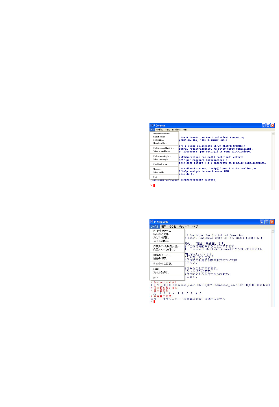
Figure 1: Part of the Windows console in an Italian

locale.

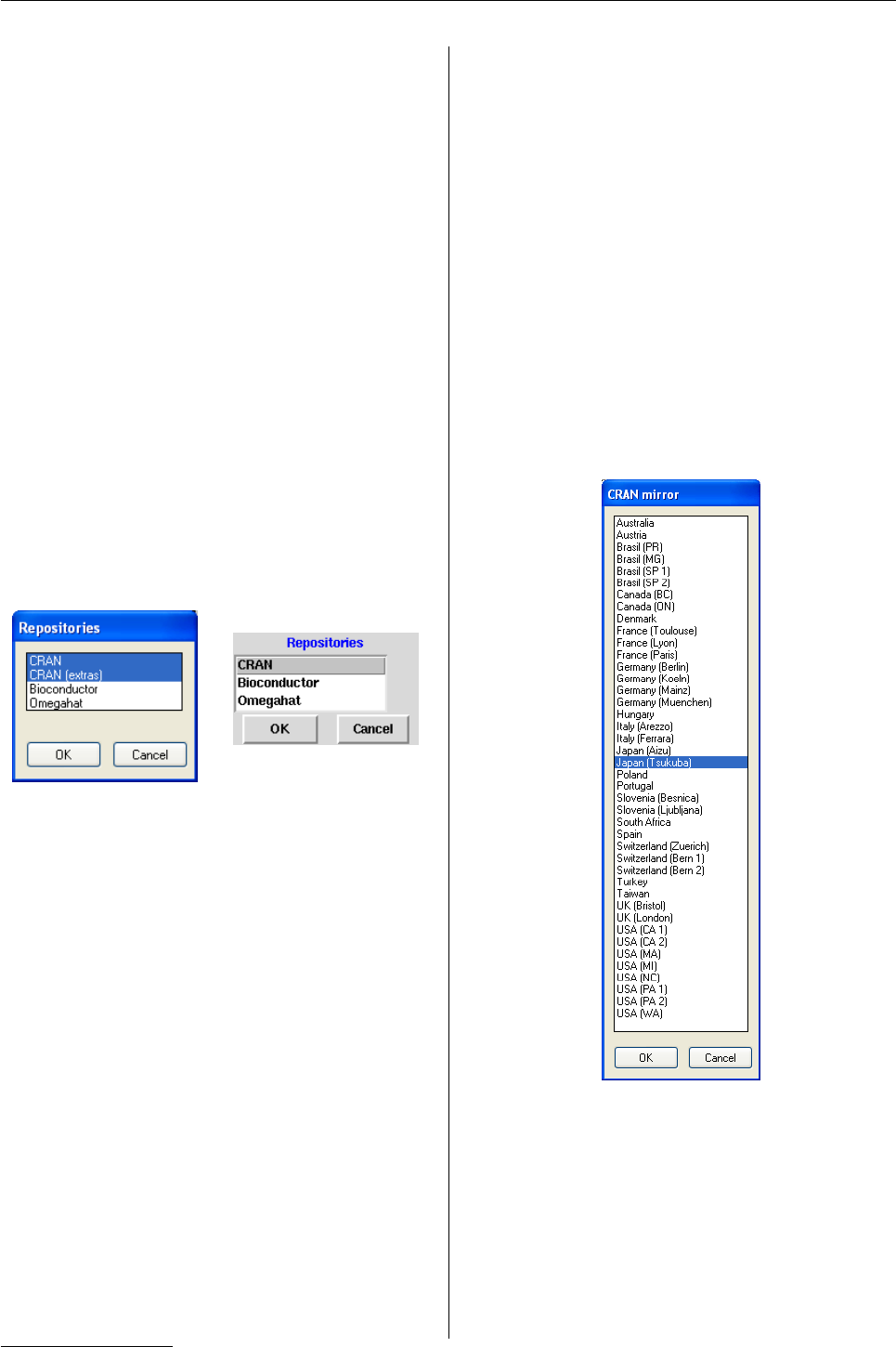
Figure 2: Part of the Windows console in Japanese.

Note the use of Japanese variable names, that the last

line is an error message in Japanese, as well as the

difference in width between English and Japanese

characters.

Hopefully, if your OS has enough support to al-

low you to work comfortably in your preferred lan-

guage, it will have enough support to allow you to

use Rin that language. Figures 1and 2show ex-

amples of internationalization for the Windows GUI:

note how the menus are translated, variable names

are accepted in the preferred language, and error

1e.g. the use of 12-hour or 24-hour clock.

2for example, the use of ,for the decimal point, and the use of ,or .or nothing as the thousands separator.

3see below.

R News ISSN 1609-3631

Vol. 5/1, May 2005 3

messages are translated too. The Japanese screen-

shot shows another difference: the Japanese charac-

ters are displayed at twice the width of the English

ones, and cursor movement has to take this into ac-

count.

The rest of this article expands on the concepts

and then some of the issues they raise for Rusers and

Rprogrammers. Quite a lot of background is needed

to appreciate what users of very different languages

need from the internationalization of R.

Locales

Alocale is a speciﬁcation of the user-speciﬁc environ-

ment within which an operating system is running

an application program such as R. What exactly this

covers is OS-speciﬁc, but key components are

• The set of ‘legal’ characters the user might in-

put: this includes which characters are alpha-

betic and which are numeric. This is the C lo-

cale category LC_CTYPE.

• How characters are sorted: the C locale cate-

gory LC_COLLATE. Even where languages share

a character set they may sort words differently:

it comes as a surprise to English-speaking vis-

itors to Denmark to ﬁnd ‘Aa’ sorted at the end

of the alphabet.

• How to represent dates and times (C locale cat-

egory LC_TIME). The meaning of times also de-

pends on the timezone which is sometimes re-

garded as part of the locale (and sometimes

not).

• Monetary formatting (C locale category

LC_MONETARY).

• Number formatting (C locale category

LC_NUMERIC).

• The preferred language in which to communi-

cate with the user (for some systems, C locale

category LC_MESSAGES).

• How characters in that language are encoded.

How these are speciﬁed is (once again) OS-

speciﬁc. The ﬁrst four categories can be set by

Sys.setlocale(): the initial settings are taken

from the OS and can be queried by calling

Sys.getlocale() (see Figure 2). On Unix-like OSes

the settings are taken from environment variables

with the names given, defaulting to the value of

LC_ALL and then of LANG. If none of these are set, the

value is likely to be Cwhich is usually implemented

as the settings appropriate in the USA. Other aspects

of the locale are reported by Sys.localeconv().

Other OSes have other ways of specifying the lo-

cale: for example both Windows and MacOS X have

listboxes in their user settings. This is becoming

more common: when I select a ‘Language’ at the lo-

gin screen for a session in Fedora Core 3 Linux I am

actually selecting a locale, not just my preferred lan-

guage.

Rdoes not fully support LC_NUMERIC, and is un-

likely ever to. Because the comma is used as the sep-

arator in argument lists, it would be impossible to

parse expressions if it were also allowed as the deci-

mal point. We do allow the decimal point to be spec-

iﬁed in scan(),read.table() and write.table().

Sys.setlocale() does allow LC_NUMERIC to be set,

with a warning and with inconsistent behaviour.

For the R user

The most important piece of advice is to specify your

locale when asking questions, since Rwill behave

differently in different locales. We have already seen

experienced Rusers insisting on R-help that R has

been broken when it seems they had changed locales.

To be sure, quote the output of Sys.getlocale() and

localeToCharset().

For the package writer

Try not to write language-speciﬁc code. A pack-

age which was submitted to CRAN with variables

named a~nos worked for the author and the CRAN

testers, but not on my Solaris systems. Use only

ASCII characters4for your variable names, and as far

as possible for your documentation.

Languages and character sets

What precisely do we mean by ‘the preferred lan-

guage’? Once again, there are many aspects to con-

sider.

• The language, such as ‘Chinese’ or ‘Spanish’.

There is an international standard ISO 6395for

two-letter abbreviations for languages, as well

as some three-letter ones. These are pretty stan-

dard, except that for Hebrew which has been

changed.

• Is this Spanish as spoken in Spain or in Latin

America?

• ISO 639 speciﬁes no as ‘Norwegian’, but Nor-

way has two ofﬁcial languages, Bokmål and

Nynorsk. Which is this?6

4Digits and upper- and lower-case A–Z, without accents.

5http://www.w3.org/WAI/ER/IG/ert/iso639.htm or http://www.loc.gov/standards/iso639-2/englangn.html

6Bokmål, usually, with nn for Nynorsk and nb for Bokmål speciﬁcally.

R News ISSN 1609-3631

Vol. 5/1, May 2005 4

• The same language can be written in different

ways. The most prominent example is Chinese,

which has Simpliﬁed and Traditional orthogra-

phy, and most readers can understand only one

of them.

• Spelling. The Unix spell program has the fol-

lowing comment in the BUGS section of its man

page:

‘British spelling was done by an

American.’

but that of itself is an example of cultural impe-

rialism. The nations living on the British Isles

do not consider themselves to speak ‘British

English’ and do not agree on spelling: for ex-

ample in general Chambers’ dictionary (pub-

lished in Scotland) prefers ‘-ise’ and the Oxford

English Dictionary prefers ‘-ize’.

To attempt to make the description more precise, the

two-letter language code is often supplemented by a

two-letter ‘country or territory’ code from ISO 31667.

So, for example

pt_BR is Portuguese as written in Brazil.

zh_CN is (simpliﬁed) Chinese as written in most

of mainland China, and zh_TW is (traditional)

Chinese as written in Taiwan (which is writ-

ten in the same way as zh_HK used in Hong

Kong).

en_US is American.

en_GB is English as written somewhere (unspeci-

ﬁed) in the UK.

We need to specify the language for at least three

purposes:

1. To delimit the set of characters which can be

used, and which of those are ‘legal’ in object

names.

2. To know the sorting order.

3. To decide what language to respond in.

In addition, we might need to know the direction of

the language, but currently Ronly supports left-to-

right processing of character strings.

The ﬁrst two are part of the locale speciﬁcation.

Specifying the language to be used for messages is

a little more complicated: a Nynorsk speaker might

prefer Nynorsk then Bokmål then generic Norwe-

gian then English, which can be expressed by set-

ting LANGUAGE=nn:nb:no (since generic ‘English’ is

the default).

Encodings

Computers work with bits and bytes, and encoding

is the act of representing characters in the language

as bytes, and vice versa. The earliest encodings (e.g.

for Telex) just represented capital letters and num-

bers but this expanded to ASCII, which has 92 print-

able characters (upper- and lower-case letters, digits

and punctuation) plus control codes, represented as

bytes with the topmost bit as 0. This is also the ISO

646 international standard and those characters are

included in most8other encodings.

Bytes allow 256 rather than 128 different charac-

ters, and ISO 646 has been extended into the bytes

with topmost bit as 1, in many different ways. There

is a series of standards ISO 8859-1 to ISO 8859-15

for such extensions, as well as many vendor-speciﬁc

ones (such as the ‘WinAnsi’ and other code pages).

Most languages have less than the 186 or more char-

acters9that an 8-bit encoding provides. The problem

is that given a sequence of bytes there is no way to

know that it is in an 8-bit encoding let alone which

one.

The CJK10 languages have tens of thousands of

characters. There have been many ways to repre-

sent such character sets, for example using shift se-

quences (like the shift, control, alt and altgr keys

on your keyboard) to shift between ‘pages’ of char-

acters. Windows uses a two-byte encoding for the

ideographs, with the ‘lead byte’ with topmost bit 1

followed by a ‘trail byte’. So the character sets used

for CJK languages on Windows occupy one or two

bytes.

A problem with such schemes is their lack of ex-

tensibility. What should we do when a new character

comes along, notably the Euro? Most commonly, re-

place something which is thought to be uncommon

(the generic currency symbol in ISO 8859-1 was re-

placed by the Euro in ISO 8859-15, amongst other

changes).

Unicode

Being able to represent one language may not be

enough: if for example we want to represent per-

sonal names we would like to be able to do so equally

for American, Chinese, Greek, Arabic and Maori11

speakers. So the idea emerged of a universal encod-

ing, to represent all the characters we might like to

7http://www.iso.org/iso/en/prods-services/iso3166ma/index.html.

8In a common Japanese encoding, backslash is replaced by Yen. As this is the encoding used for Windows Japanese fonts, ﬁle paths

look rather peculiar in a Japanese version of Windows.

9the rest are normally allocated to ‘space’ and control bytes

10Chinese, Japanese, Korean: known to Windows as ‘East Asian’. The CJK ideographs were also used for Vietnamese until the early

twentieth century.

11language code mi. Maori is usually encoded in ISO 8859-13, along with Lithuanian and Latvian!

R News ISSN 1609-3631

Vol. 5/1, May 2005 5

print—all human languages, mathematical and mu-

sical notation and so on.

This is the purpose of Unicode12, which allows up

to 232 different characters, although it is now agreed

that only 221 will ever be prescribed. The human

languages are represented in the ‘basic multilingual

plane’ (BMP), the ﬁrst 216 characters, and so most

characters you will encounter have a 4-hex-digit rep-

resentation. Thus U+03B1 is alpha, U+05D0 is aleph

(the ﬁrst letter of the Hebrew alphabet) and U+30C2

is the Katakana letter ‘di’.

If we all used Unicode, would everyone be

happy? Unfortunately not, as sometimes the same

character can be written in various ways. The

Unicode standard allows ‘only’ 20992 slots for CJK

ideographs, whereas the Taiwanese national stan-

dard deﬁnes 48711. The result is that different fonts

have different variants for e.g. U+8FCE and a variant

may be recognizable to only some of the users.

Nevertheless, Unicode is the best we have, and a

decade ago Windows NT adopted the BMP of Uni-

code as its native encoding, using 16-bit characters.

However, Unix-alike OSes expect nul (the zero byte)

to terminate a string such as a ﬁle path, and peo-

ple looked for ways to represent Unicode characters

as sequences of a variable number of bytes. By far

the most successful such scheme is UTF-8, which has

over the last couple of years become the de facto stan-

dard for Linux distributions. So when I select

English (UK) British English

as my language at the login screen for a session in Fe-

dora Core 3 Linux, I am also selecting UTF-8 as my

encoding.

In UTF-8, the 7-bit ASCII characters are repre-

sented as a single byte. All other characters are rep-

resented as two or more bytes all with topmost bit 1.

This introduces a number of implementation issues:

• Each character is represented by a variable

number of bytes, from one up to six (although

it is likely at most four will ever be used).

• Some bytes can never occur in UTF-8.

• Many byte sequences are not valid in UTF-8.

The major implementation issue in internationaliz-

ing Rhas been to support such multi-byte character

sets (MBCSs). There are other examples, including

EUC-JP used for Japanese on Unix-alikes and the

one- or two-byte encodings used for CJK on older

versions of Windows.

As UTF-8 locales can support multiple languages,

which are allowed for the ‘legal’ characters in Rob-

ject names? This may depend on the OS, but in all

the examples we know of all characters which would

be alphanumeric in at least one human language are

allowed. So for example ~n and ¨u are allowed in lo-

cale en_US.utf8 on Linux, just as they were in the

Latin-1 locale en_US (whereas on Windows the differ-

ent Latin-1 locales have different sets of ‘legal’ char-

acters, indeed different in different versions of Win-

dows for some languages). We have decided that

only the ASCII numbers will be regarded as numeric

in R.

Sorting orders in Unicode are handled by an OS

service: this is a very intricate subject so do not ex-

pect too much consistency between different imple-

mentations (which includes the same language in

different encodings).

Fonts

Being able to represent alpha, aleph and the

Katakana letter ‘di’ is one thing: being able to dis-

play them is another, and we want to be able to dis-

play them both at the console and in graphical out-

put. Effectively all fonts available cover quite small

subsets of Unicode, although they may be usable in

combinations to extend the range.

Rconsoles normally work in monospaced fonts.

That means that all printable ASCII characters have

the same width. Once we move to Unicode, char-

acters are normally categorized into three widths,

one (ASCII, Greek, Arabic, . . . ), two (most CJK

ideographs) and zero (the ‘combining characters’ of

languages such as Thai). Unfortunately there are two

conventions for CJK characters, with some fonts hav-

ing e.g. Katakana single-width and some (including

that used in Figure 2) double-width.

Which characters are available in a font can seem

capricious: for example the one I originally used to

test translations had directional single quotes but not

directional double quotes.

If displaying another language is not working in

a UTF-8 locale the most likely explanation is that the

font used is incomplete, and you may need to install

extra OS components to overcome this.

Font support for Rgraphics devices is equally dif-

ﬁcult and has currently only been achieved on Win-

dows and on comprehensively equipped X servers.

In particular, postscript() and pdf() are restricted

to Western and Eastern European languages as the

commonly-available fonts are (and some are re-

stricted to ISO 8859-1).

For the R user

Now that Ris able to accept input in different encod-

ings, we need a way to specify the encoding. Con-

nections allow you to specify the encoding via the

encoding argument, and the encoding for stdin can

be set when reading from a ﬁle by the command-

12There is a more formal deﬁnition in the ISO 10646 standard, but for our purposes Unicode is a more precisely constrained version of

the same encoding. There are various versions of Unicode, currently 4.0.1—see http://www.unicode.org.

R News ISSN 1609-3631

Vol. 5/1, May 2005 6

line argument --encoding. Also, source() has an

encoding argument.

It is important to make sure the encoding is cor-

rect: in particular a UTF-8 ﬁle will be valid input in

most locales, but will only be interpreted properly

in a UTF-8 locale or if the encoding is speciﬁed. So

to read a data ﬁle produced on Windows containing

the names of Swiss students in a UTF-8 locale you

will need one of

A <- read.table(file("students",

encoding="latin1"))

A <- read.table(file("students",

encoding="UCS-2LE"))

the second if this is a ‘Unicode’ Windows ﬁle.13

In a UTF-8 locale, characters can be entered as

e.g. \u8fce or \u{8fce} and non-printable charac-

ters will be displayed by print() in the ﬁrst of these

forms. Further, \U can be used with up to 8 hex digits

for characters not in the BMP.

For the R programmer

There is a common assumption that one byte = one

character = one display column. As from R 2.1.0

a character can use more than one byte and extend

over more than one column when printed. The func-

tion nchar() now has a type argument allowing

the number of bytes, characters or columns to be

found—note that this defaults to bytes for backwards

compatibility.

Switching between encodings

Ris able to support input in different encodings by

using on-the-ﬂy translation between encodings. This

should be an OS service, and for modern glibc-

based systems it is. Even with such systems it can

be frustratingly difﬁcult to ﬁnd out what encod-

ings they support, and although most systems accept

aliases such as ISO_8859-1,ISO8859-1,ISO_8859_1,

8859_1 and LATIN-1, it is quite possible to ﬁnd that

with three systems there is no name that they all ac-

cept. One solution is to install GNU libiconv: we

have done so for the Windows port of R, and Apple

have done so for MacOS X.

We have provided R-level support for changing

encoding via the function iconv(), and iconvlist()

will (if possible) list the supported encodings.

Quote symbols

ASCII has a quotation mark ", apostrophe ’and

grave accent ‘, although some fonts14 represent

the latter two as right and left quotes respectively.

Unicode provides a wide variety of quote sym-

bols, include left and right single (U+2018, U+2019)

and double (U+201C, U+201D) quotation marks. R

makes use of these for sQuote() and dQuote() in

UTF-8 locales.

Other languages use other conventions for quota-

tions, for example low and mirrored versions of the

right quotation mark (U+201A, U+201B), as well as

guillemets (U+00AB, U+00BB; something like ,).

Looking at translations of error messages in other

GNU projects shows little consistency between na-

tive writers of the same language, so we have made

no attempt to deﬁne language-speciﬁc versions of

sQuote() and dQuote().

Translations

Rcomes with a lot of documentation in English.

There is a Spanish translation of An Introduction to

Ravailable from CRAN, and an Italian introduction

based on it as well as links to Japanese translations

of An Introduction to R, other manuals and some help

pages.

R 2.1.0 facilitates the translation of messages from

‘English’ into other languages: it will ship with

a complete translation into Japanese and of many

of the messages into Brazilian Portuguese, Chinese,

German and Italian. Updates of these translations

and others can be added at a later date by translation

packages.

Which these ‘messages’ are was determined by

those (mainly me) who marked up the code for pos-

sible translation. We aimed to make all but the most

esoteric warning and error messages available for

translation, together with informational messages

such as the welcome message and the menus and di-

alogs of the Windows and MacOS X consoles. There

are about 4200 unique messages in command-line R

plus a few hundred in the GUIs.

One beneﬁcial side-effect even for English read-

ers has been much improvement in the consistency

of the messages, as well as some re-writing where

translators found the messages unclear.

For the R user

All the end user needs to do is to ensure that the de-

sired translations are installed and that the language

is set correctly. To test the latter, try it and see: very

likely the internal code will be able to ﬁgure out the

correct language from the locale name, and the wel-

come message (and menus if appropriate) will ap-

pear in the correct language. If not, try setting the

environment variable LANGUAGE and if that does not

13This will probably not work unless the ﬁrst two bytes are removed from the ﬁle. Windows is inclined to write a ‘Unicode’ ﬁle starting

with a Byte Order Mark 0xFEFE, whereas most Unix-alikes do not recognize a BOM. It would be technically easy to do so but apparently

politically impossible.

14most likely including the one used to display this document.

R News ISSN 1609-3631

Vol. 5/1, May 2005 7

help, read the appropriate section of the R Installation

and Administration manual.

Unix-alike versions of Rcan be built without sup-

port for translation, and it is possible that some OSes

will provide too impoverished an environment to de-

termine the language from the locale or even for the

translation support to be compiled in.

There is a pseudo-language en@quot for which

translations are supplied. This is intended for use

in UTF-8 locales, and makes use of the Unicode di-

rectional single and double quotation marks. This

should be selected via the LANGUAGE environment

variable.

For package writers

Any package can have messages marked for trans-

lation: see Writing R Extensions. Traditionally mes-

sages have been paste-d together, and such mes-

sages can be awkward or impossible to translate into

languages with other word orders. We have added

support for specifying messages via C-like format

strings, using the Rfunction gettextf. A typical us-

age is

stop(gettextf(

"autoloader did not find ’%s’ in ’%s’",

name, package),

domain = NA)

I chose this example as the Chinese translation re-

verses15 the order of the two variables. Using

gettextf() marks the format (the ﬁrst argument)

for translation and then passes the arguments to

sprintf() for C-like formatting. The argument

domain = NA is passed to stop() as the message re-

turned by gettextf() will already be translated (if

possible) and so needs no further translation. As the

quotation marks are included in the format, trans-

lators can use other conventions (and the pseudo-

language en@quot will).

Plurals are another source of difﬁculties for trans-

lators. Some languages have no plural forms, others

have ‘singular’ and ‘plural’ as in English, and oth-

ers have up to four forms. Even for those languages

with just ‘singular’ and ‘plural’ there is the question

of whether zero is singular or plural, which differs

by language. There is quite general support for plu-

rals in the R and C functions ngettextf and a small

number16 of examples in the R sources.

See Writing R Extensions for more details.

For would-be translators

Additional translations and help completing the cur-

rent ones would be most welcome. Experience has

shown that it is helpful to have a small translation

team to cross-check each other’s work, discuss id-

iomatic usage and to share the load. Translation will

be an ongoing process as Rcontinues to grow.

Please see the documents linked from

http://developer.r-project.org.

Future directions

At this point we need to gain more experience

with internationalization infrastructure. We know it

works with the main Rplatforms (recent Linux, Win-

dows, MacOS X) and Solaris and for a small set of

quite diverse languages.

We currently have no way to allow Windows

users to use many languages in one session, as Win-

dows’ implementation of Unicode is not UTF-8 and

the standard C interface on Windows does not allow

UTF-8 as an encoding. We plan on making a ‘Uni-

code’ (in the Windows sense) implementation of R

2.2.0 that uses UTF-8 internally and 16-bit characters

to interface with Windows. It is likely that such a ver-

sion will only be available for NT-based versions of

Windows.

It is hoped to support a wider range of encodings

on the postscript() and pdf() devices.

The use of encodings in documentation remains

problematic, including in this article. Texinfo is

used for the Rmanuals but does not currently sup-

port even ISO 8859-1 correctly. We have started with

some modest support for encodings in .Rd ﬁles, and

may be able to do more.

Acknowledgements

The work of the Japanese group (especially Ei-ji

Nakama and Masafumi Okada) supplied valuable

early experience in internationalization.

The translations have been made available by

translation teams and in particular some enthusiastic

individuals. The infrastructure for translation is pro-

vided by GNU gettext, suitably bent to our needs

(for Ris a large and complex project, and in particu-

lar extensible).

Brian D. Ripley

University of Oxford, UK

ripley@stats.ox.ac.uk

15using ’%2$s’ and ’%1$s’ in the translation to refer to the second and ﬁrst argument respectively.

16currently 22, about 0.5% of the messages.

R News ISSN 1609-3631

Vol. 5/1, May 2005 8

Packages and their Management in R 2.1.0

by Brian D. Ripley

R 2.1.0 introduces changes that make packages and

their management considerably more ﬂexible and

less tied to CRAN.

What is a package?

The idea of an Rpackage was based quite closely on

that of an Slibrary section: a collection of Rfunc-

tions with associated documentation and perhaps

compiled code that is loaded from a library1by the

library() command. The Help Desk article (Ligges,

2003) provides more background.

Such packages still exist, but as from R 2.1.0

there are other types of Rextensions, distinguished

by the Type: ﬁeld in the ‘DESCRIPTION’ ﬁle: the

classic package has Type: Package or no Type:

ﬁeld. The Type: ﬁeld tells R CMD INSTALL and

install.packages() what to do with the extension,

which is still distributed as a tarball or zip ﬁle con-

taining a directory of the same name as the package.

This allows new types of extensions to be added

in the future, but R 2.1.0 knows what to do with two

other types.

Translation packages

with Type: Translation. These are used to add or

update translations of the diagnostic messages pro-

duced by Rand the standard packages. The con-

vention is that languages are known by their ISO

639 two-letter (or less commonly three-letter) codes,

possibly with a ‘country or territory’ modiﬁer. So

package Translation-sl should contain translations

into Slovenian, and Translation-zhTW translations

into traditional Chinese as used in Taiwan. Writing

R Extensions describes how to prepare such a pack-

age: it contains compiled translations and so all R

CMD INSTALL and install.packages() need to do is

to create the appropriate subdirectories and copy the

compiled translations into place.

Frontend packages

with Type: Frontend. These are only supported as

source packages on Unix, and are used to install al-

ternative front-ends such as the GNOME console,

previously part of the Rdistribution and now in

CRAN package gnomeGUI. For this type of package

the installation runs configure and the make and so

allows maximal ﬂexibility for the package writer.

Source vs binary

Initially Rpackages were distributed in source

form as tarballs. Then the Windows binary

packages came along (distributed as Zip ﬁles)

and later Classic MacOS and MacOS X packages.

As from R 2.1.0 the package management func-

tions all have a type argument defaulting to the

value of getOption("pkgType"), with known values

"source","win.binary" and "mac.binary". These

distributions have different ﬁle extensions: .tar.gz,

.zip and .tgz respectively.

This allows packages of each type to be manip-

ulated on any platform: for example, whereas one

cannot install Windows binary packages on Linux,

one can download them on Linux or Solaris, or ﬁnd

out if a MacOS X binary distribution is available.

Note that install.packages on MacOS X can

now install either "source" or "mac.binary" pack-

age ﬁles, the latter being the default. Similarly,

install.packages on Windows can now install ei-

ther "source" or "win.binary" package ﬁles. The

only difference between the platforms is the default

for getOption("pkgType").

Repositories

The package management functions such

as install.packages,update.packages and

packageStatus need to know where to look for pack-

ages. Function install.packages was originally

written to access a CRAN mirror, but other reposito-

ries of packages have been created, notably that of

Bioconductor. Function packageStatus was the ﬁrst

design to allow multiple repositories.

We encourage people with collections of pack-

ages to set up a repository. Apart from the CRAN

mirrors and Bioconductor there is an Omegahat

repository, and I have a repository of hard-to-

compile Windows packages to supplement those

made automatically. We anticipate university de-

partments setting up repositories of support soft-

ware for their courses. A repository is just a tree of

ﬁles based at a URL: details of the format are in Writ-

ing R Extensions. It can include one, some or all of

"source","win.binary" and "mac.binary" types in

separate subtrees.

Specifying repositories

Specifying repositories has become quite compli-

cated: the (sometimes conﬂicting) aims were to be

intuitive to new users, very ﬂexible and as far as pos-

sible backwards compatible.

1a directory containing subdirectories of installed packages

R News ISSN 1609-3631

Vol. 5/1, May 2005 9

As before, the place(s) to look for ﬁles are speci-

ﬁed by the contriburl argument. This is a charac-

ter vector of URLs, and can include file:// URLs

if packages are stored locally, for example on a dis-

tribution CD-ROM. Different URLs in the vector can

be of different types, so one can mix a distribution

CD-ROM with a CRAN mirror.

However, as before, most people will not spec-

ify contriburl directly but rather the repos argu-

ment that replaces the CRAN argument.2The function

contrib.url is called to convert the base URLs in

repos into URLs pointing to the correct subtrees of

the repositories. For example

> contrib.url("http://base.url",

type = "source")

[1] "http://base.url/src/contrib"

> contrib.url("http://base.url",

type = "win.binary")

[1] "http://base.url/bin/windows/contrib/2.1"

> contrib.url("http://base.url",

type = "mac.binary")

[1] "http://base.url/bin/macosx/2.1"

This is of course hidden from the average user.

Figure 1: The listboxes from setRepositories() on

Windows (left) and Unix (right).

The repos argument of the package management

functions defaults to getOption("repos"). This has

a platform-speciﬁc default, and can be set by calling

setRepositories. On most systems this uses a list-

box widget, as shown in ﬁgure 1. Where no GUI is

available, a text list is used such as

> setRepositories()

--- Please select repositories for use

in this session ---

1: + CRAN

2: + CRAN (extras)

3: Bioconductor

4: Omegahat

Enter one or more numbers separated by spaces

1: 1 4

The list of repositories and which are selected by de-

fault can be customized for a user or for a site: see

?setRepositories. We envisaged people distribut-

ing a CD-ROM containing Rand a repository, with

setRepositories() customized to include the local

repository by default.

Suppose a package exists on more than one

repository?

Since multiple repositories are allowed, how is this

resolved? The rule is to select the latest version of

the package, from the ﬁrst repository on the list that

is offering it. So if a user had

> getOption("repos")

[1] "file://d:/R/local"

[2] "http://cran.us.r-project.org"

packages would be fetched from the local repository

if they were current there, and from a US CRAN mir-

ror if there is an update available there.

Figure 2: Selecting a CRAN mirror on Windows.

No default CRAN

Windows users are already used to selecting a CRAN

mirror. Now ‘factory-fresh’ Rdoes not come with a

default CRAN mirror. On Unix the default is in fact

> getOption("repos")

CRAN

"@CRAN@"

2This still exists but has been deprecated and will be removed in R 2.2.0.

R News ISSN 1609-3631

Vol. 5/1, May 2005 10

Whenever @CRAN@ is encountered in a repository

speciﬁcation, the function chooseCRANmirror is

called to ask for a mirror (and can also be called di-

rectly and from a menu item on the Windows GUI).

The Windows version is shown in Figure 2: there are

MacOS X and Tcl/Tk versions, as well as a text-based

version using menu.3

Experienced users can avoid being asked for a

mirror by setting options("repos") in their ‘.Rpro-

ﬁle’ ﬁles: examples might be

options(repos=

c(CRAN="http://cran.xx.r-project.org"))

on Unix-alikes and

options(repos=

c(CRAN="http://cran.xx.r-project.org",

CRANextra=

"http://www.stats.ox.ac.uk/pub/RWin"))

on Windows.

Although not essential, it is helpful to have a

named vector of repositories as in this example: for

example setRepositories looks at the names when

setting its initial selection.

Installing packages

Users of the Windows GUI will be used to selecting

packages to be installed from a scrollable list box.

This now works on all platforms from the command

line if install.packages is called with no pkgs (ﬁrst)

argument. Packages from all the selected reposito-

ries are listed in alphabetical order, and the packages

from bundles are listed4individually in the form

MASS (VR).

The dependencies argument introduced in

R 2.0.0 can be used to install a package and its de-

pendencies (and their dependencies . . . ), and Rwill

arrange to install the packages in a suitable order.

The dependencies argument can be used to select

only those dependencies that are essential, or to in-

clude those which are suggested (and might only be

needed to run some of the examples).

Installing all packages

System administrators often want to install ‘all’ pack-

ages, or at least as many as can be installed on their

system: a standard Linux system lacks the additional

software needed to install about 20 and a handful can

only be installed on Windows or on Linux.

The new function new.packages() is a helpful

way to ﬁnd out which packages are not installed of

those offered by the repositories selected. If called as

new.packages(ask = "graphics") a list box is used

to allow the user to select packages to be installed.

Figure 3: Selecting amongst uninstalled packages on

Linux.

Updating packages

The only real change in update.packages is the ask

argument. This defaults to ask = TRUE where as be-

fore the user is asked about each package (but with a

little more information and the option to quit). Other

options are ask = FALSE to install all updates, and

ask = "graphics" to use a listbox (similar to ﬁg-

ure 3) to de-select packages (as by default all the up-

dates are selected).

Looking at repositories

The function CRAN.packages was (as it name im-

plies) designed to look at a single CRAN mirror. It

has been superseded by available.packages which

can look at one or more repositories and by default

looks at those speciﬁed by getOption("repos")

for package type (source/binary) speciﬁed by

getOption("pkgType"). This returns a matrix

with rather more columns than before, including

"Repository", the dependencies and the contents of

bundles.

Function packageStatus is still available but has

been re-implemented on top of functions such as

available.packages. Its summary method allows

a quick comparison of the installed packages with

those offered by the selected repositories. However,

its print method is concise: see ﬁgure 4.

Bibliography

U. Ligges. R help desk: Package management. R

News, 3(3):37–39, December 2003. URL http://

CRAN.R-project.org/doc/Rnews/.8

Brian D. Ripley

University of Oxford, UK

ripley@stats.ox.ac.uk

3menu has been much enhanced for R 2.1.0.

4provided the repository has been set up to supply the information.

R News ISSN 1609-3631

Vol. 5/1, May 2005 11

> (ps <- packageStatus())

--- Please select a CRAN mirror for use in this session ---

Number of installed packages:

ok upgrade unavailable

c:/R/library 34 1 0

c:/R/rw2010/library 12 0 13

Number of available packages (each package/bundle counted only once):

installed

http://www.sourcekeg.co.uk/cran/bin/windows/contrib/2.1 31

http://www.stats.ox.ac.uk/pub/RWin/bin/windows/contrib/2.1 4

not installed

http://www.sourcekeg.co.uk/cran/bin/windows/contrib/2.1 421

http://www.stats.ox.ac.uk/pub/RWin/bin/windows/contrib/2.1 8

> summary(ps)

Installed packages:

-------------------

*** Library c:/R/library

$ok

[1] "abind" "acepack" "akima" "ash" "car"

...

$upgrade

[1] "XML"

$unavailable

NULL

*** Library c:/R/rw2010/library

$ok

[1] "base" "datasets" "graphics" "grDevices" "grid" "methods" "splines" "stats" "stats4"

[10] "tcltk" "tools" "utils"

$upgrade

NULL

$unavailable

[1] "boot" "cluster" "foreign" "KernSmooth" "lattice"

...

Available packages:

-------------------

(each package appears only once)

*** Repository http://www.sourcekeg.co.uk/cran/bin/windows/contrib/2.1

$installed

[1] "abind" "acepack" "akima" "ash" "car"

...

$"not installed"

[1] "accuracy" "adapt" "ade4"

...

[421] "zicounts"

*** Repository http://www.stats.ox.ac.uk/pub/RWin/bin/windows/contrib/2.1

$installed

[1] "GLMMGibbs" "xgobi" "XML" "yags"

$"not installed"

[1] "gsl" "hdf5" "ncdf" "RDCOMClient" "rgdal" "RNetCDF" "survnnet" "udunits"

> upgrade(ps)

XML :

0.97-0 at c:/R/library

0.97-3 at http://www.stats.ox.ac.uk/pub/RWin/bin/windows/contrib/2.1

Update (y/N)? y

Figure 4: packageStatus on a Windows machine. The voluminous summary has been edited to save space.

R News ISSN 1609-3631

Vol. 5/1, May 2005 12

Recent Changes in grid Graphics

by Paul Murrell

Introduction

The grid graphics package provides an alternative

graphics system to the “traditional” S graphics sys-

tem that is provided by the graphics package.

The majority of high-level plotting functions (func-

tions that produce whole plots) that are currently

available in the base packages and in add-on pack-

ages are built on the graphics package, but the lattice

package (Sarkar,2002), which provides high-level

Trellis plots, is built on grid.

The grid graphics package can be useful for cus-

tomising lattice plots, creating complex arrange-

ments of several lattice plots, or for producing

graphical scenes from scratch.

The basic features of grid were described in an R

News article in June 2002 (Murrell,2002). This arti-

cle provides an update on the main features that have

been added to grid since then. This article assumes

a familiarity with the basic grid ideas of units and

viewports.

Changes to grid

The most important organisational change is that

grid is now a “base” package, so it is installed as part

of the standard R installation. In other words, pack-

age writers can assume that grid is available.

The two main areas where the largest changes have

been made to grid are viewports and graphical ob-

jects. The changes to viewports are described in the

next section and summarised in Table 1at the end of

the article. A separate section describes the changes

to graphical objects with a summary in Table 2at the

end of the article.

Changes to viewports

grid provides great ﬂexibility for creating regions on

the page to draw in (viewports). This is good for be-

ing able to locate and size graphical output on the

page in very sophisticated ways (e.g., lattice plots),

but it is bad because it creates a complex environ-

ment when it comes to adding further output (e.g.,

annotating a lattice plot).

The ﬁrst change to viewports is that they are now

much more persistent; it is possible to have any num-

ber of viewports deﬁned at the same time.

There are also several new functions that provide a

consistent and straightforward mechanism for nav-

igating to a particular viewport when several view-

ports are currently deﬁned.

A viewport is just a rectangular region that provides

a geometric and graphical context for drawing. The

viewport provides several coordinate systems for lo-

cating and sizing output, and it can have graphical

parameters associated with it to affect the appear-

ance of any output produced within the viewport.

The following code describes a viewport that occu-

pies the right half of the graphics device and within

which, unless otherwise speciﬁed, all output will be

drawn using thick green lines. A new feature is that a

viewport can be given a name. In this case the view-

port is called "rightvp". The name will be important

later when we want to navigate back to this view-

port.

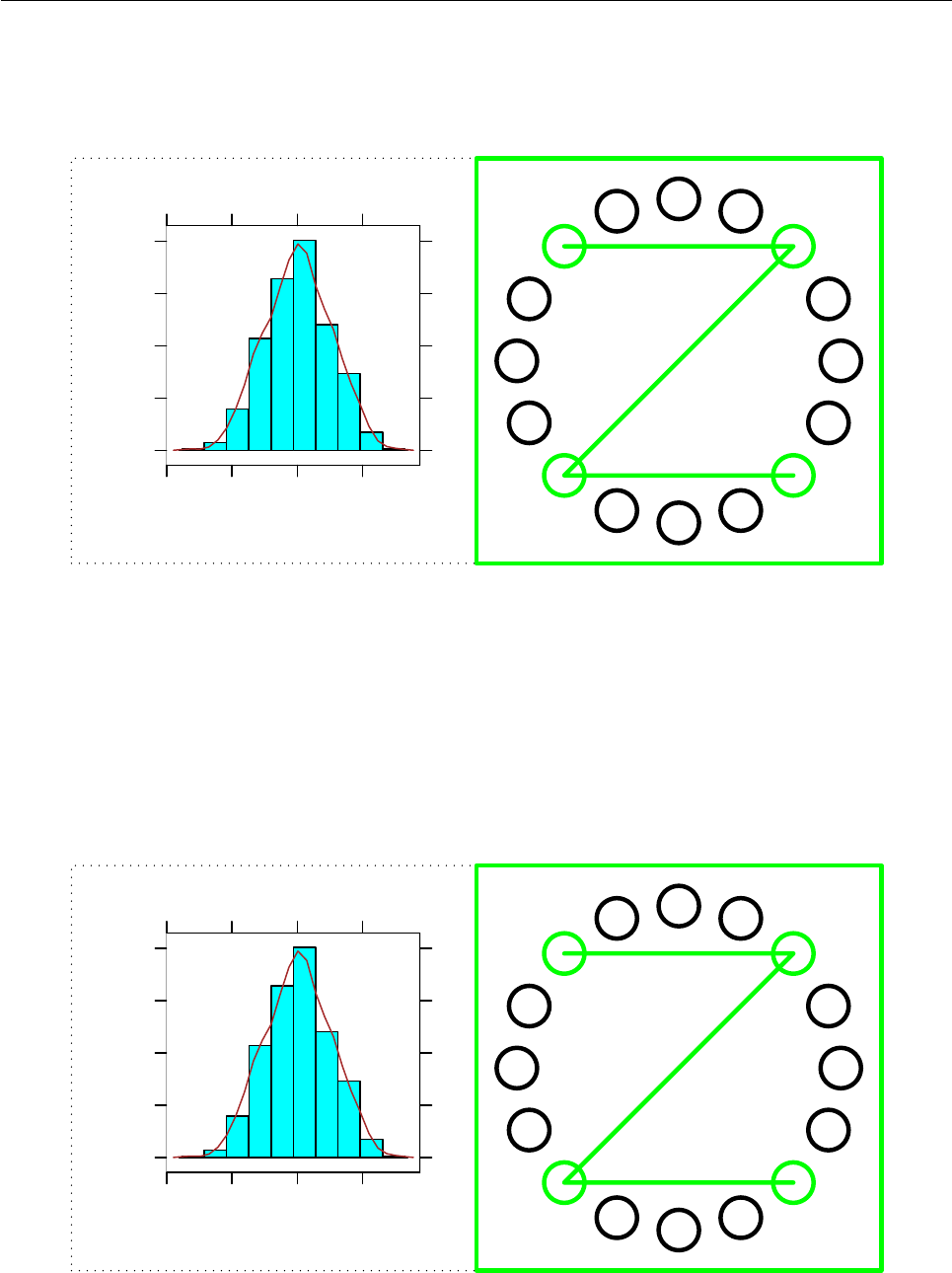
> vp1 <- viewport(x=0.5, width=0.5,

just="left",

gp=gpar(col="green", lwd=3),

name="rightvp")

The above code only creates a description of a view-

port; a corresponding region is created on a graph-

ics device by pushing the viewport on the device, as

shown below.1

> pushViewport(vp1)

Now, all drawing occurs within the context deﬁned

by this viewport until we change to another view-

port. For example, the following code draws some

basic shapes, all of which appear in the right half of

the device, with thick green lines (see the right half

of Figure 1). Another new feature is that a name

can be associated with a piece of graphical output.

In this case, the rectangle is called "rect1", the line

is called "line1", and the set of circles are called

"circles1". These names will be used later in the

section on “Changes to graphical objects”.

> grid.rect(name="rect1")

> r <- seq(0, 2*pi, length=5)[-5]

> x <- 0.5 + 0.4*cos(r + pi/4)

> y <- 0.5 + 0.4*sin(r + pi/4)

> grid.circle(x, y, r=0.05,

1The function used to be called push.viewport().

R News ISSN 1609-3631

Vol. 5/1, May 2005 13

name="circles1")

> grid.lines(x[c(2, 1, 3, 4)],

y[c(2, 1, 3, 4)],

name="line1")

There are two ways to change the viewport. You can

pop the viewport, in which case the region is perma-

nently removed from the device, or you can navigate

up from the viewport and leave the region on the de-

vice. The following code demonstrates the second

option, using the upViewport() function to revert to

using the entire graphics device for output, but leav-

ing a viewport called "rightvp" still deﬁned on the

device.

> upViewport()

Next, a second viewport is deﬁned to occupy the left

half of the device, this viewport is pushed, and some

output is drawn within it. This viewport is called

"leftvp" and the graphical output is associated with

the names "rect2","lines2", and "circles2". The

output from the code examples so far is shown in Fig-

ure 1.

> vp2 <- viewport(x=0, width=0.5,

just="left",

gp=gpar(col="blue", lwd=3),

name="leftvp")

> pushViewport(vp2)

> grid.rect(name="rect2")

> grid.circle(x, y, r=0.05,

name="circles2")

> grid.lines(x[c(3, 2, 4, 1)],

y[c(3, 2, 4, 1)],

name="line2")

●●

● ●

●●

● ●

Figure 1: Some simple shapes drawn in some simple

viewports.

There are now three viewports deﬁned on the device;

the function current.vpTree() shows all viewports

that are currently deﬁned.2

> current.vpTree()

viewport[ROOT]->(

viewport[leftvp],

viewport[rightvp])

There is always a ROOT viewport representing the en-

tire device and the two viewports we have created

are both direct children of the ROOT viewport. We

now have a tree structure of viewports that we can

navigate around. As before, we can navigate up from

the viewport we just pushed and, in addition, we can

navigate down to the previous viewport. The func-

tion downViewport() performs the navigation to a

viewport lower down the viewport tree. It requires

the name of the viewport to navigate to. In this case,

we navigate down to the viewport called "rightvp".

> upViewport()

> downViewport("rightvp")

It is now possible to add further output within the

context of the viewport called "rightvp". The fol-

lowing code draws some more circles, this time ex-

plicitly grey (but still with thick lines; see Figure 2).

The name "circles3" is associated with these extra

circles.

> x2 <- 0.5 + 0.4*cos(c(r, r+pi/8, r-pi/8))

> y2 <- 0.5 + 0.4*sin(c(r, r+pi/8, r-pi/8))

> grid.circle(x2, y2, r=0.05,

gp=gpar(col="grey"),

name="circles3")

> upViewport()

●●

● ●

●●

● ●

●

Figure 2: Navigating between viewports and anno-

tating.

What this simple demonstration shows is that it is

possible to deﬁne a number of viewports during

drawing and leave them in place for others to add

2The output of current.vpTree() has been reformatted to make the structure more obvious; the natural output is all just on a single

line.

R News ISSN 1609-3631

Vol. 5/1, May 2005 14

further output. A more sophisticated example is now

presented using a lattice plot.3

The following code creates a simple lattice plot. The

"trellis" object created by the histogram() func-

tion is stored in a variable, hist1, so that we can

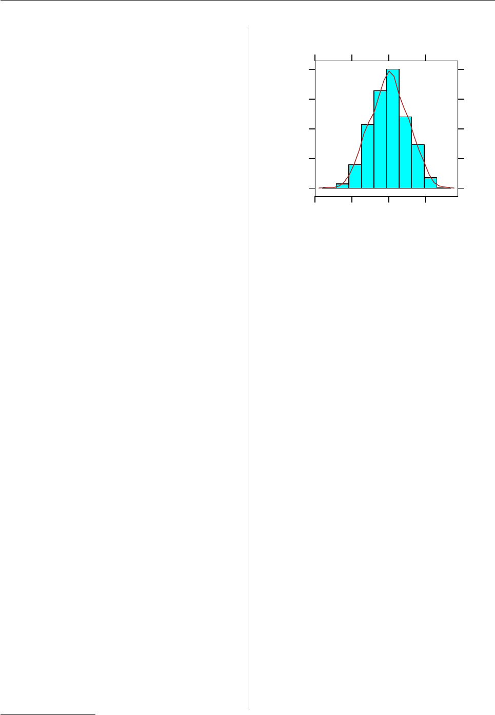
use it again later; printing hist1 produces the plot

shown in Figure 3.4

> hist1 <- histogram(

par.settings=list(fontsize=list(text=8)),

rnorm(500), type = "density",

panel=

function(x, ...) {

panel.histogram(x, ...)

panel.densityplot(x,

col="brown",

plot.points=FALSE)

})

> trellis.par.set(canonical.theme("pdf"))

> print(hist1)

The lattice package uses grid to produce output and

it deﬁnes lots of viewports to draw in. In this case,

there are six viewports created, as shown below.

> current.vpTree()

viewport[ROOT]->(

viewport[plot1.toplevel.vp]->(

viewport[plot1.],

viewport[plot1.panel.1.1.off.vp],

viewport[plot1.panel.1.1.vp],

viewport[plot1.strip.1.1.off.vp],

viewport[plot1.xlab.vp],

viewport[plot1.ylab.vp]))

rnorm(500)

Density

−2 0 2

0.0

0.1

0.2

0.3

0.4

Figure 3: A simple lattice plot.

What we are going to do is add output to the lattice

plot by navigating to a couple of the viewports that

lattice set up and draw a border around the viewport

to show where it is. We will use the frame() function

deﬁned below to draw a thick grey rectangle around

the viewport, then a ﬁlled grey rectangle at the top-

left corner, and the name of the viewport in white

within that.

> frame <- function(name) {

grid.rect(gp=gpar(lwd=3, col="grey"))

grid.rect(x=0, y=1,

height=unit(1, "lines"),

width=1.2*stringWidth(name),

just=c("left", "top"),

gp=gpar(col=NA, fill="grey"))

grid.text(name,

x=unit(2, "mm"),

y=unit(1, "npc") -

unit(0.5, "lines"),

just="left",

gp=gpar(col="white"))

}

The viewports used to draw the lattice plot con-

sist of a single main viewport called (in this case)

"plot1.toplevel.vp", and a number of other view-

ports within that for drawing the various compo-

nents of the plot. This means that the viewport

tree has three levels (including the top-most ROOT

viewport). With a multipanel lattice plot, there can

be many more viewports created, but the naming

scheme for the viewports uses a simple pattern and

3This low-level grid mechanism is general and available for any graphics output produced using grid including lattice output. An

additional higher-level interface has also been provided speciﬁcally for lattice plots (e.g., the trellis.focus() function).

4The call to trellis.par.set() sets lattice graphical parameters so that the colours used in drawing the histogram are those used on

a PDF device. This explicit control of the lattice “theme” makes it easier to exactly reproduce the histogram output in a later example.

R News ISSN 1609-3631

Vol. 5/1, May 2005 15

there are lattice functions provided to generate the

appropriate names (e.g., trellis.vpname()).

When there are more than two levels, there are two

ways to specify a particular low-level viewport. By

default, downViewport() will search within the chil-

dren of a viewport, so a single viewport name will

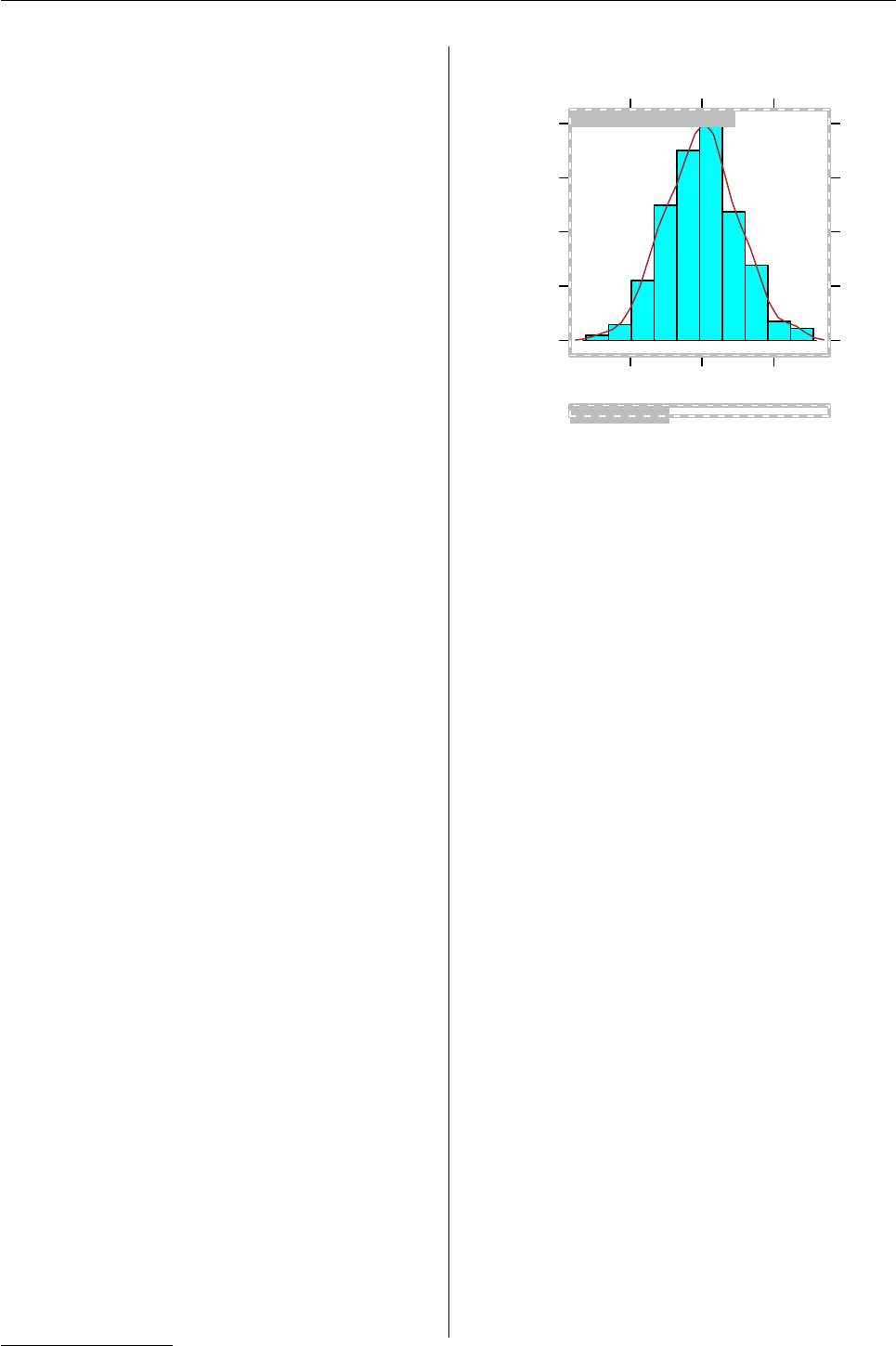
work as before. For example, the following code an-

notates the lattice plot by navigating to the viewport

"plot1.panel.1.1.off.vp" and drawing a frame to

show where it is. This example also demonstrates the

fact that downViewport() returns a value indicating

how many viewports were descended. This “‘depth”

can be passed to upViewport() to ensure that the cor-

rect number of viewports are ascended after the an-

notation.

> depth <-

downViewport("plot1.panel.1.1.off.vp")

> frame("plot1.panel.1.1.off.vp")

> upViewport(depth)

Just using the ﬁnal destination viewport name can be

ambiguous if more than one viewport in the view-

port tree has the same name, so it is also possible

to specify a viewport path. A viewport path is a list

of viewport names that must be matched in order

from parent to child. For example, this next code

uses an explicit viewport path to frame the view-

port "plot1.xlab.vp" that is a child of the viewport

"plot1.toplevel.vp".

> depth <-

downViewport(vpPath("plot1.toplevel.vp",

"plot1.xlab.vp"))

> frame("plot1.xlab.vp")

> upViewport(depth)

It is also possible to use a viewport name or view-

port path in the vp argument to drawing functions, in

which case the output will occur in the named view-

port. In this case, the viewport path is strict, which

means that the full path must be matched start-

ing from the context in which the grob was drawn.

The following code adds a dashed white line to the

borders of the frames. This example also demon-

strates that viewport paths can be speciﬁed as ex-

plicit strings, with a "::" path separator.

The ﬁnal output after all of these annotations is

shown in Figure 4.

> grid.rect(

gp=gpar(col="white", lty="dashed"),

vp="plot1.toplevel.vp::plot1.panel.1.1.off.vp")

> grid.rect(

gp=gpar(col="white", lty="dashed"),

vp="plot1.toplevel.vp::plot1.xlab.vp")

rnorm(500)

Density

−2 0 2

0.0

0.1

0.2

0.3

plot1.panel.1.1.off.vp

plot1.xlab.vp

Figure 4: Annotating the simple lattice plot.

Changes to graphical objects

All grid drawing functions create graphical objects

representing the graphical output. This is good be-

cause it makes it possible to manipulate these objects

to modify the current scene, but there needs to be a

coherent mechanism for working with these objects.

There are several new functions, and some existing

functions have been made more ﬂexible, to provide

a consistent and straightforward mechanism for ac-

cessing, modifying, and removing graphical objects.

All grid functions that produce graphical output,

also create a graphical object, or grob, that represents

the output, and there are functions to access, modify,

and remove these graphical objects. This can be used

as an alternative to modifying and rerunning the R

code to modify a plot. In some situations, it will be

the only way to modify a low-level feature of a plot.

Consider the output from the simple viewport exam-

ple (shown in Figure 2). There are seven pieces of

output, each with a corresponding grob: two rect-

angles, "rect1" and "rect2"; two lines, "line1"

and "line2"; and three sets of circles, "circles1",

"circles2", and "circles3". A particular piece

of output can be modiﬁed by modifying the corre-

sponding grob; a particular grob is identiﬁed by its

name.

The names of all (top-level) grobs in the current

scene can be obtained using the getNames() func-

tion.5

5Only introduced in R version 2.1.0; a less efﬁcient equivalent for version 2.0.0 is to use grid.get().

R News ISSN 1609-3631

Vol. 5/1, May 2005 16

> getNames()

[1] "rect1" "circles1" "line1" "rect2"

[5] "circles2" "line2" "circles3"

The following code uses the grid.get() function to

obtain a copy of all of the grobs. The ﬁrst argument

speciﬁes the names(s) of the grob(s) that should be

selected; the grep argument indicates whether the

name should be interpreted as a regular expression;

the global argument indicates whether to select just

the ﬁrst match or all possible matches.

> grid.get(".*", grep=TRUE, global=TRUE)

(rect[rect1], circle[circles1], lines[line1],

rect[rect2], circle[circles2], lines[line2],

circle[circles3])

The value returned is a gList; a list of one or more

grobs. This is a useful way to obtain copies of one or

two objects representing some portion of a scene, but

it does not return any information about the context

in which the grobs were drawn, so, for example, just

drawing the gList is unlikely to reproduce the orig-

inal output (for that, see the grid.grab() function

below).

The following code makes use of the grid.edit()

function to change the colour of the grey circles to

black (see Figure 5). In general, most arguments pro-

vided in the creation of the output are available for

editing (see the documentation for individual func-

tions). It should be possible to modify the gp argu-

ment for all grobs.

> grid.edit("circles3", gp=gpar(col="black"))

●●

● ●

●●

● ●

●

Figure 5: Editing grid output.

The following code uses grid.remove() to delete all

of the grobs whose names end with a "2" – all of the

blue output (see Figure 6).

> grid.remove(".+2$", grep=TRUE, global=TRUE)

●●

● ●

●

Figure 6: Deleting grid output.

These manipulations are possible with any grid out-

put. For example, in addition to lots of viewports, a

lattice plot creates a large number of grobs and all of

these can be accessed, modiﬁed, and deleted using

the grid functions (an example is given at the end of

the article).

Hierarchical graphical objects

Basic grobs simply consist of a description of some-

thing to draw. As shown above, it is possible to get

a copy of a grob, modify the description in a grob,

and/or remove a grob.

It is also possible to create and work with more com-

plicated graphical objects that have a tree structure,

where one graphical object is the parent of one or

more others. Such a graphical object is called a

gTree. The functions described so far all work with

gTrees as well, but there are some additional func-

tions just for creating and working with gTrees.

In simple usage, a gTree just groups several grobs

together. The following code uses the grid.grab()

function to create a gTree from the output in Figure

> nzgrab <- grid.grab(name="nz")

If we draw this gTree on a new page, the output is

exactly the same as Figure 6, but there is now only

one graphical object in the scene: the gTree called

"nz".

> grid.newpage()

> grid.draw(nzgrab)

> getNames()

[1] "nz"

R News ISSN 1609-3631

Vol. 5/1, May 2005 17

This gTree has four children; the four original grobs

that were “grabbed”. The function childNames()

prints out the names of all of the child grobs of a

gTree.

> childNames(grid.get("nz"))

[1] "rect1" "circles1" "line1"

[4] "circles3"

AgTree contains viewports used to draw its child

grobs as well as the grobs themselves, so the origi-

nal viewports are also available.

> current.vpTree()

viewport[ROOT]->(

viewport[leftvp],

viewport[rightvp])

The grid.grab() function works with any output

produced using grid, including lattice plots, and

there is a similar function grid.grabExpr(), which

will capture the output from an expression.6The fol-

lowing code creates a gTree by capturing an expres-

sion to draw the histogram in Figure 3.

> histgrab <- grid.grabExpr(

{ trellis.par.set(canonical.theme("pdf"));

print(hist1) },

name="hist", vp="leftvp")

The grid.add() function can be used to add further

child grobs to a gTree. The following code adds the

histogram gTree as a child of the gTree called "nz".

An important detail is that the histogram gTree was

created with vp="leftvp"; this means that the his-

togram gets drawn in the viewport called "leftvp"

(i.e., in the left half of the scene). The output now

looks like Figure 7.

> grid.add("nz", histgrab)

There is still only one graphical object in the scene,

the gTree called "nz", but this gTree now has ﬁve

children: two lots of circles, one line, one rectangle,

and a lattice histogram (as a gTree).

> childNames(grid.get("nz"))

[1] "rect1" "circles1" "line1"

[4] "circles3" "hist"

The functions for accessing, modifying, and re-

moving graphical objects all work with hierarchical

graphical objects like this. For example, it is pos-

sible to remove a speciﬁc child from a gTree using

grid.remove().

When dealing with a scene that includes gTrees, a

simple grob name can be ambiguous because, by de-

fault, grid.get() and the like will search within the

children of a gTree to ﬁnd a match.

Just as you can provide a viewport path in

downViewport() to unambiguously specify a partic-

ular viewport, it is possible to provide a grob path in

grid.get(),grid.edit(), or grid.remove() to un-

ambiguously specify a particular grob.

Agrob path is a list of grob names that must be

matched in order from parent to child. The following

code demonstrates the use of the gPath() function to

create a grob path. In this example, we are going to

modify one of the grobs that were created by lattice

when drawing the histogram. In particular, we are

going to modify the grob called "plot1.xlab" which

represents the x-axis label of the histogram.

In order to specify the x-axis label unambiguously,

we construct a grob path that identiﬁes the grob

"plot1.xlab", which is a child of the grob called

"hist", which itself is a child of the grob called "nz".

That path is used to modify the grob which repre-

sents the xaxis label on the histogram. The xaxis la-

bel is moved to the far right end of its viewport and

is drawn using a bold-italic font face (see Figure 8).

> grid.edit(gPath("nz", "hist", "plot1.xlab"),

x=unit(1, "npc"), just="right",

gp=gpar(fontface="bold.italic"))

Summary

When a scene is created using the grid graphics sys-

tem, a tree of viewport objects is created to represent

the drawing regions used in the construction of the

scene and a list of graphical objects is created to rep-

resent the actual graphical output.

Functions are provided to view the viewport tree and

navigate within it in order to add further output to a

scene.

Other functions are provided to view the graphical

objects in a scene, to modify those objects, and/or

remove graphical objects from the scene. If graphi-

cal objects are modiﬁed or removed, the scene is re-

drawn to reﬂect the changes. Graphical objects can

also be grouped together in a tree structure and dealt

6The function grid.grabExpr() is only available in R version 2.1.0; the grid.grab() function could be used instead by explicitly

opening a new device, drawing the histogram, and then capturing it.

R News ISSN 1609-3631

Vol. 5/1, May 2005 18

rnorm(500)

Density

−2 0 2

0.0

0.1

0.2

0.3

0.4

Figure 7: Grabbing grid output.

rnorm(500)

Density

−2 0 2

0.0

0.1

0.2

0.3

0.4

Figure 8: Editing a gTree.

R News ISSN 1609-3631

Vol. 5/1, May 2005 19

Table 1: Summary of the new and changed functions in R 2.0.0 relating to viewports.

Function Description

pushViewport() Create a region for drawing on the cur-

rent graphics device.

popViewport() Remove the current drawing region

(does not delete any output).

upViewport() Navigate to parent drawing region (but

do not remove current region).

downViewport() Navigate down to named drawing re-

gion.

current.viewport() Return the current viewport.

current.vpTree() Return the current tree of viewports that

have been created on the current device.

vpPath() Create a viewport path; a concatenated

list of viewport names.

viewport(..., name=) A viewport can have a name associated

with it.

Table 2: Summary of the new and changed functions since R 2.0.0 relating to graphical objects (some functions

only available since R 2.1.0).

Function Description

grid.get() Return a single grob or a gList of grobs.

grid.edit() Modify one or more grobs and (option-

ally) redraw.

grid.remove() Remove one or more grobs and (option-

ally) redraw.

grid.add() Add a grob to a gTree.

grid.grab() Create a gTree from the current scene.

grid.grabExpr() Create a gTree from an R expression

(only available since R 2.1.0).

gPath() Create a grob path; a concatenated list of

grob names.

getNames() List the names of the top-level grobs in

the current scene (only available since R

2.1.0).

childNames() List the names of the children of a gTree.

grid.rect(..., name=) Grid drawing functions can associate a

name with their output.

R News ISSN 1609-3631

Vol. 5/1, May 2005 20

with as a single unit.

Bibliography

P. Murrell. The grid graphics package. R News, 2(2):

14–19, June 2002. URL http://CRAN.R-project.

org/doc/Rnews/.12

D. Sarkar. Lattice. R News, 2(2):19–23, June 2002. URL

http://CRAN.R-project.org/doc/Rnews/.12

Paul Murrell

University of Auckland, New Zealand

pmurrell@auckland.ac.nz

hoa: An R package bundle for higher

order likelihood inference

by Alessandra R. Brazzale

Introduction

The likelihood function represents the basic ingre-

dient of many commonly used statistical methods

for estimation, testing and the calculation of conﬁ-

dence intervals. In practice, much application of like-

lihood inference relies on ﬁrst order asymptotic re-

sults such as the central limit theorem. The approx-

imations can, however, be rather poor if the sample

size is small or, generally, when the average infor-

mation available per parameter is limited. Thanks

to the great progress made over the past twenty-

ﬁve years or so in the theory of likelihood inference,

very accurate approximations to the distribution of

statistics such as the likelihood ratio have been devel-

oped. These not only provide modiﬁcations to well-

established approaches, which result in more accu-

rate inferences, but also give insight on when to rely

upon ﬁrst order methods. We refer to these develop-

ments as higher order asymptotics.

One intriguing feature of the theory of higher or-

der likelihood asymptotics is that relatively simple

and familiar quantities play an essential role. The

higher order approximations discussed in this paper

are for the signiﬁcance function, which we will use

to set conﬁdence limits or to calculate the p-value

associated with a particular hypothesis of interest.

We start with a concise overview of the approxi-

mations used in the remainder of the paper. Our

ﬁrst example is an elementary one-parameter model

where one can perform the calculations easily, cho-

sen to illustrate the potential accuracy of the proce-

dures. Two more elaborate examples, an application

of binary logistic regression and a nonlinear growth

curve model, follow. All examples are carried out us-

ing the R code of the hoa package bundle.

Basic ideas

Assume we observed nrealizations y1,...,ynof in-

dependently distributed random variables Y1,...,Yn

whose density function f(yi;θ)depends on an un-

known parameter θ. Let `(θ) = ∑n

i=1log f(yi;θ)

denote the corresponding log likelihood and ˆ

θ=

argmaxθ`(θ)the maximum likelihood estimator. In

almost all applications the parameter θis not scalar

but a vector of length d. Furthermore, we may

re-express it as θ= (ψ,λ), where ψis the d0-

dimensional parameter of interest, about which we

wish to make inference, and λis a so-called nuisance

parameter, which is only included to make the model

more realistic.

Conﬁdence intervals and p-values can be com-

puted using the signiﬁcance function p(ψ;ˆ

ψ) =

Pr(ˆ

Ψ≤ˆ

ψ;ψ)which records the probability left of

the observed “data point” ˆ

ψfor varying values of

the unknown parameter ψ(Fraser,1991). Exact elim-

ination of λ, however, is possible only in few special

cases (Severini,2000, Sections 8.2 and 8.3). A com-

monly used approach is to base inference about ψon

the proﬁle log likelihood `p(ψ) = `(ψ,ˆ

λψ), which we

obtain from the log likelihood function by replacing

the nuisance parameter with its constrained estimate

λψobtained by maximising `(θ) = `(ψ,λ)with re-

spect to λfor ﬁxed ψ. Let jp(ψ) = −∂2`p(ψ)/∂ψ∂ψ>

denote the observed information from the proﬁle log

likelihood. Likelihood inference for scalar ψis typi-

cally based on the

• Wald statistic, w(ψ) = jp(ˆ

ψ)1/2(ˆ

ψ−ψ);

• likelihood root,

r(ψ) = sign(ˆ

ψ−ψ)2{`p(ˆ

ψ)−`p(ψ)}1/2;

• score statistic, s(ψ) = jp(ˆ

ψ)−1/2d`p(ψ)/dψ.

Under suitable regularity conditions on f(y;θ), all of

these have asymptotic standard normal distribution

R News ISSN 1609-3631

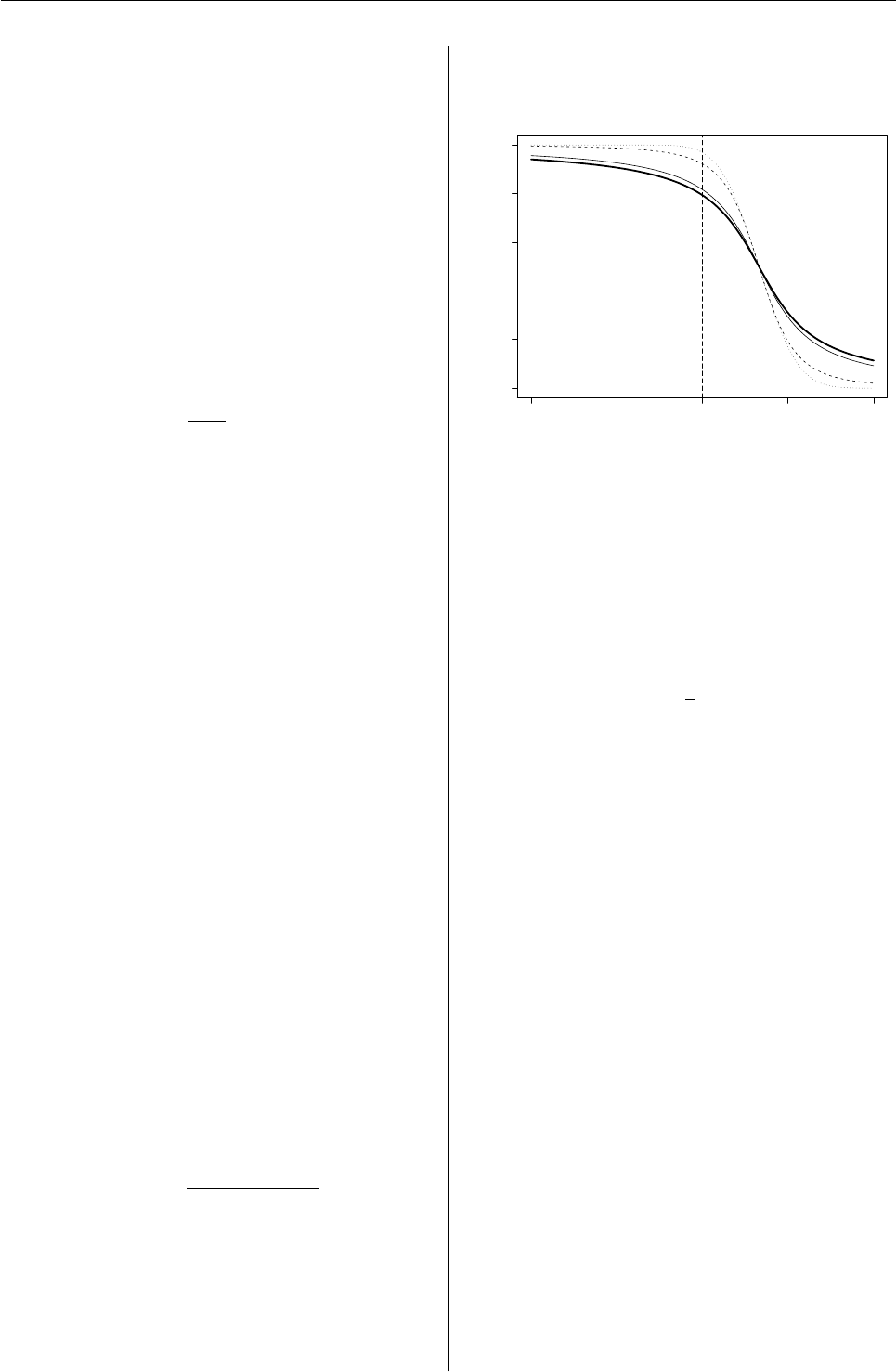
Vol. 5/1, May 2005 21

up to the ﬁrst order. Using any of the above statis-

tics we can approximate the signiﬁcance function by

Φ{w(ψ)},Φ{r(ψ)}or Φ{s(ψ)}. When d0>1, we

may use the quadratic forms of the Wald, likelihood

root and score statistics whose ﬁnite sample distribu-

tion is χ2

d0with d0degrees of freedom up to the sec-

ond order. We refer the reader to Chapters 3 and 4 of

Severini (2000) for a review of ﬁrst order likelihood

inference.

Although it is common to treat `p(ψ)as if it were

an ordinary log likelihood, ﬁrst order approxima-

tions can give poor results, particularly if the dimen-

sion of λis high and the sample size small. An im-

portant variant of the likelihood root is the modiﬁed

likelihood root

r∗(ψ) = r(ψ) + 1

r(ψ)log {q(ψ)/r(ψ)}, (1)

where q(ψ)is a suitable correction term. Expres-

sion (1) is a higher order pivot whose ﬁnite sample

distribution is standard normal up to the third or-

der. As it was the case for its ﬁrst order counter-

part r, the signiﬁcance function is approximated by

Φ{r∗(ψ)}, and there is a version of r∗for multidi-

mensional ψ(Skovgaard,2001, Section 3.1). More

details about the computation of the q(ψ)correction

term are given in the Appendix.

It is sometimes useful to decompose the modiﬁed

likelihood root as

r∗(ψ) = r(ψ) + rinf(ψ) + rnp(ψ),

where rinf is the information adjustment and rnp is the

nuisance parameter adjustment. The ﬁrst term accounts

for non normality of r, while the second compensates

rfor the presence of the nuisance parameter λ.Pierce

and Peters (1992, Section 3) discuss the behaviour of

these two terms in the multiparameter exponential

family context. They ﬁnd that while rnp is often ap-

preciable, the information adjustment rinf has typi-

cally a minor effect, provided the ψ-speciﬁc informa-

tion jp(ˆ

ψ)is not too small relative to the dimension

of λ.

A simple example

Suppose that a sample y1,...,ynis available from

the Cauchy density

f(y;θ) = 1

π{1+ (y−θ)2}. (2)

The maximum likelihood estimate ˆ

θof the unknown

location parameter θis the value which maximises

the log likelihood function

`(θ;y) = −

∑

i=1

log{1+ (yi−θ)2}.

For n=1, we obtain the exact distribution of ˆ

θ=y

from (2) as F(ˆ

θ;θ) = F(y;θ) = π−1arctan(y−θ).

−4 −2 0 2 4

0.0

0.2

0.4

0.6

0.8

1.0

significance function

Figure 1: Signiﬁcance functions for the location pa-

rameter of a Cauchy distribution when y=1.32:

exact (bold), Wald pivot (dotted), r(dashed) and r∗

(solid). The vertical dashed line corresponds to the

null hypothesis θ=0.

Assume that y=1.32 was observed. In Figure 1

we compare the exact signiﬁcance function p(θ;y) =

Pr(Y≤y;θ)(bold line) to the two ﬁrst order approx-

imations obtained from the Wald statistic

w(θ) = √2(y−θ),

(dotted line), and from the likelihood root

r(θ) = sign(ˆ

θ−θ)h2 log{1+ (y−θ)2}i1/2,

(dashed line). We also show the third order approx-

imation Φ{r∗(θ)}(solid line). Since this is a location

model and there is no nuisance parameter, the statis-

tic q(θ)in (1) is the score statistic

s(θ) = √2(y−θ)/{1+ (y−θ)2}

(see formula (6) in the Appendix). The vertical

dashed line corresponds to the null hypothesis that

θ=0. The exact p-value is 0.413, while the ﬁrst

and third order approximations yield 0.0619 (Wald),

0.155 (r) and 0.367 (r∗). The r∗statistic is strikingly

accurate, while the ﬁrst order approximations are

very poor. This is surprising if we consider that the

score function is not monotonic in yand that only

one observation is available. Figure 2summarises

the R code used to generate Figure 1and obtain the

above p-values.

Suppose now that we observed a sample of size

n=15 from the Student t distribution with 3 de-

grees of freedom. It is no longer possible to derive

the exact distribution of the maximum likelihood es-

timator ˆ

θ, but we may use the code provided in the

marg package of the hoa package bundle to compute

the p-values for testing the signiﬁcance of the loca-

tion parameter.

R News ISSN 1609-3631

Vol. 5/1, May 2005 22

## likelihood pivots

> wald.stat <- function(theta, y) {

+ sqrt(2) * (y - theta) }

> lik.root <- function(theta, y) {

+ sign(y - theta) * sqrt( 2 * log(1 + (y - theta)^2) ) }

> score.stat <- function(theta, y) {

+ ( sqrt(2) * (y - theta) )/( 1 + (y - theta)^2 ) }

> rstar <- function(theta, y) {

+ lik.root(theta, y) + 1/lik.root(theta, y) * log( score.stat(theta, y)/lik.root(theta, y) ) }

## significance functions : Figure 1

> theta.seq <- seq(-4, 4, length = 100)

> par( las = 1, mai = c(0.9, 0.9, 0.2, 0.2) )

> plot( theta.seq, pcauchy( q = 1.32 - theta.seq ), type = "l", lwd = 2, ylim = c(0,1),

+ xlab = expression(theta), ylab = "significance function", cex.lab = 1.5, cex.axis = 1.5 )

> lines( theta.seq, pnorm( wald.stat(theta.seq, 1.32) ), lty = "dotted" )

> lines( theta.seq, pnorm( lik.root(theta.seq, 1.32) ), lty = "dashed" )

> lines( theta.seq, pnorm( rstar(theta.seq, 1.32) ), lty = "solid" )

> abline( v = 0, lty = "longdash" )

## p-values

> 2 * ( min( tp <- pt(1.32, df = 1), 1 - tp ) )

> 2 * ( min( tp <- pnorm( wald.stat(0, 1.32) ), 1 - tp ) )

> 2 * ( min( tp <- pnorm( lik.root(0, 1.32) ), 1 - tp ) )

> 2 * ( min( tp <- pnorm( rstar(0, 1.32) ), 1 - tp ) )

Figure 2: R code for drawing Figure 1and calculating the p-values for testing the signiﬁcance of the location

parameter θof a Cauchy distribution when y=1.32.

## simulated data

> library(marg)

> set.seed(321)

> y <- rt(n = 15, df = 3)

> y.rsm <- rsm(y ~ 1, family = student(3))

> y.cond <- cond(y.rsm, offset = 1)

> summary(y.cond, test = 0)

The previous set of instructions yields the p-values

0.282 (Wald), 0.306 (r) and 0.354 (r∗). The difference

between ﬁrst order and higher order approximations

is slightly smaller than it was the case before. For this

particular model a sample size of n=15 still does

not provide enough information on the scalar param-

eter θto wipe out completely the effect of higher or-

der corrections.

Higher order asymptotics in R

hoa is an R package bundle which implements higher

order inference for three widely used model classes:

logistic regression, linear non normal models and

nonlinear regression with possibly non homoge-

neous variance. The corresponding code is organ-

ised in three packages, namely cond,marg and nlreg.

We already saw a (very elementary) application of

the marg code. The two examples which follow will

give a glimpse of the use of the routines in cond

and nlreg. Attention is restricted to the calculation

of p-values and conﬁdence intervals, although sev-

eral routines for accurate point estimation and model

checking are also available. The hoa bundle includes

a fourth package, called sampling, which we will not

discuss here. It implements a Metropolis-Hastings

sampler which can be used to simulate from the

conditional distribution of the higher order statistics

considered in marg.

The hoa package bundle will soon be available on

CRAN. More examples of applications, and gener-

ally of the use of likelihood asymptotics, are given in

Brazzale et al. (to appear).

Example 1: Binary data

Collet (1998) gives a set of binary data on the pres-

ence of a sore throat in a sample of 35 patients un-

dergoing surgery during which either of two devices

was used to secure the airway. In addition to the

variable of interest, device type (1=tracheal tube or

0=laryngeal mask), there are four further explana-

tory variables: the age of the patient in years, an in-

dicator variable for sex (1=male, 0=female), an indi-

cator variable for lubricant use (1=yes, 0=no) and

the duration of the surgery in minutes. The obser-

vations form the data frame airway which is part of

the hoa bundle.

A natural starting point for the analysis is a logis-

tic regression model with success probability of the

R News ISSN 1609-3631

Vol. 5/1, May 2005 23

form

Pr(Y=1; β) = exp(x>β)

1+exp(x>β),

where xrepresents the explanatory variables associ-

ated with the binary response Y(1=sore throat and

0=no sore throat). The following set of instructions

ﬁts this model to the data with all ﬁve explanatory

variables included.

## binomial model fit

> airway.glm <- glm( formula(airway),

+ family = binomial, data = airway )

> summary( airway.glm )

[omitted]

Coefficients:

Estimate Std. Error z value Pr(>|z

(Intercept) -2.75035 2.08914 -1.316 0.18

age 0.02245 0.03763 0.597 0.55

sex1 0.32076 1.01901 0.315 0.75

lubricant1 0.08448 0.97365 0.087 0.93

duration 0.07183 0.02956 2.430 0.01

type1 -1.62968 0.94737 -1.720 0.08

[omitted]

The coefﬁcient of device type is only marginally sig-

niﬁcant.

As in the previous example we may wonder

whether the sample size is large enough to allow us

to rely upon ﬁrst order inference. For the airway data

we have n=35 and p=5, so we might expect

higher order corrections to the usual approximations

to have little effect. We can check this using the rou-

tines in the cond package.

## higher order inference

> library(cond)

> airway.cond <- cond( airway.glm,

+ offset = type1 )

> summary( airway.cond )

# produces 95% confidence intervals

As our model is a canonical exponential family,

the correction term q(ψ)in (1) involves the Wald

statistic w(ψ)plus parts of the observed informa-

tion matrix (see formula (5) in the Appendix). The

95% conﬁdence intervals obtained from the Wald

pivot and from the likelihood root are respectively

(−3.486, 0.227)and (−3.682, 0.154). The third or-

der statistic r∗yields a 95% conﬁdence interval of

(−3.130, 0.256). First and third order results are

rather different, especially with respect to the lower

bound.

−5 −4 −3 −2 −1 0 1 2

−3

−2

−1

coefficient of type

pivot

Figure 3: airway data analysis: proﬁle plots of the

pivots w(ψ)(dashed line), r(ψ)(solid line) and r∗(ψ)

(bold line), where ψis the coefﬁcient of the covariate

device type.

Figure 3plots the proﬁles of the ﬁrst and third order

pivots w(ψ)(dashed line), r(ψ)(solid line) and r∗(ψ)

(bold line). The correction term q(ψ)is particularly

signiﬁcant for values of ψbelonging to the lower half

of the conﬁdence interval. The nuisance parameter

correction is rnp =0.51, while rinf =0.059 is about

ten times smaller.

Example 2: Nonlinear regression

A simple illustration of nonlinear regression is Exam-

ple 7.7 of Davison and Hinkley (1997), which refers

to the calcium data of package boot. This data set

records the calcium uptake (in nmoles/mg) of cells y

as a function of time x(in minutes), after being sus-

pended in a solution of radioactive calcium. There

are 27 observations in all. The model is

yi=β0{1−exp(−β1xi)}+σiεi, (3)

where β0and β1are unknown regression coefﬁcients

and the error term εi∼N(0, 1)is standard normal.

We complete the deﬁnition of model (3) by allowing

the response variance σ2

i=σ2(1+xi)γto depend

nonlinearly on the time covariate through the two

variance parameters γand σ2.

Figure 4gives the R code for the analysis. The

variables cal and time represent respectively the cal-

cium uptake and suspension time. Model (3) is ﬁtted

by maximum likelihood using the nlreg routine of

package nlreg, which yields ˆ

β0=4.317 (s.e. 0.323),

β1=0.207 (s.e. 0.036), ˆγ=0.536 (s.e. 0.320), and

log ˆσ2=−2.343 (s.e. 0.634). Note that the base-

line variance σ2is ﬁtted on the logarithmic scale.

This does not affect inference based on the rand r∗

statistics, which are parametrisation invariant, and

ensures positive values forσ2when the Wald statistic

1Technical details are omitted from the output.

R News ISSN 1609-3631

Vol. 5/1, May 2005 24

> library(boot)

> library(nlreg)

## maximum likelihood fit

> calcium.nl <- nlreg( cal ~ b0 * (1 - exp(-b1 * time)), weights = ~ (1 + time)^g,

+ data = calcium, start = c(b0 = 4, b1 = 0.1, g = 0) )

> summary( calcium.nl ) # yields estimates and standard errors

## pivot profiling for \gamma

> calcium.prof <- profile( calcium.nl, offset = g )

> summary( calcium.prof )

Two-sided confidence intervals for g

lower upper

r* - Fr (0.95) -0.14340 1.191

r* - Sk (0.95) -0.14320 1.190

r (0.95) -0.12441 1.154

Wald (0.95) -0.08991 1.163

Estimate Std. Error

g 0.5364 0.3196

[omitted]

## inference on proportion of maximum

> calcium.nl <- nlreg( cal ~ b0 * (1 - exp(- log(1 + exp(psi)) * time / 15)),

+ data = calcium, start = c(b0 =4.3, psi =2) )

> calcium.prof <- profile( calcium.nl, offset = psi )

> calcium.sum <- summary( calcium.prof )

> exp(calcium.sum$CI) / (1 + exp(calcium.sum$CI)) # 95% confidence intervals for \pi

## profile and contour plots : Figure 5

> calcium.prof <- profile( calcium.nl )

> par( las = 1, mai = c(0.5, 0.5, 0.2, 0.2) )

> contour( calcium.prof, alpha = 0.05, cl1 = "black", cl2 = "black", lwd2 = 2 )

Figure 4: calcium uptake data analysis: R code for model ﬁtting and pivot proﬁling for different parameters

of interest (variance parameter γand “proportion of maximum” π).

is used. Figure 4shows also how to use the profile

method of the nlreg package to set various ﬁrst and

higher order 95% conﬁdence intervals for the vari-

ance parameter γ.1A difﬁculty we had not to face in

the previous two examples is that it is no longer pos-

sible to calculate the correction term in (1) exactly.

The profile function implements two slightly dif-

ferent versions of the higher order pivot r∗which we

obtain by using the two approximations of q(ψ)dis-

cussed in the Appendix. The four statistics agree in

letting us question the heterogeneity of the response

variance.

Davison and Hinkley (1997, p. 356) consider not

only inference on the nonlinear mean function, but

also on other aspects of the model such as the

“proportion of maximum”, π=1−exp(−β1x).

For x=15 minutes they give the estimate ˆπ=

0.956 and the associated 95% bootstrap conﬁdence

interval (0.83, 0.98). We may obtain the corre-

sponding ﬁrst and higher order likelihood analogues

by reparametrizing the mean response curve into

(π,β0)and re-running the whole analysis. This time

we assume that the response variance is homoge-

neous. Because of the constraint that πmust lie

in the interval (0, 1), we actually ﬁt the model for

ψ=log{π/(1−π)}and back-transform to the orig-

inal scale by π=exp(ψ)/{1+exp(ψ)}. This yields

the intervals (0.87, 0.99)and (0.88, 0.99)for respec-

tively the Wald and likelihood root statistics and

(0.87, 0.99)for both versions of r∗, which is in agree-

ment with the bootstrap simulation.

The profile method of the nlreg package pro-

vides also all elements needed to display graphi-

cally a ﬁtted nonlinear model, as done for instance

in Figure 5with respect to the second model ﬁt. The

contour method of the nlreg package represents,

in fact, an enhanced version of the original algo-

rithm by Bates and Watts (1988, Chapter 6), to which

we refer the reader for the interpretation of these

plots. The dashed, solid and bold lines represent re-

spectively the Wald pivot, the likelihood root rand

Skovgaard’s (1996) approximation to the r∗statistic

R News ISSN 1609-3631

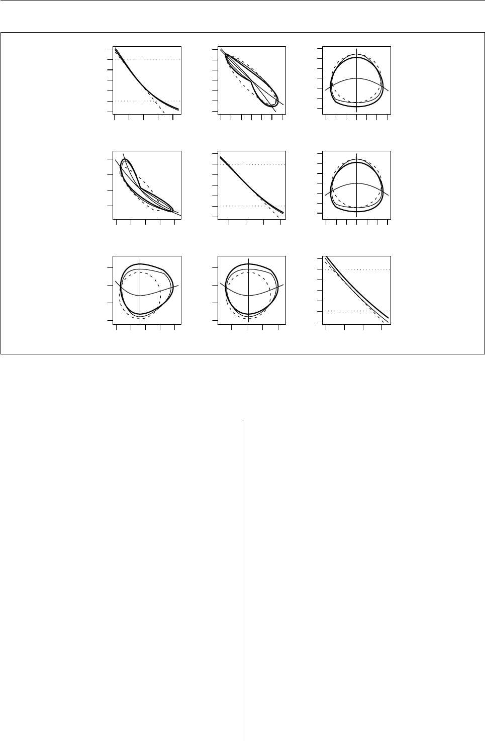
Vol. 5/1, May 2005 25

3.5 4.5 5.5

−3

−2

−1

−3 −1 1 3

−3

−2

−1

3.5 4.5 5.5

−3 −1 1 3

−3

−2

−1

3.5 4.5 5.5

−2.0

−1.5

−1.0

−0.5

2 3 4 5

−3

−2

−1

psi

−3 −1 1 3

−3

−2

−1

2345

−2.0

−1.5

−1.0

−0.5

−2.0 −1.0

−3

−2

−1

logs

Figure 5: calcium uptake data analysis: proﬁle plots and proﬁle pair sketches for the parameters β0,ψand

logσ2using the Wald statistic (dashed), the likelihood root r(solid) and Skovgaard’s (1996) approximation to

r∗(bold).

(see the Appendix). The bivariate contour plots in

the lower triangle are plotted on the original scale,

whereas the ones in the upper triangle are on the

rscale. Figure 5highlights different aspects of the

model ﬁt. First, the maximum likelihood estimate

of log σ2is biased downwards, which we can tell

from the fact the corresponding r∗proﬁle is shifted

to the right of r. Otherwise, there does not seem to

be a huge difference between ﬁrst and higher order

methods as the corresponding proﬁles and contours

are not too different. The ﬁnite sample estimates of

β0and ψare strongly correlated, while they are al-

most independent of log ˆσ2. The contours of r(ψ)

and r∗(ψ)are close to elliptic which indicates that

the log likelihood function is not too far from being

quadratic. A further indication for a small curvature

effect due to parametrisation is that the contours on

the original and on the rscale look similar.

Acknowledgments

I am in debt with Ruggero Bellio, Anthony Davison

and Nancy Reid for the many helpful discussions on

and around higher order likelihood asymptotics. I

would like to thank two anonymous referees whose

suggestions and comments helped improving a pre-

vious version of this paper.

Appendix: q(ψ)correction term

In this appendix we give the general expression of

the correction term q(ψ)in (1) and the explicit for-

mulae for two special model classes, that is, linear ex-

ponential families and regression-scale models. We

will furthermore discuss two ways of approximating

q(ψ)in case we cannot calculate it explicitly.

Basic expression

Let `(θ) = `(ψ,λ)be the log likelihood function,

θ= ( ˆ

ψ,ˆ

λ)the maximum likelihood estimator of the

d-dimensional parameter θ= (ψ,λ), and j(θ) =

−∂2`(θ)/∂θ∂θ>the d×dobserved information ma-

trix. Denote ˆ

λψthe constrained maximum likeli-

hood estimator of the nuisance parameter λgiven

the value of the scalar parameter of interest ψ. Write

jλλ(θ)the corner of j(θ) = j(ψ,λ)which corre-

sponds to λ, and ˆ

θψ= (ψ,ˆ

λψ).

R News ISSN 1609-3631

Vol. 5/1, May 2005 26

The basic expression for q(ψ)is

q(ψ) = |`;ˆ

θ(ˆ

θ)−`;ˆ

θ(ˆ

θψ)`λ>;ˆ

θ(ˆ

θψ)|

|jλλ(ˆ

θψ)||j(ˆ

θ)|1/2, (4)

where |·| indicates determinant (Severini,2000, Sec-

tion 7.4.1). The d×dmatrix appearing in the numer-

ator of q(ψ)consists of a column vector formed using

so-called sample space derivatives

`;ˆ

θ(θ) = ∂`(θ;ˆ

θ|a)

∂ˆ

θ,

and a d×(d−1)matrix of mixed derivatives

`λ>;ˆ

θ=∂2`(ψ,λ;ˆ

θ|a)

∂λ>∂ˆ

θ.

The former are deﬁned as the derivatives of the log

likelihood function `(ψ,λ;ˆ

θ|a)with respect to the

maximum likelihood estimator ˆ

θ; mixed derivatives

furthermore involve differentiation with respect to

the whole parameter θor parts of it (Severini,2000,

Section 6.2.1). Note that to do so, the data vector

has to be re-expressed as y= ( ˆ

θ,a), where arepre-

sents the observed value of an ancillary statistic upon

which we condition.

Approximations

Exact computation of the sample space derivatives

involved in expression (4) requires that we are able to

write the data vector yas a function of the maximum

likelihood estimator ˆ

θand of an ancillary statistic a.

This is, with few exceptions, only feasible for linear

exponential families and transformation models, in

which cases the q(ψ)term involves familiar likeli-

hood quantities. If the reference model is a full rank

exponential family with ψand λtaken as canonical

parameters, the correction term

q(ψ) = w(ψ)|jλλ (ˆ

θ)|/|jλλ(ˆ

θψ)|1/2(5)

depends upon the Wald statistic. In case of a

regression-scale model, that is, of a linear regression

model with non necessarily normal errors,

q(ψ) = s(ψ)|jλλ (ˆ

θψ)|/|jλλ (ˆ

θ)|1/2(6)

involves the score statistic. Here, ψis linear in (β,σ)

and the nuisance parameter λis taken linear in βand

ξ=logσ, where βand σrepresent respectively the

regression coefﬁcients and the scale parameter.

In general, the calculation of the sample space

derivatives `;ˆ

θ(θ)and mixed derivatives `λ>;ˆ

θ(θ)

may be difﬁcult or impossible. To deal with this dif-

ﬁculty, several approximations were proposed. For

a comprehensive review we refer the reader to Sec-

tion 6.7 of Severini (2000). Here we will mention

two of them. A ﬁrst approximation, due to Fraser

et al. (1999), is based upon the idea that in order to

differentiate the likelihood function `(θ;ˆ

θ|a)on the

surface in the n-dimensional sample space deﬁned

by conditioning on awe need not know exactly the

transformation from yto (ˆ

θ,a), but only the dvec-

tors which are tangent to this surface (Severini,2000,

Section 6.7.2). Skovgaard (1996) on the other hand

suggests to approximate the sample space and mixed

derivatives by suitable covariances of the log like-

lihood and of the score vector (Severini,2000, Sec-

tion 6.7.3). While the ﬁrst approximation maintains

the third order accuracy of r∗, we lose one degree

when following Skovgaard’s (1996) approach. See

Sections 7.5.3 and 7.5.4 of Severini (2000) for the de-

tails.

The hoa package

The expressions of q(ψ)implemented in the hoa

package bundle are: i) (5) and (6) for respectively the

cond and marg packages (logistic and linear non nor-

mal regression), and ii) the two approximations dis-

cussed above for the nlreg package (nonlinear het-

eroscedastic regression). The formulae are given in

Brazzale et al. (to appear). The nlreg package also

implements Skovgaard’s (2001, Section 3.1) multipa-

rameter extension of the modiﬁed likelihood root.

The implementation of the cond and nlreg packages

is discussed in Brazzale (1999) and Bellio and Braz-

zale (2003).

Bibliography

D. M. Bates and D. G. Watts. Nonlinear Regression

Analysis and Its Applications. Wiley, New York,

1988. 24

R. Bellio and A. R. Brazzale. Higher-order asymp-

totics unleashed: Software design for nonlinear

heteroscedastic models. Journal of Computational

and Graphical Statistics, 12:682–697, 2003. 26

A. R. Brazzale. Approximate conditional inference in

logistic and loglinear models. Journal of Computa-

tional and Graphical Statistics, 8:653–661, 1999. 26

A. R. Brazzale, A. C. Davison, and N. Reid. Applied

Asymptotics. Cambridge University Press, Cam-

bridge, to appear. 22,26

D. Collet. Binary data. In P. Armitage and T. Colton,

editors, Encyclopedia of Biostatistics. John Wiley &

Sons, Chichester, 1998. 22

A. C. Davison and D. V. Hinkley. Bootstrap Methods

and Their Application. Cambridge University Press,

Cambridge, 1997. 23,24

D. A. S. Fraser. Statistical inference: Likelihood to

signiﬁcance. Journal of the American Statistical Asso-

ciation, 86:258–265, 1991. 20

R News ISSN 1609-3631

Vol. 5/1, May 2005 27

D. A. S. Fraser, N. Reid, and J. Wu. A simple general

formula for tail probabilities for frequentist and

Bayesian inference. Biometrika, 86:249–264, 1999.

D. A. Pierce and D. Peters. Practical use of higher-

order asymptotics for multiparameter exponential

families. Journal of the Royal Statistical Society Series

B, 54:701–737, 1992. 21

T. A. Severini. Likelihood Methods in Statistics. Oxford

University Press, Oxford, 2000. 20,21,26

I. M. Skovgaard. An explicit large-deviation approx-

imation to one-parameter tests. Bernoulli, 2:145–

165, 1996. 26

I. M. Skovgaard. Likelihood asymptotics. Scandina-

vian Journal of Statistics, 28:3–32, 2001. 21

Alessandra R. Brazzale

Institute of Biomedical Engineering, Italian National Re-

search Council

alessandra.brazzale@isib.cnr.it

Fitting linear mixed models in R

Using the lme4 package

by Douglas Bates

The lme function, which ﬁts linear mixed models of

the form described in Pinheiro and Bates (2000), has

been available in the required R package nlme for

several years. Recently my colleagues and I have

been developing another R package, called lme4, and

its lmer function which provides more ﬂexible ﬁtting

of linear mixed models and also provides extensions

to generalized linear mixed models.

The good news for lme users is that the lmer func-

tion ﬁts a greater range of models, is more reliable,

and is faster than the lme function. The bad news

is that the model speciﬁcation has been changed

slightly. The purpose of this article is to introduce

lmer, to describe how it can be used to ﬁt linear

mixed models and to highlight some of the differ-

ences between lmer and lme.

Linear mixed models

Before describing how to ﬁt linear mixed models I

will describe what they are. In building a statisti-

cal model for experimental or observational data we

often want to characterize the dependence of a re-

sponse, such as a patient’s heart rate, on one or more

covariates, such as the patient identiﬁer, whether the

patient is in the treatment group or the control group,

and the time under treatment. We also want to char-

acterize the “unexplained” variation in the response.

Empirical models (i.e., models that are derived from

the data itself, not from external assumptions on the

mechanism generating the data) are generally cho-

sen to be linear in the parameters as these are much

simpler to use than are nonlinear models.

Some of the available covariates may be repeat-

able in the sense that (conceptually, at least) we can

obtain new observations with the same values of the

covariate as in the current study. For example, we

can recruit a new patient to the study and assign

this patient to the treatment group or to the control

group. We can then observe this patient’s heart rate

at one minute, ﬁve minutes, etc. after treatment.

Hence we would regard both the treatment factor

and the time after treatment covariate as repeatable.

A factor is repeatable if the set of possible levels

of the factor is ﬁxed and each of these levels is itself

repeatable. In most studies we would not regard the

patient identiﬁer factor (or, more generally, the “sub-

ject” factor or any other factor representing an exper-

imental unit) as being repeatable. Instead we regard

the subjects in the study as a random sample from

the population of interest.

Our goals in modeling repeatable covariates and

non-repeatable covariates are different. With a

repeatable covariate we want to characterize the

change in the response between different levels and

for this we use ﬁxed-effects terms that represent, say,

the typical rate of change of the response with respect

to time under treatment or the difference between

a typical response in the treatment and the control

groups. For a non-repeatable covariate we want to

characterize the variation induced in the response by

the different levels of the covariate and for this we

use random-effects terms.

A statistical model that incorporates both ﬁxed-

effects terms and random-effects terms is called a

mixed-effects model or, more simply, a mixed model.

Single grouping factor

As indicated above, a random effect is associated

with a grouping factor, which would be the patient

identiﬁer in our example, and possibly with other co-

variates. We specify a random-effects term in lmer by

a linear model term and a grouping factor separated

by ‘|’, which we would read as “given” or “condi-

tional on”. That is, a random effect is a linear model

term conditional on the level of the grouping factor.

Because the precedence of ‘|’ as an operator

R News ISSN 1609-3631

Vol. 5/1, May 2005 28

is lower than most other operators used in linear

model formulae, the entire random-effects expres-

sion should be enclosed in parentheses.

Many models for longitudinal data (repeated

measurements over time on each of several subjects)

incorporate random effects associated with a single

grouping factor. Consider the HR (heart rate) data

from the SASmixed package

> data("HR", package = "SASmixed")

> names(HR)

[1] "Patient" "Drug" "baseHR"

[4] "HR" "Time"

Initially we ﬁt a linear mixed model with ﬁxed-

effects terms for the base heart rate, the time since

administration of the medication, the type of drug

and the time/drug interaction. The random effect as-

sociated with the patient is a simple additive shift.

> (fm1 <- lmer(HR ~ baseHR + Time *

+ Drug + (1 | Patient), HR))

Linear mixed-effects model fit by REML

Formula: HR ~ baseHR+Time*Drug+(1|Patient)

Data: HR

AIC BIC logLik MLdeviance REMLdeviance

790.7 815.8 -386.3 791.9 772.7

Random effects:

Groups Name Variance Std.Dev.

Patient (Intercept) 44.5 6.67

Residual 29.8 5.46

# of obs: 120, groups: Patient, 24

Fixed effects:

Estimate Std. Error DF

(Intercept) 33.962 9.931 113

baseHR 0.588 0.118 113

Time -10.698 2.421 113

Drugb 3.380 3.784 113

Drugp -3.778 3.802 113

Time:Drugb 3.512 3.424 113

Time:Drugp 7.501 3.424 113

t value Pr(>|t|)

(Intercept) 3.42 0.00087

baseHR 4.97 2.5e-06

Time -4.42 2.3e-05

Drugb 0.89 0.37358

Drugp -0.99 0.32244

Time:Drugb 1.03 0.30717

Time:Drugp 2.19 0.03050

The ﬁrst few lines of the output state that the

model has been ﬁt using the REML (restricted or

residual maximum likelihood) criterion and indicate

the formula and the data set used. The next line pro-

vides several measures of the quality of the ﬁt in-

cluding Akaike’s Information Criterion, Schwartz’s

Bayesian Information Criterion, the log-likelihood

(actually the log-restricted likelihood because REML

is being used) and the ML and REML versions of the

deviance.

The estimates of the variance components are

given next. Note that the column headed Std.Dev. is

not the standard error of the estimate of the variance

component. It is simply the square root of the esti-

mated variance and is included because many peo-

ple (and I am one) ﬁnd it easier to interpret an es-

timated standard deviation instead of an estimated

variance.

Finally the estimates for the ﬁxed-effects coef-

ﬁcients are summarized. If we wish to consider

the signiﬁcance of terms rather than individual co-

efﬁcients we can use a single-argument call to the

anova generic which provides the sequential sums of

squares and the corresponding F tests.

> anova(fm1)

Analysis of Variance Table

Df Sum Sq Mean Sq Denom

baseHR 1 746 746 113

Time 1 753 753 113

Drug 2 87 43 113

Time:Drug 2 143 72 113

F value Pr(>F)

baseHR 25.05 2.1e-06

Time 25.28 1.9e-06

Drug 1.46 0.237

Time:Drug 2.40 0.095

At present the denominator degrees of freedom

shown in the coefﬁcient table and in the analysis of

variance table are upper bounds. In a sense there

is no “correct” denominator degrees of freedom be-

cause the F test is always an approximation for these

models. But, even taking this into account, it is still

the case that the denominator degrees of freedom for

the Drug term should be lower than shown. The rea-

son that these degrees of freedom are not more ac-

curately approximated at present is because it is dif-

ﬁcult to decide exactly how this should be done for

the general models described below.

Before changing the ﬁxed effects terms in the

model we may wish to examine models with more

general speciﬁcations of the random effects, such as

both a random intercept and a random slope (with

respect to time) for each patient.

> VarCorr(fm2 <- lmer(HR ~ baseHR +

+ Time * Drug + (Time | Patient),

+ HR))

Groups Name Variance Std.Dev.

Patient (Intercept) 60.6 7.79

Time 37.8 6.15

Residual 24.4 4.94

Corr

-0.563

R News ISSN 1609-3631

Vol. 5/1, May 2005 29

> head(model.matrix(~Time, HR), n = 3)

(Intercept) Time

1 1 0.01667

2 1 0.08333

3 1 0.25000

> head(ranef(fm2)$Patient, n = 3)

(Intercept) Time

201 0.871 4.04733

202 -9.341 6.79574

203 5.005 -0.07822

> anova(fm1, fm2)

Data: HR

Models:

fm1:HR ~ baseHR+Time*Drug+(1|Patient)

fm2:HR ~ baseHR+Time*Drug+(Time|Patient)

Df AIC BIC logLik Chisq Chi Df

fm1 9 810 835 -396

fm2 11 810 841 -394 3.77 2

Pr(>Chisq)

fm1

fm2 0.15

To save space I summarized this ﬁtted model us-

ing VarCorr which describes only the estimates of

the variance components. Notice that the expression

Time generates a model matrix (model.matrix) with

two columns, (Intercept) and Time, so there are

two random effects associated with each patient.

The distribution of the random effects is a bivariate

normal distribution with mean zero and a positive-

deﬁnite 2 ×2 variance-covariance matrix. The esti-

mates of the two variances and the estimated corre-

lation are given in the output.

The ranef generic function returns the BLUPs

(Best Linear Unbiased Predictors) of the random ef-

fects and anova provides a likelihood ratio test when

given multiple model ﬁts to the same data set. As

described in Pinheiro and Bates (2000), the p-value

calculated for this test will be conservative (i.e. it is

an upper bound on the true p-value) because the pa-

rameter space is bounded and in the null hypothesis

one of the parameters is at the boundary.

Multiple random-effects expres-

sions

As shown above, the estimated variance-covariance

matrix from a random-effects expression, such as

(Time|Patient), for which the model matrix has

multiple columns is a general, positive-deﬁnite, sym-

metric matrix. (“General” in the sense that there are

no constraints imposed on this matrix other than its

being positive-deﬁnite.)

Occasionally we wish to impose further con-

straints such as independence of random effects as-

sociated with the same grouping factor. For exam-

ple we can ﬁt a model with an intercept and slope

for each patient but assuming independence of these

random effects with

> VarCorr(fm3 <- lmer(HR ~ baseHR +

+ Time * Drug + (1 | Patient) +

+ (Time - 1 | Patient), HR))

Groups Name Variance Std.Dev.

Patient (Intercept) 47.9 6.92

Patient Time 25.0 5.00

Residual 25.6 5.06

> anova(fm1, fm3, fm2)

Data: HR

Models:

fm1: HR~baseHR+Time*Drug+(1|Patient)

fm3: HR~baseHR+Time*Drug+(1|Patient)

+(Time-1|Patient)

fm2: HR~baseHR+Time*Drug+(Time|Patient)

Df AIC BIC logLik Chisq Chi Df

fm1 9 810 835 -396

fm3 10 811 839 -396 0.84 1

fm2 11 810 841 -394 2.93 1

Pr(>Chisq)

fm1

fm3 0.358

fm2 0.087

The ﬁtted model fm3 has a random intercept and a

random slope for each patient, as does fm2, but in fm3

these random effects are assumed to be independent

within patient. Hence fm3 uses one fewer degree of

freedom than does fm2.

In general the random effects from each expres-

sion are modeled as independent. If the model ma-

trix from the ith random-effects expression has qi

columns and the grouping factor has kilevels (this

number is well-deﬁned because unused levels are

dropped during construction of the model frame) the

corresponding random effects vector has length kiqi

and could be arranged as a ki×qimatrix as shown in

the ranef output above. The rows share a common

ki×kivariance-covariance matrix. Different rows are

independent.

Nested and non-nested grouping factors

We have seen an example of multiple random-effects

expressions for the same grouping factor. It is more

common to create random-effects expressions asso-

ciated with different grouping factors. For example

in a multicenter trial we may have observations over

time on each of several patients at each of several in-

stitutions and it could be appropriate to use random

effects for both patient and institution.

If each patient is observed at only one institution

we say that the levels of patient are nested within the

R News ISSN 1609-3631

Vol. 5/1, May 2005 30

levels of institution; otherwise the factors are non-

nested. Notice that it only takes one patient migrat-

ing between institutions to cause the grouping fac-

tors to lose the nesting property. This may not be a

primary concern in the analysis of multicenter trials

but it is an important issue in the analysis of student

test scores over time where it is quite common to

have some portion of the students observed at mul-

tiple schools. In these cases analysis of the data as

if students were nested within schools is at best an

approximation and at worst quite inappropriate.

A major distinction between lme and lmer is that

lme is optimized for nested grouping factors whereas

lmer handles nested and non-nested grouping fac-

tors equally easily. In lmer one simply provides mul-

tiple random-effects expressions and the determina-

tion of nested or non-nested is done in the code.

Consider the star data (Student Teacher

Achievement Ratio) from the mlmRev package. These

data are from a large study - 26,796 observations

on a total of 11,598 students in 80 schools. We in-

ferred teacher ids from characteristics of the teacher

and classroom, resulting in 1387 distinct teacher ids.

(This teacher count is not entirely accurate but it is a

reasonable approximation.)

We ﬁt an initial model to the math test scores.

> VarCorr(fm4 <- lmer(math ~ gr +

+ sx + eth + cltype + (yrs |

+ id) + (yrs | sch), star))

Groups Name Variance Std.Dev.Corr

id (Intercept) 1079.2 32.85

yrs 22.9 4.78 -0.315

sch (Intercept) 292.8 17.11

yrs 56.8 7.53 -0.777

Residual 584.1 24.17

> anova(fm4)

Analysis of Variance Table

Df Sum Sq Mean Sq Denom

gr 3 1622511 540837 24566

sx 1 9641 9641 24566

eth 5 192909 38582 24566

cltype 2 63848 31924 24566

F value Pr(>F)

gr 925.9 < 2e-16

sx 16.5 4.9e-05

eth 66.0 < 2e-16

cltype 54.6 < 2e-16

It happens in this case that the grouping factors

id and sch are not nested but if they were nested

there would be no change in the model speciﬁcation.

It is likely that the lmer function would converge

more rapidly if the grouping factors were nested

but even with the nonnested grouping factors in this

large study convergence is reasonably fast.

Specifying levels

Because nested and non-nested grouping factors are

expressed in exactly the same way, it is not possible

to use implicit nesting when specifying the levels of

the grouping factors. Implicit nesting occurs when

the levels of the “inner” grouping factor are reused

for different levels of the “outer” grouping factor.

For example, if the patients are numbered starting at

patient 1 for each institution then patient 1 at insti-

tution 1 is distinguished from patient 1 at institution

2 only if it is assumed that patient is nested within

institution.

For lmer each distinct experimental unit must

correspond to a distinct level in the corresponding

grouping factor. It is easy to create a new group-

ing factor with this property from implicitly nested

factors using the interaction operator ‘:’. The Pixel

data set in the MEMSS package has one grouping fac-

tor Dog and another factor Side. If we wish to ﬁt a

model with random effects for “side within dog” we

must ﬁrst create a dog/side factor as

> Pixel$DS <- with(Pixel,Dog:Side)[drop=TRUE]

In this case the subset expression [drop=TRUE] is

not needed but it is a good practice to use it when-

ever creating such a factor. The expression results

in any combinations of levels that does not occur in

the data being dropped from the list of levels in the

newly created factor.

Summary

The lmer function in the lme4 package ﬁts linear

mixed models. There are vast changes in the inter-

nals of lmer relative to the earlier lme function and

we hope they will ensure that lmer is faster, more re-

liable, and easier to use than was lme. The biggest

impact on the user is the change in model speciﬁca-

tion, which was made so as to clarify the model being

ﬁt. The lmer function uses a single model formula in-

cluding random-effects expressions that specify both

a linear model term and a grouping factor and can be

used to ﬁt models based on multiple nested or non-

nested grouping factors. It can also be used to ﬁt

generalized linear mixed models but that is a topic

for another day.

Bibliography

J. C. Pinheiro and D. M. Bates. Mixed-Effects Models

in S and S-PLUS. Springer, 2000. 27,29

Douglas Bates

University of Wisconsin - Madison, U.S.A.

bates@wisc.edu

R News ISSN 1609-3631

Vol. 5/1, May 2005 31

Using R for Statistical Seismology

by Ray Brownrigg & David Harte

Statistical Seismology is a relatively new term used

to describe the application of statistical methodol-

ogy to earthquake data. The purpose is to raise

new questions about the physical earthquake pro-

cess, and to describe stochastic components not ex-

plained by physical models. Such stochastic quantiﬁ-

cation allows one to test the validity of various phys-

ical hypotheses, and also makes probability forecasts

more feasible.

We describe here a suite of Rpackages, known

as the "Statistical Seismology Library" (SSLib). This

paper ﬁrstly introduces SSLib, providing a little his-

tory, and a description of its structure. Then the

various components of SSLib are described in more

detail and some examples are given. While the

packages were developed primarily to analyse earth-

quake data, two of the packages (Fractal and PtPro-

cess) have more general applicability.

For a general text on seismology, see Lay and Wal-

lace (1995). Further, a large collection of seismolog-

ical software can be found at http://orfeus.knmi.

nl/other.services/software.links.shtml.

Introduction to SSLib

The Statistical Seismology Library (SSLib) is a collec-

tion of earthquake hypocentral catalogues (3D loca-

tion of the rupture initiation point, time and mag-

nitude) and Rfunctions to manipulate, describe and

model event data contained in the catalogues. At this

stage, analyses include graphical data displays, ﬁt-

ting of point process models, estimation of fractal di-

mensions, and routines to apply the M8 Algorithm.

While we have named it the "Statistical Seismology

Library", the type of analyses that are performed re-

ally only reﬂect the research interests of the authors.

Part of the rationale was to require our students and

collaborators to formally document their programs

so that others could determine what they were sup-

posed to do, and to be able to use them after they

have possibly moved on. Another aim was to make

some of our statistical methods and models more di-

rectly available to our seismologist and geophysicist

colleagues.

The library is divided into a number of Rpack-

ages. Details of these and source code can all be

found on the Statistical Seismology Library web

page (http://homepages.paradise.net.nz/david.

harte/SSLib/). Package names with a speciﬁcally

seismological character are preﬁxed by "ss" (e.g. the

New Zealand catalogue is named ssNZ), whereas

those with a more general statistical interest are not

(e.g. PtProcess and Fractal). A reference manual

(standard Rformat) for each package can also be

found on the web page, along with a Users Guide

that contains examples and shows how the different

packages relate to each other (Harte,2005e).

SSLib was started in 1996 as an S-PLUS library

(Harte,1998). After being ported to the Rlanguage

in 1999, development of SSLib switched to using the

Rimplementation. At this time, SSLib was only avail-

able on the Unix and Linux platforms, but in 2004 a

Windows version was released.

Earthquake Catalogues

Generally, users will want to use their own earth-

quake catalogues. However SSLib does contain

various earthquake catalogues including the New

Zealand catalogue and the PDE catalogue (Pre-

liminary Determinations of Epicentres) which is

a worldwide catalogue collated by the US Geo-

logical Survey. Further details of the catalogues

available in SSLib can be found on the SSLib

web page (see http://homepages.paradise.net.

nz/david.harte/SSLib/).

The earthquake catalogues are based on raw data

available from the World Wide Web. These data are

generally collected by national seismological obser-

vatories. The raw data appears in many different for-

mats, but the SSLib input routines coerce these dif-

ferent formats into a single common structure. This

allows for both a uniformity in analysis, and the abil-

ity to make comparisons between the different cata-

logues. Nevertheless, the data structure within the

catalogue packages allows for the inclusion of any

number of extra data ﬁelds; see Harte (2005e) for fur-

ther details.

Catalogue Manipulation Utilities

The ssBase package (Harte,2005b) provides cata-

logue preparation and data manipulation functions.

These include functions for date/time formatting,

data summaries, printing and data subsetting. This

package also contains other functions of a general na-

ture used by the other packages.

A catalogue can be subsetted on any combination

of location, time range, depth range or magnitude

range, with the location being rectangular (in the lat-

itude/longitude sense), circular (actually cylindrical

in 3 dimensions), spherical, or based on an arbitrary

polygon on the surface of the earth. Many of the

analysis functions will work directly with a subset

’object’.

R News ISSN 1609-3631

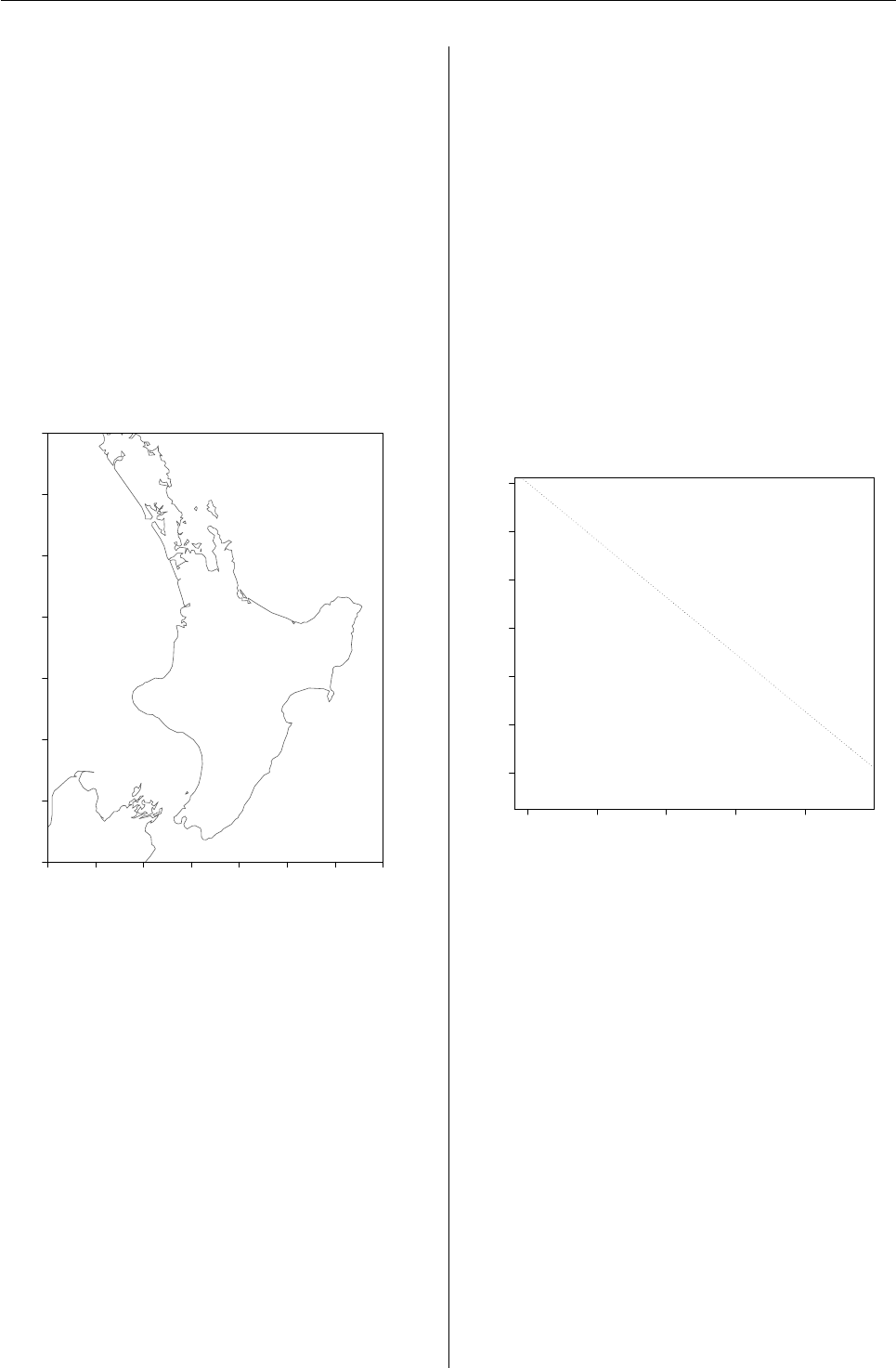
Vol. 5/1, May 2005 32

Exploratory Data Analyses

The ssEDA package (Harte,2005c) consists of func-

tions for exploratory data analysis. In particular

these can provide histograms of event depth or event

frequency (monthly or yearly), line plots of magni-

tude over time, maps of the locations of the epicen-

tres, and frequency-magnitude plots to determine a

b-value (see Figure 2) or to check the completeness of

a catalogue. Further, the epicentre maps can identify

different magnitudes and depths. Interactive graph-

ics can be used to identify individual events on epi-

central plots, and dynamic graphics can be used to

show 3-dimensional views with rotation and linked

plots.

172 173 174 175 176 177 178 179

−42 −41 −40 −39 −38 −37 −36 −35

●

●●

●

●●

●

●●

●

●●

●

●●

●

●●

●

●●

●

●●

●

●●

●

●●

●

●●

●

●●

●

●●

●

●●

●

●●

●

●●

●

●●

●

● ●

●

●●

●

●●

●

●●

●

●●

●

NZ Events Since 1965 With M ≥4.5

Figure 1: Epicentral plot of events from the NZ cata-

logue since 1965 with magnitude ≥4.5 (1777 events).

The Paciﬁc tectonic plate to the east is subducting the

Australian plate to the west.

Figure 1shows a map of the epicentres of a sub-

set of events from the New Zealand catalogue. The

colour of the point depicts the depth of the event,

with the most shallow events at the red end of the

spectrum and the deep events at the blue end of the

spectrum. The Rcommands required to display this

plot follow.

library(ssNZ)

library(ssEDA)

b <- subset.rect(NZ, minday=julian(1, 1, 1965),

minmag=4.5, minlat=-42,

maxlat=-35, minlong=172,

maxlong=179, mindepth=40)

epicentres(b, depth=c(40, 60, 80, 100, 150,

200, Inf), mapname="nz",

criteria=FALSE, cex=0.8,

usr=c(172, 179, -42, -35))

title(expression(paste("NZ Events Since 1965

With ", M >= 4.5)))

Figure 2is a frequency-magnitude plot for the

same subset as used in Figure 1and displays the

Gutenberg-Richter law (Lay and Wallace,1995). This

law says that the logarithm of the cumulative num-

ber of events with magnitude greater than mis lin-

ear as a function of m. The R commands required

to present this graph (given the call to subset.rect

from the previous ﬁgure) follow.

freq.magnitude(b)

title("Frequency Magnitude Power-Law

Relationship")

●

●●●

●

● ●

●

4.5 5.0 5.5 6.0 6.5

−3.0 −2.5 −2.0 −1.5 −1.0 −0.5 0.0

log10(Proportion of Events with Magnitude > m)

Frequency Magnitude Power−Law Relationship

Figure 2: Plot of events from the NZ catalogue since

1965 with magnitude ≥4.5 showing the Gutenberg-

Richter law. The absolute value of the slope is re-

ferred to as the b-value and is typically about one.

The interactive graphics is provided by the

epicentres.identify function through use of the

identify R function. The dynamic graphics is pro-

vided through the threeD function, which links to

an external viewer provided by the xgobi software

(Swayne et al.,1998) via the xgobi R function. Un-

fortunately xgobi is not easily usable on a Windows

system, so work is in progress to use ggobi (GGobi)

instead.

Point Process Modelling

The PtProcess package (Harte,2004), which can be

used independently of the other packages, provides

a framework for point process modelling. This in-

cludes parameter estimation, model evaluation and

R News ISSN 1609-3631

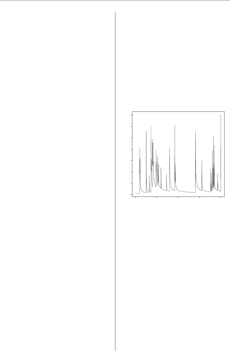
Vol. 5/1, May 2005 33

simulation. This package is likely to be of most inter-

est to a general statistical audience.

Our PtProcess package has a slightly different

emphasis to the point process packages spatstat

(available on CRAN) and ptproc (http://sandybox.

typepad.com/software/ptproc/index.html). Our

point process models are for events strictly ordered

by time, and are conditional on the history of the pro-

cess up to time t. This could be thought of as the

ground process (Daley and Vere-Jones,2003). Other

event characteristics could be added as marks, e.g.

earthquake event magnitude. The spatstat package

(Baddeley and Turner,2005) has an emphasis on the

spatial location of items, presumably at the same

point in time, e.g. tree locations or animals in a for-

est, etc. Emphasis is then on modelling the spatial

intensity. Here marks can be added, e.g. the particu-

lar species of tree. The ptproc package (Peng,2003) is

derived from our package, and has extended the pro-

cedure into multidimensional processes. However,

these additional variables are not treated as marks,

and hence provides an alternative direction to our in-

tended direction.

While the conditional intensity functions pro-

vided within the package have a distinctly seismo-

logical ﬂavour, the general methodology and struc-

ture of the package is probably applicable to a rea-

sonably large class of point process models. The

models ﬁtted are essentially marked point processes

(Daley and Vere-Jones,2003), where the mark dis-

tribution has been explicitly built into the condi-

tional intensity function. Our next task is to sepa-

rate the mark distribution and ground intensity func-

tion, and further generalise the framework so that

any number of mark distributions can be attached to

a given ground intensity function.

Currently the conditional intensity function is the

most basic "building block". The conditional inten-

sity function, λ(t|Ht), can be thought of as an instan-

taneous value of the Poisson rate parameter at time t

and is conditional on the history of the process up to

but not including t. We have given each conditional

intensity function a sufﬁx ".cif". There are a num-

ber of "generic"-like functions which perform some

operation given an intensity function, for example,

simulate a process, perform a goodness of ﬁt evalua-

tion, etc.

As an example, consider the ETAS (Epidemic

Type Aftershock Sequence) model. This assumes

that earthquake events behave in a similar way to

an epidemic, where each event reproduces a number

of aftershocks. The larger the event, the more after-

shocks that will be reproduced. If various criticality

conditions are satisﬁed, the aftershock sequence will

eventually die out. See Harte (2004) and Utsu and

Ogata (1997) for further technical details about the

ETAS model.

The package contains an example dataset pro-

vided by Yosihiko Ogata. These data were simulated

over the time interval (0, 800). Using these data and

approximate maximum likelihood solutions for the

parameters contained in p(the ETAS model contains

5 parameters), the conditional intensity function can

be plotted as follows (see Figure 3).

library(PtProcess)

data(Ogata)

p <- c(0.02, 70.77, 0.47, 0.002, 1.25)

ti <- seq(0, 800, 0.5)

plot(ti, log(etas.cif(Ogata, ti, p)),

ylab=expression(paste("log ", lambda(t))),

xlab="Time", type="l", xlim=c(0, 800),

main="Conditional Intensity Function")

0 200 400 600 800

−4 −3 −2 −1 0 1 2 3

Conditional Intensity Function

Time

log λ(t)

Figure 3: The spikes occur at event times and their

heights are proportional to the event magnitudes,

with an "Omori" decay (Lay and Wallace,1995) in the

rate after each event.

Further, the log-likelihood can be calculated as

follows.

pp.LL(Ogata, etas.cif, p, c(0, 800))

Using the vector pas initial values, maximum

likelihood parameter estimates can be calculated as

follows.

posterior <- make.posterior(Ogata, etas.cif,

c(0, 800))

neg.posterior <- function(params)

(-posterior(params))

p <- c(0.02, 70.77, 0.47, 0.002, 1.25)

z <- nlm(neg.posterior, p, hessian=TRUE,

iterlim=1000, typsize=p)

The function make.posterior creates a log-

likelihood function to be evaluated on the time inter-

val (0, 800), and also gives one the option of enforc-

ing constraints on the parameters (none here). We

R News ISSN 1609-3631

Vol. 5/1, May 2005 34

then create a negative posterior function because the

function nlm is a minimiser. The maximum likeli-

hood parameter estimates are contained within the

object z.

The creation of the posterior function was partly

done so that the function to be "optimised" within S-

PLUS had only one argument. This is not necessary

in R. Further, the use of priors has not been as useful

as was initially thought. Consequently, it is probably

best to revise the package so that the optimisation

works more directly on the pp.LL function.

One way to test for the goodness of ﬁt is to cal-

culate the transformed residual process. This effec-

tively creates a new time variable which magniﬁes or

contracts the original process, assuming that the ﬁt-

ted model is correct, in such a manner that the resul-

tant process is a homogeneous Poisson process with

rate parameter one. A plot of the transformed event

times versus the event number should roughly fol-

low the line x=y. Large deviations from this line

indicate a poorly ﬁtting model. This can be achieved

with the following code.

tau <- pp.resid(Ogata, z$estimate, etas.cif)

n <- nrow(Ogata)

plot(1:n, tau, type="l", xlab="Event Number",

ylab="Transformed Time",

xlim=c(0, n), ylim=c(0, n))

abline(a=0, b=1, lty=2, col="red")

Using the maximum likelihood parameter esti-

mates, one can simulate the process over the subse-

quent interval (800, 1200), say. This is achieved as

follows.

x <- pp.sim(Ogata, z$estimate, etas.cif,

TT=c(800, 1200))

The object xcontains the original Ogata data,

with the new simulated events appended. One may

be interested in forecasting the time taken for an

event with magnitude ≥6, say, to occur after time

800. One would then perform many such simula-

tions, and determine the empirically simulated dis-

tribution for the given event of interest.

As can be seen, the conditional intensity function

is the essential ingredient in each of the above analy-

ses, and hence an entity like this is an essential com-

ponent in a more object oriented setup for these mod-

els. It is a relatively simple step to set this up in a

more object oriented manner, however, we have held

off with this until we have disentangled the condi-

tional intensity into its ground process and a general

number of mark distributions.

Other Analyses

The ssM8 package (Harte,2005d) implements the

Keilis-Borok & Kossobokov M8 algorithm (Keilis-

Borok and Kossobokov,1990). It is an empirically

based algorithm that attempts to deduce "times of

increased probability". We have been involved in

projects that have attempted to test the efﬁcacy of

this algorithm.

The Fractal package (Harte,2005a) has been used

to calculate various fractal dimensions based on

earthquake hypocentral locations, for example, see

Harte (2001).

Problems and Future Development

We have already mentioned a number of extensions

to the Point Process package: separating the condi-

tional intensity into a ground intensity and a gen-

eral number of mark distributions, writing more ob-

ject oriented code, and determining if there is still

a need for the make.posterior function. To imple-

ment more object oriented code, the naming conven-

tions would clearly need to be changed.

There is a difference with the functions contained

in the chron package (Ripley and Hornik,2001;

Grothendieck and Petzoldt,2004) and our "date-

times" format in ssBase (Harte,2005b). We would

prefer to use the chron functions, however, we

would like the format.times function within chron

to have greater ﬂexibility, including fractional num-

bers of seconds. For example, we would like the

ability to specify a times format as hh:mm:ss.s, or

hh:mm:ss.ss. Further, many historical earthquake

events do not have all date-time components avail-

able, and our "datetimes" format has a mechanism to

deal with this. Note that the POSIX functions are in-

appropriate, as the event times are generally stored

as UTC times.

A feature that we have included in all of our pack-

ages is a "changes" manual page. This documents all

recent changes made to the package with the date.

We have found this particularly useful when old

analyses have been repeated and different answers

are produced!

As noted earlier, the type of analyses included in

SSLib largely reﬂects our own research interests. This

also means that it is continually being changed and

augmented.

Bibliography

A. Baddeley and R. Turner. Spatstat: an Rpackage

for analyzing spatial point patterns. Journal of Sta-

tistical Software, 12(6):1–42, 2005. ISSN 1548-7660.

URL http://www.jstatsoft.org.33

D. Daley and D. Vere-Jones. An Introduction to the

Theory of Point Processes, volume I: Elementary

Theory and Methods. Springer-Verlag, New York,

second edition, 2003. 33

GGobi. GGobi data visualization system. http:

//www.ggobi.org/, 2003. 32

R News ISSN 1609-3631

Vol. 5/1, May 2005 35

G. Grothendieck and T. Petzoldt. Rhelp desk: Date

and time classes in R.R News, 4(1):29–32, 2004. 34

D. Harte. Documentation for the Statistical Seis-

mology Library. Technical Report 98-10, School

of Mathematical and Computing Sciences, Vic-

toria University of Wellington, Wellington, New

Zealand, 1998. 31

D. Harte. Multifractals: Theory and Applications. Chap-

man and Hall/CRC, Boca Raton, 2001. 34

D. Harte. Package PtProcess: Time Dependent Point

Process Modelling. Statistics Research Asso-

ciates, Wellington, New Zealand, 2004. URL

http://homepages.paradise.net.nz/david.

harte/SSLib/Manuals/pp.pdf.32,33

D. Harte. Package Fractal: Fractal Analysis. Statistics

Research Associates, Wellington, New Zealand,

2005a. URL http://homepages.paradise.net.

nz/david.harte/SSLib/Manuals/fractal.pdf.

D. Harte. Package ssBase: Base Functions

for SSLib. Statistics Research Associates,

Wellington, New Zealand, 2005b. URL

http://homepages.paradise.net.nz/david.

harte/SSLib/Manuals/base.pdf.31,34

D. Harte. Package ssEDA: Exploratory Data Analysis

for Earthquake Data. Statistics Research Asso-

ciates, Wellington, New Zealand, 2005c. URL

http://homepages.paradise.net.nz/david.

harte/SSLib/Manuals/eda.pdf.32

D. Harte. Package ssM8: M8 Earthquake Fore-

casting Algorithm. Statistics Research Asso-

ciates, Wellington, New Zealand, 2005d. URL

http://homepages.paradise.net.nz/david.

harte/SSLib/Manuals/m8.pdf.34

D. Harte. Users Guide for the Statistical Seismol-

ogy Library. Statistics Research Associates,

Wellington, New Zealand, 2005e. URL

http://homepages.paradise.net.nz/david.

harte/SSLib/Manuals/guide.pdf.31

V. Keilis-Borok and V. Kossobokov. Premonitory ac-

tivation of earthquake ﬂow: algorithm M8.Phys.

Earth & Planet. Int., 61:73–83, 1990. 34

T. Lay and T. Wallace. Modern Global Seismology. Aca-

demic Press, San Diego, 1995. 31,32,33

R. Peng. Multi-dimensional point process models in

R.Journal of Statistical Software, 8(16):1–24, 2003.

ISSN 1548-7660. URL http://www.jstatsoft.

org.33

B. Ripley and K. Hornik. Date-time classes. R News,

1(2):8–11, 2001. 34

D. F. Swayne, D. Cook, and A. Buja. XGobi:

Interactive dynamic data visualization in the X

window system. Journal of Computational and

Graphical Statistics, 7(1):113–130, 1998. ISSN

1061-8600. URL http://www.research.att.com/

areas/stat/xgobi/.32

T. Utsu and Y. Ogata. Statistical analysis of seismic-

ity. In J. Healy, V. Keilis-Borok, and W. Lee, edi-

tors, Algorithms for Earthquake Statistics and Predic-

tion, pages 13–94. IASPEI, Menlo Park CA, 1997.

Ray Brownrigg

Victoria University of Wellington

ray@mcs.vuw.ac.nz

David Harte

Statistics Research Associates

david@statsresearch.co.nz

Literate programming for creating and

maintaining packages

Jonathan Rougier

Outline

I describe a strategy I have found useful for devel-

oping large packages with lots of not-obvious math-

ematics that needs careful documentation. The basic

idea is to combine the ‘noweb’ literate programming

tool with the Unix ‘make’ utility. The source of the

package itself has the usual structure, but with the

addition of a noweb directory alongside the Rand man

directories. For further reference below, the general

directory tree structure I adopt is

pkgName

zzu

%%

Rman, . . . inst



noweb



doc doc

where ‘. . . ’ denotes other optional directories such as

src and data.

The ﬁles in the noweb directory are the entry-point

R News ISSN 1609-3631

Vol. 5/1, May 2005 36

for all of the documented code in the package, in-

cluding *.R ﬁles, *.Rd ﬁles, low-level source code,

datasets, and so on. The noweb tool, under the con-

trol of the ﬁle ‘Makeﬁle’ and the Unix make utility, is

used to strip the ﬁles in the noweb directory into the

appropriate places in the other directories. Other tar-

gets in ‘Makeﬁle’ also handle things like building the

package, installing it to a speciﬁc location, cleaning

up and creating various types of documentation.

A complete example R package is available

at http://maths.dur.ac.uk/stats/people/jcr/

myPkg.tar.gz containing the code below, and a bit

more to make ‘myPkg’ into a proper R package.

Literate programming and noweb

The basic idea of literate programming is that when

writing complicated programs, it makes a lot of sense

to keep the code and the documentation of the code

together, in one ﬁle. This requires a mechanism for

treating the ﬁle one way to strip out and assemble the

code, and another way to create the documentation.

With such a mechanism in place, the functionality

of the code can be made much more transparent—

and the documentation much more informative—

because the code itself can be written in a modular or

‘bottom-up’ fashion, and then assembled in the cor-

rect order automatically.

I use the noweb literate programming tool. A

noweb ﬁle looks like a L

EX ﬁle with additional envi-

ronments delimited by <<name of environment>>=

and @. These deﬁne code chunks that ap-

pear specially-formatted in the documentation, and

which get stripped out and assembled into the ac-

tual code. Here is an example of a minimal noweb

ﬁle, called, say, ‘myDoc1.nw’.

\documentclass[a4paper]{article}

\usepackage{noweb}\noweboptions{smallcode}

\pagestyle{noweb}

\begin{document}

Here is some \LaTeX\ documentation. Followed

by the top-level source code.

<<R>>=

# The source of this file is noweb/myDoc1.nw

<<foo function>>

<<bar function>>

Now I can describe the [[foo]] function in more

detail, and then give the code.

<<foo function>>=

"foo" <- function(x) 2 * x^2 - 1

And here is the [[bar]] function.

<<bar function>>=

"bar" <- function(y) sqrt((1 + y) / 2)

% stuff for man page not shown

\end{document}

The [[name]] syntax is used by noweb to highlight

variable names. There are many additional features

of noweb that are useful to programmers. More infor-

mation can be found at the noweb homepage, http:

//www.eecs.harvard.edu/~nr/noweb/.

Tangle

noweb strips out the code chunks and assembles them

using the ‘notangle’ command. One useful feature is

that it can strip out chunks with speciﬁc identiﬁers

using the -R ﬂag. Thus the command notangle -RR

myDoc1.nw will strip all the code chunks identiﬁed

directly or indirectly by <<R>>=, assembling them in

the correct order. The result of this command is the

ﬁle

# The source of this file is noweb/myDoc1.nw

"foo" <- function(x) 2 * x^2 - 1

"bar" <- function(y) sqrt((1 + y) / 2)

which is written to standard output. By redirecting

the standard output we can arrange for this ﬁle to go

in the appropriate place in the package directory tree.

So the full command in this case would be notangle

-RR myDoc1.nw > ../R/myDoc1.R. So as long as we

are consistent in always labelling the ‘top’ chunk of

the R code with an <<R>>= identiﬁer, we can auto-

mate the process of getting the R code out.

If we want, we can do the same thing using

<<man>>= for the content of man pages, <<src>>= for

low-level code, <<data>>= for datasets, and so on.

Each of these can be stripped out and saved as a ﬁle

into the appropriate place in the package directory

tree.

Weave

To build the documentation, noweb uses the ‘noweave’

command, where it is useful to set the -delay option.

Again, this is written to the standard output, and can

be redirected to place the resulting L

EX ﬁle at the

appropriate place in the package tree. I put the L

versions of the *.nw ﬁles in the directory noweb/doc.

Thus the appropriate command is noweave -delay

myDoc1.nw > doc/myDoc1.tex. This ﬁle contains

quite a lot of L

EX commands inserted by noweb to

help with cross-referencing and indexing, and so is

not particularly easy to read. But after using latex,

the result is a dvi ﬁle which integrates the L

EX doc-

umentation and the actual code, in a very readable

format.

R News ISSN 1609-3631

Vol. 5/1, May 2005 37

April 13, 2005 myDoc1.nw 1

Here is some L

X documentation. Followed by the top-level source code.

hRi≡

# The source of this file is noweb/myDoc1.nw

hfoo functioni

hbar functioni

Now I can describe the foo function in more detail, and then give the code.

hfoo functioni≡

"foo" <- function(x) 2 * x^2 - 1

And here is the bar function.

hbar functioni≡

"bar" <- function(y) sqrt((1 + y) / 2)

Similarity to ‘Sweave’

Many users of R will be familiar with Friedrich

Leisch’s ‘Sweave’ function, available in the tools

package. Sweave provides a means of embedding R

code into a report, such as a L

EX report, and then

automatically replacing this code with its output. It

uses the notangle functionality of a literate program-

ming tool like noweb, because the R code must be

stripped out, prior to evaluating it. The difference

is that when Sweave builds the resulting document it

does more than noweave would do, because it must

actually evaluate R on each code chunk and put the

output back into the document. In the literate pro-

gramming described in this article, all that notangle

does is wrap the code chunk in a L

EX command

to format it differently. Sweave can duplicate the

simpler behaviour of notangle with the arguments

echo=TRUE,eval=FALSE in each code chunk: see the

help ﬁle for the function ‘RWeaveLatex’ for more de-

tails.

Using make

Our starting point is a collection of *.nw ﬁles in the

noweb subdirectory. We could, by hand, issue a series

of notangle and noweave commands, each time we

update one or more of these ﬁles. Happily, the Unix

tool make can be used instead. make requires a ﬁle

of speciﬁers, often called ‘Makeﬁle’, which describe

the kinds of things that can be made, and the com-

mands necessary to make them. Obvious candidates

for things we would like to make are the *.R and

*.Rd ﬁles that go into the Rand man subdirectories,

and the documentation that goes into the inst/doc

subdirectory.

The make utility is very powerful, and compli-

cated. I am not an expert at writing a ‘Makeﬁle’,

but the following approach seems to work well. My

Makefile lives in the noweb directory, and all of the

path speciﬁers take this as their starting point.

Simple make targets

Suppose that we have compiled a list of ﬁles that

ought to be in the Rsubdirectory (say, ‘RFILES’), and

we want to use the command ‘make R’ to update

these ﬁles according to changes that have occurred

in the noweb/*.nw ﬁles; the argument Ris known as

a ‘target’ of the make command. We need the follow-

ing lines in Makefile:

# make R files in ../R

R: $(RFILES)

$(RFILES): %.R : %.nw

@echo ’Building R file for $<’

@notangle -RR $< > ../R/$@

@if test ‘egrep ’^<<man>>=’ $<‘ ; then \

notangle -Rman $< > ../man/$*.Rd ; fi

After the comment, preﬁxed by #, the ﬁrst line states

that the command ‘make R’ depends on the ﬁles in

the list ‘RFILES’, which we have already compiled.

The next set of lines is executed for each component

of ‘RFILES’ in turn, conditionally on the *.R ﬁle being

older than the corresponding *.nw ﬁle. Where the *.R

ﬁle is out-of-date in this way, a message is printed,

notangle is called, and the *.R ﬁle is rebuilt and

placed in the Rsubdirectory; if there is a <<man>>=

entry, the *.Rd ﬁle is also rebuilt and placed in the

man subdirectory.

A ‘Makeﬁle’ has its own syntax. Within a target

speciﬁcation, the tags ‘$<’, ‘$@’ and ‘$*’ indicate the

origin ﬁle, the result ﬁle, and the ﬁle stem. Under

each initial line the collection of subsequent com-

mands is indented by tabbing, and the backslash at

the end of the line indicates that the next line is a con-

tinuation. The @at the start of each command line

suppresses the printing of the command to the stan-

dard output.

The attractive feature of make is that it only re-

builds ﬁles that are out-of-date, and it does this

all automatically using information in the ﬁle date-

stamps. This saves a lot of time with a large pack-

age in which there are many *.nw ﬁles in the noweb

directory. In my experience, however, one feels a

certain loss of control with so much automation.

The useful command ‘make --dry-run R’ will print

out the commands that will be performed when the

command ‘make R’ is given, but not actually do

them, which is a useful sanity check. The com-

mand ‘touch myDoc1.nw’ will change the date-stamp

on ‘myDoc1.nw’, so that all derived ﬁles such as

‘myDoc1.R’ will automatically be out-of-date, which

will force a rebuild even if ‘myDoc1.nw’ has not been

modiﬁed: this can be another useful sanity-check.

Suppose instead we want to rebuild the L

documentation in the noweb/doc subdirectory, using

the command ‘make latex’. We need the following

lines in ‘Makeﬁle’:

# make latex files in doc

latex: $(TEXFILES)

$(TEXFILES): %.tex : %.nw

@echo ’Building tex file for $<’

@noweave -delay $< > doc/$@

R News ISSN 1609-3631

Vol. 5/1, May 2005 38

@cd doc; \

latex $@ > /dev/null

where ‘TEXFILES’ is a list of ﬁles that ought to be in

the noweb/doc subdirectory. As before, each *.tex

ﬁle is only rebuilt if it is out-of-date relative to the

corresponding *.nw ﬁle. The resulting *.tex ﬁle is

put into noweb/doc, and then latex is called to create

the corresponding *.dvi ﬁle (rather lazily, the output

from latex is diverted to /dev/null and lost).

Slightly more complicated, suppose we want to

put pdf versions of the *.tex ﬁles into the subdirec-

tory inst/doc, using the command ‘make pdf’. We

need the following lines in ‘Makeﬁle’:

# make pdf files in ../inst/doc

pdf: $(TEXFILES) $(PDFFILES)

$(PDFFILES): %.pdf : %.tex

@echo ’Building pdf file for $<’

@cd doc; \

pdflatex $< > /dev/null;

@mv doc/$@ ../inst/doc/

where ‘PDFFILES’ is a list of ﬁles that ought to be

in the inst/doc subdirectory. The new feature here

is that the command ‘make pdf’ depends on both

‘TEXFILES’ and ‘PDFFILES’. This means that each

component of ‘TEXFILES’ is updated, if necessary,

before the *.pdf ﬁle is rebuilt from the *.tex ﬁle.

To rebuild the *.pdf ﬁle, the pdflatex command is

called on the *.tex ﬁle in noweb/doc, and then the

result is moved to inst/doc.

Additional lines in the ‘Makeﬁle’

The main role of additional lines in ‘Makeﬁle’ is to

supply the lists ‘RFILES’, ‘TEXFILES’ and so on. The

following commands achieve this, and a little bit else

besides, and go at the start of ‘Makeﬁle’:

## minimal Makefile

# look in other directories for files

vpath %.R ../R

vpath %.tex doc

vpath %.pdf ../inst/doc

# get lists of files

NWFILES = $(wildcard *.nw)

RFILES = $(NWFILES:.nw=.R)

TEXFILES = $(NWFILES:.nw=.tex)

PDFFILES = $(NWFILES:.nw=.pdf)

# here are the various targets for make

.PHONY: R latex pdf install

# Now insert the lines from above ...

The three ‘vpath’ lines are necessary to help make to

look in other directories than noweb for certain types

of ﬁle. Thus the *.R ﬁles are to be found in ../R,

the *.tex ﬁles in doc, and so on (all relative to the

noweb directory). The next four lines compile the

lists of various types of ﬁle: ‘NWFILES’ are found

in the noweb directory, ‘RFILES’ are ‘NWFILES’ ﬁles

with the ‘nw’ sufﬁx replaced with a ‘R’ sufﬁx, and so

on. For the ﬁnal line, the .PHONY command is a bit of

defensive programming to identify the targets of the

make command.

Example

The ﬁle http://maths.dur.ac.uk/stats/people/

jcr/myPkg.tar.gz contains a small example of an R

package created using noweb and make, where there

is only one *.nw ﬁle in the noweb directory, namely

myDoc1.nw. The following commands illustrate the

steps outlined above (‘debreu’ is my computer):

debreu% make --dry-run R

make: Nothing to be done for ‘R’.

debreu% touch myDoc1.nw

debreu% make --dry-run R

echo ’Building R file for myDoc1.nw’

notangle -RR myDoc1.nw > ../R/myDoc1.R

if test ‘egrep ’^<<man>>=’ myDoc1.nw‘ ; then \

notangle -Rman myDoc1.nw > ../man/myDoc1.Rd ; fi

debreu% make R

Building R file for myDoc1.nw

debreu% make --dry-run pdf

echo ’Building tex file for myDoc1.nw’

noweave -delay myDoc1.nw > doc/myDoc1.tex

cd doc; \

latex myDoc1.tex > /dev/null

echo ’Building pdf file for myDoc1.tex’

cd doc; \

pdflatex myDoc1.tex > /dev/null;

mv doc/myDoc1.pdf ../inst/doc/

debreu% make pdf

Building tex file for myDoc1.nw

Building pdf file for myDoc1.tex

Initially the source ﬁle myDoc1.nw is up-to-date. I

touch it to make it more recent than the derived

ﬁles myDoc1.{R,Rd,tex,pdf}. The dry run shows

the commands that will be executed when I type

make R: in this case the ﬁle myDoc1.R is built and

moved to ../R. After issuing the command make R

the only output to screen is the comment ‘Building R

ﬁle for myDoc1.nw’. The dry run for make pdf shows

a more complicated set of operations, because before

myDoc1.pdf can be built, myDoc1.tex has to be built.

More complicated targets

The make command can also be used to perform more

complicated operations. Two that I have found use-

ful are building the package, and installing the pack-

age onto my $R_LIBS path. In both cases, these oper-

ations must ﬁrst make sure that the ﬁles are all up-to-

date. For ‘make install’, for example, we might have:

R News ISSN 1609-3631

Vol. 5/1, May 2005 39

PKGNAME = myPkg

RLIBRARY = /tmp/

R=R

# install

install: $(RFILES) $(PDFFILES)

@echo ’Installing $(PKGNAME) at $(RLIBRARY)’

@cd ../..; \

$(R) CMD INSTALL -l $(RLIBRARY) $(PKGNAME)

where the variables ‘PKGNAME’, ‘RLIBRARY’ and ‘R’

are speciﬁed separately, so that it is easy to change

them for different packages, different locations on

$R_LIBS or different versions of R. These are best put

at the top of the ‘Makeﬁle’. The target install should

be added to the .PHONY line.

Issuing the make install command when every-

thing is up-to-date gives:

debreu% make --dry-run install

echo ’Installing myPkg at /tmp/’

cd ../..; R CMD INSTALL -l /tmp/ myPkg

debreu% make install

Installing myPkg at /tmp/

* Installing *source* package ’myPkg’ ...

** R

** inst

** help

>>> Building/Updating help pgs for package ’myPkg’

Formats: text html latex example

* DONE (myPkg)

If some of the ﬁles were not up-to-date then they

would have been rebuilt from the original *.nw ﬁles

ﬁrst.

Conclusion

The great thing about literate programming is that

there is no arguing with the documentation, since the

documentation actually includes the code itself, pre-

sented in a format that is easy to check. For those

of us who use L

EX, noweb is a very simple literate

programming tool. I have found using noweb to be a

good discipline when developing code that is mod-

erately complicated. I have also found that it saves

a lot of time when providing code for other people,

because the programmer’s notes and the documen-

tation become one and the same thing: I shudder to

think how I used to write the code ﬁrst, and then doc-

ument it afterwards.

For large projects, for which the development of

an R package is appropriate, it is often possible to

break the tasks down into chunks, and assign each

chunk to a separate ﬁle. At this point the Unix make

utility is useful both for automating the processing

of the individual ﬁles, and also for speeding up this

process by not bothering with up-to-date ﬁles. The

‘Makeﬁle’ that controls this process is almost com-

pletely generic, so that the one described above can

be used in any package which conforms to the out-

line given in the introduction, and which uses the

tags ‘R’, ‘man’ and so on to identify the type of code

chunk in each *.nw ﬁle.

Jonathan Rougier

Department of Mathematical Sciences, University of

Durham, UK

J.C.Rougier@durham.ac.uk

CRAN Task Views

by Achim Zeileis

With the fast-growing list of packages on CRAN (cur-

rently about 500), the following two problems be-

came more apparent over the last years:

1. When a new user comes to CRAN and is look-

ing for packages that are useful for a certain

task (e.g., econometrics, say), which of all the

packages should he/she look at as they might

contain relevant functionality?

2. If it is clear that a collection of packages is use-

ful for a certain task, it would be nice if the full

collection could be installed easily in one go.

The package ctv tries to address both problems by

providing infrastructure for maintained task views

on CRAN-style repositories. The idea is the follow-

ing: a (group of) maintainer(s) should provide: (a)

a list of packages that are relevant for a speciﬁc task

(which can be used for automatic installation) along

with (b) meta-information (from which HTML pages

can be generated) giving an overview of what each

package is doing. Both aspects of the task views are

equally important as is the fact that the views are

maintained. This should provide some quality con-

trol and also provide the meta-information in the jar-

gon used in the community that the task view ad-

dresses.

Using CRAN task views is very simple: the

HTML overviews are available at http://CRAN.

R-project.org/src/contrib/Views/ and the task

view installation tools are very similar to the package

installation tools. The list of views can be queried by

CRAN.views() that returns a list of "ctv" objects:

R> library(ctv)

R> x <- CRAN.views()

R> x

CRAN Task Views

R News ISSN 1609-3631

Vol. 5/1, May 2005 40

---------------

Name: Econometrics

Topic: Computational Econometrics

Maintainer: Achim Zeileis

Repository: http://cran.r-project.org

---------------

Name: Finance

Topic: Empirical Finance

Maintainer: Dirk Eddelbuettel

Repository: http://cran.r-project.org

---------------

Name: MachineLearning

Topic: Machine Learning&Statistical Learning

Maintainer: Torsten Hothorn

Repository: http://cran.r-project.org

---------------

Name: gR

Topic: gRaphical models in R

Maintainer: Claus Dethlefsen

Repository: http://cran.r-project.org

R> x[[1]]

CRAN Task View

--------------

Name: Econometrics

Topic: Computational Econometrics

Maintainer: Achim Zeileis

Repository: http://cran.r-project.org

Packages: bayesm, betareg, car*, Design,

dse, dynlm, Ecdat, fCalendar,

Hmisc, ineq, its, lmtest*, Matrix,

micEcon, MNP, nlme, quantreg,

sandwich*, segmented, sem,

SparseM, strucchange, systemfit,

tseries*, urca*, uroot, VR,

zicounts, zoo*

(* = core package)

Note that currently each CRAN task view is as-

sociated with a single CRAN-style repository (i.e.,

a repository which has in particular a src/contrib

structure), future versions of ctv should relax this

and make it possible to include packages from var-

ious repositories into a view, but this is not imple-

mented, yet.

A particular view can be installed subsequently

by either passing its name or the corresponding

"ctv" object to install.views():

R> install.views("Econometrics",

+ lib = "/path/to/foo")

R> install.views(x[[1]],

+ lib = "/path/to/foo")

An overview of these client-side tools is given on

the manual page of these functions.

Writing a CRAN task is also very easy: all infor-

mation can be provided in a single XML-based for-

mat called .ctv. The .ctv ﬁle speciﬁes the name,

topic and maintainer of the view, has an information

section (essentially in almost plain HTML), a list of

the associated packages and further links. For exam-

ples see the currently available views in ctv and also

the vignette contained in the package. All it takes for

a maintainer to write a new task view is to write this

.ctv ﬁle, the rest is generated automatically when

the view is submitted to us. Currently, there are task

views available for econometrics, ﬁnance, machine

learning and graphical models in R—furthermore,

task views for spatial statistic and statistics in the so-

cial sciences are under development. But to make

these tools more useful, task views for other topics

are needed: suggestions for new task views are more

than welcome and should be e-mailed to me. Of

course, other general comments about the package

ctv are also appreciated.

Achim Zeileis

Wirtschaftsuniversität Wien, Austria

Achim.Zeileis@R-project.org

Using Control Structures with Sweave

Damian Betebenner

Sweave is a tool loaded by default with the utils

package that permits the integration of R/S with

EX. In one of its more prominant applications,

Sweave enables literate statistical practice—where

R/S source code is interwoven with correspond-

ing L

EX formatted documentation (R Development

Core Team,2005;Leisch,2002a,b). A particularly ele-

gant implementation of this is the vignette() func-

tion (Leisch,2003). Another, more pedestrian, use

of Sweave, which is the focus of this article, is the

batch processing of reports whose contents, includ-

ing ﬁgures and variable values, are dynamic in na-

ture. Dynamic forms are common on the web where

a base .html template is populated with user speciﬁc

data drawn, most often, from a database. The incor-

poration of repetitive and conditional control struc-

tures into the processed ﬁles allows for almost limit-

less possibilities to weave together output from R/S

within the conﬁnes of a L

EX document and produce

professional quality dynamic output.

R News ISSN 1609-3631

Vol. 5/1, May 2005 41

Motivation for the current project came as a result

of pilot data analyses for a state department of edu-

cation. Dissemination of the analyses to schools in

the state required the production of approximately

3,000 school reports documenting the results using

school speciﬁc numbers/text, tables, and ﬁgures.

The R/Sweave/L

EX combination was deployed in

various ways to produce prototype reports. This arti-

cle provides details of the process so that others with

similar document production needs can employ this

combination of tools.

Outline of Process

The production process is quite basic in its im-

plementation: Sweave a ﬁle using an appropriate

dataframe to create a .tex that includes appropri-

ate output. Most users of Sweave would have little

problem creating such a .tex ﬁle based upon a given

dataframe. Adding the capacity to deal with numer-

ous different dataframes is possible using basic con-

trol structures available in R. In general, there are two

ﬁles necessary for the mass production of reports:

template.Rnw A template ﬁle that provides the tem-

plate into which all the relevant R output is

placed.

master.R A master ﬁle that loops over all the re-

cipients of the template ﬁle, creates the sub-

set of data to be used within the template ﬁle,

Sweaves the template and saves the output to

a recipient speciﬁc .tex ﬁle.

In the following, the essential parts of each of these

ﬁles is discussed in detail:

master.R

The master.R ﬁle implements a control structure out-

side of the Sweave process. This allows one to create

a.tex ﬁle for each recipient. The key to the creation

of these ﬁles is the creation of a distinct outfile for

each unique recipient in the list. A basic master.R

ﬁle which performs this looks like:

load(the.data.frame)

recip.list <- unique(the.data.frame$recip)

for (name in recip.list){

subset.data <- subset(the.data.frame,

the.data.frame$recip==name)

outfile <- paste(name, "tex", sep=".")

Sweave("template.Rnw", output=outfile)

}

The process starts by sourcing master.R. This

loads a master data frame that contains the data for

all the potential report recipients. A list of recipi-

ents is then derived from that dataframe. A looping

structure is implemented that subsets the appropri-

ate data ﬁle from the master data frame. Crucially,

this subsetted data frame contains the recipient spe-

ciﬁc data that is used to construct the individualized

report. Finally, a recipient speciﬁc .tex ﬁle is created

by by Sweaving the template, template.Rnw.

Depending upon the number of recipients, it is

entirely possible for thousands of .tex ﬁles to be

generated. To avoid the ﬁles accumulating in the

same directory, one can easily modify the code to

place the output in other directories. For example,

if one wished to create a distinct directory for each

recipient, the following additions would sufﬁce:

for (name in recip.list){

subset.data <- subset(the.data.frame,

the.data.frame$recip==name)

outfile <- paste(name, "tex", sep=".")

dir.create(name)

setwd(name)

Sweave(file.path("..", "template.Rnw"),

output=outfile)

setwd("..")

}

This basic control structure can be tweaked in many

ways. For example, a call can be made to a relational

database that pulls the relevant data into R for pro-

cessing. This is particularly attractive for those appli-

cations where data storage is cumbersome and better

administered with a relational database.

template.Rnw

The template, template.Rnw, is a standard Sweave

ﬁle containing L

EX markup together with docu-

mentation and code chunks. The ﬁle, as its name sug-

gests, is a template into which recipient speciﬁc num-

bers/text, tables, and ﬁgures can be included. One of

the greatest challenges to producing a template is en-

suring that it will produce the expected output given

the range of possible values it is expected to accept.

One of the easiest ways of providing recipient

speciﬁc output with the template.Rnw ﬁle is through

the liberal use of the \Sexpr function. For the afore-

mentioned school reports, the name of the school

was included throughout the text, tables, and ﬁgures

to provide a customized feel. In particular, the fancy-

hdr L

EX package was used and the school name was

included in the left header. Because school names,

and string expressions in general, vary widely in

their length, care must be exercised so that any place

that the \Sexpr is utilized, the string (or number) re-

sulting from \Sexpr will function in the L

EX docu-

ment for the range of values of the ﬁeld that occur in

the data set.

The creation of recipient speciﬁc tables is a

frequently encountered (particularly with .html)

means of dynamic report generation. There are

a number of ways of including tables into the

R News ISSN 1609-3631

Vol. 5/1, May 2005 42

template.Rnw document. Perhaps the simplest way

is through the use of the xtable function within

David Dahl’s xtable package which produces L

output for a variety of R objects. A basic code chunk

yielding .tex markup producing a table is given by

<<echo=FALSE,results=tex>>=

xtable(object, caption="table:caption",

label="table:label")

Though suitable for a variety of tasks, the func-

tion xtable is limited in its capacity to produce

complex tables (e.g., tables with multicolumn head-

ers). Another frequently encountered difﬁculty oc-

curs when tables being produced are long and possi-

bly extend over several pages. Such long tables are

not a problem with |.html| because the pages can

be of nearly inﬁnite length. However, printed pages

must have the table broken into pieces according to

the space available on the page. The L

EX code pro-

duced by xtable will not yield acceptable results. To

circumvent this, one can use the latex.table func-

tion provided by Roger Koenker’s quantreg pack-

age together with the option for using the longtable

EX package. The latex.table function accepts

matrix objects and outputs results to a speciﬁed ﬁle.

As such, its incorporation into the Sweave document

requires a slightly different two part technique than

that used with xtable:

1. latex.table is called within a code chunk and

produces the required L

EX markup and saves

it to an output ﬁle.

<<echo=False>>=

latex.table(matrix,

file=paste(name, ":table.tex",

sep=""))

2. The L

EX markup for the table is inserted into

the document (n.b., outside of a code chunk) at

the appropriate place:

\begin{center}

\input{\Sexpr{name}:table.tex}

\end{center}

As with xtable, there are still limitations to

the amount of tabular complexity available with

latex.table. Multicolumn headings, multirow

headings, colored columns, etc. are all difﬁcult if

not impossible to produce. Depending upon ones

willingness to program, however, all effects can ul-

timately be produced. Though tedious, frequent use

of Sexpr commands outside of code chunks or cat

commands within code chunks allows all L

EX com-

mands to be incorporated into the ﬁnal .tex docu-

ment upon Sweave compilation.

In many instances, particularly with tables and

ﬁgures, it’s necessary to produce multiple tables or

ﬁgures within a single Sweave document based upon

particular attributes of the recipient. For example,

with the school project each school’s report con-

tained information pertinent to each grade in the

school. Thus, a table was produced for each grade

within the school. To implement this, a loop is

placed within template.Rnw. This procedure, given

in FAQ A.8 from Friedrich Leisch’s Sweave User

Manual (Leisch,2005), is useful is many situations.

A major difﬁculty with control structures within

the template is the variable nature of the output. In

the example with school reports, some rural schools

have grades 1 through 12. Thus, if a table or ﬁgure

is produced for each grade, one must take account

of the fact that so many tables or ﬁgures will result

in the .tex document. The simplest way to accom-

modate different numbers of loop iterations within

the template is to create a \newpage each time the

loop completes. Thus, for example, each ﬁgure for

each grade receives a page to itself. This doesn’t al-

ways look acceptable for especially parsimonious ta-

bles or ﬁgures. However, combining multiple tables

on a single page can often cause overfull hbox and

vbox situations to occur. A workaround to this difﬁ-

culty is to use the L

EX\scalebox and \resizebox

commands. These commands allow great ﬂexibility

in shrinking output to ﬁt a given page. In general,

a good deal of planning and experimentation is nec-

essary to produce a template that works well for all

situations.

The extent to which one wishes to make the re-

ports speciﬁc to a particular recipient can be ex-

tended far beyond expressing the recipient speciﬁc

information in tables and ﬁgures. For reports where

the recipient is an individual, text within the re-

port can be made gender speciﬁc through the use

of if else statements based upon values in the

subsetted data frame that the template is using to

construct the recipient speciﬁc report. Supposing

the gender code in the subsetted data frame is 1

for males and 2for females, one could incorporate

he/she (or him/her) pronouns into the text using a

simple if else statement such as

\Sexpr{if (data.frame$gender==1) "he"

else "she"}

The amount of customization is limited only by the

amount of work put into constructing the template.

One is not limited to the basic L

EX classes

(e.g., article.cls or report.cls) when produc-

ing the template. The beamer.cls (Tantau,2004) is

Sweave compatible and provides extensive function-

ality to produce rich, full color .pdf output with

extensive hyperlink capabilities. Figure 1presents

a two page example demonstrating some possibili-

ties of the R/L

EX/Sweave combination for dynamic

.pdf report generation using the beamer.cls. Other

R News ISSN 1609-3631

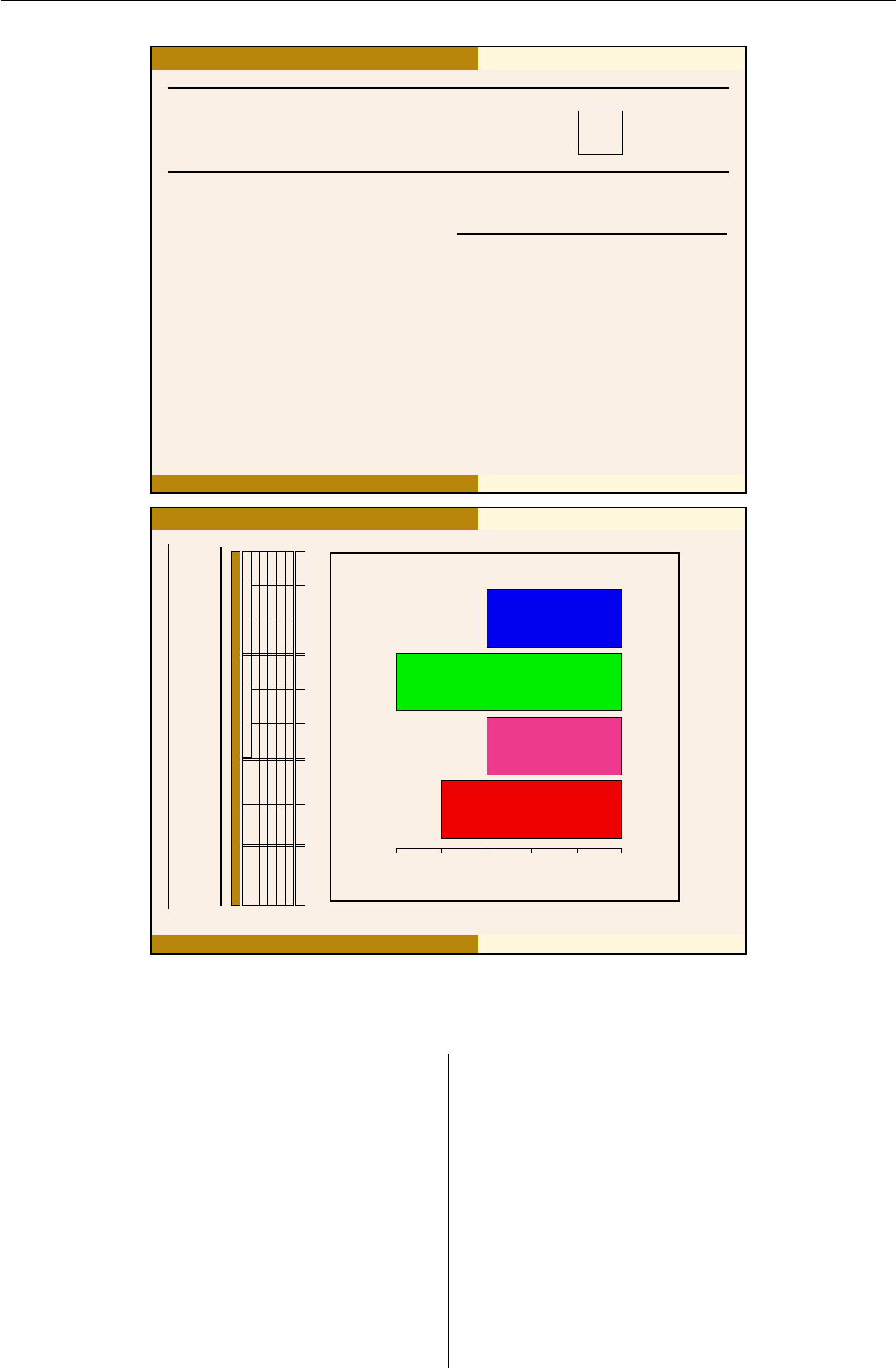
Vol. 5/1, May 2005 43

School Name Goes Here Title of Report Goes Here

School Name Goes Here

A Report on Student Achievement

Your Graphic Here

This prototype provides a picture of what is pos-

sible by using Sweave/L

X/R with the beamer.cls.

There are many possible ways to customize the re-

port. The easiest is to liberally use the Sexpr function

throughout the report. For example, one can easily

indicate the name of the recipient on the report using

Sexpr within the .Rnw template ﬁle. This allows one

a great deal of ﬂexibility with regard to inputing user

speciﬁc data directly into the document.

The ﬁrst page of the report might provide some

basic instructions for the person receiving the report.

These instructions are likely generic and don’t include

much customization. As one reﬁnes the template,

however, it is not diﬃcult to produce increasingly com-

plicated reports. One just has to be careful that the

template works for all the data that is sent to it. One

problem encountered in the school project arose when

using Sexpr{school.name}in the template.Rnw ﬁle.

Some school names used the & character. Sexpr re-

turned that string including the & which caused the

pdfL

X stage to come to a halt. Weaving user spe-

ciﬁc information into the prose is not diﬃcult using

the Sexpr command in combination with various R

functions. One just has to be careful.

Organization Producing Report Goes Here February 18, 2005 1 / 2

School Name Goes Here Title of Report Goes Here

The following tables provide data summarizing student achievement at

Insert School Name Here. One could additionally insert text to guide

the reader through the tables and ﬁgures that appear on the page.

Grade “Insert Grade Here” Reading

2004 Student Number of Percent of Multi-column header here Multi-Column header here

Performance Level Students School Total School District State School District State

Lowest Dynamic Dynamic Dynamic Dynamic Dynamic Dynamic Dynamic Dynamic

Low Middle Dynamic Dynamic Dynamic Dynamic Dynamic Dynamic Dynamic Dynamic

High Middle Dynamic Dynamic Dynamic Dynamic Dynamic Dynamic Dynamic Dynamic

Highest Dynamic Dynamic Dynamic Dynamic Dynamic Dynamic Dynamic Dynamic

Total Dynamic Dynamic Dynamic Dynamic Dynamic Dynamic Dynamic Dynamic

Lowest Low Middle High Middle Highest

0 10 20 30 40 50

A Colorful Barplot for Insert School Name Here

Organization Producing Report Goes Here February 18, 2005 2 / 2

Figure 1: A basic two-page example demonstrating dynamic .pdf using the R/L

EX/Sweave combination.

EX classes, packages and font families are avail-

able that can be combined to yield unlimited possi-

bilities.

Final Compilation

Upon Sweave completion, master.R yields numer-

ous .tex ﬁles that need to be compiled. For the

school project, approximately 3,000 .tex ﬁles were

created. In addition, there were, in most cases, three

.pdf ﬁgures created for each school. All of these ﬁles

can be compiled from within R using the texi2dvi

command available in the tools package. The fol-

lowing loop which can be placed into master.R ac-

complishes this task:

for (name in recip.list){

outfile <- paste(name, "tex", sep=".")

texi2dvi(outfile, pdf=TRUE, clean=TRUE)

}

texi2dvi will run L

EX and BIBT

EX the appropriate

number of times to resolve any reference and citation

dependencies. The result is compiled versions of all

the .tex ﬁles generated from the earlier loop contain-

ing the Sweave process. It is also possible to perform

this task outside of R using a script or batch ﬁle to

perform the same operations.

R News ISSN 1609-3631

Vol. 5/1, May 2005 44

Conclusions

For batch production of dynamic .pdf or .ps doc-

umentation, the R/Sweave/L

EX combination is

powerful and nearly limitless in its capabilities. A

major beneﬁt to producing reports using this combi-

nation of tools is how closely Sweave integrates the

processing power of R with the typesetting capabil-

ity of L

EX. The key to producing dynamic reports

for a large number of recipients is the use of itera-

tive control structures in R. This article provides the

author’s “homebrew” code. Other, more elegant, so-

lutions are likely possible.

A next step after report generation is report distri-

bution. In theory, given the appropriate server con-

ﬁguration, it should be possible to electronically dis-

tribute the reports to the appropriate recipient based

upon, for example, an email address contained in the

database. I would appreciate learning how others

have addressed this and similar problems.

Acknowledgments

I would like to thank Bill Oliver for introducing me

to R and for his gracious help. In addition, I would

like to thank one of the reviewers for providing par-

ticularly insightful improvements to my code. Fi-

nally, I would like to express gratitude to the devel-

opers/contributors of R, Sweave, and L

EX, without

their efforts none of this would be possible.

Bibliography

F. Leisch. Sweave: Dynamic generation of statistical

reports using literate data analysis. In W. Härdle

and B. Rönz, editors, Compstat 2002—Proceedings

in Computational Statistics, pages 575–580, Heidel-

berg, Germany, 2002a. Physika Verlag. ISBN 3-

7908-1517-9. URL http://www.ci.tuwien.ac.at/

~leisch/Sweave.40

F. Leisch. Sweave, Part I: Mixing R and L

EX. R News,

2(3):28–31, December 2002b. URL http://cran.

r-project.org/doc/Rnews/Rnews_2002-3.pdf.

F. Leisch. Sweave, Part II: Package Vignettes. R News,

3(2):21–24, October 2003. URL http://cran.

r-project.org/doc/Rnews/Rnews_2003-2.pdf.

F. Leisch. Sweave User Manual, 2005. 42

R Development Core Team. R: A language and envi-

ronment for statistical computing. R Foundation for

Statistical Computing, Vienna, Austria, 2005. URL

http://www.R-project.org. 3-900051-07-0. 40

T. Tantau. User’s Guide to the Beamer Class. Source-

forge.net, 2004. URL http://latex-beamer.

sourceforge.net.42

Damian Betebenner

Lynch School of Education

Educational Research, Measurement and Evaluation

Boston College

Damian.Betebenner@bc.edu

The Value of R for Preclinical Statisticians

Bill Pikounis and Andy Liaw

Merck & Co., Inc.

Participation on the R-help mailing list has shown R

to be widely used across organizations of all types

the world over. This article discusses one corner

where R has become an indispensable tool for effec-

tive statistical practice: a preclinical pharmaceutical

environment at the authors’ place of employment.

Preclinical is deﬁned here as a portion of the

research and development process for prescription

medicines. In this article that portion is deﬁned

to start with fundamental discovery, and to end up

where a potential product is ﬁrst put into human

subjects in clinical trials. There is a wide variety of

knowledge sought across this spectrum, including:

biological targets believed to be important inﬂuences

on a given disease; chemical entities that affect such

targets; effectiveness and safety in animals; formu-

lation of product itself. This brief listing is only in-

tended to provide a broad overview. In reality, there

are many more areas that could be included based on

desired granularity. A complementary term of “non-

clinical,” which is also commonly used, is perhaps

more appropriate here; however, we will stay with

the phrase preclinical for brevity.

The hallmark diversity of preclinical research

presents unlimited opportunities for statisticians.

Data are collected everywhere in the process, and in

large quantities. We have the liberty to choose meth-

ods of processing and analysis. This is a different

environment than clinical biostatistics, where SAS is

the dominant tool for various reasons. Below we

present examples and discussion on how and why

we use R and ﬁnd it invaluable.

R News ISSN 1609-3631

Vol. 5/1, May 2005 45

Daily operations

Our corporate-issued laptops run Windows XP and

we have a small cluster of dual-processor Opterons

that run 64-bit Linux for intensive jobs. The client-

server conﬁguration of VNC (TightVNC ,2004) pro-

vides a very stable way to bridge the two environ-

ments onto one monitor. An X-window session ap-

pears as just another window on the Windows desk-

top. Samba (Samba Team ,1992-2005) sets up ﬁle

sharing so that a /home directory share under Linux

appears as a network drive in Windows. The auto-

cutsel (Witrant ,2004) utility eases cut-and-paste op-

erations between the two operating systems.

If we work on data that can be comfortably ex-

plored on our laptops, we stay there. Generating

reports for our research collaborators is helped by

the right-click cutting and default pasting of a Win-

dows metaﬁle from the windows graphics device into

a Microsoft Ofﬁce document. The internal Data Ed-

itor (see ?edit) is very useful for browsing a data

frame. Once a workspace has been saved in a Win-

dows folder, launching it from Explorer automati-

cally sets the container working directory. The over-

all R GUI console is thankfully unobtrusive, and we

well appreciate the separation of it from graphics de-

vice windows in SDI mode. We ﬁnd it much more

pleasant to switch amongst desktop windows where

each stands equally on its own, rather than having to

search inside a set of windows within the same ap-

plication.

If an analysis task becomes too large (in mem-

ory or time) for the laptops, it is a simple matter

to transfer the R workspace image to a Linux box

and pick up right where we left off. Through the

aforementioned network drive mapping of a Linux

share, source code editing can be done in the same

Windows editor, and ﬁle operations of saving, copy-

ing, opening, etc. are transparently done through the

standard Windows GUI.

All these task-oriented details add up to in-

creased productivity. More importantly, however, is

the content of the environment itself. We point out

here that some of what we say in the rest of the ar-

ticle is not necessarily unique to R, and such ben-

eﬁts can be found in the other implementation of

the S language, namely S-PLUS. In his “Exegeses

on Linear Models” talk (Venables ,2000), one exe-

gesis from Bill Venables that we particularly admire,

and paraphrase here, is that “the subject should dic-

tate what the program should do and not the other

way around.” Our work environment streams a con-

stant wealth of different data structures and types

of scientiﬁc questions to address, and we can exer-

cise our freedom to choose our strategies of analy-

sis. Comprehensive data analyses are only limited

by our own human capabilities, not by R. R enables

us to seamlessly move from data management to ex-

ploration to formal evaluations to communications

of results. No excuse remains to prevent the produc-

tion of good data graphs for the purposes of valu-

able study or presentation. The implementation of

modern methods allows us to use resampling, re-

sistance/robustness, and dimension reduction meth-

ods on a routine basis, to name a few. We work

with cutting edge science, which we ﬁrmly believe

deserves cutting edge data analysis. R promotes this

for us, with its virtues of ﬂexibility, stability and efﬁ-

ciency so clearly practiced by its R Core caretakers.

Professor Brian D. Ripley, in “How Computing

has Changed Statistics” (Ripley ,2004), aptly states

of R that “the only barrier to understanding how it

works, precisely, is skill.” We interpret the mean-

ing of “how it works” to be on multiple levels, and

the level most important for us is that a true, contin-

uous investment to learn its many functions, struc-

tures, and features pays off time and again. It helps

us bring value to scientiﬁc research, gain trust from

our collaborators, and stimulates the intellect.

Illustrations

Preclinical statisticians do not get nearly enough op-

portunities to provide input to design of experi-

ments. When we do get such an opportunity, we

are especially eager to make recommendations as

quickly as possible. A recent query involved a

crossover design with binary responses. An impor-

tant part of the design plan was to estimate the num-

ber of subjects needed to see a meaningful difference

between two conditions, where incidence rates were

low. Sample size determination tends to be the pre-

dominant aspect of such study design requests.

Estimating sample size is a process of several ap-

proximations, but with some effort such approxi-

mations do not substantially diminish its value. In

this example, tracking down software that could

be readily used, or ﬁnding a literature reference

where a recipe could be programmed, was not timely

enough. So a simulation-based approach was taken.

calcPower <- function(nsubj, pyn, pny, pnnyy,

numsim=1000) {

## A simple approach to calculate the power of

## McNemar’s matched-pair test for these inputs:

## nsubj = the number of subjects/pairs of

## measurements (msmts)

## (note that msmt1 comes from condition 1 and

## msmt2 comes from condition 2)

## pyn = p(msmt1 = yes & msmt2 = no)

## pny = p(msmt1 = no & msmt2 = yes)

## pnnyy = p(msmt1 != msmt2)

## numsim = Number of Simulations

## (at least 1000 recommended)

outcomes <- rmultinom(n=numsim, size=nsubj,

prob=c(pnn=pnnyy, pyy=0,

pny=pny, pyn=pyn))

tscompares <-

apply(outcomes, 2, function(x) {

R News ISSN 1609-3631

Vol. 5/1, May 2005 46

ts <- (((x[3] - x[4])^2) / (x[3] + x[4]))

if (!is.finite(ts)) ts <- 0

})

mean(tscompares > qchisq(0.95, 1), na.rm=FALSE)

}

This simple-minded function evaluates how Mc-

Nemar’s test would behave for a given conﬁguration

of underlying parameters, thereby providing an esti-

mate of its power to detect that difference. Recall that

small occurrence rates were expected. A grid of po-

tential conﬁgurations can be evaluated:

powerGrid <-

expand.grid(pyn=seq(0.01, 0.10, by=.01),

pny=c(0.001, 0.002, 0.005,

seq(0.01, 0.09, by=.01)))

powerGrid$pnnyy <- (1 - powerGrid$pyn -

powerGrid$pny)

powerGrid <- subset(powerGrid, pyn > pny)

powerGrid <- powerGrid[order(powerGrid$pyn,

powerGrid$pny),]

powerGrid$power <-

apply(powerGrid, 1,

function(x) calcPower(100, x[1],

x[2], x[3]))

From the resulting data frame powerGrid, the

context of the study objectives and available re-

sources, a variety of alternatives were explored and

recommended to the researcher. Ensuing discussions

then produced a design that was later successfully

implemented.

We realize that potential inﬂuences of period and

sequence were ignored in the above calculations, as

well as perhaps a more suitable parametric model

approach to the postulated analysis. But as we men-

tioned previously, we felt the approximations in the

approach were reasonable enough to address the

questions at hand.

Similar sample size scenarios we have encoun-

tered include (1) survival data with simple Type I

censoring; (2) single population binomial parame-

ter estimation; (3) inspection of device performance

within its speciﬁed tolerances; and (4) comparability

of old and new drug formulations. In all these sce-

narios the principal recipe of simulating power re-

mains the same as the example above; the key differ-

ences include the postulated underlying distribution

and the methodology of estimation or testing.

One could argue the drawback of computational

time that might be needed to generate sufﬁcient grids

of sample size and power values. In the above ex-

ample, a nsim=10000 or 100000 would provide bet-

ter estimates of power and the computational time is

not prohibitive; we are talking minutes and at most

hours to get the needed results. Here is where our

small cluster of Linux servers, or simply scheduling

something to run overnight, takes advantage of what

computers are really good at.

Molecular Modeling

As another illustration, one particular area where

our group has been involved in is molecular mod-

eling. Speciﬁcally, we are referring to the problem

of predicting biological activities of small organic

molecules from their chemical “descriptors”. The

biological activities can be quantitative (e.g., per-

cent inhibition against a target enzyme) or qualita-

tive (“active” vs. “inactive”). The chemical descrip-

tors are properties/features of the molecules com-

puted from their structures. There are two possible

goals. One is simply prediction: Given a collection

of molecules with unknown biological activities, pre-

dict which ones are likely to be active. The other pos-

sible goal is interpretation: What chemical properties

or substructures are biologically relevant?

Our computational chemistry colleagues have

traditionally used techniques such as k-nearest

neighbors, partial least squares, and neural net-

works, etc. for such problems, mostly using tools

written in-house. A couple of years ago, we started

to convince our colleagues that more modern, pow-

erful tools such as random forests (Breiman,2001;

Svetnik et. al. ,2003) can be readily accessible

through R. We started working on linking Breiman

and Cutler’s Fortran code to R after we got tired

of using the Fortran code alone, since every lit-

tle change in the data or parameters required re-

compiling the source code. It would have been im-

possible to convince our colleagues to use the tool

in that form, no matter how powerful the tool may

be. As a result of making random forests available

in R, it has become an important component of the

methodologies utilized by our colleagues.

Currently, R is installed on the main computer

system for the computational chemists, who are in-

variably Unix based. Whatever R functionalities are

required, the development group (who are responsi-

ble for research and implementation of new method-

ologies) would wrap them in shell or Perl scripts.

These scripts are then used by the applications group

to support speciﬁc projects.

Delivery of Tools

Merck preclinical statisticians are outnumbered at

least ten to one by potential researchers to collaborate

with, and we have global sites that we strive to serve

since they have no access to local statisticians. As

brieﬂy alluded to in the previous section, the avail-

ability of R to communicate with other software of-

fers great potential to serve our customers.

We have recently embarked on a COM-driven1

framework to take advantage of existing infrastruc-

1COM stands for Common Object Model, a Microsoft-driven “standard” for communications between software components.

R News ISSN 1609-3631

Vol. 5/1, May 2005 47

ture. For instance, virtually everyone at Merck runs

the same version of Windows XP and the same ver-

sion of Microsoft Excel. Use of R(D)COM (Baier

and Neuwirth ,2004) allows construction of an ap-

plication where the user interface is entirely in Ex-

cel; namely, input data storage, selection of data and

choices through Userforms, and formatted output.

The underlying work of the R engine is invisible to

the user as it provides calculations and the raw out-

put to Excel for the formatting and the organized pre-

sentation. This framework leverages Excel strengths

of formatting, familiarity, and ubiquity, and R pro-

vides numerical reliability and breadth of data ana-

lytic functionality. While we are currently in early

stages, the framework has demonstrated reliability

for widespread distribution.

Summary

There are several speciﬁc aspects that make R

uniquely suitable for us and our colleagues:

• Availability of modern methodologies;

• Flexibility for implementing new methods;

• Facilities to package added functionalities;

• Seamless integration with other software;

• Liberty to (try to) install on any platform.

The ﬁrst point is discussed above. We add that col-

leagues in our department rely on R for their support

of genomic and proteomic research, where access to

(or the ability to implement) cutting-edge method-

ologies is crucial. The second through fourth points

are important for us as tool developers. The fact that

R is a full-featured language enables us to follow the

spirit of “turn ideas into software, quickly and faith-

fully” (Chambers ,1998). The packaging facility in

R lets us easily create, maintain, and distribute tools

and associated documentation. The same cannot re-

ally be said about most other statistical languages or

packages. The COM framework discussed above is

but one of many options for integration of R with

processes or GUIs, etc. The last point is important

not because R is free (as in beer), but because we are

not limited to run the software on whatever platform

a vendor chooses to support. As long as we can get

R to compile and pass all its tests, we are comfort-

able using it. As an example, when we bought our

ﬁrst 64-bit machine (a dual Opteron 244 with 16GB

of RAM), the main motivation was to overcome the

memory limitation of a 32-bit platform. Because we

can build R from source, we readily built a 64-bit ver-

sion of R on that box.

This article focused on preclinical statistics use of

R. Nearly four years ago we organized our ﬁrst in-

house introductory course on R, and about 20 people

attended, mostly from preclinical statistics and other

basic research departments that provide quantitative

analysis support to researchers. As a sign of the in-

creasing acceptance of R at Merck three years later,

attendance more than doubled and mostly included

clinical statisticians and SAS programmers. Results

based on the use of R by preclinical statisticians have

been included in regulatory responses and ﬁlings,

and no issues have arisen. We are not aware of R

use in the traditional core workﬂows of clinical trials

production work to date, but we do expect the use of

R within Merck to continue to increase in all areas,

including clinical.

In our small corner of the world that is preclinical

drug research & development, R is a guide towards

better statistical practice and helps expands our in-

ﬂuence on scientiﬁc research. It is indispensable. If

R— the software and community — did not exist, we

would be wishing that something like it would come

along.

Footnote: The ﬁrst author recently changed employ-

ment from Merck to Centocor. The preclinical/nonclinical

experiences with researchers there have been quite similar

to date.

Bibliography

T. Baier and E. Neuwirth (2004) R (D)COM

Server V1.35 URL http://cran.r-project.org/

contrib/extra/dcom/RSrv135.html 47

L. Breiman (2001) Random forests Machine Learning,

45, 5–32. 46

J. M. Chambers (1998) Programming with Data New

York: Springer-Verlag. 47

B. D. Ripley (2004) How Computing Has Changed

Statistics (and is changing. . .) Symposium in

Honour of David Cox’s 80th birthday, Neuchatel,

July 2004 URL http://www.stats.ox.ac.uk/

~ripley/Cox80.pdf 45

Samba URL http://www.samba.org/ 45

V. Svetnik, A. Liaw, C. Tong, C. Culberson,

R. P. Sheridan, and B. P. Feuston (2003) Random

Forest: A Classiﬁcation and Regression Tool for

Compound Classiﬁcation and QSAR Modeling J.

Chem. Inf. Comput. Sci. 43, 1047–1058. 46

TightVNC URL http://www.tightvnc.com/ 45

W. N. Venables (2000) Exegeses on Linear Models Pa-

per presented to the S-PLUS User’s Conference Wash-

ington, DC, 8-9th October, 1998 URL http://www.

stats.ox.ac.uk/pub/MASS3/Exegeses.pdf 45

M. Witrant (2004) autocutsel URL http://savannah.

nongnu.org/projects/autocutsel/ 45

R News ISSN 1609-3631

Vol. 5/1, May 2005 48

Recreational mathematics with R:

introducing the “magic” package

Creating and investigating magic squares with R

Robin K. S. Hankin

Preface

The R computer language (R Development Core

Team,2004) has been applied with a great deal of

success to a wide variety of statistical, physical, and

medical applications. Here, I show that R is an

equally superb research tool in the ﬁeld of recre-

ational mathematics.

Recreational mathematics is easier to recognize

than deﬁne, but seems to be characterized by requir-

ing a bare minimum of “raw material”: complex no-

tation is not needed, and problems are readily com-

municated to the general public.

This is not to say that all problems of recreational

mathematics are trivial: one could argue that much

number theory is recreational in nature; yet attempts

to prove Fermat’s Last Theorem, or the search for

ever higher perfect numbers, have been the catalyst

for the development of many fruitful new areas of

mathematics.

The study of magic squares is also an example of

nontrivial recreational mathematics as the basic con-

cept is simple to grasp—yet there remain unsolved

problems in the ﬁeld whose study has revealed deep

mathematical truths.

Here, I introduce the “magic” package, and show

that R is an excellent environment for the creation

and investigation of magic squares. I also show

that one’s appreciation of magic squares may be en-

hanced through computer tools such as R, and that

the act of translating ‘paper’ algorithms of the litera-

ture into R idiom can lead to new insight.

Magic squares

Magic squares have essentially zero practical use;

their fascination—like much of pure mathematics—

lies in the appeal of æsthetics and structure rather

than immediate usefulness.

The following deﬁnitions are almost universal:

• A semimagic square is one all of whose row sums

equal all its columnwise sums (i.e. the magic

constant).

• A magic square is a semimagic square with the

sum of both unbroken diagonals equal to the

magic constant.

• A panmagic square is a magic square all of whose

broken diagonals sum to the magic constant.

(all squares are understood to be n×nand to be

normal, that is, to comprise n2consecutive inte-

gers1). Functions is.semimagic(),is.magic(), and

is.panmagic() test for these properties.

A good place to start is the simplest—and by far

the most commonly encountered—magic square, lo

zhu:

> magic(3)

[,1] [,2] [,3]

[1,] 2 7 6

[2,] 9 5 1

[3,] 4 3 8

This magic square has been known since antiq-

uity (legend has it that the square was revealed to

humanity inscribed upon the shell of a divine turtle).

More generally, if consecutive numbers of a magic

square are joined by lines, a pleasing image is of-

ten obtained (ﬁgure 1, for example, shows a magic

square of order 7; when viewed in this way, the algo-

rithm for creating such a square should be immedi-

ately obvious).

Figure 1: Magic square of order 7 in graphical form

(obtained by magicplot(magic.2np1(3)))

1Most workers require the entries to start at 1, which is the convention here; but there are several instances where starting at 0 is far

more convenient. In any case, if xis magic, then x+n is magic for any integer n.

R News ISSN 1609-3631

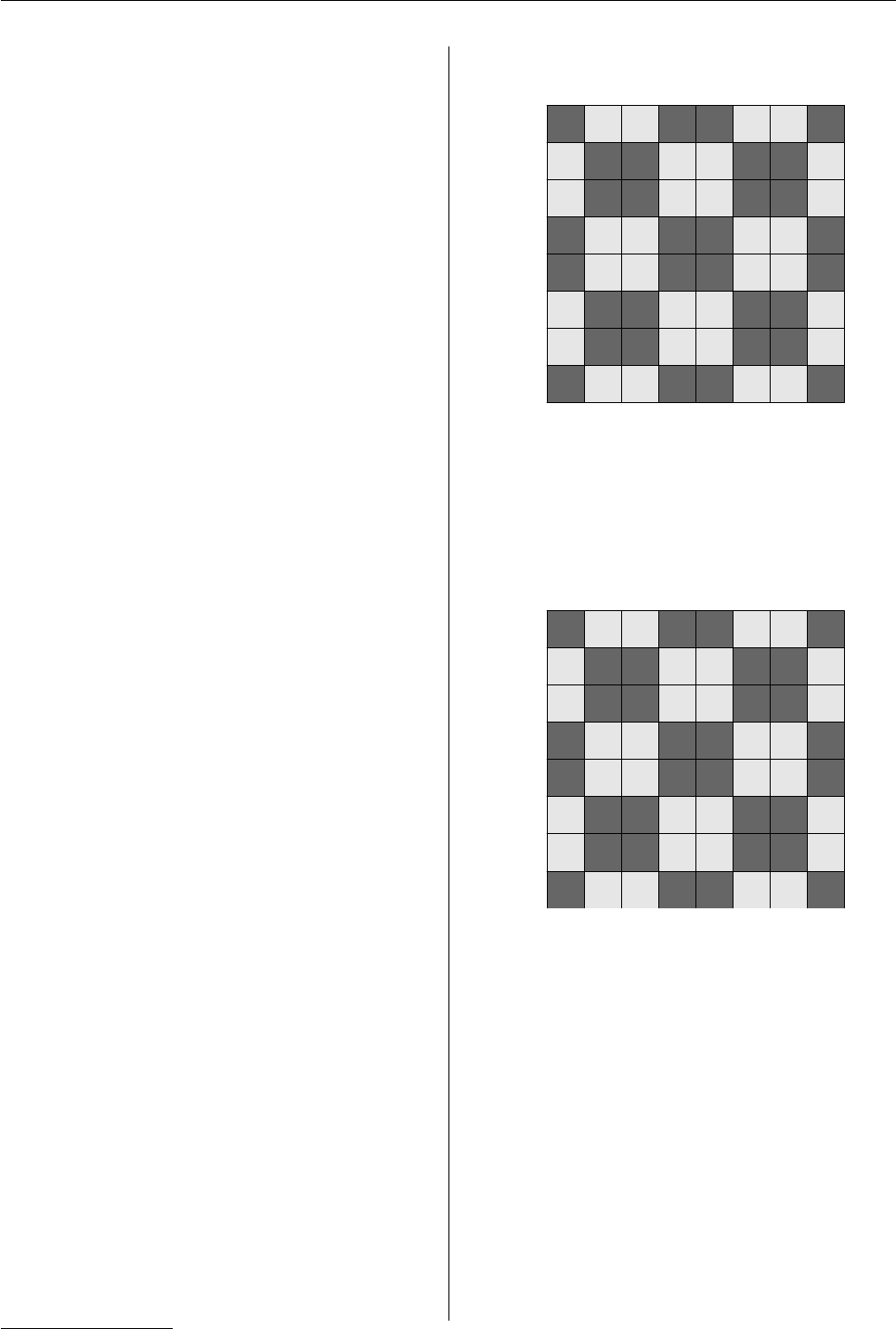
Vol. 5/1, May 2005 49

Function magic() takes an integer argument n

and returns a normal magic square of size n×n.

There are eight equivalent forms for lo zhu or in-

deed any magic square, achieved by rotating and re-

ﬂecting the matrix (Benson and Jacoby,1976); such

equivalence is tested by eq() or %eq%. Of these eight

forms, a magic square ais said to be in Frénicle’s

standard form if a[1,1]≤b[1,1] whenever a %eq% b,

and a[1,2]<a[2,1]. Function is.standard() tests

for this, and function as.standard() places a magic

square in standard form. Magic squares returned by

magic() are always in standard form.

A typical (paper) algorithm for placing magic

square ain standard form would be “rotate a

until a[1,1]<min(a[1,n],a[n,1],a[n,n]) then, if

a[1,2]>a[2,1], take the transpose”. I shall show

later that expressing such an algorithm in R leads to

new insight when considering magic hypercubes.

A wide variety of algorithms exists for calculating

magic squares. For a given order n, these algorithms

generally depend on nmodulo 4.

A typical paper algorithm for magic squares of

order n=4mwould go as follows.

Algorithm 1: in a square of order 4m,

shade the long major diagonal. Then

shade all major diagonals distant by a

multiple of 4 cells from the long diagonal.

Do the same with the minor diagonals.

Then, starting with “1” at the top left cor-

ner and proceeding from left to right and

top to bottom, count from 1 to n2, ﬁlling

in the shaded squares with the appropri-

ate number and omitting the unshaded

ones [ﬁgure 2]. Fill in the remaining (un-

shaded) squares in the same way, start-

ing at the lower right corner, moving left-

wards and upwards [ﬁgure 3].

Such paper algorithms are common in the litera-

ture but translating this one into code that uses R’s

vectorized tools effectively can lead to new insight.

The magicness of such squares may be proved by

considering the increasing and decreasing sequences

separately.

Figure 2: Half-completed magic square of order 8

Figure 3: Magic square of order 8

The interesting part of the above paper algo-

rithm lies in determining the pattern of shaded

and unshaded squares2. As the reader may

care to verify, parsing the algorithm into R id-

iom is not straightforward. An alternative,

readily computed in R, would be to recog-

nize that the repeating 4 ×4 cell a[2:5,2:5]

is kronecker(diag(2),matrix(1,2,2)) -> b say,

replicate it with kronecker(matrix(1,3,3),b) ->

g; then trim off the border by selecting only the

middle elements, in this case g[2:9,2:9]. Function

magic.4n() implements the algorithm for general m.

2If a <- matrix(1:(n*n),n,n), with jj a Boolean vector of length n2with TRUE corresponding to shaded squares, then with it is clear

that a[jj] <- rev(a[jj]) will return the above magic square.

R News ISSN 1609-3631

Vol. 5/1, May 2005 50

Magic hypercubes

One of the great strengths of R is its ability to han-

dle arbitrary dimensioned arrays in an efﬁcient and

elegant manner.

Generalizing magic squares to magic hyper-

cubes (Hendricks,1973) is thus natural when work-

ing in R. The following deﬁnitions represent a gen-

eral consensus, but are far from universal:

• A semimagic hypercube has all “rook’s move”

sums equal to the magic constant (that is,

each ∑n

ir=1a[i1,i2,...,ir−1,ir,ir+1,...,id]with

1≤r≤dis equal to the magic constant for

all values of the other i’s).

• A magic hypercube is a semimagic hypercube

with the additional requirement that all 2d−1

long (ie extreme point-to-extreme point) diag-

onals sum correctly.

• A perfect magic hypercube is a magic hypercube

with all nonbroken diagonals summing cor-

rectly3.

• A pandiagonal hypercube is a perfect magic hy-

percube with all broken diagonals summing

correctly.

(a magic hypercube is understood to be of di-

mension rep(n,d) and normal). Functions

is.semimagichypercube(),is.magichypercube()

and is.perfect(a) test for the ﬁrst three proper-

ties; the fourth is not yet implemented. Function

is.diagonally.correct() tests for correct summa-

tion of the 2d(sic) long diagonals.

Magic hypercubes of order 4n

Consider algorithm 1 generalized to a d-dimensional

hypercube. The appropriate generalization of

the repeating cell of the 8 ×8 magic square dis-

cussed above is not immediately obvious when

considering ﬁgure 2, but the R formalism (viz

kronecker(diag(2),matrix(1,2,2))) makes it

clear that the appropriate generalization is to replace

matrix(1,2,2) with array(1,rep(2,d)).

The appropriate generalization for diag(2) (call

it g) is not so straightforward, but one might be

guided by the following requirements:

• The dimension of gmust match the ﬁrst argu-

ment to kronecker(), viz rep(2,d)

• The number of 0s must be equal to the number

of 1s: sum(g==1)==sum(g==0)

• The observation that diag(2) is equal to its

transpose would generalize to requiring that

aperm(g,K) be identical to gfor any permuta-

tion K.

These lead to specifying that g[i1,...,id] should

be zero if (i1,...,id)contains an odd number of 2s

and one otherwise.

One appropriate R idiom would be to de-

ﬁne a function dimension(a,p) to be an inte-

ger matrix with the same dimensions as a, with

element (n1,n2, ..., nd)being np, then if jj =

∑d

i=1dimension(a,i), we can specify g=jj*0 and

then g[jj%%2==1] <- 1.

Another application of kronecker() gives a hy-

percube that is of extent 4m+2 in each of its ddimen-

sions, and this may be trimmed off as above to give

an array of dimensions rep(4m,d) using do.call()

and [<-. The numbers may be ﬁlled in exactly as for

the 2d case.

The resulting hypercube is magic, in the sense

deﬁned above4, although it is not perfect; function

magichypercube.4n() implements the algorithm.

The ability to generate magic hypercubes of arbitrary

dimension greater than one is apparently novel.

Standard form for hypercubes

Consider again the paper deﬁnition for Frénicle’s

standard form of a magic square a: it is rotated so

that the smallest number appears at the top left; then

if a[1,2]<a[2,1], the transpose is taken.

When coding up such an algorithm in R with an

eye to generalizing it to arbitrarily high dimensional

hypercubes, it becomes apparent that “rotation” is

not a natural operation. The generalization used in

the package is directly suggested by R’s array capa-

bilities: it is a two-step process in which the ﬁrst step

is to maneuver the smallest possible element to posi-

tion [1,1,...,1] using only operations that reverse

the index of some (or all) dimensions. An example

would be a <- a[1:n,n:1,1:n,n:1].

The second step is to use function aperm()

to ensure that the appropriate generalization of

a[1,2]<a[2,1], which would be

a[1,1,...,1,2] <a[1,...,2,1] <. . .

. . . <a[1,2,...,1] <a[2,1,...,1]

holds; the appropriate R idiom is a <-

aperm(a,order(-a[1+diag(d)]))).

This generalization of Frénicle’s standard form to

arbitrary dimensional hypercubes appears to be new;

it arises directly from the power and elegance of R’s

array handling techniques.

3This condition is quite restrictive; in the case of a tesseract, this would include subsets such as ∑n

i=1a[1, i,n−i+1, n]summing

correctly.

4If I had a rigorous proof of this, the margin might be too narrow for it.

R News ISSN 1609-3631

Vol. 5/1, May 2005 51

Conclusions

The R language is a natural environment for the in-

vestigation of magic squares and hypercubes; and

the discipline of translating published algorithms

into R idiom can yield new insight. These insights

include a new generalization of Frénicle’s standard

form to hypercubes, and also what appears to be the

ﬁrst algorithm for generating magic hypercubes of

any dimension,

Insofar as magic squares and hypercubes are wor-

thy of attention, it is worth creating fast, efﬁcient rou-

tines to carry out the “paper” algorithms of the liter-

ature. I hope that the magic package will continue to

facilitate the study of these fascinating objects.

Acknowledgements

I would like to acknowledge the many stimulating

and helpful comments made by the R-help list over

the years.

Bibliography

W. H. Benson and O. Jacoby. New recreations with

magic squares. Dover, 1976. 49

J. R. Hendricks. Magic tesseracts and N-dimensional

magic hypercubes. Journal of Recreational Mathe-

matics, 6(3):193–201, 1973. 50

R Development Core Team. R: A language and envi-

ronment for statistical computing. R Foundation for

Statistical Computing, Vienna, Austria, 2004. URL

http://www.R-project.org. ISBN 3-900051-07-0.

Robin Hankin

Southampton Oceanography Centre

European Way

Southampton

United Kingdom

SO14 3ZH

r.hankin@soc.soton.ac.uk

Programmer’s Niche

How Do You Spell That Number?

John Fox

Frank Duan recently posted a question to the r-help

mailing list asking how to translate numbers into

words. The program described in this column is a

cleaned-up and slightly enhanced version of my re-

sponse to his question. I found the problem to be an

interesting puzzle, and the solution uses several pro-

gramming techniques that demonstrate the ﬂexibil-

ity of R, including its ability to manipulate character-

string data and to employ recursive function calls.

One intriguing aspect of the problem is that it re-

quired me to raise into consciousness my subcon-

scious knowledge about how numbers are spoken

and written in English. I was much more aware

of these conventions in the languages (French and

Spanish) that I had studied as a non-native speaker.

A bit later, I realized that there are variations among

English-speaking countries in the manner in which

numbers are spoken and written down. Because I

was born in the United States and have lived most

of my adult life in Canada, I’m terminally confused

about English spelling and usage. Canadian conven-

tions are an amalgam of American and British rules.

In any event, it didn’t take much time to see that

the numbers from one to nineteen are represented

by individual words; the numbers from twenty-one

to ninety-nine are formed as compound words, with

components for the tens and units digits — with the

exceptions of multiples of ten (twenty,thirty, etc.),

which are single words. The Chicago Manual of Style

tells me that these compound words should be hy-

phenated (but offered little additional useful advice

about how numbers are to be written out). Num-

bers from 100 to 999 are written by tacking on (at

the left) a phrase like “six hundred” — that is, com-

posed of a number from one to nine plus the sufﬁx

hundred (and there is no hyphen). Above this point,

additional terms are added at the left, representing

multiples of powers of 1000. In American English

(and in Canada), the ﬁrst few powers of 1000 have

the following names, to be used as sufﬁxes:

10001thousand

10002million

10003billion

10004trillion

Thus, for example, the number 210,363,258 would

be rendered “two hundred ten million, three hun-

dred sixty-three thousand, two hundred ﬁfty-eight.”

There really is no point in going beyond tril-

lions, because double-precision numbers can repre-

sent integers exactly only to about 15 decimal dig-

its, or hundreds of trillions. Of course, I could

allow numbers to be speciﬁed optionally by ar-

bitrarily long character strings of numerals (e.g.,

"210363258347237492310"), but I didn’t see a real

need to go higher than hundreds of trillions.

One approach to converting numbers to words

would be to manipulate the numbers as integers, but

R News ISSN 1609-3631

Vol. 5/1, May 2005 52

it seemed to me simpler to convert numbers to char-

acter strings of numerals, which could then be split

into individual characters: (1) larger integers can

be represented exactly as double-precision ﬂoating-

point numbers than as integers in R; (2) it is easier to

manipulate the individual numerals than to perform

repeated integer arithmetic to extract digits; and (3)

having the numerals in character form allows me to

take advantage of R’s ability to index vectors by ele-

ment names (see below).

I therefore deﬁned the following function to con-

vert a number to a vector of characters containing the

numerals composing the number:

> makeDigits <- function(x)

+ strsplit(as.character(x), "")[[1]]

Here are some examples of the use of this func-

tion:

> makeDigits(123456)

[1] "1" "2" "3" "4" "5" "6"

> makeDigits(-123456)

[1] "-" "1" "2" "3" "4" "5" "6"

> makeDigits(1000000000)

[1] "1" "e" "+" "0" "9"

Notice the problems revealed by the second and

third examples: It’s necessary to make provision for

negative numbers, and R wants to render certain

numbers in scientiﬁc notation.1By setting the scipen

(“scientiﬁc notation penalty”) option to a large num-

ber, we can avoid the second problem:

> options(scipen=100)

> makeDigits(1000000000)

[1] "1" "0" "0" "0" "0" "0" "0" "0" "0" "0"

It also seemed useful to have a function that con-

verts a vector of numerals in character form back into

a number:

> makeNumber <- function(x)

+ as.numeric(paste(x, collapse=""))

> makeNumber(c("1", "2", "3", "4", "5"))

[1] 12345

Finally, by way of preparation, I constructed sev-

eral vectors of number words:

> ones <- c("zero", "one", "two", "three",

+ "four", "five", "six", "seven",

+ "eight", "nine")

> teens <- c("ten", "eleven", "twelve",

+ "thirteen", "fourteen", "fifteen",

+ "sixteen", " seventeen", "eighteen",

+ "nineteen")

> names(ones) <- names(teens) <- 0:9

> tens <- c("twenty", "thirty", "forty",

+ "fifty", "sixty", "seventy", "eighty",

+ "ninety")

> names(tens) <- 2:9

> suffixes <- c("thousand,", "million,",

+ "billion,", "trillion,")

Because the names of the elements of the ﬁrst

three vectors are numerals, they can conveniently be

indexed; for example:

> ones["5"]

"five"

> teens["3"]

"thirteen"

> tens["7"]

"seventy"

The vector of sufﬁxes includes a comma after

each word.

Figure 1shows a function for converting a single

integer to words; I’ve added line numbers to make it

easier to describe how the function works:

And here are some examples of its use, wrapping

long lines of output to ﬁt on the page:

> number2words(123456789)

[1] "one hundred twenty-three million,

four hundred fifty-six thousand,

seven hundred eighty-nine"

> number2words(-123456789)

[1] "minus one hundred twenty-three million,

four hundred fifty-six thousand,

seven hundred eighty-nine"

> number2words(-123456000)

[1] "minus one hundred twenty-three million,

four hundred fifty-six thousand"

I believe that the ﬁrst ﬁve lines of the function are

essentially self-explanatory. The rest of the function

probably requires some explanation, however:

[6] If the number is composed of a single digit,

then we can ﬁnd the answer by simply in-

dexing into the vector ones; the function

as.vector is used to remove the name of

(i.e., the numeral labelling) the selected el-

ement.

[7-9] If the number is composed of two digits

and is less than or equal to 19, then we can

get the answer by indexing into teens with

the last digit (i.e., the second element of the

digits vector). If the number is 20 or larger,

then we need to attach the tens digit to the

ones digit, with a hyphen in between. If,

1I don’t want to mislead the reader: I discovered these and other problems the hard way, when they surfaced as bugs. The account

here is a reconstruction that avoids my missteps. I can honestly say, however, that it took me much longer to write this column explaining

how the program works than to write the original program. Moreover, in the process of writing up the program, I saw several ways to

improve it, especially in clarity — a useful lesson.

R News ISSN 1609-3631

Vol. 5/1, May 2005 53

[ 1] number2words <- function(x){

[ 2] negative <- x < 0

[ 3] x <- abs(x)

[ 4] digits <- makeDigits(x)

[ 5] nDigits <- length(digits)

[ 6] result <- if (nDigits == 1) as.vector(ones[digits])

[ 7] else if (nDigits == 2)

[ 8] if (x <= 19) as.vector(teens[digits[2]])

[ 9] else trim(paste(tens[digits[1]], "-", ones[digits[2]], sep=""))

[10] else if (nDigits == 3) {

[11] tail <- makeNumber(digits[2:3])

[12] if (tail == 0) paste(ones[digits[1]], "hundred")

[13] else trim(paste(ones[digits[1]], "hundred", number2words(tail)))

[14] }

[15] else {

[16] nSuffix <- ((nDigits + 2) %/% 3) - 1

[17] if (nSuffix > length(suffixes) || nDigits > 15)

[18] stop(paste(x, "is too large!"))

[19] pick <- 1:(nDigits - 3*nSuffix)

[20] trim(paste(number2words(makeNumber(digits[pick])),

[21] suffixes[nSuffix], number2words(makeNumber(digits[-pick]))))

[22] }

[23] if (negative) paste("minus", result) else result

[24] }

Figure 1: A function to convert a single integer into words.

however, the ones digit is 0, ones["0"] is

"zero", and thus we have an embarrassing

result such as "twenty-zero". More gener-

ally, the program can produce spurious hy-

phens, commas, spaces, and the strings ",

zero" and "-zero" in appropriate places.

My solution was to write a function to trim

these off:

trim <- function(text){

gsub("(^\ *)|((\ *|-|,\ zero|-zero)$)",

"", text)

}

The trim function makes use of R’s ability

to process “regular expressions.” See Lum-

ley (2003) for a discussion of the use of regu-

lar expressions in R.

[10-14] If the number consists of three digits,

then the ﬁrst digit is used for hundreds, and

the remaining two digits can be processed as

an ordinary two-digit number; this is done

by a recursive call to number2words2— un-

less the last two digits are 0, in which case,

we don’t need to convert them into words.

The hundreds digit is then pasted onto the

representation of the last two digits, and the

result is trimmed. Notice that makeNumber

is used to put the last two digits back into a

number (called tail).

[15-22] Finally, if the number contains more than

three digits, we’re into the realm of thou-

sands, millions, etc. The computation on line

[16] determines with which power of 1000

we’re dealing. Then, if the number is not too

large, the appropriate digits are stripped off

from the left of the number and attached to

the proper sufﬁx; the remaining digits to the

right are recomposed into a number and pro-

cessed with a recursive call, to be attached at

the right.

[23] If the original number was negative, the

word "minus" is pasted onto the front before

the result is returned.

The ﬁnal function, called numbers2words (shown

in Figure 2), adds some bells and whistles: The vari-

ous vectors of names are deﬁned locally in the func-

tion; the utility functions makeDigits,makeNumbers,

and trim, are similarly deﬁned as local functions;

and the function number2words, renamed helper,

is also made local. Using a helper function rather

than a recursive call permits efﬁcient vectorization,

via sapply, at the end of numbers2words. Were

2It’s traditional in S to use Recall for a recursive function call, but I’m not fond of this convention, and I don’t see an argument for it

here: It’s unlikely that number2words will be renamed, and in any event, it will become a local function in the ﬁnal version of the program

(see below).

R News ISSN 1609-3631

Vol. 5/1, May 2005 54

numbers2words to call itself recursively, the local def-

initions of objects (such as the vector ones and the

function trim) would be needlessly recomputed at

each call, rather than only once. Because of R’s lex-

ical scoping, objects deﬁned in the environment of

numbers2words are visible to helper. For more on

recursion in R, see Venables (2001).

numbers2words includes a couple of additional

features. First, according to the Oxford English Dic-

tionary, the deﬁnition of “billion” differs in the U.S.

and (traditionally) in Britain: “1. orig. and still

commonly in Great Britain: A million millions. (=

U.S. trillion.) ... 2. In U.S., and increasingly in

Britain: A thousand millions.” Thus, if the argument

billion is set to "UK", a different vector of sufﬁxes

is used. Moreover, provision is made to avoid awk-

ward translations that repeat the word “million,”

such as “ﬁve thousand million, one hundred million,

... ,” which is instead, and more properly rendered as

“ﬁve thousand, one hundred million, ... .”

Second, Bill Venables tells me that outside of the

U.S., it is common to write or speak a number such

101 as “one hundred and one” rather than as “one

hundred one.” (Both of these phrases seem correct

to me, but as I said, I’m hopelessly confused about

international variations in English.) I have there-

fore included another argument, called and, which

is pasted into the number at the appropriate point.

By default, this argument set is to "" when billion

is "US" and to "and" when billion is "UK".

Some examples, again wrapping long lines of

output:

> numbers2words(c(1234567890123, -0123, 1000))

[1] "one trillion,

two hundred thirty-four billion,

five hundred sixty-seven million,

eight hundred ninety thousand,

one hundred twenty-three"

[2] "minus one hundred twenty-three"

[3] "one thousand"

> numbers2words(c(1234567890123, -0123, 1000),

+ billion="UK")

[1] "one billion,

two hundred and thirty-four thousand,

five hundred and sixty-seven million,

eight hundred and ninety thousand,

one hundred and twenty-three"

[2] "minus one hundred and twenty-three"

[3] "one thousand"

> numbers2words(c(1234567890123, -0123, 1000),

+ and="and")

[1] "one trillion,

two hundred and thirty-four billion,

five hundred and sixty-seven million,

eight hundred and ninety thousand,

one hundred and twenty-three"

[2] "minus one hundred and twenty-three"

[3] "one thousand"

Finally, a challenge to the reader: At present,

numbers2words rounds its input to whole numbers.

Modify the program so that it takes a digits argu-

ment (with default 0), giving the number of places to

the right of the decimal point to which numbers are

to be rounded, and then make provision for translat-

ing such numbers (e.g., 1234567.890) into words.

John Fox

Sociology, McMaster University

jfox@mcmaster.ca

Bibliography

T. Lumley. Programmer’s niche: Little bits of string.

R News, 3(3):40–41, December 2003. URL http:

//CRAN.R-project.org/doc/Rnews/.53

B. Venables. Programmer’s niche. R News, 1(1):27–

30, January 2001. URL http://CRAN.R-project.

org/doc/Rnews/.54

R News ISSN 1609-3631

Vol. 5/1, May 2005 55

numbers2words <- function(x, billion=c("US", "UK"),

and=if (billion == "US") "" else "and"){

billion <- match.arg(billion)

trim <- function(text){

gsub("(^\ *)|((\ *|-|,\ zero|-zero)$)", "", text)

}

makeNumber <- function(x) as.numeric(paste(x, collapse=""))

makeDigits <- function(x) strsplit(as.character(x), "")[[1]]

helper <- function(x){

negative <- x < 0

x <- abs(x)

digits <- makeDigits(x)

nDigits <- length(digits)

result <- if (nDigits == 1) as.vector(ones[digits])

else if (nDigits == 2)

if (x <= 19) as.vector(teens[digits[2]])

else trim(paste(tens[digits[1]], "-", ones[digits[2]], sep=""))

else if (nDigits == 3) {

tail <- makeNumber(digits[2:3])

if (tail == 0) paste(ones[digits[1]], "hundred")

else trim(paste(ones[digits[1]], trim(paste("hundred", and)),

helper(tail)))

}

else {

nSuffix <- ((nDigits + 2) %/% 3) - 1

if (nSuffix > length(suffixes) || nDigits > 15)

stop(paste(x, "is too large!"))

pick <- 1:(nDigits - 3*nSuffix)

trim(paste(helper(makeNumber(digits[pick])),

suffixes[nSuffix], helper(makeNumber(digits[-pick]))))

}

if (billion == "UK"){

words <- strsplit(result, " ")[[1]]

if (length(grep("million,", words)) > 1)

result <- sub(" million, ", ", ", result)

}

if (negative) paste("minus", result) else result

}

opts <- options(scipen=100)

on.exit(options(opts))

ones <- c("zero", "one", "two", "three", "four", "five", "six", "seven",

"eight", "nine")

teens <- c("ten", "eleven", "twelve", "thirteen", "fourteen", "fifteen",

"sixteen", " seventeen", "eighteen", "nineteen")

names(ones) <- names(teens) <- 0:9

tens <- c("twenty", "thirty", "forty", "fifty", "sixty", "seventy", "eighty",

"ninety")

names(tens) <- 2:9

suffixes <- if (billion == "US")

c("thousand,", "million,", "billion,", "trillion,")

else

c("thousand,", "million,", "thousand million,", "billion,")

x <- round(x)

if (length(x) > 1) sapply(x, helper) else helper(x)

}

Figure 2: A function to convert a vector of integers into a vector of strings containing word-equivalents of the

integers.

R News ISSN 1609-3631

Vol. 5/1, May 2005 56

Book Review of

Julian J. Faraway: Linear Models with R

Chapman & Hall/CRC, Boca Raton FL, USA, 2005

229 pages, ISBN 1-58488-425-8

http://www.stat.lsa.umich.edu/∼faraway/LMR

This book is useful to serve for the practical as-

pects of an advanced undergraduate linear regres-

sion course. Regarding the potential readership, the

Author writes in the preface that the book is “not in-

troductory” and that it “presumes some knowledge

of basic statistical theory and practice. Readers are

expected to know the essentials of statistical infer-

ence such as estimation, hypothesis testing and con-

ﬁdence intervals. A basic knowledge of data anal-

ysis is presumed. Some linear algebra and calculus

are also required.” Thus this book is most suitable

for undergraduate statistics majors at least half way

through their degrees. The book needs to be accom-

panied by a theoretical book, such as Seber and Lee

(2003). A somewhat similar competitor to the book

is Fox (2002).

With a large number (16) of chapters in this small-

ish book, most of them are short and mention ideas

brieﬂy. Of course, some chapters are on core practical

topics such as residual diagnostics, transformations,

weighted and generalized least squares, ANOVA

(factorial designs, block designs), ANCOVA, vari-

able selection techniques, and inference. A good fea-

ture of the book is that more ‘optional’ topics are

covered, include missing values, regression splines,

robust regression (M-estimation and least trimmed

squares), permutation tests, shrinkage methods such

as partial least squares, measurement error mod-

els including SIMEX, latin squares and iteratively

reweighted least squares. Most instructors are un-

likely to be familiar with all these topics, and the

book does a good job in giving a very gentle intro-

duction to these topics. The reader is usually referred

to references at the back for further reading.

The book has two small appendices. The ﬁrst de-

scribes R installation, functions and data, while the

second is a quick introduction to R. The examples in

the book are based on R 1.9.0. In my copy there were

a few font problems, e.g., p.189 has (αβ)i j instead of

(αβ)i j.

The tone of the book is that of an informal tutorial

with some necessary theory interdispersed through-

out. Explanations are good overall, and the math-

ematical notation is quite standard. The Author’s

website serves as the repository for the book’s pack-

age, called faraway, and includes errata, R com-

mands and data sets (the package is also on CRAN.)

The Author writes “Data analysis cannot be learned

without actually doing it” and this is facilitated

by practical exercises (which are usually short and

sharp) at the end of each chapter. Solutions appear

unavailable.

The book centers on lm() and assumes familiar-

ity with the S language, e.g., I found it referred to “.”

in a formula without reminding or telling the reader

that it means all variables in the data frame other

than the response. The book is rather unsuitable as a

reference book, for example, summation constraints

∑

j=1

αj=0 is a popular parameterization for a factor

with Jlevels. The function contr.sum is alluded to

but not mentioned directly in the book, nor how to

switch between different parameterizations. Ideally,

a handy summary of topics such as the Wilkinson-

Rogers operators (e.g., *,/,:) and all the different

contrast options available should be put into an ap-

pendix for fast and easy reference. This would make

Chambers and Hastie (1991) less necessary for stu-

dents to buy or refer to. The book makes good and

frequent use of basic graphics with a liberal sprin-

kling of plots everywhere, and many examples.

Altogether, there are 27 data sets used in the book;

the large majority of these are small. Even though

the ﬁgures are in black and white, the reader is not

encouraged to use colors in the plotting—something

very useful on a computer screen. It would be good

also that the reader be reminded how to create PDF

ﬁles of ﬁgures (especially if the user uses Linux),

which is useful if the user writes reports.

The book has many good points but I picked up

a few bad points. For example, the use of extractor

functions is not always taken where possible, e.g.,

coef(fit) should be used instead of fit$coef. Also,

numerous examples use cut-and-paste from previ-

ous output rather than extracting quantities from ob-

jects, for example, p.20, 60.975 is used rather than

mdls$sigma. I would have liked the paragraph on

additive models expanded to make the reader aware

of how to check the linearity assumptions using lm()

and regression splines.

I thought there were a number of omissions.

The prediction problem should be mentioned (in

S-PLUS data-dependent terms such as scale(x),

poly(x, 2) and bs(x) give problems, whereas in

R, a data-dependent function called inside another

function are problematic, e.g., poly(scale(x), 2)).

Other omissions include not mentioning computa-

tional details such as the QR-algorithm and not us-

ing more advanced graphics such as those found in

the lattice package.

Although I agree that the book is “not in-

troductory”, neither is it advanced. For exam-

ple, a broken stick regression model is ﬁtted in

R News ISSN 1609-3631

Vol. 5/1, May 2005 57

Section 7.2.1. Improvements to this example in-

clude using coef() instead of $coef, and using

the predict generic function, i.e., predict(gb,

data.frame(pop15=seq(20,48,by=1))). The two

(dotted) lines described in the text actually do not

show up on the plot. Furthermore, although it is in-

structional to create two basis functions lhs() and

rhs(), the reader is not informed that bs(pop15,

degree=1, df=1, knot=35) would be equivalent.

In conclusion, the book is quite suitable to serve

for the practical component of an advanced under-

graduate course in linear models to reasonably pre-

pared students. A sequel on generalized linear mod-

els and extensions would be a natural next step!

Bibliography

J. Fox. An R and S-Plus Companion to Applied Regres-

sion, 2002. Thousand Oaks, CA: Sage Publications.

G. A. F. Seber and A. J. Lee. Linear Regression Analysis,

2nd Edition, 2003. New York: Wiley. 56

Chambers, J. M. and Hastie, T. J. Statistical Models

in S, 1991. Paciﬁc Grove, Calif.: Wadsworth &

Brooks/Cole. 56

Thomas Yee

University of Auckland, New Zealand

yee@stat.auckland.ac.nz

R Foundation News

by Bettina Grün

Donations and new members

Donations

Adelchi Azzalini (Italy)

BC Cancer Agency, Vancouver (Canada)

David W. Crawford (USA)

Peter L. Flom (USA)

Google Inc., Mountain View, California (USA)

Faculty of Economics, University of Groningen

(Netherlands)

Shigeru Mase (Japan)

Merck and Co., Inc. (USA)

Network Theory Ltd, Bristol (United Kingdom)

Stanford University, California (USA)

Douglas Wilson (Canada)

Ivo Welch (USA)

New benefactors

Burns Statistics Ltd., London, U.K.

Loyalty Matrix Inc., California, USA

Statisticon AB, Uppsala, Sweden

Merck and Co., Inc., USA

New supporting institutions

Baxter Healthcare Corp., California, USA

Department of Mathematics and Statistics, Utah

State University, USA

Department of Statistics, Iowa State University, USA

Dipartimento di Statistica, Università Ca’ Foscari di

Venezia, Italy

School of Economics and Finance, Victoria Univer-

sity of Wellington, New Zealand

New supporting members

Claudio Agostinelli (Italy)

Roger J. Bos (USA)

Dianne Cook (USA)

Gregor Gorjanc (Slovenia)

Ivan Kojadinovic (France)

Iago Mosqueira (Spain)

Jonas Ranstam (Sweden)

Christian Schulz (Gerrmany)

Mario Walter (Germany)

Bettina Grün

Technische Universität Wien, Austria

Bettina.Gruen@ci.tuwien.ac.at

Changes in R

by the R Core Team

User-visible changes

• box plots by boxplot() or bxp() now have the

median line three times the normal line width

in order to distinguish it from the quartile ones.

• Unix-alike versions of R can now be used in

UTF-8 locales on suitably equipped OSes. See

the internationalization section below.

R News ISSN 1609-3631

Vol. 5/1, May 2005 58

• The meaning of ’encoding’ for a connection has

changed: See the internationalization section

below.

• There has been some rationalization of the for-

mat of warning/error messages, to make them

easier to translate. Generally names of func-

tions and arguments are single-quoted, and

classes double-quoted.

• Reading text ﬁles with embedded "\" (as in

Windows ﬁle names) may now need to use

scan(* , allowEscapes = FALSE), see also

below.

New features

• %% now warns if its accuracy is likely to be

affected by lack of precision (as in 1e18 %%

11, the unrealistic expectation of PR#7409), and

tries harder to return a value in range when it

is.

•abbreviate() now warns if used with non-

ASCII chars, as the algorithm is designed for

English words.

• The default methods for add1() and drop1()

check for changes in the number of cases in use.

The "lm" and "glm" methods for add1() quoted

the <none> model on the original ﬁtted values

when using (with a warning) a smaller set of

cases for the expanded models.

• Added alarm() function to generate a bell or

beep or visual alert.

•all/any() now attempt to coerce their argu-

ments to logical, as documented in the Blue

Book. This means e.g. any(list()) works.

• New functions for multivariate linear

models: anova.mlm(),SSD(),estVar(),

mauchley.test() (for sphericity).

vcov() now does something more sensible for

"mlm" class objects.

•as.data.frame.table() has a new argument

’responseName’ (contributed by Bill Venables).

•as.dist() and cophenetic() are now generic,

and the latter has a new method for objects of

class "dendrogram".

•as.ts() is now generic.

•binomial() has a new "cauchit" link (sug-

gested by Roger Koenker).

•chisq.test() has a new argument ’rescale.p’.

It is now possible to simulate (slowly) the P

value also in the 1D case (contributed by Rolf

Turner).

•choose(n,k) and lchoose(.) now also work

for arbitrary (real) n in accordance with the

general binomial theorem. choose(*,k) is

more accurate (and faster) for small k.

• Added colorRamp() and colorRampPalette()

functions for color interpolation.

•colSums()/rowSums() now allow arrays with a

zero-length extent (requested by PR#7775).

•confint() has stub methods for classes "glm"

and "nls" that invoke those in package MASS.

This avoids using the "lm" method for "glm"

objects if MASS is not attached.

confint() has a default method using asymp-

totic normality.

•contr.SAS() has been moved from the ’nlme’

package to the ’stats’ package.

• New function convertColors() maps between

color spaces. colorRamp() uses it.

• The cov() function in the non-Pearson cases

now ranks data after removal of missing val-

ues, not before. The pairwise-complete method

should now be consistent with cor.test. (Code

contributed by Shigenobu Aoki.)

• Added delayedAssign() function to replace

delay(), which is now deprecated.

•dir.create() has a new argument ’recursive’

serving the same purpose as Unix’s mkdir -p.

•do.call() now takes either a function or a

character string as its ﬁrst argument. The sup-

plied arguments can optionally be quoted.

•duplicated() and unique() now accept "list"

objects, but are fast only for simple list objects.

•ecdf() now has jumps of the correct size (a

multiple of 1/n) if there are ties. (Wished by

PR#7292).

•eff.aovlist() assumed orthogonal contrasts

for any term with more than one degree of free-

dom: this is now documented and checked for.

Where each term only occurs in only one stra-

tum the efﬁciencies are all one: this is detected

and orthogonal contrasts are not required.

• New function encodeString() to encode char-

acter strings in the same way that printing

does.

R News ISSN 1609-3631

Vol. 5/1, May 2005 59

•file("clipboard") now work for reading the

primary selection on Unix-alikes with an active

X11 display. (It has long worked for reading

and writing under Windows.) The secondary

selection can also be read: see ?ﬁle.

file() now allows mode "w+b" as well as

"w+".

•file.append() has been tuned, including for

the case of appending many ﬁles to a single ﬁle.

• Functions flush.console() and select.list()

are now available on all platforms. There is a

Tcl/Tk-based version of select.list() called

tk_select.list() in package tcltk.

•gc() now reports maximum as well as current

memory use.

• A new function getGraphicsEvent() has been

added which will allow mouse or keyboard in-

put from a graphics device. (NB: currently only

the Windows screen device supports this func-

tion. This should improve before the 2.1.0 re-

lease.)

• New functions gray.colors()/grey.colors()

for gray color palettes.

•grep(),gsub(),sub() and regexpr() now al-

ways attempt to coerce their ’pattern’, ’x’, ’re-

placement’ and ’text’ arguments to character.

Previously this was undocumented but done

by [g]sub() and regexpr() for some values of

their other arguments. (Wish of PR#7742.)

•gsub/sub() have a new ’ﬁxed’ method.

• New function hcl() for creating colors for a

given hue, chroma and luminance (i.e. percep-

tual hsv).

•isTRUE() convenience function to be used for

programming.

•kmeans() now returns an object of class

"kmeans" which has a print() method.

Two alternative algorithms have been imple-

mented.

If the number of centres is supplied, it has a

new option of multiple random starts.

• The limits on the grid size in layout() are now

documented, and have been raised somewhat

by using more efﬁcient internal structures.

•legend() now accepts positioning by keyword,

e.g. "topleft", and can put a title within the

legend. (Suggested by Elizabeth Purdom in

PR#7400.)

•mahalanobis() now has a ’...’ argument which

is passed to solve() for computing the inverse

of the covariance matrix, this replaces the for-

mer ’tol.inv’ argument.

•menu() uses a multi-column layout if possible

for more than 10 choices.

menu(graphics = TRUE) is implemented

on most platforms via select.list() or

tk_select.list().

• New function message() in ’base’ for gener-

ating "simple" diagnostic messages, replacing

such a function in the ’methods’ package.

•na.contiguous() is now (S3) generic with ﬁrst

argument renamed to ’object’.

• New function normalizePath() to ﬁnd canon-

ical paths (and on Windows, canonical names

of components).

• The default in options("expressions") has

been increased to 5000, and the maximal set-

table value to 500000.

•p.adjust() has a new method "BY".

•pbeta() now uses a different algorithm for

large values of at least one of the shape pa-

rameters, which is much faster and is accurate

and reliable for very large values. (This affects

pbinom(),pf(),qbeta() and other functions

using pbeta at C level.)

•pch="." now by default produces a rectangle

at least 0.01" per side on high-resolution de-

vices. (It used to be one-pixel square even

on high-resolution screens and Windows print-

ers, but 1/72" on postscript() and pdf() de-

vices.) Additionally, the size is now scalable by

’cex’; see ?points and note that the details are

subject to change.

•pdf() now responds to the ’paper’ and ’page-

centre’ arguments. The default value of ’paper’

is "special" for backward-compatibility (this is

different from the default for postscript()).

•plot.data.frame() tries harder to produce

sensible plots for non-numeric data frames

with one or two columns.

• The predict() methods for "prcomp" and

"princomp" now match the columns of ’new-

data’ to the original ﬁt using column names if

these are available.

• New function recordGraphics() to encapsu-

late calculations and graphics output together

on graphics engine display list. To be used with

care.

R News ISSN 1609-3631

Vol. 5/1, May 2005 60

• New function RSiteSearch() to query R-

related resources on-line (contributed by

Jonathan Baron and Andy Liaw).

•scan() arranges to share storage of duplicated

character strings read in: this can dramati-

cally reduce the memory requirements for large

character vectors which will subsequently be

turned into factors with relatively few levels.

For a million items this halved the time and re-

duced storage by a factor of 20.

scan() has a new argument ’allowEscapes’

(default TRUE) that controls when C-style es-

capes in the input are interpreted. Previously

only \n and \r were interpreted, and then only

within quoted strings when no separator was

supplied.

scan() used on an open connection now

pushes back on the connection its private

‘ungetc’ and so is safer to use to read partial

lines.

•scatter.smooth() and loess.smooth() now

handle missing values in their inputs.

•seq.Date() and seq.POSIXt() now allow ’to’

to be before ’from’ if ’by’ is negative.

•sprintf() has been enhanced to allow the

POSIX/XSI speciﬁers like "%2$6d", and also ac-

cepts "%x" and "%X".

sprintf() does limited coercion of its argu-

ments.

sprintf() accepts vector arguments and op-

erates on them in parallel (after re-cycling if

needed).

• New function strtrim() to trim character vec-

tors to a display width, allowing for double-

width characters in multi-byte character sets.

•subset() now has a method for matrices, sim-

ilar to that for data frames.

• Faster algorithm in summaryRprof().

•sunflowerplot() has new arguments ’col’ and

’bg’.

•sys.function() now has argument ’which’ (as

has long been presaged on its help page).

•Sys.setlocale("LC_ALL", ) now only sets

the locale categories which R uses, and

Sys.setlocale("LC_NUMERIC", ) now gives a

warning (as it can cause R to malfunction).

•unclass() is no longer allowed for environ-

ments and external pointers (since these cannot

be copied and so unclass() was destructive of

its argument). You can still change the "class"

attribute.

• File-name matching is no longer case-

insensitive with unz() connections, even on

Windows.

• New argument ’immediate.’ to warning() to

send an immediate warning.

• New convenience wrappers write.csv() and

write.csv2().

• There is a new version for write.table()

which is implemented in C. For simple matri-

ces and data frames this is several times faster

than before, and uses negligible memory com-

pared to the object size.

The old version (which no longer coerces a ma-

trix to a data frame and then back to a matrix)

is available for now as write.table0().

• The functions xinch(),yinch(), and xyinch()

have been moved from package ’grDevices’

into package ’graphics’.

• Plotmath now allows underline in expressions.

(PR#7286, contributed by Uwe Ligges.)

• BATCH on Unix no longer sets --gui="none"

as the X11 module is only loaded if needed.

• The X11 module (and the hence X11(),jpeg()

and png() devices and the X-based dataentry

editor) is now in principle available under all

Unix GUIs except --gui="none", and this is re-

ﬂected in capabilities().

capabilities("X11") determines if an X

server can be accessed, and so is more likely to

be accurate.

• Printing of arrays now honours the ’right’ ar-

gument if there are more than two dimensions.

• Tabular printing of numbers now has headers

right-justiﬁed, as they were prior to version

1.7.0 (spotted by Rob Baer).

• Lazy-loading databases are now cached in

memory at ﬁrst use: this enables R to run much

faster from slow ﬁle systems such as USB ﬂash

drives. There is a small (less than 2Mb) increase

in default memory usage.

• The implicit class structure for numeric vectors

has been changed, so that integer/real vectors

try ﬁrst methods for class "integer"/"double"

and then those for class "numeric".

The implicit classes for matrices and arrays

have been changed to be "matrix"/"array" fol-

lowed by the class(es) of the underlying vec-

tor.

R News ISSN 1609-3631

Vol. 5/1, May 2005 61

•splines::splineDesign() now allows the

evaluation of a B-spline basis everywhere in-

stead of just inside the "inner" knots, by setting

the new argument ‘outer.ok = TRUE’.

• Hashing has been tweaked to use half as much

memory as before.

• Readline is not used for tilde expansion when

R is run with --no-readline, nor from embed-

ded applications. Then " name" is no longer ex-

panded, but " " still is.

• The regular expression code is now based on

that in glibc 2.3.3. It has stricter conformance

to POSIX, so metachars such as + * may need

to be escaped where before they did not (but

could have been).

• New encoding ’TeXtext.enc’ improves the way

postscript() works with Computer Modern

fonts.

• Replacement in a non-existent column of a data

frame tries harder to create a column of the cor-

rect length and so avoid a corrupt data frame.

• For Windows and readline-based history, the

saved ﬁle size is re-read from R_HISTSIZE im-

mediately before saving.

• Collected warnings during start-up are now

printed before the initial prompt rather than af-

ter the ﬁrst command.

• Changes to package ’grid’:

–preDrawDetails(),drawDetails(), and

postDrawDetails() methods are now

recorded on the graphics engine display

list. This means that calculations within

these methods are now run when a device

is resized or when output is copied from

one device to another.

–Fixed bug in grid.text() when ’rot’ ar-

gument has length 0. (privately reported

by Emmanuel Paradis)

–New getNames() function to return just

the names of all top-level grobs on the dis-

play list.

–Recording on the grid display list is

turned off within preDrawDetails(),

drawDetails(), and postDrawDetails()

methods.

–Grid should recover better from errors or

user-interrupts during drawing (i.e., not

leave you in a strange viewport or with

strange graphical parameter settings).

–New function grid.refresh() to redraw

the grid display list.

–New function grid.record() to capture

calculations with grid graphics output.

–grobWidth and grobHeight ("grobwidth"

and "grobheight" units) for primitives

(text, rects, etc, ...) are now calculated

based on a bounding box for the relevant

grob.

NOTE: this has changed the calculation of

the size of a scalar rect (or circle or lines).

–New arguments ’warn’ and ’wrap’ for

function grid.grab()

–New function grid.grabExpr() which

captures the output from an expression

(i.e., not from the current scene) without

doing any drawing (i.e., no impact on the

current scene).

–upViewport() now (invisibly) returns the

path that it goes up (suggested by Ross

Ihaka).

–The ’gamma’ gpar has been deprecated

(this is a device property not a property

of graphical objects; suggested by Ross

Ihaka).

–New ’lex’ gpar; a line width multiplier.

–grid.text() now handles any language

object as mathematical annotation (in-

stead of just expressions).

–plotViewport() has default value for

’margins’ argument (that match the de-

fault value for par(mar)).

–The ’extension’ argument to dataViewport()

can now be vector, in which case the ﬁrst

value is used to extend the xscale and the

second value is used to extend the y scale.

(suggested by Ross Ihaka).

–All ’just’ arguments (for viewports, lay-

outs, rectangles, text) can now be numeric

values (typically between 0 [left] and 1

[right]) as well as character values ("left",

"right", ...).

For rectangles and text, there are addi-

tional ’hjust’ and ’vjust’ arguments which

allow numeric vectors of justiﬁcation in

each direction (e.g., so that several pieces

of text can have different justiﬁcations).

(suggested by Ross Ihaka)

–New ’edits’ argument for grid.xaxis()

and grid.yaxis() to allow speciﬁcation

of on-the-ﬂy edits to axis children.

–applyEdit(x, edit) returns x if target of

edit (i.e., child speciﬁed by a gPath) can-

not be found.

–Fix for calculation of length of

max/min/sum unit. Length is now (cor-

rectly) reported as 1 (was reported as

length of ﬁrst arg).

R News ISSN 1609-3631

Vol. 5/1, May 2005 62

–Viewport names can now be any string

(they used to have to be a valid R symbol).

–The ’label’ argument for grid.xaxis()

and grid.yaxis() can now also be a lan-

guage object or string vector, in which

case it speciﬁes custom labels for the tick

marks.

Internationalization

• Unix-alike versions of R can now be used in

UTF-8 and other multi-byte locales on suit-

ably equipped OSes if conﬁgured with option

--enable-mbcs (which is the default). [The

changes to font handling in the X11 module

are based on the Japanization patches of Eiji

Nakama.]

Windows versions of R can be used in ‘East

Asian’ locales on suitable versions of Windows.

See the ’Internationalization’ chapter in the ’In-

stallation and Administration’ manual.

• New command-line ﬂag --encoding to specify

the encoding to be assumed for stdin (but not

for a console).

• New function iconv() to convert charac-

ter vectors between encodings, on those

OSes which support this. See the new

capabilities("iconv").

• The meaning of ’encoding’ for a connection has

changed: it now allows any charset encoding

supported by iconv on the platform, and can

re-encode output as well as input.

As the new speciﬁcation is a character string

and the old was numeric, this should not cause

incorrect operation.

• New function localeToCharset() to

ﬁnd/guess encoding(s) from the locale name.

•nchar() returns the true number of bytes

stored (including any embedded nuls), this be-

ing 2 for missing values. It has an optional ar-

gument ’type’ with possible non-default values

"chars" and "width" to give the number of char-

acters or the display width in columns.

• Characters can be entered in hexadecimal as

e.g. \x9c, and in UTF-8 and other multibyte

locales as \uxxxx,\u{xxxx},\Uxxxxxxxx or

\U{xxxxxxxx}. Non-printable Unicode char-

acters are displayed C-style as \uxxxx or

\Uxxxxxxxx.

• LC_MONETARY is set to the locale, which af-

fects the result of Sys.localeconv(), but noth-

ing else in R itself. (It could affect add-on pack-

ages.)

•source() now has an ’encoding’ argument

which can be used to make it try out vari-

ous possible encodings. This is made use of

by example() which will convert (non-UTF-8)

Latin-1 example ﬁles in a UTF-8 locale.

•read/writeChar() work in units of characters,

not bytes.

•.C() now accepts an ENCODING= argument

where re-encoding is supported by the OS. See

‘Writing R Extensions’.

• delimMatch (tools) now reports match posi-

tions and lengths in units of characters, not

bytes. The delimiters can be strings, not just

single ASCII characters.

• .Rd ﬁles can indicate via a \encoding{} argu-

ment the encoding that should be assumed for

non-ASCII characters they contain.

• Phrases in .Rd ﬁles can be marked by \enc{}{}

to show a transliteration to ASCII for use in e.g.

text help.

• The use of ’pch’ in points() now allows for

multi-byte character sets: in such a locale a

glyph can either be speciﬁed as a multi-byte

single character or as a number, the Unicode

point.

• New function l10n_info() reports on aspects

of the locale/charset currently in use.

•scan() is now aware of double-byte locales

such as Shift-JIS in which ASCII characters can

occur as the second (’trail’) byte.

• Functions sQuote() and dQuote() use the Uni-

code directional quotes if in a UTF-8 locale.

• The infrastructure is now in place for C-level

error and warning messages to be translated

and used on systems with Native Language

Support. This has been used for the startup

message in English and to translate American-

isms such as ’color’ into English: translations

to several other languages are under way, and

some are included in this release.

See ’Writing R Extensions’ for how to make use

of this in a package: all the standard packages

have been set up to do translation, and the ’lan-

guage’ ’en@quot’ is implemented to allow Uni-

code directional quotes in a UTF-8 locale.

• R-level stop(),warning() and message()

messages can be translated, as can other mes-

sages via the new function gettext(). Tools

xgettext() and xgettext2pot() are provided

in package tools to help manage error mes-

sages.

gettextf() is a new wrapper to call sprintf()

using gettext() on the format string.

R News ISSN 1609-3631

Vol. 5/1, May 2005 63

• Function ngettext() allows the management

of singular and plural forms of messages.

Utilities

• New functions mirror2html() and

checkCRAN().

• R CMD check has a new option

’--use-valgrind’.

• R CMD check now checks that Fortran and C++

ﬁles have LF line endings, as well as C ﬁles.

It also checks Makevars[.in] ﬁles for portable

compilation ﬂags.

• R CMD check will now work on a source tarball

and prints out information about the version of

R and the package.

•tools:::.install_package_code_files()

(used to collate R ﬁles when installing pack-

ages) ensures ﬁles are separated by a line feed.

•vignette() now returns an object of class "vi-

gnette" whose print() method opens the cor-

responding PDF ﬁle. The edit() method can

be used to open the code of the vignette in an

editor.

• R CMD INSTALL on Unix has a new option

’--build’ matching that on Windows, to pack-

age as tarball the installed package.

• R CMD INSTALL on Unix can now install bi-

nary bundles.

• R CMD build now changes src ﬁles to LF line

endings if necessary.

• R CMD build now behaves consistently be-

tween source and binary builds: in each case

it prepares a source directory and then either

packages that directory as a tarball or calls R

CMD INSTALL -build on the prepared sources.

This means that R CMD build --binary now

respects .Rbuildignore and will rebuild vi-

gnettes (unless the option --no-vignettes is

used). For the latter, it now installs the current

sources into a temporary library and uses that

version of the package/bundle to rebuild the

vignettes.

• R CMD build now reports empty directories in

the source tree.

• New function write_PACKAGES() in package

’tools’ to help with preparing local package

repositories. (Based on a contribution by Uwe

Ligges.) How to prepare such repositories is

documented in the ’R Installation and Admin-

istration’ manual.

•package.skeleton() adds a bit more to DE-

SCRIPTION.

• Sweave changes:

–\usepackage[nogin]{Sweave} in the

header of an Sweave ﬁle suppresses auto-

setting of graphical parameters such as

the width of the graphics output.

–The new \SweaveInput{} command

works similar to LaTeX’s \input{} com-

mand.

–Option value strip.white=all strips all

blank lines from the output of a code

chunk.

–Code chunks with eval=false are com-

mented out by Stangle() and hence no

longer tested by R CMD check.

Documentation

• File doc/html/faq.html no longer exists, and

doc/manual/R-FAQ.html (which has active

links to other manuals) is used instead. (If

makeinfo >= 4.7 is not available, the version on

CRAN is linked to.)

• Manual ’Writing R Extensions’ has further de-

tails on writing new front-ends for R using the

new public header ﬁles.

• There are no longer any restrictions on charac-

ters in the \name{} ﬁeld of a .Rd ﬁle: in partic-

ular _ is supported.

C-level facilities

• There are new public C/C++ header ﬁles Rin-

terface.h and R_ext/RStartup.h for use with ex-

ternal GUIs.

• Added an onExit() function to graphics de-

vices, to be executed upon user break if non-

NULL.

• ISNAN now works even in C++ code that un-

deﬁnes the ’isnan’ macro.

• R_alloc’s limit on 64-bit systems has been

raised from just under 231 bytes (2Gb) to just

under 234 (16Gb), and is now checked.

• New math utility functions log1pmx(x),

lgamma1p(x),logspace_add(logx, logy),

and logspace_sub(logx, logy).

R News ISSN 1609-3631

Vol. 5/1, May 2005 64

Deprecated & defunct

• The aqua module for MacOS X has been re-

moved: --with-aqua now refers to the unbun-

dled Cocoa GUI.

• Capabilities "bzip2", "GNOME, "libz" and

"PCRE" are defunct.

• The undocumented use of UseMethod() with

no argument was deprecated in 2.0.1 and is

now regarded as an error.

• Capability "IEEE754" is deprecated.

• The ’CRAN’ argument to update.packages(),

old.packages(),new.packages(),

download.packages() and install.packages()

is deprecated in favour of ’repos’, which re-

places it as a positional argument (so this is

only relevant for calls with named args).

• The S3 methods for getting and setting names

of "dist" objects have been removed (as they

provided names with a different length from

the "dist" object itself).

• Option "repositories" is no longer used and so

not set.

•loadURL() is deprecated in favour of

load(url()).

•delay() is deprecated. Use delayAssign() in-

stead.

Installation changes

• New conﬁgure option --enable-utf8 to en-

able support for UTF-8 locales, on by default.

• R_XTRA_[CF]FLAGS are now used during

the conﬁguration tests, and [CF]PICFLAGS if

--enable-R-shlib was speciﬁed. This ensures

that features such as inlining are only used if

the compilation ﬂags speciﬁed support them.

(PR#7257)

• Files FAQ, RESOURCES, doc/html/resources.html

are no longer in the SVN sources but are made

by ’make dist’.

• The GNOME GUI is unbundled, now provided

as a package on CRAN.

• Conﬁguring without having the recom-

mended packages is now an error unless

--with-recommended-packages=no (or equiv-

alent) is used.

• Conﬁguring without having the X11 head-

ers and libraries is now an error unless

--with-x=no (or equivalent) is used.

• Conﬁgure tries harder to ﬁnd a minimal set

of FLIBS. Under some circumstances this may

remove from R_LD_LIBRARY_PATH path el-

ements that ought to have speciﬁed in LD-

FLAGS (but were not).

• The C code for most of the graphics device

drivers and their afm ﬁles are now in package

grDevices.

• R is now linked against ncurses/termlib/termcap

only if readline is speciﬁed (now the default)

and that requires it.

• Makeinfo 4.7 or later is now required for build-

ing the HTML and Info versions of the manu-

als.

Installation changes

• There are new types of packages, identiﬁed by

the Type ﬁeld in the DESCRIPTION ﬁle. For

example the GNOME console is now a sepa-

rate package (on CRAN), and translations can

be distributed as packages.

• There is now support of installing from within

R both source and binary packages on Ma-

cOS X and Windows. Most of the R func-

tions now have a ’type’ argument defaulting to

getOption("pkgType") and with possible val-

ues "source", "win.binary" and "mac.binary".

The default is "source" except under Windows

and the CRAN GUI build for MacOS X.

•install.packages() and friends now accept a

vector of URLs for ’repos’ or ’contriburl’ and

get the newest available version of a package

from the ﬁrst repository on the list in which it is

found. The argument ’CRAN’ is still accepted,

but deprecated.

install.packages() on Unix can now install

from local .tar.gz ﬁles via repos = NULL (as has

long been done on Windows).

install.packages() no longer asks if down-

loaded packages should be deleted: they will

be deleted at the end of the session anyway

(and can be deleted by the user at any time).

If the repository provides the information,

install.packages() will now accept the name

of a package in a bundle.

If ’pkgs’ is omitted install.packages() will

use a listbox to display the available packages,

on suitable systems.

’dependencies’ can be a character vector to al-

low only some levels of dependencies (e.g. not

"Suggests") to be requested.

R News ISSN 1609-3631

Vol. 5/1, May 2005 65

• There is a new possible value

update.packages(ask="graphics") that uses

a widget to (de)select packages, on suitable sys-

tems.

• The option used is now getOption("repos")

not getOption("CRAN") and it is initially set to

a dummy value. Its value can be a character

vector (preferably named) giving one or sev-

eral repositories.

A new function chooseCRANmirror() will se-

lect a CRAN mirror. This is called automati-

cally if the contrib.url() encounters the ini-

tial dummy value of getOption("repos")

A new function setRepositories() can be

used to create getOption("repos") from a

(platform-speciﬁc) list of known repositories.

• New function new.packages() to report unin-

stalled packages available at the requested

repositories. This also reports incomplete bun-

dles. It will optionally install new packages.

• New function available.packages(), similar

to CRAN.packages() but for use with multiple

repositories. Both now only report packages

whose R version requirements are met.

•update.packages() and old.packages() have

a new option ’checkBuilt’ to allow packages in-

stalled under earlier versions of R to be up-

dated.

•remove.packages() can now remove bundles.

• The Contains: ﬁeld of the DESCRIPTION ﬁle

of package bundles is now installed, so later

checks can ﬁnd out if the bundle is complete.

•packageStatus() is now built on top of *.pack-

ages, and gains a ’method’ argument. It de-

faults to the same repositories as the other

tools, those speciﬁed by getOption("repos").

Bug ﬁxes

• Conﬁguring for Tcl/Tk makes use

of ${TK_LIB_SPEC} ${TK_LIBS} not

${TK_LIB_SPEC} ${TK_XLIBSW}, which is cor-

rect for recent versions of Tk, but conceivably

not for old tkConﬁg.sh ﬁles.

•detach() was not recomputing the S4 methods

for primitives correctly.

• Methods package now has class "expression"

partly ﬁxed in basic classes, so S4 classes can

extend these (but "expression" is pretty broken

as a vector class in R).

• Collected warnings had messages with un-

needed trailing space.

• S4 methods for primitive functions must be ex-

ported from namespaces; this is now done au-

tomatically. Note that is.primitive() is now

in ’base’, not ’methods’.

• Package grid:

–Fixed bug in grid.text() when "rot" ar-

gument has length 0. (reported by Em-

manuel Paradis)

•.install_package_vignette_index() cre-

ated an index even in an empty ’doc’ directory.

• The print() method for factors now escapes

characters in the levels in the same way as they

are printed.

•str() removed any class from environment ob-

jects.

str() no longer interprets control characters

in character strings and factor levels; also no

longer truncates factor levels unless they are

longer than ’nchar.max’. Truncation of such

long strings is now indicated ”outside” the

string.

str(<S4.object>) was misleading for the case

of a single slot.

str() now also properly displays S4 class deﬁ-

nitions (such as returned by getClass().

•print.factor(quote=TRUE) was not quoting

levels, causing ambiguity when the levels con-

tained spaces or quotes.

• R CMD check was confused by a trailing / on

a package name.

•write.table() was writing incorrect column

names if the data frame contained any matrix-

like columns.

•write.table() was not quoting row names for

a 0-column x.

•t(x)’s default method now also preserves

names(dimnames(x)) for 1D arrays ’x’.

•r <- a %*% b no longer gives names(dimnames(r))

== c("", "") unless one of aor bhas named

dimnames.

• Some .Internal functions that were supposed

to return invisibly did not. This was behind

PR#7397 and PR#7466.

•eval(expr, NULL, encl) now looks up vari-

ables in encl, as eval(expr, list(), encl) al-

ways did

• Coercing as.data.frame(NULL) to a pairlist

caused an error.

R News ISSN 1609-3631

Vol. 5/1, May 2005 66

•p.adjust(p, ..) now correctly works when

‘p’ contains NAs (or when it is of length 0 or

length 2 for method = "hommel").

• ’methods’ initialization was calling a function

intended for .Call() with .C().

•optim() needed a check that the objective func-

tion returns a value of length 1 (spotted by Ben

Bolker).

•X11() was only scaling its fonts to pointsize if

the dpi was within 0.5 of 100dpi.

•X11() font selection was looking for any sym-

bol font, and sometimes got e.g. bold italic if

the server has such a font.

•dpois(*, lambda=Inf) now returns 0 (or -Inf

for log).

• Using pch="" gave a square (pch=0)! Now it is

regarded as the same as NA, which was also

undocumented but omits the point.

• Base graphics now notices (ab)lines which have

a zero coordinate on log scale, and omits them.

(PR#7559)

•stop() and warning() now accept NULL as

they are documented to do (although this

seems of little use and is equivalent to "").

•weighted.mean() now checks the length of the

weight vector w.

•getAnywhere() was confused by names with

leading or trailing dots (spotted by Robert

McGehee)

•eval() was not handling values from return()

correctly.

•par(omd) is now of the form c(x1, x2, y1,

y2) to match the documentation and for S-

PLUS compatibility.

[Previously, par(omd) was of the form

c(bottom, left, top, right) like par(oma)

and par(omi)]

•formatC() did not check its ’ﬂag’ argu-

ment, and could segfault if it was incorrect.

(PR#7686)

• Contrasts needed to be coerced to numeric (e.g.

from integer) inside model.matrix. (PR#7695)

•socketSelect() did not check for buffered in-

put.

• Reads on a non-blocking socket with no avail-

able data were not handled properly and could

result in a segfault.

• The "aovlist" method for se.contrast() failed

in some very simple cases that were effectively

not multistratum designs, e.g. only one treat-

ment occurring in only one stratum.

•pgamma() uses completely re-written algo-

rithms, and should work for all (even very

extreme) arguments; this is based on Morten

Welinder’s contribution related to PR#7307.

•dpois(10, 2e-308, log=TRUE) and similar

cases gave -Inf.

•x <- 2^(0:1000); plot(x, x^.9, type="l",

log="xy") and x <- 2^-(1070:170); plot(x,

x^.9, type="l", log="xy") now both work

•summary.lm() asked for a report on a reason-

able occurrence, but the check failed to take ac-

count of NAs.

•lm() was miscalculating ’df.residual’ for empty

models with a matrix response.

•summary.lm() now behaves more sensibly for

empty models.

•plot.window() was using the wrong sign

when adjusting xlim/ylim for positive ’asp’

and a reversed axis.

• If malloc() fails when allocating a large ob-

ject the allocator now does a gc and tries the

malloc() again.

•packageSlot() and getGroupMembers() are

now exported from the ’methods’ package

as they should from documentation and the

Green Book.

•rhyper() was giving numbers slightly too

small, due to a bug in the original algorithm.

(PR#7314)

•gsub() was sometimes incorrectly matching ^

inside a string, e.g. gsub("^12", "x", "1212")

was "xx".

•[g]sub(perl = TRUE) was giving random re-

sults for a 0-length initial match. (PR#7742)

•[g]sub was ignoring most 0-length matches,

including all initial ones. Note that sub-

stitutions such as gsub("[[:space:]]*", "

", ...) now work as they do in ’sed’

(whereas the effect was previously the same as

gsub("[[:space:]]+", " ", ...)). (In part

PR#7742)

• Promises are now evaluated when extracted

from an environment using $or [[ ]] .

•reshape(direction="wide") had some sort-

ing problems when guessing time points

(PR#7669)

R News ISSN 1609-3631

Vol. 5/1, May 2005 67

•par() set ’xaxp’ before ’xlog’ and ’yaxp’ before

’ylog’, causing PR#831.

• The logic in tclRequire() to check the avail-

ability of a Tcl package turned out to be falli-

ble. It now uses a try()-and-see mechanism

instead.

• Opening a unz() connection on a non-existent

ﬁle left a ﬁle handle in use.

• "dist" objects of length 0 failed to print.

• INSTALL and the libR try harder to ﬁnd a tem-

porary directory (since there might be one left

over with the same PID).

•acf() could cause a segfault with some

datasets. (PR#7771)

•tan(1+LARGEi) now gives 0+1i rather than

0+NaNi (PR#7781)

•summary(data.frame(mat = I(matrix(1:8,

4)))) does not go into inﬁnite recursion any-

more.

•writeBin() performed byte-swapping incor-

rectly on complex vectors, also swapping real

and imaginary parts. (PR#7778)

•read.table() sometimes discarded as blank

lines containing only white space, even if

sep=",".

Changes on CRAN

by Kurt Hornik

New contributed packages

AMORE A MORE ﬂexible neural network package.

This package was born to release the TAO ro-

bust neural network algorithm to the R users.

It has grown and can be of interest for the users

wanting to implement their own training algo-

rithms as well as for those others whose needs

lie only in the “user space”. By Manuel Caste-

jón Limas, Joaquín B. Ordieres Meré, Eliseo P.

Vergara González, Francisco Javier Martínez de

Pisón Ascacibar, Alpha V. Pernía Espinoza, and

Fernando Alba Elías.

BHH2 Functions and data sets reproducing some

examples in “Statistics for Experimenters II” by

G. E. P. Box, J. S. Hunter, and W. C. Hunter,

2005, John Wiley and Sons. By Ernesto Barrios.

Bolstad Functions and data sets for the book “Intro-

duction to Bayesian Statistics” by W. M. Bol-

stad, 2004, John Wiley and Sons. By James Cur-

ran.

Ecdat Data sets from econometrics textbooks. By

Yves Croissant.

GDD Platform and X11 independent device for cre-

ating bitmaps (png, gif and jpeg). By Simon Ur-

banek.

GeneNT The package implements a two-stage algo-

rithm to screen co-expressed gene pairs with

controlled FDR and MAS. The packages also

constructs relevance networks and clusters co-

expressed genes (both similarly co-expressed

and transitively co-expressed). By Dongxiao

Zhu.

Geneland Detection of spatial structure from ge-

netic data. By Gilles Guillot.

HTMLapplets Functions inserting dynamic scatter-

plots and grids in documents generated by

R2HTML. By Gregoire Thomas.

IDPmisc The IDPmisc package contains different

high-level graphics functions for displaying

large datasets, brewing color ramps, draw-

ing nice arrows, creating ﬁgures with differ-

ently colored margins and plot regions, and

other useful goodies. By Andreas Ruckstuhl,

Thomas Unternährer, and Rene Locher.

LDheatmap Produces a graphical display, as a heat

map, of measures of pairwise linkage disequi-

libria between SNPs. Users may optionally in-

clude the physical locations or genetic map dis-

tances of each SNP on the plot. By Ji-Hyung

Shin, Sigal Blay, Jinko Graham, and Brad Mc-

Neney.

LogicReg Routines for Logic Regression. By Charles

Kooperberg and Ingo Ruczinski.

MEMSS Data sets and sample analyses from

“Mixed-effects Models in S and S-PLUS” by J.

Pinheiro and D. Bates, 2000, Springer. By Dou-

glas Bates.

MatchIt Select matched samples of the original

treated and control groups with similar covari-

ate distributions—can be used to match exactly

on covariates, to match on propensity scores,

or perform a variety of other matching proce-

dures. By Daniel Ho, Kosuke Imai, Gary King,

and Elizabeth Stuart.

R News ISSN 1609-3631

Vol. 5/1, May 2005 68

Matching Provides functions for multivariate and

propensity score matching and for ﬁnding op-

timal balance based on a genetic search algo-

rithm. A variety of univariate and multivariate

tests to determine if balance has been obtained

are also provided. By Jasjeet Singh Sekhon.

NORMT3 Evaluates the probability density func-

tion of the sum of the Gaussian and Student’s t

density on 3 degrees of freedom. Evaluates the

p.d.f. of the sphered Student’s tdensity func-

tion. Also evaluates the erf and erfc functions

on complex-valued arguments. By Guy Nason.

PK Estimation of pharmacokinetic parameters. By

Martin Wolfsegger.

ProbForecastGOP Probabilistic weather ﬁeld fore-

casts using the Geostatistical Output Pertur-

bation method introduced by Gel, Raftery

and Gneiting (2004). By Yulia Gel, Adrian

E. Raftery, Tilmann Gneiting, and Veronica J.

Berrocal.

R.matlab Provides methods to read and write MAT

ﬁles. It also makes it possible to communi-

cate (evaluate code, send and retrieve objects

etc.) with Matlab v6 or higher running locally

or on a remote host. The auxiliary Java class

provides static methods to read and write Java

data types. By Henrik Bengtsson.

R.oo Methods and classes for object-oriented pro-

gramming in R with or without references. By

Henrik Bengtsson.

RGrace Mouse/menu driven interactive plotting

application. By M. Kondrin.

RII Estimation of the relative index of inequality

for interval-censored data using natural cubic

splines. By Jamie Sergeant.

ROCR ROC graphs, sensitivity/speciﬁcity curves,

lift charts, and precision/recall plots are popu-

lar examples of trade-off visualizations for spe-

ciﬁc pairs of performance measures. ROCR is

a ﬂexible tool for creating cutoff-parametrized

2D performance curves by freely combining

two from over 25 performance measures (new

performance measures can be added using a

standard interface). By Tobias Sing, Oliver

Sander, Niko Beerenwinkel, and Thomas

Lengauer.

ResistorArray Electrical properties of resistor net-

works. By Robin K. S. Hankin.

Rlab Functions and data sets for the NCSU ST370

class. By Dennis D. Boos, Atina Dunlap Brooks,

and Douglas Nychka.

SciViews A bundle of packages to implement a full

reusable GUI API for R. Contains svGUI with

the main GUI features, svDialogs for the dialog

boxes, svIO for data import/export, svMisc

with miscellaneous supporting functions, and

svViews providing views and report features

(views are HTML presentations of the content

of R objects, combining text, tables and graphs

in the same document). By Philippe Grosjean

& Eric Lecoutre.

SemiPar Functions for semiparametric regression

analysis, to complement the book “Semipara-

metric Regression” by R. Ruppert, M. P. Wand,

and R. J. Carroll, 2003, Cambridge University

Press. By Matt Wand.

SeqKnn Estimate missing values sequentially from

the gene that had least missing rate in microar-

ray data. By Ki-Yeol Kim and Gwan-Su Yi.

UsingR Data sets to accompany the textbook “Us-

ing R for Introductory Statistics” by J. Verzani,

2005, Chapman & Hall/CRC. By John Verzani.

Zelig Everyone’s statistical software: an easy-to-use

program that can estimate, and help interpret

the results of, an enormous range of statisti-

cal models. By Kosuke Imai, Gary King, and

Olivia Lau.

adlift Adaptive Wavelet transforms for signal de-

noising. By Matt Nunes and Marina Popa.

alr3 Methods and data to accompany the textbook

“Applied Linear Regression” by S. Weisberg,

2005, Wiley. By Sanford Weisberg.

arules Provides the basic infrastructure for mining

and analyzing association rules and an inter-

face to the C implementations of Apriori and

Eclat by Christian Borgelt. By Bettina Gruen,

Michael Hahsler and Kurt Hornik.

bayesm Covers many important models used in

marketing and micro-econometrics applica-

tions. The package includes: Bayes Re-

gression (univariate or multivariate depen-

dent variable), Multinomial Logit (MNL) and

Multinomial Probit (MNP), Multivariate Pro-

bit, Multivariate Mixtures of Normals, Hi-

erarchical Linear Models with normal prior

and covariates, Hierarchical Multinomial Log-

its with mixture of normals prior and covari-

ates, Bayesian analysis of choice-based conjoint

data, Bayesian treatment of linear instrumental

variables models, and Analyis of Multivariate

Ordinal survey data with scale usage hetero-

geneity. By Peter Rossi and Rob McCulloch.

bitops Functions for Bitwise operations on integer

vectors. S original by Steve Dutky, initial R port

R News ISSN 1609-3631

Vol. 5/1, May 2005 69

and extensions by Martin Maechler. Revised

and modiﬁed by Steve Dutky.

boost Contains a collection of boosting methods,

these are ‘BagBoost’, ‘LogitBoost’, ‘AdaBoost’

and ‘L2Boost’, along with feature preselection

by the Wilcoxon test statistic. Moreover, meth-

ods for the simulation of data according to cor-

relation and mean structures of existing real

datasets are included. By Marcel Dettling.

changeLOS Change in length of hospital stay (LOS).

By Matthias Wangler and Jan Beyersmann.

clac Clust Along Chromosomes, a method to call

gains/losses in CGH array data. By Pei

Wang, with contributions from Balasubrama-

nian Narasimhan.

climatol Functions to ﬁll missing data in climato-

logical (monthly) series and to test their homo-

geneity, plus functions to draw wind-rose and

Walter&Lieth diagrams. By José A. Guijarro.

clue CLUster Ensembles. By Kurt Hornik, with con-

tributions from Walter Boehm.

coin Conditional inference procedures for the gen-

eral independence problem including two-

sample, K-sample, correlation, censored, or-

dered and multivariate problems. By Torsten

Hothorn and Kurt Hornik, with contributions

by Mark van de Wiel and Achim Zeileis.

colorspace Carries out mapping between assorted

color spaces. By Ross Ihaka.

concor Concordance, providing “SVD by blocks”.

By R. Lafosse.

ctv Server-side and client-side tools for task views to

CRAN-style repositories. By Achim Zeileis and

Kurt Hornik.

cyclones Functions for locating local min-

ima/maxima. By Rasmus E. Benestad.

eco Fits parametric and nonparametric Bayesian

models for ecological inference in 2 by 2 ta-

bles. The models are ﬁt using the Markov chain

Monte Carlo algorithms that are described in

Imai and Lu (2004). By Ying Lu and Kosuke

Imai.

edci Detection of edgepoints in images based on the

difference of two asymmetric M kernel estima-

tors. Linear and circular regression clustering

based on redescending M estimators. Detec-

tion of linear edges in images. By Tim Garlipp.

elasticnet Elastic net regularization and variable se-

lection. Also implements the sparse PCA algo-

rithm based on the elastic net/lasso. By Hui

Zou and Trevor Hastie.

ensembleBMA Uses Bayesian Model Averaging to

create probabilistic forecasts of ensembles us-

ing a mixture of normal distributions. By

Adrian E. Raftery, J. McLean Sloughter, and

Michael Polakowski.

epitools Basic tools for applied epidemiology. By

Tomas Aragon.

epsi Smoothing methods for images which are

based on a redescending M kernel estimator

which preserves edges and corners. By Tim

Garlipp.

far Modelizations and previsions functions for

Functional AutoRegressive processes using

nonparametric methods: functional kernel, es-

timation of the covariance operator in a sub-

space, . . . . By Damon Julien and Guillas Serge.

frailtypack Fit a shared gamma frailty model and

Cox proportional hazards model using a Penal-

ized Likelihood on the hazard function. Left

truncated, censored data and strata (max=2)

are allowed. Original Fortran routines by Vir-

ginie Rondeau. Modiﬁed Fortran routines, R

code and packaging by Juan R Gonzalez.

gcmrec Parameters estimation of the general semi-

parametric model for recurrent event data pro-

posed by Peña and Hollander. By Juan R. Gon-

zalez, Elizabeth H. Slate, and Edsel A Peña.

genalg R based genetic algorithm for binary and

ﬂoating point chromosomes. By Egon Wil-

lighagen.

gmp Multiple precision Arithmetic (prime numbers,

. . . ), “arithmetic without limitations” using the

C library gmp. By Antoine Lucas, Immanuel

Scholz, Rainer Boehme, and Sylvain Jasson.

gsl An R wrapper for the special functions and quasi

random number generators of the Gnu Scien-

tiﬁc Library (http://www.gnu.org/software/

gsl/). By Robin K. S. Hankin; qrng functions

by Duncan Murdoch.

hmm.discnp Fits hidden Markov models with dis-

crete non-parametric observation distributions

to data sets. Simulates data from such models.

By Rolf Turner and Limin Liu..

hopach The Hierarchical Ordered Partitioning and

Collapsing Hybrid (HOPACH) clustering algo-

rithm. By Katherine S. Pollard, with Mark J.

van der Laan.

intcox Implementation of the Iterated Convex Mino-

rant Algorithm for the Cox proportional haz-

ard model for interval censored event data. By

Volkmar Henschel, Christiane Heiss, and Ul-

rich Mansmann.

R News ISSN 1609-3631

Vol. 5/1, May 2005 70

irr Coefﬁcients of Interrater Reliability and Agree-

ment for quantitative, ordinal and nominal

data: ICC, Finn-Coefﬁcient, Robinson’s A,

Kendall’s W, Cohen’s Kappa, . . . . By Matthias

Gamer.

kknn Weighted k-Nearest Neighbors Classiﬁcation

and Regression. By Klaus Schliep & Klaus

Hechenbichler.

ks Bandwidth matrices for kernel density estimators

and kernel discriminant analysis for bivariate

data. By Tarn Duong.

labdsv A variety of ordination and vegetation anal-

yses useful in analysis of datasets in commu-

nity ecology. Includes many of the common

ordination methods, with graphical routines to

facilitate their interpretation, as well as several

novel analyses. By David W. Roberts.

latticeExtra Generic function and standard methods

for Trellis-based displays. By Deepayan Sarkar.

ltm Analysis of multivariate Bernoulli data using la-

tent trait models (including the Rasch model)

under the Item Response Theory approach. By

Dimitris Rizopoulos.

maanova Analysis of N-dye Micro Array experi-

ment using mixed model effect. Containing

analysis of variance, permutation and boot-

strap, cluster and consensus tree. By Hao Wu,

with ideas from Gary Churchill, Katie Kerr and

Xiangqin Cui.

matlab Emulate MATLAB code using R. By P. Roe-

buck.

mcmc Functions for Markov chain Monte Carlo

(MCMC). By Charles J. Geyer.

meta Fixed and random effects meta-analysis. Func-

tions for tests of bias, forest and funnel plot. By

Guido Schwarzer.

micEcon Tools for microeconomic analysis and mi-

croeconomic modelling. By Arne Henningsen.

minpack.lm Provides R interface for two func-

tions from MINPACK library, solving nonlin-

ear least squares problem by modiﬁcation of

the Levenberg-Marquardt algorithm. By Timur

V. Elzhov.

mlica An R code implementation of the maximum

likelihood (ﬁxed point) algorithm of Hyvaeri-

nen, Karhuna and Oja for independent compo-

nent analysis. By Andrew Teschendorff.

mlmRev Data and examples from a multilevel mod-

elling software review as well as other well-

known data sets from the multilevel modelling

literature. By Douglas Bates.

mvoutlier Outlier detection using robust estima-

tions of location and covariance structure. By

Moritz Gschwandtner and Peter Filzmoser.

nice Get or set UNIX priority (niceness) of running

R process. By Charles J. Geyer.

ouch Fit and compare Ornstein-Uhlenbeck models

for evolution along a phylogenetic tree. By

Aaron A. King.

outliers A collection of some tests commonly used

for identifying outliers. By Lukasz Komsta.

perturb Evaluates collinearity by adding random

noise to selected variables. By John Hendrickx.

phpSerialize Serializes R objects for import by PHP

into an associative array. Can be used to build

interactive web pages with R. By Dieter Menne.

pls Multivariate regression by partial least squares

regression (PLSR) and principal components

regression (PCR). This package supersedes the

pls.pcr package. By Ron Wehrens and Bjørn-

Helge Mevik.

plsgenomics Provides routines for PLS-based ge-

nomic analyses. By Anne-Laure Boulesteix and

Korbinian Strimmer.

plugdensity Kernel density estimation with global

bandwidth selection via “plug-in”". By Eva

Herrmann (C original); R interface et cetera by

Martin Maechler.

polycor Computes polychoric and polyserial corre-

lations by quick “two-step” methods or ML,

optionally with standard errors; tetrachoric

and biserial correlations are special cases. By

John Fox.

ppc Sample classiﬁcation of protein mass spectra by

peak probability contrasts. By Balasubrama-

nian Narasimhan, R. Tibshirani, and T. Hastie.

proto An object oriented system using prototype

or object-based (rather than class-based) object

oriented ideas. By Louis Kates and Thomas

Petzoldt.

pvclust Assessing the uncertainty in hierarchi-

cal cluster analysis. By Ryota Suzuki and

Hidetoshi Shimodaira.

qtlDesign Tools for the design of QTL experiments.

By Saunak Sen, Jaya Satagopan, and Gary

Churchill.

qvalue Q-value estimation for false discovery rate

control. By Alan Dabney and John D. Storey,

with assistance from Gregory R. Warnes.

R News ISSN 1609-3631

Vol. 5/1, May 2005 71

relsurv Various functions for regression in relative

survival. By Maja Pohar.

resper Two accept-and-reject algorithms to sample

from permutations. By Johannes Hüsing.

rstream Uniﬁed object oriented interface for multi-

ple independent streams of random numbers

from different sources. By Josef Leydold.

rwt Performing digital signal processing. By P. Roe-

buck, based on MATLAB extension by Rice

University’s DSP group.

seqinr Exploratory data analysis and data visualiza-

tion for biological sequence (DNA and protein)

data. By Delphine Charif and Jean Lobry.

spectrino Spectra organizer, visualization and data

extraction from within R. By Teodor Krastev.

stepwise A stepwise approach to identifying recom-

bination breakpoints in a sequence alignment.

By Jinko Graham, Brad McNeney, and Fran-

coise Seillier-Moiseiwitsch, R interface by Sigal

Blay.

survBayes Fits a proportional hazards model to time

to event data by a Bayesian approach. Right

and interval censored data and a log-normal

frailty term can be ﬁtted. By Volkmar Henschel,

Christiane Heiss, Ulrich Mansmann.

tdist Computes the distribution of a linear combina-

tion of independent Student’s t-variables (with

small degrees of freedom, dff ≤100) and/or

standard Normal Zrandom variables. By Vik-

tor Witkovsky and Alexander Savin.

tweedie Maximum likelihood computations for

Tweedie families. By Peter Dunn.

uroot Unit root tests (KPSS, ADF, CH and HEGY)

and graphics for seasonal time series. By Javier

López-de-Lacalle & Ignacio Díaz-Emparanza.

vabayelMix Performs inference of a gaussian mix-

ture model within a bayesian framework us-

ing an optimal separable approximation to the

posterior density. The optimal posterior ap-

proximation is obtained using a variational ap-

proach. By Andrew Teschendorff.

veriﬁcation Contains utilities for veriﬁcation of dis-

crete and probabilistic forecasts. By the NCAR

Research Application Program.

zicounts Fits classical and zero-inﬂated count data

regression model as well as censored count

data regression. By S M Mwalili.

Other changes

• Packages CoCoAn,gpls, and multiv were

moved from the main CRAN section to the

Archive.

• Package Dopt was moved from the Devel sec-

tion of CRAN to the Archive.

• Package multidim had to be removed from

CRAN.

Kurt Hornik

Wirtschaftsuniversität Wien, Austria

Kurt.Hornik@R-project.org

Events

Chambers Workshop

A workshop entitled “40 Years of Statistical Comput-

ing and Beyond” was held at Bell Laboratories, Mur-

ray Hill, NJ, U.S.A. on April 29, 2005 to mark the oc-

casion of John Chambers’ retirement from the Labs

but not from active research. He is continuing his

record of innovation by becoming the ﬁrst Emeritus

Member of Technical Staff in the history of Bell Labs.

R is an implementation of the S language and

John is the originator and principal designer of S.

Without John’s work on S there never would have

been an R. His patient responding to questions dur-

ing early development of R was crucial to its success

and, since 2000, he has been a member of the R De-

velopment Core Team.

The history and development of the S language

and of its implementation in R were featured in

many of the presentations at the workshop, espe-

cially in those by Rick Becker and Allan Wilks. Nat-

urally, the highlight of the day was John’s presen-

tation in which he ﬁrst looked back on his 40 years

of involvement in statistical computing and the de-

velopment of languages for programming with data

and then gave some tantalizing glimpses into the fu-

ture. The agenda for the workshop can be seen at

http://stat.bell-labs.com.

DSC 2005

DSC 2005 – Directions in Statistical Computing – will

be held from the evening of August 12 through Au-

gust 15, in Seattle, Washington. This conference fol-

lows on from the successful DSC 1999, 2001, and 2003

conferences at the Vienna University of Technology.

R News ISSN 1609-3631

Vol. 5/1, May 2005 72

The workshop will focus on, but is not limited to,

open source statistical computing.

We are inviting abstracts for contributed

presentations on issues related to the devel-

opment of statistical computing and graphics

environments. Abstracts should be sent to

dsc2005@u.washington.edu, by May 15 and ques-

tions to tlumley@u.washington.edu. More informa-

tion is available at http://depts.washington.edu/

dsc2005/ and online registration will soon open at

that website.

Bioconductor User Conference

The 2005 Bioconductor User Conference will be

hosted at the Fred Hutchinson Cancer Research Cen-

ter in Seattle on August 16 and 17, following the

DSC. The two day meeting will consist of morn-

ing lectures and afternoon laboratories. Scheduled

speakers include: Michael Boutros, Eric Schadt, Srid-

har Ramaswamy, Rafael Irizarry, and Robert Gentle-

man. The conference web site can be found at http:

//www.bioconductor.org/meeting05. For more de-

tails contact biocworkshop@fhcrc.org.

Editor-in-Chief:

Douglas Bates

Department of Statistics

1300 University Ave University of Wisconsin

Madison, WI 53706

USA

Editorial Board:

Paul Murrell and Torsten Hothorn.

Editor Programmer’s Niche:

Bill Venables

Editor Help Desk:

Uwe Ligges

Email of editors and editorial board:

firstname.lastname @R-project.org

R News is a publication of the R Foundation for Sta-

tistical Computing, communications regarding this

publication should be addressed to the editors. All

articles are copyrighted by the respective authors.

Please send submissions to regular columns to the

respective column editor, all other submissions to

the editor-in-chief or another member of the edi-

torial board (more detailed submission instructions

can be found on the R homepage).

R Project Homepage:

http://www.R-project.org/

This newsletter is available online at

http://CRAN.R-project.org/doc/Rnews/

R News ISSN 1609-3631

PDF Rnews 2005 1

PDF Rnews_2005-1 CRAN: R News

Navigation menu

Versions of this User Manual:

Views

Navigation